Hybrid representation and simulation of stiff biochemical networks

COMPUTER SCIENCE REPORTS

Report 2/11

July 2011

HYBRID REPRESENTATION AND SIMULATION OF STIFF BIOCHEMICAL NETWORKS THROUGH

GENERALISED HYBRID PETRI NETS

MOSTAFA HERAJY MONIKA HEINER

Faculty of Mathematics, Natural Sciences and Computer Science

Institute of Computer Science

Computer Science Reports Brandenburg University of Technology Cottbus ISSN: 1437-7969 Send requests to: BTU Cottbus Institut für Informatik Postfach 10 13 44 D-03013 Cottbus

Computer Science Reports 02/11

July 2011

Brandenburg University of Technology Cottbus

Faculty of Mathematics, Natural Sciences and Computer Science

Institute of Computer Science

Mostafa Herajy, Monika Heiner [email protected], [email protected],

www-dssz.informatik.tu-cottbus.de

Hybrid Representation and Simulation of Stiff Biochemical Networks through

Generalised Hybrid Petri Nets

Computer Science Reports Brandenburg University of Technology Cottbus Institute of Computer Science Head of Institute: Prof. Dr. Hartmut König [email protected] BTU Cottbus Institut für Informatik Postfach 10 13 44 D-03013 Cottbus Research Groups: Headed by: Computer Engineering Prof. Dr. H. Th. Vierhaus Computer Network and Communication Systems Prof. Dr. H. König Data Structures and Software Dependability Prof. Dr. M. Heiner Database and Information Systems Prof. Dr. I. Schmitt Programming Languages and Compiler Construction Prof. Dr. P. Hofstedt Software and Systems Engineering Prof. Dr. C. Lewerentz Theoretical Computer Science Prof. Dr. K. Meer Graphics Systems PD Dr. D. Cunningham Systems Prof. Dr. R. Kraemer Distributed Systems and Operating Systems Prof. Dr. J. Nolte Internet-Technology Prof. Dr. G. Wagner CR Subject Classification (1998): I.6.5, I.6.8, D.2.2, J.3 Printing and Binding: BTU Cottbus ISSN: 1437-7969

Hybrid Representation and Simulation of Stiff Biochemical

Networks through Generalised Hybrid Petri Nets

Mostafa Herajy, and Monika HeinerData Structures and Software Dependability,

Computer Science DepartmentBrandenburg University of Technology

Cottbus, Germany

Abstract

With the progress of computational modelling and simulation of biochemical networks,there is a need to manage multi-scale models, which may contain species or reactionsat different scales. A visual language like Petri nets can provide a valuable tool forrepresenting and simulating such stiff biochemical networks. In this paper we introducea new Petri nets class, Generalised Hybrid Petri Nets (GHPNbio) tailored to the specificneeds for modelling and simulation of biochemical networks. It provides rich modellingand simulation functionalities by combining all features of Continuous Petri Nets andGeneralised Stochastic Petri Nets, including three types of deterministic transitions. Inthis paper, we focus on modelling and simulation of stiff biochemical networks, in whichsome reactions are represented and simulated stochastically, while others are carried outdeterministically. Two related simulation algorithms are presented, supporting static(off-line) partitioning and dynamic (on-line) partitioning. We discuss three case stud-ies, demonstrating the use of GHPNbio and the efficiency of the developed simulationalgorithms.

1 Introduction

Computer simulation is an essential tool for studying biochemical systems. The de-terministic approach is the traditional way of simulating biochemical pathways [Pah09,WUKC04]. In this approach, reactions and their influence on the concentrations ofthe involved species are represented by a set of ordinary differential equations (ODEs).While this approach has the advantage of a well established mathematical basis andstrong documentation, it lacks to capture the phenomena which may occur due to theunderlying discreteness and random fluctuation in molecular numbers [LCPG08, Pah09],especially in situations where the number of molecules is small.

The stochastic approach [Gil76] overcomes the drawbacks of deterministic simula-tions and provides a very natural way of simulating biochemical pathways, since it can

5

M Herajy, M Heiner Generalised Hybrid Petri Nets

R1 :S1c1−→ S2

R2 :S2c2−→ S1

R3 :S1 + S2c3−→ S3

S1

S2

S3

R2 R1 R3

Figure 1: An example of a stiff biochemical network: Reaction set (left) [RPCG03] andits Petri nets representation (right). Assuming mass-action kinetics with c1 = c2 = 105

and c3 = 0.0005 and the initial state x(0) = (10000, 10000, 100), reaction R3 is muchslower than R1 and R2.

successfully capture the fluctuations of the underlying model. Furthermore it deals cor-rectly with the problem of extremely low numbers of molecules [ACT+05, MA99]. Nev-ertheless, a major drawback of the stochastic simulation is that it is computationallyexpensive when it comes to simulate larger biological models [ACT+05, LCPG08, Pah09],especially when there are large numbers of molecules of some chemical species.

The situation becomes even more complicated for stiff models, i.e. models which com-bine slow and fast reactions and/or species with small and large numbers of molecules.Figure 1 shows an example for this case [RPCG03].

In this situation, neither stochastic nor deterministic simulation are appropriate toefficiently analyse it, because stochastic simulations will be very slow and the con-tinuous ones will fail to capture the fluctuation caused by species with low copies ofmolecules. Hybrid simulation of biochemical networks has been previously studied in,e.g., [ACT+05, GCPS06, HR02, KMS04, SK05]. To overcome the problem of stiffness,sets of reactions are divided into two subsets: slow and fast. The slow set is simulatedstochastically, while the fast one is simulated deterministically – either using the ODEsystem or stochastically using the chemical Langevin equation.

On the other side, the tight analogy between Petri nets and biochemical reactionsmakes them a natural choice to model chemical reaction networks [HGD08, RML93].Being bipartite and inherently concurrent are common properties shared by Petri netsand biochemical reaction networks. Qualitative Petri net [HGD08] can be used to analysethe biochemical systems qualitatively, while stochastic and continuous Petri nets are usedto simulate them quantitatively.

Continuous Petri Nets provide a way for modelling systems in which states changecontinuously over time. In systems biology, biochemically interpreted continuous Petrinets (CPNbio) provide a convenient means of describing ODEs in a structure-orientedmanner. Pre-places of the transitions represent reactants and the marking of placesstands for the species’ concentrations. Each transition t is associated with a rate functionv(t) which defines the kinetic rate. The corresponding ODE which represents the change

BTU TR 2/2011 6


of the concentration of the species p is generated by (1), see e.g. [GH06],

dp

dt=

∑t∈•p

f(t, p)v(t)−∑t∈p•

f(p, t)v(t) (1)

where f(t, p) is the arc weight connecting transition t with place p, likewise f(p, t), and•p, p• are the pre- and post-transitions of place p, respectively. Note that place namesare here read as real-valued variables.

In contrast to continuous Petri nets, stochastic Petri nets preserve the discrete statedescription as it is the standard in Petri nets. Biochemical models are simulated stochas-tically by associating a probability-distributed firing rate (waiting time) with each tran-sition. To extend the modelling capabilities of stochastic Petri nets (SPN) for the appro-priate modelling of biological system and experimental conditions in the wet-lab, two ex-tensions of SPN have been introduced – biochemically interpreted Generalised StochasticPetri Nets (GSPNbio), and Extended Stochastic Petri Nets (XSPNbio) [HLGM09]. Theextensions include inhibitor and read arcs and deterministically time-delayed transitions.

In this paper, we introduce a new class of Petri nets which combines the power ofCPNbio and XSPNbio – Generalised Hybrid Petri Nets (GHPNbio). They are partic-ularly well suited to represent and simulate stiff biochemical networks. The modellingpower of this class of Petri nets allows the combination of both discrete and continu-ous network parts in one model, which permits to represent, e.g., a biological switch inwhich continuous elements are turned on/off by discrete elements. The models can besimulated using static partitioning in which the partitioning is done off-line before thesimulation starts, or using dynamic partitioning in which the partitioning is done on-lineduring the simulation.

This paper is organized as follows: we start off with recalling some related work,specifically Petri nets classes which have been recently used in the context of biochemicalmodelling. Afterwards the theoretical background for hybrid simulation of stiff biochem-ical networks is presented. Then, we introduce GHPNbio and show how they can besimulated using static or dynamic partitioning. Three examples demonstrate how stiffbiochemical networks can be conveniently modelled and efficiently be simulated usingGHPNbio. We conclude with a brief discussion and conclusions.

2 Related Work

Hybrid Petri nets [AD98] incorporate both continuous and discrete capabilities and canbe used to model systems which contain both discrete and continuous elements. Manyvariations of hybrid Petri nets have been introduced during the last two decades, withdifferent modelling goals.

Hybrid Dynamic Nets (HDN) [Dra98] allow any function for defining state-dependenttransition rates, without structural restrictions. In our net class, we restrict the domainof rate functions to the transitions’ pre-places. This constraint is very useful in the bio-logical context and crucial for the efficiency of our tools, since the reactions’ propensities

BTU TR 2/2011 7


( i.e the transition’s rates) are calculated in terms of the reactions’ reactants. We providea special arc type called modifier to allow any place in the transitions’ rate functions.

Hybrid Functional Petri Nets (HFPN) were introduced in [MTA+03] to allow anyfunction to be assigned as input/output weight or as transition delay. Hybrid FunctionalPetri Nets with extension (HFPNe) [NDMM04] extend HFPN by generic entities andgeneric data types. However, dynamic partitioning of transitions into discrete and con-tinuous ones is not considered. In [YLL09], transitions can be simulated in an adaptiveway, but distinction between discrete and continuous places is not supported. Othertransition types (immediate transitions) are not supported neither.

Contrary, Fluid Stochastic Petri Nets (FSPNs) [TK93] combine both stochastic andcontinuous net parts into one net class. However, they suffer from unclear and inconsis-tent graphical representations [HK99] which make them inappropriate for our purposeof representing and simulating biochemical networks. More importantly, they do notsupport the full range of deterministically delayed transitions as we do.

Hybrid simulation of biochemical networks using a combination of both stochasticand deterministic reactions was introduced in [HR02], however time-dependent propen-sities are not considered, and the reactions are partitioned statically. In [ACT+05,GCPS06], time-dependent propensities are considered when determining the reactiontype and the next time, at which a stochastic reaction will occur. A survey of differenthybrid simulation methods can be found in [Pah09]. In our paper we consider time-dependent propensities when locating stochastic events as well as other event types likefiring of immediate, deterministic, or scheduled transitions.

In [ACT+05, GCPS06, YLL09], reactions are partitioned dynamically based on twothresholds: one for transitions and the other one for places. In our approach we aregoing to use two additional thresholds to decide the repartitioning time. This willanswer the question of when we need to reconsider repartitioning of the biochemical net-works. Unlike most of the previous works of studying multi-scale biochemical networkswhich concentrated on the simulation aspect only [ACT+05, HR02, GCPS06, WGMH10,HMMW10], we pay attention to the representation aspect as well.

The specific contribution of our paper is the provision of a new class of Petri nets,Generalised Hybrid Petri Nets, to support stiff biochemical networks both on represen-tation and simulation level. The models can be simulated using both static and dynamicpartitioning. Additionally, GHPNbio inherits from Snoopy [RMH10] – a tool to designand animate or simulate hierarchical graphs, among them qualitative, stochastic, con-tinuous and hybrid Petri nets – some very useful features which do not exist in any ofthe previously mentioned Petri nets classes like logical nodes and hierarchies which arecrucial means for modelling large scale biochemical networks.

3 Theory

Consider a well mixed system of N chemical species S1, . . . , SN , which interact using Mchemical reactions R1, . . . , RM . The state of the system at any time t, can be representedby an N -vector X(t) = X1(t), . . . ,XN (t), where Xi(t) gives the number of molecules of

BTU TR 2/2011 8


specie Si at time t. The goal is to find an estimated evolution of the vector X over thetime t, starting from an initial state X(t0) [Gil07]. In the following we often refer to areaction Ri by just giving its index i, as it is habit in related literature.

If the thermodynamic limit condition holds (i.e. the number of molecules and thevolume of the system approach infinity), then the evolution of the above system can berepresented as a set of ordinary differential equations(ODEs) [HR02, WUKC04] in theform of (2), where the concentration of species Si is denoted by [Si]. Please note thatequation (1) – which is used to generate the ODEs from Petri nets – has also the sameform as (2), where the function v(t) is a state dependant transition rate.

d[Si]

dt= fi([S1], . . . , [SN ]) (2)

However if the system contains some species with low numbers of molecules, thenthe thermodynamic limit condition will be violated and deterministic simulation willnot reflect the actual model behaviour [Gil76]. In this case, stochastic simulation can beused to simulate the model at the molecular level which takes into account the inherentlydiscrete and stochastic nature of chemical reactions [MA99].

Gillespie [Gil76, Gil77] derived two Monte Carlo based simulation algorithms to sim-ulate Markov systems. The direct and first reaction methods are two variations tosimulate a set of coupled reactions.

According to the direct method [Gil76, Gil77], the next time τ a reaction will occuris specified by

τ = − 1

a0(x)ln r1 , (3)

and the reaction, Rµ to occur is determined by

µ−1∑i=1

ai(x) < r2a0(x) ≤µ∑i=1

ai(x) , (4)

where r1 and r2 are two random numbers which are generated from a uniformdistribution (0, 1), ai(x) is the propensity of reaction Ri at a state X(t) = x, and

a0(x) =

M∑i=1

ai(x) is the total (cumulative) propensity [Pah09].

However, neither stochastic nor deterministic approaches are appropriate to simulatestiff models due to the aforesaid reasons. One choice in such a situation is hybridsimulation. In hybrid simulation, reactions are divided into two groups: fast and slow.In the former case the macroscopic conditions are fulfilled and they can be simulatedusing an ODE system, while in the latter case the set of slow reactions are simulatedusing stochastic methods [HR02, SK05, Gou05, GCPS06]. Figure 2 summarizes therelationship between stochastic, deterministic and hybrid simulation.

Due to the combination of both deterministic and stochastic reactions in the hybridsimulation approach, the propensities of the stochastic reactions depend on the state

BTU TR 2/2011 9


More F

ast

Mor

e A

ccur

ate

Stochastic

Hybrid

Deterministic

Figure 2: The relationship between hybrid simulation and other methods of simulatingbiochemical networks.

change of deterministically simulated reactions [HR02, SK05, Pah09]. Gillespie [Gil91]derived the correct reaction probability density function for this case as

P (τ, µ|X(t), t) = aµ(X(t+ τ)) exp (−∫ t+τ

ta0(X(t))dt) , (5)

In [HR02], fast reactions are represented by a continuous Markov process being cou-pled to Markov jump process for slow reactions where the CTMC is approximated byODEs. However, they do not consider time varying propensities for slow reactions;instead a probability is introduced that no reaction occurs to decrease the approxima-tion error [Pah09]. Other hybrid methods, for example in [ACT+05, GCPS06], considertime-varying propensities of slow reactions using (6).

g(x) =

∫ t+τ

tas0(x)dt− ξ = 0 , (6)

where ξ is a random number exponentially distributed with a unit mean, and as0(x) isthe cumulative propensity of slow reactions.

Using (6), the hybrid simulation algorithm can switch between deterministic andstochastic simulation by integrating the set of ODEs representing fast reactions alongwith the cumulative propensity, as0(x), till (6) is satisfied, which means that a stochasticevent has occurred. Then, a stochastic reaction Rµ is selected such that

µ−1∑i=1

asi (x) < r2as0(x) ≤

µ∑i=1

asi (x) , (7)

BTU TR 2/2011 10


where asi (x) is the propensity of the ith slow reaction, and r2 is a random numberuniformly distributed in (0,1).

In simulating GHPNbio’s models, we not only have to detect stochastic events, butalso other event types such as immediate and deterministic events. Immediate eventsrepresent a firing of an immediate transition while deterministic events represent a firingof a deterministically delayed time transition. The detailed algorithm is presented in4.3.

4 Generalised Hybrid Petri Nets

In this part, we discuss in more detail the different aspects of the Generalised HybridPetri Nets class. We start by its modelling capabilities for biological systems, specifi-cally in simulating stiff biochemical networks, and explain how GHPNbio models can besimulated.

4.1 Modelling

To model stiff biochemical networks, Generalised Hybrid Petri Nets (GHPNbio) combineboth stochastic and continuous elements in one and the same model. Indeed, continuousand stochastic Petri nets complement each other. The fluctuation and discreteness canbe powerfully modelled using stochastic simulation and at the same time, the computa-tionally expensive parts can be simulated deterministically using ODE solvers. Modellingand simulation of stiff biochemical networks is one of the outstanding functionalities thatGHPNs can provide in the area of systems biology.

Generally speaking, biochemical systems can involve reactions from more than onetype of biological networks, for example regulatory, metabolic or transduction pathways.Incorporating reactions which belong to distinct (biological) networks, tends to resultinto stiff systems. This follows from the fact that regulatory networks’ species maycontain a few number of molecules, while metabolic networks’ species may contain alarge number of molecules [KMS04].

In the rest of this section, we will discuss in more details the newly introduced netclass in terms of the graphical representation of its elements as well as the firing rulesand connectivity between the continuous and stochastic net parts.

4.1.1 Graphical Representation

GHPNbio contains two types of places: discrete and continuous. Discrete places (sin-gle line circle) contain non-negative integer numbers which represent the number ofmolecules in a given specie. On the other hand, continuous places - which are repre-sented by shaded line circle - contain non-negative real numbers which represent theconcentration of a certain species. Furthermore GHPNbio contains five transition types:continuous, stochastic, deterministic, immediate, and scheduled transitions [HGD08].Continuous transitions (shaded line square) fire continuously in the same way like in

BTU TR 2/2011 11


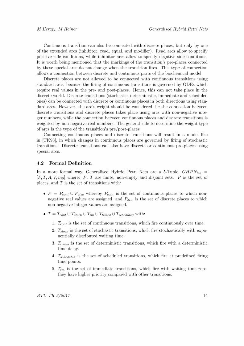
continuous Petri nets. Their semantics are governed by ordinary differential equations.Their ODEs define the changes in the transitions’ pre- and post-places.

Stochastic transitions which are drawn in Snoopy as a square, fire randomly withan exponentially distributed random delay. The user can specify a set of firing ratefunctions, which determine the random firing delay. The transition’s pre-places can beused to define the firing rate functions of the stochastic transitions. Deterministic transi-tions (represented as black squares) fire after a specified constant time delay, immediatetransitions (black bar) fire with zero delay, and have always higher priority in the caseof conflicts with other transitions. They may carry weights which specify the relativefiring frequency in the case of conflicts between more than one immediate transition.Scheduled transitions (grey squares) fire at user-specified absolute time points. Moredetails about the biochemical interpretation of deterministic, scheduled, and immediatetransitions can be found in [HLGM09].

The connection between those two types of nodes (places and transitions) takes placeusing a set of different arcs. GHPNbio contains six types of arcs: standard, inhibitor,read, equal, reset and modifier arcs. Standard arcs connect transitions with places or viceversa. They can be continuous, i.e carry non-negative real-valued weights (stoichiometryin the biochemical context), or discrete i.e carry non-negative integer-valued weights.Special arcs like inhibitor, read, equal and reset arcs can only be used to connect placesto transitions, but not vice versa. Further arc types – like modifier and equal arcs –simplify the modelling task. For example, a modifier arc permits to include any place inthe transitions’ rate functions and simultaneously preserves the net structure restriction.The connection rules and their underlying semantics are discussed in more details below.Figure 3 provides a graphical illustration of those elements. Although this graphicalnotation is the default one, they can be easily customised using our Petri nets editingtool, Snoopy.

As a simple example for the above discussion, consider again the stiff biochemicalnetwork in Figure 1. Using GHPNbio, the slow reaction R3 can be modelled using astochastic transition while the other two fast reactions, R1 and R2, can be representedusing continuous transitions. Places are partitioned into discrete and continuous basedon the connection rules which will be discussed next.

4.1.2 Connection Rules

A critical question arises when considering the combination of discrete and continuouselements: how are these two different parts connected with each other? Figure 4, pro-vides a graphical illustration of how the connection between different elements of theintroduced GHPNbio takes place. We denote here by discrete transitions: stochastic,immediate, deterministic or scheduled transitions.

Firstly, we will consider the connection between continuous transitions and the otherelements of GHPNbio. Continuous transitions can be connected with continuous placesin both directions using continuous arcs (i.e arc with real-valued weight). This meansthat continuous places can be pre- or post-places of continuous transitions. These con-nections typically represent deterministic biological interactions.

BTU TR 2/2011 12


Discrete

Standard

Continuous

Stochastic

Inhibitor Equal Reset ModifierRead

Continuous Immediate Deterministic

<1>

Scheduled

[_SimStart,1,_SimEnd]

Places

Transitions

Edges

Figure 3: Graphical representation of the GHPNbio’s elements. Places are classified ascontinuous and discrete, transitions as continuous, stochastic, immediate, deterministic,and scheduled, and arcs as standard, inhibitor, read, equal, and modifier.

or

or

oror

or

or

or

or

Continuous TransitionDiscrete Transition

Figure 4: Possible connections between GHPNbio’s elements: Discrete places can notbe connected with continuous transitions using standard arcs.

BTU TR 2/2011 13


Continuous transition can also be connected with discrete places, but only by oneof the extended arcs (inhibitor, read, equal, and modifier). Read arcs allow to specifypositive side conditions, while inhibitor arcs allow to specify negative side conditions.It is worth being mentioned that the markings of the transition’s pre-places connectedby these special arcs do not change when the transition fires. This type of connectionallows a connection between discrete and continuous parts of the biochemical model.

Discrete places are not allowed to be connected with continuous transitions usingstandard arcs, because the firing of continuous transitions is governed by ODEs whichrequire real values in the pre- and post-places. Hence, this can not take place in thediscrete world. Discrete transitions (stochastic, deterministic, immediate and scheduledones) can be connected with discrete or continuous places in both directions using stan-dard arcs. However, the arc’s weight should be considered, i.e the connection betweendiscrete transitions and discrete places takes place using arcs with non-negative inte-ger numbers, while the connection between continuous places and discrete transitions isweighted by non-negative real numbers. The general rule to determine the weight typeof arcs is the type of the transition’s pre/post-places.

Connecting continuous places and discrete transitions will result in a model likein [TK93], in which changes in continuous places are governed by firing of stochastictransitions. Discrete transitions can also have discrete or continuous pre-places usingspecial arcs.

4.2 Formal Definition

In a more formal way, Generalised Hybrid Petri Nets are a 5-Tuple, GHPNbio =[P, T,A, V,m0] where: P , T are finite, non-empty and disjoint sets. P is the set ofplaces, and T is the set of transitions with:

• P = Pcont ∪ Pdisc whereby Pcont is the set of continuous places to which non-negative real values are assigned, and Pdisc is the set of discrete places to whichnon-negative integer values are assigned.

• T = Tcont ∪ Tstoch ∪ Tim ∪ Ttimed ∪ Tscheduled with:

1. Tcont is the set of continuous transitions, which fire continuously over time.

2. Tstoch is the set of stochastic transitions, which fire stochastically with expo-nentially distributed waiting time.

3. Ttimed is the set of deterministic transitions, which fire with a deterministictime delay.

4. Tscheduled is the set of scheduled transitions, which fire at predefined firingtime points.

5. Tim is the set of immediate transitions, which fire with waiting time zero;they have higher priority compared with other transitions.

BTU TR 2/2011 14


• A = Acont ∪Adisc ∪Ainhibit ∪Aread ∪Aequal ∪Areset∪Amodifier is the set of directed edges, whereby:

1. Acont : ((Pcont×T )∪(T ×Pcont))→ R+0 defines the set of continuous, directed

arcs, weighted by non-negative real values.

2. Adisc : ((P × T ) ∪ (T × P )) → N0 defines the set of discrete, directed arcs,weighted by non-negative integer values.

3. Aread : (P × T )→ R+0 if P ∈ Pcont, or

Aread : (P × T )→ N0 if P ∈ Pdiscdefines the set of read arcs.

4. Aequal : (Pdisc × T )→ N+0 , defines the set of equal arcs.

5. Ainhibit : (P × T )→ R+0 if P ∈ Pcont, or

Ainhibit : (P × T )→ N0 if P ∈ Pdiscdefines the set of inhibits arcs.

6. Areset : (P × Tdiscrete)→ {0, 1} defines the set of reset arcs, where Tdiscrete =Tstoch ∪ Tim ∪ Ttimed ∪ Tscheduled is the set of discrete transitions.

7. Amodifier : (P × T )→ {0, 1} defines the set of modifier arcs.

• V is a set of functions V = {f, g, d, w} where :

1. f : Tcont → Hc is a function which assigns a rate function hc to each contin-

uous transition t ∈ Tcont, such that Hc = {hct |hct : R|•t|0 → R+

0 , t ∈ Tcont} isthe set of all rates functions and f(t) = hct , ∀t ∈ Tcont.

2. g : Tstoch → Hs is a function which assigns a stochastic hazard function hstto each transition t ∈ Tstoch, whereby Hs = {hst |hst : R|

•t|0 → R+

0 , t ∈ Tstoch}is the set of all stochastic hazard functions, and g(t) = hst∀t ∈ Tstoch .

3. d : Ttimed ∪ Tscheduled → R+0 , is a function which assigns a constant time to

each deterministic and scheduled transition representing the waiting time.

4. w : Tim → Hw is a function which assigns a weight function hw to each

immediate transition t ∈ Tim, such that Hw = {hwt |hwt : R|•t|0 → R+

0 , t ∈ Tim}is the set of all weight functions, and w(t) = hwt , ∀t ∈ Tim

• m0 = mcont ∪ mdisc is the initial marking for both the continuous and discrete

places, whereby mcont ∈ R+|Pcont|0 , mdisc ∈ N|Pdisc|

0 .

Here, N0 denotes the set of non-negative integer numbers, R+0 denotes the set of

non-negative real numbers, and •t denotes the pre-places of a transition t.The formal definition above covers the syntactical aspects of Generalised Hybrid

Petri Nets. Their operational semantics will be formally defined in the next section,when we discuss their simulation.

BTU TR 2/2011 15


4.3 Simulation of GHPN

After the modelling aspects of GHPNbio have been presented in the previous section,we discuss here the approach which is used to simulate GHPNbio. The key idea behindsimulation of Generalised Hybrid Petri Nets is to numerically solve the set of ordinary dif-ferential equations generated by the continuous transitions until a discrete event occurs.The event type is dispatched, and afterwards the continuous simulation is resumed. Westart by discussing the simulation of statically partitioned GHPNbio, then the dynamicpartitioning of GHPNbio is presented, which substantially simplifies the modelling ofbiochemical networks using GHPNbio.

4.3.1 Simulation of Statically Partitioned GHPNbio

In the following we illustrate how GHPNbio can be simulated using an extended versionof the algorithms which are discussed in [ACT+05, GCPS06, HR02]. Algorithm (1) sum-marizes the steps which are needed to simulate Generalised Hybrid Petri Nets. Startingfrom an initial marking which corresponds to the initial state of a biochemical system,the algorithm computes state changes over time t, which is represented by the currentmarking m(CurrentT ime). Initially the current marking is set to the initial marking,and the individual propensities a(t) as well as the cumulative propensity are calculatedfor both stochastic and continuous transitions (lines 3-5). Deterministically time de-layed transitions do not have propensities, since they fire after a pre-defined time delay,likewise for scheduled transitions. Note that in the algorithm we consider scheduledtransitions as deterministically time delayed transitions since they can be considered asa special case of them. Note that immediate transitions also do not have propensitiesassociated with them (see Section 4.1.1).

If there is a non-stochastic transition in the underlying model, then the algorithmdetermines the next stochastic transition to fire by integrating the set of ODEs as wellas the cumulative propensities until equation (6) is satisfied.

The numerical integrator stops when an event Ei occurs. The event may be anenabling of an immediate or deterministically time delayed transition, a deterministicallytime delayed transition has finished its delay, a stochastic event occurred, or the end ofsimulation time has been reached. Then, the appropriate action will be taken.

Line 11 updates all of the transitions’ propensities that share a pre-place with acontinuous transition. The function IsEnabled(t) checks for enabling of a transition t,while Fire(t) fires an enabled transition. The details of these functions are easy to beimplemented, therefore they are not further considered here.

CheckImmediateTransitions() checks if there is any immediate transition enabled.If such a transition is found, it will be fired. If there are several immediate transitionsenabled then the first one to fire is selected based on their weights. More precisely,if an immediate transition k is enabled in the current marking m, then it fires withprobability:

BTU TR 2/2011 16


Algorithm 1 Simulating Static Partitioned GHPNbio

1: CurrentT ime← 0;2: ξ ← exp(1){Generate a random number exponentially distributed with a unit mean}3: m(CurrentT ime)← m(0); {current marking=initial marking}4: ∀t ∈ {Tcont ∪ Tstoch} calculate a(t);5: a0 ←

∑a(t), ∀t ∈ Tstoch;

6: while CurrentTime < EndTime do7: if There are non-stochastic transitions then8: Initialize the ODE solver by m(CurrentT ime);9: Simultaneously integrate the system of ODEs generated using (1) and

g(m(CurrentT ime)) until an event E occurs;10: CurrentT ime = the current integrator time;11: Update(a(ti), a0), ∀ti :•ti ∩ {•tj ∪ t•j} 6= φ,∀tj ∈ Tcont;12: if E is: ∃t ∈ Tim and IsEnabled(t) then13: CheckImmediateTransitions();14: else if E is: ∃t ∈ Tdeter and IsEnabled(t) then15: CheckDeterministicTransitions();16: else if E is: ∃t ∈ Tdeter and FireTime(t)= CurrentT ime then17: CheckDeterministicTransitions();18: else if E is: g(m(CurrentT ime)) ≥ 0 then19: g(m(CurrentT ime))← 0;20: ξ ← exp(1);21: tchosen ← a transition index i satisfying (7);22: Fire(tchosen);23: Update(a(ti)), ∀ti : •ti ∩{t•chosen∪ •tchosen}6= φ24: else if E is: CurrentT ime ≥ EndTime then25: break;26: end if27: else28: CurrentT ime = CurrentT ime+exp(a0) {See (3).}29: if CurrentT ime < EndTime AND a0 > 0 then30: tchosen ← a transition index i satisfying (4);31: Fire(tchosen);32: Update(a(ti)), ∀ti : •ti ∩{t•chosen∪ •tchosen}6= φ33: end if34: end if35: end while

w(k,m)∑i∈Tim∧isEnabled(i)

w(i,m), (8)

BTU TR 2/2011 17


where w(k,m) is the weight assigned to an immediate transition k in the currentmarking m. It is worth mentioning here that immediate transitions have priority over allother transitions in the case of conflict. The purpose of CheckDeterministicTransitions()is twofold. Firstly, it checks if there are any enabled deterministic transitions; it putsthem in the delay list along with their proposed time to fire. If there are transitions inthe delay list which have finished their delay, then it fires them.

Lines 19-23 and lines 30-32 perform the same task, but for different conditions. Inthe former case, a stochastic transition is selected to be fired when the ODE integratordetermines that a stochastic event has occurred. The stochastic transition is selectedbased on equation (7). While in the latter case, the model contains only stochastictransitions. Thus the next reaction time is computed based on equation (3), and thenext transition to fire is selected based on (4).

When a transition fires, the propensity of this transition as well as of any othertransitions that are affected by this firing are computed and the cumulative propensity isupdated. The simulation ends when the current simulation time exceeds the simulation’send time which is specified by the user.

While this algorithm can simulate any GHPNbio, it requires the user to specify thepartitioning in advance. Sometimes it is not easy for naive users to do the partition-ing off-line. It is also possible that a good partitioning changes dynamically over time.Therefore, we present in the next section an algorithm which supports on-line partition-ing. In some cases, the cost of this dynamic partitioning is more computational overhead[Pah09].

4.3.2 Transition Partitioning

Static partitioning of Petri nets into stochastic and continuous net parts is not alwaysappropriate. During simulation the transitions’ rates can drastically vary between lowand high. Furthermore off-line partitioning is not user friendly, since it is not easy fornaive users to determine which transitions should be considered stochastically and whichone continuously [Pah09]. The latter problem could be overcome by running stochas-tic simulation for only one trajectory in order to determine partitioning automatically[ACT+05]. Another solution is to use stochastic analysis techniques.

The partitioning of the reactions into slow and fast can be done through the use oftwo thresholds: one for the transitions’ rates and the other one for the places’ marking[ACT+05, GCPS06].

However one important question remains: when do we need to consider repartition-ing? One solution to this problem is to reconsider repartitioning after a specific timeperiod (for example every one or two seconds). However this will not correctly solvethe problem since during this period there may be changes in some species’ populations.Moreover it results in computational overhead when there is no need to repartition.In our partitioning approach we solve this problem by specifying two other thresholds:a0max , a0min .

Consider equation (3), which determines the next time point a stochastic event willoccur. Larger values of a0 will result in smaller time steps in stochastic simulation. On

BTU TR 2/2011 18


the other hand, smaller values of a0 will keep the time step small. In fact this alsoaffects equation (6) which determines when we switch from deterministic to stochasticsimulation. The same arguments holds for (6). The main idea here is that we can controlthe speed and accuracy of the hybrid simulation by specifying a lower and upper boundof a0. Then the algorithm will realize that it needs to repartition the net when a0 dropsbelow a0min or exceeds a0max .

Algorithm (2) summarizes the steps which are needed to carry out on-line partitioningof the network. It considers repartitioning if equation (9), (10) or both are violated.

a0min ≤ a0 ≤ a0max (9)

#p ≥ Λ, ∀p ∈ {•t ∪ t•}∀t ∈ Tcont (10)

where Λ is a threshold for the number of tokens in a place p.An inappropriate choice of the thresholds can result in unsuitable partitioning which

may turn out to be more computational expensive than static partitioning.The algorithm takes as inputs the stochastic and continuous transitions, amin, amax

– the upper and lower bounds of the cumulative propensity, respectively, the transitions’rate threshold λ, and the places’ marking threshold Λ. Note that the other transitiontypes are not repartitioned. At the end of the partitioning the algorithm returns T

′stoch

and T′cont as the new partitioning.

The idea of repartitioning is then very easy. If one of the transitions violates thepartitioning criterion, it will be added to the stochastic transitions, otherwise it will beadded to the continuous one.

This algorithmic idea, together with the one which is presented in Section 4.3.1,provide a dynamic simulation of the Petri nets’ elements which have been introduced inthis paper.

BTU TR 2/2011 19


Algorithm 2 Dynamic Partitioning of GHPNbio

Input: amin, amax, λ, Λ, Tstoch, TcontOutput: T

′stoch, T

′cont

1: if a0 < amin OR a0 > amax OR #p < Λ ∀p ∈ •Tcont ∪ T •cont then2: for all t ∈ Tstoch ∪ Tcont do3: if at > λ AND ∀p ∈ {•t ∪ t•},#p > Λ then4: if t ∈ Tstoch then5: a0 ← a0 − a(t)6: T

′cont ← T

′cont ∪ {t}

7: Tstoch ← Tstoch − {t}8: end if9: else

10: if t ∈ Tcont then11: a0 ← a0 + a(t)12: Tcont ← Tcont − {t}13: T

′stoch ← T

′stoch ∪ {t}

14: end if15: end if16: end for17: return T

′stoch, T

′cont

18: else19: return Tstoch, Tcont {No partitioning is needed}20: end if

4.4 Implementation

The presented Petri nets class and its simulation are implemented in Snoopy [RMH10].Snoopy is available free of charge for non-commercial use. It is platform independent andruns under Mac OS X, Windows and Linux (selected distributions). We implementedGillespie’s direct method [Gil76] to simulate stochastic transitions, while SUNDIALSCVODE [HBG+05] is used to integrate the resulting ODEs due to continuous transitions.

Snoopy supports also a dedicated net class to simulate Petri nets which containonly continuous elements and provides 14 different ODEs integrators. The addition offurther stochastic simulators is easy due to the generic design of Snoopy (see futurework). Snoopy supports also many other useful modelling features like hierarchy andlogical nodes which are very useful tools when considering modelling and simulation oflarge scale biochemical networks. Furthermore, a model developed with Snoopy can beexported to a variety of analysis tools. Additionally, using GHPNbio the same modelcan be simulated continuously or stochastically independently of its original modellingmethod, thanks to dynamic partitioning.

BTU TR 2/2011 20


5 Case Studies

In this section, we present three case studies to illustrate hybrid modelling and simula-tion of GHPNbio: Goutsias model, Circadian oscillation model, and T7 Phage model.Using the first example we aim to demonstrate the speed up of the computation whilepreserving accuracy. In the second and third examples we use models where stochas-ticity plays a role when there are a few number of molecules. Stochasticity can also bepreserved when GHPN is used.

5.1 Goutsias Model

This model has been used by Goutsias in [Gou05] as an example for systems that can beeffectively partitioned into two distinct subsystems, one that comprises slow reactionsand one that comprises fast reactions. It has been studied in [WGMH10] and [HMMW10]as example for hybrid numerical solutions of the chemical master equation. We use thesame reactions which have been originally proposed by [Gou05], and the more challengingparameters which have been used in [HMMW10].

Figure 5 is a hybrid Petri net representation of Goutsias’ model. The partitioningof transitions and places into discrete and continuous ones is based on running onetrajectory of a fully stochastic simulation. R1, R3, R9, and R10 are reactions withhigh rates compared to the other reactions. Thus this set of reactions is representedby continuous transitions which in turn are simulated by ODEs integrator. Note thatplaces are partitioned into continuous and discrete ones according to the type of pre-and post-transitions. Places are considered as discrete ones if the adjacent arcs do notpreclude this interpretation. Figure 6 is a time course result of the places DNA, DNA.D,and DNA.2D. The hybrid simulation result coincides with the stochastic one for thethree species.

5.2 Circadian Oscillation

In some organisms, there is a control mechanism which is responsible for ensuring aperiodic oscillation of certain molecular species [HL07]. This phenomenon is known ascircadian rhythm and it can be found in many organisms (e.g Drosophila).

In this case study, we consider a simple model which demonstrates this phenomenon.The model consists of two genes which are represented in Figure 7 by two places G1 andG2. The model includes also one activator and one repressor which are represented bythe places A and R, respectively. The activator and repressor control the two genes andtheir mRNAs, mRNA G1 and mRNA G2. A and R can be activated to form a complexA R which takes place through reaction R12.

The Petri net in Figure 7 contains 9 places and 12 transitions. Note that placeswith the same name are logical places. This feature is used to simplify the graphicalrepresentation of the Petri net. The complete list of reactions as well as the parameter listcan be found in [HL07]. Figure 8 gives a time course simulation result of the GHPNbio inFigure 7. Using the parameter values given in Figure 8, continuous simulation produces

BTU TR 2/2011 21


DNA

DNA_2DDNA_D

M 10

D10

RNA

10

R2R4

R5

R6

R7

R8

R9

R10

R1 R3

k1

0.043

k2

0.0007

k3

71.5

k4

3.9e−06

k5

0.02

k6

0.48

k7

0.0002

k8

9e−12

k9

0.08

k10

0.5

2

2

Figure 5: A GHPNbio representation of the Goutsias model. Numbers in ovals representreaction rate constants.

0

0.5

1

1.5

2

0 10 20 30 40 50 60 70 80

Num

ber o

f Mol

ecul

es

time

Goutsias Model Specie

Stochastic (DNA)Hybrid(DNA)

continuous(DNA)Stochastic (DNA.2D)

Hybrid(DNA.2D)continuous(DNA.2D)Stochastic (DNA.D)

Hybrid(DNA.D)continuous(DNA.D)

Figure 6: Continuous, stochastic and hybrid simulation result of the Goutsias model:hybrid simulation result is closer to stochastic than to continuous simulation result.

oscillations. However, if the rate constant of reaction R17, i.e. (k17), is changed from0.2 to 0.08, the continuous simulation fails to produce the desired oscillation [HL07,JHNS02].

It is shown in [JHNS02] that stochastic simulation can still produce the expected

BTU TR 2/2011 22


G10.2

G2_active

9

G1_active

9

A

A

G20.2

mRNA_G1

A_R

R

mRNA_G2

R1

R2

R3

R4

R9

R10

R8

R11

R12

R16

R18R17

R7

R6R5

R14

R15

R13

k1

50

k3

100

k5

500

k7

10

k9

50

k11

1

k13

50

k2

1

k4

1

k6

50

k8

50

k10

100

k12

2

k14

0.01

k16

5

k15

0.5

k17

0.2

k18

1

Figure 7: A GHPNbio representation of the circadian oscillation model. Places givenin grey colour are logical places. The parameter k17, highlighted in yellow, is a keyparameter in this model.

BTU TR 2/2011 23


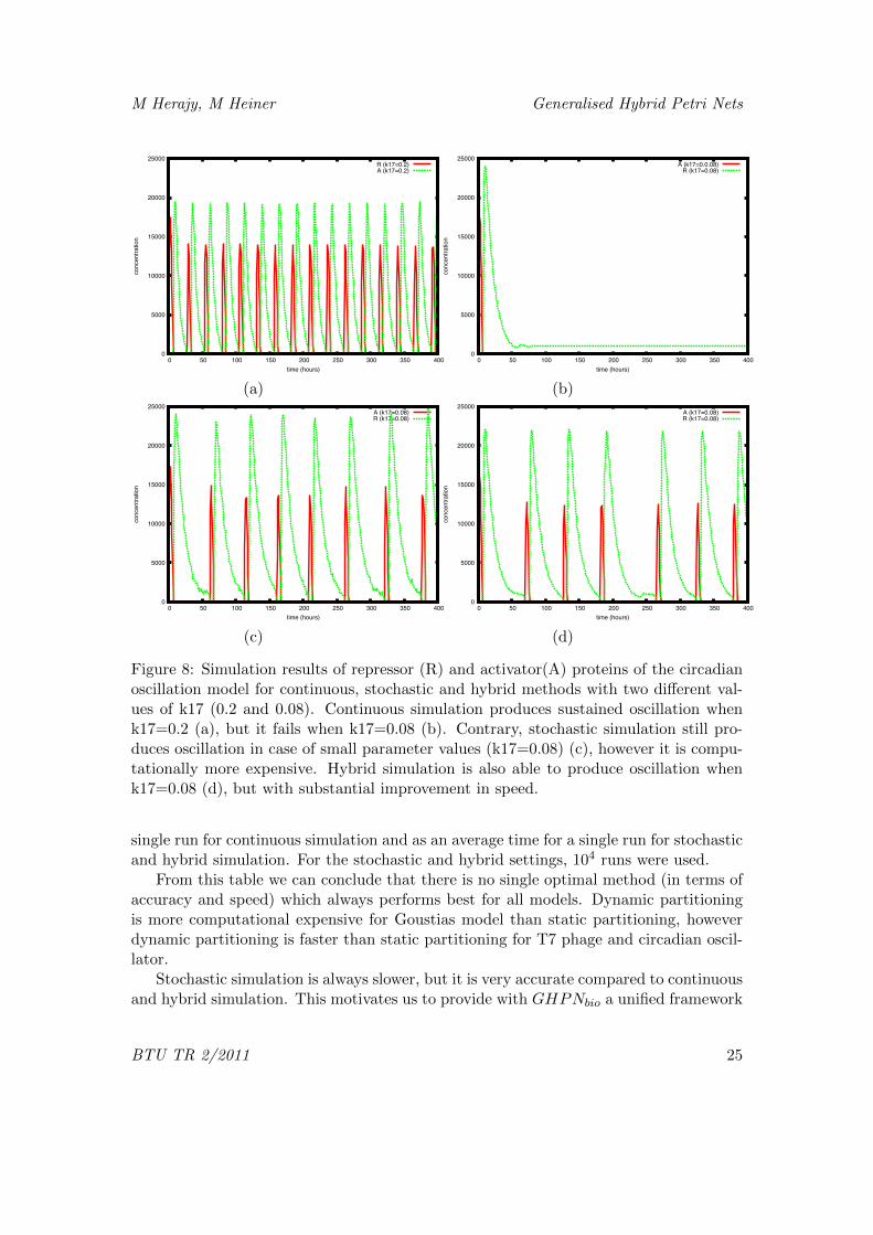
oscillation even if there are reactions with low rates.Hybrid simulation can also produce such an oscillation of this model when species

with low numbers of molecules or reactions of low rates are simulated stochastically,while the others are simulated continuously. However, static partitioning of the Petri netinto continuous and stochastic parts will slow down the simulation, since the propensityvalues are changing during the simulation due to the oscillation.

Thus we opted to dynamically partition the model into fast and slow parts duringthe simulation. Figure 8 shows the simulation result when the Petri net in Figure 7 issimulated using continuous, stochastic, and hybrid methods with different values of k17(0.2 and 0.08). The parameters in the partitioning algorithm are set to get a trade offbetween accuracy and speed.

5.3 T7 Phage Model

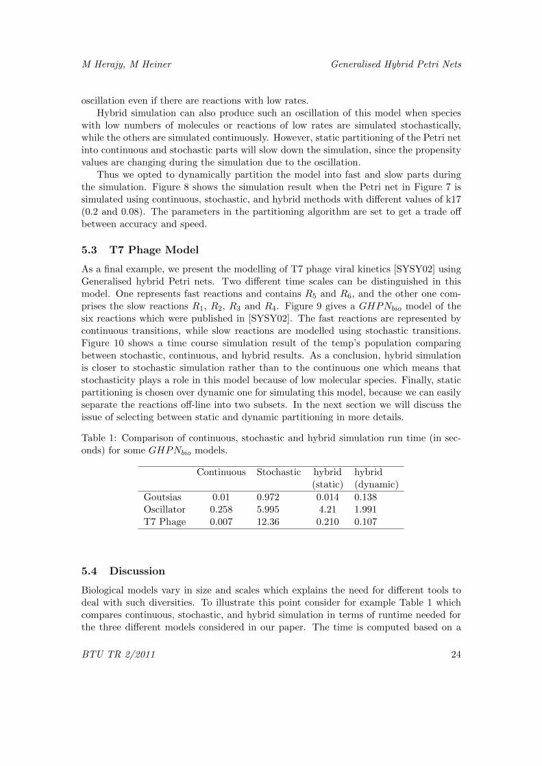
As a final example, we present the modelling of T7 phage viral kinetics [SYSY02] usingGeneralised hybrid Petri nets. Two different time scales can be distinguished in thismodel. One represents fast reactions and contains R5 and R6, and the other one com-prises the slow reactions R1, R2, R3 and R4. Figure 9 gives a GHPNbio model of thesix reactions which were published in [SYSY02]. The fast reactions are represented bycontinuous transitions, while slow reactions are modelled using stochastic transitions.Figure 10 shows a time course simulation result of the temp’s population comparingbetween stochastic, continuous, and hybrid results. As a conclusion, hybrid simulationis closer to stochastic simulation rather than to the continuous one which means thatstochasticity plays a role in this model because of low molecular species. Finally, staticpartitioning is chosen over dynamic one for simulating this model, because we can easilyseparate the reactions off-line into two subsets. In the next section we will discuss theissue of selecting between static and dynamic partitioning in more details.

Table 1: Comparison of continuous, stochastic and hybrid simulation run time (in sec-onds) for some GHPNbio models.

Continuous Stochastic hybrid hybrid(static) (dynamic)

Goutsias 0.01 0.972 0.014 0.138Oscillator 0.258 5.995 4.21 1.991T7 Phage 0.007 12.36 0.210 0.107

5.4 Discussion

Biological models vary in size and scales which explains the need for different tools todeal with such diversities. To illustrate this point consider for example Table 1 whichcompares continuous, stochastic, and hybrid simulation in terms of runtime needed forthe three different models considered in our paper. The time is computed based on a

BTU TR 2/2011 24


0

5000

10000

15000

20000

25000

0 50 100 150 200 250 300 350 400

conc

entra

tion

time (hours)

R (k17=0.2)A (k17=0.2)

(a)

0

5000

10000

15000

20000

25000

0 50 100 150 200 250 300 350 400

conc

entra

tion

time (hours)

A (k17=0.0.08)R (k17=0.08)

(b)

0

5000

10000

15000

20000

25000

0 50 100 150 200 250 300 350 400

conc

entra

tion

time (hours)

A (k17=0.08)R (k17=0.08)

(c)

0

5000

10000

15000

20000

25000

0 50 100 150 200 250 300 350 400

conc

entra

tion

time (hours)

A (k17=0.08)R (k17=0.08)

(d)

Figure 8: Simulation results of repressor (R) and activator(A) proteins of the circadianoscillation model for continuous, stochastic and hybrid methods with two different val-ues of k17 (0.2 and 0.08). Continuous simulation produces sustained oscillation whenk17=0.2 (a), but it fails when k17=0.08 (b). Contrary, stochastic simulation still pro-duces oscillation in case of small parameter values (k17=0.08) (c), however it is compu-tationally more expensive. Hybrid simulation is also able to produce oscillation whenk17=0.08 (d), but with substantial improvement in speed.

single run for continuous simulation and as an average time for a single run for stochasticand hybrid simulation. For the stochastic and hybrid settings, 104 runs were used.

From this table we can conclude that there is no single optimal method (in terms ofaccuracy and speed) which always performs best for all models. Dynamic partitioningis more computational expensive for Goustias model than static partitioning, howeverdynamic partitioning is faster than static partitioning for T7 phage and circadian oscil-lator.

Stochastic simulation is always slower, but it is very accurate compared to continuousand hybrid simulation. This motivates us to provide with GHPNbio a unified framework

BTU TR 2/2011 25


gen

Struct

temp

1

R1

R2

R3

R4

R5

R6

c1

0.025

c2

0.25

c3

1

c4

7.5e−006

c5

1000

c6

1.99

Figure 9: A GHPNbio representation of T7 phage model.

0

5

10

15

20

0 50 100 150 200

Amou

nt o

f Wat

er

time

HybridContinuousStochastic

Figure 10: Time course simulation result of species tem in the T7 phage model.

to simulate one and the same model using different simulation methods which givesbiologists a tool to easily try different methods and to choose the most suitable one.

6 Conclusions

In this paper, we have presented a new class of Petri nets which combines both Gener-alised stochastic Petri nets and continuous Petri nets into one net class, the GeneralisedHybrid Petri Nets. The introduced net class has several functionalities which help biol-

BTU TR 2/2011 26


ogists to model and simulate their biochemical networks through an easy to use visuallanguage. GHPNbio models can be simulated statically through off-line partitioning ordynamically by on-line partitioning.

Deciding the partitioning off-line will save the dynamic partitioning overhead forcertain biological applications. Providing an automatic way to achieve this goal couldbe important from the user’s point of view. For this purpose, future investigation ofanalysis techniques of stochastic Petri nets might be of help. Another intended furtherextension is to support more than one stochastic simulator within Snoopy. This can beeasily achieved due to the generic implementation of the simulator.

The cases studies which we have used in this paper have been chosen to illustratedifferent aspects of the hybrid approach. We are currently challenging Snoopy withother, more complex case studies than discussed in this paper.

7 Acknowledgements

Mostafa Herajy is supported by the GERLS (German Egyptian Research Long TermScholarships) program, which is administered by the DAAD in close cooperation withthe MHESR and German universities.

References

[ACT+05] A. Alfonsi, E. Cances, G. Turinici, B. Ventura, and W. Huisinga. Adaptivesimulation of hybrid stochastic and deterministic models for biochemicalsystems. ESAIM: Proc., 14:1–13, 2005.

[AD98] H. Alla and R. David. Continuous and hybrid Petri nets. J. Circ. Syst.Comp., 8(1):159 –188, 1998.

[Dra98] R. Drath. Hybrid object nets: an object oriented concept for modelingcomplex hybrid systems. In 3rd International Conference on Automationof Mixed Processes: Hybrid Dynamical Systems (ADPM), ADPM’98, pages437–442, 1998.

[GCPS06] M. Griffith, T. Courtney, J. Peccoud, and W. Sanders. Dynamic parti-tioning for hybrid simulation of the bistable hiv-1 transactivation network.Bioinformatics, 22(22):2782–2789, 2006.

[GH06] D. Gilbert and M. Heiner. From Petri Nets to Differential Equations - AnIntegrative Approach for Biochemical Network Analysis. In Susanna Do-natelli and P. Thiagarajan, editors, Petri Nets and Other Models of Concur-rency - ICATPN 2006, volume 4024 of Lecture Notes in Computer Science,pages 181–200. Springer Berlin / Heidelberg, 2006.

BTU TR 2/2011 27

https://www.researchgate.net/publication/47800196_Adaptive_Simulation_of_Hybrid_Stochastic_and_Deterministic_Models_for_Biochemical_Systems?el=1_x_8&enrichId=rgreq-67c5d228-aa5c-4270-9ea3-929db7adfca1&enrichSource=Y292ZXJQYWdlOzI1NDg2MjI2NTtBUzo5ODg5MDUwNjMwOTY0MEAxNDAwNTg4NzQyNjgy





https://www.researchgate.net/publication/6836250_Dynamic_partitioning_for_hybrid_simulation_of_the_bistable_HIV-1_transactivation_network?el=1_x_8&enrichId=rgreq-67c5d228-aa5c-4270-9ea3-929db7adfca1&enrichSource=Y292ZXJQYWdlOzI1NDg2MjI2NTtBUzo5ODg5MDUwNjMwOTY0MEAxNDAwNTg4NzQyNjgy




[Gil76] D. Gillespie. A general method for numerically simulating the stochastictime evolution of coupled chemical reactions. J. Comput. Phys., 22(4):403– 434, 1976.

[Gil77] D. Gillespie. Exact Stochastic Simulation of Coupled Chemical Reactions.J. Phys. Chem., 81(25):2340–2361, 1977.

[Gil91] D. Gillespie. Markov Processes: An Introduction for Physical Scientists.Academic Press, October 1991.

[Gil07] D. Gillespie. Stochastic simulation of chemical kinetics. Annual review ofphysical chemistry, 58(1):35–55, 2007.

[Gou05] J. Goutsias. Quasiequilibrium approximation of fast reaction kinetics instochastic biochemical systems. J. Chem. Phys., 122(184102):1–15, 2005.

[HBG+05] A. Hindmarsh, P. Brown, K. Grant, S. Lee, R. Serban, D. Shumaker, andC. Woodward. Sundials: Suite of nonlinear and differential/algebraic equa-tion solvers. ACM Trans. Math. Softw., 31:363–396, September 2005.

[HGD08] M. Heiner, D. Gilbert, and R. Donaldson. Petri nets for systems and syn-thetic biology. In Formal Methods for Computational Systems Biology, vol-ume 5016 of Lecture Notes in Computer Science, pages 215–264. SpringerBerlin / Heidelberg, 2008.

[HK99] G. Horton and M. Kowarschik. Discrete-Continuous Modeling Using HybridStochastic Petri Nets. In European Simulation Symposium. SCS PublishingHouse., 1999.

[HL07] A. Hellander and P. Lotstedt. Hybrid method for the chemical masterequation. J. Comput. Phys., 227:100–122, November 2007.

[HLGM09] M. Heiner, S. Lehrack, D. Gilbert, and W. Marwan. Extended StochasticPetri Nets for Model-Based Design of Wetlab Experiments. In Transactionson Computational Systems Biology XI, pages 138–163. Springer, Berlin,Heidelberg, 2009.

[HMMW10] T. Henzinger, L. Mikeev, M. Mateescu, and V. Wolf. Hybrid numericalsolution of the chemical master equation. In Proceedings of CMSB ’10,CMSB ’10, pages 55–65, New York, NY, USA, 2010. ACM.

[HR02] E. Haseltine and J. Rawlings. Approximate simulation of coupled fastand slow reactions for stochastic chemical kinetics. J. Chem. Phys.,117(15):6959–6969, 2002.

[JHNS02] J. Jose, H. Hao, N. Naama, and S. Stanislas. Mechanisms of noise-resistancein genetic oscillators. Proceedings of the National Academy of Sciences ofthe United States of America, 99(9):5988–5992, April 2002.

BTU TR 2/2011 28

https://www.researchgate.net/publication/216078491_Extended_Stochastic_Petri_Nets_for_Model-Based_Design_of_Wetlab_Experiments?el=1_x_8&enrichId=rgreq-67c5d228-aa5c-4270-9ea3-929db7adfca1&enrichSource=Y292ZXJQYWdlOzI1NDg2MjI2NTtBUzo5ODg5MDUwNjMwOTY0MEAxNDAwNTg4NzQyNjgy




https://www.researchgate.net/publication/51992412_SUNDIALS_Suite_of_nonlinear_and_differentialalgebraic_equation_solvers?el=1_x_8&enrichId=rgreq-67c5d228-aa5c-4270-9ea3-929db7adfca1&enrichSource=Y292ZXJQYWdlOzI1NDg2MjI2NTtBUzo5ODg5MDUwNjMwOTY0MEAxNDAwNTg4NzQyNjgy






[KMS04] T. Kiehl, R. Mattheyses, and M. Simmons. Hybrid simulation of cellularbehavior. Bioinformatics, 20:316–322, February 2004.

[LCPG08] H. Li, Y. Cao, L. Petzold, and D. Gillespie. Algorithms and software forstochastic simulation of biochemical reacting systems. Biotechnol. Progr.,24(1):56–61, 2008.

[MA99] H. Mcadams and A. Arkin. It’s a noisy business! Trends in Genetics,15(2):65–69, 1999.

[MTA+03] H. Matsuno, Y. Tanaka, H. Aoshima, A. Doi, M. Matsui, and S. Miyano.Biopathways representation and simulation on hybrid functional Petri net.In silico biology, 3(3), 2003.

[NDMM04] M. Nagasaki, A. Doi, H. Matsuno, and S. Miyano. A versatile Petri netbased architecture for modeling and simulation of complex biological pro-cesses. Genome informatics. International Conference on Genome Infor-matics, 15(1):180–197, 2004.

[Pah09] J. Pahle. Biochemical simulations: stochastic, approximate stochastic andhybrid approaches. Brief Bioinform, 10(1):53–64, 2009.

[RMH10] C. Rohr, W. Marwan, and M. Heiner. Snoopy–a unifying Petri net frame-work to investigate biomolecular networks. Bioinformatics, 26(7):974–975,April 2010.

[RML93] V. Reddy, M. Mavrovouniotis, and M. Liebman. Petri net representationsin metabolic pathways. In Proceedings of the 1st International Conferenceon Intelligent Systems for Molecular Biology, pages 328–336. AAAI Press,1993.

[RPCG03] M. Rathinam, L. Petzold, Y. Cao, and D. Gillespie. Stiffness in stochasticchemically reacting systems: The implicit tau-leaping method. J. of Chem.Phys, 119:12784–12794, 2003.

[SK05] H. Salis and Y. Kaznessis. Accurate hybrid stochastic simulation of a systemof coupled chemical or biochemical reactions. J. Chem. Phys, 122(5), 2005.

[SYSY02] R. Srivastava, L. You, J. Summers, and J Yin. Stochastic vs. deterministicmodeling of intracellular viral kinetics. J. theor. Biol., 218(3):309–321,October 2002.

[TK93] K. Trivedi and V. Kulkarni. FSPNs: Fluid Stochastic Petri Nets. In 14thInternational Conference on Application and Theory of Petri Nets, pages24–31, 1993.

[WGMH10] V. Wolf, R. Goel, M. Mateescu, and T. Henzinger. Solving the chemicalmaster equation using sliding windows. BMC Syst. Biol., 4(1):42, 2010.

BTU TR 2/2011 29

https://www.researchgate.net/publication/5951155_Algorithms_and_Software_for_Stochastic_Simulation_of_Biochemical_Reacting_Systems?el=1_x_8&enrichId=rgreq-67c5d228-aa5c-4270-9ea3-929db7adfca1&enrichSource=Y292ZXJQYWdlOzI1NDg2MjI2NTtBUzo5ODg5MDUwNjMwOTY0MEAxNDAwNTg4NzQyNjgy



https://www.researchgate.net/publication/10584384_Biopathways_representation_and_simulation_on_hybrid_functional_Petri_Net?el=1_x_8&enrichId=rgreq-67c5d228-aa5c-4270-9ea3-929db7adfca1&enrichSource=Y292ZXJQYWdlOzI1NDg2MjI2NTtBUzo5ODg5MDUwNjMwOTY0MEAxNDAwNTg4NzQyNjgy





https://www.researchgate.net/publication/228733169_Stiffness_in_Stochastically_Reacting_Systems_The_Implict_Tau-Leaping_Method?el=1_x_8&enrichId=rgreq-67c5d228-aa5c-4270-9ea3-929db7adfca1&enrichSource=Y292ZXJQYWdlOzI1NDg2MjI2NTtBUzo5ODg5MDUwNjMwOTY0MEAxNDAwNTg4NzQyNjgy



https://www.researchgate.net/publication/8021340_A_versatile_Petri_net_based_architecture_for_modeling_and_simulation_of_complex_biological_processes_Genome_Informatics_14_Submitted?el=1_x_8&enrichId=rgreq-67c5d228-aa5c-4270-9ea3-929db7adfca1&enrichSource=Y292ZXJQYWdlOzI1NDg2MjI2NTtBUzo5ODg5MDUwNjMwOTY0MEAxNDAwNTg4NzQyNjgy




https://www.researchgate.net/publication/11079902_Stochastic_vs_Deterministic_Modeling_of_Intracellular_Viral_Kinetics?el=1_x_8&enrichId=rgreq-67c5d228-aa5c-4270-9ea3-929db7adfca1&enrichSource=Y292ZXJQYWdlOzI1NDg2MjI2NTtBUzo5ODg5MDUwNjMwOTY0MEAxNDAwNTg4NzQyNjgy




[WUKC04] O. Wolkenhauer, M. Ullah, W. Kolch, and K. Cho. Modeling and simulationof intracellular dynamics: choosing an appropriate framework. IEEE Trans.Nanobiosci., 3(3):200–207, 2004.

[YLL09] H. Yang, C. Lin, and Q. Li. Hybrid simulation of biochemical systems usinghybrid adaptive Petri nets. In Proceedings of the Fourth International ICSTConference on Performance Evaluation Methodologies and Tools, pages410–420. ICST, 2009.

BTU TR 2/2011 30

https://www.researchgate.net/publication/8242863_Modeling_and_Simulation_of_Intracellular_Dynamics_Choosing_an_Appropriate_Framework?el=1_x_8&enrichId=rgreq-67c5d228-aa5c-4270-9ea3-929db7adfca1&enrichSource=Y292ZXJQYWdlOzI1NDg2MjI2NTtBUzo5ODg5MDUwNjMwOTY0MEAxNDAwNTg4NzQyNjgy



Hybrid representation and simulation of stiff biochemical networks

Documents

Transcript of Hybrid representation and simulation of stiff biochemical networks