Non-radial oscillation modes as a probe of density discontinuities in neutron stars

arX

iv:a

stro

-ph/

0206

142v

1 1

0 Ju

n 20

02Mon. Not. R. Astron. Soc. 000, 000–000 (0000) Printed 12 January 2014 (MN LATEX style file v1.4)

Non-radial oscillation modes as a probe of density

discontinuities in neutron stars

G. Miniutti1, J. A. Pons1, E. Berti2, L. Gualtieri1, and V. Ferrari 1

1 Dipartimento di Fisica “G.Marconi”, Universita di Roma “La Sapienza”

and Sezione INFN ROMA1, piazzale Aldo Moro 2, I-00185 Roma, Italy

2 Department of Physics, Aristotle University of Thessaloniki, Thessaloniki 54006, Greece

12 January 2014

ABSTRACT

A phase transition occurring in the inner core of a neutron star could be as-

sociated to a density discontinuity that would affect the frequency spectrum

of the non-radial oscillation modes in two ways. Firstly, it would produce a

softening of the equation of state, leading to more compact equilibrium config-

urations and changing the frequency of the fundamental and pressure modes of

the neutron star. Secondly, a new non-zero frequency g– mode would appear,

associated to each discontinuity. These discontinuity g–modes have typical

frequencies larger than those of g–modes previously studied in the literature

(thermal, core g– modes, or g–modes due to chemical inhomogeneities in the

outer layers), and smaller than that of the fundamental mode; therefore they

should be distinguishable from the other modes of non radial oscillation. In

this paper we investigate how high density discontinuities change the fre-

quency spectrum of the non-radial oscillations, in the framework of the gen-

eral relativistic theory of stellar perturbations. Our purpose is to understand

whether a gravitational signal, emitted at the frequencies of the quasi normal

modes, may give some clear information on the equation of state of the neu-

tron star and, in particular, on the parameters that characterize the density

discontinuity. We discuss some astrophysical processes that may be associated

to the excitation of these modes, and estimate how much gravitational energy

should the modes convey to produce a signal detectable by high frequency

gravitational detectors.

Key words: gravitational waves — stars: oscillations — relativity — stars:neutron

c© 0000 RAS

http://arxiv.org/abs/astro-ph/0206142v1

2 G. Miniutti et al.

1 INTRODUCTION

The equation of state (EOS) of dense matter at supranuclear densities has been a long

sought-after problem in nuclear physics. Since the first observational evidences of their ex-

istence in the late 60’s, neutron stars (NS) have proved to be a unique astrophysical envi-

ronment in which very different fields of physics, ranging from nuclear physics to particle

physics and general relativity, can be tested. Accurate estimates of some properties of NSs,

such as masses and radii, associated to further information on the thermal history, would

allow to set constraints on the nature of nuclear forces. This has been attempted by several

means (but so far with limited success), by correlating multi-wavelength observations with

different telescopes, X-ray, or γ−ray observatories (Thorsett & Chakrabarty 1999; Rutledge

et al. 2001; Pons et al. 2002b), or through the study of neutrinos from proto-neutron stars

(Pons et al. 1999; Pons et al. 2001), or studying QPO properties (Osherovich & Titarchuk

1999; Stella & Vietri 1999).

In the next future, a new observational window will be opened by a network of gravita-

tional wave detectors: the ground based interferometers (LIGO, VIRGO, GEO600, TAMA),

which are now in the final stage of construction or in the commissioning phase, will explore

the frequency region of 10-1000 Hz, and the space-based interferometer LISA will enlarge

the observational window to 10−4 −10−1 Hz. In addition, a joint panel of European experts

have performed an assessment study for a new generation of interferometric detectors with

extremely high sensitivity in the kHz region (EURO,EURO-XYLOPHONE), which would

provide a very powerful mean to investigate the physics of neutron stars through gravita-

tional waves. Since these instruments are currently under study, it is important to envisage

which sources they would be able to see, and what kind of information could be inferred from

the detected signals. In this paper, we address to one interesting possibility in this exciting

new field: the prospects of probing phase transitions occurring in the inner core of neutron

stars. In particular, we shall focus on phase transitions that produce a density discontinuity.

Density discontinuities may occur either at high or low density, depending on the physi-

cal processes prevailing in the different regions of the star. At low density, the characteristic

chemical profile in the outer layers is determined by the history of the star, because shell

burning, flash nuclear burning and accretion phenomena leave layers of different composition

on its surface. At the interfaces between different layers, the chemical composition changes

abruptly, and if no significant diffusion is present, the density gradient is well approximated

c© 0000 RAS, MNRAS 000, 000–000

Discontinuity modes in NS 3

by a discontinuity. This introduces an additional local source of buoyancy which gives rise to

a discontinuity g–mode, even if no other source of buoyancy is present, i.e. even in zero tem-

perature NSs. The properties of the g–modes due to discontinuities in the outer layers in cold

NSs have been studied by Finn (1987) and McDermott (1990). Subsequently, Strohmayer

(1993) computed the oscillation frequencies of two finite-temperature models with a density

discontinuity associated to the 56Fe to 62Ni transition. He found that if the discontinuity is

trapped into the crust no mode can be found directly associated with it, while if it is located

in the fluid ocean a g–mode appears, and the frequency distribution of the g–modes due to

entropy gradients changes.

However, density discontinuities are not necessarily confined to the outer layers of a neu-

tron star: they could also arise as a consequence of phase transitions in the inner core, where

the equation of state is still poorly known. Several first or second order phase transitions have

been proposed to occur at supranuclear densities, and they typically involve pion and/or

kaon condensation as well as the transition from ordinary nuclear matter to quark matter

(Heiselberg & Hjorth-Jensen 2000; Prakash et al. 1997 and references therein). Whether

these transitions are first or second order, and whether they admit density discontinuities

or a continuous transition with a mixed phase, is still matter of debate. In modeling the

phase transition, one possibility is to impose local conservation laws and to use a Maxwell

construction, which produces a density discontinuity. Glendenning (1992) pointed out that,

since conservation laws must be imposed globally, any first order phase transition should be

accompanied by a smooth mixed phase region, which satisfies the Gibbs rules. However, it

should be noted that there is much uncertainty on the effect that Coulomb repulsive forces

and surface tension have on the structure of the mixed phase. If Coulomb and surface ener-

gies are large, the mixed phase is disfavoured, the region where it occurs shrinks, and this

seems to be the case in a quark-hadron phase transition (Alford et al. 2001). In this case,

density discontinuities may appear near the boundaries of the Gibbs’ structured phase, when

the volume fraction of one of the phases is very small.

Astrophysical observations play an important role in clarifying these issues, because

neutron stars provide a unique opportunity to study the behaviour of matter in this very high

density regime. In the present paper we study how density discontinuities affect the spectrum

of the quasi normal modes of a neutron star, with the purpose of understanding what kind

of information can be inferred on the high density equation of state from the gravitational

signal emitted by an oscillating neutron star. We shall consider some astrophysical processes

c© 0000 RAS, MNRAS 000, 000–000


in which the quasi normal modes could be excited (a glitch, the onset of the phase transition,

binary coalescence of NS’s) and we shall estimate the amount of energy that should go into

such modes to produce a signal that may be detected by the proposed high frequency

gravitational detectors. In this respect, our work differs from a previous work of Sotani et

al. (Sotani, Tominaga & Maeda 2001), who focused on the calculation of the modes and

discussed the stability of the considered models. For simplicity, we consider the case of cold

neutron stars and assume a simple polytropic EOS.

In Sec. 2 we briefly describe the relevant equations of stellar perturbations which we

integrate to find the mode frequencies. In Sec. 3 we discuss the results of the integration,

extracting the information that the discontinuity g–modes carry on the parameters of the

density discontinuity. In Sec. 4 we consider some astrophysical processes that are associated

to the excitation of the quasi-normal modes, and discuss the detectability of the emitted

gravitational radiation. In Sec. 5 we draw the conclusions.

2 THE MATHEMATICAL FRAMEWORK

In order to find the frequencies of the quasi-normal modes, we will integrate the equations

describing the polar, non radial perturbations of a non rotating star as formulated by Lind-

blom and Detweiler (Lindblom & Detweiler 1983; Detweiler & Lindblom 1985). We write

the perturbed metric tensor as

ds2 = − eν(1 + rlH0lmYlmeiωt)dt2 − 2iωrl+1H1lmYlmeiωtdtdr + eλ(1 − rlH0lmYlmeiωt)dr2

+ r2(1 − rlKlmYlmeiωt)(dθ2 + sin2 θdφ2), (1)

and the polar components of the Lagrangian displacement of the perturbed fluid elements

as

ξr = e−λ/2rl−1WlmYlmeiωt ,

ξθ = −rl−2Vlm∂θYlmeiωt , (2)

ξφ = −rl(r sin θ)−2Vlm∂φYlmeiωt .

Ylm(θ, φ) are the spherical harmonic functions. In the following we shall restrict our analysis

to the l = m = 2 component, which dominates the emission of gravitational radiation. By

defining the variable X

X = ω2(ρ + p)e−ν/2V − r−1e(ν−λ)/2p′

W +1

2(ρ + p)eν/2H0 , (3)

c© 0000 RAS, MNRAS 000, 000–000


where p and ρ are the fluid’s pressure and energy density and the prime indicates differ-

entiation with respect to r, one can write a fourth-order system of linear equations for

(H1, K, W, X)

H′

1 =1

r

(

−[

(l + 1) + eλ(2M(r)/r + r2(p − ρ))]

H1 + eλ[H0 + K − 4(ρ + p)V ])

,

K′

=1

r

(

H0 + (n + 1)H1 − [(l + 1) − r1

2ν

′

]K − 2(ρ + p)eλ/2W)

,

W′

= −(l + 1)

rW + reλ/2

(

e−ν/2X

γp−

l(l + 1)V

r2+

1

2H0 + K

)

,

X′

= −l

rX + (ρ + p)eν/2

1

2

(

1

r−

1

2ν

′

)

H0 +1

2r[r2ω2 + (n + 1)]H1 +

1

2r(3

2rν

′

− 1)K

−ν′ l(l + 1)V

r2−

1

r

[

eλ/2[(ρ + p) + ω2] −1

2r2(r−2e−λ/2ν

′

)′

]

W

, (4)

where n = (l − 1)(l + 2)/2, ω2 = ω2e−ν , and γ is the adiabatic index

γ =ρ + p

p

(

∂p

∂ρ

)

s

=ρ + p

pc2s . (5)

The functions V and H0 are

H0 =2r2e−ν/2X − [1

2(n + 1)rν

′

− r2ω2]e−λH1 + [n − ω2r2 − 12ν

′

(3M(r) − r + r3p)]K

3M(r)/r + n + r2p

V =1

ω2

(

Xe−ν/2

(ρ + p)−

ν′

e−λ/2W

2r−

1

2H0

)

. (6)

For each given value of l and ω, Eqs. (4) admit only two linearly independent solutions

regular at r = 0; we find the general solution as a linear combination of the two, such that

the perturbation of the Lagrangian pressure, ∆p, vanishes at the surface. This procedure is

slightly different from that proposed by Lindblom and Detweiler (1983), but a comparison

of the results of the two procedures shows that they are absolutely equivalent.

It should be noted that, in this formulation, both the ξr and ∆p are continuous even

when the density is discontinuous.

It is well known that outside the star, the variables associated to the fluid motion are

zero and the equations reduce to a second-order equation for the Zerilli function Z(

d2

dr2∗

+ ω2

)

Z = UZ ,

U =2(r − 2M)

r4(nr + 3M)2

[

n2(n + 1)r3 + 3Mn2r2 + 9M2(M + nr)]

, (7)

where r∗ ≡ r +2M log(r/2M − 1) and M is the mass of the star. The asymptotic behaviour

of the Zerilli function is

Z ∼ Ain(ω)eiωr∗ + Aout(ω)e−iωr∗ . (8)

c© 0000 RAS, MNRAS 000, 000–000


A quasi normal mode of the star is defined to be a solution of the perturbed equations

belonging to a complex eigenfrequency ω0 + iωim, which is regular at the center, continuous

at the surface, and which behaves as a pure outgoing wave at infinity. Therefore, if ω0 is

the mode frequency, Ain(ω0) must vanish. In order to find the frequency of the quasi-normal

modes we use the following algorithm (Chandrashekar & Ferrari 1990), which is appropriate

when the real part of the frequency ω0 is much larger than the imaginary part ωim = 1/τ , as

it is in our case. For real values of the frequency, the function Z must have the asymptotic

form

Z →

α −n + 1

ω

β

r−

1

2ω2

[

n(n + 1)α − 3Mω(

1 +2

n

)

β]

1

r2+ . . .

cos ωr∗

−

β +n + 1

ω

α

r−

1

2ω2

[

n(n + 1)β + 3Mω(

1 +2

n

)

α]

1

r2+ . . .

sin ωr∗ . (9)

The functions α(ω) and β(ω) can be determined by matching the numerically integrated

solution with the above asymptotic expression for Z. The amplitude of the standing grav-

itational wave at infinity is (α2 + β2)1/2, and it can be shown to have a deep minimum at

the frequency ω0 where Ain(ω0) vanishes (Chandrasekhar, Ferrari & Winston 1991); thus, we

find the frequency of a quasi normal mode by searching for the values of ω0 where (α2+β2)1/2

has a minimum.

3 RESULTS

To study the effect of high density discontinuities on the oscillation spectrum of a NS, we

shall consider a simple polytropic equation of state of the form

p =

KρΓ ρ > ρd + ∆ρ

K

(

1 +∆ρ

ρd

)Γ

ρΓ ρ < ρd

, (10)

where the discontinuity of amplitude ∆ρ, is located at a density ρd, which we choose to be

greater than the nuclear saturation density ρ0 = 2.8 ·1014 g/cm3. This simplified equation of

state will allow us to study in a systematic way the properties of the quasi normal modes,

and the relation between the mode frequencies and the global properties of the chosen

models. This EOS has been used in the past to study the g–modes associated to low density

discontinuities (Finn 1987; McDermott 1990) and, in a slightly modified form, to study the

g–modes due to high-density discontinuities (Sotani et al., 2001).

To find the frequency of the surface g–modes, Finn introduced the so called slow-motion

formalism (Finn 1986) which is very accurate in the low-frequency limit. In our case the

c© 0000 RAS, MNRAS 000, 000–000


mode frequencies are higher since they are associated to high density discontinuities, and

the full system of perturbation equations has to be integrated. As a consistency check of

our code, we have repeated some of Finn’s calculations for low density discontinuities (Finn

1987) finding an excellent agreement (better than three significant digits).

It should be mentioned that g-modes may have real, imaginary or zero frequency, de-

pending on whether the considered stellar model is stable under convection; different regimes

can be identified by looking at the sign of the square of the Brunt-Vaisala frequency

N2 =1

2eν−λ ν

′ p′

p

(

1

γ−

1

γ0

)

, with γ0 =ρ + p

p

p′

ρ ′. (11)

A real, imaginary or zero N correspond, respectively, to convective stability, instability or

marginal instability. If the star is isentropic and chemically homogeneous, γ = γ0 and all

g-modes degenerate to zero frequency. Thus, in the case of our zero temperature, chemically

homogeneous star, N is zero everywhere, except when the density changes abruptly at

r = Rd; at that point, the adiabatic index γ remains finite, the equilibrium index γ0 vanishes,

N is different from zero, and a g–mode appears.

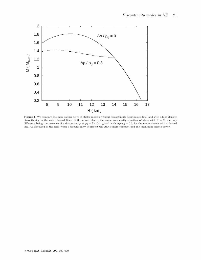
Before discussing the behaviour of the quasi normal mode frequencies, let us shortly

describe how the structure of a neutron star changes if a phase transition associated to a

density discontinuity occurs in its inner core. In Figure 1 we plot the mass-radius relation

for a star with and without discontinuity. The parameters are ρd = 7 · 1014 g/cm3 and

∆ρ/ρd = 0.3. The polytropic index is Γ = 2 in both cases, and we set K(1 + ∆ρ/ρd)2 =

180 km2, in order to have the same equation of state for the two models when ρ < ρd. Figure

1 shows that the maximum mass is lower for the model with a density discontinuity; this is

a general behaviour, which is due to the softening of the equation of state introduced by the

discontinuity. As a rule of thumb, for a fixed mass, a star with a discontinuity is more compact

than one with the same mass and no discontinuity at all; for instance, from Figure 1 we see

that for M = 1.4 M⊙ the star with no phase transition has a radius of R = 13.44 km, while

the one with a density discontinuity has R = 9.66 km. These general properties continue

to hold also if EOSs more realistic than eq. (10) are used, and if phase transitions due to

kaon/pion condensation or to the nucleation of quark matter are considered (Heiselberg &

Hjorth-Jensen 2000). Thus the EOS we use, though approximate, allows us to infer the mode

properties that are known to depend much more on the star’s macroscopic properties (mass,

radius, etc.), than on the specific microscopic interactions.

c© 0000 RAS, MNRAS 000, 000–000


In our study, we shall consider stars with a fixed mass M = 1.4 M⊙, because astronomical

observations show that NSs that have not spent a significant part of their life accreting matter

from a companion in a binary system, have masses in a narrow range around this fiducial

value (Thorsett & Chakrabarty 1999). We shall choose different values of the polytropic

exponent Γ = (1.67, 1.83, 2.00, 2.25), and assign the constant K in such a way that models

with the same Γ have the same EOS for ρ < ρd , independently of the particular values of

∆ρ/ρd and ρd. Since we require that all stars have the same mass, we will have to adjust the

central density accordingly. This means that different stars have a different matter content

in their core. Furthermore, we select models with reasonable radii (8.5 km ≤ R ≤ 17.9 km)

and, since we want to study high density discontinuities, we fix their location at Rd ≤ 0.8 R.

The amplitude of the discontinuity is chosen to vary within ∆ρ/ρd = (0.1 − 0.3); larger

values would not allow stable stellar models with reasonable values of mass and radius.

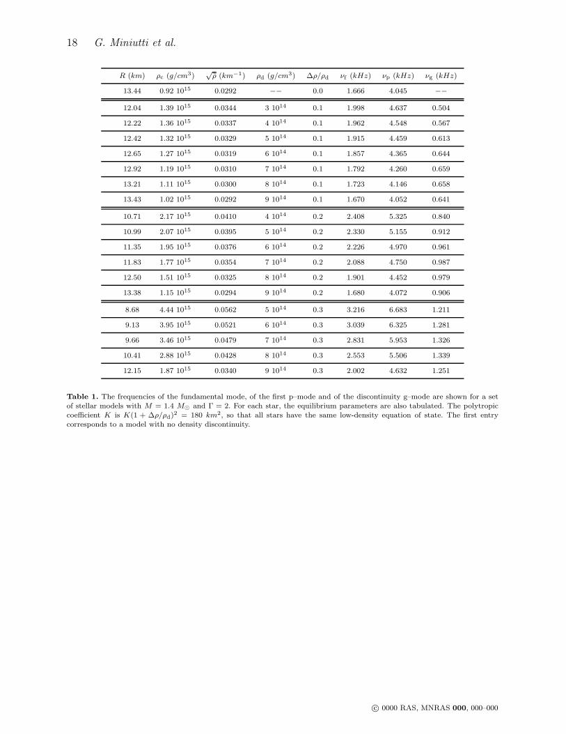
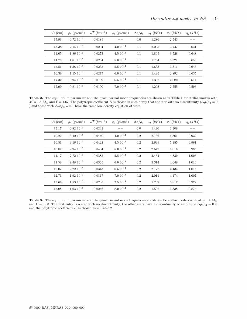
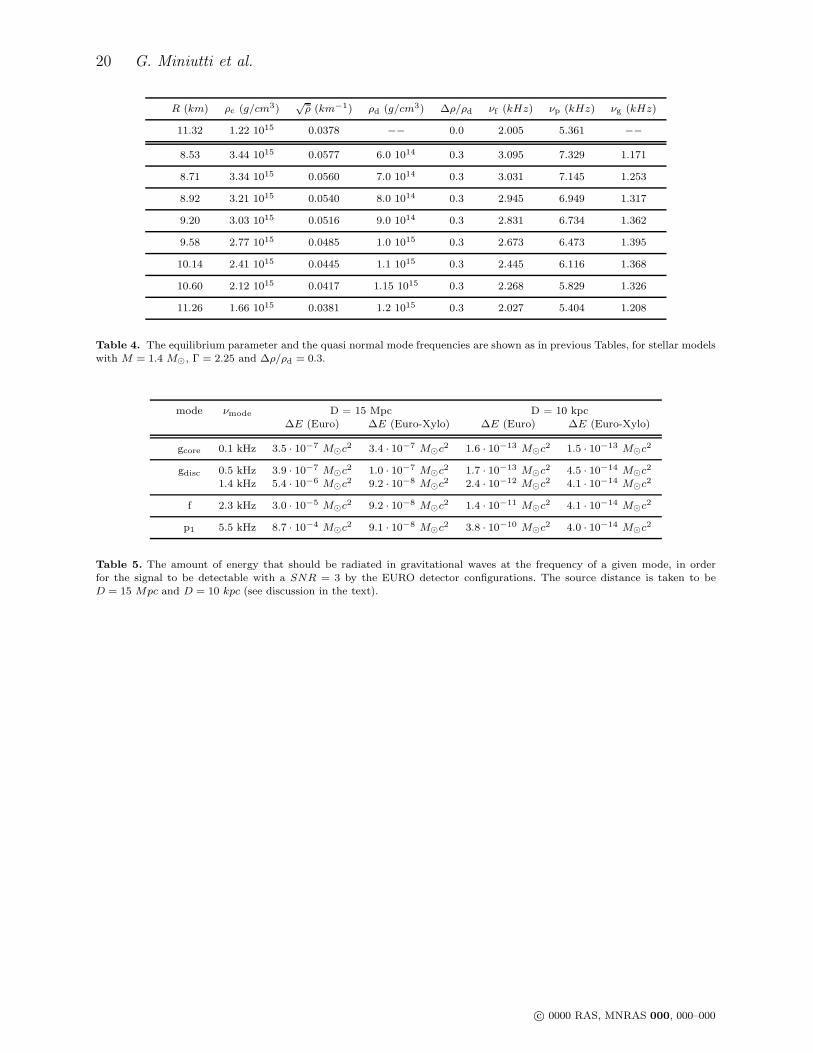
In Tables 1–4 we summarize the results of the numerical integration of the Eqs. (4) and

(7) for these stellar models, as well as the equilibrium parameters. The frequencies of the

fundamental mode (νf), the first pressure mode (νp), and the discontinuity g–mode (νg) are

tabulated for different values of the parameters. The models considered in Table 1 have

the same value of the polytropic exponent, Γ = 2, and refer to three different values of

∆ρ/ρd = ( 0.1, 0.2, 0.3 ). In the remaining three Tables (2-4), we change the polytropic

index and for each value we consider a different ∆ρ/ρd. These choices allow to study the

mode frequencies for a wide range of stellar models.

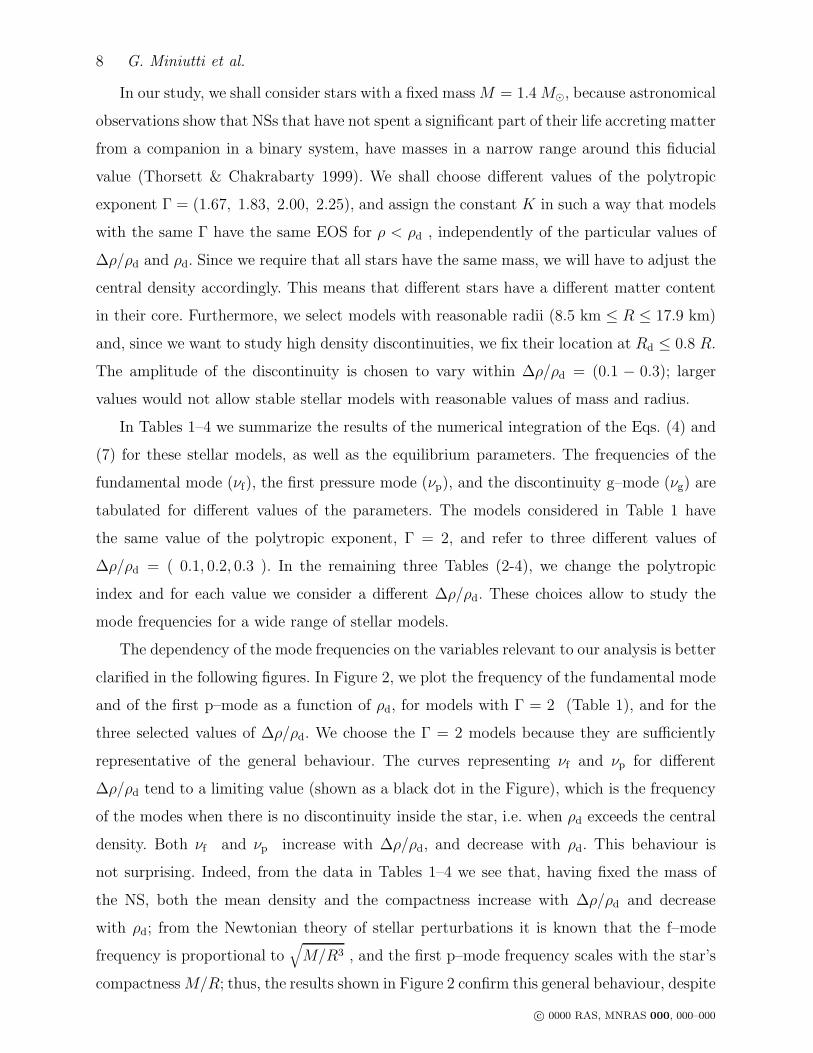
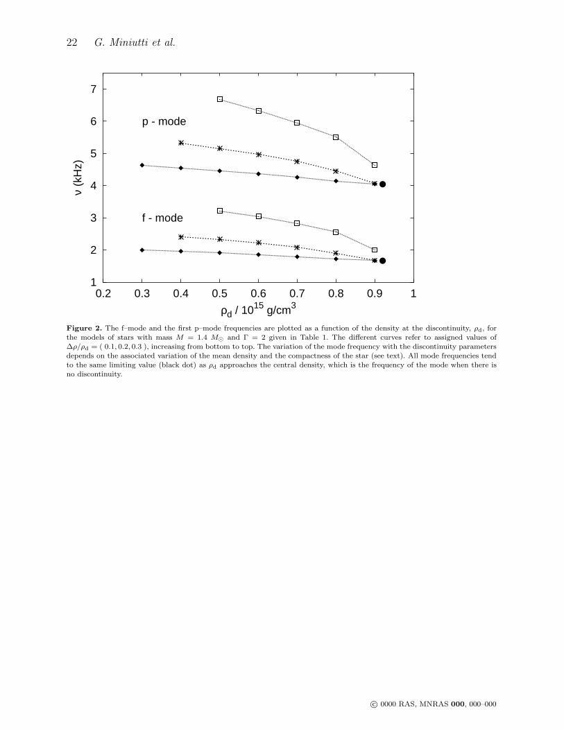
The dependency of the mode frequencies on the variables relevant to our analysis is better

clarified in the following figures. In Figure 2, we plot the frequency of the fundamental mode

and of the first p–mode as a function of ρd, for models with Γ = 2 (Table 1), and for the

three selected values of ∆ρ/ρd. We choose the Γ = 2 models because they are sufficiently

representative of the general behaviour. The curves representing νf and νp for different

∆ρ/ρd tend to a limiting value (shown as a black dot in the Figure), which is the frequency

of the modes when there is no discontinuity inside the star, i.e. when ρd exceeds the central

density. Both νf and νp increase with ∆ρ/ρd, and decrease with ρd. This behaviour is

not surprising. Indeed, from the data in Tables 1–4 we see that, having fixed the mass of

the NS, both the mean density and the compactness increase with ∆ρ/ρd and decrease

with ρd; from the Newtonian theory of stellar perturbations it is known that the f–mode

frequency is proportional to√

M/R3 , and the first p–mode frequency scales with the star’s

compactness M/R; thus, the results shown in Figure 2 confirm this general behaviour, despite

c© 0000 RAS, MNRAS 000, 000–000


the structural changes produced by the density discontinuity. The dependency of νf and

νp on the mean density and compactness of the star has been studied in general relativity

for a large number of realistic EOSs; empirical relations have been derived between the

mode frequencies and the parameters of the star, that could be used to infer the mass and

the radius of neutron stars if a gravitational signal emitted by these pulsation modes were

detected (Andersson & Kokkotas 1996; Andersson & Kokkotas 1998; Kokkotas, Apostolatos

& Andersson 2001). These fits were obtained on the assumption that the density is continuous

inside the star, and it is interesting to see whether a discontinuity introduces deviations from

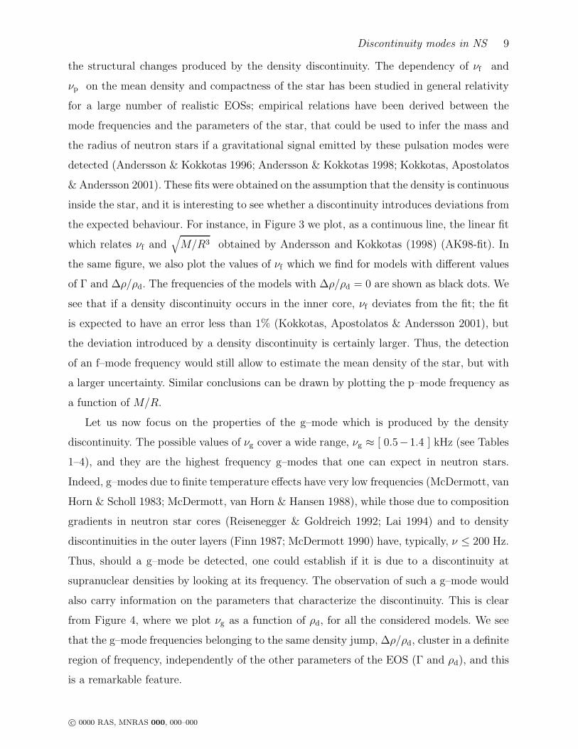
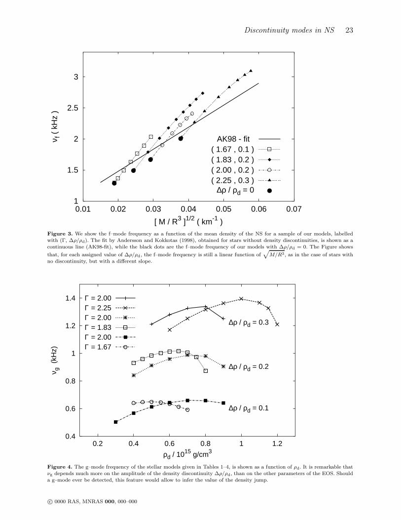
the expected behaviour. For instance, in Figure 3 we plot, as a continuous line, the linear fit

which relates νf and√

M/R3 obtained by Andersson and Kokkotas (1998) (AK98-fit). In

the same figure, we also plot the values of νf which we find for models with different values

of Γ and ∆ρ/ρd. The frequencies of the models with ∆ρ/ρd = 0 are shown as black dots. We

see that if a density discontinuity occurs in the inner core, νf deviates from the fit; the fit

is expected to have an error less than 1% (Kokkotas, Apostolatos & Andersson 2001), but

the deviation introduced by a density discontinuity is certainly larger. Thus, the detection

of an f–mode frequency would still allow to estimate the mean density of the star, but with

a larger uncertainty. Similar conclusions can be drawn by plotting the p–mode frequency as

a function of M/R.

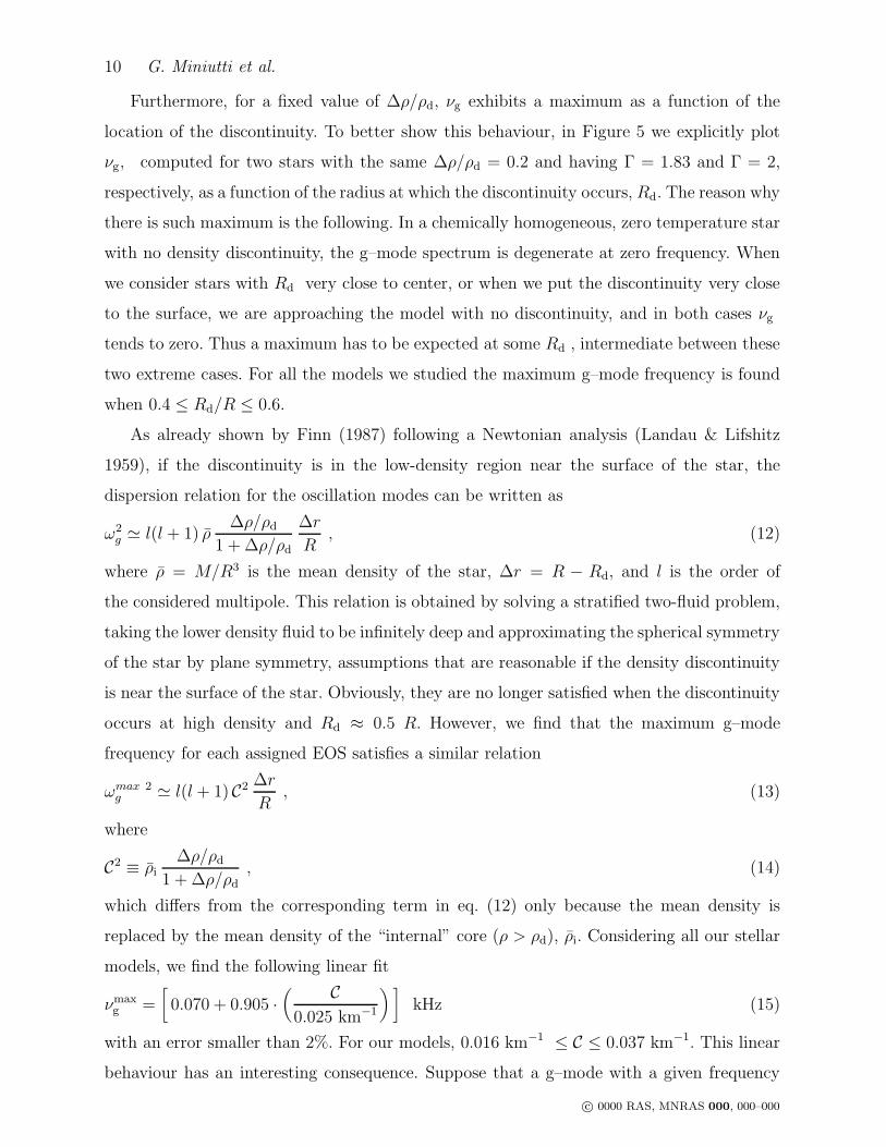
Let us now focus on the properties of the g–mode which is produced by the density

discontinuity. The possible values of νg cover a wide range, νg ≈ [ 0.5−1.4 ] kHz (see Tables

1–4), and they are the highest frequency g–modes that one can expect in neutron stars.

Indeed, g–modes due to finite temperature effects have very low frequencies (McDermott, van

Horn & Scholl 1983; McDermott, van Horn & Hansen 1988), while those due to composition

gradients in neutron star cores (Reisenegger & Goldreich 1992; Lai 1994) and to density

discontinuities in the outer layers (Finn 1987; McDermott 1990) have, typically, ν ≤ 200 Hz.

Thus, should a g–mode be detected, one could establish if it is due to a discontinuity at

supranuclear densities by looking at its frequency. The observation of such a g–mode would

also carry information on the parameters that characterize the discontinuity. This is clear

from Figure 4, where we plot νg as a function of ρd, for all the considered models. We see

that the g–mode frequencies belonging to the same density jump, ∆ρ/ρd, cluster in a definite

region of frequency, independently of the other parameters of the EOS (Γ and ρd), and this

is a remarkable feature.

c© 0000 RAS, MNRAS 000, 000–000


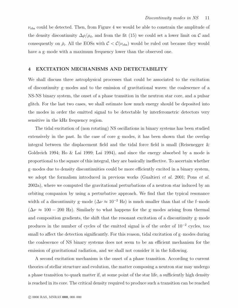
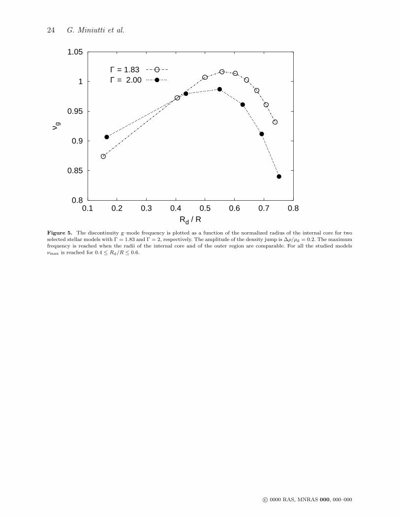
Furthermore, for a fixed value of ∆ρ/ρd, νg exhibits a maximum as a function of the

location of the discontinuity. To better show this behaviour, in Figure 5 we explicitly plot

νg, computed for two stars with the same ∆ρ/ρd = 0.2 and having Γ = 1.83 and Γ = 2,

respectively, as a function of the radius at which the discontinuity occurs, Rd. The reason why

there is such maximum is the following. In a chemically homogeneous, zero temperature star

with no density discontinuity, the g–mode spectrum is degenerate at zero frequency. When

we consider stars with Rd very close to center, or when we put the discontinuity very close

to the surface, we are approaching the model with no discontinuity, and in both cases νg

tends to zero. Thus a maximum has to be expected at some Rd , intermediate between these

two extreme cases. For all the models we studied the maximum g–mode frequency is found

when 0.4 ≤ Rd/R ≤ 0.6.

As already shown by Finn (1987) following a Newtonian analysis (Landau & Lifshitz

1959), if the discontinuity is in the low-density region near the surface of the star, the

dispersion relation for the oscillation modes can be written as

ω2g ≃ l(l + 1) ρ

∆ρ/ρd

1 + ∆ρ/ρd

∆r

R, (12)

where ρ = M/R3 is the mean density of the star, ∆r = R − Rd, and l is the order of

the considered multipole. This relation is obtained by solving a stratified two-fluid problem,

taking the lower density fluid to be infinitely deep and approximating the spherical symmetry

of the star by plane symmetry, assumptions that are reasonable if the density discontinuity

is near the surface of the star. Obviously, they are no longer satisfied when the discontinuity

occurs at high density and Rd ≈ 0.5 R. However, we find that the maximum g–mode

frequency for each assigned EOS satisfies a similar relation

ωmax 2g ≃ l(l + 1) C2 ∆r

R, (13)

where

C2 ≡ ρi∆ρ/ρd

1 + ∆ρ/ρd, (14)

which differs from the corresponding term in eq. (12) only because the mean density is

replaced by the mean density of the “internal” core (ρ > ρd), ρi. Considering all our stellar

models, we find the following linear fit

νmaxg =

[

0.070 + 0.905 ·(

C

0.025 km−1

) ]

kHz (15)

with an error smaller than 2%. For our models, 0.016 km−1≤ C ≤ 0.037 km−1. This linear

behaviour has an interesting consequence. Suppose that a g–mode with a given frequency

c© 0000 RAS, MNRAS 000, 000–000


νobs could be detected. Then, from Figure 4 we would be able to constrain the amplitude of

the density discontinuity ∆ρ/ρd, and from the fit (15) we could set a lower limit on C and

consequently on ρi. All the EOSs with C < C(νobs) would be ruled out because they would

have a g–mode with a maximum frequency lower than the observed one.

4 EXCITATION MECHANISMS AND DETECTABILITY

We shall discuss three astrophysical processes that could be associated to the excitation

of discontinuity g–modes and to the emission of gravitational waves: the coalescence of a

NS-NS binary system, the onset of a phase transition in the neutron star core, and a pulsar

glitch. For the last two cases, we shall estimate how much energy should be deposited into

the modes in order the emitted signal to be detectable by interferometric detectors very

sensitive in the kHz frequency region.

The tidal excitation of (non rotating) NS oscillations in binary systems has been studied

extensively in the past. In the case of core g–modes, it has been shown that the overlap

integral between the displacement field and the tidal force field is small (Reisenegger &

Goldreich 1994; Ho & Lai 1999; Lai 1994), and since the energy absorbed by a mode is

proportional to the square of this integral, they are basically ineffective. To ascertain whether

g–modes due to density discontinuities could be more efficiently excited in a binary system,

we adopt the formalism introduced in previous works (Gualtieri et al. 2001; Pons et al.

2002a), where we computed the gravitational perturbations of a neutron star induced by an

orbiting companion by using a perturbative approach. We find that the typical resonance

width of a discontinuity g–mode (∆ν ≈ 10−2 Hz) is much smaller than that of the f–mode

(∆ν ≈ 100 − 200 Hz). Similarly to what happens for the g–modes arising from thermal

and composition gradients, the shift that the resonant excitation of a discontinuity g–mode

produces in the number of cycles of the emitted signal is of the order of 10−2 cycles, too

small to affect the detection significantly. For this reason, tidal excitation of g–modes during

the coalescence of NS binary systems does not seem to be an efficient mechanism for the

emission of gravitational radiation, and we shall not consider it in the following.

A second excitation mechanism is the onset of a phase transition. According to current

theories of stellar structure and evolution, the matter composing a neutron star may undergo

a phase transition to quark matter if, at some point of the star life, a sufficiently high density

is reached in its core. The critical density required to produce such a transition can be reached

c© 0000 RAS, MNRAS 000, 000–000


soon after the core-collapse which gives birth to the neutron star, or at a later stage of the

evolution, due to accretion (Cheng & Dai 1998) and/or spin-down (Ma & Xie 1996). The

onset of a phase transition is accompanied by a sudden reduction of the stellar radius and

the difference in binding energy between the initial and final configuration is expected to

be radiated away. The binding energy released during this late mini-collapse is of the same

order as that emitted during neutron star formation following a gravitational core–collapse,

i.e. ≈ 2 × 1053erg = 0.1M⊙c2 (Alcock, Farhi & Olinto 1986; Bombaci & Datta 2000). How

much of this energy reservoir can be redistributed in the different modes of oscillation of the

star and radiated in gravitational wave is, however, an open issue. Therefore, the only thing

we can reasonably estimate is which fraction of this energy should go into the quasi normal

modes in order the signal emitted at the corresponding frequencies to be detectable.

The quasi normal modes of oscillation of a star may also be excited as a consequence of a

glitch. Glitches are sudden changes in the rotation frequency of the neutron star crust which

superimpose to the usual gradual spin-down under magnetic torque. They are observed in

many pulsars and are thought to be related to quakes occurring in the solid structures such

as the crust, the superfluid vortices and, perhaps, the lattice of quark matter in the stellar

core (Anderson & Itoh 1975; Ruderman 1976; Pines & Alpar 1985). The observed glitches

are very small, with a typical fractional spin variation of about ∆Ω/Ω ≈ 10−6 −10−8, which

would be associated to an energy release of the order of ∆E ≈ IΩ∆Ω, where I is the

moment of inertia of the star. For the glitches observed in the Crab and Vela pulsars this

simple estimate gives ∆E ≃ 2 · 10−13 M⊙c2 and ∆E ≃ 3 · 10−12 M⊙c2, respectively. As

before, we shall assume that a fraction of this energy is redistributed into the quasi normal

modes of oscillation of the perturbed star, and we shall evaluate how much is needed to

excite a mode to a detectable level.

4.1 Detectability

The frequency of the discontinuity g–modes we have studied ranges between νg ≃ [0.5 −

1.4] kHz, while νf ≃ [1.3 − 3.2] kHz and for the first p-mode νp ≃ [2.5 − 7.3] kHz. In order

to detect a signal emitted as a consequence of the excitation of these modes a very sensitive

high frequency detector would be needed. In the following we shall consider the gravitational

laser interferometric detector EURO, that has recently been proposed in a preliminary as-

sessment study and for which the sensitivity has been estimated by Sathyaprakash and

c© 0000 RAS, MNRAS 000, 000–000


Schutz (http://www.astro.cf.ac.uk/geo/euro). EURO should be extremely sensitive in the

kHz region, which is crucial to infer informations about neutron stars interior from gravi-

tational wave data, and it has been envisaged in two experimental configurations: one for

which the noise curve in the frequency region 10 − 104 Hz can be written as

Sn(ν) = 10−50

[

3.6 109

ν4+

1.3 105

ν2+ 1.3 10−3 νk

(

1 +ν2

ν2k

)]

Hz−1 , (16)

where νk = 103 Hz; the second configuration is the more ambitious Xylophone detector, for

which the shot noise, i.e. the third term within brackets in (16), should be eliminated by

running several narrow-banded interferometers. We will refer to these two possible configu-

rations as EURO and EURO-Xylo, respectively. We shall assume that the gravitation signal

from a star pulsating in a quasi-normal mode is a damped sinusoid of the form (Echeverria

1989)

h(t) = Ae(tarr−t)/τ sin [2πν (t − tarr)] , (17)

where tarr is the arrival time and τ the damping time of the oscillation. The amplitude A

can be expressed in terms of the total energy ∆E⊙ = ∆E/M⊙c2 deposited into the mode,

and of the distance D of the source by (Kokkotas, Apostolatos & Andersson 2001)

A ≃ 7.6 10−23

√

∆E⊙

10−10

1 s

τ

(

1 kpc

D

) (

103 Hz

ν

)

. (18)

Given a detector with noise spectrum Sn(ν), and assuming that the matched filtering tech-

nique is used to extract the signal, the signal to noise ratio (SNR), can be written as

SNR =

[

FA2τ

2Sn

]1/2

, (19)

where F = 4Q2/(1 + 4Q2) is a form factor, and Q = πντ is the quality factor of the

oscillation.

It should be noted that in the case of discontinuity g–modes, since the gravitational

damping time ranges between τ ≈ (107 − 1012) s, the oscillations will be damped by other

dominant dissipative mechanisms rather than by the emission of gravitational waves. In

newly born neutron stars (or hybrid stars with a quark core) the dominant damping mech-

anism is neutrino viscosity, with a typical timescale of 10 − 102 s (van den Horn & van

Weert 1981; Goodwin & Pethick 1982; Thompson & Duncan 1993). In the glitches scenario

(or other similar excitations occurring in late stages of the evolution of neutron stars) the

neutron star is cold and neutrinos are not coupled to the matter. The dissipative mecha-

nisms are then associated to the kinematical properties of matter. In this case, bulk, shear

c© 0000 RAS, MNRAS 000, 000–000

http://www.astro.cf.ac.uk/geo/euro


viscosity and boundary layer dissipation are more efficient than gravitational damping. In

any case, the typical dissipative time-scales are thought to be much larger than the neu-

trino damping time-scale in proto-neutron(quark) stars (Bildsten & Ushomirsky 2000), but

a word of caution is needed. It has been found that quark-matter viscosity is much larger

than that of normal neutron star matter (Madsen 1992), and therefore it would quickly

damp the oscillations in the dense quark core (τ ∼ 10−2 s). However, these results are still

under debate, and it remains to be carefully analyzed how the outer shell would react to the

strong damping in the inner region, and whether or not boundary effects would change the

picture. Note however that, for the range of frequencies considered in this paper, the quality

factor Q ≫ 1 as long as τ is greater that, say, 10−2 s; thus, the form factor in Eq. (19) can

be taken equal to one, and the signal to noise ratio happens to be quite insensitive to the

damping time.

In the following, we shall estimate the amount of energy that should go into a quasi

normal mode to produce a gravitational signal detectable with a signal to noise ratio SNR =

3, either by EURO or by EURO-Xylo detector. For g–mode pulsations, we consider the two

limiting frequencies ν1 = 0.5 kHz and ν2 = 1.4 kHz, being the g–mode frequency of all our

models included in this range. The excitation of a core g–mode at 0.1 kHz (Reisenegger &

Goldreich 1992; Lai 1994) is also computed for comparison. For the f– and p–modes, our

estimates are done for two frequencies, νf = 2.3 kHz and νp = 5.5 kHz, which are obtained

as an average over the corresponding range of variation for all our models. The gravitational

damping time of the fundamental and p–mode are smaller than the other dissipative time

scales; thus, in this case the emission of gravitational waves is the dominant dissipative

mechanism and both τf and τp have been used explicitly in our estimates.

For the two different excitation scenarios, mini-collapse and glitches, we shall consider

sources located at distances D = 15 Mpc and D = 10 kpc, respectively. Note that the

Virgo cluster, with its some 2 103 members, is at D ≈ 15 Mpc and that the Vela and Crab

pulsars, that are known to produce glitches, are at distances of D = 0.5 kpc and D = 2 kpc,

respectively.

Our estimates are given in Table (5), and show that the high frequency detectors would be

a very interesting instrument to probe, through gravitational signals, the nature of neutron

stars interiors. Note that, since for the EURO configuration the sensitivity at high frequency

is strongly limited by the shot noise, a p–mode at νp = 5.5 kHz could be detected only with

the advanced EURO-Xylo configuration. If one focuses on the fundamental mode and the

c© 0000 RAS, MNRAS 000, 000–000


discontinuity g–mode, the minimal energies required to detect a signal with SNR = 3 with

the EURO detector range within 1.6 · 10−13 ≤ ∆E/M⊙c2 ≤ 3.0 · 10−5, depending on the

source distance and on the frequency of the signal. With the EURO-Xylo configuration,

this range becomes 4.1 · 10−14 ≤ ∆E/M⊙c2 ≤ 3.4 · 10−7. As mentioned before, the amount

of binding energy which is expected to be released in a mini-collapse is approximately the

same as that emitted during a core-collapse Supernova. In the Supernova case, it has been

suggested that the fraction of this energy radiated in gravitational waves is in the range

[10−8 − 10−6] M⊙c2 (Monchmeyer et al. 1991; Dimmelmeier, Font & Muller 2001; Zwerger

& Muller 1997); if we assume that a comparable amount of energy goes in gravitational

waves also in the case of a mini-collapse, the chance for a quasi normal mode signal to be

detectable from a source closer than 15 Mpc is promising. The situation is clearly even more

interesting for galactic sources, since the amount of energy required to excite a mode at a

detectable level is typically a small fraction of the total energy reservoir.

5 CONCLUSIONS

According to the relativistic theory of stellar perturbations, a star perturbed by any external

or internal process emits gravitational waves at the characteristic frequencies of its quasi

normal modes. It has been shown that both the mass and the radius of a pulsating cold

neutron star could be inferred, if the quasi normal modes were identified by a spectral

analysis in the detected wave (Andersson & Kokkotas 1998). More recently, the possibility

of tracing the presence of a superfluid core through the detection of superfluid modes has

also been investigated (Andersson & Comer 2001). As described in the introduction, g-

modes are also good markers of the internal composition of a neutron star: low frequency

g-modes indicate a non homogeneous composition in the outer layers or in the core of the

star, or a thermal profile, whereas the high frequency g-modes which we study in this paper,

are associated to phase transitions occurring at supranuclear densities (Sotani et al., 2001).

Although the analysis has been restricted to simplified polytropic EOSs, our results can be

generalized to realistic equations of state, since it is known that the oscillation frequencies

depend more on global properties, like mass and radius, than on the specific form of the

microscopical interactions. We have analyzed models of stars with a mass of 1.4 M⊙, since

astrophysical observations show that most of the well measured masses of neutron stars in

binary systems cluster in a narrow range around this value.

c© 0000 RAS, MNRAS 000, 000–000


We find that high frequency discontinuity g–modes exhibit several interesting features: i)

the linear relation known to exist between the frequency of the fundamental mode and the

square root of the average density, still holds for neutron stars with density discontinuities.

Thus, a measure of the f-mode frequency would be useful to constrain the neutron star

radius, provided the mass is measured independently, even when a phase transition takes

place in its core. However, the presence of the discontinuity introduces a larger error on

the NS radius determination. ii) Should density discontinuities actually exist, the associated

g–mode will have a frequency of about 1 kHz, somewhat lower than that of the f-mode,

and therefore clearly distinguishable. It may be reminded that thermal or chemical g-modes

appear at significantly lower frequencies (< 200 Hz). iii) Since the g–mode frequency strongly

depends on the amplitude of the discontinuity, it could be used to infer the value of ∆ρ/ρd.

In addition, since the maximum of νg, considered as a function of the discontinuity radius

Rd, is related to ∆ρ/ρd and to the average density, ρi, of the core internal to Rd, (see eqs.

(14) and (15)) it would be possible to set a lower bound on ρi, and to rule out all EOSs for

which the combination C2 ≡ ρi∆ρ/ρd

1+∆ρ/ρdis smaller than the observed one.

In the spirit of previous works (Andersson & Comer 2001), which discussed the ob-

servability of oscillation modes produced by the existence of superfluid components in the

interior of a neutron star, we have analyzed some astrophysical processes in which high

frequency modes could be excited, and we have evaluated the amount of energy that the

modes should convey to produce a gravitational signal detectable with a SNR=3 by the high

frequency gravitational detectors under study. We find that the required energy does not

conflict with the estimates of the energy expected to be released in gravitational waves at

the onset of a phase transition, or during a glitch. In particular, the detector EURO, espe-

cially in the configuration known as EURO-Xylophone, would have a significant chance to

reveal the gravitational signal associated to the excitation of the fundamental mode, of the

first pressure mode and of the discontinuity g–mode following a galactic glitch or a stellar

core-collapse or a mini-collapse induced by the onset of a phase transition to quark matter

within 10-15 Mpc. By cross-correlating the information carried by these mode frequencies,

and in particular by the high frequency discontinuity g–modes, we would acquire extremely

valuable indications on the properties of nuclear matter at supranuclear density.

Acknowledgements

c© 0000 RAS, MNRAS 000, 000–000


We would like to thank O. Benhar for useful discussions. We thank B.S. Sathyaprakash

for providing us the power spectral density of the EURO detector.

This work has been supported by the EU Programme ’Improving the Human Research

Potential and the Socio-Economic Knowledge Base’ (Research Training Network Contract

HPRN-CT-2000-00137). JAP is supported by the Marie Curie Fellowship No. HPMF-CT-

2001-01217.

c© 0000 RAS, MNRAS 000, 000–000


R (km) ρc (g/cm3)√

ρ (km−1) ρd (g/cm3) ∆ρ/ρd νf (kHz) νp (kHz) νg (kHz)

13.44 0.92 1015 0.0292 −− 0.0 1.666 4.045 −−

12.04 1.39 1015 0.0344 3 1014 0.1 1.998 4.637 0.504

12.22 1.36 1015 0.0337 4 1014 0.1 1.962 4.548 0.567

12.42 1.32 1015 0.0329 5 1014 0.1 1.915 4.459 0.613

12.65 1.27 1015 0.0319 6 1014 0.1 1.857 4.365 0.644

12.92 1.19 1015 0.0310 7 1014 0.1 1.792 4.260 0.659

13.21 1.11 1015 0.0300 8 1014 0.1 1.723 4.146 0.658

13.43 1.02 1015 0.0292 9 1014 0.1 1.670 4.052 0.641

10.71 2.17 1015 0.0410 4 1014 0.2 2.408 5.325 0.840

10.99 2.07 1015 0.0395 5 1014 0.2 2.330 5.155 0.912

11.35 1.95 1015 0.0376 6 1014 0.2 2.226 4.970 0.961

11.83 1.77 1015 0.0354 7 1014 0.2 2.088 4.750 0.987

12.50 1.51 1015 0.0325 8 1014 0.2 1.901 4.452 0.979

13.38 1.15 1015 0.0294 9 1014 0.2 1.680 4.072 0.906

8.68 4.44 1015 0.0562 5 1014 0.3 3.216 6.683 1.211

9.13 3.95 1015 0.0521 6 1014 0.3 3.039 6.325 1.281

9.66 3.46 1015 0.0479 7 1014 0.3 2.831 5.953 1.326

10.41 2.88 1015 0.0428 8 1014 0.3 2.553 5.506 1.339

12.15 1.87 1015 0.0340 9 1014 0.3 2.002 4.632 1.251

Table 1. The frequencies of the fundamental mode, of the first p–mode and of the discontinuity g–mode are shown for a setof stellar models with M = 1.4 M⊙ and Γ = 2. For each star, the equilibrium parameters are also tabulated. The polytropiccoefficient K is K(1 + ∆ρ/ρd)2 = 180 km2, so that all stars have the same low-density equation of state. The first entrycorresponds to a model with no density discontinuity.

c© 0000 RAS, MNRAS 000, 000–000




17.96 0.72 1015 0.0189 −− 0.0 1.286 2.543 −−

13.38 2.14 1015 0.0294 4.0 1014 0.1 2.035 3.747 0.641

14.05 1.86 1015 0.0273 4.5 1014 0.1 1.895 3.528 0.648

14.75 1.61 1015 0.0254 5.0 1014 0.1 1.764 3.321 0.650

15.51 1.38 1015 0.0235 5.5 1014 0.1 1.633 3.311 0.646

16.39 1.15 1015 0.0217 6.0 1014 0.1 1.495 2.892 0.635

17.32 0.94 1015 0.0199 6.5 1014 0.1 1.367 2.680 0.614

17.90 0.81 1015 0.0190 7.0 1014 0.1 1.293 2.555 0.593

Table 2. The equilibrium parameter and the quasi normal mode frequencies are shown as in Table 1 for stellar models withM = 1.4 M⊙ and Γ = 1.67. The polytropic coefficient K is chosen in such a way that the star with no discontinuity (∆ρ/ρd = 0) and those with ∆ρ/ρd = 0.1 have the same low-density equation of state.



15.17 0.82 1015 0.0243 −− 0.0 1.490 3.308 −−

10.22 3.40 1015 0.0440 4.0 1014 0.2 2.736 5.361 0.932

10.51 3.16 1015 0.0422 4.5 1014 0.2 2.639 5.185 0.961

10.82 2.94 1015 0.0404 5.0 1014 0.2 2.542 5.016 0.985

11.17 2.72 1015 0.0385 5.5 1014 0.2 2.434 4.839 1.003

11.58 2.48 1015 0.0365 6.0 1014 0.2 2.314 4.648 1.014

12.07 2.22 1015 0.0343 6.5 1014 0.2 2.177 4.434 1.016

12.71 1.92 1015 0.0317 7.0 1014 0.2 2.011 4.174 1.007

13.66 1.53 1015 0.0285 7.5 1014 0.2 1.789 3.817 0.972

15.08 1.03 1015 0.0246 8.0 1014 0.2 1.507 3.338 0.874

Table 3. The equilibrium parameter and the quasi normal mode frequencies are shown for stellar models with M = 1.4 M⊙

and Γ = 1.83. The first entry is a star with no discontinuity, the other stars have a discontinuity of amplitude ∆ρ/ρd = 0.2,and the polytropic coefficient K is chosen as in Table 2.

c© 0000 RAS, MNRAS 000, 000–000




11.32 1.22 1015 0.0378 −− 0.0 2.005 5.361 −−

8.53 3.44 1015 0.0577 6.0 1014 0.3 3.095 7.329 1.171

8.71 3.34 1015 0.0560 7.0 1014 0.3 3.031 7.145 1.253

8.92 3.21 1015 0.0540 8.0 1014 0.3 2.945 6.949 1.317

9.20 3.03 1015 0.0516 9.0 1014 0.3 2.831 6.734 1.362

9.58 2.77 1015 0.0485 1.0 1015 0.3 2.673 6.473 1.395

10.14 2.41 1015 0.0445 1.1 1015 0.3 2.445 6.116 1.368

10.60 2.12 1015 0.0417 1.15 1015 0.3 2.268 5.829 1.326

11.26 1.66 1015 0.0381 1.2 1015 0.3 2.027 5.404 1.208

Table 4. The equilibrium parameter and the quasi normal mode frequencies are shown as in previous Tables, for stellar modelswith M = 1.4 M⊙, Γ = 2.25 and ∆ρ/ρd = 0.3.

mode νmode D = 15 Mpc D = 10 kpc∆E (Euro) ∆E (Euro-Xylo) ∆E (Euro) ∆E (Euro-Xylo)

gcore 0.1 kHz 3.5 · 10−7 M⊙c2 3.4 · 10−7 M⊙c2 1.6 · 10−13 M⊙c2 1.5 · 10−13 M⊙c2

gdisc 0.5 kHz 3.9 · 10−7 M⊙c2 1.0 · 10−7 M⊙c2 1.7 · 10−13 M⊙c2 4.5 · 10−14 M⊙c2

1.4 kHz 5.4 · 10−6 M⊙c2 9.2 · 10−8 M⊙c2 2.4 · 10−12 M⊙c2 4.1 · 10−14 M⊙c2

f 2.3 kHz 3.0 · 10−5 M⊙c2 9.2 · 10−8 M⊙c2 1.4 · 10−11 M⊙c2 4.1 · 10−14 M⊙c2

p1 5.5 kHz 8.7 · 10−4 M⊙c2 9.1 · 10−8 M⊙c2 3.8 · 10−10 M⊙c2 4.0 · 10−14 M⊙c2

Table 5. The amount of energy that should be radiated in gravitational waves at the frequency of a given mode, in orderfor the signal to be detectable with a SNR = 3 by the EURO detector configurations. The source distance is taken to beD = 15 Mpc and D = 10 kpc (see discussion in the text).

c© 0000 RAS, MNRAS 000, 000–000


0.2

0.4

0.6

0.8

1

1.2

1.4

1.6

1.8

2

8 9 10 11 12 13 14 15 16 17

M (

Msu

n )

R ( km )

∆ρ / ρd = 0

∆ρ / ρd = 0.3

Figure 1. We compare the mass-radius curve of stellar models without discontinuity (continuous line) and with a high densitydiscontinuity in the core (dashed line). Both curves refer to the same low-density equation of state with Γ = 2, the onlydifference being the presence of a discontinuity at ρd = 7 · 1014 g/cm3 with ∆ρ/ρd = 0.3, for the model shown with a dashedline. As discussed in the text, when a discontinuity is present the star is more compact and the maximum mass is lower.

c© 0000 RAS, MNRAS 000, 000–000


1

2

3

4

5

6

7

0.2 0.3 0.4 0.5 0.6 0.7 0.8 0.9 1

ν (k

Hz)

ρd / 1015 g/cm3

f - mode

p - mode

Figure 2. The f–mode and the first p–mode frequencies are plotted as a function of the density at the discontinuity, ρd, forthe models of stars with mass M = 1.4 M⊙ and Γ = 2 given in Table 1. The different curves refer to assigned values of∆ρ/ρd = ( 0.1, 0.2, 0.3 ), increasing from bottom to top. The variation of the mode frequency with the discontinuity parametersdepends on the associated variation of the mean density and the compactness of the star (see text). All mode frequencies tendto the same limiting value (black dot) as ρd approaches the central density, which is the frequency of the mode when there isno discontinuity.

c© 0000 RAS, MNRAS 000, 000–000


1

1.5

2

2.5

3

0.01 0.02 0.03 0.04 0.05 0.06 0.07

ν f (

kH

z )

[ M / R3 ]1/2 ( km-1 )

AK98 - fit ( 1.67 , 0.1 )( 1.83 , 0.2 )( 2.00 , 0.2 )( 2.25 , 0.3 )

∆ρ / ρd = 0

Figure 3. We show the f–mode frequency as a function of the mean density of the NS for a sample of our models, labelledwith (Γ, ∆ρ/ρd). The fit by Andersson and Kokkotas (1998), obtained for stars without density discontinuities, is shown as acontinuous line (AK98-fit), while the black dots are the f–mode frequency of our models with ∆ρ/ρd = 0. The Figure shows

that, for each assigned value of ∆ρ/ρd, the f–mode frequency is still a linear function of√

M/R3, as in the case of stars withno discontinuity, but with a different slope.

0.4

0.6

0.8

1

1.2

1.4

0.2 0.4 0.6 0.8 1 1.2

ν g (

kHz)

ρd / 1015 g/cm3

∆ρ / ρd = 0.3

∆ρ / ρd = 0.2

∆ρ / ρd = 0.1

Γ = 2.00Γ = 2.25Γ = 2.00Γ = 1.83Γ = 2.00Γ = 1.67

Figure 4. The g–mode frequency of the stellar models given in Tables 1–4, is shown as a function of ρd. It is remarkable thatνg depends much more on the amplitude of the density discontinuity ∆ρ/ρd, than on the other parameters of the EOS. Shoulda g–mode ever be detected, this feature would allow to infer the value of the density jump.

c© 0000 RAS, MNRAS 000, 000–000


0.8

0.85

0.9

0.95

1

1.05

0.1 0.2 0.3 0.4 0.5 0.6 0.7 0.8

ν g

Rd / R

Γ = 1.83 Γ = 2.00

Figure 5. The discontinuity g–mode frequency is plotted as a function of the normalized radius of the internal core for twoselected stellar models with Γ = 1.83 and Γ = 2, respectively. The amplitude of the density jump is ∆ρ/ρd = 0.2. The maximumfrequency is reached when the radii of the internal core and of the outer region are comparable. For all the studied modelsνmax is reached for 0.4 ≤ Rd/R ≤ 0.6.

c© 0000 RAS, MNRAS 000, 000–000


REFERENCES

Alcock C., Farhi E., Olinto A., 1986, ApJ, 310, 261

Alford M.G, Rajagopal K., Reddy S., Wilczek F., 2001, Phys. Rev. D64, 074017

Anderson P.W., Itoh N., 1975, Nature, 256, 25

Andersson N., Kokkotas K.D., 1996, Phys. Rev. Lett., 77, 4134

Andersson N., Kokkotas K.D., 1998, MNRAS, 299, 1059

Andersson N., Comer G. L., 2001, Phys. Rev. Lett., 24, 241101

Bildsten L., Ushomirsky G., 2000, ApJ, 529, L33

Bombaci I., Datta B., 2000, ApJ, 530, L69

Chandrasekhar S., Ferrari V., 1990, Proc. R. Soc. Lond., A432, 247

Chandrasekhar S., Ferrari V., Winston R., 1991, Proc. R. Soc. Lond., A434, 635

Cheng K.S., Dai Z.G., 1998, ApJ, 492, 281

Detweiler S., Lindblom I., 1985, ApJ, 292, 12

Dimmelmeier H., Font J.A., Muller E., 2001, ApJ, 560, L163

Echeverria F., 1989, Phys. Rev. D40, 3194

Finn L.S., 1986, MNRAS, 222, 393

Finn L.S., 1987, MNRAS, 227, 265

Glendenning N.K., 1992, Phys. Rev. D46, 1274

Goodwin B.T., Pethick C.J., 1982, ApJ, 253, 816

Gualtieri L., Berti E., Pons J. A., Miniutti G., Ferrari V., 2001, Phys. Rev. D64, 104007

Heiselberg H., Hjorth-Jensen M., 2000, Phys. Rep., 328, 237

Ho W.C.G., Lai D., 1999, MNRAS, 308, 153

Kokkotas K.D., Apostolatos T., Andersson N., 2001, MNRAS, 320, 307

Lai D., 1994, MNRAS, 270, 611

Landau L., Lifshitz E., 1959, Fluid Mechanics, London, Pergamon

Lindblom I., Detweiler S., 1983, ApJ Suppl. Series, 53, 73

Ma F., Xie B., 1996, ApJ, 462, L63

Madsen J., 1992, Phys. Rev. D46, 3290

McDermott P.N. 1990, MNRAS, 245, 508

McDermott P.N., van Horn H.M., Hansen C.J., 1988, ApJ, 325, 725

McDermott, P.N., van Horn H.M., Scholl J.F., 1983, ApJ, 268, 837

Monchmeyer R., Schafer G., Muller E., Kates R., 1991, A&A, 246, 417

Osherovich V., Titarchuk L., 1999, ApJ, 522, L113

Pines D., Alpar M.A., 1985, Nature, 316, 27

Pons J.A., Berti E., Gualtieri L., Miniutti G., Ferrari V., 2002, Phys. Rev. D65, 104021

Pons J.A., Reddy S., Prakash M., Lattimer J.M., Miralles J.A., 1999, ApJ, 513, 780

Pons J.A., Steiner A.W., Prakash M., Lattimer J.M., 2001, Phys. Rev. Lett., 86, 5223

Pons J.A., Walter F.W., Lattimer J.M., Prakash M., Neuhauser R., An P., 2002, ApJ, 564, 981

Prakash M., Bombaci I., Prakash M., Ellis P.J., Lattimer J.M., Knoren R., 1997, Phys. Rep. 280, 1

Reisenegger A., Goldreich P., 1992, ApJ, 395, 240

Reisenegger A., Goldreich P., 1994, ApJ, 426, 688

Ruderman M., 1976, Nature, 203, 213

Rutledege R.E., Bildsten L., Brown E.F., Pavlov G.G., Zavlin V.E., 2001, ApJ, 559, 1054

Sotani H., Tominaga K., Maeda K., 2001, Phys. Rev. D65, 024010

Stella L., Vietri M., 1999, Phys. Rev. Lett., 82, 17

c© 0000 RAS, MNRAS 000, 000–000


Strohmayer T.E., 1993, ApJ, 417, 273

Thompson C., Duncan R., 1993, ApJ, 408, 194

Thorsett S.E., Chakrabarty D., 1999, ApJ, 512, 288

van den Horn L.J., van Weert Ch.G., 1981, ApJ, 251, L97

Zwerger T., Muller E., 1997, A&A, 320, 209

c© 0000 RAS, MNRAS 000, 000–000

Non-radial oscillation modes as a probe of density discontinuities in neutron stars

Documents

Transcript of Non-radial oscillation modes as a probe of density discontinuities in neutron stars