Non-oscillatory relaxation methods for the shallow-water equations in one and two space dimensions

INTERNATIONAL JOURNAL FOR NUMERICAL METHODS IN FLUIDSInt. J. Numer. Meth. Fluids 2004; 46:457–484 (DOI: 10.1002/�d.766)

Non-oscillatory relaxation methods for the shallow-waterequations in one and two space dimensions

Mohammed Sea��d∗;†

Fachbereich Mathematik; TU Darmstadt; 64289 Darmstadt; Germany

SUMMARY

In this paper, a new family of high-order relaxation methods is constructed. These methods combinegeneral higher-order reconstruction for spatial discretization and higher order implicit-explicit schemesor TVD Runge–Kutta schemes for time integration of relaxing systems. The new methods retain allthe attractive features of classical relaxation schemes such as neither Riemann solvers nor characteristicdecomposition are needed. Numerical experiments with the shallow-water equations in both one andtwo space dimensions on �at and non-�at topography demonstrate the high resolution and the ability ofour relaxation schemes to better resolve the solution in the presence of shocks and dry areas withoutusing either Riemann solvers or front tracking techniques. Copyright ? 2004 John Wiley & Sons, Ltd.

KEY WORDS: shallow-water equations; relaxation methods; higher order non-oscillatory schemes;Runge–Kutta methods

1. INTRODUCTION

During the last decades there has been an enormous amount of activity related to the con-struction of approximate solutions for the shallow-water equation written in conservative formas

Ut + F(U)x=S(U) (1)

where

U=

(h

hu

); F(U)=

hu

hu2 +g2h2

; S(U)=

(0

−ghZx

)

∗Correspondence to: M. Sea��d, Fachbereich Mathematik, TU Darmstadt, 64289 Darmstadt, Germany.†E-mail: [email protected]

Contract=grant sponsor: Deutsche Forschungsgemeinschaft (DFG); contract=grant number: 1105=9-1

Published online 16 August 2004 Received 29 June 2003Copyright ? 2004 John Wiley & Sons, Ltd. Revised 30 January 2004

458 M. SEA�ID

where Z(x) is the function characterizing the bottom topography, h(t; x) is the height of thewater above the bottom, g is the acceleration due to gravity, u is the �ow velocity. Thetwo-dimensional shallow-water equations in conservative form read,

Ut + F(U)x +G(U)y=S(U) (2)

where

U=

h

hu

hv

; F(U)=

hu

hu2 + 12gh

2

huv

G(U) =

hv

huv

hv2 + 12gh

2

; S(U)=

0

−ghZx−ghZy

Here, the variables h(t; x; y), g, Z(x; y) are the same as in the one-dimensional case, u andv are �ow velocity in the x and y direction, respectively.Equations (1) and (2) have been widely used to model water �ows, �ood waves, dam-break

problems, and have been studied in a number of books and papers in, among others [1–8].Computing their numerical solutions is not trivial due to non-linearity, the presence of theconvective term and the coupling of the equations through S(U). Hence, in many problems (1)and (2), the convective terms are distinctly more important than the source terms; particularlywhen certain non-dimensional parameters reach high values (as example of these parametersthe Froude number), these convective terms are a source of computational di�culties andoscillations. It is well known that the solutions of Equations (1) and (2) present steep frontsand even shock discontinuities, which need to be resolved accurately in applications and oftencause severe numerical di�culties [2, 9].Relaxation schemes have recently been extensively applied and studied, see for example

References [10–15]. The original relaxation model in Reference [10] was �rstly proposed forthe homogeneous hyperbolic system,

Ut + F(U)x= 0 (3)

where U(t; x)∈RN is a N -vector of conserved quantities, F(U)∈RN is non-linear �ux functionsuch that the Jacobian @F(U)=@U is diagonalizable with real eigenvalues. In Reference [10],the conservation law is replaced by the system (known as relaxation system),

Ut +Vx = 0

Vt +A2Ux = −1�(V − F(U))

(4)

where V∈RN , A2 ∈RN×N is a diagonal matrix with positive diagonal elements A2k , k=1; : : : ;N , and � is the relaxation time. We use A2 to denote the matrix A in Reference [10] to avoid

Copyright ? 2004 John Wiley & Sons, Ltd. Int. J. Numer. Meth. Fluids 2004; 46:457–484

NON-OSCILLATORY RELAXATION METHODS FOR THE SHALLOW-WATER EQUATIONS 459

square roots in formulas below. In the above and in what follows bold face type denotesvector quantities.The relaxation system (4) has a typical semilinear structure with the two linear characteristic

variables

V+AU and V −AU (5)

The main feature in considering this model lies essentially on the semilinear structure of therelaxation system, which can be solved numerically without using Riemann solvers. Moreoverit can be shown analytically, see for example [16–18], that solution to (4) approaches solutionto the original problem (3) as �−→ 0 if the subcharacteristic condition

�21A21+�22A22+ · · ·+ �2N

A2N61 (6)

is satis�ed in (4), where �1; : : : ; �N are the eigenvalues of @F(U)[email protected] relaxation schemes have been designed typically in Reference [10], such that a �rst-

order upwind scheme and second-order MUSCL scheme used for the space discretizationand a second-order implicit–explicit TVD Runge–Kutta scheme for the time integration. Infact, relaxation schemes are a combination of non-oscillatory upwind space discretizationand a TVD implicit–explicit time integration of the resulting semi-discrete system, see forinstance References [10, 14, 16]. The fully discrete system of Equation (4) is referred to as arelaxing system while that of the limiting system as the relaxation rate tends to zero, �→ 0, iscalled relaxed scheme. For systems of conservation laws, these schemes o�er a very attractivealternative for standard integration schemes, consult [10, 19] for numerical illustrations. Theapplication of relaxation scheme for the solution of hyperbolic conservation laws with sourceterms was also discussed in References [12, 13, 20, 21]. In all these works, only �rst- andsecond-order schemes have been discussed.Despite the performance and competitive features of relaxations methods, there is not, to

our knowledge, any attempt to solve the two-dimensional shallow-water equations using re-laxation methods. However, there is a work that is related to this problem. Authors in Refer-ence [22] have applied the �rst- and second-order relaxation schemes to the one-dimensionalshallow-water equations. High-order accurate methods are important in scienti�c computingbecause they o�er a mean to obtain accurate solutions with less work that may be required formethods of lower accuracy. In this paper, following the same ideas, we �rst extend the relax-ation schemes of Reference [10] to higher-order by combining a third-order central weightedessentially non-oscillatory (CWENO) reconstruction and a third-order TVD implicit–explicitRunge–Kutta scheme. Then, we use the resulting scheme to compute the solutions of sometest problems on shallow-water �ows. The obtained results demonstrate good shock resolu-tion with high accuracy in smooth regions and without any non-physical oscillations nearthe shock areas. From a practical point of view, the performance of our relaxation schemeis very attractive since the computed solutions remain, stable, monotone and highly accurateeven on coarse meshes without solving Riemann problems or requiring special front trackingtechniques.The organization of the paper is as follows: Section 2 is devoted to the construction of

third-order semi-discrete relaxation schemes for both one- and two-dimensional problems. InSection 3, we introduce a third-order implicit–explicit TVD Runge–Kutta scheme for time


460 M. SEA�ID

integration. Section 4 illustrates the performance and accuracy of the schemes through exper-iments with several benchmark tests on shallow-water problems in both one and two space-dimensional cases. In the last section some conclusions are listed.

2. HIGHER ORDER RELAXATION SCHEME

2.1. The one-dimensional shallow-water equations

The relaxation system we propose for Equation (1) is

Ut +Vx = S(U)

Vt +A2Ux = −1�(V − F(U))

(7)

At the limit (�−→ 0) Equation (7) are reduced to the original system (1) by the local equi-librium V=F(U). The two linear characteristic variables of (7) are

V+AU and V −AU (8)

To discretize the system of equations (7) we assume, for simplicity, an equally spaced gridwith grid space size �x= xi+1=2 − xi−1=2 and we consider a cell in the spatial domain whichwe denote Ii=[xi−1=2; xi+1=2] containing the gridpoint xi. We use

Ui+1=2 =U(xi+1=2; t) and Ui=1�x

∫ xi+1=2

xi−1=2

U(x; t) d x

to denote the point-value and the approximate cell-average of the function U at (xi+1=2; t), and(xi; t), respectively. We also use the following di�erence notation:

DxUi=Ui+1=2 −Ui−1=2

�x(9)

Then, a semi-discrete approximation for the system of equations (7) can be written as

dUidt

+DxVi = S(U)i

dVidt+A2DxUi = −1

�(Vi − F(U)i)

(10)

The kth component of the approximate solution is reconstructed by a piecewise polynomialover the grid points as

Uk(x; t)=∑iPi(x;U)�i(x); �i= IIi (11)



where Pi’s are polynomials de�ned in Ii. The values of Uk at the cell boundary point betweencells Ii and Ii+1, xi+1=2, are denoted as

U+k (xi+1=2;U)=Pi+1(xi+1=2;U) and U−

k (xi+1=2;U)=Pi(xi+1=2;U)

Now and henceforth, the subscript k will be dropped. The degree of the polynomial Pi isdetermined by the required order of accuracy of the method. In this paper, we consider thethird-order CWENO reconstruction in Reference [23] which is also the compact central schemereconstruction [24]. Thus,

Pi(x;U)=!LPL(x) +!RPR(x) +!CPC(x)

where

!l=�l∑m �m

; l; m∈ {L; R; C}; �l=cl

(�+ ISl)p; cL= cR=

14; cC =

12

(12)

Note that the normalizing factor∑

m �m is used here to guarantee∑

l !l=1. The smoothnessindicators ISl and the polynomials Pl(x) are given by

ISL=(Ui −Ui−1)2; ISR=(Ui+1 −Ui)2; ISC =13=3(Ui+1 − 2Ui +Ui−1)2 + 1=4(Ui+1 −Ui−1)2

PL(x)=Ui +Ui −Ui−1� x

(x − xi); PR(x)=Ui +Ui+1 −Ui�x

(x − xi)

PC(x) =Ui − 1=12(Ui+1 − 2Ui +Ui−1) + Ui+1 −Ui−12(�x)

(x − xi)

+(Ui+1 − 2Ui +Ui−1)

(�x)2(x − xi)2

The constant � in (12) guarantees that the denominator does not vanish and is empiricallytaken to be 10−6. Likewise the value of p is chosen to provide the highest accuracy insmooth areas and ensures the non-oscillatory nature of the solution near the discontinuitiesand is selected to be p=2.With this background we can now reconstruct the characteristic variables (8) as

follows:

(V + AkU )i+1=2 = (V + AkU )−i+1=2 =Pi(xi+1=2;V+AU)

(V − AkU )i+1=2 = (V − AkU )+i+1=2 =Pi+1(xi+1=2;V −AU)


462 M. SEA�ID

Hence

Ui+1=2 =12Ak

(Pi(xi+1=2;V+AU)− Pi+1(xi+1=2;V −AU))

Vi+1=2 = 12(Pi(xi+1=2;V+AV) +Pi+1(xi+1=2;V −AU))

For completeness we write down the explicit expressions of the �ux variables below

Vi+1=2 = 12(Pi(xi+1=2;V+AU) +Pi+1(xi+1=2;V −Au))

= 12

{!+L[(V + Aku)i + 1

2((V + AkU )i − (V + AkU )i−1)]

+!+R[(V + AkU )i + 1

2((V + AkU )i+1 − (V + AkU )i)]

+!+C[(V + AkU )i − 1

12 ((V + AkU )i+1 − 2(V + AkU )i + (V + AkU )i−1)

+ 14((V + AkU )i+1 − (V + AkU )i−1)

+ 14((V + Aku)i+1 − 2(V + Aku)i + (V + AkU )i−1)

]+!−

L

[(V − AkU )i+1 + 1

2((V − AkU )i+1 − (V − AkU )i)]

+!−R

[(V − AkU )i+1 + 1

2((V − AkU )i+2 − (V − AkU )i+1)]

+!−C

[(V − AkU )i+1 − 1

12 ((V − AkU )i+2 − 2(V − AkU )i+1 + (V − AkU )i)

+ 14((V − AkU )i+2 − (V − AkU )i)

= 14((V − AkU )i+2 − 2(V − AkU )i+1 + (V − AkU )i)

]}

where

!±l =

�±l∑m �

±m; l; m∈ {L; R; C}; �±

l =cl

(�+ IS±l )p

; cL= cR=14; cC =

12

(13)

IS±L =((V ± AkU )i − (V ± AkU )i−1)2; IS±

R =((V ± AkU )i+1 − (V ± AkU )i)2

IS±C =

133 ((V ± AkU )i+1 − 2(V ± AkU )i + (V ± AkU )i−1)2

+ 14((V ± AkU )i+1 − (V ± AkU )i−1)2



The expression for Ui+1=2 can be derived analogously. Therefore, we obtain the followingexpressions for Ui+1=2 and analogously for Vi+1=2:

Ui+1=2 =Ui +Ui+1

2− Vi+1 − Vi

2Ak+�+i + �−

i+1

4Ak

Vi+1=2 =Vi + Vi+12

− Ak Ui+1 −Ui2

+�+i − �−

i+1

4

where

�±i =!

±L ((V ± AkU )i − (V ± AkU )i−1) +!±

R ((V ± AkU )i+1 − (V ± AkU )i)

+!±C

2((V ± AkU )i+1 − (V ± AkU )i−1)

+!±C

3((V ± AkU )i+1 − 2(V ± AkU )i + (V ± AkU )i−1)

In (10) we approximate the �ux F(U)i and the source S(U)i using the fourth-order Simpsonquadrature rule,

F(U)i= 16(F(Ui+1=2) + 4F(Ui) + F(Ui−1=2)) (14)

and similarly for S(U)i with the reconstruction given above is used

Ui+1=2 =U−i+1=2; Ui=Pi(xi;U); Ui−1=2 =U+

i−1=2

Thus, for the third-order reconstruction we obtain the following approximations:

Ui+1=2 =!LPL(xi+1=2) +!RPR(xi+1=2) +!CPC(xi+1=2)

Ui =!LPL(xi) + wRPR(xi) +!CPC(xi) (15)

Ui−1=2 =!LPL(xi−1=2) +!RPR(xi−1=2) +!CPC(xi−1=2)

with the corresponding weights, !L, !R, !C of the polynomials de�ned accordingly.

2.2. The two-dimensional shallow-water equations

The two-dimensional relaxation system associated with Equation (2) reads,

Ut +Vx +Wy = S(U)

Vt +A2Ux =−1�(V − F(U)) (16)

Wt + B2Uy =−1�(W −G(U))


464 M. SEA�ID

Consequently, in the limit system (16) approaches the original system (2) by the local equi-librium V=F(U) and W=G(U). System (16) has linear characteristic variables given by

V ±AU and W ± BU (17)

For the space discretization of Equation (16), we cover the spatial domain with rectangularcells Ci; j=[xi−1=2; xi+1=2]× [yj−1=2; yj+1=2] of uniform sizes �x and �y. The cells, Ci; j, arecentred at (xi= i�x; yj= j�y). We use the notations Ui±1=2; j(t)=U(xi±1=2; yj; t), Ui; j±1=2(t)=U(xi, yj±1=2, t) and

Ui; j(t)=1�x

1�y

∫ xi+1=2

xi−1=2

∫ yi+1=2

yj−1=2

U(x; y; t) d x dy

to denote the point-values and the approximate cell-average of U at (xi±1=2, yj, t), (xi, yj±1=2, t),and (xi; yj; t), respectively. Then, the semi-discrete approximation of (16) is,

dUi; jdt

+DxVi; j +DyWi; j = S(U)i; j

dVi; jdt

+A2DxUi; j =−1�(Vi; j − F(U)i; j) (18)

dWi; j

dt+ B2DyUi; j =−1

�(Wi; j −G(U)i; j)

where Dx and Dy are di�erence operators de�ned by

DxUi; j=Ui+1=2; j −Ui−1=2; j

�x; DyUi; j=

Ui; j+1=2 −Ui; j−1=2�y

The approximate solution is reconstructed by a piecewise polynomial over the grid points as

U (x; y; t)=∑i; j

Pi; j(x; y;U)�i; j(x; y); �i; j= ICi; j (19)

where Pi; j’s are polynomials de�ned in Ci; j and reconstructed dimension by dimension as

Pi; j(x; y;U)=Pi(x;U) +Pj(y;U)

In the following, we formulate the x- direction polynomial Pi(x;U), the formulation ofPj(y;U) can be done analogously. Hence

Pi(x;U)=!LPL(x) +!RPR(x) +!CPC(x)

where the weights !l, l∈ {L; R; C} are the same as in (12) with

ISL=(Ui; j −Ui−1; j)2; ISR=(Ui+1; j −Ui; j)2



ISC = 133 (Ui+1; j − 2Ui; j +Ui−1; j)2 + 1

4(Ui+1; j −Ui−1; j)2

PL(x)=Ui; j2+Ui; j −Ui−1; j

�x(x − xi); PR(x)=

Ui; j2+Ui+1; j −Ui; j

�x(x − xi)

PC(x) =Ui; j2

− 124 (Ui+1; j − 2Ui; j +Ui−1; j)− 1

24 (Ui; j+1 − 2Ui; j +Ui; j−1)

+Ui+1; j −Ui−1; j

2(�x)(x − xi) + (Ui+1; j − 2Ui; j +Ui−1; j)

(�x)2(x − xi)2

We can now discretize the characteristic variables (17) as follows:

(V + AkU )i+1=2; j =Pi(xi+1=2;V+AU); (V − AkU )i+1=2; j=Pi+1(xi+1=2;V −AU)(W + BkU )i; j+1=2 =Pj(yj+1=2;W+ BU); (W − BkU )i; j+1=2 =Pj+1(yj+1=2;W − BU)

(20)

Recall that U , V , W , Ak and Bk are the kth (k=1; : : : ; N ) components of U, V, W, A andB, respectively. Solving (20) for the unknowns Ui+1=2; j, Vi+1=2; j, Ui; j+1=2, and Wi; j+1=2 gives,

Ui+1=2; j =12Ak

(Pi(xi+1=2;V+AU)− Pi+1(xi+1=2;V −AU))

vi+1=2; j = 12

(Pi(xi+1=2;V+AU) +Pi+1(xi+1=2;V −AU))

Ui; j+1=2 =12Bk

(Pj(yj+1=2;W+ BU)− Pj+1(xj+1=2;W − BU))

Wi; j+1=2 = 12(Pj(xj+1=2;W+ BU) +Pj+1(xj+1=2;W − BU))

Therefore, we obtain the following expressions for the numerical �uxes in (18):

Ui+1=2; j =Ui; j +Ui+1; j

2− Vi+1; j − Vi; j

2Ak+�x;+i; j + �

x;−i+1; j

4Ak

Vi+1=2; j =Vi; j + Vi+1; j

2− Ak Ui+1; j −Ui; j

2+�x;+i; j − �x;−i+1; j

4

Ui; j+1=2 =Ui; j +Ui; j+1

2− Wi; j+1 −Wi; j

2Bk+�y;+i; j + �

y;−i; j+1

4Bk

Wi; j+1=2 =Wi; j +Wi+1; j

2− Bk Ui; j+1 −Ui; j

2+�y;+i; j − �y;−i; j+1

4


466 M. SEA�ID

where �x;±i; j and �y;±i; j are the slopes of V ± AU and W ± BU on the cell Ci; j, respectively.They are de�ned by

�x;±i; j =!±L ((V ± AkU )i; j − (V ± AkU )i−1; j) +!±

R ((V ± AkU )i+1; j − (V ± AkU )i; j)

+!±C

2((V ± AkU )i+1; j − (V ± AkU )i−1; j)

+!±C

3((V ± AkU )i+1; j − 2(V ± AkU )i; j + (V ± AkU )i−1; j)

− !±C

6((V ± AkU )i; j+1 − 2(V ± AkU )i; j + (V ± AkU )i; j−1)

�y;±i; j =!±L ((W ± BkU )i; j − (W ± BkU )i; j−1) +!±

R ((W ± BkU )i; j+1 − (W ± BkU )i; j)

+!±C

2((W ± BkU )i; j+1 − (W ± BkU )i; j−1)

+!±C

3((W ± BkU )i; j+1 − 2(W ± BkU )i; j + (W ± BkU )i; j−1)

− !±C

6((W ± BkU )i+1; j − 2(W ± BkU )i; j + (W ± BkU )i−1; j)

The weight parameters !±L , !

±R and !

±C for �

x;±i; j are given by (13) with,

IS±L =((V ± AkU )i; j − (V ± AkU )i−1; j)2; IS±

R =((V ± AkU )i+1; j − (V ± AkU )i; j)2

IS±C =

133 ((V ± AkU )i+1; j − 2(V ± AkU )i; j + (V ± AkU )i−1; j)2

+ 14((V ± AkU )i+1; j − (V ± AkU )i−1; j)2

The corresponding weight parameters for �y;±i; j are obtained by changing V ±AkU to W ±BkUin the above formulas and di�erentiating respect to the y- direction. We close by pointing outthat in this higher-order scheme we approximate F(U)i; j, G(U)i; j and S(U)i; j in (18) usingthe fourth-order Simpson quadrature rule dimension by dimension as in (14).

RemarkAnother way to construct relaxation system that gives at the limit Equation (2) is to incorporatethe source term into the �ux function and use straightforwardly the scheme as in [10], i.e.

Ut +Vx +Wy = 0

Vt + A2Ux =−1�(V − F(U)) + 1

2�

∫ x

S(U) dx (21)

Wt + B2Uy =−1�(W −G(U)) + 1

2�

∫ y

S(U) dy



The above semi-discretization remains valid for (21) with the only di�erence that the relax-ation system (21) approaches, in the limit, the original system (2) by the local equilibrium,

V= F(U)=F(U)− 12

∫ x

S(U) d x; and W= G(U)=G(U)− 12

∫ y

S(U) dy (22)

We would like to point out that construction (21) has been experimented in Reference [22] forthe �rst- and second-order schemes. In our computational test problems, the results obtained bythe construction (21) are not presented because they overlap those obtained by the construction(16). This would not be the case if same characteristic speed A= A and B= B are used inboth constructions, compare the results in Reference [22].

2.3. TVD Runge–Kutta methods

The semi-discrete formulations (10) or (18) can be rewritten in common ordinary di�erentialequations notation as

dYdt=F(Y)− 1

�G(Y) (23)

where the time-dependent vector functions

Y=

(Ui

Vi

); F(Y)=

(S(U)i − DxVi

−A2DxUi

); G(Y)=

(0

Vi − F(U)i

)

for the one-dimensional case (10) or

Y=

Ui; j

Vi; j

Wi; j

; F(Y)=

S(U)i; j − DxVi; j − DyWi; j

−A2DxUi; j

−B2DyUi; j

G(Y)=

0

Vi; j − F(U)i; jWi; j −G(U)i; j

for the two-dimensional formulation (18). Due to the presence of sti� term in (23), onecannot use fully explicit schemes to integrate Equation (23), particularly when �−→ 0. Onthe other hand, integrating Equation (23) by fully implicit scheme, either linear or non-linearalgebraic equations have to be solved at every time step of the computational process. To �ndsolutions of such systems is computationally very demanding. In this paper we consider analternative approach based on implicit–explicit (IMEX) Runge–Kutta splitting. The non-sti�stage of the splitting for F is straightforwardly treated by an explicit Runge–Kutta scheme,while the sti� stage for G is approximated by a diagonally implicit Runge–Kutta scheme.Compare References [25, 26] for more details.


468 M. SEA�ID

Let �t be the time step and Yn denotes the approximate solution at t= n�t. We formulatethe IMEX scheme for system (23) as,

Kl =Yn +�tl−1∑m=1almF(Km)− �t

�

s∑m=1almG(Km); l=1; 2; : : : ; s

Yn+1 =Yn +�ts∑l=1blF(Kl)− �t

�

s∑l=1blG(Kl)

(24)

The s× s matrices A=(alm), alm=0 for m¿l and A=(alm) are chosen such that the resultingscheme is explicit in F, and implicit in G. The s-vectors b and b are the canonical coe�cientswhich characterize the IMEX s-stage Runge–Kutta scheme [26]. They can be given by thestandard double tableau in Butcher notation as

0 0 0 0 0 0c2 a21 0 0 0 0c3 a31 a32 0 0 0...

......

......

...cs as1 as2 · · · ass−1 0

b1 b2 · · · bs−1 bs

0 0 0 0 0 0c2 a21 a22 0 0 0c3 a31 a32 a33 0 0...

......

......

...cs as1 as2 · · · ass−1 ass

b1 b2 · · · bs−1 bs

Here, c and c are s-vectors used in the non-autonomous cases. The left and right tablesrepresent the explicit and the implicit Runge–Kutta methods, respectively. The implementationof the IMEX algorithm to solve (23) can be carried out in the following steps:

1. For l=1; : : : ; s,

(a) Evaluate K∗l as: K∗

l =Yn +�tl−2∑m=1almF(Km) +�tall−1F(Kl−1)

(b) Solve for Kl : Kl=K∗l − �t

�

l−1∑m=1almG(Km)− �t

�allG(Kl)

2. Update Yn+1 as: Yn+1 =Yn +�ts∑l=1blF(Kl)− �t

�

s∑l=1blG(Kl)

Notice that, using the above relaxation scheme neither linear algebraic equation nor non-linearsource terms can arise. In addition, the high-order relaxation scheme is stable independentlyof �, so that the choice of �t is based only on the usual CFL condition

CFL= max16k6N

(�t�x; Ak

�t�x

)61 (25)

for the one-dimensional problems or

CFL= max16k6N

(�t�; Ak

�t�x; Bk

�t�y

)61 (26)

for the two-dimensional problems. In (26), � denotes the maximum cell size, �= max(�x,�y).



In our numerical computations we use the third-order IMEX scheme proposed in Refer-ence [25], the associated double Butcher tables can be represented as

0 0 0 0� � 0 0

1− � �− 1 2− 2� 0

0 12

12

0 0 0 0� 0 � 0

1− � 0 2− 2� �

0 12

12

(27)

where �=(3 +√3)=6. Other IMEX schemes of third and higher-order are also discussed in

Reference [26]. However, most of them used more intermediate stages than the IMEX method(27). In practice, less stages in IMEX methods require less computational cost and also avoidorder reduction in the overall method. The sensibility of relaxation schemes on the selectionof IMEX methods has been addressed in Reference [27]. The authors in Reference [27] haveperformed several numerical tests on one-dimensional hyperbolic systems with relaxation.Obviously, at the limit (�−→ 0) the time integration procedure tends to a time integrationscheme of the limit equations based on the explicit scheme given by the left table in (27).

Remarks

(i) Note that the �rst- and second-order relaxation schemes studied earlier in Reference [10]can be interpreted as (19) by taking

Pi; j(x; y;U)=Ui; j and Pi; j(x; y;U)=Ui; j +U�i; j�x

(x − xi) + Ui; j�y(y − yj)

respectively. Here U�i; j=�x and Ui; j=�y are discrete slopes in the x and y directionsapproximated in Reference [10] by MUSCL method along with a chosen slop limiterfunction. The second-order time integration procedure in Reference [10] can be alsorepresented as (24) where the explicit and implicit Runge–Kutta tables are given by

0 0 01 1 0

12

12

−1 −1 02 1 1

12

12

(ii) In order to avoid initial and boundary layers in (16), initial and boundary conditionsare chosen to be consistent to the associated local equilibrium. For instance, if initialdata U=U0 and Dirichlet boundary condition U=Ub are given, then boundary andinitial conditions for (16) are given by

V(t;x) = F(Ub); W(t;x)=G(Ub)

V(0;x) = F(U0(x)); W(0;x)=G(U0(x))(28)

If instead, the relaxation system (21) is used, then boundary and initial conditions forV and W are chosen according to equilibrium (22). In general, any choice that leadsat the limit to the associated boundary and initial equilibrium can be also used.


470 M. SEA�ID

(iii) In practice, the characteristic speeds Ak and Bk in (16) can be chosen based on roughestimates of eigenvalues of @F(U)=@U and @G(U)=@U, respectively. Another choice isto calculate A and B locally at every cell as

Ai+1=2; j = maxU∈{U−

i+1=2; j ; U+i+1=2; j}

∣∣∣∣ @F@Uk (U )∣∣∣∣

Bi; j+1=2 = maxU∈{U−

i; j+1=2 ; U+i; j+1=2}

∣∣∣∣ @G@Uk (U )∣∣∣∣

(29)

where

U+i+1=2; j =Pi+1(xi+1=2;U); U−

i+1=2; j=Pi(xi+1=2;U)

U+i; j+1=2 =Pj+1(yj+1=2;U); U−

i; j+1=2 =Pj(yj+1=2;U)

A global choice is simply to take the maximum over the grid points in (29).

Ak =Bk = maxi; j(Ai+1=2; j ; Bi; j+1=2); k=1; : : : ; N

It is worth saying that, larger Ak and Bk values usually add more numerical dissipation.

3. NUMERICAL EXPERIMENTS

In this section, we perform numerical tests with our third-order relaxation scheme on theone- and two-dimensional shallow-water equations. In all our computations the CFL numberis �xed and time steps �t are calculated according to condition (25) or (26) that depend oneither one- or two-dimensional problem. Furthermore, the relaxation rate � is set to 10−6 inall the test examples presented in this section.

3.1. One-dimensional examples

The one-dimensional relaxation system of shallow-water equations is given by (7) withA2 = diag{A21 ; A22}. In all the test cases presented here we choose

A1 =A2 = max(sup|u+√gh|; sup|u−

√gh|) (30)

Note that u ±√gh are the two eigenvalues of the one-dimensional shallow-water equations.The following test cases are selected:

3.1.1. Dam-break problem. First we consider the dam-break problem in a rectangular channelwith �at bottom, Z(x)=0. The channel is of length 2000 m, the space discretization �x=10 m and the initial conditions are given by

h(0; x)=

{hl if x61000 m;

hr if x¿1000 m;u(0; x)=0 m=s



0 200 400 600 800 1000 1200 1400 1600 1800 20004

5

6

7

8

9

10

11

x

h

Height

0 200 400 600 800 1000 1200 1400 1600 1800 2000

0

0.5

1

1.5

2

2.5

3

x

u

Velocity

Figure 1. Water height and velocity plots for dam-break on wet bed, hr=hl = 0:5, at t=50 s.

0 200 400 600 800 1000 1200 1400 1600 1800 2000

0

1

2

3

4

5

6

7

8

9

10

x

h

Height

0 200 400 600 800 1000 1200 1400 1600 1800 2000

0

2

4

6

8

10

12

x

uVelocity

Figure 2. Water height and velocity plots for dam-break on wet bed, hr=hl = 0:005, at t=50 s.

where hl¿hr in order to be consistent with the physical phenomenon of a dam-break from theleft to the right. At t=0 the dam collapses and the �ow problem consists of a shock wavetraveling downstream and a rarefaction wave traveling upstream. We start by assuming that inboth sides of the dam there are water with corresponding heights hl = 10m and hr = 5m (depthratio hr=hl = 0:5), for the second test hl = 10m and hr = 0:05m (depth ratio hr=hl = 0:005). Notethat the �ow structure in the channel is subcritical for depth ratio greater than 0:5, and issupercritical when depth ratio becomes smaller than 0:5. In Figures 1 and 2 we plot waterheight and velocity �eld at t=50 s using CFL=0:5 for both tests. The relaxation schemecaptured correctly the discontinuity and the shock without need for very �ne mesh, compareReference [4].Next, we consider a dry bed in the downstream of the dam, hl = 10 m and hr = 0 m (depth

ratio hr=hl =∞). This example is more di�cult than the previous one because of the singularitythat occurs at the transition point of the advancing front. The water height and the velocity


472 M. SEA�ID

0 200 400 600 800 1000 1200 1400 1600 1800 2000

0

1

2

3

4

5

6

7

8

9

10

x

h

Height

0 200 400 600 800 1000 1200 1400 1600 1800 20000

2

4

6

8

10

12

14

16

18

20

x

u

Velocity

Figure 3. Water height and velocity plots for dam-break on dry bed, hr=hl =∞, at t=40 s.

�ow at t=40 s are shown in Figure 3 using CFL=0:5. These results are in very closeagreement with the exact solution and with small conservation error in velocity variable dueto the fact that the third-order polynomial reconstruction (11) reduces to �rst-order accuracyin area where the velocity peak is localized. No oscillations or negative values have beenobserved in the solution. The analytical reference solutions for these test problems are due toReference [1].To compare the accuracy of our relaxation scheme to the �rst- and second-order schemes

originally introduced in Reference [10], we have reproduced the results for the dam-breakon wet bed (depth ratio hr=hl = 0:5) using �rst-, second- and third-order relaxation schemes.In Table I we display the relative errors at t=25 s measured in term of L1- norm by thedi�erence between the pointvalues of the exact solution and the reconstructed pointvaluesof the computed solution. We compare errors in both variables height h, and velocity u. InTable I, M stands for the number of gridpoints used in the computation. These results showthat the relaxation schemes achieve their designed order of accuracy for this test problem.The high accuracy of our scheme over the relaxation schemes from Reference [10] is clearlydemonstrated in both, height and velocity variables. Notice that the number of gridpoints forthe second-order relaxation scheme to have the same error as the third-order scheme is almosttwo times that of the third-order scheme. The decay rate is slow for the velocity variable.

3.1.2. Flow over a hump. To investigate the ability of our algorithm to preserve the correctsteady-state solutions, we apply the relaxation scheme to a series of benchmark test problemsfor lake at rest, subcritical, and transcritical �ows. They are widely used to test numericalalgorithms for the shallow-water equations. In all these test examples the channel length is25 m and the bottom topography Z is de�ned as,

Z(x)=

{0:2− 0:05(x − 10)2 if 86x612

0 otherwise(31)



Table I. Error-norms for dam-break on wet bed, hr=hl = 0:5, with CFL=0:5.

Errors in h Errors in v

M Scheme L1-error Rate L1-error Rate

1st order 7.905E-1 — 9.982E-1 —200 2nd order 3.311E-1 — 6.036E-1 —

3rd order 1.035E-1 — 3.713E-1 —

1st order 6.288E-1 0.33 8.872E-1 0.17400 2nd order 1.392E-1 1.25 2.997E-1 1.01

3rd order 2.641E-2 1.97 1.259E-1 1.56


3rd order 4.418E-3 2.58 2.539E-2 2.31


3rd order 4.774E-4 3.21 3.218E-3 2.98


3rd order 3.598E-5 3.73 3.832E-4 3.07

The initial conditions are given by

h(0; x) + Z(x)=H m; u(0; x)=0 m=s (32)

Numerical results are shown for the �ow at rest, the subcritical �ow, the transcritical �owwithout shock, and the transcritical �ow with shock. All these results are displayed at t=200susing 200 gridpoints and a CFL number �xed to 0:5. The analytical solutions are also plotted(by solid lines) within the obtained numerical results.Flow at rest: This test problem consists of Equations (1) and (31) augmented with initial

condition (32), where H =2 m. Figure 4 presents the computed water level and discharge,hu. As can be seen in this �gure, the relaxation scheme preserves the correct steady �ow,to almost machine accuracy. On the hump region, the scheme produces small errors in thevelocity component due to the spatial reconstruction (11).Subcritical �ow: We solve Equations (1) and (31)–(32) subject to an upstream boundary

condition on the discharge hu=4:42m2=s and a downstream condition on the height H =2m.The results are shown in Figure 5 for the water level and discharge. Once again, the relaxationscheme resolves accurately this test problem with small errors in the discharge plot over thehump area.Transcritical �ow without shock: In this test case, we solve the Equations (1) and (31)–

(32) using an upstream boundary condition for the discharge hu=1:53m2=s and a downstreamboundary condition for the water level H =0:66m only if the �ow is subcritical. If the �owis supercritical, no condition is imposed. Figure 6 shows the water level and the dischargeplots. As mentioned by many authors, the correct capturing of the discharge is more di�cultthan the water height in these test problems.


474 M. SEA�ID

0 5 10 15 20 250

0.5

1

1.5

2

2.5

x

h

Height

0 5 10 15 20 25-0.05

-0.04

-0.03

-0.02

-0.01

0

0.01

0.02

0.03

0.04

0.05

x

hu

Discharge

Figure 4. Water height and discharge plots for �ow at rest.

0 5 10 15 20 250

0.5

1

1.5

2

2.5

x

h

Height

0 5 10 15 20 254.3

4.35

4.4

4.45

4.5

4.55

x

huDischarge

Figure 5. Water height and discharge plots for subcritical �ow.

Transcritical �ow with shock: This test problem is similar to the previous one but withdi�erent boundary conditions. Here, a discharge of hu=0:18m2=s is imposed as the upstreamboundary condition and a water level of H =0:33m as the downstream boundary condition.The obtained results for this test are displayed in Figure 7. In comparison with the resultsreported in Reference [22] for the �ow over a hump, the present relaxation scheme providesa good accuracy, such as the solution of �ow discharge.

3.1.3. Drain on a non-�at bottom. This is a challenging numerical test example as it involvesthe calculation of dry areas in the computational domain. As proposed in Reference [6], thelength of the channel is 25m and the bed pro�le Z is mathematically de�ned by (31). Theinitial conditions are,

h(0; x) + Z(x)=0:5m; u(0; x)=0m=s



0 5 10 15 20 250

0.2

0.4

0.6

0.8

1

x

h

Height

0 5 10 15 20 251.48

1.49

1.5

1.51

1.52

1.53

1.54

1.55

1.56

1.57

1.58

x

hu

Discharge

Figure 6. Water height and discharge plots for transcritical �ow without shock.

0 5 10 15 20 250

0.05

0.1

0.15

0.2

0.25

0.3

0.35

0.4

0.45

x

h

Height

0 5 10 15 20 250.05

0.1

0.15

0.2

0.25

0.3

x

hu

Discharge

Figure 7. Water height and discharge plots for transcritical �ow with shock.

Re�ective conditions are used on the upstream boundary and the downstream boundary con-dition is that of a dry bed. The steady state solution of this problem is a �ow at rest, in theleft part of the hump h+Z =0:2m, u=0m=s and dry �ow, h=0m, u=0m=s in the right ofthe hump.We discretize the space domain into 250 uniform gridpoints and CFL=0:5. In Figure 8, we

present the evolution of water depth and the discharge plots at several times t=10; 20; 100,and 1000 s. The relaxation scheme performs very well for this case and gives results whichconverge to the expected steady-state solution. These results compare well with those publishedin Reference [6].Notice that no modi�cations have been added to the method to overcome the dry areas in the

computational domain. However, since for such area one or both eigenvalues of the Jacobian


476 M. SEA�ID

0 5 10 15 20 250

0.1

0.2

0.3

0.4

0.5 t = 0

t = 10

t = 20

t = 100

t = 1000

x

h

Height

0 5 10 15 20 25

0

0.05

0.1

0.15

0.2

0.25

0.3

0.35

t = 0 t = 1000 t = 100

t = 20

t = 10

x

hu

Discharge

Figure 8. Water height and discharge plots for drain on non-�at bottom at di�erent times.

can pass through zero, the characteristic speeds A1 and A2 in (30) are not valid any more. Toovercome the zero speeds in the relaxation system (7), we perturb these characteristic speedsby 10−2 far from zero. The monotonicity of the scheme is preserved and no non-physicaloscillations or extra numerical di�usion have been detected during the computations.

3.2. Two-dimensional examples

The two-dimensional relaxation system of shallow-water equations is constructed as (16) withA2 = diag{A21 ; A22; A23} and B2 = diag{B21; B22; B23}. The selection of these parameters is madebased on the eigenvalues {u; u±√gh} and {v; v±√gh} of the Jacobian matrices @F(U)=@Uand @G(U)=@U, as

A1 = A2 =A3 = max(sup|u|; sup|u−√gh|; sup|u+

√gh|)

B1 = B2 =B3 = max(sup|v|; sup|v−√gh|; sup|v+

√gh|)

A threshold of 10−2 is added to these characteristic speeds wherever they vanish. This per-turbation is needed to treat dry cells in the computational domain. We perform the followingtest cases:

3.2.1. Circular dam-break problem. This example was �rst proposed in Reference [3]. Thespace domain is a 50 m long square with a cylindrical dam with radius 11 m and centredin the square. The initial water height is 10 m inside the dam and 1 m outside the dam andwater is initially at rest. At t=0, the cylindrical wall forming the dam collapses and timeevolution of water level is computed. As in Reference [3], we discretize the domain uniformlyin 50× 50 gridpoints and the solution is displayed at t=0:69 s. The contour plot of waterheight is shown in Figure 9. In this �gure we have also included the surface plot for a betterinsight. As can be seen a bore has formed and the water drains from the deepest region asa rarefaction wave progresses outwards. The �ow in that region becomes supercritical. The



0 5 10 15 20 25 30 35 40 45 500

5

10

15

20

25

30

35

40

45

50

22.74

3.48

4.22

4.96

5.7 6.447.187.92

8.66

9.4

010

2030

4050

010

2030

40501

2

3

4

5

6

7

8

9

10

Figure 9. Contour and surface plots of water height for the circular dam-break problem on wet bed.

0 5 10 15 20 25 30 35 40 45 500

5

10

15

20

25

30

35

40

45

50

0.01

0.81818

1.6264

2.4345

3.24

27

4.0509

4.8591

5.66

73

6.47557.2836

8.0918 8.9

010

2030

4050

010

2030

40500

2

4

6

8

10

Figure 10. Contour and surface plots of water height for the circular dam-break problem on dry bed.

results show that the circular symmetry is preserved very well by our relaxation scheme. Theresults agree with Reference [3].We now turn our attention to the presence of dry areas in the computational domain. In

order to illustrate the performance of the relaxation scheme we set the downstream water depthto 0 m and we solve the problem using the same mesh as for the previous test. Figure 10shows the results at t=0:69 s. We see that no bore forms, instead a rarefaction wave extends


478 M. SEA�ID

-1.5 -1 -0.5 0 0.5 1 1.5-1.5

-1

-0.5

0

0.5

1

1.50.98529

1.1

0.947060.

9088

2

0.87059

0.832350.83235

-1.5 -1 -0.5 0 0.5 1 1.5 -1.5

-1

-0.5

0

0.5

1

1.5

0.0073335

0.0

0733

35

0.1

6867

0.13934

0.06

6001

0.051334

0.11 0.11

0.051334

0.0

5133

4

0.0073335

0.0

0733

35

Figure 11. Contour plots for water height (left) and x-velocity (right) in the shock focusing problem.

into the dry bed. Clearly, the relaxation scheme is capable of resolving sharply dry areas anddiscontinuities.Our next concern is to ascertain the behaviour of the relaxation scheme on a shock focusing

problem. To this end we consider square domain [−1:5; 1:5]× [−1:5; 1:5] containing a circularwall of radius 0:35 and centred in the square. Initially the model is at rest with water heightof 0:1 inside the wall and 1 outside. Here units have been chosen so that the gravitationalconstant g is unity. By removing the wall we observe a circular shock wave moves inwards,passes through the singularity and then the shock wave expands outwards, the computationaldomain is divided into 100× 100 square cells and the numerical solution is computed at timet=1. Figure 11 illustrates the contour plots of water depth h and x-velocity u. The numericalsolution preserves rotational symmetry in a perfect way and the problem is solved correctlyby our relaxation scheme.

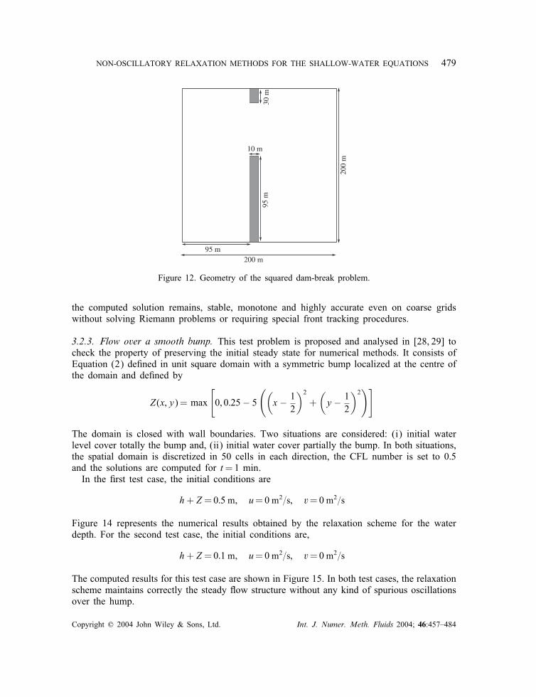
3.2.2. Squared dam-break problem. We consider a 200m long and 200m wide �at reservoirwith two di�erent constant levels of water separated by a dam. At t=0 part of the dambreaks instantaneously. The dam is 10 m thick and the breach is assumed to be 75 m wide,as shown in Figure 12. Initially,

h(0; x; y)=

{10 m if x¡100 m

5 m otherwiseu(0; x; y)= v(0; x; y)=0 m=s

In the left column of Figure 13 we plot the water surface elevation, while the right columncontains the corresponding velocity vectors. All computations are made on a uniform meshof 50× 50 gridpoints. Compared with the numerical results reported in Reference [5], therelaxation scheme solves the problem accurately with less di�usion than the method used inReference [5]. Note that the performance of our relaxation scheme is very attractive since



10 m

95 m

95 m

30 m

200 m

200

m

Figure 12. Geometry of the squared dam-break problem.

the computed solution remains, stable, monotone and highly accurate even on coarse gridswithout solving Riemann problems or requiring special front tracking procedures.

3.2.3. Flow over a smooth bump. This test problem is proposed and analysed in [28, 29] tocheck the property of preserving the initial steady state for numerical methods. It consists ofEquation (2) de�ned in unit square domain with a symmetric bump localized at the centre ofthe domain and de�ned by

Z(x; y)= max

[0; 0:25− 5

((x − 1

2

)2+(y − 1

2

)2)]

The domain is closed with wall boundaries. Two situations are considered: (i) initial waterlevel cover totally the bump and, (ii) initial water cover partially the bump. In both situations,the spatial domain is discretized in 50 cells in each direction, the CFL number is set to 0:5and the solutions are computed for t=1 min.In the �rst test case, the initial conditions are

h+ Z =0:5 m; u=0 m2=s; v=0 m2=s

Figure 14 represents the numerical results obtained by the relaxation scheme for the waterdepth. For the second test case, the initial conditions are,

h+ Z =0:1 m; u=0 m2=s; v=0 m2=s

The computed results for this test case are shown in Figure 15. In both test cases, the relaxationscheme maintains correctly the steady �ow structure without any kind of spurious oscillationsover the hump.


480 M. SEA�ID

t = 3.6

0 20 40 60 80 100 120 140 160 180 2000

20

40

60

80

100

120

140

160

180

200t = 3.6

5.6

6.65

7

7.35

5.95

7.7

7.35

8.05

9.8

9.1 8.05

t = 7.2

0 20 40 60 80 100 120 140 160 180 2000

20

40

60

80

100

120

140

160

180

200t = 7.2

5.19.8

9.4083 9.0167

8.625

8.23

33

8.625

7.0583

5.4917

6.2756.275

6.275

7.0583

7.45

8.23

33

7.8417

5.88

33

5.4917

5.8833

6.6667

t = 10.8

0 20 40 60 80 100 120 140 160 180 2000

20

40

60

80

100

120

140

160

180

200t = 10.8

5.6

5.956.3

6.65

6.65

6.657

6.3

5.95

5.6

7

7.35

7.78.05

8.4

8.75

8.75

9.1

9.45

9.8

9.1

Figure 13. Water surface elevation and velocity �eld for squared dam-break problem.



0 0.1

0.1

0.20.2 0.2

0.2

0.3

0.3

0.4

0.40.4

0.4

0.5 0.6

0.60.6

0.7 0.8

0.80.8

0.9 1

11

0

0 00

0.1

0.2

0.3

0.4

0.5

0.6

0.7

0.8

0.9

1

0.47289

0.40

602

0.29458

0.25

Figure 14. Contour and surface plots of water depth for �ow over a totally covered bump.

0 0.1 0.20.2 0.2

0.2

0.1

0.3

0.3

0.4

0.40.4

0.4

0.5 0.6

0.60.6

0.7 0.8

0.80.8

0.9 1

1

1

0

0 00

0.1

0.2

0.3

0.4

0.5

0.6

0.7

0.8

0.9

1

0.079167

0.0

0416

67

0.066667

0.15

Figure 15. Contour and surface plots of water depth for �ow over a partially covered bump.

3.2.4. Flow over a shaped bump. Our purpose in the following test problem is to examinethe ability of our relaxation scheme to handle the two-dimensional shallow-water equationson non-�at bottom. In this academic test, we consider the Equation (2) in the rectangularchannel [0; 2]× [0; 1] with an elliptical-shaped hump de�ned by [8],

Z(x; y)=0:8 exp(−5(x − 0:9)2 − 50(y − 0:5)2) (33)


482 M. SEA�ID

0 0.2 0.4 0.6 0.8 1 1.2 1.4 1.6 1.8 20

0.10.20.30.40.50.60.70.80.9

1t = 0.6

0 0.2 0.4 0.6 0.8 1 1.2 1.4 1.6 1.8 20

0.10.20.30.40.50.60.70.80.9

1t = 0.6

0 0.2 0.4 0.6 0.8 1 1.2 1.4 1.6 1.8 20

0.10.20.30.40.50.60.70.80.9

1t = 0.9

0 0.2 0.4 0.6 0.8 1 1.2 1.4 1.6 1.8 20

0.10.20.30.40.50.60.70.80.9

1t = 0.9

0 0.2 0.4 0.6 0.8 1 1.2 1.4 1.6 1.8 20

0.10.20.30.40.50.60.70.80.9

1t = 1.2

0 0.2 0.4 0.6 0.8 1 1.2 1.4 1.6 1.8 20

0.10.20.30.40.50.60.70.80.9

1t = 1.2

0 0.2 0.4 0.6 0.8 1 1.2 1.4 1.6 1.8 20

0.10.20.30.40.50.60.70.80.9

1t = 1.5

0 0.2 0.4 0.6 0.8 1 1.2 1.4 1.6 1.8 20

0.10.20.30.40.50.60.70.80.9

1t = 1.5

0 0.2 0.4 0.6 0.8 1 1.2 1.4 1.6 1.8 20

0.10.20.30.40.50.60.70.80.9

1t = 1.8

0 0.2 0.4 0.6 0.8 1 1.2 1.4 1.6 1.8 20

0.10.20.30.40.50.60.70.80.9

1t = 1.8

Figure 16. Contours of water surface for �ow over a shaped hump using 200× 100 gridpoints (leftcolumn) and 400× 200 gridpoints (right column) at times 0:6, 0:9, 1:2, 1:5 and 1:8.



Note that hump (33) is centred at (0:9; 0:5) with a minimum and maximum heights of 0:01and 0:8, respectively. Initially, the �ow is at rest and the water surface is �at with a smallperturbation in the vertical slab [0:05; 0:15] as

h(0; x; y)=

{1:01− Z(x; y) if 0:05¡x¡0:15

1− Z(x; y) otherwise

Out�ow boundary conditions are imposed on all domain boundaries, and we use two meshesof 200× 100 and 400× 200 gridpoints for comparison. In our computation we set the dimen-sionless g=1. In Figure 16, we display contour plots of the water distribution as it �ows pastthe hump. Note that the speed of water �ow is slower above the hump than elsewhere in thechannel, producing a distortion of the initially �at distribution of the water. We can see thatthe small complex structures of the water �ow being captured by our relaxation scheme.

4. CONCLUSIONS

Relaxation schemes of �rst- and second-order accuracy were introduced in Reference [10]. Inthis paper we have reconstructed high-order relaxation schemes by using WENO ideas anda class of TVD high-order Runge–Kutta time integration methods. We have further general-ized and extended the relaxation schemes for the two-dimensional shallow-water equations.This procedure combines the attractive attributes of the two methods to yield a procedurefor either �at or non-�at topography. The new method retains all the attractive features ofcentral schemes such as neither Riemann solvers nor characteristic decomposition are needed.Furthermore, the scheme does not require either non-linear solution or special front trackingtechniques.The third-order relaxation method have been tested on systems of shallow-water equations

in one and two space dimensions. The obtained results indicate good shock resolution withhigh accuracy in smooth regions and without any non-physical oscillations near the shockareas. The convergence to the correct steady-state solution has been clearly veri�ed in �ow atrest and drain on non-�at bottom. Although we have restricted our numerical computations tothe frictionless shallow-water problems, the current relaxation scheme can be straightforwardlyextended to more general shallow-water �ows with bottom friction and Coriolis forces.

ACKNOWLEDGEMENT

The author thanks an anonymous reviewer for his helpful comments which subsequently improved thecurrent manuscript, such as the inclusion of the �ow at rest in test problems.

REFERENCES

1. Stoker JJ. Water Waves. Interscience Publishers, Inc.: New York, 1986.2. Toro EF. Shock-Capturing Methods for Free-Surface Shallow Flows. Wiley: New York, 2001.3. Alcrudo F, Navarro PG. A high resolution Godunov-type scheme in �nite volumes for the 2D shallow waterequations. International Journal for Numerical Methods in Fluids 1993; 16:489–505.

4. Delis AI, Skeels CP. TVD schemes for open channel �ow. International Journal for Numerical Methods inFluids 1998; 26:791–809.


484 M. SEA�ID

5. Fennema RJ, Chaudhry MH. Explicit methods for 2D-transient free-surface �ows. Journal of HydraulicEngineering 1990; 116:1013–1034.

6. Gallou�et T, Herard JM, Seguin N. Some approximate Godunov schemes to compute shallow water equationswith topography. Computers and Fluids 2003; 32:479–513.

7. Levy D, Puppo G, Russo G. Central-Upwind schemes for the Saint–Venant system. Mathematical Modellingand Numerical Analysis 2002; 36:397–425.

8. LeVeque Randall J. Balancing source terms and �ux gradients in high-resolution Godunov methods: the quasi-steady wave-propagation algorithm. Journal of Computational Physics 1998; 146:346–365.

9. LeVeque Randall J. Numerical Methods for Conservation Laws (2nd edn). Lectures in Mathematics. ETH:Z�urich, 1992.

10. Jin S, Xin Z. The relaxation schemes for systems of conservation laws in arbitrary space dimensions.Communications on Pure and Applied Mathematics 1995; 48:235–276.

11. Aregba-Driollet D, Natalini R. Convergence of relaxation scheme for conservation laws. Applicable Analysis1996; 61:163–193.

12. Chalabi A. Convergence of relaxation scheme for hyperbolic conservation laws with sti� source terms.Mathematics of Computation 1999; 68:955–970.

13. Chen GQ, Levermore CD, Liu TP. Hyperbolic conservation laws with sti� relaxation terms and entropy.Communications on Pure and Applied Mathematics 1994; 47:787–830.

14. Liu HL, Warnecke G. Convergence rates for relaxation schemes approximating conservation laws. SIAM Journalon Numerical Analysis 2000; 37:1316–1337.

15. Klar A. Relaxation schemes for a Lattice–Boltzmann type discrete velocity model and numerical Navier–Stokeslimit. Journal of Computational Physics 1999; 148:1–17.

16. Natalini R. Convergence to equilibrium for relaxation approximations of conservation laws. Communicationson Pure and Applied Mathematics 1996; 49:795–823.

17. Xu WQ. Relaxation limit for piecewise smooth solutions to conservation laws. Journal of Di�erential Equations2000; 162:140–173.

18. Lattanzio C, Serre D. Convergence of a relaxation scheme for hyperbolic systems of conservation laws.Numerische Mathematik 2001; 88:121–134.

19. Banda MK, Sea��d M. A class of the relaxation schemes for two-dimensional Euler systems of gas dynamics.Lecture Notes in Computer Science 2002; 2329:930–939.

20. Fan H, Jin S, Teng Z. Zero reaction limit for hyperbolic conservation laws with source terms. Journal ofDi�erential Equations 2000; 168:270–294.

21. Jin S, Pareschi L, Toscani G. Uniformly accurate di�usive relaxation schemes for multiscale transport equations.SIAM Journal on Numerical Analysis 2000; 38:913–936.

22. Delis AI, Katsaounis Th. Relaxation schemes for the shallow water equations. International Journal forNumerical Methods in Fluids 2003; 41:695–719.

23. Kurganov A, Levy D. A third-order semi-discrete central scheme for conservation laws and convection–di�usionequations. SIAM Journal on Scienti�c Computing 2000; 22:1461–1488.

24. Levy D, Puppo G, Russo G. Compact central WENO schemes for multidimensional conservation laws. SIAMJournal on Scienti�c Computing 2000; 22:656–672.

25. Ascher U, Ruuth S, Spiteri R. Implicit–explicit Runge–Kutta methods for time-dependent partial di�erentialequations. Applied Numerical Mathematics 1997; 25:151–167.

26. Pareschi L, Russo G. Implicit–Explicit Runge–Kutta schemes for sti� systems of di�erential equations. RecentTrends in Numerical Analysis 2000; 3:269–289.

27. Pareschi L, Russo G. Implicit–Explicit Runge–Kutta schemes and applications to hyperbolic systems withrelaxation. Journal of Scienti�c Computing, in press.

28. Brufau P, V�azquez-Cend�on ME, Garc��a-Navarro P. A numerical model for the �ooding and drying of irregulardomains. International Journal for Numerical Methods in Fluids 2002; 39:247–275.

29. Brufau P, Garc��a-Navarro P. Unsteady free surface �ow simulation over complex topography with amultidimensional upwind technique. Journal of Computational Physics 2003; 186:503–526.

30. Banda MK, Sea��d M. Higher-order relaxation schemes for hyperbolic systems of conservation laws. Submitted.31. Bermudez A, V�azquez-Cend�on ME. Upwind methods for hyperbolic conservation laws with source terms.

Computers & Fluids 1994; 23:1049–1071.32. Lax P, Liu X. Solution of two-dimensional Riemann problems of gas dynamics by positive schemes. SIAM

Journal on Scienti�c Computing 1998; 19:319–340.33. Weinan E, Liu JG. Essentially compact schemes for unsteady viscous incompressible �ows. Journal of

Computational Physics 1996; 126:122–138.


Non-oscillatory relaxation methods for the shallow-water equations in one and two space dimensions

Documents

Transcript of Non-oscillatory relaxation methods for the shallow-water equations in one and two space dimensions