NON-FICKIAN TRACER CURVES ARE ALSO GAUSSIAN: AN EXPERIMENTAL DEMONSTRATION AND DISSCUSION OF CONSEQUENCES TO TRANSPORT THEORY.

Alfredo Constain1 ; Jairo Carvajal2 ; Alejandro Carvajal3

ABSTRACT

Currently Non- Fickian tracer curves are synonymous of Non-Gaussian functions due to several restrictions imposed over defining equations to accomplish the concept that the asymmetry of such curves is something real with same physical meaning to all observers viewing them. This approach leads to deep contradictions between facts and model, being very difficult to deal with. In this article an alternate model that considers the Non-Fickian asymmetry as a virtual thing is proposed. The authors develop a mass transport model based rather on Galileo´s Principle, which means that dispersion coefficient is a function of time. This last feature is fully developed in this article showing that Non-Fickian functions are Gaussian indeed. A detailed field journey is documented herein.

.

Keywords: Contamination dynamics, tracer techniques, fluid measurement systems.

INTRODUCTION

Several available mass transport theories in turbulent flows has been developed along of the years, pushed by urgent demand of methods to measure concentration patterns, both in time and space, of contaminant substances, proven that they behave similarly than tracers used to test these theories. So, it was been accepted that in real three-dimensional flows the spreading of solutes results from combination of both effects: mixing of turbulence and shear effect of velocity fields. However, a detailed microscopic description of this set of phenomena is inherently complex and mathematical very difficult. Rather, other kind of models of integral nature has been preferred to get a direct picture of reality that may be tested experimentally also. One of these key integral theories defines the Longitudinal Dispersion Coefficient, E, as a parameter advised to describe shear effect within a diffusion model. Derived from restrictions associated mainly with the uniform flow condition in flows, currently the E parameter has been taken as constant. However, this regime almost never is found, implying that in some way its value would be time dependent. Despite these considerations, state of the art approaches maintain a strong dependence with the constancy of it. This fact, as has been considered, has led to a blind street, avoiding a congruent interpretation of earlier stages of diffusion-dispersion process, specially the skewed nature of tracer 1 Corresponding author: Amazonas Technologies, e-mail: alfredo.constain@amazonastech.com 2 Amazonas Technologies, e-mail: jairo.carvajal@amazonastech.com 3 Amazonas Technologies, e-mail: acr@amazonastech.com

2

curves. This paper deals with an alternate view of E nature, considering that it has to be a function of time.

SOME DIFFICULTIES RELATED WITH BASIC DIFFUSION-ADVECTION THEORY OF G.I. TAYLOR AND AN ALTERNATE MODEL TO SOLVE THEM. The use of Coefficient concept to describe dispersion in pipes was introduced by G.I. Taylor in a relatively later age of evolution of transport mass theories, about 1954 (Taylor, 1954). Starting from a prior idea of 1921(Taylor, 1921) he demonstrated that steady statistical description of a mass that is spreading in one coordinate is convergent with Einstein´s “Random Walk” model (Einstein, 1955) in which the distance squared is proportional to time in this process. This concept fulfils with the two following equations: Taylor´s mass balance equation and Fick´s solution function for concentration, in uniform flow regime.

2

2

xC

ExC

UtC

x ∂∂

=∂∂

+∂∂

(1)

And

tEtxUX

etEA

MtxC 4

2)(

4),(

−−= (2)

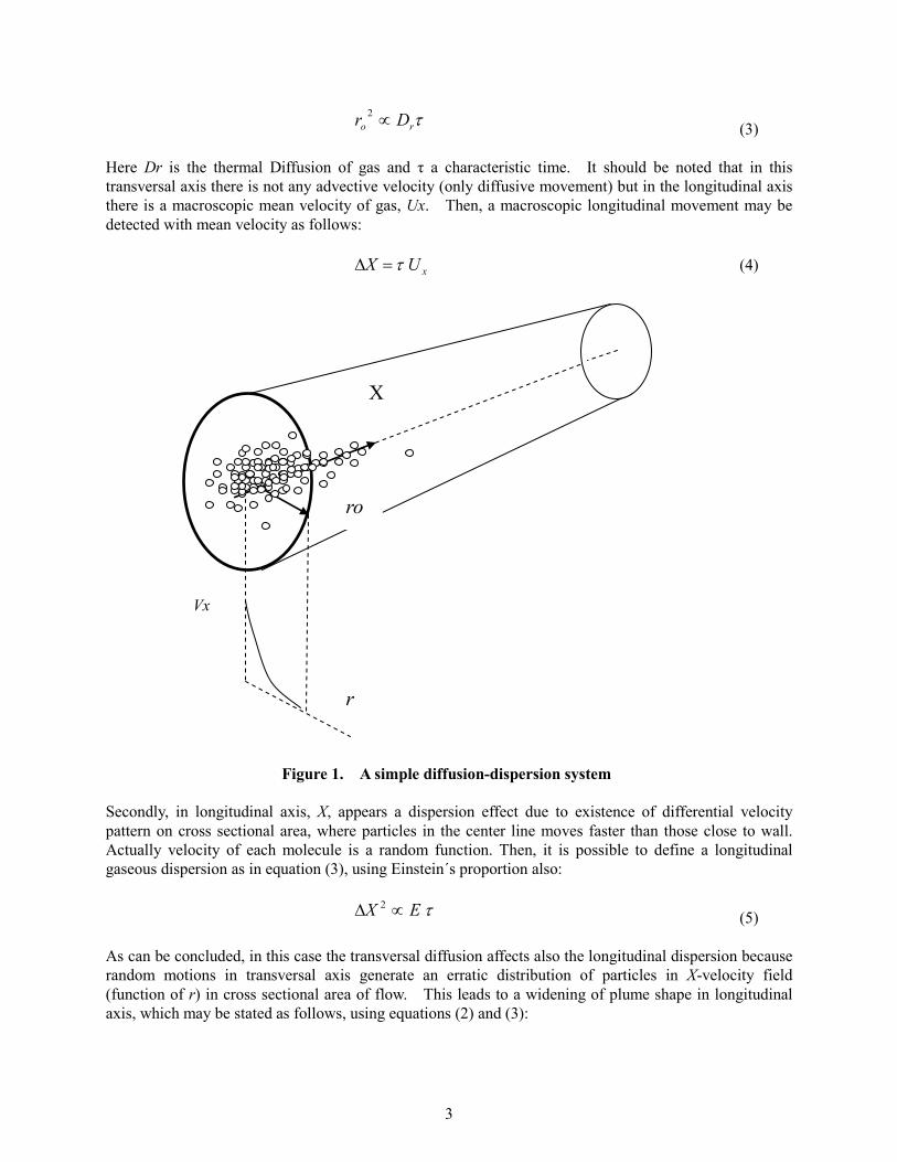
Here E is a constant, M is the tracer mass, and A is cross sectional area of flow in which holds a mean velocity, Ux. Later, Elder y Fischer extended their analysis to a more than one coordinate and to natural turbulent flows. However, were evident the great divergences of these steady models with experimental results, especially with the interpretation and explanation of asymmetry of tracer curves. These discrepancies are especially important since experimentally has been verified several times that Longitudinal dispersion Coefficient, E, increases approximately with distance differently from expected current theory, implying a persistent skewness in tracer curves. (Day, 1977). An alternate model to deal with these difficulties may be stated if it is considered that tracer curves are Gaussian despite their skewness, and then Longitudinal Dispersion Coefficient is a time function. To understand this concept is necessary to consider that in general, beside longitudinal transport there is also a transversal one (assuming vertical transport negligible), and that this situation has to be reflected in nature of E coefficient. Currently is taken as a matter of fact that E is constant due to restrictions related to uniform flow in which mass transport depends only on concentration gradients (Fischer, 1973). It will be considered here that E may be time function rather that a constant to solve some model difficulties. AN ELEMENTAL MODEL OF MASS TRANSPORT IN WHICH TRANSVERSAL DIFFUSION AND LONGITUDINAL DISPERSION OF A GAS LEAD TO A DEFINITION OF E (t). Gaseous chromatography technique have used since long time ago a model of mass transport in which simultaneous existence of transversal and longitudinal random motions leads to a time dependence for longitudinal dispersion coefficient. To show this it may be considered a capillar pipe filled with a gas containing a tracer in which the longitudinal velocity distribution, vx, is a function of radial (transversal) distance, being greater in pipe axis and null in the wall of pipe (Guaresimov et al, 1980). Figure 1. Initially there is diffusion along the radius, ro, of capillar pipe meaning that motions of tracer particles are random in this axis. Accordlying with Einstein´s relationship it can be written:

3

τro Dr ∝2

(3) Here Dr is the thermal Diffusion of gas and τ a characteristic time. It should be noted that in this transversal axis there is not any advective velocity (only diffusive movement) but in the longitudinal axis there is a macroscopic mean velocity of gas, Ux. Then, a macroscopic longitudinal movement may be detected with mean velocity as follows: xUX τ=∆ (4) Figure 1. A simple diffusion-dispersion system Secondly, in longitudinal axis, X, appears a dispersion effect due to existence of differential velocity pattern on cross sectional area, where particles in the center line moves faster than those close to wall. Actually velocity of each molecule is a random function. Then, it is possible to define a longitudinal gaseous dispersion as in equation (3), using Einstein´s proportion also:

τEX ∝∆ 2 (5)

As can be concluded, in this case the transversal diffusion affects also the longitudinal dispersion because random motions in transversal axis generate an erratic distribution of particles in X-velocity field (function of r) in cross sectional area of flow. This leads to a widening of plume shape in longitudinal axis, which may be stated as follows, using equations (2) and (3):

ro

X

Vx

r

4

τ2xUE ∝ (6)

This equation means that longitudinal dispersion coefficient is a time function as consequence of its dependence on transversal diffusion. Explicitly it can be written, with k as proportion coefficient: τ2)( xUktEE == (7) Now, it is interesting examine some theoretical justifications for this result. Then, it is possible to write the following two-coordinate equation without considering any advective (macroscopic) movement, being C the mean concentration on control plane:

2

2

2

2

yC

xC

tC

yx ∂∂

+∂∂

=∂∂ εε (8)

It is evident from this definition that the time variation of concentration depends either on both variations of concentration as function of X and Y simultaneously, or on only one of these. It is a summary variation in the same form that energy is a summary variation either on work and heat together or one of these alone. It can be said that time function in equation (7) absorbs anyone variations of two different axis in space. This result may be generalized in the following way, using E parameter:

2

2

2

2

2

2

yC

xC

xC

E yx ∂∂

+∂∂

=∂∂ εε (9)

This can be operating as follows:

∂∂

∂∂

+= 2

2

2

2

/xC

yC

E yx εε (10)

Now, in a general sense, if considered mass is finite and if diffusion is not steady as second Fick´s law states (Damaskin et al, 1980), then it can be written the following equation:

)(tE yx εε +=

(11) And then:

2

2

2

2

2

2

)(yC

xC

xC

tE yx ∂∂

+∂∂

=∂∂ εε (12)

So, although coefficient E goes multiplying only second derivate in X of C, it may represent also the variation of same order in Y of C, if it is a time function. Finally in this subject, when transversal diffusion ceases, the tracer fills almost uniformly the cross sectional area of flow, S. This restriction is known as “Complete Mixing condition”. Beyond this point, although E is taken currently to describe only dispersion in X –axis, is clear that it is useful to describe Y-axis diffusion also, and that it is function of time. THERMODYNAMIC ANALISYS OF LONGITUDINAL DISPERSION COEFFICIENT AND ITS NATURE AS TIME FUNCTION.

5

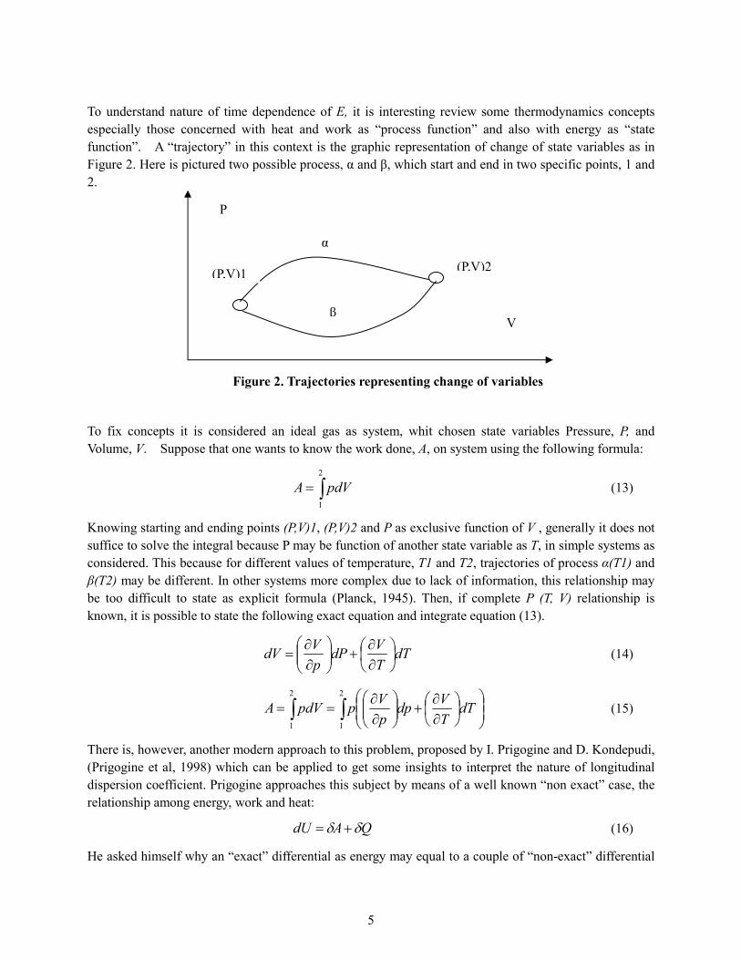
To understand nature of time dependence of E, it is interesting review some thermodynamics concepts especially those concerned with heat and work as “process function” and also with energy as “state function”. A “trajectory” in this context is the graphic representation of change of state variables as in Figure 2. Here is pictured two possible process, α and β, which start and end in two specific points, 1 and 2.

Figure 2. Trajectories representing cha

To fix concepts it is considered an ideal gas as system, whit chVolume, V. Suppose that one wants to know the work done, A, on

∫=2

1

pdVA

Knowing starting and ending points (P,V)1, (P,V)2 and P as exclusivsuffice to solve the integral because P may be function of another stconsidered. This because for different values of temperature, T1 andβ(T2) may be different. In other systems more complex due to lackbe too difficult to state as explicit formula (Planck, 1945). Thenknown, it is possible to state the following exact equation and integr

dTTV

dPpV

dV

∂∂

+

∂∂

=

∫ ∫

∂∂

+

∂∂

==2

1

2

1 TV

dppV

ppdVA

There is, however, another modern approach to this problem, propos(Prigogine et al, 1998) which can be applied to get some insights dispersion coefficient. Prigogine approaches this subject by means relationship among energy, work and heat:

QAdU δδ +=

He asked himself why an “exact” differential as energy may equal

(P,V)2

(P,V)1

β

α

P

nge of variables

osen state variables Pressure, P, and system using the following formula:

(13)

e function of V , generally it does not ate variable as T, in simple systems as T2, trajectories of process α(T1) and of information, this relationship may , if complete P (T, V) relationship is ate equation (13).

(14)

dT (15)

ed by I. Prigogine and D. Kondepudi, to interpret the nature of longitudinal of a well known “non exact” case, the

(16)

to a couple of “non-exact” differential

V

6

as work and heat. This is a logical contradiction because there is none mathematical argument that justify this asymmetry. A deep examination of thermodynamic reasons behind this problem led to Prigogine to find a way to avoid contradiction. The core of problem is that classical thermodynamics should define process as ideal, quasi-static entities. i.e.: infinitely slow process (t→∞), condition required to avoid irreversibility complexities. This condition automatically exclude to known the form in which the process is realized (which is done in a finite time). If it is possible to define energy transformation as real, irreversible process, then also is possible to define differentials whose description may be done in terms of rates, or function of time. In this case, all the information may be known (at least in theory) and the differential equation may be written in an exact form as follows:

)()( tdQtdAdU += (17) Generally speaking, if a process is taken as irreversible, then its differential definition may be done in terms of rates which mean exact differentials. To apply this concept to classical definition of E, it may be used the Fischer´s semi-empirical formula (Fischer, 1966).

*

22

UhWUk

E x

×××

≈ (18)

Here k is an empirical constant (function of kind of stream), W is the mean wide of stream, h the mean depth and U* is the so called “shear velocity” (function of depth and slope of flow). Now, it is possible to define an exact differential equation, linear function of Ux and W, as follows:

dWWE

dUxUxE

dE )()(∂∂

+∂∂

= (19)

Then:

*22

UhUxWk

UxE

×××

=∂∂

(20)

And:

*22

UhWUxk

WE

×××

=∂∂

(21)

Cross derivates are:

*4

2*

2*22

UhUxWk

UxUhWk

UxUh

WUxk

UxWE

×××

=×××

=∂

×××

∂=

∂

∂∂

∂ (22)

And

*

42

*2*

22

UhUxWk

WUhUxk

WUh

UxWk

WUxE

×××

=×××

=∂

×××

∂=

∂

∂∂

∂ (23)

Then:

UxWE

WUxE

∂

∂∂

∂=

∂

∂∂

∂ (24)

7

And finally:

∫ =C

dE 0 (25)

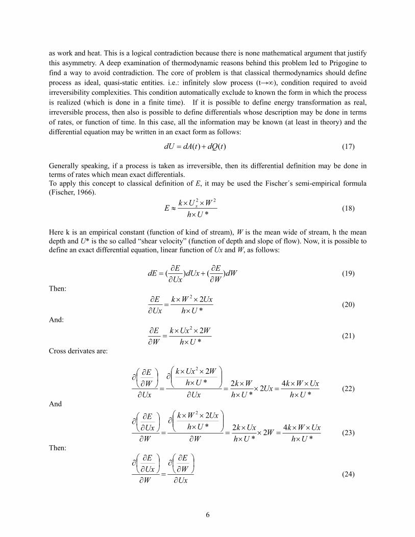
This is an important result because also the dispersion process is clearly an irreversible phenomenon, and then may be written as an exact differential equation, considering the finite rate concept, developed before: )()( WdEUxdEdE += (26) )()( tgtfdE += (27) Then E should be a function of time. By the other hand the thermodynamic concept “state function” defined by equation (25) means inherently a process in time, starting and ending at defined instants. For irreversible thermodynamics the “process” concept is linked naturally with changes in finite times. Figure 3

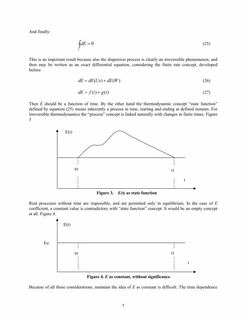
Figure 3. E(t) as state function Real processes without time are impossible, and are permitted only in equilibrium. In the case of E coefficient, a constant value is contradictory with “state function” concept. It would be an empty concept at all. Figure 4.

Figure 4. E as constant, without significance Because of all these considerations, maintain the idea of E as constant is difficult. The time dependence

Eo

E(t)

t

E(t)

to t1

t

t1

to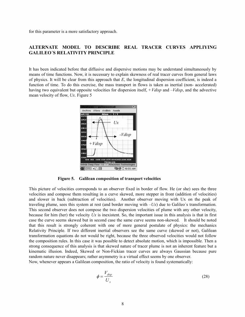

8

for this parameter is a more satisfactory approach. ALTERNATE MODEL TO DESCRIBE REAL TRACER CURVES APPLIYING GALILEO´S RELATIVITY PRINCIPLE It has been indicated before that diffusive and dispersive motions may be understand simultaneously by means of time functions. Now, it is necessary to explain skewness of real tracer curves from general laws of physics. It will be clear from this approach that E, the longitudinal dispersion coefficient, is indeed a function of time. To do this exercise, the mass transport in flows is taken as inertial (non- accelerated) having two equivalent but opposite velocities for dispersion itself, +Vdisp and –Vdisp, and the advective mean velocity of flow, Ux. Figure 5

Figure 5. Figure 5. Galilean composition of transport velocities This picture of velocities corresponds to an observer fixed in border of flow. He (or she) sees the three velocities and compose them resulting in a curve skewed, more stepper in front (addition of velocities) and slower in back (subtraction of velocities). Another observer moving with Ux on the peak of traveling plume, sees this system at rest (and border moving with –Ux) due to Galileo´s transformation. This second observer does not compose the two dispersion velocities of plume with any other velocity, because for him (her) the velocity Ux is inexistent. So, the important issue in this analysis is that in first case the curve seems skewed but in second case the same curve seems non-skewed. It should be noted that this result is strongly coherent with one of more general postulate of physics: the mechanics Relativity Principle. If two different inertial observers see the same curve (skewed or not), Galilean transformation equations do not would be right, because the three observed velocities would not follow the composition rules. In this case it was possible to detect absolute motion, which is impossible. Then a strong consequence of this analysis is that skewed nature of tracer plume is not an inherent feature but a kinematic illusion. Indeed, Skewed or Non-Fickian tracer curves are always Gaussian because pure random nature never disappears; rather asymmetry is a virtual effect seems by one observer. Now, whenever appears a Galilean composition, the ratio of velocity is found systematically:

x

disp

U

V=φ (28)

Ux

+Vdisp

-Vdisp

9

Then, accepting a simple definition “Random Walk” for statistical displacements of tracer particles in one axis it holds (Constain et al, 2003):

τE22 =∆ (29) Here ∆ and τ are spatial and temporal characteristics diffusion parameters of random motions in turbulent flows, then, the mean velocity of dispersion in tracers is defined as:

ττE

Vdisp

2=

∆= (30)

And then:

τE

UU

xx

21= (31)

This is a definition with some mathematical structure than Chezy´s equation but is not restricted to uniform flow only because random motions are favored precisely in non-uniform turbulent flow. Now, from the point of view of this paper is interesting to clear Coefficient E.

2

22 τφ xUE = (32)

It can be demonstrated that exist a relationship between τ, the characteristic time of diffusion, and t as general time (independent variable). This numerical relationship is determinate by the Poisson´s distribution applied to random motions of diffusion. Equation (33)

215.0≈= βτt

(33)

Then, the equation (37) remains:

2

22 tUE x βφ= (34)

This definition for longitudinal dispersion coefficient has the same structure than equation (7) with equivalent k as follows:

2

2φ=k (35)

By the other hand, function Φ itself is a thermodynamic “state function” whereas is defined also as:

∫ =C

d 0φ (36)

And then, if it operates in an irreversible process it will be time function also. It may be established that Φ(t) function describes the tracer plume evolution which is not different that the history of interactions of tracer particles along the flow. From physical-chemistry point of view it may be observed that free

10

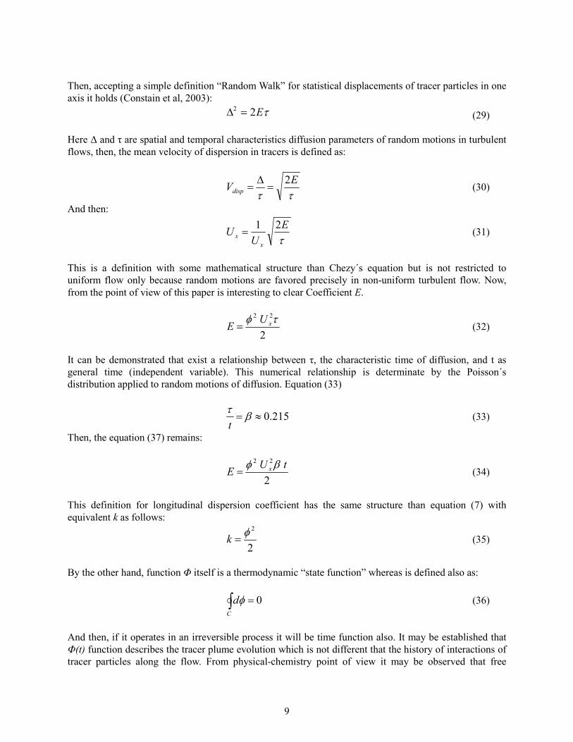
enthalpy (Gibbs potential) for a certain mass of tracer poured into a turbulent flow in an irreversible process, has to decrease in time indicating the transformation of this formation energy in heat. So the fate of Φ(t) should be the same than G in this kind of process. Certainly, in the range of interest, Φ(t) function has been tested as in Figure 6 in experimental works. Then, E is a time function by following reasons: first, because presence of transversal diffusion which affects the time dependence of E, as has been explained before and second because the longitudinal dispersion itself is time dependent, reflecting the irreversible nature of process. All these processes are linked among them by means of complex mechanisms which lead finally to spend all the available (potential) energy put at the start of pouring process as formation energy.

Figure 6. Φ(t) reflecting thermodynamic evolution of plume These mechanisms modify finally the form in which the velocity of dispersion module, V disp, is changed in time, and then how is Φ variation in time. i.e.: the skewness degree of curve. This leads to following general definition for E:

2

)()(

22 tUttE x βφ= (37)

So, although in a moment ceases the effect of transversal diffusion (Complete Mixing condition) the longitudinal dispersion continues changing the shape of E in time. Consequently, this coefficient is not apart from energy evolution in a tracer plume, since the very birth to extinction. EXPERIMENTAL VERIFICATION OF TIME DEPENDENCE OF LONGITUDINAL DISPERSION COEFFICIENT IN NATURAL STREAMS. It is necessary now to put equation (37) in an experimental test to verify the scope of its foundations. To do that one may uses the classical Fick´s definition for tracer concentration:

tEtxUL

etES

MtC 4

2)(

4)(

−−=

π (38)

Here S is the cross sectional area of flow, M the mass of poured tracer and L the fixed distance of

Φ(t)

t

11

measurement in stream. If one replaces equation (37) in (38) it remains as follows:

222

2)(

2)( txU

txUL

etQM

tC β

πβφ

−−= (39)

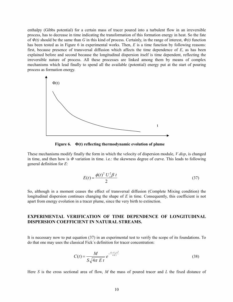
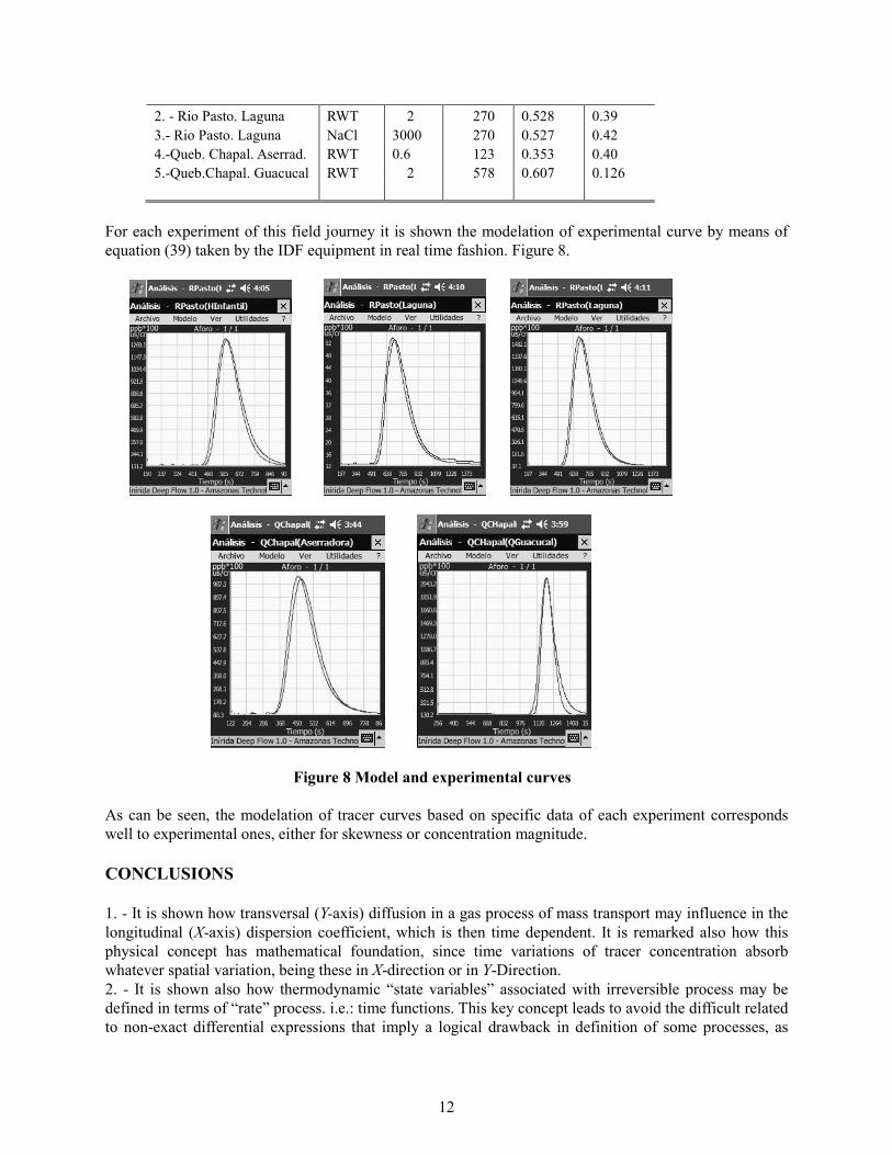
This relationship, tested many times in field journeys, resembles well the skew nature of tracer curves and also the due magnitude of concentration. It is analyzed immediately five (5) experiments done in the southern region of Colombia by means of scientific tool “Inirida Deep Flow” (IDF) developed by authors. This measurement system contains a hand computer, a digital interface which traduces physical signals into binary streams to be treated properly by high level software. This interface connects simultaneously two distinct probes, one fluorimetric (Rhodamine WT) and other conduct metric (NaCl). The screen presents experimental tracer curves in real time basis with theoretical models superimposed. Also tables with numerical data from results measurements. The models are drawn by means of equation (39) fed by specific data from experiment and stream. Following is presented photos of equipment and measured streams. Figure 7. The presented experiments correspond four to Rhodamine WT and one to common salt. The results are presented in Table 1. Here L is distance, M tracer mass. Also is given the Φ parameter for corresponding distance.

Figure 7. Some aspects of scientific tool and measurement activities

Table 1. Measurement data in field journey

Exp. Tracer M (g)

L (m)

Ux (m/s)

Φ

1. - Rio Pasto. Hospital RWT 8 500 1.10 0.30

12

2. - Rio Pasto. Laguna 3.- Rio Pasto. Laguna 4.-Queb. Chapal. Aserrad.

RWT NaCl RWT

2 3000 0.6

270 270 123

0.528 0.527 0.353

0.39 0.42 0.40

5.-Queb.Chapal. Guacucal RWT 2 578 0.607 0.126

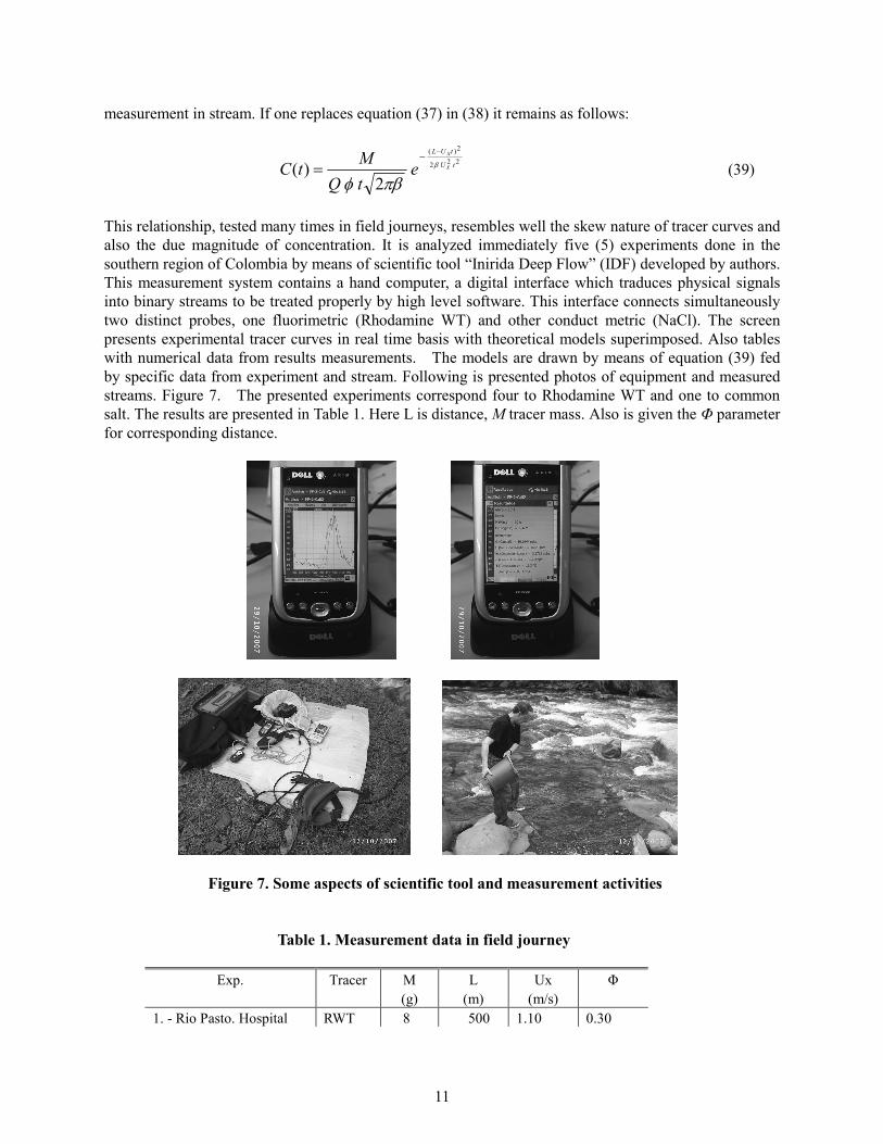
For each experiment of this field journey it is shown the modelation of experimental curve by means of equation (39) taken by the IDF equipment in real time fashion. Figure 8.

Figure 8 Model and experimental curves As can be seen, the modelation of tracer curves based on specific data of each experiment corresponds well to experimental ones, either for skewness or concentration magnitude. CONCLUSIONS 1. - It is shown how transversal (Y-axis) diffusion in a gas process of mass transport may influence in the longitudinal (X-axis) dispersion coefficient, which is then time dependent. It is remarked also how this physical concept has mathematical foundation, since time variations of tracer concentration absorb whatever spatial variation, being these in X-direction or in Y-Direction. 2. - It is shown also how thermodynamic “state variables” associated with irreversible process may be defined in terms of “rate” process. i.e.: time functions. This key concept leads to avoid the difficult related to non-exact differential expressions that imply a logical drawback in definition of some processes, as

13

energy balance. To the aim of this article, however this concept is used to indicate rather that if E is a “state function” evolving in an irreversible flow, then it is a time function. 3. - It is explained how E as time function, embodies simultaneously the transverse diffusion of tracer, which ends when this fills almost completely the cross section of flow, and the longitudinal dispersion which is decreasing due to irreversible nature of phenomena. This implies the existence of a skewness degree function, Φ, which is linked with all complex process of energy degradation in plume evolution. 4. - The Φ function appears as a consequence of Galilean composition of velocities in tracer plume, taken as inertial system. This composition implies that skewness is not a universal concept, meaning that distinct observers will see different shapes, due to necessity of avoid the existence of absolute motion. 5. - There is five experiments with tracers (four of Rhodamina WT and one of common salt) which are examined from modelation view point, finding that theoretical models got by means of equation (39) follow very close the experimental curves. 6. - This tracer technique may be used with advantage in contaminant studies, due to its inherently simple procedure and accurate of its results. REFERENCES Constain A.; Lemos R.; Carvajal A., (2003). “Tecnología IMHE: Nuevos desarrollos en la hidráulica”. Revista Ingeniería Civil, CEDEX, Vol 129. Spain Day, T.J. (1977). “Longitudinal dispersion of fluid particles in mountain streams: Theory and field evidence”, Journal of Hydrology (NZ), Vol 16, No.1. USA. Damaskin B.B.; Petri O.A.; (1978).Fundamentos de electroquímica teórica, Editorial Mir, Moscow. Einstein A. (1955). Investigations on the theory of the Brownian Movement. Dover Publications, New York. Fischer J.B. (1966). “Longitudinal dispersion in laboratory and natural channels”, PhD Thesis, CALTECH. USA. Fischer J.B.; (1973). “Longitudinal dispersion and turbulent mixing in open- channel flow”, Reviews of fluid mechanics, USA. Guaresimov YA.; Dreving V.; Eriomin E.; Kiseliov A.; Lebedev V.; Panchenkov G.; Shliguin A. (1980).Curso de Química Física, Tomo 1, Editorial Mir, Moscow. Planck, M.; (1945). Treatise on thermodynamics. Dover Publications, New York. Prigogine I.; Kondepudi D.; (1998). Modern Thermodynamics. Wiley, New York. Prigogine I., (1997).El fin de las certidumbres. Editorial Taurus, Bogotá. Taylor G.I.; (1954). “The dispersion of matter in turbulent flow through a pipe”. Proceedings of the Royal society of London, 233. UK. Taylor G.I.; (1921). “Diffusion by continuous movement”, Proceedings of the London society of mathematics, Series 2-20, UK.