Numerical simulation of non-Fickian transport in geological formations with multiple-scale...

Numerical simulation of non-Fickian transport in

geological formations with multiple-scale

heterogeneities

Andrea CortisDepartment of Environmental Sciences and Energy Research, Weizmann Institute of Science, Rehovot, Israel

Claudio GalloCenter for Advanced Studies, Research and Development in Sardinia (CRS4), Pula, Italy

Harvey Scher and Brian BerkowitzDepartment of Environmental Sciences and Energy Research, Weizmann Institute of Science, Rehovot, Israel

Received 8 October 2003; revised 9 February 2004; accepted 27 February 2004; published 21 April 2004.

[1] We develop a numerical method to model contaminant transport in heterogeneousgeological formations. The method is based on a unified framework that takes into accountthe different levels of uncertainty often associated with characterizing heterogeneities atdifferent spatial scales. It treats the unresolved, small-scale heterogeneities (residues)probabilistically using a continuous time random walk (CTRW) formalism and the large-scale heterogeneity variations (trends) deterministically. This formulation leads to aFokker-Planck equation with a memory term (FPME) and a generalized concentration fluxterm. The former term captures the non-Fickian behavior arising from the residues, and thelatter term accounts for the trends, which are included with explicit treatment at theheterogeneity interfaces. The memory term allows a transition between non-Fickian andFickian transport, while the coupling of these dynamics with the trends quantifies theunique nature of the transport over a broad range of temporal and spatial scales. Theadvection-dispersion equation (ADE) is shown to be a special case of our unifiedframework. The solution of the ADE is used as a reference for the FPME solutions for thesame formation structure. Numerical treatment of the equations involves solution forthe Laplace transformed concentration by means of classical finite element methods, andsubsequent inversion in the time domain. We use the numerical method to quantifytransport in a two-dimensional domain for different expressions for the memory term. Theparameters defining these expressions are measurable quantities. The calculationsdemonstrate long tailing arising (principally) from the memory term and the effects onarrival times that are controlled largely by the generalized concentration fluxterm. INDEX TERMS: 1832 Hydrology: Groundwater transport; 1829 Hydrology: Groundwater

hydrology; 1869 Hydrology: Stochastic processes; KEYWORDS: continuous time random walk, non-Fickian

transport, nonstationary heterogeneity, numerical simulation

Citation: Cortis, A., C. Gallo, H. Scher, and B. Berkowitz (2004), Numerical simulation of non-Fickian transport in geological

formations with multiple-scale heterogeneities, Water Resour. Res., 40, W04209, doi:10.1029/2003WR002750.

1. Introduction

[2] The nature of the paths traveled by a contaminant inan aquifer is strongly influenced by the heterogeneities ofthe geological formation which determine the underlyingflow field. Heterogeneities are present at all scales, from thesubmillimeter pore scale to the basin scale itself. Theubiquity and high degree of variability in heterogeneitiesthus rules out the possibility of obtaining complete knowl-edge of the pore space in which fluid and contaminant aretransported.[3] At the field scale, reasonable definition of the mac-

roscopic characteristics of a geological formation can be

feasible, at a sufficiently coarse resolution, enabling (at leastsemi) deterministic modeling of flow and transport. How-ever, smaller-scale heterogeneities, which can have a keyinfluence on overall transport behavior, will always remainunresolved, and must be considered in a probabilisticmanner. This latter treatment naturally involves a statisticalmeasure, e.g., tracer travel times over a suitable lengthscale. The basic question, which we address in this paper,is how to integrate quantitative treatment of the small-scaleand large-scale heterogeneities, and the effects of theirinterplay, in modeling overall transport behaviors.[4] An extensive literature exists which considers a

geological medium as a single, stationary domain. In suchcases, ‘‘uniform’’ heterogeneities, which can be expressedstatistically, are used to account for variability in the domain

Copyright 2004 by the American Geophysical Union.0043-1397/04/2003WR002750

W04209

WATER RESOURCES RESEARCH, VOL. 40, W04209, doi:10.1029/2003WR002750, 2004

1 of 16

properties. The advection-dispersion equation (ADE) withtime-independent center of mass velocity, and constantdispersion coefficients, has been the classical tool forpredicting contaminant transport. However, solutions of thisequation do not correctly quantify many field-scale obser-vations, which are characterized by transport coefficientsthat have been systematically found to be (length or time)scale-dependent [e.g., Gelhar et al. 1992]. This scale-dependent transport, often referred to as ‘‘anomalous’’ or‘‘non-Fickian’’ transport, is exhibited in breakthroughcurves by the appearance of anomalously early and latetime arrivals.[5] More sophisticated stochastic perturbative approaches

have also been applied (as reviewed by, e.g., Dagan [1989],Gelhar [1993], and Dagan and Neuman [1997]). Theseapproaches, however, employ an ensemble-averaged ADE,and assume intrinsically that transport is occurring inweakly heterogeneous media (with variance of log-hydrau-lic conductivity �1). An ensemble average over the entiredomain is only suitable if the size of all the significantheterogeneities is much less than the domain size. Withrespect to a distribution of heterogeneities with a largevariance, characteristic of most naturally occurring geolog-ical formations, preferential pathways separate flow andtransport into ‘‘faster’’ and ‘‘slower’’ regions; lowest-orderperturbation theory is not suitable to describe such behavior.In fact, significant deviations from predicted transportbehavior have been observed in field experiments [e.g.,Adams and Gelhar, 1992; Boggs et al., 1992] as well as innumerical transport simulations [e.g., Burr and Sudicky,1994; Naff et al., 1998; Salandin and Fiorotto, 1998;McLaughlin and Ruan, 2001; Pannone and Kitanidis,2001; Dentz et al., 2002] and laboratory experiments[Silliman and Simpson, 1987; Levy and Berkowitz, 2003].Other related stochastic approaches, deal with solute trans-port through the ADE and the use of time dependentmacrodispersion coefficients [e.g., Dagan, 1994]. However,a consistent use of a time dependent dispersion coefficientsrequires its consideration in the framework of a non local intime transport equation, i.e., the generalized master equationas discussed in section 2.[6] In the context of heterogeneous media, a different

(nonperturbative) stochastic/probabilistic approach, basedon the continuous time random walk (CTRW) formalism,has been introduced and successfully applied to hydro-geological systems by Berkowitz and Scher [1998, 2001].These researchers noted that a broad distribution of char-acteristic timescales, notably power law transport timedistributions, can result from a broad distribution ofheterogeneity length scales [Berkowitz and Scher, 1995].This phenomenological picture is the basis of CTRWmodels. Significantly, forms of the ADE, as well as avariety of mobile-immobile and multirate mass transfermodels [e.g., Roth and Jury, 1993; Haggerty and Gorelick,1995; Cunningham et al., 1997; Carrera et al., 1998;Haggerty and Gorelick, 1998] can be derived as specialcases within the CTRW framework [e.g., Berkowitz et al.,2002; Dentz and Berkowitz, 2003]. The formulation of thefractional differential equations is equivalent to a specificasymptotic case of the CTRW.[7] Less attention has been devoted to quantitative treat-

ment of transport in nonstationary geological formations,

i.e., in domains that contain both well-defined, large-scaletrends and heterogeneities, as well as the inevitable small-scale, unresolved heterogeneities. Most numerical effortsare founded on discretization of the domain of interest intohomogeneous zones with prescribed hydrogeological prop-erties; the ADE with constant (or sometimes stochastic)parameters is then applied. In particular, the acquisition ofhighly detailed hydrogeological measurements is advocated,in order to permit definition of heterogeneities at as high aresolution as possible [e.g., Koltermann and Gorelick, 1996;Labolle et al., 1996; Feehley et al., 2000; Labolle and Fogg,2001]. The ADE is then applied to quantify transportthrough such domains. However, as shown convincinglyby, e.g., [Eggleston and Rojstaczer, 1998] and [Sidle et al.,1998], unresolved heterogeneities, sometimes called ‘‘resi-dues’’, will always exist at a scale smaller than that of themeasurement resolution. It has been demonstrated [e.g.,Levy and Berkowitz, 2003] that small-scale heterogeneitiesexisting even in ‘‘homogeneous’’ domains affect signifi-cantly the overall transport behavior. Thus the question ofhow best to integrate resolved and unresolved heterogene-ities in transport modeling remains open.[8] Recently, Berkowitz et al. [2002] proposed an alter-

native way to treat these multiple-scale heterogeneities,based on the CTRW formalism. In this framework, theunresolved small-scale heterogeneities are treated statisti-cally by means of an ensemble averaged master equation(ME). The latter results in a generalized master equation(GME) that contains terms with a nonlocal dependence ontime. The non-Fickian behavior arising at this small scalecan be traced to a broad distribution of effective local transittimes, which gives rise to a memory term [Dentz et al.,2004]. At a larger scale the heterogeneities are treateddeterministically and the relevant equation for the massbalance of a nonstationary medium is the classical (ME)[Risken, 1989]. Under the assumption of slowly varyingconcentration over a finite length scale, it is possible to splitthe solute flux derived from the ME into advective anddispersive parts. The resulting equation is a Fokker-Planckequation which accounts for the transitions in the geologicalformations in an explicit way. Contrary to the classical ADEcase (with spatially dependent dispersivity), the splitting ofthe ME introduces a new advection term proportional to thedivergence of the dispersivity tensor, hereafter referred to asthe Fokker-Plank advection term.[9] Following the ideas presented by Berkowitz et al.

[2002], we propose to represent the evolution of a contam-inant in a two-scale system combining the small scale GMEterms, with the large-scale Fokker-Planck advection terminto a single equation, hereafter referred to as the Fokker-Planck with memory equation (FPME). This equation ismost conveniently solved in Laplace space, and subsequentlyinverted to the time domain to obtain profiles and break-through curves for the concentration. The present paperis concerned with the solution of the FPME for two-dimensional configurations.[10] In section 2, we discuss derivation of the FPME, and

in section 3 we discuss the physical derivation and motiva-tion of the key element determining the residue-scale originof non-Fickian behavior y(s, t), the probability rate of alocal displacement s at transit time t. In section 4, wediscuss numerical solution of the FPME, and provide details

2 of 16

W04209 CORTIS ET AL.: NON-FICKIAN TRANSPORT IN GEOLOGICAL FORMATIONS W04209

of the inverse Laplace transform method we used to obtainthe time-dependent concentrations. In section 5 we contrastand discuss the concentration contour plots and break-through curves that result from the solutions of the FPMEand the ADE, for a two-dimensional field with a range ofdisorder.

2. Basic Equations

[11] We start from the assumption that our system con-sists of two separate scales: a small unresolved scale y and aresolved macroscopic length scale x. The system underconsideration is shown schematically in Figure 1. We alsoassume that we know exactly the structure of the hetero-geneities at the x scale, but we do not have a perfectknowledge of the heterogeneities at the smaller scale y.The unresolved scale will be treated in a stochastic frame-work by means of the CTRW theory, whereas the resolvedheterogeneities will be treated deterministically: the twoscales will then be matched to obtain the overall governingequation.

2.1. Small Scale

[12] We begin by analyzing the problem at the small-scaley. As we treat the small scale heterogeneities stochastically,we need to account for the unknown heterogeneities bymeans of an ensemble average of the classical masterequation for the bulk concentration cb(y, t)

@cb y; tð Þ@t

¼ �Xy0

wyðy0; yÞcbðy; tÞ þXy0

wyðy; y0Þcbðy0; tÞ; ð1Þ

where wy(y, y0) is the transition rate (units of reciprocal

time) from y0 to y in a single realization, which varies‘‘randomly’’ from site to site. It is most expedient in thefollowing to work with the Laplace Transform ~cb(y, u)

u~cbðy; uÞ � c0ðyÞ ¼ �Xy0

wyðy0; yÞ~cbðy; uÞþXy0

wyðy; y0Þ~cbðy0; uÞ;

ð2Þ

where u is the Laplace parameter. It is possible to show[Klafter and Silbey, 1980; Berkowitz et al., 2002] that the

ensemble average of the master equation can be written as ageneralized master equation (GME),

u~cbðy; uÞ � c0ðyÞ ¼ �Xy0

~fðy0 � y; uÞ~cbðy; uÞ

þXy0

~fðy� y0; uÞ~cbðy0; uÞ; ð3Þ

where ~f(s, u) is a memory function which can be expressedas

~fðs; uÞ ¼ u~yðs; uÞ

1�P

s~yðs; uÞ

; ð4Þ

where ~y(s, u) is the Laplace transform of the probability rateof a displacement s at time t. As shown by Kenkre et al.[1973] and Shlesinger [1974], the form of equation (4)shows the complete equivalence of the GME and CTRW.[13] Equation (3) does not separate out the effects of the

varying velocity field into advective and dispersive contri-butions to the tracer transport. This separation can beobtained under the assumption that cb(y, t) is slowly varyingover a finite length scale for which we can write thefollowing Taylor expansion

~cbðy0; uÞ � ~cbðy; uÞ þ ðy0 � yÞ ry~cbðy; uÞ þ1

2ðy0 � yÞðy0 � yÞ

: ryry~cbðy; uÞ þ . . . ð5Þ

This assumption requires only that variations in the spatialparticle transitions be relatively small (i.e., that the spatialmoments of y(s, t) exist and constitute a length scale overwhich one can assume the concentration is slowly varying);large fluctuations can still occur in the particle transitiontimes (rates). Under this assumption, following Berkowitz etal. [2002], it is possible to show that the differentialequation governing the fluid concentration reads

n u~cðy; uÞ � c0ðyÞð Þ ¼ �ry ~jðy; uÞ; ð6Þ

where ~c is the fluid concentration related to the~cb = n~c, via theporosity n, and the concentration flux ~j(y, u) is defined as

~jðy; uÞ ¼ qyðuÞ~cðy; uÞ � ry DyðuÞ~cðy; uÞ� �

: ð7Þ

Here qy(u) and Dy(u) are the time-dependent fluid flux andgeneralized dispersion coefficient, respectively:

qyðuÞ ¼ u

Ps~yðs; uÞs

1� ~yðuÞ; DyðuÞ ¼ u

Ps~yðs; uÞ 1

2ss

1� ~yðuÞ; ð8Þ

where ~y(u)�Ss~y(s, u). We define the transport velocity vy =

qy/n.[14] In transport applications the time range of interest is

the one in which there has been an accumulation of manyparticle transitions, i.e., t/�t � 1, where �t is a characteristictime (to be defined in a specific application). In the limit ofsmall u�t (while retaining the general form of ~y(s, u)), themain u dependence is determined by the denominator inequation (8), i.e., by ~y(u) [Berkowitz et al., 2002].

Figure 1. Two-scale system under consideration. Theunresolved heterogeneities at the small-scale y are treatedstochastically, whereas the resolved heterogeneities at thelarge-scale x are treated deterministically.

W04209 CORTIS ET AL.: NON-FICKIAN TRANSPORT IN GEOLOGICAL FORMATIONS

3 of 16

W04209

[15] For convenience and without loss of generality interms of u [Dentz et al., 2004] we at this point separate thetransition rate probability in the form ~y(s, u) = ~y(u) p(s),Ssp(s) = 1. We can now rewrite the generalized fluid fluxand dispersion coefficients [Berkowitz et al., 2002] as

qyðuÞ ¼ u~yðuÞ

1� ~yðuÞ

Xs

pðsÞs; DyðuÞ ¼ u~yðuÞ

1� ~yðuÞ

Xs

pðsÞ 12ss

ð9Þ

and multiplying and dividing by �t we obtain qy(u) = ~M (u)qand Dy(u) = ~M (u)D where

~MðuÞ ¼ �tu~yðuÞ

1� ~yðuÞð10Þ

is a memory function, and

qy ¼ 1

�t

Xs

pðsÞs; Dy ¼ 1

�t

Xs

1

2pðsÞss: ð11Þ

It will be useful in the following to combine the equations inequation (11) in the form

Dy ¼ jP

s pðsÞsj�t

Ps12pðsÞss

jP

s pðsÞsj� ayjqyj ð12Þ

where the tensor

ay ¼P

s12pðsÞss

jP

s pðsÞsj; ð13Þ

has dimension of length.[16] With the above definitions, equation (6) can now be

rewritten as

n u~cðy; uÞ � c0ðyÞð Þ ¼ � ~MðuÞry qy ~cðy; uÞ � Dy ry~cðy; uÞh i

;

ð14Þ

which is the equation valid for a non-Fickian transport in anensemble averaged medium at the y scale.[17] Dentz et al. [2004] demonstrated that, for the case of

an infinite ensemble-averaged medium, the particle trackingsimulations of equation (3) match perfectly the solution ofequation (14), i.e., the split between the advective and thedispersive part of the total flux derived from the Taylorexpansion in equation (5) leads to accurate results for a broadclass of ~y(s, u). Moreover, the solution of equation (14)is equal to the ADE solution divided by ~M (u) and withu replaced by u/ ~M (u).[18] Given a unit steady state flux boundary condition ~j =

u�1 at the inlet (x = 0) and a natural boundary condition@~c/@x = 0 at the outlet (x = 1), the exact 1-D analyticalsolution of equation (14) for ~j(u) at x = 1 is

~jðuÞ¼ 1

u

2 z exp 12ða�1

y þ zÞ� �

expðzÞ zþ a�1y þ 2u=ð ~MvyÞ

� �þ z� a�1

y � 2u=ð ~MvyÞ� �h i

ð15Þ

where

z ¼ 1

ay

ffiffiffiffiffiffiffiffiffiffiffiffiffiffiffiffiffiffiffiffiffi1þ 4 uay

~M vy

s: ð16Þ

2.2. Large Scale

[19] In the case of a nonstationary medium, i.e., amedium which has known varying properties at a scalex � y, the appropriate starting point is the master equation(2) at the scale x, and not the ensemble-averaged masterequation (3) [Berkowitz et al., 2002]. This is because thetransition rates wx(x

0, x) are assumed to be known, at least inprinciple. Substituting in equation (2) the same expansion asin equation (5) (for the scale x), yields a Fokker-Planckequation [Risken, 1989]

nðxÞ u~cðx; uÞ � c0ðxÞð Þ ¼ �rx qðxÞ~cðx; uÞ � rx DðxÞ~cðx; uÞð Þ½ �;ð17Þ

with time independent transport coefficients and a x-depen-dent q and D. Note that in equation (17), D(x) is a factor forthe concentration ~c whereas in the classical ADE approachequation (14), D(x) is a factor for r~c.

2.3. Integrating the Small and Large Scales

[20] In the present work, we propose to combine the non-Fickian transport induced by the small (and intermediate)scale unresolved heterogeneities, with a Fokker-Plancktreatment of the (deterministically known) large scale het-erogeneities. The position dependence of ~y(s, u; x) iscarried by p(s; x), while the ~y(u; x) is considered to be apurely local change in the u dependence and scaling. Intro-ducing the space dependent memory term ~M (u; x), specificdischarge qy(x) and dispersion Dy(x) in equation (17), weobtain

nðxÞ u~cðx; uÞ � c0ðxÞð Þ ¼ �rx ~Mðu; xÞqyðxÞ~cðx; uÞ � rx

h ~Mðu; xÞDyðxÞ~cðx; uÞ� �i

ð18Þ

which is a Fokker-Planck equation with a memory term.Developing the second derivative in equation (18) we canwrite

nðxÞ u~cðx; uÞ � c0ðxÞð Þ ¼ � ~Mðu; xÞ qyðxÞ � rx DyðxÞ� �h

rx~cðx; uÞ�rx DyðxÞ rx~cðx; uÞ� �

þ ~cðx; uÞr2x DyðxÞ

i: ð19Þ

[21] For the hydrogeological applications consideredherein, it can be shown that spatial derivatives of ~M (u; x)are small and are not included in equation (19) (mass isconserved to an excellent approximation in our results) andwe shall assume that the term rx

2Dy(x) can be neglected,so that equation (19) simplifies to

nðxÞ u~cðx; uÞ � c0ðxÞð Þ ¼ � ~Mðu; xÞ qyðxÞ � rx DyðxÞ� �h

rx~cðx; uÞ � rx DyðxÞ rx~cðx; uÞ� �i

:

ð20Þ

Dropping the term r2Dy is reasonable when the D field canbe seen as varying piecewise. Of course, the term should not

4 of 16


be neglected if the dispersion field can be resolved onintermediate scales smaller than the large (facies) scale (butlarger than the microscopic heterogeneities). Equation (20) isa general equation which accounts simultaneously for thenonlocal effects of the small-scale, unresolved heterogene-ities, and the large-scale, known heterogeneities. Clearly, for amacroscopically homogeneous medium (i.e., no variations inn, qy,Dy, andM(u) over the scale x), equation (20) reduces tothe form (14) but at the scale x. Recall thatM(u) as given byequation (10) accounts for the small-scale (y) heterogeneities.[22] We have thus mapped the effect of the small-scale

heterogeneities on the distribution of local transit times intothe memory term ~M (u; x) which is responsible for theanomalous (non-Fickian) dispersion, while the effect of themacroscopic heterogeneities is mapped into the qy(x) andDy(x). In the Fokker-Planck equation the effect of themacroscopic heterogeneities are additionally included inthe important drift correction term, rx Dy(x).

2.4. Special Cases of the FPME

[23] If one discards the drift ‘‘correction term’’,rx Dy(x)and sets ~M (u; x) = 1, equation (20) is formally identical to theclassical ADE equation, and the term qy(x) can be identifiedwith the classical Darcy velocity, for which we have rx qy(x) = 0. At a local, averaged scale it is still possible todefine a dispersivity tensor ay such that Dy = ayjqyj (seeequation (13)). Note, however, that our dispersivity tensora has a different interpretation altogether with respect to thecorresponding dispersivity tensor appearing in the classicalADE [cf., e.g., Bear, 1972; Bear and Bachmat, 1991].[24] It is also worth noting that, if and only if ~M (u; x) =

u1�b (which corresponds to a y (t) � t�(1+b) for large t/�t)with a constant b < 1, equation (20) reduces to a fractionalderivative equation (FDE) [Metzler and Klafter, 2000]

nðxÞ @cðx; tÞ@t

¼ � @1�b

@t1�b qðxÞ rxcðx; tÞ � rx DðxÞ rxcðx; tÞð Þ½ �:

ð21Þwith the definition of the operator

@�b

@t�b cðx; tÞ �1

GðbÞ

Z t

0

dt0cðx; t0Þ

ðt � t0Þ1�b ð22Þ

which possesses the important propertyL{@�bc(x, t)/@t�b} =u�b~c(x, u).[25] We stress that in the theory we develop here the

functional form of the memory function, in the FPME, isgeneral and depends only on the particle motion as dictatedby the underlying flow patterns and by interactions with themedia (as examined in section 3). The FDE is limited to thespecial case of ~M (u; x) = u1�b at small u�t with b < 1 asindicated above. In this asymptotic limit, the solutions ofequation (21) are not necessarily physically meaningful forsmall t (see Appendix A).

3. Transition Rate Probability Y(t)

3.1. Physical Interpretation

[26] In any particular application of an equation such asequation (20), one must obtain the form of y(y, t) fromdelineation of the main physical processes. The hydrogeo-logical applications we have considered to date include

transport in fracture networks, ‘‘macroscopically homoge-neous’’ sands, and heterogeneous porous media [e.g.,Berkowitz and Scher, 1998; Kosakowski et al., 2001; Levyand Berkowitz, 2003].[27] In order to understand the physical meaning of the

transition rate probability y(t), it is instructive to review anexample of diffusion in a random molecular system [Scherand Lax, 1973]. We then discuss alternative forms of thistransition rate probability, as they can be applied to hydro-geological systems.[28] We start directly from the ME and work with the

w transition rates introduced in equation (1). These are therates at which a particle on one molecular site transfers toanother site. The change in the probability Q(t) (normalizedconcentration) for a particle to remain at a site is determinedby the first term on the right-hand side of theME equation (1)

dQ

dt¼ �Q

Xj

wðrjÞ; ð23Þ

thus

QðtÞ ¼ exp �tXj

w rj� � !

: ð24Þ

The ensemble average of equation (24) is easily computedand for

wðrÞ ¼ wM exp �r=R0ð Þ ð25Þ

one obtains, for large wMt

hQðtÞi ¼ expð�PðlnðwMtÞÞÞ with yðtÞ ¼ � dhQðtÞidt

ð26Þ

where P(x) is a polynomial with the leading term (h/3)(ln(wMt))

3 and h � 4prR03 and r is equal to the molecular site

density. The value of h represents the average number of sitesin a sphere of radius R0, the effective transfer distance. As hdecreases, the fluctuations of neighboring sites within R0

increases. These fluctuations amplify the spread in thetransfer rates w(r) in equation (25), i.e., small variations inintersite separation give rise to large variations in transitiontimes. The key pdf isy(t), the distribution of these timeswhilethe spatial displacements are slowly varying. Hence h is ameasure of the disorder of the system. The ‘‘geometry’’ ofthe medium is set by r and R0 calibrates the transfer distance.[29] The example of diffusion in a random molecular

system illustrates the important interplay of length scale ‘and fluctuations. If one considered ‘ � (4pr/3)�1/3, theaverage intersite distance, then the transition rates w wouldinvolve an average over many sites of the effective transport(local currents) and there would be a suppression of thefluctuations.[30] Similar considerations hold for chemical transport in

a steady flow in disordered porous media or random fracturenetworks (RFN). In one mechanism the transition rates, w,are a function of the local flow velocity v and fieldand laboratory observations of the transport also indicatea sensitivity to fluctuations, i.e., in v [e.g., Levy andBerkowitz 2003]. The natural length scale ‘ of a porous


5 of 16

W04209

medium that is sufficient to capture the fluctuations in v isone that is large enough to define a local porosity and smallenough compared to the coherence lengths of the flow field(the heterogeneity scale). In a RFN one has that ‘ is of theorder of the length of the segment between the intersections.These fluctuations in v determine the spread in transitiontimes. As we assume here smooth variation in the spatialdisplacements and work in the limit of a spatial continuum,we focus on retaining a good model for y(t; x).[31] As a simple example one assessment of the disorder

in a porous medium is the permeability distribution which isoften assumed to be lognormally distributed. If we make theassumption, adequate for this discussion, that the velocitydistribution resulting from a lognormal permeability distri-bution follows a similar distribution, and we use t / 1/v,one has, for large dimensionless times t(t � t/�t), y(t) =ffiffiffia

p

p1t exp(�gln2t) where g � 1

2b2and b is the log standard

deviation, which is a measure of the disorder. Again this is aform of y(t) / exp(�P(ln(t))) with g playing the role ofh. Clearly, of course, the actual flow regime influencesthe relationship between the permeability and velocitydistributions.[32] Generally, the situation is more complicated in that

the transition times can be caused by mechanisms other thanthose strictly of the flow field. The chemicals can diffuseinto and out of ‘‘stagnant’’ zones of the medium, and/oradsorb/desorb from the internal surfaces. One option issimply to incorporate these additional effects on overallmigration of contaminant in an ‘‘effective’’ form of thetransition rate probability y(t). Alternatively, especially interms of a RFN, we can denote such time delays as td andinclude them in the expression

yðy; tÞ / cðyÞZ 1

0

dxdtdFeff ð~xÞQ tdð Þd t � yx� tdð Þ ð27Þ

where c(y) is a pdf of lengths (e.g., fragments in a RFN),Feff(x) = SAr(A)f(x; A), x � 1/v, x = y, r(A) is a pdf ofaperture A, f (x; A) is the pdf of flow velocitycorresponding to aperture A (for a RFN); Q(td) is the delaytime pdf. If Q(td) = d(td) the expression in equation (27)reduces to our previous one [Scher et al., 2002]. Inequation (27) we have a combined effect of transit stepsdue to flow and multirate transfer.

3.2. Choice of Y(t)

[33] As discussed above, for application of equation (20),we need to choose a transition rate probability densityfunction y(t). Clearly, for application to specific, real sys-tems, the functional form of y(t) and parameter values withinit must be fit or derived from measurable properties of themedium, the flow field and/or the tracer transport itself. Herewe consider three possible ‘‘generic’’ forms of y(t).3.2.1. Asymptotic Y(t)[34] First, a form easily parameterized in Laplace space is

~yðuÞ ¼ ð1þ a uþ b ubÞ�1: ð28Þ

We shall refer to this model as the ‘‘asymptotic’’ form. Thisform of y(t) is closely related to the general algebraic formy(t) � t(�1�b) which has been a foundation of CTRW theory(as discussed in detail by, e.g., Berkowitz and Scher [2001]).

To illustrate this, note that it is sufficient to add to theLaplace Transform of this algebraic form the first term ofthe integer power expansion

~yðuÞ ¼ 1� b ub � a u; ð29Þ

which for small u can be approximated by equation (28).These forms have no temporal cutoff and transport remainsnon-Fickian for all time. The limits of applicability of thisfunction (and in fact of any choice of ~y(u)) are discussed inAppendix A.3.2.2. Truncated Power Law Y(t)[35] The second form of y(t) that we shall consider is the

so-called ‘‘truncated power law’’

yðtÞ ¼ t1 t�b2 exp t�1

2

� �G �b; t�1

2

� �n o�1 expð�t=t2Þð1þ t=t1Þ1þb ð30Þ

where t2 � t2/t1 and G(a, x) is the incomplete Gammafunction [Abramowitz and Stegun, 1970]. For t1 � t � t2,y(t) / (t/t1)

�1�b. In this time regime the transport behavioris anomalous for 0 < b < 2. For transport times t � t2 thetransport behavior is Fickian. For b > 2 the transportbehavior becomes Fickian already for t � t1 and the uppercutoff t2 plays only a minor role on the transport behavior.Thus the form (30) emphasizes the intermediate rangealgebraic behavior and the crossover time to normaltransport discussed above. This form of y(t) is discussedin detail by Dentz et al. [2004].[36] The virtues of these two representative expressions

of y(t) are their analytical forms for ~y(u), which expeditethe extensive use of numerical inverse Laplace transforms(see section 4). In Figures 2a and 2b we comparethe behavior of the two different y(t) expressions inequations (28) and (30). The parameters of the asymptoticmodel represented in Figure 2a are b = 0.75, b = 10, a = bb.This model is compared to two expressions for the truncatedpower law y(t) for the same value of the b parameter, witht1 = 1 and exponential truncation times t2 equal to 102 and106, respectively. In Figure 2b we decrease the value ofthe power law exponent to b = 0.5, while keeping all otherparameters unchanged. This case corresponds to a morehighly disperse system.[37] The main measurable outputs of our calculations

are breakthrough curves. In Figures 2c and 2d wecompare the 1-D BTC solutions of equation (15) forthe two different y(t) expressions in equations (28) and(30), for vy = 1, and ay = 0.05. The long tailing arisingfrom the memory function is clearly evident in Figures 2cand 2d. We recall that the b < 1 region corresponds to ahighly dispersive flow situation. Smaller values of b(Figure 2d) thus correspond to longer tailing. Notice thatwhen the truncation time is much larger than the overalltransport time (in this case tmax = 103), the truncatedpower law model does not yet show the effect of theexponential truncation, and the corresponding break-through curve continues to increase in time in the samefashion as the asymptotic model. However, when t2 �tmax the truncated power law model introduces the tran-sition to a Gaussian-like spreading, i.e., the domain iseffectively homogenized by the introduction of the trun-cation parameter.

6 of 16


3.2.3. Modified Exponential Y(t)[38] The third expression we consider is the one

derived [Scher and Lax, 1973] for diffusion in a randommolecular system (an asymptotic form of which isdiscussed in section 3.1)

yðtÞ ¼ � d

dte�hR1

01�e�te�x½ �x2 dx; ð31Þ

for which an analytic expression can be obtained

yðtÞ ¼ 2 h 3F31; 1; 12; 2; 2

; �t

� �e�2 h t 4F4

1; 1; 1; 12; 2; 2; 2

; �t

� �;

ð32Þ

where pFq is the generalized hypergeometric functiondefined as

pFqa1; a2; ; apb1; b2; ; bq

; x

� �¼X10

ða1Þk ða2Þk ðapÞkðb1Þk ðb2Þk ðbqÞk

xk

k!;

ð33Þ

and (a)k = G(a + k)/{G(a)} = a(a + 1) . . . (a + k � 1) is thePochhammer symbol, also known as the ‘‘rising factorial’’.We notice that the expression (32) has the structure of anexponential function (y(t) � exp(�t)) modified by theintroduction of the two functions 3F3 and 4F4. A plot ofthese two functions is shown in Figure 3. These hypergeo-metric functions are always positive and tend for smalltimes to the value 1, reducing y(t) to a pure exponential.

The limits of these functions for t ! 1 are also constantsequal to p2/12 and z(3)/3, for 3F3 and 4F4 respectively, the zfunction being defined as by Abramowitz and Stegun[1970]. We recall that when the y(t) is a pure exponential,then the spreading behavior is purely Gaussian. This can beeasily seen by substituting the Laplace transform of the pureexponential ~y(u) = (1 + u)�1 into equation (10) toobtain ~M = 1. Thus equation (32) can actually account forthe transition from a purely diffusive regime (at extremelysmall times when the tracer does not yet ‘‘see’’ themicroscopic heterogeneities around the spreading source)to (eventually) another ‘‘homogenized’’ regime in which thelength scales involved in the overall transport are much

Figure 2. Comparison of the asymptotic equation (28) and truncated power law equation (30)y(t)functions. The behavior of both y(t) functions is shown for (a) b = 0.75 and (b) b = 0.5. The asymptoticy(t) is plotted for b = 10, a = bb; the function (30) is plotted for two different values of the truncation timet2, with t1 = 1. (c and d) Breakthrough curves corresponding to the different y(t) in Figures 2a and 2b fora 1-D flow over a unit domain, with a free flow boundary condition at the outlet. The time t isdimensionless.

Figure 3. Plot of the 3F3 and 4F4 functions in equation (32)versus dimensionless time t.


7 of 16

W04209

larger than the correlation length of the disordered poroussystem. The regime of most practical interest, however, liesin the broad transition between these two extremes in whichanomalous transport prevails.[39] In order to perform the actual numerical computa-

tions, we approximate the y(t) in equation (32) by joiningtogether two expressions valid for short and long timeranges. Our numerical analysis indicates that the short timebehavior is well approximated by the first 28 terms of theTaylor expansion of equation (32) around time t = 0 fortimes t < t0, while the large time (t > t0) asymptoticexpression is given by [Scher and Lax, 1973]

1

t

h6

p2 þ 6ðgþ ln tÞ2� �

e�h6ðp2 ðgþln tÞþ2 ðgþln tÞ3þ4 zð3Þð Þ; ð34Þ

where g is the Euler constant. The Laplace transform of thisy(t) is evaluated numerically for all values of the u Laplaceparameter using an adaptive Clenshaw-Curtis quadraturescheme [Trefethen, 2000].[40] As shown in Figure 4, the y(t) in equation (32)

exhibits a very wide change in behavior as a function of h.For the largest value of h, y(t) is close to a pure exponentialdecay (dashed line). For lower values of h there are anumber of decades of t where y(t) can be closely approx-imated by an algebraic decay, i.e., a straight line withconstant slope. For these values of h this slope slowlydecreases as t increases. The range of time corresponding toa slope greater than �3 is the range of anomalous transport.For each value of h there is a crossover with increasing t tonormal or Gaussian behavior. However the crossover time isa sensitive function of h.[41] The behavior of y(t) in Figure 4 exhibits all the

features necessary to understand the subtle aspects ofanomalous transport. The key is the role played by disorder.As the disorder increases the spectrum of transition timesincreases i.e., y(t) decays slower over a larger time range.The nearly constant slope in this range is set equal to�(1 + b) and b characterizes this time range but is not anintrinsic parameter of the system as is h. Hence anomaloustransport (b < 2) results from an interplay of the disorder ofthe system and the duration of the observation. At largeenough duration (which is often impractically large for aheterogeneous field site) all transport is normal. The often

discussed ‘‘preasymptotic’’ regime usually covers the mea-surable range.[42] The breakthrough curves presented in Figure 5 are

the solutions of equation (15) for v = 1 and a = 0.05, andshow the effect of the disorder parameter h on the spread-ing. The smaller value of h corresponds to a longer tailing,whereas for larger values the breakthrough curves tend to amore Gaussian-like shape. The h parameter has a clearcounterpart in hydrological applications, which will bediscussed elsewhere.

4. Finite Element Discretization of the Equations

[43] Analytical solutions for equation (17) exist onlyfor very particular choices of the memory function and forspecific boundary conditions. A numerical treatment forgeneral forms of this equation is therefore needed.[44] Broadly speaking, any already existing numerical

scheme for the solution of the time-independent ADE canbe easily modified to find a solution for the Laplace-trans-formed concentration ~c(x, u). The treatment of the diver-gence of the dispersion tensor in the advective part ofequation (20), however, requires particular care. In fact, ifthe field-scale domain is represented (as is often the case ingeological descriptions) as an ensemble of different regionswith piecewise constant properties, then the derivative ofthe dispersion is different from zero only at the discontinu-ity interfaces and can only be defined in the distributionssense. We write this generalized derivative as

@

@xDyðxÞ ¼ DDyðx0Þdðx0Þ; ð35Þ

where DDy(x0) is the dispersion jump, and d(x0) is the Diracdelta function at the discontinuity point x0. If we seek asolution of equation (18) in the strong sense, the mostobvious way to deal with the infinity involved with theDirac delta function is to approximate the jump with a linearvariation of the dispersion in a small region about theinterface.[45] It is also possible to account for the discontinuities

explicitly by seeking a solution to the PDE equation (18) ina weak sense, using a Finite Element Method (FEM)formulation. For a careful discretization of the numerical

Figure 4. Evolution of the transition probability y(t)versus dimensionless time t in equation (32) for differentvalues of the h parameter. The dashed line represents theexponential limit of the function for h = 0.75.

Figure 5. Breakthrough curves relative to the transitionprobability function y(t) in equation (32) versus dimension-less time t for different values of the disorder parameter h,with vy = 1 and ay = 0.05.

8 of 16


mesh in the interface region, the two methods turn out togive numerically equivalent results. In the present work, weuse the linear approximation approach. The concentration~c(x, u) solution of equation (18) is subsequently inverted inthe time domain by means of an inverse Laplace transformalgorithm.[46] The inversion for the Laplace transform involves

finding the solution f(t) of an integral equation of the firstkind [Krylov and Skoblya, 1977]:

Z 1

0

f ðtÞe�u tdt ¼ FðuÞ; ð36Þ

where F(u) is a given function of the complex parameter u.In our case, the function to be inverted ~c(x, u), is notspecified in analytical form, but only through the numericalvalues obtained from the solution of equation (18). Wechose the de Hoog et al. [1982] Laplace inversionalgorithm. This algorithm makes use of complex valuedLaplace parameters. This algorithm works as follows. Thetime vector for which we want to obtain the concentrationsis split into sections of the same order of magnitude, andindividual sections are inverted at a given time. Simulta-neous inversion for times covering several orders ofmagnitudes gives inaccurate results for the small times.The Laplace parameter u is expressed as

u ¼ 1

2T� log10 �þ i2prð Þ ð37Þ

where T is the maximum of the considered section of thetime vector, and r = [1, 2, . . ., 2M + 1] so that there are2M + 1 terms in the Fourier series expansion. The �parameter is typically of the order of 10�9. Thus, to obtainthe smooth breakthrough curve (solving equation (15) for

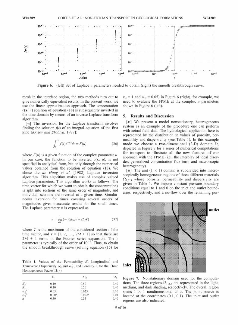
vy = 1 and ay = 0.05) in Figure 6 (right), for example, weneed to evaluate the FPME at the complex u parametersshown in Figure 6 (left).

5. Results and Discussion

[47] We present a model nonstationary, heterogeneoussystem as an example of the procedure one can performwith actual field data. The hydrological application here isrepresented by the distribution in values of porosity, per-meability and dispersiviity (see Table 1). In this examplemode we choose a two-dimensional (2-D) domain W,depicted in Figure 7 for a series of numerical computationsfor transport to illustrate all the new features of ourapproach with the FPME (i.e., the interplay of local disor-der, generalized concentration flux term and macroscopicheterogeneity).[48] The unit (1 � 1) domain is subdivided into macro-

scopically homogeneous regions of three different materialsW1,2,3 whose porosity, permeability and dispersivity aregiven in Table 1. We impose constant pressure boundaryconditions equal to 1 and 0 on the inlet and outlet bound-aries, respectively, and a no-flow over the remaining por-

Figure 6. (left) Set of Laplace u parameters needed to obtain (right) the smooth breakthrough curve.

Table 1. Values of the Permeability K, Longitudinal and

Transverse Dispersivity ayl and ay

t , and Porosity n for the Three

Homogeneous Facies W1,2,3

W1 W2 W3

Kx 0.10 0.50 0.40Ky 0.10 0.50 0.40

ayl 0.05 0.025 0.10

ayt 0.005 0.0025 0.01

n 0.30 0.35 0.40

Figure 7. Nonstationary domain used for the computa-tions. The three regions W1,2,3 are represented in the light,medium, and dark shading, respectively. The overall regionspans 1 � 1 nondimensional units. The point source islocated at the coordinates (0.1, 0.1). The inlet and outletregions are also indicated.


9 of 16

W04209

tions of the boundary. We assume an initial resident con-centration c0(x) = 0, a constant concentration at the injectionpoint (0.1, 0.1), a free boundary condition at the outletboundary, and a no-flux boundary condition on the remain-der of the domain. The approximation of the interface zonebetween the different macroscopically homogeneousregions is obtained by linearizing the spatial derivative ofthe dispersivity over a small region about the interface itself.[49] The first step in the actual computations is the

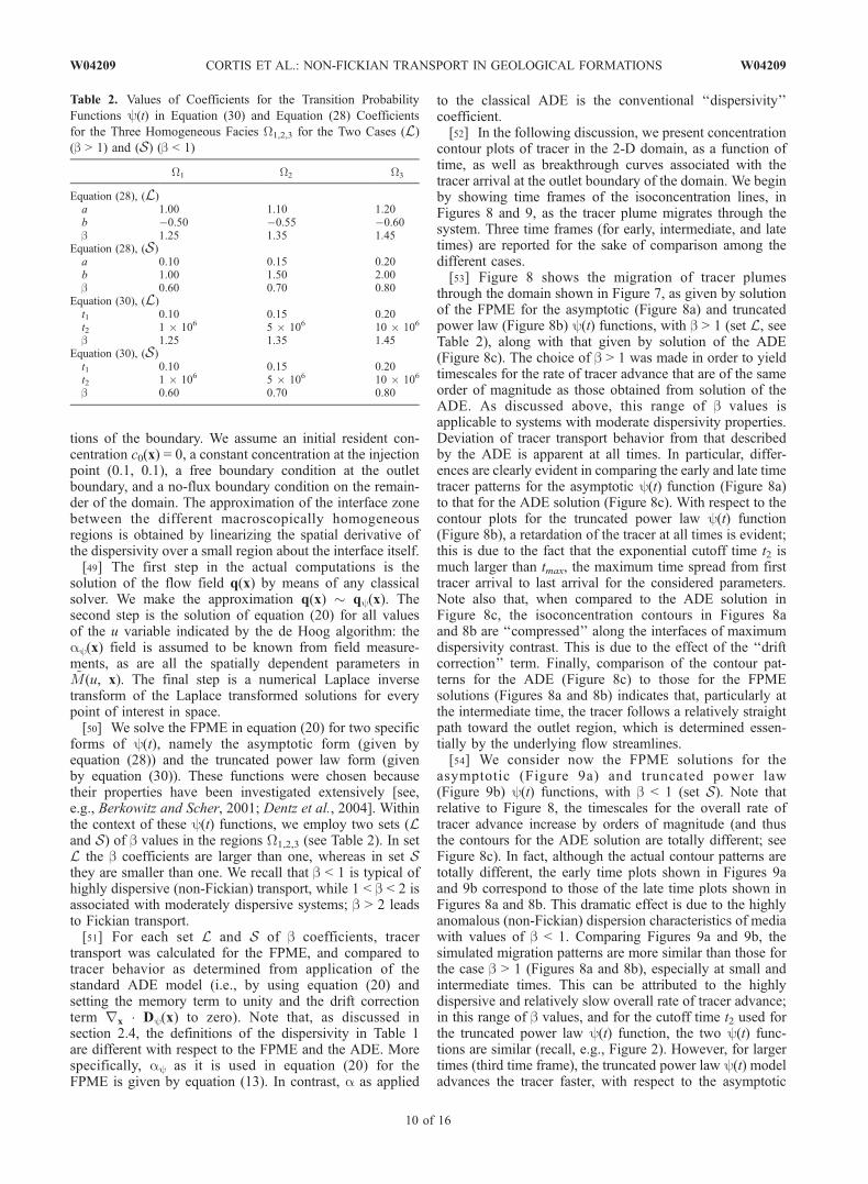
solution of the flow field q(x) by means of any classicalsolver. We make the approximation q(x) � qy(x). Thesecond step is the solution of equation (20) for all valuesof the u variable indicated by the de Hoog algorithm: theay(x) field is assumed to be known from field measure-ments, as are all the spatially dependent parameters in~M(u, x). The final step is a numerical Laplace inversetransform of the Laplace transformed solutions for everypoint of interest in space.[50] We solve the FPME in equation (20) for two specific

forms of y(t), namely the asymptotic form (given byequation (28)) and the truncated power law form (givenby equation (30)). These functions were chosen becausetheir properties have been investigated extensively [see,e.g., Berkowitz and Scher, 2001; Dentz et al., 2004]. Withinthe context of these y(t) functions, we employ two sets (Land S) of b values in the regions W1,2,3 (see Table 2). In setL the b coefficients are larger than one, whereas in set Sthey are smaller than one. We recall that b < 1 is typical ofhighly dispersive (non-Fickian) transport, while 1 < b < 2 isassociated with moderately dispersive systems; b > 2 leadsto Fickian transport.[51] For each set L and S of b coefficients, tracer

transport was calculated for the FPME, and compared totracer behavior as determined from application of thestandard ADE model (i.e., by using equation (20) andsetting the memory term to unity and the drift correctionterm rx Dy(x) to zero). Note that, as discussed insection 2.4, the definitions of the dispersivity in Table 1are different with respect to the FPME and the ADE. Morespecifically, ay as it is used in equation (20) for theFPME is given by equation (13). In contrast, a as applied

to the classical ADE is the conventional ‘‘dispersivity’’coefficient.[52] In the following discussion, we present concentration

contour plots of tracer in the 2-D domain, as a function oftime, as well as breakthrough curves associated with thetracer arrival at the outlet boundary of the domain. We beginby showing time frames of the isoconcentration lines, inFigures 8 and 9, as the tracer plume migrates through thesystem. Three time frames (for early, intermediate, and latetimes) are reported for the sake of comparison among thedifferent cases.[53] Figure 8 shows the migration of tracer plumes

through the domain shown in Figure 7, as given by solutionof the FPME for the asymptotic (Figure 8a) and truncatedpower law (Figure 8b) y(t) functions, with b > 1 (set L, seeTable 2), along with that given by solution of the ADE(Figure 8c). The choice of b > 1 was made in order to yieldtimescales for the rate of tracer advance that are of the sameorder of magnitude as those obtained from solution of theADE. As discussed above, this range of b values isapplicable to systems with moderate dispersivity properties.Deviation of tracer transport behavior from that describedby the ADE is apparent at all times. In particular, differ-ences are clearly evident in comparing the early and late timetracer patterns for the asymptotic y(t) function (Figure 8a)to that for the ADE solution (Figure 8c). With respect to thecontour plots for the truncated power law y(t) function(Figure 8b), a retardation of the tracer at all times is evident;this is due to the fact that the exponential cutoff time t2 ismuch larger than tmax, the maximum time spread from firsttracer arrival to last arrival for the considered parameters.Note also that, when compared to the ADE solution inFigure 8c, the isoconcentration contours in Figures 8aand 8b are ‘‘compressed’’ along the interfaces of maximumdispersivity contrast. This is due to the effect of the ‘‘driftcorrection’’ term. Finally, comparison of the contour pat-terns for the ADE (Figure 8c) to those for the FPMEsolutions (Figures 8a and 8b) indicates that, particularly atthe intermediate time, the tracer follows a relatively straightpath toward the outlet region, which is determined essen-tially by the underlying flow streamlines.[54] We consider now the FPME solutions for the

asymptotic (Figure 9a) and truncated power law(Figure 9b) y(t) functions, with b < 1 (set S). Note thatrelative to Figure 8, the timescales for the overall rate oftracer advance increase by orders of magnitude (and thusthe contours for the ADE solution are totally different; seeFigure 8c). In fact, although the actual contour patterns aretotally different, the early time plots shown in Figures 9aand 9b correspond to those of the late time plots shown inFigures 8a and 8b. This dramatic effect is due to the highlyanomalous (non-Fickian) dispersion characteristics of mediawith values of b < 1. Comparing Figures 9a and 9b, thesimulated migration patterns are more similar than those forthe case b > 1 (Figures 8a and 8b), especially at small andintermediate times. This can be attributed to the highlydispersive and relatively slow overall rate of tracer advance;in this range of b values, and for the cutoff time t2 used forthe truncated power law y(t) function, the two y(t) func-tions are similar (recall, e.g., Figure 2). However, for largertimes (third time frame), the truncated power law y(t) modeladvances the tracer faster, with respect to the asymptotic

Table 2. Values of Coefficients for the Transition Probability

Functions y(t) in Equation (30) and Equation (28) Coefficients

for the Three Homogeneous Facies W1,2,3 for the Two Cases (L)

(b > 1) and (S) (b < 1)

W1 W2 W3

Equation (28), (L)a 1.00 1.10 1.20b �0.50 �0.55 �0.60b 1.25 1.35 1.45

Equation (28), (S)a 0.10 0.15 0.20b 1.00 1.50 2.00b 0.60 0.70 0.80

Equation (30), (L)t1 0.10 0.15 0.20t2 1 � 106 5 � 106 10 � 106

b 1.25 1.35 1.45Equation (30), (S)

t1 0.10 0.15 0.20t2 1 � 106 5 � 106 10 � 106

b 0.60 0.70 0.80

10 of 16


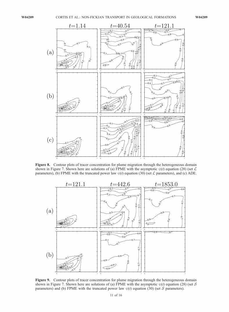
Figure 8. Contour plots of tracer concentration for plume migration through the heterogeneous domainshown in Figure 7. Shown here are solutions of (a) FPME with the asymptotic y(t) equation (28) (set Lparameters), (b) FPME with the truncated power law y(t) equation (30) (set L parameters), and (c) ADE.

Figure 9. Contour plots of tracer concentration for plume migration through the heterogeneous domainshown in Figure 7. Shown here are solutions of (a) FPME with the asymptotic y(t) equation (28) (set Sparameters) and (b) FPME with the truncated power law y(t) equation (30) (set S parameters).


11 of 16

W04209

model. This is because the truncation time t2 is of the orderof the overall transport and therefore the behavior of thetracer in the truncated power law is already Fickian at thesetimes. In contrast, longer tailing arises when transport isnon-Fickian. Finally, as before, it is possible to discern theeffects of the dispersivity interfaces on the contour patterns.[55] We now analyze the different simulated transport

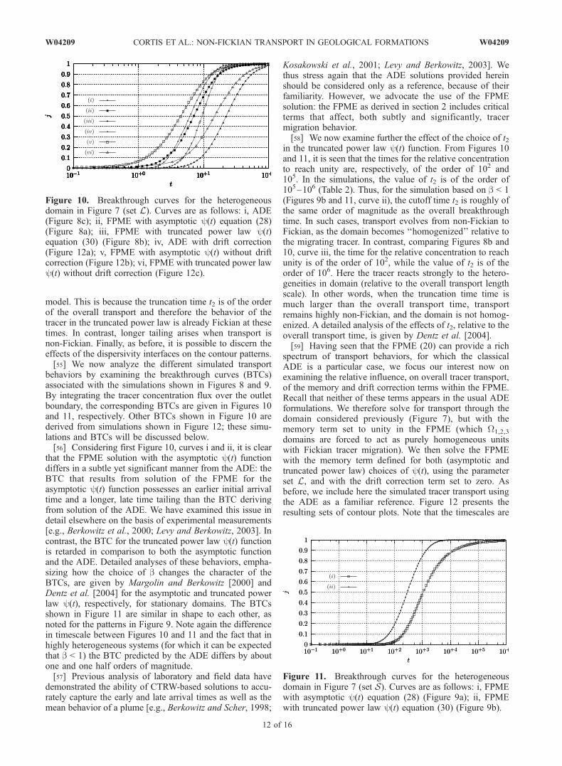
behaviors by examining the breakthrough curves (BTCs)associated with the simulations shown in Figures 8 and 9.By integrating the tracer concentration flux over the outletboundary, the corresponding BTCs are given in Figures 10and 11, respectively. Other BTCs shown in Figure 10 arederived from simulations shown in Figure 12; these simu-lations and BTCs will be discussed below.[56] Considering first Figure 10, curves i and ii, it is clear

that the FPME solution with the asymptotic y(t) functiondiffers in a subtle yet significant manner from the ADE: theBTC that results from solution of the FPME for theasymptotic y(t) function possesses an earlier initial arrivaltime and a longer, late time tailing than the BTC derivingfrom solution of the ADE. We have examined this issue indetail elsewhere on the basis of experimental measurements[e.g., Berkowitz et al., 2000; Levy and Berkowitz, 2003]. Incontrast, the BTC for the truncated power law y(t) functionis retarded in comparison to both the asymptotic functionand the ADE. Detailed analyses of these behaviors, empha-sizing how the choice of b changes the character of theBTCs, are given by Margolin and Berkowitz [2000] andDentz et al. [2004] for the asymptotic and truncated powerlaw y(t), respectively, for stationary domains. The BTCsshown in Figure 11 are similar in shape to each other, asnoted for the patterns in Figure 9. Note again the differencein timescale between Figures 10 and 11 and the fact that inhighly heterogeneous systems (for which it can be expectedthat b < 1) the BTC predicted by the ADE differs by aboutone and one half orders of magnitude.[57] Previous analysis of laboratory and field data have

demonstrated the ability of CTRW-based solutions to accu-rately capture the early and late arrival times as well as themean behavior of a plume [e.g., Berkowitz and Scher, 1998;

Kosakowski et al., 2001; Levy and Berkowitz, 2003]. Wethus stress again that the ADE solutions provided hereinshould be considered only as a reference, because of theirfamiliarity. However, we advocate the use of the FPMEsolution: the FPME as derived in section 2 includes criticalterms that affect, both subtly and significantly, tracermigration behavior.[58] We now examine further the effect of the choice of t2

in the truncated power law y(t) function. From Figures 10and 11, it is seen that the times for the relative concentrationto reach unity are, respectively, of the order of 102 and105. In the simulations, the value of t2 is of the order of105–106 (Table 2). Thus, for the simulation based on b < 1(Figures 9b and 11, curve ii), the cutoff time t2 is roughly ofthe same order of magnitude as the overall breakthroughtime. In such cases, transport evolves from non-Fickian toFickian, as the domain becomes ‘‘homogenized’’ relative tothe migrating tracer. In contrast, comparing Figures 8b and10, curve iii, the time for the relative concentration to reachunity is of the order of 102, while the value of t2 is of theorder of 106. Here the tracer reacts strongly to the hetero-geneities in domain (relative to the overall transport lengthscale). In other words, when the truncation time time ismuch larger than the overall transport time, transportremains highly non-Fickian, and the domain is not homog-enized. A detailed analysis of the effects of t2, relative to theoverall transport time, is given by Dentz et al. [2004].[59] Having seen that the FPME (20) can provide a rich

spectrum of transport behaviors, for which the classicalADE is a particular case, we focus our interest now onexamining the relative influence, on overall tracer transport,of the memory and drift correction terms within the FPME.Recall that neither of these terms appears in the usual ADEformulations. We therefore solve for transport through thedomain considered previously (Figure 7), but with thememory term set to unity in the FPME (which W1,2,3

domains are forced to act as purely homogeneous unitswith Fickian tracer migration). We then solve the FPMEwith the memory term defined for both (asymptotic andtruncated power law) choices of y(t), using the parameterset L, and with the drift correction term set to zero. Asbefore, we include here the simulated tracer transport usingthe ADE as a familiar reference. Figure 12 presents theresulting sets of contour plots. Note that the timescales are

Figure 10. Breakthrough curves for the heterogeneousdomain in Figure 7 (set L). Curves are as follows: i, ADE(Figure 8c); ii, FPME with asymptotic y(t) equation (28)(Figure 8a); iii, FPME with truncated power law y(t)equation (30) (Figure 8b); iv, ADE with drift correction(Figure 12a); v, FPME with asymptotic y(t) without driftcorrection (Figure 12b); vi, FPME with truncated power lawy(t) without drift correction (Figure 12c).

Figure 11. Breakthrough curves for the heterogeneousdomain in Figure 7 (set S). Curves are as follows: i, FPMEwith asymptotic y(t) equation (28) (Figure 9a); ii, FPMEwith truncated power law y(t) equation (30) (Figure 9b).

12 of 16


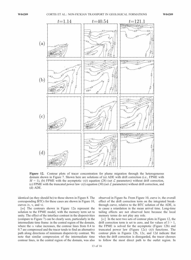
identical (as they should be) to those shown in Figure 8. Thecorresponding BTCs for these cases are shown in Figure 10,curves iv, v, and vi.[60] The contours shown in Figure 12a represent the

solution to the FPME model, with the memory term set tounity. The effect of the interface contrast in the dispersivities(compare to Figure 7) can be clearly seen, particularly in theintermediate time frame: in the central region of the domain,where the a value increases, the contour lines from 0.4 to0.7 are compressed and the tracer tends to find an alternativepath along directions of minimum dispersivity contrast. Wenote that similar compression of the intermediate timecontour lines, in the central region of the domain, was also

observed in Figure 8a. From Figure 10, curve iv, the overalleffect of the drift correction term on the integrated break-through curve, relative to the BTC solution of the ADE, isto cause a retardation in the mean arrival time. Long-timetailing effects are not observed here because the localmemory terms do not play any role.[61] In the next two sets of contour plots in Figure 12, the

drift correction term is set to zero, and for values of b > 1,the FPME is solved for the asymptotic (Figure 12b) andtruncated power law (Figure 12c) y(t) functions. Thecontour plots in Figures 12b, 12c, and 12d indicate thatwhen the drift correction is disregarded, the tracer choosesto follow the most direct path to the outlet region. In

Figure 12. Contour plots of tracer concentration for plume migration through the heterogeneousdomain shown in Figure 7. Shown here are solutions of (a) ADE with drift correction (i.e., FPME with~M = 1), (b) FPME with the asymptotic y(t) equation (28) (set L parameters) without drift correction,(c) FPME with the truncated power law y(t) equation (30) (set L parameters) without drift correction, and(d) ADE.


13 of 16

W04209

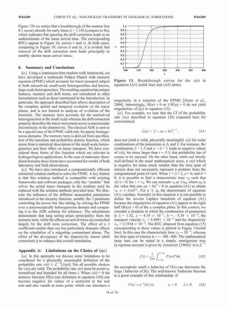
Figure 12b we notice that a breakthrough of the contour line0.1 occurs already for early times (t = 1.14) (compare to 8a),which indicates that ignoring the drift correction leads to anunderestimate of the mean arrival time. The correspondingBTCs appear in Figure 10, curves v and vi. In both cases,comparing to Figure 10, curves ii and iii, it is evident thatremoval of the drift correction term leads principally tonotably shorter mean arrival times.

6. Summary and Conclusions

[62] Using a continuous time random walk framework, wehave developed a multiscale Fokker Planck with memoryequation (FPME) which accounts for tracer transport subjectto both unresolved, small-scale heterogeneities and known,large-scale heterogeneities. The resulting equation has uniquefeatures, memory and drift terms, not considered in otherformulations such as those mentioned in the Introduction. Inparticular, the approach described here allows description ofthe complete spatial and temporal evolution of the tracerplume, and is not limited to analysis of evolution of themoments. The memory term accounts for the unresolvedheterogeneities at the small scale whereas the drift correctionproperly describes the tracer movement across a macroscopicdiscontinuity in the dispersivity. The classical ADE is seen tobe a special case of the FPME valid only for purely homoge-neous domains. The memory term is derived from specifica-tion of the transition rate probability density function, whichstems from a statistical description of the small-scale hetero-geneities and their effect on tracer transport. We have con-sidered three forms of this function which are relevant tohydrogeological applications. In the case of stationary disor-dered domains these forms have accounted for results of bothlaboratory and field observations.[63] We have also introduced a computationally efficient

numerical solution method to solve the FPME. A key featureis that this solution method is compatible with existingframeworks and software packages; only the ‘‘module’’ thatsolves the actual tracer transport in the medium need bereplaced with the solution methods provided here. We illus-trate the influence of the different measurable parametersintroduced in the memory function, notably the b parametercontrolling the power law like tailing, by solving the FPMEover a macroscopically heterogeneous domain and compar-ing it to the ADE solution for reference. The calculationsdemonstrate that long tailing arises (principally) from thememory term, while the effects on arrival times are controlledlargely by the drift term correction. The effect of a bcoefficient smaller than one has particularly dramatic effectson the retardation of a migrating contaminant plume. Theeffect of the divergence of the dispersivity tensor (driftcorrection) is to enhance this overall retardation.

Appendix A: Limitations on the Choice of ~Y(u)

[64] In this appendix we discuss some limitations to beconsidered for a physically meaningful definition of theprobability rate y(t) � L�1[~y(u)]. Not all possible choicesfor ~y(u) are valid. The probability rate y(t) must be positive,normalized and bounded for all times t. When y(t) < 0 thememory function ~M (u) (see definition in equation (10)) canbecome negative for values of u restricted to the realaxis and also vanish at some point, which can introduce a

singularity in a solution of the FPME [Dentz et al.,2004]. Interestingly, ~M (u) = 0 or 1/ ~M (u) = 0 do not yieldsingularities of ~j(u) in equation (15).[65] For example, we note that the LT of the probability

rate ~y(u) described in equation (28) (repeated here forconvenience)

~yðuÞ ¼ 1þ auþ bub� ��1

: ðA1Þ

does not yield a valid, physically meaningful y(t) for somecombinations of the parameters a, b, and b. For instance, thecombination b = 1.5 and a = b = 1 leads to negative valuesof y(t), for times larger than t � 5.3; this probability has ofcourse to be rejected. On the other hand, while not strictlywell-defined in the usual mathematical sense, a y(t) whichis negative for times much smaller than the time span ofinterest does not necessarily represent a problem from thecomputational point of view. When 1 < b < 2, a > 0, and b <0, it is possible to find a characteristic time t0 such thaty(t) < 0, for t < t0. We can estimate t0 as 1/u0, where u0 isthe value that sets au + bub = 0 in equation (A1) to obtaint0 � (�b/a)

1b�1. For u ^ u0 the denominator of equation

(A1) vanishes. Formally in this situation it is not possible todefine the inverse Laplace transform of equation (A1)because the singularities of equation (A1) appear in the righthalf (Re(u) > 0) of the u complex plane. In this context, weconsider a situation in which the combination of parametersis b = 1.32, a = 4.19 � 10�1, b = �5.39 � 10�2, thetransport velocity vy = 5.4991 � 10�3 and the dispersivityay = 2.1934 � 10�3. The BTC obtained from equation (15)corresponding to these values is plotted in Figure 13(solidline). In this case the characteristic time t0 � 10�3, whereasthe time span of interest is t � 100–400. The mathematicalissue here can be stated in a simple, nonrigorous way(a rigorous account is given by Zemanian [1968]): in a L�1

f ðtÞ ¼ 1

2pi

Z sþi1

s�i1FðuÞeutdu ðA2Þ

the asymptotic small u behavior of F(u) can determine thelarge t behavior of f(t). The well-known Tauberian theoremis a good example of this relationship: if

FðuÞ � u�bAð1=uÞ u ! 0 b > 0 ðA3Þ

Figure 13. Breakthrough curves for the y(t) inequations (A1) (solid line) and (A5) (dots).

14 of 16


then

f ðtÞ � tb�1AðtÞ=GðbÞ t ! 1 ðA4Þ

where A(t) is a slowly varying function of t, e.g., A / ln t.[66] To further demonstrate that y(t) < 0 for small times

(well below the time range of interest) does not causeessential difficulties, we point out that it is possible to makethe probability rate y(t) positive for all time by adding asecond-order correction in the denominator:

~y0ðuÞ ¼ 1þ auþ bub þ t0u2� ��1

: ðA5Þ

To within O(u2), equations (A1) and (A5) have the sameleading asymptotic small u (u � 10�2) dependence. InFigure 13 we present the BTC corresponding to the ~y(u) inequation (A5) (dots). The two solutions are essentiallyidentical. Thus, for all practical purposes, the originalexpression in (38) can be used regardless of its negativevalues for large u (corresponding to small times). Theformal approach [Zemanian, 1968] avoids the large ubehavior by using a relation between f(t) and F(u) whereF(u) in equation (A2) is analytic in an open strip s1 <Re(u) < s2.[67] Wepoint out that the probability rates in equations (30)

and (32) are positive for all values of their respectiveparameters and are thus not subject to the the limitations ofequation (A1). It is obviously better toworkwith awell-posedy(t) at the outset. In general one can develop an asymptoticseries for F(u) in the u ! 1 limit by integrating a Taylorexpansion of f(t) in equation (36),

FðuÞ �Z 1

0

dte�utðf ð0Þ þ tf1 þ1

2t2f2 þ . . .Þ � f ð0Þ=uþ f1=u

2 . . .

ðA6Þ

where f1 � df/dtj0 and f2 � d2f/dt2j0. Hence ~y(u)u;1 �! y(0)/u and therefore ~M (u) u; 1�! y (0). One canavoid difficulties if y(0) > 0 and y(t) is well behaved forsmall t. It should be pointed that this is not the case for theFDE equation (21) with b < 1. The equivalent to theasymptotic limit of small u defining the operators in the FDEcorresponds to a ~y(u) = 1/(1 + ub), which does not have afinite y(0), i.e., y(t) is unbounded as t ! 0. The solution ofthe FDE is thus physically meaningful only for large t.

[68] Acknowledgments. The financial support of BP International,the Israel Science Foundation (grant 147/01), the European Commission-Marie Curie Individual Fellowship programme, and the Sardinian RegionalAuthorities is gratefully acknowledged.

ReferencesAbramowitz, M., and I. Stegun (1970), Handbook of Mathematical Func-tions, Dover, Mineola, N. Y.

Adams, E. E., and L. W. Gelhar (1992), Field study of dispersion in aheterogeneous aquifer: 2. Spatial moment analysis, Water Resour. Res.,28, 3293–3308.

Bear, J. (1972), Dynamics of Fluids in Porous Media, Elsevier Sci., NewYork.

Bear, J., and Y. Bachmat (1991), Introduction to Modeling of TransportPhenomena in Porous Media, Kluwer Acad., Norwell, Mass.

Berkowitz, B., and H. Scher (1995), On characterization of anomalousdispersion in porous and fractured media, Water Resour. Res., 31,1461–1466.

Berkowitz, B., and H. Scher (1998), Theory of anomalous chemical trans-port in random fracture networks, Phys. Rev. E, 57, 5858–5869.

Berkowitz, B., and H. Scher (2001), The role of probabilistic approaches totransport theory in heterogeneous media, Transp. Porous Media, 42,241–263.

Berkowitz, B., H. Scher, and S. E. Silliman (2000), Anomalous transport inlaboratory-scale, heterogeneous porous media, Water Resour. Res., 36,149–158.

Berkowitz, B., J. Klafter, R. Metzler, and H. Scher (2002), Physical picturesof transport in heterogeneous media: Advection-dispersion, random walkand fractional derivative formulations, Water Resour. Res., 38, 1191,doi:10.1029/2001WR001030.

Boggs, J. M., S. C. Young, and L. C. Beard (1992), Field study of disper-sion in a heterogeneous aquifer: 1. Overview and site description, WaterResour. Res., 28, 3281–3291.

Burr, D. T., and E. A. Sudicky (1994), Nonreactive and reactive solutetransport in three-dimensional heterogeneous porous media: Mean dis-placement, plume spreading, and uncertainty, Water Resour. Res., 30,791–815.

Carrera, J., X. Sanchez-Vila, I. Benet, A. Medina, G. Galarza, and J. Guimera(1998), On matrix diffusion: Formulations, solution methods, and quali-tative effects, Hydrogeol. J., 6, 178–190.

Cunningham, J. A., C. J. Werth, M. Reinhard, and P. V. Roberts (1997),Effects of grain-scale mass transfer on the transport of volatile organicsthrough sediments: 1. Model development, Water Resour. Res., 33,2713–2726.

Dagan, G. (1989), Flow and Transport in Porous Formations, Springer-Verlag, New York.

Dagan, G. (1994), The significance of heterogeneitiy of evolving scales totransport in porous formations, Water Resour. Res., 30, 3327–3336.

Dagan, G., and S. P. Neuman (Eds.) (1997), Subsurface Flow and Trans-port: A Stochastic Approach, Cambridge Univ. Press, New York.

de Hoog, F. R., J. H. Knight, and A. N. Stokes (1982), An improvedmethod for numerical inversion of Laplace transforms, SIAM J. Sci. Stat.Comput., 3, 357–366.

Dentz, M., and B. Berkowitz (2003), Transport behavior of a passive solutein continuous time random walks and multirate mass transfer, WaterResour. Res., 39(5), 1111, doi:10.1029/2001WR001163.

Dentz, M., H. Kinzelbach, S. Attinger, and W. Kinzelbach (2002), Temporalbehavior of a solute cloud in a heterogeneous porous medium: 3. Numer-ical simulations, Water Resour. Res., 38(7), 1118, doi:10.1029/2001WR000436.

Dentz, M., A. Cortis, H. Scher, and B. Berkowitz (2004), Time behavior ofsolute transport in heterogeneous media: Transition from anomalous tonormal transport Adv, Water Resour., 27(2), 155–173, doi:10.1016/j.advwatres.2003.11.002.

Eggleston, J., and S. Rojstaczer (1998), Identification of large-scale hydrau-lic conductivity trends and the influence of trends on contaminant trans-port, Water Resour. Res., 34, 2155–2168.

Feehley, C. E., C. Zheng, and F. J. Molz (2000), A dual-domain masstransfer approach for modeling solute transport in heterogeneous aqui-fers: Application to the Macrodispersion Experiment (MADE) site,WaterResour. Res., 36, 2501–2515.

Gelhar, L. W. (1993), Stochastic Subsurface Hydrology, Prentice-Hall, OldTappan, N. J.

Gelhar, L. W., C. Welty, and K. R. Rehfeldt (1992), A critical review of dataon field-scale dispersion in aquifers,Water Resour. Res., 28, 1955–1974.

Haggerty, R., and S. M. Gorelick (1995), Multiple-rate mass transfer formodeling diffusion and surface reactions in media with pore-scale het-erogeneity, Water Resour. Res., 31, 2383–2400.

Haggerty, R., and S. M. Gorelick (1998), Modeling mass transfer processesin soil columns with pore-scale heterogeneity, Soil Sci. Soc. Am. Proc.,62, 62–74.

Kenkre, V. M., E. W. Montroll, and M. F. Shlesinger (1973), Generalizedmaster equations for continuous-time random walks, J. Stat. Phys., 9,45–50.

Klafter, J., and R. Silbey (1980), Derivation of continuous-time randomwalk equations, Phys. Rev. Lett., 44, 55–58.

Koltermann, C. E., and S. M. Gorelick (1996), Heterogeneity in sedimen-tary deposits: A review of structure-imitating, process-imitating anddescriptive approaches, Water Resour. Res., 32, 2617–2658.

Kosakowski, G., B. Berkowitz, and H. Scher (2001), Analysis of fieldobservations of tracer transport in a fractured till, J. Contam. Hydrol.,47, 29–51.

Krylov, V. I., and N. S. Skoblya (1977), A Handbook of Methods of Ap-proximate Fourier Transformation and Inversion of the Laplace Trans-form, Mir, Moscow.


15 of 16

W04209

Labolle, E. M., and G. E. Fogg (2001), Role of molecular diffusion incontaminant migration and recovery in an alluvial aquifer system,Transp. Porous Media, 42, 155–179.

Labolle, E. M., G. E. Fogg, and F. B. Tompson (1996), Random-walksimulation of transport in heterogeneous porous media: Local mass-conservation problem and implementation methods, Water Resour.Res., 32, 583–593.

Levy, M., and B. Berkowitz (2003), Measurement and analysis of non-Fickian dispersion in heterogeneous porous media, J. Contam. Hydrol.,64, 203–226.

Margolin, G., and B. Berkowitz (2000), Application of continuous timerandom walks to transport in porous media, J. Phys. Chem. B, 104,3942–3947. (Correction, J. Phys. Chem. B, 104, 8762, 2000).

McLaughlin, D., and F. Ruan (2001), Macrodispersivity and large-scalehydrogeologic variability, Transp. Porous Media, 42, 133–154.

Metzler, R., and J. Klafter (2000), The random walk’s guide to anomalousdiffusion: A fractional dynamics approach, Phys. Rep., 339, 1–77.

Naff, R., D. F. Haley, and E. A. Sudicky (1998), High-resolutionMonte Carlo simulation of flow and conservative transport in hetero-geneous porous media: 2. Transport results, Water Resour. Res., 34,679–697.

Pannone, M., and P. K. Kitanidis (2001), Large-time spatial covariance ofconcentration of conservative solute and application to the Cape Codtracer test, Transp. Porous Media, 42, 109–132.

Risken, H. (1989), The Fokker-Planck Equation: Methods of Solution andApplications, Springer Ser. Synergetics, vol. 18, 2nd ed., Springer-Verlag, New York.

Roth, K., and W. A. Jury (1993), Linear transport models for adsorbingsolutes, Water Resour. Res., 29, 1195–1203.

Salandin, P., and V. Fiorotto (1998), Solute transport in highly heteroge-neous aquifers, Water Resour. Res., 34, 949–961.

Scher, H., and M. Lax (1973), Stochastic transport in a disordered solid. II.Impurity conduction, Phys. Rev. B, 7, 4502–4519.

Scher, H., G. Margolin, and B. Berkowitz (2002), Towards a unified frame-work for anomalous transport in heterogeneous media, Chem. Phys., 284,349–359.

Shlesinger, M. F. (1974), Asymptotic solutions of continuous-time randomwalks, J. Stat. Phys., 10, 421–434.

Sidle, C., B. Nilson, M. Hansen, and J. Frederica (1998), Spatially varyinghydraulic and solute transport characteristics of a fractured till deter-mined by field tracer tests, Funen, Denmark, Water Resour. Res., 34,2515–2527.

Silliman, S. E., and E. S. Simpson (1987), Laboratory evidence of the scaleeffect in dispersion of solutes in porous media, Water Resour. Res., 23,1667–1673.

Trefethen, L. N. (2000), Spectral Methods in Matlab, Soc. for Ind. andAppl. Math., Philadelphia, Pa.

Zemanian, A. H. (1968), Generalized Integral Transformations, Wiley-Interscience, Hoboken, N. J.

��B. Berkowitz, A. Cortis, and H. Scher, Department of Environmental

Sciences and Energy Research, Weizmann Institute of Science, Rehovot76100, Israel. ([email protected]; [email protected]; [email protected])

C. Gallo, CRS4, Parco Scientifico e Tecnologico, Localita Pixina MannaEdificio 1, C.P. 25, I-09010 Pula (CA), Italy. ([email protected])

16 of 16


Numerical simulation of non-Fickian transport in geological formations with multiple-scale...

Documents

Transcript of Numerical simulation of non-Fickian transport in geological formations with multiple-scale...