Author's personal copy

Acta Astronautica 64 (2009) 554–570www.elsevier.com/locate/actaastro

Control of satellite imaging formations inmulti-body regimesKathleen C. Howell∗, Lindsay D. Millard

School of Aeronautics and Astronautics, Purdue University, West Lafayette, Indiana, USA

Received 20 March 2007; accepted 10 October 2008Available online 17 December 2008

Abstract

Libration point orbits may be ideal locations for satellite imaging formations. Therefore, control of these arrays in multi-bodyregimes is critical. A continuous feedback control algorithm is developed that maintains a formation of satellites in motion that isbounded relative to a halo orbit. This algorithm is derived based on the dynamic characteristics of the phase space near periodicorbits in the circular restricted three-body problem (CR3BP). By adjusting parameters of the control algorithm appropriately,satellites in the formation follow trajectories that are particularly advantageous to imaging arrays. Image reconstruction andcoverage of the (u, v) plane are simulated for interferometric satellite configurations, demonstrating potential applications of thealgorithm and the resulting motion.© 2008 Elsevier Ltd. All rights reserved.

1. Introduction

Satellite imaging formations have numerous applica-tions in the future of space exploration. These include:exosolar planets, identification of black holes, and spec-tral characterization of distant stars. Libration point or-bits may be ideal locations for such imaging arrays[1–3]. Therefore, control of these arrays in multi-bodyregimes is critical.

Much of the available research in formation flightapplications focuses on Earth orbiting configurations,where the influence of other gravitational perturbationscan be safely ignored [4,5]. However, interest in forma-tions that evolve near the vicinity of the Sun–Earth libra-tion points has inspired new studies regarding formationkeeping in the three-body problem [6–12]. Howell andMarchand consider linear optimal control, as appliedto nonlinear time-varying systems, as well as nonlinear

∗Corresponding author.E-mail addresses: howell@purdue.edu (K.C. Howell),

lmillard@purdue.edu.

0094-5765/$ - see front matter © 2008 Elsevier Ltd. All rights reserved.doi:10.1016/j.actaastro.2008.10.008

control techniques, including input and output feedbacklinearization [13]. These control strategies are appliedto a two spacecraft formation where the chief spacecraftevolves along a three-dimensional periodic halo orbitnear the L2 libration point. In a later work, the controlstrategies are shown to be effective in the full ephemerismodel [14]. Howell and Barden investigate formationflying in the vicinity of the libration points in the cir-cular restricted three-body problem (CR3BP). Initially,their focus is the determination of the natural behavioron the center manifold near the libration points. Thefirst stage of their study captures a naturally occurringsix-satellite formation near the libration points [15,16].Further analysis considered strategies to maintain a pe-riodic, planar formation of the six vehicles in an orbitabout the Sun–Earth L1 point [17,18]. The deviation ofeach spacecraft is controlled impulsively relative to theplane of the initial formation, one that is specified to becontained within the center manifold. The natural flowin the center subspace is such that the relative distancesbetween each spacecraft remain essentially boundedand the relative configuration of the formation is time

Author's personal copy

K.C. Howell, L.D. Millard / Acta Astronautica 64 (2009) 554–570 555

independent. Marchand and Howell extend this analysisby revealing other potentially interesting nominal mo-tions as well as discrete control strategies for deploy-ment and station-keeping [19].

Research in the specific area of interferometric satel-lite formation control has also been pursued. Differentmethods have been explored to determine satellite mo-tion that minimizes fuel while attaining an adequatelyresolute image. Chakravorty develops a model for theprocess of image formation in a multi-spacecraft inter-ferometric system [20,21]. Hyland extends this modelto formulate an image-quality based figure of merit foroptimal control strategies [22,23]. Hussein, Scheeres,and Hyland identify a special class of two-dimensional(2D) spiral motions that satisfy the necessary imag-ing requirements for certain interferometric imagingmissions. Isolation of this class of motion serves as abasis for the identification of a relationship betweenimage quality and fuel expenditure. The spacecraft areassumed to be moving in free space; the only forcesacting on the system are control forces [24,25]. Husseinet al. expand this analysis by formulating an optimalcontrol problem to minimize measurement noise andfuel while maximizing certain image metrics. Althoughthe two-point boundary value problem remains un-solved, necessary conditions for optimality are definedand these reveal the general behavior of an optimal so-lution. Again, the spacecraft are assumed to be movingin free space [26,27]. Finally, Hussein and Bloch applydynamic coverage optimal control (a geometric controlmethod) to interferometric imaging arrays. However,the formulation incorporates assumptions that include:a system that evolves only on planar or paraboloidalRiemannian manifolds and is not evolving in any gravi-tational field [28,29]. Most recently, Millard and Howellsolve for formation satellite motion that maximizesimage resolution while minimizing fuel. The nonlinearoptimal control problem is formulated in the CR3BP,where a formation of two satellites is assumed to bemoving near a Sun–Earth collinear libration point [38].

The goal in the present investigation is the develop-ment of a feedback control algorithm that maintains anarbitrary number of satellites within some bounded re-gion relative to a halo orbit. This algorithm is devel-oped based on the dynamical characteristics of the phasespace near periodic orbits in the CR3BP. By adjustingparameters of the control algorithm appropriately, tra-jectories that are particularly advantageous to opticalformations emerge. Image reconstruction and coverageof the (u,v) plane are simulated for interferometric satel-lite formations, demonstrating potential applications ofthe algorithm and resulting motion.

2. Optics

The resolution of an image produced by an inter-ferometric satellite array is largely determined by thecorresponding coverage of the (u,v) plane. In turn, cov-erage of the (u,v) plane is derived based on several char-acteristics of the satellite configuration and motion inphysical space. Therefore, to determine the formationmotion that may be advantageous to imaging, a mathe-matical model relating satellite motion in physical spaceto coverage of the (u,v) plane, and thus image recon-struction, is necessary. The model developed here is asimplified approximation but captures the essential fea-tures for analysis.

2.1. Background

A light beam is an electromagnetic wave propagatingthrough space. This electromagnetic wave is composedof an oscillating electric field and an oscillating mag-netic field; these fields are perpendicular to each otherand to the direction of propagation of the wave. Theelectric field, F(t,z), associated with a linearly polarized,plane electromagnetic wave traveling in the positive zdirection at a time t is modeled as follows:

F(t, z) ≡ am cos

(2� f t − 2�

�z

)≡ am cos(�t − kz) (1)

The value f (cycles/s) is the temporal frequency of theoscillating electric field, the value � (m) is the spatialwavelength of the oscillating electric field, and am isthe maximum amplitude (N/C) of the oscillating electricfield. Alternatively, the traveling wave is written in termsof the wave number, k, and the angular frequency, �.

As a result of the extremely high frequencies (shortwavelengths) of light waves, the human eye cannot de-tect the oscillations of the electric field at a particularpoint. Instead, the eye inherently performs a time aver-aging. Consider a unit surface area perpendicular to aplane electromagnetic wave; then, the rate at which en-ergy flows through the surface area at a given time, t,is evaluated as

R(t) = a2m�0c

cos2(2� f t − kz) (2)

where �0 is the constant of permeability of free space(4�×10−7 N/A/A) and c is the speed of light in a vac-uum (3×108m/s). The time average of R(t) is the lightintensity. This is the quantity that is detectable by thehuman eye. This time average is represented by the

Author's personal copy

556 K.C. Howell, L.D. Millard / Acta Astronautica 64 (2009) 554–570

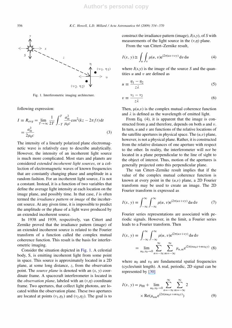
y

x

S

η

υ

z

(υ1, η1)

(υ2, η2)

Fig. 1. Interferometric imaging architecture.

following expression:

I ≡ Ravg = limT→∞

1

2T

∫ T

−T

a2m�0c

cos2(kz − 2� f t)dt

= a2m2�0c

(3)

The intensity of a linearly polarized plane electromag-netic wave is relatively easy to describe analytically.However, the intensity of an incoherent light sourceis much more complicated. Most stars and planets areconsidered extended incoherent light sources, or a col-lection of electromagnetic waves of known frequenciesthat are constantly changing phase and amplitude in arandom fashion. For an incoherent light source, I is nota constant. Instead, it is a function of two variables thatdefine the average light intensity at each location on theimage plane, and possibly time. In that case, I is oftentermed the irradiance pattern or image of the incoher-ent source. At any given time, it is impossible to predictthe amplitude or the phase of a light wave produced byan extended incoherent source.

In 1938 and 1939, respectively, van Cittert andZernike proved that the irradiance pattern (image) ofan extended incoherent source is related to the Fouriertransform of a function called the complex mutualcoherence function. This result is the basis for interfer-ometric imaging.

Consider the situation depicted in Fig. 1. A celestialbody, S, is emitting incoherent light from some pointin space. This source is approximately located in a 2Dplane, at some long distance, z, from the observationpoint. The source plane is denoted with an (x, y) coor-dinate frame. A spacecraft interferometer is located inthe observation plane, labeled with an (�,�) coordinateframe. Two apertures, that collect light photons, are lo-cated within the observation plane. These two aperturesare located at points (�1,�1) and (�2,�2). The goal is to

construct the irradiance pattern (image), I(x,y), of Swithmeasurements of the light source in the (�,�) plane.

From the van Cittert–Zernike result,

I (x, y)�∫u

∫v

�(u, v)ei2�(ux+vy) dv du (4)

where I(x,y) is the image of the source S and the quan-tities u and v are defined as

u ≡ �1 − �2z�

(5)

v ≡ �1 − �2z�

(6)

Then, �(u,v) is the complex mutual coherence functionand � is defined as the wavelength of emitted light.

From Eq. (4), it is apparent that the image is con-structed from � and therefore, depends on both u and v.In turn, u and v are functions of the relative locations ofthe satellite apertures in physical space. The (u,v) plane,however, is not a physical plane. Rather, it is constructedfrom the relative distances of one aperture with respectto the other. In reality, the interferometer will not belocated in a plane perpendicular to the line of sight tothe object of interest. Thus, motion of the apertures isgenerally projected onto this perpendicular plane.

The van Cittert–Zernike result implies that if thevalue of the complex mutual coherence function isknown at every point in the (u,v) plane, a 2D Fouriertransform may be used to create an image. The 2DFourier transform is expressed as

I (x, y) ≡∫ ∞

−∞

∫ ∞

−∞�(u, v)ei2�(ux+vy) du dv (7)

Fourier series representations are associated with pe-riodic signals. However, in the limit, a Fourier seriesleads to a Fourier transform. Then

I (x, y) ≡∫ ∞

−∞

∫ ∞

−∞�(u, v)ei2�(ux+vy) du dv

= limu0,v0→0

∞∑n=−∞

∞∑m=−∞

�n,mei2�(nu0x+mv0 y) (8)

where u0 and v0 are fundamental spatial frequencies(cycles/unit length). A real, periodic, 2D signal can berepresented by [30]

I (x, y) = �00 + limu0,v0→0

∞∑n=−∞

∞∑m=−∞

2

× Re(�nmei2�(nu0x+mv0 y)) (9)

Author's personal copy

K.C. Howell, L.D. Millard / Acta Astronautica 64 (2009) 554–570 557

The complex Fourier coefficient, �nm, can be written inpolar form

�nm = Anmei�nm (10)

where Anm is the amplitude of the Fourier coefficientand �nm is the phase. Then

I (x, y) = �00 + 2∞∑n=1

∞∑m=1

Anm

× cos(2�(nu0x + mv0y) + �nm) (11)

0.1

0.2

0.3

0.4

0.5

0.6

0.7

0.8

0.9

1

Fig. 2. Digitized monochromatic picture is the “true” image of theobserved planet.

-2

-1

0

1

2

3

4

v [1/km]

u [1/km]

v [1

/km

]

Am

plitu

de o

f Fo

urie

r C

ompo

nent

at (

u, v

)

0

0.5

1.0

1.5

-0.5

-1.0

-1.5

x 10-4

x 10-4

x 10-4

0

-1.0

1.00

1.0

-1.0

0

0.5

1.0

1.5

-0.5

-1.0

-1.5

x 10 -4

u [1/km]

x 105

01.0

-1.0

x 105

0 0.5 1.0-0.5-1.0-1.5 1.5

Figs. 3. (left) and 4 (right) Two-dimensional fast Fourier transform of actual image (left). Contour plot of mutual coherence function on the(u,v) plane (right).

The 2D cosine function is the basic building block ofthe image. The 2D cosine function possesses two dif-ferent frequencies, one in the x-direction, i.e., u≡ nu0,and one in the y-direction, v ≡mv0. These are spatialfrequencies represented in (cycles/unit length). Any real2D image may be created by superimposing (in space)an infinite number of 2D cosine functions. Therefore,every value of the mutual coherence function in the (u,v)plane corresponds to one 2D cosine function. Further-more, the complex mutual coherence function at a pointin the (u,v) plane is equivalent to a complex Fourier co-efficient, which defines the amplitude and phase at eachspatial frequency [31].

2.2. Simulating image reconstruction

To simulate interferometric image reconstruction, adigitized monochromatic picture is selected to representthe actual image. In practice, the “actual image” is theirradiance pattern if an infinite number of measurementsin the (u,v) plane are possible. The simulated image isconstructed as a matrix of numbers between zero andone, with each number representing a different shadeof the image color. For example, Fig. 2 is comprised of200×200 pixels. It is represented by a 200×200 matrixwith entries varying between zero and one, dependingon the shade of the individual pixel. Since interferomet-ric imaging is being simulated numerically (thus, theactual image has a finite number of pixels), only a finite

Author's personal copy

558 K.C. Howell, L.D. Millard / Acta Astronautica 64 (2009) 554–570

Fig. 5. The reconstructed image approaches the actual image asmore points in the (u,v) plane are measured.

number of well-placed measurements are required tocompletely and accurately reconstruct the image. In re-ality, an infinite number of measurements are necessaryin order to completely reconstruct the actual image. Itis also assumed that the interferometer can measure themutual coherence function exactly at any given point onthe (u,v) plane.

Next, a 2D Fast Fourier Transform (FFT) of this im-age matrix is computed numerically. The FFT providesthe Fourier amplitude associated with each combi-nation of spatial frequencies in the image. In otherwords, the 2D FFT is the mutual coherence functionof the “actual image”. Plots of these amplitudes as afunction of the spatial frequencies, u and v, appearin Figs. 3 and 4. An interferometer can measure themutual coherence function at different locations inthe (u,v) plane. These locations in the (u,v) plane aredetermined by the distance between the spacecraft inthe interferometric array, the number of spacecraft,the motion of the individual spacecraft, the distanceto the object being observed, and the wavelength oflight being observed. From Eqs. (5) and (6), a relation-ship between the locations of spacecraft in physicalspace and specific points on the (u,v) plane is de-scribed. Of course, it requires two spacecraft, or abaseline, moving in physical space to yield points onthe (u,v) plane. As more and more points on the (u,v)

plane are measured (more and more Fourier amplitudesare obtained) the reconstructed mutual coherence func-tion approaches the actual mutual coherence functionand the image becomes more resolute, as is apparentin Fig. 5.

The amplitudes of the Fourier component, when u andv are small, are very large. These amplitudes correspondto the coarse features of the image. When u and v arelarge, the Fourier component is small, corresponding tofiner features in the image.

3. Dynamical model: CR3BP

The motion of a particle (spacecraft) in the CR3BPis described in terms of rotating coordinates relative tothe barycenter of the system primaries. For this anal-ysis, focus is placed on formations near the librationpoints in the Sun–Earth/Moon system, since these tendto be the most advantageous for interferometric imag-ing. In this frame, the rotating x-axis is directed fromthe Sun towards the Earth–Moon barycenter. The z-axisis normal to the plane of motion of the primaries, andthe y-axis completes the right-handed triad. The gen-eral non-dimensional equations of motion, relative tothe system barycenter, are of the form

x − 2 y − x = − (1 − �G)(x + �G)

r31

− �G(x − (1 − �G))

r32(12)

y + 2x − y = − (1 − �G)y

r31− �G y

r32(13)

z = − (1 − �G)z

r31− �Gz

r32(14)

where

r1 = ((x + �G)2 + y2 + z2)1/2 (15)

r2 = ((x − (1 − �G))2 + y2 + z2)1/2 (16)

The quantity �G is a non-dimensional mass parameterassociated with the system. For the Sun–Earth system,�G ≈ 3.0404×10−6. A more compact notation incorpo-rates a pseudo-potential function, U, such that

U = (1 − �G)

r1+ �G

r2+ 1

2(x2 + y2) (17)

Author's personal copy

K.C. Howell, L.D. Millard / Acta Astronautica 64 (2009) 554–570 559

Then, the scalar equations of motion are rewritten in theform

x − 2 y =Ux (18)

y + 2x =Uy (19)

z =Uz (20)

where the symbol Uj denotes �U/� j . Eqs. (13)–(15)or Eqs. (19)–(21) comprise the dynamical model in theCR3BP.

Given a solution to the nonlinear differential equa-tions, linear variational equations of motion in theCR3BP can be derived as

˙X (t) = A(t)X (t) (21)

where X (t) ≡ [x y z x y z]T represents vari-ations with respect to a reference trajectory. Generally,the reference solutions of interest are not constant. Inthis analysis, the reference trajectory is periodic. In par-ticular, the focus of this work is the family of periodichalo orbits. Thus, A(t) is periodic and time-varying, ofthe form

A(t) =

⎡⎢⎢⎢⎢⎢⎣

0 0 0 1 0 00 0 0 0 1 00 0 0 0 0 1

Uxx Uxy Uxz 0 2 0Uyx Uyy Uyz −2 0 0Uzx Uzy Uzz 0 0 0

⎤⎥⎥⎥⎥⎥⎦ (22)

The partials Ukl are also functions of time, although thefunctional dependence on time, t, has been dropped.

The general form of the solution to the system inEq. (21) is

X (t) = (t, t0)X (t0) (23)

where (t,t0) is the state transition matrix (STM). TheSTM is a linear map from the initial state at the initialtime t0 to a state at some later time t, and, thus, offersan approximation of the impact of the variations in theinitial state on the evolution of the trajectory. The STMmust satisfy the matrix differential equation

(t, t0) = A(t)(t, t0) (24)

given the initial condition

(t0, t0) = I6 (25)

where I6 is the 6×6 identity matrix.It is clear that the STM at time t can be numeri-

cally determined by integrating Eq. (24) from the initialvalue. Since the STM is a 6×6 matrix, propagation of

Eqs. (24) and (25), requires the integration of 36 first-order, scalar, differential equations. Since the elementsof A(t) depend on the reference trajectory, Eq. (24) mustbe integrated simultaneously with the nonlinear equa-tions of motion to generate reference states. This ne-cessitates the integration of an additional six first-orderequations, for a total of 42 differential equations.

4. Continuous Floquet control

4.1. Derivation of the control law

The main result from Floquet is that, for a time-varying, periodic, linear system, the STM can be fac-tored into two matrices, E and J, in the form

(t, 0) = E(t)eJ t E−1(0) (26)

The matrix J is a constant matrix, usually in the Jordannormal form. Its diagonal entries, �i are the Poincaréexponents, the analog of the eigenvalues for constant-coefficient systems. The matrix E(t) is periodic withthe same period, T, as the original system in Eq. (21).Solving a Floquet problem for all time thus requires thedetermination of the constant matrix J and the periodicmatrix E(t) over one period.

Since the matrix E is periodic, E(0)= E(T) and, att= T, Eq. (26) becomes

(T, 0) = E(0)eJT E−1(0) (27)

Thus, E(0) is the matrix of eigenvectors of the mon-odromy matrix, (T,0). The eigenvalues of the mon-odromy matrix, �i, are related to the Poincaré exponents�i, i.e.,

�i = e�i T (28)

After numerically integrating Eq. (24) over one period,the Poincaré exponents and the eigenvector matrix att= 0 can be obtained. Since E(t) is periodic, and there-fore bounded, the stability of the system is governed by�i (or �i) alone.

The reference trajectory, or halo orbit, of interest isinherently unstable. In fact, the six-dimensional eigen-structure of the monodromy matrix is characterized byone unstable eigenvalue (�1), one stable eigenvalue (�2),and four eigenvalues in the center subspace. Two ofthese neutrally stable eigenvalues are located on the unitcircle (�3 and �4) and the remaining two are exactlyequal to one (�5 and �6).

At any point in time, the perturbation X (t) can beexpressed in terms of any six-dimensional basis. The

Author's personal copy

560 K.C. Howell, L.D. Millard / Acta Astronautica 64 (2009) 554–570

Floquet modes (e j ), defined by the columns of E(t),form a non-orthogonal six-dimensional basis. Hence

X (t) =6∑j=1

X j (t) =6∑j=1

c j (t)e j (t) (29)

where X j (t) denotes the component of X (t) along thejth mode, e j (t), and the coefficients cj(t) are determinedas the elements of the vector c(t) defined by

c(t) = E(t)−1X (t) (30)

This Floquet structure is implemented by Gómez et al.[11] and later by Howell and Keeter [32] as the basis of astation keeping strategy for a single spacecraft evolvingalong a halo orbit. Both investigations determine theimpulsive maneuver scheme that is required to removethe component in the direction of the unstable mode(as defined in Eq. (29)), of the perturbation X (t) atdiscrete intervals. For instance, let

Xdesired (t) =6∑j=2

(1 + � j (t))X j (t) (31)

denote the desired perturbation relative to the referenceorbit, where the �(t) is some, yet to be determined, co-efficient vector. Note that the limits of the summationrange from 2 through 6 which implies that the pertur-bation in the direction of the unstable mode e1 has beenremoved. The linearized control problem then reducesto computing the impulsive maneuver, �v(t), such that

6∑j=2

(1 + � j (t))X j (t) =6∑

k=1

Xk(t) +[

03×1�v(t)3×1

](32)

After some reduction, Eq. (32) can be rewritten in ma-trix form as[

X2(t) X3(t) X4(t) X5(t) X6(t)03×3

−I3×3

]×

[�(t)5×1

�v(t)3×1

]= X1(t) (33)

where � represents a 5×1 vector formed by the �j com-ponents in Eq. (32). Therefore, the maneuver, �v3×1,that is required to remove the unstable mode e1 fromthe perturbation at any given time can be approximatedfrom Eq. (33). Howell and Keeter identify this required�v3×1 via a minimum norm solution. If the maneuver isconstrained to the Sun–Earth line (x-direction), �v1×1is actually a scalar, and the system possesses an exactsolution.

If exactly three modes are removed and control ispossible in three directions, the system also possesses

an exact solution. For example, Marchand and Howelldemonstrate the impulsive �v(t)3×1 that is required toremove the portion of the perturbation along modes e1,e3, and e4. It can be determined exactly from[

�(t)3×1�v(t)3×1

]=

[X2(t) X5(t) X6(t)

03×3−I3×3

]−1

× (X1(t) + X3(t) + X4(t)) (34)

Similarly, the �v3×1 vector that is required to removemodes e1, e5, and e6 is exactly determined from[

�(t)3×1�v(t)3×1

]=

[X2(t) X3(t) X4(t)

03×3−I3×3

]−1

× (X1(t) + X5(t) + X6(t)) (35)

As formulated in Eqs. (34) and (35), �v(t)3×1 is theimpulsive control necessary to remove perturbations inthe direction of one unstable mode and two semi-stablemodes in the linearized system represented in Eq. (21)at a given time. This methodology can be applied in alinear time-varying feedback loop,

˙X (t) = A(t)X (t) + Bu(t)

= A(t)X (t) +[

03×1�v(t)3×1

](36)

Y (t) = CX (t) (37)

where B = [03×3 I3×3]T, indicating that the control in-put can instantaneously change only the velocity of thesatellite (not position) and C= I6, implying full statefeedback.

4.2. Stability of the controlled linear system

In the linearized system of the variational equations,the Floquet result can be applied to transform the time-varying periodic linear system in Eq. (21) to a time-invariant linear system [33–35]. The transformationproceeds as follows:

Initial system: ˙X (t) = A(t)X (t)

Coordinate transformation: X (t) = E(t)Z (t) (38)

Resulting system: Z (t) = J Z (t) (39)

It is important to note that E(t) is the periodic Floquetmodal matrix and J is the constant Floquet matrix con-taining the Poincaré exponents. Thus both J and E(t)are bounded and invertible. Addition of a state feedback

Author's personal copy

K.C. Howell, L.D. Millard / Acta Astronautica 64 (2009) 554–570 561

loop to the initial system as in Eq. (36), then completingthe transformation using Eq. (38), yields the following:

Feedback system:

˙X (t) = A(t)X (t) + Bu(t)

= [A(t) + Bk(t)]X (t) (40)

Y (t) = CX (t)

Coordinate transformation: X (t) = E(t)Z (t)

Resulting system:

˙Z (t) = [J + E(t)−1Bk(t)E(t)]Z (t) (41)

W (t) = CE(t)Z (t) (42)

where k(t) is some yet to be determined control ef-fort. Let Q be the Jordan canonical form of J, where

Q= SJS−1. Then application of another transformation,yields

Feedback system:

˙Z (t) = [J + E(t)−1Bk(t)E(t)]Z (t)

W (t) = CE(t)Z (t)

Coordinate transformation : Z (t) = S−1�(t) (43)

Resulting system:

˙�(t) = [Q + SE(t)−1Bk(t)E(t)S−1]�(t) (44)

(t) = CE(t)S−1�(t) (45)

The diagonal entries of Q are now the Poincaré expo-nents corresponding to the system monodromy matrix.The system can be simplified by renaming some vari-ables:

˙�(t) = [Q + g(t)w(t)]�(t) (46)

(t) = h(t)�(t) (47)

where g(t)=SE(t)−1B, w(t)=k(t)E(t)S−1, and h(t)=CE(t)S−1. Because of the form of the Q matrix, thesystem is partitioned into modes that will be controlled(unstable and semi-stable modes) and modes that will beignored (stable and semi-stable modes). This is accom-plished via simple row operations that do not changethe system. A partitioned system results

w(t) = [wc(t) wi (t)] (48)

g(t) =[gc(t)gi (t)

](49)

Q =[Qc 0

0 Qi

](50)

h(t) =[hc(t) 0

0 hi (t)

](51)

where the subscript “c” is associated with modes thatwill be controlled and the subscript “i” corresponds tomodes that will be ignored. The size of the zero com-ponents in the Q matrix is dependent on the number ofmodes to be controlled or ignored. If n modes are con-trolled and m modes are ignored, where n+m= 6, theentire system reduces to

[ ˙�c(n×1)(t)˙�i(m×1)(t)

]=

[Qc(n×n) + gc(n×3)(t)wc(3×n)(t) gc(n×3)(t)wi(3×m)(t)

gi(m×3)(t)wc(3×n)(t) Qi(m×m) + gi(m×3)(t)wi(3×m)(t)

]×

[�c(n×1)(t)�i(m×1)(t)

](52)

(t) =[hc(n×n) 0n×m

0m×n hi(m×m)

] [�c(n×1)(t)�i(m×1)(t)

](53)

Let wi(3×m)(t)= 03×m because it only affects ignorablemodes, then Eq. (52) reduces to the following[ ˙�c(n×1)(t)

˙�i(m×1)(t)

]

=[Qc(n×n) + gc(n×3)(t)wc(3×n)(t) 0n×m

gi(m×3)(t)wc(3×n)(t) Qi(m×m)

]

×[

�c(n×1)(t)�i(m×1)(t)

](54)

The state matrix is now upper diagonal. Define Q′c as

a matrix with desirable system eigenvalues and set itequal to the upper n×n block of the current state matrix,

Q′c(n×n) = Qc(n×n) + gc(n×3)(t)wc(3×n)(t) (55)

The control is evaluated as

wc(3×n)(t) = [gc(n×3)(t)]−1(Q′

c(n×n) − Qc(n×n)) (56)

Eq. (56) will yield an exact solution if exactly threemodes are controlled. If more or less than three modesare controlled, Eq. (56) can generate a minimum normsolution or no solution. This follows from the fact thatgc(n×3)(t) is only square (and invertible) when the di-mensions of Bc are 3×3.

This example, with a focus on three modes, is no-table as demonstrated by Eqs. (34) and (35). Assumingexactly three modes are removed, the control gain k(t)

Author's personal copy

562 K.C. Howell, L.D. Millard / Acta Astronautica 64 (2009) 554–570

for use with (21) can be identified, i.e.,

w(t) = k(t)E(t)S−1 (57)

[g−1c(3×3)(t)(Q

′c(3×3) − Qc(3×3)) 03×3]SE(t)

−1

= k(t) (58)

It is apparent from Eq. (54), that the function,gi(m×3)(t)wc(3×n)(t), is periodic. From the definition ofw(t),

g(t)w(t) = g(t)k(t)E(t)S−1 (59)

By substituting k(t) from Eq. (58)

g(t)w(t) = g(t)[g−1c(3×3)(Q

′c(3×3) − Qc(3×3)) 03×3] (60)

and substituting the partitioned matrices g(t) and w(t)from Eqs. (48) and (49), respectively,[gc(3×3)(t)wc(3×3)(t) gc(3×3)(t)wi(3×3)(t)gi(3×3)(t)wc(3×3)(t) gi(3×3)(t)wi(3×3)(t)

]

=[gc(3×3)(t)gi(3×3)(t)

]× [g−1

c(3×3)(Q′c(3×3) − Qc(3×3)) 03×3] (61)

Therefore

gi(3×3)(t)wc(3×3)(t)

= gi(3×3)(t)g−1c(3×3)(t)(Q

′c(3×3) − Qc(3×3)) (62)

Because g(t) is periodic, (g(t)= SE(t)−1B and E(T)are periodic by definition), gi(3×3)(t)wc(3×3)(t) is alsoperiodic. Thus, the stability of the system matrix inEq. (54) is determined by the eigenvalues of Q′

c and Qi.Since our linearized system includes four eigenval-

ues along the imaginary axis, one stable, as well as oneunstable mode, the gain k(t) will not yield a system thatis asymptotically stable. In other words, for Eq. (56) toresult in an exact solution, exactly three modes must bemodified. The system in Eq. (21) possesses five modesthat are not asymptotically stable; therefore, the motionof the controlled system will be bounded relative to anominal halo orbit, but not asymptotically approach it.If more than three modes are removed, the solution toEq. (56) can be found via a minimum norm approxi-mation. However, the stability of such a solution is notapproached analytically here. In the case of interfero-metric imaging arrays, bounded motion creates morefavorable (u,v) plane coverage.

This continuous algorithm allows the eigenvalues ofmatrixQc to be shifted to desired locations. If the eigen-values of Q′

c are selected to equal the eigenvalues ofQi, the impulsive maneuvers in Eqs. (34) and (35), canbe reproduced continuously and the resulting motion is

bounded in the linear system. Other bounded solutionsare also available when the eigenvalues of Q′

c are se-lected to be stable but not equal to those of Qi.

4.3. Stability of controlled nonlinear system

Because the control (�v3×3) is determined usinglinearized variational equations (representing perturba-tions), the stability of the feedback controller applied inthe nonlinear system is difficult to assess analytically.The algorithm is implemented (in state space form) asfollows:

x1 = x2 + �vx (63)

x2 = 2(x4 + �vy) + x1

− · · · − (1 − �G)(x1 + �G)

R31

− �G(x1 − (1 − �G))

R32

(64)

x3 = x4 + �vy (65)

x4 = − 2(x2 + �vx ) + x3

− · · · − (1 − �G)x3R31

− �Gx3R32

(66)

x5 = x6 + �vz (67)

x6 = − (1 − �G)x5R31

− �Gx5R32

(68)

where �v3×1=[�vx

�vy�vz

]is determined from the gain k(t),

x1 = x, x2 = x, x3 = y, x4 = y, x5 = z, x6 = z and

R1 = ((x1 + �G)2 + x23 + x25 )

1/2 (69)

R2 = ((x1 − (1 − �G))2 + x23 + x25 )

1/2 (70)

When the control as derived in the linear system issimulated in the nonlinear system, the spacecraft tra-jectories remain bounded relative to a nominal haloorbit over extended periods of time. The distance ofa satellite relative to a Sun–Earth/Moon L2 orbit overapproximately forty years (or 80 halo orbit periods) ap-pears in Fig. 6(a). The motion is periodic and bounded.The satellite is initially placed 1.25km away from thelibration point orbit, shown in the upper left corner ofFig. 6(b). The initial velocity of the satellite is equalto the velocity of the corresponding point on thehalo orbit, labeled “L2” in the same figure. Fig. 6(b)also illustrates the motion of the satellite over thecourse of approximately 40 years. This motion is in an

Author's personal copy

K.C. Howell, L.D. Millard / Acta Astronautica 64 (2009) 554–570 563

-1.5 -1 -0.5 0 0.5 1 1.5-0.4

-0.3

-0.2

-0.1

0

0.1

0.2

0.3

0.4

Inertial Y [km]

Iner

tial Z

[km

]

-1.5 -1 -0.5 0 0.5 1 1.5

-1.5

-1

-0.5

0

0.5

1

1.5

Inertial X [km]

Iner

tial Y

[km

]

-1.5 -1 -0.5 0 0.5 1 1.5-0.4

-0.3

-0.2

-0.1

0

0.1

0.2

0.3

0.4

Inertial X [km]

Iner

tial Z

[km

]

-1.5 -1 -0.5 0 0.5 1 1.5-0.4

-0.3

-0.2

-0.1

0

0.1

0.2

0.3

0.4

Inertial Y [km]

Iner

tial Z

[km

]

L2 OrbitSatellite

Time [years]

0 5 10 15 20 25 30 35 400

0.5

1

1.5

Dis

tanc

e fr

om L

2 O

rbit

[km

]

0 5 10 15 20 25 30 35 40-1.5

-1

-0.5

0

0.5

1

1.5D

ista

nce

from

L2

Orb

it (C

ompo

nent

s) [

km]

Inertial X Direction

Inertial Y Direction

Inertial Z Direction

Fig. 6. (a) Distance of satellite from L2 (Sun–Earth/Moon) orbit with Floquet control. (b) Bounded, quasi-periodic motion of satellite relativeto L2 (Sun–Earth/Moon) orbit with Floquet control.

Author's personal copy

564 K.C. Howell, L.D. Millard / Acta Astronautica 64 (2009) 554–570

-0.5 0 0.5 1 1.5-3

-2

-1

0

1

2

3

Inertial X [km]

Iner

tial Z

[km

]

-0.4 -0.2 0 0.2 0.4 0.6

-3

-2

-1

0

1

2

3

Inertial Y [km]

Iner

tial Z

[km

]

L2 Orbit

SAT1

SAT2

SAT3

SAT4

SAT5

-0.5 0 0.5 1 1.5

-0.4

-0.2

0

0.2

0.4

0.6

Inertial X [km]

Iner

tial Y

[km

]

-0.5 0 0.5 1 1.5-3

-2

-1

0

1

2

3

Inertial X [km]

Iner

tial Z

[km

]

-0.5

0

0.5

11.5

-0.4

-0.2

0

0.2

0.4

0.6-3

-2

-1

0

1

2

3

Inertial X [km]

Inertial Y [km]

Iner

tial Z

[km

]

Fig. 7. (a) Short baseline formation motion relative to Sun–Earth L2 orbit (approximately one period or 180 days). (b) Short baseline formationthree-dimensional motion relative to Sun–Earth L2 orbit (approximately one period or 180 days).

inertial frame, relative to the L2 halo orbit and appearsin three inertial projections: y–z, x–y, and x–z. The satel-lite is controlled via the continuous Floquet controller,

with Q′c selected such that eig(Q′

c) = eig(Qi ) and theeigenvalues of Qi are the stable mode and the two shortperiod center modes of Q.

Author's personal copy

K.C. Howell, L.D. Millard / Acta Astronautica 64 (2009) 554–570 565

99 Measurements (180.5355 days)

-5 0 5

-2

-1

0

1

2

3x 10-4

x 10-5 x 10-5 x 10-5 x 10-5

x 10-4 x 10-4 x 10-4

U [1/km]

V [

1/km

]

-5 0 5

-2

-1

0

1

2

3

U [1/km]

V [

1/km

]

-5 0 5

-2

-1

0

1

2

3

U [1/km]

V [

1/km

]

-5 0 5

-2

-1

0

1

2

3

U [1/km]

V [

1/km

]

-0.4 -0.2 0 0.2 0.4 0.6

-3

-2

-1

0

1

2

3

Y [km]

Z [

km]

-0.4 -0.2 0 0.2 0.4 0.6

-3

-2

-1

0

1

2

3

Y [km]

Z [

km]

-0.4 -0.2 0 0.2 0.4 0.6-3

-2

-1

0

1

2

3

Y [km]

Z [

km]

-0.4 -0.2 0 0.2 0.4 0.6-3

-2

-1

0

1

2

3

Y [km]

Z [

km]

10 Measurements (18.2359 days)5 Measurements (9.118 days)1 Measurement (1.8236 days)

Fig. 8. Image reconstruction via short baseline formation.

5. Formation simulation and image reconstruction

A number of assumptions are incorporated into theimage reconstruction methodology. First, the image ismodeled as fixed, i.e., it remains unchanged throughoutthe measurement period of 180 days. The interferometeris considered perfect; no noise is present in the measure-ment of the mutual coherence function and no starlightnulling is necessary. The satellite formation processesone measurement every 1.8 days. The object of inter-est is assumed to be stationary and located in the iner-tial X-direction from the formation. The “true image”is considered to be the picture of Jupiter in Fig. 2.

5.1. Example 1: short baseline, five satellite formation

By appropriate choice of Q′c, natural, nearly peri-

odic motions in the phase space can be exploited thatare particularly advantageous to interferometric arrays.These solutions offer adequate, repeated coverage of the(u,v) plane in a desired direction as well as controlledmotion in physical space. The motion of a short base-line (5km) formation moving near the Sun–Earth/MoonL2 point appears in Figs. 7(a) and (b). The formation

is used to construct an image of a Jupiter-like planet(Fig. 2) located 4.2 light years from Earth (a planetnear our closest star, Alpha Centauri) at a wavelength of500nm. The corresponding coverage of the (u,v) planeand simulated image reconstruction appear in Fig. 8.

This type of formation could be compared with theplanned interferometric imaging mission, TerrestrialPlanet Finder (TPF) [1]. The TPF mission attemptsto identify Earth-like planets in other solar systems.The nominal mission design includes five satellitesflying in precise formation; a physical combinationof interferometric beams is required to locate exoso-lar planets. Several levels of control are necessary tocoordinate the position of active optics to nanometeraccuracy. Although the motion of this example array isadvantageous to optical imaging, much tighter controland coordination, perhaps in conjunction with a strat-egy similar to the described control method, would berequired for the TPF mission.

The five satellites in the short baseline formation areinitially placed in the configuration that appears in theupper left corner of Fig. 7(a) (in the inertial frame).The initial velocities of the satellites are all equal to thevelocity of the corresponding point on the halo orbit,

Author's personal copy

566 K.C. Howell, L.D. Millard / Acta Astronautica 64 (2009) 554–570

0 50 100 150 200 250 300 350 400

3.087

3.088

3.089

3.09

3.091

3.092

3.093

3.094

3.095

3.096

3.097

x 10-8

Time [days]

Con

trol

[m

m/s

2 ]

SAT2SAT4

0 50 100 150 200 250 300 350 400

6.177

6.178

6.179

6.180

6.181

6.182

6.183

6.184

6.185

6.186

6.187

Time [days]

Con

trol

[m

m/s

2 ]

SAT1SAT5

x 10-8

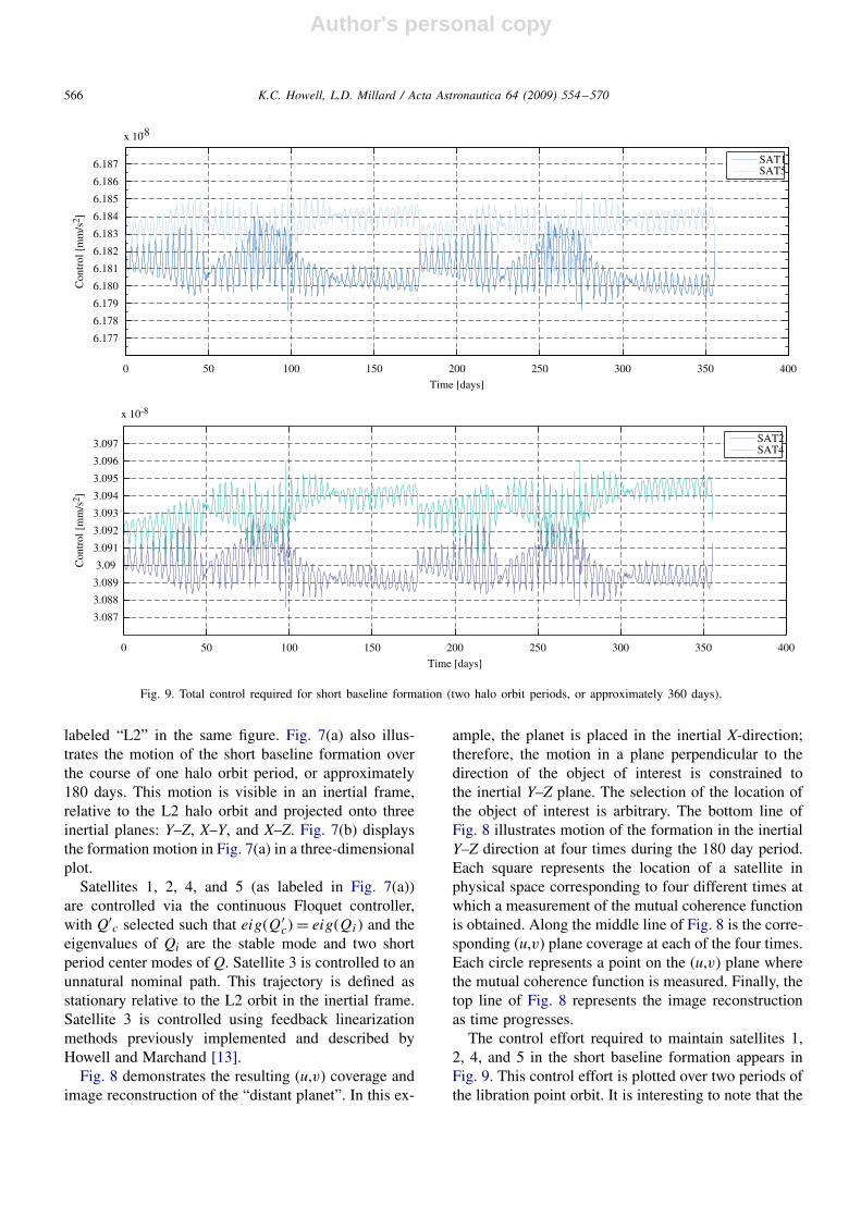
Fig. 9. Total control required for short baseline formation (two halo orbit periods, or approximately 360 days).

labeled “L2” in the same figure. Fig. 7(a) also illus-trates the motion of the short baseline formation overthe course of one halo orbit period, or approximately180 days. This motion is visible in an inertial frame,relative to the L2 halo orbit and projected onto threeinertial planes: Y–Z, X–Y, and X–Z. Fig. 7(b) displaysthe formation motion in Fig. 7(a) in a three-dimensionalplot.

Satellites 1, 2, 4, and 5 (as labeled in Fig. 7(a))are controlled via the continuous Floquet controller,with Q′

c selected such that eig(Q′c) = eig(Qi ) and the

eigenvalues of Qi are the stable mode and two shortperiod center modes of Q. Satellite 3 is controlled to anunnatural nominal path. This trajectory is defined asstationary relative to the L2 orbit in the inertial frame.Satellite 3 is controlled using feedback linearizationmethods previously implemented and described byHowell and Marchand [13].

Fig. 8 demonstrates the resulting (u,v) coverage andimage reconstruction of the “distant planet”. In this ex-

ample, the planet is placed in the inertial X-direction;therefore, the motion in a plane perpendicular to thedirection of the object of interest is constrained tothe inertial Y–Z plane. The selection of the location ofthe object of interest is arbitrary. The bottom line ofFig. 8 illustrates motion of the formation in the inertialY–Z direction at four times during the 180 day period.Each square represents the location of a satellite inphysical space corresponding to four different times atwhich a measurement of the mutual coherence functionis obtained. Along the middle line of Fig. 8 is the corre-sponding (u,v) plane coverage at each of the four times.Each circle represents a point on the (u,v) plane wherethe mutual coherence function is measured. Finally, thetop line of Fig. 8 represents the image reconstructionas time progresses.

The control effort required to maintain satellites 1,2, 4, and 5 in the short baseline formation appears inFig. 9. This control effort is plotted over two periods ofthe libration point orbit. It is interesting to note that the

Author's personal copy

K.C. Howell, L.D. Millard / Acta Astronautica 64 (2009) 554–570 567

Fig. 10. (a) Long baseline formation motion relative to Sun–Earth L2 orbit (approximately one period or 180 days). (b) Long baseline formationthree-dimensional motion relative to Sun–Earth L2 orbit (approximately one period or 180 days).

Author's personal copy

568 K.C. Howell, L.D. Millard / Acta Astronautica 64 (2009) 554–570

Fig. 11. Image reconstruction via long baseline formation.

required control is nearly periodic. Also, the amount ofcontrol required tomaintain satellites 1 and 5 in the shortbaseline formation is approximately twice that requiredfor satellites 2 and 4.

5.2. Example 2: long baseline, 16 satellite formation

With a critical set of values for the elements of thema-trix Q′

c, natural solutions in the phase space relative tothe halo orbit emerge that maintain a 16 satellite forma-tion bounded within a maximum baseline requirementover long periods of time. These solutions create quasi-randomly distributed satellites in many look-directions,as evident in Figs. 10(a) and (b). But, throughout thesimulation, the satellites do not collide. Since the natu-ral formation motion is quasi-periodic (as in Fig. 6) thesatellites are not likely to collide for extended periodsof time. The formation is imaging an object located at1AU from the Earth at 7MHz (AM radio wavelengths).

This type of formation can be compared with theplanned solar imaging radio array (SIRA) mission. Oneof the goals of the SIRA mission is to perform low-frequency radio imaging of the Sun to determine thedynamics and interaction of coronal mass ejections [3].The nominal mission design includes 16 satellites, ini-tially arranged on a sphere, with a maximum baseline

of between 5 and 25km. The SIRA mission must main-tain adequate coverage of the (u, v) plane in all look-directions at all times for radio waves with frequenciesbetween 30kHz and 15MHz. If a quasi-random distri-bution of satellites is maintained in SIRA, coverage ofthe (u,v) plane is adequate for many mission sciencegoals [36]. The SIRA mission may not require substan-tial control beyond that described here.

The 16 satellites in the long baseline formation areinitially placed on a spiral around a sphere as seen inthe upper left corner of Fig. 10(a) (in the inertial frame).This initial configuration is being considered for theSIRA mission [37]. As in the previous example, the ini-tial velocities of the satellites are all equal to the veloc-ity of the corresponding point on the halo orbit, labeled“L2” in the same figure. Fig. 10(a) also illustrates themotion of the long baseline formation over the courseof one halo orbit period, or approximately 180 days.This motion remains bounded within the sphere andmaintains a quasi-random distribution of satellites overthe time. Fig. 10(b) displays the formation motion inFig. 10(a) on a three-dimensional plot.

The (u, v) coverage and image reconstruction of anobject located at 1AU from the Earth is demonstratedin Fig. 11. In this example, the “planet” is again placedin the inertial X-direction. As in Fig. 9, the bottom line

Author's personal copy

K.C. Howell, L.D. Millard / Acta Astronautica 64 (2009) 554–570 569

of Fig. 11 illustrates motion of the formation in the in-ertial Y–Z direction at four times during the 180 dayperiod. Each square represents the location of a satellitein physical space at the instant that corresponds to mea-surement of the mutual coherence function. The middleline in Fig. 11 is the corresponding (u,v) plane coverageand the top line of Fig. 11 reflects image reconstructionas time progresses.

6. Summary and concluding remarks

In the present study, a continuous control algorithmis developed that facilitates bounded motion of satelliteformations over long periods of time near halo orbitsin the circular restricted three-body problem (CR3BP).The feedback controller is designed based on the lin-ear variational equations. Through simulation, the lin-ear controller is demonstrated to be effective using thefull nonlinear CR3BP equations of motion. By chang-ing certain parameters within the control algorithm, tra-jectories that are particularly advantageous to satelliteimaging formations emerge. Image reconstruction andcoverage of the (u,v) plane are simulated for interfero-metric satellite configurations, demonstrating potentialapplications of the control algorithm and resulting mo-tion.

Motion advantageous to imaging arrays can be pro-duced via more traditional control methods, where a de-sired unnatural trajectory is strictly followed. However,such approaches sometimes ignore multi-body dynam-ics or simply remove them using control methods suchas feedback linearization. By including multi-body dy-namics in the development of the control algorithm, nat-ural motions in the multi-body regime are exploited andpotentially reduce required control effort. Some forma-tions that do not require tight control, such as the con-figuration proposed in SIRA, potentially benefit.

Acknowledgments

The authors would like to thank Zubin Olikara forhigh fidelity modeling of satellite motion within the for-mations. This work was performed at Purdue Universitywith support from NASA Goddard Space Flight Centerunder contract numbers NCC5-727 and NNG04GP69G.

References

[1] TPF Science Working Group, Terrestrial planet finder: a NASAorigins program to search for habitable planets, 1999.

[2] K.C. Gendreau, W.C. Cash, A.F. Shipley, N. White,The MAXIM pathfinder X-ray interferometry mission, in:

Proceedings of the International Society for Optical Engineering(SPIE) Conference, August 26–28, Waikoloa, Hawaii, 2002.

[3] R. MacDowall, M. Kaiser, N. Gopalswamy, Solar imaging radioarray (SIRA): radio aperture synthesis from space, in: 34thAAS Solar Physics Division Meeting, vol. 23, 2003, pp. 20–22.

[4] D.P. Scharf, F.Y. Hadaegh, S.R. Ploen, A survey of spacecraftformation flying guidance and control (part I): guidance, in:American Control Conference, June 4–6, Denver, Colorado,2003.

[5] D.P. Scharf, F.Y. Hadaegh, S.R. Ploen, A survey of spacecraftformation flying guidance and control (part II): control,in: American Control Conference, June 30–July 2, Boston,Massachusetts, 2004.

[6] P. Gurfil, N.J. Kasdin, Dynamics and control of spacecraftformation flying in three-body trajectories, in: AIAA Guidance,Navigation, and Control Conference and Exhibit, AIAA Paper2001-4026, August 6–9, Montreal, Canada, 2001.

[7] P. Gurfil, M. Idan, N.J. Kasdin, Adaptive neural control ofdeep-space formation flying, in: American Control Conference(ACC) Proceedings, vol. 4, May 8–10, Anchorage, Alaska,2002, pp. 2842–2847.

[8] R.J. Luquette, R.M. Sanner, A non-linear approach to spacecraftformation control in the vicinity of a collinear libration point,in: AAS/AIAA Astrodynamics Conference, Proceedings, July30–August 2, Quebec, 2001, pp. 437–445.

[9] N.H. Hamilton, Formation flying satellite control around theL2 Sun–Earth libration point, M.S. Thesis, George WashingtonUniversity, Washington, DC, December 2002.

[10] D. Folta, J.R. Carpenter, C. Wagner, Formation flying withdecentralized control in libration point orbits, in: InternationalSymposium: Spaceflight Dynamics, Biarritz, France, June 2000.

[11] G. Gómez, K.C. Howell, J. Masdemont, C. Simó, Station-keeping strategies for translunar libration point orbits, Advancesin Astronautical Sciences 99 (pt. 2) (1998) 949–967.

[12] G. Gómez, M. Lo, J. Masdemont, K. Museth, Simulation offormation flight near Lagrange points for the TPF mission, in:AAS/AIAA Astrodynamics Conference, AAS Paper 01-305,July 30–August 2, Quebec, Canada, 2001.

[13] K.C. Howell, B.G. Marchand, Control strategies for formationflight in the vicinity of the libration points, in: AIAA/AASSpace Flight Mechanics Conference, AAS Paper 03-113,February 9–13, Ponce, Puerto Rico, 2003.

[14] B.G. Marchand, K.C. Howell, Aspherical formations near thelibration points in the sun–earth/moon ephemeris system, in:2004 AAS/AIAA Spaceflight Mechanics Conference, AASPaper 04-157, February 8–11, Maui, Hawaii, 2004.

[15] B.T. Barden, K.C. Howell, Fundamental motions near collinearlibration points and their transitions, The Journal of theAstronautical Sciences 46 (4) (1998) 361–378.

[16] B.T. Barden, K.C. Howell, Formation flying in the vicinity oflibration point orbits, Advances in Astronautical Sciences 99(pt. 2) (1998) 969–988.

[17] K.C. Howell, B.T. Barden, Trajectory design and stationkeepingfor multiple spacecraft in formation near the sun–earth L1 point,in: IAF 50th International Astronautical Congress, IAF/AIAAPaper 99-A707, October 4–8, Amsterdam, Netherlands, 1999.

[18] B.T. Barden, K.C. Howell, Dynamical issues associatedwith relative configurations of multiple spacecraft near thesun–earth/moon L1 point, in: AAS/AIAA AstrodynamicsSpecialist Conference, AAS Paper 99-450, August 16–19,Girdwood, Alaska, 1999.

[19] B.G. Marchand, K.C. Howell, Formation flight near L1 andL2 in the sun–earth/moon ephemeris system including solar

Author's personal copy

570 K.C. Howell, L.D. Millard / Acta Astronautica 64 (2009) 554–570

radiation pressure, in: AAS/AIAA Astrodynamics SpecialistConference, Big Sky, Montana, August 3–8, 2003. AAS Paper03-596.

[20] S. Chakravorty, Design and optimal control of multi-spacecraftinterferometric imaging systems, Ph.D. Thesis, University ofMichigan, 2004.

[21] M. Born, E. Wolf, Principles of Optics, Pergamon Press, NewYork, 1964.

[22] D.C. Hyland, Interferometric imaging concepts with reducedformation-keeping constraints, in: AIAA Space 2001Conference, Albuquerque, New Mexico, August 2001.

[23] D.C. Hyland, The inverse Huygens–Fesnel principle andit’s implications for interferometric imaging, The Journal ofAstronautical Sciences, 2003.

[24] I.I. Hussein, D.J. Scheeres, D.C. Hyland, Formation pathplanning for optimal fuel and image quality for a class ofinterferometric imaging missions, AAS Paper 03-172, February2003.

[25] I.I. Hussein, D.J. Scheeres, D.C. Hyland, Control of a satelliteformation for imaging applications, in: Proceedings of theAmerican Control Conference, 2003, pp. 308–313.

[26] I.I. Hussein, D.J. Scheeres, D.C. Hyland, Optimal formationcontrol for imaging and fuel usage, in: 15th AAS/AIAA SpaceFlight Mechanics Conference, AAS Paper 05-160, January23–27, Copper Mountain, Colorado, 2005.

[27] I.I. Hussein, D.J. Scheeres, D.C. Hyland, Optimal formationcontrol for imaging and fuel usage with terminal imagingconstraints, in: IEEE Conference on Control Applications, 2005.

[28] I.I. Hussein, A.M. Bloch, Dynamic coverage optimal control forinterferometric imaging spacecraft formations, in: 43rd IEEEConference on Decision and Control, Paradise Island, Bahamas,December 2004, pp. 1812–1817.

[29] I.I. Hussein, A.M. Bloch, Dynamic coverage optimal controlfor interferometric imaging spacecraft formations (part II):the nonlinear case, in: Proceedings of the American ControlConference, 2005, pp. 2391–2396.

[30] G.B. Folland, Fourier Analysis and it’s Applications,Brooks/Cole Publishing Company, Pacific Grove, California,1992.

[31] S.S. Joshi, An informal introduction to synthetic apertureimaging, JPL Interoffice Memorandum 3450-98-0004, January12, 1998, pp. 1–16.

[32] K.C. Howell, T.M. Keeter, Station-keeping strategies forlibration point orbits: target point and Floquet mode approaches,in: AAS/AIAA Spaceflight Mechanics Meeting, February13–16, Albuquerque, New Mexico, 1995.

[33] W. Wiesel, W. Shelton, Modal control of an unstable periodicorbit, The Journal of the Astronautical Sciences 31 (1983)63–76.

[34] H. Poincaré, Les Methodes Nouvelles de la MechaniqueCeleste, Dover, New York, 1957.

[35] V. Szebehely, Theory of Orbits, Academic Press, New York,1967.

[36] R. MacDowall, SIRA: uniform distributions in the (u,v) apertureplane, presentation, NASA Goddard Space Flight Center,October 3, 2005.

[37] D. Folta, B. Naasz, F. Vaughn, Solar imaging radio array (SIRA)trajectory and formation analysis, Presentation, DynamicsAnalysis Branch, NASA Goddard Space Flight Center, January30, 2003.

[38] L.D. Millard, K.C. Howell, Control of interferometric spacecraftarrays for (u, v) plan coverage in multi-body regimes, Journalof Astronautical Sciences 56 (1) (January–March 2008).