Tax Regimes and Corrupt OfficialsILIAS BOULTZIS

Abstract

In this paper a simple model of public good provision is considered. The economy

consists of 2 individuals (principals) that have fixed endowment in private good and a

government (agent) that has the monopoly of political coercion. In such a model, if the

government is benevolent the choice of tax system (ie proportional, lump sum etc) is

irrelevant to the provision of public good. On the other hand, in case the government is

also a rent seeker, the choice of tax system becomes important. A uniform tax system that

restricts government’s ability to redistribute income is superior from the point of view of

individuals.

1. Introduction

The issue of optimal taxation in the presence of bribes was first studied by Dixit,

Grossman and Helpman (1997) who show that adopting an inefficient tax system restricts

government’s ability to collect bribes. This paper builds on the ideas of Dixit, Grossman

and Helpman and provides support for the introduction of a flat tax rate. The discussion

about optimal tax systems has become of general interest lately because of the choice of

many countries (mainly in Eastern Europe) to curtail their ability to redistribute income

through taxation by adopting a flat tax rate

I assume a simple economy with one public and one private non produced good. The

private sector of this economy consists of two individuals with different endowments.

Public good provision is chosen by a non-benevolent government that has the monopoly

of political coercion.

In essence we have a common agency problem. All individuals that make up the

private sector (principals) have different ideal government policies (public good

1

financing) because of their difference in endowments. In order to persuade the

government (agent) to decide favorably for them, they design a bribing schedule that

assigns a level of bribes at each government decision (i.e. they offer the agent a “menu”).

This paper shows that when the government is non-benevolent the tax system1

becomes important for the well being of the private sector since it crucially affects both

the amount of bribes paid as well as the quantity of public good provided. As it will be

shown in chapter 3, a proportional tax leads to an efficient equilibrium with zero bribes,

while a system of individual lump-sum taxes and subsidies leads to a transfer of the

whole private sector endowment to the government in the form of bribes.2The case of a

single lump-sum tax lies in between the other two as it leads to a partial transfer of

private resources to the government and a positive but inefficiently small public good

provision.

The rest of the paper is organized as follows. In chapter 2 three benchmark cases are

considered: a) an uncoordinated (Nash) equilibrium, b) a solution with a benevolent

government that follows a Benthamite social utility function and c) coordination of the

public good provision by a selfish governing individual. In the two coordinated cases (b

and c) 3 tax systems are examined (proportional tax, single lump-sum tax and individual

lump-sum taxes or subsidies)3 and the results are compared. In chapter 3, I turn to the

case of a non-benevolent government. The situation in this chapter is modeled and solved

following the general approach in Dixit, Grossman and Helpman (1997). The 3 tax

systems mentioned above are reexamined under the assumption that the government

maximizes the total revenue from bribes and the results are compared to those of chapter

2.In chapter 4 I give a brief account of the relevant literature. Finally in chapter 5, I

present some insights and policy implications that are related to the analysis in this paper.

1 The terms tax regime and tax system are used with the same meaning.2 This is a version of the result Dixit, Grossman and Helpman (1997) got when studying optimal taxes and transfers a la Diamond and Mirrles (1971)3 These three tax regimes cover more or less all the range of possible tax regimes for this simple model. Furthermore more complex and realistic tax-regimes can be thought to be combinations of these three simple ones. In this sense the analysis in this paper can give an insight for the analysis of more general situations.

2

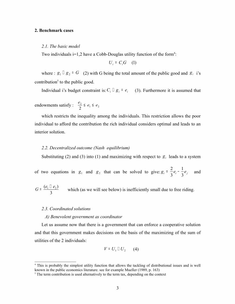
2. Benchmark cases

2.1. The basic model

Two individuals i=1,2 have a Cobb-Douglas utility function of the form4:

)1(GCU ii =

where : Ggg =+ 21 (2) with G being the total amount of the public good and ig i’s

contribution5 to the public good.

Individual i’s budget constraint is: iii egC =+ (3). Furthermore it is assumed that

endowments satisfy : 212

2eee

≤≤

which restricts the inequality among the individuals. This restriction allows the poor

individual to afford the contribution the rich individual considers optimal and leads to an

interior solution.

2.2. Decentralized outcome (Nash equilibrium)

Substituting (2) and (3) into (1) and maximizing with respect to ig leads to a system

of two equations in 1g and 2g that can be solved to give: jii eeg31

32 −= and

3)( 21 eeG += which (as we will see below) is inefficiently small due to free riding.

2.3. Coordinated solutions

A) Benevolent government as coordinator

Let us assume now that there is a government that can enforce a cooperative solution

and that this government makes decisions on the basis of the maximizing of the sum of

utilities of the 2 individuals:

21 UUV += (4)

4 This is probably the simplest utility function that allows the tackling of distributional issues and is well known in the public economics literature. see for example Mueller (1989, p. 163)5 The term contribution is used alternatively to the term tax, depending on the context

3

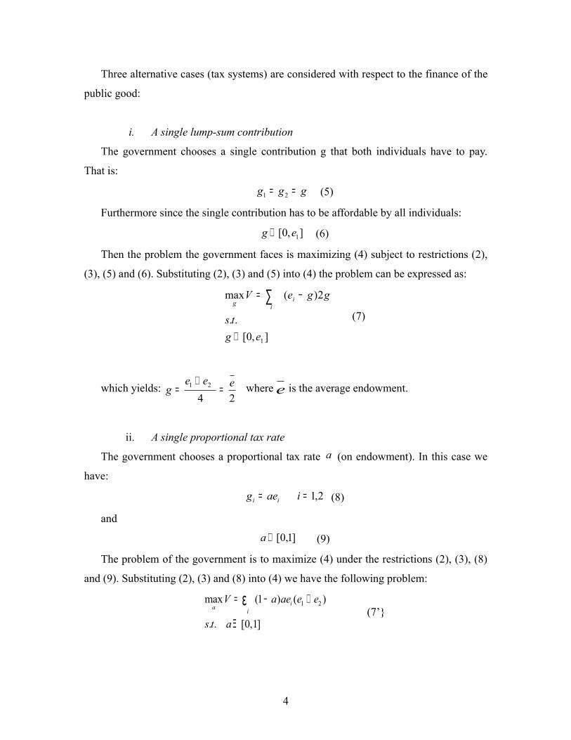
Three alternative cases (tax systems) are considered with respect to the finance of the

public good:

i. A single lump-sum contribution

The government chooses a single contribution g that both individuals have to pay.

That is:

ggg == 21 (5)

Furthermore since the single contribution has to be affordable by all individuals:

],0[ 1eg ∈ (6)

Then the problem the government faces is maximizing (4) subject to restrictions (2),

(3), (5) and (6). Substituting (2), (3) and (5) into (4) the problem can be expressed as:

],0[..

2)(max

1egts

ggeV iig

∈

−= ∑ (7)

which yields: 24

21 eeeg =

+= where e is the average endowment.

ii. A single proportional tax rate

The government chooses a proportional tax rate a (on endowment). In this case we

have:

2,1== iaeg ii (8)

and

]1,0[∈a (9)

The problem of the government is to maximize (4) under the restrictions (2), (3), (8)

and (9). Substituting (2), (3) and (8) into (4) we have the following problem:

1 2max (1 ) ( )

. . [0,1]

ia iV a ae e e

s t a

= − +

Ξ

ε (7’}

4

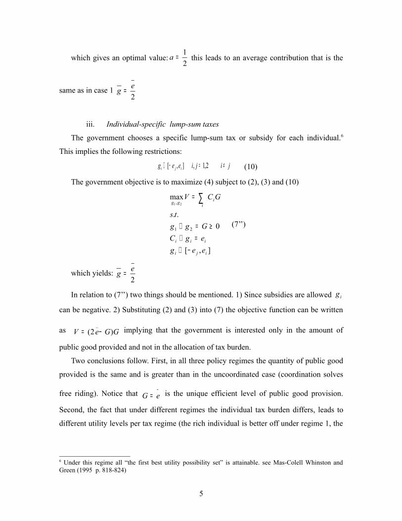
which gives an optimal value:21=a this leads to an average contribution that is the

same as in case 1 2eg =

iii. Individual-specific lump-sum taxes

The government chooses a specific lump-sum tax or subsidy for each individual.6

This implies the following restrictions:

jijieeg iji ≠=−∈ 2,1,],[ (10)

The government objective is to maximize (4) subject to (2), (3) and (10)

],[

0..

max

21

, 21

iji

iii

iigg

eegegCGgg

ts

GCV

−∈=+

≥=+

= ∑

(7’’)

which yields: 2eg =

In relation to (7’’) two things should be mentioned. 1) Since subsidies are allowed ig

can be negative. 2) Substituting (2) and (3) into (7) the objective function can be written

as GGeV )2(_

−= implying that the government is interested only in the amount of

public good provided and not in the allocation of tax burden.

Two conclusions follow. First, in all three policy regimes the quantity of public good

provided is the same and is greater than in the uncoordinated case (coordination solves

free riding). Notice that −= eG is the unique efficient level of public good provision.

Second, the fact that under different regimes the individual tax burden differs, leads to

different utility levels per tax regime (the rich individual is better off under regime 1, the

6 Under this regime all “the first best utility possibility set” is attainable. see Mas-Colell Whinston and Green (1995 p. 818-824)

5

poor individual is better off under regime 2 while under regime 3 utility allocation is

indeterminate)7.

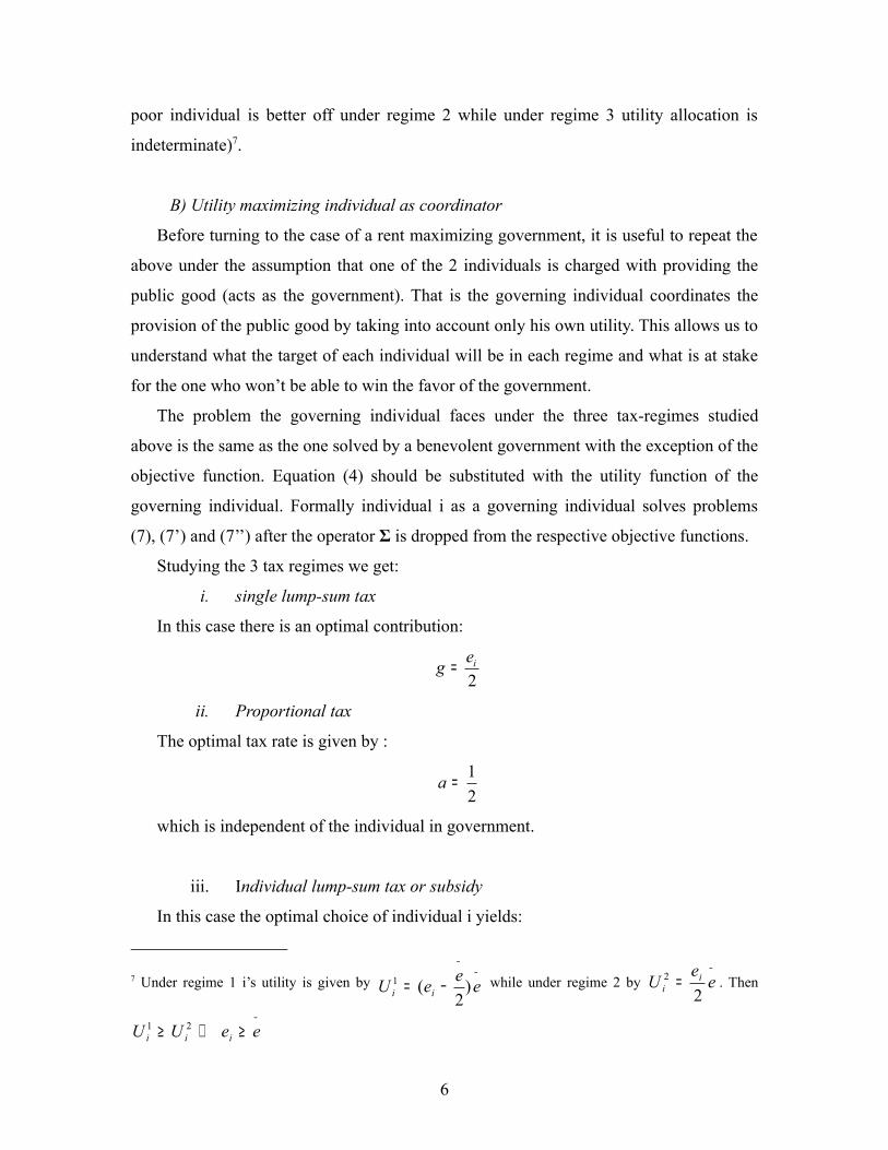
B) Utility maximizing individual as coordinator

Before turning to the case of a rent maximizing government, it is useful to repeat the

above under the assumption that one of the 2 individuals is charged with providing the

public good (acts as the government). That is the governing individual coordinates the

provision of the public good by taking into account only his own utility. This allows us to

understand what the target of each individual will be in each regime and what is at stake

for the one who won’t be able to win the favor of the government.

The problem the governing individual faces under the three tax-regimes studied

above is the same as the one solved by a benevolent government with the exception of the

objective function. Equation (4) should be substituted with the utility function of the

governing individual. Formally individual i as a governing individual solves problems

(7), (7’) and (7’’) after the operator Σ is dropped from the respective objective functions.

Studying the 3 tax regimes we get:

i. single lump-sum tax

In this case there is an optimal contribution:

2ieg =

ii. Proportional tax

The optimal tax rate is given by :

21=a

which is independent of the individual in government.

iii. Individual lump-sum tax or subsidy

In this case the optimal choice of individual i yields:

7 Under regime 1 i’s utility is given by −

−

−= eeeU ii )2

(1 while under regime 2 by −

= eeU ii 22 . Then

−≥⇔≥ eeUU iii

21

6

)(21

jii eeg −= and jj eg =

Notice that in this case when the poor individual is the governing one his

contribution is negative. This implies not only that he doesn’t finance the public good

but also that his private consumption is subsidized by the rich individual. On the other

hand, the poor person has a very small income in relation to the rich individual’s needs

in public good and therefore the rich has to make up the difference by contributing it

himself when he is the governor.

The analysis above gives us an insight on an issue that will be significant in the next

chapter. What is the relation between the conflict of interests in the private sector and

the tax-regime.

Under regime 1 the conflict of interest is mild. The two individuals have different

optimal policies but if one of the two achieves his optimal policy the other one ends up

with positive consumption (less than maximum tax burden). In regime 2 there is no

conflict of interest. Both individuals favor the same policy. In regime 3 on the other

hand the conflict of interest is extreme. If one of the two individuals manages to

enforce his optimal policy, the other one is in essence left with nothing (by virtue of the

private good being necessary).

In the next chapter I turn to a situation in which the individuals use bribes in order

to induce a favorable policy from the government.

.

3. Non benevolent government8

3.1. Basic Setting

A two-stage game between the private and public sector is assumed. At stage 1, the

two individuals submit independently and simultaneously a contribution schedule. A

contribution or bribing schedule is a function that assigns a bribe to every policy

available to the government. It is a function of the array of government policies. It will in

general take the form: ),;,( 2121 eeggBB ii = (11). At stage 2, the government chooses the

8The methods used in this chapter are described in detail in Dixit, Grossman and Helpman (1997). A textbook analysis can be found in Grossman and Helpman books “Special Interest Politics” (2001 ch. 8) and “Interest Groups and Trade Policy” (2002 ch. 1).

7

policy that maximizes its objective function, which is assumed to depend positively on

bribes, and collects the corresponding bribes9. In other words this is a case of a “menu

auction” in which the government acts as an auctioneer.

Let’s turn now to the notion of equilibrium. Since we are dealing with a two stage

game we are looking for a subgame-perfect Nash equilibrium which will consist of 2

contribution schedules and a choice of policies:

⟩⟨ },{),,;,(),,;,( *2

*12121

*22121

*1 ggeeggBeeggB

In order to proceed an objective function has to be specified for the government, the

player that moves second. The approach in Dixit, Grossman and Helpman (1997) allows

the government objective to be a general function of government policy and bribes. A

usual assumption within this framework is expressing it as a weighted average of the sum

of individual utilities and total bribes10. In our case this approach yields:

∑ ∑−+=i i

ii BbUbV )1( (12) where 01 ≥≥ b is a parameter of benevolence.

According to (12) the government in addition to total bribes assigns a positive weight

to a Benthamite social utility function.11 In this paper it will be assumed that b=0.

Although this assumption might seem extreme it simplifies algebra significantly.

Furthermore the qualitative results obtained are driven by the non benevolence of the

government and therefore should not be affected by the introduction of a positive b. In the second stage of the game the government chooses policy given the bribing

schedules the individuals have announced in stage 1. Setting b=0 and substituting (11)

into (12) we get the objective of the government in the second stage of the game:

),;,(),;,( 2121221211 eeggBeeggBV += which the government maximizes with respect

to 21 , gg .

Let’s now turn to the private sector and the problem of how bribing schedules are

formed. The utility function of principal i is as we have already seen is given by eq. (1):

9 It is assumed that the bribing schedules announced in the first period are binding for the private sector. After the government policy is realized the individuals can’t refrain from paying the bribe that corresponds to the schedules they have announced .10 See Grossman and Helpman (1995).11 A more general social utility function that depends positively on the welfare of all individuals can be used.

8

The budget constraint in the presence of bribes becomes:

iiii eBgC =++ (13)

where Bi is the bribe, individual i, pays to the government.

Equation (2) holds in this setting as well, along with certain feasibility restrictions

described bellow:

0≥iC , 0≥≥ ii Be and 021 ≥+= ggG (14)

Equation (13) states the fact that the private endowment is now divided between

private good consumption, tax and bribe. Furthermore in contrast to the case where the

government is benevolent, individuals are now faced with a decision. Namely they have

to decide on the bribing schedule they offer to the government in the first stage of the

game.

Before continuing it is practical to express the individual utility as a function of bribe

and government policy. Substituting (13) and (2) into (1) we get:

))((),,( 2121 ggBgeggBU iiiii +−−= (15)

Any bribing schedule in order to be part of a subgame-perfect Nash equilibrium

should satisfy two conditions:

i. It should be optimal in equilibrium from the point of view of the

individual

ii. It should be a Nash Equilibrium of the first period subgame played among

the individuals in the private sector.

As argued by Dixit, Grossman and Helpman (1997) there will be typically many, such

equilibria. Therefore we will focus here, as they do, in the smaller class of truthful

equilibria. “Truthful equilibria can arise when each principal offers the agent a payment

function that is truthful. A truthful payment function for principal i rewards the agent for

every change in the action (his choice of policy) exactly the amount of the resulting

change in the principal’s welfare, provided that the payment both before and after the

change is strictly positive”12.

12 See Dixit, Grossman and Helpman (1997). Check also this paper for justification of this class of equilibria

9

In other words a contribution schedule is truthful if it induces a change in bribes as a

response to a change in government policy in such a way that individual utility is always

held constant. Such a contribution schedule is unique for every constant utility level.

Formally following definition 3 in Dixit, Grossman and Helpman (1997) the bribe

schedule );,( 21 ii ggB ∆ is truthful relative to the constant i∆ if

}};,(,0max{,min{);,( 2121*

iiiii ggEeggB ∆=∆ iandeg ii ∀∈∀ ],0[ (16)

where iE is implicitly defined by :

iiii ggggEU ∆=∆ ),),;,(( 2121 iandeg ii ∀∈∀ ],0[ (17)

Where i∆ is the constant utility level that will be determined in equilibrium in a way

that satisfies condition ii above. Notice that the contribution schedule defined by (16) and

(17) above will be optimal from the point of view of the individual since the FOC for

utility maximization will always be satisfied.

Using (17) along with (15) we can get: iii

ii gegg

ggE −++

∆−=∆

2121 );,(

The meaning of the above then can be summarized as follows:

Individual i announces that he will contribute iii ge

G−+

∆− in response to the

government’s choice of 21 , gg . If the government’s choice of policy though induces a

negative payment he will contribute 0. Likewise if the chosen policy leads to a

contribution in excess of ie he will contribute ie .What should be noticed is that equation (17) is the definition of compensating

variation. This is not surprising. As we have seen truthfulness implies that the principals

pay to the agent in the form of bribes the whole shift in their utility caused by a change in

the agent’s choice of policy. That is their bribing schedule is the compensating variation

(when in the relevant bounds)13. Furthermore since the changes in the agent’s actions do

not affect the level of the principals’ utility, this is held constant at i∆ (welfare anchor).

Since the system (16) & (17) determines the bribing schedules up to the constant i∆

what is left for fully characterizing the truthful equilibrium of the game is determining the

13 See equation (16)

10

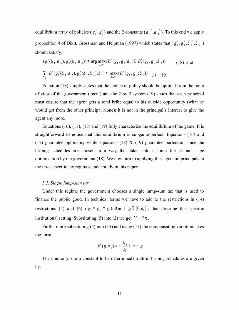
equilibrium array of policies ( *2

*1 , gg ) and the 2 constants ( *

2*

1 , ∆∆ ). To this end we apply

proposition 4 of Dixit, Grossman and Helpman (1997) which states that ( *2

*1 , gg , *

2*

1 , ∆∆ )

should satisfy:

)};,();,({maxarg)),(),,(( 221*2121

*1,21

*221

*1

21

∆+∆=∆∆∆∆ ggBggBgggg (18) and

)};,({max));,(),,(( 21*

,21*221

*1

*

21ii

i ggii ggBggB ∆=∆∆∆∆∆∑ i∀ (19)

Equation (18) simply states that the choice of policy should be optimal from the point

of view of the government (agent) and the 2 by 2 system (19) states that each principal

must ensure that the agent gets a total bribe equal to his outside opportunity (what he

would get from the other principal alone); it is not in the principal’s interest to give the

agent any more.

Equations (16), (17), (18) and (19) fully characterize the equilibrium of the game. It is

straightforward to notice that this equilibrium is subgame-perfect. Equations (16) and

(17) guarantee optimality while equations (18) & (19) guarantee perfection since the

bribing schedules are chosen in a way that takes into account the second stage

optimization by the government (18). We now turn to applying these general principals to

the three specific tax regimes under study in this paper.

3.2. Single lump-sum tax

Under this regime the government chooses a single lump-sum tax that is used to

finance the public good. In technical terms we have to add to the restrictions in (14)

restrictions (5) and (6) ( 021 ≥≡= ggg and ],0[ 1eg ∈ ) that describe this specific

institutional setting. Substituting (5) into (2) we get gG 2= .

Furthermore substituting (5) into (15) and using (17) the compensating variation takes

the form:

geg

gE ii

ii −+∆−=∆2

);(

The unique (up to a constant to be determined) truthful bribing schedules are given

by:

11

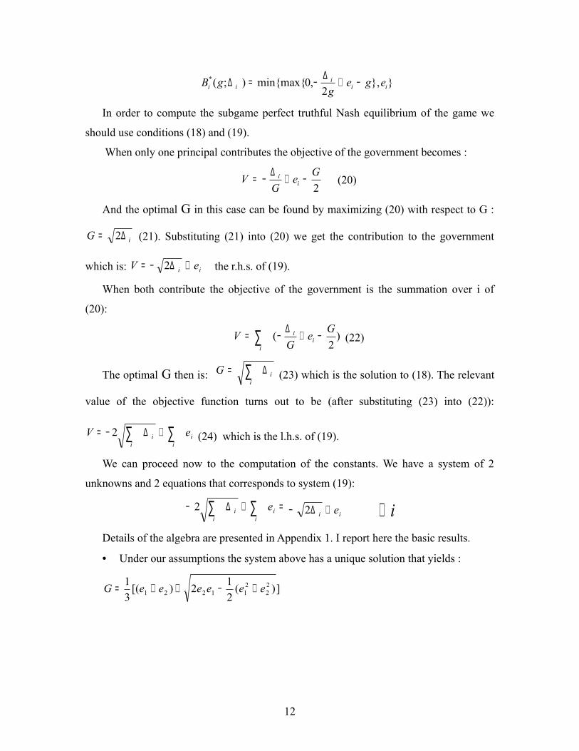
}},2

,0min{max{);(*ii

iii ege

ggB −+∆−=∆

In order to compute the subgame perfect truthful Nash equilibrium of the game we

should use conditions (18) and (19).

When only one principal contributes the objective of the government becomes :

2Ge

GV i

i −+∆−= (20)

And the optimal G in this case can be found by maximizing (20) with respect to G :

iG ∆= 2 (21). Substituting (21) into (20) we get the contribution to the government

which is: ii eV +∆−= 2 the r.h.s. of (19).

When both contribute the objective of the government is the summation over i of

(20):

)2

( GeG

V ii

i−+∆−= ∑ (22)

The optimal G then is: ii

G ∆= ∑ (23) which is the solution to (18). The relevant

value of the objective function turns out to be (after substituting (23) into (22)):

ii

ii

eV ∑∑ +∆−= 2 (24) which is the l.h.s. of (19).

We can proceed now to the computation of the constants. We have a system of 2

unknowns and 2 equations that corresponds to system (19):

=+∆− ∑∑ ii

ii

e2ii e+∆− 2 i∀

Details of the algebra are presented in Appendix 1. I report here the basic results.

• Under our assumptions the system above has a unique solution that yields :

])(212)[(

31 2

2211221 eeeeeeG +−++=

12

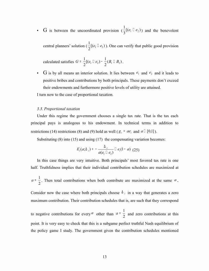
• G is between the uncoordinated provision ( )[(31

21 ee + ) and the benevolent

central planners’ solution ( )[(21

21 ee + ). One can verify that public good provision

calculated satisfies )(21)[(

21

2121 BBeeG +−+= .

• G is by all means an interior solution. It lies between 1e and 2e and it leads to

positive bribes and contributions by both principals. These payments don’t exceed

their endowments and furthermore positive levels of utility are attained.

I turn now to the case of proportional taxation.

3.3. Proportional taxation

Under this regime the government chooses a single tax rate. That is the tax each

principal pays is analogous to his endowment. In technical terms in addition to

restrictions (14) restrictions (8) and (9) hold as well ( ii aeg = and ]1,0[∈a ).

Substituting (8) into (15) and using (17) the compensating variation becomes:

)1()(

);(21

aeeea

aE ii

ii −++

∆−=∆ (25)

In this case things are very intuitive. Both principals’ most favored tax rate is one

half. Truthfulness implies that their individual contribution schedules are maximized at

21=a . Then total contributions when both contribute are maximized at the same a .

Consider now the case where both principals choose i∆ in a way that generates a zero

maximum contribution. Their contribution schedules that is, are such that they correspond

to negative contributions for every a other than 21=a and zero contributions at this

point. It is very easy to check that this is a subgame perfect truthful Nash equilibrium of

the policy game I study. The government given the contribution schedules mentioned

13

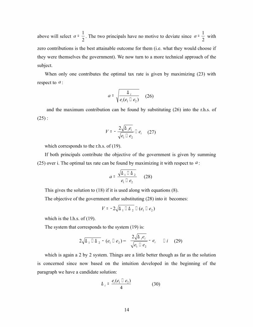
above will select 21=a . The two principals have no motive to deviate since

21=a with

zero contributions is the best attainable outcome for them (i.e. what they would choose if

they were themselves the government). We now turn to a more technical approach of the

subject.

When only one contributes the optimal tax rate is given by maximizing (23) with

respect to a :

)( 21 eeea

i

i

+∆= (26)

and the maximum contribution can be found by substituting (26) into the r.h.s. of

(25) :

iii e

eee

V ++

∆−=

21

2 (27)

which corresponds to the r.h.s. of (19).

If both principals contribute the objective of the government is given by summing

(25) over i. The optimal tax rate can be found by maximizing it with respect to a :

21

21

eea

+∆+∆

= (28)

This gives the solution to (18) if it is used along with equations (8).

The objective of the government after substituting (28) into it becomes:

)(2 2121 eeV ++∆+∆−=

which is the l.h.s. of (19).

The system that corresponds to the system (19) is:

)(2 2121 ee +−∆+∆ = iii e

eee

−+

∆

21

2 i∀ (29)

which is again a 2 by 2 system. Things are a little better though as far as the solution

is concerned since now based on the intuition developed in the beginning of the

paragraph we have a candidate solution:

4)( 21 eeei

i+=∆ (30)

14

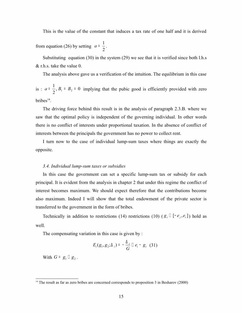
This is the value of the constant that induces a tax rate of one half and it is derived

from equation (26) by setting 21=a .

Substituting equation (30) in the system (29) we see that it is verified since both l.h.s

& r.h.s. take the value 0.

The analysis above gave us a verification of the intuition. The equilibrium in this case

is : 0,21

21 === BBa implying that the pubic good is efficiently provided with zero

bribes14.

The driving force behind this result is in the analysis of paragraph 2.3.B. where we

saw that the optimal policy is independent of the governing individual. In other words

there is no conflict of interests under proportional taxation. In the absence of conflict of

interests between the principals the government has no power to collect rent.

I turn now to the case of individual lump-sum taxes where things are exactly the

opposite.

3.4. Individual lump-sum taxes or subsidies

In this case the government can set a specific lump-sum tax or subsidy for each

principal. It is evident from the analysis in chapter 2 that under this regime the conflict of

interest becomes maximum. We should expect therefore that the contributions become

also maximum. Indeed I will show that the total endowment of the private sector is

transferred to the government in the form of bribes.

Technically in addition to restrictions (14) restrictions (10) ( ],[ iji eeg −∈ ) hold as

well.

The compensating variation in this case is given by :

iii

ii geG

ggE −+∆−=∆ );,( 21 (31)

With 21 ggG += .

14 The result as far as zero bribes are concerned corresponds to proposition 3 in Besharov (2000)

15

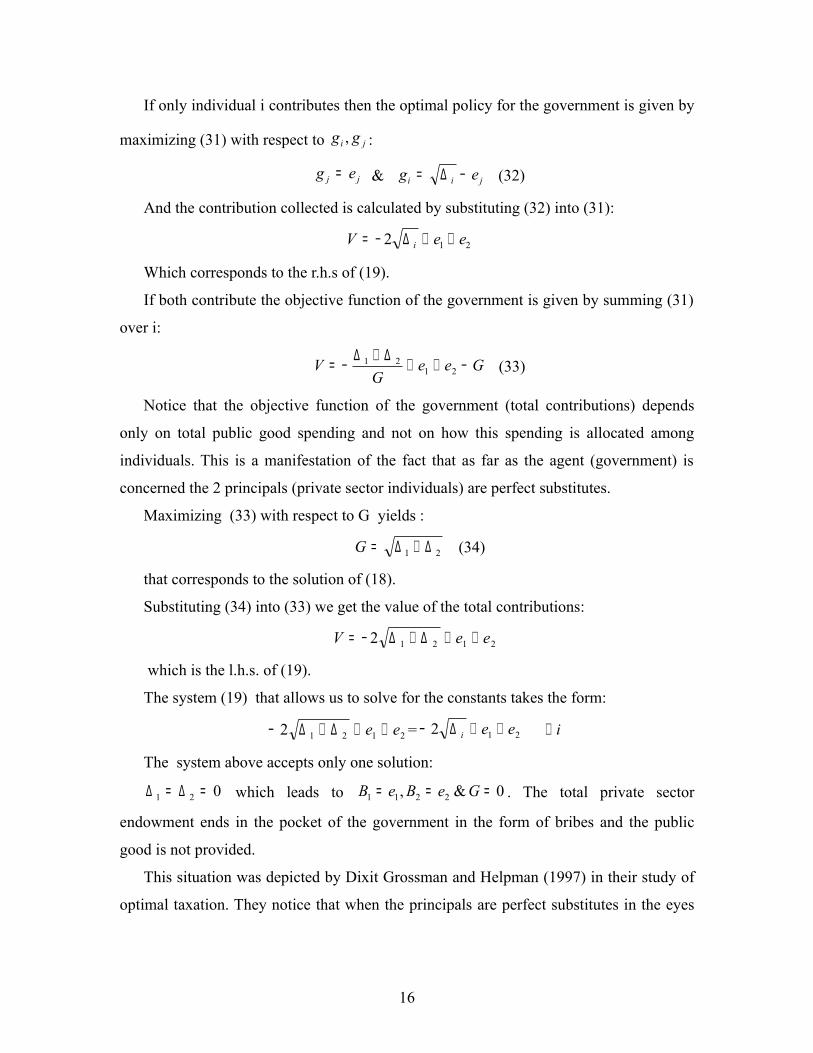
If only individual i contributes then the optimal policy for the government is given by

maximizing (31) with respect to ji gg , :

jj eg = & jii eg −∆= (32)

And the contribution collected is calculated by substituting (32) into (31):

212 eeV i ++∆−=

Which corresponds to the r.h.s of (19).

If both contribute the objective function of the government is given by summing (31)

over i:

GeeG

V −++∆+∆−= 2121 (33)

Notice that the objective function of the government (total contributions) depends

only on total public good spending and not on how this spending is allocated among

individuals. This is a manifestation of the fact that as far as the agent (government) is

concerned the 2 principals (private sector individuals) are perfect substitutes.

Maximizing (33) with respect to G yields :

21 ∆+∆=G (34)

that corresponds to the solution of (18).

Substituting (34) into (33) we get the value of the total contributions:

21212 eeV ++∆+∆−=

which is the l.h.s. of (19).

The system (19) that allows us to solve for the constants takes the form:

21212 ee ++∆+∆− = 212 eei ++∆− i∀

The system above accepts only one solution:

021 =∆=∆ which leads to 0&, 2211 === GeBeB . The total private sector

endowment ends in the pocket of the government in the form of bribes and the public

good is not provided.

This situation was depicted by Dixit Grossman and Helpman (1997) in their study of

optimal taxation. They notice that when the principals are perfect substitutes in the eyes

16

of the agent the principals are caught in a Bertrand-type competition that allows the agent

to capture all potential benefits15.

3.5. Comparisons

Comparing the cases of benevolent and non benevolent government reveals the

importance of the selection of tax regimes. Whenever there is room for rent seeking

activities both private welfare and public good provision are affected. The fact that the

bribes to government are financed at the expense of both private and public good

consumption should not come as a surprise. We know from Dixit, Helpman and

Grossman (1997)16 that truthful equilibria are efficient from the point of view of both

principals and agent. This implies that in equilibrium the private sector will consume the

two goods in the desired ratio. In turn this implies that a tax regime that increases bribes

reduces public good provision as well as private good consumption. Under benevolent

government all three regimes yield the same results (efficient provision of public good).

On the other hand, if the government is not benevolent the equilibria attained range from

zero bribes and efficient public good provision to maximum bribes with zero public good

provision depending on the degree of conflict of interests induced by the tax system.

Another thing that should be noted is the role of assuming endogenous government

budget. In the application considered by Dixit, Helpman and Grossman (1997) the sole

purpose of taxation was redistribution of income (taxes sum up to zero). In this case the

conflict of interests is maximized since individuals can be divided in to those who are in

the paying and those who are in the receiving end of the government policy. This

necessarily implies maximum conflict of interests and therefore maximum bribes. When

the budget is considered exogenous as in Besharov (2000, 2003) the conflict of interest is

non existent under a single lump-sum tax regime and mild under a proportional tax,

leading to zero bribes under the first regime and positive bribes under the second. As we

have seen in chapter 2 of this paper things are reversed when taxes are considered

endogenous (used to finance a useful public good).

15 Again the maximum bribe result corresponds to proposition 5 in Besharov (2000)16 See their proposition 4

17

4. Related Literature

The methodology used in this paper was introduced by Bernheim and Whinston

(1986) who described it as “menu auctions”. Grossman and Helpman (1995) used this

approach to discuss “menus” that are continuous functions of the agents’ actions. Their

primary consideration was lobbying in international trade (tariff setting) and they

assumed that the principals have transferable utility (quasi-linear utility function). The

generalization of Grossman and Helpman work for non-transferable utility was done by

Dixit, Grossman and Helpman (1997). In their paper they also study an application

regarding optimal taxation in an economy with production where the government uses

taxes and subsidies to redistribute income. They were motivated in this study by the work

of Diamond and Mirrles (1971). They show that only lump-sum transfers will be used to

achieve the government’s targets and that any surplus generated by the lobbying activity

will be absorbed by the government in the form of bribes. The “menu auction” approach

was also used in a public economics literature by Persson (1998) who used it to study

local public good provision17.

The issue of the relation between tax systems and bribes to government officials was

first studied in Besharov (2000, 2003). In his papers Besharov considers an economy

with production in which the purpose of taxation is to cover an exogenous budget. He

shows that the well -being of the principals is crucially affected by the tax system and

that a distortive taxation (one that affects the principals’ productive decisions) reduces the

amount of bribes.

On the other hand the approach used here is that of an economy without production

(fixed tax base) but with an endogenous budget since the government decides on public

good provision. These differences trigger three points of departure from Besharov’s

work: 1) The tax system affects the provision of public good as well as the level of

bribes. 2) The effect tax systems have on bribes are in general different when the

government budget is endogenous 3) When an inefficiency is required to avoid bribes

17 See also Persson and Tabellini (2003 p. 171-174)

18

attaining their upper bound this does not need to be a tax system that distorts productive

decisions. The inefficiency required to this end can be introduced in a model with fixed

endowments through a restriction on the government’s redistributive ability (i.e. a tax

system that minimizes conflict of interests in the private sector).

5. Conclusions and policy implications

In this paper it has been shown that the choice of tax regime affects the degree of

corruption in an economy (the amount of resources allocated to bribes). This fact is well

known through the work of Dixit, Grossman and Helpman. In their paper they state that

in order to avoid government collecting all benefits from rent seeking activity

inefficiency should be introduced through the tax system. To this end they point to a tax

regime that distorts productive decisions and thus makes first best outcomes unattainable.

My paper builds on this idea and shows that the same result can be achieved through

inefficiency in income redistribution (i.e. lack of policy instruments) that doesn’t

necessarily lead to a pareto inferior allocation. The driving force behind this result is the

notion of conflict of interests. If the government can efficiently redistribute welfare

among individuals the conflict of interests is maximal since everybody wants to be in the

receiving end of this redistribution and is willing to bribe accordingly. On the other hand

if welfare redistribution is impossible the basis for rent seeking disappears since

everybody in the economy agrees on the choice of policy. This is an argument for the

restriction of policy instruments or in other words for simple and uniform tax systems.

As one does expect though restricting policy instruments is not costless in general.

Two extensions of the basic model studied in this paper can help us understand possible

costs. Think first of a government that is partly benevolent, that is a government that

assigns a positive weight to a social utility function in addition to total bribes. Assuming

that equality is promoted through the social utility function a tradeoff between equality

and corruption will be associated with the choice of tax system. On the other hand

consider introducing production to the simple exchange economy studied in this paper.

Again a proportional income tax which has been shown to eradicate bribes here will be

19

distortive and lead to inefficient production. This in turn generates a tradeoff between

productive efficiency and corruption as far as the choice of tax system is considered.

In practice a society when choosing a tax system faces both tradeoffs discussed

above. This analysis could at least partly account for differences in tax regimes among

countries and possibly explain why some countries in Europe have recently decided to

introduce a flat tax rate while others seem unwilling to do so.

20

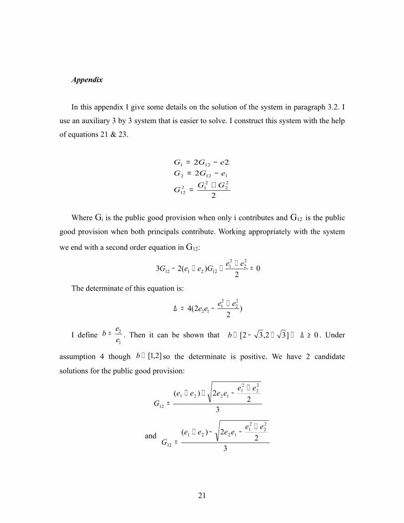
Appendix

In this appendix I give some details on the solution of the system in paragraph 3.2. I

use an auxiliary 3 by 3 system that is easier to solve. I construct this system with the help

of equations 21 & 23.

Where Gi is the public good provision when only i contributes and G12 is the public

good provision when both principals contribute. Working appropriately with the system

we end with a second order equation in G12:

02

)(2322

21

122112 =+++− eeGeeG

The determinate of this equation is:

)2

2(422

21

12eeee +−=∆

I define 1

2

eeb = . Then it can be shown that 0]32,32[ ≥∆⇒+−∈b . Under

assumption 4 though ]2,1[∈b so the determinate is positive. We have 2 candidate

solutions for the public good provision:

32

2)(22

21

1221

12

eeeeee

G

+−++

=

and 3

22)(

22

21

1221

12

eeeeee

G

+−−+

=

21

2

222

22

212

12

1122

121

GGG

eGGeGG

+=

−=−=

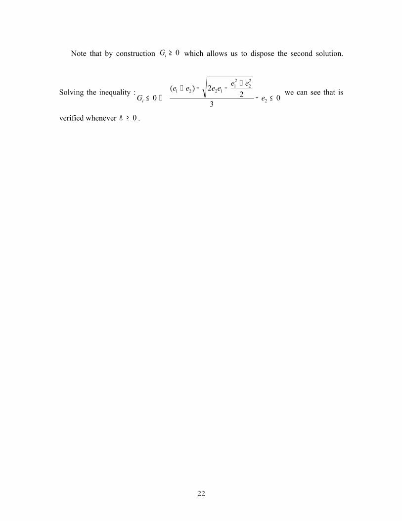
Note that by construction 0≥iG which allows us to dispose the second solution.

Solving the inequality :0

32

2)(0 2

22

21

1221

≤−

+−−+⇔≤ e

eeeeeeGi

we can see that is

verified whenever 0≥∆ .

22

References

Bernheim B.Douglas & Whinston Michael D. (1986), “Menu Auctions, Resource

Allocation and Economic Influence”, QJE 101 (February 1986): 1-31.

Besharov Gregory “The Optimality of Inefficient Restrictions on Tax Systems: An

Influence Cost Approach” Stanford University (January 10,2000) Discussion Paper.

Besharov Gregory “Why not Lump-Sum Taxation?” Duke University (September 9,2003)

Working Paper (03-20).

Diamond Peter A. & Mirrlees James A. “Optimal Taxation & Public Production”, 2 pts

AER 61 (March 1971): 8-27, (June 1971): 261-278.

Dixit Avinash, Grossman Gene M. & Helpman Elhanan (1997), “Common Agency and

Coordination: General Theory and Application to Government Policy Making”, JPE,

Vol. 105, No 4 (Aug 1997), 752-769

Grossman Gene M. & Helpman Elhanan, “Protection for Sale”, AER 84 (September

1994): 833-850.

Grossman Gene M. & Helpman Elhanan, “Interest groups & Trade Policy” (2002),

Princeton: Princeton University Press.

Grossman Gene M. & Helpman Elhanan , “Special Interest Politics” (2002), Cambridge

Mass. :MIT Press

Mas-Collel Andreu, Whinston Michael D. & Green Jerry R. “ Microeconomic Theory”

(1995), New York : Oxford University Press.

Mueller Dennis C. “Public Choice II” (1989), Cambridge : Cambridge University Press.

Persson Torsten “Economic Policy and Special Interest Politics”, EJ 108 (March 1998)

310-327

Persson Torsten & Tabellini Guido “Political Economics” (2000), Cambridge Mass. :

MIT Press

23