Non-Fickian dispersion in porous media:

1. Multiscale measurements using single-well injection

withdrawal tracer tests

P. Gouze,1 T. Le Borgne,1,2 R. Leprovost,1 G. Lods,1 T. Poidras,1 and P. Pezard1

Received 18 June 2007; revised 20 February 2008; accepted 9 April 2008; published 28 June 2008.

[1] We present a set of single-well injection withdrawal tracer tests in a paleoreef porousreservoir displaying important small-scale heterogeneity. An improved dual-packer probewas designed to perform dirac-like tracer injection and accurate downhole automaticmeasurements of the tracer concentration during the recovery phase. By flushing thetracer, at constant flow rate, for increasing time duration, we can probe distinctly differentreservoir volumes and test the multiscale predictability of the (non-Fickian) dispersionmodels. First we describe the characteristics, from microscale to meter scale, of thereservoir rock. Second, the specificity of the tracer test setup and the results obtained usingtwo different tracers and measurement methods (salinity-conductivity and fluorescentdye–optical measurement, respectively) are presented. All the tracer tests display stronglytailed breakthrough curves (BTC) consistent with diffusion in immobile regions.Conductivity results, measured over 3 orders of magnitude only, could have beeneasily interpreted by the conventional mobile-immobile (MIM) diffusive mass transfermodel of asymptotic log-log slope of �2. However, the fluorescent dye sensor,which allows exploring much lower concentration values, shows that a change in thelog-log slope occurs at larger time with an asymptotic value of �1.5, corresponding to thedouble-porosity model. These results suggest that the conventional, one-slope MIMtransfer rate model is too simplistic to account for the real multiscale heterogeneity of thediffusion-dominant fraction of the reservoir.

Citation: Gouze, P., T. Le Borgne, R. Leprovost, G. Lods, T. Poidras, and P. Pezard (2008), Non-Fickian dispersion in porous media:

1. Multiscale measurements using single-well injection withdrawal tracer tests, Water Resour. Res., 44, W06426,

doi:10.1029/2007WR006278.

1. Introduction

[2] Modeling contaminant movement is a fundamentalprerequisite to support geoenvironmental risk evaluation aswell as the management and remediation of water resources.Presently, most of operational modeling tools have beenconstructed around the resolution of the so-called advec-tion-dispersion equation (ADE) assuming that dispersionbehaves as a diffusion-like (Fickian) process [Adams andGelhar, 1992]. In this case, the mean and the variance of thecontaminant (or tracer) spatial distribution scale with time(t) and

ffiffit

p, respectively, and the variance of the temporal

distribution (i.e., of the breakthrough curve measured at agiven observation spot) is finite. However, an increasingnumber of examples, both from situ [Adams and Gelhar,1992; Meigs and Beauheim, 2001; Becker and Shapiro,2003] and laboratory [Silliman and Simpson, 1987;Berkowitzet al., 2000; Levy and Berkowitz, 2003] tracer tests, displaystrongly asymmetric BTCs with long tails (i.e., for times

after the advective peak has passed) that appears to decreasemore or less as a power law of time C(t)�t�a, and indicatesan apparently infinite variance of the BTCs. Then, itbecomes more and more certain that Fickian models failsto capture the real nature of the dispersion in naturalsystems submitted to common hydrological stresses; evenin those thought as macroscopically homogeneous [Levyand Berkowitz, 2003]. In most cases, BTC analysis givesfitted values of the exponent a ranging from 1.5 and 2.5.However, it is generally difficult to measure accurately theBTC power law slope. Indeed, in the vicinity of the mainconcentration peak, measured concentration may be corrup-ted by the transition from the Fickian concentration decreaseto the rate-limited decrease. Then, as concentrationdecreases toward very low values, measurement inaccuracymay spoil the estimate of the slope. Finally, it is difficult toevaluate if the observed BTC tail represents effectively theasymptotic behavior of the tracer recovery or a transitionalbehavior. To tackle the asymptotic non-Fickian dispersionbehavior, high-resolution sensors and long-lasting recordingof the tracer recovery are required.[3] Non-Fickian dispersion properties, their origin and

their relation to the geological heterogeneity are still debated.Authors have explored different approaches for better cap-turing the processes that control non-Fickian dispersion.Non-Fickian dispersion may be the result of long-range

1Geosciences, UMR 5243, Universite de Montpellier 2, CNRS,Montpellier, France.

2Now at Geosciences Rennes, UMR 6118, Universite de Rennes 1,CNRS, Rennes, France.

Copyright 2008 by the American Geophysical Union.0043-1397/08/2007WR006278$09.00

W06426

WATER RESOURCES RESEARCH, VOL. 44, W06426, doi:10.1029/2007WR006278, 2008ClickHere

for

FullArticle

1 of 15

spatial correlation of geological structures and permeability.Multichannel model, in which all the velocities are infinitelycorrelated is the end-member case of this class model[Becker and Shapiro, 2003; Gylling et al., 1999]. Theoverall mass transport is the sum of elementary transportin channels of distinctly different properties (leading todifferent flow rate and residence time), each of the channelsbeing independent from each others. With this model, it ispossible to reproduce power law-tailed BTC, by choosingthe appropriate distribution of channel properties. Yet,recent results obtained by Becker and Shapiro [2003] whenanalyzing both well-to-well and single-well injection with-drawal tracing experiments show that the scaling of theresidence time distribution is strongly controlled by theboundary condition (either prescribed flow rate or pre-scribed pressure) at the injection point and by flow geom-etry. The existence of long-range spatial correlation is alsothe basic assumption in models that describe dispersion asthe result of alpha-normal (Levy flight) velocity distribution[Benson et al., 2001], although quantitative relation be-tween alpha-normal velocity distribution and the effectivevelocity correlation is not straightforward [Le Borgne et al.,2007].[4] Alternatively, non-Fickian dispersion may be repre-

sented by long-range temporal correlations of the solutemotion that may be due to mass transfers in small-scalegeological structures. For instance, the mobile-immobilemass transfer (MIM) model assumes mass exchanges be-tween the moving fluid and a less permeable domain inwhich fluid is considered as immobile [Haggerty andGorelick, 1995; Carrera et al., 1998; Haggerty et al.,2000]. The discrimination between the effects of spatialcorrelations controlled by large-scale structures and tempo-ral correlations controlled by small-scale structures, bothleading to non-Fickian transport, is a difficult task because itis most probable that both may be present simultaneously insome heterogeneous reservoirs. Nevertheless, it is possibleto minimize velocity spatial correlation by performingsingle-well injection withdrawal (SWIW) tracing experi-ments and selecting reservoir targets displaying large-scalehomogeneity.[5] SWIW tracing tests, also called push-pull or echo

tracer tests, consist in injecting a given mass of tracer in the

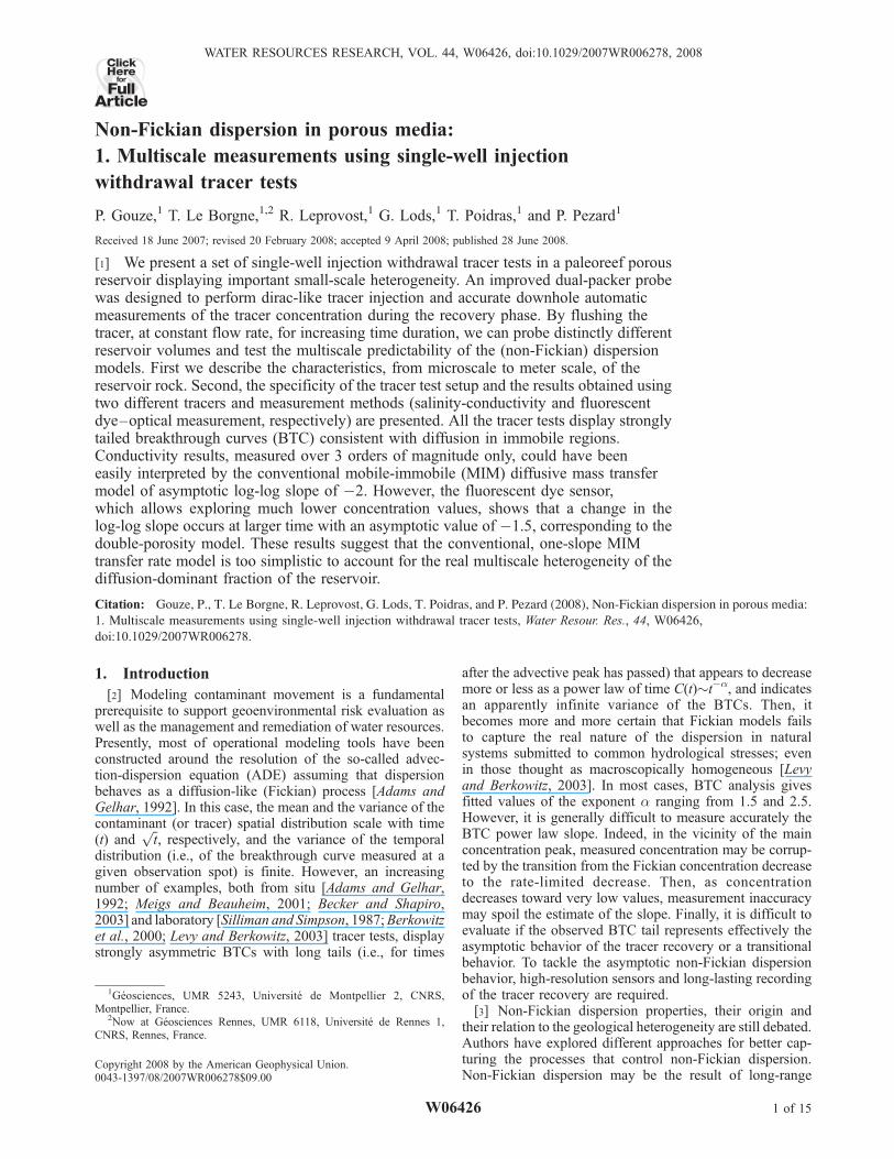
medium and reversing flow after a certain time in order tomeasure the tracer breakthrough curve at the injection point[Gelhar and Collins, 1971, Tsang, 1995, Haggerty et al.,2001, Khrapitchev and Callaghan, 2003]. This techniquepresents several advantages. First, the reversal of flowwarrants an optimal tracer mass recovery. Second, SWIWtracer test allows measuring the irreversible dispersion (ormixing) whereas reversible dispersion; that is, the spreadingdue to long-range correlated path, taking place during thetracer push phase is canceled during the withdrawal phase[Becker and Shapiro, 2003, Khrapitchev and Callaghan,2003]. The quantification of the reversible and irreversibledispersion refers to a given scale of observation which, inour case, is the maximal distance moved by the tracerduring the SWIW tracer test. More precisely, velocitycorrelation, over distance smaller than the exploration sizewill result in irreversible dispersion (diffusion and mixing)whereas adjective spreading due to velocity correlationlarger than the exploration size will be canceled (Figure 1).Thus, the measured dispersion using SWIW tests is onlycaused by tracer molecules that do not follow the same pathon the injection and the withdrawal phases. Third, usingSWIW tests, tracer may be pushed at different distancesfrom the injection point, thus visiting different volumes ofthe system using a single well. This latter aspect, which wasbarely investigated in previous studies, allows exploring thedispersion processes for increasing volumes of reservoir,and testing, and subsequently validating, the predictivenature of the models.[6] A set of SWIW tracer tests is presented in this paper.

Our objective was to obtain high-quality measurements toexplore the asymptotic behavior of this type of mass trans-fers and to investigate the scale effect on dispersion. For thisfirst set of experiments, the intention was to focus on thestudy of the diffusion processes in immobile zones (i.e.,matrix diffusion). Consequently, we intentionally targetedan aquifer displaying large-scale homogeneity (i.e., nofractures or large range correlated permeability zones), butsmall-scale heterogeneity. A second requirement was tominimize regional flow that may invalidate the radialsymmetry assumption. For that seawater intrusion zonesare ideal, because of the relative motionlessness due to the

Figure 1. Schematic representation of the reversible-irreversible dispersion. SWIW tracer tests act tocancel long-range velocity correlations. Gray zones denote the concentration distribution (left) at the endof the push duration (t = Tpush + 1/2 Tinj) and (right) when the tracer mass center is back to the initialposition at time t = 2Tpush + Tinj. The black zone on the left corresponds to the tracer at the initial time (t = 0).

2 of 15

W06426 GOUZE ET AL.: NON-FICKIAN DISPERSION IN POROUS MEDIA, 1 W06426

strong hydrostatic constraints imposed by the water layeringconfiguration.[7] The purpose of this paper is to describe the tracing

experiments, compare them to previously published dataand discuss the results in the frame of non-Fickian disper-sion. First, the test site and the rock properties are presentedin section 2. The experimental setup, together with thedescription of the new equipment and methodology devel-oped for this purpose are presented in section 3. In section 4,the set of SWIW tracer tests is presented and results arediscussed and tentatively modeled by the classical MIMmass transfer model. Finally, summary and conclusions aregiven in section 5. In a companion paper [Le Borgne andGouze, 2008], an improved MIM mass transfer model isexplored using a continuous time random walk modelexplaining the observations at large scales.

2. Site Location and Reservoir Properties

2.1. The Ses Sitjoles Test Site

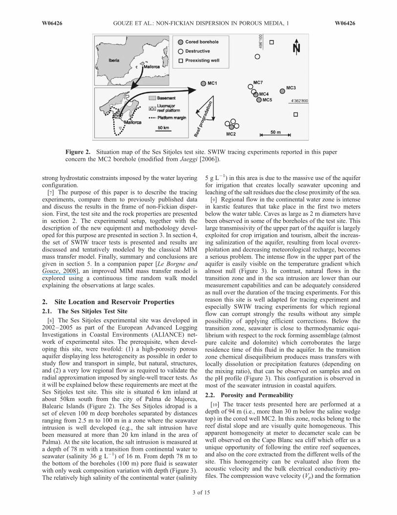
[8] The Ses Sitjoles experimental site was developed in2002–2005 as part of the European Advanced LoggingInvestigations in Coastal Environments (ALIANCE) net-work of experimental sites. The prerequisite, when devel-oping this site, were twofold: (1) a high-porosity porousaquifer displaying less heterogeneity as possible in order tostudy flow and transport in simple, but natural, structures,and (2) a very low regional flow as required to validate theradial approximation imposed by single-well tracer tests. Asit will be explained below these requirements are meet at theSes Sitjoles test site. This site is situated 6 km inland atabout 50km south from the city of Palma de Majorca,Balearic Islands (Figure 2). The Ses Sitjoles idropad is aset of eleven 100 m deep boreholes separated by distancesranging from 2.5 m to 100 m in a zone where the seawaterintrusion is well developed (e.g., the salt intrusion havebeen measured at more than 20 km inland in the area ofPalma). At the site location, the salt intrusion is measured ata depth of 78 m with a transition from continental water toseawater (salinity 36 g L�1) of 16 m. From depth 78 m tothe bottom of the boreholes (100 m) pore fluid is seawaterwith only weak composition variation with depth (Figure 3).The relatively high salinity of the continental water (salinity

5 g L�1) in this area is due to the massive use of the aquiferfor irrigation that creates locally seawater upconing andleaching of the salt residues due the close proximity of the sea.[9] Regional flow in the continental water zone is intense

in karstic features that take place in the first two metersbelow the water table. Caves as large as 2 m diameters havebeen observed in some of the boreholes of the test site. Thislarge transmissivity of the upper part of the aquifer is largelyexploited for crop irrigation and tourism, albeit the increas-ing salinization of the aquifer, resulting from local overex-ploitation and decreasing meteorological recharge, becomesa serious problem. The intense flow in the upper part of theaquifer is easily visible on the temperature gradient whichalmost null (Figure 3). In contrast, natural flows in thetransition zone and in the sea intrusion are lower than ourmeasurement capabilities and can be adequately consideredas null over the duration of the tracing experiments. For thisreason this site is well adapted for tracing experiment andespecially SWIW tracing experiments for which regionalflow can corrupt strongly the results without any simplepossibility of applying efficient corrections. Below thetransition zone, seawater is close to thermodynamic equi-librium with respect to the rock forming assemblage (almostpure calcite and dolomite) which corroborates the largeresidence time of this fluid in the aquifer. In the transitionzone chemical disequilibrium produces mass transfers withlocally dissolution or precipitation features (depending onthe mixing ratio), that can be observed on samples and onthe pH profile (Figure 3). This configuration is observed inmost of the seawater intrusion in coastal aquifers.

2.2. Porosity and Permeability

[10] The tracer tests presented here are performed at adepth of 94 m (i.e., more than 30 m below the saline wedgetop) in the cored well MC2. In this zone, rocks belong to thereef distal slope and are visually quite homogeneous. Thisapparent homogeneity at meter to decameter scale can bewell observed on the Capo Blanc sea cliff which offer us aunique opportunity of following the entire reef sequences,and also on the core extracted from the different wells of thesite. This homogeneity can be evaluated also from theacoustic velocity and the bulk electrical conductivity pro-files. The compression wave velocity (Vp) and the formation

Figure 2. Situation map of the Ses Sitjoles test site. SWIW tracing experiments reported in this paperconcern the MC2 borehole (modified from Jaeggi [2006]).

W06426 GOUZE ET AL.: NON-FICKIAN DISPERSION IN POROUS MEDIA, 1

3 of 15

W06426

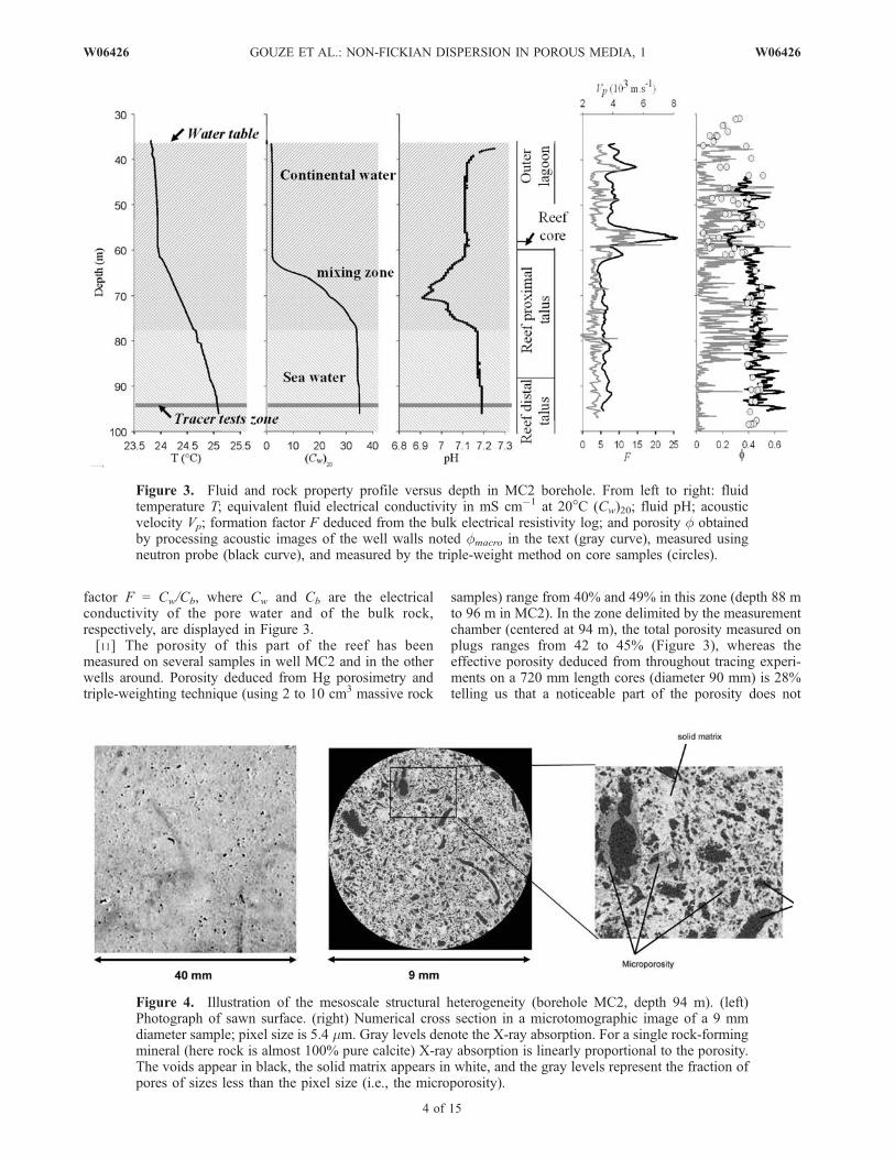
factor F = Cw/Cb, where Cw and Cb are the electricalconductivity of the pore water and of the bulk rock,respectively, are displayed in Figure 3.[11] The porosity of this part of the reef has been

measured on several samples in well MC2 and in the otherwells around. Porosity deduced from Hg porosimetry andtriple-weighting technique (using 2 to 10 cm3 massive rock

samples) range from 40% and 49% in this zone (depth 88 mto 96 m in MC2). In the zone delimited by the measurementchamber (centered at 94 m), the total porosity measured onplugs ranges from 42 to 45% (Figure 3), whereas theeffective porosity deduced from throughout tracing experi-ments on a 720 mm length cores (diameter 90 mm) is 28%telling us that a noticeable part of the porosity does not

Figure 3. Fluid and rock property profile versus depth in MC2 borehole. From left to right: fluidtemperature T; equivalent fluid electrical conductivity in mS cm�1 at 20�C (Cw)20; fluid pH; acousticvelocity Vp; formation factor F deduced from the bulk electrical resistivity log; and porosity f obtainedby processing acoustic images of the well walls noted fmacro in the text (gray curve), measured usingneutron probe (black curve), and measured by the triple-weight method on core samples (circles).

Figure 4. Illustration of the mesoscale structural heterogeneity (borehole MC2, depth 94 m). (left)Photograph of sawn surface. (right) Numerical cross section in a microtomographic image of a 9 mmdiameter sample; pixel size is 5.4 mm. Gray levels denote the X-ray absorption. For a single rock-formingmineral (here rock is almost 100% pure calcite) X-ray absorption is linearly proportional to the porosity.The voids appear in black, the solid matrix appears in white, and the gray levels represent the fraction ofpores of sizes less than the pixel size (i.e., the microporosity).

4 of 15

W06426 GOUZE ET AL.: NON-FICKIAN DISPERSION IN POROUS MEDIA, 1 W06426

belong to the mobile (advective) domain. The connectedporosity was also evaluated from analyzing X-ray micro-tomography images (resolution 5.4 mm, Figure 4) of smallplugs of 9 mm diameter. This approach allows the discrim-ination between connected and nonconnected porosity[Noiriel et al., 2005]. Connected porosity evaluated thisway ranges from 27 to 30%, (total porosity from 32 to 36%)but it must be stated here that the samples were chosen tocontain no visible macropores (i.e., pores larger than 1 mm).Nevertheless, the ratio of the effective porosity to the totalporosity appears coherent with measurements performed onlarger size samples. The observation of the borehole cores(diameter 90 mm) shows that locally enhanced porosityzones exist because of fossil accumulations and bigger coralfragments, but these features represent a very small fractionof the reservoir volume at the depth of the experiment. Thiscan be seen also on the macroporosity (fmacro) profileobtained from the acoustic well wall imagery. This measureintegrates the cross-sectioned macropores larger than about10 mm2. The profile displayed in Figure 3 shows that atdepth 94m fmacro is smaller than 3% and should not modifythe meter-scale permeability, neither forming long-rangechannels.[12] The presently observed porosity is not the primary

porosity, because the system has followed a complexdiagenic history [Pomar and Ward, 1999]. The d18O valuesare negative (d18O � –4%) in MC2. These negative valuesare typical of a diagenesis from groundwater of meteoricorigin. However, as the initial porous medium had a highporosity and was quite homogeneous at meter to decameterscale (typical from reef talus), diagenesis was probablyhomogeneously distributed. As a result, the actual porosityremains quite homogeneous. Studies at larger scale, includ-ing classical geophysical logging (for example using sonicpropagation) and well wall imaging (optical and acoustical),shows that the spatial changes in porosity follow thesequences of subhorizontal sigmoidal progradation lens

resulting from the growth of the distal talus reef platform.Porosity variations are typically occurring over verticaldistances of five to ten meters, and tens to hundred metershorizontally. For a more complete description of the aquiferpetrologic properties at large scale, the reader can refer toJaeggi [2006]. The high-porosity porous media ensures alarge connectivity of the pore and throats and the existenceof a single connected void cluster and few long-distancedead head paths. Albeit it is difficult to measure theseparameters at meter scale, the analysis of the X-ray tomo-graphic images on several centimeter-scale samples showsthe existence of a single connected void cluster with few tono centimeter-scale dead end structures.[13] Permeability was measured from pumping test be-

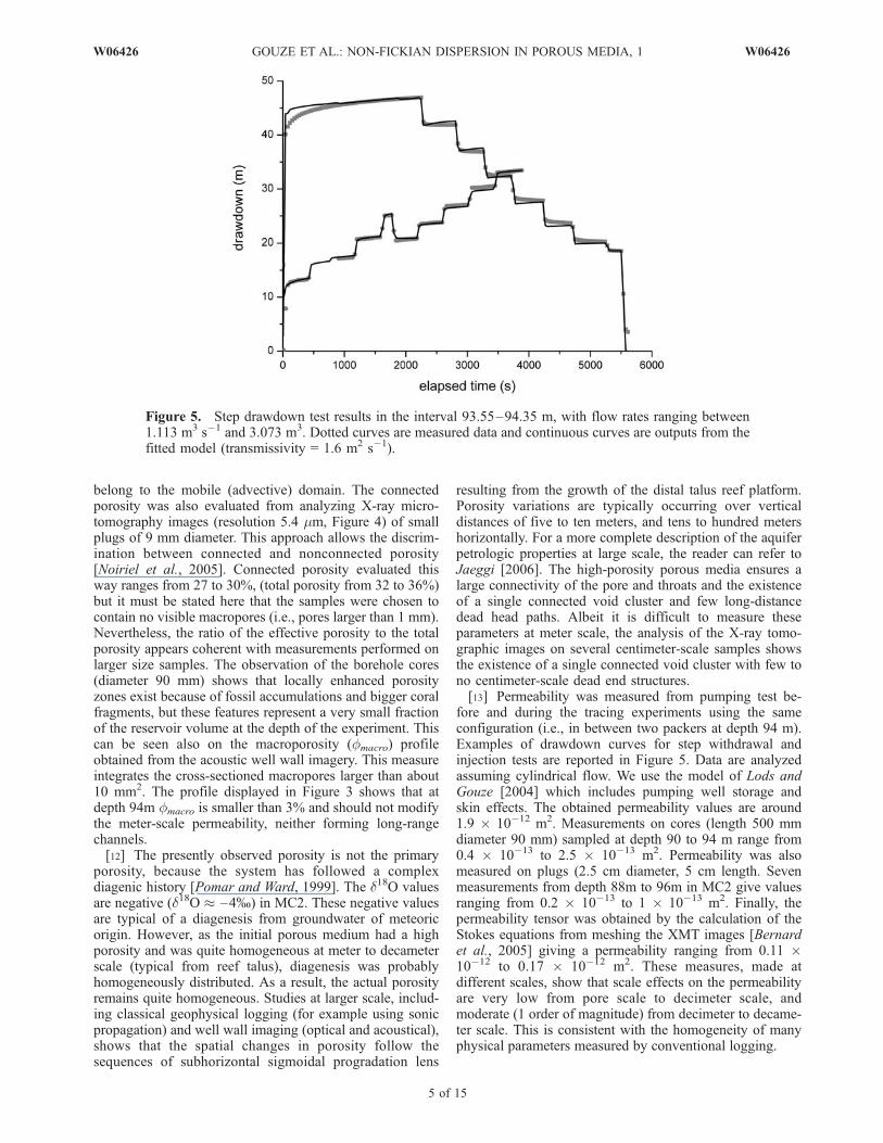
fore and during the tracing experiments using the sameconfiguration (i.e., in between two packers at depth 94 m).Examples of drawdown curves for step withdrawal andinjection tests are reported in Figure 5. Data are analyzedassuming cylindrical flow. We use the model of Lods andGouze [2004] which includes pumping well storage andskin effects. The obtained permeability values are around1.9 � 10�12 m2. Measurements on cores (length 500 mmdiameter 90 mm) sampled at depth 90 to 94 m range from0.4 � 10�13 to 2.5 � 10�13 m2. Permeability was alsomeasured on plugs (2.5 cm diameter, 5 cm length. Sevenmeasurements from depth 88m to 96m in MC2 give valuesranging from 0.2 � 10�13 to 1 � 10�13 m2. Finally, thepermeability tensor was obtained by the calculation of theStokes equations from meshing the XMT images [Bernardet al., 2005] giving a permeability ranging from 0.11 �10�12 to 0.17 � 10�12 m2. These measures, made atdifferent scales, show that scale effects on the permeabilityare very low from pore scale to decimeter scale, andmoderate (1 order of magnitude) from decimeter to decame-ter scale. This is consistent with the homogeneity of manyphysical parameters measured by conventional logging.

Figure 5. Step drawdown test results in the interval 93.55–94.35 m, with flow rates ranging between1.113 m3 s�1 and 3.073 m3. Dotted curves are measured data and continuous curves are outputs from thefitted model (transmissivity = 1.6 m2 s�1).

W06426 GOUZE ET AL.: NON-FICKIAN DISPERSION IN POROUS MEDIA, 1

5 of 15

W06426

2.3. Pore-Scale Heterogeneity

[14] The fundament of the MIM mass transfer model is toaccount for the mass exchanges between the moving fluidand the zones where the fluid is assumed to be immobile(the matrix). MIM model assumes that solutes may betrapped in immobile zones from which they are slowlyreleased by diffusion [Haggerty and Gorelick, 1995;Carrera et al., 1998; Haggerty et al., 2000]. It follows thatlarge residence times are expected in the immobile domainbecause of mass transfers controlled by diffusion, which areat the origin of long-lasting tails of the BTCs [e.g., Haggertyet al., 2001]. Subsequently, it must be assumed that porousmedia is structurally bimodal with a mobile domain whereadvection is dominant and an immobile domain where masstransfers are diffusion-dominant. Some parts of the porousmedia, such as dead ends and trapped pores are clearlyimmobile, whereas others, such as intergrain porosity, maybe assumed immobile as soon as permeability is very lowcompared to the main permeable structure of the rock (seereview by Haggerty and Gorelick [1995]). The contributionof the immobile domain to the change in the mobileconcentration is modeled by linear mass exchange processeswhich are embedded in a sink-source term in the advection-dispersion equation. This sink-source term can be expressedby a convolution product of a time-dependent function,called memory function, and the time variation of themobile concentration (see section 4.4). The memory func-tion depends on the properties of the immobile domain only,and therefore it is an intrinsic characteristic of the diffusivitypattern of the immobile domain and of its accessibility tothe solute moving in mobile domain. Then, in the frame ofthe MIM mass transfer model, pore-scale heterogeneity ofthe mobile domain and pore-scale heterogeneity of theimmobile domain must be distinguished. The characteristicof the macropores cluster forming the mobile domain willcontrol macroscopic dispersion whereas dead-end macro-

pores and microporosity will control diffusion in the immo-bile domain.[15] Both macropores and microscale structures can be

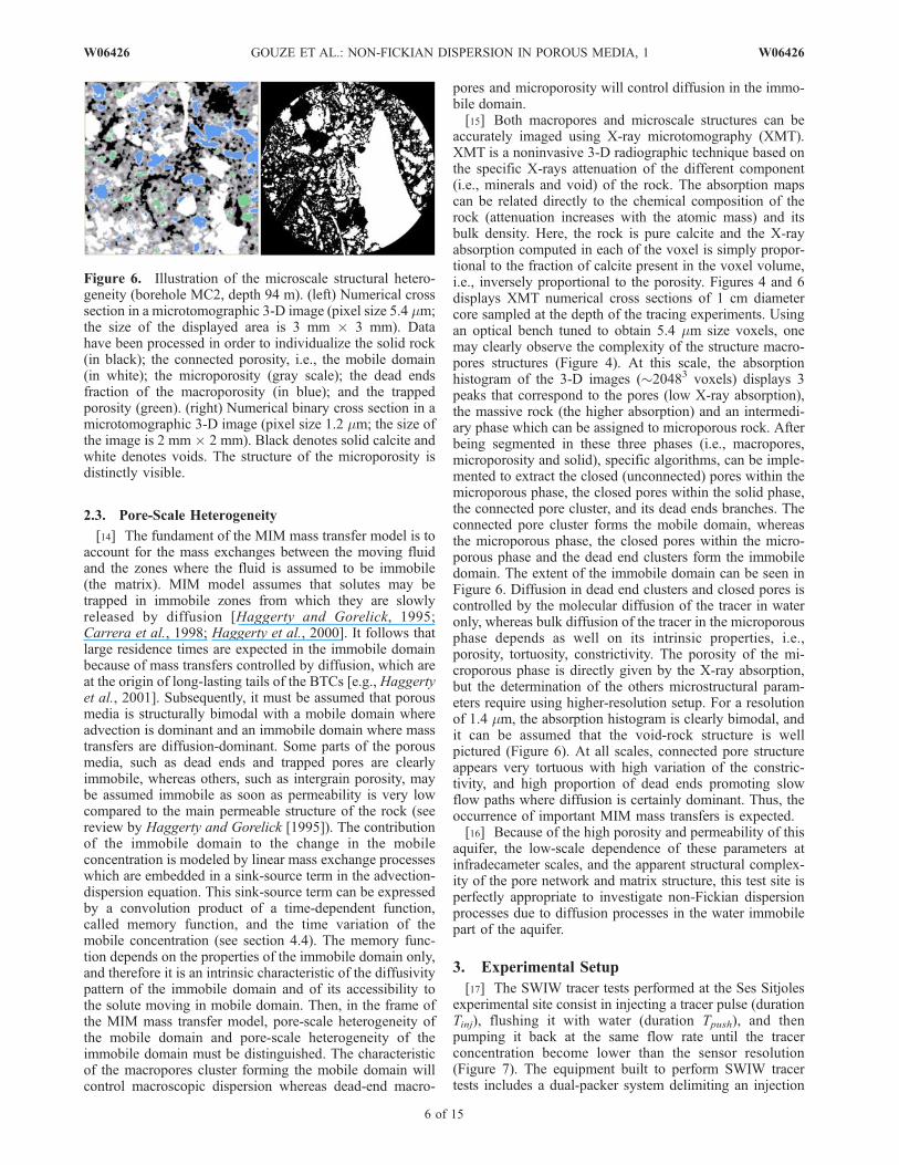
accurately imaged using X-ray microtomography (XMT).XMT is a noninvasive 3-D radiographic technique based onthe specific X-rays attenuation of the different component(i.e., minerals and void) of the rock. The absorption mapscan be related directly to the chemical composition of therock (attenuation increases with the atomic mass) and itsbulk density. Here, the rock is pure calcite and the X-rayabsorption computed in each of the voxel is simply propor-tional to the fraction of calcite present in the voxel volume,i.e., inversely proportional to the porosity. Figures 4 and 6displays XMT numerical cross sections of 1 cm diametercore sampled at the depth of the tracing experiments. Usingan optical bench tuned to obtain 5.4 mm size voxels, onemay clearly observe the complexity of the structure macro-pores structures (Figure 4). At this scale, the absorptionhistogram of the 3-D images (�20483 voxels) displays 3peaks that correspond to the pores (low X-ray absorption),the massive rock (the higher absorption) and an intermedi-ary phase which can be assigned to microporous rock. Afterbeing segmented in these three phases (i.e., macropores,microporosity and solid), specific algorithms, can be imple-mented to extract the closed (unconnected) pores within themicroporous phase, the closed pores within the solid phase,the connected pore cluster, and its dead ends branches. Theconnected pore cluster forms the mobile domain, whereasthe microporous phase, the closed pores within the micro-porous phase and the dead end clusters form the immobiledomain. The extent of the immobile domain can be seen inFigure 6. Diffusion in dead end clusters and closed pores iscontrolled by the molecular diffusion of the tracer in wateronly, whereas bulk diffusion of the tracer in the microporousphase depends as well on its intrinsic properties, i.e.,porosity, tortuosity, constrictivity. The porosity of the mi-croporous phase is directly given by the X-ray absorption,but the determination of the others microstructural param-eters require using higher-resolution setup. For a resolutionof 1.4 mm, the absorption histogram is clearly bimodal, andit can be assumed that the void-rock structure is wellpictured (Figure 6). At all scales, connected pore structureappears very tortuous with high variation of the constric-tivity, and high proportion of dead ends promoting slowflow paths where diffusion is certainly dominant. Thus, theoccurrence of important MIM mass transfers is expected.[16] Because of the high porosity and permeability of this

aquifer, the low-scale dependence of these parameters atinfradecameter scales, and the apparent structural complex-ity of the pore network and matrix structure, this test site isperfectly appropriate to investigate non-Fickian dispersionprocesses due to diffusion processes in the water immobilepart of the aquifer.

3. Experimental Setup

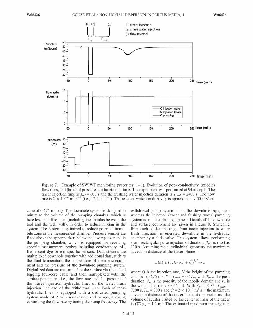
[17] The SWIW tracer tests performed at the Ses Sitjolesexperimental site consist in injecting a tracer pulse (durationTinj), flushing it with water (duration Tpush), and thenpumping it back at the same flow rate until the tracerconcentration become lower than the sensor resolution(Figure 7). The equipment built to perform SWIW tracertests includes a dual-packer system delimiting an injection

Figure 6. Illustration of the microscale structural hetero-geneity (borehole MC2, depth 94 m). (left) Numerical crosssection in a microtomographic 3-D image (pixel size 5.4 mm;the size of the displayed area is 3 mm � 3 mm). Datahave been processed in order to individualize the solid rock(in black); the connected porosity, i.e., the mobile domain(in white); the microporosity (gray scale); the dead endsfraction of the macroporosity (in blue); and the trappedporosity (green). (right) Numerical binary cross section in amicrotomographic 3-D image (pixel size 1.2 mm; the size ofthe image is 2 mm � 2 mm). Black denotes solid calcite andwhite denotes voids. The structure of the microporosity isdistinctly visible.

6 of 15

W06426 GOUZE ET AL.: NON-FICKIAN DISPERSION IN POROUS MEDIA, 1 W06426

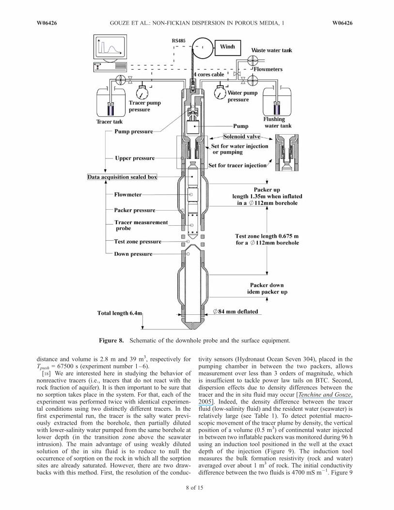
zone of 0.675 m long. The downhole system is designed tominimize the volume of the pumping chamber, which ishere less than five liters (including the annulus between thetool and the well wall), in order to reduce mixing in thesystem. The design is optimized to reduce potential immo-bile zone in the measurement chamber. Pressure sensors arefitted above the upper packer, below the lower packer and inthe pumping chamber, which is equipped for receivingspecific measurement probes including conductivity, pH,fluorescent dye or ion specific sensors. Data streams aremultiplexed downhole together with additional data, such asthe fluid temperature, the temperature of electronic equip-ment and the pressure of the downhole pumping system.Digitalized data are transmitted to the surface via a standardlogging four-core cable and then multiplexed with thesurface parameters, i.e., the flow rate and the pressure ofthe tracer injection hydraulic line, of the water flushinjection line and of the withdrawal line. Each of thesehydraulic lines is equipped with a dedicated pumpingsystem made of 2 to 3 serial-assembled pumps, allowingcontrolling the flow rate by tuning the pump frequency. The

withdrawal pump system is in the downhole equipmentwhereas the injection (tracer and flushing water) pumpingsystem is in the surface equipment. Details of the downholeand surface equipment are given in Figure 8. Switchingfrom each of the line (e.g., from tracer injection to waterflush injection) is operated downhole in the hydraulicchamber by a slide valve. This system allows performingsharp rectangular pulse injection of duration (Tinj as short as120 s. Assuming radial cylindrical geometry the maximumadvection distance of the tracer plume is

x ffi QT=2Hpfmð Þ þ r2w� �1=2�rw;

where Q is the injection rate, H the height of the pumpingchamber (0.675 m), T = Tpush + 0.5Tinj with Tpush the pushduration, fm is the porosity of the mobile domain and rw isthe well radius (here 0.056 m). With fm = 0.35, Tpush =7200 s, Tinj = 300 s and Q = 2 � 10�4 m3 s�1 the maximumadvection distance of the tracer is about one meter and thevolume of aquifer visited by the center of mass of the traceris QT/fm = 4.2 m3. The estimated maximum investigation

Figure 7. Example of SWIWT monitoring (tracer test 1–1). Evolution of (top) conductivity, (middle)flow rates, and (bottom) pressure as a function of time. The experiment was performed at 94 m depth. Thetracer injection time is Tinj = 600 s and the flushing water injection duration is Tpush = 2400 s. The flowrate is 2 � 10�4 m3 s�1 (i.e., 12 L min�1). The resident water conductivity is approximately 50 mS/cm.

W06426 GOUZE ET AL.: NON-FICKIAN DISPERSION IN POROUS MEDIA, 1

7 of 15

W06426

distance and volume is 2.8 m and 39 m3, respectively forTpush = 67500 s (experiment number 1–6).[18] We are interested here in studying the behavior of

nonreactive tracers (i.e., tracers that do not react with therock fraction of aquifer). It is then important to be sure thatno sorption takes place in the system. For that, each of theexperiment was performed twice with identical experimen-tal conditions using two distinctly different tracers. In thefirst experimental run, the tracer is the salty water previ-ously extracted from the borehole, then partially dilutedwith lower-salinity water pumped from the same borehole atlower depth (in the transition zone above the seawaterintrusion). The main advantage of using weakly dilutedsolution of the in situ fluid is to reduce to null theoccurrence of sorption on the rock in which all the sorptionsites are already saturated. However, there are two draw-backs with this method. First, the resolution of the conduc-

tivity sensors (Hydronaut Ocean Seven 304), placed in thepumping chamber in between the two packers, allowsmeasurement over less than 3 orders of magnitude, whichis insufficient to tackle power law tails on BTC. Second,dispersion effects due to density differences between thetracer and the in situ fluid may occur [Tenchine and Gouze,2005]. Indeed, the density difference between the tracerfluid (low-salinity fluid) and the resident water (seawater) isrelatively large (see Table 1). To detect potential macro-scopic movement of the tracer plume by density, the verticalposition of a volume (0.5 m3) of continental water injectedin between two inflatable packers was monitored during 96 husing an induction tool positioned in the well at the exactdepth of the injection (Figure 9). The induction toolmeasures the bulk formation resistivity (rock and water)averaged over about 1 m3 of rock. The initial conductivitydifference between the two fluids is 4700 mS m�1. Figure 9

Figure 8. Schematic of the downhole probe and the surface equipment.

8 of 15

W06426 GOUZE ET AL.: NON-FICKIAN DISPERSION IN POROUS MEDIA, 1 W06426

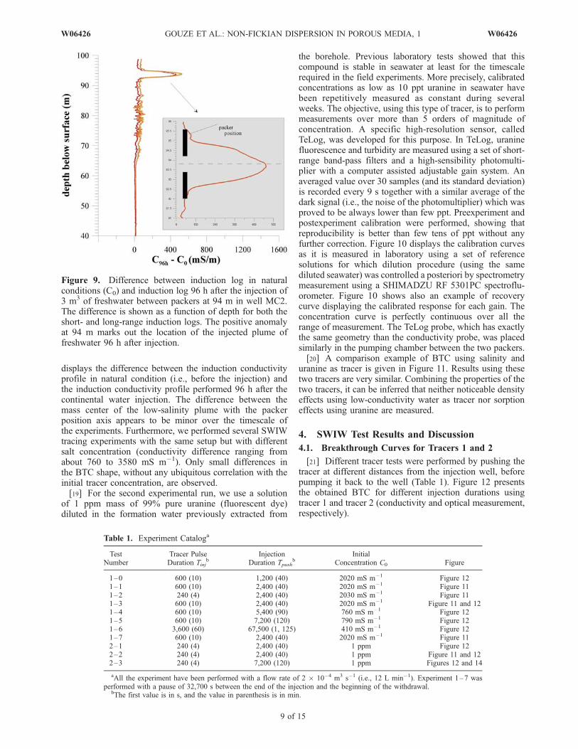
displays the difference between the induction conductivityprofile in natural condition (i.e., before the injection) andthe induction conductivity profile performed 96 h after thecontinental water injection. The difference between themass center of the low-salinity plume with the packerposition axis appears to be minor over the timescale ofthe experiments. Furthermore, we performed several SWIWtracing experiments with the same setup but with differentsalt concentration (conductivity difference ranging fromabout 760 to 3580 mS m�1). Only small differences inthe BTC shape, without any ubiquitous correlation with theinitial tracer concentration, are observed.[19] For the second experimental run, we use a solution

of 1 ppm mass of 99% pure uranine (fluorescent dye)diluted in the formation water previously extracted from

the borehole. Previous laboratory tests showed that thiscompound is stable in seawater at least for the timescalerequired in the field experiments. More precisely, calibratedconcentrations as low as 10 ppt uranine in seawater havebeen repetitively measured as constant during severalweeks. The objective, using this type of tracer, is to performmeasurements over more than 5 orders of magnitude ofconcentration. A specific high-resolution sensor, calledTeLog, was developed for this purpose. In TeLog, uraninefluorescence and turbidity are measured using a set of short-range band-pass filters and a high-sensibility photomulti-plier with a computer assisted adjustable gain system. Anaveraged value over 30 samples (and its standard deviation)is recorded every 9 s together with a similar average of thedark signal (i.e., the noise of the photomultiplier) which wasproved to be always lower than few ppt. Preexperiment andpostexperiment calibration were performed, showing thatreproducibility is better than few tens of ppt without anyfurther correction. Figure 10 displays the calibration curvesas it is measured in laboratory using a set of referencesolutions for which dilution procedure (using the samediluted seawater) was controlled a posteriori by spectrometrymeasurement using a SHIMADZU RF 5301PC spectroflu-orometer. Figure 10 shows also an example of recoverycurve displaying the calibrated response for each gain. Theconcentration curve is perfectly continuous over all therange of measurement. The TeLog probe, which has exactlythe same geometry than the conductivity probe, was placedsimilarly in the pumping chamber between the two packers.[20] A comparison example of BTC using salinity and

uranine as tracer is given in Figure 11. Results using thesetwo tracers are very similar. Combining the properties of thetwo tracers, it can be inferred that neither noticeable densityeffects using low-conductivity water as tracer nor sorptioneffects using uranine are measured.

4. SWIW Test Results and Discussion

4.1. Breakthrough Curves for Tracers 1 and 2

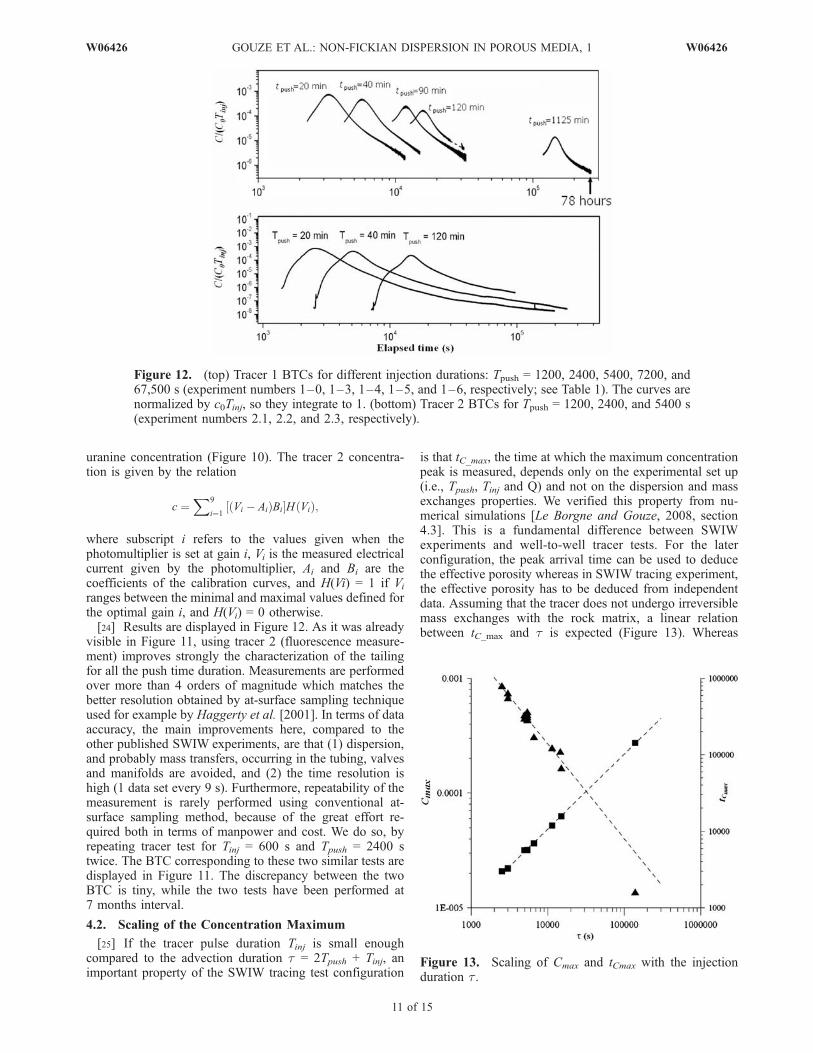
[21] Different tracer tests were performed by pushing thetracer at different distances from the injection well, beforepumping it back to the well (Table 1). Figure 12 presentsthe obtained BTC for different injection durations usingtracer 1 and tracer 2 (conductivity and optical measurement,respectively).

Figure 9. Difference between induction log in naturalconditions (C0) and induction log 96 h after the injection of3 m3 of freshwater between packers at 94 m in well MC2.The difference is shown as a function of depth for both theshort- and long-range induction logs. The positive anomalyat 94 m marks out the location of the injected plume offreshwater 96 h after injection.

Table 1. Experiment Cataloga

TestNumber

Tracer PulseDuration Tinj

bInjection

Duration Tpushb

InitialConcentration C0 Figure

1–0 600 (10) 1,200 (40) 2020 mS m–1 Figure 121–1 600 (10) 2,400 (40) 2020 mS m–1 Figure 111–2 240 (4) 2,400 (40) 2030 mS m–1 Figure 111–3 600 (10) 2,400 (40) 2020 mS m–1 Figure 11 and 121–4 600 (10) 5,400 (90) 760 mS m–1 Figure 121–5 600 (10) 7,200 (120) 790 mS m–1 Figure 121–6 3,600 (60) 67,500 (1, 125) 410 mS m–1 Figure 121–7 600 (10) 2,400 (40) 2020 mS m–1 Figure 112–1 240 (4) 2,400 (40) 1 ppm Figure 122–2 240 (4) 2,400 (40) 1 ppm Figure 11 and 122–3 240 (4) 7,200 (120) 1 ppm Figures 12 and 14

aAll the experiment have been performed with a flow rate of 2 � 10�4 m3 s�1 (i.e., 12 L min�1). Experiment 1–7 wasperformed with a pause of 32,700 s between the end of the injection and the beginning of the withdrawal.

bThe first value is in s, and the value in parenthesis is in min.

W06426 GOUZE ET AL.: NON-FICKIAN DISPERSION IN POROUS MEDIA, 1

9 of 15

W06426

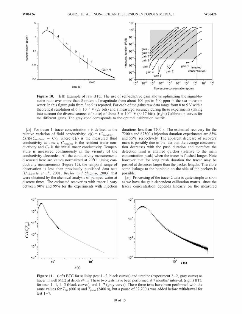
[22] For tracer 1, tracer concentration c is defined as therelative variation of fluid conductivity: c(t) = (Cresident �C(t))/(Cresident � C0), where C(t) is the measured fluidconductivity at time t, Cresident is the resident water con-ductivity and C0 is the initial tracer conductivity. Temper-ature is measured continuously in the vicinity of theconductivity electrodes. All the conductivity measurementsdiscussed here are values normalized at 20�C. Using con-ductivity measurements (Figure 12), the temporal range ofobservation is less than previously published data sets[Haggerty et al., 2001, Becker and Shapiro, 2003] thatwere obtained by the chemical analysis of pumped water atdiscrete times. The estimated recoveries with tracer 1 varybetween 90% and 99% for the experiments with injection

durations less than 7200 s. The estimated recovery for the7200 s and 67500 s injection duration experiments are 85%and 55%, respectively. The apparent decrease of recoverymass is possibly due to the fact that the average concentra-tion decreases with the push duration and therefore thedetection limit is attained quicker (relative to the mainconcentration peak) when the tracer is flushed longer. Notehowever that for long push duration the tracer may bepushed at distances larger than the packer lengths. Thereforesome leakage to the borehole on the side of the packers ispossible.[23] Processing of the tracer 2 data is quite simple as soon

as we have the gain-dependent calibration matrix, since thetracer concentration depends linearly on the measured

Figure 10. (left) Example of raw BTC. The use of self-adaptive gain allows optimizing the signal-to-noise ratio over more than 5 orders of magnitude from about 100 ppt to 500 ppm in the sea intrusionwater. In this figure gain from 3 to 9 is reported. For each of the gains raw data range from 0 to 5 V with atheoretical resolution of 6 � 10�7 V (23 bits) and a measured accuracy during these experiments (takinginto account the diverse sources of noise) of about 3 � 10�5 V (� 17 bits). (right) Calibration curves forthe different gains. The gray zone corresponds to the optimal calibration matrix.

Figure 11. (left) BTC for salinity (test 1–2, black curves) and uranine (experiment 2–2, gray curve) astracer in well MC2 at depth 94 m. These two tests have been performed at 7 months’ interval. (right) BTCfor tests 1–1, 1–3 (black curves), and 1–7 (gray curve). These three tests have been performed with thesame values for Tinj (600 s) and Tpush (2400 s), but a pause of 32,700 s was added before withdrawal fortest 1–7.

10 of 15

W06426 GOUZE ET AL.: NON-FICKIAN DISPERSION IN POROUS MEDIA, 1 W06426

uranine concentration (Figure 10). The tracer 2 concentra-tion is given by the relation

c ¼X9

i¼1Vi � Aið ÞBi½ �H Við Þ;

where subscript i refers to the values given when thephotomultiplier is set at gain i, Vi is the measured electricalcurrent given by the photomultiplier, Ai and Bi are thecoefficients of the calibration curves, and H(Vi) = 1 if Viranges between the minimal and maximal values defined forthe optimal gain i, and H(Vi) = 0 otherwise.[24] Results are displayed in Figure 12. As it was already

visible in Figure 11, using tracer 2 (fluorescence measure-ment) improves strongly the characterization of the tailingfor all the push time duration. Measurements are performedover more than 4 orders of magnitude which matches thebetter resolution obtained by at-surface sampling techniqueused for example by Haggerty et al. [2001]. In terms of dataaccuracy, the main improvements here, compared to theother published SWIW experiments, are that (1) dispersion,and probably mass transfers, occurring in the tubing, valvesand manifolds are avoided, and (2) the time resolution ishigh (1 data set every 9 s). Furthermore, repeatability of themeasurement is rarely performed using conventional at-surface sampling method, because of the great effort re-quired both in terms of manpower and cost. We do so, byrepeating tracer test for Tinj = 600 s and Tpush = 2400 stwice. The BTC corresponding to these two similar tests aredisplayed in Figure 11. The discrepancy between the twoBTC is tiny, while the two tests have been performed at7 months interval.

4.2. Scaling of the Concentration Maximum

[25] If the tracer pulse duration Tinj is small enoughcompared to the advection duration t = 2Tpush + Tinj, animportant property of the SWIW tracing test configuration

is that tC_max, the time at which the maximum concentrationpeak is measured, depends only on the experimental set up(i.e., Tpush, Tinj and Q) and not on the dispersion and massexchanges properties. We verified this property from nu-merical simulations [Le Borgne and Gouze, 2008, section4.3]. This is a fundamental difference between SWIWexperiments and well-to-well tracer tests. For the laterconfiguration, the peak arrival time can be used to deducethe effective porosity whereas in SWIW tracing experiment,the effective porosity has to be deduced from independentdata. Assuming that the tracer does not undergo irreversiblemass exchanges with the rock matrix, a linear relationbetween tC_max and t is expected (Figure 13). Whereas

Figure 12. (top) Tracer 1 BTCs for different injection durations: Tpush = 1200, 2400, 5400, 7200, and67,500 s (experiment numbers 1–0, 1–3, 1–4, 1–5, and 1–6, respectively; see Table 1). The curves arenormalized by c0Tinj, so they integrate to 1. (bottom) Tracer 2 BTCs for Tpush = 1200, 2400, and 5400 s(experiment numbers 2.1, 2.2, and 2.3, respectively).

Figure 13. Scaling of Cmax and tCmax with the injectionduration t.

W06426 GOUZE ET AL.: NON-FICKIAN DISPERSION IN POROUS MEDIA, 1

11 of 15

W06426

the scaling of tC_max is useless to identify MIM masstransfers, the scaling of the maximal concentration Cmax

with the advection duration t may be used to get a firstinsight into the overall dispersion and to determine non-Fickian behaviors since a deficit of mass at the peak time isexpected if BTCs display heavy tailing. Numerical experi-ments [Le Borgne and Gouze, 2008, Figure 7] show that, forSWIW configuration, Cmax is expected to decrease as apower law of time: Cmax �t�b(with t Tinj) in the case ofthe MIM mass transfer model. The value of b is character-istic of the transfer rate distribution in the immobile domain[Le Borgne and Gouze, 2008]. The comparison of themeasured Cmaxt values with the power law trends showsthat a noticeable deviation is observed for the largestinjection time (Figure 13). The origin of this lower valueof Cmax will be discussed by Le Borgne and Gouze [2008].

4.3. Late Time Behavior of the BTCs

[26] Many examples of in situ [Adams and Gelhar, 1992;Meigs and Beauheim, 2001; Becker and Shapiro, 2003] andlaboratory [Silliman and Simpson, 1987; Berkowitz et al.,2000; Levy and Berkowitz, 2003] tracer tests display stronglyasymmetric BTCs with long tails similar to ours, indicatingthe occurrence of non-Fickian dispersion processes. Gener-ally, the late time BTC appears to decrease more or less as apower law of time C(t) � t�aand is explained by theclassical MIM mass transfer model. In particular, SWIWexperiments have been discussed by Haggerty et al. [2001](WIPP site) and Becker and Shapiro [2003]. Both theseauthors obtained BTC with a late time slope (–a) with a �2, whereas we observed late time slope that converges tovalues closer to those expected from the conventionaldouble-porosity model (a = 1.5). While Haggerty et al.[2001] interpret their results by MIM mass transfer model,implying that non-Fickian BTC arises from small-scalemultirate mass transfers with the immobile domain, Beckerand Shapiro [2003] proposed that the origin of the observedlate time slope is due to large-scale correlations of thevelocity field which could be modeled by a stream tube

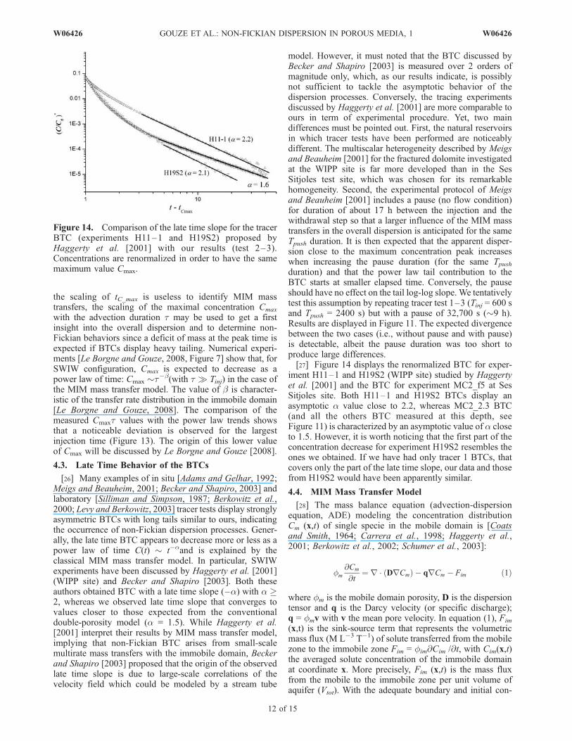
model. However, it must noted that the BTC discussed byBecker and Shapiro [2003] is measured over 2 orders ofmagnitude only, which, as our results indicate, is possiblynot sufficient to tackle the asymptotic behavior of thedispersion processes. Conversely, the tracing experimentsdiscussed by Haggerty et al. [2001] are more comparable toours in term of experimental procedure. Yet, two maindifferences must be pointed out. First, the natural reservoirsin which tracer tests have been performed are noticeablydifferent. The multiscalar heterogeneity described by Meigsand Beauheim [2001] for the fractured dolomite investigatedat the WIPP site is far more developed than in the SesSitjoles test site, which was chosen for its remarkablehomogeneity. Second, the experimental protocol of Meigsand Beauheim [2001] includes a pause (no flow condition)for duration of about 17 h between the injection and thewithdrawal step so that a larger influence of the MIM masstransfers in the overall dispersion is anticipated for the sameTpush duration. It is then expected that the apparent disper-sion close to the maximum concentration peak increaseswhen increasing the pause duration (for the same Tpushduration) and that the power law tail contribution to theBTC starts at smaller elapsed time. Conversely, the pauseshould have no effect on the tail log-log slope. We tentativelytest this assumption by repeating tracer test 1–3 (Tinj = 600 sand Tpush = 2400 s) but with a pause of 32,700 s (�9 h).Results are displayed in Figure 11. The expected divergencebetween the two cases (i.e., without pause and with pause)is detectable, albeit the pause duration was too short toproduce large differences.[27] Figure 14 displays the renormalized BTC for exper-

iment H11–1 and H19S2 (WIPP site) studied by Haggertyet al. [2001] and the BTC for experiment MC2_f5 at SesSitjoles site. Both H11–1 and H19S2 BTCs display anasymptotic a value close to 2.2, whereas MC2_2.3 BTC(and all the others BTC measured at this depth, seeFigure 11) is characterized by an asymptotic value of a closeto 1.5. However, it is worth noticing that the first part of theconcentration decrease for experiment H19S2 resembles theones we obtained. If we have had only tracer 1 BTCs, thatcovers only the part of the late time slope, our data and thosefrom H19S2 would have been apparently similar.

4.4. MIM Mass Transfer Model

[28] The mass balance equation (advection-dispersionequation, ADE) modeling the concentration distributionCm (x,t) of single specie in the mobile domain is [Coatsand Smith, 1964; Carrera et al., 1998; Haggerty et al.,2001; Berkowitz et al., 2002; Schumer et al., 2003]:

fm

@Cm

@t¼ r � DrCmð Þ � qrCm � Fim ð1Þ

where fm is the mobile domain porosity, D is the dispersiontensor and q is the Darcy velocity (or specific discharge);q = fmv with v the mean pore velocity. In equation (1), Fim

(x,t) is the sink-source term that represents the volumetricmass flux (M L�3 T�1) of solute transferred from the mobilezone to the immobile zone Fim = fim@Cim /@t, with Cim(x,t)the averaged solute concentration of the immobile domainat coordinate x. More precisely, Fim (x,t) is the mass fluxfrom the mobile to the immobile zone per unit volume ofaquifer (Vtot). With the adequate boundary and initial con-

Figure 14. Comparison of the late time slope for the tracerBTC (experiments H11–1 and H19S2) proposed byHaggerty et al. [2001] with our results (test 2–3).Concentrations are renormalized in order to have the samemaximum value Cmax.

12 of 15

W06426 GOUZE ET AL.: NON-FICKIAN DISPERSION IN POROUS MEDIA, 1 W06426

ditions, equation (1) expresses the mass conservation bal-ance in time and space. The immobile domain correspondsto portions of aquifer where flow is negligible compared towhat exists in the mobile domain; it then includes thefraction of solid containing connected microporosity orintergrains porosity as well as stagnant water in dead ends[Haggerty and Gorelick, 1995]. If the mean microporosityof the immobile domain is fim

0, then fim= (1 � fm)fim0.

Note that in the most general case, fim and fm aredistributed values, but we will consider here that this valuesare constants over the volume of rock visited by the tracer.For linear mass transfer processes, such as diffusive masstransfer, Fim may be expressed as a convolution product[Carrera et al., 1998; Haggerty et al., 2000; Dentz andBerkowitz, 2003]:

Fim x; tð Þ ¼Z t

t0¼0

@Cm x; t � t0ð Þ@t

G t0ð Þdt0 ¼ @Cm x; tð Þ@t

*G x; tð Þ ð2Þ

where notation ‘*’ refers to the convolution product, G[T�1] is the memory function which contains all theinformation about the mass transfer process, the geometryand the volume fraction of the immobile domain and itsaccessibility to the tracer particle issued from the mobiledomain. The memory function G(t) denotes the probabilitydensity that a tracer particle entering the immobile zone att = 0 remains in it at time t.[29] For weakly variable velocity field, such as implied

by the Fickian dispersion model in the mobile domain, anapproximation of the tracer concentration for late time Cm�lt

(t) is given by Haggerty et al. [2000] for Cm (x,t = 0) = 0:

Cm�lt � �tadC0tinj@G

@t; tad � t � tres ð3Þ

where C0 is the pulse concentration at t = 0 and tinj theduration of the pulse and tad is the average advectiveresidence time of the solute moving from the input to thean observation location xobs: tad = xobs/v. Indeed, at late time,i.e., as the concentration pulse has moved far past the

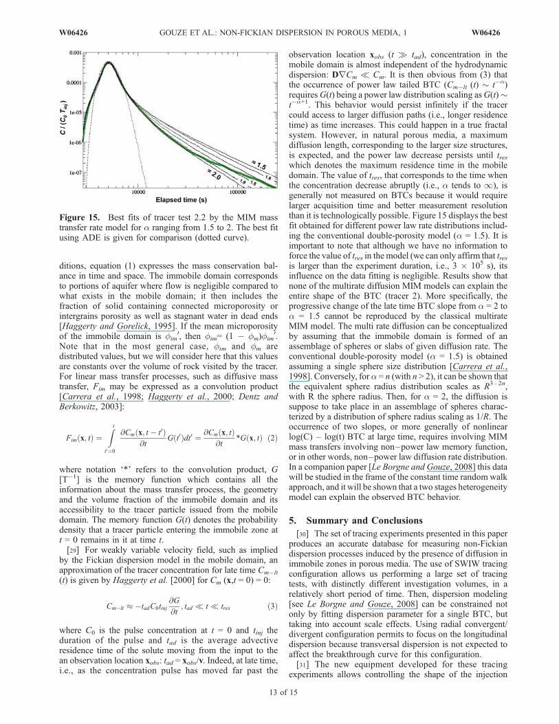
observation location xobs (t tad), concentration in themobile domain is almost independent of the hydrodynamicdispersion: DrCm � Cm. It is then obvious from (3) thatthe occurrence of power law tailed BTC (Cm�lt (t) � t�a)requiresG(t) being a power law distribution scaling asG(t)�t�a+1. This behavior would persist infinitely if the tracercould access to larger diffusion paths (i.e., longer residencetime) as time increases. This could happen in a true fractalsystem. However, in natural porous media, a maximumdiffusion length, corresponding to the larger size structures,is expected, and the power law decrease persists until treswhich denotes the maximum residence time in the mobiledomain. The value of tres, that corresponds to the time whenthe concentration decrease abruptly (i.e., a tends to 1), isgenerally not measured on BTCs because it would requirelarger acquisition time and better measurement resolutionthan it is technologically possible. Figure 15 displays the bestfit obtained for different power law rate distributions includ-ing the conventional double-porosity model (a = 1.5). It isimportant to note that although we have no information toforce the value of tres in the model (we can only affirm that tresis larger than the experiment duration, i.e., 3 � 105 s), itsinfluence on the data fitting is negligible. Results show thatnone of the multirate diffusion MIM models can explain theentire shape of the BTC (tracer 2). More specifically, theprogressive change of the late time BTC slope from a = 2 toa = 1.5 cannot be reproduced by the classical multirateMIM model. The multi rate diffusion can be conceptualizedby assuming that the immobile domain is formed of anassemblage of spheres or slabs of given diffusion rate. Theconventional double-porosity model (a = 1.5) is obtainedassuming a single sphere size distribution [Carrera et al.,1998]. Conversely, fora = n (with n > 2), it can be shown thatthe equivalent sphere radius distribution scales as R3–2n,with R the sphere radius. Then, for a = 2, the diffusion issuppose to take place in an assemblage of spheres charac-terized by a distribution of sphere radius scaling as 1/R. Theoccurrence of two slopes, or more generally of nonlinearlog(C) – log(t) BTC at large time, requires involving MIMmass transfers involving non–power law memory function,or in other words, non–power law diffusion rate distribution.In a companion paper [Le Borgne and Gouze, 2008] this datawill be studied in the frame of the constant time random walkapproach, and it will be shown that a two stages heterogeneitymodel can explain the observed BTC behavior.

5. Summary and Conclusions

[30] The set of tracing experiments presented in this paperproduces an accurate database for measuring non-Fickiandispersion processes induced by the presence of diffusion inimmobile zones in porous media. The use of SWIW tracingconfiguration allows us performing a large set of tracingtests, with distinctly different investigation volumes, in arelatively short period of time. Then, dispersion modeling[see Le Borgne and Gouze, 2008] can be constrained notonly by fitting dispersion parameter for a single BTC, buttaking into account scale effects. Using radial convergent/divergent configuration permits to focus on the longitudinaldispersion because transversal dispersion is not expected toaffect the breakthrough curve for this configuration.[31] The new equipment developed for these tracing

experiments allows controlling the shape of the injection

Figure 15. Best fits of tracer test 2.2 by the MIM masstransfer rate model for a ranging from 1.5 to 2. The best fitusing ADE is given for comparison (dotted curve).

W06426 GOUZE ET AL.: NON-FICKIAN DISPERSION IN POROUS MEDIA, 1

13 of 15

W06426

pulse (i.e., rectangular injection, with very small durationsso that it approaches dirac injection). For both tracers,measurements are performed directly in the pumping cham-ber, minimizing strongly the dispersion in the tubing whichsuperimposes onto the reservoir dispersion when measuringthe tracer concentration with surface equipments. Further-more, measurements are performed continuously: one dataevery 9 s, each of them representing the average of 30 dataacquisitions. Finally, to overcome flow rate variationsinduced by fluctuations of the borehole skin effect, forinstance because of fine particles accumulation in the wellannulus during withdrawal phase, the flow rate is automat-ically maintained constant whatever the pressure fluctua-tions are.[32] The combination of two tracers, for which measure-

ment techniques are distinct (conductivity measurement andoptical measurement), allows us verifying the pertinence ofthe experimental procedure. More specifically, this method-ology is implemented for verifying that the tracers behaveas passive tracers and that density effects do not induceperturbations on the BTCs. The use of fluorescent dye astracer (tracer 2) in seawater has proved to be practical andallows accurate measurements up to 5 orders of magnitudeon the concentration during the recovery phase. Massrecovery for tracer 2 is always close to 1 showing that (1)tracer is chemically conservative; (2) no mass loss due toleak along the packers is encountered during the tracer testsexcept for test 1–6 (Tpush = 67500 s) for which it isexpected that the maximal tracer penetration distanceexceeds the length of the packers; (3) the tracer tests allowmeasuring the almost complete dispersion behavior and (4)the tracer experiment in SWIW mode permits to cancelreversible dispersion, i.e., the effect of long-range velocitycorrelation that could exist because of preferential flowpath.[33] Recorded BTCs do not show a linear late time log-

log slope as it is predicted by the conventional MIM masstransfer model. The first part of the late time slope displaysa gradual decrease of the concentration which could havebeen fitted almost satisfactory with a MIM model charac-terized by a = 2. Indeed, using the tracer 1 data only, thismisinterpretation could have been done. The second part ofthe late time BTC shows a clear asymptotic behavior towarda = 1.5. This seems to indicate that a double-porositybehavior take place when the tracer visit immobile domaina large size and/or low diffusivity, or in other words, that afraction of the immobile domain is made of homogeneouslarge size and/or low diffusivity structure. This wouldexplain the departure from the linear relation between log(Cmax) and log (t) for large values of t (Figure 13). Thisassumption will be studied in a companion paper Le Borgneand Gouze [2008]. Determining the origin of this anoma-lous behavior, compared to the conventional MIM masstransfer model, requires a better characterization of theimmobile domain characteristics including the diffusivityheterogeneity and the accessibility of the immobile domainto the tracer moving in the mobile domain. A simpleobservation of the microstructures (e.g., Figures 4 and 6)shows that modeling the complexity of the diffusion path bya simple power law distribution of diffusion rates is prob-ably unrealistic. This investigation will be presented in aforthcoming paper.

[34] Acknowledgments. This work was funded by the Europeanproject ‘‘ALIANCE’’ (Advanced Logging Investigations in Coastal Envi-ronments, contract EKV-2001-00039). All the members of the ALIANCEteam are gratefully acknowledged for their support, as well as C. Gonzalezand A. Baron of the Ministry of Environment of the Balearic IslandsGovernment.

ReferencesAdams, A. E., and L. W. Gelhar (1992), Field study of dispersion in aheterogeneous aquifer: 2. Spatial moments analysis, Water Resour.Res., 28(12), 3293–3307.

Becker, M. W., and A. M. Shapiro (2003), Interpreting tracer breakthroughtailing from different forced-gradient tracer experiment configurations infractured bedrock, Water Resour. Res., 39(1), 1024, doi:10.1029/2001WR001190.

Benson, D. A., R. Schumer, M. M. Meerschaert, and S. W. Wheatcraft(2001), Fractional dispersion, Levy motion, and the MADE tracer tests,Transp. Porous Media, 42, 211–240, doi:10.1023/A:1006733002131.

Berkowitz, B., H. Scher, and S. E. Silliman (2000), Anomalous transport inlaboratory-scale, heterogeneous porous media,Water Resour. Res., 36(1),149–158, doi:10.1029/1999WR900295.

Berkowitz, B., J. Klafter, R. Metzler, and H. Scher (2002), Physical picturesof transport in heterogeneous media: Advection-dispersion, random-walk, and fractional derivative formulations, Water Resour. Res.,38(10), 1191, doi:10.1029/2001WR001030.

Bernard, D., Ø. Nielsen, L. Salvo, and P. Cloetens (2005), Permeabilityassessment by 3D interdendritic flow simulations on microtomographymappings of Al-Cu alloys, Mater. Sci. Eng. A, 392(1–2), 112–120,doi:10.1016/j.msea.2004.09.004.

Carrera, J., X. Sanchez-Vila, I. Benet, A. Medina, G. Galarza, and J. Gimera(1998), On matrix diffusion: Formulations, solution methods and quali-tat ive effects, Hydrogeol. J. , 6(1), 178 – 190, doi:10.1007/s100400050143.

Coats, K. H., and B. D. Smith (1964), Dead end pore volume and dispersionin porous media, SPEJ Soc. Pet. Eng. J., 4, 73–84, doi:10.2118/647-PA.

Dentz, M., and B. Berkowitz (2003), Transport behavior of a passive solutein continuous time random walks and multirate mass transfer, WaterResour. Res., 39(5), 1111, doi:10.1029/2001WR001163.

Gelhar, L. W., and M. A. Collins (1971), General analysis of longitudinaldispersion in nonuniform flow, Water Resour. Res., 7(6), 1511–1521,doi:10.1029/WR007i006p01511.

Gylling, B., L. Moreno, and I. Neretnieks (1999), The Channel NetworkModel—A tool for transport simulation in fractured media, GroundWater, 37(3), 367–375, doi:10.1111/j.1745-6584.1999.tb01113.x.

Haggerty, R., and S. M. Gorelick (1995), Multiple-rate mass transfer formodeling diffusion and surface reactions in media with pore-scale het-erogeneity, Water Resour. Res., 31(10), 2383–2400.

Haggerty, R., S. A. McKenna, and L. C. Meigs (2000), On the late-timebehavior of tracer test breakthrough curves, Water Resour. Res., 36(12),3467–3480, doi:10.1029/2000WR900214.

Haggerty, R. S., S. W. Fleming, L. C. Meigs, and S. A. McKenna (2001),Tracer tests in a fractured dolomite: 2. Analysis of mass transfer insingle-well injection-withdrawal tests, Water Resour. Res., 37(5),1129–1142, doi:10.1029/2000WR900334.

Jaeggi, D. (2006), Multiscalar porosity structure of a miocene reefal carbo-nate complex, Ph.D. dissertation, Naturwiss., Eidg. Tech. Hochsch. ETHZurich, Zurich, Switzerland.

Khrapitchev, A. A., and P. T. Callaghan (2003), Reversible and irreversibledispersion in a porous medium, Phys. Fluids, 15, 2649 – 2660,doi:10.1063/1.1596914.

Le Borgne, T., and P. Gouze (2008), Non-Fickian dispersion in porousmedia: 2. Model validation from measurements at different scales, WaterResour. Res., 44, W06427, doi:10.1029/2007WR006279.

Le Borgne, T., J.-R. de Dreuzy, P. Davy, and O. Bour (2007), Characteriza-tion of the velocity field organization in heterogeneous media by condi-tional correlation, Water Resour. Res., 43, W02419, doi:10.1029/2006WR004875.

Levy, M., and B. Berkowitz (2003), Measurement and analysis of non-Fickian dispersion in heterogeneous porous media, J. Contam. Hydrol.,64(3–4), 203–226, doi:10.1016/S0169-7722(02)00204-8.

Lods, G., and P. Gouze (2004), WTFM, a software for well tests analysis infractured media combining fractional flow with double porosity and lea-kance, Comput. Geosci., 30, 937–947, doi:10.1016/j.cageo.2004.06.003.

Meigs, L. C., and R. L. Beauheim (2001), Tracer tests in fractured dolomite:1. Experimental design and observed tracer recoveries, Water Resour.Res., 37(5), 1113–1128, doi:10.1029/2000WR900335.

14 of 15

W06426 GOUZE ET AL.: NON-FICKIAN DISPERSION IN POROUS MEDIA, 1 W06426

Noiriel, C., D. Bernard, P. Gouze, and X. Thibault (2005), Hydraulic proper-ties andmicrogeometry evolution in the course of limestone dissolution byCO2-enriched water, Oil Gas Sci. Technol., 60(1), 177–192, doi:10.2516/ogst:2005011.

Pomar, L. W. C., and C. Ward (1999), Reservoir-scale hetrogeneity indepositional packages and diagenetic patterns on a reef-rimmed platform,Upper Miocene, Mallorca, Spain, AAPG Bull., 83, 1759–1773.

Schumer, R., D. A. Benson, M. M. Meerschaert, and B. Baeumer (2003),Fractal mobile/immobile solute transport, Water Resour. Res., 39(10),1296, doi:10.1029/2003WR002141.

Silliman, S. E., and E. S. Simpson (1987), Laboratory evidence of the scaleeffect in dispersion of solutes in porous media,Water Resour. Res., 23(8),1667–1673, doi:10.1029/WR023i008p01667.

Tenchine, S., and P. Gouze (2005), Density contrast effects on tracer dis-persion in variable aperture fractures, Adv. Water Resour., 28(3), 273–289, doi:10.1016/j.advwatres.2004.10.009.

Tsang, Y. W. (1995), Study of alternative tracer tests in characterizingtransport in fractured rocks, Geophys. Res. Lett., 22(11), 1421–1424,doi:10.1029/95GL01093.

����������������������������P. Gouze, R. Leprovost, G. Lods, P. Pezard, and T. Poidras, Geosciences,

UMR 5243, Universite de Montpellier 2, CNRS, F-5243, Montpellier,France.

T. Le Borgne, Geosciences Rennes, UMR 6118, Universite de Rennes 1,CNRS, F-35042, Rennes, France. (tanguy.le-borgne@univ.rennes1.fr)

W06426 GOUZE ET AL.: NON-FICKIAN DISPERSION IN POROUS MEDIA, 1

15 of 15

W06426