No evidence for strong fields during the R3–N3 Icelandic geomagnetic reversal

ELSEVIER Earth and Planetary Science Letters 167 (1999) 15–34

No evidence for strong fields during the R3–N3 Icelandic geomagneticreversal

A.T. Goguitchaichvili Ł, M. Prevot, P. Camps

Laboratoire de Geophysique et Tectonique, CNRS and Universite de Montpellier 2, 1, Place Eugene Bataillon, Case 60,34095 Montpellier cedex 05, France

Received 28 August 1998; revised version received 21 December 1998; accepted 9 January 1999

Abstract

A previous study of the R3–N3 Icelandic reversal, which corresponds probably to the Matuyama–Reunion reversal,provided relatively large virtual dipole moments when the pole is close to equator. To check these former results, obtainedusing the Shaw paleointensity method, we resampled the very same sections and flows and reanalysed the samples usingthe Thellier method. 38 lava units (and one baked horizon) from 4 sections provide intermediate R3–N3 paleofielddirections. Most of them, possibly related to a single eruption, display similar directions corresponding to the near equatorVGP cluster. Unfortunately, most of the intermediate lava flows are thermally unstable, as attested by the irreversibilityof the susceptibility versus temperature (k–T) curves, which precludes their use for paleointensity purpose. The rest ofthe units provide fairly reversible k–T curves and a near magnetite Tc due to Fe-rich titanomagnetite resulting fromoxyexsolution at high temperature. 25 baked units or lava flows of this kind yield reliable Thellier paleointensity data.Average paleostrengths of 44:7š 14:9 µT and 32:5š 22:9 µT were found for the reversed R3 and the normal N3 polarityzones, respectively. Combining these non-transitional paleostrengths with other Thellier data from over the world indicatesthat the Pliocene dipole moment was close to 8 ð 1022 A m2. The average paleostrength is reduced to 11:3 š 3:0 µTduring the R3–N3 transition. We find no indication for the ‘strong fields’ (20.4 to 38.6 µT) previously obtained by theShaw method. Thus our results do not confirm the existence of large virtual dipole moments when the pole approaches theequator. 1999 Elsevier Science B.V. All rights reserved.

Keywords: magnetic field; reversals; paleomagnetism; intensity; Iceland

1. Introduction

The field paleostrength during geomagnetic rever-sals is an important feature of the geodynamo. Assedimentary rocks have the disadvantage of provid-ing only relative paleointensity and also smoothingthe geomagnetic field variations during recording,the most reliable data are obtained from volcanic

Ł Corresponding author. Fax: C33 467 523908;E-mail: [email protected]

sequences. There is general agreement that typicallythe transitional field is largely reduced with respectto the ‘stable’ (non-reversing) field. Van Zijl et al.,[1] were the first to document this point using atotal TRM (thermoremanent magnetization) method.These authors found that the magnitude of the pa-leofield decreased by approximately a factor of fiveduring the Early Jurassic reversal recorded by theStromberg volcanics. Using a variant of van Zijl’smethod, Lawley [2] found that icelandic Tertiarylava flows recording polarity transitions or geomag-

0012-821X/99/$ – see front matter 1999 Elsevier Science B.V. All rights reserved.PII: S 0 0 1 2 - 8 2 1 X ( 9 9 ) 0 0 0 1 0 - 2

16 A.T. Goguitchaichvili et al. / Earth and Planetary Science Letters 167 (1999) 15–34

netic excursions provide a mean paleointensity about10 times less than that previously found [3] for theaverage Neogene stable field. Because total TRM pa-leointensity methods have some obvious drawbacks[4], more recent studies of reversals [5,6] used themore reliable paleointensity method of Thellier andThellier [4]. These studies confirmed that the fieldmagnitude is much smaller during the transition. Inthe best documented record (Steens Mountain rever-sal), the average paleointensity during the transitionwas found to be 4–5 times less than that of the sta-ble Miocene field [5]. Somewhat similar conclusionswere reached in a more indirect way by studying theintensity of the cleaned remanence of large numbersof volcanic flows in Iceland [7–9], in Polynesia [6]or in various regions of the world [10]. In all cases,it was concluded that the local field intensity (or vir-tual dipole moment, VDM) decreases rapidly as thefield paleodirection (or Virtual Geomagnetic Pole,VGP, position) deviates from that of the axial dipoledirection (or geographic axis).

In this context, a surprising paleointensity resultwas reported by Shaw [11] from his study of theR3–N3 geomagnetic reversal from South WesternIceland (Hvalfjordur-Esja area). Most of the transi-tional directions of the R3–N3 reversal correspondto a cluster of near equatorial VGPs [12] which,according to Shaw, might reflect some standstill ofthe geomagnetic field. Using his own paleointensitymethod Shaw found that during this assumed stand-still of the field in a transitional state, the VDMincreases to values similar to those of the pre andpost-transitional values. This result led him to pro-pose that the geomagnetic field could have a thirdmetastable state. The purpose of the work reportedhere was to check the validity of Shaw’s paleoin-tensity data through an extensive resampling of theN3–R3 reversal and new measurements using thealternative Thellier method of paleointensity deter-mination.

2. Geology and previous work

The Hvalfjordur-Esja area in Southwest part ofIceland (¾50 km East from Reykjavik, Fig. 1),mostly consists of several hundreds lava flows oftholeiitic basalt of Plio-Pleistocene age (about 3.5

Ma to present), with no major break in volcanicactivity in the time interval of 2.8–1.8 Ma [13,14].Radiometric dates from these lava flows are veryscare and generally of low reliability [15,16]. Con-sequently, paleomagnetism has been an essentialtool for deciphering the stratigraphy of this vol-canic sequence [17]. Einarsson’s [17] magnetic po-larity zone N4 was recently assigned to the Gaussgeomagnetic epoch [18]. Thus, the N4–R3 transi-tion would represent the Gauss–Matuyama reversal,while the R3–N3 boundary would correspond tothe Matuyama=Reunion boundary, recently dated at2:07š 0:02 [19].

Previous paleomagnetic data about the R3–N3transition were obtained by Sigurgeirsson [12], Wil-son et al.’s [19] and Kristjanson et al. [16]. The mostdetailed paleodirectional study was carried out byKristjansson and Sigurgeirsson [18] who restudiedall significant transitional sites known so far, includ-ing Shaw’s sites. Our own sampling strategy waslargely based on their results.

3. Sampling

We sampled 5 sections in the Hvalfjordur-Esjaarea near Reykjavik (Fig. 1). We made an effort tosample all of Shaw’s sections and especially the tran-sitional lava flows suspected to record large VDMs.For this search, we benefited from the field notes ofShaw and Kristjansson. For several units we wereable to find 25-year old paleomagnetic holes, andin such cases we could drill the very same blockas Shaw did. In total about 670 oriented cores be-longing to 120 units were sampled: 114 units aretypical continental basaltic lava flows; 1 is a thindike; and 5 are reddish baked horizons (paleosolsor sediments) interbedded between flows. The latterunits are usually good material for Thellier pale-ointensity experiments. Flow contacts are in mostcases clearly distinguishable. We drilled typically 5–9 cores per volcanic unit. Cores were obtained witha gasoline-powered portable drill, and then orientedin most cases using both magnetic compass and sunshadow.

The sections which record the R3–N3 transition(FL, HU, PV and KY) are within 5–6 km from eachother (Fig. 1). Their magnetostratigraphic succession

A.T. Goguitchaichvili et al. / Earth and Planetary Science Letters 167 (1999) 15–34 17

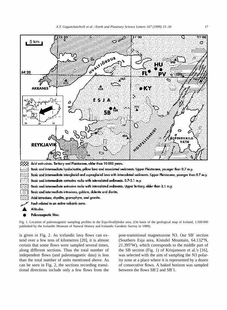
Fig. 1. Location of paleomagnetic sampling profiles in the Esja-Hvalfjordur area. (On basis of the geological map of Iceland, 1:500 000published by the Icelandic Museum of Natural History and Icelandic Geodetic Survey in 1989).

is given in Fig. 2. As icelandic lava flows can ex-tend over a few tens of kilometres [20], it is almostcertain that some flows were sampled several times,along different sections. Thus the total number ofindependent flows (and paleomagnetic data) is lessthan the total number of units mentioned above. Ascan be seen in Fig. 2, the sections recording transi-tional directions include only a few flows from the

post-transitional magnetozone N3. Our SB0 section(Southern Esja area, Kistufel Mountain, 64.132ºN,21.395ºW), which corresponds to the middle part ofthe SB section (Fig. 1) of Krisjansson et al.’s [16],was selected with the aim of sampling the N3 polar-ity zone at a place where it is represented by a dozenof consecutive flows. A baked horizon was sampledbetween the flows SB02 and SB01.


Fig. 2. Magnetostratigraphy of the Northern Esja volcanic sections. The altitudes and approximate flow thickness are indicated togetherwith the unit label. TEq: Intermediate polarity flows corresponding to the near equatorial VGP cluster. TR: Intermediate polarity flowsdistinct from this cluster. BH: Baked horizon (sediment or volcano-sedimentary unit).


According to Shaw (pers. commun.), the mainevidence (3 data from a total of 4) for large VDMsduring the R3–N3 transition came from 3 flows atsection HU. The comparison of our field observa-tions and paleomagnetic data with unpublished datafrom Shaw (personal communication) leads us tobelieve that these 3 flows correspond to our unitsHU11, HU12 and HU14. No flow can have beenmissed by us in this part of section where outcrop iscontinuous.

4. Curie temperatures and thermomagneticcurves in low fields

Low-field susceptibility versus temperature mea-surements (k–T curves) were performed in vacuum(<10�2 mbar) using a modified Bartington appa-ratus. At least one sample per unit was progres-sively heated up to generally 650ºC and subse-quently cooled at a rate of 5º=min. Curie temper-atures were determined following the method de-scribed by Prevot et al. [21]. We defined three typesof k–T curves which are illustrated in Fig. 3.

Type A curves are reasonably reversible (Fig. 3,samples 96G141D and 97G175C) and show a singlemagnetic phase with Tc between 550ºC and 585ºC,suggestive of almost pure magnetite. The baked hori-zons belong to that type (Fig. 3, sample 97G224C)but display a decrease of initial susceptibility upto 200ºC which is probably due to the presence ofsuperparamagnetic particles. The reversible curvesand high Tc, quite encouraging for paleointensitystudies, were observed for about 40% of our col-lection including all baked horizons. These samplescome mostly from the R3 magnetozone and from thetransitional sequence of the PV section.

The lower part of Fig. 3 illustrates the irreversibleand more complex thermomagnetic behaviour ob-served for most (60%) of units and correspondingto types B or C. Those types are commonly foundin the KY and SB0 sections and the transitionalsequence of the HU section. Two or even three dif-ferent magnetic phases could be recognized duringheating (in sample 97G190B for example). It is notalways sure, however, that these magnetic phaseswere all pre-existent to the laboratory heating. TypeB is characterized by a magnetic mineral with Tc in

the range 200ºC to 300ºC and a k–T curve reversibleup to 300ºC to 400ºC (e.g. sample 96G057C). Themagnetic phase is probably a Ti-rich titanomagnetite.In type C, the mineral with low Tc seems to disap-pear completely when heated at 400ºC (e.g. sample97G242C). The cooling curve shows evidence forsingle magnetite-like phase. This behaviour is prob-ably due to the presence of titanomaghemite whichdissociates between 300ºC and 400ºC producing analmost pure magnetite [22].

5. Paleodirectional results

Remanence measurements were made using ei-ther a CTF cryogenic magnetometer or a JR-5Aspinner magnetometer. Stepwise alternating field(AF) cleaning was carried out using a laboratorymade AF demagnetizer providing fields up to 150mT. Alternatively, a stepwise thermal treatment upto 600ºC was carried out using a non-inductive PY-ROX furnace with a residual magnetic field of 15to 20 nT. Heatings were generally performed in airand in some cases under vacuum. After each heatingstep, the low field susceptibility at room temperaturewas measured using a Bartington MS2 susceptibilitymeter to check for possible magnetic changes. Acorrection was applied to the directions assuming atectonic tilt of 5º in the 135º E direction [18].

The viscosity index [23], measured on 514 speci-mens, is generally quite small. Units with reverse ornormal polarity show an unimodal log-normal dis-tribution [24] with mode close to 4%. In contrast,the samples with intermediate paleodirections followa bimodal distribution with modes of about 3% and9%. This more viscous group corresponds to flowsyielding k–T curves of types B or C.

In total 465 specimens were progressively de-magnetized. Most of them carry essentially a singlecomponent of magnetization, observed both uponthermal or alternating fields treatments (Fig. 4, sam-ples 96G176A, 97G167A, 96G106C). A generallysmall secondary component, probably of viscous ori-gin, is sometimes present and easily removed. Thecharacteristic remanence (ChRM) is generally de-stroyed at temperatures between 500ºC and 560ºC,which suggests that the magnetic carrier is Fe-rich titanomagnetite. The median destructive fields


Fig. 3. Susceptibility vs. temperature curves of representative samples with thermally stable magnetite-like behaviour (k–T curve of typeA, samples: 96G141D, 97G224C and 97G175C) and examples of irreversible curves (samples: 97G190B; 96G057C and 97G242C).Solid lines refer to the heating=cooling in vacuum and dashed lines to the heating=cooling in air.

(MDFs) range mostly from 25 to 40 mT, suggestingpseudo-single domain grains as remanence carriers.Higher coercivity components (MDF more than 100mT, sample 96G106C in Fig. 4) were systematicallyfound in samples from baked horizons, which indi-cates the presence of single-domain grains. In a fewcases however the remanence is almost completelydestroyed near 340ºC (Fig. 4, sample 96G098A), andMDFs are only of the order of 10–15 mT.

In a few other cases, in particular the uppermostKY flows, up to three magnetization componentscan be present (Fig. 4, sample 96G072A). In ad-dition to a viscous overprint, a second component,destroyed at moderate temperatures (340 to 400ºC),is present. This is probably an isothermal overprintdue to lightning essentially carried by a magneti-cally soft titanomagnetite with intermediate Curietemperature [25]. This interpretation is supported by

the scattering of the NRM directions in this flow(KY010).

Several flows with intermediate ChRM directionprovided poor-quality thermal demagnetization di-agrams (Fig. 4, sample 96G187C). Although thepaleofield direction could be determined, these sam-ples were not used for paleointensity experiments.However, about one third of the units with inter-mediate directions have a largely dominant ChRMwith only a minor secondary component which issystematically and completely removed at 150ºC or10 mT.

5.1. Directions of characteristic remanentmagnetization

For each sample, we determined the primary di-rection by means of a least-squares method [26],


Fig. 4. Orthogonal vector plots of stepwise thermal or alternating field demagnetization of representative samples (stratigraphiccoordinates). The numbers refer either to the temperatures in ºC or to peak alternating fields in mT. Open (closed) symbols: projectioninto the vertical (horizontal) plane.

averaged the directions thus obtained by flow, andcalculated the statistical parameters assuming a Fish-erian distribution (Table 1). Our data generally agreewith those of Kristjansson et al. [16] and Krist-jansson and Sigurgeirsson [18] although some dif-ferences can be observed for some transitional di-rections. Because of the use of progressive AF andthermal cleaning and principal component analysisin the present study, the new data should be morereliable. Our data are illustrated in terms of VGPsin Fig. 5. Our overall record starts with the upper

part of magnetozone R3 which yields an averagedirection close to that of the axial dipole direction inIceland (Table 3).

The distinction between non-transitional and tran-sitional units was made from the VGP path, consid-ering that transitional data must have a VGP latitudeless than 60º and must not be isolated in the timeseries. With this definition, we found that all VGPswith latitude less than 55º belong to the R3–N3transitional period. As pointed out above, the mostdistinctive feature of this transition is the presence of


Table 1Average direction of cleaned remanence and corresponding VGP positions for all units from the Esja area

Flow n=N Inc Dec k Þ95 Plat Plong M.Z.

KY16 2=2 �66.8 221.3 �63.7 263.1 R2KY15 6=6 �67.4 214.2 175 5.1 �63.3 270.3 R2KY14 6=6 �67.6 190.8 243 4.3 �75.2 310.9 R2KY13 3=4 �67 200.3 1324 3.4 �71.9 292.4 R2KY012B 3=3 �70.3 203.5 332 6.8 �74.7 277.3 R2KY012A 3=5 �69.7 185.1 341 6.7 �79.1 322.6 R2KY011 4=5 57.6 55.5 104 9.1 45.9 79.9 N3�R2?KY010 1=3 71.9 46.1 66.7 65.4 N3KY10 3=5 66.6 37.3 5787 1.6 70.6 88.1 N3KY9 3=5 71.9 44 428 6.1 67.7 67.2 N3KY8 5=5 68.8 22.3 488 3.5 73.4 104.3 N3KY7 6=6 84.1 311.2 1195 1.9 67 312.3 N3KY6 5=5 80.5 200.8 229 5.1 46.4 329.3 R3–N3KY5 4=6 77.7 180.6 566 3.9 40.6 338.5 R3–N3KY4 4=5 �21.1 47 79 10.4 6.9 112.4 R3–N3KY3 6=6 �26.1 47.6 167 5.2 4.1 112.8 R3–N3KY2 5=5 �53.4 52.7 193 5.5 �16.5 115.3 R3–N3KY1 4=4 �64.9 54.6 211 6.3 �28.9 119.2 R3–N3KY00 6=6 �70.1 57.1 101 6.7 �36.2 121.2 R3–N3KY0-1 3=5 �66.8 258.8 31 22.5 �47.6 230.1 R3–N3

FL11 7=7 �56.9 160.7 151 4.9 �61.1 11.4 R2FL10 1=4 40.1 95.9 17.9 53.3 ?FL9 6=6 72.3 46.6 198 4.8 67 64.1 N3FL02 3=4 76.3 36.6 6730 1.5 74.1 52.9 N3FL01=FL02 4=4 69.4 51.2 397 4.6 62.1 67.7 N3FL01 3=3 78.2 30.6 525 5.4 77.2 41.1 N3FL8 6=6 64.8 27.6 198 4.8 69.9 104.7 N3FL7 3=4 78.7 55.3 212 8.5 68.1 33.7 N3FL6 3=5 �14.2 54.7 30 22.5 7.8 103.9 R3–N3FL5 5=5 �24.1 47.1 25 15.1 5.4 112.8 R3–N3FL4 3=3 �23.2 49.3 477 5.6 5.1 110.7 R3–N3FL3 5=5 �21.1 49.3 109 7.4 6.2 110.3 R3–N3FL2 5=5 �44.6 55.6 275 4.6 �10.2 109.9 R3–N3FL1 5=5 �73.2 260.5 158 6.1 �53.3 218.6 R3–N3

FL*7 3=3 �81.1 198.3 1970 2.8 �79.3 189.2 R3FL*6 3=3 �81.2 198.9 855 4.2 �79.1 189.1 R3FL*5 2=3 �81.2 187 �81.1 172.2 R3FL*4 3=3 �78.1 176.4 546 5.3 �86.7 133.6 R3FL*3 3=3 �82.7 142.3 730 4.6 �73.4 127.1 R3FL*2 3=3 �64.8 232.9 704 4.7 �56.7 254.6 R3FL*1 3=3 �69.2 237.4 2876 2.3 �59.2 242.9 R3

HU38 3=3 �72 170.1 132 10.8 �81.3 17.1 R2HU37 3=4 �82.8 144.3 442 5.9 �73.6 128.3 R2HU35 4=4 �72.7 136.2 331 5.1 �68.5 72.8 R2HU34 4=4 �78.4 143.2 165 7.2 �74.9 98.3 R2HU33 3=3 �79.2 178.9 181 8.4 �85.1 154.2 R2HU32 0=3 ?HU30 4=4 �66.9 140.4 144 7.7 �65.5 52.9 R2HU29 3=3 �67.8 173.4 118 11.4 �76.1 356.4 R2HU28 4=4 �70.2 161.4 245 5.9 �76.3 30.8 R2HU27 3=4 �76.1 147.5 288 7.3 �75.8 81.3 R2


Table 1 (continued)


HU26 3=3 �70.9 160.1 114 11.6 �76.7 36.1 R2HU25 3=3 �67.3 143.1 1849 2.9 �66.1 50.4 R2HU24 3=5 �79.8 107.2 113 11.6 �62.9 113.4 R2HU23=24 2=2 �77.1 116.4 �64.1 100.4 R2HU23 3=3 �78.3 162.4 169 9.5 �82.1 101.2 R2Hudyke 3=3 24.1 12.2 142 10.4 37.6 143.7 DykeHU22 4=4 65.1 56.8 88 9.9 55.3 70.5 N3HU21 4=4 67.9 43.8 129 8.1 63.8 78.1 N3HU20 3=3 69.5 41.6 103 12.2 66.3 76.6 N3HU19 3=3 �20.2 51.3 797 4.4 6.1 108.3 R3–N3HU18 4=4 �15.7 52.8 237 6.1 7.7 106.1 R3–N3HU17 4=4 �16.8 53.8 2446 1.9 6.9 105.3 R3–N3HU16 4=4 �19 54.8 526 4.1 5.4 104.8 R3–N3HU15 5=5 �16.5 49.8 573 3.2 8.4 109 R3–N3HU14 4=4 �23.6 54.9 681 3.5 3 105.6 R3–N3HU13 4=4 �25.1 53.3 185 6.8 2.8 107.4 R3–N3HU12 3=5 �15.6 51.3 424 4.5 8.3 107.3 R3–N3HU11 6=6 �14.1 49.7 1097 2.1 9.6 108.6 R3–N3HU10 5=6 �31.3 55.5 103 7.6 �1.5 106.8 R3–N3HU9 5=5 �68.3 48.4 901 2.6 �31.9 124.9 R3–N3HU8 5=6 �73.8 169.9 103 6.9 �83.6 30.7 R3HU7 5=6 �77 199.4 710 2.9 �81.7 133.2 R3HU6 5=5 �77.6 157.5 418 3.7 �80.4 91.2 R3HU5 6=6 �73.7 157.5 332 3.7 �78.6 55.8 R3HU4B 6=6 �74.5 151.8 174 5.1 �76.7 67.7 R3HU4A 3=3 �69.5 140.4 467 5.7 �67.2 58.8 R3HU04A 3=3 �71.8 121.1 325 6.8 �61.2 81.7 R3HU03=4A 4=5 �66.5 136.5 524 4 �62.4 56.3 R3HU03 3=3 �74.8 119.3 555 5.2 �63.2 91.2 R3

PV010 4=4 �79.2 123.2 286 5.4 �67.9 106.5 R2PV09 4=4 72.9 37.3 73 10.8 71.5 69.7 N3PV08 4=4 68.6 35.5 123 8.3 68.2 85.3 N3PV07B 3=3 �17.6 48.5 1637 3.1 8.3 110.4 R3–N3PV07A 3=3 �22.3 53.1 268 7.5 4.3 107.1 R3–N3PV06 3=3 �16.1 47.4 155 9.9 9.4 111.2 R3–N3PV05 4=4 �14.8 44.7 229 6.1 10.9 113.6 R3–N3PV04 4=4 �17.4 52.7 412 4.5 7 106.4 R3–N3PV03 5=5 �15.6 50.9 313 4.3 8.5 107.8 R3–N3PV02 4=4 �16.9 48.1 163 7.2 8.8 110.8 R3–N3PV01 5=5 �17.7 48.4 217 5.2 8.2 110.5 R3–N3PV10 3=3 �18.6 49.7 199 8.8 7.4 109.5 R3–N3PV9 4=4 �19.3 51.6 252 5.8 6.4 107.8 R3–N3PV8 3=4 �23.3 47.2 495 5.5 5.7 112.7 R3–N3PV7B 3=3 �22.1 49.8 1752 2.9 5.5 110.1 R3–N3PV7A 3=3 �19.4 46.2 558 5.2 8.1 112.9 R3–N3PV5=7A 2=2 �34.3 50.8 �1.7 111.6 R3–N3PV5 3=3 �7.6 47.9 2415 2.5 13.4 109.2 R3–N3PV6 3=3 �64.7 188.9 785 4.4 �71.7 339.1 R3PV4 3=3 �61.8 170.8 29 23.4 �68.2 357.1 R3PV3 4=4 �72.7 188.5 287 5.4 �82.6 301.2 R3PV2 4=4 �73.7 177.9 776 3.3 �85.4 352 R3PV1 3=3 �77.2 182.9 3414 2.1 �88.2 199.8 R3


Table 1 (continued)


SB016 3=3 62.6 355.8 473 5.7 69.7 167.4 N3SB015 3=4 59.8 356.2 745 4.5 66.4 165.8 N3SB014 3=3 63.5 337.4 57 16.5 67.2 203.1 N3SB013 3=3 57.5 345.6 47 18.1 62.6 183.8 N3SB012 4=4 66.7 5.3 572 3.8 74.9 145.3 N3SB011 3=3 67.4 350.2 106 12.1 75.2 183.8 N3SB010 4=4 66.3 4.8 188 6.7 74.4 146.8 N3SB09 3=3 68.1 3.2 706 4.6 77.1 149.7 N3SB08 3=3 66.1 351.4 350 6.6 73.5 179.1 N3SB07 3=3 61.3 7.1 226 8.2 67.9 144.6 N3SB06 3=3 62.3 0.3 148 10.2 69.5 158.1 N3SB05 4=5 65.1 9.1 316 5.2 72.3 138.1 N3SB04 3=3 66.4 2.8 55 16.7 74.6 151.6 N3SB03 4=4 66.7 354.9 470 4.2 74.9 171.5 N3SB02 3=3 62.6 9.6 750 4.5 69.1 138.9 N3SB01=2 5=5 69.2 10.1 397 3.8 77.5 129.3 N3SB01 4=4 �71.1 259.6 157 7.4 �51.9 222.8 R3–N3

N D number of treated samples; n D number of specimens used for calculation; I D inclination; D D declination. k and Þ95: precisionparameter and radius of 95% confidence cone of Fisher statistics, Plat=plong: latitude=longitude of VGP position MZ: magnetozone. Thedata corresponding to the near-equatorial VGP cluster (see Fig. 5) are set in bold typeface.

a tight cluster of near equatorial VGPs located southof India (Fig. 5) which, in the best exposure (HU), isrecorded by ten consecutive flows. Altogether, 32volcanic units yield this intermediate paleodirection(Table 3). We suspect this cluster corresponds to

Fig. 5. Virtual geomagnetic poles from the units recording the R3–N3 geomagnetic reversal.

a sequence of lava flows erupted in a very shortinterval of time. In sections KY0 and KY, two to threetransitional units precede or follow this sequence.Some of the pre-cluster transitional directions arealso found in other sections: the KY-1 direction is


similar to that of the FL1 and SB01 units; and theKY01 direction is similar to the HU9 direction.

The N3 magnetozone is recorded in all sectionsby at least two (section PV0) and as many as 16(section SB0) flows. The dispersion of directions isthe same as for the R3 zone but the average directiondiffers by about 10º from the local direction of theaxial dipole field (Table 3). Unit KY012A, whichprovides a VGP latitude of 45.9º, might correspondto the N3–R2 transition.

The R2 polarity zone, documented in the upperpart of most sections, cannot be distinguished fromthe R3 zone neither in terms of dispersion or averagedirection (Table 3).

6. Paleointensity determination

6.1. Experimental procedure

Paleointensity experiments were performed on223 samples belonging to 53 units using the originalThellier method. In this experiment, the laboratoryfield (30 µT) is reversed between the two heatingsat each temperature step. The laboratory field inten-sity was held with a precision of ¾0.1 µT. Heatingsand coolings were made in a vacuum better than10�2 mbar. Generally, eleven to sixteen tempera-ture steps were distributed between 150ºC and thehighest Curie point of the sample. Increments were45–50ºC up to 450ºC and 20–30ºC above. The tem-perature reproducibility between two heatings at thesame step was in general better than 2–3ºC. Controlheatings (so called pTRM checks) were performedafter every second heating step throughout the wholeexperiment.

The samples selected for paleointensity experi-ments carry a single component remanence with ahigh MDF (>25 mT in most cases). The viscosityindex was generally less than 5% for the reverseand normal polarity samples and less than 10% fortransitional directions. All samples from the bakedsedimentary units had viscosity indexes between 10and 20% and were also selected. The k–T curves ofmost of the selected units are of type A. However,some units with somewhat irreversible curves werealso selected.

6.2. Reliability of paleointensity data

In Table 2 we report the results for all the sampleswhich yielded a linear segment from at last 3 pointson the NRM–TRM diagram. We define paleointen-sities as class I if: (1) the k–T curves are of type A;(2) TRM=NRM checks are positive; (3) the result isbased on at least 4 NRM–TRM points correspondingto a NRM fraction larger than 1=3; (4) the overallquality factor [27] exceeds 5. The less reliable datawill be named class II paleointensity data.

Class I data are illustrated on Fig. 6. All 26 spec-imens from baked horizons but one provide databelonging to this class (96G315A). For lava flows,very good data were obtained from the R3 magne-tozone (sample 96G120B) and, occasionally, fromthe transitional sequence (sample 97G124B). Typicaldiagrams of class II paleointensity data and exam-ples of rejected data are shown in Fig. 7. In somecases (e.g. sample 97G178B), a linear segment isobserved up to 520–537ºC but the last pTRM checksare negative. Thus, one might suspect the occurrenceof a progressive alteration of the magnetic propertiesduring the successive heatings [21]. Although classII data are technically of less quality, some credit canbe given to these determinations. The same paleoin-tensity value (Table 2) is obtained for the baked hori-zon HU03=4 (class I data) and the overlying HU04Aflow (class II data). Also, as we will see below,the average paleostrength is about the same whencalculated from the class I or the entire data set.

Two examples of data not used for paleointen-sity experiments are also presented in Fig. 7. Sam-ple 97G253B is an example of dramatic magneticchanges occurring during heatings as signalled bypoor pTRM checks. These changes are probably themain reason for the strong curvature of the NRM–TRM curve. Such behaviour can be due to the re-organization of the domain structure of small PSDgrains as a result of heating at low temperatures [28].This reorganization can result in an important NRMloss which is not accompanied by any correlatedTRM increase. In contrast, sample 97G340C, whichalso exhibits a strongly concave up NRM–TRMcurve, yields almost perfect pTRM checks. This kindof behaviour is generally attributed to multidomain=pseudosingle domain (PSD) grains [29].


Fig. 6. Example of Arai-Nagata (NRM–TRM) plots for class I samples, with associated orthogonal vector diagrams and susceptibility vs.temperature curves. Triangles denote the pTRM=NRM checks. In the orthogonal vector diagrams, circles (ð’s) represent projection intothe horizontal (vertical) plan.


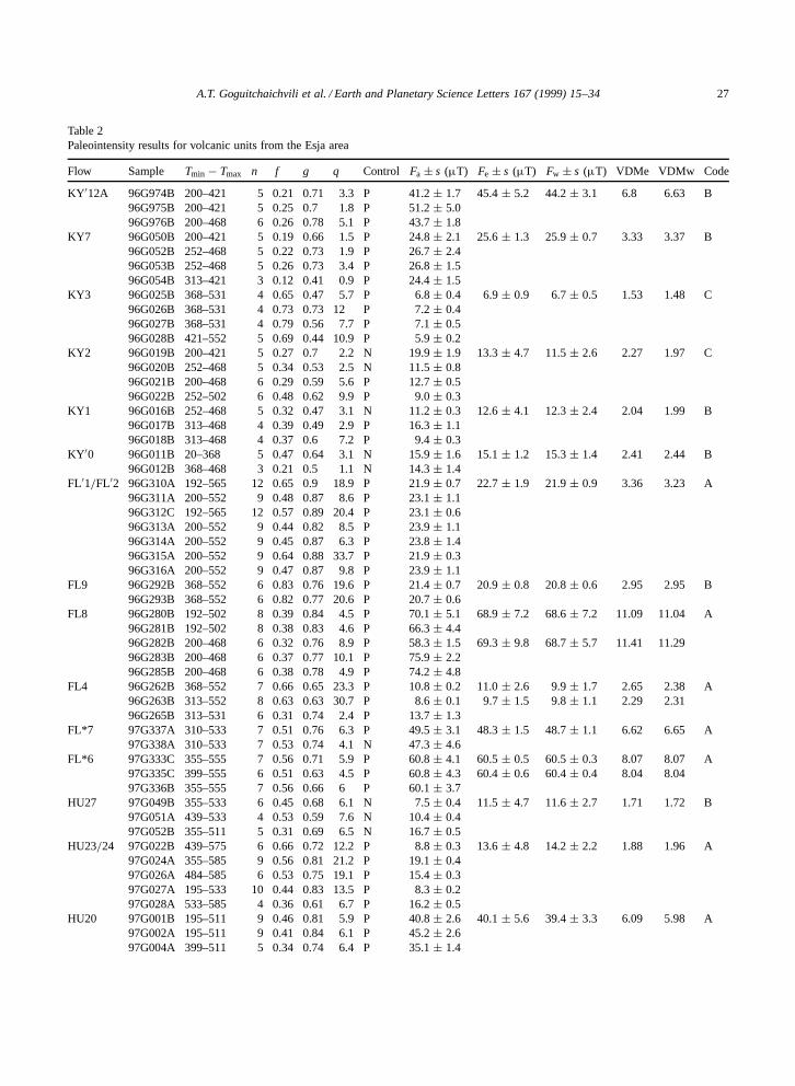
Table 2Paleointensity results for volcanic units from the Esja area

Flow Sample Tmin � Tmax n f g q Control Fa š s (µT) Fe š s (µT) Fw š s (µT) VDMe VDMw Code

KY012A 96G974B 200–421 5 0.21 0.71 3.3 P 41.2 š 1.7 45.4 š 5.2 44.2 š 3.1 6.8 6.63 B96G975B 200–421 5 0.25 0.7 1.8 P 51.2 š 5.096G976B 200–468 6 0.26 0.78 5.1 P 43.7 š 1.8

KY7 96G050B 200–421 5 0.19 0.66 1.5 P 24.8 š 2.1 25.6 š 1.3 25.9 š 0.7 3.33 3.37 B96G052B 252–468 5 0.22 0.73 1.9 P 26.7 š 2.496G053B 252–468 5 0.26 0.73 3.4 P 26.8 š 1.596G054B 313–421 3 0.12 0.41 0.9 P 24.4 š 1.5

KY3 96G025B 368–531 4 0.65 0.47 5.7 P 6.8 š 0.4 6.9 š 0.9 6.7 š 0.5 1.53 1.48 C96G026B 368–531 4 0.73 0.73 12 P 7.2 š 0.496G027B 368–531 4 0.79 0.56 7.7 P 7.1 š 0.596G028B 421–552 5 0.69 0.44 10.9 P 5.9 š 0.2

KY2 96G019B 200–421 5 0.27 0.7 2.2 N 19.9 š 1.9 13.3 š 4.7 11.5 š 2.6 2.27 1.97 C96G020B 252–468 5 0.34 0.53 2.5 N 11.5 š 0.896G021B 200–468 6 0.29 0.59 5.6 P 12.7 š 0.596G022B 252–502 6 0.48 0.62 9.9 P 9.0 š 0.3

KY1 96G016B 252–468 5 0.32 0.47 3.1 N 11.2 š 0.3 12.6 š 4.1 12.3 š 2.4 2.04 1.99 B96G017B 313–468 4 0.39 0.49 2.9 P 16.3 š 1.196G018B 313–468 4 0.37 0.6 7.2 P 9.4 š 0.3

KY00 96G011B 20–368 5 0.47 0.64 3.1 N 15.9 š 1.6 15.1 š 1.2 15.3 š 1.4 2.41 2.44 B96G012B 368–468 3 0.21 0.5 1.1 N 14.3 š 1.4

FL01=FL02 96G310A 192–565 12 0.65 0.9 18.9 P 21.9 š 0.7 22.7 š 1.9 21.9 š 0.9 3.36 3.23 A96G311A 200–552 9 0.48 0.87 8.6 P 23.1 š 1.196G312C 192–565 12 0.57 0.89 20.4 P 23.1 š 0.696G313A 200–552 9 0.44 0.82 8.5 P 23.9 š 1.196G314A 200–552 9 0.45 0.87 6.3 P 23.8 š 1.496G315A 200–552 9 0.64 0.88 33.7 P 21.9 š 0.396G316A 200–552 9 0.47 0.87 9.8 P 23.9 š 1.1

FL9 96G292B 368–552 6 0.83 0.76 19.6 P 21.4 š 0.7 20.9 š 0.8 20.8 š 0.6 2.95 2.95 B96G293B 368–552 6 0.82 0.77 20.6 P 20.7 š 0.6

FL8 96G280B 192–502 8 0.39 0.84 4.5 P 70.1 š 5.1 68.9 š 7.2 68.6 š 7.2 11.09 11.04 A96G281B 192–502 8 0.38 0.83 4.6 P 66.3 š 4.496G282B 200–468 6 0.32 0.76 8.9 P 58.3 š 1.5 69.3 š 9.8 68.7 š 5.7 11.41 11.2996G283B 200–468 6 0.37 0.77 10.1 P 75.9 š 2.296G285B 200–468 6 0.38 0.78 4.9 P 74.2 š 4.8

FL4 96G262B 368–552 7 0.66 0.65 23.3 P 10.8 š 0.2 11.0 š 2.6 9.9 š 1.7 2.65 2.38 A96G263B 313–552 8 0.63 0.63 30.7 P 8.6 š 0.1 9.7 š 1.5 9.8 š 1.1 2.29 2.3196G265B 313–531 6 0.31 0.74 2.4 P 13.7 š 1.3

FL*7 97G337A 310–533 7 0.51 0.76 6.3 P 49.5 š 3.1 48.3 š 1.5 48.7 š 1.1 6.62 6.65 A97G338A 310–533 7 0.53 0.74 4.1 N 47.3 š 4.6

FL*6 97G333C 355–555 7 0.56 0.71 5.9 P 60.8 š 4.1 60.5 š 0.5 60.5 š 0.3 8.07 8.07 A97G335C 399–555 6 0.51 0.63 4.5 P 60.8 š 4.3 60.4 š 0.6 60.4 š 0.4 8.04 8.0497G336B 355–555 7 0.56 0.66 6 P 60.1 š 3.7

HU27 97G049B 355–533 6 0.45 0.68 6.1 N 7.5 š 0.4 11.5 š 4.7 11.6 š 2.7 1.71 1.72 B97G051A 439–533 4 0.53 0.59 7.6 N 10.4 š 0.497G052B 355–511 5 0.31 0.69 6.5 N 16.7 š 0.5

HU23=24 97G022B 439–575 6 0.66 0.72 12.2 P 8.8 š 0.3 13.6 š 4.8 14.2 š 2.2 1.88 1.96 A97G024A 355–585 9 0.56 0.81 21.2 P 19.1 š 0.497G026A 484–585 6 0.53 0.75 19.1 P 15.4 š 0.397G027A 195–533 10 0.44 0.83 13.5 P 8.3 š 0.297G028A 533–585 4 0.36 0.61 6.7 P 16.2 š 0.5

HU20 97G001B 195–511 9 0.46 0.81 5.9 P 40.8 š 2.6 40.1 š 5.6 39.4 š 3.3 6.09 5.98 A97G002A 195–511 9 0.41 0.84 6.1 P 45.2 š 2.697G004A 399–511 5 0.34 0.74 6.4 P 35.1 š 1.4


Table 2 (continued)


HU19 96G206B 246–502 7 0.35 0.64 4.3 P 14.7 š 0.8 12.1 š 2.4 11.1 š 1.5 2.93 2.71 B96G207B 352–537 7 0.61 0.71 18.1 P 10.1 š 0.296G208B 440–537 5 0.64 0.67 10.9 P 11.4 š 0.4

HU12 96G173B 352–471 4 0.25 0.59 5.6 P 11.9 š 0.3 13.9 š 4.2 13.3 š 2.4 3.53 3.36 A96G174B 352–471 4 0.22 0.61 11.1 P 11.2 š 0.196G175B 352–471 4 0.25 0.63 5.7 P 18.7 š 0.5

HU11 96G166B 421–552 5 0.7 0.61 14.5 P 6.5 š 0.2 7.3 š 0.8 7.3 š 0.4 1.83 1.84 A96G167B 421–552 5 0.69 0.7 18.1 P 7.9 š 0.296G170B 352–537 7 0.68 0.77 24.2 P 7.5 š 0.2

HU8 96G148B 246–502 7 0.49 0.68 5.5 N 28.2 š 1.8 46.7 š 2.7 46.8 š 1.9 6.69 6.71 A96G150B 313–502 6 0.37 0.58 8.8 N 23.6 š 0.596G151B 352–369 9 0.94 0.84 47.1 P 48.6 š 0.896G152B 301–569 10 0.94 0.86 47.5 P 44.8 š 0.7

HU7 96G140B 301–537 8 0.48 0.79 6.3 P 72.6 š 4.5 65.9 š 14.8 60.3 š 6.1 10.48 9.59 A96G141B 246–537 10 0.52 0.84 11.9 P 83.0 š 3.1 68.2 š 14.3 62.5 š 6.4 11.1 10.296G142B 20–521 9 0.41 0.84 8.7 P 85.4 š 3.396G143B 20–521 8 0.42 0.72 4.6 P 69.1 š 5.396G144B 352–521 5 0.46 0.76 8.1 P 61.7 š 3.396G145B 352–537 6 0.37 0.76 7.5 P 56.2 š 2.196G146B 352–537 6 0.58 0.79 23.9 P 52.3 š 1.1

HU6 96G135B 352–502 5 0.39 0.73 5.3 P 51.4 š 2.8 53.5 š 3.0 53.2 š 2.2 7.56 7.51 B96G138B 352–471 4 0.32 0.74 3.7 P 55.6 š 3.6

HU5 96G129B 246–569 11 0.92 0.84 66.5 P 25.8 š 0.3 30.9 š 6.1 28.5 š 2.7 4.48 4.14 A96G130B 301–569 10 0.91 0.79 74.3 P 28.8 š 0.3 27.3 š 2.8 28.3 š 1.5 3.87 4.0196G131B 301–471 5 0.24 0.73 1.8 P 38.8 š 3.296G132B 352–471 4 0.18 0.65 3.4 P 37.2 š 2.896G133B 352–521 6 0.59 0.75 5.1 P 24.1 š 1.896G134B 301–569 10 0.94 0.76 77.9 P 30.1 š 0.3

HU4B 96G123B 246–521 8 0.33 0.81 4.7 N 32.8 š 1.8 32.6 š 5.6 33.8 š 2.6 4.69 4.86 A96G124B 246–502 8 0.28 0.77 3.3 N 30.1 š 1.796G125B 20–521 9 0.48 0.84 9.6 P 41.2 š 1.796G127B 20–502 8 0.47 0.77 4.3 P 32.7 š 2.996G128B 20–502 8 0.24 0.82 5.6 N 26.1 š 0.9

HU4A 96G119B 246–502 7 0.61 0.77 11.7 P 20.4 š 0.8 24.7 š 3.5 25.9 š 1.8 3.79 3.98 A96G120B 246–569 11 0.93 0.76 38.7 P 28.5 š 0.596G121B 301–569 10 0.93 0.79 55.1 P 26.1 š 0.396G122A 246–502 7 0.48 0.73 7.8 P 23.7 š 1.1

HU04A 96G113B 246–471 6 0.25 0.74 5.1 P 32.2 š 1.2 30.2 š 2.9 30.0 š 2.1 4.44 4.4 A96G114B 301–471 5 0.24 0.71 5.8 P 28.2 š 0.8

HU03=4A 96G106B 192–584 12 0.69 0.9 14.2 P 29.7 š 1.3 31.2 š 1.7 31.6 š 0.7 5.44 5.5 A96G107B 20–552 10 0.74 0.88 13.1 P 29.8 š 1.596G108B 20–552 10 0.75 0.89 15.9 P 31.8 š 1.396G109B 200–531 8 0.51 0.85 12.1 P 32.0 š 1.296G110B 200–552 10 0.47 0.87 7.5 P 30.3 š 1.696G111A 200–531 8 0.5 0.85 18.7 P 34.5 š 0.896G112B 192–565 11 0.52 0.88 14.5 P 30.5 š 0.9

PV09 97G200B 400–537 6 0.51 0.66 8.7 N 22.8 š 0.8 22.8 š 0.2 22.8 š 0.1 3.21 3.21 B97G201A 450–537 5 0.39 0.54 2.4 N 22.7 š 2.0

PV05 97G176B 350–520 6 0.23 0.71 5.8 N 9.5 š 0.3 9.3 š 2.3 9.9 š 1.2 2.33 2.48 A97G178B 300–520 7 0.26 0.79 6.5 N 12.4 š 0.497G179A 300–520 7 0.2 0.78 2.8 N 8.0 š 0.4

PV04 97G171B 300–537 9 0.57 0.6 12.2 P 7.6 š 0.2 12.7 š 3.8 12.9 š 1.9 3.19 3.25 A97G173B 490–537 7 0.75 0.53 10.3 P 11.5 š 0.497G174A 20–520 10 0.49 0.83 15.6 P 15.1 š 0.5


Table 2 (continued)


97G175B 20–520 10 0.45 0.84 12.3 P 15.6 š 0.5PV03 97G165B 300–537 8 0.47 0.64 8.9 P 14.7 š 0.4 16.3 š 2.6 16.2 š 1.1 4.12 4.09 A

97G166B 200–520 9 0.36 0.8 4.3 P 15.9 š 1.0 17.4 š 2.7 16.9 š 1.6 4.42 4.2897G167B 350–537 7 0.44 0.63 4.2 P 13.4 š 1.097G169B 150–537 10 0.31 0.77 6.6 P 17.4 š 0.697G170B 150–537 10 0.35 0.73 6.3 P 20.1 š 0.8

PV02 97G160B 300–537 8 0.67 0.66 8.4 P 13.8 š 0.7 13.1 š 2.8 12.8 š 1.4 3.29 3.21 A97G161B 250–537 9 0.45 0.64 6.1 N 16.6 š 0.797G162C 300–557 9 0.67 0.69 7.6 P 10.5 š 0.697G163B 200–537 10 0.41 0.73 12.4 P 11.3 š 0.3

PV01 97G156C 350–537 7 0.55 0.72 11.1 P 11.1 š 0.3 11.2 š 0.1 11.2 š 0.1 2.77 2.77 A97G157B 350–537 7 0.56 0.71 6 P 11.4 š 0.797G158B 350–537 7 0.49 0.67 5.6 P 11.3 š 0.797G159B 350–537 7 0.47 0.68 4.8 P 11.1 š 0.7

PV9 97G146B 200–537 9 0.68 0.74 12.1 P 10.9 š 0.5 13.5 š 1.8 13.2 š 0.9 3.36 3.28 A97G147B 250–537 8 0.46 0.64 6.2 P 13.5 š 0.697G148B 300–537 7 0.41 0.67 5.8 P 11.4 š 0.797G149B 300–537 7 0.41 0.65 13.1 P 15.2 š 0.6

PV8 97G142B 300–520 6 0.23 0.7 2.7 P 6.3 š 0.4 7.5 š 1.7 7.3 š 0.9 1.87 1.83 A97G143B 150–537 10 0.56 0.81 13.6 P 10.1 š 0.497G144B 300–520 6 0.21 0.73 3.2 P 6.4 š 0.397G145C 300–520 6 0.23 0.72 2.8 P 7.1 š 0.4

PV7B 97G137B 200–520 8 0.27 0.69 5.3 N 5.9 š 0.2 5.7 š 0.6 5.6 š 0.4 1.35 1.33 A97G138B 300–520 6 0.22 0.68 2.5 N 5.2 š 0.397G140C 300–520 6 0.25 0.63 2.3 N 6.1 š 0.4

PV7A 97G134A 150–490 8 0.23 0.67 3.3 P 10.4 š 0.5 11.5 š 1.3 11.7 š 0.9 2.84 2.9 A97G135B 150–490 8 0.24 0.69 4.9 P 12.4 š 0.4

PV5=7A 97G132B0 195–399 6 0.17 0.72 2.1 P 13.4 š 0.7 11.7 š 2.4 10.3 š 2.2 2.72 2.39 A97G133A 355–533 7 0.62 0.79 30.8 P 10.1 š 0.2

PV5 97G123B 350–520 5 0.41 0.67 16.7 P 7.9 š 0.1 8.0 š 0.1 7.9 š 0.1 2.06 2.05 A97G124B 250–520 8 0.39 0.68 22.2 P 7.9 š 0.197G126B 300–520 6 0.49 0.65 7.7 P 8.1 š 0.3

PV3 97G108C 150–537 10 0.57 0.79 5.9 P 39.8 š 3.0 45.5 š 12.2 49.6 š 4.9 6.77 7.38 B97G109B 150–537 10 0.56 0.82 6.1 P 39.3 š 3.097G110D 450–520 5 0.54 0.65 15.8 P 40.2 š 0.897G111C 350–520 7 0.41 0.71 9.1 P 31.2 š 0.997Gl13C 350–537 8 0.45 0.72 9.1 P 56.8 š 2.197Gl14C 400–537 5 0.52 0.73 8.2 P 40.9 š 1.997G116B 400–557 6 0.64 0.67 18.7 P 66.7 š 1.9

PV2 97G105B 400–537 5 0.46 0.71 3.2 P 54.3 š 5.2 53.4 š 1.6 52.9 š 1.0 7.38 7.32 A97G106C 400–537 5 0.59 0.69 10.7 P 51.5 š 2.3 53.7 š 3.1 53.4 š 2.2 7.43 7.3997G107B 450–557 5 0.78 0.54 7.6 P 54.4 š 3.0

PV1 97G096B 400–520 4 0.53 0.61 5.1 P 25.2 š 1.6 28.5 š 4.4 28.0 š 1.9 3.88 3.81 B97G097C 350–520 5 0.52 0.57 6.7 P 30.8 š 1.397G098C 350–520 5 0.56 0.61 5.7 P 22.5 š 1.497G099B 350–520 5 0.51 0.61 5 P 31.5 š 1.997G100B 350–520 5 0.41 0.66 2.5 P 32.3 š 3.4

SB014 97G282A 246–511 8 0.22 0.82 2.1 P 9.2 š 0.8 19.3 š 10.7 19.4 š 6.2 3.16 3.17 A97G283B 195–511 9 0.51 0.84 15.6 P 18.3 š 0.597G285B 310–484 5 0.39 0.71 2.3 P 30.5 š 3.6

SB05 97G235B 20–245 3 0.34 0.47 15.3 N 27.8 š 0.8 30.8 š 12.7 31.6 š 7.3 5.36 5.49 B97G238B 20–484 8 0.36 0.82 3.2 N 20.2 š 1.997G239A 20–245 3 0.47 0.46 5.5 N 44.7 š 1.7


Table 2 (continued)


SB112 97G220B 195–439 7 0.36 0.81 7.9 P 18.8 š 0.7 12.0 š 3.9 12.6 š 1.7 1.78 1.87 A97G221B 195–484 8 0.31 0.81 4.9 P 14.1 š 0.897G222B 195–484 8 0.61 0.82 5.3 P 9.7 š 0.997G223B 195–484 8 0.59 0.79 7.2 P 9.5 š 0.697G224B 195–484 8 0.48 0.8 5.8 P 11.1 š 0.7

Tmin � Tmax is the temperature interval used for paleointensity determination; n is the number of points defining a straight segment onthe NRM–TRM plots; f , g and q are the fraction of NRM used for paleointensity determination, the gap factor and quality factor [27]respectively. The column ‘Control’ indicates whether the pTRM=NRM checks were positive (P, changes generally less than 15%) ornegative (N) within the temperature interval used. Fa š s is the individual paleointensity estimate and associated standard error. Fe š sand Fw š s are arithmetic flow mean and weighted flow mean [5] paleointensities, respectively. VDMe and VDMw are associated VirtualDipole Moments. Codes A, B and C indicates the k–T type (see text). Bold font denotes type I paleointensity determinations (see text).

Microscopic observations are sometimes decisiveto identify the ChRM in volcanic rocks in orderto discriminate between primary TRM and pri-mary TCRM (thermochemical magnetization). Mi-croscopic observations under reflected light werecarried out on 16 selected unheated samples whichprovided class I paleointensity data. In general twogenerations of titanomagnetite of different sizes arepresent, with sometimes a skeletal form indicat-ing a relatively rapid cooling of the magma. Thesmall crystals (less than a few µm) are dominantin all samples, but their small sizes preclude theidentification of possible intergrowths. The larger ti-tanomagnetite grains are sometimes associated withprimary ilmenite (sandwich or composite structures[30]). Moreover, in general titanomagnetite con-tains a few to many exsolution lamellae of ilmenite(trellis type). Sometimes, ilmenite is partly trans-formed into titanohematite. In most of the flows,

Fig. 7. Example of Arai-Nagata (NRM–TRM) plots for class II samples and examples of rejected data. Same symbols and notations asin Fig. 6.

the pseudobrookite–hematite paragenesis (in lamel-lar form) was also observed in a few crystals. Allthese parageneses are characteristics of titanomag-netite oxyexsolution, a transformation which is re-puted to occur at high temperatures (>600ºC). Thisevidence suggests that the primary remanence car-ried by the near-magnetite phase is a TRM.

7. Results

Eighty-two samples belonging to 25 units provideclass I paleointensity determinations correspondingto magnetozones R3 (31 data, 9 lava units), R3–N3(29 data, 10 units), N3 (19 data, 5 units) and R2 (5data only, from one baked layer). The quality factorranges from 4.9 to 77.9 with an average equal to 15.1and the NRM fraction from 0.32 to 0.94 (average0.54). Within flow paleointensity dispersion varies


from 1 to 35%, but in most cases it is less than20%.

Fig. 8 shows the dependence of the local fieldpaleointensity versus the angular deviation from theaxial dipole field direction and the dependence of theVDM versus the VGP colatitude. Table 3 lists bothaverage directions and paleointensities for the fourmagnetozones. For all of them, the average pale-ostrength and standard deviation are similar when allthe data or only class I data (Table 3) are considered.For example, for the R3 magnetozone, the mean ands.d. of all VDMs is 6:1 š 1:9 ð 1022 A m2, which isin close agreement with the estimates from the classI only data (Table 3).

During the R3–N3 transition the average localpaleostrength obtained from all data is 2:8 š 0:7 ð1022 A m2, which agrees with the mean obtainedfrom the class I data, all restricted to the VGP cluster(Table 3). The magnitude is four times less than thatof the pre-transitional field.

The class I paleointensity values from the N3zone show a large dispersion between 12 µT (bakedhorizon SB01=2) and 69.3 µT (lava flow FL8), thesetwo values being well documented (Table 2). Theaverage absolute intensity is three times higher thanthe transitional mean magnitude, but 25% less thanfound for the R3 polarity zone. The significanceof this unusually high dispersion will be discussedbelow.

Only one determination (of type I) was obtainedfrom magnetozone R2 (13:6 š 4:8 µT from bakedunit HU23=24). The lava flow HU27 yields a simi-larly weak paleostrength, but it is less reliable. Moredata are obviously needed for this magnetozone.

Table 3Average characteristics of the geomagnetic field and corresponding virtual dipole before, during and after R3–N3 reversal

M.Z. nd Inc Dec k Þ95 Plat Plong Np Fe š s.d. (µT) VDM š s.d.

R2 21 �74 169.5 60 4.1 �83.7 34N3 30 67.7 16.1 27 5.1 74 119.1 5 32:5š 22:9 5:03š 3:5R3–N3 32 �19.7 50.3 188 1.9 6.6 109.1 10 11:3š 3:0 2:79š 0:7R3 22 �76.2 173.2 58 4.2 �86.9 64.7 9 44:7š 14:9 6:25š 2:1

Here, R3–N3 magnetozone includes only the units with near equatorial VGPs. nd is the number of units used to calculate the averagedirection: Inc and Dec are average inclination and declination respectively. k and Þ95: precision parameter and radius of 95% confidencecone of Fisher statistics. Plat=plong: latitude=longitude of corresponding VGP position. Np is the number of units to calculate the averagepaleointensity (type I data only); Fe š s.d. is the average absolute intensity with corresponding standard deviation. VDM š s.d. is theaverage moment and the corresponding standard deviation of virtual dipole (1022 A m2). The expected inclination due to an axial dipoleis 76.4º in Iceland.

8. Discussion and conclusions

8.1. Transitional field

Our best estimate of the average paleostrengthduring the R3–N3 Icelandic reversal (11 š 3 µT) iscomparable to the values obtained for other transi-tions using also the Thellier method: 15 š 5 µT inIceland for the Gauss=Matuyama reversal [31] and11š 5 µT for the much better documented Miocenereversal recorded by the Steens Basalt in Oregon[5]. Our experiments relative to the R3–N3 rever-sal show no evidence for strong paleostrengths likethose obtained by Shaw [11] for some of the flowsbelonging to the near equatorial VGP cluster. He re-ported paleointensities as high as 38.6 µT while ourhighest paleostrength is only 17.4 µT. Shaw’s pale-ostrengths for transitional flows also show a muchlarger scatter (from 1.8 to 38.6 µT) than the presentones (from 7.3 to 17.4 µT). In contrast to othercases [5,31] and Shaw’s claim the fluctuations ofpaleostrength observed from our data are not strati-graphically ordered. Possibly, they do not reflectmore than experimental uncertainties.

We suggest that some of Shaw’s data are in errorbecause undetected magnetic alteration of magneticminerals occurred during his experiments. Two ofthe units which provided strong paleofield usingthe Shaw’s method (HU13 and HU15) show quiteirreversible k–T curves and cannot be reasonablyexpected to give reliable paleointensity using anythermal method, particularly the Shaw method whichrequires heating at once up to the Curie point. As forthe third unit (HU12), the paleostrength found here


Fig. 8. Plots of VDM vs. paleocolatitude (A) and paleointensity vs. angular distance from the axial dipole field direction (B). Full=Opendiamonds correspond to the class I and class II paleointensities respectively. Average Pliocene VDM is from Table 4.


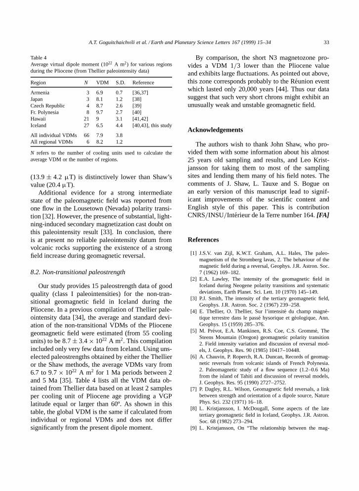
Table 4Average virtual dipole moment (1022 A m2) for various regionsduring the Pliocene (from Thellier paleointensity data)

Region N VDM S.D. Reference

Armenia 3 6.9 0.7 [36,37]Japan 3 8.1 1.2 [38]Czech Republic 4 8.7 2.6 [39]Fr. Polynesia 8 9.7 2.7 [40]Hawaii 21 9 3.1 [41,42]Iceland 27 6.5 4.4 [40,43], this study

All individual VDMs 66 7.9 3.8All regional VDMs 6 8.2 1.2

N refers to the number of cooling units used to calculate theaverage VDM or the number of regions.

(13:9 š 4:2 µT) is distinctively lower than Shaw’svalue (20.4 µT).

Additional evidence for a strong intermediatestate of the paleomagnetic field was reported fromone flow in the Lousetown (Nevada) polarity transi-tion [32]. However, the presence of substantial, light-ning-induced secondary magnetization cast doubt onthis paleointensity result [33]. In conclusion, thereis at present no reliable paleointensity datum fromvolcanic rocks supporting the existence of a strongfield increase during geomagnetic reversal.

8.2. Non-transitional paleostrength

Our study provides 15 paleostrength data of goodquality (class I paleointensities) for the non-tran-sitional geomagnetic field in Iceland during thePliocene. In a previous compilation of Thellier pale-ointensity data [34], the average and standard devi-ation of the non-transitional VDMs of the Pliocenegeomagnetic field were estimated (from 55 coolingunits) to be 8:7š 3:4ð 1022 A m2. This compilationincluded only very few data from Iceland. Using uns-elected paleostrengths obtained by either the Thellieror the Shaw methods, the average VDMs vary from6.7 to 9:7 ð 1022 A m2 for 1 Ma periods between 2and 5 Ma [35]. Table 4 lists all the VDM data ob-tained from Thellier data based on at least 2 samplesper cooling unit of Pliocene age providing a VGPlatitude equal or larger than 60º. As shown in thistable, the global VDM is the same if calculated fromindividual or regional VDMs and does not differsignificantly from the present dipole moment.

By comparison, the short N3 magnetozone pro-vides a VDM 1=3 lower than the Pliocene valueand exhibits large fluctuations. As pointed out above,this zone corresponds probably to the Reunion eventwhich lasted only 20,000 years [44]. Thus our datasuggest that such very short chrons might exhibit anunusually weak and unstable geomagnetic field.

Acknowledgements

The authors wish to thank John Shaw, who pro-vided them with some information about his almost25 years old sampling and results, and Leo Krist-jansson for taking them to most of the samplingsites and lending them many of his field notes. Thecomments of J. Shaw, L. Tauxe and S. Bogue onan early version of this manuscript lead to signif-icant improvements of the scientific content andEnglish style of this paper. This is contributionCNRS=INSU=Interieur de la Terre number 164. [FA]

References

[1] J.S.V. van Zijl, K.W.T. Graham, A.L. Hales, The paleo-magnetism of the Stromberg lavas, 2. The behaviour of themagnetic field during a reversal, Geophys. J.R. Astron. Soc.7 (1962) 169–182.

[2] E.A. Lawley, The intensity of the geomagnetic field inIceland during Neogene polarity transitions and systematicdeviations, Earth Planet. Sci. Lett. 10 (1970) 145–149.

[3] P.J. Smith, The intensity of the tertiary geomagnetic field,Geophys. J.R. Astron. Soc. 2 (1967) 239–258.

[4] E. Thellier, O. Thellier, Sur l’intensite du champ magne-tique terrestre dans le passe hysorique et geologique, Ann.Geophys. 15 (1959) 285–376.

[5] M. Prevot, E.A. Mankinen, R.S. Coe, C.S. Gromme, TheSteens Mountain (Oregon) geomagnetic polarity transition2. Field intensity variation and discussion of reversal mod-els, J. Geophys. Res. 90 (1985) 10417–10448.

[6] A. Chauvin, P. Roperch, R.A. Duncan, Records of geomag-netic reversals from volcanic islands of French Polynesia.2. Paleomagnetic study of a flow sequence (1.2–0.6 Ma)from the island of Tahiti and discussion of reversal models,J. Geophys. Res. 95 (1990) 2727–2752.

[7] P. Dagley, R.L. Wilson, Geomagnetic field reversals, a linkbetween strength and orientation of a dipole source, NaturePhys. Sci. 232 (1971) 16–18.

[8] L. Kristjansson, I. McDougall, Some aspects of the latetertiary geomagnetic field in Iceland, Geophys. J.R. Astron.Soc. 68 (1982) 273–294.

[9] L. Kristjansson, On “The relationship between the mag-


nitude and direction of the geomagnetic field during thelate tertiary in eastern Iceland” by N. Roberts and J. Shaw,Geophys. J.R. Astron. Soc. 80 (1985) 555–559.

[10] P. Camps, M. Prevot, A statistical model of the fluctuationsin the geomagnetic field from paleosecular variation toreversal, Science 273 (1996) 776–779.

[11] J. Shaw, Strong geomagnetic fields during a single Icelandicpolarity transition, Geophys. J.R. Astron. Soc. 40 (1975)345–350.

[12] T. Sigurgeirsson, Direction of magnetization in Icelandicbasalts, Adv. Phys. 6 (Philos. Mag. suppl.) (1957) 240–246.

[13] I.B. Fridleifsson, Petrology and structure of the Esja Qua-ternary volcanic region, SW Iceland, D. Phil. Thesis, Ox-ford University, 1973, 208 pp.

[14] I.B. Fridleifsson, The geological history of mt. Esja and itssurroundings, A rbok ferdafelags Islands, (1985) 141–172.

[15] G. Palmasson, K. Saemundsson, Iceland in relation to theMid-Atlantic ridge, Annu. Rev. Earth Planet. Sci. 2 (1974)25–50.

[16] L. Kristjansson, I.B. Fridleifsson, N.D. Watkins, Stratigra-phy and paleomagnetism of the Esja, Eyrarfjall and Arkaf-jall mountains, Iceland, J. Geophys. 47 (1980) 31–42.

[17] T. Einarsson, Magneto-geological mapping in Iceland withthe use of a compass, Adv. Phys. 6 (Philos. Mag. Suppl.)(1957) 232–239.

[18] L. Kristjansson, M. Sigurgeirsson, The R3–N3 and R5–N5paleomagnetic transition zones in SW-Iceland revisited, J.Geomag. Geoelectr. 45 (1993) 275–288.

[19] R.L. Wilson, N.D. Watkins, T. Einarsson, T. Sigurgeirsson,S.E. Haggerty, P.J. Smith, P. Dagley, A.G. McCormack,Paleomagnetism of ten lava sequences from SW Iceland,Geophys. J.R. Astron. Soc. 29 (1972) 459–471.

[20] G.P.L. Walker, Zeolite zones and dyke distribution in re-lation to the structure of the basalts in eastern Iceland, J.Geol. 68 (1960) 515–528.

[21] M. Prevot, E.A. Mankinen, A. Gromme, A. Lecaille, Highpaleointensities of the geomagnetic field from thermomag-netic study on rift valley pillow basalts from the Mid-Atlantic Ridge, J. Geophys. Res. 88 (1983) 2316–2326.

[22] O. Ozdemir, Inversion of titanomaghemites, Phys. EarthPlanet. Inter. 65 (1987) 125–136.

[23] E. Thellier, O. Thellier, Recherches geomagnetiques sur decoulees volcaniques d’Auverne, Ann. Geophys. 1 (1944)37–52.

[24] M. Prevot, Some aspects of magnetic viscosity in subaerialand submarine volcanic rocks, Geophys. J.R. Astron. Soc.66 (1981) 169–182.

[25] P. Camps, M. Prevot, R.S. Coe, Revisiting the initial sitesof geomagnetic field impulses during the Steens MountainReversal, Geophys. J. Int. 123 (1995) 484–506.

[26] J.L. Kirshvink, The least-square line and plane and analy-sis of paleomagnetic data, Geophys. J.R. Astron. Soc. 62(1980) 699–718.

[27] R.S. Coe, Geomagnetic paleointensity from radiocarbon-dated flows on Hawaii and the question of the Pacificnondipole low, J. Geophys. Res. 83 (1978) 1740–1756.

[28] A. Kosterov, M. Prevot, Possible mechanisms causing fail-

ure of Thellier paleointensity experiments in some basalts,Geophys. J. Int. in press.

[29] S. Levi, The effect of magnetic particle size in paleoin-tensity determination of the geomagnetic field, Phys. EarthPlanet. Inter. 13 (1977) 245–259.

[30] S.E. Haggerty, Oxidation of opaque mineral oxides inbasalts, in: Oxides Minerals, Mineralogical Society ofAmerica, 1976, 300 pp.

[31] A.T. Goguitchaichvili, M. Prevot, J. Thompson, N. Roberts,An attempt to determine absolute geomagnetic field inten-sity in Southwestern Iceland during the Gauss–Matuyamareversal, Phys. Planet. Earth Inter. (submitted, 1998).

[32] J. Shaw, Further evidence for a strong intermediate stateof the paleomagnetic field, Geophys. J.R. Astron. Soc. 48(1977) 263–269.

[33] N. Roberts, J. Shaw, Secondary magnetization cast doubton exceptional palaeointensity values from the LousetownCreek lavas of Nevada, USA, Geophys. J. Int. 101 (1990)251–257.

[34] M. Prevot, M.E.M. Derder, M. McWilliams, J. Thompson,Intensity of the Earth’s magnetic field: evidence for a Meso-zoic dipole low, Earth Planet. Sci. Lett. 97 (1990) 129–139.

[35] M. Perrin, V. Shcherbakov, Paleointensity of the earth’smagnetic field for the past 400 Ma: Evidence for a dipolestructure during the Mesozoic low, J. Geomag. Geoelctr. 49(1997) 601–614.

[36] A.S. Bolshakov, G.M. Solodovnikov, The field strength ofthe ancient magnetic field of the Earth in the Pliocene–Quaternary epoch, Izv. Earth Phys. 5 (1969) 88–93.

[37] O.L. Bagina, D.O. Minasyan, G.N. Petrova, Determinationof the intensity of the ancient geomagnetic field from theeffusive rocks of Armenian SSR, Izv. Earth Phys. ArmenianSSR 2 (1976) 81–86, in Russian.

[38] S. Sasajima, K. Maenaka, Variation of the geomagneticfield intensity since the late Miocene, J. Geophys. Res. 74(1969) 1037–1044.

[39] M. Krs, Geomagnetic field intensity during the Plio-Pleis-tocene derived from the thermo-remanence of porcellanitesand paleo-slags, Pure Appl. Geophys. 69 (1979) 158–167.

[40] W.E. Senanyake, M.W. McElhinny, P.L. McFadden, Com-parison between the Thellier’s and Shaw’s palaeointensitymethods using basalts less than 5 My old, J. Geomag.Geoelectr. 34 (1982) 141–161.

[41] S.W. Bogue, R.S. Coe, Transitional paleointensities fromKauai, Hawaii, and geomagnetic reversal models, J. Geo-phys. Res. 89 (1984) 10341–10354.

[42] S.W. Bogue, H.A. Paul, Distinctive behaviour following ge-omagnetic reversals, Geophys. Res. Lett. 20 (1993) 2399–2402.

[43] H. Tanaka, M. Kono, S. Kaneko, Palaeosecular variation ofdirection and intensity from two Pliocene–Pleistocene lavasections in Southwestern Iceland, J. Geomag. Geoelectr. 47(1995) 89–102.

[44] S.C. Cande, D.V. Kent, Revised calibration of the geo-magnetic polarity time scale for the late Cretaceous andCenozoic, J. Geophys. Res. 100 (1995) 6093–6095.

No evidence for strong fields during the R3–N3 Icelandic geomagnetic reversal

Documents

Transcript of No evidence for strong fields during the R3–N3 Icelandic geomagnetic reversal