Nitrate leaching and soil moisture prediction with the LEACHM model

Fertilizer Research 27: 171-180, 1991. © 1991 Kluwer Academic Publishers. Printed in the Netherlands. 171

Nitrate leaching and soil moisture prediction with the LEACHM model

C. Ramos & E .A . Carbonell Instituto Valenciano de Investigaciones Agrarias, Apdo. Oficial, 46113 Moncada, Spain

Key words: Nitrate leaching, soil moisture, soil mineral nitrogen, models

Abstract

The LEACHM model developed by Wagenet and Hutson [1989] was used to predict the mineral nitrogen and water content in the soil under a winter wheat crop from February to April in two years and three locations. The model grossly overestimated soil water content, probably due to the bad fitting of the assumed water retentivity function to the experimental data at high water contents, and to the presence of a relatively shallow water table (1.0-1.5 m). Measured soil hydraulic conductivity varied with water content in a different manner than predicted by the model. By assuming a sandy or gravelly soil layer between the bottom of the measured soil profile and the water table, prediction of soil water content improved considerably. Simulation showed that, under the experimental conditions studied, soil mineral nitrogen varied mainly due to the fertilizer additions, mineralization and denitrification. Nitrogen uptake by plants and leaching were small. Low values of nitrate leaching were predicted by the model because of low drainage. Large differences between predicted and observed values in the mineral nitrogen in the soil occurred in some cases, both in the total amount and its profile distribution.

Introduction

Transport of water and solutes in the soil under field conditions is a research area of continuous interest as some recent publications show [21, 24, 34]. There are different modeling ap- proaches to describe solute leaching in field soils, but testing of these models has, in general, been restricted to those who developed them. As pointed out by some workers [1, 25] there is a need for validating these models under different soil and environmental conditions. Following this idea, we present here an application of the model LEACHM [29], to estimate soil moisture and soil mineral nitrogen under a winter wheat crop in two years (1983, 1984) and three experimental locations (Bouwing, PAGV, EEST), using an existing data set [9].

Description of LEACHM

A detailed description of the model was given by their developers [29]. Here, a general view of the model will be given and the main points relevant

to its specific use in our simulations will be emphasized.

LEACHM evolved from modeling efforts in the last twenty years and has successfully been used by several workers to describe pesticide movement in field soils [28, 30]. It is a research type model that can be used for management purposes if some of the required inputs, difficult to obtain, are estimated and not actually measured. It has four modules, all of which with similar schemes, to simulate water and chemical movement. One of these modules, LEACHN, describes nitrogen transport and transformation and it is the one used in the present simulations; a second one, LEACHP, deals with pesticides; a third one, LEACHC, describes flow of inorganic ions (Ca, Mg, Na, K, SO 4, C1, CO 3, HCO3) and a fourth one, LEACHW, describes water transport only. LEACHM has also a heat flow subroutine that allows to adjust rate constants according to temperature, although this adjust- ment is not included in the second version used here. Figure 1 shows a flowchart for LEACHN.

In each of the four modules, there is a main

172

I-EACHN Initializes all variables to zero i

READN Reads data file

I .................................................................... I

K+0+h from es RETPRED Retentivity and conductivity J texture? I parameters from sand, silt, I

' I clay, bulk density regression. I no

WATDAT Calculates water retentivity and hydraulic I conductivity data for the soll hydrological

constants used, and prinE~ in tabular form.

1 ~ Day End of yes > E~D

I- A- last day? i ?o

GROWIH Simulates canopy growth and root growth and distrlbu~ion using empirical or regression equations.

POTET Calculates daily potential evaporation and transpiration from pan evaporation and crop cover.

I .....................................................................

i er=l~l=ert y e s Add urea, ammonium and nitrate and ,'addition?, ,or i ioo b ........ bed solotioo L 1 <" p h a s e s _ _ ]

I

T i m e - b--- Time + nt i day? yes - - - > A

Time

L . . . . . . . . . . . . . . . . . . . . . . I . . . . . . . . . . . . . . . . . . . . . . . . . . ; - : . . . . . . . . . . . . . . . . . .

I .... - ................................................................ TSTEP Calculates the length of the time step (at)

according ~o expected water flux density or specified limits.

ETR~/qS Potential transpiration and evaporation for ~he time step asst~ming sinusoldal change during the day.

%PdPTAK Calculates water uptake by plants according to root distribution, moil water potential and hydraulic conductlvlty.

WATFLO Finite difference solution of soil water flow equation using appropriate upper boundary and specified lower boundary condition.

HEAT Finite difference simulation of heat flow

.....................................................................

PRATE

SINKN

SOLN

Mass balance checks, cumulative and profile totals.

! I

iTi .... p iot? i

n o

b

Adjust temperature and/or water content dependent transformation rates.

Gains and losses of nitrogen species by plant uptake, microbial action and volatilization.

Finite difference solution of solute transport equation including sorption and source/sink terms.

CADATE Calendar date from day no.

I OUTN Print mass balance components

I ] and profile clara.

Fig. i. Flow chart for LEACHN, the nitrogen module of L E A C H M (after Wagenet and Hutson [29]). Subroutines are given in capitals,

program that initializes variables, calls subroutines and performs mass balancing. Sub- routines deal with the different processes such as water and solute flow, evapotranspiration, sinks, sources, plant growth, heat flow, and also with data input and output, and time step calculation. Main required inputs for LEACHN are: 1. Soil data for the different layers of equal

thickness: -initial water content or water potential. -hydrological constants for the moisture re-

tentivity and hydraulic conductivity curves. The model can also estimate these curves from particle size distribution.

-initial inorganic nitrogen content. 2. Soil surface boundary conditions:

-irrigation and rainfall amounts and rate of application.

-mineral nitrogen fertilizer application rates and dates.

- m e a n temperature and diurnal amplitude

for each period regarded as having a constant temperature regime (only if a temperature simulation is required).

-weekly totals of pan evaporation. 3. Crop data:

- time of planting. - r o o t and crop maturity and harvest dates. - r o o t and ground cover growth parameters. - pan factor for converting pan evaporation to

potential crop evapotranspiration. - lower soil and plant water potentials for

water extraction by plants. 4. Other constants needed include diffusion

coefficients, maximum value for time step, dispersivity coefficient, rate constants for the nitrogen transformations considered (urea hy- drolysis, ammonia volatilization, nitrification and denitrification) and the adsorption coefficients for urea, ammonium and nitrate.

LEACHM is not intended to: - u s e unequal depth increments.

- predict runoff water quantity or quality. - s imula te how plants respond to soil or en-

vironmental changes. -p red ic t crop yields. - predict solute distributions in situations with

two- or three-dimensional flux patterns.

Soil water

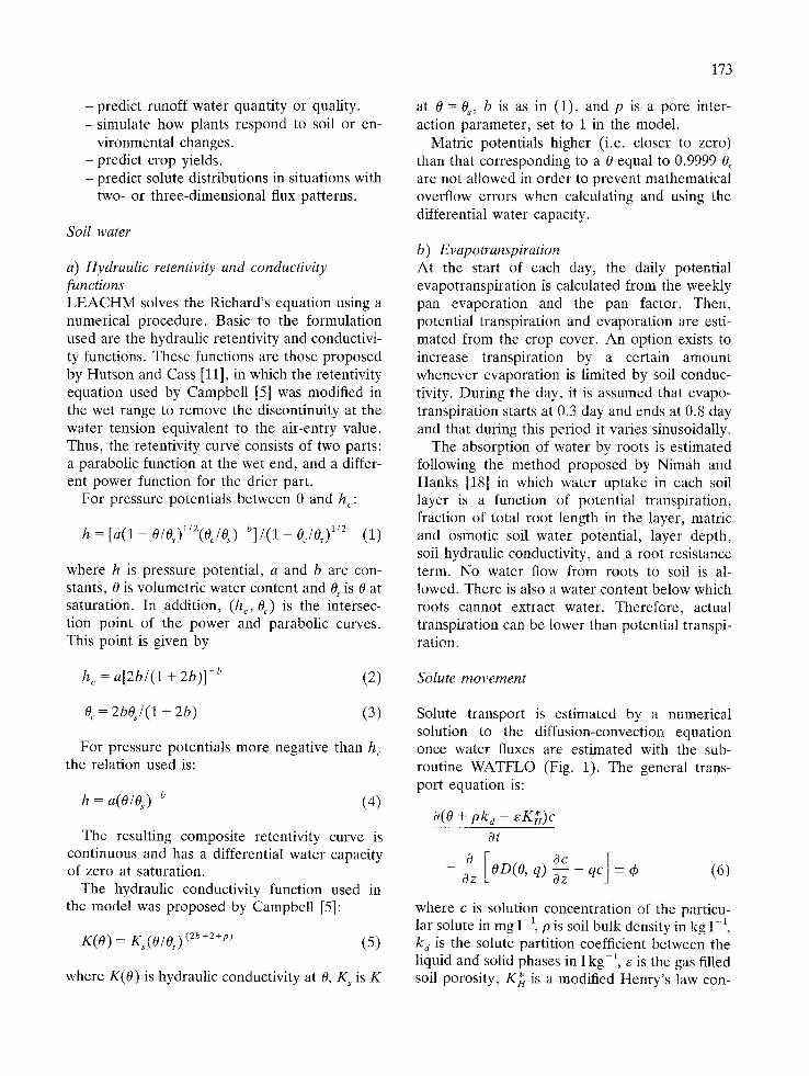
a) Hydraulic retentivity and conductivity functions L E A C H M solves the Richard's equation using a numerical procedure. Basic to the formulation used are the hydraulic retentivity and conductivity functions. These functions are those proposed by Hutson and Cass [11], in which the retentivity equation used by Campbell [5] was modified in the wet range to remove the discontinuity at the water tension equivalent to the air-entry value. Thus, the retentivity curve consists of two parts: a parabolic function at the wet end, and a different power function for the drier part.

For pressure potentials between 0 and he:

h = [a(1 - 0/0s)I/2(0c/0~) b]/(1 - Oc/Os) 1/2 (1)

where h is pressure potential, a and b are constants, 0 is volumetric water content and 0, is 0 at saturation. In addition, (hc, Oc) is the intersec- tion point of the power and parabolic curves. This point is given by

h c = a[2b/(1 + 2b)l -v (2)

0 c = 2bOs/(1 + 2b) (3)

For pressure potentials more negative than h c the relation used is:

h = a(O/~) b (4)

The resulting composite retentivity curve is continuous and has a differential water capacity of zero at saturation.

The hydraulic conductivity function used in the model was proposed by Campbell [5]:

K(0) = K (0/0s)(2b+2+p (5)

where K(O) is hydraulic conductivity at 0, K s is K

173

at 0 = 0,, b is as in (1), and p is a pore inter- action parameter, set to 1 in the model.

Matric potentials higher (i.e. closer to zero) than that corresponding to a 0 equal to 0.9999 0 s are not allowed in order to prevent mathematical overflow errors when calculating and using the differential water capacity.

b) Evapotranspiration At the start of each day, the daily potential evapotranspiration is calculated from the weekly pan evaporation and the pan factor. Then, potential transpiration and evaporation are estimated from the crop cover. An option exists to increase transpiration by a certain amount whenever evaporation is limited by soil conductivity. During the day, it is assumed that evapotranspiration starts at 0.3 day and ends at 0.8 day and that during this period it varies sinusoidally.

The absorption of water by roots is estimated following the method proposed by Nimah and Hanks [18] in which water uptake in each soil layer is a function of potential transpiration, fraction of total root length in the layer, matric and osmotic soil water potential, layer depth, soil hydraulic conductivity, and a root resistance term. No water flow from roots to soil is allowed. There is also a water content below which roots cannot extract water. Therefore, actual transpiration can be lower than potential transpiration.

Solute movement

Solute transport is estimated by a numerical solution to the diffusion-convection equation once water fluxes are estimated with the subroutine WATFLO (Fig. 1). The general transport equation is:

o(o + +

Ot

0 [OD(O,q) Oc ] - Oz ~ z - q c +- 6 (6)

where c is solution concentration of the particu- lar solute in mg 1- i, P is soil bulk density in kg 1-1, k~ is the solute partition coefficient between the liquid and solid phases in 1 kg 1, e is the gas filled soil porosity, K~ is a modified Henry's law con-

174

stant, q is the macroscopic water flux in mm day -1, D(O, q) is the apparent diffusion coefficient in mm 2 day -1 that includes mechanical dispersion and chemical diffusion, z is the soil depth in mm, and 4) indicates sources and/or sink terms in mg 1-1 day -1. The chemical diffusion component of D(O, q) depends on two empirical constants m and n [20].

Since the finite difference Solution of equation (6) may cause considerable numerical dispersion, a correction for this is made. The model developers found that, for time steps less than 0.1 day and for layer thicknesses (Az) less than 100 mm, numerical dispersion was equivalent to an increase in dispersivity of 0.16 Az. This numerical dispersion correction is applied to the mechanical dispersion coefficient only.

Nitrogen transformations and plant uptake

The nitrogen transformation reactions considered in L E A C H N are:

ammonia (gas)

k i / k4 k2

urea > ammonium > nitrate c 1 C 2 C 3

k 3 > gas

where k 1, k2, k 3, and k 4 represent the rate constants of the different processes and c a, c 2 and c 3 are the concentrations of urea, ammonium and nitrate, respectively. Concentra- tions and rates can apply to the liquid phase only or to the liquid + solid phases.

Nitrogen uptake by plants is calculated as [19]:

I = 2~'o~rc

where I is the rate of nutrient uptake per unit length of root in m g m -1 day -1, r is the mean root radius in mm, c is nutrient concentration in solution in mg 1-1, and a is a root uptake coefficient in m day -1

Simulation objectives

There were two main reasons why L E A C H N could not be applied directly to the data set provided: 1) plant growth description is for corn,

and 2) plant growth is not limited by any environmental factor (temperature, water or nitrogen supply) and depends only on time. There- fore, the simulation objectives were limited to the evaluation of L E A C H N in a situation where the effects of plant growth on soil water and mineral nitrogen could be considered negligible in comparison to other nitrogen or water sinks or sources such as drainage, fertilizer additions, or chemical transformations and transport. Thus, the option available in the model, in which root distribution and crop cover are assumed constant, was used. The period in which these conditions were likely to be met was from the first soil sampling (early February) to the third soil sampling (late March or early April). Inspection of the data set on nitrogen uptake by the crop in this period confirmed that, in general, it was quite small (8 kg ha -I on average) compared to the initial mineral nitrogen in the soil or the fertilizer additions.

Input data

a) Soil-water parameters

Details on soil moisture content, water retentivity curves and hydraulic conductivity measurements are given elsewhere [9].

To calculate the parameters a and b required by the model, log I hi was plotted against log 0. The points corresponding to low water content followed approximately a straight line. Then, a and b were estimated by linear regression. The complete retentivity curve was obtained by ap- plying eqs. (1) to (4).

Table 1 shows the soil hydraulic parameters used in the simulations. K s and e s were given in the data set, except for the 40 - 100 cm layer of the Bouwing plot where K s had to be obtained by extrapolation, using the log-linear relationship between K and O. The hypothetical 'sandy' layer was introduced for convenience and will be discussed later.

b) Potential evapotranspiration estimation

L E A C H M calculates crop evapotranspiration by multiplying the required pan evaporation data by

Table 1. Soil hydraulic parameters

175

Plot Layer K s (cm) (mm day 1)

Campbell's parameters

0~ a b (cm 3 cm 3) (kPa)

Bouwing

EEST & PAGV

0-40 636 40-100 856

(100-110)(1) 856 0-20 1780

20-40 264 40-100 2300

0.517 -6.61 4.93 0.517 -8.32 5.06 0.517 -1.00 2.00 0.411 -17.0 2.70 0.499 -9.8 3.15 0.523 -10.7 3.50

(1) hypothetical 'sandy' layer (see text)

a pan factor. Since the data set did not provide pan evaporation data, reference (i.e. potential) evapotranspiration, ETo, was calculated following the FAO modified Penman method [6], using a computer program in which the empirical coefficients required in the FAO procedure were those derived by Frevert et al. [7], and the relationship between air temperature and saturated water vapor pressure was taken from Weiss [31]. In the program input, E T o was then substi- tuted for pan evaporation assuming a pan factor of 1.

For comparative purposes two additional methods of E T o estimation were used: 1) the FAO radiation method [6], and 2) the Makkink method, originally calibrated for Dutch conditions [6]. Daily climate data from nine weeks taken at random from the two sites and years, during the February-March period, were used in the comparison.

In L E A C H M , crop cover fraction is numeri- cally equal to the ratio of plant transpiration to evapotranspiration when the soil surface is not limiting evaporation. In the simulation, a constant value for the crop cover fraction was taken for the whole study period. This fraction was estimated using results by Ritchie and Burnet t [22] . They found that in a subhumid climate and under nonlimiting soil water conditions, the transpiration to evapotranspiration ratio was a common function of the leaf area index for cotton and grain sorghum. In the present case, the leaf area index for the different plots and years in the selected periods varied mainly from about 0.15 to 0.40. These values correspond, using the relationship found by these workers, to a transpirat ion/evapotranspirat ion ratio of 0.06

and 0.23, respectively. Therefore , a constant value of 0.15 for the crop cover fraction was selected for the whole study period.

c) Rate constants and other parameters

Rate constants for the nitrogen transformations and other parameter values were chosen after a review of literature data. A summary of these values is presented in Table 2.

Most of the rate constant values found in the literature had been obtained at higher temperatures than those occurring in the upper soil layers during the simulation period (estimated to be about 5°C on average). A temperature adjust- ment was made using a Q(10°C) of 2.3, an average value found by different workers [2, 23, 32].

Although the model does not consider mineralization, it was modified to include a constant mineralization rate of 0.15 and 0.075 k g N h a -1 day -1 for layers 0-30 cm and 30-60 cm, respectively. These values are somewhat lower than those reported by others [2, 17, 33] for temperatures 5 to 15°C higher.

Results and discussion

a) Soil water

Before comparing field soil moisture predictions with measured data, the adequacy of the soil hydraulic functions will be discussed. Figure 2 shows the fitting of the Hutson and Cass model [11] used in L E A C H M to the experimental data for the 0-40 cm layer in the Bouwing plot. It is

176

Table 2. Some parameter values used in the simulations

Parameter Value Observed range References

Diffus. coef. in water (romP/day) 120 86-173 3, 19 Apparent diff. coef. constants

m 0.005 0.005-0.010 20 n 10 10 20

Dispersivity (mm) 40 1-300 4, 8, 13 NH~ partition coef. (din 3 kg -1) 5 1-9 14, 15, 17 Nitrific. rate const. (day 1) (1) 0.05-0.30 (2) 12, 15, 16, 26, 27

0-30 cm 0.10 30-60 cm 0.05 60-100 cm 0.02

Denitrif. rate const. (day 1) (1) 0.0003-0.02 (2) 10, 12, 15, 16, 27 0-30 cm 0.005

30-60 cm 0.002 60-100 cm 0.0001

(1) Assuming first order kinetics (2) Values adjusted to T= 5°C assuming Q(10°C)= 2.3

"-¢~ r F E i i

FBO U-WING 3 I 0 - 4 0 c m

e j o ~" 2 . . . . e ~ e / / • do. to

no e ~ . e - - mode[ (Hutson &Cas:

1

I 0 •

-t

o.'s o'.~ o13 o;2 8, =m ~. on,- ~

0/2 ' ' ' o18 '

- tog O

Fig. 2. Fitting of experimental data to the Hutson and Cass soil retentivity function [11] for the 0-40cm layer at the Bouwing site.

apparent that in the wetter part of the curve (i.e. 0 > 0c), corresponding to the parabolic relationship, the model predicted higher 0 values than measured. The good fitting for the drier part of the curve is because here the relationship between 0 and h follows well a power function and a and b were actually obtained from these points by linear regression. Results for the 40-100 cm depth and for all depths in the EEST and PAGV plots showed a similar type of curves to that in Fig. 2.

Figure 3 shows the relationship between log K and log0. In Campbell's model, used in LEACHM, a linear relationship is proposed for

4 - # l J i i i , i

ouw .ol I O-40crn k

3 ~ , ~ o ~ e

j e 2 e / o ,

-0 1

/ E J • data 0 / / -- Campbe[l's mode[

i

-2

- 3 015 014 0r3 012 0,cmS.orn 3 i i i .i i r

0.2 0.4 0 6 0.8

- log 0

Fig. 3. Fitting of experimental data to the Campbell soil hydraulic conductivity function [5] for the 0-40 cm layer at the Bouwing site.

the whole range of 0. However, data clearly show two linear relationships. Changes were made in LEACHM so that by entering appropriate p values for each of the linear parts of the log K vs. log 0 relationship, a good fitting was obtained in the whole range of 0.

Soil water content was first simulated in the Bouwing plot and although no data were available on the water table depth in 1983, it was assumed at 1.5 m depth, guessing from 1984

E u

-o

0

20

z,O

60

80

0.2

100 - - measured

c m 3 . CfT~ - 3

0.4

I

. . . . • k 7

I I

L7 1 1

. . . . j

0.6

I - - - - s imulQted [ r t 100 110 I 12o I . . . . . . . . ,~r.,,~o,.d w~h ,, "g~ .Ly" ,"Y' o , - ~ , ~

Fig. 4. Predicted and measured volumetric soil water profile at the Bouwing site on 28-3-83, with or without a hypothetical sandy or gravelly layer at 100-110 cm (see text).

data. Simulation results indicated a high upward water flux and an increase in soil moisture. This contrasted very much with measured values (Fig. 4). This difference is probably due to the bad fitting of the soil water retentivity function at low water tension, and to the imposed bottom boundary condition. Under equilibrium conditions, having a water table at 0.5 m deeper than the bottom of the soil profile is equivalent to maintaining a constant water suction of 5 kPa at that depth; at this suction the simulated water content was much higher than that measured (Fig. 2).

177

Since at the time of the first soil sampling each year the soil water profile was probably close to equilibrium with the water table, at least in the deeper layers, an attempt was made to improve the simulated values by trying to decrease the predicted upward water flux from the water table. Lowering water table levels was successful only when set at unrealistic values (i.e. >5 m). Another way of preventing the predicted upward water flow from the water table was to assume a soil layer at 100-110 cm with a sandy or gravely texture since small water tensions would decrease its water content and its hydraulic conductivity would become very small, reducing the wetting influence of the water table on the soil above This procedure was quite successful. Dif- ferences between measured and simulated soil water profiles were similar for all samplings and years in the Bouwing plot, and the introduction of the hypothetical 'sandy' layer considerably improved the simulation (Fig. 4). Information provided later by the farmer confirmed the presence of layers of gravel at approximately 1.00- 1.20m depth (JJR Groot, personal communi- cation).

Table 3 summarizes soil water content predictions and measurements. It is very apparent that LEACHM overestimated soil water content in all cases. Although not presented in Table 3, differences between predicted and measured soil

Table 3. Soil water balance (mm) for different plots and dates

Plot Date (1) Initial Rainfall (3) content (2)

Predicted (3) Measured Soil water ET Drainage Soil water soil water predic.-measur.

Bouwing 28-2-83 377 8 Bouwing 28-3-83 377 64 Bouwing 13-3-84 348 20 Bouwing 3-4-84 348 48

EEST 2-3-83 443 6 EEST 30-3-83 443 57 EEST 15-3-84 447 26 EEST 5-4-84 447 56

PAGV 1-3-83 356 6 PAGV 29-3-83 356 57 PAGV 14-3-83 371 26 PAGV 3-4-84 371 50

18 -109 476 385 91 51 -96 486 391 95 24 -129 474 346 128 60 -140 477 334 143

18 -44 475 368 107 58 -34 476 466 10 28 -29 473 421 52 66 -40 476 436 40

16 -109 456 436 20 44 -110 477 373 104 25 89 462 367 95 53 -102 471 361 110

(1) Date of the second and third sampling each year. (2) Measured at the first (initial) sampling each year. (3) Cumulative since the first sampling each year.

178

"T ~= 12

10

<C a ~

g g

0 0

i , , i i i

.~ •

,,~ \ x o

o

i i | i i i

2 4 6 8 10 12

PENMAN METHOD (F'AOJ j mrn ,week -1

Fig. 5. Comparison of ET0 estimates by three different methods for the February-March period in the two experimental years and locations.

water content for the whole profile Bouwing plot, assuming the 'sandy' layer, ranged from -12 to 19mm, indicating a better simulation. Upward flow (i.e. negative drainage) was simulated in all cases (Table 3).

Predicted soil water in the whole profile ten- ded to be quite constant for all plots and years, irrespective of the soil water content at the first sampling each year and of rainfall or ET. This suggests that the water table had a dominant influence on the soil water content.

Although calculated ET was small in comparison to drainage, and therefore errors in its estimation would have a small influence on predicted soil water, it is interesting to compare the three methods of estimating ETO (Fig. 5). The two radiation methods gave lower ET values than the Penman-FAO method. This difference may be due to the quite low total radiation values measured during the two months used in the comparison. These results point out some of the uncertainties that still remain when trying to estimate potential crop evapotranspiration.

b) Soil mineral nitrogen

A comparison of the predicted and measured soil mineral nitrogen is presented in Table 4. The main components considered in the nitrogen balance are also shown. There was a tendency to underestimate soil mineral nitrogen with

©

, t Z

2

O r ~

"4

I ] I I

t ' q t " q v , - ~

LEACHM, although in PAGV 1983 predicted values were more than twice those measured. Disregarding these results, the relative errors ranged from - 3 8 to 41%, with an average value of -11%.

Nitrate leaching prediction was extremely low, undoubtedly due to the lack of water drainage. Although predicted drainage was negative, some losses of nitrate nitrogen were estimated, probably because of an occasional downward flux of nitrate below the soil bottom boundary and then an upward flow, the latter with an imposed zero nitrate concentration.

Predicted mineralization values were almost the same for all plots and years because of the assumed constant rate and the similar time inter- vals between soil sampling in all cases. Denitrifi- cation losses were comparable to mineralization gains, whereas simulated plant uptake was about half those values.

It is concluded that, under the experimental conditions considered, the soil water retentivity function used in LEACHM was not appropriate and resulted in a overestimation of soil water content. This, in turn, affected nitrate leaching estimation and may partially explain some of the differences observed between predicted and measured soil mineral nitrogen values.

References

1. Addiscon TM and Wagenet RJ (1985) Concepts of solute leaching in soils: a review of modeling ap- proaches. J Soil Sci 36:411-424

2. Addiscott TM and Whitmore AP (1987) Computer simulation of changes in soil mineral nitrogen and crop nitrogen during autumn, winter and spring. J Agric Sci 109:141-157

3. Barber SA (1984) Soil Nutrient Bioavailability. New York: Wiley

4. Beese F and Wierenga PJ (1983) The variability of the apparent diffusion coefficient in undisturbed soil col- umns. Z Pflanzenernaehr Bodenk 146:302-315

5. Campbell G (1974) A simple method for determining unsaturated conductivity from moisture retention data. Soil Sci 117:311-314

6. Doorenbos J and Pruitt WO (1984) Crop water require- ments. FAO Irrig & Drain Paper No. 24, FAO, Rome

7. Frevert DK, Hill RW and Braaten BC (1983) Estima- tion of FAO evapotranspiration coefficients. J Irrig Drain Eng 109:265-270

8. Gelhar LW, Matutoglou A, Welty C and Rehfeldt KR

179

(1985) A review of field-scale physical solute transport processes in saturated and unsaturated porous media, EPRI Topical Report EA-4190, Electric Power Re-

9. Groot JJR and Verberne ELJ (1991) Response of wheat to nitrogen fertilisation, a data set to validate simulation models for nitrogen dynamics in crop and soil. Fert Res 27:349-383

10. Hagin J and Welte E (1984) Nitrogen Dynamics Model Verification and Practical Application. Verlag Erich Goltze, G6ttingen, F.R.G.

11. Hutson JL and Cass A (1987) A retentivity function for use in soil-water simulation models. J Soil Sci 38: 105-113

12. Johnsson H, Bergstr6m L, Jansson PE and Paustian K (1987) Simulated nitrogen dynamics and losses in a layered agricultural soil. Agric Ecosystems Environ 18: 333-356

13. Jury WS (1988) Solute transport and dispersion. In: Steffen WL and Denmead OT (eds.) Flow and Trans- port in the Natural Environment: Advances and Appli- cations, pp 1-16. Berlin: Springer-Verlag

14. Khan MA, Green RE and Cheng P (1981) A numerical simulation model to describe nitrogen movement in the soil with intermittent irrigation. HITAHR Res Ser 010- 11.81 University of Hawaii at Manoa

15. Misra C, Nielsen DR and Biggar JW (1974) Nitrogen transformations in soil during leaching: II. Steady state nitrification and nitrate reduction. Soil Sci Soc Am Proc 38:294-299

16. Myrold DD and Tiedje JM (1986) Simultaneous estimation of several nitrogen cycle rates using 15N: Theory and application. Soil Biol Biochem 18:559-568

17. Neeteson JJ, Greenwood DJ and Draycott A (1987) A dynamic model to predict yield and optimum nitrogen fertilizer application rate for potatoes. Proceedings 262. The Fertiliser Society, London

18. Nimah MN and Hanks RJ (1973) Model for esti~uation of soil water, plant, and atmospheric interrelations: I. Description and sensitivity. Soil Sci Am Proc 37: 522- 527

19. Nye PH and Tinker PB (1977) Solute Movement in the Soil-Root System. Berkeley: University of California Press

20. Olsen SR and Kemper WD (1968) Movement of nu- trients to plant roots. Adv Agron 20:91-151

21. Richter J (1987) The Soil as a Reactor. Modelling Processes in the Soil. Catena Verlag, Cremlingen, FRG

22. Ritchie JT and Burnett E (1971) Dry land evaporative flux in a subhumid climate: II. Plant influences. Agron J 63:56-62

23. Stanford G, Frere MH and Van der Pol RA (1975) Effect of fluctuating temperatures on soil nitrogen mineralization. Soil Sci 119:222-226

24. Steffen WL and Denmead OT (eds.) (1988) Flow and Transport in the Natural Environment: Advances and Applications. Springer-Verlag, Berlin

25. Tanji KK (1982) Modeling of the soil nitrogen cycle. In: Stevenson FJ (ed.) Nitrogen in Agricultural Soils, pp 721-772. Madison, Wisconsin: Am Soc Agron

180

26.

27.

28.

29.

Tanji KK and Mehran M (1979) Conceptual and dynamic models for nitrogen in irrigated croplands. In" Pratt PF (principal investigator) Nitrate in effluents from irrigated lands. Final Report to the National Sci- ence Foundation, Univ of California, Riverside Wagenet RJ, Biggar JW and Nielsen DR (1977) Tracing the transformations of urea fertilizer during leaching. Soil Sci Soc Am J 41:896-902 Wagenet RJ and Hutson JL (1986) Predicting the fate of nonvolatile pesticides in the unsaturated zone. J Environ Qual 15:315-322 Wagenet RJ and Hutson JL (1989) LEACHM: Leach- ing Estimation and Chemistry Model: A process based model of water and solute movement transformations, plant uptake and chemical reactions in the unsaturated zone. Continuum Vol 2 Version 2 Water Resources Inst, Cornell Univ Ithaca, NY

30. Wagenet RJ, Hutson JL and Biggar JW (1989) Simula- ting the fate of a volatile pesticide in unsaturated soil: A case study with DBCP. J Environ Qual 18:78-84

31. Weiss A (1983) A quantitative approach to the Pruitt and Doorenbos version of the Penman equation. Irrig Sci 4:267-275

32. Westerman DT and Crothers SE (1980) Measuring soil nitrogen mineralization under field conditions. Agron J 72:1009-1012

33. Whitmore AP and Addiscott TM (1986) Computer simulation of winter leaching losses of nitrate from soils cropped with winter wheat. Soil Use Management 2: 26-30

34. Wierenga PJ and Bachelet D (eds.) (1988) Validation of Flow and Transport Models for the Unsaturated Zone. Proc Int Conf, Ruidoso, NM New Mexico State Uni- versity

Nitrate leaching and soil moisture prediction with the LEACHM model

Documents

Transcript of Nitrate leaching and soil moisture prediction with the LEACHM model