NIST Handbook of Mathematical Functions - Jean-Paul Calvi
967
NIST Handbook of Mathematical Functions Modern developments in theoretical and applied science depend on knowledge of the properties of mathematical functions, from elementary trigonometric functions to the multitude of special functions. These functions appear whenever natural phenomena are studied, engineering problems are formulated, and numerical simulations are per- formed. They also crop up in statistics, financial models, and economic analysis. Using them effectively requires practitioners to have ready access to a reliable collection of their properties. This handbook results from a 10-year project conducted by the National Institute of Standards and Technology with an international group of expert authors and validators. Printed in full color, it is destined to replace its predecessor, the classic but long-outdated Handbook of Mathematical Functions, edited by Abramowitz and Stegun. Included with every copy of the book is a CD with a searchable PDF. Frank W. J. Olver is Professor Emeritus in the Institute for Physical Science and Technology and the Department of Mathematics at the University of Maryland. From 1961 to 1986 he was a Mathematician at the National Bureau of Standards in Washington, D.C. Professor Olver has published 76 papers in refereed and leading mathematics journals, and he is the author of Asymptotics and Special Functions (1974). He has served as editor of SIAM Journal on Numerical Analysis, SIAM Journal on Mathematical Analysis, Mathematics of Computation, Methods and Applications of Analysis, and the NBS Journal of Research. Daniel W. Lozier leads the Mathematical Software Group in the Mathematical and Computational Sciences Division of NIST. He received his Ph.D. in applied mathematics from the University of Maryland in 1979 and has been at NIST since 1970. He is an active member of the SIAM Activity Group on Orthogonal Polynomials and Special Functions, having served two terms as chair and one as vice-chair, and currently is serving as secretary. He has been an editor of Mathematics of Computation and the NIST Journal of Research. Ronald F. Boisvert leads the Mathematical and Computational Sciences Division of the Information Technology Laboratory at NIST. He received his Ph.D. in computer science from Purdue University in 1979 and has been at NIST since then. He has served as editor-in-chief of the ACM Transactions on Mathematical Software. He is currently co-chair of the Publications Board of the Association for Computing Machinery (ACM) and chair of the International Federation for Information Processing (IFIP) Working Group 2.5 (Numerical Software). Charles W. Clark received his Ph.D. in physics from the University of Chicago in 1979. He is a member of the U.S. Senior Executive Service and Chief of the Electron and Optical Physics Division and acting Group Leader of the NIST Synchrotron Ultraviolet Radiation Facility (SURF III). Clark serves as Program Manager for Atomic and Molecular Physics at the U.S. Office of Naval Research and is a Fellow of the Joint Quantum Institute of NIST and the University of Maryland at College Park and a Visiting Professor at the National University of Singapore.
-
Upload
khangminh22 -
Category
Documents
-
view
0 -
download
0
Transcript of NIST Handbook of Mathematical Functions - Jean-Paul Calvi

NIST Handbook of Mathematical Functions
Modern developments in theoretical and applied science depend on knowledge of the properties of mathematicalfunctions, from elementary trigonometric functions to the multitude of special functions. These functions appearwhenever natural phenomena are studied, engineering problems are formulated, and numerical simulations are per-formed. They also crop up in statistics, financial models, and economic analysis. Using them effectively requirespractitioners to have ready access to a reliable collection of their properties.
This handbook results from a 10-year project conducted by the National Institute of Standards and Technologywith an international group of expert authors and validators. Printed in full color, it is destined to replace itspredecessor, the classic but long-outdated Handbook of Mathematical Functions, edited by Abramowitz and Stegun.Included with every copy of the book is a CD with a searchable PDF.
Frank W. J. Olver is Professor Emeritus in the Institute for Physical Science and Technology and the Departmentof Mathematics at the University of Maryland. From 1961 to 1986 he was a Mathematician at the National Bureauof Standards in Washington, D.C. Professor Olver has published 76 papers in refereed and leading mathematicsjournals, and he is the author of Asymptotics and Special Functions (1974). He has served as editor of SIAMJournal on Numerical Analysis, SIAM Journal on Mathematical Analysis, Mathematics of Computation, Methodsand Applications of Analysis, and the NBS Journal of Research.
Daniel W. Lozier leads the Mathematical Software Group in the Mathematical and Computational Sciences Divisionof NIST. He received his Ph.D. in applied mathematics from the University of Maryland in 1979 and has been atNIST since 1970. He is an active member of the SIAM Activity Group on Orthogonal Polynomials and SpecialFunctions, having served two terms as chair and one as vice-chair, and currently is serving as secretary. He has beenan editor of Mathematics of Computation and the NIST Journal of Research.
Ronald F. Boisvert leads the Mathematical and Computational Sciences Division of the Information TechnologyLaboratory at NIST. He received his Ph.D. in computer science from Purdue University in 1979 and has been atNIST since then. He has served as editor-in-chief of the ACM Transactions on Mathematical Software. He is currentlyco-chair of the Publications Board of the Association for Computing Machinery (ACM) and chair of the InternationalFederation for Information Processing (IFIP) Working Group 2.5 (Numerical Software).
Charles W. Clark received his Ph.D. in physics from the University of Chicago in 1979. He is a member of the U.S.Senior Executive Service and Chief of the Electron and Optical Physics Division and acting Group Leader of theNIST Synchrotron Ultraviolet Radiation Facility (SURF III). Clark serves as Program Manager for Atomic andMolecular Physics at the U.S. Office of Naval Research and is a Fellow of the Joint Quantum Institute of NIST andthe University of Maryland at College Park and a Visiting Professor at the National University of Singapore.

Rainbow over Woolsthorpe Manor
From the frontispiece of the Notes and Records of the Royal Society of London, v. 36 (1981–82), with permission. Photographby Dr. Roy L. Bishop, Physics Department, Acadia University, Nova Scotia, Canada, with permission.
Commentary
The faint line below the main colored arc is a supernumerary rainbow, produced by the interference ofdifferent sun-rays traversing a raindrop and emerging in the same direction. For each color, the intensityprofile across the rainbow is an Airy function. Airy invented his function in 1838 precisely to describethis phenomenon more accurately than Young had done in 1800 when pointing out that supernumeraryrainbows require the wave theory of light and are impossible to explain with Newton’s picture of light asa stream of independent corpuscles. The house in the picture is Newton’s birthplace.
Sir Michael V. BerryH. H. Wills Physics Laboratory
Bristol, United Kingdom

NIST Handbook of Mathematical Functions
Frank W. J. Olver
Editor-in-Chief and Mathematics Editor
Daniel W. Lozier
General Editor
Ronald F. Boisvert
Information Technology Editor
Charles W. Clark
Physical Sciences Editor
and

cambridge university press
Cambridge, New York, Melbourne, Madrid, Cape Town, Singapore,São Paulo, Delhi, Dubai, Tokyo
Cambridge University Press32 Avenue of the Americas, New York, NY 10013-2473, USA
www.cambridge.orgInformation on this title: www.cambridge.org/9780521140638
c© National Institute of Standards and Technology 2010
Pursuant to Title 17 USC 105, the National Institute of Standards and Technology (NIST), UnitedStates Department of Commerce, is authorized to receive and hold copyrights transferred to it by
assignment or otherwise. Authors of the work appearing in this publication have assigned copyright tothe work to NIST, United States Department of Commerce, as represented by the Secretary of
Commerce. These works are owned by NIST.
Limited copying and internal distribution of the content of this publication is permitted for researchand teaching. Reproduction, copying, or distribution for any commercial purpose is strictly prohibited.Bulk copying, reproduction, or redistribution in any form is not permitted. Questions regarding this
copyright policy should be directed to NIST.
While NIST has made every effort to ensure the accuracy and reliability of the information in thispublication, it is expressly provided “as is.” NIST and Cambridge University Press together andseparately make no warranty of any type, including warranties of merchantability or fitness for a
particular purpose. NIST and Cambridge University Press together and separately make no warrantiesor representations as to the correctness, accuracy, or reliability of the information. As a condition of
using it, you explicitly release NIST and Cambridge University Press from any and all liability for anydamage of any type that may result from errors or omissions.
Certain products, commercial and otherwise, are mentioned in this publication. These mentions are forinformational purposes only, and do not imply recommendation or endorsement by NIST.
All rights reserved.
This publication is in copyright. Subject to statutory exceptionand to the provisions of relevant collective licensing agreements,no reproduction of any part may take place without the written
permission of Cambridge University Press.
First published 2010
Printed in the United States of America
A catalog record for this publication is available from the British Library.
ISBN 978-0-521-19225-5 HardbackISBN 978-0-521-14063-8 Paperback
Additional resources for this publication at http://dlmf.nist.gov/.
Cambridge University Press and the National Institute of Standardsand Technology have no responsibility for the persistence or
accuracy of URLs for external or third-party Internet Web sitesreferred to in this publication and do not guarantee that any
content on such Web sites is, or will remain, accurate orappropriate.

Contents
Foreword . . . . . . . . . . . . . . . . . . viiPreface . . . . . . . . . . . . . . . . . . . ixMathematical Introduction . . . . . . . xiii
1 Algebraic and Analytic MethodsR. Roy, F. W. J. Olver, R. A. Askey, R. Wong 1
2 Asymptotic ApproximationsF. W. J. Olver, R. Wong . . . . . . . . . . 41
3 Numerical MethodsN. M. Temme . . . . . . . . . . . . . . . . 71
4 Elementary FunctionsR. Roy, F. W. J. Olver . . . . . . . . . . . . 103
5 Gamma FunctionR. A. Askey, R. Roy . . . . . . . . . . . . . 135
6 Exponential, Logarithmic, Sine, andCosine IntegralsN. M. Temme . . . . . . . . . . . . . . . . 149
7 Error Functions, Dawson’s and FresnelIntegralsN. M. Temme . . . . . . . . . . . . . . . . 159
8 Incomplete Gamma and RelatedFunctionsR. B. Paris . . . . . . . . . . . . . . . . . . 173
9 Airy and Related FunctionsF. W. J. Olver . . . . . . . . . . . . . . . . 193
10 Bessel FunctionsF. W. J. Olver, L. C. Maximon . . . . . . . 215
11 Struve and Related FunctionsR. B. Paris . . . . . . . . . . . . . . . . . . 287
12 Parabolic Cylinder FunctionsN. M. Temme . . . . . . . . . . . . . . . . 303
13 Confluent Hypergeometric FunctionsA. B. Olde Daalhuis . . . . . . . . . . . . . 321
14 Legendre and Related FunctionsT. M. Dunster . . . . . . . . . . . . . . . . 351
15 Hypergeometric FunctionA. B. Olde Daalhuis . . . . . . . . . . . . . 383
16 Generalized Hypergeometric Functionsand Meijer G-FunctionR. A. Askey, A. B. Olde Daalhuis . . . . . . 403
17 q-Hypergeometric and Related Func-tionsG. E. Andrews . . . . . . . . . . . . . . . . 419
18 Orthogonal PolynomialsT. H. Koornwinder, R. Wong, R. Koekoek,R. F. Swarttouw . . . . . . . . . . . . . . . 435
19 Elliptic IntegralsB. C. Carlson . . . . . . . . . . . . . . . . 485
20 Theta FunctionsW. P. Reinhardt, P. L. Walker . . . . . . . 523
21 Multidimensional Theta FunctionsB. Deconinck . . . . . . . . . . . . . . . . 537
22 Jacobian Elliptic FunctionsW. P. Reinhardt, P. L. Walker . . . . . . . 549
23 Weierstrass Elliptic and ModularFunctionsW. P. Reinhardt, P. L. Walker . . . . . . . 569
24 Bernoulli and Euler PolynomialsK. Dilcher . . . . . . . . . . . . . . . . . . 587
25 Zeta and Related FunctionsT. M. Apostol . . . . . . . . . . . . . . . . 601
26 Combinatorial AnalysisD. M. Bressoud . . . . . . . . . . . . . . . 617
27 Functions of Number TheoryT. M. Apostol . . . . . . . . . . . . . . . . 637
28 Mathieu Functions and Hill’s EquationG. Wolf . . . . . . . . . . . . . . . . . . . 651
29 Lamé FunctionsH. Volkmer . . . . . . . . . . . . . . . . . . 683
30 Spheroidal Wave FunctionsH. Volkmer . . . . . . . . . . . . . . . . . . 697
31 Heun FunctionsB. D. Sleeman, V. B. Kuznetsov . . . . . . 709
32 Painlevé TranscendentsP. A. Clarkson . . . . . . . . . . . . . . . . 723
33 Coulomb FunctionsI. J. Thompson . . . . . . . . . . . . . . . 741
34 3j, 6j, 9j SymbolsL. C. Maximon . . . . . . . . . . . . . . . . 757
35 Functions of Matrix ArgumentD. St. P. Richards . . . . . . . . . . . . . . 767
36 Integrals with Coalescing SaddlesM. V. Berry, C. J. Howls . . . . . . . . . . 775Bibliography . . . . . . . . . . . . . . . . 795Notations . . . . . . . . . . . . . . . . . 873Index . . . . . . . . . . . . . . . . . . . . 887
v


Foreword
In 1964 the National Institute of Standards and Technology1 published the Handbook of Mathe-matical Functions with Formulas, Graphs, and Mathematical Tables, edited by Milton Abramowitzand Irene A. Stegun. That 1046-page tome proved to be an invaluable reference for the many scien-tists and engineers who use the special functions of applied mathematics in their day-to-day work,so much so that it became the most widely distributed and most highly cited NIST publicationin the first 100 years of the institution’s existence.2 The success of the original handbook, widelyreferred to as “Abramowitz and Stegun” (“A&S”), derived not only from the fact that it providedcritically useful scientific data in a highly accessible format, but also because it served to standardizedefinitions and notations for special functions. The provision of standard reference data of this typeis a core function of NIST.
Much has changed in the years since A&S was published. Certainly, advances in applied mathe-matics have continued unabated. However, we have also seen the birth of a new age of computingtechnology, which has not only changed how we utilize special functions, but also how we commu-nicate technical information. The document you are now holding, or the Web page you are nowreading, represents an effort to extend the legacy of A&S well into the 21st century. The newprinted volume, the NIST Handbook of Mathematical Functions, serves a similar function as theoriginal A&S, though it is heavily updated and extended. The online version, the NIST DigitalLibrary of Mathematical Functions (DLMF), presents the same technical information along withextensions and innovative interactive features consistent with the new medium. The DLMF maywell serve as a model for the effective presentation of highly mathematical reference material on theWeb.
The production of these new resources has been a very complex undertaking some 10 years inthe making. This could not have been done without the cooperation of many mathematicians,information technologists, and physical scientists both within NIST and externally. Their unfailingdedication is acknowledged deeply and gratefully. Particular attention is called to the generoussupport of the National Science Foundation, which made possible the participation of experts fromacademia and research institutes worldwide.
Dr. Patrick D. GallagherDirector, NIST
November 20, 2009Gaithersburg, Maryland
1Then known as the National Bureau of Standards.2D. R. Lide (ed.), A Century of Excellence in Measurement, Standards, and Technology, CRC Press, 2001.
vii


Preface
The NIST Handbook of Mathematical Functions, to-gether with its Web counterpart, the NIST Digital Li-brary of Mathematical Functions (DLMF), is the cul-mination of a project that was conceived in 1996 at theNational Institute of Standards and Technology (NIST).The project had two equally important goals: to developan authoritative replacement for the highly successfulHandbook of Mathematical Functions with Formulas,Graphs, and Mathematical Tables, published in 1964 bythe National Bureau of Standards (M. Abramowitz andI. A. Stegun, editors); and to disseminate essentially thesame information from a public Web site operated byNIST. The new Handbook and DLMF are the work ofmany hands: editors, associate editors, authors, valida-tors, and numerous technical experts. A summary ofthe responsibilities of these groups may help in under-standing the structure and results of this project.
Executive responsibility was vested in the editors:Frank W. J. Olver (University of Maryland, CollegePark, and NIST), Daniel W. Lozier (NIST), Ronald F.Boisvert (NIST), and Charles W. Clark (NIST). Olverwas responsible for organizing and editing the mathe-matical content after receiving it from the authors; forcommunicating with the associate editors, authors, val-idators, and other technical experts; and for assemblingthe Notations section and the Index. In addition,Olver was author or co-author of five chapters. Lozierdirected the NIST research, technical, and support staffassociated with the project, administered grants andcontracts, together with Boisvert compiled the Soft-ware sections for the Web version of the chapters,conducted editorial and staff meetings, represented theproject within NIST and at professional meetings inthe United States and abroad, and together with Olvercarried out the day-to-day development of the project.Boisvert and Clark were responsible for advising andassisting in matters related to the use of informationtechnology and applications of special functions in thephysical sciences (and elsewhere); they also participatedin the resolution of major administrative problems whenthey arose.
The associate editors are eminent domain expertswho were recruited to advise the project on strategy, ex-ecution, subject content, format, and presentation, andto help identify and recruit suitable candidate authorsand validators. The associate editors were:
Richard A. AskeyUniversity of Wisconsin, Madison
Michael V. BerryUniversity of Bristol
Walter Gautschi (resigned 2002)Purdue University
Leonard C. MaximonGeorge Washington University
Morris NewmanUniversity of California, Santa Barbara
Ingram OlkinStanford University
Peter PauleJohannes Kepler University
William P. ReinhardtUniversity of Washington
Nico M. TemmeCentrum voor Wiskunde en Informatica
Jet Wimp (resigned 2001)Drexel University
The technical information provided in the Hand-book and DLMF was prepared by subject experts fromaround the world. They are identified on the title pagesof the chapters for which they served as authors and inthe table of Contents.
The validators played a critical role in the project,one that was absent in its 1964 counterpart: to providecritical, independent reviews during the development ofeach chapter, with attention to accuracy and appropri-ateness of subject coverage. These reviews have con-tributed greatly to the quality of the product. The val-idators were:
T. M. ApostolCalifornia Institute of Technology
A. R. BarnettUniversity of Waikato, New Zealand
A. I. BobenkoTechnische Universität, Berlin
B. B. L. BraaksmaUniversity of Groningen
D. M. BressoudMacalester College
ix

x Preface
B. C. CarlsonIowa State University
B. DeconinckUniversity of Washington
T. M. DunsterUniversity of California, San Diego
A. GilUniversidad de Cantabria
A. R. ItsIndiana University–Purdue University, Indianapo-lis
B. R. JuddJohns Hopkins University
R. KoekoekDelft University of Technology
T. H. KoornwinderUniversity of Amsterdam
R. J. MuirheadPfizer Global R&D
E. NeumanUniversity of Illinois, Carbondale
A. B. Olde DaalhuisUniversity of Edinburgh
R. B. ParisUniversity of Abertay Dundee
R. RoyBeloit College
S. N. M. RuijsenaarsUniversity of Leeds
J. SeguraUniversidad de Cantabria
R. F. SwarttouwVrije Universiteit Amsterdam
N. M. TemmeCentrum voor Wiskunde en Informatica
H. VolkmerUniversity of Wisconsin, Milwaukee
G. WolfUniversität Duisberg-Essen
R. WongCity University of Hong Kong
All of the mathematical information contained in theHandbook is also contained in the DLMF, along withadditional features such as more graphics, expanded ta-bles, and higher members of some families of formulas;in consequence, in the Handbook there are occasionalgaps in the numbering sequences of equations, tables,and figures. The Web address where additional DLMFcontent can be found is printed in blue at appropriateplaces in the Handbook. The home page of the DLMFis accessible at http://dlmf.nist.gov/.
The DLMF has been constructed specifically foreffective Web usage and contains features unique toWeb presentation. The Web pages contain many ac-tive links, for example, to the definitions of symbolswithin the DLMF, and to external sources of reviews,full texts of articles, and items of mathematical soft-ware. Advanced capabilities have been developed atNIST for the DLMF, and also as part of a larger re-search effort intended to promote the use of the Webas a tool for doing mathematics. Among these capabili-ties are: a facility to allow users to download LaTeX andMathML encodings of every formula into document pro-cessors and software packages (eventually, a fully seman-tic downloading capability may be possible); a searchengine that allows users to locate formulas based onqueries expressed in mathematical notation; and user-manipulable 3-dimensional color graphics.
Production of the Handbook and DLMF was a mam-moth undertaking, made possible by the dedicated lead-ership of Bruce R. Miller (NIST), Bonita V. Saunders(NIST), and Abdou S. Youssef (George WashingtonUniversity and NIST). Miller was responsible for infor-mation architecture, specializing LaTeX for the needs ofthe project, translation from LaTeX to MathML, andthe search interface. Saunders was responsible for meshgeneration for curves and surfaces, data computationand validation, graphics production, and interactiveWeb visualization. Youssef was responsible for mathe-matics search indexing and query processing. They wereassisted by the following NIST staff: Marjorie A. Mc-Clain (LaTeX, bibliography), Joyce E. Conlon (bibliog-raphy), Gloria Wiersma (LaTeX), Qiming Wang (graph-ics generation, graphics viewers), and Brian Antonishek(graphics viewers).
The editors acknowledge the many other individualswho contributed to the project in a variety of ways.Among the research, technical, and support staff atNIST these are B. K. Alpert, T. M. G. Arrington, R.Bickel, B. Blaser, P. T. Boggs, S. Burley, G. Chu, A.Dienstfrey, M. J. Donahue, K. R. Eberhardt, B. R.Fabijonas, M. Fancher, S. Fletcher, J. Fowler, S. P.Frechette, C. M. Furlani, K. B. Gebbie, C. R. Hagwood,A. N. Heckert, M. Huber, P. K. Janert, R. N. Kacker,R. F. Kayser, P. M. Ketcham, E. Kim, M. J. Lieber-

Preface xi
man, R. R. Lipman, M. S. Madsen, E. A. P. Mai, W.Mehuron, P. J. Mohr, S. Olver, D. R. Penn, S. Phoha,A. Possolo, S. P. Ressler, M. Rubin, J. Rumble, C. A.Schanzle, B. I. Schneider, N. Sedransk, E. L. Shirley,G. W. Stewart, C. P. Sturrock, G. Thakur, S. Wakid,and S. F. Zevin. Individuals from outside NIST are S. S.Antman, A. M. Ashton, C. M. Bender, J. J. Benedetto,R. L. Bishop, J. M. Borwein, H. W. Braden, C. Brezin-ski, F. Chyzak, J. N. L. Connor, R. Cools, A. Cuyt,I. Daubechies, P. J. Davis, C. F. Dunkl, J. P. Goed-bloed, B. Gordon, J. W. Jenkins, L. H. Kellogg, C. D.Kemp, K. S. Kölbig, S. G. Krantz, M. D. Kruskal, W.Lay, D. A. Lutz, E. L. Mansfield, G. Marsaglia, B. M.McCoy, W. Miller, Jr., M. E. Muldoon, S. P. Novikov,P. J. Olver, W. C. Parke, M. Petkovsek, W. H. Reid, B.Salvy, C. Schneider, M. J. Seaton, N. C. Severo, I. A.Stegun, F. Stenger, M. Steuerwalt, W. G. Strang, P. R.Turner, J. Van Deun, M. Vuorinen, E. J. Weniger, H.Wiersma, R. C. Winther, D. B. Zagier, and M. Zelen.Undoubtedly, the editors have overlooked some individ-uals who contributed, as is inevitable in a large long-lasting project. Any oversight is unintentional, and theeditors apologize in advance.
The project was funded in part by NSF Award9980036, administered by the NSF’s Knowledge andDistributed Intelligence Program. Within NIST finan-cial resources and staff were committed by the Informa-
tion Technology Laboratory, Physics Laboratory, Sys-tems Integration for Manufacturing Applications Pro-gram of the Manufacturing Engineering Laboratory,Standard Reference Data Program, and Advanced Tech-nology Program.
Notwithstanding the great care that has been exer-cised by the editors, authors, validators, and the NISTstaff, it is almost inevitable that in a work of the mag-nitude and scope of the NIST Handbook and DLMFerrors will still be present. Users need to be aware thatnone of these individuals nor the National Institute ofStandards and Technology can assume responsibility forany possible consequences of such errors.
Lastly, the editors appreciate the skill, and long ex-perience, that was brought to bear by the publisher,Cambridge University Press, on the production andpublication of the new Handbook.
Frank W. J. OlverEditor-in-Chief and Mathematics Editor
Daniel W. LozierGeneral Editor
Ronald F. BoisvertInformation Technology Editor
Charles W. ClarkPhysical Sciences Editor

Mathematical Introduction
Organization and Objective
The mathematical content of the NIST Handbook ofMathematical Functions has been produced over a ten-year period. This part of the project has been carriedout by a team comprising the mathematics editor, au-thors, validators, and the NIST professional staff. Also,valuable initial advice on all aspects of the project wasprovided by ten external associate editors.
The NIST Handbook has essentially the same ob-jective as the Handbook of Mathematical Functions thatwas issued in 1964 by the National Bureau of Standardsas Number 55 in the NBS Applied Mathematics Series(AMS). This objective is to provide a reference tool forresearchers and other users in applied mathematics, thephysical sciences, engineering, and elsewhere who en-counter special functions in the course of their everydaywork.
The mathematical project team has endeavored totake into account the hundreds of research papers andnumerous books on special functions that have appearedsince 1964. As a consequence, in addition to providingmore information about the special functions that werecovered in AMS 55, the NIST Handbook includes sev-eral special functions that have appeared in the interimin applied mathematics, the physical sciences, and en-gineering, as well as in other areas. See, for example,Chapters 16, 17, 18, 19, 21, 27, 29, 31, 32, 34, 35, and36.
Two other ways in which this Handbook differs fromAMS 55, and other handbooks, are as follows.
First, the editors instituted a validation process forthe whole technical content of each chapter. This pro-cess greatly extended normal editorial checking proce-dures. All chapters went through several drafts (nine insome cases) before the authors, validators, and editorswere fully satisfied.
Secondly, as described in the Preface, a Web ver-sion (the NIST DLMF) is also available.
Methodology
The first three chapters of the NIST Handbook andDLMF are methodology chapters that provide detailedcoverage of, and references for, mathematical topics thatare especially important in the theory, computation,and application of special functions. (These chapterscan also serve as background material for university
graduate courses in complex variables, classical anal-ysis, and numerical analysis.)
Particular care is taken with topics that are not dealtwith sufficiently thoroughly from the standpoint of thisHandbook in the available literature. These include, forexample, multivalued functions of complex variables, forwhich new definitions of branch points and principal val-ues are supplied (§§1.10(vi), 4.2(i)); the Dirac delta (ordelta function), which is introduced in a more readilycomprehensible way for mathematicians (§1.17); numer-ically satisfactory solutions of differential and differenceequations (§§2.7(iv), 2.9(i)); and numerical analysis forcomplex variables (Chapter 3).
In addition, there is a comprehensive account of thegreat variety of analytical methods that are used forderiving and applying the extremely important asymp-totic properties of the special functions, including dou-ble asymptotic properties (Chapter 2 and §§10.41(iv),10.41(v)).
Notation for the Special Functions
The first section in each of the special function chapters(Chapters 5–36) lists notation that has been adoptedfor the functions in that chapter. This section may alsoinclude important alternative notations that have ap-peared in the literature. With a few exceptions theadopted notations are the same as those in standardapplied mathematics and physics literature.
The exceptions are ones for which the existing no-tations have drawbacks. For example, for the hyperge-ometric function we often use the notation F(a, b; c; z)(§15.2(i)) in place of the more conventional 2F1(a, b; c; z)or F (a, b; c; z). This is because F is akin to the notationused for Bessel functions (§10.2(ii)), inasmuch as F is anentire function of each of its parameters a, b, and c: thisresults in fewer restrictions and simpler equations. Sim-ilarly in the case of confluent hypergeometric functions(§13.2(i)).
Other examples are: (a) the notation for the Fer-rers functions—also known as associated Legendre func-tions on the cut—for which existing notations can eas-ily be confused with those for other associated Legendrefunctions (§14.1); (b) the spherical Bessel functions forwhich existing notations are unsymmetric and inelegant(§§10.47(i) and 10.47(ii)); and (c) elliptic integrals forwhich both Legendre’s forms and the more recent sym-metric forms are treated fully (Chapter 19).
xiii

xiv Mathematical Introduction
The Notations section beginning on p. 873 includesall the notations for the special functions adopted in thisHandbook. In the corresponding section for the DLMFsome of the alternative notations that appear in the firstsection of the special function chapters are also included.
Common Notations and Definitions
C complex plane (excluding infinity).D decimal places.det determinant.δj,k or δjk Kronecker delta: 0 if j 6= k; 1 if
j = k.∆ (or ∆x) forward difference operator:
∆f(x) = f(x+ 1)− f(x).∇ (or ∇x) backward difference operator:
∇f(x) = f(x)− f(x− 1). (See alsodel operator in the Notationssection.)
empty sums zero.empty products unity.∈ element of./∈ not an element of.∀ for every.=⇒ implies.⇐⇒ is equivalent to.n! factorial: 1 · 2 · 3 · · ·n if
n = 1, 2, 3, . . .; 1 if n = 0.n!! double factorial: 2 · 4 · 6 · · ·n if
n = 2, 4, 6, . . . ; 1 · 3 · 5 · · ·n ifn = 1, 3, 5, . . . ; 1 if n = 0,−1.
bxc floor or integer part: the integersuch that x− 1 < bxc ≤ x, with xreal.
dxe ceiling: the integer such thatx ≤ dxe < x+ 1, with x real.
f(z)|C = 0 f(z) is continuous at all points of asimple closed contour C in C.
<∞ is finite, or converges.� much greater than.= imaginary part.iff if and only if.inf greatest lower bound (infimum).sup least upper bound (supremum).∩ intersection.∪ union.(a, b) open interval in R, or open
straight-line segment joining a and bin C.
[a, b] closed interval in R, or closedstraight-line segment joining a and bin C.
(a, b] or [a, b) half-closed intervals.
⊂ is contained in.⊆ is, or is contained in.lim inf least limit point.[aj,k] or [ajk] matrix with (j, k)th element aj,k or
ajk.A−1 inverse of matrix A.tr A trace of matrix A.AT transpose of matrix A.I unit matrix.mod or modulo m ≡ n (mod p) means p divides
m− n, where m, n, and p arepositive integers with m > n.
N set of all positive integers.(α)n Pochhammer’s symbol:
α(α+ 1)(α+ 2) · · · (α+ n− 1) ifn = 1, 2, 3, . . . ; 1 if n = 0.
Q set of all rational numbers.R real line (excluding infinity).< real part.res residue.S significant figures.signx −1 if x < 0; 0 if x = 0; 1 if x > 0.\ set subtraction.Z set of all integers.nZ set of all integer multiples of n.
Graphics
Special functions with one real variable are depictedgraphically with conventional two-dimensional (2D) linegraphs. See, for example, Figures 10.3.1–10.3.4.
With two real variables, special functions are de-picted as 3D surfaces, with vertical height correspond-ing to the value of the function, and coloring added toemphasize the 3D nature. See Figures 10.3.5–10.3.8 forexamples.
Special functions with a complex variable are de-picted as colored 3D surfaces in a similar way to func-tions of two real variables, but with the vertical heightcorresponding to the modulus (absolute value) of thefunction. See, for example, Figures 5.3.4–5.3.6. How-ever, in many cases the coloring of the surface is choseninstead to indicate the quadrant of the plane to whichthe phase of the function belongs, thereby achieving a4D effect. In these cases the phase colors that corre-spond to the 1st, 2nd, 3rd, and 4th quadrants are ar-ranged in alphabetical order: blue, green, red, and yel-low, respectively, and a “Quadrant Colors” icon appearsalongside the figure. See, for example, Figures 10.3.9–10.3.16.
Lastly, users may notice some lack of smoothness inthe color boundaries of some of the 4D-type surfaces;see, for example, Figure 10.3.9. This nonsmoothnessarises because the mesh that was used to generate the

Mathematical Introduction xv
figure was optimized only for smoothness of the surface,and not for smoothness of the color boundaries.
Applications
All of the special function chapters include sections de-voted to mathematical, physical, and sometimes otherapplications of the main functions in the chapter. Thepurpose of these sections is simply to illustrate the im-portance of the functions in other disciplines; no at-tempt is made to provide exhaustive coverage.
Computation
All of the special function chapters contain sectionsthat describe available methods for computing the mainfunctions in the chapter, and most also provide refer-ences to numerical tables of, and approximations for,these functions. In addition, the DLMF provides refer-ences to research papers in which software is developed,together with links to sites where the software can beobtained.
In referring to the numerical tables and approxima-tions we use notation typified by x = 0(.05)1, 8D or 8S.This means that the variable x ranges from 0 to 1 inintervals of 0.05, and the corresponding function valuesare tabulated to 8 decimal places or 8 significant figures.
Another numerical convention is that decimals fol-lowed by dots are unrounded; without the dots theyare rounded. For example, to 4D π is 3.1415 . . . (un-rounded) and 3.1416 (rounded).
Verification
For all equations and other technical information thisHandbook and the DLMF either provide references tothe literature for proof or describe steps that can befollowed to construct a proof. In the Handbook this in-formation is grouped at the section level and appearsunder the heading Sources in the References section.In the DLMF this information is provided in pop-upwindows at the subsection level.
For equations or other technical information that ap-peared previously in AMS 55, the DLMF usually in-cludes the corresponding AMS 55 equation number, orother form of reference, together with corrections, ifneeded. However, none of these citations are to be re-garded as supplying proofs.
Special Acknowledgment
I pay tribute to my friend and predecessor MiltonAbramowitz. His genius in the creation of the NationalBureau of Standards Handbook of Mathematical Func-tions paid enormous dividends to the world’s scientific,mathematical, and engineering communities, and pavedthe way for the development of the NIST Handbook ofMathematical Functions and NIST Digital Library ofMathematical Functions.
Frank W. J. Olver, Mathematics Editor


Chapter 1
Algebraic and Analytic MethodsR. Roy1, F. W. J. Olver2, R. A. Askey3 and R. Wong4
Notation 21.1 Special Notation . . . . . . . . . . . . . 2
Areas 21.2 Elementary Algebra . . . . . . . . . . . . 21.3 Determinants . . . . . . . . . . . . . . . 31.4 Calculus of One Variable . . . . . . . . . 41.5 Calculus of Two or More Variables . . . . 71.6 Vectors and Vector-Valued Functions . . 91.7 Inequalities . . . . . . . . . . . . . . . . 121.8 Fourier Series . . . . . . . . . . . . . . . 131.9 Calculus of a Complex Variable . . . . . . 14
1.10 Functions of a Complex Variable . . . . . 181.11 Zeros of Polynomials . . . . . . . . . . . 221.12 Continued Fractions . . . . . . . . . . . . 241.13 Differential Equations . . . . . . . . . . . 251.14 Integral Transforms . . . . . . . . . . . . 271.15 Summability Methods . . . . . . . . . . . 331.16 Distributions . . . . . . . . . . . . . . . . 351.17 Integral and Series Representations of the
Dirac Delta . . . . . . . . . . . . . . . . 37
References 39
1Department of Mathematics and Computer Science, Beloit College, Beloit, Wisconsin.2Institute for Physical Science and Technology and Department of Mathematics, University of Maryland, College Park, Maryland.3Department of Mathematics, University of Wisconsin, Madison, Wisconsin.4Liu Bie Ju Centre for Mathematical Sciences, City University of Hong Kong, Kowloon, Hong Kong.Acknowledgments: The authors thank Leonard Maximon and William Parke for their assistance with the writing of §1.17.Copyright c© 2009 National Institute of Standards and Technology. All rights reserved.
1

2 Algebraic and Analytic Methods
Notation
1.1 Special Notation
(For other notation see pp. xiv and 873.)
x, y real variables.z real variable in §§1.5–1.6.z, w complex variables in §§1.9–1.11.j, k, ` integers.m,n nonnegative integers, unless specified
otherwise.〈f, g〉 distribution.deg degree.primes derivatives with respect to the variable,
except where indicated otherwise.
Areas
1.2 Elementary Algebra
1.2(i) Binomial Coefficients
In (1.2.1)–(1.2.5) k and n are nonnegative integers andk ≤ n.
1.2.1
(n
k
)=
n!(n− k)!k!
=(
n
n− k
).
Binomial Theorem
1.2.2
(a+ b)n = an +(n
1
)an−1b+
(n
2
)an−2b2
+ · · ·+(
n
n− 1
)abn−1 + bn.
1.2.3
(n
0
)+(n
1
)+ · · ·+
(n
n
)= 2n.
1.2.4
(n
0
)−(n
1
)+ · · ·+ (−1)n
(n
n
)= 0.
1.2.5
(n
0
)+(n
2
)+(n
4
)+ · · ·+
(n
k
)= 2n−1,
where k is n or n− 1 according as n is even or odd.In (1.2.6)–(1.2.9) k and m are nonnegative integers
and n is unrestricted.
1.2.6
(n
k
)=n(n− 1) · · · (n− k + 1)
k!
=(−1)k(−n)k
k!= (−1)k
(k − n− 1
k
).
1.2.7
(n+ 1k
)=(n
k
)+(
n
k − 1
).
1.2.8
m∑k=0
(n+ k
k
)=(n+m+ 1
m
).
1.2.9
(n
0
)−(n
1
)+ · · ·+(−1)m
(n
m
)= (−1)m
(n− 1m
).
1.2(ii) Finite Series
Arithmetic Progression
1.2.10a+ (a+ d) + (a+ 2d) + · · ·+ (a+ (n− 1)d)
= na+ 12n(n− 1)d = 1
2n(a+ `),
where ` = last term of the series = a+ (n− 1)d.
Geometric Progression
1.2.11a+ ax+ ax2 + · · ·+ axn−1
=a(1− xn)
1− x, x 6= 1.
1.2(iii) Partial Fractions
Let α1, α2, . . . , αn be distinct constants, and f(x) be apolynomial of degree less than n. Then
1.2.12
f(x)(x− α1)(x− α2) · · · (x− αn)
=A1
x− α1+
A2
x− α2+ · · ·+ An
x− αn,
where
1.2.13 Aj =f(αj)∏
k 6=j(αj − αk)
.
Also,
1.2.14
f(x)(x− α1)n
=B1
x− α1+
B2
(x− α1)2+ · · ·+ Bn
(x− α1)n,
where
1.2.15 Bj =f (n−j)(α1)
(n− j)!,
and f (k) is the k-th derivative of f (§1.4(iii)).If m1,m2, . . . ,mn are positive integers and deg f <∑nj=1mj , then there exist polynomials fj(x), deg fj <
mj , such that
1.2.16
f(x)(x− α1)m1(x− α2)m2 · · · (x− αn)mn
=f1(x)
(x− α1)m1+
f2(x)(x− α2)m2
+ · · ·+ fn(x)(x− αn)mn
.
To find the polynomials fj(x), j = 1, 2, . . . , n, multiplyboth sides by the denominator of the left-hand side andequate coefficients. See Chrystal (1959, pp. 151–159).

1.3 Determinants 3
1.2(iv) Means
The arithmetic mean of n numbers a1, a2, . . . , an is
1.2.17 A =a1 + a2 + · · ·+ an
n.
The geometric mean G and harmonic mean H of npositive numbers a1, a2, . . . , an are given by
1.2.18 G = (a1a2 · · · an)1/n,
1.2.191H
=1n
(1a1
+1a2
+ · · ·+ 1an
).
If r is a nonzero real number, then the weighted meanM(r) of n nonnegative numbers a1, a2, . . . , an, and npositive numbers p1, p2, . . . , pn with
1.2.20 p1 + p2 + · · ·+ pn = 1,is defined by
1.2.21 M(r) = (p1ar1 + p2a
r2 + · · ·+ pna
rn)1/r,
with the exception
1.2.22 M(r) = 0, r < 0 and a1a2 . . . an = 0.
1.2.23 limr→∞
M(r) = max(a1, a2, . . . , an),
1.2.24 limr→−∞
M(r) = min(a1, a2, . . . , an).
For pj = 1/n, j = 1, 2, . . . , n,
1.2.25 M(1) = A, M(−1) = H,
and
1.2.26 limr→0
M(r) = G.
The last two equations require aj > 0 for all j.
1.3 Determinants
1.3(i) Definitions and Elementary Properties
1.3.1 det[ajk] =∣∣∣∣a11 a12
a21 a22
∣∣∣∣ = a11a22 − a12a21.
1.3.2
det[ajk]
=
∣∣∣∣∣∣a11 a12 a13
a21 a22 a23
a31 a32 a33
∣∣∣∣∣∣= a11
∣∣∣∣a22 a23
a32 a33
∣∣∣∣− a12
∣∣∣∣a21 a23
a31 a33
∣∣∣∣+ a13
∣∣∣∣a21 a22
a31 a32
∣∣∣∣= a11a22a33 − a11a23a32 − a12a21a33
+ a12a23a31 + a13a21a32 − a13a22a31.
Higher-order determinants are natural generalizations.The minor Mjk of the entry ajk in the nth-order de-terminant det[ajk] is the (n − 1)th-order determinantderived from det[ajk] by deleting the jth row and thekth column. The cofactor Ajk of ajk is
1.3.3 Ajk = (−1)j+kMjk.
An nth-order determinant expanded by its jth row isgiven by
1.3.4 det[ajk] =n∑`=1
aj`Aj`.
If two rows (or columns) of a determinant are inter-changed, then the determinant changes sign. If two rows(columns) of a determinant are identical, then the de-terminant is zero. If all the elements of a row (column)of a determinant are multiplied by an arbitrary factorµ, then the result is a determinant which is µ times theoriginal. If µ times a row (column) of a determinant isadded to another row (column), then the value of thedeterminant is unchanged.
1.3.5 det[ajk]T = det[ajk],
1.3.6 det[ajk]−1 =1
det[ajk],
1.3.7 det([ajk][bjk]) = (det[ajk])(det[bjk]).
Hadamard’s Inequality
For real-valued ajk,
1.3.8
∣∣∣∣a11 a12
a21 a22
∣∣∣∣2 ≤ (a211 + a2
12)(a221 + a2
22),
1.3.9 det[ajk]2 ≤
(n∑k=1
a21k
)(n∑k=1
a22k
). . .
(n∑k=1
a2nk
).
Compare also (1.3.7) for the left-hand side. Equalityholds iff
1.3.10 aj1ak1 + aj2ak2 + · · ·+ ajnakn = 0
for every distinct pair of j, k, or when one of the factors∑nk=1 a
2jk vanishes.
1.3(ii) Special Determinants
An alternant is a determinant function of n variableswhich changes sign when two of the variables are inter-changed. Examples:
1.3.11 det[fk(xj)], j = 1, . . . , n; k = 1, . . . , n,
1.3.12 det[f(xj , yk)], j = 1, . . . , n; k = 1, . . . , n.
Vandermonde Determinant or Vandermondian
1.3.13
∣∣∣∣∣∣∣∣∣1 x1 x2
1 · · · xn−11
1 x2 x22 · · · xn−1
2...
......
. . ....
1 xn x2n · · · xn−1
n
∣∣∣∣∣∣∣∣∣ =∏
1≤j<k≤n
(xk − xj).

4 Algebraic and Analytic Methods
Cauchy Determinant
1.3.14
det[
1aj − bk
]= (−1)n(n−1)/2
×∏
1≤j<k≤n
(ak − aj)(bk − bj)
/n∏
j,k=1
(aj − bk).
Circulant
1.3.15
∣∣∣∣∣∣∣∣∣a1 a2 · · · anan a1 · · · an−1
......
. . ....
a2 a3 · · · a1
∣∣∣∣∣∣∣∣∣=
n∏k=1
(a1 + a2ωk + a3ω2k + · · ·+ anω
n−1k ),
where ω1, ω2, . . . , ωn are the nth roots of unity (1.11.21).
Krattenthaler’s Formula
For
1.3.16tjk = (xj + an)(xj + an−1) · · · (xj + ak+1)
× (xj + bk)(xj + bk−1) · · · (xj + b2),
1.3.17 det[tjk] =∏
1≤j<k≤n
(xj − xk)∏
2≤j≤k≤n
(bj − ak).
1.3(iii) Infinite Determinants
Let aj,k be defined for all integer values of j and k, andDn[aj,k] denote the (2n+ 1)× (2n+ 1) determinant
1.3.18
Dn[aj,k] =
∣∣∣∣∣∣∣∣∣a−n,−n a−n,−n+1 . . . a−n,na−n+1,−n a−n+1,−n+1 . . . a−n+1,n
......
. . ....
an,−n an,−n+1 . . . an,n
∣∣∣∣∣∣∣∣∣ .If Dn[aj,k] tends to a limit L as n → ∞, then we saythat the infinite determinant D∞[aj,k] converges andD∞[aj,k] = L.
Of importance for special functions are infinite de-terminants of Hill’s type. These have the property thatthe double series
1.3.19
∞∑j,k=−∞
|aj,k − δj,k|
converges (§1.9(vii)). Here δj,k is the Kronecker delta.Hill-type determinants always converge.
For further information see Whittaker and Watson(1927, pp. 36–40) and Magnus and Winkler (1966, §2.3).
1.4 Calculus of One Variable
1.4(i) Monotonicity
If f(x1) ≤ f(x2) for every pair x1, x2 in an intervalI such that x1 < x2, then f(x) is nondecreasing on I.If the ≤ sign is replaced by <, then f(x) is increas-ing (also called strictly increasing) on I. Similarly fornonincreasing and decreasing (strictly decreasing) func-tions. Each of the preceding four cases is classified asmonotonic; sometimes strictly monotonic is used for thestrictly increasing or strictly decreasing cases.
1.4(ii) Continuity
A function f(x) is continuous on the right (or fromabove) at x = c if
1.4.1 f(c+) ≡ limx→c+
f(x) = f(c),
that is, for every arbitrarily small positive constant εthere exists δ (> 0) such that
1.4.2 |f(c+ α)− f(c)| < ε,
for all α such that 0 ≤ α < δ. Similarly, it is continuouson the left (or from below) at x = c if
1.4.3 f(c−) ≡ limx→c−
f(x) = f(c).
And f(x) is continuous at c when both (1.4.1) and(1.4.3) apply.
If f(x) is continuous at each point c ∈ (a, b), thenf(x) is continuous on the interval (a, b) and we writef ∈ C (a, b). If also f(x) is continuous on the rightat x = a, and continuous on the left at x = b, thenf(x) is continuous on the interval [a, b], and we writef(x) ∈ C [a, b].
A removable singularity of f(x) at x = c occurs whenf(c+) = f(c−) but f(c) is undefined. For example,f(x) = (sinx)/x with c = 0.
A simple discontinuity of f(x) at x = c occurs whenf(c+) and f(c−) exist, but f(c+) 6= f(c−). If f(x)is continuous on an interval I save for a finite numberof simple discontinuities, then f(x) is piecewise (or sec-tionally) continuous on I. For an example, see Figure1.4.1
Figure 1.4.1: Piecewise continuous function on [a, b).

1.4 Calculus of One Variable 5
1.4(iii) Derivatives
The derivative f ′(x) of f(x) is defined by
1.4.4 f ′(x) =df
dx= limh→0
f(x+ h)− f(x)h
.
When this limit exists f is differentiable at x.
1.4.5 (f + g)′(x) = f ′(x) + g′(x),
1.4.6 (fg)′(x) = f ′(x)g(x) + f(x)g′(x),
1.4.7
(f
g
)′(x) =
f ′(x)g(x)− f(x)g′(x)(g(x))2
.
Higher Derivatives
1.4.8 f (2)(x) =d2f
dx2 =d
dx
(df
dx
),
1.4.9 f (n) = f (n)(x) =d
dxf (n−1)(x).
If f (n) exists and is continuous on an interval I, thenwe write f ∈ Cn (I). When n ≥ 1, f is continuously dif-ferentiable on I. When n is unbounded, f is infinitelydifferentiable on I and we write f ∈ C∞ (I).
Chain Rule
For h(x) = f(g(x)),
1.4.10 h′(x) = f ′(g(x))g′(x).
Maxima and Minima
A necessary condition that a differentiable function f(x)has a local maximum (minimum) at x = c, that is,f(x) ≤ f(c), (f(x) ≥ f(c)) in a neighborhood c − δ ≤x ≤ c+ δ (δ > 0) of c, is f ′(c) = 0.
Mean Value Theorem
If f(x) is continuous on [a, b] and differentiable on (a, b),then there exists a point c ∈ (a, b) such that
1.4.11 f(b)− f(a) = (b− a)f ′(c).If f ′(x) ≥ 0 (≤ 0) (= 0) for all x ∈ (a, b), then f isnondecreasing (nonincreasing) (constant) on (a, b).
Leibniz’s Formula
1.4.12
(fg)(n) = f (n)g +(n
1
)f (n−1)g′ + · · ·
+(n
k
)f (n−k)g(k) + · · ·+ fg(n).
Faà Di Bruno’s Formula
1.4.13
dn
dxnf(g(x))
=∑(
n!m1!m2! · · ·mn!
)f (k)(g(x))
×(g′(x)
1!
)m1(g′′(x)
2!
)m2
. . .
(g(n)(x)n!
)mn,
where the sum is over all nonnegative integersm1,m2, . . . ,mn that satisfy m1 + 2m2 + · · ·+nmn = n,and k = m1 +m2 + · · ·+mn.
L’Hôpital’s Rule
If
1.4.14 limx→a
f(x) = limx→a
g(x) = 0 (or ∞),
then
1.4.15 limx→a
f(x)g(x)
= limx→a
f ′(x)g′(x)
,
when the last limit exists.
1.4(iv) Indefinite Integrals
If F ′(x) = f(x), then∫f dx = F (x) + C, where C is a
constant.
Integration by Parts
1.4.16
∫fg dx =
(∫f dx
)g −
∫ (∫f dx
)dg
dxdx.
1.4.17
∫xn dx =
xn+1
n+ 1+ C, n 6= −1,
ln |x|+ C, n = −1.
For the function ln see §4.2(i).See §§4.10, 4.26(ii), 4.26(iv), 4.40(ii), and 4.40(iv)
for indefinite integrals involving the elementary func-tions.
For extensive tables of integrals, see Apelblat (1983),Bierens de Haan (1867), Gradshteyn and Ryzhik (2000),Gröbner and Hofreiter (1949, 1950), and Prudnikovet al. (1986a,b, 1990, 1992a,b).
1.4(v) Definite Integrals
Suppose f(x) is defined on [a, b]. Let a = x0 < x1 <· · · < xn = b, and ξj denote any point in [xj , xj+1],j = 0, 1, . . . , n− 1. Then
1.4.18
∫ b
a
f(x) dx = limn−1∑j=0
f(ξj)(xj+1 − xj)
as max(xj+1 − xj)→ 0. Continuity, or piecewise conti-nuity, of f(x) on [a, b] is sufficient for the limit to exist.
1.4.19∫ b
a
(cf(x) + dg(x)) dx = c
∫ b
a
f(x) dx+ d
∫ b
a
g(x) dx,
c and d constants.
1.4.20
∫ b
a
f(x) dx = −∫ a
b
f(x) dx.
1.4.21
∫ b
a
f(x) dx =∫ c
a
f(x) dx+∫ b
c
f(x) dx.

6 Algebraic and Analytic Methods
Infinite Integrals
1.4.22
∫ ∞a
f(x) dx = limb→∞
∫ b
a
f(x) dx.
Similarly for∫ a−∞. Next, if f(b) = ±∞, then
1.4.23
∫ b
a
f(x) dx = limc→b−
∫ c
a
f(x) dx.
Similarly when f(a) = ±∞.When the limits in (1.4.22) and (1.4.23) exist, the
integrals are said to be convergent. If the limits existwith f(x) replaced by |f(x)|, then the integrals are ab-solutely convergent. Absolute convergence also impliesconvergence.
Cauchy Principal Values
Let c ∈ (a, b) and assume that∫ c−εa
f(x) dx and∫ bc+ε
f(x) dx exist when 0 < ε < min(c − a, b − c), butnot necessarily when ε = 0. Then we define
1.4.24∫ b
a
f(x) dx = P
∫ b
a
f(x) dx
= limε→0+
(∫ c−ε
a
f(x) dx+∫ b
c+ε
f(x) dx
),
when this limit exists.Similarly, assume that
∫ b−b f(x) dx exists for all fi-
nite values of b (> 0), but not necessarily when b =∞.Then we define
1.4.25∫ ∞−∞
f(x) dx = P
∫ ∞−∞
f(x) dx = limb→∞
∫ b
−bf(x) dx,
when this limit exists.
Fundamental Theorem of Calculus
For F ′(x) = f(x) with f(x) continuous,
1.4.26
∫ b
a
f(x) dx = F (b)− F (a),
1.4.27d
dx
∫ x
a
f(t) dt = f(x).
Change of Variables
If φ′(x) is continuous or piecewise continuous, then
1.4.28
∫ b
a
f(φ(x))φ′(x) dx =∫ φ(b)
φ(a)
f(t) dt.
First Mean Value Theorem
For f(x) continuous and φ(x) ≥ 0 and integrable on[a, b], there exists c ∈ [a, b], such that
1.4.29
∫ b
a
f(x)φ(x) dx = f(c)∫ b
a
φ(x) dx.
Second Mean Value Theorem
For f(x) monotonic and φ(x) integrable on [a, b], thereexists c ∈ [a, b], such that1.4.30∫ b
a
f(x)φ(x) dx = f(a)∫ c
a
φ(x) dx+ f(b)∫ b
c
φ(x) dx.
Repeated Integrals
If f(x) is continuous or piecewise continuous on [a, b],then
1.4.31
∫ b
a
dxn
∫ xn
a
dxn−1 · · ·∫ x2
a
dx1
∫ x1
a
f(x) dx
=1n!
∫ b
a
(b− x)nf(x) dx.
Square-Integrable Functions
A function f(x) is square-integrable if
1.4.32 ‖f‖22 ≡∫ b
a
|f(x)|2 dx <∞.
Functions of Bounded Variation
With a < b, the total variation of f(x) on a finite orinfinite interval (a, b) is
1.4.33 Va,b(f) = supn∑j=1
|f(xj)− f(xj−1)|,
where the supremum is over all sets of points x0 <x1 < · · · < xn in the closure of (a, b), that is, (a, b)with a, b added when they are finite. If Va,b(f) < ∞,then f(x) is of bounded variation on (a, b). In this case,g(x) = Va,x(f) and h(x) = Va,x(f) − f(x) are nonde-creasing bounded functions and f(x) = g(x)− h(x).
If f(x) is continuous on the closure of (a, b) and f ′(x)is continuous on (a, b), then
1.4.34 Va,b(f) =∫ b
a
|f ′(x) dx|,
whenever this integral exists.Lastly, whether or not the real numbers a and b sat-
isfy a < b, and whether or not they are finite, we defineVa,b(f) by (1.4.34) whenever this integral exists. Thisdefinition also applies when f(x) is a complex functionof the real variable x. For further information on totalvariation see Olver (1997b, pp. 27–29).
1.4(vi) Taylor’s Theorem for Real Variables
If f(x) ∈ Cn+1 [a, b], then
1.4.35 f(x) =n∑k=0
f (k)(a)k!
(x− a)k +Rn,
1.4.36 Rn =f (n+1)(c)(n+ 1)!
(x− a)n+1, a < c < x,
and1.4.37 Rn =
1n!
∫ x
a
(x− t)nf (n+1)(t) dt.

1.5 Calculus of Two or More Variables 7
1.4(vii) Maxima and Minima
If f(x) is twice-differentiable, and if also f ′(x0) = 0 andf ′′(x0) < 0 (> 0), then x = x0 is a local maximum(minimum) (§1.4(iii)) of f(x). The overall maximum(minimum) of f(x) on [a, b] will either be at a localmaximum (minimum) or at one of the end points a orb.
1.4(viii) Convex Functions
A function f(x) is convex on (a, b) if
1.4.38 f((1− t)c+ td) ≤ (1− t)f(c) + tf(d)for any c, d ∈ (a, b), and t ∈ [0, 1]. See Figure 1.4.2. Asimilar definition applies to closed intervals [a, b].
If f(x) is twice differentiable, then f(x) is convex ifff ′′(x) ≥ 0 on (a, b). A continuously differentiable func-tion is convex iff the curve does not lie below its tangentat any point.
Figure 1.4.2: Convex function f(x). g(t) = f((1− t)c+td), l(t) = (1− t)f(c) + tf(d), c, d ∈ (a, b), 0 ≤ t ≤ 1.
1.5 Calculus of Two or More Variables
1.5(i) Partial Derivatives
A function f(x, y) is continuous at a point (a, b) if
1.5.1 lim(x,y)→(a,b)
f(x, y) = f(a, b),
that is, for every arbitrarily small positive constant εthere exists δ (> 0) such that
1.5.2 |f(a+ α, b+ β)− f(a, b)| < ε,
for all α and β that satisfy |α|, |β| < δ.A function is continuous on a point set D if it is
continuous at all points of D. A function f(x, y) ispiecewise continuous on I1× I2, where I1 and I2 are in-tervals, if it is piecewise continuous in x for each y ∈ I2and piecewise continuous in y for each x ∈ I1.
1.5.3∂f
∂x= Dxf = fx = lim
h→0
f(x+ h, y)− f(x, y)h
,
1.5.4∂f
∂y= Dyf = fy = lim
h→0
f(x, y + h)− f(x, y)h
.
1.5.5∂2f
∂x ∂y=
∂
∂x
(∂f
∂y
),
∂2f
∂y ∂x=
∂
∂y
(∂f
∂x
).
The function f(x, y) is continuously differentiable iff , ∂f/∂x , and ∂f/∂y are continuous, and twice-continuously differentiable if also ∂2f
/∂x2 , ∂2f
/∂y2 ,
∂2f/ ∂x ∂y, and ∂2f/ ∂y ∂x are continuous. In the lat-ter event
1.5.6∂2f
∂x ∂y=
∂2f
∂y ∂x.
Chain Rule
1.5.7d
dtf(x(t), y(t)) =
∂f
∂x
dx
dt+∂f
∂y
dy
dt,
1.5.8∂
∂uf(x(u, v), y(u, v)) =
∂f
∂x
∂x
∂u+∂f
∂y
∂y
∂u,
1.5.9
∂
∂vf(x(u, v), y(u, v), z(u, v))
=∂f
∂x
∂x
∂v+∂f
∂y
∂y
∂v+∂f
∂z
∂z
∂v.
Implicit Function Theorem
If F (x, y) is continuously differentiable, F (a, b) = 0,and ∂F/∂y 6= 0 at (a, b), then in a neighborhood of(a, b), that is, an open disk centered at a, b, the equa-tion F (x, y) = 0 defines a continuously differentiablefunction y = g(x) such that F (x, g(x)) = 0, b = g(a),and g′(x) = −Fx/Fy.
1.5(ii) Coordinate Systems
Polar Coordinates
With 0 ≤ r <∞, 0 ≤ φ ≤ 2π,
1.5.10 x = r cosφ, y = r sinφ,
1.5.11∂
∂x= cosφ
∂
∂r− sinφ
r
∂
∂φ,
1.5.12∂
∂y= sinφ
∂
∂r+
cosφr
∂
∂φ.
The Laplacian is given by
1.5.13 ∇2f =∂2f
∂x2 +∂2f
∂y2 =∂2f
∂r2 +1r
∂f
∂r+
1r2
∂2f
∂φ2 .
Cylindrical Coordinates
With 0 ≤ r <∞, 0 ≤ φ ≤ 2π, −∞ < z <∞,
1.5.14 x = r cosφ, y = r sinφ, z = z.
Equations (1.5.11) and (1.5.12) still apply, but
1.5.15
∇2f =∂2f
∂x2 +∂2f
∂y2 +∂2f
∂z2 =∂2f
∂r2 +1r
∂f
∂r+
1r2
∂2f
∂φ2 +∂2f
∂z2 .

8 Algebraic and Analytic Methods
Spherical Coordinates
With 0 ≤ ρ <∞, 0 ≤ φ ≤ 2π, 0 ≤ θ ≤ π,
1.5.16 x = ρ sin θ cosφ, y = ρ sin θ sinφ, z = ρ cos θ.
The Laplacian is given by
1.5.17
∇2f =∂2f
∂x2 +∂2f
∂y2 +∂2f
∂z2
=1ρ2
∂
∂ρ
(ρ2 ∂f
∂ρ
)+
1ρ2 sin2 θ
∂2f
∂φ2
+1
ρ2 sin θ∂
∂θ
(sin θ
∂f
∂θ
).
For applications and other coordinate systems see§§12.17, 14.19(i), 14.30(iv), 28.32, 29.18, 30.13, 30.14.See also Morse and Feshbach (1953a, pp. 655-666).
1.5(iii) Taylor’s Theorem; Maxima and Minima
If f is n+ 1 times continuously differentiable, then
1.5.18
f(a+ λ, b+ µ) = f +(λ∂
∂x+ µ
∂
∂y
)f + · · ·
+1n!
(λ∂
∂x+ µ
∂
∂y
)nf +Rn,
where f and its partial derivatives on the right-handside are evaluated at (a, b), and Rn/(λ2 + µ2)n/2 → 0as (λ, µ)→ (0, 0).
f(x, y) has a local minimum (maximum) at (a, b) if
1.5.19∂f
∂x=∂f
∂y= 0 at (a, b),
and the second-order term in (1.5.18) is positive definite(negative definite), that is,
1.5.20∂2f
∂x2 > 0 (< 0) at (a, b),
and
1.5.21∂2f
∂x2
∂2f
∂y2 −(
∂2f
∂x ∂y
)2> 0 at (a, b).
1.5(iv) Leibniz’s Theorem for Differentiation ofIntegrals
Finite Integrals
1.5.22
d
dx
∫ β(x)
α(x)
f(x, y) dy= f(x, β(x))β′(x)− f(x, α(x))α′(x)
+∫ β(x)
α(x)
∂f
∂xdy.
Sufficient conditions for validity are: (a) f and ∂f/∂xare continuous on a rectangle a ≤ x ≤ b, c ≤ y ≤ d;(b) when x ∈ [a, b] both α(x) and β(x) are continuouslydifferentiable and lie in [c, d].
Infinite Integrals
Suppose that a, b, c are finite, d is finite or +∞, andf(x, y), ∂f/∂x are continuous on the partly-closed rect-angle or infinite strip [a, b] × [c, d). Suppose also that∫ dcf(x, y) dy converges and
∫ dc
(∂f/∂x ) dy convergesuniformly on a ≤ x ≤ b, that is, given any positive num-ber ε, however small, we can find a number c0 ∈ [c, d)that is independent of x and is such that
1.5.23
∣∣∣∣∣∫ d
c1
(∂f/∂x ) dy
∣∣∣∣∣ < ε,
for all c1 ∈ [c0, d) and all x ∈ [a, b]. Then
1.5.24d
dx
∫ d
c
f(x, y) dy =∫ d
c
∂f
∂xdy, a < x < b.
1.5(v) Multiple Integrals
Double Integrals
Let f(x, y) be defined on a closed rectangle R = [a, b]×[c, d]. For
1.5.25 a = x0 < x1 < · · · < xn = b,
1.5.26 c = y0 < y1 < · · · < ym = d,
let (ξj , ηk) denote any point in the rectangle [xj , xj+1]×[yk, yk+1], j = 0, . . . , n− 1, k = 0, . . . ,m− 1. Then thedouble integral of f(x, y) over R is defined by
1.5.27
∫∫R
f(x, y) dA
= lim∑j,k
f(ξj , ηk)(xj+1 − xj)(yk+1 − yk)
as max((xj+1−xj)+(yk+1−yk))→ 0. Sufficient condi-tions for the limit to exist are that f(x, y) is continuous,or piecewise continuous, on R.
For f(x, y) defined on a point set D contained in arectangle R, let
1.5.28 f∗(x, y) =
{f(x, y), if (x, y) ∈ D,0, if (x, y) ∈ R \D.
Then1.5.29
∫∫D
f(x, y) dA =∫∫
R
f∗(x, y) dA,
provided the latter integral exists.If f(x, y) is continuous, and D is the set
1.5.30 a ≤ x ≤ b, φ1(x) ≤ y ≤ φ2(x),with φ1(x) and φ2(x) continuous, then
1.5.31
∫∫D
f(x, y) dA =∫ b
a
∫ φ2(x)
φ1(x)
f(x, y) dy dx,
where the right-hand side is interpreted as the repeatedintegral
1.5.32
∫ b
a
(∫ φ2(x)
φ1(x)
f(x, y) dy
)dx.

1.6 Vectors and Vector-Valued Functions 9
In particular, φ1(x) and φ2(x) can be constants.Similarly, if D is the set
1.5.33 c ≤ y ≤ d, ψ1(y) ≤ x ≤ ψ2(y),
with ψ1(y) and ψ2(y) continuous, then
1.5.34
∫∫D
f(x, y) dA =∫ d
c
∫ ψ2(y)
ψ1(y)
f(x, y) dx dy.
Change of Order of Integration
If D can be represented in both forms (1.5.30) and(1.5.33), and f(x, y) is continuous on D, then
1.5.35∫ b
a
∫ φ2(x)
φ1(x)
f(x, y) dy dx =∫ d
c
∫ ψ2(y)
ψ1(y)
f(x, y) dx dy.
Infinite Double Integrals
Infinite double integrals occur when f(x, y) becomes in-finite at points in D or when D is unbounded. In thecases (1.5.30) and (1.5.33) they are defined by takinglimits in the repeated integrals (1.5.32) and (1.5.34) inan analogous manner to (1.4.22)–(1.4.23).
Moreover, if a, b, c, d are finite or infinite constantsand f(x, y) is piecewise continuous on the set (a, b) ×(c, d), then
1.5.36
∫ b
a
∫ d
c
f(x, y) dy dx =∫ d
c
∫ b
a
f(x, y) dx dy,
whenever both repeated integrals exist and at least oneis absolutely convergent.
Triple Integrals
Finite and infinite integrals can be defined in a similarway. Often the (x, y, z) sets are of the form
1.5.37a ≤ x ≤ b, φ1(x) ≤ y ≤ φ2(x),ψ1(x, y) ≤ z ≤ ψ2(x, y).
1.5(vi) Jacobians and Change of Variables
Jacobian
1.5.38∂(f, g)∂(x, y)
=∣∣∣∣∂f/∂x ∂f/∂y∂g/∂x ∂g/∂y
∣∣∣∣ ,1.5.39
∂(x, y)∂(r, φ)
= r (polar coordinates).
1.5.40∂(f, g, h)∂(x, y, z)
=
∣∣∣∣∣∣∂f/∂x ∂f/∂y ∂f/∂z∂g/∂x ∂g/∂y ∂g/∂z∂h/∂x ∂h/∂y ∂h/∂z
∣∣∣∣∣∣ ,1.5.41
∂(x, y, z)∂(ρ, θ, φ)
= ρ2 sin θ (spherical coordinates).
Change of Variables
1.5.42
∫∫D
f(x, y) dx dy
=∫∫
D∗f(x(u, v), y(u, v))
∣∣∣∣∂(x, y)∂(u, v)
∣∣∣∣ du dv,where D is the image of D∗ under a mapping (u, v) →(x(u, v), y(u, v)) which is one-to-one except perhaps fora set of points of area zero.
1.5.43
∫∫∫D
f(x, y, z) dx dy dz
=∫∫∫
D∗f(x(u, v, w), y(u, v, w), z(u, v, w))
×∣∣∣∣ ∂(x, y, z)∂(u, v, w)
∣∣∣∣ du dv dw.Again the mapping is one-to-one except perhaps for aset of points of volume zero.
1.6 Vectors and Vector-Valued Functions
1.6(i) Vectors
1.6.1 a = (a1, a2, a3), b = (b1, b2, b3).
Dot Product (or Scalar Product)
1.6.2 a · b = a1b1 + a2b2 + a3b3.
Magnitude and Angle of Vector a
1.6.3 ‖a‖ =√
a · a,
1.6.4 cos θ =a · b‖a‖ ‖b‖
;
θ is the angle between a and b.
Unit Vectors
1.6.5 i = (1, 0, 0), j = (0, 1, 0), k = (0, 0, 1),
1.6.6 a = a1i + a2j + a3k.
Cross Product (or Vector Product)
1.6.7 i× j = k, j× k = i, k× i = j,
1.6.8 j× i = −k, k× j = −i, i× k = −j.
1.6.9
a× b =
∣∣∣∣∣∣i j ka1 a2 a3
b1 b2 b3
∣∣∣∣∣∣= (a2b3− a3b2)i + (a3b1− a1b3)j + (a1b2− a2b1)k= ‖a‖‖b‖(sin θ)n,
where n is the unit vector normal to a and b whosedirection is determined by the right-hand rule; see Fig-ure 1.6.1.

10 Algebraic and Analytic Methods
Figure 1.6.1: Vector notation. Right-hand rule for crossproducts.
Area of parallelogram with vectors a and b as sides= ‖a× b‖.
Volume of a parallelepiped with vectors a, b, and cas edges = |a · (b× c)|.
1.6.10 a× (b× c) = b(a · c)− c(a · b),
1.6.11 (a× b)× c = b(a · c)− a(b · c).
1.6(ii) Vectors: Alternative Notations
The following notations are often used in the physicsliterature; see for example Lorentz et al. (1923, pp. 122–123).
Einstein Summation Convention
Much vector algebra involves summation over suffices ofproducts of vector components. In almost all cases ofrepeated suffices, we can suppress the summation no-tation entirely, if it is understood that an implicit sumis to be taken over any repeated suffix. Thus pairs ofindefinite suffices in an expression are resolved by beingsummed over (or “traced” over).
Example
1.6.12 ajbj =3∑j=1
ajbj = a · b.
Next,
1.6.13 e1 = (1, 0, 0), e2 = (0, 1, 0), e3 = (0, 0, 1);
compare (1.6.5). Thus ajej = a.
Levi-Civita Symbol
1.6.14
εjk` =
+1, if j, k, ` is even permutation of 1, 2, 3,−1, if j, k, ` is odd permutation of 1, 2, 3,
0, otherwise.
Examples
1.6.15 ε123 = ε312 = 1, ε213 = ε321 = −1, ε221 = 0.
1.6.16 εjk`ε`mn = δj,mδk,n − δj,nδk,m,where δj,k is the Kronecker delta.1.6.17 ej × ek = εjk`e`;compare (1.6.8).
1.6.18 ajej × bkek = εjk`ajbke`;compare (1.6.7)–(1.6.8).
Lastly, the volume of a parallelepiped with vectorsa, b, and c as edges is |εjk`ajbkc`|.
1.6(iii) Vector-Valued Functions
Del Operator
1.6.19 ∇ = i∂
∂x+ j
∂
∂y+ k
∂
∂z.
The gradient of a differentiable scalar functionf(x, y, z) is
1.6.20 grad f = ∇f =∂f
∂xi +
∂f
∂yj +
∂f
∂zk.
The divergence of a differentiable vector-valued func-tion F = F1i + F2j + F3k is
1.6.21 div F = ∇ · F =∂F1
∂x+∂F2
∂y+∂F3
∂z.
The curl of F is
1.6.22
curl F = ∇× F =
∣∣∣∣∣∣∣i j k∂
∂x
∂
∂y
∂
∂zF1 F2 F3
∣∣∣∣∣∣∣=(∂F3
∂y− ∂F2
∂z
)i +(∂F1
∂z− ∂F3
∂x
)j
+(∂F2
∂x− ∂F1
∂y
)k.
1.6.23 ∇(fg) = f∇g + g∇f,
1.6.24 ∇(f/g) = (g∇f − f∇g)/g2,
1.6.25 ∇ · (fF) = f(∇ · F) + F · ∇f,
1.6.26 ∇ · (F×G) = G · (∇× F)− F · (∇×G),
1.6.27 ∇ · (∇× F) = div curl F = 0,
1.6.28 ∇× (fF) = f(∇× F) + (∇f)× F,
1.6.29 ∇× (∇f) = curl grad f = 0,
1.6.30 ∇2f = ∇ · (∇f),
1.6.31 ∇2(fg) = f∇2g + g∇2f + 2(∇f · ∇g),
1.6.32 ∇ · (∇f ×∇g) = 0,
1.6.33 ∇ · (f∇g − g∇f) = f∇2g − g∇2f,
1.6.34 ∇× (∇× F) = curl curl F = ∇(∇ · F)−∇2F.

1.6 Vectors and Vector-Valued Functions 11
1.6(iv) Path and Line Integrals
Note: The terminology open and closed sets and bound-ary points in the (x, y) plane that is used in this sub-section and §1.6(v) is analogous to that introduced forthe complex plane in §1.9(ii).
c(t) = (x(t), y(t), z(t)), with t ranging over an inter-val and x(t), y(t), z(t) differentiable, defines a path.
1.6.35 c′(t) = (x′(t), y′(t), z′(t)).
The length of a path for a ≤ t ≤ b is
1.6.36
∫ b
a
‖c′(t)‖ dt.
The path integral of a continuous function f(x, y, z) is
1.6.37
∫c
f ds =∫ b
a
f(x(t), y(t), z(t))‖c′(t)‖ dt.
The line integral of a vector-valued function F = F1i +F2j + F3k along c is given by
1.6.38
∫c
F · ds =∫ b
a
F(c(t)) · c′(t) dt
=∫ b
a
(F1dx
dt+ F2
dy
dt+ F3
dz
dt
)dt
=∫
c
F1 dx+ F2 dy + F3 dz.
A path c1(t), t ∈ [a, b], is a reparametrization of c(t′),t′ ∈ [a′, b′], if c1(t) = c(t′) and t′ = h(t) with h(t) differ-entiable and monotonic. If h(a) = a′ and h(b) = b′, thenthe reparametrization is called orientation-preserving,and1.6.39
∫c
F · ds =∫
c1
F · ds.
If h(a) = b′ and h(b) = a′, then the reparametrizationis orientation-reversing and
1.6.40
∫c
F · ds = −∫
c1
F · ds.
In either case1.6.41
∫c
f ds =∫
c1
f ds,
when f is continuous, and
1.6.42
∫c
∇f · ds = f(c(b))− f(c(a)),
when f is continuously differentiable.The geometrical image C of a path c is called a sim-
ple closed curve if c is one-to-one, with the exceptionc(a) = c(b). The curve C is piecewise differentiable if cis piecewise differentiable. Note that C can be given anorientation by means of c.
Green’s Theorem
Let
1.6.43 F(x, y) = F1(x, y)i + F2(x, y)j
and S be the closed and bounded point set in the (x, y)plane having a simple closed curve C as boundary. If Cis oriented in the positive (anticlockwise) sense, then
1.6.44∫∫S
(∂F2
∂x− ∂F1
∂y
)dA =
∫C
F · ds =∫C
F1 dx+F2 dy.
Sufficient conditions for this result to hold are thatF1(x, y) and F2(x, y) are continuously differentiable onS, and C is piecewise differentiable.
The area of S can be found from (1.6.44) by takingF(x, y) = −yi, xj, or − 1
2yi + 12xj.
1.6(v) Surfaces and Integrals over Surfaces
A parametrized surface S is defined by
1.6.45 Φ(u, v) = (x(u, v), y(u, v), z(u, v))
with (u, v) ∈ D, an open set in the plane.For x, y, and z continuously differentiable, the vec-
tors
1.6.46 Tu =∂x
∂u(u0, v0)i +
∂y
∂u(u0, v0)j +
∂z
∂u(u0, v0)k
and
1.6.47 Tv =∂x
∂v(u0, v0)i +
∂y
∂v(u0, v0)j +
∂z
∂v(u0, v0)k
are tangent to the surface at Φ(u0, v0). The surface issmooth at this point if Tu×Tv 6= 0. A surface is smoothif it is smooth at every point. The vector Tu × Tv at(u0, v0) is normal to the surface at Φ(u0, v0).
The area A(S) of a parametrized smooth surface isgiven by
1.6.48 A(S) =∫∫
D
‖Tu ×Tv‖ du dv,
and
1.6.49
‖Tu ×Tv‖
=
√(∂(x, y)∂(u, v)
)2
+(∂(y, z)∂(u, v)
)2
+(∂(x, z)∂(u, v)
)2
.
The area is independent of the parametrizations.For a sphere x = ρ sin θ cosφ, y = ρ sin θ sinφ,
z = ρ cos θ,
1.6.50 ‖Tθ ×Tφ‖ = ρ2 |sin θ| .For a surface z = f(x, y),
1.6.51 A(S) =∫∫
D
√1 +
(∂f
∂x
)2
+(∂f
∂y
)2
dA.

12 Algebraic and Analytic Methods
For a surface of revolution, y = f(x), x ∈ [a, b],about the x-axis,
1.6.52 A(S) = 2π∫ b
a
|f(x)|√
1 + (f ′(x))2 dx,
and about the y-axis,
1.6.53 A(S) = 2π∫ b
a
|x|√
1 + (f ′(x))2 dx.
The integral of a continuous function f(x, y, z) overa surface S is
1.6.54∫∫S
f(x, y, z) dS =∫∫
D
f(Φ(u, v))‖Tu ×Tv‖ du dv.
For a vector-valued function F,
1.6.55
∫∫S
F · dS =∫∫
D
F · (Tu ×Tv) du dv,
where dS is the surface element with an attached nor-mal direction Tu ×Tv.
A surface is orientable if a continuously varying nor-mal can be defined at all points of the surface. Anorientable surface is oriented if suitable normals havebeen chosen. A parametrization Φ(u, v) of an orientedsurface S is orientation preserving if Tu × Tv has thesame direction as the chosen normal at each point of S,otherwise it is orientation reversing.
If Φ1 and Φ2 are both orientation preserving or bothorientation reversing parametrizations of S defined onopen sets D1 and D2 respectively, then
1.6.56
∫∫Φ1(D1)
F · dS =∫∫
Φ2(D2)
F · dS;
otherwise, one is the negative of the other.
Stokes’s Theorem
Suppose S is an oriented surface with boundary ∂Swhich is oriented so that its direction is clockwise rela-tive to the normals of S. Then
1.6.57
∫∫S
(∇× F) · dS =∫∂S
F · ds,
when F is a continuously differentiable vector-valuedfunction.
Gauss’s (or Divergence) Theorem
Suppose S is a piecewise smooth surface which formsthe complete boundary of a bounded closed point setV , and S is oriented by its normal being outwards fromV . Then
1.6.58
∫∫∫V
(∇ · F) dV =∫∫
S
F · dS,
when F is a continuously differentiable vector-valuedfunction.
Green’s Theorem (for Volume)
For f and g twice-continuously differentiable functions
1.6.59
∫∫∫V
(f∇2g +∇f · ∇g) dV =∫∫
S
f∂g
∂ndA,
and1.6.60∫∫∫
V
(f∇2g − g∇2f) dV =∫∫
S
(f∂g
∂n− g ∂f
∂n
)dA,
where ∂g/∂n = ∇g · n is the derivative of g normal tothe surface outwards from V and n is the unit outernormal vector.
1.7 Inequalities
1.7(i) Finite Sums
In this subsection A and B are positive constants.
Cauchy–Schwarz Inequality
1.7.1
n∑j=1
ajbj
2
≤
n∑j=1
a2j
n∑j=1
b2j
.
Equality holds iff aj = cbj , ∀j; c = constant.
Conversely, if(∑n
j=1 ajbj
)2
≤ AB for all bj such
that∑nj=1 b
2j ≤ B, then
∑nj=1 a
2j ≤ A.
Hölder’s Inequality
For p > 1,1p
+1q
= 1, aj ≥ 0, bj ≥ 0,
1.7.2
n∑j=1
ajbj ≤
n∑j=1
apj
1/p n∑j=1
bqj
1/q
.
Equality holds iff apj = cbqj , ∀j; c = constant.Conversely, if
∑nj=1 ajbj ≤ A1/pB1/q for all bj such
that∑nj=1 b
qj ≤ B, then
∑nj=1 a
pj ≤ A.
Minkowski’s Inequality
For p > 1, aj ≥ 0, bj ≥ 0,
1.7.3
n∑j=1
(aj + bj)p
1/p
≤
n∑j=1
apj
1/p
+
n∑j=1
bpj
1/p
.
The direction of the inequality is reversed, that is, ≥,when 0 < p < 1. Equality holds iff aj = cbj , ∀j;c = constant.
1.7(ii) Integrals
In this subsection a and b (> a) are real constants thatcan be ∓∞, provided that the corresponding integralsconverge. Also A and B are constants that are not si-multaneously zero.

1.8 Fourier Series 13
Cauchy–Schwarz Inequality
1.7.4(∫ b
a
f(x)g(x) dx
)2≤∫ b
a
(f(x))2 dx
∫ b
a
(g(x))2 dx.
Equality holds iff Af(x) = Bg(x) for all x.
Hölder’s Inequality
For p > 1,1p
+1q
= 1, f(x) ≥ 0, g(x) ≥ 0,
1.7.5
∫ b
a
f(x)g(x) dx
≤
(∫ b
a
(f(x))p dx
)1/p(∫ b
a
(g(x))q dx
)1/q.
Equality holds iff A(f(x))p = B(g(x))q for all x.
Minkowski’s Inequality
For p > 1, f(x) ≥ 0, g(x) ≥ 0,1.7.6(∫ b
a
(f(x) + g(x))p dx
)1/p≤
(∫ b
a
(f(x))p dx
)1/p
+
(∫ b
a
(g(x))p dx
)1/p.
The direction of the inequality is reversed, that is, ≥,when 0 < p < 1. Equality holds iff Af(x) = Bg(x) forall x.
1.7(iii) Means
For the notation, see §1.2(iv).
1.7.7 H ≤ G ≤ A,with equality iff a1 = a2 = · · · = an.
1.7.8 min(a1, a2, . . . , an)≤M(r)≤max(a1, a2, . . . , an),
with equality iff a1 = a2 = · · · = an, or r < 0 and someaj = 0.
1.7.9 M(r) ≤M(s), r < s,
with equality iff a1 = a2 = · · · = an, or s ≤ 0 and someaj = 0.
1.7(iv) Jensen’s Inequality
For f integrable on [0, 1], a < f(x) < b, and φ convexon (a, b) (§1.4(viii)),
1.7.10 φ
(∫ 1
0
f(x) dx)≤∫ 1
0
φ(f(x)) dx,
1.7.11 exp(∫ 1
0
ln(f(x)) dx)<
∫ 1
0
f(x) dx.
For exp and ln see §4.2.
1.8 Fourier Series
1.8(i) Definitions and Elementary Properties
Formally,
1.8.1 f(x) = 12a0 +
∞∑n=1
(an cos(nx) + bn sin(nx)),
1.8.2
an =1π
∫ π
−πf(x) cos(nx) dx, n = 0, 1, 2, . . . ,
bn =1π
∫ π
−πf(x) sin(nx) dx, n = 1, 2, . . . .
The series (1.8.1) is called the Fourier series of f(x),and an, bn are the Fourier coefficients of f(x).
If f(−x) = f(x), then bn = 0 for all n.If f(−x) = −f(x), then an = 0 for all n.
Alternative Form
1.8.3 f(x) =∞∑
n=−∞cne
inx,
1.8.4 cn =1
2π
∫ π
−πf(x)e−inx dx.
Bessel’s Inequality
1.8.5 12a
20 +
∞∑n=1
(a2n + b2n) ≤ 1
π
∫ π
−π(f(x))2 dx.
1.8.6
∞∑n=−∞
|cn|2 ≤1
2π
∫ π
−π|f(x)|2 dx.
Asymptotic Estimates of Coefficients
If f(x) is of period 2π, and f (m)(x) is piecewise contin-uous, then
1.8.7 an, bn, cn = o(n−m
), n→∞.
Uniqueness of Fourier Series
If f(x) and g(x) are continuous, have the same periodand same Fourier coefficients, then f(x) = g(x) for allx.
Lebesgue Constants
1.8.8 Ln =1π
∫ π
0
∣∣sin(n+ 12
)t∣∣
sin(
12 t) dt, n = 0, 1, . . . .
As n→∞
1.8.9 Ln ∼ (4/π2) lnn;
see Frenzen and Wong (1986).

14 Algebraic and Analytic Methods
Riemann–Lebesgue Lemma
For f(x) piecewise continuous on [a, b] and real λ,
1.8.10
∫ b
a
f(x)eiλx dx→ 0, as λ→∞.
(1.8.10) continues to apply if either a or b or both areinfinite and/or f(x) has finitely many singularities in(a, b), provided that the integral converges uniformly(§1.5(iv)) at a, b, and the singularities for all sufficientlylarge λ.
1.8(ii) Convergence
Let f(x) be an absolutely integrable function of period2π, and continuous except at a finite number of points inany bounded interval. Then the series (1.8.1) convergesto the sum
1.8.11 12f(x−) + 1
2f(x+)
at every point at which f(x) has both a left-hand deriva-tive (that is, (1.4.4) applies when h→ 0−) and a right-hand derivative (that is, (1.4.4) applies when h→ 0+).The convergence is non-uniform, however, at pointswhere f(x−) 6= f(x+); see §6.16(i).
For other tests for convergence see Titchmarsh(1962, pp. 405–410).
1.8(iii) Integration and Differentiation
If an and bn are the Fourier coefficients of a piecewisecontinuous function f(x) on [0, 2π], then
1.8.12∫ x
0
(f(t)− 12a0) dt =
∞∑n=1
an sin(nx) + bn(1− cos(nx))n
,
0 ≤ x ≤ 2π.
If a function f(x) ∈ C2 [0, 2π] is periodic, with pe-riod 2π, then the series obtained by differentiating theFourier series for f(x) term by term converges at everypoint to f ′(x).
1.8(iv) Transformations
Parseval’s Formula
1.8.131π
∫ π
−πf(x)g(x) dx = 1
2a0a′0 +
∞∑n=1
(ana′n + bnb′n),
when f(x) and g(x) are square-integrable and an, bn anda′n, b
′n are their respective Fourier coefficients.
Poisson’s Summation Formula
Suppose that f(x) is twice continuously differentiableand f(x) and |f ′′(x)| are integrable over (−∞,∞).Then1.8.14
∞∑n=−∞
f(x+ n) =∞∑
n=−∞e2πinx
∫ ∞−∞
f(t)e−2πint dt.
An alternative formulation is as follows. Supposethat f(x) is continuous and of bounded variation on[0,∞). Suppose also that f(x) is integrable on [0,∞)and f(x)→ 0 as x→∞. Then1.8.15
12f(0) +
∞∑n=1
f(n) =∫ ∞
0
f(x) dx
+ 2∞∑n=1
∫ ∞0
f(x) cos(2πnx) dx.
As a special case
1.8.16
∞∑n=−∞
e−(n+x)2ω
=√π
ω
(1 + 2
∞∑n=1
e−n2π2/ω cos(2nπx)
),
<ω > 0.
1.8(v) Examples
For collections of Fourier-series expansions see Prud-nikov et al. (1986a, v. 1, pp. 725–740), Gradshteyn andRyzhik (2000, pp. 45–49), and Oberhettinger (1973).
1.9 Calculus of a Complex Variable
1.9(i) Complex Numbers
1.9.1 z = x+ iy, x, y ∈ R.Real and Imaginary Parts
1.9.2 <z = x, =z = y.
Polar Representation
1.9.3 x = r cos θ, y = r sin θ,where
1.9.4 r = (x2 + y2)1/2,
and when z 6= 0,
1.9.5 θ = ω, π − ω, −π + ω, or − ω,according as z lies in the 1st, 2nd, 3rd, or 4th quadrants.Here
1.9.6 ω = arctan(|y/x|) ∈[0, 1
2π].

1.9 Calculus of a Complex Variable 15
Modulus and Phase
1.9.7 |z| = r, ph z = θ + 2nπ, n ∈ Z.
The principal value of ph z corresponds to n = 0, thatis, −π ≤ ph z ≤ π. It is single-valued on C \ {0}, excepton the interval (−∞, 0) where it is discontinuous andtwo-valued. Unless indicated otherwise, these principalvalues are assumed throughout this Handbook. (How-ever, if we require a principal value to be single-valued,then we can restrict −π < ph z ≤ π.)
1.9.8 |<z| ≤ |z|, |=z| ≤ |z|,
1.9.9 z = reiθ,
where
1.9.10 eiθ = cos θ + i sin θ;
see §4.14.
Complex Conjugate
1.9.11 z = x− iy,
1.9.12 |z| = |z|,1.9.13 ph z = −ph z.
Arithmetic Operations
If z1 = x1 + iy1, z2 = x2 + iy2, then
1.9.14 z1 ± z2 = x1 ± x2 + i(y1 ± y2),
1.9.15 z1z2 = x1x2 − y1y2 + i(x1y2 + x2y1),
1.9.16z1
z2=z1z2
|z2|2=x1x2 + y1y2 + i(x2y1 − x1y2)
x22 + y2
2
,
provided that z2 6= 0. Also,
1.9.17 |z1z2| = |z1| |z2|,
1.9.18 ph(z1z2) = ph z1 + ph z2,
1.9.19
∣∣∣∣z1
z2
∣∣∣∣ =|z1||z2|
,
1.9.20 phz1
z2= ph z1 − ph z2.
Equations (1.9.18) and (1.9.20) hold for general valuesof the phases, but not necessarily for the principal val-ues.
Powers
1.9.21
zn =(xn −
(n
2
)xn−2y2 +
(n
4
)xn−4y4 − · · ·
)+ i
((n
1
)xn−1y −
(n
3
)xn−3y3 + · · ·
),
n = 1, 2, . . . .
DeMoivre’s Theorem
1.9.22 cosnθ + i sinnθ = (cos θ + i sin θ)n, n ∈ Z.
Triangle Inequality
1.9.23 ||z1| − |z2|| ≤ |z1 + z2| ≤ |z1|+ |z2| .
1.9(ii) Continuity, Point Sets, andDifferentiation
Continuity
A function f(z) is continuous at a point z0 iflimz→z0
f(z) = f(z0). That is, given any positive num-
ber ε, however small, we can find a positive number δsuch that |f(z) − f(z0)| < ε for all z in the open disk|z − z0| < δ.
A function of two complex variables f(z, w) is con-tinuous at (z0, w0) if lim
(z,w)→(z0,w0)f(z, w) = f(z0, w0);
compare (1.5.1) and (1.5.2).
Point Sets in C
A neighborhood of a point z0 is a disk |z − z0| < δ. Anopen set in C is one in which each point has a neighbor-hood that is contained in the set.
A point z0 is a limit point (limiting point or accu-mulation point) of a set of points S in C (or C ∪ ∞)if every neighborhood of z0 contains a point of S dis-tinct from z0. (z0 may or may not belong to S.) Asa consequence, every neighborhood of a limit point ofS contains an infinite number of points of S. Also, theunion of S and its limit points is the closure of S.
A domain D, say, is an open set in C that is con-nected, that is, any two points can be joined by a polyg-onal arc (a finite chain of straight-line segments) lyingin the set. Any point whose neighborhoods always con-tain members and nonmembers of D is a boundary pointof D. When its boundary points are added the domainis said to be closed, but unless specified otherwise a do-main is assumed to be open.
A region is an open domain together with none,some, or all of its boundary points. Points of a regionthat are not boundary points are called interior points.
A function f(z) is continuous on a region R if foreach point z0 in R and any given number ε (> 0) we canfind a neighborhood of z0 such that |f(z)− f(z0)| < εfor all points z in the intersection of the neighborhoodwith R.
Differentiation
A function f(z) is differentiable at a point z if the fol-lowing limit exists:
1.9.24 f ′(z) =df
dz= limh→0
f(z + h)− f(z)h
.
Differentiability automatically implies continuity.
16 Algebraic and Analytic Methods
Cauchy–Riemann Equations
If f ′(z) exists at z = x+iy and f(z) = u(x, y)+iv(x, y),then1.9.25
∂u
∂x=∂v
∂y,
∂u
∂y= −∂v
∂xat (x, y).
Conversely, if at a given point (x, y) the partialderivatives ∂u/∂x , ∂u/∂y , ∂v/∂x , and ∂v/∂y exist,are continuous, and satisfy (1.9.25), then f(z) is differ-entiable at z = x+ iy.
Analyticity
A function f(z) is said to be analytic (holomorphic) atz = z0 if it is differentiable in a neighborhood of z0.
A function f(z) is analytic in a domain D if it is an-alytic at each point of D. A function analytic at everypoint of C is said to be entire.
If f(z) is analytic in an open domain D, then eachof its derivatives f ′(z), f ′′(z), . . . exists and is analyticin D.
Harmonic Functions
If f(z) = u(x, y)+iv(x, y) is analytic in an open domainD, then u and v are harmonic in D, that is,
1.9.26∂2u
∂x2 +∂2u
∂y2 =∂2v
∂x2 +∂2v
∂y2 = 0,
or in polar form ((1.9.3)) u and v satisfy
1.9.27∂2u
∂r2 +1r
∂u
∂r+
1r2
∂2u
∂θ2 = 0
at all points of D.
1.9(iii) Integration
An arc C is given by z(t) = x(t) + iy(t), a ≤ t ≤ b,where x and y are continuously differentiable. If x(t)and y(t) are continuous and x′(t) and y′(t) are piece-wise continuous, then z(t) defines a contour.
A contour is simple if it contains no multiple points,that is, for every pair of distinct values t1, t2 of t,z(t1) 6= z(t2). A simple closed contour is a simple con-tour, except that z(a) = z(b).
Next,
1.9.28
∫C
f(z) dz =∫ b
a
f(z(t))(x′(t) + iy′(t)) dt,
for a contour C and f(z(t)) continuous, a ≤ t ≤ b. Iff(z(t0)) = ∞, a ≤ t0 ≤ b, then the integral is definedanalogously to the infinite integrals in §1.4(v). Similarlywhen a = −∞ or b = +∞.
Jordan Curve Theorem
Any simple closed contour C divides C into two open do-mains that have C as common boundary. One of thesedomains is bounded and is called the interior domainof C; the other is unbounded and is called the exteriordomain of C.
Cauchy’s Theorem
If f(z) is continuous within and on a simple closed con-tour C and analytic within C, then
1.9.29
∫C
f(z) dz = 0.
Cauchy’s Integral Formula
If f(z) is continuous within and on a simple closed con-tour C and analytic within C, and if z0 is a point withinC, then
1.9.30 f(z0) =1
2πi
∫C
f(z)z − z0
dz,
and1.9.31
f (n)(z0) =n!
2πi
∫C
f(z)(z − z0)n+1
dz, n = 1, 2, 3, . . . ,
provided that in both cases C is described in the posi-tive rotational (anticlockwise) sense.
Liouville’s Theorem
Any bounded entire function is a constant.
Winding Number
If C is a closed contour, and z0 6∈ C, then
1.9.321
2πi
∫C
1z − z0
dz = N (C, z0),
where N (C, z0) is an integer called the winding num-ber of C with respect to z0. If C is simple and orientedin the positive rotational sense, then N (C, z0) is 1 or 0depending whether z0 is inside or outside C.
Mean Value Property
For u(z) harmonic,
1.9.33 u(z) =1
2π
∫ 2π
0
u(z + reiφ) dφ.
Poisson Integral
If h(w) is continuous on |w| = R, then with z = reiθ
1.9.34 u(reiθ) =1
2π
∫ 2π
0
(R2 − r2)h(Reiφ) dφR2 − 2Rr cos(φ− θ) + r2
is harmonic in |z| < R. Also with |w| = R, limz→w
u(z) =
h(w) as z → w within |z| < R.
1.9(iv) Conformal Mapping
The extended complex plane, C ∪ {∞}, consists of thepoints of the complex plane C together with an idealpoint ∞ called the point at infinity. A system of opendisks around infinity is given by
1.9.35 Sr = {z | |z| > 1/r} ∪ {∞}, 0 < r <∞.
Each Sr is a neighborhood of ∞. Also,
1.9.36 ∞± z = z ±∞ =∞,

1.9 Calculus of a Complex Variable 17
1.9.37 ∞ · z = z · ∞ =∞, z 6= 0,
1.9.38 z/∞ = 0,
1.9.39 z/0 =∞, z 6= 0.A function f(z) is analytic at ∞ if g(z) = f(1/z) isanalytic at z = 0, and we set f ′(∞) = g′(0).
Conformal Transformation
Suppose f(z) is analytic in a domain D and C1, C2 aretwo arcs in D passing through z0. Let C ′1, C
′2 be the
images of C1 and C2 under the mapping w = f(z). Theangle between C1 and C2 at z0 is the angle between thetangents to the two arcs at z0, that is, the difference ofthe signed angles that the tangents make with the pos-itive direction of the real axis. If f ′(z0) 6= 0, then theangle between C1 and C2 equals the angle between C ′1and C ′2 both in magnitude and sense. We then say thatthe mapping w = f(z) is conformal (angle-preserving)at z0.
The linear transformation f(z) = az + b, a 6= 0, hasf ′(z) = a and w = f(z) maps C conformally onto C.
Bilinear Transformation
1.9.40 w = f(z) =az + b
cz + d, ad− bc 6= 0, c 6= 0.
1.9.41 f(−d/c) =∞, f(∞) = a/c.
1.9.42 f ′(z) =ad− bc
(cz + d)2, z 6= −d/c.
1.9.43 f ′(∞) =bc− adc2
.
1.9.44 z =dw − b−cw + a
.
The transformation (1.9.40) is a one-to-one confor-mal mapping of C ∪ {∞} onto itself.
The cross ratio of z1, z2, z3, z4 ∈ C ∪ {∞} is definedby
1.9.45(z1 − z2)(z3 − z4)(z1 − z4)(z3 − z2)
,
or its limiting form, and is invariant under bilineartransformations.
Other names for the bilinear transformation are frac-tional linear transformation, homographic transforma-tion, and Möbius transformation.
1.9(v) Infinite Sequences and Series
A sequence {zn} converges to z if limn→∞
zn = z. For
zn = xn + iyn, the sequence {zn} converges iff the se-quences {xn} and {yn} separately converge. A series∑∞n=0 zn converges if the sequence sn =
∑nk=0 zk con-
verges. The series is divergent if sn does not converge.The series converges absolutely if
∑∞n=0 |zn| converges.
A series∑∞n=0 zn converges (diverges) absolutely when
limn→∞
|zn|1/n < 1 (> 1), or when limn→∞
|zn+1/zn | < 1
(> 1). Absolutely convergent series are also convergent.Let {fn(z)} be a sequence of functions defined on a
set S. This sequence converges pointwise to a functionf(z) if
1.9.46 f(z) = limn→∞
fn(z)
for each z ∈ S. The sequence converges uniformly on S,if for every ε > 0 there exists an integer N , independentof z, such that
1.9.47 |fn(z)− f(z)| < ε
for all z ∈ S and n ≥ N .A series
∑∞n=0 fn(z) converges uniformly on S, if the
sequence sn(z) =∑nk=0 fk(z) converges uniformly on S.
Weierstrass M -test
Suppose {Mn} is a sequence of real numbers such that∑∞n=0Mn converges and |fn(z)| ≤ Mn for all z ∈ S
and all n ≥ 0. Then the series∑∞n=0 fn(z) converges
uniformly on S.A doubly-infinite series
∑∞n=−∞ fn(z) converges
(uniformly) on S iff each of the series∑∞n=0 fn(z) and∑∞
n=1 f−n(z) converges (uniformly) on S.
1.9(vi) Power Series
For a series∑∞n=0 an(z − z0)n there is a number R,
0 ≤ R ≤ ∞, such that the series converges for all z in|z − z0| < R and diverges for z in |z − z0| > R. Thecircle |z − z0| = R is called the circle of convergence ofthe series, and R is the radius of convergence. Insidethe circle the sum of the series is an analytic functionf(z). For z in |z − z0| ≤ ρ (< R), the convergence isabsolute and uniform. Moreover,
1.9.48 an =f (n)(z0)n!
,
and
1.9.49 R = lim infn→∞
|an|−1/n.
For the converse of this result see §1.10(i).
Operations
When∑anz
n and∑bnz
n both converge
1.9.50
∞∑n=0
(an ± bn)zn =∞∑n=0
anzn ±
∞∑n=0
bnzn,
and
1.9.51
( ∞∑n=0
anzn
)( ∞∑n=0
bnzn
)=∞∑n=0
cnzn,
where
1.9.52 cn =n∑k=0
akbn−k.
Next, let
1.9.53 f(z) = a0 + a1z + a2z2 + · · · , a0 6= 0.

18 Algebraic and Analytic Methods
Then the expansions (1.9.54), (1.9.57), and (1.9.60) holdfor all sufficiently small |z|.
1.9.541
f(z)= b0 + b1z + b2z
2 + · · · ,
where
1.9.55 b0 = 1/a0, b1 = −a1/a20, b2 = (a2
1 − a0a2)/a30,
1.9.56
bn = −(a1bn−1 + a2bn−2 + · · ·+ anb0)/a0, n ≥ 1.With a0 = 1,
1.9.57 ln f(z) = q1z + q2z2 + q3z
3 + · · · ,(principal value), where
1.9.58q1 = a1, q2 = (2a2 − a2
1)/2,q3 = (3a3 − 3a1a2 + a3
1)/3,and1.9.59
qn = (nan − (n− 1)a1qn−1 − (n− 2)a2qn−2 − · · ·− an−1q1)/n,
n ≥ 2.Also,
1.9.60 (f(z))ν = p0 + p1z + p2z2 + · · · ,
(principal value), where ν ∈ C,
1.9.61 p0 = 1, p1 = νa1, p2 = ν((ν − 1)a21 + 2a2)/2,
and1.9.62
pn = ((ν − n+ 1)a1pn−1 + (2ν − n+ 2)a2pn−2 + · · ·+ ((n− 1)ν − 1)an−1p1 + nνan)/n,
n ≥ 1.For the definitions of the principal values of ln f(z) and(f(z))ν see §§4.2(i) and 4.2(iv).
Lastly, a power series can be differentiated any num-ber of times within its circle of convergence:
1.9.63f (m)(z) =
∞∑n=0
(n+ 1)man+m(z − z0)n,
|z − z0| < R, m = 0, 1, 2, . . . .
1.9(vii) Inversion of Limits
Double Sequences and Series
A set of complex numbers {zm,n} where m and n takeall positive integer values is called a double sequence. Itconverges to z if for every ε > 0, there is an integer Nsuch that
1.9.64 |zm,n − z| < ε
for all m,n ≥ N . Suppose {zm,n} converges to z andthe repeated limits
1.9.65 limm→∞
(limn→∞
zm,n
), lim
n→∞
(limm→∞
zm,n
)
exist. Then both repeated limits equal z.A double series is the limit of the double sequence
1.9.66 zp,q =p∑
m=0
q∑n=0
ζm,n.
If the limit exists, then the double series is convergent ;otherwise it is divergent. The double series is absolutelyconvergent if it is convergent when ζm,n is replaced by|ζm,n|.
If a double series is absolutely convergent, then itis also convergent and its sum is given by either of therepeated sums
1.9.67
∞∑m=0
( ∞∑n=0
ζm,n
),
∞∑n=0
( ∞∑m=0
ζm,n
).
Term-by-Term Integration
Suppose the series∑∞n=0 fn(z), where fn(z) is contin-
uous, converges uniformly on every compact set of adomain D, that is, every closed and bounded set in D.Then
1.9.68
∫C
∞∑n=0
fn(z) dz =∞∑n=0
∫C
fn(z) dz
for any finite contour C in D.
Dominated Convergence Theorem
Let (a, b) be a finite or infinite interval, andf0(t), f1(t), . . . be real or complex continuous functions,t ∈ (a, b). Suppose
∑∞n=0 fn(t) converges uniformly in
any compact interval in (a, b), and at least one of thefollowing two conditions is satisfied:
1.9.69
∫ b
a
∞∑n=0
|fn(t)| dt <∞,
1.9.70
∞∑n=0
∫ b
a
|fn(t)| dt <∞.
Then
1.9.71
∫ b
a
∞∑n=0
fn(t) dt =∞∑n=0
∫ b
a
fn(t) dt.
1.10 Functions of a Complex Variable
1.10(i) Taylor’s Theorem for Complex Variables
Let f(z) be analytic on the disk |z − z0| < R. Then
1.10.1 f(z) =∞∑n=0
f (n)(z0)n!
(z − z0)n.
The right-hand side is the Taylor series for f(z) atz = z0, and its radius of convergence is at least R.

1.10 Functions of a Complex Variable 19
Examples
1.10.2 ez = 1 +z
1!+z2
2!+ · · · , |z| <∞,
1.10.3 ln(1 + z) = z − z2
2+z3
3− · · · , |z| < 1,
1.10.4
(1− z)−α = 1 + αz +α(α+ 1)
2!z2 +
α(α+ 1)(α+ 2)3!
z3
+ · · · , |z| < 1.Again, in these examples ln(1 + z) and (1 − z)−α havetheir principal values; see §§4.2(i) and 4.2(iv).
Zeros
An analytic function f(z) has a zero of order (or mul-tiplicity) m (≥1) at z0 if the first nonzero coefficient inits Taylor series at z0 is that of (z− z0)m. When m = 1the zero is simple.
1.10(ii) Analytic Continuation
Let f1(z) be analytic in a domain D1. If f2(z), analyticin D2, equals f1(z) on an arc in D = D1 ∩ D2, or onjust an infinite number of points with a limit point inD, then they are equal throughout D and f2(z) is calledan analytic continuation of f1(z). We write (f1, D1),(f2, D2) to signify this continuation.
Suppose z(t) = x(t) + iy(t), a ≤ t ≤ b, is an arc anda = t0 < t1 < · · · < tn = b. Suppose the subarc z(t),t ∈ [tj−1, tj ] is contained in a domain Dj , j = 1, . . . , n.The function f1(z) on D1 is said to be analytically con-tinued along the path z(t), a ≤ t ≤ b, if there is a chain(f1, D1), (f2, D2), . . . , (fn, Dn).
Analytic continuation is a powerful aid in establish-ing transformations or functional equations for complexvariables, because it enables the problem to be reducedto: (a) deriving the transformation (or functional equa-tion) with real variables; followed by (b) finding thedomain on which the transformed function is analytic.
Schwarz Reflection Principle
Let C be a simple closed contour consisting of a seg-ment AB of the real axis and a contour in the upperhalf-plane joining the ends of AB . Also, let f(z) be an-alytic within C, continuous within and on C, and realon AB . Then f(z) can be continued analytically acrossAB by reflection, that is,
1.10.5 f(z) = f(z).
1.10(iii) Laurent Series
Suppose f(z) is analytic in the annulus r1 < |z − z0| <r2, 0 ≤ r1 < r2 ≤ ∞, and r ∈ (r1, r2). Then
1.10.6 f(z) =∞∑
n=−∞an(z − z0)n,
where
1.10.7 an =1
2πi
∫|z−z0|=r
f(z)(z − z0)n+1
dz,
and the integration contour is described once in the pos-itive sense. The series (1.10.6) converges uniformly andabsolutely on compact sets in the annulus.
Let r1 = 0, so that the annulus becomes the punc-tured neighborhood N : 0 < |z − z0| < r2, and assumethat f(z) is analytic in N , but not at z0. Then z = z0
is an isolated singularity of f(z). This singularity is re-movable if an = 0 for all n < 0, and in this case theLaurent series becomes the Taylor series. Next, z0 is apole if an 6= 0 for at least one, but only finitely many,negative n. If −n is the first negative integer (countingfrom −∞) with a−n 6= 0, then z0 is a pole of order (ormultiplicity) n. Lastly, if an 6= 0 for infinitely manynegative n, then z0 is an isolated essential singularity.
The singularities of f(z) at infinity are classified inthe same way as the singularities of f(1/z) at z = 0.
An isolated singularity z0 is always removable whenlimz→z0 f(z) exists, for example (sin z)/z at z = 0.
The coefficient a−1 of (z−z0)−1 in the Laurent seriesfor f(z) is called the residue of f(z) at z0, and denotedby resz=z0 [f(z)], res
z=z0[f(z)], or (when there is no ambi-
guity) res[f(z)].A function whose only singularities, other than the
point at infinity, are poles is called a meromorphic func-tion. If the poles are infinite in number, then the pointat infinity is called an essential singularity : it is thelimit point of the poles.
Picard’s Theorem
In any neighborhood of an isolated essential singularity,however small, an analytic function assumes every valuein C with at most one exception.
1.10(iv) Residue Theorem
If f(z) is analytic within a simple closed contour C, andcontinuous within and on C—except in both instancesfor a finite number of singularities within C—then
1.10.8
12πi
∫C
f(z) dz = sum of the residues of f(z) within C.
Here and elsewhere in this subsection the path C is de-scribed in the positive sense.

20 Algebraic and Analytic Methods
Phase (or Argument) Principle
If the singularities within C are poles and f(z) is ana-lytic and nonvanishing on C, then
1.10.9 N − P =1
2πi
∫C
f ′(z)f(z)
dz =1
2π∆C(ph f(z)),
where N and P are respectively the numbers of zerosand poles, counting multiplicity, of f within C, and∆C(ph f(z)) is the change in any continuous branch ofph(f(z)) as z passes once around C in the positive sense.For examples of applications see Olver (1997b, pp. 252–254).
In addition,1.10.10
12πi
∫C
zf ′(z)f(z)
dz = (sum of locations of zeros)
− (sum of locations of poles),each location again being counted with multiplicityequal to that of the corresponding zero or pole.
Rouché’s Theorem
If f(z) and g(z) are analytic on and inside a simpleclosed contour C, and |g(z)| < |f(z)| on C, then f(z)and f(z) + g(z) have the same number of zeros insideC.
1.10(v) Maximum-Modulus Principle
Analytic Functions
If f(z) is analytic in a domain D, z0 ∈ D and |f(z)| ≤|f(z0)| for all z ∈ D, then f(z) is a constant in D.
Let D be a bounded domain with boundary ∂D andlet D = D∪∂D. If f(z) is continuous on D and analyticin D, then |f(z)| attains its maximum on ∂D.
Harmonic Functions
If u(z) is harmonic in D, z0 ∈ D, and u(z) ≤ u(z0) forall z ∈ D, then u(z) is constant in D. Moreover, if D isbounded and u(z) is continuous on D and harmonic inD, then u(z) is maximum at some point on ∂D.
Schwarz’s Lemma
In |z| < R, if f(z) is analytic, |f(z)| ≤M , and f(0) = 0,then1.10.11 |f(z)| ≤ M |z|
Rand |f ′(0)| ≤ M
R.
Equalities hold iff f(z) = Az, where A is a constantsuch that |A| = M/R.
1.10(vi) Multivalued Functions
Functions which have more than one value at a givenpoint z are called multivalued (or many-valued) func-tions. Let F (z) be a multivalued function and D be adomain. If we can assign a unique value f(z) to F (z) ateach point of D, and f(z) is analytic on D, then f(z) isa branch of F (z).
Example
F (z) =√z is two-valued for z 6= 0. If D = C \ (−∞, 0]
and z = reiθ, then one branch is√reiθ/2, the other
branch is −√reiθ/2, with −π < θ < π in both cases.
Similarly if D = C \ [0,∞), then one branch is√reiθ/2,
the other branch is −√reiθ/2, with 0 < θ < 2π in both
cases.A cut domain is one from which the points on finitely
many nonintersecting simple contours (§1.9(iii)) havebeen removed. Each contour is called a cut. A cut neigh-borhood is formed by deleting a ray emanating from thecenter. (Or more generally, a simple contour that startsat the center and terminates on the boundary.)
Suppose F (z) is multivalued and a is a point suchthat there exists a branch of F (z) in a cut neighborhoodof a, but there does not exist a branch of F (z) in anypunctured neighborhood of a. Then a is a branch pointof F (z). For example, z = 0 is a branch point of
√z.
Branches can be constructed in two ways:(a) By introducing appropriate cuts from the branch
points and restricting F (z) to be single-valued in the cutplane (or domain).
(b) By specifying the value of F (z) at a point z0 (nota branch point), and requiring F (z) to be continuous onany path that begins at z0 and does not pass throughany branch points or other singularities of F (z).
If the path circles a branch point at z = a k timesin the positive sense, and returns to z0 without encir-cling any other branch point, then its value is denotedconventionally as F ((z0 − a)e2kπi + a).
Example
Let α and β be real or complex numbers that are notintegers. The function F (z) = (1−z)α(1+z)β is many-valued with branch points at ±1. Branches of F (z) canbe defined, for example, in the cut plane D obtainedfrom C by removing the real axis from 1 to∞ and from−1 to −∞; see Figure 1.10.1. One such branch is ob-tained by assigning (1− z)α and (1 + z)β their principalvalues (§4.2(iv)).
Figure 1.10.1: Domain D.
Alternatively, take z0 to be any point in D and setF (z0) = eα ln(1−z0)eβ ln(1+z0) where the logarithms as-sume their principal values. (Thus if z0 is in the in-terval (−1, 1), then the logarithms are real.) Then thevalue of F (z) at any other point is obtained by analyticcontinuation.

1.10 Functions of a Complex Variable 21
Thus if F (z) is continued along a path that circlesz = 1 m times in the positive sense and returns toz0 without circling z = −1, then F ((z0 − 1)e2mπi +1) = eα ln(1−z0)eβ ln(1+z0)e2πimα. If the path also circlesz = −1 n times in the clockwise or negative sense be-fore returning to z0, then the value of F (z0) becomeseα ln(1−z0)eβ ln(1+z0)e2πimαe−2πinβ .
1.10(vii) Inverse Functions
Lagrange Inversion Theorem
Suppose f(z) is analytic at z = z0, f ′(z0) 6= 0, andf(z0) = w0. Then the equation
1.10.12 f(z) = w
has a unique solution z = F (w) analytic at w = w0, and
1.10.13 F (w) = z0 +∞∑n=1
Fn(w − w0)n
in a neighborhood of w0, where nFn is the residue of1/(f(z) − f(z0))n at z = z0. (In other words nFn isthe coefficient of (z − z0)−1 in the Laurent expansionof 1/(f(z) − f(z0))n in powers of (z − z0); compare§1.10(iii).)
Furthermore, if g(z) is analytic at z0, then
1.10.14 g(F (w)) = g(z0) +∞∑n=1
Gn(w − w0)n,
where nGn is the residue of g′(z)/(f(z) − f(z0))n atz = z0.
Extended Inversion Theorem
Suppose that
1.10.15 f(z) = f(z0) +∞∑n=0
fn(z − z0)µ+n,
where µ > 0, f0 6= 0, and the series converges in aneighborhood of z0. (For example, when µ is an integerf(z)−f(z0) has a zero of order µ at z0.) Let w0 = f(z0).Then (1.10.12) has a solution z = F (w), where
1.10.16 F (w) = z0 +∞∑n=1
Fn(w − w0)n/µ
in a neighborhood of w0, nFn being the residue of1/(f(z)− f(z0))n/µ at z = z0.
It should be noted that different branches of (w −w0)1/µ used in forming (w−w0)n/µ in (1.10.16) give riseto different solutions of (1.10.12). Also, if in additiong(z) is analytic at z0, then
1.10.17 g(F (w)) = g(z0) +∞∑n=1
Gn(w − w0)n/µ,
where nGn is the residue of g′(z)/(f(z) − f(z0))n/µ atz = z0.
1.10(viii) Functions Defined by ContourIntegrals
Let D be a domain and [a, b] be a closed finite segmentof the real axis. Assume that for each t ∈ [a, b], f(z, t)is an analytic function of z in D, and also that f(z, t)is a continuous function of both variables. Then
1.10.18 F (z) =∫ b
a
f(z, t) dt
is analytic in D and its derivatives of all orders can befound by differentiating under the sign of integration.
This result is also true when b =∞, or when f(z, t)has a singularity at t = b, with the following conditions.For each t ∈ [a, b), f(z, t) is analytic in D; f(z, t) is acontinuous function of both variables when z ∈ D andt ∈ [a, b); the integral (1.10.18) converges at b, and thisconvergence is uniform with respect to z in every com-pact subset S of D.
The last condition means that given ε (> 0) thereexists a number a0 ∈ [a, b) that is independent of z andis such that
1.10.19
∣∣∣∣∣∫ b
a1
f(z, t) dt
∣∣∣∣∣ < ε,
for all a1 ∈ [a0, b) and all z ∈ S; compare §1.5(iv).
M -test
If |f(z, t)| ≤ M(t) for z ∈ S and∫ baM(t) dt converges,
then the integral (1.10.18) converges uniformly and ab-solutely in S.
1.10(ix) Infinite Products
Let pk,m =∏mn=k(1 + an). If for some k ≥ 1, pk,m →
pk 6= 0 as m → ∞, then we say that the infinite prod-uct
∏∞n=1(1 + an) converges. (The integer k may be
greater than one to allow for a finite number of zerofactors.) The convergence of the product is absolute if∏∞n=1(1 + |an|) converges. The product
∏∞n=1(1 + an),
with an 6= −1 for all n, converges iff∑∞n=1 ln(1 + an)
converges; and it converges absolutely iff∑∞n=1 |an| con-
verges.Suppose an = an(z), z ∈ D, a domain. The conver-
gence of the infinite product is uniform if the sequenceof partial products converges uniformly.
M -test
Suppose that an(z) are analytic functions in D. If thereis an N , independent of z ∈ D, such that
1.10.20 | ln(1 + an(z))| ≤Mn, n ≥ N ,and
1.10.21
∞∑n=1
Mn <∞,
then the product∏∞n=1(1 + an(z)) converges uniformly
to an analytic function p(z) in D, and p(z) = 0 only

22 Algebraic and Analytic Methods
when at least one of the factors 1 + an(z) is zero in D.This conclusion remains true if, in place of (1.10.20),|an(z)| ≤Mn for all n, and again
∑∞n=1Mn <∞.
Weierstrass Product
If {zn} is a sequence such that∑∞n=1 |z−2
n | is convergent,then
1.10.22 P (z) =∞∏n=1
(1− z
zn
)ez/zn
is an entire function with zeros at zn.
1.10(x) Infinite Partial Fractions
Suppose D is a domain, and
1.10.23 F (z) =∞∏n=1
an(z), z ∈ D,
where an(z) is analytic for all n ≥ 1, and the conver-gence of the product is uniform in any compact subsetof D. Then F (z) is analytic in D.
If, also, an(z) 6= 0 when n ≥ 1 and z ∈ D, thenF (z) 6= 0 on D and
1.10.24F ′(z)F (z)
=∞∑n=1
a′n(z)an(z)
.
Mittag-Leffler’s Expansion
If {an} and {zn} are sequences such that zm 6= zn(m 6= n) and
∑∞n=1 |anz−2
n | is convergent, then
1.10.25 f(z) =∞∑n=1
an
(1
z − zn+
1zn
)is analytic in C, except for simple poles at z = zn ofresidue an.
1.11 Zeros of Polynomials
1.11(i) Division Algorithm
Horner’s Scheme
Let
1.11.1 f(z) = anzn + an−1z
n−1 + · · ·+ a0.
Then
1.11.2 f(z) = (z−α)(bnzn−1 +bn−1zn−2 + · · ·+b1)+b0,
where bn = an,
1.11.3 bk = αbk+1 + ak, k = n− 1, n− 2, . . . , 0,
1.11.4 f(α) = b0.
Extended Horner Scheme
With bk as in (1.11.1)–(1.11.3) let cn = an and
1.11.5 ck = αck+1 + bk, k = n− 1, n− 2, . . . , 1.Then
1.11.6 f ′(α) = c1.
More generally, for polynomials f(z) and g(z), thereare polynomials q(z) and r(z), found by equating coef-ficients, such that
1.11.7 f(z) = g(z)q(z) + r(z),where 0 ≤ deg r(z) < deg g(z).
1.11(ii) Elementary Properties
A polynomial of degree n with real or complex coef-ficients has exactly n real or complex zeros countingmultiplicity. Every monic (coefficient of highest poweris one) polynomial of odd degree with real coefficientshas at least one real zero with sign opposite to that ofthe constant term. A monic polynomial of even degreewith real coefficients has at least two zeros of oppositesigns when the constant term is negative.
Descartes’ Rule of Signs
The number of positive zeros of a polynomial with realcoefficients cannot exceed the number of times the co-efficients change sign, and the two numbers have sameparity. A similar relation holds for the changes in signof the coefficients of f(−z), and hence for the numberof negative zeros of f(z).
Example
1.11.8f(z) = z8 + 10z3 + z − 4,
f(−z) = z8 − 10z3 − z − 4.
Both polynomials have one change of sign; hence foreach polynomial there is one positive zero, one negativezero, and six complex zeros.
Next, let f(z) = anzn + an−1z
n−1 + · · · + a0. Thezeros of znf(1/z) = a0z
n + a1zn−1 + · · ·+ an are recip-
rocals of the zeros of f(z).The discriminant of f(z) is defined by
1.11.9 D = a2n−2n
∏j<k
(zj − zk)2,
where z1, z2, . . . , zn are the zeros of f(z). The elemen-tary symmetric functions of the zeros are (with an 6= 0)
1.11.10
z1 + z2 + · · ·+ zn = −an−1/an,∑1≤j<k≤n
zjzk = an−2/an,
...z1z2 · · · zn = (−1)na0/an.

1.11 Zeros of Polynomials 23
1.11(iii) Polynomials of Degrees Two, Three,and Four
Quadratic Equations
The roots of az2 + bz + c = 0 are
1.11.11−b±
√D
2a, D = b2 − 4ac.
The sum and product of the roots are respectively −b/aand c/a.
Cubic Equations
Set z = w − 13a to reduce f(z) = z3 + az2 + bz + c
to g(w) = w3 + pw + q, with p = (3b − a2)/3, q =(2a3 − 9ab+ 27c)/27. The discriminant of g(w) is
1.11.12 D = −4p3 − 27q2.
Let1.11.13 A = 3
√− 27
2 q + 32
√−3D, B = −3p/A.
The roots of g(w) = 0 are
1.11.14 13 (A+B), 1
3 (ρA+ ρ2B), 13 (ρ2A+ ρB),
with
1.11.15 ρ = − 12 + 1
2
√−3 = e2πi/3, ρ2 = e−2πi/3.
Addition of − 13a to each of these roots gives the roots
of f(z) = 0.
Example
f(z) = z3−6z2 +6z−2, g(w) = w3−6w−6, A = 3 3√
4,B = 3 3
√2. Roots of f(z) = 0 are 2 + 3
√4 + 3
√2,
2 + 3√
4ρ+ 3√
2ρ2, 2 + 3√
4ρ2 + 3√
2ρ.For another method see §4.43.
Quartic Equations
Set z = w− 14a to reduce f(z) = z4 + az3 + bz2 + cz+ d
to
1.11.16
g(w) = w4 + pw2 + qw + r,
p = (−3a2 + 8b)/8, q = (a3 − 4ab+ 8c)/8,r = (−3a4 + 16a2b− 64ac+ 256d)/256.
The discriminant of g(w) is1.11.17
D = 16p4r− 4p3q2− 128p2r2 + 144pq2r− 27q4 + 256r3.
For the roots α1, α2, α3, α4 of g(w) = 0 and the rootsθ1, θ2, θ3 of the resolvent cubic equation
1.11.18 z3 − 2pz2 + (p2 − 4r)z + q2 = 0,we have
1.11.19
2α1 =√−θ1 +
√−θ2 +
√−θ3,
2α2 =√−θ1 −
√−θ2 −
√−θ3,
2α3 = −√−θ1 +
√−θ2 −
√−θ3,
2α4 = −√−θ1 −
√−θ2 +
√−θ3.
The square roots are chosen so that
1.11.20√−θ1
√−θ2
√−θ3 = −q.
Add − 14a to the roots of g(w) = 0 to get those of
f(z) = 0.
Example
f(z) = z4 − 4z3 + 5z + 2, g(w) = w4 − 6w2 − 3w + 4.Resolvent cubic is z3 + 12z2 + 20z + 9 = 0 with rootsθ1 = −1, θ2 = − 1
2 (11 +√
85), θ3 = − 12 (11 −
√85),
and√−θ1 = 1,
√−θ2 = 1
2 (√
17 +√
5),√−θ3 =
12 (√
17 −√
5). So 2α1 = 1 +√
17, 2α2 = 1 −√
17,2α3 = −1 +
√5, 2α4 = −1 −
√5, and the roots of
f(z) = 0 are 12 (3±
√17), 1
2 (1±√
5).
1.11(iv) Roots of Unity and of Other Constants
The roots of
1.11.21 zn − 1 = (z − 1)(zn−1 + zn−2 + · · ·+ z + 1) = 0
are 1, e2πi/n, e4πi/n, . . . , e(2n−2)πi/n, and of zn + 1 = 0they are eπi/n, e3πi/n, . . . , e(2n−1)πi/n.
The roots of
1.11.22 zn = a+ ib, a, b real,
are
1.11.23 n√R
(cos(α+ 2kπ
n
)+ i sin
(α+ 2kπ
n
)),
where R = (a2 + b2)1/2, α = ph(a+ ib), with the prin-cipal value of phase (§1.9(i)), and k = 0, 1, . . . , n− 1.
1.11(v) Stable Polynomials
1.11.24 f(z) = a0 + a1z + · · ·+ anzn,
with real coefficients, is called stable if the real parts ofall the zeros are strictly negative.
Hurwitz Criterion
Let
1.11.25
D1 = a1, D2 =∣∣∣∣a1 a3
a0 a2
∣∣∣∣ , D3 =
∣∣∣∣∣∣a1 a3 a5
a0 a2 a4
0 a1 a3
∣∣∣∣∣∣ ,and
1.11.26 Dk = det[h(1)k , h
(3)k , . . . , h
(2k−1)k ],
where the column vector h(m)k consists of the first k
members of the sequence am, am−1, am−2, . . . with aj =0 if j < 0 or j > n.
Then f(z), with an 6= 0, is stable iff a0 6= 0;D2k > 0, k = 1, . . . ,
⌊12n⌋; signD2k+1 = sign a0,
k = 0, 1, . . . ,⌊
12n−
12
⌋.

24 Algebraic and Analytic Methods
1.12 Continued Fractions
1.12(i) Notation
The notation used throughout this Handbook for thecontinued fraction
1.12.1b0 +
a1
b1 +a2
b2 + .. .is
1.12.2 b0 +a1
b1 +a2
b2+· · · .
1.12(ii) Convergents
1.12.3 C = b0 +a1
b1 +a2
b2 +· · · , an 6= 0,
1.12.4 Cn = b0 +a1
b1 +a2
b2 +· · ·
an
bn=AnBn
.
Cn is called the nth approximant or convergent to C.An and Bn are called the nth (canonical) numeratorand denominator respectively.
Recurrence Relations
1.12.5Ak = bkAk−1+akAk−2 , Bk = bkBk−1+akBk−2,
k = 1, 2, 3, . . . ,
1.12.6 A−1 = 1, A0 = b0, B−1 = 0, B0 = 1.
Determinant Formula
1.12.7
AnBn−1 −BnAn−1 = (−1)n−1n∏k=1
ak, n = 0, 1, 2, . . . .
1.12.8 Cn −Cn−1 =(−1)n−1
∏nk=1 ak
Bn−1Bn, n = 1, 2, 3, . . . ,
1.12.9 Cn = b0 +a1
B0B1− · · ·+ (−1)n−1
∏nk=1 ak
Bn−1Bn.
1.12.10 an =An−1Bn −AnBn−1
An−1Bn−2 −An−2Bn−1, n = 1, 2, 3, . . . ,
1.12.11 an =BnBn−2
Cn−1 − CnCn−1 − Cn−2
, n = 2, 3, 4, . . . ,
1.12.12 bn =AnBn−2 −An−2Bn
An−1Bn−2 −An−2Bn−1, n = 1, 2, 3, . . . ,
1.12.13 bn =BnBn−1
Cn − Cn−2
Cn−1 − Cn−2, n = 2, 3, 4, . . . ,
1.12.14 b0 = A0 = C0, b1 = B1, a1 = A1 −A0B1.
Equivalence
Two continued fractions are equivalent if they have thesame convergents.
b0 +a1
b1 +a2
b2 +· · · is equivalent to b′0 +
a′1b′1 +
a′2b′2 +
· · · if there is a sequence {dn}∞n=0, d0 = 1,
dn 6= 0, such that
1.12.15 a′n = dndn−1an, n = 1, 2, 3, . . . ,and
1.12.16 b′n = dnbn, n = 0, 1, 2, . . . .
Formally,
1.12.17
b0 +a1
b1 +a2
b2 +a3
b3 +· · · = b0 +
a1/b1
1 +a2/(b1b2)
1 +a3/(b2b3)
1 +· · ·
an/(bn−1bn)1 +
· · ·
= b0 +1
(1/a1 )b1 +1
(a1/a2 )b2 +1
(a2/(a1a3) )b3 +1
(a1a3/(a2a4) )b4 +· · ·.
Series
1.12.18 p0 +n∑k=1
p1p2 · · · pk = p0 +p1
1−p2
1 + p2 −p3
1 + p3 −· · ·
pn
1 + pn, n = 0, 1, 2, . . . ,
when pk 6= 0, k = 1, 2, 3, . . . .
1.12.19
n∑k=0
ckxk = c0 +
c1x
1−(c2/c1 )x
1 + (c2/c1 )x−(c3/c2 )x
1 + (c3/c2 )x−· · ·
(cn/cn−1 )x1 + (cn/cn−1 )x
, n = 0, 1, 2, . . . ,
when ck 6= 0, k = 1, 2, 3, . . . .

1.13 Differential Equations 25
Fractional Transformations
Define
1.12.20 Cn(w) = b0 +a1
b1 +a2
b2 +· · · an
bn + w.
Then1.12.21 Cn(w) =
An +An−1w
Bn +Bn−1w, Cn(0) = Cn, Cn(∞) = Cn−1 =
An−1
Bn−1.
1.12(iii) Existence of Convergents
A sequence {Cn} in the extended complex plane, C∪{∞}, can be a sequence of convergents of the continued fraction(1.12.3) iff
1.12.22 C0 6=∞, Cn 6= Cn−1, n = 1, 2, 3, . . . .
1.12(iv) Contraction and Extension
A contraction of a continued fraction C is a continued fraction C ′ whose convergents {C ′n} form a subsequence ofthe convergents {Cn} of C. Conversely, C is called an extension of C ′. If C ′n = C2n, n = 0, 1, 2, . . . , then C ′ is calledthe even part of C. The even part of C exists iff b2k 6= 0, k = 1, 2, . . . , and up to equivalence is given by
1.12.23 b0 +a1b2
a2 + b1b2 −a2a3b4
a3b4 + b2(a4 + b3b4)−a4a5b2b6
a5b6 + b4(a6 + b5b6)−a6a7b4b8
a7b8 + b6(a8 + b7b8)−· · · .
If C ′n = C2n+1, n = 0, 1, 2, . . . , then C ′ is called the odd part of C. The odd part of C exists iff b2k+1 6= 0,k = 0, 1, 2, . . . , and up to equivalence is given by
1.12.24a1 + b0b1
b1−
a1a2b3/b1
a2b3 + b1(a3 + b2b3)−a3a4b1b5
a4b5 + b3(a5 + b4b5)−a5a6b3b7
a6b7 + b5(a7 + b6b7)−· · · .
1.12(v) Convergence
A continued fraction converges if the convergents Cntend to a finite limit as n→∞.
Pringsheim’s Theorem
The continued fractiona1
b1 +a2
b2 +· · · converges when
1.12.25 |bn| ≥ |an|+ 1, n = 1, 2, 3, . . . .With these conditions the convergents Cn satisfy |Cn| <1 and Cn → C with |C| ≤ 1.
Van Vleck’s Theorem
Let the elements of the continued fraction1
b1 +1
b2 +· · · satisfy
1.12.26 − 12π + δ < ph bn < 1
2π − δ, n = 1, 2, 3, . . . ,where δ is an arbitrary small positive constant. Thenthe convergents Cn satisfy
1.12.27 − 12π + δ < phCn < 1
2π − δ, n = 1, 2, 3, . . . ,and the even and odd parts of the continued fractionconverge to finite values. The continued fraction con-verges iff, in addition,
1.12.28
∞∑n=1
|bn| =∞.
In this case |phC| ≤ 12π.
1.12(vi) Applications
For analytical and numerical applictions of continuedfractions to special functions see §3.10.
1.13 Differential Equations
1.13(i) Existence of Solutions
A domain in the complex plane is simply-connected if ithas no “holes”; more precisely, if its complement in theextended plane C ∪ {∞} is connected.
The equation
1.13.1d2w
dz2 + f(z)dw
dz+ g(z)w = 0,
where z ∈ D, a simply-connected domain, and f(z),g(z) are analytic in D, has an infinite number of an-alytic solutions in D. A solution becomes unique, forexample, when w and dw/dz are prescribed at a pointin D.

26 Algebraic and Analytic Methods
Fundamental Pair
Two solutions w1(z) and w2(z) are called a fundamentalpair if any other solution w(z) is expressible as
1.13.2 w(z) = Aw1(z) +Bw2(z),where A and B are constants. A fundamental pair canbe obtained, for example, by taking any z0 ∈ D andrequiring that1.13.3
w1(z0) = 1, w′1(z0) = 0, w2(z0) = 0, w′2(z0) = 1.
Wronskian
The Wronskian of w1(z) and w2(z) is defined by
1.13.4 W {w1(z), w2(z)} = w1(z)w′2(z)− w2(z)w′1(z).Then
1.13.5 W {w1(z), w2(z)} = ce−Rf(z) dz,
where c is independent of z. If f(z) = 0, then the Wron-skian is constant.
The following three statements are equivalent:w1(z) and w2(z) comprise a fundamental pair in D;W {w1(z), w2(z)} does not vanish in D; w1(z) and w2(z)are linearly independent, that is, the only constants Aand B such that
1.13.6 Aw1(z) +Bw2(z) = 0, ∀z ∈ D,are A = B = 0.
1.13(ii) Equations with a Parameter
Assume that in the equation
1.13.7d2w
dz2 + f(u, z)dw
dz+ g(u, z)w = 0,
u and z belong to domains U and D respectively, thecoefficients f(u, z) and g(u, z) are continuous functionsof both variables, and for each fixed u (fixed z) the twofunctions are analytic in z (in u). Suppose also that at(a fixed) z0 ∈ D, w and ∂w/∂z are analytic functionsof u. Then at each z ∈ D, w, ∂w/∂z and ∂2w
/∂z2 are
analytic functions of u.
1.13(iii) Inhomogeneous Equations
The inhomogeneous (or nonhomogeneous) equation
1.13.8d2w
dz2 + f(z)dw
dz+ g(z)w = r(z)
with f(z), g(z), and r(z) analytic in D has infinitelymany analytic solutions in D. If w0(z) is any onesolution, and w1(z), w2(z) are a fundamental pair ofsolutions of the corresponding homogeneous equation(1.13.1), then every solution of (1.13.8) can be expressedas
1.13.9 w(z) = w0(z) +Aw1(z) +Bw2(z),where A and B are constants.
Variation of Parameters
With the notation of (1.13.8) and (1.13.9)
1.13.10
w0(z) = w2(z)∫
w1(z)r(z)W {w1(z), w2(z)}
dz
− w1(z)∫
w2(z)r(z)W {w1(z), w2(z)}
dz.
1.13(iv) Change of Variables
Transformation of the Point at Infinity
The substitution ξ = 1/z in (1.13.1) gives
1.13.11d2W
dξ2 + F (ξ)dW
dξ+G(ξ)W = 0,
where
1.13.12
W (ξ) = w
(1ξ
),
F (ξ) =2ξ− 1ξ2f
(1ξ
),
G(ξ) =1ξ4g
(1ξ
).
Elimination of First Derivative by Change of DependentVariable
The substitution
1.13.13 w(z) = W (z) exp(− 1
2
∫f(z) dz
)in (1.13.1) gives
1.13.14d2W
dz2 −H(z)W = 0,
where
1.13.15 H(z) = 14f
2(z) + 12f′(z)− g(z).
Elimination of First Derivative by Change of IndependentVariable
In (1.13.1) substitute
1.13.16 η =∫
exp(−∫f(z) dz
)dz.
Then
1.13.17d2w
dη2 + g(z) exp(
2∫f(z) dz
)w = 0.
Liouville Transformation
Let W (z) satisfy (1.13.14), ζ(z) be any thrice-differentiable function of z, and
1.13.18 U(z) = (ζ ′(z))1/2W (z).
Then1.13.19
d2U
dζ2 =(ż2H(z)− 1
2 {z, ζ})U.

1.14 Integral Transforms 27
Here dots denote differentiations with respect to ζ, and{z, ζ} is the Schwarzian derivative:
1.13.20 {z, ζ} = −2ż 1/2 d2
dζ2 (ż− 1/2 ) =...z
ż− 3
2
(z̈
ż
)2.
Cayley’s Identity
For arbitrary ξ and ζ,
1.13.21 {z, ζ} = (dξ/dζ )2 {z, ξ}+ {ξ, ζ} .
1.13.22 {z, ζ} = −(dz/dζ )2 {ζ, z} .
1.13(v) Products of Solutions
The product of any two solutions of (1.13.1) satisfies
1.13.23
d3w
dz3 + 3fd2w
dz2 + (2f2 + f ′ + 4g)dw
dz+ (4fg+ 2g′)w = 0.
If U(z) and V (z) are respectively solutions of
1.13.24d2U
dz2 + IU = 0,d2V
dz2 + JV = 0,
then W = UV is a solution of
1.13.25
d
dz
(W ′′′ + 2(I + J)W ′ + (I ′ + J ′)W
I − J
)= −(I − J)W.
1.13(vi) Singularities
For classification of singularities of (1.13.1) and expan-sions of solutions in the neighborhoods of singularities,see §2.7.
1.13(vii) Closed-Form Solutions
For an extensive collection of solutions of differentialequations of the first, second, and higher orders seeKamke (1977).
1.14 Integral Transforms
1.14(i) Fourier Transform
The Fourier transform of a real- or complex-valuedfunction f(t) is defined by
1.14.1 F (x) =1√2π
∫ ∞−∞
f(t)eixt dt.
(Some references replace ixt by −ixt.)If f(t) is absolutely integrable on (−∞,∞), then
F (x) is continuous, F (x)→ 0 as x→ ±∞, and
1.14.2 |F (x)| ≤ 1√2π
∫ ∞−∞|f(t)| dt.
Inversion
Suppose that f(t) is absolutely integrable on (−∞,∞)and of bounded variation in a neighborhood of t = u(§1.4(v)). Then
1.14.3 12 (f(u+) + f(u−)) =
1√2π
∫ ∞−∞
F (x)e−ixu dx,
where the last integral denotes the Cauchy principalvalue (1.4.25).
In many applications f(t) is absolutely integrableand f ′(t) is continuous on (−∞,∞). Then
1.14.4 f(t) =1√2π
∫ ∞−∞
F (x)e−ixt dx.
Convolution
For Fourier transforms, the convolution (f ∗g)(t) of twofunctions f(t) and g(t) defined on (−∞,∞) is given by
1.14.5 (f ∗ g)(t) =1√2π
∫ ∞−∞
f(t− s)g(s) ds.
If f(t) and g(t) are absolutely integrable on (−∞,∞),then so is (f ∗ g)(t), and its Fourier transform isF (x)G(x), where G(x) is the Fourier transform of g(t).
Parseval’s Formula
Suppose f(t) and g(t) are absolutely integrable on(−∞,∞), and F (x) and G(x) are their respectiveFourier transforms. Then
1.14.6 (f ∗ g)(t) =1√2π
∫ ∞−∞
F (x)G(x)e−itx dx,
1.14.7
∫ ∞−∞
F (x)G(x) dx =∫ ∞−∞
f(t)g(−t) dt,
1.14.8
∫ ∞−∞|F (x)|2 dx =
∫ ∞−∞|f(t)|2 dt.
(1.14.8) is Parseval’s formula.
Uniqueness
If f(t) and g(t) are continuous and absolutely inte-grable on (−∞,∞), and F (x) = G(x) for all x, thenf(t) = g(t) for all t.
1.14(ii) Fourier Cosine and Sine Transforms
These are defined respectively by
1.14.9 Fc(x) =
√2π
∫ ∞0
f(t) cos(xt) dt,
1.14.10 Fs(x) =
√2π
∫ ∞0
f(t) sin(xt) dt.

28 Algebraic and Analytic Methods
Inversion
If f(t) is absolutely integrable on [0,∞) and of boundedvariation (§1.4(v)) in a neighborhood of t = u, then
1.14.11 12 (f(u+) +f(u−)) =
√2π
∫ ∞0
Fc(x) cos(ux) dx,
1.14.12 12 (f(u+) + f(u−)) =
√2π
∫ ∞0
Fs(x) sin(ux) dx.
Parseval’s Formula
If∫∞
0|f(t)| dt < ∞, g(t) is of bounded variation on
(0,∞) and g(t)→ 0 as t→∞, then
1.14.13
∫ ∞0
Fc(x)Gc(x) dx =∫ ∞
0
f(t)g(t) dt,
1.14.14
∫ ∞0
Fs(x)Gs(x) dx =∫ ∞
0
f(t)g(t) dt,
1.14.15
∫ ∞0
(Fc(x))2 dx =∫ ∞
0
(f(t))2 dt,
1.14.16
∫ ∞0
(Fs(x))2 dx =∫ ∞
0
(f(t))2 dt,
where Gc(x) and Gs(x) are respectively the cosine andsine transforms of g(t).
1.14(iii) Laplace Transform
Suppose f(t) is a real- or complex-valued function and sis a real or complex parameter. The Laplace transformof f is defined by
1.14.17 L (f(t); s) =∫ ∞
0
e−stf(t) dt.
Alternative notations are L (f(t)), L (f ; s), or evenL (f), when it is not important to display all the vari-ables.
Convergence and Analyticity
Assume that on [0,∞) f(t) is piecewise continuous andof exponential growth, that is, constants M and α existsuch that
1.14.18 |f(t)| ≤Meαt, 0 ≤ t <∞.Then L (f(t); s) is an analytic function of s for <s > α.Moreover,
1.14.19 L (f(t); s)→ 0, <s→∞.Throughout the remainder of this subsection we as-
sume (1.14.18) is satisfied and <s > α.
Inversion
If f(t) is continuous and f ′(t) is piecewise continuouson [0,∞), then1.14.20
f(t) =1
2πilimT→∞
∫ σ+iT
σ−iTets L (f(t); s) ds, σ > α.
Moreover, if L (f(t); s) = O(s−K
)in some half-plane
<s ≥ γ and K > 1, then (1.14.20) holds for σ > γ.
Translation
If <s > max(<(a+ α), α), then
1.14.21 L (f(t); s− a) = L(eatf(t); s
).
Also, if a ≥ 0 then
1.14.22 L (H(t− a)f(t− a); s) = e−as L (f(t); s),
where H is the Heaviside function; see (1.16.13).
Differentiation and Integration
If f(t) is piecewise continuous, then1.14.23
dn
dsnL (f(t); s) = L ((−t)nf(t); s), n = 1, 2, 3, . . . .
If also limt→0+ f(t)/t exists, then
1.14.24
∫ ∞s
L (f(t);u) du = L
(f(t)t
; s).
Periodic Functions
If a > 0 and f(t+ a) = f(t) for t > 0, then
1.14.25 L (f(t); s) =1
1− e−as
∫ a
0
e−stf(t) dt.
Alternatively if f(t+ a) = −f(t) for t > 0, then
1.14.26 L (f(t); s) =1
1 + e−as
∫ a
0
e−stf(t) dt.
Derivatives
If f(t) is continuous on [0,∞) and f ′(t) is piecewisecontinuous on (0,∞), then
1.14.27 L (f ′(t); s) = sL (f(t); s)− f(0+).
If f(t) and f ′(t) are piecewise continuous on [0,∞)with discontinuities at (0 =) t0 < t1 < · · · < tn, then
1.14.28
L (f ′(t); s) = sL (f(t); s)− f(0+)
−n∑k=1
e−stk(f(tk+)− f(tk−)).
Next, assume f(t), f ′(t), . . . , f (n−1)(t) are contin-uous and each satisfies (1.14.18). Also assume thatf (n)(t) is piecewise continuous on [0,∞). Then1.14.29
L(f (n)(t); s
)= sn L (f(t); s)− sn−1f(0+)
− sn−2f ′(0+)− · · · − f (n−1)(0+).
Convolution
For Laplace transforms, the convolution of two functionsf(t) and g(t), defined on [0,∞), is
1.14.30 (f ∗ g)(t) =∫ t
0
f(u)g(t− u) du.
If f(t) and g(t) are piecewise continuous, then
1.14.31 L (f ∗ g) = L (f) L (g).

1.14 Integral Transforms 29
Uniqueness
If f(t) and g(t) are continuous and L (f) = L (g), thenf(t) = g(t).
1.14(iv) Mellin Transform
The Mellin transform of a real- or complex-valued func-tion f(x) is defined by
1.14.32 M (f ; s) =∫ ∞
0
xs−1f(x) dx.
Alternative notations for M (f ; s) are M (f(x); s)and M (f).
If xσ−1f(x) is integrable on (0,∞) for all σ ina < σ < b, then the integral (1.14.32) converges andM (f ; s) is an analytic function of s in the vertical stripa < <s < b. Moreover, for a < σ < b,
1.14.33 limt→±∞
M (f ;σ + it) = 0.
Note: If f(x) is continuous and α and β are realnumbers such that f(x) = O(xα) as x → 0+ andf(x) = O
(xβ)
as x → ∞, then xσ−1f(x) is integrableon (0,∞) for all σ ∈ (−α,−β).
Inversion
Suppose the integral (1.14.32) is absolutely convergenton the line <s = σ and f(x) is of bounded variation ina neighborhood of x = u. Then1.14.34
12 (f(u+) + f(u−)) =
12πi
limT→∞
∫ σ+iT
σ−iTu−s M (f ; s) ds.
If f(x) is continuous on (0,∞) and M (f ;σ + it) isintegrable on (−∞,∞), then
1.14.35 f(x) =1
2πi
∫ σ+i∞
σ−i∞x−s M (f ; s) ds.
Parseval-type Formulas
Suppose x−σf(x) and xσ−1g(x) are absolutely in-tegrable on (0,∞) and either M (g;σ + it) orM (f ; 1− σ − it) is absolutely integrable on (−∞,∞).Then for y > 0,
1.14.36
∫ ∞0
f(x)g(yx) dx
=1
2πi
∫ σ+i∞
σ−i∞y−s M (f ; 1− s) M (g; s) ds,
1.14.37
∫ ∞0
f(x)g(x) dx
=1
2πi
∫ σ+i∞
σ−i∞M (f ; 1− s) M (g; s) ds.
When f is real and σ = 12 ,
1.14.38
∫ ∞0
(f(x))2 dx =1
2π
∫ ∞−∞
∣∣M (f ; 1
2 + it)∣∣2 dt.
Convolution
Let1.14.39 (f ∗ g)(x) =
∫ ∞0
f(y)g(x
y
)dy
y.
If xσ−1f(x) and xσ−1g(x) are absolutely integrable on(0,∞), then for s = σ + it,
1.14.40
∫ ∞0
xs−1(f ∗ g)(x) dx = M (f ; s) M (g; s).
1.14(v) Hilbert Transform
The Hilbert transform of a real-valued function f(t) isdefined in the following equivalent ways:
1.14.41 H (f ;x) =H (f(t);x) =H(f) =1π
∫ ∞−∞
f(t)t− x
dt,
1.14.42 H (f ;x) = limy→0+
1π
∫ ∞−∞
t− x(t− x)2 + y2
f(t) dt,
1.14.43 H (f ;x) = limε→0+
1π
∫ ∞ε
f(x+ t)− f(x− t)t
dt.
Inversion
Suppose f(t) is continuously differentiable on (−∞,∞)and vanishes outside a bounded interval. Then
1.14.44 f(x) = − 1π
∫ ∞−∞
H (f ;u)u− x
du.
Inequalities
If |f(t)|p, p > 1, is integrable on (−∞,∞), then so is|H (f ;x)|p and
1.14.45
∫ ∞−∞|H (f ;x)|p dx ≤ Ap
∫ ∞−∞|f(t)|p dt,
where Ap = tan(
12π/p
)when 1 < p ≤ 2, or cot
(12π/p
)when p ≥ 2. These bounds are sharp, and equality holdswhen p = 2.
Fourier Transform
When f(t) satisfies the same conditions as those for(1.14.44),
1.14.461√2π
∫ ∞−∞H (f ; t)eixt dt = −i(signx)F (x),
where F (x) is given by (1.14.1).
1.14(vi) Stieltjes Transform
The Stieltjes transform of a real-valued function f(t) isdefined by
1.14.47 S (f ; s) = S (f(t); s) = S(f) =∫ ∞
0
f(t)s+ t
dt.
Sufficient conditions for the integral to converge arethat s is a positive real number, and f(t) = O
(t−δ)
as t→∞, where δ > 0.

30 Algebraic and Analytic Methods
If the integral converges, then it converges uniformlyin any compact domain in the complex s-plane not con-taining any point of the interval (−∞, 0]. In this case,S (f ; s) represents an analytic function in the s-planecut along the negative real axis, and
1.14.48
dm
dsmS (f ; s) = (−1)mm!
∫ ∞0
f(t) dt(s+ t)m+1
,
m = 0, 1, 2, . . . .
Inversion
If f(t) is absolutely integrable on [0, R] for every finiteR, and the integral (1.14.47) converges, then
1.14.49limt→0+
S (f ;−σ − it)− S (f ;−σ + it)2πi
= 12 (f(σ+) + f(σ−)),
for all values of the positive constant σ for which theright-hand side exists.
Laplace Transform
If f(t) is piecewise continuous on [0,∞) and the integral(1.14.47) converges, then
1.14.50 S(f) = L (L (f)).
1.14(vii) Tables
Table 1.14.1: Fourier transforms.
f(t)1√2π
∫ ∞−∞
f(t)eixt dt
{1, |t| < a,
0, otherwise
√2π
sin(ax)x
e−a|t|√
2π
a
a2 + x2, a > 0
te−a|t|√
2π
2iax(a2 + x2)2
, a > 0
|t|e−a|t|√
2π
a2 − x2
(a2 + x2)2, a > 0
e−a|t|
|t|1/2(a+ (a2 + x2)1/2)1/2
(a2 + x2)1/2, a > 0
sinh(at)sinh(πt)
1√2π
sin acoshx+ cos a
, −π <a < π
cosh(at)cosh(πt)
√2π
cos(
12a)
cosh(
12x)
coshx+ cos a, −π <
a < π
e−at2 1√
2ae−x
2/(4a), a > 0
sin(at2)
− 1√2a
sin(x2
4a− π
4
), a > 0
cos(at2) 1√
2acos(x2
4a− π
4
), a > 0

1.14 Integral Transforms 31
Table 1.14.2: Fourier cosine transforms.
f(t)√
2π
∫ ∞0
f(t) cos(xt) dt, x > 0
{1, 0 < t ≤ a,0, otherwise
√2π
sin(ax)x
1a2 + t2
√π
2e−ax
a, <a > 0
1(a2 + t2)2
√π
2(1 + ax)e−ax
2a3, <a > 0
4a3
4a4 + t4√πe−ax sin
(ax+ 1
4π), <a > 0
e−at√
2π
a
a2 + x2, <a > 0
e−at2 1√
2ae−x
2/(4a), <a > 0
sin(at2)
− 1√2a
sin(x2
4a− π
4
), a > 0
cos(at2) 1√
2acos(x2
4a− π
4
), a > 0
ln(
1 +a2
t2
) √2π
1− e−ax
x, <a > 0
ln(a2 + t2
b2 + t2
) √2πe−bx − e−ax
x, <a > 0,
<b > 0
Table 1.14.3: Fourier sine transforms.
f(t)√
2π
∫ ∞0
f(t) sin(xt) dt, x > 0
t−1
√π
2
t−1/2 x−1/2
t−3/2 2x1/2
t
a2 + t2
√π
2e−ax, <a > 0
t
(a2 + t2)2
√π
8x
ae−ax, <a > 0
1t(a2 + t2)
√π
21− e−ax
a2, <a > 0
e−at
t
√2π
arctan(xa
), <a > 0
e−at√
2π
x
a2 + x2, <a > 0
te−at√
2π
2ax(a2 + x2)2
, <a > 0
te−at2
(2a)−3/2xe−x2/(4a), |ph a| < 1
2π
sin(at)t
1√2π
ln∣∣∣∣x+ a
x− a
∣∣∣∣, a > 0
arctan(t
a
) √π
2e−ax
x, a > 0
ln∣∣∣∣ t+ a
t− a
∣∣∣∣ √2π
sin(ax)x
, a > 0

32 Algebraic and Analytic Methods
Table 1.14.4: Laplace transforms.
f(t)∫ ∞
0
e−stf(t) dt
11s
, <s > 0
tn
n!1
sn+1, <s > 0
1√πt
1√s
, <s > 0
e−at1
s+ a, <(s+ a) > 0
tne−at
n!1
(s+ a)n+1, <(s+ a) > 0
e−at − e−bt
b− a1
(s+ a)(s+ b), a 6= b,<s > −<a,<s > −<b
sin(at)a
s2 + a2, <s > |=a|
cos(at)s
s2 + a2, <s > |=a|
sinh(at)a
s2 − a2, <s > |<a|
cosh(at)s
s2 − a2, <s > |<a|
t sin(at)2as
(s2 + a2)2, <s > |=a|
t cos(at)s2 − a2
(s2 + a2)2, <s > |=a|
e−bt − e−at
tln(s+ a
s+ b
), <s > −<a,
<s > −<b
2(1− cosh(at))t
ln(
1− a2
s2
), <(s+ a) > 0
2(1− cos(at))t
ln(
1 +a2
s2
), <s > 0
sin(at)t
arctan(as
), <s > 0
Table 1.14.5: Mellin transforms.
f(x)∫ ∞
0
xs−1f(x) dx
{1, x < a,
0, x ≥ aas
s, a ≥ 0, <s > 0{
ln(a/x), x < a,
0, x ≥ aas
s2, a ≥ 0, <s > 1
11− x
π cot(sπ), 0 < <s < 1,(Cauchy p. v.)
11 + x
π csc(sπ), 0 < <s < 1
ln(1 + ax)π csc(sπ)sas
, |ph a| < π,−1 < <s < 0
ln∣∣∣∣1 + x
1− x
∣∣∣∣ π tan(
12sπ
)s
, −1 < <s < 1
ln(1 + x)x
π csc(sπ)1− s
, 0 < <s < 1
arctanx −π sec
(12sπ
)2s
, −1 < <s < 0
arccotxπ sec
(12sπ
)2s
, 0 < <s < 1
1 + x cos θ1 + 2x cos θ + x2
π cos(sθ)sin(sπ)
, −π < θ < π,0 < <s < 1
x sin θ1 + 2x cos θ + x2
π sin(sθ)sin(sπ)
, −π < θ < π,0 < <s < 1
1.14(viii) Compendia
For more extensive tables of the integral transformsof this section and tables of other integral transforms,see Erdélyi et al. (1954a,b), Gradshteyn and Ryzhik(2000), Marichev (1983), Oberhettinger (1972, 1974,1990), Oberhettinger and Badii (1973), Oberhettingerand Higgins (1961), Prudnikov et al. (1986a,b, 1990,1992a,b).

1.15 Summability Methods 33
1.15 Summability Methods
1.15(i) Definitions for Series
1.15.1 sn =n∑k=0
ak.
Abel Summability
1.15.2
∞∑n=0
an = s (A),
if
1.15.3 limx→1−
∞∑n=0
anxn = s.
Cesàro Summability
1.15.4
∞∑n=0
an = s (C,1),
if1.15.5 lim
n→∞
s0 + s1 + · · ·+ snn+ 1
= s.
General Cesàro Summability
For α > −1,
1.15.6
∞∑n=0
an = s (C,α),
if
1.15.7 limn→∞
n!(α+ 1)n
n∑k=0
(α+ 1)kk!
an−k = s.
Borel Summability
1.15.8
∞∑n=0
an = s (B),
if
1.15.9 limt→∞
e−t∞∑n=0
snn!tn = s.
1.15(ii) Regularity
Methods of summation are regular if they are consis-tent with conventional summation. All of the methodsdescribed in §1.15(i) are regular. For example if
1.15.10
∞∑n=0
an = s,
then
1.15.11
∞∑n=0
an = s (A).
1.15(iii) Summability of Fourier Series
Poisson Kernel
1.15.12
P (r, θ) =1− r2
1− 2r cos θ + r2=
∞∑n=−∞
r|n|einθ, 0 ≤ r < 1,
1.15.131
2π
∫ 2π
0
P (r, θ) dθ = 1.
As r → 1−
1.15.14 P (r, θ)→ 0,
uniformly for θ ∈ [δ, 2π−δ]. (Here and elsewhere in thissubsection δ is a constant such that 0 < δ < π.)
Fejér Kernel
For n = 0, 1, 2, . . . ,
1.15.15 Kn(θ) =1
n+ 1
(sin(
12 (n+ 1)θ
)sin(
12θ) )2
,
1.15.161
2π
∫ 2π
0
Kn(θ) dθ = 1.
As n→∞
1.15.17 Kn(θ)→ 0,
uniformly for θ ∈ [δ, 2π − δ].
Abel Means
1.15.18 A(r, θ) =∞∑
n=−∞r|n|F (n)einθ,
where
1.15.19 F (n) =1
2π
∫ 2π
0
f(t)e−int dt.
A(r, θ) is a harmonic function in polar coordinates((1.9.27)), and
1.15.20 A(r, θ) =1
2π
∫ 2π
0
P (r, θ − t)f(t) dt.
Cesàro (or (C,1)) Means
Let
1.15.21 σn(θ) =s0(θ) + s1(θ) + · · ·+ sn(θ)
n+ 1,
n = 0, 1, 2, . . . , where
1.15.22 sn(θ) =n∑
k=−n
F (k)eikθ.
Then
1.15.23 σn(θ) =1
2π
∫ 2π
0
Kn(θ − t)f(t) dt.

34 Algebraic and Analytic Methods
Convergence
If f(θ) is periodic and integrable on [0, 2π], then asn → ∞ the Abel means A(r, θ) and the (C,1) meansσn(θ) converge to
1.15.24 12 (f(θ+) + f(θ−))
at every point θ where both limits exist. If f(θ) is alsocontinuous, then the convergence is uniform for all θ.
For real-valued f(θ), if
1.15.25
∞∑n=−∞
F (n)einθ
is the Fourier series of f(θ), then the series
1.15.26 F (0) + 2∞∑n=1
F (n)einθ
can be extended to the interior of the unit circle as ananalytic function
1.15.27
G(z) = G(x+ iy) = u(x, y) + iv(x, y)
= F (0) + 2∞∑n=1
F (n)zn.
Here u(x, y) = A(r, θ) is the Abel (or Poisson) sum off(θ), and v(x, y) has the series representation
1.15.28 −∞∑
n=−∞i(signn)F (n)r|n|einθ;
compare §1.15(v).
1.15(iv) Definitions for Integrals
Abel Summability∫∞−∞ f(t) dt is Abel summable to L, or
1.15.29
∫ ∞−∞
f(t) dt = L (A),
when1.15.30 lim
ε→0+
∫ ∞−∞
e−ε|t|f(t) dt = L.
Cesàro Summability∫∞−∞ f(t) dt is (C,1) summable to L, or
1.15.31
∫ ∞−∞
f(t) dt = L (C,1),
when
1.15.32 limR→∞
∫ R
−R
(1− |t|
R
)f(t) dt = L.
If∫∞−∞ f(t) dt converges and equals L, then the in-
tegral is Abel and Cesàro summable to L.
1.15(v) Summability of Fourier Integrals
Poisson Kernel
1.15.33 P (x, y) =2y
x2 + y2, y > 0, −∞ < x <∞.
1.15.341
2π
∫ ∞−∞
P (x, y) dx = 1.
For each δ > 0,
1.15.35
∫|x|≥δ
P (x, y) dx→ 0, as y → 0.
Let1.15.36 h(x, y) =
1√2π
∫ ∞−∞
e−y|t|e−ixtF (t) dt,
where F (t) is the Fourier transform of f(x) (§1.14(i)).Then1.15.37 h(x, y) =
12π
∫ ∞−∞
f(t)P (x− t, y) dt
is the Poisson integral of f(t).If f(x) is integrable on (−∞,∞), then
1.15.38 limy →0+
∫ ∞−∞|h(x, y)− f(x)| dx = 0.
Suppose now f(x) is real-valued and integrable on(−∞,∞). Let
1.15.39 Φ(z) = Φ(x+ iy) =i
π
∫ ∞−∞
f(t)1
(x− t) + iydt,
where y > 0 and −∞ < x < ∞. Then Φ(z) is an ana-lytic function in the upper half-plane and its real partis the Poisson integral h(x, y); compare (1.9.34). Theimaginary part
1.15.40 =Φ(x+ iy) =1π
∫ ∞−∞
f(t)x− t
(x− t)2 + y2dt
is the conjugate Poisson integral of f(x). Moreover,limy→0+=Φ(x+ iy) is the Hilbert transform of f(x)(§1.14(v)).
Fejér Kernel
1.15.41 KR(s) =1πR
1− cos(Rs)s2
,
1.15.42
∫ ∞−∞
KR(s) ds = 1.
For each δ > 0,
1.15.43
∫|s|≥δ
KR(s) ds→ 0, as R→∞.
Let
1.15.44 σR(θ) =1√2π
∫ R
−R
(1− |t|
R
)e−iθtF (t) dt,
then
1.15.45 σR(θ) =∫ ∞−∞
f(t)KR(θ − t) dt.

1.16 Distributions 35
If f(θ) is integrable on (−∞,∞), then
1.15.46 limR→∞
∫ ∞−∞|σR(θ)− f(θ)| dθ = 0.
1.15(vi) Fractional Integrals
For <α > 0, the fractional integral operator of order αis defined by
1.15.47 Iαf(x) =1
Γ(α)
∫ x
0
(x− t)α−1f(t) dt.
For Γ(α) see §5.2, and compare (1.4.31) in the case whenα is a positive integer.
1.15.48 IαIβ = Iα+β , <α > 0, <β > 0.
For extensions of (1.15.48) see Love (1972b).If
1.15.49 f(x) =∞∑k=0
akxk,
then
1.15.50 Iαf(x) =∞∑k=0
k!Γ(k + α+ 1)
akxk+α.
1.15(vii) Fractional Derivatives
For 0 < <α < n, n an integer,
1.15.51 Dαf(x) =dn
dxnIn−αf(x),
1.15.52 DkIα = DnIα+n−k, k = 1, 2, . . . , n.
When none of α, β, and α+ β is an integer
1.15.53 DαDβ = Dα+β .
Note that D1/2D 6= D3/2. See also Love (1972b).
1.15(viii) Tauberian Theorems
If
1.15.54
∞∑n=0
an = s (A), an > −K
n, n > 0, K > 0,
then
1.15.55
∞∑n=0
an = s.
If
1.15.56 limx→1−
(1− x)∞∑n=0
anxn = s,
and either |an| ≤ K or an ≥ 0, then
1.15.57 limn→∞
a0 + a1 + · · ·+ ann+ 1
= s.
1.16 Distributions
1.16(i) Test Functions
Let φ be a function defined on an open interval I =(a, b), which can be infinite. The closure of the set ofpoints where φ 6= 0 is called the support of φ. If the sup-port of φ is a compact set (§1.9(vii)), then φ is calleda function of compact support. A test function is aninfinitely differentiable function of compact support.
A sequence {φn} of test functions converges to a testfunction φ if the support of every φn is contained in afixed compact set K and as n→∞ the sequence {φ(k)
n }converges uniformly on K to φ(k) for k = 0, 1, 2, . . . .
The linear space of all test functions with the abovedefinition of convergence is called a test function space.We denote it by D(I).
A mapping Λ on D(I) is a linear functional if it takescomplex values and
1.16.1 Λ(α1φ1 + α2φ2) = α1Λ(φ1) + α2Λ(φ2),where α1 and α2 are real or complex constants. Λ :D(I) → C is called a distribution if it is a continuouslinear functional on D(I), that is, it is a linear functionaland for every φn → φ in D(I),
1.16.2 limn→∞
Λ(φn) = Λ(φ).
From here on we write 〈Λ, φ〉 for Λ(φ). The spaceof all distributions will be denoted by D∗(I). A distri-bution Λ is called regular if there is a function f on I,which is absolutely integrable on every compact subsetof I, such that
1.16.3 〈Λ, φ〉 =∫I
f(x)φ(x) dx.
We denote a regular distribution by Λf , or simply f ,where f is the function giving rise to the distribution.(If a distribution is not regular, it is called singular.)
Define
1.16.4 〈Λ1 + Λ2, φ〉 = 〈Λ1, φ〉+ 〈Λ2, φ〉 ,
1.16.5 〈cΛ, φ〉 = c 〈Λ, φ〉 = 〈Λ, cφ〉 ,where c is a constant. More generally, if α(x) is aninfinitely differentiable function, then
1.16.6 〈αΛ, φ〉 = 〈Λ, αφ〉 .We say that a sequence of distributions {Λn} convergesto a distribution Λ in D∗ if
1.16.7 limn→∞
〈Λn, φ〉 = 〈Λ, φ〉
for all φ ∈ D(I).
1.16(ii) Derivatives of a Distribution
The derivative Λ′ of a distribution is defined by
1.16.8 〈Λ′, φ〉 = −〈Λ, φ′〉 , φ ∈ D(I).

36 Algebraic and Analytic Methods
Similarly
1.16.9
⟨Λ(k), φ
⟩= (−1)k
⟨Λ, φ(k)
⟩, k = 1, 2, . . . .
For any locally integrable function f , its distributionalderivative is Df = Λ′f .
1.16(iii) Dirac Delta Distribution
1.16.10 〈δ, φ〉 = φ(0), φ ∈ D(I),
1.16.11 〈δx0 , φ〉 = φ(x0), φ ∈ D(I),
1.16.12
⟨δ(n)x0, φ⟩
= (−1)nφ(n)(x0), φ ∈ D(I).
The Dirac delta distribution is singular.
1.16(iv) Heaviside Function
1.16.13 H(x) =
{1, x > 0,0, x ≤ 0.
1.16.14 H(x− x0) =
{1, x > x0,
0, x ≤ x0.
1.16.15 DH = δ,
1.16.16 DH(x− x0) = δx0 .
Suppose f(x) is infinitely differentiable except at x0,where left and right derivatives of all orders exist, and
1.16.17 σn = f (n)(x0+)− f (n)(x0−).
Then
1.16.18Dmf = f (m) + σ0δ
(m−1)x0
+ σ1δ(m−2)x0
+ · · ·+ σm−1δx0 , m = 1, 2, . . . .
For α > −1,
1.16.19 xα+ = xαH(x) =
{xα, x > 0,0, x ≤ 0.
For α > 0,
1.16.20 Dxα+ = αxα−1+ .
For α < −1 and α not an integer, define
1.16.21 xα+ =1
(α+ 1)nDnxα+n
+ ,
where n is an integer such that α + n > −1. Similarly,we write
1.16.22 ln+ x = H(x) lnx =
{lnx, x > 0,0, x ≤ 0,
and define
1.16.23 (−1)nn!x−1−n+ = D(n+1) ln+ x, n = 0, 1, 2, . . . .
1.16(v) Tempered Distributions
The space T (R) of test functions for tempered dis-tributions consists of all infinitely-differentiable func-tions such that the function and all its derivatives areO(|x|−N
)as |x| → ∞ for all N .
A sequence {φn} of functions in T is said to convergeto a function φ ∈ T as n → ∞ if the sequence {φ(k)
n }converges uniformly to φ(k) on every finite interval andif the constants ck,N in the inequalities
1.16.24 |xNφ(k)n | ≤ ck,N
do not depend on n.A tempered distribution is a continuous linear func-
tional Λ on T . (See the definition of a distribution in§1.16(i).) The set of tempered distributions is denotedby T ∗.
A sequence of tempered distributions Λn convergesto Λ in T ∗ if
1.16.25 limn→∞
〈Λn, φ〉 = 〈Λ, φ〉 ,
for all φ ∈ T .The derivatives of tempered distributions are defined
in the same way as derivatives of distributions.For a detailed discussion of tempered distributions
see Lighthill (1958).
1.16(vi) Distributions of Several Variables
Let D(Rn) = Dn be the set of all infinitely differentiablefunctions in n variables, φ(x1, x2, . . . , xn), with compactsupport in Rn. If k = (k1, . . . , kn) is a multi-index andx = (x1, . . . , xn) ∈ Rn, then we write xk = xk11 · · ·xknnand φ(k)(x) = ∂kφ/( ∂xk11 · · · ∂xknn ). A sequence {φm}of functions in Dn converges to a function φ ∈ Dn ifthe supports of φm lie in a fixed compact subset K ofRn and φ(k)
m converges uniformly to φ(k) in K for everymulti-index k = (k1, k2, . . . , kn). A distribution in Rn isa continuous linear functional on Dn.
The partial derivatives of distributions in Rn canbe defined as in §1.16(ii). A locally integrable functionf(x) = f(x1, x2, . . . , xn) gives rise to a distribution Λfdefined by
1.16.26 〈Λf , φ〉 =∫
Rnf(x)φ(x) dx, φ ∈ Dn.
The distributional derivative Dkf of f is defined by1.16.27 ⟨
Dkf, φ⟩
= (−1)|k|∫
Rnf(x)φ(k)(x) dx, φ ∈ Dn,
where k is a multi-index and |k| = k1 + k2 + · · ·+ kn.For tempered distributions the space of test func-
tions Tn is the set of all infinitely-differentiable functionsφ of n variables that satisfy
1.16.28 |xmφ(k)(x)| ≤ cm,k, x ∈ Rn.

1.17 Integral and Series Representations of the Dirac Delta 37
Here m = (m1,m2, . . . ,mn) and k = (k1, k2, . . . , kn) aremulti-indices, and cm,k are constants. Tempered distri-butions are continuous linear functionals on this spaceof test functions. The space of tempered distributionsis denoted by T ∗n .
1.16(vii) Fourier Transforms of Distributions
Suppose φ is a test function in Tn. Then its Fouriertransform is
1.16.29 F (x) = F =1
(2π)n/2
∫Rnφ(t)eix·t dt,
where x = (x1, x2, . . . , xn) and x · t = x1t1 + · · · +xntn. F (x) is also in Tn. For a multi-index α =(α1, α2, . . . , αn), set |α| = α1 + α2 + · · ·+ αn and
1.16.30 Dα = i−|α|Dα =(
1i
∂
∂x1
)α1
· · ·(
1i
∂
∂xn
)αn,
1.16.31 P (x) = P =∑
cαxα =∑
cαxα11 · · ·xαnn ,
and
1.16.32 P (D) =∑
cαDα.
Then
1.16.331
(2π)n/2
∫Rn
(P (D)φ)(t)eix·t dt = P (−x)F (x),
and
1.16.341
(2π)n/2
∫RnP (t)φ(t)eix·t dt = P (D)F (x).
If u ∈ T ∗n is a tempered distribution, then its Fouriertransform F(u) is defined by
1.16.35 〈F(u), φ〉 = 〈u, F 〉 , φ ∈ Tn,
where F is given by (1.16.29). The Fourier transformF(u) of a tempered distribution is again a tempereddistribution, and
1.16.36 F(P (D)u) = P (−x)F(u),
1.16.37 F(Pu) = P (D)F(u).
In (1.16.36) and (1.16.37) the derivatives in P (D) areunderstood to be in the sense of distributions.
1.17 Integral and Series Representations ofthe Dirac Delta
1.17(i) Delta Sequences
In applications in physics and engineering, the Diracdelta distribution (§1.16(iii)) is historically and custom-arily replaced by the Dirac delta (or Dirac delta func-tion) δ(x). This is an operator with the properties:
1.17.1 δ(x) = 0, x ∈ R, x 6= 0,
and1.17.2
∫ ∞−∞
δ(x− a)φ(x) dx = φ(a), a ∈ R,
subject to certain conditions on the function φ(x).From the mathematical standpoint the left-hand sideof (1.17.2) can be interpreted as a generalized integralin the sense that
1.17.3 limn→∞
∫ ∞−∞
δn(x− a)φ(x) dx = φ(a),
for a suitably chosen sequence of functions δn(x), n =1, 2, . . . . Such a sequence is called a delta sequence andwe write, symbolically,
1.17.4 limn→∞
δn(x) = δ(x), x ∈ R.
An example of a delta sequence is provided by
1.17.5 δn(x− a) =√n
πe−n(x−a)2 .
In this case
1.17.6 limn→∞
√n
π
∫ ∞−∞
e−n(x−a)2φ(x) dx = φ(a),
for all functions φ(x) that are continuous when x ∈(−∞,∞), and for each a,
∫∞−∞ e−n(x−a)2φ(x) dx con-
verges absolutely for all sufficiently large values of n.The last condition is satisfied, for example, when φ(x) =O(eαx
2)
as x→ ±∞, where α is a real constant.More generally, assume φ(x) is piecewise continuous
(§1.4(ii)) when x ∈ [−c, c] for any finite positive realvalue of c, and for each a,
∫∞−∞ e−n(x−a)2φ(x) dx con-
verges absolutely for all sufficiently large values of n.Then1.17.7
limn→∞
√n
π
∫ ∞−∞
e−n(x−a)2φ(x) dx = 12φ(a−) + 1
2φ(a+).
1.17(ii) Integral Representations
Formal interchange of the order of integration in theFourier integral formula ((1.14.1) and (1.14.4)):
1.17.81
2π
∫ ∞−∞
e−iat(∫ ∞−∞
φ(x)eitx dx)dt = φ(a)
yields
1.17.9
∫ ∞−∞
(1
2π
∫ ∞−∞
ei(x−a)t dt
)φ(x) dx = φ(a).
The inner integral does not converge. However, forn = 1, 2, . . . ,
1.17.101
2π
∫ ∞−∞
e−t2/(4n)ei(x−a)t dt =
√n
πe−n(x−a)2 .
Hence comparison with (1.17.5) shows that (1.17.9) canbe interpreted as a generalized integral (1.17.3) with
1.17.11 δn(x− a) =1
2π
∫ ∞−∞
e−t2/(4n)ei(x−a)t dt,

38 Algebraic and Analytic Methods
provided that φ(x) is continuous when x ∈ (−∞,∞),and for each a,
∫∞−∞ e−n(x−a)2φ(x) dx converges abso-
lutely for all sufficiently large values of n (as in the caseof (1.17.6)). Then comparison of (1.17.2) and (1.17.9)yields the formal integral representation
1.17.12 δ(x− a) =1
2π
∫ ∞−∞
ei(x−a)t dt.
Other similar integral representations of the Diracdelta that appear in the physics literature include thefollowing:
Bessel Functions and Spherical Bessel Functions(§§10.2(ii), 10.47(ii))
1.17.13δ(x− a) = x
∫ ∞0
t Jν(xt) Jν(at) dt,
<ν > −1, x > 0, a > 0,1.17.14
δ(x− a) =2xaπ
∫ ∞0
t2 j`(xt) j`(at) dt, x > 0, a > 0.
See Arfken and Weber (2005, Eq. (11.59)) and Konopin-ski (1981, p. 242). For a generalization of (1.17.14) seeMaximon (1991).
Coulomb Functions (§33.14(iv))
1.17.15
δ(x− a) =∫ ∞
0
s(x, `; r) s(a, `; r) dr, a > 0, x > 0.
See Seaton (2002).
Airy Functions (§9.2)
1.17.16 δ(x− a) =∫ ∞−∞
Ai(t− x) Ai(t− a) dt.
See Vallée and Soares (2004, §3.5.3).
1.17(iii) Series Representations
Formal interchange of the order of summation and inte-gration in the Fourier summation formula ((1.8.3) and(1.8.4)):
1.17.171
2π
∞∑k=−∞
e−ika(∫ π
−πφ(x)eikx dx
)= φ(a),
yields
1.17.18
∫ π
−πφ(x)
(1
2π
∞∑k=−∞
eik(x−a)
)dx = φ(a).
The sum∑∞k=−∞ eik(x−a) does not converge, but
(1.17.18) can be interpreted as a generalized integralin the sense that
1.17.19 limn→∞
∫ π
−πδn(x− a)φ(x) dx = φ(a),
where
1.17.20
δn(x− a)
=1
2π
n∑k=−n
eik(x−a)
(=
sin((n+ 1
2 )(x− a))
2π sin(
12 (x− a)
) ),
provided that φ(x) is continuous and of period 2π; see§1.8(ii).
By analogy with §1.17(ii) we have the formal seriesrepresentation
1.17.21 δ(x− a) =1
2π
∞∑k=−∞
eik(x−a).
Other similar series representations of the Diracdelta that appear in the physics literature include thefollowing:
Legendre Polynomials (§§14.7(i) and 18.3)
1.17.22 δ(x− a) =∞∑k=0
(k + 12 )Pk(x)Pk(a).
Laguerre Polynomials (§18.3)
1.17.23 δ(x− a) = e−(x+a)/2∞∑k=0
Lk(x)Lk(a).
Hermite Polynomials (§18.3)
1.17.24 δ(x− a) =e−(x2+a2)/2
√π
∞∑k=0
Hk(x)Hk(a)2kk!
.
Spherical Harmonics (§14.30)
1.17.25
δ(cos θ1 − cos θ2) δ(φ1 − φ2)
=∞∑`=0
∑̀m=−`
Y`,m(θ1, φ1)Y ∗`,m(θ2, φ2).
(1.17.22)–(1.17.24) are special cases of Morse andFeshbach (1953a, Eq. (6.3.11)). For (1.17.25) see Ar-fken and Weber (2005, p. 792).
1.17(iv) Mathematical Definitions
The references given in §§1.17(ii)–1.17(iii) are from thephysics literature. For mathematical interpretations of(1.17.13), (1.17.15), (1.17.16) and (1.17.22)–(1.17.25)that resemble those given in §§1.17(ii) and 1.17(iii) for(1.17.12) and (1.17.21), see Li and Wong (2008). For(1.17.14) combine (1.17.13) and (10.47.3).

References 39
References
Sources
The following list gives the references or other indica-tions of proofs that were used in constructing the varioussections of this chapter. These sources supplement thereferences that are quoted in the text.
§1.2 Chrystal (1959, pp. 62–70, 482–483, 489), Hardyet al. (1967, pp. 12–15).
§1.3 Vein and Dale (1999, pp. 3–12, 33–34, 51–52, 57,79–81), For (1.3.17) see Bressoud (1999, p. 67).
§1.4 Hardy (1952, Chapters 5–7, and pp. 234–235,247–248, 258, 285–292, 327–328), Olver (1997b,pp. 28, 73), Rudin (1976, Chapter 5), Hardy et al.(1967, pp. 70–77). For (1.4.13) see Riordan (1958,pp. 35–36) and Knuth (1968, p. 50). For (1.4.31)integrate by parts.
§1.5 Marsden and Tromba (1996, Chapters 2, 3, 5, 6,and pp. 358–371), Davis and Snider (1987, Chap-ter 5), Protter and Morrey (1991, pp. 288, 298)For (1.5.36) see Love (1970, 1972a).
§1.6 Marsden and Tromba (1996, Chapter 1 andpp. 144–147, 273–283, 396–417, 421–459, 470, 485,506). For (1.6.9) see Hubbard and Hubbard (2002,pp. 82–84).
§1.7 Hardy et al. (1967, pp. 1–32, 130–147, 151).
§1.8 Protter and Morrey (1991, Chapter 10), Tolstov(1962, Chapter 1 and p. 77), Titchmarsh (1962,Chapter 13 and pp. 419, 421). For the Riemann–Lebesgue lemma see Olver (1997b, p. 73). ForPoisson’s summation formula see Rademacher(1973, pp. 71–75), Titchmarsh (1986a, p. 61). For(1.8.16) set f(x) = e−ωx
2in (1.8.14).
§1.9 Copson (1935, Chapters 1–3 and pp. 56–69, 92–98), Levinson and Redheffer (1970, Chapters 1–3, and pp. 259–277, 349–351, 360), Markushevich(1983, pp. 14–18, 41–46, 131–135), Markushevich(1985, vol. 1, §34), Ahlfors (1966, pp. 168–169).For a proof of the Jordan Curve Theorem see, forexample, Dienes (1931, pp. 177–197). The theo-rem is valid with less restrictive conditions thanthose assumed here. For the operations on series,see Henrici (1974, Chapter 1) or Olver (1997b,pp. 19–22). For (1.9.69)–(1.9.71), see Titchmarsh(1962, §1.77).
§1.10 Copson (1935, pp. 72–81, 106–113, 117–120,192–193, 438–440), Levinson and Redheffer (1970,pp. 64–77, 140–143, 162–170, 392–395, 398–402), Markushevich (1983, pp. 106–121, 234–245),Titchmarsh (1962, pp. 13–19, 165–169, 246–250).For (1.10.13) and (1.10.14) see Copson (1935,§6.23). See also Andrews et al. (1999, pp. 629–631) and Henrici (1974, pp. 57–59). The ExtendedInversion Theorem is proved in a similar way.
§1.11 Burnside and Panton (1960, Chapter 2 andpp. 80–81), Dummit and Foote (1999, pp. 300–301, 591–595, 611–616), Henrici (1977, vol. 2,pp. 555–559). For the Horner scheme, see Burn-side and Panton (1960, pp. 8–9). The doubleHorner scheme is derived similarly.
§1.12 Jones and Thron (1980, pp. 20, 31–37, 42–43, 88,92), Lorentzen and Waadeland (1992, pp. 8–9, 30,32, 84–85).
§1.13 Olver (1997b, pp. 141–142, 145–147, 190–191),Temme (1996a, pp. 84, 103), Watson (1944,pp. 145–146). For (1.13.10) see Simmons (1972,pp. 90–92).
§1.14 Titchmarsh (1986a, pp. 3–15, 42, 50–60, 119–132, and 176–210), Schiff (1999, pp. 12–57, 91–93,151–157, and 209–218), Paris and Kaminski (2001,pp. 79–89), Wong (1989, pp. 147–152 and 192–194), Henrici (1986, vol. 3, pp. 197–202), Wid-der (1941, pp. 325–328, 340–341), Davies (1984,pp. 11–13, 103–108, 152–153, 209–211), Pinkusand Zafrany (1997, pp. 147–149). For (1.14.46)see Sneddon (1972, p. 234).
§1.15 Hardy (1949, pp. 10, 154–155), Weiss (1965,pp. 131–135, 143–148), Andrews et al. (1999,pp. 111–114, 602–607), Wong (1989, pp. 197–198), Widder (1941, Chapter 5). For (1.15.24)see Körner (1989, Chapters 2, 27).
§1.16 Wong (1989, pp. 241–254, 261–279).
§1.17 (1.17.6) is a special case of Theorem 7.1 ofOlver (1997b, Chapter 3) when φ(a) 6= 0. Thistheorem also extends straightforwardly to coverφ(a) = 0. (1.17.7) is proved in a similar man-ner. For (1.17.10) complete the square in the to-tal power of e, make the change of variable τ =(t/(2
√n)−i(x−a)
√n, and use
∫∞−∞ e−τ
2dτ =
√π.


Chapter 2
Asymptotic ApproximationsF. W. J. Olver1 and R. Wong2
Areas 422.1 Definitions and Elementary Properties . . 422.2 Transcendental Equations . . . . . . . . . 432.3 Integrals of a Real Variable . . . . . . . . 432.4 Contour Integrals . . . . . . . . . . . . . 462.5 Mellin Transform Methods . . . . . . . . 482.6 Distributional Methods . . . . . . . . . . 51
2.7 Differential Equations . . . . . . . . . . . 552.8 Differential Equations with a Parameter . 582.9 Difference Equations . . . . . . . . . . . 612.10 Sums and Sequences . . . . . . . . . . . 632.11 Remainder Terms; Stokes Phenomenon . 66
References 69
1Institute for Physical Science and Technology and Department of Mathematics, University of Maryland, College Park, Maryland.2Liu Bie Ju Centre for Mathematical Sciences, City University of Hong Kong, Kowloon, Hong Kong.Copyright c© 2009 National Institute of Standards and Technology. All rights reserved.
41

42 Asymptotic Approximations
Areas
2.1 Definitions and Elementary Properties
2.1(i) Asymptotic and Order Symbols
Let X be a point set with a limit point c. As x → c inX
f(x) ∼ φ(x)⇐⇒ f(x)/φ(x)→ 1.2.1.1
f(x) = o(φ(x))⇐⇒ f(x)/φ(x)→ 0.2.1.2
f(x) = O(φ(x))⇐⇒ |f(x)/φ(x)| is bounded.2.1.3
The symbol O can also apply to the whole set X, andnot just as x→ c.
Examples
2.1.4 tanhx ∼ x, x→ 0 in C.
2.1.5 e−x = o(1), x→ +∞ in R.
2.1.6 sin(πx+ x−1
)= O
(x−1
), x→ ±∞ in Z.
2.1.7 eix = O(1), x ∈ R.In (2.1.5) R can be replaced by any fixed ray in thesector |phx| < 1
2π, or by the whole of the sector|phx| ≤ 1
2π − δ. (Here and elsewhere in this chapterδ is an arbitrary small positive constant.) But (2.1.5)does not hold as x → ∞ in |phx| < 1
2π (for example,set x = 1 + it and let t→ ±∞.)
If∑∞s=0 asz
s converges for all sufficiently small |z|,then for each nonnegative integer n
2.1.8
∞∑s =n
aszs = O(zn), z → 0 in C.
Example
2.1.9 ez = 1 + z +O(z2), z → 0 in C.
The symbols o and O can be used generically. Forexample,
2.1.10 o(φ) = O(φ) , o(φ) + o(φ) = o(φ) ,it being understood that these equalities are not re-versible. (In other words = here really means ⊆.)
2.1(ii) Integration and Differentiation
Integration of asymptotic and order relations is permis-sible, subject to obvious convergence conditions. Forexample, suppose f(x) is continuous and f(x) ∼ xν asx→ +∞ in R, where ν (∈ C) is a constant. Then
2.1.11
∫ ∞x
f(t) dt ∼ − xν+1
ν + 1, <ν < −1,
2.1.12
∫f(x) dx ∼
a constant, <ν < −1,lnx, ν = −1,xν+1/(ν + 1), <ν > −1.
Differentiation requires extra conditions. For exam-ple, if f(z) is analytic for all sufficiently large |z| in asector S and f(z) = O(zν) as z →∞ in S, ν being real,then f ′(z) = O
(zν−1
)as z → ∞ in any closed sector
properly interior to S and with the same vertex (Ritt’stheorem). This result also holds with both O’s replacedby o’s.
2.1(iii) Asymptotic Expansions
Let∑asx−s be a formal power series (convergent or
divergent) and for each positive integer n,
2.1.13 f(x) =n−1∑s=0
asx−s +O
(x−n
)as x → ∞ in an unbounded set X in R or C. Then∑asx−s is a Poincaré asymptotic expansion, or simply
asymptotic expansion, of f(x) as x→∞ in X. Symbol-ically,
2.1.14 f(x) ∼ a0 + a1x−1 + a2x
−2 + · · · , x→∞ in X.
Condition (2.1.13) is equivalent to
2.1.15 xn
(f(x)−
n−1∑s=0
asx−s
)→ an, x→∞ in X,
for each n = 0, 1, 2, . . . . If∑asx−s converges for all
sufficiently large |x|, then it is automatically the asymp-totic expansion of its sum as x→∞ in C.
If c is a finite limit point of X, then
2.1.16
f(x) ∼ a0 + a1(x− c) + a2(x− c)2 + · · · , x→ c in X,
means that for each n, the difference between f(x)and the nth partial sum on the right-hand side isO((x− c)n) as x→ c in X.
Most operations on asymptotic expansions can becarried out in exactly the same manner as for conver-gent power series. These include addition, subtraction,multiplication, and division. Substitution, logarithms,and powers are also permissible; compare Olver (1997b,pp. 19–22). Differentiation, however, requires the kindof extra conditions needed for the O symbol (§2.1(ii)).For reversion see §2.2.
Asymptotic expansions of the forms (2.1.14),(2.1.16) are unique. But for any given set of coefficientsa0, a1, a2, . . . , and suitably restricted X there is an in-finity of analytic functions f(x) such that (2.1.14) and(2.1.16) apply. For (2.1.14) X can be the positive realaxis or any unbounded sector in C of finite angle. Asan example, in the sector |ph z| ≤ 1
2π − δ (< 12π) each
of the functions 0, e−z, and e−√z (principal value) has
the null asymptotic expansion
2.1.17 0 + 0 · z−1 + 0 · z−2 + · · · , z →∞.

2.2 Transcendental Equations 43
2.1(iv) Uniform Asymptotic Expansions
If the set X in §2.1(iii) is a closed sector α ≤ phx ≤β, then by definition the asymptotic property (2.1.13)holds uniformly with respect to phx ∈ [α, β] as |x| →∞. The asymptotic property may also hold uniformlywith respect to parameters. Suppose u is a parameter(or set of parameters) ranging over a point set (or sets)U, and for each nonnegative integer n∣∣∣∣∣xn
(f(u, x)−
n−1∑s=0
as(u)x−s)∣∣∣∣∣
is bounded as x→∞ in X, uniformly for u ∈ U. (Thecoefficients as(u) may now depend on u.) Then
2.1.18 f(u, x) ∼∞∑s=0
as(u)x−s
as x→∞ in X, uniformly with respect to u ∈ U.Similarly for finite limit point c in place of ∞.
2.1(v) Generalized Asymptotic Expansions
Let φs(x), s = 0, 1, 2, . . . , be a sequence of functionsdefined in X such that for each s
2.1.19 φs+1(x) = o(φs(x)), x→ c in X,where c is a finite, or infinite, limit point of X. Then{φs(x)} is an asymptotic sequence or scale. Supposealso that f(x) and fs(x) satisfy
2.1.20 f(x) =n−1∑s=0
fs(x) +O(φn(x)), x→ c in X,
for n = 0, 1, 2, . . . . Then∑fs(x) is a generalized
asymptotic expansion of f(x) with respect to the scale{φs(x)}. Symbolically,
2.1.21 f(x) ∼∞∑s=0
fs(x); {φs(x)}, x→ c in X.
As in §2.1(iv), generalized asymptotic expansions canalso have uniformity properties with respect to param-eters. For an example see §14.15(i).
Care is needed in understanding and manipulatinggeneralized asymptotic expansions. Many propertiesenjoyed by Poincaré expansions (for example, multipli-cation) do not always carry over. It can even happenthat a generalized asymptotic expansion converges, butits sum is not the function being represented asymptot-ically; for an example see §18.15(iii).
2.2 Transcendental Equations
Let f(x) be continuous and strictly increasing whena < x <∞ and2.2.1 f(x) ∼ x, x→∞.Then for y > f(a) the equation f(x) = y has a uniqueroot x = x(y) in (a,∞), and2.2.2 x(y) ∼ y, y →∞.
Example
2.2.3 t2 − ln t = y.
With x = t2, f(x) = x − 12 lnx. We may take a = 1
2 .From (2.2.2)
2.2.4 t = y12 (1 + o(1)) , y →∞.
Higher approximations are obtainable by successive re-substitutions. For example
2.2.5 t2 = y + ln t = y + 12 ln y + o(1),
and hence
2.2.6 t = y12(1 + 1
4y−1 ln y + o
(y−1
)), y →∞.
An important case is the reversion of asymptoticexpansions for zeros of special functions. In place of(2.2.1) assume that
2.2.7 f(x) ∼ x+ f0 + f1x−1 + f2x
−2 + · · · , x→∞.
Then
2.2.8 x ∼ y − F0 − F1y−1 − F2y
−2 − · · · , y →∞,
where F0 = f0 and sFs (s ≥ 1) is the coefficient ofx−1 in the asymptotic expansion of (f(x))s (Lagrange’sformula for the reversion of series). Conditions for thevalidity of the reversion process in C are derived in Olver(1997b, pp. 14–16). Applications to real and complexzeros of Airy functions are given in Fabijonas and Olver(1999). For other examples see de Bruijn (1961, Chap-ter 2).
2.3 Integrals of a Real Variable
2.3(i) Integration by Parts
Assume that the Laplace transform
2.3.1
∫ ∞0
e−xtq(t) dt
converges for all sufficiently large x, and q(t) is infinitelydifferentiable in a neighborhood of the origin. Then
2.3.2
∫ ∞0
e−xtq(t) dt ∼∞∑s=0
q(s)(0)xs+1
, x→ +∞.
If, in addition, q(t) is infinitely differentiable on[0,∞) and
2.3.3 σn = sup(0,∞)
(t−1 ln |q(n)(t)/q(n)(0)|)
is finite and bounded for n = 0, 1, 2, . . . , then the ntherror term (that is, the difference between the integraland nth partial sum in (2.3.2)) is bounded in absolutevalue by |q(n)(0)/(xn(x − σn))| when x exceeds both 0and σn.

44 Asymptotic Approximations
For the Fourier integral∫ b
a
eixtq(t) dt
assume a and b are finite, and q(t) is infinitely differen-tiable on [a, b]. Then
2.3.4
∫ b
a
eixtq(t) dt ∼ eiax∞∑s=0
q(s)(a)(i
x
)s+1
− eibx∞∑s=0
q(s)(b)(i
x
)s+1
,
x→ +∞.
Alternatively, assume b = ∞, q(t) is infinitely differen-tiable on [a,∞), and each of the integrals
∫eixtq(s)(t) dt,
s = 0, 1, 2, . . . , converges as t→∞ uniformly for all suf-ficiently large x. Then
2.3.5∫ ∞a
eixtq(t) dt ∼ eiax∞∑s=0
q(s)(a)(i
x
)s+1
, x→ +∞.
In both cases the nth error term is bounded in abso-lute value by x−n Va,b
(q(n−1)(t)
), where the variational
operator Va,b is defined by
2.3.6 Va,b(f(t)) =∫ b
a
|f ′(t) dt|;
see §1.4(v). For other examples, see Wong (1989, Chap-ter 1).
2.3(ii) Watson’s Lemma
Assume again that the integral (2.3.1) converges for allsufficiently large x, but now
2.3.7 q(t) ∼∞∑s=0
ast(s+λ−µ)/µ, t→ 0+,
where λ and µ are positive constants. Then the seriesobtained by substituting (2.3.7) into (2.3.1) and inte-grating formally term by term yields an asymptotic ex-pansion:
2.3.8∫ ∞0
e−xtq(t) dt ∼∞∑s=0
Γ(s+ λ
µ
)as
x(s+λ)/µ, x→ +∞.
For the function Γ see §5.2(i).This result is probably the most frequently used
method for deriving asymptotic expansions of specialfunctions. Since q(t) need not be continuous (as long asthe integral converges), the case of a finite integrationrange is included.
Other types of singular behavior in the integrandcan be treated in an analogous manner. For example,2.3.9∫ ∞
0
e−xtq(t) ln t dt ∼∞∑s=0
Γ′(s+ λ
µ
)as
x(s+λ)/µ
− (lnx)∞∑s=0
Γ(s+ λ
µ
)as
x(s+λ)/µ,
provided that the integral on the left-hand side of (2.3.9)converges for all sufficiently large values of x. (In otherwords, differentiation of (2.3.8) with respect to the pa-rameter λ (or µ) is legitimate.)
Another extension is to more general factors thanthe exponential function. In addition to (2.3.7) assumethat f(t) and q(t) are piecewise continuous (§1.4(ii)) on(0,∞), and2.3.10 |f(t)| ≤ A exp(−atκ), 0 ≤ t <∞,
2.3.11 q(t) = O(exp(btκ)), t→ +∞,where A, a, b, κ are positive constants. Then
2.3.12
∫ ∞0
f(xt)q(t) dt ∼∞∑s=0
M
(f ;s+ λ
µ
)as
x(s+λ)/µ,
x→ +∞,where M (f ;α) is the Mellin transform of f(t) (§2.5(i)).
For a more detailed treatment of the integral (2.3.12)see §§2.5, 2.6.
2.3(iii) Laplace’s Method
When p(t) is real and x is a large positive parameter,the main contribution to the integral
2.3.13 I(x) =∫ b
a
e−xp(t)q(t) dt
derives from the neighborhood of the minimum of p(t)in the integration range. Without loss of generality, weassume that this minimum is at the left endpoint a.Furthermore:
(a) p′(t) and q(t) are continuous in a neighborhood ofa, save possibly at a, and the minimum of p(t) in[a, b) is approached only at a.
(b) As t→ a+
2.3.14
p(t) ∼ p(a) +∞∑s=0
ps(t− a)s+µ,
q(t) ∼∞∑s=0
qs(t− a)s+λ−1,
and the expansion for p(t) is differentiable. Againλ and µ are positive constants. Also p0 > 0 (con-sistent with (a)).
(c) The integral (2.3.13) converges absolutely for allsufficiently large x.

2.3 Integrals of a Real Variable 45
Then2.3.15∫ b
a
e−xp(t)q(t) dt ∼ e−xp(a)∞∑s=0
Γ(s+ λ
µ
)bs
x(s+λ)/µ,
x→ +∞,where the coefficients bs are defined by the expansion
2.3.16q(t)p′(t)
∼∞∑s=0
bsv(s+λ−µ)/µ, v → 0+,
in which v = p(t)− p(a). For example,
2.3.17
b0 =q0
µpλ/µ0
,
b1 =(q1
µ− (λ+ 1)p1q0
µ2p0
)1
p(λ+1)/µ0
,
b2 =(q2
µ− (λ+ 2)(p1q1 + p2q0)
µ2p0
+(λ+ 2)(λ+ µ+ 2)p2
1q0
2µ3p20
)1
p(λ+2)/µ0
.
In general2.3.18
bs =1µ
rest=a
[q(t)
(p(t)− p(a))(λ+s)/µ
], s = 0, 1, 2, . . . .
Watson’s lemma can be regarded as a special case ofthis result.
For error bounds for Watson’s lemma and Laplace’smethod see Boyd (1993) and Olver (1997b, Chapter 3).These references and Wong (1989, Chapter 2) also con-tain examples.
2.3(iv) Method of Stationary Phase
When the parameter x is large the contributions fromthe real and imaginary parts of the integrand in
2.3.19 I(x) =∫ b
a
eixp(t)q(t) dt
oscillate rapidly and cancel themselves over most of therange. However, cancellation does not take place nearthe endpoints, owing to lack of symmetry, nor in theneighborhoods of zeros of p′(t) because p(t) changes rel-atively slowly at these stationary points.
The first result is the analog of Watson’s lemma(§2.3(ii)). Assume that q(t) again has the expansion(2.3.7) and this expansion is infinitely differentiable, q(t)is infinitely differentiable on (0,∞), and each of the inte-grals
∫eixtq(s)(t) dt, s = 0, 1, 2, . . . , converges at t =∞,
uniformly for all sufficiently large x. Then
2.3.20
∫ ∞0
eixtq(t) dt
∼∞∑s=0
exp(
(s+ λ)πi2µ
)Γ(s+ λ
µ
)as
x(s+λ)/µ,
x→ +∞,
where the coefficients as are given by (2.3.7).For the more general integral (2.3.19) we assume,
without loss of generality, that the stationary point (ifany) is at the left endpoint. Furthermore:
(a) On (a, b), p(t) and q(t) are infinitely differentiableand p′(t) > 0.
(b) As t→ a+ the asymptotic expansions (2.3.14) ap-ply, and each is infinitely differentiable. Again λ,µ, and p0 are positive.
(c) If the limit p(b) of p(t) as t → b− is finite, theneach of the functions
2.3.21 Ps(t) =(
1p′(t)
d
dt
)sq(t)p′(t)
, s = 0, 1, 2, . . . ,
tends to a finite limit Ps(b).
(d) If p(b) =∞, then P0(b) = 0 and each of the inte-grals
2.3.22∫eixp(t)Ps(t)p′(t) dt, s = 0, 1, 2, . . . ,
converges at t = b uniformly for all sufficientlylarge x.
If p(b) is finite, then both endpoints contribute:2.3.23∫ b
a
eixp(t)q(t) dt
∼ eixp(a)∞∑s=0
exp(
(s+ λ)πi2µ
)Γ(s+ λ
µ
)bs
x(s+λ)/µ
− eixp(b)∞∑s=0
Ps(b)(i
x
)s+1
, x→ +∞.
But if (d) applies, then the second sum is absent. Thecoefficients bs are defined as in §2.3(iii).
For proofs of the results of this subsection, errorbounds, and an example, see Olver (1974). For otherestimates of the error term see Lyness (1971). For ex-tensions to oscillatory integrals with logarithmic singu-larities see Wong and Lin (1978).
2.3(v) Coalescing Peak and Endpoint:Bleistein’s Method
In the integral
2.3.24 I(α, x) =∫ k
0
e−xp(α,t)q(α, t)tλ−1 dt
k (≤ ∞) and λ are positive constants, α is a variableparameter in an interval α1 ≤ α ≤ α2 with α1 ≤ 0 and0 < α2 ≤ k, and x is a large positive parameter. As-sume also that ∂2p(α, t)
/∂t2 and q(α, t) are continuous
in α and t, and for each α the minimum value of p(α, t)

46 Asymptotic Approximations
in [0, k) is at t = α, at which point ∂p(α, t)/∂t van-ishes, but both ∂2p(α, t)
/∂t2 and q(α, t) are nonzero.
When x → +∞ Laplace’s method (§2.3(iii)) applies,but the form of the resulting approximation is discon-tinuous at α = 0. In consequence, the approximation isnonuniform with respect to α and deteriorates severelyas α→ 0.
A uniform approximation can be constructed byquadratic change of integration variable:
2.3.25 p(α, t) = 12w
2 − aw + b,
where a and b are functions of α chosen in such a waythat t = 0 corresponds to w = 0, and the stationarypoints t = α and w = a correspond. Thus
2.3.26 a = (2p(α, 0)− 2p(α, α))1/2, b = p(α, 0),
2.3.27
w = (2p(α, 0)− 2p(α, α))1/2 ± (2p(α, t)− 2p(α, α))1/2,
the upper or lower sign being taken according as t ≷ α.The relationship between t and w is one-to-one, andbecause
2.3.28dw
dt= ± 1
(2p(α, t)− 2p(α, α))1/2
∂p(α, t)∂t
it is free from singularity at t = α.The integral (2.3.24) transforms into
2.3.29
I(α, x) = e−xp(α,0)
×∫ κ
0
exp(−x(
12w
2 − aw))f(α,w)wλ−1 dw,
where
2.3.30 f(α,w) = q(α, t)(t
w
)λ−1dt
dw,
κ = κ(α) being the value of w at t = k. We now expandf(α,w) in a Taylor series centered at the peak valuew = a of the exponential factor in the integrand:
2.3.31 f(α,w) =∞∑s=0
φs(α)(w − a)s,
with the coefficients φs(α) continuous at α = 0. Thedesired uniform expansion is then obtained formally asin Watson’s lemma and Laplace’s method. We replacethe limit κ by ∞ and integrate term-by-term:
2.3.32 I(α, x) ∼ e−xp(α,0)
xλ/2
∞∑s=0
φs(α)Fs(a√x)
xs/2, x→∞,
where
2.3.33 Fs(y) =∫ ∞
0
exp(− 1
2τ2 + yτ
)(τ − y)sτλ−1 dτ.
For examples and proofs see Olver (1997b, Chapter9), Bleistein (1966), Bleistein and Handelsman (1975,Chapter 9), and Wong (1989, Chapter 7).
2.4 Contour Integrals
2.4(i) Watson’s Lemma
The result in §2.3(ii) carries over to a complex param-eter z. Except that λ is now permitted to be complex,with <λ > 0, we assume the same conditions on q(t) andalso that the Laplace transform in (2.3.8) converges forall sufficiently large values of <z. Then
2.4.1
∫ ∞0
e−ztq(t) dt ∼∞∑s=0
Γ(s+ λ
µ
)as
z(s+λ)/µ
as z → ∞ in the sector |ph z| ≤ 12π − δ (< 1
2π), withz(s+λ)/µ assigned its principal value.
If q(t) is analytic in a sector α1 < ph t < α2 con-taining ph t = 0, then the region of validity may beincreased by rotation of the integration paths. We as-sume that in any closed sector with vertex t = 0 andproperly interior to α1 < ph t < α2, the expansion(2.3.7) holds as t → 0, and q(t) = O
(eσ|t|
)as t → ∞,
where σ is a constant. Then (2.4.1) is valid in anyclosed sector with vertex z = 0 and properly interiorto −α2 − 1
2π < ph z < −α1 + 12π. (The branches of
t(s+λ−µ)/µ and z(s+λ)/µ are extended by continuity.)For examples and extensions (including uniformity
and loop integrals) see Olver (1997b, Chapter 4), Wong(1989, Chapter 1), and Temme (1985).
2.4(ii) Inverse Laplace Transforms
On the interval 0 < t < ∞ let q(t) be differentiableand e−ctq(t) be absolutely integrable, where c is a realconstant. Then the Laplace transform
2.4.2 Q(z) =∫ ∞
0
e−ztq(t) dt
is continuous in <z ≥ c and analytic in <z > c, and byinversion (§1.14(iii))
2.4.3 q(t) =1
2πilimη→∞
∫ σ+iη
σ−iηetzQ(z) dz, 0 < t <∞,
where σ (≥ c) is a constant.Now assume that c > 0 and we are given a function
Q(z) that is both analytic and has the expansion
2.4.4 Q(z) ∼∞∑s=0
Γ(s+ λ
µ
)as
z(s+λ)/µ, z →∞,
in the half-plane <z ≥ c. Here <λ > 0, µ > 0, andz(s+λ)/µ has its principal value. Assume also (2.4.4) isdifferentiable. Then by integration by parts the integral
2.4.5 q(t) =1
2πi
∫ σ+i∞
σ−i∞etzQ(z) dz, 0 < t <∞,
is seen to converge absolutely at each limit, and be in-dependent of σ ∈ [c,∞). Furthermore, as t → 0+, q(t)has the expansion (2.3.7).

2.4 Contour Integrals 47
For large t, the asymptotic expansion of q(t) may beobtained from (2.4.3) by Haar’s method. This dependson the availability of a comparison function F (z) forQ(z) that has an inverse transform
2.4.6 f(t) =1
2πilimη→∞
∫ σ+iη
σ−iηetzF (z) dz
with known asymptotic behavior as t → +∞. By sub-traction from (2.4.3)2.4.7
q(t)−f(t) =eσt
2πlimη→∞
∫ η
−ηeitτ (Q(σ+iτ)−F (σ+iτ)) dτ.
If this integral converges uniformly at each limit forall sufficiently large t, then by the Riemann–Lebesguelemma (§1.8(i))
2.4.8 q(t) = f(t) + o(ect), t→ +∞.
If, in addition, the corresponding integrals with Q andF replaced by their derivatives Q(j) and F (j), j =1, 2, . . . ,m, converge uniformly, then by repeated inte-grations by parts
2.4.9 q(t) = f(t) + o(t−mect
), t→ +∞.
The most successful results are obtained on moving theintegration contour as far to the left as possible. Forexamples see Olver (1997b, pp. 315–320).
2.4(iii) Laplace’s Method
Let P denote the path for the contour integral
2.4.10 I(z) =∫ b
a
e−zp(t)q(t) dt,
in which a is finite, b is finite or infinite, and ω is the an-gle of slope of P at a, that is, lim(ph(t− a)) as t → aalong P. Assume that p(t) and q(t) are analytic onan open domain T that contains P, with the possibleexceptions of t = a and t = b. Other assumptions are:
(a) In a neighborhood of a
2.4.11
p(t) = p(a) +∞∑s=0
ps(t− a)s+µ,
q(t) =∞∑s=0
qs(t− a)s+λ−1,
with <λ > 0, µ > 0, p0 6= 0, and the branches of(t − a)λ and (t − a)µ continuous and constructedwith ph(t− a)→ ω as t→ a along P.
(b) z ranges along a ray or over an annular sectorθ1 ≤ θ ≤ θ2, |z| ≥ Z, where θ = ph z, θ2− θ1 < π,and Z > 0. I(z) converges at b absolutely anduniformly with respect to z.
(c) Excluding t = a, <(eiθp(t)− eiθp(a)
)is positive
when t ∈P, and is bounded away from zero uni-formly with respect to θ ∈ [θ1, θ2] as t → b alongP.
Then
2.4.12 I(z) ∼ e−zp(a)∞∑s=0
Γ(s+ λ
µ
)bs
z(s+λ)/µ
as z →∞ in the sector θ1 ≤ ph z ≤ θ2. The coefficientsbs are determined as in §2.3(iii), the branch of ph p0
being chosen to satisfy
2.4.13 |θ + µω + ph p0| ≤ 12π.
For examples see Olver (1997b, Chapter 4). For er-ror bounds see Boyd (1993).
2.4(iv) Saddle Points
Now suppose that in (2.4.10) the minimum of <(zp(t))on P occurs at an interior point t0. Temporarily as-sume that θ (= ph z) is fixed, so that t0 is independentof z. We may subdivide
2.4.14 I(z) =∫ b
t0
e−zp(t)q(t) dt−∫ a
t0
e−zp(t)q(t) dt,
and apply the result of §2.4(iii) to each integral on theright-hand side, the role of the series (2.4.11) beingplayed by the Taylor series of p(t) and q(t) at t = t0.If p′(t0) 6= 0, then µ = 1, λ is a positive integer, andthe two resulting asymptotic expansions are identical.Thus the right-hand side of (2.4.14) reduces to the er-ror terms. However, if p′(t0) = 0, then µ ≥ 2 anddifferent branches of some of the fractional powers of p0
are used for the coefficients bs; again see §2.3(iii). Inconsequence, the asymptotic expansion obtained from(2.4.14) is no longer null.
Zeros of p′(t) are called saddle points (or cols) owingto the shape of the surface |p(t)|, t ∈ C, in their vicin-ity. Cases in which p′(t0) 6= 0 are usually handled bydeforming the integration path in such a way that theminimum of <(zp(t)) is attained at a saddle point or atan endpoint. Additionally, it may be advantageous toarrange that =(zp(t)) is constant on the path: this willusually lead to greater regions of validity and sharper er-ror bounds. Paths on which =(zp(t)) is constant are alsothe ones on which | exp(−zp(t))| decreases most rapidly.For this reason the name method of steepest descents isoften used. However, for the purpose of simply derivingthe asymptotic expansions the use of steepest descentpaths is not essential.
In the commonest case the interior minimum t0 of<(zp(t)) is a simple zero of p′(t). The final expansion
48 Asymptotic Approximations
then has the form2.4.15∫ b
a
e−zp(t)q(t) dt ∼ 2e−zp(t0)∞∑s=0
Γ(s+ 1
2
) b2szs+(1/2)
,
in which2.4.16
b0 =q
(2p′′)1/2,
b2 =(
2q′′ − 2p′′′q′
p′′+(
5(p′′′)2
6(p′′)2− piv
2p′′
)q
)1
(2p′′)3/2,
with p, q and their derivatives evaluated at t0. Thebranch of ω0 = ph(p′′(t0)) is the one satisfying |θ+2ω+ω0| ≤ 1
2π, where ω is the limiting value of ph(t− t0) ast→ t0 from b.
Higher coefficients b2s in (2.4.15) can be found from(2.3.18) with λ = 1, µ = 2, and s replaced by 2s. Forintegral representations of the b2s and their asymptoticbehavior as s→∞ see Boyd (1995). The last referencealso includes examples, as do Olver (1997b, Chapter 4),Wong (1989, Chapter 2), and Bleistein and Handelsman(1975, Chapter 7).
2.4(v) Coalescing Saddle Points: Chester,Friedman, and Ursell’s Method
Consider the integral
2.4.17 I(α, z) =∫
P
e−zp(α,t)q(α, t) dt
in which z is a large real or complex parameter, p(α, t)and q(α, t) are analytic functions of t and continuous in tand a second parameter α. Suppose that on the integra-tion path P there are two simple zeros of ∂p(α, t)/∂tthat coincide for a certain value α̂ of α. The problem ofobtaining an asymptotic approximation to I(α, z) thatis uniform with respect to α in a region containing α̂is similar to the problem of a coalescing endpoint andsaddle point outlined in §2.3(v).
The change of integration variable is given by
2.4.18 p(α, t) = 13w
3 + aw2 + bw + c,
with a and b chosen so that the zeros of ∂p(α, t)/∂t cor-respond to the zeros w1(α), w2(α), say, of the quadraticw2 + 2aw + b. Then2.4.19
I(α, z)
= e−cz∫
Q
exp(−z(
13w
3 + aw2 + bw))f(α,w) dw,
where Q is the w-map of P, and
2.4.20 f(α,w) = q(α, t)dt
dw= q(α, t)
w2 + 2aw + b
∂p(α, t)/∂t.
The function f(α,w) is analytic at w = w1(α) andw = w2(α) when α 6= α̂, and at the confluence of these
points when α = α̂. For large |z|, I(α, z) is approx-imated uniformly by the integral that corresponds to(2.4.19) when f(α,w) is replaced by a constant. Bymaking a further change of variable
2.4.21 w = z−1/3v − a,and assigning an appropriate value to c to modify thecontour, the approximating integral is reducible to anAiry function or a Scorer function (§§9.2, 9.12).
For examples, proofs, and extensions see Olver(1997b, Chapter 9), Wong (1989, Chapter 7), OldeDaalhuis and Temme (1994), Chester et al. (1957), andBleistein and Handelsman (1975, Chapter 9).
For a symbolic method for evaluating the coefficientsin the asymptotic expansions see Vidūnas and Temme(2002).
2.4(vi) Other Coalescing Critical Points
The problems sketched in §§2.3(v) and 2.4(v) involveonly two of many possibilities for the coalescence of end-points, saddle points, and singularities in integrals asso-ciated with the special functions. For a coalescing sad-dle point and a pole see Wong (1989, Chapter 7) and vander Waerden (1951); in this case the uniform approxi-mants are complementary error functions. For a coalesc-ing saddle point and endpoint see Olver (1997b, Chapter9) and Wong (1989, Chapter 7); if the endpoint is analgebraic singularity then the uniform approximants areparabolic cylinder functions with fixed parameter, andif the endpoint is not a singularity then the uniformapproximants are complementary error functions.
For two coalescing saddle points and an endpoint seeLeubner and Ritsch (1986). For two coalescing saddlepoints and an algebraic singularity see Temme (1986),Jin and Wong (1998). For a coalescing saddle point,a pole, and a branch point see Ciarkowski (1989). Formany coalescing saddle points see §36.12. For doubleintegrals with two coalescing stationary points see Qiuand Wong (2000).
2.5 Mellin Transform Methods
2.5(i) Introduction
Let f(t) be a locally integrable function on (0,∞), thatis,∫ Tρf(t) dt exists for all ρ and T satisfying 0 < ρ <
T <∞. The Mellin transform of f(t) is defined by
2.5.1 M (f ; z) =∫ ∞
0
tz−1f(t) dt,
when this integral converges. The domain of analytic-ity of M (f ; z) is usually an infinite strip a < <z < bparallel to the imaginary axis. The inversion formula isgiven by
2.5.2 f(t) =1
2πi
∫ c+i∞
c−i∞t−z M (f ; z) dz,

2.5 Mellin Transform Methods 49
with a < c < b.One of the two convolution integrals associated with
the Mellin transform is of the form
2.5.3 I(x) =∫ ∞
0
f(t)h(xt) dt, x > 0,
and
2.5.4 M (I; z) = M (f ; 1− z) M (h; z).If M (f ; 1− z) and M (h; z) have a common strip ofanalyticity a < <z < b, then
2.5.5 I(x) =1
2πi
∫ c+i∞
c−i∞x−z M (f ; 1− z) M (h; z) dz,
where a < c < b. When x = 1, this identity is aParseval-type formula; compare §1.14(iv).
If M (f ; 1− z) and M (h; z) can be continued ana-lytically to meromorphic functions in a left half-plane,and if the contour <z = c can be translated to <z = dwith d < c, then2.5.6
I(x) =∑
d<<z<c
res[x−z M (f ; 1− z) M (h; z)
]+ E(x),
where
2.5.7 E(x) =1
2πi
∫ d+i∞
d−i∞x−z M (f ; 1− z) M (h; z) dz.
The sum in (2.5.6) is taken over all poles ofx−z M (f ; 1− z) M (h; z) in the strip d < <z < c, andit provides the asymptotic expansion of I(x) for smallvalues of x. Similarly, if M (f ; 1− z) and M (h; z) canbe continued analytically to meromorphic functions ina right half-plane, and if the vertical line of integra-tion can be translated to the right, then we obtain anasymptotic expansion for I(x) for large values of x.
Example
2.5.8 I(x) =∫ ∞
0
J2ν (xt)1 + t
dt, ν > − 12 ,
where Jν denotes the Bessel function (§10.2(ii)), andx is a large positive parameter. Let h(t) = J2
ν (t) andf(t) = 1/(1 + t). Then from Table 1.14.5 and Watson(1944, p. 403)
2.5.9 M (f ; 1− z) =π
sin(πz), 0 < <z < 1,
2.5.10
M (h; z) =2z−1 Γ
(ν + 1
2z)
Γ2(1− 1
2z)
Γ(1 + ν − 1
2z)
Γ(z)π
sin(πz),
−2ν < <z < 1.In the half-plane <z > max(0,−2ν), the productM (f ; 1− z) M (h; z) has a pole of order two at eachpositive integer, and2.5.11
resz=n
[x−z M (f ; 1− z) M (h; z)
]= (an lnx+ bn)x−n,
where
2.5.12 an =2n−1 Γ
(ν + 1
2n)
Γ2(1− 1
2n)
Γ(1 + ν − 1
2n)
Γ(n),
2.5.13bn = −an
(ln 2 + 1
2 ψ(ν + 1
2n)
+ ψ(1− 1
2n)
+ 12 ψ(1 + ν − 1
2n)− ψ(n)
),
and ψ is the logarithmic derivative of the gamma func-tion (§5.2(i)).
We now apply (2.5.5) with max(0,−2ν) < c < 1,and then translate the integration contour to the right.This is allowable in view of the asymptotic formula
2.5.14 |Γ(x+ iy)| =√
2πe−π|y|/2|y|x−(1/2) (1 + o(1)) ,as y → ±∞, uniformly for bounded |x|; see (5.11.9).Then as in (2.5.6) and (2.5.7), with d = 2n+ 1− ε (0 <ε < 1), we obtain
2.5.15I(x) = −
2n∑s=0
(as lnx+ bs)x−s +O(x−2n−1+ε
),
n = 0, 1, 2, . . . .From (2.5.12) and (2.5.13), it is seen that as = bs = 0when s is even. Hence
2.5.16 I(x) =n−1∑s=0
(cs lnx+ ds)x−2s−1 +O(x−2n−1+ε
),
where cs = −a2s+1, ds = −b2s+1.
2.5(ii) Extensions
Let f(t) and h(t) be locally integrable on (0,∞) and
2.5.17 f(t) ∼∞∑s=0
astαs , t→ 0+,
where <αs > <αs′ for s > s′, and <αs → +∞ ass→∞. Also, let
2.5.18 h(t) ∼ exp(iκtp)∞∑s=0
bst−βs , t→ +∞,
where κ is real, p > 0, <βs > <βs′ for s > s′, and<βs → +∞ as s → ∞. To ensure that the integral(2.5.3) converges we assume that
2.5.19 f(t) = O(t−b), t→ +∞,
with b+ <β0 > 1, and
2.5.20 h(t) = O(tc), t→ 0+,with c + <α0 > −1. To apply the Mellin transformmethod outlined in §2.5(i), we require the transformsM (f ; 1− z) and M (h; z) to have a common strip of an-alyticity. This, in turn, requires −b < <α0, −c < <β0,and either −c < <α0 + 1 or 1 − b < <β0. FollowingHandelsman and Lew (1970, 1971) we now give an ex-tension of this method in which none of these conditionsis required.

50 Asymptotic Approximations
First, we introduce the truncated functions f1(t) andf2(t) defined by
2.5.21 f1(t) =
{f(t), 0 < t ≤ 1,0, 1 < t <∞,
2.5.22 f2(t) = f(t)− f1(t).
Similarly,
2.5.23 h1(t) =
{h(t), 0 < t ≤ 1,0, 1 < t <∞,
2.5.24 h2(t) = h(t)− h1(t).
With these definitions and the conditions (2.5.17)–(2.5.20) the Mellin transforms converge absolutely anddefine analytic functions in the half-planes shown in Ta-ble 2.5.1.
Table 2.5.1: Domains of convergence for Mellin trans-forms.
Transform Domain of Convergence
M (f1; z) <z > −<α0
M (f2; z) <z < b
M (h1; z) <z > −cM (h2; z) <z < <β0
Furthermore, M (f1; z) can be continued analyt-ically to a meromorphic function on the entire z-plane, whose singularities are simple poles at −αs,s = 0, 1, 2, . . . , with principal part
2.5.25 as/ (z + αs) .
By Table 2.5.1, M (f2; z) is an analytic function inthe half-plane <z < b. Hence we can extend the defini-tion of the Mellin transform of f by setting
2.5.26 M (f ; z) = M (f1; z) + M (f2; z)
for <z < b. The extended transform M (f ; z) has thesame properties as M (f1; z) in the half-plane <z < b.
Similarly, if κ = 0 in (2.5.18), then M (h2; z) can becontinued analytically to a meromorphic function on theentire z-plane with simple poles at βs, s = 0, 1, 2, . . . ,with principal part
2.5.27 −bs/ (z − βs) .Alternatively, if κ 6= 0 in (2.5.18), then M (h2; z) canbe continued analytically to an entire function.
Since M (h1; z) is analytic for <z > −c by Table2.5.1, the analytically-continued M (h2; z) allows us toextend the Mellin transform of h via
2.5.28 M (h; z) = M (h1; z) + M (h2; z)
in the same half-plane. From (2.5.26) and (2.5.28), itfollows that both M (f ; 1− z) and M (h; z) are definedin the half-plane <z > max(1− b,−c).
We are now ready to derive the asymptotic expan-sion of the integral I(x) in (2.5.3) as x → ∞. First wenote that
2.5.29 I(x) =2∑
j,k=1
Ijk(x),
where2.5.30 Ijk(x) =
∫ ∞0
fj(t)hk(xt) dt.
By direct computation2.5.31 I21(x) = 0, for x ≥ 1.Next from Table 2.5.1 we observe that the integrals forthe transform pair M (fj ; 1− z) and M (hk; z) are ab-solutely convergent in the domain Djk specified in Table2.5.2, and these domains are nonempty as a consequenceof (2.5.19) and (2.5.20).
Table 2.5.2: Domains of analyticity for Mellin trans-forms.
Transform Pair Domain Djk
M (f1; 1− z), M (h1; z) −c < <z < 1 + <α0
M (f1; 1− z), M (h2; z) <z < min(1 + <α0,<β0)
M (f2; 1− z), M (h1; z) max(−c, 1− b) < <zM (f2; 1− z), M (h2; z) 1− b < <z < <β0
For simplicity, write2.5.32 Gjk(z) = M (fj ; 1− z) M (hk; z).From Table 2.5.2, we see that each Gjk(z) is analyticin the domain Djk. Furthermore, each Gjk(z) has ananalytic or meromorphic extension to a half-plane con-taining Djk. Now suppose that there is a real numberpjk in Djk such that the Parseval formula (2.5.5) appliesand
2.5.33 Ijk(x) =1
2πi
∫ pjk+i∞
pjk−i∞x−zGjk(z) dz.
If, in addition, there exists a number qjk > pjk suchthat2.5.34 sup
pjk ≤x≤qjk|Gjk(x+ iy)| → 0, y → ±∞,
then
2.5.35Ijk(x) =
∑pjk<<z<qjk
res[−x−zGjk(z)
]+ Ejk(x),
where
2.5.36 Ejk(x) =1
2πi
∫ qjk+i∞
qjk−i∞x−zGjk(z) dz = o
(x−qjk
)as x → +∞. (The last order estimate follows fromthe Riemann–Lebesgue lemma, §1.8(i).) The asymp-totic expansion of I(x) is then obtained from (2.5.29).
For further discussion of this method and examples,see Wong (1989, Chapter 3), Paris and Kaminski (2001,Chapter 5), and Bleistein and Handelsman (1975, Chap-ters 4 and 6). The first reference also contains explicit

2.6 Distributional Methods 51
expressions for the error terms, as do Soni (1980) andCarlson and Gustafson (1985).
The Mellin transform method can also be extendedto derive asymptotic expansions of multidimensional in-tegrals having algebraic or logarithmic singularities, orboth; see Wong (1989, Chapter 3), Paris and Kaminski(2001, Chapter 7), and McClure and Wong (1987). Seealso Brüning (1984) for a different approach.
2.5(iii) Laplace Transforms with SmallParameters
Let h(t) satisfy (2.5.18) and (2.5.20) with c > −1, andconsider the Laplace transform
2.5.37 L (h; ζ) =∫ ∞
0
h(t)e−ζt dt.
Put x = 1/ζ and break the integration range at t = 1,as in (2.5.23) and (2.5.24). Then
2.5.38 ζL (h; ζ) = I1(x) + I2(x),where2.5.39 Ij(x) =
∫ ∞0
e−thj(xt) dt, j = 1, 2.
Since M (e−t; z) = Γ(z), by the Parseval formula(2.5.5), there are real numbers p1 and p2 such that−c < p1 < 1, p2 < min(1,<β0), and2.5.40
Ij(x) =1
2πi
∫ pj+i∞
pj−i∞x−z Γ(1− z) M (hj ; z) dz, j = 1, 2.
Since M (h; z) is analytic for <z > −c, by (2.5.14),
2.5.41
I1(x) = M (h1; 1)x−1
+1
2πi
∫ ρ+i∞
ρ−i∞x−z Γ(1− z) M (h1; z) dz,
for any ρ satisfying 1 < ρ < 2. Similarly, since M (h2; z)can be continued analytically to a meromorphic func-tion (when κ = 0) or to an entire function (whenκ 6= 0), we can choose ρ so that M (h2; z) has no polesin 1 < <z ≤ ρ < 2. Thus
2.5.42
I2(x) =∑
<β0≤<z≤1
res[−x−z Γ(1− z) M (h2; z)
]+
12πi
∫ ρ+i∞
ρ−i∞x−z Γ(1− z) M (h2; z) dz.
On substituting (2.5.41) and (2.5.42) into (2.5.38),we obtain2.5.43
L (h; ζ) = M (h1; 1)
+∑
<β0≤<z≤1
res[−ζz−1 Γ(1− z) M (h2; z)
]+
∑1<<z<l
res[−ζz−1 Γ(1− z) M (h; z)
]+
12πi
∫ l−δ+i∞
l−δ−i∞ζz−1 Γ(1− z) M (h; z) dz,
where l (≥ 2) is an arbitrary integer and δ is an arbi-trary small positive constant. The last term is clearlyO(ζl−δ−1
)as ζ → 0+.
If κ = 0 in (2.5.18) and c > −1 in (2.5.20), and ifnone of the exponents in (2.5.18) are positive integers,then the expansion (2.5.43) gives the following usefulresult:
2.5.44
L (h; ζ) ∼∞∑n=0
bn Γ(1− βn)ζβn−1
+∞∑n=0
(−ζ)n
n!M (h;n+ 1), ζ → 0+.
Example
2.5.45 L (h; ζ) =∫ ∞
0
e−ζt
1 + tdt, <ζ > 0.
With h(t) = 1/(1 + t), we have M (h; z) = π csc(πz) for0 < <z < 1. In the notation of (2.5.18) and (2.5.20),κ = 0, βs = s + 1, and c = 0. Straightforward calcula-tion gives
2.5.46
resz=k
[−ζz−1 Γ(1− z)π csc(πz)
]= (− ln ζ + ψ(k))
ζk−1
(k − 1)!,
where ψ(z) = Γ′(z)/Γ(z). From (2.5.28)
2.5.47resz=1
[−ζz−1 Γ(1− z) M (h2; z)
]= (− ln ζ − γ)−M (h1; 1),
where γ is Euler’s constant (§5.2(ii)). Insertion of theseresults into (2.5.43) yields2.5.48
L (h; ζ) ∼ (− ln ζ)∞∑k=0
ζk
k!+∞∑k=0
ψ(k + 1)ζk
k!, ζ → 0+.
To verify (2.5.48) we may use
2.5.49 L (h; ζ) = eζ E1(ζ);compare (6.2.2) and (6.6.3).
For examples in which the integral defining theMellin transform M (h; z) does not exist for any valueof z, see Wong (1989, Chapter 3), Bleistein and Han-delsman (1975, Chapter 4), and Handelsman and Lew(1970).
2.6 Distributional Methods
2.6(i) Divergent Integrals
Consider the integral
2.6.1 S(x) =∫ ∞
0
1(1 + t)1/3(x+ t)
dt,
where x > 0. For t > 1,
2.6.2 (1 + t)−1/3 =∞∑s=0
(− 1
3
s
)t−s−(1/3).

52 Asymptotic Approximations
Motivated by Watson’s lemma (§2.3(ii)), we substitute(2.6.2) in (2.6.1), and integrate term by term. This leadsto integrals of the form
2.6.3
∫ ∞0
t−s−(1/3)
x+ tdt, s = 1, 2, 3, . . . .
Although divergent, these integrals may be interpretedin a generalized sense. For instance, we have
2.6.4∫ ∞0
tα−1
(x+ t)α+βdt =
Γ(α) Γ(β)Γ(α+ β)
1xβ
, <α > 0, <β > 0.
But the right-hand side is meaningful for all values ofα and β, other than nonpositive integers. We maytherefore define the integral on the left-hand side of(2.6.4) by the value on the right-hand side, except whenα, β = 0,−1,−2, . . . . With this interpretation
2.6.5
∫ ∞0
t−s−(1/3)
x+ tdt =
2π√3
(−1)s
xs+(1/3), s = 0, 1, 2, . . . .
Inserting (2.6.2) into (2.6.1) and integrating formallyterm-by-term, we obtain
2.6.6 S(x) ∼ 2π√3
∞∑s=0
(−1)s(− 1
3
s
)x−s−(1/3), x→∞.
However this result is incorrect. The correct result isgiven by
2.6.7
S(x) ∼ 2π√3
∞∑s=0
(−1)s(− 1
3
s
)x−s−(1/3)
−∞∑s=1
3s(s− 1)!2 · 5 · · · (3s− 1)
x−s;
see §2.6(ii).The fact that expansion (2.6.6) misses all the terms
in the second series in (2.6.7) raises the question: whatwent wrong with our process of reaching (2.6.6)? In thefollowing subsections, we use some elementary facts ofdistribution theory (§1.16) to study the proper use ofdivergent integrals. An important asset of the distribu-tion method is that it gives explicit expressions for theremainder terms associated with the resulting asymp-totic expansions.
For an introduction to distribution theory, see Wong(1989, Chapter 5). For more advanced discussions, seeGel’fand and Shilov (1964) and Rudin (1973).
2.6(ii) Stieltjes Transform
Let f(t) be locally integrable on [0,∞). The Stieltjestransform of f(t) is defined by
2.6.8 S (f ; z) =∫ ∞
0
f(t)t+ z
dt.
To derive an asymptotic expansion of S (f ; z) for largevalues of |z|, with |ph z| < π, we assume that f(t) pos-sesses an asymptotic expansion of the form
2.6.9 f(t) ∼∞∑s=0
ast−s−α, t→ +∞,
with 0 < α ≤ 1. For each n = 1, 2, 3, . . . , set
2.6.10 f(t) =n−1∑s=0
ast−s−α + fn(t).
To each function in this equation, we shall assign a tem-pered distribution (i.e., a continuous linear functional)on the space T of rapidly decreasing functions on R.Since f(t) is locally integrable on [0,∞), it defines adistribution by
2.6.11 〈f, φ〉 =∫ ∞
0
f(t)φ(t) dt, φ ∈ T .
In particular,
2.6.12⟨t−α, φ
⟩=∫ ∞
0
t−αφ(t) dt, φ ∈ T ,
when 0 < α < 1. Since the functions t−s−α, s =1, 2, . . . , are not locally integrable on [0,∞), we can-not assign distributions to them in a similar manner.However, they are multiples of the derivatives of t−α.Motivated by the definition of distributional derivatives,we can assign them the distributions defined by
2.6.13⟨t−s−α, φ
⟩=
1(α)s
∫ ∞0
t−αφ(s)(t) dt, φ ∈ T ,
where (α)s = α(α + 1) · · · (α + s− 1). Similarly, in thecase α = 1, we define
2.6.14⟨t−s−1, φ
⟩= − 1
s!
∫ ∞0
(ln t)φ(s+1)(t) dt, φ ∈ T .
To assign a distribution to the function fn(t), we firstlet fn,n(t) denote the nth repeated integral (§1.4(v)) offn:
2.6.15 fn,n(t) =(−1)n
(n− 1)!
∫ ∞t
(τ − t)n−1fn(τ) dτ.
For 0 < α < 1, it is easily seen that fn,n(t) is boundedon [0, R] for any positive constant R, and is O(t−α) ast→∞. For α = 1, we have fn,n(t) = O
(t−1)
as t→∞and fn,n(t) = O(ln t) as t → 0+. In either case, wedefine the distribution associated with fn(t) by
2.6.16 〈fn, φ〉 = (−1)n∫ ∞
0
fn,n(t)φ(n)(t) dt, φ ∈ T ,
since the nth derivative of fn,n is fn.We have now assigned a distribution to each func-
tion in (2.6.10). A natural question is: what is theexact relation between these distributions? The answeris provided by the identities (2.6.17) and (2.6.20) givenbelow.

2.6 Distributional Methods 53
For 0 < α < 1 and n ≥ 1, we have2.6.17
〈f, φ〉 =n−1∑s=0
as⟨t−s−α, φ
⟩−
n∑s=1
cs
⟨δ(s−1), φ
⟩+ 〈fn, φ〉
for any φ ∈ T , where
2.6.18 cs =(−1)s
(s− 1)!M (f ; s),
M (f ; z) being the Mellin transform of f(t) or its ana-lytic continuation (§2.5(ii)). The Dirac delta distribu-tion in (2.6.17) is given by
2.6.19
⟨δ(s), φ
⟩= (−1)sφ(s)(0), s = 0, 1, 2, . . . ;
compare §1.16(iii).For α = 1
2.6.20
〈f, φ〉 =n−1∑s=0
as⟨t−s−1, φ
⟩−
n∑s=1
ds
⟨δ(s−1), φ
⟩+ 〈fn, φ〉
for any φ ∈ T , where
2.6.21
(−1)s+1ds+1 =ass!
s∑k=1
1k
+1s!
limz→s+1
(M (f ; z)
+as
z − s− 1
),
for s = 0, 1, 2, . . . .To apply the results (2.6.17) and (2.6.20) to the
Stieltjes transform (2.6.8), we take a specific functionφ ∈ T . Let ε be a positive number, and
2.6.22 φε(t) =e−εt
t+ z, t ∈ (0,∞).
From (2.6.13) and (2.6.14)
2.6.23 limε→0
⟨t−s−α, φε
⟩=
π
sin(πα)(−1)s
zs+α,
2.6.24 limε→0
⟨t−s−1, φε
⟩=
(−1)s+1
zs+1
s∑k=1
1k
+(−1)s
zs+1ln z,
with s = 0, 1, 2, . . . . From (2.6.11) and (2.6.16), we alsohave
2.6.25 limε→0〈f, φε〉 = S (f ; z),
2.6.26 limε→0〈fn, φε〉 = n!
∫ ∞0
fn,n(t)(t+ z)n+1
dt.
On substituting (2.6.15) into (2.6.26) and interchangingthe order of integration, the right-hand side of (2.6.26)becomes
(−1)n
zn
∫ ∞0
τnfn(τ)τ + z
dτ.
To summarize,
2.6.27
S (f ; z) =π
sin(πα)
n−1∑s=0
(−1)saszs+α
−n∑s=1
(s− 1)!cszs
+Rn(z),
if α ∈ (0, 1) in (2.6.9), or
2.6.28
S (f ; z) = ln zn−1∑s=0
(−1)saszs+1
+n−1∑s=0
(−1)sd̃szs+1
+Rn(z),
if α = 1 in (2.6.9). Here cs is given by (2.6.18),
2.6.29 d̃s = limz→s+1
(M (f ; z) +
asz − s− 1
),
and
2.6.30 Rn(z) =(−1)n
zn
∫ ∞0
τnfn(τ)τ + z
dτ.
The expansion (2.6.7) follows immediately from(2.6.27) with z = x and f(t) = (1 + t)−(1/3); its regionof validity is |phx| ≤ π − δ (< π). The distributionmethod outlined here can be extended readily to func-tions f(t) having an asymptotic expansion of the form
2.6.31 f(t) ∼ eict∞∑s=0
ast−s−α, t→ +∞,
where c (6= 0) is real, and 0 < α ≤ 1. For a more de-tailed discussion of the derivation of asymptotic expan-sions of Stieltjes transforms by the distribution method,see McClure and Wong (1978) and Wong (1989, Chapter6). Corresponding results for the generalized Stieltjestransform
2.6.32
∫ ∞0
f(t)(t+ z)ρ
dt, ρ > 0,
can be found in Wong (1979). An application has beengiven by López (2000) to derive asymptotic expansionsof standard symmetric elliptic integrals, complete witherror bounds; see §19.27(vi).
2.6(iii) Fractional Integrals
The Riemann–Liouville fractional integral of order µ isdefined by
2.6.33 Iµf(x) =1
Γ(µ)
∫ x
0
(x− t)µ−1f(t) dt, µ > 0;
see §1.15(vi). We again assume f(t) is locally integrableon [0,∞) and satisfies (2.6.9). We now derive an asymp-totic expansion of Iµf(x) for large positive values of x.
In terms of the convolution product
2.6.34 (f ∗ g)(x) =∫ x
0
f(x− t)g(t) dt
of two locally integrable functions on [0,∞), (2.6.33)can be written
2.6.35 Iµf(x) =1
Γ(µ)(tµ−1 ∗ f)(x).

54 Asymptotic Approximations
The replacement of f(t) by its asymptotic expansion(2.6.9), followed by term-by-term integration leads toconvolution integrals of the form
2.6.36(tµ−1 ∗ t−s−α)(x) =
∫ x
0
(x− t)µ−1t−s−α dt,
s = 0, 1, 2, . . . .
Of course, except when s = 0 and 0 < α < 1, none ofthese integrals exists in the usual sense. However, theleft-hand side can be considered as the convolution ofthe two distributions associated with the functions tµ−1
and t−s−α, given by (2.6.12) and (2.6.13).To define convolutions of distributions, we first in-
troduce the space K+ of all distributions of the formDnf , where n is a nonnegative integer, f is a locally in-tegrable function on R which vanishes on (−∞, 0], andDnf denotes the nth derivative of the distribution as-sociated with f . For F = Dnf and G = Dmg in K+,we define
2.6.37 F ∗G = Dn+m(f ∗ g).
It is easily seen that K+ forms a commutative, asso-ciative linear algebra. Furthermore, K+ contains thedistributions H, δ, and tλ, t > 0, for any real (or com-plex) number λ, where H is the distribution associatedwith the Heaviside function H(t) (§1.16(iv)), and tλ isthe distribution defined by (2.6.12)–(2.6.14), dependingon the value of λ. Since δ = DH, it follows that forµ 6= 1, 2, . . . ,
2.6.38 tµ−1 ∗ δ(s−1) =Γ(µ)
Γ(µ+ 1− s)tµ−s, t > 0.
Using (5.12.1), we can also show that when µ 6= 1, 2, . . .and µ− α is not a nonnegative integer,
2.6.39
tµ−1 ∗ t−s−α =Γ(µ) Γ(1− s− α)Γ(µ+ 1− s− α)
tµ−s−α, t > 0,
and
2.6.40
tµ−1 ∗ t−s−1 =(−1)s
µ · s!Ds+1 (tµ (ln t− γ − ψ(µ+ 1))) ,
t > 0,
where γ is Euler’s constant (§5.2(ii)).To derive the asymptotic expansion of Iµf(x), we
recall equations (2.6.17) and (2.6.20). In the sense ofdistributions, they can be written
2.6.41 f =n−1∑s=0
ast−s−α −
n∑s=1
csδ(s−1) + fn,
and
2.6.42 f =n−1∑s=0
ast−s−1 −
n∑s=1
dsδ(s−1) + fn.
Substituting into (2.6.35) and using (2.6.38)–(2.6.40),we obtain
2.6.43
tµ−1 ∗ f =n−1∑s=0
asΓ(µ) Γ(1− s− α)Γ(µ+ 1− s− α)
tµ−s−α
−n∑s=1
csΓ(µ)
Γ(µ− s+ 1)tµ−s + tµ−1 ∗ fn
when 0 < α < 1, or
2.6.44
tµ−1 ∗ f =n−1∑s=0
(−1)sasµ · s!
Ds+1 (tµ (ln t− γ − ψ(µ+ 1)))
−n∑s=1
dsΓ(µ)
Γ(µ− s+ 1)tµ−s + tµ−1 ∗ fn
when α = 1. These equations again hold onlyin the sense of distributions. Since the functiontµ (ln t− γ − ψ(µ+ 1)) and all its derivatives are lo-cally absolutely continuous in (0,∞), the distributionalderivatives in the first sum in (2.6.44) can be replaced bythe corresponding ordinary derivatives. Furthermore,since f (n)
n,n(t) = fn(t), it follows from (2.6.37) that the re-mainder terms tµ−1∗fn in the last two equations can beassociated with a locally integrable function in (0,∞).On replacing the distributions by their correspondingfunctions, (2.6.43) and (2.6.44) give
2.6.45
Iµf(x) =n−1∑s=0
asΓ(1− s− α)
Γ(µ+ 1− s− α)xµ−s−α
−n∑s=1
csΓ(µ+ 1− s)
xµ−s +1xnδn(x),
when 0 < α < 1, or
2.6.46
Iµf(x)
=n−1∑s=0
(−1)sass! Γ(µ+ 1)
ds+1
dxs+1 (xµ (lnx−γ−ψ(µ+ 1)))
−n∑s=1
dsΓ(µ− s+ 1)
xµ−s +1xnδn(x),
when α = 1, where
2.6.47 δn(x) =n∑j=0
(n
j
)Γ(µ+ 1)
Γ(µ+ 1− j)Iµ(tn−jfn,j
)(x),
fn,j(t) being the jth repeated integral of fn; compare(2.6.15).
Example
Let f(t) = t1−α/(1 + t), 0 < α < 1. Then
2.6.48 Iµf(x) =1
Γ(µ)
∫ x
0
(x− t)µ−1t1−α(1 + t)−1 dt,

2.7 Differential Equations 55
where µ > 0. For 0 < t <∞
2.6.49 f(t) =n−1∑s=0
(−1)st−s−α + (−1)nt1−n−α
1 + t.
In the notation of (2.6.10), as = (−1)s and
2.6.50 fn(t) = (−1)nt1−n−α
1 + t.
Since
2.6.51 M (f ; s) = (−1)sπ/ sin(πα),
from (2.6.45) it follows that
2.6.52
Iµf(x) =n−1∑s=0
(−1)sΓ(1− s− α)
Γ(µ+ 1− s− α)xµ−s−α
− π
sin(πα)
n∑s=1
1Γ(µ+ 1− s)
xµ−s
(s− 1)!
+1xnδn(x).
Moreover,
2.6.53
|δn(x)| ≤ Γ(µ+ 1) Γ(1− α)Γ(µ+ 1− α) Γ(n+ α)
×n∑j=0
(n
j
)Γ(n+ α− j)|Γ(µ+ 1− j)|
xµ−α
for x > 0.It may be noted that the integral (2.6.48) can
be expressed in terms of the hypergeometric function2F1(1, 2− α; 2− α+ µ;−x); see §15.2(i).
For proofs and other examples, see McClure andWong (1979) and Wong (1989, Chapter 6). If both fand g in (2.6.34) have asymptotic expansions of the form(2.6.9), then the distribution method can also be usedto derive an asymptotic expansion of the convolutionf ∗ g; see Li and Wong (1994).
2.6(iv) Regularization
The method of distributions can be further extended toderive asymptotic expansions for convolution integrals:
2.6.54 I(x) =∫ ∞
0
f(t)h(xt) dt.
We assume that for each n = 1, 2, 3, . . . ,
2.6.55 f(t) =n−1∑s=0
asts+α−1 + fn(t),
where 0 < α ≤ 1 and fn(t) = O(tn+α−1
)as t → 0+.
Also,
2.6.56 h(t) =n−1∑s=0
bst−s−β + hn(t),
where 0 < β ≤ 1, and hn(t) = O(t−n−β
)as t → ∞.
Multiplication of these expansions leads to2.6.57
f(t)h(xt) =n−1∑j=0
n−1∑k=0
ajbktj+α−1−k−βx−k−β
+n−1∑j=0
ajtj+α−1hn(xt)
+n−1∑k=0
bkx−k−βt−k−βfn(t) + fn(t)hn(xt).
On inserting this identity into (2.6.54), we immediatelyencounter divergent integrals of the form
2.6.58
∫ ∞0
tλ dt, λ ∈ R.
However, in the theory of generalized functions (distri-butions), there is a method, known as “regularization”,by which these integrals can be interpreted in a mean-ingful manner. In this sense
2.6.59
∫ ∞0
tλ dt = 0, λ ∈ C.
From (2.6.55) and (2.6.59)
2.6.60 M (f ; z) = M (fn; z),where M (f ; z) is the Mellin transform of f or its ana-lytic continuation. Also, when α 6= β,
2.6.61 M (hx; j + α) = x−j−α M (h; j + α),where hx(t) = h(xt). Inserting (2.6.57) into (2.6.54), weobtain from (2.6.59)–(2.6.61)
2.6.62
I(x) =n−1∑j=0
aj M (h; j + α)x−j−α
+n−1∑k=0
bk M (f ; 1− k − β)x−k−β + δn(x)
when α 6= β, where
δn(x) =∫ ∞
0
fn(t)hn(xt) dt.
There is a similar expansion, involving logarithmicterms, when α = β. For rigorous derivations of theseresults and also order estimates for δn(x), see Wong(1979) and Wong (1989, Chapter 6).
2.7 Differential Equations
2.7(i) Regular Singularities: Fuchs–FrobeniusTheory
An ordinary point of the differential equation
2.7.1d2w
dz2 + f(z)dw
dz+ g(z)w = 0

56 Asymptotic Approximations
is one at which the coefficients f(z) and g(z) are ana-lytic. All solutions are analytic at an ordinary point,and their Taylor-series expansions are found by equat-ing coefficients.
Other points z0 are singularities of the differentialequation. If both (z−z0)f(z) and (z−z0)2g(z) are ana-lytic at z0, then z0 is a regular singularity (or singularityof the first kind). All other singularities are classifiedas irregular.
In a punctured neighborhood N of a regular singu-larity z0
2.7.2
f(z) =∞∑s=0
fs(z − z0)s−1, g(z) =∞∑s=0
gs(z − z0)s−2,
with at least one of the coefficients f0, g0, g1 nonzero.Let α1, α2 denote the indices or exponents, that is, theroots of the indicial equation
2.7.3 Q(α) ≡ α(α− 1) + f0α+ g0 = 0.Provided that α1−α2 is not zero or an integer, equation(2.7.1) has independent solutions wj(z), j = 1, 2, suchthat
2.7.4 wj(z) = (z − z0)αj∞∑s=0
as,j(z − z0)s, z ∈ N,
with a0,j = 1, and
2.7.5 Q(αj + s)as,j = −s−1∑r=0
((αj + r)fs−r + gs−r) ar,j ,
when s = 1, 2, 3, . . . .If α1 − α2 = 0, 1, 2, . . . , then (2.7.4) applies only in
the case j = 1. But there is an independent solution
2.7.6
w2(z) = (z − z0)α2
∞∑s=0
s6=α1−α2
bs(z − z0)s
+ cw1(z) ln(z − z0), z ∈ N.
The coefficients bs and constant c are again determinedby equating coefficients in the differential equation, be-ginning with c = 1 when α1 − α2 = 0, or with b0 = 1when α1 − α2 = 1, 2, 3, . . . .
The radii of convergence of the series (2.7.4), (2.7.6)are not less than the distance of the next nearest singu-larity of the differential equation from z0.
To include the point at infinity in the foregoing clas-sification scheme, we transform it into the origin by re-placing z in (2.7.1) with 1/z; see Olver (1997b, pp. 153–154). For corresponding definitions, together with ex-amples, for linear differential equations of arbitrary or-der see §§16.8(i)–16.8(ii).
2.7(ii) Irregular Singularities of Rank 1
If the singularities of f(z) and g(z) at z0 are no worsethan poles, then z0 has rank `− 1, where ` is the least
integer such that (z−z0)`f(z) and (z−z0)2`g(z) are an-alytic at z0. Thus a regular singularity has rank 0. Themost common type of irregular singularity for specialfunctions has rank 1 and is located at infinity. Then
2.7.7 f(z) =∞∑s=0
fszs, g(z) =
∞∑s=0
gszs,
these series converging in an annulus |z| > a, with atleast one of f0, g0, g1 nonzero.
Formal solutions are
2.7.8 eλjzzµj∞∑s =0
as,jzs
, j = 1, 2,
where λ1, λ2 are the roots of the characteristic equation
2.7.9 λ2 + f0λ+ g0 = 0,
2.7.10 µj = −(f1λj + g1)/(f0 + 2λj),a0,j = 1, and
2.7.11
(f0 + 2λj)sas,j = (s− µj)(s− 1− µj)as−1,j
+s∑r=1
(λjfr+1 + gr+1
− (s− r − µj)fr) as−r,j ,when s = 1, 2, . . . . The construction fails iff λ1 = λ2,that is, when f2
0 = 4g0: this case is treated below.For large s,
2.7.12
as,1 ∼Λ1
(λ1 − λ2)s
×∞∑j=0
aj,2(λ1 − λ2)j Γ(s+ µ2 − µ1 − j),
2.7.13
as,2 ∼Λ2
(λ2 − λ1)s
×∞∑j=0
aj,1(λ2 − λ1)j Γ(s+ µ1 − µ2 − j),
where Λ1 and Λ2 are constants, and the Jth remain-der terms in the sums are O(Γ(s+ µ2 − µ1 − J)) andO(Γ(s+ µ1 − µ2 − J)), respectively (Olver (1994a)).Hence unless the series (2.7.8) terminate (in which casethe corresponding Λj is zero) they diverge. However,there are unique and linearly independent solutionswj(z), j = 1, 2, such that
2.7.14 wj(z) ∼ eλjz((λ2 − λ1)z)µj∞∑s=0
as,jzs
as z →∞ in the sectors
2.7.15 − 32π + δ ≤ ph((λ2 − λ1)z) ≤ 3
2π − δ, j = 1,
2.7.16 − 12π + δ ≤ ph((λ2 − λ1)z) ≤ 5
2π − δ, j = 2,δ being an arbitrary small positive constant.
Although the expansions (2.7.14) apply only in thesectors (2.7.15) and (2.7.16), each solution wj(z) can

2.7 Differential Equations 57
be continued analytically into any other sector. Typicalconnection formulas are
2.7.17w1(z) = e2πiµ1w1(ze−2πi) + C1w2(z),w2(z) = e−2πiµ2w2(ze2πi) + C2w1(z),
in which C1, C2 are constants, the so-called Stokes mul-tipliers. In combination with (2.7.14) these formulasyield asymptotic expansions for w1(z) in 1
2π + δ ≤ph((λ2 − λ1)z) ≤ 5
2π − δ, and w2(z) in − 32π + δ ≤
ph((λ2 − λ1)z) ≤ 12π − δ. Furthermore,
2.7.18 Λ1 = −ie(µ2−µ1)πiC1/(2π), Λ2 = iC2/(2π).Note that the coefficients in the expansions (2.7.12),
(2.7.13) for the “late” coefficients, that is, as,1, as,2 withs large, are the “early” coefficients aj,2, aj,1 with j small.This phenomenon is an example of resurgence, a classi-fication due to Écalle (1981a,b). See §2.11(v) for otherexamples.
The exceptional case f20 = 4g0 is handled by Fabry’s
transformation:
2.7.19 w = e−f0z/2W, t = z1/2.
The transformed differential equation either has a reg-ular singularity at t =∞, or its characteristic equationhas unequal roots.
For error bounds for (2.7.14) see Olver (1997b,Chapter 7). For the calculation of Stokes multiplierssee Olde Daalhuis and Olver (1995b). For extensionsto singularities of higher rank see Olver and Stenger(1965). For extensions to higher-order differential equa-tions see Stenger (1966a,b), Olver (1997a, 1999), andOlde Daalhuis and Olver (1998).
2.7(iii) Liouville–Green (WKBJ) Approximation
For irregular singularities of nonclassifiable rank, a pow-erful tool for finding the asymptotic behavior of solu-tions, complete with error bounds, is as follows:
Liouville–Green Approximation Theorem
In a finite or infinite interval (a1, a2) let f(x) be real,positive, and twice-continuously differentiable, and g(x)be continuous. Then in (a1, a2) the differential equation
2.7.20d2w
dx2 = (f(x) + g(x))w
has twice-continuously differentiable solutions2.7.21
w1(x) = f−1/4(x) exp(∫
f1/2(x) dx)
(1 + ε1(x)) ,
2.7.22
w2(x) = f−1/4(x) exp(−∫f1/2(x) dx
)(1 + ε2(x)) ,
such that
2.7.23|εj(x)|, 1
2f−1/2(x)|ε′j(x)| ≤ exp
(12 Vaj ,x(F )
)− 1,
j = 1, 2,
provided that Vaj ,x(F ) < ∞. Here F (x) is the error-control function
2.7.24 F (x) =∫ (
1f1/4
d2
dx2
(1
f1/4
)− g
f1/2
)dx,
and V denotes the variational operator (§2.3(i)). Thus2.7.25
Vaj ,x(F ) =∫ x
aj
∣∣∣∣( 1f1/4(t)
d2
dt2
(1
f1/4(t)
)− g(t)f1/2(t)
)dt
∣∣∣∣ .Assuming also Va1,a2(F ) <∞, we have
2.7.26
w1(x) ∼ f−1/4(x) exp(∫
f1/2(x) dx)
, x→ a1+,
2.7.27
w2(x) ∼ f−1/4(x) exp(−∫f1/2(x) dx
), x→ a2−.
Suppose in addition |∫f1/2(x) dx| is unbounded as
x→ a1+ and x→ a2−. Then there are solutions w3(x),w4(x), such that2.7.28
w3(x) ∼ f−1/4(x) exp(∫
f1/2(x) dx)
, x→ a2−,
2.7.29
w4(x) ∼ f−1/4(x) exp(−∫f1/2(x) dx
), x→ a1+.
The solutions with the properties (2.7.26), (2.7.27) areunique, but not those with the properties (2.7.28),(2.7.29). In fact, since
2.7.30 w1(x)/w4(x)→ 0, x→ a1+,w1(x) is a recessive (or subdominant) solution as x →a1+, and w4(x) is a dominant solution as x → a1+.Similarly for w2(x) and w3(x) as x→ a2−.
Example
2.7.31d2w
dx2 = (x+ lnx)w, 0 < x <∞.
We cannot take f = x and g = lnx because∫gf−1/2 dx
would diverge as x → +∞. Instead set f = x + lnx,g = 0. By approximating
2.7.32 f1/2 = x1/2 + 12x−1/2 lnx+O
(x−3/2(lnx)2
),
we arrive at
2.7.33 w2(x) ∼ x−(1/4)−√x exp
(2x1/2 − 2
3x3/2),
2.7.34 w3(x) ∼ x−(1/4)+√x exp
(23x
3/2 − 2x1/2),
as x→ +∞, w2(x) being recessive and w3(x) dominant.For other examples, and also the corresponding re-
sults when f(x) is negative, see Olver (1997b, Chap-ter 6), Olver (1980a), Taylor (1978, 1982), and Smith(1986). The first of these references includes extensionsto complex variables and reversions for zeros.

58 Asymptotic Approximations
2.7(iv) Numerically Satisfactory Solutions
One pair of independent solutions of the equation
2.7.35 d2w/dz2 = w
is w1(z) = ez, w2(z) = e−z. Another is w3(z) = cosh z,w4(z) = sinh z. In theory either pair may be used toconstruct any other solution
2.7.36 w(z) = Aw1(z) +Bw2(z),or
2.7.37 w(z) = Cw3(z) +Dw4(z),where A,B,C,D are constants. From the numericalstandpoint, however, the pair w3(z) and w4(z) has thedrawback that severe numerical cancellation can occurwith certain combinations of C and D, for example ifC and D are equal, or nearly equal, and z, or <z, islarge and negative. This kind of cancellation cannottake place with w1(z) and w2(z), and for this reason,and following Miller (1950), we call w1(z) and w2(z) anumerically satisfactory pair of solutions.
The solutions w1(z) and w2(z) are respectively re-cessive and dominant as <z → −∞, and vice versa as<z → +∞. This is characteristic of numerically satis-factory pairs. In a neighborhood, or sectorial neighbor-hood of a singularity, one member has to be recessive.In consequence, if a differential equation has more thanone singularity in the extended plane, then usually morethan two standard solutions need to be chosen in orderto have numerically satisfactory representations every-where.
In oscillatory intervals, and again following Miller(1950), we call a pair of solutions numerically satisfac-tory if asymptotically they have the same amplitude andare 1
2π out of phase.
2.8 Differential Equations with a Parameter
2.8(i) Classification of Cases
Many special functions satisfy an equation of the form
2.8.1 d2w/dz2 =
(u2f(z) + g(z)
)w,
in which u is a real or complex parameter, and asymp-totic solutions are needed for large |u| that are uniformwith respect to z in a point set D in R or C. For ex-ample, u can be the order of a Bessel function or degreeof an orthogonal polynomial. The form of the asymp-totic expansion depends on the nature of the transitionpoints in D, that is, points at which f(z) has a zero orsingularity. Zeros of f(z) are also called turning points.
There are three main cases. In Case I there are notransition points in D and g(z) is analytic. In Case IIf(z) has a simple zero at z0 and g(z) is analytic at z0.In Case III f(z) has a simple pole at z0 and (z−z0)2g(z)is analytic at z0.
The same approach is used in all three cases. Firstwe apply the Liouville transformation (§1.13(iv)) to(2.8.1). This introduces new variables W and ξ, relatedby
2.8.2 W = ż−1/2w,
dots denoting differentiations with respect to ξ. Then
2.8.3d2W
dξ2 =(u2ż2f(z) + ψ(ξ)
)W,
where
2.8.4 ψ(ξ) = ż2g(z) + ż1/2 d2
dξ2 (ż−1/2).
The transformation is now specialized in such a waythat: (a) ξ and z are analytic functions of each other atthe transition point (if any); (b) the approximating dif-ferential equation obtained by neglecting ψ(ξ) (or partof ψ(ξ)) has solutions that are functions of a single vari-able. The actual choices are as follows:
2.8.5 ż2f(z) = 1, ξ =∫f1/2(z) dz,
for Case I,
2.8.6 ż2f(z) = ξ, 23ξ
3/2 =∫ z
z0
f1/2(t) dt,
for Case II,
2.8.7 ż2f(z) = 1/ξ, 2ξ1/2 =∫ z
z0
f1/2(t) dt,
for Case III.The transformed equation has the form
2.8.8 d2W/dξ2 =
(u2ξm + ψ(ξ)
)W,
with m = 0 (Case I), m = 1 (Case II), m = −1(Case III). In Cases I and II the asymptotic solutionsare in terms of the functions that satisfy (2.8.8) withψ(ξ) = 0. These are elementary functions in Case I,and Airy functions (§9.2) in Case II. In Case III theapproximating equation is
2.8.9d2W
dξ2 =(u2
ξ+
ρ
ξ2
)W,
where ρ = lim(ξ2ψ(ξ)) as ξ → 0. Solutions areBessel functions, or modified Bessel functions, of order±(1 + 4ρ)1/2 (§§10.2, 10.25).
For another approach to these problems based onconvergent inverse factorial series expansions see Dun-ster et al. (1993) and Dunster (2001a, 2004).

2.8 Differential Equations with a Parameter 59
2.8(ii) Case I: No Transition Points
The transformed differential equation is
2.8.10 d2W/dξ2 = (u2 + ψ(ξ))W,
in which ξ ranges over a bounded or unbounded intervalor domain ∆, and ψ(ξ) is C∞ or analytic on ∆. Theparameter u is assumed to be real and positive. Corre-sponding to each positive integer n there are solutionsWn,j(u, ξ), j = 1, 2, that depend on arbitrarily chosenreference points αj , are C∞ or analytic on ∆, and asu→∞2.8.11
Wn,1(u, ξ) = euξ
(n−1∑s=0
As(ξ)us
+O
(1un
)), ξ ∈∆1(α1),
2.8.12
Wn,2(u, ξ) = e−uξ
(n−1∑s=0
(−1)sAs(ξ)us
+O
(1un
)),
ξ ∈∆2(α2),
with A0(ξ) = 1 and
2.8.13
As+1(ξ) =− 12A′s(ξ)+ 1
2
∫ψ(ξ)As(ξ) dξ, s = 0, 1, 2, . . . ,
(the constants of integration being arbitrary). The ex-pansions (2.8.11) and (2.8.12) are both uniform and dif-ferentiable with respect to ξ. The regions of validity∆j(αj) comprise those points ξ that can be joined toαj in ∆ by a path Qj along which <v is nondecreasing(j = 1) or nonincreasing (j = 2) as v passes from αj toξ. In addition, VQj
(A1) and VQj(An) must be bounded
on ∆j(αj).For error bounds, extensions to pure imaginary or
complex u, an extension to inhomogeneous differentialequations, and examples, see Olver (1997b, Chapter 10).This reference also supplies sufficient conditions to en-sure that the solutions Wn,1(u, ξ) and Wn,2(u, ξ) havingthe properties (2.8.11) and (2.8.12) are independent ofn.
2.8(iii) Case II: Simple Turning Point
The transformed differential equation is
2.8.14 d2W/dξ2 = (u2ξ + ψ(ξ))W,
and for simplicity ξ is assumed to range over a finite orinfinite interval (α1, α2) with α1 < 0, α2 > 0. Again,u > 0 and ψ(ξ) is C∞ on (α1, α2). Corresponding toeach positive integer n there are solutions Wn,j(u, ξ),j = 1, 2, that are C∞ on (α1, α2), and as u→∞
2.8.15 Wn,1(u, ξ) = Ai(u2/3ξ
)(n−1∑s=0
As(ξ)u2s
+O
(1
u2n−1
))+ Ai′
(u2/3ξ
)(n−2∑s=0
Bs(ξ)u2s+(4/3)
+O
(1
u2n−1
)),
2.8.16 Wn,2(u, ξ) = Bi(u2/3ξ
)(n−1∑s=0
As(ξ)u2s
+O
(1
u2n−1
))+ Bi′
(u2/3ξ
)(n−2∑s=0
Bs(ξ)u2s+(4/3)
+O
(1
u2n−1
)).
Here A0(ξ) = 1,
2.8.17 Bs(ξ) =
1
2ξ1/2
∫ ξ
0
(ψ(v)As(v)−A′′s (v))dv
v1/2, ξ > 0,
12(−ξ)1/2
∫ 0
ξ
(ψ(v)As(v)−A′′s (v))dv
(−v)1/2, ξ < 0,
and2.8.18 As+1(ξ) = − 1
2B′s(ξ) + 1
2
∫ψ(ξ)Bs(ξ) dξ,
when s = 0, 1, 2, . . . . For Ai and Bi see §9.2. The expan-sions (2.8.15) and (2.8.16) are both uniform and differ-entiable with respect to ξ. These results are valid whenVα1,α2
(|ξ|1/2B0
)and Vα1,α2
(|ξ|1/2Bn−1
)are finite.
An alternative way of representing the error terms in(2.8.15) and (2.8.16) is as follows. Let c = −0.36604...be the real root of the equation
2.8.19 Ai(x) = Bi(x)
of smallest absolute value, and define the envelopes of
Ai(x) and Bi(x) by
2.8.20 env Ai(x) = env Bi(x) =(Ai2(x) + Bi2(x)
)1/2,
−∞ < x ≤ c,
2.8.21env Ai(x) =
√2 Ai(x), env Bi(x) =
√2 Bi(x),
c ≤ x <∞.
These envelopes are continuous functions of x, and asu→∞

60 Asymptotic Approximations
2.8.22
Wn,1(u, ξ) = Ai(u2/3ξ
) n−1∑s=0
As(ξ)u2s
+ Ai′(u2/3ξ
) n−2∑s=0
Bs(ξ)u2s+(4/3)
+ env Ai(u2/3ξ
)O
(1
u2n−1
),
2.8.23
Wn,2(u, ξ) = Bi(u2/3ξ
) n−1∑s=0
As(ξ)u2s
+ Bi′(u2/3ξ
) n−2∑s=0
Bs(ξ)u2s+(4/3)
+ env Bi(u2/3ξ
)O
(1
u2n−1
),
uniformly with respect to ξ ∈ (α1, α2).For error bounds, more delicate error estimates, ex-
tensions to complex ξ and u, zeros, connection formulas,extensions to inhomogeneous equations, and examples,
see Olver (1997b, Chapters 11, 13), Olver (1964b), Reid(1974a,b), Boyd (1987), and Baldwin (1991).
For other examples of uniform asymptotic approx-imations and expansions of special functions in termsof Airy functions see especially §10.20 and §§12.10(vii),12.10(viii); also §§12.14(ix), 13.20(v), 13.21(iii),13.21(iv), 15.12(iii), 18.15(iv), 30.9(i), 30.9(ii), 32.11(ii),32.11(iii), 33.12(i), 33.12(ii), 33.20(iv), 36.12(ii), 36.13.
2.8(iv) Case III: Simple Pole
The transformed equation (2.8.8) is renormalized as
2.8.24d2W
dξ2 =(u2
4ξ+ν2 − 1
4ξ2+ψ(ξ)ξ
)W.
We again assume ξ ∈ (α1, α2) with −∞ ≤ α1 < 0,0 < α2 ≤ ∞. Also, ψ(ξ) is C∞ on (α1, α2), and u > 0.The constant ν (=
√1 + 4ρ) is real and nonnegative.
There are two cases: ξ ∈ (0, α2) and ξ ∈ (α1, 0).In the former, corresponding to any positive integer nthere are solutions Wn,j(u, ξ), j = 1, 2, that are C∞ on(0, α2), and as u→∞
2.8.25 Wn,1(u, ξ) = ξ1/2 Iν
(uξ1/2
) n−1∑s=0
As(ξ)u2s
+ ξ Iν+1
(uξ1/2
) n−2∑s=0
Bs(ξ)u2s+1
+ ξ1/2 Iν
(uξ1/2
)O
(1
u2n−1
),
2.8.26 Wn,2(u, ξ) = ξ1/2Kν
(uξ1/2
) n−1∑s=0
As(ξ)u2s
− ξ Kν+1
(uξ1/2
) n−2∑s=0
Bs(ξ)u2s+1
+ ξ1/2Kν
(uξ1/2
)O
(1
u2n−1
).
Here A0(ξ) = 1,
2.8.27 Bs(ξ) = −A′s(ξ) +1ξ1/2
∫ ξ
0
(ψ(v)As(v)−
(ν + 1
2
)A′s(v)
) dv
v1/2,
2.8.28 As+1(ξ) = νBs(ξ)− ξB′s(ξ) +∫ψ(ξ)Bs(ξ) dξ,
s = 0, 1, 2, . . . . For Iν and Kν see §10.25(ii). The expansions (2.8.25) and (2.8.26) are both uniform and differentiablewith respect to ξ. These results are valid when V0,α2
(ξ1/2B0
)and V0,α2
(ξ1/2Bn−1
)are finite.
If ξ ∈ (α1, 0), then there are solutions Wn,j(u, ξ), j = 3, 4, that are C∞ on (α1, 0), and as u→∞
2.8.29 Wn,3(u, ξ) = |ξ|1/2 Jν(u|ξ|1/2
)(n−1∑s=0
As(ξ)u2s
+O
(1
u2n−1
))− |ξ| Jν+1
(u|ξ|1/2
)(n−2∑s=0
Bs(ξ)u2s+1
+O
(1
u2n−2
)),
2.8.30 Wn,4(u, ξ) = |ξ|1/2 Yν(u|ξ|1/2
)(n−1∑s=0
As(ξ)u2s
+O
(1
u2n−1
))− |ξ|Yν+1
(u|ξ|1/2
)(n−2∑s=0
Bs(ξ)u2s+1
+O
(1
u2n−2
)).
Here A0(ξ) = 1,
2.8.31 Bs(ξ) = −A′s(ξ) +1|ξ|1/2
∫ 0
ξ
(ψ(v)As(v)−
(ν + 1
2
)A′s(v)
) dv
|v|1/2,
s = 0, 1, 2, . . . , and (2.8.28) again applies. For Jν and Yν see §10.2(ii). The expansions (2.8.29) and (2.8.30) are bothuniform and differentiable with respect to ξ. These results are valid when Vα1,0
(|ξ|1/2B0
)and Vα1,0
(|ξ|1/2Bn−1
)are
finite.Again, an alternative way of representing the error terms in (2.8.29) and (2.8.30) is by means of envelope functions.
Let x = Xν be the smallest positive root of the equation
2.8.32 Jν(x) + Yν(x) = 0.

2.9 Difference Equations 61
Define
2.8.33 env Jν(x) =√
2 Jν(x), env Yν(x) =√
2 |Yν(x)|, 0 < x ≤ Xν ,
2.8.34 env Jν(x) = env Yν(x) =(J2ν (x) + Y 2
ν (x))1/2
, Xν ≤ x <∞.Then as u→∞
2.8.35 Wn,3(u, ξ) = |ξ|1/2 Jν(u|ξ|1/2
) n−1∑s=0
As(ξ)u2s
− |ξ| Jν+1
(u|ξ|1/2
) n−2∑s=0
Bs(ξ)u2s+1
+ |ξ|1/2 env Jν(u|ξ|1/2
)O
(1
u2n−1
),
2.8.36 Wn,4(u, ξ) = |ξ|1/2 Yν(u|ξ|1/2
) n−1∑s=0
As(ξ)u2s
− |ξ|Yν+1
(u|ξ|1/2
) n−2∑s=0
Bs(ξ)u2s+1
+ |ξ|1/2 env Yν(u|ξ|1/2
)O
(1
u2n−1
),
uniformly with respect to ξ ∈ (α1, 0).For error bounds, more delicate error estimates, ex-
tensions to complex ξ, ν, and u, zeros, and examples seeOlver (1997b, Chapter 12), Boyd (1990a), and Dunster(1990a).
For other examples of uniform asymptotic approx-imations and expansions of special functions in termsof Bessel functions or modified Bessel functions offixed order see §§13.8(iii), 13.21(i), 13.21(iv), 14.15(i),14.15(iii), 14.20(vii), 15.12(iii), 18.15(i), 18.15(iv),18.24, 33.20(iv).
2.8(v) Multiple and Fractional Turning Points
The approach used in preceding subsections for equa-tion (2.8.1) also succeeds when z0 is a multiple or frac-tional turning point. For the former f(z) has a zeroof multiplicity λ = 2, 3, 4, . . . and g(z) is analytic. Forthe latter (z − z0)−λf(z) and g(z) are both analytic atz0, λ (> −2) being a real constant. In both cases uni-form asymptotic approximations are obtained in termsof Bessel functions of order 1/(λ + 2). More generally,g(z) can have a simple or double pole at z0. (In thecase of the double pole the order of the approximatingBessel functions is fixed but no longer 1/(λ+ 2).) How-ever, in all cases with λ > −2 and λ 6= 0 or ±1, onlyuniform asymptotic approximations are available, notuniform asymptotic expansions. For results, includingerror bounds, see Olver (1977c).
For connection formulas for Liouville–Green ap-proximations across these transition points see Olver(1977b,a, 1978).
2.8(vi) Coalescing Transition Points
Corresponding to the problems for integrals outlined in§§2.3(v), 2.4(v), and 2.4(vi), there are analogous prob-lems for differential equations.
For two coalescing turning points see Olver (1975a,1976) and Dunster (1996a); in this case the uniform
approximants are parabolic cylinder functions. (Forenvelope functions for parabolic cylinder functions see§14.15(v)).
For a coalescing turning point and double pole seeBoyd and Dunster (1986) and Dunster (1990b); in thiscase the uniform approximants are Bessel functions ofvariable order.
For a coalescing turning point and simple pole seeNestor (1984) and Dunster (1994b); in this case the uni-form approximants are Whittaker functions (§13.14(i))with a fixed value of the second parameter.
For further examples of uniform asymptotic approx-imations in terms of parabolic cylinder functions see§§13.20(iii), 13.20(iv), 14.15(v), 15.12(iii), 18.24.
For further examples of uniform asymptotic approx-imations in terms of Bessel functions or modified Besselfunctions of variable order see §§13.21(ii), 14.15(ii),14.15(iv), 14.20(viii), 30.9(i), 30.9(ii).
For examples of uniform asymptotic approximationsin terms of Whittaker functions with fixed second pa-rameter see §18.15(i) and §28.8(iv).
Lastly, for an example of a fourth-order differentialequation, see Wong and Zhang (2007).
2.9 Difference Equations
2.9(i) Distinct Characteristic Values
Many special functions that depend on parameters sat-isfy a three-term linear recurrence relation
2.9.1w(n+ 2) + f(n)w(n+ 1) + g(n)w(n) = 0,
n = 0, 1, 2, . . . ,
or equivalently the second-order homogeneous linear dif-ference equation
2.9.2∆2w(n) + (2 + f(n)) ∆w(n)
+ (1 + f(n) + g(n))w(n) = 0, n = 0, 1, 2, . . . ,
in which ∆ is the forward difference operator (§3.6(i)).

62 Asymptotic Approximations
Often f(n) and g(n) can be expanded in series
2.9.3f(n) ∼
∞∑s=0
fsns, g(n) ∼
∞∑s=0
gsns
, n→∞,
with g0 6= 0. (For the case g0 = 0 see the final para-graph of §2.9(ii) with Q negative.) This situation isanalogous to second-order homogeneous linear differen-tial equations with an irregular singularity of rank 1 at
infinity (§2.7(ii)). Formal solutions are
2.9.4 ρnj nαj
∞∑s =0
as,jns
, j = 1, 2,
where ρ1, ρ2 are the roots of the characteristic equation
2.9.5 ρ2 + f0ρ+ g0 = 0,
2.9.6 αj = (f1ρj + g1)/(f0ρj + 2g0),a0,j = 1, and
2.9.7 ρj(f0 + 2ρj)sas,j =s∑r=1
(ρ2j2r+1
(αj + r − sr + 1
)+ ρj
r+1∑q=0
(αj + r − sr + 1− q
)fq + gr+1
)as−r,j ,
s = 1, 2, 3, . . . . The construction fails iff ρ1 = ρ2, thatis, when f2
0 = 4g0.When f2
0 6= 4g0, there are linearly independent so-lutions wj(n), j = 1, 2, such that
2.9.8 wj(n) ∼ ρnj nαj∞∑s=0
as,jns
, n→∞.
If |ρ2| > |ρ1|, or if |ρ2| = |ρ1| and <α2 > <α1, thenw1(n) is recessive and w2(n) is dominant as n→∞. Asin the case of differential equations (§§2.7(iii), 2.7(iv))recessive solutions are unique and dominant solutionsare not; furthermore, one member of a numerically sat-isfactory pair has to be recessive. When |ρ2| = |ρ1| and<α2 = <α1 neither solution is dominant and both areunique.
For proofs see Wong and Li (1992a). For errorbounds see Zhang et al. (1996). See also Olver (1967b).
For asymptotic expansions in inverse factorial seriessee Olde Daalhuis (2004a).
2.9(ii) Coincident Characteristic Values
When the roots of (2.9.5) are equal we denote themboth by ρ. Assume first 2g1 6= f0f1. Then (2.9.1) hasindependent solutions wj(n), j = 1, 2, such that
2.9.9 wj(n) ∼ ρn exp((−1)jκ
√n)nα
∞∑s=0
(−1)jscsns/2
,
where
2.9.10√g0κ =
√2f0f1 − 4g1, 4g0α = g0 + 2g1,
c0 = 1, and higher coefficients are determined by formalsubstitution.
Alternatively, suppose that 2g1 = f0f1. Then theindices α1, α2 are the roots of
2.9.11 2g0α2 − (f0f1 + 2g0)α+ 2g2 − f0f2 = 0.
Provided that α2 − α1 is not zero or an integer, (2.9.1)has independent solutions wj(n), j = 1, 2, of the form
2.9.12 wj(n) ∼ ρnnαj∞∑s=0
as,jns
, n→∞,
with a0,j = 1 and higher coefficients given by (2.9.7) (inthe present case the coefficients of as,j and as−1,j arezero).
If α2−α1 = 0, 1, 2, . . . , then (2.9.12) applies only inthe case j = 1. But there is an independent solution
2.9.13
w2(n) ∼ ρnnα2
∞∑s=0
s6=α2−α1
bsns
+ cw1(n) lnn, n→∞.
The coefficients bs and constant c are again determinedby formal substitution, beginning with c = 1 whenα2 − α1 = 0, or with b0 = 1 when α2 − α1 = 1, 2, 3, . . . .(Compare (2.7.6).)
For proofs and examples, see Wong and Li (1992a).For error bounds see Zhang et al. (1996).
For analogous results for difference equations of theform
2.9.14 w(n+ 2) + nP f(n)w(n+ 1) + nQg(n)w(n) = 0,
in which P and Q are any integers see Wong and Li(1992b).
2.9(iii) Other Approximations
For asymptotic approximations to solutions of second-order difference equations analogous to the Liouville–Green (WKBJ) approximation for differential equations(§2.7(iii)) see Spigler and Vianello (1992, 1997) andSpigler et al. (1999). Error bounds and applicationsare included.

2.10 Sums and Sequences 63
For discussions of turning points, transition points,and uniform asymptotic expansions for solutions of lin-ear difference equations of the second order see Wangand Wong (2003, 2005).
For an introduction to, and references for, the gen-eral asymptotic theory of linear difference equations ofarbitrary order, see Wimp (1984, Appendix B).
2.10 Sums and Sequences
2.10(i) Euler–Maclaurin Formula
As in §24.2, let Bn and Bn(x) denote the nth Bernoullinumber and polynomial, respectively, and B̃n(x) thenth Bernoulli periodic function Bn(x− bxc).
Assume that a,m, and n are integers such thatn > a, m > 0, and f (2m)(x) is absolutely integrableover [a, n]. Then
2.10.1n∑j=a
f(j) =∫ n
a
f(x) dx+ 12f(a) + 1
2f(n)
+m−1∑s=1
B2s
(2s)!
(f (2s−1)(n)− f (2s−1)(a)
)+∫ n
a
B2m− B̃2m(x)(2m)!
f (2m)(x) dx.
This is the Euler–Maclaurin formula. Another versionis the Abel–Plana formula:
2.10.2n∑j=a
f(j) =∫ n
a
f(x) dx+ 12f(a) + 1
2f(n)
− 2∫ ∞
0
=(f(a+ iy))e2πy − 1
dy
+m∑s=1
B2s
(2s)!f (2s−1)(n)
+ 2(−1)m
(2m)!
∫ ∞0
=(f (2m)(n+ iϑny))y2m dy
e2πy − 1,
ϑn being some number in the interval (0, 1). Sufficientconditions for the validity of this second result are:
(a) On the strip a ≤ <z ≤ n, f(z) is analytic in itsinterior, f (2m)(z) is continuous on its closure, andf(z) = o
(e2π|=z|) as =z → ±∞, uniformly with
respect to <z ∈ [a, n].
(b) f(z) is real when a ≤ z ≤ n.
(c) The first infinite integral in (2.10.2) converges.
Example
2.10.3 S(n) =n∑j=1
j ln j
for large n. From (2.10.1)2.10.4
S(n) = 12n
2 lnn− 14n
2 + 12n lnn+ 1
12 lnn+ C
+m−1∑s=2
(−B2s)2s(2s− 1)(2s− 2)
1n2s−2
+Rm(n),
where m (≥ 2) is arbitrary, C is a constant, and
2.10.5 Rm(n) =∫ ∞n
B̃2m(x)−B2m
2m(2m− 1)x2m−1dx.
From §24.12(i), (24.2.2), and (24.4.27), B̃2m(x)−B2m isof constant sign (−1)m. Thus Rm(n) and Rm+1(n) areof opposite signs, and since their difference is the termcorresponding to s = m in (2.10.4), Rm(n) is boundedin absolute value by this term and has the same sign.
Formula (2.10.2) is useful for evaluating the con-stant term in expansions obtained from (2.10.1). In thepresent example it leads to
2.10.6 C =γ + ln(2π)
12− ζ ′(2)
2π2=
112− ζ ′(−1),
where γ is Euler’s constant (§5.2(ii)) and ζ ′ is the deriva-tive of the Riemann zeta function (§25.2(i)). eC is some-times called Glaisher’s constant. For further informa-tion on C see §5.17.
Other examples that can be verified in a similar wayare:2.10.7
n−1∑j=1
jα ∼ ζ(−α) +nα+1
α+ 1
∞∑s=0
(α+ 1s
)Bsns
, n→∞,
where α (6= −1) is a real constant, and
2.10.8
n−1∑j=1
1j∼ lnn+ γ − 1
2n−∞∑s=1
B2s
2s1n2s
, n→∞.
In both expansions the remainder term is bounded inabsolute value by the first neglected term in the sum,and has the same sign, provided that in the case of(2.10.7), truncation takes place at s = 2m− 1, where mis any positive integer satisfying m ≥ 1
2 (α+ 1).For extensions of the Euler–Maclaurin formula to
functions f(x) with singularities at x = a or x = n (orboth) see Sidi (2004). See also Weniger (2007).
For an extension to integrals with Cauchy principalvalues see Elliott (1998).
2.10(ii) Summation by Parts
The formula for summation by parts is
2.10.9
n−1∑j=1
ujvj = Un−1vn +n−1∑j=1
Uj(vj − vj+1),

64 Asymptotic Approximations
where2.10.10 Uj = u1 + u2 + · · ·+ uj .
This identity can be used to find asymptotic approxima-tions for large n when the factor vj changes slowly withj, and uj is oscillatory; compare the approximation ofFourier integrals by integration by parts in §2.3(i).Example
2.10.11 S(α, β, n) =n−1∑j=1
eijβjα,
where α and β are real constants with eiβ 6= 1.As a first estimate for large n
2.10.12
|S(α, β, n)| ≤n−1∑j=1
jα = O(1), O(lnn), or O(nα+1
),
according as α < −1, α = −1, or α > −1; see (2.10.7),(2.10.8). With uj = eijβ , vj = jα,
2.10.13 Uj = eiβ(eijβ − 1)/(eiβ − 1),and
2.10.14
S(α, β, n) =eiβ
eiβ − 1
ei(n−1)βnα − 1
+n−1∑j=1
eijβ (jα − (j + 1)α)
.
Since
2.10.15 jα − (j + 1)α = −αjα−1 + α(α− 1)O(jα−2
)for any real constant α and the set of all positive integersj, we derive2.10.16
S(α, β, n) =eiβ
eiβ − 1
(ei(n−1)βnα − αS(α− 1, β, n)
+O(nα−1
)+O(1)
).
From this result and (2.10.12)2.10.17 S(α, β, n) = O(nα) +O(1).Then replacing α by α − 1 and resubstituting in(2.10.16), we have2.10.18
S(α, β, n) =einβ
eiβ − 1nα +O
(nα−1
)+O(1), n→∞,
which is a useful approximation when α > 0.For extensions to α ≤ 0, higher terms, and other
examples, see Olver (1997b, Chapter 8).
2.10(iii) Asymptotic Expansions of EntireFunctions
The asymptotic behavior of entire functions defined byMaclaurin series can be approached by converting thesum into a contour integral by use of the residue theo-rem and applying the methods of §§2.4 and 2.5.
Example
From §§16.2(i)–16.2(ii)
2.10.19 0F2(−; 1, 1;x) =∞∑j=0
xj
(j!)3.
We seek the behavior as x→ +∞. From (1.10.8)
2.10.20
n−1∑j =0
xj
(j!)3=
12i
∫C
xt
(Γ(t+ 1))3cot(πt) dt,
where C comprises the two semicircles and two parts ofthe imaginary axis depicted in Figure 2.10.1.
Figure 2.10.1: t-plane. Contour C .
From the identities
2.10.21cot(πt)
2i= −1
2− 1e−2πit − 1
=12
+1
e2πit − 1,
and Cauchy’s theorem, we have
2.10.22
n−1∑j =0
xj
(j!)3=∫ n−(1/2)
−1/2
xt
(Γ(t+ 1))3dt
−∫
C1
xt
(Γ(t+ 1))3
dt
e−2πit − 1
+∫
C2
xt
(Γ(t+ 1))3
dt
e2πit − 1,
where C1,C2 denote respectively the upper and lowerhalves of C . (5.11.7) shows that the integrals aroundthe large quarter circles vanish as n→∞. Hence
2.10.23
0F2(−; 1, 1;x) =∫ ∞−1/2
xt
(Γ(t+ 1))3dt
+ 2<∫ i∞
−1/2
xt
(Γ(t+ 1))3
dt
e−2πit − 1
=∫ ∞
0
xt
(Γ(t+ 1))3dt+O(1),
x→ +∞,

2.10 Sums and Sequences 65
the last step following from |xt| ≤ 1 when t is on theinterval [− 1
2 , 0], the imaginary axis, or the small semi-circle. By application of Laplace’s method (§2.3(iii))and use again of (5.11.7), we obtain
2.10.24 0F2(−; 1, 1;x) ∼exp(3x1/3
)2π31/2x1/3
, x→ +∞.
For generalizations and other examples see Olver(1997b, Chapter 8), Ford (1960), and Berndt and Evans(1984). See also Paris and Kaminski (2001, Chapter 5)and §§16.11(i)–16.11(ii).
2.10(iv) Taylor and Laurent Coefficients:Darboux’s Method
Let f(z) be analytic on the annulus 0 < |z| < r, withLaurent expansion
2.10.25 f(z) =∞∑
n=−∞fnz
n, 0 < |z| < r.
What is the asymptotic behavior of fn as n → ∞ orn → −∞? More specially, what is the behavior of thehigher coefficients in a Taylor-series expansion?
These problems can be brought within the scope of§2.4 by means of Cauchy’s integral formula
2.10.26 fn =1
2πi
∫C
f(z)zn+1
dz,
where C is a simple closed contour in the annulus thatencloses z = 0. For examples see Olver (1997b, Chap-ters 8, 9).
However, if r is finite and f(z) has algebraic or loga-rithmic singularities on |z| = r, then Darboux’s methodis usually easier to apply. We need a “comparison func-tion” g(z) with the properties:
(a) g(z) is analytic on 0 < |z| < r.
(b) f(z)− g(z) is continuous on 0 < |z| ≤ r.
(c) The coefficients in the Laurent expansion
2.10.27 g(z) =∞∑
n=−∞gnz
n, 0 < |z| < r,
have known asymptotic behavior as n→ ±∞.
By allowing the contour in Cauchy’s formula to ex-pand, we find that2.10.28
fn − gn =1
2πi
∫|z|=r
f(z)− g(z)zn+1
dz
=1
2πrn
∫ 2π
0
(f(reiθ
)− g
(reiθ
))e−niθ dθ.
Hence by the Riemann–Lebesgue lemma (§1.8(i))
2.10.29 fn = gn + o(r−n
), n→ ±∞.
This result is refinable in two important ways. First,the conditions can be weakened. It is unnecessary forf(z)− g(z) to be continuous on |z| = r: it suffices thatthe integrals in (2.10.28) converge uniformly. For exam-ple, Condition (b) can be replaced by:
(b′) On the circle |z| = r, the function f(z) − g(z)has a finite number of singularities, and at eachsingularity zj , say,
2.10.30 f(z)− g(z) = O((z − zj)σj−1
), z → zj ,
where σj is a positive constant.
Secondly, when f(z)− g(z) is m times continuouslydifferentiable on |z| = r the result (2.10.29) can bestrengthened. In these circumstances the integrals in(2.10.28) are integrable by parts m times, yielding
2.10.31 fn = gn + o(r−n|n|−m
), n→ ±∞.
Furthermore, (2.10.31) remains valid with the weakercondition
2.10.32 f (m)(z)− g(m)(z) = O((z − zj)σj−1
),
in the neighborhood of each singularity zj , again withσj > 0.
Example
Let α be a constant in (0, 2π) and Pn denote the Leg-endre polynomial of degree n. From §14.7(iv)
2.10.33
f(z) ≡ 1(1− 2z cosα+ z2)1/2
=∞∑n=0
Pn(cosα)zn, |z| < 1.
The singularities of f(z) on the unit circle are branchpoints at z = e±iα. To match the limiting behavior off(z) at these points we set
2.10.34g(z) = e−πi/4(2 sinα)−1/2
(e−iα − z
)−1/2
+ eπi/4(2 sinα)−1/2(eiα − z
)−1/2.
Here the branch of(e−iα − z
)−1/2 is continuous inthe z-plane cut along the outward-drawn ray throughz = e−iα and equals eiα/2 at z = 0. Similarly for(eiα − z
)−1/2. In Condition (c) we have2.10.35
gn =(
2π sinα
)1/2 Γ(n+ 1
2
)n!
cos(nα+ 1
2α−14π),
and in the supplementary conditions we may set m = 1.Then from (2.10.31) and (5.11.7)2.10.36
Pn(cosα) =(
2πn sinα
)1/2cos(nα+ 1
2α−14π)+o(n−1
).
For higher terms see §18.15(iii).

66 Asymptotic Approximations
For uniform expansions when two singularities coa-lesce on the circle of convergence see Wong and Zhao(2005).
For other examples and extensions see Olver (1997b,Chapter 8), Olver (1970), Wong (1989, Chapter 2),and Wong and Wyman (1974). See also Flajolet andOdlyzko (1990).
2.11 Remainder Terms; StokesPhenomenon
2.11(i) Numerical Use of AsymptoticExpansions
When a rigorous bound or reliable estimate for the re-mainder term is unavailable, it is unsafe to judge theaccuracy of an asymptotic expansion merely from thenumerical rate of decrease of the terms at the point oftruncation. Even when the series converges this is un-wise: the tail needs to be majorized rigorously beforethe result can be guaranteed. For divergent expansionsthe situation is even more difficult. First, it is impossi-ble to bound the tail by majorizing its terms. Secondly,the asymptotic series represents an infinite class of func-tions, and the remainder depends on which member wehave in mind.
As an example consider
2.11.1 I(m) =∫ π
0
cos(mt)t2 + 1
dt,
with m a large integer. By integration by parts (§2.3(i))
2.11.2 I(m) ∼ (−1)m∞∑s=1
qs(π)m2s
, m→∞,
with
2.11.3
q1(t) = − 2t(t2 + 1)2
, q2(t) =24(t3 − t)(t2 + 1)4
,
q3(t) = −240(3t5 − 10t3 + 3t)(t2 + 1)6
.
On rounding to 5D, we have q1(π) = −0.05318, q2(π) =0.04791, q3(π) = −0.08985. Hence
2.11.4I(10) ∼ −0.00053 18 + 0.00000 48− 0.00000 01
= −0.00052 71.But this answer is incorrect: to 7D I(10) =−0.00045 58. The error term is, in fact, approximately700 times the last term obtained in (2.11.4). The ex-planation is that (2.11.2) is a more accurate expansionfor the function I(m)− 1
2πe−m than it is for I(m); see
Olver (1997b, pp. 76–78).In order to guard against this kind of error remaining
undetected, the wanted function may need to be com-puted by another method (preferably nonasymptotic)for the smallest value of the (large) asymptotic variable
x that is intended to be used. If the results agree withinS significant figures, then it is likely—but not certain—that the truncated asymptotic series will yield at leastS correct significant figures for larger values of x. Forfurther discussion see Bosley (1996).
In C both the modulus and phase of the asymptoticvariable z need to be taken into account. Suppose anasymptotic expansion holds as z →∞ in any closed sec-tor within α < ph z < β, say, but not in α ≤ ph z ≤ β.Then numerical accuracy will disintegrate as the bound-ary rays ph z = α, ph z = β are approached. In conse-quence, practical application needs to be confined to asector α′ ≤ ph z ≤ β′ well within the sector of validity,and independent evaluations carried out on the bound-aries for the smallest value of |z| intended to be used.The choice of α′ and β′ is facilitated by a knowledge ofthe relevant Stokes lines; see §2.11(iv) below.
However, regardless whether we can bound the re-mainder, the accuracy achievable by direct numericalsummation of a divergent asymptotic series is alwayslimited. The rest of this section is devoted to generalmethods for increasing this accuracy.
2.11(ii) Connection Formulas
From §8.19(i) the generalized exponential integral isgiven by
2.11.5 Ep(z) =e−zzp−1
Γ(p)
∫ ∞0
e−zttp−1
1 + tdt
when <p > 0 and |ph z| < 12π, and by analytic con-
tinuation for other values of p and z. Application ofWatson’s lemma (§2.4(i)) yields
2.11.6 Ep(z) ∼e−z
z
∞∑s=0
(−1)s(p)szs
when p is fixed and z → ∞ in any closed sector within|ph z| < 3
2π. As noted in §2.11(i), poor accuracy isyielded by this expansion as ph z approaches 3
2π or− 32π.
However, on combining (2.11.6) with the connection for-mula (8.19.18), with m = 1, we derive
2.11.7 Ep(z) ∼2πie−pπi
Γ(p)zp−1 +
e−z
z
∞∑s=0
(−1)s(p)szs
,
valid as z →∞ in any closed sector within 12π < ph z <
72π; compare (8.20.3). Since the ray ph z = 3
2π is wellaway from the new boundaries, the compound expan-sion (2.11.7) yields much more accurate results whenph z → 3
2π. In effect, (2.11.7) “corrects” (2.11.6) by in-troducing a term that is relatively exponentially small inthe neighborhood of ph z = π, is increasingly significantas ph z passes from π to 3
2π, and becomes the dominantcontribution after ph z passes 3
2π. See also §2.11(iv).

2.11 Remainder Terms; Stokes Phenomenon 67
2.11(iii) Exponentially-Improved Expansions
The procedure followed in §2.11(ii) enabled Ep(z) tobe computed with as much accuracy in the sectorπ ≤ ph z ≤ 3π as the original expansion (2.11.6) in|ph z| ≤ π. We now increase substantially the accuracyof (2.11.6) in |ph z| ≤ π by re-expanding the remainderterm.
Optimum truncation in (2.11.6) takes place at s =n− 1, with |p+ n− 1| = |z|, approximately. Thus
2.11.8 n = ρ− p+ α,
where z = ρeiθ, and |α| is bounded as n → ∞. From(2.11.5) and the identity
2.11.91
1 + t=n−1∑s=0
(−1)sts + (−1)ntn
1 + t, t 6= −1,
we have
2.11.10
Ep(z) =e−z
z
n−1∑s=0
(−1)s(p)szs
+ (−1)n2π
Γ(p)zp−1Fn+p(z),
where
2.11.11
Fn+p(z) =e−z
2π
∫ ∞0
e−zttn+p−1
1 + tdt=
Γ(n+ p)2π
En+p(z)zn+p−1
.
With n given by (2.11.8), we have
2.11.12
Fn+p(z) =e−z
2π
∫ ∞0
exp(−ρ(teiθ − ln t
)) tα−1
1 + tdt.
For large ρ the integrand has a saddle point at t =e−iθ. Following §2.4(iv), we rotate the integration paththrough an angle −θ, which is valid by analytic con-tinuation when −π < θ < π. Then by application ofLaplace’s method (§§2.4(iii) and 2.4(iv)), we have
2.11.13
Fn+p(z) ∼e−i(ρ+α)θ
1 + e−iθe−ρ−z
(2πρ)1/2
∞∑s=0
a2s(θ, α)ρs
, ρ→∞,
uniformly when θ ∈ [−π + δ, π − δ] (δ > 0) and |α| isbounded. The coefficients are rational functions of αand 1 + eiθ, for example, a0(θ, α) = 1, and
2.11.14
a2(θ, α) =112
(6α2 − 6α+ 1)− α
1 + eiθ+
1(1 + eiθ)2
.
Owing to the factor e−ρ, that is, e−|z| in (2.11.13),Fn+p(z) is uniformly exponentially small compared withEp(z). For this reason the expansion of Ep(z) in|ph z| ≤ π − δ supplied by (2.11.8), (2.11.10), and(2.11.13) is said to be exponentially improved.
If we permit the use of nonelementary functions asapproximants, then even more powerful re-expansionsbecome available. One is uniformly valid for −π + δ ≤
ph z ≤ 3π − δ with bounded |α|, and achieves uniformexponential improvement throughout 0 ≤ ph z ≤ π:
2.11.15
Fn+p(z) ∼ (−1)nie−pπi(
12 erfc
(√12ρ c(θ)
)
− ieiρ(π−θ)e−ρ−z
(2πρ)1/2
∞∑s=0
h2s(θ, α)ρs
).
Here erfc is the complementary error function (§7.2(i)),and2.11.16 c(θ) =
√2(1 + eiθ + i(θ − π)),
the branch being continuous with c(θ) ∼ π−θ as θ → π.Also,
2.11.17
h2s(θ, α) =eiα(π−θ)
1 + e−iθa2s(θ, α)
+ (−1)s−1i1 · 3 · 5 · · · (2s− 1)
(c(θ))2s+1,
with a2s(θ, α) as in (2.11.13), (2.11.14). In particular,
2.11.18 h0(θ, α) =eiα(π−θ)
1 + e−iθ− i
c(θ).
For the sector −3π+ δ ≤ ph z ≤ π− δ the conjugateresult applies.
Further details for this example are supplied in Olver(1991a, 1994b). See also Paris and Kaminski (2001,Chapter 6), and Dunster (1996b, 1997).
2.11(iv) Stokes Phenomenon
Two different asymptotic expansions in terms of ele-mentary functions, (2.11.6) and (2.11.7), are availablefor the generalized exponential integral in the sector12π < ph z < 3
2π. That the change in their forms isdiscontinuous, even though the function being approx-imated is analytic, is an example of the Stokes phe-nomenon. Where should the change-over take place?Can it be accomplished smoothly?
Satisfactory answers to these questions were foundby Berry (1989); see also the survey by Paris and Wood(1995). These answers are linked to the terms involvingthe complementary error function in the more power-ful expansions typified by the combination of (2.11.10)and (2.11.15). Thus if 0 ≤ θ ≤ π − δ (< π), thenc(θ) lies in the right half-plane. Hence from §7.12(i)
erfc(√
12ρ c(θ)
)is of the same exponentially-small or-
der of magnitude as the contribution from the otherterms in (2.11.15) when ρ is large. On the other hand,when π + δ ≤ θ ≤ 3π − δ, c(θ) is in the left half-plane
and erfc(√
12ρ c(θ)
)differs from 2 by an exponentially-
small quantity. In the transition through θ = π,
erfc(√
12ρ c(θ)
)changes very rapidly, but smoothly,
from one form to the other; compare the graph of itsmodulus in Figure 2.11.1 in the case ρ = 100.

68 Asymptotic Approximations
Figure 2.11.1: Graph of | erfc(√
50 c(θ))|.
In particular, on the ray θ = π greatest accuracyis achieved by (a) taking the average of the expansions(2.11.6) and (2.11.7), followed by (b) taking account ofthe exponentially-small contributions arising from theterms involving h2s(θ, α) in (2.11.15).
Rays (or curves) on which one contribution in acompound asymptotic expansion achieves maximumdominance over another are called Stokes lines (θ =π in the present example). As these lines arecrossed exponentially-small contributions, such as thatin (2.11.7), are “switched on” smoothly, in the mannerof the graph in Figure 2.11.1.
For higher-order Stokes phenomena see Olde Daal-huis (2004b) and Howls et al. (2004).
2.11(v) Exponentially-Improved Expansions(continued)
Expansions similar to (2.11.15) can be constructed formany other special functions. However, to enjoy theresurgence property (§2.7(ii)) we often seek insteadexpansions in terms of the F -functions introduced in§2.11(iii), leaving the connection of the error-functiontype behavior as an implicit consequence of this prop-erty of the F -functions. In this context the F -functionsare called terminants, a name introduced by Dingle(1973).
For illustration, we give re-expansions of the re-mainder terms in the expansions (2.7.8) arising indifferential-equation theory. For notational convenienceassume that the original differential equation (2.7.1) isnormalized so that λ2 − λ1 = 1. (This means that, ifnecessary, z is replaced by z/(λ2 − λ1).) From (2.7.12),(2.7.13) it is then seen that the optimum number ofterms, n, in (2.7.14) is approximately |z|. We set
2.11.19 wj(z) = eλjzzµjn−1∑s=0
as,jzs
+R(j)n (z), j = 1, 2,
and expand
2.11.20 R(1)n (z) = (−1)n−1ie(µ2−µ1)πieλ2zzµ2
(C1
m−1∑s=0
(−1)sas,2Fn+µ2−µ1−s(z)
zs+R(1)
m,n(z)
),
2.11.21 R(2)n (z) = (−1)nie(µ2−µ1)πieλ1zzµ1
(C2
m−1∑s=0
(−1)sas,1Fn+µ1−µ2−s(ze
−πi)zs
+R(2)m,n(z)
),
with m = 0, 1, 2, . . . , and C1, C2 as in (2.7.17). Then as z →∞, with |n− |z|| bounded and m fixed,
2.11.22 R(1)m,n(z) =
{O(e−|z|−zz−m
), |ph z| ≤ π,
O(z−m), π ≤ |ph z| ≤ 52π − δ,
2.11.23 R(2)m,n(z) =
{O(e−|z|+zz−m
), 0 ≤ ph z ≤ 2π,
O(z−m), − 32π + δ ≤ ph z ≤ 0 and 2π ≤ ph z ≤ 7
2π − δ,
uniformly with respect to ph z in each case.The relevant Stokes lines are ph z = ±π for w1(z),
and ph z = 0, 2π for w2(z). In addition to achiev-ing uniform exponential improvement, particularly in|ph z| ≤ π for w1(z), and 0 ≤ ph z ≤ 2π for w2(z), there-expansions (2.11.20), (2.11.21) are resurgent.
For further details see Olde Daalhuis and Olver(1994). For error bounds see Dunster (1996c). For otherexamples see Boyd (1990b), Paris (1992a,b), and Wongand Zhao (2002b).
Often the process of re-expansion can be repeatedany number of times. In this way we arrive at hy-
perasymptotic expansions. For integrals, see Berry andHowls (1991), Howls (1992), and Paris and Kaminski(2001, Chapter 6). For second-order differential equa-tions, see Olde Daalhuis and Olver (1995a), Olde Daal-huis (1995, 1996), and Murphy and Wood (1997).
For higher-order differential equations, see OldeDaalhuis (1998a,b). The first of these two referencesalso provides an introduction to the powerful Boreltransform theory. In this connection see also Byatt-Smith (2000).
For nonlinear differential equations see Olde Daal-huis (2005a,b).

2.11 Remainder Terms; Stokes Phenomenon 69
For another approach see Paris (2001a,b).
2.11(vi) Direct Numerical Transformations
The transformations in §3.9 for summing slowly conver-gent series can also be very effective when applied todivergent asymptotic series.
A simple example is provided by Euler’s transforma-tion (§3.9(ii)) applied to the asymptotic expansion forthe exponential integral (§6.12(i)):
2.11.24 exE1(x) ∼∞∑s=0
(−1)ss!xs+1
, x→ +∞.
Taking x = 5 and rounding to 5D, we obtain2.11.25
e5E1(5) = 0.20000− 0.04000 + 0.01600− 0.00960+ 0.00768− 0.00768 + 0.00922− 0.01290+ 0.02064− 0.03716 + 0.07432− · · · .
The numerically smallest terms are the 5th and 6th.Truncation after 5 terms yields 0.17408, compared withthe correct value
2.11.26 e5E1(5) = 0.17042 . . . .We now compute the forward differences ∆j , j =
0, 1, 2, . . . , of the moduli of the rounded values of thefirst 6 neglected terms:
2.11.27
∆0 = 0.00768 , ∆1 = 0.00154 ,∆2 = 0.00214 , ∆3 = 0.00192 ,∆4 = 0.00280 , ∆5 = 0.00434 .
Multiplying these differences by (−1)j2−j−1 and sum-ming, we obtain
2.11.280.00384− 0.00038 + 0.00027− 0.00012
+ 0.00009− 0.00007 = 0.00363.Subtraction of this result from the sum of the first 5terms in (2.11.25) yields 0.17045, which is much closerto the true value.
The process just used is equivalent to re-expandingthe remainder term of the original asymptotic series(2.11.24) in powers of 1/(x+ 5) and truncating the newseries optimally. Further improvements in accuracy canbe realized by making a second application of the Eulertransformation; see Olver (1997b, pp. 540–543).
Similar improvements are achievable by Aitken’s∆2-process, Wynn’s ε-algorithm, and other accelera-tion transformations. For a comprehensive survey seeWeniger (1989).
The following example, based on Weniger (1996), il-lustrates their power.
For large |z|, with |ph z| ≤ 32π−δ (< 3
2π), the Whit-taker function of the second kind has the asymptoticexpansion (§13.19)
2.11.29 Wκ,µ(z) ∼∞∑n=0
an,
in which
2.11.30an =
e−z/2
zn−κn!(µ2 − (κ− 1
2 )2) (µ2 − (κ− 3
2 )2)
· · ·(µ2 − (κ− n+ 1
2 )2).
With z = 1.0, κ = 2.3, µ = 0.5, the values of an to 8Dare supplied in the second column of Table 2.11.1.
Table 2.11.1: Whittaker functions with Levin’s transfor-mation.
n an sn dn
0 0.60653 066 0.60653 066 0.60653 066
1 −1.81352 667 −1.20699 601 −0.91106 488
2 0.35363 770 −0.85335 831 −0.82413 405
3 0.02475 464 −0.82860 367 −0.83323 429
4 −0.00736 451 −0.83596 818 −0.83303 750
5 0.00676 062 −0.82920 756 −0.83298 901
6 −0.01125 643 −0.84046 399 −0.83299 429
7 0.02796 418 −0.81249 981 −0.83299 530
8 −0.09364 504 −0.90614 485 −0.83299 504
9 0.39736 710 −0.50877 775 −0.83299 501
10 −2.05001 686 −2.55879 461 −0.83299 503
The next column lists the partial sums sn = a0+a1+· · · + an. Optimum truncation occurs just prior to thenumerically smallest term, that is, at s4. Comparisonwith the true value
2.11.31 W2.3,0.5(1.0) = −0.83299 50268 27526 · · ·shows that this direct estimate is correct to almost 3D.
The fourth column of Table 2.11.1 gives the resultsof applying the following variant of Levin’s transforma-tion:
2.11.32 dn =
∑nj=0(−1)j
(nj
)(j + 1)n−1 sj
aj+1∑nj=0(−1)j
(nj
)(j + 1)n−1 1
aj+1
.
By n = 10 we already have 8 correct decimals. Further-more, on proceeding to higher values of n with higherprecision, much more accuracy is achievable. For exam-ple, using double precision d20 is found to agree with(2.11.31) to 13D.
However, direct numerical transformations need tobe used with care. Their extrapolation is based on as-sumed forms of remainder terms that may not alwaysbe appropriate for asymptotic expansions. For example,extrapolated values may converge to an accurate valueon one side of a Stokes line (§2.11(iv)), and converge toa quite inaccurate value on the other.

70 Asymptotic Approximations
References
General References
The main references used in writing this chapter areOlver (1997b) and Wong (1989).
For additional bibliographic reading see Bender(1974), Bleistein and Handelsman (1975), Copson(1965), de Bruijn (1961), Dingle (1973), Erdélyi (1956),Jones (1972, 1997), Lauwerier (1974), Odlyzko (1995),Paris and Kaminski (2001), Slavyanov and Lay (2000),Temme (1995c), and Wasow (1965).
Sources
The following list gives the references or other indica-tions of proofs that were used in constructing the varioussections of this chapter. These sources supplement thereferences that are quoted in the text.
§2.1 Olver (1997b, Chapter 1).
§2.2 Olver (1997b, pp. 11–16), Fabijonas and Olver(1999).
§2.3 Olver (1997b, Chapter 3). For (2.3.9) see Wong(1989, §2.2). For (2.3.12) use termwise integrationin an analogous manner to that used to prove Wat-son’s lemma (Olver (1997b, pp. 71–72). (2.3.18)follows from (1.10.15) and (1.10.17) with f(t) =p(t), g(t) = q(t)
/(p′(t)(p(t)− p(a))(λ/µ)−1
), us-
ing Cauchy’s integral formula for the residue, andintegrating by parts. See also Cicuta and Mon-taldi (1975).
§2.4 Olver (1997b, Chapter 4 and pp. 315–320), Wong(1989, p. 31).
§2.5 Wong (1989, Chapter 3), Doetsch (1955, §6.5).
§2.6 Wong (1989, Chapter 6).
§2.7 Olver (1997b, Chapters 5–7), Olver (1994a),Olde Daalhuis and Olver (1994), Olde Daalhuis(1998a).
§2.8 Olver (1997b, Chapters 10–12).
§2.10 Olver (1997b, Chapter 8).
§2.11 Olver (1997b, pp. 76–78 and 540–543), Olver(1991a), Weniger (1996). The computations in theexample in §2.11(vi) were carried out at NIST.

Chapter 3
Numerical MethodsN. M. Temme1
Areas 723.1 Arithmetics and Error Measures . . . . . 723.2 Linear Algebra . . . . . . . . . . . . . . . 733.3 Interpolation . . . . . . . . . . . . . . . . 753.4 Differentiation . . . . . . . . . . . . . . . 773.5 Quadrature . . . . . . . . . . . . . . . . 783.6 Linear Difference Equations . . . . . . . . 85
3.7 Ordinary Differential Equations . . . . . . 883.8 Nonlinear Equations . . . . . . . . . . . . 903.9 Acceleration of Convergence . . . . . . . 933.10 Continued Fractions . . . . . . . . . . . . 943.11 Approximation Techniques . . . . . . . . 963.12 Mathematical Constants . . . . . . . . . 100
References 100
1Centrum voor Wiskunde en Informatica, Department MAS, Amsterdam, The Netherlands.Acknowledgments: The author thanks W. Gautschi and C. Brezinski for their valuable contributions, and F. W. J. Olver for
assisting with the writing of §§3.6, 3.7, 3.8, and 3.11.Copyright c© 2009 National Institute of Standards and Technology. All rights reserved.
71

72 Numerical Methods
Areas
3.1 Arithmetics and Error Measures
3.1(i) Floating-Point Arithmetic
Computer arithmetic is described for the binary basedsystem with base 2; another frequently used system isthe hexadecimal system with base 16.
A nonzero normalized binary floating-point machinenumber x is represented as
3.1.1 x = (−1)s · (b0.b1b2 . . . bp−1) · 2E , b0 = 1,
where s is equal to 1 or 0, each bj , j ≥ 1, is either 0 or1, b1 is the most significant bit, p (∈ N) is the numberof significant bits bj , bp−1 is the least significant bit, Eis an integer called the exponent, b0.b1b2 . . . bp−1 is thesignificand, and f = .b1b2 . . . bp−1 is the fractional part.
The set of machine numbers Rfl is the union of 0 andthe set
3.1.2 (−1)s2Ep−1∑j=0
bj2−j ,
with b0 = 1 and all allowable choices of E, p, s, and bj .
Let Emin ≤ E ≤ Emax with Emin < 0 and Emax > 0.For given values of Emin, Emax, and p, the format widthin bits N of a computer word is the total number of bits:the sign (one bit), the significant bits b1, b2, . . . , bp−1
(p− 1 bits), and the bits allocated to the exponent (theremaining N − p bits). The integers p, Emin, and Emax
are characteristics of the machine. The machine epsilonεM , that is, the distance between 1 and the next largermachine number with E = 0 is given by εM = 2−p+1.The machine precision is 1
2εM = 2−p. The lower andupper bounds for the absolute values of the nonzero ma-chine numbers are given by
3.1.3 Nmin ≡ 2Emin ≤ |x| ≤ 2Emax+1(1− 2−p
)≡ Nmax.
Underflow (overflow) after computing x 6= 0 occurswhen |x| is smaller (larger) than Nmin (Nmax).
IEEE Standard
The current standard is the ANSI/IEEE Standard 754;see IEEE (1985, §§1–4). In the case of normalized bi-nary representation the memory positions for single pre-cision (N = 32, p = 24, Emin = −126, Emax = 127)and double precision (N = 64, p = 53, Emin = −1022,Emax = 1023) are as in Figure 3.1.1. The respec-tive machine precisions are 1
2εM = 0.596 × 10⁻⁷ and12εM = 0.111× 10⁻¹⁵.
1
s8
E
23 bits
fN = 32,p = 24
1
s11
E
52 bits
fN = 64,p = 53
Figure 3.1.1: Floating-point arithmetic. Memory posi-tions in single and double precision, in the case of binaryrepresentation.
Rounding
Let x be any positive number with
3.1.4 x = (1.b1b2 . . . bp−1bpbp+1 . . . ) · 2E ,Nmin ≤ x ≤ Nmax, and
3.1.5x− = (1.b1b2 . . . bp−1) · 2E ,x+ = ((1.b1b2 . . . bp−1) + εM ) · 2E .
Then rounding by chopping or rounding down of xgives x−, with maximum relative error εM . Symmet-ric rounding or rounding to nearest of x gives x− or x+,whichever is nearer to x, with maximum relative errorequal to the machine precision 1
2εM = 2−p.Negative numbers x are rounded in the same way as
−x.For further information see Goldberg (1991) and
Overton (2001).
3.1(ii) Interval Arithmetic
Interval arithmetic is intended for bounding the totaleffect of rounding errors of calculations with machinenumbers. With this arithmetic the computed result canbe proved to lie in a certain interval, which leads to vali-dated computing with guaranteed and rigorous inclusionregions for the results.
Let G be the set of closed intervals {[a, b]}. The ele-mentary arithmetical operations on intervals are definedas follows:
3.1.6 I ∗ J = {x ∗ y |x ∈ I, y ∈ J}, I, J ∈ G,where ∗ ∈ {+,−, ·, /}, with appropriate roundings ofthe end points of I ∗ J when machine numbers are be-ing used. Division is possible only if the divisor intervaldoes not contain zero.
A basic text on interval arithmetic and analysis isAlefeld and Herzberger (1983), and for applications andfurther information see Moore (1979) and Petković andPetković (1998). The last reference includes analogs forarithmetic in the complex plane C.
3.1(iii) Rational Arithmetics
Computer algebra systems use exact rational arithmeticwith rational numbers p/q, where p and q are multi-length integers. During the calculations common di-visors are removed from the rational numbers, and the

3.2 Linear Algebra 73
final results can be converted to decimal representationsof arbitrary length. For further information see Matulaand Kornerup (1980).
3.1(iv) Level-Index Arithmetic
To eliminate overflow or underflow in finite-precisionarithmetic numbers are represented by using general-ized logarithms ln`(x) given by
3.1.7 ln0(x) = x, ln`(x) = ln(ln`−1(x)), ` = 1, 2, . . . ,
with x ≥ 0 and ` the unique nonnegative integer suchthat a ≡ ln`(x) ∈ [0, 1). In level-index arithmetic xis represented by ` + a (or −(` + a) for negative num-bers). Also in this arithmetic generalized precision canbe defined, which includes absolute error and relativeprecision (§3.1(v)) as special cases.
For further information see Clenshaw and Olver(1984) and Clenshaw et al. (1989). For applications seeLozier (1993).
For further references on level-index arithmetic (andalso other arithmetics) see Anuta et al. (1996). See alsoHayes (2009).
3.1(v) Error Measures
If x∗ is an approximation to a real or complex numberx, then the absolute error is
3.1.8 εa = |x∗ − x| .If x 6= 0, the relative error is
3.1.9 εr =∣∣∣∣x∗ − xx
∣∣∣∣ =εa|x|.
The relative precision is
3.1.10 εrp = |ln(x∗/x )| ,where xx∗ > 0 for real variables, and xx∗ 6= 0 forcomplex variables (with the principal value of the loga-rithm).
The mollified error is
3.1.11 εm =|x∗ − x|
max(|x| , 1).
For error measures for complex arithmetic see Olver(1983).
3.2 Linear Algebra
3.2(i) Gaussian Elimination
To solve the system
3.2.1 Ax = b,
with Gaussian elimination, where A is a nonsingularn×n matrix and b is an n×1 vector, we start with theaugmented matrix
3.2.2
a11 · · · a1n b1...
. . ....
...an1 · · · ann bn
.By repeatedly subtracting multiples of each row
from the subsequent rows we obtain a matrix of theform
3.2.3
u11 u12 · · · u1n y1
0 u22 · · · u2n y2
.... . . . . .
......
0 · · · 0 unn yn
.During this reduction process we store the multipli-
ers `jk that are used in each column to eliminate otherelements in that column. This yields a lower triangularmatrix of the form
3.2.4 L =
1 0 · · · 0`21 1 · · · 0...
. . . . . ....
`n1 · · · `n,n−1 1
.If we denote by U the upper triangular matrix com-prising the elements ujk in (3.2.3), then we have thefactorization, or triangular decomposition,
3.2.5 A = LU.
With y = [y1, y2, . . . , yn]T the process of solution canthen be regarded as first solving the equation Ly = bfor y (forward elimination), followed by the solution ofUx = y for x (back substitution).
For more details see Golub and Van Loan (1996,pp. 87–100).
Example
3.2.6
1 2 32 3 13 1 2
=
1 0 02 1 03 5 1
1 2 30 −1 −50 0 18
.In solving Ax = [1, 1, 1]T, we obtain by forward elim-ination y = [1,−1, 3]T, and by back substitution x =[ 16 ,
16 ,
16 ]T.
In practice, if any of the multipliers `jk are undulylarge in magnitude compared with unity, then Gaussianelimination is unstable. To avoid instability the rowsare interchanged at each elimination step in such a waythat the absolute value of the element that is used as adivisor, the pivot element, is not less than that of theother available elements in its column. Then |`jk| ≤ 1in all cases. This modification is called Gaussian elimi-nation with partial pivoting.
For more information on pivoting see Golub andVan Loan (1996, pp. 109–123).

74 Numerical Methods
Iterative Refinement
When the factorization (3.2.5) is available, the accu-racy of the computed solution x can be improved withlittle extra computation. Because of rounding errors,the residual vector r = b−Ax is nonzero as a rule. Wesolve the system Aδx = r for δx, taking advantage ofthe existing triangular decomposition of A to obtain animproved solution x + δx.
3.2(ii) Gaussian Elimination for a TridiagonalMatrix
Tridiagonal matrices are ones in which the only nonzeroelements occur on the main diagonal and two adjacentdiagonals. Thus
3.2.7 A =
b1 c1 0a2 b2 c2
. . . . . . . . .an−1 bn−1 cn−1
0 an bn
.Assume that A can be factored as in (3.2.5), but with-out partial pivoting. Then
3.2.8 L =
1 0 0`2 1 0
. . . . . . . . .`n−1 1 0
0 `n 1
,
3.2.9 U =
d1 u1 00 d2 u2
. . . . . . . . .0 dn−1 un−1
0 0 dn
,where uj = cj , j = 1, 2, . . . , n− 1, d1 = b1, and
3.2.10 `j = aj/dj−1, dj = bj − `jcj−1, j = 2, . . . , n.Forward elimination for solving Ax = f then becomesy1 = f1,
3.2.11 yj = fj − `jyj−1, j = 2, . . . , n,and back substitution is xn = yn/dn, followed by
3.2.12 xj = (yj − ujxj+1)/dj , j = n− 1, . . . , 1.For more information on solving tridiagonal systems
see Golub and Van Loan (1996, pp. 152–160).
3.2(iii) Condition of Linear Systems
The p-norm of a vector x = [x1, . . . , xn]T is given by
3.2.13‖x‖p =
n∑j=1
|xj |p1/p
, p = 1, 2, . . . ,
‖x‖∞ = max1≤j≤n
|xj | .
The Euclidean norm is the case p = 2.The p-norm of a matrix A = [ajk] is
3.2.14 ‖A‖p = maxx6=0
‖Ax‖p‖x‖p
.
The cases p = 1, 2, and ∞ are the most important:
3.2.15
‖A‖1 = max1≤k≤n
n∑j=1
|ajk| ,
‖A‖∞ = max1≤j≤n
n∑k=1
|ajk| ,
‖A‖2 =√ρ(AAT),
where ρ(AAT) is the largest of the absolute values ofthe eigenvalues of the matrix AAT; see §3.2(iv). (Weare assuming that the matrix A is real; if not AT is re-placed by AH, the transpose of the complex conjugateof A.)
The sensitivity of the solution vector x in (3.2.1) tosmall perturbations in the matrix A and the vector bis measured by the condition number
3.2.16 κ(A) = ‖A‖p ‖A−1‖p,where ‖ · ‖p is one of the matrix norms. For any norm(3.2.14) we have κ(A) ≥ 1. The larger the value κ(A),the more ill-conditioned the system.
Let x∗ denote a computed solution of the system(3.2.1), with r = b −Ax∗ again denoting the residual.Then we have the a posteriori error bound
3.2.17‖x∗ − x‖p‖x‖p
≤ κ(A)‖r‖p‖b‖p
.
For further information see Brezinski (1999) andTrefethen and Bau (1997, Chapter 3).
3.2(iv) Eigenvalues and Eigenvectors
If A is an n× n matrix, then a real or complex numberλ is called an eigenvalue of A, and a nonzero vector xa corresponding (right) eigenvector, if
3.2.18 Ax = λx.A nonzero vector y is called a left eigenvector of Acorresponding to the eigenvalue λ if yTA = λyT or,equivalently, ATy = λy. A normalized eigenvector hasEuclidean norm 1; compare (3.2.13) with p = 2.
The polynomial
3.2.19 pn(λ) = det[λI−A]is called the characteristic polynomial of A and its zerosare the eigenvalues of A. The multiplicity of an eigen-value is its multiplicity as a zero of the characteristicpolynomial (§3.8(i)). To an eigenvalue of multiplicitym, there correspond m linearly independent eigenvec-tors provided that A is nondefective, that is, A has acomplete set of n linearly independent eigenvectors.

3.3 Interpolation 75
3.2(v) Condition of Eigenvalues
If A is nondefective and λ is a simple zero of pn(λ), thenthe sensitivity of λ to small perturbations in the matrixA is measured by the condition number
3.2.20 κ(λ) =1|yTx|
,
where x and y are the normalized right and left eigen-vectors of A corresponding to the eigenvalue λ. Because∣∣yTx
∣∣ = |cos θ|, where θ is the angle between yT andx we always have κ(λ) ≥ 1. When A is a symmetricmatrix, the left and right eigenvectors coincide, yield-ing κ(λ) = 1, and the calculation of its eigenvalues is awell-conditioned problem.
3.2(vi) Lanczos Tridiagonalization of aSymmetric Matrix
Define the Lanczos vectors vj by v0 = 0, a nor-malized vector v1 (perhaps chosen randomly), and forj = 1, 2, . . . , n− 1,
3.2.21βj+1vj+1 = Avj − αjvj − βjvj−1,
αj = vTj Avj , βj+1 = vT
j+1Avj .
Then all vj , 1 ≤ j ≤ n, are normalized and vTj vk = 0
for j, k = 1, 2, . . . , n, j 6= k. The tridiagonal matrix
3.2.22 B =
α1 β2 0β2 α2 β3
. . . . . . . . .βn−1 αn−1 βn
0 βn αn
has the same eigenvalues as A. Its characteristic poly-nomial can be obtained from the recursion
3.2.23pk+1(λ) = (λ− αk+1)pk(λ)− β2
k+1pk−1(λ),k = 0, 1, . . . , n− 1,
with p−1(λ) = 0, p0(λ) = 1.For numerical information see Stewart (2001,
pp. 347–368).
3.2(vii) Computation of Eigenvalues
Many methods are available for computing eigenvalues;see Golub and Van Loan (1996, Chapters 7, 8), Tre-fethen and Bau (1997, Chapter 5), and Wilkinson (1988,Chapters 8, 9).
3.3 Interpolation
3.3(i) Lagrange Interpolation
The nodes or abscissas zk are real or complex; functionvalues are fk = f(zk). Given n+1 distinct points zk and
n+1 corresponding function values fk, the Lagrange in-terpolation polynomial is the unique polynomial Pn(z)of degree not exceeding n such that Pn(zk) = fk,k = 0, 1, . . . , n. It is given by
3.3.1 Pn(z) =n∑k=0
`k(z)fk =n∑k=0
ωn+1(z)(z − zk)ω′n+1(zk)
fk,
where
3.3.2 `k(z) =n∏′
j=0
z − zjzk − zj
, `k(zj) = δk,j .
Here the prime signifies that the factor for j = k is tobe omitted, δk,j is the Kronecker symbol, and ωn+1 isthe nodal polynomial
3.3.3 ωn+1(z) =n∏k=0
(z − zk).
With an error term the Lagrange interpolation for-mula for f is given by
3.3.4 f(z) =n∑k=0
`k(z)fk +Rn(z).
If f , x (= z), and the nodes xk are real, and f (n+1) iscontinuous on the smallest closed interval I containingx, x0, x1, . . . , xn, then the error can be expressed
3.3.5 Rn(x) =f (n+1)(ξ)(n+ 1)!
ωn+1(x),
for some ξ ∈ I. If f is analytic in a simply-connecteddomain D (§1.13(i)), then for z ∈ D,
3.3.6 Rn(z) =ωn+1(z)
2πi
∫C
f(ζ)(ζ − z)ωn+1(ζ)
dζ,
where C is a simple closed contour in D described inthe positive rotational sense and enclosing the pointsz, z1, z2, . . . , zn.
3.3(ii) Lagrange Interpolation withEqually-Spaced Nodes
The (n+ 1)-point formula (3.3.4) can be written in theform3.3.7
ft = f(x0 + th) =n1∑k=n0
Ankfk +Rn,t, n0 < t < n1,
where the nodes xk = x0 + kh (h > 0) and function fare real,
3.3.8 n0 = − 12 (n− σ), n1 = 1
2 (n+ σ),
3.3.9 σ = 12 (1− (−1)n),
and Ank are the Lagrangian interpolation coefficients de-fined by
3.3.10 Ank =(−1)n1+k
(k − n0)! (n1 − k)!(t− k)
n1∏m=n0
(t−m).

76 Numerical Methods
The remainder is given by3.3.11
Rn,t = Rn(x0 + th) =hn+1
(n+ 1)!f (n+1)(ξ)
n1∏k=n0
(t− k),
where ξ is as in §3.3(i).Let cn be defined by
3.3.12 cn =1
(n+ 1)!max
n1∏k=n0
|t− k| ,
where the maximum is taken over t-intervals given inthe formulas below. Then for these t-intervals,
3.3.13 |Rn,t| ≤ cnhn+1∣∣∣f (n+1)(ξ)
∣∣∣ .Linear Interpolation
3.3.14 ft = (1− t)f0 + tf1 +R1,t, 0 < t < 1,
3.3.15 c1 = 18 , 0 < t < 1.
Three-Point Formula
3.3.16 ft =1∑
k=−1
A2kfk +R2,t, |t| < 1,
3.3.17 A2−1 = 1
2 t(t− 1), A20 = 1− t2, A2
1 = 12 t(t+ 1),
3.3.18 c2 = 1/(9√
3) = 0.0641 . . . , |t| < 1.For four-point to eight-point formulas see http:
//dlmf.nist.gov/3.3.ii.
3.3(iii) Divided Differences
The divided differences of f relative to a sequence ofdistinct points z0, z1, z2, . . . are defined by
3.3.34
[z0]f = f0,
[z0, z1]f = ([z1]f − [z0]f)/(z1 − z0),[z0, z1, z2]f = ([z1, z2]f − [z0, z1]f)/(z2 − z0),
and so on. Explicitly, the divided difference of order nis given by3.3.35
[z0, z1, . . . , zn]f =n∑k=0
f(zk)
/ ∏0≤j≤nj 6=k
(zk − zj)
.
If f and the zk (= xk) are real, and f is n times contin-uously differentiable on a closed interval containing thexk, then
3.3.36 [x0, x1, . . . , xn]f =f (n)(ξ)n!
and again ξ is as in §3.3(i). If f is analytic in a simply-connected domain D, then for z ∈ D,
3.3.37 [z0, z1, . . . , zn]f =1
2πi
∫C
f(ζ)ωn+1(ζ)
dζ,
where ωn+1(ζ) is given by (3.3.3), and C is a simpleclosed contour in D described in the positive rotationalsense and enclosing z0, z1, . . . , zn.
3.3(iv) Newton’s Interpolation Formula
This represents the Lagrange interpolation polynomialin terms of divided differences:
3.3.38
f(z) = [z0]f + (z − z0)[z0, z1]f+ (z − z0)(z − z1)[z0, z1, z2]f + · · ·+ (z − z0)(z − z1) · · · (z − zn−1)[z0, z1, . . . , zn]f+Rn(z).
The interpolation error Rn(z) is as in §3.3(i). New-ton’s formula has the advantage of allowing easy up-dating: incorporation of a new point zn+1 requires onlyaddition of the term with [z0, z1, . . . , zn+1]f to (3.3.38),plus the computation of this divided difference. An-other advantage is its robustness with respect to con-fluence of the set of points z0, z1, . . . , zn. For example,for k+ 1 coincident points the limiting form is given by[z0, z0, . . . , z0]f = f (k)(z0)/k!.
3.3(v) Inverse Interpolation
In this method we interchange the roles of the points zkand the function values fk. It can be used for solving anonlinear scalar equation f(z) = 0 approximately. An-other approach is to combine the methods of §3.8 withdirect interpolation and §3.4.
Example
To compute the first negative zero a1 =−2.33810 7410 . . . of the Airy function f(x) = Ai(x)(§9.2). The inverse interpolation polynomial is given by
3.3.39x(f) = [f0]x+ (f − f0)[f0, f1]x
+ (f − f0)(f − f1)[f0, f1, f2]x;
compare (3.3.38). With x0 = −2.2, x1 = −2.3, x2 =−2.4, we obtain
3.3.40x = −2.2
+ 1.44011 1973(f − 0.09614 53780) + 0.08865 85832× (f − 0.09614 53780)(f − 0.02670 63331),
and with f = 0 we find that x = −2.33823 2462, with4 correct digits. By using this approximation to x asa new point, x3 = x, and evaluating [f0, f1, f2, f3]x =1.12388 6190, we find that x = −2.33810 7409, with 9correct digits.
For comparison, we use Newton’s interpolation for-mula (3.3.38)
3.3.41f(x) = 0.09614 53780 + 0.69439 04495(x+ 2.1)
− 0.03007 14275(x+ 2.2)(x+ 2.3),
with the derivative
3.3.42 f ′(x) = 0.55906 90257− 0.06014 28550x,

3.4 Differentiation 77
and compute an approximation to a1 by using New-ton’s rule (§3.8(ii)) with starting value x = −2.5. Thisgives the new point x3 = −2.33934 0514. Then byusing x3 in Newton’s interpolation formula, evaluat-ing [x0, x1, x2, x3]f = −0.26608 28233 and recomputingf ′(x), another application of Newton’s rule with start-ing value x3 gives the approximation x = 2.33810 7373,with 8 correct digits.
3.3(vi) Other Interpolation Methods
For Hermite interpolation, trigonometric interpolation,spline interpolation, rational interpolation (by usingcontinued fractions), interpolation based on Chebyshevpoints, and bivariate interpolation, see Bulirsch andRutishauser (1968), Davis (1975, pp. 27–31), and Masonand Handscomb (2003, Chapter 6). These referencesalso describe convergence properties of the interpolationformulas.
For interpolation of a bounded function f on R thecardinal function of f is defined by
3.3.43 C(f, h)(x) =∞∑
k=−∞
f(kh)S(k, h)(x),
where3.3.44 S(k, h)(x) =
sin(π(x− kh)/h)π(x− kh)/h
,
is called the Sinc function. For theory and applicationssee Stenger (1993, Chapter 3).
3.4 Differentiation
3.4(i) Equally-Spaced Nodes
The Lagrange (n+ 1)-point formula is3.4.1
hf ′t = hf ′(x0 + th) =n1∑k=n0
Bnk fk + hR′n,t, n0 < t < n1,
and follows from the differentiated form of (3.3.4). TheBnk are the differentiated Lagrangian interpolation coef-ficients:
3.4.2 Bnk = dAnk/dt ,
where Ank is as in (3.3.10).If f (n+2)(x) is continuous on the interval I defined
in §3.3(i), then the remainder in (3.4.1) is given by
3.4.3
hR′n,t =hn+1
(n+ 1)!
(f (n+1)(ξ0)
d
dt
n1∏k=n0
(t− k)
+ f (n+2)(ξ1)n1∏k=n0
(t− k)
),
where ξ0 and ξ1 ∈ I.
For the values of n0 and n1 used in the formulasbelow3.4.4
h∣∣R′n,t∣∣ ≤ hn+1
(cn
∣∣∣f (n+2)(ξ1)∣∣∣+
1n+ 1
∣∣∣f (n+1)(ξ0)∣∣∣) ,
n0 < t < n1,where cn is defined by (3.3.12), with numerical valuesas in §3.3(ii).
Two-Point Formula
3.4.5 hf ′t = −f0 + f1 + hR′1,t, 0 < t < 1.
Three-Point Formula
3.4.6hf ′t = − 1
2 (1− 2t)f−1− 2tf0 + 12 (1 + 2t)f1 +hR′2,t,
|t| < 1.For four-point to eight-point formulas see http:
//dlmf.nist.gov/3.4.i.For corresponding formulas for second, third, and
fourth derivatives, with t = 0, see Collatz (1960, Ta-ble III, pp. 538–539). For formulas for derivatives withequally-spaced real nodes and based on Sinc approxi-mations (§3.3(vi)), see Stenger (1993, §3.5).
3.4(ii) Analytic Functions
If f can be extended analytically into the complex plane,then from Cauchy’s integral formula (§1.9(iii))
3.4.171k!f (k)(x0) =
12πi
∫C
f(ζ)(ζ − x0)k+1
dζ,
where C is a simple closed contour described in the pos-itive rotational sense such that C and its interior lie inthe domain of analyticity of f , and x0 is interior to C.Taking C to be a circle of radius r centered at x0, weobtain
3.4.181k!f (k)(x0) =
12πrk
∫ 2π
0
f(x0 + reiθ)e−ikθ dθ.
The integral on the right-hand side can be approximatedby the composite trapezoidal rule (3.5.2).
Example
f(z) = ez, x0 = 0. The integral (3.4.18) becomes
3.4.191k!
=1
2πrk
∫ 2π
0
er cos θ cos(r sin θ − kθ) dθ.
With the choice r = k (which is crucial when k is largebecause of numerical cancellation) the integrand equalsek at the dominant points θ = 0, 2π, and in combina-tion with the factor k−k in front of the integral sign thisgives a rough approximation to 1/k!. The choice r = kis motivated by saddle-point analysis; see §2.4(iv) or ex-amples in §3.5(ix). As explained in §§3.5(i) and 3.5(ix)the composite trapezoidal rule can be very efficient forcomputing integrals with analytic periodic integrands.

78 Numerical Methods
3.4(iii) Partial Derivatives
First-Order
For partial derivatives we use the notation ut,s = u(x0+th, y0 + sh).
3.4.20∂u0,0
∂x=
12h
(u1,0 − u−1,0) +O(h2),
3.4.21
∂u0,0
∂x=
14h
(u1,1 − u−1,1 + u1,−1 − u−1,−1) +O(h2).
Second-Order
3.4.22∂2u0,0
∂x2 =1h2
(u1,0 − 2u0,0 + u−1,0) +O(h2),
3.4.23
∂2u0,0
∂x2 =1
12h2(−u2,0 + 16u1,0 − 30u0,0
+ 16u−1,0 − u−2,0) +O(h4),
3.4.24
∂2u0,0
∂x2 =1
3h2(u1,1−2u0,1 +u−1,1 +u1,0−2u0,0 +u−1,0
+ u1,−1 − 2u0,−1 + u−1,−1) +O(h2).
3.4.25
∂2u0,0
∂x ∂y=
14h2
(u1,1 − u1,−1 − u−1,1 + u−1,−1) +O(h2),
3.4.26
∂2u0,0
∂x ∂y=− 1
2h2(u1,0+u−1,0+u0,1+u0,−1−2u0,0
− u1,1 − u−1,−1) +O(h2).
Laplacian
3.4.27 ∇2u =∂2u
∂x2 +∂2u
∂y2 .
3.4.28∇2u0,0 =
1h2
(u1,0 + u0,1 + u−1,0 + u0,−1 − 4u0,0)
+O(h2),
3.4.29
∇2u0,0
=1
12h2(−60u0,0 + 16(u1,0 + u0,1 + u−1,0 + u0,−1)
− (u2,0 + u0,2 + u−2,0 + u0,−2)) +O(h4).
For fourth-order formulas and the biharmonic oper-ator see http://dlmf.nist.gov/3.4.iii.
The results in this subsection for the partial deriva-tives follow from Panow (1955, Table 10). Those for theLaplacian and the biharmonic operator follow from theformulas for the partial derivatives.
For additional formulas involving values of ∇2u and∇4u on square, triangular, and cubic grids, see Collatz(1960, Table VI, pp. 542–546).
3.5 Quadrature
3.5(i) Trapezoidal Rules
The elementary trapezoidal rule is given by
3.5.1
∫ b
a
f(x) dx = 12h(f(a) + f(b))− 1
12h3f ′′(ξ),
where h = b− a, f ∈ C2 [a, b], and a < ξ < b.The composite trapezoidal rule is
3.5.2∫ b
a
f(x) dx = h( 12f0 + f1 + · · ·+ fn−1 + 1
2fn) + En(f),
where h = (b − a)/n, xk = a + kh, fk = f(xk),k = 0, 1, . . . , n, and
3.5.3 En(f) = −b− a12
h2f ′′(ξ), a < ξ < b.
If in addition f is periodic, f ∈ Ck (R), and theintegral is taken over a period, then
3.5.4 En(f) = O(hk), h→ 0.
In particular, when k = ∞ the error term is anexponentially-small function of 1/h, and in these cir-cumstances the composite trapezoidal rule is exception-ally efficient. For an example see §3.5(ix).
Similar results hold for the trapezoidal rule in theform
3.5.5
∫ ∞−∞
f(t) dt = h
∞∑k=−∞
f(kh) + Eh(f),
with a function f that is analytic in a strip containingR. For further information and examples, see Good-win (1949a). In Stenger (1993, Chapter 3) the rule(3.5.5) is considered in the framework of Sinc approx-imations (§3.3(vi)). See also Poisson’s summation for-mula (§1.8(iv)).
If k in (3.5.4) is not arbitrarily large, and if odd-orderderivatives of f are known at the end points a and b,then the composite trapezoidal rule can be improved bymeans of the Euler–Maclaurin formula (§2.10(i)). SeeDavis and Rabinowitz (1984, pp. 134–142) and Temme(1996a, p. 25).
3.5(ii) Simpson’s Rule
Let h = 12 (b−a) and f ∈ C4 [a, b]. Then the elementary
Simpson’s rule is
3.5.6
∫ b
a
f(x) dx = 13h(f(a) + 4f( 1
2 (a+ b)) + f(b))
− 190h
5f (4)(ξ),
where a < ξ < b.

3.5 Quadrature 79
Now let h = (b−a)/n, xk = a+kh, and fk = f(xk),k = 0, 1, . . . , n. Then the composite Simpson’s rule is
3.5.7
∫ b
a
f(x) dx = 13h(f0 + 4f1 + 2f2 + 4f3 + 2f4 + · · ·
+ 4fn−1 + fn) + En(f),
where n is even and
3.5.8 En(f) = −b− a180
h4f (4)(ξ), a < ξ < b.
Simpson’s rule can be regarded as a combination oftwo trapezoidal rules, one with step size h and one withstep size h/2 to refine the error term.
3.5(iii) Romberg Integration
Further refinements are achieved by Romberg integra-tion. If f ∈ C2m+2 [a, b], then the remainder En(f) in(3.5.2) can be expanded in the form
3.5.9 En(f) = c1h2 + c2h
4 + · · ·+ cmh2m +O
(h2m+2
),
where h = (b− a)/n. As in Simpson’s rule, by combin-ing the rule for h with that for h/2, the first error termc1h
2 in (3.5.9) can be eliminated. With the Rombergscheme successive terms c1h2, c2h
4, . . . , in (3.5.9) areeliminated, according to the formula
3.5.10
Gk( 12h) = Gk−1( 1
2h) +Gk−1( 1
2h)−Gk−1(h)4k − 1
, k ≥ 1,
beginning with
3.5.11 G0(h) = h( 12f0 + f1 + · · ·+ fn−1 + 1
2fn),
although we may also start with the elementary rulewith G0(h) = 1
2h(f(a) + f(b)) and h = b− a. To gener-ate Gk(h) the quantities G0(h), G0(h/2), . . . , G0(h/2k)are needed. These can be found by means of the recur-sion
3.5.12 G0( 12h) = 1
2G0(h) + 12h
n−1∑k=0
f(x0 + (k + 1
2 )h),
which depends on function values computed previously.If f ∈ C2k+2 (a, b), then for j, k = 0, 1, . . . ,
3.5.13
∫ b
a
f(x) dx−Gk(b− a
2j
)= − (b− a)2k+3
2k(k+1)
4−j(k+1)
(2k + 2)!|B2k+2| f (2k+2)(ξ),
for some ξ ∈ (a, b). For the Bernoulli numbers Bm see§24.2(i).
When f ∈ C∞, the Romberg method affords ameans of obtaining high accuracy in many cases witha relatively simple adaptive algorithm. However, as il-lustrated by the next example, other methods may bemore efficient.
Example
With J0(t) denoting the Bessel function (§10.2(ii)) theintegral
3.5.14
∫ ∞0
e−pt J0(t) dt =1√p2 + 1
is computed with p = 1 on the interval [0, 30]. Using(3.5.10) with h = 30/4 = 7.5 we obtain G7(h) with 14correct digits. About 29 = 512 function evaluations areneeded. (With the 20-point Gauss–Laguerre formula(§3.5(v)) the same precision can be achieved with 15function evaluations.) With j = 2 and k = 7, the coef-ficient of the derivative f (16)(ξ) in (3.5.13) is found tobe (0.14 . . . )× 10−13.
See Davis and Rabinowitz (1984, pp. 440–441) formodifications of the Romberg method when the func-tion f is singular.
3.5(iv) Interpolatory Quadrature Rules
An interpolatory quadrature rule
3.5.15
∫ b
a
f(x)w(x) dx =n∑k=1
wkf(xk) + En(f),
with weight function w(x), is one for which En(f) = 0whenever f is a polynomial of degree ≤ n − 1. Thenodes x1, x2, . . . , xn are prescribed, and the weights wkand error term En(f) are found by integrating the prod-uct of the Lagrange interpolation polynomial of degreen− 1 and w(x).
If the extreme members of the set of nodesx1, x2, . . . , xn are the endpoints a and b, then thequadrature rule is said to be closed. Or if the setx1, x2, . . . , xn lies in the open interval (a, b), then thequadrature rule is said to be open.
Rules of closed type include the Newton–Cotes for-mulas such as the trapezoidal rules and Simpson’srule. Examples of open rules are the Gauss formu-las (§3.5(v)), the midpoint rule, and Fejér’s quadraturerule. For the latter a = −1, b = 1, and the nodesxk are the extrema of the Chebyshev polynomial Tn(x)(§3.11(ii) and §18.3). If we add −1 and 1 to this set ofxk, then the resulting closed formula is the frequently-used Clenshaw–Curtis formula, whose weights are pos-itive and given by
3.5.16 wk =gkn
1−bn/2c∑j=1
bj4j2 − 1
cos(2jkπ/n)
,
where xk = cos(kπ/n), k = 0, 1, . . . , n, and
3.5.17 gk =
{1, k = 0, n,2, otherwise,
bj =
{1, j = 1
2n,
2, otherwise.For further information, see Mason and Handscomb
(2003, Chapter 8), Davis and Rabinowitz (1984, pp. 74–92), and Clenshaw and Curtis (1960).

80 Numerical Methods
For a detailed comparison of the Clenshaw–Curtisformula with Gauss quadrature (§3.5(v)), see Trefethen(2008).
3.5(v) Gauss Quadrature
Let {pn} denote the set of monic polynomials pn of de-gree n (coefficient of xn equal to 1) that are orthogonalwith respect to a positive weight function w on a finiteor infinite interval (a, b); compare §18.2(i). In Gaussquadrature (also known as Gauss–Christoffel quadra-ture) we use (3.5.15) with nodes xk the zeros of pn,and weights wk given by
3.5.18 wk =∫ b
a
pn(x)(x− xk)p′n(xk)
w(x) dx.
The wk are also known as Christoffel coefficients orChristoffel numbers and they are all positive. The re-mainder is given by
3.5.19 En(f) = γnf(2n)(ξ)/(2n)!,
where
3.5.20 γn =∫ b
a
p2n(x)w(x) dx,
and ξ is some point in (a, b). As a consequence, the ruleis exact for polynomials of degree ≤ 2n− 1.
In practical applications the weight function w(x) ischosen to simulate the asymptotic behavior of the inte-grand as the endpoints are approached. For C∞ func-tions Gauss quadrature can be very efficient. In adap-tive algorithms the evaluation of the nodes and weightsmay cause difficulties, unless exact values are known.
For the derivation of Gauss quadrature formulas seeGautschi (2004, pp. 22–32), Gil et al. (2007a, §5.3), andDavis and Rabinowitz (1984, §§2.7 and 3.6). Stroud andSecrest (1966) includes computational methods and ex-tensive tables. For further extensions, applications, andcomputation of orthogonal polynomials and Gauss-typeformulas, see Gautschi (1994, 1996, 2004). For effec-tive testing of Gaussian quadrature rules see Gautschi(1983).
For the classical orthogonal polynomials related tothe following Gauss rules, see §18.3. The given quanti-ties γn follow from (18.2.5), (18.2.7), Table 18.3.1, andthe relation γn = hn
/k2n .
Gauss–Legendre Formula
3.5.21
[a, b] = [−1, 1], w(x) = 1, γn =22n+1
2n+ 1(n!)4
((2n)!)2.
The nodes xk and weights wk for n = 5, 10 areshown in Tables 3.5.1 and 3.5.2. The pn(x) are themonic Legendre polynomials, that is, the polynomialsPn(x) (§18.3) scaled so that the coefficient of the highestpower of x in their explicit forms is unity.
Table 3.5.1: Nodes and weights for the 5-point Gauss–Legendre formula.
±xk wk0.00000 00000 00000 0.56888 88888 888890.53846 93101 05683 0.47862 86704 993660.90617 98459 38664 0.23692 68850 56189
Table 3.5.2: Nodes and weights for the 10-point Gauss–Legendre formula.
±xk wk0.14887 43389 81631 211 0.29552 42247 14752 8700.43339 53941 29247 191 0.26926 67193 09996 3550.67940 95682 99024 406 0.21908 63625 15982 0440.86506 33666 88984 511 0.14945 13491 50580 5930.97390 65285 17171 720 0.06667 13443 08688 138
For corresponding results for n = 20, 40, 80; seehttp://dlmf.nist.gov/3.5.v.
Gauss–Chebyshev Formula
3.5.22
[a, b] = [−1, 1], w(x) = (1− x2)−1/2, γn =π
22n−1.
The nodes xk and weights wk are known explicitly:
3.5.23
xk = cos(
2k − 12n
π
), wk =
π
n, k = 1, 2, . . . , n.
Nodes and weights are also known explicitly for theother three weight functions in the set w(x) = (1 −x)±1/2(1+x)±1/2; see http://dlmf.nist.gov/3.5.v.
Gauss–Jacobi Formula
3.5.26[a, b] = [−1, 1], w(x) = (1− x)α(1 + x)β , γn =
Γ(n+ α+ 1) Γ(n+ β + 1) Γ(n+ α+ β + 1)(2n+ α+ β + 1)(Γ(2n+ α+ β + 1))2
22n+α+β+1n!,
α > −1, β > −1.
The pn(x) are the monic Jacobi polynomials P (α,β)n (x) (§18.3).
Gauss–Laguerre Formula
3.5.27 [a, b) = [0,∞), w(x) = xαe−x, γn = n! Γ(n+ α+ 1), α > −1.

3.5 Quadrature 81
If α 6= 0 this is called the generalized Gauss–Laguerre formula.The nodes xk and weights wk for α = 0 and n = 5, 10 are shown in Tables 3.5.6 and 3.5.7. The pn(x) are the
monic Laguerre polynomials Ln(x) (§18.3).
Table 3.5.6: Nodes and weights for the 5-point Gauss–Laguerre formula.
xk wk0.26356 03197 18141 0.52175 56105 828090.14134 03059 10652×101 0.39866 68110 831760.35964 25771 04072×101 0.75942 44968 17076×10−1
0.70858 10005 85884×101 0.36117 58679 92205×10−2
0.12640 80084 42758×102 0.23369 97238 57762×10−4
Table 3.5.7: Nodes and weights for the 10-point Gauss–Laguerre formula.
xk wk0.13779 34705 40492 431 0.30844 11157 65020 1410.72945 45495 03170 498 0.40111 99291 55273 5520.18083 42901 74031 605×101 0.21806 82876 11809 4220.34014 33697 85489 951×101 0.62087 45609 86777 475×10−1
0.55524 96140 06380 363×101 0.95015 16975 18110 055×10−2
0.83301 52746 76449 670×101 0.75300 83885 87538 775×10−3
0.11843 78583 79000 656×102 0.28259 23349 59956 557×10−4
0.16279 25783 13781 021×102 0.42493 13984 96268 637×10−6
0.21996 58581 19807 620×102 0.18395 64823 97963 078×10−8
0.29920 69701 22738 916×102 0.99118 27219 60900 856×10−12
For the corresponding results for n = 15, 20 see http://dlmf.nist.gov/3.5.v.
Gauss–Hermite Formula
3.5.28 (a, b) = (−∞,∞), w(x) = e−x2, γn =
√πn!2n.
The nodes xk and weights wk for n = 5, 10 are shown in Tables 3.5.10 and 3.5.11. The pn(x) are the monicHermite polynomials Hn(x) (§18.3).
Table 3.5.10: Nodes and weights for the 5-point Gauss–Hermite formula.
±xk wk0.00000 00000 00000 0.94530 87204 829420.95857 24646 13819 0.39361 93231 522410.20201 82870 45609×101 0.19953 24205 90459×10−1
Table 3.5.11: Nodes and weights for the 10-point Gauss–Hermite formula.
±xk wk0.34290 13272 23704 609 0.61086 26337 35325 7990.10366 10829 78951 365×101 0.24013 86110 82314 6860.17566 83649 29988 177×101 0.33874 39445 54810 631×10−1
0.25327 31674 23278 980×101 0.13436 45746 78123 269×10−2
0.34361 59118 83773 760×101 0.76404 32855 23262 063×10−5
For the corresponding results for n = 15, 20 see http://dlmf.nist.gov/3.5.v.
Gauss Formula for a Logarithmic Weight Function
3.5.29 [a, b] = [0, 1], w(x) = ln(1/x).The nodes xk and weights wk for n = 5, 10 are shown in Tables 3.5.14 and 3.5.15.

82 Numerical Methods
Table 3.5.14: Nodes and weights for the 5-point Gauss formula for the logarithmic weight function.
xk wk0.29134 47215 19721×10−1 0.29789 34717 828940.17397 72133 20898 0.34977 62265 132240.41170 25202 84902 0.23448 82900 440520.67731 41745 82820 0.98930 45951 66331×10−1
0.89477 13610 31008 0.18911 55214 31958×10−1
Table 3.5.15: Nodes and weights for the 10-point Gauss formula for the logarithmic weight function.
xk wk0.90426 30962 19965 064×10−2 0.12095 51319 54570 5150.53971 26622 25006 295×10−1 0.18636 35425 64071 8700.13531 18246 39250 775 0.19566 08732 77759 9830.24705 24162 87159 824 0.17357 71421 82906 9210.38021 25396 09332 334 0.13569 56729 95484 2020.52379 23179 71843 201 0.93646 75853 81105 260×10−1
0.66577 52055 16424 597 0.55787 72735 14158 741×10−1
0.79419 04160 11966 217 0.27159 81089 92333 311×10−1
0.89816 10912 19003 538 0.95151 82602 84851 500×10−2
0.96884 79887 18633 539 0.16381 57633 59826 325×10−2
For the corresponding results for n = 15, 20 see http://dlmf.nist.gov/3.5.v.
3.5(vi) Eigenvalue/Eigenvector Characterizationof Gauss Quadrature Formulas
All the monic orthogonal polynomials {pn} used withGauss quadrature satisfy a three-term recurrence rela-tion (§18.2(iv)):3.5.30
pk+1(x) = (x− αk)pk(x)− βkpk−1(x), k = 0, 1, . . . ,with βk > 0, p−1(x) = 0, and p0(x) = 1.
The Gauss nodes xk (the zeros of pn) are the eigen-values of the (symmetric tridiagonal) Jacobi matrix oforder n× n:3.5.31
Jn =
α0
√β1 0
√β1 α1
√β2
. . . . . . . . .√βn−2 αn−2
√βn−1
0√βn−1 αn−1
.
Let vk denote the normalized eigenvector of Jn cor-responding to the eigenvalue xk. Then the weights aregiven by
3.5.32 wk = β0v2k,1, k = 1, 2, . . . , n,
where β0 =∫ baw(x) dx and vk,1 is the first element of
vk. Also, the error constant (3.5.20) is given by
3.5.33 γn = β0β1 · · ·βn.
Tables 3.5.1, 3.5.2, 3.5.6, 3.5.7, 3.5.10, and 3.5.11can be verified by application of the results given in thepresent subsection. In these cases the coefficients αkand βk are obtainable explicitly from results given in§18.9(i).
3.5(vii) Oscillatory Integrals
Integrals of the form
3.5.34
∫ b
a
f(x) cos(ωx) dx,∫ b
a
f(x) sin(ωx) dx,
can be computed by Filon’s rule. See Davis and Rabi-nowitz (1984, pp. 146–168).
Oscillatory integral transforms are treated in Wong(1982) by a method based on Gaussian quadrature. Acomparison of several methods, including an extensionof the Clenshaw–Curtis formula (§3.5(iv)), is given inEvans and Webster (1999).
For computing infinite oscillatory integrals, Long-man’s method may be used. The integral is writtenas an alternating series of positive and negative subin-tegrals that are computed individually; see Longman(1956). Convergence acceleration schemes, for exampleLevin’s transformation (§3.9(v)), can be used when eval-uating the series. Further methods are given in Clen-denin (1966) and Lyness (1985).
For a comprehensive survey of quadrature of highlyoscillatory integrals, including multidimensional inte-grals, see Iserles et al. (2006).

3.5 Quadrature 83
3.5(viii) Complex Gauss Quadrature
For the Bromwich integral
3.5.35
I(f) =1
2πi
∫ c+i∞
c−i∞eζζ−sf(ζ) dζ, s > 0, c > c0 > 0,
a complex Gauss quadrature formula is available. Heref(ζ) is assumed analytic in the half-plane <ζ > c0 andbounded as ζ →∞ in |ph ζ| ≤ 1
2π. The quadrature rulefor (3.5.35) is
3.5.36 I(f) =n∑k=1
wkf(ζk) + En(f),
where En(f) = 0 if f(ζ) is a polynomial of degree≤ 2n − 1 in 1/ζ. Complex orthogonal polynomialspn(1/ζ) of degree n = 0, 1, 2, . . . , in 1/ζ that satisfythe orthogonality condition
3.5.37
∫ c+i∞
c−i∞eζζ−spk(1/ζ)p`(1/ζ) dζ = 0, k 6= `,
are related to Bessel polynomials (§§10.49(ii) and18.34). The complex Gauss nodes ζk have positive realpart for all s > 0.
The nodes and weights of the 5-point complex Gaussquadrature formula (3.5.36) for s = 1 are shown in Ta-ble 3.5.18. Extensive tables of quadrature nodes andweights can be found in Krylov and Skoblya (1985).
Table 3.5.18: Nodes and weights for the 5-point complex Gauss quadrature formula with s = 1.
ζk wk3.65569 4325+6.54373 6899i 3.83966 1630−0.27357 03863i3.65569 4325−6.54373 6899i 3.83966 1630+0.27357 03863i5.70095 3299+3.21026 5600i −25.07945 221 +2.18725 2294i5.70095 3299−3.21026 5600i −25.07945 221 −2.18725 2294i6.28670 4752+0.00000 0000i 43.47958 116 +0.00000 0000i
Example. Laplace Transform Inversion
From §1.14(iii)
3.5.38 G(p) =∫ ∞
0
e−ptg(t) dt,
3.5.39 g(t) =1
2πi
∫ σ+i∞
σ−i∞etpG(p) dp,
with appropriate conditions. The pair
3.5.40 g(t) = J0(t), G(p) =1√p2 + 1
,
where J0(t) is the Bessel function (§10.2(ii)), satisfythese conditions, provided that σ > 0. The integral(3.5.39) has the form (3.5.35) if we set ζ = tp, c = tσ,and f(ζ) = t−1ζsG(ζ/t). We choose s = 1 so thatf(ζ) = O(1) at infinity. Equation (3.5.36), without theerror term, becomes
3.5.41 g(t) =n∑k=1
wkζk√ζ2k + t2
,
approximately.Using Table 3.5.18 we compute g(t) for n = 5. The
results are given in the middle column of Table 3.5.19,accompanied by the actual 10D values in the last col-umn. Agreement is very good for small values of t, butnot for larger values. For these cases the integrationpath may need to be deformed; see §3.5(ix).
Table 3.5.19: Laplace transform inversion.
t g(t) J0(t)0.0 1.00000 00000 1.00000 000000.5 0.93846 98072 0.93846 980721.0 0.76519 76866 0.76519 768652.0 0.22389 07791 0.22389 103265.0 −0.17759 67713 −0.17902 54097
10.0 −0.24593 57645 −0.07540 53543
3.5(ix) Other Contour Integrals
A frequent problem with contour integrals is heavy can-cellation, which occurs especially when the value of theintegral is exponentially small compared with the maxi-mum absolute value of the integrand. To avoid cancella-tion we try to deform the path to pass through a saddlepoint in such a way that the maximum contribution ofthe integrand is derived from the neighborhood of thesaddle point. For example, steepest descent paths canbe used; see §2.4(iv).
Example
In (3.5.35) take s = 1 and f(ζ) = e−2λ√ζ , with
λ > 0. When λ is large the integral becomes expo-nentially small, and application of the quadrature ruleof §3.5(viii) is useless. In fact from (7.14.4) and the

84 Numerical Methods
inversion formula for the Laplace transform (§1.14(iii))we have
3.5.42 erfcλ =1
2πi
∫ c+i∞
c−i∞eζ−2λ
√ζ dζ
ζ, c > 0,
where erfc z is the complementary error function, andfrom (7.12.1) it follows that
3.5.43 erfcλ ∼ e−λ2
√πλ
, λ→∞.
With the transformation ζ = λ2t, (3.5.42) becomes
3.5.44 erfcλ =1
2πi
∫ c+i∞
c−i∞eλ
2(t−2√t) dt
t, c > 0,
with saddle point at t = 1, and when c = 1 the verticalpath intersects the real axis at the saddle point. Thesteepest descent path is given by =(t− 2
√t) = 0, or in
polar coordinates t = reiθ we have r = sec2(
12θ). Thus
3.5.45 erfcλ =e−λ
2
2π
∫ π
−πe−λ
2 tan2( 12 θ) dθ.
The integrand can be extended as a periodic C∞ func-tion on R with period 2π and as noted in §3.5(i), thetrapezoidal rule is exceptionally efficient in this case.
Table 3.5.20 gives the results of applying the com-posite trapezoidal rule (3.5.2) with step size h; n indi-cates the number of function values in the rule that arelarger than 10−15 (we exploit the fact that the integrandis even). All digits shown in the approximation in thefinal row are correct.
Table 3.5.20: Composite trapezoidal rule for the integral(3.5.45) with λ = 10.
h erfcλ n
0.25 0.20949 49432 96679×10−44 50.20 0.20886 11645 34559×10−44 60.15 0.20884 87588 72946×10−44 80.10 0.20884 87583 76254×10−44 11
A second example is provided in Gil et al. (2001),where the method of contour integration is used to eval-uate Scorer functions of complex argument (§9.12). Seealso Gil et al. (2003b).
If f is meromorphic, with poles near the saddlepoint, then the foregoing method can be modified. Aspecial case is the rule for Hilbert transforms (§1.14(v)):
3.5.46 H (f ;x) =1π
∫ ∞−∞
f(t)t− x
dt, x ∈ R,
where the integral is the Cauchy principal value. SeeKress and Martensen (1970).
Other contour integrals occur in standard inte-gral transforms or their inverses, for example, Han-kel transforms (§10.22(v)), Kontorovich–Lebedev trans-forms (§10.43(v)), and Mellin transforms (§1.14(iv)).
3.5(x) Cubature Formulas
Table 3.5.21 supplies cubature rules, including weightswj , for the disk D, given by x2 + y2 ≤ h2:
3.5.471πh2
∫∫D
f(x, y) dx dy =n∑j=1
wjf(xj , yj) +R,
and the square S, given by |x| ≤ h, |y| ≤ h:
3.5.481
4h2
∫∫S
f(x, y) dx dy =n∑j=1
wjf(xj , yj) +R.
For these results and further information on cuba-ture formulas see Cools (2003).
For integrals in higher dimensions, Monte Carlomethods are another—often the only—alternative. Thestandard Monte Carlo method samples points uniformlyfrom the integration region to estimate the integral andits error. In more advanced methods points are sampledfrom a probability distribution, so that they are concen-trated in regions that make the largest contribution tothe integral. With N function values, the Monte Carlomethod aims at an error of order 1/
√N , independently
of the dimension of the domain of integration. See Davisand Rabinowitz (1984, pp. 384–417) and Schürer (2004).

3.6 Linear Difference Equations 85
Table 3.5.21: Cubature formulas for disk and square.
Diagram (xj , yj) wj R
(0, 0) 12 O
(h4)
(±h, 0) 18
(0,±h) 18
(± 12h,±
12h) 1
4 O(h4)
(0, 0) 16 O
(h6)
(±h, 0), (0,±h) 124
(± 12h,±
12h) 1
6
(0, 0) 14 O
(h6)
(± 13
√6h, 0) 1
8
(± 16
√6h,± 1
2
√2h) 1
8
(0, 0) 49 O
(h4)
(±h, 0), (0,±h) 19
(±h,±h) 136
(± 13
√3h,± 1
3
√3h) 1
4 O(h4)
(0, 0) 1681 O
(h6)
(±√
35h, 0), (0,±
√35h) 10
81
(±√
35h, 0), (±
√35h, 0) 25
324
3.6 Linear Difference Equations
3.6(i) Introduction
Many special functions satisfy second-order recurrencerelations, or difference equations, of the form
3.6.1 anwn+1 − bnwn + cnwn−1 = dn,
or equivalently,
3.6.2an ∆2wn−1
+ (2an− bn) ∆wn−1 + (an− bn + cn)wn−1 = dn,
where ∆wn−1 = wn−wn−1, ∆2wn−1 = ∆wn−∆wn−1,and n ∈ Z. If dn = 0, ∀n, then the difference equationis homogeneous; otherwise it is inhomogeneous.
Difference equations are simple and attractive forcomputation. In practice, however, problems of severeinstability often arise and in §§3.6(ii)–3.6(vii) we showhow these difficulties may be overcome.
3.6(ii) Homogeneous Equations
Given numerical values of w0 and w1, the solution wnof the equation
3.6.3 anwn+1 − bnwn + cnwn−1 = 0,with an 6= 0, ∀n, can be computed recursively forn = 2, 3, . . . . Unless exact arithmetic is being used,however, each step of the calculation introduces round-ing errors. These errors have the effect of perturbingthe solution by unwanted small multiples of wn and ofan independent solution gn, say. This is of little conse-quence if the wanted solution is growing in magnitudeat least as fast as any other solution of (3.6.3), and therecursion process is stable.
But suppose that wn is a nontrivial solution suchthat
3.6.4 wn/gn → 0, n→∞.Then wn is said to be a recessive (equivalently, min-imal or distinguished) solution as n → ∞, and it isunique except for a constant factor. In this situationthe unwanted multiples of gn grow more rapidly thanthe wanted solution, and the computations are unstable.Stability can be restored, however, by backward recur-sion, provided that cn 6= 0, ∀n: starting from wN andwN+1, with N large, equation (3.6.3) is applied to gen-erate in succession wN−1, wN−2, . . . , w0. The unwantedmultiples of gn now decay in comparison with wn, henceare of little consequence.
The values of wN and wN+1 needed to begin thebackward recursion may be available, for example, fromasymptotic expansions (§2.9). However, there are alter-native procedures that do not require wN and wN+1 tobe known in advance. These are described in §§ 3.6(iii)and 3.6(v).
3.6(iii) Miller’s Algorithm
Because the recessive solution of a homogeneous equa-tion is the fastest growing solution in the backward di-rection, it occurred to J.C.P. Miller (Bickley et al. (1952,pp. xvi–xvii)) that arbitrary “trial values” can be as-signed to wN and wN+1, for example, 1 and 0. A “trialsolution” is then computed by backward recursion, in

86 Numerical Methods
the course of which the original components of the un-wanted solution gn die away. It therefore remains toapply a normalizing factor Λ. The process is then re-peated with a higher value of N , and the normalizedsolutions compared. If agreement is not within a pre-scribed tolerance the cycle is continued.
The normalizing factor Λ can be the true value of w0
divided by its trial value, or Λ can be chosen to satisfya known property of the wanted solution of the form
3.6.5
∞∑n=0
λnwn = 1,
where the λ’s are constants. The latter method is usu-ally superior when the true value of w0 is zero or patho-logically small.
For further information on Miller’s algorithm, in-cluding examples, convergence proofs, and error anal-yses, see Wimp (1984, Chapter 4), Gautschi (1967,1997a), and Olver (1964a). See also Gautschi (1967)and Gil et al. (2007a, Chapter 4) for the computationof recessive solutions via continued fractions.
3.6(iv) Inhomogeneous Equations
Similar principles apply to equation (3.6.1) whenancn 6= 0, ∀n, and dn 6= 0 for some, or all, values of
n. If, as n → ∞, the wanted solution wn grows (de-cays) in magnitude at least as fast as any solution ofthe corresponding homogeneous equation, then forward(backward) recursion is stable.
A new problem arises, however, if, as n → ∞, theasymptotic behavior of wn is intermediate to those oftwo independent solutions fn and gn of the correspond-ing inhomogeneous equation (the complementary func-tions). More precisely, assume that f0 6= 0, gn 6= 0 forall sufficiently large n, and as n→∞
3.6.6 fn/gn → 0, wn/gn → 0.
Then computation of wn by forward recursion is unsta-ble. If it also happens that fn/wn → 0 as n→∞, thencomputation of wn by backward recursion is unstableas well. However, wn can be computed successfully inthese circumstances by boundary-value methods, as fol-lows.
Let us assume the normalizing condition is of theform w0 = λ, where λ is a constant, and then solve thefollowing tridiagonal system of algebraic equations forthe unknowns w(N)
1 , w(N)2 , . . . , w
(N)N−1; see §3.2(ii). Here
N is an arbitrary positive integer.
3.6.7
−b1 a1 0
c2 −b2 a2
. . . . . . . . .
cN−2 −bN−2 aN−2
0 cN−1 −bN−1
w(N)1
w(N)2
...
w(N)N−2
w(N)N−1
=
d1 − c1λd2
...
dN−2
dN−1
.
Then as N →∞ with n fixed, w(N)n → wn.
3.6(v) Olver’s Algorithm
To apply the method just described a succession of val-ues can be prescribed for the arbitrary integer N andthe results compared. However, a more powerful pro-cedure combines the solution of the algebraic equationswith the determination of the optimum value of N . Itis applicable equally to the computation of the reces-sive solution of the homogeneous equation (3.6.3) or thecomputation of any solution wn of the inhomogeneousequation (3.6.1) for which the conditions of §3.6(iv) aresatisfied.
Suppose again that f0 6= 0, w0 is given, and we wishto calculate w1, w2, . . . , wM to a prescribed relative ac-curacy ε for a given value of M . We first compute, byforward recurrence, the solution pn of the homogeneousequation (3.6.3) with initial values p0 = 0, p1 = 1. Atthe same time we construct a sequence en, n = 0, 1, . . . ,
defined by
3.6.8 anen = cnen−1 − dnpn,beginning with e0 = w0. (This part of the process isequivalent to forward elimination.) The computation iscontinued until a value N (≥M) is reached for which
3.6.9
∣∣∣∣ eNpNpN+1
∣∣∣∣ ≤ ε min1≤n≤M
∣∣∣∣ enpnpn+1
∣∣∣∣ .Then wn is generated by backward recursion from
3.6.10 pn+1wn = pnwn+1 + en,
starting with wN = 0. (This part of the process is backsubstitution.)
An example is included in the next subsection.For further information, including a more general formof normalizing condition, other examples, convergenceproofs, and error analyses, see Olver (1967a), Olver andSookne (1972), and Wimp (1984, Chapter 6).

3.6 Linear Difference Equations 87
3.6(vi) Examples
Example 1. Bessel Functions
The difference equation3.6.11 wn+1 − 2nwn + wn−1 = 0, n = 1, 2, . . . ,is satisfied by Jn(1) and Yn(1), where Jn(x) and Yn(x)are the Bessel functions of the first kind. For large n,
3.6.12 Jn(1) ∼ 1(2πn)1/2
( e
2n
)n,
3.6.13 Yn(1) ∼(
2πn
)1/2(2ne
)n,
(§10.19(i)). Thus Yn(1) is dominant and can be com-puted by forward recursion, whereas Jn(1) is recessiveand has to be computed by backward recursion. Thebackward recursion can be carried out using indepen-dently computed values of JN (1) and JN+1(1) or byuse of Miller’s algorithm (§3.6(iii)) or Olver’s algorithm(§3.6(v)).Example 2. Weber Function
The Weber function En(1) satisfies3.6.14 wn+1 − 2nwn + wn−1 = −(2/π)(1− (−1)n),
for n = 1, 2, . . . , and as n→∞
3.6.15 E2n(1) ∼ 2(4n2 − 1)π
,
3.6.16 E2n+1(1) ∼ 2(2n+ 1)π
;
see §11.11(ii). Thus the asymptotic behavior of theparticular solution En(1) is intermediate to those ofthe complementary functions Jn(1) and Yn(1); more-over, the conditions for Olver’s algorithm are satisfied.We apply the algorithm to compute En(1) to 8S forthe range n = 1, 2, . . . , 10, beginning with the valueE0(1) = −0.56865 663 obtained from the Maclaurinseries expansion (§11.10(iii)).
In the notation of §3.6(v) we have M = 10 andε = 1
2 × 10⁻⁸. The least value of N that satisfies(3.6.9) is found to be 16. The results of the compu-tations are displayed in Table 3.6.1. The values of wnfor n = 1, 2, . . . , 10 are the wanted values of En(1). (Itshould be observed that for n > 10, however, the wnare progressively poorer approximations to En(1): theunderlined digits are in error.)
Table 3.6.1: Weber function wn = En(1) computed by Olver’s algorithm.
n pn en en/(pnpn+1) wn0 0.00000 000 −0.56865 663 −0.56865 6631 0.10000 000×101 0.70458 291 0.35229 146 0.43816 2432 0.20000 000×101 0.70458 291 0.50327 351×10−1 0.17174 1953 0.70000 000×101 0.96172 597×101 0.34347 356×10−1 0.24880 5384 0.40000 000×102 0.96172 597×101 0.76815 174×10−3 0.47850 795×10−1
5 0.31300 000×103 0.40814 124×103 0.42199 534×10−3 0.13400 0986 0.30900 000×104 0.40814 124×103 0.35924 754×10−5 0.18919 443×10−1
7 0.36767 000×105 0.47221 340×105 0.25102 029×10−5 0.93032 343×10−1
8 0.51164 800×106 0.47221 340×105 0.11324 804×10−7 0.10293 811×10−1
9 0.81496 010×107 0.10423 616×108 0.87496 485×10−8 0.71668 638×10−1
10 0.14618 117×109 0.10423 616×108 0.24457 824×10−10 0.65021 292×10−2
11 0.29154 738×1010 0.37225 201×1010 0.19952 026×10−10 0.58373 946×10−1
12 0.63994 242×1011 0.37225 201×1010 0.37946 279×10−13 0.44851 387×10−2
13 0.15329 463×1013 0.19555 304×1013 0.32057 909×10−13 0.49269 383×10−1
14 0.39792 611×1014 0.19555 304×1013 0.44167 174×10−16 0.32792 861×10−2
15 0.11126 602×1016 0.14186 384×1016 0.38242 250×10−16 0.42550 628×10−1
16 0.33340 012×1017 0.14186 384×1016 0.39924 861×10−19 0.00000 000
3.6(vii) Linear Difference Equations of OtherOrders
Similar considerations apply to the first-order equation
3.6.17 anwn+1 − bnwn = dn.
Thus in the inhomogeneous case it may sometimes benecessary to recur backwards to achieve stability. For
analyses and examples see Gautschi (1997a).For a difference equation of order k (≥ 3),
3.6.18 an,kwn+k + an,k−1wn+k−1 + · · ·+ an,0wn = dn,
or for systems of k first-order inhomogeneous equations,boundary-value methods are the rule rather than theexception. Typically k − ` conditions are prescribed atthe beginning of the range, and ` conditions at the end.

88 Numerical Methods
Here ` ∈ [0, k], and its actual value depends on theasymptotic behavior of the wanted solution in relationto those of the other solutions. Within this frameworkforward and backward recursion may be regarded as thespecial cases ` = 0 and ` = k, respectively.
For further information see Wimp (1984, Chapters7–8), Cash and Zahar (1994), and Lozier (1980).
3.7 Ordinary Differential Equations
3.7(i) Introduction
Consideration will be limited to ordinary linear second-order differential equations
3.7.1d2w
dz2 + f(z)dw
dz+ g(z)w = h(z),
where f , g, and h are analytic functions in a domainD ⊂ C. If h = 0 the differential equation is homoge-neous, otherwise it is inhomogeneous. For applicationsto special functions f , g, and h are often simple rationalfunctions.
For general information on solutions of equation(3.7.1) see §1.13. For classification of singularities of(3.7.1) and expansions of solutions in the neighborhoodsof singularities, see §2.7. For an introduction to numer-ical methods for ordinary differential equations, see As-cher and Petzold (1998), Hairer et al. (1993), and Iserles(1996).
3.7(ii) Taylor-Series Method: Initial-ValueProblems
Assume that we wish to integrate (3.7.1) along a finitepath P from z = a to z = b in a domain D. Thepath is partitioned at P + 1 points labeled successivelyz0, z1, . . . , zP , with z0 = a, zP = b.
By repeated differentiation of (3.7.1) all derivativesof w(z) can be expressed in terms of w(z) and w′(z) asfollows. Write3.7.2
w(s)(z) = fs(z)w(z)+gs(z)w′(z)+hs(z), s = 0, 1, 2, . . . ,with
3.7.3f0(z) = 1, g0(z) = 0, h0(z) = 0,f1(z) = 0, g1(z) = 1, h1(z) = 0.
Then for s = 2, 3, . . . ,
3.7.4
fs(z) = f ′s−1(z)− g(z)gs−1(z),gs(z) = fs−1(z)− f(z)gs−1(z) + g′s−1(z),hs(z) = h(z)gs−1(z) + h′s−1(z).
Write τj = zj+1 − zj , j = 0, 1, . . . , P , expand w(z)and w′(z) in Taylor series (§1.10(i)) centered at z = zj ,and apply (3.7.2). Then
3.7.5
[w(zj+1)w′(zj+1)
]= A(τj , zj)
[w(zj)w′(zj)
]+ b(τj , zj),
where A(τ, z) is the matrix
3.7.6 A(τ, z) =[A11(τ, z) A12(τ, z)A21(τ, z) A22(τ, z)
],
and b(τ, z) is the vector
3.7.7 b(τ, z) =[b1(τ, z)b2(τ, z)
],
with
3.7.8
A11(τ, z) =∞∑s=0
τs
s!fs(z),
A12(τ, z) =∞∑s=0
τs
s!gs(z),
A21(τ, z) =∞∑s=0
τs
s!fs+1(z),
A22(τ, z) =∞∑s=0
τs
s!gs+1(z),
3.7.9 b1(τ, z) =∞∑s=0
τs
s!hs(z), b2(τ, z) =
∞∑s=0
τs
s!hs+1(z).
If the solution w(z) that we are seeking grows inmagnitude at least as fast as all other solutions of(3.7.1) as we pass along P from a to b, then w(z)and w′(z) may be computed in a stable manner forz = z0, z1, . . . , zP by successive application of (3.7.5) forj = 0, 1, . . . , P − 1, beginning with initial values w(a)and w′(a).
Similarly, if w(z) is decaying at least as fast as allother solutions along P, then we may reverse the label-ing of the zj along P and begin with initial values w(b)and w′(b).
3.7(iii) Taylor-Series Method: Boundary-ValueProblems
Now suppose the path P is such that the rate of growthof w(z) along P is intermediate to that of two othersolutions. (This can happen only for inhomogeneousequations.) Then to compute w(z) in a stable mannerwe solve the set of equations (3.7.5) simultaneously forj = 0, 1, . . . , P , as follows. Let A be the (2P )×(2P +2)band matrix

3.7 Ordinary Differential Equations 89
3.7.10 A =
−A(τ0, z0) I 0 · · · 0 0
0 −A(τ1, z1) I · · · 0 0...
.... . . . . .
......
0 0 · · · −A(τP−2, zP−2) I 0
0 0 · · · 0 −A(τP−1, zP−1) I
(I and 0 being the identity and zero matrices of order 2× 2.) Also let w denote the (2P + 2)× 1 vector
3.7.11 w = [w(z0), w′(z0), w(z1), w′(z1), . . . , w(zP ), w′(zP )]T ,and b the (2P )× 1 vector
3.7.12 b = [b1(τ0, z0), b2(τ0, z0), b1(τ1, z1), b2(τ1, z1), . . . , b1(τP−1, zP−1), b2(τP−1, zP−1)]T .
Then
3.7.13 Aw = b.
This is a set of 2P equations for the 2P + 2 unknowns,w(zj) and w′(zj), j = 0, 1, . . . , P . The remaining twoequations are supplied by boundary conditions of theform
3.7.14α0w(z0) + β0w
′(z0) = γ0,
α1w(zP ) + β1w′(zP ) = γ1,
where the α’s, β’s, and γ’s are constants.If, for example, β0 = β1 = 0, then on moving the
contributions of w(z0) and w(zP ) to the right-hand sideof (3.7.13) the resulting system of equations is not tridi-agonal, but can readily be made tridiagonal by annihi-lating the elements of A that lie below the main diago-nal and its two adjacent diagonals. The equations canthen be solved by the method of §3.2(ii), if the differen-tial equation is homogeneous, or by Olver’s algorithm(§3.6(v)). The latter is especially useful if the endpointb of P is at ∞, or if the differential equation is inho-mogeneous.
It will be observed that the present formulation ofthe Taylor-series method permits considerable paral-lelism in the computation, both for initial-value andboundary-value problems.
For further information and examples, see OldeDaalhuis and Olver (1998, §7) and Lozier and Olver(1993). General methods for boundary-value problemsfor ordinary differential equations are given in Ascheret al. (1995).
3.7(iv) Sturm–Liouville Eigenvalue Problems
Let (a, b) be a finite or infinite interval and q(x) be areal-valued continuous (or piecewise continuous) func-tion on the closure of (a, b). The Sturm–Liouville eigen-value problem is the construction of a nontrivial solution
of the system
3.7.15d2wk
dx2 + (λk − q(x))wk = 0,
3.7.16 wk(a) = wk(b) = 0,
with limits taken in (3.7.16) when a or b, or both, areinfinite. The values λk are the eigenvalues and the cor-responding solutions wk of the differential equation arethe eigenfunctions. The eigenvalues λk are simple, thatis, there is only one corresponding eigenfunction (apartfrom a normalization factor), and when ordered increas-ingly the eigenvalues satisfy
3.7.17 λ1 < λ2 < λ3 < · · · , limk→∞ λk =∞.
If q(x) is C∞ on the closure of (a, b), then the dis-cretized form (3.7.13) of the differential equation canbe used. This converts the problem into a tridiagonalmatrix problem in which the elements of the matrix arepolynomials in λ; compare §3.2(vi). The larger the ab-solute values of the eigenvalues λk that are being sought,the smaller the integration steps |τj | need to be.
For further information, including other methodsand examples, see Pryce (1993, §2.5.1).
3.7(v) Runge–Kutta Method
The Runge–Kutta method applies to linear or nonlineardifferential equations. The method consists of a set ofrules each of which is equivalent to a truncated Taylor-series expansion, but the rules avoid the need for ana-lytic differentiations of the differential equation.
First-Order Equations
For w′ = f(z, w) the standard fourth-order rule reads
3.7.18 wn+1 = wn + 16 (k1 + 2k2 + 2k3 + k4) +O
(h5),

90 Numerical Methods
where h = zn+1 − zn and
3.7.19
k1 = hf(zn, wn),k2 = hf(zn + 1
2h,wn + 12k1),
k3 = hf(zn + 12h,wn + 1
2k2),k4 = hf(zn + h,wn + k3).
The order estimate O(h5)
holds if the solution w(z) hasfive continuous derivatives.
Second-Order Equations
For w′′ = f(z, w,w′) the standard fourth-order rulereads
3.7.20wn+1 = wn + 1
6h(6w′n + k1 + k2 + k3) +O(h5),
w′n+1 = w′n + 16 (k1 + 2k2 + 2k3 + k4) +O
(h5),
where3.7.21
k1 = hf(zn, wn, w′n),k2 = hf(zn + 1
2h,wn + 12hw
′n + 1
8hk1, w′n + 1
2k1),k3 = hf(zn + 1
2h,wn + 12hw
′n + 1
8hk2, w′n + 1
2k2),k4 = hf(zn + h,wn + hw′n + 1
2hk3, w′n + k3).
The order estimates O(h5)
hold if the solution w(z) hasfive continuous derivatives.
An extensive literature exists on the numerical solu-tion of ordinary differential equations by Runge–Kutta,multistep, or other methods. See, for example, Butcher(1987), Dekker and Verwer (1984, Chapter 3), Haireret al. (1993, Chapter 2), and Hairer and Wanner (1996,Chapter 4).
3.8 Nonlinear Equations
3.8(i) Introduction
The equation to be solved is
3.8.1 f(z) = 0,where z is a real or complex variable and the function fis nonlinear. Solutions are called roots of the equation,or zeros of f . If f(z0) = 0 and f ′(z0) 6= 0, then z0 is asimple zero of f . If f(z0) = f ′(z0) = · · · = f (m−1)(z0) =0 and f (m)(z0) 6= 0, then z0 is a zero of f of multiplicitym; compare §1.10(i).
Sometimes the equation takes the form
3.8.2 z = φ(z),and the solutions are called fixed points of φ.
Equations (3.8.1) and (3.8.2) are usually solved byiterative methods. Let z1, z2, . . . be a sequence of ap-proximations to a root, or fixed point, ζ. If
3.8.3 |zn+1 − ζ| < A |zn − ζ|p
for all n sufficiently large, where A and p are indepen-dent of n, then the sequence is said to have convergence
of the pth order. (More precisely, p is the largest of thepossible set of indices for (3.8.3).) If p = 1 and A < 1,then the convergence is said to be linear or geometric.If p = 2, then the convergence is quadratic; if p = 3,then the convergence is cubic, and so on.
An iterative method converges locally to a solution ζif there exists a neighborhood N of ζ such that zn → ζwhenever the initial approximation z0 lies within N .
3.8(ii) Newton’s Rule
This is an iterative method for real twice-continuouslydifferentiable, or complex analytic, functions:
3.8.4 zn+1 = zn −f(zn)f ′(zn)
, n = 0, 1, . . . .
If ζ is a simple zero, then the iteration converges lo-cally and quadratically. For multiple zeros the conver-gence is linear, but if the multiplicity m is known thenquadratic convergence can be restored by multiplyingthe ratio f(zn)/f ′(zn) in (3.8.4) by m.
For real functions f(x) the sequence of approxima-tions to a real zero ξ will always converge (and convergequadratically) if either:
(a) f(x0)f ′′(x0) > 0 and f ′(x), f ′′(x) do not changesign between x0 and ξ (monotonic convergence).
(b) f(x0)f ′′(x0) < 0, f ′(x), f ′′(x) do not change signin the interval (x0, x1), and ξ ∈ [x0, x1] (mono-tonic convergence after the first iteration).
Example
f(x) = x− tanx. The first positive zero of f(x) lies inthe interval (π, 3
2π); see Figure 4.15.3. From this graphwe estimate an initial value x0 = 4.65. Newton’s rule isgiven by
3.8.5 xn+1 = φ(xn), φ(x) = x+ x cot2 x− cotx.Results appear in Table 3.8.1. The choice of x0 hereis critical. When x0 ≤ 4.2875 or x0 ≥ 4.7125, New-ton’s rule does not converge to the required zero. Theconvergence is faster when we use instead the functionf(x) = x cosx−sinx; in addition, the successful intervalfor the starting value x0 is larger.
Table 3.8.1: Newton’s rule for x− tanx = 0.
n xn0 4.65000 00000 0001 4.60567 66065 9002 4.55140 53475 7513 4.50903 76975 6174 4.49455 61600 1855 4.49341 56569 3916 4.49340 94580 9037 4.49340 94579 0918 4.49340 94579 091

3.8 Nonlinear Equations 91
3.8(iii) Other Methods
Bisection Method
If f(a)f(b) < 0 with a < b, then the interval [a, b] con-tains one or more zeros of f . Bisection of this interval isused to decide where at least one zero is located. All ze-ros of f in the original interval [a, b] can be computed toany predetermined accuracy. Convergence is slow how-ever; see Kaufman and Lenker (1986) and Nievergelt(1995).
Regula Falsi
Let x0 and x1 be such that f0 = f(x0) and f1 =f(x1) have opposite signs. Inverse linear interpolation(§3.3(v)) is used to obtain the first approximation:
3.8.6 x2 = x1 −x1 − x0
f1 − f0f1 =
f1x0 − f0x1
f1 − f0.
We continue with x2 and either x0 or x1, dependingwhich of f0 and f1 is of opposite sign to f(x2), and soon. The convergence is linear, and again more than onezero may occur in the original interval [x0, x1].
Secant Method
Whether or not f0 and f1 have opposite signs, x2 iscomputed as in (3.8.6). If the wanted zero ξ is simple,then the method converges locally with order of conver-gence p = 1
2 (1 +√
5) = 1.618 . . . . Because the methodrequires only one function evaluation per iteration, itsnumerical efficiency is ultimately higher than that ofNewton’s method. There is no guaranteed convergence:the first approximation x2 may be outside [x0, x1].
Steffensen’s Method
This iterative method for solving z = φ(z) is given by3.8.7
zn+1 = zn −(φ(zn)− zn)2
φ(φ(zn))− 2φ(zn) + zn, n = 0, 1, 2, . . . .
It converges locally and quadratically for both R and C.For other efficient derivative-free methods, see Le
(1985).
Eigenvalue Methods
For the computation of zeros of orthogonal polynomialsas eigenvalues of finite tridiagonal matrices (§3.5(vi)),see Gil et al. (2007a, pp. 205–207). For the computa-tion of zeros of Bessel functions, Coulomb functions, andconical functions as eigenvalues of finite parts of infinitetridiagonal matrices, see Grad and Zakraǰsek (1973),Ikebe (1975), Ikebe et al. (1991), Ball (2000), and Gilet al. (2007a, pp. 205–213).
3.8(iv) Zeros of Polynomials
The polynomial
3.8.8 p(z) = anzn + an−1z
n−1 + · · ·+ a0, an 6= 0,
has n zeros in C, counting each zero according to its mul-tiplicity. Explicit formulas for the zeros are available ifn ≤ 4; see §§1.11(iii) and 4.43. No explicit general for-mulas exist when n ≥ 5.
After a zero ζ has been computed, the factor z−ζ isfactored out of p(z) as a by-product of Horner’s scheme(§1.11(i)) for the computation of p(ζ). In this way poly-nomials of successively lower degree can be used to findthe remaining zeros. (This process is called deflation.)However, to guard against the accumulation of round-ing errors, a final iteration for each zero should also beperformed on the original polynomial p(z).
Example
p(z) = z4 − 1. The zeros are ±1 and ±i. Newton’smethod is given by
3.8.9 zn+1 = φ(zn), φ(z) =3z4 + 1
4z3.
The results for z0 = 1.5 are given in Table 3.8.2.
Table 3.8.2: Newton’s rule for z4 − 1 = 0.
n zn0 1.50000 00000 0001 1.19907 40740 7412 1.04431 68969 4143 1.00274 20038 6764 1.00001 12265 4905 1.00000 00001 8916 1.00000 00000 000
As in the case of Table 3.8.1 the quadratic natureof convergence is clearly evident: as the zero is ap-proached, the number of correct decimal places doublesat each iteration.
Newton’s rule can also be used for complex zeros ofp(z). However, when the coefficients are all real, com-plex arithmetic can be avoided by the following iterativeprocess.
Bairstow’s Method
Let z2−sz−t be an approximation to the real quadraticfactor of p(z) that corresponds to a pair of conjugatecomplex zeros or to a pair of real zeros. We con-struct sequences qj and rj , j = n + 1, n, . . . , 0, fromqn+1 = rn+1 = 0, qn = rn = an, and for j ≤ n− 1,
3.8.10qj = aj + sqj+1 + tqj+2, rj = qj + srj+1 + trj+2.
Then the next approximation to the quadratic factor isz2 − (s+ ∆s)z − (t+ ∆t), where
3.8.11
∆s =r3q0 − r2q1
r22 − `r3
, ∆t =`q1 − r2q0
r22 − `r3
, ` = sr2 + tr3.

92 Numerical Methods
The method converges locally and quadratically, ex-cept when the wanted quadratic factor is a multiple fac-tor of q(z). On the last iteration qnz
n−2 + qn−1zn−3 +
· · ·+ q2 is the quotient on dividing p(z) by z2 − sz − t.
Example
p(z) = z4 − 2z2 + 1. With the starting values s0 = 74 ,
t0 = − 12 , an approximation to the quadratic factor
z2 − 2z + 1 = (z − 1)2 is computed (s = 2, t = −1).Table 3.8.3 gives the successive values of s and t. Thequadratic nature of the convergence is evident.
Table 3.8.3: Bairstow’s method for factoring z4−2z2+1.
n sn tn0 1.75000 00000 000 −0.50000 00000 0001 2.13527 29454 109 −1.21235 75284 9432 2.01786 10488 956 −1.02528 61401 5393 2.00036 06329 466 −1.00047 63067 5224 2.00000 01474 803 −1.00000 01858 2985 2.00000 00000 000 −1.00000 00000 000
This example illustrates the fact that the methodsucceeds even if the two zeros of the wanted quadraticfactor are real and the same.
For further information on the computation of zerosof polynomials see McNamee (2007).
3.8(v) Zeros of Analytic Functions
Newton’s rule is the most frequently used iterative pro-cess for accurate computation of real or complex zerosof analytic functions f(z). Another iterative method isHalley’s rule:
3.8.12 zn+1 = zn −f(zn)
f ′(zn)− (f ′′(zn)f(zn)/(2f ′(zn))).
This is useful when f(z) satisfies a second-order lineardifferential equation because of the ease of computingf ′′(zn). The rule converges locally and is cubically con-vergent.
Initial approximations to the zeros can often befound from asymptotic or other approximations to f(z),or by application of the phase principle or Rouché’s the-orem; see §1.10(iv). These results are also useful in en-suring that no zeros are overlooked when the complexplane is being searched.
For an example involving the Airy functions, seeFabijonas and Olver (1999).
For fixed-point methods for computing zeros of spe-cial functions, see Segura (2002), Gil and Segura (2003),and Gil et al. (2007a, Chapter 7).
3.8(vi) Conditioning of Zeros
Suppose f(z) also depends on a parameter α, denotedby f(z, α). Then the sensitivity of a simple zero z tochanges in α is given by
3.8.13dz
dα= −∂f
∂α
/∂f
∂z.
Thus if f is the polynomial (3.8.8) and α is the co-efficient aj , say, then
3.8.14dz
daj= − zj
f ′(z).
For moderate or large values of n it is not uncommonfor the magnitude of the right-hand side of (3.8.14) tobe very large compared with unity, signifying that thecomputation of zeros of polynomials is often an ill-posedproblem.
Example. Wilkinson’s Polynomial
The zeros of
3.8.15 p(x) = (x− 1)(x− 2) · · · (x− 20)are well separated but extremely ill-conditioned. Con-sider x = 20 and j = 19. We have p′(20) = 19! anda19 = 1 + 2 + · · · + 20 = 210. The perturbation factor(3.8.14) is given by
3.8.16dx
da19= −2019
19!= (−4.30 . . . )× 107.
Corresponding numerical factors in this examplefor other zeros and other values of j are obtained inGautschi (1984, §4).
3.8(vii) Systems of Nonlinear Equations
For fixed-point iterations and Newton’s method for solv-ing systems of nonlinear equations, see Gautschi (1997b,Chapter 4, §9) and Ortega and Rheinboldt (1970).
3.8(viii) Fixed-Point Iterations: Fractals
The convergence of iterative methods
3.8.17 zn+1 = φ(zn), n = 0, 1, . . . ,for solving fixed-point problems (3.8.2) cannot alwaysbe predicted, especially in the complex plane.
Consider, for example, (3.8.9). Starting this itera-tion in the neighborhood of one of the four zeros ±1,±i,sequences {zn} are generated that converge to these ze-ros. For an arbitrary starting point z0 ∈ C, conver-gence cannot be predicted, and the boundary of the setof points z0 that generate a sequence converging to aparticular zero has a very complicated structure. It iscalled a Julia set. In general the Julia set of an an-alytic function f(z) is a fractal, that is, a set that isself-similar. See Julia (1918) and Devaney (1986).

3.9 Acceleration of Convergence 93
3.9 Acceleration of Convergence
3.9(i) Sequence Transformations
All sequences (series) in this section are sequences (se-ries) of real or complex numbers.
A transformation of a convergent sequence {sn} withlimit σ into a sequence {tn} is called limit-preserving if{tn} converges to the same limit σ.
The transformation is accelerating if it is limit-preserving and if
3.9.1 limn→∞
tn − σsn − σ
= 0.
Similarly for convergent series if we regard the sum asthe limit of the sequence of partial sums.
It should be borne in mind that a sequence (series)transformation can be effective for one type of sequence(series) but may not accelerate convergence for anothertype. It may even fail altogether by not being limit-preserving.
3.9(ii) Euler’s Transformation of Series
If S =∑∞k=0(−1)kak is a convergent series, then
3.9.2 S =∞∑k=0
(−1)k2−k−1 ∆ka0,
provided that the right-hand side converges. Here ∆ isthe forward difference operator :
3.9.3 ∆ka0 = ∆k−1a1 − ∆k−1a0, k = 1, 2, . . . .
Thus
3.9.4 ∆ka0 =k∑
m=0
(−1)m(k
m
)ak−m.
Euler’s transformation is usually applied to alter-nating series. Examples are provided by the followinganalytic transformations of slowly-convergent series intorapidly convergent ones:
3.9.5
ln 2 = 1− 12
+13− 1
4+ · · ·= 1
1 · 21+
12 · 22
+1
3 · 23+ · · · ,
3.9.6
π
4= 1− 1
3+
15− 1
7+ · · ·
=12
(1 +
1!1 · 3
+2!
3 · 5+
3!3 · 5 · 7
+ · · ·).
3.9(iii) Aitken’s ∆2-Process
3.9.7 tn = sn −(∆sn)2
∆2sn= sn −
(sn+1 − sn)2
sn+2 − 2sn+1 + sn.
This transformation is accelerating if {sn} is a linearlyconvergent sequence, i.e., a sequence for which
3.9.8 limn→∞
sn+1 − σsn − σ
= ρ, |ρ| < 1.
When applied repeatedly, Aitken’s process is knownas the iterated ∆2-process. See Brezinski and Redivo Za-glia (1991, pp. 39–42).
3.9(iv) Shanks’ Transformation
Shanks’ transformation is a generalization of Aitken’s∆2-process. Let k be a fixed positive integer. Thenthe transformation of the sequence {sn} into a sequence{tn,2k} is given by
3.9.9 tn,2k =Hk+1(sn)Hk(∆2sn)
, n = 0, 1, 2, . . . ,
where Hm is the Hankel determinant
3.9.10 Hm(un) =
∣∣∣∣∣∣∣∣∣un un+1 · · · un+m−1
un+1 un+2 · · · un+m
......
. . ....
un+m−1 un+m · · · un+2m−2
∣∣∣∣∣∣∣∣∣ .The ratio of the Hankel determinants in (3.9.9) can
be computed recursively by Wynn’s epsilon algorithm:3.9.11
ε(n)−1 = 0, ε
(n)0 = sn, n = 0, 1, 2, . . . ,
ε(n)m+1 = ε
(n+1)m−1 +
1
ε(n+1)m − ε(n)
m
, n,m = 0, 1, 2, . . . .
Then tn,2k = ε(n)2k . Aitken’s ∆2-process is the case
k = 1.If sn is the nth partial sum of a power series f ,
then tn,2k = ε(n)2k is the Padé approximant [(n + k)/k]f
(§3.11(iv)).For further information on the epsilon algorithm see
Brezinski and Redivo Zaglia (1991, pp. 78–95).
Example
In Table 3.9.1 values of the transforms tn,2k are suppliedfor
3.9.12 sn =n∑j=1
(−1)j+1
j2,
with s∞ = 112π
2 = 0.82246 70334 24 . . . .

94 Numerical Methods
Table 3.9.1: Shanks’ transformation for sn =∑nj=1(−1)j+1j−2.
n tn,2 tn,4 tn,6 tn,8 tn,10
0 0.80000 00000 00 0.82182 62806 24 0.82244 84501 47 0.82246 64909 60 0.82246 70175 411 0.82692 30769 23 0.82259 02017 65 0.82247 05346 57 0.82246 71342 06 0.82246 70363 452 0.82111 11111 11 0.82243 44785 14 0.82246 61821 45 0.82246 70102 48 0.82246 70327 793 0.82300 13550 14 0.82247 78118 35 0.82246 72851 83 0.82246 70397 56 0.82246 70335 904 0.82221 76684 88 0.82246 28314 41 0.82246 69467 93 0.82246 70314 36 0.82246 70333 755 0.82259 80392 16 0.82246 88857 22 0.82246 70670 21 0.82246 70341 24 0.82246 70334 406 0.82239 19390 77 0.82246 61352 37 0.82246 70190 76 0.82246 70331 54 0.82246 70334 187 0.82251 30483 23 0.82246 75033 13 0.82246 70400 56 0.82246 70335 37 0.82246 70334 268 0.82243 73137 33 0.82246 67719 32 0.82246 70301 49 0.82246 70333 73 0.82246 70334 239 0.82248 70624 89 0.82246 71865 91 0.82246 70351 34 0.82246 70334 48 0.82246 70334 24
10 0.82245 30535 15 0.82246 69397 57 0.82246 70324 88 0.82246 70334 12 0.82246 70334 24
3.9(v) Levin’s and Weniger’s Transformations
We give a special form of Levin’s transformation inwhich the sequence s = {sn} of partial sums sn =∑nj=0 aj is transformed into:
3.9.13
L(n)k (s) =
∑kj=0(−1)j
(kj
)cj,k,n sn+j/an+j+1∑k
j=0(−1)j(kj
)cj,k,n/an+j+1
,
where k is a fixed nonnegative integer, and
3.9.14 cj,k,n =(n+ j + 1)k−1
(n+ k + 1)k−1.
Sequences that are accelerated by Levin’s transforma-tion include logarithmically convergent sequences, i.e.,sequences sn converging to σ such that
3.9.15 limn→∞
sn+1 − σsn − σ
= 1.
For further information see Brezinski and Redivo Za-glia (1991, pp. 39–42).
In Weniger’s transformations the numbers cj,k,n in(3.9.13) are chosen as follows:
3.9.16 cj,k,n =(β + n+ j)k−1
(β + n+ k)k−1
,
or
3.9.17 cj,k,n =(−γ − n− j)k−1
(−γ − n− k)k−1
,
where (a)0 = 1 and (a)j = a(a + 1) · · · (a + j − 1) arePochhammer symbols (§5.2(iii)), and the constants βand γ are chosen arbitrarily subject to certain condi-tions. See Weniger (1989).
3.9(vi) Applications and FurtherTransformations
For examples and other transformations for convergentsequences and series, see Wimp (1981, pp. 156–199),Brezinski and Redivo Zaglia (1991, pp. 55–72), and Sidi
(2003, Chapters 6, 12–13, 15–16, 19–24, and pp. 483–492).
For applications to asymptotic expansions, see§2.11(vi), Olver (1997b, pp. 540–543), and Weniger(1989, 2003).
3.10 Continued Fractions
3.10(i) Introduction
See §1.12 for relevant properties of continued fractions,including the following definitions:
3.10.1 C = b0 +a1
b1 +a2
b2 +· · · , an 6= 0,
3.10.2 Cn = b0 +a1
b1 +a2
b2 +· · · an
bn=AnBn
.
Cn is the nth approximant or convergent to C.
3.10(ii) Relations to Power Series
Every convergent, asymptotic, or formal series
3.10.3 u0 + u1 + u2 + · · ·can be converted into a continued fraction C of type(3.10.1), and with the property that the nth convergentCn = An/Bn to C is equal to the nth partial sum of theseries in (3.10.3), that is,
3.10.4AnBn
= u0 + u1 + · · ·+ un, n = 0, 1, . . . .
For instance, if none of the un vanish, then we can define
3.10.5
b0 = u0, b1 = 1, a1 = u1,
bn = 1 +unun−1
, an = − unun−1
, n ≥ 2.
However, other continued fractions with the samelimit may converge in a much larger domain of thecomplex plane than the fraction given by (3.10.4) and(3.10.5). For example, by converting the Maclaurin

3.10 Continued Fractions 95
expansion of arctan z (4.24.3), we obtain a continuedfraction with the same region of convergence (|z| ≤ 1,z 6= ±i), whereas the continued fraction (4.25.4) con-verges for all z ∈ C except on the branch cuts from i toi∞ and −i to −i∞.
Stieltjes Fractions
A continued fraction of the form
3.10.6 C =a0
1−a1z
1−a2z
1−· · ·
is called a Stieltjes fraction (S-fraction). We say that itcorresponds to the formal power series
3.10.7 f(z) = c0 + c1z + c2z2 + · · ·
if the expansion of its nth convergent Cn in ascendingpowers of z agrees with (3.10.7) up to and including theterm in zn−1, n = 1, 2, 3, . . . .
Quotient-Difference Algorithm
For several special functions the S-fractions are knownexplicitly, but in any case the coefficients an can al-ways be calculated from the power-series coefficients bymeans of the quotient-difference algorithm; see Table3.10.1.
Table 3.10.1: Quotient-difference scheme.
e10
e20
e30
e40
q01
q11
q21
q31
. . .
e01
e11
e21
e31
q02
q12
q22
. . .
e02
e12
e22
q03
q13
. . .
e03
e13
. . .
. . .
The first two columns in this table are defined by
3.10.8en0 = 0, n = 1, 2, . . . ,qn1 = cn+1/cn, n = 0, 1, . . . ,
where the cn ( 6= 0) appear in (3.10.7). We continue bymeans of the rhombus rule
3.10.9ekj = ek+1
j−1 + qk+1j − qkj , j ≥ 1, k ≥ 0,
qkj+1 = qk+1j ek+1
j /ekj , j ≥ 1, k ≥ 0.
Then the coefficients an of the S-fraction (3.10.6) aregiven by
3.10.10
a0 = c0, a1 = q01 , a2 = e0
1, a3 = q02 , a4 = e0
2, . . . .
The quotient-difference algorithm is frequently un-stable and may require high-precision arithmetic or ex-act arithmetic. A more stable version of the algorithmis discussed in Stokes (1980). For applications to Besselfunctions and Whittaker functions (Chapters 10 and13), see Gargantini and Henrici (1967).
Jacobi Fractions
A continued fraction of the form
3.10.11 C =β0
1− α0z −β1z
2
1− α1z −β2z
2
1− α2z −· · ·
is called a Jacobi fraction (J-fraction). We say that it isassociated with the formal power series f(z) in (3.10.7)if the expansion of its nth convergent Cn in ascend-ing powers of z, agrees with (3.10.7) up to and includ-ing the term in z2n−1, n = 1, 2, 3, . . . . For the samefunction f(z), the convergent Cn of the Jacobi fraction(3.10.11) equals the convergent C2n of the Stieltjes frac-tion (3.10.6).
Examples of S- and J-Fractions
For elementary functions, see §§ 4.9 and 4.35.For special functions see §5.10 (gamma function),
§7.9 (error function), §8.9 (incomplete gamma func-tions), §8.17(v) (incomplete beta function), §8.19(vii)(generalized exponential integral), §§10.10 and 10.33(quotients of Bessel functions), §13.6 (quotients of con-fluent hypergeometric functions), §13.19 (quotients ofWhittaker functions), and §15.7 (quotients of hyperge-ometric functions).
For further information and examples see Lorentzenand Waadeland (1992, pp. 292–330, 560–599) and Cuytet al. (2008).
3.10(iii) Numerical Evaluation of ContinuedFractions
Forward Recurrence Algorithm
The An and Bn of (3.10.2) can be computed by meansof three-term recurrence relations (1.12.5). However,this may be unstable; also overflow and underflow mayoccur when evaluating An and Bn (making it necessaryto re-scale from time to time).
Backward Recurrence Algorithm
To compute the Cn of (3.10.2) we perform the iterateddivisions3.10.12
un = bn, uk = bk +ak+1
uk+1, k = n− 1, n− 2, . . . , 0.
Then u0 = Cn. To achieve a prescribed accuracy, eithera priori knowledge is needed of the value of n, or n isdetermined by trial and error. In general this algorithmis more stable than the forward algorithm; see Jonesand Thron (1974).

96 Numerical Methods
Forward Series Recurrence Algorithm
The continued fraction
3.10.13 C =a0
1−a1
1−a2
1−· · ·
can be written in the form
3.10.14 C =∞∑k=0
tk,
where
3.10.15
t0 = a0, tk = ρktk−1, ρ0 = 0,
ρk =ak(1 + ρk−1)
1− ak(1 + ρk−1), k = 1, 2, 3, . . . .
The nth partial sum t0 + t1 + · · ·+ tn−1 equals the nthconvergent of (3.10.13), n = 1, 2, 3, . . . . In contrast tothe preceding algorithms in this subsection no scalingproblems arise and no a priori information is needed.
In Gautschi (1979b) the forward series algorithm isused for the evaluation of a continued fraction of anincomplete gamma function (see §8.9).
Steed’s Algorithm
This forward algorithm achieves efficiency and stabil-ity in the computation of the convergents Cn = An/Bn,and is related to the forward series recurrence algorithm.Again, no scaling problems arise and no a priori infor-mation is needed.
Let3.10.16
C0 = b0, D1 = 1/b1, ∇C1 = a1D1, C1 = C0 +∇C1.
(∇ is the backward difference operator.) Then for n ≥ 2,
3.10.17
Dn =1
Dn−1an + bn,
∇Cn = (bnDn − 1)∇Cn−1,Cn = Cn−1 +∇Cn.
The recurrences are continued until (∇Cn)/Cn is withina prescribed relative precision.
For further information on the preceding algorithms,including convergence in the complex plane and meth-ods for accelerating convergence, see Blanch (1964) andLorentzen and Waadeland (1992, Chapter 3). For theevaluation of special functions by using continued frac-tions see Cuyt et al. (2008), Gautschi (1967, §1), Gilet al. (2007a, Chapter 6), and Wimp (1984, Chapter 4,§5). See also §§6.18(i), 7.22(i), 8.25(iv), 10.74(v), 14.32,28.34(ii), 29.20(i), 30.16(i), 33.23(v).
3.11 Approximation Techniques
3.11(i) Minimax Polynomial Approximations
Let f(x) be continuous on a closed interval [a, b].Then there exists a unique nth degree polynomial
pn(x), called the minimax (or best uniform) polyno-mial approximation to f(x) on [a, b], that minimizesmaxa≤x≤b |εn(x)|, where εn(x) = f(x)− pn(x).
A sufficient condition for pn(x) to be the minimaxpolynomial is that |εn(x)| attains its maximum at n+ 2distinct points in [a, b] and εn(x) changes sign at theseconsecutive maxima.
If we have a sufficiently close approximation
3.11.1 pn(x) = anxn + an−1x
n−1 + · · ·+ a0
to f(x), then the coefficients ak can be computed iter-atively. Assume that f ′(x) is continuous on [a, b] andlet x0 = a, xn+1 = b, and x1, x2, . . . , xn be the zeros ofε′n(x) in (a, b) arranged so that3.11.2 x0 < x1 < x2 < · · · < xn < xn+1.
Also, let
3.11.3 mj = (−1)jεn(xj), j = 0, 1, . . . , n+ 1.(Thus the mj are approximations to m, where ±m isthe maximum value of |εn(x)| on [a, b].)
Then (in general) a better approximation to pn(x)is given by
3.11.4
n∑k=0
(ak + δak)xk,
where
3.11.5
n∑k=0
xkj δak = (−1)j(mj −m), j = 0, 1, . . . , n+ 1.
This is a set of n+ 2 equations for the n+ 2 unknownsδa0, δa1, . . . , δan and m.
The iterative process converges locally and quadrat-ically (§3.8(i)).
A method for obtaining a sufficiently accurate firstapproximation is described in the next subsection.
For the theory of minimax approximations seeMeinardus (1967). For examples of minimax polynomialapproximations to elementary and special functions seeHart et al. (1968). See also Cody (1970) and Ralston(1965).
3.11(ii) Chebyshev-Series Expansions
The Chebyshev polynomials Tn are given by
3.11.6 Tn(x) = cos(n arccosx), −1 ≤ x ≤ 1.They satisfy the recurrence relation3.11.7
Tn+1(x)− 2xTn(x) + Tn−1(x) = 0, n = 1, 2, . . . ,with initial values T0(x) = 1, T1(x) = x. They enjoy anorthogonal property with respect to integrals:
3.11.8
∫ 1
−1
Tj(x)Tk(x)√1− x2
dx =
π, j = k = 0,12π, j = k 6= 0,0, j 6= k,

3.11 Approximation Techniques 97
as well as an orthogonal property with respect to sums,as follows. When n > 0 and 0 ≤ j ≤ n, 0 ≤ k ≤ n,
3.11.9
n∑′′
`=0
Tj(x`)Tk(x`) =
n, j = k = 0 or n,12n, j = k 6= 0 or n,0, j 6= k,
where x` = cos(π`/n) and the double prime means thatthe first and last terms are to be halved.
For these and further properties of Chebyshev poly-nomials, see Chapter 18, Gil et al. (2007a, Chapter 3),and Mason and Handscomb (2003).
Chebyshev Expansions
If f is continuously differentiable on [−1, 1], then with
3.11.10 cn =2π
∫ π
0
f(cos θ) cos(nθ) dθ, n = 0, 1, 2, . . . ,
the expansion
3.11.11 f(x) =∞∑′
n=0
cn Tn(x), −1 ≤ x ≤ 1,
converges uniformly. Here the single prime on thesummation symbol means that the first term is to behalved. In fact, (3.11.11) is the Fourier-series expansionof f(cos θ); compare (3.11.6) and §1.8(i).
Furthermore, if f ∈ C∞ [−1, 1], then the conver-gence of (3.11.11) is usually very rapid; compare (1.8.7)with k arbitrary.
For general intervals [a, b] we rescale:
3.11.12 f(x) =∞∑′
n=0
dn Tn
(2x− a− bb− a
).
Because the series (3.11.12) converges rapidly we ob-tain a very good first approximation to the minimaxpolynomial pn(x) for [a, b] if we truncate (3.11.12) atits (n + 1)th term. This is because in the notation of§3.11(i)
3.11.13 εn(x) = dn+1 Tn+1
(2x− a− bb− a
),
approximately, and the right-hand side enjoys exactlythose properties concerning its maxima and minimathat are required for the minimax approximation; com-pare Figure 18.4.3.
More precisely, it is known that for the interval [a, b],the ratio of the maximum value of the remainder
3.11.14
∣∣∣∣∣∞∑
k=n+1
dk Tk
(2x− a− bb− a
)∣∣∣∣∣to the maximum error of the minimax polynomial pn(x)is bounded by 1+Ln, where Ln is the nth Lebesgue con-stant for Fourier series; see §1.8(i). Since L0 = 1, Lnis a monotonically increasing function of n, and (for ex-ample) L1000 = 4.07 . . . , this means that in practice the
gain in replacing a truncated Chebyshev-series expan-sion by the corresponding minimax polynomial approx-imation is hardly worthwhile. Moreover, the set of min-imax approximations p0(x), p1(x), p2(x), . . . , pn(x) re-quires the calculation and storage of 1
2 (n+ 1)(n+ 2) co-efficients, whereas the corresponding set of Chebyshev-series approximations requires only n+ 1 coefficients.
Calculation of Chebyshev Coefficients
The cn in (3.11.11) can be calculated from (3.11.10), butin general it is more efficient to make use of the orthogo-nal property (3.11.9). Also, in cases where f(x) satisfiesa linear ordinary differential equation with polynomialcoefficients, the expansion (3.11.11) can be substitutedin the differential equation to yield a recurrence relationsatisfied by the cn.
For details and examples of these methods, see Clen-shaw (1957, 1962) and Miller (1966). See also Masonand Handscomb (2003, Chapter 10) and Fox and Parker(1968, Chapter 5).
Summation of Chebyshev Series: Clenshaw’s Algorithm
For the expansion (3.11.11), numerical values of theChebyshev polynomials Tn(x) can be generated by ap-plication of the recurrence relation (3.11.7). A moreefficient procedure is as follows. Let cn Tn(x) be thelast term retained in the truncated series. Beginningwith un+1 = 0, un = cn, we apply3.11.15
uk = 2xuk+1 − uk+2 + ck, k = n− 1, n− 2, . . . , 0.Then the sum of the truncated expansion equals 1
2 (u0−u2). For error analysis and modifications of Clenshaw’salgorithm, see Oliver (1977).
Complex Variables
If x is replaced by a complex variable z and f(z) isanalytic, then the expansion (3.11.11) converges withinan ellipse. However, in general (3.11.11) affords no ad-vantage in C for numerical purposes compared with theMaclaurin expansion of f(z).
For further details on Chebyshev-series expansionsin the complex plane, see Mason and Handscomb (2003,§5.10).
3.11(iii) Minimax Rational Approximations
Let f be continuous on a closed interval [a, b] and w bea continuous nonvanishing function on [a, b]: w is calleda weight function. Then the minimax (or best uniform)rational approximation
3.11.16 Rk,`(x) =p0 + p1x+ · · ·+ pkx
k
1 + q1x+ · · ·+ q`x`
of type [k, `] to f on [a, b] minimizes the maximum valueof |εk,`(x)| on [a, b], where
3.11.17 εk,`(x) =Rk,`(x)− f(x)
w(x).

98 Numerical Methods
The theory of polynomial minimax approximationgiven in §3.11(i) can be extended to the case when pn(x)is replaced by a rational function Rk,`(x). There existsa unique solution of this minimax problem and thereare at least k + ` + 2 values xj , a ≤ x0 < x1 < · · · <xk+`+1 ≤ b, such that mj = m, where
3.11.18 mj = (−1)jεk,`(xj), j = 0, 1, . . . , k + `+ 1,and ±m is the maximum of |εk,`(x)| on [a, b].
A collection of minimax rational approximations toelementary and special functions can be found in Hartet al. (1968).
A widely implemented and used algorithm for calcu-lating the coefficients pj and qj in (3.11.16) is Remez’ssecond algorithm. See Remez (1957), Werner et al.(1967), and Johnson and Blair (1973).Example
With w(x) = 1 and 14-digit computation, we obtainthe following rational approximation of type [3, 3] tothe Bessel function J0(x) (§10.2(ii)) on the interval0 ≤ x ≤ j0,1, where j0,1 is the first positive zero ofJ0(x):
3.11.19 R3,3(x) =p0 + p1x+ p2x
2 + p3x3
1 + q1x+ q2x2 + q3x3,
with coefficients given in Table 3.11.1.
Table 3.11.1: Coefficients pj , qj for the minimax rationalapproximation R3,3(x).
j pj qj0 0.99999 99891 78541 −0.34038 93820 9347 −0.34039 05233 88382 −0.18915 48376 3222 0.06086 50162 98123 0.06658 31942 0166 −0.01864 47680 9090
The error curve is shown in Figure 3.11.1.
Figure 3.11.1: Error R3,3(x) − J0(x) of the minimaxrational approximation R3,3(x) to the Bessel functionJ0(x) for 0 ≤ x ≤ j0,1 (= 0.89357 . . .).
3.11(iv) Padé Approximations
Let
3.11.20 f(z) = c0 + c1z + c2z2 + · · ·
be a formal power series. The rational function
3.11.21Np,q(z)Dp,q(z)
=a0 + a1z + · · ·+ apz
p
b0 + b1z + · · ·+ bqzq
is called a Padé approximant at zero of f if
3.11.22 Np,q(z)− f(z)Dp,q(z) = O(zp+q+1
), z → 0.
It is denoted by [p/q]f (z). Thus if b0 6= 0, then theMaclaurin expansion of (3.11.21) agrees with (3.11.20)up to, and including, the term in zp+q.
The requirement (3.11.22) implies
3.11.23
a0 = c0b0,
a1 = c1b0 + c0b1,
...ap = cpb0 + cp−1b1 + · · ·+ cp−qbq,
0 = cp+1b0 + cpb1 + · · ·+ cp−q+1bq,
...0 = cp+qb0 + cp+q−1b1 + · · ·+ cpbq,
where cj = 0 if j < 0. With b0 = 1, the last q equationsgive b1, . . . , bq as the solution of a system of linear equa-tions. The first p+ 1 equations then yield a0, . . . , ap.
The array of Padé approximants
3.11.24
[0/0]f [0/1]f [0/2]f · · ·[1/0]f [1/1]f [1/2]f · · ·[2/0]f [2/1]f [2/2]f · · ·
......
.... . .
is called a Padé table. Approximants with the same de-nominator degree are located in the same column of thetable.
For convergence results for Padé approximants, andthe connection with continued fractions and Gaussianquadrature, see Baker and Graves-Morris (1996, §4.7).
The Padé approximants can be computed by Wynn’scross rule. Any five approximants arranged in the Padétable as
W
S
C
N
E
satisfy3.11.25
(N − C)−1 + (S − C)−1 = (W − C)−1 + (E − C)−1.
Starting with the first column [n/0]f , n = 0, 1, 2, . . . ,and initializing the preceding column by [n/− 1]f =∞,n = 1, 2, . . . , we can compute the lower triangular partof the table via (3.11.25). Similarly, the upper triangu-lar part follows from the first row [0/n]f , n = 0, 1, 2, . . . ,by initializing [−1/n]f = 0, n = 1, 2, . . . .

3.11 Approximation Techniques 99
For the recursive computation of [n+ k/k]f byWynn’s epsilon algorithm, see (3.9.11) and the subse-quent text.
Laplace Transform Inversion
Numerical inversion of the Laplace transform (§1.14(iii))
3.11.26 F (s) = L (f ; s) =∫ ∞
0
e−stf(t) dt
requires f = L −1 F to be obtained from numerical val-ues of F . A general procedure is to approximate F bya rational function R (vanishing at infinity) and thenapproximate f by r = L −1R. When F has an explicitpower-series expansion a possible choice of R is a Padéapproximation to F . See Luke (1969b, §16.4) for severalexamples involving special functions.
For further information on Padé approximations, seeBaker and Graves-Morris (1996, §4.7), Brezinski (1980,pp. 9–39 and 126–177), and Lorentzen and Waadeland(1992, pp. 367–395).
3.11(v) Least Squares Approximations
Suppose a function f(x) is approximated by the poly-nomial
3.11.27 pn(x) = anxn + an−1x
n−1 + · · ·+ a0
that minimizes
3.11.28 S =J∑j=1
(f(xj)− pn(xj))2.
Here xj , j = 1, 2, . . . , J , is a given set of distinct realpoints and J ≥ n+1. From the equations ∂S/∂ak = 0,k = 0, 1, . . . , n, we derive the normal equations
3.11.29
X0 X1 · · · Xn
X1 X2 · · · Xn+1
......
. . ....
Xn Xn+1 · · · X2n
a0
a1
...an
=
F0
F1
...Fn
,where
3.11.30 Xk =J∑j=1
xkj , Fk =J∑j=1
f(xj)xkj .
(3.11.29) is a system of n+1 linear equations for thecoefficients a0, a1, . . . , an. The matrix is symmetric andpositive definite, but the system is ill-conditioned whenn is large because the lower rows of the matrix are ap-proximately proportional to one another. If J = n+ 1,then pn(x) is the Lagrange interpolation polynomial forthe set x1, x2, . . . , xJ (§3.3(i)).
More generally, let f(x) be approximated by a linearcombination
3.11.31 Φn(x) = anφn(x)+an−1φn−1(x)+ · · ·+a0φ0(x)
of given functions φk(x), k = 0, 1, . . . , n, that minimizes
3.11.32
J∑j =1
w(xj) (f(xj)− Φn(xj))2,
w(x) being a given positive weight function, and againJ ≥ n+ 1. Then (3.11.29) is replaced by
3.11.33
X00 X01 · · · X0n
X10 X11 · · · X1n
......
. . ....
Xn0 Xn1 · · · Xnn
a0
a1
...an
=
F0
F1
...Fn
,with
3.11.34 Xk` =J∑j=1
w(xj)φk(xj)φ`(xj),
and
3.11.35 Fk =J∑j=1
w(xj)f(xj)φk(xj).
Since Xk` = X`k, the matrix is again symmetric.If the functions φk(x) are linearly independent on
the set x1, x2, . . . , xJ , that is, the only solution of thesystem of equations
3.11.36
n∑k=0
ckφk(xj) = 0, j = 1, 2, . . . , J ,
is c0 = c1 = · · · = cn = 0, then the approximationΦn(x) is determined uniquely.
Now suppose that Xk` = 0 when k 6= `, that is, thefunctions φk(x) are orthogonal with respect to weightedsummation on the discrete set x1, x2, . . . , xJ . Then thesystem (3.11.33) is diagonal and hence well-conditioned.
A set of functions φ0(x), φ1(x), . . . , φn(x) that is lin-early independent on the set x1, x2, . . . , xJ (compare(3.11.36)) can always be orthogonalized in the sensegiven in the preceding paragraph by the Gram–Schmidtprocedure; see Gautschi (1997b).
Example. The Discrete Fourier Transform
We take n complex exponentials φk(x) = eikx, k =0, 1, . . . , n−1, and approximate f(x) by the linear com-bination (3.11.31). The functions φk(x) are orthogonalon the set x0, x1, . . . , xn−1, xj = 2πj/n, with respect tothe weight function w(x) = 1, in the sense that
3.11.37
n−1∑j =0
φk(xj)φ`(xj) = nδk,`, k, ` = 0, 1, . . . , n− 1,
δk,` being Kronecker’s symbol and the bar denotingcomplex conjugate. In consequence we can solve thesystem
3.11.38 fj =n−1∑k=0
akφk(xj), j = 0, 1, . . . , n− 1,

100 Numerical Methods
and obtain
3.11.39 ak =1n
n−1∑j=0
fjφk(xj), k = 0, 1, . . . , n− 1.
With this choice of ak and fj = f(xj), the correspond-ing sum (3.11.32) vanishes.
The pair of vectors {f ,a}
3.11.40f = [f0, f1, . . . , fn−1]T,a = [a0, a1, . . . , an−1]T,
is called a discrete Fourier transform pair.
The Fast Fourier Transform
The direct computation of the discrete Fourier trans-form (3.11.38), that is, of3.11.41
fj =n−1∑k=0
akωjkn , ωn = e2πi/n, j = 0, 1, . . . , n− 1,
requires approximately n2 multiplications. The methodof the fast Fourier transform (FFT) exploits the struc-ture of the matrix Ω with elements ωjkn , j, k =0, 1, . . . , n−1. If n = 2m, then Ω can be factored into mmatrices, the rows of which contain only a few nonzeroentries and the nonzero entries are equal apart fromsigns. In consequence of this structure the number ofoperations can be reduced to nm = n log2 n operations.
The property
3.11.42 ω2(k−(n/2))n = ωkn/2
is of fundamental importance in the FFT algorithm. Ifn is not a power of 2, then modifications are possible.For the original reference see Cooley and Tukey (1965).For further details and algorithms, see Van Loan (1992).
For further information on least squares approxima-tions, including examples, see Gautschi (1997b, Chapter2) and Björck (1996, Chapters 1 and 2).
3.11(vi) Splines
Splines are defined piecewise and usually by low-degreepolynomials. Given n+ 1 distinct points xk in the realinterval [a, b], with (a =)x0 < x1 < · · · < xn−1 < xn(=b), on each subinterval [xk, xk+1], k = 0, 1, . . . , n− 1, alow-degree polynomial is defined with coefficients deter-mined by, for example, values fk and f ′k of a functionf and its derivative at the nodes xk and xk+1. Theset of all the polynomials defines a function, the spline,on [a, b]. By taking more derivatives into account, thesmoothness of the spline will increase.
For splines based on Bernoulli and Euler polynomi-als, see §24.17(ii).
For many applications a spline function is a moreadaptable approximating tool than the Lagrange in-terpolation polynomial involving a comparable number
of parameters; see §3.3(i), where a single polynomialis used for interpolating f(x) on the complete interval[a, b]. Multivariate functions can also be approximatedin terms of multivariate polynomial splines. See de Boor(2001), Chui (1988), and Schumaker (1981) for furtherinformation.
In computer graphics a special type of spline is usedwhich produces a Bézier curve. A cubic Bézier curve isdefined by four points. Two are endpoints: (x0, y0) and(x3, y3); the other points (x1, y1) and (x2, y2) are con-trol points. The slope of the curve at (x0, y0) is tangentto the line between (x0, y0) and (x1, y1); similarly theslope at (x3, y3) is tangent to the line between x2, y2
and x3, y3. The curve is described by x(t) and y(t),which are cubic polynomials with t ∈ [0, 1]. A completespline results by composing several Bézier curves. Aspecial applications area of Bézier curves is mathemati-cal typography and the design of type fonts. See Knuth(1986, pp. 116-136).
3.12 Mathematical Constants
The fundamental constant
3.12.1 π = 3.14159 26535 89793 23846 . . .
can be defined analytically in numerous ways, for exam-ple,
3.12.2 π = 4∫ 1
0
dt
1 + t2.
Other constants that appear in this Handbook includethe base e of natural logarithms
3.12.3 e = 2.71828 18284 59045 23536 . . . ,
see §4.2(ii), and Euler’s constant γ
3.12.4 γ = 0.57721 56649 01532 86060 . . . ,
see §5.2(ii).For access to online high-precision numerical values
of mathematical constants see Sloane (2003). For his-torical and other information see Finch (2003).
References
General References
Lozier and Olver (1994) gives an overview of the numer-ical evaluation of special functions. For more detailedinformation see Gautschi (1997b), Gil et al. (2007a),Henrici (1974, 1977, 1986), Hildebrand (1974), Luke(1969a,b).

References 101
Sources
The following list gives the references or other indica-tions of proofs that were used in constructing the varioussections of this chapter. These sources supplement thereferences that are quoted in the text.
§3.2 Young and Gregory (1988, pp. 741–743), Wilkin-son (1988, Chapter 2, §§8–10, and pp. 394–395,423).
§3.3 Davis (1975, Chapters 2–4), National Bureau ofStandards (1944, pp. xv–xvii), Hildebrand (1974,Chapter 2), Ostrowski (1973, pp. 18–26).
§3.4 Hildebrand (1974, pp. 85–89). The coefficients Bnkare obtained by differentiation of the Ank ; compare(3.4.2).
§3.5 Davis and Rabinowitz (1984, pp. 54–58, 118–120, 137, 434–436), Bauer et al. (1963), Goluband Welsch (1969), Salzer (1955). For (3.5.18)–(3.5.19) see Waldvogel (2006). For Table 3.5.21see Stroud (1971, pp. 243–249, 278–279).
In §3.5(v) all numerical values of the nodes xk andcorresponding weights wk that appear in the ta-bles in the text and on the Web site can be com-
puted, for example, by means of the quadruple-precision analogs of the softwares recur andgauss given in Gautschi (1994), or in the case ofthe tables for the logarithmic weight function withrecur replaced by cheb, also provided in Gautschi(1994). The three softwares can be used for othervalues of n, and other values of the parameters αand β that appear in some of the weight functions.
§3.6 Olver (1967a).
§3.8 Gautschi (1997b, pp. 217–225, 230–234), Os-trowski (1973, Chapters 3–11), Traub (1964,pp. 268–269), National Physical Laboratory(1961, pp. 57–59), Hildebrand (1974, p. 582).
§3.9 Knopp (1964, pp. 253–255).
§3.10 Blanch (1964), Rutishauser (1957), Wall (1948,pp. 17–19), Barnett et al. (1974), Barnett (1981a).
§3.11 Powell (1967), Meinardus (1967, §3), Wynn(1966).
§3.12 For more digits in (3.12.1), (3.12.3), and (3.12.4)see OEIS Sequences A000796, A001113, andA001620. See also Sloane (2003).


Chapter 4
Elementary FunctionsR. Roy1 and F. W. J. Olver2
Notation 1044.1 Special Notation . . . . . . . . . . . . . 104
Logarithm, Exponential, Powers 1044.2 Definitions . . . . . . . . . . . . . . . . . 1044.3 Graphics . . . . . . . . . . . . . . . . . . 1064.4 Special Values and Limits . . . . . . . . . 1074.5 Inequalities . . . . . . . . . . . . . . . . 1084.6 Power Series . . . . . . . . . . . . . . . . 1084.7 Derivatives and Differential Equations . . 1084.8 Identities . . . . . . . . . . . . . . . . . 1094.9 Continued Fractions . . . . . . . . . . . . 1094.10 Integrals . . . . . . . . . . . . . . . . . . 1104.11 Sums . . . . . . . . . . . . . . . . . . . 1104.12 Generalized Logarithms and Exponentials 1114.13 Lambert W -Function . . . . . . . . . . . 111
Trigonometric Functions 1114.14 Definitions and Periodicity . . . . . . . . 1124.15 Graphics . . . . . . . . . . . . . . . . . . 1124.16 Elementary Properties . . . . . . . . . . 1154.17 Special Values and Limits . . . . . . . . . 1164.18 Inequalities . . . . . . . . . . . . . . . . 1164.19 Maclaurin Series and Laurent Series . . . 1164.20 Derivatives and Differential Equations . . 1174.21 Identities . . . . . . . . . . . . . . . . . 1174.22 Infinite Products and Partial Fractions . . 1184.23 Inverse Trigonometric Functions . . . . . 1184.24 Inverse Trigonometric Functions: Further
Properties . . . . . . . . . . . . . . . . . 1214.25 Continued Fractions . . . . . . . . . . . . 121
4.26 Integrals . . . . . . . . . . . . . . . . . . 1224.27 Sums . . . . . . . . . . . . . . . . . . . 123
Hyperbolic Functions 1234.28 Definitions and Periodicity . . . . . . . . 1234.29 Graphics . . . . . . . . . . . . . . . . . . 1234.30 Elementary Properties . . . . . . . . . . 1244.31 Special Values and Limits . . . . . . . . . 1254.32 Inequalities . . . . . . . . . . . . . . . . 1254.33 Maclaurin Series and Laurent Series . . . 1254.34 Derivatives and Differential Equations . . 1254.35 Identities . . . . . . . . . . . . . . . . . 1254.36 Infinite Products and Partial Fractions . . 1264.37 Inverse Hyperbolic Functions . . . . . . . 1274.38 Inverse Hyperbolic Functions: Further
Properties . . . . . . . . . . . . . . . . . 1294.39 Continued Fractions . . . . . . . . . . . . 1294.40 Integrals . . . . . . . . . . . . . . . . . . 1294.41 Sums . . . . . . . . . . . . . . . . . . . 130
Applications 1304.42 Solution of Triangles . . . . . . . . . . . 1304.43 Cubic Equations . . . . . . . . . . . . . . 1314.44 Other Applications . . . . . . . . . . . . 131
Computation 1314.45 Methods of Computation . . . . . . . . . 1314.46 Tables . . . . . . . . . . . . . . . . . . . 1324.47 Approximations . . . . . . . . . . . . . . 1324.48 Software . . . . . . . . . . . . . . . . . . 133
References 133
1Department of Mathematics and Computer Science, Beloit College, Beloit, Wisconsin.2Institute for Physical Science and Technology and Department of Mathematics, University of Maryland, College Park, Maryland.Acknowledgments: The authors are grateful to Steven G. Krantz and Peter R. Turner for advice on early drafts of this chapter.Copyright c© 2009 National Institute of Standards and Technology. All rights reserved.
103

104 Elementary Functions
Notation
4.1 Special Notation
(For other notation see pp. xiv and 873.)
k,m, n integers.a, c real or complex constants.x, y real variables.z = x+ iy complex variable.e base of natural logarithms.
It is assumed the user is familiar with the definitionsand properties of elementary functions of real argumentsx. The main purpose of the present chapter is to extendthese definitions and properties to complex argumentsz.
The main functions treated in this chapter are thelogarithm ln z, Ln z; the exponential exp z, ez; the cir-cular trigonometric (or just trigonometric) functionssin z, cos z, tan z, csc z, sec z, cot z; the inverse trigono-metric functions arcsin z, Arcsin z, etc.; the hyper-bolic trigonometric (or just hyperbolic) functions sinh z,cosh z, tanh z, csch z, sech z, coth z; the inverse hyper-bolic functions arcsinh z, Arcsinh z, etc.
Sometimes in the literature the meanings of ln andLn are interchanged; similarly for arcsin z and Arcsin z,etc. Sometimes “arc” is replaced by the index “−1”,e.g. sin−1 z for arcsin z and Sin−1 z for Arcsin z.
Logarithm, Exponential, Powers
4.2 Definitions
4.2(i) The Logarithm
The general logarithm function Ln z is defined by
4.2.1 Ln z =∫ z
1
dt
t, z 6= 0,
where the integration path does not intersect the origin.This is a multivalued function of z with branch point atz = 0.
The principal value, or principal branch, is definedby
4.2.2 ln z =∫ z
1
dt
t,
where the path does not intersect (−∞, 0]; see Fig-ure 4.2.1. ln z is a single-valued analytic function onC\ (−∞, 0] and real-valued when z ranges over the pos-itive real numbers.
Figure 4.2.1: z-plane: Branch cut for ln z and zα.
The real and imaginary parts of ln z are given by
4.2.3 ln z = ln |z|+ i ph z, −π < ph z < π.
For ph z see §1.9(i).The only zero of ln z is at z = 1.Most texts extend the definition of the principal
value to include the branch cut
4.2.4 z = x, −∞ < x < 0,
by replacing (4.2.3) with
4.2.5 ln z = ln |z|+ i ph z, −π < ph z ≤ π.
With this definition the general logarithm is given by
4.2.6 Ln z = ln z + 2kπi,
where k is the excess of the number of times the pathin (4.2.1) crosses the negative real axis in the positivesense over the number of times in the negative sense.
In this Handbook we allow a further extension byregarding the cut as representing two sets of points, oneset corresponding to the “upper side” and denoted byz = x + i0, the other set corresponding to the “lowerside” and denoted by z = x−i0. Again see Figure 4.2.1.Then
4.2.7 ln(x± i0) = ln |x| ± iπ, −∞ < x < 0,
with either upper signs or lower signs taken throughout.Consequently ln z is two-valued on the cut, and discon-tinuous across the cut. We regard this as the closeddefinition of the principal value.
In contrast to (4.2.5) the closed definition is symmet-ric. As a consequence, it has the advantage of extendingregions of validity of properties of principal values. Forexample, with the definition (4.2.5) the identity (4.8.7)is valid only when |ph z| < π, but with the closed defi-nition the identity (4.8.7) is valid when |ph z| ≤ π. Foranother example see (4.2.37).
In this Handbook it is usually clear from the contextwhich definition of principal value is being used. How-ever, in the absence of any indication to the contraryit is assumed that the definition is the closed one. Forother examples in this chapter see §§4.23, 4.24, 4.37,and 4.38.
4.2 Definitions 105
4.2(ii) Logarithms to a General Base a
With a, b 6= 0 or 1,
4.2.8 loga z = ln z/ln a ,
4.2.9 loga z =logb zlogb a
,
4.2.10 loga b =1
logb a.
Natural logarithms have as base the unique positivenumber
4.2.11 e = 2.71828 18284 59045 23536 . . .such that
4.2.12 ln e = 1.Equivalently,
4.2.13
∫ e
1
dt
t= 1.
Thus
4.2.14 loge z = ln z,
4.2.15 log10 z = (ln z)/(ln 10) = (log10 e) ln z,
4.2.16 ln z = (ln 10) log10 z,
4.2.17 log10 e = 0.43429 44819 03251 82765 . . . ,
4.2.18 ln 10 = 2.30258 50929 94045 68401 . . . .loge x = lnx is also called the Napierian or hyperboliclogarithm. log10 x is the common or Briggs logarithm.
4.2(iii) The Exponential Function
4.2.19 exp z = 1 +z
1!+z2
2!+z3
3!+ · · · .
The function exp is an entire function of z, with no realor complex zeros. It has period 2πi:
4.2.20 exp(z + 2πi) = exp z.Also,
4.2.21 exp(−z) = 1/ exp(z).
4.2.22 | exp z| = exp(<z).The general value of the phase is given by
4.2.23 ph(exp z) = =z + 2kπ, k ∈ Z.If z = x+ iy, then
4.2.24 exp z = ex cos y + iex sin y.If ζ 6= 0 then
4.2.25 exp z = ζ ⇐⇒ z = Ln ζ.
4.2(iv) Powers
Powers with General Bases
The general ath power of z is defined by
4.2.26 za = exp(aLn z), z 6= 0.
In particular, z0 = 1, and if a = n = 1, 2, 3, . . . , then
4.2.27za = z · z · · · z︸ ︷︷ ︸
n times
= 1/z−a.
In all other cases, za is a multivalued function withbranch point at z = 0. The principal value is
4.2.28 za = exp(a ln z).
This is an analytic function of z on C \ (−∞, 0], andis two-valued and discontinuous on the cut shown inFigure 4.2.1, unless a ∈ Z.
4.2.29 |za| = |z|<a exp(−(=a) ph z),
4.2.30 ph(za) = (<a) ph z + (=a) ln |z|,where ph z ∈ [−π, π] for the principal value of za, andis unrestricted in the general case. When a is real
4.2.31 |za| = |z|a, ph(za) = aph z.
Unless indicated otherwise, it is assumed throughoutthis Handbook that a power assumes its principal value.With this convention,
4.2.32 ez = exp z,
but the general value of ez is
4.2.33 ez = (exp z) exp(2kzπi), k ∈ Z.
For z = 1
4.2.34 e = 1 +11!
+12!
+13!
+ · · · .
If za has its general value, with a 6= 0, and if w 6= 0,then4.2.35 za = w ⇐⇒ z = exp
(1a
Lnw).
This result is also valid when za has its principal value,provided that the branch of Lnw satisfies
4.2.36 −π ≤ =(
1a
Lnw)≤ π.
Another example of a principal value is provided by
4.2.37√z2 =
{z, <z ≥ 0,−z, <z ≤ 0.
Again, without the closed definition the ≥ and ≤ signswould have to be replaced by > and <, respectively.

106 Elementary Functions
4.3 Graphics
4.3(i) Real Arguments
Figure 4.3.1: lnx and ex.
4.3(ii) Complex Arguments: Conformal Maps
Figure 4.3.2 illustrates the conformal mapping of the strip −π < =z < π onto the whole w-plane cut along thenegative real axis, where w = ez and z = lnw (principal value). Corresponding points share the same letters, withbars signifying complex conjugates. Lines parallel to the real axis in the z-plane map onto rays in the w-plane, andlines parallel to the imaginary axis in the z-plane map onto circles centered at the origin in the w-plane. In thelabeling of corresponding points r is a real parameter that can lie anywhere in the interval (0,∞).
(i) z-plane (ii) w-plane
A B C C D D E E F
z 0 r r + iπ r − iπ iπ −iπ −r + iπ −r − iπ −rw 1 er −er + i0 −er − i0 −1 + i0 −1− i0 −e−r + i0 −e−r − i0 e−r
Figure 4.3.2: Conformal mapping of exponential and logarithm. w = ez, z = lnw.

4.4 Special Values and Limits 107
4.3(iii) Complex Arguments: Surfaces
In the graphics shown in this subsection height corresponds to the absolute value of the function and color to thephase. See also p. xiv.
Figure 4.3.3: ln(x+ iy) (principal value). There is abranch cut along the negative real axis.
Figure 4.3.4: ex+iy.
4.4 Special Values and Limits
4.4(i) Logarithms
4.4.1 ln 1 = 0,
4.4.2 ln(−1± i0) = ±πi,
4.4.3 ln(±i) = ± 12πi.
4.4(ii) Powers
4.4.4 e0 = 1,
4.4.5 e±πi = −1,
4.4.6 e±πi/2 = ±i,
4.4.7 e2πki = 1, k ∈ Z,
4.4.8 e±πi/3 =12± i√
32,
4.4.9 e±2πi/3 = −12± i√
32,
4.4.10 e±πi/4 =1√2± i 1√
2,
4.4.11 e±3πi/4 = − 1√2± i 1√
2,
4.4.12 i±i = e∓π/2.
4.4(iii) Limits
4.4.13 limx→∞
x−a lnx = 0, <a > 0,
4.4.14 limx→0
xa lnx = 0, <a > 0,
4.4.15 limx→∞
xae−x = 0,
4.4.16 limz →∞
zae−z = 0, |ph z| ≤ 12π − δ (< 1
2π),
where a (∈ C) and δ (∈ (0, 12π]) are constants.
4.4.17 limn→∞
(1 +
z
n
)n= ez, z = constant.
4.4.18 limn→∞
(1 +
1n
)n= e.
4.4.19limn→∞
((n∑k=1
1k
)− lnn
)= γ = 0.57721 56649 01532 86060 . . . ,
where γ is Euler’s constant; see (5.2.3).

108 Elementary Functions
4.5 Inequalities
4.5(i) Logarithms
4.5.1x
1 + x< ln(1 + x) < x, x > −1, x 6= 0,
4.5.2 x < − ln(1− x) <x
1− x, x < 1, x 6= 0,
4.5.3 | ln(1− x)| < 32x, 0 < x ≤ 0.5828 . . . ,
4.5.4 lnx ≤ x− 1, x > 0,
4.5.5 lnx ≤ a(x1/a − 1), a, x > 0,
4.5.6 | ln(1 + z)| ≤ − ln(1− |z|), |z| < 1.For more inequalities involving the logarithm func-
tion see Mitrinović (1964, pp. 75–77), Mitrinović (1970,pp. 272–276), and Bullen (1998, pp. 159–160).
4.5(ii) Exponentials
In (4.5.7)–(4.5.12) it is assumed that x 6= 0. (Whenx = 0 the inequalities become equalities.)
4.5.7 e−x/(1−x) < 1− x < e−x, x < 1,
4.5.8 1 + x < ex, −∞ < x <∞,
4.5.9 ex <1
1− x, x < 1,
4.5.10x
1 + x< 1− e−x < x, x > −1,
4.5.11 x < ex − 1 <x
1− x, x < 1,
4.5.12 ex/(1+x) < 1 + x, x > −1,
4.5.13 exy/(x+y) <
(1 +
x
y
)y< ex, x > 0, y > 0,
4.5.14 e−x < 1− 12x, 0 < x ≤ 1.5936 . . . ,
4.5.15 14 |z| < |e
z − 1| < 74 |z|, 0 < |z| < 1,
4.5.16 |ez − 1| ≤ e|z| − 1 ≤ |z|e|z|, z ∈ C.For more inequalities involving the exponential func-
tion see Mitrinović (1964, pp. 73–77), Mitrinović (1970,pp. 266–271), and Bullen (1998, pp. 81–83).
4.6 Power Series
4.6(i) Logarithms
4.6.1 ln(1 + z) = z− 12z
2 + 13z
3 − · · · , |z| ≤ 1, z 6= −1,
4.6.2ln z =
(z − 1z
)+
12
(z − 1z
)2+
13
(z − 1z
)3+ · · · ,
<z ≥ 12 ,
4.6.3ln z = (z − 1)− 1
2 (z − 1)2 + 13 (z − 1)3 − · · · ,|z − 1| ≤ 1, z 6= 0,
4.6.4
ln z = 2
((z − 1z + 1
)+
13
(z − 1z + 1
)3+
15
(z − 1z + 1
)5+ · · ·
),
<z ≥ 0, z 6= 0,
4.6.5
ln(z + 1z − 1
)= 2
(1z
+1
3z3+
15z5
+ · · ·)
, |z| ≥ 1, z 6= ±1,
4.6.6 ln(z + a) = ln a+ 2
((z
2a+ z
)+
13
(z
2a+ z
)3+
15
(z
2a+ z
)5+ · · ·
), a > 0, <z ≥ −a, z 6= −a.
4.6(ii) Powers
Binomial Expansion
4.6.7
(1+z)a = 1+a
1!z+
a(a− 1)2!
z2+a(a− 1)(a− 2)
3!z3+· · · ,
valid when a is any real or complex constant and |z| < 1.If a = 0, 1, 2, . . . , then the series terminates and z is un-restricted.
4.7 Derivatives and Differential Equations
4.7(i) Logarithms
4.7.1d
dzln z =
1z,
4.7.2d
dzLn z =
1z,
4.7.3dn
dznln z = (−1)n−1(n− 1)!z−n,
4.7.4dn
dznLn z = (−1)n−1(n− 1)!z−n.

4.8 Identities 109
For a nonvanishing analytic function f(z), the gen-eral solution of the differential equation
4.7.5dw
dz=f ′(z)f(z)
is
4.7.6 w(z) = Ln(f(z)) + constant.
4.7(ii) Exponentials and Powers
4.7.7d
dzez = ez,
4.7.8d
dzeaz = aeaz,
4.7.9d
dzaz = az ln a, a 6= 0.
When az is a general power, ln a is replaced by thebranch of Ln a used in constructing az.
4.7.10d
dzza = aza−1,
4.7.11dn
dznza = a(a− 1)(a− 2) · · · (a− n+ 1)za−n.
The general solution of the differential equation
4.7.12dw
dz= f(z)w
is4.7.13 w = exp
(∫f(z) dz
)+ constant.
The general solution of the differential equation
4.7.14d2w
dz2 = aw, a 6= 0,
is
4.7.15 w = Ae√az +Be−
√az,
where A and B are arbitrary constants.For other differential equations see Kamke (1977,
pp. 396–413).
4.8 Identities
4.8(i) Logarithms
In (4.8.1)–(4.8.4) z1z2 6= 0.
4.8.1 Ln(z1z2) = Ln z1 + Ln z2.
This is interpreted that every value of Ln(z1z2) is oneof the values of Ln z1 + Ln z2, and vice versa.
4.8.2 ln(z1z2) = ln z1 + ln z2, −π ≤ ph z1 + ph z2 ≤ π,
4.8.3 Lnz1
z2= Ln z1 − Ln z2,
4.8.4 lnz1
z2= ln z1 − ln z2, −π ≤ ph z1 − ph z2 ≤ π.
In (4.8.5)–(4.8.7) and (4.8.10) z 6= 0.
4.8.5 Ln(zn) = nLn z, n ∈ Z,
4.8.6 ln(zn) = n ln z, n ∈ Z, −π ≤ nph z ≤ π,
4.8.7 ln1z
= − ln z, |ph z| ≤ π.
4.8.8 Ln(exp z) = z + 2kπi, k ∈ Z,
4.8.9 ln(exp z) = z, −π ≤ =z ≤ π,
4.8.10 exp(ln z) = exp(Ln z) = z.
If a 6= 0 and az has its general value, then
4.8.11 Ln(az) = z Ln a+ 2kπi, k ∈ Z.If a 6= 0 and az has its principal value, then
4.8.12 ln(az) = z ln a+ 2kπi,where the integer k is chosen so that <(−iz ln a)+2kπ ∈[−π, π].
4.8.13 ln(ax) = x ln a, a > 0.
4.8(ii) Powers
4.8.14 az1az2 = az1+z2 ,
4.8.15 azbz = (ab)z, −π ≤ ph a+ ph b ≤ π,
4.8.16 ez1ez2 = ez1+z2 ,
4.8.17 (ez1)z2 = ez1z2 , −π ≤ =z1 ≤ π.The restriction on z1 can be removed when z2 is aninteger.
4.9 Continued Fractions
4.9(i) Logarithms
4.9.1ln(1 + z) =
z
1 +z
2 +z
3 +4z
4 +4z
5 +9z
6 +9z7+· · · ,
|ph(1 + z)| < π.
4.9.2 ln(
1 + z
1− z
)=
2z1−
z2
3−4z2
5−9z2
7−16z2
9−· · · ,
valid when z ∈ C \ (−∞,−1] ∪ [1,∞); see Figure4.23.1(i).
For other continued fractions involving logarithmssee Lorentzen and Waadeland (1992, pp. 566–568). Seealso Cuyt et al. (2008, pp. 196–200).

110 Elementary Functions
4.9(ii) Exponentials
For z ∈ C,
4.9.3
ez =1
1−z
1 +z
2−z
3 +z
2−z
5 +z
2−· · ·
= 1 +z
1−z
2 +z
3−z
2 +z
5−z
2 +z
7−· · ·
= 1 +z
1− (z/2) +z2/(4 · 3)
1 +z2/(4 · 15)
1 +z2/(4 · 35)
1+· · ·
z2/(4(4n2 − 1))1+
· · ·
4.9.4 ez − en−1(z) =zn
n!−n!z
(n+ 1) +z
(n+ 2)−(n+ 1)z
(n+ 3) +2z
(n+ 4)−(n+ 2)z
(n+ 5) +3z
(n+ 6)−· · ·,
where
4.9.5 en(z) =n∑k=0
zk
k!.
For other continued fractions involving the exponential function see Lorentzen and Waadeland (1992, pp. 563–564). See also Cuyt et al. (2008, pp. 193–195).
4.9(iii) Powers
See Cuyt et al. (2008, pp. 217–220).
4.10 Integrals
4.10(i) Logarithms
4.10.1
∫dz
z= ln z,
4.10.2
∫ln z dz = z ln z − z,
4.10.3
∫zn ln z dz =
zn+1
n+ 1ln z − zn+1
(n+ 1)2, n 6= −1,
4.10.4
∫dz
z ln z= ln(ln z),
4.10.5
∫ 1
0
ln t1− t
dt = −π2
6,
4.10.6
∫ 1
0
ln t1 + t
dt = −π2
12,
4.10.7
∫ x
0
dt
ln t= li(x), x > 1.
The left-hand side of (4.10.7) is a Cauchy principal value(§1.4(v)). For li(x) see §6.2(i).
4.10(ii) Exponentials
For a, b 6= 0,
4.10.8
∫eaz dz =
eaz
a,
4.10.9
∫dz
eaz + b=
1ab
(az − ln(eaz + b)),
4.10.10
∫eaz − 1eaz + 1
dz =2a
ln(eaz/2 + e−az/2
),
4.10.11
∫ ∞−∞
e−cx2dx =
√π
c, <c > 0,
4.10.12
∫ ln 2
0
xex
ex − 1dx =
π2
12,
4.10.13
∫ ∞0
dx
ex + 1= ln 2.
4.10(iii) Compendia
Extensive compendia of indefinite and definite integralsof logarithms and exponentials include Apelblat (1983,pp. 16–47), Bierens de Haan (1939), Gröbner and Hofre-iter (1949, pp. 107–116), Gröbner and Hofreiter (1950,pp. 52–90), Gradshteyn and Ryzhik (2000, Chapters 2–4), and Prudnikov et al. (1986a, §§1.3, 1.6, 2.3, 2.6).
4.11 Sums
For infinite series involving logarithms and/or exponen-tials, see Gradshteyn and Ryzhik (2000, Chapter 1),Hansen (1975, §44), and Prudnikov et al. (1986a, Chap-ter 5).

4.12 Generalized Logarithms and Exponentials 111
4.12 Generalized Logarithms andExponentials
A generalized exponential function φ(x) satisfies theequations
4.12.1 φ(x+ 1) = eφ(x), −1 < x <∞,
4.12.2 φ(0) = 0,
and is strictly increasing when 0 ≤ x ≤ 1. Its inverseψ(x) is called a generalized logarithm. It, too, is strictlyincreasing when 0 ≤ x ≤ 1, and
4.12.3 ψ(ex) = 1 + ψ(x), −∞ < x <∞,
4.12.4 ψ(0) = 0.
These functions are not unique. The simplest choiceis given by
4.12.5 φ(x) = ψ(x) = x, 0 ≤ x ≤ 1.
Then
4.12.6 φ(x) = ln(x+ 1), −1 < x < 0,
and
4.12.7 φ(x) = exp exp · · · exp(x− bxc), x > 1,
where the exponentiations are carried out bxc times.Correspondingly,
4.12.8 ψ(x) = ex − 1, −∞ < x < 0,
and
4.12.9 ψ(x) = `+ ln(`) x, x > 1,
where ln(`) x denotes the `-th repeated logarithm of x,and ` is the positive integer determined by the condition
4.12.10 0 ≤ ln(`) x < 1.
Both φ(x) and ψ(x) are continuously differentiable.For further information, see Clenshaw et al. (1986).
For C∞ generalized logarithms, see Walker (1991). Foranalytic generalized logarithms, see Kneser (1950).
4.13 Lambert W -Function
The Lambert W -function W (x) is the solution of theequation
4.13.1 WeW = x.
On the x-interval [0,∞) there is one real solution,and it is nonnegative and increasing. On the x-interval(−1/e, 0) there are two real solutions, one increasingand the other decreasing. We call the solution for whichW (x) ≥W (−1/e) the principal branch and denote it byWp(x). The other solution is denoted by Wm(x). SeeFigure 4.13.1.
Figure 4.13.1: Branches Wp(x) and Wm(x) of the Lam-bert W -function. A and B denote the points −1/e ande, respectively, on the x-axis.
Properties include:
4.13.2Wp(−1/e) = Wm(−1/e) = −1,Wp(0) = 0, Wp(e) = 1.
4.13.3 U + lnU = x, U = U(x) = W (ex).
4.13.4dW
dx=
e−W
1 +W, x 6= −1
e.
4.13.5 Wp(x) =∞∑n=1
(−1)n−1 nn−2
(n− 1)!xn, |x| < 1
e.
4.13.6
W(−e−1−(t2/2)
)=∞∑n=0
(−1)n−1cntn, |t| < 2
√π,
where t ≥ 0 for Wp, t ≤ 0 for Wm,
4.13.7 c0 = 1, c1 = 1, c2 = 13 , c3 = 1
36 , c4 = − 1270 ,
4.13.8 cn =1
n+ 1
(cn−1 −
n−1∑k=2
kckcn+1−k
), n ≥ 2,
and
4.13.9 1 · 3 · 5 · · · (2n+ 1)c2n+1 = gn,
where gn is defined in §5.11(i).As x→ +∞
4.13.10
Wp(x) = ξ − ln ξ +ln ξξ
+(ln ξ)2
2ξ2− ln ξ
ξ2+O
((ln ξ)3
ξ3
),
where ξ = lnx. As x→ 0−4.13.11
Wm(x) =−η− ln η− ln ηη− (ln η)2
2η2− ln ηη2
+O(
(ln η)3
η3
),
where η = ln(−1/x).For the foregoing results and further information see
Borwein and Corless (1999), Corless et al. (1996), deBruijn (1961, pp. 25–28), Olver (1997b, pp. 12–13), andSiewert and Burniston (1973).
For integral representations of all branches of theLambert W -function see Kheyfits (2004).

112 Elementary Functions
Trigonometric Functions
4.14 Definitions and Periodicity
4.14.1 sin z =eiz − e−iz
2i,
4.14.2 cos z =eiz + e−iz
2,
4.14.3 cos z ± i sin z = e±iz,
4.14.4 tan z =sin zcos z
,
4.14.5 csc z =1
sin z,
4.14.6 sec z =1
cos z,
4.14.7 cot z =cos zsin z
=1
tan z.
The functions sin z and cos z are entire. In C the ze-ros of sin z are z = kπ, k ∈ Z; the zeros of cos z arez =
(k + 1
2
)π, k ∈ Z. The functions tan z, csc z, sec z,
and cot z are meromorphic, and the locations of theirzeros and poles follow from (4.14.4) to (4.14.7).
For k ∈ Z4.14.8 sin(z + 2kπ) = sin z,
4.14.9 cos(z + 2kπ) = cos z,
4.14.10 tan(z + kπ) = tan z.
4.15 Graphics
4.15(i) Real Arguments
Figure 4.15.1: sinx and cosx. Figure 4.15.2: Arcsinx and Arccosx. Principal valuesare shown with thickened lines.
Figure 4.15.3: tanx and cotx. Figure 4.15.4: arctanx and arccotx. Only principal val-ues are shown. arccotx is discontinuous at x = 0.

4.15 Graphics 113
Figure 4.15.5: cscx and secx.
�Figure 4.15.6: arccscx and arcsecx. Only principalvalues are shown. (Both functions are complex when−1 < x < 1.)
4.15(ii) Complex Arguments: Conformal Maps
Figure 4.15.7 illustrates the conformal mapping of the strip − 12π < <z <
12π onto the whole w-plane cut along the
real axis from −∞ to −1 and 1 to ∞, where w = sin z and z = arcsinw (principal value). Corresponding pointsshare the same letters, with bars signifying complex conjugates. Lines parallel to the real axis in the z-plane maponto ellipses in the w-plane with foci at w = ±1, and lines parallel to the imaginary axis in the z-plane map ontorectangular hyperbolas confocal with the ellipses. In the labeling of corresponding points r is a real parameter thatcan lie anywhere in the interval (0,∞).
(i) z-plane (ii) w-plane
A B C C D D E E F
z 0 12π
12π + ir 1
2π − ir ir −ir − 12π + ir − 1
2π − ir − 12π
w 0 1 cosh r + i0 cosh r − i0 i sinh r −i sinh r − cosh r + i0 − cosh r − i0 −1
Figure 4.15.7: Conformal mapping of sine and inverse sine. w = sin z, z = arcsinw.
4.15(iii) Complex Arguments: Surfaces
In the graphics shown in this subsection height corresponds to the absolute value of the function and color to thephase. See also p. xiv.

114 Elementary Functions
Figure 4.15.8: sin(x+ iy). Figure 4.15.9: arcsin(x+ iy) (principal value). Thereare branch cuts along the real axis from −∞ to −1 and1 to ∞.
Figure 4.15.10: tan(x+ iy). Figure 4.15.11: arctan(x+ iy) (principal value). Thereare branch cuts along the imaginary axis from −i∞ to−i and i to i∞.
Figure 4.15.12: csc(x+ iy). Figure 4.15.13: arccsc(x+ iy) (principal value). Thereis a branch cut along the real axis from −1 to 1.

4.16 Elementary Properties 115
The corresponding surfaces for cos(x+ iy),cot(x+ iy), and sec(x+ iy) are similar. In consequenceof the identities
4.15.1 cos(x+ iy) = sin(x+ 1
2π + iy),
4.15.2 cot(x+ iy) = − tan(x+ 1
2π + iy),
4.15.3 sec(x+ iy) = csc(x+ 1
2π + iy),
they can be obtained by translating the surfaces shownin Figures 4.15.8, 4.15.10, 4.15.12 by − 1
2π parallel tothe x-axis, and adjusting the phase coloring in the caseof Figure 4.15.10.
The corresponding surfaces for arccos(x+ iy),arccot(x+ iy), arcsec(x+ iy) can be visualized fromFigures 4.15.9, 4.15.11, 4.15.13 with the aid of equa-tions (4.23.16)–(4.23.18).
4.16 Elementary Properties
Figure 4.16.1: Quadrants for the angle θ.
Table 4.16.1: Signs of the trigonometric functions in thefour quadrants.
Quadrant sin θ, csc θ cos θ, sec θ tan θ, cot θ
I + + +
II + − −III − − +
IV − + −
Table 4.16.2: Trigonometric functions: quarter periodsand change of sign.
x −θ 12π ± θ π ± θ 3
2π ± θ 2π ± θsinx − sin θ cos θ ∓ sin θ − cos θ ± sin θ
cosx cos θ ∓ sin θ − cos θ ± sin θ cos θ
tanx − tan θ ∓ cot θ ± tan θ ∓ cot θ ± tan θ
cscx − csc θ sec θ ∓ csc θ − sec θ ± csc θ
secx sec θ ∓ csc θ − sec θ ± csc θ sec θ
cotx − cot θ ∓ tan θ ± cot θ ∓ tan θ ± cot θ
Table 4.16.3: Trigonometric functions: interrelations. All square roots have their principal values when the functionsare real, nonnegative, and finite.
sin θ = a cos θ = a tan θ = a csc θ = a sec θ = a cot θ = a
sin θ a (1− a2)1/2 a(1 + a2)−1/2 a−1 a−1(a2 − 1)1/2 (1 + a2)−1/2
cos θ (1− a2)1/2 a (1 + a2)−1/2 a−1(a2 − 1)1/2 a−1 a(1 + a2)−1/2
tan θ a(1− a2)−1/2 a−1(1− a2)1/2 a (a2 − 1)−1/2 (a2 − 1)1/2 a−1
csc θ a−1 (1− a2)−1/2 a−1(1 + a2)1/2 a a(a2 − 1)−1/2 (1 + a2)1/2
sec θ (1− a2)−1/2 a−1 (1 + a2)1/2 a(a2 − 1)−1/2 a a−1(1 + a2)1/2
cot θ a−1(1− a2)1/2 a(1− a2)−1/2 a−1 (a2 − 1)1/2 (a2 − 1)−1/2 a

116 Elementary Functions
4.17 Special Values and Limits
Table 4.17.1: Trigonometric functions: values at multiples of 112π.
θ sin θ cos θ tan θ csc θ sec θ cot θ
0 0 1 0 ∞ 1 ∞π/12 1
4
√2(√
3− 1) 14
√2(√
3 + 1) 2−√
3√
2(√
3 + 1)√
2(√
3− 1) 2 +√
3
π/6 12
12
√3 1
3
√3 2 2
3
√3
√3
π/4 12
√2 1
2
√2 1
√2
√2 1
π/3 12
√3 1
2
√3 2
3
√3 2 1
3
√3
5π/12 14
√2(√
3 + 1) 14
√2(√
3− 1) 2 +√
3√
2(√
3− 1)√
2(√
3 + 1) 2−√
3
π/2 1 0 ∞ 1 ∞ 0
7π/12 14
√2(√
3 + 1) − 14
√2(√
3− 1) −(2 +√
3)√
2(√
3− 1) −√
2(√
3 + 1) −(2−√
3)
2π/3 12
√3 − 1
2 −√
3 23
√3 −2 − 1
3
√3
3π/4 12
√2 − 1
2
√2 −1
√2 −
√2 −1
5π/6 12 − 1
2
√3 − 1
3
√3 2 − 2
3
√3 −
√3
11π/12 14
√2(√
3− 1) − 14
√2(√
3 + 1) −(2−√
3)√
2(√
3 + 1) −√
2(√
3− 1) −(2 +√
3)
π 0 −1 0 ∞ −1 ∞
4.17.1 limz →0
sin zz
= 1,
4.17.2 limz →0
tan zz
= 1.
4.17.3 limz →0
1− cos zz2
=12.
4.18 Inequalities
Jordan’s Inequality
4.18.12xπ≤ sinx ≤ x, 0 ≤ x ≤ 1
2π.
4.18.2 x ≤ tanx, 0 ≤ x < 12π,
4.18.3 cosx ≤ sinxx≤ 1, 0 ≤ x ≤ π,
4.18.4 π <sin(πx)x(1− x)
≤ 4, 0 < x < 1.
With z = x+ iy,
4.18.5 | sinh y| ≤ | sin z| ≤ cosh y,
4.18.6 | sinh y| ≤ | cos z| ≤ cosh y,
4.18.7 | csc z| ≤ csch |y|,
4.18.8 | cos z| ≤ cosh |z|,
4.18.9 | sin z| ≤ sinh |z|,
4.18.10 | cos z| < 2, | sin z| ≤ 65 |z|, |z| < 1.
For more inequalities see Mitrinović (1964, pp. 101–111), Mitrinović (1970, pp. 235–265), and Bullen (1998,pp. 250–254).
4.19 Maclaurin Series and Laurent Series
4.19.1 sin z = z − z3
3!+z5
5!− z7
7!+ · · · ,
4.19.2 cos z = 1− z2
2!+z4
4!− z6
6!+ · · · .
In (4.19.3)–(4.19.9), Bn are the Bernoulli numbersand En are the Euler numbers (§§24.2(i)–24.2(ii)).
4.19.3
tan z = z +z3
3+
215z5 +
17315
z7 + · · ·
+(−1)n−122n(22n − 1)B2n
(2n)!z2n−1 + · · · ,
|z| < 12π,
4.19.4
csc z =1z
+z
6+
7360
z3 +31
15120z5 + · · ·
+(−1)n−12(22n−1 − 1)B2n
(2n)!z2n−1 + · · · ,
0 < |z| < π,

4.20 Derivatives and Differential Equations 117
4.19.5
sec z = 1 +z2
2+
524z4 +
61720
z6 + · · ·
+(−1)nE2n
(2n)!z2n + · · · , |z| < 1
2π,
4.19.6
cot z =1z− z
3− z3
45− 2
945z5 − · · ·
− (−1)n−122nB2n
(2n)!z2n−1 − · · · , 0 < |z| < π,
4.19.7 ln(
sin zz
)=∞∑n=1
(−1)n22n−1B2n
n(2n)!z2n, |z| < π,
4.19.8
ln(cos z) =∞∑n=1
(−1)n22n−1(22n − 1)B2n
n(2n)!z2n, |z| < 1
2π,
4.19.9
ln(
tan zz
)=∞∑n=1
(−1)n−122n(22n−1 − 1)B2n
n(2n)!z2n,
|z| < 12π.
4.20 Derivatives and Differential Equations
4.20.1d
dzsin z = cos z,
4.20.2d
dzcos z = − sin z,
4.20.3d
dztan z = sec2 z,
4.20.4d
dzcsc z = − csc z cot z,
4.20.5d
dzsec z = sec z tan z,
4.20.6d
dzcot z = − csc2 z,
4.20.7dn
dznsin z = sin
(z + 1
2nπ),
4.20.8dn
dzncos z = cos
(z + 1
2nπ).
With a 6= 0, the general solutions of the differentialequations
4.20.9d2w
dz2 + a2w = 0,
4.20.10
(dw
dz
)2+ a2w2 = 1,
4.20.11dw
dz− a2w2 = 1,
are respectively
4.20.12 w = A cos(az) +B sin(az),
4.20.13 w = (1/a) sin(az + c),
4.20.14 w = (1/a) tan(az + c),
where A,B, c are arbitrary constants.For other differential equations see Kamke (1977,
pp. 355–358 and 396–400).
4.21 Identities
4.21(i) Addition Formulas
4.21.1 sinu±cosu=√
2 sin(u± 1
4π)
=√
2 cos(u∓ 1
4π).
4.21.2 sin(u± v) = sinu cos v ± cosu sin v,
4.21.3 cos(u± v) = cosu cos v ∓ sinu sin v,
4.21.4 tan(u± v) =tanu± tan v
1∓ tanu tan v,
4.21.5 cot(u± v) =± cotu cot v − 1
cotu± cot v.
4.21.6 sinu+ sin v = 2 sin(u+ v
2
)cos(u− v
2
),
4.21.7 sinu− sin v = 2 cos(u+ v
2
)sin(u− v
2
),
4.21.8 cosu+ cos v = 2 cos(u+ v
2
)cos(u− v
2
),
4.21.9 cosu− cos v = −2 sin(u+ v
2
)sin(u− v
2
).
4.21.10 tanu± tan v =sin(u± v)cosu cos v
,
4.21.11 cotu± cot v =sin(v ± u)sinu sin v
.
4.21(ii) Squares and Products
4.21.12 sin2 z + cos2 z = 1,
4.21.13 sec2 z = 1 + tan2 z,
4.21.14 csc2 z = 1 + cot2 z.
4.21.15 2 sinu sin v = cos(u− v)− cos(u+ v),
4.21.16 2 cosu cos v = cos(u− v) + cos(u+ v),
4.21.17 2 sinu cos v = sin(u− v) + sin(u+ v).
4.21.18 sin2 u− sin2 v = sin(u+ v) sin(u− v),
4.21.19 cos2 u− cos2 v = − sin(u+ v) sin(u− v),
4.21.20 cos2 u− sin2 v = cos(u+ v) cos(u− v).

118 Elementary Functions
4.21(iii) Multiples of the Argument
4.21.21 sinz
2= ±
(1− cos z
2
)1/2,
4.21.22 cosz
2= ±
(1 + cos z
2
)1/2,
4.21.23
tanz
2= ±
(1− cos z1 + cos z
)1/2=
1− cos zsin z
=sin z
1 + cos z.
In (4.21.21)–(4.21.23) Table 4.16.1 and analytic contin-uation will assist in resolving sign ambiguities.
4.21.24 sin(−z) = − sin z,
4.21.25 cos(−z) = cos z,
4.21.26 tan(−z) = − tan z.
4.21.27 sin(2z) = 2 sin z cos z =2 tan z
1 + tan2 z,
4.21.28
cos(2z) = 2 cos2 z − 1 = 1− 2 sin2 z
= cos2 z − sin2 z =1− tan2 z
1 + tan2 z,
4.21.29
tan(2z) =2 tan z
1− tan2 z=
2 cot zcot2 z − 1
=2
cot z − tan z.
4.21.30 sin(3z) = 3 sin z − 4 sin3 z,
4.21.31 cos(3z) = −3 cos z + 4 cos3 z,
4.21.32 sin(4z) = 8 cos3 z sin z − 4 cos z sin z,
4.21.33 cos(4z) = 8 cos4 z − 8 cos2 z + 1.
De Moivre’s Theorem
When n ∈ Z
4.21.34 cos(nz) + i sin(nz) = (cos z + i sin z)n.
This result is also valid when n is fractional or complex,provided that −π ≤ <z ≤ π.
4.21.35
sin(nz) = 2n−1n−1∏k=0
sin(z +
kπ
n
), n = 1, 2, 3, . . . .
If t = tan(
12z), then
4.21.36
sin z =2t
1 + t2, cos z =
1− t2
1 + t2, dz =
21 + t2
dt.
4.21(iv) Real and Imaginary Parts; Moduli
With z = x+ iy
4.21.37 sin z = sinx cosh y + i cosx sinh y,
4.21.38 cos z = cosx cosh y − i sinx sinh y,
4.21.39 tan z =sin(2x) + i sinh(2y)cos(2x) + cosh(2y)
,
4.21.40 cot z =sin(2x)− i sinh(2y)cosh(2y)− cos(2x)
.
4.21.41
| sin z|= (sin2 x+ sinh2 y)1/2 =
(12 (cosh(2y)− cos(2x))
)1/2,
4.21.42| cos z| = (cos2 x+ sinh2 y)1/2
=(
12 (cosh(2y) + cos(2x))
)1/2,
4.21.43 | tan z| =(
cosh(2y)− cos(2x)cosh(2y) + cos(2x)
)1/2.
4.22 Infinite Products and Partial Fractions
4.22.1 sin z = z
∞∏n=1
(1− z2
n2π2
),
4.22.2 cos z =∞∏n=1
(1− 4z2
(2n− 1)2π2
).
When z 6= nπ, n ∈ Z,
4.22.3 cot z =1z
+ 2z∞∑n=1
1z2 − n2π2
,
4.22.4 csc2 z =∞∑
n=−∞
1(z − nπ)2
,
4.22.5 csc z =1z
+ 2z∞∑n=1
(−1)n
z2 − n2π2.
4.23 Inverse Trigonometric Functions
4.23(i) General Definitions
The general values of the inverse trigonometric functionsare defined by
4.23.1 Arcsin z =∫ z
0
dt
(1− t2)1/2,
4.23.2 Arccos z =∫ 1
z
dt
(1− t2)1/2,
4.23.3 Arctan z =∫ z
0
dt
1 + t2, z 6= ±i,
4.23.4 Arccsc z = Arcsin(1/z),
4.23.5 Arcsec z = Arccos(1/z),
4.23.6 Arccot z = Arctan(1/z).

4.23 Inverse Trigonometric Functions 119
In (4.23.1) and (4.23.2) the integration paths may notpass through either of the points t = ±1. The function(1− t2)1/2 assumes its principal value when t ∈ (−1, 1);elsewhere on the integration paths the branch is deter-mined by continuity. In (4.23.3) the integration pathmay not intersect ±i. Each of the six functions is amultivalued function of z. Arctan z and Arccot z havebranch points at z = ±i; the other four functions havebranch points at z = ±1.
4.23(ii) Principal Values
The principal values (or principal branches) of the in-verse sine, cosine, and tangent are obtained by introduc-ing cuts in the z-plane as indicated in Figures 4.23.1(i)and 4.23.1(ii), and requiring the integration paths in(4.23.1)–(4.23.3) not to cross these cuts. Compare the
principal value of the logarithm (§4.2(i)). The princi-pal branches are denoted by arcsin z, arccos z, arctan z,respectively. Each is two-valued on the correspondingcuts, and each is real on the part of the real axis thatremains after deleting the intersections with the corre-sponding cuts.
The principal values of the inverse cosecant, secant,and cotangent are given by
4.23.7 arccsc z = arcsin(1/z),
4.23.8 arcsec z = arccos(1/z).
4.23.9 arccot z = arctan(1/z), z 6= ±i.These functions are analytic in the cut plane depictedin Figures 4.23.1(iii) and 4.23.1(iv).
Except where indicated otherwise, it is assumedthroughout this Handbook that the inverse trigonomet-ric functions assume their principal values.
(i) arcsin z and arccos z (ii) arctan z (iii) arccsc z and arcsec z (iv) arccot zFigure 4.23.1: z-plane. Branch cuts for the inverse trigonometric functions.
Graphs of the principal values for real arguments are given in §4.15. This section also includes conformal mappings,and surface plots for complex arguments.
4.23(iii) Reflection Formulas
4.23.10 arcsin(−z) = − arcsin z,
4.23.11 arccos(−z) = π − arccos z.
4.23.12 arctan(−z) = − arctan z, z 6= ±i.
4.23.13 arccsc(−z) = − arccsc z,
4.23.14 arcsec(−z) = π − arcsec z.
4.23.15 arccot(−z) = − arccot z, z 6= ±i.
4.23.16 arccos z = 12π − arcsin z,
4.23.17 arcsec z = 12π − arccsc z.
4.23.18 arccot z = ± 12π − arctan z, <z ≷ 0.
4.23(iv) Logarithmic Forms
Throughout this subsection all quantities assume theirprincipal values.
Inverse Sine
4.23.19arcsin z = −i ln
((1− z2)1/2 + iz
),
z ∈ C \ (−∞,−1) ∪ (1,∞);
compare Figure 4.23.1(i). On the cuts
4.23.20
arcsinx = 12π ± i ln
((x2 − 1)1/2 + x
), x ∈ [1,∞),
4.23.21
arcsinx = − 12π ± i ln
((x2 − 1)1/2 − x
),
x ∈ (−∞,−1],

120 Elementary Functions
upper signs being taken on upper sides, and lower signson lower sides.
Inverse Cosine
4.23.22arccos z = 1
2π + i ln(
(1− z2)1/2 + iz)
,
z ∈ C \ (−∞,−1) ∪ (1,∞);
compare Figure 4.23.1(i). An equivalent definition is
4.23.23
arccos z = −2i ln
((1 + z
2
)1/2
+ i
(1− z
2
)1/2)
,
z ∈ C \ (−∞,−1) ∪ (1,∞);
see Kahan (1987).On the cuts
4.23.24 arccosx = ∓i ln(
(x2 − 1)1/2 + x)
, x ∈ [1,∞),
4.23.25arccosx = π ∓ i ln
((x2 − 1)1/2 − x
),
x ∈ (−∞,−1],
the upper/lower signs corresponding to the upper/lowersides.
Inverse Tangent
4.23.26
arctan z =i
2ln(i+ z
i− z
), z/i ∈ C \ (−∞,−1] ∪ [1,∞);
compare Figure 4.23.1(ii). On the cuts
4.23.27arctan(iy) = ±1
2π +
i
2ln(y + 1y − 1
),
y ∈ (−∞,−1) ∪ (1,∞),
the upper/lower sign corresponding to the right/leftside.
Other Inverse Functions
For the corresponding results for arccsc z, arcsec z, andarccot z, use (4.23.7)–(4.23.9). Care needs to be takenon the cuts, for example, if 0 < x <∞ then 1/(x+i0) =(1/x)− i0.
4.23(v) Fundamental Property
With k ∈ Z, the general solutions of the equations4.23.28 z = sinw,4.23.29 z = cosw,
4.23.30 z = tanw,are respectively
4.23.31 w = Arcsin z = (−1)k arcsin z + kπ,
4.23.32 w = Arccos z = ± arccos z + 2kπ,
4.23.33 w = Arctan z = arctan z + kπ, z 6= ±i.
4.23(vi) Real and Imaginary Parts
4.23.34 arcsin z = arcsinβ + i ln(α+ (α2 − 1)1/2
),
4.23.35 arccos z = arccosβ − i ln(α+ (α2 − 1)1/2
),
4.23.36
arctan z = 12 arctan
(2x
1− x2 − y2
)+ 1
4 i ln(x2 + (y + 1)2
x2 + (y − 1)2
),
where z = x + iy and x ∈ [−1, 1] in (4.23.34) and(4.23.35), and |z| < 1 in (4.23.36). Also,
4.23.37 α = 12
((x+ 1)2 + y2
)1/2+ 1
2
((x− 1)2 + y2
)1/2,
4.23.38 β = 12
((x+ 1)2 + y2
)1/2 − 12
((x− 1)2 + y2
)1/2.
4.23(vii) Special Values and Interrelations
Table 4.23.1: Inverse trigonometric functions: principal values at 0, ±1, ±∞.
x arcsinx arccosx arctanx arccscx arcsecx arccotx
−∞ – – − 12π 0 1
2π 0
−1 − 12π π − 1
4π − 12π π − 1
4π
0 0 12π 0 – – ∓ 1
2π
1 12π 0 1
4π12π 0 1
4π
∞ – – 12π 0 1
2π 0

4.24 Inverse Trigonometric Functions: Further Properties 121
For interrelations see Table 4.16.3. For example,from the heading and last entry in the penultimate col-umn we have arcsec a = arccot
((a2 − 1)−1/2
).
4.23(viii) Gudermannian Function
The Gudermannian gd(x) is defined by
4.23.39 gd(x) =∫ x
0
sech t dt, −∞ < x <∞.
Equivalently,
4.23.40
gd(x) = 2 arctan(ex)− 12π
= arcsin(tanhx) = arccsc(cothx)= arccos(sechx) = arcsec(coshx)= arctan(sinhx) = arccot(cschx).
The inverse Gudermannian function is given by
4.23.41 gd−1(x) =∫ x
0
sec t dt, − 12π < x < 1
2π.
Equivalently, and again when − 12π < x < 1
2π,
4.23.42
gd−1(x) = ln tan(
12x+ 1
4π)
= ln(secx+ tanx)= arcsinh(tanx) = arccsch(cotx)= arccosh(secx) = arcsech(cosx)= arctanh(sinx) = arccoth(cscx).
4.24 Inverse Trigonometric Functions:Further Properties
4.24(i) Power Series
4.24.1
arcsin z = z+12z3
3+
1 · 32 · 4
z5
5+
1 · 3 · 52 · 4 · 6
z7
7+ · · · , |z| ≤ 1.
4.24.2
arccos z = (2(1− z))1/2
×
(1 +
∞∑n=1
1 · 3 · 5 · · · (2n− 1)22n(2n+ 1)n!
(1− z)n)
,
|1− z| ≤ 2.
4.24.3
arctan z = z − z3
3+z5
5− z7
7+ · · · , |z| ≤ 1, z 6= ±i.
4.24.4
arctan z = ±π2− 1z
+1
3z3− 1
5z5+ · · · , <z ≷ 0, |z| ≥ 1.
4.24.5
arctan z =z
z2 + 1
×
(1 +
23
z2
1 + z2+
2 · 43 · 5
(z2
1 + z2
)2+ · · ·
),
<(z2) > − 12 ,
which requires z (= x+ iy) to lie between the two rect-angular hyperbolas given by
4.24.6 x2 − y2 = − 12 .
4.24(ii) Derivatives
4.24.7d
dzarcsin z = (1− z2)−1/2,
4.24.8d
dzarccos z = −(1− z2)−1/2,
4.24.9d
dzarctan z =
11 + z2
.
4.24.10d
dzarccsc z = ∓ 1
z(z2 − 1)1/2, <z ≷ 0.
4.24.11d
dzarcsec z = ± 1
z(z2 − 1)1/2, <z ≷ 0.
4.24.12d
dzarccot z = − 1
1 + z2.
4.24(iii) Addition Formulas
4.24.13Arcsinu±Arcsin v
= Arcsin(u(1− v2)1/2 ± v(1− u2)1/2
),
4.24.14Arccosu±Arccos v
= Arccos(uv ∓ ((1− u2)(1− v2))1/2
),
4.24.15 Arctanu±Arctan v = Arctan(u± v1∓ uv
),
4.24.16
Arcsinu±Arccos v
= Arcsin(uv ± ((1− u2)(1− v2))1/2
)= Arccos
(v(1− u2)1/2 ∓ u(1− v2)1/2
),
4.24.17
Arctanu±Arccot v = Arctan(uv ± 1v ∓ u
)= Arccot
(v ∓ uuv ± 1
).
The above equations are interpreted in the sense thatevery value of the left-hand side is a value of the right-hand side and vice versa. All square roots have eitherpossible value.
4.25 Continued Fractions
4.25.1
tan z =z
1−z2
3−z2
5−z2
7−· · · , z 6= ± 1
2π, ± 32π, . . . .

122 Elementary Functions
4.25.2 tan(az) =a tan z1 +
(1− a2) tan2 z
3 +(4− a2) tan2 z
5 +(9− a2) tan2 z
7+· · · , |<z| < 1
2π, az 6= ± 12π,±
32π, . . . .
4.25.3arcsin z√
1− z2=
z
1−1 · 2z2
3−1 · 2z2
5−3 · 4z2
7−3 · 4z2
9−· · · ,
valid when z lies in the open cut plane shown in Figure4.23.1(i).
4.25.4 arctan z =z
1 +z2
3 +4z2
5 +9z2
7 +16z2
9+· · · ,
valid when z lies in the open cut plane shown in Figure4.23.1(ii).4.25.5
e2a arctan(1/z) = 1 +2a
z − a+a2 + 13z +
a2 + 45z +
a2 + 97z+
· · · ,
valid when z lies in the open cut plane shown in Figure4.23.1(iv).
See Lorentzen and Waadeland (1992, pp. 560–571)for other continued fractions involving inverse trigono-metric functions. See also Cuyt et al. (2008, pp. 201–203, 205–210).
4.26 Integrals
4.26(i) Introduction
Throughout this section the variables are assumed tobe real. The results in §§4.26(ii) and 4.26(iv) can beextended to the complex plane by using continuousbranches and avoiding singularities.
4.26(ii) Indefinite Integrals
4.26.1
∫sinx dx = − cosx,
4.26.2
∫cosx dx = sinx.
4.26.3
∫tanx dx = − ln(cosx), − 1
2π < x < 12π.
4.26.4
∫cscx dx = ln
(tan 1
2x), 0 < x < π.
4.26.5
∫secx dx = gd−1(x), − 1
2π < x < 12π.
For the right-hand side see (4.23.41) and (4.23.42).
4.26.6
∫cotx dx = ln(sinx), 0 < x < π.
4.26.7
∫eax sin(bx) dx=
eax
a2 + b2(a sin(bx)−b cos(bx)),
4.26.8
∫eax cos(bx) dx=
eax
a2 + b2(a cos(bx)+b sin(bx)).
4.26(iii) Definite Integrals
Throughout this subsection m and n are integers.
Orthogonality Properties
4.26.9
∫ π
0
sin(mt) sin(nt) dt = 0, m 6= n,
4.26.10
∫ π
0
cos(mt) cos(nt) dt = 0, m 6= n,
4.26.11
∫ π
0
sin2(nt) dt =∫ π
0
cos2(nt) dt = 12π, n 6= 0.
4.26.12
∫ ∞0
sin(mt)t
dt =
12π, m > 0,0, m = 0,− 1
2π, m < 0.
4.26.13
∫ ∞0
sin(t2)dt =
∫ ∞0
cos(t2)dt =
12
√π
2.
4.26(iv) Inverse Trigonometric Functions
4.26.14∫arcsinx dx = x arcsinx+ (1− x2)1/2, −1 < x < 1,
4.26.15∫arccosx dx = x arccosx− (1− x2)1/2, −1 < x < 1.
4.26.16
∫arctanx dx = x arctanx− 1
2 ln(1 + x2
),
−∞ < x <∞,
4.26.17∫arccscx dx = x arccscx+ ln
(x+ (x2 − 1)1/2
),
1 < x <∞,
4.26.18∫arcsecx dx = x arcsecx− ln
(x+ (x2 − 1)1/2
),
1 < x <∞,
4.26.19∫arccotx dx = x arccotx+ 1
2 ln(1 + x2
), 0 < x <∞.
4.26.20∫x arcsinx dx =
(x2
2− 1
4
)arcsinx+
x
4(1− x2)1/2,
−1 < x < 1,
4.26.21∫x arccosx dx =
(x2
2− 1
4
)arccosx− x
4(1− x2)1/2,
−1 < x < 1.

4.27 Sums 123
4.26(v) Compendia
Extensive compendia of indefinite and definite integralsof trigonometric and inverse trigonometric functions in-clude Apelblat (1983, pp. 48–109), Bierens de Haan(1939), Gradshteyn and Ryzhik (2000, Chapters 2–4),Gröbner and Hofreiter (1949, pp. 116–139), Gröbnerand Hofreiter (1950, pp. 94–160), and Prudnikov et al.(1986a, §§1.5, 1.7, 2.5, 2.7).
4.27 Sums
For sums of trigonometric and inverse trigonometricfunctions see Gradshteyn and Ryzhik (2000, Chapter1), Hansen (1975, §§14–42), Oberhettinger (1973), andPrudnikov et al. (1986a, Chapter 5).
Hyperbolic Functions
4.28 Definitions and Periodicity
4.28.1 sinh z =ez − e−z
2,
4.28.2 cosh z =ez + e−z
2,
4.28.3 cosh z ± sinh z = e±z,
4.28.4 tanh z =sinh zcosh z
,
4.28.5 csch z =1
sinh z,
4.28.6 sech z =1
cosh z,
4.28.7 coth z =1
tanh z.
Relations to Trigonometric Functions
4.28.8 sin(iz) = i sinh z,
4.28.9 cos(iz) = cosh z,
4.28.10 tan(iz) = i tanh z,
4.28.11 csc(iz) = −i csch z,
4.28.12 sec(iz) = sech z,
4.28.13 cot(iz) = −i coth z.
As a consequence, many properties of the hyperbolicfunctions follow immediately from the correspondingproperties of the trigonometric functions.
Periodicity and Zeros
The functions sinh z and cosh z have period 2πi, andtanh z has period πi. The zeros of sinh z and cosh z arez = ikπ and z = i
(k + 1
2
)π, respectively, k ∈ Z.
4.29 Graphics
4.29(i) Real Arguments
Figure 4.29.1: sinhx and coshx. Figure 4.29.2: Principal values of arcsinhx andarccoshx. (arccoshx is complex when x < 1.)

124 Elementary Functions
Figure 4.29.3: tanhx and cothx. Figure 4.29.4: Principal values of arctanhx andarccothx. (arctanhx is complex when x < −1 or x > 1,and arccothx is complex when −1 < x < 1.)
Figure 4.29.5: cschx and sechx. Figure 4.29.6: Principal values of arccschx andarcsechx. (arcsechx is complex when x < 0 and x > 1.)
4.29(ii) Complex Arguments
The conformal mapping w = sinh z is obtainable from Figure 4.15.7 by rotating both the w-plane and the z-planethrough an angle 1
2π, compare (4.28.8).The surfaces for the complex hyperbolic and inverse hyperbolic functions are similar to the surfaces depicted in
§4.15(iii) for the trigonometric and inverse trigonometric functions. They can be visualized with the aid of equations(4.28.8)–(4.28.13).
4.30 Elementary Properties
Table 4.30.1: Hyperbolic functions: interrelations. All square roots have their principal values when the functionsare real, nonnegative, and finite.
sinh θ = a cosh θ = a tanh θ = a csch θ = a sech θ = a coth θ = a
sinh θ a (a2 − 1)1/2 a(1− a2)−1/2 a−1 a−1(1− a2)1/2 (a2 − 1)−1/2
cosh θ (1 + a2)1/2 a (1− a2)−1/2 a−1(1 + a2)1/2 a−1 a(a2 − 1)−1/2
tanh θ a(1 + a2)−1/2 a−1(a2 − 1)1/2 a (1 + a2)−1/2 (1− a2)1/2 a−1
csch θ a−1 (a2 − 1)−1/2 a−1(1− a2)1/2 a a(1− a2)−1/2 (a2 − 1)1/2
sech θ (1 + a2)−1/2 a−1 (1− a2)1/2 a(1 + a2)−1/2 a a−1(a2 − 1)1/2
coth θ a−1(a2 + 1)1/2 a(a2 − 1)−1/2 a−1 (1 + a2)1/2 (1− a2)−1/2 a

4.31 Special Values and Limits 125
4.31 Special Values and Limits
Table 4.31.1: Hyperbolic functions: values at multiplesof 1
2πi.
z 0 12πi πi 3
2πi ∞sinh z 0 i 0 −i ∞cosh z 1 0 −1 0 ∞tanh z 0 ∞i 0 −∞i 1
csch z ∞ −i ∞ i 0
sech z 1 ∞ −1 ∞ 0
coth z ∞ 0 ∞ 0 1
4.31.1 limz →0
sinh zz
= 1,
4.31.2 limz →0
tanh zz
= 1,
4.31.3 limz →0
cosh z − 1z2
=12.
4.32 Inequalities
For x real,
4.32.1 coshx ≤(
sinhxx
)3,
4.32.2 sinx cosx < tanhx < x, x > 0,
4.32.3
| coshx− cosh y| ≥ |x− y|√
sinhx sinh y, x > 0, y > 0,
4.32.4 arctanx ≤ 12π tanhx, x ≥ 0.
For these and other inequalities involving hyperbolicfunctions see Mitrinović (1964, pp. 61, 76, 159) andMitrinović (1970, p. 270).
4.33 Maclaurin Series and Laurent Series
4.33.1 sinh z = z +z3
3!+z5
5!+ · · · ,
4.33.2 cosh z = 1 +z2
2!+z4
4!+ · · · .
4.33.3
tanh z = z − z3
3+
215z5 − 17
315z7 + · · ·
+22n(22n − 1)B2n
(2n)!z2n−1 + · · · ,
|z| < 12π.
For B2n see §24.2(i). For expansions that correspondto (4.19.4)–(4.19.9), change z to iz and use (4.28.8)–(4.28.13).
4.34 Derivatives and Differential Equations
4.34.1d
dzsinh z = cosh z,
4.34.2d
dzcosh z = sinh z,
4.34.3d
dztanh z = sech2 z,
4.34.4d
dzcsch z = − csch z coth z,
4.34.5d
dzsech z = − sech z tanh z,
4.34.6d
dzcoth z = − csch2 z.
With a 6= 0, the general solutions of the differentialequations
4.34.7d2w
dz2 − a2w = 0,
4.34.8
(dw
dz
)2− a2w2 = 1,
4.34.9
(dw
dz
)2− a2w2 = −1,
4.34.10dw
dz+ a2w2 = 1,
are respectively
4.34.11 w = A cosh(az) +B sinh(az),
4.34.12 w = (1/a) sinh(az + c),
4.34.13 w = (1/a) cosh(az + c),
4.34.14 w = (1/a) coth(az + c),
where A,B, c are arbitrary constants.For other differential equations see Kamke (1977,
pp. 289–400).
4.35 Identities
4.35(i) Addition Formulas
4.35.1 sinh(u± v) = sinhu cosh v ± coshu sinh v,
4.35.2 cosh(u± v) = coshu cosh v ± sinhu sinh v,
4.35.3 tanh(u± v) =tanhu± tanh v
1± tanhu tanh v,
4.35.4 coth(u± v) =± cothu coth v + 1
cothu± coth v.

126 Elementary Functions
4.35.5 sinhu+ sinh v = 2 sinh(u+ v
2
)cosh
(u− v
2
),
4.35.6 sinhu− sinh v = 2 cosh(u+ v
2
)sinh
(u− v
2
),
4.35.7 coshu+cosh v = 2 cosh(u+ v
2
)cosh
(u− v
2
),
4.35.8 coshu− cosh v = 2 sinh(u+ v
2
)sinh
(u− v
2
),
4.35.9 tanhu± tanh v =sinh(u± v)coshu cosh v
,
4.35.10 cothu± coth v =sinh(v ± u)sinhu sinh v
.
4.35(ii) Squares and Products
4.35.11 cosh2 z − sinh2 z = 1,
4.35.12 sech2 z = 1− tanh2 z,
4.35.13 csch2 z = coth2 z − 1.
4.35.14 2 sinhu sinh v = cosh(u+ v)− cosh(u− v),
4.35.15 2 coshu cosh v = cosh(u+ v) + cosh(u− v),
4.35.16 2 sinhu cosh v = sinh(u+ v) + sinh(u− v).
4.35.17 sinh2 u− sinh2 v = sinh(u+ v) sinh(u− v),
4.35.18 cosh2 u− cosh2 v = sinh(u+ v) sinh(u− v),
4.35.19 sinh2 u+ cosh2 v = cosh(u+ v) cosh(u− v).
4.35(iii) Multiples of the Argument
4.35.20 sinhz
2=(
cosh z − 12
)1/2,
4.35.21 coshz
2=(
cosh z + 12
)1/2,
4.35.22
tanhz
2=(
cosh z − 1cosh z + 1
)1/2=
cosh z − 1sinh z
=sinh z
cosh z + 1.
The square roots assume their principal value on thepositive real axis, and are determined by continuity else-where.4.35.23 sinh(−z) = − sinh z,
4.35.24 cosh(−z) = cosh z,
4.35.25 tanh(−z) = − tanh z.
4.35.26 sinh(2z) = 2 sinh z cosh z =2 tanh z
1− tanh2 z,
4.35.27cosh(2z) = 2 cosh2 z − 1 = 2 sinh2 z + 1
= cosh2 z + sinh2 z,
4.35.28 tanh(2z) =2 tanh z
1 + tanh2 z,
4.35.29 sinh(3z) = 3 sinh z + 4 sinh3 z,
4.35.30 cosh(3z) = −3 cosh z + 4 cosh3 z,
4.35.31 sinh(4z) = 4 sinh3 z cosh z + 4 cosh3 z sinh z,
4.35.32 cosh(4z) = cosh4 z + 6 sinh2 z cosh2 z + sinh4 z.
4.35.33
cosh(nz)± sinh(nz) = (cosh z ± sinh z)n, n ∈ Z.
4.35(iv) Real and Imaginary Parts; Moduli
With z = x+ iy
4.35.34 sinh z = sinhx cos y + i coshx sin y,
4.35.35 cosh z = coshx cos y + i sinhx sin y,
4.35.36 tanh z =sinh(2x) + i sin(2y)cosh(2x) + cos(2y)
,
4.35.37 coth z =sinh(2x)− i sin(2y)cosh(2x)− cos(2y)
.
4.35.38| sinh z| = (sinh2 x+ sin2 y)1/2
=(
12 (cosh(2x)− cos(2y))
)1/2,
4.35.39| cosh z| = (sinh2 x+ cos2 y)1/2
=(
12 (cosh(2x) + cos(2y))
)1/2,
4.35.40 | tanh z| =(
cosh(2x)− cos(2y)cosh(2x) + cos(2y)
)1/2.
4.36 Infinite Products and Partial Fractions
4.36.1 sinh z = z
∞∏n=1
(1 +
z2
n2π2
),
4.36.2 cosh z =∞∏n=1
(1 +
4z2
(2n− 1)2π2
).
When z 6= nπi, n ∈ Z,
4.36.3 coth z =1z
+ 2z∞∑n=1
1z2 + n2π2
,
4.36.4 csch2 z =∞∑
n=−∞
1(z − nπi)2
,
4.36.5 csch z =1z
+ 2z∞∑n=1
(−1)n
z2 + n2π2.

4.37 Inverse Hyperbolic Functions 127
4.37 Inverse Hyperbolic Functions
4.37(i) General Definitions
The general values of the inverse hyperbolic functionsare defined by
4.37.1 Arcsinh z =∫ z
0
dt
(1 + t2)1/2,
4.37.2 Arccosh z =∫ z
1
dt
(t2 − 1)1/2,
4.37.3 Arctanh z =∫ z
0
dt
1− t2, z 6= ±1,
4.37.4 Arccsch z = Arcsinh(1/z),
4.37.5 Arcsech z = Arccosh(1/z),
4.37.6 Arccoth z = Arctanh(1/z).
In (4.37.1) the integration path may not pass througheither of the points t = ±i, and the function (1 + t2)1/2
assumes its principal value when t is real. In (4.37.2)the integration path may not pass through either of thepoints ±1, and the function (t2−1)1/2 assumes its prin-cipal value when t ∈ (1,∞). Elsewhere on the inte-gration paths in (4.37.1) and (4.37.2) the branches aredetermined by continuity. In (4.37.3) the integrationpath may not intersect ±1. Each of the six functionsis a multivalued function of z. Arcsinh z and Arccsch z
have branch points at z = ±i; the other four functionshave branch points at z = ±1.
4.37(ii) Principal Values
The principal values (or principal branches) of the in-verse sinh, cosh, and tanh are obtained by introducingcuts in the z-plane as indicated in Figure 4.37.1(i)-(iii),and requiring the integration paths in (4.37.1)–(4.37.3)not to cross these cuts. Compare the principal value ofthe logarithm (§4.2(i)). The principal branches are de-noted by arcsinh, arccosh, arctanh respectively. Each istwo-valued on the corresponding cut(s), and each is realon the part of the real axis that remains after deletingthe intersections with the corresponding cuts.
The principal values of the inverse hyperbolic cose-cant, hyperbolic secant, and hyperbolic tangent aregiven by
4.37.7 arccsch z = arcsinh(1/z),
4.37.8 arcsech z = arccosh(1/z).
4.37.9 arccoth z = arctanh(1/z), z 6= ±1.
These functions are analytic in the cut plane depictedin Figure 4.37.1(iv), (v), (vi), respectively.
Except where indicated otherwise, it is assumedthroughout this Handbook that the inverse hyperbolicfunctions assume their principal values.
(i) arcsinh z (ii) arccosh z (iii) arctanh z
(iv) arccsch z (v) arcsech z (vi) arccoth zFigure 4.37.1: z-plane. Branch cuts for the inverse hyperbolic functions.
Graphs of the principal values for real arguments are given in §4.29. This section also indicates conformalmappings, and surface plots for complex arguments.
128 Elementary Functions
4.37(iii) Reflection Formulas
4.37.10 arcsinh(−z) = − arcsinh z.
4.37.11 arccosh(−z) = ±πi+ arccosh z, =z ≷ 0.
4.37.12 arctanh(−z) = − arctanh z, z 6= ±1.
4.37.13 arccsch(−z) = − arccsch z.
4.37.14 arcsech(−z) = ∓πi+ arcsech z, =z ≷ 0.
4.37.15 arccoth(−z) = − arccoth z, z 6= ±1.
4.37(iv) Logarithmic Forms
Throughout this subsection all quantities assume theirprincipal values.
Inverse Hyperbolic Sine
4.37.16arcsinh z = ln
((z2 + 1)1/2 + z
),
z/i ∈ C \ (−∞,−1) ∪ (1,∞);compare Figure 4.37.1(i). On the cuts4.37.17
arcsinh(iy) = 12πi± ln
((y2 − 1)1/2 + y
), y ∈ [1,∞),
4.37.18arcsinh(iy) = − 1
2πi± ln(
(y2 − 1)1/2 − y)
,
y ∈ (−∞,−1],the upper/lower signs corresponding to the right/leftsides.
Inverse Hyperbolic Cosine
4.37.19
arccosh z = ln(±(z2 − 1)1/2 + z
), z ∈ C \ (−∞, 1),
the upper or lower sign being taken according as <z ≷ 0;compare Figure 4.37.1(ii). Also,4.37.20
arccosh(iy) = ± 12πi+ ln
((y2 + 1)1/2 ± y
), y ≷ 0.
It should be noted that the imaginary axis is not a cut;the function defined by (4.37.19) and (4.37.20) is ana-lytic everywhere except on (−∞, 1]. Compare Figure4.37.1(ii).
An equivalent definition is
4.37.21arccosh z = 2 ln
((z + 1
2
)1/2
+(z − 1
2
)1/2)
,
z ∈ C \ (−∞, 1);see Kahan (1987).
On the part of the cuts from −1 to 14.37.22
arccoshx = ± ln(i(1− x2)1/2 + x
), x ∈ (−1, 1],
the upper/lower sign corresponding to the upper/lowerside.
On the part of the cut from −∞ to −1
4.37.23
arccoshx = ±πi+ ln(
(x2 − 1)1/2 − x)
, x ∈ (−∞,−1],
the upper/lower sign corresponding to the upper/lowerside.
Inverse Hyperbolic Tangent
4.37.24
arctanh z = 12 ln(
1 + z
1− z
), z ∈ C \ (−∞,−1] ∪ [1,∞);
compare Figure 4.37.1(iii). On the cuts
4.37.25arctanhx = ± 1
2πi+ 12 ln(x+ 1x− 1
),
x ∈ (−∞,−1) ∪ (1,∞),
the upper/lower sign corresponding to the upper/lowersides.
Other Inverse Functions
For the corresponding results for arccsch z, arcsech z,and arccoth z, use (4.37.7)–(4.37.9); compare §4.23(iv).
4.37(v) Fundamental Property
With k ∈ Z, the general solutions of the equations
4.37.26 z = sinhw,
4.37.27 z = coshw,
4.37.28 z = tanhw,
are respectively given by
4.37.29 w = Arcsinh z = (−1)k arcsinh z + kπi,
4.37.30 w = Arccosh z = ± arccosh z + 2kπi,
4.37.31 w = Arctanh z = arctanh z + kπi, z 6= ±1.
4.37(vi) Interrelations
Table 4.30.1 can also be used to find interrelationsbetween inverse hyperbolic functions. For example,arcsech a = arccoth
((1− a2)−1/2
).

4.38 Inverse Hyperbolic Functions: Further Properties 129
4.38 Inverse Hyperbolic Functions: FurtherProperties
4.38(i) Power Series
4.38.1arcsinh z = z− 1
2z3
3+
1 · 32 · 4
z5
5− 1 · 3 · 5
2 · 4 · 6z7
7+ · · · ,
|z| < 1.
4.38.2
arcsinh z = ln(2z)+12
12z2− 1 · 3
2 · 41
4z4+
1 · 3 · 52 · 4 · 6
16z6−· · · ,
<z > 0, |z| > 1.
4.38.3
arccosh z = ln(2z)− 12
12z2− 1 · 3
2 · 41
4z4
− 1 · 3 · 52 · 4 · 6
16z6− · · · , |z| > 1.
4.38.4arccosh z
= (2(z − 1))1/2
×
(1 +
∞∑n=1
(−1)n1 · 3 · 5 · · · (2n− 1)
22nn!(2n+ 1)(z − 1)n
),
<z > 0, |z − 1| ≤ 2.
4.38.5
arctanh z = z +z3
3+z5
5+z7
7+ · · · , |z| ≤ 1, z 6= ±1.
4.38.6
arctanh z =±iπ2
+1z
+1
3z3+
15z5
+ · · · , =z ≷ 0, |z| ≥ 1.
4.38.7
arctanh z =z
1− z2
×
(1 +
23
z2
z2 − 1+
2 · 43 · 5
(z2
z2 − 1
)2
+ · · ·
),
<(z2) < 12 ,
which requires z (= x+ iy) to lie between the two rect-angular hyperbolas given by
4.38.8 x2 − y2 = 12 .
4.38(ii) Derivatives
In the following equations square roots have their prin-cipal values.
4.38.9d
dzarcsinh z = (1 + z2)−1/2.
4.38.10d
dzarccosh z = ±(z2 − 1)−1/2, <z ≷ 0.
4.38.11d
dzarctanh z =
11− z2
.
4.38.12d
dzarccsch z = ∓ 1
z(1 + z2)1/2, <z ≷ 0.
4.38.13d
dzarcsech z = − 1
z(1− z2)1/2.
4.38.14d
dzarccoth z =
11− z2
.
4.38(iii) Addition Formulas
4.38.15Arcsinhu±Arcsinh v
= Arcsinh(u(1 + v2)1/2 ± v(1 + u2)1/2
),
4.38.16Arccoshu±Arccosh v
= Arccosh(uv ± ((u2 − 1)(v2 − 1))1/2
),
4.38.17 Arctanhu±Arctanh v = Arctanh(u± v1± uv
),
4.38.18
Arcsinhu±Arccosh v
= Arcsinh(uv ± ((1 + u2)(v2 − 1))1/2
)= Arccosh
(v(1 + u2)1/2 ± u(v2 − 1)1/2
),
4.38.19
Arctanhu±Arccoth v = Arctanh(uv ± 1v ± u
)= Arccoth
(v ± uuv ± 1
).
The above equations are interpreted in the sense thatevery value of the left-hand side is a value of the right-hand side and vice-versa. All square roots have eitherpossible value.
4.39 Continued Fractions
4.39.1
tanh z =z
1 +z2
3 +z2
5 +z2
7 +· · · , z 6= ± 1
2πi,±32πi, . . . .
4.39.2
arcsinh z√1 + z2
=z
1 +1 · 2z2
3 +1 · 2z2
5 +3 · 4z2
7 +3 · 4z2
9 +· · · ,
where z is in the open cut plane of Figure 4.37.1(i).
4.39.3 arctanh z =z
1−z2
3−4z2
5−9z2
7−· · · ,
where z is in the open cut plane of Figure 4.37.1(iii).For these and other continued fractions involving in-
verse hyperbolic functions see Lorentzen and Waadeland(1992, pp. 569–571). See also Cuyt et al. (2008, pp. 211–217).
4.40 Integrals
4.40(i) Introduction
Throughout this section the variables are assumed tobe real. The results in §§4.40(ii) and 4.40(iv) can beextended to the complex plane by using continuousbranches and avoiding singularities.

130 Elementary Functions
4.40(ii) Indefinite Integrals
4.40.1
∫sinhx dx = coshx,
4.40.2
∫coshx dx = sinhx,
4.40.3
∫tanhx dx = ln(coshx).
4.40.4
∫cschx dx = ln
(tanh
(12x))
, 0 < x <∞.
4.40.5
∫sechx dx = gd(x).
For the right-hand side see (4.23.39) and (4.23.40).
4.40.6
∫cothx dx = ln(sinhx), 0 < x <∞.
4.40(iii) Definite Integrals
4.40.7 ∫ ∞0
e−xsin(ax)sinhx
dx = 12π coth
(12πa
)− 1a
, a 6= 0,
4.40.8
∫ ∞0
sinh(ax)sinh(πx)
dx = 12 tan
(12a), −π < a < π,
4.40.9
∫ ∞−∞
eax(cosh
(12x))2 dx =
4πasin(πa)
, −1 < a < 1,
4.40.10∫ ∞0
tanh(ax)− tanh(bx)x
dx = ln(ab
), a > 0, b > 0.
4.40(iv) Inverse Hyperbolic Functions
4.40.11
∫arcsinhx dx = x arcsinhx− (1 + x2)1/2.
4.40.12∫arccoshx dx = x arccoshx− (x2− 1)1/2, 1 < x <∞,
4.40.13
∫arctanhx dx = x arctanhx+ 1
2 ln(1− x2
),
−1 < x < 1,
4.40.14∫arccschx dx = x arccschx+ arcsinhx, 0 < x <∞,
4.40.15∫arcsechx dx = x arcsechx+ arcsinx, 0 < x < 1,
4.40.16
∫arccothx dx = x arccothx+ 1
2 ln(x2 − 1
),
1 < x <∞.
4.40(v) Compendia
Extensive compendia of indefinite and definite integralsof hyperbolic functions include Apelblat (1983, pp. 96–109), Bierens de Haan (1939), Gröbner and Hofre-iter (1949, pp. 139–160), Gröbner and Hofreiter (1950,pp. 160–167), Gradshteyn and Ryzhik (2000, Chapters2–4), and Prudnikov et al. (1986a, §§1.4, 1.8, 2.4, 2.8).
4.41 Sums
For sums of hyperbolic functions see Gradshteyn andRyzhik (2000, Chapter 1), Hansen (1975, §43), Prud-nikov et al. (1986a, §5.3), and Zucker (1979).
Applications
4.42 Solution of Triangles
4.42(i) Planar Right Triangles
Figure 4.42.1: Planar right triangle.
4.42.1 sinA =a
c=
1cscA
,
4.42.2 cosA =b
c=
1secA
,
4.42.3 tanA =a
b=
1cotA
.
4.42(ii) Planar Triangles
Figure 4.42.2: Planar triangle.
4.42.4a
sinA=
b
sinB=
c
sinC,

4.43 Cubic Equations 131
4.42.5 c2 = a2 + b2 − 2ab cosC,
4.42.6 a = b cosC + c cosB
4.42.7 area = 12bc sinA = (s(s− a)(s− b)(s− c))1/2 ,
where s = 12 (a+ b+ c) (the semiperimeter).
4.42(iii) Spherical Triangles
Figure 4.42.3: Spherical triangle.
4.42.8 cos a = cos b cos c+ sin b sin c cosA,
4.42.9sinAsin a
=sinBsin b
=sinCsin c
,
4.42.10 sin a cosB = cos b sin c− sin b cos c cosA,
4.42.11 cos a cosC = sin a cot b− sinC cotB,
4.42.12 cosA = − cosB cosC + sinB sinC cos a.For these and other formulas see Smart (1962, Chap-
ter 1).
4.43 Cubic Equations
Let
4.43.1
A =(− 4
3p)1/2
, B =(
43p)1/2
,
C =(−27q2
4p3
)1/2, D = −
(27q2
4p3
)1/2,
where p(6= 0) and q are real constants. The roots of
4.43.2 z3 + pz + q = 0are:
(a) A sin a, A sin(a+ 2
3π), and A sin
(a+ 4
3π), with
sin(3a) = C, when p < 0 and C ≤ 1.
(b) A cosh a, A cosh(a+ 2
3πi), and A cosh
(a+ 4
3πi),
with cosh(3a) = C, when p < 0 and C > 1.
(c) B sinh a, B sinh(a+ 2
3πi), and B sinh
(a+ 4
3πi),
with sinh(3a) = D, when p > 0.
Note that in Case (a) all the roots are real, whereasin Cases (b) and (c) there is one real root and a conju-gate pair of complex roots. See also §1.11(iii).
4.44 Other Applications
For applications of generalized exponentials and gener-alized logarithms to computer arithmetic see §3.1(iv).
For an application of the Lambert W -function togeneralized Gaussian noise see Chapeau-Blondeau andMonir (2002).
Computation
4.45 Methods of Computation
4.45(i) Real Variables
Logarithms
The function lnx can always be computed from its as-cending power series after preliminary scaling. Supposefirst 1/10 ≤ x ≤ 10. Then we take square roots repeat-edly until |y| is sufficiently small, where
4.45.1 y = x2−m − 1.
After computing ln(1 + y) from (4.6.1)
4.45.2 lnx = 2m ln(1 + y).
For other values of x set x = 10mξ, where 1/10 ≤ξ ≤ 10 and m ∈ Z. Then
4.45.3 lnx = ln ξ +m ln 10.
Exponentials
Let x have any real value. First, rescale via
4.45.4 m =⌊
x
ln 10+
12
⌋, y = x−m ln 10.
Then
4.45.5 ex = 10mey,
and since |y| ≤ 12 ln 10 = 1.15 . . . , ey can be computed
straightforwardly from (4.2.19).
Trigonometric Functions
Let x have any real value. We first compute ξ = x/π,followed by
4.45.6 m =⌊ξ + 1
2
⌋, θ = π(ξ −m).
Then
4.45.7 sinx = (−1)m sin θ, cosx = (−1)m cos θ,
and since |θ| ≤ 12π = 1.57 . . . , sin θ and cos θ can be
computed straightforwardly from (4.19.1) and (4.19.2).The other trigonometric functions can be found from
the definitions (4.14.4)–(4.14.7).

132 Elementary Functions
Inverse Trigonometric Functions
The function arctanx can always be computed fromits ascending power series after preliminary transfor-mations to reduce the size of x. From (4.24.15) withu = v = ((1 + x2)1/2 − 1)/x, we have
4.45.8
2 arctan(1 + x2)1/2 − 1
x= arctanx, 0 < x <∞.
Beginning with x0 = x, generate the sequence
4.45.9 xn =(1 + x2
n−1)1/2 − 1xn−1
, n = 1, 2, 3, . . . ,
until xn is sufficiently small. We then computearctanxn from (4.24.3), followed by
4.45.10 arctanx = 2n arctanxn.
Another method, when x is large, is to sum
4.45.11 arctanx =π
2− 1x
+1
3x3− 1
5x5+ . . . ;
compare (4.24.4).As an example, take x = 9.47376. Then
4.45.12x1 = 0.90000 . . . , x2 = 0.38373 . . . ,x3 = 0.18528 . . . , x4 = 0.09185 . . . .
From (4.24.3) arctanx4 = 0.09160 . . . . From(4.45.10)
4.45.13 arctanx = 16 arctanx4 = 1.46563 . . . .
As a check, from (4.45.11)
4.45.14
arctanx = 1.57079 . . .− 0.10555 . . .+ 0.00039 . . .− · · ·= 1.46563 . . . .
For the remaining inverse trigonometric functions,we may use the identities provided by the fourthrow of Table 4.16.3. For example, arcsinx =arctan
(x(1− x2)−1/2
).
Hyperbolic and Inverse Hyperbolic Functions
The hyperbolic functions can be computed directly fromthe definitions (4.28.1)–(4.28.7). The inverses arcsinh,arccosh, and arctanh can be computed from the loga-rithmic forms given in §4.37(iv), with real arguments.For arccsch, arcsech, and arccoth we have (4.37.7)–(4.37.9).
Other Methods
See Luther (1995), Ziv (1991), Cody and Waite (1980),Rosenberg and McNamee (1976), Carlson (1972a). Forinterval-arithmetic algorithms, see Markov (1981). ForShift-and-Add and CORDIC algorithms, see Muller(1997), Merrheim (1994), Schelin (1983). For multi-precision methods, see Smith (1989), Brent (1976).
4.45(ii) Complex Variables
For ln z and ez
4.45.15 ln z = ln |z|+ iph z, −π ≤ ph z ≤ π,
4.45.16 ez = e<z(cos(=z) + i sin(=z)).
See §1.9(i) for the precise relationship of ph z to thearctangent function.
The trigonometric functions may be computed fromthe definitions (4.14.1)–(4.14.7), and their inverses fromthe logarithmic forms in §4.23(iv), followed by (4.23.7)–(4.23.9). Similarly for the hyperbolic and inverse hy-perbolic functions; compare (4.28.1)–(4.28.7), §4.37(iv),and (4.37.7)–(4.37.9).
For other methods see Miel (1981).
4.45(iii) Lambert W -Function
For x ∈ [−1/e,∞) the principal branch Wp(x) can becomputed by solving the defining equation WeW = xnumerically, for example, by Newton’s rule (§3.8(ii)).Initial approximations are obtainable, for example, fromthe power series (4.13.6) (with t ≥ 0) when x is close to−1/e, from the asymptotic expansion (4.13.10) when xis large, and by numerical integration of the differentialequation (4.13.4) (§3.7) for other values of x.
Similarly for Wm(x) in the interval [−1/e, 0).See also Barry et al. (1995) and Chapeau-Blondeau
and Monir (2002).
4.46 Tables
Extensive numerical tables of all the elementary func-tions for real values of their arguments appear inAbramowitz and Stegun (1964, Chapter 4). This hand-book also includes lists of references for earlier tables,as do Fletcher et al. (1962) and Lebedev and Fedorova(1960).
For 40D values of the first 500 roots of tanx = x, seeRobinson (1972). (These roots are zeros of the Besselfunction J3/2(x); see §10.21.)
For 10S values of the first five complex roots ofsin z = az, cos z = az, and cosh z = az, for selectedpositive values of a, see Fettis (1976).
See also Luther (1995).
4.47 Approximations
4.47(i) Chebyshev-Series Expansions
Clenshaw (1962) and Luke (1975, Chapter 3) give 20Dcoefficients for ln, exp, sin, cos, tan, cot, arcsin, arctan,arcsinh. Schonfelder (1980) gives 40D coefficients forsin, cos, tan.

4.48 Software 133
4.47(ii) Rational Functions
Hart et al. (1968) give ln, exp, sin, cos, tan, cot, arcsin,arccos, arctan, sinh, cosh, tanh, arcsinh, arccosh. Pre-cision is variable.
4.47(iii) Padé Approximations
Luke (1975, Chapter 3) supplies real and complex ap-proximations for ln, exp, sin, cos, tan, arctan, arcsinh.Precision is variable.
4.47(iv) Additional References
See Luke (1975, pp. 288–289) and Luke (1969b, pp.74–76).
4.48 Software
See http://dlmf.nist.gov/4.48.
References
General References
The main references used in writing this chapter areLevinson and Redheffer (1970), Hobson (1928), Wall(1948), and Whittaker and Watson (1927). For addi-tional bibliographic reading see Copson (1935) and Sil-verman (1967).
Sources
The following list gives the references or other indica-tions of proofs that were used in constructing the varioussections of this chapter. These sources supplement thereferences that are quoted in the text.
§4.2 Levinson and Redheffer (1970, pp. 62–67), Hobson(1928, pp. 289–301).
§4.3 These graphics were produced at NIST.
§4.4 Levinson and Redheffer (1970, pp. 62–63, 69),Hardy (1952, pp. 403–420).
§4.5 (4.5.1) and (4.5.5) can be verified by the methodsof Hardy et al. (1967, pp. 106–107). (4.5.2) and(4.5.4) follow from (4.5.1). (4.5.3) follows fromthe fact that x = 0 and x = 0.5828 . . . are suc-cessive zeros of 3
2x+ ln(1− x). (4.5.6) is obtainedfrom the Maclaurin expansion of ln(1 + z). (4.5.7)to (4.5.12) are obtained by exponentiating the in-equalities (4.5.1) and (4.5.2). For (4.5.13), seeHardy et al. (1967, p. 102). (4.5.14) follows fromthe fact that 1 − 1
2x − e−x has 0 and 1.5936 . . .
as consecutive zeros. (4.5.15) and (4.5.16) can bederived from the Maclaurin expansion of ez.
§4.6 For (4.6.1) see Hardy (1952, pp. 471–473).(4.6.2)–(4.6.6) are variations of this. For (4.6.7)see Hardy (1952, pp. 476–477).
§4.7 Levinson and Redheffer (1970, pp. 53–54, 62–69).
§4.8 Levinson and Redheffer (1970, pp. 62–66), Hobson(1928, pp. 297–299).
§4.10 (4.10.1)–(4.10.4) and (4.10.8)–(4.10.10) can beverified by differentiation. For (4.10.5) and(4.10.6), expand by the geometric series and in-tegrate term by term to get a series which canbe summed by Andrews et al. (1999, p. 12). For(4.10.11) apply (5.4.6) and (5.9.1). To evaluate(4.10.12) and (4.10.13), expand by the geometricseries and integrate term by term. The diloga-rithm series which appears from (4.10.12) can besummed by Andrews et al. (1999, p. 105).
§4.13 To verify the radius of convergence of the series(4.13.6) map the plane of W onto the plane of tvia t = (−2v)1/2, where v = W + lnW + 1 − iπ.Then W is analytic at t = 0, and its nearest singu-larities to the origin are located at t = 2
√πe±πi/4.
Figure 4.13.1 was produced at NIST.
§4.14 Levinson and Redheffer (1970, pp. 55–57).
§4.15 These graphics were produced at NIST.
§4.16 Hobson (1928, pp. 19–24).
§4.17 Hobson (1928, pp. 29–32, 53–75).
§4.18 For (4.18.1) see Copson (1935, p. 136). (4.18.3)follows by the same method and (4.18.2) is aconsequence. (4.18.5) to (4.18.9) are straightfor-ward and (4.18.10) is obtained from the Maclau-rin expansions of cos z and sin z. For the sec-ond inequality in (4.18.4), it is sufficient to showf(x) ≡ 4x(1 − x) − sin(πx) ≥ 0 for 0 ≤ x ≤1/2. The function f(x) is zero at x = 0 andx = 1/2 and it has no zeros in (0, 1/2), becausef ′(x) = 4(1 − 2x) − π cos(πx) can have only onezero in (0, 1/2) where y = 4(1 − 2x) intersectsy = π cos(πx). The first inequality is proved sim-ilarly.
§4.19 Hobson (1928, pp. 288–293, 360–367).
§4.20 Levinson and Redheffer (1970, pp. 53–60).
§4.21 Hobson (1928, Chapter 4 and pp. 19, 21, 45, 52–53, 60, 63–69, 237–239, 331). For (4.21.35) seeWalker (1996, §1.9).

134 Elementary Functions
§4.22 Hobson (1928, Chapter 17), Levinson and Red-heffer (1970, pp. 387–389).
§4.23 Levinson and Redheffer (1970, pp. 68–70), Hob-son (1928, pp. 32–33, 332–333), Fletcher et al.(1962, §§12.1, 12.2). (4.23.10)–(4.23.18) andalso Table 4.23.1 follow from the definitions in§§4.23(i), 4.23(ii). To verify (4.23.19), denotethe right-hand side by φ(z), and the domainC \ (−∞,−1] ∪ [1,∞) by D. If z = x ∈ (−1, 1),then φ′(x) = (1 − x2)−1/2 and φ(0) = 0. Hence(4.23.19) applies; compare (4.23.1) with Arcsin re-placed by arcsin. We may now extend (4.23.19) tothe rest of D simply by showing that φ(z) is ana-lytic on D; compare §1.10(ii). Since the principalvalue of (1−z2)1/2 is analytic on D, the only possi-ble singularities of φ(z) occur on the branch cut ofthe logarithm, that is, when (1− z2)1/2 = −iz− twith t ∈ [0,∞). By squaring the last equation wesee that (1− z2)1/2 + iz is real only when z lies onthe imaginary axis, and it is then positive. Theproofs of (4.23.22), (4.23.23), (4.23.26) are simi-lar, or in the case of (4.23.22) we may simply referto (4.23.16). (4.23.40) and (4.23.42) may be ver-ified by differentiation plus comparison of valuesas x→ 0.
§4.24 Hobson (1928, pp. 54–55, 279–280, 321), Levin-son and Redheffer (1970, pp. 68–70). For (4.24.10)and (4.24.11) note that the principal value of(z2−1)1/2 is discontinuous on the imaginary axis,hence we switch to the other branch when crossingthis axis. This accounts for the two signs.
§4.25 Jones and Thron (1980, pp. 202–203), Wall(1948, pp. 343–349).
§4.26 (4.26.1)–(4.26.8) and (4.26.14)–(4.26.21) may beverified by differentiation. For (4.26.12) and(4.26.13) see Copson (1935, pp. 137 and 227).
§4.28 Hobson (1928, pp. 322–326), Levinson and Red-heffer (1970, pp. 56–57).
§4.29 These graphics were produced at NIST.
§4.30 Hobson (1928, pp. 323–326).
§4.31 Hobson (1928, p. 326), Levinson and Redheffer(1970, p. 61).
§4.35 Hobson (1928, pp. 323–325, 331).
§4.36 For (4.36.1)–(4.36.5) replace z by iz in (4.22.1)–(4.22.5) and apply (4.28.8)–(4.28.13).
§4.37 Levinson and Redheffer (1970, pp. 68–69).(4.37.11) follows from (4.37.19). The equationsin §4.37(iv) may be verified in a similar mannerto those of §4.23(iv). The only new feature is thatin (4.37.19) the principal value of (z2 − 1)1/2 isdiscontinuous on the imaginary axis, hence to con-tinue (z2−1)1/2 analytically we switch to the otherbranch. This accounts for the ± sign in (4.37.19).
§4.38 For (4.38.1) expand (1 + z2)−1/2 by the bino-mial theorem and integrate term by term. For(4.38.2), write (1+z2)−1/2 = z−1(1+(1/z2))−1/2,<z > 0, and then expand and integrate. To findthe constant of integration note that for large z,arcsinh z behaves like ln(2z) and the constant isln 2. (4.38.3) is proved similarly. (4.38.4)–(4.38.7)follow from the corresponding series for inversetrigonometric functions in §4.24. For (4.38.9)–(4.38.14) take the derivatives of the logarithmicforms of inverse hyperbolic functions in §4.37(iv).For (4.38.15)–(4.38.19) use similar analysis to thatfor §4.24(iii).
§4.40 (4.40.1)–(4.40.6) and (4.40.11)–(4.40.16) may beverified by differentiation. For (4.40.7)–(4.40.10)see Copson (1935, p. 155).
§4.42 Hobson (1928, p. 18 and Chapter 10).
§4.43 Hobson (1928, p. 335).

Chapter 5
Gamma FunctionR. A. Askey1 and R. Roy2
Notation 1365.1 Special Notation . . . . . . . . . . . . . 136
Properties 1365.2 Definitions . . . . . . . . . . . . . . . . . 1365.3 Graphics . . . . . . . . . . . . . . . . . . 1365.4 Special Values and Extrema . . . . . . . 1375.5 Functional Relations . . . . . . . . . . . 1385.6 Inequalities . . . . . . . . . . . . . . . . 1385.7 Series Expansions . . . . . . . . . . . . . 1395.8 Infinite Products . . . . . . . . . . . . . 1395.9 Integral Representations . . . . . . . . . 1395.10 Continued Fractions . . . . . . . . . . . . 1405.11 Asymptotic Expansions . . . . . . . . . . 1405.12 Beta Function . . . . . . . . . . . . . . . 1425.13 Integrals . . . . . . . . . . . . . . . . . . 1435.14 Multidimensional Integrals . . . . . . . . 143
5.15 Polygamma Functions . . . . . . . . . . . 1445.16 Sums . . . . . . . . . . . . . . . . . . . 1445.17 Barnes’ G-Function (Double Gamma
Function) . . . . . . . . . . . . . . . . . 1445.18 q-Gamma and Beta Functions . . . . . . 145
Applications 1455.19 Mathematical Applications . . . . . . . . 1455.20 Physical Applications . . . . . . . . . . . 145
Computation 1465.21 Methods of Computation . . . . . . . . . 1465.22 Tables . . . . . . . . . . . . . . . . . . . 1465.23 Approximations . . . . . . . . . . . . . . 1465.24 Software . . . . . . . . . . . . . . . . . . 147
References 147
1Department of Mathematics, University of Wisconsin, Madison, Wisconsin.2Department of Mathematics and Computer Science, Beloit College, Beloit, Wisconsin.Acknowledgments: This chapter is based in part on Abramowitz and Stegun (1964, Chapter 6) by P. J. Davis.Copyright c© 2009 National Institute of Standards and Technology. All rights reserved.
135

136 Gamma Function
Notation
5.1 Special Notation
(For other notation see pp. xiv and 873.)
j,m, n nonnegative integers.k nonnegative integer, except in §5.20.x, y real variables.z = x+ iy complex variable.a, b, q, s, w real or complex variables with |q| < 1.δ arbitrary small positive constant.γ Euler’s constant (§5.2(ii)).primes derivatives with respect to the variable.
The main functions treated in this chapter are thegamma function Γ(z), the psi function (or digammafunction) ψ(z), the beta function B(a, b), and the q-gamma function Γq(z).
The notation Γ(z) is due to Legendre. Alternativenotations for this function are: Π(z − 1) (Gauss) and(z − 1)!. Alternative notations for the psi function are:Ψ(z− 1) (Gauss) Jahnke and Emde (1945); Ψ(z) Davis(1933); F(z − 1) Pairman (1919).
Properties
5.2 Definitions
5.2(i) Gamma and Psi Functions
Euler’s Integral
5.2.1 Γ(z) =∫ ∞
0
e−ttz−1 dt, <z > 0.
When <z ≤ 0, Γ(z) is defined by analytic continuation.It is a meromorphic function with no zeros, and withsimple poles of residue (−1)n/n! at z = −n. 1/Γ(z) isentire, with simple zeros at z = −n.
5.2.2 ψ(z) = Γ′(z)/Γ(z), z 6= 0,−1,−2, . . . .ψ(z) is meromorphic with simple poles of residue −1 atz = −n.
5.2(ii) Euler’s Constant
5.2.3γ = lim
n→∞
(1 +
12
+13
+ · · ·+ 1n− lnn
)= 0.57721 56649 01532 86060 . . . .
5.2(iii) Pochhammer’s Symbol
5.2.4 (a)0 = 1, (a)n = a(a+ 1)(a+ 2) · · · (a+ n− 1),
5.2.5 (a)n = Γ(a+ n)/Γ(a), a 6= 0,−1,−2, . . . .
5.3 Graphics
5.3(i) Real Argument
Figure 5.3.1: Γ(x) and 1/Γ(x). x0 = 1.46 . . . , Γ(x0) =0.88 . . . ; see §5.4(iii).
2 4 6x
]1
2
4
0
Figure 5.3.2: ln Γ(x). This function is convex on (0,∞);compare §5.5(iv).
Figure 5.3.3: ψ(x).
5.3(ii) Complex Argument
In the graphics shown in this subsection, both the heightand color correspond to the absolute value of the func-tion. See also p. xiv.

5.4 Special Values and Extrema 137
Figure 5.3.4: |Γ(x+ iy)|.
Figure 5.3.5: 1/|Γ(x+ iy)|.
Figure 5.3.6: |ψ(x+ iy)|.
5.4 Special Values and Extrema
5.4(i) Gamma Function
5.4.1 Γ(1) = 1, n! = Γ(n+ 1).
5.4.2 n!! =
{2
12n Γ
(12n+ 1
), n even,
π−12 2
12n+ 1
2 Γ(
12n+ 1
), n odd.
(The second line of Formula (5.4.2) also applies whenn = −1.)
5.4.3 |Γ(iy)| =(
π
y sinh(πy)
)1/2,
5.4.4 Γ(
12 + iy
)Γ(
12 − iy
)=∣∣Γ( 1
2 + iy)∣∣2 =
π
cosh(πy),
5.4.5 Γ(
14 + iy
)Γ(
34 − iy
)=
π√
2cosh(πy) + i sinh(πy)
.
5.4.6Γ(
12
)= π1/2
= 1.77245 38509 05516 02729 . . . ,
5.4.7 Γ(
13
)= 2.67893 85347 07747 63365 . . . ,
5.4.8 Γ(
23
)= 1.35411 79394 26400 41694 . . . ,
5.4.9 Γ(
14
)= 3.62560 99082 21908 31193 . . . ,
5.4.10 Γ(
34
)= 1.22541 67024 65177 64512 . . . .
5.4.11 Γ′(1) = −γ.
5.4(ii) Psi Function
5.4.12 ψ(1) = −γ, ψ′(1) = 16π
2,
5.4.13 ψ(
12
)= −γ − 2 ln 2, ψ′
(12
)= 1
2π2.
For higher derivatives of ψ(z) at z = 1 and z = 12 , see
§5.15.
5.4.14 ψ(n+ 1) =n∑k=1
1k− γ,
5.4.15ψ(n+ 1
2
)= −γ− 2 ln 2 + 2
(1 + 1
3 + · · ·+ 12n−1
),
n = 1, 2, . . . .
5.4.16 =ψ(iy) =12y
+π
2coth(πy),
5.4.17 =ψ(
12 + iy
)=π
2tanh(πy),
5.4.18 =ψ(1 + iy) = − 12y
+π
2coth(πy).
If p, q are integers with 0 < p < q, then
5.4.19
ψ
(p
q
)= −γ − ln q − π
2cot(πp
q
)+
12
q−1∑k=1
cos(
2πkpq
)ln(
2− 2 cos(
2πkq
)).

138 Gamma Function
5.4(iii) Extrema
Table 5.4.1: Γ′(xn) = ψ(xn) = 0.
n xn Γ(xn)
0 1.46163 21449 0.88560 31944
1 −0.50408 30083 −3.54464 36112
2 −1.57349 84732 2.30240 72583
3 −2.61072 08875 −0.88813 63584
4 −3.63529 33665 0.24512 75398
5 −4.65323 77626 −0.05277 96396
6 −5.66716 24513 0.00932 45945
7 −6.67841 82649 −0.00139 73966
8 −7.68778 83250 0.00018 18784
9 −8.69576 41633 −0.00002 09253
10 −9.70267 25406 0.00000 21574
Compare Figure 5.3.1.As n→∞,
5.4.20 xn = −n+1π
arctan( π
lnn
)+O
(1
n(lnn)2
).
For error bounds for this estimate see Walker (2007,Theorem 5).
5.5 Functional Relations
5.5(i) Recurrence
5.5.1 Γ(z + 1) = z Γ(z),
5.5.2 ψ(z + 1) = ψ(z) +1z.
5.5(ii) Reflection
5.5.3 Γ(z) Γ(1− z) = π/ sin(πz), z 6= 0,±1, . . . ,
5.5.4 ψ(z)− ψ(1− z) = −π/ tan(πz), z 6= 0,±1, . . . .
5.5(iii) Multiplication
Duplication Formula
For 2z 6= 0,−1,−2, . . . ,
5.5.5 Γ(2z) = π−1/222z−1 Γ(z) Γ(z + 1
2
).
Gauss’s Multiplication Formula
For nz 6= 0,−1,−2, . . . ,
5.5.6 Γ(nz) = (2π)(1−n)/2nnz−(1/2)n−1∏k=0
Γ(z +
k
n
).
5.5.7
n−1∏k =1
Γ(k
n
)= (2π)(n−1)/2n−1/2.
5.5.8 ψ(2z) = 12
(ψ(z) + ψ
(z + 1
2
))+ ln 2,
5.5.9 ψ(nz) =1n
n−1∑k=0
ψ
(z +
k
n
)+ lnn.
5.5(iv) Bohr–Mollerup Theorem
If a positive function f(x) on (0,∞) satisfies f(x+ 1) =xf(x), f(1) = 1, and ln f(x) is convex (see §1.4(viii)),then f(x) = Γ(x).
5.6 Inequalities
5.6(i) Real Variables
Throughout this subsection x > 0.
5.6.1 1 < (2π)−1/2x(1/2)−xex Γ(x) < e1/(12x),
5.6.21
Γ(x)+
1Γ(1/x)
≤ 2,
5.6.31
(Γ(x))2+
1(Γ(1/x))2
≤ 2,
Gautschi’s Inequality
5.6.4 x1−s <Γ(x+ 1)Γ(x+ s)
< (x+ 1)1−s, 0 < s < 1.
5.6.5
exp(
(1− s)ψ(x+ s1/2
))≤ Γ(x+ 1)
Γ(x+ s)≤ exp
((1− s)ψ
(x+ 1
2 (s+ 1)))
,
0 < s < 1.
5.6(ii) Complex Variables
5.6.6 |Γ(x+ iy)| ≤ |Γ(x)|,
5.6.7 |Γ(x+ iy)| ≥ (sech(πy))1/2 Γ(x), x ≥ 12 .
For b− a ≥ 1, a ≥ 0, and z = x+ iy with x > 0,
5.6.8
∣∣∣∣Γ(z + a)Γ(z + b)
∣∣∣∣ ≤ 1|z|b−a
.
For x ≥ 0,
5.6.9 |Γ(z)| ≤ (2π)1/2|z|x−(1/2)e−π|y|/2 exp(
16 |z|−1).

5.7 Series Expansions 139
5.7 Series Expansions
5.7(i) Maclaurin and Taylor Series
Throughout this subsection ζ(k) is as in Chapter 25.
5.7.11
Γ(z)=∞∑k=1
ckzk,
where c1 = 1, c2 = γ, and
5.7.2(k − 1)ck = γck−1 − ζ(2)ck−2 + ζ(3)ck−3 − · · ·
+ (−1)k ζ(k − 1)c1, k ≥ 3.
For 15D numerical values of ck see Abramowitz andStegun (1964, p. 256), and for 31D values see Wrench(1968).
5.7.3
ln Γ(1 + z) = − ln(1 + z)
+ z(1− γ) +∞∑k=2
(−1)k(ζ(k)− 1)zk
k,
|z| < 2.
5.7.4 ψ(1 + z) = −γ +∞∑k=2
(−1)k ζ(k)zk−1, |z| < 1,
5.7.5
ψ(1 + z) =12z− π
2cot(πz) +
1z2 − 1
+ 1
− γ −∞∑k=1
(ζ(2k + 1)− 1)z2k,
|z| < 2, z 6= 0,±1.
For 20D numerical values of the coefficients of theMaclaurin series for Γ(z + 3) see Luke (1969b, p. 299).
5.7(ii) Other Series
When z 6= 0,−1,−2, . . . ,
5.7.6
ψ(z) = −γ − 1z
+∞∑k=1
z
k(k + z)
= −γ +∞∑k=0
(1
k + 1− 1k + z
),
and
5.7.7 ψ
(z + 1
2
)− ψ
(z2
)= 2
∞∑k=0
(−1)k
k + z.
Also,
5.7.8 =ψ(1 + iy) =∞∑k=1
y
k2 + y2.
5.8 Infinite Products
5.8.1
Γ(z) = limk→∞
k!kz
z(z + 1) · · · (z + k), z 6= 0,−1,−2, . . . ,
5.8.21
Γ(z)= zeγz
∞∏k=1
(1 +
z
k
)e−z/k,
5.8.3∣∣∣∣ Γ(x)Γ(x+ iy)
∣∣∣∣2 =∞∏k=0
(1 +
y2
(x+ k)2
), x 6= 0,−1, . . . .
If
5.8.4
m∑k=1
ak =m∑k=1
bk,
then
5.8.5
∞∏k=0
(a1 + k)(a2 + k) · · · (am + k)(b1 + k)(b2 + k) · · · (bm + k)
=Γ(b1) Γ(b2) · · ·Γ(bm)Γ(a1) Γ(a2) · · ·Γ(am)
,
provided that none of the bk is zero or a negative integer.
5.9 Integral Representations
5.9(i) Gamma Function
5.9.11µ
Γ(ν
µ
)1
zν/µ=∫ ∞
0
exp(−ztµ)tν−1 dt,
<ν > 0, µ > 0, and <z > 0. (The fractional powershave their principal values.)
Hankel’s Loop Integral
5.9.21
Γ(z)=
12πi
∫ (0+)
−∞ett−z dt,
where the contour begins at −∞, circles the origin oncein the positive direction, and returns to −∞. t−z hasits principal value where t crosses the positive real axis,and is continuous. See Figure 5.9.1.
0
Figure 5.9.1: t-plane. Contour for Hankel’s loop inte-gral.
5.9.3 c−z Γ(z) =∫ ∞−∞|t|2z−1e−ct
2dt, c > 0, <z > 0,
where the path is the real axis.
5.9.4Γ(z) =
∫ ∞1
tz−1e−t dt+∞∑k=0
(−1)k
(z + k)k!,
z 6= 0,−1,−2, . . . .

140 Gamma Function
5.9.5Γ(z) =
∫ ∞0
tz−1
(e−t −
n∑k=0
(−1)ktk
k!
)dt,
−n− 1 < <z < −n.
5.9.6 Γ(z) cos(
12πz
)=∫ ∞
0
tz−1 cos t dt, 0 < <z < 1,
5.9.7 Γ(z) sin(
12πz
)=∫ ∞
0
tz−1 sin t dt, −1 < <z < 1.
5.9.8
Γ(
1 +1n
)cos( π
2n
)=∫ ∞
0
cos(tn) dt, n = 2, 3, 4, . . . ,
5.9.9
Γ(
1 +1n
)sin( π
2n
)=∫ ∞
0
sin(tn) dt, n = 2, 3, 4, . . . .
Binet’s Formula
5.9.10
ln Γ(z) =(z − 1
2
)ln z − z + 1
2 ln(2π)
+ 2∫ ∞
0
arctan(t/z)e2πt − 1
dt,
where |ph z| < π/2 and the inverse tangent has its prin-cipal value.
5.9.11
ln Γ(z + 1) = −γz − 12πi
∫ −c+∞i−c−∞i
πz−s
s sin(πs)ζ(−s) ds,
where |ph z| ≤ π− δ (< π), 1 < c < 2, and ζ(s) is as inChapter 25.
For additional representations see Whittaker andWatson (1927, §§12.31–12.32).
5.9(ii) Psi Function, Euler’s Constant, andDerivatives
For <z > 0,
5.9.12 ψ(z) =∫ ∞
0
(e−t
t− e−zt
1− e−t
)dt,
5.9.13 ψ(z) = ln z +∫ ∞
0
(1t− 1
1− e−t
)e−tz dt,
5.9.14 ψ(z) =∫ ∞
0
(e−t − 1
(1 + t)z
)dt
t,
5.9.15 ψ(z) = ln z − 12z− 2
∫ ∞0
t dt
(t2 + z2)(e2πt − 1).
5.9.16 ψ(z) + γ =∫ ∞
0
e−t − e−zt
1− e−tdt =
∫ 1
0
1− tz−1
1− tdt.
5.9.17 ψ(z + 1) = −γ +1
2πi
∫ −c+∞i−c−∞i
πz−s−1
sin(πs)ζ(−s) ds,
where |ph z| ≤ π − δ(< π) and 1 < c < 2.
5.9.18
γ = −∫ ∞
0
e−t ln t dt =∫ ∞
0
(1
1 + t− e−t
)dt
t
=∫ 1
0
(1− e−t) dtt−∫ ∞
1
e−tdt
t
=∫ ∞
0
(e−t
1− e−t− e−t
t
)dt.
5.9.19 Γ(n)(z) =∫ ∞
0
(ln t)ne−ttz−1 dt, n ≥ 0, <z > 0.
5.10 Continued Fractions
For <z > 0,
5.10.1
ln Γ(z) + z −(z − 1
2
)ln z − 1
2 ln(2π)
=a0
z +a1
z +a2
z +a3
z +a4
z +a5
z+· · · ,
where5.10.2
a0 = 112 , a1 = 1
30 , a2 = 53210 , a3 = 195
371 ,
a4 = 2299922737 , a5 = 299 44523
197 33142 , a6 = 10 95352 410094 82642 75462 .
For exact values of a7 to a11 and 40S values of a0
to a40, see Char (1980). Also see Cuyt et al. (2008,pp. 223–228), Jones and Thron (1980, pp. 348–350),and Lorentzen and Waadeland (1992, pp. 221–224) forfurther information.
5.11 Asymptotic Expansions
5.11(i) Poincaré-Type Expansions
As z →∞ in the sector |ph z| ≤ π − δ (< π),5.11.1
ln Γ(z)
∼(z − 1
2
)ln z − z + 1
2 ln(2π) +∞∑k=1
B2k
2k(2k − 1)z2k−1
and
5.11.2 ψ(z) ∼ ln z − 12z−∞∑k=1
B2k
2kz2k.
For the Bernoulli numbers B2k, see §24.2(i).With the same conditions,
5.11.3 Γ(z) ∼ e−zzz(
2πz
)1/2( ∞∑k=0
gkzk
),
where5.11.4
g0 = 1, g1 = 112 , g2 = 1
288 , g3 = − 13951840 ,
g4 = − 57124 88320 , g5 = 1 63879
2090 18880 , g6 = 52 468197 52467 96800 .
Also,
5.11.5 gk =√
2(
12
)ka2k,

5.11 Asymptotic Expansions 141
where a0 = 12
√2 and
5.11.6
a0ak +12a1ak−1 +
13a2ak−2 + · · ·+ 1
k + 1aka0
=1kak−1, k ≥ 1.
Wrench (1968) gives exact values of gk up to g20. Spira(1971) corrects errors in Wrench’s results and also sup-plies exact and 45D values of gk for k = 21, 22, . . . , 30.For an asymptotic expansion of gk as k →∞ see Boyd(1994).
Terminology
The expansion (5.11.1) is called Stirling’s series (Whit-taker and Watson (1927, §12.33)), whereas the expan-sion (5.11.3), or sometimes just its leading term, isknown as Stirling’s formula (Abramowitz and Stegun(1964, §6.1), Olver (1997b, p. 88)).
Next, and again with the same conditions,
5.11.7 Γ(az + b) ∼√
2πe−az(az)az+b−(1/2),
where a (> 0) and b (∈ C) are both fixed, and
5.11.8
ln Γ(z + h) ∼(z + h− 1
2
)ln z − z + 1
2 ln(2π)
+∞∑k=2
(−1)k Bk(h)k(k − 1)zk−1
,
where h (∈ [0, 1]) is fixed, and Bk(h) is the Bernoullipolynomial defined in §24.2(i).
Lastly, as y → ±∞,
5.11.9 |Γ(x+ iy)| ∼√
2π|y|x−(1/2)e−π|y|/2,
uniformly for bounded real values of x.
5.11(ii) Error Bounds and ExponentialImprovement
If the sums in the expansions (5.11.1) and (5.11.2) areterminated at k = n− 1 (k ≥ 0) and z is real and pos-itive, then the remainder terms are bounded in mag-nitude by the first neglected terms and have the samesign. If z is complex, then the remainder terms arebounded in magnitude by sec2n
(12 ph z
)for (5.11.1), and
sec2n+1(
12 ph z
)for (5.11.2), times the first neglected
terms.For the remainder term in (5.11.3) write
5.11.10Γ(z) = e−zzz
(2πz
)1/2(K−1∑k=0
gkzk
+RK(z)
),
K = 1, 2, 3, . . . .
Then5.11.11
|RK(z)| ≤ (1 + ζ(K)) Γ(K)
2(2π)K+1 |z|K(
1+min(sec(ph z), 2K12 ))
,
|ph z| ≤ 12π,
where ζ(K) is as in Chapter 25. For this result and asimilar bound for the sector 1
2π ≤ ph z ≤ π see Boyd(1994).
For further information see Olver (1997b, pp. 293–295), and for other error bounds see Whittaker and Wat-son (1927, §12.33), Spira (1971), and Schäfke and Fin-sterer (1990).
For re-expansions of the remainder terms in (5.11.1)and (5.11.3) in series of incomplete gamma functionswith exponential improvement (§2.11(iii)) in the asymp-totic expansions, see Berry (1991), Boyd (1994), andParis and Kaminski (2001, §6.4).
5.11(iii) Ratios
In this subsection a, b, and c are real or complex con-stants.
If z →∞ in the sector |ph z| ≤ π − δ (< π), then
5.11.12Γ(z + a)Γ(z + b)
∼ za−b,
5.11.13Γ(z + a)Γ(z + b)
∼ za−b∞∑k=0
Gk(a, b)zk
.
Also, with the added condition <(b− a) > 0,
5.11.14
Γ(z + a)Γ(z + b)
∼(z +
a+ b− 12
)a−b ∞∑k=0
Hk(a, b)(z + 1
2 (a+ b− 1))2k .
Here
5.11.15
G0(a, b) = 1, G1(a, b) = 12 (a− b)(a+ b− 1),
G2(a, b) =112
(a− b
2
)(3(a+ b− 1)2 − (a− b+ 1)),
5.11.16
H0(a, b) = 1, H1(a, b) = − 112
(a− b
2
)(a− b+ 1),
H2(a, b) =1
240
(a− b
4
)(2(a− b+ 1) + 5(a− b+ 1)2).
In terms of generalized Bernoulli polynomials B(`)n (x)
(§24.16(i)), we have for k = 0, 1, . . . ,
5.11.17 Gk(a, b) =(a− bk
)B
(a−b+1)k (a),
5.11.18 Hk(a, b) =(a− b
2k
)B
(a−b+1)2k
(a− b+ 1
2
).
Lastly, and again if z → ∞ in the sector |ph z| ≤

142 Gamma Function
π − δ (< π), then5.11.19
Γ(z + a) Γ(z + b)Γ(z + c)
∼∞∑k=0
(−1)k(c− a)k(c− b)k
k!Γ(a+ b− c+ z − k).
For the error term in (5.11.19) in the case z = x (> 0)and c = 1, see Olver (1995).
5.12 Beta Function
In this section all fractional powers have their princi-pal values, except where noted otherwise. In (5.12.1)–(5.12.4) it is assumed <a > 0 and <b > 0.
Euler’s Beta Integral
5.12.1 B(a, b) =∫ 1
0
ta−1(1− t)b−1 dt =Γ(a) Γ(b)Γ(a+ b)
.
5.12.2
∫ π/2
0
sin2a−1 θ cos2b−1 θ dθ = 12 B(a, b).
5.12.3
∫ ∞0
ta−1 dt
(1 + t)a+b= B(a, b).
5.12.4∫ 1
0
ta−1(1− t)b−1
(t+ z)a+bdt= B(a, b)(1+z)−az−b, |ph z| < π.
5.12.5∫ π/2
0
(cos t)a−1 cos(bt) dt
=π
2a1
aB(
12 (a+ b+ 1), 1
2 (a− b+ 1)) , <a > 0.
5.12.6
∫ π
0
(sin t)a−1eibt dt
=π
2a−1
eiπb/2
aB(
12 (a+ b+ 1), 1
2 (a− b+ 1)) ,
<a > 0.5.12.7∫ ∞
0
cosh(2bt)(cosh t)2a
dt = 4a−1 B(a+ b, a− b), <a > |<b|.
5.12.8
12π
∫ ∞−∞
dt
(w + it)a(z − it)b=
(w + z)1−a−b
(a+ b− 1) B(a, b),
<(a+ b) > 1, <w > 0, <z > 0.In (5.12.8) the fractional powers have their principalvalues when w > 0 and z > 0, and are continued viacontinuity.
5.12.9
12πi
∫ c+∞i
c−∞it−a(1− t)−1−b dt =
1bB(a, b)
,
0 < c < 1, <(a+ b) > 0.5.12.10
12πi
∫ (1+)
0
ta−1(t− 1)b−1 dt =sin(πb)π
B(a, b), <a > 0,
with the contour as shown in Figure 5.12.1.
10
Figure 5.12.1: t-plane. Contour for first loop integral forthe beta function.
In (5.12.11) and (5.12.12) the fractional powers arecontinuous on the integration paths and take their prin-cipal values at the beginning.
5.12.111
e2πia − 1
∫ (0+)
∞ta−1(1 + t)−a−b dt = B(a, b),
when <b > 0, a is not an integer and the contour cutsthe real axis between −1 and the origin. See Figure5.12.2.
]1 0
Figure 5.12.2: t-plane. Contour for second loop integralfor the beta function.
Pochhammer’s Integral
When a, b ∈ C
5.12.12
∫ (1+,0+,1−,0−)
P
ta−1(1− t)b−1 dt
= −4eπi(a+b) sin(πa) sin(πb) B(a, b),where the contour starts from an arbitrary point P inthe interval (0, 1), circles 1 and then 0 in the positivesense, circles 1 and then 0 in the negative sense, and re-turns to P . It can always be deformed into the contourshown in Figure 5.12.3.
Figure 5.12.3: t-plane. Contour for Pochhammer’s inte-gral.

5.13 Integrals 143
5.13 Integrals
In (5.13.1) the integration path is a straight line parallel to the imaginary axis.
5.13.11
2πi
∫ c+i∞
c−i∞Γ(s+ a) Γ(b− s)z−s ds =
Γ(a+ b)za
(1 + z)a+b, <(a+ b) > 0, −<a < c < <b, |ph z| < π.
5.13.21
2π
∫ ∞−∞|Γ(a+ it)|2e(2b−π)t dt =
Γ(2a)(2 sin b)2a
, a > 0, 0 < b < π.
Barnes’ Beta Integral
5.13.31
2π
∫ ∞−∞
Γ(a+ it) Γ(b+ it) Γ(c− it) Γ(d− it) dt =Γ(a+ c) Γ(a+ d) Γ(b+ c) Γ(b+ d)
Γ(a+ b+ c+ d), <a,<b,<c,<d > 0.
Ramanujan’s Beta Integral
5.13.4∫ ∞−∞
dt
Γ(a+ t) Γ(b+ t) Γ(c− t) Γ(d− t)=
Γ(a+ b+ c+ d− 3)Γ(a+ c− 1) Γ(a+ d− 1) Γ(b+ c− 1) Γ(b+ d− 1)
, <(a+ b+ c+ d) > 3.
de Branges–Wilson Beta Integral
5.13.51
4π
∫ ∞−∞
∏4k =1 Γ(ak + it) Γ(ak − it)
Γ(2it) Γ(−2it)dt =
∏1≤j<k≤4 Γ(aj + ak)
Γ(a1 + a2 + a3 + a4), <(ak) > 0, k = 1, 2, 3, 4.
For compendia of integrals of gamma functions see Apelblat (1983, pp. 124–127 and 129–130), Erdélyi et al.(1954a,b), Gradshteyn and Ryzhik (2000, pp. 644–652), Oberhettinger (1974, pp. 191–204), Oberhettinger and Badii(1973, pp. 307–316), Prudnikov et al. (1986b, pp. 57–64), Prudnikov et al. (1992a, pp. 127–130), and Prudnikov et al.(1992b, pp. 113–123).
5.14 Multidimensional Integrals
Let Vn be the simplex: t1 + t2 + · · ·+ tn ≤ 1, tk ≥ 0. Then for <zk > 0, k = 1, 2, . . . , n+ 1,
5.14.1
∫Vn
tz1−11 tz2−1
2 · · · tzn−1n dt1 dt2 · · · dtn =
Γ(z1) Γ(z2) · · ·Γ(zn)Γ(1 + z1 + z2 + · · ·+ zn)
,
5.14.2
∫Vn
(1−
n∑k=1
tk
)zn+1−1 n∏k =1
tzk−1k dtk =
Γ(z1) Γ(z2) · · ·Γ(zn+1)Γ(z1 + z2 + · · ·+ zn+1)
.
Selberg-type Integrals
Let5.14.3 ∆(t1, t2, . . . , tn) =
∏1≤j<k≤n
(tj − tk).
Then
5.14.4
∫[0,1]n
t1t2 · · · tm|∆(t1, . . . , tn)|2cn∏
k =1
ta−1k (1− tk)b−1 dtk =
1(Γ(1 + c))n
m∏k=1
a+ (n− k)ca+ b+ (2n− k − 1)c
×n∏k=1
Γ(a+ (n− k)c) Γ(b+ (n− k)c) Γ(1 + kc)Γ(a+ b+ (2n− k − 1)c)
,
provided that <a, <b > 0, <c > −min(1/n,<a/(n− 1),<b/(n− 1)).Secondly,
5.14.5
∫[0,∞)n
t1t2 · · · tm|∆(t1, . . . , tn)|2cn∏k=1
ta−1k e−tk dtk =
m∏k=1
(a+ (n− k)c)∏nk=1 Γ(a+ (n− k)c) Γ(1 + kc)
(Γ(1 + c))n,
when <a > 0, <c > −min(1/n,<a/(n− 1)).Thirdly,
5.14.61
(2π)n/2
∫(−∞,∞)n
|∆(t1, . . . , tn)|2cn∏k=1
exp(− 1
2 t2k
)dtk =
∏nk=1 Γ(1 + kc)(Γ(1 + c))n
, <c > −1/n.

144 Gamma Function
Dyson’s Integral
5.14.71
(2π)n
∫[−π,π]n
∏1≤j<k≤n
|eiθj − eiθk |2b dθ1 · · · dθn =Γ(1 + bn)
(Γ(1 + b))n, <b > −1/n.
5.15 Polygamma Functions
The functions ψ(n)(z), n = 1, 2, . . . , are called thepolygamma functions. In particular, ψ′(z) is thetrigamma function; ψ′′, ψ(3), ψ(4) are the tetra-, penta-,and hexagamma functions respectively. Most propertiesof these functions follow straightforwardly by differen-tiation of properties of the psi function. This includesasymptotic expansions: compare §§2.1(ii)–2.1(iii).
In (5.15.2)–(5.15.7) n,m = 1, 2, 3, . . . , and forζ(n+ 1) see §25.6(i).
5.15.1 ψ′(z) =∞∑k=0
1(k + z)2
, z 6= 0,−1,−2, . . . ,
5.15.2 ψ(n)(1) = (−1)n+1n! ζ(n+ 1),
5.15.3 ψ(n)(
12
)= (−1)n+1n!(2n+1 − 1) ζ(n+ 1),
5.15.4 ψ′(n− 1
2
)= 1
2π2 − 4
n−1∑k=1
1(2k − 1)2
,
5.15.5 ψ(n)(z + 1) = ψ(n)(z) + (−1)nn!z−n−1,
5.15.6
ψ(n)(1− z) + (−1)n−1 ψ(n)(z) = (−1)nπdn
dzncot(πz),
5.15.7 ψ(n)(mz) =1
mn+1
m−1∑k=0
ψ(n)
(z +
k
m
).
As z →∞ in |ph z| ≤ π − δ (< π)
5.15.8 ψ′(z) ∼ 1z
+1
2z2+∞∑k=1
B2k
z2k+1.
For B2k see §24.2(i).For continued fractions for ψ′(z) and ψ′′(z) see Cuyt
et al. (2008, pp. 231–238).
5.16 Sums
5.16.1
∞∑k=1
(−1)k ψ′(k) = −π2
8,
5.16.2
∞∑k=1
1kψ′(k + 1) = ζ(3) = −1
2ψ′′(1).
For further sums involving the psi function seeHansen (1975, pp. 360–367). For sums of gamma func-tions see Andrews et al. (1999, Chapters 2 and 3) and§§15.2(i), 16.2.
For related sums involving finite field analogs of thegamma and beta functions (Gauss and Jacobi sums)see Andrews et al. (1999, Chapter 1) and Terras (1999,pp. 90, 149).
5.17 Barnes’ G-Function (Double GammaFunction)
5.17.1 G(z + 1) = Γ(z)G(z), G(1) = 1,
5.17.2 G(n) = (n− 2)!(n− 3)! · · · 1!, n = 2, 3, . . . .
5.17.3
G(z + 1) = (2π)z/2 exp(− 1
2z(z + 1)− 12γz
2)
×∞∏k=1
((1 +
z
k
)kexp(−z +
z2
2k
)).
5.17.4
LnG(z + 1) = 12z ln(2π)− 1
2z(z + 1)
+ z Ln Γ(z + 1)−∫ z
0
Ln Γ(t+ 1) dt.
In this equation (and in (5.17.5) below), the Ln’s havetheir principal values on the positive real axis and arecontinued via continuity, as in §4.2(i).
When z →∞ in |ph z| ≤ π − δ (< π),
5.17.5
LnG(z + 1) ∼ 14z
2 + z Γ(z + 1)−(
12z(z + 1) + 1
12
)Ln z
− lnA+∞∑k=1
B2k+2
2k(2k + 1)(2k + 2)z2k;
see Ferreira and López (2001). This reference also pro-vides bounds for the error term. Here B2k+2 is theBernoulli number (§24.2(i)), and A is Glaisher’s con-stant, given by
5.17.6 A = eC = 1.28242 71291 00622 63687 . . . ,
where
5.17.7
C = limn→∞
(n∑k=1
k ln k −(
12n
2 + 12n+ 1
12
)lnn+ 1
4n2
)
=γ + ln(2π)
12− ζ ′(2)
2π2=
112− ζ ′(−1),
and ζ ′ is the derivative of the zeta function (Chapter25).
For Glaisher’s constant see also Greene and Knuth(1982, p. 100) and §2.10(i).

5.18 q-Gamma and Beta Functions 145
5.18 q-Gamma and Beta Functions
5.18(i) q-Factorials
5.18.1 (a; q)n =n−1∏k=0
(1− aqk), n = 0, 1, 2, . . . ,
5.18.2
n!q = 1(1 + q) · · · (1 + q+ · · ·+ qn−1) = (q; q)n (1− q)−n.When |q| < 1,
5.18.3 (a; q)∞ =∞∏k=0
(1− aqk).
See also §17.2(i).
5.18(ii) q-Gamma Function
When 0 < q < 1,
5.18.4 Γq(z) = (q; q)∞ (1− q)1−z/ (qz; q)∞ ,
5.18.5 Γq(1) = Γq(2) = 1,
5.18.6 n!q = Γq(n+ 1),
5.18.7 Γq(z + 1) =1− qz
1− qΓq(z).
Also, ln Γq(x) is convex for x > 0, and the analog of theBohr-Mollerup theorem (§5.5(iv)) holds.
If 0 < q < r < 1, then
5.18.8 Γq(x) < Γr(x),
when 0 < x < 1 or when x > 2, and
5.18.9 Γq(x) > Γr(x),
when 1 < x < 2.
5.18.10 limq →1−
Γq(z) = Γ(z).
For generalized asymptotic expansions of ln Γq(z) as|z| → ∞ see Olde Daalhuis (1994) and Moak (1984).
5.18(iii) q-Beta Function
5.18.11 Bq(a, b) =Γq(a) Γq(b)Γq(a+ b)
.
5.18.12Bq(a, b) =
∫ 1
0
ta−1 (tq; q)∞(tqb; q)∞
dqt,
0 < q < 1, <a > 0, <b > 0.
For q-integrals see §17.2(v).
Applications
5.19 Mathematical Applications
5.19(i) Summation of Rational Functions
As shown in Temme (1996a, §3.4), the results given in§5.7(ii) can be used to sum infinite series of rationalfunctions.
Example
5.19.1 S =∞∑k=0
ak, ak =k
(3k + 2)(2k + 1)(k + 1).
By decomposition into partial fractions (§1.2(iii))
5.19.2
ak =2
k + 23
− 1k + 1
2
− 1k + 1
=(
1k + 1
− 1k + 1
2
)− 2
(1
k + 1− 1k + 2
3
).
Hence from (5.7.6), (5.4.13), and (5.4.19)
5.19.3 S = ψ(
12
)− 2ψ
(23
)− γ = 3 ln 3− 2 ln 2− 1
3π√
3.
5.19(ii) Mellin–Barnes Integrals
Many special functions f(z) can be represented as aMellin–Barnes integral, that is, an integral of a productof gamma functions, reciprocals of gamma functions,and a power of z, the integration contour being doubly-infinite and eventually parallel to the imaginary axis atboth ends. The left-hand side of (5.13.1) is a typicalexample. By translating the contour parallel to itselfand summing the residues of the integrand, asymptoticexpansions of f(z) for large |z|, or small |z|, can be ob-tained complete with an integral representation of theerror term. For further information and examples see§2.5 and Paris and Kaminski (2001, Chapters 5, 6, and8).
5.19(iii) n-Dimensional Sphere
The volume V and surface area S of the n-dimensionalsphere of radius r are given by
5.19.4 V =π
12nrn
Γ( 12n+ 1)
, S =2π
12nrn−1
Γ( 12n)
=n
rV.
5.20 Physical Applications
Rutherford Scattering
In nonrelativistic quantum mechanics, collisions be-tween two charged particles are described with the aid ofthe Coulomb phase shift ph Γ(`+ 1 + iη); see (33.2.10)and Clark (1979).

146 Gamma Function
Solvable Models of Statistical Mechanics
Suppose the potential energy of a gas of n point chargeswith positions x1, x2, . . . , xn and free to move on theinfinite line −∞ < x <∞, is given by
5.20.1 W =12
n∑`=1
x2` −
∑1≤`<j≤n
ln |x` − xj |.
The probability density of the positions when the gas isin thermodynamic equilibrium is:
5.20.2 P (x1, . . . , xn) = C exp(−W/(kT )),
where k is the Boltzmann constant, T the temperatureand C a constant. Then the partition function (withβ = 1/(kT )) is given by
5.20.3
ψn(β) =∫
Rne−βW dx
= (2π)n/2β−(n/2)−(βn(n−1)/4)
× (Γ(1 + 1
2β))−n
n∏j=1
Γ(1 + 1
2jβ).
See (5.14.6).For n charges free to move on a circular wire of ra-
dius 1,5.20.4 W = −
∑1≤`<j≤n
ln |eiθ` − eiθj |,
and the partition function is given by
5.20.5ψn(β) =
1(2π)n
∫[−π,π]n
e−βW dθ1 · · · dθn
= Γ(1 + 1
2nβ)(Γ(1 + 1
2β))−n.
See (5.14.7).For further information see Mehta (2004).
Elementary Particles
Veneziano (1968) identifies relationships between par-ticle scattering amplitudes described by the beta func-tion, an important early development in string theory.Carlitz (1972) describes the partition function of densehadronic matter in terms of a gamma function.
Computation
5.21 Methods of Computation
An effective way of computing Γ(z) in the right half-plane is backward recurrence, beginning with a valuegenerated from the asymptotic expansion (5.11.3). Orwe can use forward recurrence, with an initial value ob-tained e.g. from (5.7.3). For the left half-plane we cancontinue the backward recurrence or make use of thereflection formula (5.5.3).
Similarly for ln Γ(z), ψ(z), and the polygamma func-tions.
Another approach is to apply numerical quadrature(§3.5) to the integral (5.9.2), using paths of steepestdescent for the contour. See Schmelzer and Trefethen(2007).
For a comprehensive survey see van der Laan andTemme (1984, Chapter III). See also Borwein andZucker (1992).
5.22 Tables
5.22(i) Introduction
For early tables for both real and complex variables seeFletcher et al. (1962), Lebedev and Fedorova (1960),and Luke (1975, p. 21).
5.22(ii) Real Variables
Abramowitz and Stegun (1964, Chapter 6) tabulatesΓ(x), ln Γ(x), ψ(x), and ψ′(x) for x = 1(.005)2 to10D; ψ′′(x) and ψ(3)(x) for x = 1(.01)2 to 10D; Γ(n),1/Γ(n) , Γ
(n+ 1
2
), ψ(n), log10 Γ(n), log10 Γ
(n+ 1
3
),
log10 Γ(n+ 1
2
), and log10 Γ
(n+ 2
3
)for n = 1(1)101
to 8–11S; Γ(n+ 1) for n = 100(100)1000 to 20S.Zhang and Jin (1996, pp. 67–69 and 72) tabulatesΓ(x), 1/Γ(x) , Γ(−x), ln Γ(x), ψ(x), ψ(−x), ψ′(x),and ψ′(−x) for x = 0(.1)5 to 8D or 8S; Γ(n+ 1) forn = 0(1)100(10)250(50)500(100)3000 to 51S.
5.22(iii) Complex Variables
Abramov (1960) tabulates ln Γ(x+ iy) for x = 1 (.01)2, y = 0 (.01) 4 to 6D. Abramowitz and Stegun (1964,Chapter 6) tabulates ln Γ(x+ iy) for x = 1 (.1) 2,y = 0 (.1) 10 to 12D. This reference also includesψ(x+ iy) for the same arguments to 5D. Zhang and Jin(1996, pp. 70, 71, and 73) tabulates the real and imagi-nary parts of Γ(x+ iy), ln Γ(x+ iy), and ψ(x+ iy) forx = 0.5, 1, 5, 10, y = 0(.5)10 to 8S.
5.23 Approximations
5.23(i) Rational Approximations
Cody and Hillstrom (1967) gives minimax rational ap-proximations for ln Γ(x) for the ranges 0.5 ≤ x ≤ 1.5,1.5 ≤ x ≤ 4, 4 ≤ x ≤ 12; precision is variable.Hart et al. (1968) gives minimax polynomial and ratio-nal approximations to Γ(x) and ln Γ(x) in the intervals0 ≤ x ≤ 1, 8 ≤ x ≤ 1000, 12 ≤ x ≤ 1000; precisionis variable. Cody et al. (1973) gives minimax rationalapproximations for ψ(x) for the ranges 0.5 ≤ x ≤ 3 and3 ≤ x <∞; precision is variable.
For additional approximations see Hart et al. (1968,Appendix B), Luke (1975, pp. 22–23), and Weniger(2003).

5.24 Software 147
5.23(ii) Expansions in Chebyshev Series
Luke (1969b) gives the coefficients to 20D for theChebyshev-series expansions of Γ(1 + x), 1/Γ(1 + x),Γ(x+ 3), ln Γ(x+ 3), ψ(x+ 3), and the first six deriva-tives of ψ(x+ 3) for 0 ≤ x ≤ 1. These coefficients arereproduced in Luke (1975). Clenshaw (1962) also gives20D Chebyshev-series coefficients for Γ(1 + x) and itsreciprocal for 0 ≤ x ≤ 1. See Luke (1975, pp. 22–23)for additional expansions.
5.23(iii) Approximations in the Complex Plane
See Schmelzer and Trefethen (2007) for a survey of ra-tional approximations to various scaled versions of Γ(z).
For rational approximations to ψ(z) + γ see Luke(1975, pp. 13–16).
5.24 Software
See http://dlmf.nist.gov/5.24.
References
General References
The main references used in writing this chapter areAndrews et al. (1999), Carlson (1977b), Erdélyi et al.(1953a), Nielsen (1906a), Olver (1997b), Paris andKaminski (2001), Temme (1996a), and Whittaker andWatson (1927) .
Sources
The following list gives the references or other indica-tions of proofs that were used in constructing the varioussections of this chapter. These sources supplement thereferences that are quoted in the text.
§5.2 Olver (1997b, Chapter 2, §§1 and 2), Temme(1996a, Chapters 1 and 3).
§5.3 These graphics were computed at NIST.
§5.4 Olver (1997b, Chapter 2, §§1 and 2), Andrewset al. (1999, §1.2). For (5.4.2) use (5.4.6)and (5.5.1). For (5.4.20) use (5.11.2) to solveψ(1− x) = π cot(πx) with x = −n + u and nlarge.
§5.5 Olver (1997b, Chapter 2, §§1 and 2), Temme(1996a, Chapter 3), Andrews et al. (1999, §1.9).(5.5.9) follows from (5.5.6).
§5.6 Gautschi (1959b, 1974), Alzer (1997a), Laforgia(1984), Kershaw (1983), Lorch (2002), Carlson(1977b, §3.10), Paris and Kaminski (2001, §2.1.3).For (5.6.1) see §5.11(ii).
§5.7 Wrench (1968) (errors on p. 621 are correctedhere), Erdélyi et al. (1953a, §1.17), Olver (1997b,Chapter 2, §2), Temme (1996a, §3.4). (5.7.7) fol-lows from (5.7.6) and (5.5.2).
§5.8 Olver (1997b, Chapter 2, §1), Whittaker and Wat-son (1927, §12.13).
§5.9 Olver (1997b, Chapter 2, §§1 and 2), Temme(1996a, Chapter 3), Whittaker and Watson (1927,§§12.3–12.32 and §13.6). (5.9.3) follows from(5.2.1) by a change of variables. (5.9.8) and (5.9.9)follow from (5.9.6) and (5.9.7). (5.9.15) and(5.9.17) are the differentiated forms of (5.9.10)and (5.9.11). (5.9.19) is the differentiated formof (5.2.1).
§5.10 Wall (1948, Chapter 19).
§5.11 Olver (1997b, Chapter 3, §8, Chapter 4, §5, andChapter 8, §4), Temme (1996a, §3.6.2), Paris andKaminski (2001, §2.2.5). (5.11.7) and (5.11.9) arederived from (5.11.3).
§5.12 Carlson (1977b, §4.2 and p. 70), Nielsen (1906a,§64), Temme (1996a, §3.8: an error in Ex.3.13 iscorrected here), Olver (1997b, p. 38). (5.12.11)follows from (5.12.3).
§5.13 Paris and Kaminski (2001, §3.3.4), Titchmarsh(1986a, pp. 188 and 194), Andrews et al. (1999,§3.6).
§5.14 Andrews et al. (1999, §§1.8, 8.1–8.3, and 8.7),Mehta (2004, pp. 224–227).
§5.16 Jordan (1939, pp. 344–345).
§5.17 Whittaker and Watson (1927, p. 264), Olver(1997b, Chapter 8, §3.3), and the differentiatedform of (25.4.1).
§5.18 Andrews et al. (1999, §§10.1–10.3).
§5.19 Stein and Shakarchi (2003, pp. 208–209) andRobnik (1980). The formula for V can also beverified by setting tk = (xk/r)2 and zk = 1
2 , k =1, 2, . . . , n, in (5.14.1). The formula for S can beverified in a similar way from (5.14.2), or derivedby differentiating the formula for V .
§5.20 Andrews et al. (1999, §8.2), Mehta (2004, Chap-ters 4 and 11).

Chapter 6
Exponential, Logarithmic, Sine, and Cosine IntegralsN. M. Temme1
Notation 1506.1 Special Notation . . . . . . . . . . . . . 150
Properties 1506.2 Definitions and Interrelations . . . . . . . 1506.3 Graphics . . . . . . . . . . . . . . . . . . 1516.4 Analytic Continuation . . . . . . . . . . . 1516.5 Further Interrelations . . . . . . . . . . . 1516.6 Power Series . . . . . . . . . . . . . . . . 1516.7 Integral Representations . . . . . . . . . 1526.8 Inequalities . . . . . . . . . . . . . . . . 1526.9 Continued Fraction . . . . . . . . . . . . 1536.10 Other Series Expansions . . . . . . . . . 1536.11 Relations to Other Functions . . . . . . . 1536.12 Asymptotic Expansions . . . . . . . . . . 153
6.13 Zeros . . . . . . . . . . . . . . . . . . . 1546.14 Integrals . . . . . . . . . . . . . . . . . . 1546.15 Sums . . . . . . . . . . . . . . . . . . . 154
Applications 1546.16 Mathematical Applications . . . . . . . . 1546.17 Physical Applications . . . . . . . . . . . 155
Computation 1556.18 Methods of Computation . . . . . . . . . 1556.19 Tables . . . . . . . . . . . . . . . . . . . 1566.20 Approximations . . . . . . . . . . . . . . 1566.21 Software . . . . . . . . . . . . . . . . . . 157
References 157
1Centrum voor Wiskunde en Informatica, Department MAS, Amsterdam, The Netherlands.Acknowledgments: This chapter is based in part on Abramowitz and Stegun (1964, Chapter 5) by Walter Gautschi and William
F. Cahill. Walter Gautschi provided the author with a list of references and comments collected since the original publication.Copyright c© 2009 National Institute of Standards and Technology. All rights reserved.
149

150 Exponential, Logarithmic, Sine, and Cosine Integrals
Notation
6.1 Special Notation
(For other notation see pp. xiv and 873.)
x real variable.z complex variable.n nonnegative integer.δ arbitrary small positive constant.γ Euler’s constant (§5.2(ii)).
Unless otherwise noted, primes indicate derivativeswith respect to the argument.
The main functions treated in this chapter are theexponential integrals Ei(x), E1(z), and Ein(z); the log-arithmic integral li(x); the sine integrals Si(z) and si(z);the cosine integrals Ci(z) and Cin(z).
Properties
6.2 Definitions and Interrelations
6.2(i) Exponential and Logarithmic Integrals
The principal value of the exponential integral E1(z) isdefined by
6.2.1 E1(z) =∫ ∞z
e−t
tdt, z 6= 0,
where the path does not cross the negative real axis orpass through the origin. As in the case of the logarithm(§4.2(i)) there is a cut along the interval (−∞, 0] andthe principal value is two-valued on (−∞, 0).
Unless indicated otherwise, it is assumed throughoutthis Handbook that E1(z) assumes its principal value.This is also true of the functions Ci(z) and Chi(z) de-fined in §6.2(ii).
6.2.2 E1(z) = e−z∫ ∞
0
e−t
t+ zdt, |ph z| < π.
6.2.3 Ein(z) =∫ z
0
1− e−t
tdt.
Ein(z) is sometimes called the complementary exponen-tial integral. It is entire.
6.2.4 E1(z) = Ein(z)− ln z − γ.In the next three equations x > 0.
6.2.5 Ei(x) = −∫ ∞−x
e−t
tdt =
∫ x
−∞
et
tdt,
6.2.6 Ei(−x) = −∫ ∞x
e−t
tdt = −E1(x),
6.2.7 Ei(±x) = −Ein(∓x) + lnx+ γ.
(Ei(x) is undefined when x = 0, or when x is not real.)The logarithmic integral is defined by
6.2.8 li(x) =∫ x
0
dt
ln t= Ei(lnx), x > 1.
The generalized exponential integral Ep(z), p ∈ C,is treated in Chapter 8.
6.2(ii) Sine and Cosine Integrals
6.2.9 Si(z) =∫ z
0
sin tt
dt.
Si(z) is an odd entire function.
6.2.10 si(z) = −∫ ∞z
sin tt
dt = Si(z)− 12π.
6.2.11 Ci(z) = −∫ ∞z
cos tt
dt,
where the path does not cross the negative real axis orpass through the origin. This is the principal value;compare (6.2.1).
6.2.12 Cin(z) =∫ z
0
1− cos tt
dt.
Cin(z) is an even entire function.
6.2.13 Ci(z) = −Cin(z) + ln z + γ.
Values at Infinity
6.2.14 limx→∞
Si(x) = 12π, lim
x→∞Ci(x) = 0.
Hyperbolic Analogs of the Sine and Cosine Integrals
6.2.15 Shi(z) =∫ z
0
sinh tt
dt,
6.2.16 Chi(z) = γ + ln z +∫ z
0
cosh t− 1t
dt.
6.2(iii) Auxiliary Functions
6.2.17 f(z) = Ci(z) sin z − si(z) cos z,
6.2.18 g(z) = −Ci(z) cos z − si(z) sin z.
6.2.19 Si(z) = 12π − f(z) cos z − g(z) sin z,
6.2.20 Ci(z) = f(z) sin z − g(z) cos z.
6.2.21df(z)dz
= − g(z),dg(z)dz
= f(z)− 1z.
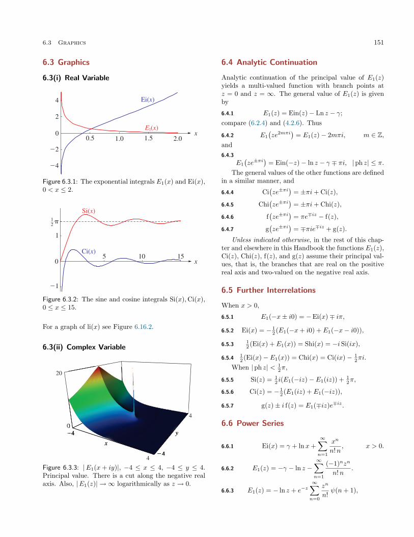
6.3 Graphics 151
6.3 Graphics
6.3(i) Real Variable
Figure 6.3.1: The exponential integrals E1(x) and Ei(x),0 < x ≤ 2.
Figure 6.3.2: The sine and cosine integrals Si(x),Ci(x),0 ≤ x ≤ 15.
For a graph of li(x) see Figure 6.16.2.
6.3(ii) Complex Variable
Figure 6.3.3: |E1(x+ iy)|, −4 ≤ x ≤ 4, −4 ≤ y ≤ 4.Principal value. There is a cut along the negative realaxis. Also, |E1(z)| → ∞ logarithmically as z → 0.
6.4 Analytic Continuation
Analytic continuation of the principal value of E1(z)yields a multi-valued function with branch points atz = 0 and z = ∞. The general value of E1(z) is givenby
6.4.1 E1(z) = Ein(z)− Ln z − γ;compare (6.2.4) and (4.2.6). Thus
6.4.2 E1
(ze2mπi
)= E1(z)− 2mπi, m ∈ Z,
and6.4.3
E1
(ze±πi
)= Ein(−z)− ln z − γ ∓ πi, |ph z| ≤ π.
The general values of the other functions are definedin a similar manner, and
6.4.4 Ci(ze±πi
)= ±πi+ Ci(z),
6.4.5 Chi(ze±πi
)= ±πi+ Chi(z),
6.4.6 f(ze±πi
)= πe∓iz − f(z),
6.4.7 g(ze±πi
)= ∓πie∓iz + g(z).
Unless indicated otherwise, in the rest of this chap-ter and elsewhere in this Handbook the functions E1(z),Ci(z), Chi(z), f(z), and g(z) assume their principal val-ues, that is, the branches that are real on the positivereal axis and two-valued on the negative real axis.
6.5 Further Interrelations
When x > 0,
6.5.1 E1(−x± i0) = −Ei(x)∓ iπ,
6.5.2 Ei(x) = − 12 (E1(−x+ i0) + E1(−x− i0)),
6.5.3 12 (Ei(x) + E1(x)) = Shi(x) = −iSi(ix),
6.5.4 12 (Ei(x)− E1(x)) = Chi(x) = Ci(ix)− 1
2πi.
When |ph z| < 12π,
6.5.5 Si(z) = 12 i(E1(−iz)− E1(iz)) + 1
2π,
6.5.6 Ci(z) = − 12 (E1(iz) + E1(−iz)),
6.5.7 g(z)± i f(z) = E1(∓iz)e∓iz.
6.6 Power Series
6.6.1 Ei(x) = γ + lnx+∞∑n=1
xn
n!n, x > 0.
6.6.2 E1(z) = −γ − ln z −∞∑n=1
(−1)nzn
n!n.
6.6.3 E1(z) = − ln z + e−z∞∑n=0
zn
n!ψ(n+ 1),

152 Exponential, Logarithmic, Sine, and Cosine Integrals
where ψ denotes the logarithmic derivative of thegamma function (§5.2(i)).
6.6.4 Ein(z) =∞∑n=1
(−1)n−1zn
n!n,
6.6.5 Si(z) =∞∑n=0
(−1)nz2n+1
(2n+ 1)!(2n+ 1),
6.6.6 Ci(z) = γ + ln z +∞∑n=1
(−1)nz2n
(2n)!(2n).
The series in this section converge for all finite values ofx and |z|.
6.7 Integral Representations
6.7(i) Exponential Integrals
6.7.1∫ ∞0
e−at
t+ bdt=
∫ ∞0
eiat
t+ ibdt= eabE1(ab), a > 0, b > 0,
6.7.2ex∫ α
0
e−xt
1− tdt = Ei(x)− Ei((1− α)x),
0 ≤ α < 1, x > 0.
6.7.3∫ ∞x
eit
a2 + t2dt=
i
2a(eaE1(a− ix)−e−aE1(−a− ix)
),
a > 0, x > 0,
6.7.4∫ ∞x
teit
a2 + t2dt = 1
2
(eaE1(a− ix) + e−aE1(−a− ix)
),
a > 0, x > 0.
6.7.5
∫ ∞x
e−t
a2 + t2dt = − 1
2ai(eiaE1(x+ ia)
− e−iaE1(x− ia))
,a > 0, x ∈ R,
6.7.6∫ ∞x
te−t
a2 + t2dt = 1
2
(eiaE1(x+ ia) + e−iaE1(x− ia)
),
a > 0, x ∈ R.
6.7.7
∫ 1
0
e−at sin(bt)t
dt = =Ein(a+ ib), a, b ∈ R,
6.7.8
∫ 1
0
e−at(1− cos(bt))t
dt = <Ein(a+ ib)− Ein(a),
a, b ∈ R.Many integrals with exponentials and rational func-
tions, for example, integrals of the type∫ezR(z) dz,
where R(z) is an arbitrary rational function, can berepresented in finite form in terms of the function E1(z)and elementary functions; see Lebedev (1965, p. 42).
6.7(ii) Sine and Cosine Integrals
When z ∈ C
6.7.9 si(z) = −∫ π/2
0
e−z cos t cos(z sin t) dt,
6.7.10 Ein(z)− Cin(z) =∫ π/2
0
e−z cos t sin(z sin t) dt,
6.7.11
∫ 1
0
(1− e−at) cos(bt)t
dt=<Ein(a+ ib)−Cin(b),
a, b ∈ R.
6.7(iii) Auxiliary Functions
6.7.12 g(z) + i f(z) = e−iz∫ ∞z
eit
tdt, |ph z| ≤ π.
The path of integration does not cross the negative realaxis or pass through the origin.
6.7.13 f(z) =∫ ∞
0
sin tt+ z
dt =∫ ∞
0
e−zt
t2 + 1dt,
6.7.14 g(z) =∫ ∞
0
cos tt+ z
dt =∫ ∞
0
te−zt
t2 + 1dt.
The first integrals on the right-hand sides apply when|ph z| < π; the second ones when <z ≥ 0 and (in thecase of (6.7.14)) z 6= 0.
When |ph z| < π
6.7.15 f(z) = 2∫ ∞
0
K0
(2√zt)
cos t dt,
6.7.16 g(z) = 2∫ ∞
0
K0
(2√zt)
sin t dt.
For K0 see §10.25(ii).
6.7(iv) Compendia
For collections of integral representations see Bierens deHaan (1939, pp. 56–59, 72–73, 82–84, 121, 133–136, 155,179–181, 223, 225–227, 230, 259–260, 374, 377, 397–398,408, 416, 424, 431, 438–439, 442–444, 488, 496–500,567–571, 585, 602, 638, 675–677), Corrington (1961),Erdélyi et al. (1954a, vol. 1, pp. 267–270), Geller and Ng(1969), Nielsen (1906b), Oberhettinger (1974, pp. 244–246), Oberhettinger and Badii (1973, pp. 364–371), andWatrasiewicz (1967).
6.8 Inequalities
In this section x > 0.
6.8.112
ln(
1 +2x
)< exE1(x) < ln
(1 +
1x
),
6.8.2x
x+ 1< xexE1(x) <
x+ 1x+ 2
,
6.8.3x(x+ 3)
x2 + 4x+ 2< xexE1(x) <
x2 + 5x+ 2x2 + 6x+ 6
.

6.9 Continued Fraction 153
6.9 Continued Fraction
6.9.1E1(z) =
e−z
z +1
1 +1z +
21 +
2z +
31 +
3z+· · · ,
|ph z| < π.
See also Cuyt et al. (2008, pp. 287–290).
6.10 Other Series Expansions
6.10(i) Inverse Factorial Series
6.10.1
E1(z) = e−z(c0z
+c1
z(z + 1)+
2!c2z(z + 1)(z + 2)
+3!c3
z(z + 1)(z + 2)(z + 3)+ · · ·
),
<z > 0,where
6.10.2 c0 = 1, c1 = −1, c2 = 12 , c3 = − 1
3 , c4 = 16 ,
and
6.10.3 ck = −k−1∑j=0
cjk − j
, k ≥ 1.
For a more general result (incomplete gamma func-tion), and also for a result for the logarithmic integral,see Nielsen (1906a, p. 283: Formula (3) is incorrect).
6.10(ii) Expansions in Series of Spherical BesselFunctions
For the notation see §10.47(ii).
6.10.4 Si(z) = z
∞∑n=0
(jn(
12z))2
,
6.10.5 Cin(z) =∞∑n=1
an(jn(
12z))2
,
6.10.6Ei(x) = γ+ln |x|+
∞∑n=0
(−1)n(x−an)(
i(1)n
(12x))2
,
x 6= 0,where
6.10.7 an = (2n+ 1) (1− (−1)n + ψ(n+ 1)− ψ(1)) ,and ψ denotes the logarithmic derivative of the gammafunction (§5.2(i)).6.10.8
Ein(z) = ze−z/2
(i(1)0
(12z)
+∞∑n=1
2n+ 1n(n+ 1)
i(1)n
(12z))
.
For (6.10.4)–(6.10.8) and further results see Harris(2000) and Luke (1969b, pp. 56–57). An expansionfor E1(z) can be obtained by combining (6.2.4) and(6.10.8).
6.11 Relations to Other Functions
For the notation see §§8.2(i) and 13.2(i).
Incomplete Gamma Function
6.11.1 E1(z) = Γ(0, z).
Confluent Hypergeometric Function
6.11.2 E1(z) = e−z U(1, 1, z),
6.11.3 g(z) + i f(z) = U(1, 1,−iz).
6.12 Asymptotic Expansions
6.12(i) Exponential and Logarithmic Integrals
6.12.1E1(z) ∼ e−z
z
(1− 1!
z+
2!z2− 3!z3
+ · · ·)
,
z →∞, |ph z| ≤ 32π − δ(<
32π).
When |ph z| ≤ 12π the remainder is bounded in magni-
tude by the first neglected term, and has the same signwhen ph z = 0. When 1
2π ≤ | ph z| < π the remainderterm is bounded in magnitude by csc(|ph z|) times thefirst neglected term. For these and other error boundssee Olver (1997b, pp. 109–112) with α = 0.
For re-expansions of the remainder term leading tolarger sectors of validity, exponential improvement, anda smooth interpretation of the Stokes phenomenon, see§§2.11(ii)–2.11(iv), with p = 1.6.12.2
Ei(x) ∼ ex
x
(1 +
1!x
+2!x2
+3!x3
+ · · ·)
, x→ +∞.
If the expansion is terminated at the nth term, then theremainder term is bounded by 1 + χ(n + 1) times thenext term. For the function χ see §9.7(i).
The asymptotic expansion of li(x) as x → ∞ is ob-tainable from (6.2.8) and (6.12.2).
6.12(ii) Sine and Cosine Integrals
The asymptotic expansions of Si(z) and Ci(z) are givenby (6.2.19), (6.2.20), together with
6.12.3 f(z) ∼ 1z
(1− 2!
z2+
4!z4− 6!z6
+ · · ·),
6.12.4 g(z) ∼ 1z2
(1− 3!
z2+
5!z4− 7!z6
+ · · ·),
as z →∞ in |ph z| ≤ π − δ (< π).The remainder terms are given by
6.12.5 f(z) =1z
n−1∑m=0
(−1)m(2m)!z2m
+R(f)n (z),
6.12.6 g(z) =1z2
n−1∑m=0
(−1)m(2m+ 1)!z2m
+R(g)n (z),

154 Exponential, Logarithmic, Sine, and Cosine Integrals
where, for n = 0, 1, 2, . . . ,
6.12.7 R(f)n (z) = (−1)n
∫ ∞0
e−ztt2n
t2 + 1dt,
6.12.8 R(g)n (z) = (−1)n
∫ ∞0
e−ztt2n+1
t2 + 1dt.
When |ph z| ≤ 14π, these remainders are bounded in
magnitude by the first neglected terms in (6.12.3) and(6.12.4), respectively, and have the same signs as theseterms when ph z = 0. When 1
4π ≤ |ph z| < 12π the
remainders are bounded in magnitude by csc(2|ph z|)times the first neglected terms.
For other phase ranges use (6.4.6) and (6.4.7).For exponentially-improved asymptotic expansions, use(6.5.5), (6.5.6), and §6.12(i).
6.13 Zeros
The function Ei(x) has one real zero x0, given by6.13.1 x0 = 0.37250 74107 81366 63446 19918 66580 . . . .Ci(x) and si(x) each have an infinite number of pos-itive real zeros, which are denoted by ck, sk, respec-tively, arranged in ascending order of absolute value fork = 0, 1, 2, . . . . Values of c1 and c2 to 30D are given byMacLeod (1996).
As k →∞,6.13.2
ck, sk ∼ α+1α− 16
31α3
+167315
1α5− 5 07746
1051α7
+ · · · ,
where α = kπ for ck, and α = (k + 12 )π for sk.
For these results, together with the next three termsin (6.13.2), see MacLeod (2002a). See also Riekstynš(1991, pp. 176–177).
6.14 Integrals
6.14(i) Laplace Transforms
6.14.1
∫ ∞0
e−atE1(t) dt =1a
ln(1 + a), <a > −1,
6.14.2
∫ ∞0
e−at Ci(t) dt = − 12a
ln(1 + a2
), <a > 0,
6.14.3
∫ ∞0
e−at si(t) dt = −1a
arctan a, <a > 0.
6.14(ii) Other Integrals
6.14.4
∫ ∞0
E21(t) dt = 2 ln 2,
6.14.5
∫ ∞0
cos tCi(t) dt =∫ ∞
0
sin t si(t) dt = − 14π,
6.14.6
∫ ∞0
Ci2(t) dt =∫ ∞
0
si2(t) dt = 12π,
6.14.7
∫ ∞0
Ci(t) si(t) dt = ln 2.
6.14(iii) Compendia
For collections of integrals, see Apelblat (1983, pp. 110–123), Bierens de Haan (1939, pp. 373–374, 409, 479,571–572, 637, 664–673, 680–682, 685–697), Erdélyi et al.(1954a, vol. 1, pp. 40–42, 96–98, 177–178, 325), Gellerand Ng (1969), Gradshteyn and Ryzhik (2000, §§5.2–5.3and 6.2–6.27), Marichev (1983, pp. 182–184), Nielsen(1906b), Oberhettinger (1974, pp. 139–141), Oberhet-tinger (1990, pp. 53–55 and 158–160), Oberhettingerand Badii (1973, pp. 172–179), Prudnikov et al. (1986b,vol. 2, pp. 24–29 and 64–92), Prudnikov et al. (1992a,§§3.4–3.6), Prudnikov et al. (1992b, §§3.4–3.6), and Wa-trasiewicz (1967).
6.15 Sums
6.15.1
∞∑n=1
Ci(πn) = 12 (ln 2− γ),
6.15.2
∞∑n=1
si(πn)n
= 12π(lnπ − 1),
6.15.3
∞∑n=1
(−1)n Ci(2πn) = 1− ln 2− 12γ,
6.15.4
∞∑n=1
(−1)nsi(2πn)n
= π( 32 ln 2− 1).
For further sums see Fempl (1960), Hansen (1975,pp. 423–424), Harris (2000), Prudnikov et al. (1986b,vol. 2, pp. 649–650), and Slavić (1974).
Applications
6.16 Mathematical Applications
6.16(i) The Gibbs Phenomenon
Consider the Fourier series
6.16.1
sinx+ 13 sin(3x) + 1
5 sin(5x) + · · ·
=
14π, 0 < x < π,
0, x = 0,− 1
4π, −π < x < 0.
The nth partial sum is given by
6.16.2Sn(x) =
n−1∑k=0
sin((2k + 1)x)2k + 1
=12
∫ x
0
sin(2nt)sin t
dt
= 12 Si(2nx) +Rn(x),

6.17 Physical Applications 155
where
6.16.3 Rn(x) =12
∫ x
0
(1
sin t− 1t
)sin(2nt) dt.
By integration by parts
6.16.4 Rn(x) = O(n−1
), n→∞,
uniformly for x ∈ [−π, π]. Hence, if x is fixed andn → ∞, then Sn(x) → 1
4π, 0, or − 14π according as
0 < x < π, x = 0, or −π < x < 0; compare (6.2.14).
These limits are not approached uniformly, however.The first maximum of 1
2 Si(x) for positive x occurs atx = π and equals (1.1789 . . . ) × 1
4π; compare Figure6.3.2. Hence if x = π/(2n) and n → ∞, then the lim-iting value of Sn(x) overshoots 1
4π by approximately18%. Similarly if x = π/n, then the limiting value ofSn(x) undershoots 1
4π by approximately 10%, and soon. Compare Figure 6.16.1.
This nonuniformity of convergence is an illustrationof the Gibbs phenomenon. It occurs with Fourier-seriesexpansions of all piecewise continuous functions. SeeCarslaw (1930) for additional graphs and information.
Figure 6.16.1: Graph of Sn(x), n = 250, −0.1 ≤ x ≤ 0.1,illustrating the Gibbs phenomenon.
6.16(ii) Number-Theoretic Significance of li(x)
If we assume Riemann’s hypothesis that all nonreal ze-ros of ζ(s) have real part of 1
2 (§25.10(i)), then
6.16.5 li(x)− π(x) = O(√x lnx
), x→∞,
where π(x) is the number of primes less than or equalto x. Compare §27.12 and Figure 6.16.2. See also Baysand Hudson (2000).
Figure 6.16.2: The logarithmic integral li(x), togetherwith vertical bars indicating the value of π(x) for x =10, 20, . . . , 1000.
6.17 Physical Applications
Geller and Ng (1969) cites work with applications fromdiffusion theory, transport problems, the study of theradiative equilibrium of stellar atmospheres, and theevaluation of exchange integrals occurring in quantummechanics. For applications in astrophysics, see also vande Hulst (1980). Lebedev (1965) gives an application toelectromagnetic theory (radiation of a linear half-waveoscillator), in which sine and cosine integrals are used.
Computation
6.18 Methods of Computation
6.18(i) Main Functions
For small or moderate values of x and |z|, the expan-sion in power series (§6.6) or in series of spherical Besselfunctions (§6.10(ii)) can be used. For large x or |z| theseseries suffer from slow convergence or cancellation (orboth). However, this problem is less severe for the se-ries of spherical Bessel functions because of their morerapid rate of convergence, and also (except in the caseof (6.10.6)) absence of cancellation when z = x (> 0).
For large x and |z|, expansions in inverse factorialseries (§6.10(i)) or asymptotic expansions (§6.12) areavailable. The attainable accuracy of the asymptoticexpansions can be increased considerably by exponen-tial improvement. Also, other ranges of ph z can becovered by use of the continuation formulas of §6.4.
Quadrature of the integral representations is anothereffective method. For example, the Gauss-Laguerre for-mula (§3.5(v)) can be applied to (6.2.2); see Todd (1954)and Tseng and Lee (1998). For an application of theGauss-Legendre formula (§3.5(v)) see Tooper and Mark(1968).

156 Exponential, Logarithmic, Sine, and Cosine Integrals
Lastly, the continued fraction (6.9.1) can be used if|z| is bounded away from the origin. Convergence be-comes slow when z is near the negative real axis, how-ever.
6.18(ii) Auxiliary Functions
Power series, asymptotic expansions, and quadraturecan also be used to compute the functions f(z) and g(z).In addition, Acton (1974) developed a recurrence pro-cedure, as follows. For n = 0, 1, 2, . . . , define
6.18.1
An =∫ ∞
0
te−zt
1 + t2
(t2
1 + t2
)ndt,
Bn =∫ ∞
0
e−zt
1 + t2
(t2
1 + t2
)ndt,
Cn =∫ ∞
0
e−zt(
t2
1 + t2
)ndt.
Then f(z) = B0, g(z) = A0, and
6.18.2An−1 = An +
z
2nCn, Bn−1 =
2nBn + zAn−1
2n− 1,
Cn−1 = Cn +Bn−1, n = 1, 2, 3, . . . .A0, B0, and C0 can be computed by Miller’s algorithm(§3.6(iii)), starting with initial values (AN , BN , CN ) =(1, 0, 0), say, where N is an arbitrary large integer, andnormalizing via C0 = 1/z.
6.18(iii) Zeros
Zeros of Ci(x) and si(x) can be computed to high pre-cision by Newton’s rule (§3.8(ii)), using values suppliedby the asymptotic expansion (6.13.2) as initial approx-imations.
6.18(iv) Other References
For a comprehensive survey of computational methodsfor the functions treated in this chapter, see van derLaan and Temme (1984, Ch. IV).
6.19 Tables
6.19(i) Introduction
Lebedev and Fedorova (1960) and Fletcher et al. (1962)give comprehensive indexes of mathematical tables.This section lists relevant tables that appeared later.
6.19(ii) Real Variables
• Abramowitz and Stegun (1964, Chapter 5)includes x−1 Si(x), −x−2 Cin(x), x−1 Ein(x),−x−1 Ein(−x), x = 0(.01)0.5; Si(x), Ci(x),Ei(x), E1(x), x = 0.5(.01)2; Si(x), Ci(x),xe−x Ei(x), xexE1(x), x = 2(.1)10; x f(x),x2 g(x), xe−x Ei(x), xexE1(x), x−1 = 0(.005)0.1;Si(πx), Cin(πx), x = 0(.1)10. Accuracy varies butis within the range 8S–11S.
• Zhang and Jin (1996, pp. 652, 689) includes Si(x),Ci(x), x = 0(.5)20(2)30, 8D; Ei(x), E1(x), x =[0, 100], 8S.
6.19(iii) Complex Variables, z = x+ iy
• Abramowitz and Stegun (1964, Chapter 5) in-cludes the real and imaginary parts of zez E1(z),x = −19(1)20, y = 0(1)20, 6D; ez E1(z), x =−4(.5) − 2, y = 0(.2)1, 6D; E1(z) + ln z, x =−2(.5)2.5, y = 0(.2)1, 6D.
• Zhang and Jin (1996, pp. 690–692) in-cludes the real and imaginary parts of E1(z),±x = 0.5, 1, 3, 5, 10, 15, 20, 50, 100, y =0(.5)1(1)5(5)30, 50, 100, 8S.
6.20 Approximations
6.20(i) Approximations in Terms of ElementaryFunctions
• Hastings (1955) gives several minimax polyno-mial and rational approximations for E1(x)+lnx,xexE1(x), and the auxiliary functions f(x) andg(x). These are included in Abramowitz and Ste-gun (1964, Ch. 5).
• Cody and Thacher (1968) provides minimax ra-tional approximations for E1(x), with accuraciesup to 20S.
• Cody and Thacher (1969) provides minimax ra-tional approximations for Ei(x), with accuraciesup to 20S.
• MacLeod (1996) provides rational approximationsfor the sine and cosine integrals and for the auxil-iary functions f and g, with accuracies up to 20S.
6.20(ii) Expansions in Chebyshev Series
• Clenshaw (1962) gives Chebyshev coefficients for−E1(x) − ln |x| for −4 ≤ x ≤ 4 and exE1(x) forx ≥ 4 (20D).
• Luke and Wimp (1963) covers Ei(x) for x ≤ −4(20D), and Si(x) and Ci(x) for x ≥ 4 (20D).
• Luke (1969b, pp. 41–42) gives Chebyshev expan-sions of Ein(ax), Si(ax), and Cin(ax) for −1 ≤x ≤ 1, a ∈ C. The coefficients are given in termsof series of Bessel functions.

6.21 Software 157
• Luke (1969b, pp. 321–322) covers Ein(x) and−Ein(−x) for 0 ≤ x ≤ 8 (the Chebyshev coef-ficients are given to 20D); E1(x) for x ≥ 5 (20D),and Ei(x) for x ≥ 8 (15D). Coefficients for the sineand cosine integrals are given on pp. 325–327.
• Luke (1969b, p. 25) gives a Chebyshev expansionnear infinity for the confluent hypergeometric U -function (§13.2(i)) from which Chebyshev expan-sions near infinity for E1(z), f(z), and g(z) followby using (6.11.2) and (6.11.3). Luke also includesa recursion scheme for computing the coefficientsin the expansions of the U functions. If |ph z| < πthe scheme can be used in backward direction.
6.20(iii) Padé-Type and Rational Expansions
• Luke (1969b, pp. 402, 410, and 415–421) givesmain diagonal Padé approximations for Ein(z),Si(z), Cin(z) (valid near the origin), and E1(z)(valid for large |z|); approximate errors are givenfor a selection of z-values.
• Luke (1969b, pp. 411–414) gives rational approx-imations for Ein(z).
6.21 Software
See http://dlmf.nist.gov/6.21.
References
General References
For general bibliographic reading see Andrews et al.(1999), Jeffreys and Jeffreys (1956), Lebedev (1965),Olver (1997b), and Temme (1996a).
Sources
The following list gives the references or other indica-tions of proofs that were used in constructing the varioussections of this chapter. These sources supplement thereferences that are quoted in the text.
§6.2 Olver (1997b, pp. 40–42).
§6.3 These graphics were produced at NIST.
§6.4 For (6.4.1) see Olver (1997b, p. 40). (6.4.3) followsfrom (6.6.2) and (6.6.4). (6.4.4) and (6.4.5) followfrom (6.2.13) and (6.2.16). (6.4.6) and (6.4.7) fol-low from (6.2.17), (6.2.18), and (6.4.4).
§6.5 For (6.5.1) and (6.5.2) see Olver (1997b, p. 41).(6.5.3) and (6.5.4) follow from (6.6.1), (6.6.2),(6.6.5), and (6.6.6). For (6.5.5) and (6.5.6) seeOlver (1997b, p. 42). (6.5.7) follows from (6.2.10),(6.2.17), (6.2.18), (6.5.5), and (6.5.6).
§6.6 Olver (1997b, pp. 40–43). (6.6.3) follows from(6.11.2) and (13.2.9).
§6.7 (6.7.1) and (6.7.2) follow from the definitions(§6.2(i)). (6.7.3)–(6.7.6) follow from differentia-tion with respect to x. (6.7.7) and (6.7.8) fol-low from replacing the trigonometric functionsby exponentials. For (6.7.9)–(6.7.11) see Nielsen(1906b, p. 13: there are sign errors in Eq. (27)).(6.7.12)–(6.7.14) follow from (6.5.7), (6.2.1), and(6.2.2); for the second equations in (6.7.13) and(6.7.14) see Temme (1996a, pp. 187–188). For(6.7.15) and (6.7.16) use (10.32.10).
§6.8 See Gautschi (1959b) for (6.8.1), and Luke (1969b,p. 201) for (6.8.2) and (6.8.3).
§6.9 Nielsen (1906b, pp. 42–44), or Lorentzen andWaadeland (1992, p. 577).
§6.10 Nielsen (1906a, p. 283). (6.10.3) follows from1/(1− ln(1− t)) =
∑∞k=0 ckt
k.
§6.11 Temme (1996a, pp. 180 and 187). For (6.11.3)use (6.5.7).
§6.12 For (6.12.2) see Olver (1997b, p. 227). (6.12.3)and (6.12.4) follow from (6.7.13) and (6.7.14)by applying Watson’s lemma (§2.4(i)). (6.12.5)–(6.12.8) follow from (6.7.13), (6.7.14), andthe identity (t2 + 1)−1 =
∑n−1m=0(−1)mt2m +
(−1)nt2n(t2+1)−1. The error bounds are obtainedby setting t =
√τ in (6.12.7) and (6.12.8), rotat-
ing the integration path in the τ -plane throughan angle −2 ph z, and then replacing |τ + 1| by itsminimum value on the path.
§6.13 See Cody and Thacher (1969) for x0 in (6.13.1).
§6.14 Nielsen (1906b, pp. 48–50, 53, and 54: there isa 1
2 missing in the formula that corresponds to(6.14.2) and a sign error in the formula that cor-responds to (6.14.7)).
§6.15 Slavić (1974).
§6.16 Temme (1996a, pp. 181–182: the numerical value1.089490 . . . on p. 182 should be replaced by1.1789 . . . ). Gibbs reported this phenomenon in aletter to Nature, 59 (1899, p. 606). Figures 6.16.1and 6.16.2 were produced at NIST.

Chapter 7
Error Functions, Dawson’s and Fresnel IntegralsN. M. Temme1
Notation 1607.1 Special Notation . . . . . . . . . . . . . 160
Properties 1607.2 Definitions . . . . . . . . . . . . . . . . . 1607.3 Graphics . . . . . . . . . . . . . . . . . . 1607.4 Symmetry . . . . . . . . . . . . . . . . . 1617.5 Interrelations . . . . . . . . . . . . . . . 1627.6 Series Expansions . . . . . . . . . . . . . 1627.7 Integral Representations . . . . . . . . . 1627.8 Inequalities . . . . . . . . . . . . . . . . 1637.9 Continued Fractions . . . . . . . . . . . . 1637.10 Derivatives . . . . . . . . . . . . . . . . 1637.11 Relations to Other Functions . . . . . . . 1647.12 Asymptotic Expansions . . . . . . . . . . 1647.13 Zeros . . . . . . . . . . . . . . . . . . . 1657.14 Integrals . . . . . . . . . . . . . . . . . . 166
7.15 Sums . . . . . . . . . . . . . . . . . . . 1667.16 Generalized Error Functions . . . . . . . . 1667.17 Inverse Error Functions . . . . . . . . . . 1667.18 Repeated Integrals of the Complementary
Error Function . . . . . . . . . . . . . . . 1677.19 Voigt Functions . . . . . . . . . . . . . . 167
Applications 1687.20 Mathematical Applications . . . . . . . . 1687.21 Physical Applications . . . . . . . . . . . 169
Computation 1697.22 Methods of Computation . . . . . . . . . 1697.23 Tables . . . . . . . . . . . . . . . . . . . 1697.24 Approximations . . . . . . . . . . . . . . 1707.25 Software . . . . . . . . . . . . . . . . . . 170
References 170
1Centrum voor Wiskunde en Informatica, Department MAS, Amsterdam, The Netherlands.Acknowledgments: This chapter is based in part on Abramowitz and Stegun (1964, Chapter 7) by Walter Gautschi. Walter
Gautschi provided the author with a list of references and comments collected since the original publication.Copyright c© 2009 National Institute of Standards and Technology. All rights reserved.
159

160 Error Functions, Dawson’s and Fresnel Integrals
Notation
7.1 Special Notation
(For other notation see pp. xiv and 873.)
x real variable.z complex variable.n nonnegative integer.δ arbitrary small positive constant.γ Euler’s constant (§5.2(ii)).
Unless otherwise noted, primes indicate derivativeswith respect to the argument.
The main functions treated in this chapter are theerror function erf z; the complementary error functionserfc z and w(z); Dawson’s integral F (z); the Fresnel in-tegrals F(z), C(z), and S(z); the Goodwin–Staton inte-gral G(z); the repeated integrals of the complementaryerror function inerfc(z); the Voigt functions U(x, t) andV(x, t).
Alternative notations are P (z) = 12 erfc
(−z/√
2),
Q(z) = Φ(z) = 12 erfc
(z/√
2), Erf z = 1
2
√π erf z,
Erfi z = ez2F (z), C1(z) = C
(√2/πz
), S1(z) =
S(√
2/πz)
, C2(z) = C(√
2z/π)
, S2(z) = S(√
2z/π)
.
The notations P (z), Q(z), and Φ(z) are used inmathematical statistics, where these functions are calledthe normal or Gaussian probability functions.
Properties
7.2 Definitions
7.2(i) Error Functions
7.2.1 erf z =2√π
∫ z
0
e−t2dt,
7.2.2 erfc z =2√π
∫ ∞z
e−t2dt = 1− erf z,
7.2.3
w(z) = e−z2(
1 +2i√π
∫ z
0
et2dt
)= e−z
2erfc(−iz).
erf z, erfc z, and w(z) are entire functions of z, as isF (z) in the next subsection.
Values at Infinity
7.2.4limz→∞
erf z = 1, limz→∞
erfc z = 0,
|ph z| ≤ 14π − δ(<
14π).
7.2(ii) Dawson’s Integral
7.2.5 F (z) = e−z2∫ z
0
et2dt.
7.2(iii) Fresnel Integrals
7.2.6 F(z) =∫ ∞z
e12πit
2dt,
7.2.7 C(z) =∫ z
0
cos(
12πt
2)dt,
7.2.8 S(z) =∫ z
0
sin(
12πt
2)dt,
F(z), C(z), and S(z) are entire functions of z, as aref(z) and g(z) in the next subsection.
Values at Infinity
7.2.9 limx→∞
C(x) = 12 , lim
x→∞S(x) = 1
2 .
7.2(iv) Auxiliary Functions
7.2.10
f(z) =(
12 − S(z)
)cos(
12πz
2)−(
12 − C(z)
)sin(
12πz
2),
7.2.11
g(z) =(
12 − C(z)
)cos(
12πz
2)
+(
12 − S(z)
)sin(
12πz
2).
7.2(v) Goodwin–Staton Integral
7.2.12 G(z) =∫ ∞
0
e−t2
t+ zdt, |ph z| < π.
7.3 Graphics
7.3(i) Real Variable
Figure 7.3.1: Complementary error functions erfcx anderfc(10x), −3 ≤ x ≤ 3.

7.4 Symmetry 161
Figure 7.3.2: Dawson’s integral F (x), −3.5 ≤ x ≤ 3.5.
Figure 7.3.3: Fresnel integrals C(x) and S(x), 0 ≤ x ≤ 4.
Figure 7.3.4: | F(x)|2, −8 ≤ x ≤ 8. Fresnel (1818) intro-duced the integral F(x) in his study of the interferencepattern at the edge of a shadow. He observed that theintensity distribution is given by |F(x)|2.
7.3(ii) Complex Variable
Figure 7.3.5: | erf(x+ iy)|, −3 ≤ x ≤ 3, −3 ≤ y ≤ 3.Compare §7.13(i).
Figure 7.3.6: | erfc(x+ iy)|, −3 ≤ x ≤ 3, −3 ≤ y ≤ 3.Compare §§7.12(i) and 7.13(ii).
7.4 Symmetry
7.4.1 erf(−z) = − erf(z),
7.4.2 erfc(−z) = 2− erfc(z),
7.4.3 w(−z) = 2e−z2− w(z).
7.4.4 F (−z) = −F (z).
7.4.5 C(−z) = −C(z), S(−z) = −S(z),
7.4.6 C(iz) = i C(z), S(iz) = −i S(z).
7.4.7f(iz) = (1/
√2)e
14πi−
12πiz
2− i f(z),
g(iz) = (1/√
2)e−14πi−
12πiz
2+ i g(z).

162 Error Functions, Dawson’s and Fresnel Integrals
7.4.8f(−z) =
√2 cos
(14π + 1
2πz2)− f(z),
g(−z) =√
2 sin(
14π + 1
2πz2)− g(z).
7.5 Interrelations
7.5.1 F (z) = 12 i√π(e−z
2−w(z)
)=− 1
2 i√πe−z
2erf(iz).
7.5.2 C(z) + i S(z) = 12 (1 + i)−F(z).
7.5.3 C(z) = 12 + f(z) sin
(12πz
2)− g(z) cos
(12πz
2),
7.5.4 S(z) = 12 − f(z) cos
(12πz
2)− g(z) sin
(12πz
2).
7.5.5 e−12πiz
2F(z) = g(z) + i f(z).
7.5.6 e±12πiz
2(g(z)± i f(z)) = 1
2 (1± i)− (C(z)± i S(z)).In (7.5.8)–(7.5.10)
7.5.7 ζ = 12
√π(1∓ i)z,
and either all upper signs or all lower signs are takenthroughout.
7.5.8 C(z)± i S(z) = 12 (1± i) erf ζ.
7.5.9 C(z)± i S(z) = 12 (1± i)
(1− e± 1
2πiz2w(iζ)
).
7.5.10 g(z)± i f(z) = 12 (1± i)eζ
2erfc ζ.
7.5.11 | F(x)|2 = f2(x) + g2(x), x ≥ 0,
7.5.12
| F(x)|2 = 2 + f2(−x) + g2(−x)− 2√
2 cos(
14π + 1
2πx2)
f(−x)
− 2√
2 cos(
14π −
12πx
2)
g(−x),x ≤ 0.
See Figure 7.3.4.
7.5.13 G(x) =√π F (x)− 1
2e−x2
Ei(x2), x > 0.
For Ei(x) see §6.2(i).
7.6 Series Expansions
7.6(i) Power Series
7.6.1 erf z =2√π
∞∑n=0
(−1)nz2n+1
n!(2n+ 1),
7.6.2 erf z =2√πe−z
2∞∑n=0
2nz2n+1
1 · 3 · · · (2n+ 1),
7.6.3 w(z) =∞∑n=0
(iz)n
Γ(
12n+ 1
) .7.6.4 C(z) =
∞∑n=0
(−1)n( 12π)2n
(2n)!(4n+ 1)z4n+1,
7.6.5
C(z) = cos(
12πz
2) ∞∑n=0
(−1)nπ2n
1 · 3 · · · (4n+ 1)z4n+1
+ sin(
12πz
2) ∞∑n=0
(−1)nπ2n+1
1 · 3 · · · (4n+ 3)z4n+3.
7.6.6 S(z) =∞∑n=0
(−1)n( 12π)2n+1
(2n+ 1)!(4n+ 3)z4n+3,
7.6.7
S(z) = − cos(
12πz
2) ∞∑n=0
(−1)nπ2n+1
1 · 3 · · · (4n+ 3)z4n+3
+ sin(
12πz
2) ∞∑n=0
(−1)nπ2n
1 · 3 · · · (4n+ 1)z4n+1.
The series in this subsection and in §7.6(ii) converge forall finite values of |z|.
7.6(ii) Expansions in Series of Spherical BesselFunctions
For the notation see §§10.47(ii) and 18.3.
7.6.8 erf z =2z√π
∞∑n=0
(−1)n(
i(1)2n
(z2)− i
(1)2n+1
(z2)),
7.6.9erf(az) =
2z√πe( 1
2−a2)z2
∞∑n=0
T2n+1(a) i(1)n
(12z
2),
−1 ≤ a ≤ 1.
7.6.10 C(z) = z
∞∑n=0
j2n(
12πz
2),
7.6.11 S(z) = z
∞∑n=0
j2n+1
(12πz
2).
For further results see Luke (1969b, pp. 57–58).
7.7 Integral Representations
7.7(i) Error Functions and Dawson’s Integral
Integrals of the type∫e−z
2R(z) dz, where R(z) is an ar-
bitrary rational function, can be written in closed formin terms of the error functions and elementary functions.
7.7.1 erfc z =2πe−z
2∫ ∞
0
e−z2t2
t2 + 1dt, |ph z| ≤ 1
4π,
7.7.2
w(z) =1πi
∫ ∞−∞
e−t2dt
t− z=
2zπi
∫ ∞0
e−t2dt
t2 − z2, =z > 0.
7.7.3
∫ ∞0
e−at2+2izt dt =
12
√π
ae−z
2/a +i√aF
(z√a
),
<a > 0.
7.7.4∫ ∞0
e−at√t+ z2
dt =√π
aeaz
2erfc
(√az), <a > 0, <z > 0.

7.8 Inequalities 163
7.7.5
∫ 1
0
e−at2
t2 + 1dt =
π
4ea(1− (erf
√a)2)
, <a > 0.
7.7.6
∫ ∞x
e−(at2+2bt+c) dt
=12
√π
ae(b2−ac)/a erfc
(√ax+
b√a
), <a > 0.
7.7.7∫ ∞x
e−a2t2−(b2/t2) dt =
√π
4a(e2ab erfc(ax+ (b/x))
+ e−2ab erfc(ax− (b/x)))
,x > 0, |ph a| < 1
4π.
7.7.8
∫ ∞0
e−a2t2−(b2/t2) dt =
√π
2ae−2ab,
|ph a| < 14π, |ph b| < 1
4π.
7.7.9
∫ x
0
erf t dt = x erf x+1√π
(e−x
2− 1).
7.7(ii) Auxiliary Functions
7.7.10 f(z) =1
π√
2
∫ ∞0
e−πz2t/2
√t(t2 + 1)
dt, |ph z| ≤ 14π,
7.7.11 g(z) =1
π√
2
∫ ∞0
√te−πz
2t/2
t2 + 1dt, |ph z| ≤ 1
4π,
7.7.12 g(z) + i f(z) = e−πiz2/2
∫ ∞z
eπit2/2 dt.
Mellin–Barnes Integrals
7.7.13f(z) =
(2π)−3/2
2πi
∫ c+i∞
c−i∞ζ−s Γ(s) Γ
(s+ 1
2
)× Γ
(s+ 3
4
)Γ(
14 − s
)ds,
7.7.14g(z) =
(2π)−3/2
2πi
∫ c+i∞
c−i∞ζ−s Γ(s) Γ
(s+ 1
2
)× Γ
(s+ 1
4
)Γ(
34 − s
)ds.
In (7.7.13) and (7.7.14) the integration paths arestraight lines, ζ = 1
16π2z4, and c is a constant such
that 0 < c < 14 in (7.7.13), and 0 < c < 3
4 in (7.7.14).
7.7.15
∫ ∞0
e−at cos(t2)dt =
√π
2f(
a√2π
), <a > 0,
7.7.16
∫ ∞0
e−at sin(t2)dt =
√π
2g(
a√2π
), <a > 0.
7.7(iii) Compendia
For other integral representations see Erdélyi et al.(1954a, vol. 1, pp. 265–267, 270), Ng and Geller (1969),Oberhettinger (1974, pp. 246–248), and Oberhettingerand Badii (1973, pp. 371–377).
7.8 Inequalities
Let M(x) denote Mills’ ratio:
7.8.1 M(x) =
∫∞xe−t
2dt
e−x2 = ex2∫ ∞x
e−t2dt.
(Other notations are often used.) Then
7.8.21
x+√x2 + 2
< M(x) ≤ 1x+
√x2 + (4/π)
, x ≥ 0,
7.8.3
√π
2√πx+ 2
≤ M(x) <1
x+ 1, x ≥ 0,
7.8.4 M(x) <2
3x+√x2 + 4
, x > − 12
√2,
7.8.5
x2
2x2 + 1≤ x2(2x2 + 5)
4x4 + 12x2 + 3≤ xM(x)
<2x4 + 9x2 + 4
4x4 + 20x2 + 15<
x2 + 12x2 + 3
,
x ≥ 0.
Next,
7.8.6
∫ x
0
eat2dt <
13ax
(2eax
2+ ax2 − 2
), a, x > 0.
7.8.7
∫ x
0
et2dt <
ex2 − 1x
, x > 0.
7.9 Continued Fractions
7.9.1
√πez
2erfc z =
z
z2 +
12
1 +1
z2 +
32
1 +2
z2 +· · · ,
<z > 0,
7.9.2
√πez
2erfc z =
2z2z2 + 1−
1 · 22z2 + 5−
3 · 42z2 + 9−
· · · ,
<z > 0,
7.9.3
w(z) =i√π
1z −
12
z −1z −
32
z −2z −
· · · , =z > 0.
See also Cuyt et al. (2008, pp. 255–260, 263–267,270–273).
7.10 Derivatives
7.10.1
dn+1erf zdzn+1 = (−1)n
2√πHn(z)e−z
2, n = 0, 1, 2, . . . .
For the Hermite polynomial Hn(z) see §18.3.
7.10.2 w′(z) = −2z w(z) + (2i/√π),
164 Error Functions, Dawson’s and Fresnel Integrals
7.10.3
w(n+2)(z) + 2z w(n+1)(z) + 2(n+ 1)w(n)(z) = 0,n = 0, 1, 2, . . . .
7.10.4df(z)dz
= −πz g(z),dg(z)dz
= πz f(z)− 1.
7.11 Relations to Other Functions
Incomplete Gamma Functions and GeneralizedExponential Integral
For the notation see §§8.2(i) and 8.19(i).
7.11.1 erf z =1√πγ(
12 , z
2),
7.11.2 erfc z =1√π
Γ(
12 , z
2),
7.11.3 erfc z =z√πE 1
2
(z2).
Confluent Hypergeometric Functions
For the notation see §13.2(i).
7.11.4 erf z =2z√πM(
12 ,
32 ,−z
2)
=2z√πe−z
2M(1, 3
2 , z2),
7.11.5
erfc z =1√πe−z
2U(
12 ,
12 , z
2)
=z√πe−z
2U(1, 3
2 , z2).
7.11.6C(z) + i S(z) = zM
(12 ,
32 ,
12πiz
2)
= zeπiz2/2M
(1, 3
2 ,−12πiz
2).
Generalized Hypergeometric Functions
For the notation see §§16.2(i) and 16.2(ii).
7.11.7 C(z) = z 1F2
(14 ; 5
4 ,12 ;− 1
16π2z4),
7.11.8 S(z) = 16πz
31F2
(34 ; 7
4 ,32 ;− 1
16π2z4).
7.12 Asymptotic Expansions
7.12(i) Complementary Error Function
As z →∞7.12.1
erfc z ∼ e−z2
√πz
∞∑m=0
(−1)m1 · 3 · 5 · · · (2m− 1)
(2z2)m,
erfc(−z) ∼ 2− e−z2
√πz
∞∑m=0
(−1)m1 · 3 · 5 · · · (2m− 1)
(2z2)m,
both expansions being valid when |ph z| ≤ 34π − δ
(< 34π).When |ph z| ≤ 1
4π the remainder terms are boundedin magnitude by the first neglected terms, and havethe same sign as these terms when ph z = 0. When14π ≤ |ph z| < 1
2π the remainder terms are boundedin magnitude by csc(2|ph z|) times the first neglected
terms. For these and other error bounds see Olver(1997b, pp. 109–112), with α = 1
2 and z replaced byz2; compare (7.11.2).
For re-expansions of the remainder terms leading tolarger sectors of validity, exponential improvement, anda smooth interpretation of the Stokes phenomenon, see§§2.11(ii)–2.11(iv) and use (7.11.3). (Note that some ofthese re-expansions themselves involve the complemen-tary error function.)
7.12(ii) Fresnel Integrals
The asymptotic expansions of C(z) and S(z) are givenby (7.5.3), (7.5.4), and
7.12.2 f(z) ∼ 1πz
∞∑m=0
(−1)m1 · 3 · 5 · · · (4m− 1)
(πz2)2m,
7.12.3 g(z) ∼ 1π2z3
∞∑m=0
(−1)m1 · 3 · 5 · · · (4m+ 1)
(πz2)2m,
as z → ∞ in |ph z| ≤ 12π − δ(<
12π). The remainder
terms are given by
7.12.4 f(z) =1πz
n−1∑m=0
(−1)m1 · 3 · · · (4m− 1)
(πz2)2m+R(f)
n (z),
7.12.5
g(z) =1
π2z3
n−1∑m=0
(−1)m1 · 3 · · · (4m+ 1)
(πz2)2m+R(g)
n (z),
where, for n = 0, 1, 2, . . . and |ph z| < 14π,
7.12.6 R(f)n (z) =
(−1)n
π√
2
∫ ∞0
e−πz2t/2t2n−(1/2)
t2 + 1dt,
7.12.7 R(g)n (z) =
(−1)n
π√
2
∫ ∞0
e−πz2t/2t2n+(1/2)
t2 + 1dt.
When |ph z| ≤ 18π, R(f)
n (z) and R(g)n (z) are bounded in
magnitude by the first neglected terms in (7.12.2) and(7.12.3), respectively, and have the same signs as theseterms when ph z = 0. They are bounded by | csc(4 ph z)|times the first neglected terms when 1
8π ≤ |ph z| < 14π.
For other phase ranges use (7.4.7) and (7.4.8). Forexponentially-improved expansions use (7.5.7), (7.5.10),and §7.12(i).
7.12(iii) Goodwin–Staton Integral
See Olver (1997b, p. 115) for an expansion of G(z) withbounds for the remainder for real and complex values ofz.

7.13 Zeros 165
7.13 Zeros
7.13(i) Zeros of erf z
erf z has a simple zero at z = 0, and in the first quad-rant of C there is an infinite set of zeros zn = xn + iyn,n = 1, 2, 3, . . . , arranged in order of increasing absolutevalue. The other zeros of erf z are −zn, zn, −zn.
Table 7.13.1 gives 10D values of the first five xn andyn. For graphical illustration see Figure 7.3.5.
Table 7.13.1: Zeros xn + iyn of erf z.
n xn yn
1 1.45061 61632 1.88094 30002
2 2.24465 92738 2.61657 51407
3 2.83974 10469 3.17562 80996
4 3.33546 07354 3.64617 43764
5 3.76900 55670 4.06069 72339
As n→∞
7.13.1xn ∼ λ− 1
4µλ−1 + 1
16 (1− µ+ 12µ
2)λ−3 − · · · ,yn ∼ λ+ 1
4µλ−1 + 1
16 (1− µ+ 12µ
2)λ−3 + · · · ,where
7.13.2 λ =√
(n− 18 )π, µ = ln
(λ√
2π).
7.13(ii) Zeros of erfc z
In the second quadrant of C, erfc z has an infinite set ofzeros zn = xn + iyn, n = 1, 2, 3, . . . , arranged in orderof increasing absolute value. The other zeros of erfc zare zn. The zeros of w(z) are izn and izn.
Table 7.13.2 gives 10D values of the first five xn andyn. For graphical illustration see Figure 7.3.6.
Table 7.13.2: Zeros xn + iyn of erfc z.
n xn yn
1 −1.35481 01281 1.99146 68428
2 −2.17704 49061 2.69114 90243
3 −2.78438 76132 3.23533 08684
4 −3.28741 07894 3.69730 97025
5 −3.72594 87194 4.10610 72847
As n→∞
7.13.3xn ∼ −λ+ 1
4µλ−1 − 1
16 (1− µ+ 12µ
2)λ−3 + · · · ,yn ∼ λ+ 1
4µλ−1 + 1
16 (1− µ+ 12µ
2)λ−3 + · · · ,where
7.13.4 λ =√
(n− 18 )π, µ = ln
(2λ√
2π).
7.13(iii) Zeros of the Fresnel Integrals
At z = 0, C(z) has a simple zero and S(z) has a triplezero. In the first quadrant of C C(z) has an infinite setof zeros zn = xn+ iyn, n = 1, 2, 3, . . . , arranged in orderof increasing absolute value. Similarly for S(z). Let znbe a zero of one of the Fresnel integrals. Then −zn, zn,−zn, izn, −izn, izn, −izn are also zeros of the sameintegral.
Tables 7.13.3 and 7.13.4 give 10D values of the firstfive xn and yn of C(z) and S(z), respectively.
Table 7.13.3: Complex zeros xn + iyn of C(z).
n xn yn
1 1.74366 74862 0.30573 50636
2 2.65145 95973 0.25290 39555
3 3.32035 93363 0.22395 34581
4 3.87573 44884 0.20474 74706
5 4.36106 35170 0.19066 97324
As n→∞ the xn and yn corresponding to the zerosof C(z) satisfy
7.13.5 xn ∼ λ+α(απ − 4)
8πλ3+ · · · , yn ∼
α
2λ+ · · · ,
with
7.13.6 λ =√
4n− 1, α = (2/π) ln(πλ).
Table 7.13.4: Complex zeros xn + iyn of S(z).
n xn yn
1 2.00925 70118 0.28854 78973
2 2.83347 72325 0.24428 52408
3 3.46753 30835 0.21849 26805
4 4.00257 82433 0.20085 10251
5 4.47418 92952 0.18768 85891
As n→∞ the xn and yn corresponding to the zerosof S(z) satisfy (7.13.5) with
7.13.7 λ = 2√n, α = (2/π) ln(πλ).
7.13(iv) Zeros of F(z)
In consequence of (7.5.5) and (7.5.10), zeros of F(z) arerelated to zeros of erfc z. Thus if zn is a zero of erfc z(§7.13(ii)), then (1 + i)zn/
√π is a zero of F(z).
For an asymptotic expansion of the zeros of∫ z0
exp(
12πit
2)dt (= F(0) − F(z) = C(z) + i S(z)) see
Tuẑilin (1971).

166 Error Functions, Dawson’s and Fresnel Integrals
7.14 Integrals
7.14(i) Error Functions
Fourier Transform
7.14.1∫ ∞0
e2iat erfc(bt) dt =1
a√πF(ab
)+
i
2a
(1− e−(a/b)2
),
a ∈ C, |ph b| < 14π.
When a = 0 the limit is taken.
Laplace Transforms
7.14.2
∫ ∞0
e−at erf(bt) dt =1aea
2/(4b2) erfc( a
2b
),
<a > 0, |ph b| < 14π,
7.14.3∫ ∞0
e−at erf√bt dt =
1a
√b
a+ b, <a > 0, <b > 0,
7.14.4∫ ∞0
e(a−b)t erfc(√
at+√c
t
)dt
=e−2(
√ac+√bc)
√b(√a+√b)
, |ph a| < 12π, <b > 0, <c ≥ 0.
7.14(ii) Fresnel Integrals
Laplace Transforms
7.14.5
∫ ∞0
e−at C(t) dt =1a
f( aπ
), <a > 0,
7.14.6
∫ ∞0
e−at S(t) dt =1a
g( aπ
), <a > 0,
7.14.7∫ ∞0
e−at C
(√2tπ
)dt =
(√a2 + 1 + a)
12
2a√a2 + 1
, <a > 0,
7.14.8∫ ∞0
e−at S
(√2tπ
)dt =
(√a2 + 1− a)
12
2a√a2 + 1
, <a > 0.
7.14(iii) Compendia
For collections of integrals see Apelblat (1983, pp. 131–146), Erdélyi et al. (1954a, vol. 1, pp. 40, 96, 176–177),Geller and Ng (1971), Gradshteyn and Ryzhik (2000,§§5.4 and 6.28–6.32), Marichev (1983, pp. 184–189), Ngand Geller (1969), Oberhettinger (1974, pp. 138–139,142–143), Oberhettinger (1990, pp. 48–52, 155–158),Oberhettinger and Badii (1973, pp. 171–172, 179–181),Prudnikov et al. (1986b, vol. 2, pp. 30–36, 93–143),Prudnikov et al. (1992a, §§3.7–3.8), and Prudnikov et al.(1992b, §§3.7–3.8). In a series of ten papers Hadži (1968,1969, 1970, 1972, 1973, 1975a,b, 1976a,b, 1978) gives
many integrals containing error functions and Fresnelintegrals, also in combination with the hypergeometricfunction, confluent hypergeometric functions, and gen-eralized hypergeometric functions.
7.15 Sums
For sums involving the error function see Hansen (1975,p. 423) and Prudnikov et al. (1986b, vol. 2, pp. 650–651).
7.16 Generalized Error Functions
Generalizations of the error function and Dawson’s in-tegral are
∫ x0e−t
p
dt and∫ x
0etp
dt. These functions canbe expressed in terms of the incomplete gamma functionγ(a, z) (§8.2(i)) by change of integration variable.
7.17 Inverse Error Functions
7.17(i) Notation
The inverses of the functions x = erf y, x = erfc y,y ∈ R, are denoted by
7.17.1 y = inverf x, y = inverfcx,
respectively.
7.17(ii) Power Series
With t = 12
√πx,
7.17.2 inverf x = t+ 13 t
3 + 730 t
5 + 127630 t
7 + · · · , |x| < 1.
For 25S values of the first 200 coefficients see Strecok(1968).
7.17(iii) Asymptotic Expansion of inverfcx forSmall x
As x→ 0
7.17.3 inverfcx∼ u−1/2 +a2u3/2 +a3u
5/2 +a4u7/2 + · · · ,
where
7.17.4a2 = 1
8v, a3 = − 132 (v2 + 6v − 6),
a4 = 1384 (4v3 + 27v2 + 108v − 300),
7.17.5 u = −2/ ln(πx2 ln(1/x)
),
and
7.17.6 v = ln(ln(1/x))− 2 + lnπ.

7.18 Repeated Integrals of the Complementary Error Function 167
7.18 Repeated Integrals of theComplementary Error Function
7.18(i) Definition
7.18.1 i−1erfc(z) =2√πe−z
2, i0erfc(z) = erfc z,
and for n = 0, 1, 2, . . . ,
7.18.2
inerfc(z)
=∫ ∞z
in−1erfc(t) dt =2√π
∫ ∞z
(t− z)n
n!e−t
2dt.
7.18(ii) Graphics
Figure 7.18.1: Repeated integrals of the scaled com-plementary error function 2n Γ
(12n+ 1
)inerfc(x), n =
0, 1, 2, 4, 8, 16.
7.18(iii) Properties
7.18.3d
dzinerfc(z) = − in−1erfc(z), n = 0, 1, 2, . . . ,
7.18.4
dn
dzn
(ez
2erfc z
)= (−1)n2nn!ez
2inerfc(z),
n = 0, 1, 2, . . . .
7.18.5
d2W
dz2 + 2zdW
dz− 2nW = 0,
W (z) = A inerfc(z) +B inerfc(−z),where n = 1, 2, 3, . . . , and A, B are arbitrary constants.
7.18.6 inerfc(z) =∞∑k=0
(−1)kzk
2n−kk! Γ(1 + 1
2 (n− k)) .
7.18.7inerfc(z) = − z
nin−1erfc(z) +
12n
in−2erfc(z),
n = 1, 2, 3, . . . .
7.18(iv) Relations to Other Functions
For the notation see §§18.3, 13.2(i), and 12.2.
Hermite Polynomials
7.18.8 (−1)n inerfc(z) + inerfc(−z) =i−n
2n−1n!Hn(iz).
Confluent Hypergeometric Functions
7.18.9
inerfc(z) = e−z2
(1
2n Γ(
12n+ 1
)M( 12n+ 1
2 ,12 , z
2)
− z
2n−1 Γ(
12n+ 1
2
)M( 12n+ 1, 3
2 , z2))
,
7.18.10 inerfc(z) =e−z
2
2n√πU(
12n+ 1
2 ,12 , z
2).
Parabolic Cylinder Functions
7.18.11 inerfc(z) =e−z
2/2
√2n−1π
U(n+ 1
2 , z√
2).
Probability Functions
7.18.12 inerfc(z) =1√
2n−1πHhn
(√2z).
See Jeffreys and Jeffreys (1956, §§23.081–23.09).
7.18(v) Continued Fraction
7.18.13
inerfc(z)in−1erfc(z)
=1/2z +
(n+ 1)/2z +
(n+ 2)/2z+
· · · , <z > 0.
See also Cuyt et al. (2008, p. 269).
7.18(vi) Asymptotic Expansion
7.18.14inerfc(z) ∼ 2√
π
e−z2
(2z)n+1
∞∑m=0
(−1)m(2m+ n)!n!m!(2z)2m
,
z →∞, |ph z| ≤ 34π − δ(<
34π).
7.19 Voigt Functions
7.19(i) Definitions
For x ∈ R and t > 0,
7.19.1 U(x, t) =1√4πt
∫ ∞−∞
e−(x−y)2/(4t)
1 + y2dy,
7.19.2 V(x, t) =1√4πt
∫ ∞−∞
ye−(x−y)2/(4t)
1 + y2dy.
7.19.3
U(x, t) + iV(x, t) =√π
4tez
2erfc z, z = (1− ix)/(2
√t).
7.19.4
H(a, u) =a
π
∫ ∞−∞
e−t2dt
(u− t)2 + a2=
1a√π
U
(u
a,
14a2
).
H(a, u) is sometimes called the line broadening func-tion; see, for example, Finn and Mugglestone (1965).

168 Error Functions, Dawson’s and Fresnel Integrals
7.19(ii) Graphics
Figure 7.19.1: Voigt function U(x, t), t = 0.1, 2.5, 5, 10.
Figure 7.19.2: Voigt function V(x, t), t = 0.1, 2.5, 5, 10.
7.19(iii) Properties
7.19.5 limt→0
U(x, t) =1
1 + x2, lim
t→0V(x, t) =
x
1 + x2.
7.19.6 U(−x, t) = U(x, t), V(−x, t) = −V(x, t).
7.19.7 0 < U(x, t) ≤ 1, −1 ≤ V(x, t) ≤ 1.
7.19.8 V(x, t) = xU(x, t) + 2t∂U(x, t)∂x
,
7.19.9 U(x, t) = 1− xV(x, t)− 2t∂V(x, t)∂x
.
7.19(iv) Other Integral Representations
7.19.10 U
(u
a,
14a2
)= a
∫ ∞0
e−at−14 t
2cos(ut) dt,
7.19.11 V
(u
a,
14a2
)= a
∫ ∞0
e−at−14 t
2sin(ut) dt.
Applications
7.20 Mathematical Applications
7.20(i) Asymptotics
For applications of the complementary error function inuniform asymptotic approximations of integrals—saddlepoint coalescing with a pole or saddle point coalescingwith an endpoint—see Wong (1989, Chapter 7), Olver(1997b, Chapter 9), and van der Waerden (1951).
The complementary error function also plays aubiquitous role in constructing exponentially-improvedasymptotic expansions and providing a smooth inter-pretation of the Stokes phenomenon; see §§2.11(iii) and2.11(iv).
7.20(ii) Cornu’s Spiral
Let the set {x(t), y(t), t} be defined by x(t) = C(t),y(t) = S(t), t ≥ 0. Then the set {x(t), y(t)} is calledCornu’s spiral : it is the projection of the corkscrewon the {x, y}-plane. See Figure 7.20.1. The spiral hasseveral special properties (see Temme (1996a, p. 184)).Let P (t) = P (x(t), y(t)) be any point on the projectedspiral. Then the arc length between the origin andP (t) equals t, and is directly proportional to the cur-vature at P (t), which equals πt. Furthermore, becausedy/dx = tan
(12πt
2), the angle between the x-axis and
the tangent to the spiral at P (t) is given by 12πt
2.
Figure 7.20.1: Cornu’s spiral, formed from Fresnel inte-grals, is defined parametrically by x = C(t), y = S(t),t ∈ [0,∞).

7.21 Physical Applications 169
7.20(iii) Statistics
The normal distribution function with mean m andstandard deviation σ is given by7.20.1
1σ√
2π
∫ x
−∞e−(t−m)2/(2σ2) dt
=12
erfc(m− xσ√
2
)= Q
(m− xσ
)= P
(x−mσ
).
For applications in statistics and probability theory,also for the role of the normal distribution functions(the error functions and probability integrals) in theasymptotics of arbitrary probability density functions,see Johnson et al. (1994, Chapter 13) and Patel andRead (1982, Chapters 2 and 3).
7.21 Physical Applications
The error functions, Fresnel integrals, and related func-tions occur in a variety of physical applications. Fresnelintegrals and Cornu’s spiral occurred originally in theanalysis of the diffraction of light; see Born and Wolf(1999, §8.7). More recently, Cornu’s spiral appears inthe design of highways and railroad tracks, robot tra-jectory planning, and computer-aided design; see Meekand Walton (1992).
Carslaw and Jaeger (1959) gives many applicationsand points out the importance of the repeated integralsof the complementary error function inerfc(z). Friedand Conte (1961) mentions the role of w(z) in the theoryof linearized waves or oscillations in a hot plasma; w(z)is called the plasma dispersion function or Faddeevafunction; see Faddeeva and Terent’ev (1954). Ng andGeller (1969) cites work with applications from atomicphysics and astrophysics.
Voigt functions can be regarded as the convolutionof a Gaussian and a Lorentzian, and appear when theanalysis of light (or particulate) absorption (or emis-sion) involves thermal motion effects. These applica-tions include astrophysics, plasma diagnostics, neutrondiffraction, laser spectroscopy, and surface scattering.See Mitchell and Zemansky (1961, §IV.2), Armstrong(1967), and Ahn et al. (2001). Dawson’s integral ap-pears in de-convolving even more complex motional ef-fects; see Pratt (2007).
Computation
7.22 Methods of Computation
7.22(i) Main Functions
The methods available for computing the main func-tions in this chapter are analogous to those described in
§§6.18(i)–6.18(iv) for the exponential integral and sineand cosine integrals, and similar comments apply. Ad-ditional references are Matta and Reichel (1971) for theapplication of the trapezoidal rule, for example, to thefirst of (7.7.2), and Gautschi (1970) and Cuyt et al.(2008) for continued fractions.
7.22(ii) Goodwin–Staton Integral
See Goodwin and Staton (1948).
7.22(iii) Repeated Integrals of theComplementary Error Function
The recursion scheme given by (7.18.1) and (7.18.7) canbe used for computing inerfc(x). See Gautschi (1977a),where forward and backward recursions are used; seealso Gautschi (1961).
7.22(iv) Voigt Functions
The computation of these functions can be based onalgorithms for the complementary error function withcomplex argument; compare (7.19.3).
7.22(v) Other References
For a comprehensive survey of computational methodsfor the functions treated in this chapter, see van derLaan and Temme (1984, Ch. V).
7.23 Tables
7.23(i) Introduction
Lebedev and Fedorova (1960) and Fletcher et al. (1962)give comprehensive indexes of mathematical tables.This section lists relevant tables that appeared later.
7.23(ii) Real Variables
• Abramowitz and Stegun (1964, Chapter 7) in-cludes erf x, (2/
√π)e−x
2, x ∈ [0, 2], 10D;
(2/√π)e−x
2, x ∈ [2, 10], 8S; xex
2erfcx,
x−2 ∈ [0, 0.25], 7D; 2n Γ(
12n+ 1
)inerfc(x), n =
1(1)6, 10, 11, x ∈ [0, 5], 6S; F (x), x ∈ [0, 2], 10D;xF (x), x−2 ∈ [0, 0.25], 9D; C(x), S(x), x ∈ [0, 5],7D; f(x), g(x), x ∈ [0, 1], x−1 ∈ [0, 1], 15D.
• Abramowitz and Stegun (1964, Table 27.6) in-cludes the Goodwin–Staton integral G(x), x =1(.1)3(.5)8, 4D; also G(x) + lnx, x = 0(.05)1, 4D.
• Finn and Mugglestone (1965) includes the Voigtfunction H(a, u), u ∈ [0, 22], a ∈ [0, 1], 6S.
• Zhang and Jin (1996, pp. 637, 639) includes(2/√π)e−x
2, erf x, x = 0(.02)1(.04)3, 8D; C(x),
S(x), x = 0(.2)10(2)100(100)500, 8D.

170 Error Functions, Dawson’s and Fresnel Integrals
7.23(iii) Complex Variables, z = x+ iy
• Abramowitz and Stegun (1964, Chapter 7) in-cludes w(z), x = 0(.1)3.9, y = 0(.1)3, 6D.
• Zhang and Jin (1996, pp. 638, 640–641) in-cludes the real and imaginary parts of erf z,x ∈ [0, 5], y = 0.5(.5)3, 7D and 8D, re-spectively; the real and imaginary parts of∫∞xe±it
2dt, (1/
√π)e∓i(x
2+(π/4))∫∞xe±it
2dt, x =
0(.5)20(1)25, 8D, together with the correspond-ing modulus and phase to 8D and 6D (degrees),respectively.
7.23(iv) Zeros
• Fettis et al. (1973) gives the first 100 zeros of erf zand w(z) (the table on page 406 of this referenceis for w(z), not for erfc z), 11S.
• Zhang and Jin (1996, p. 642) includes the first 10zeros of erf z, 9D; the first 25 distinct zeros of C(z)and S(z), 8S.
7.24 Approximations
7.24(i) Approximations in Terms of ElementaryFunctions
• Hastings (1955) gives several minimax polynomialand rational approximations for erf x, erfcx andthe auxiliary functions f(x) and g(x).
• Cody (1969) provides minimax rational approxi-mations for erf x and erfcx. The maximum rela-tive precision is about 20S.
• Cody (1968) gives minimax rational approxima-tions for the Fresnel integrals (maximum relativeprecision 19S); for a Fortran algorithm and com-ments see Snyder (1993).
• Cody et al. (1970) gives minimax rational approxi-mations to Dawson’s integral F (x) (maximum rel-ative precision 20S–22S).
7.24(ii) Expansions in Chebyshev Series
• Luke (1969b, pp. 323–324) covers 12
√π erf x and
ex2F (x) for −3 ≤ x ≤ 3 (the Chebyshev co-
efficients are given to 20D);√πxex
2erfcx and
2xF (x) for x ≥ 3 (the Chebyshev coefficients aregiven to 20D and 15D, respectively). Coefficientsfor the Fresnel integrals are given on pp. 328–330(20D).
• Bulirsch (1967) provides Chebyshev coefficientsfor the auxiliary functions f(x) and g(x) for x ≥ 3(15D).
• Schonfelder (1978) gives coefficients of Cheby-shev expansions for x−1 erf x on 0 ≤ x ≤ 2, forxex
2erfcx on [2,∞), and for ex
2erfcx on [0,∞)
(30D).
• Shepherd and Laframboise (1981) gives coeffi-cients of Chebyshev series for (1 + 2x)ex
2erfcx
on (0,∞) (22D).
7.24(iii) Padé-Type Expansions
• Luke (1969b, vol. 2, pp. 422–435) gives main di-agonal Padé approximations for F (z), erf z, erfc z,C(z), and S(z); approximate errors are given fora selection of z-values.
7.25 Software
See http://dlmf.nist.gov/7.25.
References
General References
For general bibliographic reading see Carslaw andJaeger (1959), Lebedev (1965), Olver (1997b), andTemme (1996a).
Sources
The following list gives the references or other indica-tions of proofs that were used in constructing the varioussections of this chapter. These sources supplement thereferences that are quoted in the text.
§7.2 Olver (1997b, pp. 43–44) and Temme (1996a,pp. 180, 182–183, 275–276).
§7.3 These graphics were produced at NIST.
§7.4 (7.4.7) follows from (7.2.10), (7.2.11), and (7.4.6).(7.4.8) follows from (7.4.7).
§7.5 (7.5.1) follows from (7.2.1)–(7.2.3). (7.5.2) fol-lows from (7.2.6)–(7.2.9). (7.5.3) and (7.5.4) fol-low from (7.2.10) and (7.2.11). (7.5.5) and (7.5.6)follow from (7.2.10), (7.2.11), and (7.5.2). (7.5.8)follows from (7.2.1), (7.2.7), and (7.2.8). (7.5.9)follows from (7.2.2), (7.2.3), (7.5.7), and (7.5.8).(7.5.10) follows from (7.2.2), (7.5.6), and (7.5.8).(7.5.11) follows from (7.5.5). (7.5.12) follows from(7.4.8) and (7.5.11). For (7.5.13) see Olver (1997b,p. 44).
References 171
§7.6 For (7.6.1)–(7.6.3) see van der Laan and Temme(1984, pp. 185–186). (7.6.4) and (7.6.6) followfrom (7.2.7) and (7.2.8). (7.6.5) and (7.6.7) fol-low from (7.5.8) and (7.6.2). For (7.6.8) differ-entiate: use (7.2.1) for the left-hand side, and(10.47.7) and the second of (10.29.1) for the right-hand side. The same method can be used for(7.6.10) and (7.6.11). For (7.6.9) write the co-efficients in the Chebyshev-series expansion ofexp(a2z2
)erf(az) as integrals (§3.11(ii)), then ap-
ply (5.12.5), (7.6.2), and (13.6.9).
§7.7 (7.7.1), (7.7.2), and (7.7.4) are given in van derLaan and Temme (1984, pp. 185–186). (7.7.3)follows from integrating from 0 to iz/a and fromiz/a to ∞. (7.7.5) follows by differentiating withrespect to a (after multiplying the equation bye−a). (7.7.6), (7.7.7), and (7.7.9) follow by dif-ferentiating with respect to x. For (7.7.8) letx → 0+ in (7.7.7) and use (7.2.2), (7.2.4). For(7.7.10) and (7.7.11) see van der Laan and Temme(1984, Chapter V). (7.7.12) follows from (7.5.5)and (7.2.6). (7.7.13) and (7.7.14) follow by tak-ing Mellin transforms (§1.14(iv)), and applying(7.7.10), (7.7.11), (5.12.1).
§7.8 See Mills (1926), Mitrinović (1970, p. 177), andGautschi (1959b) for (7.8.2); Kesavan and Vasude-vamurthy (1985) for the lower bound in (7.8.3);Laforgia and Sismondi (1988) for the upper boundin (7.8.3); Gupta (1970) for (7.8.4); Luke (1969b,p. 201) for (7.8.5); Martić (1978) for (7.8.6);Crstici and Tudor (1975) for (7.8.7). See also Wu(1982).
§7.9 Nielsen (1906a, p. 217) and Lorentzen and Waade-land (1992, pp. 576–577). (7.9.2) is the even partof (7.9.1) (compare §1.12(iv)).
§7.10 These results may be verified by differentiationof the definitions given in §7.2.
§7.11 These results may be verified by comparing thepower-series expansions of both sides of each equa-tion. For (7.11.5) use (7.7.1) and (13.4.4).
§7.12 (7.12.2) and (7.12.3) follow from (7.7.10) and(7.7.11) by applying Watson’s lemma in its ex-tended form (§2.4(i)). (7.12.4)–(7.12.7) followfrom (7.7.10), (7.7.11), and the identity (t2 +1)−1 =
∑n−1m=0(−1)mt2m+(−1)nt2n(t2+1)−1. The
error bounds are obtained by setting t =√τ in
(7.12.6) and (7.12.7), rotating the integration pathin the τ -plane through an angle −4 ph z, and thenreplacing |τ+1| by its minimum value on the path.
§7.13 Fettis et al. (1973), Fettis and Caslin (1973), andKreyszig (1957).
§7.14 For (7.14.1) and (7.14.2) integrate by partsand apply (7.7.3), (7.7.6). (7.14.3) follows from(7.14.4) with c = 0. For (7.14.4) integrate by partsand apply (10.32.10), (10.39.2). For (7.14.5) and(7.14.6) integrate by parts, and use (7.7.15) and(7.7.16). For (7.14.7) and (7.14.8) consider the in-tegrals
∫∞0e−at
(C(√
2t/π)± i S
(√2t/π
))dt
and integrate by parts. The results are 1/
(a√
2(a∓ i))
, from which (7.14.7) and (7.14.8)follow.
§7.17 For (7.17.2) see Carlitz (1963). (7.17.3) followsfrom Blair et al. (1976) after modifications.
§7.18 Hartree (1936) and Lorentzen and Waadeland(1992, p. 577). The graphs were produced atNIST.
§7.19 (7.19.3) follows from (7.2.3) and (7.7.2). (7.19.5)follows from the definitions (7.19.1), (7.19.2), to-gether with (1.17.6) or §2.3(iii). For the first of(7.19.7) use (7.19.1) for the lower bound, and(7.19.10) for the upper bound. For the secondof (7.19.7) use (7.19.11). For (7.19.8) and (7.19.9)again use the definitions (7.19.1) and (7.19.2). For(7.19.10) and (7.19.11) see Armstrong (1967). Thegraphs were produced at NIST.
§7.20 The diagram was produced by the author.


Chapter 8
Incomplete Gamma and Related FunctionsR. B. Paris1
Notation 1748.1 Special Notation . . . . . . . . . . . . . 174
Incomplete Gamma Functions 1748.2 Definitions and Basic Properties . . . . . 1748.3 Graphics . . . . . . . . . . . . . . . . . . 1758.4 Special Values . . . . . . . . . . . . . . . 1768.5 Confluent Hypergeometric Representations 1778.6 Integral Representations . . . . . . . . . 1778.7 Series Expansions . . . . . . . . . . . . . 1788.8 Recurrence Relations and Derivatives . . 1788.9 Continued Fractions . . . . . . . . . . . . 1798.10 Inequalities . . . . . . . . . . . . . . . . 1798.11 Asymptotic Approximations and Expansions 1798.12 Uniform Asymptotic Expansions for Large
Parameter . . . . . . . . . . . . . . . . . 1818.13 Zeros . . . . . . . . . . . . . . . . . . . 1828.14 Integrals . . . . . . . . . . . . . . . . . . 1828.15 Sums . . . . . . . . . . . . . . . . . . . 1838.16 Generalizations . . . . . . . . . . . . . . 183
Related Functions 1838.17 Incomplete Beta Functions . . . . . . . . 1838.18 Asymptotic Expansions of Ix(a, b) . . . . 1848.19 Generalized Exponential Integral . . . . . 1858.20 Asymptotic Expansions of Ep(z) . . . . . 1878.21 Generalized Sine and Cosine Integrals . . 188
Applications 1898.22 Mathematical Applications . . . . . . . . 1898.23 Statistical Applications . . . . . . . . . . 1898.24 Physical Applications . . . . . . . . . . . 189
Computation 1908.25 Methods of Computation . . . . . . . . . 1908.26 Tables . . . . . . . . . . . . . . . . . . . 1908.27 Approximations . . . . . . . . . . . . . . 1918.28 Software . . . . . . . . . . . . . . . . . . 191
References 191
1Division of Mathematical Sciences, University of Abertay Dundee, Dundee, United Kingdom.Acknowledgments: This chapter is based in part on Abramowitz and Stegun (1964, Chapters 5 and 6), by W. Gautschi and
F. Cahill, and P. J. Davis, respectively.Copyright c© 2009 National Institute of Standards and Technology. All rights reserved.
173

174 Incomplete Gamma and Related Functions
Notation
8.1 Special Notation
(For other notation see pp. xiv and 873.)
x real variable.z complex variable.a, p real or complex parameters.k, n nonnegative integers.δ arbitrary small positive constant.Γ(z) gamma function (§5.2(i)).ψ(z) Γ′(z)/Γ(z).
Unless otherwise indicated, primes denote deriva-tives with respect to the argument.
The functions treated in this chapter are the incom-plete gamma functions γ(a, z), Γ(a, z), γ∗(a, z), P (a, z),and Q(a, z); the incomplete beta functions Bx(a, b) andIx(a, b); the generalized exponential integral Ep(z); thegeneralized sine and cosine integrals si(a, z), ci(a, z),Si(a, z), and Ci(a, z).
Alternative notations include: Prym’s functionsPz(a) = γ(a, z), Qz(a) = Γ(a, z), Nielsen (1906a,pp. 25–26), Batchelder (1967, p. 63); (a, z)! =γ(a+ 1, z), [a, z]! = Γ(a+ 1, z), Dingle (1973);B(a, b, x) = Bx(a, b), I(a, b, x) = Ix(a, b), Magnus et al.(1966); Si(a, x) → Si(1− a, x), Ci(a, x) → Ci(1− a, x),Luke (1975).
Incomplete Gamma Functions
8.2 Definitions and Basic Properties
8.2(i) Definitions
The general values of the incomplete gamma functionsγ(a, z) and Γ(a, z) are defined by
8.2.1 γ(a, z) =∫ z
0
ta−1e−t dt, <a > 0,
8.2.2 Γ(a, z) =∫ ∞z
ta−1e−t dt,
without restrictions on the integration paths. However,when the integration paths do not cross the negativereal axis, and in the case of (8.2.2) exclude the origin,γ(a, z) and Γ(a, z) take their principal values; compare
§4.2(i). Except where indicated otherwise in this Hand-book these principal values are assumed. For example,
8.2.3 γ(a, z) + Γ(a, z) = Γ(a), a 6= 0,−1,−2, . . . .Normalized functions are:
8.2.4 P (a, z) =γ(a, z)Γ(a)
, Q(a, z) =Γ(a, z)Γ(a)
,
8.2.5 P (a, z) +Q(a, z) = 1.In addition,
8.2.6 γ∗(a, z) = z−a P (a, z) =z−a
Γ(a)γ(a, z).
8.2.7 γ∗(a, z) =1
Γ(a)
∫ 1
0
ta−1e−zt dt, <a > 0.
8.2(ii) Analytic Continuation
In this subsection the functions γ and Γ have their gen-eral values.
The function γ∗(a, z) is entire in z and a. When z 6=0, Γ(a, z) is an entire function of a, and γ(a, z) is mero-morphic with simple poles at a = −n, n = 0, 1, 2, . . . ,with residue (−1)n/n!.
For m ∈ Z,
8.2.8 γ(a, ze2πmi
)= e2πmia γ(a, z), a 6= 0,−1,−2, . . . ,
8.2.9 Γ(a, ze2πmi
)= e2πmia Γ(a, z) + (1− e2πmia) Γ(a).
(8.2.9) also holds when a is zero or a negative integer,provided that the right-hand side is replaced by its lim-iting value. For example, in the case m = −1 we have
8.2.10 e−πia Γ(a, zeπi
)− eπia Γ
(a, ze−πi
)= − 2πi
Γ(1− a),
without restriction on a.Lastly,
8.2.11 Γ(a, ze±πi
)= Γ(a)(1− zae±πia γ∗(a,−z)).
8.2(iii) Differential Equations
If w = γ(a, z) or Γ(a, z), then
8.2.12d2w
dz2 +(
1 +1− az
)dw
dz= 0.
If w = ezz1−a Γ(a, z), then
8.2.13d2w
dz2 −(
1 +1− az
)dw
dz+
1− az2
w = 0.
Also,
8.2.14 zd2γ∗
dz2 + (a+ 1 + z)dγ∗
dz+ a γ∗ = 0.

8.3 Graphics 175
8.3 Graphics
8.3(i) Real Variables
Figure 8.3.1: Γ(a, x), a = 0.25, 1, 2, 2.5, 3. Figure 8.3.2: γ(a, x), a = 0.25, 0.5, 0.75, 1.
Figure 8.3.3: γ(a, x), a = 1, 2, 2.5, 3. Figure 8.3.4: γ∗(a, x) (= x−a P (a, x)), a = 0.25, 0.5,0.75, 1, 2.
Figure 8.3.5: x−a − γ∗(a, x) (= x−aQ(a, x)), a = 0.25,0.5, 1, 2.
Figure 8.3.6: γ∗(a, x) (= x−a P (a, x)), −4 ≤ x ≤ 4,−5 ≤ a ≤ 4.

176 Incomplete Gamma and Related Functions
Some monotonicity properties of γ∗(a, x) and Γ(a, x)in the four quadrants of the (a, x)-plane in Figure 8.3.6are given in Erdélyi et al. (1953b, §9.6).
Figure 8.3.7: x−a− γ∗(a, x) (= x−aQ(a, x)), 0 ≤ x ≤ 4,−5 ≤ a ≤ 5.
8.3(ii) Complex Argument
In the graphics shown in this subsection, height corre-sponds to the absolute value of the function and colorto the phase. See p. xiv.
Figure 8.3.8: Γ(0.25, x+ iy), −3 ≤ x ≤ 3, −3 ≤ y ≤ 3.Principal value. There is a cut along the negative realaxis. When x = y = 0, Γ(0.25, 0) = Γ(0.25) = 3.625 . . . .
Figure 8.3.9: γ(0.25, x+ iy), −3 ≤ x ≤ 3, −3 ≤ y ≤ 3.Principal value. There is a cut along the negative realaxis.
Figure 8.3.10: γ∗(0.25, x+ iy), −3 ≤ x ≤ 3, −3 ≤ y ≤ 3.
For additional graphics see http://dlmf.nist.gov/8.3.ii.
8.4 Special Values
For erf(z), erfc(z), and F (z), see §§7.2(i), 7.2(ii). ForEn(z) see §8.19(i).
8.4.1 γ(
12 , z
2)
= 2∫ z
0
e−t2dt =
√π erf(z),
8.4.2 γ∗(a, 0) =1
Γ(a+ 1),
8.4.3 γ∗(
12 ,−z
2)
=2ez
2
z√πF (z).
8.4.4 Γ(0, z) =∫ ∞z
t−1e−t dt = E1(z),
8.4.5 Γ(1, z) = e−z,

8.5 Confluent Hypergeometric Representations 177
8.4.6 Γ(
12 , z
2)
= 2∫ ∞z
e−t2dt =
√π erfc(z).
For n = 0, 1, 2, . . . ,
8.4.7 γ(n+ 1, z) = n!(1− e−zen(z)),
8.4.8 Γ(n+ 1, z) = n!e−zen(z),
8.4.9 P (n+ 1, z) = 1− e−zen(z),
8.4.10 Q(n+ 1, z) = e−zen(z),
where
8.4.11 en(z) =n∑k=0
zk
k!.
Also
8.4.12 γ∗(−n, z) = zn,
8.4.13 Γ(1− n, z) = z1−nEn(z),
8.4.14 Q(n+ 1
2 , z2)
= erfc(z) +e−z
2
√π
n∑k=1
z2k−1(12
)k
,
8.4.15
Γ(−n, z) =(−1)n
n!
(E1(z)− e−z
n−1∑k=0
(−1)kk!zk+1
)
=(−1)n
n!(ψ(n+ 1)− ln z)−z−n
∞∑k=0k 6=n
(−z)k
k!(k − n).
8.5 Confluent HypergeometricRepresentations
For the confluent hypergeometric functions M , M,U , and the Whittaker functions Mκ,µ and Wκ,µ, see§§13.2(i) and 13.14(i).
8.5.1
γ(a, z) = a−1zae−zM(1, 1 + a, z)
= a−1zaM(a, 1 + a,−z), a 6= 0,−1,−2, . . . .
8.5.2 γ∗(a, z) = e−z M(1, 1 + a, z) = M(a, 1 + a,−z).
8.5.3
Γ(a, z) = e−z U(1− a, 1− a, z) = zae−z U(1, 1 + a, z).
8.5.4 γ(a, z) = a−1z12a−
12 e−
12 zM 1
2a−12 ,
12a
(z).
8.5.5 Γ(a, z) = e−12 zz
12a−
12 W 1
2a−12 ,
12a
(z).
8.6 Integral Representations
8.6(i) Integrals Along the Real Line
For the Bessel function Jν(z) and modified Bessel func-tion Kν(z), see §§10.2(ii) and 10.25(ii).8.6.1
γ(a, z) =za
sin(πa)
∫ π
0
ez cos t cos(at+ z sin t) dt,
a /∈ Z,8.6.2
γ(a, z) = z12a
∫ ∞0
e−tt12a−1 Ja
(2√zt)dt, <a > 0.
8.6.3
γ(a, z) = za∫ ∞
0
exp(−at− ze−t
)dt, <a > 0.
8.6.4Γ(a, z) =
zae−z
Γ(1− a)
∫ ∞0
t−ae−t
z + tdt,
|ph z| < π, <a < 1,
8.6.5 Γ(a, z) = zae−z∫ ∞
0
e−zt
(1 + t)1−a dt, <z > 0,
8.6.6Γ(a, z) =
2z12ae−z
Γ(1− a)
∫ ∞0
e−tt−12aKa
(2√zt)dt,
<a < 1,
8.6.7 Γ(a, z) = za∫ ∞
0
exp(at− zet
)dt, <z > 0.
8.6(ii) Contour Integrals
8.6.8
γ(a, z) =−iza
2 sin(πa)
∫ (0+)
−1
ta−1ezt dt, z 6= 0, a /∈ Z;
ta−1 takes its principal value where the path intersectsthe positive real axis, and is continuous elsewhere onthe path.
8.6.9Γ(−a, ze±πi
)=
eze∓πia
Γ(1 + a)
∫ ∞0
tae−zt
t− 1dt,
<z > 0, <a > −1,where the integration path passes above or below thepole at t = 1, according as upper or lower signs aretaken.
Mellin–Barnes Integrals
In (8.6.10)–(8.6.12), c is a real constant and the path ofintegration is indented (if necessary) so that it separatesthe poles of the gamma function from the other pole inthe integrand, in the case of (8.6.10) and (8.6.11), andfrom the poles at s = 0, 1, 2, . . . in the case of (8.6.12).
8.6.10γ(a, z) =
12πi
∫ c+i∞
c−i∞
Γ(s)a− s
za−s ds,
|ph z| < 12π, a 6= 0,−1,−2, . . . ,

178 Incomplete Gamma and Related Functions
8.6.11
Γ(a, z) =1
2πi
∫ c+i∞
c−i∞Γ(s+ a)
z−s
sds, |ph z| < 1
2π,
8.6.12
Γ(a, z) = − za−1e−z
Γ(1− a)
× 12πi
∫ c+i∞
c−i∞Γ(s+ 1− a)
πz−s
sin(πs)ds,
|ph z| < 32π, a 6= 1, 2, 3, . . . .
8.6(iii) Compendia
For collections of integral representations of γ(a, z)and Γ(a, z) see Erdélyi et al. (1953b, §9.3), Ober-hettinger (1972, pp. 68–69), Oberhettinger and Badii(1973, pp. 309–312), Prudnikov et al. (1992b, §3.10),and Temme (1996a, pp. 282–283).
8.7 Series Expansions
For the functions en(z), i(1)n (z), and L(α)
n (x) see (8.4.11),§§10.47(ii), and 18.3, respectively.8.7.1
γ∗(a, z) = e−z∞∑k=0
zk
Γ(a+ k + 1)=
1Γ(a)
∞∑k=0
(−z)k
k!(a+ k).
8.7.2
γ(a, x+ y)− γ(a, x)= Γ(a, x)− Γ(a, x+ y)
= e−xxa−1∞∑n=0
(1− a)n(−x)n
(1− e−yen(y)),
|y| < |x|.
8.7.3
Γ(a, z) = Γ(a)−∞∑k=0
(−1)kza+k
k!(a+ k)
= Γ(a)
(1− zae−z
∞∑k=0
zk
Γ(a+ k + 1)
),
a 6= 0,−1,−2, . . . .
8.7.4
γ(a, x) = Γ(a)x12ae−x
∞∑n=0
en(−1)x12n In+a
(2x1/2
),
a 6= 0,−1,−2, . . . .
8.7.5
γ∗(a, z) = e−12 z∞∑n=0
(1− a)nΓ(n+ a+ 1)
(2n+ 1) i(1)n
(12z).
8.7.6 Γ(a, x) = xae−x∞∑n=0
L(a)n (x)n+ 1
, x > 0.
For an expansion for γ(a, ix) in series of Bessel func-tions Jn(x) that converges rapidly when a > 0 and x(≥ 0) is small or moderate in magnitude see Barakat(1961).
8.8 Recurrence Relations and Derivatives
8.8.1 γ(a+ 1, z) = a γ(a, z)− zae−z,
8.8.2 Γ(a+ 1, z) = aΓ(a, z) + zae−z.
If w(a, z) = γ(a, z) or Γ(a, z), then
8.8.3 w(a+2, z)− (a+1+z)w(a+1, z)+azw(a, z) = 0.
8.8.4 z γ∗(a+ 1, z) = γ∗(a, z)− e−z
Γ(a+ 1).
8.8.5 P (a+ 1, z) = P (a, z)− zae−z
Γ(a+ 1),
8.8.6 Q(a+ 1, z) = Q(a, z) +zae−z
Γ(a+ 1).
For n = 0, 1, 2, . . . ,8.8.7
γ(a+ n, z) = (a)n γ(a, z)− zae−zn−1∑k=0
Γ(a+ n)Γ(a+ k + 1)
zk,
8.8.8
γ(a, z)
=Γ(a)
Γ(a− n)γ(a− n, z)− za−1e−z
n−1∑k=0
Γ(a)Γ(a− k)
z−k,
8.8.9
Γ(a+ n, z) = (a)n Γ(a, z) + zae−zn−1∑k=0
Γ(a+ n)Γ(a+ k + 1)
zk,
8.8.10
Γ(a, z)
=Γ(a)
Γ(a− n)Γ(a− n, z) + za−1e−z
n−1∑k=0
Γ(a)Γ(a− k)
z−k,
8.8.11 P (a+ n, z) = P (a, z)− zae−zn−1∑k=0
zk
Γ(a+ k + 1),
8.8.12 Q(a+ n, z) = Q(a, z) + zae−zn−1∑k=0
zk
Γ(a+ k + 1).
8.8.13d
dzγ(a, z) = − d
dzΓ(a, z) = za−1e−z,
8.8.14∂
∂aγ∗(a, z)
∣∣∣∣a=0
= −E1(z)− ln z.
For E1(z) see §8.19(i).For n = 0, 1, 2, . . . ,
8.8.15dn
dzn(z−a γ(a, z)) = (−1)nz−a−n γ(a+ n, z),
8.8.16dn
dzn(z−a Γ(a, z)) = (−1)nz−a−n Γ(a+ n, z),
8.8.17dn
dzn(ez γ(a, z)) = (−1)n(1− a)ne
z γ(a− n, z),
8.8.18dn
dzn(zaez γ∗(a, z)) = za−nez γ∗(a− n, z),
8.8.19dn
dzn(ez Γ(a, z)) = (−1)n(1− a)ne
z Γ(a− n, z).

8.9 Continued Fractions 179
8.9 Continued Fractions
8.9.1 Γ(a+ 1)ez γ∗(a, z) =1
1−z
a+ 1 +z
a+ 2−(a+ 1)za+ 3 +
2za+ 4−
(a+ 2)za+ 5 +
3za+ 6−
· · · , a 6= −1,−2, . . . ,
8.9.2 z−aez Γ(a, z) =z−1
1 +(1− a)z−1
1 +z−1
1 +(2− a)z−1
1 +2z−1
1 +(3− a)z−1
1 +3z−1
1 +· · · , |ph z| < π.
For these expansions and further information see Jonesand Thron (1985). See also Cuyt et al. (2008, pp. 240–251).
8.10 Inequalities
8.10.1 x1−aex Γ(a, x) ≤ 1, x > 0, 0 < a ≤ 1,
8.10.2 γ(a, x) ≥ xa−1
a(1− e−x), x > 0, 0 < a ≤ 1.
The inequalities in (8.10.1) and (8.10.2) are reversedwhen a ≥ 1. If ϑ is defined by
8.10.3 x1−aex Γ(a, x) = 1 +a− 1x
ϑ,
then ϑ→ 1 as x→∞, and
8.10.4 0 < ϑ ≤ 1, x > 0, a ≤ 2.
For further inequalities of these types see Qi and Mei(1999).
Padé Approximants
For n = 1, 2, . . . ,
8.10.5 An < x1−aex Γ(a, x) < Bn, x > 0, a < 1,
where
8.10.6
A1 =x
x+ 1− a, B1 =
x+ 1x+ 2− a
,
A2 =x(x+ 3− a)
x2 + 2(2− a)x+ (1− a)(2− a),
B2 =x2 + (5− a)x+ 2
x2 + 2(3− a)x+ (2− a)(3− a).
For hypergeometric polynomial representations of Anand Bn, see Luke (1969b, §14.6).
Next, define
8.10.7 I =∫ x
0
ta−1et dt = Γ(a)xa γ∗(a,−x), <a > 0.
Then
8.10.8
(a+ 1)(a+ 2)− x(a+ 1)(a+ 2 + x)
< ax−ae−xI <a+ 1
a+ 1 + x,
x > 0, a ≥ 0.
Also, define
8.10.9 ca = (Γ(1 + a))1/(a−1), da = (Γ(1 + a))−1/a.
Then
8.10.10
x
2a
((1 +
2x
)a− 1)< x1−aex Γ(a, x)
≤ x
aca
((1 +
cax
)a− 1)
,
x ≥ 0, 0 < a < 1,
and
8.10.11
(1− e−αax)a ≤ P (a, x) ≤ (1− e−βax)a, x ≥ 0, a > 0,
where
8.10.12
αa =
{1, 0 < a < 1,da, a > 1,
βa =
{da, 0 < a < 1,1, a > 1.
Equalities in (8.10.11) apply only when a = 1.Lastly,
8.10.13Γ(n, n)Γ(n)
<12<
Γ(n, n− 1)Γ(n)
, n = 1, 2, 3, . . . .
8.11 Asymptotic Approximations andExpansions
8.11(i) Large z, Fixed a
Define
8.11.1 uk = (−1)k(1− a)k = (a− 1)(a− 2) · · · (a− k),
8.11.2
Γ(a, z) = za−1e−z
(n−1∑k=0
ukzk
+Rn(a, z)
), n = 1, 2, . . . .
Then as z →∞ with a and n fixed
8.11.3 Rn(a, z) = O(z−n
), |ph z| ≤ 3
2π − δ,where δ denotes an arbitrary small positive constant.
If a is real and z (= x) is positive, then Rn(a, x) isbounded in absolute value by the first neglected termun/x
n and has the same sign provided that n ≥ a − 1.For bounds on Rn(a, z) when a is real and z is complexsee Olver (1997b, pp. 109–112). For an exponentially-improved asymptotic expansion (§2.11(iii)) see Olver(1991a).

180 Incomplete Gamma and Related Functions
8.11(ii) Large a, Fixed z
8.11.4 γ(a, z) = zae−z∞∑k=0
zk
(a)k+1
, a 6= 0,−1,−2, . . . .
This expansion is absolutely convergent for all finite z,and it can also be regarded as a generalized asymptoticexpansion (§2.1(v)) of γ(a, z) as a → ∞ in |ph a| ≤π − δ.
Also,
8.11.5P (a, z) ∼ zae−z
Γ(1 + a)∼ (2πa)−
12 ea−z(z/a)a,
a→∞, |ph a| ≤ π − δ.
8.11(iii) Large a, Fixed x/a
If x = λa, with λ fixed, then as a→ +∞
8.11.6 γ(a, x) ∼ −xae−x∞∑k=0
(−a)kbk(λ)(x− a)2k+1
, 0 < λ < 1,
8.11.7 Γ(a, x) ∼ xae−x∞∑k=0
(−a)kbk(λ)(x− a)2k+1
, λ > 1,
where
8.11.8 b0(λ) = 1, b1(λ) = λ, b2(λ) = λ(2λ+ 1),
and for k = 1, 2, . . . ,
8.11.9 bk(λ) = λ(1− λ)b′k−1(λ) + (2k − 1)λbk−1(λ).
The expansion (8.11.7) also applies when a → −∞with λ < 0, and in this case Gautschi (1959a) suppliesnumerical bounds for the remainders in the truncatedexpansion (8.11.7). For extensions to complex variablessee Temme (1994a, §4), and also Mahler (1930), Tricomi(1950b), and Paris (2002b).
8.11(iv) Large a, Bounded (x− a)/(2a)12
If x = a+ (2a)12 y and a→ +∞, then
8.11.10
P (a+ 1, x) = 12 erfc(−y)− 1
3
√2πa
(1+y2)e−y2+O
(a−1
),
8.11.11 γ∗(1− a,−x) = xa−1
(− cos(πa) +
sin(πa)π
(2√π F (y) +
23
√2πa
(1− y2
))ey
2+O
(a−1
)),
in both cases uniformly with respect to bounded realvalues of y. For Dawson’s integral F (y) see §7.2(ii).See Tricomi (1950b) for these approximations, togetherwith higher terms and extensions to complex variables.For related expansions involving Hermite polynomialssee Pagurova (1965).
8.11(v) Other Approximations
As z →∞,8.11.12
Γ(z, z) ∼ zz−1e−z
(√π
2z
12 − 1
3+√
2π24z
12− 4
135z
+√
2π576z
32
+8
2835z2+ . . .
),
|ph z| ≤ π − δ.For the function en(z) defined by (8.4.11),
8.11.13 limn→∞
en(nx)enx
=
0, x > 1,12 , x = 1,1, 0 ≤ x < 1.
With x = 1, an asymptotic expansion of en(nx)/enx
follows from (8.11.14) and (8.11.16).
If Sn(x) is defined by
8.11.14 enx = en(nx) +(nx)n
n!Sn(x),
then8.11.15 Sn(x) =
γ(n+ 1, nx)(nx)ne−nx
.
As n→∞8.11.16
Sn(1)− 12n!en
nn∼− 2
3 + 4135n
−1− 82835n
−2− 168505n
−3+. . . ,
8.11.17
Sn(−1)∼− 12 + 1
8n−1 + 1
32n−2− 1
128n−3− 13
512n−4 + . . . .
Also,
8.11.18 Sn(x) ∼∞∑k=0
dk(x)n−k, n→∞,
uniformly for x ∈ (−∞, 1− δ], with
8.11.19 dk(x) =(−1)kbk(x)(1− x)2k+1
, k = 0, 1, 2, . . . ,
and bk(x) as in §8.11(iii).For (8.11.18) and extensions to complex values of x
see Buckholtz (1963). For a uniformly valid expansionfor n→∞ and x ∈ [δ, 1], see Wong (1973b).

8.12 Uniform Asymptotic Expansions for Large Parameter 181
8.12 Uniform Asymptotic Expansions forLarge Parameter
Define
8.12.1 λ = z/a, η = (2(λ− 1− lnλ))1/2 ,where the branch of the square root is continuous andsatisfies η(λ) ∼ λ− 1 as λ→ 1. Then
8.12.2 12η
2 = λ− 1− lnλ,dη
dλ=λ− 1λη
.
Also, denote
8.12.3 P (a, z) = 12 erfc
(−η√a/2)− S(a, η),
8.12.4 Q(a, z) = 12 erfc
(η√a/2)
+ S(a, η),
8.12.5Γ(a+ 1)
e±πia
2πiΓ(−a, ze±πi
)= ∓ 1
2 erfc(±iη
√a/2)
+ iT (a, η),
and8.12.6
z−a γ∗(−a,−z)
= cos(πa)− 2 sin(πa)
(e
12aη
2
√π
F(η√a/2)
+T (a, η)
),
where F (x) is Dawson’s integral; see §7.2(ii). Then asa→∞ in the sector |ph a| ≤ π − δ(< π),
8.12.7 S(a, η) ∼ e−12aη
2
√2πa
∞∑k=0
ck(η)a−k,
8.12.8 T (a, η) ∼ e12aη
2
√2πa
∞∑k=0
ck(η)(−a)−k,
in each case uniformly with respect to λ in the sector|phλ| ≤ 2π − δ (< 2π).
With µ = λ− 1, the coefficients ck(η) are given by
8.12.9 c0(η) =1µ− 1η, c1(η) =
1η3− 1µ3− 1µ2− 1
12µ,
8.12.10 ck(η) =1η
d
dηck−1(η) + (−1)k
gkµ
, k = 1, 2, . . . ,
where gk, k = 0, 1, 2, . . . , are the coefficients that ap-pear in the asymptotic expansion (5.11.3) of Γ(z). Theright-hand sides of equations (8.12.9), (8.12.10) have re-movable singularities at η = 0, and the Maclaurin seriesexpansion of ck(η) is given by
8.12.11 ck(η) =∞∑n=0
dk,nηn, |η| < 2
√π,
where d0,0 = − 13 ,
8.12.12
d0,n = (n+ 2)αn+2, n ≥ 1,dk,n = (−1)kgkd0,n + (n+ 2)dk−1,n+2, n ≥ 0, k ≥ 1,
and α3, α4, . . . are defined by
8.12.13 λ− 1 = η + 13η
2 +∞∑n=3
αnηn, |η| < 2
√π.
In particular,
8.12.14α3 = 1
36 , α4 = − 1270 , α5 = 1
4320 ,
α6 = 117010 , α7 = − 139
54 43200 , α8 = 12 04120 .
For numerical values of dk,n to 30D for k = 0(1)9 andn = 0(1)Nk, where Nk = 28 − 4 bk/2c, see DiDonatoand Morris (1986).
Special cases are given by8.12.15
Q(a, a) ∼ 12
+1√2πa
∞∑k=0
ck(0)a−k, |ph a| ≤ π − δ,
8.12.16
e±πia
2i sin(πa)Q(−a, ae±πi
)∼ ±1
2− i√
2πa
∞∑k=0
ck(0)(−a)−k, |ph a| ≤ π − δ,
where
8.12.17
c0(0) = − 13 , c1(0) = − 1
540 ,
c2(0) = 256048 , c3(0) = 101
1 55520 ,
c4(0) = − 31 8481136951 55200 , c5(0) = − 27 45493
81517 36320 .
For error bounds for (8.12.7) see Paris (2002a). Forthe asymptotic behavior of ck(η) as k →∞ see Dunsteret al. (1998) and Olde Daalhuis (1998c). The last ref-erence also includes an exponentially-improved version(§2.11(iii)) of the expansions (8.12.4) and (8.12.7) forQ(a, z).
A different type of uniform expansion with coeffi-cients that do not possess a removable singularity atz = a is given by8.12.18
Q(a, z)P (a, z)
}∼ za−
12 e−z
Γ(a)
(d(±χ)
∞∑k=0
Ak(χ)zk/2
±∞∑k=1
Bk(χ)zk/2
),
for z →∞ in |ph z| < 12π, with <(z − a) ≤ 0 for P (a, z)
and <(z − a) ≥ 0 for Q(a, z). Here8.12.19
χ = (z − a)/√z, d(±χ) =
√12πe
χ2/2 erfc(±χ/√
2),
and8.12.20
A0(χ) = 1, A1(χ) = 12χ+ 1
6χ3, B1(χ) = 1
3 + 16χ
2.
Higher coefficients Ak(χ), Bk(χ), up to k = 8, are givenin Paris (2002b).
Lastly, a uniform approximation for Γ(a, ax) forlarge a, with error bounds, can be found in Dunster(1996a).
For other uniform asymptotic approximations of theincomplete gamma functions in terms of the functionerfc see Paris (2002b) and Dunster (1996a).
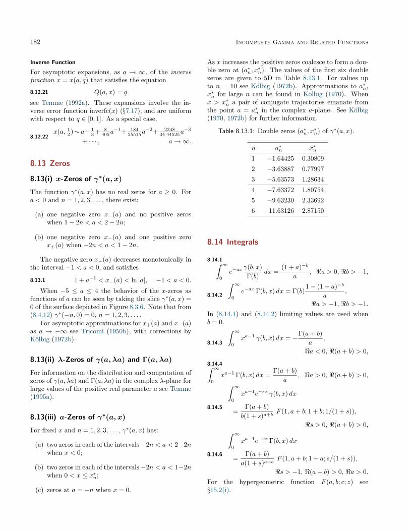
182 Incomplete Gamma and Related Functions
Inverse Function
For asymptotic expansions, as a → ∞, of the inversefunction x = x(a, q) that satisfies the equation
8.12.21 Q(a, x) = q
see Temme (1992a). These expansions involve the in-verse error function inverfc(x) (§7.17), and are uniformwith respect to q ∈ [0, 1]. As a special case,
8.12.22x(a, 1
2 )∼ a− 13 + 8
405a−1+ 184
25515a−2+ 2248
34 44525a−3
+ · · · , a→∞.
8.13 Zeros
8.13(i) x-Zeros of γ∗(a, x)
The function γ∗(a, x) has no real zeros for a ≥ 0. Fora < 0 and n = 1, 2, 3, . . . , there exist:
(a) one negative zero x−(a) and no positive zeroswhen 1− 2n < a < 2− 2n;
(b) one negative zero x−(a) and one positive zerox+(a) when −2n < a < 1− 2n.
The negative zero x−(a) decreases monotonically inthe interval −1 < a < 0, and satisfies
8.13.1 1 + a−1 < x−(a) < ln |a|, −1 < a < 0.
When −5 ≤ a ≤ 4 the behavior of the x-zeros asfunctions of a can be seen by taking the slice γ∗(a, x) =0 of the surface depicted in Figure 8.3.6. Note that from(8.4.12) γ∗(−n, 0) = 0, n = 1, 2, 3, . . . .
For asymptotic approximations for x+(a) and x−(a)as a → −∞ see Tricomi (1950b), with corrections byKölbig (1972b).
8.13(ii) λ-Zeros of γ(a, λa) and Γ(a, λa)
For information on the distribution and computation ofzeros of γ(a, λa) and Γ(a, λa) in the complex λ-plane forlarge values of the positive real parameter a see Temme(1995a).
8.13(iii) a-Zeros of γ∗(a, x)
For fixed x and n = 1, 2, 3, . . . , γ∗(a, x) has:
(a) two zeros in each of the intervals −2n < a < 2−2nwhen x < 0;
(b) two zeros in each of the intervals −2n < a < 1−2nwhen 0 < x ≤ x∗n;
(c) zeros at a = −n when x = 0.
As x increases the positive zeros coalesce to form a dou-ble zero at (a∗n, x
∗n). The values of the first six double
zeros are given to 5D in Table 8.13.1. For values upto n = 10 see Kölbig (1972b). Approximations to a∗n,x∗n for large n can be found in Kölbig (1970). Whenx > x∗n a pair of conjugate trajectories emanate fromthe point a = a∗n in the complex a-plane. See Kölbig(1970, 1972b) for further information.
Table 8.13.1: Double zeros (a∗n, x∗n) of γ∗(a, x).
n a∗n x∗n
1 −1.64425 0.30809
2 −3.63887 0.77997
3 −5.63573 1.28634
4 −7.63372 1.80754
5 −9.63230 2.33692
6 −11.63126 2.87150
8.14 Integrals
8.14.1∫ ∞0
e−axγ(b, x)Γ(b)
dx =(1 + a)−b
a, <a > 0, <b > −1,
8.14.2
∫ ∞0
e−ax Γ(b, x) dx = Γ(b)1− (1 + a)−b
a,
<a > −1, <b > −1.In (8.14.1) and (8.14.2) limiting values are used whenb = 0.
8.14.3
∫ ∞0
xa−1 γ(b, x) dx = −Γ(a+ b)a
,
<a < 0, <(a+ b) > 0,
8.14.4∫ ∞0
xa−1 Γ(b, x) dx =Γ(a+ b)
a, <a > 0, <(a+ b) > 0,
8.14.5
∫ ∞0
xa−1e−sx γ(b, x) dx
=Γ(a+ b)b(1 + s)a+b
F (1, a+ b; 1 + b; 1/(1 + s)),
<s > 0, <(a+ b) > 0,
8.14.6
∫ ∞0
xa−1e−sx Γ(b, x) dx
=Γ(a+ b)
a(1 + s)a+bF (1, a+ b; 1 + a; s/(1 + s)),
<s > −1, <(a+ b) > 0, <a > 0.For the hypergeometric function F (a, b; c; z) see§15.2(i).

8.15 Sums 183
For additional integrals see Apelblat (1983, §8.2),Erdélyi et al. (1953b, §9.3), Erdélyi et al. (1954a,b),Gradshteyn and Ryzhik (2000, §6.45), Marichev (1983,pp.189–190), Oberhettinger (1972, pp. 68–69), Prud-nikov et al. (1986b, §§1.2, 2.10), and Prudnikov et al.(1992a, §3.10).
8.15 Sums
8.15.1 γ(a, λx) = λa∞∑k=0
γ(a+ k, x)(1− λ)k
k!.
For sums of infinite series whose terms include in-complete gamma functions, see Prudnikov et al. (1986b,§5.2).
8.16 Generalizations
For a generalization of the incomplete gamma function,including asymptotic approximations, see Chaudhryand Zubair (1994, 2001) and Chaudhry et al. (1996).Other generalizations are considered in Guthmann(1991) and Paris (2003).
Related Functions
8.17 Incomplete Beta Functions
8.17(i) Definitions and Basic Properties
Throughout §§8.17 and 8.18 we assume that a > 0,b > 0, and 0 ≤ x ≤ 1. However, in the case of §8.17 itis straightforward to continue most results analyticallyto other real values of a, b, and x, and also to complexvalues.8.17.1 Bx(a, b) =
∫ x
0
ta−1(1− t)b−1 dt,
8.17.2 Ix(a, b) = Bx(a, b)/B(a, b),
where, as in §5.12, B(a, b) denotes the Beta function:
8.17.3 B(a, b) =Γ(a) Γ(b)Γ(a+ b)
.
8.17.4 Ix(a, b) = 1− I1−x(b, a),
8.17.5 Ix(m,n−m+ 1) =n∑
j=m
(n
j
)xj(1− x)n−j ,
8.17.6 Ix(a, a) = 12 I4x(1−x)
(a, 1
2
), 0 ≤ x ≤ 1
2 .
For a historical profile of Bx(a, b) see Dutka (1981).
8.17(ii) Hypergeometric Representations
8.17.7 Bx(a, b) =xa
aF (a, 1− b; a+ 1;x),
8.17.8 Bx(a, b) =xa(1− x)b
aF (a+ b, 1; a+ 1;x),
8.17.9 Bx(a, b) =xa(1− x)b−1
aF
(1, 1− ba+ 1
;x
x− 1
).
For the hypergeometric function F (a, b; c; z) see§15.2(i).
8.17(iii) Integral Representation
With a > 0, b > 0, and 0 < x < 1,
8.17.10 Ix(a, b) =xa(1− x)b
2πi
∫ c+i∞
c−i∞s−a(1−s)−b ds
s− x,
where x < c < 1 and the branches of s−a and (1− s)−bare continuous on the path and assume their principalvalues when s = c.
Further integral representations can be obtained bycombining the results given in §8.17(ii) with §15.6.
8.17(iv) Recurrence Relations
With
8.17.11 x′ = 1− x, c = a+ b− 1,
8.17.12 Ix(a, b) = x Ix(a− 1, b) + x′ Ix(a, b− 1),
8.17.13 (a+ b) Ix(a, b) = a Ix(a+ 1, b) + b Ix(a, b+ 1),
8.17.14
(a+ bx) Ix(a, b) = xb Ix(a− 1, b+ 1) + a Ix(a+ 1, b),
8.17.15
(b+ ax′) Ix(a, b) = ax′ Ix(a+ 1, b− 1) + b Ix(a, b+ 1),
8.17.16
a Ix(a+ 1, b) = (a+ cx) Ix(a, b)− cx Ix(a− 1, b),
8.17.17
b Ix(a, b+ 1) = (b+ cx′) Ix(a, b)− cx′ Ix(a, b− 1),
8.17.18 Ix(a, b) = Ix(a+ 1, b− 1) +xa(x′)b−1
aB(a, b),
8.17.19 Ix(a, b) = Ix(a− 1, b+ 1)− xa−1(x′)b
bB(a, b),
8.17.20 Ix(a, b) = Ix(a+ 1, b) +xa(x′)b
aB(a, b),
8.17.21 Ix(a, b) = Ix(a, b+ 1)− xa(x′)b
bB(a, b).

184 Incomplete Gamma and Related Functions
8.17(v) Continued Fraction
8.17.22 Ix(a, b) =xa(1− x)b
aB(a, b)
(1
1 +d1
1 +d2
1 +d3
1+· · ·
),
where
8.17.23
d2m =m(b−m)x
(a+ 2m− 1)(a+ 2m),
d2m+1 = − (a+m)(a+ b+m)x(a+ 2m)(a+ 2m+ 1)
.
The 4m and 4m + 1 convergents are less than Ix(a, b),and the 4m+2 and 4m+3 convergents are greater thanIx(a, b).
See also Cuyt et al. (2008, pp. 385–389).The expansion (8.17.22) converges rapidly for x <
(a + 1)/(a + b + 2). For x > (a + 1)/(a + b + 2) or1 − x < (b + 1)/(a + b + 2), more rapid convergence isobtained by computing I1−x(b, a) and using (8.17.4).
8.17(vi) Sums
For sums of infinite series whose terms involve the in-complete Beta function see Hansen (1975, §62).
8.18 Asymptotic Expansions of Ix(a, b)
8.18(i) Large Parameters, Fixed x
If b and x are fixed, with b > 0 and 0 < x < 1, then asa→∞8.18.1
Ix(a, b) = Γ(a+ b)xa(1− x)b−1
×
(n−1∑k=0
1Γ(a+ k + 1) Γ(b− k)
(x
1− x
)k+O
(1
Γ(a+ n+ 1)
)),
for each n = 0, 1, 2, . . . . If b = 1, 2, 3, . . . and n ≥ b,then the O-term can be omitted and the result is exact.
If b → ∞ and a and x are fixed, with a > 0 and0 < x < 1, then (8.18.1), with a and b interchanged andx replaced by 1− x, can be combined with (8.17.4).
8.18(ii) Large Parameters: Uniform AsymptoticExpansions
Large a, Fixed b
Let
8.18.2 ξ = − lnx.Then as a→∞, with b (> 0) fixed,
8.18.3 Ix(a, b) ∼ Γ(a+ b)Γ(a)
∞∑k=0
dkFk,
uniformly for x ∈ (0, 1). The functions Fk are definedby
8.18.4 aFk+1 = (k + b− aξ)Fk + kξFk−1,
with
8.18.5 F0 = a−bQ(b, aξ), F1 =b− aξa
F0 +ξbe−aξ
aΓ(b),
and Q(a, z) as in §8.2(i). The coefficients dk are definedby the generating function
8.18.6
(1− e−t
t
)b−1
=∞∑k=0
dk(t− ξ)k.
In particular,
8.18.7 d0 =(
1− xξ
)b−1
, d1 =xξ + x− 1(1− x)ξ
(b− 1)d0.
Compare also §24.16(i).
Symmetric Case
Let
8.18.8 x0 = a/(a+ b).
Then as a+ b→∞,
8.18.9
Ix(a, b) ∼ 12 erfc
(−η√b/2)
+1√
2π(a+ b)
×(x
x0
)a( 1− x1− x0
)b ∞∑k=0
(−1)kck(η)(a+ b)k
,
uniformly for x ∈ (0, 1) and a/(a + b), b/(a + b) ∈[δ, 1− δ], where δ again denotes an arbitrary small pos-itive constant. For erfc see §7.2(i). Also,
8.18.10 − 12η
2 = x0 ln(x
x0
)+ (1− x0) ln
(1− x1− x0
),
with η/(x− x0) > 0, and
8.18.11 c0(η) =1η−√x0(1− x0)x− x0
,
with limiting value
8.18.12 c0(0) =1− 2x0
3√x0(1− x0)
.
For this result, and for higher coefficients ck(η) seeTemme (1996a, §11.3.3.2). All of the ck(η) are analyticat η = 0.

8.19 Generalized Exponential Integral 185
General Case
Let Γ̃(z) denote the scaled gamma function
8.18.13 Γ̃(z) = (2π)−1/2ezz(1/2)−z Γ(z),µ = b/a, and x0 again be as in (8.18.8). Then as a→∞8.18.14
Ix(a, b) ∼ Q(b, aζ)
− (2πb)−1/2
Γ̃(b)
(x
x0
)a( 1− x1− x0
)b ∞∑k=0
hk(ζ, µ)ak
,
uniformly for b ∈ (0,∞) and x ∈ (0, 1). Here8.18.15
µ ln ζ − ζ = lnx+ µ ln(1− x) + (1 + µ) ln(1 + µ)− µ,with (ζ − µ)/(x0 − x) > 0, and
8.18.16 h0(ζ, µ) = µ
(1
ζ − µ− (1 + µ)−3/2
x0 − x
),
with limiting value
8.18.17 h0(µ, µ) =13
(1− µ√1 + µ
− 1).
For this result and higher coefficients hk(ζ, µ) seeTemme (1996a, §11.3.3.3). All of the hk(ζ, µ) are ana-lytic at ζ = µ (corresponding to x = x0).
Inverse Function
For asymptotic expansions for large values of a and/orb of the x-solution of the equation
8.18.18 Ix(a, b) = p, 0 ≤ p ≤ 1,see Temme (1992b).
8.19 Generalized Exponential Integral
8.19(i) Definition and Integral Representations
For p, z ∈ C8.19.1 Ep(z) = zp−1 Γ(1− p, z).Most properties of Ep(z) follow straightforwardly fromthose of Γ(a, z). For an extensive treatment of E1(z)see Chapter 6.
8.19.2 Ep(z) = zp−1
∫ ∞z
e−t
tpdt.
When the path of integration excludes the origin anddoes not cross the negative real axis (8.19.2) defines theprincipal value of Ep(z), and unless indicated otherwisein this Handbook principal values are assumed.
Other Integral Representations
8.19.3 Ep(z) =∫ ∞
1
e−zt
tpdt, |ph z| < 1
2π,
8.19.4Ep(z) =
zp−1e−z
Γ(p)
∫ ∞0
tp−1e−zt
1 + tdt,
|ph z| < 12π, <p > 0.
Integral representations of Mellin–Barnes type forEp(z) follow immediately from (8.6.11), (8.6.12), and(8.19.1).
8.19(ii) Graphics
Figure 8.19.1: Ep(x), 0 ≤ x ≤ 3, 0 ≤ p ≤ 8.
In Figures 8.19.2 and 8.19.3, height corresponds to theabsolute value of the function and color to the phase.See p. xiv.

186 Incomplete Gamma and Related Functions
Figure 8.19.2: E 12(x+ iy), −4 ≤ x ≤ 4, −4 ≤ y ≤
4. Principal value. There is a branch cut along thenegative real axis.
Figure 8.19.3: E1(x+ iy), −4 ≤ x ≤ 4, −4 ≤ y ≤4. Principal value. There is a branch cut along thenegative real axis.
For additional graphics see http://dlmf.nist.gov/8.19.ii.
8.19(iii) Special Values
8.19.5 E0(z) = z−1e−z, z 6= 0,
8.19.6 Ep(0) =1
p− 1, <p > 1,
8.19.7
En(z) =(−z)n−1
(n− 1)!E1(z)+
e−z
(n− 1)!
n−2∑k=0
(n−k−2)!(−z)k,
n = 2, 3, . . . .
8.19(iv) Series Expansions
For n = 1, 2, 3, . . . ,
8.19.8
En(z) =(−z)n−1
(n− 1)!(ψ(n)− ln z)−
∞∑k=0
k 6=n−1
(−z)k
k!(1− n+ k),
and
8.19.9
En(z) =(−1)nzn−1
(n− 1)!ln z+
e−z
(n− 1)!
n−1∑k=1
(−z)k−1 Γ(n− k)
+e−z(−z)n−1
(n− 1)!
∞∑k=0
zk
k!ψ(k + 1),
with |ph z| ≤ π in both equations. For ψ(x) see §5.2(i).When p ∈ C
8.19.10 Ep(z) = zp−1 Γ(1− p)−∞∑k=0
(−z)k
k!(1− p+ k),
8.19.11
Ep(z) = Γ(1− p)
(zp−1 − e−z
∞∑k=0
zk
Γ(2− p+ k)
),
again with |ph z| ≤ π in both equations. The right-hand sides are replaced by their limiting forms whenp = 1, 2, 3, . . . .
8.19(v) Recurrence Relation and Derivatives
8.19.12 pEp+1(z) + z Ep(z) = e−z.
8.19.13d
dzEp(z) = −Ep−1(z),
8.19.14d
dz(ez Ep(z)) = ez Ep(z)
(1 +
p− 1z
)− 1z.
p-Derivatives
For j = 1, 2, 3, . . . ,
8.19.15
∂jEp(z)∂pj
= (−1)j∫ ∞
1
(ln t)jt−pe−zt dt, <z > 0.
For properties and numerical tables see Milgram (1985),and also (when p = 1) MacLeod (2002b).
8.19(vi) Relation to Confluent HypergeometricFunction
8.19.16 Ep(z) = zp−1e−z U(p, p, z).
For U(a, b, z) see §13.2(i).

8.20 Asymptotic Expansions of Ep(z) 187
8.19(vii) Continued Fraction
8.19.17Ep(z) = e−z
(1z +
p
1 +1z +
p+ 11 +
2z +
· · ·
),
|ph z| < π.See also Cuyt et al. (2008, pp. 277–285).
8.19(viii) Analytic Continuation
The general function Ep(z) is attained by extending thepath in (8.19.2) across the negative real axis. Unless pis a nonpositive integer, Ep(z) has a branch point atz = 0. For z 6= 0 each branch of Ep(z) is an entirefunction of p.
8.19.18Ep(ze2mπi
)=
2πiempπi
Γ(p)sin(mpπ)sin(pπ)
zp−1 +Ep(z),
m ∈ Z, z 6= 0.
8.19(ix) Inequalities
For n = 1, 2, 3, . . . and x > 0,
8.19.19n− 1n
En(x) < En+1(x) < En(x),
8.19.20 (En(x))2 < En−1(x)En+1(x),
8.19.211
x+ n< exEn(x) ≤ 1
x+ n− 1,
8.19.22d
dx
En(x)En−1(x)
> 0.
8.19(x) Integrals
8.19.23
∫ ∞z
Ep−1(t) dt = Ep(z), |ph z| < π,
8.19.24
∫ ∞0
e−atEn(t) dt
=(−1)n−1
an
(ln(1 + a) +
n−1∑k=1
(−1)kak
k
),
n = 1, 2, . . . , <a > −1,
8.19.25∫ ∞0
e−attb−1Ep(t) dt =Γ(b)(1 + a)−b
p+ b− 1× F (1, b; p+ b; a/(1 + a)),
<a > −1, <(p+ b) > 1.
8.19.26
∫ ∞0
Ep(t)Eq(t) dt =L(p) + L(q)p+ q − 1
,
p > 0, q > 0, p+ q > 1,where8.19.27
L(p) =∫ ∞
0
e−tEp(t) dt =12pF(1, 1; 1 + p; 1
2
), p > 0.
For the hypergeometric function F (a, b; c; z) see§15.2(i). When p = 1, 2, 3, . . . , L(p) can also be evalu-ated via (8.19.24).
For collections of integrals involving Ep(z), espe-cially for integer p, see Apelblat (1983, §§7.1–7.2) andLeCaine (1945).
8.19(xi) Further Generalizations
For higher-order generalized exponential integrals seeMeijer and Baken (1987) and Milgram (1985).
8.20 Asymptotic Expansions of Ep(z)
8.20(i) Large z
8.20.1
Ep(z) =e−z
z
(n−1∑k=0
(−1)k(p)kzk
+(−1)n(p)ne
z
zn−1En+p(z)
),
n = 1, 2, 3, . . . .As z →∞
8.20.2 Ep(z) ∼e−z
z
∞∑k=0
(−1)k(p)kzk
, |ph z| ≤ 32π − δ,
and
8.20.3Ep(z) ∼ ±
2πiΓ(p)
e∓pπizp−1 +e−z
z
∞∑k=0
(−1)k(p)kzk
,
12π + δ ≤ ±ph z ≤ 7
2π − δ,δ again denoting an arbitrary small positive constant.Where the sectors of validity of (8.20.2) and (8.20.3)overlap the contribution of the first term on the right-hand side of (8.20.3) is exponentially small compared tothe other contribution; compare §2.11(ii).
For an exponentially-improved asymptotic expan-sion of Ep(z) see §2.11(iii).
8.20(ii) Large p
For x ≥ 0 and p > 1 let x = λp and define A0(λ) = 1,
8.20.4Ak+1(λ) = (1− 2kλ)Ak(λ) + λ(λ+ 1)
dAk(λ)dλ
,
k = 0, 1, 2, . . . ,so that Ak(λ) is a polynomial in λ of degree k− 1 whenk ≥ 1. In particular,8.20.5
A1(λ) = 1, A2(λ) = 1− 2λ, A3(λ) = 1− 8λ+ 6λ2.
Then as p→∞
8.20.6 Ep(λp) ∼e−λp
(λ+ 1)p
∞∑k=0
Ak(λ)(λ+ 1)2k
1pk,
uniformly for λ ∈ [0,∞).For further information, including extensions to
complex values of x and p, see Temme (1994a, §4) andDunster (1996b, 1997).

188 Incomplete Gamma and Related Functions
8.21 Generalized Sine and Cosine Integrals
8.21(i) Definitions: General Values
With γ and Γ denoting here the general values of theincomplete gamma functions (§8.2(i)), we define
8.21.1 ci(a, z)± i si(a, z) = e±12πia Γ
(a, ze∓
12πi),
8.21.2 Ci(a, z)± i Si(a, z) = e±12πia γ
(a, ze∓
12πi).
From §§8.2(i) and 8.2(ii) it follows that each of thefour functions si(a, z), ci(a, z), Si(a, z), and Ci(a, z) is amultivalued function of z with branch point at z = 0.Furthermore, si(a, z) and ci(a, z) are entire functionsof a, and Si(a, z) and Ci(a, z) are meromorphic func-tions of a with simple poles at a = −1,−3,−5, . . . anda = 0,−2,−4, . . . , respectively.
8.21(ii) Definitions: Principal Values
When ph z = 0 (and when a 6= −1,−3,−5, . . . , in thecase of Si(a, z), or a 6= 0,−2,−4, . . . , in the case ofCi(a, z)) the principal values of si(a, z), ci(a, z), Si(a, z),and Ci(a, z) are defined by (8.21.1) and (8.21.2) withthe incomplete gamma functions assuming their princi-pal values (§8.2(i)). Elsewhere in the sector |ph z| ≤ πthe principal values are defined by analytic continuationfrom ph z = 0; compare §4.2(i).
From here on it is assumed that unless indicatedotherwise the functions si(a, z), ci(a, z), Si(a, z), andCi(a, z) have their principal values.
Properties of the four functions that are stated be-low in §§8.21(iii) and 8.21(iv) follow directly from thedefinitions given above, together with properties of theincomplete gamma functions given earlier in this chap-ter. In the case of §8.21(iv) the equation
8.21.3
∫ ∞0
ta−1e±it dt = e±12πia Γ(a), 0 < <a < 1,
(obtained from (5.2.1) by rotation of the integrationpath) is also needed.
8.21(iii) Integral Representations
8.21.4 si(a, z) =∫ ∞z
ta−1 sin t dt, <a < 1,
8.21.5 ci(a, z) =∫ ∞z
ta−1 cos t dt, <a < 1,
8.21.6 Si(a, z) =∫ z
0
ta−1 sin t dt, <a > −1,
8.21.7 Ci(a, z) =∫ z
0
ta−1 cos t dt, <a > 0.
In these representations the integration paths do notcross the negative real axis, and in the case of (8.21.4)and (8.21.5) the paths also exclude the origin.
8.21(iv) Interrelations
8.21.8
Si(a, z) = Γ(a) sin(
12πa
)− si(a, z), a 6= −1,−3,−5, . . . ,
8.21.9
Ci(a, z) = Γ(a) cos(
12πa
)− ci(a, z), a 6= 0,−2,−4, . . . .
8.21(v) Special Values
8.21.10 si(0, z) = − si(z), ci(0, z) = −Ci(z),
8.21.11 Si(0, z) = Si(z).
For the functions on the right-hand sides of (8.21.10)and (8.21.11) see §6.2(ii).
8.21.12 Si(a,∞) = Γ(a) sin(
12πa
), a 6= −1,−3,−5, . . . ,
8.21.13 Ci(a,∞) = Γ(a) cos(
12πa
), a 6= 0,−2,−4, . . . .
8.21(vi) Series Expansions
Power-Series Expansions
8.21.14Si(a, z) = za
∞∑k=0
(−1)kz2k+1
(2k + a+ 1)(2k + 1)!,
a 6= −1,−3,−5, . . . ,
8.21.15
Ci(a, z) = za∞∑k=0
(−1)kz2k
(2k + a)(2k)!, a 6= 0,−2,−4, . . . .
Spherical-Bessel-Function Expansions
8.21.16Si(a, z) = za
∞∑k=0
(2k + 3
2
) (1− 1
2a)k(
12 + 1
2a)k+1
j2k+1(z),
a 6= −1,−3,−5, . . . ,
8.21.17Ci(a, z) = za
∞∑k=0
(2k + 1
2
) (12 −
12a)k(
12a)k+1
j2k(z),
a 6= 0,−2,−4, . . . .
For jn(z) see §10.47(ii). For (8.21.16), (8.21.17), andfurther expansions in series of Bessel functions see Luke(1969b, pp. 56–57).

Applications 189
8.21(vii) Auxiliary Functions
8.21.18 f(a, z) = si(a, z) cos z − ci(a, z) sin z,
8.21.19 g(a, z) = si(a, z) sin z + ci(a, z) cos z.
8.21.20 si(a, z) = f(a, z) cos z + g(a, z) sin z,
8.21.21 ci(a, z) = −f(a, z) sin z + g(a, z) cos z.
When |ph z| < π and <a < 1,
8.21.22 f(a, z) =∫ ∞
0
sin t(t+ z)1−a dt,
8.21.23 g(a, z) =∫ ∞
0
cos t(t+ z)1−a dt.
When |ph z| < 12π,
8.21.24
f(a, z) =za
2
∫ ∞0
((1 + it)a−1 + (1− it)a−1
)e−zt dt,
8.21.25
g(a, z) =za
2i
∫ ∞0
((1− it)a−1 − (1 + it)a−1
)e−zt dt.
8.21(viii) Asymptotic Expansions
When z →∞ with |ph z| ≤ π − δ (< π),
8.21.26 f(a, z) ∼ za−1∞∑k=0
(−1)k(1− a)2k
z2k,
8.21.27 g(a, z) ∼ za−1∞∑k=0
(−1)k(1− a)2k+1
z2k+1.
For the corresponding expansions for si(a, z) andci(a, z) apply (8.21.20) and (8.21.21).
Applications
8.22 Mathematical Applications
8.22(i) Terminant Function
The so-called terminant function Fp(z), defined by
8.22.1 Fp(z) =Γ(p)2π
z1−pEp(z) =Γ(p)2π
Γ(1− p, z),
plays a fundamental role in re-expansions of re-mainder terms in asymptotic expansions, includingexponentially-improved expansions and a smooth inter-pretation of the Stokes phenomenon. See §§2.11(ii)–2.11(v) and the references supplied in these subsections.
8.22(ii) Riemann Zeta Function and IncompleteRiemann Zeta Function
The function Γ(a, z), with |ph a| ≤ 12π and ph z = 1
2π,has an intimate connection with the Riemann zeta func-tion ζ(s) (§25.2(i)) on the critical line <s = 1
2 . See Parisand Cang (1997).
If ζx(s) denotes the incomplete Riemann zeta func-tion defined by
8.22.2 ζx(s) =1
Γ(s)
∫ x
0
ts−1
et − 1dt, <s > 1,
so that limx→∞ ζx(s) = ζ(s), then
8.22.3 ζx(s) =∞∑k=1
k−s P (s, kx), <s > 1.
For further information on ζx(s), including zeros anduniform asymptotic approximations, see Kölbig (1970,1972a) and Dunster (2006).
8.23 Statistical Applications
The functions P (a, x) and Q(a, x) are used extensivelyin statistics as the probability integrals of the gammadistribution; see Johnson et al. (1994, pp. 337–414).Particular forms are the chi-square distribution func-tions; see Johnson et al. (1994, pp. 415–493). The func-tion Bx(a, b) and its normalization Ix(a, b) play a similarrole in statistics in connection with the beta distribu-tion; see Johnson et al. (1995, pp. 210–275). In queue-ing theory the Erlang loss function is used, which canbe expressed in terms of the reciprocal of Q(a, x); seeJagerman (1974) and Cooper (1981, pp. 80, 316–319).
8.24 Physical Applications
8.24(i) Incomplete Gamma Functions
The function γ(a, x) appears in: discussions of power-law relaxation times in complex physical systems (Sor-nette (1998)); logarithmic oscillations in relaxationtimes for proteins (Metzler et al. (1999)); Gaussianorbitals and exponential (Slater) orbitals in quantumchemistry (Shavitt (1963), Shavitt and Karplus (1965));population biology and ecological systems (Camachoet al. (2002)).
8.24(ii) Incomplete Beta Functions
The function Ix(a, b) appears in: Monte Carlo sam-pling in statistical mechanics (Kofke (2004)); analy-sis of packings of soft or granular objects (Prellbergand Owczarek (1995)); growth formulas in cosmology(Hamilton (2001)).

190 Incomplete Gamma and Related Functions
8.24(iii) Generalized Exponential Integral
The function Ep(x), with p > 0, appears in theoriesof transport and radiative equilibrium (Hopf (1934),Kourganoff (1952), Altaç (1996)).
With more general values of p, Ep(x) supplies fun-damental auxiliary functions that are used in the com-putation of molecular electronic integrals in quantumchemistry (Harris (2002), Shavitt (1963)), and also waveacoustics of overlapping sound beams (Ding (2000)).
Computation
8.25 Methods of Computation
8.25(i) Series Expansions
Although the series expansions in §§8.7, 8.19(iv), and8.21(vi) converge for all finite values of z, they are cum-bersome to use when |z| is large owing to slowness ofconvergence and cancellation. For large |z| the corre-sponding asymptotic expansions (generally divergent)are used instead. See also Luke (1975, pp. 101–102)and Temme (1994a).
8.25(ii) Quadrature
See Allasia and Besenghi (1987a) for the numerical com-putation of Γ(a, z) from (8.6.4) by means of the trape-zoidal rule.
8.25(iii) Asymptotic Expansions
DiDonato and Morris (1986) describes an algorithm forcomputing P (a, x) and Q(a, x) for a ≥ 0, x ≥ 0, anda + x 6= 0 from the uniform expansions in §8.12. Thealgorithm supplies 14S accuracy. A numerical inver-sion procedure is also given for calculating the value ofx (with 10S accuracy), when a and P (a, x) are speci-fied, based on Newton’s rule (§3.8(ii)). See also Temme(1987, 1994a).
8.25(iv) Continued Fractions
The computation of γ(a, z) and Γ(a, z) by means of con-tinued fractions is described in Jones and Thron (1985)and Gautschi (1979a, §§4.3, 5). See also Jacobsen et al.(1986) and Temme (1996a, p. 280).
8.25(v) Recurrence Relations
Expansions involving incomplete gamma functions of-ten require the generation of sequences P (a+ n, x),Q(a+ n, x), or γ∗(a+ n, x) for fixed a and n =0, 1, 2, . . . . An efficient procedure, based partly on therecurrence relations (8.8.5) and (8.8.6), is described inGautschi (1979a, 1999).
Stable recursive schemes for the computation ofEp(x) are described in Miller (1960) for x > 0 and inte-ger p. For x > 0 and real p see Amos (1980) and Chiccoliet al. (1987, 1988). See also Chiccoli et al. (1990) andStegun and Zucker (1974).
8.26 Tables
8.26(i) Introduction
For tables published before 1961 see Fletcher et al.(1962) and Lebedev and Fedorova (1960).
8.26(ii) Incomplete Gamma Functions
• Khamis (1965) tabulates P (a, x) for a =0.05(.05)10(.1)20(.25)70, 0.0001 ≤ x ≤ 250 to10D.
• Pagurova (1963) tabulates P (a, x) and Q(a, x)(with different notation) for a = 0(.05)3, x =0(.05)1 to 7D.
• Pearson (1965) tabulates the function I(u, p) (=P (p+ 1, u)) for p = −1(.05)0(.1)5(.2)50, u =0(.1)up to 7D, where I(u, up) rounds off to 1 to7D; also I(u, p) for p = −0.75(.01)− 1, u = 0(.1)6to 5D.
• Zhang and Jin (1996, Table 3.8) tabulatesγ(a, x) for a = 0.5, 1, 3, 5, 10, 25, 50, 100, x =0(.1)1(1)3, 5(5)30, 50, 100 to 8D or 8S.
8.26(iii) Incomplete Beta Functions
• Pearson (1968) tabulates Ix(a, b) for x =0.01(.01)1, a, b = 0.5(.5)11(1)50, with b ≤ a, to7D.
• Zhang and Jin (1996, Table 3.9) tabulates Ix(a, b)for x = 0(.05)1, a = 0.5, 1, 3, 5, 10, b = 1, 10 to8D.
8.26(iv) Generalized Exponential Integral
• Abramowitz and Stegun (1964, pp. 245–248) tab-ulates En(x) for n = 2, 3, 4, 10, 20, x = 0(.01)2to 7D; also (x + n)exEn(x) for n = 2, 3, 4, 10, 20,x−1 = 0(.01)0.1(.05)0.5 to 6S.

8.27 Approximations 191
• Chiccoli et al. (1988) presents a short table ofEp(x) for p = − 9
2 (1)− 12 , 0 ≤ x ≤ 200 to 14S.
• Pagurova (1961) tabulates En(x) for n = 0(1)20,x = 0(.01)2(.1)10 to 4-9S; exEn(x) for n =2(1)10, x = 10(.1)20 to 7D; exEp(x) for p =0(.1)1, x = 0.01(.01)7(.05)12(.1)20 to 7S or 7D.
• Stankiewicz (1968) tabulates En(x) for n =1(1)10, x = 0.01(.01)5 to 7D.
• Zhang and Jin (1996, Table 19.1) tabulatesEn(x) for n = 1, 2, 3, 5, 10, 15, 20, x =0(.1)1, 1.5, 2, 3, 5, 10, 20, 30, 50, 100 to 7D or 8S.
8.27 Approximations
8.27(i) Incomplete Gamma Functions
• DiDonato (1978) gives a simple approximation forthe function F (p, x) = x−pex
2/2∫∞xe−t
2/2tp dt(which is related to the incomplete gamma func-tion by a change of variables) for real p andlarge positive x. This takes the form F (p, x) =4x/h(p, x), approximately, where h(p, x) = 3(x2−p) +
√(x2 − p)2 + 8(x2 + p) and is shown to pro-
duce an absolute error O(x−7
)as x→∞.
• Luke (1975, §4.3) gives Padé approximation meth-ods, combined with a detailed analysis of the er-ror terms, valid for real and complex variables ex-cept on the negative real z-axis. See also Temme(1994a, §3).
• Luke (1969b, pp. 25, 40–41) gives Chebyshev-series expansions for Γ(a, ωz) (by specifying pa-rameters) with 1 ≤ ω < ∞, and γ(a, ωz) with0 ≤ ω ≤ 1; see also Temme (1994a, §3).
• Luke (1969b, p. 186) gives hypergeometric poly-nomial representations that converge uniformly oncompact subsets of the z-plane that exclude z = 0and are valid for |ph z| < π.
8.27(ii) Generalized Exponential Integral
• Luke (1975, p. 103) gives Chebyshev-series expan-sions for E1(x) and related functions for x ≥ 5.
• Luke (1975, p. 106) gives rational and Padé ap-proximations, with remainders, for E1(z) andz−1
∫ z0t−1(1− e−t) dt for complex z with |ph z| ≤
π.
• Verbeeck (1970) gives polynomial and rational ap-proximations for Ep(x) = (e−x/x)P (z), approxi-mately, where P (z) denotes a quotient of polyno-mials of equal degree in z = x−1.
8.28 Software
See http://dlmf.nist.gov/8.28.
References
General References
The main references used in writing this chapter areErdélyi et al. (1953b), Luke (1969b), and Temme(1996a). For additional bibliographic reading seeGautschi (1998), Olver (1997b), and Wong (1989).
Sources
The following list gives the references or other indica-tions of proofs that were used in constructing the varioussections of this chapter. These sources supplement thereferences that are quoted in the text.
§8.2 Olver (1997b, p. 45), Temme (1996b). (8.2.12)–(8.2.14) follow from the definitions in §8.2(i).
§8.3 The graphics were produced at NIST.
§8.4 Erdélyi et al. (1953b, Chapter 9). (8.4.14) followsfrom (8.4.6) and (8.8.6). (8.4.15) follows from thefirst series in (8.7.3) by combining Γ(a) with theterm k = n of the series, then taking the limit asa→ −n.
§8.5 Slater (1960, §5.6) and §13.2(vii). For (8.5.4) see(13.18.4).
§8.6 For (8.6.1) use (8.6.8), replacing t by eit with−π ≤ t ≤ π. For (8.6.2) substitute for Ja
(2√zt)
by (10.2.2), integrate term by term and refer to(8.7.1) and (8.2.6). (8.6.6) may be proved ina similar manner with the aid also of (10.25.2),(10.27.4), (8.2.3), and analytic continuation whena = −2,−3,−4, . . . . For (8.6.3) and (8.6.7) apply(8.2.1) and (8.2.2), taking new integration vari-ables ze∓t. For (8.6.4) and (8.6.5) see Temme(1996a, §§11.2.1–11.2.2). For (8.6.8) assume tem-porarily <a > 0, collapse the integration pathonto the interval [−1, 0] and use (8.2.1). For(8.6.9) see Temme (1996b). For (8.6.10)–(8.6.12)see Paris and Kaminski (2001, §3.4.3).
§8.7 Erdélyi et al. (1953b, Chapter 9). (8.7.3) followsfrom (8.7.1) and (8.2.3). For (8.7.5) use (8.5.2)and (13.11.1).
§8.8 Erdélyi et al. (1953b, Chapter 9). These resultsalso follow straightforwardly from §8.2(i).

192 Incomplete Gamma and Related Functions
§8.10 Olver (1997b, pp. 66–67), Luke (1969b, pp. 195,201). For (8.10.10)–(8.10.13), see Gautschi(1959b), Alzer (1997b), and Vietoris (1983).
§8.11 Olver (1997b, pp. 66, 109–112), Temme (1996a,p. 280). For (8.11.4) see (8.5.1) or (8.7.1). (8.11.5)follows from the leading terms of (8.11.4) and(5.11.3). For (8.11.6) and (8.11.7) see Gautschi(1959a) and Temme (1994a). (8.11.12) can beobtained from (8.12.15), (8.2.4), and (5.11.3).(8.11.15) follows from (8.4.7) with z = nx. For(8.11.16) see Ramanujan (1962, pp. 323–324). For(8.11.17) see Copson (1933).
§8.12 Temme (1979b, 1992a, 1996b), Paris (2002b),and Ferreira et al. (2005).
§8.13 Erdélyi et al. (1953b, §9.6), Tricomi (1950b),Lew (1994), and Kölbig (1972b).
§8.14 (8.14.1)–(8.14.2) are obtained by term-by-termintegration using (8.7.1) and (8.7.3). (8.14.3)–(8.14.6) are obtained by specializing (13.10.10),(13.10.11), (13.10.3), (13.10.4) by means of(8.5.1)–(8.5.3).
§8.15 Tricomi (1950b).
§8.17 Temme (1996a, §§11.3–11.3.2). For (8.17.5) com-bine (8.17.8) and (15.8.1). For (8.17.6) combine(8.17.8), (15.8.18), and (15.8.1). For the last para-graph of §8.17(v) see Zhang and Jin (1996, p. 65).
§8.18 Temme (1996a, §§11.3.3.1–11.3.3.3). For (8.18.1)use (8.17.9) and apply §15.12(ii).
§8.19 For (8.19.1)–(8.19.4) see Temme (1996a, p. 180).For (8.19.5)–(8.19.7) use (8.19.1), (8.19.3),(8.4.15). (8.19.8) follows from (8.4.13) and(8.4.15). (8.19.9) follows from (6.6.3), (8.19.1),and (8.4.15). (8.19.10) and (8.19.11) follow from
(8.19.1) and (8.7.3). For (8.19.12)–(8.19.16) com-bine (8.19.1) with (8.8.2), (8.8.16), (8.8.19), and(8.5.3). For (8.19.17) combine (8.9.2) and (8.19.1).For (8.19.18) see Olver (1994b). For (8.19.19)–(8.19.22) see Hopf (1934, pp. 26–27). For(8.19.23) use (8.19.13). For (8.19.24)–(8.19.27)see Kourganoff (1952, Appendix 1). The graph-ics were produced at NIST.
§8.20 Olver (1991a), Gautschi (1959a).
§8.21 For §8.21(iii) follow the prescription given in thefinal paragraph of §8.21(ii). Thus for (8.21.4)and (8.21.5) replace z by iz with ph z = 0 in(8.2.2), deform the path of integration to runalong the positive imaginary axis, and replace tby it. Then extend to the sector |ph z| ≤ πby analytic continuation. Similarly for (8.21.6)and (8.21.7). For §8.21(iv) temporarily restrict0 < <a < 1. Then (8.21.8) and (8.21.9) follow im-mediately from (8.21.3)–(8.21.7). Subsequently,ease the restrictions on a by analytic continuationwith respect to a; compare §8.21(i). For (8.21.12)and (8.21.13) use (8.21.8) and (8.21.9), and also(8.21.4) and (8.21.5). (8.21.14) and (8.21.15) areobtained by expansion of the trigonometric func-tions in (8.21.6), (8.21.7), and termwise integra-tion. See also Luke (1975, p. 115). (8.21.22) and(8.21.23) follow from (8.21.4), (8.21.5), (8.21.18),and (8.21.19). For (8.21.24) and (8.21.25) as-sume ph z = 0, and in the integrals for ci(a, z) ±i si(a, z) obtained from (8.21.4) and (8.21.5) sett = (1 + τ)z, rotate the integration paths inthe τ -plane through ± 1
2π, and apply (8.21.18)and (8.21.19). The restriction ph z = 0 is easedto |ph z| < 1
2π by analytic continuation. For(8.21.26) and (8.21.27) apply Watson’s lemma to(8.21.24) and (8.21.25), and then extend the sectorof validity from |ph z| ≤ 1
2π− δ to |ph z| ≤ π− δ;see §2.4(i).

Chapter 9
Airy and Related FunctionsF. W. J. Olver1
Notation 1949.1 Special Notation . . . . . . . . . . . . . 194
Airy Functions 1949.2 Differential Equation . . . . . . . . . . . 1949.3 Graphics . . . . . . . . . . . . . . . . . . 1959.4 Maclaurin Series . . . . . . . . . . . . . . 1969.5 Integral Representations . . . . . . . . . 1969.6 Relations to Other Functions . . . . . . . 1969.7 Asymptotic Expansions . . . . . . . . . . 1989.8 Modulus and Phase . . . . . . . . . . . . 1999.9 Zeros . . . . . . . . . . . . . . . . . . . 2009.10 Integrals . . . . . . . . . . . . . . . . . . 2029.11 Products . . . . . . . . . . . . . . . . . . 203
Related Functions 2049.12 Scorer Functions . . . . . . . . . . . . . 2049.13 Generalized Airy Functions . . . . . . . . 2069.14 Incomplete Airy Functions . . . . . . . . 208
Applications 2089.15 Mathematical Applications . . . . . . . . 2089.16 Physical Applications . . . . . . . . . . . 209
Computation 2099.17 Methods of Computation . . . . . . . . . 2099.18 Tables . . . . . . . . . . . . . . . . . . . 2109.19 Approximations . . . . . . . . . . . . . . 2119.20 Software . . . . . . . . . . . . . . . . . . 212
References 212
1Institute for Physical Science and Technology and Department of Mathematics, University of Maryland, College Park, Maryland.Acknowledgments: This chapter is based in part on Abramowitz and Stegun (1964, Chapter 10) by H. A. Antosiewicz. The author
is pleased to acknowledge the assistance of Bruce R. Fabijonas for computing the numerical tables in §9.9, and of Leonard Maximon forwriting §9.16.
Copyright c© 2009 National Institute of Standards and Technology. All rights reserved.
193

194 Airy and Related Functions
Notation
9.1 Special Notation
(For other notation see pp. xiv and 873.)
k nonnegative integer, except in §9.9(iii).x real variable.z(= x+ iy) complex variable.δ arbitrary small positive constant.primes derivatives with respect to argument.
The main functions treated in this chapter are theAiry functions Ai(z) and Bi(z), and the Scorer func-tions Gi(z) and Hi(z) (also known as inhomogeneousAiry functions).
Other notations that have been used are as fol-lows: Ai(−x) and Bi(−x) for Ai(x) and Bi(x) (Jef-freys (1928), later changed to Ai(x) and Bi(x)); U(x) =√πBi(x), V (x) =
√πAi(x) (Fock (1945)); A(x) =
3− 1/3πAi(−3− 1/3x
)(Szegö (1967, §1.81)); e0(x) =
πHi(−x), ẽ0(x) = −πGi(−x) (Tumarkin (1959)).
Airy Functions
9.2 Differential Equation
9.2(i) Airy’s Equation
9.2.1d2w
dz2 = zw.
All solutions are entire functions of z.Standard solutions are:
9.2.2 w = Ai(z), Bi(z), Ai(ze∓2πi/3
).
9.2(ii) Initial Values
9.2.3 Ai(0) =1
32/3 Γ(
23
) = 0.35502 80538 . . . ,
9.2.4 Ai′(0) = − 131/3 Γ
(13
) = −0.25881 94037 . . . ,
9.2.5 Bi(0) =1
31/6 Γ(
23
) = 0.61492 66274 . . . ,
9.2.6 Bi′(0) =31/6
Γ(
13
) = 0.44828 83573 . . . .
9.2(iii) Numerically Satisfactory Pairs ofSolutions
Table 9.2.1 lists numerically satisfactory pairs of solu-tions of (9.2.1) for the stated regions; compare §2.7(iv).
Table 9.2.1: Numerically satisfactory solutions of Airy’sequation.
Pair Region
Ai(x),Bi(x) −∞ < x <∞
Ai(z),Bi(z)
{|ph z| ≤ 1
3π
−∞ < z ≤ 0
Ai(z),Ai(ze−2πi/3
)− 1
3π ≤ ph z ≤ πAi(z),Ai
(ze2πi/3
)−π ≤ ph z ≤ 1
3π
Ai(ze∓2πi/3
)|ph(−z)| ≤ 2
3π
9.2(iv) Wronskians
9.2.7 W {Ai(z),Bi(z)} =1π,
9.2.8 W{
Ai(z),Ai(ze∓2πi/3
)}=e±πi/6
2π,
9.2.9 W{
Ai(ze−2πi/3
),Ai(ze2πi/3
)}=
12πi
.
9.2(v) Connection Formulas
9.2.10 Bi(z) = e−πi/6 Ai(ze−2πi/3
)+eπi/6 Ai
(ze2πi/3
).
9.2.11 Ai(ze∓2πi/3
)= 1
2e∓πi/3 (Ai(z)± iBi(z)) .
9.2.12
Ai(z) + e−2πi/3 Ai(ze−2πi/3
)+ e2πi/3 Ai
(ze2πi/3
)= 0,
9.2.13
Bi(z) + e−2πi/3 Bi(ze−2πi/3
)+ e2πi/3 Bi
(ze2πi/3
)= 0.
9.2.14 Ai(−z) = eπi/3 Ai(zeπi/3
)+e−πi/3 Ai
(ze−πi/3
),
9.2.15 Bi(−z) = e−πi/6 Ai(zeπi/3
)+eπi/6 Ai
(ze−πi/3
).
9.2(vi) Riccati Form of Differential Equation
9.2.16dW
dz+W 2 = z,
W = (1/w) dw/dz , where w is any nontrivial solutionof (9.2.1). See also Smith (1990).

9.3 Graphics 195
9.3 Graphics
9.3(i) Real Variable
Figure 9.3.1: Ai(x), Bi(x), M(x). For M(x) see §9.8(i). Figure 9.3.2: Ai′(x), Bi′(x), N(x). For N(x) see §9.8(i).
9.3(ii) Complex Variable
In the graphics shown in this subsection, height corresponds to the absolute value of the function and color to thephase. See also p. xiv.
Figure 9.3.3: Ai(x+ iy). Figure 9.3.4: Bi(x+ iy).
Figure 9.3.5: Ai′(x+ iy). Figure 9.3.6: Bi′(x+ iy).

196 Airy and Related Functions
9.4 Maclaurin Series
For z ∈ C
9.4.1 Ai(z) = Ai(0)(
1 +13!z3 +
1 · 46!
z6 +1 · 4 · 7
9!z9 + · · ·
)+ Ai′(0)
(z +
24!z4 +
2 · 57!
z7 +2 · 5 · 8
10!z10 + · · ·
),
9.4.2 Ai′(z) = Ai′(0)(
1 +23!z3 +
2 · 56!
z6 +2 · 5 · 8
9!z9 + · · ·
)+ Ai(0)
(12!z2 +
1 · 45!
z5 +1 · 4 · 7
8!z8 + · · ·
),
9.4.3 Bi(z) = Bi(0)(
1 +13!z3 +
1 · 46!
z6 +1 · 4 · 7
9!z9 + · · ·
)+ Bi′(0)
(z +
24!z4 +
2 · 57!
z7 +2 · 5 · 8
10!z10 + · · ·
),
9.4.4 Bi′(z) = Bi′(0)(
1 +23!z3 +
2 · 56!
z6 +2 · 5 · 8
9!z9 + · · ·
)+ Bi(0)
(12!z2 +
1 · 45!
z5 +1 · 4 · 7
8!z8 + · · ·
).
9.5 Integral Representations
9.5(i) Real Variable
9.5.1 Ai(x) =1π
∫ ∞0
cos(
13 t
3 + xt)dt.
9.5.2
Ai(−x) =x 1/2
π
∫ ∞−1
cos(x 3/2 ( 1
3 t3 + t2 − 2
3 ))dt, x > 0.
9.5.3
Bi(x)
=1π
∫ ∞0
exp(− 1
3 t3 + xt
)dt+
1π
∫ ∞0
sin(
13 t
3 + xt)dt.
See also (9.10.19), (9.11.3), (36.9.2), and Vallée andSoares (2004, §2.1.3).
9.5(ii) Complex Variable
9.5.4 Ai(z) =1
2πi
∫ ∞eπi/3∞e−πi/3
exp(
13 t
3 − zt)dt,
9.5.5
Bi(z) =1
2π
∫ ∞eπi/3−∞
exp(
13 t
3 − zt)dt
+1
2π
∫ ∞e−πi/3−∞
exp(
13 t
3 − zt)dt.
9.5.6 Ai(z) =√
32π
∫ ∞0
exp(− t
3
3− z3
3t3
)dt.
9.5.7
Ai(z) =e−ζ
π
∫ ∞0
exp(−z 1/2 t2
)cos(
13 t
3)dt, |ph z| < π.
9.5.8
Ai(z) =e−ζζ −1/6
√π(48) 1/6 Γ
(56
) ∫ ∞0
e−tt− 1/6
(2+
t
ζ
)− 1/6
dt,
|ph z| < 23π.
In (9.5.7) and (9.5.8) ζ = 23z
3/2 .See also (9.10.18) and (9.11.4).
9.6 Relations to Other Functions
9.6(i) Airy Functions as Bessel Functions,Hankel Functions, and Modified BesselFunctions
For the notation see §§10.2(ii) and 10.25(ii). With
9.6.1 ζ = 23z
3/2,
9.6.2
Ai(z) = π−1√z/3K±1/3(ζ)
= 13
√z(I−1/3(ζ)− I1/3(ζ)
)= 1
2
√z/3e2πi/3H
(1)1/3
(ζeπi/2
)= 1
2
√z/3eπi/3H(1)
−1/3
(ζeπi/2
)= 1
2
√z/3e−2πi/3H
(2)1/3
(ζe−πi/2
)= 1
2
√z/3e−πi/3H(2)
−1/3
(ζe−πi/2
),
9.6.3
Ai′(z) = −π−1(z/√
3)K±2/3(ζ)
= (z/3)(I2/3(ζ)− I−2/3(ζ)
)= 1
2 (z/√
3)e−πi/6H(1)2/3
(ζeπi/2
)= 1
2 (z/√
3)e−5πi/6H(1)−2/3
(ζeπi/2
)= 1
2 (z/√
3)eπi/6H(2)2/3
(ζe−πi/2
)= 1
2 (z/√
3)e5πi/6H(2)−2/3
(ζe−πi/2
),
9.6.4
Bi(z) =√z/3
(I1/3(ζ) + I−1/3(ζ)
)= 1
2
√z/3
(eπi/6H
(1)1/3
(ζe−πi/2
)+ e−πi/6H
(2)1/3
(ζeπi/2
))= 1
2
√z/3
(e−πi/6H
(1)−1/3
(ζe−πi/2
)+ eπi/6H
(2)−1/3
(ζeπi/2
)),

9.6 Relations to Other Functions 197
9.6.5
Bi′(z) = (z/√
3)(I2/3(ζ) + I−2/3(ζ)
)= 1
2 (z/√
3)(eπi/3H
(1)2/3
(ζe−πi/2
)+ e−πi/3H
(2)2/3
(ζeπi/2
))= 1
2 (z/√
3)(e−πi/3H
(1)−2/3
(ζe−πi/2
)+ eπi/3H
(2)−2/3
(ζeπi/2
)),
9.6.6
Ai(−z) = (√z/3)
(J1/3(ζ) + J−1/3(ζ)
)= 1
2
√z/3
(eπi/6H
(1)1/3(ζ) + e−πi/6H
(2)1/3(ζ)
)= 1
2
√z/3
(e−πi/6H
(1)−1/3(ζ) + eπi/6H
(2)−1/3(ζ)
),
9.6.7
Ai′(−z) = (z/3)(J2/3(ζ)− J−2/3(ζ)
)= 1
2 (z/√
3)(e−πi/6H
(1)2/3(ζ) + eπi/6H
(2)2/3(ζ)
)= 1
2 (z/√
3)(e−5πi/6H
(1)−2/3(ζ)
+ e5πi/6H(2)−2/3(ζ)
),
9.6.8
Bi(−z) =√z/3
(J−1/3(ζ)− J1/3(ζ)
)= 1
2
√z/3
(e2πi/3H
(1)1/3(ζ) + e−2πi/3H
(2)1/3(ζ)
)= 1
2
√z/3
(eπi/3H
(1)−1/3(ζ) + e−πi/3H
(2)−1/3(ζ)
),
9.6.9
Bi′(−z) = (z/√
3)(J−2/3(ζ) + J2/3(ζ)
)= 1
2 (z/√
3)(eπi/3H
(1)2/3(ζ) + e−πi/3H
(2)2/3(ζ)
)= 1
2 (z/√
3)(e−πi/3H
(1)−2/3(ζ)
+ eπi/3H(2)−2/3(ζ)
).
9.6(ii) Bessel Functions, Hankel Functions, andModified Bessel Functions as AiryFunctions
Again, for the notation see §§10.2(ii) and 10.25(ii).With
9.6.10 z = ( 32ζ)2/3,
9.6.11 J±1/3(ζ) = 12
√3/z
(√3 Ai(−z)∓ Bi(−z)
),
9.6.12 J±2/3(ζ) = 12 (√
3/z)(±√
3 Ai′(−z) + Bi′(−z)),
9.6.13 I±1/3(ζ) = 12
√3/z
(∓√
3 Ai(z) + Bi(z)),
9.6.14 I±2/3(ζ) = 12 (√
3/z)(±√
3 Ai′(z) + Bi′(z)),
9.6.15 K±1/3(ζ) = π√
3/zAi(z),
9.6.16 K±2/3(ζ) = −π(√
3/z) Ai′(z),
9.6.17H
(1)1/3(ζ) = e−πi/3H
(1)−1/3(ζ)
= e−πi/6√
3/z (Ai(−z)− iBi(−z)) ,
9.6.18H
(1)2/3(ζ) = e−2πi/3H
(1)−2/3(ζ)
= eπi/6(√
3/z)(Ai′(−z)− iBi′(−z)
),
9.6.19H
(2)1/3(ζ) = eπi/3H
(2)−1/3(ζ)
= eπi/6√
3/z (Ai(−z) + iBi(−z)) ,
9.6.20H
(2)2/3(ζ) = e2πi/3H
(2)−2/3(ζ)
= e−πi/6(√
3/z)(Ai′(−z) + iBi′(−z)
).
9.6(iii) Airy Functions as ConfluentHypergeometric Functions
For the notation see §§13.1, 13.2, and 13.14(i). With ζas in (9.6.1),
9.6.21Ai(z) = 1
2π−1/2z−1/4W0,1/3(2ζ)
= 3−1/6π−1/2ζ2/3e−ζ U(
56 ,
53 , 2ζ
),
9.6.22Ai′(z) = − 1
2π−1/2z1/4W0,2/3(2ζ)
= −31/6π−1/2ζ4/3e−ζ U(
76 ,
73 , 2ζ
),
9.6.23
Bi(z) =1
21/3 Γ(
23
)z−1/4M0,−1/3(2ζ)
+3
25/3 Γ(
13
)z−1/4M0,1/3(2ζ),
9.6.24
Bi′(z) =21/3
Γ(
13
)z1/4M0,−2/3(2ζ)
+3
210/3 Γ(
23
)z1/4M0,2/3(2ζ),
9.6.25
Bi(z) =1
31/6 Γ(
23
)e−ζ 1F1
(16 ; 1
3 ; 2ζ)
+35/6
22/3 Γ(
13
)ζ2/3e−ζ 1F1
(56 ; 5
3 ; 2ζ),
9.6.26
Bi′(z) =31/6
Γ(
13
)e−ζ 1F1
(− 1
6 ;− 13 ; 2ζ
)+
37/6
27/3 Γ(
23
)ζ4/3e−ζ 1F1
(76 ; 7
3 ; ζ).

198 Airy and Related Functions
9.7 Asymptotic Expansions
9.7(i) Notation
Here δ denotes an arbitrary small positive constant and
9.7.1 ζ = 23z
3/2 .
Also u0 = v0 = 1 and for k = 1, 2, . . . ,
9.7.2uk =
(2k + 1)(2k + 3)(2k + 5) · · · (6k − 1)(216)k(k)!
,
vk =6k + 11− 6k
uk.
Lastly,
9.7.3 χ(n) = π 1/2 Γ(
12n+ 1
)/Γ(
12n+ 1
2
).
Numerical values of this function are given in Table 9.7.1for n = 1(1)20 to 2D. For large n,
9.7.4 χ(n) ∼ ( 12πn) 1/2 .
Table 9.7.1: χ(n).
n χ(n) n χ(n) n χ(n) n χ(n)1 1.57 6 3.20 11 4.25 16 5.092 2.00 7 3.44 12 4.43 17 5.243 2.36 8 3.66 13 4.61 18 5.394 2.67 9 3.87 14 4.77 19 5.545 2.95 10 4.06 15 4.94 20 5.68
9.7(ii) Poincaré-Type Expansions
As z →∞ the following asymptotic expansions are validuniformly in the stated sectors.
9.7.5 Ai(z) ∼ e−ζ
2√πz1/4
∞∑k=0
(−1)kukζk
, |ph z| ≤ π − δ,
9.7.6 Ai′(z) ∼ −z1/4e−ζ
2√π
∞∑k=0
(−1)kvkζk
, |ph z| ≤ π − δ,
9.7.7 Bi(z) ∼ eζ√πz1/4
∞∑k=0
ukζk
, |ph z| ≤ 13π − δ,
9.7.8 Bi′(z) ∼ z1/4eζ√π
∞∑k=0
vkζk
, |ph z| ≤ 13π − δ.
9.7.9 Ai(−z) ∼ 1√πz1/4
(cos(ζ − 1
4π) ∞∑k=0
(−1)ku2k
ζ2k+ sin
(ζ − 1
4π) ∞∑k=0
(−1)ku2k+1
ζ2k+1
), |ph z| ≤ 2
3π − δ,
9.7.10 Ai′(−z) ∼ z1/4
√π
(sin(ζ − 1
4π) ∞∑k=0
(−1)kv2k
ζ2k− cos
(ζ − 1
4π) ∞∑k=0
(−1)kv2k+1
ζ2k+1
), |ph z| ≤ 2
3π − δ,
9.7.11 Bi(−z) ∼ 1√πz1/4
(− sin
(ζ − 1
4π) ∞∑k=0
(−1)ku2k
ζ2k+ cos
(ζ − 1
4π) ∞∑k=0
(−1)ku2k+1
ζ2k+1
), |ph z| ≤ 2
3π − δ,
9.7.12 Bi′(−z) ∼ z1/4
√π
(cos(ζ − 1
4π) ∞∑k=0
(−1)kv2k
ζ2k+ sin
(ζ − 1
4π) ∞∑k=0
(−1)kv2k+1
ζ2k+1
), |ph z| ≤ 2
3π − δ.
9.7.13Bi(ze±πi/3
)∼√
2π
e±πi/6
z1/4
(cos(ζ − 1
4π ∓12 i ln 2
) ∞∑k=0
(−1)ku2k
ζ2k+ sin
(ζ − 1
4π ∓12 i ln 2
) ∞∑k=0
(−1)ku2k+1
ζ2k+1
),
|ph z| ≤ 23π − δ,
9.7.14
Bi′(ze±πi/3
)∼√
2πe∓πi/6z1/4
(− sin
(ζ − 1
4π ∓12 i ln 2
) ∞∑k=0
(−1)kv2k
ζ2k+ cos
(ζ − 1
4π ∓12 i ln 2
) ∞∑k=0
(−1)kv2k+1
ζ2k+1
),
|ph z| ≤ 23π − δ.

9.8 Modulus and Phase 199
9.7(iii) Error Bounds for Real Variables
In (9.7.5) and (9.7.6) the nth error term, that is, the er-ror on truncating the expansion at n terms, is boundedin magnitude by the first neglected term and has thesame sign, provided that the following term is of op-posite sign, that is, if n ≥ 0 for (9.7.5) and n ≥ 1 for(9.7.6).
In (9.7.7) and (9.7.8) the nth error term is boundedin magnitude by the first neglected term multiplied by2χ(n) exp (σπ/(72ζ)) where σ = 5 for (9.7.7) and σ = 7for (9.7.8), provided that n ≥ 1 in both cases.
In (9.7.9)–(9.7.12) the nth error term in each infiniteseries is bounded in magnitude by the first neglectedterm and has the same sign, provided that the followingterm in the series is of opposite sign.
As special cases, when 0 < x <∞9.7.15
Ai(x) ≤ e−ξ
2√πx1/4
, |Ai′(x)| ≤ x1/4e−ξ
2√π
(1 +
772ξ
),
9.7.16
Bi(x) ≤ eξ√πx1/4
(1 +
5π72ξ
exp(
5π72ξ
)),
Bi′(x) ≤ x1/4eξ√π
(1 +
7π72ξ
exp(
7π72ξ
)),
where ξ = 23x
3/2.
9.7(iv) Error Bounds for Complex Variables
When n ≥ 1 the nth error term in (9.7.5) and (9.7.6) isbounded in magnitude by the first neglected term mul-tiplied by
9.7.17
2 exp(
σ
36|ζ|
), 2χ(n) exp
(σπ
72|ζ|
)or
4χ(n)| cos(ph ζ)|n
exp(
σπ
36|<ζ|
),
according as |ph z| ≤ 13π, 1
3π ≤ |ph z| ≤ 23π, or
23π ≤ |ph z| ≤ π. Here σ = 5 for (9.7.5) and σ = 7for (9.7.6).
Corresponding bounds for the errors in (9.7.7) to(9.7.14) may be obtained by use of these results andthose of §9.2(v) and their differentiated forms.
For other error bounds see Boyd (1993).
9.7(v) Exponentially-Improved Expansions
In (9.7.5) and (9.7.6) let
9.7.18 Ai(z) =e−ζ
2√πz1/4
(n−1∑k=0
(−1)kukζk
+Rn(z)
),
9.7.19 Ai′(z) = −z1/4e−ζ
2√π
(n−1∑k=0
(−1)kvkζk
+ Sn(z)
),
with n = b2|ζ|c. Then9.7.20
Rn(z) = (−1)nm−1∑k=0
(−1)kukGn−k(2ζ)
ζk+Rm,n(z),
9.7.21
Sn(z) = (−1)n−1m−1∑k=0
(−1)kvkGn−k(2ζ)
ζk+ Sm,n(z),
where9.7.22 Gp(z) =
ez
2πΓ(p) Γ(1− p, z).
(For the notation see §8.2(i).) And as z → ∞ with mfixed9.7.23
Rm,n(z), Sm,n(z) = O(e−2|ζ|ζ−m
), |ph z| ≤ 2
3π.
For re-expansions of the remainder terms in (9.7.7)–(9.7.14) combine the results of this section with thoseof §9.2(v) and their differentiated forms, as in §9.7(iv).
For higher re-expansions of the remainder terms seeOlde Daalhuis (1995, 1996), and Olde Daalhuis andOlver (1995a).
9.8 Modulus and Phase
9.8(i) Definitions
Throughout this section x is real and nonpositive.
9.8.1 Ai(x) = M(x) sin θ(x),
9.8.2 Bi(x) = M(x) cos θ(x),
9.8.3 M(x) =√
Ai2(x) + Bi2(x),
9.8.4 θ(x) = arctan(Ai(x)/Bi(x)).
9.8.5 Ai′(x) = N(x) sinφ(x),
9.8.6 Bi′(x) = N(x) cosφ(x),
9.8.7 N(x) =√
Ai′2(x) + Bi′2(x),
9.8.8 φ(x) = arctan(Ai′(x)/Bi′(x)
).
Graphs of M(x) and N(x) are included in §9.3(i).The branches of θ(x) and φ(x) are continuous and fixedby θ(0) = −φ(0) = 1
6π. (These definitions of θ(x) andφ(x) differ from Abramowitz and Stegun (1964, Chap-ter 10), and agree more closely with those used in Miller(1946) and Olver (1997b, Chapter 11).)
In terms of Bessel functions, and with ξ = 23 |x|
3/2,
9.8.9 |x|1/2M2(x) = 12ξ(J2
1/3(ξ) + Y 21/3(ξ)
),
9.8.10 |x|−1/2N2(x) = 12ξ(J2
2/3(ξ) + Y 22/3(ξ)
),
9.8.11 θ(x) = 23π + arctan
(Y1/3(ξ)/ J1/3(ξ)
),
9.8.12 φ(x) = 13π + arctan
(Y2/3(ξ)/ J2/3(ξ)
).

200 Airy and Related Functions
9.8(ii) Identities
Primes denote differentiations with respect to x, whichis continued to be assumed real and nonpositive.
9.8.13 M(x)N(x) sin(θ(x)− φ(x)) = π−1,
9.8.14M2(x) θ′(x) = −π−1 , N2(x)φ′(x) = π−1x ,N(x)N ′(x) = xM(x)M ′(x) ,
9.8.15N2(x) = M ′
2(x) +M2(x) θ′2(x)
= M ′2(x) + π−2M−2(x),
9.8.16x2M2(x) = N ′
2(x) +N2(x)φ′2(x)
= N ′2(x) + π−2x2N−2(x),
9.8.17tan(θ(x)− φ(x)) = 1/(πM(x)M ′(x))
= −M(x) θ′(x)/M ′(x),
9.8.18M ′′(x) = xM(x) + π−2M−3(x) ,(M2)′′′
(x)− 4x(M2)′
(x)− 2M2(x) = 0,
9.8.19 θ′2(x)+ 1
2 (θ′′′(x)/ θ′(x))− 34 (θ′′(x)/ θ′(x))2 =−x.
9.8(iii) Monotonicity
As x increases from−∞ to 0 each of the functionsM(x),M ′(x), |x|−1/4N(x), M(x)N(x), θ′(x), φ′(x) is increas-ing, and each of the functions |x|1/4M(x), θ(x), φ(x) isdecreasing.
9.8(iv) Asymptotic Expansions
As x→ −∞9.8.20
M2(x) ∼ 1π(−x)1/2
∞∑k=0
1 · 3 · 5 · · · (6k − 1)k!(96)k
1x3k
,
9.8.21
N2(x) ∼ (−x)1/2
π
∞∑k=0
1 · 3 · 5 · · · (6k − 1)k!(96)k
1 + 6k1− 6k
1x3k
,
9.8.22
θ(x) ∼ π
4+
23
(−x)3/2
(1 +
532
1x3
+11056144
1x6
+8282565536
1x9
+12820 31525587 20256
1x12
+ · · ·),
9.8.23
φ(x) ∼ −π4
+23
(−x)3/2
(1− 7
321x3− 1463
61441x6
− 4 952713 27680
1x9− 2065 30429
83 886081x12− · · ·
).
In (9.8.20) and (9.8.21) the remainder after n termsdoes not exceed the (n+1)th term in absolute value andis of the same sign, provided that n ≥ 0 for (9.8.20) andn ≥ 1 for (9.8.21).
For higher terms in (9.8.22) and (9.8.23) see Fabi-jonas et al. (2004). Also, approximate values (25S) ofthe coefficients of the powers x−15, x−18, . . . , x−56 areavailable in Sherry (1959).
9.9 Zeros
9.9(i) Distribution and Notation
On the real line, Ai(x), Ai′(x), Bi(x), Bi′(x) each havean infinite number of zeros, all of which are negative.They are denoted by ak, a′k, bk, b′k, respectively, ar-ranged in ascending order of absolute value for k =1, 2, . . . .
Ai(z) and Ai′(z) have no other zeros. However, Bi(z)and Bi′(z) each have an infinite number of complex ze-ros. They lie in the sectors 1
3π < ph z < 12π and
− 12π < ph z < − 1
3π, and are denoted by βk, β′k, re-spectively, in the former sector, and by β̄k, β̄′k, in theconjugate sector, again arranged in ascending order ofabsolute value (modulus) for k = 1, 2, . . . . See §9.3(ii)for visualizations.
For the distribution in C of the zeros of Ai′(z) −σAi(z), where σ is an arbitrary complex constant, seeMuravĕı (1976).
9.9(ii) Relation to Modulus and Phase
9.9.1 θ(ak) = φ(a′k+1
)= kπ,
9.9.2 θ(bk) = φ(b′k) = (k − 12 )π.
9.9.3 Ai′(ak) =(−1)k−1
πM(ak), Bi′(bk) =
(−1)k−1
πM(bk),
9.9.4 Ai(a′k) =(−1)k−1
πN(a′k), Bi(b′k) =
(−1)k
πN(b′k).
9.9(iii) Derivatives With Respect to k
If k is regarded as a continuous variable, then
9.9.5
Ai′(ak) = (−1)k−1
(−dakdk
)−1/2
,
Ai(a′k) = (−1)k−1
(a′k
da′kdk
)−1/2
.
See Olver (1954, Appendix).

9.9 Zeros 201
9.9(iv) Asymptotic Expansions
For large k
9.9.6 ak = −T(
38π(4k − 1)
),
9.9.7 Ai′(ak) = (−1)k−1V(
38π(4k − 1)
),
9.9.8 a′k = −U(
38π(4k − 3)
),
9.9.9 Ai(a′k) = (−1)k−1W(
38π(4k − 3)
).
9.9.10 bk = −T(
38π(4k − 3)
),
9.9.11 Bi′(bk) = (−1)k−1V(
38π(4k − 3)
),
9.9.12 b′k = −U(
38π(4k − 1)
),
9.9.13 Bi(b′k) = (−1)kW(
38π(4k − 1)
).
9.9.14
βk = eπi/3T(
38π(4k − 1) + 3
4 i ln 2),
9.9.15
Bi′(βk) = (−1)k√
2e−πi/6V(
38π(4k − 1) + 3
4 i ln 2),
9.9.16
β′k = eπi/3U(
38π(4k − 3) + 3
4 i ln 2),
9.9.17
Bi(β′k) = (−1)k−1√
2eπi/6W(
38π(4k − 3) + 3
4 i ln 2).
Here
9.9.18 T (t) ∼ t2/3(
1 +548t−2 − 5
36t−4 +
7712582944
t−6 − 1080 5687569 67296
t−8 +16 23755 96875
3344 30208t−10 − · · ·
),
9.9.19 U(t) ∼ t2/3(
1− 748t−2 +
35288
t−4 − 1 812232 07360
t−6 +186 8337112 44160
t−8 − 9 11458 843611911 02976
t−10 + · · ·),
9.9.20 V (t) ∼ π−1/2t1/6(
1 +548t−2− 1525
4608t−4 +
23 978756 63552
t−6− 7 48989 406258918 13888
t−8 +14419 83037 34375
4 28070 66624t−10− · · ·
),
9.9.21
W (t) ∼ π−1/2t−1/6
(1− 7
96t−2 +
16736144
t−4 − 843 94709265 42080
t−6 +78 02771 354211 01921 58720
t−8 − 20444 90510 519456 52298 15808
t−10 + · · ·).
For higher terms see Fabijonas and Olver (1999).For error bounds for the asymptotic expansions of ak, bk, a′k, and b′k see Pittaluga and Sacripante (1991), and a
conjecture given in Fabijonas and Olver (1999).
9.9(v) Tables
Tables 9.9.1 and 9.9.2 give 10D values of the first five real zeros of Ai, Ai′, Bi, Bi′, together with the associated valuesof the derivative or the function. Tables 9.9.3 and 9.9.4 give the corresponding results for the first five complex zerosof Bi and Bi′ in the upper half plane.
For versions of Tables 9.9.1–9.9.4 that cover k = 1(1)10 see http://dlmf.nist.gov/9.9.v.
Table 9.9.1: Zeros of Ai and Ai′.
k ak Ai′(ak) a′k Ai(a′k)1 −2.33810 74105 0.70121 08227 −1.01879 29716 0.53565 665602 −4.08794 94441 −0.80311 13697 −3.24819 75822 −0.41901 547803 −5.52055 98281 0.86520 40259 −4.82009 92112 0.38040 646864 −6.78670 80901 −0.91085 07370 −6.16330 73556 −0.35790 794375 −7.94413 35871 0.94733 57094 −7.37217 72550 0.34230 12444
Table 9.9.2: Real zeros of Bi and Bi′.
k bk Bi′(bk) b′k Bi(b′k)1 −1.17371 32227 0.60195 78880 −2.29443 96826 −0.45494 438362 −3.27109 33028 −0.76031 01415 −4.07315 50891 0.39652 283613 −4.83073 78417 0.83699 10126 −5.51239 57297 −0.36796 916154 −6.16985 21283 −0.88947 99014 −6.78129 44460 0.34949 911685 −7.37676 20794 0.92998 36386 −7.94017 86892 −0.33602 62401

202 Airy and Related Functions
Table 9.9.3: Complex zeros of Bi.
e−πi/3 βk Bi′(βk)k modulus phase modulus phase1 2.35387 33809 0.09533 49591 0.99310 68457 2.64060 025212 4.09328 73094 0.04178 55604 1.13612 83345 −0.51328 287203 5.52350 35011 0.02668 05442 1.22374 37881 2.62462 835914 6.78865 95301 0.01958 69751 1.28822 92493 −0.51871 638295 7.94555 90160 0.01547 08228 1.33979 47726 2.62185 44560
Table 9.9.4: Complex zeros of Bi′.
e−πi/3 β′k Bi(β′k)k modulus phase modulus phase1 1.12139 32942 0.33072 66208 0.75004 14897 0.46597 789302 3.25690 82266 0.05938 99367 0.59221 66315 −2.63235 403293 4.82400 26102 0.03278 56423 0.53787 06321 0.51549 329924 6.16568 66408 0.02266 24588 0.50611 02160 −2.62362 859205 7.37383 79870 0.01731 96481 0.48406 00643 0.51928 28169
9.10 Integrals
9.10(i) Indefinite Integrals
9.10.1
∫ ∞z
Ai(t) dt = π(Ai(z) Gi′(z)−Ai′(z) Gi(z)
),
9.10.2
∫ z
−∞Ai(t) dt = π
(Ai(z) Hi′(z)−Ai′(z) Hi(z)
),
9.10.3
∫ z
−∞Bi(t) dt =
∫ z
0
Bi(t) dt
= π(Bi′(z) Gi(z)− Bi(z) Gi′(z)
)= π
(Bi(z) Hi′(z)− Bi′(z) Hi(z)
).
For the functions Gi and Hi see §9.12.
9.10(ii) Asymptotic Approximations
9.10.4∫ ∞x
Ai(t) dt ∼ 12π−1/2x−3/4 exp
(− 2
3x3/2)
, x→∞,
9.10.5∫ x
0
Bi(t) dt ∼ π−1/2x−3/4 exp(
23x
3/2)
, x→∞.
9.10.6∫ x
−∞Ai(t) dt = π−1/2(−x)−3/4 cos
(23 (−x)3/2 + 1
4π)
+O(|x|−9/4
), x→ −∞,
9.10.7∫ x
−∞Bi(t) dt = π−1/2(−x)−3/4 sin
(23 (−x)3/2 + 1
4π)
+O(|x|−9/4
), x→ −∞.
For higher terms in (9.10.4)–(9.10.7) see Vallée andSoares (2004, §3.1.3). For error bounds see Boyd (1993).
See also Muldoon (1970).
9.10(iii) Other Indefinite Integrals
Let w(z) be any solution of Airy’s equation (9.2.1).Then
9.10.8
∫zw(z) dz = w′(z),
9.10.9
∫z2w(z) dz = zw′(z)− w(z),
9.10.10∫zn+3w(z) dz = zn+2w′(z)− (n+ 2)zn+1w(z)
+ (n+ 1)(n+ 2)∫znw(z) dz,
n = 0, 1, 2, . . . .See also §9.11(iv).
9.10(iv) Definite Integrals
9.10.11
∫ ∞0
Ai(t) dt = 13 ,
∫ 0
−∞Ai(t) dt = 2
3 ,

9.11 Products 203
9.10.12
∫ 0
−∞Bi(t) dt = 0.
9.10(v) Laplace Transforms
9.10.13
∫ ∞−∞
ept Ai(t) dt = ep3/3, <p > 0.
9.10.14∫ ∞0
e−pt Ai(t) dt = e−p3/3
(13−p 1F1
(13 ; 4
3 ; 13p
3)
34/3 Γ(
43
)+p2
1F1
(23 ; 5
3 ; 13p
3)
35/3 Γ(
53
) ),
p ∈ C.
9.10.15∫ ∞0
e−pt Ai(−t) dt
=13ep
3/3
(Γ(
13 ,
13p
3)
Γ(
13
) +Γ(
23 ,
13p
3)
Γ(
23
) ), <p > 0,
9.10.16
∫ ∞0
e−pt Bi(−t) dt
=1√3ep
3/3
(Γ(
23 ,
13p
3)
Γ(
23
) −Γ(
13 ,
13p
3)
Γ(
13
) ),
<p > 0.
For the confluent hypergeometric function 1F1 and theincomplete gamma function Γ see §§13.1, 13.2, and8.2(i).
For Laplace transforms of products of Airy functionssee Shawagfeh (1992).
9.10(vi) Mellin Transform
9.10.17∫ ∞0
tα−1 Ai(t) dt =Γ(α)
3(α+2)/3 Γ(
13α+ 2
3
) , <α > 0.
9.10(vii) Stieltjes Transforms
9.10.18
Ai(z) =z5/4e−(2/3)z3/2
27/2π
∫ ∞0
t−1/2e−(2/3)t3/2 Ai(t)z3/2 + t3/2
dt,
|ph z| < 23π.
9.10.19
Bi(x) =x5/4e(2/3)x3/2
25/2π
∫ ∞0
t−1/2e−(2/3)t3/2 Ai(t)x3/2 − t3/2
dt,
x > 0,
where the last integral is a Cauchy principal value(§1.4(v)).
9.10(viii) Repeated Integrals
9.10.20∫ x
0
∫ v
0
Ai(t) dt dv = x
∫ x
0
Ai(t) dt−Ai′(x) + Ai′(0),
9.10.21∫ x
0
∫ v
0
Bi(t) dt dv = x
∫ x
0
Bi(t) dt− Bi′(x) + Bi′(0),
9.10.22∫ ∞0
∫ ∞t
· · ·∫ ∞t
Ai(−t)( dt)n =2 cos
(13 (n− 1)π
)3(n+2)/3 Γ
(13n+ 2
3
) ,
n = 1, 2, . . . .
9.10(ix) Compendia
For further integrals, including the Airy transform,see §9.11(iv), Widder (1979), Prudnikov et al. (1990,§1.8.1), Prudnikov et al. (1992a, pp. 405–413), Prud-nikov et al. (1992b, §4.3.25), Vallée and Soares (2004,Chapters 3, 4).
9.11 Products
9.11(i) Differential Equation
9.11.1d3w
dz3 − 4zdw
dz− 2w = 0, w = w1w2,
where w1 and w2 are any solutions of (9.2.1). Forexample, w = Ai2(z), Ai(z) Bi(z), Ai(z) Ai
(ze∓2πi/3
),
M2(z). Numerically satisfactory triads of solutions canbe constructed where needed on R or C by inspectionof the asymptotic expansions supplied in §9.7.
9.11(ii) Wronskian
9.11.2 W{
Ai2(z),Ai(z) Bi(z),Bi2(z)}
= 2π−3.
9.11(iii) Integral Representations
9.11.3 Ai2(x) =1
4π√
3
∫ ∞0
J0
(112 t
3 + xt)t dt, x ≥ 0,
where J0 is the Bessel function (§10.2(ii)).
9.11.4
Ai2(z) + Bi2(z) =1
π3/2
∫ ∞0
exp(zt− 1
12 t3)t−1/2 dt.
For an integral representation of the Dirac delta in-volving a product of two Ai functions see §1.17(ii).
For further integral representations see Reid (1995,1997a,b).

204 Airy and Related Functions
9.11(iv) Indefinite Integrals
Let w1, w2 be any solutions of (9.2.1), not necessarilydistinct. Then
9.11.5
∫w1w2 dz = −w′1w′2 + zw1w2,
9.11.6
∫w1w
′2 dz = 1
2 (w1w2 + zW {w1, w2}) ,
9.11.7∫w′1w
′2 dz = 1
3 (w1w′2 + w′1w2 + zw′1w
′2 − z2w1w2),
9.11.8∫zw1w2 dz = 1
6 (w1w′2 + w′1w2)− 1
3 (zw′1w′2 − z2w1w2),
9.11.9
∫zw1w
′2 dz = 1
2w′1w′2 + 1
4z2 W {w1, w2},
9.11.10
∫zw′1w
′2 dz = 3
10 (−w1w2 + zw1w′2 + zw′1w2)
+ 15 (z2w′1w
′2 − z3w1w2).
For∫znw1w2 dz,
∫znw1w
′2 dz,
∫znw′1w
′2 dz, where
n is any positive integer, see Albright (1977). For re-lated integrals see Gordon (1969, Appendix B).
For any continuously-differentiable function f
9.11.11
∫1w2
1
f ′(w2
w1
)dz =
1W {w1, w2}
f
(w2
w1
).
Examples
9.11.12
∫dz
Ai2(z)= π
Bi(z)Ai(z)
,
9.11.13
∫dz
Ai(z) Bi(z)= π ln
(Bi(z)Ai(z)
),
9.11.14
∫Ai(z) Bi(z)(
Ai2(z) + Bi2(z))2 dz =
π
2Bi2(z)
Ai2(z) + Bi2(z).
9.11(v) Definite Integrals
9.11.15∫ ∞0
tα−1 Ai2(t) dt =2 Γ(α)
π1/212(2α+5)/6 Γ(
13α+ 5
6
) ,
<α > 0.
9.11.16
∫ ∞−∞
Ai3(t) dt =Γ2(
13
)4π2
,
9.11.17
∫ ∞−∞
Ai2(t) Bi(t) dt =Γ2(
13
)4√
3π2.
9.11.18
∫ ∞0
Ai4(t) dt =ln 324π2
.
9.11.19∫ ∞0
dt
Ai2(t) + Bi2(t)=∫ ∞
0
t dt
Ai′2(t) + Bi′2(t)=π2
6.
For further definite integrals see Prudnikov et al.(1990, §1.8.2), Laurenzi (1993), Reid (1995, 1997a,b),and Vallée and Soares (2004, Chapters 3, 4).
Related Functions
9.12 Scorer Functions
9.12(i) Differential Equation
9.12.1d2w
dz2 − zw =1π.
Solutions of this equation are the Scorer functions andcan be found by the method of variation of parameters(§1.13(iii)). The general solution is given by
9.12.2 w(z) = Aw1(z) +Bw2(z) + p(z),where A and B are arbitrary constants, w1(z) and w2(z)are any two linearly independent solutions of Airy’sequation (9.2.1), and p(z) is any particular solution of(9.12.1). Standard particular solutions are
9.12.3 −Gi(z) , Hi(z) , e∓2πi/3 Hi(ze∓2πi/3
),
where
9.12.4 Gi(z) = Bi(z)∫ ∞z
Ai(t) dt+ Ai(z)∫ z
0
Bi(t) dt,
9.12.5 Hi(z) = Bi(z)∫ z
−∞Ai(t) dt−Ai(z)
∫ z
−∞Bi(t) dt.
Gi(z) and Hi(z) are entire functions of z.
9.12(ii) Graphs
See Figures 9.12.1 and 9.12.2.
9.12(iii) Initial Values
9.12.6
Gi(0) = 12 Hi(0) = 1
3 Bi(0)
= 1/(
37/6 Γ(
23
))= 0.20497 55424 . . . ,
9.12.7Gi′(0) = 1
2 Hi′(0) = 13 Bi′(0) = 1
/(35/6 Γ
(13
))= 0.14942 94524 . . . .
9.12(iv) Numerically Satisfactory Solutions
−Gi(x) is a numerically satisfactory companion to thecomplementary functions Ai(x) and Bi(x) on the inter-val 0 ≤ x <∞. Hi(x) is a numerically satisfactory com-panion to Ai(x) and Bi(x) on the interval −∞ < x ≤ 0.
In C, numerically satisfactory sets of solutions aregiven by
9.12.8 −Gi(z),Ai(z),Bi(z), |ph z| ≤ 13π,

9.12 Scorer Functions 205
Figure 9.12.1: Gi(x), Gi′(x). Figure 9.12.2: Hi(x), Hi′(x).
9.12.9
Hi(z),Ai(ze−2πi/3
),Ai(ze2πi/3
), |ph(−z)| ≤ 2
3π,
and
9.12.10e∓2πi/3 Hi
(ze∓2πi/3
),Ai(z),Ai
(ze±2πi/3
),
−π ≤ ±ph z ≤ 13π.
9.12(v) Connection Formulas
9.12.11 Gi(z) + Hi(z) = Bi(z),
9.12.12
Gi(z) = 12eπi/3 Hi
(ze−2πi/3
)+ 1
2e−πi/3 Hi
(ze2πi/3
),
9.12.13 Gi(z) = e∓πi/3 Hi(ze±2πi/3
)± iAi(z),
9.12.14
Hi(z) = e±2πi/3 Hi(ze±2πi/3
)+ 2e∓πi/6 Ai
(ze∓2πi/3
).
9.12(vi) Maclaurin Series
9.12.15
Gi(z) =3−2/3
π
∞∑k=0
cos(
2k − 13
π
)Γ(k + 1
3
)(31/3z)k
k!,
9.12.16
Gi′(z) =3−1/3
π
∞∑k=0
cos(
2k + 13
π
)Γ(k + 2
3
)(31/3z)k
k!.
9.12.17 Hi(z) =3−2/3
π
∞∑k=0
Γ(k + 1
3
)(31/3z)k
k!,
9.12.18 Hi′(z) =3−1/3
π
∞∑k=0
Γ(k + 2
3
)(31/3z)k
k!.
9.12(vii) Integral Representations
9.12.19 Gi(x) =1π
∫ ∞0
sin(
13 t
3 + xt)dt, x ∈ R.
9.12.20 Hi(z) =1π
∫ ∞0
exp(− 1
3 t3 + zt
)dt,
9.12.21
Gi(z) =− 1π
∫ ∞0
exp(− 1
3 t3 − 1
2zt)
cos(
12
√3zt+ 2
3π)dt.
If ζ = 23z
3/2 or 23x
3/2, and K1/3 is the modifiedBessel function (§10.25(ii)), then
9.12.22 Hi(−z) =4z2
33/2π2
∫ ∞0
K1/3(t)ζ2 + t2
dt, |ph z| < 13π,
9.12.23 Gi(x) =4x2
33/2π2
∫ ∞0
K1/3(t)ζ2 − t2
dt, x > 0,
where the last integral is a Cauchy principal value(§1.4(v)).
Mellin–Barnes Type Integral
9.12.24
Hi(z) =3−2/3
2π2i
∫ i∞
−i∞Γ(
13 + 1
3 t)
Γ(−t)(31/3eπiz)t dt,
where the integration contour separates the poles ofΓ(
13 + 1
3 t)
from those of Γ(−t).
9.12(viii) Asymptotic Expansions
Functions and Derivatives
As z →∞, and with δ denoting an arbitrary small pos-itive constant,
9.12.25 Gi(z) ∼ 1πz
∞∑k=0
(3k)!k!(3z3)k
, |ph z| ≤ 13π − δ,
9.12.26 Gi′(z) ∼ − 1πz2
∞∑k=0
(3k + 1)!k!(3z3)k
, |ph z| ≤ 13π − δ.
9.12.27
Hi(z) ∼ − 1πz
∞∑k=0
(3k)!k!(3z3)k
, |ph(−z)| ≤ 23π − δ,

206 Airy and Related Functions
9.12.28
Hi′(z) ∼ 1πz2
∞∑k=0
(3k + 1)!k!(3z3)k
, |ph(−z)| ≤ 23π − δ.
For other phase ranges combine these results withthe connection formulas (9.12.11)–(9.12.14) and theasymptotic expansions given in §9.7. For example, withthe notation of §9.7(i).
9.12.29Hi(z) ∼ − 1
πz
∞∑k=0
(3k)!k!(3z3)k
+eζ√πz1/4
∞∑k=0
ukζk
,
|ph z| ≤ π − δ.
Integrals
9.12.30∫ z
0
Gi(t) dt ∼ 1π
ln z +2γ + ln 3
3π− 1π
∞∑k=1
(3k − 1)!k!(3z3)k
,
|ph z| ≤ 13π − δ.
9.12.31
∫ z
0
Hi(−t) dt ∼ 1π
ln z +2γ + ln 3
3π
+1π
∞∑k=1
(−1)k−1 (3k − 1)!k!(3z3)k
,
|ph z| ≤ 23π − δ,
where γ is Euler’s constant (§5.2(ii)).
9.12(ix) Zeros
All zeros, real or complex, of Gi(z) and Hi(z) are simple.Neither Hi(z) nor Hi′(z) has real zeros.Gi(z) has no nonnegative real zeros and Gi′(z)
has exactly one nonnegative real zero, given by z =0.60907 54170 7 . . . . Both Gi(z) and Gi′(z) have aninfinity of negative real zeros, and they are interlaced.
For the above properties and further results, includ-ing the distribution of complex zeros, asymptotic ap-proximations for the numerically large real or complexzeros, and numerical tables see Gil et al. (2003c).
For graphical illustration of the real zeros see Fig-ures 9.12.1 and 9.12.2.
9.13 Generalized Airy Functions
9.13(i) Generalizations from the DifferentialEquation
Equations of the form
9.13.1d2w
dz2 = znw, n = 1, 2, 3, . . . ,
are used in approximating solutions to differential equa-tions with multiple turning points; see §2.8(v). Thegeneral solution of (9.13.1) is given by
9.13.2 w = z1/2 Zp(ζ),where
9.13.3 p =1
n+ 2, ζ =
2n+ 2
z(n+2)/2 = 2pz1/(2p) ,
and Zp is any linear combination of the modified Besselfunctions Ip and epπiKp (§10.25(ii)).
Swanson and Headley (1967) define independent so-lutions An(z) and Bn(z) of (9.13.1) by
9.13.4An(z) = (2p/π) sin(pπ)z1/2Kp(ζ) ,
Bn(z) = (pz)1/2 (I−p(ζ) + Ip(ζ)) ,when z is real and positive, and by analytic continuationelsewhere. (All solutions of (9.13.1) are entire functionsof z.) When n = 1, An(z) and Bn(z) become Ai(z) andBi(z), respectively.
Properties of An(z) and Bn(z) follow from the cor-responding properties of the modified Bessel functions.They include:
9.13.5
An(0) = p1/2Bn(0) =p1−p
Γ(1− p),
−A′n(0) = p1/2B′n(0) =pp
Γ(p).
9.13.6 An(−z) =
{pz1/2 (J−p(ζ) + Jp(ζ)) , n odd,p1/2Bn(z), n even,
9.13.7 Bn(−z) =
{(pz)1/2 (J−p(ζ)− Jp(ζ)) , n odd,p−1/2An(z), n even.
9.13.8 W {An(z), Bn(z)} =2πp1/2 sin(pπ).
As z →∞9.13.9 An(z) =
√p/π sin(pπ)z−n/4e−ζ
(1 +O
(ζ−1
)), |ph z| ≤ 3pπ − δ,
9.13.10 An(−z) =
{2√p/π cos
(12pπ
)z−n/4
(cos(ζ − 1
4π)
+ e|=ζ|O(ζ−1
)), |ph z| ≤ 2pπ − δ, n odd,√
p/πz−n/4eζ(1 +O
(ζ−1
)), |ph z| ≤ pπ − δ, n even,
9.13.11 Bn(z) = π−1/2z−n/4eζ(1 +O
(ζ−1
)), |ph z| ≤ pπ − δ,
9.13.12 Bn(−z) =
{−(2/
√π ) sin
(12pπ
)z−n/4
(sin(ζ − 1
4π)
+ e|=ζ|O(ζ−1
)), |ph z| ≤ 2pπ − δ, n odd,
(1/√π ) sin(pπ)z−n/4e−ζ
(1 +O
(ζ−1
)), |ph z| ≤ 3pπ − δ, n even.

9.13 Generalized Airy Functions 207
The distribution in C and asymptotic properties of thezeros of An(z), A′n(z), Bn(z), and B′n(z) are investi-gated in Swanson and Headley (1967) and Headley andBarwell (1975).
In Olver (1977a, 1978) a different normalization isused. In place of (9.13.1) we have
9.13.13d2w
dt2= 1
4m2tm−2w,
where m = 3, 4, 5, . . . . For real variables the solutionsof (9.13.13) are denoted by Um(t), Um(−t) when m iseven, and by Vm(t), V m(t) when m is odd. (The over-bar has nothing to do with complex conjugates.) Theirrelations to the functions An(z) and Bn(z) are given by
9.13.14 m = n+ 2 = 1/p , t = ( 12m)−2/mz = ζ2/m ,
9.13.15
√2π(
12m)(m−1)/m csc(π/m )An(z)
=
{Um(t), m even,Vm(t), m odd,
9.13.16
√π(
12m)(m−2)/(2m) csc(π/m )Bn(z)
=
{Um(−t), m even,V m(t), m odd.
Properties and graphs of Um(t), Vm(t), V m(t) areincluded in Olver (1977a) together with properties andgraphs of real solutions of the equation
9.13.17d2w
dt2= − 1
4m2tm−2w, m even,
which are denoted by Wm(t), Wm(−t).In C, the solutions of (9.13.13) used in Olver (1978)
are
9.13.18 w = Um(te−2jπi/m), j = 0,±1,±2, . . . .The function on the right-hand side is recessive in thesector −(2j−1)π/m ≤ ph z ≤ (2j+1)π/m, and is there-fore an essential member of any numerically satisfactorypair of solutions in this region.
Another normalization of (9.13.17) is used inSmirnov (1960), given by
9.13.19d2w
dx2 + xαw = 0,
where α > −2 and x > 0. Solutions are w = U1(x, α),U2(x, α), where9.13.20
U1(x, α)
=1
(α+ 2)1/(α+2)
× Γ(α+ 1α+ 2
)x1/2 J−1/(α+2)
(2
α+ 2x(α+2)/2
),
9.13.21
U2(x, α) = (α+ 2)1/(α+2)
× Γ(α+ 3α+ 2
)x1/2 J1/(α+2)
(2
α+ 2x(α+2)/2
),
and J denotes the Bessel function (§10.2(ii)).When α is a positive integer the relation of these
functions to Wm(t), Wm(−t) is as follows:
9.13.22 α = m− 2 , x = (m/2)2/mt ,
9.13.23
U1(x, α) =π1/2
2(m+2)/(2m) Γ(1/m)(Wm(t) +Wm(−t)) ,
9.13.24
U2(x, α) =π1/2m2/m
2(m+2)/(2m) Γ(−1/m)(Wm(t)−Wm(−t)) .
For properties of the zeros of the functions definedin this subsection see Laforgia and Muldoon (1988) andreferences given therein.
9.13(ii) Generalizations from IntegralRepresentations
Reid (1972) and Drazin and Reid (1981, Appendix) in-troduce the following contour integrals in constructingapproximate solutions to the Orr–Sommerfeld equationfor fluid flow:
9.13.25Ak(z, p) =
12πi
∫Lk
t−p exp(zt− 1
3 t3)dt,
k = 1, 2, 3, p ∈ C,
9.13.26B0(z, p) =
12πi
∫L0
t−p exp(zt− 1
3 t3)dt,
p = 0,±1,±2, . . . ,
9.13.27Bk(z, p) =
∫Ik
t−p exp(zt− 1
3 t3)dt,
k = 1, 2, 3, p = 0,±1,±2, . . . ,
with z ∈ C in all cases. The integration paths L0, L1,L2, L3 are depicted in Figure 9.13.1. I1, I2, I3 aredepicted in Figure 9.13.2. When p is not an integerthe branch of t−p in (9.13.25) is usually chosen to beexp(−p(ln |t|+ i ph t)) with 0 ≤ ph t < 2π.

208 Airy and Related Functions
Figure 9.13.1: t-plane. Paths L0, L1, L2, L3. Figure 9.13.2: t-plane. Paths I1, I2, I3.
When p = 0
9.13.28 A1(z, 0) = Ai(z),
9.13.29
A2(z, 0) = e2πi/3 Ai(ze2πi/3
),
A3(z, 0) = e−2πi/3 Ai(ze−2πi/3
),
and
9.13.30 B0(z, 0) = 0 , B1(z, 0) = πHi(z) .Each of the functions Ak(z, p) and Bk(z, p) satisfies
the differential equation
9.13.31d3w
dz3 − zdw
dz+ (p− 1)w = 0,
and the difference equation
9.13.32 f(p− 3)− zf(p− 1) + (p− 1)f(p) = 0.The Ak(z, p) are related by
9.13.33
A2(z, p) = e−2(p−1)πi/3A1
(ze2πi/3, p
),
A3(z, p) = e2(p−1)πi/3A1
(ze−2πi/3, p
).
Connection formulas for the solutions of (9.13.31) in-clude
9.13.34 A1(z, p) +A2(z, p) +A3(z, p) +B0(z, p) = 0,
9.13.35 B2(z, p)−B3(z, p) = 2πiA1(z, p),
9.13.36 B3(z, p)−B1(z, p) = 2πiA2(z, p),
9.13.37 B1(z, p)−B2(z, p) = 2πiA3(z, p).Further properties of these functions, and also of
similar contour integrals containing an additional fac-tor (ln t)q, q = 1, 2, . . . , in the integrand, are derived
in Reid (1972), Drazin and Reid (1981, Appendix), andBaldwin (1985). These properties include Wronskians,asymptotic expansions, and information on zeros.
For further generalizations via integral representa-tions see Chin and Hedstrom (1978), Janson et al. (1993,§10), and Kamimoto (1998).
9.14 Incomplete Airy Functions
Incomplete Airy functions are defined by the con-tour integral (9.5.4) when one of the integration lim-its is replaced by a variable real or complex param-eter. For information, including asymptotic approxi-mations, computation, and applications, see Levey andFelsen (1969), Constantinides and Marhefka (1993), andMichaeli (1996).
Applications
9.15 Mathematical Applications
Airy functions play an indispensable role in the con-struction of uniform asymptotic expansions for contourintegrals with coalescing saddle points, and for solu-tions of linear second-order ordinary differential equa-tions with a simple turning point. For descriptions of,and references to, the underlying theory see §§2.4(v)and 2.8(iii).

9.16 Physical Applications 209
9.16 Physical Applications
Airy functions are applied in many branches of bothclassical and quantum physics. The function Ai(x) firstappears as an integral in two articles by G.B. Airy onthe intensity of light in the neighborhood of a caustic(Airy (1838, 1849)). Details of the Airy theory are givenin van de Hulst (1957) in the chapter on the optics of araindrop. See also Berry (1966, 1969).
The frequent appearances of the Airy functions inboth classical and quantum physics is associated withwave equations with turning points, for which asymp-totic (WKBJ) solutions are exponential on one side andoscillatory on the other. The Airy functions consti-tute uniform approximations whose region of validity in-cludes the turning point and its neighborhood. Withinclassical physics, they appear prominently in physicaloptics, electromagnetism, radiative transfer, fluid me-chanics, and nonlinear wave propagation. Examplesdealing with the propagation of light and with radiationof electromagnetic waves are given in Landau and Lif-shitz (1962). Extensive use is made of Airy functions ininvestigations in the theory of electromagnetic diffrac-tion and radiowave propagation (Fock (1965)). A quitedifferent application is made in the study of the diffrac-tion of sound pulses by a circular cylinder (Friedlander(1958)).
In fluid dynamics, Airy functions enter severaltopics. In the study of the stability of a two-dimensional viscous fluid, the flow is governed by theOrr–Sommerfeld equation (a fourth-order differentialequation). Again, the quest for asymptotic approxima-tions that are uniformly valid solutions to this equa-tion in the neighborhoods of critical points leads (af-ter choosing solvable equations with similar asymptoticproperties) to Airy functions. Other applications ap-pear in the study of instability of Couette flow of an in-viscid fluid. These examples of transitions to turbulenceare presented in detail in Drazin and Reid (1981) withthe problem of hydrodynamic stability. The investiga-tion of the transition between subsonic and supersonicof a two-dimensional gas flow leads to the Euler–Tricomiequation (Landau and Lifshitz (1987)). An applicationof Airy functions to the solution of this equation is givenin Gramtcheff (1981).
Airy functions play a prominent role in problems de-fined by nonlinear wave equations. These first appearedin connection with the equation governing the evolutionof long shallow water waves of permanent form, gener-ally called solitons, and are predicted by the Korteweg–de Vries (KdV) equation (a third-order nonlinear partialdifferential equation). The KdV equation and solitonshave applications in many branches of physics, includingplasma physics lattice dynamics, and quantum mechan-
ics. (Ablowitz and Segur (1981), Ablowitz and Clarkson(1991), and Whitham (1974).)
Reference to many of these applications as well asto the theory of elasticity and to the heat equationare given in Vallée and Soares (2004): a book devotedspecifically to the Airy and Scorer functions and theirapplications in physics.
An example from quantum mechanics is given inLandau and Lifshitz (1965), in which the exact solu-tion of the Schrödinger equation for the motion of aparticle in a homogeneous external field is expressed interms of Ai(x). Solutions of the Schrödinger equationinvolving the Airy functions are given for other poten-tials in Vallée and Soares (2004). This reference pro-vides several examples of applications to problems inquantum mechanics in which Airy functions give uni-form asymptotic approximations, valid in the neighbor-hood of a turning point. A study of the semiclassicaldescription of quantum-mechanical scattering is givenin Ford and Wheeler (1959a,b). In the case of the rain-bow, the scattering amplitude is expressed in terms ofAi(x), the analysis being similar to that given originallyby Airy (1838) for the corresponding problem in optics.
An application of the Scorer functions is to the prob-lem of the uniform loading of infinite plates (Rothman(1954a,b)).
Computation
9.17 Methods of Computation
9.17(i) Maclaurin Expansions
Although the Maclaurin-series expansions of §§9.4 and9.12(vi) converge for all finite values of z, they are cum-bersome to use when |z| is large owing to slowness ofconvergence and cancellation. For large |z| the asymp-totic expansions of §§9.7 and 9.12(viii) should be usedinstead. Since these expansions diverge, the accuracythey yield is limited by the magnitude of |z|. How-ever, in the case of Ai(z) and Bi(z) this accuracy canbe increased considerably by use of the exponentially-improved forms of expansion supplied in §9.7(v).
9.17(ii) Differential Equations
A comprehensive and powerful approach is to integratethe defining differential equation (9.2.1) by direct nu-merical methods. As described in §3.7(ii), to ensure sta-bility the integration path must be chosen in such a waythat as we proceed along it the wanted solution growsat least as fast as all other solutions of the differentialequation. In the case of Ai(z), for example, this means

210 Airy and Related Functions
that in the sectors 13π < |ph z| < π we may integrate
along outward rays from the origin with initial valuesobtained from §9.2(ii). But when |ph z| < 1
3π the inte-gration has to be towards the origin, with starting valuesof Ai(z) and Ai′(z) computed from their asymptotic ex-pansions. On the remaining rays, given by ph z = ± 1
3πand π, integration can proceed in either direction.
For further information see Lozier and Olver (1993)and Fabijonas et al. (2004). The former reference in-cludes a parallelized version of the method.
In the case of the Scorer functions, integration ofthe differential equation (9.12.1) is more difficult than(9.2.1), because in some regions stable directions of in-tegration do not exist. An example is provided by Gi(x)on the positive real axis. In these cases boundary-valuemethods need to be used instead; see §3.7(iii).
9.17(iii) Integral Representations
Among the integral representations of the Airy func-tions the Stieltjes transform (9.10.18) furnishes a wayof computing Ai(z) in the complex plane, once valuesof this function can be generated on the positive realaxis. For details, including the application of a gener-alized form of Gaussian quadrature, see Gordon (1969,Appendix A) and Schulten et al. (1979).
Gil et al. (2002a) describes two methods for thecomputation of Ai(z) and Ai′(z) for z ∈ C. In thefirst method the integration path for the contour inte-gral (9.5.4) is deformed to coincide with paths of steep-est descent (§2.4(iv)). The trapezoidal rule (§3.5(i)) isthen applied. The second method is to apply general-ized Gauss–Laguerre quadrature (§3.5(v)) to the inte-gral (9.5.8). For the second method see also Gautschi(2002a). The methods for Ai′(z) are similar.
For quadrature methods for Scorer functions seeGil et al. (2001), Lee (1980), and Gordon (1970, Ap-pendix A); but see also Gautschi (1983).
9.17(iv) Via Bessel Functions
In consequence of §9.6(i), algorithms for generatingBessel functions, Hankel functions, and modified Besselfunctions (§10.74) can also be applied to Ai(z), Bi(z),and their derivatives.
9.17(v) Zeros
Zeros of the Airy functions, and their derivatives, can becomputed to high precision via Newton’s rule (§3.8(ii))or Halley’s rule (§3.8(v)), using values supplied by theasymptotic expansions of §9.9(iv) as initial approxima-tions. This method was used in the computation of thetables in §9.9(v). See also Fabijonas et al. (2004).
For the computation of the zeros of the Scorer func-tions and their derivatives see Gil et al. (2003c).
9.18 Tables
9.18(i) Introduction
Additional listings of early tables of the functionstreated in this chapter are given in Fletcher et al. (1962)and Lebedev and Fedorova (1960).
9.18(ii) Real Variables
• Miller (1946) tabulates Ai(x), Ai′(x) for x =−20(.01)2; log10 Ai(x), Ai′(x)/Ai(x) for x =0(.1)25(1)75; Bi(x), Bi′(x) for x = −10(.1)2.5;log10 Bi(x), Bi′(x)/Bi(x) for x = 0(.1)10; M(x),N(x), θ(x), φ(x) (respectively F (x), G(x), χ(x),ψ(x)) for x = −80(1) − 30(.1)0. Precision is gen-erally 8D; slightly less for some of the auxiliaryfunctions. Extracts from these tables are includedin Abramowitz and Stegun (1964, Chapter 10),together with some auxiliary functions for largearguments.
• Fox (1960, Table 3) tabulates 2π1/2x1/4×exp( 2
3x3/2) Ai(x), 2π1/2x−1/4 exp( 2
3x3/2) Ai′(x),
π1/2x1/4 exp(− 23x
3/2) Bi(x), and π1/2x−1/4×exp(− 2
3x3/2) Bi′(x) for 3
2x−3/2 = 0(.001)0.05, to-
gether with similar auxiliary functions for negativevalues of x. Precision is 10D.
• Zhang and Jin (1996, p. 337) tabulates Ai(x),Ai′(x), Bi(x), Bi′(x) for x = 0(1)20 to 8S andfor x = −20(1)0 to 9D.
• Yakovleva (1969) tabulates Fock’s functionsU(x) ≡
√πBi(x), U ′(x) ≡
√πBi′(x), V (x) ≡√
πAi(x), V ′(x) ≡√πAi′(x) for x = −9(.001)9.
Precision is 7S.
9.18(iii) Complex Variables
• Woodward and Woodward (1946) tabulates thereal and imaginary parts of Ai(z), Ai′(z), Bi(z),Bi′(z) for <z = −2.4(.2)2.4, =z = −2.4(.2)0. Pre-cision is 4D.
• Harvard (1945) tabulates the real and imaginaryparts of h1(z), h′1(z), h2(z), h′2(z) for −x0 ≤<z ≤ x0, 0 ≤ =z ≤ y0, |x0 + iy0| < 6.1,with interval 0.1 in <z and =z. Precision is 8D.Here h1(z) = −24/331/6iAi
(e−πi/3z
), h2(z) =
24/331/6iAi(eπi/3z
).

9.19 Approximations 211
9.18(iv) Zeros
• Miller (1946) tabulates ak, Ai′(ak), a′k, Ai(a′k),k = 1(1)50; bk, Bi′(bk), b′k, Bi(b′k), k = 1(1)20.Precision is 8D. Entries for k = 1(1)20 are repro-duced in Abramowitz and Stegun (1964, Chap-ter 10).
• Sherry (1959) tabulates ak, Ai′(ak), a′k, Ai(a′k),k = 1(1)50; 20S.
• Zhang and Jin (1996, p. 339) tabulates ak, Ai′(ak),a′k, Ai(a′k), bk, Bi′(bk), b′k, Bi(b′k), k = 1(1)20; 8D.
• Corless et al. (1992) gives the real and imaginaryparts of βk for k = 1(1)13; 14S.
• See also §9.9(v).
9.18(v) Integrals
• Rothman (1954a) tabulates∫ x
0Ai(t) dt and∫ x
0Bi(t) dt for x = −10(.1)∞ and −10(.1)2, re-
spectively; 7D. The entries in the columns headed∫ x0
Ai(−x) dx and∫ x
0Bi(−x) dx all have the wrong
sign. The tables are reproduced in Abramowitzand Stegun (1964, Chapter 10), and the sign er-rors are corrected in later reprintings.
• NBS (1958) tabulates∫ x
0Ai(−t) dt and∫ x
0
∫ v0
Ai(−t) dt dv (see (9.10.20)) for x =−2(.01)5 to 8D and 7D, respectively.
• Zhang and Jin (1996, p. 338) tabulates∫ x
0Ai(t) dt
and∫ x
0Bi(t) dt for x = −10(.2)10 to 8D or 8S.
9.18(vi) Scorer Functions
• Scorer (1950) tabulates Gi(x) and Hi(−x) for x =0(.1)10; 7D.
• Rothman (1954b) tabulates∫ x
0Gi(t) dt, Gi′(x),∫ x
0Hi(−t) dt, −Hi′(−x) for x = 0(.1)10; 7D.
• NBS (1958) tabulates A0(x) ≡ πHi(−x) and−A′0(x) ≡ πHi′(−x) for x = 0(.01)1(.02)5(.05)11and 1/x = 0.01(.01)0.1;
∫ x0A0(t) dt for x =
0.5, 1(1)11. Precision is 8D.
• Nosova and Tumarkin (1965) tabulates e0(x) ≡πHi(−x), e′0(x) ≡ −πHi′(−x), ẽ0(−x) ≡−πGi(x), ẽ ′0(−x) ≡ πGi′(x) for x = −1(.01)10;7D. Also included are the real and imaginary partsof e0(z) and ie′0(z), where z = iy and y = 0(.01)9;6-7D.
• Gil et al. (2003c) tabulates the only positive zeroof Gi′(z), the first 10 negative real zeros of Gi(z)and Gi′(z), and the first 10 complex zeros of Gi(z),Gi′(z), Hi(z), and Hi′(z). Precision is 11 or 12S.
9.18(vii) Generalized Airy Functions
• Smirnov (1960) tabulates U1(x, α), U2(x, α),defined by (9.13.20), (9.13.21), and also∂U1(x, α)/∂x , ∂U2(x, α)/∂x , for α = 1, x =−6(.01)10 to 5D or 5S, and also for α = ± 1
4 , ± 13 ,
± 12 , ± 2
3 , ± 34 , 5
4 , 43 , 3
2 , 53 , 7
4 , 2, x = 0(.01)6; 4D.
9.19 Approximations
9.19(i) Approximations in Terms of ElementaryFunctions
• Mart́ın et al. (1992) provides two simple formu-las for approximating Ai(x) to graphical accuracy,one for −∞ < x ≤ 0, the other for 0 ≤ x <∞.
• Moshier (1989, §6.14) provides minimax ratio-nal approximations for calculating Ai(x), Ai′(x),Bi(x), Bi′(x). They are in terms of the variable ζ,where ζ = 2
3x3/2 when x is positive, ζ = 2
3 (−x)3/2
when x is negative, and ζ = 0 when x = 0. Theapproximations apply when 2 ≤ ζ < ∞, that is,when 32/3 ≤ x < ∞ or −∞ < x ≤ −32/3. Theprecision in the coefficients is 21S.
9.19(ii) Expansions in Chebyshev Series
These expansions are for real arguments x and are sup-plied in sets of four for each function, correspondingto intervals −∞ < x ≤ a, a ≤ x ≤ 0, 0 ≤ x ≤ b,b ≤ x < ∞. The constants a and b are chosen numer-ically, with a view to equalizing the effort required forsumming the series.
• Prince (1975) covers Ai(x), Ai′(x), Bi(x), Bi′(x).The Chebyshev coefficients are given to 10-11D.Fortran programs are included. See also Razazand Schonfelder (1981).
• Németh (1992, Chapter 8) covers Ai(x),Ai′(x), Bi(x), Bi′(x), and integrals
∫ x0
Ai(t) dt,∫ x0
Bi(t) dt,∫ x
0
∫ v0
Ai(t) dt dv,∫ x
0
∫ v0
Bi(t) dt dv(see also (9.10.20) and (9.10.21)). The Cheby-shev coefficients are given to 15D. Chebyshevcoefficients are also given for expansions of thesecond and higher (real) zeros of Ai(x), Ai′(x),Bi(x), Bi′(x), again to 15D.
• Razaz and Schonfelder (1980) covers Ai(x),Ai′(x), Bi(x), Bi′(x). The Chebyshev coefficientsare given to 30D.

212 Airy and Related Functions
9.19(iii) Approximations in the Complex Plane
• Corless et al. (1992) describe a method of approx-imation based on subdividing C into a triangularmesh, with values of Ai(z), Ai′(z) stored at thenodes. Ai(z) and Ai′(z) are then computed fromTaylor-series expansions centered at one of thenearest nodes. The Taylor coefficients are gener-ated by recursion, starting from the stored valuesof Ai(z), Ai′(z) at the node. Similarly for Bi(z),Bi′(z).
9.19(iv) Scorer Functions
• MacLeod (1994) supplies Chebyshev-series expan-sions to cover Gi(x) for 0 ≤ x <∞ and Hi(x) for−∞ < x ≤ 0. The Chebyshev coefficients aregiven to 20D.
9.20 Software
See http://dlmf.nist.gov/9.20.
References
General References
The main references used in writing this chapter areMiller (1946) and Olver (1997b). For additional bibli-ographic reading see Bleistein and Handelsman (1975),Jeffreys and Jeffreys (1956), Lebedev (1965), Temme(1996a), Wasow (1965, 1985), and Wong (1989).
Sources
The following list gives the references or other indica-tions of proofs that were used in constructing the varioussections of this chapter. These sources supplement thereferences that are quoted in the text.
§9.2 Miller (1946), Olver (1997b, Chapter 11).
§9.3 These graphics were produced by NIST.
§9.4 Miller (1946, p. B17), Olver (1997b, p. 54).
§9.5 Miller (1946, p. B17), Olver (1997b, p. 103). For(9.5.4) see Olver (1997b, p. 53). For (9.5.5) com-bine (9.2.10) and (9.5.4). For (9.5.6) see Reid(1995). For (9.5.7) see Copson (1963). (9.5.8)follows from the first of (9.6.2) and (10.32.9).
§9.6 Miller (1946, p. B17), Olver (1997b, pp. 392–393).For (9.6.21)–(9.6.24) combine (9.6.1)–(9.6.5) and(10.39.8)–(10.39.10). For (9.6.25), (9.6.26) com-bine (9.6.23), (9.6.24) with (13.14.2) and refer to§13.1.
§9.7 For (9.7.4) and Table 9.7.1 see Olver (1997b,p. 225). For (9.7.5)–(9.7.14) and §9.7(iii) see Olver(1997b, pp. 392–393 and 413–414). For §9.7(iv)see (9.6.1)–(9.6.5) and Olver (1997b, pp. 266–267).For (9.7.18)–(9.7.23) see Olver (1991b, 1993a).
§9.8 For (9.8.9)–(9.8.12) combine (9.6.17) and (9.6.18)with (10.4.3). For (9.8.13) use (9.2.7). For(9.8.14)–(9.8.19) combine (9.8.9)–(9.8.12) with§10.18(ii); see also Olver (1997b, p. 404), Miller(1946, p. B10). For §9.8(iii) see Olver (1997b,p. 404). For §9.8(iv) combine (9.8.9)–(9.8.12) with§10.18(iii); see also Miller (1946, p. B48).
§9.9 Olver (1997b, pp. 404, 414–415), Miller (1946,p. B48), Olver (1954, Appendix). For the com-putation of Tables 9.9.1–9.9.4 see §9.17(v).
§9.10 For (9.10.1) combine (9.12.4) and its differenti-ated form with the first of (9.10.11). For (9.10.2)combine (9.12.11) and its differentiated form with(9.10.1), then apply (9.2.7) and (9.10.11). (9.10.3)is proved in a similar manner. For (9.10.4)–(9.10.7) integrate the leading terms of the asymp-totic expansions given in §9.7(ii) and use (9.10.11),(9.10.12). To verify (9.10.8)–(9.10.10)—and also(9.10.20), (9.10.21)—differentiate, and refer to(9.2.1). For (9.10.11) and (9.10.12) see Olver(1997b, p. 431). For (9.10.13) see Widder (1979).For (9.10.14)–(9.10.16) see Gibbs (1973, problem72–21). For (9.10.17) see Olver (1997b, p. 338).For (9.10.18) and (9.10.19) see Schulten et al.(1979). To verify (9.10.20) and (9.10.21) differen-tiate, and refer to (9.2.1). For (9.10.22) see Olver(1997b, pp. 342–344).
§9.11 For (9.11.1) see §1.13(v). For (9.11.2) use (9.2.1)and (9.2.7). For (9.11.3) and (9.11.4) see Lebedev(1965, p. 142) and Muldoon (1977). For (9.11.5)–(9.11.14) see Albright (1977) and Albright andGavathas (1986). For (9.11.15) see Reid (1995).For (9.11.16) and (9.11.17) see Reid (1997a). For(9.11.18) see Laurenzi (1993).
For (9.11.19) extend the definitions of §9.8(i) topositive values of x, obtain the indefinite inte-grals of 1/M2(x) and x/N2(x) via the first twoof (9.8.14), then combine the values of θ(0) andφ(0) given in §9.8(i) with θ(+∞) = φ(+∞) = 0obtained from (9.8.4), (9.8.8), and §9.7(ii). (Com-municated by M.E. Muldoon.)

References 213
§9.12 For (9.12.1)–(9.12.7) see Olver (1997b, pp. 430–431). For §9.12(iv) refer to the asymptotic expan-sions given in §§9.7(ii) and 9.12(viii). (9.12.11)–(9.12.14) can be verified with the aid of §§9.2(ii)and 9.12(iii). For (9.12.17) expand the integral in(9.12.20) in powers of zt and integrate term-by-term by means of (5.2.1). For (9.12.15) substi-tute into (9.12.11) by means of (9.12.17), (9.4.3),(9.2.5), (9.2.6), and use (5.5.3). For (9.12.16) and(9.12.18) use differentiation. (9.12.20) can be ver-ified by showing that the right-hand side satisfiesthe differential equation (9.12.1) and the initialconditions given in §9.12(iii). For (9.12.19) com-bine (9.5.3) and (9.12.11). For (9.12.21), see Lee(1980). For (9.12.22), (9.12.23) see Gordon (1970,Appendix A). For (9.12.24) see Exton (1983). For(9.12.25), (9.12.27) see Olver (1997b, pp. 431–432). For (9.12.26), (9.12.28) refer to §2.1(ii).Except for the constant term, (9.12.31) can be
verified by termwise integration of (9.12.27). Toevaluate the constant term replace z by −x (≤0) in (9.12.20) and integrate (§1.5(v)) to ob-tain π
∫ x0
Hi(−t) dt =∫∞
0(1 − e−xt)e−
13 t
3t−1 dt.
Next, integrate the right-hand side of this equa-tion by parts—integrating the factor t−1 and dif-ferentiating the rest. As x → ∞ the asymp-totic expansions of
∫∞0xe−xte−
13 t
3(ln t) dt and∫∞
0e−xtt2e−
13 t
3(ln t) dt follow from (2.3.9). Also,∫∞
0t2e−
13 t
3(ln t) dt can be found by replacing 1
3 t3
by t and referring to the first of (5.9.18). For(9.12.30) integrate (9.12.25) and obtain the con-stant term by combining (9.12.12) and (9.12.31).(Equations (9.12.30) and (9.12.31) first appearedin Rothman (1954b). As noted in this referencethese results were derived by the author of thepresent DLMF chapter, but the proof was not in-cluded.) The graphs were produced by NIST.


Chapter 10
Bessel FunctionsF. W. J. Olver1 and L. C. Maximon2
Notation 21710.1 Special Notation . . . . . . . . . . . . . 217
Bessel and Hankel Functions 21710.2 Definitions . . . . . . . . . . . . . . . . . 21710.3 Graphics . . . . . . . . . . . . . . . . . . 21810.4 Connection Formulas . . . . . . . . . . . 22210.5 Wronskians and Cross-Products . . . . . 22210.6 Recurrence Relations and Derivatives . . 22210.7 Limiting Forms . . . . . . . . . . . . . . 22310.8 Power Series . . . . . . . . . . . . . . . . 22310.9 Integral Representations . . . . . . . . . 22310.10 Continued Fractions . . . . . . . . . . . . 22610.11 Analytic Continuation . . . . . . . . . . . 22610.12 Generating Function and Associated Series 22610.13 Other Differential Equations . . . . . . . 22610.14 Inequalities; Monotonicity . . . . . . . . . 22710.15 Derivatives with Respect to Order . . . . 22710.16 Relations to Other Functions . . . . . . . 22810.17 Asymptotic Expansions for Large Argument 22810.18 Modulus and Phase Functions . . . . . . 23010.19 Asymptotic Expansions for Large Order . 23110.20 Uniform Asymptotic Expansions for Large
Order . . . . . . . . . . . . . . . . . . . 23210.21 Zeros . . . . . . . . . . . . . . . . . . . 23510.22 Integrals . . . . . . . . . . . . . . . . . . 24010.23 Sums . . . . . . . . . . . . . . . . . . . 24610.24 Functions of Imaginary Order . . . . . . . 248
Modified Bessel Functions 24810.25 Definitions . . . . . . . . . . . . . . . . . 24810.26 Graphics . . . . . . . . . . . . . . . . . . 24910.27 Connection Formulas . . . . . . . . . . . 25110.28 Wronskians and Cross-Products . . . . . 25110.29 Recurrence Relations and Derivatives . . 25110.30 Limiting Forms . . . . . . . . . . . . . . 25210.31 Power Series . . . . . . . . . . . . . . . . 25210.32 Integral Representations . . . . . . . . . 25210.33 Continued Fractions . . . . . . . . . . . . 25310.34 Analytic Continuation . . . . . . . . . . . 25310.35 Generating Function and Associated Series 25410.36 Other Differential Equations . . . . . . . 25410.37 Inequalities; Monotonicity . . . . . . . . . 25410.38 Derivatives with Respect to Order . . . . 25410.39 Relations to Other Functions . . . . . . . 254
10.40 Asymptotic Expansions for Large Argument 25510.41 Asymptotic Expansions for Large Order . 25610.42 Zeros . . . . . . . . . . . . . . . . . . . 25810.43 Integrals . . . . . . . . . . . . . . . . . . 25810.44 Sums . . . . . . . . . . . . . . . . . . . 26010.45 Functions of Imaginary Order . . . . . . . 26110.46 Generalized and Incomplete Bessel Func-
tions; Mittag-Leffler Function . . . . . . . 261
Spherical Bessel Functions 26210.47 Definitions and Basic Properties . . . . . 26210.48 Graphs . . . . . . . . . . . . . . . . . . . 26210.49 Explicit Formulas . . . . . . . . . . . . . 26410.50 Wronskians and Cross-Products . . . . . 26510.51 Recurrence Relations and Derivatives . . 26510.52 Limiting Forms . . . . . . . . . . . . . . 26510.53 Power Series . . . . . . . . . . . . . . . . 26510.54 Integral Representations . . . . . . . . . 26610.55 Continued Fractions . . . . . . . . . . . . 26610.56 Generating Functions . . . . . . . . . . . 26610.57 Uniform Asymptotic Expansions for Large
Order . . . . . . . . . . . . . . . . . . . 26610.58 Zeros . . . . . . . . . . . . . . . . . . . 26610.59 Integrals . . . . . . . . . . . . . . . . . . 26710.60 Sums . . . . . . . . . . . . . . . . . . . 267
Kelvin Functions 26710.61 Definitions and Basic Properties . . . . . 26710.62 Graphs . . . . . . . . . . . . . . . . . . . 26810.63 Recurrence Relations and Derivatives . . 26910.64 Integral Representations . . . . . . . . . 26910.65 Power Series . . . . . . . . . . . . . . . . 26910.66 Expansions in Series of Bessel Functions . 27010.67 Asymptotic Expansions for Large Argument 27110.68 Modulus and Phase Functions . . . . . . 27210.69 Uniform Asymptotic Expansions for Large
Order . . . . . . . . . . . . . . . . . . . 27310.70 Zeros . . . . . . . . . . . . . . . . . . . 27310.71 Integrals . . . . . . . . . . . . . . . . . . 274
Applications 27410.72 Mathematical Applications . . . . . . . . 27410.73 Physical Applications . . . . . . . . . . . 275
1Institute for Physical Science and Technology and Department of Mathematics, University of Maryland, College Park, Maryland.2Center for Nuclear Studies, Department of Physics, The George Washington University, Washington, D.C.
215

216
Computation 27610.74 Methods of Computation . . . . . . . . . 27610.75 Tables . . . . . . . . . . . . . . . . . . . 27810.76 Approximations . . . . . . . . . . . . . . 281
10.77 Software . . . . . . . . . . . . . . . . . . 281
References 281
Acknowledgments: This chapter is based in part on Abramowitz and Stegun (1964, Chapters 9, 10, and 11) by F. W. J. Olver,H. A. Antosiewicz, and Y. L. Luke, respectively. The authors are pleased to acknowledge assistance of Martin E. Muldoon with §§10.21and 10.42, Adri Olde Daalhuis with the verification of Eqs. (10.15.6)–(10.15.9), (10.38.6), (10.38.7), (10.60.7)–(10.60.9), and (10.61.9)–(10.61.12), Peter Paule and Frédéric Chyzak for the verification of Eqs. (10.15.6)–(10.15.9), (10.38.6), (10.38.7), (10.56.1)–(10.56.5),(10.60.4), (10.60.6), (10.60.10), and (10.60.11) by application of computer algebra, Nico Temme with the verification of Eqs. (10.15.6)–(10.15.9), (10.38.6), and (10.38.7), and Roderick Wong with the verification of §§10.22(v) and 10.43(v).
Copyright c© 2009 National Institute of Standards and Technology. All rights reserved.

Notation 217
Notation
10.1 Special Notation
(For other notation see pp. xiv and 873.)m,n integers. In §§10.47–10.71 n is nonnegative.k nonnegative integer (except in §10.73).x, y real variables.z complex variable.ν real or complex parameter (the order).δ arbitrary small positive constant.ϑ z(d/dz ).ψ(x) Γ′(x)/Γ(x): logarithmic derivative of the
gamma function (§5.2(i)).primes derivatives with respect to argument, except
where indicated otherwise.The main functions treated in this chapter are the
Bessel functions Jν(z), Yν(z); Hankel functions H(1)ν (z),
H(2)ν (z); modified Bessel functions Iν(z), Kν(z); spher-
ical Bessel functions jn(z), yn(z), h(1)n (z), h
(2)n (z); mod-
ified spherical Bessel functions i(1)n (z), i
(2)n (z), kn(z);
Kelvin functions berν(x), beiν(x), kerν(x), keiν(x). Forthe spherical Bessel functions and modified sphericalBessel functions the order n is a nonnegative integer.For the other functions when the order ν is replaced byn, it can be any integer. For the Kelvin functions theorder ν is always assumed to be real.
A common alternative notation for Yν(z) is Nν(z).Other notations that have been used are as follows.
Abramowitz and Stegun (1964): jn(z), yn(z),h
(1)n (z), h(2)
n (z), for jn(z), yn(z), h(1)n (z), h
(2)n (z), respec-
tively, when n ≥ 0.Jeffreys and Jeffreys (1956): Hsν(z) for H
(1)ν (z),
Hiν(z) for H(2)ν (z), Khν(z) for (2/π)Kν(z).
Whittaker and Watson (1927): Kν(z) forcos(νπ)Kν(z).
For older notations see British Association for theAdvancement of Science (1937, pp. xix–xx) and Watson(1944, Chapters 1–3).
Bessel and Hankel Functions
10.2 Definitions
10.2(i) Bessel’s Equation
10.2.1 z2 d2w
dz2 + zdw
dz+ (z2 − ν2)w = 0.
This differential equation has a regular singularity atz = 0 with indices ±ν, and an irregular singularity atz =∞ of rank 1; compare §§2.7(i) and 2.7(ii).
10.2(ii) Standard Solutions
Bessel Function of the First Kind
10.2.2 Jν(z) = ( 12z)
ν∞∑k=0
(−1)k( 1
4z2)k
k! Γ(ν + k + 1).
This solution of (10.2.1) is an analytic function of z ∈ C,except for a branch point at z = 0 when ν is not an in-teger. The principal branch of Jν(z) corresponds to theprincipal value of ( 1
2z)ν (§4.2(iv)) and is analytic in the
z-plane cut along the interval (−∞, 0].When ν = n (∈ Z), Jν(z) is entire in z.For fixed z (6= 0) each branch of Jν(z) is entire in ν.
Bessel Function of the Second Kind (Weber’s Function)
10.2.3 Yν(z) =Jν(z) cos(νπ)− J−ν(z)
sin(νπ).
When ν is an integer the right-hand side is replaced byits limiting value:
10.2.4Yn(z) =
1π
∂Jν(z)∂ν
∣∣∣∣ν=n
+(−1)n
π
∂Jν(z)∂ν
∣∣∣∣ν=−n
,
n = 0,±1,±2, . . . .
Whether or not ν is an integer Yν(z) has a branch pointat z = 0. The principal branch corresponds to the prin-cipal branches of J±ν(z) in (10.2.3) and (10.2.4), witha cut in the z-plane along the interval (−∞, 0].
Except in the case of J±n(z), the principal branchesof Jν(z) and Yν(z) are two-valued and discontinuous onthe cut ph z = ±π; compare §4.2(i).
Both Jν(z) and Yν(z) are real when ν is real andph z = 0.
For fixed z (6= 0) each branch of Yν(z) is entire in ν.
Bessel Functions of the Third Kind (Hankel Functions)
These solutions of (10.2.1) are denoted by H(1)ν (z) and
H(2)ν (z), and their defining properties are given by
10.2.5 H(1)ν (z) ∼
√2/(πz)ei(z−
12νπ−
14π)
as z →∞ in −π + δ ≤ ph z ≤ 2π − δ, and
10.2.6 H(2)ν (z) ∼
√2/(πz)e−i(z−
12νπ−
14π)
as z → ∞ in −2π + δ ≤ ph z ≤ π − δ, where δ is anarbitrary small positive constant. Each solution has abranch point at z = 0 for all ν ∈ C. The principalbranches correspond to principal values of the squareroots in (10.2.5) and (10.2.6), again with a cut in thez-plane along the interval (−∞, 0].
The principal branches of H(1)ν (z) and H
(2)ν (z) are
two-valued and discontinuous on the cut ph z = ±π.For fixed z ( 6= 0) each branch of H(1)
ν (z) and H(2)ν (z)
is entire in ν.

218 Bessel Functions
Branch Conventions
Except where indicated otherwise, it is assumed through-out this Handbook that the symbols Jν(z), Yν(z),H
(1)ν (z), andH(2)
ν (z) denote the principal values of thesefunctions.Cylinder Functions
The notation Cν(z) denotes Jν(z), Yν(z), H(1)ν (z),
H(2)ν (z), or any nontrivial linear combination of these
functions, the coefficients in which are independent of zand ν.
10.2(iii) Numerically Satisfactory Pairs ofSolutions
Table 10.2.1 lists numerically satisfactory pairs of so-lutions (§2.7(iv)) of (10.2.1) for the stated intervals or
regions in the case <ν ≥ 0. When <ν < 0, ν is replacedby −ν throughout.
Table 10.2.1: Numerically satisfactory pairs of solutionsof Bessel’s equation.
Pair Interval or Region
Jν(x), Yν(x) 0 < x <∞Jν(z), Yν(z) neighborhood of 0 in |ph z| ≤ πJν(z), H(1)
ν (z) 0 ≤ ph z ≤ πJν(z), H(2)
ν (z) −π ≤ ph z ≤ 0
H(1)ν (z), H(2)
ν (z) neighborhood of ∞ in |ph z| ≤ π
10.3 Graphics
10.3(i) Real Order and Variable
See Figures 10.3.1–10.3.8. For the modulus and phase functions Mν(x), θν(x), Nν(x), and φν(x) see §10.18.
Figure 10.3.1: J0(x), Y0(x), J1(x), Y1(x), 0 ≤ x ≤ 10. Figure 10.3.2: J5(x), Y5(x),M5(x), 0 ≤ x ≤ 15.
Figure 10.3.3: J ′5(x), Y ′5(x), N5(x), 0 ≤ x ≤ 15. Figure 10.3.4: θ5(x), φ5(x), 0 ≤ x ≤ 15.

10.3 Graphics 219
Figure 10.3.5: Jν(x), 0 ≤ x ≤ 10, 0 ≤ ν ≤ 5. Figure 10.3.6: Yν(x), 0 < x ≤ 10, 0 ≤ ν ≤ 5.
Figure 10.3.7: J ′ν(x), 0 ≤ x ≤ 10, 0 ≤ ν ≤ 5. Figure 10.3.8: Y ′ν(x), 0.2 ≤ x ≤ 10, 0 ≤ ν ≤ 5.

220 Bessel Functions
10.3(ii) Real Order, Complex Variable
See Figures 10.3.9–10.3.16. In these graphics, height corresponds to the absolute value of the function and color tothe phase. See also p. xiv.
Figure 10.3.9: J0(x+ iy),−10 ≤ x ≤ 10,−4 ≤ y ≤ 4. Figure 10.3.10: H(1)0 (x+ iy), −10 ≤ x ≤ 5,−2.8 ≤ y ≤
4. Principal value. There is a cut along the negativereal axis.
Figure 10.3.11: J1(x+ iy),−10 ≤ x ≤ 10,−4 ≤ y ≤ 4. Figure 10.3.12: H(1)1 (x+ iy), −10 ≤ x ≤ 5,−2.8 ≤ y ≤
4. Principal value. There is a cut along the negativereal axis.

10.3 Graphics 221
Figure 10.3.13: J5(x+ iy),−10 ≤ x ≤ 10,−4 ≤ y ≤ 4. Figure 10.3.14: H(1)5 (x+ iy), −20 ≤ x ≤ 10,−4 ≤ y ≤
4. Principal value. There is a cut along the negativereal axis.
Figure 10.3.15: J5.5(x+ iy), −10 ≤ x ≤ 10,−4 ≤ y ≤ 4.Principal value. There is a cut along the negative realaxis.
Figure 10.3.16: H(1)5.5 (x+ iy), −20 ≤ x ≤ 10,−4 ≤ y ≤
4. Principal value. There is a cut along the negativereal axis.
10.3(iii) Imaginary Order, Real Variable
See Figures 10.3.17–10.3.19. For the notation see §10.24.
Figure 10.3.17: J̃1/2(x), Ỹ1/2(x), 0.01 ≤ x ≤ 10. Figure 10.3.18: J̃1(x), Ỹ1(x), 0.01 ≤ x ≤ 10.

222 Bessel Functions
Figure 10.3.19: J̃5(x), Ỹ5(x), 0.01 ≤ x ≤ 10.
10.4 Connection Formulas
Other solutions of (10.2.1) include J−ν(z), Y−ν(z),H
(1)−ν (z), and H
(2)−ν (z).
10.4.1J−n(z) = (−1)n Jn(z),
Y−n(z) = (−1)n Yn(z),
10.4.2H
(1)−n(z) = (−1)nH(1)
n (z),
H(2)−n(z) = (−1)nH(2)
n (z).
10.4.3H(1)ν (z) = Jν(z) + i Yν(z),
H(2)ν (z) = Jν(z)− i Yν(z),
10.4.4Jν(z) =
12
(H(1)ν (z) +H(2)
ν (z)),
Yν(z) =12i
(H(1)ν (z)−H(2)
ν (z)).
10.4.5 Jν(z) = csc(νπ) (Y−ν(z)− Yν(z) cos(νπ)) .
10.4.6H
(1)−ν (z) = eνπiH(1)
ν (z),
H(2)−ν (z) = e−νπiH(2)
ν (z).
10.4.7H(1)ν (z) = i csc(νπ)
(e−νπi Jν(z)− J−ν(z)
)= csc(νπ)
(Y−ν(z)− e−νπi Yν(z)
),
10.4.8H(2)ν (z) = i csc(νπ)
(J−ν(z)− eνπi Jν(z)
)= csc(νπ)
(Y−ν(z)− eνπi Yν(z)
).
In (10.4.5), (10.4.7), and (10.4.8) limiting values aretaken when ν = n; compare (10.2.3) and (10.2.4).
See also §10.11.
10.5 Wronskians and Cross-Products
10.5.1
W {Jν(z), J−ν(z)} = Jν+1(z) J−ν(z) + Jν(z) J−ν−1(z)= −2 sin(νπ)/(πz),
10.5.2
W {Jν(z), Yν(z)} = Jν+1(z)Yν(z)− Jν(z)Yν+1(z)= 2/(πz),
10.5.3
W {Jν(z), H(1)ν (z)} = Jν+1(z)H(1)
ν (z)− Jν(z)H(1)ν+1(z)
= 2i/(πz),10.5.4
W {Jν(z), H(2)ν (z)} = Jν+1(z)H(2)
ν (z)− Jν(z)H(2)ν+1(z)
= −2i/(πz),
10.5.5
W{H(1)ν (z), H(2)
ν (z)}
= H(1)ν+1(z)H(2)
ν (z)
−H(1)ν (z)H(2)
ν+1(z)= −4i/(πz).
10.6 Recurrence Relations and Derivatives
10.6(i) Recurrence Relations
With Cν(z) defined as in §10.2(ii),
10.6.1Cν−1(z) + Cν+1(z) = (2ν/z) Cν(z),Cν−1(z)− Cν+1(z) = 2 C ′ν(z).
10.6.2C ′ν(z) = Cν−1(z)− (ν/z) Cν(z),C ′ν(z) = −Cν+1(z) + (ν/z) Cν(z).
10.6.3J ′0(z) = − J1(z), Y ′0(z) = −Y1(z),
H(1)0
′(z) = −H(1)
1 (z), H(2)0
′(z) = −H(2)
1 (z).If fν(z) = zp Cν(λzq), where p, q, and λ (6= 0) are
real or complex constants, then
10.6.4
fν−1(z) + fν+1(z) = (2ν/λ)z−qfν(z),(p+ νq)fν−1(z) + (p− νq)fν+1(z)
= (2ν/λ)z1−qf ′ν(z).
10.6.5zf ′ν(z) = λqzqfν−1(z) + (p− νq)fν(z),zf ′ν(z) = −λqzqfν+1(z) + (p+ νq)fν(z).
10.6(ii) Derivatives
For k = 0, 1, 2, . . . ,
10.6.6
(1z
d
dz
)k(zν Cν(z)) = zν−k Cν−k(z),(
1z
d
dz
)k(z−ν Cν(z)) = (−1)kz−ν−k Cν+k(z).
10.6.7 C (k)ν (z) =
12k
k∑n=0
(−1)n(k
n
)Cν−k+2n(z).

10.7 Limiting Forms 223
10.6(iii) Cross-Products
Let
10.6.8
pν = Jν(a)Yν(b)− Jν(b)Yν(a),qν = Jν(a)Y ′ν(b)− J ′ν(b)Yν(a),rν = J ′ν(a)Yν(b)− Jν(b)Y ′ν(a),sν = J ′ν(a)Y ′ν(b)− J ′ν(b)Y ′ν(a),
where a and b are independent of ν. Then
10.6.9
pν+1 − pν−1 = −2νaqν −
2νbrν ,
qν+1 + rν =ν
apν −
ν + 1b
pν+1,
rν+1 + qν =ν
bpν −
ν + 1a
pν+1,
sν = 12pν+1 + 1
2pν−1 −ν2
abpν ,
and
10.6.10 pνsν − qνrν = 4/(π2ab).
10.7 Limiting Forms
10.7(i) z → 0
When ν is fixed and z → 0,
10.7.1 J0(z)→ 1, Y0(z) ∼ (2/π) ln z,
10.7.2 H(1)0 (z) ∼ −H(2)
0 (z) ∼ (2i/π) ln z,
10.7.3 Jν(z) ∼ ( 12z)
ν/Γ(ν + 1), ν 6= −1,−2,−3, . . . ,
10.7.4
Yν(z) ∼ −(1/π) Γ(ν)( 12z)−ν ,
<ν > 0 or ν = − 12 ,−
32 ,−
52 , . . . ,
10.7.5Y−ν(z) ∼ −(1/π) cos(νπ) Γ(ν)( 1
2z)−ν ,
<ν > 0, ν 6= 12 ,
32 ,
52 , . . . ,
10.7.6Yiν(z) =
i csch(νπ)Γ(1− iν)
( 12z)−iν − i coth(νπ)
Γ(1 + iν)( 1
2z)iν
+ e|ν ph z| o(1), ν ∈ R and ν 6= 0.
See also §10.24 when z = x (> 0).
10.7.7
H(1)ν (z) ∼ −H(2)
ν (z) ∼ −(i/π) Γ(ν)( 12z)−ν , <ν > 0.
For H(1)−ν (z) and H
(2)−ν (z) when <ν > 0 combine
(10.4.6) and (10.7.7). For H(1)iν (z) and H
(2)iν (z) when
ν ∈ R and ν 6= 0 combine (10.4.3), (10.7.3), and(10.7.6).
10.7(ii) z →∞When ν is fixed and z →∞,10.7.8
Jν(z) =√
2/(πz)(
cos(z − 1
2νπ −14π)
+ e|=z| o(1)),
Yν(z) =√
2/(πz)(
sin(z − 1
2νπ −14π)
+ e|=z| o(1))
,
|ph z| ≤ π − δ(< π).
For the corresponding results for H(1)ν (z) and
H(2)ν (z) see (10.2.5) and (10.2.6).
10.8 Power Series
For Jν(z) see (10.2.2) and (10.4.1). When ν is not an in-teger the corresponding expansions for Yν(z), H(1)
ν (z),and H
(2)ν (z) are obtained by combining (10.2.2) with
(10.2.3), (10.4.7), and (10.4.8).When n = 0, 1, 2, . . . ,
10.8.1
Yn(z) = −( 1
2z)−n
π
n−1∑k=0
(n− k − 1)!k!
(14z
2)k
+2π
ln(
12z)Jn(z)−
( 12z)
n
π
∞∑k=0
(ψ(k + 1)
+ ψ(n+ k + 1))(− 1
4z2)k
k!(n+ k)!,
where ψ(x) = Γ′(x)/Γ(x) (§5.2(i)). In particular,10.8.2
Y0(z) =2π
(ln(
12z)+γ)J0(z)+
2π
( 14z
2
(1!)2−(1+ 1
2 )( 1
4z2)2
(2!)2
+ (1 + 12 + 1
3 )( 1
4z2)3
(3!)2−· · ·
),
where γ is Euler’s constant (§5.2(ii)).For negative values of n use (10.4.1).The corresponding results for H(1)
n (z) and H(2)n (z)
are obtained via (10.4.3) with ν = n.10.8.3
Jν(z) Jµ(z) = ( 12z)
ν+µ∞∑k=0
(ν + µ+ k + 1)k(− 14z
2)k
k! Γ(ν + k + 1) Γ(µ+ k + 1).
10.9 Integral Representations
10.9(i) Integrals along the Real Line
Bessel’s Integral
10.9.1
J0(z) =1π
∫ π
0
cos(z sin θ) dθ =1π
∫ π
0
cos(z cos θ) dθ,
10.9.2
Jn(z) =1π
∫ π
0
cos(z sin θ − nθ) dθ
=i−n
π
∫ π
0
eiz cos θ cos(nθ) dθ, n ∈ Z.

224 Bessel Functions
Neumann’s Integral
10.9.3
Y0(z) =4π2
∫ 12π
0
cos(z cos θ)(γ + ln
(2z sin2 θ
))dθ,
where γ is Euler’s constant (§5.2(ii)).
Poisson’s and Related Integrals
10.9.4
Jν(z) =( 1
2z)ν
π12 Γ(ν + 1
2
) ∫ π
0
cos(z cos θ)(sin θ)2ν dθ
=2( 1
2z)ν
π12 Γ(ν + 1
2
) ∫ 1
0
(1− t2)ν−12 cos(zt) dt,
<ν > − 12 .
10.9.5
Yν(z) =2( 1
2z)ν
π12 Γ(ν + 1
2
) (∫ 1
0
(1− t2)ν−12 sin(zt) dt
−∫ ∞
0
e−zt(1 + t2)ν−12 dt
),
<ν > − 12 , |ph z| < 1
2π.
Schläfli’s and Related Integrals
10.9.6
Jν(z) =1π
∫ π
0
cos(z sin θ − νθ) dθ
− sin(νπ)π
∫ ∞0
e−z sinh t−νt dt, |ph z| < 12π,
10.9.7
Yν(z) =1π
∫ π
0
sin(z sin θ − νθ) dθ
− 1π
∫ ∞0
(eνt + e−νt cos(νπ)
)e−z sinh t dt,
|ph z| < 12π.
Mehler–Sonine and Related Integrals
10.9.8
Jν(x) =2π
∫ ∞0
sin(x cosh t− 12νπ) cosh(νt) dt,
Yν(x) = − 2π
∫ ∞0
cos(x cosh t− 12νπ) cosh(νt) dt,
|<ν| < 1, x > 0.
In particular,
10.9.9
J0(x) =2π
∫ ∞0
sin(x cosh t) dt, x > 0,
Y0(x) = − 2π
∫ ∞0
cos(x cosh t) dt, x > 0.
10.9.10
H(1)ν (z) =
e−12νπi
πi
∫ ∞−∞
eiz cosh t−νt dt, 0 < ph z < π,
10.9.11
H(2)ν (z) =−e
12νπi
πi
∫ ∞−∞
e−iz cosh t−νt dt, −π < ph z < 0.
10.9.12
Jν(x) =2( 1
2x)−ν
π12 Γ(
12 − ν
) ∫ ∞1
sin(xt) dt(t2 − 1)ν+ 1
2,
Yν(x) = −2( 1
2x)−ν
π12 Γ(
12 − ν
) ∫ ∞1
cos(xt) dt(t2 − 1)ν+ 1
2,
|<ν| < 12 , x > 0.
10.9.13
(z + ζ
z − ζ
)12ν
Jν
((z2 − ζ2)
12
)=
1π
∫ π
0
eζ cos θ cos(z sin θ − νθ) dθ
− sin(νπ)π
∫ ∞0
e−ζ cosh t−z sinh t−νt dt,
<(z + ζ) > 0,
10.9.14(z + ζ
z − ζ
)12ν
Yν
((z2 − ζ2)
12
)=
1π
∫ π
0
eζ cos θ sin(z sin θ − νθ) dθ
− 1π
∫ ∞0
(eνt+ζ cosh t + e−νt−ζ cosh t cos(νπ)
)× e−z sinh t dt, <(z ± ζ) > 0.
10.9.15
(z + ζ
z − ζ
)12ν
H(1)ν
((z2 − ζ2)
12
)=
1πie−
12νπi
∫ ∞−∞
eiz cosh t+iζ sinh t−νt dt,
=(z ± ζ) > 0,
10.9.16
(z + ζ
z − ζ
)12ν
H(2)ν
((z2 − ζ2)
12
)= − 1
πie
12νπi
∫ ∞−∞
e−iz cosh t−iζ sinh t−νt dt,
=(z ± ζ) < 0.
10.9(ii) Contour Integrals
Schläfli–Sommerfeld Integrals
When |ph z| < 12π,
10.9.17 Jν(z) =1
2πi
∫ ∞+πi
∞−πiez sinh t−νt dt,
and
10.9.18
H(1)ν (z) =
1πi
∫ ∞+πi
−∞ez sinh t−νt dt,
H(2)ν (z) = − 1
πi
∫ ∞−πi−∞
ez sinh t−νt dt.

10.9 Integral Representations 225
Schläfli’s Integral
10.9.19 Jν(z) =( 1
2z)ν
2πi
∫ (0+)
−∞exp
(t− z2
4t
)dt
tν+1,
where the integration path is a simple loop contour, andtν+1 is continuous on the path and takes its principalvalue at the intersection with the positive real axis.
Hankel’s Integrals
In (10.9.20) and (10.9.21) the integration paths are sim-ple loop contours not enclosing t = −1. Also, (t2−1)ν−
12
is continuous on the path, and takes its principal valueat the intersection with the interval (1,∞).10.9.20
Jν(z) =Γ(
12 − ν
)( 1
2z)ν
π32 i
∫ (1+)
0
cos(zt)(t2 − 1)ν−12 dt,
ν 6= 12 ,
32 , . . . .
10.9.21
H(1)ν (z) =
Γ(
12 − ν
)( 1
2z)ν
π32 i
∫ (1+)
1+i∞eizt(t2 − 1)ν−
12 dt,
H(2)ν (z) =
Γ(
12 − ν
)( 1
2z)ν
π32 i
∫ (1+)
1−i∞e−izt(t2 − 1)ν−
12 dt,
ν 6= 12 ,
32 , . . . , |ph z| < 1
2π.
Mellin–Barnes Type Integrals
10.9.22
Jν(x) =1
2πi
∫ i∞
−i∞
Γ(−t)( 12x)ν+2t
Γ(ν + t+ 1)dt, <ν > 0, x > 0,
where the integration path passes to the left of t =0, 1, 2, . . . .
10.9.23 Jν(z) =1
2πi
∫ −∞+ic
−∞−ic
Γ(t)Γ(ν − t+ 1)
( 12z)
ν−2t dt,
where c is a positive constant and the integration pathencloses the points t = 0,−1,−2, . . . .
In (10.9.24) and (10.9.25) c is any constant exceed-ing max(<ν, 0).10.9.24
H(1)ν (z) = −e
− 12νπi
2π2
∫ c+i∞
c−i∞Γ(t) Γ(t− ν)(− 1
2 iz)ν−2t dt,
0 < ph z < π,10.9.25
H(2)ν (z) =
e12νπi
2π2
∫ c+i∞
c−i∞Γ(t) Γ(t− ν)( 1
2 iz)ν−2t dt,
−π < ph z < 0.For (10.9.22)–(10.9.25) and further integrals of this
type see Paris and Kaminski (2001, pp. 114–116).
10.9(iii) Products
10.9.26 Jµ(z) Jν(z) =2π
∫ π/2
0
Jµ+ν(2z cos θ) cos(µ− ν)θ dθ, <(µ+ ν) > −1.
10.9.27 Jν(z) Jν(ζ) =2π
∫ π/2
0
J2ν
(2(zζ)
12 sin θ
)cos ((z − ζ) cos θ) dθ, <ν > − 1
2 ,
where the square root has its principal value.
10.9.28 Jν(z) Jν(ζ) =1
2πi
∫ c+i∞
c−i∞exp
(12t− z2 + ζ2
2t
)Iν
(zζ
t
)dt
t, <ν > −1,
where c is a positive constant. For the function Iν see §10.25(ii).
Mellin–Barnes Type
10.9.29 Jµ(x) Jν(x) =1
2πi
∫ i∞
−i∞
Γ(−t) Γ(2t+ µ+ ν + 1)( 12x)µ+ν+2t
Γ(t+ µ+ 1) Γ(t+ ν + 1) Γ(t+ µ+ ν + 1)dt, x > 0,
where the path of integration separates the poles of Γ(−t) from those of Γ(2t+ µ+ ν + 1). See Paris and Kaminski(2001, p. 116) for related results.
Nicholson’s Integral
10.9.30 J2ν (z) + Y 2
ν (z) =8π2
∫ ∞0
cosh(2νt)K0(2z sinh t) dt, |ph z| < 12π.
For the function K0 see §10.25(ii).

226 Bessel Functions
10.9(iv) Compendia
For collections of integral representations of Bessel andHankel functions see Erdélyi et al. (1953b, §§7.3 and7.12), Erdélyi et al. (1954a, pp. 43–48, 51–60, 99–105,108–115, 123–124, 272–276, and 356–357), Gröbner andHofreiter (1950, pp. 189–192), Marichev (1983, pp. 191–192 and 196–210), Magnus et al. (1966, §3.6), and Wat-son (1944, Chapter 6).
10.10 Continued Fractions
Assume Jν−1(z) 6= 0. Then
10.10.1
Jν(z)Jν−1(z)
=1
2νz−1 −1
2(ν + 1)z−1 −1
2(ν + 2)z−1 −· · · ,
z 6= 0,
10.10.2
Jν(z)Jν−1(z)
=12z/ν
1−
14z
2/(ν(ν + 1))1−
14z
2/((ν + 1)(ν + 2))1−
· · · ,
ν 6= 0,−1,−2, . . . .
See also Cuyt et al. (2008, pp. 349–356).
10.11 Analytic Continuation
When m ∈ Z,
10.11.1 Jν(zemπi
)= emνπi Jν(z),
10.11.2
Yν(zemπi
)= e−mνπi Yν(z) + 2i sin(mνπ) cot(νπ) Jν(z).
10.11.3
sin(νπ)H(1)ν
(zemπi
)= − sin((m− 1)νπ)H(1)
ν (z)
− e−νπi sin(mνπ)H(2)ν (z),
10.11.4
sin(νπ)H(2)ν
(zemπi
)= eνπi sin(mνπ)H(1)
ν (z)
+ sin((m+ 1)νπ)H(2)ν (z).
10.11.5H(1)ν
(zeπi
)= −e−νπiH(2)
ν (z),
H(2)ν
(ze−πi
)= −eνπiH(1)
ν (z).
If ν = n (∈ Z), then limiting values are taken in(10.11.2)–(10.11.4):
10.11.6 Yn(zemπi
)= (−1)mn(Yn(z) + 2imJn(z)),
10.11.7
H(1)n
(zemπi
)= (−1)mn−1((m−1)H(1)
n (z) +mH(2)n (z)),
10.11.8
H(2)n
(zemπi
)= (−1)mn(mH(1)
n (z) + (m+ 1)H(2)n (z)).
For real ν,
10.11.9Jν(z) = Jν(z), Yν(z) = Yν(z),
H(1)ν (z) = H
(2)ν (z), H(2)
ν (z) = H(1)ν (z).
For complex ν replace ν by ν on the right-hand sides.
10.12 Generating Function and AssociatedSeries
For z ∈ C and t ∈ C \{0},
10.12.1 e12 z(t−t
−1) =∞∑
m=−∞tm Jm(z).
For z, θ ∈ C,
10.12.2
cos(z sin θ) = J0(z) + 2∞∑k=1
J2k(z) cos(2kθ),
sin(z sin θ) = 2∞∑k=0
J2k+1(z) sin((2k + 1)θ),
10.12.3
cos(z cos θ) = J0(z) + 2∞∑k=1
(−1)k J2k(z) cos(2kθ),
sin(z cos θ) = 2∞∑k=0
(−1)k J2k+1(z) cos((2k + 1)θ).
10.12.4 1 = J0(z) + 2J2(z) + 2J4(z) + 2J6(z) + · · · ,
10.12.5cos z = J0(z)− 2J2(z) + 2J4(z)− 2J6(z) + · · · ,sin z = 2J1(z)− 2J3(z) + 2J5(z)− · · · ,
10.12.612z cos z = J1(z)− 9J3(z) + 25J5(z)− 49J7(z) + · · · ,12z sin z = 4J2(z)− 16J4(z) + 36J6(z)−· · · .
10.13 Other Differential Equations
In the following equations ν, λ, p, q, and r are real orcomplex constants with λ 6= 0, p 6= 0, and q 6= 0.
10.13.1 w′′ +(λ2 −
ν2 − 14
z2
)w = 0, w = z
12 Cν(λz),
10.13.2 w′′+(λ2
4z− ν2 − 1
4z2
)w = 0, w = z
12 Cν
(λz
12
),
10.13.3 w′′ + λ2zp−2w = 0, w = z12 C1/p
(2λz
12p/p
),
10.13.4 w′′ − 2ν − 1z
w′ + λ2w = 0, w = zν Cν(λz),
10.13.5z2w′′ + (1− 2r)zw′ + (λ2q2z2q + r2 − ν2q2)w
= 0, w = zr Cν(λzq),
10.13.6 w′′ + (λ2e2z − ν2)w = 0, w = Cν(λez),

10.14 Inequalities; Monotonicity 227
10.13.7
z2(z2 − ν2)w′′ + z(z2 − 3ν2)w′
+ ((z2 − ν2)2 − (z2 + ν2))w = 0,w = C ′ν(z),
10.13.8
w(2n) = (−1)nλ2nz−nw,
w = z12n Cn
(2λekπi/nz
12
), k = 0, 1, . . . , 2n− 1.
In (10.13.9)–(10.13.11) Cν(z), Dµ(z) are any cylin-der functions of orders ν, µ, respectively, and ϑ =z(d/dz ).10.13.9
z2w′′′ + 3zw′′ + (4z2 + 1− 4ν2)w′ + 4zw = 0,w = Cν(z)Dν(z),
10.13.10
z3w′′′ + z(4z2 + 1− 4ν2)w′ + (4ν2 − 1)w = 0,w = z Cν(z)Dν(z),
10.13.11(ϑ4 − 2(ν2 + µ2)ϑ2 + (ν2 − µ2)2
)w
+ 4z2(ϑ+ 1)(ϑ+ 2)w = 0, w = Cν(z)Dµ(z).For further differential equations see Kamke (1977,
pp. 440–451). See also Watson (1944, pp. 95–100).
10.14 Inequalities; Monotonicity
10.14.1| Jν(x)| ≤ 1, ν ≥ 0, x ∈ R,| Jν(x)| ≤ 2−
12 , ν ≥ 1, x ∈ R.
10.14.2 0 < Jν(ν) <2
13
323 Γ(
23
)ν
13
, ν > 0.
For monotonicity properties of Jν(ν) and J ′ν(ν) seeLorch (1992).
10.14.3 | Jn(z)| ≤ e|=z|, n ∈ Z.
10.14.4 | Jν(z)| ≤| 12z|
νe|=z|
Γ(ν + 1), ν ≥ − 1
2 .
10.14.5
| Jν(νx)| ≤xν exp
(ν(1− x2)
12
)(
1 + (1− x2)12
)ν , ν ≥ 0, 0 < x ≤ 1;
see Siegel (1953).
10.14.6| J ′ν(νx)| ≤ (1 + x2)
14
x(2πν)12
xν exp(ν(1− x2)
12
)(
1 + (1− x2)12
)ν ,
ν > 0, 0 < x ≤ 1;see Watson (1944, p. 255). For a related bound forYν(νx) see Siegel and Sleator (1954).
10.14.7 1 ≤ Jν(νx)xν Jν(ν)
≤ eν(1−x), ν ≥ 0, 0 < x ≤ 1;
see Paris (1984). For similar bounds for Cν(x)(§10.2(ii)) see Laforgia (1986).
Kapteyn’s Inequality
10.14.8
| Jn(nz)| ≤
∣∣∣zn exp(n(1− z2)
12
)∣∣∣∣∣∣1 + (1− z2)12
∣∣∣n , n = 0, 1, 2, . . . ,
where (1− z2)12 has its principal value.
10.14.9 | Jn(nz)| ≤ 1, n = 0, 1, 2, . . . , z ∈ K,
where K is defined in §10.20(ii).
For inequalities for the function Γ(ν + 1)(2/x)ν Jν(x)with ν > − 1
2 see Neuman (2004).
For further monotonicity properties see Landau(1999, 2000).
10.15 Derivatives with Respect to Order
Noninteger Values of ν
10.15.1
∂Jν(z)∂ν
= Jν(z) ln(
12z)
− ( 12z)
ν∞∑k=0
(−1)kψ(ν + k + 1)Γ(ν + k + 1)
( 14z
2)k
k!,
10.15.2
∂Yν(z)∂ν
= cot(νπ)(∂Jν(z)∂ν
− π Yν(z))
− csc(νπ)∂J−ν(z)∂ν
− π Jν(z).
Integer Values of ν
10.15.3
∂Jν(z)∂ν
∣∣∣∣ν=n
=π
2Yn(z) +
n!2( 1
2z)n
n−1∑k=0
( 12z)
k Jk(z)k!(n− k)
,
10.15.4
∂Yν(z)∂ν
∣∣∣∣ν=n
= −π2Jn(z) +
n!2( 1
2z)n
n−1∑k=0
( 12z)
k Yk(z)k!(n− k)
,
10.15.5
∂Jν(z)∂ν
∣∣∣∣ν=0
=π
2Y0(z),
∂Yν(z)∂ν
∣∣∣∣ν=0
= −π2J0(z).
228 Bessel Functions
Half-Integer Values of ν
For the notations Ci and Si see §6.2(ii). When x > 0,10.15.6
∂Jν(x)∂ν
∣∣∣∣ν= 1
2
=
√2πx
(Ci(2x) sinx− Si(2x) cosx) ,
10.15.7
∂Jν(x)∂ν
∣∣∣∣ν=− 1
2
=
√2πx
(Ci(2x) cosx+ Si(2x) sinx) ,
10.15.8
∂Yν(x)∂ν
∣∣∣∣ν= 1
2
=
√2πx
(Ci(2x) cosx
+ (Si(2x)− π) sinx) ,10.15.9
∂Yν(x)∂ν
∣∣∣∣ν=− 1
2
= −√
2πx
(Ci(2x) sinx
− (Si(2x)− π) cosx) .For further results see Brychkov and Geddes (2005)
and Landau (1999, 2000).
10.16 Relations to Other Functions
Elementary Functions
10.16.1
J 12(z) = Y− 1
2(z) =
(2πz
)12
sin z,
J− 12(z) = −Y 1
2(z) =
(2πz
)12
cos z,
10.16.2
H(1)12
(z) = −iH(1)
− 12(z) = −i
(2πz
)12
eiz,
H(2)12
(z) = iH(2)
− 12(z) = i
(2πz
)12
e−iz.
For these and general results when ν is half an oddinteger see §§10.47(ii) and 10.49(i).
Airy Functions
See §§9.6(i) and 9.6(ii).
Parabolic Cylinder Functions
With the notation of §12.14(i),10.16.3
J 14(z) = −2−
14π−
12 z−
14
(W(
0, 2z12
)−W
(0,−2z
12
)),
J− 14(z) = 2−
14π−
12 z−
14
(W(
0, 2z12
)+W
(0,−2z
12
)).
10.16.4
J 34(z) = −2−
14π−
12 z−
34
(W ′(
0, 2z12
)−W ′
(0,−2z
12
)),
J− 34(z) =−2−
14π−
12 z−
34
(W ′(
0, 2z12
)+W ′
(0,−2z
12
)).
Principal values on each side of these equations corre-spond.
Confluent Hypergeometric Functions
10.16.5 Jν(z) =( 1
2z)νe∓iz
Γ(ν + 1)M(ν + 1
2 , 2ν + 1,±2iz),
10.16.6
H(1)ν (z)
H(2)ν (z)
}= ∓2π−
12 ie∓νπi(2z)ν
× e±iz U(ν + 12 , 2ν + 1,∓2iz).
For the functions M and U see §13.2(i).
10.16.7Jν(z) =
e∓(2ν+1)πi/4
22ν Γ(ν + 1)(2z)−
12 M0,ν(±2iz),
2ν 6= −1,−2− 3, . . . ,
10.16.8H
(1)ν (z)
H(2)ν (z)
}= e∓(2ν+1)πi/4
(2πz
)12
W 0,ν(∓2iz).
For the functions M0,ν and W 0,ν see §13.14(i).In all cases principal branches correspond at least
when |ph z| ≤ 12π.
Generalized Hypergeometric Functions
10.16.9 Jν(z) =( 1
2z)ν
Γ(ν + 1) 0F1
(−; ν + 1;− 1
4z2).
For 0F1 see (16.2.1).With F as in §15.2(i), and with z and ν fixed,
10.16.10 Jν(z) = ( 12z)
ν lim F(λ, µ; ν + 1;−z2/(4λµ)
),
as λ and µ→∞ in C. For this result see Watson (1944,§5.7).
10.17 Asymptotic Expansions for LargeArgument
10.17(i) Hankel’s Expansions
Define a0(ν) = 1,10.17.1
ak(ν) =(4ν2 − 12)(4ν2 − 32) · · · (4ν2 − (2k − 1)2)
k!8k,
k ≥ 1,
10.17.2 ω = z − 12νπ −
14π,
and let δ denote an arbitrary small positive constant.Then as z →∞, with ν fixed,
10.17.3
Jν(z) ∼(
2πz
)12(
cosω∞∑k=0
(−1)ka2k(ν)z2k
− sinω∞∑k=0
(−1)ka2k+1(ν)z2k+1
),
|ph z| ≤ π − δ,

10.17 Asymptotic Expansions for Large Argument 229
10.17.4
Yν(z) ∼(
2πz
)12(
sinω∞∑k=0
(−1)ka2k(ν)z2k
+ cosω∞∑k=0
(−1)ka2k+1(ν)z2k+1
),
|ph z| ≤ π − δ,
10.17.5H(1)ν (z) ∼
(2πz
)12
eiω∞∑k=0
ikak(ν)zk
,
−π + δ ≤ ph z ≤ 2π − δ,
10.17.6H(2)ν (z) ∼
(2πz
)12
e−iω∞∑k=0
(−i)k ak(ν)zk
,
−2π + δ ≤ ph z ≤ π − δ,
where the branch of z12 is determined by
10.17.7 z12 = exp
(12 ln |z|+ 1
2 i ph z).
Corresponding expansions for other ranges of ph zcan be obtained by combining (10.17.3), (10.17.5),(10.17.6) with the continuation formulas (10.11.1),(10.11.3), (10.11.4) (or (10.11.7), (10.11.8)), and alsothe connection formula given by the second of (10.4.4).
10.17(ii) Asymptotic Expansions of Derivatives
We continue to use the notation of §10.17(i). Also,b0(ν) = 1, b1(ν) = (4ν2 + 3)/8, and for k ≥ 2,
10.17.8 bk(ν) =
((4ν2 − 12)(4ν2 − 32) · · · (4ν2 − (2k − 3)2)
)(4ν2 + 4k2 − 1)
k!8k.
Then as z →∞ with ν fixed,
10.17.9 J ′ν(z) ∼ −(
2πz
)12(
sinω∞∑k=0
(−1)kb2k(ν)z2k
+ cosω∞∑k=0
(−1)kb2k+1(ν)z2k+1
), |ph z| ≤ π − δ,
10.17.10 Y ′ν(z) ∼(
2πz
)12(
cosω∞∑k=0
(−1)kb2k(ν)z2k
− sinω∞∑k=0
(−1)kb2k+1(ν)z2k+1
), |ph z| ≤ π − δ,
10.17.11 H(1)ν
′(z) ∼ i
(2πz
)12
eiω∞∑k=0
ikbk(ν)zk
, −π + δ ≤ ph z ≤ 2π − δ,
10.17.12 H(2)ν
′(z) ∼ −i
(2πz
)12
e−iω∞∑k=0
(−i)k bk(ν)zk
, −2π + δ ≤ ph z ≤ π − δ.
10.17(iii) Error Bounds for Real Argument andOrder
In the expansions (10.17.3) and (10.17.4) assume thatν ≥ 0 and z > 0. Then the remainder associatedwith the sum
∑`−1k=0(−1)ka2k(ν)z−2k does not exceed
the first neglected term in absolute value and has thesame sign provided that ` ≥ max( 1
2ν −14 , 1). Simi-
larly for∑`−1k=0(−1)ka2k+1(ν)z−2k−1, provided that ` ≥
max( 12ν −
34 , 1).
In the expansions (10.17.5) and (10.17.6) assumethat ν > − 1
2 and z > 0. If these expansions are ter-minated when k = ` − 1, then the remainder term isbounded in absolute value by the first neglected term,provided that ` ≥ max(ν − 1
2 , 1).
10.17(iv) Error Bounds for Complex Argumentand Order
For (10.17.5) and (10.17.6) write10.17.13
H(1)ν (z)
H(2)ν (z)
}=(
2πz
)12
e±iω
(`−1∑k=0
(±i)k ak(ν)zk
+R±` (ν, z)
),
` = 1, 2, . . . .Then
10.17.14
∣∣R±` (ν, z)∣∣ ≤ 2|a`(ν)| Vz,±i∞
(t−`)
× exp(|ν2 − 1
4 | Vz,±i∞(t−`)),
where V denotes the variational operator (2.3.6), andthe paths of variation are subject to the condition that|=t| changes monotonically. Bounds for Vz,i∞
(t−`)
aregiven by

230 Bessel Functions
10.17.15 Vz,i∞(t−`)≤
|z|−`, 0 ≤ ph z ≤ π,χ(`)|z|−`, − 1
2π ≤ ph z ≤ 0 or π ≤ ph z ≤ 32π,
2χ(`)|=z|−`, −π < ph z ≤ − 12π or 3
2π ≤ ph z < 2π,
where χ(`) = π12 Γ(
12`+ 1
)/Γ(
12`+ 1
2
); see §9.7(i). The
bounds (10.17.15) also apply to Vz,−i∞(t−`)
in the con-jugate sectors.
Corresponding error bounds for (10.17.3) and(10.17.4) are obtainable by combining (10.17.13) and(10.17.14) with (10.4.4).
10.17(v) Exponentially-Improved Expansions
As in §9.7(v) denote
10.17.16 Gp(z) =ez
2πΓ(p) Γ(1− p, z),
where Γ(1− p, z) is the incomplete gamma function(§8.2(i)). Then in (10.17.13) as z → ∞ with |` − 2|z||bounded and m (≥ 0) fixed,
10.17.17
R±` (ν, z) = (−1)`2 cos(νπ)
×
(m−1∑k=0
(±i)k ak(ν)zk
G`−k(∓2iz)
+R±m,`(ν, z)
),
where
10.17.18
R±m,`(ν, z) = O(e−2|z|z−m
), |ph(ze∓
12πi)| ≤ π.
For higher re-expansions of the remainder terms seeOlde Daalhuis and Olver (1995a) and Olde Daalhuis(1995, 1996).
10.18 Modulus and Phase Functions
10.18(i) Definitions
For ν ≥ 0 and x > 0
10.18.1 Mν(x)eiθν(x) = H(1)ν (x),
10.18.2 Nν(x)eiφν(x) = H(1)ν
′(x),
where Mν(x) (> 0), Nν(x) (> 0), θν(x), and φν(x) arecontinuous real functions of ν and x, with the branchesof θν(x) and φν(x) fixed by
10.18.3 θν(x)→ − 12π, φν(x)→ 1
2π, x→ 0+.
10.18(ii) Basic Properties
10.18.4Jν(x) = Mν(x) cos θν(x),
Yν(x) = Mν(x) sin θν(x),
10.18.5J ′ν(x) = Nν(x) cosφν(x),
Y ′ν(x) = Nν(x) sinφν(x),
10.18.6Mν(x) =
(J2ν (x) + Y 2
ν (x))12 ,
Nν(x) =(J ′ν
2(x) + Y ′ν2(x)
)12,
10.18.7θν(x) = Arctan(Yν(x)/ Jν(x)),
φν(x) = Arctan(Y ′ν(x)/ J ′ν(x)).
10.18.8
M2ν (x) θ′ν(x) =
2πx, N2
ν (x)φ′ν(x) =2(x2 − ν2)
πx3,
10.18.9
N2ν (x)
= M ′ν2(x) +M2
ν (x) θ′ν2(x) = M ′ν
2(x) +4
(πxMν(x))2,
10.18.10
(x2−ν2)Mν(x)M ′ν(x) +x2Nν(x)N ′ν(x) +xN2ν (x) = 0.
10.18.11
tan(φν(x)− θν(x)) =Mν(x) θ′ν(x)M ′ν(x)
=2
πxMν(x)M ′ν(x),
10.18.12 Mν(x)Nν(x) sin(φν(x)− θν(x)) =2πx.
10.18.13
x2M ′′ν (x) + xM ′ν(x) + (x2 − ν2)Mν(x) =4
π2M3ν (x)
,
10.18.14
w′′ +(
1 +14 − ν
2
x2
)w =
4π2w3
, w = x12 Mν(x),
10.18.15x3w′′′ + x(4x2 + 1− 4ν2)w′ + (4ν2 − 1)w
= 0, w = xM2ν (x).
10.18.16 θ′ν2(x) +
12θ′′′ν (x)θ′ν(x)
− 34
(θ′′ν (x)θ′ν(x)
)2= 1−
ν2 − 14
x2.

10.19 Asymptotic Expansions for Large Order 231
10.18(iii) Asymptotic Expansions for Large Argument
As x→∞, with ν fixed and µ = 4ν2,
10.18.17 M2ν (x) ∼ 2
πx
(1 +
12µ− 1(2x)2
+1 · 32 · 4
(µ− 1)(µ− 9)(2x)4
+1 · 3 · 52 · 4 · 6
(µ− 1)(µ− 9)(µ− 25)(2x)6
+ · · ·),
10.18.18
θν(x) ∼ x−(
12ν +
14
)π +
µ− 12(4x)
+(µ− 1)(µ− 25)
6(4x)3+
(µ− 1)(µ2 − 114µ+ 1073)5(4x)5
+(µ− 1)(5µ3 − 1535µ2 + 54703µ− 3 75733)
14(4x)7+ · · · .
Also,
10.18.19 N2ν (x) ∼ 2
πx
(1− 1
2µ− 3(2x)2
− 12 · 4
(µ− 1)(µ− 45)(2x)4
− · · ·),
the general term in this expansion being
10.18.20 − (2k − 3)!!(2k)!!
(µ− 1)(µ− 9) · · · (µ− (2k − 3)2)(µ− (2k + 1)(2k − 1)2)(2x)2k
, k ≥ 2,
and10.18.21 φν(x) ∼ x−
(12ν − 1
4
)π +
µ+ 32(4x)
+µ2 + 46µ− 63
6(4x)3+µ3 + 185µ2 − 2053µ+ 1899
5(4x)5+· · · .
The remainder after k terms in (10.18.17) does not exceed the (k+ 1)th term in absolute value and is of the samesign, provided that k > ν − 1
2 .
10.19 Asymptotic Expansions for LargeOrder
10.19(i) Asymptotic Forms
If ν → ∞ through positive real values, with z (6= 0)fixed, then10.19.1 Jν(z) ∼ 1√
2πν
( ez2ν
)ν,
10.19.2
Yν(z) ∼ −iH(1)ν (z) ∼ iH(2)
ν (z) ∼ −√
2πν
( ez2ν
)−ν.
10.19(ii) Debye’s Expansions
If ν → ∞ through positive real values with α (> 0)fixed, then10.19.3
Jν(ν sechα) ∼ eν(tanhα−α)
(2πν tanhα)12
∞∑k=0
Uk(cothα)νk
,
Yν(ν sechα) ∼ − eν(α−tanhα)
( 12πν tanhα)
12
∞∑k=0
(−1)kUk(cothα)
νk,
10.19.4
J ′ν(ν sechα)∼(
sinh(2α)4πν
)12
eν(tanhα−α)∞∑k=0
Vk(cothα)νk
,
Y ′ν(ν sechα)
∼(
sinh(2α)πν
)12
eν(α−tanhα)∞∑k=0
(−1)kVk(cothα)
νk.
If ν → ∞ through positive real values with β(∈(0, 1
2π))
fixed, and
10.19.5 ξ = ν(tanβ − β)− 14π,
then
10.19.6
Jν(ν secβ) ∼(
2πν tanβ
)12(
cos ξ∞∑k=0
U2k(i cotβ)ν2k
− i sin ξ∞∑k=0
U2k+1(i cotβ)ν2k+1
),
Yν(ν secβ) ∼(
2πν tanβ
)12(
sin ξ∞∑k=0
U2k(i cotβ)ν2k
+ i cos ξ∞∑k=0
U2k+1(i cotβ)ν2k+1
),
10.19.7
J ′ν(ν secβ) ∼(
sin(2β)πν
)12(− sin ξ
∞∑k=0
V2k(i cotβ)ν2k
− i cos ξ∞∑k=0
V2k+1(i cotβ)ν2k+1
),
Y ′ν(ν secβ) ∼(
sin(2β)πν
)12(
cos ξ∞∑k=0
V2k(i cotβ)ν2k
− i sin ξ∞∑k=0
V2k+1(i cotβ)ν2k+1
).

232 Bessel Functions
In these expansions Uk(p) and Vk(p) are the polynomialsin p of degree 3k defined in §10.41(ii).
For error bounds for the first of (10.19.3) see Olver(1997b, p. 382).
10.19(iii) Transition Region
As ν →∞, with a(∈ C) fixed,
10.19.8
Jν
(ν + aν
13
)∼ 2
13
ν13
Ai(−2
13 a) ∞∑k=0
Pk(a)ν2k/3
+2
23
νAi′(−2
13 a) ∞∑k=0
Qk(a)ν2k/3
, |ph ν| ≤ 12π − δ,
Yν
(ν + aν
13
)∼ −2
13
ν13
Bi(−2
13 a) ∞∑k=0
Pk(a)ν2k/3
− 223
νBi′(−2
13 a) ∞∑k=0
Qk(a)ν2k/3
, |ph ν| ≤ 12π − δ.
Also,
10.19.9H
(1)ν
(ν + aν
13
)H
(2)ν
(ν + aν
13
) ∼ 243
ν13e∓πi/3 Ai
(e∓πi/32
13 a) ∞∑k=0
Pk(a)ν2k/3
+2
53
νe±πi/3 Ai′
(e∓πi/32
13 a) ∞∑k=0
Qk(a)ν2k/3
,
with sectors of validity − 12π + δ ≤ ± ph ν ≤ 3
2π − δ.Here Ai and Bi are the Airy functions (§9.2), and10.19.10
P0(a) = 1, P1(a) = − 15a, P2(a) = − 9
100a5 + 3
35a2,
P3(a) = 9577000a
6 − 1733150a
3 − 1225 ,
P4(a) = 2720000a
10 − 235731 47000a
7 + 59031 38600a
4 + 9473 46500a,
10.19.11
Q0(a) = 310a
2, Q1(a) = − 1770a
3 + 170 ,
Q2(a) = − 91000a
7 + 6113150a
4 − 373150a,
Q3(a) = − 54928000a
8 − 1 107676 93000a
5 + 7912375a
2.
For corresponding expansions for derivatives seehttp://dlmf.nist.gov/10.19.iii.
For proofs and also for the corresponding expansionsfor second derivatives see Olver (1952).
For higher coefficients in (10.19.8) in the case a = 0(that is, in the expansions of Jν(ν) and Yν(ν)), see Wat-son (1944, §8.21) and Temme (1997).
10.20 Uniform Asymptotic Expansions forLarge Order
10.20(i) Real Variables
Define ζ = ζ(z) to be the solution of the differentialequation
10.20.1
(dζ
dz
)2=
1− z2
ζz2
that is infinitely differentiable on the interval 0 < z <∞, including z = 1. Then10.20.2
23ζ
32 =
∫ 1
z
√1− t2t
dt = ln
(1 +√
1− z2
z
)−√
1− z2,
0 < z ≤ 1,
10.20.3
23
(−ζ)32 =
∫ z
1
√t2 − 1t
dt =√z2 − 1− arcsec z,
1 ≤ z <∞,all functions taking their principal values, with ζ =∞, 0,−∞, corresponding to z = 0, 1,∞, respectively.
As ν →∞ through positive real values
10.20.4
Jν(νz) ∼(
4ζ1− z2
)14
Ai(ν
23 ζ)
ν13
∞∑k=0
Ak(ζ)ν2k
+Ai′(ν
23 ζ)
ν53
∞∑k=0
Bk(ζ)ν2k
,
10.20.5
Yν(νz) ∼ −(
4ζ1− z2
)14
Bi(ν
23 ζ)
ν13
∞∑k=0
Ak(ζ)ν2k
+Bi′(ν
23 ζ)
ν53
∞∑k=0
Bk(ζ)ν2k
,
10.20.6H
(1)ν (νz)
H(2)ν (νz)
}∼ 2e∓πi/3
(4ζ
1− z2
)14
Ai(e±2πi/3ν
23 ζ)
ν13
∞∑k=0
Ak(ζ)ν2k
+e±2πi/3 Ai′
(e±2πi/3ν
23 ζ)
ν53
∞∑k=0
Bk(ζ)ν2k
,

10.20 Uniform Asymptotic Expansions for Large Order 233
10.20.7 J ′ν(νz) ∼ −2z
(1− z2
4ζ
)14
Ai(ν
23 ζ)
ν43
∞∑k=0
Ck(ζ)ν2k
+Ai′(ν
23 ζ)
ν23
∞∑k=0
Dk(ζ)ν2k
,
10.20.8 Y ′ν(νz) ∼ 2z
(1− z2
4ζ
)14
Bi(ν
23 ζ)
ν43
∞∑k=0
Ck(ζ)ν2k
+Bi′(ν
23 ζ)
ν23
∞∑k=0
Dk(ζ)ν2k
,
10.20.9H
(1)ν
′(νz)
H(2)ν
′(νz)
}∼ 4e∓2πi/3
z
(1− z2
4ζ
)14
e∓2πi/3 Ai(e±2πi/3ν
23 ζ)
ν43
∞∑k=0
Ck(ζ)ν2k
+Ai′(e±2πi/3ν
23 ζ)
ν23
∞∑k=0
Dk(ζ)ν2k
,
uniformly for z ∈ (0,∞) in all cases, where Ai and Biare the Airy functions (§9.2).
In the following formulas for the coefficients Ak(ζ),Bk(ζ), Ck(ζ), and Dk(ζ), uk, vk are the constants de-fined in §9.7(i), and Uk(p), Vk(p) are the polynomials inp of degree 3k defined in §10.41(ii).
Interval 0 < z < 1
10.20.10 Ak(ζ) =2k∑j=0
( 32 )jvjζ−3j/2U2k−j
((1− z2)−
12
),
10.20.11
Bk(ζ) = −ζ− 12
2k+1∑j=0
( 32 )jujζ−3j/2U2k−j+1
((1− z2)−
12
),
10.20.12
Ck(ζ) = −ζ 12
2k+1∑j=0
( 32 )jvjζ−3j/2V2k−j+1
((1− z2)−
12
),
10.20.13 Dk(ζ) =2k∑j=0
( 32 )jujζ−3j/2V2k−j
((1− z2)−
12
).
Interval 1 < z <∞In formulas (10.20.10)–(10.20.13) replace ζ
12 , ζ−
12 ,
ζ−3j/2, and (1 − z2)−12 by −i(−ζ)
12 , i(−ζ)−
12 ,
i3j(−ζ)−3j/2, and i(z2 − 1)−12 , respectively.
Note: Another way of arranging the above formu-las for the coefficients Ak(ζ), Bk(ζ), Ck(ζ), and Dk(ζ)would be by analogy with (12.10.42) and (12.10.46). Inthis way there is less usage of many-valued functions.
Values at ζ = 0
10.20.14
A0(0) = 1, A1(0) = − 1225 ,
A2(0) = 1 514392182 95000 , A3(0) = − 8872 78009
250 49351 25000 ,
B0(0) = 1702
13 , B1(0) = − 1213
10 23750213 ,
B2(0) = 1 65425 378333774 32055 000002
13 ,
B3(0) = − 430 99056 39368 592535 68167 34399 42500 000002
13 .
Each of the coefficients Ak(ζ), Bk(ζ), Ck(ζ), andDk(ζ), k = 0, 1, 2, . . . , is real and infinitely differen-tiable on the interval −∞ < ζ < ∞. For (10.20.14)
and further information on the coefficients see Temme(1997).
For numerical tables of ζ = ζ(z), (4ζ/(1 − z2))14
and Ak(ζ), Bk(ζ), Ck(ζ), and Dk(ζ) see Olver (1962,pp. 28–42).
10.20(ii) Complex Variables
The function ζ = ζ(z) given by (10.20.2) and (10.20.3)can be continued analytically to the z-plane cut alongthe negative real axis. Corresponding points of the map-ping are shown in Figures 10.20.1 and 10.20.2.
The equations of the curved boundaries D1E1 andD2E2 in the ζ-plane are given parametrically by
10.20.15 ζ = ( 32 )
23 (τ ∓ iπ)
23 , 0 ≤ τ <∞,
respectively.The curves BP1E1 and BP2E2 in the z-plane are
the inverse maps of the line segments
10.20.16 ζ = e∓iπ/3τ , 0 ≤ τ ≤ ( 32π)
23 ,
respectively. They are given parametrically by10.20.17
z = ±(τ coth τ − τ2)12 ± i(τ2 − τ tanh τ)
12 , 0 ≤ τ ≤ τ0,
where τ0 = 1.19968 . . . is the positive root of the equa-tion τ = coth τ . The points P1, P2 where these curvesintersect the imaginary axis are ±ic, where
10.20.18 c = (τ20 − 1)
12 = 0.66274 . . . .
The eye-shaped closed domain in the uncut z-planethat is bounded by BP1E1 and BP2E2 is denoted byK; see Figure 10.20.3.
As ν → ∞ through positive real values the expan-sions (10.20.4)–(10.20.9) apply uniformly for |ph z| ≤π − δ, the coefficients Ak(ζ), Bk(ζ), Ck(ζ), and Dk(ζ),being the analytic continuations of the functions definedin §10.20(i) when ζ is real.
For proofs of the above results and for error boundsand extensions of the regions of validity see Olver(1997b, pp. 419–425). For extensions to complex ν seeOlver (1954). For resurgence properties of the coeffi-cients (§2.7(ii)) see Howls and Olde Daalhuis (1999).For further results see Dunster (2001a), Wang and Wong(2002), and Paris (2004).

234 Bessel Functions
Figure 10.20.1: z-plane. P1 and P2 are the points ±ic.c = 0.66274 . . . .
Figure 10.20.2: ζ-plane. E1 and E2 are the pointse∓πi/3(3π/2)2/3.
Figure 10.20.3: z-plane. Domain K (unshaded). c = 0.66274 . . . .

10.21 Zeros 235
10.20(iii) Double Asymptotic Properties
For asymptotic properties of the expansions (10.20.4)–(10.20.6) with respect to large values of z see §10.41(v).
10.21 Zeros
10.21(i) Distribution
The zeros of any cylinder function or its derivative aresimple, with the possible exceptions of z = 0 in thecase of the functions, and z = 0,±ν in the case of thederivatives.
If ν is real, then Jν(z), J ′ν(z), Yν(z), and Y ′ν(z), eachhave an infinite number of positive real zeros. All ofthese zeros are simple, provided that ν ≥ −1 in the caseof J ′ν(z), and ν ≥ − 1
2 in the case of Y ′ν(z). When all oftheir zeros are simple, the mth positive zeros of thesefunctions are denoted by jν,m, j′ν,m, yν,m, and y′ν,m re-spectively, except that z = 0 is counted as the first zeroof J ′0(z). Since J ′0(z) = − J1(z) we have
10.21.1 j′0,1 = 0, j′0,m = j1,m−1 , m = 2, 3, . . . .When ν ≥ 0, the zeros interlace according to the
inequalities
10.21.2jν,1 < jν+1,1 < jν,2 < jν+1,2 < jν,3 < · · · ,yν,1 < yν+1,1 < yν,2 < yν+1,2 < yν,3 < · · · ,
10.21.3
ν ≤ j′ν,1 < yν,1 < y′ν,1 < jν,1 < j′ν,2 < yν,2 < · · · .The positive zeros of any two real distinct cylinder
functions of the same order are interlaced, as are thepositive zeros of any real cylinder function Cν(z) andthe contiguous function Cν+1(z). See also Elbert andLaforgia (1994).
When ν ≥ −1 the zeros of Jν(z) are all real. Ifν < −1 and ν is not an integer, then the number ofcomplex zeros of Jν(z) is 2 b−νc. If b−νc is odd, thentwo of these zeros lie on the imaginary axis.
If ν ≥ 0, then the zeros of J ′ν(z) are all real.For information on the real double zeros of J ′ν(z)
and Y ′ν(z) when ν < −1 and ν < − 12 , respectively, see
Döring (1971) and Kerimov and Skorokhodov (1986).The latter reference also has information on double zerosof the second and third derivatives of Jν(z) and Yν(z).
No two of the functions J0(z), J1(z), J2(z), . . . , haveany common zeros other than z = 0; see Watson (1944,§15.28).
10.21(ii) Analytic Properties
If ρν is a zero of the cylinder function
10.21.4 Cν(z) = Jν(z) cos(πt) + Yν(z) sin(πt),where t is a parameter, then
10.21.5 C ′ν(ρν) = Cν−1(ρν) = −Cν+1(ρν).
If σν is a zero of C ′ν(z), then
10.21.6 Cν(σν) =σνν
Cν−1(σν) =σνν
Cν+1(σν).
The parameter t may be regarded as a continuousvariable and ρν , σν as functions ρν(t), σν(t) of t. Ifν ≥ 0 and these functions are fixed by
10.21.7 ρν(0) = 0, σν(0) = j′ν,1,
then
10.21.8
jν,m = ρν(m), yν,m = ρν(m− 12 ), m = 1, 2, . . . ,
10.21.9j′ν,m = σν(m− 1), y′ν,m = σν(m− 1
2 ),m = 1, 2, . . . .
10.21.10
C ′ν(ρν) =(ρν2dρνdt
)− 12
, Cν(σν) =(σ2ν − ν2
2σνdσνdt
)− 12
,
10.21.11
2ρ2ν
dρνdt
d3ρν
dt3
− 3ρ2ν
(d2ρν
dt2
)2− 4π2ρ2
ν
(dρνdt
)2+ (4ρ2
ν + 1− 4ν2)(dρνdt
)4= 0.
The functions ρν(t) and σν(t) are related to the in-verses of the phase functions θν(x) and φν(x) defined in§10.18(i): if ν ≥ 0, then
10.21.12θν(jν,m) = (m− 1
2 )π, θν(yν,m) = (m− 1)π,m = 1, 2, . . . ,
10.21.13φν(j′ν,m
)= (m− 1
2 )π, φν(y′ν,m
)= mπ,m = 1, 2, . . . .
For sign properties of the forward differences thatare defined by
10.21.14∆ρν(t) = ρν(t+ 1)− ρν(t),
∆2ρν(t) = ∆ρν(t+ 1)− ∆ρν(t), . . . ,
when t = 1, 2, 3, . . . , and similarly for σν(t), see Lorchand Szego (1963, 1964), Lorch et al. (1970, 1972), andMuldoon (1977).
10.21(iii) Infinite Products
10.21.15 Jν(z) =( 1
2z)ν
Γ(ν + 1)
∞∏k=1
(1− z2
j2ν,k
), ν ≥ 0,
10.21.16 J ′ν(z) =( 1
2z)ν−1
2 Γ(ν)
∞∏k=1
(1− z2
j′ν,k2
), ν > 0.

236 Bessel Functions
10.21(iv) Monotonicity Properties
Any positive zero c of the cylinder function Cν(x) andany positive zero c′ of C ′ν(x) such that c′ > |ν| are de-finable as continuous and increasing functions of ν:
10.21.17dc
dν= 2c
∫ ∞0
K0(2c sinh t)e−2νt dt,
10.21.18
dc′
dν=
2c′
c′2 − ν2
∫ ∞0
(c′2 cosh(2t)− ν2)
× K0(2c′ sinh t)e−2νt dt,
where K0 is defined in §10.25(ii).In particular, jν,m, yν,m, j′ν,m, and y′ν,m are increas-
ing functions of ν when ν ≥ 0. It is also true that thepositive zeros j′′ν and j′′′ν of J ′′ν (x) and J ′′′ν (x), respec-tively, are increasing functions of ν when ν > 0, pro-vided that in the latter case j′′′ν >
√3 when 0 < ν < 1.
jν,m /ν and j′ν,m /ν are decreasing functions of νwhen ν > 0 for m = 1, 2, 3, . . . .
For further monotonicity properties see Elbert(2001), Lorch (1990, 1993, 1995), Lorch and Szego(1990, 1995), and Muldoon (1981). For inequalities forzeros arising from monotonicity properties see Laforgiaand Muldoon (1983).
10.21(v) Inequalities
For bounds for the smallest real or purely imaginaryzeros of Jν(x) when ν is real see Ismail and Muldoon(1995).
10.21(vi) McMahon’s Asymptotic Expansionsfor Large Zeros
If ν (≥ 0) is fixed, µ = 4ν2, and m→∞, then
10.21.19
jν,m, yν,m ∼ a−µ− 1
8a− 4(µ− 1)(7µ− 31)
3(8a)3− 32(µ− 1)(83µ2 − 982µ+ 3779)
15(8a)5
− 64(µ− 1)(6949µ3 − 1 53855µ2 + 15 85743µ− 62 77237)105(8a)7
− · · · ,
where a = (m+ 12ν −
14 )π for jν,m, a = (m+ 1
2ν −34 )π for yν,m. With a = (t+ 1
2ν −14 )π, the right-hand side is the
asymptotic expansion of ρν(t) for large t.
10.21.20
j′ν,m, y′ν,m ∼ b−
µ+ 38b− 4(7µ2 + 82µ− 9)
3(8b)3− 32(83µ3 + 2075µ2 − 3039µ+ 3537)
15(8b)5
− 64(6949µ4 + 2 96492µ3 − 12 48002µ2 + 74 14380µ− 58 53627)105(8b)7
− · · · ,
where b = (m + 12ν −
34 )π for j′ν,m, b = (m + 1
2ν −14 )π
for y′ν,m, and b = (t+ 12ν + 1
4 )π for σν(t).For the next three terms in (10.21.19) and the
next two terms in (10.21.20) see Bickley et al. (1952,p. xxxvii) or Olver (1960, pp. xvii–xviii).
For error bounds see Wong and Lang (1990), Wong(1995), and Elbert and Laforgia (2000). See also Lafor-gia (1979).
For the mth positive zero j′′ν,m of J ′′ν (x) Wong andLang (1990) gives the corresponding expansion
10.21.21 j′′ν,m ∼ c−µ+ 7
8c− 28µ2 + 424µ+ 1724
3(8c)3− · · · ,
where c = (m + 12ν −
14 )π if 0 < ν < 1, and c =
(m + 12ν −
54 )π if ν > 1. An error bound is included
for the case ν ≥ 32 .
10.21(vii) Asymptotic Expansions for LargeOrder
Let Cν(x), ρν(t), and σν(t) be defined as in §10.21(ii)and M(x), θ(x), N(x), and φ(x) denote the modulus
and phase functions for the Airy functions and theirderivatives as in §9.8.
As ν →∞ with t (> 0) fixed,
10.21.22 ρν(t) ∼ ν∞∑k=0
αkν2k/3
,
10.21.23 C ′ν(ρν(t)) ∼ (2/ν)23
πM(−2
13α) ∞∑k=0
βkν2k/3
,
where α is given by
10.21.24 θ(−2
13α)
= πt,
and
10.21.25
α0 = 1, α1 = α, α2 = 310α
2,
α3 = − 1350α
3 + 170 , α4 = − 479
63000α4 − 1
3150α,
α5 = 2023180 85000α
5 − 5511 61700α
2,
10.21.26
β0 = 1, β1 = − 45α, β2 = 18
35α2,
β3 = − 88315α
3 − 111575 , β4 = 79586
6 06375α4 + 9824
6 06375α.
10.21 Zeros 237
As ν →∞ with t (> − 16 ) fixed,
10.21.27 σν(t) ∼ ν∞∑k=0
α′kν2k/3
,
10.21.28 Cν(σν(t)) ∼ (2/ν)13
πN(−2
13α′) ∞∑k=0
β′kν2k/3
,
where α′ is given by
10.21.29 φ(−2
13α′)
= πt,
and10.21.30
α′0 = 1, α′1 = α′, α′2 = 310α′2 − 1
10α′−1
,
α′3 = − 1350α
′3 − 125 −
1200α
′−3,
α′4 = − 47963000α
′4 + 50931500α
′ + 11500α
′−2 − 12000α
′−5,
10.21.31
β′0 = 1, β′1 = − 15α′, β′2 = 9
350α′2 + 1
100α′−1
,
β′3 = 8915750α
′3 − 474500 + 1
3000α′−3
.
In particular, with the notation as below,
10.21.32 jν,m ∼ ν∞∑k=0
αkν2k/3
,
10.21.33 yν,m ∼ ν∞∑k=0
αkν2k/3
,
10.21.34 J ′ν(jν,m) ∼ (−1)m(2/ν)
23
πM(am)
∞∑k=0
βkν2k/3
,
10.21.35 Y ′ν(yν,m) ∼ (−1)m−1 (2/ν)23
πM(bm)
∞∑k=0
βkν2k/3
,
and
10.21.36 j′ν,m ∼ ν∞∑k=0
α′kν2k/3
,
10.21.37 y′ν,m ∼ ν∞∑k=0
α′kν2k/3
,
10.21.38 Jν(j′ν,m
)∼ (−1)m−1 (2/ν)
13
πN(a′m)
∞∑k=0
β′kν2k/3
,
10.21.39 Yν(y′ν,m
)∼ (−1)m−1 (2/ν)
13
πN(b′m)
∞∑k=0
β′kν2k/3
.
Here am, bm, a′m, b′m are the mth negative zeros ofAi(x), Bi(x), Ai′(x), Bi′(x), respectively (§9.9), αk, βk,α′k, β′k are given by (10.21.25), (10.21.26), (10.21.30),and (10.21.31), with α = −2−
13 am in the case of
jν,m and J ′ν(jν,m), α = −2−13 bm in the case of yν,m
and Y ′ν(yν,m), α′ = −2−13 a′m in the case of j′ν,m
and Jν(j′ν,m
), α′ = −2−
13 b′m in the case of y′ν,m and
Yν(y′ν,m
).
For error bounds for (10.21.32) see Qu and Wong(1999); for (10.21.36) and (10.21.37) see Elbert andLaforgia (1997). See also Spigler (1980).
For the first zeros rounded numerical values of thecoefficients are given by
10.21.40
jν,1 ∼ ν + 1.85575 71ν13 + 1.03315 0ν−
13 − 0.00397ν−1 − 0.0908ν−
53 + 0.043ν−
73 + · · · ,
yν,1 ∼ ν + 0.93157 68ν13 + 0.26035 1ν−
13 + 0.01198ν−1 − 0.0060ν−
53 − 0.001ν−
73 + · · · ,
J ′ν(jν,1) ∼ −1.11310 28ν−23 ÷ (1 + 1.48460 6ν−
23 + 0.43294ν−
43 − 0.1943ν−2 + 0.019ν−
83 + · · ·),
Y ′ν(yν,1) ∼ 0.95554 86ν−23 ÷ (1 + 0.74526 1ν−
23 + 0.10910ν−
43 − 0.0185ν−2 − 0.003ν−
83 + · · ·),
j′ν,1 ∼ ν + 0.80861 65ν13 + 0.07249 0ν−
13 − 0.05097ν−1 + 0.0094ν−
53 + · · · ,
y′ν,1 ∼ ν + 1.82109 80ν13 + 0.94000 7ν−
13 − 0.05808ν−1 − 0.0540ν−
53 +· · · .
Jν(j′ν,1)∼ 0.67488 51ν−
13 (1− 0.16172 3ν−
23 + 0.02918ν−
43 − 0.0068ν−2 + · · ·),
Yν(y′ν,1)∼ 0.57319 40ν−
13 (1− 0.36422 0ν−
23 + 0.09077ν−
43 + 0.0237ν−2 + · · ·).
For numerical coefficients for m = 2, 3, 4, 5 see Olver(1951, Tables 3–6).
The expansions (10.21.32)–(10.21.39) become pro-gressively weaker as m increases. The approximationsthat follow in §10.21(viii) do not suffer from this draw-back.
10.21(viii) Uniform Asymptotic Approximationsfor Large Order
As ν →∞ the following four approximations hold uni-formly for m = 1, 2, . . . :
10.21.41 jν,m = νz(ζ) +z(ζ)(h(ζ))2B0(ζ)
2ν+O
(1ν3
),
ζ = ν−23 am,

238 Bessel Functions
10.21.42
J ′ν(jν,m) =− 2ν
23
Ai′(am)z(ζ)h(ζ)
(1 +O
(1ν2
)), ζ = ν−
23 am,
10.21.43
j′ν,m = νz(ζ)+z(ζ)(h(ζ))2C0(ζ)
2ζν+O
(1ν
), ζ = ν−
23 a′m,
10.21.44
Jν(j′ν,m
)=h(ζ) Ai(a′m)
ν13
(1 +O
(1ν
43
)), ζ = ν−
23 a′m.
Here am and a′m denote respectively the zeros of theAiry function Ai(z) and its derivative Ai′(z); see §9.9.Next, z(ζ) is the inverse of the function ζ = ζ(z) definedby (10.20.3). B0(ζ) and C0(ζ) are defined by (10.20.11)and (10.20.12) with k = 0. Lastly,
10.21.45 h(ζ) =(4ζ/(1− z2)
)14 .
(Note: If the term z(ζ)(h(ζ))2C0(ζ)/(2ζν) in (10.21.43)is omitted, then the uniform character of the error termO(1/ν ) is destroyed.)
Corresponding uniform approximations for yν,m,Y ′ν(yν,m), y′ν,m, and Yν
(y′ν,m
), are obtained from
(10.21.41)–(10.21.44) by changing the symbols j, J, Ai,Ai′, am, and a′m to y, Y, −Bi, −Bi′, bm, and b′m, re-spectively.
For derivations and further information, includingextensions to uniform asymptotic expansions, see Olver(1954, 1960). The latter reference includes numericaltables of the first few coefficients in the uniform asymp-totic expansions.
10.21(ix) Complex Zeros
This subsection describes the distribution in C of thezeros of the principal branches of the Bessel functionsof the second and third kinds, and their derivatives, inthe case when the order is a positive integer n. For fur-ther information, including uniform asymptotic expan-sions, extensions to other branches of the functions andtheir derivatives, and extensions to half-integer valuesof the order, see Olver (1954). (There is an inaccuracyin Figures 11 and 14 in this reference. Each curve thatrepresents an infinite string of nonreal zeros should belocated on the opposite side of its straight line asymp-tote. This inaccuracy was repeated in Abramowitz andStegun (1964, Figures 9.5 and 9.6). See Kerimov andSkorokhodov (1985a,b) and Figures 10.21.3–10.21.6.)
See also Cruz and Sesma (1982); Cruz et al. (1991),Kerimov and Skorokhodov (1984c, 1987, 1988), Kokolo-giannaki et al. (1992), and references supplied in§10.75(iii).
Zeros of Yn(nz) and Y ′n(nz)
In Figures 10.21.1, 10.21.3, and 10.21.5 the two contin-uous curves that join the points ±1 are the boundaries
of K, that is, the eye-shaped domain depicted in Figure10.20.3. These curves therefore intersect the imaginaryaxis at the points z = ±ic, where c = 0.66274 . . . .
The first set of zeros of the principal value of Yn(nz)are the points z = yn,m /n, m = 1, 2, . . . , on the positivereal axis (§10.21(i)). Secondly, there is a conjugate pairof infinite strings of zeros with asymptotes =z = ±ia/n,where
10.21.46 a = 12 ln 3 = 0.54931 . . . .
Lastly, there are two conjugate sets, with n zeros in eachset, that are asymptotically close to the boundary of Kas n → ∞. Figures 10.21.1, 10.21.3, and 10.21.5 plotthe actual zeros for n = 1, 5, and 10, respectively.
The zeros of Y ′n(nz) have a similar pattern to thoseof Yn(nz).
Zeros of H(1)n (nz), H
(2)n (nz), H
(1)n
′(nz), H
(2)n
′(nz)
In Figures 10.21.2, 10.21.4, and 10.21.6 the continuouscurve that joins the points ±1 is the lower boundary ofK.
The first set of zeros of the principal value ofH
(1)n (nz) is an infinite string with asymptote =z =−id/n, where
10.21.47 d = 12 ln 2 = 0.34657 . . . .
The only other set comprises n zeros that are asymp-totically close to the lower boundary of K as n → ∞.Figures 10.21.2, 10.21.4, and 10.21.6 plot the actual ze-ros for n = 1, 5, and 10, respectively.
The zeros of H(1)n
′(nz) have a similar pattern to
those of H(1)n (nz). The zeros of H(2)
n (nz) and H(2)n
′(nz)
are the complex conjugates of the zeros of H(1)n (nz) and
H(1)n
′(nz), respectively.
Zeros of J0(z)− i J1(z) and Jn(z)− i Jn+1(z)
For information see Synolakis (1988), MacDonald (1989,1997), and Ikebe et al. (1993).
10.21(x) Cross-Products
Throughout this subsection we assume ν ≥ 0, x > 0,λ > 1, and we denote 4ν2 by µ.
The zeros of the functions
10.21.48 Jν(x)Yν(λx)− Yν(x) Jν(λx)
and
10.21.49 J ′ν(x)Y ′ν(λx)− Y ′ν(x) J ′ν(λx)
are simple and the asymptotic expansion of the mthpositive zero as m→∞ is given by
10.21.50 α+p
α+q − p2
α3+r − 4pq + 2p3
α5+ · · · ,

10.21 Zeros 239
Figure 10.21.1: Zeros ••• of Yn(nz) in |ph z| ≤ π. Casen = 1, −1.6 ≤ <z ≤ 2.6.
Figure 10.21.2: Zeros • • • of H(1)n (nz) in |ph z| ≤ π.
Case n = 1, −2.8 ≤ <z ≤ 1.4.
Figure 10.21.3: Zeros ••• of Yn(nz) in |ph z| ≤ π. Casen = 5, −2.6 ≤ <z ≤ 1.6.
Figure 10.21.4: Zeros • • • of H(1)n (nz) in |ph z| ≤ π.
Case n = 5, −2.6 ≤ <z ≤ 1.6.
Figure 10.21.5: Zeros ••• of Yn(nz) in |ph z| ≤ π. Casen = 10, −2.3 ≤ <z ≤ 1.9.
Figure 10.21.6: Zeros • • • of H(1)n (nz) in |ph z| ≤ π.
Case n = 10, −2.3 ≤ <z ≤ 1.9.

240 Bessel Functions
where, in the case of (10.21.48),
10.21.51
α =mπ
λ− 1, p =
µ− 18λ
, q =(µ− 1)(µ− 25)(λ3 − 1)
6(4λ)3(λ− 1),
r =(µ− 1)(µ2 − 114µ+ 1073)(λ5 − 1)
5(4λ)5(λ− 1),
and, in the case of (10.21.49),
10.21.52
α =(m− 1)πλ− 1
, p =µ+ 3
8λ,
q =(µ2 + 46µ− 63)(λ3 − 1)
6(4λ)3(λ− 1),
r =(µ3 + 185µ2 − 2053µ+ 1899)(λ5 − 1)
5(4λ)5(λ− 1).
The asymptotic expansion of the large positive zeros(not necessarily the mth) of the function
10.21.53 J ′ν(x)Yν(λx)− Y ′ν(x) Jν(λx)is given by (10.21.50), where
10.21.54
α =(m− 1
2 )πλ− 1
, p =(µ+ 3)λ− (µ− 1)
8λ(λ− 1), q =
(µ2 + 46µ− 63)λ3 − (µ− 1)(µ− 25)6(4λ)3(λ− 1)
,
r =(µ3 + 185µ2 − 2053µ+ 1899)λ5 − (µ− 1)(µ2 − 114µ+ 1073)
5(4λ)5(λ− 1).
Higher coefficients in the asymptotic expansions inthis subsection can be obtained by expressing the cross-products in terms of the modulus and phase functions(§10.18), and then reverting the asymptotic expansionfor the difference of the phase functions.
For further information see Cochran (1963, 1964,1966a,b), Kalähne (1907), Martinek et al. (1966), Mul-doon (1979), and Salchev and Popov (1976).
10.21(xi) Riccati–Bessel Functions
The Riccati–Bessel functions are ( 12πx)
12 Jν(x) and
( 12πx)
12 Yν(x). Except possibly for x = 0 their ze-
ros are the same as those of Jν(x) and Yν(x), respec-tively. For information on the zeros of the derivativesof Riccati–Bessel functions, and also on zeros of theircross-products, see Boyer (1969). This information in-cludes asymptotic approximations analogous to thosegiven in §§10.21(vi), 10.21(vii), and 10.21(x).
10.21(xii) Zeros of αJν(x) + xJ ′ν(x)
For properties of the positive zeros of the functionαJν(x)+xJ ′ν(x), with α and ν real, see Landau (1999).
10.21(xiii) Rayleigh Function
The Rayleigh function σn(ν) is defined by
10.21.55 σn(ν) =∞∑m=1
(jν,m)−2n, n = 1, 2, 3, . . . .
For properties, computation, and generalizations seeKapitsa (1951a), Kerimov (1999), and Gupta and Mul-doon (2000). See also Watson (1944, §§15.5, 15.51).
10.21(xiv) ν-Zeros
For information on zeros of Bessel and Hankel functionsas functions of the order, see Cochran (1965), Cochranand Hoffspiegel (1970), Hethcote (1970), and Conde andKalla (1979).
10.22 Integrals
10.22(i) Indefinite Integrals
In this subsection Cν(z) and Dµ(z) denote cylinder functions(§10.2(ii)) of orders ν and µ, respectively, not necessarilydistinct.10.22.1
∫zν+1 Cν(z) dz = zν+1 Cν+1(z),
∫z−ν+1 Cν(z) dz = −z−ν+1 Cν−1(z).
10.22.2
∫zν Cν(z) dz = π
12 2ν−1 Γ
(ν + 1
2
)z (Cν(z) Hν−1(z)− Cν−1(z) Hν(z)) , ν 6= − 1
2 .

10.22 Integrals 241
For the Struve function Hν(z) see §11.2(i).
10.22.3
∫eizzν Cν(z) dz =
eizzν+1
2ν + 1(Cν(z)− iCν+1(z)), ν 6= − 1
2 ,∫eizz−ν Cν(z) dz =
eizz−ν+1
1− 2ν(Cν(z) + iCν−1(z)), ν 6= 1
2 .
Products
10.22.4
∫z Cµ(az)Dµ(bz) dz =
z (aCµ+1(az)Dµ(bz)− bCµ(az)Dµ+1(bz))a2 − b2
, a2 6= b2,
10.22.5
∫z Cµ(az)Dµ(az) dz = 1
4z2 (2 Cµ(az)Dµ(az)− Cµ−1(az)Dµ+1(az)− Cµ+1(az)Dµ−1(az)) ,
10.22.6
∫Cµ(az)Dν(az)
dz
z= −az(Cµ+1(az)Dν(az)− Cµ(az)Dν+1(az))
µ2 − ν2+
Cµ(az)Dν(az)µ+ ν
, µ2 6= ν2,
10.22.7
∫zµ+ν+1 Cµ(az)Dν(az) dz =
zµ+ν+2
2(µ+ ν + 1)(Cµ(az)Dν(az) + Cµ+1(az)Dν+1(az)) , µ+ ν 6= −1,∫
z−µ−ν+1 Cµ(az)Dν(az) dz =z−µ−ν+2
2(1− µ− ν)(Cµ(az)Dν(az) + Cµ−1(az)Dν−1(az)) , µ+ ν 6= 1.
10.22(ii) Integrals over Finite Intervals
Throughout this subsection x > 0.
10.22.8
∫ x
0
Jν(t) dt = 2∞∑k=0
Jν+2k+1(x), <ν > −1.
10.22.9
∫ x
0
J2n(t) dt =∫ x
0
J0(t) dt− 2n−1∑k=0
J2k+1(x),∫ x
0
J2n+1(t) dt = 1− J0(x)− 2n∑k=1
J2k(x), n = 0, 1, . . . .
10.22.10
∫ x
0
tµ Jν(t) dt = xµΓ(
12ν + 1
2µ+ 12
)Γ(
12ν −
12µ+ 1
2
) ∞∑k=0
(ν + 2k + 1) Γ(
12ν −
12µ+ 1
2 + k)
Γ(
12ν + 1
2µ+ 32 + k
) Jν+2k+1(x), <(µ+ ν + 1) > 0.
10.22.11
∫ x
0
1− J0(t)t
dt =12
∞∑k=1
ψ(k + 1)− ψ(1)k!
( 12x)k Jk(x),
10.22.12
x
∫ x
0
1− J0(t)t
dt = 2∞∑k=0
(2k + 3)(ψ(k + 2)− ψ(1)) J2k+3(x)
= x− 2J1(x) + 2∞∑k=0
(2k + 5) (ψ(k + 3)− ψ(1)− 1) J2k+5(x),
where ψ(x) = Γ′(x)/Γ(x) (§5.2(i)). See also (10.22.39).
Trigonometric Arguments
10.22.13
∫ 12π
0
J2ν(2z cos θ) cos(2µθ) dθ = 12π Jν+µ(z) Jν−µ(z), <ν > − 1
2 ,
10.22.14
∫ π
0
J2ν(2z sin θ) cos(2µθ) dθ = π cos(µπ) Jν+µ(z) Jν−µ(z), <ν > − 12 ,
10.22.15
∫ π
0
J2ν(2z sin θ) sin(2µθ) dθ = π sin(µπ) Jν+µ(z) Jν−µ(z), <ν > −1.
10.22.16
∫ 12π
0
J0(2z sin θ) cos(2nθ) dθ = 12π J
2n(z), n = 0, 1, 2, . . . .

242 Bessel Functions
10.22.17∫ 12π
0
Y2ν(2z cos θ) cos(2µθ) dθ = 12π cot(2νπ) Jν+µ(z) Jν−µ(z)− 1
2π csc(2νπ) Jµ−ν(z) J−µ−ν(z), − 12 < <ν <
12 ,
10.22.18
∫ 12π
0
Y0(2z sin θ) cos(2nθ) dθ = 12π Jn(z)Yn(z), n = 0, 1, 2, . . . .
10.22.19
∫ 12π
0
Jµ(z sin θ)(sin θ)µ+1(cos θ)2ν+1 dθ = 2ν Γ(ν + 1)z−ν−1 Jµ+ν+1(z), <µ > −1, <ν > −1,
10.22.20
∫ 12π
0
Jµ(z sin θ)(sin θ)µ(cos θ)2µ dθ = π12 2µ−1z−µ Γ
(µ+ 1
2
)J2µ
(12z), <µ > − 1
2 ,
10.22.21
∫ 12π
0
Yµ(z sin θ)(sin θ)µ(cos θ)2µ dθ = π12 2µ−1z−µ Γ
(µ+ 1
2
)Jµ(
12z)Yµ(
12z), <µ > − 1
2 .
10.22.22∫ 12π
0
Jµ(z sin2 θ
)Jν(z cos2 θ
)(sin θ)2µ+1(cos θ)2ν+1 dθ =
Γ(µ+ 1
2
)Γ(ν + 1
2
)Jµ+ν+ 1
2(z)
(8πz)12 Γ(µ+ ν + 1)
, <µ > − 12 ,<ν > −
12 .
10.22.23
∫ 12π
0
Jµ(z sin2 θ
)Jν(z cos2 θ
)(sin θ)2α−1 sec θ dθ =
(µ+ ν + α) Γ(µ+ α)2α−1
ν Γ(µ+ 1)zαJµ+ν+α(z),
<(µ+ α) > 0, <ν > 0.
10.22.24
∫ 12π
0
Jµ(z sin2 θ
)Jν(z cos2 θ
)cot θ dθ = 1
2µ−1 Jµ+ν(z), <µ > 0,<ν > −1.
10.22.25
∫ 12π
0
Jµ(z sin θ) Iν(z cos θ)(tan θ)µ+1 dθ =Γ(
12ν −
12µ)( 1
2z)µ
2Γ(
12ν + 1
2µ+ 1) Jν(z), <ν > <µ > −1.
For Iν see §10.25(ii).
10.22.26
∫ 12π
0
Jµ(z sin θ) Jν(ζ cos θ)(sin θ)µ+1(cos θ)ν+1 dθ =zµζν Jµ+ν+1
(√ζ2 + z2
)(ζ2 + z2)
12 (µ+ν+1)
, <µ > −1,<ν > −1.
Products
10.22.27
∫ x
0
t J2ν−1(t) dt = 2
∞∑k=0
(ν + 2k) J2ν+2k(x), <ν > 0,
10.22.28
∫ x
0
t(J2ν−1(t)− J2
ν+1(t))dt = 2ν J2
ν (x), <ν > 0,
10.22.29
∫ x
0
t J20 (t) dt = 1
2x2(J2
0 (x) + J21 (x)
).
10.22.30
∫ x
0
Jn(t) Jn+1(t) dt = 12
(1− J2
0 (x))−
n∑k=1
J2k (x) =
∞∑k=n+1
J2k (x), n = 0, 1, 2, . . . .
Convolutions
10.22.31
∫ x
0
Jµ(t) Jν(x− t) dt = 2∞∑k=0
(−1)k Jµ+ν+2k+1(x), <µ > −1,<ν > −1.
10.22.32
∫ x
0
Jν(t) J1−ν(x− t) dt = J0(x)− cosx, −1 < <ν < 2.
10.22.33
∫ x
0
Jν(t) J−ν(x− t) dt = sinx, |<ν| < 1.
10.22.34
∫ x
0
t−1 Jµ(t) Jν(x− t) dt =Jµ+ν(x)
µ, <µ > 0,<ν > −1.

10.22 Integrals 243
10.22.35
∫ x
0
Jµ(t) Jν(x− t) dtt(x− t)
=(µ+ ν) Jµ+ν(x)
µνx, <µ > 0,<ν > 0.
Fractional Integral
10.22.361
Γ(α)
∫ x
0
(x− t)α−1 Jν(t) dt = 2α∞∑k=0
(α)kk!
Jν+α+2k(x), <α > 0,<ν ≥ 0.
When α = m = 1, 2, 3, . . . the left-hand side of (10.22.36) is the mth repeated integral of Jν(x) (§§1.4(v) and 1.15(vi)).
Orthogonality
If ν > −1, then
10.22.37
∫ 1
0
t Jν(jν,`t) Jν(jν,mt) dt = 12δ`,m (J ′ν(jν,`))
2,
where jν,` and jν,m are zeros of Jν(x) (§10.21(i)), and δ`,m is Kronecker’s symbol.Also, if a, b, ν are real constants with b 6= 0 and ν > −1, then
10.22.38
∫ 1
0
t Jν(α`t) Jν(αmt) dt = δ`,m
(a2
b2+ α2
` − ν2
)(Jν(α`))2
2α2`
,
where α` and αm are positive zeros of a Jν(x) + bx J ′ν(x). (Compare (10.22.55)).
10.22(iii) Integrals over the Interval (x,∞)
When x > 0
10.22.39
∫ ∞x
J0(t)t
dt+ γ + ln(
12x)
=∫ x
0
1− J0(t)t
dt =∞∑k=1
(−1)k−1 ( 12x)2k
2k(k!)2,
10.22.40
∫ ∞x
Y0(t)t
dt = − 1π
(ln(
12x)
+ γ)2 +
π
6+
2π
∞∑k=1
(−1)k(ψ(k + 1) +
12k− ln
(12x)) ( 1
2x)2k
2k(k!)2,
where γ is Euler’s constant (§5.2(ii)).
10.22(iv) Integrals over the Interval (0,∞)
10.22.41
∫ ∞0
Jν(t) dt = 1, <ν > −1,
10.22.42
∫ ∞0
Yν(t) dt = − tan(
12νπ
), |<ν| < 1.
10.22.43
∫ ∞0
tµ Jν(t) dt = 2µΓ(
12ν + 1
2µ+ 12
)Γ(
12ν −
12µ+ 1
2
) , <(µ+ ν) > −1, <µ < 12 ,
10.22.44
∫ ∞0
tµ Yν(t) dt =2µ
πΓ(
12µ+ 1
2ν + 12
)Γ(
12µ−
12ν + 1
2
)sin(
12µ−
12ν)π, <(µ± ν) > −1, <µ < 1
2 .
10.22.45
∫ ∞0
1− J0(t)tµ
dt = −π sec
(12µπ
)2µ Γ2
(12µ+ 1
2
) , 1 < <µ < 3.
10.22.46
∫ ∞0
tν+1 Jν(at)(t2 + b2)µ+1
dt =aµbν−µ
2µ Γ(µ+ 1)Kν−µ(ab), a > 0, <b > 0, −1 < <ν < 2<µ+ 3
2 .
10.22.47
∫ ∞0
tν Yν(at)t2 + b2
dt = −bν−1Kν(ab), a > 0,<b > 0,− 12 < <ν <
52 .
For Kν see §10.25(ii).10.22.48 ∫ ∞
0
Jµ(x coshφ)(coshφ)1−µ(sinhφ)2ν+1 dφ = 2ν Γ(ν + 1)x−ν−1 Jµ−ν−1(x), x > 0,<ν > −1,<µ > 2<ν + 12 .

244 Bessel Functions
10.22.49
∫ ∞0
tµ−1e−at Jν(bt) dt =( 1
2b)ν
aµ+νΓ(µ+ ν) F
(µ+ ν
2,µ+ ν + 1
2; ν + 1;− b
2
a2
), <(µ+ ν) > 0,<(a± ib) > 0,
10.22.50
∫ ∞0
tµ−1e−at Yν(bt) dt = cot(νπ)( 1
2b)ν Γ(µ+ ν)
(a2 + b2)12 (µ+ν)
F(µ+ ν
2,
1− µ+ ν
2; ν + 1;
b2
a2 + b2
)− csc(νπ)
( 12b)−ν Γ(µ− ν)
(a2 + b2)12 (µ−ν)
F(µ− ν
2,
1− µ− ν2
; 1− ν;b2
a2 + b2
),
<µ > |<ν|,<(a± ib) > 0.
For the hypergeometric function F see §15.2(i).
10.22.51
∫ ∞0
Jν(bt) exp(−p2t2
)tν+1 dt =
bν
(2p2)ν+1exp(− b2
4p2
), <ν > −1, <(p2) > 0,
10.22.52
∫ ∞0
Jν(bt) exp(−p2t2) dt =√π
2pexp
(− b2
8p2
)Iν/2
(b2
8p2
), <ν > −1,<(p2) > 0,
10.22.53∫ ∞0
Y2ν(bt) exp(−p2t2
)dt = −
√π
2pexp(− b2
8p2
)(Iν
(b2
8p2
)tan(νπ) +
1πKν
(b2
8p2
)sec(νπ)
), |<ν| < 1
2 , <(p2) > 0.
For I and K see §10.25(ii).
10.22.54
∫ ∞0
Jν(bt) exp(−p2t2
)tµ−1 dt =
( 12b/p)
ν Γ(
12ν + 1
2µ)
2pµexp(− b2
4p2
)M(
12ν −
12µ+ 1, ν + 1,
b2
4p2
),
<(µ+ ν) > 0, <(p2) > 0.
For the confluent hypergeometric function M see §13.2(i).
Orthogonality
10.22.55
∫ ∞0
t−1 Jν+2`+1(t) Jν+2m+1(t) dt =δ`,m
2(2`+ ν + 1), ν + `+m > −1.
Weber–Schafheitlin Discontinuous Integrals, including Special Cases
10.22.56
∫ ∞0
Jµ(at) Jν(bt)tλ
dt =aµ Γ
(12ν + 1
2µ−12λ+ 1
2
)2λbµ−λ+1 Γ
(12ν −
12µ+ 1
2λ+ 12
) F(
12 (µ+ ν − λ+ 1), 1
2 (µ− ν − λ+ 1);µ+ 1;a2
b2
),
0 < a < b, <(µ+ ν + 1) > <λ > −1.
If 0 < b < a, then interchange a and b, and also µ and ν. If b = a, then
10.22.57
∫ ∞0
Jµ(at) Jν(at)tλ
dt =( 1
2a)λ−1 Γ(
12µ+ 1
2ν −12λ+ 1
2
)Γ(λ)
2 Γ(
12λ+ 1
2ν −12µ+ 1
2
)Γ(
12λ+ 1
2µ−12ν + 1
2
)Γ(
12λ+ 1
2µ+ 12ν + 1
2
) ,
<(µ+ ν + 1) > <λ > 0.
10.22.58
∫ ∞0
Jν(at) Jν(bt)tλ
dt =(ab)ν Γ
(ν − 1
2λ+ 12
)2λ(a2 + b2)ν−
12λ+ 1
2 Γ(
12λ+ 1
2
) F(
2ν + 1− λ4
,2ν + 3− λ
4; ν + 1;
4a2b2
(a2 + b2)2
),
a 6= b, <(2ν + 1) > <λ > −1.
When <µ > −1
10.22.59
∫ ∞0
eibt Jµ(at) dt =
exp(iµ arcsin(b/a))
(a2 − b2)12
, 0 ≤ b < a,
iaµ exp(
12µπi
)(b2 − a2)
12
(b+ (b2 − a2)
12
)µ , 0 < a < b.
10.22.60
∫ ∞0
eibt Y0(at) dt =
(2i/π)(a2 − b2)−
12 arcsin(b/a), 0 ≤ b < a,
(b2 − a2)−12
(−1 +
2iπ
ln(
a
b+ (b2 − a2)12
)), 0 < a < b.
10.22 Integrals 245
When <µ > 0,
10.22.61
∫ ∞0
t−1eibt Jµ(at) dt =
(1/µ) exp(iµ arcsin(b/a)), 0 ≤ b ≤ a,
aµ exp(
12µπi
)µ(b+ (b2 − a2)
12
)µ , 0 < a ≤ b.
When <ν > <µ > −1,
10.22.62
∫ ∞0
tµ−ν+1 Jµ(at) Jν(bt) dt =
0, 0 < b < a,2µ−ν+1aµ(b2 − a2)ν−µ−1
bν Γ(ν − µ), 0 < a ≤ b.
When <µ > 0,
10.22.63
∫ ∞0
Jµ(at) Jµ−1(bt) dt =
bµ−1a−µ, 0 < b < a,
(2b)−1, b = a(> 0),0, 0 < a < b.
When n = 0, 1, 2, . . . and <µ > −n− 1,
10.22.64
∫ ∞0
Jµ+2n+1(at) Jµ(bt) dt =
bµ Γ(µ+ n+ 1)
aµ+1n!F(−n, µ+ n+ 1;µ+ 1;
b2
a2
), 0 < b < a,
(−1)n/(2a), b = a(> 0),0, 0 < a < b.
10.22.65
∫ ∞0
J0(at) (J0(bt)− J0(ct))dt
t=
{0, 0 ≤ b < a, 0 < c ≤ a,ln(c/a), 0 ≤ b < a ≤ c.
Other Double Products
In (10.22.66)–(10.22.70) a, b, c are positive constants.
10.22.66
∫ ∞0
e−at Jν(bt) Jν(ct) dt =1
π(bc)12Qν− 1
2
(a2 + b2 + c2
2bc
), <ν > − 1
2 .
10.22.67
∫ ∞0
t exp(−p2t2) Jν(at) Jν(bt) dt =1
2p2exp
(−a
2 + b2
4p2
)Iν
(ab
2p2
), <ν > −1,<(p2) > 0.
10.22.68
∫ ∞0
t exp(−p2t2) J0(at)Y0(at) dt = − 12πp2
exp(− a2
2p2
)K0
(a2
2p2
), <(p2) > 0.
For the associated Legendre function Q see §14.3(ii) with µ = 0. For I and K see §10.25(ii).
10.22.69
∫ ∞0
Jν(at) Jν(bt)t dt
t2 − z2=
{12πi Jν(bz)H(1)
ν (az), a > b12πi Jν(az)H(1)
ν (bz), b > a
}, <ν > −1,=z > 0.
10.22.70
∫ ∞0
Yν(at) Jν+1(bt)t dt
t2 − z2=
12π Jν+1(bz)H(1)
ν (az), a ≥ b > 0, <ν > − 32 ,=z > 0.
Equation (10.22.70) also remains valid if the order ν + 1 of the J functions on both sides is replaced by ν + 2n− 3,n = 1, 2, . . . , and the constraint <ν > − 3
2 is replaced by <ν > −n+ 12 .
See also §1.17(ii) for an integral representation of the Dirac delta in terms of a product of Bessel functions.
Triple Products
In (10.22.71) and (10.22.72) a, b, c are positive constants.
10.22.71
∫ ∞0
Jµ(at) Jν(bt) Jν(ct)t1−µ dt =(bc)µ−1(sinφ)µ−
12
(2π)12 aµ
P12−µν− 1
2(cosφ),
<µ > − 12 ,<ν > −1, |b− c| < a < b+ c, cosφ = (b2 + c2 − a2)/(2bc).
10.22.72
∫ ∞0
Jµ(at) Jν(bt) Jν(ct)t1−µ dt =(bc)µ−1 cos(νπ)(sinhχ)µ−
12
( 12π
3)12 aµ
Q12−µν− 1
2(coshχ),
<µ > − 12 ,<ν > −1, a > b+ c, coshχ = (a2 − b2 − c2)/(2bc).

246 Bessel Functions
For the Ferrers function P and the associated Legendre function Q, see §§14.3(i) and 14.3(ii), respectively.In (10.22.74) and (10.22.75), a, b, c are positive constants and
10.22.73 A = s(s− a)(s− b)(s− c), s = 12 (a+ b+ c).
(Thus if a, b, c are the sides of a triangle, then A12 is the area of the triangle.)
If <ν > − 12 , then
10.22.74
∫ ∞0
Jν(at) Jν(bt) Jν(ct)t1−ν dt =
2ν−1Aν−
12
π12 (abc)ν Γ
(ν + 1
2
) , A > 0,
0, A ≤ 0.
If |ν| < 12 , then
10.22.75
∫ ∞0
Yν(at) Jν(bt) Jν(ct)t1+ν dt =
− (abc)ν(−A)−ν−
12
π12 2ν+1 Γ
(12 − ν
) , 0 < a < |b− c|,
0, |b− c| < a < b+ c,
(abc)ν(−A)−ν−12
π12 2ν+1 Γ
(12 − ν
) , a > b+ c.
Additional infinite integrals over the product of three Bessel functions (including modified Bessel functions) aregiven in Gervois and Navelet (1984, 1985a,b, 1986a,b).
10.22(v) Hankel Transform
The Hankel transform (or Bessel transform) of a func-tion f(x) is defined as
10.22.76 g(y) =∫ ∞
0
f(x) Jν(xy)(xy)12 dx.
Hankel’s inversion theorem is given by
10.22.77 f(y) =∫ ∞
0
g(x) Jν(xy)(xy)12 dx.
Sufficient conditions for the validity of (10.22.77) arethat
∫∞0|f(x)| dx < ∞ when ν ≥ −1
2 , or that∫∞0|f(x)| dx < ∞ and
∫ 1
0xν+ 1
2 |f(x)| dx < ∞ when−1 < ν < − 1
2 ; see Titchmarsh (1986a, Theorem 135,Chapter 8) and Akhiezer (1988, p. 62).
For asymptotic expansions of Hankel transforms seeWong (1976, 1977) and Frenzen and Wong (1985).
For collections of Hankel transforms see Erdélyi et al.(1954b, Chapter 8) and Oberhettinger (1972).
10.22(vi) Compendia
For collections of integrals of the functions Jν(z), Yν(z),H
(1)ν (z), and H
(2)ν (z), including integrals with respect
to the order, see Andrews et al. (1999, pp. 216–225),Apelblat (1983, §12), Erdélyi et al. (1953b, §§7.7.1–7.7.7 and 7.14–7.14.2), Erdélyi et al. (1954a,b), Grad-shteyn and Ryzhik (2000, §§5.5 and 6.5–6.7), Gröbnerand Hofreiter (1950, pp. 196–204), Luke (1962), Mag-nus et al. (1966, §3.8), Marichev (1983, pp. 191–216),Oberhettinger (1974, §§1.10 and 2.7), Oberhettinger(1990, §§1.13–1.16 and 2.13–2.16), Oberhettinger andBadii (1973, §§1.14 and 2.12), Okui (1974, 1975), Prud-nikov et al. (1986b, §§1.8–1.10, 2.12–2.14, 3.2.4–3.2.7,
3.3.2, and 3.4.1), Prudnikov et al. (1992a, §§3.12–3.14),Prudnikov et al. (1992b, §§3.12–3.14), Watson (1944,Chapters 5, 12, 13, and 14), and Wheelon (1968).
10.23 Sums
10.23(i) Multiplication Theorem
10.23.1
Cν(λz) = λ±ν∞∑k=0
(∓1)k(λ2 − 1)k( 12z)
k
k!Cν±k(z),
|λ2 − 1| < 1.If C = J and the upper signs are taken, then the restric-tion on λ is unnecessary.
10.23(ii) Addition Theorems
Neumann’s Addition Theorem
10.23.2 Cν(u± v) =∞∑
k=−∞
Cν∓k(u) Jk(v), |v| < |u|.
The restriction |v| < |u| is unnecessary when C = J andν is an integer. Special cases are:
10.23.3 J20 (z) + 2
∞∑k=1
J2k (z) = 1,
10.23.4
2n∑k=0
(−1)k Jk(z) J2n−k(z)
+ 2∞∑k=1
Jk(z) J2n+k(z) = 0, n ≥ 1,
10.23.5n∑k=0
Jk(z) Jn−k(z) + 2∞∑k=1
(−1)k Jk(z) Jn+k(z) = Jn(2z).

10.23 Sums 247
Graf’s and Gegenbauer’s Addition Theorems
Define
10.23.6w =
√u2 + v2 − 2uv cosα,
u− v cosα = w cosχ, v sinα = w sinχ,
the branches being continuous and chosen so that w → uand χ → 0 as v → 0. If u, v are real and positive and0 ≤ α ≤ π, then w and χ are real and nonnegative, andthe geometrical relationship is shown in Figure 10.23.1.
Figure 10.23.1: Graf’s and Gegenbauer’s addition theo-rems.
10.23.7Cν(w)
cossin (νχ) =
∞∑k=−∞
Cν+k(u) Jk(v)cossin (kα),
|ve±iα| < |u|.
10.23.8
Cν(w)wν
= 2ν Γ(ν)
×∞∑k=0
(ν + k)Cν+k(u)uν
Jν+k(v)vν
C(ν)k (cosα),
ν 6= 0,−1, . . . , |ve±iα| < |u|,
where C(ν)k (cosα) is Gegenbauer’s polynomial (§18.3).
The restriction |ve±iα| < |u| is unnecessary in (10.23.7)when C = J and ν is an integer, and in (10.23.8) whenC = J.
The degenerate form of (10.23.8) when u = ∞ isgiven by
10.23.9
eiv cosα =Γ(ν)( 1
2v)ν
∞∑k=0
(ν + k)ik Jν+k(v)C(ν)k (cosα),
ν 6= 0,−1, . . . .
Partial Fractions
For expansions of products of Bessel functions of thefirst kind in partial fractions see Rogers (2005).
10.23(iii) Series Expansions of ArbitraryFunctions
Neumann’s Expansion
10.23.10 f(z) = a0 J0(z) + 2∞∑k=1
ak Jk(z), |z| < c,
where c is the distance of the nearest singularity of theanalytic function f(z) from z = 0,
10.23.11 ak =1
2πi
∫|z|=c′
f(t)Ok(t) dt, 0 < c′ < c,
and Ok(t) is Neumann’s polynomial, defined by the gen-erating function:
10.23.12
1t− z
= J0(z)O0(t) + 2∞∑k=1
Jk(z)Ok(t), |z| < |t|.
On(t) is a polynomial of degree n+1 in 1/t : O0(t) =1/t and
10.23.13
On(t) =14
bn/2c∑k=0
(n− k − 1)!nk!
(2t
)n−2k+1
, n = 1, 2, . . . .
For the more general form of expansion
10.23.14 zνf(z) = a0 Jν(z) + 2∞∑k=1
ak Jν+k(z)
see Watson (1944, §16.13), and for further generaliza-tions see Watson (1944, Chapter 16) and (Erdélyi et al.,1953b, §7.10.1).
Examples
10.23.15( 1
2z)ν =
∞∑k=0
(ν + 2k) Γ(ν + k)k!
Jν+2k(z),
ν 6= 0,−1,−2, . . . ,
10.23.16
Y0(z) =2π
(ln(
12z)
+ γ)J0(z)− 4
π
∞∑k=1
(−1)kJ2k(z)k
,
10.23.17
Yn(z) = −n!( 1
2z)−n
π
n−1∑k=0
( 12z)
k Jk(z)k!(n− k)
+2π
(ln(
12z)− ψ(n+ 1)
)Jn(z)
− 2π
∞∑k=1
(−1)k(n+ 2k) Jn+2k(z)
k(n+ k),
where γ is Euler’s constant and ψ(n+ 1) =Γ′(n+ 1)/Γ(n+ 1) (§5.2).
Other examples are provided by (10.12.1)–(10.12.6),(10.23.2), and (10.23.7).

248 Bessel Functions
Fourier–Bessel Expansion
Assume f(t) satisfies
10.23.18
∫ 1
0
t12 |f(t)| dt <∞,
and define10.23.19
am =2
(Jν+1(jν,m))2
∫ 1
0
tf(t) Jν(jν,mt) dt, ν ≥ − 12 ,
where jν,m is as in §10.21(i). If 0 < x < 1, then
10.23.20 12f(x−) + 1
2f(x+) =∞∑m=1
am Jν(jν,mx),
provided that f(t) is of bounded variation (§1.4(v)) onan interval [a, b] with 0 < a < x < b < 1. This re-sult is proved in Watson (1944, Chapter 18) and furtherinformation is provided in this reference, including thebehavior of the series near x = 0 and x = 1.
As an example,
10.23.21 xν =∞∑m=1
2Jν(jν,mx)jν,m Jν+1(jν,m)
, ν > 0, 0 ≤ x < 1.
(Note that when x = 1 the left-hand side is 1 and theright-hand side is 0.)
Other Series Expansions
For other types of expansions of arbitrary functionsin series of Bessel functions, see Watson (1944, Chap-ters 17–19) and Erdélyi et al. (1953b, §§ 7.10.2–7.10.4).See also Schäfke (1960, 1961b).
10.23(iv) Compendia
For collections of sums of series involving Bessel or Han-kel functions see Erdélyi et al. (1953b, §7.15), Grad-shteyn and Ryzhik (2000, §§8.51–8.53), Hansen (1975),Luke (1969b, §9.4), Prudnikov et al. (1986b, pp. 651–691 and 697–700), and Wheelon (1968, pp. 48–51).
10.24 Functions of Imaginary Order
With z = x and ν replaced by iν, Bessel’s equation(10.2.1) becomes
10.24.1 x2 d2w
dx2 + xdw
dx+ (x2 + ν2)w = 0.
For ν ∈ R and x ∈ (0,∞) define
10.24.2J̃ν(x) = sech
(12πν
)<(Jiν(x)),
Ỹν(x) = sech(
12πν
)<(Yiν(x)),
and
10.24.3 Γ(1 + iν) =(
πν
sinh(πν)
)12
eiγν ,
where γν is real and continuous with γ0 = 0; compare(5.4.3). Then
10.24.4 J̃−ν(x) = J̃ν(x), Ỹ−ν(x) = Ỹν(x),
and J̃ν(x), Ỹν(x) are linearly independent solutions of(10.24.1):
10.24.5 W {J̃ν(x), Ỹν(x)} = 2/(πx).As x→ +∞, with ν fixed,
10.24.6
J̃ν(x) =√
2/(πx) cos(x− 1
4π)
+O(x−
32
),
Ỹν(x) =√
2/(πx) sin(x− 1
4π)
+O(x−
32
).
As x→ 0+, with ν fixed,
10.24.7 J̃ν(x) =(
2 tanh(12πν)
πν
)12
cos(ν ln( 1
2x)− γν)
+O(x2),
10.24.8 Ỹν(x) =(
2 coth( 12πν)
πν
)12
sin(ν ln( 1
2x)− γν)
+O(x2), ν > 0,and
10.24.9 Ỹ0(x) = Y0(x) =2π
(ln( 1
2x) + γ)
+O(x2 lnx),
where γ denotes Euler’s constant §5.2(ii).In consequence of (10.24.6), when x is large J̃ν(x)
and Ỹν(x) comprise a numerically satisfactory pair ofsolutions of (10.24.1); compare §2.7(iv). Also, in con-sequence of (10.24.7)–(10.24.9), when x is small eitherJ̃ν(x) and tanh( 1
2πν) Ỹν(x) or J̃ν(x) and Ỹν(x) comprisea numerically satisfactory pair depending whether ν 6= 0or ν = 0.
For graphs of J̃ν(x) and Ỹν(x) see §10.3(iii).For mathematical properties and applications of
J̃ν(x) and Ỹν(x), including zeros and uniform asymp-totic expansions for large ν, see Dunster (1990a). Inthis reference J̃ν(x) and Ỹν(x) are denoted respectivelyby Fiν(x) and Giν(x).
Modified Bessel Functions
10.25 Definitions
10.25(i) Modified Bessel’s Equation
10.25.1 z2 d2w
dz2 + zdw
dz− (z2 + ν2)w = 0.
This equation is obtained from Bessel’s equation(10.2.1) on replacing z by ±iz, and it has the same kindsof singularities. Its solutions are called modified Besselfunctions or Bessel functions of imaginary argument.

10.26 Graphics 249
10.25(ii) Standard Solutions
10.25.2 Iν(z) = (12z)
ν∞∑k=0
( 14z
2)k
k! Γ(ν + k + 1).
This solution has properties analogous to those of Jν(z),defined in §10.2(ii). In particular, the principal branchof Iν(z) is defined in a similar way: it corresponds to theprincipal value of ( 1
2z)ν , is analytic in C\(−∞, 0], and
two-valued and discontinuous on the cut ph z = ±π.The defining property of the second standard solu-
tion Kν(z) of (10.25.1) is
10.25.3 Kν(z) ∼√π/(2z)e−z,
as z → ∞ in |ph z| ≤ 32π − δ (< 3
2π). It has a branchpoint at z = 0 for all ν ∈ C. The principal branchcorresponds to the principal value of the square root in(10.25.3), is analytic in C\(−∞, 0], and two-valued anddiscontinuous on the cut ph z = ±π.
Both Iν(z) and Kν(z) are real when ν is real andph z = 0.
For fixed z (6= 0) each branch of Iν(z) and Kν(z) isentire in ν.
Branch Conventions
Except where indicated otherwise it is assumed through-out this Handbook that the symbols Iν(z) and Kν(z)denote the principal values of these functions.
Symbol Zν(z)
Corresponding to the symbol Cν introduced in §10.2(ii),we sometimes use Zν(z) to denote Iν(z), eνπiKν(z), orany nontrivial linear combination of these functions, thecoefficients in which are independent of z and ν.
10.25(iii) Numerically Satisfactory Pairs ofSolutions
Table 10.25.1 lists numerically satisfactory pairs of solu-tions (§2.7(iv)) of (10.25.1). It is assumed that <ν ≥ 0.When <ν < 0, Iν(z) is replaced by I−ν(z).
Table 10.25.1: Numerically satisfactory pairs of solu-tions of the modified Bessel’s equation.
Pair Region
Iν(z),Kν(z) |ph z| ≤ 12π
Iν(z),Kν
(ze∓πi
)12π ≤ ±ph z ≤ 3
2π
10.26 Graphics
10.26(i) Real Order and Variable
See Figures 10.26.1–10.26.6.
Figure 10.26.1: I0(x), I1(x), K0(x), K1(x), 0 ≤ x ≤ 3. Figure 10.26.2: e−x I0(x), e−x I1(x), exK0(x), exK1(x),0 ≤ x ≤ 10.

250 Bessel Functions
Figure 10.26.3: Iν(x), 0 ≤ x ≤ 5, 0 ≤ ν ≤ 4. Figure 10.26.4: Kν(x), 0.1 ≤ x ≤ 5, 0 ≤ ν ≤ 4.
Figure 10.26.5: I ′ν(x), 0 ≤ x ≤ 5, 0 ≤ ν ≤ 4. Figure 10.26.6: K ′ν(x), 0.3 ≤ x ≤ 5, 0 ≤ ν ≤ 4.
10.26(ii) Real Order, Complex Variable
Apply (10.27.6) and (10.27.8) to §10.3(ii).
10.26(iii) Imaginary Order, Real Variable
See Figures 10.26.7–10.26.10. For the notation, see §10.45.
Figure 10.26.7: Ĩ1/2(x), K̃1/2(x), 0.01 ≤ x ≤ 3. Figure 10.26.8: Ĩ1(x), K̃1(x), 0.01 ≤ x ≤ 3.

10.27 Connection Formulas 251
Figure 10.26.9: Ĩ5(x), K̃5(x), 0.01 ≤ x ≤ 3. Figure 10.26.10: K̃5(x), 0.01 ≤ x ≤ 3.
10.27 Connection Formulas
Other solutions of (10.25.1) are I−ν(z) and K−ν(z).
10.27.1 I−n(z) = In(z),
10.27.2 I−ν(z) = Iν(z) + (2/π) sin(νπ)Kν(z),
10.27.3 K−ν(z) = Kν(z).
10.27.4 Kν(z) = 12πI−ν(z)− Iν(z)
sin(νπ).
When ν is an integer limiting values are taken:
10.27.5
Kn(z) =(−1)n−1
2
(∂Iν(z)∂ν
∣∣∣∣ν=n
+∂Iν(z)∂ν
∣∣∣∣ν=−n
),
n = 0,±1,±2, . . . .
In terms of the solutions of (10.2.1),
10.27.6
Iν(z) = e∓νπi/2 Jν
(ze±πi/2
), −π ≤ ±ph z ≤ 1
2π,
10.27.7
Iν(z) = 12e∓νπi/2
(H(1)ν
(ze±πi/2
)+H(2)
ν
(ze±πi/2
)),
−π ≤ ±ph z ≤ 12π.
10.27.8
Kν(z)
=
{12πie
νπi/2H(1)ν
(zeπi/2
), −π ≤ ph z ≤ 1
2π,
− 12πie
−νπi/2H(2)ν
(ze−πi/2
), − 1
2π ≤ ph z ≤ π.
10.27.9
πi Jν(z) = e−νπi/2Kν
(ze−πi/2
)− eνπi/2Kν
(zeπi/2
), |ph z| ≤ 1
2π.
10.27.10
−π Yν(z) = e−νπi/2Kν
(ze−πi/2
)+ eνπi/2Kν
(zeπi/2
),
|ph z| ≤ 12π.
10.27.11
Yν(z) = e±(ν+1)πi/2 Iν
(ze∓πi/2
)− (2/π)e∓νπi/2Kν
(ze∓πi/2
),
− 12π ≤ ±ph z ≤ π.
See also §10.34.Many properties of modified Bessel functions follow
immediately from those of ordinary Bessel functions byapplication of (10.27.6)–(10.27.8).
10.28 Wronskians and Cross-Products
10.28.1
W {Iν(z), I−ν(z)} = Iν(z) I−ν−1(z)− Iν+1(z) I−ν(z)
= −2 sin(νπ)/(πz),
10.28.2
W {Kν(z), Iν(z)} = Iν(z)Kν+1(z) + Iν+1(z)Kν(z)
= 1/z.
10.29 Recurrence Relations and Derivatives
10.29(i) Recurrence Relations
With Zν(z) defined as in §10.25(ii),
10.29.1Zν−1(z)−Zν+1(z) = (2ν/z) Zν(z),
Zν−1(z) + Zν+1(z) = 2Z ′ν (z).
10.29.2Z ′ν (z) = Zν−1(z)− (ν/z) Zν(z),
Z ′ν (z) = Zν+1(z) + (ν/z) Zν(z).
10.29.3 I ′0(z) = I1(z), K ′0(z) = −K1(z).

252 Bessel Functions
10.29(ii) Derivatives
For k = 0, 1, 2, . . . ,
10.29.4
(1z
d
dz
)k(zν Zν(z)) = zν−k Zν−k(z),(
1z
d
dz
)k(z−ν Zν(z)) = z−ν−k Zν+k(z).
10.29.5
Z (k)ν (z) =
12k
(Zν−k(z) +
(k
1
)Zν−k+2(z)
+(k
2
)Zν−k+4(z)+ · · ·+Zν+k(z)
).
10.30 Limiting Forms
10.30(i) z → 0
When ν is fixed and z → 0,
10.30.1 Iν(z) ∼ ( 12z)
ν/Γ(ν + 1), ν 6= −1,−2,−3, . . . ,
10.30.2 Kν(z) ∼ 12 Γ(ν)( 1
2z)−ν , <ν > 0,
10.30.3 K0(z) ∼ − ln z.For Kν(x), when ν is purely imaginary and x → 0+,see (10.45.2) and (10.45.7).
10.30(ii) z →∞
When ν is fixed and z →∞,
10.30.4 Iν(z) ∼ ez/√
2πz, |ph z| ≤ 12π − δ,
10.30.5Iν(z) ∼ e±(ν+ 1
2 )πie−z/√
2πz,12π + δ ≤ ±ph z ≤ 3
2π − δ.
For Kν(z) see (10.25.3).
10.31 Power Series
For Iν(z) see (10.25.2) and (10.27.1). When ν is notan integer the corresponding expansion for Kν(z) is ob-tained from (10.25.2) and (10.27.4).
When n = 0, 1, 2, . . . ,
10.31.1
Kn(z) = 12 ( 1
2z)−n
n−1∑k=0
(n− k − 1)!k!
(− 14z
2)k
+ (−1)n+1 ln(
12z)In(z)
+ (−1)n 12 ( 1
2z)n∞∑k=0
(ψ(k + 1)
+ ψ(n+ k + 1))( 1
4z2)k
k!(n+ k)!,
where ψ(x) = Γ′(x)/Γ(x) (§5.2(i)). In particular,10.31.2
K0(z) = −(ln(
12z)
+ γ)I0(z) +
14z
2
(1!)2
+ (1 + 12 )
( 14z
2)2
(2!)2+ (1 + 1
2 + 13 )
( 14z
2)3
(3!)2+· · · .
For negative values of n use (10.27.3).10.31.3
Iν(z) Iµ(z) = ( 12z)
ν+µ∞∑k=0
(ν + µ+ k + 1)k( 14z
2)k
k! Γ(ν + k + 1) Γ(µ+ k + 1).
10.32 Integral Representations
10.32(i) Integrals along the Real Line
10.32.1
I0(z) =1π
∫ π
0
e±z cos θ dθ =1π
∫ π
0
cosh(z cos θ) dθ.
10.32.2
Iν(z) =( 1
2z)ν
π12 Γ(ν + 1
2
) ∫ π
0
e±z cos θ(sin θ)2ν dθ
=( 1
2z)ν
π12 Γ(ν + 1
2
) ∫ 1
−1
(1− t2)ν−12 e±zt dt,
<ν > − 12 .
10.32.3 In(z) =1π
∫ π
0
ez cos θ cos(nθ) dθ.
10.32.4
Iν(z) =1π
∫ π
0
ez cos θ cos(νθ) dθ
− sin(νπ)π
∫ ∞0
e−z cosh t−νt dt, |ph z| < 12π.
10.32.5
K0(z) = − 1π
∫ π
0
e±z cos θ(γ + ln
(2z(sin θ)2
))dθ.
10.32.6
K0(x) =∫ ∞
0
cos(x sinh t) dt =∫ ∞
0
cos(xt)√t2 + 1
dt, x > 0.
10.32.7
Kν(x) = sec(
12νπ
) ∫ ∞0
cos(x sinh t) cosh(νt) dt
= csc(
12νπ
) ∫ ∞0
sin(x sinh t) sinh(νt) dt,
|<ν| < 1, x > 0.
10.32.8
Kν(z) =π
12 ( 1
2z)ν
Γ(ν + 1
2
) ∫ ∞0
e−z cosh t(sinh t)2ν dt
=π
12 ( 1
2z)ν
Γ(ν + 1
2
) ∫ ∞1
e−zt(t2 − 1)ν−12 dt,
<ν > − 12 , |ph z| < 1
2π.
10.32.9
Kν(z) =∫ ∞
0
e−z cosh t cosh(νt) dt, |ph z| < 12π.

10.33 Continued Fractions 253
10.32.10
Kν(z) = 12 ( 1
2z)ν
∫ ∞0
exp(−t− z
2
4t
)dt
tν+1, |ph z| < 1
4π.
Basset’s Integral
10.32.11Kν(xz) =
Γ(ν + 1
2
)(2z)ν
π12xν
∫ ∞0
cos(xt) dt(t2 + z2)ν+ 1
2,
<ν > − 12 , x > 0, |ph z| < 1
2π.
10.32(ii) Contour Integrals
10.32.12
Iν(z) =1
2πi
∫ ∞+iπ
∞−iπez cosh t−νt dt, |ph z| < 1
2π.
Mellin–Barnes Type
10.32.13Kν(z) =
( 12z)
ν
4πi
∫ c+i∞
c−i∞Γ(t) Γ(t− ν)( 1
2z)−2t dt,
c > max(<ν, 0), |ph z| < π.10.32.14
Kν(z) =1
2π2i
( π2z
)12e−z cos(νπ)
×∫ i∞
−i∞Γ(t) Γ
(12 − t− ν
)Γ(
12 − t+ ν
)(2z)t dt,
ν − 12 /∈ Z, |ph z| < 3
2π.
In (10.32.14) the integration contour separates the polesof Γ(t) from the poles of Γ
(12 − t− ν
)Γ(
12 − t+ ν
).
10.32(iii) Products
10.32.15
Iµ(z) Iν(z) =2π
∫ 12π
0
Iµ+ν(2z cos θ) cos((µ− ν)θ) dθ,
<(µ+ ν) > −1.
10.32.16
Iµ(x)Kν(x) =∫ ∞
0
Jµ±ν(2x sinh t)e(−µ±ν)t dt,
<(µ∓ ν) > − 12 , <(µ± ν) > −1, x > 0.
10.32.17
Kµ(z)Kν(z) = 2∫ ∞
0
Kµ±ν(2z cosh t) cosh((µ∓ ν)t) dt,
|ph z| < 12π.
10.32.18
Kν(z)Kν(ζ)
=12
∫ ∞0
exp(− t
2− z2 + ζ2
2t
)Kν
(zζ
t
)dt
t,
|ph z| < π, |ph ζ| < π, |ph(z + ζ)| < 14π.
Mellin–Barnes Type
10.32.19Kµ(z)Kν(z) =
18πi
∫ c+i∞
c−i∞
Γ(t+ 1
2µ+ 12ν)
Γ(t+ 1
2µ−12ν)
Γ(t− 1
2µ+ 12ν)
Γ(t− 1
2µ−12ν)
Γ(2t)( 1
2z)−2t dt,
c > 12 (|<µ|+ |<ν|), |ph z| < 1
2π.
For similar integrals for Jν(z)Kν(z) and Iν(z)Kν(z) seeParis and Kaminski (2001, p. 116).
10.32(iv) Compendia
For collections of integral representations of modifiedBessel functions, or products of modified Bessel func-tions, see Erdélyi et al. (1953b, §§7.3, 7.12, and 7.14.2),Erdélyi et al. (1954a, pp. 48–60, 105–115, 276–285, and357–359), Gröbner and Hofreiter (1950, pp. 193–194),Magnus et al. (1966, §3.7), Marichev (1983, pp. 191–216), and Watson (1944, Chapters 6, 12, and 13).
10.33 Continued Fractions
Assume Iν−1(z) 6= 0. Then
10.33.1
Iν(z)Iν−1(z)
=1
2νz−1+1
2(ν + 1)z−1+1
2(ν + 2)z−1+· · · ,
z 6= 0,
10.33.2
Iν(z)Iν−1(z)
=12z/ν
1+
14z
2/(ν(ν + 1))1+
14z
2/((ν + 1)(ν + 2))1+
· · · ,
ν 6= 0,−1,−2, . . . .See also Cuyt et al. (2008, pp. 361–367).
10.34 Analytic Continuation
When m ∈ Z,
10.34.1 Iν(zemπi
)= emνπi Iν(z),
10.34.2
Kν
(zemπi
)= e−mνπiKν(z)−πi sin(mνπ) csc(νπ) Iν(z).
10.34.3
Iν(zemπi
)= (i/π)
(±emνπiKν
(ze±πi
)∓ e(m∓1)νπiKν(z)
),
10.34.4Kν
(zemπi
)= csc(νπ)
(± sin(mνπ)Kν
(ze±πi
)∓ sin((m∓ 1)νπ)Kν(z)
).
254 Bessel Functions
If ν = n(∈ Z), then limiting values are taken in(10.34.2) and (10.34.4):
10.34.5
Kn
(zemπi
)= (−1)mnKn(z) + (−1)n(m−1)−1mπi In(z),
10.34.6Kn
(zemπi
)= ±(−1)n(m−1)mKn
(ze±πi
)∓ (−1)nm(m∓ 1)Kn(z).
For real ν,
10.34.7 Iν(z) = Iν(z), Kν(z) = Kν(z).
For complex ν replace ν by ν on the right-hand sides.
10.35 Generating Function and AssociatedSeries
For z ∈ C and t ∈ C \{0},
10.35.1 e12 z(t+t
−1) =∞∑
m=−∞tm Im(z).
For z, θ ∈ C,
10.35.2 ez cos θ = I0(z) + 2∞∑k=1
Ik(z) cos(kθ),
10.35.3
ez sin θ = I0(z) + 2∞∑k=0
(−1)k I2k+1(z) sin((2k + 1)θ)
+ 2∞∑k=1
(−1)k I2k(z) cos(2kθ).
10.35.4 1 = I0(z)− 2I2(z) + 2I4(z)− 2I6(z) + · · · ,
10.35.5 e±z = I0(z)± 2I1(z) + 2I2(z)± 2I3(z) + · · · ,
10.35.6cosh z = I0(z) + 2I2(z) + 2I4(z) + 2I6(z) + . . . ,
sinh z = 2I1(z) + 2I3(z) + 2I5(z) + . . . .
10.36 Other Differential Equations
The quantity λ2 in (10.13.1)–(10.13.6) and (10.13.8) canbe replaced by −λ2 if at the same time the symbol C inthe given solutions is replaced by Z. Also,
10.36.1z2(z2 + ν2)w′′ + z(z2 + 3ν2)w′
−((z2 + ν2)2 + z2 − ν2
)w = 0, w = Z ′ν (z),
10.36.2
z2w′′ + z(1± 2z)w′ + (±z − ν2)w = 0,w = e∓z Zν(z).
Differential equations for products can be obtainedfrom (10.13.9)–(10.13.11) by replacing z by iz.
10.37 Inequalities; Monotonicity
If ν (≥ 0) is fixed, then throughout the interval 0 <x < ∞, Iν(x) is positive and increasing, and Kν(x) ispositive and decreasing.
If x (> 0) is fixed, then throughout the interval0 < ν <∞, Iν(x) is decreasing, and Kν(x) is increasing.
For sharper inequalities when the variables are realsee Paris (1984) and Laforgia (1991).
If 0 ≤ ν < µ and |ph z| < π, then
10.37.1 |Kν(z)| < |Kµ(z)|.See also Pal′tsev (1999) and Petropoulou (2000).
10.38 Derivatives with Respect to Order
10.38.1
∂Iν(z)∂ν
= Iν(z) ln(
12z)− ( 1
2z)ν∞∑k=0
ψ(ν + k + 1)Γ(ν + k + 1)
( 14z
2)k
k!,
10.38.2
∂Kν(z)∂ν
= 12π csc(νπ)
(∂I−ν(z)∂ν
− ∂Iν(z)∂ν
)− π cot(νπ)Kν(z), ν /∈ Z.
Integer Values of ν
10.38.3
(−1)n∂Iν(z)∂ν
∣∣∣∣ν=n
= −Kn(z)
+n!
2( 12z)
n
n−1∑k=0
(−1)k( 1
2z)k Ik(z)
k!(n− k),
10.38.4∂Kν(z)∂ν
∣∣∣∣ν=n
=n!
2( 12z)
n
n−1∑k=0
( 12z)
kKk(z)k!(n− k)
.
10.38.5∂Iν(z)∂ν
∣∣∣∣ν=0
= −K0(z),∂Kν(z)∂ν
∣∣∣∣ν=0
= 0.
Half-Integer Values of ν
For the notations E1 and Ei see §6.2(i). When x > 0,10.38.6
∂Iν(x)∂ν
∣∣∣∣ν=± 1
2
= − 1√2πx
(E1(2x)ex ± Ei(2x)e−x
),
10.38.7∂Kν(x)∂ν
∣∣∣∣ν=± 1
2
= ±√
π
2xE1(2x)ex.
For further results see Brychkov and Geddes (2005).
10.39 Relations to Other Functions
Elementary Functions
10.39.1
I 12(z) =
(2πz
)12
sinh z, I− 12(z) =
(2πz
)12
cosh z,
10.39.2 K 12(z) = K− 1
2(z) =
( π2z
)12e−z.
For these and general results when ν is half an odd in-teger see §§10.47(ii) and 10.49(ii).

10.40 Asymptotic Expansions for Large Argument 255
Airy Functions
See §§9.6(i) and 9.6(ii).
Parabolic Cylinder Functions
With the notation of §12.2(i),
10.39.3 K 14(z) = π
12 z−
14 U(
0, 2z12
),
10.39.4
K 34(z) = 1
2π12 z−
34
(12 U(
1, 2z12
)+ U
(−1, 2z
12
)).
Principal values on each side of these equations corre-spond. For these and further results see Miller (1955,pp. 42–43 and 77–79).
Confluent Hypergeometric Functions
10.39.5 Iν(z) =( 1
2z)νe±z
Γ(ν + 1)M(ν + 1
2 , 2ν + 1,∓2z),
10.39.6 Kν(z) = π12 (2z)νe−z U
(ν + 1
2 , 2ν + 1, 2z),
10.39.7
Iν(z) =(2z)−
12 M0,ν(2z)
22ν Γ(ν + 1), 2ν 6= −1,−2,−3, . . . ,
10.39.8 Kν(z) =( π
2z
)12W0,ν(2z).
For the functions M , U , M0,ν , and W0,ν see §§13.2(i)and 13.14(i).
Generalized Hypergeometric Functions andHypergeometric Function
10.39.9 Iν(z) =( 1
2z)ν
Γ(ν + 1) 0F1
(−; ν + 1; 1
4z2),
10.39.10 Iν(z) = (12z)
ν lim F(λ, µ; ν + 1; z2/(4λµ)
),
as λ and µ → ∞ in C, with z and ν fixed. For thefunctions 0F1 and F see (16.2.1) and §15.2(i).
10.40 Asymptotic Expansions for LargeArgument
10.40(i) Hankel’s Expansions
With the notation of §§10.17(i) and 10.17(ii), as z →∞with ν fixed,10.40.1
Iν(z) ∼ ez
(2πz)12
∞∑k=0
(−1)kak(ν)zk
, |ph z| ≤ 12π − δ,
10.40.2
Kν(z) ∼( π
2z
)12e−z
∞∑k=0
ak(ν)zk
, |ph z| ≤ 32π − δ,
10.40.3
I ′ν(z) ∼ ez
(2πz)12
∞∑k=0
(−1)kbk(ν)zk
, |ph z| ≤ 12π − δ,
10.40.4
K ′ν(z) ∼ −( π
2z
)12e−z
∞∑k=0
bk(ν)zk
, |ph z| ≤ 32π − δ.
Corresponding expansions for Iν(z), Kν(z), I ′ν(z),and K ′ν(z) for other ranges of ph z are obtainable bycombining (10.34.3), (10.34.4), (10.34.6), and their dif-ferentiated forms, with (10.40.2) and (10.40.4). In par-ticular, use of (10.34.3) with m = 0 yields the followingmore general (and more accurate) version of (10.40.1):
10.40.5
Iν(z) ∼ ez
(2πz)12
∞∑k=0
(−1)kak(ν)zk
± ie±νπi e−z
(2πz)12
∞∑k=0
ak(ν)zk
,
− 12π + δ ≤ ±ph z ≤ 3
2π − δ.Products
With µ = 4ν2 and fixed,10.40.6
Iν(z)Kν(z) ∼ 12z
(1− 1
2µ− 1(2z)2
+1 · 32 · 4
(µ− 1)(µ− 9)(2z)4
− · · ·),
10.40.7
I ′ν(z)K ′ν(z) ∼ − 12z
(1 +
12µ− 3(2z)2
− 12 · 4
(µ− 1)(µ− 45)(2z)4
+ · · ·),
as z → ∞ in |ph z| ≤ 12π − δ. The general terms in
(10.40.6) and (10.40.7) can be written down by analogywith (10.18.17), (10.18.19), and (10.18.20).
ν-Derivative
For fixed ν,
10.40.8∂Kν(z)∂ν
∼( π
2z
)12 νe−z
z
∞∑k=0
αk(ν)(8z)k
,
as z →∞ in |ph z| ≤ 32π − δ. Here α0(ν) = 1 and
10.40.9
αk(ν) =(4ν2 − 12)(4ν2 − 32) · · · (4ν2 − (2k + 1)2)
(k + 1)!
×(
14ν2 − 12
+1
4ν2 − 32+ · · ·
+1
4ν2 − (2k + 1)2
).
10.40(ii) Error Bounds for Real Argument andOrder
In the expansion (10.40.2) assume that z > 0 and thesum is truncated when k = ` − 1. Then the remain-der term does not exceed the first neglected term in
256 Bessel Functions
absolute value and has the same sign provided that` ≥ max(|ν| − 1
2 , 1).For the error term in (10.40.1) see §10.40(iii).
10.40(iii) Error Bounds for Complex Argumentand Order
For (10.40.2) write
10.40.10Kν(z) =
( π2z
)12e−z
(`−1∑k=0
ak(ν)zk
+R`(ν, z)
),
` = 1, 2, . . . .Then10.40.11
|R`(ν, z)| ≤ 2|a`(ν)| Vz,∞(t−`)
exp(|ν2− 1
4 | Vz,∞(t−1)),
where V denotes the variational operator (§2.3(i)), andthe paths of variation are subject to the condition that|<t| changes monotonically. Bounds for Vz,∞
(t−`)
aregiven by10.40.12
Vz,∞(t−`)≤
|z|−`, |ph z| ≤ 1
2π,
χ(`)|z|−`, 12π ≤ |ph z| ≤ π,
2χ(`)|<z|−`, π ≤ |ph z| ≤ 32π,
where χ(`) = π12 Γ(
12`+ 1
)/Γ(
12`+ 1
2
); see §9.7(i).
A similar result for (10.40.1) is obtained by combin-ing (10.34.3), with m = 0, and (10.40.10)–(10.40.12);see Olver (1997b, p. 269).
10.40(iv) Exponentially-Improved Expansions
In (10.40.10)10.40.13
R`(ν, z) = (−1)`2 cos(νπ)
×
(m−1∑k=0
ak(ν)zk
G`−k(2z) +Rm,`(ν, z)
),
where Gp(z) is given by (10.17.16). If z → ∞ with|`− 2|z|| bounded and m (≥ 0) fixed, then
10.40.14 Rm,`(ν, z) = O(e−2|z|z−m
), |ph z| ≤ π.
For higher re-expansions of the remainder term seeOlde Daalhuis and Olver (1995a), Olde Daalhuis (1995,1996), and Paris (2001a,b).
10.41 Asymptotic Expansions for LargeOrder
10.41(i) Asymptotic Forms
If ν →∞ through positive real values with z( 6= 0) fixed,then10.41.1 Iν(z) ∼ 1√
2πν
( ez2ν
)ν,
10.41.2 Kν(z) ∼√
π
2ν
( ez2ν
)−ν.
10.41(ii) Uniform Expansions for Real Variable
As ν →∞ through positive real values,
10.41.3 Iν(νz) ∼ eνη
(2πν)12 (1 + z2)
14
∞∑k=0
Uk(p)νk
,
10.41.4 Kν(νz) ∼( π
2ν
)12 e−νη
(1 + z2)14
∞∑k=0
(−1)kUk(p)νk
,
10.41.5 I ′ν(νz) ∼ (1 + z2)14 eνη
(2πν)12 z
∞∑k=0
Vk(p)νk
,
10.41.6
K ′ν(νz) ∼ −( π
2ν
)12 (1 + z2)
14 e−νη
z
∞∑k=0
(−1)kVk(p)νk
,
uniformly for 0 < z <∞. Here
10.41.7 η = (1 + z2)12 + ln
z
1 + (1 + z2)12,
10.41.8 p = (1 + z2)−12 ,
where the branches assume their principal values. Also,Uk(p) and Vk(p) are polynomials in p of degree 3k, givenby U0(p) = V0(p) = 1, and
10.41.9Uk+1(p) = 1
2p2(1− p2)U ′k(p) +
18
∫ p
0
(1− 5t2)Uk(t) dt,
Vk+1(p) = Uk+1(p)− 12p(1− p
2)Uk(p)− p2(1− p2)U ′k(p), k = 0, 1, 2, . . . .
For k = 1, 2, 3,
10.41.10U1(p) = 1
24 (3p− 5p3), U2(p) = 11152 (81p2 − 462p4 + 385p6),
U3(p) = 14 14720 (30375p3 − 3 69603p5 + 7 65765p7 − 4 25425p9),
10.41.11V1(p) = 1
24 (−9p+ 7p3), V2(p) = 11152 (−135p2 + 594p4 − 455p6),
V3(p) = 14 14720 (−42525p3 + 4 51737p5 − 8 83575p7 + 4 75475p9).

10.41 Asymptotic Expansions for Large Order 257
For U4(p), U5(p), U6(p), see Bickley et al. (1952,p. xxxv).
For numerical tables of η = η(z) and the coefficientsUk(p), Vk(p), see Olver (1962, pp. 43–51).
10.41(iii) Uniform Expansions for ComplexVariable
The expansions (10.41.3)–(10.41.6) also hold uniformlyin the sector |ph z| ≤ 1
2π− δ (< 12π), with the branches
of the fractional powers in (10.41.3)–(10.41.8) extendedby continuity from the positive real z-axis.
Figures 10.41.1 and 10.41.2 show correspondingpoints of the mapping of the z-plane and the η-plane.The curve E1BE2 in the z-plane is the upper boundaryof the domain K depicted in Figure 10.20.3 and rotatedthrough an angle − 1
2π. Thus B is the point z = c,where c is given by (10.20.18).
For derivations of the results in this subsection, andalso error bounds, see Olver (1997b, pp. 374–378). Forextensions of the regions of validity in the z-plane andextensions to complex values of ν see Olver (1997b,pp. 378–382).
Figure 10.41.1: z-plane. Figure 10.41.2: η-plane.
For expansions in inverse factorial series see Dunsteret al. (1993).
10.41(iv) Double Asymptotic Properties
The series (10.41.3)–(10.41.6) can also be regarded asgeneralized asymptotic expansions for large |z|. Thusas z →∞ with ` (≥ 1) and ν (> 0) both fixed,10.41.12
Iν(νz) =eνη
(2πν)12 (1 + z2)
14
(`−1∑k=0
Uk(p)νk
+O
(1z`
)),
|ph z| ≤ 12π − δ,
10.41.13
Kν(νz) =( π
2ν
)12 e−νη
(1 + z2)14
×
(`−1∑k=0
(−1)kUk(p)νk
+O
(1z`
)),
|ph z| ≤ 32π − δ.
Similarly for (10.41.5) and (10.41.6).
In the case of (10.41.13) with positive real values ofz the result is a consequence of the error bounds givenin Olver (1997b, pp. 377–378). Then by expanding thequantities η, (1 + z2)−
14 , and Uk(p), k = 0, 1, . . . , `− 1,
and rearranging, we arrive at an expansion of theright-hand side of (10.41.13) in powers of z−1. More-over, because of the uniqueness property of asymptoticexpansions (§2.1(iii)) this expansion must agree with(10.40.2), with z replaced by νz, up to and includingthe term in z−(`−1). It also enjoys the same sector ofvalidity.
To establish (10.41.12) we substitute into (10.34.3),withm = 0 and z replaced by νz, by means of (10.41.13)observing that when |z| is large the effect of replacingz by ze±πi is to replace η, (1 + z2)
14 , and p by −η,
±i(1 + z2)14 , and −p, respectively.
258 Bessel Functions
10.41(v) Double Asymptotic Properties(Continued)
Similar analysis can be developed for the uniformasymptotic expansions in terms of Airy functionsgiven in §10.20. We first prove that for the expan-sions (10.20.6) for the Hankel functions H(1)
ν (νz) andH
(2)ν (νz) the z-asymptotic property applies when z →±i∞, respectively. This is a consequence of the er-ror bounds associated with these expansions. We thenextend the validity of this property from z → ±i∞to z → ∞ in the sector −π + δ ≤ ph z ≤ 2π − δ
in the case of H(1)ν (νz), and to z → ∞ in the sec-
tor −2π + δ ≤ ph z ≤ π − δ in the case of H(2)ν (νz).
This is done by re-expansion with the aid of (10.20.10),(10.20.11), and §10.41(ii), followed by comparison with(10.17.5) and (10.17.6), with z replaced by νz. Lastly,we substitute into (10.4.4), again with z replaced by νz.The final results are:10.41.14
Jν(νz)
=(
4ζ1− z2
)14
Ai(ν
23 ζ)
ν13
(∑̀k=0
Ak(ζ)ν2k
+O
(1
ζ3`+3
))
+Ai′(ν
23 ζ)
ν53
(`−1∑k=0
Bk(ζ)ν2k
+O
(1
ζ3`+1
)) ,
10.41.15
Yν(νz)
= −(
4ζ1− z2
)14
Bi(ν
23 ζ)
ν13
(∑̀k=0
Ak(ζ)ν2k
+O
(1
ζ3`+3
))
+Bi′(ν
23 ζ)
ν53
(`−1∑k=0
Bk(ζ)ν2k
+O
(1
ζ3`+1
)) ,
as z →∞ in |ph z| ≤ π−δ, or equivalently as ζ →∞ in|ph(−ζ)| ≤ 2
3π − δ, for fixed ` (≥ 0) and fixed ν (> 0).It needs to be noted that the results (10.41.14) and
(10.41.15) do not apply when z → 0+ or equivalentlyζ → +∞. This is because Ak(ζ) and ζ−
12Bk(ζ), k =
0, 1, . . . , do not form an asymptotic scale (§2.1(v)) asζ → +∞; see Olver (1997b, pp. 422–425).
10.42 Zeros
Properties of the zeros of Iν(z) and Kν(z) may be de-duced from those of Jν(z) and H
(1)ν (z), respectively,
by application of the transformations (10.27.6) and(10.27.8).
For example, if ν is real, then the zeros of Iν(z) areall complex unless−2` < ν < −(2`−1) for some positiveinteger `, in which event Iν(z) has two real zeros.
The distribution of the zeros of Kn(nz) in the sector− 3
2π ≤ ph z ≤ 12π in the cases n = 1, 5, 10 is obtained on
rotating Figures 10.21.2, 10.21.4, 10.21.6, respectively,through an angle − 1
2π so that in each case the cut liesalong the positive imaginary axis. The zeros in the sec-tor − 1
2π ≤ ph z ≤ 32π are their conjugates.
Kn(z) has no zeros in the sector |ph z| ≤ 12π; this
result remains true when n is replaced by any real num-ber ν. For the number of zeros of Kν(z) in the sector|ph z| ≤ π, when ν is real, see Watson (1944, pp. 511–513).
See also Kerimov and Skorokhodov (1984b,a).
10.43 Integrals
10.43(i) Indefinite Integrals
Let Zν(z) be defined as in §10.25(ii). Then
10.43.1
∫zν+1 Zν(z) dz = zν+1 Zν+1(z),∫z−ν+1 Zν(z) dz = z−ν+1 Zν−1(z).
10.43.2∫zν Zν(z) dz = π
12 2ν−1 Γ
(ν + 1
2
)z
× (Zν(z) Lν−1(z)−Zν−1(z) Lν(z)) ,ν 6= − 1
2 .For the modified Struve function Lν(z) see §11.2(i).10.43.3∫
e±zzν Zν(z) dz =e±zzν+1
2ν + 1(Zν(z)∓Zν+1(z)) ,
ν 6= − 12 ,∫
e±zz−ν Zν(z) dz =e±zz−ν+1
1− 2ν(Zν(z)∓Zν−1(z)) ,
ν 6= 12 .
10.43(ii) Integrals over the Intervals (0, x) and(x,∞)
10.43.4∫ x
0
I0(t)− 1t
dt
=12
∞∑k=1
(−1)k−1ψ(k + 1)− ψ(1)k!
( 12x)k Ik(x)
=2x
∞∑k=0
(−1)k(2k + 3)(ψ(k + 2)− ψ(1)) I2k+3(x).
10.43.5∫ ∞x
K0(t)t
dt =12(ln(
12x)
+ γ)2 +
π2
24−∞∑k=1
(ψ(k + 1)
+12k− ln
(12x)) ( 1
2x)2k
2k(k!)2,

10.43 Integrals 259
where ψ = Γ′/Γ and γ is Euler’s constant (§5.2).10.43.6∫ x
0
e−t In(t) dt= xe−x(I0(x)+I1(x))+n(e−x I0(x)−1)
+ 2e−xn−1∑k=1
(n− k) Ik(x),
n = 0, 1, 2, . . . .
10.43.7
∫ x
0
e±ttν Iν(t) dt =e±xxν+1
2ν + 1(Iν(x)∓ Iν+1(x)),
<ν > − 12 ,
10.43.8∫ x
0
e±tt−ν Iν(t) dt = −e±xx−ν+1
2ν − 1(Iν(x)∓ Iν−1(x))
∓ 2−ν+1
(2ν − 1) Γ(ν), ν 6= 1
2 .
10.43.9∫ x
0
e±ttν Kν(t) dt =e±xxν+1
2ν + 1(Kν(x)±Kν+1(x))
∓ 2ν Γ(ν + 1)2ν + 1
, <ν > − 12 ,
10.43.10∫ ∞x
ett−ν Kν(t) dt =exx−ν+1
2ν − 1(Kν(x) +Kν−1(x)),
<ν > 12 .
10.43(iii) Fractional Integrals
The Bickley function Kiα(x) is defined by
10.43.11 Kiα(x) =1
Γ(α)
∫ ∞x
(t− x)α−1K0(t) dt,
when <α > 0 and x > 0, and by analytic continuationelsewhere. Equivalently,
10.43.12 Kiα(x) =∫ ∞
0
e−x cosh t
(cosh t)αdt, x > 0.
Properties
10.43.13 Kiα(x) =∫ ∞x
Kiα−1(t) dt,
10.43.14 Ki0(x) = K0(x),
10.43.15 Ki−n(x) = (−1)ndn
dxnK0(x), n = 1, 2, 3, . . . .
10.43.16 Kiα(0) =√π Γ(
12α)
2 Γ(
12α+ 1
2
) , α 6= 0,−2,−4, . . . .
10.43.17αKiα+1(x) + xKiα(x)
+ (1− α) Kiα−1(x)− xKiα−2(x) = 0.
For further properties of the Bickley function, in-cluding asymptotic expansions and generalizations, seeAmos (1983, 1989) and Luke (1962, Chapter 8).
10.43(iv) Integrals over the Interval (0,∞)
10.43.18
∫ ∞0
Kν(t) dt = 12π sec( 1
2πν), |<ν| < 1.
10.43.19∫ ∞0
tµ−1Kν(t) dt = 2µ−2 Γ(
12µ−
12ν)
Γ(
12µ+ 1
2ν),
|<ν| < <µ.
10.43.20
∫ ∞0
cos(at)K0(t) dt =π
2(1 + a2)12
, |=a| < 1,
10.43.21
∫ ∞0
sin(at)K0(t) dt =arcsinh a(1 + a2)
12
, |=a| < 1.
When <µ > |<ν|,
10.43.22
∫ ∞0
tµ−1e−atKν(t) dt =
(
12π) 1
2 Γ(µ− ν) Γ(µ+ ν)(1− a2)−12µ+ 1
4 P−µ+ 1
2ν− 1
2(a), −1 < a < 1,(
12π) 1
2 Γ(µ− ν) Γ(µ+ ν)(a2 − 1)−12µ+ 1
4 P−µ+ 1
2ν− 1
2(a), <a ≥ 0, a 6= 1.
For the second equation there is a cut in the a-plane along the interval [0, 1], and all quantities assume their principalvalues (§4.2(i)). For the Ferrers function P and the associated Legendre function P, see §§14.3(i) and 14.21(i).
10.43.23
∫ ∞0
tν+1 Iν(bt) exp(−p2t2) dt =bν
(2p2)ν+1exp
(b2
4p2
), <ν > −1,<(p2) > 0,
10.43.24
∫ ∞0
Iν(bt) exp(−p2t2
)dt =
√π
2pexp(b2
8p2
)I 1
2ν
(b2
8p2
), <ν > −1, <(p2) > 0,
10.43.25
∫ ∞0
Kν(bt) exp(−p2t2
)dt =
√π
4psec(
12πν
)exp(b2
8p2
)K 1
2ν
(b2
8p2
), |<ν| < 1, <(p2) > 0.

260 Bessel Functions
10.43.26
∫ ∞0
Kµ(at) Jν(bt)tλ
dt =bν Γ
(12ν −
12λ+ 1
2µ+ 12
)Γ(
12ν −
12λ−
12µ+ 1
2
)2λ+1aν−λ+1
× F(ν − λ+ µ+ 1
2,ν − λ− µ+ 1
2; ν + 1;− b
2
a2
),
<(ν + 1− λ) > |<µ|,<a > |=b|.For the hypergeometric function F see §15.2(i).
10.43.27
∫ ∞0
tµ+ν+1Kµ(at) Jν(bt) dt =(2a)µ(2b)ν Γ(µ+ ν + 1)
(a2 + b2)µ+ν+1, <(ν + 1) > |<µ|,<a > |=b|.
10.43.28
∫ ∞0
t exp(−p2t2) Iν(at) Iν(bt) dt =1
2p2exp
(a2 + b2
4p2
)Iν
(ab
2p2
), <ν > −1,<(p2) > 0,
10.43.29
∫ ∞0
t exp(−p2t2) I0(at)K0(at) dt =1
4p2exp
(a2
2p2
)K0
(a2
2p2
), <(p2) > 0.
For infinite integrals of triple products of modified and unmodified Bessel functions, see Gervois and Navelet(1984, 1985a,b, 1986a,b).
10.43(v) Kontorovich–Lebedev Transform
The Kontorovich–Lebedev transform of a function g(x)is defined as
10.43.30 f(y) =2yπ2
sinh(πy)∫ ∞
0
g(x)x
Kiy(x) dx.
Then10.43.31 g(x) =
∫ ∞0
f(y)Kiy(x) dy,
provided that either of the following sets of conditionsis satisfied:
(a) On the interval 0 < x < ∞, x−1g(x) is con-tinuously differentiable and each of xg(x) andx d(x−1g(x))
/dx is absolutely integrable.
(b) g(x) is piecewise continuous and of bounded varia-tion on every compact interval in (0,∞), and eachof the following integrals
10.43.32
∫ 12
0
g(x)x
ln(
1x
)dx,
∫ ∞12
|g(x)|x
12
dx,
converges.
For asymptotic expansions of the direct transform(10.43.30) see Wong (1981), and for asymptotic ex-pansions of the inverse transform (10.43.31) see Naylor(1990, 1996).
For collections of the Kontorovich–Lebedev trans-form, see Erdélyi et al. (1954b, Chapter 12), Prudnikovet al. (1986b, pp. 404–412), and Oberhettinger (1972,Chapter 5).
10.43(vi) Compendia
For collections of integrals of the functions Iν(z) andKν(z), including integrals with respect to the order, see
Apelblat (1983, §12), Erdélyi et al. (1953b, §§7.7.1–7.7.7and 7.14–7.14.2), Erdélyi et al. (1954a,b), Gradshteynand Ryzhik (2000, §§5.5, 6.5–6.7), Gröbner and Hofre-iter (1950, pp. 197–203), Luke (1962), Magnus et al.(1966, §3.8), Marichev (1983, pp. 191–216), Oberhet-tinger (1972), Oberhettinger (1974, §§1.11 and 2.7),Oberhettinger (1990, §§1.17–1.20 and 2.17–2.20), Ober-hettinger and Badii (1973, §§1.15 and 2.13), Okui (1974,1975), Prudnikov et al. (1986b, §§1.11–1.12, 2.15–2.16,3.2.8–3.2.10, and 3.4.1), Prudnikov et al. (1992a, §§3.15,3.16), Prudnikov et al. (1992b, §§3.15, 3.16), Watson(1944, Chapter 13), and Wheelon (1968).
10.44 Sums
10.44(i) Multiplication Theorem
10.44.1Zν(λz) = λ±ν
∞∑k=0
(λ2 − 1)k( 12z)
k
k!Zν±k(z),
|λ2 − 1| < 1.If Z = I and the upper signs are taken, then the re-striction on λ is unnecessary.
Examples
10.44.2
Iν(z) =∞∑k=0
zk
k!Jν+k(z), Jν(z) =
∞∑k=0
(−1)kzk
k!Iν+k(z).
10.44(ii) Addition Theorems
Neumann’s Addition Theorem
10.44.3
Zν(u± v) =∞∑
k=−∞
(±1)k Zν+k(u) Ik(v), |v| < |u|.
The restriction |v| < |u| is unnecessary when Z = I andν is an integer.
10.45 Functions of Imaginary Order 261
Graf’s and Gegenbauer’s Addition Theorems
For results analogous to (10.23.7) and (10.23.8) see Wat-son (1944, §§11.3 and 11.41).
10.44(iii) Neumann-Type Expansions
10.44.4
(12z)ν =
∞∑k=0
(−1)k(ν + 2k) Γ(ν + k)
k!Iν+2k(z),
ν 6= 0,−1,−2, . . . .
10.44.5 K0(z) = −(ln(
12z)
+ γ)I0(z) + 2
∞∑k=1
I2k(z)k
,
10.44.6
Kn(z) =n!( 1
2z)−n
2
n−1∑k=0
(−1)k( 1
2z)k Ik(z)
k!(n− k)
+ (−1)n−1(ln(
12z)− ψ(n+ 1)
)In(z)
+ (−1)n∞∑k=1
(n+ 2k) In+2k(z)k(n+ k)
,
where γ is Euler’s constant and ψ = Γ′/Γ (§5.2).
10.44(iv) Compendia
For collections of sums and series involving modi-fied Bessel functions see Erdélyi et al. (1953b, §7.15),Hansen (1975), and Prudnikov et al. (1986b, pp. 691–700).
10.45 Functions of Imaginary Order
With z = x, and ν replaced by iν, the modified Bessel’sequation (10.25.1) becomes
10.45.1 x2 d2w
dx2 + xdw
dx+ (ν2 − x2)w = 0.
For ν ∈ R and x ∈ (0,∞) define
Ĩν(x) = <(Iiν(x)), K̃ν(x) = Kiν(x).10.45.2
Then
Ĩ−ν(x) = Ĩν(x), K̃−ν(x) = K̃ν(x),10.45.3
and Ĩν(x), K̃ν(x) are real and linearly independent so-lutions of (10.45.1):
10.45.4 W {K̃ν(x), Ĩν(x)} = 1/x.As x→ +∞
10.45.5Ĩν(x) = (2πx)−
12 ex
(1 +O(x−1)
),
K̃ν(x) = (π/(2x))12 e−x
(1 +O(x−1)
).
As x→ 0+10.45.6
Ĩν(x) =(
sinh(πν)πν
)12
cos(ν ln(
12x)− γν
)+O
(x2),
where γν is as in §10.24. The corresponding result forK̃ν(x) is given by10.45.7
K̃ν(x) = −(
π
ν sinh(πν)
)12
sin(ν ln(
12x)− γν
)+O
(x2),
when ν > 0, and
10.45.8 K̃0(x) = K0(x) = − ln( 12x)− γ +O(x2 lnx),
where γ again denotes Euler’s constant (§5.2(ii)).In consequence of (10.45.5)–(10.45.7), Ĩν(x) and
K̃ν(x) comprise a numerically satisfactory pair of solu-tions of (10.45.1) when x is large, and either Ĩν(x) and(1/π) sinh(πν) K̃ν(x), or Ĩν(x) and K̃ν(x), comprise anumerically satisfactory pair when x is small, depend-ing whether ν 6= 0 or ν = 0.
For graphs of Ĩν(x) and K̃ν(x) see §10.26(iii).For properties of Ĩν(x) and K̃ν(x), including uni-
form asymptotic expansions for large ν and zeros, seeDunster (1990a). In this reference Ĩν(x) is denoted by(1/π) sinh(πν)Liν(x). See also Gil et al. (2003a) andBalogh (1967).
10.46 Generalized and Incomplete BesselFunctions; Mittag-Leffler Function
The function φ(ρ, β; z) is defined by
10.46.1 φ(ρ, β; z) =∞∑k=0
zk
k! Γ(ρk + β), ρ > −1.
From (10.25.2)
10.46.2 Iν(z) =(
12z)νφ(1, ν + 1; 1
4z2).
For asymptotic expansions of φ(ρ, β; z) as z → ∞in various sectors of the complex z-plane for fixed realvalues of ρ and fixed real or complex values of β, seeWright (1935) when ρ > 0, and Wright (1940b) when−1 < ρ < 0. For exponentially-improved asymp-totic expansions in the same circumstances, togetherwith smooth interpretations of the corresponding Stokesphenomenon (§§2.11(iii)–2.11(v)) see Wong and Zhao(1999a) when ρ > 0, and Wong and Zhao (1999b) when−1 < ρ < 0.
The Laplace transform of φ(ρ, β; z) can be expressedin terms of the Mittag-Leffler function:
10.46.3 Ea,b(z) =∞∑k=0
zk
Γ(ak + b), a > 0.
See Paris (2002c). This reference includesexponentially-improved asymptotic expansions forEa,b(z) when |z| → ∞, together with a smooth interpre-tation of Stokes phenomena. See also Wong and Zhao(2002a), and for further information on the Mittag-Leffler function see Erdélyi et al. (1955, §18.1) andParis and Kaminski (2001, §5.1.4).

262 Bessel Functions
For incomplete modified Bessel functions and Han-kel functions, including applications, see Cicchetti andFaraone (2004).
Spherical Bessel Functions
10.47 Definitions and Basic Properties
10.47(i) Differential Equations
10.47.1 z2 d2w
dz2 + 2zdw
dz+(z2 − n(n+ 1)
)w = 0,
10.47.2 z2 d2w
dz2 + 2zdw
dz−(z2 + n(n+ 1)
)w = 0.
Here, and throughout the remainder of §§10.47–10.60,n is a nonnegative integer. (This is in contrast toother treatments of spherical Bessel functions, includingAbramowitz and Stegun (1964, Chapter 10), in whichn can be any integer. However, there is a gain in sym-metry, without any loss of generality in applications, onrestricting n ≥ 0.)
Equations (10.47.1) and (10.47.2) each have a reg-ular singularity at z = 0 with indices n, −n − 1, andan irregular singularity at z = ∞ of rank 1; compare§§2.7(i)–2.7(ii).
10.47(ii) Standard Solutions
Equation (10.47.1)
10.47.3
jn(z) =√
12π/z Jn+ 1
2(z) = (−1)n
√12π/z Y−n− 1
2(z),
10.47.4
yn(z) =√
12π/z Yn+ 1
2(z) = (−1)n+1
√12π/z J−n− 1
2(z),
10.47.5
h(1)n (z)
=√
12π/z H
(1)
n+ 12(z) = (−1)n+1i
√12π/z H
(1)
−n− 12(z),
10.47.6
h(2)n (z) =
√12π/z H
(2)
n+ 12(z) = (−1)ni
√12π/z H
(2)
−n− 12(z).
jn(z) and yn(z) are the spherical Bessel functions of thefirst and second kinds, respectively; h
(1)n (z) and h
(2)n (z)
are the spherical Bessel functions of the third kind.
Equation (10.47.2)
10.47.7 i(1)n (z) =
√12π/z In+ 1
2(z)
10.47.8 i(2)n (z) =
√12π/z I−n− 1
2(z)
10.47.9 kn(z) =√
12π/z Kn+ 1
2(z) =
√12π/z K−n− 1
2(z).
i(1)n (z), i
(2)n (z), and kn(z) are the modified spherical
Bessel functions.Many properties of jn(z), yn(z), h
(1)n (z), h
(2)n (z),
i(1)n (z), i
(2)n (z), and kn(z) follow straightforwardly
from the above definitions and results given inpreceding sections of this chapter. For exam-ple, z−n jn(z), zn+1 yn(z), zn+1 h
(1)n (z), zn+1 h
(2)n (z),
z−n i(1)n (z), zn+1 i
(2)n (z), and zn+1 kn(z) are all entire
functions of z.
10.47(iii) Numerically Satisfactory Pairs ofSolutions
For (10.47.1) numerically satisfactory pairs of solutionsare given by Table 10.2.1 with the symbols J, Y, H, andν replaced by j, y, h, and n, respectively.
For (10.47.2) numerically satisfactory pairs of solu-tions are i
(1)n (z) and kn(z) in the right half of the z-plane,
and i(1)n (z) and kn(−z) in the left half of the z-plane.
10.47(iv) Interrelations
10.47.10
h(1)n (z) = jn(z) + i yn(z), h(2)
n (z) = jn(z)− i yn(z).
10.47.11 kn(z) = (−1)n+1 12π(
i(1)n (z)− i(2)
n (z)).
10.47.12 i(1)n (z) = i−n jn(iz), i(2)
n (z) = i−n−1 yn(iz).
10.47.13 kn(z) = − 12πi
n h(1)n (iz) = − 1
2πi−n h(2)
n (−iz).
10.47(v) Reflection Formulas
jn(−z) = (−1)n jn(z), yn(−z) = (−1)n+1 yn(z),10.47.14
h(1)n (−z) = (−1)n h(2)
n (z), h(2)n (−z) = (−1)n h(1)
n (z).10.47.15
i(1)n (−z) = (−1)n i(1)
n (z), i(2)n (−z) = (−1)n+1 i(2)
n (z),10.47.16
10.47.17 kn(−z) = − 12π(
i(1)n (z) + i(2)
n (z)).
10.48 Graphs
For unmodified spherical Bessel functions see Fig-ures 10.48.1–10.48.4. For modified spherical Besselfunctions see Figures 10.48.5–10.48.7.

10.48 Graphs 263
Figure 10.48.1: jn(x), n = 0(1)4, 0 ≤ x ≤ 12. Figure 10.48.2: yn(x), n = 0(1)4, 0 < x ≤ 12.
Figure 10.48.3: j5(x), y5(x),√
j25(x) + y25(x), 0 ≤ x ≤ 12. Figure 10.48.4: j′5(x), y′5(x),
√j′5
2(x) + y′52(x), 0 ≤ x ≤
12.
Figure 10.48.5: i(1)0 (x), i
(2)0 (x), k0(x), 0 ≤ x ≤ 4. Figure 10.48.6: i
(1)1 (x), i(2)
1 (x), k1(x), 0 ≤ x ≤ 4.
Figure 10.48.7: i(1)5 (x), i
(2)5 (x), k5(x), 0 ≤ x ≤ 8.

264 Bessel Functions
10.49 Explicit Formulas
10.49(i) Unmodified Functions
Define ak(ν) as in (10.17.1). Then
10.49.1
ak(n+ 12 ) =
(n+ k)!
2kk!(n− k)!, k = 0, 1, . . . , n,
0, k = n+ 1, n+ 2, . . . .
10.49.2
jn(z) = sin(z − 1
2nπ) bn/2c∑k=0
(−1)ka2k(n+ 1
2 )z2k+1
+ cos(z − 1
2nπ) b(n−1)/2c∑
k=0
(−1)ka2k+1(n+ 1
2 )z2k+2
.
10.49.3
j0(z) =sin zz
, j1(z) =sin zz2− cos z
z,
j2(z) =(−1z
+3z3
)sin z − 3
z2cos z.
10.49.4
yn(z) = − cos(z − 1
2nπ) bn/2c∑k=0
(−1)ka2k(n+ 1
2 )z2k+1
+ sin(z − 1
2nπ) b(n−1)/2c∑
k=0
(−1)ka2k+1(n+ 1
2 )z2k+2
.
10.49.5
y0(z) = −cos zz
, y1(z) = −cos zz2− sin z
z,
y2(z) =(
1z− 3z3
)cos z − 3
z2sin z.
10.49.6 h(1)n (z) = eiz
n∑k=0
ik−n−1 ak(n+ 12 )
zk+1,
10.49.7 h(2)n (z) = e−iz
n∑k=0
(−i)k−n−1 ak(n+ 12 )
zk+1.
10.49(ii) Modified Functions
Again, with ak(n+ 12 ) as in (10.49.1),
10.49.8
i(1)n (z) = 1
2ez
n∑k=0
(−1)kak(n+ 1
2 )zk+1
+ (−1)n+1 12e−z
n∑k=0
ak(n+ 12 )
zk+1.
10.49.9
i(1)0 (z) =
sinh zz
, i(1)1 (z) = − sinh z
z2+
cosh zz
,
i(1)2 (z) =
(1z
+3z3
)sinh z − 3
z2cosh z.
10.49.10
i(2)n (z) = 1
2ez
n∑k=0
(−1)kak(n+ 1
2 )zk+1
+ (−1)n 12e−z
n∑k=0
ak(n+ 12 )
zk+1.
10.49.11
i(2)0 (z) =
cosh zz
, i(2)1 (z) = −cosh z
z2+
sinh zz
,
i(2)2 (z) =
(1z
+3z3
)cosh z − 3
z2sinh z.
10.49.12 kn(z) = 12πe−z
n∑k=0
ak(n+ 12 )
zk+1.
10.49.13
k0(z) = 12πe−z
z, k1(z) = 1
2πe−z(
1z
+1z2
),
k2(z) = 12πe−z(
1z
+3z2
+3z3
).∑n
k=0 ak(n+ 12 )zn−k is sometimes called the Bessel
polynomial of degree n. For a survey of properties ofthese polynomials and their generalizations see Gross-wald (1978). See also §18.34, de Bruin et al. (1981a,b),and Dunster (2001c).
10.49(iii) Rayleigh’s Formulas
10.49.14
jn(z) = zn(−1z
d
dz
)n sin zz
,
yn(z) = −zn(−1z
d
dz
)n cos zz
.
10.49.15
i(1)n (z) = zn
(1z
d
dz
)n sinh zz
,
i(2)n (z) = zn
(1z
d
dz
)n cosh zz
.
10.49.16 kn(z) = (−1)n 12πz
n
(1z
d
dz
)ne−z
z.
10.49(iv) Sums or Differences of Squares
Denote
10.49.17 sk(n+ 12 ) =
(2k)!(n+ k)!22k(k!)2(n− k)!
, k = 0, 1, . . . , n.
Then
10.49.18 j2n(z) + y2n(z) =
n∑k=0
sk(n+ 12 )
z2k+2.
10.49.19
j20(z) + y20(z) = z−2, j21(z) + y2
1(z) = z−2 + z−4,
j22(z) + y22(z) = z−2 + 3z−4 + 9z−6.
10.49.20(i(1)n (z)
)2−(
i(2)n (z)
)2= (−1)n+1
n∑k=0
(−1)ksk(n+ 1
2 )z2k+2
.

10.50 Wronskians and Cross-Products 265
10.49.21(i(1)0 (z)
)2
−(
i(2)0 (z)
)2
= −z−2,(i(1)1 (z)
)2
−(
i(2)1 (z)
)2
= z−2 − z−4,(i(1)2 (z)
)2
−(
i(2)2 (z)
)2
= −z−2 + 3z−4 − 9z−6.
10.50 Wronskians and Cross-Products
10.50.1
W {jn(z), yn(z)} = z−2,
W{
h(1)n (z), h(2)
n (z)}
= −2iz−2.
10.50.2
W{
i(1)n (z), i(2)
n (z)}
= (−1)n+1z−2,
W{
i(1)n (z), kn(z)
}= W
{i(2)n (z), kn(z)
}= − 1
2πz−2.
10.50.3jn+1(z) yn(z)− jn(z) yn+1(z) = z−2,
jn+2(z) yn(z)− jn(z) yn+2(z) = (2n+ 3)z−3.
10.50.4
j0(z) jn(z) + y0(z) yn(z)
= cos(
12nπ
) bn/2c∑k=0
(−1)ka2k(n+ 1
2 )z2k+2
+ sin(
12nπ
) b(n−1)/2c∑k=0
(−1)ka2k+1(n+ 1
2 )z2k+3
,
where ak(n+ 12 ) is given by (10.49.1).
Results corresponding to (10.50.3) and (10.50.4) fori(1)n (z) and i
(2)n (z) are obtainable via (10.47.12).
10.51 Recurrence Relations and Derivatives
10.51(i) Unmodified Functions
Let fn(z) denote any of jn(z), yn(z), h(1)n (z), or h
(2)n (z).
Then
10.51.1
fn−1(z) + fn+1(z) = ((2n+ 1)/z)fn(z),nfn−1(z)− (n+ 1)fn+1(z) = (2n+ 1)f ′n(z),
n = 1, 2, . . . ,
10.51.2f ′n(z) = fn−1(z)−((n+1)/z)fn(z), n = 1, 2, . . . ,f ′n(z) = −fn+1(z) + (n/z)fn(z), n = 0, 1, . . . .
10.51.3
(1z
d
dz
)m(zn+1fn(z)) = zn−m+1fn−m(z),
m = 0, 1, . . . , n,(1z
d
dz
)m(z−nfn(z)) = (−1)mz−n−mfn+m(z),
m = 0, 1, . . . .
10.51(ii) Modified Functions
Let gn(z) denote i(1)n (z), i
(2)n (z), or (−1)n kn(z). Then
10.51.4
gn−1(z)− gn+1(z) = ((2n+ 1)/z)gn(z)ngn−1(z) + (n+ 1)gn+1(z) = (2n+ 1)g′n(z),
n = 1, 2, . . . ,
10.51.5g′n(z) = gn−1(z)−((n+1)/z)gn(z), n = 1, 2, . . . ,g′n(z) = gn+1(z) + (n/z)gn(z), n = 0, 1, . . . .
10.51.6
(1z
d
dz
)m(zn+1gn(z)) = zn−m+1gn−m(z),
m = 0, 1, . . . , n,(1z
d
dz
)m(z−ngn(z)) = z−n−mgn+m(z),
m = 0, 1, . . . .
10.52 Limiting Forms
10.52(i) z → 0
10.52.1 jn(z), i(1)n (z) ∼ zn/(2n+ 1)!!,
10.52.2
− yn(z), i h(1)n (z),−i h(2)
n (z), (−1)n i(2)n (z), (2/π) kn(z)
∼ (2n− 1)!!/zn+1.
10.52(ii) z →∞
10.52.3jn(z) = z−1 sin(z − 1
2nπ) + e|=z|O(z−2),
yn(z) = −z−1 cos(z − 12nπ) + e|=z|O(z−2),
10.52.4 h(1)n (z) ∼ i−n−1z−1eiz, h(2)
n (z) ∼ in+1z−1e−iz,
10.52.5
i(1)n (z) ∼ i(2)
n (z) ∼ 12z−1ez, |ph z| ≤ 1
2π − δ(<12π),
10.52.6 kn(z) ∼ 12πz
−1e−z.
10.53 Power Series
10.53.1 jn(z) = zn∞∑k=0
(− 12z
2)k
k!(2n+ 2k + 1)!!,
10.53.2
yn(z) = − 1zn+1
n∑k=0
(2n− 2k − 1)!!( 12z
2)k
k!
+(−1)n+1
zn+1
∞∑k=n+1
(− 12z
2)k
k!(2k − 2n− 1)!!.

266 Bessel Functions
10.53.3 i(1)n (z) = zn
∞∑k=0
( 12z
2)k
k!(2n+ 2k + 1)!!,
10.53.4
i(2)n (z) =
(−1)n
zn+1
n∑k=0
(2n− 2k − 1)!!(− 12z
2)k
k!
+1
zn+1
∞∑k=n+1
( 12z
2)k
k!(2k − 2n− 1)!!.
For h(1)n (z) and h
(2)n (z) combine (10.47.10), (10.53.1),
and (10.53.2). For kn(z) combine (10.47.11), (10.53.3),and (10.53.4).
10.54 Integral Representations
10.54.1 jn(z) =zn
2n+1n!
∫ π
0
cos(z cos θ)(sin θ)2n+1 dθ.
10.54.2 jn(z) =(−i)n
2
∫ π
0
eiz cos θ Pn(cos θ) sin θ dθ.
10.54.3 kn(z) =π
2
∫ ∞1
e−zt Pn(t) dt, |ph z| < 12π.
10.54.4jn(z) =
(−i)n+1
2π
∫ (−1+,1+)
i∞eiztQn(t) dt,
|ph z| < 12π.
10.54.5
h(1)n (z) =
(−i)n+1
π
∫ (1+)
i∞eiztQn(t) dt,
h(2)n (z) =
(−i)n+1
π
∫ (−1+)
i∞eiztQn(t) dt,
|ph z| < 12π.
For the Legendre polynomial Pn and the associated Leg-endre function Qn see §§18.3 and 14.21(i), with µ = 0and ν = n.
Additional integral representations can be obtainedby combining the definitions (10.47.3)–(10.47.9) withthe results given in §10.9 and §10.32.
10.55 Continued Fractions
For continued fractions for jn+1(z)/ jn(z) andi(1)n+1(z)/ i
(1)n (z) see Cuyt et al. (2008, pp. 350, 353,
362, 363, 367–369).
10.56 Generating Functions
When 2|t| < |z|,
10.56.1cos√z2 − 2ztz
=cos zz
+∞∑n=1
tn
n!jn−1(z),
10.56.2sin√z2 − 2ztz
=sin zz
+∞∑n=1
tn
n!yn−1(z).
10.56.3cosh
√z2 + 2iztz
=cosh zz
+∞∑n=1
(it)n
n!i(1)n−1(z),
10.56.4sinh√z2 + 2iztz
=sinh zz
+∞∑n=1
(it)n
n!i(2)n−1(z),
10.56.5
exp(−√z2 + 2izt
)z
=e−z
z+
2π
∞∑n=1
(−it)n
n!kn−1(z).
10.57 Uniform Asymptotic Expansions forLarge Order
Asymptotic expansions for jn((n+ 1
2 )z), yn
((n+ 1
2 )z),
h(1)n
((n+ 1
2 )z), h
(2)n
((n+ 1
2 )z), i
(1)n
((n+ 1
2 )z), and
kn((n+ 1
2 )z)
as n → ∞ that are uniform with respectto z can be obtained from the results given in §§10.20and 10.41 by use of the definitions (10.47.3)–(10.47.7)and (10.47.9). Subsequently, for i
(2)n
((n+ 1
2 )z)
the con-nection formula (10.47.11) is available.
For the corresponding expansion for j′n((n+ 1
2 )z)
use10.57.1
j′n((n+ 1
2 )z)
=π
12
((2n+ 1)z)12J ′n+ 1
2
((n+ 1
2 )z)
− π12
((2n+ 1)z)32Jn+ 1
2
((n+ 1
2 )z).
Similarly for the expansions of the derivatives of theother six functions.
10.58 Zeros
For n ≥ 0 the mth positive zeros of jn(x), j′n(x), yn(x),and y′n(x) are denoted by an,m, a′n,m, bn,m, and b′n,m,respectively, except that for n = 0 we count x = 0 asthe first zero of j′0(x).
With the notation of §10.21(i),10.58.1 an,m = jn+ 1
2 ,m, bn,m = yn+ 1
2 ,m,
10.58.2
j′n(an,m) =√
π
2 jn+ 12 ,m
J ′n+ 12
(jn+ 1
2 ,m
),
y′n(bn,m) =√
π
2 yn+ 12 ,m
Y ′n+ 12
(yn+ 1
2 ,m
).
Hence properties of an,m and bn,m are derivablestraightforwardly from results given in §§10.21(i)–10.21(iii), 10.21(vi)–10.21(viii), and 10.21(x). However,there are no simple relations that connect the zerosof the derivatives. For some properties of a′n,m andb′n,m, including asymptotic expansions, see Olver (1960,pp. xix–xxi).
See also Davies (1973), de Bruin et al. (1981a,b),and Gottlieb (1985).

10.59 Integrals 267
10.59 Integrals
10.59.1
∫ ∞−∞
eibt jn(t) dt =
πin Pn(b), −1 < b < 1,12π(±i)n, b = ±1,0, ±b > 1,
where Pn is the Legendre polynomial (§18.3).For an integral representation of the Dirac delta in
terms of a product of spherical Bessel functions of thefirst kind see §1.17(ii), and for a generalization see Max-imon (1991).
Additional integrals can be obtained by combiningthe definitions (10.47.3)–(10.47.9) with the results givenin §10.22 and §10.43. For integrals of products see alsoMehrem et al. (1991).
10.60 Sums
10.60(i) Addition Theorems
Define u, v, w, and α as in §10.23(ii). Then with Pnagain denoting the Legendre polynomial of degree n,
10.60.1
cosww
= −∞∑n=0
(2n+ 1) jn(v) yn(u)Pn(cosα),
|ve±iα| < |u|.
10.60.2sinww
=∞∑n=0
(2n+ 1) jn(v) jn(u)Pn(cosα).
10.60.3
e−w
w=
2π
∞∑n=0
(2n+ 1) i(1)n (v) kn(u)Pn(cosα),
|ve±iα| < |u|.
10.60(ii) Duplication Formulas
10.60.4
jn(2z) = −n!zn+1n∑k=0
2n− 2k + 1k!(2n− k + 1)!
jn−k(z) yn−k(z),
10.60.5
yn(2z)
= n!zn+1n∑k=0
n− k + 12
k!(2n− k + 1)!(j2n−k(z)− y2
n−k(z)),
10.60.6
kn(2z) =1πn!zn+1
n∑k=0
(−1)k2n− 2k + 1
k!(2n− k + 1)!k2n−k(z).
10.60(iii) Other Series
10.60.7 eiz cosα =∞∑n=0
(2n+ 1)in jn(z)Pn(cosα),
10.60.8 ez cosα =∞∑n=0
(2n+ 1) i(1)n (z)Pn(cosα),
10.60.9 e−z cosα =∞∑n=0
(−1)n(2n+ 1) i(1)n (z)Pn(cosα).
10.60.10
J0(z sinα) =∞∑n=0
(4n+ 1)(2n)!
22n(n!)2j2n(z)P2n(cosα).
10.60.11
∞∑n=0
j2n(z) =Si(2z)
2z.
For Si see §6.2(ii).
10.60.12
∞∑n=0
(2n+ 1) j2n(z) = 1,
10.60.13
∞∑n=0
(−1)n(2n+ 1) j2n(z) =sin(2z)
2z,
10.60.14
∞∑n=0
(2n+ 1)(j′n(z))2 = 13 .
For further sums of series of spherical Besselfunctions, or modified spherical Bessel functions, see§6.10(ii), Luke (1969b, pp. 55–58), Vavreck and Thomp-son (1984), Harris (2000), and Rottbrand (2000).
10.60(iv) Compendia
For collections of sums of series relevant to sphericalBessel functions or Bessel functions of half odd integerorder see Erdélyi et al. (1953b, pp. 43–45 and 98–105),Gradshteyn and Ryzhik (2000, §§8.51, 8.53), Hansen(1975), Magnus et al. (1966, pp. 106–108 and 123–138),and Prudnikov et al. (1986b, pp. 635–637 and 651–700).See also Watson (1944, Chapters 11 and 16).
Kelvin Functions
10.61 Definitions and Basic Properties
10.61(i) Definitions
Throughout §§10.61–§10.71 it is assumed that x ≥ 0,ν ∈ R, and n is a nonnegative integer.10.61.1
berν x+ i beiν x = Jν
(xe3πi/4
)= eνπi Jν
(xe−πi/4
)= eνπi/2 Iν
(xeπi/4
)= e3νπi/2 Iν
(xe−3πi/4
),
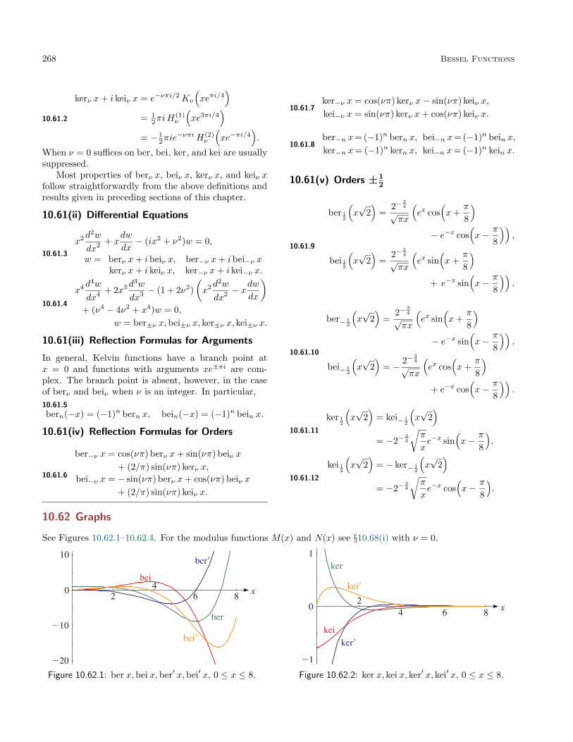
268 Bessel Functions
10.61.2
kerν x+ i keiν x = e−νπi/2Kν
(xeπi/4
)= 1
2πiH(1)ν
(xe3πi/4
)= − 1
2πie−νπiH(2)
ν
(xe−πi/4
).
When ν = 0 suffices on ber, bei, ker, and kei are usuallysuppressed.
Most properties of berν x, beiν x, kerν x, and keiν xfollow straightforwardly from the above definitions andresults given in preceding sections of this chapter.
10.61(ii) Differential Equations
10.61.3
x2 d2w
dx2 + xdw
dx− (ix2 + ν2)w = 0,
w = berν x+ i beiν x, ber−ν x+ i bei−ν xkerν x+ i keiν x, ker−ν x+ i kei−ν x.
10.61.4
x4 d4w
dx4 + 2x3 d3w
dx3 − (1 + 2ν2)(x2 d
2w
dx2 − xdw
dx
)+ (ν4 − 4ν2 + x4)w = 0,
w = ber±ν x, bei±ν x, ker±ν x, kei±ν x.
10.61(iii) Reflection Formulas for Arguments
In general, Kelvin functions have a branch point atx = 0 and functions with arguments xe±πi are com-plex. The branch point is absent, however, in the caseof berν and beiν when ν is an integer. In particular,10.61.5
bern(−x) = (−1)n bern x, bein(−x) = (−1)n bein x.
10.61(iv) Reflection Formulas for Orders
10.61.6
ber−ν x = cos(νπ) berν x+ sin(νπ) beiν x+ (2/π) sin(νπ) kerν x,
bei−ν x = − sin(νπ) berν x+ cos(νπ) beiν x+ (2/π) sin(νπ) keiν x.
10.61.7ker−ν x = cos(νπ) kerν x− sin(νπ) keiν x,kei−ν x = sin(νπ) kerν x+ cos(νπ) keiν x.
10.61.8ber−n x= (−1)n bern x, bei−n x= (−1)n bein x,ker−n x= (−1)n kern x, kei−n x= (−1)n kein x.
10.61(v) Orders ±12
10.61.9
ber 12
(x√
2)
=2−
34
√πx
(ex cos
(x+
π
8
)− e−x cos
(x− π
8
)),
bei 12
(x√
2)
=2−
34
√πx
(ex sin
(x+
π
8
)+ e−x sin
(x− π
8
)).
10.61.10
ber− 12
(x√
2)
=2−
34
√πx
(ex sin
(x+
π
8
)− e−x sin
(x− π
8
)),
bei− 12
(x√
2)
= − 2−34
√πx
(ex cos
(x+
π
8
)+ e−x cos
(x− π
8
)).
10.61.11
ker 12
(x√
2)
= kei− 12
(x√
2)
= −2−34
√π
xe−x sin
(x− π
8
),
10.61.12
kei 12
(x√
2)
= − ker− 12
(x√
2)
= −2−34
√π
xe−x cos
(x− π
8
).
10.62 Graphs
See Figures 10.62.1–10.62.4. For the modulus functions M(x) and N(x) see §10.68(i) with ν = 0.
Figure 10.62.1: ber x, bei x, ber′ x,bei′ x, 0 ≤ x ≤ 8. Figure 10.62.2: ker x, kei x, ker′ x, kei′ x, 0 ≤ x ≤ 8.

10.63 Recurrence Relations and Derivatives 269
Figure 10.62.3: e−x/√
2 ber x, e−x/√
2 bei x,e−x/
√2M(x), 0 ≤ x ≤ 8.
Figure 10.62.4: ex/√
2 ker x, ex/√
2 kei x, ex/√
2N(x), 0 ≤x ≤ 8.
10.63 Recurrence Relations and Derivatives
10.63(i) berν x, beiν x, kerν x, keiν x
Let fν(x), gν(x) denote any one of the ordered pairs:
10.63.1berν x, beiν x; beiν x,−berν x;kerν x, keiν x; keiν x,− kerν x.
Then10.63.2
fν−1(x) + fν+1(x) = −(ν√
2/x) (fν(x)− gν(x)) ,fν+1(x) + gν+1(x)− fν−1(x)− gν−1(x) = 2
√2f ′ν(x),
f ′ν(x) = −(1/√
2) (fν−1(x) + gν−1(x))− (ν/x)fν(x),f ′ν(x) = (1/
√2) (fν+1(x) + gν+1(x)) + (ν/x)fν(x).
10.63.3
√2 ber′ x = ber1 x+ bei1 x,√2 bei′ x = −ber1 x+ bei1 x.
10.63.4
√2 ker′ x = ker1 x+ kei1 x,√2 kei′ x = − ker1 x+ kei1 x.
10.63(ii) Cross-Products
Let10.63.5
pν = ber2ν x+ bei2ν x, qν = berν x bei′ν x−ber′ν xbeiν x,
rν = berν x ber′ν x+ beiν x bei′ν x,
sν =(ber′ν x
)2 +(bei′ν x
)2.
Then
10.63.6
pν+1 = pν−1 − (4ν/x)rν ,qν+1 = −(ν/x)pν + rν = −qν−1 + 2rν ,rν+1 = −((ν + 1)/x)pν+1 + qν ,
sν = 12pν+1 + 1
2pν−1 − (ν2/x2)pν ,
and
10.63.7 pνsν = r2ν + q2
ν .
Equations (10.63.6) and (10.63.7) also hold when thesymbols ber and bei in (10.63.5) are replaced through-out by ker and kei, respectively.
10.64 Integral Representations
Schläfli-Type Integrals
10.64.1
bern(x√
2)
=(−1)n
π
∫ π
0
cos(x sin t−nt) cosh(x sin t) dt,
10.64.2
bein(x√
2)
=(−1)n
π
∫ π
0
sin(x sin t−nt) sinh(x sin t) dt.
See Apelblat (1991) for these results, and also for simi-lar representations for berν
(x√
2), beiν
(x√
2), and their
ν-derivatives.
10.65 Power Series
10.65(i) berν x and beiν x
10.65.1
berν x = ( 12x)ν
∞∑k=0
cos(
34νπ + 1
2kπ)
k! Γ(ν + k + 1)( 1
4x2)k,
beiν x = ( 12x)ν
∞∑k=0
sin(
34νπ + 1
2kπ)
k! Γ(ν + k + 1)( 1
4x2)k.
10.65.2
ber x = 1−( 1
4x2)2
(2!)2+
( 14x
2)4
(4!)2− · · · ,
bei x = 14x
2 −( 1
4x2)3
(3!)2+
( 14x
2)5
(5!)2−· · · .

270 Bessel Functions
10.65(ii) kerν x and keiν x
When ν is not an integer combine (10.65.1) with (10.61.6). Also, with ψ(x) = Γ′(x)/Γ(x),
10.65.3
kern x = 12 ( 1
2x)−nn−1∑k=0
(n− k − 1)!k!
cos(
34nπ + 1
2kπ)( 1
4x2)k − ln
(12x)
bern x
+ 14π bein x+ 1
2 ( 12x)n
∞∑k=0
ψ(k + 1) + ψ(n+ k + 1)k!(n+ k)!
cos(
34nπ + 1
2kπ)( 1
4x2)k,
10.65.4
kein x = − 12 ( 1
2x)−nn−1∑k=0
(n− k − 1)!k!
sin(
34nπ + 1
2kπ)( 1
4x2)k − ln
(12x)
bein x
− 14π bern x+ 1
2 ( 12x)n
∞∑k=0
ψ(k + 1) + ψ(n+ k + 1)k!(n+ k)!
sin(
34nπ + 1
2kπ)( 1
4x2)k.
10.65.5
ker x = − ln(
12x)
ber x+ 14π bei x+
∞∑k=0
(−1)kψ(2k + 1)((2k)!)2
( 14x
2)2k,
kei x = − ln(
12x)
bei x− 14π ber x+
∞∑k=0
(−1)kψ(2k + 2)
((2k + 1)!)2( 1
4x2)2k+1.
10.65(iii) Cross-Products and Sums of Squares
10.65.6 ber2ν x+ bei2ν x = ( 1
2x)2ν∞∑k=0
1Γ(ν + k + 1) Γ(ν + 2k + 1)
( 14x
2)2k
k!,
10.65.7 berν xbei′ν x− ber′ν xbeiν x = ( 12x)2ν+1
∞∑k=0
1Γ(ν + k + 1) Γ(ν + 2k + 2)
( 14x
2)2k
k!,
10.65.8 berν xber′ν x+ beiν xbei′ν x = 12 ( 1
2x)2ν−1∞∑k=0
1Γ(ν + k + 1) Γ(ν + 2k)
( 14x
2)2k
k!,
10.65.9(ber′ν x
)2 +(bei′ν x
)2 = ( 12x)2ν−2
∞∑k=0
2k2 + 2νk + 14ν
2
Γ(ν + k + 1) Γ(ν + 2k + 1)( 1
4x2)2k
k!.
10.65(iv) Compendia
For further power series summable in terms of Kelvin functions and their derivatives see Hansen (1975).
10.66 Expansions in Series of Bessel Functions
10.66.1 berν x+ i beiν x =∞∑k=0
e(3ν+k)πi/4xk Jν+k(x)2k/2k!
=∞∑k=0
e(3ν+3k)πi/4xk Iν+k(x)2k/2k!
.
10.66.2 bern(x√
2)
=∞∑
k=−∞
(−1)n+k Jn+2k(x) I2k(x), bein(x√
2)
=∞∑
k=−∞
(−1)n+k Jn+2k+1(x) I2k+1(x).

10.67 Asymptotic Expansions for Large Argument 271
10.67 Asymptotic Expansions for Large Argument
10.67(i) berν x, beiν x, kerν x, keiν x, and Derivatives
Define ak(ν) and bk(ν) as in §§10.17(i) and 10.17(ii). Then as x→∞ with ν fixed,
10.67.1 kerν x ∼ e−x/√
2( π
2x
)12∞∑k=0
ak(ν)xk
cos(x√2
+(ν
2+k
4+
18
)π
),
10.67.2 keiν x ∼ −e−x/√
2( π
2x
)12∞∑k=0
ak(ν)xk
sin(x√2
+(ν
2+k
4+
18
)π
).
10.67.3 berν x ∼ex/√
2
(2πx)12
∞∑k=0
ak(ν)xk
cos(x√2
+(ν
2+
3k4− 1
8
)π
)− 1π
(sin(2νπ) kerν x+ cos(2νπ) keiν x),
10.67.4 beiν x ∼ex/√
2
(2πx)12
∞∑k=0
ak(ν)xk
sin(x√2
+(ν
2+
3k4− 1
8
)π
)+
1π
(cos(2νπ) kerν x− sin(2νπ) keiν x).
10.67.5 ker′ν x ∼ −e−x/√
2( π
2x
)12∞∑k=0
bk(ν)xk
cos(x√2
+(ν
2+k
4− 1
8
)π
),
10.67.6 kei′ν x ∼ e−x/√
2( π
2x
)12∞∑k=0
bk(ν)xk
sin(x√2
+(ν
2+k
4− 1
8
)π
).
10.67.7 ber′ν x ∼ex/√
2
(2πx)12
∞∑k=0
bk(ν)xk
cos(x√2
+(ν
2+
3k4
+18
)π
)− 1π
(sin(2νπ) ker′ν x+ cos(2νπ) kei′ν x),
10.67.8 bei′ν x ∼ex/√
2
(2πx)12
∞∑k=0
bk(ν)xk
sin(x√2
+(ν
2+
3k4
+18
)π
)+
1π
(cos(2νπ) ker′ν x− sin(2νπ) kei′ν x).
The contributions of the terms in kerν x, keiν x, ker′ν x, and kei′ν x on the right-hand sides of (10.67.3), (10.67.4),(10.67.7), and (10.67.8) are exponentially small compared with the other terms, and hence can be neglected in thesense of Poincaré asymptotic expansions (§2.1(iii)). However, their inclusion improves numerical accuracy.
10.67(ii) Cross-Products and Sums of Squares in the Case ν = 0
As x→∞
10.67.9 ber2 x+ bei2 x ∼ ex√
2
2πx
(1 +
14√
21x
+164
1x2− 33
256√
21x3− 1797
81921x4
+ · · ·),
10.67.10 ber x bei′ x− ber′ xbei x ∼ ex√
2
2πx
(1√2
+18
1x
+9
64√
21x2
+39512
1x3
+75
8192√
21x4
+ · · ·),
10.67.11 ber x ber′ x+ bei x bei′ x ∼ ex√
2
2πx
(1√2− 3
81x− 15
64√
21x2− 45
5121x3
+315
8192√
21x4
+ · · ·),
10.67.12(ber′ x
)2 +(bei′ x
)2 ∼ ex√
2
2πx
(1− 3
4√
21x
+964
1x2
+75
256√
21x3
+24758192
1x4
+· · ·).
10.67.13 ker2 x+ kei2 x ∼ π
2xe−x√
2
(1− 1
4√
21x
+164
1x2
+33
256√
21x3− 1797
81921x4
+ · · ·),
10.67.14 ker x kei′ x− ker′ x kei x ∼ − π
2xe−x√
2
(1√2− 1
81x
+9
64√
21x2− 39
5121x3
+75
8192√
21x4
+ · · ·),
10.67.15 ker x ker′ x+ kei x kei′ x ∼ − π
2xe−x√
2
(1√2
+38
1x− 15
64√
21x2
+45512
1x3
+315
8192√
21x4
+ · · ·),
10.67.16(ker′ x
)2 +(kei′ x
)2 ∼ π
2xe−x√
2
(1 +
34√
21x
+964
1x2− 75
256√
21x3
+24758192
1x4
+· · ·).

272 Bessel Functions
10.68 Modulus and Phase Functions
10.68(i) Definitions
10.68.1 Mν(x)eiθν(x) = berν x+ ibeiν x,
10.68.2 Nν(x)eiφν(x) = kerν x+ i keiν x,where Mν(x) (> 0), Nν(x) (> 0), θν(x), and φν(x) are continuous real functions of x and ν, with the branches ofθν(x) and φν(x) chosen to satisfy (10.68.18) and (10.68.21) as x→∞. (See also §10.68(iv).)
10.68(ii) Basic Properties
10.68.3 berν x = Mν(x) cos θν(x), beiν x = Mν(x) sin θν(x),
10.68.4 kerν x = Nν(x) cosφν(x), keiν x = Nν(x) sinφν(x).
10.68.5 Mν(x) = (ber2ν x+ bei2ν x) 1/2 , Nν(x) = (ker2
ν x+ kei2ν x) 1/2 ,
10.68.6 θν(x) = Arctan(beiν x/berν x), φν(x) = Arctan(keiν x/ kerν x).
10.68.7 M−n(x) = Mn(x), θ−n(x) = θn(x)− nπ.With arguments (x) suppressed,
10.68.8ber′ν x = 1
2 Mν+1 cos(θν+1− 1
4π)− 1
2 Mν−1 cos(θν−1− 1
4π)
= (ν/x)Mν cos θν +Mν+1 cos(θν+1− 1
4π)
= −(ν/x)Mν cos θν −Mν−1 cos(θν−1− 1
4π),
10.68.9bei′ν x = 1
2 Mν+1 sin(θν+1− 1
4π)− 1
2 Mν−1 sin(θν−1− 1
4π)
= (ν/x)Mν sin θν +Mν+1 sin(θν+1− 1
4π)
= −(ν/x)Mν sin θν −Mν−1 sin(θν−1− 1
4π).
10.68.10 ber′ x = M1 cos(θ1− 1
4π), bei′ x = M1 sin
(θ1− 1
4π).
10.68.11 M ′ν = (ν/x)Mν +Mν+1 cos(θν+1− θν − 1
4π)
= −(ν/x)Mν −Mν−1 cos(θν−1− θν − 1
4π),
10.68.12 θ′ν = (Mν+1 /Mν) sin(θν+1− θν − 1
4π)
= −(Mν−1 /Mν) sin(θν−1− θν − 1
4π).
10.68.13 M ′0 = M1 cos(θ1− θ0− 1
4π), θ′0 = (M1 /M0) sin
(θ1− θ0− 1
4π).
10.68.14 d(xM2ν θ′ν)/dx = xM2
ν , x2M ′′ν +xM ′ν −ν2Mν = x2Mν θ′ν
2.
Equations (10.68.8)–(10.68.14) also hold with the symbols ber, bei, M, and θ replaced throughout by ker, kei,N, and φ, respectively. In place of (10.68.7),
10.68.15 N−ν(x) = Nν(x), φ−ν(x) = φν(x) + νπ.
10.68(iii) Asymptotic Expansions for Large Argument
When ν is fixed, µ = 4ν2, and x→∞
10.68.16 Mν(x) =ex/√
2
(2πx)12
(1− µ− 1
8√
21x
+(µ− 1)2
2561x2− (µ− 1)(µ2 + 14µ− 399)
6144√
21x3
+O
(1x4
)),
10.68.17 lnMν(x) =x√2− 1
2ln(2πx)− µ− 1
8√
21x− (µ− 1)(µ− 25)
384√
21x3− (µ− 1)(µ− 13)
1281x4
+O
(1x5
),
10.68.18 θν(x) =x√2
+(
12ν − 1
8
)π +
µ− 18√
21x
+µ− 1
161x2− (µ− 1)(µ− 25)
384√
21x3
+O
(1x5
).
10.68.19 Nν(x) = e−x/√
2( π
2x
)12(
1 +µ− 18√
21x
+(µ− 1)2
2561x2
+(µ− 1)(µ2 + 14µ− 399)
6144√
21x3
+O
(1x4
)),
10.68.20 lnNν(x) = − x√2
+12
ln( π
2x
)+µ− 18√
21x
+(µ− 1)(µ− 25)
384√
21x3− (µ− 1)(µ− 13)
1281x4
+O
(1x5
),
10.68.21 φν(x) = − x√2−(
12ν +
18
)π − µ− 1
8√
21x
+µ− 1
161x2
+(µ− 1)(µ− 25)
384√
21x3
+O
(1x5
).

10.69 Uniform Asymptotic Expansions for Large Order 273
10.68(iv) Further Properties
Additional properties of the modulus and phase functions are given in Young and Kirk (1964, pp. xi–xv). However,care needs to be exercised with the branches of the phases. Thus this reference gives φ1(0) = 5
4π (Eq. (6.10)), andlimx→∞(φ1(x) + (x/
√2)) = − 5
8π (Eqs. (10.20) and (Eqs. (10.26b)). However, numerical tabulations show that ifthe second of these equations applies and φ1(x) is continuous, then φ1(0) = − 3
4π; compare Abramowitz and Stegun(1964, p. 433).
10.69 Uniform Asymptotic Expansions for Large Order
Let Uk(p) and Vk(p) be the polynomials defined in §10.41(ii), and
10.69.1 ξ = (1 + ix2) 1/2 .
Then as ν → +∞,
10.69.2 berν(νx) + ibeiν(νx) ∼ eνξ
(2πνξ) 1/2
(xe3πi/4
1 + ξ
)ν ∞∑k=0
Uk(ξ−1)νk
,
10.69.3 kerν(νx) + i keiν(νx) ∼ e−νξ(
π
2νξ
)1/2 (xe3πi/4
1 + ξ
)−ν ∞∑k=0
(−1)kUk(ξ−1)νk
,
10.69.4 ber′ν(νx) + ibei′ν(νx) ∼ eνξ
x
(ξ
2πν
)1/2 (xe3πi/4
1 + ξ
)ν ∞∑k=0
Vk(ξ−1)νk
,
10.69.5 ker′ν(νx) + i kei′ν(νx) ∼ −e−νξ
x
(πξ
2ν
)1/2 (xe3πi/4
1 + ξ
)−ν ∞∑k=0
(−1)kVk(ξ−1)νk
,
uniformly for x ∈ (0,∞). All fractional powers take their principal values.All four expansions also enjoy the same kind of double asymptotic property described in §10.41(iv).Accuracy in (10.69.2) and (10.69.4) can be increased by including exponentially-small contributions as in (10.67.3),
(10.67.4), (10.67.7), and (10.67.8) with x replaced by νx.
10.70 Zeros
Asymptotic approximations for large zeros are as follows. Let µ = 4ν2 and f(t) denote the formal series
10.70.1µ− 116t
+µ− 132t2
+(µ− 1)(5µ+ 19)
1536t3+
3(µ− 1)2
512t4+· · · .
If m is a large positive integer, then
10.70.2
zeros of berν x ∼√
2(t− f(t)), t = (m− 12ν −
38 )π,
zeros of beiν x ∼√
2(t− f(t)), t = (m− 12ν + 1
8 )π,
zeros of kerν x ∼√
2(t+ f(−t)), t = (m− 12ν −
58 )π,
zeros of keiν x ∼√
2(t+ f(−t)), t = (m− 12ν −
18 )π.
In the case ν = 0, numerical tabulations (Abramowitz and Stegun (1964, Table 9.12)) indicate that each of(10.70.2) corresponds to the mth zero of the function on the left-hand side. For the next six terms in the series(10.70.1) see MacLeod (2002a).

274 Bessel Functions
10.71 Integrals
10.71(i) Indefinite Integrals
In the following equations fν , gν is any one of the four ordered pairs given in (10.63.1), and f̂ν , ĝν is either the sameordered pair or any other ordered pair in (10.63.1).
10.71.1
∫x1+νfν dx = −x
1+ν
√2
(fν+1 − gν+1) = −x1+ν(νxgν − g′ν
),
10.71.2
∫x1−νfν dx =
x1−ν√
2(fν−1 − gν−1) = x1−ν
(νxgν + g′ν
).
10.71.3
∫x(fν ĝν − gν f̂ν) dx =
x
2√
2
(f̂ν(fν+1 + gν+1)− ĝν(fν+1 − gν+1)− fν(f̂ν+1 + ĝν+1) + gν(f̂ν+1 − ĝν+1)
)= 1
2x(f ′ν f̂ν − fν f̂ ′ν + g′ν ĝν − gν ĝ′ν),
10.71.4
∫x(fν ĝν + gν f̂ν) dx = 1
4x2(2fν ĝν − fν−1ĝν+1 − fν+1ĝν−1 + 2gν f̂ν − gν−1f̂ν+1 − gν+1f̂ν−1).
10.71.5
∫x(f2
ν + g2ν) dx = x(fνg′ν − f ′νgν) = − x√
2(fνfν+1 + gνgν+1 − fνgν+1 + fν+1gν),
10.71.6
∫xfνgν dx = 1
4x2 (2fνgν − fν−1gν+1 − fν+1gν−1) ,
10.71.7
∫x(f2
ν − g2ν) dx = 1
2x2(f2ν − fν−1fν+1 − g2
ν + gν−1gν+1
).
Examples
10.71.8
∫xM2
ν (x) dx = x(berν xbei′ν x− ber′ν xbeiν x),∫xN2
ν (x) dx = x(kerν x kei′ν x− ker′ν x keiν x),
where Mν(x) and Nν(x) are the modulus functions introduced in §10.68(i).
10.71(ii) Definite Integrals
See Kerr (1978) and Glasser (1979).
10.71(iii) Compendia
For infinite double integrals involving Kelvin functionssee Prudnikov et al. (1986b, pp. 630–631).
For direct and inverse Laplace transforms of Kelvinfunctions see Prudnikov et al. (1992a, §3.19) and Prud-nikov et al. (1992b, §3.19).
Applications
10.72 Mathematical Applications
10.72(i) Differential Equations with TurningPoints
Bessel functions and modified Bessel functions are of-ten used as approximants in the construction of uniformasymptotic approximations and expansions for solutionsof linear second-order differential equations containing a
parameter. The canonical form of differential equationfor these problems is given by
10.72.1d2w
dz2 =(u2f(z) + g(z)
)w,
where z is a real or complex variable and u is a largereal or complex parameter.
Simple Turning Points
In regions in which (10.72.1) has a simple turning pointz0, that is, f(z) and g(z) are analytic (or with weakerconditions if z = x is a real variable) and z0 is a sim-ple zero of f(z), asymptotic expansions of the solutionsw for large u can be constructed in terms of Airy func-tions or equivalently Bessel functions or modified Besselfunctions of order 1
3 (§9.6(i)). These expansions are uni-form with respect to z, including the turning point z0
and its neighborhood, and the region of validity oftenincludes cut neighborhoods (§1.10(vi)) of other singu-larities of the differential equation, especially irregularsingularities.
For further information and references see §§2.8(i)and 2.8(iii).

10.73 Physical Applications 275
Multiple or Fractional Turning Points
If f(z) has a double zero z0, or more generally z0 is azero of order m, m = 2, 3, 4, . . . , then uniform asymp-totic approximations (but not expansions) can be con-structed in terms of Bessel functions, or modified Besselfunctions, of order 1/(m + 2). The number m can alsobe replaced by any real constant λ (> −2) in the sensethat (z − z0)−λ f(z) is analytic and nonvanishing atz0; moreover, g(z) is permitted to have a single or dou-ble pole at z0. The order of the approximating Besselfunctions, or modified Bessel functions, is 1/(λ+ 2), ex-cept in the case when g(z) has a double pole at z0. See§2.8(v) for references.
10.72(ii) Differential Equations with Poles
In regions in which the function f(z) has a simple poleat z = z0 and (z − z0)2g(z) is analytic at z = z0 (thecase λ = −1 in §10.72(i)), asymptotic expansions of thesolutions w of (10.72.1) for large u can be constructedin terms of Bessel functions and modified Bessel func-tions of order ±
√1 + 4ρ, where ρ is the limiting value of
(z − z0)2g(z) as z → z0. These asymptotic expansionsare uniform with respect to z, including cut neighbor-hoods of z0, and again the region of uniformity oftenincludes cut neighborhoods of other singularities of thedifferential equation.
For further information and references see §§2.8(i)and 2.8(iv).
10.72(iii) Differential Equations with a DoublePole and a Movable Turning Point
In (10.72.1) assume f(z) = f(z, α) and g(z) = g(z, α)depend continuously on a real parameter α, f(z, α) hasa simple zero z = z0(α) and a double pole z = 0, ex-cept for a critical value α = a, where z0(a) = 0. Assumethat whether or not α = a, z2g(z, α) is analytic at z = 0.Then for large u asymptotic approximations of the solu-tions w can be constructed in terms of Bessel functions,or modified Bessel functions, of variable order (in factthe order depends on u and α). These approximationsare uniform with respect to both z and α, includingz = z0(a), the cut neighborhood of z = 0, and α = a.See §2.8(vi) for references.
10.73 Physical Applications
10.73(i) Bessel and Modified Bessel Functions
Bessel functions first appear in the investigation of aphysical problem in Daniel Bernoulli’s analysis of thesmall oscillations of a uniform heavy flexible chain. Forthis problem and its further generalizations, see Ko-renev (2002, Chapter 4, §37) and Gray et al. (1922,Chapter I, §1, Chapter XVI, §4).
Bessel functions of the first kind, Jn(x), arise nat-urally in applications having cylindrical symmetry inwhich the physics is described either by Laplace’s equa-tion ∇2V = 0, or by the Helmholtz equation (∇2 +k2)ψ = 0.
Laplace’s equation governs problems in heat conduc-tion, in the distribution of potential in an electrostaticfield, and in hydrodynamics in the irrotational motion ofan incompressible fluid. See Jackson (1999, Chapter 3,§§3.7, 3.8, 3.11, 3.13), Lamb (1932, Chapter V, §§100–102; Chapter VIII, §§186, 191–193; Chapter X, §§303,304), Happel and Brenner (1973, Chapter 3, §3.3; Chap-ter 7, §7.3), Korenev (2002, Chapter 4, §43), and Grayet al. (1922, Chapter XI). In cylindrical coordinates r,φ, z, (§1.5(ii) we have
10.73.1 ∇2V =1r
∂
∂r
(r∂V
∂r
)+
1r2
∂2V
∂φ2 +∂2V
∂z2 = 0,
and on separation of variables we obtain solutions of theform e±inφe±κz Jn(κr), from which a solution satisfyingprescribed boundary conditions may be constructed.
The Helmholtz equation, (∇2 + k2)ψ = 0, followsfrom the wave equation
10.73.2 ∇2ψ =1c2∂2ψ
∂t2,
on assuming a time dependence of the form e±ikt. Thisequation governs problems in acoustic and electromag-netic wave propagation. See Jackson (1999, Chap-ter 9, §9.6), Jones (1986, Chapters 7, 8), and LordRayleigh (1945, Vol. I, Chapter IX, §§200–211, 218, 219,221a; Vol. II, Chapter XIII, §272a; Chapter XV, §302;Chapter XVIII; Chapter XIX, §350; Chapter XX, §357;Chapter XXI, §369). It is fundamental in the studyof electromagnetic wave transmission. Consequently,Bessel functions Jn(x), and modified Bessel functionsIn(x), are central to the analysis of microwave andoptical transmission in waveguides, including coaxialand fiber. See Krivoshlykov (1994, Chapter 2, §2.2.10;Chapter 5, §5.2.2), Kapany and Burke (1972, Chap-ters 4–6; Chapter 7, §A.1), and Slater (1942, Chapter 4,§§20, 25).
Bessel functions enter in the study of the scatter-ing of light and other electromagnetic radiation, notonly from cylindrical surfaces but also in the statisti-cal analysis involved in scattering from rough surfaces.See Smith (1997, Chapter 3, §3.7; Chapter 6, §6.4),Beckmann and Spizzichino (1963, Chapter 4, §§4.2, 4.3;Chapter 5, §§5.2, 5.3; Chapter 6, §6.1; Chapter 7, §7.1.),Kerker (1969, Chapter 5, §5.6.4; Chapter 7, §7.5.6), andBayvel and Jones (1981, Chapter 1, §§1.6.5, 1.6.6).
More recently, Bessel functions appear in the in-verse problem in wave propagation, with applications inmedicine, astronomy, and acoustic imaging. See Coltonand Kress (1998, Chapter 2, §§2.4, 2.5; Chapter 3, §3.4).

276 Bessel Functions
In the theory of plates and shells, the oscillations of acircular plate are determined by the differential equa-tion10.73.3 ∇4W + λ2 ∂
2W
∂t2= 0.
See Korenev (2002). On separation of variables intocylindrical coordinates, the Bessel functions Jn(x), andmodified Bessel functions In(x) and Kn(x), all appear.
10.73(ii) Spherical Bessel Functions
The functions jn(x), yn(x), h(1)n (x), and h
(2)n (x) arise
in the solution (again by separation of variables) ofthe Helmholtz equation in spherical coordinates ρ, θ, φ(§1.5(ii)):10.73.4
(∇2 + k2)f =1ρ2
∂
∂ρ
(ρ2 ∂f
∂ρ
)+
1ρ2 sin θ
∂
∂θ
(sin θ
∂f
∂θ
)+
1ρ2 sin2 θ
∂2f
∂φ2 + k2f.
With the spherical harmonic Y`,m(θ, φ) defined asin §14.30(i), the solutions are of the form f =g`(kρ)Y`,m(θ, φ) with g` = j`, y`, h
(1)` , or h
(2)` , depending
on the boundary conditions. Accordingly, the sphericalBessel functions appear in all problems in three dimen-sions with spherical symmetry involving the scatteringof electromagnetic radiation. See Jackson (1999, Chap-ter 9, §9.6), Bayvel and Jones (1981, Chapter 1, §1.5.1),and Konopinski (1981, Chapter 9, §9.1). In quantummechanics the spherical Bessel functions arise in the so-lution of the Schrödinger wave equation for a particlein a central potential. See Messiah (1961, Chapter IX,§§7–10).
10.73(iii) Kelvin Functions
The analysis of the current distribution in circularconductors leads to the Kelvin functions ber x, bei x,ker x, and kei x. See Relton (1965, Chapter X, §§10.2,10.3), Bowman (1958, Chapter III, §§51–53), McLach-lan (1961, Chapters VIII and IX), and Russell (1909).The McLachlan reference also includes other applica-tions of Kelvin functions.
10.73(iv) Bickley Functions
See Bickley (1935) and Altaç (1996).
10.73(v) Rayleigh Function
For applications of the Rayleigh function σn(ν)(§10.21(xiii)) to problems of heat conduction and dif-fusion in liquids see Kapitsa (1951b).
Computation
10.74 Methods of Computation
10.74(i) Series Expansions
The power-series expansions given in §§10.2 and 10.8,together with the connection formulas of §10.4, can beused to compute the Bessel and Hankel functions whenthe argument x or z is sufficiently small in absolutevalue. In the case of the modified Bessel function Kν(z)see especially Temme (1975).
In other circumstances the power series are prone toslow convergence and heavy numerical cancellation.
If x or |z| is large compared with |ν|2, then theasymptotic expansions of §§10.17(i)–10.17(iv) are avail-able. Furthermore, the attainable accuracy can beincreased substantially by use of the exponentially-improved expansions given in §10.17(v), even more soby application of the hyperasymptotic expansions to befound in the references in that subsection.
For large positive real values of ν the uniform asymp-totic expansions of §§10.20(i) and 10.20(ii) can be used.Moreover, because of their double asymptotic properties(§10.41(v)) these expansions can also be used for largex or |z|, whether or not ν is large. It should be noted,however, that there is a difficulty in evaluating the co-efficients Ak(ζ), Bk(ζ), Ck(ζ), and Dk(ζ), from the ex-plicit expressions (10.20.10)–(10.20.13) when z is closeto 1 owing to severe cancellation. Temme (1997) showshow to overcome this difficulty by use of the Maclaurinexpansions for these coefficients or by use of auxiliaryfunctions.
Similar observations apply to the computation ofmodified Bessel functions, spherical Bessel functions,and Kelvin functions. In the case of the spherical Besselfunctions the explicit formulas given in §§10.49(i) and10.49(ii) are terminating cases of the asymptotic expan-sions given in §§10.17(i) and 10.40(i) for the Bessel func-tions and modified Bessel functions. And since there areno error terms they could, in theory, be used for all val-ues of z; however, there may be severe cancellation when|z| is not large compared with n2.
10.74(ii) Differential Equations
A comprehensive and powerful approach is to integratethe differential equations (10.2.1) and (10.25.1) by di-rect numerical methods. As described in §3.7(ii), toinsure stability the integration path must be chosen insuch a way that as we proceed along it the wanted so-lution grows in magnitude at least as fast as all othersolutions of the differential equation.

10.74 Methods of Computation 277
In the interval 0 < x < ν, Jν(x) needs to be inte-grated in the forward direction and Yν(x) in the back-ward direction, with initial values for the former ob-tained from the power-series expansion (10.2.2) and forthe latter from asymptotic expansions (§§10.17(i) and10.20(i)). In the interval ν < x <∞ either direction ofintegration can be used for both functions.
Similarly, to maintain stability in the interval 0 <x < ∞ the integration direction has to be forwards inthe case of Iν(x) and backwards in the case of Kν(x),with initial values obtained in an analogous manner tothose for Jν(x) and Yν(x).
For z ∈ C the function H(1)ν (z), for example, can
always be computed in a stable manner in the sector0 ≤ ph z ≤ π by integrating along rays towards theorigin.
Similar considerations apply to the spherical Besselfunctions and Kelvin functions.
For further information, including parallel methodsfor solving the differential equations, see Lozier andOlver (1993).
10.74(iii) Integral Representations
For evaluation of the Hankel functions H(1)ν (z) and
H(2)ν (z) for complex values of ν and z based on the in-
tegral representations (10.9.18) see Remenets (1973).For applications of generalized Gauss–Laguerre
quadrature (§3.5(v)) to the evaluation of the modifiedBessel functions Kν(z) for 0 < ν < 1 and 0 < x < ∞see Gautschi (2002a). The integral representation usedis based on (10.32.8).
For evaluation of Kν(z) from (10.32.14) with ν = nand z complex, see Mechel (1966).
10.74(iv) Recurrence Relations
If values of the Bessel functions Jν(z), Yν(z), or theother functions treated in this chapter, are needed forinteger-spaced ranges of values of the order ν, then asimple and powerful procedure is provided by recurrencerelations typified by the first of (10.6.1).
Suppose, for example, ν = n ∈ 0, 1, 2, . . . , andx ∈ (0,∞). Then Jn(x) and Yn(x) can be generatedby either forward or backward recurrence on n whenn < x, but if n > x then to maintain stability Jn(x) hasto be generated by backward recurrence on n, and Yn(x)has to be generated by forward recurrence on n. In thecase of Jn(x), the need for initial values can be avoidedby application of Olver’s algorithm (§3.6(v)) in conjunc-tion with Equation (10.12.4) used as a normalizing con-dition, or in the case of noninteger orders, (10.23.15).
For further information see Gautschi (1967), Olverand Sookne (1972), Temme (1975), Campbell (1980),and Kerimov and Skorokhodov (1984a).
10.74(v) Continued Fractions
For applications of the continued-fraction expansions(10.10.1), (10.10.2), (10.33.1), and (10.33.2) to the com-putation of Bessel functions and modified Bessel func-tions see Gargantini and Henrici (1967), Amos (1974),Gautschi and Slavik (1978), Tretter and Walster (1980),Thompson and Barnett (1986), and Cuyt et al. (2008).
10.74(vi) Zeros and Associated Values
Newton’s rule (§3.8(i)) or Halley’s rule (§3.8(v)) can beused to compute to arbitrarily high accuracy the real orcomplex zeros of all the functions treated in this chapter.Necessary values of the first derivatives of the functionsare obtained by the use of (10.6.2), for example. New-ton’s rule is quadratically convergent and Halley’s ruleis cubically convergent. See also Segura (1998, 2001).
Methods for obtaining initial approximations tothe zeros include asymptotic expansions (§§10.21(vi)-10.21(ix)), graphical intersection of 2D graphs in R(e.g., §10.3(i)) with the x-axis, or graphical intersectionof 3D complex-variable surfaces (e.g., §10.3(ii)) with theplane z = 0.
To ensure that no zeros are overlooked, standardtools are the phase principle and Rouché’s theorem; see§1.10(iv).
Real Zeros
See Olver (1960, pp. xvi–xxix), Grad and Zakraǰsek(1973), Temme (1979a), Ikebe et al. (1991), Zafiropou-los et al. (1996), Vrahatis et al. (1997a), Ball (2000),and Gil and Segura (2003).
Complex Zeros
See Leung and Ghaderpanah (1979), Kerimov andSkorokhodov (1984b,c, 1985a,b), Skorokhodov (1985),Modenov and Filonov (1986), and Vrahatis et al.(1997b).
Multiple Zeros
See Kerimov and Skorokhodov (1985c, 1986, 1987,1988).
10.74(vii) Integrals
Hankel Transform
See Cornille (1972), Johansen and Sørensen (1979),Gabutti (1979), Gabutti and Minetti (1981), Candel(1981), Wong (1982), Lund (1985), Piessens and Bran-ders (1985), Hansen (1985), Bezvoda et al. (1986), Pu-oskari (1988), Christensen (1990), Campos (1995), Lu-cas and Stone (1995), Barakat and Parshall (1996), Sidi(1997), Secada (1999).

278 Bessel Functions
Fourier–Bessel Expansion
For the computation of the integral (10.23.19) seePiessens and Branders (1983, 1985), Lewanowicz (1991),and Zhilĕıkin and Kukarkin (1995).
Spherical Bessel Transform
The spherical Bessel transform is the Hankel transform(10.22.76) in the case when ν is half an odd positiveinteger.
See Lehman et al. (1981), Puoskari (1988), andSharafeddin et al. (1992).
Kontorovich–Lebedev Transform
See Ehrenmark (1995).
Products
For infinite integrals involving products of two Besselfunctions of the first kind, see Linz and Kropp (1973),Gabutti (1980), Ikonomou et al. (1995), and Lucas(1995).
10.74(viii) Functions of Imaginary Order
For the computation of the functions Ĩν(x) and K̃ν(x)defined by (10.45.2) see Temme (1994b) and Gil et al.(2002b, 2003a, 2004a).
10.75 Tables
10.75(i) Introduction
Comprehensive listings and descriptions of tables ofthe functions treated in this chapter are provided inBateman and Archibald (1944), Lebedev and Fedorova(1960), Fletcher et al. (1962), and Luke (1975, §9.13.2).Only a few of the more comprehensive of these early ta-bles are included in the listings in the following subsec-tions. Also, for additional listings of tables pertainingto complex arguments see Babushkina et al. (1997).
10.75(ii) Bessel Functions and their Derivatives
• British Association for the Advancement ofScience (1937) tabulates J0(x), J1(x), x =0(.001)16(.01)25, 10D; Y0(x), Y1(x), x =0.01(.01)25, 8–9S or 8D. Also included are aux-iliary functions to facilitate interpolation of thetables of Y0(x), Y1(x) for small values of x, as wellas auxiliary functions to compute all four func-tions for large values of x.
• Bickley et al. (1952) tabulates Jn(x), Yn(x) orxn Yn(x), n = 2(1)20, x = 0(.01 or .1) 10(.1)25,8D (for Jn(x)), 8S (for Yn(x) or xn Yn(x)); Jn(x),Yn(x), n = 0(1)20, x = 0 or 0.1(.1)25, 10D (forJn(x)), 10S (for Yn(x)).
• Olver (1962) provides tables for the uniformasymptotic expansions given in §10.20(i), includ-ing ζ and (4ζ
/(1− x2) )
14 as functions of x (= z)
and the coefficients Ak(ζ), Bk(ζ), Ck(ζ), Dk(ζ)as functions of ζ. These enable Jν(νx), Yν(νx),J ′ν(νx), Y ′ν(νx) to be computed to 10S when ν ≥15, except in the neighborhoods of zeros.
• The main tables in Abramowitz and Stegun (1964,Chapter 9) give J0(x) to 15D, J1(x), J2(x),Y0(x), Y1(x) to 10D, Y2(x) to 8D, x = 0(.1)17.5;Yn(x) − (2/π) Jn(x) lnx, n = 0, 1, x = 0(.1)2,8D; Jn(x), Yn(x), n = 3(1)9, x = 0(.2)20, 5Dor 5S; Jn(x), Yn(x), n = 0(1)20(10)50, 100, x =1, 2, 5, 10, 50, 100, 10S; modulus and phase func-tions
√xMn(x), θn(x) − x, n = 0, 1, 2, 1/x =
0(.01)0.1, 8D.
• Achenbach (1986) tabulates J0(x), J1(x), Y0(x),Y1(x), x = 0(.1)8, 20D or 18–20S.
• Zhang and Jin (1996, pp. 185–195) tab-ulates Jn(x), J ′n(x), Yn(x), Y ′n(x), n =0(1)10(10)50, 100, x = 1, 5, 10, 25, 50,100, 9S; Jn+α(x), J ′n+α(x), Yn+α(x), Y ′n+α(x),n = 0(1)5, 10, 30, 50, 100, α = 1
4 ,13 ,
12 ,
23 ,
34 ,
x = 1, 5, 10, 50, 8S; real and imaginary partsof Jn+α(z), J ′n+α(z), Yn+α(z), Y ′n+α(z), n =0(1)15, 20(10)50, 100, α = 0, 1
2 , z = 4+2i, 20+10i,8S.
10.75(iii) Zeros and Associated Values of theBessel Functions, Hankel Functions,and their Derivatives
Real Zeros
• British Association for the Advancement ofScience (1937) tabulates j0,m, J1(j0,m), j1,m,J0(j1,m), m = 1(1)150, 10D; y0,m, Y1(y0,m), y1,m,Y0(y1,m), m = 1(1)50, 8D.
• Olver (1960) tabulates jn,m, J ′n(jn,m), j′n,m,Jn(j′n,m
), yn,m, Y ′n(yn,m), y′n,m, Yn
(y′n,m
), n =
0( 12 )20 1
2 , m = 1(1)50, 8D. Also included are ta-bles of the coefficients in the uniform asymptoticexpansions of these zeros and associated values asn → ∞; see §10.21(viii), and more fully Olver(1954).
• Morgenthaler and Reismann (1963) tabulates j′n,mfor n = 21(1)51 and j′n,m< 100, 7-10S.
• Abramowitz and Stegun (1964, Chapter 9) tabu-lates jn,m, J ′n(jn,m), j′n,m, Jn
(j′n,m
), n = 0(1)8,
m = 1(1)20, 5D (10D for n = 0), yn,m, Y ′n(yn,m),y′n,m, Yn
(y′n,m
), n = 0(1)8, m = 1(1)20, 5D
10.75 Tables 279
(8D for n = 0), J0(j0,m x), m = 1(1)5, x =0(.02)1, 5D. Also included are the first 5 zeros ofthe functions xJ1(x)− λJ0(x), J1(x)− λxJ0(x),J0(x)Y0(λx) − Y0(x) J0(λx), J1(x)Y1(λx) −Y1(x) J1(λx), J1(x)Y0(λx)−Y1(x) J0(λx) for vari-ous values of λ and λ−1 in the interval [0, 1], 4–8D.
• Abramowitz and Stegun (1964, Chapter 10)tabulates jν,m, J ′ν(jν,m), j′ν,m, Jν
(j′ν,m
), yν,m,
Y ′ν(yν,m), y′ν,m, Yν(y′ν,m
), ν = 1
2 (1)19 12 , m =
1(1)mν , where mν ranges from 8 at ν = 12 down
to 1 at ν = 19 12 , 6–7D.
• Makinouchi (1966) tabulates all values of jν,m andyν,m in the interval (0, 100), with at least 29S.These are for ν = 0(1)5, 10, 20; ν = 3
2 , 52 ;
ν = m/n with m = 1(1)n − 1 and n = 3(1)8,except for ν = 1
2 .
• Döring (1971) tabulates the first 100 values of ν(> 1) for which J ′−ν(x) has the double zero x = ν,10D.
• Heller (1976) tabulates j0,m, J1(j0,m), j1,m,J0(j1,m), j′1,m, J1
(j′1,m
)for m = 1(1)100, 25D.
• Wills et al. (1982) tabulates j0,m, j1,m, y0,m, y1,m
for m = 1(1)30, 35D.
• Kerimov and Skorokhodov (1985c) tabulates 201double zeros of J ′′−ν(x), 10 double zeros of J ′′′−ν(x),101 double zeros of Y ′−ν(x), 201 double zeros ofY ′′−ν(x), and 10 double zeros of Y ′′′−ν(x), all to 8 or9D.
• Zhang and Jin (1996, pp. 196–198) tabulates jn,m,j′n,m, yn,m, y′n,m, n = 0(1)3, m = 1(1)10, 8D;the first five zeros of Jn(x)Yn(λx)−Jn(λx)Yn(x),J ′n(x)Y ′n(λx) − J ′n(λx)Y ′n(x), n = 0, 1, 2, λ =1.1(.1)1.6, 1.8, 2(.5)5, 7D.
Complex Zeros
• Abramowitz and Stegun (1964, p. 373) tabulatesthe three smallest zeros of Y0(z), Y1(z), Y ′1(z) inthe sector 0 < ph z ≤ π, together with the cor-responding values of Y1(z), Y0(z), Y1(z), respec-tively, to 9D. (There is an error in the value ofY0(z) at the 3rd zero of Y1(z): the last four digitsshould be 2533; see Amos (1985).)
• Döring (1966) tabulates all zeros of Y0(z), Y1(z),H
(1)0 (z), H(1)
1 (z), that lie in the sector |z| < 158,|ph z| ≤ π, to 10D. Some of the smaller zeros ofYn(z) and H
(1)n (z) for n = 2, 3, 4, 5, 15 are also
included.
• Kerimov and Skorokhodov (1985a) tabulates 5(nonreal) complex conjugate pairs of zeros of theprincipal branches of Yn(z) and Y ′n(z) for n =0(1)5, 8D.
• Kerimov and Skorokhodov (1985b) tabulates 50zeros of the principal branches of H(1)
0 (z) andH
(1)1 (z), 8D.
• Kerimov and Skorokhodov (1987) tabulates 100complex double zeros ν of Y ′ν
(ze−πi
)and
H(1)ν
′(ze−πi
), 8D.
• MacDonald (1989) tabulates the first 30 zeros, inascending order of absolute value in the fourthquadrant, of the function J0(z) − i J1(z), 6D.(Other zeros of this function can be obtained byreflection in the imaginary axis).
• Zhang and Jin (1996, p. 199) tabulates the realand imaginary parts of the first 15 conjugate pairsof complex zeros of Y0(z), Y1(z), Y ′1(z) and thecorresponding values of Y1(z), Y0(z), Y1(z), re-spectively, 10D.
10.75(iv) Integrals of Bessel Functions
• Abramowitz and Stegun (1964, Chapter 11) tab-ulates
∫ x0J0(t) dt,
∫ x0Y0(t) dt, x = 0(.1)10, 10D;∫ x
0t−1(1 − J0(t)) dt,
∫∞xt−1 Y0(t) dt, x = 0(.1)5,
8D.
• Zhang and Jin (1996, p. 270) tabulates∫ x
0J0(t) dt,∫ x
0t−1(1 − J0(t)) dt,
∫ x0Y0(t) dt,
∫∞xt−1 Y0(t) dt,
x = 0(.1)1(.5)20, 8D.
10.75(v) Modified Bessel Functions and theirDerivatives
• British Association for the Advancement of Sci-ence (1937) tabulates I0(x), I1(x), x = 0(.001)5,7–8D; K0(x), K1(x), x = 0.01(.01)5, 7–10D;e−x I0(x), e−x I1(x), exK0(x), exK1(x), x =5(.01)10(.1)20, 8D. Also included are auxiliaryfunctions to facilitate interpolation of the tablesof K0(x), K1(x) for small values of x.
• Bickley et al. (1952) tabulates x−n In(x) ore−x In(x), xnKn(x) or exKn(x), n = 2(1)20,x = 0(.01 or .1) 10(.1) 20, 8S; In(x), Kn(x),n = 0(1)20, x = 0 or 0.1(.1)20, 10S.
• Olver (1962) provides tables for the uniformasymptotic expansions given in §10.41(ii), includ-ing η and the coefficients Uk(p), Vk(p) as func-tions of p = (1 + x2)−
12 . These enable Iν(νx),
Kν(νx), I ′ν(νx), K ′ν(νx) to be computed to 10Swhen ν ≥ 16.

280 Bessel Functions
• The main tables in Abramowitz and Stegun (1964,Chapter 9) give e−x In(x), exKn(x), n = 0, 1, 2,x = 0(.1)10(.2)20, 8D–10D or 10S;
√xe−x In(x),
(√x/π) exKn(x), n = 0, 1, 2, 1/x = 0(.002)0.05;
K0(x) + I0(x) lnx, x(K1(x) − I1(x) lnx), x =0(.1)2, 8D; e−x In(x), exKn(x), n = 3(1)9,x = 0(.2)10(.5)20, 5S; In(x), Kn(x), n =0(1)20(10)50, 100, x = 1, 2, 5, 10, 50, 100, 9–10S.
• Achenbach (1986) tabulates I0(x), I1(x), K0(x),K1(x), x = 0(.1)8, 19D or 19–21S.
• Zhang and Jin (1996, pp. 240–250) tabu-lates In(x), I ′n(x), Kn(x), K ′n(x), n =0(1)10(10)50, 100, x = 1, 5, 10, 25, 50, 100, 9S;In+α(x), I ′n+α(x), Kn+α(x), K ′n+α(x), n = 0(1)5,10, 30, 50, 100, α = 1
4 , 13 , 1
2 , 23 , 3
4 , x = 1, 5, 10, 50,8S; real and imaginary parts of In+α(z), I ′n+α(z),Kn+α(z), K ′n+α(z), n = 0(1)15, 20(10)50, 100,α = 0, 1
2 , z = 4 + 2i, 20 + 10i, 8S.
10.75(vi) Zeros of Modified Bessel Functionsand their Derivatives
• Parnes (1972) tabulates all zeros of the principalvalue of Kn(z), for n = 2(1)10, 9D.
• Leung and Ghaderpanah (1979), tabulates all ze-ros of the principal value of Kn(z), for n = 2(1)10,29S.
• Kerimov and Skorokhodov (1984b) tabulates allzeros of the principal values of Kn(z) and K ′n(z),for n = 2(1)20, 9S.
• Kerimov and Skorokhodov (1984c) tabulates allzeros of I−n− 1
2(z) and I ′−n− 1
2(z) in the sector
0 ≤ ph z ≤ 12π for n = 1(1)20, 9S.
• Kerimov and Skorokhodov (1985b) tabulates allzeros of Kn(z) and K ′n(z) in the sector − 1
2π <ph z ≤ 3
2π for n = 0(1)5, 8D.
10.75(vii) Integrals of Modified BesselFunctions
• Abramowitz and Stegun (1964, Chapter 11) tabu-lates e−x
∫ x0I0(t) dt, ex
∫∞xK0(t) dt, x = 0(.1)10,
7D; e−x∫ x
0t−1(I0(t) − 1) dt, xex
∫∞xt−1K0(t) dt,
x = 0(.1)5, 6D.
• Bickley and Nayler (1935) tabulates Kin(x)(§10.43(iii)) for n = 1(1)16, x = 0(.05)0.2(.1) 2, 3,9D.
• Zhang and Jin (1996, p. 271) tabu-lates e−x
∫ x0I0(t) dt, e−x
∫ x0t−1(I0(t) − 1) dt,
ex∫∞xK0(t) dt, xex
∫∞xt−1K0(t) dt, x =
0(.1)1(.5)20, 8D.
10.75(viii) Modified Bessel Functions ofImaginary or Complex Order
For the notation see §10.45.
• Žurina and Karmazina (1967) tabulates K̃ν(x) forν = 0.01(.01)10, x = 0.1(.1)10.2, 7S.
• Rappoport (1979) tabulates the real and imag-inary parts of K 1
2 +iτ (x) for τ = 0.01(.01)10,x = 0.1(.2)9.5, 7S.
10.75(ix) Spherical Bessel Functions, ModifiedSpherical Bessel Functions, and theirDerivatives
• The main tables in Abramowitz and Stegun (1964,Chapter 10) give jn(x), yn(x) n = 0(1)8, x =0(.1)10, 5–8S; jn(x), yn(x) n = 0(1)20(10)50,100, x = 1, 2, 5, 10, 50, 100, 10S; i
(1)n (x), kn(x),
n = 0, 1, 2, x = 0(.1)5, 4–9D; i(1)n (x), kn(x),
n = 0(1)20(10)50, 100, x = 1, 2, 5, 10, 50, 100, 10S.(For the notation see §10.1 and §10.47(ii).)
• Zhang and Jin (1996, pp. 296–305) tabulates
jn(x), j′n(x), yn(x), y′n(x), i(1)n (x), i
(1)n
′(x), kn(x),
k′n(x), n = 0(1)10(10)30, 50, 100, x = 1, 5, 10, 25,50, 100, 8S; x jn(x), (x jn(x))′, x yn(x), (x yn(x))′
(Riccati–Bessel functions and their derivatives),n = 0(1)10(10)30, 50, 100, x = 1, 5, 10, 25,50, 100, 8S; real and imaginary parts of jn(z),
j′n(z), yn(z), y′n(z), i(1)n (z), i
(1)n
′(z), kn(z), k′n(z),
n = 0(1)15, 20(10)50, 100, z = 4 + 2i, 20 + 10i,8S. (For the notation replace j, y, i, k by j, y, i(1),k, respectively.)
10.75(x) Zeros and Associated Values ofDerivatives of Spherical BesselFunctions
For the notation see §10.58.
• Olver (1960) tabulates a′n,m, jn(a′n,m
), b′n,m,
yn(b′n,m
), n = 1(1)20, m = 1(1)50, 8D. Also in-
cluded are tables of the coefficients in the uniformasymptotic expansions of these zeros and associ-ated values as n→∞.

10.76 Approximations 281
10.75(xi) Kelvin Functions and their Derivatives
• Young and Kirk (1964) tabulates bern x, bein x,kern x, kein x, n = 0, 1, x = 0(.1)10, 15D; bern x,bein x, kern x, kein x, modulus and phase func-tions Mn(x), θn(x), Nn(x), φn(x), n = 0, 1, 2,x = 0(.01)2.5, 8S, and n = 0(1)10, x = 0(.1)10,7S. Also included are auxiliary functions to facili-tate interpolation of the tables for n = 0(1)10 forsmall values of x. (Concerning the phase functionssee §10.68(iv).)
• Abramowitz and Stegun (1964, Chapter 9) tab-ulates bern x, bein x, kern x, kein x, n = 0, 1,x = 0(.1)5, 9–10D; xn(kern x + (bern x)(lnx)),xn(kein x + (bein x)(lnx)), n = 0, 1, x =0(.1)1, 9D; modulus and phase functions Mn(x),θn(x), Nn(x), φn(x), n = 0, 1, x =0(.2)7, 6D;
√xe−x/
√2Mn(x), θn(x) − (x/
√2),√
xex/√
2Nn(x), φn(x) + (x/√
2), n = 0, 1, 1/x =0(.01)0.15, 5D.
• Zhang and Jin (1996, p. 322) tabulates ber x,ber′x, bei x, bei′x, ker x, ker′x, kei x, kei′x, x =0(1)20, 7S.
10.75(xii) Zeros of Kelvin Functions and theirDerivatives
• Zhang and Jin (1996, p. 323) tabulates the first 20real zeros of ber x, ber′x, bei x, bei′x, ker x, ker′x,kei x, kei′x, 8D.
10.76 Approximations
10.76(i) Introduction
Because of the comprehensive nature of more recentsoftware packages (§10.77), the following subsections in-clude only references that give representative examplesof the kind of approximations that can be used to gen-erate the functions that appear in the present chapter.For references to other approximations, see for example,Luke (1975, §9.13.3).
10.76(ii) Bessel Functions, Hankel Functions,and Modified Bessel Functions
Real Variable and Order : Functions
Luke (1971a,b, 1972), Luke (1975, Tables 9.1, 9.2, 9.5,9.6, 9.11–9.15, 9.17–9.21), Weniger and Č́ıžek (1990),Németh (1992, Chapters 4–6).
Real Variable and Order : Zeros
Piessens (1984, 1990), Piessens and Ahmed (1986),Németh (1992, Chapter 7).
Real Variable and Order : Integrals
Luke (1975, Tables 9.3, 9.4, 9.7–9.9, 9.16, 9.22), Németh(1992, Chapter 10).
Complex Variable; Real Order
Luke (1975, Tables 9.23–9.28), Coleman and Monaghan(1983), Coleman (1987), Zhang (1996), Zhang and Bel-ward (1997).
Real Variable; Imaginary Order
Poquérusse and Alexiou (1999).
10.76(iii) Other Functions
Bickley Functions
Blair et al. (1978).
Spherical Bessel Functions
Delic (1979).
Kelvin Functions
Luke (1975, Table 9.10), Németh (1992, Chapter 9).
10.77 Software
See http://dlmf.nist.gov/10.77.
References
General References
The main references used in writing this chapter areWatson (1944) and Olver (1997b).
Sources
The following list gives the references or other indica-tions of proofs that were used in constructing the varioussections of this chapter. These sources supplement thereferences that are quoted in the text.
§10.2 Olver (1997b, pp. 57, 237–238, 242–243) andWatson (1944, pp. 38–45, 57–64, 196–198). Theconclusions in §10.2(iii) follow from §2.7(iv) andthe limiting forms of the solutions as z → 0 andas z →∞; see §10.7.
§10.3 These graphics were produced at NIST.
§10.4 Olver (1997b, pp. 56, 238–239, 242–243) andWatson (1944, pp. 74–75).
§10.5 For the Wronskians use (1.13.5) and the limitingforms in §10.7. Then for the cross-products apply(10.6.2).

282 Bessel Functions
§10.6 For (10.6.1) and (10.6.2) see Olver (1997b,pp. 58–59, 240–242) or Watson (1944, pp. 45, 66,73–74). (10.6.3) are special cases, and (10.6.4),(10.6.5) follow by straightforward substitution.For (10.6.6) see Watson (1944, pp. 46). For(10.6.7) use induction combined with the secondof (10.6.1). For (10.6.8)–(10.6.10) see Goodwin(1949b).
§10.7 For (10.7.1) and (10.7.3) use (10.2.2) and(10.8.2). For (10.7.2) use (10.4.3) and (10.7.1).For (10.7.4) and (10.7.5) use (10.2.3) and (10.7.3)when ν is not an integer; (10.4.1), (10.8.1) other-wise. For (10.7.6) use (10.2.3) and (10.7.3). For(10.7.7) use (10.4.3), (10.7.3), and (10.7.4). For(10.7.8) see (10.17.3) and (10.17.4).
§10.8 Olver (1997b, p. 243) and Watson (1944, p. 147).
§10.9 Watson (1944, pp. 19–21, 47–48, 68–71, 150,160–170, 174–180, 436, 438, 441–444). For(10.9.3) see Olver (1997b, p. 244) (with “Exer-cises 2.2 and 9.5” corrected to “Exercises 2.3 and9.5”). For (10.9.5), (10.9.10), (10.9.11), (10.9.13),(10.9.14) see Erdélyi et al. (1953b, pp. 18, 21, 82).(The condition <(z ± ζ) > 0 in (10.9.14) is weakerthan the corresponding condition in Erdélyi et al.(1953b, p. 82, Eq. (18)).) (10.9.15), (10.9.16) fol-low from (10.9.10), (10.9.11) by change of vari-ables z = ζ coshφ, t → t − ln tanh(1
2φ), φ > 0.For (10.9.27) see Erdélyi et al. (1953b, p. 47). Seealso Olver (1997b, pp. 340–341).
§10.10 Watson (1944, §§5.6, 9.65).
§10.11 For (10.11.1)–(10.11.5) use (10.2.2), (10.2.3),(10.4.3). For (10.11.6)–(10.11.8) take limits. For(10.11.9) use the Schwarz Reflection Principle(§1.10(ii)).
§10.12 For (10.12.1) see Olver (1997b, pp. 55–56). For(10.12.2)–(10.12.6) set t = eiθ and ieiθ, and ap-ply other straighforward substitutions, includingdifferentiations with respect to θ in the case of(10.12.6). See also Watson (1944, pp. 22–23).
§10.13 These results are obtainable from (10.2.1) bystraightforward substitutions. See also §1.13(v).
§10.14 Watson (1944, pp. 49, 258–259, 268–270, 406)and Olver (1997b, pp. 59, 426).
§10.15 For (10.15.1) see Watson (1944, pp. 61–62) orOlver (1997b, p. 243). For (10.15.2) use (10.2.3).For (10.15.3)–(10.15.5) see Olver (1997b, p. 244).(10.15.6)–(10.15.9) appear without proof in Mag-nus et al. (1966, §3.3.3). To derive (10.15.6)
the left-hand side satisfies the differential equa-tion x2(d2W
/dx2 ) + x(dW/dx ) + (x2 − 1
4 )W =√2/(πx) sinx, obtained by differentiating (10.2.1)
with respect to ν, setting ν = 12 , and referring
to (10.16.1) for w. This inhomogeneous equationfor W can be solved by variation of parameters(§1.13(ii)), using the fact that independent so-lutions of the corresponding homogeneous equa-tion are J 1
2(x) and Y 1
2(x) with Wronskian 2/(πx),
and subsequently referring to (6.2.9) and (6.2.11).Similarly for (10.15.7). (10.15.8) and (10.15.9)follow from (10.15.2), (10.15.6), (10.15.7), and(10.16.1).
§10.16 For (10.16.3), (10.16.4) see Miller (1955, p. 43).For (10.16.5) and (10.16.6) see Olver (1997b,pp. 255, 259) and apply (10.27.8). For (10.16.7)and (10.16.8) apply (13.14.4) and (13.14.5). For(10.16.9) combine (10.2.2) and (16.2.1).
§10.17 Olver (1997b, pp. 237–242, 266–269), Watson(1944, pp. 205–206). (10.17.8)–(10.17.12) followby differentiation of the corresponding expansionsin §10.17(i); compare §2.1(iii). For (10.17.16)–(10.17.18) see Olver (1991b, Theorem 1) or Olver(1993a, Theorem 1.1), and (10.16.6).
§10.18 For (10.18.3) see §10.7(i). (10.18.4)–(10.18.16)are verifiable by straightforward substitutions.For (10.18.17), and also the concluding para-graph of §10.18(iii), see Watson (1944, pp. 448–449). For (10.18.19) substitute into N2
ν (x) =
H(1)ν
′(x)H(2)
ν
′(x) by means of (10.17.11),
(10.17.12). The general term in (10.18.20) canbe verified via (10.18.10). For (10.18.18) the firsttwo terms can be found from (10.18.7), (10.17.3),(10.17.4), except for an arbitrary integer multipleof π. Higher terms can be calculated via (10.18.8),(10.18.17). By continuity, the multiple of π is in-dependent of ν, hence it may be determined, e.g.by setting ν = 1
2 and referring to (10.16.1). Sim-ilar methods can be used for (10.18.21), togetherwith the interlacing properties of the zeros ofJ1/2(z), Y1/2(z), and their derivatives (§10.21(i)).See also Bickley et al. (1952, p. xxxiv).
§10.19 (10.19.1), (10.19.2) follow from (10.2.2),(10.2.3), (10.4.3), (10.8.1), (5.5.3), (5.11.3). For(10.19.3) and (10.19.6) see Watson (1944, pp. 241–245) and Bickley et al. (1952, p. xxxv). The ex-pansions for the derivatives are established in asimilar manner, with the coefficients calculated byterm-by-term differentiation; compare §2.1(iii).
§10.20 Olver (1997b, pp. 419–425), Olver (1954).

References 283
§10.21 For §10.21(i) see Watson (1944, pp. 477–487),Olver (1997b, pp. 244–249), Döring (1971), andKerimov and Skorokhodov (1985a). For §10.21(ii)see Watson (1944, pp. 508 and 510) and Olver(1950). (In the latter reference t in (10.21.4) is re-placed by −t.) (10.21.5) and (10.21.6) follow from(10.6.2). (10.21.12) and (10.21.13) follow from(10.18.3), (10.21.2), (10.21.3), and the fact thatθν(x) is increasing when x > 0, whereas φν(x)is decreasing when 0 < x < ν and increasingwhen x > ν; compare (10.18.8). For (10.21.15),(10.21.16) see Watson (1944, pp. 497–498). For§10.21(iv) see Watson (1944, pp. 508–510), Lorch(1990, 1995), Wong and Lang (1991), McCann(1977), Lewis and Muldoon (1977), and Mercer(1992). For (10.21.19) see Watson (1944, pp. 503–507) or Olver (1997b, pp. 247–248). Similar meth-ods can be used for (10.21.20). For (10.21.22)–(10.21.40) see Olver (1951, 1952). The zeros de-picted in Figures 10.21.1–10.21.6 were computedat NIST using methods referred to in §10.74(vi).For (10.21.48)–(10.21.54) see McMahon (9495),Gray et al. (1922, p. 261), and Cochran (1964).
§10.22 For (10.22.1)–(10.22.3) differentiate and use(10.6.2), (11.4.27), (11.4.28). For (10.22.4)–(10.22.7) see Watson (1944, pp. 132–136). For(10.22.8)–(10.22.12) see Luke (1962, pp. 51–53).To verify (10.22.13) construct the expansion ofthe left-hand side in powers of z by use of(10.2.2), followed by term-by-term integrationwith the aid of (5.12.5) and (5.12.1). Then com-pare the result with the corresponding expan-sion of the right-hand side obtained from (10.8.3).Next, the result
∫ 2π
0J2ν(2z sin θ)e±2iµθ dθ =
πe±iµπ Jν+µ(z) Jν−µ(z), <ν > − 12 , is proved in
a similar manner with the aid of (5.12.6) in placeof (5.12.5)—from which (10.22.14) and (10.22.15)both follow. (10.22.17) follows by combining(10.22.13) and (10.2.3); (10.22.16) is a specialcase of (10.22.14). For (10.22.18) replace θ by12π − θ and set µ = n in (10.22.17); then apply(10.2.3) and let ν → 0. For (10.22.19), (10.22.22),(10.22.25), (10.22.26) see Watson (1944, Chap-ter 12). (In the case of (10.22.25), page 374 of thisreference lacks a factor 1
2 on the right-hand side.)The verification of (10.22.20) is similar to that of(10.22.13), the role of (5.12.5) now being playedby (5.12.2). For (10.22.21) combine (10.2.3) and(10.22.20). For (10.22.23) and (10.22.24) seeLuke (1962, p. 302 (36) and p. 303 (39), respec-tively). For (10.22.27) see Watson (1944, p. 151).For (10.22.28), (10.22.29) differentiate and use(10.6.2). For (10.22.30) with n ≥ 1 it follows by
differentiation and use of (10.6.2) that the left-hand side equals
∫ x0t−1 J2
n(t) dt − 12 J
2n(x); appli-
cation of Watson (1944, p. 152) yields the secondresult, then for the first result refer to (10.23.3).Some modifications of the proof of (10.22.30) areneeded when n = 0. For (10.22.31)–(10.22.35) seeWatson (1944, p. 380). For (10.22.36) replace tby z − t, substitute for tα via (10.23.15) (with zreplaced by t, and ν replaced by α), and then ap-ply (10.22.34). For (10.22.37) use (10.22.4) and(10.22.5); a similar proof applies to (10.22.38) af-ter replacing Cµ±1(az) and Dµ±1(bz) by ∓C ′µ(az)and ∓D ′µ(bz), respectively, by means of (10.6.2).For the first result in (10.22.39) use (10.22.43)with ν = 0 and µ replaced by µ − 1, split theintegration range at t = x and take limits asµ → 0; for the second result substitute into thefirst result by (10.2.2) and integrate term by term.(10.22.40), is proved in a similar manner, start-ing from (10.22.44) and substituting by means of(10.8.2) and (10.2.2) with ν = 0 for the term-by-term integration. For (10.22.41)–(10.22.45) seeLuke (1962, pp. 56–57). For (10.22.46) see Erdélyiet al. (1953b, p. 96). (10.22.47) is the specialcase of Eq. (6) of Watson (1944, §13.53) obtainedby setting µ = b = 0, ρ = ν + 1, and sub-sequently replacing k by b. For (10.22.48) seeSneddon (1966, Eq. (2.1.32)). For (10.22.49)–(10.22.59) see Watson (1944, pp. 385, 394, 403–405, 407; there is an error in Eq. (1), p. 407). For(10.22.60) differentiate (10.22.59) with respect toµ and use (10.2.4) with n = 0. For (10.22.61) seeWatson (1944, p. 405). (10.22.62) follows from(10.22.56) with λ = ν − µ − 1 and (15.4.6). For(10.22.63), (10.22.64) see Watson (1944, p. 404).For (10.22.65) apply (10.22.56) with µ = ν = 0,then let λ → 1. For (10.22.66), (10.22.67) seeWatson (1944, pp. 389, 395). For (10.22.68) seta = b in (10.22.67), differentiate with respect to νand apply (10.2.4) and (10.27.5) with n = 0. For(10.22.69), (10.22.70), see Watson (1944, p. 429,Eqs. (3),(4), with µ = ν+1 in (3)). For (10.22.71),(10.22.72) see Watson (1944, pp. 411, 412). For(10.22.74), (10.22.75) see Watson (1944, pp. 411)and Askey et al. (1986).
§10.23 Watson (1944, §§5.22, 11.3, 11.4, 16.11 andpp. 64, 67, 71, 138). (10.23.2) is obtained from(10.23.7) by taking χ = 0 and α = 0, π. For(10.23.21) see Temme (1996a, p. 247).
§10.24 (10.24.6)–(10.24.9) follow from (10.24.2)–(10.24.4) combined with (10.2.2), (10.2.3),(10.8.2), (10.17.3), and (10.17.4). (10.24.5) canbe verified from (1.13.5) and either (10.24.6) or

284 Bessel Functions
(10.24.7)–(10.24.9) and their differentiated forms.
§10.25 Olver (1997b, pp. 60, 236–237, 250). The con-clusions in §10.25(iii) follow from §2.7(iv) and thelimiting forms of the solutions as z → 0 and z →∞; see (10.25.3) and §10.30. See also (10.27.3).
§10.26 These graphics were produced at NIST.
§10.27 For (10.27.1)–(10.27.6) and (10.27.8) see Olver(1997b, pp. 60–61 and 250–252), Watson (1944,pp. 77–79), and (10.11.5). For (10.27.7),(10.27.9),–(10.27.11) combine these results with(10.4.4), and also use (10.34.2) with m = 1.
§10.28 For the Wronskians use (1.13.5) and the limit-ing forms in §10.30. For the cross-products apply(10.29.2).
§10.29 Watson (1944, p. 79). For (10.29.5) use induc-tion combined with the second of (10.29.1).
§10.30 For (10.30.1) use (10.25.2). For (10.30.2) and(10.30.3) use (10.27.4) when ν is not an inte-ger; (10.27.3), (10.31.1) otherwise. For (10.30.4),(10.30.5) use (10.40.1) and (10.34.1) withm = ±1.
§10.31 Olver (1997b, p. 253) or Watson (1944, p. 80).For (10.31.3) combine (10.8.3) and (10.27.6).
§10.32 Watson (1944, pp. 79, 80, 172, 181–183, 191,193, 439–441), Erdélyi et al. (1953b, p. 82, 97–98), Paris and Kaminski (2001, p. 114). Alsouse (10.27.8). For (10.32.16) see Dixon and Fer-rar (1930). (An error in the conditions has beencorrected.) For (10.32.19) see Titchmarsh (1986a,Eq. (7.10.2)).
§10.33 Combine (10.10.1), (10.10.2) with (10.27.6).
§10.34 Watson (1944, p. 80) and Olver (1997b, pp. 253,381). For (10.34.3) take m = ±1 in (10.34.2), andcombine with (10.34.1).
§10.35 For (10.35.1) replace z and t in (10.12.1) byiz and −it, respectively, and apply (10.27.6).(10.35.2)–(10.35.6) are obtained by setting t = eiθ,t = −ieiθ, together with other straightforwardsubstitutions.
§10.37 Olver (1997b, pp. 251–252). For (10.37.1) seeEveritt and Jones (1977).
§10.38 (10.38.1) is obtained by differentiation of(10.25.2); compare (10.15.1). For (10.38.2) use(10.27.4). (10.38.3)–(10.38.5) are proved in a sim-ilar way to (10.15.3)–(10.15.5). (10.38.6) and(10.38.7) are stated without proof and in a slightlydifferent notation in Magnus et al. (1966, §3.3.3).
Both cases of (10.38.6) can be derived by amethod analogous to that used for (10.15.6) and(10.15.7). (10.38.7) follows from (10.38.2) and(10.38.6).
§10.39 For (10.39.5)–(10.39.10) combine (10.16.5)–(10.16.10) with (10.27.6) and (10.27.8).
§10.40 Watson (1944, pp. 202–203, 206–207), Olver(1997b, pp. 250–251, 266–269, 325). Also use(10.27.8). (10.40.3) and (10.40.4) are obtainedby differentiation of (10.40.1) and (10.40.2); com-pare §2.1(iii). (10.40.6) and (10.40.7) are ob-tained by multiplication of (10.40.1)–(10.40.4):that the coefficients are the same as in (10.18.17)and (10.18.19) is a consequence of the fact thatIν(x)Kν(x) and I ′ν(x)K ′ν(x) satisfy the same dif-ferential equations as M2
ν (x) = |H(1)ν (x)|2 =
H(1)ν (x)H(2)
ν (x) and N2ν (x) = |H(1)
ν
′(x)|2 =
H(1)ν
′(x)H(2)
ν
′(x), respectively, except for replace-
ment of x by ix. For the statement concerning theaccuracy of (10.40.5) use the error bounds givenby (10.40.10)–(10.40.12). For (10.40.14) see Olver(1991b) together with (10.39.6).
§10.41 Olver (1997b, pp. 374–378). For (10.41.1),(10.41.2) combine (10.19.1), (10.19.2) with(10.27.6), (10.27.8).
§10.42 Watson (1944, pp. 511–513) and Olver (1997b,p. 254).
§10.43 For (10.43.1)–(10.43.3) differentiate, apply(10.29.2), and also (11.4.29) and (11.4.30) in thecase of (10.43.2). For (10.43.4) replace x by ixin (10.22.11), (10.22.12) and use (10.27.6). For(10.43.5) combine (10.22.39) and (10.22.40) bymeans of (10.4.3) to obtain an expansion for∫∞x
(H(1)0 (t)/t) dt; then replace x by ix and use
(10.27.8). For (10.43.6)–(10.43.10) differentiate,apply §10.29(i) and also verify the limiting behav-ior as x→ 0 or x→∞. For (10.43.12) substituteinto (10.43.11) by means of (10.32.9) with ν = 0,invert the order of integration and apply (5.2.1).(10.43.13)–(10.43.16) follow from (10.43.12), andin the case of (10.43.16), (5.12.1). For (10.43.17)see Bickley and Nayler (1935). For §10.43(iv) seeWatson (1944, pp. 388, 394–395, 410). For someresults it is necessary to use the connection formu-las (10.27.6); for example, to obtain (10.43.23) seta = ib in Watson (1944, p. 394, Eq. (4)). Equa-tions (10.43.22) follow from Eq. (7) of Watson(1944, §13.21). For (10.43.25) see Erdélyi et al.(1953b, p. 51). For (10.43.29) combine (10.22.68),

References 285
(10.27.6), (10.27.10). In §10.43(v), for Condi-tions (a) see Sneddon (1972, pp. 359–361). ForConditions (b) see Lebedev et al. (1965, pp. 194–196).
§10.44 For (10.44.1) combine (10.23.1) with (10.27.6)or with (10.27.8). Equations (10.44.2) arespecial cases of (10.23.1) and (10.44.1) withλ = i. For (10.44.3) combine (10.23.2) and(10.27.1) with (10.27.6) or with (10.27.8). For(10.44.4)–(10.44.6) combine (10.23.15)–(10.23.17)with (10.27.6), (10.27.8), and (10.4.3).
§10.45 Equations (10.45.5)–(10.45.8) follow from(10.25.2), (10.27.4), (10.31.2), (10.40.1), and(10.40.2). The Wronskian (10.45.4) can be verifiedfrom (1.13.5) and either (10.45.5) or (10.45.6)–(10.45.8) and their differentiated forms.
§10.47 For (10.47.3)–(10.47.9) use (10.2.3), (10.4.6),(10.27.3). For §10.47(iii) use §10.52. For(10.47.10)–(10.47.13) use (10.4.3), (10.27.4),(10.27.6), (10.27.8), and the definitions (10.47.3)–(10.47.9). For (10.47.14)–(10.47.16) use (10.11.1),(10.11.2), (10.34.1), with m = 1 in each case, andthe definitions (10.47.3)–(10.47.9). For (10.47.17)use (10.47.11) and (10.47.16).
§10.48 These graphs were produced at NIST.
§10.49 For (10.49.1)–(10.49.7) observe that when ν =n + 1
2 the asymptotic expansions (10.17.3)–(10.17.6) terminate, and as a consequence of theerror bounds of §10.17(iv) they represent the left-hand sides exactly. For (10.49.8)–(10.49.13) usethe same method as for (10.49.1)–(10.49.7), orcombine the results of §10.49(i) with (10.47.12)and (10.47.13). For the first of (10.49.14) combinethe second of (10.51.3), with n = 0 and m = n,and the first of (10.49.3). Similarly for the secondof (10.49.14) and also (10.49.15), (10.49.16). For(10.49.18) observe that from (10.18.6), (10.47.3),and (10.47.4), j2n(z) + y2
n(z) = (π/(2z))M2n+ 1
2(z).
Then apply (10.18.17). To derive (10.49.20) com-bine (10.47.12) and (10.49.18).
§10.50 That the Wronskians are constant multiples ofz−2 follows from (1.13.5). The constants can befound from the limiting forms (and their deriva-tives) given in §§10.52(i) or 10.52(ii). For (10.50.3)combine (10.50.1) with (10.51.1) and (10.51.2).For (10.50.4) use (10.49.2)–(10.49.5).
§10.51 For (10.51.1) and (10.51.2) combine (10.6.1)and (10.6.2) with the definitions (10.47.3)–(10.47.5). For (10.51.3) apply induction with the
aid of (10.51.2). For (10.51.4) and (10.51.5) com-bine (10.29.1) and (10.29.2) with the definitions(10.47.7) and (10.47.9). For (10.51.6) apply in-duction with the aid of (10.51.5).
§10.52 For (10.52.1), (10.52.2) use §10.53. For(10.52.3)–(10.52.6) use (10.49.2), (10.49.4),(10.49.6)–(10.49.8), (10.49.10), and (10.49.12).
§10.53 Combine (10.2.2) and (10.25.2) with (10.47.3),(10.47.4), and (10.47.7).
§10.54 Watson (1944, pp. 50 and 174–175). For(10.54.1) use (10.9.4).
§10.56 To verify (10.56.1) and (10.56.2) show thateach side of both equations satisfies the differen-tial equation (2t − z)(d2w
/dt2 ) + (dw/dt ) = zw
via the first of (10.51.1) and (10.49.3), (10.49.5).Then check the initial conditions at t = 0.(10.56.3) and (10.56.4) follow from (10.56.1) and(10.56.2) via (10.47.12); then (10.56.5) followsfrom (10.47.11).
§10.57 For (10.57.1) use the differentiated form of thefirst of (10.47.3).
§10.59 For (10.59.1) suppose first b 6= 0. The left-handside is 2i
∫∞0
sin(bt) jn(t) dt or 2∫∞
0cos(bt) jn(t) dt
according as n is odd or even, see (10.47.14).Next, apply (10.22.64) with a = 1, µ = 1
2 or− 1
2 , and subsequently replace 2n + 1 or 2n by n.For J±( 1/2 )(bt) and Jn+( 1/2 )(t) we have (10.16.1)and (10.47.3); also the function 2F1 is interpretedas a Legendre polynomial for both odd and evenn via (14.3.11), (14.3.13), and (14.3.14). Whenb = 0, use (10.22.43), (10.47.3), and also Pn(0) =(−1)
12n(
12
)12n
/( 1
2n)! or 0, according as the non-negative integer n is even or odd; see (14.5.1) and§5.5.
§10.60 For (10.60.1)–(10.60.3) use (10.23.8) with ν = 12
and C = Y, J,H(1); subsequently apply (10.47.12)and (10.47.13) in the case of (10.60.3). For(10.60.4) set Cν = Yν , u = v = z, ν =−n − 1
2 , and α = π in (10.23.8). Then re-fer to (10.47.3), (10.47.4), and also apply thefollowing results obtained from Table 18.6.1:C
(−n− 12 )
k (−1) equals (2n+ 1)!/(k!(2n+ 1− k)!)when k = 0, 1, . . . , 2n + 1, and equals 0 whenk = 2n+ 2, 2n+ 3, . . . . For (10.60.5) use the sameprocedure, but with Cν = Jν . (10.60.6) follows bycombining (10.60.4) and (10.60.5) with §10.47(iv).For (10.60.7)–(10.60.9) see Watson (1944, pp.368–369). For (10.60.10) use Watson (1944, p. 370,Eq. (9)) with ν = 1
2 , φ = α, φ′ = 12π; also

286 Bessel Functions
Eq. (18.7.9). For (10.60.11) see Watson (1944,p. 152). For (10.60.12) and (10.60.13) substituteu = v = z, with α = 0 and π, into (10.60.2). For(10.60.14) see Vavreck and Thompson (1984).
§10.61 For (10.61.3) set z = xe3πi/4 in (10.2.1).(10.61.4) follows by taking real and imagi-nary parts, and straightforward substitutions.For (10.61.5)–(10.61.8) see Whitehead (1911).(10.61.11) and (10.61.12) follow from the termi-nating forms of (10.67.1) and (10.67.2). Then(10.61.9) and (10.61.10) follow from these re-sults and the terminating forms of (10.67.3) and(10.67.4). (Compare the derivation of the resultsgiven in §10.49(i) from (10.17.3)–(10.17.6).) Theversion of (10.61.9)–(10.61.10) given in Apelblat(1991) contains two sign errors.
§10.62 These graphs were produced at NIST.
§10.63 For (10.63.1)–(10.63.4) set z = xe3πi/4 in(10.6.1) and (10.6.2). For (10.63.5)–(10.63.7) seta = xe3πi/4. Then from (10.61.1) and (10.63.5)Jν(a) Jν(ā) = pν , J ′ν(a) J ′ν(ā) = sν , Jν(a) J ′ν(ā) =e3πi/4(rν − iqν), Jν(ā) J ′ν(a) = e−3πi/4(rν + iqν).Combine these results with (10.6.2) and eliminatethe derivatives. See also Petiau (1955, pp. 266–267) (but this reference contains errors). Forthe functions kerν x and keiν x use the second of(10.61.2).
§10.65 Whitehead (1911). For (10.65.1), (10.65.2)combine (10.2.2), (10.61.1). For (10.65.3)–(10.65.5) combine (10.31.1), (10.61.1), and(10.61.2); see also Young and Kirk (1964, p. x).
§10.66 For (10.66.1) apply (10.23.1) with C = J andλ = e3πi/4; also (10.44.1) with Z = I and λ =
eπi/4. For (10.66.2) apply (10.23.2) with C = J,ν = n, u = −x, v = ix, and equate real andimaginary parts.
§10.67 For (10.67.1)–(10.67.8) combine (10.61.1),(10.61.2), and their differentiated forms with(10.40.1)–(10.40.4). To obtain the exponentially-small terms in (10.67.3), (10.67.4), (10.67.7),and (10.67.8), use the identity πi Iν
(xeπi/4
)=
Kν
(xe−3πi/4
)− eνπiKν
(xeπi/4
), obtained from
(10.27.6) and (10.27.9). The final sentence in§10.67(i) is justified by error bounds obtained as in§10.40(iii). For (10.67.9)–(10.67.16), first replacethe cos and sin functions in (10.67.1)–(10.67.4)by exponential functions by constructing the cor-responding expansions for berν x ± i beiν x andkerν x± i keiν x and discarding the exponentially-small terms. Then set ν = 0 and apply straight-forward manipulations.
§10.68 (10.68.3)–(10.68.15) are derived from the defini-tions §10.68(i), the differential equation (10.61.3),the reflection formulas in §10.61(iv), and re-currence relations in §10.63(i) by straightfor-ward manipulations. For (10.68.16)–(10.68.21)combine (10.68.5) and (10.68.6) with (10.67.1)–(10.67.4), ignoring the exponentially-small termsin (10.67.3) and (10.67.4). See also Whitehead(1911) and Young and Kirk (1964, pp. xiv–xv).
§10.69 Combine the results given in §§10.41(ii) and10.41(iii) with the definitions (10.61.1) and(10.61.2).
§10.70 Revert (10.68.18) and (10.68.21) (§2.2).
§10.71 Differentiate and use (10.63.2) and (10.68.5).See also Young and Kirk (1964, pp. xvi–xvii).

Chapter 11
Struve and Related FunctionsR. B. Paris1
Notation 28811.1 Special Notation . . . . . . . . . . . . . 288
Struve and Modified Struve Functions 28811.2 Definitions . . . . . . . . . . . . . . . . . 28811.3 Graphics . . . . . . . . . . . . . . . . . . 28911.4 Basic Properties . . . . . . . . . . . . . . 29111.5 Integral Representations . . . . . . . . . 29211.6 Asymptotic Expansions . . . . . . . . . . 29311.7 Integrals and Sums . . . . . . . . . . . . 29311.8 Analogs to Kelvin Functions . . . . . . . 294
Related Functions 29411.9 Lommel Functions . . . . . . . . . . . . 294
11.10 Anger–Weber Functions . . . . . . . . . 29511.11 Asymptotic Expansions of Anger–Weber
Functions . . . . . . . . . . . . . . . . . 297
Applications 29811.12 Physical Applications . . . . . . . . . . . 298
Computation 29811.13 Methods of Computation . . . . . . . . . 29911.14 Tables . . . . . . . . . . . . . . . . . . . 29911.15 Approximations . . . . . . . . . . . . . . 30011.16 Software . . . . . . . . . . . . . . . . . . 300
References 300
1Division of Mathematical Sciences, University of Abertay Dundee, Dundee, United Kingdom.Acknowledgments: This chapter is based in part on Abramowitz and Stegun (1964, Chapter 12) by M. Abramowitz. The author
is indebted to Adri Olde Daalhuis for correcting a long-standing error in Eq. (11.10.23) in previous literature.Copyright c© 2009 National Institute of Standards and Technology. All rights reserved.
287

288 Struve and Related Functions
Notation
11.1 Special Notation
(For other notation see pp. xiv and 873.)x real variable.z complex variable.ν real or complex order.n integer order.k nonnegative integer.δ arbitrary small positive constant.
Unless indicated otherwise, primes denote deriva-tives with respect to the argument. For the functionsJν(z), Yν(z), H(1)
ν (z), H(2)ν (z), Iν(z), and Kν(z) see
§§10.2(ii), 10.25(ii).The functions treated in this chapter are the Struve
functions Hν(z) and Kν(z), the modified Struve func-tions Lν(z) and Mν(z), the Lommel functions sµ,ν(z)and Sµ,ν(z), the Anger function Jν(z), the Weber func-tion Eν(z), and the associated Anger–Weber functionAν(z).
Struve and Modified StruveFunctions
11.2 Definitions
11.2(i) Power-Series Expansions
11.2.1 Hν(z) = (12z)
ν+1∞∑n=0
(−1)n( 12z)
2n
Γ(n+ 3
2
)Γ(n+ ν + 3
2
) ,11.2.2
Lν(z) = −ie− 12πiν Hν(iz)
= ( 12z)
ν+1∞∑n=0
( 12z)
2n
Γ(n+ 3
2
)Γ(n+ ν + 3
2
) .Principal values correspond to principal values of( 1
2z)ν+1; compare §4.2(i).
The expansions (11.2.1) and (11.2.2) are absolutelyconvergent for all finite values of z. The functionsz−ν−1 Hν(z) and z−ν−1 Lν(z) are entire functions of zand ν.
11.2.3 H0(z) =2π
(z − z3
12 · 32+
z5
12 · 32 · 52− · · ·
),
11.2.4 L0(z) =2π
(z +
z3
12 · 32+
z5
12 · 32 · 52+ · · ·
).
11.2.5 Kν(z) = Hν(z)− Yν(z),
11.2.6 Mν(z) = Lν(z)− Iν(z).
Principal values of Kν(z) and Mν(z) correspond toprincipal values of the functions on the right-hand sidesof (11.2.5) and (11.2.6).
Unless indicated otherwise, Hν(z), Kν(z), Lν(z),and Mν(z) assume their principal values throughoutthis Handbook.
11.2(ii) Differential Equations
Struve’s Equation
11.2.7d2w
dz2 +1z
dw
dz+(
1− ν2
z2
)w =
( 12z)
ν−1
√π Γ(ν + 1
2
) .Particular solutions:
11.2.8 w = Hν(z),Kν(z).
Modified Struve’s Equation
11.2.9d2w
dz2 +1z
dw
dz−(
1 +ν2
z2
)w =
( 12z)
ν−1
√π Γ(ν + 1
2
) .Particular solutions:
11.2.10 w = Lν(z),Mν(z).
11.2(iii) Numerically Satisfactory Solutions
In this subsection A and B are arbitrary constants.When z = x, 0 < x < ∞, and <ν ≥ 0, numerically
satisfactory general solutions of (11.2.7) are given by
11.2.11 w = Hν(x) +AJν(x) +B Yν(x),
11.2.12 w = Kν(x) +AJν(x) +B Yν(x).
(11.2.11) applies when x is bounded, and (11.2.12) ap-plies when x is bounded away from the origin.
When z ∈ C and <ν ≥ 0, numerically satisfactorygeneral solutions of (11.2.7) are given by
11.2.13 w = Hν(z) +AJν(z) +BH(1)ν (z),
11.2.14 w = Hν(z) +AJν(z) +BH(2)ν (z),
11.2.15 w = Kν(z) +AH(1)ν (z) +BH(2)
ν (z).
(11.2.13) applies when 0 ≤ ph z ≤ π and |z| is bounded.(11.2.14) applies when −π ≤ ph z ≤ 0 and |z| isbounded. (11.2.15) applies when |ph z| ≤ π and z isbounded away from the origin.
When <ν ≥ 0, numerically satisfactory general so-lutions of (11.2.9) are given by
11.2.16 w = Lν(z) +AKν(z) +B Iν(z),
11.2.17 w = Mν(z) +AKν(z) +B Iν(z).
(11.2.16) applies when |ph z| ≤ 12π with |z| bounded.
(11.2.17) applies when |ph z| ≤ 12π with z bounded
away from the origin.

11.3 Graphics 289
11.3 Graphics
11.3(i) Struve Functions
Figure 11.3.1: Hν(x) for 0 ≤ x ≤ 12 and ν =0, 1
2 , 1,32 , 2, 3.
Figure 11.3.2: Kν(x) for 0 < x ≤ 16 and ν =0, 1
2 , 1,32 , 2, 3.
Figure 11.3.3: Hν(x) for 0 ≤ x ≤ 12 and ν =−3,−2,− 3
2 ,−1,− 12 .
Figure 11.3.4: Kν(x) for 0 < x ≤ 16 and ν =−4,−3,−2,−1, 0. If ν = − 1
2 ,−32 , . . . , then Kν(x) is
identically zero.
Figure 11.3.5: Hν(x) for 0 ≤ x ≤ 8 and −4 ≤ ν ≤ 4. Figure 11.3.6: Kν(x) for 0 ≤ x ≤ 8 and −4 ≤ ν ≤ 4.

290 Struve and Related Functions
Figure 11.3.7: |H0(x+ iy)| for −8 ≤ x ≤ 8 and −3 ≤y ≤ 3.
Figure 11.3.8: |K0(x+ iy)| (principal value) for −8 ≤x ≤ 8 and −3 ≤ y ≤ 3. There is a cut along thenegative real axis.
For further graphics see http://dlmf.nist.gov/11.3.i.
11.3(ii) Modified Struve Functions
Figure 11.3.13: Lν(x) for 0 ≤ x < 4.38 and ν =0, 1
2 , 1,32 , 2, 3.
Figure 11.3.14: Mν(x) for 0 ≤ x ≤ 16 and ν =0, 1
2 , 1,32 , 2, 3.
Figure 11.3.15: Lν(x) for 0 ≤ x < 4.25 and ν =−3,−2,− 3
2 ,−1,− 12 .
�
Figure 11.3.16: Mν(x) for 0 < x ≤ 16 and ν =−3,−2,− 3
2 ,−1,− 12 .

11.4 Basic Properties 291
Figure 11.3.17: Lν(x) for 0 ≤ x ≤ 5.6 and −4 ≤ ν ≤ 4.Figure 11.3.18: Mν(x) for 0 ≤ x ≤ 8 and −4 ≤ ν ≤ 4.
For further graphics see http://dlmf.nist.gov/11.3.ii.
11.4 Basic Properties
11.4(i) Half-Integer Orders
For n = 0, 1, 2, . . . ,
11.4.1 Kn+ 12(z) =
(2πz
)12 n∑m=0
(2m)! 2−2m
m! (n−m)!( 1
2z)n−2m,
11.4.2
Ln+ 12(z) = I−n− 1
2(z)
−(
2πz
)12 n∑m=0
(−1)m(2m)! 2−2m
m! (n−m)!( 1
2z)n−2m,
11.4.3 H−n− 12(z) = (−1)n Jn+ 1
2(z),
11.4.4 L−n− 12(z) = In+ 1
2(z).
11.4.5 H 12(z) =
(2πz
)12
(1− cos z),
11.4.6 H− 12(z) =
(2πz
)12
sin z,
11.4.7 L 12(z) =
(2πz
)12
(cosh z − 1),
11.4.8 L− 12(z) =
(2πz
)12
sinh z,
11.4.9
H 32(z) =
( z
2π
)12(
1 +2z2
)−(
2πz
)12 (
sin z +cos zz
),
11.4.10 H− 32(z) =
(2πz
)12(
cos z − sin zz
),
11.4.11
L 32(z) =−
( z
2π
)12(
1− 2z2
)+(
2πz
)12(
sinh z− cosh zz
),
11.4.12 L− 32(z) =
(2πz
)12(
cosh z − sinh zz
).
11.4(ii) Inequalities
11.4.13 Hν(x) ≥ 0, x > 0, ν ≥ 12 .
11.4.14
Hν(z) =2( 1
2z)ν+1
√π Γ(ν + 3
2
) (1 + ϑ), ν 6= − 32 ,−
52 ,−
72 , . . . ,
where
11.4.15 |ϑ| < 23
exp( 1
4 |z|2
|ν0 + 32 |− 1),
and |ν0+ 32 | is the smallest of the numbers |ν+ 3
2 |, |ν+ 52 |,
|ν + 92 |, . . . .
11.4(iii) Analytic Continuation
11.4.16 Hν
(zemπi
)= emπi(ν+1) Hν(z), m ∈ Z,
11.4.17 Lν(zemπi
)= emπi(ν+1) Lν(z), m ∈ Z.

292 Struve and Related Functions
11.4(iv) Expansions in Series of BesselFunctions
11.4.18
Hν(z) =4
π1/2 Γ(ν + 1
2
)×∞∑k=0
(2k + ν + 1) Γ(k + ν + 1)k!(2k + 1)(2k + 2ν + 1)
J2k+ν+1(z),
ν 6= −1,−2,−3, . . . ,
11.4.19 Hν(z) =( z
2π
)1/2 ∞∑k=0
( 12z)
k
k!(k + 12 )Jk+ν+ 1
2(z),
11.4.20 Hν(z) =( 1
2z)ν+ 1
2
Γ(ν + 1
2
) ∞∑k=0
( 12z)
k
k!(k + ν + 12 )Jk+ 1
2(z),
11.4.21
H0(z) =4π
∞∑k=0
J2k+1(z)2k + 1
= 2∞∑k=0
(−1)k J2k+ 1
2
(12z),
11.4.22
H1(z) =2π
(1− J0(z)) +4π
∞∑k=1
J2k(z)4k2 − 1
= 4∞∑k=0
J2k+ 12
(12z)J2k+ 3
2
(12z).
For these and further results see Luke (1969b, §9.4.5),and §10.23(iii).
11.4(v) Recurrence Relations and Derivatives
11.4.23
Hν−1(z) + Hν+1(z) =2νz
Hν(z) +( 1
2z)ν
√π Γ(ν + 3
2
) ,11.4.24
Hν−1(z)−Hν+1(z) = 2H′ν(z)−( 1
2z)ν
√π Γ(ν + 3
2
) ,11.4.25
Lν−1(z)− Lν+1(z) =2νz
Lν(z) +( 1
2z)ν
√π Γ(ν + 3
2
) ,11.4.26
Lν−1(z) + Lν+1(z) = 2L′ν(z)−( 1
2z)ν
√π Γ(ν + 3
2
) .11.4.27
d
dz(zν Hν(z)) = zν Hν−1(z),
11.4.28d
dz
(z−ν Hν(z)
)=
2−ν√π Γ(ν + 3
2
)−z−ν Hν+1(z),
11.4.29d
dz(zν Lν(z)) = zν Lν−1(z),
11.4.30d
dz
(z−ν Lν(z)
)=
2−ν√π Γ(ν + 3
2
) + z−ν Lν+1(z).
11.4.31
Hν−m(z) = zm−ν(
1z
d
dz
)m(zνHν(z)), m = 1, 2, 3, . . . ,
where Hν(z) denotes either Hν(z) or Lν(z).
11.4.32 H′0(z) =2π−H1(z),
d
dz(zH1(z)) = zH0(z),
11.4.33 L′0(z) =2π
+ L1(z),d
dz(z L1(z)) = z L0(z).
11.4(vi) Derivatives with Respect to Order
For derivatives with respect to the order ν, see Apelblat(1989) and Brychkov and Geddes (2005).
11.4(vii) Zeros
For properties of zeros of Hν(x) see Steinig (1970).For asymptotic expansions of zeros of H0(x) see
MacLeod (2002a).
11.5 Integral Representations
11.5(i) Integrals Along the Real Line
11.5.1
Hν(z) =2( 1
2z)ν
√π Γ(ν + 1
2
) ∫ 1
0
(1− t2)ν−12 sin(zt) dt
=2( 1
2z)ν
√π Γ(ν + 1
2
) ∫ π/2
0
sin(z cos θ)(sin θ)2ν dθ,
<ν > − 12 ,
11.5.2
Kν(z) =2( 1
2z)ν
√π Γ(ν + 1
2
) ∫ ∞0
e−zt(1 + t2)ν−12 dt, <z > 0,
11.5.3 K0(z) =2π
∫ ∞0
e−z sinh t dt, <z > 0,
11.5.4Mν(z) = −
2( 12z)
ν
√π Γ(ν + 1
2
) ∫ 1
0
e−zt(1− t2)ν−12 dt,
<ν > − 12 ,
11.5.5 M0(z) = − 2π
∫ π/2
0
e−z cos θ dθ,
11.5.6
Lν(z) =2( 1
2z)ν
√π Γ(ν + 1
2
) ∫ π/2
0
sinh(z cos θ)(sin θ)2ν dθ,
<ν > − 12 ,
11.5.7
I−ν(x)− Lν(x)
=2( 1
2x)ν√π Γ(ν + 1
2
) ∫ ∞0
(1 + t2)ν−12 sin(xt) dt,
x > 0, <ν < 12 .
11.5(ii) Contour Integrals
For loop-integral versions of (11.5.1), (11.5.2), (11.5.4),and (11.5.7) see Babister (1967, §§3.3 and 3.14).

11.6 Asymptotic Expansions 293
Mellin–Barnes Integrals
11.5.8
( 12x)−ν−1 Hν(x)
= − 12πi
∫ i∞
−i∞
π csc(πs)Γ(
32 + s
)Γ(
32 + ν + s
) ( 14x
2)s ds,
x > 0, <ν > −1,
11.5.9
( 12z)−ν−1 Lν(z)
=1
2πi
∫ (0+)
∞
π csc(πs)Γ(
32 + s
)Γ(
32 + ν + s
) (− 14z
2)s ds.
In (11.5.8) and (11.5.9) the path of integration separatesthe poles of the integrand at s = 0, 1, 2, . . . from thoseat s = −1,−2,−3, . . . .
11.5(iii) Compendia
For further integral representations see Babister (1967,§§3.3, 3.14), Erdélyi et al. (1954a, §§5.17, 15.3), Mag-nus et al. (1966, p. 114), Oberhettinger (1972), Ober-hettinger (1974, §2.7), Oberhettinger and Badii (1973,§2.14), and Watson (1944, pp. 330, 374, and 426).
11.6 Asymptotic Expansions
11.6(i) Large |z|, Fixed ν
11.6.1
Kν(z) ∼ 1π
∞∑k=0
Γ(k + 1
2
)( 1
2z)ν−2k−1
Γ(ν + 1
2 − k) , |ph z| ≤ π − δ,
where δ is an arbitrary small positive constant. If theseries on the right-hand side of (11.6.1) is truncatedafter m(≥ 0) terms, then the remainder term Rm(z) isO(zν−2m−1
). If ν is real, z is positive, andm+ 1
2−ν ≥ 0,then Rm(z) is of the same sign and numerically less thanthe first neglected term.
11.6.2Mν(z) ∼ 1
π
∞∑k=0
(−1)k+1 Γ(k + 1
2
)( 1
2z)ν−2k−1
Γ(ν + 1
2 − k) ,
|ph z| ≤ 12π − δ.
For re-expansions of the remainder terms in (11.6.1)and (11.6.2), see Dingle (1973, p. 445).
For the corresponding expansions for Hν(z) andLν(z) combine (11.6.1), (11.6.2) with (11.2.5), (11.2.6),(10.17.4), and (10.40.1).
11.6.3∫ z
0
K0(t) dt− 2π
(ln(2z) + γ)
∼ 2π
∞∑k=1
(−1)k+1 (2k)!(2k − 1)!(k!)2(2z)2k
, |ph z| ≤ π − δ,
11.6.4
∫ z
0
M0(t) dt+2π
(ln(2z) + γ)
∼ 2π
∞∑k=1
(2k)!(2k − 1)!(k!)2(2z)2k
, |ph z| ≤ 12π − δ,
where γ is Euler’s constant (§5.2(ii)).
11.6(ii) Large |ν|, Fixed z
11.6.5 Hν(z),Lν(z) ∼ z
πν√
2
( ez2ν
)ν, |ph ν| ≤ π − δ.
More fully, the series (11.2.1) and (11.2.2) can be re-garded as generalized asymptotic expansions (§2.1(v)).
11.6(iii) Large |ν|, Fixed z/ν
For fixed λ(> 1)11.6.6
Kν(λν) ∼( 1
2λν)ν−1
√π Γ(ν + 1
2
) ∞∑k=0
k!ck(λ)νk
, |ph ν| ≤ 12π − δ,
and for fixed λ (> 0)
11.6.7Mν(λν) ∼ −
( 12λν)ν−1
√π Γ(ν + 1
2
) ∞∑k=0
k!ck(iλ)νk
,
|ph ν| ≤ 12π − δ.
Here
11.6.8
c0(λ) = 1, c1(λ) = 2λ−2,
c2(λ) = 6λ−4 − 12λ−2, c3(λ) = 20λ−6 − 4λ−4,
c4(λ) = 70λ−8 − 452 λ−6 + 3
8λ−4,
and for higher coefficients ck(λ) see Dingle (1973,p. 203).
For the corresponding result for Hν(λν) use (11.2.5)and (10.19.6). See also Watson (1944, p. 336).
For fixed λ (> 0)
11.6.9 Lν(λν) ∼ Iν(λν), |ph ν| ≤ 12π − δ,
and for an estimate of the relative error in this approx-imation see Watson (1944, p. 336).
11.7 Integrals and Sums
11.7(i) Indefinite Integrals
11.7.1
∫zν Hν−1(z) dz = zν Hν(z),
11.7.2∫z−ν Hν+1(z) dz = −z−ν Hν(z) +
2−νz√π Γ(ν + 3
2
) ,11.7.3
∫zν Lν−1(z) dz = zν Lν(z),

294 Struve and Related Functions
11.7.4
∫z−ν Lν+1(z) dz = z−ν Lν(z)− 2−νz
√π Γ(ν + 3
2
) .If
11.7.5 fν(z) =∫ z
0
tν Hν(t) dt,
then
11.7.6
fν+1(z) = (2ν + 1)fν(z)− zν+1 Hν(z)
+( 1
2z2)ν+1
(ν + 1)√π Γ(ν + 3
2
) , <ν > −1.
11.7(ii) Definite Integrals
11.7.7∫ π/2
0
Hν(z sin θ)(sin θ)ν+1
(cos θ)2νdθ
=2−ν√π
Γ(
12 − ν
)zν−1(1− cos z), − 3
2 < <ν <12 ,
11.7.8
∫ ∞0
H0(t)dt
t= 1
2π,
∫ ∞0
H1(t)dt
t2= 1
4π,
11.7.9
∫ ∞0
Hν(t) dt = − cot(
12πν
), −2 < <ν < 0,
11.7.10 ∫ ∞0
t−ν−1 Hν(t) dt =π
2ν+1 Γ(ν + 1), <ν > − 3
2 ,
11.7.11∫ ∞0
tµ−ν−1 Hν(t) dt =Γ(
12µ)2µ−ν−1 tan
(12πµ
)Γ(ν − 1
2µ+ 1) ,
|<µ| < 1, <ν > <µ− 32 ,
11.7.12
∫ ∞0
t−µ−ν Hµ(t) Hν(t) dt
=√π Γ(µ+ ν)
2µ+ν Γ(µ+ ν + 1
2
)Γ(µ+ 1
2
)Γ(ν + 1
2
) ,
<(µ+ ν) > 0.For other integrals involving products of Struve func-
tions see Zanovello (1978, 1995). For integrals involvingproducts of Mν(t) functions, see Paris and Sy (1983,Appendix).
11.7(iii) Laplace Transforms
The following Laplace transforms of Hν(t) require <a >0 for convergence, while those of Lν(t) require <a > 1.11.7.13∫ ∞
0
e−at H0(t) dt =2
π√
1 + a2ln
(1 +√
1 + a2
a
),
11.7.14∫ ∞0
e−at H1(t) dt =2πa− 2aπ√
1 + a2ln
(1 +√
1 + a2
a
),
11.7.15
∫ ∞0
e−at L0(t) dt =2
π√a2−1
arcsin(
1a
),
11.7.16∫ ∞0
e−at L1(t) dt =2a
π√a2−1
arctan(
1√a2−1
)− 2πa.
11.7(iv) Integrals with Respect to Order
For integrals of Hν(x) and Lν(x) with respect to theorder ν, see Apelblat (1989).
11.7(v) Compendia
For further integrals see Apelblat (1983, §12.16), Babis-ter (1967, Chapter 3), Erdélyi et al. (1954a, §§4.19,6.8, 8.15, 9.4, 10.3, 11.3, and 15.3), Luke (1962,Chapters 9, 11), Gradshteyn and Ryzhik (2000, §6.8),Marichev (1983, pp. 192–193 and 215–216), Oberhet-tinger (1972), Oberhettinger (1974, §1.12), Oberhet-tinger (1990, §§1.21 and 2.21), Oberhettinger and Badii(1973, §1.16), Prudnikov et al. (1990, §§1.4 and 2.7),Prudnikov et al. (1992a, §3.17), and Prudnikov et al.(1992b, §3.17).
For sums of Struve functions see Hansen (1975,p. 456) and Prudnikov et al. (1990, §6.4.1).
11.8 Analogs to Kelvin Functions
For properties of Struve functions of argument xe±3πi/4
see McLachlan and Meyers (1936).
Related Functions
11.9 Lommel Functions
11.9(i) Definitions
The inhomogeneous Bessel differential equation
11.9.1d2w
dz2 +1z
dw
dz+(
1− ν2
z2
)w = zµ−1
can be regarded as a generalization of (11.2.7). Pro-vided that µ ± ν 6= −1,−3,−5, . . . , (11.9.1) has thegeneral solution
11.9.2 w = sµ,ν(z) +AJν(z) +B Yν(z),
where A, B are arbitrary constants, sµ,ν(z) is the Lom-mel function defined by
11.9.3 sµ,ν(z) = zµ+1∞∑k=0
(−1)kz2k
ak+1(µ, ν),
and
11.9.4
ak(µ, ν) =k∏
m=1
((µ+ 2m− 1)2 − ν2
), k = 0, 1, 2, . . . .

11.10 Anger–Weber Functions 295
Another solution of (11.9.1) that is defined for all values of µ and ν is Sµ,ν(z), where
11.9.5 Sµ,ν(z) = sµ,ν(z) + 2µ−1 Γ(
12µ+ 1
2ν + 12
)Γ(
12µ−
12ν + 1
2
) (sin(
12 (µ− ν)π
)Jν(z)− cos
(12 (µ− ν)π
)Yν(z)
),
the right-hand side being replaced by its limiting form when µ± ν is an odd negative integer.
Reflection Formulas
11.9.6 sµ,−ν(z) = sµ,ν(z), Sµ,−ν(z) = Sµ,ν(z).For the foregoing results and further information see Watson (1944, §§10.7–10.73) and Babister (1967, §3.16).
11.9(ii) Expansions in Series of Bessel Functions
When µ± ν 6= −1,−2,−3, . . . ,
11.9.7 sµ,ν(z) = 2µ+1∞∑k=0
(2k + µ+ 1) Γ(k + µ+ 1)k!(2k + µ− ν + 1)(2k + µ+ ν + 1)
J2k+µ+1(z),
11.9.8 sµ,ν(z) = 2(µ+ν−1)/2 Γ(
12µ+ 1
2ν + 12
)z(µ+1−ν)/2
∞∑k=0
( 12z)
k
k!(2k + µ− ν + 1)Jk+ 1
2 (µ+ν+1)(z).
For these and further results see Luke (1969b, §9.4.5).
11.9(iii) Asymptotic Expansion
For fixed µ and ν,
11.9.9Sµ,ν(z) ∼ zµ−1
∞∑k=0
(−1)kak(−µ, ν)z−2k,
z →∞, |ph z| ≤ π − δ(< π).
For ak(µ, ν) see (11.9.4). If either of µ±ν equals an oddpositive integer, then the right-hand side of (11.9.9) ter-minates and represents Sµ,ν(z) exactly.
For uniform asymptotic expansions, for large ν andfixed µ = −1, 0, 1, 2, . . . , of solutions of the inhomoge-neous modified Bessel differential equation that corre-sponds to (11.9.1) see Olver (1997b, pp. 388–390).
11.9(iv) References
For further information on Lommel functions see Wat-son (1944, §§10.7–10.75) and Babister (1967, Chap-ter 3). For descriptive properties of sµ,ν(x) see Steinig(1972).
For collections of integral representations and inte-grals see Apelblat (1983, §12.17), Babister (1967, p. 85),Erdélyi et al. (1954a, §§4.19 and 5.17), Gradshteyn andRyzhik (2000, §6.86), Marichev (1983, p. 193), Ober-hettinger (1972, pp. 127–128, 168–169, and 188–189),Oberhettinger (1974, §§1.12 and 2.7), Oberhettinger(1990, pp. 105–106 and 191–192), Oberhettinger andBadii (1973, §2.14), Prudnikov et al. (1990, §§1.6 and2.9), Prudnikov et al. (1992a, §3.34), and Prudnikovet al. (1992b, §3.32).
11.10 Anger–Weber Functions
11.10(i) Definitions
The Anger function Jν(z) and Weber function Eν(z)are defined by
11.10.1 Jν(z) =1π
∫ π
0
cos(νθ − z sin θ) dθ,
11.10.2 Eν(z) =1π
∫ π
0
sin(νθ − z sin θ) dθ.
Each is an entire function of z and ν. Also,11.10.3
1π
∫ 2π
0
cos(νθ − z sin θ) dθ = (1 + cos(2πν)) Jν(z)
+ sin(2πν) Eν(z).The associated Anger–Weber function Aν(z) is de-
fined by
11.10.4 Aν(z) =1π
∫ ∞0
e−νt−z sinh t dt, <z > 0.
(11.10.4) also applies when <z = 0 and <ν > 0.
11.10(ii) Differential Equations
The Anger and Weber functions satisfy the inhomoge-neous Bessel differential equation
11.10.5d2w
dz2 +1z
dw
dz+(
1− ν2
z2
)w = f(ν, z),
where11.10.6 f(ν, z) =
(z − ν)πz2
sin(πν), w = Jν(z),or11.10.7
f(ν, z) = − 1πz2
(z + ν + (z − ν) cos(πν)), w = Eν(z).

296 Struve and Related Functions
11.10(iii) Maclaurin Series
11.10.8 Jν(z) = cos(
12πν
)S1(ν, z) + sin
(12πν
)S2(ν, z),
11.10.9 Eν(z) = sin(
12πν
)S1(ν, z)− cos
(12πν
)S2(ν, z),
where
11.10.10 S1(ν, z) =∞∑k=0
(−1)k( 12z)
2k
Γ(k+ 1
2ν + 1)
Γ(k− 1
2ν+1) ,
11.10.11 S2(ν, z) =∞∑k=0
(−1)k( 12z)
2k+1
Γ(k+ 1
2ν+ 32
)Γ(k− 1
2ν+ 32
) .These expansions converge absolutely for all finite val-ues of z.
11.10(iv) Graphics
Figure 11.10.1: Anger function Jν(x) for −8 ≤ x ≤ 8and ν = 0, 1
2 , 1,32 .
Figure 11.10.2: Weber function Eν(x) for −8 ≤ x ≤ 8and ν = 0, 1
2 , 1,32 .
Figure 11.10.3: Anger function Jν(x) for −10 ≤ x ≤ 10and 0 ≤ ν ≤ 5.
Figure 11.10.4: Weber function Eν(x) for −10 ≤ x ≤ 10and 0 ≤ ν ≤ 5.
11.10(v) Interrelations
11.10.12 Jν(−z) = J−ν(z), Eν(−z) = −E−ν(z).
11.10.13 sin(πν) Jν(z) = cos(πν) Eν(z)−E−ν(z),
11.10.14 sin(πν) Eν(z) = J−ν(z)− cos(πν) Jν(z).
11.10.15 Jν(z) = Jν(z) + sin(πν) Aν(z),
11.10.16 Eν(z) = −Yν(z)− cos(πν) Aν(z)−A−ν(z).
11.10(vi) Relations to Other Functions
11.10.17 Jν(z) =sin(πν)π
(s0,ν(z)− ν s−1,ν(z)),
11.10.18Eν(z) = − 1
π(1 + cos(πν)) s0,ν(z)
− ν
π(1− cos(πν)) s−1,ν(z).

11.11 Asymptotic Expansions of Anger–Weber Functions 297
11.10.19J− 1
2(z) = E 1
2(z)
= ( 12πz)
− 12 (A+(χ) cos z−A−(χ) sin z),
11.10.20J 1
2(z) = −E− 1
2(z)
= ( 12πz)
− 12 (A+(χ) sin z+A−(χ) cos z),
where
11.10.21 A±(χ) = C(χ)± S(χ), χ = (2z/π)12 .
For the Fresnel integrals C and S see §7.2(iii).For n = 1, 2, 3, . . . ,
11.10.22
En(z) = −Hn(z) +1π
m1∑k=0
Γ(k + 1
2
)Γ(n+ 1
2−k) ( 1
2z)n−2k−1,
and11.10.23
E−n(z) = −H−n(z)
+(−1)n+1
π
m2∑k=0
Γ(n−k− 1
2
)Γ(k + 3
2
) ( 12z)−n+2k+1,
where
11.10.24 m1 =⌊
12n−
12
⌋, m2 =
⌈12n−
32
⌉.
11.10(vii) Special Values
Jν(0) =sin(πν)πν
, Eν(0) =1− cos(πν)
πν.11.10.25
E0(z) = −H0(z), E1(z) =2π−H1(z).11.10.26
11.10.27∂
∂νJν(z)
∣∣∣∣ν=0
= 12πH0(z),
11.10.28∂
∂νEν(z)
∣∣∣∣ν=0
= 12π J0(z).
11.10.29 Jn(z) = Jn(z), n ∈ Z.
11.10(viii) Expansions in Series of Products ofBessel Functions
11.10.30
Jν(z) =
2 sin(
12νπ
) ∞∑k=0
(−1)k Jk− 12ν+ 1
2
(12z)Jk+ 1
2ν+ 12
(12z)
+ 2 cos(
12νπ
) ∞∑′
k=0
(−1)k Jk− 12ν
(12z)Jk+ 1
2ν
(12z),
11.10.31
Eν(z) =
−2 cos(
12νπ
) ∞∑k=0
(−1)k Jk− 12ν+ 1
2
(12z)Jk+ 1
2ν+ 12
(12z)
+ 2 sin(
12νπ
) ∞∑′
k=0
(−1)k Jk− 12ν
(12z)Jk+ 1
2ν
(12z),
where the prime on the second summation symbolsmeans that the first term is to be halved.
11.10(ix) Recurrence Relations and Derivatives
11.10.32 Jν−1(z) + Jν+1(z) =2νz
Jν(z)− 2πz
sin(πν),
11.10.33
Eν−1(z) + Eν+1(z) =2νz
Eν(z)− 2πz
(1− cos(πν)).
11.10.34 2 J′ν(z) = Jν−1(z)− Jν+1(z),
11.10.35 2 E′ν(z) = Eν−1(z)−Eν+1(z),
11.10.36 z J′ν(z)± ν Jν(z) = ±z Jν∓1(z)± sin(πν)π
,
11.10.37
zE′ν(z)± ν Eν(z) = ±zEν∓1(z)± (1− cos(πν))π
.
11.10(x) Integrals and Sums
For collections of integral representations and integralssee Erdélyi et al. (1954a, §§4.19 and 5.17), Marichev(1983, pp. 194–195 and 214–215), Oberhettinger (1972,p. 128), Oberhettinger (1974, §§1.12 and 2.7), Oberhet-tinger (1990, pp. 105 and 189–190), Prudnikov et al.(1990, §§1.5 and 2.8), Prudnikov et al. (1992a, §3.18),Prudnikov et al. (1992b, §3.18), and Zanovello (1977).
For sums see Hansen (1975, pp. 456–457) and Prud-nikov et al. (1990, §§6.4.2–6.4.3).
11.11 Asymptotic Expansions ofAnger–Weber Functions
11.11(i) Large |z|, Fixed ν
Let F0(ν) = G0(ν) = 1, and for k = 1, 2, 3, . . . ,
11.11.1
Fk(ν) = (ν2 − 12)(ν2 − 32) · · · (ν2 − (2k − 1)2),
Gk(ν) = (ν2 − 22)(ν2 − 42) · · · (ν2 − (2k)2).
Then as z →∞ in |ph z| ≤ π − δ (< π)
11.11.2
Jν(z) ∼ Jν(z)
+sin(πν)πz
( ∞∑k=0
Fk(ν)z2k
− ν
z
∞∑k=0
Gk(ν)z2k
),
11.11.3
Eν(z) ∼ −Yν(z)− 1 + cos(πν)πz
∞∑k=0
Fk(ν)z2k
− ν(1− cos(πν))πz2
∞∑k=0
Gk(ν)z2k
,
11.11.4 Aν(z) ∼ 1πz
∞∑k=0
Fk(ν)z2k
− ν
πz2
∞∑k=0
Gk(ν)z2k
.

298 Struve and Related Functions
11.11(ii) Large |ν|, Fixed z
If z is fixed, and ν → ∞ in |ph ν| ≤ π in such a waythat ν is bounded away from the set of all integers, then
11.11.5 Jν(z) =sin(πν)πν
(1− νz
ν2 − 1+O
(1ν2
)),
11.11.6
Eν(z) =2πν
(sin2
(12πν
)+
νz
ν2 − 1cos2
(12πν
)+O
(1ν2
)).
If ν = n(∈ Z), then (11.10.29) applies for Jn(z), and
11.11.7
E2n(z) ∼ 2z(4n2 − 1)π
,
E2n+1(z) ∼ 2(2n+ 1)π
, n→ ±∞.
11.11(iii) Large ν, Fixed z/ν
For fixed λ (> 0),
11.11.8Aν(λν) ∼ 1
π
∞∑k=0
(2k)! ak(λ)ν2k+1
,
ν →∞, |ph ν| ≤ π − δ (< π),
where
11.11.9
a0 =1
1 + λ, a1 = − λ
2(1 + λ)4,
a2 =9λ2 − λ
24(1 + λ)7, a3 = −225λ3 − 54λ2 + λ
720(1 + λ)10.
For fixed λ(> 1),
11.11.10 A−ν(λν) ∼ − 1π
∞∑k=0
(2k)! ak(−λ)ν2k+1
, ν → +∞.
For fixed λ, 0 < λ < 1,
11.11.11
A−ν(λν) ∼√
2πν
e−νµ∞∑k=0
( 12 )kbk(λ)νk
, ν → +∞,
where
11.11.12 µ =√
1− λ2 − ln
(1 +√
1− λ2
λ
),
and
11.11.13
b0(λ) =1
(1− λ2)1/4, b1(λ) =
2 + 3λ2
12(1− λ2)7/4,
b2(λ) =4 + 300λ2 + 81λ4
864(1− λ2)13/4.
In particular, as ν → +∞,
11.11.14 A−ν(λν) ∼ 1πν(λ− 1)
, λ > 1,
11.11.15
A−ν(λν) ∼(
2πν
)1/2(1 +√
1− λ2
λ
)νe−ν√
1−λ2
(1− λ2)1/4,
0 < λ < 1.
Also, as ν → +∞,
11.11.16 A−ν(ν) ∼ 24/3
37/6 Γ(
23
)ν1/3
,
and
11.11.17
A−ν(ν + aν1/3
)= 21/3ν−1/3 Hi
(−21/3a
)+O
(ν−1
),
uniformly for bounded real values of a. For the Scorerfunction Hi see §9.12(i).
All of (11.11.10)–(11.11.17) can be regarded as spe-cial cases of two asymptotic expansions given in Olver(1997b, pp. 352–357) for A−ν(λν) as ν → +∞, one be-ing uniform for δ ≤ λ ≤ 1, where δ again denotes anarbitrary small positive constant, and the other beinguniform for 1 ≤ λ < ∞. (Note that Olver’s definitionof Aν(z) omits the factor 1/π in (11.10.4).) See alsoWatson (1944, §10.15).
Lastly, corresponding asymptotic approximationsand expansions for Jν(λν) and Eν(λν) follow from(11.10.15) and (11.10.16) and the corresponding asymp-totic expansions for the Bessel functions Jν(z) andYν(z); see §10.19(ii). In particular,
11.11.18 Jν(ν) ∼ 21/3
32/3 Γ(
23
)ν1/3
, ν → +∞,
11.11.19 Eν(ν) ∼ 21/3
37/6 Γ(
23
)ν1/3
, ν → +∞.
Applications
11.12 Physical Applications
Applications of Struve functions occur in water-waveand surface-wave problems (Hirata (1975) and Ahmadiand Widnall (1985)), unsteady aerodynamics (Shaw(1985) and Wehausen and Laitone (1960)), distribu-tion of fluid pressure over a vibrating disk (McLachlan(1934)), resistive MHD instability theory (Paris and Sy(1983)), and optical diffraction (Levine and Schwinger(1948)). More recently Struve functions have appearedin many particle quantum dynamical studies of spindecoherence (Shao and Hänggi (1998)) and nanotubes(Pedersen (2003)).

Computation 299
Computation
11.13 Methods of Computation
11.13(i) Introduction
Subsequent subsections treat the computation of Struvefunctions. The treatment of Lommel and Anger–Weberfunctions is similar. For a review of methods for thecomputation of Hν(z) see Zanovello (1975).
11.13(ii) Series Expansions
Although the power-series expansions (11.2.1) and(11.2.2), and the Bessel-function expansions of §11.4(iv)converge for all finite values of z, they are cumbersometo use when |z| is large owing to slowness of convergenceand cancellation. For large |z| and/or |ν| the asymptoticexpansions given in §11.6 should be used instead.
11.13(iii) Quadrature
For numerical purposes the most convenient of the rep-resentations given in §11.5, at least for real variables,include the integrals (11.5.2)–(11.5.5) for Kν(z) andMν(z). Subsequently Hν(z) and Lν(z) are obtainablevia (11.2.5) and (11.2.6). Other integrals that appearin §11.5(i) have highly oscillatory integrands unless z issmall.
For complex variables the methods described in§§3.5(viii) and 3.5(ix) are available.
11.13(iv) Differential Equations
A comprehensive approach is to integrate the defin-ing inhomogeneous differential equations (11.2.7) and(11.2.9) numerically, using methods described in §3.7.To insure stability the integration path must be chosenso that as we proceed along it the wanted solution growsin magnitude at least as rapidly as the complementarysolutions.
Suppose ν ≥ 0 and x is real and positive. Then fromthe limiting forms for small argument (§§11.2(i), 10.7(i),10.30(i)), limiting forms for large argument (§§11.6(i),10.7(ii), 10.30(ii)), and the connection formulas (11.2.5)and (11.2.6), it is seen that Hν(x) and Lν(x) can becomputed in a stable manner by integrating forwards,that is, from the origin toward infinity. The solutionKν(x) needs to be integrated backwards for small x,and either forwards or backwards for large x dependingwhether or not ν exceeds 1
2 . For Mν(x) both forwardand backward integration are unstable, and boundary-value methods are required (§3.7(iii)).
11.13(v) Difference Equations
Sequences of values of Hν(z) and Lν(z), with z fixed,can be computed by application of the inhomogeneousdifference equations (11.4.23) and (11.4.25). There aresimilar problems to those described in §11.13(iv) con-cerning stability. In consequence forward recurrence,backward recurrence, or boundary-value methods maybe necessary. See §3.6 for implementation of these meth-ods, and with the Weber function En(x) as an example.
11.14 Tables
11.14(i) Introduction
For tables before 1961 see Fletcher et al. (1962) andLebedev and Fedorova (1960). Tables listed in theseIndices are omitted from the subsections that follow.
11.14(ii) Struve Functions
• Abramowitz and Stegun (1964, Chapter 12) tab-ulates Hn(x), Hn(x)− Yn(x), and In(x)− Ln(x)for n = 0, 1 and x = 0(.1)5, x−1 = 0(.01)0.2 to 6Dor 7D.
• Agrest et al. (1982) tabulates Hn(x)and e−x Ln(x) for n = 0, 1 and x =0(.001)5(.005)15(.01)100 to 11D.
• Barrett (1964) tabulates Ln(x) for n = 0, 1 andx = 0.2(.005)4(.05)10(.1)19.2 to 5 or 6S, x =6(.25)59.5(.5)100 to 2S.
• Zanovello (1975) tabulates Hn(x) for n = −4(1)15and x = 0.5(.5)26 to 8D or 9S.
• Zhang and Jin (1996) tabulates Hn(x) and Ln(x)for n = −4(1)3 and x = 0(1)20 to 8D or 7S.
11.14(iii) Integrals
• Abramowitz and Stegun (1964, Chap-ter 12) tabulates
∫ x0
(I0(t) − L0(t)) dt and(2/π)
∫∞xt−1 H0(t) dt for x = 0(.1)5 to 5D or
7D;∫ x
0(H0(t) − Y0(t)) dt − (2/π) lnx,
∫ x0
(I0(t) −L0(t)) dt−(2/π) lnx, and
∫∞xt−1(H0(t)−Y0(t)) dt
for x−1 = 0(.01)0.2 to 6D.
• Agrest et al. (1982) tabulates∫ x
0H0(t) dt and
e−x∫ x
0L0(t) dt for x = 0(.001)5(.005)15(.01)100
to 11D.
11.14(iv) Anger–Weber Functions
• Bernard and Ishimaru (1962) tabulates Jν(x) andEν(x) for ν = −10(.1)10 and x = 0(.1)10 to 5D.
• Jahnke and Emde (1945) tabulates En(x) for n =1, 2 and x = 0(.01)14.99 to 4D.

300 Struve and Related Functions
11.14(v) Incomplete Functions
• Agrest and Maksimov (1971, Chapter 11) definesincomplete Struve, Anger, and Weber functionsand includes tables of an incomplete Struve func-tion Hn(x, α) for n = 0, 1, x = 0(.2)10, andα = 0(.2)1.4, 1
2π, together with surface plots.
11.15 Approximations
11.15(i) Expansions in Chebyshev Series
• Luke (1975, pp. 416–421) gives Chebyshev-seriesexpansions for Hn(x), Ln(x), 0 ≤ |x| ≤ 8,and Hn(x) − Yn(x), x ≥ 8, for n = 0, 1;∫ x
0t−m H0(t) dt,
∫ x0t−m L0(t) dt, 0 ≤ |x| ≤ 8,
m = 0, 1 and∫ x
0(H0(t)−Y0(t)) dt,
∫∞xt−1(H0(t)−
Y0(t)) dt, x ≥ 8; the coefficients are to 20D.
• MacLeod (1993) gives Chebyshev-series expan-sions for L0(x), L1(x), 0 ≤ x ≤ 16, and I0(x) −L0(x), I1(x) − L1(x), x ≥ 16; the coefficients areto 20D.
11.15(ii) Rational and PolynomialApproximations
• Newman (1984) gives polynomial approximationsfor Hn(x) for n = 0, 1, 0 ≤ x ≤ 3, and rational-fraction approximations for Hn(x) − Yn(x) forn = 0, 1, x ≥ 3. The maximum errors do notexceed 1.2×10⁻⁸ for the former and 2.5×10⁻⁸ forthe latter.
11.16 Software
See http://dlmf.nist.gov/11.16.
References
General References
The main references used in writing this chapter areBabister (1967, Chapter 3) and Watson (1944, Chapter10). For additional bibliographic reading see Erdélyiet al. (1953b, §7.5), Luke (1969b), Luke (1975, Chapter10), Magnus et al. (1966, §3.10), and Olver (1997b).
Sources
The following list gives the references or other indica-tions of proofs that were used in constructing the varioussections of this chapter. These sources supplement thereferences that are quoted in the text.
§11.2 Watson (1944, pp. 328–329), Olver (1997b,pp. 274–277). The notation Mν(z) is new andthis function has been introduced to play a simi-lar role to Lν(z) that Kν(z) does to Hν(z). For§11.2(iii) see §2.7(iv) and Olver (1997b, pp. 274–277). The last reference restricts (11.2.15) to thesector |ph z| ≤ 1
2π, and instead covers the sector12π ≤ ph z ≤ 3
2π with another set of solutions.(Similarly for the conjugate sector − 3
2π ≤ ph z ≤− 1
2π.)
§11.3 The graphics were produced at NIST.
§11.4 Watson (1944, §§10.4, 10.45). (11.4.1), (11.4.2)both follow from Erdélyi et al. (1953b, p. 39,Eq. (64)): for (11.4.1) set ξ = z anduse (11.2.5); for (11.4.2) replace Yn+ 1
2(ξ) by
(−1)n+1 J−n− 12(ξ) in consequence of (10.2.3),
then set ξ = iz and use (11.2.2), (10.27.6). For(11.4.3), (11.4.4) see Babister (1967, pp. 64, 75).For (11.4.5)–(11.4.12) combine (11.4.3), (11.4.4)with (10.47.3), (10.47.7), §10.49(i), §10.49(ii),(11.4.23), (11.4.25). (11.4.16), (11.4.17) followfrom (11.2.1), (11.2.2). For (11.4.31) see Babis-ter (1967, pp. 60, 74).
§11.5 For (11.5.1)–(11.5.3), (11.5.6), and (11.5.7) seeWatson (1944, pp. 328,331,332), together with(11.2.5) in the case of (11.5.2) and (11.5.3), and(11.2.2) in the case of (11.5.6). For (11.5.4) and(11.5.5) see Babister (1967, Eq. (3.102)) and col-lapse the integration path on to the interval [0, 1].For (11.5.8) see Babister (1967, §3.7) with modi-fied convergence conditions. For (11.5.9) deformthe integration path in (11.5.8) into a loop anduse (11.2.2).
§11.6 For (11.6.1) apply Watson’s lemma (§2.4(i))to (11.5.2), or combine Watson (1944, p. 333,Eq. (2)) with (11.2.5). See also the subsequenttext in this reference, and Olver (1997b, p. 277,Ex. 15.5). For (11.6.2) convert (11.5.4) to a loopintegral
∫ (1+)
0to remove the restriction <ν > − 1
2 ,extend the loop to pass through the point t = ∞on the positive real axis, then apply Laplace’smethod (§2.4(iii)) to each of the two integralswith paths from t = 0 to t = ∞, one pass-ing below t = 1 and the other passing abovet = 1. For (11.6.3) write the integrals over the

References 301
intervals [0,∞) and [z,∞); use (11.6.1) with thefirst term extracted, and a limiting procedureon the integral over [0,∞). For (11.6.4) replacez by iz in (11.6.3) and apply (11.2.5), (11.2.6),(10.27.11). For (11.6.5) apply (5.11.7) to (11.2.1),(11.2.2). For (11.6.6) and (11.6.9) see Watson(1944, §10.43): a similar method can be used for(11.6.7), starting from (11.5.4).
§11.7 For (11.7.1)–(11.7.6) use §11.4(v). For (11.7.7)–(11.7.12) see Babister (1967, pp. 68, 71–72), Wat-son (1944, pp. 392, 397). For (11.7.13)–(11.7.16)see Babister (1967, §§3.13, 3.15).
§11.9 Watson (1944, §10.75).
§11.10 Watson (1944, pp. 308–312). The nota-tion Aν(z), without the factor 1/π, was intro-duced in Olver (1997b, p. 84). For (11.10.12)use (11.10.1), (11.10.2). For (11.10.16) com-bine (11.10.14), (11.10.15), and (10.2.3). For(11.10.19), (11.10.20), use (11.10.8)–(11.10.11)with ν = ± 1
2 and identify the resulting sumswith those associated with the right-hand sidesvia (7.6.5), (7.6.7). For (11.10.22), (11.10.23)see Watson (1944, pp. 336–337) or Erdélyi et al.
(1953b, p. 40). The upper summation limitin (11.10.23) is given incorrectly in Watson(1944, p. 337), and this error is reproduced inErdélyi et al. (1953b), as well as in later print-ings of Abramowitz and Stegun (1964, Chapter12)—earlier printings contained a different error.(11.10.23) can be derived by combining (11.2.1)with (11.10.12), (11.10.22). For (11.10.25)use (11.10.1) and (11.10.2). For (11.10.26)use (11.10.22). (11.10.27) and (11.10.28) canbe obtained by differentiation of (11.10.1) and(11.10.2), followed by straightforward manipula-tion of the integrals and comparison with (11.5.1)and (11.10.1). For (11.10.29) use (11.10.1) and(10.9.2). For (11.10.30)–(11.10.31) see Luke(1969b, p. 55).
The graphics were produced at NIST.
§11.11 Watson (1944, §§10.14–10.15). (11.11.2),(11.11.3) follow from (11.10.15), (11.10.16).(11.11.5), (11.11.6) follow from (11.10.8)–(11.10.11). Eqs. (11.11.7) follow from (11.6.5).For (11.11.11), see Dingle (1973, p. 388). For(11.11.8)–(11.11.19), see Olver (1997b, pp. 103and 352).


Chapter 12
Parabolic Cylinder FunctionsN. M. Temme1
Notation 30412.1 Special Notation . . . . . . . . . . . . . 304
Properties 30412.2 Differential Equations . . . . . . . . . . . 30412.3 Graphics . . . . . . . . . . . . . . . . . . 30512.4 Power-Series Expansions . . . . . . . . . 30712.5 Integral Representations . . . . . . . . . 30712.6 Continued Fraction . . . . . . . . . . . . 30812.7 Relations to Other Functions . . . . . . . 30812.8 Recurrence Relations and Derivatives . . 30912.9 Asymptotic Expansions for Large Variable 30912.10 Uniform Asymptotic Expansions for Large
Parameter . . . . . . . . . . . . . . . . . 30912.11 Zeros . . . . . . . . . . . . . . . . . . . 312
12.12 Integrals . . . . . . . . . . . . . . . . . . 31312.13 Sums . . . . . . . . . . . . . . . . . . . 31312.14 The Function W (a, x) . . . . . . . . . . 31412.15 Generalized Parabolic Cylinder Functions 317
Applications 31712.16 Mathematical Applications . . . . . . . . 31712.17 Physical Applications . . . . . . . . . . . 317
Computation 31712.18 Methods of Computation . . . . . . . . . 31812.19 Tables . . . . . . . . . . . . . . . . . . . 31812.20 Approximations . . . . . . . . . . . . . . 31812.21 Software . . . . . . . . . . . . . . . . . . 318
References 318
1Centrum voor Wiskunde en Informatica, Department MAS, Amsterdam, The Netherlands.Acknowledgments: This chapter is based in part on Abramowitz and Stegun (1964, Chapter 19) by J. C. P. Miller.Copyright c© 2009 National Institute of Standards and Technology. All rights reserved.
303
304 Parabolic Cylinder Functions
Notation
12.1 Special Notation
(For other notation see pp. xiv and 873.)
x, y real variables.z complex variable.n, s nonnegative integers.a, ν real or complex parameters.δ arbitrary small positive constant.
Unless otherwise noted, primes indicate derivativeswith respect to the variable, and fractional powers taketheir principal values.
The main functions treated in this chapter are theparabolic cylinder functions (PCFs), also known asWeber parabolic cylinder functions: U(a, z), V (a, z),U(a, z), and W (a, z). These notations are due to Miller(1952, 1955). An older notation, due to Whittaker(1902), for U(a, z) is Dν(z). The notations are relatedby U(a, z) = D−a− 1
2(z). Whittaker’s notation Dν(z) is
useful when ν is a nonnegative integer (Hermite poly-nomial case).
Properties
12.2 Differential Equations
12.2(i) Introduction
PCFs are solutions of the differential equation
12.2.1d2w
dz2 +(az2 + bz + c
)w = 0,
with three distinct standard forms
12.2.2d2w
dz2 −(
14z
2 + a)w = 0,
12.2.3d2w
dz2 +(
14z
2 − a)w = 0,
12.2.4d2w
dz2 +(ν + 1
2 −14z
2)w = 0.
Each of these equations is transformable into theothers. Standard solutions are U(a,±z), V (a,±z),U(a,±x) (not complex conjugate), U(−a,±iz) for(12.2.2); W (a,±x) for (12.2.3); Dν(±z) for (12.2.4),where
12.2.5 Dν(z) = U(− 1
2 − ν, z).
All solutions are entire functions of z and entire func-tions of a or ν.
For real values of z (= x), numerically satisfactorypairs of solutions (§2.7(iv)) of (12.2.2) are U(a, x) and
V (a, x) when x is positive, or U(a,−x) and V (a,−x)when x is negative. For (12.2.3) W (a, x) and W (a,−x)comprise a numerically satisfactory pair, for all x ∈ R.The solutions W (a,±x) are treated in §12.14.
In C, for j = 0, 1, 2, 3, U((−1)j−1a, (−i)j−1z
)and
U((−1)ja, (−i)jz
)comprise a numerically satisfactory
pair of solutions in the half-plane 14 (2j − 3)π ≤ ph z ≤
14 (2j + 1)π.
12.2(ii) Values at z = 0
12.2.6 U(a, 0) =√π
212a+ 1
4 Γ(
34 + 1
2a) ,
12.2.7 U ′(a, 0) = −√π
212a−
14 Γ(
14 + 1
2a) ,
12.2.8 V (a, 0) =π2
12a+ 1
4(Γ(
34 −
12a))2 Γ
(14 + 1
2a) ,
12.2.9 V ′(a, 0) =π2
12a+ 3
4(Γ(
14 −
12a))2 Γ
(34 + 1
2a) .
12.2(iii) Wronskians
12.2.10 W {U(a, z), V (a, z)} =√
2/π,
12.2.11 W {U(a, z), U(a,−z)} =√
2πΓ(
12 + a
) ,12.2.12 W {U(a, z), U(−a,±iz)} = ∓ie±iπ( 1
2a+ 14 ).
12.2(iv) Reflection Formulas
For n = 0, 1, . . . ,
12.2.13 U(−n− 1
2 ,−z)
= (−1)n U(−n− 1
2 , z),
12.2.14 V(n+ 1
2 ,−z)
= (−1)n V(n+ 1
2 , z).
12.2(v) Connection Formulas
12.2.15
U(a,−z) = − sin(πa)U(a, z) +π
Γ( 12 + a)
V (a, z),
12.2.16 V (a,−z) =cos(πa)Γ( 1
2 − a)U(a, z) + sin(πa)V (a, z).
12.2.17√2π U(−a,±iz) = Γ
(12 + a
) (e∓iπ( 1
2a−14 ) U(a, z)
+ e±iπ( 12a−
14 ) U(a,−z)
).
12.2.18√2π U(a, z) = Γ
(12 − a
) (e∓iπ( 1
2a+ 14 ) U(−a,±iz)
+ e±iπ( 12a+ 1
4 ) U(−a,∓iz)),

12.3 Graphics 305
12.2.19
U(a, z) = ±ie±iπa U(a,−z)
+√
2πΓ(
12 + a
)e±iπ( 12a−
14 ) U(−a,±iz).
12.2.20
V (a, z)
=∓i
Γ( 12 − a)
U(a, z) +
√2πe∓iπ( 1
2a−14 ) U(−a,±iz).
12.2(vi) Solution U(a, x); Modulus and PhaseFunctions
When z (= x) is real the solution U(a, x) is defined by
12.2.21 U(a, x) = Γ( 12 − a)V (a, x),
unless a = 12 ,
32 , . . . , in which case U(a, x) is undefined.
Its importance is that when a is negative and |a| is large,U(a, x) and U(a, x) asymptotically have the same enve-lope (modulus) and are 1
2π out of phase in the oscil-latory interval −2
√−a < x < 2
√−a. Properties of
U(a, x) follow immediately from those of V (a, x) via(12.2.21).
In the oscillatory interval we define
12.2.22 U(a, x) + i U(a, x) = F (a, x)eiθ(a,x),
12.2.23 U ′(a, x) + i U′(a, x) = −G(a, x)eiψ(a,x),
where F (a, x) (>0), θ(a, x), G(a, x) (>0), and ψ(a, x)are real. F or G is the modulus and θ or ψ is the corre-sponding phase.
For properties of the modulus and phase func-tions, including differential equations, see Miller (1955,pp. 72–73). For graphs of the modulus functions see§12.3(i).
12.3 Graphics
12.3(i) Real Variables
Figure 12.3.1: U(a, x), a = 0.5, 2, 3.5, 5, 8. Figure 12.3.2: V (a, x), a = 0.5, 2, 3.5, 5, 8.
�
Figure 12.3.3: U(a, x), a = −0.5, −2, −3.5, −5.
�
�
Figure 12.3.4: V (a, x), a = −0.5, −2, −3.5, −5.

306 Parabolic Cylinder Functions
Figure 12.3.5: U(−8, x), U(−8, x), F (−8, x), −4√
2 ≤x ≤ 4
√2.
�
Figure 12.3.6: U ′(−8, x), U′(−8, x), G(−8, x), −4
√2 ≤
x ≤ 4√
2.
Figure 12.3.7: U(a, x), −2.5 ≤ a ≤ 2.5, −2.5 ≤ x ≤ 2.5. Figure 12.3.8: V (a, x), −2.5 ≤ a ≤ 2.5, −2.5 ≤ x ≤ 2.5.
12.3(ii) Complex Variables
In the graphics shown in this subsection, height corresponds to the absolute value of the function and color to thephase. See also p. xiv.

12.4 Power-Series Expansions 307
Figure 12.3.9: U(3.5, x+ iy), −3.6 ≤ x ≤ 5, −5 ≤ y ≤5.
Figure 12.3.10: U(−3.5, x+ iy), −5 ≤ x ≤ 5, −3.5 ≤y ≤ 3.5.
12.4 Power-Series Expansions
12.4.1 U(a, z) = U(a, 0)u1(a, z) + U ′(a, 0)u2(a, z),
12.4.2 V (a, z) = V (a, 0)u1(a, z) + V ′(a, 0)u2(a, z),where the initial values are given by (12.2.6)–(12.2.9),and u1(a, z) and u2(a, z) are the even and odd solutionsof (12.2.2) given by
12.4.3
u1(a, z) = e−14 z
2(
1 + (a+ 12 )z2
2!
+ (a+ 12 )(a+ 5
2 )z4
4!+ · · ·
),
12.4.4
u2(a, z) = e−14 z
2(z + (a+ 3
2 )z3
3!
+ (a+ 32 )(a+ 7
2 )z5
5!+ · · ·
).
Equivalently,12.4.5
u1(a, z) = e14 z
2(
1+(a− 12 )z2
2!+(a− 1
2 )(a− 52 )z4
4!+ · · ·
),
12.4.6
u2(a, z) = e14 z
2(z+(a− 3
2 )z3
3!+(a− 3
2 )(a− 72 )z5
5!+ · · ·
).
These series converge for all values of z.
12.5 Integral Representations
12.5(i) Integrals Along the Real Line
12.5.1
U(a, z) =e−
14 z
2
Γ(
12 + a
) ∫ ∞0
ta−12 e−
12 t
2−zt dt, <a > − 12 ,
12.5.2
U(a, z) =ze−
14 z
2
Γ(
14 + 1
2a) ∫ ∞
0
t12a−
34 e−t
(z2 + 2t
)− 12a−
34 dt,
|ph z| < 12π, <a > − 1
2 ,
12.5.3
U(a, z) =e−
14 z
2
Γ(
34 + 1
2a) ∫ ∞
0
t12a−
14 e−t
(z2 + 2t
)− 12a−
14 dt,
|ph z| < 12π, <a > − 3
2 ,
12.5.4
U(a, z) =
√2πe
14 z
2
×∫ ∞
0
t−a−12 e−
12 t
2cos(zt+
(12a+ 1
4
)π)dt,
<a < 12 .
12.5(ii) Contour Integrals
The following integrals correspond to those of §12.5(i).
12.5.5U(a, z) =
Γ(
12 − a
)2πi
e−14 z
2∫ (0+)
−∞ezt−
12 t
2ta−
12 dt,
a 6= 12 ,
32 ,
52 , . . . , −π < ph t < π.
Restrictions on a are not needed in the following tworepresentations:
12.5.6U(a, z) =
e14 z
2
i√
2π
∫ c+i∞
c−i∞e−zt+
12 t
2t−a−
12 dt,
− 12π < ph t < 1
2π, c > 0 ,
12.5.7
V (a, z) =e−
14 z
2
2π
(∫ −ic+∞−ic−∞
+∫ ic+∞
ic−∞
)ezt−
12 t
2ta−
12 dt,
−π < ph t < π, c > 0.

308 Parabolic Cylinder Functions
For proofs and further results see Miller (1955, §4)and Whittaker (1902).
12.5(iii) Mellin–Barnes Integrals
12.5.8
U(a, z) =e−
14 z
2z−a−
12
2πiΓ(
12 + a
)×∫ i∞
−i∞Γ(t) Γ
(12 + a− 2t
)2tz2t dt,
a 6= − 12 ,−
32 ,−
52 , . . . , |ph z| < 3
4π,where the contour separates the poles of Γ(t) from thoseof Γ
(12 + a− 2t
).
12.5.9
V (a, z) =
√2π
e14 z
2za−
12
2πiΓ(
12 − a
)×∫ i∞
−i∞Γ(t) Γ
(12 − a− 2t
)2tz2t cos (πt) dt,
a 6= 12 ,
32 ,
52 , . . . , |ph z| < 1
4π,where the contour separates the poles of Γ(t) from thoseof Γ
(12 − a− 2t
).
12.5(iv) Compendia
For further collections of integral representations seeApelblat (1983, pp. 427-436), Erdélyi et al. (1953b,v. 2, pp. 119–120), Erdélyi et al. (1954a, pp. 289–291 and 362), Gradshteyn and Ryzhik (2000, §§9.24–9.25), Magnus et al. (1966, pp. 328–330), Oberhet-tinger (1974, pp. 251–252), and Oberhettinger and Badii(1973, pp. 378–384).
12.6 Continued Fraction
For a continued-fraction expansion of the ratioU(a, x)/U(a− 1, x) see Cuyt et al. (2008, pp. 340–341).
12.7 Relations to Other Functions
12.7(i) Hermite Polynomials
For the notation see §18.3.
12.7.1 U(− 1
2 , z)
= D0(z) = e−14 z
2,
12.7.2
U(−n− 1
2 , z)
= Dn(z) = e−14 z
2Hen(z)
= 2−n/2e−14 z
2Hn
(z/√
2)
,
n = 0, 1, 2, . . . ,
12.7.3
V(n+ 1
2 , z)
=√
2/πe14 z
2(−i)n Hen(iz)
=√
2/πe14 z
2(−i)n2−
12nHn
(iz/√
2)
,
n = 0, 1, 2, . . . .
12.7(ii) Error Functions, Dawson’s Integral, andProbability Function
For the notation see §§7.2 and 7.18.
12.7.4 V(− 1
2 , z)
= (2/√
π )e14 z
2F(z/√
2),
12.7.5 U(
12 , z)
= D−1(z) =√
12π e
14 z
2erfc
(z/√
2),
12.7.6
U(n+ 1
2 , z)
= D−n−1(z)
=√π
2(−1)n
n!e−
14 z
2dn(e
12 z
2erfc
(z/√
2))
dzn,
n = 0, 1, 2, . . . ,
12.7.7
U(n+ 1
2 , z)
= e14 z
2Hhn(z)
=√π 2
12 (n−1)e
14 z
2inerfc
(z/√
2)
,
n = −1, 0, 1, . . . .
12.7(iii) Modified Bessel Functions
For the notation see §10.25(ii).12.7.8
U(−2, z) =z5/2
4√
2π
(2K 1
4
(14z
2)+3K 3
4
(14z
2)−K 5
4
(14z
2)),
12.7.9 U(−1, z) =z3/2
2√
2π
(K 1
4
(14z
2)
+K 34
(14z
2)),
12.7.10 U(0, z) =√
z
2πK 1
4
(14z
2),
12.7.11 U(1, z) =z3/2
√2π
(K 3
4
(14z
2)−K 1
4
(14z
2)).
For these, the corresponding results for U(a, z) witha = 2, ±3, − 1
2 , − 32 , − 5
2 , and the corresponding re-sults for V (a, z) with a = 0, ±1, ±2, ±3, 1
2 , 32 , 5
2 , seeMiller (1955, pp. 42–43 and 77–79).
12.7(iv) Confluent Hypergeometric Functions
For the notation see §§13.2(i) and 13.14(i).The even and odd solutions of (12.2.2) (see (12.4.3)–
(12.4.6)) are given by
12.7.12u1(a, z) = e−
14 z
2M(
12a+ 1
4 ,12 ,
12z
2)
= e14 z
2M(− 1
2a+ 14 ,
12 ,−
12z
2),
12.7.13u2(a, z) = ze−
14 z
2M(
12a+ 3
4 ,32 ,
12z
2)
= ze14 z
2M(− 1
2a+ 34 ,
32 ,−
12z
2).
Also,
12.7.14
U(a, z) = 2−14−
12ae−
14 z
2U(
12a+ 1
4 ,12 ,
12z
2)
= 2−34−
12aze−
14 z
2U(
12a+ 3
4 ,32 ,
12z
2)
= 2−12az−
12 W− 1
2a,±14
(12z
2).

12.8 Recurrence Relations and Derivatives 309
(It should be observed that the functions on the right-hand sides of (12.7.14) are multivalued; hence, for ex-ample, z cannot be replaced simply by −z.)
12.8 Recurrence Relations and Derivatives
12.8(i) Recurrence Relations
12.8.1 z U(a, z)−U(a− 1, z) + (a+ 12 )U(a+ 1, z) = 0,
12.8.2 U ′(a, z) + 12z U(a, z) + (a+ 1
2 )U(a+ 1, z) = 0,
12.8.3 U ′(a, z)− 12z U(a, z) +U(a− 1, z) = 0,
12.8.4 2U ′(a, z) +U(a− 1, z) + (a+ 12 )U(a+ 1, z) = 0.
(12.8.1)–(12.8.4) are also satisfied by U(a, z).
12.8.5 z V (a, z)−V (a+ 1, z) + (a− 12 )V (a− 1, z) = 0,
12.8.6 V ′(a, z)− 12z V (a, z)− (a− 1
2 )V (a− 1, z) = 0,
12.8.7 V ′(a, z) + 12z V (a, z)−V (a+ 1, z) = 0,
12.8.8 2V ′(a, z)−V (a+ 1, z)− (a− 12 )V (a− 1, z) = 0.
12.8(ii) Derivatives
For m = 0, 1, 2, . . . ,12.8.9dm
dzm
(e
14 z
2U(a, z)
)= (−1)m
(12 + a
)me
14 z
2U(a+m, z),
12.8.10dm
dzm
(e−
14 z
2U(a, z)
)= (−1)me−
14 z
2U(a−m, z),
12.8.11dm
dzm
(e
14 z
2V (a, z)
)= e
14 z
2V (a+m, z),
12.8.12
dm
dzm
(e−
14 z
2V (a, z)
)= (−1)m
(12 − a
)me−
14 z
2V (a−m, z).
12.9 Asymptotic Expansions for LargeVariable
12.9(i) Poincaré-Type Expansions
Throughout this subsection δ is an arbitrary small pos-itive constant.
As z →∞
12.9.1U(a, z) ∼ e− 1
4 z2z−a−
12
∞∑s=0
(−1)s(
12 + a
)2s
s!(2z2)s,
|ph z| ≤ 34π − δ(<
34π) ,
12.9.2V (a, z) ∼
√2πe
14 z
2za−
12
∞∑s=0
(12 − a
)2s
s!(2z2)s,
|ph z| ≤ 14π − δ(<
14π) .
12.9.3
U(a, z) ∼ e− 14 z
2z−a−
12
∞∑s=0
(−1)s(
12 + a
)2s
s!(2z2)s
± i√
2πΓ(
12 + a
)e∓iπae 14 z
2za−
12
∞∑s=0
(12 − a
)2s
s!(2z2)s,
14π + δ ≤ ±ph z ≤ 5
4π − δ ,
12.9.4
V (a, z) ∼√
2πe
14 z
2za−
12
∞∑s=0
(12 − a
)2s
s!(2z2)s
± i
Γ(
12 − a
)e− 14 z
2z−a−
12
∞∑s=0
(−1)s(
12 + a
)2s
s!(2z2)s,
− 14π + δ ≤ ±ph z ≤ 3
4π − δ.
12.9(ii) Bounds and Re-Expansions for theRemainder Terms
Bounds and re-expansions for the error term in (12.9.1)can be obtained by use of (12.7.14) and §§13.7(ii),13.7(iii). Corresponding results for (12.9.2) can be ob-tained via (12.2.20).
12.10 Uniform Asymptotic Expansions forLarge Parameter
12.10(i) Introduction
In this section we give asymptotic expansions of PCFsfor large values of the parameter a that are uniform withrespect to the variable z, when both a and z (= x) arereal. These expansions follow from Olver (1959), wheredetailed information is also given for complex variables.
With the transformations
12.10.1 a = ± 12µ
2, x = µt√
2,
(12.2.2) becomes
12.10.2d2w
dt2= µ4(t2 ± 1)w.
With the upper sign in (12.10.2), expansions can beconstructed for large µ in terms of elementary functionsthat are uniform for t ∈ (−∞,∞) (§2.8(ii)). With thelower sign there are turning points at t = ±1, whichneed to be excluded from the regions of validity. Thesecases are treated in §§12.10(ii)–12.10(vi).
The turning points can be included if expansionsin terms of Airy functions are used instead of elemen-tary functions (§2.8(iii)). These cases are treated in§§12.10(vii)–12.10(viii).
Throughout this section the symbol δ again denotesan arbitrary small positive constant.

310 Parabolic Cylinder Functions
12.10(ii) Negative a, 2√−a < x <∞
As a→ −∞
12.10.3 U(− 1
2µ2, µt√
2)∼ g(µ)e−µ
2ξ
(t2 − 1)14
∞∑s=0
As(t)µ2s
,
12.10.4
U ′(− 1
2µ2, µt√
2)∼ − µ√
2g(µ)(t2 − 1)
14 e−µ
2ξ∞∑s=0
Bs(t)µ2s
,
12.10.5
V(− 1
2µ2, µt√
2)∼ 2g(µ)
Γ( 12 + 1
2µ2)
eµ2ξ
(t2 − 1)14
×∞∑s=0
(−1)sAs(t)µ2s
,
12.10.6
V ′(− 1
2µ2, µt√
2)∼√
2µg(µ)Γ( 1
2 + 12µ
2)(t2 − 1)
14
× eµ2ξ∞∑s=0
(−1)sBs(t)µ2s
,
uniformly for t ∈ [1 + δ,∞), where
12.10.7 ξ = 12 t√t2 − 1− 1
2 ln(t+√t2 − 1
).
The coefficients are given by
12.10.8 As(t) =us(t)
(t2 − 1)32 s, Bs(t) =
vs(t)(t2 − 1)
32 s,
where us(t) and vs(t) are polynomials in t of degree 3s,(s odd), 3s− 2 (s even, s ≥ 2). For s = 0, 1, 2,
12.10.9
u0(t) = 1, u1(t) =t(t2 − 6)
24,
u2(t) =−9t4 + 249t2 + 145
1152,
12.10.10
v0(t) = 1, v1(t) =t(t2 + 6)
24,
v2(t) =15t4 − 327t2 − 143
1152.
Higher polynomials us(t) can be calculated from the re-currence relation
12.10.11 (t2 − 1)u′s(t)− 3stus(t) = rs−1(t),where
12.10.128rs(t) = (3t2 + 2)us(t)− 12(s+ 1)trs−1(t)
+ 4(t2 − 1)r′s−1(t),and the vs(t) then follow from
12.10.13 vs(t) = us(t) + 12 tus−1(t)− rs−2(t).
Lastly, the function g(µ) in (12.10.3) and (12.10.4)has the asymptotic expansion:
12.10.14 g(µ) ∼ h(µ)
(1 +
12
∞∑s=1
γs
( 12µ
2)s
),
where
12.10.15 h(µ) = 2−14µ
2− 14 e−
14µ
2µ
12µ
2− 12 ,
and the coefficients γs are defined by
12.10.16 Γ(
12 + z
)∼√
2πe−zzz∞∑s=0
γszs
;
compare (5.11.8). For s ≤ 4
12.10.17γ0 = 1, γ1 = − 1
24 , γ2 = 11152 ,
γ3 = 10034 14720 , γ4 = − 4027
398 13120 .
12.10(iii) Negative a, −∞ < x < −2√−a
When µ → ∞, asymptotic expansions for the func-tions U
(− 1
2µ2,−µt
√2)
and V(− 1
2µ2,−µt
√2)
that areuniform for t ∈ [1 + δ,∞) are obtainable by substitu-tion into (12.2.15) and (12.2.16) by means of (12.10.3)and (12.10.5). Similarly for U ′
(− 1
2µ2,−µt
√2)
andV ′(− 1
2µ2,−µt
√2).
12.10(iv) Negative a, −2√−a < x < 2
√−a
As a→ −∞
12.10.18 U(− 1
2µ2, µt√
2)∼ 2g(µ)
(1− t2)14
(cosκ
∞∑s=0
(−1)sÃ2s(t)µ4s
− sinκ∞∑s=0
(−1)sÃ2s+1(t)µ4s+2
),
12.10.19 U ′(− 1
2µ2, µt√
2)∼ µ√
2g(µ)(1− t2)14
(sinκ
∞∑s=0
(−1)sB̃2s(t)µ4s
+ cosκ∞∑s=0
(−1)sB̃2s+1(t)µ4s+2
),
12.10.20 V(− 1
2µ2, µt√
2)∼ 2g(µ)
Γ(
12 + 1
2µ2)(1− t2)
14
(cosχ
∞∑s=0
(−1)sÃ2s(t)µ4s
− sinχ∞∑s=0
(−1)sÃ2s+1(t)µ4s+2
),
12.10.21 V ′(− 1
2µ2, µt√
2)∼ µ√
2g(µ)(1− t2)14
Γ(
12 + 1
2µ2) (
sinχ∞∑s=0
(−1)sB̃2s(t)µ4s
+ cosχ∞∑s=0
(−1)sB̃2s+1(t)µ4s+2
),

12.10 Uniform Asymptotic Expansions for Large Parameter 311
uniformly for t ∈ [−1 + δ, 1 − δ]. The quantities κ andχ are defined by
12.10.22 κ = µ2η − 14π, χ = µ2η + 1
4π,
where
12.10.23 η = 12 arccos t− 1
2 t√
1− t2,
and the coefficients Ãs(t) and B̃s(t) are given by
12.10.24 Ãs(t) =us(t)
(1− t2)32 s, B̃s(t) =
vs(t)(1− t2)
32 s
;
compare (12.10.8).
12.10(v) Positive a, −∞ < x <∞
As a→∞12.10.25
U(
12µ
2, µt√
2)∼ g(µ)e−µ
2ξ
(t2 + 1)14
∞∑s=0
us(t)(t2 + 1)
32 s
1µ2s
,
uniformly for t ∈ R. Here bars do not denote complexconjugates; instead
12.10.26 ξ = 12 t√t2 + 1 + 1
2 ln(t+√t2 + 1
),
12.10.27 us(t) = isus(−it),
and the function g(µ) has the asymptotic expansion
12.10.28 g(µ) ∼ 1µ√
2h(µ)
(1 +
12
∞∑s=1
(−1)sγs
( 12µ
2)s
),
where h(µ) and γs are as in §12.10(ii).With the same conditions
12.10.29
U ′(
12µ
2, µt√
2)
∼ − µ√2g(µ)(t2 + 1)
14 e−µ
2ξ∞∑s=0
vs(t)(t2 + 1)
32 s
1µ2s
,
where
12.10.30 vs(t) = isvs(−it).
12.10(vi) Modifications of Expansions inElementary Functions
In Temme (2000) modifications are given of Olver’s ex-pansions. An example is the following modification of(12.10.3)
12.10.31 U(− 1
2µ2, µt√
2)∼ h(µ)e−µ
2ξ
(t2 − 1)14
∞∑s=0
As(τ)µ2s
,
where ξ and h(µ) are as in (12.10.7) and (12.10.15) ,
12.10.32 τ =12
(t√
t2 − 1− 1),
and the coefficients As(τ) are the product of τs and apolynomial in τ of degree 2s. They satisfy the recursion
12.10.33
As+1(τ) = −4τ2(τ + 1)2 d
dτAs(τ)
− 14
∫ τ
0
(20u2 + 20u+ 3
)As(u) du,
s = 0, 1, 2, . . . ,starting with Ao(τ) = 1. Explicitly,
12.10.34
A1(τ) = − 112τ(20τ2 + 30τ + 9),
A2(τ) = 1288τ
2(6160τ4 + 18480τ3 + 19404τ2
+ 8028τ + 945).
The modified expansion (12.10.31) shares the prop-erty of (12.10.3) that it applies when µ→∞ uniformlywith respect to t ∈ [1 + δ,∞). In addition, it enjoys adouble asymptotic property: it holds if either or bothµ and t tend to infinity. Observe that if t → ∞, thenAs(τ) = O
(t−2s
), whereas As(t) = O(1) or O
(t−2)
ac-cording as s is even or odd. The proof of the doubleasymptotic property then follows with the aid of errorbounds; compare §10.41(iv).
For additional information see Temme (2000). Seealso Olver (1997b, pp. 206–208) and Jones (2006).
12.10(vii) Negative a, −2√−a < x <∞.
Expansions in Terms of AiryFunctions
The following expansions hold for large positive real val-ues of µ, uniformly for t ∈ [−1 + δ,∞). (For complexvalues of µ and t see Olver (1959).)
12.10.35 U
(−1
2µ2, µt
√2)∼ 2π
12µ
13 g(µ)φ(ζ)
Ai(µ
43 ζ) ∞∑s=0
As(ζ)µ4s
+Ai′(µ
43 ζ)
µ83
∞∑s=0
Bs(ζ)µ4s
,
12.10.36 U ′(−1
2µ2, µt
√2)∼ (2π)
12µ
23 g(µ)
φ(ζ)
Ai(µ
43 ζ)
µ43
∞∑s=0
Cs(ζ)µ4s
+ Ai′(µ
43 ζ) ∞∑s=0
Ds(ζ)µ4s
,

312 Parabolic Cylinder Functions
12.10.37 V(− 1
2µ2, µt√
2)∼ 2π
12µ
13 g(µ)φ(ζ)
Γ(
12 + 1
2µ2)
Bi(µ
43 ζ) ∞∑s=0
As(ζ)µ4s
+Bi′(µ
43 ζ)
µ83
∞∑s=0
Bs(ζ)µ4s
,
12.10.38 V ′(− 1
2µ2, µt√
2)∼ (2π)
12µ
23 g(µ)
φ(ζ) Γ(
12 + 1
2µ2)Bi
(µ
43 ζ)
µ43
∞∑s=0
Cs(ζ)µ4s
+ Bi′(µ
43 ζ) ∞∑s=0
Ds(ζ)µ4s
.
The variable ζ is defined by
12.10.39
23ζ
32 = ξ, 1 ≤ t, (ζ ≥ 0);
23 (−ζ)
32 = η, −1 < t ≤ 1, (ζ ≤ 0),
where ξ, η are given by (12.10.7), (12.10.23), respec-tively, and
12.10.40 φ(ζ) =(
ζ
t2 − 1
)14
.
The function ζ = ζ(t) is real for t > −1 and analytic att = 1. Inversely, with w = 2−
13 ζ,
12.10.41t = 1 + w − 1
10w2 + 11
350w3 − 823
63000w4
+ 1 50653242 55000w
5 + · · · , |ζ| <(
34π) 2
3 .
For g(µ) see (12.10.14). The coefficients As(ζ) andBs(ζ) are given by12.10.42
As(ζ) = ζ−3s2s∑m=0
βm(φ(ζ))6(2s−m)u2s−m(t),
ζ2Bs(ζ) = −ζ−3s2s+1∑m=0
αm(φ(ζ))6(2s−m+1)u2s−m+1(t),
where φ(ζ) is as in (12.10.40), uk(t) is as in §12.10(ii),α0 = 1, and
12.10.43
αm =(2m+ 1)(2m+ 3) · · · (6m− 1)
m!(144)m,
βm = −6m+ 16m− 1
αm.
The coefficients Cs(ζ) and Ds(ζ) in (12.10.36) and(12.10.38) are given by
12.10.44Cs(ζ) = χ(ζ)As(ζ) +A′s(ζ) + ζBs(ζ),Ds(ζ) = As(ζ) + χ(ζ)Bs−1(ζ) +B′s−1(ζ),
where12.10.45 χ(ζ) =
φ′(ζ)φ(ζ)
=1− 2t(φ(ζ))6
4ζ.
Explicitly,12.10.46
ζCs(ζ) = −ζ−3s2s+1∑m=0
βm(φ(ζ))6(2s−m+1)v2s−m+1(t),
Ds(ζ) = ζ−3s2s∑m=0
αm(φ(ζ))6(2s−m)v2s−m(t),
where vk(t) is as in §12.10(ii).
Modified Expansions
The expansions (12.10.35)–(12.10.38) can be modified,again see Temme (2000), and the new expansions hold ifeither or both µ and t tend to infinity. This is provableby the methods used in §10.41(v).
12.10(viii) Negative a, −∞ < x < 2√−a.
Expansions in Terms of AiryFunctions
When µ → ∞, asymptotic expansions forU(− 1
2µ2,−µt
√2)
and V(− 1
2µ2,−µt
√2)
that are uni-form for t ∈ [−1 + δ,∞) are obtained by substitutioninto (12.2.15) and (12.2.16) by means of (12.10.35)and (12.10.37). Similarly for U ′
(− 1
2µ2,−µt
√2)
andV ′(− 1
2µ2,−µt
√2).
12.11 Zeros
12.11(i) Distribution of Real Zeros
If a ≥ − 12 , then U(a, x) has no real zeros. If − 3
2 <a < − 1
2 , then U(a, x) has no positive real zeros. If−2n − 3
2 < a < −2n + 12 , n = 1, 2, . . . , then U(a, x)
has n positive real zeros. Lastly, when a = −n − 12 ,
n = 1, 2, . . . (Hermite polynomial case) U(a, x) has nzeros and they lie in the interval [−2
√−a, 2
√−a ]. For
further information on these cases see Dean (1966).If a > − 1
2 , then V (a, x) has no positive real zeros,and if a = 3
2 − 2n, n ∈ Z, then V (a, x) has a zero atx = 0.
12.11(ii) Asymptotic Expansions of Large Zeros
When a > − 12 , U(a, z) has a string of complex zeros that
approaches the ray ph z = 34π as z → ∞, and a conju-
gate string. When a > − 12 the zeros are asymptotically
given by za,s and z̄a,s, where s is a large positive integerand12.11.1
za,s = e34πi√
2τs
(1− iaλs
2τs+
2a2λ2s − 8a2λs + 4a2 + 3
16τ2s
+O(λ3sτ−3s
)),
with
12.11.2 τs =(2s+ 1
2 −a)π+ i ln
(π−
12 2−a−
12 Γ(
12 + a
)),

12.12 Integrals 313
and
12.11.3 λs = ln τs − 12πi.
When a = 12 these zeros are the same as the zeros of
the complementary error function erfc(z/√
2); compare(12.7.5). Numerical calculations in this case show thatz 1
2 ,scorresponds to the sth zero on the string; compare
§7.13(ii).
12.11(iii) Asymptotic Expansions for LargeParameter
For large negative values of a the real zeros of U(a, x),U ′(a, x), V (a, x), and V ′(a, x) can be approximatedby reversion of the Airy-type asymptotic expansions of§§12.10(vii) and 12.10(viii). For example, let the sthreal zeros of U(a, x) and U ′(a, x), counted in descend-ing order away from the point z = 2
√−a, be denoted
by ua,s and u′a,s, respectively. Then
12.11.4 ua,s ∼ 212µ
(p0(α) +
p1(α)µ4
+p2(α)µ8
+ · · ·),
as µ (=√−2a) → ∞, s fixed. Here α = µ−
43 as, as
denoting the sth negative zero of the function Ai (see§9.9(i)). The first two coefficients are given by
12.11.5 p0(ζ) = t(ζ),where t(ζ) is the function inverse to ζ(t), defined by(12.10.39) (see also (12.10.41)), and
12.11.6 p1(ζ) =t3 − 6t
24(t2 − 1)2+
548((t2 − 1)ζ3)
12.
Similarly, for the zeros of U ′(a, x) we have
12.11.7 u′a,s ∼ 212µ
(q0(β) +
q1(β)µ4
+q2(β)µ8
+ · · ·),
where β = µ−43 a′s, a
′s denoting the sth negative zero of
the function Ai′ and
12.11.8 q0(ζ) = t(ζ).For the first zero of U(a, x) we also have
12.11.9
ua,1 ∼ 212µ(
1− 1.85575 708µ−4/3 − 0.34438 34µ−8/3
− 0.16871 5µ−4 − 0.11414µ−16/3 − 0.0808µ−20/3
− · · ·),
where the numerical coefficients have been rounded off.For further information, including associated func-
tions, see Olver (1959).
12.12 Integrals
12.12.1∫ ∞0
e−14 t
2tµ−1 U(a, t) dt =
√π2−
12 (µ+a+ 1
2 ) Γ(µ)Γ(
12 (µ+ a+ 3
2 )) ,
<µ > 0 ,
12.12.2∫ ∞0
e−34 t
2t−a−
32 U(a, t) dt
= 214 + 1
2a Γ(−a− 1
2
)cos(( 1
4a+ 18 )π), <a < − 1
2 ,
12.12.3
∫ ∞0
e−14 t
2t−a−
12 (x2 + t2)−1 U(a, t) dt
=√π/2 Γ
(12 − a
)x−a−
32 e
14x
2U(−a, x),<a < 1
2 , x > 0.
Nicholson-type Integral
12.12.4
(U(a, z))2 + (U(a, z))2
=2
32
πΓ(
12 − a
) ∫ ∞0
e2at+ 12 z
2 tanh t√sinh (2t)
dt, <a < 12 .
When z (= x) is real the left-hand side equals (F (a, x))2;compare (12.2.22).
For further integrals see §§13.10, 13.23, and use(12.7.14).
For compendia of integrals see Erdélyi et al. (1953b,v. 2, pp. 121–122), Erdélyi et al. (1954a,b, v. 1, pp. 60–61, 115, 210–211, and 336; v. 2, pp. 76–80, 115, 151,171, and 395–398), Gradshteyn and Ryzhik (2000, §7.7),Magnus et al. (1966, pp. 330–331), Marichev (1983,pp. 190–191), Oberhettinger (1974, pp. 144–145), Ober-hettinger (1990, pp. 106–108 and 192), Oberhettingerand Badii (1973, pp. 181–185), Prudnikov et al. (1986b,pp. 36–37, 155–168, 243–246, 289–290, 327–328, 419–420, and 619), Prudnikov et al. (1992a, §3.11), andPrudnikov et al. (1992b, §3.11).
See also Barr (1968) and Lowdon (1970).
12.13 Sums
12.13(i) Addition Theorems
12.13.1
U(a, x+ y) = e12xy+ 1
4y2∞∑m=0
(−y)m
m!U(a−m,x),
12.13.2
U(a, x+ y)
= e−12xy−
14y
2∞∑m=0
(−a− 1
2
m
)ym U(a+m,x),
12.13.3
V (a, x+ y) = e12xy+ 1
4y2∞∑m=0
(a− 1
2
m
)ym V (a−m,x),
12.13.4 V (a, x+ y) = e−12xy−
14y
2∞∑m=0
ym
m!V (a+m,x).

314 Parabolic Cylinder Functions
12.13.5
U(a, x cos t+ y sin t)
= e14 (x sin t−y cos t)2
×∞∑m=0
(−a− 1
2
m
)(tan t)m U(m+ a, x)U
(−m− 1
2 , y),
<a ≤ − 12 , 0 ≤ t ≤
14π.
12.13.6
n!U(n+ 1
2 , z)
= ine−12 z
2erfc(z/
√2)U
(−n− 1
2 , iz)
+b 1
2n+ 12c∑
m=1
U(2m− n− 1
2 , z),
n = 0, 1, 2, . . . .
For erfc see §7.2(i).
12.13(ii) Other Series
For other series see Dhar (1940), Hansen (1975, pp. 421–422), Hillion (1997), Miller (1974), Prudnikov et al.(1986b, p. 651), Shanker (1940b,a,c), and Varma (1941).
12.14 The Function W (a, x)
12.14(i) Introduction
In this section solutions of equation (12.2.3) are consid-ered. This equation is important when a and z (= x)are real, and we shall assume this to be the case. Inother cases the general theory of (12.2.2) is available.W (a, x) and W (a,−x) form a numerically satisfactorypair of solutions when −∞ < x <∞.
12.14(ii) Values at z = 0 and Wronskian
12.14.1 W (a, 0) = 2−34
∣∣∣∣∣Γ(
14 + 1
2 ia)
Γ(
34 + 1
2 ia) ∣∣∣∣∣
12
,
12.14.2 W ′(a, 0) = −2−14
∣∣∣∣∣Γ(
34 + 1
2 ia)
Γ(
14 + 1
2 ia) ∣∣∣∣∣
12
.
12.14.3 W {W (a, x),W (a,−x)} = 1.
12.14(iii) Graphs
For the modulus functions F̃ (a, x) and G̃(a, x) see§12.14(x).
Figure 12.14.1: k− 1/2 W (3, x), k 1/2 W (3,−x), F̃ (3, x),0 ≤ x ≤ 8.
Figure 12.14.2: k− 1/2 W ′(3, x), k 1/2 W ′(3,−x), G̃(3, x),0 ≤ x ≤ 8.
Figure 12.14.3: k− 1/2 W (−3, x), k 1/2 W (−3,−x),F̃ (−3, x), 0 ≤ x ≤ 8.
Figure 12.14.4: k− 1/2 W ′(−3, x), k 1/2 W ′(−3,−x),G̃(−3, x), 0 ≤ x ≤ 8.

12.14 The Function W (a, x) 315
12.14(iv) Connection Formula
12.14.4
W (a, x) =√k/2 e
14πa
(eiρ U
(ia, xe−πi/4
)+ e−iρ U
(−ia, xeπi/4
)),
where
12.14.5 k =√
1 + e2πa − eπa, 1/k =√
1 + e2πa + eπa,
12.14.6 ρ = 18π + 1
2φ2,
12.14.7 φ2 = ph Γ(
12 + ia
),
the branch of ph being zero when a = 0 and defined bycontinuity elsewhere.
12.14(v) Power-Series Expansions
12.14.8 W (a, x) = W (a, 0)w1(a, x) +W ′(a, 0)w2(a, x).
Here w1(a, x) and w2(a, x) are the even and odd solu-tions of (12.2.3):
12.14.9 w1(a, x) =∞∑n=0
αn(a)x2n
(2n)!,
12.14.10 w2(a, x) =∞∑n=0
βn(a)x2n+1
(2n+ 1)!,
where αn(a) and βn(a) satisfy the recursion relations
12.14.11αn+2 = aαn+1 − 1
2 (n+ 1)(2n+ 1)αn,
βn+2 = aβn+1 − 12 (n+ 1)(2n+ 3)βn,
with12.14.12
α0(a) = 1, α1(a) = a, β0(a) = 1, β1(a) = a.
Other expansions, involving cos(
14x
2)
and sin(
14x
2),
can be obtained from (12.4.3) to (12.4.6) by replacinga by −ia and z by xeπi/4 ; see Miller (1955, p. 80), andalso (12.14.15) and (12.14.16).
12.14(vi) Integral Representations
These follow from the contour integrals of §12.5(ii),which are valid for general complex values of the ar-gument z and parameter a. See Miller (1955, p. 26).
12.14(vii) Relations to Other Functions
Bessel Functions
For the notation see §10.2(ii). When x > 0
12.14.13 W (0,±x) = 2−54√πx(J− 1
4
(14x
2)∓J 1
4
(14x
2)),
12.14.14d
dxW (0,±x) = −2−
94x√πx(J 3
4
(14x
2)± J− 3
4
(14x
2)).
Confluent Hypergeometric Functions
For the notation see §13.2(i).The even and odd solutions of (12.2.3) (see
§12.14(v)) are given by
12.14.15w1(a, x) = e−
14 ix
2M(
14 −
12 ia,
12 ,
12 ix
2)
= e14 ix
2M(
14 + 1
2 ia,12 ,−
12 ix
2),
12.14.16w2(a, x) = xe−
14 ix
2M(
34 −
12 ia,
32 ,
12 ix
2)
= xe14 ix
2M(
34 + 1
2 ia,32 ,−
12 ix
2).
12.14(viii) Asymptotic Expansions for LargeVariable
Write
12.14.17 W (a, x) =
√2kx
(s1(a, x) cosω−s2(a, x) sinω) ,
12.14.18
W (a,−x) =
√2kx
(s1(a, x) sinω + s2(a, x) cosω) ,
where
12.14.19 ω = 14x
2 − a lnx+ 14π + 1
2φ2,
with φ2 given by (12.14.7). Then as x→∞12.14.20
s1(a, x) ∼ 1 +d2
1!2x2− c4
2!22x4− d6
3!23x6+
c84!24x8
+ · · · ,
12.14.21
s2(a, x) ∼ − c21!2x2
− d4
2!22x4+
c63!23x6
+d8
4!24x8− · · · .
The coefficients c2r and d2r are obtainable by equatingreal and imaginary parts in
12.14.22 c2r + id2r =Γ(2r + 1
2 + ia)
Γ(
12 + ia
) .
Equivalently,
12.14.23 s1(a, x) + is2(a, x) ∼∞∑r=0
(−i)r(
12 + ia
)2r
2rr!x2r.
12.14(ix) Uniform Asymptotic Expansions forLarge Parameter
The differential equation
12.14.24d2w
dt2= µ4(1− t2)w
follows from (12.2.3), and has solutionsW(
12µ
2,±µt√
2). For real µ and t oscillations occur
outside the t-interval [−1, 1]. Airy-type uniform asymp-totic expansions can be used to include either one ofthe turning points ±1. In the following expansions,obtained from Olver (1959), µ is large and positive, andδ is again an arbitrary small positive constant.

316 Parabolic Cylinder Functions
Positive a, 2√a < x <∞
12.14.25
W(
12µ
2, µt√
2)
∼ 2−12 e−
14πµ
2l(µ)
(t2 − 1)14
(cosσ
∞∑s=0
(−1)sA2s(t)µ4s
− sinσ∞∑s=0
(−1)sA2s+1(t)µ4s+2
),
12.14.26
W(
12µ
2,−µt√
2)∼ 2
12 e
14πµ
2l(µ)
(t2 − 1)14
(sinσ
∞∑s=0
(−1)sA2s(t)µ4s
+ cosσ∞∑s=0
(−1)sA2s+1(t)µ4s+2
),
uniformly for t ∈ [1 + δ,∞). Here As(t) is as in§12.10(ii), σ is defined by
12.14.27 σ = µ2ξ + 14π,
with ξ given by (12.10.7), and
12.14.28 l(µ) =√
2e18πµ
2ei(
12φ2− 1
8π)g(µe−14πi),
with g(µ) as in §12.10(ii). The function l(µ) has theasymptotic expansion
12.14.29 l(µ) ∼ 214
µ12
∞∑s=0
lsµ4s
,
with
12.14.30 l0 = 1, l1 = − 11152 , l2 = − 16123
398 13120 .
Positive a, −2√a < x < 2
√a
12.14.31
W(
12µ
2, µt√
2)∼ l(µ)eµ
2η
212 e
14πµ
2(1− t2)14
∞∑s=0
(−1)sÃs(t)µ2s
,
uniformly for t ∈ [−1 + δ, 1 − δ], with η given by(12.10.23) and Ãs(t) given by (12.10.24).
The expansions for the derivatives corresponding to(12.14.25), (12.14.26), and (12.14.31) may be obtainedby formal term-by-term differentiation with respect tot; compare the analogous results in §§12.10(ii)–12.10(v).
Airy-type Uniform Expansions
12.14.32 W(
12µ
2, µt√
2)∼ π
12µ
13 l(µ)
212 e
14πµ
2 φ(ζ)
Bi(−µ 4
3 ζ) ∞∑s=0
(−1)sAs(ζ)µ4s
+Bi′(−µ 4
3 ζ)
µ83
∞∑s=0
(−1)sBs(ζ)µ4s
,
12.14.33 W(
12µ
2,−µt√
2)∼ π
12µ
13 l(µ)
2−12 e−
14πµ
2 φ(ζ)
Ai(−µ 4
3 ζ) ∞∑s=0
(−1)sAs(ζ)µ4s
+Ai′(−µ 4
3 ζ)
µ83
∞∑s=0
(−1)sBs(ζ)µ4s
,
uniformly for t ∈ [−1 + δ,∞), with ζ, φ(ζ), As(ζ), and Bs(ζ) as in §12.10(vii). For the corresponding expansions forthe derivatives see Olver (1959).
Negative a, −∞ < x <∞In this case there are no real turning points, and the solutions of (12.2.3), with z replaced by x, oscillate on theentire real x-axis.
12.14.34 W(− 1
2µ2, µt√
2)∼ l(µ)
(t2 + 1)14
(cosσ
∞∑s=0
(−1)su2s(t)(t2 + 1)3sµ4s
− sinσ∞∑s=0
(−1)su2s+1(t)(t2 + 1)3s+ 3
2µ4s+2
),
12.14.35 W ′(− 1
2µ2, µt√
2)∼ − µ√
2l(µ)(t2 + 1)
14
(sinσ
∞∑s=0
(−1)sv2s(t)(t2 + 1)3sµ4s
+ cosσ∞∑s=0
(−1)sv2s+1(t)(t2 + 1)3s+ 3
2µ4s+2
),
uniformly for t ∈ R, where
12.14.36 σ = µ2ξ + 14π,
and ξ and the coefficients us(t) and vs(t) as in §12.10(v).
12.14(x) Modulus and Phase Functions
As noted in §12.14(ix), when a is negative the solutionsof (12.2.3), with z replaced by x, are oscillatory on thewhole real line; also, when a is positive there is a cen-tral interval −2
√a < x < 2
√a in which the solutions
are exponential in character. In the oscillatory intervalswe write
12.14.37
k− 1/2 W (a, x) + ik 1/2 W (a,−x) = F̃ (a, x)eieθ(a,x),

12.15 Generalized Parabolic Cylinder Functions 317
12.14.38
k− 1/2 W ′(a, x) + ik 1/2 W ′(a,−x) = −G̃(a, x)ei eψ(a,x),
where k is defined in (12.14.5), and F̃ (a, x) (>0), θ̃(a, x),G̃(a, x) (>0), and ψ̃(a, x) are real. F̃ or G̃ is the mod-ulus and θ̃ or ψ̃ is the corresponding phase. Compare§12.2(vi).
For properties of the modulus and phase functions,including differential equations and asymptotic expan-sions for large x, see Miller (1955, pp. 87–88). Forgraphs of the modulus functions see §12.14(iii).
12.14(xi) Zeros of W (a, x), W ′(a, x)
For asymptotic expansions of the zeros of W (a, x) andW ′(a, x), see Olver (1959).
12.15 Generalized Parabolic CylinderFunctions
The equation
12.15.1d2w
dz2 +(ν + λ−1 − λ−2zλ
)w = 0
can be viewed as a generalization of (12.2.4). Thisequation arises in the study of non-self-adjoint ellipticboundary-value problems involving an indefinite weightfunction. See Faierman (1992) for power series andasymptotic expansions of a solution of (12.15.1).
Applications
12.16 Mathematical Applications
PCFs are used as basic approximating functions inthe theory of contour integrals with a coalescing sad-dle point and an algebraic singularity, and in the the-ory of differential equations with two coalescing turn-ing points; see §§2.4(vi) and 2.8(vi). For examples see§§13.20(iii), 13.20(iv), 14.15(v), and 14.26.
Sleeman (1968b) considers certain orthogonalityproperties of the PCFs and corresponding eigenvalues.In Brazel et al. (1992) exponential asymptotics are con-sidered in connection with an eigenvalue problem in-volving PCFs.
PCFs are also used in integral transforms with re-spect to the parameter, and inversion formulas exist forkernels containing PCFs. See Erdélyi (1941a), Cherry(1948), and Lowdon (1970). Integral transforms andsampling expansions are considered in Jerri (1982).
12.17 Physical Applications
The main applications of PCFs in mathematical physicsarise when solving the Helmholtz equation
12.17.1 ∇2w + k2w = 0,
where k is a constant, and ∇2 is the Laplacian
12.17.2 ∇2 =∂2
∂x2 +∂2
∂y2 +∂2
∂z2
in Cartesian coordinates x, y, z of three-dimensionalspace (§1.5(ii)). By using instead coordinates of theparabolic cylinder ξ, η, ζ, defined by
12.17.3 x = ξη, y = 12ξ
2 − 12η
2, z = ζ,
(12.17.1) becomes
12.17.41
ξ2 + η2
(∂2w
∂ξ2 +∂2w
∂η2
)+∂2w
∂ζ2 + k2w = 0.
Setting w = U(ξ)V (η)W (ζ) and separating variables,we obtain
12.17.5
d2U
dξ2 +(σξ2 + λ
)U = 0,
d2V
dη2 +(ση2 − λ
)V = 0,
d2W
dζ2 +(k2 − σ
)W = 0,
with arbitrary constants σ, λ. The first two equationscan be transformed into (12.2.2) or (12.2.3).
In a similar manner coordinates of the paraboloid ofrevolution transform the Helmholtz equation into equa-tions related to the differential equations considered inthis chapter. See Buchholz (1969, §4) and Morse andFeshbach (1953a, pp. 515 and 553).
Buchholz (1969) collects many results on boundary-value problems involving PCFs. Miller (1974) treatsseparation of variables by group theoretic methods.Dean (1966) describes the role of PCFs in quantum me-chanical systems closely related to the one-dimensionalharmonic oscillator.
Problems on high-frequency scattering in homoge-neous media by parabolic cylinders lead to asymptoticmethods for integrals involving PCFs. For this topic andother boundary-value problems see Boyd (1973), Hillion(1997), Magnus (1941), Morse and Feshbach (1953a,b),Müller (1988), Ott (1985), Rice (1954), and Shanmugam(1978).
Lastly, parabolic cylinder functions arise in the de-scription of ultra cold atoms in harmonic trapping po-tentials; see Busch et al. (1998) and Edwards et al.(1999).

318 Parabolic Cylinder Functions
Computation
12.18 Methods of Computation
Because PCFs are special cases of confluent hypergeo-metric functions, the methods of computation describedin §13.29 are applicable to PCFs. These include the useof power-series expansions, recursion, integral represen-tations, differential equations, asymptotic expansions,and expansions in series of Bessel functions. See, espe-cially, Temme (2000) and Gil et al. (2004b, 2006b,c).
12.19 Tables
• Abramowitz and Stegun (1964, Chapter 19) in-cludes U(a, x) and V (a, x) for ±a = 0(.1)1(.5)5,x = 0(.1)5, 5S; W (a,±x) for ±a = 0(.1)1(1)5,x = 0(.1)5, 4-5D or 4-5S.
• Miller (1955) includes W (a, x), W (a,−x), and re-duced derivatives for a = −10(1)10, x = 0(.1)10,8D or 8S. Modulus and phase functions, and alsoother auxiliary functions are tabulated.
• Fox (1960) includes modulus and phase functionsfor W (a, x) and W (a,−x), and several auxiliaryfunctions for x−1 = 0(.005)0.1, a = −10(1)10, 8S.
• Kireyeva and Karpov (1961) includesDp(x(1 + i))for ±x = 0(.1)5, p = 0(.1)2, and ±x = 5(.01)10,p = 0(.5)2, 7D.
• Karpov and Čistova (1964) includes Dp(x) forp = −2(.1)0, ±x = 0(.01)5; p = −2(.05)0,±x = 5(.01)10, 6D.
• Karpov and Čistova (1968) includese−
14x
2Dp(−x) and e−
14x
2Dp(ix) for x = 0(.01)5
and x−1 = 0(.001 or .0001)5, p = −1(.1)1, 7D or8S.
• Murzewski and Sowa (1972) includes D−n(x)(= U
(n− 1
2 , x))
for n = 1(1)20, x = 0(.05)3, 7S.
• Zhang and Jin (1996, pp. 455–473) includesU(±n− 1
2 , x), V
(±n− 1
2 , x), U
(±ν − 1
2 , x),
V(±ν − 1
2 , x), and derivatives, ν = n + 1
2 ,n = 0(1)10(10)30, x = 0.5, 1, 5, 10, 30, 50, 8S;W (a,±x), W (−a,±x), and derivatives, a =h(1)5 + h, x = 0.5, 1 and a = h(1)5 + h, x = 5,h = 0, 0.5, 8S. Also, first zeros of U(a, x), V (a, x),and of derivatives, a = −6(.5)−1, 6D; first threezeros of W (a,−x) and of derivative, a = 0(.5)4,6D; first three zeros of W (−a,±x) and of deriva-tive, a = 0.5(.5)5.5, 6D; real and imaginary
parts of U(a, z), a = −1.5(1)1.5, z = x + iy,x = 0.5, 1, 5, 10, y = 0(.5)10, 8S.
For other tables prior to 1961 see Fletcher et al.(1962) and Lebedev and Fedorova (1960).
12.20 Approximations
Luke (1969b, pp. 25 and 35) gives Chebyshev-seriesexpansions for the confluent hypergeometric functionsU(a, b, x) and M(a, b, x) (§13.2(i)) whose regions of va-lidity include intervals with endpoints x = ∞ andx = 0, respectively. As special cases of these resultsa Chebyshev-series expansion for U(a, x) valid whenλ ≤ x <∞ follows from (12.7.14), and Chebyshev-seriesexpansions for U(a, x) and V (a, x) valid when 0 ≤ x ≤ λfollow from (12.4.1), (12.4.2), (12.7.12), and (12.7.13).Here λ denotes an arbitrary positive constant.
12.21 Software
See http://dlmf.nist.gov/12.21.
References
General References
The main references used in writing this chapter areErdélyi et al. (1953b, v. 2), Miller (1955), and Olver(1959). For additional bibliographic reading see Buch-holz (1969), Lebedev (1965), Magnus et al. (1966),Olver (1997b), and Temme (1996a).
Sources
The following list gives the references or other indica-tions of proofs that were used in constructing the varioussections of this chapter. These sources supplement thereferences that are quoted in the text.
§12.2 See Miller (1955, pp. 9–10, 17, 63–64, and 72),Miller (1952), Miller (1950), and Olver (1997b,Chapter 5, §3.3).
§12.3 These graphics were produced at NIST.
§12.4 See Miller (1955, pp. 61–63).
§12.5 See Whittaker (1902) and Miller (1955, pp. 19and 25–26). For (12.5.4) combine (12.2.18) and(12.5.1). In Miller (1955, p. 26) the conditions ona given in Eqs. (12.5.8) and (12.5.9) are missing.These conditions are needed to ensure that in eachintegrand no poles of the two gamma functions co-incide.
References 319
§12.7 See Miller (1955, pp. 40–43, 73–74, 76, and 77–79). For (12.7.7) combine (7.18.11) and (7.18.12).
§12.8 See Miller (1955, p. 65). (12.8.9), (12.8.10),(12.8.11), and (12.8.12) can be obtained from(12.5.1), (12.5.6), (12.5.7), and (12.5.9), respec-tively.
§12.9 (12.9.1) is obtained from (12.7.14) and (13.7.3).(12.9.2)–(12.9.4) follow from (12.2.18) and(12.2.20). See also Whittaker (1902) and Whit-taker and Watson (1927, pp. 348–349).
§12.10 See Olver (1959). Equations (12.10.42)–(12.10.46) are rearrangements of Olver’s resultsand have the advantage of avoiding the many-valued functions in the explicit expressions forAs(ζ), Bs(ζ), Cs(ζ), and Ds(ζ).
§12.11 See Whittaker and Watson (1927, p. 354),
Dean (1966), Riekstynš (1991, p. 195), andOlver (1959). (12.11.9) is obtained by truncat-ing (12.11.4) at its second term, and applying(12.10.41) with terms up to and including w5.
§12.12 See Erdélyi et al. (1953b, Chapter 8). For(12.12.4) see Durand (1975).
§12.13 (12.13.1)–(12.13.4) follow from the results in§12.8(ii) and Taylor’s theorem (§1.10(i)). For(12.13.5) see Shanker (1939) or Erdélyi et al.(1953b, Chapter 8). For (12.13.6) see Lepe (1985).
§12.14 See Miller (1955, pp. 17–18, 26, 43, 80–82, 87,89), Miller (1952), and Olver (1959). The graphswere produced at NIST.
§12.17 See Jeffreys and Jeffreys (1956, §§18.04 and23.08) and Morse and Feshbach (1953a,b, pp. 553,1403–1405).


Chapter 13
Confluent Hypergeometric FunctionsA. B. Olde Daalhuis1
Notation 32213.1 Special Notation . . . . . . . . . . . . . 322
Kummer Functions 32213.2 Definitions and Basic Properties . . . . . 32213.3 Recurrence Relations and Derivatives . . 32513.4 Integral Representations . . . . . . . . . 32613.5 Continued Fractions . . . . . . . . . . . . 32713.6 Relations to Other Functions . . . . . . . 32713.7 Asymptotic Expansions for Large Argument 32813.8 Asymptotic Approximations for Large Pa-
rameters . . . . . . . . . . . . . . . . . . 33013.9 Zeros . . . . . . . . . . . . . . . . . . . 33113.10 Integrals . . . . . . . . . . . . . . . . . . 33213.11 Series . . . . . . . . . . . . . . . . . . . 33313.12 Products . . . . . . . . . . . . . . . . . . 33313.13 Addition and Multiplication Theorems . . 333
Whittaker Functions 33413.14 Definitions and Basic Properties . . . . . 33413.15 Recurrence Relations and Derivatives . . 33613.16 Integral Representations . . . . . . . . . 33713.17 Continued Fractions . . . . . . . . . . . . 338
13.18 Relations to Other Functions . . . . . . . 33813.19 Asymptotic Expansions for Large Argument 33913.20 Uniform Asymptotic Approximations for
Large µ . . . . . . . . . . . . . . . . . . 33913.21 Uniform Asymptotic Approximations for
Large κ . . . . . . . . . . . . . . . . . . 34113.22 Zeros . . . . . . . . . . . . . . . . . . . 34213.23 Integrals . . . . . . . . . . . . . . . . . . 34313.24 Series . . . . . . . . . . . . . . . . . . . 34413.25 Products . . . . . . . . . . . . . . . . . . 34513.26 Addition and Multiplication Theorems . . 345
Applications 34513.27 Mathematical Applications . . . . . . . . 34513.28 Physical Applications . . . . . . . . . . . 346
Computation 34613.29 Methods of Computation . . . . . . . . . 34613.30 Tables . . . . . . . . . . . . . . . . . . . 34713.31 Approximations . . . . . . . . . . . . . . 34713.32 Software . . . . . . . . . . . . . . . . . . 347
References 347
1School of Mathematics, Edinburgh University, Edinburgh, United Kingdom.Acknowledgments: This chapter is based in part on Abramowitz and Stegun (1964, Chapter 13) by L.J. Slater. The author is
indebted to J. Wimp for several references.Copyright c© 2009 National Institute of Standards and Technology. All rights reserved.
321

322 Confluent Hypergeometric Functions
Notation
13.1 Special Notation
(For other notation see pp. xiv and 873.)
m integer.n, s nonnegative integers.x, y real variables.z complex variable.δ arbitrary small positive constant.γ Euler’s constant (§5.2(ii)).Γ(x) Gamma function (§5.2(i)).ψ(x) Γ′(x)/Γ(x) .
The main functions treated in this chapter are theKummer functions M(a, b, z) and U(a, b, z), Olver’sfunction M(a, b, z), and the Whittaker functionsMκ,µ(z) and Wκ,µ(z).
Other notations are: 1F1(a; b; z) (§16.2(i)) andΦ(a; b; z) (Humbert (1920)) for M(a, b, z); Ψ(a; b; z)(Erdélyi et al. (1953a, §6.5)) for U(a, b, z); V (b −a, b, z) (Olver (1997b, p. 256)) for ez U(a, b,−z);Γ(1 + 2µ)Mκ,µ (Buchholz (1969, p. 12)) for Mκ,µ(z).
For an historical account of notations see Slater(1960, Chapter 1).
Kummer Functions
13.2 Definitions and Basic Properties
13.2(i) Differential Equation
Kummer’s Equation
13.2.1 zd2w
dz2 + (b− z)dwdz− aw = 0.
This equation has a regular singularity at the originwith indices 0 and 1 − b, and an irregular singularityat infinity of rank one. It can be regarded as the lim-iting form of the hypergeometric differential equation(§15.10(i)) that is obtained on replacing z by z/b , let-ting b → ∞, and subsequently replacing the symbol cby b. In effect, the regular singularities of the hypergeo-metric differential equation at b and ∞ coalesce into anirregular singularity at ∞.
Standard Solutions
The first two standard solutions are:13.2.2
M(a, b, z) =∞∑s=0
(a)s(b)ss!
zs = 1 +a
bz+
a(a+ 1)b(b+ 1)2!
z2 + · · · ,
and
13.2.3 M(a, b, z) =∞∑s=0
(a)sΓ(b+ s)s!
zs,
except that M(a, b, z) does not exist when b is a non-positive integer. In other cases
13.2.4 M(a, b, z) = Γ(b) M(a, b, z).The series (13.2.2) and (13.2.3) converge for all
z ∈ C. M(a, b, z) is entire in z and a, and is a mero-morphic function of b. M(a, b, z) is entire in z, a, andb.
Although M(a, b, z) does not exist when b = −n,n = 0, 1, 2, . . . , many formulas containing M(a, b, z)continue to apply in their limiting form. In particular,13.2.5
limb→−n
M(a, b, z)Γ(b)
= M(a,−n, z)
=(a)n+1
(n+ 1)!zn+1M(a+ n+ 1, n+ 2, z).
When a = −n, n = 0, 1, 2, . . . , M(a, b, z) is a poly-nomial in z of degree not exceeding n; this is also true ofM(a, b, z) provided that b is not a nonpositive integer.
Another standard solution of (13.2.1) is U(a, b, z),which is determined uniquely by the property
13.2.6 U(a, b, z) ∼ z−a, z →∞, |ph z| ≤ 32π − δ,
where δ is an arbitrary small positive constant. In gen-eral, U(a, b, z) has a branch point at z = 0. The princi-pal branch corresponds to the principal value of z−a in(13.2.6), and has a cut in the z-plane along the interval(−∞, 0]; compare §4.2(i).
When a = −n, n = 0, 1, 2, . . . , U(a, b, z) is a poly-nomial in z of degree n:
13.2.7 U(−n, b, z) = (−1)nn∑s=0
(n
s
)(b+ s)n−s(−z)
s.
Similarly, when a− b+ 1 = −n, n = 0, 1, 2, . . .,
13.2.8 U(a, a+ n+ 1, z) = z−an∑s=0
(n
s
)(a)sz
−s.

13.2 Definitions and Basic Properties 323
When b = n+ 1, n = 0, 1, 2, . . . ,
13.2.9
U(a, n+ 1, z) =(−1)n+1
n! Γ(a− n)
∞∑k=0
(a)k(n+ 1)kk!
zk (ln z + ψ(a+ k)− ψ(1 + k)− ψ(n+ k + 1))
+1
Γ(a)
n∑k=1
(k − 1)!(1− a+ k)n−k(n− k)!
z−k,
if a 6= 0,−1,−2, . . . , or
13.2.10
U(a, n+ 1, z) = (−1)a−a∑k=0
(−ak
)(n+ k + 1)−a−k(−z)k,
if a = 0,−1,−2, . . . .When b = −n, n = 0, 1, 2, . . . , the following equa-
tion can be combined with (13.2.9) and (13.2.10):
13.2.11 U(a,−n, z) = zn+1 U(a+ n+ 1, n+ 2, z).
13.2(ii) Analytic Continuation
When m ∈ Z,
13.2.12
U(a, b, ze2πim
)=
2πie−πibm sin(πbm)Γ(1 + a− b) sin(πb)
M(a, b, z)
+ e−2πibm U(a, b, z).
Except when z = 0 each branch of U(a, b, z) is en-tire in a and b. Unless specified otherwise, however,U(a, b, z) is assumed to have its principal value.
13.2(iii) Limiting Forms as z → 0
13.2.13 M(a, b, z) = 1 +O(z).
Next, in cases when a = −n or −n+ b− 1, where nis a nonnegative integer,
13.2.14 U(−n, b, z) = (−1)n(b)n +O(z),
13.2.15
U(−n+ b− 1, b, z) = (−1)n(2− b)nz1−b +O
(z2−b).
In all other cases13.2.16
U(a, b, z) =Γ(b− 1)
Γ(a)z1−b +O
(z2−<b), <b ≥ 2, b 6= 2,
13.2.17
U(a, 2, z) =1
Γ(a)z−1 +O(ln z),
13.2.18
U(a, b, z) =Γ(b− 1)
Γ(a)z1−b +
Γ(1− b)Γ(a− b+ 1)
+O(z2−<b),
1 ≤ <b < 2, b 6= 1,
13.2.19
U(a, 1, z) = − 1Γ(a)
(ln z + ψ(a) + 2γ) +O(z ln z),
13.2.20
U(a, b, z) =Γ(1− b)
Γ(a− b+ 1)+O
(z1−<b), 0 < <b < 1,
13.2.21
U(a, 0, z) =1
Γ(a+ 1)+O(z ln z),
13.2.22
U(a, b, z) =Γ(1− b)
Γ(a− b+ 1)+O(z), <b ≤ 0, b 6= 0.
13.2(iv) Limiting Forms as z →∞Except when a = 0,−1, . . . (polynomial cases),
13.2.23 M(a, b, z) ∼ ezza−b/
Γ(a) , |ph z| ≤ 12π − δ,
where δ is an arbitrary small positive constant.For U(a, b, z) see (13.2.6).
13.2(v) Numerically Satisfactory Solutions
Fundamental pairs of solutions of (13.2.1) that are nu-merically satisfactory (§2.7(iv)) in the neighborhood ofinfinity are
13.2.24U(a, b, z) , ez U
(b− a, b, e−πiz
),
− 12π ≤ ph z ≤ 3
2π,
13.2.25U(a, b, z) , ez U
(b− a, b, eπiz
),
− 32π ≤ ph z ≤ 1
2π.
A fundamental pair of solutions that is numericallysatisfactory near the origin is13.2.26
M(a, b, z), z1−bM(a− b+ 1, 2− b, z), b 6∈ Z.

324 Confluent Hypergeometric Functions
When b = n+ 1 = 1, 2, 3, . . . , a fundamental pair that is numerically satisfactory near the origin is M(a, n+ 1, z)and
13.2.27
n∑k=1
n!(k − 1)!(n− k)!(1− a)k
z−k −∞∑k=0
(a)k(n+ 1)kk!
zk (ln z + ψ(a+ k)− ψ(1 + k)− ψ(n+ k + 1)) ,
if a− n 6= 0,−1,−2, . . . , or M(a, n+ 1, z) and
13.2.28
n∑k=1
n!(k − 1)!(n− k)!(1− a)k
z−k
−−a∑k=0
(a)k(n+ 1)kk!
zk (ln z+ψ(1− a− k)−ψ(1 + k)−ψ(n+ k + 1))+(−1)1−a(−a)!∞∑
k=1−a
(k − 1 + a)!(n+ 1)kk!
zk,
if a = 0,−1,−2, . . . , or M(a, n+ 1, z) and
13.2.29
n∑k=a
(k − 1)!(n− k)!(k − a)!
z−k,
if a = 1, 2, . . . , n.When b = −n = 0,−1,−2, . . . , a fundamental pair that is numerically satisfactory near the origin is zn+1×
M(a+ n+ 1, n+ 2, z) and
13.2.30n+1∑k=1
(n+ 1)!(k − 1)!(n− k + 1)!(−a− n)k
zn−k+1 −∞∑k=0
(a+ n+ 1)k(n+ 2)kk!
zn+k+1 (ln z + ψ(a+ n+ k + 1)− ψ(1 + k)− ψ(n+ k + 2)) ,
if a 6= 0,−1,−2, . . . , or zn+1M(a+ n+ 1, n+ 2, z) and
13.2.31
n+1∑k=1
(n+ 1)!(k − 1)!(n− k + 1)!(−a− n)k
zn−k+1
−−a−n−1∑k=0
(a+ n+ 1)k(n+ 2)kk!
zn+k+1 (ln z + ψ(−a− n− k)− ψ(1 + k)− ψ(n+ k + 2))
+ (−1)n−a(−a− n− 1)!∞∑
k=−a−n
(k + a+ n)!(n+ 2)kk!
zn+k+1,
if a = −n− 1,−n− 2,−n− 3, . . . , or zn+1M(a+ n+ 1, n+ 2, z) and
13.2.32
n+1∑k=a+n+1
(k − 1)!(n− k + 1)!(k − a− n− 1)!
zn−k+1,
if a = 0,−1, . . . ,−n.
13.2(vi) Wronskians
13.2.33 W{M(a, b, z), z1−b M(a− b+ 1, 2− b, z)
}= sin(πb)z−bez/π,
13.2.34 W {M(a, b, z), U(a, b, z)} = − z−bez/
Γ(a) ,
13.2.35 W{M(a, b, z), ez U
(b− a, b, e±πiz
)}= e∓bπiz−bez
/Γ(b− a) ,
13.2.36 W{z1−b M(a− b+ 1, 2− b, z), U(a, b, z)
}= − z−bez
/Γ(a− b+ 1) ,
13.2.37 W{z1−b M(a− b+ 1, 2− b, z), ez U
(b− a, b, e±πiz
)}= − z−bez
/Γ(1− a) ,
13.2.38 W{U(a, b, z), ez U
(b− a, b, e±πiz
)}= e±(a−b)πiz−bez.

13.3 Recurrence Relations and Derivatives 325
13.2(vii) Connection Formulas
Kummer’s Transformations
13.2.39 M(a, b, z) = ezM(b− a, b,−z),
13.2.40 U(a, b, z) = z1−b U(a− b+ 1, 2− b, z).
13.2.411
Γ(b)M(a, b, z) =
e∓aπi
Γ(b− a)U(a, b, z) +
e±(b−a)πi
Γ(a)ez U
(b− a, b, e±πiz
).
Also, when b is not an integer
13.2.42 U(a, b, z) =Γ(1− b)
Γ(a− b+ 1)M(a, b, z) +
Γ(b− 1)Γ(a)
z1−bM(a− b+ 1, 2− b, z).
13.3 Recurrence Relations and Derivatives
13.3(i) Recurrence Relations
13.3.1 (b− a)M(a− 1, b, z) + (2a− b+ z)M(a, b, z)− aM(a+ 1, b, z) = 0,
13.3.2 b(b− 1)M(a, b− 1, z) + b(1− b− z)M(a, b, z) + z(b− a)M(a, b+ 1, z) = 0,
13.3.3 (a− b+ 1)M(a, b, z)− aM(a+ 1, b, z) + (b− 1)M(a, b− 1, z) = 0,
13.3.4 bM(a, b, z)− bM(a− 1, b, z)− zM(a, b+ 1, z) = 0,
13.3.5 b(a+ z)M(a, b, z) + z(a− b)M(a, b+ 1, z)− abM(a+ 1, b, z) = 0,
13.3.6 (a− 1 + z)M(a, b, z) + (b− a)M(a− 1, b, z) + (1− b)M(a, b− 1, z) = 0.
13.3.7 U(a− 1, b, z) + (b− 2a− z)U(a, b, z) + a(a− b+ 1)U(a+ 1, b, z) = 0,
13.3.8 (b− a− 1)U(a, b− 1, z) + (1− b− z)U(a, b, z) + z U(a, b+ 1, z) = 0,
13.3.9 U(a, b, z)− aU(a+ 1, b, z)− U(a, b− 1, z) = 0,
13.3.10 (b− a)U(a, b, z) + U(a− 1, b, z)− z U(a, b+ 1, z) = 0,
13.3.11 (a+ z)U(a, b, z)− z U(a, b+ 1, z) + a(b− a− 1)U(a+ 1, b, z) = 0,
13.3.12 (a− 1 + z)U(a, b, z)− U(a− 1, b, z) + (a− b+ 1)U(a, b− 1, z) = 0.Kummer’s differential equation (13.2.1) is equivalent to
13.3.13 (a+ 1)zM(a+ 2, b+ 2, z) + (b+ 1)(b− z)M(a+ 1, b+ 1, z)− b(b+ 1)M(a, b, z) = 0,and
13.3.14 (a+ 1)z U(a+ 2, b+ 2, z) + (z − b)U(a+ 1, b+ 1, z)− U(a, b, z) = 0.
13.3(ii) Differentiation Formulas
13.3.15d
dzM(a, b, z) =
a
bM(a+ 1, b+ 1, z),
13.3.16dn
dznM(a, b, z) =
(a)n(b)n
M(a+ n, b+ n, z),
13.3.17(zd
dzz
)n (za−1M(a, b, z)
)= (a)nz
a+n−1M(a+ n, b, z),
13.3.18
dn
dzn(zb−1M(a, b, z)
)= (b− n)nz
b−n−1M(a, b− n, z),
13.3.19
(zd
dzz
)n (zb−a−1e−zM(a, b, z)
)= (b− a)nz
b−a+n−1e−zM(a− n, b, z),
13.3.20
dn
dzn(e−zM(a, b, z)
)= (−1)n
(b− a)n(b)n
e−zM(a, b+ n, z),
13.3.21
dn
dzn(zb−1e−zM(a, b, z)
)= (b− n)nz
b−n−1e−zM(a− n, b− n, z).

326 Confluent Hypergeometric Functions
13.3.22d
dzU(a, b, z) = −aU(a+ 1, b+ 1, z),
13.3.23dn
dznU(a, b, z) = (−1)n(a)n U(a+ n, b+ n, z),
13.3.24
(zd
dzz
)n (za−1 U(a, b, z)
)= (a)n(a− b+ 1)nz
a+n−1 U(a+ n, b, z),
13.3.25
dn
dzn(zb−1 U(a, b, z)
)= (−1)n(a− b+ 1)nz
b−n−1 U(a, b− n, z),
13.3.26
(zd
dzz
)n (zb−a−1e−z U(a, b, z)
)= (−1)nzb−a+n−1e−z U(a− n, b, z),
13.3.27dn
dzn(e−z U(a, b, z)
)= (−1)ne−z U(a, b+ n, z),
13.3.28
dn
dzn(zb−1e−z U(a, b, z)
)= (−1)nzb−n−1e−z U(a− n, b− n, z).
Other versions of several of the identities in this sub-section can be constructed with the aid of the operatoridentity
13.3.29
(zd
dzz
)n= zn
dn
dznzn, n = 1, 2, 3, . . . .
13.4 Integral Representations
13.4(i) Integrals Along the Real Line
13.4.1
M(a, b, z) =1
Γ(a) Γ(b− a)
∫ 1
0
eztta−1(1− t)b−a−1 dt,
<b > <a > 0,
13.4.2
M(a, b, z) =1
Γ(b− c)
∫ 1
0
M(a, c, zt)tc−1(1− t)b−c−1 dt,
<b > <c > 0,
13.4.3
M(a, b,−z) =z
12−
12 b
Γ(a)
∫ ∞0
e−tta−12 b−
12 Jb−1
(2√zt)dt,
<a > 0.For the function Jb−1 see §10.2(ii).
13.4.4U(a, b, z) =
1Γ(a)
∫ ∞0
e−ztta−1(1 + t)b−a−1 dt,
<a > 0, |ph z| < 12π,
13.4.5
U(a, b, z)
=z1−a
Γ(a) Γ(1 + a− b)
∫ ∞0
U(b− a, b, t)e−tta−1
t+ zdt,
|ph z| < π, <a > max (<b− 1, 0),
13.4.6
U(a, b, z)
=(−1)nz1−b−n
Γ(1 + a− b)
∫ ∞0
M(b− a, b, t)e−ttb+n−1
t+ zdt,
|ph z| < π, n = 0, 1, 2, . . . , −<b < n < 1 + <(a− b),
13.4.7
U(a, b, z) =2z
12−
12 b
Γ(a) Γ(a− b+ 1)
×∫ ∞
0
e−tta−12 b−
12 Kb−1
(2√zt)dt,
<a > max (<b− 1, 0),
13.4.8
U(a, b, z) = zc−a
×∫ ∞
0
e−zttc−12F1(a, a− b+ 1; c;−t) dt,
|ph z| < 12π,
where c is arbitrary, <c > 0. For the functions Kb−1
and 2F1 see §10.25(ii) and §§15.1, 15.2(i).
13.4(ii) Contour Integrals
13.4.9
M(a, b, z) =Γ(1 + a− b)
2πiΓ(a)
∫ (1+)
0
eztta−1(t− 1)b−a−1 dt,
b− a 6= 1, 2, 3, . . . , <a > 0.
13.4.10
M(a, b, z)
= e−aπiΓ(1− a)
2πiΓ(b− a)
∫ (0+)
1
eztta−1(1− t)b−a−1 dt,
a 6= 1, 2, 3, . . . , <(b− a) > 0.
Figure 13.4.1: Contour of integration in (13.4.11).(Compare Figure 5.12.3.)
13.4.11
M(a, b, z)= e−bπi Γ(1− a) Γ(1 + a− b)
× 14π2
∫ (0+,1+,0−,1−)
α
eztta−1(1− t)b−a−1 dt,
a, b− a 6= 1, 2, 3, . . . .The contour of integration starts and terminates at apoint α on the real axis between 0 and 1. It encirclest = 0 and t = 1 once in the positive sense, and thenonce in the negative sense. See Figure 13.4.1. The frac-tional powers are continuous and assume their principal

13.5 Continued Fractions 327
values at t = α. Similar conventions also apply to theremaining integrals in this subsection.
13.4.12
M(a, c, z)
=Γ(b)2πi
z1−b∫ (0+,1+)
−∞eztt−b 2F1(a, b; c; 1/t ) dt,
b 6= 0,−1,−2, . . . , |ph z| < 12π.
At the point where the contour crosses the interval(1,∞), t−b and the 2F1 function assume their princi-pal values; compare §§15.1 and 15.2(i). A special case
is
13.4.13M(a, b, z) =
z1−b
2πi
∫ (0+,1+)
−∞eztt−b
(1− 1
t
)−adt,
|ph z| < 12π.
13.4.14
U(a, b, z)
= e−aπiΓ(1− a)
2πi
∫ (0+)
∞e−ztta−1(1 + t)b−a−1 dt,
a 6= 1, 2, 3, . . . , |ph z| < 12π.
The contour cuts the real axis between−1 and 0. At thispoint the fractional powers are determined by ph t = πand ph(1 + t) = 0.
13.4.15U(a, b, z)
Γ(c) Γ(c− b+ 1)=z1−c
2πi
∫ (0+)
−∞eztt−c 2F1
(a, c; a+ c− b+ 1; 1− 1
t
)dt, |ph z| < 1
2π.
Again, t−c and the 2F1 function assume their princi-pal values where the contour intersects the positive realaxis.
13.4(iii) Mellin–Barnes Integrals
If a 6= 0,−1,−2, . . . , then13.4.16
M(a, b,−z) =1
2πiΓ(a)
∫ i∞
−i∞
Γ(a+ t) Γ(−t)Γ(b+ t)
zt dt,
|ph z| < 12π,
where the contour of integration separates the poles ofΓ(a+ t) from those of Γ(−t).
If a and a− b+ 1 6= 0,−1,−2, . . . , then13.4.17
U(a, b, z)
=z−a
2πi
∫ i∞
−i∞
Γ(a+ t) Γ(1 + a− b+ t) Γ(−t)Γ(a) Γ(1 + a− b)
z−t dt,
|ph z| < 32π,
where the contour of integration separates the poles ofΓ(a+ t) Γ(1 + a− b+ t) from those of Γ(−t).13.4.18
U(a, b, z) =z1−bez
2πi
∫ i∞
−i∞
Γ(b− 1 + t) Γ(t)Γ(a+ t)
z−t dt,
|ph z| < 12π,
where the contour of integration passes all the poles ofΓ(b− 1 + t) Γ(t) on the right-hand side.
13.5 Continued Fractions
If a, b ∈ C such that a 6= −1,−2,−3, . . . , and a − b 6=0, 1, 2, . . . , then
13.5.1M(a, b, z)
M(a+ 1, b+ 1, z)= 1 +
u1z
1 +u2z
1 +· · · ,
where
13.5.2
u2n+1 =a− b− n
(b+ 2n)(b+ 2n+ 1),
u2n =a+ n
(b+ 2n− 1)(b+ 2n).
This continued fraction converges to the meromorphicfunction of z on the left-hand side everywhere in C. Formore details on how a continued fraction converges to ameromorphic function see Jones and Thron (1980).
If a, b ∈ C such that a 6= 0,−1,−2, . . . , and b− a 6=2, 3, 4, . . . , then
13.5.3U(a, b, z)
U(a, b− 1, z)= 1 +
v1/z
1 +v2/z
1 +· · · ,
where
13.5.4 v2n+1 = a+ n , v2n = a− b+ n+ 1 .
This continued fraction converges to the meromorphicfunction of z on the left-hand side throughout the sector|ph z| < π.
See also Cuyt et al. (2008, pp. 322–330).
13.6 Relations to Other Functions
13.6(i) Elementary Functions
13.6.1 M(a, a, z) = ez,
13.6.2 M(1, 2, 2z) =ez
zsinh z,
13.6.3 M(0, b, z) = U(0, b, z) = 1,
13.6.4 U(a, a+ 1, z) = z−a.

328 Confluent Hypergeometric Functions
13.6(ii) Incomplete Gamma Functions
For the notation see §§6.2(i), 7.2(i), 8.2(i), and 8.19(i).When a − b is an integer or a is a positive integerthe Kummer functions can be expressed as incompletegamma functions (or generalized exponential integrals).For example,13.6.5
M(a, a+ 1,−z) = e−zM(1, a+ 1, z) = az−a γ(a, z),
13.6.6U(a, a, z) = z1−a U(1, 2− a, z)
= z1−aez Ea(z) = ez Γ(1− a, z).Special cases are the error functions
13.6.7 M(
12 ,
32 ,−z
2)
=√π
2zerf(z),
13.6.8 U(
12 ,
12 , z
2)
=√πez
2erfc(z).
13.6(iii) Modified Bessel Functions
When b = 2a the Kummer functions can be expressedas modified Bessel functions. For the notation see§§10.25(ii) and 9.2(i).13.6.9
M(ν + 1
2 , 2ν + 1, 2z)
= Γ(1 + ν)ez (z/2)−ν Iν(z),13.6.10
U(ν + 1
2 , 2ν + 1, 2z)
=1√πez (2z)−ν Kν(z),
13.6.11 U(
56 ,
53 ,
43z
3/2)
=√π
35/6 exp(
23z
3/2)
22/3zAi(z).
13.6(iv) Parabolic Cylinder Functions
For the notation see §12.2.
13.6.12 U(
12a+ 1
4 ,12 ,
12z
2)
= 212a+ 1
4 e14 z
2U(a, z),
13.6.13 U(
12a+ 3
4 ,32 ,
12z
2)
= 212a+ 3
4e
14 z
2
zU(a, z).
13.6.14M(
12a+ 1
4 ,12 ,
12z
2)
=2
12a−
34 Γ(
12a+ 3
4
)e
14 z
2
√π
× (U(a, z) + U(a,−z)) ,
13.6.15M(
12a+ 3
4 ,32 ,
12z
2)
=2
12a−
54 Γ(
12a+ 1
4
)e
14 z
2
z√π
× (U(a,−z)− U(a, z)) .
13.6(v) Orthogonal Polynomials
Special cases of §13.6(iv) are as follows. For the nota-tion see §§18.3, 18.19.
Hermite Polynomials
13.6.16 M(−n, 1
2 , z2)
= (−1)nn!
(2n)!H2n(z),
13.6.17 M(−n, 3
2 , z2)
= (−1)nn!
(2n+ 1)!2zH2n+1(z),
13.6.18 U(
12 −
12n,
32 , z
2)
= 2−nz−1Hn(z).
Laguerre Polynomials
13.6.19
U(−n, α+ 1, z) = (−1)n(α+ 1)nM(−n, α+ 1, z)
= (−1)nn!L(α)n (z).
Charlier Polynomials
13.6.20
U(−n, z − n+ 1, a) = (−z)nM(−n, z − n+ 1, a)= an Cn(z, a).
13.6(vi) Generalized Hypergeometric Functions
13.6.21 U(a, b, z) = z−a 2F0
(a, a− b+ 1;−;−z−1
).
For the definition of 2F0
(a, a− b+ 1;−;−z−1
)when
neither a nor a− b+1 is a nonpositive integer see §16.5.
13.7 Asymptotic Expansions for LargeArgument
13.7(i) Poincaré-Type Expansions
As x→∞
13.7.1 M(a, b, x) ∼ exxa−b
Γ(a)
∞∑s=0
(1− a)s(b− a)ss!
x−s,
provided that a 6= 0,−1, . . . .As z →∞
13.7.2
M(a, b, z) ∼ ezza−b
Γ(a)
∞∑s=0
(1− a)s(b− a)ss!
z−s +e±πiaz−a
Γ(b− a)
∞∑s=0
(a)s(a− b+ 1)ss!
(−z)−s, − 12π + δ ≤ ±ph z ≤ 3
2π − δ,
unless a = 0,−1, . . . and b− a = 0,−1, . . . . Here δ denotes an arbitrary small positive constant. Also,
13.7.3 U(a, b, z) ∼ z−a∞∑s=0
(a)s(a− b+ 1)ss!
(−z)−s, |ph z| ≤ 32π − δ.
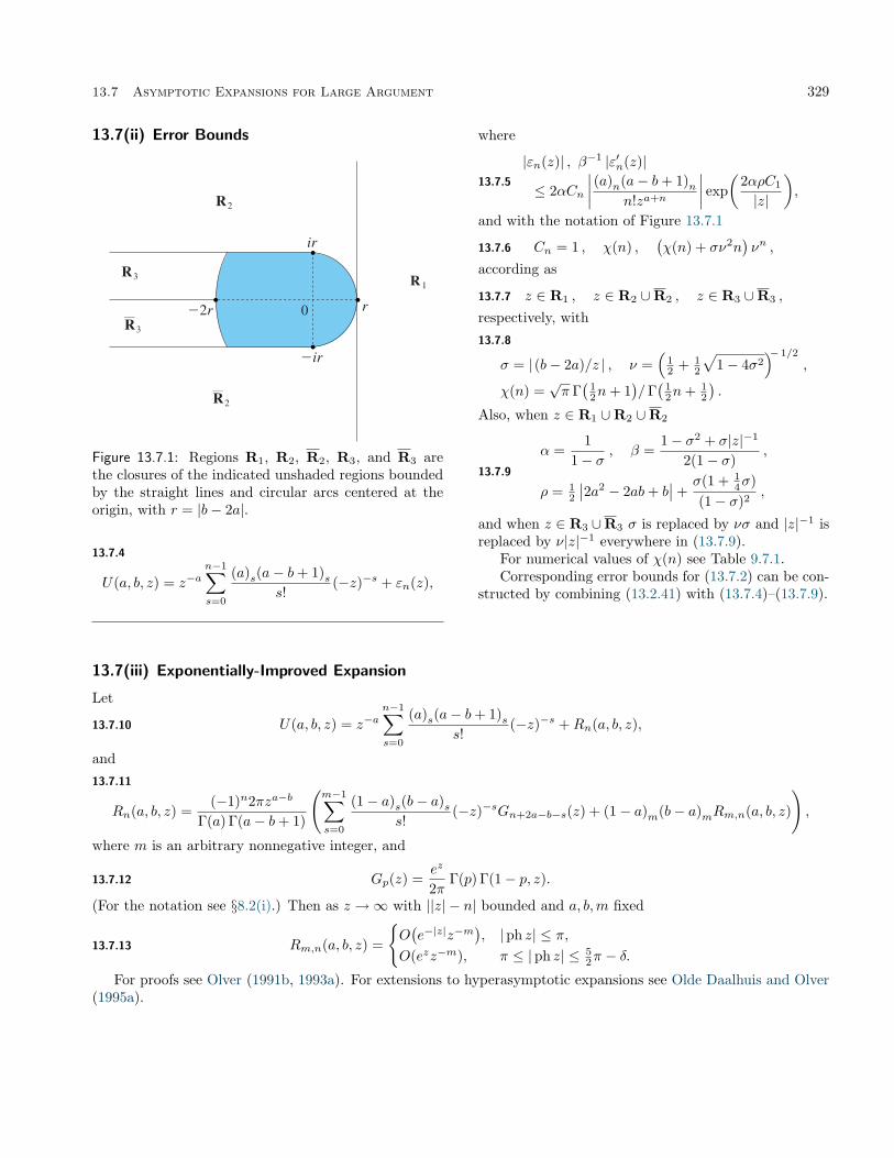
13.7 Asymptotic Expansions for Large Argument 329
13.7(ii) Error Bounds
Figure 13.7.1: Regions R1, R2, R2, R3, and R3 arethe closures of the indicated unshaded regions boundedby the straight lines and circular arcs centered at theorigin, with r = |b− 2a|.
13.7.4
U(a, b, z) = z−an−1∑s=0
(a)s(a− b+ 1)ss!
(−z)−s + εn(z),
where
13.7.5
|εn(z)| , β−1 |ε′n(z)|
≤ 2αCn
∣∣∣∣ (a)n(a− b+ 1)nn!za+n
∣∣∣∣ exp(
2αρC1
|z|
),
and with the notation of Figure 13.7.1
13.7.6 Cn = 1 , χ(n) ,(χ(n) + σν2n
)νn ,
according as
13.7.7 z ∈ R1 , z ∈ R2 ∪R2 , z ∈ R3 ∪R3 ,respectively, with13.7.8
σ = | (b− 2a)/z | , ν =(
12 + 1
2
√1− 4σ2
)− 1/2
,
χ(n) =√π Γ(
12n+ 1
)/Γ(
12n+ 1
2
).
Also, when z ∈ R1 ∪R2 ∪R2
13.7.9
α =1
1− σ, β =
1− σ2 + σ|z|−1
2(1− σ),
ρ = 12
∣∣2a2 − 2ab+ b∣∣+
σ(1 + 14σ)
(1− σ)2,
and when z ∈ R3 ∪R3 σ is replaced by νσ and |z|−1 isreplaced by ν|z|−1 everywhere in (13.7.9).
For numerical values of χ(n) see Table 9.7.1.Corresponding error bounds for (13.7.2) can be con-
structed by combining (13.2.41) with (13.7.4)–(13.7.9).
13.7(iii) Exponentially-Improved Expansion
Let
13.7.10 U(a, b, z) = z−an−1∑s=0
(a)s(a− b+ 1)ss!
(−z)−s +Rn(a, b, z),
and13.7.11
Rn(a, b, z) =(−1)n2πza−b
Γ(a) Γ(a− b+ 1)
(m−1∑s=0
(1− a)s(b− a)ss!
(−z)−sGn+2a−b−s(z) + (1− a)m(b− a)mRm,n(a, b, z)
),
where m is an arbitrary nonnegative integer, and
13.7.12 Gp(z) =ez
2πΓ(p) Γ(1− p, z).
(For the notation see §8.2(i).) Then as z →∞ with ||z| − n| bounded and a, b,m fixed
13.7.13 Rm,n(a, b, z) =
{O(e−|z|z−m
), |ph z| ≤ π,
O(ezz−m), π ≤ |ph z| ≤ 52π − δ.
For proofs see Olver (1991b, 1993a). For extensions to hyperasymptotic expansions see Olde Daalhuis and Olver(1995a).

330 Confluent Hypergeometric Functions
13.8 Asymptotic Approximations for LargeParameters
13.8(i) Large |b|, Fixed a and z
If b→∞ in C in such a way that |b+ n| ≥ δ > 0 for alln = 0, 1, 2, . . . , then
13.8.1 M(a, b, z) =n−1∑s=0
(a)s(b)ss!
zs +O(|b|−n
).
For fixed a and z in C
13.8.2 M(a, b, z) ∼ Γ(b)Γ(b− a)
∞∑s=0
(a)sqs(z, a)b−s−a,
as b→∞ in |ph b| ≤ π − δ, where q0(z, a) = 1 and13.8.3(et − 1
)a−1 exp(t+ z(1− e−t)
)=∞∑s=0
qs(z, a)ts+a−1.
When the foregoing results are combined with Kum-mer’s transformation (13.2.39), an approximation is ob-tained for the case when |b| is large, and |b− a| and |z|are bounded.
13.8(ii) Large b and z, Fixed a and b/z
Let λ = z/b > 0 and ζ =√
2(λ− 1− lnλ) withsign(ζ) = sign(λ− 1). Then
13.8.4 M(a, b, z) ∼ b 12ae
14 ζ
2b
λ(λ− 1ζ
)a−1
U(a− 1
2 ,−ζ√b)
+
(λ
(λ− 1ζ
)a−1
−(
ζ
λ− 1
)a) U(a− 3
2 ,−ζ√b)
ζ√b
and
13.8.5 U(a, b, z) ∼ b− 12ae
14 ζ
2b
λ(λ− 1ζ
)a−1
U(a− 1
2 , ζ√b)−
(λ
(λ− 1ζ
)a−1
−(
ζ
λ− 1
)a) U(a− 3
2 , ζ√b)
ζ√b
as b → ∞, uniformly in compact λ-intervals of (0,∞) and compact real a-intervals. For the parabolic cylinderfunction U see §12.2, and for an extension to an asymptotic expansion see Temme (1978).
Special cases are
13.8.6 M(a, b, b) =√π
(b
2
)12a(
1Γ(
12 (a+ 1)
) +(a+ 1)
√8/b
3 Γ(
12a) +O
(1b
)),
and
13.8.7 U(a, b, b) =√π (2b)−
12a
(1
Γ(
12 (a+ 1)
) − (a+ 1)√
8/b3 Γ(
12a) +O
(1b
)).
To obtain approximations for M(a, b, z) and U(a, b, z) that hold as b → ∞, with a > 12 − b and z > 0 combine
(13.14.4), (13.14.5) with §13.20(i).Also, more complicated—but more powerful—uniform asymptotic approximations can be obtained by combining
(13.14.4), (13.14.5) with §§13.20(iii) and 13.20(iv).
13.8(iii) Large a
For the notation see §§10.2(ii), 10.25(ii), and 2.8(iv).When a→ +∞ with b (≤ 1) fixed,
13.8.8 U(a, b, x) =2e
12x
Γ(a)
(√2β
tanh(w
2
)(1− e−w
β
)−bβ1−bK1−b(2βa) + a−1
(a−1 + β
1 + β
)1−be−2βaO(1)
),
where w = arccosh(1 + (2a)−1x
), and β = (w + sinhw)/2 . (13.8.8) holds uniformly with respect to x ∈ [0,∞). For
the case b > 1 the transformation (13.2.40) can be used.For an extension to an asymptotic expansion complete with error bounds see Temme (1990b), and for related
results see §13.21(i).When a→ −∞ with b (≥ 1) fixed,
13.8.9 M(a, b, x) = Γ(b)e12x(( 1
2b− a)x)12−
12 b(Jb−1
(√2x(b− 2a)
)+ envJb−1
(√2x(b− 2a)
)O(|a|−
12
)),

13.9 Zeros 331
and
13.8.10
U(a, b, x) = Γ(
12b− a+ 1
2
)e
12xx
12−
12 b(
cos(aπ) Jb−1
(√2x(b− 2a)
)− sin(aπ)Yb−1
(√2x(b− 2a)
)+ envYb−1
(√2x(b− 2a)
)O(|a|−
12
)),
uniformly with respect to bounded positive values of x in each case.For asymptotic approximations to M(a, b, x) and U(a, b, x) as a → −∞ that hold uniformly with respect to
x ∈ (0,∞) and bounded positive values of (b− 1)/ |a|, combine (13.14.4), (13.14.5) with §§13.21(ii), 13.21(iii).
13.9 Zeros
13.9(i) Zeros of M(a, b, z)
If a and b − a 6= 0,−1,−2, . . . , then M(a, b, z) has in-finitely many z-zeros in C. When a, b ∈ R the number ofreal zeros is finite. Let p(a, b) be the number of positivezeros. Then
13.9.1 p(a, b) = d−ae , a < 0, b ≥ 0,
13.9.2 p(a, b) = 0, a ≥ 0, b ≥ 0,
13.9.3 p(a, b) = 1, a ≥ 0, −1 < b < 0,
13.9.4 p(a, b) =⌊− 1
2b⌋−⌊− 1
2 (b+ 1)⌋
, a ≥ 0, b ≤ −1.
13.9.5
p(a, b) = d−ae − d−be , d−ae ≥ d−be, a < 0, b < 0,
13.9.6
p(a, b) =⌊
12 (d−be − d−ae+ 1)
⌋−⌊
12 (d−be − d−ae)
⌋,
d−be > d−ae > 0.
The number of negative real zeros n(a, b) is given by
13.9.7 n(a, b) = p(b− a, b).When a < 0 and b > 0 let φr, r = 1, 2, 3, . . . , be the
positive zeros of M(a, b, x) arranged in increasing orderof magnitude, and let jb−1,r be the rth positive zero ofthe Bessel function Jb−1(x) (§10.21(i)). Then
13.9.8
φr =j2b−1,r
2b− 4a
(1 +
2b(b− 2) + j2b−1,r
3(2b− 4a)2
)+O
(1a5
),
as a→ −∞ with r fixed.Inequalities for φr are given in Gatteschi (1990), and
identities involving infinite series of all of the complexzeros of M(a, b, x) are given in Ahmed and Muldoon(1980).
For fixed a, b ∈ C the large z-zeros of M(a, b, z) sat-isfy
13.9.9z = ±(2n+ a)πi+ ln
(− Γ(a)
Γ(b− a)(±2nπi)b−2a
)+O
(n−1 lnn
),
where n is a large positive integer, and the logarithmtakes its principal value (§4.2(i)).
Let Pα denote the closure of the domain that isbounded by the parabola y2 = 4α(x + α) and con-tains the origin. Then M(a, b, z) has no zeros in theregions P b/a , if 0 < b ≤ a; P1, if 1 ≤ a ≤ b; Pα,where α = (2a− b+ ab)/(a(a+ 1)) , if 0 < a < 1and a ≤ b < 2a/(1− a) . The same results apply forthe nth partial sums of the Maclaurin series (13.2.2) ofM(a, b, z).
More information on the location of real zeros canbe found in Zarzo et al. (1995).
For fixed b and z in C the large a-zeros of M(a, b, z)are given by13.9.10
a = −π2
4z(n2 + (b− 3
2 )n)
− 116z
((b− 3
2 )2π2 + 43z
2 − 8b(z − 1)− 4b2 − 3)
+O(n−1
),
where n is a large positive integer.For fixed a and z in C the function M(a, b, z) has
only a finite number of b-zeros.
13.9(ii) Zeros of U(a, b, z)
For fixed a and b in C, U(a, b, z) has a finite number ofz-zeros in the sector |ph z| ≤ 3
2π− δ(<32π). Let T (a, b)
be the total number of zeros in the sector |ph z| < π,P (a, b) be the corresponding number of positive zeros,and a, b, and a − b + 1 be nonintegers. For the caseb ≤ 113.9.11
T (a, b) = b−ac+ 1, a < 0, Γ(a) Γ(a− b+ 1) > 0,
13.9.12 T (a, b) = b−ac , a < 0, Γ(a) Γ(a− b+ 1) < 0,
13.9.13 T (a, b) = 0, a > 0,and
13.9.14 P (a, b) = db− a− 1e , a+ 1 < b,
13.9.15 P (a, b) = 0, a+ 1 ≥ b.For the case b ≥ 1 we can use T (a, b) = T (a−b+1, 2−b)and P (a, b) = P (a− b+ 1, 2− b).
In Wimp (1965) it is shown that if a, b ∈ R and2a − b > −1, then U(a, b, z) has no zeros in the sector|ph z| ≤ 1
2π.Inequalities for the zeros of U(a, b, x) are given in
Gatteschi (1990).

332 Confluent Hypergeometric Functions
For fixed b and z in C the large a-zeros of U(a, b, z)are given by
13.9.16
a ∼ −n− 2π
√zn− 2z
π2+ 1
2b+ 14
+z2(
13 − 4π−2
)+ z − (b− 1)2 + 1
4
4π√zn
+O
(1n
),
where n is a large positive integer.For fixed a and z in C, U(a, b, z) has two infinite
strings of b-zeros that are asymptotic to the imaginaryaxis as |b| → ∞.
13.10 Integrals
13.10(i) Indefinite Integrals
When a 6= 1,
13.10.1
∫M(a, b, z) dz =
1a− 1
M(a− 1, b− 1, z),
13.10.2
∫U(a, b, z) dz = − 1
a− 1U(a− 1, b− 1, z).
Other formulas of this kind can be constructed by in-version of the differentiation formulas given in §13.3(ii).
13.10(ii) Laplace Transforms
For the notation see §§15.1, 15.2(i), and 10.25(ii).
13.10.3∫ ∞0
e−zttb−1 M(a, c, kt) dt = Γ(b)z−b 2F1(a, b; c; k/z ),
<b > 0, <z > max (<k, 0),
13.10.4
∫ ∞0
e−zttb−1 M(a, b, t) dt = z−b(
1− 1z
)−a,
<b > 0, <z > 1,
13.10.5
∫ ∞0
e−ttb−1 M(a, c, t) dt =Γ(b) Γ(c− a− b)Γ(c− a) Γ(c− b)
,
<(c− a) > <b > 0,
13.10.6
∫ ∞0
e−zt−t2t2b−2 M
(a, b, t2
)dt
= 12π− 1
2 Γ(b− 1
2
)U(b− 1
2 , a+ 12 ,
14z
2),
<b > 12 , <z > 0,
13.10.7
∫ ∞0
e−zttb−1 U(a, c, t) dt
= Γ(b) Γ(b− c+ 1)
× z−b 2F1
(a, b; a+ b− c+ 1; 1− 1
z
),
<b > max (<c− 1, 0), <z > 0.
Loop Integrals
13.10.8
12πi
∫ (0+)
−∞etzt−a M(a, b, y/t ) dt
=1
Γ(a)z
12 (2a−b−1)y
12 (1−b) Ib−1(2
√zy),
<z > 0.
13.10.9
12πi
∫ (0+)
−∞etzt−a U(a, b, y/t ) dt
=2z
12 (2a−b−1)y
12 (1−b)
Γ(a) Γ(a− b+ 1)Kb−1(2
√zy), <z > 0.
For additional Laplace transforms see Erdélyi et al.(1954a, §§4.22, 5.20), Oberhettinger and Badii (1973,§1.17), and Prudnikov et al. (1992a, §§3.34, 3.35). In-verse Laplace transforms are given in Oberhettinger andBadii (1973, §2.16) and Prudnikov et al. (1992b, §§3.33,3.34).
13.10(iii) Mellin Transforms
13.10.10∫ ∞0
tλ−1 M(a, b,−t) dt=Γ(λ) Γ(a− λ)Γ(a) Γ(b− λ)
, 0 < <λ < <a,
13.10.11∫ ∞0
tλ−1 U(a, b, t) dt =Γ(λ) Γ(a− λ) Γ(λ− b+ 1)
Γ(a) Γ(a− b+ 1),
max (<b− 1, 0) < <λ < <a.For additional Mellin transforms see Erdélyi et al.
(1954a, §§6.9, 7.5), Marichev (1983, pp. 283–287), andOberhettinger (1974, §§1.13, 2.8).
13.10(iv) Fourier Transforms
13.10.12
∫ ∞0
cos(2xt) M(a, b,−t2
)dt
=√π
2 Γ(a)x2a−1e−x
2U(b− 1
2 , a+ 12 , x
2),
<a > 0.For additional Fourier transforms see Erdélyi et al.
(1954a, §§1.14, 2.14, 3.3) and Oberhettinger (1990,§§1.22, 2.22).
13.10(v) Hankel Transforms
For the notation see §10.2(ii).
13.10.13
∫ ∞0
e−ttb−1− 12ν M(a, b, t) Jν
(2√xt)dt
= x−a+ 12νe−x M(ν − b+ 1, ν − a+ 1, x),
x > 0, 2<a < <ν + 52 , <b > 0,
13.10.14
∫ ∞0
e−tt12ν M(a, b, t) Jν
(2√xt)dt
=x
12νe−x
Γ(b− a)U(a, a− b+ ν + 2, x),
x > 0, −1 < <ν < 2<(b− a)− 12 ,

13.11 Series 333
13.10.15∫ ∞0
t12ν U(a, b, t) Jν
(2√xt)dt
=Γ(ν − b+ 2)
Γ(a)x
12ν U(ν − b+ 2, ν − a+ 2, x),
x > 0, max (<b− 2,−1) < <ν < 2<a+ 12 ,
13.10.16∫ ∞0
e−tt12ν U(a, b, t) Jν
(2√xt)dt
= Γ(ν − b+ 2)x12νe−x M(a, a− b+ ν + 2, x),x > 0, max (<b− 2,−1) < <ν.
For additional Hankel transforms and also otherBessel transforms see Erdélyi et al. (1954b, §8.18) andOberhettinger (1972, §§1.16 and 3.4.42–46, 4.4.45–47,5.94–97).
13.10(vi) Other Integrals
For integral transforms in terms of Whittaker functionssee §13.23(iv). Additional integrals can be found inApelblat (1983, pp. 388–392), Erdélyi et al. (1954b),Gradshteyn and Ryzhik (2000, §7.6), Magnus et al.(1966, §6.1.2), Prudnikov et al. (1990, §§1.13, 1.14, 2.19,4.2.2), Prudnikov et al. (1992a, §§3.35, 3.36), and Prud-nikov et al. (1992b, §§3.33, 3.34). See also (13.4.2),(13.4.5), (13.4.6).
13.11 Series
For z ∈ C,
13.11.1
M(a, b, z) = Γ(a− 1
2
)e
12 z(
14z)12−a
×∞∑s=0
(2a− 1)s(2a− b)s(b)ss!
×(a− 1
2 + s)Ia− 1
2 +s
(12z),
a+ 12 , b 6= 0,−1,−2, . . . .
(13.6.9) is a special case.For additional expansions combine (13.14.4),
(13.14.5), and §13.24. For other series expansions seeHansen (1975, §§66 and 87), Prudnikov et al. (1990,§6.6), and Tricomi (1954, §1.8). See also §13.13.
13.12 Products
13.12.1
M(a, b, z)M(−a,−b,−z)
+a(a− b)z2
b2(1− b2)M(1 + a, 2 + b, z)M(1− a, 2− b,−z) = 1.
For generalizations of this quadratic relation see Ma-jima et al. (2000).
For integral representations, integrals, and seriescontaining products of M(a, b, z) and U(a, b, z) seeErdélyi et al. (1953a, §6.15.3).
13.13 Addition and MultiplicationTheorems
13.13(i) Addition Theorems for M(a, b, z)
The function M(a, b, x+ y) has the following expan-sions:
13.13.1
∞∑n=0
(a)nyn
(b)nn!M(a+ n, b+ n, x),
13.13.2(x+ y
x
)1−b ∞∑n=0
(1− b)n(− y/x )n
n!M(a, b− n, x),
|y| < |x|,13.13.3(
x
x+ y
)a ∞∑n=0
(a)nyn
n!(x+ y)nM(a+ n, b, x), <(y/x) > − 1
2 ,
13.13.4 ey∞∑n=0
(b− a)n(−y)n
(b)nn!M(a, b+ n, x),
13.13.5
ey(
x
x+ y
)b−a ∞∑n=0
(b− a)nyn
n!(x+ y)n
× M(a− n, b, x), <((y + x)/x) > 12 ,
13.13.6
ey(x+ y
x
)1−b ∞∑n=0
(1− b)n(−y)n
n!xn
× M(a− n, b− n, x), |y| < |x|.
13.13(ii) Addition Theorems for U(a, b, z)
The function U(a, b, x+ y) has the following expansions:
13.13.7
∞∑n=0
(a)n(−y)n
n!U(a+ n, b+ n, x), |y| < |x|,
13.13.8(x+ y
x
)1−b ∞∑n=0
(1 + a− b)n(− y/x )n
n!U(a, b− n, x),
|y| < |x|,13.13.9(
x
x+ y
)a ∞∑n=0
(a)n(1 + a− b)nyn
n!(x+ y)nU(a+ n, b, x),
<(y/x) > − 12 ,
13.13.10 ey∞∑n=0
(−y)n
n!U(a, b+ n, x), |y| < |x|,
13.13.11ey(
x
x+ y
)b−a ∞∑n=0
(−y)n
n!(x+ y)nU(a− n, b, x),
<(y/x) > − 12 ,
13.13.12
ey(x+ y
x
)1−b ∞∑n=0
(−y)n
n!xnU(a− n, b− n, x), |y| < |x|.

334 Confluent Hypergeometric Functions
13.13(iii) Multiplication Theorems forM(a, b, z) and U(a, b, z)
To obtain similar expansions for M(a, b, xy) andU(a, b, xy), replace y in the previous two subsectionsby (y − 1)x.
Whittaker Functions
13.14 Definitions and Basic Properties
13.14(i) Differential Equation
Whittaker’s Equation
13.14.1d2W
dz2 +(−1
4+κ
z+
14 − µ
2
z2
)W = 0.
This equation is obtained from Kummer’s equation(13.2.1) via the substitutions W = e−
12 zz
12 +µw, κ =
12b− a, and µ = 1
2b−12 . It has a regular singularity at
the origin with indices 12±µ, and an irregular singularity
at infinity of rank one.
Standard Solutions
Standard solutions are:
13.14.2 Mκ,µ(z) = e−12 zz
12 +µM
(12 + µ− κ, 1 + 2µ, z
),
13.14.3 Wκ,µ(z) = e−12 zz
12 +µ U
(12 + µ− κ, 1 + 2µ, z
),
except that Mκ,µ(z) does not exist when 2µ =−1,−2,−3, . . . .
Conversely,
13.14.4 M(a, b, z) = e12 zz−
12 bM 1
2 b−a,12 b−
12(z),
13.14.5 U(a, b, z) = e12 zz−
12 bW 1
2 b−a,12 b−
12(z).
The series13.14.6
Mκ,µ(z) = e−12 zz
12 +µ
∞∑s=0
(12 + µ− κ
)s
(1 + 2µ)ss!zs
= z12 +µ
∞∑n=0
2F1
(−n, 1
2 + µ− κ1 + 2µ
; 2)(− 1
2z)n
n!,
2µ 6= −1,−2,−3, . . . ,converge for all z ∈ C.
In general Mκ,µ(z) and Wκ,µ(z) are many-valuedfunctions of z with branch points at z = 0 andz = ∞. The principal branches correspond tothe principal branches of the functions z
12 +µ and
U(
12 + µ− κ, 1 + 2µ, z
)on the right-hand sides of the
equations (13.14.2) and (13.14.3); compare §4.2(i).Although Mκ,µ(z) does not exist when 2µ =
−1,−2,−3, . . . , many formulas containing Mκ,µ(z) con-tinue to apply in their limiting form. For example, ifn = 0, 1, 2, . . . , then13.14.7
lim2µ→−n−1
Mκ,µ(z)Γ(2µ+ 1)
=
(− 1
2n− κ)n+1
(n+ 1)!Mκ, 12 (n+1)(z)
= e−12 zz−
12n
∞∑s=n+1
(− 1
2n− κ)s
Γ(s− n)s!zs.
If 2µ = ±n, where n = 0, 1, 2, . . . , then
13.14.8
Wκ,± 12n
(z) =(−1)ne−
12 zz
12n+ 1
2
n! Γ(
12 −
12n− κ
) ( n∑k=1
n!(k − 1)!(n− k)!
(κ+ 1
2 −12n)k
z−k
−∞∑k=0
(12n+ 1
2 − κ)k
(n+ 1)kk!zk(ln z + ψ
(12n+ 1
2 − κ+ k)− ψ(1 + k)− ψ(n+ 1 + k)
)),
κ− 12n−
12 6= 0, 1, 2, . . . ,
or
13.14.9
Wκ,± 12n
(z) = (−1)κ−12n−
12 e−
12 zz
12n+ 1
2
κ− 12n−
12∑
k=0
(κ− 1
2n−12
k
)(n+ 1 + k)κ−k− 1
2n−12(−z)k, κ− 1
2n−12 = 0, 1, 2, . . . .
13.14(ii) Analytic Continuation
13.14.10 Mκ,µ
(ze±πi
)= ±ie±µπiM−κ,µ(z).
In (13.14.11)–(13.14.13) m is any integer.
13.14.11 Mκ,µ
(ze2mπi
)= (−1)me2mµπiMκ,µ(z).

13.14 Definitions and Basic Properties 335
13.14.12 Wκ,µ
(ze2mπi
)=
(−1)m+12πi sin(2πµm)Γ(
12 − µ− κ
)Γ(1 + 2µ) sin(2πµ)
Mκ,µ(z) + (−1)me−2mµπiWκ,µ(z).
13.14.13
(−1)mWκ,µ
(ze2mπi
)= −e
2κπi sin(2mµπ) + sin((2m− 2)µπ)sin(2µπ)
Wκ,µ(z)
− sin(2mµπ)2πieκπi
sin(2µπ) Γ(
12 + µ− κ
)Γ(
12 − µ− κ
) W−κ,µ(zeπi).Except when z = 0, each branch of the functions
Mκ,µ(z)/Γ(2µ+ 1) and Wκ,µ(z) is entire in κ and µ.Also, unless specified otherwise Mκ,µ(z) and Wκ,µ(z)are assumed to have their principal values.
13.14(iii) Limiting Forms as z → 0
13.14.14
Mκ,µ(z) = zµ+ 12 (1 +O(z)) , 2µ 6= −1,−2,−3, . . . .
In cases when 12 −κ±µ = −n, where n is a nonneg-
ative integer,13.14.15
W 12±µ+n,µ(z) = (−1)n(1± 2µ)nz
12±µ +O
(z
32±µ
).
In all other cases
13.14.16Wκ,µ(z) =
Γ(2µ)Γ(
12 + µ− κ
)z 12−µ +O
(z
32−<µ
),
<µ ≥ 12 , µ 6= 1
2 ,
13.14.17 Wκ, 12(z) =
1Γ(1− κ)
+O(z ln z),
13.14.18
Wκ,µ(z) =Γ(2µ)
Γ(
12 + µ− κ
)z 12−µ +
Γ(−2µ)Γ(
12 − µ− κ
)z 12 +µ
+O(z
32−<µ
), 0 ≤ <µ < 1
2 , µ 6= 0,
13.14.19
Wκ,0(z) = −√z
Γ(
12 − κ
) (ln z + ψ(
12 − κ
)+ 2γ
)+O
(z 3/2 ln z
).
For Wκ,µ(z) with <µ < 0 use (13.14.31).
13.14(iv) Limiting Forms as z →∞Except when µ− κ = − 1
2 ,−32 , . . . (polynomial cases),
13.14.20Mκ,µ(z) ∼ Γ(1 + 2µ)e
12 zz−κ
/Γ(
12 + µ− κ
),
|ph z| ≤ 12π − δ,
where δ is an arbitrary small positive constant. Also,
13.14.21 Wκ,µ(z) ∼ e− 12 zzκ, |ph z| ≤ 3
2π − δ.13.14(v) Numerically Satisfactory Solutions
Fundamental pairs of solutions of (13.14.1) that are nu-merically satisfactory (§2.7(iv)) in the neighborhood ofinfinity are
13.14.22 Wκ,µ(z), W−κ,µ(e−πiz
), − 1
2π ≤ ph z ≤ 32π,
13.14.23 Wκ,µ(z), W−κ,µ(eπiz
), − 3
2π ≤ ph z ≤ 12π.
A fundamental pair of solutions that is numericallysatisfactory in the sector |ph z| ≤ π near the origin is
13.14.24 Mκ,µ(z), Mκ,−µ(z), 2µ 6∈ Z.
When 2µ is an integer we may use the results of§13.2(v) with the substitutions b = 2µ+1, a = µ−κ+ 1
2 ,and W = e−
12 zz
12 +µw, where W is the solution of
(13.14.1) corresponding to the solution w of (13.2.1).
13.14(vi) Wronskians
13.14.25 W {Mκ,µ(z),Mκ,−µ(z)} = −2µ,
13.14.26 W {Mκ,µ(z),Wκ,µ(z)} = − Γ(1 + 2µ)Γ(
12 + µ− κ
) ,13.14.27
W{Mκ,µ(z),W−κ,µ
(e±πiz
)}=
Γ(1 + 2µ)Γ(
12 + µ+ κ
)e∓( 12 +µ)πi,
13.14.28 W {Mκ,−µ(z),Wκ,µ(z)} = − Γ(1− 2µ)Γ(
12 − µ− κ
) ,13.14.29
W{Mκ,−µ(z),W−κ,µ
(e±πiz
)}=
Γ(1− 2µ)Γ(
12 − µ+ κ
)e∓( 12−µ)πi,
13.14.30 W{Wκ,µ(z),W−κ,µ
(e±πiz
)}= e∓κπi.
13.14(vii) Connection Formulas
13.14.31 Wκ,µ(z) = Wκ,−µ(z).
13.14.32
1Γ(1 + 2µ)
Mκ,µ(z) =e±(κ−µ− 1
2 )πi
Γ(
12 + µ+ κ
) Wκ,µ(z)
+e±κπi
Γ(
12 + µ− κ
) W−κ,µ(e±πiz).When 2µ is not an integer
13.14.33
Wκ,µ(z) =Γ(−2µ)
Γ(
12 − µ− κ
)Mκ,µ(z)
+Γ(2µ)
Γ(
12 + µ− κ
)Mκ,−µ(z).

336 Confluent Hypergeometric Functions
13.15 Recurrence Relations and Derivatives
13.15(i) Recurrence Relations
13.15.1 (κ− µ− 12 )Mκ−1,µ(z) + (z − 2κ)Mκ,µ(z) + (κ+ µ+ 1
2 )Mκ+1,µ(z) = 0,
13.15.2 2µ(1 + 2µ)√zMκ− 1
2 ,µ−12(z)− (z + 2µ)(1 + 2µ)Mκ,µ(z) + (κ+ µ+ 1
2 )√zMκ+ 1
2 ,µ+ 12(z) = 0,
13.15.3 (κ− µ− 12 )Mκ− 1
2 ,µ+ 12(z) + (1 + 2µ)
√zMκ,µ(z)− (κ+ µ+ 1
2 )Mκ+ 12 ,µ+ 1
2(z) = 0,
13.15.4 2µMκ− 12 ,µ−
12(z)− 2µMκ+ 1
2 ,µ−12(z)−
√zMκ,µ(z) = 0,
13.15.5 2µ(1 + 2µ)Mκ,µ(z)− 2µ(1 + 2µ)√zMκ− 1
2 ,µ−12(z)− (κ− µ− 1
2 )√zMκ− 1
2 ,µ+ 12(z) = 0,
13.15.6 2µ(1 + 2µ)√zMκ+ 1
2 ,µ−12(z) + (z − 2µ)(1 + 2µ)Mκ,µ(z) + (κ− µ− 1
2 )√zMκ− 1
2 ,µ+ 12(z) = 0,
13.15.7 2µ(1 + 2µ)√zMκ+ 1
2 ,µ−12(z)− 2µ(1 + 2µ)Mκ,µ(z) + (κ+ µ+ 1
2 )√zMκ+ 1
2 ,µ+ 12(z) = 0.
13.15.8 Wκ+ 12 ,µ+ 1
2(z)−
√zWκ,µ(z) + (κ− µ− 1
2 )Wκ− 12 ,µ+ 1
2(z) = 0,
13.15.9 Wκ+ 12 ,µ−
12(z)−
√zWκ,µ(z) + (κ+ µ− 1
2 )Wκ− 12 ,µ−
12(z) = 0,
13.15.10 2µWκ,µ(z)−√zWκ+ 1
2 ,µ+ 12(z) +
√zWκ+ 1
2 ,µ−12(z) = 0,
13.15.11 Wκ+1,µ(z) + (2κ− z)Wκ,µ(z) + (κ− µ− 12 )(κ+ µ− 1
2 )Wκ−1,µ(z) = 0,
13.15.12 (κ− µ− 12 )√zWκ− 1
2 ,µ+ 12(z) + 2µWκ,µ(z)− (κ+ µ− 1
2 )√zWκ− 1
2 ,µ−12(z) = 0,
13.15.13 (κ+ µ− 12 )√zWκ− 1
2 ,µ−12(z)− (z + 2µ)Wκ,µ(z) +
√zWκ+ 1
2 ,µ+ 12(z) = 0,
13.15.14 (κ− µ− 12 )√zWκ− 1
2 ,µ+ 12(z)− (z − 2µ)Wκ,µ(z) +
√zWκ+ 1
2 ,µ−12(z) = 0.
13.15(ii) Differentiation Formulas
13.15.15dn
dzn
(e
12 zzµ−
12 Mκ,µ(z)
)= (−1)n(−2µ)ne
12 zzµ−
12 (n+1)Mκ− 1
2n,µ−12n
(z),
13.15.16dn
dzn
(e
12 zz−µ−
12 Mκ,µ(z)
)=
(12 + µ− κ
)n
(1 + 2µ)ne
12 zz−µ−
12 (n+1)Mκ− 1
2n,µ+ 12n
(z),
13.15.17
(zd
dzz
)n (e
12 zz−κ−1Mκ,µ(z)
)=(
12 + µ− κ
)ne
12 zzn−κ−1Mκ−n,µ(z),
13.15.18dn
dzn
(e−
12 zzµ−
12 Mκ,µ(z)
)= (−1)n(−2µ)ne
− 12 zzµ−
12 (n+1)Mκ+ 1
2n,µ−12n
(z),
13.15.19dn
dzn
(e−
12 zz−µ−
12 Mκ,µ(z)
)= (−1)n
(12 + µ+ κ
)n
(1 + 2µ)ne−
12 zz−µ−
12 (n+1) Mκ+ 1
2n,µ+ 12n
(z),
13.15.20
(zd
dzz
)n (e−
12 zzκ−1Mκ,µ(z)
)=(
12 + µ+ κ
)ne−
12 zzκ+n−1 Mκ+n,µ(z).
13.15.21dn
dzn
(e
12 zz−µ−
12 Wκ,µ(z)
)= (−1)n
(12 + µ− κ
)ne
12 zz−µ−
12 (n+1) Wκ− 1
2n,µ+ 12n
(z),
13.15.22dn
dzn
(e
12 zzµ−
12 Wκ,µ(z)
)= (−1)n
(12 − µ− κ
)ne
12 zzµ−
12 (n+1) Wκ− 1
2n,µ−12n
(z),
13.15.23
(zd
dzz
)n (e
12 zz−κ−1Wκ,µ(z)
)=(
12 + µ− κ
)n
(12 − µ− κ
)ne
12 zzn−κ−1Wκ−n,µ(z),
13.15.24dn
dzn
(e−
12 zz−µ−
12 Wκ,µ(z)
)= (−1)ne−
12 zz−µ−
12 (n+1)Wκ+ 1
2n,µ+ 12n
(z),
13.15.25dn
dzn
(e−
12 zzµ−
12 Wκ,µ(z)
)= (−1)ne−
12 zzµ−
12 (n+1)Wκ+ 1
2n,µ−12n
(z),
13.15.26
(zd
dzz
)n (e−
12 zzκ−1Wκ,µ(z)
)= (−1)ne−
12 zzκ+n−1Wκ+n,µ(z).
Other versions of several of the identities in this subsection can be constructed by use of (13.3.29).

13.16 Integral Representations 337
13.16 Integral Representations
13.16(i) Integrals Along the Real Line
In this subsection see §§10.2(ii), 10.25(ii) for the functions J2µ, I2µ, and K2µ, and §§15.1, 15.2(i) for 2F1.
13.16.1 Mκ,µ(z) =Γ(1 + 2µ)zµ+ 1
2 2−2µ
Γ(
12 + µ− κ
)Γ(
12 + µ+ κ
) ∫ 1
−1
e12 zt(1 + t)µ−
12−κ(1− t)µ− 1
2 +κ dt, <µ+ 12 > |<κ|,
13.16.2 Mκ,µ(z) =Γ(1 + 2µ)zλ
Γ(1 + 2µ− 2λ) Γ(2λ)
∫ 1
0
Mκ−λ,µ−λ(zt)e12 z(t−1)tµ−λ−
12 (1− t)2λ−1 dt, <µ+ 1
2 > <λ > 0,
13.16.31
Γ(1 + 2µ)Mκ,µ(z) =
√ze
12 z
Γ(
12 + µ+ κ
) ∫ ∞0
e−ttκ−12 J2µ
(2√zt)dt, <(κ+ µ) + 1
2 > 0,
13.16.41
Γ(1 + 2µ)Mκ,µ(z) =
√ze−
12 z
Γ(
12 + µ− κ
) ∫ ∞0
e−tt−κ−12 I2µ
(2√zt)dt, <(κ− µ)− 1
2 > 0.
13.16.5 Wκ,µ(z) =zµ+ 1
2 2−2µ
Γ(
12 + µ− κ
) ∫ ∞1
e−12 zt(t− 1)µ−
12−κ(t+ 1)µ−
12 +κ dt, <µ+ 1
2 > <κ, |ph z| < 12π,
13.16.6
Wκ,µ(z) =e−
12 zzκ+1
Γ(
12 + µ− κ
)Γ(
12 − µ− κ
) ∫ ∞0
W−κ,µ(t)e−12 tt−κ−1
t+ zdt, |ph z| < π, <( 1
2 + µ− κ) > max (2<µ, 0),
13.16.7Wκ,µ(z) =
(−1)ne−12 zz
12−µ−n
Γ(1 + 2µ) Γ(
12 − µ− κ
) ∫ ∞0
M−κ,µ(t)e−12 ttn+µ− 1
2
t+ zdt,
|ph z| < π, n = 0, 1, 2, . . . , −<(1 + 2µ) < n < |<µ|+ <κ < 12 ,
13.16.8 Wκ,µ(z) =2√ze−
12 z
Γ(
12 + µ− κ
)Γ(
12 − µ− κ
) ∫ ∞0
e−tt−κ−12 K2µ
(2√zt)dt, <(µ− κ) + 1
2 > 0,
13.16.9 Wκ,µ(z) = e−12 zzκ+c
∫ ∞0
e−zttc−12F1
( 12 + µ− κ, 1
2 − µ− κc
;−t)dt, |ph z| < 1
2π,
where c is arbitrary, <c > 0.
13.16(ii) Contour Integrals
For contour integral representations combine (13.14.2) and (13.14.3) with §13.4(ii). See Buchholz (1969, §2.3), Erdélyiet al. (1953a, §6.11.3), and Slater (1960, Chapter 3). See also §13.16(iii).
13.16(iii) Mellin–Barnes Integrals
If 12 + µ− κ 6= 0,−1,−2, . . . , then
13.16.101
Γ(1 + 2µ)Mκ,µ
(e±πiz
)=
e12 z±( 1
2 +µ)πi
2πiΓ(
12 + µ− κ
) ∫ i∞
−i∞
Γ(t− κ) Γ(
12 + µ− t
)Γ(
12 + µ+ t
) zt dt, |ph z| < 12π,
where the contour of integration separates the poles of Γ(t− κ) from those of Γ(
12 + µ− t
).
If 12 ± µ− κ 6= 0,−1,−2, . . . , then
13.16.11 Wκ,µ(z) =e−
12 z
2πi
∫ i∞
−i∞
Γ(
12 + µ+ t
)Γ(
12 − µ+ t
)Γ(−κ− t)
Γ(
12 + µ− κ
)Γ(
12 − µ− κ
) z−t dt, |ph z| < 32π,
where the contour of integration separates the poles of Γ(
12 + µ+ t
)Γ(
12 − µ+ t
)from those of Γ(−κ− t).
13.16.12 Wκ,µ(z) =e
12 z
2πi
∫ i∞
−i∞
Γ(
12 + µ+ t
)Γ(
12 − µ+ t
)Γ(1− κ+ t)
z−t dt, |ph z| < 12π,
where the contour of integration passes all the poles of Γ(
12 + µ+ t
)Γ(
12 − µ+ t
)on the right-hand side.
338 Confluent Hypergeometric Functions
13.17 Continued Fractions
If κ, µ ∈ C such that µ± (κ− 12 ) 6= −1,−2,−3, . . . , then
13.17.1
√zMκ,µ(z)
Mκ− 12 ,µ+ 1
2(z)
= 1 +u1z
1 +u2z
1 +· · · ,
where
13.17.2
u2n+1 = −12 + µ+ κ+ n
(2µ+ 2n+ 1)(2µ+ 2n+ 2),
u2n =12 + µ− κ+ n
(2µ+ 2n)(2µ+ 2n+ 1).
This continued fraction converges to the meromorphicfunction of z on the left-hand side for all z ∈ C. Formore details on how a continued fraction converges to ameromorphic function see Jones and Thron (1980).
If κ, µ ∈ C such that µ+ 12±(κ+1) 6= −1,−2,−3, . . . ,
then
13.17.3Wκ,µ(z)√
zWκ− 12 ,µ−
12(z)
= 1 +v1/z
1 +v2/z
1 +· · · ,
where
13.17.4 v2n+1 = 12 + µ− κ+ n, v2n = 1
2 − µ− κ+ n.
This continued fraction converges to the meromorphicfunction of z on the left-hand side throughout the sector|ph z| < π.
See also Cuyt et al. (2008, pp. 336–337).
13.18 Relations to Other Functions
13.18(i) Elementary Functions
13.18.1 M0, 12(2z) = 2 sinh z,
13.18.2
Mκ,κ− 12(z) = Wκ,κ− 1
2(z) = Wκ,−κ+ 1
2(z) = e−
12 zzκ,
13.18.3 Mκ,−κ− 12(z) = e
12 zz−κ.
13.18(ii) Incomplete Gamma Functions
For the notation see §§6.2(i), 7.2(i), and 8.2(i). When12−κ±µ is an integer the Whittaker functions can be ex-pressed as incomplete gamma functions (or generalizedexponential integrals). For example,
13.18.4 Mµ− 12 ,µ
(z) = 2µe12 zz
12−µ γ(2µ, z),
13.18.5 Wµ− 12 ,µ
(z) = e12 zz
12−µ Γ(2µ, z).
Special cases are the error functions
13.18.6 M− 14 ,
14
(z2)
= 12e
12 z
2√πz erf(z),
13.18.7 W− 14 ,−
14
(z2)
= e12 z
2√πz erfc(z).
13.18(iii) Modified Bessel Functions
When κ = 0 the Whittaker functions can be expressedas modified Bessel functions. For the notation see§§10.25(ii) and 9.2(i).
13.18.8 M0,ν(2z) = 22ν+ 12 Γ(1 + ν)
√z Iν(z),
13.18.9 W0,ν(2z) =√
2z/π Kν(z),
13.18.10 W0, 13
(43z
32
)= 2√πz
14 Ai(z).
13.18(iv) Parabolic Cylinder Functions
For the notation see §12.2.
13.18.11 W− 12a,±
14
(12z
2)
= 212a√z U(a, z),
13.18.12M− 1
2a,−14
(12z
2)
= 212a−1 Γ
(12a+ 3
4
)√z/π
× (U(a, z) + U(a,−z)) ,
13.18.13M− 1
2a,14
(12z
2)
= 212a−2 Γ
(12a+ 1
4
)√z/π
× (U(a,−z)− U(a, z)) .
13.18(v) Orthogonal Polynomials
Special cases of §13.18(iv) are as follows. For the nota-tion see §18.3.
Hermite Polynomials
13.18.14 M 14 +n,− 1
4
(z2)
= (−1)nn!
(2n)!e−
12 z
2√z H2n(z),
13.18.15
M 34 +n, 14
(z2)
= (−1)nn!
(2n+ 1)!e−
12 z
2√z
2H2n+1(z),
13.18.16 W 14 + 1
2n,14
(z2)
= 2−ne−12 z
2√z Hn(z).
Laguerre Polynomials
13.18.17
W 12α+ 1
2 +n, 12α(z) = (−1)n(α+ 1)nM 1
2α+ 12 +n, 12α
(z)
= (−1)nn!e−12 zz
12α+ 1
2 L(α)n (z).

13.19 Asymptotic Expansions for Large Argument 339
13.19 Asymptotic Expansions for Large Argument
As x→∞13.19.1 Mκ,µ(x) ∼ Γ(1 + 2µ)
Γ(
12 + µ− κ
)e 12xx−κ
∞∑s=0
(12 − µ+ κ
)s
(12 + µ+ κ
)s
s!x−s, µ− κ 6= − 1
2 ,−32 , . . . .
As z →∞
13.19.2
Mκ,µ(z) ∼ Γ(1 + 2µ)Γ(
12 + µ− κ
)e 12 zz−κ
∞∑s=0
(12 − µ+ κ
)s
(12 + µ+ κ
)s
s!z−s
+Γ(1 + 2µ)
Γ(
12 + µ+ κ
)e− 12 z±( 1
2 +µ−κ)πizκ∞∑s=0
(12 + µ− κ
)s
(12 − µ− κ
)s
s!(−z)−s,
− 12π + δ ≤ ±ph z ≤ 3
2π − δ,provided that both µ∓ κ 6= − 1
2 ,−32 , . . . . Again, δ denotes an arbitrary small positive constant. Also,
13.19.3 Wκ,µ(z) ∼ e− 12 zzκ
∞∑s=0
(12 + µ− κ
)s
(12 − µ− κ
)s
s!(−z)−s, |ph z| ≤ 3
2π − δ.
Error bounds and exponentially-improved expan-sions are derivable by combining §§13.7(ii) and 13.7(iii)with (13.14.2) and (13.14.3). See also Olver (1965).
For an asymptotic expansion of Wκ,µ(z) as z → ∞that is valid in the sector |ph z| ≤ π − δ and where thereal parameters κ, µ are subject to the growth condi-tions κ = o(z), µ = o(
√z), see Wong (1973a).
13.20 Uniform Asymptotic Approximationsfor Large µ
13.20(i) Large µ, Fixed κ
When µ→∞ in the sector |phµ| ≤ 12π−δ(<
12π), with
κ(∈ C) fixed
13.20.1 Mκ,µ(z) = zµ+ 12(1 +O
(µ−1
)),
uniformly for bounded values of |z|; also13.20.2
Wκ,µ(x) = π−12 Γ(κ+ µ)
(14x)12−µ (1 +O
(µ−1
)),
uniformly for bounded positive values of x. For anextension of (13.20.1) to an asymptotic expansion, to-gether with error bounds, see Olver (1997b, Chapter 10,Ex. 3.4).
13.20(ii) Large µ, 0 ≤ κ ≤ (1− δ)µLet
13.20.3 X =√
4µ2 − 4κx+ x2.
Then as µ→∞13.20.4
Mκ,µ(x) =
√2µxX
(4µ2x
2µ2 − κx+ µX
)µ×(
2(µ− κ)X + x− 2κ
)κe
12X−µ
(1 +O
(1µ
)),
13.20.5
Wκ,µ(x) =√x
X
(2µ2 − κx+ µX
(µ− κ)x
)µ (X + x− 2κ
2
)κ× e−
12X−κ
(1 +O
(1µ
)),
uniformly with respect to x ∈ (0,∞) and κ ∈ [0, (1 −δ)µ], where δ again denotes an arbitrary small positiveconstant.
13.20(iii) Large µ, −(1− δ)µ ≤ κ ≤ µLet
13.20.6 α =√
2|κ− µ|/µ,
13.20.7 X =√|x2 − 4κx+ 4µ2|,
13.20.8 Φ(κ, µ, x) =(µ2ζ2 − 2κµ+ 2µ2
x2 − 4κx+ 4µ2
)14 √
x,
with the variable ζ defined implicitly as follows:(a) In the case −µ < κ < µ
13.20.9
ζ√ζ2 + α2 + α2 arcsinh
(ζ
α
)=X
µ− 2κµ
ln
(X + x− 2κ
2√µ2 − κ2
)−2 ln
(µX + 2µ2 − κxx√µ2 − κ2
).
(b) In the case µ = κ
13.20.10 ζ = ±
√x
µ− 2− 2 ln
(x
2µ
),
the upper or lower sign being taken according as x ≷ 2µ.(In both cases (a) and (b) the x-interval (0,∞) is
mapped one-to-one onto the ζ-interval (−∞,∞), with

340 Confluent Hypergeometric Functions
x = 0 and ∞ corresponding to ζ = −∞ and ∞, respec-tively.) Then as µ→∞13.20.11
Wκ,µ(x) =(
12µ)− 1
4
(κ+ µ
e
)12 (κ+µ)
Φ(κ, µ, x)
× U(µ− κ, ζ
√2µ) (
1 +O(µ−1 lnµ
)),
13.20.12
Mκ,µ(x) = (8µ)14
(2µe
)2µ (e
κ+ µ
)12 (κ+µ)
Φ(κ, µ, x)
× U(µ− κ,−ζ
√2µ) (
1 +O(µ−1 lnµ
)),
uniformly with respect to x ∈ (0,∞) and κ ∈ [−(1 −δ)µ, µ]. For the parabolic cylinder function U see §12.2.
These results are proved in Olver (1980b). This ref-erence also supplies error bounds and corresponding ap-proximations when x, κ, and µ are replaced by ix, iκ,and iµ, respectively.
13.20(iv) Large µ, µ ≤ κ ≤ µ/δ
Again define α, X, and Φ(κ, µ, x) by (13.20.6)–(13.20.8), but with ζ now defined by
13.20.13
ζ√ζ2 − α2 − α2 arccosh
(ζ
α
)=X
µ− 2κ
µln
(X + x− 2κ
2√κ2 − µ2
)− 2 ln
(κx− µX − 2µ2
x√κ2 − µ2
), x ≥ 2κ+ 2
√κ2 − µ2,
13.20.14
ζ√α2 − ζ2 + α2 arcsin
(ζ
α
)=X
µ+
2κµ
arctan(x− 2κX
)− 2 arctan
(κx− 2µ2
µX
),
2κ− 2√κ2 − µ2 ≤ x ≤ 2κ+ 2
√κ2 − µ2,
13.20.15
−ζ√ζ2 − α2 − α2 arccosh
(− ζα
)= −X
µ+
2κµ
ln
(2κ−X − x2√κ2 − µ2
)+ 2 ln
(µX + 2µ2 − κxx√κ2 − µ2
),
0 < x ≤ 2κ− 2√κ2 − µ2,
when µ < κ, and by (13.20.10) when µ = κ. (As in §13.20(iii) x = 0 and ∞ correspond to ζ = −∞ and ∞,respectively). Then as µ→∞
13.20.16 Wκ,µ(x) =(
12µ)− 1
4
(κ+ µ
e
)12 (κ+µ)
Φ(κ, µ, x)(U(µ− κ, ζ
√2µ)
+ envU(µ− κ, ζ
√2µ)O(µ−
23
)),
13.20.17 Mκ,µ(x) = (8µ)14
(2µe
)2µ (e
κ+ µ
)12 (κ+µ)
Φ(κ, µ, x)(U(µ− κ,−ζ
√2µ)
+ envU(µ− κ, ζ
√2µ)O(µ−
23
)),
uniformly with respect to ζ ∈ [0,∞) and κ ∈ [µ, µ/δ].Also,
13.20.18 Wκ,µ(x) =(
12µ)− 1
4
(κ+ µ
e
)12 (κ+µ)
Φ(κ, µ, x)(U(µ− κ, ζ
√2µ)
+ envU(µ− κ,−ζ
√2µ)O(µ−
23
)),
13.20.19
Mκ,µ(x) = (8µ)14
(2µe
)2µ (e
κ+ µ
)12 (κ+µ)
Φ(κ, µ, x)(U(µ− κ,−ζ
√2µ)
+ envU(µ− κ,−ζ
√2µ)O(µ−
23
)),
uniformly with respect to ζ ∈ (−∞, 0] and κ ∈ [µ, µ/δ].For the parabolic cylinder functions U and U see
§12.2, and for the env functions associated with U andU see §14.15(v).
These results are proved in Olver (1980b). Equa-tions (13.20.17) and (13.20.18) are simpler than (6.10)and (6.11) in this reference. Olver (1980b) also supplieserror bounds and corresponding approximations when
x, κ, and µ are replaced by ix, iκ, and iµ, respectively.
It should be noted that (13.20.11), (13.20.16), and(13.20.18) differ only in the common error terms. Hencewithout the error terms the approximation holds for−(1 − δ)µ ≤ κ ≤ µ/δ. Similarly for (13.20.12),(13.20.17), and (13.20.19).
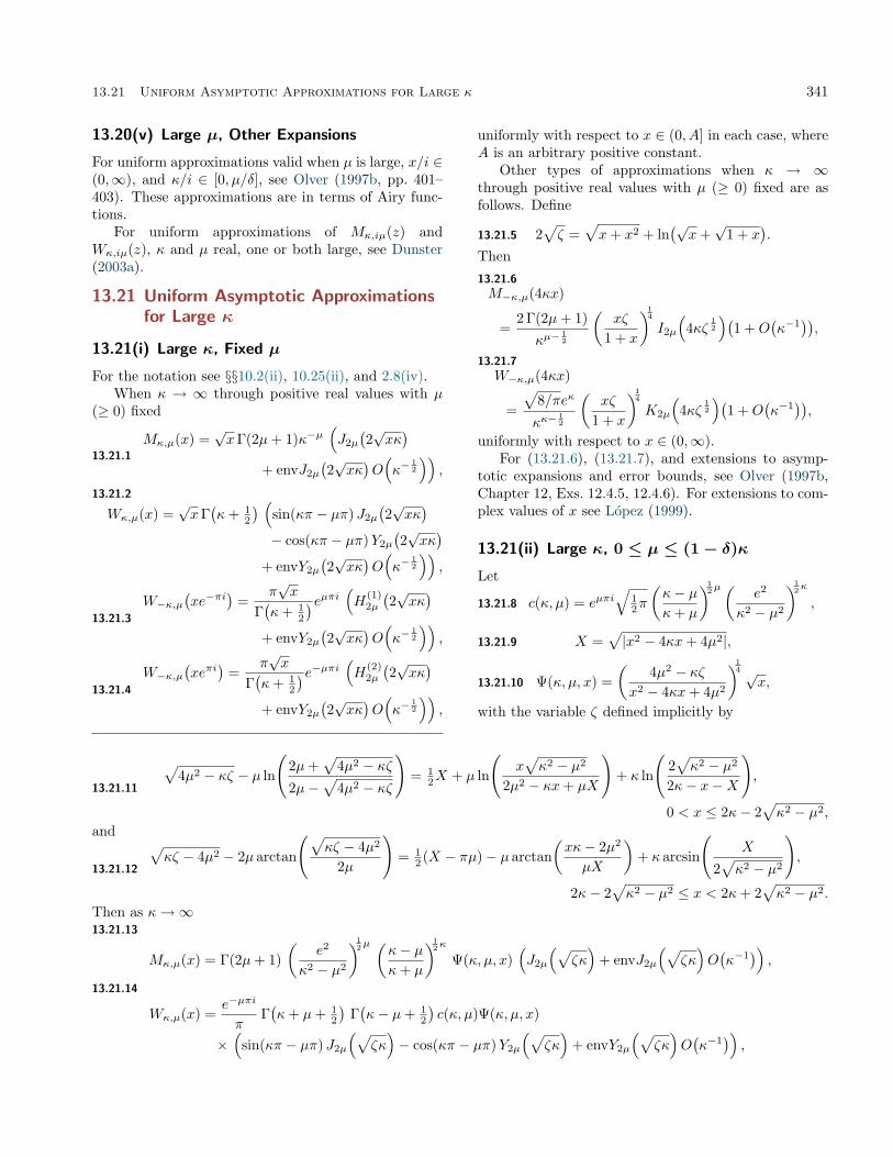
13.21 Uniform Asymptotic Approximations for Large κ 341
13.20(v) Large µ, Other Expansions
For uniform approximations valid when µ is large, x/i ∈(0,∞), and κ/i ∈ [0, µ/δ], see Olver (1997b, pp. 401–403). These approximations are in terms of Airy func-tions.
For uniform approximations of Mκ,iµ(z) andWκ,iµ(z), κ and µ real, one or both large, see Dunster(2003a).
13.21 Uniform Asymptotic Approximationsfor Large κ
13.21(i) Large κ, Fixed µ
For the notation see §§10.2(ii), 10.25(ii), and 2.8(iv).When κ → ∞ through positive real values with µ
(≥ 0) fixed
13.21.1
Mκ,µ(x) =√xΓ(2µ+ 1)κ−µ
(J2µ
(2√xκ)
+ envJ2µ
(2√xκ)O(κ−
12
)),
13.21.2
Wκ,µ(x) =√xΓ(κ+ 1
2
) (sin(κπ − µπ) J2µ
(2√xκ)
− cos(κπ − µπ)Y2µ
(2√xκ)
+ envY2µ
(2√xκ)O(κ−
12
)),
13.21.3
W−κ,µ(xe−πi
)=
π√x
Γ(κ+ 1
2
)eµπi (H(1)2µ
(2√xκ)
+ envY2µ
(2√xκ)O(κ−
12
)),
13.21.4
W−κ,µ(xeπi
)=
π√x
Γ(κ+ 1
2
)e−µπi (H(2)2µ
(2√xκ)
+ envY2µ
(2√xκ)O(κ−
12
)),
uniformly with respect to x ∈ (0, A] in each case, whereA is an arbitrary positive constant.
Other types of approximations when κ → ∞through positive real values with µ (≥ 0) fixed are asfollows. Define
13.21.5 2√ζ =
√x+ x2 + ln
(√x+√
1 + x).
Then13.21.6
M−κ,µ(4κx)
=2 Γ(2µ+ 1)κµ−
12
(xζ
1 + x
)14
I2µ
(4κζ
12
)(1 +O
(κ−1
)),
13.21.7
W−κ,µ(4κx)
=
√8/πeκ
κκ−12
(xζ
1 + x
)14
K2µ
(4κζ
12
)(1 +O
(κ−1
)),
uniformly with respect to x ∈ (0,∞).For (13.21.6), (13.21.7), and extensions to asymp-
totic expansions and error bounds, see Olver (1997b,Chapter 12, Exs. 12.4.5, 12.4.6). For extensions to com-plex values of x see López (1999).
13.21(ii) Large κ, 0 ≤ µ ≤ (1− δ)κLet
13.21.8 c(κ, µ) = eµπi√
12π
(κ− µκ+ µ
)12µ(
e2
κ2 − µ2
)12κ
,
13.21.9 X =√|x2 − 4κx+ 4µ2|,
13.21.10 Ψ(κ, µ, x) =(
4µ2 − κζx2 − 4κx+ 4µ2
)14 √
x,
with the variable ζ defined implicitly by
13.21.11
√4µ2 − κζ − µ ln
(2µ+
√4µ2 − κζ
2µ−√
4µ2 − κζ
)= 1
2X + µ ln
(x√κ2 − µ2
2µ2 − κx+ µX
)+ κ ln
(2√κ2 − µ2
2κ− x−X
),
0 < x ≤ 2κ− 2√κ2 − µ2,
and
13.21.12
√κζ − 4µ2 − 2µ arctan
(√κζ − 4µ2
2µ
)= 1
2 (X − πµ)− µ arctan(xκ− 2µ2
µX
)+ κ arcsin
(X
2√κ2 − µ2
),
2κ− 2√κ2 − µ2 ≤ x < 2κ+ 2
√κ2 − µ2.
Then as κ→∞13.21.13
Mκ,µ(x) = Γ(2µ+ 1)(
e2
κ2 − µ2
)12µ(κ− µκ+ µ
)12κ
Ψ(κ, µ, x)(J2µ
(√ζκ)
+ envJ2µ
(√ζκ)O(κ−1
)),
13.21.14
Wκ,µ(x) =e−µπi
πΓ(κ+ µ+ 1
2
)Γ(κ− µ+ 1
2
)c(κ, µ)Ψ(κ, µ, x)
×(
sin(κπ − µπ) J2µ
(√ζκ)− cos(κπ − µπ)Y2µ
(√ζκ)
+ envY2µ
(√ζκ)O(κ−1
)),

342 Confluent Hypergeometric Functions
13.21.15
W−κ,µ(xe−πi
)= c(κ, µ)Ψ(κ, µ, x)
(H
(1)2µ
(√ζκ)
+ envY2µ
(√ζκ)O(κ−1
)),
13.21.16
W−κ,µ(xeπi
)= e−2µπic(κ, µ)Ψ(κ, µ, x)
(H
(2)2µ
(√ζκ)
+ envY2µ
(√ζκ)O(κ−1
)),
uniformly with respect to µ ∈ [0, (1 − δ)κ] and x ∈(0, (1− δ)(2κ+ 2
√κ2 − µ2)
], where δ again denotes an
arbitrary small positive constant. For the functions J2µ,Y2µ, H(1)
2µ , and H(2)2µ see §10.2(ii), and for the env func-
tions associated with J2µ and Y2µ see §2.8(iv).These approximations are proved in Dunster (1989).
This reference also includes error bounds and extensionsto asymptotic expansions and complex values of x.
13.21(iii) Large κ, 0 ≤ µ ≤ (1− δ)κ(Continued)
Let
13.21.17 ĉ(κ, µ) =√
2πκ16
(κ− µκ+ µ
)12µ(
e2
κ2 − µ2
)12κ
,
13.21.18 X =√|x2 − 4κx+ 4µ2|,
13.21.19 Ψ̂(κ, µ, x) =
(ζ̂
x2 − 4κx+ 4µ2
)14 √
2x,
and define the variable ζ̂ implicitly by
13.21.20ζ̂ = −
(3
2κ
(−1
2X + 2µ arctan
(xκ− x
√κ2 − µ2 − 2µ2
µX
)+ κ arccos
(x− 2κ
2√κ2 − µ2
)))2/3,
2κ− 2√κ2 − µ2 < x ≤ 2κ+ 2
√κ2 − µ2,
and
13.21.21 ζ̂ =
(3
2κ
(12X + µ ln
(x√κ2 − µ2
κx− 2µ2 − µX
)+ κ ln
(2√κ2 − µ2
x− 2κ+X
)))2/3, x ≥ 2κ+ 2
√κ2 − µ2.
Then as κ→∞
13.21.22Mκ,µ(x) =
12π
Γ(2µ+ 1) Γ(κ− µ+ 1
2
)ĉ(κ, µ) Ψ̂(κ, µ, x)
×(
sin(κπ − µπ) Ai(κ
23 ζ̂)
+ cos(κπ − µπ) Bi(κ
23 ζ̂)
+ envBi(κ
23 ζ̂)O(κ−1
)),
13.21.23 Wκ,µ(x) =√
2πκ16
(κ+ µ
κ− µ
)12µ(κ2 − µ2
e2
)12κ
Ψ̂(κ, µ, x)(
Ai(κ
23 ζ̂)
+ envAi(κ
23 ζ̂)O(κ−1
)),
13.21.24 W−κ,µ(xe−πi
)= e(κ− 1
6 )πiĉ(κ, µ)Ψ̂(κ, µ, x)(
Ai(κ
23 ζ̂e−
23πi)
+ envBi(κ
23 ζ̂)O(κ−1
)),
13.21.25 W−κ,µ(xeπi
)= e−(κ− 1
6 )πiĉ(κ, µ)Ψ̂(κ, µ, x)(
Ai(κ
23 ζ̂e
23πi)
+ envBi(κ
23 ζ̂)O(κ−1
)),
uniformly with respect to µ ∈ [0, (1 − δ)κ] and x ∈[(1 + δ)(2κ− 2
√κ2 − µ2),∞
). For the functions Ai
and Bi see §9.2(i), and for the env functions associatedwith Ai and Bi see §2.8(iii).
These approximations are proved in Dunster (1989).This reference also includes error bounds and extensionsto asymptotic expansions and complex values of x.
13.21(iv) Large κ, Other Expansions
For a uniform asymptotic expansion in terms of Airyfunctions for Wκ,µ(4κx) when κ is large and positive,µ is real with |µ| bounded, and x ∈ [δ,∞) see Olver(1997b, Chapter 11, Ex. 7.3). This expansion is simpler
in form than the expansions of Dunster (1989) that cor-respond to the approximations given in §13.21(iii), butthe conditions on µ are more restrictive.
For asymptotic expansions having double asymp-totic properties see Skovgaard (1966).
See also §13.20(v).
13.22 Zeros
From (13.14.2) and (13.14.3)Mκ,µ(z) has the same zerosas M
(12 + µ− κ, 1 + 2µ, z
)and Wκ,µ(z) has the same
zeros as U(
12 + µ− κ, 1 + 2µ, z
), hence the results given
in §13.9 can be adopted.Asymptotic approximations to the zeros when the
parameters κ and/or µ are large can be found by rever-

13.23 Integrals 343
sion of the uniform approximations provided in §§13.20and 13.21. For example, if µ(≥ 0) is fixed and κ(> 0) islarge, then the rth positive zero φr of Mκ,µ(z) is givenby
13.22.1 φr =j22µ,r
4κ+ j2µ,r O
(κ−
32
),
where j2µ,r is the rth positive zero of the Bessel func-tion J2µ(x) (§10.21(i)). (13.22.1) is a weaker version of(13.9.8).
13.23 Integrals
13.23(i) Laplace and Mellin Transforms
For the notation see §§15.1, 15.2(i), and 10.25(ii).
13.23.1
∫ ∞0
e−zttν−1Mκ,µ(t) dt =Γ(µ+ ν + 1
2
)(z + 1
2
)µ+ν+ 12
2F1
( 12 + µ− κ, 1
2 + µ+ ν
1 + 2µ;
1z + 1
2
), <(µ+ ν + 1
2 ) > 0, <z > 12 .
13.23.2
∫ ∞0
e−zttµ−12 Mκ,µ(t) dt = Γ(2µ+ 1)
(z + 1
2
)−κ−µ− 12(z − 1
2
)κ−µ− 12 , <µ > − 1
2 , <z > 12 ,
13.23.31
Γ(1 + 2µ)
∫ ∞0
e−12 ttν−1Mκ,µ(t) dt =
Γ(µ+ ν + 1
2
)Γ(κ− ν)
Γ(
12 + µ+ κ
)Γ(
12 + µ− ν
) , − 12 −<µ < <ν < <κ.
13.23.4
∫ ∞0
e−zttν−1Wκ,µ(t) dt = Γ(
12 + µ+ ν
)Γ(
12 − µ+ ν
)2F1
( 12 − µ+ ν, 1
2 + µ+ ν
ν − κ+ 1; 1
2 − z)
,
<(ν + 12 ) > |<µ|, <z > − 1
2 ,
13.23.5
∫ ∞0
e12 ttν−1Wκ,µ(t) dt =
Γ(
12 + µ+ ν
)Γ(
12 − µ+ ν
)Γ(−κ− ν)
Γ(
12 + µ− κ
)Γ(
12 − µ− κ
) , |<µ| − 12 < <ν < −<κ.
13.23.61
Γ(1 + 2µ)2πi
∫ (0+)
−∞ezt+
12 t−1tκMκ,µ
(t−1)dt =
z−κ−12
Γ(
12 + µ− κ
) I2µ(2√z), <z > 0.
13.23.71
2πi
∫ (0+)
−∞ezt+
12 t−1tκWκ,µ
(t−1)dt =
2z−κ−12
Γ(
12 + µ− κ
)Γ(
12 − µ− κ
) K2µ
(2√z), <z > 0.
For additional Laplace and Mellin transforms see Erdélyi et al. (1954a, §§4.22, 5.20, 6.9, 7.5), Marichev (1983,pp. 283–287), Oberhettinger and Badii (1973, §1.17), Oberhettinger (1974, §§1.13, 2.8), and Prudnikov et al. (1992a,§§3.34, 3.35). Inverse Laplace transforms are given in Oberhettinger and Badii (1973, §2.16) and Prudnikov et al.(1992b, §§3.33, 3.34).
13.23(ii) Fourier Transforms
13.23.81
Γ(1 + 2µ)
∫ ∞0
cos(2xt)e−12 t
2t−2µ−1Mκ,µ
(t2)dt =
√πe−
12x
2xµ+κ−1
2 Γ(
12 + µ+ κ
) W 12κ−
32µ,
12κ+ 1
2µ
(x2), <(κ+ µ) > − 1
2 .
For additional Fourier transforms see Erdélyi et al. (1954a, §§1.14, 2.14, 3.3) and Oberhettinger (1990, §§1.22,2.22).
13.23(iii) Hankel Transforms
For the notation see §10.2(ii).13.23.9∫ ∞
0
e−12 ttµ−
12 (ν+1)Mκ,µ(t) Jν
(2√xt)dt =
Γ(1 + 2µ)Γ(
12 − µ+ κ+ ν
) e− 12xx
12 (κ−µ− 3
2 ) M 12 (κ+3µ−ν+ 1
2 ), 12 (κ−µ+ν− 12 )(x),
x > 0, − 12 < <µ < <(κ+ 1
2ν) + 34 ,

344 Confluent Hypergeometric Functions
13.23.10
1Γ(1 + 2µ)
∫ ∞0
e−12 tt
12 (ν−1)−µMκ,µ(t) Jν
(2√xt)dt =
e−12xx
12 (κ+µ− 3
2 )
Γ(
12 + µ+ κ
) W 12 (κ−3µ+ν+ 1
2 ), 12 (κ+µ−ν− 12 )(x),
x > 0, −1 < <ν < 2<(µ+ κ) + 12 .
13.23.11
∫ ∞0
e12 tt
12 (ν−1)−µWκ,µ(t) Jν
(2√xt)dt =
Γ(ν − 2µ+ 1)Γ(
12 + µ− κ
) e 12xx
12 (µ−κ− 3
2 ) W 12 (κ+3µ−ν− 1
2 ), 12 (κ−µ+ν+ 12 )(x),
x > 0, max(2<µ− 1,−1) < <ν < 2<(µ− κ) + 32 ,
13.23.12∫ ∞0
e−12 tt
12 (ν−1)−µWκ,µ(t) Jν
(2√xt)dt =
Γ(ν − 2µ+ 1)Γ(
32 − µ− κ+ ν
) e− 12xx
12 (µ+κ− 3
2 ) M 12 (κ−3µ+ν+ 1
2 ), 12 (ν−µ−κ+ 12 )(x),
x > 0, max(2<µ− 1,−1) < <ν.For additional Hankel transforms and also other Bessel transforms see Erdélyi et al. (1954b, §8.18) and Oberhet-
tinger (1972, §1.16 and 3.4.42–46, 4.4.45–47, 5.94–97).
13.23(iv) Integral Transforms in terms of Whittaker Functions
Let f(x) be absolutely integrable on the interval [r,R] for all positive r < R, f(x) = O(xρ0) as x → 0+, andf(x) = O(e−ρ1x) as x→ +∞, where ρ1 >
12 . Then for µ in the half-plane <µ ≥ µ1 > max
(−ρ0,<κ− 1
2
)13.23.13 g(µ) =
1Γ(1 + 2µ)
∫ ∞0
f(x)x−32 Mκ,µ(x) dx,
13.23.14 f(x) =1
πi√x
∫ µ1+i∞
µ1−i∞µg(µ) Γ
(12 + µ− κ
)Wκ,µ(x) dµ.
For additional integral transforms see Magnus et al. (1966, p. 189), Prudnikov et al. (1992b, §§4.3.39–4.3.42), andWimp (1964).
13.23(v) Other Integrals
Additional integrals involving confluent hypergeometric functions can be found in Apelblat (1983, pp. 388–392),Erdélyi et al. (1954b), Gradshteyn and Ryzhik (2000, §7.6), and Prudnikov et al. (1990, §§1.13, 1.14, 2.19, 4.2.2).See also (13.16.2), (13.16.6), (13.16.7).
13.24 Series
13.24(i) Expansions in Series of Whittaker Functions
For expansions of arbitrary functions in series of Mκ,µ(z) functions see Schäfke (1961b).
13.24(ii) Expansions in Series of Bessel Functions
For z ∈ C, and again with the notation of §§10.2(ii) and 10.25(ii),13.24.1
Mκ,µ(z) = Γ(κ+ µ)22κ+2µz12−κ
∞∑s=0
(−1)s(2κ+ 2µ)s(2κ)s
(1 + 2µ)ss!(κ+ µ+ s) Iκ+µ+s
(12z), 2µ, κ+ µ 6= −1,−2,−3, . . . ,
and
13.24.21
Γ(1 + 2µ)Mκ,µ(z) = 22µzµ+ 1
2
∞∑s=0
p(µ)s (z)
(2√κz)−2µ−s
J2µ+s
(2√κz),
where p(µ)0 (z) = 1, p(µ)
1 (z) = 16z
2, and higher polynomials p(µ)s (z) are defined by
13.24.3 exp(− 1
2z
(coth t− 1
t
))(t
sinh t
)1−2µ
=∞∑s=0
p(µ)s (z)
(− tz
)s.
(13.18.8) is a special case of (13.24.1).Additional expansions in terms of Bessel functions are given in Luke (1959). See also López (1999).For other series expansions see Prudnikov et al. (1990, §6.6). See also §13.26.

13.25 Products 345
13.25 Products
13.25.1
Mκ,µ(z)Mκ,−µ−1(z)
+( 1
2 + µ+ κ)( 12 + µ− κ)
4µ(1 + µ)(1 + 2µ)2Mκ,µ+1(z)Mκ,−µ(z) = 1.
For integral representations, integrals, and seriescontaining products of Mκ,µ(z) and Wκ,µ(z) see Erdélyiet al. (1953a, §6.15.3).
13.26 Addition and MultiplicationTheorems
13.26(i) Addition Theorems for Mκ,µ(z)
The function Mκ,µ(x+ y) has the following expansions:
13.26.1
e−12y
(x
x+ y
)µ− 12 ∞∑n=0
(−2µ)nn!
(−y√x
)n× Mκ− 1
2n,µ−12n
(x), |y| < |x|,
13.26.2e−
12y
(x+ y
x
)µ+ 12 ∞∑n=0
(12 + µ− κ
)n
(1 + 2µ)nn!
(y√x
)n× Mκ− 1
2n,µ+ 12n
(x),
13.26.3e−
12y
(x+ y
x
)κ ∞∑n=0
(12 + µ− κ
)nyn
n!(x+ y)nMκ−n,µ(x),
<(y/x) > − 12 ,
13.26.4
e12y
(x
x+ y
)µ− 12 ∞∑n=0
(−2µ)nn!
(−y√x
)n× Mκ+ 1
2n,µ−12n
(x), |y| < |x|,
13.26.5e
12y
(x+ y
x
)µ+ 12 ∞∑n=0
(12 + µ+ κ
)n
(1 + 2µ)nn!
(−y√x
)n× Mκ+ 1
2n,µ+ 12n
(x),
13.26.6e
12y
(x
x+ y
)κ ∞∑n=0
(12 + µ+ κ
)nyn
n!(x+ y)nMκ+n,µ(x),
<((y + x)/x) > 12 .
13.26(ii) Addition Theorems for Wκ,µ(z)
The function Wκ,µ(x+ y) has the following expansions:
13.26.7e−
12y
(x
x+ y
)µ− 12 ∞∑n=0
(12 − µ− κ
)n
n!
(−y√x
)n× Wκ− 1
2n,µ−12n
(x), |y| < |x|,
13.26.8e−
12y
(x+ y
x
)µ+ 12 ∞∑n=0
(12 + µ− κ
)n
n!
(−y√x
)n× Wκ− 1
2n,µ+ 12n
(x), |y| < |x|,
13.26.9
e−12y
(x+ y
x
)κ ∞∑n=0
(12 + µ− κ
)n
(12 − µ− κ
)n
n!
×(
y
x+ y
)nWκ−n,µ(x), <(y/x) > − 1
2 ,
13.26.10
e12y
(x
x+ y
)µ− 12 ∞∑n=0
1n!
(−y√x
)n× Wκ+ 1
2n,µ−12n
(x), |y| < |x|,
13.26.11
e12y
(x+ y
x
)µ+ 12 ∞∑n=0
1n!
(−y√x
)n× Wκ+ 1
2n,µ+ 12n
(x), |y| < |x|,
13.26.12e
12y
(x
x+ y
)κ ∞∑n=0
1n!
(−yx+ y
)nWκ+n,µ(x),
<(y/x) > − 12 .
13.26(iii) Multiplication Theorems for Mκ,µ(z)and Wκ,µ(z)
To obtain similar expansions for Mκ,µ(xy) andWκ,µ(xy), replace y in the previous two subsections by(y − 1)x.
Applications
13.27 Mathematical Applications
Confluent hypergeometric functions are connected withrepresentations of the group of third-order triangularmatrices. The elements of this group are of the form
13.27.1 g =
1 α β0 γ δ0 0 1
,
where α, β, γ, δ are real numbers, and γ > 0. Vilenkin(1968, Chapter 8) constructs irreducible representationsof this group, in which the diagonal matrices correspondto operators of multiplication by an exponential func-tion. The other group elements correspond to integraloperators whose kernels can be expressed in terms ofWhittaker functions. This identification can be usedto obtain various properties of the Whittaker functions,including recurrence relations and derivatives.
For applications of Whittaker functions to the uni-form asymptotic theory of differential equations with acoalescing turning point and simple pole see §§2.8(vi)and 18.15(i).

346 Confluent Hypergeometric Functions
13.28 Physical Applications
13.28(i) Exact Solutions of the Wave Equation
The reduced wave equation ∇2w = k2w in paraboloidalcoordinates, x = 2
√ξη cosφ, y = 2
√ξη sinφ, z =
ξ − η, can be solved via separation of variables w =f1(ξ)f2(η)eipφ, where
13.28.1
f1(ξ) = ξ−12V
(1)
κ, 12p(2ikξ) , f2(η) = η−
12V
(2)
κ, 12p(−2ikη) ,
and V(j)κ,µ(z), j = 1, 2, denotes any pair of solutions of
Whittaker’s equation (13.14.1). See Hochstadt (1971,Chapter 7).
For potentials in quantum mechanics that are solv-able in terms of confluent hypergeometric functions seeNegro et al. (2000).
13.28(ii) Coulomb Functions
See Chapter 33.
13.28(iii) Other Applications
For dynamics of many-body systems see Meden andSchönhammer (1992); for tomography see D’Arianoet al. (1994); for generalized coherent states see Barutand Girardello (1971); for relativistic cosmology seeCrisóstomo et al. (2004).
Computation
13.29 Methods of Computation
13.29(i) Series Expansions
Although the Maclaurin series expansion (13.2.2) con-verges for all finite values of z, it is cumbersome to usewhen |z| is large owing to slowness of convergence andcancellation. For large |z| the asymptotic expansionsof §13.7 should be used instead. Accuracy is limitedby the magnitude of |z|. However, this accuracy canbe increased considerably by use of the exponentially-improved forms of expansion supplied by the combina-tion of (13.7.10) and (13.7.11), or by use of the hyper-asymptotic expansions given in Olde Daalhuis and Olver(1995a). For large values of the parameters a and b theapproximations in §13.8 are available.
Similarly for the Whittaker functions.
13.29(ii) Differential Equations
A comprehensive and powerful approach is to integratethe differential equations (13.2.1) and (13.14.1) by di-rect numerical methods. As described in §3.7(ii), toinsure stability the integration path must be chosen insuch a way that as we proceed along it the wanted so-lution grows in magnitude at least as fast as all othersolutions of the differential equation.
For M(a, b, z) and Mκ,µ(z) this means that in thesector |ph z| ≤ π we may integrate along outward raysfrom the origin with initial values obtained from (13.2.2)and (13.14.2).
For U(a, b, z) and Wκ,µ(z) we may integrate alongoutward rays from the origin in the sectors 1
2π <|ph z| < 3
2π, with initial values obtained from connec-tion formulas in §13.2(vii), §13.14(vii). In the sector|ph z| < 1
2π the integration has to be towards the ori-gin, with starting values computed from asymptotic ex-pansions (§§13.7 and 13.19). On the rays ph z = ± 1
2π,integration can proceed in either direction.
13.29(iii) Integral Representations
The integral representations (13.4.1) and (13.4.4) can beused to compute the Kummer functions, and (13.16.1)and (13.16.5) for the Whittaker functions. In Allasiaand Besenghi (1991) and Allasia and Besenghi (1987b)the high accuracy of the trapezoidal rule for the compu-tation of Kummer functions is described. Gauss quadra-ture methods are discussed in Gautschi (2002b).
13.29(iv) Recurrence Relations
The recurrence relations in §§13.3(i) and 13.15(i) canbe used to compute the confluent hypergeometric func-tions in an efficient way. In the following two examplesOlver’s algorithm (§3.6(v)) can be used.
Example 1
We assume 2µ 6= −1,−2,−3, . . . . Then we have
13.29.1
z2(n+ µ− 12 )((n+ µ+ 1
2 )2 − κ2)
(n+ µ)(n+ µ+ 12 )(n+ µ+ 1)
y(n+ 1)
+ 16((n+ µ)2 − 1
2κz −14
)y(n)
− 16((n+ µ)2 − 1
4
)y(n− 1) = 0,
with recessive solution
13.29.2 y(n) = z−n−µ−12 Mκ,n+µ(z),
normalizing relation
13.29.3 e−12 z =
∞∑s=0
(2µ)s(
12 + µ− κ
)s
(2µ)2ss!(−z)sy(s),
and estimate
13.29.4 y(n) = 1 +O(n−1
), n→∞.
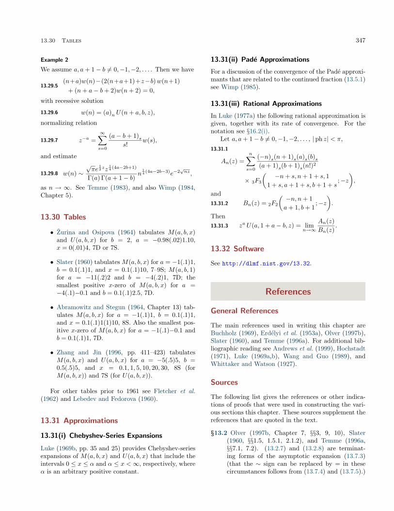
13.30 Tables 347
Example 2
We assume a, a+ 1− b 6= 0,−1,−2, . . . . Then we have
13.29.5(n+a)w(n)−(2(n+a+1)+z−b)w(n+1)
+ (n+ a− b+ 2)w(n+ 2) = 0,
with recessive solution
13.29.6 w(n) = (a)n U(n+ a, b, z),
normalizing relation
13.29.7 z−a =∞∑s=0
(a− b+ 1)ss!
w(s),
and estimate
13.29.8 w(n) ∼√πe
12 zz
14 (4a−2b+1)
Γ(a) Γ(a+ 1− b)n
14 (4a−2b−3)e−2
√nz,
as n → ∞. See Temme (1983), and also Wimp (1984,Chapter 5).
13.30 Tables
• Žurina and Osipova (1964) tabulates M(a, b, x)and U(a, b, x) for b = 2, a = −0.98(.02)1.10,x = 0(.01)4, 7D or 7S.
• Slater (1960) tabulates M(a, b, x) for a = −1(.1)1,b = 0.1(.1)1, and x = 0.1(.1)10, 7–9S; M(a, b, 1)for a = −11(.2)2 and b = −4(.2)1, 7D; thesmallest positive x-zero of M(a, b, x) for a =−4(.1)−0.1 and b = 0.1(.1)2.5, 7D.
• Abramowitz and Stegun (1964, Chapter 13) tab-ulates M(a, b, x) for a = −1(.1)1, b = 0.1(.1)1,and x = 0.1(.1)1(1)10, 8S. Also the smallest pos-itive x-zero of M(a, b, x) for a = −1(.1)−0.1 andb = 0.1(.1)1, 7D.
• Zhang and Jin (1996, pp. 411–423) tabulatesM(a, b, x) and U(a, b, x) for a = −5(.5)5, b =0.5(.5)5, and x = 0.1, 1, 5, 10, 20, 30, 8S (forM(a, b, x)) and 7S (for U(a, b, x)).
For other tables prior to 1961 see Fletcher et al.(1962) and Lebedev and Fedorova (1960).
13.31 Approximations
13.31(i) Chebyshev-Series Expansions
Luke (1969b, pp. 35 and 25) provides Chebyshev-seriesexpansions of M(a, b, x) and U(a, b, x) that include theintervals 0 ≤ x ≤ α and α ≤ x <∞, respectively, whereα is an arbitrary positive constant.
13.31(ii) Padé Approximations
For a discussion of the convergence of the Padé approxi-mants that are related to the continued fraction (13.5.1)see Wimp (1985).
13.31(iii) Rational Approximations
In Luke (1977a) the following rational approximation isgiven, together with its rate of convergence. For thenotation see §16.2(i).
Let a, a+ 1− b 6= 0,−1,−2, . . . , |ph z| < π,13.31.1
An(z) =n∑s=0
(−n)s(n+ 1)s(a)s(b)s(a+ 1)s(b+ 1)s(n!)2
× 3F3
(−n+ s, n+ 1 + s, 1
1 + s, a+ 1 + s, b+ 1 + s;−z
),
and13.31.2 Bn(z) = 2F2
(−n, n+ 1a+ 1, b+ 1
;−z).
Then13.31.3 za U(a, 1 + a− b, z) = lim
n→∞
An(z)Bn(z)
.
13.32 Software
See http://dlmf.nist.gov/13.32.
References
General References
The main references used in writing this chapter areBuchholz (1969), Erdélyi et al. (1953a), Olver (1997b),Slater (1960), and Temme (1996a). For additional bib-liographic reading see Andrews et al. (1999), Hochstadt(1971), Luke (1969a,b), Wang and Guo (1989), andWhittaker and Watson (1927).
Sources
The following list gives the references or other indica-tions of proofs that were used in constructing the vari-ous sections this chapter. These sources supplement thereferences that are quoted in the text.
§13.2 Olver (1997b, Chapter 7, §§3, 9, 10), Slater(1960, §§1.5, 1.5.1, 2.1.2), and Temme (1996a,§§7.1, 7.2). (13.2.7) and (13.2.8) are terminat-ing forms of the asymptotic expansion (13.7.3)(that the ∼ sign can be replaced by = in thesecircumstances follows from (13.7.4) and (13.7.5).)
348 Confluent Hypergeometric Functions
To verify (13.2.12) replace the U functions by Mfunctions by means of (13.2.42) and (13.2.4), thenrecall that each M function is an entire functionof z. For (13.2.13)–(13.2.22) see Temme (1996a,Ex. 7.6: an error in the equation that correspondsto (13.2.19) has been corrected). For (13.2.23)see (13.7.2). (13.2.27)–(13.2.32) are obtained byconsidering limiting forms of the connection for-mulas in §13.2(vii); see Olver (1997b, Chapter 7,Ex. 10.6) and Slater (1960, §§1.5–1.5.1).
§13.3 Slater (1960, §§2.1, 2.2). Note that in this ref-erence (2.2.7) and (2.1.32) contain errors. Thecorrect versions are (13.3.13) and (13.3.28), re-spectively. To see that (13.3.13) and (13.3.14) areequivalent to (13.2.1) use (13.3.16) and (13.3.23).For the operator identity (13.3.29) see Fleury andTurbiner (1994).
§13.4 Buchholz (1969, §1.4), Erdélyi et al. (1953a,§6.11), and Slater (1960, Chapter 3). For (13.4.5)use (13.2.41); compare the proof of Lemma 3.1 inOlde Daalhuis and Olver (1994). For (13.4.16)–(13.4.18) combine the results of Buchholz (1969,§5.4) with (13.14.2), (13.14.3).
§13.5 Jones and Thron (1980, Theorems 6.3 and 6.5).
§13.6 See Temme (1996a, §§7.2–7.3 and p. 254) andBuchholz (1969, §3.3). In the former refer-ence each of the equations on p. 180 that cor-respond to (13.6.7) and (13.6.8) contains an er-ror. For (13.6.16)–(13.6.18) combine §13.6(iv)with §12.7(i) and (18.5.18). (The last equationis needed to illustrate that xnHn(x) is an evenfunction of x.) For (13.6.19) see (18.11.2). For(13.6.20) combine (18.20.8) with (16.2.3), replacethe 1F1 notation by M (§13.1), and then use(13.2.42) (in which the final term vanishes). Alter-natively, for (13.6.20) combine (16.2.3) with An-drews et al. (1999, p. 347). When neither a nora− b+ 1 is a nonpositive integer (13.6.21) can beverified by comparison of (13.4.17) and (16.5.1).If a is a nonpositive integer, then both sides of(13.6.21) reduce to a polynomial in z (compare§§13.2(i) and 16.2(iv)), and (13.6.21) follows bycomparing coefficients. Similarly if a − b + 1 is anonpositive integer, then both sides of (13.6.21)reduce to z1−b times a polynomial in z with iden-tical coefficients.
§13.7 Temme (1996a, §7.2) or Olver (1997b, pp. 256–258), and Olver (1965).
§13.8 Slater (1960, §4.3), Temme (1978), and Temme(1990b). For (13.8.2) and (13.8.3) use Watson’s
lemma for loop integrals (Olver (1997b, §4.5)) and(13.4.10).
§13.9 Buchholz (1969, Chapter 17), Erdélyi et al.(1953a, §6.16), Slater (1960, Chapter 6), and Tri-comi (1950a). The proof of (13.9.8) is given inTricomi (1947). (13.9.9) follows from (13.7.2).For the paragraph following (13.9.9) see Andrewset al. (1999, §4.16). For (13.9.10) and (13.9.16) use(13.8.9), (13.8.10), and the asymptotics of zeros ofBessel functions (§10.21(vi)). For the final para-graph of §13.9(ii) apply Kummer’s transformation(13.2.39) to the final term in the connection rela-tion (13.2.42) and then use the asymptotic rela-tion (13.8.1).
§13.10 Erdélyi et al. (1953a, §§6.10, 6.15.2) and Slater(1960, Chapter 3). Also Buchholz (1969, §11.1),including the references given there. (13.10.14)and (13.10.16) are from Erdélyi et al. (1954b,§8.18). For (13.10.14) substitute the integral(13.4.1) for M(a, b, t), interchange the order ofintegration, then apply (13.4.3) and (13.6.1) fol-lowed by (13.4.4). For (13.10.16) interchange theroles of (13.4.1) and (13.4.4).
§13.11 Slater (1960, §2.7.3: Eq. (2.7.14) has errors).
§13.12 (13.12.1) follows from the fact that its left-hand side is bounded at infinity: use (13.2.39),(13.2.41), and (13.7.3).
§13.13 Erdélyi et al. (1953a, §6.14) and Slater (1960,§§2.3–2.3.3). In the first reference Equation (2)needs the constraint |λ− 1| < 1 and Equation (6)should have no constraint. In the second referenceEq. (2.3.6) contains an error: (x + y)n should bereplaced by (x+ y)−n.
§13.14 Olver (1997b, Chapter 7, §§9–11, and Ex. 11.2),Buchholz (1969, §2.3a), Slater (1960, §§1.7.1,2.4.2), Temme (1996a, §7.2). For (13.14.8) and(13.14.9) take limiting values in (13.14.33), using(13.14.2) and (13.2.2). For (13.14.14)–(13.14.19)combine §13.2(iii) and (13.14.4), (13.14.5). For(13.14.20), (13.14.21) use (13.19.2), (13.19.3). For(13.14.32) and (13.14.33) combine (13.2.41) and(13.2.42) with (13.14.4) and (13.14.5). (13.14.31)follows from (13.14.33).
§13.15 Slater (1960, §§2.4, 2.4.1, 2.5). Note that(2.5.4) and (2.5.10) contain errors: the correct ver-sions are (13.15.2) and (13.15.10), respectively.
§13.16 Buchholz (1969, §5.4), Erdélyi et al. (1953a,§6.11), and Slater (1960, Chapter 3). For §13.16(i)combine §13.4(i) with (13.14.4) and (13.14.5).

References 349
§13.17 Jones and Thron (1980, Theorems 6.3 and 6.5).
§13.18 Combine §13.6 with (13.14.4) and (13.14.5).
§13.19 Temme (1996a, §7.2).
§13.20 Olver (1997b, Chapter 7, §11.2). For (13.20.2)use (13.14.3) and apply the method of steepestdescents (§2.4(iv)) to the integral representation(13.4.14).
§13.21 Slater (1960, §4.4.3). The asymptotic approxi-mations (13.21.2)–(13.21.4) follow from §13.21(ii)and (5.11.7).
§13.22 Olver (1997b, Chapter 12, (7.05)).
§13.23 Buchholz (1969, §§10, 11.1), Erdélyi et al.(1953a, §§6.10, 6.15.2), Slater (1960, Chapter3), and Snow (1952, Chapter XI). (13.23.3) and(13.23.5) can also be derived as limiting formsof (13.23.1) and (13.23.4), respectively; com-pare (15.4.20). For (13.23.9)–(13.23.12) combine§13.10(v) with (13.14.4) and (13.14.5).
§13.24 Slater (1960, §2.7.3) and Buchholz (1969, §7.4).In the first reference (2.7.16) contains an error.
§13.25 For (13.25.1) combine (13.12.1) with (13.14.4).
§13.26 Slater (1960, §§2.6–2.6.3). Note that (2.6.3)and (2.6.6) contain errors; the correct versions are(13.26.3) and (13.26.6), respectively.


Chapter 14
Legendre and Related FunctionsT. M. Dunster1
Notation 35214.1 Special Notation . . . . . . . . . . . . . 352
Real Arguments 35214.2 Differential Equations . . . . . . . . . . . 35214.3 Definitions and Hypergeometric Represen-
tations . . . . . . . . . . . . . . . . . . . 35314.4 Graphics . . . . . . . . . . . . . . . . . . 35514.5 Special Values . . . . . . . . . . . . . . . 35914.6 Integer Order . . . . . . . . . . . . . . . 36014.7 Integer Degree and Order . . . . . . . . . 36014.8 Behavior at Singularities . . . . . . . . . 36114.9 Connection Formulas . . . . . . . . . . . 36214.10 Recurrence Relations and Derivatives . . 36214.11 Derivatives with Respect to Degree or Order36314.12 Integral Representations . . . . . . . . . 36314.13 Trigonometric Expansions . . . . . . . . . 36414.14 Continued Fractions . . . . . . . . . . . . 36414.15 Uniform Asymptotic Approximations . . . 36514.16 Zeros . . . . . . . . . . . . . . . . . . . 36814.17 Integrals . . . . . . . . . . . . . . . . . . 36814.18 Sums . . . . . . . . . . . . . . . . . . . 37014.19 Toroidal (or Ring) Functions . . . . . . . 371
14.20 Conical (or Mehler) Functions . . . . . . 372
Complex Arguments 37514.21 Definitions and Basic Properties . . . . . 37514.22 Graphics . . . . . . . . . . . . . . . . . . 37514.23 Values on the Cut . . . . . . . . . . . . . 37614.24 Analytic Continuation . . . . . . . . . . . 37614.25 Integral Representations . . . . . . . . . 37714.26 Uniform Asymptotic Expansions . . . . . 37714.27 Zeros . . . . . . . . . . . . . . . . . . . 37714.28 Sums . . . . . . . . . . . . . . . . . . . 37714.29 Generalizations . . . . . . . . . . . . . . 377
Applications 37814.30 Spherical and Spheroidal Harmonics . . . 37814.31 Other Applications . . . . . . . . . . . . 379
Computation 37914.32 Methods of Computation . . . . . . . . . 37914.33 Tables . . . . . . . . . . . . . . . . . . . 38014.34 Software . . . . . . . . . . . . . . . . . . 380
References 380
1Department of Mathematics and Statistics, San Diego State University, San Diego, California.Acknowledgments: This chapter is based in part on Abramowitz and Stegun (1964, Chapter 8) by Irene A. Stegun. The author
is indebted to Richard Paris for correcting a long-standing error in Eq. (14.18.3) in previous literature.Copyright c© 2009 National Institute of Standards and Technology. All rights reserved.
351

352 Legendre and Related Functions
Notation
14.1 Special Notation
(For other notation see pp. xiv and 873.)
x, y, τ real variables.z = x+ iy complex variable.m, n nonnegative integers used for order and
degree, respectively.µ, ν general order and degree, respectively.− 1
2 + iτ complex degree, τ ∈ R.γ Euler’s constant (§5.2(ii)).δ arbitrary small positive constant.ψ(x) logarithmic derivative of gamma function
(§5.2(i)).ψ′(x) dψ(x)/dx .F(a, b; c; z) Olver’s scaled hypergeometric function:
F (a, b; c; z)/Γ(c) .
Multivalued functions take their principal values(§4.2(i)) unless indicated otherwise.
The main functions treated in this chapter are theLegendre functions Pν(x), Qν(x), Pν(z), Qν(z); Ferrersfunctions Pµν (x), Qµ
ν (x) (also known as the Legendrefunctions on the cut); associated Legendre functionsPµν (z), Qµν (z), Qµ
ν (z); conical functions Pµ− 12 +iτ
(x),
Qµ
− 12 +iτ
(x), Q̂µ
− 12 +iτ
(x), Pµ− 12 +iτ
(x), Qµ− 12 +iτ
(x) (alsoknown as Mehler functions).
Among other notations commonly used in the lit-erature Erdélyi et al. (1953a) and Olver (1997b) de-note Pµν (x) and Qµ
ν (x) by Pµν (x) and Qµν (x), respectively.
Magnus et al. (1966) denotes Pµν (x), Qµν (x), Pµν (z), and
Qµν (z) by Pµν (x), Qµν (x), Pµν (z), and Qµ
ν (z), respectively.Hobson (1931) denotes both Pµν (x) and Pµν (x) by Pµν (x);similarly for Qµ
ν (x) and Qµν (x).
Real Arguments
14.2 Differential Equations
14.2(i) Legendre’s Equation
14.2.1(1− x2
) d2w
dx2 − 2xdw
dx+ ν(ν + 1)w = 0.
Standard solutions: Pν(±x), Qν(±x), Q−ν−1(±x),Pν(±x), Qν(±x), Q−ν−1(±x). Pν(x) and Qν(x) arereal when ν ∈ R and x ∈ (−1, 1), and Pν(x) and Qν(x)are real when ν ∈ R and x ∈ (1,∞).
14.2(ii) Associated Legendre Equation
14.2.2(1− x2
) d2w
dx2 − 2xdw
dx+(ν(ν + 1)− µ2
1− x2
)w = 0.
Standard solutions: Pµν (±x), P−µν (±x), Qµν (±x),
Qµ−ν−1(±x), Pµν (±x), P−µν (±x), Qµ
ν (±x), Qµ−ν−1(±x).
(14.2.2) reduces to (14.2.1) when µ = 0. Fer-rers functions and the associated Legendre functionsare related to the Legendre functions by the equa-tions P0
ν(x) = Pν(x), Q0ν(x) = Qν(x), P 0
ν (x) = Pν(x),Q0ν(x) = Qν(x), Q0
ν(x) = Qν(x) = Qν(x)/Γ(ν + 1).Pµν (x), Pµ− 1
2 +iτ(x), and Qµ
ν (x) are real when ν, µ,and τ ∈ R, and x ∈ (−1, 1); Pµν (x), Qµν (x), and Qµ
ν (x)are real when ν and µ ∈ R, and x ∈ (1,∞).
Unless stated otherwise in §§14.2–14.20 it is assumedthat the arguments of the functions Pµν (x) and Qµ
ν (x) liein the interval (−1, 1), and the arguments of the func-tions Pµν (x), Qµν (x), andQµ
ν (x) lie in the interval (1,∞).For extensions to complex arguments see §§14.21–14.28.
14.2(iii) Numerically Satisfactory Solutions
Equation (14.2.2) has regular singularities at x = 1, −1,and ∞, with exponent pairs
{− 1
2µ,12µ}
,{− 1
2µ,12µ}
,and {−ν − 1, ν}, respectively; compare §2.7(i).
When µ − ν 6= 0,−1,−2, . . . , and µ + ν 6=−1,−2,−3, . . . , P−µν (x) and P−µν (−x) are linearly in-dependent, and when <µ ≥ 0 they are recessive atx = 1 and x = −1, respectively. Hence they comprisea numerically satisfactory pair of solutions (§2.7(iv)) of(14.2.2) in the interval −1 < x < 1. When µ − ν =0,−1,−2, . . . , or µ + ν = −1,−2,−3, . . . , P−µν (x) andP−µν (−x) are linearly dependent, and in these cases ei-ther may be paired with almost any linearly indepen-dent solution to form a numerically satisfactory pair.
When <µ ≥ 0 and <ν ≥ − 12 , P−µν (x) and Qµ
ν (x)are linearly independent, and recessive at x = 1 andx = ∞, respectively. Hence they comprise a numeri-cally satisfactory pair of solutions of (14.2.2) in the in-terval 1 < x <∞. With the same conditions, P−µν (−x)and Qµ
ν (−x) comprise a numerically satisfactory pair ofsolutions in the interval −∞ < x < −1.
14.2(iv) Wronskians and Cross-Products
14.2.3
W{
P−µν (x),P−µν (−x)}
=2
Γ(µ− ν) Γ(ν + µ+ 1) (1− x2),
14.2.4 W {Pµν (x),Qµν (x)} =
Γ(ν + µ+ 1)Γ(ν − µ+ 1) (1− x2)
,
14.2.5 Pµν+1(x) Qµν (x)−Pµν (x) Qµ
ν+1(x) =Γ(ν + µ+ 1)Γ(ν − µ+ 2)
,

14.3 Definitions and Hypergeometric Representations 353
14.2.6 W{
P−µν (x),Qµν (x)
}=
cos(µπ)1− x2
,
14.2.7 W{P−µν (x), Pµν (x)
}= − 2 sin(µπ)
π (x2 − 1),
14.2.8 W{P−µν (x),Qµ
ν (x)}
= − 1Γ(ν + µ+ 1) (x2 − 1)
,
14.2.9 W{Qµν (x),Qµ
−ν−1(x)}
=cos(νπ)x2 − 1
,
14.2.10
W {Pµν (x), Qµν (x)} = −eµπi Γ(ν + µ+ 1)Γ(ν − µ+ 1) (x2 − 1)
,
14.2.11
Pµν+1(x)Qµν (x)− Pµν (x)Qµν+1(x) = eµπiΓ(ν + µ+ 1)Γ(ν − µ+ 2)
.
14.3 Definitions and Hypergeometric Representations
14.3(i) Interval −1 < x < 1
The following are real-valued solutions of (14.2.2) when µ, ν ∈ R and x ∈ (−1, 1).
Ferrers Function of the First Kind
14.3.1 Pµν (x) =(
1 + x
1− x
)µ/2F(ν + 1,−ν; 1− µ; 1
2 −12x).
Ferrers Function of the Second Kind
14.3.2
Qµν (x) =
π
2 sin(µπ)
(cos(µπ)
(1 + x
1− x
)µ/2F(ν + 1,−ν; 1− µ; 1
2 −12x)
− Γ(ν + µ+ 1)Γ(ν − µ+ 1)
(1− x1 + x
)µ/2F(ν + 1,−ν; 1 + µ; 1
2 −12x))
.
Here and elsewhere in this chapter
14.3.3 F(a, b; c;x) =1
Γ(c)F (a, b; c;x)
is Olver’s hypergeometric function (§15.1).Pµν (x) exists for all values of µ and ν. Qµ
ν (x) is undefined when µ+ ν = −1,−2,−3, . . . .When µ = m = 0, 1, 2, . . . , (14.3.1) reduces to
14.3.4 Pmν (x) = (−1)mΓ(ν +m+ 1)
2m Γ(ν −m+ 1)(1− x2
)m/2F(ν +m+ 1,m− ν;m+ 1; 1
2 −12x);
equivalently,
14.3.5 Pmν (x) = (−1)mΓ(ν +m+ 1)Γ(ν −m+ 1)
(1− x1 + x
)m/2F(ν + 1,−ν;m+ 1; 1
2 −12x).
When µ = m (∈ Z) (14.3.2) is replaced by its limiting value; see Hobson (1931, §132) for details. See also (14.3.12)–(14.3.14) for this case.
14.3(ii) Interval 1 < x <∞
Associated Legendre Function of the First Kind
14.3.6 Pµν (x) =(x+ 1x− 1
)µ/2F(ν + 1,−ν; 1− µ; 1
2 −12x).

354 Legendre and Related Functions
Associated Legendre Function of the Second Kind
14.3.7
Qµν (x) = eµπiπ1/2 Γ(ν + µ+ 1)
(x2 − 1
)µ/22ν+1xν+µ+1
F(
12ν + 1
2µ+ 1, 12ν + 1
2µ+ 12 ; ν + 3
2 ;1x2
), µ+ ν 6= −1,−2,−3, . . . .
When µ = m = 1, 2, 3, . . . , (14.3.6) reduces to
14.3.8 Pmν (x) =Γ(ν +m+ 1)
2m Γ(ν −m+ 1)(x2 − 1
)m/2F(ν +m+ 1,m− ν;m+ 1; 1
2 −12x).
As standard solutions of (14.2.2) we take the pair P−µν (x) and Qµν (x), where
14.3.9 P−µν (x) =(x− 1x+ 1
)µ/2F(ν + 1,−ν;µ+ 1; 1
2 −12x),
and14.3.10 Qµ
ν (x) = e−µπiQµν (x)
Γ(ν + µ+ 1).
Like Pµν (x), but unlike Qµν (x), Qµν (x) is real-valued when ν, µ ∈ R and x ∈ (1,∞), and is defined for all values of ν
and µ. The notation Qµν (x) is due to Olver (1997b, pp. 170 and 178).
14.3(iii) Alternative Hypergeometric Representations
14.3.11 Pµν (x) = cos(
12 (ν + µ)π
)w1(ν, µ, x) + sin
(12 (ν + µ)π
)w2(ν, µ, x),
14.3.12 Qµν (x) = − 1
2π sin(
12 (ν + µ)π
)w1(ν, µ, x) + 1
2π cos(
12 (ν + µ)π
)w2(ν, µ, x),
where
14.3.13 w1(ν, µ, x) =2µ Γ
(12ν + 1
2µ+ 12
)Γ(
12ν −
12µ+ 1
) (1− x2
)−µ/2F(− 1
2ν −12µ,
12ν −
12µ+ 1
2 ; 12 ;x2
),
14.3.14 w2(ν, µ, x) =2µ Γ
(12ν + 1
2µ+ 1)
Γ(
12ν −
12µ+ 1
2
) x(1− x2
)−µ/2F(
12 −
12ν −
12µ,
12ν −
12µ+ 1; 3
2 ;x2).
14.3.15 P−µν (x) = 2−µ(x2 − 1
)µ/2F(µ− ν, ν + µ+ 1;µ+ 1; 1
2 −12x),
14.3.16
cos(νπ)P−µν (x) =2νπ1/2xν−µ
(x2 − 1
)µ/2Γ(ν + µ+ 1)
F(
12µ−
12ν,
12µ−
12ν + 1
2 ; 12 − ν;
1x2
)−
π1/2(x2 − 1
)µ/22ν+1 Γ(µ− ν)xν+µ+1
F(
12ν + 1
2µ+ 1, 12ν + 1
2µ+ 12 ; ν + 3
2 ;1x2
),
14.3.17 P−µν (x) =π(x2 − 1
)µ/22µ
(F(
12µ−
12ν,
12ν + 1
2µ+ 12 ; 1
2 ;x2)
Γ(
12µ−
12ν + 1
2
)Γ(
12ν + 1
2µ+ 1) − xF
(12µ−
12ν + 1
2 ,12ν + 1
2µ+ 1; 32 ;x2
)Γ(
12µ−
12ν)
Γ(
12ν + 1
2µ+ 12
) ),
14.3.18 P−µν (x) = 2−µxν−µ(x2 − 1
)µ/2F(
12µ−
12ν,
12µ−
12ν + 1
2 ;µ+ 1; 1− 1x2
),
14.3.19 Qµν (x) =
2ν Γ(ν + 1)(x+ 1)µ/2
(x− 1)(µ/2)+ν+1F(ν + 1, ν + µ+ 1; 2ν + 2;
21− x
),
14.3.20
2 sin(µπ)π
Qµν (x) =
(x+ 1)µ/2
Γ(ν + µ+ 1)(x− 1)µ/2F(ν + 1,−ν; 1− µ; 1
2 −12x)
− (x− 1)µ/2
Γ(ν − µ+ 1)(x+ 1)µ/2F(ν + 1,−ν;µ+ 1; 1
2 −12x).
For further hypergeometric representations of Pµν (x) and Qµν (x) see Erdélyi et al. (1953a, pp. 123–139), Andrewset al. (1999, §3.1), Magnus et al. (1966, pp. 153–163), and §15.8(iv).

14.4 Graphics 355
14.3(iv) Relations to Other Functions
In terms of the Gegenbauer function C(β)α (x) and the Jacobi function φ
(α,β)λ (t) (§§15.9(iii), 15.9(ii)):
14.3.21 Pµν (x) =2µ Γ(1− 2µ) Γ(ν + µ+ 1)
Γ(ν − µ+ 1) Γ(1− µ) (1− x2)µ/2C
( 12−µ)ν+µ (x).
14.3.22 Pµν (x) =2µ Γ(1− 2µ) Γ(ν + µ+ 1)
Γ(ν − µ+ 1) Γ(1− µ) (x2 − 1)µ/2C
( 12−µ)ν+µ (x).
14.3.23 Pµν (x) =1
Γ(1− µ)
(x+ 1x− 1
)µ/2φ
(−µ,µ)−i(2ν+1)
(arcsinh
(( 1
2x−12 ) 1/2
)).
Compare also (18.11.1).
14.4 Graphics
14.4(i) Ferrers Functions: 2D Graphs
Figure 14.4.1: P0ν(x), ν = 0, 1
2 , 1, 2, 4. Figure 14.4.2: Q0ν(x), ν = 0, 1
2 , 1, 2, 4.
Figure 14.4.3: P−1/2ν (x), ν = 0, 1
2 , 1, 2, 4. Figure 14.4.4: Q1/2ν (x), ν = 0, 1
2 , 1, 2, 4.
For additional graphs see http://dlmf.nist.gov/14.4.i.

356 Legendre and Related Functions
Figure 14.4.7: P−µ0 (x), µ = 0, 12 , 1, 2, 4. Figure 14.4.8: Qµ
0 (x), µ = 0, 12 , 1, 2, 4.
Figure 14.4.9: P−µ1/2(x), µ = 0, 12 , 1, 2, 4.
�
Figure 14.4.10: Qµ1/2(x), µ = 0, 1
2 , 1, 2, 4.
For additional graphs see http://dlmf.nist.gov/14.4.i.
14.4(ii) Ferrers Functions: 3D Surfaces
Figure 14.4.13: P0ν(x), 0 ≤ ν ≤ 10,−1 < x < 1. Figure 14.4.14: Q0
ν(x), 0 ≤ ν ≤ 10,−1 < x < 1.

14.4 Graphics 357
Figure 14.4.15: P−µ0 (x), 0 ≤ µ ≤ 10,−1 < x < 1. Figure 14.4.16: Qµ0 (x), 0 ≤ µ ≤ 6.2,−1 < x < 1.
14.4(iii) Associated Legendre Functions: 2D Graphs
Figure 14.4.17: P 0ν (x), ν = 0, 1
2 , 1, 2, 4. Figure 14.4.18: Q0ν(x), ν = 0, 1
2 , 1, 2, 4.
Figure 14.4.19: P−1/2ν (x), ν = 0, 1
2 , 1, 2, 4. Figure 14.4.20: Q1/2ν (x), ν = 0, 1
2 , 1, 2, 4.
For additional graphs see http://dlmf.nist.gov/14.4.iii.

358 Legendre and Related Functions
Figure 14.4.23: P−µ0 (x), µ = 0, 12 , 1, 2, 4. Figure 14.4.24: Qµ
0 (x), µ = 0, 2, 4, 8.
Figure 14.4.25: P−µ1/2(x), µ = 0, 12 , 1, 2, 4. Figure 14.4.26: Qµ
1/2(x), µ = 0, 2, 4, 8.
For additional graphs see http://dlmf.nist.gov/14.4.iii.
14.4(iv) Associated Legendre Functions: 3D Surfaces
Figure 14.4.29: P 0ν (x), 0 ≤ ν ≤ 10, 1 < x < 10. Figure 14.4.30: Q0
ν(x), 0 ≤ ν ≤ 10, 1 < x < 10.

14.5 Special Values 359
Figure 14.4.31: P−µ0 (x), 0 ≤ µ ≤ 10, 1 < x < 10. Figure 14.4.32: Qµ0 (x), 0 ≤ µ ≤ 10, 1 < x < 10.
14.5 Special Values
14.5(i) x = 0
14.5.1 Pµν (0) =2µπ1/2
Γ(
12ν −
12µ+ 1
)Γ(
12 −
12ν −
12µ) ,
14.5.2dPµν (x)dx
∣∣∣∣x=0
= − 2µ+1π1/2
Γ(
12ν −
12µ+ 1
2
)Γ(− 1
2ν −12µ) ,
14.5.3
Qµν (0) = −
2µ−1π1/2 sin(
12 (ν + µ)π
)Γ(
12ν + 1
2µ+ 12
)Γ(
12ν −
12µ+ 1
) ,
ν + µ 6= −1,−3,−5, . . . ,
14.5.4
dQµν (x)dx
∣∣∣∣x=0
=2µπ1/2 cos
(12 (ν + µ)π
)Γ(
12ν + 1
2µ+ 1)
Γ(
12ν −
12µ+ 1
2
) ,
ν + µ 6= −2,−4,−6, . . . .
14.5(ii) µ = 0, ν = 0, 1
14.5.5 P0(x) = P0(x) = 1,
14.5.6 P1(x) = P1(x) = x.
14.5.7 Q0(x) =12
ln(
1 + x
1− x
),
14.5.8 Q1(x) =x
2ln(
1 + x
1− x
)− 1.
14.5.9 Q0(x) =12
ln(x+ 1x− 1
),
14.5.10 Q1(x) =x
2ln(x+ 1x− 1
)− 1.
14.5(iii) µ = ±12
In this subsection and the next two, 0 < θ < π andξ > 0.
14.5.11 P1/2ν (cos θ) =
(2
π sin θ
)1/2cos((ν + 1
2
)θ),
14.5.12 P−1/2ν (cos θ) =
(2
π sin θ
)1/2 sin((ν + 1
2
)θ)
ν + 12
,
14.5.13 Q1/2ν (cos θ) = −
( π
2 sin θ
)1/2sin((ν + 1
2
)θ),
14.5.14 Q−1/2ν (cos θ) = −
( π
2 sin θ
)1/2 cos((ν + 1
2
)θ)
ν + 12
.
14.5.15
P 1/2ν (cosh ξ) =
(2
π sinh ξ
)1/2cosh
((ν + 1
2
)ξ),
14.5.16
P−1/2ν (cosh ξ) =
(2
π sinh ξ
)1/2 sinh((ν + 1
2
)ξ)
ν + 12
,
14.5.17
Q±1/2ν (cosh ξ) =
(π
2 sinh ξ
)1/2 exp(−(ν + 1
2
)ξ)
Γ(ν + 3
2
) .
14.5(iv) µ = −ν
14.5.18 P−νν (cos θ) =(sin θ)ν
2ν Γ(ν + 1),
14.5.19 P−νν (cosh ξ) =(sinh ξ)ν
2ν Γ(ν + 1).

360 Legendre and Related Functions
14.5(v) µ = 0, ν = ±12
In this subsection K(k) and E(k) denote the com-plete elliptic integrals of the first and second kinds; see§19.2(ii).
14.5.20 P 12(cos θ) =
2π
(2E(sin(
12θ))−K
(sin(
12θ)))
,
14.5.21 P− 12(cos θ) =
2πK(sin(
12θ)),
14.5.22 Q 12(cos θ) = K
(cos(
12θ))− 2E
(cos(
12θ)),
14.5.23 Q− 12(cos θ) = K
(cos(
12θ)).
14.5.24 P 12(cosh ξ) =
2πeξ/2E
((1− e−2ξ
)1/2),
14.5.25 P− 12(cosh ξ) =
2π cosh
(12ξ) K(tanh
(12ξ)),
14.5.26
Q 12(cosh ξ) = 2π−1/2 cosh ξ sech
(12ξ)K(sech
(12ξ))
− 4π−1/2 cosh(
12ξ)E(sech
(12ξ)),
14.5.27 Q− 12(cosh ξ) = 2π−1/2e−ξ/2K
(e−ξ).
14.6 Integer Order
14.6(i) Nonnegative Integer Orders
For m = 0, 1, 2, . . . ,
14.6.1 Pmν (x) = (−1)m(1− x2
)m/2 dmPν(x)dxm
,
14.6.2 Qmν (x) = (−1)m
(1− x2
)m/2 dmQν(x)dxm
.
14.6.3 Pmν (x) =(x2 − 1
)m/2 dmPν(x)dxm
,
14.6.4 Qmν (x) =(x2 − 1
)m/2 dmQν(x)dxm
,
14.6.5 (ν + 1)mQmν (x) = (−1)m
(x2 − 1
)m/2 dmQν(x)dxm
.
14.6(ii) Negative Integer Orders
For m = 1, 2, 3, . . . ,
14.6.6 P−mν (x) =(1− x2
)−m/2 ∫ 1
x
. . .
∫ 1
x
Pν(x) (dx)m .
14.6.7 P−mν (x) =(x2 − 1
)−m/2 ∫ x
1
. . .
∫ x
1
Pν(x) (dx)m ,
14.6.8
Q−mν (x) = (−1)m(x2 − 1
)−m/2×∫ ∞x
. . .
∫ ∞x
Qν(x) (dx)m .
For connections between positive and negative inte-ger orders see (14.9.3), (14.9.4), and (14.9.13).
14.7 Integer Degree and Order
14.7(i) µ = 0
For n = 0, 1, 2, . . . ,
14.7.1 P0n(x) = Pn(x) = P 0
n(x) = Pn(x), x ∈ R,where Pn(x) is the Legendre polynomial of degree n. Foradditional properties of Pn(x) see Chapter 18.14.7.2
Q0n(x) = Qn(x) =
12Pn(x) ln
(1 + x
1− x
)−Wn−1(x),
where W−1(x) = 0, and for n ≥ 1,14.7.3
Wn−1(x) =n−1∑s=0
(n+ s)!(ψ(n+ 1)− ψ(s+ 1))2s(n− s)!(s!)2
(x− 1)s;
equivalently,
14.7.4 Wn−1(x) =n∑k=1
1kPk−1(x)Pn−k(x).
14.7.5 W0(x) = 1, W1(x) = 32x, W2(x) = 5
2x2 − 2
3 .
Next,
14.7.6 Q0n(x) = Qn(x) = n!Q0
n(x) = n!Qn(x),where14.7.7
Qn(x) =12Pn(x) ln
(x+ 1x− 1
)−Wn−1(x), n = 0, 1, 2, . . . .
14.7(ii) Rodrigues-Type Formulas
For m = 0, 1, 2, . . . , and n = 0, 1, 2, . . . ,
14.7.8 Pmn (x) = (−1)m(1− x2
)m/2 dm
dxmPn(x),
14.7.9 Qmn (x) = (−1)m
(1− x2
)m/2 dm
dxmQn(x),
14.7.10
Pmn (x) = (−1)m+n
(1− x2
)m/22nn!
dm+n
dxm+n
(1− x2
)n.
14.7.11 Pmn (x) =(x2 − 1
)m/2 dm
dxmPn(x),
14.7.12 Qmn (x) =(x2 − 1
)m/2 dm
dxmQn(x),
14.7.13 Pn(x) =1
2nn!dn
dxn(x2 − 1
)n,
14.7.14 Pmn (x) =
(x2 − 1
)m/22nn!
dm+n
dxm+n
(x2 − 1
)n,
14.7.15 Pmm (x) =(2m)!2mm!
(x2 − 1
)m/2.
When m is even and m ≤ n, Pmn (x) and Pmn (x) arepolynomials of degree n. Also,
14.7.16 Pmn (x) = Pmn (x) = 0, m > n.

14.8 Behavior at Singularities 361
14.7(iii) Reflection Formulas
14.7.17 Pmn (−x) = (−1)n−m Pmn (x),
14.7.18 Q±mn (−x) = (−1)n−m−1 Q±mn (x).
14.7(iv) Generating Functions
When −1 < x < 1 and |h| < 1,
14.7.19
∞∑n=0
Pn(x)hn =(1− 2xh+ h2
)−1/2,
14.7.20∞∑n=0
Qn(x)hn =1
(1− 2xh+ h2)1/2
× ln
(x− h+
(1− 2xh+ h2
)1/2(1− x2)1/2
).
When −1 < x < 1 and |h| > 1,
14.7.21
∞∑n=0
Pn(x)h−n−1 =(1− 2xh+ h2
)−1/2.
When x > 1, (14.7.19) applies with |h| < x −(x2 − 1
)1/2. Also, with the same conditions14.7.22∞∑n=0
Qn(x)hn =1
(1− 2xh+ h2)1/2
× ln
(x− h+
(1− 2xh+ h2
)1/2(x2 − 1)1/2
).
Lastly, when x > 1, (14.7.21) applies with |h| >x+
(x2 − 1
)1/2.For other generating functions see Magnus et al.
(1966, pp. 232–233) and Rainville (1960, pp. 163–165,168, 170–171, 184).
14.8 Behavior at Singularities
14.8(i) x→ 1− or x→ −1+
As x→ 1−,14.8.1
Pµν (x) ∼ 1Γ(1− µ)
(2
1− x
)µ/2, µ 6= 1, 2, 3, . . . ,
14.8.2
Pmν (x) ∼ (−1)m(ν −m+ 1)2m
m!
(1− x
2
)m/2,
m = 1, 2, 3, . . . , ν 6= m− 1,m− 2, . . . ,−m,14.8.3
Qν(x) =12
ln(
21− x
)− γ − ψ(ν + 1) +O(1− x),
ν 6= −1,−2,−3, . . . ,
where γ is Euler’s constant (§5.2(ii)). In the next threerelations <µ > 0.14.8.4
Qµν (x) ∼ 1
2cos(µπ) Γ(µ)
(2
1− x
)µ/2, µ 6= 1
2 ,32 ,
52 , . . . ,
14.8.5
Qµν (x)
∼ (−1)µ+(1/2) π Γ(ν + µ+ 1)2 Γ(µ+ 1) Γ(ν − µ+ 1)
(1− x
2
)µ/2,
µ = 12 ,
32 ,
52 , . . . , ν ± µ 6= −1,−2,−3, . . . ,
14.8.6 Q−µν (x) ∼ Γ(µ) Γ(ν − µ+ 1)2 Γ(ν + µ+ 1)
(2
1− x
)µ/2,
ν ± µ 6= −1,−2,−3, . . . .
The behavior of Pµν (x) and Qµν (x) as x → −1+ fol-
lows from the above results and the connection formulas(14.9.8) and (14.9.10).
14.8(ii) x→ 1+
14.8.7
Pµν (x) ∼ 1Γ(1− µ)
(2
x− 1
)µ/2, µ 6= 1, 2, 3, . . . ,
14.8.8
Pmν (x) ∼ Γ(ν +m+ 1)m! Γ(ν −m+ 1)
(x− 1
2
)m/2,
m = 1, 2, 3, . . . , ν ±m 6= −1,−2,−3, . . . ,
14.8.9
Qν(x) = − ln(x− 1)2 Γ(ν + 1)
+12 ln 2− γ − ψ(ν + 1)
Γ(ν + 1)+O(x− 1), ν 6= −1,−2,−3, . . . ,
14.8.10 Q−n(x)→ (−1)n+1(n− 1)!, n = 1, 2, 3, . . . ,
14.8.11 Qµν (x) ∼ Γ(µ)
2 Γ(ν + µ+ 1)
(2
x− 1
)µ/2,
<µ > 0, ν + µ 6= −1,−2,−3, . . . .
14.8(iii) x→∞
14.8.12Pµν (x) ∼
Γ(ν + 1
2
)π1/2 Γ(ν − µ+ 1)
(2x)ν ,
<ν > − 12 , µ− ν 6= 1, 2, 3, . . . ,
14.8.13Pµν (x) ∼
Γ(−ν − 1
2
)π1/2 Γ(−µ− ν)(2x)ν+1
,
<ν < − 12 , ν + µ 6= 0, 1, 2, . . . ,
14.8.14Pµ−1/2(x) ∼ 1
Γ(
12 − µ
) ( 2πx
)1/2lnx,
µ 6= 12 ,
32 ,
52 , . . . ,

362 Legendre and Related Functions
14.8.15
Qµν (x) ∼ π1/2
Γ(ν + 3
2
)(2x)ν+1
, ν 6= − 32 ,−
52 ,−
72 , . . . ,
14.8.16Qµ−n−(1/2)(x) ∼
π1/2 Γ(µ+ n+ 1
2
)n! Γ
(µ− n+ 1
2
)(2x)n+(1/2)
,
n = 1, 2, 3, . . . , µ− n+ 12 6= 0,−1,−2, . . . .
14.9 Connection Formulas
14.9(i) Connections Between P±µν (x),
P±µ−ν−1(x), Q±µν (x), Qµ−ν−1(x)
14.9.1
π sin(µπ)2 Γ(ν − µ+ 1)
P−µν (x) = − 1Γ(ν + µ+ 1)
Qµν (x)
+cos(µπ)
Γ(ν − µ+ 1)Q−µν (x).
14.9.2
2 sin(µπ)π Γ(ν − µ+ 1)
Q−µν (x) =1
Γ(ν + µ+ 1)Pµν (x)
− cos(µπ)Γ(ν − µ+ 1)
P−µν (x),
14.9.3 P−mν (x) = (−1)mΓ(ν −m+ 1)Γ(ν +m+ 1)
Pmν (x),
14.9.4Q−mν (x) = (−1)m
Γ(ν −m+ 1)Γ(ν +m+ 1)
Qmν (x),
ν 6= m− 1,m− 2, . . . .
14.9.5 Pµ−ν−1(x) = Pµν (x), P−µ−ν−1(x) = P−µν (x),
14.9.6
π cos(νπ) cos(µπ) Pµν (x) = sin((ν + µ)π) Qµν (x)
− sin((ν − µ)π) Qµ−ν−1(x).
14.9(ii) Connections Between P±µν (±x),Q−µν (±x), Qµν (x)
14.9.7
sin((ν − µ)π)Γ(ν + µ+ 1)
Pµν (x) =sin(νπ)
Γ(ν − µ+ 1)P−µν (x)
− sin(µπ)Γ(ν − µ+ 1)
P−µν (−x),
14.9.812π sin((ν − µ)π) P−µν (x) = − cos((ν − µ)π) Q−µν (x)
− Q−µν (−x),
14.9.9
2Γ(ν + µ+ 1) Γ(µ− ν)
Qµν (x)
= − cos(νπ) P−µν (x) + cos(µπ) P−µν (−x),
14.9.10
(2/π) sin((ν − µ)π) Q−µν (x) = cos((ν − µ)π) P−µν (x)− P−µν (−x).
14.9(iii) Connections Between P±µν (x),
P±µ−ν−1(x), Q±µν (x), Qµ−ν−1(x)
14.9.11 P−µ−ν−1(x) = P−µν (x), Pµ−ν−1(x) = Pµν (x),
14.9.12 cos(νπ)P−µν (x) = − Qµν (x)
Γ(µ− ν)+
Qµ−ν−1(x)
Γ(ν + µ+ 1).
14.9.13
P−mν (x) =Γ(ν −m+ 1)Γ(ν +m+ 1)
Pmν (x), ν 6= m− 1,m− 2, . . . .
14.9.14 Q−µν (x) = Qµν (x),
14.9.15
2 sin(µπ)π
Qµν (x) =
Pµν (x)Γ(ν + µ+ 1)
− P−µν (x)Γ(ν − µ+ 1)
.
14.9(iv) Whipple’s Formula
14.9.16
Qµν (x)
=(
12π)1/2 (
x2 − 1)−1/4
P−ν−(1/2)−µ−(1/2)
(x(x2 − 1
)−1/2).
Equivalently,14.9.17
Pµν (x)
= (2/π)1/2(x2 − 1
)−1/4Qν+(1/2)−µ−(1/2)
(x(x2 − 1
)−1/2).
14.10 Recurrence Relations and Derivatives
14.10.1Pµ+2ν (x) + 2(µ+ 1)x
(1− x2
)−1/2Pµ+1ν (x)
+ (ν − µ)(ν + µ+ 1) Pµν (x) = 0,
14.10.2
(1− x2
)1/2Pµ+1ν (x)− (ν − µ+ 1) Pµν+1(x)
+ (ν + µ+ 1)xPµν (x) = 0,
14.10.3(ν − µ+ 2) Pµν+2(x)− (2ν + 3)xPµν+1(x)
+ (ν + µ+ 1) Pµν (x) = 0,
14.10.4
(1− x2
) dPµν (x)dx
= (µ− ν − 1) Pµν+1(x) + (ν + 1)xPµν (x),
14.10.5(1− x2
) dPµν (x)dx
= (ν + µ) Pµν−1(x)− νxPµν (x).
Qµν (x) also satisfies (14.10.1)–(14.10.5).
14.10.6Pµ+2ν (x) + 2(µ+ 1)x
(x2 − 1
)−1/2Pµ+1ν (x)
− (ν − µ)(ν + µ+ 1)Pµν (x) = 0,
14.10.7
(x2 − 1
)1/2Pµ+1ν (x)− (ν − µ+ 1)Pµν+1(x)
+ (ν + µ+ 1)xPµν (x) = 0.Qµν (x) also satisfies (14.10.6) and (14.10.7). In addition,Pµν (x) and Qµν (x) satisfy (14.10.3)–(14.10.5).

14.11 Derivatives with Respect to Degree or Order 363
14.11 Derivatives with Respect to Degree or Order
14.11.1∂
∂νPµν (x) = π cot(νπ) Pµν (x)− 1
πAµν (x),
14.11.2∂
∂νQµν (x) = − 1
2π2 Pµν (x) +
π sin(µπ)sin(νπ) sin((ν + µ)π)
Qµν (x)− 1
2 cot((ν + µ)π)Aµν (x) + 12 csc((ν + µ)π)Aµν (−x),
where
14.11.3 Aµν (x) = sin(νπ)(
1 + x
1− x
)µ/2 ∞∑k=0
(12 −
12x)k Γ(k − ν) Γ(k + ν + 1)k! Γ(k − µ+ 1)
(ψ(k + ν + 1)− ψ(k − ν)) .
14.11.4∂
∂µPµν (x)
∣∣∣∣µ=0
= (ψ(−ν)− π cot(νπ)) Pν(x) + Qν(x),
14.11.5∂
∂µQµν (x)
∣∣∣∣µ=0
= − 14π
2 Pν(x) + (ψ(−ν)− π cot(νπ)) Qν(x).
(14.11.1) holds if Pµν (x) is replaced by Pµν (x), provided that the factor ( (1 + x)/(1− x) )µ/2 in (14.11.3) is replacedby ((x+ 1)/(x− 1))µ/2. (14.11.4) holds if Pµν (x), Pν(x), and Qν(x) are replaced by Pµν (x), Pν(x), and Qν(x),respectively.
For further results see Magnus et al. (1966, pp. 177–178).
14.12 Integral Representations
14.12(i) −1 < x < 1
Mehler–Dirichlet Formula
14.12.1 Pµν (cos θ) =21/2(sin θ)µ
π1/2 Γ(
12 − µ
) ∫ θ
0
cos((ν + 1
2
)t)
(cos t− cos θ)µ+(1/2)dt, 0 < θ < π, <µ < 1
2 .
14.12.2 P−µν (x) =
(1− x2
)−µ/2Γ(µ)
∫ 1
x
Pν(t)(t− x)µ−1 dt, <µ > 0;
compare (14.6.6).14.12.3
Qµν (cos θ) =
π1/2 Γ(ν + µ+ 1)(sin θ)µ
2µ+1 Γ(µ+ 1
2
)Γ(ν − µ+ 1)
(∫ ∞0
(sinh t)2µ
(cos θ + i sin θ cosh t)ν+µ+1dt+
∫ ∞0
(sinh t)2µ
(cos θ − i sin θ cosh t)ν+µ+1dt
),
0 < θ < π, <µ > − 12 , <(ν ± µ) > −1.
14.12(ii) 1 < x <∞
14.12.4 P−µν (x) =21/2 Γ
(µ+ 1
2
) (x2 − 1
)µ/2π1/2 Γ(ν + µ+ 1) Γ(µ− ν)
∫ ∞0
cosh((ν + 1
2
)t)
(x+ cosh t)µ+(1/2)dt, ν + µ 6= −1,−2,−3, . . . , <(µ− ν) > 0.
14.12.5 P−µν (x) =
(x2 − 1
)−µ/2Γ(µ)
∫ x
1
Pν(t)(x− t)µ−1 dt, <µ > 0.
14.12.6 Qµν (x) =
π1/2(x2 − 1
)µ/22µ Γ
(µ+ 1
2
)Γ(ν − µ+ 1)
∫ ∞0
(sinh t)2µ(x+ (x2 − 1)1/2 cosh t
)ν+µ+1 dt, <(ν + 1) > <µ > − 12 .
14.12.7 Pmν (x) =(ν + 1)m
π
∫ π
0
(x+
(x2 − 1
)1/2cosφ
)νcos(mφ) dφ,
14.12.8 Pmn (x) =2mm!(n+m)!
(x2 − 1
)m/2(2m)!(n−m)!π
∫ π
0
(x+
(x2 − 1
)1/2cosφ
)n−m(sinφ)2m dφ, n ≥ m.

364 Legendre and Related Functions
14.12.9 Qmn (x) =
1n!
∫ u
0
(x−
(x2 − 1
)1/2cosh t
)ncosh(mt) dt,
where14.12.10 u =
12
ln(x+ 1x− 1
).
14.12.11 Qmn (x) =
(x2 − 1
)m/22n+1n!
∫ 1
−1
(1− t2
)n(x− t)n+m+1
dt,
14.12.12 Qmn (x) =
1(n−m)!
Pmn (x)∫ ∞x
dt
(t2 − 1) (Pmn (t))2 , n ≥ m.
Neumann’s Integral
14.12.13 Qn(x) =1
2(n!)
∫ 1
−1
Pn(t)x− t
dt.
Heine’s Integral
14.12.14 Qn(x) =1n!
∫ ∞0
dt(x+ (x2 − 1)1/2 cosh t
)n+1 .
For further integral representations see Erdélyi et al. (1953a, pp. 158–159) and Magnus et al. (1966, pp. 184–190),and for contour integrals and other representations see §14.25.
14.13 Trigonometric Expansions
When 0 < θ < π,
14.13.1 Pµν (cos θ) =2µ+1(sin θ)µ
π1/2
∞∑k=0
Γ(ν + µ+ k + 1)Γ(ν + k + 3
2
) (µ+ 1
2
)k
k!sin((ν + µ+ 2k + 1)θ),
14.13.2 Qµν (cos θ) = π1/22µ(sin θ)µ
∞∑k=0
Γ(ν + µ+ k + 1)Γ(ν + k + 3
2
) (µ+ 1
2
)k
k!cos((ν + µ+ 2k + 1)θ),
14.13.3 Pn(cos θ) =22n+2(n!)2
π(2n+ 1)!
∞∑k=0
1 · 3 · · · (2k − 1)k!
(n+ 1)(n+ 2) · · · (n+ k)(2n+ 3)(2n+ 5) · · · (2n+ 2k + 1)
sin((n+ 2k + 1)θ),
14.13.4 Qn(cos θ) =22n+1(n!)2
(2n+ 1)!
∞∑k=0
1 · 3 · · · (2k − 1)k!
(n+ 1)(n+ 2) · · · (n+ k)(2n+ 3)(2n+ 5) · · · (2n+ 2k + 1)
cos((n+ 2k + 1)θ).
For these and other trigonometric expansions see Erdélyi et al. (1953a, pp. 146–147).
14.14 Continued Fractions
14.14.1 12
(x2 − 1
)1/2 Pµν (x)Pµ−1ν (x)
=x0
y0 +x1
y1 +x2
y2 +· · · ,
where
14.14.2 xk = 14 (ν − µ− k + 1)(ν + µ+ k)
(x2 − 1
), yk = (µ+ k)x,
provided that xk+1 and yk do not vanish simultaneously for any k = 0, 1, 2, . . . .
14.14.3 (ν − µ)Qµν (x)Qµν−1(x)
=x0
y0 −x1
y1 −x2
y2 −· · · , ν 6= µ,
where now
14.14.4 xk = (ν + µ+ k)(ν − µ+ k), yk = (2ν + 2k + 1)x,again provided xk+1 and yk do not vanish simultaneously for any k = 0, 1, 2, . . . .

14.15 Uniform Asymptotic Approximations 365
14.15 Uniform Asymptotic Approximations
14.15(i) Large µ, Fixed ν
For the interval −1 < x < 1 with fixed ν, real µ, and arbitrary fixed values of the nonnegative integer J ,
14.15.1 P−µν (±x) =(
1∓ x1± x
)µ/2J−1∑j=0
(ν + 1)j(−ν)jj! Γ(j + 1 + µ)
(1∓ x
2
)j+O
(1
Γ(J + 1 + µ)
)as µ→∞, uniformly with respect to x. In other words, the convergent hypergeometric series expansions of P−µν (±x)are also generalized (and uniform) asymptotic expansions as µ → ∞, with scale 1/Γ(j + 1 + µ) , j = 0, 1, 2, . . . ;compare §2.1(v).
Provided that µ−ν /∈ Z the corresponding expansions for Pµν (x) and Q∓µν (x) can be obtained from the connectionformulas (14.9.7), (14.9.9), and (14.9.10).
For the interval 1 < x < ∞ the following asymptotic approximations hold when µ → ∞, with ν (≥ − 12 ) fixed,
uniformly with respect to x:
14.15.2 P−µν (x) =1
Γ(µ+ 1)
(2µuπ
)1/2Kν+ 1
2(µu)
(1 +O
(1µ
)),
14.15.3 Qµν (x) =
1µν+(1/2)
(πu2
)1/2Iν+ 1
2(µu)
(1 +O
(1µ
)),
where u is given by (14.12.10). Here I and K are the modified Bessel functions (§10.25(ii)).For asymptotic expansions and explicit error bounds, see Dunster (2003b) and Gil et al. (2000).
14.15(ii) Large µ, 0 ≤ ν + 12≤ (1− δ)µ
In this and subsequent subsections δ denotes an arbitrary constant such that 0 < δ < 1.As µ→∞,
14.15.4 P−µν (x) =1
Γ(µ+ 1)(1− α2
)−µ/2(1− α1 + α
)(ν/2)+(1/4) ( px
)1/2e−µρ
(1 +O
(1µ
)),
uniformly with respect to x ∈ (−1, 1) and ν + 12 ∈ [0, (1− δ)µ], where
14.15.5 α =ν + 1
2
µ(< 1),
14.15.6 p =x
(α2x2 + 1− α2)1/2,
and14.15.7 ρ =
12
ln(
1 + p
1− p
)+
12α ln
(1− αp1 + αp
).
With the same conditions, the corresponding approximation for P−µν (−x) is obtained by replacing e−µρ by eµρ onthe right-hand side of (14.15.4). Approximations for Pµν (x) and Q∓µν (x) can then be achieved via (14.9.7), (14.9.9),and (14.9.10).
Next,
14.15.8 P−µν (x) =(
2µπ
)1/2 1Γ(µ+ 1)
(1− α1 + α
)(ν/2)+(1/4) (1−α2
)−µ/2( α2 + η2
α2 (x2 − 1) + 1
)1/4Kν+ 1
2(µη)
(1+O
(1µ
)),
14.15.9 Qµν (x) =
(π2
)1/2( eµ
)ν+(1/2)(1− α1 + α
)µ/2 (1− α2
)−(ν/2)−(1/4)(
α2 + η2
α2 (x2 − 1) + 1
)1/4Iν+ 1
2(µη)
(1 +O
(1µ
)),
uniformly with respect to x ∈ (1,∞) and ν + 12 ∈ [0, (1− δ)µ]. Here α is again given by (14.15.5), and η is defined
implicitly by
14.15.10
α ln((α2 + η2
)1/2+ α
)− α ln η −
(α2 + η2
)1/2=
12
ln
((1 + α2
)x2 + 1− α2 − 2x
(α2x2 − α2 + 1
)1/2(x2 − 1) (1− α2)
)
+12α ln
(α2(2x2 − 1
)+ 1 + 2αx
(α2x2 − α2 + 1
)1/21− α2
).

366 Legendre and Related Functions
The interval 1 < x < ∞ is mapped one-to-one to the interval 0 < η < ∞, with the points x = 1 and x = ∞corresponding to η =∞ and η = 0, respectively. For asymptotic expansions and explicit error bounds, see Dunster(2003b).
14.15(iii) Large ν, Fixed µ
For ν →∞ and fixed µ (≥ 0),
14.15.11 P−µν (cos θ) =1νµ
(θ
sin θ
)1/2(Jµ((ν + 1
2
)θ)
+O
(1ν
)envJµ
((ν + 1
2
)θ))
,
14.15.12 Q−µν (cos θ) = − π
2νµ
(θ
sin θ
)1/2(Yµ((ν + 1
2
)θ)
+O
(1ν
)envYµ
((ν + 1
2
)θ))
,
uniformly for θ ∈ (0, π− δ]. For the Bessel functions J and Y see §10.2(ii), and for the env functions associated withJ and Y see §2.8(iv).
Next,
14.15.13 P−µν (cosh ξ) =1νµ
(ξ
sinh ξ
)1/2Iµ((ν + 1
2
)ξ) (
1 +O
(1ν
)),
14.15.14 Qµν (cosh ξ) =
νµ
Γ(ν + µ+ 1)
(ξ
sinh ξ
)1/2Kµ
((ν + 1
2
)ξ) (
1 +O
(1ν
)),
uniformly for ξ ∈ (0,∞).For asymptotic expansions and explicit error bounds, see Olver (1997b, Chapter 12, §§12, 13) and Jones (2001).
For convergent series expansions see Dunster (2004).See also Olver (1997b, pp. 311–313) and §18.15(iii) for a generalized asymptotic expansion in terms of elementary
functions for Legendre polynomials Pn(cos θ) as n→∞ with θ fixed.
14.15(iv) Large ν, 0 ≤ µ ≤ (1− δ)(ν + 12)
As ν →∞,
14.15.15 P−µν (x) = β
(y − α2
1− α2 − x2
)1/4 (Jµ
((ν + 1
2
)y1/2
)+O
(1ν
)envJµ
((ν + 1
2
)y1/2
)),
14.15.16 Q−µν (x) = −πβ2
(y − α2
1− α2 − x2
)1/4(Yµ
((ν + 1
2
)y1/2
)+O
(1ν
)envYµ
((ν + 1
2
)y1/2
)),
uniformly with respect to x ∈ [0, 1) and µ ∈ [0, (1− δ)(ν + 12 )]. For α, β, and y see below.
Next,
14.15.17 P−µν (x) = β
(α2 − y
x2 − 1 + α2
)1/4Iµ
((ν + 1
2
)|y|1/2
) (1 +O
(1ν
)),
14.15.18 Qµν (x) =
1β Γ(ν + µ+ 1)
(α2 − y
x2 − 1 + α2
)1/4Kµ
((ν + 1
2
)|y|1/2
)(1 +O
(1ν
)),
uniformly with respect to x ∈ (1,∞) and µ ∈ [0, (1− δ)(ν + 12 )]. In (14.15.15)–(14.15.18)
14.15.19 α =µ
ν + 12
(< 1),
14.15.20 β = eµ(ν − µ+ 1
2
ν + µ+ 12
)(ν/2)+(1/4) ((ν + 1
2
)2 − µ2)−µ/2
,
and the variable y is defined implicitly by
14.15.21
(y − α2
)1/2 − α arctan
((y − α2
)1/2α
)= arccos
(x
(1− α2)1/2
)− α
2arccos
((1 + α2
)x2 − 1 + α2
(1− α2) (1− x2)
),
x ≤(1− α2
)1/2, y ≥ α2,

14.15 Uniform Asymptotic Approximations 367
and
14.15.22
(α2 − y
)1/2+ 1
2α ln |y| − α ln((α2 − y
)1/2+ α
)= ln
(x+
(x2 − 1 + α2
)1/2(1− α2)1/2
)+α
2ln
( (1− α2
) ∣∣1− x2∣∣
(1 + α2)x2 − 1 + α2 + 2αx (x2 − 1 + α2)1/2
),
x ≥(1− α2
)1/2, y ≤ α2,
where the inverse trigonometric functions take their principal values (§4.23(ii)). The points x =(1− α2
)1/2, x = 1,and x =∞ are mapped to y = α2, y = 0, and y = −∞, respectively. The interval 0 ≤ x <∞ is mapped one-to-oneto the interval −∞ < y ≤ y0, where y = y0 is the (positive) solution of (14.15.21) when x = 0.
For asymptotic expansions and explicit error bounds, see Boyd and Dunster (1986).
14.15(v) Large ν, (ν + 12)δ ≤ µ ≤ (ν + 1
2)/δ
Here we introduce the envelopes of the parabolic cylinder functions U(−c, x), U(−c, x), which are defined in §12.2.For f(x) = U(−c, x) or U(−c, x), with c and x nonnegative,
14.15.23 env f(x) =
{((U(−c, x))2 + (U(−c, x))2
)1/2, 0 ≤ x ≤ Xc,√
2f(x), Xc ≤ x <∞,
where x = Xc denotes the largest positive root of the equation U(−c, x) = U(−c, x).As ν →∞,
14.15.24
P−µν (x) =1(
ν + 12
)1/4 2(ν+µ)/2 Γ(
12ν + 1
2µ+ 34
) (ζ2 − α2
x2 − a2
)1/4×(U(µ− ν − 1
2 , (2ν + 1)1/2ζ)
+O(ν−2/3
)envU
(µ− ν − 1
2 , (2ν + 1)1/2ζ))
,
14.15.25
Q−µν (x) =π(
ν + 12
)1/4 2(ν+µ+2)/2 Γ(
12ν + 1
2µ+ 34
) (ζ2 − α2
x2 − a2
)1/4×(U(µ− ν − 1
2 , (2ν + 1)1/2ζ)
+O(ν−2/3
)envU
(µ− ν − 1
2 , (2ν + 1)1/2ζ))
,
uniformly with respect to x ∈ [0, 1) and µ ∈ [δ(ν + 12 ), ν + 1
2 ]. Here
14.15.26 a =
((ν + µ+ 1
2
) ∣∣ν − µ+ 12
∣∣)1/2ν + 1
2
, α =
(2∣∣ν − µ+ 1
2
∣∣ν + 1
2
)1/2,
and the variable ζ is defined implicitly by14.15.27
12ζ(ζ2−α2
)1/2− 12α2 arccosh
(ζ
α
)=(1−a2
)1/2arctanh
(1x
(x2 − a2
1− a2
)1/2)− arccosh
(xa
), a ≤ x < 1, α ≤ ζ <∞,
and14.15.28
12α2 arcsin
(ζ
α
)+
12ζ(α2 − ζ2
)1/2= arcsin
(xa
)−(1− a2
)1/2arctan
(x
(1− a2
a2 − x2
)1/2)
, −a ≤ x ≤ a, −α ≤ ζ ≤ α,
when a > 0, and
14.15.29 ζ2 = − ln(1− x2
), −1 < x < 1,
when a = 0. The inverse hyperbolic and trigonometric functions take their principal values (§§4.23(ii), 4.37(ii)).When a > 0 the interval −a ≤ x < 1 is mapped one-to-one to the interval −α ≤ ζ <∞, with the points x = −a,
x = a, and x = 1 corresponding to ζ = −α, ζ = α, and ζ = ∞, respectively. When a = 0 the interval −1 < x < 1is mapped one-to-one to the interval −∞ < ζ < ∞, with the points x = −1, 0, and 1 corresponding to ζ = −∞, 0,and ∞, respectively.

368 Legendre and Related Functions
Next, as ν →∞,
14.15.30 P−µν (x) =1(
ν + 12
)1/4 2(ν+µ)/2 Γ(
12ν + 1
2µ+ 34
) (ζ2 + α2
x2 + a2
)1/4U(µ− ν − 1
2 , (2ν + 1)1/2ζ) (
1+O(ν−1 ln ν
)),
uniformly with respect to x ∈ (−1, 1) and µ ∈ [ν + 12 , (1/δ)(ν + 1
2 )]. Here ζ is defined implicitly by
14.15.31
12ζ(ζ2 + α2
)1/2+
12α2 arcsinh
(ζ
α
)=(1 + a2
)1/2arctanh
(x
(1 + a2
x2 + a2
)1/2)− arcsinh
(xa
),
−1 < x < 1, −∞ < ζ <∞,when a > 0, which maps the interval −1 < x < 1 one-to-one to the interval −∞ < ζ < ∞: the points x = −1 andx = 1 correspond to ζ = −∞ and ζ =∞, respectively. When a = 0 (14.15.29) again applies. (The inverse hyperbolicfunctions again take their principal values.)
Since (14.15.30) holds for negative x, corresponding approximations for Q∓µν (x), uniformly valid in the interval−1 < x < 1, can be obtained from (14.9.9) and (14.9.10).
For error bounds and other extensions see Olver (1975b).
14.16 Zeros
14.16(i) Notation
Throughout this section we assume that µ and ν arereal, and when they are not integers we write
14.16.1 µ = m+ δµ, ν = n+ δν ,
where m, n ∈ Z and δµ, δν ∈ (0, 1). For all cases con-cerning Pµν (x) and Pµν (x) we assume that ν ≥ − 1
2 with-out loss of generality (see (14.9.5) and (14.9.11)).
14.16(ii) Interval −1 < x < 1
The number of zeros of Pµν (x) in the interval (−1, 1) ismax(dν−|µ|e, 0) if any of the following sets of conditionshold:
(a) µ ≤ 0.
(b) µ > 0, n ≥ m, and δν > δµ.
(c) µ > 0, n < m, and m− n is odd.
(d) ν = 0, 1, 2, 3, . . . .
The number of zeros of Pµν (x) in the interval (−1, 1)is max(dν − |µ|e, 0) + 1 if either of the following sets ofconditions holds:
(a) µ > 0, n > m, and δν ≤ δµ.
(b) µ > 0, n < m, and m− n is even.
The zeros of Qµν (x) in the interval (−1, 1) interlace
those of Pµν (x). Qµν (x) has max(dν − |µ|e, 0) + k zeros
in the interval (−1, 1), where k can take one of the val-ues −1, 0, 1, 2, subject to max(dν − |µ|e, 0) + k being
even or odd according as cos(νπ) and cos(µπ) have op-posite signs or the same sign. In the special case µ = 0and ν = n = 0, 1, 2, 3, . . . , Qn(x) has n+ 1 zeros in theinterval −1 < x < 1.
For uniform asymptotic approximations for the ze-ros of P−mn (x) in the interval −1 < x < 1 when n→∞with m (≥ 0) fixed, see Olver (1997b, p. 469).
14.16(iii) Interval 1 < x <∞Pµν (x) has exactly one zero in the interval (1,∞) if ei-ther of the following sets of conditions holds:
(a) µ > 0, µ > ν, µ /∈ Z, and sin((µ− ν)π) andsin(µπ) have opposite signs.
(b) µ ≤ ν, µ /∈ Z, and bµc is odd.
For all other values of µ and ν (with ν ≥ − 12 ) Pµν (x)
has no zeros in the interval (1,∞).Qµν (x) has no zeros in the interval (1,∞) when
ν > −1, and at most one zero in the interval (1,∞)when ν < −1.
14.17 Integrals
14.17(i) Indefinite Integrals
14.17.1∫ (1− x2
)−µ/2Pµν (x) dx=−
(1− x2
)−(µ−1)/2Pµ−1ν (x).
14.17.2∫ (1− x2
)µ/2Pµν (x) dx =
(1− x2
)(µ+1)/2
(ν − µ)(ν + µ+ 1)Pµ+1ν (x),
µ 6= ν or −ν − 1.

14.17 Integrals 369
14.17.3∫xPµν (x) Qµ
ν (x) dx =1
2ν(ν + 1)((µ2 − (ν + 1)(ν + x2)) Pµν (x) Qµ
ν (x)
+ (ν + 1)(ν − µ+ 1)x(Pµν (x) Qµν+1(x) + Pµν+1(x) Qµ
ν (x))− (ν − µ+ 1)2 Pµν+1(x) Qµν+1(x)
),
ν 6= 0,−1.
14.17.4∫x
(1− x2)3/2Pµν (x) Qµ
ν (x) dx
=1
(1− 4µ2) (1− x2)1/2
((1− 2µ2 + 2ν(ν + 1)) Pµν (x) Qµ
ν (x) + (2ν + 1)(µ− ν − 1)x(Pµν (x) Qµν+1(x) + Pµν+1(x) Qµ
ν (x))
+ 2(µ− ν − 1)2 Pµν+1(x) Qµν+1(x)
),
µ 6= ± 12 .
In (14.17.1)–(14.17.4), P may be replaced by Q, and in (14.17.3) and (14.17.4), Q may be replaced by P.For further results, see Maximon (1955) and Prudnikov et al. (1990, pp. 37–39). See also (14.12.2), (14.12.5), and
(14.12.12).
14.17(ii) Barnes’ Integral
14.17.5
∫ 1
0
xσ(1− x2
)µ/2P−µν (x) dx =
Γ(
12σ + 1
2
)Γ(
12σ + 1
)2µ+1 Γ
(12σ −
12ν + 1
2µ+ 1)
Γ(
12σ + 1
2ν + 12µ+ 3
2
) , <σ > −1, <µ > −1.
14.17(iii) Orthogonality Properties
For l,m, n = 0, 1, 2, . . . ,
14.17.6
∫ 1
−1
Pml (x) Pmn (x) dx = δl,n(n+m)!
(n−m)!(n+ 1
2
) ,14.17.7
∫ 1
−1
Pml (x) P−mn (x) dx = (−1)mδl,n1
l + 12
,
14.17.8
∫ 1
−1
Pln(x) Pmn (x)1− x2
dx = δl,m(n+m)!
(n−m)!m, m > 0,
14.17.9
∫ 1
−1
Pln(x) P−mn (x)1− x2
dx = (−1)lδl,m1l, l > 0.
14.17(iv) Definite Integrals of Products
With ψ(x) = Γ′(x)/Γ(x) (§5.2(i)),
14.17.10
∫ 1
−1
Pν(x) Pλ(x) dx =2 (2 sin(νπ) sin(λπ) (ψ(ν + 1)− ψ(λ+ 1)) + π sin((λ− ν)π))
π2(λ− ν)(λ+ ν + 1), λ 6= ν or −ν − 1.
14.17.11
∫ 1
−1
(Pν(x))2 dx =π2 − 2 sin2(νπ)ψ′(ν + 1)
π2(ν + 1
2
) , ν 6= − 12 .
14.17.12
∫ 1
−1
Qν(x) Qλ(x) dx =
((ψ(ν + 1)− ψ(λ+ 1))(1 + cos(νπ) cos(λπ)) + 1
2π sin((λ− ν)π))
(λ− ν)(λ+ ν + 1),
λ 6= ν or −ν − 1, λ and ν 6= −1,−2,−3, . . . .
14.17.13
∫ 1
−1
(Qν(x))2 dx =π2 − 2
(1 + cos2(νπ)
)ψ′(ν + 1)
2(2ν + 1), ν 6= − 1
2 or −1,−2,−3, . . . .
14.17.14∫ 1
−1
Pν(x) Qλ(x) dx =2 sin(νπ) cos(λπ) (ψ(ν + 1)− ψ(λ+ 1)) + π cos((λ− ν)π)− π
π(λ− ν)(λ+ ν + 1), <λ > 0, <ν > 0, λ 6= ν.

370 Legendre and Related Functions
14.17.15∫ 1
−1
Pν(x) Qν(x) dx = − sin(2νπ)ψ′(ν + 1)π(2ν + 1)
, <ν > 0.
14.17.16∫ 1
−1
Pml (x) Qmn (x) dx =
(1− (−1)l+n
)(l +m)!
(l − n)(l + n+ 1)(l −m)!,
l,m, n = 0, 1, 2, . . . , l 6= n.
14.17.17∫ π
0
Ql(cos θ) Pm(cos θ) Pn(cos θ) sin θ dθ
= 0, l,m, n = 1, 2, 3, . . . , |m− n| < l < m+ n.(When l + m + n is even the condition |m− n| < l <m+ n is not needed.) Next,
14.17.18
∫ ∞1
Pν(x)Qλ(x) dx =1
(λ− ν)(ν + λ+ 1),
<λ > <ν > 0.
14.17.19∫ ∞1
Qν(x)Qλ(x) dx
=ψ(λ+ 1)− ψ(ν + 1)(λ− ν)(λ+ ν + 1)
,
<(λ+ ν) > −1, λ 6= ν, λ and ν 6= −1,−2,−3, . . . .
14.17.20
∫ ∞1
(Qν(x))2 dx =ψ′(ν + 1)
2ν + 1, <ν > − 1
2 .
For further results, see Prudnikov et al. (1990,pp. 194–240); also (34.3.21).
14.17(v) Laplace Transforms
For Laplace transforms and inverse Laplace transformsinvolving associated Legendre functions, see Erdélyiet al. (1954a, pp. 179–181, 270–272), Oberhettinger andBadii (1973, pp. 113–118, 317–324), Prudnikov et al.(1992a, §§3.22, 3.32, and 3.33), and Prudnikov et al.(1992b, §§3.20, 3.30, and 3.31).
14.17(vi) Mellin Transforms
For Mellin transforms involving associated Legendrefunctions see Oberhettinger (1974, pp. 69–82) andMarichev (1983, pp. 247–283), and for inverse trans-forms see Oberhettinger (1974, pp. 205–215).
14.18 Sums
14.18(i) Expansion Theorem
For expansions of arbitrary functions in series of Leg-endre polynomials see §18.18(i), and for expansions ofarbitrary functions in series of associated Legendre func-tions see Schäfke (1961b).
14.18(ii) Addition Theorems
In (14.18.1) and (14.18.2), θ1, θ2, and θ1 + θ2 all lie in [0, π), and φ is real.
14.18.1 Pν(cos θ1 cos θ2 + sin θ1 sin θ2 cosφ) = Pν(cos θ1) Pν(cos θ2) + 2∞∑m=1
(−1)m P−mν (cos θ1) Pmν (cos θ2) cos(mφ),
14.18.2 Pn(cos θ1 cos θ2 + sin θ1 sin θ2 cosφ) =n∑
m=−n(−1)m P−mn (cos θ1) Pmn (cos θ2) cos(mφ).
In (14.18.3), θ1 lies in (0, 12π), θ2 and θ1 + θ2 both lie in (0, π), θ1 < θ2, φ is real, and ν 6= −1,−2,−3, . . . .
14.18.3 Qν(cos θ1 cos θ2 + sin θ1 sin θ2 cosφ) = Pν(cos θ1) Qν(cos θ2) + 2∞∑m=1
(−1)m P−mν (cos θ1) Qmν (cos θ2) cos(mφ).
In (14.18.4) and (14.18.5), ξ1 and ξ2 are positive, and φ is real; also in (14.18.5) ξ1 < ξ2 and ν 6= −1,−2,−3, . . . .
14.18.4
Pν(cosh ξ1 cosh ξ2 − sinh ξ1 sinh ξ2 cosφ) = Pν(cosh ξ1)Pν(cosh ξ2) + 2∞∑m=1
(−1)m P−mν (cosh ξ1)Pmν (cosh ξ2) cos(mφ),
14.18.5
Qν(cosh ξ1 cosh ξ2 − sinh ξ1 sinh ξ2 cosφ) = Pν(cosh ξ1)Qν(cosh ξ2) + 2∞∑m=1
(−1)m P−mν (cosh ξ1)Qmν (cosh ξ2) cos(mφ).

14.19 Toroidal (or Ring) Functions 371
14.18(iii) Other Sums
14.18.6 (x− y)n∑k=0
(2k + 1)Pk(x)Pk(y) = (n+ 1) (Pn+1(x)Pn(y)− Pn(x)Pn+1(y)) ,
14.18.7 (x− y)n∑k=0
(2k + 1)Pk(x)Qk(y) = (n+ 1) (Pn+1(x)Qn(y)− Pn(x)Qn+1(y))− 1.
Zonal Harmonic Series
14.18.8 Pν(−x) =sin(νπ)π
∞∑n=0
2n+ 1(ν − n)(ν + n+ 1)
Pn(x), ν /∈ Z.
Dougall’s Expansion
14.18.9 P−µν (x) =sin(νπ)π
∞∑n=0
(−1)n2n+ 1
(ν − n)(ν + n+ 1)P−µn (x), −1 < x ≤ 1, µ ≥ 0, ν /∈ Z.
For a series representation of the Dirac delta in terms of products of Legendre polynomials see (1.17.22).
14.18(iv) Compendia
For collections of sums involving associated Legendre functions, see Hansen (1975, pp. 367–377, 457–460, and 475),Erdélyi et al. (1953a, §3.10), Gradshteyn and Ryzhik (2000, §8.92), Magnus et al. (1966, pp. 178–184), and Prudnikovet al. (1990, §§5.2, 6.5). See also §18.18 and (34.3.19).
14.19 Toroidal (or Ring) Functions
14.19(i) Introduction
When ν = n− 12 , n = 0, 1, 2, . . . , µ ∈ R, and x ∈ (1,∞) solutions of (14.2.2) are known as toroidal or ring functions.
This form of the differential equation arises when Laplace’s equation is transformed into toroidal coordinates (η, θ, φ),which are related to Cartesian coordinates (x, y, z) by
14.19.1 x =c sinh η cosφcosh η − cos θ
, y =c sinh η sinφ
cosh η − cos θ, z =
c sin θcosh η − cos θ
,
where the constant c is a scaling factor. Most required properties of toroidal functions come directly from the resultsfor Pµν (x) and Qµ
ν (x). In particular, for µ = 0 and ν = ± 12 see §14.5(v).
14.19(ii) Hypergeometric Representations
With F as in §14.3 and ξ > 0,
14.19.2 Pµν− 1
2(cosh ξ) =
Γ(1− 2µ)22µ
Γ(1− µ) (1− e−2ξ)µ e(ν+(1/2))ξF(
12 − µ,
12 + ν − µ; 1− 2µ; e−2ξ
), µ 6= 1
2 .
14.19.3 Qµ
ν− 12(cosh ξ) =
π1/2(1− e−2ξ
)µe(ν+(1/2))ξ
F(µ+ 1
2 , ν + µ+ 12 ; ν + 1; e−2ξ
).
14.19(iii) Integral Representations
With ξ > 0,
14.19.4 Pmn− 12(cosh ξ) =
Γ(n+m+ 1
2
)(sinh ξ)m
2mπ1/2 Γ(n−m+ 1
2
)Γ(m+ 1
2
) ∫ π
0
(sinφ)2m
(cosh ξ + cosφ sinh ξ)n+m+(1/2)dφ,
14.19.5 Qmn− 1
2(cosh ξ) =
Γ(n+ 1
2
)Γ(n+m+ 1
2
)Γ(n−m+ 1
2
) ∫ ∞0
cosh(mt)(cosh ξ + cosh t sinh ξ)n+(1/2)
dt, m < n+ 12 .

372 Legendre and Related Functions
14.19(iv) Sums
With ξ > 0,
14.19.6 Qµ
− 12(cosh ξ) + 2
∞∑n=1
Γ(µ+ n+ 1
2
)Γ(µ+ 1
2
) Qµ
n− 12(cosh ξ) cos(nφ) =
(12π)1/2 (sinh ξ)µ
(cosh ξ − cosφ)µ+(1/2), <µ > − 1
2 .
14.19(v) Whipple’s Formula for Toroidal Functions
With ξ > 0,
14.19.7 Pmn− 12(cosh ξ) =
Γ(n+m+ 1
2
)Γ(n−m+ 1
2
) ( 2π sinh ξ
)1/2Qnm− 1
2(coth ξ),
14.19.8 Qmn− 1
2(cosh ξ) =
Γ(m− n+ 1
2
)Γ(m+ n+ 1
2
) ( π
2 sinh ξ
)1/2Pnm− 1
2(coth ξ).
14.20 Conical (or Mehler) Functions
14.20(i) Definitions and Wronskians
Throughout §14.20 we assume that ν = − 12 + iτ , with µ ≥ 0 and τ ≥ 0. (14.2.2) takes the form
14.20.1(1− x2
) d2w
dx2 − 2xdw
dx−(τ2 +
14
+µ2
1− x2
)w = 0.
Solutions are known as conical or Mehler functions. For −1 < x < 1 and τ > 0, a numerically satisfactory pair ofreal conical functions is P−µ− 1
2 +iτ(x) and P−µ− 1
2 +iτ(−x).
Another real-valued solution Q̂−µ− 12 +iτ
(x) of (14.20.1) was introduced in Dunster (1991). This is defined by
14.20.2 Q̂−µ− 12 +iτ
(x) = <(eµπi Q−µ− 1
2 +iτ(x))− 1
2π sin(µπ) P−µ− 12 +iτ
(x).
Equivalently,
14.20.3 Q̂−µ− 12 +iτ
(x) =πe−τπ sin(µπ) sinh(τπ)2(cosh2(τπ)− sin2(µπ))
P−µ− 12 +iτ
(x) +π(e−τπ cos2(µπ) + sinh(τπ))
2(cosh2(τπ)− sin2(µπ))P−µ− 1
2 +iτ(−x).
Q̂−µ− 12 +iτ
(x) exists except when µ = 12 ,
32 , . . . and τ = 0; compare §14.3(i). It is an important companion solution to
P−µ− 12 +iτ
(x) when τ is large; compare §§14.20(vii), 14.20(viii), and 10.25(iii).
14.20.4 W{
P−µ− 12 +iτ
(x),P−µ− 12 +iτ
(−x)}
=2
|Γ(µ+ 1
2 + iτ)|2(1− x2)
.
14.20.5 W{
P−µ− 12 +iτ
(x), Q̂−µ− 12 +iτ
(x)}
=π(e−τπ cos2(µπ) + sinh(τπ))
|Γ(µ+ 1
2 + iτ)|2(cosh2(τπ)− sin2(µπ))(1− x2)
,
provided that Q̂−µ− 12 +iτ
(x) exists.
Lastly, for the range 1 < x <∞, P−µ− 12 +iτ
(x) is a real-valued solution of (14.20.1); in terms of Qµ− 12±iτ
(x) (whichare complex-valued in general):
14.20.6 P−µ− 12 +iτ
(x) =ie−µπi
sinh(τπ)∣∣Γ(µ+ 1
2 + iτ)∣∣2 (Qµ− 1
2 +iτ(x)−Qµ− 1
2−iτ(x))
, τ 6= 0.

14.20 Conical (or Mehler) Functions 373
14.20(ii) Graphics
Figure 14.20.1: P0− 1
2 +iτ(x), τ = 0, 1, 2, 4, 8. Figure 14.20.2: Q̂0
− 12 +iτ
(x), τ = 0, 12 , 1, 2, 4.
Figure 14.20.3: P−1/2
− 12 +iτ
(x), τ = 0, 1, 2, 4, 8. Figure 14.20.4: Q̂−1/2
− 12 +iτ
(x), τ = 12 , 1, 2, 4. (This function
does not exist when τ = 0.)
For additional graphs see http://dlmf.nist.gov/14.20.ii.
14.20(iii) Behavior as x→ 1
The behavior of P−µ− 12 +iτ
(±x) as x → 1− is given in§14.8(i). For µ > 0 and x→ 1−,
14.20.7 Q̂µ
− 12 +iτ
(x) ∼ 12 Γ(µ)
(2
1− x
)µ/2,
14.20.8
Q̂−µ− 12 +iτ
(x) ∼ π Γ(µ)(e−τπ cos2(µπ) + sinh(τπ))
2(cosh2(τπ)− sin2(µπ))∣∣Γ(µ+ 1
2 + iτ)∣∣2
×(
21− x
)µ/2.
14.20(iv) Integral Representation
When 0 < θ < π,
14.20.9 P− 12 +iτ (cos θ) =
2π
∫ θ
0
cosh(τφ)√2(cosφ− cos θ)
dφ.
14.20(v) Trigonometric Expansion
14.20.10
P− 12 +iτ (cos θ) = 1 +
4τ2 + 12
22sin2
(12θ)
+
(4τ2 + 12
) (4τ2 + 32
)22 · 42
sin4(
12θ)
+ · · · , 0 ≤ θ ≤ π.
From (14.20.9) or (14.20.10) it is evident thatP− 1
2 +iτ (cos θ) is positive for real θ.
14.20(vi) Generalized Mehler–FockTransformation
14.20.11
f(τ) =τ
πsinh(τπ) Γ
(12 − µ+ iτ
)× Γ
(12 − µ− iτ
) ∫ ∞1
Pµ− 12 +iτ
(x)g(x) dx,
where14.20.12 g(x) =
∫ ∞0
Pµ− 12 +iτ
(x)f(τ) dτ.

374 Legendre and Related Functions
Special cases:
14.20.13 P− 12 +iτ (x) =
cosh(τπ)π
∫ ∞1
P− 12 +iτ (t)
x+ tdt,
14.20.14
π
∫ ∞0
τ tanh(τπ)cosh(τπ)
P− 12 +iτ (x)P− 1
2 +iτ (y) dτ =1
y + x.
14.20(vii) Asymptotic Approximations: Largeτ , Fixed µ
For τ →∞ and fixed µ,
14.20.15P−µ− 1
2 +iτ(cos θ) =
1τµ
(θ
sin θ
)1/2Iµ(τθ)
× (1 +O(1/τ )) ,
14.20.16Q̂−µ− 1
2 +iτ(cos θ) =
1τµ
(θ
sin θ
)1/2Kµ(τθ)
× (1 +O(1/τ )) ,uniformly for θ ∈ (0, π − δ], where I and K are themodified Bessel functions (§10.25(ii)) and δ is an arbi-trary constant such that 0 < δ < π. For asymptoticexpansions and explicit error bounds, see Olver (1997b,pp. 473–474). See also Žurina and Karmazina (1966).
14.20(viii) Asymptotic Approximations: Largeτ , 0 ≤ µ ≤ Aτ
In this subsection and §14.20(ix), A and δ denote arbi-trary constants such that A > 0 and 0 < δ < 2.
As τ →∞,
14.20.17
P−µ− 12 +iτ
(x) = σ(µ, τ)(
α2 + η
1 + α2 − x2
)1/4Iµ
(τη1/2
)× (1 +O(1/τ )) ,
14.20.18
Q̂−µ− 12 +iτ
(x) = σ(µ, τ)(
α2 + η
1 + α2 − x2
)1/4Kµ
(τη1/2
)× (1 +O(1/τ )) ,
uniformly for x ∈ [−1 + δ, 1) and µ ∈ [0, Aτ ]. Here
14.20.19 α = µ/τ,
14.20.20 σ(µ, τ) =exp(µ− τ arctanα)
(µ2 + τ2)µ/2.
The variable η is defined implicitly by
14.20.21
(α2 + η
)1/2+ 1
2α ln η − α ln((α2 + η
)1/2+ α
)= arccos
(x
(1 + α2)1/2
)+α
2ln
(1 + α2 +
(α2 − 1
)x2 − 2αx
(1 + α2 − x2
)1/2(1 + α2) (1− x2)
),
where the inverse trigonometric functions take their principal values. The interval −1 < x < 1 is mapped one-to-oneto the interval 0 < η <∞, with the points x = −1 and x = 1 corresponding to η =∞ and η = 0, respectively.
For extensions to complex arguments (including the range 1 < x <∞), asymptotic expansions, and explicit errorbounds, see Dunster (1991).
14.20(ix) Asymptotic Approximations: Large µ, 0 ≤ τ ≤ AµAs µ→∞,
14.20.22 P−µ− 12 +iτ
(x) =β exp(µβ arctanβ)
Γ(µ+ 1) (1 + β2)µ/2e−µρ
(1 + β2 − x2β2)1/4
(1 +O
(1µ
)),
uniformly for x ∈ (−1, 1) and τ ∈ [0, Aµ]. Here
14.20.23 β = τ/µ,
and the variable ρ is defined by
14.20.24 ρ =12
ln
((1− β2
)x2 + 1 + β2 + 2x
(1 + β2 − β2x2
)1/21− x2
)+ β arctan
(βx√
1 + β2 − β2x2
)− 1
2ln(1 + β2
),
with the inverse tangent taking its principal value. Theinterval −1 < x < 1 is mapped one-to-one to the inter-val −∞ < ρ < ∞, with the points x = −1, x = 0, andx = 1 corresponding to ρ = −∞, ρ = 0, and ρ = ∞,
respectively.
With the same conditions, the corresponding ap-proximation for P−µ− 1
2 +iτ(−x) is obtainable by replacing
e−µρ by eµρ on the right-hand side of (14.20.22). Ap-

Complex Arguments 375
proximations for Pµ− 12 +iτ
(x) and Q̂−µ− 12 +iτ
(x) can then beachieved via (14.9.7) and (14.20.3).
For extensions to complex arguments (including therange 1 < x <∞), asymptotic expansions, and expliciterror bounds, see Dunster (1991).
14.20(x) Zeros and Integrals
For zeros of P− 12 +iτ (x) see Hobson (1931, §237).
For integrals with respect to τ involving P− 12 +iτ (x),
see Prudnikov et al. (1990, pp. 218–228).
Complex Arguments
14.21 Definitions and Basic Properties
14.21(i) Associated Legendre Equation
14.21.1(1− z2
) d2w
dz2 − 2zdw
dz+(ν(ν + 1)− µ2
1− z2
)w = 0.
Standard solutions: the associated Legendre functionsPµν (z), P−µν (z), Qµ
ν (z), and Qµ−ν−1(z). P±µν (z) and
Qµν (z) exist for all values of ν, µ, and z, except pos-
sibly z = ±1 and ∞, which are branch points (orpoles) of the functions, in general. When z is com-plex P±µν (z), Qµν (z), and Qµ
ν (z) are defined by (14.3.6)–(14.3.10) with x replaced by z: the principal branchesare obtained by taking the principal values of all themultivalued functions appearing in these representa-tions when z ∈ (1,∞), and by continuity elsewhere
in the z-plane with a cut along the interval (−∞, 1];compare §4.2(i). The principal branches of P±µν (z) andQµν (z) are real when ν, µ ∈ R and z ∈ (1,∞).
14.21(ii) Numerically Satisfactory Solutions
When <ν ≥ −12 and <µ ≥ 0, a numerically satis-
factory pair of solutions of (14.21.1) in the half-plane|ph z| ≤ 1
2π is given by P−µν (z) and Qµν (z).
14.21(iii) Properties
Many of the properties stated in preceding sectionsextend immediately from the x-interval (1,∞) to thecut z-plane C\(−∞, 1]. This includes, for example,the Wronskian relations (14.2.7)–(14.2.11); hypergeo-metric representations (14.3.6)–(14.3.10) and (14.3.15)–(14.3.20); results for integer orders (14.6.3)–(14.6.5),(14.6.7), (14.6.8), (14.7.6), (14.7.7), and (14.7.11)–(14.7.16); behavior at singularities (14.8.7)–(14.8.16);connection formulas (14.9.11)–(14.9.16); recurrence re-lations (14.10.3)–(14.10.7). The generating functionexpansions (14.7.19) (with P replaced by P) and(14.7.22) apply when |h| < min
∣∣∣z ± (z2 − 1)1/2∣∣∣;
(14.7.21) (with P replaced by P) applies when |h| >max
∣∣∣z ± (z2 − 1)1/2∣∣∣.
14.22 Graphics
In the graphics shown in this section, height correspondsto the absolute value of the function and color to thephase. See also p. xiv.
Figure 14.22.1: P 01/2 (x+ iy),−5 ≤ x ≤ 5,−5 ≤ y ≤ 5.
There is a cut along the real axis from −∞ to −1.Figure 14.22.2: P− 1/2
1/2 (x+ iy),−5 ≤ x ≤ 5,−5 ≤ y ≤ 5.There is a cut along the real axis from −∞ to 1.

376 Legendre and Related Functions
Figure 14.22.3: P−11/2 (x+ iy),−5 ≤ x ≤ 5,−5 ≤ y ≤ 5.
There is a cut along the real axis from −∞ to 1.Figure 14.22.4: Q0
0(x+ iy),−5 ≤ x ≤ 5,−5 ≤ y ≤ 5.There is a cut along the real axis from −1 to 1.
14.23 Values on the Cut
When −1 < x < 1,
14.23.1 Pµν (x± i0) = e∓µπi/2 Pµν (x),
14.23.2 Qµν (x± i0) =
e±µπi/2
Γ(ν + µ+ 1)(Qµν (x)∓ 1
2πiPµν (x)).
In terms of the hypergeometric function F (§14.3(i))14.23.3
Qµν (x± i0) =
e∓νπi/2π3/2(1− x2
)µ/22ν+1
(xF(
12µ−
12ν + 1
2 ,12ν + 1
2µ+ 1; 32 ;x2
)Γ(
12ν −
12µ+ 1
2
)Γ(
12ν + 1
2µ+ 12
) ∓iF(
12µ−
12ν,
12ν + 1
2µ+ 12 ; 1
2 ;x2)
Γ(
12ν −
12µ+ 1
)Γ(
12ν + 1
2µ+ 1)) .
Conversely,
14.23.4 Pµν (x) = e±µπi/2 Pµν (x± i0),
14.23.5Qµν (x) = 1
2 Γ(ν + µ+ 1)(e−µπi/2Qµ
ν (x+ i0)
+ eµπi/2Qµν (x− i0)
),
or equivalently,
14.23.6Qµν (x) = e∓µπi/2 Γ(ν + µ+ 1)Qµ
ν (x± i0)± 1
2πie±µπi/2 Pµν (x± i0).
If cuts are introduced along the intervals (−∞,−1]and [1,∞), then (14.23.4) and (14.23.6) could be usedto extend the definitions of Pµν (x) and Qµ
ν (x) to complexx.
The conical function defined by (14.20.2) can be rep-resented similarly by
14.23.7Q̂−µ− 1
2 +iτ(x) = 1
2e3µπi/2Q−µ− 1
2 +iτ(x− i0)
+ 12e−3µπi/2Q−µ− 1
2−iτ(x+ i0).
14.24 Analytic Continuation
Let s be an arbitrary integer, and P−µν(zesπi
)and
Qµν
(zesπi
)denote the branches obtained from the prin-
cipal branches by making 12s circuits, in the positive
sense, of the ellipse having ±1 as foci and passingthrough z. Then
14.24.1
P−µν(zesπi
)= esνπi P−µν (z)
+2i sin
((ν + 1
2
)sπ)e−sπi/2
cos(νπ) Γ(µ− ν)Qµν (z),
14.24.2 Qµν
(zesπi
)= (−1)se−sνπiQµ
ν (z),
the limiting value being taken in (14.24.1) when 2ν isan odd integer.
Next, let P−µν,s (z) and Qµν,s(z) denote the branches
obtained from the principal branches by encircling thebranch point 1 (but not the branch point −1) s timesin the positive sense. Then
14.24.3 P−µν,s (z) = esµπi P−µν (z),

14.25 Integral Representations 377
14.24.4
Qµν,s(z) = e−sµπiQµ
ν (z)
− πi sin(sµπ)sin(µπ) Γ(ν − µ+ 1)
P−µν (z),
the limiting value being taken in (14.24.4) when µ ∈ Z.For fixed z, other than ±1 or ∞, each branch of
P−µν (z) and Qµν (z) is an entire function of each param-
eter ν and µ.The behavior of P−µν (z) and Qµ
ν (z) as z → −1 fromthe left on the upper or lower side of the cut from −∞to 1 can be deduced from (14.8.7)–(14.8.11), combinedwith (14.24.1) and (14.24.2) with s = ±1.
14.25 Integral Representations
The principal values of P−µν (z) and Qµν (z) (§14.21(i))
are given by
14.25.1
P−µν (z)
=
(z2 − 1
)µ/22ν Γ(µ− ν) Γ(ν + 1)
∫ ∞0
(sinh t)2ν+1
(z + cosh t)ν+µ+1dt,
<µ > <ν > −1,
14.25.2
Qµν (z) =
π1/2(z2 − 1
)µ/22µ Γ
(µ+ 1
2
)Γ(ν − µ+ 1)
×∫ ∞
0
(sinh t)2µ(z + (z2 − 1)1/2 cosh t
)ν+µ+1 dt,
<(ν + 1) > <µ > − 12 ,
where the multivalued functions have their principal val-ues when 1 < z <∞ and are continuous in C \ (−∞, 1].
For corresponding contour integrals, with less re-strictions on µ and ν, see Olver (1997b, pp. 174–179),and for further integral representations see Magnuset al. (1966, §4.6.1).
14.26 Uniform Asymptotic Expansions
The uniform asymptotic approximations given in §14.15for P−µν (x) and Qµ
ν (x) for 1 < x < ∞ are ex-tended to domains in the complex plane in the followingreferences: §§14.15(i) and 14.15(ii), Dunster (2003b);§14.15(iii), Olver (1997b, Chapter 12); §14.15(iv), Boydand Dunster (1986). For an extension of §14.15(iv) tocomplex argument and imaginary parameters, see Dun-ster (1990b).
See also Frenzen (1990), Gil et al. (2000), Shivaku-mar and Wong (1988), Ursell (1984), and Wong (1989)for uniform asymptotic approximations obtained fromintegral representations.
14.27 Zeros
Pµν (x± i0) (either side of the cut) has exactly one zeroin the interval (−∞,−1) if either of the following setsof conditions holds:
(a) µ < 0, µ /∈ Z, ν ∈ Z, and sin((µ− ν)π) andsin(µπ) have opposite signs.
(b) µ, ν ∈ Z, µ+ ν < 0, and ν is odd.
For all other values of the parameters Pµν (x± i0) hasno zeros in the interval (−∞,−1).
For complex zeros of Pµν (z) see Hobson (1931, §§233,234, and 238).
14.28 Sums
14.28(i) Addition Theorem
When <z1 > 0, <z2 > 0, |ph(z1 − 1)| < π, and|ph(z2 − 1)| < π,
14.28.1
Pν
(z1z2 −
(z2
1 − 1)1/2 (
z22 − 1
)1/2cosφ
)= Pν(z1)Pν(z2) + 2
∞∑m=1
(−1)mΓ(ν −m+ 1)Γ(ν +m+ 1)
× Pmν (z1)Pmν (z2) cos(mφ),where the branches of the square roots have their prin-cipal values when z1, z2 ∈ (1,∞) and are continuouswhen z1, z2 ∈ C \ (0, 1]. For this and similar results seeErdélyi et al. (1953a, §3.11).
14.28(ii) Heine’s Formula
14.28.2∞∑n=0
(2n+ 1)Qn(z1)Pn(z2) =1
z1 − z2, z1 ∈ E1, z2 ∈ E2,
where E1 and E2 are ellipses with foci at ±1, E2 beingproperly interior to E1. The series converges uniformlyfor z1 outside or on E1, and z2 within or on E2.
14.28(iii) Other Sums
See §14.18(iv).
14.29 Generalizations
Solutions of the equation
14.29.1
(1− z2
) d2w
dz2 − 2zdw
dz
+(ν(ν + 1)− µ2
1
2(1− z)− µ2
2
2(1 + z)
)w
= 0
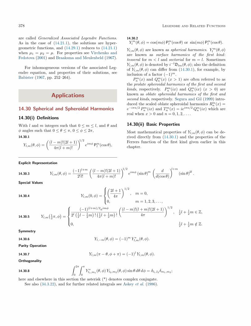
378 Legendre and Related Functions
are called Generalized Associated Legendre Functions.As in the case of (14.21.1), the solutions are hyper-geometric functions, and (14.29.1) reduces to (14.21.1)when µ1 = µ2 = µ. For properties see Virchenko andFedotova (2001) and Braaksma and Meulenbeld (1967).
For inhomogeneous versions of the associated Leg-endre equation, and properties of their solutions, seeBabister (1967, pp. 252–264).
Applications
14.30 Spherical and Spheroidal Harmonics
14.30(i) Definitions
With l and m integers such that 0 ≤ m ≤ l, and θ andφ angles such that 0 ≤ θ ≤ π, 0 ≤ φ ≤ 2π,14.30.1
Yl,m(θ, φ) =(
(l −m)!(2l + 1)4π(l +m)!
)1/2eimφ Pml (cos θ),
14.30.2
Y ml (θ, φ) = cos(mφ) Pml (cos θ) or sin(mφ) Pml (cos θ).
Yl,m(θ, φ) are known as spherical harmonics. Y ml (θ, φ)are known as surface harmonics of the first kind :tesseral for m < l and sectorial for m = l. SometimesYl,m(θ, φ) is denoted by i−lDlm(θ, φ); also the definitionof Yl,m(θ, φ) can differ from (14.30.1), for example, byinclusion of a factor (−1)m.
Pmn (x) and Qmn (x) (x > 1) are often referred to asthe prolate spheroidal harmonics of the first and secondkinds, respectively. Pmn (ix) and Qmn (ix) (x > 0) areknown as oblate spheroidal harmonics of the first andsecond kinds, respectively. Segura and Gil (1999) intro-duced the scaled oblate spheroidal harmonics Rmn (x) =e−iπn/2 Pmn (ix) and Tmn (x) = ieiπn/2Qmn (ix) which arereal when x > 0 and n = 0, 1, 2, . . . .
14.30(ii) Basic Properties
Most mathematical properties of Yl,m(θ, φ) can be de-rived directly from (14.30.1) and the properties of theFerrers function of the first kind given earlier in thischapter.
Explicit Representation
14.30.3 Yl,m(θ, φ) =(−1)l+m
2ll!
((l −m)!(2l + 1)
4π(l +m)!
)1/2eimφ (sin θ)m
(d
d(cos θ)
)l+m(sin θ)2l .
Special Values
14.30.4 Yl,m(0, φ) =
(
2l + 14π
)1/2
, m = 0,
0, m = 1, 2, 3, . . . ,
14.30.5 Yl,m(
12π, φ
)=
(−1)(l+m)/2eimφ
2l(
12 l −
12m)
!(
12 l + 1
2m)
!
((l −m)!(l +m)!(2l + 1)
4π
)1/2
, 12 l + 1
2m ∈ Z,
0, 12 l + 1
2m /∈ Z.
Symmetry
14.30.6 Yl,−m(θ, φ) = (−1)m Y ∗l,m(θ, φ).
Parity Operation
14.30.7 Yl,m(π − θ, φ+ π) = (−1)l Yl,m(θ, φ).
Orthogonality
14.30.8
∫ 2π
0
∫ π
0
Y ∗l1,m1(θ, φ)Yl2,m2(θ, φ) sin θ dθ dφ = δl1,l2δm1,m2 ;
here and elsewhere in this section the asterisk (*) denotes complex conjugate.See also (34.3.22), and for further related integrals see Askey et al. (1986).

14.31 Other Applications 379
14.30(iii) Sums
Distributional Completeness
For a series representation of the product of two Diracdeltas in terms of products of spherical harmonics see§1.17(iii).
Addition Theorem
14.30.9
Pl(cos θ1 cos θ2 + sin θ1 sin θ2 cos(φ1 − φ2))
=4π
2l + 1
l∑m=−l
Y ∗l,m(θ1, φ1)Yl,m(θ2, φ2).
See also (18.18.9) and (34.3.19).
14.30(iv) Applications
In general, spherical harmonics are defined as the classof homogeneous harmonic polynomials. See Andrewset al. (1999, Chapter 9). The special class of spheri-cal harmonics Yl,m(θ, φ), defined by (14.30.1), appear inmany physical applications. As an example, Laplace’sequation ∇2W = 0 in spherical coordinates (§1.5(ii)):
14.30.10
1ρ2
∂
∂ρ
(ρ2 ∂W
∂ρ
)+
1ρ2 sin θ
∂
∂θ
(sin θ
∂W
∂θ
)+
1ρ2 sin2 θ
∂2W
∂φ2 = 0,
has solutions W (ρ, θ, φ) = ρl Yl,m(θ, φ), which are ev-erywhere one-valued and continuous.
In the quantization of angular momentum the spher-ical harmonics Yl,m(θ, φ) are normalized solutions of theeigenvalue equation
14.30.11 L2 Yl,m = h̄2l(l + 1)Yl,m,
where h̄ is the reduced Planck’s constant, and L2 is theangular momentum operator in spherical coordinates:
14.30.12 L2 = −h̄2
(1
sin θ∂
∂θ
(sin θ
∂
∂θ
)+
1sin2 θ
∂2
∂φ2
);
see Edmonds (1974, §2.5).For applications in geophysics see Stacey (1977,
§§4.2, 6.3, and 8.1).
14.31 Other Applications
14.31(i) Toroidal Functions
Applications of toroidal functions include expansion ofvacuum magnetic fields in stellarators and tokamaks(van Milligen and López Fraguas (1994)), analytic solu-tions of Poisson’s equation in channel-like geometries(Hoyles et al. (1998)), and Dirichlet problems withtoroidal symmetry (Gil et al. (2000)).
14.31(ii) Conical Functions
The conical functions Pm− 12 +iτ
(x) appear in boundary-value problems for the Laplace equation in toroidal co-ordinates (§14.19(i)) for regions bounded by cones, bytwo intersecting spheres, or by one or two confocal hy-perboloids of revolution (Kölbig (1981)). These func-tions are also used in the Mehler–Fock integral trans-form (§14.20(vi)) for problems in potential and heat the-ory, and in elementary particle physics (Sneddon (1972,Chapter 7) and Braaksma and Meulenbeld (1967)). Theconical functions and Mehler–Fock transform general-ize to Jacobi functions and the Jacobi transform; seeKoornwinder (1984a) and references therein.
14.31(iii) Miscellaneous
Many additional physical applications of Legendre poly-nomials and associated Legendre functions include so-lution of the Helmholtz equation, as well as theLaplace equation, in spherical coordinates (Temme(1996a)), quantum mechanics (Edmonds (1974)), andhigh-frequency scattering by a sphere (Nussenzveig(1965)). See also §18.39.
Legendre functions Pν(x) of complex degree ν ap-pear in the application of complex angular momentumtechniques to atomic and molecular scattering (Connorand Mackay (1979)).
Computation
14.32 Methods of Computation
Essentially the same comments that are made in §15.19concerning the computation of hypergeometric func-tions apply to the functions described in the presentchapter. In particular, for small or moderate valuesof the parameters µ and ν the power-series expansionsof the various hypergeometric function representationsgiven in §§14.3(i)–14.3(iii), 14.19(ii), and 14.20(i) canbe selected in such a way that convergence is stable,and reasonably rapid, especially when the argument ofthe functions is real. In other cases recurrence relations(§14.10) provide a powerful method when applied in astable direction (§3.6); see Olver and Smith (1983) andGautschi (1967).
Other methods include:
• Application of the uniform asymptotic expansionsfor large values of the parameters given in §§14.15and 14.20(vii)–14.20(ix).
• Numerical integration (§3.7) of the defining differ-ential equations (14.2.2), (14.20.1), and (14.21.1).

380 Legendre and Related Functions
• Quadrature (§3.5) of the integral representationsgiven in §§14.12, 14.19(iii), 14.20(iv), and 14.25;see Segura and Gil (1999) and Gil et al. (2000).
• Evaluation (§3.10) of the continued fractions givenin §14.14. See Gil and Segura (2000).
14.33 Tables
• Abramowitz and Stegun (1964, Chapter 8) tabu-lates Pn(x) for n = 0(1)3, 9, 10, x = 0(.01)1, 5–8D; P′n(x) for n = 1(1)4, 9, 10, x = 0(.01)1, 5–7D;Qn(x) and Q′n(x) for n = 0(1)3, 9, 10, x = 0(.01)1,6–8D; Pn(x) and P ′n(x) for n = 0(1)5, 9, 10, x =1(.2)10, 6S; Qn(x) and Q′n(x) for n = 0(1)3, 9, 10,x = 1(.2)10, 6S. (Here primes denote derivativeswith respect to x.)
• Zhang and Jin (1996, Chapter 4) tabulates Pn(x)for n = 2(1)5, 10, x = 0(.1)1, 7D; Pn(cos θ)for n = 1(1)4, 10, θ = 0(5◦)90◦, 8D; Qn(x) forn = 0(1)2, 10, x = 0(.1)0.9, 8S; Qn(cos θ) forn = 0(1)3, 10, θ = 0(5◦)90◦, 8D; Pmn (x) form = 1(1)4, n−m = 0(1)2, n = 10, x = 0, 0.5, 8S;Qmn (x) for m = 1(1)4, n = 0(1)2, 10, 8S; Pmν (cos θ)
for m = 0(1)3, ν = 0(.25)5, θ = 0(15◦)90◦, 5D;Pn(x) for n = 2(1)5, 10, x = 1(1)10, 7S; Qn(x)for n = 0(1)2, 10, x = 2(1)10, 8S. Correspondingvalues of the derivative of each function are alsoincluded, as are 6D values of the first 5 ν-zerosof Pmν (cos θ) and of its derivative for m = 0(1)4,θ = 10◦, 30◦, 150◦.
• Belousov (1962) tabulates Pmn (cos θ) (normalized)for m = 0(1)36, n −m = 0(1)56, θ = 0(2.5◦)90◦,6D.
• Žurina and Karmazina (1964, 1965) tabulate theconical functions P− 1
2 +iτ (x) for τ = 0(.01)50,x = −0.9(.1)0.9, 7S; P− 1
2 +iτ (x) for τ = 0(.01)50,x = 1.1(.1)2(.2)5(.5)10(10)60, 7D. Auxiliary ta-bles are included to facilitate computation forlarger values of τ when −1 < x < 1.
• Žurina and Karmazina (1963) tabulates the con-ical functions P1
− 12 +iτ
(x) for τ = 0(.01)25, x =
−0.9(.1)0.9, 7S; P 1− 1
2 +iτ(x) for τ = 0(.01)25, x =
1.1(.1)2(.2)5(.5)10(10)60, 7S. Auxiliary tables areincluded to assist computation for larger values ofτ when −1 < x < 1.
For tables prior to 1961 see Fletcher et al. (1962)and Lebedev and Fedorova (1960).
14.34 Software
See http://dlmf.nist.gov/14.34.
References
General References
The main reference used in writing this chapter isOlver (1997b). For additional bibliographic reading seeErdélyi et al. (1953a, Chapter III), Hobson (1931), Jef-freys and Jeffreys (1956), MacRobert (1967), Magnuset al. (1966), Robin (1957, 1958, 1959), Snow (1952),Szegö (1967), Temme (1996a), and Wong (1989).
Sources
The following list gives the references or other indica-tions of proofs that were used in constructing the varioussections of this chapter. These sources supplement thereferences that are quoted in the text.
§14.2 For §§14.2(i), 14.2(ii) see Olver (1997b, pp. 169).For §14.2(iii) see Olver (1997b, p. 172) for the pairP−µν (x) and Qµ
ν (x). The result for P−µν (x) andP−µν (−x) follows from the fact that when <µ ≥ 0,P−µν (x) is recessive as x → 1− and P−µν (−x) isrecessive as x → −1+; see §14.8(i). For §14.2(iv)see Olver (1997b, p. 172) for (14.2.4), (14.2.5); theother results may be derived in a similar manner,or by application of the connection formulas in§14.9.
§14.3 For (14.3.1)–(14.3.4) see Olver (1997b, pp. 159,186). The version of (14.3.4) given in Hob-son (1931, p. 386) has an error. For (14.3.5)use (14.3.1) and (14.9.3). For (14.3.8) see Olver(1997b, p. 159, Eq. (9.05)). For (14.3.11) and(14.3.12) see Olver (1997b, p. 187). For (14.3.16)–(14.3.20) see Erdélyi et al. (1953a, pp. 123–139).For (14.3.21) combine (14.3.22) and (14.23.4). For(14.3.22) see Erdélyi et al. (1953a, p. 175). For(14.3.23) see (14.3.6) and Olver (1997b, p. 167).
§14.4 These graphics were produced at NIST.
§14.5 (14.5.1)–(14.5.4) may be derived from (14.3.11)–(14.3.14) and also (14.10.4) with P replaced by Q.For (14.5.5)–(14.5.10) use §14.7(i). For (14.5.11)–(14.5.19) see Erdélyi et al. (1953a, p. 150).(14.5.20)–(14.5.27) are given in Magnus et al.(1966, p. 173): to verify these compare the hyper-geometric representations of the Legendre func-tions and elliptic integrals (§§14.3 and 19.5).
§14.6 See Erdélyi et al. (1953a, pp. 148–149). For(14.6.5) combine (14.3.10) and (14.6.4).

References 381
§14.7 Olver (1997b, pp. 174, 181–182, 188). For(14.7.17), (14.7.18) use (14.9.8), (14.9.10). For(14.7.19)–(14.7.22) see Erdélyi et al. (1953a,p. 154) and Olver (1997b, pp. 51, 85).
§14.8 Olver (1997b, pp. 171, 173, 186), Erdélyi et al.(1953a, p. 163). (14.8.5) may be derived from(14.8.1), (14.9.2). (14.8.10) may be derived from(14.8.7), (14.9.12). (14.8.16) may be derived from(14.8.15), (14.9.12).
§14.9 Olver (1997b, pp. 171, 174, 186, 188). For(14.9.3), (14.9.4) use (14.9.1), (14.9.2). For(14.9.17) use (14.9.14), (14.9.16).
§14.10 Erdélyi et al. (1953a, pp. 160–161).
§14.11 (14.11.1) may be derived from (14.3.1).(14.11.2) may be derived from (14.9.10) and(14.11.1). (14.11.4) may be derived from (14.3.1)and the hypergeometric expansion for Qν(x)(Hobson (1931, §132)). (14.11.5) may be derivedfrom (14.9.8), (14.9.10), and (14.11.4).
§14.12 Erdélyi et al. (1953a, pp. 155–159), Olver(1997b, pp. 181–183, 185).
§14.13 Erdélyi et al. (1953a, pp. 146, 151).
§14.14 (14.14.1) follows from (14.10.6). (14.14.3)follows from (14.10.3), with Pµν (x) replaced byQµν (x). For further details see Gil et al. (2000).
§14.15 Dunster (2003b), Olver (1997b, pp. 463–469),Boyd and Dunster (1986). (14.15.1) may be de-rived from (14.3.1) and §15.12(ii). For (14.15.24)–(14.15.31) see Olver (1975b).
§14.16 Hobson (1931, pp. 386–389, 399–401).
§14.17 Erdélyi et al. (1953a, pp. 170–172), Olver(1997b, pp. 188–189). (14.17.1)–(14.17.4) may beverified by differentiation and using the recurrencerelations (§14.10). (14.17.7), (14.17.9) may be de-rived from (14.9.3), (14.17.6), (14.17.8). The ver-sion of (14.17.16) given in Erdélyi et al. (1953a,p. 171, Eq. (18)) is incorrect. For (14.17.17) seeDin (1981).
§14.18 Erdélyi et al. (1953a, pp. 162, 167–169), Olver(1997b, p. 183). Errors in Erdélyi et al. (1953a,
pp. 168–169) have been corrected. (14.18.2) maybe derived from (14.7.16), (14.9.3), (14.18.1).(14.18.8) may be derived from (14.7.17), (14.18.9).
§14.19 Erdélyi et al. (1953a, pp. 156–157, 166,173). For (14.19.7), (14.19.8) combine (14.9.16),(14.9.17) with (14.9.11)–(14.9.13).
§14.20 (14.20.3) follows from (14.9.10), (14.20.2).(14.20.4), (14.20.5) follow from (14.2.3), (14.20.3).(14.20.6) follows from (14.3.10), (14.9.12).(14.20.7), (14.20.8) follow from §14.8(i) and(14.20.3). (14.20.9) follows from (14.12.1). For(14.20.10) see Erdélyi et al. (1953a, p. 174).For (14.20.11)–(14.20.14) see Braaksma andMeulenbeld (1967). For (14.20.15) see Olver(1997b, p. 473). (14.20.16) may be derived from(14.20.18). For §§14.20(viii), 14.20(ix) see Dun-ster (1991, Eqs. (5.11), (5.14) have been cor-rected). The graphs were produced at NIST.
§14.21 Olver (1997b, pp. 169–185), Erdélyi et al.(1953a, Chapter 3).
§14.22 These graphics were produced at NIST.
§14.23 For (14.23.1), (14.23.5) see Olver (1997b,p. 185). For (14.23.7) see Dunster (1991).(14.23.2) may be derived from (14.23.4), (14.24.2).(14.23.3) may be derived from (14.3.11), (14.3.12),(14.9.14). (14.23.4) may be derived from(14.23.1). (14.23.6) may be derived from(14.23.1), (14.23.2).
§14.24 Olver (1997b, p, 179).
§14.25 For (14.25.1) see Olver (1997b, p. 179). For(14.25.2) see Erdélyi et al. (1953a, p. 155).
§14.27 Hobson (1931, pp. 391–399).
§14.28 Erdélyi et al. (1953a, p. 168) or Olver (1997b,p. 473).
§14.30 Edmonds (1974, pp. 20–24, 63). (Note thatEdmonds’ Pml (x) differs by a factor (−1)m fromPml (x).) (14.30.4) may be derived from (14.8.1),(14.8.2), (14.30.1). (14.30.5) may be derived from(14.5.1), (14.30.1). (14.30.7) may be derived from(14.7.17), (14.30.1). (14.30.3) also follows from(14.30.1), (14.7.10).


Chapter 15
Hypergeometric FunctionA. B. Olde Daalhuis1
Notation 38415.1 Special Notation . . . . . . . . . . . . . 384
Properties 38415.2 Definitions and Analytical Properties . . . 38415.3 Graphics . . . . . . . . . . . . . . . . . . 38515.4 Special Cases . . . . . . . . . . . . . . . 38615.5 Derivatives and Contiguous Functions . . 38715.6 Integral Representations . . . . . . . . . 38815.7 Continued Fractions . . . . . . . . . . . . 38915.8 Transformations of Variable . . . . . . . . 39015.9 Relations to Other Functions . . . . . . . 39315.10 Hypergeometric Differential Equation . . 39415.11 Riemann’s Differential Equation . . . . . 396
15.12 Asymptotic Approximations . . . . . . . . 39615.13 Zeros . . . . . . . . . . . . . . . . . . . 39815.14 Integrals . . . . . . . . . . . . . . . . . . 39815.15 Sums . . . . . . . . . . . . . . . . . . . 39915.16 Products . . . . . . . . . . . . . . . . . . 399
Applications 39915.17 Mathematical Applications . . . . . . . . 39915.18 Physical Applications . . . . . . . . . . . 400
Computation 40015.19 Methods of Computation . . . . . . . . . 40015.20 Software . . . . . . . . . . . . . . . . . . 401
References 401
1School of Mathematics, Edinburgh University, Edinburgh, United Kingdom.Acknowledgments: This chapter is based in part on Chapter 15 of Abramowitz and Stegun (1964) by Fritz Oberhettinger. The
author thanks Richard Askey and Simon Ruijsenaars for many helpful recommendations.Copyright c© 2009 National Institute of Standards and Technology. All rights reserved.
383

384 Hypergeometric Function
Notation
15.1 Special Notation
(For other notation see pp. xiv and 873.)
x real variable.z = x+ iy complex variable.a, b, c real or complex parameters.k, `,m, n integers.s nonnegative integer.δ arbitrary small positive constant.Γ(z) gamma function (§5.2(i)).ψ(z) Γ′(z)/Γ(z) .
Unless indicated otherwise primes denote derivativeswith respect to the variable.
We use the following notations for the hypergeomet-ric function:
15.1.1 2F1(a, b; c; z) = F (a, b; c; z) = F
(a, b
c; z),
and also15.1.2
F (a, b; c; z)Γ(c)
= F(a, b; c; z) = F(a, b
c; z)
= 2F1(a, b; c; z),
(Olver (1997b, Chapter 5)).
Properties
15.2 Definitions and Analytical Properties
15.2(i) Gauss Series
The hypergeometric function F (a, b; c; z) is defined bythe Gauss series15.2.1
F (a, b; c; z) =∞∑s=0
(a)s(b)s(c)ss!
zs
= 1 +ab
cz +
a(a+ 1)b(b+ 1)c(c+ 1)2!
z2 + · · ·
=Γ(c)
Γ(a) Γ(b)
∞∑s=0
Γ(a+ s) Γ(b+ s)Γ(c+ s)s!
zs,
on the disk |z| < 1, and by analytic continuation else-where. In general, F (a, b; c; z) does not exist when
c = 0,−1,−2, . . . . The branch obtained by introduc-ing a cut from 1 to +∞ on the real z-axis, that is, thebranch in the sector |ph(1− z)| ≤ π, is the principalbranch (or principal value) of F (a, b; c; z).
For all values of c
15.2.2 F(a, b; c; z) =∞∑s=0
(a)s(b)sΓ(c+ s)s!
zs, |z| < 1,
again with analytic continuation for other values of z,and with the principal branch defined in a similar way.
Except where indicated otherwise principal branchesof F (a, b; c; z) and F(a, b; c; z) are assumed throughoutthis Handbook.
The difference between the principal branches on thetwo sides of the branch cut (§4.2(i)) is given by
15.2.3
F(a, b
c;x+ i0
)− F
(a, b
c;x− i0
)=
2πiΓ(a) Γ(b)
(x− 1)c−a−b F(c− a, c− bc− a− b+ 1
; 1− x)
,
x > 1.
On the circle of convergence, |z| = 1, the Gauss se-ries:
(a) Converges absolutely when <(c− a− b) > 0.
(b) Converges conditionally when −1 <<(c− a− b) ≤ 0 and z = 1 is excluded.
(c) Diverges when <(c− a− b) ≤ −1.
For the case z = 1 see also §15.4(ii).
15.2(ii) Analytic Properties
The principal branch of F(a, b; c; z) is an entire func-tion of a, b, and c. The same is true of other branches,provided that z = 0, 1, and∞ are excluded. As a multi-valued function of z, F(a, b; c; z) is analytic everywhereexcept for possible branch points at z = 0, 1, and ∞.The same properties hold for F (a, b; c; z), except thatas a function of c, F (a, b; c; z) in general has poles atc = 0,−1,−2, . . . .
Because of the analytic properties with respect to a,b, and c, it is usually legitimate to take limits in for-mulas involving functions that are undefined for certainvalues of the parameters.

15.3 Graphics 385
For example, when a = −m, m = 0, 1, 2, . . . , andc 6= 0,−1,−2, . . . , F (a, b; c; z) is a polynomial:
15.2.4
F (−m, b; c; z)
=m∑n=0
(−m)n(b)n(c)nn!
zn =m∑n=0
(−1)n(m
n
)(b)n(c)n
zn.
This formula is also valid when c = −m − `, ` =0, 1, 2, . . . , provided that we use the interpretation
15.2.5 F
(−m, b−m− `
; z)
= limc→−m−`
(lim
a→−mF
(a, b
c; z))
,
and not
15.2.6 F
(−m, b−m− `
; z)
= lima→−m
F
(a, b
a− `; z),
which is sometimes used in the literature. (Both in-terpretations give solutions of the hypergeometric dif-ferential equation (15.10.1), as does F(a, b; c; z), whichis analytic at c = 0,−1,−2, . . . .) For illustration seeFigures 15.3.6 and 15.3.7.
In the case c = −m the right-hand side of (15.2.4)becomes the first m + 1 terms of the Maclaurin seriesfor (1− z)−b.
15.3 Graphics
15.3(i) Graphs
Figure 15.3.1: F(
43 ,
916 ; 14
5 ;x),−100 ≤ x ≤ 1. Figure 15.3.2: F (5,−10; 1;x),−0.023 ≤ x ≤ 1.
Figure 15.3.3: F (1,−10; 10;x),−3 ≤ x ≤ 1. Figure 15.3.4: F (5, 10; 1;x),−1 ≤ x ≤ 0.022.

386 Hypergeometric Function
15.3(ii) Surfaces
In Figures 15.3.5 and 15.3.6, height corresponds to the absolute value of the function and color to the phase. Seealso p. xiv.
Figure 15.3.5: F(
43 ,
916 ; 14
5 ;x+ iy), 0 ≤ x ≤ 2,−0.5 ≤
y ≤ 0.5. (There is a cut along the real axis from 1 to∞.)
Figure 15.3.6: F(−3, 3
5 ;u+ iv; 12
),−6 ≤ u ≤ 2,−2 ≤
v ≤ 2. (With c = u + iv the only poles occur at c =0,−1,−2; compare §15.2(ii).)
Figure 15.3.7: |F(−3, 3
5 ;u+ iv; 12
)|,−6 ≤ u ≤ 2,−2 ≤
v ≤ 2.
15.4 Special Cases
15.4(i) Elementary Functions
The following results hold for principal branches when|z| < 1, and by analytic continuation elsewhere. Excep-tions are (15.4.8) and (15.4.10), that hold for |z| < π/4 ,and (15.4.12), (15.4.14), and (15.4.16), that hold for|z| < π/2 .
15.4.1 F (1, 1; 2; z) = −z−1 ln(1− z),
15.4.2 F(
12 , 1; 3
2 ; z2)
=12z
ln(
1 + z
1− z
),
15.4.3 F(
12 , 1; 3
2 ;−z2)
= z−1 arctan z,
15.4.4 F(
12 ,
12 ; 3
2 ; z2)
= z−1 arcsin z,
15.4.5 F(
12 ,
12 ; 3
2 ;−z2)
= z−1 ln(z +
√1 + z2
).
15.4.6 F (a, b; b; z) = (1− z)−a;compare §15.2(ii).
15.4.7 F(a, 1
2 + a; 12 ; z2
)= 1
2
((1 + z)−2a + (1− z)−2a
),
15.4.8 F(a, 1
2 + a; 12 ;− tan2 z
)= (cos z)2a cos(2az).
15.4.9
F(a, 1
2 + a; 32 ; z2
)=
1(2− 4a)z
((1 + z)1−2a − (1− z)1−2a
),
15.4.10
F(a, 1
2 + a; 32 ;− tan2 z
)= (cos z)2a sin((1− 2a)z)
(1− 2a) sin z.
15.4.11
F(−a, a; 1
2 ;−z2)
= 12
((√1 + z2 + z
)2a+(√
1 + z2 − z)2a)
,
15.4.12 F(−a, a; 1
2 ; sin2 z)
= cos(2az).
15.4.13
F(a, 1− a; 1
2 ;−z2)
=1
2√
1 + z2
((√1 + z2 + z
)2a−1
+(√
1 + z2 − z)2a−1
),
15.4.14 F(a, 1− a; 1
2 ; sin2 z)
=cos((2a− 1)z)
cos z.

15.5 Derivatives and Contiguous Functions 387
15.4.15
F(a, 1− a; 3
2 ;−z2)
=1
(2− 4a)z
((√1 + z2 + z
)1−2a
−(√
1 + z2 − z)1−2a
),
15.4.16 F(a, 1− a; 3
2 ; sin2 z)
=sin((2a− 1)z)(2a− 1) sin z
.
15.4.17 F(a, 1
2 + a; 1 + 2a; z)
=(
12 + 1
2
√1− z
)−2a,
15.4.18 F(a, 1
2 + a; 2a; z)
=1√
1− z(
12 + 1
2
√1− z
)1−2a.
15.4.19 F (a+ 1, b; a; z) = (1−(1−(b/a ))z) (1−z)−1−b.
For an extensive list of elementary representationssee Prudnikov et al. (1990, pp. 468–488).
15.4(ii) Argument Unity
If <(c− a− b) > 0, then
15.4.20 F (a, b; c; 1) =Γ(c) Γ(c− a− b)Γ(c− a) Γ(c− b)
.
If c = a+ b, then
15.4.21 limz→1−
F (a, b; a+ b; z)− ln(1− z)
=Γ(a+ b)Γ(a) Γ(b)
.
If <(c− a− b) = 0 and c 6= a+ b, then
15.4.22
limz→1−
(1− z)a+b−c(F (a, b; c; z)
− Γ(c) Γ(c− a− b)Γ(c− a) Γ(c− b)
)=
Γ(c) Γ(a+ b− c)Γ(a) Γ(b)
.
If <(c− a− b) < 0, then
15.4.23 limz→1−
F (a, b; c; z)(1− z)c−a−b
=Γ(c) Γ(a+ b− c)
Γ(a) Γ(b).
Chu–Vandermonde Identity
15.4.24 F (−n, b; c; 1) =(c− b)n
(c)n, n = 0, 1, 2, . . . .
Dougall’s Bilateral Sum
This is a generalization of (15.4.20). If a, b are not in-tegers and <(c+ d− a− b) > 1, then
15.4.25∞∑
n=−∞
Γ(a+ n) Γ(b+ n)Γ(c+ n) Γ(d+ n)
=π2
sin(πa) sin(πb)Γ(c+ d− a− b− 1)
Γ(c− a) Γ(d− a) Γ(c− b) Γ(d− b).
15.4(iii) Other Arguments
15.4.26 F (a, b; a− b+ 1;−1) =Γ(a− b+ 1) Γ
(12a+ 1
)Γ(a+ 1) Γ
(12a− b+ 1
) .15.4.27 F (1, a; a+ 1;−1) = 1
2a(ψ(
12a+ 1
2
)− ψ
(12a)).
15.4.28
F(a, b; 1
2a+ 12b+ 1
2 ; 12
)=√π
Γ(
12a+ 1
2b+ 12
)Γ(
12a+ 1
2
)Γ(
12b+ 1
2
) .15.4.29
F(a, b; 1
2a+ 12b+ 1; 1
2
)=
2√π
a− bΓ(
12a+ 1
2b+ 1)
×
(1
Γ(
12a)
Γ(
12b+ 1
2
)− 1
Γ(
12a+ 1
2
)Γ(
12b)) .
15.4.30 F(a, 1− a; b; 1
2
)=
21−b√π Γ(b)Γ(
12a+ 1
2b)
Γ(
12b−
12a+ 1
2
) .15.4.31
F(a, 1
2 + a; 32 − 2a;− 1
3
)=(
89
)−2a Γ(
43
)Γ(
32 − 2a
)Γ(
32
)Γ(
43 − 2a
) .15.4.32
F(a, 1
2 + a; 56 + 2
3a; 19
)=√π
(34
)a Γ(
56 + 2
3a)
Γ(
12 + 1
3a)
Γ(
56 + 1
3a) .
15.4.33
F(
3a, 13 + a; 2
3 + 2a; e iπ/3)
=√πe iπa/2
(1627
)(3a+1)/6 Γ(
56 + a
)Γ(
23 + a
)Γ(
23
) .15.5 Derivatives and Contiguous Functions
15.5(i) Differentiation Formulas
15.5.1d
dzF (a, b; c; z) =
ab
cF (a+ 1, b+ 1; c+ 1; z),
15.5.2
dn
dznF (a, b; c; z) =
(a)n(b)n(c)n
F (a+ n, b+ n; c+ n; z).
15.5.3
(zd
dzz
)n (za−1 F (a, b; c; z)
)= (a)nz
a+n−1 F (a+ n, b; c; z).
15.5.4
dn
dzn(zc−1 F (a, b; c; z)
)= (c− n)nz
c−n−1 F (a, b; c− n; z).
15.5.5(zd
dzz
)n (zc−a−1(1− z)a+b−c F (a, b; c; z)
)= (c− a)nz
c−a+n−1(1− z)a−n+b−c F (a− n, b; c; z).

388 Hypergeometric Function
15.5.6dn
dzn((1− z)a+b−c F (a, b; c; z)
)=
(c− a)n(c− b)n(c)n
(1− z)a+b−c−n F (a, b; c+ n; z).
15.5.7((1− z) d
dz(1− z)
)n ((1− z)a−1 F (a, b; c; z)
)= (−1)n
(a)n(c− b)n(c)n
(1− z)a+n−1
× F (a+ n, b; c+ n; z).
15.5.8((1− z) d
dz(1− z)
)n (zc−1(1− z)b−c F (a, b; c; z)
)= (c− n)nz
c−n−1(1− z)b−c+n F (a− n, b; c− n; z).
15.5.9
dn
dzn(zc−1(1− z)a+b−c F (a, b; c; z)
)= (c− n)nz
c−n−1(1− z)a+b−c−n
× F (a− n, b− n; c− n; z).Other versions of several of the identities in this sub-
section can be constructed with the aid of the operatoridentity
15.5.10
(zd
dzz
)n= zn
dn
dznzn, n = 1, 2, 3, . . . .
See Erdélyi et al. (1953a, pp. 102–103).
15.5(ii) Contiguous Functions
The six functions F (a± 1, b; c; z), F (a, b± 1; c; z),F (a, b; c± 1; z) are said to be contiguous to F (a, b; c; z).
15.5.11
(c− a)F (a− 1, b; c; z)+ (2a− c+ (b− a)z)F (a, b; c; z)+ a(z − 1)F (a+ 1, b; c; z) = 0,
15.5.12(b− a)F (a, b; c; z) + aF (a+ 1, b; c; z)− b F (a, b+ 1; c; z) = 0,
15.5.13
(c− a− b)F (a, b; c; z)+ a(1− z)F (a+ 1, b; c; z)− (c− b)F (a, b− 1; c; z) = 0,
15.5.14
c (a+ (b− c)z)F (a, b; c; z)− ac(1− z)F (a+ 1, b; c; z)+ (c− a)(c− b)z F (a, b; c+ 1; z) = 0,
15.5.15(c− a− 1)F (a, b; c; z) + aF (a+ 1, b; c; z)− (c− 1)F (a, b; c− 1; z) = 0,
15.5.16c(1− z)F (a, b; c; z)− c F (a− 1, b; c; z)
+ (c− b)z F (a, b; c+ 1; z) = 0,
15.5.17
(a− 1 + (b+ 1− c)z)F (a, b; c; z)+ (c− a)F (a− 1, b; c; z)− (c− 1)(1− z)F (a, b; c− 1; z) = 0,
15.5.18
c(c− 1)(z − 1)F (a, b; c− 1; z)+ c (c− 1− (2c− a− b− 1)z)F (a, b; c; z)+ (c− a)(c− b)z F (a, b; c+ 1; z) = 0.
By repeated applications of (15.5.11)–(15.5.18) anyfunction F (a+ k, b+ `; c+m; z), in which k, `,m areintegers, can be expressed as a linear combination ofF (a, b; c; z) and any one of its contiguous functions, withcoefficients that are rational functions of a, b, c, and z.
An equivalent equation to the hypergeometric differ-ential equation (15.10.1) is15.5.19
z(1− z)(a+ 1)(b+ 1)F (a+ 2, b+ 2; c+ 2; z)+ (c− (a+ b+ 1)z)(c+ 1)F (a+ 1, b+ 1; c+ 1; z)− c(c+ 1)F (a, b; c; z) = 0.
Further contiguous relations include:15.5.20
z(1− z) (dF (a, b; c; z)/dz )= (c− a)F (a− 1, b; c; z) + (a− c+ bz)F (a, b; c; z)= (c− b)F (a, b− 1; c; z) + (b− c+ az)F (a, b; c; z),
15.5.21
c(1− z) (dF (a, b; c; z)/dz )= (c−a)(c−b)F (a, b; c+ 1; z)+c(a+b−c)F (a, b; c; z).
15.6 Integral Representations
The function F(a, b; c; z) (not F (a, b; c; z)) has the fol-lowing integral representations:15.6.1
1Γ(b) Γ(c− b)
∫ 1
0
tb−1(1− t)c−b−1
(1− zt)adt, <c > <b > 0.
15.6.2
Γ(1 + b− c)2πiΓ(b)
∫ (1+)
0
tb−1(t− 1)c−b−1
(1− zt)adt,
c− b 6= 1, 2, 3, . . . , <b > 0.
15.6.3e−bπi
Γ(1− b)2πiΓ(c− b)
∫ (0+)
∞
tb−1(t+ 1)a−c
(t− zt+ 1)adt,
b 6= 1, 2, 3, . . . , <(c− b) > 0.
15.6.4e−bπi
Γ(1− b)2πiΓ(c− b)
∫ (0+)
1
tb−1(1− t)c−b−1
(1− zt)adt,
b 6= 1, 2, 3, . . . , <(c− b) > 0.
15.6.5
e−cπi Γ(1− b) Γ(1 + b− c)
× 14π2
∫ (0+,1+,0−,1−)
A
tb−1(1− t)c−b−1
(1− zt)adt,
b, c− b 6= 1, 2, 3, . . . .
15.6.6
12πiΓ(a) Γ(b)
∫ i∞
−i∞
Γ(a+ t) Γ(b+ t) Γ(−t)Γ(c+ t)
(−z)t dt,
a, b 6= 0,−1,−2, . . . .

15.7 Continued Fractions 389
15.6.7
12πiΓ(a) Γ(b) Γ(c− a) Γ(c− b)
∫ i∞
−i∞Γ(a+ t) Γ(b+ t) Γ(c− a− b− t) Γ(−t)(1− z)t dt,
a, b, c− a, c− b 6= 0,−1,−2, . . . .
15.6.81
Γ(c− d)
∫ 1
0
F(a, b; d; zt)td−1(1− t)c−d−1 dt, <c > <d > 0.
15.6.9
∫ 1
0
td−1(1− t)c−d−1
(1− zt)a+b−λ F(λ− a, λ− b
d; zt)
F(a+ b− λ, λ− d
c− d;
(1− t)z1− zt
)dt, <c > <d > 0.
These representations are valid when |ph(1− z)| < π,except (15.6.6) which holds for |ph(−z)| < π. In allcases the integrands are continuous functions of t onthe integration paths, except possibly at the endpoints.In addition:
In (15.6.1) all functions in the integrand assumetheir principal values.
In (15.6.2) the point 1/z lies outside the integrationcontour, tb−1 and (t − 1)c−b−1 assume their principalvalues where the contour cuts the interval (1,∞), and(1− zt)a = 1 at t = 0.
In (15.6.3) the point 1/(z − 1) lies outside the in-tegration contour, the contour cuts the real axis be-tween t = −1 and 0, at which point ph t = π andph(1 + t) = 0.
In (15.6.4) the point 1/z lies outside the integrationcontour, and at the point where the contour cuts thenegative real axis ph t = π and ph(1− t) = 0.
In (15.6.5) the integration contour starts and termi-nates at a point A on the real axis between 0 and 1.It encircles t = 0 and t = 1 once in the positive di-rection, and then once in the negative direction. SeeFigure 15.6.1. At the starting point ph t and ph(1− t)are zero. Compare Figure 5.12.3.
In (15.6.6) the integration contour separates thepoles of Γ(a+ t) and Γ(b+ t) from those of Γ(−t), and(−z)t has its principal value.
In (15.6.7) the integration contour separatesthe poles of Γ(a+ t) and Γ(b+ t) from those ofΓ(c− a− b− t) and Γ(−t), and (1 − z)t has its prin-cipal value.
In each of (15.6.8) and (15.6.9) all functions in theintegrand assume their principal values.
Figure 15.6.1: t-plane. Contour of integration in(15.6.5).
15.7 Continued Fractions
If |ph(1− z)| < π, then
15.7.1F(a, b; c; z)
F(a, b+ 1; c+ 1; z)= t0 −
u1z
t1 −u2z
t2 −u3z
t3 −· · · ,
where
15.7.2tn = c+ n, u2n+1 = (a+ n)(c− b+ n),u2n = (b+ n)(c− a+ n).
If |z| < 1, then
15.7.3F(a, b; c; z)
F(a, b+ 1; c+ 1; z)= v0−
w1
v1 −w2
v2 −w3
v3 −· · · ,
where
15.7.4vn = c+ n+ (b− a+ n+ 1)z,wn = (b+ n)(c− a+ n)z.
If <z < 12 , then
15.7.5
F(a, b; c; z)F(a+ 1, b+ 1; c+ 1; z)
= x0 +y1
x1 +y2
x2 +y3
x3 +· · ·,
where
15.7.6xn = c+ n− (a+ b+ 2n+ 1)z,yn = (a+ n)(b+ n)z(1− z).
See also Cuyt et al. (2008, pp. 295–309).

390 Hypergeometric Function
15.8 Transformations of Variable
15.8(i) Linear Transformations
All functions in this subsection and §15.8(ii) assume their principal values.
15.8.1F(a, b
c; z)
= (1− z)−a F(a, c− b
c;
z
z − 1
)= (1− z)−b F
(c− a, b
c;
z
z − 1
)= (1− z)c−a−b F
(c− a, c− b
c; z)
,
|ph(1− z)| < π.
15.8.2
sin(π(b− a))π
F(a, b
c; z)
=(−z)−a
Γ(b) Γ(c− a)F(a, a− c+ 1a− b+ 1
;1z
)− (−z)−b
Γ(a) Γ(c− b)F(b, b− c+ 1b− a+ 1
;1z
), |ph(−z)| < π.
15.8.3
sin(π(b− a))π
F(a, b
c; z)
=(1− z)−a
Γ(b) Γ(c− a)F(a, c− ba− b+ 1
;1
1− z
)− (1− z)−b
Γ(a) Γ(c− b)F(b, c− ab− a+ 1
;1
1− z
),
|ph(−z)| < π.15.8.4
sin(π(c− a− b))π
F(a, b
c; z)
=1
Γ(c− a) Γ(c− b)F(
a, b
a+ b− c+ 1; 1− z
)− (1− z)c−a−b
Γ(a) Γ(b)F(c− a, c− bc− a− b+ 1
; 1− z)
,
|ph z| < π, |ph(1− z)| < π.15.8.5
sin(π(c− a− b))π
F(a, b
c; z)
=z−a
Γ(c− a) Γ(c− b)F(a, a− c+ 1a+ b− c+ 1
; 1− 1z
)− (1− z)c−a−bza−c
Γ(a) Γ(b)F(c− a, 1− ac− a− b+ 1
; 1− 1z
), |ph z| < π, |ph(1− z)| < π.
15.8(ii) Linear Transformations: Limiting Cases
With m = 0, 1, 2, . . . , polynomial cases of (15.8.2)–(15.8.5) are given by
15.8.6 F
(−m, bc
; z)
=(b)m(c)m
(−z)m F(−m, 1− c−m
1− b−m;
1z
)=
(b)m(c)m
(1− z)m F(−m, c− b1− b−m
;1
1− z
),
15.8.7 F
(−m, bc
; z)
=(c− b)m
(c)mF
(−m, b
b− c−m+ 1; 1− z
)=
(c− b)m(c)m
zm F
(−m, 1− c−mb− c−m+ 1
; 1− 1z
),
with the understanding that if b = −`, ` = 0, 1, 2, . . . , then m ≤ `.When b− a is an integer limits are taken in (15.8.2) and (15.8.3) as follows.If b− a is a nonnegative integer, then
15.8.8
F(a, a+m
c; z)
=(−z)−a
Γ(a+m)
m−1∑k=0
(a)k(m− k − 1)!k! Γ(c− a− k)
z−k +(−z)−a
Γ(a)
∞∑k=0
(a+m)kk!(k +m)! Γ(c− a− k −m)
(−1)kz−k−m
× (ln(−z) + ψ(k + 1) + ψ(k +m+ 1)− ψ(a+ k +m)− ψ(c− a− k −m)) ,|z| > 1, |ph(−z)| < π,
15.8.9
F(a, a+m
c; z)
=(1− z)−a
Γ(a+m) Γ(c− a)
m−1∑k=0
(a)k(c− a−m)k(m− k − 1)!k!
(z − 1)−k
+(−1)m(1− z)−a−m
Γ(a) Γ(c− a−m)
∞∑k=0
(a+m)k(c− a)kk!(k +m)!
(1− z)−k
× (ln(1− z) + ψ(k + 1) + ψ(k +m+ 1)− ψ(a+ k +m)− ψ(c− a+ k)),|z − 1| > 1, |ph(1− z)| < π.
In (15.8.8) when c − a − k − m is a nonpositive integer ψ(c− a− k −m)/Γ(c− a− k −m) is interpreted as(−1)m+k+a−c+1(m+ k + a− c)!. Also, if a is a nonpositive integer, then (15.8.6) applies.

15.8 Transformations of Variable 391
Alternatively, if b− a is a negative integer, then we interchange a and b in F(a, b; c; z).In a similar way, when c− a− b is an integer limits are taken in (15.8.4) and (15.8.5) as follows.If c− a− b is a nonnegative integer, then
15.8.10
F(
a, b
a+ b+m; z)
=1
Γ(a+m) Γ(b+m)
m−1∑k=0
(a)k(b)k(m− k − 1)!k!
(z − 1)k − (z − 1)m
Γ(a) Γ(b)
∞∑k=0
(a+m)k(b+m)kk!(k +m)!
(1− z)k
× (ln(1− z)− ψ(k + 1)− ψ(k +m+ 1) + ψ(a+ k +m) + ψ(b+ k +m)) ,|z − 1| < 1, |ph(1− z)| < π,
15.8.11
F(
a, b
a+ b+m; z)
=z−a
Γ(a+m)
m−1∑k=0
(a)k(m− k − 1)!k! Γ(b+m− k)
(1− 1
z
)k− z−a
Γ(a)
∞∑k=0
(a+m)kk!(k +m)! Γ(b− k)
(−1)k(
1− 1z
)k+m
×(
ln(
1− zz
)− ψ(k + 1)− ψ(k +m+ 1) + ψ(a+ k +m) + ψ(b− k)
),
<z > 12 , |ph z| < π, |ph(1− z)| < π.
In (15.8.11) when b − k is a nonpositive integer,ψ(b− k)/Γ(b− k) is interpreted as (−1)k−b+1(k − b)!.Also, if a or b or both are nonpositive integers, then(15.8.7) applies.
Lastly, if c−a− b is a negative integer, then we firstapply the transformation15.8.12
F(a, b; a+ b−m; z) = (1− z)−m F(ã, b̃; ã+ b̃+m; z
),
ã = a−m, b̃ = b−m.
15.8(iii) Quadratic Transformations
A quadratic transformation relates two hypergeometricfunctions, with the variable in one a quadratic functionof the variable in the other, possibly combined with afractional linear transformation.
A necessary and sufficient condition that there ex-ists a quadratic transformation is that at least one ofthe equations shown in Table 15.8.1 is satisfied.
Table 15.8.1: Quadratic transformations of the hyper-geometric function.
Group 1 Group 2 Group 3 Group 4
c = a− b+ 1 a = b+ 12
c = 2a c = b− a+ 1 b = a+ 12 c = 1
2
c = 2b c = 12 (a+ b+ 1) c = a+ b+ 1
2 c = 32
a+ b = 1 c = a+ b− 12
The hypergeometric functions that correspond toGroups 1 and 2 have z as variable. The hypergeomet-ric functions that correspond to Groups 3 and 4 havea nonlinear function of z as variable. The transforma-tion formulas between two hypergeometric functions inGroup 2, or two hypergeometric functions in Group 3,are the linear transformations (15.8.1).
In the equations that follow in this subsection allfunctions take their principal values.
Group 1 −→ Group 3
15.8.13 F
(a, b
2b; z)
=(1− 1
2z)−a
F
(12a,
12a+ 1
2
b+ 12
;(
z
2− z
)2)
, |ph(1− z)| < π,
15.8.14 F
(a, b
2b; z)
= (1− z)−a/2F
(12a, b−
12a
b+ 12
;z2
4z − 4
), |ph(1− z)| < π.
Group 2 −→ Group 3
15.8.15 F
(a, b
a− b+ 1; z)
= (1 + z)−a F( 1
2a,12a+ 1
2
a− b+ 1;
4z(1 + z)2
), |z| < 1,
15.8.16 F
(a, b
a− b+ 1; z)
= (1− z)−a F( 1
2a,12a− b+ 1
2
a− b+ 1;−4z
(1− z)2
), |z| < 1.

392 Hypergeometric Function
15.8.17 F
(a, b
12 (a+ b+ 1)
; z)
= (1− 2z)−a F
(12a,
12a+ 1
212 (a+ b+ 1)
;4z(z − 1)(1− 2z)2
), <z < 1
2 ,
15.8.18 F
(a, b
12 (a+ b+ 1)
; z)
= F
(12a,
12b
12 (a+ b+ 1)
; 4z(1− z)
), <z < 1
2 .
15.8.19 F
(a, 1− a
c; z)
= (1− 2z)1−a−c(1− z)c−1 F
( 12 (a+ c), 1
2 (a+ c− 1)c
;4z(z − 1)(1− 2z)2
), <z < 1
2 ,
15.8.20 F
(a, 1− a
c; z)
= (1− z)c−1 F
( 12 (c− a), 1
2 (a+ c− 1)c
; 4z(1− z))
, <z < 12 .
Group 2 −→ Group 1
15.8.21 F
(a, b
a− b+ 1; z)
=(1 +√z)−2a
F
(a, a− b+ 1
2
2a− 2b+ 1;
4√z
(1 +√z)2
), |ph z| < π, |z| < 1.
15.8.22 F
(a, b
12 (a+ b+ 1)
; z)
=
(√1− z−1 − 1√1− z−1 + 1
)aF
(a, 1
2 (a+ b)a+ b
;4√
1− z−1(√1− z−1 + 1
)2)
, |ph(−z)| < π, <z < 12 .
15.8.23
F
(a, 1− a
c; z)
=(√
1− z−1 − 1)1−a (√
1− z−1 + 1)a−2c+1 (
1− z−1)c−1
F
(c− a, c− 1
2
2c− 1;
4√
1− z−1(√1− z−1 + 1
)2)
,
|ph(−z)| < π, <z < 12 .
Group 2 −→ Group 4
15.8.24
F
(a, b
a− b+ 1; z)
= (1− z)−aΓ(a− b+ 1) Γ
(12
)Γ(
12a+ 1
2
)Γ(
12a− b+ 1
) F( 12a,
12a− b+ 1
212
;(z + 1z − 1
)2)
+ (1 + z)(1− z)−a−1 Γ(a− b+ 1) Γ(− 1
2
)Γ(
12a)
Γ(
12a− b+ 1
2
) F( 12a+ 1
2 ,12a− b+ 132
;(z + 1z − 1
)2)
,
|ph(−z)| < π.
15.8.25
F
(a, b
12 (a+ b+ 1)
; z)
=Γ(
12 (a+ b+ 1)
)Γ(
12
)Γ(
12a+ 1
2
)Γ(
12b+ 1
2
) F( 12a,
12b
12
; (1− 2z)2
)
+ (1− 2z)Γ(
12 (a+ b+ 1)
)Γ(− 1
2
)Γ(
12a)
Γ(
12b) F
(12a+ 1
2 ,12b+ 1
232
; (1− 2z)2
),
|ph z| < π, |ph(1− z)| < π.
15.8.26
F
(a, 1− a
c; z)
= (1− z)c−1 Γ(c) Γ(
12
)Γ(
12 (c− a+ 1)
)Γ(
12c+ 1
2a) F( 1
2c−12a,
12c+ 1
2a−12
12
; (1− 2z)2
)
+ (1− 2z)(1− z)c−1 Γ(c) Γ(− 1
2
)Γ(
12c−
12a)
Γ(
12 (c+ a− 1)
) F( 12c−
12a+ 1
2 ,12c+ 1
2a32
; (1− 2z)2
),
|ph z| < π, |ph(1− z)| < π.
Group 4 −→ Group 2
15.8.27
2 Γ(
12
)Γ(a+ b+ 1
2
)Γ(a+ 1
2
)Γ(b+ 1
2
) F(a, b; 1
2 ; z)
= F(2a, 2b; a+ b+ 1
2 ; 12 −
12
√z)
+ F(2a, 2b; a+ b+ 1
2 ; 12 + 1
2
√z),
|ph z| < π, |ph(1− z)| < π.

15.9 Relations to Other Functions 393
15.8.28
2√z Γ(− 1
2
)Γ(a+ b− 1
2
)Γ(a− 1
2
)Γ(b− 1
2
) F(a, b; 3
2 ; z)
= F(2a− 1, 2b− 1; a+ b− 1
2 ; 12 −
12
√z)
− F(2a− 1, 2b− 1; a+ b− 1
2 ; 12 + 1
2
√z), |ph z| < π, |ph(1− z)| < π.
15.8(iv) Quadratic Transformations (Continued)
When the intersection of two groups in Table 15.8.1 is not empty there exist special quadratic transformations, withonly one free parameter, between two hypergeometric functions in the same group.
Examples
b = 13a+ 1
3 , c = 2b = a− b+ 1 in Groups 1 and 2.(15.8.21) becomes
15.8.29 F
(a, 1
3a+ 13
23a+ 2
3
; z
)=(1 +√z)−2a
F
(a, 2
3a+ 16
43a+ 1
3
;4√z
(1 +√z)2
).
This is a quadratic transformation between two cases in Group 1.We can also use (15.8.13), followed by the inverse of (15.8.15), and obtain
15.8.30(1− 1
2z)−a
F
(12a,
12a+ 1
213a+ 5
6
;(
z
2− z
)2)
= F
(a, 1
3a+ 13
23a+ 2
3
; z
)= (1 + z)−a F
(12a,
12a+ 1
223a+ 2
3
;4z
(1 + z)2
),
which is a quadratic transformation between two cases in Group 3.For further examples see Andrews et al. (1999, pp. 130–132 and 176–177).
15.8(v) Cubic Transformations
Examples
15.8.31 F
(3a, 3a+ 1
2
4a+ 23
; z
)=(1− 9
8z)−2a
F
(a, a+ 1
2
2a+ 56
;27z2(z − 1)(9z − 8)2
), <z < 8
9 .
With ζ = e 2πi/3 (1− z)/(z − e 4πi/3
)
15.8.32
(1− z3
)a(−z)3a
(1
Γ(a+ 2
3
)Γ(
23
) F(a, a+ 13
23
; z−3
)+
e13πi
z Γ(a) Γ(
43
) F(a+ 13 , a+ 2
343
; z−3
))
=3
32a+ 1
2 e12aπi Γ
(a+ 1
3
)(1− ζ)a
2π Γ(2a+ 2
3
)(−ζ)2a
F
(a+ 1
3 , 3a2a+ 2
3
; ζ−1
), |z| > 1, |ph(−z)| < 1
3π.
Ramanujan’s Cubic Transformation
15.8.33
F
(13 ,
23
1; 1−
(1− z1 + 2z
)3)
= (1 + 2z)F( 1
3 ,23
1; z3
),
provided that z lies in the intersection of theopen disks
∣∣z − 14 ±
14
√3i∣∣ < 1
2
√3, or equivalently,
|ph((1− z)/(1 + 2z) )| < π/3. This is used in a cubicanalog of the arithmetic-geometric mean. See Borweinand Borwein (1991), and also Berndt et al. (1995).
For further examples and higher-order transforma-tions see Goursat (1881), Watson (1910), and Vidūnas(2005); see also Erdélyi et al. (1953a, pp. 67 and 113–114).
15.9 Relations to Other Functions
15.9(i) Orthogonal Polynomials
For the notation see §§18.3 and 18.19.
Jacobi
15.9.1
P (α,β)n (x) =
(α+ 1)nn!
F
(−n, n+ α+ β + 1
α+ 1;
1− x2
).
Gegenbauer (or Ultraspherical)
15.9.2 C(λ)n (x) =
(2λ)nn!
F
(−n, n+ 2λλ+ 1
2
;1− x
2
).
15.9.3 C(λ)n (x) = (2x)n
(λ)nn!
F
(− 1
2n,12 (1− n)
1− λ− n;
1x2
).
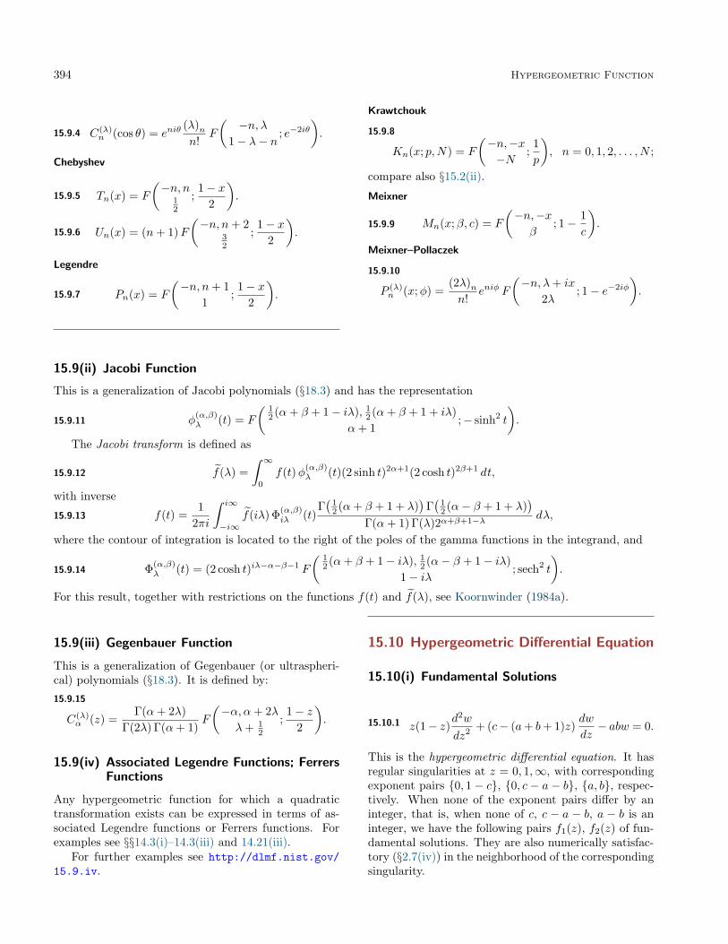
394 Hypergeometric Function
15.9.4 C(λ)n (cos θ) = eniθ
(λ)nn!
F
(−n, λ
1− λ− n; e−2iθ
).
Chebyshev
15.9.5 Tn(x) = F
(−n, n
12
;1− x
2
).
15.9.6 Un(x) = (n+ 1)F(−n, n+ 2
32
;1− x
2
).
Legendre
15.9.7 Pn(x) = F
(−n, n+ 1
1;
1− x2
).
Krawtchouk
15.9.8
Kn(x; p,N) = F
(−n,−x−N
;1p
), n = 0, 1, 2, . . . , N ;
compare also §15.2(ii).
Meixner
15.9.9 Mn(x;β, c) = F
(−n,−xβ
; 1− 1c
).
Meixner–Pollaczek
15.9.10
P (λ)n (x;φ) =
(2λ)nn!
eniφ F
(−n, λ+ ix
2λ; 1− e−2iφ
).
15.9(ii) Jacobi Function
This is a generalization of Jacobi polynomials (§18.3) and has the representation
15.9.11 φ(α,β)λ (t) = F
( 12 (α+ β + 1− iλ), 1
2 (α+ β + 1 + iλ)α+ 1
;− sinh2 t
).
The Jacobi transform is defined as
15.9.12 f̃(λ) =∫ ∞
0
f(t)φ(α,β)λ (t)(2 sinh t)2α+1(2 cosh t)2β+1 dt,
with inverse
15.9.13 f(t) =1
2πi
∫ i∞
−i∞f̃(iλ) Φ(α,β)
iλ (t)Γ(
12 (α+ β + 1 + λ)
)Γ(
12 (α− β + 1 + λ)
)Γ(α+ 1) Γ(λ)2α+β+1−λ dλ,
where the contour of integration is located to the right of the poles of the gamma functions in the integrand, and
15.9.14 Φ(α,β)λ (t) = (2 cosh t)iλ−α−β−1 F
( 12 (α+ β + 1− iλ), 1
2 (α− β + 1− iλ)1− iλ
; sech2 t
).
For this result, together with restrictions on the functions f(t) and f̃(λ), see Koornwinder (1984a).
15.9(iii) Gegenbauer Function
This is a generalization of Gegenbauer (or ultraspheri-cal) polynomials (§18.3). It is defined by:
15.9.15
C(λ)α (z) =
Γ(α+ 2λ)Γ(2λ) Γ(α+ 1)
F
(−α, α+ 2λλ+ 1
2
;1− z
2
).
15.9(iv) Associated Legendre Functions; FerrersFunctions
Any hypergeometric function for which a quadratictransformation exists can be expressed in terms of as-sociated Legendre functions or Ferrers functions. Forexamples see §§14.3(i)–14.3(iii) and 14.21(iii).
For further examples see http://dlmf.nist.gov/15.9.iv.
15.10 Hypergeometric Differential Equation
15.10(i) Fundamental Solutions
15.10.1 z(1− z)d2w
dz2 + (c− (a+ b+ 1)z)dw
dz− abw = 0.
This is the hypergeometric differential equation. It hasregular singularities at z = 0, 1,∞, with correspondingexponent pairs {0, 1 − c}, {0, c − a − b}, {a, b}, respec-tively. When none of the exponent pairs differ by aninteger, that is, when none of c, c − a − b, a − b is aninteger, we have the following pairs f1(z), f2(z) of fun-damental solutions. They are also numerically satisfac-tory (§2.7(iv)) in the neighborhood of the correspondingsingularity.

15.10 Hypergeometric Differential Equation 395
Singularity z = 0
15.10.2
f1(z) = F
(a, b
c; z),
f2(z) = z1−c F
(a− c+ 1, b− c+ 1
2− c; z),
15.10.3 W {f1(z), f2(z)} = (1− c)z−c(1− z)c−a−b−1.
Singularity z = 1
15.10.4
f1(z) = F
(a, b
a+ b+ 1− c; 1− z
),
f2(z) = (1− z)c−a−b F(c− a, c− bc− a− b+ 1
; 1− z),
15.10.5 W {f1(z), f2(z)}= (a+b−c)z−c(1−z)c−a−b−1.
Singularity z =∞
15.10.6
f1(z) = z−a F
(a, a− c+ 1a− b+ 1
;1z
),
f2(z) = z−b F
(b, b− c+ 1b− a+ 1
;1z
),
15.10.7 W {f1(z), f2(z)} = (a− b)z−c(z − 1)c−a−b−1.
(a) If c equals n = 1, 2, 3, . . . , and a = 1, 2, . . . , n−1,then fundamental solutions in the neighborhood of z =0 are given by (15.10.2) with the interpretation (15.2.5)for f2(z).
(b) If c equals n = 1, 2, 3, . . . , and a 6= 1, 2, . . . , n−1,then fundamental solutions in the neighborhood of z =0 are given by F (a, b;n; z) and
15.10.8
F
(a, b
n; z)
ln z −n−1∑k=1
(n− 1)!(k − 1)!(n− k − 1)!(1− a)k(1− b)k
(−z)−k
+∞∑k=0
(a)k(b)k(n)kk!
zk (ψ(a+ k) + ψ(b+ k)− ψ(1 + k)− ψ(n+ k)) , a, b 6= n− 1, n− 2, . . . , 0,−1,−2, . . . ,
or
15.10.9
F
(−m, bn
; z)
ln z −n−1∑k=1
(n− 1)!(k − 1)!(n− k − 1)!(m+ 1)k(1− b)k
(−z)−k
+m∑k=0
(−m)k(b)k(n)kk!
zk (ψ(1 +m− k) + ψ(b+ k)− ψ(1 + k)− ψ(n+ k))
+ (−1)mm!∞∑
k=m+1
(k − 1−m)!(b)k(n)kk!
zk, a = −m, m = 0, 1, 2, . . . ; b 6= n− 1, n− 2, . . . , 0,−1,−2, . . . ,
or
15.10.10
F
(−m,−`
n; z)
ln z −n−1∑k=1
(n− 1)!(k − 1)!(n− k − 1)!(m+ 1)k(`+ 1)k
(−z)−k
+∑̀k=0
(−m)k(−`)k(n)kk!
zk (ψ(1 +m− k) + ψ(1 + `− k)− ψ(1 + k)− ψ(n+ k))
+ (−1)`` !m∑
k=`+1
(k − 1− `)!(−m)k(n)kk!
zk, a = −m, m = 0, 1, 2, . . . ; b = −`, ` = 0, 1, 2, . . . ,m.
Moreover, in (15.10.9) and (15.10.10) the symbols a andb are interchangeable.
(c) If c equals 2−n = 0,−1,−2, . . . , then fundamen-tal solutions in the neighborhood of z = 0 are given byzn−1 times those in (a) and (b) with a and b replacedby a+ n− 1 and b+ n− 1, respectively.
(d) If a + b + 1 − c equals n = 1, 2, 3, . . . , or2 − n = 0,−1,−2, . . . , then fundamental solutions inthe neighborhood of z = 1 are given by those in (a),(b), and (c) with z replaced by 1− z.
(e) Finally, if a − b + 1 equals n = 1, 2, 3, . . . , or2−n = 0,−1,−2, . . . , then fundamental solutions in the
neighborhood of z =∞ are given by z−a times those in(a), (b), and (c) with b and z replaced by a− c+ 1 and1/z , respectively.
15.10(ii) Kummer’s 24 Solutions andConnection Formulas
The three pairs of fundamental solutions given by(15.10.2), (15.10.4), and (15.10.6) can be transformedinto 18 other solutions by means of (15.8.1), leading to atotal of 24 solutions known as Kummer’s solutions. Seehttp://dlmf.nist.gov/15.10.ii for Kummer’s solu-tions and their connection formulas.

396 Hypergeometric Function
15.11 Riemann’s Differential Equation
15.11(i) Equations with Three Singularities
The importance of (15.10.1) is that any homogeneous linear differential equation of the second order with at mostthree distinct singularities, all regular, in the extended plane can be transformed into (15.10.1). The most generalform is given by
15.11.1
d2w
dz2 +(
1− a1 − a2
z − α+
1− b1 − b2z − β
+1− c1 − c2z − γ
)dw
dz
+(
(α− β)(α− γ)a1a2
z − α+
(β − α)(β − γ)b1b2z − β
+(γ − α)(γ − β)c1c2
z − γ
)w
(z − α)(z − β)(z − γ)= 0,
with15.11.2 a1 + a2 + b1 + b2 + c1 + c2 = 1.Here {a1, a2}, {b1, b2}, {c1, c2} are the exponent pairsat the points α, β, γ, respectively. Cases in which thereare fewer than three singularities are included automat-ically by allowing the choice {0, 1} for exponent pairs.Also, if any of α, β, γ, is at infinity, then we take thecorresponding limit in (15.11.1).
The complete set of solutions of (15.11.1) is denotedby Riemann’s P -symbol :
15.11.3 w = P
α β γa1 b1 c1 za2 b2 c2
.In particular,
15.11.4 w = P
0 1 ∞0 0 a z
1− c c− a− b b
denotes the set of solutions of (15.10.1).
15.11(ii) Transformation Formulas
A conformal mapping of the extended complex planeonto itself has the form
15.11.5 t = (κz + λ)/(µz + ν) ,
where κ, λ, µ, ν are real or complex constants such thatκν−λµ = 1. These constants can be chosen to map anytwo sets of three distinct points {α, β, γ} and {α̃, β̃, γ̃}onto each other. Symbolically:
15.11.6 P
α β γa1 b1 c1 za2 b2 c2
= P
α̃ β̃ γ̃a1 b1 c1 ta2 b2 c2
.The reduction of a general homogeneous linear differ-ential equation of the second order with at most threeregular singularities to the hypergeometric differentialequation is given by
15.11.7 P
α β γa1 b1 c1 za2 b2 c2
=(z − αz − γ
)a1(z − βz − γ
)b1P
0 1 ∞
0 0 a1 + b1 + c1(z − α)(β − γ)(z − γ)(β − α)
a2 − a1 b2 − b1 a1 + b1 + c2
.We also have
15.11.8 zλ(1− z)µ P
0 1 ∞a1 b1 c1 za2 b2 c2
= P
0 1 ∞a1 + λ b1 + µ c1 − λ− µ za2 + λ b2 + µ c2 − λ− µ
,for arbitrary λ and µ.
15.12 Asymptotic Approximations
15.12(i) Large Variable
For the asymptotic behavior of F(a, b; c; z) as z → ∞with a, b, c fixed, combine (15.2.2) with (15.8.2) or(15.8.8).
15.12(ii) Large c
Let δ denote an arbitrary small positive constant. Alsolet a, b, z be real or complex and fixed, and at least oneof the following conditions be satisfied:
(a) a and/or b ∈ {0,−1,−2, . . . }.
(b) <z < 12 and |c+ n| ≥ δ for all n ∈ {0, 1, 2, . . . }.

15.12 Asymptotic Approximations 397
(c) <z = 12 and |ph c| ≤ π − δ.
(d) <z > 12 and α− − 1
2π + δ ≤ ph c ≤ α+ + 12π − δ,
where
15.12.1 α± = arctan(
ph z − ph(1− z)∓ πln |1− z−1|
),
with z restricted so that ±α± ∈ [0, 12π).
Then for fixed m ∈ {0, 1, 2, . . . },15.12.2
F (a, b; c; z) =m−1∑s=0
(a)s(b)s(c)ss!
zs +O(c−m
), |c| → ∞.
Similar results for other sectors are given in Wagner(1988). For the more general case in which a2 = o(c)and b2 = o(c) see Wagner (1990).
15.12(iii) Other Large Parameters
Again, throughout this subsection δ denotes an arbi-trary small positive constant, and a, b, c, z are real or
complex and fixed.
As λ→∞,
15.12.3
F
(a, b
c+ λ; z)∼ Γ(c+ λ)
Γ(c− b+ λ)
∞∑s=0
qs(z)(b)sλ−s−b,
where q0(z) = 1 and qs(z), s = 1, 2, . . . , are defined bythe generating function
15.12.4(et − 1t
)b−1
et(1−c)(1− z + ze−t
)−a =∞∑s=0
qs(z)ts.
If |ph(1− z)| < π, then (15.12.3) applies when |phλ| ≤12π − δ. If <z ≤ 1
2 , then (15.12.3) applies when|phλ| ≤ π − δ.
If |ph(z − 1)| < π, then as λ → ∞ with |phλ| ≤π − δ,
15.12.5
F(a+ λ, b− λ
c; 1
2 −12z
)= 2(a+b−1)/2 (z + 1)(c−a−b−1)/2
(z − 1)c/2√ζ sinh ζ
(λ+ 1
2a−12b)1−c(
Ic−1
((λ+ 1
2a−12b)ζ
)(1 +O(λ−2))
+Ic−2
((λ+ 1
2a−12b)ζ
)2λ+ a− b
((c− 1
2
) (c− 3
2
)(1ζ− coth ζ
)+ 1
2 (2c− a− b− 1)(a+ b− 1) tanh(
12ζ)
+O(λ−2)))
,
where
15.12.6 ζ = arccosh z.
For Iν(z) see §10.25(ii). For this result and an extension to an asymptotic expansion with error bounds see Jones(2001).
See also Dunster (1999) where the asymptotics of Jacobi polynomials is described; compare (15.9.1).If |ph z| < π, then as λ→∞ with |phλ| ≤ π − δ,
15.12.7
F
(a, b− λc+ λ
;−z)
= 2b−c+(1/2)
(z + 12√z
)λ(λa/2 U
(a− 1
2 ,−α√λ)(
(1 + z)c−a−bz1−c(
α
z − 1
)1−a+O(λ−1)
)
+λ (a−1)/2
αU(a− 3
2 ,−α√λ)(
(1 + z)c−a−bz1−c(
α
z − 1
)1−a− 2c−b−( 1/2 )
(α
z − 1
)a+O(λ−1)
)),
where
15.12.8 α =
(−2 ln
(1−
(z − 1z + 1
)2))1/2
,
with the branch chosen to be continuous and <α > 0 when <( (z − 1)/(z + 1)) > 0. For U(a, z) see §12.2, and foran extension to an asymptotic expansion see Olde Daalhuis (2003a).

398 Hypergeometric Function
If |ph z| < π, then as λ→∞ with |phλ| ≤ 12π − δ,
15.12.9
(z + 1)3λ/2(2λ)c−1 F(a+ λ, b+ 2λ
c;−z
)= λ−1/3
(eπi(a−c+λ+(1/3)) Ai
(e− 2πi/3λ 2/3 β2
)+ eπi(c−a−λ−(1/3)) Ai
(e 2πi/3λ 2/3 β2
)) (a0(ζ) +O(λ−1)
)+ λ−2/3
(eπi(a−c+λ+(2/3)) Ai′
(e− 2πi/3λ 2/3 β2
)+ eπi(c−a−λ−(2/3)) Ai′
(e 2πi/3λ 2/3 β2
)) (a1(ζ) +O(λ−1)
),
where15.12.10 ζ = arccosh
(14z − 1
),
15.12.11 β =(−3
2ζ +
94
ln(
2 + eζ
2 + e−ζ
))1/3,
with the branch chosen to be continuous and β > 0 when ζ > 0. Also,
15.12.12 a0(ζ) = 12G0(β) + 1
2G0(−β), a1(ζ) =(
12G0(β)− 1
2G0(−β))/β,
where
15.12.13 G0(±β) =(2 + e±ζ
)c−b−( 1/2 ) (1 + e±ζ
)a−c+( 1/2 ) (z − 1− e±ζ
)−a+( 1/2 )
√β
eζ − e−ζ.
For Ai(z) see §9.2, and for further information and an extension to an asymptotic expansion see Olde Daalhuis(2003b). (Two errors in this reference are corrected in (15.12.9).)
By combination of the foregoing results of this subsection with the linear transformations of §15.8(i) and the con-nection formulas of §15.10(ii), similar asymptotic approximations for F (a+ e1λ, b+ e2λ; c+ e3λ; z) can be obtainedwith ej = ±1 or 0, j = 1, 2, 3. For more details see Olde Daalhuis (2010). For other extensions, see Wagner (1986)and Temme (2003).
15.13 Zeros
Let N(a, b, c) denote the number of zeros of F (a, b; c; z) in the sector |ph(1− z)| < π. If a, b, c are real, a, b, c, c−a,c− b 6= 0,−1,−2, . . . , and, without loss of generality, b ≥ a, c ≥ a+ b (compare (15.8.1)), then
15.13.1 N(a, b, c) =
0, a > 0,b−ac+ 1
2 (1 + S), a < 0, c− a > 0,b−ac+ 1
2 (1 + S) + ba− c+ 1cS, a < 0, c− a < 0,
where S = sign(Γ(a) Γ(b) Γ(c− a) Γ(c− b)).If a, b, c, c − a, or c − b ∈ {0,−1,−2, . . . }, then
F (a, b; c; z) is not defined, or reduces to a polynomial,or reduces to (1− z)c−a−b times a polynomial.
For further information on the location of real zerossee Zarzo et al. (1995). A small table of zeros is givenin Conde and Kalla (1981).
15.14 Integrals
The Mellin transform of the hypergeometric function ofnegative argument is given by15.14.1∫ ∞
0
xs−1 F(a, b
c;−x
)dx =
Γ(s) Γ(a− s) Γ(b− s)Γ(a) Γ(b) Γ(c− s)
,
min(<a,<b) > <s > 0.Integrals of the form
∫xα(x+ t)β F (a, b; c;x) dx and
more complicated forms are given in Apelblat (1983,
pp. 370–387), Prudnikov et al. (1990, §§1.15 and 2.21),and Gradshteyn and Ryzhik (2000, §7.5).
Fourier transforms of hypergeometric functions aregiven in Erdélyi et al. (1954a, §§1.14 and 2.14). Laplacetransforms of hypergeometric functions are given inErdélyi et al. (1954a, §4.21), Oberhettinger and Badii(1973, §1.19), and Prudnikov et al. (1992a, §3.37). In-verse Laplace transforms of hypergeometric functionsare given in Erdélyi et al. (1954a, §5.19), Oberhet-tinger and Badii (1973, §2.18), and Prudnikov et al.(1992b, §3.35). Mellin transforms of hypergeometricfunctions are given in Erdélyi et al. (1954a, §6.9), Ober-hettinger (1974, §1.15), and Marichev (1983, pp. 288–299). Inverse Mellin transforms are given in Erdélyiet al. (1954a, §7.5). Hankel transforms of hypergeomet-ric functions are given in Oberhettinger (1972, §1.17)and Erdélyi et al. (1954b, §8.17).

15.15 Sums 399
For other integral transforms see Erdélyi et al.(1954b), Prudnikov et al. (1992b, §4.3.43), and also§15.9(ii).
15.15 Sums
15.15.1
F(a, b
c;
1z
)=(
1− z0
z
)−a ∞∑s=0
(a)ss!
× F(−s, bc
;1z0
)(1− z
z0
)−s.
Here z0 (6= 0) is an arbitrary complex constant and theexpansion converges when |z− z0| > max(|z0|, |z0 − 1|).For further information see Bühring (1987a) and Kalla(1992).
For compendia of finite sums and infinite series in-volving hypergeometric functions see Prudnikov et al.(1990, §§5.3 and 6.7) and Hansen (1975).
15.16 Products
15.16.1
F
(a, b
c− 12
; z)F
(c− a, c− bc+ 1
2
; z)
=∞∑s=0
(c)s(c+ 1
2
)s
Aszs, |z| < 1,
where A0 = 1 and As, s = 1, 2, . . . , are defined by thegenerating function15.16.2
(1− z)a+b−c F (2a, 2b; 2c− 1; z) =∞∑s=0
Aszs, |z| < 1.
Also,
15.16.3F
(a, b
c; z)F
(a, b
c; ζ)
=∞∑s=0
(a)s(b)s(c− a)s(c− b)s(c)s(c)2ss!
(zζ)s F(a+ s, b+ s
c+ 2s; z + ζ − zζ
),
|z| < 1, |ζ| < 1, |z + ζ − zζ| < 1.
15.16.4 F
(a, b
c; z)F
(−a,−b−c
; z)
+ab(a− c)(b− c)c2(1− c2)
z2 F
(1 + a, 1 + b
2 + c; z)F
(1− a, 1− b
2− c; z)
= 1.
Generalized Legendre’s Relation
15.16.5
F
( 12 + λ,− 1
2 − ν1 + λ+ µ
; z)F
( 12 − λ,
12 + ν
1 + ν + µ; 1− z
)+ F
( 12 + λ, 1
2 − ν1 + λ+ µ
; z)F
(− 1
2 − λ,12 + ν
1 + ν + µ; 1− z
)− F
( 12 + λ, 1
2 − ν1 + λ+ µ
; z)F
( 12 − λ,
12 + ν
1 + ν + µ; 1− z
)=
Γ(1 + λ+ µ) Γ(1 + ν + µ)Γ(λ+ µ+ ν + 3
2
)Γ(
12 + ν
) ,
|ph z| < π, |ph(1− z)| < π.
For further results of this kind, and also series ofproducts of hypergeometric functions, see Erdélyi et al.(1953a, §2.5.2).
Applications
15.17 Mathematical Applications
15.17(i) Differential Equations
This topic is treated in §§15.10 and 15.11.The logarithmic derivatives of some hypergeomet-
ric functions for which quadratic transformations ex-ist (§15.8(iii)) are solutions of Painlevé equations. See§32.10(vi).
15.17(ii) Conformal Mappings
The quotient of two solutions of (15.10.1) maps theclosed upper half-plane =z ≥ 0 conformally onto acurvilinear triangle. See Klein (1894) and Hochstadt(1971). Hypergeometric functions, especially completeelliptic integrals, also play an important role in quasi-conformal mapping. See Anderson et al. (1997).
15.17(iii) Group Representations
For harmonic analysis it is more natural to represent hy-pergeometric functions as a Jacobi function (§15.9(ii)).For special values of α and β there are many group-theoretic interpretations. First, as spherical functionson noncompact Riemannian symmetric spaces of rankone, but also as associated spherical functions, inter-twining functions, matrix elements of SL(2,R), andspherical functions on certain nonsymmetric Gelfand
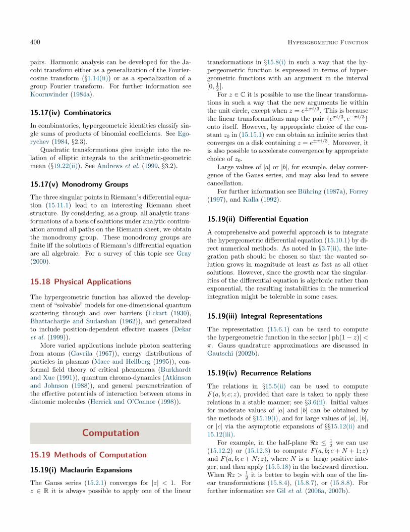
400 Hypergeometric Function
pairs. Harmonic analysis can be developed for the Ja-cobi transform either as a generalization of the Fourier-cosine transform (§1.14(ii)) or as a specialization of agroup Fourier transform. For further information seeKoornwinder (1984a).
15.17(iv) Combinatorics
In combinatorics, hypergeometric identities classify sin-gle sums of products of binomial coefficients. See Ego-rychev (1984, §2.3).
Quadratic transformations give insight into the re-lation of elliptic integrals to the arithmetic-geometricmean (§19.22(ii)). See Andrews et al. (1999, §3.2).
15.17(v) Monodromy Groups
The three singular points in Riemann’s differential equa-tion (15.11.1) lead to an interesting Riemann sheetstructure. By considering, as a group, all analytic trans-formations of a basis of solutions under analytic continu-ation around all paths on the Riemann sheet, we obtainthe monodromy group. These monodromy groups arefinite iff the solutions of Riemann’s differential equationare all algebraic. For a survey of this topic see Gray(2000).
15.18 Physical Applications
The hypergeometric function has allowed the develop-ment of “solvable” models for one-dimensional quantumscattering through and over barriers (Eckart (1930),Bhattacharjie and Sudarshan (1962)), and generalizedto include position-dependent effective masses (Dekaret al. (1999)).
More varied applications include photon scatteringfrom atoms (Gavrila (1967)), energy distributions ofparticles in plasmas (Mace and Hellberg (1995)), con-formal field theory of critical phenomena (Burkhardtand Xue (1991)), quantum chromo-dynamics (Atkinsonand Johnson (1988)), and general parametrization ofthe effective potentials of interaction between atoms indiatomic molecules (Herrick and O’Connor (1998)).
Computation
15.19 Methods of Computation
15.19(i) Maclaurin Expansions
The Gauss series (15.2.1) converges for |z| < 1. Forz ∈ R it is always possible to apply one of the linear
transformations in §15.8(i) in such a way that the hy-pergeometric function is expressed in terms of hyper-geometric functions with an argument in the interval[0, 1
2 ].For z ∈ C it is possible to use the linear transforma-
tions in such a way that the new arguments lie withinthe unit circle, except when z = e±πi/3. This is becausethe linear transformations map the pair {eπi/3, e−πi/3}onto itself. However, by appropriate choice of the con-stant z0 in (15.15.1) we can obtain an infinite series thatconverges on a disk containing z = e±πi/3. Moreover, itis also possible to accelerate convergence by appropriatechoice of z0.
Large values of |a| or |b|, for example, delay conver-gence of the Gauss series, and may also lead to severecancellation.
For further information see Bühring (1987a), Forrey(1997), and Kalla (1992).
15.19(ii) Differential Equation
A comprehensive and powerful approach is to integratethe hypergeometric differential equation (15.10.1) by di-rect numerical methods. As noted in §3.7(ii), the inte-gration path should be chosen so that the wanted so-lution grows in magnitude at least as fast as all othersolutions. However, since the growth near the singular-ities of the differential equation is algebraic rather thanexponential, the resulting instabilities in the numericalintegration might be tolerable in some cases.
15.19(iii) Integral Representations
The representation (15.6.1) can be used to computethe hypergeometric function in the sector |ph(1− z)| <π. Gauss quadrature approximations are discussed inGautschi (2002b).
15.19(iv) Recurrence Relations
The relations in §15.5(ii) can be used to computeF (a, b; c; z), provided that care is taken to apply theserelations in a stable manner; see §3.6(ii). Initial valuesfor moderate values of |a| and |b| can be obtained bythe methods of §15.19(i), and for large values of |a|, |b|,or |c| via the asymptotic expansions of §§15.12(ii) and15.12(iii).
For example, in the half-plane <z ≤ 12 we can use
(15.12.2) or (15.12.3) to compute F (a, b; c+N + 1; z)and F (a, b; c+N ; z), where N is a large positive inte-ger, and then apply (15.5.18) in the backward direction.When <z > 1
2 it is better to begin with one of the lin-ear transformations (15.8.4), (15.8.7), or (15.8.8). Forfurther information see Gil et al. (2006a, 2007b).

15.20 Software 401
15.20 Software
See http://dlmf.nist.gov/15.20.
References
General References
The main references used in writing this chapter areAndrews et al. (1999) and Temme (1996a). For addi-tional bibliographic reading see Erdélyi et al. (1953a),Hochstadt (1971), Luke (1969a), Olver (1997b), Slater(1966), Wang and Guo (1989), and Whittaker and Wat-son (1927).
Sources
The following list gives the references or other indica-tions of proofs that were used in constructing the varioussections of this chapter. These sources supplement thereferences that are quoted in the text.
§15.2 Andrews et al. (1999, §2.1), Olver (1997b,Chapter 5, Theorem 9.1), Temme (1996a, §5.1).(15.2.3) is a consequence of (15.8.4).
§15.3 These graphics were produced at NIST.
§15.4 Andrews et al. (1999, §2.2). For (15.4.1)–(15.4.6) see Temme (1996a, §5.1). For (15.4.7) use(15.8.27), (15.4.6), and (5.5.5). For (15.4.9) use(15.8.28), (15.4.6), and (5.5.5). For (15.4.11) use(15.8.1) and (15.4.7). For (15.4.13) use (15.8.1)and (15.4.11). For (15.4.15) use (15.8.1) and(15.4.9). For (15.4.17) and (15.4.18) use (15.8.15)and (15.4.6). For (15.4.19) use (15.5.11) and(15.4.6). For (15.4.21) use (15.8.10). For (15.4.22)and (15.4.23) use (15.8.4), (5.5.3), and (5.5.1). For(15.4.25) see Dougall (1907) or Andrews et al.(1999, §2.8). For (15.4.26) use (15.8.24) and(5.5.5). For (15.4.27) use (15.2.1) and (5.7.7).For (15.4.28) use (15.8.1), (15.4.26), and (5.5.5).For (15.4.29) use (15.8.1), (15.5.15), (15.4.26),(5.5.5), and (5.5.1). For (15.4.30) use (15.8.1)and (15.4.28). For (15.4.31) use (15.8.1), Erdélyiet al. (1953a, Eq. (2.11.41)), (15.4.20), and (5.5.5).For (15.4.32) use (15.8.30), (15.4.28), (5.5.5),and (5.5.6). (Note that Erdélyi et al. (1953a,Eq. (2.8.54)) contains an error.) For (15.4.33) letz → −∞ in (15.8.32) and use (5.5.5).
§15.5 Andrews et al. (1999, §2.5). For (15.5.2)–(15.5.9)use induction. For (15.5.10) see Fleury and Tur-biner (1994).
§15.6 Andrews et al. (1999, §§2.2, 2.4, 2.9), Erdélyiet al. (1953a, §2.1.3), and Whittaker and Wat-son (1927, pp. 290–291). (15.6.3) follows from(15.6.4).
§15.7 Andrews et al. (1999, pp. 94, 97–98, and Ex. 26on p. 119), Lorentzen and Waadeland (1992, §6.1),and Berndt (1989, pp. 134–137). These refer-ences contain several restrictions on the param-eters a, b, and c. This is because they use thefunction F (a, b; c; z). No restrictions are neededfor F(a, b; c; z).
§15.8 For (15.8.1)–(15.8.4) see Olver (1997b, Chap-ter 5, §10). For (15.8.5) combine (15.8.1) and(15.8.2). (15.8.6) and (15.8.7) are obtained aslimits of (15.8.2)–(15.8.5) as a → −m, togetherwith (5.5.3). For (15.8.8) and (15.8.10) see Erdélyiet al. (1953a, §§2.1.4 and 2.3.1). (15.8.9) and(15.8.11) follow from (15.8.10) and (15.8.8), re-spectively, via (15.8.1). For §15.8(iii) see Andrewset al. (1999, §3.1). For (15.8.31) and (15.8.32)see Goursat (1881, Eq. (110)) and Watson (1910).The version of (15.8.31) given in Erdélyi et al.(1953a, p. 114 (40)) contains a typographical er-ror. For (15.8.33) see Chan (1998).
§15.9 For (15.9.1)–(15.9.10) see §§18.5(ii) and 18.20(ii).For (15.9.15) see Erdélyi et al. (1953a, §§3.15.1and 3.15.2).
§15.10 Andrews et al. (1999, §2.3), Olver (1997b,pp. 163–168), and Luke (1969a, Chapter III).(15.10.9) is a corrected version of (2.3.20) in thefirst reference.
§15.11 Andrews et al. (1999, §2.3) or Olver (1997b,pp. 156–158).
§15.12 For (15.12.2) see Wagner (1988). The region ofvalidity given in Luke (1969a, p. 235) is incorrect.For (15.12.3) see Luke (1969a, §7.2) and Olver(1997b, p. 162). The sector of validity given inthe first reference is incorrect. See the third foot-note in the second reference.
§15.13 Runckel (1971).
§15.14 Andrews et al. (1999, §2.4).
§15.16 Burchnall and Chaundy (1940, 1948) and El-liott (1903). For (15.16.4) use (15.8.2) and(15.8.4), combined with (15.8.1) to show that theleft-hand side of (15.16.4) is an entire function ofz. Then apply Liouville’s theorem (1.9(iii)).


Chapter 16
Generalized Hypergeometric Functions and MeijerG-Function
R. A. Askey1 and A. B. Olde Daalhuis2
Notation 40416.1 Special Notation . . . . . . . . . . . . . 404
Generalized Hypergeometric Functions 40416.2 Definition and Analytic Properties . . . . 40416.3 Derivatives and Contiguous Functions . . 40516.4 Argument Unity . . . . . . . . . . . . . . 40516.5 Integral Representations and Integrals . . 40816.6 Transformations of Variable . . . . . . . . 40816.7 Relations to Other Functions . . . . . . . 40916.8 Differential Equations . . . . . . . . . . . 40916.9 Zeros . . . . . . . . . . . . . . . . . . . 41016.10 Expansions in Series of pFq Functions . . 41016.11 Asymptotic Expansions . . . . . . . . . . 41116.12 Products . . . . . . . . . . . . . . . . . . 412
Two-Variable Hypergeometric Functions 41216.13 Appell Functions . . . . . . . . . . . . . 41216.14 Partial Differential Equations . . . . . . . 41316.15 Integral Representations and Integrals . . 414
16.16 Transformations of Variables . . . . . . . 414
Meijer G-Function 41516.17 Definition . . . . . . . . . . . . . . . . . 41516.18 Special Cases . . . . . . . . . . . . . . . 41616.19 Identities . . . . . . . . . . . . . . . . . 41616.20 Integrals and Series . . . . . . . . . . . . 41616.21 Differential Equation . . . . . . . . . . . 41716.22 Asymptotic Expansions . . . . . . . . . . 417
Applications 41716.23 Mathematical Applications . . . . . . . . 41716.24 Physical Applications . . . . . . . . . . . 417
Computation 41816.25 Methods of Computation . . . . . . . . . 41816.26 Approximations . . . . . . . . . . . . . . 41816.27 Software . . . . . . . . . . . . . . . . . . 418
References 418
1Department of Mathematics, University of Wisconsin, Madison, Wisconsin.2School of Mathematics, Edinburgh University, Edinburgh, United Kingdom.Acknowledgments: The authors are pleased to acknowledge the assistance of B. L. J. Braaksma with §§16.5 and 16.11.Copyright c© 2009 National Institute of Standards and Technology. All rights reserved.
403

404 Generalized Hypergeometric Functions and Meijer G-Function
Notation
16.1 Special Notation
(For other notation see pp. xiv and 873.)
p, q nonnegative integers.k, n nonnegative integers, unless
stated otherwise.z complex variable.a1, a2, . . . , apb1, b2, . . . , bq
}real or complex parameters.
δ arbitrary small positive constant.a vector (a1, a2, . . . , ap).b vector (b1, b2, . . . , bq).(a)k (a1)k(a2)k · · · (ap)k.(b)k (b1)k(b2)k · · · (bq)k.D d/dz .ϑ z d/dz .
The main functions treated in this chap-ter are the generalized hypergeometric function
pFq
(a1,...,apb1,...,bq
; z)
, the Appell (two-variable hypergeomet-ric) functions F1(α;β, β′; γ;x, y), F2(α;β, β′; γ, γ′;x, y),F3(α, α′;β, β′; γ;x, y), F4(α;β; γ, γ′;x, y), and the Mei-jer G-function Gm,np,q
(z; a1,...,ap
b1,...,bq
). Alternative no-
tations are pFq(
ab ; z), pFq(a1, . . . , ap; b1, . . . , bq; z),
and pFq(a; b; z) for the generalized hypergeometricfunction, F1(α, β, β′; γ;x, y), F2(α, β, β′; γ, γ′;x, y),F3(α, α′, β, β′; γ;x, y), F4(α, β; γ, γ′;x, y), for the Ap-pell functions, and Gm,np,q (z; a; b) for the Meijer G-function.
Generalized HypergeometricFunctions
16.2 Definition and Analytic Properties
16.2(i) Generalized Hypergeometric Series
Throughout this chapter it is assumed that none of thebottom parameters b1, b2, . . . , bq is a nonpositive inte-ger, unless stated otherwise. Then formally
16.2.1 pFq
(a1, . . . , apb1, . . . , bq
; z)
=∞∑k=0
(a1)k · · · (ap)k(b1)k · · · (bq)k
zk
k!.
Equivalently, the function is denoted by pFq(
ab ; z)
orpFq(a; b; z), and sometimes, for brevity, by pFq(z).
16.2(ii) Case p ≤ qWhen p ≤ q the series (16.2.1) converges for all finitevalues of z and defines an entire function.
16.2(iii) Case p = q + 1
Suppose first one or more of the top parameters aj isa nonpositive integer. Then the series (16.2.1) termi-nates and the generalized hypergeometric function is apolynomial in z.
If none of the aj is a nonpositive integer, then theradius of convergence of the series (16.2.1) is 1, andoutside the open disk |z| < 1 the generalized hyper-geometric function is defined by analytic continuationwith respect to z. The branch obtained by introducinga cut from 1 to +∞ on the real axis, that is, the branchin the sector |ph(1− z)| ≤ π, is the principal branch(or principal value) of q+1Fq(a; b; z); compare §4.2(i).Elsewhere the generalized hypergeometric function is amultivalued function that is analytic except for possiblebranch points at z = 0, 1, and ∞. Unless indicated oth-erwise it is assumed that in this Handbook generalizedhypergeometric functions assume their principal values.
On the circle |z| = 1 the series (16.2.1) is absolutelyconvergent if <γq > 0, convergent except at z = 1 if−1 < <γq ≤ 0, and divergent if <γq ≤ −1, where16.2.2 γq = (b1 + · · ·+ bq)− (a1 + · · ·+ aq+1).
16.2(iv) Case p > q + 1
Polynomials
In general the series (16.2.1) diverges for all nonzerovalues of z. However, when one or more of the topparameters aj is a nonpositive integer the series termi-nates and the generalized hypergeometric function is apolynomial in z. Note that if −m is the value of the nu-merically largest aj that is a nonpositive integer, thenthe identity16.2.3
p+1Fq
(−m,a
b; z)
=(a)m(−z)m
(b)mq+1Fp
(−m, 1−m− b
1−m− a;
(−1)p+q
z
)can be used to interchange p and q.
Note also that any partial sum of the generalized hy-pergeometric series can be represented as a generalizedhypergeometric function via16.2.4m∑k=0
(a)k(b)k
zk
k!
=(a)mz
m
(b)mm! q+2Fp
(−m, 1, 1−m− b
1−m− a;
(−1)p+q+1
z
).
Non-Polynomials
See §16.5 for the definition of pFq(a; b; z) as a contourintegral when p > q+1 and none of the ak is a nonposi-tive integer. (However, except where indicated otherwisein this Handbook we assume that when p > q+1 at leastone of the ak is a nonpositive integer.)

16.3 Derivatives and Contiguous Functions 405
16.2(v) Behavior with Respect to Parameters
Let
16.2.5 pFq(a; b; z) = pFq
(a1, . . . , apb1, . . . , bq
; z)/
(Γ(b1) · · ·Γ(bq)) =∞∑k=0
(a1)k · · · (ap)kΓ(b1 + k) · · ·Γ(bq + k)
zk
k!;
compare (15.2.2) in the case p = 2, q = 1. When p ≤ q + 1 and z is fixed and not a branch point, any branch ofpFq(a; b; z) is an entire function of each of the parameters a1, . . . , ap, b1, . . . , bq.
16.3 Derivatives and Contiguous Functions
16.3(i) Differentiation Formulas
16.3.1dn
dznpFq
(a1, . . . , apb1, . . . , bq
; z)
=(a)n(b)n
pFq
(a1 + n, . . . , ap + n
b1 + n, . . . , bq + n; z),
16.3.2dn
dzn
(zγ pFq
(a1, . . . , apb1, . . . , bq
; z))
= (γ − n+ 1)nzγ−n
p+1Fq+1
(γ + 1, a1, . . . , ap
γ + 1− n, b1, . . . , bq; z),
16.3.3
(zd
dzz
)n(zγ−1
p+1Fq
(γ, a1, . . . , apb1, . . . , bq
; z))
= (γ)nzγ+n−1
p+1Fq
(γ + n, a1, . . . , ap
b1, . . . , bq; z),
16.3.4dn
dzn
(zγ−1
pFq+1
(a1, . . . , apγ, b1, . . . , bq
; z))
= (γ − n)nzγ−n−1
pFq+1
(a1, . . . , ap
γ − n, b1, . . . , bq; z).
Other versions of these identities can be constructed with the aid of the operator identity
16.3.5
(zd
dzz
)n= zn
dn
dznzn, n = 1, 2, . . . .
16.3(ii) Contiguous Functions
Two generalized hypergeometric functions pFq(a; b; z) are (generalized) contiguous if they have the same pair ofvalues of p and q, and corresponding parameters differ by integers. If p ≤ q + 1, then any q + 2 distinct contiguousfunctions are linearly related. Examples are provided by the following recurrence relations:
16.3.6 z 0F1(−; b+ 1; z) + b(b− 1) 0F1(−; b; z)− b(b− 1) 0F1(−; b− 1; z) = 0,
16.3.7
3F2
(a1 + 2, a2, a3
b1, b2; z)a1(a1+1)(1−z)+3F2
(a1 + 1, a2, a3
b1, b2; z)a1 (b1+b2−3a1−2+z(2a1−a2−a3+1))
+ 3F2
(a1, a2, a3
b1, b2; z)(
(2a1 − b1)(2a1 − b2) + a1 − a21 − z(a1 − a2)(a1 − a3)
)− 3F2
(a1 − 1, a2, a3
b1, b2; z)
(a1 − b1)(a1 − b2) = 0.
For further examples see §§13.3(i), 15.5(ii), and the following references: Rainville (1960, §48), Wimp (1968), andLuke (1975, §5.13).
16.4 Argument Unity
16.4(i) Classification
The function q+1Fq(a; b; z) is well-poised if
16.4.1 a1 + b1 = · · · = aq + bq = aq+1 + 1.
It is very well-poised if it is well-poised and a1 = b1 + 1.The special case q+1Fq(a; b; 1) is k-balanced if aq+1 is a nonpositive integer and
16.4.2 a1 + · · ·+ aq+1 + k = b1 + · · ·+ bq.
When k = 1 the function is said to be balanced or Saalschützian.

406 Generalized Hypergeometric Functions and Meijer G-Function
16.4(ii) Examples
The function q+1Fq with argument unity and general values of the parameters is discussed in Bühring (1992). Specialcases are as follows:
Pfaff–Saalschütz Balanced Sum
16.4.3 3F2
(−n, a, bc, d
; 1)
=(c− a)n(c− b)n(c)n(c− a− b)n
,
when c+ d = a+ b+ 1− n, n = 0, 1, . . . . See Erdélyi et al. (1953a, §4.4(4)) for a non-terminating balanced identity.
Dixon’s Well-Poised Sum
16.4.4 3F2
(a, b, c
a− b+ 1, a− c+ 1; 1)
=Γ(
12a+ 1
)Γ(a− b+ 1) Γ(a− c+ 1) Γ
(12a− b− c+ 1
)Γ(a+ 1) Γ
(12a− b+ 1
)Γ(
12a− c+ 1
)Γ(a− b− c+ 1)
,
when <(a− 2b− 2c) > −2, or when the series terminates with a = −n:
16.4.5 3F2
(−n, b, c
1− b− n, 1− c− n; 1)
=
0, n = 2k + 1,(2k)! Γ(b+ k) Γ(c+ k) Γ(b+ c+ 2k)k! Γ(b+ 2k) Γ(c+ 2k) Γ(b+ c+ k)
, n = 2k,
where k = 0, 1, . . . .
Watson’s Sum
16.4.6 3F2
(a, b, c
12 (a+ b+ 1), 2c
; 1)
=Γ(
12
)Γ(c+ 1
2
)Γ(
12 (a+ b+ 1)
)Γ(c+ 1
2 (1− a− b))
Γ(
12 (a+ 1)
)Γ(
12 (b+ 1)
)Γ(c+ 1
2 (1− a))
Γ(c+ 1
2 (1− b)) ,
when <(2c− a− b) > −1, or when the series terminates with a = −n.
Whipple’s Sum
16.4.7 3F2
(a, 1− a, cd, 2c− d+ 1
; 1)
=π Γ(d) Γ(2c− d+ 1)21−2c
Γ(c+ 1
2 (a− d+ 1))
Γ(c+ 1− 1
2 (a+ d))
Γ(
12 (a+ d)
)Γ(
12 (d− a+ 1)
) ,when <c > 0 or when a is an integer.
Džrbasjan’s Sum
This is (16.4.7) in the case c = −n:
16.4.8 3F2
(−n, a, 1− ad, 1− d− 2n
; 1)
=
(12 (a+ d)
)n
(12 (d− a+ 1)
)n(
12d)n
(12 (d+ 1)
)n
, n = 0, 1, . . . .
Rogers–Dougall Very Well-Poised Sum
16.4.9 5F4
(a, 1
2a+ 1, b, c, d12a, a− b+ 1, a− c+ 1, a− d+ 1
; 1
)=
Γ(a− b+ 1) Γ(a− c+ 1) Γ(a− d+ 1) Γ(a− b− c− d+ 1)Γ(a+ 1) Γ(a− b− c+ 1) Γ(a− b− d+ 1) Γ(a− c− d+ 1)
,
when <(b+ c+ d− a) < 1, or when the series terminates with d = −n.
Dougall’s Very Well-Poised Sum
16.4.10
7F6
(a, 1
2a+ 1, b, c, d, f,−n12a, a− b+ 1, a− c+ 1, a− d+ 1, a− f + 1, a+ n+ 1
; 1
)
=(a+ 1)n(a− b− c+ 1)n(a− b− d+ 1)n(a− c− d+ 1)n(a− b+ 1)n(a− c+ 1)n(a− d+ 1)n(a− b− c− d+ 1)n
, n = 0, 1, . . . ,
when 2a+ 1 = b+ c+ d+ f − n. The last condition is equivalent to the sum of the top parameters plus 2 equals thesum of the bottom parameters, that is, the series is 2-balanced.

16.4 Argument Unity 407
16.4(iii) Identities
16.4.11 3F2
(a, b, c
d, e; 1)
=Γ(e) Γ(d+ e− a− b− c)Γ(e− a) Γ(d+ e− b− c) 3F2
(a, d− b, d− cd, d+ e− b− c
; 1),
when <(d+ e− a− b− c) > 0 and <(e− a) > 0. The function 3F2(a, b, c; d, e; 1) is analytic in the parametersa, b, c, d, e when its series expansion converges and the bottom parameters are not negative integers or zero. (16.4.11)provides a partial analytic continuation to the region when the only restrictions on the parameters are <(e− a) > 0,and d, e, and d + e − b − c 6= 0,−1, . . . . A detailed treatment of analytic continuation in (16.4.11) and asymptoticapproximations as the variables a, b, c, d, e approach infinity is given by Aomoto (1987).
There are two types of three-term identities for 3F2’s. The first are recurrence relations that extend those for2F1’s; see §15.5(ii). Examples are (16.3.7) with z = 1. Also,
16.4.12
(a− d)(b− d)(c− d)(
3F2
(a, b, c
d+ 1, e; 1)− 3F2
(a, b, c
d, e; 1))
+ abc 3F2
(a, b, c
d, e; 1)
= d(d− 1)(a+ b+ c− d− e+ 1)(
3F2
(a, b, c
d, e; 1)− 3F2
(a, b, c
d− 1, e; 1))
,
and16.4.13 3F2
(a, b, c
d, e; 1)
=c(e− a)de
3F2
(a, b+ 1, c+ 1d+ 1, e+ 1
; 1)
+d− cd
3F2
(a, b+ 1, cd+ 1, e
; 1).
Methods of deriving such identities are given by Bailey (1964), Rainville (1960), Raynal (1979), and Wilson (1978).Lists are given by Raynal (1979) and Wilson (1978). See Raynal (1979) for a statement in terms of 3j symbols(Chapter 34). Also see Wilf and Zeilberger (1992a,b) for information on the Wilf–Zeilberger algorithm which can beused to find such relations.
The other three-term relations are extensions of Kummer’s relations for 2F1’s given in §15.10(ii). See Bailey(1964, pp. 19–22).
Balanced 4F3(1) series have transformation formulas and three-term relations. The basic transformation is givenby
16.4.14 4F3
(−n, a, b, cd, e, f
; 1)
=(e− a)n(f − a)n
(e)n(f)n4F3
(−n, a, d− b, d− c
d, a− e− n+ 1, a− f − n+ 1; 1),
when a+ b+ c−n+ 1 = d+ e+f . These series contain 6j symbols as special cases when the parameters are integers;compare §34.4.
The characterizing properties (18.22.2), (18.22.10), (18.22.19), (18.22.20), and (18.26.14) of the Hahn and Wilsonclass polynomials are examples of the contiguous relations mentioned in the previous three paragraphs.
Contiguous balanced series have parameters shifted by an integer but still balanced. One example of such athree-term relation is the recurrence relation (18.26.16) for Racah polynomials. See Raynal (1979), Wilson (1978),and Bailey (1964).
A different type of transformation is that of Whipple:
16.4.15
7F6
(a, 1
2a+ 1, b, c, d, e, f12a, a− b+ 1, a− c+ 1, a− d+ 1, a− e+ 1, a− f + 1
; 1
)
=Γ(a− d+ 1) Γ(a− e+ 1) Γ(a− f + 1) Γ(a− d− e− f + 1)Γ(a+ 1) Γ(a− d− e+ 1) Γ(a− d− f + 1) Γ(a− e− f + 1) 4F3
(a− b− c+ 1, d, e, f
a− b+ 1, a− c+ 1, d+ e+ f − a; 1),
when the series on the right terminates and the series on the left converges. When the series on the right does notterminate, a second term appears. See Bailey (1964, §4.4(4)).
Transformations for both balanced 4F3(1) and very well-poised 7F6(1) are included in Bailey (1964, pp. 56–63). Asimilar theory is available for very well-poised 9F8(1)’s which are 2-balanced. See Bailey (1964, §§4.3(7) and 7.6(1))for the transformation formulas and Wilson (1978) for contiguous relations.
Relations between three solutions of three-term recurrence relations are given by Masson (1991). See alsoLewanowicz (1985) (with corrections in Lewanowicz (1987)) for further examples of recurrence relations.
16.4(iv) Continued Fractions
For continued fractions for ratios of 3F2 functions with argument unity, see Cuyt et al. (2008, pp. 315–317).

408 Generalized Hypergeometric Functions and Meijer G-Function
16.4(v) Bilateral Series
Denote, formally, the bilateral hypergeometric function
16.4.16 pHq
(a1, . . . , apb1, . . . , bq
; z)
=∞∑
k=−∞
(a1)k . . . (ap)k(b1)k . . . (bq)k
zk.
Then16.4.17 2H2
(a, b
c, d; 1)
=Γ(c) Γ(d) Γ(1− a) Γ(1− b) Γ(c+ d− a− b− 1)
Γ(c− a) Γ(d− a) Γ(c− b) Γ(d− b), <(c+ d− a− b) > 1.
This is Dougall’s bilateral sum; see Andrews et al. (1999, §2.8).
16.5 Integral Representations and Integrals
When z 6= 0 and ak 6= 0,−1,−2, . . . , k = 1, 2, . . . , p,
16.5.1
(p∏k=1
Γ(ak)/
q∏k=1
Γ(bk))pFq
(a1, . . . , apb1, . . . , bq
; z)
=1
2πi
∫L
(p∏k=1
Γ(ak + s)/
q∏k=1
Γ(bk + s))
Γ(−s)(−z)s ds,
where the contour of integration separates the poles of Γ(ak + s), k = 1, . . . , p, from those of Γ(−s).Suppose first that L is a contour that starts at infinity on a line parallel to the positive real axis, encircles the
nonnegative integers in the negative sense, and ends at infinity on another line parallel to the positive real axis. Thenthe integral converges when p < q+ 1 provided that z 6= 0, or when p = q+ 1 provided that 0 < |z| < 1, and providesan integral representation of the left-hand side with these conditions.
Secondly, suppose that L is a contour from −i∞ to i∞. Then the integral converges when q < p + 1 and|ph(−z)| < (p+ 1− q)π/2. In the case p = q the left-hand side of (16.5.1) is an entire function, and the right-handside supplies an integral representation valid when |ph(−z)| < π/2. In the case p = q + 1 the right-hand side of(16.5.1) supplies the analytic continuation of the left-hand side from the open unit disk to the sector |ph(1− z)| < π;compare §16.2(iii). Lastly, when p > q + 1 the right-hand side of (16.5.1) can be regarded as the definition of the(customarily undefined) left-hand side. In this event, the formal power-series expansion of the left-hand side (obtainedfrom (16.2.1)) is the asymptotic expansion of the right-hand side as z → 0 in the sector |ph(−z)| ≤ (p+1−q−δ)π/2,where δ is an arbitrary small positive constant.
Next, when p ≤ q,
16.5.2 p+1Fq+1
(a0, . . . , apb0, . . . , bq
; z)
=Γ(b0)
Γ(a0) Γ(b0 − a0)
∫ 1
0
ta0−1(1− t)b0−a0−1pFq
(a1, . . . , apb1, . . . , bq
; zt)dt, <b0 > <a0 > 0,
16.5.3 p+1Fq
(a0, . . . , apb1, . . . , bq
; z)
=1
Γ(a0)
∫ ∞0
e−tta0−1pFq
(a1, . . . , apb1, · · · , bq
; zt)dt, <z < 1, <a0 > 0,
16.5.4 pFq+1
(a1, . . . , apb0, . . . , bq
; z)
=Γ(b0)2πi
∫ c+i∞
c−i∞ett−b0 pFq
(a1, . . . , apb1, . . . , bq
;z
t
)dt, c > 0, <b0 > 0.
In (16.5.2)–(16.5.4) all many-valued functions in the integrands assume their principal values, and all integrationpaths are straight lines.
(16.5.2) also holds when p = q + 1, provided that |ph(1− z)| < π. In (16.5.3) the restriction <z < 1 can beremoved when p < q. (16.5.4) also holds when p = q + 1, provided that max(0,<z) < c. Lastly, the restrictions onthe parameters can be eased by replacing the integration paths with loop contours; see Luke (1969a, §3.6).
Laplace transforms and inverse Laplace transforms of generalized hypergeometric functions are given in Prudnikovet al. (1992a, §3.38) and Prudnikov et al. (1992b, §3.36). For further integral representations and integrals seeApelblat (1983, §16), Erdélyi et al. (1953a, §4.6), Erdélyi et al. (1954a, §§6.9 and 7.5), Luke (1969a, §3.6), andPrudnikov et al. (1990, §§2.22, 4.2.4, and 4.3.1).
16.6 Transformations of Variable
Quadratic
16.6.1 3F2
(a, b, c
a− b+ 1, a− c+ 1; z)
= (1− z)−a 3F2
(a− b− c+ 1, 1
2a,12 (a+ 1)
a− b+ 1, a− c+ 1;−4z
(1− z)2
).

16.7 Relations to Other Functions 409
Cubic
16.6.2 3F2
(a, 2b− a− 1, 2− 2b+ a
b, a− b+ 32
;z
4
)= (1− z)−a 3F2
(13a,
13a+ 1
3 ,13a+ 2
3
b, a− b+ 32
;−27z
4(1− z)3
).
For Kummer-type transformations of 2F2 functions see Miller (2003) and Paris (2005a), and for further transfor-mations see Erdélyi et al. (1953a, §4.5).
16.7 Relations to Other Functions
For orthogonal polynomials see Chapter 18. For 3j, 6j, 9j symbols see Chapter 34. Further representations of specialfunctions in terms of pFq functions are given in Luke (1969a, §§6.2–6.3), and an extensive list of q+1Fq functionswith rational numbers as parameters is given in Krupnikov and Kölbig (1997).
16.8 Differential Equations
16.8(i) Classification of Singularities
An ordinary point of the differential equation
16.8.1dnw
dzn+ fn−1(z)
dn−1w
dzn−1 + fn−2(z)dn−2w
dzn−2 + · · ·+ f1(z)dw
dz+ f0(z)w = 0
is a value z0 of z at which all the coefficients fj(z), j = 0, 1, . . . , n−1, are analytic. If z0 is not an ordinary point but(z − z0)n−jfj(z), j = 0, 1, . . . , n − 1, are analytic at z = z0, then z0 is a regular singularity. All other singularitiesare irregular. Compare §2.7(i) in the case n = 2. Similar definitions apply in the case z0 =∞: we transform ∞ intothe origin by replacing z in (16.8.1) by 1/z; again compare §2.7(i).
For further information see Hille (1976, pp. 360–370).
16.8(ii) The Generalized Hypergeometric Differential Equation
With the notation16.8.2 D =
d
dz, ϑ = z
d
dz,
the function w = pFq(a; b; z) satisfies the differential equation
16.8.3 (ϑ(ϑ+ b1 − 1) · · · (ϑ+ bq − 1)− z(ϑ+ a1) · · · (ϑ+ ap))w = 0.Equivalently,
16.8.4 zqDq+1w +q∑
j =1
zj−1(αjz + βj)Djw + α0w = 0, p ≤ q,
or
16.8.5 zq(1− z)Dq+1w +q∑
j =1
zj−1(αjz + βj)Djw + α0w = 0, p = q + 1,
where αj and βj are constants. Equation (16.8.4) has a regular singularity at z = 0, and an irregular singularity atz = ∞, whereas (16.8.5) has regular singularities at z = 0, 1, and ∞. In each case there are no other singularities.Equation (16.8.3) is of order max(p, q+ 1). In Letessier et al. (1994) examples are discussed in which the generalizedhypergeometric function satisfies a differential equation that is of order 1 or even 2 less than might be expected.
When no bj is an integer, and no two bj differ by an integer, a fundamental set of solutions of (16.8.3) is givenby
16.8.6 w0(z) = pFq
(a1, . . . , apb1, . . . , bq
; z), wj(z) = z1−bj
pFq
(1 + a1 − bj , . . . , 1 + ap − bj
2− bj , 1 + b1 − bj , . . . ∗ . . . , 1 + bq − bj; z)
, j = 1, . . . , q,
where ∗ indicates that the entry 1 + bj − bj is omitted. For other values of the bj , series solutions in powers of z(possibly involving also ln z) can be constructed via a limiting process; compare §2.7(i) in the case of second-orderdifferential equations. For details see Smith (1939a,b), and Nørlund (1955).
When p = q + 1, and no two aj differ by an integer, another fundamental set of solutions of (16.8.3) is given by
16.8.7 w̃j(z) = (−z)−aj q+1Fq
(aj , 1− b1 + aj , . . . , 1− bq + aj
1− a1 + aj , . . . ∗ . . . , 1− aq+1 + aj;
1z
), j = 1, . . . , q + 1,

410 Generalized Hypergeometric Functions and Meijer G-Function
where ∗ indicates that the entry 1− aj + aj is omitted. We have the connection formula
16.8.8 q+1Fq
(a1, . . . , aq+1
b1, . . . , bq; z)
=q+1∑j=1
q+1∏k=1k 6=j
Γ(ak−aj)Γ(ak)
/q∏
k=1
Γ(bk−aj)Γ(bk)
w̃j(z), |ph(−z)| ≤ π.
More generally if z0 (∈ C) is an arbitrary constant, |z − z0| > max (|z0|, |z0 − 1|), and |ph(z0 − z)| < π, then
16.8.9
(q+1∏k=1
Γ(ak)/
q∏k=1
Γ(bk))q+1Fq
(a1, . . . , aq+1
b1, . . . , bq; z)
=q+1∑j=1
(z0 − z)−aj∞∑n=0
Γ(aj + n)n!
q+1∏k=1k 6=j
Γ(ak − aj − n)
/q∏
k=1
Γ(bk − aj − n)
× q+1Fq
(a1 − aj − n, . . . , aq+1 − aj − nb1 − aj − n, . . . , bq − aj − n
; z0
)(z − z0)−n .
(Note that the generalized hypergeometric functions on the right-hand side are polynomials in z0.)When p = q + 1 and some of the aj differ by an integer a limiting process can again be applied. For details see
Nørlund (1955). In this reference it is also explained that in general when q > 1 no simple representations in terms ofgeneralized hypergeometric functions are available for the fundamental solutions near z = 1. Analytical continuationformulas for q+1Fq(a; b; z) near z = 1 are given in Bühring (1987b) for the case q = 2, and in Bühring (1992) for thegeneral case.
16.8(iii) Confluence of Singularities
If p ≤ q, then
16.8.10 lim|α| →∞
p+1Fq
(a1, . . . , ap, α
b1, . . . , bq;z
α
)= pFq
(a1, . . . , apb1, . . . , bq
; z).
Thus in the case p = q the regular singularities of the function on the left-hand side at α and ∞ coalesce into anirregular singularity at ∞.
Next, if p ≤ q + 1 and |phβ| ≤ π − δ (< π), then
16.8.11 lim|β| →∞
pFq+1
(a1, . . . , apb1, . . . , bq, β
;βz)
= pFq
(a1, . . . , apb1, . . . , bq
; z),
provided that in the case p = q+1 we have |z| < 1 when |phβ| ≤ 12π, and |z| < | sin(phβ)| when 1
2π ≤ |phβ| ≤ π−δ(< π).
16.9 Zeros
Assume that p = q and none of the aj is a nonpositive integer. Then pFp(a; b; z) has at most finitely many zeros ifand only if the aj can be re-indexed for j = 1, . . . , p in such a way that aj − bj is a nonnegative integer.
Next, assume that p = q and that the aj and the quotients (a)j/(b)j are all real. Then pFp(a; b; z) has at mostfinitely many real zeros.
These results are proved in Ki and Kim (2000). For further information on zeros see Hille (1929).
16.10 Expansions in Series of pFq Functions
The following expansion, with appropriate conditions and together with similar results, is given in Fields and Wimp(1961):
16.10.1
p+rFq+s
(a1, . . . , ap, c1, . . . , crb1, . . . , bq, d1, . . . , ds
; zζ)
=∞∑k=0
(a)k(α)k(β)k(−z)k
(b)k(γ + k)kk! p+2Fq+1
(α+ k, β + k, a1 + k, . . . , ap + k
γ + 2k + 1, b1 + k, . . . , bq + k; z)r+2Fs+2
(−k, γ + k, c1, . . . , crα, β, d1, . . . , ds
; ζ).
Here α, β, and γ are free real or complex parameters.

16.11 Asymptotic Expansions 411
The next expansion is given in Nørlund (1955, equation (1.21)):
16.10.2 p+1Fp
(a1, . . . , ap+1
b1, . . . , bp; zζ)
= (1− z)−a1
∞∑k=0
(a1)kk! p+1Fp
(−k, a2, . . . , ap+1
b1, . . . , bp; ζ)(
z
z − 1
)k.
When |ζ − 1| < 1 the series on the right-hand side converges in the half-plane <z < 12 .
Expansions of the form∑∞n=1(±1)n pFp+1
(a; b;−n2z2
)are discussed in Miller (1997), and further series of gener-
alized hypergeometric functions are given in Luke (1969b, Chapter 9), Luke (1975, §§5.10.2 and 5.11), and Prudnikovet al. (1990, §§5.3, 6.8–6.9).
16.11 Asymptotic Expansions
16.11(i) Formal Series
For subsequent use we define two formal infinite series, Ep,q(z) and Hp,q(z), as follows:
16.11.1 Ep,q(z) = (2π) (p−q)/2κ−ν−( 1/2 )eκz1/κ
∞∑k=0
ck
(κz 1/κ
)ν−k, p < q + 1,
16.11.2 Hp,q(z) =p∑
m=1
∞∑k=0
(−1)k
k!Γ(am + k)
p∏`=1` 6=m
Γ(a` − am − k)
/q∏`=1
Γ(b` − am − k)
z−am−k.
In (16.11.1)
16.11.3 κ = q − p+ 1, ν = a1 + · · ·+ ap − b1 − · · · − bq + 12 (q − p),
and
16.11.4 c0 = 1, ck = − 1kκκ
k−1∑m=0
cmek,m, k ≥ 1,
where
16.11.5 ek,m =q+1∑j=1
(1− ν − κbj +m)κ+k−m
p∏`=1
(a` − bj)
/q+1∏`=1` 6=j
(b` − bj)
,
and bq+1 = 1.It may be observed that Hp,q(z) represents the sum of the residues of the poles of the integrand in (16.5.1) at
s = −aj ,−aj − 1, . . . , j = 1, . . . , p, provided that these poles are all simple, that is, no two of the aj differ by aninteger. (If this condition is violated, then the definition of Hp,q(z) has to be modified so that the residues are thoseassociated with the multiple poles. In consequence, logarithmic terms may appear. See (15.8.8) for an example.)
16.11(ii) Expansions for Large Variable
In this subsection we assume that none of a1, a2, . . . , ap is a nonpositive integer.
Case p = q + 1
The formal series (16.11.2) for Hq+1,q(z) converges if |z| > 1, and
16.11.6
(q+1∏`=1
Γ(a`)/
q∏`=1
Γ(b`))q+1Fq
(a1, . . . , aq+1
b1, . . . , bq; z)
= Hq+1,q(−z), |ph(−z)| ≤ π;
compare (16.8.8).
Case p = q
As z →∞ in |ph z| ≤ π,
16.11.7
(q∏`=1
Γ(a`)/
q∏`=1
Γ(b`))qFq
(a1, . . . , aqb1, . . . , bq
; z)∼ Hq,q(ze∓πi) + Eq,q(z),
where upper or lower signs are chosen according as z lies in the upper or lower half-plane. (Either sign may be usedwhen ph z = 0 since the first term on the right-hand side becomes exponentially small compared with the secondterm.)
For the special case a1 = 1, p = q = 2 explicit representations for the right-hand side of (16.11.7) in terms ofgeneralized hypergeometric functions are given in Kim (1972).

412 Generalized Hypergeometric Functions and Meijer G-Function
Case p = q − 1
As z →∞ in |ph z| ≤ π,
16.11.8
(q−1∏`=1
Γ(a`)/
q∏`=1
Γ(b`))q−1Fq
(a1, . . . , aq−1
b1, . . . , bq;−z
)∼ Hq−1,q(z) + Eq−1,q(ze−πi) + Eq−1,q(zeπi).
Case p ≤ q − 2
As z →∞ in |ph z| ≤ π,
16.11.9
(p∏`=1
Γ(a`)/
q∏`=1
Γ(b`))pFq
(a1, . . . , apb1, . . . , bq
;−z)∼ Ep,q(ze−πi) + Ep,q(zeπi).
16.11(iii) Expansions for Large Parameters
If z is fixed and |ph(1− z)| < π, then for each nonnegative integer m
16.11.10
p+1Fp
(a1 + r, . . . , ak−1 + r, ak, . . . , ap+1
b1 + r, . . . , bk + r, bk+1, . . . , bp; z)
=m−1∑n=0
(a1 + r)n · · · (ak−1 + r)n(ak)n · · · (ap+1)n(b1 + r)n · · · (bk + r)n(bk+1)n · · · (bp)n
zn
n!+O
(1rm
),
as r → +∞. Here k can have any integer value from 1 to p. Also if p < q, then
16.11.11 pFq
(a1 + r, . . . , ap + r
b1 + r, . . . , bq + r; z)
=m−1∑n=0
(a1 + r)n · · · (ap + r)n(b1 + r)n · · · (bq + r)n
zn
n!+O
(1
r(q−p)m
),
again as r → +∞. For these and other results see Knottnerus (1960). See also Luke (1969a, §7.3).Asymptotic expansions for the polynomials p+2Fq(−r, r + a0,a; b; z) as r →∞ through integer values are given
in Fields and Luke (1963a,b) and Fields (1965).
16.12 Products
16.12.1 0F1(−; a; z) 0F1(−; b; z) = 2F3
( 12 (a+ b), 1
2 (a+ b− 1)a, b, a+ b− 1
; 4z).
16.12.2
(2F1
(a, b
a+ b+ 12
; z))2
= 3F2
(2a, 2b, a+ b
a+ b+ 12 , 2a+ 2b
; z).
More generally,
16.12.3
(2F1
(a, b
c; z))2
=∞∑k=0
(2a)k(2b)k(c− 1
2
)k
(c)k(2c− 1)kk! 4F3
(− 1
2k,12 (1− k), a+ b− c+ 1
2 ,12
a+ 12 , b+ 1
2 ,32 − k − c
; 1
)zk, |z| < 1.
For further identities see Goursat (1883) and Erdélyi et al. (1953a, §4.3).
Two-Variable Hypergeometric Functions
16.13 Appell Functions
The following four functions of two real or complex variables x and y cannot be expressed as a product of two 2F1
functions, in general, but they satisfy partial differential equations that resemble the hypergeometric differential

16.14 Partial Differential Equations 413
equation (15.10.1):
16.13.1 F1(α;β, β′; γ;x, y) =∞∑
m,n=0
(α)m+n(β)m(β′)n(γ)m+nm!n!
xmyn, max (|x|, |y|) < 1,
16.13.2 F2(α;β, β′; γ, γ′;x, y) =∞∑
m,n=0
(α)m+n(β)m(β′)n(γ)m(γ′)nm!n!
xmyn, |x|+ |y| < 1,
16.13.3 F3(α, α′;β, β′; γ;x, y) =∞∑
m,n=0
(α)m(α′)n(β)m(β′)n(γ)m+nm!n!
xmyn, max (|x|, |y|) < 1,
16.13.4 F4(α;β; γ, γ′;x, y) =∞∑
m,n=0
(α)m+n(β)m+n
(γ)m(γ′)nm!n!xmyn,
√|x|+
√|y| < 1.
Here and elsewhere it is assumed that neither of the bottom parameters γ and γ′ is a nonpositive integer.
16.14 Partial Differential Equations
16.14(i) Appell Functions
16.14.1
x(1− x)∂2F1
∂x2 + y(1− x)∂2F1
∂x ∂y+ (γ − (α+ β + 1)x)
∂F1
∂x− βy∂F1
∂y− αβ F1 = 0,
y(1− y)∂2F1
∂y2 + x(1− y)∂2F1
∂x ∂y+ (γ − (α+ β′ + 1)y)
∂F1
∂y− β′x∂F1
∂x− αβ′ F1 = 0,
16.14.2
x(1− x)∂2F2
∂x2 − xy∂2F2
∂x ∂y+ (γ − (α+ β + 1)x)
∂F2
∂x− βy∂F2
∂y− αβ F2 = 0,
y(1− y)∂2F2
∂y2 − xy∂2F2
∂x ∂y+ (γ′ − (α+ β′ + 1)y)
∂F2
∂y− β′x∂F2
∂x− αβ′ F2 = 0,
16.14.3
x(1− x)∂2F3
∂x2 + y∂2F3
∂x ∂y+ (γ − (α+ β + 1)x)
∂F3
∂x− αβ F3 = 0,
y(1− y)∂2F3
∂y2 + x∂2F3
∂x ∂y+ (γ − (α′ + β′ + 1)y)
∂F3
∂y− α′β′ F3 = 0,
16.14.4
x(1− x)∂2F4
∂x2 − 2xy∂2F4
∂x ∂y− y2 ∂
2F4
∂y2 + (γ − (α+ β + 1)x)∂F4
∂x− (α+ β + 1)y
∂F4
∂y− αβ F4 = 0,
y(1− y)∂2F4
∂y2 − 2xy∂2F4
∂x ∂y− x2 ∂
2F4
∂x2 + (γ′ − (α+ β + 1)y)∂F4
∂y− (α+ β + 1)x
∂F4
∂x− αβ F4 = 0.
16.14(ii) Other Functions
In addition to the four Appell functions there are 24 other sums of double series that cannot be expressed as aproduct of two 2F1 functions, and which satisfy pairs of linear partial differential equations of the second order. Twoexamples are provided by
16.14.5 G2(α, α′;β, β′;x, y) =∞∑
m,n=0
Γ(α+m) Γ(α′ + n) Γ(β + n−m) Γ(β′ +m− n)Γ(α) Γ(α′) Γ(β) Γ(β′)
xmyn
m!n!, |x| < 1, |y| < 1,
16.14.6 G3(α, α′;x, y) =∞∑
m,n=0
Γ(α+ 2n−m) Γ(α′ + 2m− n)Γ(α) Γ(α′)
xmyn
m!n!, |x|+ |y| < 1
4 .
(The region of convergence |x| + |y| < 14 is not quite maximal.) See Erdélyi et al. (1953a, §§5.7.1–5.7.2) for further
information.
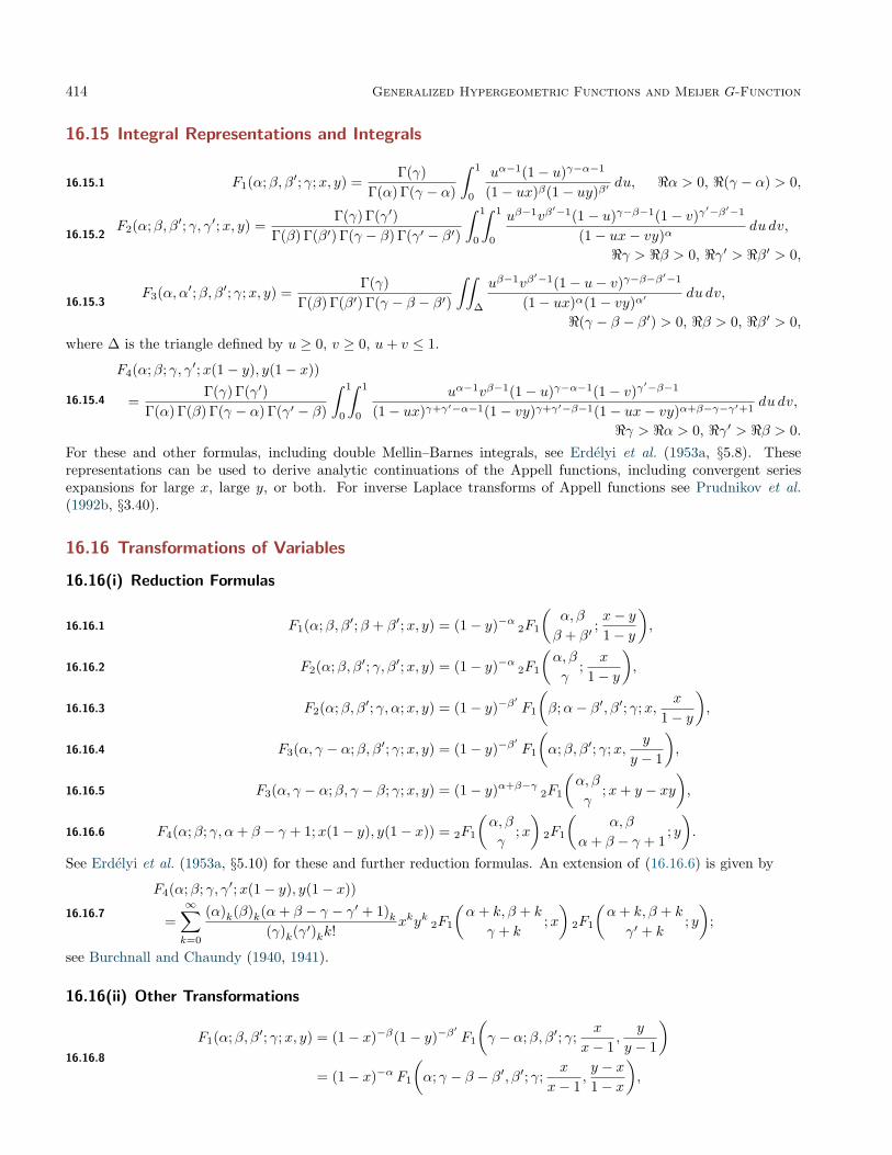
414 Generalized Hypergeometric Functions and Meijer G-Function
16.15 Integral Representations and Integrals
16.15.1 F1(α;β, β′; γ;x, y) =Γ(γ)
Γ(α) Γ(γ − α)
∫ 1
0
uα−1(1− u)γ−α−1
(1− ux)β(1− uy)β′du, <α > 0, <(γ − α) > 0,
16.15.2F2(α;β, β′; γ, γ′;x, y) =
Γ(γ) Γ(γ′)Γ(β) Γ(β′) Γ(γ − β) Γ(γ′ − β′)
∫ 1
0
∫ 1
0
uβ−1vβ′−1(1− u)γ−β−1(1− v)γ
′−β′−1
(1− ux− vy)αdu dv,
<γ > <β > 0, <γ′ > <β′ > 0,
16.15.3F3(α, α′;β, β′; γ;x, y) =
Γ(γ)Γ(β) Γ(β′) Γ(γ − β − β′)
∫∫∆
uβ−1vβ′−1(1− u− v)γ−β−β
′−1
(1− ux)α(1− vy)α′du dv,
<(γ − β − β′) > 0, <β > 0, <β′ > 0,where ∆ is the triangle defined by u ≥ 0, v ≥ 0, u+ v ≤ 1.
16.15.4
F4(α;β; γ, γ′;x(1− y), y(1− x))
=Γ(γ) Γ(γ′)
Γ(α) Γ(β) Γ(γ − α) Γ(γ′ − β)
∫ 1
0
∫ 1
0
uα−1vβ−1(1− u)γ−α−1(1− v)γ′−β−1
(1− ux)γ+γ′−α−1(1− vy)γ+γ′−β−1(1− ux− vy)α+β−γ−γ′+1du dv,
<γ > <α > 0, <γ′ > <β > 0.For these and other formulas, including double Mellin–Barnes integrals, see Erdélyi et al. (1953a, §5.8). Theserepresentations can be used to derive analytic continuations of the Appell functions, including convergent seriesexpansions for large x, large y, or both. For inverse Laplace transforms of Appell functions see Prudnikov et al.(1992b, §3.40).
16.16 Transformations of Variables
16.16(i) Reduction Formulas
16.16.1 F1(α;β, β′;β + β′;x, y) = (1− y)−α 2F1
(α, β
β + β′;x− y1− y
),
16.16.2 F2(α;β, β′; γ, β′;x, y) = (1− y)−α 2F1
(α, β
γ;
x
1− y
),
16.16.3 F2(α;β, β′; γ, α;x, y) = (1− y)−β′F1
(β;α− β′, β′; γ;x,
x
1− y
),
16.16.4 F3(α, γ − α;β, β′; γ;x, y) = (1− y)−β′F1
(α;β, β′; γ;x,
y
y − 1
),
16.16.5 F3(α, γ − α;β, γ − β; γ;x, y) = (1− y)α+β−γ2F1
(α, β
γ;x+ y − xy
),
16.16.6 F4(α;β; γ, α+ β − γ + 1;x(1− y), y(1− x)) = 2F1
(α, β
γ;x)
2F1
(α, β
α+ β − γ + 1; y).
See Erdélyi et al. (1953a, §5.10) for these and further reduction formulas. An extension of (16.16.6) is given by
16.16.7
F4(α;β; γ, γ′;x(1− y), y(1− x))
=∞∑k=0
(α)k(β)k(α+ β − γ − γ′ + 1)k(γ)k(γ′)kk!
xkyk 2F1
(α+ k, β + k
γ + k;x)
2F1
(α+ k, β + k
γ′ + k; y)
;
see Burchnall and Chaundy (1940, 1941).
16.16(ii) Other Transformations
16.16.8
F1(α;β, β′; γ;x, y) = (1− x)−β(1− y)−β′F1
(γ − α;β, β′; γ;
x
x− 1,
y
y − 1
)= (1− x)−α F1
(α; γ − β − β′, β′; γ;
x
x− 1,y − x1− x
),

Meijer G-Function 415
16.16.9 F2(α;β, β′; γ, γ′;x, y) = (1− x)−α F2
(α; γ − β, β′; γ, γ′; x
x− 1,
y
1− x
),
16.16.10
F4(α;β; γ, γ′;x, y) =Γ(γ′) Γ(β − α)Γ(γ′ − α) Γ(β)
(−y)−α F4
(α;α− γ′ + 1; γ, α− β + 1;
x
y,
1y
)+
Γ(γ′) Γ(α− β)Γ(γ′ − β) Γ(α)
(−y)−β F4
(β;β − γ′ + 1; γ, β − α+ 1;
x
y,
1y
).
For quadratic transformations of Appell functions see Carlson (1976).
Meijer G-Function
16.17 Definition
Again assume a1, a2, . . . , ap and b1, b2, . . . , bq are real or complex parameters. Assume also that m and n are integerssuch that 0 ≤ m ≤ q and 0 ≤ n ≤ p, and none of ak − bj is a positive integer when 1 ≤ k ≤ n and 1 ≤ j ≤ m. Thenthe Meijer G-function is defined via the Mellin–Barnes integral representation:
16.17.1
Gm,np,q (z; a; b) = Gm,np,q
(z;a1, . . . , apb1, . . . , bq
)=
12πi
∫L
(m∏`=1
Γ(b` − s)n∏`=1
Γ(1− a` + s)/(
q−1∏`=m
Γ(1− b`+1 + s)p−1∏`=n
Γ(a`+1 − s)))
zs ds,
where the integration path L separates the poles of the factors Γ(b` − s) from those of the factors Γ(1− a` + s).There are three possible choices for L, illustrated in Figure 16.17.1 in the case m = 1, n = 2:
(i) L goes from −i∞ to i∞. The integral converges if p+ q < 2(m+ n) and |ph z| < (m+ n− 12 (p+ q))π.
(ii) L is a loop that starts at infinity on a line parallel to the positive real axis, encircles the poles of the Γ(b` − s)once in the negative sense and returns to infinity on another line parallel to the positive real axis. The integralconverges for all z ( 6= 0) if p < q, and for 0 < |z| < 1 if p = q ≥ 1.
(iii) L is a loop that starts at infinity on a line parallel to the negative real axis, encircles the poles of the Γ(1− a` + s)once in the positive sense and returns to infinity on another line parallel to the negative real axis. The integralconverges for all z if p > q, and for |z| > 1 if p = q ≥ 1.
Case (i) Case (ii) Case (iii)Figure 16.17.1: s-plane. Path L for the integral representation (16.17.1) of the Meijer G-function.
When more than one of Cases (i), (ii), and (iii) is applicable the same value is obtained for the Meijer G-function.Assume p ≤ q, no two of the bottom parameters bj , j = 1, . . . ,m, differ by an integer, and aj−bk is not a positive
integer when j = 1, 2, . . . , n and k = 1, 2, . . . ,m. Then
16.17.2 Gm,np,q
(z;a1, . . . , apb1, . . . , bq
)=
m∑k=1
Am,np,q,k(z) pFq−1
(1 + bk − a1, . . . , 1 + bk − ap
1 + bk − b1, . . . ∗ . . . , 1 + bk − bq; (−1)p−m−nz
),

416 Generalized Hypergeometric Functions and Meijer G-Function
where ∗ indicates that the entry 1 + bk − bk is omitted. Also,
16.17.3 Am,np,q,k(z) =m∏`=1` 6=k
Γ(b` − bk)n∏`=1
Γ(1 + bk − a`)zbk/(
q−1∏`=m
Γ(1 + bk − b`+1)p−1∏`=n
Γ(a`+1 − bk)
).
16.18 Special Cases
The 1F1 and 2F1 functions introduced in Chapters 13 and 15, as well as the more general pFq functions introducedin the present chapter, are all special cases of the Meijer G-function. This is a consequence of the following relations:
16.18.1
pFq
(a1, . . . , apb1, . . . , bq
; z)
=(
q∏k=1
Γ(bk)/
p∏k=1
Γ(ak))G1,pp,q+1
(−z; 1− a1, . . . , 1− ap
0, 1− b1, . . . , 1− bq
)=(
q∏k=1
Γ(bk)/
p∏k=1
Γ(ak))Gp,1q+1,p
(−1z
;1, b1, . . . , bqa1, . . . , ap
).
As a corollary, special cases of the 1F1 and 2F1 functions, including Airy functions, Bessel functions, parabolic cylinderfunctions, Ferrers functions, associated Legendre functions, and many orthogonal polynomials, are all special casesof the Meijer G-function. Representations of special functions in terms of the Meijer G-function are given in Erdélyiet al. (1953a, §5.6), Luke (1969a, §§6.4–6.5), and Mathai (1993, §3.10).
16.19 Identities
16.19.1 Gm,np,q
(1z
;a1, . . . , apb1, . . . , bq
)= Gn,mq,p
(z;
1− b1, . . . , 1− bq1− a1, . . . , 1− ap
),
16.19.2 zµGm,np,q
(z;a1, . . . , apb1, . . . , bq
)= Gm,np,q
(z;a1 + µ, . . . , ap + µ
b1 + µ, . . . , bq + µ
),
16.19.3 Gm,n+1p+1,q+1
(z;
a0, . . . , apb1, . . . , bq, a0
)= Gm,np,q
(z;a1, . . . , apb1, . . . , bq
),
16.19.4 Gm,np,q
(z;a1, . . . , apb1, . . . , bq
)=
2p+1+b1+···+bq−m−n−a1−···−ap
πm+n− 12 (p+q)
G2m,2n2p,2q
(22p−2qz2;
12a1,
12a1 + 1
2 , . . . ,12ap,
12ap + 1
212b1,
12b1 + 1
2 , . . . ,12bq,
12bq + 1
2
),
16.19.5 ϑGm,np,q
(z;a1, . . . , apb1, . . . , bq
)= Gm,np,q
(z;a1 − 1, a2, . . . , ap
b1, . . . , bq
)+ (a1 − 1)Gm,np,q
(z;a1, . . . , apb1, . . . , bq
),
16.19.6
∫ 1
0
t−a0(1− t)a0−bq+1−1Gm,np,q
(zt;
a1, . . . , apb1, . . . , bq
)dt = Γ(a0 − bq+1)Gm,n+1
p+1,q+1
(z;
a0, . . . , apb1, . . . , bq+1
),
where again ϑ = z d/dz . For conditions for (16.19.6) see Luke (1969a, Chapter 5). This reference and Mathai (1993,§§2.2 and 2.4) also supply additional identities.
16.20 Integrals and Series
Integrals of the Meijer G-function are given in Apelblat (1983, §19), Erdélyi et al. (1953a, §5.5.2), Erdélyi et al.(1954a, §§6.9 and 7.5), Luke (1969a, §3.6), Luke (1975, §5.6), Mathai (1993, §3.10), and Prudnikov et al. (1990,§2.24). Extensive lists of Laplace transforms and inverse Laplace transforms of the Meijer G-function are given inPrudnikov et al. (1992a, §3.40) and Prudnikov et al. (1992b, §3.38).
Series of the Meijer G-function are given in Erdélyi et al. (1953a, §5.5.1), Luke (1975, §5.8), and Prudnikov et al.(1990, §6.11).

16.21 Differential Equation 417
16.21 Differential Equation
w = Gm,np,q (z; a; b) satisfies the differential equation
16.21.1((−1)p−m−nz(ϑ− a1 + 1) · · · (ϑ− ap + 1)− (ϑ− b1) · · · (ϑ− bq)
)w = 0,
where again ϑ = z d/dz . This equation is of order max(p, q). In consequence of (16.19.1) we may assume, withoutloss of generality, that p ≤ q. With the classification of §16.8(i), when p < q the only singularities of (16.21.1) are aregular singularity at z = 0 and an irregular singularity at z = ∞. When p = q the only singularities of (16.21.1)are regular singularities at z = 0, (−1)p−m−n, and ∞.
A fundamental set of solutions of (16.21.1) is given by
16.21.2 G1,pp,q
(ze(p−m−n−1)πi;
a1, . . . , apbj , b1, . . . , bj−1, bj+1, . . . , bq
), j = 1, . . . , q.
For other fundamental sets see Erdélyi et al. (1953a, §5.4) and Marichev (1984).
16.22 Asymptotic Expansions
Asymptotic expansions of Gm,np,q (z; a; b) for large z are given in Luke (1969a, §§5.7 and 5.10) and Luke (1975, §5.9).For asymptotic expansions of Meijer G-functions with large parameters see Fields (1973, 1983).
Applications
16.23 Mathematical Applications
16.23(i) Differential Equations
A variety of problems in classical mechanics and math-ematical physics lead to Picard–Fuchs equations. Theseequations are frequently solvable in terms of generalizedhypergeometric functions, and the monodromy of gen-eralized hypergeometric functions plays an importantrole in describing properties of the solutions. See, forexample, Berglund et al. (1994).
16.23(ii) Random Graphs
A substantial transition occurs in a random graph ofn vertices when the number of edges becomes approx-imately 1
2n. In Janson et al. (1993) limiting distribu-tions are discussed for the sparse connected componentsof these graphs, and the asymptotics of three 2F2 func-tions are applied to compute the expected value of theexcess.
16.23(iii) Conformal Mapping
The Bieberbach conjecture states that if∑∞n=0 anz
n isa conformal map of the unit disk to any complex do-main, then |an| ≤ n|a1|. In the proof of this conjecturede Branges (1985) uses the inequality
16.23.1 3F2
(−n, n+ α+ 2, 1
2 (α+ 1)α+ 1, 1
2 (α+ 3);x
)> 0,
when 0 ≤ x < 1, α > −2, and n = 0, 1, 2, . . . . The proofof this inequality is given in Askey and Gasper (1976).See also Kazarinoff (1988).
16.23(iv) Combinatorics and Number Theory
Many combinatorial identities, especially ones involvingbinomial and related coefficients, are special cases of hy-pergeometric identities. In Petkovšek et al. (1996) toolsare given for automated proofs of these identities.
16.24 Physical Applications
16.24(i) Random Walks
Generalized hypergeometric functions and Appell func-tions appear in the evaluation of the so-called Watsonintegrals which characterize the simplest possible latticewalks. They are also potentially useful for the solutionof more complicated restricted lattice walk problems,and the 3D Ising model; see Barber and Ninham (1970,pp. 147–148).
16.24(ii) Loop Integrals in Feynman Diagrams
Appell functions are used for the evaluation of one-loopintegrals in Feynman diagrams. See Cabral-Rosetti andSanchis-Lozano (2000).
For an extension to two-loop integrals see Moch et al.(2002).

418 Generalized Hypergeometric Functions and Meijer G-Function
16.24(iii) 3j, 6j, and 9j Symbols
The 3j symbols, or Clebsch–Gordan coefficients, playan important role in the decomposition of reducible rep-resentations of the rotation group into irreducible rep-resentations. They can be expressed as 3F2 functionswith unit argument. The coefficients of transformationsbetween different coupling schemes of three angular mo-menta are related to the Wigner 6j symbols. These arebalanced 4F3 functions with unit argument. Lastly, spe-cial cases of the 9j symbols are 5F4 functions with unitargument. For further information see Chapter 34 andVarshalovich et al. (1988, §§8.2.5, 8.8, and 9.2.3).
Computation
16.25 Methods of Computation
Methods for computing the functions of the presentchapter include power series, asymptotic expansions, in-tegral representations, differential equations, and recur-rence relations. They are similar to those described forconfluent hypergeometric functions, and hypergeomet-ric functions in §§13.29 and 15.19. There is, however,an added feature in the numerical solution of differen-tial equations and difference equations (recurrence re-lations). This occurs when the wanted solution is in-termediate in asymptotic growth compared with othersolutions. In these cases integration, or recurrence, ineither a forward or a backward direction is unstable. In-stead a boundary-value problem needs to be formulatedand solved. See §§3.6(vii), 3.7(iii), Olde Daalhuis andOlver (1998), Lozier (1980), and Wimp (1984, Chap-ters 7, 8).
16.26 Approximations
For discussions of the approximation of generalized hy-pergeometric functions and the Meijer G-function interms of polynomials, rational functions, and Cheby-shev polynomials see Luke (1975, §§5.12 - 5.13) andLuke (1977b, Chapters 1 and 9).
16.27 Software
See http://dlmf.nist.gov/16.27.
References
General References
The main references used in writing this chapter areErdélyi et al. (1953a), Luke (1969a, 1975). For addi-tional bibliographic reading see Andrews et al. (1999)and Slater (1966).
Sources
The following list gives the references or other indica-tions of proofs that were used in constructing the varioussections of this chapter. These sources supplement thereferences that are quoted in the text.
§16.2 Luke (1975, Chapter 5), Slater (1966, Chap-ter 2). The statement that follows (16.2.5) followsfrom the uniform convergence of (16.2.5) whenp ≤ q, and also when p = q + 1 provided that|z| < 1. For other values of z, apply the straight-forward generalization (to higher-order differentialequations) of Theorem 3.2 in Olver (1997b, Chap-ter 5).
§16.3 Luke (1975, §5.2.2), Rainville (1960, §48). For(16.3.5) see Fleury and Turbiner (1994).
§16.4 Andrews et al. (1999, Chapters 2 and 3), Slater(1966, Chapters 2 and 6). For (16.4.13) see Dono-van et al. (1999).
§16.5 Luke (1969a, §3.6). To justify the last sentencein the third paragraph, translate the integrationcontour L in (16.5.1) to the right, then apply theresidue theorem (§1.10(iv)) making use of the es-timate (5.11.9) for the gamma function; compare§2.4(ii).
§16.6 For (16.6.1) see Whipple (1927). For (16.6.2) seeBailey (1929).
§16.8 Luke (1969a, §§3.5 and 5.1). For (16.8.9) seeBühring (1988).
§16.11 Paris and Kaminski (2001, §2.3), Wright(1940a, p. 391), Meijer (1946, p. 1172), Luke(1969a, Chapter 7).
§16.12 Erdélyi et al. (1953a, §4.3). For (16.12.1) seeBailey (1928). For (16.12.2) see Clausen (1828).For (16.12.3) see Chaundy (1969, Chapter 12,Problem 12).
§16.13 Erdélyi et al. (1953a, §5.7).
§16.14 Erdélyi et al. (1953a, §5.9).
§16.16 Erdélyi et al. (1953a, §5.11).
§16.17 Luke (1969a, Chapter 5).
§16.18 Luke (1969a, Chapter 5).
§16.19 These results are straightforward consequencesof the definition (16.17.1).
§16.21 Luke (1969a, Chapter 5).

Chapter 17
q-Hypergeometric and Related FunctionsG. E. Andrews1
Notation 42017.1 Special Notation . . . . . . . . . . . . . 420
Properties 42017.2 Calculus . . . . . . . . . . . . . . . . . . 42017.3 q-Elementary and q-Special Functions . . 42217.4 Basic Hypergeometric Functions . . . . . 42317.5 0φ0, 1φ0, 1φ1 Functions . . . . . . . . . . 42317.6 2φ1 Function . . . . . . . . . . . . . . . 42417.7 Special Cases of Higher rφs Functions . . 42617.8 Special Cases of rψr Functions . . . . . . 42717.9 Transformations of Higher rφr Functions 42817.10 Transformations of rψr Functions . . . . 42917.11 Transformations of q-Appell Functions . . 430
17.12 Bailey Pairs . . . . . . . . . . . . . . . . 43017.13 Integrals . . . . . . . . . . . . . . . . . . 43117.14 Constant Term Identities . . . . . . . . . 43117.15 Generalizations . . . . . . . . . . . . . . 432
Applications 43217.16 Mathematical Applications . . . . . . . . 43217.17 Physical Applications . . . . . . . . . . . 432
Computation 43217.18 Methods of Computation . . . . . . . . . 43217.19 Software . . . . . . . . . . . . . . . . . . 432
References 432
1Department of Mathematics, Pennsylvania State University, University Park, Pennsylvania.Copyright c© 2009 National Institute of Standards and Technology. All rights reserved.
419

420 q-Hypergeometric and Related Functions
Notation
17.1 Special Notation
(For other notation see pp. xiv and 873.)
k, j,m, n, r, s nonnegative integers.z complex variable.x real variable.q (∈ C) base: unless stated otherwise |q| < 1.(a; q)n q-shifted factorial:
(1− a)(1− aq) · · ·(1− aqn−1
).
The main functions treated in this chapter arethe basic hypergeometric (or q-hypergeometric) func-tion rφs(a1, a2, . . . , ar; b1, b2, . . . , bs; q, z), the bilateralbasic hypergeometric (or bilateral q-hypergeometric)function rψs(a1, a2, . . . , ar; b1, b2, . . . , bs; q, z), and theq-analogs of the Appell functions Φ(1)(a; b, b′; c;x, y),Φ(2)(a; b, b′; c, c′;x, y), Φ(3)(a, a′; b, b′; c;x, y), andΦ(4)(a; b; c, c′;x, y).
Another function notation used is the “idem” func-tion:
f(χ1;χ2, . . . , χn) + idem(χ1;χ2, . . . , χn)
=n∑j=1
f(χj ;χ1, χ2, . . . , χj−1, χj+1, . . . , χn).
These notations agree with Gasper and Rahman(2004) (except for the q-Appell functions which are notconsidered in this reference). A slightly different no-tation is that in Bailey (1935) and Slater (1966); see§17.4(i). Fine (1988) uses F (a, b; t : q) for a particularspecialization of a 2φ1 function.
Properties
17.2 Calculus
17.2(i) q-Calculus
For n = 0, 1, 2, . . . ,
17.2.1 (a; q)n = (1− a)(1− aq) · · · (1− aqn−1),
17.2.2 (a; q)−n =1
(aq−n; q)n=
(−q/a)nq(n2)
(q/a; q)n.
For ν ∈ C
17.2.3 (a; q)ν =∞∏j=0
(1− aqj
1− aqν+j
),
when this product converges.
17.2.4 (a; q)∞ =∞∏j=0
(1− aqj),
17.2.5 (a1, a2, . . . , ar; q)n =r∏j=1
(aj ; q)n ,
17.2.6 (a1, a2, . . . , ar; q)∞ =r∏j=1
(aj ; q)∞ .
17.2.7(a; q−1
)n
=(a−1; q
)n
(−a)nq−(n2),
17.2.8
(a; q−1
)n
(b; q−1)n=
(a−1; q
)n
(b−1; q)n
(ab
)n,
17.2.9 (a; q)n =(q1−n/a; q
)n
(−a)nq(n2),
17.2.10(a; q)n(b; q)n
=
(q1−n/a; q
)n
(q1−n/b; q)n
(ab
)n,
17.2.11(aq−n; q
)n
= (q/a; q)n
(−aq
)nq−(n2),
17.2.12(aq−n; q)n(bq−n; q)n
=(q/a; q)n(q/b; q)n
(ab
)n.
17.2.13 (a; q)n−k =(a; q)n
(q1−n/a; q)k
(− qa
)kq(k2)−nk,
17.2.14(a; q)n−k(b; q)n−k
=(a; q)n(b; q)n
(q1−n/b; q
)k
(q1−n/a; q)k
(b
a
)k,
17.2.15(aq−n; q
)k
=(a; q)k (q/a; q)n
(q1−k/a; q)nq−nk,
17.2.16(aq−n; q
)n−k =
(q/a; q)n(q/a; q)k
(−aq
)n−kq(k2)−(n2),
17.2.17 (aqn; q)k =(a; q)k
(aqk; q
)n
(a; q)n,
17.2.18(aqk; q
)n−k =
(a; q)n(a; q)k
.
17.2.19 (a; q)2n =(a, aq; q2
)n,
more generally,
17.2.20 (a; q)kn =(a, aq, . . . , aqk−1; qk
)n.
17.2.21(a2; q2
)n
= (a; q)n (−a; q)n ,
17.2.22
(qa
12 ,−aq 1
2 ; q)n(
a12 ,−a 1
2 ; q)n
=
(aq2; q2
)n
(a; q2)n=
1− aq2n
1− a,
more generally,
17.2.23
(aq
1k , qωka
1k , . . . , qωk−1
k a1k ; q)n(
a1k , ωka
1k , . . . , ωk−1
k a1k ; q)n
=
(aqk; qk
)n
(a; qk)n=
1− aqkn
1− a,

17.2 Calculus 421
where ωk = e2πi/k.
17.2.24
limτ→0
(a/τ ; q)n τn = lim
σ→∞(aσ; q)n σ
−n = (−a)nq(n2),
17.2.25 limτ→0
(a/τ ; q)n(b/τ ; q)n
= limσ→∞
(aσ; q)n(bσ; q)n
=(ab
)n,
17.2.26 limτ→0
(a/τ ; q)n (b/τ ; q)n(c/τ2; q)n
= (−1)n(ab
c
)nq(n2).
17.2(ii) Binomial Coefficients
17.2.27
[n
m
]q
=(q; q)n
(q; q)m (q; q)n−m
=(q−n; q)m (−1)mqnm−(m2 )
(q; q)m,
17.2.28 limq→1
[n
m
]q
=(n
m
)=
n!m!(n−m)!
,
17.2.29
[m+ n
m
]q
=
(qn+1; q
)m
(q; q)m,
17.2.30
[−nm
]q
=[m+ n− 1
m
]q
(−1)mq−mn−(m2 ),
17.2.31
[n
m
]q
=[n− 1m− 1
]q
+ qm[n− 1m
]q
,
17.2.32
[n
m
]q
=[n− 1m
]q
+ qn−m[n− 1m− 1
]q
,
17.2.33
limn→∞
[n
m
]q
=1
(q; q)m=
1(1− q)(1− q2) · · · (1− qm)
,
17.2.34 limn→∞
[rn+ u
sn+ t
]q
=1
(q; q)∞=∞∏j=1
1(1− qj)
,
provided that r > s.
17.2(iii) Binomial Theorem
17.2.35n∑j=0
[n
j
]q
(−z)jq(j2) = (z; q)n
= (1− z)(1− zq) · · · (1− zqn−1).In the limit as q → 1, (17.2.35) reduces to the stan-
dard binomial theorem
17.2.36
n∑j=0
(n
j
)(−z)j = (1− z)n.
Also,
17.2.37
∞∑n=0
(a; q)n(q; q)n
zn =(az; q)∞(z; q)∞
,
provided that |z| < 1. When a = qm+1, where m is anonnegative integer, (17.2.37) reduces to the q-binomialseries
17.2.38
∞∑n=0
[n+m
n
]q
zn =1
(z; q)m+1
.
17.2.39
n∑j=0
[n
j
]q2qj = (−q; q)n ,
17.2.40
2n∑j=0
(−1)j[2nj
]q
=(q; q2
)n.
When n → ∞ in (17.2.35), and when m → ∞ in(17.2.38), the results become convergent infinite seriesand infinite products (see (17.5.1) and (17.5.4)).
17.2(iv) Derivatives
The q-derivatives of f(z) are defined by
17.2.41 Dqf(z) =
f(z)− f(zq)
(1− q)z, z 6= 0,
f ′(0), z = 0,
and
17.2.42 f [n](z) = Dnq f(z) =
z−n(1− q)−n
∑nj=0 q
−nj+(j+12 )(−1)j
[nj
]qf(zqj), z 6= 0,
f (n)(0) (q; q)nn!(1− q)n
, z = 0.
When q → 1 the q-derivatives converge to the corre-sponding ordinary derivatives.
Product Rule
17.2.43 Dq(f(z)g(z)) = g(z)f [1](z) + f(zq)g[1](z).
Leibniz Rule
17.2.44 Dnq (f(z)g(z)) =n∑j=0
[n
j
]q
f [n−j](zqj)g[j](z).
q-differential equations are considered in §17.6(iv).

422 q-Hypergeometric and Related Functions
17.2(v) Integrals
If f(x) is continuous at x = 0, then
17.2.45
∫ 1
0
f(x) dqx = (1− q)∞∑j=0
f(qj)qj ,
and more generally,
17.2.46
∫ a
0
f(x) dqx = a(1− q)∞∑j=0
f(aqj)qj .
If f(x) is continuous on [0, a], then
17.2.47 limq→1−
∫ a
0
f(x) dqx =∫ a
0
f(x) dx.
Infinite Range
17.2.48
∫ ∞0
f(x) dqx
= limn→∞
∫ q−n
0
f(x) dqx= (1− q)∞∑
j=−∞f(qj)qj ,
provided that∑∞j=−∞ f(qj)qj converges.
17.2(vi) Rogers–Ramanujan Identities
17.2.49
1 +∞∑n=1
qn2
(1− q)(1− q2) · · · (1− qn)
=∞∏n=0
1(1− q5n+1)(1− q5n+4)
,
17.2.50
1 +∞∑n=1
qn2+n
(1− q)(1− q2) · · · (1− qn)
=∞∏n=0
1(1− q5n+2)(1− q5n+3)
.
These identities are the first in a large collection ofsimilar results. See §17.14.
17.3 q-Elementary and q-Special Functions
17.3(i) Elementary Functions
q-Exponential Functions
17.3.1 eq(x) =∞∑n=0
(1− q)nxn
(q; q)n=
1((1− q)x; q)∞
,
17.3.2 Eq(x) =∞∑n=0
(1− q)nq(n2)xn
(q; q)n= (−(1− q)x; q)∞ .
q-Sine Functions
17.3.3
sinq(x) =12i
(eq(ix)− eq(−ix))
=∞∑n=0
(1− q)2n+1(−1)nx2n+1
(q; q)2n+1
,
17.3.4
Sinq(x) =12i
(Eq(ix)− Eq(−ix))
=∞∑n=0
(1− q)2n+1qn(2n+1)(−1)nx2n+1
(q; q)2n+1
.
q-Cosine Functions
17.3.5
cosq(x) =12
(eq(ix)+eq(−ix)) =∞∑n=0
(1− q)2n(−1)nx2n
(q; q)2n
,
17.3.6
Cosq(x) =12
(Eq(ix) + Eq(−ix))
=∞∑n=0
(1− q)2nqn(2n−1)(−1)nx2n
(q; q)2n
.
See also Suslov (2003).
17.3(ii) Gamma and Beta Functions
See §5.18.
17.3(iii) Bernoulli Polynomials; Euler andStirling Numbers
q-Bernoulli Polynomials
17.3.7
βn(x, q) = (1− q)1−nn∑r=0
(−1)r(n
r
)r + 1
(1− qr+1)qrx.
q-Euler Numbers
17.3.8
Am,s(q)
= q(s−m
2 )+(s2)s∑j=0
(−1)jq(j2)[m+ 1j
]q
(1− qs−j)m
(1− q)m.
q-Stirling Numbers
17.3.9
am,s(q) =q−(s2)(1− q)s
(q; q)s
s∑j=0
(−1)jq(j2)[s
j
]q
(1− qs−j)m
(1− q)m.
These were introduced in Carlitz (1954b, 1958). Theβn(x, q) are, in fact, rational functions of q, and notnecessarily polynomials. The Am,s(q) are always poly-nomials in q, and the am,s(q) are polynomials in q for0 ≤ s ≤ m.
17.3(iv) Theta Functions
See §§17.8 and 20.5.
17.3(v) Orthogonal Polynomials
See §§18.27–18.29.

17.4 Basic Hypergeometric Functions 423
17.4 Basic Hypergeometric Functions
17.4(i) rφs Functions
17.4.1
r+1φs
(a0, a1, a2, . . . , arb1, b2, . . . , bs
; q, z)
= r+1φs(a0, a1, . . . , ar; b1, b2, . . . , bs; q, z)
=∞∑n=0
(a0; q)n (a1; q)n · · · (ar; q)n(q; q)n (b1; q)n · · · (bs; q)n
((−1)nq(
n2))s−r
zn.
Here and elsewhere it is assumed that the bj do not takeany of the values q−n. The infinite series converges forall z when s > r, and for |z| < 1 when s = r.
17.4.2
limq→1− r+1φr
(qa0 , qa1 , . . . , qar
qb1 , . . . , qbr; q, z
)= r+1Fr
(a0, a1, . . . , arb1, . . . , br
; z).
For the function on the right-hand side see §16.2(i).This notation is from Gasper and Rahman (2004).
It is slightly at variance with the notation in Bailey(1935) and Slater (1966). In these references the factor(
(−1)nq(n2))s−r
is not included in the sum. In practicethis discrepancy does not usually cause serious problemsbecause the case most often considered is r = s.
17.4(ii) rψs Functions
17.4.3
rψs
(a1, a2, . . . , arb1, b2, . . . , bs
; q, z)
= rψs(a1, a2, . . . , ar; b1, b2, . . . , bs; q, z)
=∞∑
n=−∞
(a1, a2, . . . , ar; q)n (−1)(s−r)nq(s−r)(n2)zn
(b1, b2, . . . , bs; q)n
=∞∑n=0
(a1, a2, . . . , ar; q)n (−1)(s−r)nq(s−r)(n2)zn
(b1, b2, . . . , bs; q)n
+∞∑n=1
(q/b1, q/b2, . . . , q/bs; q)n(q/a1, q/a2, . . . , q/ar; q)n
(b1b2 · · · bsa1a2 · · · arz
)n.
Here and elsewhere the bj must not take any of thevalues q−n, and the aj must not take any of the valuesqn+1. The infinite series converge when s ≥ r providedthat |(b1 · · · bs)/(a1 · · · arz)| < 1 and also, in the cases = r, |z| < 1.
17.4.4
limq→1− r
ψr
(qa1 , qa2 , . . . , qar
qb1 , qb2 , . . . , qbr; q, z
)= rHr
(a1, a2, . . . , arb1, b2, . . . , br
; z).
For the function rHr see §16.4(v).
17.4(iii) Appell Functions
The following definitions apply when |x| < 1 and |y| <1:
17.4.5
Φ(1)(a; b, b′; c;x, y)
=∑m,n≥0
(a; q)m+n (b; q)m (b′; q)n xmyn
(q; q)m (q; q)n (c; q)m+n
,
17.4.6
Φ(2)(a; b, b′; c, c′;x, y)
=∑m,n≥0
(a; q)m+n (b; q)m (b′; q)n xmyn
(q; q)m (q; q)n (c; q)m (c′; q)n,
17.4.7
Φ(3)(a, a′; b, b′; c;x, y)
=∑m,n≥0
(a, b; q)m (a′, b′; q)n xmyn
(q; q)m (q; q)n (c; q)m+n
,
17.4.8 Φ(4)(a; b; c, c′;x, y) =∑m,n≥0
(a, b; q)m+n xmyn
(q, c; q)m (q, c′; q)n.
17.4(iv) Classification
The series (17.4.1) is said to be balanced orSaalschützian when it terminates, r = s, z = q, and
17.4.9 qa0a1 · · · as = b1b2 · · · bs.The series (17.4.1) is said to be k-balanced when
r = s and
17.4.10 qka0a1 · · · as = b1b2 · · · bs.The series (17.4.1) is said to be well-poised when
r = s and
17.4.11 a0q = a1b1 = a2b2 = · · · = asbs.
The series (17.4.1) is said to be very-well-poisedwhen r = s, (17.4.11) is satisfied, and
17.4.12 b1 = −b2 =√a0.
The series (17.4.1) is said to be nearly-poised whenr = s and
17.4.13 a0q = a1b1 = a2b2 = · · · = as−1bs−1.
17.5 0φ0, 1φ0, 1φ1 Functions
Euler’s Second Sum
17.5.1
0φ0(−;−; q, z) =∞∑n=0
(−1)nq(n2)zn
(q; q)n= (z; q)∞ , |z| < 1;
compare (17.3.2).
q-Binomial Series
17.5.2 1φ0(a;−; q, z) =(az; q)∞(z; q)∞
, |z| < 1;
compare (17.2.37).

424 q-Hypergeometric and Related Functions
q-Binomial Theorem
17.5.3 1φ0
(q−n;−; q, z
)=(zq−n; q
)n.
This is (17.2.35) reformulated.
Euler’s First Sum
17.5.4 1φ0(0;−; q, z) =∞∑n=0
zn
(q; q)n=
1(z; q)∞
, |z| < 1;
compare (17.3.1).
Cauchy’s Sum
17.5.5 1φ1
(ac
; q, c/a)
=(c/a; q)∞(c; q)∞
, |c| < |a|.
17.6 2φ1 Function
17.6(i) Special Values
q-Gauss Sum
17.6.1 2φ1
(a, b
c; q, c/(ab)
)=
(c/a, c/b; q)∞(c, c/(ab); q)∞
.
First q-Chu–Vandermonde Sum
17.6.2 2φ1
(a, q−n
c; q, cqn/a
)=
(c/a; q)n(c; q)n
.
Second q-Chu–Vandermonde Sum
This reverses the order of summation in (17.6.2):
17.6.3 2φ1
(a, q−n
c; q, q
)=an (c/a; q)n
(c; q)n.
Andrews–Askey Sum
17.6.4
2φ1
(b2, b2
/c
c; q2, cq
/b2)
=12
(b2, q; q2
)∞
(c, cq/b2; q2)∞
((c/b; q)∞(b; q)∞
+(−c/b; q)∞(−b; q)∞
),
|cq| < |b2|.Bailey–Daum q-Kummer Sum
17.6.5
2φ1
(a, b
aq/b; q,−q/b
)=
(−q; q)∞(aq, aq2
/b2 ; q2
)∞
(−q/b, aq/b; q)∞,
|b| > |q|.
17.6(ii) 2φ1 Transformations
Heine’s First Transformation
17.6.62φ1
(a, b
c; q, z
)=
(b, az; q)∞(c, z; q)∞
2φ1
(c/b, z
az; q, b
),
|z| < 1, |b| < 1.
Heine’s Second Tranformation
17.6.7
2φ1
(a, b
c; q, z
)=
(c/b, bz; q)∞(c, z; q)∞
2φ1
(abz/c , bbz
; q, c/b)
,
|z| < 1, |c| < |b|.Heine’s Third Transformation
17.6.8
2φ1
(a, b
c; q, z
)=
(abz/c ; q)∞(z; q)∞
2φ1
(c/a, c/b
c; q, abz/c
),
|z| < 1, |abz| < |c|.
Fine’s First Transformation
17.6.9 2φ1
(q, aq
bq; q, z
)= − (1− b)(aq/b)
(1− (aq/b ))
∞∑n=0
(aq, azq/b; q)n qn
(azq2/b; q)n+
(aq, azq/b; q)∞(aq/b; q)∞
2φ1
(q, 0bq
; q, z)
, |z| < 1.
Fine’s Second Transformation
17.6.10 (1− z) 2φ1
(q, aq
bq; q, z
)=∞∑n=0
(b/a; q)n (−az)nq(n2+n)/2
(bq, zq; q)n, |z| < 1.
Fine’s Third Transformation
17.6.111− z1− b 2φ1
(q, aq
bq; q, z
)=∞∑n=0
(aq; q)n (azq/b; q)2n bn
(zq, aq/b; q)n− aq
∞∑n=0
(aq; q)n (azq/b; q)2n+1 (bq)n
(zq; q)n (aq/b; q)n+1
, |z| < 1, |b| < 1.
Rogers–Fine Identity
17.6.12 (1− z) 2φ1
(q, aq
bq; q, z
)=∞∑n=0
(aq, azq/b; q)n(bq, zq; q)n
(1− azq2n+1)(bz)nqn2, |z| < 1.

17.6 2φ1 Function 425
Nonterminating Form of the q-Vandermonde Sum
17.6.13 2φ1(a, b; c; q, q) +(q/c, a, b; q)∞
(c/q, aq/c, bq/c; q)∞2φ1
(aq/c, bq/c; q2/c; q, q
)=
(q/c, abq/c; q)∞(aq/c, bq/c; q)∞
,
17.6.14
∞∑n=0
(a; q)n(b; q2
)nzn
(q; q)n (azb; q2)n=
(az, bz; q2
)∞
(z, azb; q2)∞2φ1
(a, b
bz; q2, zq
).
Three-Term 2φ1 Transformations
17.6.15
2φ1
(a, b
c; q, z
)=
(abz/c, q/c; q)∞(az/c, q/a; q)∞
2φ1
(c/a, cq/(abz)cq/(az)
; q, bq/c)
−(b, q/c, c/a, az/q, q2/(az); q
)∞
(c/q, bq/c, q/a, az/c, cq/(az); q)∞2φ1
(aq/c, bq/c
q2/c; q, z
), |z| < 1, |bq| < |c|.
17.6.16
2φ1
(a, b
c; q, z
)=
(b, c/a, az, q/(az); q)∞(c, b/a, z, q/z; q)∞
2φ1
(a, aq/c
aq/b; q, cq/(abz)
)+
(a, c/b, bz, q/(bz); q)∞(c, a/b, z, q/z; q)∞
2φ1
(b, bq/c
bq/a; q, cq/(abz)
), |z| < 1, |abz| < |cq|.
17.6(iii) Contiguous Relations
Heine’s Contiguous Relations
17.6.17 2φ1
(a, b
c/q; q, z
)− 2φ1
(a, b
c; q, z
)= cz
(1− a)(1− b)(q − c)(1− c) 2φ1
(aq, bq
cq; q, z
),
17.6.18 2φ1
(aq, b
c; q, z
)− 2φ1
(a, b
c; q, z
)= az
1− b1− c 2φ1
(aq, bq
cq; q, z
),
17.6.19 2φ1
(aq, b
cq; q, z
)− 2φ1
(a, b
c; q, z
)= az
(1− b)(1− (c/a))(1− c)(1− cq) 2φ1
(aq, bq
cq2; q, z
),
17.6.20 2φ1
(aq, b/q
c; q, z
)− 2φ1
(a, b
c; q, z
)= az
(1− b/(aq))1− c 2φ1
(aq, b
cq; q, z
),
17.6.21 b(1− a) 2φ1
(aq, b
c; q, z
)− a(1− b) 2φ1
(a, bq
c; q, z
)= (b− a) 2φ1
(a, b
c; q, z
),
17.6.22 a
(1− b
c
)2φ1
(a, b/q
c; q, z
)− b
(1− a
c
)2φ1
(a/q, b
c; q, z
)= (a− b)
(1− abz
cq
)2φ1
(a, b
c; q, z
),
17.6.23
q(
1− a
c
)2φ1
(a/q, b
c; q, z
)+ (1− a)
(1− abz
c
)2φ1
(aq, b
c; q, z
)=(
1 + q − a− aq
c+a2z
c− abz
c
)2φ1
(a, b
c; q, z
),
17.6.24
(1− c)(q − c)(abz − c) 2φ1
(a, b
c/q; q, z
)+ z(c− a)(c− b) 2φ1
(a, b
cq; q, z
)= (c− 1)(c(q − c) + z(ca+ cb− ab− abq)) 2φ1
(a, b
c; q, z
).
17.6(iv) Differential Equations
Iterations of D
17.6.25 Dnq 2φ1
(a, b
c; q, zd
)=
(a, b; q)n dn
(c; q)n (1− q)n 2φ1
(aqn, bqn
cqn; q, dz
),
17.6.26 Dnq(
(z; q)∞(abz/c; q)∞
2φ1
(a, b
c; q, z
))=
(c/a, c/b; q)n(c; q)n (1− q)n
(ab
c
)n (zqn; q)∞(abz/c; q)∞
2φ1
(a, b
cqn; q, zqn
).

426 q-Hypergeometric and Related Functions
q-Differential Equation
17.6.27
z(c− abqz)D2q 2φ1
(a, b
c; q, z
)+(
1− c1− q
+(1− a)(1− b)− (1− abq)
1− qz
)Dq 2φ1
(a, b
c; q, z
)− (1− a)(1− b)
(1− q)2 2φ1
(a, b
c; q, z
)= 0.
(17.6.27) reduces to the hypergeometric equation (15.10.1) with the substitutions a→ qa, b→ qb, c→ qc, followedby limq→1−.
17.6(v) Integral Representations
17.6.28 2φ1
(qα, qβ
qγ; q, z
)=
Γq(γ)Γq(β) Γq(γ − β)
∫ 1
0
tβ−1 (tq; q)γ−β−1
(xt; q)αdqt.
17.6.29 2φ1
(a, b
c; q, z
)=(−12πi
)(a, b; q)∞(q, c; q)∞
∫ i∞
−i∞
(q1+ζ , cqζ ; q
)∞
(aqζ , bqζ ; q)∞
π(−z)ζ
sin(πζ)dζ,
where |z| < 1, |ph(−z)| < π, and the contour of integration separates the poles of(q1+ζ , cqζ ; q
)∞ / sin(πζ) from
those of 1/(aqζ , bqζ ; q
)∞, and the infimum of the distances of the poles from the contour is positive.
17.6(vi) Continued Fractions
For continued-fraction representations of the 2φ1 func-tion, see Cuyt et al. (2008, pp. 395–399).
17.7 Special Cases of Higher rφs Functions
17.7(i) 2φ2 Functions
q-Analog of Bailey’s 2F1(−1) Sum
17.7.1 2φ2
(a, q/a
−q, b; q,−b
)=
(ab, bq/a; q2
)∞
(b; q)∞, |b| < 1.
q-Analog of Gauss’s 2F1(−1) Sum
17.7.2 2φ2
(a2, b2
abq12 ,−abq 1
2; q,−q
)=
(a2q, b2q; q2
)∞
(q, a2b2q; q2)∞.
Sum Related to (17.6.4)
17.7.3
2φ2
(c2/b2 , b2
c, cq; q2, q
)=
12
(b2, q; q2
)∞
(c, cq; q2)∞
((c/b; q)∞(b; q)∞
+(−c/b; q)∞(−b; q)∞
).
17.7(ii) 3φ2 Functions
q-Pfaff–Saalschütz Sum
17.7.4 3φ2
(a, b, q−n
c, abq1−n/c; q, q
)=
(c/a, c/b; q)n(c, c/(ab); q)n
.
Nonterminating Form of the q-Saalschütz Sum
17.7.5
3φ2
(a, b, c
e, f; q, q
)+
(q/e, a, b, c, qf/e; q)∞(e/q, aq/e, bq/e, cq/e, f ; q)∞
× 3φ2
(aq/e, bq/e, cq/e
q2/e, qf/e; q, q
)=
(q/e, f/a, f/b, f/c; q)∞(aq/e, bq/e, cq/e, f ; q)∞
,
where ef = abcq.
F. H. Jackson’s Terminating q-Analog of Dixon’s Sum
17.7.6
3φ2
(q−2n, b, c
q1−2n/b, q1−2n/c; q,
q2−n
bc
)=
(b, c; q)n (q, bc; q)2n
(q, bc; q)n (b, c; q)2n
.
Continued Fractions
For continued-fraction representations of a ratio of 3φ2
functions, see Cuyt et al. (2008, pp. 399–400).
17.7(iii) Other rφs Functions
q-Analog of Dixon’s 3F2(1) Sum
17.7.7
4φ3
(a,−qa 1
2 , b, c
−a 12 , aq/b, aq/c
; q,qa
12
bc
)
=
(aq, qa
12 /b, qa
12 /c, aq/(bc); q
)∞(
aq/b, aq/c, qa12 , qa
12 /(bc); q
)∞
.
Gasper–Rahman q-Analog of Watson’s 3F2 Sum
17.7.8
8φ7
(λ, qλ
12 ,−qλ 1
2 , a, b, c,−c, λq/c2
λ12 ,−λ 1
2 , λq/a, λq/b, λq/c,−λq/c, c2; q,−λq
ab
)
=
(λq, c2/λ; q
)∞
(aq, bq, c2q/a, c2q/b; q2
)∞
(λq/a, λq/b; q)∞ (q, abq, c2q, c2q/(ab); q2)∞,

17.8 Special Cases of rψr Functions 427
where λ = −c(ab/q) 12 .
Andrews’ Terminating q-Analog of (17.7.8)
17.7.9
4φ3
(q−n, aqn, c,−c
(aq)12 ,−(aq)
12 , c2
; q, q)
=
0, n odd,cn(q, aq/c2; q2
)n/2
(aq, c2q; q2)n/2, n even.
Gasper–Rahman q-Analog of Whipple’s 3F2 Sum
17.7.10
8φ7
(−c, q(−c) 1
2 ,−q(−c) 12 , a, q/a, c,−d,−q/d
(−c) 12 ,−(−c) 1
2 ,−cq/a,−ac,−q, cq/d, cd; q, c
)
=(−c,−cq; q)∞
(acd, acq/d, cdq/a, cq2/(ad); q2
)∞
(cd, cq/d,−ac,−cq/a; q)∞.
Andrews’ Terminating q-Analog
17.7.11
4φ3
(q−n, qn+1, c,−ce, c2q/e,−q
; q, q)
=
(eq−n, eqn+1, c2q1−n/e, c2qn+2/e; q2
)∞
(e, c2q/e; q)∞.
First q-Analog of Bailey’s 4F3(1) Sum
17.7.12
4φ3
(a, aq, b2q2n, q−2n
b, bq, a2q2; q2, q2
)=an (−q, b/a; q)n
(−aq, b; q)n.
Second q-Analog of Bailey’s 4F3(1) Sum
17.7.13
4φ3
(a, aq, b2q2n−2, q−2n
b, bq, a2; q2, q2
)=an (−q, b/a; q)n (1− bqn−1)
(−a, b; q)n (1− bq2n−1).
F. H. Jackson’s q-Analog of Dougall’s 7F6(1) Sum
17.7.14
8φ7
(a, qa
12 ,−qa 1
2 , b, c, d, e, q−n
a12 ,−a 1
2 , aq/b, aq/c, aq/d, aq/e, aqn+1; q, q
)
=(aq, aq/(bc), aq/(bd), aq/(cd); q)n(aq/b, aq/c, aq/d, aq/(bcd); q)n
,
where a2q = bcdeq−n.
Limiting Cases of (17.7.14)
17.7.15
6φ5
(a, qa
12 ,−qa 1
2 , b, c, d
a12 ,−a 1
2 , aq/b, aq/c, aq/d; q,
aq
bcd
)
=(aq, aq/(bc), aq/(bd), aq/(cd); q)∞(aq/b, aq/c, aq/d, aq/(bcd); q)∞
,
and when d = q−n,
17.7.16
6φ5
(a, qa
12 ,−qa 1
2 , b, c, q−n
a12 ,−a 1
2 , aq/b, aq/c, aqn+1; q,
aqn+1
bc
)
=(aq, aq/(bc); q)n(aq/b, aq/c; q)n
.
See http://dlmf.nist.gov/17.7.iii for additionalresults.
17.8 Special Cases of rψr Functions
Jacobi’s Triple Product
17.8.1
∞∑n=−∞
(−z)nqn(n−1)/2 = (q, z, q/z; q)∞ ;
compare (20.5.9).
Ramanujan’s 1ψ1 Summation
17.8.2 1ψ1
(ab
; q, z)
=(q, b/a, az, q/(az); q)∞(b, q/a, z, b/(az); q)∞
.
Quintuple Product Identity
17.8.3
∞∑n=−∞
(−1)nqn(3n−1)/2z3n(1 + zqn)
= (q,−z,−q/z; q)∞(qz2, q/z2; q2
)∞ .
Bailey’s Bilateral Summations
17.8.4 2ψ2(b, c; aq/b, aq/c; q,−aq/(bc)) =(aq/(bc); q)∞
(aq2/b2, aq2/c2, q2, aq, q/a; q2
)∞
(aq/b, aq/c, q/b, q/c,−aq/(bc); q)∞,
17.8.5 3ψ3
(b, c, d
q/b, q/c, q/d; q,
q
bcd
)=
(q, q/(bc), q/(bd), q/(cd); q)∞(q/b, q/c, q/d, q/(bcd); q)∞
,
17.8.6 4ψ4
(−qa 1
2 , b, c, d
−a 12 , aq/b, aq/c, aq/d
; q,qa
32
bcd
)=
(aq, aq/(bc), aq/(bd), aq/(cd), qa
12 /b, qa
12 /c, qa
12 /d, q, q/a; q
)∞(
aq/b, aq/c, aq/d, q/b, q/c, q/d, qa12 , qa−
12 , qa
32 /(bcd); q
)∞
,

428 q-Hypergeometric and Related Functions
17.8.7
6ψ6
(qa
12 ,−qa 1
2 , b, c, d, e
a12 ,−a 1
2 , aq/b, aq/c, aq/d, aq/e; q,
qa2
bcde
)=
(aq, aq/(bc), aq/(bd), aq/(be), aq/(cd), aq/(ce), aq/(de), q, q/a; q)∞(aq/b, aq/c, aq/d, aq/e, q/b, q/c, q/d, q/e, qa2/(bcde); q)∞
.
17.9 Transformations of Higher rφr Functions
17.9(i) 2φ1 → 2φ2, 3φ1, or 3φ2
F. H. Jackson’s Transformations
17.9.1 2φ1
(a, b
c; q, z
)=
(za; q)∞(z; q)∞
2φ2
(a, c/b
c, az; q, bz
),
17.9.2 2φ1
(q−n, b
c; q, z
)=
(c/b; q)n(c; q)n
bn 3φ1
(q−n, b, q/c
bq1−n/c; q, z/c
),
17.9.3 2φ1
(a, b
c; q, z
)=
(abz/c; q)∞(bz/c; q)∞
3φ2
(a, c/b, 0c, cq/bz
; q, q),
17.9.4 2φ1
(q−n, b
c; q, z
)=
(c/b; q)n(c; q)n
(bz
q
)n3φ2
(q−n, q/z, q1−n/c
bq1−n/c, 0; q, q
),
17.9.5 2φ1
(q−n, b
c; q, z
)=
(c/b; q)n(c; q)n
3φ2
(q−n, b, bzq−n/c
bq1−n/c, 0; q, q
).
17.9(ii) 3φ2 → 3φ2
Transformations of 3φ2-Series
17.9.6 3φ2
(a, b, c
d, e; q, de/(abc)
)=
(e/a, de/(bc); q)∞(e, de/(abc); q)∞
3φ2
(a, d/b, d/c
d, de/(bc); q, e/a
),
17.9.7 3φ2
(a, b, c
d, e; q, de/(abc)
)=
(b, de/(ab), de/(bc); q)∞(d, e, de/(abc); q)∞
3φ2
(d/b, e/b, de/(abc)de/(ab), de/(bc)
; q, b),
17.9.8 3φ2
(q−n, b, c
d, e; q, q
)=
(de/(bc); q)n(e; q)n
(bc
d
)n3φ2
(q−n, d/b, d/c
d, de/(bc); q, q
),
17.9.9 3φ2
(q−n, b, c
d, e; q, q
)=
(e/c; q)n(e; q)n
cn 3φ2
(q−n, c, d/b
d, cq1−n/e; q,
bq
e
),
17.9.10 3φ2
(q−n, b, c
d, e; q,
deqn
bc
)=
(e/c; q)n(e; q)n
3φ2
(q−n, c, d/b
d, cq1−n/e; q, q
).
q-Sheppard Identity
17.9.11 3φ2
(q−n, b, c
d, e; q, q
)=
(e/c, d/c; q)n(e, d; q)n
cn 3φ2
(q−n, c, cbq1−n/(de)cq1−n/e , cq1−n/d
; q, q),
For further results see http://dlmf.nist.gov/17.9.ii.
17.9(iii) Further rφs Functions
Sears’ Balanced 4φ3 Transformations
With def = abcq1−n
17.9.14
4φ3
(q−n, a, b, c
d, e, f; q, q
)=
(e/a, f/a; q)n(e, f ; q)n
an 4φ3
(q−n, a, d/b, d/c
d, aq1−n/e, aq1−n/f; q, q
)=
(a, ef/(ab), ef/(ac); q)n(e, f, ef/(abc); q)n
4φ3
(q−n, e/a, f/a, ef/(abc)ef/(ab), ef/(ac), q1−n/a
; q, q).

17.10 Transformations of rψr Functions 429
Watson’s q-Analog of Whipple’s Theorem
With n a nonnegative integer
17.9.15(aq, aq/(de); q)n(aq/d, aq/e; q)n
4φ3
(aq/(bc), d, e, q−n
aq/b, aq/c, deq−n/a; q, q
)= 8φ7
(a, qa
12 ,−qa 1
2 , b, c, d, e, q−n
a12 ,−a 1
2 , aq/b, aq/c, aq/d, aq/e, aqn+1; q,
a2q2+n
bcde
).
Bailey’s Transformation of Very-Well-Poised 8φ7
17.9.16
8φ7
(a, qa
12 ,−qa 1
2 , b, c, d, e, f
a12 ,−a 1
2 , aq/b, aq/c, aq/d, aq/e, aq/f; q,
a2q2
bcdef
)
=(aq, aq/(de), aq/(df), aq/(ef); q)∞(aq/d, aq/e, aq/f, aq/(def); q)∞
4φ3
(aq/(bc), d, e, f
aq/b, aq/c, def/a; q, q
)+
(aq, aq/(bc), d, e, f, a2q2/(bdef), a2q2/(cdef); q
)∞
(aq/b, aq/c, aq/d, aq/e, aq/f, a2q2/(bcdef), def/(aq); q)∞4φ3
(aq/(de), aq/(df), aq/(ef), a2q2/(bcdef)a2q2/(bdef), a2q2/(cdef), aq2/(def)
; q, q).
For additional results see http://dlmf.nist.gov/17.9.iii and Gasper and Rahman (2004, Appendix III andChapter 2).
17.9(iv) Bibasic Series
Mixed-Base Heine-Type Transformations
17.9.19
∞∑n=0
(a; q2
)n
(b; q)n(q2; q2)n (c; q)n
zn =(b; q)∞
(az; q2
)∞
(c; q)∞ (z; q2)∞
∞∑n=0
(c/b; q)2n
(z; q2
)nb2n
(q; q)2n (az; q2)n
+(b; q)∞
(azq; q2
)∞
(c; q)∞ (zq; q2)∞
∞∑n=0
(c/b; q)2n+1
(zq; q2
)nb2n+1
(q; q)2n+1 (azq; q2)n.
17.9.20
∞∑n=0
(a; qk
)n
(b; q)kn zn
(qk; qk)n (c; q)kn=
(b; q)∞(az; qk
)∞
(c; q)∞ (z; qk)∞
∞∑n=0
(c/b; q)n(z; qk
)nbn
(q; q)n (az; qk)n, k = 1, 2, 3, . . . .
17.10 Transformations of rψr Functions
Bailey’s 2ψ2 Transformations
17.10.1 2ψ2
(a, b
c, d; q, z
)=
(az, d/a, c/b, dq/(abz); q)∞(z, d, q/b, cd/(abz); q)∞
2ψ2
(a, abz/d
az, c; q,
d
a
),
17.10.2 2ψ2
(a, b
c, d; q, z
)=
(az, bz, cq/(abz), dq/(abz); q)∞(q/a, q/b, c, d; q)∞
2ψ2
(abz/c, abz/d
az, bz; q,
cd
abz
).
Other Transformations
17.10.3
8ψ8
(qa
12 ,−qa 1
2 , c, d, e, f, aq−n, q−n
a12 ,−a 1
2 , aq/c, aq/d, aq/e, aq/f, qn+1, aqn+1; q,
a2q2n+2
cdef
)
=(aq, q/a, aq/(cd), aq/(ef); q)n
(q/c, q/d, aq/e, aq/f ; q)n4ψ4
(e, f, aqn+1/(cd), q−n
aq/c, aq/d, qn+1, ef/(aqn); q, q
),
17.10.4
2ψ2
(e, f
aq/c, aq/d; q,
aq
ef
)=
(q/c, q/d, aq/e, aq/f ; q)∞(aq, q/a, aq/(cd), aq/(ef); q)∞
∞∑n=−∞
(1− aq2n) (c, d, e, f ; q)n(1− a) (aq/c, aq/d, aq/e, aq/f ; q)n
(qa3
cdef
)nqn
2.
17.10.5
(aq/b, aq/c, aq/d, aq/e, q/(ab), q/(ac), q/(ad), q/(ae); q)∞(fa, ga, f/a, g/a, qa2, q/a2; q)∞
8ψ8
(qa,−qa, ba, ca, da, ea, fa, ga
a,−a, aq/b, aq/c, aq/d, aq/e, aq/f, aq/g; q,
q2
bcdefg
)=
(q, q/(bf), q/(cf), q/(df), q/(ef), qf/b, qf/c, qf/d, qf/e; q)∞(fa, q/(fa), aq/f, f/a, g/f, fg, qf2; q)∞
× 8φ7
(f2, qf,−qf, fb, fc, fd, fe, fg
f,−f, fq/b, fq/c, fq/d, fq/e, fq/g; q,
q2
bcdefg
)+ idem(f ; g).

430 q-Hypergeometric and Related Functions
17.10.6
(aq/b, aq/c, aq/d, aq/e, aq/f, q/(ab), q/(ac), q/(ad), q/(ae), q/(af); q)∞(ag, ah, ak, g/a, h/a, k/a, qa2, q/a2; q)∞
× 10ψ10
(qa,−qa, ba, ca, da, ea, fa, ga, ha, ka
a,−a, aq/b, aq/c, aq/d, aq/e, aq/f, aq/g, aq/h, aq/k; q,
q2
bcdefghk
)=
(q, q/(bg), q/(cg), q/(dg), q/(eg), q/(fg), qg/b, qg/c, qg/d, qg/e, qg/f ; q)∞(gh, gk, h/g, ag, q/(ag), g/a, aq/g, qg2; q)∞
× 10φ9
(g2, qg,−qg, gb, gc, gd, ge, gf, gh, gk
g,−g, qg/b, qg/c, qg/d, qg/e, qg/f, qg/h, qg/k; q,
q2
bcdefghk
)+ idem(g;h, k).
17.11 Transformations of q-Appell Functions
17.11.1 Φ(1)(a; b, b′; c;x, y) =(a, bx, b′y; q)∞
(c, x, y; q)∞3φ2
(c/a, x, y
bx, b′y; q, a
),
17.11.2 Φ(2)(a; b, b′; c, c′;x, y) =(b, ax; q)∞(c, x; q)∞
∑n,r=0
(a, b′; q)n (c/b, x; q)r bryn
(q, c′; q)n (q)r (ax; q)n+r
,
17.11.3 Φ(3)(a, a′; b, b′; c;x, y) =(a, bx; q)∞(c, x; q)∞
∑n,r=0
(a′, b′; q)n (x; q)r (c/a; q)n+r aryn
(q, c/a; q)n (q, bx; q)r.
Of (17.11.1)–(17.11.3) only (17.11.1) has a natural generalization: the following sum reduces to (17.11.1) whenn = 2.
17.11.4
∑m1,...,mn=0
(a; q)m1+m2+···+mn (b1; q)m1(b2; q)m2
· · · (bn; q)mn xm11 xm2
2 · · ·xmnn(q; q)m1
(q; q)m2· · · (q; q)mn (c; q)m1+m2+···+mn
=(a, b1x1, b2x2, . . . , bnxn; q)∞
(c, x1, x2, . . . , xn; q)∞n+1φn
(c/a, x1, x2, . . . , xnb1x1, b2x2, . . . , bnxn
; q, a).
17.12 Bailey Pairs
Bailey Transform
17.12.1
∞∑n=0
αnγn =∞∑n=0
βnδn,
where
17.12.2 βn =n∑j=0
αjun−jvn+j , γn =∞∑j=n
δjuj−nvj+n.
Bailey Pairs
A sequence of pairs of rational functions of several vari-ables (αn, βn), n = 0, 1, 2, . . . , is called a Bailey pairprovided that for each n = 0
17.12.3 βn =n∑j=0
αj(q; q)n−j (aq; q)n+j
.
Weak Bailey Lemma
If (αn, βn) is a Bailey pair, then
17.12.4
∞∑n=0
qn2anβn =
1(aq; q)∞
∞∑n=0
qn2anαn.
Strong Bailey Lemma
If (αn, βn) is a Bailey pair, then so is (α′n, β′n), where
17.12.5(aq
ρ1,aq
ρ2; q)n
α′n = (ρ1, ρ2; q)n
(aq
ρ1ρ2
)nαn(
aq
ρ1,aq
ρ2; q)n
β′n
=n∑j=0
(ρ1, ρ2; q)j
(aq
ρ1ρ2; q)n−j
(aq
ρ1ρ2
)jβj
(q; q)n−j
When (17.12.5) is iterated the resulting infinite se-quence of Bailey pairs is called a Bailey Chain.
The Bailey pair that implies the Rogers–Ramanujanidentities §17.2(vi) is:
17.12.6
αn =(a; q)n (1− aq2n)(−1)nqn(3n−1)/2an
(q; q)n (1− a),
βn =1
(q; q)n.
The Bailey pair and Bailey chain concepts have beenextended considerably. See Andrews (2000, 2001), An-drews and Berkovich (1998), Andrews et al. (1999),

17.13 Integrals 431
Milne and Lilly (1992), Spiridonov (2002), and Warnaar(1998).
17.13 Integrals
In this section, for the function Γq see §5.18(ii).17.13.1∫ d
−c
(−qx/c; q)∞ (qx/d; q)∞(−ax/c; q)∞ (bx/d; q)∞
dqx
=(1− q) (q; q)∞ (ab; q)∞ cd (−c/d; q)∞ (−d/c; q)∞(a; q)∞ (b; q)∞ (c+ d) (−bc/d; q)∞ (−ad/c; q)∞
,
or, when 0 < q < 1,17.13.2∫ d
−c
(−qx/c; q)∞ (qx/d; q)∞(−xqα/c; q)∞ (xqβ/d; q)∞
dqx
=Γq(α) Γq(β)Γq(α+ β)
cd
c+ d
(−c/d; q)∞ (−d/c; q)∞(−qβc/d; q)∞ (−qαd/c; q)∞
.
Ramanujan’s Integrals
17.13.3∫ ∞0
tα−1
(−tqα+β ; q
)∞
(−t; q)∞dqt =
Γ(α) Γ(1− α) Γq(β)Γq(1− α) Γq(α+ β)
,
17.13.4
∫ ∞0
tα−1
(−ctqα+β ; q
)∞
(−ct; q)∞dqt
=Γq(α) Γq(β) (−cqα; q)∞
(−q1−α/c; q
)∞
Γq(α+ β) (−c; q)∞ (−q/c; q)∞.
Askey (1980) conjectured extensions of the foregoingintegrals that are closely related to Macdonald (1982).These conjectures are proved independently in Hab-sieger (1988) and Kadell (1988).
17.14 Constant Term Identities
Zeilberger–Bressoud Theorem (Andrews’ q-Dyson Conjecture)
17.14.1(q; q)a1+a2+···+an
(q; q)a1(q; q)a2
· · · (q; q)an= coeff. of x0
1x02 · · ·x0
n in∏
1≤j<k≤n
(xjxk
; q)aj
(qxkxj
; q)ak
.
Rogers–Ramanujan Constant Term Identities
In the following, G(q) and H(q) denote the left-hand sides of (17.2.49) and (17.2.50), respectively.
17.14.2
∞∑n=0
qn(n+1)
(q2; q2)n (−q; q2)n+1
= coeff. of z0 in
(−zq; q2
)∞
(−z−1q; q2
)∞
(q2; q2
)∞
(z−1q2; q2)∞ (−q; q2)∞ (z−1q; q2)∞
=1
(−q; q2)∞coeff. of z0 in
(−zq; q2
)∞
(−z−1q; q2
)∞
(q2; q2
)∞
(z−1q; q)∞=
H(q)(−q; q2)∞
,
17.14.3
∞∑n=0
qn(n+1)
(q2; q2)n (−q; q2)n+1
= coeff. of z0 in
(−zq; q2
)∞
(−z−1q; q2
)∞
(q2; q2
)∞
(z−1; q2)∞ (−q; q2)∞ (z−1q; q2)∞
=1
(−q; q2)∞coeff. of z0 in
(−zq; q2
)∞
(−z−1q; q2
)∞
(q2; q2
)∞
(z−1; q)∞=
G(q)(−q; q2)∞
,
17.14.4
∞∑n=0
qn2
(q2; q2)n (q; q2)n= coeff. of z0 in
(−zq; q2
)∞
(−z−1q; q2
)∞
(q2; q2
)∞
(−z−1; q2)∞ (q; q2)∞ (z−1; q2)∞
=1
(q; q2)∞coeff. of z0 in
(−zq; q2
)∞
(−z−1q; q2
)∞
(q2; q2
)∞
(z−2; q4)∞=
G(q4)(q; q2)∞
,
17.14.5
∞∑n=0
qn2+2n
(q2; q2)n (q; q2)n+1
= coeff. of z0 in
(−zq; q2
)∞
(−z−1q; q2
)∞
(q2; q2
)∞
(−q2z−1; q2)∞ (q; q2)∞ (z−1q2; q2)∞
=1
(q; q2)∞coeff. of z0 in
(−zq; q2
)∞
(−z−1q; q2
)∞
(q2; q2
)∞
(q4z−2; q4)∞=
H(q4)(q; q2)∞
.

432 q-Hypergeometric and Related Functions
Macdonald (1982) includes extensive conjectures ongeneralizations of (17.14.1) to root systems. These con-jectures were proved in Cherednik (1995), Habsieger(1986), and Kadell (1994); see also Macdonald (1998).For additional results of the type (17.14.2)–(17.14.5) seeAndrews (1986, Chapter 4).
17.15 Generalizations
For higher-dimensional basic hypergometric functions,see Milne (1985b,c,d,a, 1988, 1994, 1997) and Gustafson(1987).
Applications
17.16 Mathematical Applications
Many special cases of q-series arise in the theory ofpartitions, a topic treated in §§27.14(i) and 26.9. InLie algebras Lepowsky and Milne (1978) and Lepowskyand Wilson (1982) laid foundations for extensive inter-action with q-series. These and other applications aredescribed in the surveys Andrews (1974, 1986). Morerecent applications are given in Gasper and Rahman(2004, Chapter 8) and Fine (1988, Chapters 1 and 2).
17.17 Physical Applications
In exactly solved models in statistical mechanics (Bax-ter (1981, 1982)) the methods and identities of §17.12play a substantial role. See Berkovich and McCoy(1998) and Bethuel (1998) for recent surveys.
Quantum groups also apply q-series extensively.Quantum groups are really not groups at all but certainHopf algebras. They were given this name because theyplay a role in quantum physics analogous to the role ofLie groups and special functions in classical mechanics.See Kassel (1995).
A substantial literature on q-deformed quantum-mechanical Schrödinger equations has developed re-cently. It involves q-generalizations of exponentials andLaguerre polynomials, and has been applied to the prob-lems of the harmonic oscillator and Coulomb potentials.See Micu and Papp (2005), where many earlier refer-ences are cited.
Computation
17.18 Methods of Computation
The two main methods for computing basic hypergeo-metric functions are: (1) numerical summation of thedefining series given in §§17.4(i) and 17.4(ii); (2) modu-lar transformations. Method (1) is applicable within thecircles of convergence of the defining series, although itis often cumbersome owing to slowness of convergenceand/or severe cancellation. Method (2) is very powerfulwhen applicable (Andrews (1976, Chapter 5)); however,it is applicable only rarely. Lehner (1941) uses Method(2) in connection with the Rogers–Ramanujan identi-ties.
Method (1) can sometimes be improved by appli-cation of convergence acceleration procedures; see §3.9.Shanks (1955) applies such methods in several q-seriesproblems; see Andrews et al. (1986).
17.19 Software
See http://dlmf.nist.gov/17.19.
References
General References
The main reference used in writing this chapter isGasper and Rahman (2004). For additional biblio-graphic reading see Andrews (1974, 1976, 1986), An-drews et al. (1999), Bailey (1935), Fine (1988), Kac andCheung (2002), and Slater (1966).
Sources
The following list gives the references or other indica-tions of proofs that were used in constructing the varioussections of this chapter. These sources supplement thereferences that are quoted in the text.
§17.2 Andrews (1976, pp. 17, 36, 37, 49 and §7.3).(17.2.43) is derived from (17.2.41); (17.2.42) and(17.2.44) follow by induction.
§17.5 Andrews (1976, pp. 17, 19, 36), Gasper and Rah-man (2004, pp. 25–26).
§17.6 Gasper and Rahman (2004, pp. 13–15, 18, 23,26–28, 115, 356, 363–364). For (17.6.9)–(17.6.12)see Fine (1988, pp. 12–15), and for (17.6.14) seeAndrews (1966a).

References 433
§17.7 Gasper and Rahman (2004, pp. 17, 19, 28–29, 42–44, 58, 61–62, 81–83, 355–356), Andrews(1996). For (17.7.3) combine Gasper and Rahman(2004, p. 359, Equation (III.4)) with (17.6.4).
§17.8 Gasper and Rahman (2004, pp. 15–16, 52, 140–141, 146–147, 149–150, 153).
§17.9 Gasper and Rahman (2004, pp. 43, 50, 63–64,70–73, 359, 361), Andrews (1966b). For (17.9.11)apply (17.9.10) to (17.9.9) and interchange theroles of d and e.
§17.10 Gasper and Rahman (2004, pp. 147–150, 364–366).
§17.11 Andrews (1972).
§17.12 Andrews (1984).
§17.13 Gasper and Rahman (2004, p. 52), Berndt(1991, p. 29), Askey (1980).
§17.14 Zeilberger and Bressoud (1985), Andrews(1986, p. 34).

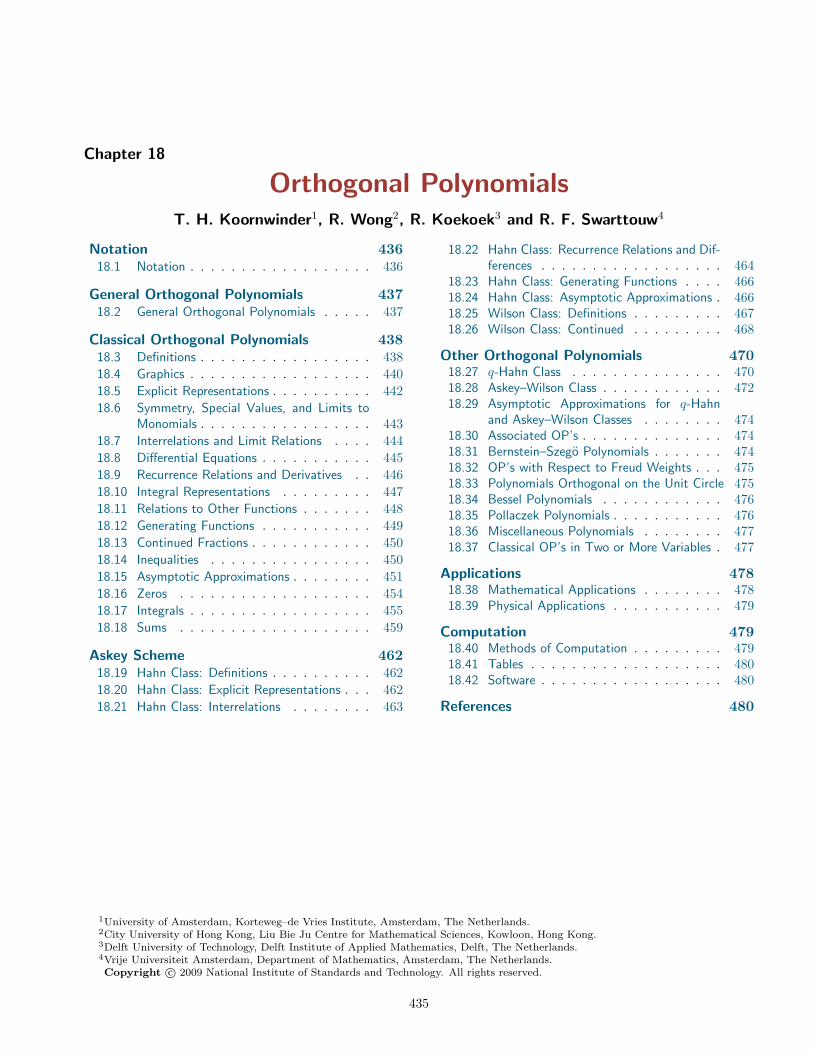
Chapter 18
Orthogonal PolynomialsT. H. Koornwinder1, R. Wong2, R. Koekoek3 and R. F. Swarttouw4
Notation 43618.1 Notation . . . . . . . . . . . . . . . . . . 436
General Orthogonal Polynomials 43718.2 General Orthogonal Polynomials . . . . . 437
Classical Orthogonal Polynomials 43818.3 Definitions . . . . . . . . . . . . . . . . . 43818.4 Graphics . . . . . . . . . . . . . . . . . . 44018.5 Explicit Representations . . . . . . . . . . 44218.6 Symmetry, Special Values, and Limits to
Monomials . . . . . . . . . . . . . . . . . 44318.7 Interrelations and Limit Relations . . . . 44418.8 Differential Equations . . . . . . . . . . . 44518.9 Recurrence Relations and Derivatives . . 44618.10 Integral Representations . . . . . . . . . 44718.11 Relations to Other Functions . . . . . . . 44818.12 Generating Functions . . . . . . . . . . . 44918.13 Continued Fractions . . . . . . . . . . . . 45018.14 Inequalities . . . . . . . . . . . . . . . . 45018.15 Asymptotic Approximations . . . . . . . . 45118.16 Zeros . . . . . . . . . . . . . . . . . . . 45418.17 Integrals . . . . . . . . . . . . . . . . . . 45518.18 Sums . . . . . . . . . . . . . . . . . . . 459
Askey Scheme 46218.19 Hahn Class: Definitions . . . . . . . . . . 46218.20 Hahn Class: Explicit Representations . . . 46218.21 Hahn Class: Interrelations . . . . . . . . 463
18.22 Hahn Class: Recurrence Relations and Dif-ferences . . . . . . . . . . . . . . . . . . 464
18.23 Hahn Class: Generating Functions . . . . 46618.24 Hahn Class: Asymptotic Approximations . 46618.25 Wilson Class: Definitions . . . . . . . . . 46718.26 Wilson Class: Continued . . . . . . . . . 468
Other Orthogonal Polynomials 47018.27 q-Hahn Class . . . . . . . . . . . . . . . 47018.28 Askey–Wilson Class . . . . . . . . . . . . 47218.29 Asymptotic Approximations for q-Hahn
and Askey–Wilson Classes . . . . . . . . 47418.30 Associated OP’s . . . . . . . . . . . . . . 47418.31 Bernstein–Szegö Polynomials . . . . . . . 47418.32 OP’s with Respect to Freud Weights . . . 47518.33 Polynomials Orthogonal on the Unit Circle 47518.34 Bessel Polynomials . . . . . . . . . . . . 47618.35 Pollaczek Polynomials . . . . . . . . . . . 47618.36 Miscellaneous Polynomials . . . . . . . . 47718.37 Classical OP’s in Two or More Variables . 477
Applications 47818.38 Mathematical Applications . . . . . . . . 47818.39 Physical Applications . . . . . . . . . . . 479
Computation 47918.40 Methods of Computation . . . . . . . . . 47918.41 Tables . . . . . . . . . . . . . . . . . . . 48018.42 Software . . . . . . . . . . . . . . . . . . 480
References 480
1University of Amsterdam, Korteweg–de Vries Institute, Amsterdam, The Netherlands.2City University of Hong Kong, Liu Bie Ju Centre for Mathematical Sciences, Kowloon, Hong Kong.3Delft University of Technology, Delft Institute of Applied Mathematics, Delft, The Netherlands.4Vrije Universiteit Amsterdam, Department of Mathematics, Amsterdam, The Netherlands.Copyright c© 2009 National Institute of Standards and Technology. All rights reserved.
435

436 Orthogonal Polynomials
Notation
18.1 Notation
18.1(i) Special Notation
(For other notation see pp. xiv and 873.)
x, y real variables.z(= x+ iy) complex variable.q real variable such that 0 < q < 1, unless
stated otherwise.`,m nonnegative integers.n nonnegative integer, except in §18.30.N positive integer.δ(x− a) Dirac delta (§1.17).δ arbitrary small positive constant.pn(x) polynomial in x of degree n.p−1(x) 0.w(x) weight function (≥ 0) on an open
interval (a, b).wx weights (> 0) at points x ∈ X of a finite
or countably infinite subset of R.OP’s orthogonal polynomials.
x-Differences
Forward differences:
∆x (f(x)) = f(x+ 1)− f(x),
∆n+1x (f(x)) = ∆x ( ∆n
x(f(x))) .
Backward differences:
∇x (f(x)) = f(x)− f(x− 1),
∇n+1x (f(x)) = ∇x (∇nx(f(x))) .
Central differences in imaginary direction:
δx (f(x)) =(f(x+ 1
2 i)− f(x− 12 i))/i,
δn+1x (f(x)) = δx ( δnx (f(x))) .
q-Pochhammer Symbol
(z; q)0 = 1, (z; q)n = (1− z)(1− zq) · · · (1− zqn−1),
(z1, . . . , zk; q)n = (z1; q)n · · · (zk; q)n .
Infinite q-Product
(z; q)∞ =∞∏j=0
(1− zqj),
(z1, . . . , zk; q)∞ = (z1; q)∞ · · · (zk; q)∞ .
18.1(ii) Main Functions
The main functions treated in this chapter are:
Classical OP’s
Jacobi: P (α,β)n (x).
Ultraspherical (or Gegenbauer): C(λ)n (x).
Chebyshev of first, second, third, and fourth kinds:Tn(x), Un(x), Vn(x), Wn(x).
Shifted Chebyshev of first and second kinds: T ∗n(x),U∗n(x).
Legendre: Pn(x).
Shifted Legendre: P ∗n(x).
Laguerre: L(α)n (x) and Ln(x) = L
(0)n (x). (L(α)
n (x) withα 6= 0 is also called Generalized Laguerre.)
Hermite: Hn(x), Hen(x).
Hahn Class OP’s
Hahn: Qn(x;α, β,N).
Krawtchouk: Kn(x; p,N).
Meixner: Mn(x;β, c).
Charlier: Cn(x, a).
Continuous Hahn: pn(x; a, b, a, b
).
Meixner–Pollaczek: P (λ)n (x;φ).
Wilson Class OP’s
Wilson: Wn(x; a, b, c, d).
Racah: Rn(x;α, β, γ, δ).
Continuous Dual Hahn: Sn(x; a, b, c).
Dual Hahn: Rn(x; γ, δ,N).
q-Hahn Class OP’s
q-Hahn: Qn(x;α, β,N ; q).
Big q-Jacobi: Pn(x; a, b, c; q).
Little q-Jacobi: pn(x; a, b; q).
q-Laguerre: L(α)n (x; q).
Stieltjes–Wigert: Sn(x; q).
Discrete q-Hermite I: hn(x; q).
Discrete q-Hermite II: h̃n(x; q).
Askey–Wilson Class OP’s
Askey–Wilson: pn(x; a, b, c, d | q).Al-Salam–Chihara: Qn(x; a, b | q).Continuous q-Ultraspherical: Cn(x;β | q).Continuous q-Hermite: Hn(x | q).Continuous q−1-Hermite: hn(x | q)q-Racah: Rn(x;α, β, γ, δ | q).
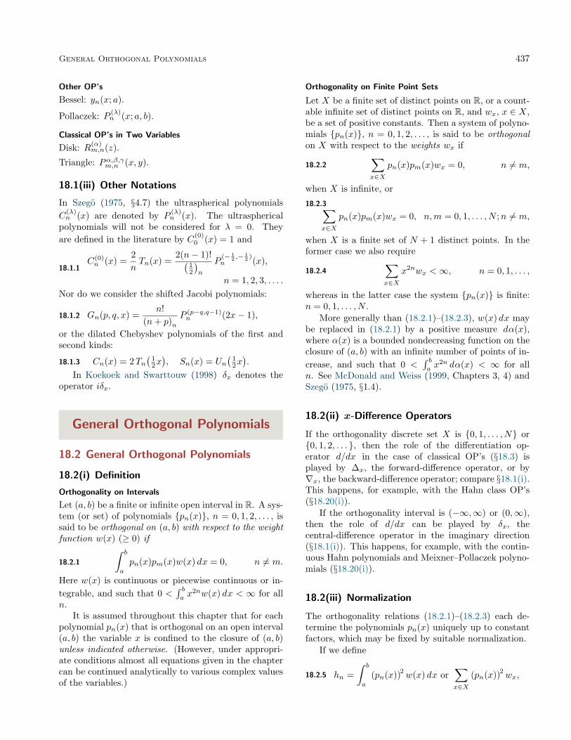
General Orthogonal Polynomials 437
Other OP’s
Bessel: yn(x; a).
Pollaczek: P (λ)n (x; a, b).
Classical OP’s in Two Variables
Disk: R(α)m,n(z).
Triangle: Pα,β,γm,n (x, y).
18.1(iii) Other Notations
In Szegö (1975, §4.7) the ultraspherical polynomialsC
(λ)n (x) are denoted by P
(λ)n (x). The ultraspherical
polynomials will not be considered for λ = 0. Theyare defined in the literature by C(0)
0 (x) = 1 and
18.1.1C(0)n (x) =
2nTn(x) =
2(n− 1)!(12
)n
P(− 1
2 ,−12 )
n (x),
n = 1, 2, 3, . . . .Nor do we consider the shifted Jacobi polynomials:
18.1.2 Gn(p, q, x) =n!
(n+ p)nP (p−q,q−1)n (2x− 1),
or the dilated Chebyshev polynomials of the first andsecond kinds:
18.1.3 Cn(x) = 2Tn(
12x), Sn(x) = Un
(12x).
In Koekoek and Swarttouw (1998) δx denotes theoperator iδx.
General Orthogonal Polynomials
18.2 General Orthogonal Polynomials
18.2(i) Definition
Orthogonality on Intervals
Let (a, b) be a finite or infinite open interval in R. A sys-tem (or set) of polynomials {pn(x)}, n = 0, 1, 2, . . . , issaid to be orthogonal on (a, b) with respect to the weightfunction w(x) (≥ 0) if
18.2.1
∫ b
a
pn(x)pm(x)w(x) dx = 0, n 6= m.
Here w(x) is continuous or piecewise continuous or in-tegrable, and such that 0 <
∫ bax2nw(x) dx < ∞ for all
n.It is assumed throughout this chapter that for each
polynomial pn(x) that is orthogonal on an open interval(a, b) the variable x is confined to the closure of (a, b)unless indicated otherwise. (However, under appropri-ate conditions almost all equations given in the chaptercan be continued analytically to various complex valuesof the variables.)
Orthogonality on Finite Point Sets
Let X be a finite set of distinct points on R, or a count-able infinite set of distinct points on R, and wx, x ∈ X,be a set of positive constants. Then a system of polyno-mials {pn(x)}, n = 0, 1, 2, . . . , is said to be orthogonalon X with respect to the weights wx if
18.2.2∑x∈X
pn(x)pm(x)wx = 0, n 6= m,
when X is infinite, or
18.2.3∑x∈X
pn(x)pm(x)wx = 0, n,m = 0, 1, . . . , N ;n 6= m,
when X is a finite set of N + 1 distinct points. In theformer case we also require
18.2.4∑x∈X
x2nwx <∞, n = 0, 1, . . . ,
whereas in the latter case the system {pn(x)} is finite:n = 0, 1, . . . , N .
More generally than (18.2.1)–(18.2.3), w(x) dx maybe replaced in (18.2.1) by a positive measure dα(x),where α(x) is a bounded nondecreasing function on theclosure of (a, b) with an infinite number of points of in-crease, and such that 0 <
∫ bax2n dα(x) < ∞ for all
n. See McDonald and Weiss (1999, Chapters 3, 4) andSzegö (1975, §1.4).
18.2(ii) x-Difference Operators
If the orthogonality discrete set X is {0, 1, . . . , N} or{0, 1, 2, . . . }, then the role of the differentiation op-erator d/dx in the case of classical OP’s (§18.3) isplayed by ∆x, the forward-difference operator, or by∇x, the backward-difference operator; compare §18.1(i).This happens, for example, with the Hahn class OP’s(§18.20(i)).
If the orthogonality interval is (−∞,∞) or (0,∞),then the role of d/dx can be played by δx, thecentral-difference operator in the imaginary direction(§18.1(i)). This happens, for example, with the contin-uous Hahn polynomials and Meixner–Pollaczek polyno-mials (§18.20(i)).
18.2(iii) Normalization
The orthogonality relations (18.2.1)–(18.2.3) each de-termine the polynomials pn(x) uniquely up to constantfactors, which may be fixed by suitable normalization.
If we define
18.2.5 hn =∫ b
a
(pn(x))2 w(x) dx or∑x∈X
(pn(x))2 wx,

438 Orthogonal Polynomials
18.2.6
h̃n =∫ b
a
x (pn(x))2 w(x) dx or∑x∈X
x (pn(x))2 wx,
and
18.2.7 pn(x) = knxn + k̃nx
n−1 + ˜̃knx
n−2 + · · · ,then two special normalizations are: (i) orthonormalOP’s: hn = 1, kn > 0; (ii) monic OP’s: kn = 1.
18.2(iv) Recurrence Relations
As in §18.1(i) we assume that p−1(x) ≡ 0.
First Form
18.2.8
pn+1(x) = (Anx+Bn)pn(x)− Cnpn−1(x), n ≥ 0.Here An, Bn (n ≥ 0), and Cn (n ≥ 1) are real constants,and An−1AnCn > 0 for n ≥ 1. Then18.2.9
An =kn+1
kn, Bn =
(k̃n+1
kn+1− k̃nkn
)An = − h̃n
hnAn,
Cn =An
˜̃kn +Bnk̃n − ˜̃
kn+1
kn−1=
AnAn−1
hnhn−1
.
Second Form
18.2.10
xpn(x) = anpn+1(x) + bnpn(x) + cnpn−1(x), n ≥ 0.Here an, bn (n ≥ 0), cn (n ≥ 1) are real constants, andan−1cn > 0 (n ≥ 1). Then
18.2.11
an =knkn+1
, bn =k̃nkn− k̃n+1
kn+1=h̃nhn,
cn =˜̃kn − an ˜̃
kn+1 − bnk̃nkn−1
= an−1hnhn−1
.
If the OP’s are orthonormal, then cn = an−1 (n ≥ 1).If the OP’s are monic, then an = 1 (n ≥ 0).
Conversely, if a system of polynomials {pn(x)} sat-isfies (18.2.10) with an−1cn > 0 (n ≥ 1), then {pn(x)}
is orthogonal with respect to some positive measure onR (Favard’s theorem). The measure is not necessarilyof the form w(x) dx nor is it necessarily unique.
18.2(v) Christoffel–Darboux Formula
18.2.12n∑`=0
p`(x)p`(y)h`
=kn
hnkn+1
pn+1(x)pn(y)− pn(x)pn+1(y)x− y
,
x 6= y.
Confluent Form
18.2.13n∑`=0
(p`(x))2
h`=
knhnkn+1
(p′n+1(x)pn(x)− p′n(x)pn+1(x)
).
18.2(vi) Zeros
All n zeros of an OP pn(x) are simple, and they arelocated in the interval of orthogonality (a, b). The zerosof pn(x) and pn+1(x) separate each other, and if m < nthen between any two zeros of pm(x) there is at leastone zero of pn(x).
For illustrations of these properties see Figures18.4.1–18.4.7.
Classical Orthogonal Polynomials
18.3 Definitions
Table 18.3.1 provides the definitions of Jacobi, Laguerre,and Hermite polynomials via orthogonality and normal-ization (§§18.2(i) and 18.2(iii)). This table also includesthe following special cases of Jacobi polynomials: ultra-spherical, Chebyshev, and Legendre.

18.3 Definitions 439T
able
18.3
.1:
Ort
hogo
nalit
ypr
oper
ties
for
clas
sica
lO
P’s
:in
terv
als,
wei
ght
func
tion
s,no
rmal
izat
ions
,le
adin
gco
effici
ents
,an
dpa
ram
eter
cons
trai
nts.
Inth
ese
cond
rowA
deno
tes
2α+β
+1
Γ(n
+α
+1)
Γ(n
+β
+1)/ ((
2n+α
+β
+1)
Γ(n
+α
+β
+1)n
!).
For
furt
her
impl
icat
ions
ofth
epa
ram
eter
cons
trai
nts
see
the
Not
ein§1
8.5(
iii).
Nam
epn(x
)(a,b
)w
(x)
hn
kn
k̃n
/ kn
Con
stra
ints
Jaco
biP
(α,β
)n
(x)
(−1,
1)(1−x
)α(1
+x
)βA
(n+α
+β
+1)n
2nn
!n
(α−β
)2n
+α
+β
α,β
>−
1
Ult
rasp
heri
cal
(Geg
enba
uer)
C(λ
)n
(x)
(−1,
1)(1−x
2)λ−
1 221−
2λπ
Γ(n
+2λ
)(n
+λ
)(Γ
(λ))
2n
!
2n(λ
) nn
!0
λ>−
1 2,λ6=
0
Che
bysh
evof
first
kind
Tn(x
)(−
1,1)
(1−x
2)−
1 2
{ 1 2π,n>
0π,
n=
0
{ 2n−
1,n>
01,
n=
00
Che
bysh
evof
seco
ndki
ndUn(x
)(−
1,1)
(1−x
2)1 2
1 2π
2n0
Che
bysh
evof
thir
dki
ndVn(x
)(−
1,1)
(1−x
)1 2(1
+x
)−1 2
π2n
1 2
Che
bysh
evof
four
thki
ndWn(x
)(−
1,1)
(1−x
)−1 2(1
+x
)1 2π
2n−
1 2
Shift
edC
heby
shev
offir
stki
ndT∗ n(x
)(0,1
)(x−x
2)−
1 2
{ 1 2π,n>
0π,
n=
0
{ 22n−
1,n>
01,
n=
0−
1 2n
Shift
edC
heby
shev
ofse
cond
kind
U∗ n(x
)(0,1
)(x−x
2)1 2
1 8π
22n
−1 2n
Leg
endr
ePn(x
)(−
1,1)
12/
(2n
+1)
2n( 1 2
) n
/ n!0
Shift
edL
egen
dre
P∗ n(x
)(0,1
)1
1/(2n
+1)
22n( 1 2
) n
/ n!−
1 2n
Lag
uerr
eL
(α)
n(x
)(0,∞
)e−
xxα
Γ(n
+α
+1)
/n!
(−1)n/n
!−n
(n+α
)α>−
1
Her
mit
eHn(x
)(−∞,∞
)e−
x2
π1 22nn
!2n
0
Her
mit
eH
e n(x
)(−∞,∞
)e−
1 2x2
(2π
)1 2n
!1
0

440 Orthogonal Polynomials
For exact values of the coefficients of the Jacobipolynomials P (α,β)
n (x), the ultraspherical polynomialsC
(λ)n (x), the Chebyshev polynomials Tn(x) and Un(x),
the Legendre polynomials Pn(x), the Laguerre poly-nomials Ln(x), and the Hermite polynomials Hn(x),see Abramowitz and Stegun (1964, pp. 793–801). TheJacobi polynomials are in powers of x − 1 for n =0, 1, . . . , 6. The ultraspherical polynomials are in pow-ers of x for n = 0, 1, . . . , 6. The other polynomials arein powers of x for n = 0, 1, . . . , 12. See also §18.5(iv).Chebyshev
In this chapter, formulas for the Chebyshev polynomialsof the second, third, and fourth kinds will not be givenas extensively as those of the first kind. However, mostof these formulas can be obtained by specialization offormulas for Jacobi polynomials, via (18.7.4)–(18.7.6).
In addition to the orthogonal property given byTable 18.3.1, the Chebyshev polynomials Tn(x), n =0, 1, . . . , N , are orthogonal on the discrete point set com-prising the zeros xN+1,n, n = 1, 2, . . . , N+1, of TN+1(x):
18.3.1
N+1∑n=1
Tj(xN+1,n)Tk(xN+1,n) = 0,
0 ≤ j ≤ N , 0 ≤ k ≤ N , j 6= k,where
18.3.2 xN+1,n = cos((n− 1
2 )π/(N + 1)).
When j = k 6= 0 the sum in (18.3.1) is 12 (N + 1). When
j = k = 0 the sum in (18.3.1) is N + 1.
For proofs of these results and for similar propertiesof the Chebyshev polynomials of the second, third, andfourth kinds see Mason and Handscomb (2003, §4.6).
For another version of the discrete orthogonalityproperty of the polynomials Tn(x) see (3.11.9).
Legendre
Legendre polynomials are special cases of Legendrefunctions, Ferrers functions, and associated Legendrefunctions (§14.7(i)). In consequence, additional proper-ties are included in Chapter 14.
18.4 Graphics
18.4(i) Graphs
Figure 18.4.1: Jacobi polynomials P (1.5,−0.5)n (x), n =
1, 2, 3, 4, 5.
Figure 18.4.2: Jacobi polynomials P (1.25,0.75)n (x), n =
7, 8. This illustrates inequalities for extrema of a Jacobipolynomial; see (18.14.16). See also Askey (1990).
Figure 18.4.3: Chebyshev polynomials Tn(x), n =1, 2, 3, 4, 5.

18.4 Graphics 441
Figure 18.4.4: Legendre polynomials Pn(x), n =1, 2, 3, 4, 5.
Figure 18.4.5: Laguerre polynomials Ln(x), n =1, 2, 3, 4, 5.
Figure 18.4.6: Laguerre polynomials L(α)3 (x), α =
0, 1, 2, 3, 4.Figure 18.4.7: Monic Hermite polynomials hn(x) =2−nHn(x), n = 1, 2, 3, 4, 5.
18.4(ii) Surfaces
Figure 18.4.8: Laguerre polynomials L(α)3 (x), 0 ≤ α ≤ 3,
0 ≤ x ≤ 10.Figure 18.4.9: Laguerre polynomials L(α)
4 (x), 0 ≤ α ≤ 3,0 ≤ x ≤ 10.

442 Orthogonal Polynomials
18.5 Explicit Representations
18.5(i) Trigonometric Functions
Chebyshev
With x = cos θ,
18.5.1 Tn(x) = cos(nθ),
18.5.2 Un(x) = (sin (n+ 1)θ)/sin θ ,
18.5.3 Vn(x) = (sin (n+ 12 )θ)
/sin(
12θ),
18.5.4 Wn(x) = (cos (n+ 12 )θ)
/cos(
12θ).
18.5(ii) Rodrigues Formulas
18.5.5 pn(x) =1
κnw(x)dn
dxn(w(x)(F (x))n) .
In this equation w(x) is as in Table 18.3.1, and F (x),κn are as in Table 18.5.1.
Table 18.5.1: Classical OP’s: Rodrigues formulas(18.5.5).
pn(x) F (x) κn
P(α,β)n (x) 1− x2 (−2)nn!
C(λ)n (x) 1− x2
(−2)n(λ+ 1
2
)nn!
(2λ)nTn(x) 1− x2 (−2)n
(12
)n
Un(x) 1− x2(−2)n
(32
)n
n+ 1
Vn(x) 1− x2(−2)n
(32
)n
2n+ 1Wn(x) 1− x2 (−2)n
(12
)n
Pn(x) 1− x2 (−2)nn!
L(α)n (x) x n!
Hn(x) 1 (−1)n
Hen(x) 1 (−1)n
Related formula:18.5.6
L(α)n
(1x
)=
(−1)n
n!xn+α+1e 1/x dn
dxn
(x−α−1e− 1/x
).
18.5(iii) Finite Power Series, theHypergeometric Function, andGeneralized Hypergeometric Functions
For the definitions of 2F1, 1F1, and 2F0 see §16.2.
Jacobi
18.5.7
P (α,β)n (x)
=n∑`=0
(n+ α+ β + 1)`(α+ `+ 1)n−``! (n− `)!
(x− 1
2
)̀=
(α+ 1)nn! 2F1
(−n, n+ α+ β + 1
α+ 1;
1− x2
),
18.5.8
P (α,β)n (x)
= 2−nn∑`=0
(n+ α
`
)(n+ β
n− `
)(x− 1)n−`(x+ 1)`
=(α+ 1)n
n!
(x+ 1
2
)n2F1
(−n,−n− β
α+ 1;x− 1x+ 1
),
and two similar formulas by symmetry; compare thesecond row in Table 18.6.1.
Ultraspherical
18.5.9 C(λ)n (x) =
(2λ)nn! 2F1
(−n, n+ 2λλ+ 1
2
;1− x
2
),
18.5.10
C(λ)n (x) =
bn/2c∑`=0
(−1)`(λ)n−``! (n− 2`)!
(2x)n−2`
= (2x)n(λ)nn! 2F1
(− 1
2n,−12n+ 1
2
1− λ− n;
1x2
),
18.5.11
C(λ)n (cos θ) =
n∑`=0
(λ)`(λ)n−``! (n− `)!
cos((n− 2`)θ)
= einθ(λ)nn! 2F1
(−n, λ
1− λ− n; e−2iθ
).

18.6 Symmetry, Special Values, and Limits to Monomials 443
Laguerre
18.5.12
L(α)n (x) =
n∑`=0
(α+ `+ 1)n−`(n− `)! `!
(−x)`
=(α+ 1)n
n! 1F1
(−nα+ 1
;x).
Hermite
18.5.13
Hn(x) = n!bn/2c∑`=0
(−1)`(2x)n−2`
`! (n− 2`)!
= (2x)n 2F0
(− 1
2n,−12n+ 1
2
−;− 1
x2
).
For corresponding formulas for Chebyshev, Legen-dre, and the Hermite Hen polynomials apply (18.7.3)–(18.7.6), (18.7.9), and (18.7.11).
Note. The first of each of equations (18.5.7) and(18.5.8) can be regarded as definitions of P (α,β)
n (x) whenthe conditions α > −1 and β > −1 are not satisfied.However, in these circumstances the orthogonality prop-erty (18.2.1) disappears. For this reason, and also in theinterest of simplicity, in the case of the Jacobi polyno-mials P (α,β)
n (x) we assume throughout this chapter thatα > −1 and β > −1, unless stated otherwise. Similarlyin the cases of the ultraspherical polynomials C(λ)
n (x)and the Laguerre polynomials L(α)
n (x) we assume thatλ > − 1
2 , λ 6= 0, and α > −1, unless stated otherwise.
18.5(iv) Numerical Coefficients
Chebyshev
18.5.14
T0(x) = 1, T1(x) = x, T2(x) = 2x2 − 1,T3(x) = 4x3 − 3x, T4(x) = 8x4 − 8x2 + 1,T5(x) = 16x5 − 20x3 + 5x,T6(x) = 32x6 − 48x4 + 18x2 − 1.
18.5.15
U0(x) = 1, U1(x) = 2x, U2(x) = 4x2 − 1,U3(x) = 8x3 − 4x, U4(x) = 16x4 − 12x2 + 1,U5(x) = 32x5 − 32x3 + 6x,U6(x) = 64x6 − 80x4 + 24x2 − 1.
Legendre
18.5.16
P0(x) = 1, P1(x) = x, P2(x) = 32x
2 − 12 ,
P3(x) = 52x
3 − 32x, P4(x) = 35
8 x4 − 15
4 x2 + 3
8 ,
P5(x) = 638 x
5 − 354 x
3 + 158 x,
P6(x) = 23116 x
6 − 31516 x
4 + 10516 x
2 − 516 .
Laguerre
18.5.17
L0(x) = 1, L1(x) = −x+ 1, L2(x) = 12x
2 − 2x+ 1,L3(x) = − 1
6x3 + 3
2x2 − 3x+ 1,
L4(x) = 124x
4 − 23x
3 + 3x2 − 4x+ 1,L5(x) = − 1
120x5 + 5
24x4 − 5
3x3 + 5x2 − 5x+ 1,
L6(x) = 1720x
6 − 120x
5 + 58x
4 − 103 x
3 + 152 x
2 − 6x+ 1.
Hermite
18.5.18
H0(x) = 1, H1(x) = 2x, H2(x) = 4x2 − 2,H3(x) = 8x3 − 12x, H4(x) = 16x4 − 48x2 + 12,H5(x) = 32x5 − 160x3 + 120x,H6(x) = 64x6 − 480x4 + 720x2 − 120.
18.5.19
He0(x) = 1, He1(x) = x, He2(x) = x2 − 1,He3(x) = x3 − 3x, He4(x) = x4 − 6x2 + 3,He5(x) = x5 − 10x3 + 15x,He6(x) = x6 − 15x4 + 45x2 − 15.
For the corresponding polynomials of degrees 7through 12 see Abramowitz and Stegun (1964, Ta-bles 22.3, 22.5, 22.9, 22.10, 22.12).
18.6 Symmetry, Special Values, and Limitsto Monomials
18.6(i) Symmetry and Special Values
For Jacobi, ultraspherical, Chebyshev, Legendre, andHermite polynomials, see Table 18.6.1.
Laguerre
18.6.1 L(α)n (0) =
(α+ 1)nn!
.

444 Orthogonal Polynomials
Table 18.6.1: Classical OP’s: symmetry and special values.
pn(x) pn(−x) pn(1) p2n(0) p′2n+1(0)
P(α,β)n (x) (−1)n P (β,α)
n (x) (α+ 1)n/n!
P(α,α)n (x) (−1)n P (α,α)
n (x) (α+ 1)n/n! (− 14 )n(n+ α+ 1)n
/n! (− 1
4 )n(n+ α+ 1)n+1
/n!
C(λ)n (x) (−1)n C(λ)
n (x) (2λ)n/n! (−1)n(λ)n/n! 2(−1)n(λ)n+1
/n!
Tn(x) (−1)n Tn(x) 1 (−1)n (−1)n(2n+ 1)
Un(x) (−1)n Un(x) n+ 1 (−1)n (−1)n(2n+ 2)
Vn(x) (−1)nWn(x) 2n+ 1 (−1)n (−1)n(2n+ 2)
Wn(x) (−1)n Vn(x) 1 (−1)n (−1)n(2n+ 2)
Pn(x) (−1)n Pn(x) 1 (−1)n(
12
)n
/n! 2(−1)n
(12
)n+1
/n!
Hn(x) (−1)nHn(x) (−1)n(n+ 1)n 2(−1)n(n+ 1)n+1
Hen(x) (−1)n Hen(x) (− 12 )n(n+ 1)n (− 1
2 )n(n+ 1)n+1
18.6(ii) Limits to Monomials
18.6.2 limα→∞
P(α,β)n (x)
P(α,β)n (1)
=(
1 + x
2
)n,
18.6.3 limβ →∞
P(α,β)n (x)
P(α,β)n (−1)
=(
1− x2
)n,
18.6.4 limλ→∞
C(λ)n (x)
C(λ)n (1)
= xn,
18.6.5 limα→∞
L(α)n (αx)
L(α)n (0)
= (1− x)n.
18.7 Interrelations and Limit Relations
18.7(i) Linear Transformations
Ultraspherical and Jacobi
18.7.1 C(λ)n (x) =
(2λ)n(λ+ 1
2
)n
P(λ− 1
2 ,λ−12 )
n (x),
18.7.2 P (α,α)n (x) =
(α+ 1)n(2α+ 1)n
C(α+ 1
2 )n (x).
Chebyshev, Ultraspherical, and Jacobi
18.7.3 Tn(x) = P(− 1
2 ,−12 )
n (x)/P
(− 12 ,−
12 )
n (1) ,
18.7.4
Un(x) = C(1)n (x) = (n+ 1)P ( 1
2 ,12 )
n (x)/P
( 12 ,
12 )
n (1) ,
18.7.5 Vn(x) = (2n+ 1)P ( 12 ,−
12 )
n (x)/P
( 12 ,−
12 )
n (1) ,
18.7.6 Wn(x) = P(− 1
2 ,12 )
n (x)/P
(− 12 ,
12 )
n (1) .
18.7.7 T ∗n(x) = Tn(2x− 1),
18.7.8 U∗n(x) = Un(2x− 1).See also (18.9.9)–(18.9.12).
Legendre, Ultraspherical, and Jacobi
18.7.9 Pn(x) = C( 12 )n (x) = P (0,0)
n (x).
18.7.10 P ∗n(x) = Pn(2x− 1).
Hermite
18.7.11 Hen(x) = 2−12nHn
(2−
12x),
18.7.12 Hn(x) = 212n Hen
(2
12x).

18.8 Differential Equations 445
18.7(ii) Quadratic Transformations
18.7.13P
(α,α)2n (x)
P(α,α)2n (1)
=P
(α,− 12 )
n
(2x2 − 1
)P
(α,− 12 )
n (1),
18.7.14P
(α,α)2n+1 (x)
P(α,α)2n+1 (1)
=xP
(α, 12 )n
(2x2 − 1
)P
(α, 12 )n (1)
.
18.7.15 C(λ)2n (x) =
(λ)n(12
)n
P(λ− 1
2 ,−12 )
n
(2x2 − 1
),
18.7.16 C(λ)2n+1(x) =
(λ)n+1(12
)n+1
xP(λ− 1
2 ,12 )
n
(2x2 − 1
).
18.7.17 U2n(x) = Vn(2x2 − 1
),
18.7.18 T2n+1(x) = xWn
(2x2 − 1
).
18.7.19 H2n(x) = (−1)n22nn!L(− 12 )
n
(x2),
18.7.20 H2n+1(x) = (−1)n22n+1n!xL( 12 )n
(x2).
18.7(iii) Limit Relations
Jacobi → Laguerre
18.7.21 limβ→∞
P (α,β)n (1− (2x/β )) = L(α)
n (x).
18.7.22 limα→∞
P (α,β)n ((2x/α)− 1) = (−1)n L(β)
n (x).
Jacobi → Hermite
18.7.23 limα→∞
α−12n P (α,α)
n
(α−
12x)
=Hn(x)2nn!
.
Ultraspherical → Hermite
18.7.24 limλ→∞
λ−12n C(λ)
n
(λ−
12x)
=Hn(x)n!
.
18.7.25 limλ→0
1λC(λ)n (x) =
2nTn(x), n ≥ 1.
Laguerre → Hermite
18.7.26
limα→∞
(2α
)12n
L(α)n
((2α)
12x+ α
)=
(−1)n
n!Hn(x).
See Figure 18.21.1 for the Askey schematic represen-tation of most of these limits.
18.8 Differential Equations
See Table 18.8.1 and also Table 22.6 of Abramowitz andStegun (1964).
Table 18.8.1: Classical OP’s: differential equations A(x)f ′′(x) +B(x)f ′(x) + C(x)f(x) + λnf(x) = 0.
f(x) A(x) B(x) C(x) λn
P(α,β)n (x) 1− x2 β − α− (α+ β + 2)x 0 n(n+ α+ β + 1)(
sin 12x)α+ 1
2(cos 1
2x)β+ 1
2
×P (α,β)n (cosx)
1 014 − α
2
4 sin2 12x
+14 − β
2
4 cos2 12x
(n+ 1
2 (α+ β + 1))2
(sinx)α+ 12 P
(α,α)n (cosx) 1 0 ( 1
4 − α2)/ sin2 x (n+ α+ 1
2 )2
C(λ)n (x) 1− x2 −(2λ+ 1)x 0 n(n+ 2λ)
Tn(x) 1− x2 −x 0 n2
Un(x) 1− x2 −3x 0 n(n+ 2)
Pn(x) 1− x2 −2x 0 n(n+ 1)
L(α)n (x) x α+ 1− x 0 n
e−12x
2xα+ 1
2 L(α)n
(x2)
1 0 −x2 + ( 14 − α
2)x−2 4n+ 2α+ 2
Hn(x) 1 −2x 0 2n
e−12x
2Hn(x) 1 0 −x2 2n+ 1
Hen(x) 1 −x 0 n

446 Orthogonal Polynomials
18.9 Recurrence Relations and Derivatives
18.9(i) Recurrence Relations
18.9.1 pn+1(x) = (Anx+Bn)pn(x)− Cnpn−1(x).
For pn(x) = P(α,β)n (x),
18.9.2
An =(2n+ α+ β + 1)(2n+ α+ β + 2)
2(n+ 1)(n+ α+ β + 1),
Bn =(α2 − β2)(2n+ α+ β + 1)
2(n+ 1)(n+ α+ β + 1)(2n+ α+ β),
Cn =(n+ α)(n+ β)(2n+ α+ β + 2)
(n+ 1)(n+ α+ β + 1)(2n+ α+ β).
For the other classical OP’s see Table 18.9.1; comparealso §18.2(iv).
Table 18.9.1: Classical OP’s: recurrence relations(18.9.1).
pn(x) An Bn Cn
C(λ)n (x) 2n+λ
n+1 0 n+2λ−1n+1
Tn(x) 2− δn,0 0 1
Un(x) 2 0 1
T ∗n(x) 4− 2δn,0 −2 + δn,0 1
U∗n(x) 4 −2 1
Pn(x) 2n+1n+1 0 n
n+1
P ∗n(x) 4n+2n+1 − 2n+1
n+1nn+1
L(α)n (x) − 1
n+12n+α+1n+1
n+αn+1
Hn(x) 2 0 2n
Hen(x) 1 0 n
18.9(ii) Contiguous Relations in the Parametersand the Degree
Jacobi
18.9.3 P (α,β−1)n (x)− P (α−1,β)
n (x) = P(α,β)n−1 (x),
18.9.4
(1− x)P (α+1,β)n (x) + (1 + x)P (α,β+1)
n (x) = 2P (α,β)n (x).
18.9.5
(2n+ α+ β + 1)P (α,β)n (x)
= (n+ α+ β + 1)P (α,β+1)n (x) + (n+ α)P (α,β+1)
n−1 (x),
18.9.6(n+ 1
2α+ 12β + 1)(1 + x)P (α,β+1)
n (x)
= (n+ 1)P (α,β)n+1 (x) + (n+ β + 1)P (α,β)
n (x),and a similar pair to (18.9.5) and (18.9.6) by symmetry;compare the second row in Table 18.6.1.
Ultraspherical
18.9.7 (n+ λ)C(λ)n (x) = λ
(C(λ+1)n (x)− C(λ+1)
n−2 (x)),
18.9.8
4λ(n+ λ+ 1)(1− x2)C(λ+1)n (x)
= −(n+ 1)(n+ 2)C(λ)n+2(x)
+ (n+ 2λ)(n+ 2λ+ 1)C(λ)n (x).
Chebyshev
18.9.9 Tn(x) = 12 (Un(x)− Un−2(x)) ,
18.9.10 (1− x2)Un(x) = − 12 (Tn+2(x)− Tn(x)) .
18.9.11 Wn(x) +Wn−1(x) = 2Tn(x),
18.9.12 Tn+1(x) + Tn(x) = (1 + x)Wn(x).
Laguerre
18.9.13 L(α)n (x) = L(α+1)
n (x)− L(α+1)n−1 (x),
18.9.14xL(α+1)
n (x) = −(n+ 1)L(α)n+1(x)
+ (n+ α+ 1)L(α)n (x).
18.9(iii) Derivatives
Jacobi
18.9.15d
dxP (α,β)n (x) = 1
2 (n+α+ β + 1)P (α+1,β+1)n−1 (x),
18.9.16
d
dx
((1− x)α(1 + x)β P (α,β)
n (x))
= −2(n+ 1)(1− x)α−1(1 + x)β−1 P(α−1,β−1)n+1 (x).
18.9.17
(2n+ α+ β)(1− x2)d
dxP (α,β)n (x)
= n (α− β − (2n+ α+ β)x)P (α,β)n (x)
+ 2(n+ α)(n+ β)P (α,β)n−1 (x),
18.9.18
(2n+ α+ β + 2)(1− x2)d
dxP (α,β)n (x)
= (n+α+β+ 1) (α−β+ (2n+α+β+ 2)x)P (α,β)n (x)
− 2(n+ 1)(n+ α+ β + 1)P (α,β)n+1 (x).
Ultraspherical
18.9.19d
dxC(λ)n (x) = 2λC(λ+1)
n−1 (x),
18.9.20
d
dx
((1− x2)λ−
12 C(λ)
n (x))
= − (n+ 1)(n+ 2λ− 1)2(λ− 1)
(1− x2)λ−32 C
(λ−1)n+1 (x).

18.10 Integral Representations 447
Chebyshev
18.9.21d
dxTn(x) = nUn−1(x),
18.9.22d
dx
((1− x2)
12 Un(x)
)= −(n+ 1)(1− x2)−
12 Tn+1(x).
Laguerre
18.9.23d
dxL(α)n (x) = −L(α+1)
n−1 (x),
18.9.24d
dx
(e−xxα L(α)
n (x))
= (n+ 1)e−xxα−1 L(α−1)n+1 (x).
Hermite
18.9.25d
dxHn(x) = 2nHn−1(x),
18.9.26d
dx
(e−x
2Hn(x)
)= −e−x
2Hn+1(x).
18.9.27d
dxHen(x) = nHen−1(x),
18.9.28d
dx
(e−
12x
2Hen(x)
)= −e− 1
2x2
Hen+1(x).
18.10 Integral Representations
18.10(i) Dirichlet-Mehler-Type Integral Representations
Ultraspherical
18.10.1P
(α,α)n (cos θ)
P(α,α)n (1)
=C
(α+ 12 )
n (cos θ)
C(α+ 1
2 )n (1)
=2α+ 1
2 Γ(α+ 1)π
12 Γ(α+ 1
2
) (sin θ)−2α
∫ θ
0
cos((n+ α+ 1
2 )φ)
(cosφ− cos θ)−α+ 12dφ, 0 < θ < π, α > − 1
2 .
Legendre
18.10.2 Pn(cos θ) =2
12
π
∫ θ
0
cos((n+ 1
2 )φ)
(cosφ− cos θ)12dφ, 0 < θ < π.
Generalizations of (18.10.1) are given in Gasper (1975, (6),(8)) and Koornwinder (1975b, (5.7),(5.8)).
18.10(ii) Laplace-Type Integral Representations
Jacobi
18.10.3
P(α,β)n (cos θ)
P(α,β)n (1)
=2 Γ(α+ 1)
π12 Γ(α− β) Γ
(β + 1
2
)×∫ 1
0
∫ π
0
((cos 1
2θ)2 − r2(sin 1
2θ)2 + ir sin θ cosφ
)n(1− r2)α−β−1r2β+1(sinφ)2β dφ dr,
α > β > − 12 .
Ultraspherical
18.10.4P
(α,α)n (cos θ)
P(α,α)n (1)
=C
(α+ 12 )
n (cos θ)
C(α+ 1
2 )n (1)
=Γ(α+ 1)
π12 Γ (α+ 1
2 )
∫ π
0
(cos θ + i sin θ cosφ)n (sinφ)2α dφ, α > − 12 .
Legendre
18.10.5 Pn(cos θ) =1π
∫ π
0
(cos θ + i sin θ cosφ)n dφ.
Laguerre
18.10.6 L(α)n
(x2)
=2(−1)n
π12 Γ(α+ 1
2
)n!
∫ ∞0
∫ π
0
(x2 − r2 + 2ixr cosφ)n e−r2r2α+1(sinφ)2α dφ dr, α > − 1
2 .
Hermite
18.10.7 Hn(x) =2n
π12
∫ ∞−∞
(x+ it)ne−t2dt.
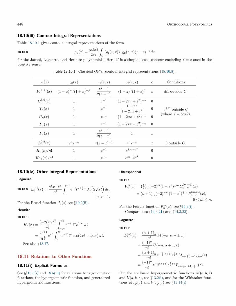
448 Orthogonal Polynomials
18.10(iii) Contour Integral Representations
Table 18.10.1 gives contour integral representations of the form
18.10.8 pn(x) =g0(x)2πi
∫C
(g1(z, x))n g2(z, x)(z − c)−1 dz
for the Jacobi, Laguerre, and Hermite polynomials. Here C is a simple closed contour encircling z = c once in thepositive sense.
Table 18.10.1: Classical OP’s: contour integral representations (18.10.8).
pn(x) g0(x) g1(z, x) g2(z, x) c Conditions
P(α,β)n (x) (1− x)−α(1 + x)−β
z2 − 12(z − x)
(1− z)α(1 + z)β x ±1 outside C.
C(λ)n (x) 1 z−1 (1− 2xz + z2)−λ 0
e±iθ outside C(where x = cos θ).
Tn(x) 1 z−1 1− xz1− 2xz + z2
0
Un(x) 1 z−1 (1− 2xz + z2)−1 0
Pn(x) 1 z−1 (1− 2xz + z2)−12 0
Pn(x) 1z2 − 1
2(z − x)1 x
L(α)n (x) exx−α z(z − x)−1 zαe−z x 0 outside C.
Hn(x)/n! 1 z−1 e2xz−z2 0
Hen(x)/n! 1 z−1 exz−12 z
20
18.10(iv) Other Integral Representations
Laguerre
18.10.9 L(α)n (x) =
exx−12α
n!
∫ ∞0
e−ttn+ 12α Jα
(2√xt)dt,
α > −1.
For the Bessel function Jν(z) see §10.2(ii).
Hermite
18.10.10
Hn(x) =(−2i)nex
2
π12
∫ ∞−∞
e−t2tne2ixt dt
=2n+1
π12ex
2∫ ∞
0
e−t2tn cos
(2xt− 1
2nπ)dt.
See also §18.17.
18.11 Relations to Other Functions
18.11(i) Explicit Formulas
See §§18.5(i) and 18.5(iii) for relations to trigonometricfunctions, the hypergeometric function, and generalizedhypergeometric functions.
Ultraspherical
18.11.1
Pmn (x) =(
12
)m
(−2)m(1− x2)12m C
(m+ 12 )
n−m (x)
= (n+ 1)m(−2)−m(1− x2)12m P
(m,m)n−m (x),
0 ≤ m ≤ n.
For the Ferrers function Pmn (x), see §14.3(i).Compare also (14.3.21) and (14.3.22).
Laguerre
18.11.2
L(α)n (x) =
(α+ 1)nn!
M(−n, α+ 1, x)
=(−1)n
n!U(−n, α+ 1, x)
=(α+ 1)n
n!z−
12 (α+1)e
12 zMn+ 1
2 (α+1), 12α(z)
=(−1)n
n!z−
12 (α+1)e
12 zWn+ 1
2 (α+1), 12α(z).
For the confluent hypergeometric functions M(a, b, z)and U(a, b, z), see §13.2(i), and for the Whittaker func-tions Mκ,µ(z) and Wκ,µ(z) see §13.14(i).

18.12 Generating Functions 449
Hermite
18.11.3
Hn(x) = 2n U(− 1
2n,12 , x
2)
= 2nxU(− 1
2n+ 12 ,
32 , x
2)
= 212ne
12x
2U(−n− 1
2 , 212x).
18.11.4
Hen(x) = 212n U
(− 1
2n,12 ,
12x
2)
= 212 (n−1)xU
(− 1
2n+ 12 ,
32 ,
12x
2)
= e14x
2U(−n− 1
2 , x).
For the parabolic cylinder function U(a, z), see §12.2.
18.11(ii) Formulas of Mehler–Heine Type
Jacobi
18.11.5
limn→∞
1nα
P (α,β)n
(1− z2
2n2
)= limn→∞
1nα
P (α,β)n
(cos
z
n
)=
2α
zαJα(z).
Laguerre
18.11.6 limn→∞
1nα
L(α)n
( zn
)=
1z
12α
Jα
(2z
12
).
Hermite
18.11.7 limn→∞
(−1)nn12
22nn!H2n
(z
2n12
)=
1π
12
cos z,
18.11.8 limn→∞
(−1)n
22nn!H2n+1
(z
2n12
)=
2π
12
sin z.
For the Bessel function Jν(z), see §10.2(ii). Thelimits (18.11.5)–(18.11.8) hold uniformly for z in anybounded subset of C.
18.12 Generating Functions
With the notation of §§10.2(ii), 10.25(ii), and 15.2,
Jacobi
18.12.1
2α+β
R(1 +R− z)α(1 +R+ z)β
=∞∑n=0
P (α,β)n (x)zn, R =
√1− 2xz + z2, |z| < 1.
18.12.2
(12 (1− x)z
)− 12α Jα
(√2(1− x)z
)×(
12 (1 + x)z
)− 12β Iβ
(√2(1 + x)z
)=∞∑n=0
P(α,β)n (x)
Γ(n+ α+ 1) Γ(n+ β + 1)zn.
18.12.3
(1 + z)−α−β−1
× 2F1
( 12 (α+ β + 1), 1
2 (α+ β + 2)β + 1
;2(x+ 1)z(1 + z)2
)=∞∑n=0
(α+ β + 1)n(β + 1)n
P (α,β)n (x)zn, |z| < 1,
and a similar formula by symmetry; compare the secondrow in Table 18.6.1. For the hypergeometric function2F1 see §§15.1, 15.2(i).Ultraspherical
18.12.4
(1− 2xz + z2)−λ =∞∑n=0
C(λ)n (x)zn
=∞∑n=0
(2λ)n(λ+ 1
2
)n
P(λ− 1
2 ,λ−12 )
n (x)zn,
|z| < 1.18.12.5
1− xz(1− 2xz + z2)λ+1
=∞∑n=0
n+ 2λ2λ
C(λ)n (x)zn, |z| < 1.
18.12.6
Γ(λ+ 1
2
)ez cos θ( 1
2z sin θ)12−λ Jλ− 1
2(z sin θ)
=∞∑n=0
C(λ)n (cos θ)(2λ)n
zn, 0 ≤ θ ≤ π.
Chebyshev
18.12.71− z2
1− 2xz + z2= 1 + 2
∞∑n=1
Tn(x)zn, |z| < 1.
18.12.81− xz
1− 2xz + z2=∞∑n=0
Tn(x)zn, |z| < 1.
18.12.9 − ln(1− 2xz + z2
)= 2
∞∑n=1
Tn(x)n
zn, |z| < 1.
18.12.101
1− 2xz + z2=∞∑n=0
Un(x)zn, |z| < 1.
Legendre
18.12.111√
1− 2xz + z2=∞∑n=0
Pn(x)zn, |z| < 1.
18.12.12 exz J0
(z√
1− x2)
=∞∑n=0
Pn(x)n!
zn.
Laguerre
18.12.13
(1− z)−α−1 exp(
xz
z − 1
)=∞∑n=0
L(α)n (x)zn, |z| < 1.
18.12.14
Γ(α+ 1)(xz)−12αez Jα
(2√xz)
=∞∑n=0
L(α)n (x)
(α+ 1)nzn.

450 Orthogonal Polynomials
Hermite
18.12.15 e2xz−z2 =∞∑n=0
Hn(x)n!
zn,
18.12.16 exz−12 z
2=∞∑n=0
Hen(x)n!
zn.
18.13 Continued Fractions
We use the terminology of §1.12(ii).Chebyshev
Tn(x) is the denominator of the nth approximant to:
18.13.1− 1x+
− 12x+
− 12x+
· · · ,
and Un(x) is the denominator of the nth approximantto:
18.13.2− 1
2x+− 1
2x+− 1
2x+· · · .
Legendre
Pn(x) is the denominator of the nth approximant to:
18.13.3a1
x+− 1
232x+
− 23
53x+
− 34
74x+
· · · ,
where a1 is an arbitrary nonzero constant.Laguerre
Ln(x) is the denominator of the nth approximant to:18.13.4
a1
1− x+− 1
212 (3− x) +
− 23
13 (5− x) +
− 34
14 (7− x)+
· · · ,
where a1 is again an arbitrary nonzero constant.Hermite
Hn(x) is the denominator of the nth approximant to:
18.13.51
2x+− 2
2x+− 4
2x+− 6
2x+· · · .
See also Cuyt et al. (2008, pp. 91–99).
18.14 Inequalities
18.14(i) Upper Bounds
Jacobi
18.14.1|P (α,β)
n (x)| ≤ P (α,β)n (1) =
(α+ 1)nn!
,
−1 ≤ x ≤ 1, α ≥ β > −1, α ≥ − 12 ,
18.14.2|P (α,β)
n (x)| ≤ |P (α,β)n (−1)| =
(β + 1)nn!
,
−1 ≤ x ≤ 1, β ≥ α > −1, β ≥ − 12 .
18.14.3
(12 (1− x)
)12α+ 1
4(
12 (1 + x)
)12β+ 1
4 |P (α,β)n (x)|
≤ Γ(max(α, β) + n+ 1)
π12n!(n+ 1
2 (α+ β + 1))max(α,β)+ 1
2,
−1 ≤ x ≤ 1, − 12 ≤ α ≤
12 , − 1
2 ≤ β ≤12 .
Ultraspherical
18.14.4
|C(λ)n (x)| ≤ C(λ)
n (1) =(2λ)nn!
, −1 ≤ x ≤ 1, λ > 0.
18.14.5|C(λ)
2m(x)| ≤ |C(λ)2m(0)| =
∣∣∣∣ (λ)mm!
∣∣∣∣ ,−1 ≤ x ≤ 1, − 1
2 < λ < 0,
18.14.6|C(λ)
2m+1(x)| <−2(λ)m+1
((2m+ 1)(2λ+ 2m+ 1))12 m!
,
−1 ≤ x ≤ 1, − 12 < λ < 0.
18.14.7(n+ λ)1−λ(1− x2)
12λ|C(λ)
n (x)| < 21−λ
Γ(λ),
−1 ≤ x ≤ 1, 0 < λ < 1.
Laguerre
18.14.8 e−12x∣∣∣L(α)n (x)
∣∣∣ ≤ L(α)n (0) =
(α+ 1)nn!
,
0 ≤ x <∞, α ≥ 0.
Hermite
18.14.91
(2nn!)12e−
12x
2|Hn(x)| ≤ 1, −∞ < x <∞.
For further inequalities see Abramowitz and Stegun(1964, §22.14).
18.14(ii) Turan-Type Inequalities
Legendre
18.14.10 (Pn(x))2 ≥ Pn−1(x)Pn+1(x), −1 ≤ x ≤ 1.
Jacobi
Let Rn(x) = P(α,β)n (x)/P (α,β)
n (1). Then18.14.11
(Rn(x))2≥Rn−1(x)Rn+1(x), −1 ≤ x ≤ 1, β ≥ α > −1.
Laguerre
18.14.12
(L(α)n (x))2 ≥ L(α)
n−1(x)L(α)n+1(x), 0 ≤ x <∞, α ≥ 0.
Hermite
18.14.13 (Hn(x))2 ≥ Hn−1(x)Hn+1(x), −∞ < x <∞.
18.14(iii) Local Maxima and Minima
Jacobi
Let the maxima xn,m, m = 0, 1, . . . , n, of |P (α,β)n (x)| in
[−1, 1] be arranged so that
18.14.14 −1 = xn,0 < xn,1 < · · · < xn,n−1 < xn,n = 1.When (α+ 1
2 )(β + 12 ) > 0 choose m so that
18.14.15 xn,m ≤ (β − α)/(α+ β + 1) ≤ xn,m+1.
Then

18.15 Asymptotic Approximations 451
18.14.16|P (α,β)
n (xn,0)| > |P (α,β)n (xn,1)| > · · · > |P (α,β)
n (xn,m)|,|P (α,β)
n (xn,n)| > |P (α,β)n (xn,n−1)| > · · · > |P (α,β)
n (xn,m+1)|, α > − 12 , β > −
12 .
18.14.17|P (α,β)
n (xn,0)| < |P (α,β)n (xn,1)| < · · · < |P (α,β)
n (xn,m)|,|P (α,β)
n (xn,n)| < |P (α,β)n (xn,n−1)| < · · · < |P (α,β)
n (xn,m+1)|, −1 < α < − 12 ,−1 < β < − 1
2 .
Also,18.14.18
|P (α,β)n (xn,0)| < |P (α,β)
n (xn,1)| < · · · < |P (α,β)n (xn,n)|,
α ≥ − 12 , −1 < β ≤ − 1
2 ,
18.14.19
|P (α,β)n (xn,0)| > |P (α,β)
n (xn,1)| > · · · > |P (α,β)n (xn,n)|,
β ≥ − 12 , −1 < α ≤ − 1
2 ,except that when α = β = − 1
2 (Chebyshev case)|P (α,β)
n (xn,m)| is constant.
Szegö–Szász Inequality
18.14.20∣∣∣∣∣P (α,β)n (xn,n−m)
P(α,β)n (1)
∣∣∣∣∣ >∣∣∣∣∣P
(α,β)n+1 (xn+1,n−m+1)
P(α,β)n+1 (1)
∣∣∣∣∣ ,α = β > − 1
2 , m = 1, 2, . . . , n.For extensions of (18.14.20) see Askey (1990) and Wongand Zhang (1994a,b).
Laguerre
Let the maxima xn,m, m = 0, 1, . . . , n − 1, of |L(α)n (x)|
in [0,∞) be arranged so that
18.14.21 0 = xn,0 < xn,1 < · · · < xn,n−1 < xn,n =∞.When α > − 1
2 choose m so that
18.14.22 xn,m ≤ α+ 12 ≤ xn,m+1.
Then18.14.23
|L(α)n (xn,0)| > |L(α)
n (xn,1)| > · · · > |L(α)n (xn,m)|,
|L(α)n (xn,n−1)|> |L(α)
n (xn,n−2)|> · · ·> |L(α)n (xn,m+1)|.
Also, when α ≤ − 12
18.14.24
|L(α)n (xn,0)| < |L(α)
n (xn,1)| < · · · < |L(α)n (xn,n−1)|.
Hermite
The successive maxima of |Hn(x)| form a decreasing se-quence for x ≤ 0, and an increasing sequence for x ≥ 0.
18.15 Asymptotic Approximations
18.15(i) Jacobi
With the exception of the penultimate paragraph, weassume throughout this subsection that α, β, and M
(= 0, 1, 2, . . .) are all fixed.18.15.1(
sin 12θ)α+ 1
2(cos 1
2θ)β+ 1
2 P (α,β)n (cos θ)
= π−122n+α+β+1 B(n+ α+ 1, n+ β + 1)
×
(M−1∑m=0
fm(θ)2m(2n+ α+ β + 2)m
+O(n−M
)),
as n→∞, uniformly with respect to θ ∈ [δ, π−δ]. Here,and elsewhere in §18.15, δ is an arbitrary small positiveconstant. Also, B(a, b) is the beta function (§5.12) and
18.15.2 fm(θ) =m∑`=0
Cm,`(α, β)`!(m− `)!
cos θn,m,`(sin 1
2θ)` (cos 1
2θ)m−` ,
where18.15.3
Cm,`(α, β) =(
12 + α
)`
(12 − α
)`
(12 + β
)m−`
(12 − β
)m−`,
and
18.15.4 θn,m,` = 12 (2n+α+β+m+1)θ− 1
2 (α+ `+ 12 )π.
When α, β ∈ (− 12 ,
12 ), the error term in (18.15.1) is less
than twice the first neglected term in absolute value.See Hahn (1980), where corresponding results are givenwhen x is replaced by a complex variable z that isbounded away from the orthogonality interval [−1, 1].
Next, let
18.15.5 ρ = n+ 12 (α+ β + 1).
Then as n→∞,
18.15.6
(sin 12θ)
α+ 12 (cos 1
2θ)β+ 1
2 P (α,β)n (cos θ)
=Γ(n+ α+ 1)
212 ραn!
(θ
12 Jα(ρθ)
M∑m=0
Am(θ)ρ2m
+ θ32 Jα+1(ρθ)
M−1∑m=0
Bm(θ)ρ2m+1
+ εM (ρ, θ)
),
where Jν(z) is the Bessel function (§10.2(ii)), and18.15.7
εM (ρ, θ) =
{θ O(ρ−2M−(3/2)
), cρ−1 ≤ θ ≤ π − δ,
θα+(5/2)O(ρ−2M+α
), 0 ≤ θ ≤ cρ−1,
with c denoting an arbitrary positive constant. Also,
18.15.8
A0(θ) = 1, θB0(θ) =14g(θ),
A1(θ) =18g′(θ)− 1 + 2α
8g(θ)θ− 1
32(g(θ))2,

452 Orthogonal Polynomials
where18.15.9
g(θ) =(
14 −α
2) (
cot(
12θ)−(
12θ)−1)−(
14 −β
2)
tan(
12θ).
For higher coefficients see Baratella and Gatteschi(1988), and for another estimate of the error term seeWong and Zhao (2003).
For large β, fixed α, and 0 ≤ n/β ≤ c, Dunster(1999) gives asymptotic expansions of P (α,β)
n (z) thatare uniform in unbounded complex z-domains contain-ing z = ±1. These expansions are in terms of Whittakerfunctions (§13.14). This reference also supplies asymp-totic expansions of P (α,β)
n (z) for large n, fixed α, and0 ≤ β/n ≤ c. The latter expansions are in terms ofBessel functions, and are uniform in complex z-domainsnot containing neighborhoods of 1. For a complemen-tary result, see Wong and Zhao (2004). By using thesymmetry property given in the second row of Table18.6.1, the roles of α and β can be interchanged.
For an asymptotic expansion of P (α,β)n (z) as n→∞
that holds uniformly for complex z bounded away from[−1, 1], see Elliott (1971). The first term of this expan-sion also appears in Szegö (1975, Theorem 8.21.7).
18.15(ii) Ultraspherical
For fixed λ ∈ (0, 1) and fixed M = 0, 1, 2, . . . ,18.15.10
C(λ)n (cos θ) =
22λ Γ(λ+ 1
2
)π
12 Γ(λ+ 1)
(2λ)n(λ+ 1)n
×
(M−1∑m=0
(λ)m(1− λ)mm! (n+ λ+ 1)m
cos θn,m(2 sin θ)m+λ
+O
(1nM
)),
as n→∞ uniformly with respect to θ ∈ [δ, π−δ], where
18.15.11 θn,m = (n+m+ λ)θ − 12 (m+ λ)π.
For a bound on the error term in (18.15.10) see Szegö(1975, Theorem 8.21.11).
Asymptotic expansions for C(λ)n (cos θ) can be ob-
tained from the results given in §18.15(i) by settingα = β = λ− 1
2 and referring to (18.7.1). See also Szegö(1933) and Szegö (1975, Eq. (8.21.14)).
18.15(iii) Legendre
For fixed M = 0, 1, 2, . . . ,18.15.12
Pn(cos θ) =(
2sin θ
)12 M−1∑m=0
(− 1
2
m
)(m− 1
2
n
)cosαn,m(2 sin θ)m
+O
(1
nM+ 12
),
as n → ∞, uniformly with respect to θ ∈ [δ, π − δ],where
18.15.13 αn,m = (n−m+ 12 )θ + (n− 1
2m−14 )π.
Also, when 16π < θ < 5
6π, the right-hand side of(18.15.12) with M = ∞ converges; paradoxically, how-ever, the sum is 2Pn(cos θ) and not Pn(cos θ) as statederroneously in Szegö (1975, §8.4(3)).
For these results and further information see Olver(1997b, pp. 311–313). For another form of the asymp-totic expansion, complete with error bound, see Szegö(1975, Theorem 8.21.5).
For asymptotic expansions of Pn(cos θ) andPn(cosh ξ) that are uniformly valid when 0 ≤ θ ≤ π− δand 0 ≤ ξ < ∞ see §14.15(iii) with µ = 0 and ν = n.These expansions are in terms of Bessel functions andmodified Bessel functions, respectively.
18.15(iv) Laguerre
In Terms of Elementary Functions
For fixed M = 0, 1, 2, . . . , and fixed α,
18.15.14 L(α)n (x) =
n12α−
14 e
12x
π12x
12α+ 1
4
(cos θ(α)
n (x)
(M−1∑m=0
am(x)n
12m
+O
(1
n12M
))+ sin θ(α)
n (x)
(M−1∑m=1
bm(x)n
12m
+O
(1
n12M
))),
as n→∞, uniformly on compact x-intervals in (0,∞), where
18.15.15 θ(α)n (x) = 2(nx)
12 −
(12α+ 1
4
)π.
The leading coefficients are given by
18.15.16 a0(x) = 1, a1(x) = 0, b1(x) =1
48x12
(4x2 − 12α2 − 24αx− 24x+ 3
).
In Terms of Bessel Functions
Define
18.15.17 ν = 4n+ 2α+ 2,

18.15 Asymptotic Approximations 453
18.15.18 ξ = 12
(√x− x2 + arcsin (
√x))
, 0 ≤ x ≤ 1.
Then for fixed M = 0, 1, 2, . . . , and fixed α,18.15.19
L(α)n (νx) =
e12νx
2αx12α+ 1
4 (1− x)14
(ξ
12 Jα(νξ)
M−1∑m=0
Am(ξ)ν2m
+ ξ−12 Jα+1(νξ)
M−1∑m=0
Bm(ξ)ν2m+1
+ ξ12 envJα(νξ)O
(1
ν2M−1
)),
as n → ∞ uniformly for 0 ≤ x ≤ 1 − δ. Here Jν(z) denotes the Bessel function (§10.2(ii)), envJν(z) denotesits envelope (§2.8(iv)), and δ is again an arbitrary small positive constant. The leading coefficients are given byA0(ξ) = 1 and
18.15.20 B0(ξ) = −12
(1− 4α2
8+ ξ
(1− xx
)12(
4α2 − 18
+14
x
1− x+
524
(x
1− x
)2)).
In Terms of Airy Functions
Again define ν as in (18.15.17); also,
18.15.21
ζ = −(
34
(arccos
(√x)−√x− x2
))23
, 0 ≤ x ≤ 1,
ζ =(
34
(√x2 − x− arccosh
(√x)))2
3, x ≥ 1.
Then for fixed M = 0, 1, 2, . . . , and fixed α,
18.15.22
L(α)n (νx) ∼ (−1)n
e12νx
2α−12x
12α+ 1
4
×(
ζ
x− 1
)14
Ai(ν
23 ζ)
ν13
M−1∑m=0
Em(ζ)ν2m
+Ai′(ν
23 ζ)
ν53
M−1∑m=0
Fm(ζ)ν2m
+ envAi(ν
23 ζ)O
(1
ν2M− 23
) ,
as n→∞ uniformly for δ ≤ x <∞. Here Ai denotes the Airy function (§9.2), Ai′ denotes its derivative, and envAidenotes its envelope (§2.8(iii)). The leading coefficients are given by E0(ζ) = 1 and
18.15.23 F0(ζ) = − 548ζ2
+(x− 1xζ
)12(
12α2 − 1
8− 1
4x
x− 1+
524
(x
x− 1
)2), 0 ≤ x <∞.
18.15(v) Hermite
Define18.15.24 µ = 2n+ 1,
18.15.25 λn =
{Γ(n+ 1)
/Γ(
12n+ 1
), n even,
Γ(n+ 2)/(
µ12 Γ(
12n+ 3
2
)), n odd,
and
18.15.26 ωn,m(x) = µ12x− 1
2 (m+ n)π.Then for fixed M = 0, 1, 2, . . . ,
18.15.27
Hn(x) = λne12x
2
(M−1∑m=0
um(x) cosωn,m(x)µ
12m
+O
(1
µ12M
)),
as n→∞, uniformly on compact x-intervals on R. Thecoefficients um(x) are polynomials in x, and u0(x) = 1,
u1(x) = 16x
3.For more powerful asymptotic expansions as n→∞
in terms of elementary functions that apply uniformlywhen 1 + δ ≤ t < ∞, −1 + δ ≤ t ≤ 1 − δ, or−∞ < t ≤ −1− δ, where t = x
/√2n+ 1 and δ is again
an arbitrary small positive constant, see §§12.10(i)–12.10(iv) and 12.10(vi). And for asymptotic expansionsas n → ∞ in terms of Airy functions that apply uni-formly when −1 + δ ≤ t < ∞ or −∞ < t ≤ 1 − δ,see §§12.10(vii) and 12.10(viii). With µ =
√2n+ 1 the
expansions in Chapter 12 are for the parabolic cylinderfunction U
(− 1
2µ2, µt√
2), which is related to the Her-
mite polynomials via
18.15.28 Hn(x) = 214 (µ2−1)e
12µ
2t2 U(− 1
2µ2, µt√
2)
;
compare (18.11.3).For an error bound for the first term in the Airy-
function expansions see Olver (1997b, p. 403).

454 Orthogonal Polynomials
18.15(vi) Other Approximations
The asymptotic behavior of the classical OP’s as x →±∞ with the degree and parameters fixed is evidentfrom their explicit polynomial forms; see, for example,(18.2.7) and the last two columns of Table 18.3.1.
For asymptotic approximations of Jacobi, ultras-pherical, and Laguerre polynomials in terms of Hermitepolynomials, see López and Temme (1999a). Theseapproximations apply when the parameters are large,namely α and β (subject to restrictions) in the caseof Jacobi polynomials, λ in the case of ultrasphericalpolynomials, and |α|+ |x| in the case of Laguerre poly-nomials. See also Dunster (1999).
18.16 Zeros
18.16(i) Distribution
See §18.2(vi).
18.16(ii) Jacobi
Let θn,m, m = 1, 2, . . . , n, denote the zeros ofP
(α,β)n (cos θ) with
18.16.1 0 < θn,1 < θn,2 < · · · < θn,n < π.
Then θn,m is strictly increasing in α and strictly de-creasing in β; furthermore, if α = β, then θn,m is strictlyincreasing in α.Inequalities
18.16.2(m− 1
2 )πn+ 1
2
≤ θn,m ≤mπ
n+ 12
, α, β ∈ [− 12 ,
12 ],
18.16.3
(m− 12 )π
n≤ θn,m ≤
mπ
n+ 1,
α = β, α ∈ [− 12 ,
12 ], m = 1, 2, . . . ,
⌊12n⌋.
Also, with ρ defined as in (18.15.5)18.16.4(m+ 1
2 (α+ β − 1))π
ρ< θn,m <
mπ
ρ, α, β ∈ [− 1
2 ,12 ],
except when α2 = β2 = 14 .
18.16.5θn,m >
(m+ 1
2α−14
)π
n+ α+ 12
,
α = β, α ∈ (− 12 ,
12 ), m = 1, 2, . . . ,
⌊12n⌋.
Let jα,m be the mth positive zero of the Bessel func-tion Jα(x) (§10.21(i)). Then18.16.6
θn,m ≤jα,m(
ρ2 + 112 (1− α2 − 3β2)
) 12
, α, β ∈ [− 12 ,
12 ],
18.16.7
θn,m ≥jα,m(
ρ2 + 14 −
12 (α2 + β2)− π−2(1− 4α2)
) 12
,
α, β ∈ [− 12 ,
12 ], m = 1, 2, . . . ,
⌊12n⌋.
Asymptotic Behavior
Let φm = jα,m/ρ . Then as n→∞, with α (> − 12 ) and
β (≥ −1− α) fixed,
18.16.8
θn,m = φm +((α2 − 1
4
) 1− φm cotφm2φm
− 14 (α2 − β2) tan
(12φm
)) 1ρ2
+ φ2mO
(1ρ3
),
uniformly for m = 1, 2, . . . , bcnc, where c is an arbitraryconstant such that 0 < c < 1.
18.16(iii) Ultraspherical and Legendre
For ultraspherical and Legendre polynomials, set α = βand α = β = 0, respectively, in the results given in§18.16(ii).
18.16(iv) Laguerre
The zeros of L(α)n (x) are denoted by xn,m, m =
1, 2, . . . , n, with
18.16.9 0 < xn,1 < xn,2 < · · · < xn,n.
Also, ν is again defined by (18.15.17).
Inequalities
For n = 1, 2, . . . ,m, and with jα,m as in §18.16(ii),
18.16.10 xn,m > j2α,m
/ν ,
18.16.11
xn,m < (4m+ 2α+ 2)(
2m+ α+ 1
+((2m+ α+ 1)2 + 1
4 − α2)12)/
ν.
The constant j2α,m in (18.16.10) is the best possible since
the ratio of the two sides of this inequality tends to 1 asn→∞.
For the smallest and largest zeros we have
18.16.12 xn,1 > 2n+α− 2− (1 + 4(n− 1)(n+α− 1))12 ,
18.16.13 xn,n < 2n+α− 2 + (1 + 4(n− 1)(n+α− 1))12 .
Asymptotic Behavior
As n→∞, with α and m fixed,
18.16.14
xn,n−m+1 = ν + 223 am ν
13 + 1
5243 a2
m ν− 1
3 +O(n−1
),
where am is themth negative zero of Ai(x) (§9.9(i)). Forthree additional terms in this expansion see Gatteschi(2002). Also,
18.16.15 xn,m < ν + 223 am ν
13 + 2−
23 a2
m ν− 1
3 ,
when α /∈ (− 12 ,
12 ).
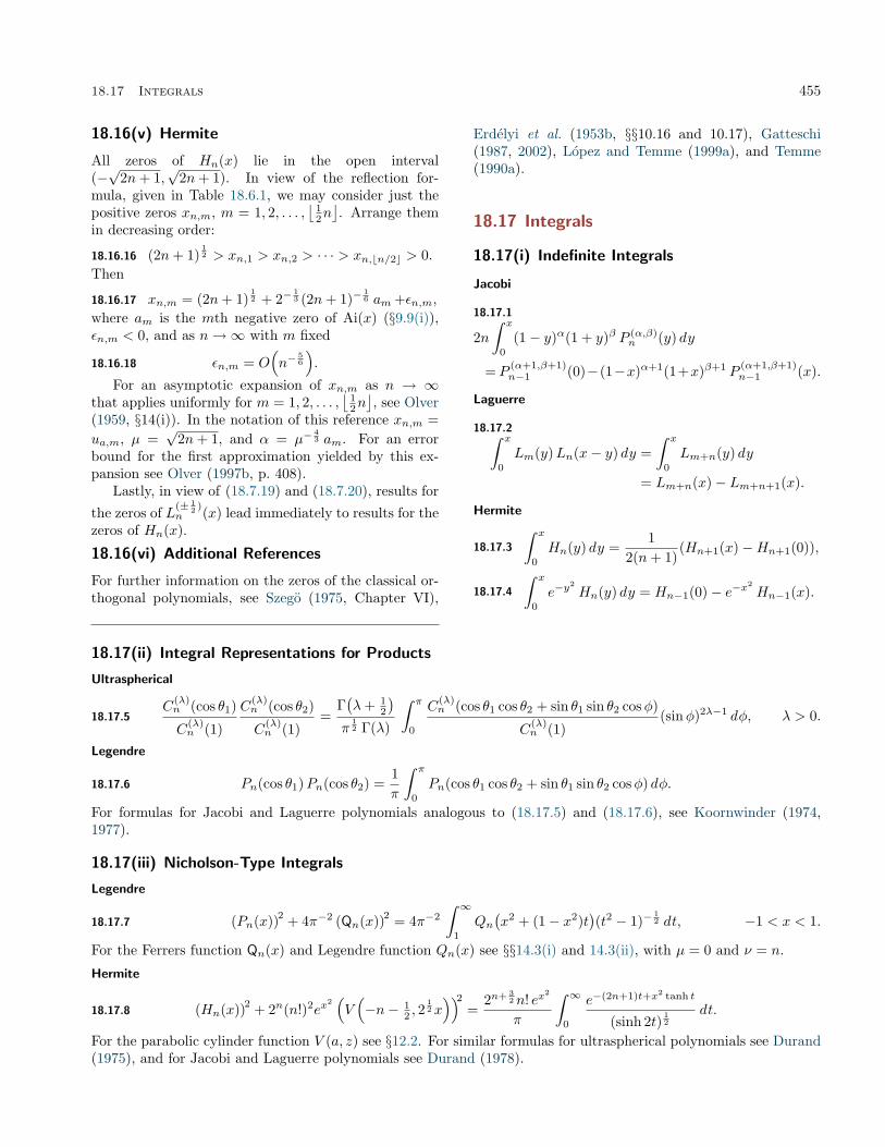
18.17 Integrals 455
18.16(v) Hermite
All zeros of Hn(x) lie in the open interval(−√
2n+ 1,√
2n+ 1). In view of the reflection for-mula, given in Table 18.6.1, we may consider just thepositive zeros xn,m, m = 1, 2, . . . ,
⌊12n⌋. Arrange them
in decreasing order:
18.16.16 (2n+ 1)12 > xn,1 > xn,2 > · · · > xn,bn/2c > 0.
Then
18.16.17 xn,m = (2n+ 1)12 + 2−
13 (2n+ 1)−
16 am +εn,m,
where am is the mth negative zero of Ai(x) (§9.9(i)),εn,m < 0, and as n→∞ with m fixed
18.16.18 εn,m = O(n−
56
).
For an asymptotic expansion of xn,m as n → ∞that applies uniformly for m = 1, 2, . . . ,
⌊12n⌋, see Olver
(1959, §14(i)). In the notation of this reference xn,m =ua,m, µ =
√2n+ 1, and α = µ−
43 am. For an error
bound for the first approximation yielded by this ex-pansion see Olver (1997b, p. 408).
Lastly, in view of (18.7.19) and (18.7.20), results for
the zeros of L(± 12 )
n (x) lead immediately to results for thezeros of Hn(x).
18.16(vi) Additional References
For further information on the zeros of the classical or-thogonal polynomials, see Szegö (1975, Chapter VI),
Erdélyi et al. (1953b, §§10.16 and 10.17), Gatteschi(1987, 2002), López and Temme (1999a), and Temme(1990a).
18.17 Integrals
18.17(i) Indefinite Integrals
Jacobi
18.17.1
2n∫ x
0
(1− y)α(1 + y)β P (α,β)n (y) dy
= P(α+1,β+1)n−1 (0)−(1−x)α+1(1+x)β+1 P
(α+1,β+1)n−1 (x).
Laguerre
18.17.2∫ x
0
Lm(y)Ln(x− y) dy =∫ x
0
Lm+n(y) dy
= Lm+n(x)− Lm+n+1(x).
Hermite
18.17.3
∫ x
0
Hn(y) dy =1
2(n+ 1)(Hn+1(x)−Hn+1(0)),
18.17.4
∫ x
0
e−y2Hn(y) dy = Hn−1(0)− e−x
2Hn−1(x).
18.17(ii) Integral Representations for Products
Ultraspherical
18.17.5C
(λ)n (cos θ1)
C(λ)n (1)
C(λ)n (cos θ2)
C(λ)n (1)
=Γ(λ+ 1
2
)π
12 Γ(λ)
∫ π
0
C(λ)n (cos θ1 cos θ2 + sin θ1 sin θ2 cosφ)
C(λ)n (1)
(sinφ)2λ−1 dφ, λ > 0.
Legendre
18.17.6 Pn(cos θ1)Pn(cos θ2) =1π
∫ π
0
Pn(cos θ1 cos θ2 + sin θ1 sin θ2 cosφ) dφ.
For formulas for Jacobi and Laguerre polynomials analogous to (18.17.5) and (18.17.6), see Koornwinder (1974,1977).
18.17(iii) Nicholson-Type Integrals
Legendre
18.17.7 (Pn(x))2 + 4π−2 (Qn(x))2 = 4π−2
∫ ∞1
Qn(x2 + (1− x2)t
)(t2 − 1)−
12 dt, −1 < x < 1.
For the Ferrers function Qn(x) and Legendre function Qn(x) see §§14.3(i) and 14.3(ii), with µ = 0 and ν = n.
Hermite
18.17.8 (Hn(x))2 + 2n(n!)2ex2(V(−n− 1
2 , 212x))2
=2n+ 3
2n! ex2
π
∫ ∞0
e−(2n+1)t+x2 tanh t
(sinh 2t)12
dt.
For the parabolic cylinder function V (a, z) see §12.2. For similar formulas for ultraspherical polynomials see Durand(1975), and for Jacobi and Laguerre polynomials see Durand (1978).

456 Orthogonal Polynomials
18.17(iv) Fractional Integrals
Jacobi
18.17.9(1− x)α+µ P
(α+µ,β−µ)n (x)
Γ(α+ µ+ n+ 1)=∫ 1
x
(1− y)α P (α,β)n (y)
Γ(α+ n+ 1)(y − x)µ−1
Γ(µ)dy, µ > 0, −1 < x < 1,
18.17.10xβ+µ(x+ 1)n
Γ(β + µ+ n+ 1)P (α,β+µ)n
(x− 1x+ 1
)=∫ x
0
yβ(y + 1)n
Γ(β + n+ 1)P (α,β)n
(y − 1y + 1
)(x− y)µ−1
Γ(µ)dy, µ > 0, x > 0,
18.17.11
Γ(n+ α+ β − µ+ 1)xn+α+β−µ+1
P (α,β−µ)n
(1− 2x−1
)=∫ ∞x
Γ(n+ α+ β + 1)yn+α+β+1
P (α,β)n
(1− 2y−1
) (y − x)µ−1
Γ(µ)dy,
α+ β + 1 > µ > 0, x > 1,and three formulas similar to (18.17.9)–(18.17.11) by symmetry; compare the second row in Table 18.6.1.
Ultraspherical
18.17.12
Γ(λ− µ)C(λ−µ)n
(x−
12
)xλ−µ+ 1
2n=∫ ∞x
Γ(λ)C(λ)n
(y−
12
)yλ+ 1
2n
(y − x)µ−1
Γ(µ)dy, λ > µ > 0, x > 0,
18.17.13x
12n(x− 1)λ+µ− 1
2
Γ(λ+ µ+ 1
2
) C(λ+µ)n
(x−
12
)C
(λ+µ)n (1)
=∫ x
1
y12n(y − 1)λ−
12
Γ(λ+ 1
2
) C(λ)n
(y−
12
)C
(λ)n (1)
(x− y)µ−1
Γ(µ)dy, µ > 0, x > 1.
Laguerre
18.17.14xα+µ L
(α+µ)n (x)
Γ(α+ µ+ n+ 1)=∫ x
0
yα L(α)n (y)
Γ(α+ n+ 1)(x− y)µ−1
Γ(µ)dy, µ > 0, x > 0.
18.17.15 e−x L(α)n (x) =
∫ ∞x
e−y L(α+µ)n (y)
(y − x)µ−1
Γ(µ)dy, µ > 0.
18.17(v) Fourier Transforms
Throughout this subsection we assume y > 0; sometimes however, this restriction can be eased by analytic continu-ation.
Jacobi
18.17.16
∫ 1
−1
(1− x)α(1 + x)β P (α,β)n (x)eixy dx
=(iy)neiy
n!2n+α+β+1 B(n+ α+ 1, n+ β + 1) 1F1(n+ α+ 1; 2n+ α+ β + 2;−2iy).
For the beta function B(a, b) see §5.12, and for the confluent hypergeometric function 1F1 see (16.2.1) and Chapter13.
Ultraspherical
18.17.17
∫ 1
0
(1− x2)λ−12 C
(λ)2n (x) cos(xy) dx =
(−1)nπ Γ(2n+ 2λ) Jλ+2n(y)(2n)! Γ(λ)(2y)λ
,
18.17.18
∫ 1
0
(1− x2)λ−12 C
(λ)2n+1(x) sin(xy) dx =
(−1)nπ Γ(2n+ 2λ+ 1) J2n+λ+1(y)(2n+ 1)! Γ(λ)(2y)λ
.
For the Bessel function Jν see §10.2(ii).
Legendre
18.17.19
∫ 1
−1
Pn(x)eixy dx = in√
2πyJn+ 1
2(y),
18.17.20
∫ 1
0
Pn(1− 2x2
)cos(xy) dx = (−1)n 1
2π Jn+ 12
(12y)J−n− 1
2
(12y),
18.17.21
∫ 1
0
Pn(1− 2x2
)sin(xy) dx = 1
2π(Jn+ 1
2
(12y))2
.

18.17 Integrals 457
Hermite
18.17.221
2√π
∫ ∞−∞
e−14x
2Hen(x)e
12 ixy dx = ine−
14y
2Hen(y),
18.17.23
∫ ∞0
e−12x
2He2n(x) cos(xy) dx = (−1)n
√12πy
2ne−12y
2,
18.17.24
∫ ∞0
e−x2
He2n(2x) cos(xy) dx = (−1)n 12
√πe−
14y
2He2n(y).
18.17.25
∫ ∞0
e−12x
2Hen(x) Hen+2m(x) cos(xy) dx = (−1)m
√12πn! y2me−
12y
2L(2m)n
(y2),
18.17.26
∫ ∞0
e−12x
2Hen(x) Hen+2m+1(x) sin(xy) dx = (−1)m
√12πn! y2m+1e−
12y
2L(2m+1)n
(y2).
18.17.27
∫ ∞0
e−12x
2He2n+1(x) sin(xy) dx = (−1)n
√12πy
2n+1e−12y
2,
18.17.28
∫ ∞0
e−x2
He2n+1(2x) sin(xy) dx = (−1)n 12
√πe−
14y
2He2n+1(y).
Laguerre
18.17.29
∫ ∞0
x2me−12x
2L(2m)n
(x2)
cos(xy) dx = (−1)m√
12π
1n!e−
12y
2Hen(y) Hen+2m(y).
18.17.30
∫ ∞0
x2ne−12x
2L
(n− 12 )
n
(12x
2)
cos(xy) dx =√
12πy
2ne−12y
2L
(n− 12 )
n
(12y
2).
18.17.31
∫ ∞0
e−axxν−2n L(ν−2n)2n−1 (ax) cos(xy) dx = i
(−1)n Γ(ν)2(2n− 1)!
y2n−1((a+ iy)−ν − (a− iy)−ν
), ν > 2n− 1, a > 0,
18.17.32
∫ ∞0
e−axxν−1−2n L(ν−1−2n)2n (ax) cos(xy) dx =
(−1)n Γ(ν)2(2n)!
y2n((a+ iy)−ν + (a− iy)−ν
), ν > 2n, a > 0.
18.17(vi) Laplace Transforms
Jacobi
18.17.33
∫ 1
−1
e−(x+1)z P (α,β)n (x)(1− x)α(1 + x)β dx
=(−1)n2α+β+n+1 Γ(α+ n+ 1) Γ(β + n+ 1)
Γ(α+ β + 2n+ 2)n!zn 1F1
(β + n+ 1
α+ β + 2n+ 2;−2z
), z ∈ C.
For the confluent hypergeometric function 1F1 see (16.2.1) and Chapter 13.
Laguerre
18.17.34
∫ ∞0
e−xz L(α)n (x)e−xxα dx =
Γ(α+ n+ 1)zn
n!(z + 1)α+n+1, <z > −1.
Hermite
18.17.35
∫ ∞−∞
e−xzHn(x)e−x2dx = π
12 (−z)ne 1
4 z2, z ∈ C.
18.17(vii) Mellin Transforms
Jacobi
18.17.36
∫ 1
−1
(1− x)z−1(1 + x)β P (α,β)n (x) dx =
2β+z Γ(z) Γ(1 + β + n)(1 + α− z)nn! Γ(1 + β + z + n)
, <z > 0.

458 Orthogonal Polynomials
Ultraspherical
18.17.37
∫ 1
0
(1− x2)λ−12 C(λ)
n (x)xz−1 dx =π 21−2λ−z Γ(n+ 2λ) Γ(z)
n! Γ(λ) Γ(
12 + 1
2n+ λ+ 12z)
Γ(
12 + 1
2z −12n) , <z > 0.
Legendre
18.17.38
∫ 1
0
P2n(x)xz−1 dx =(−1)n
(12 −
12z)n
2(
12z)n+1
, <z > 0,
18.17.39
∫ 1
0
P2n+1(x)xz−1 dx =(−1)n
(1− 1
2z)n
2(
12 + 1
2z)n+1
, <z > −1.
Laguerre
18.17.40
∫ ∞0
e−ax L(α)n (bx)xz−1 dx =
Γ(z + n)n!
(a− b)na−n−z 2F1
(−n, 1 + α− z
1− n− z;
a
a− b
), <a > 0, <z > 0.
For the hypergeometric function 2F1 see §§15.1 and 15.2(i).
Hermite
18.17.41
∫ ∞0
e−ax Hen(x)xz−1 dx = Γ(z + n)a−n−22F2
(− 1
2n,−12n+ 1
2
− 12z −
12n,−
12z −
12n+ 1
2
;− 12a
2
),
<a > 0. Also, <z > 0, n even; <z > −1, n odd.For the generalized hypergeometric function 2F2 see (16.2.1).
18.17(viii) Other Integrals
Chebyshev
18.17.42
∫ 1
−1
Tn(y)(1− y2)−
12
y − xdy = π Un−1(x),
18.17.43
∫ 1
−1
Un−1(y)(1− y2)
12
y − xdy = −π Tn(x).
These integrals are Cauchy principal values (§1.4(v)).
Legendre
18.17.44
∫ 1
−1
Pn(x)− Pn(t)|x− t|
dt = 2(1 + 1
2 + · · ·+ 1n
)Pn(x), −1 ≤ x ≤ 1.
The case x = 1 is a limit case of an integral for Jacobi polynomials; see Askey and Razban (1972).
18.17.45 (n+ 12 )(1 + x)
12
∫ x
−1
(x− t)− 12 Pn(t) dt = Tn(x) + Tn+1(x),
18.17.46 (n+ 12 )(1− x)
12
∫ 1
x
(t− x)−12 Pn(t) dt = Tn(x)− Tn+1(x).
Laguerre
18.17.47
∫ x
0
tαL
(α)m (t)
L(α)m (0)
(x− t)β L(β)n (x− t)L
(β)n (0)
dt =Γ(α+ 1) Γ(β + 1)
Γ(α+ β + 2)xα+β+1L
(α+β+1)m+n (x)
L(α+β+1)m+n (0)
.
Hermite
18.17.48
∫ ∞−∞
Hm(y)e−y2Hn(x− y)e−(x−y)2 dy = π
12 2−
12 (m+n+1)Hm+n
(2−
12x)e−
12x
2.
18.17.49
∫ ∞−∞
H`(x)Hm(x)Hn(x)e−x2dx =
212 (`+m+n)` !m !n !
√π
( 12`+ 1
2m−12n) ! ( 1
2m+ 12n−
12` ) ! ( 1
2n+ 12`−
12m ) !
,
provided that `+m+ n is even and the sum of any two of `,m, n is not less than the third; otherwise the integral iszero.

18.18 Sums 459
18.17(ix) Compendia
For further integrals, see Apelblat (1983, pp. 189–204), Erdélyi et al. (1954a, pp. 38–39, 94–95, 170–176, 259–261, 324), Erdélyi et al. (1954b, pp. 42–44,271–294), Gradshteyn and Ryzhik (2000, pp. 788–806),Gröbner and Hofreiter (1950, pp. 23–30), Marichev(1983, pp. 216–247), Oberhettinger (1972, pp. 64–67),Oberhettinger (1974, pp. 83–92), Oberhettinger (1990,pp. 44–47 and 152–154), Oberhettinger and Badii (1973,pp. 103–112), Prudnikov et al. (1986b, pp. 420–617),Prudnikov et al. (1992a, pp. 419–476), and Prudnikovet al. (1992b, pp. 280–308).
18.18 Sums
18.18(i) Series Expansions of ArbitraryFunctions
Jacobi
Let f(z) be analytic within an ellipse E with fociz = ±1, and
18.18.1
an =n!(2n+ α+ β + 1) Γ(n+ α+ β + 1)2α+β+1 Γ(n+ α+ 1) Γ(n+ β + 1)
×∫ 1
−1
f(x)P (α,β)n (x)(1− x)α(1 + x)β dx.
Then
18.18.2 f(z) =∞∑n=0
an P(α,β)n (z),
when z lies in the interior of E. Moreover, the series(18.18.2) converges uniformly on any compact domainwithin E.
Alternatively, assume f(x) is real and continuousand f ′(x) is piecewise continuous on (−1, 1). Assumealso the integrals
∫ 1
−1(f(x))2(1 − x)α(1 + x)β dx and∫ 1
−1(f ′(x))2(1 − x)α+1(1 + x)β+1 dx converge. Then
(18.18.2), with z replaced by x, applies when −1 < x <1; moreover, the convergence is uniform on any compactinterval within (−1, 1).
Chebyshev
See §3.11(ii), or set α = β = ± 12 in the above results for
Jacobi and refer to (18.7.3)–(18.7.6).
Legendre
This is the case α = β = 0 of Jacobi. Equation (18.18.1)becomes
18.18.3 an =(n+ 1
2
) ∫ 1
−1
f(x)Pn(x) dx.
Laguerre
Assume f(x) is real and continuous and f ′(x)is piecewise continuous on (0,∞). Assume also∫∞
0(f(x))2e−xxα dx converges. Then
18.18.4 f(x) =∞∑n=0
bn L(α)n (x), 0 < x <∞,
where
18.18.5 bn =n!
Γ(n+ α+ 1)
∫ ∞0
f(x)L(α)n (x)e−xxα dx.
The convergence of the series (18.18.4) is uniform onany compact interval in (0,∞).
Hermite
Assume f(x) is real and continuous and f ′(x) ispiecewise continuous on (−∞,∞). Assume also∫∞−∞(f(x))2e−x
2dx converges. Then
18.18.6 f(x) =∞∑n=0
dnHn(x), −∞ < x <∞,
where
18.18.7 dn =1√π2nn!
∫ ∞−∞
f(x)Hn(x)e−x2dx.
The convergence of the series (18.18.6) is uniform onany compact interval in (−∞,∞).
18.18(ii) Addition Theorems
Ultraspherical
18.18.8
C(λ)n (cos θ1 cos θ2 + sin θ1 sin θ2 cosφ)
=n∑`=0
22`(n− `)!2λ+ 2`− 12λ− 1
((λ)`)2
(2λ)n+`
(sin θ1)` C(λ+`)n−` (cos θ1)(sin θ2)` C(λ+`)
n−` (cos θ2)C(λ− 12 )
` (cosφ),
λ > 0, λ 6= 12 .
For the case λ = 12 use (18.18.9); compare (18.7.9).
Legendre
18.18.9
Pn(cos θ1 cos θ2 + sin θ1 sin θ2 cosφ)
= Pn(cos θ1)Pn(cos θ2) + 2n∑`=1
(n− `)! (n+ `)!22`(n!)2
(sin θ1)` P (`,`)n−` (cos θ1)(sin θ2)` P (`,`)
n−` (cos θ2) cos(`φ).

460 Orthogonal Polynomials
For (18.18.8), (18.18.9), and the corresponding formula for Jacobi polynomials see Koornwinder (1975a). See also(14.30.9).
Laguerre
18.18.10 L(α1+···+αr+r−1)n (x1 + · · ·+ xr) =
∑m1+···+mr=n
L(α1)m1
(x1) · · ·L(αr)mr (xr).
Hermite
18.18.11(a2
1 + · · ·+ a2r)
12n
n!Hn
(a1x1 + · · ·+ arxr
(a21 + · · ·+ a2
r)12
)=
∑m1+···+mr=n
am11 · · · amrrm1! · · ·mr!
Hm1(x1) · · ·Hmr (xr).
18.18(iii) Multiplication Theorems
Laguerre
18.18.12L
(α)n (λx)
L(α)n (0)
=n∑`=0
(n
`
)λ`(1− λ)n−`
L(α)` (x)
L(α)` (0)
.
Hermite
18.18.13 Hn(λx) = λnbn/2c∑`=0
(−n)2`
`!(1− λ−2)`Hn−2`(x).
18.18(iv) Connection Formulas
Jacobi
18.18.14 P (γ,β)n (x) =
(β + 1)n(α+ β + 2)n
n∑`=0
α+ β + 2`+ 1α+ β + 1
(α+ β + 1)`(n+ β + γ + 1)`(β + 1)`(n+ α+ β + 2)`
(γ − α)n−`(n− `)!
P(α,β)` (x),
18.18.15
(1 + x
2
)n=
(β + 1)n(α+ β + 2)n
n∑`=0
α+ β + 2`+ 1α+ β + 1
(α+ β + 1)`(n− `+ 1)`(β + 1)`(n+ α+ β + 2)`
P(α,β)` (x),
and a similar pair of equations by symmetry; comparethe second row in Table 18.6.1.
Ultraspherical
18.18.16
C(µ)n (x)
=bn/2c∑`=0
λ+ n− 2`λ
(µ)n−`(λ+ 1)n−`
(µ− λ)``!
C(λ)n−2`(x),
18.18.17
(2x)n = n!bn/2c∑`=0
λ+ n− 2`λ
1(λ+ 1)n−` `!
C(λ)n−2`(x).
Laguerre
18.18.18 L(β)n (x) =
n∑`=0
(β − α)n−`(n− `)!
L(α)` (x),
18.18.19 xn = (α+ 1)n
n∑`=0
(−n)`(α+ 1)`
L(α)` (x).
Hermite
18.18.20 (2x)n =bn/2c∑`=0
(−n)2`
`!Hn−2`(x).
18.18(v) Linearization Formulas
Chebyshev
18.18.21 Tm(x)Tn(x) = 12 (Tm+n(x) + Tm−n(x)).
Ultraspherical
18.18.22
C(λ)m (x)C(λ)
n (x)
=min(m,n)∑`=0
(m+ n+ λ− 2`)(m+ n− 2`)!(m+ n+ λ− `)`! (m− `)! (n− `)!
×(λ)`(λ)m−`(λ)n−`(2λ)m+n−`
(λ)m+n−`(2λ)m+n−2`
C(λ)m+n−2`(x).

18.18 Sums 461
Hermite
18.18.23
Hm(x)Hn(x) =min(m,n)∑`=0
(m
`
)(n
`
)2``!Hm+n−2`(x).
The coefficients in the expansions (18.18.22) and(18.18.23) are positive, provided that in the former caseλ > 0.
18.18(vi) Bateman-Type Sums
Jacobi
With
18.18.24 bn,` =(n
`
)(n+ α+ β + 1)`(−β − n)n−`
2`(α+ 1)n,
18.18.25
P(α,β)n (x)
P(α,β)n (1)
P(α,β)n (y)
P(α,β)n (1)
=n∑`=0
bn,`(x+ y)`
×P
(α,β)` ( (1 + xy)/(x+ y) )
P(α,β)` (1)
,
18.18.26P
(α,β)n (x)
P(α,β)n (1)
=n∑`=0
bn,`(x+ 1)`.
18.18(vii) Poisson Kernels
Laguerre
18.18.27
∞∑n=0
n! L(α)n (x)L(α)
n (y)(α+ 1)n
zn
=Γ(α+ 1)(xyz)−
12α
1− z
× exp(−(x+ y)z
1− z
)Iα
(2(xyz)
12
1− z
),
|z| < 1.
For the modified Bessel function Iν(z) see §10.25(ii).
Hermite
18.18.28
∞∑n=0
Hn(x)Hn(y)2nn!
zn
= (1− z2)−12 exp
(2xyz − (x2 + y2)z2
1− z2
),
|z| < 1.
These Poisson kernels are positive, provided thatx, y are real, 0 ≤ z < 1, and in the case of (18.18.27)x, y ≥ 0.
18.18(viii) Other Sums
In this subsection the variables x and y are not confinedto the closures of the intervals of orthogonality; compare§18.2(i).
Ultraspherical
18.18.29
n∑`=0
C(λ)` (x)C(µ)
n−`(x) = C(λ+µ)n (x).
18.18.30
n∑`=0
`+ 2λ2λ
C(λ)` (x)xn−` = C(λ+1)
n (x).
Chebyshev
18.18.31
n∑`=0
T`(x)xn−` = Un(x).
18.18.32 2n∑`=0
T2`(x) = 1 + U2n(x),
18.18.33 2n∑`=0
T2`+1(x) = U2n+1(x).
18.18.34 2(1− x2)n∑`=0
U2`(x) = 1− T2n+2(x),
18.18.35 2(1− x2)n∑`=0
U2`+1(x) = x− T2n+3(x).
Legendre and Chebyshev
18.18.36
n∑`=0
P`(x)Pn−`(x) = Un(x).
Laguerre
18.18.37
n∑`=0
L(α)` (x) = L(α+1)
n (x),
18.18.38
n∑`=0
L(α)` (x)L(β)
n−`(y) = L(α+β+1)n (x+ y).
Hermite and Laguerre
18.18.39n∑`=0
(n
`
)H`
(2
12x)Hn−`
(2
12 y)
= 212nHn(x+ y),
18.18.40n∑`=0
(n
`
)H2`(x)H2n−2`(y) = (−1)n22nn!Ln
(x2 + y2
).
18.18(ix) Compendia
For further sums see Hansen (1975, pp. 292-330), Grad-shteyn and Ryzhik (2000, pp. 978–993), and Prudnikovet al. (1986b, pp. 637-644 and 700-718).

462 Orthogonal Polynomials
Askey Scheme
18.19 Hahn Class: Definitions
Hahn, Krawtchouk, Meixner, and Charlier
Tables 18.19.1 and 18.19.2 provide definitions via orthogonality and normalization (§§18.2(i), 18.2(iii)) for the Hahnpolynomials Qn(x;α, β,N), Krawtchouk polynomials Kn(x; p,N), Meixner polynomials Mn(x;β, c), and Charlierpolynomials Cn(x, a).
Table 18.19.1: Orthogonality properties for Hahn, Krawtchouk, Meixner, and Charlier OP’s: discrete sets, weightfunctions, normalizations, and parameter constraints.
pn(x) X wx hn
Qn(x;α, β,N),n = 0, 1, . . . , N
{0, 1, . . . , N}(α+ 1)x(β + 1)N−x
x!(N − x)!,
α, β > −1 or α, β < −N
(−1)n(n+ α+ β + 1)N+1(β + 1)nn!(2n+ α+ β + 1)(α+ 1)n(−N)nN !
If α, β < −N , then (−1)Nwx > 0 and(−1)Nhn > 0.
Kn(x; p,N),n = 0, 1, . . . , N
{0, 1, . . . , N}
(N
x
)px(1− p)N−x,
0 < p < 1
(1− pp
)n/(N
n
)
Mn(x;β, c) {0, 1, 2, . . . } (β)xcx/x! ,
β > 0, 0 < c < 1c−nn!
(β)n(1− c)β
Cn(x, a) {0, 1, 2, . . . } ax/x! , a > 0 a−nean!
Table 18.19.2: Hahn, Krawtchouk, Meixner, and Char-lier OP’s: leading coefficients.
pn(x) kn
Qn(x;α, β,N)(n+ α+ β + 1)n(α+ 1)n(−N)n
Kn(x; p,N) p−n/(−N)n
Mn(x;β, c) (1− c−1)n/
(β)n
Cn(x, a) (−a)−n
Continuous Hahn
These polynomials are orthogonal on (−∞,∞), andwith <a > 0, <b > 0 are defined as follows.
18.19.1 pn(x) = pn(x; a, b, a, b
),
18.19.2
w(z; a, b, a, b) = Γ(a+ iz) Γ(b+ iz) Γ(a− iz) Γ(b− iz
),
18.19.3 w(x) = w(x; a, b, a, b) = |Γ(a+ ix) Γ(b+ ix)|2,
18.19.4
hn =2π Γ(n+ a+ a) Γ
(n+ b+ b
)|Γ(n+ a+ b
)|2
(2n+ 2<(a+ b)− 1) Γ(n+ 2<(a+ b)− 1)n!,
18.19.5 kn =(n+ 2<(a+ b)− 1)n
n!.
Meixner–Pollaczek
These polynomials are orthogonal on (−∞,∞), and aredefined as follows.
18.19.6 pn(x) = P (λ)n (x;φ),
18.19.7 w(λ)(z;φ) = Γ(λ+ iz) Γ(λ− iz)e(2φ−π)z,
18.19.8w(x) = w(λ)(x;φ) = |Γ(λ+ ix)|2 e(2φ−π)x,
λ > 0, 0 < φ < π,
18.19.9 hn =2π Γ(n+ 2λ)(2 sinφ)2λn!
, kn =(2 sinφ)n
n!.
18.20 Hahn Class: Explicit Representations
18.20(i) Rodrigues Formulas
For comments on the use of the forward-difference op-erator ∆x, the backward-difference operator ∇x, andthe central-difference operator δx, see §18.2(ii).

18.21 Hahn Class: Interrelations 463
Hahn, Krawtchouk, Meixner, and Charlier
18.20.1
pn(x) =1
κnwx∇nx
(wx
n−1∏`=0
F (x+ `)
), x ∈ X.
In (18.20.1) X and wx are as in Table 18.19.1. For theHahn polynomials pn(x) = Qn(x;α, β,N) and18.20.2
F (x) = (x+ α+ 1)(x−N), κn = (−N)n(α+ 1)n.For the Krawtchouk, Meixner, and Charlier polynomi-als, F (x) and κn are as in Table 18.20.1.
Table 18.20.1: Krawtchouk, Meixner, and CharlierOP’s: Rodrigues formulas (18.20.1).
pn(x) F (x) κn
Kn(x; p,N) x−N (−N)n
Mn(x;β, c) x+ β (β)n
Cn(x, a) 1 1
Continuous Hahn
18.20.3
w(x; a, b, a, b) pn(x; a, b, a, b
)=
1n!δnx(w(x; a+ 1
2n, b+ 12n, a+ 1
2n, b+ 12n)).
Meixner–Pollaczek
18.20.4 w(λ)(x;φ)P (λ)n (x;φ) =
1n!δnx
(w(λ+ 1
2n)(x;φ)).
18.20(ii) Hypergeometric Function andGeneralized Hypergeometric Functions
For the definition of hypergeometric and generalized hy-pergeometric functions see §16.2.18.20.5
Qn(x;α, β,N) = 3F2
(−n, n+ α+ β + 1,−x
α+ 1,−N; 1)
,
n = 0, 1, . . . , N .
18.20.6Kn(x; p,N) = 2F1
(−n,−x−N
; p−1
),
n = 0, 1, . . . , N .
18.20.7 Mn(x;β, c) = 2F1
(−n,−xβ
; 1− c−1
).
18.20.8 Cn(x, a) = 2F0
(−n,−x−
;−a−1
).
18.20.9
pn(x; a, b, a, b
)=in(a+ a)n
(a+ b
)n
n!
× 3F2
(−n, n+ 2<(a+ b)− 1, a+ ix
a+ a, a+ b; 1).
(For symmetry properties of pn(x; a, b, a, b
)with respect
to a, b, a, b see Andrews et al. (1999, Corollary 3.3.4).)18.20.10
P (λ)n (x;φ) =
(2λ)nn!
einφ 2F1
(−n, λ+ ix
2λ; 1− e−2iφ
).
18.21 Hahn Class: Interrelations
18.21(i) Dualities
Duality of Hahn and Dual Hahn
18.21.1Qn(x;α, β,N) =Rx(n(n+ α+ β + 1);α, β,N),
n, x = 0, 1, . . . , N .For the dual Hahn polynomial Rn(x; γ, δ,N) see §18.25.
Self-Dualities
18.21.2
Kn(x; p,N) = Kx(n; p,N), n, x = 0, 1, . . . , N .Mn(x;β, c) = Mx(n;β, c), n, x = 0, 1, 2, . . . .Cn(x, a) = Cx(n, a), n, x = 0, 1, 2, . . . .
18.21(ii) Limit Relations and Special Cases
Hahn → Krawtchouk
18.21.3 limt→∞
Qn(x; pt, (1− p)t,N) = Kn(x; p,N).
Hahn → Meixner
18.21.4
limN→∞
Qn(x; b− 1, N(c−1 − 1), N
)= Mn(x; b, c).
Hahn → Jacobi
18.21.5 limN→∞
Qn(Nx;α, β,N) =P
(α,β)n (1− 2x)
P(α,β)n (1)
.
Krawtchouk → Charlier
18.21.6 limN→∞
Kn
(x;N−1a,N
)= Cn(x, a).
Meixner → Charlier
18.21.7 limβ→∞
Mn
(x;β, a(a+ β)−1
)= Cn(x, a).
Meixner → Laguerre
18.21.8 limc→1
Mn
((1− c)−1x;α+ 1, c
)=L
(α)n (x)
L(α)n (0)
.
Charlier → Hermite
18.21.9 lima→∞
(2a)12n Cn
((2a)
12x+ a, a
)= (−1)nHn(x).
Continuous Hahn → Meixner–Pollaczek
18.21.10
limt→∞
t−n pn(x− t;λ+ it,−t tanφ, λ− it,−t tanφ)
=(−1)n
(cosφ)nP (λ)n (x;φ).
18.21.11
pn(x; a, a+ 1
2 , a, a+ 12
)= 2−2n(4a+ n)n P
(2a)n
(2x; 1
2π).

464 Orthogonal Polynomials
Meixner–Pollaczek → Laguerre
18.21.12 limφ→0
P( 12α+ 1
2 )n
(−(2φ)−1x;φ
)= L(α)
n (x).
A graphical representation of limits in §§18.7(iii),18.21(ii), and 18.26(ii) is provided by the Askey schemedepicted in Figure 18.21.1.
Figure 18.21.1: Askey scheme. The number of free real parameters is zero for Hermite polynomials. It increasesby one for each row ascended in the scheme, culminating with four free real parameters for the Wilson and Racahpolynomials. (This is with the convention that the real and imaginary parts of the parameters are counted separatelyin the case of the continuous Hahn polynomials.)
18.22 Hahn Class: Recurrence Relationsand Differences
18.22(i) Recurrence Relations in n
Hahn
With
18.22.1 pn(x) = Qn(x;α, β,N),
18.22.2
−xpn(x) = Anpn+1(x)− (An +Cn) pn(x) +Cnpn−1(x),where
18.22.3
An =(n+ α+ β + 1)(n+ α+ 1)(N − n)(2n+ α+ β + 1)(2n+ α+ β + 2)
,
Cn =n(n+ α+ β +N + 1)(n+ β)(2n+ α+ β)(2n+ α+ β + 1)
.
Krawtchouk, Meixner, and Charlier
These polynomials satisfy (18.22.2) with pn(x), An, andCn as in Table 18.22.1.
Table 18.22.1: Recurrence relations (18.22.2) forKrawtchouk, Meixner, and Charlier polynomials.
pn(x) An Cn
Kn(x; p,N) p(N − n) n(1− p)
Mn(x;β, c)c(n+ β)
1− cn
1− cCn(x, a) a n

18.22 Hahn Class: Recurrence Relations and Differences 465
Continuous Hahn
With
18.22.4 qn(x) = pn(x; a, b, a, b
)/pn(ia; a, b, a, b
),
18.22.5(a+ ix)qn(x)
= Ãnqn+1(x)− (Ãn + C̃n)qn(x) + C̃nqn−1(x),
where
18.22.6
Ãn = − (n+ 2<(a+ b)− 1)(n+ a+ a)(n+ a+ b)(2n+ 2<(a+ b)− 1)(2n+ 2<(a+ b))
,
C̃n =n(n+ b+ a− 1)(n+ b+ b− 1)
(2n+ 2<(a+ b)− 2)(2n+ 2<(a+ b)− 1).
Meixner–Pollaczek
With
18.22.7 pn(x) = P (λ)n (x;φ),
18.22.8(n+ 1)pn+1(x) = 2 (x sinφ+(n+λ) cosφ) pn(x)
− (n+ 2λ− 1)pn−1(x).
18.22(ii) Difference Equations in x
Hahn
With
18.22.9 pn(x) = Qn(x;α, β,N),
18.22.10
A(x)pn(x+ 1)− (A(x) + C(x)) pn(x)+ C(x)pn(x− 1)− n(n+ α+ β + 1)pn(x) = 0,
where
18.22.11A(x) = (x+ α+ 1)(x−N),C(x) = x(x− β −N − 1).
Krawtchouk, Meixner, and Charlier
18.22.12A(x)pn(x+ 1)− (A(x) + C(x)) pn(x)
+ C(x)pn(x− 1) + λnpn(x) = 0.
For A(x), C(x), and λn in (18.22.12) see Table 18.22.2.
Table 18.22.2: Difference equations (18.22.12) forKrawtchouk, Meixner, and Charlier polynomials.
pn(x) A(x) C(x) λn
Kn(x; p,N) p(x−N) (p− 1)x −n
Mn(x;β, c) c(x+ β) x n(1− c)
Cn(x, a) a x n
Continuous Hahn
With
18.22.13 pn(x) = pn(x; a, b, a, b
),
18.22.14
A(x)pn(x+ i)− (A(x) + C(x)) pn(x)+ C(x)pn(x− i)+ n(n+ 2<(a+ b)− 1)pn(x) = 0,
where18.22.15
A(x) = (x+ ia)(x+ ib), C(x) = (x− ia)(x− ib).Meixner–Pollaczek
With
18.22.16 pn(x) = P (λ)n (x;φ),
18.22.17A(x)pn(x+ i)− (A(x) + C(x)) pn(x)
+ C(x)pn(x− i) + 2n sinφ pn(x) = 0,where
18.22.18 A(x) = eiφ(x+ iλ), C(x) = e−iφ(x− iλ).
18.22(iii) x-Differences
Hahn
18.22.19
∆xQn(x;α, β,N)
= −n(n+ α+ β + 1)(α+ 1)N
Qn−1(x;α+ 1, β + 1, N − 1),
18.22.20
∇x(
(α+ 1)x(β + 1)N−xx! (N − x)!
Qn(x;α, β,N))
=N + 1β
(α)x(β)N+1−xx! (N + 1− x)!
× Qn+1(x;α− 1, β − 1, N + 1).
Krawtchouk
18.22.21 ∆xKn(x; p,N) = − n
pNKn−1(x; p,N − 1),
18.22.22
∇x((
N
x
)px(1− p)N−xKn(x; p,N)
)=(N + 1x
)px(1− p)N−xKn+1(x; p,N + 1).
Meixner
18.22.23 ∆xMn(x;β, c) =−n(1− c)βc
Mn−1(x;β + 1, c),
18.22.24
∇x(
(β)xcx
x!Mn(x;β, c)
)=
(β − 1)xcx
x!Mn+1(x;β − 1, c).
Charlier
18.22.25 ∆x Cn(x, a) = −naCn−1(x, a),
18.22.26 ∇x(ax
x!Cn(x, a)
)=ax
x!Cn+1(x, a).

466 Orthogonal Polynomials
Continuous Hahn
18.22.27 δx(pn(x; a, b, a, b
))= (n+ 2<(a+ b)− 1) pn−1
(x; a+ 1
2 , b+ 12 , a+ 1
2 , b+ 12
),
18.22.28 δx(w(x; a+ 1
2 , b+ 12 , a+ 1
2 , b+ 12 )pn(x; a+ 1
2 , b+ 12 , a+ 1
2 , b+ 12 ))
= −(n+ 1)w(x; a, b, a, b)pn+1(x; a, b, a, b).
Meixner–Pollaczek
18.22.29 δx
(P (λ)n (x;φ)
)= 2 sinφP (λ+ 1
2 )n−1 (x;φ),
18.22.30δx
(w(λ+ 1
2 )(x;φ)P (λ+ 12 )
n (x;φ))
= −(n+ 1)w(λ)(x;φ)P (λ)n+1(x;φ).
18.23 Hahn Class: Generating Functions
For the definition of generalized hypergeometric func-tions see §16.2.
Hahn
18.23.1
1F1
(−xα+ 1
;−z)
1F1
(x−Nβ + 1
; z)
=N∑n=0
(−N)n(β + 1)nn!
Qn(x;α, β,N)zn, x = 0, 1, . . . , N .
18.23.2
2F0
(−x,−x+ β +N + 1
−;−z
)× 2F0
(x−N, x+ α+ 1
−; z)
=N∑n=0
(−N)n(α+ 1)nn!
Qn(x;α, β,N)zn,
x = 0, 1, . . . , N .
Krawtchouk
18.23.3(1− 1− p
pz
)x(1 + z)N−x =
N∑n=0
(N
n
)Kn(x; p,N)zn,
x = 0, 1, . . . , N .
Meixner
18.23.4
(1− z
c
)x(1− z)−x−β =
∞∑n=0
(β)nn!
Mn(x;β, c)zn,
x = 0, 1, 2, . . . , |z| < 1.
Charlier
18.23.5 ez(
1− z
a
)x=∞∑n=0
Cn(x, a)n!
zn, x = 0, 1, 2, . . . .
Continuous Hahn
18.23.6
1F1
(a+ ix
2<a;−iz
)1F1
(b− ix2<b
; iz)
=∞∑n=0
pn(x; a, b, a, b
)(2<a)n(2<b)n
zn.
Meixner–Pollaczek
18.23.7
(1− eiφz)−λ+ix(1− e−iφz)−λ−ix
=∞∑n=0
P (λ)n (x;φ)zn, |z| < 1.
18.24 Hahn Class: AsymptoticApproximations
Krawtchouk
With x = λN and ν = n/N , Li and Wong (2000) givesan asymptotic expansion for Kn(x; p,N) as n → ∞,that holds uniformly for λ and ν in compact subinter-vals of (0, 1). This expansion is in terms of the paraboliccylinder function and its derivative.
With µ = N/n and x fixed, Qiu and Wong (2004)gives an asymptotic expansion for Kn(x; p,N) as n →∞, that holds uniformly for µ ∈ [1,∞). This expan-sion is in terms of confluent hypergeometric functions.Asymptotic approximations are also provided for thezeros of Kn(x; p,N) in various cases depending on thevalues of p and µ.
Meixner
For two asymptotic expansions of Mn(nx;β, c) as n →∞, with β and c fixed, see Jin and Wong (1998). Thefirst expansion holds uniformly for δ ≤ x ≤ 1 + δ, andthe second for 1− δ ≤ x ≤ 1 + δ−1, δ being an arbitrarysmall positive constant. Both expansions are in termsof parabolic cylinder functions.
For asymptotic approximations for the zeros ofMn(nx;β, c) in terms of zeros of Ai(x) (§9.9(i)), see Jinand Wong (1999).
Charlier
Dunster (2001b) provides various asymptotic expan-sions for Cn(x, a) as n → ∞, in terms of elementaryfunctions or in terms of Bessel functions. Taken to-gether, these expansions are uniformly valid for −∞ <x <∞ and for a in unbounded intervals—each of whichcontains [0, (1−δ)n], where δ again denotes an arbitrary

18.25 Wilson Class: Definitions 467
small positive constant. See also Bo and Wong (1994)and Goh (1998).
Meixner–Pollaczek
For an asymptotic expansion of P (λ)n (nx;φ) as n→∞,
with φ fixed, see Li and Wong (2001). This expansionis uniformly valid in any compact x-interval on the realline and is in terms of parabolic cylinder functions. Cor-responding approximations are included for the zeros ofP
(λ)n (nx;φ).
Approximations in Terms of Laguerre Polynomials
For asymptotic approximations to P(λ)n (x;φ) as |x +
iλ| → ∞, with n fixed, see Temme and López (2001).These approximations are in terms of Laguerre polyno-mials and hold uniformly for ph(x+ iλ) ∈ [0, π]. Com-pare also (18.21.12). Similar approximations are in-cluded for Jacobi, Krawtchouk, and Meixner polyno-mials.
18.25 Wilson Class: Definitions
18.25(i) Preliminaries
For the Wilson class OP’s pn(x) with x = λ(y): if they-orthogonality set is {0, 1, . . . , N}, then the role of thedifferentiation operator d/dx in the Jacobi, Laguerre,and Hermite cases is played by the operator ∆y fol-lowed by division by ∆y(λ(y)), or by the operator ∇yfollowed by division by ∇y(λ(y)). Alternatively if they-orthogonality interval is (0,∞), then the role of d/dxis played by the operator δy followed by division byδy(λ(y)).
Table 18.25.1 lists the transformations of vari-able, orthogonality ranges, and parameter constraintsthat are needed in §18.2(i) for the Wilson polynomi-als Wn(x; a, b, c, d), continuous dual Hahn polynomialsSn(x; a, b, c), Racah polynomials Rn(x;α, β, γ, δ), anddual Hahn polynomials Rn(x; γ, δ,N).
Table 18.25.1: Wilson class OP’s: transformations of variable, orthogonality ranges, and parameter constraints.
pn(x) x = λ(y) Orthogonalityrange for y Constraints
Wn(x; a, b, c, d) y2 (0,∞) <(a, b, c, d) > 0;nonreal parameters in conjugate pairs
Sn(x; a, b, c) y2 (0,∞) <(a, b, c) > 0;nonreal parameters in conjugate pairs
Rn(x;α, β, γ, δ) y(y + γ + δ + 1) {0, 1, . . . , N} α+ 1 or β + δ + 1 or γ + 1 = −N ;for further constraints see (18.25.1)
Rn(x; γ, δ,N) y(y + γ + δ + 1) {0, 1, . . . , N} γ, δ > −1 or < −N
Further Constraints for Racah Polynomials
If α+ 1 = −N , then the weights will be positive iff oneof the following eight sets of inequalities holds:
18.25.1
−δ − 1 < β < γ + 1 < −N + 1.
N − 1 < −δ − 1 < β < γ + 1.
γ, δ > −1, β > N + γ.
γ, δ > −1, β < −N − δ.N − 1 < N + γ < β < −N − δ.N + γ < β < −N − δ < −N − 1.
γ, δ < −N, β > −1− δ.γ, δ < −N, β < γ + 1.
The first four sets imply γ + δ > −2, and the last fourimply γ + δ < −2N .
18.25(ii) Weights and Normalizations:Continuous Cases
18.25.2
∫ ∞0
pn(x)pm(x)w(x) dx = hnδn,m.
Wilson
18.25.3 pn(x) = Wn(x; a1, a2, a3, a4),
18.25.4 w(y2) =12y
∣∣∣∣∏j Γ(aj + iy)
Γ(2iy)
∣∣∣∣2 ,18.25.5 hn =
n! 2π∏j<` Γ(n+ aj + a`)
(2n− 1 +∑j aj) Γ
(n− 1 +
∑j aj
) .

468 Orthogonal Polynomials
Continuous Dual Hahn
18.25.6 pn(x) = Sn(x; a1, a2, a3),
18.25.7 w(y2) =12y
∣∣∣∣∏j Γ(aj + iy)
Γ(2iy)
∣∣∣∣2 ,18.25.8 hn = n! 2π
∏j<`
Γ(n+ aj + a`).
18.25(iii) Weights and Normalizations: DiscreteCases
18.25.9
N∑y=0
pn(y(y+γ+δ+1))pm(y(y+γ+δ+1))
× γ + δ + 1 + 2yγ + δ + 1 + y
ωy = hnδn,m.
Racah
18.25.10 pn(x) = Rn(x;α, β, γ, δ), α+ 1 = −N ,
18.25.11
ωy =(α+ 1)y(β + δ + 1)y(γ + 1)y(γ + δ + 2)y
(−α+ γ + δ + 1)y(−β + γ + 1)y(δ + 1)yy!,
18.25.12
hn =(−β)N (γ + δ + 2)N
(−β + γ + 1)N (δ + 1)N
(n+ α+ β + 1)nn!(α+ β + 2)2n
×(α+ β − γ + 1)n(α− δ + 1)n(β + 1)n
(α+ 1)n(β + δ + 1)n(γ + 1)n.
Dual Hahn
18.25.13 pn(x) = Rn(x; γ, δ,N),
18.25.14 ωy =(−1)y(−N)y(γ + 1)y(γ + δ + 1)2
(N + γ + δ + 2)y(δ + 1)yy!,
18.25.15 hn =n! (N − n)! (γ + δ + 2)NN ! (γ + 1)n(δ + 1)N−n
.
18.25(iv) Leading Coefficients
Table 18.25.2 provides the leading coefficients kn(§18.2(iii)) for the Wilson, continuous dual Hahn,Racah, and dual Hahn polynomials.
Table 18.25.2: Wilson class OP’s: leading coefficients.
pn(x) kn
Wn(x; a, b, c, d) (−1)n(n+ a+ b+ c+ d− 1)n
Sn(x; a, b, c) (−1)n
Rn(x;α, β, γ, δ)(n+ α+ β + 1)n
(α+ 1)n(β + δ + 1)n(γ + 1)nRn(x; γ, δ,N)
1(γ + 1)n(−N)n
18.26 Wilson Class: Continued
18.26(i) Representations as GeneralizedHypergeometric Functions
For the definition of generalized hypergeometric func-tions see §16.2.
18.26.1 Wn
(y2; a, b, c, d
)= (a+ b)n(a+ c)n(a+ d)n 4F3
(−n, n+ a+ b+ c+ d− 1, a+ iy, a− iy
a+ b, a+ c, a+ d; 1).
18.26.2Sn(y2; a, b, c
)(a+ b)n(a+ c)n
= 3F2
(−n, a+ iy, a− iy
a+ b, a+ c; 1).
18.26.3Rn(y(y + γ + δ + 1);α, β, γ, δ) = 4F3
(−n, n+ α+ β + 1,−y, y + γ + δ + 1
α+ 1, β + δ + 1, γ + 1; 1)
,
α+ 1 or β + δ + 1 or γ + 1 = −N ; n = 0, 1, . . . , N .
18.26.4 Rn(y(y + γ + δ + 1); γ, δ,N) = 3F2
(−n,−y, y + γ + δ + 1
γ + 1,−N; 1)
, n = 0, 1, . . . , N .
18.26(ii) Limit Relations
Wilson → Continuous Dual Hahn
18.26.5 limd→∞
Wn(x; a, b, c, d)(a+ d)n
= Sn(x; a, b, c).

18.26 Wilson Class: Continued 469
Wilson → Continuous Hahn
18.26.6 limt→∞
Wn
((x+ t)2; a− it, b− it, a+ it, b+ it
)(−2t)nn!
= pn(x; a, b, a, b
).
Wilson → Jacobi
18.26.7 limt→∞
Wn
(12 (1− x)t2; 1
2α+ 12 ,
12α+ 1
2 ,12β + 1
2 + it, 12β + 1
2 − it)
t2nn!= P (α,β)
n (x).
Continuous Dual Hahn → Meixner–Pollaczek
18.26.8 limt→∞
Sn((x− t)2;λ+ it, λ− it, t cotφ
)/tn = n!(cscφ)n P (λ)
n (x;φ).
Racah → Dual Hahn
18.26.9 limβ→∞
Rn(x;−N − 1, β, γ, δ) = Rn(x; γ, δ,N).
Racah → Hahn
18.26.10 limδ→∞
Rn(x(x+ γ + δ + 1);α, β,−N − 1, δ) = Qn(x;α, β,N).
Dual Hahn → Krawtchouk
18.26.11 limt→∞
Rn(x(x+ t+ 1); pt, (1− p)t,N) = Kn(x; p,N).
Dual Hahn → Meixner
With
18.26.12 r(x;β, c,N) = x(x+ β + c−1(1− c)N),
18.26.13 limN→∞
Rn(r(x;β, c,N);β − 1, c−1(1− c)N,N
)= Mn(x;β, c).
See also Figure 18.21.1.
18.26(iii) Difference Relations
For comments on the use of the forward-difference operator ∆x, the backward-difference operator ∇x, and thecentral-difference operator δx, see §18.2(ii).
For each family only the y-difference that lowers n is given. See Koekoek and Swarttouw (1998, Chapter 1) forfurther formulas.
18.26.14 δy(Wn
(y2; a, b, c, d
))/δy(y2) = −n(n+ a+ b+ c+ d− 1) Wn−1
(y2; a+ 1
2 , b+ 12 , c+ 1
2 , d+ 12
).
18.26.15 δy(Sn(y2; a, b, c
))/δy(y2) = −nSn−1
(y2; a+ 1
2 , b+ 12 , c+ 1
2
).
18.26.16
∆y (Rn(y(y + γ + δ + 1);α, β, γ, δ))∆y (y(y + γ + δ + 1))
=n(n+ α+ β + 1)
(α+ 1)(β + δ + 1)(γ + 1)Rn−1(y(y + γ + δ + 2);α+ 1, β + 1, γ + 1, δ).
18.26.17∆y (Rn(y(y + γ + δ + 1); γ, δ,N))
∆y (y(y + γ + δ + 1))= − n
(γ + 1)NRn−1(y(y + γ + δ + 2); γ + 1, δ,N − 1).
18.26(iv) Generating Functions
For the hypergeometric function 2F1 see §§15.1 and 15.2(i).
Wilson
18.26.18 2F1
(a+ iy, d+ iy
a+ d; z)
2F1
(b− iy, c− iy
b+ c; z)
=∞∑n=0
Wn
(y2; a, b, c, d
)(a+ d)n(b+ c)nn!
zn, |z| < 1.

470 Orthogonal Polynomials
Continuous Dual Hahn
18.26.19 (1− z)−c+iy 2F1
(a+ iy, b+ iy
a+ b; z)
=∞∑n=0
Sn(y2; a, b, c
)(a+ b)nn!
zn, |z| < 1.
Racah
18.26.20
2F1
(−y,−y + β − γ
β + δ + 1; z)
2F1
(y −N, y + γ + 1−δ −N
; z)
=N∑n=0
(−N)n(γ + 1)n(−δ −N)nn!
Rn(y(y + γ + δ + 1);−N − 1, β, γ, δ)zn.
Dual Hahn
18.26.21 (1− z)y 2F1
(y −N, y + γ + 1−δ −N
; z)
=N∑n=0
(γ + 1)n(−N)n(−δ −N)nn!
Rn(y(y + γ + δ + 1); γ, δ,N)zn.
18.26(v) Asymptotic Approximations
For asymptotic expansions of Wilson polynomials oflarge degree see Wilson (1991), and for asymptotic ap-proximations to their largest zeros see Chen and Ismail(1998).
Other Orthogonal Polynomials
18.27 q-Hahn Class
18.27(i) Introduction
The q-hypergeometric OP’s comprise the q-Hahn classOP’s and the Askey–Wilson class OP’s (§18.28). Forthe notation of q-hypergeometric functions see §§17.2and 17.4(i).
The q-Hahn class OP’s comprise systems of OP’s{pn(x)}, n = 0, 1, . . . , N , or n = 0, 1, 2, . . . , that areeigenfunctions of a second-order q-difference operator.Thus
18.27.1
A(x)pn(qx) +B(x)pn(x) + C(x)pn(q−1x) = λnpn(x),
where A(x), B(x), and C(x) are independent of n, andwhere the λn are the eigenvalues. In the q-Hahn classOP’s the role of the operator d/dx in the Jacobi, La-guerre, and Hermite cases is played by the q-derivativeDq, as defined in (17.2.41). A (nonexhaustive) classifica-tion of such systems of OP’s was made by Hahn (1949).There are 18 families of OP’s of q-Hahn class. Thesefamilies depend on further parameters, in addition toq. The generic (top level) cases are the q-Hahn polyno-mials and the big q-Jacobi polynomials, each of whichdepends on three further parameters.
All these systems of OP’s have orthogonality prop-erties of the form
18.27.2∑x∈X
pn(x)pm(x) |x| vx = hnδn,m,
where X is given by X = {aqy}y∈I+ or X = {aqy}y∈I+∪{−bqy}y∈I− . Here a, b are fixed positive real numbers,and I+ and I− are sequences of successive integers, finiteor unbounded in one direction, or unbounded in bothdirections. If I+ and I− are both nonempty, then theyare both unbounded to the right. Some of the systemsof OP’s that occur in the classification do not have aunique orthogonality property. Thus in addition to arelation of the form (18.27.2), such systems may alsosatisfy orthogonality relations with respect to a contin-uous weight function on some interval.
Here only a few families are mentioned. They aredefined by their q-hypergeometric representations, fol-lowed by their orthogonality properties. For other for-mulas, including q-difference equations, recurrence re-lations, duality formulas, special cases, and limit rela-tions, see Koekoek and Swarttouw (1998, Chapter 3).See also Gasper and Rahman (2004, pp. 195–199, 228–230) and Ismail (2005, Chapters 13, 18, 21).
18.27(ii) q-Hahn Polynomials
18.27.3
Qn(x) = Qn(x;α, β,N ; q) = 3φ2
(q−n, αβqn+1, x
αq, q−N; q, q
),
n = 0, 1, . . . , N .
18.27.4
N∑y=0
Qn(q−y)Qm(q−y)(αq, q−N ; q)y(αβq)−y
(q, β−1q−N ; q)y
= hnδn,m, n,m = 0, 1, . . . , N.
For hn see Koekoek and Swarttouw (1998, Eq. (3.6.2)).

18.27 q-Hahn Class 471
18.27(iii) Big q-Jacobi Polynomials
18.27.5 Pn(x; a, b, c; q) = 3φ2
(q−n, abqn+1, x
aq, cq; q, q
),
and
18.27.6
P (α,β)n (x; c, d; q)
=cnq−(α+1)n
(qα+1,−qα+1c−1d; q
)n
(q,−q; q)n× Pn
(qα+1c−1dx; qα, qβ ,−qαc−1d; q
).
The orthogonality relations are given by (18.27.2), with
18.27.7 pn(x) = Pn(x; a, b, c; q),
18.27.8 X = {aq`+1}`=0,1,2,... ∪ {cq`+1}`=0,1,2,...,
18.27.9vx =
(a−1x, c−1x; q)∞(x, bc−1x; q)∞
,
0 < a < q−1, 0 < b < q−1, c < 0,and
18.27.10 pn(x) = P (α,β)n (x; c, d; q)
18.27.11 X = {cq`}`=0,1,2,... ∪ {−dq`}`=0,1,2,...,
18.27.12
vx =(qx/c,−qx/d; q)∞
(qα+1x/c,−qβ+1x/d; q)∞, α, β > −1, c, d > 0.
For hn see Koekoek and Swarttouw (1998, Eq. (3.5.2)).
18.27(iv) Little q-Jacobi Polynomials
18.27.13
pn(x) = pn(x; a, b; q) = 2φ1
(q−n, abqn+1
aq; q, qx
).
18.27.14
∞∑y=0
pn(qy)pm(qy)(bq; q)y (aq)y
(q; q)y
= hnδn,m, 0 < a < q−1, b < q−1 .For hn see Koekoek and Swarttouw (1998, Eq. (3.12.2)).
18.27(v) q-Laguerre Polynomials
18.27.15
L(α)n (x; q) =
(qα+1; q
)n
(q; q)n1φ1
(q−n
qα+1; q,−xqn+α+1
).
The measure is not uniquely determined:
18.27.16
∫ ∞0
L(α)n (x; q)L(α)
m (x; q)xα
(−x; q)∞dx
=
(qα+1; q
)n
(q; q)n qnh
(1)0 δn,m, α > −1,
where h(1)0 is given in Koekoek and Swarttouw (1998,
Eq. (3.21.2), and
18.27.17
∞∑y=−∞
L(α)n (cqy; q)L(α)
m (cqy; q)qy(α+1)
(−cqy; q)∞
=
(qα+1; q
)n
(q; q)n qnh
(2)0 δn,m, α > −1, c > 0,
where h(2)0 is given in Koekoek and Swarttouw (1998,
Eq. (3.21.3).
18.27(vi) Stieltjes–Wigert Polynomials
18.27.18
Sn(x; q) =n∑`=0
q`2(−x)`
(q; q)` (q; q)n−`
=1
(q; q)n1φ1
(q−n
0; q,−qn+1x
).
(Sometimes in the literature x is replaced by q12x.)
The measure is not uniquely determined:
18.27.19∫ ∞0
Sn(x; q)Sm(x; q)(−x,−qx−1; q)∞
dx =ln(q−1)
qn(q; q)∞(q; q)n
δn,m,
and
18.27.20∫ ∞0
Sn
(q
12x; q
)Sm
(q
12x; q
)exp(− (lnx)2
2 ln(q−1)
)dx
=
√2πq−1 ln(q−1)qn (q; q)n
δn,m.
18.27(vii) Discrete q-Hermite I and IIPolynomials
Discrete q-Hermite I
18.27.21
hn(x; q) = (q; q)n
bn/2c∑`=0
(−1)`q`(`−1)xn−2`
(q2; q2)` (q; q)n−2`
= xn 2φ0
(q−n, q−n+1
−; q2, x−2q2n−1
).
18.27.22∞∑`=0
(hn(q`; q
)hm(q`; q
)+ hn
(−q`; q
)hm(−q`; q
))×(q`+1,−q`+1; q
)∞ q`
= (q; q)n (q,−1,−q; q)∞ qn(n−1)/2δn,m.

472 Orthogonal Polynomials
Discrete q-Hermite II
18.27.23
h̃n(x; q) = (q; q)n
bn/2c∑`=0
(−1)`q−2n`q`(2`+1)xn−2`
(q2; q2)` (q; q)n−2`
= xn 2φ1
(q−n, q−n+1
0; q2,−x−2q2
).
18.27.24∞∑
`=−∞
(h̃n(cq`; q
)h̃m(cq`; q
)+ h̃n
(−cq`; q
)h̃m(−cq`; q
)) q`
(−c2q2`; q2)∞
= 2
(q2,−c2q,−c−2q; q2
)∞
(q,−c2,−c−2q2; q2)∞
(q; q)nqn2 δn,m,
c > 0.(For discrete q-Hermite II polynomials the measure isnot uniquely determined.)
18.28 Askey–Wilson Class
18.28(i) Introduction
The Askey–Wilson class OP’s comprise the four-parameter families of Askey–Wilson polynomials and ofq-Racah polynomials, and cases of these families ob-tained by specialization of parameters. The Askey–Wilson polynomials form a system of OP’s {pn(x)},n = 0, 1, 2, . . . , that are orthogonal with respect to aweight function on a bounded interval, possibly sup-plemented with discrete weights on a finite set. Theq-Racah polynomials form a system of OP’s {pn(x)},n = 0, 1, 2, . . . , N , that are orthogonal with respectto a weight function on a sequence {q−y + cqy+1},y = 0, 1, . . . , N , with c a constant. Both the Askey–Wilson polynomials and the q-Racah polynomials canbest be described as functions of z (resp. y) such thatPn(z) = pn( 1
2 (z + z−1)) in the Askey–Wilson case, andPn(y) = pn(q−y + cqy+1) in the q-Racah case, and bothare eigenfunctions of a second-order q-difference opera-tor similar to (18.27.1).
In the remainder of this section the Askey–Wilsonclass OP’s are defined by their q-hypergeometric repre-sentations, followed by their orthogonal properties. Forfurther properties see Koekoek and Swarttouw (1998,Chapter 3). See also Gasper and Rahman (2004,
pp. 180–199) and Ismail (2005, Chapter 15). For thenotation of q-hypergeometric functions see §§17.2 and17.4(i).
18.28(ii) Askey–Wilson Polynomials
18.28.1
pn(cos θ)= pn(cos θ; a, b, c, d | q)
= a−nn∑`=0
q`(abq`, acq`, adq`; q
)n−`
×(q−n, abcdqn−1; q
)`
(q; q)`
`−1∏j=0
(1− 2aqj cos θ + a2q2j)
= a−n (ab, ac, ad; q)n
× 4φ3
(q−n, abcdqn−1, aeiθ, ae−iθ
ab, ac, ad; q, q
).
Assume a, b, c, d are all real, or two of them are realand two form a conjugate pair, or none of them are realbut they form two conjugate pairs. Furthermore, |ab|,|ac|, |ad|, |bc|, |bd|, |cd| < 1. Then18.28.2∫ 1
−1
pn(x)pm(x)w(x) dx = hnδn,m, |a|, |b|, |c|, |d| ≤ 1,
where
18.28.3 2π sin θ w(cos θ) =
∣∣∣∣∣(e2iθ; q
)∞
(aeiθ, beiθ, ceiθ, deiθ; q)∞
∣∣∣∣∣2
,
18.28.4 h0 =(abcd; q)∞
(q, ab, ac, ad, bc, bd, cd; q)∞,
18.28.5
hn = h0(1− abcdqn−1) (q, ab, ac, ad, bc, bd, cd; q)n
(1− abcdq2n−1) (abcd; q)n,
n = 1, 2, . . . .More generally, without the constraints in (18.28.2),
18.28.6∫ 1
−1
pn(x)pm(x)w(x) dx+∑`
pn(x`)pm(x`)ω` = hnδn,m,
with w(x) and hn as above. Also, x` are the points12 (αq` + α−1q−`) with α any of the a, b, c, d whose ab-solute value exceeds 1, and the sum is over the ` =0, 1, 2, . . . with |αq`| > 1. See Koekoek and Swarttouw(1998, Eq. (3.1.3)) for the value of ω` when α = a.

18.28 Askey–Wilson Class 473
18.28(iii) Al-Salam–Chihara Polynomials
18.28.7
Qn(cos θ; a, b | q)= pn(cos θ; a, b, 0, 0 | q)
= a−nn∑`=0
q`
(abq`; q
)n−` (q−n; q)`
(q; q)`
×`−1∏j=0
(1− 2aqj cos θ + a2q2j)
=(ab; q)nan
3φ2
(q−n, aeiθ, ae−iθ
ab, 0; q, q
)=(be−iθ; q
)neinθ 2φ1
(q−n, aeiθ
b−1q1−neiθ; q, b−1qe−iθ
).
18.28.8
12π
∫ π
0
Qn(cos θ; a, b | q)Qm(cos θ; a, b | q)
×
∣∣∣∣∣(e2iθ; q
)∞
(aeiθ, beiθ; q)∞
∣∣∣∣∣2
dθ =δn,m
(qn+1, abqn; q)∞,
a, b ∈ R or a = b; |ab| < 1; |a|, |b| ≤ 1.More generally, without the constraints |a|, |b| ≤ 1discrete terms need to be added to the right-handside of (18.28.8); see Koekoek and Swarttouw (1998,Eq. (3.8.3)).
18.28(iv) q−1-Al-Salam–Chihara Polynomials
18.28.9
Qn(
12 (aq−y + a−1qy); a, b | q−1
)= (−1)nbnq−
12n(n−1)
×((ab)−1; q
)n 3φ1
(q−n, q−y, a−2qy
(ab)−1; q, qnab−1
).
18.28.10∞∑y=0
(1− q2ya−2)(a−2, (ab)−1; q
)y
(1− a−2) (q, bqa−1; q)y(ba−1)yqy
2
× Qn(
12 (aq−y + a−1qy); a, b | q−1
)× Qm
(12 (aq−y + a−1qy); a, b | q−1
)=
(qa−2; q
)∞
(ba−1q; q)∞
(q, (ab)−1; q
)n
(ab)nq−n2δn,m.
Eq. (18.28.10) is valid when either
18.28.11 0 < q < 1, a, b ∈ R, ab > 1, a−1b < q−1,
or18.28.12
0 < q < 1, a/i , b/i ∈ R, (=a)(=b) > 0, a−1b < q−1.
If, in addition to (18.28.11) or (18.28.12), we havea−1b ≤ q, then the measure in (18.28.10) is uniquelydetermined. Also, if q < a−1b < q−1, then (18.28.10)
holds with a, b interchanged. For further nondegeneratecases see Chihara and Ismail (1993) and Christiansenand Ismail (2006).
18.28(v) Continuous q-UltrasphericalPolynomials
18.28.13
Cn(cos θ;β | q)
=n∑`=0
(β; q)` (β; q)n−`(q; q)` (q; q)n−`
ei(n−2`)θ
=(β; q)n(q; q)n
einθ 2φ1
(q−n, β
β−1q1−n ; q, β−1qe−2iθ
).
18.28.14
Cn(cos θ;β | q)
=
(β2; q
)n
(q; q)n β12n
4φ3
(q−n, β2qn, β
12 eiθ, β
12 e−iθ
βq12 ,−β,−βq 1
2; q, q
).
18.28.15
12π
∫ π
0
Cn(cos θ;β | q)Cm(cos θ;β | q)
∣∣∣∣∣(e2iθ; q
)∞
(βe2iθ; q)∞
∣∣∣∣∣2
dθ
=(β, βq; q)∞(β2, q; q)∞
(1− β)(β2; q
)n
(1− βqn) (q; q)nδn,m, −1 < β < 1.
These polynomials are also called Rogers polynomi-als.
18.28(vi) Continuous q-Hermite Polynomials
18.28.16
Hn(cos θ | q) =n∑`=0
(q; q)n ei(n−2`)θ
(q; q)` (q; q)n−`
= einθ 2φ0
(q−n, 0−
; q, qne−2iθ
).
18.28.17
12π
∫ π
0
Hn(cos θ | q)Hm(cos θ | q)∣∣(e2iθ; q
)∞
∣∣2 dθ=
δn,m(qn+1; q)∞
.
18.28(vii) Continuous q−1-Hermite Polynomials
18.28.18
hn(sinh t | q) =n∑`=0
q12 `(`+1) (q−n; q)`
(q; q)`e(n−2`)t
= ent 1φ1
(q−n
0; q,−qe−2t
)= i−nHn
(i sinh t | q−1
).
For continuous q−1-Hermite polynomials the orthog-onality measure is not unique. See Askey (1989) andIsmail and Masson (1994) for examples.

474 Orthogonal Polynomials
18.28(viii) q-Racah Polynomials
With x = q−y + γδqy+1,18.28.19
Rn(x) = Rn(x;α, β, γ, δ | q)
=n∑`=0
q`(q−n, αβqn+1; q
)`
(αq, βδq, γq, q; q)`
`−1∏j=0
(1−qjx+γδq2j+1)
= 4φ3
(q−n, αβqn+1, q−y, γδqy+1
αq, βδq, γq; q, q
),
αq, βδq, or γq = q−N ; n = 0, 1, . . . , N.
18.28.20
N∑y=0
Rn(q−y + γδqy+1)Rm(q−y + γδqy+1)ωy
= hnδn,m, n,m = 0, 1, . . . , N .For ωy and hn see Koekoek and Swarttouw (1998,Eq. (3.2.2)).
18.29 Asymptotic Approximations forq-Hahn and Askey–Wilson Classes
Ismail (1986) gives asymptotic expansions as n → ∞,with x and other parameters fixed, for continuousq-ultraspherical, big and little q-Jacobi, and Askey–Wilson polynomials. These asymptotic expansionsare in fact convergent expansions. For Askey–Wilsonpn(cos θ; a, b, c, d | q) the leading term is given by
18.29.1(bc, bd, cd; q)n
(Qn(eiθ; a, b, c, d | q)
+Qn(e−iθ; a, b, c, d | q)),
where with z = e±iθ,18.29.2
Qn(z; a, b, c, d | q) ∼zn(az−1, bz−1, cz−1, dz−1; q
)∞
(z−2, bc, bd, cd; q)∞,
n→∞; z, a, b, c, d, q fixed.For a uniform asymptotic expansion of the Stieltjes–
Wigert polynomials, see Wang and Wong (2006).For asymptotic approximations to the largest zeros
of the q-Laguerre and continuous q−1-Hermite polyno-mials see Chen and Ismail (1998).
18.30 Associated OP’s
In the recurrence relation (18.2.8) assume that the co-efficients An, Bn, and Cn+1 are defined when n is acontinuous nonnegative real variable, and let c be anarbitrary positive constant. Assume also
18.30.1 AnAn+1Cn+1 > 0, n ≥ 0.Then the associated orthogonal polynomials pn(x; c) aredefined by
18.30.2 p−1(x; c) = 0, p0(x; c) = 1,
and
18.30.3pn+1(x; c) = (An+cx+Bn+c)pn(x; c)
− Cn+cpn−1(x; c), n = 0, 1, . . . .Assume also that Eq. (18.30.3) continues to hold,
except that when n = 0, Bc is replaced by an arbitraryreal constant. Then the polynomials pn(x, c) generatedin this manner are called corecursive associated OP’s.
Associated Jacobi Polynomials
These are defined by
18.30.4 P (α,β)n (x; c) = pn(x; c), n = 0, 1, . . . ,
where pn(x; c) is given by (18.30.2) and (18.30.3), withAn, Bn, and Cn as in (18.9.2). Explicitly,18.30.5
(−1)n(α+ β + c+ 1)nn! P (α,β)n (x; c)
(α+ β + 2c+ 1)n(β + c+ 1)n
=n∑`=0
(−n)`(n+ α+ β + 2c+ 1)`(c+ 1)`(β + c+ 1)`
(12x+ 1
2
)̀× 4F3
(`− n, n+ `+ α+ β + 2c+ 1, β + c, c
β + `+ c+ 1, `+ c+ 1, α+ β + 2c; 1),
where the generalized hypergeometric function 4F3 isdefined by (16.2.1).
For corresponding corecursive associated Jacobipolynomials see Letessier (1995).
Associated Legendre Polynomials
These are defined by
18.30.6 Pn(x; c) = P (0,0)n (x; c), n = 0, 1, . . . .
Explicitly,
18.30.7 Pn(x; c) =n∑`=0
c
`+ cP`(x)Pn−`(x).
(These polynomials are not to be confused with associ-ated Legendre functions §14.3(ii).)
For further results on associated Legendre polyno-mials see Chihara (1978, Chapter VI, §12); on associ-ated Jacobi polynomials, see Wimp (1987) and Ismailand Masson (1991). For associated Pollaczek polynomi-als (compare §18.35) see Erdélyi et al. (1953b, §10.21).For associated Askey–Wilson polynomials see Rahman(2001).
18.31 Bernstein–Szegö Polynomials
Let ρ(x) be a polynomial of degree ` and positive when−1 ≤ x ≤ 1. The Bernstein–Szegö polynomials {pn(x)},n = 0, 1, . . . , are orthogonal on (−1, 1) with respectto three types of weight function: (1 − x2)−
12 (ρ(x))−1,
(1− x2)12 (ρ(x))−1, (1− x)
12 (1 + x)−
12 (ρ(x))−1. In con-
sequence, pn(cos θ) can be given explicitly in terms ofρ(cos θ) and sines and cosines, provided that ` < 2nin the first case, ` < 2n + 2 in the second case, and` < 2n+ 1 in the third case. See Szegö (1975, §2.6).

18.32 OP’s with Respect to Freud Weights 475
18.32 OP’s with Respect to Freud Weights
A Freud weight is a weight function of the form
18.32.1 w(x) = exp(−Q(x)), −∞ < x <∞,
where Q(x) is real, even, nonnegative, and continu-ously differentiable. Of special interest are the casesQ(x) = x2m, m = 1, 2, . . . . No explicit expressionsfor the corresponding OP’s are available. However, forasymptotic approximations in terms of elementary func-tions for the OP’s, and also for their largest zeros, seeLevin and Lubinsky (2001) and Nevai (1986). For auniform asymptotic expansion in terms of Airy func-tions (§9.2) for the OP’s in the case Q(x) = x4 see Boand Wong (1999).
18.33 Polynomials Orthogonal on the UnitCircle
18.33(i) Definition
A system of polynomials {φn(z)}, n = 0, 1, . . . , whereφn(z) is of proper degree n, is orthonormal on the unitcircle with respect to the weight function w(z) (≥ 0) if
18.33.11
2πi
∫|z| =1
φn(z)φm(z)w(z)dz
z= δn,m,
where the bar signifies complex conjugate. See Simon(2005a,b) for general theory.
18.33(ii) Recurrence Relations
Denote
18.33.2 φn(z) = κnzn +
n∑`=1
κn,n−`zn−`,
where κn(> 0), and κn,n−`(∈ C) are constants. Alsodenote
18.33.3 φ∗n(z) = κnzn +
n∑`=1
κn,n−`zn−`,
where the bar again signifies compex conjugate. Then
18.33.4 κnzφn(z) = κn+1φn+1(z)− φn+1(0)φ∗n+1(z),
18.33.5 κnφn+1(z) = κn+1zφn(z) + φn+1(0)φ∗n(z),
18.33.6κnφn(0)φn+1(z) + κn−1φn+1(0)zφn−1(z)
= (κnφn+1(0) + κn+1φn(0)z)φn(z).
18.33(iii) Connection with OP’s on the Line
Assume that w(eiφ) = w(e−iφ). Set
18.33.7
w1(x) = (1− x2)−12w(x+ i(1− x2)
12
),
w2(x) = (1− x2)12w(x+ i(1− x2)
12
).
Let {pn(x)} and {qn(x)}, n = 0, 1, . . . , be OP’s withweight functions w1(x) and w2(x), respectively, on(−1, 1). Then18.33.8
pn(
12 (z + z−1)
)= (const.)×
(z−nφ2n(z) + znφ2n(z−1)
)= (const.)×
(z−n+1φ2n−1(z) + zn−1φ2n−1(z−1)
),
18.33.9
qn(
12 (z + z−1)
)= (const.)× z−n−1φ2n+2(z)− zn+1φ2n+2(z−1)
z − z−1
= (const.)× z−nφ2n+1(z)− znφ2n+1(z−1)z − z−1
.
Conversely,18.33.10
z−nφ2n(z)= Anpn
(12 (z + z−1)
)+Bn(z − z−1)qn−1
(12 (z + z−1)
),
18.33.11
z−n+1φ2n−1(z)= Cnpn
(12 (z + z−1)
)+Dn(z − z−1)qn−1
(12 (z + z−1)
),
where An, Bn, Cn, and Dn are independent of z.
18.33(iv) Special Cases
Trivial
18.33.12 φn(z) = zn, w(z) = 1.Szegö–Askey
18.33.13
φn(z)
=n∑`=0
(λ+ 1)`(λ)n−``! (n− `)!
z` =(λ)nn! 2F1
(−n, λ+ 1−λ− n+ 1
; z),
with
18.33.14
w(z) =(1− 1
2 (z + z−1))λ,
w1(x) = (1− x)λ−12 (1 + x)−
12 ,
w2(x) = (1− x)λ+ 12 (1 + x)
12 , λ > − 1
2 .
For the hypergeometric function 2F1 see §§15.1 and15.2(i).Askey
18.33.15
φn(z) =n∑`=0
(aq2; q2
)`
(a; q2
)n−`
(q2; q2)` (q2; q2)n−`(q−1z)`
=
(a; q2
)n
(q2; q2)n2φ1
(aq2, q−2n
a−1q2−2n; q2,
qz
a
),
with18.33.16 w(z) =
∣∣∣(qz; q2)∞
/ (aqz; q2
)∞
∣∣∣2 , a2q2 < 1.
For the notation, including the basic hypergeometricfunction 2φ1, see §§17.2 and 17.4(i).
When a = 0 the Askey case is also known as theRogers–Szegö case.

476 Orthogonal Polynomials
18.33(v) Biorthogonal Polynomials on the UnitCircle
See Baxter (1961) for general theory. See Askey(1982) and Pastro (1985) for special cases extending(18.33.13)–(18.33.14) and (18.33.15)–(18.33.16), respec-tively. See Gasper (1981) and Hendriksen and vanRossum (1986) for relations with Laurent polynomialsorthogonal on the unit circle. See Al-Salam and Ismail(1994) for special biorthogonal rational functions on theunit circle.
18.34 Bessel Polynomials
18.34(i) Definitions and Recurrence Relation
For the confluent hypergeometric function 1F1 and thegeneralized hypergeometric function 2F0 see §16.2(ii)and §16.2(iv).18.34.1
yn(x; a) = 2F0
(−n, n+ a− 1
−;−x
2
)= (n+ a− 1)n
(x2
)n1F1
(−n
−2n− a+ 2;
2x
).
Other notations in use are given by
18.34.2 yn(x) = yn(x; 2), θn(x) = xnyn(x−1),and18.34.3
yn(x; a, b) = yn(2x/b; a), θn(x; a, b) = xnyn(x−1; a, b).Often only the polynomials (18.34.2) are called Besselpolynomials, while the polynomials (18.34.1) and(18.34.3) are called generalized Bessel polynomials. Seealso §10.49(ii).18.34.4
yn+1(x; a) = (Anx+Bn) yn(x; a)− Cn yn−1(x; a),where
18.34.5
An =(2n+ a)(2n+ a− 1)
2(n+ a− 1),
Bn =(a− 2)(2n+ a− 1)
(n+ a− 1)(2n+ a− 2),
Cn =−n(2n+ a)
(n+ a− 1)(2n+ a− 2).
18.34(ii) Orthogonality
Because the coefficients Cn in (18.34.4) are not all pos-itive, the polynomials yn(x; a) cannot be orthogonalon the line with respect to a positive weight function.There is orthogonality on the unit circle, however:18.34.6
12πi
∫|z| =1
za−2 yn(z; a) ym(z; a)e−2/z dz
=(−1)n+a−1n! 2a−1
(n+ a− 2)!(2n+ a− 1)δn,m, a = 1, 2, . . . ,
the integration path being taken in the positive rota-tional sense.
Orthogonality can also be expressed in terms of mo-ment functionals; see Durán (1993), Evans et al. (1993),and Maroni (1995).
18.34(iii) Other Properties
18.34.7
x2 y′′n(x; a)+(ax+2) y′n(x; a)−n(n+a−1) yn(x; a) = 0,
where primes denote derivatives with respect to x.
18.34.8 limα→∞
P(α,a−α−2)n (1 + αx)
P(α,a−α−2)n (1)
= yn(x; a).
For uniform asymptotic expansions of yn(x; a) asn → ∞ in terms of Airy functions (§9.2) see Wongand Zhang (1997) and Dunster (2001c). For uniformasymptotic expansions in terms of Hermite polynomialssee López and Temme (1999b).
For further information on Bessel polynomials see§10.49(ii).
18.35 Pollaczek Polynomials
18.35(i) Definition and HypergeometricRepresentation
18.35.1 P(λ)−1 (x; a, b) = 0, P
(λ)0 (x; a, b) = 1,
and
18.35.2
(n+ 1)P (λ)n+1(x; a, b) = 2((n+ λ+ a)x+ b)P (λ)
n (x; a, b)
− (n+ 2λ− 1)P (λ)n−1(x; a, b),n = 0, 1, . . . .
Next, let
18.35.3 τa,b(θ) =a cos θ + b
sin θ, 0 < θ < π.
Then
18.35.4
P (λ)n (cos θ; a, b)
=(λ− iτa,b(θ))n
n!einθ
× 2F1
(−n, λ+ iτa,b(θ)
−n− λ+ 1 + iτa,b(θ); e−2iθ
)=
n∑`=0
(λ+ iτa,b(θ))``!
(λ− iτa,b(θ))n−`(n− `)!
ei(n−2`)θ.
For the hypergeometric function 2F1 see §§15.1, 15.2(i).

18.36 Miscellaneous Polynomials 477
18.35(ii) Orthogonality
18.35.5∫ 1
−1
P (λ)n (x; a, b)P (λ)
m (x; a, b)w(λ)(x; a, b) dx = 0,
n 6= m,
where
18.35.6
w(λ)(cos θ; a, b) = π−1 22λ−1 e(2θ−π) τa,b(θ)
× (sin θ)2λ−1 |Γ(λ+ iτa,b(θ))|2 ,a ≥ b ≥ −a, λ > − 1
2 , 0 < θ < π.
18.35(iii) Other Properties
18.35.7
(1− zeiθ)−λ+iτa,b(θ)(1− ze−iθ)−λ−iτa,b(θ)
=∞∑n=0
P (λ)n (cos θ; a, b)zn, |z| < 1, 0 < θ < π.
18.35.8 P (λ)n (x; 0, 0) = C(λ)
n (x),
18.35.9 P (λ)n (cosφ; 0, x sinφ) = P (λ)
n (x;φ).
For the polynomials C(λ)n (x) and P
(λ)n (x;φ) see §§18.3
and 18.19, respectively.See Bo and Wong (1996) for an asymptotic ex-
pansion of P ( 12 )
n
(cos (n−
12 θ); a, b
)as n → ∞, with a
and b fixed. This expansion is in terms of the Airyfunction Ai(x) and its derivative (§9.2), and is uni-form in any compact θ-interval in (0,∞). Also in-cluded is an asymptotic approximation for the zeros ofP
( 12 )
n
(cos (n−
12 θ); a, b
).
18.36 Miscellaneous Polynomials
18.36(i) Jacobi-Type Polynomials
These are OP’s on the interval (−1, 1) with respect toan orthogonality measure obtained by adding constantmultiples of “Dirac delta weights” at −1 and 1 to theweight function for the Jacobi polynomials. For furtherinformation see Koornwinder (1984a) and Kwon et al.(2006).
Similar OP’s can also be constructed for the La-guerre polynomials; see Koornwinder (1984b, (4.8)).
18.36(ii) Sobolev OP’s
Sobolev OP’s are orthogonal with respect to an in-ner product involving derivatives. For an introduc-tory survey to this subject, see Marcellán et al. (1993).Other relevant references include Iserles et al. (1991)and Koekoek et al. (1998).
18.36(iii) Multiple OP’s
These are polynomials in one variable that are orthog-onal with respect to a number of different measures.They are related to Hermite-Padé approximation andcan be used for proofs of irrationality or transcendenceof interesting numbers. For further information see Is-mail (2005, Chapter 23).
18.36(iv) Orthogonal Matrix Polynomials
These are matrix-valued polynomials that are orthogo-nal with respect to a square matrix of measures on thereal line. Classes of such polynomials have been foundthat generalize the classical OP’s in the sense that theysatisfy second-order matrix differential equations withcoefficients independent of the degree. For further in-formation see Durán and Grünbaum (2005).
18.37 Classical OP’s in Two or MoreVariables
18.37(i) Disk Polynomials
Definition in Terms of Jacobi Polynomials
18.37.1
R(α)m,n
(reiθ
)= ei(m−n)θr|m−n|
P(α,|m−n|)min(m,n)
(2r2 − 1
)P
(α,|m−n|)min(m,n) (1)
,
r ≥ 0, θ ∈ R, α > −1.
Orthogonality
18.37.2∫∫x2+y2<1
R(α)m,n(x+ iy)R(α)
j,` (x− iy) (1− x2 − y2)α dx dy
= 0, m 6= j and/or n 6= `.
Equivalent Definition
The following three conditions, taken together, deter-mine R(α)
m,n(z) uniquely:
18.37.3 R(α)m,n(z) =
min(m,n)∑j=0
cjzm−jzn−j ,
where cj are real or complex constants, with c0 6= 0;
18.37.4
∫∫x2+y2<1
R(α)m,n(x+ iy)(x− iy)m−j(x+ iy)n−j
× (1− x2 − y2)α dx dy = 0,j = 1, 2, . . . ,min(m,n);
18.37.5 R(α)m,n(1) = 1.

478 Orthogonal Polynomials
Explicit Representation
18.37.6
R(α)m,n(z) =
min(m,n)∑j=0
(−1)j(α+ 1)m+n−j(−m)j(−n)j(α+ 1)m(α+ 1)nj!
× zm−j zn−j .
18.37(ii) OP’s on the Triangle
Definition in Terms of Jacobi Polynomials
18.37.7
Pα,β,γm,n (x, y) = P(α,β+γ+2n+1)m−n (2x− 1)
×xn P (β,γ)n
(2x−1y − 1
),
m ≥ n ≥ 0, α, β, γ > −1.
Orthogonality
18.37.8
∫∫0<y<x<1
Pα,β,γm,n (x, y)Pα,β,γj,` (x, y)
× (1− x)α(x− y)βyγ dx dy = 0,m 6= j and/or n 6= `.
See Dunkl and Xu (2001, §2.3.3) for analogs of(18.37.1) and (18.37.7) on a d-dimensional simplex.
18.37(iii) OP’s Associated with Root Systems
Orthogonal polynomials associated with root systemsare certain systems of trigonometric polynomials in sev-eral variables, symmetric under a certain finite group(Weyl group), and orthogonal on a torus. In one vari-able they are essentially ultraspherical, Jacobi, continu-ous q-ultraspherical, or Askey–Wilson polynomials. Inseveral variables they occur, for q = 1, as Jack polyno-mials and also as Jacobi polynomials associated with rootsystems; see Macdonald (1995, Chapter VI, §10), Stan-ley (1989), Kuznetsov and Sahi (2006, Part 1), Heckman(1991). For general q they occur as Macdonald polyno-mials for root system An, as Macdonald polynomials forgeneral root systems, and as Macdonald-Koornwinderpolynomials; see Macdonald (1995, Chapter VI), Mac-donald (2000, 2003), Koornwinder (1992).
Applications
18.38 Mathematical Applications
18.38(i) Classical OP’s: Numerical Analysis
Approximation Theory
The scaled Chebyshev polynomial 21−n Tn(x), n ≥ 1,enjoys the “minimax” property on the interval [−1, 1],that is, |21−n Tn(x)| has the least maximum value
among all monic polynomials of degree n. In conse-quence, expansions of functions that are infinitely dif-ferentiable on [−1, 1] in series of Chebyshev polynomi-als usually converge extremely rapidly. For these resultsand applications in approximation theory see §3.11(ii)and Mason and Handscomb (2003, Chapter 3), Cheney(1982, p. 108), and Rivlin (1969, p. 31).
Quadrature
Classical OP’s play a fundamental role in Gaussianquadrature. If the nodes in a quadrature formula witha positive weight function are chosen to be the zeros ofthe nth degree OP with the same weight function, andthe interval of orthogonality is the same as the integra-tion range, then the weights in the quadrature formulacan be chosen in such a way that the formula is exactfor all polynomials of degree not exceeding 2n− 1. See§3.5(v).
Differential Equations
Linear ordinary differential equations can be solved di-rectly in series of Chebyshev polynomials (or otherOP’s) by a method originated by Clenshaw (1957). Thisprocess has been generalized to spectral methods forsolving partial differential equations. For further infor-mation see Mason and Handscomb (2003, Chapters 10and 11), Gottlieb and Orszag (1977, pp. 7–19), and Guo(1998, pp. 120–151).
18.38(ii) Classical OP’s: Other Applications
Integrable Systems
The Toda equation provides an important model of acompletely integrable system. It has elegant structures,including N -soliton solutions, Lax pairs, and Bäcklundtransformations. While the Toda equation is an impor-tant model of nonlinear systems, the special functionsof mathematical physics are usually regarded as solu-tions to linear equations. However, by using Hirota’stechnique of bilinear formalism of soliton theory, Naka-mura (1996) shows that a wide class of exact solutionsof the Toda equation can be expressed in terms of var-ious special functions, and in particular classical OP’s.For instance,
18.38.1 Vn(x) = 2nHn+1(x)Hn−1(x)/
(Hn(x))2 ,
with Hn(x) as in §18.3, satisfies the Toda equation
18.38.2(d2/dx2 ) lnVn(x) = Vn+1(x) + Vn−1(x)
− 2Vn(x), n = 1, 2, . . . .
Complex Function Theory
The Askey–Gasper inequality18.38.3n∑
m=0
P (α,0)m (x) ≥ 0, −1 ≤ x ≤ 1, α > −1, n = 0, 1, . . . ,

18.39 Physical Applications 479
was used in de Branges’ proof of the long-standingBieberbach conjecture concerning univalent functionson the unit disk in the complex plane. See de Branges(1985).
Zonal Spherical Harmonics
Ultraspherical polynomials are zonal spherical harmon-ics. As such they have many applications. See, forexample, Andrews et al. (1999, Chapter 9). See also§14.30.
Random Matrix Theory
Hermite polynomials (and their Freud-weight analogs(§18.32)) play an important role in random matrix the-ory. See Fyodorov (2005) and Deift (1998, Chapter 5).
Riemann–Hilbert Problems
See Deift (1998, Chapter 7) and Ismail (2005, Chap-ter 22).
Radon Transform
See Deans (1983, Chapters 4, 7).
18.38(iii) Other OP’s
Group Representations
For group-theoretic interpretations of OP’s see Vilenkinand Klimyk (1991, 1992, 1993).
Coding Theory
For applications of Krawtchouk polynomi-als Kn(x; p,N) and q-Racah polynomialsRn(x;α, β, γ, δ | q) to coding theory see Bannai (1990,pp. 38–43), Leonard (1982), and Chihara (1987).
18.39 Physical Applications
18.39(i) Quantum Mechanics
Classical OP’s appear when the time-dependentSchrödinger equation is solved by separation of vari-ables. Consider, for example, the one-dimensional formof this equation for a particle of mass m with potentialenergy V (x):
18.39.1
(−h̄2
2m∂2
∂x2 + V (x))ψ(x, t) = ih̄
∂
∂tψ(x, t),
where h̄ is the reduced Planck’s constant. On substitut-ing ψ(x, t) = η(x)ζ(t), we obtain two ordinary differen-tial equations, each of which involve the same constantE. The equation for η(x) is
18.39.2d2η
dx2 +2mh̄2 (E − V (x)) η = 0.
For a harmonic oscillator, the potential energy is givenby
18.39.3 V (x) = 12mω
2x2,
where ω is the angular frequency. For (18.39.2) to have anontrivial bounded solution in the interval −∞ < x <∞, the constant E (the total energy of the particle)must satisfy
18.39.4 E = En =(n+ 1
2
)h̄ω, n = 0, 1, 2, . . . .
The corresponding eigenfunctions are
18.39.5 ηn(x) = π−14 2−
12n(n! b)−
12 Hn(x/b)e−x
2/2b2 ,
where b = (h̄/mω)1/2, and Hn is the Hermite polyno-mial. For further details, see Seaborn (1991, p. 224) orNikiforov and Uvarov (1988, pp. 71-72).
A second example is provided by the three-dimensional time-independent Schrödinger equation
18.39.6 ∇2ψ +2mh̄2 (E − V (x))ψ = 0,
when this is solved by separation of variables in spher-ical coordinates (§1.5(ii)). The eigenfunctions of one ofthe separated ordinary differential equations are Legen-dre polynomials. See Seaborn (1991, pp. 69-75).
For a third example, one in which the eigenfunctionsare Laguerre polynomials, see Seaborn (1991, pp. 87-93)and Nikiforov and Uvarov (1988, pp. 76-80 and 320-323).
18.39(ii) Other Applications
For applications of Legendre polynomials in fluid dy-namics to study the flow around the outside of a puff ofhot gas rising through the air, see Paterson (1983).
For applications and an extension of the Szegö–Szász inequality (18.14.20) for Legendre polynomials(α = β = 0) to obtain global bounds on the varia-tion of the phase of an elastic scattering amplitude, seeCornille and Martin (1972, 1974).
For physical applications of q-Laguerre polynomialssee §17.17.
For interpretations of zeros of classical OP’s asequilibrium positions of charges in electrostatic prob-lems (assuming logarithmic interaction), see Ismail(2000a,b).
Computation
18.40 Methods of Computation
Orthogonal polynomials can be computed from their ex-plicit polynomial form by Horner’s scheme (§1.11(i)).Usually, however, other methods are more efficient, es-pecially the numerical solution of difference equations(§3.6) and the application of uniform asymptotic ex-pansions (when available) for OP’s of large degree.

480 Orthogonal Polynomials
However, for applications in which the OP’s appearonly as terms in series expansions (compare §18.18(i))the need to compute them can be avoided altogetherby use instead of Clenshaw’s algorithm (§3.11(ii)) andits straightforward generalization to OP’s other thanChebyshev. For further information see Clenshaw(1955), Gautschi (2004, §§2.1, 8.1), and Mason andHandscomb (2003, §2.4).
18.41 Tables
18.41(i) Polynomials
For Pn(x) (= Pn(x)) see §14.33.Abramowitz and Stegun (1964, Tables 22.4, 22.6,
22.11, and 22.13) tabulates Tn(x), Un(x), Ln(x), andHn(x) for n = 0(1)12. The ranges of x are 0.2(.2)1for Tn(x) and Un(x), and 0.5, 1, 3, 5, 10 for Ln(x) andHn(x). The precision is 10D, except for Hn(x) which is6-11S.
18.41(ii) Zeros
For Pn(x), Ln(x), and Hn(x) see §3.5(v). See alsoAbramowitz and Stegun (1964, Tables 25.4, 25.9, and25.10).
18.41(iii) Other Tables
For tables prior to 1961 see Fletcher et al. (1962) andLebedev and Fedorova (1960).
18.42 Software
See http://dlmf.nist.gov/18.42.
References
General References
The main references for writing this chapter are An-drews et al. (1999), Askey and Wilson (1985), Chi-hara (1978), Koekoek and Swarttouw (1998), and Szegö(1975).
Sources
The following list gives the references or other indica-tions of proofs that were used in constructing the varioussections of this chapter. These sources supplement thereferences that are quoted in the text.
§18.2 Andrews et al. (1999, Chapter 5), Szegö (1975,§§2.2(i), 3.2), Chihara (1978, Chapter 1, Theo-rem 3.3 and p. 21).
§18.3 In Table 18.3.1, for Row 2 see Szegö (1975, §2.4,Item 1, (4.3.3), and (4.21.6)): the entry in thelast column follows from (18.5.7); for Row 3 seeSzegö (1975, (4.7.1), (4.7.14), and (4.7.9)): theentry in the last column follows from the symme-try in the fourth row of Table 18.6.1; for Rows4–7 see Andrews et al. (1999, §5.1 and Remark2.5.3); for Row 10 specialize Row 2 to α = β = 0;for Row 12 see Szegö (1975, §2.4, Item 2, (5.1.1),and (5.1.8)): the entry in the last column followsfrom (18.5.12); for Row 13 see Szegö (1975, §2.4,Item 3, (5.5.1), and (5.5.6)): the entry in the lastcolumn follows from the symmetry in the tenthrow of Table 18.6.1.
§18.4 These graphics were produced at NIST.
§18.5 To verify (18.5.1)–(18.5.4) substitute them in thefourth through seventh rows, respectively, of Ta-ble 18.3.1. Alternatively, combine Szegö (1975,(4.1.7), (4.1.8)) with (18.7.5), (18.7.6). In Table18.5.1, for Rows 2, 3, 9, 10 see Szegö (1975, (4.3.1),(4.7.12), (5.1.5), (5.5.3)); Rows 4–7 follow fromRow 2 combined with (18.5.1)–(18.5.4) and Table18.6.1, second row; Row 8 is the case α = β = 0of Row 2. For (18.5.6) see Truesdell (1948, §18,(5)). For (18.5.7) see Szegö (1975, (4.21.2)). For(18.5.8) see Szegö (1975, (4.3.2)). For (18.5.9)see Szegö (1975, (4.7.6)). For (18.5.10) see Szegö(1975, (4.7.31)). For (18.5.11) see Andrews et al.(1999, (6.4.11)). For (18.5.12) see Szegö (1975,(5.3.3)). For (18.5.13) see Szegö (1975, (5.5.4)).For (18.5.14)–(18.5.19) apply the recurrence rela-tions (§18.9(i)), with initial values obtained fromthe values of kn and k̃n/kn given in Table 18.3.1with n = 0, 1.
§18.6 For (18.6.1) see Szegö (1975, (5.1.7)). For Ta-ble 18.6.1, Rows 2, 4, 10, see Szegö (1975, (4.1.3),(4.1.1), (4.7.4), (2.3.3), (4.7.3), (5.5.5)); the en-tries in the fourth and fifth columns of Rows 3and 4 of Table 18.6.1 follow from (18.5.9) com-bined (for Row 3) with (18.7.2); the other entriesof Row 3 of Table 18.6.1 are the case α = β ofRow 2; Rows 5–8 follow from (18.5.1)–(18.5.4);Row 9 is the case α = 0 of Row 3. (18.6.2) followsfrom (18.6.3) by the second row of Table 18.6.1.(18.6.3) follows from (18.5.7) together with thesecond row of Table 18.6.1. (18.6.4) follows from(18.5.10) together with the fourth row of Table18.6.1. (18.6.5) follows from (18.5.12) togetherwith (18.6.1).

References 481
§18.7 For (18.7.1)–(18.7.6) and (18.7.13), (18.7.14) seeSzegö (1975, (4.1.5), (4.1.7), (4.1.8), (4.7.1)).(18.7.7)–(18.7.12) follow from the definitions givenby Table 18.3.1. (18.7.15) and (18.7.16) fol-low from (18.7.13) and (18.7.14), combined with(18.7.1). (18.7.17) follows from (18.7.4), (18.7.5),and (18.7.13). (18.7.18) follows from (18.7.3),(18.7.6), and (18.7.14). For (18.7.19) and(18.7.20) see Szegö (1975, (5.6.1)). For (18.7.21)see Szegö (1975, (5.3.4)). (18.7.22) follows from(18.7.21) and the symmetry in Row 2 of Ta-ble 18.6.1. (18.7.23) follows from (18.7.24) and(18.7.1). For (18.7.24) see Szegö (1975, (5.6.3)).For (18.7.25) see Szegö (1975, (4.7.8)). For(18.7.26) see Calogero (1978).
§18.8 For Table 18.8.1, Rows 2, 3, 5, 9–10, 11–12,see Szegö (1975, (4.2.4), (4.24.2), (4.7.5), (5.1.2),(5.5.2)), respectively; Row 4 is the special caseα = β of Row 2; Rows 6, 7, 8 are the special casesα = β = − 1
2 , α = β = 12 , α = β = 0, respectively,
of Row 2.
§18.9 For (18.9.1), (18.9.2) see Szegö (1975, (4.5.1)).For Table 18.9.1, Rows 2, 9, 10, see Szegö (1975,(4.7.17), (5.1.10), (5.5.8)), respectively; Rows 3and 4 are rewritings of elementary trigonometricidentities in view of (18.5.1), (18.5.2); Row 7 is thespecial case α = β = 0 of (18.9.2). For (18.9.3)–(18.9.5) see Rainville (1960, §138, (17), (16), (14)).For (18.9.6) see Szegö (1975, (4.5.4)). For (18.9.7)see Szegö (1975, (4.7.29)). For (18.9.8) sub-stitute (18.7.15) or (18.7.16); the resulting for-mula is a special case of Rainville (1960, §138,(11)). (18.9.9)–(18.9.12) are rewritings of elemen-tary trigonometric identities in view of (18.5.1)–(18.5.4). For (18.9.13), (18.9.14) see Szegö (1975,(5.1.13), (5.1.14)). For (18.9.15) see Szegö (1975,(4.21.7)). (18.9.16) is an immediate corollary of(18.5.5) and Table 18.5.1, Row 2. For (18.9.17)and (18.9.18) see Koornwinder (2006, §4). For(18.9.19) see Szegö (1975, (4.7.14)). (18.9.20) is animmediate corollary of (18.5.5) and Table 18.5.1,Row 3. (18.9.21) and (18.9.22) are rewritings ofelementary trigonometric differentiation formulas.For (18.9.23) see Szegö (1975, (5.1.14)). (18.9.24)is an immediate corollary of (18.5.5) and Table18.5.1, Row 9. For (18.9.25) see Szegö (1975,(5.5.10)). (18.9.26) is an immediate corollary of(18.5.5) and Table 18.5.1, Row 10.
§18.10 For (18.10.1) combine (14.12.1) and (14.3.21).For (18.10.2) see Szegö (1975, (4.8.6)). For(18.10.3) see Askey (1975, (4.20)). For (18.10.4)see Andrews et al. (1999, Theorem 6.7.4). For
(18.10.5) see Szegö (1975, (4.8.10)). (18.10.6) canbe obtained as a limit case of (18.10.3) in view of(18.7.21). (18.10.7) can be obtained as a limit caseof (18.10.4) in view of (18.7.23). Table 18.10.1follows from the corresponding Rodrigues formu-las (§18.5(ii)) or generating functions (§18.12); seeSzegö (1975, (4.4.6), (4.82.1), (4.8.16), (4.8.1),(5.4.8)). For (18.10.9), (18.10.10) see Andrewset al. (1999, (6.2.15), (6.1.4)).
§18.11 For (18.11.1) see Andrews et al. (1999, (9.6.7)).(18.11.2) is a rewriting of (18.5.12). For (18.11.3)see Temme (1990a, (3.1)). For (18.11.5) seeSzegö (1975, Theorem 8.1.1). For (18.11.6) seeSzegö (1975, Theorem 8.22.4). For (18.11.7) and(18.11.8) see Szegö (1975, Theorem 8.22.8).
§18.12 For (18.12.1) see Andrews et al. (1999, (6.4.3)).For (18.12.2) see Bateman (1905, pp. 113–114)and Koornwinder (1974, p. 128). For (18.12.3)see Andrews et al. (1999, (6.4.7)). For (18.12.4)see Szegö (1975, (4.7.23)). (18.12.5) followsby combining (18.12.4) and its z-differentiatedform. For (18.12.6) see Rainville (1960, §144,(7)). For (18.12.7) see Andrews et al. (1999,(5.1.16)). (18.12.8) is an immediate consequenceof (18.12.7). For (18.12.9) see Szegö (1975,(4.7.25)). (18.12.10) is the special case λ = 1of (18.12.4) in view of (18.7.4). (18.12.11) is thespecial case λ = 1
2 of (18.12.4). (18.12.12) is thespecial case λ = 1
2 of (18.12.6). For (18.12.13) seeAndrews et al. (1999, (6.2.4)). For (18.12.14) seeSzegö (1975, (5.1.16)). For (18.12.15) see Andrewset al. (1999, (6.1.7)).
§18.13 Lorentzen and Waadeland (1992, pp. 446–448).
§18.14 For (18.14.1) and (18.14.2) see Szegö (1975,Theorem 7.32.1). For (18.14.3) see Chow et al.(1994). For (18.14.4), (18.14.5), and (18.14.6)see Szegö (1975, Theorem 7.33.1). For (18.14.7)see Lorch (1984). For (18.14.8) see Koornwinder(1977, Remark 4.1). For (18.14.9) see Szász(1951). For (18.14.10) see Szegö (1948). For(18.14.11) see Gasper (1972). For (18.14.12),(18.14.13) see Skovgaard (1954). For (18.14.14)–(18.14.19) see Szegö (1975, discussion followingTheorem 7.32.1). For (18.14.20) see Szász (1950).For (18.14.21)–(18.14.24) see Szegö (1975, Theo-rem 7.6.1). For the last statement about the suc-cessive maxima of |Hn(x)| see Szegö (1975, The-orem 7.6.3).
§18.15 Frenzen and Wong (1985, 1988), Szegö (1975,Theorems 8.21.11, 8.22.2, 8.22.6).

482 Orthogonal Polynomials
§18.16 Szegö (1975, Theorems 6.21.1, 6.21.2, 6.21.3,6.3.2). For (18.16.6), (18.16.7) see Gatteschi(1987). For (18.16.8) see Frenzen and Wong(1985). For (18.16.10) and (18.16.11) see Szegö(1975, Theorem 6.31.3). For (18.16.12) and(18.16.13) see Ismail and Li (1992). For (18.16.14)see Tricomi (1949). For (18.16.15) see Szegö(1975, Theorem 6.32). See also Gatteschi (2002).For (18.16.16)–(18.16.18) see Szegö (1975, Theo-rem 6.32) and Sun (1996).
§18.17 For (18.17.1) see Erdélyi et al. (1953b,§10.8(38)). For the first equation in (18.17.2) ap-ply the convolution property of the Laplace trans-form (§1.14(iii)) to (18.17.34) with α = 0. Forthe second equation combine (18.9.23), (18.9.13),and (18.6.1). For (18.17.3) and (18.17.4) use(18.9.25) and (18.9.26). For (18.17.5) see Ismail(2005, (9.6.2)). (18.17.6) is the case α = 0 of(18.17.5). For (18.17.7), (18.17.8) see Durand(1975). For (18.17.9) and (18.17.10) see Andrewset al. (1999, Theorem 6.7.2). For (18.17.11)–(18.17.15) see Askey and Fitch (1969). For(18.17.16) use (18.5.5), integrate by parts n times,expand e−iy(1−x) in a Maclaurin series, and inte-grate term by term. For (18.17.17) use (18.5.5),integrate repeatedly by parts, expand cos(xy) ina Maclaurin series, and integrate term by term;the proofs of (18.17.18) and (18.17.19) are simi-lar. For (18.17.20) expand cos(xy) in a Maclau-rin series, make the change of integration vari-able 1 − 2x2 = t, apply (18.5.5), integrate byparts n times, and use (10.8.3); the proof of(18.17.21) is similar. For (18.17.22) see Strichartz(1994, §7.6). For (18.17.23) use (18.12.16) andthe fact that the Fourier transform of e−
12x
2is
e−12y
2; the proofs of (18.17.24), (18.17.27), and
(18.17.28) are similar, except that in the caseof (18.17.24), (18.12.15) replaces (18.12.16). For(18.17.25) use (18.18.23); similarly for (18.17.26).For (18.17.29) take the inverse Fourier transformand apply (18.17.25). For (18.17.30) consider theFourier transform of this function instead of thecosine transform, and replace L(n− 1
2 )n
(12x
2)
by itsexplicit form (18.5.12); then integrate term byterm and rearrange the the consequential finitedouble sum into a single sum. For (18.17.31)use (18.5.5) and then integrate by parts; simi-larly for (18.17.32). For (18.17.33) expand theexponential in the integral as a power series in zand interchange integration and summation. Theresulting integral can be evaluated by consider-ing the term ` = 0 in(18.18.14). (18.17.33) mayalso be verified by applying Kummer’s transfor-
mation (13.2.39) to (18.17.16). (18.17.34) followsby substituting (18.5.12) into the integrand andperforming termwise integration. (18.17.35) fol-lows by use of (18.5.5) and integration by parts.For (18.17.36) use (18.5.7) and apply (16.4.3). For(18.17.37) use (18.5.5) and integrate by parts ntimes. For (18.17.38) use the first equality in(18.5.10), with λ = 1
2 and n replaced by 2n, in-tegrate term by term, then apply (16.4.3); theproof of (18.17.39) is similar. For (18.17.40) use(18.5.12), integrate term by term, then apply(15.8.6). For (18.17.41) use (18.5.13) and inte-grate term by term. (18.17.42) and (18.17.43)follow from the case α = β = ± 1
2 of Szegö(1975, Theorem 4.61.2), where the hypergeomet-ric function on the right-hand side is rewritten asin Erdélyi et al. (1953b, 19.8(19)). For (18.17.44)see Tuck (1964). (18.17.46) is obtained from(18.17.9) for α = β = 0, µ = 1
2 , together with(18.7.5), (18.7.3), and the second row of Table18.6.1. (18.17.45) is obtained from (18.17.46)by symmetry; compare Rows 5 and 9 of Table18.6.1. (18.17.47) and (18.17.48) follow by useof (18.17.34) and (18.17.35). For (18.17.49) seeAndrews et al. (1999, p. 328).
§18.18 For (18.18.2) see Szegö (1975, Theorem 9.1.2and the Remarks on p. 248). For (18.18.3)–(18.18.7) see Lebedev (1965, pp. 68–71 and 88–89) and Nikiforov and Uvarov (1988, pp. 21 and59). For (18.18.8) see Carlson (1971). (18.18.9)is the case α = 0 of (18.18.8). (18.18.10) fol-lows from (18.12.13). (18.18.11) follows from(18.12.15). (18.18.12) follows by computing∫∞
0L
(α)n (λx)L(α)
` (x)e−xxα dx with use of the Ro-drigues formula (Table 18.5.1), integration byparts, and (18.5.12). (18.18.13) follows from(18.18.12) for α = ± 1
2 by (18.7.19), (18.7.20).For (18.18.14) see Andrews et al. (1999, The-orem 7.1.3). For (18.18.15) see Askey (1974).For (18.18.16) see Andrews et al. (1999, Theo-rem 7.1.4′). (18.18.17) follows from (18.18.16),(18.6.4), and the fourth row of Table 18.6.1.(18.18.18) follows from (18.12.13). (18.18.19) fol-lows from (18.18.12) by dividing both sides by λn
and letting λ→∞. (18.18.20) is the case β = ± 12
of (18.18.19) in view of (18.7.19), (18.7.20). For(18.18.21)–(18.18.23) see Andrews et al. (1999,(5.1.6), Theorems 6.8.2 and 6.8.1 and Remarks6.8.2 and 6.8.1). For (18.18.25), (18.18.26) seeKoornwinder (1974). For (18.18.27), (18.18.28)see Andrews et al. (1999, (6.2.25), (6.1.13)). Forthe positivity of the Poisson kernels see Askey(1975, p. 16). (18.18.29) follows from (18.12.4).

References 483
(18.18.30) follows from (18.12.4) and (18.12.5).(18.18.31) is the limiting case of (18.18.30) asλ→ 0. Each of the formulas (18.18.32)–(18.18.35)is equivalent to a difference formula together witha trivial n = 0 case, and each difference for-mula can be rewritten via (18.5.1), (18.5.2) as awell-known trigonometric identity. (18.18.36) isthe special case λ = µ = 1
2 of (18.18.29). For(18.18.37) see Szegö (1975, (5.1.13)). (18.18.38)follows from (18.12.13), and is the special caser = 2 of (18.18.10). For (18.18.39) see Szegö(1975, (5.5.11)). (18.18.40) is the special caseα = − 1
2 of (18.18.38) in view of (18.7.19).
§18.19 For Table 18.19.1 see Ismail (2005, (6.2.4),(6.2.35), (6.1.4), (6.1.21)). For Table 18.19.2,Rows 2, 4, see Ismail (2005, (6.2.7), (6.1.7));Row 3 follows from (18.20.6); Row 5 followsfrom (18.20.8). For (18.19.1)–(18.19.4) see Askey(1985, (4), (5)). (18.19.5) follows from (18.20.9).For (18.19.6)–(18.19.9) see Ismail (2005, (5.9.8),(5.9.9)). The formula for kn in (18.19.9) followsfrom (18.20.10).
§18.20 For (18.20.2) see Karlin and McGregor (1961,(1.8)). For Table 18.20.1, Rows 2, 3, see Is-mail (2005, (6.2.42), (6.1.17)); for Row 4 see Chi-hara (1978, Chapter V, (3.2)). (18.20.3) followsby iteration of (18.22.28). (18.20.4) follows byiteration of (18.22.30). For (18.20.5)–(18.20.8)and (18.20.10) see Ismail (2005, (6.2.3), (6.2.34),(6.1.3), (6.1.20), (5.9.5)). For (18.20.9) see Askey(1985).
§18.21 For (18.21.3), (18.21.5), (18.21.7), (18.21.8)see Ismail (2005, §6.2, unnumbered formula af-ter (6.2.34), also (6.2.17), (6.1.19), (6.1.18)). For(18.21.1) see Karlin and McGregor (1961, (1.19)).The three identities in (18.21.2) follow from(18.20.6), (18.20.7), (18.20.8). (18.21.4) followsfrom (18.20.5) and (18.20.7). (18.21.6) followsfrom (18.20.6) and (18.20.8). (18.21.9) followsfrom (18.22.2), Row 4 in Table 18.22.1, (18.9.1),and Row 10 in Table 18.9.1. (18.21.10) followsfrom (18.20.9) and (18.20.10). For (18.21.11)see Koornwinder (1989, (2.6)). (18.21.12) followsfrom (18.20.10) and (18.5.12). For Figure 18.21.1see Askey and Wilson (1985, p. 46), together withcorrection in Askey (1985).
§18.22 For (18.22.1)–(18.22.3) see Ismail (2005, (6.2.8)and (6.2.9)). For Table 18.22.1 see Ismail(2005, (6.2.36), (6.1.5), and (6.1.25)). (18.22.4)–(18.22.6) is a limiting case of Andrews et al.(1999, (3.8.2)), in view of (18.26.6). For (18.22.7)–(18.22.8) see Ismail (2005, (5.9.1)). For (18.22.9)–
(18.22.11) see Ismail (2005, (6.2.16)). For Ta-ble 18.22.2, Rows 2 and 3, see Ismail (2005,(6.2.38), (6.1.15)); Row 4 follows from Ta-ble 18.22.1, Row 4, and the third identity in(18.21.2). (18.22.13)–(18.22.15) is a limiting caseof Koekoek and Swarttouw (1998, (1.1.6)) in viewof (18.26.6). Koekoek and Swarttouw (1998,(1.1.6)) is a limiting case of Askey and Wil-son (1985, (5.7)) in view of Koekoek and Swart-touw (1998, (5.1.1)). (18.22.16)–(18.22.17) fol-low from (18.22.14) in view of (18.21.10). For(18.22.19)–(18.22.25) see Ismail (2005, (6.2.5),(6.2.13), (6.2.39), (6.2.40), (6.1.13), §6.1, unnum-bered formula following (6.1.15), also (6.1.23)).(18.22.26) follows from (18.22.24) and (18.21.7).(18.22.27) follows from (18.20.9). (18.22.28) fol-lows from (18.22.14) and (18.22.27). (18.22.29)follows from (18.20.10). (18.22.30) follows from(18.22.28) in view of (18.21.10).
§18.23 For (18.23.3)–(18.23.5), (18.23.7) see Is-mail (2005, (6.2.43), (6.1.8), (6.1.22), (5.9.3)).(18.23.1) and (18.23.2) follow by expanding thefactors on the left as power series in z, and sub-stituting (18.20.5) on the right. (18.23.6) is a lim-iting case of (18.26.18) via (18.26.6).
§18.25 For Table 18.25.1, Rows 2, 3, 4, see Wilson(1980); for Row 5 see Ismail (2005, (6.2.20)).(18.25.1) follows from (18.25.11). For (18.25.3)–(18.25.5) see Wilson (1980) and Andrews et al.(1999, (3.8.3)). For (18.25.6)–(18.25.8) see Wil-son (1980). For (18.25.10)–(18.25.12) see Wilson(1980). For (18.25.13)–(18.25.15) see Ismail (2005,(6.2.20)). Table 18.25.2 follows from §18.26(i).
§18.26 For (18.26.1) see Andrews et al. (1999, Def-inition 3.8.1). For (18.26.2) and (18.26.3) seeWilson (1980). For (18.26.4) see Ismail (2005,(6.2.19)). For (18.26.5) and (18.26.7) see Wil-son (1980). (18.26.6) follows from (18.26.1) and(18.20.9). (18.26.8) follows from (18.26.2) and(18.20.10). (18.26.9) follows from (18.26.3) and(18.26.4). (18.26.10) follows from (18.26.3) and(18.20.5). For (18.26.11) see Karlin and McGregor(1961, (1.21)). (18.26.12), (18.26.13) follow from(18.26.4) and (18.20.7). (18.26.14)–(18.26.17) fol-low from §18.26(i). For (18.26.18) see Ismail et al.(1990, (6.1)). (18.26.19) follows by expandingboth factors on the left as power series in z, andsubstituting (18.26.2) on the right. (18.26.20) fol-lows from (18.26.18), (18.26.1), (18.26.3). For(18.26.21) see Ismail (2005, (6.2.31)).
§18.27 For (18.27.3), (18.27.4) see Gasper and Rah-man (2004, (7.2.21), (7.2.22)) and Ismail (2005,

484 Orthogonal Polynomials
(18.5.1), (18.5.2)). For (18.27.8)–(18.27.11) seeGasper and Rahman (2004, (7.3.10), (7.3.12))and Ismail (2005, (18.4.7), (18.4.14)). For(18.27.14) see Gasper and Rahman (2004, (7.3.1),(7.3.3)). For (18.27.16), (18.27.17) see Ismail(2005, (21.8.2), (21.8.4)) and Moak (1981, Theo-rem 2). For (18.27.18)–(18.27.20) see Ismail (2005,(21.8.3), (21.8.46)). For (18.27.21)–(18.27.24) seeAl-Salam and Carlitz (1965).
§18.28 For (18.28.1)–(18.28.6) see Askey and Wil-son (1985), Gasper and Rahman (2004, (7.5.2),(7.5.15), (7.5.21)), Ismail (2005, (15.2.4),(15.2.5)). For (18.28.7), (18.28.8) see Ismail(2005, (15.1.5), (15.1.6), (15.1.11)). For (18.28.9)–(18.28.12) see Askey and Ismail (1984, Chapter 3).For (18.28.13)–(18.28.15) see Gasper and Rahman(2004, (7.4.2), (7.4.14)–(7.4.16)) and Ismail (2005,(13.2.3)–(13.2.5), (13.2.11)). For (18.28.16)–(18.28.18) see Ismail (2005, (13.1.7), (13.1.11),
(21.2.1), (21.2.5)). For (18.28.19), (18.28.20) seeGasper and Rahman (2004, (7.2.11)) and Ismail(2005, (15.6.1), (15.6.7)).
§18.30 For (18.30.5) see Wimp (1987, Theorem 1).(18.30.7) is mentioned in Chihara (1978, Chap-ter VI, (12.6)), and proved in Barrucand and Dick-inson (1968).
§18.33 For (18.33.1), (18.33.4), (18.33.8), and (18.33.9)see Szegö (1975, (11.1.8), (11.4.6), (11.4.7),(11.5.2)). (18.33.6) follows from (18.33.4),(18.33.5). (18.33.10), (18.33.11) follow from(18.33.8), (18.33.9). For (18.33.13)–(18.33.16) seeAskey (1982) and Pastro (1985).
§18.34 Ismail (2005, Chapter 4).
§18.35 Ismail (2005, Chapter 5).
§18.37 Dunkl and Xu (2001, §2.4.3), Koornwinder(1975c).

Chapter 19
Elliptic IntegralsB. C. Carlson1
Notation 48619.1 Special Notation . . . . . . . . . . . . . 486
Legendre’s Integrals 48619.2 Definitions . . . . . . . . . . . . . . . . . 48619.3 Graphics . . . . . . . . . . . . . . . . . . 48819.4 Derivatives and Differential Equations . . 49019.5 Maclaurin and Related Expansions . . . . 49019.6 Special Cases . . . . . . . . . . . . . . . 49119.7 Connection Formulas . . . . . . . . . . . 49119.8 Quadratic Transformations . . . . . . . . 49219.9 Inequalities . . . . . . . . . . . . . . . . 49419.10 Relations to Other Functions . . . . . . . 49419.11 Addition Theorems . . . . . . . . . . . . 49519.12 Asymptotic Approximations . . . . . . . . 49519.13 Integrals of Elliptic Integrals . . . . . . . 49619.14 Reduction of General Elliptic Integrals . . 496
Symmetric Integrals 49719.15 Advantages of Symmetry . . . . . . . . . 49719.16 Definitions . . . . . . . . . . . . . . . . . 49719.17 Graphics . . . . . . . . . . . . . . . . . . 49919.18 Derivatives and Differential Equations . . 50019.19 Taylor and Related Series . . . . . . . . . 50119.20 Special Cases . . . . . . . . . . . . . . . 502
19.21 Connection Formulas . . . . . . . . . . . 50319.22 Quadratic Transformations . . . . . . . . 50419.23 Integral Representations . . . . . . . . . 50619.24 Inequalities . . . . . . . . . . . . . . . . 50619.25 Relations to Other Functions . . . . . . . 50719.26 Addition Theorems . . . . . . . . . . . . 50919.27 Asymptotic Approximations and Expansions 51019.28 Integrals of Elliptic Integrals . . . . . . . 51119.29 Reduction of General Elliptic Integrals . . 512
Applications 51419.30 Lengths of Plane Curves . . . . . . . . . 51419.31 Probability Distributions . . . . . . . . . 51519.32 Conformal Map onto a Rectangle . . . . 51519.33 Triaxial Ellipsoids . . . . . . . . . . . . . 51519.34 Mutual Inductance of Coaxial Circles . . . 51619.35 Other Applications . . . . . . . . . . . . 516
Computation 51719.36 Methods of Computation . . . . . . . . . 51719.37 Tables . . . . . . . . . . . . . . . . . . . 51819.38 Approximations . . . . . . . . . . . . . . 51919.39 Software . . . . . . . . . . . . . . . . . . 519
References 519
1Mathematics Department and Ames Laboratory (U.S. Department of Energy), Iowa State University, Ames, Iowa.Acknowledgments: The parts of this chapter that deal with Legendre’s integrals are based in part on Abramowitz and Stegun (1964,
Chapter 17) by L. M. Milne-Thomson. I am greatly indebted to R. C. Winther for indispensable technical support and to F. W. J. Olverfor long-sustained encouragement of a new approach to elliptic integrals. I thank E. Neuman for improvements to §§19.9 and 19.24(i).
Copyright c© 2009 National Institute of Standards and Technology. All rights reserved.
485

486 Elliptic Integrals
Notation
19.1 Special Notation
(For other notation see pp. xiv and 873.)
l,m, n nonnegative integers.φ real or complex argument (or amplitude).k real or complex modulus.k′ complementary real or complex modulus,
k2 + k′2 = 1.
α2 real or complex parameter.B(a, b) beta function (§5.12).
All square roots have their principal values. Allderivatives are denoted by differentials, not by primes.
The first set of main functions treated in this chapterare Legendre’s complete integrals
19.1.1 K(k), E(k), Π(α2, k
),
of the first, second, and third kinds, respectively, andLegendre’s incomplete integrals
19.1.2 F (φ, k), E(φ, k), Π(φ, α2, k
),
of the first, second, and third kinds, respectively. Thisnotation follows Byrd and Friedman (1971, 110). Weuse also the function D(φ, k), introduced by Jahnkeet al. (1966, p. 43). The functions (19.1.1) and (19.1.2)are used in Erdélyi et al. (1953b, Chapter 13), exceptthat Π
(α2, k
)and Π
(φ, α2, k
)are denoted by Π1(ν, k)
and Π(φ, ν, k), respectively, where ν = −α2.In Abramowitz and Stegun (1964, Chapter 17) the
functions (19.1.1) and (19.1.2) are denoted, in order, byK(α), E(α), Π(n\α), F (φ\α), E(φ\α), and Π(n;φ\α),where α = arcsin k and n is the α2 (not related to k) in(19.1.1) and (19.1.2). Also, frequently in this reference αis replaced by m and \α by |m, where m = k2. However,it should be noted that in Chapter 8 of Abramowitz andStegun (1964) the notation used for elliptic integrals dif-fers from Chapter 17 and is consistent with that used inthe present chapter and the rest of the NIST Handbookand DLMF.
The second set of main functions treated in thischapter is
19.1.3
RC(x, y) , RF (x, y, z) , RG(x, y, z) ,RJ(x, y, z, p) , RD(x, y, z) ,R−a(b1, b2, . . . , bn; z1, z2, . . . , zn).
RF (x, y, z), RG(x, y, z), and RJ(x, y, z, p) are the sym-metric (in x, y, and z) integrals of the first, second, andthird kinds; they are complete if exactly one of x, y, andz is identically 0.
R−a(b1, b2, . . . , bn; z1, z2, . . . , zn) is a multivariatehypergeometric function that includes all the functionsin (19.1.3).
A third set of functions, introduced by Bulirsch(1965a,b, 1969a), is
19.1.4el1(x, kc), el2(x, kc, a, b),el3(x, kc, p), cel(kc, p, a, b).
The first three functions are incomplete integrals of thefirst, second, and third kinds, and the cel function in-cludes complete integrals of all three kinds.
Legendre’s Integrals
19.2 Definitions
19.2(i) General Elliptic Integrals
Let s2(t) be a cubic or quartic polynomial in t with sim-ple zeros, and let r(s, t) be a rational function of s andt containing at least one odd power of s. Then
19.2.1
∫r(s, t) dt
is called an elliptic integral. Because s2 is a polynomial,we have
19.2.2 r(s, t) =(p1 + p2s)(p3 − p4s)s(p3 + p4s)(p3 − p4s)s
=ρ
s+ σ,
where pj is a polynomial in t while ρ and σ are rationalfunctions of t. Thus the elliptic part of (19.2.1) is
19.2.3
∫ρ(t)s(t)
dt.
19.2(ii) Legendre’s Integrals
Assume 1 − sin2 φ ∈ C\(−∞, 0] and 1 − k2 sin2 φ ∈C\(−∞, 0], except that one of them may be 0, and1− α2 sin2 φ ∈ C\{0}. Then
19.2.4
F (φ, k) =∫ φ
0
dθ√1− k2 sin2 θ
=∫ sinφ
0
dt√1− t2
√1− k2t2
,
19.2.5
E(φ, k) =∫ φ
0
√1− k2 sin2 θ dθ
=∫ sinφ
0
√1− k2t2√1− t2
dt.
19.2.6
D(φ, k) =∫ φ
0
sin2 θ dθ√1− k2 sin2 θ
=∫ sinφ
0
t2 dt√1− t2
√1− k2t2
= (F (φ, k)− E(φ, k))/k2.

19.2 Definitions 487
19.2.7
Π(φ, α2, k
)=∫ φ
0
dθ√1− k2 sin2 θ(1− α2 sin2 θ)
=∫ sinφ
0
dt√1− t2
√1− k2t2(1− α2t2)
.
The paths of integration are the line segments connect-ing the limits of integration. The integral for E(φ, k) iswell defined if k2 = sin2 φ = 1, and the Cauchy principalvalue (§1.4(v)) of Π
(φ, α2, k
)is taken if 1−α2 sin2 φ van-
ishes at an interior point of the integration path. Also,if k2 and α2 are real, then Π
(φ, α2, k
)is called a circular
or hyperbolic case according as α2(α2 − k2)(α2 − 1) isnegative or positive. The circular and hyperbolic casesalternate in the four intervals of the real line separatedby the points α2 = 0, k2, 1.
The cases with φ = π/2 are the complete integrals:
19.2.8
K(k) = F (π/2, k), E(k) = E(π/2, k),D(k) = D(π/2, k) = (K(k)− E(k))/k2,
Π(α2, k
)= Π
(π/2, α2, k
),
19.2.9 K ′(k) = K(k′), E′(k) = E(k′), k′ =√
1− k2.
If m is an integer, then
19.2.10
F (mπ ± φ, k) = 2mK(k)± F (φ, k),E(mπ ± φ, k) = 2mE(k)± E(φ, k),D(mπ ± φ, k) = 2mD(k)±D(φ, k).
19.2(iii) Bulirsch’s Integrals
Bulirsch’s integrals are linear combinations of Legen-dre’s integrals that are chosen to facilitate computa-tional application of Bartky’s transformation (Bartky(1938)). Two are defined by
19.2.11
cel(kc, p, a, b)
=∫ π/2
0
a cos2 θ + b sin2 θ
cos2 θ + p sin2 θ
dθ√cos2 θ + k2
c sin2 θ,
19.2.12
el2(x, kc, a, b)
=∫ arctan x
0
a+ b tan2 θ√(1 + tan2 θ)(1 + k2
c tan2 θ)dθ.
Here a, b, p are real parameters, and kc and x are real orcomplex variables, with p 6= 0, kc 6= 0. If −∞ < p < 0,then the integral in (19.2.11) is a Cauchy principal value.
With
19.2.13 kc = k′, p = 1− α2, x = tanφ,special cases include19.2.14
K(k) = cel(kc, 1, 1, 1),E(k) = cel
(kc, 1, 1, k2
c
), D(k) = cel(kc, 1, 0, 1),
(E(k)− k′2K(k))/k2 = cel(kc, 1, 1, 0),Π(α2, k
)= cel(kc, p, 1, 1),
and
19.2.15
F (φ, k) = el1(x, kc) = el2(x, kc, 1, 1),
E(φ, k) = el2(x, kc, 1, k2
c
),
D(φ, k) = el2(x, kc, 0, 1).
The integrals are complete if x =∞. If 1 < k ≤ 1/ sinφ,then kc is pure imaginary.
Lastly, corresponding to Legendre’s incomplete inte-gral of the third kind we have
19.2.16
el3(x, kc, p)
=∫ arctan x
0
dθ
(cos2 θ + p sin2 θ)√
cos2 θ + k2c sin2 θ
= Π(arctanx, 1− p, k), x2 6= −1/p.
19.2(iv) RC(x, y)
Let x ∈ C\(−∞, 0) and y ∈ C\{0}. We define
19.2.17 RC(x, y) =12
∫ ∞0
dt√t+ x(t+ y)
,
where the Cauchy principal value is taken if y < 0. For-mulas involving Π
(φ, α2, k
)that are customarily differ-
ent for circular cases, ordinary hyperbolic cases, and(hyperbolic) Cauchy principal values, are united in asingle formula by using RC(x, y).
In (19.2.18)–(19.2.22) the inverse trigonometric andhyperbolic functions assume their principal values(§§4.23(ii) and 4.37(ii)). When x and y are positive,RC(x, y) is an inverse circular function if x < y and aninverse hyperbolic function (or logarithm) if x > y:
19.2.18
RC(x, y) =1√y − x
arctan
√y − xx
=1√y − x
arccos√x/y, 0 ≤ x < y,
19.2.19
RC(x, y) =1√x− y
arctanh
√x− yx
=1√x− y
ln√x+√x− y
√y
, 0 < y < x.
The Cauchy principal value is hyperbolic:
19.2.20
RC(x, y) =√
x
x− yRC(x− y,−y)
=1√x− y
arctanh√
x
x− y
=1√x− y
ln√x+√x− y√−y
, y < 0 ≤ x.

488 Elliptic Integrals
If the line segment with endpoints x and y lies inC\(−∞, 0], then
19.2.21 RC(x, y) =∫ 1
0
(v2x+ (1− v2)y)−1/2 dv,
19.2.22
RC(x, y) =2π
∫ π/2
0
RC(y, x cos2 θ + y sin2 θ
)dθ.
19.3 Graphics
19.3(i) Real Variables
See Figures 19.3.1–19.3.6 for complete and incompleteLegendre’s elliptic integrals.
Figure 19.3.1: K(k) and E(k) as functions of k2 for−2 ≤ k2 ≤ 1. Graphs of K ′(k) and E′(k) are the mirrorimages in the vertical line k2 = 1
2 .
Figure 19.3.2: RC(x, 1) and the Cauchy principal valueof RC(x,−1) for 0 ≤ x ≤ 5. Both functions areasymptotic to ln(4x)/
√4x as x→∞; see (19.2.19) and
(19.2.20). Note that RC(x,±y) = y−1/2RC(x/y,±1),y > 0.
Figure 19.3.3: F (φ, k) as a function of k2 and sin2 φ for−1 ≤ k2 ≤ 2, 0 ≤ sin2 φ ≤ 1. If sin2 φ = 1 (≥ k2), thenthe function reduces to K(k), becoming infinite whenk2 = 1. If sin2 φ = 1/k2 (< 1), then it has the valueK(1/k)/k: put c = k2 in (19.25.5) and use (19.25.1).
Figure 19.3.4: E(φ, k) as a function of k2 and sin2 φfor −1 ≤ k2 ≤ 2, 0 ≤ sin2 φ ≤ 1. If sin2 φ = 1(≥ k2), then the function reduces to E(k), with value 1at k2 = 1. If sin2 φ = 1/k2 (< 1), then it has the valuek E(1/k) + (k′2/k)K(1/k), with limit 1 as k2 → 1+:put c = k2 in (19.25.7) and use (19.25.1).

19.4 Derivatives and Differential Equations 489
Figure 19.3.5: Π(α2, k
)as a function of k2 and α2 for
−2 ≤ k2 < 1, −2 ≤ α2 ≤ 2. Cauchy principal val-ues are shown when α2 > 1. The function is un-bounded as α2 → 1−, and also (with the same signas 1 − α2) as k2 → 1−. As α2 → 1+ it has the limitK(k)−(E(k)/k′2). If α2 = 0, then it reduces to K(k). Ifk2 = 0, then it has the value 1
2π/√
1− α2 when α2 < 1,and 0 when α2 > 1. See §19.6(i).
Figure 19.3.6: Π(φ, 2, k) as a function of k2 and sin2 φfor −1 ≤ k2 ≤ 3, 0 ≤ sin2 φ < 1. Cauchy princi-pal values are shown when sin2 φ > 1
2 . The functiontends to +∞ as sin2 φ → 1
2 , except in the last case be-low. If sin2 φ = 1 (> k2), then the function reduces toΠ(2, k) with Cauchy principal value K(k)− Π
(12k
2, k),
which tends to −∞ as k2 → 1−. See (19.6.5) and(19.6.6). If sin2 φ = 1/k2 (< 1), then by (19.7.4) itreduces to Π
(2/k2, 1/k
)/k, k2 6= 2, with Cauchy prin-
cipal value (K(1/k) − Π(
12 , 1/k
))/k, 1 < k2 < 2, by
(19.6.5). Its value tends to −∞ as k2 → 1+ by (19.6.6),and to the negative of the second lemniscate constant(see (19.20.22)) as k2(= csc2 φ)→ 2−.
19.3(ii) Complex Variables
In Figures 19.3.7 and 19.3.8 for complete Legendre’s el-liptic integrals with complex arguments, height corre-sponds to the absolute value of the function and colorto the phase. See also p. xiv.
Figure 19.3.7: K(k) as a function of complex k2 for−2 ≤ <(k2) ≤ 2, −2 ≤ =(k2) ≤ 2. There is a branchcut where 1 < k2 <∞.
Figure 19.3.8: E(k) as a function of complex k2 for−2 ≤ <(k2) ≤ 2, −2 ≤ =(k2) ≤ 2. There is a branchcut where 1 < k2 <∞.
For further graphics, see http://dlmf.nist.gov/19.3.ii.

490 Elliptic Integrals
19.4 Derivatives and Differential Equations
19.4(i) Derivatives
19.4.1
dK(k)dk
=E(k)− k′2K(k)
kk′2,
d(E(k)− k′2K(k))dk
= kK(k),
19.4.2
dE(k)dk
=E(k)−K(k)
k,
d(E(k)−K(k))dk
= −k E(k)k′2
,
19.4.3d2E(k)dk2 = −1
k
dK(k)dk
=k′
2K(k)− E(k)k2k′2
,
19.4.4∂Π(α2, k
)∂k
=k
k′2(k2 − α2)(E(k)− k′2 Π
(α2, k
)).
19.4.5
∂F (φ, k)∂k
=E(φ, k)− k′2 F (φ, k)
kk′2− k sinφ cosφ
k′2√
1− k2 sin2 φ,
19.4.6∂E(φ, k)
∂k=E(φ, k)− F (φ, k)
k,
19.4.7
∂Π(φ, α2, k
)∂k
=k
k′2(k2 − α2)
(E(φ, k)− k′2 Π
(φ, α2, k
)− k2 sinφ cosφ√
1− k2 sin2 φ
).
19.4(ii) Differential Equations
Let Dk = ∂/∂k . Then19.4.8
(kk′2D2k+(1−3k2)Dk−k)F (φ, k) =
−k sinφ cosφ(1− k2 sin2 φ)3/2
,
19.4.9 (kk′2D2k + k′
2Dk + k)E(φ, k) =
k sinφ cosφ√1− k2 sin2 φ
.
If φ = π/2, then these two equations become hyper-geometric differential equations (15.10.1) for K(k) andE(k). An analogous differential equation of third orderfor Π
(φ, α2, k
)is given in Byrd and Friedman (1971,
118.03).
19.5 Maclaurin and Related Expansions
If |k| < 1 and |α| < 1, then19.5.1
K(k) =π
2
∞∑m=0
(12
)m
(12
)m
m! m!k2m =
π
2 2F1
(12 ,
12 ; 1; k2
),
where 2F1 is the Gauss hypergeometric function (§§15.1and 15.2(i)).19.5.2
E(k) =π
2
∞∑m=0
(− 1
2
)m
(12
)m
m! m!k2m =
π
2 2F1
(− 1
2 ,12 ; 1; k2
),
19.5.3
D(k) =π
4
∞∑m=0
(32
)m
(12
)m
(m+ 1)! m!k2m =
π
4 2F1
(32 ,
12 ; 2; k2
),
19.5.4Π(α2, k
)=π
2
∞∑n=0
(12
)n
n!
n∑m=0
(12
)m
m!k2mα2n−2m
=π
2F1
(12 ; 1
2 , 1; 1; k2, α2),
where F1(α;β, β′; γ;x, y) is an Appell function (§16.13).
For Jacobi’s nome q:
19.5.5
q = exp(−πK ′(k)/K(k)) = r+8r2 +84r3 +992r4 + · · · ,r = 1
16k2, 0 ≤ k ≤ 1.
Also,
19.5.6
q = λ+2λ5 +15λ9 +150λ13 +1707λ17 + · · · , 0 ≤ k ≤ 1,
where
19.5.7 λ = (1−√k′)/(2(1 +
√k′)).
Coefficients of terms up to λ49 are given in Lee (1990),along with tables of fractional errors in K(k) and E(k),0.1 ≤ k2 ≤ 0.9999, obtained by using 12 different trun-cations of (19.5.6) in (19.5.8) and (19.5.9).
19.5.8 K(k) =π
2
(1 + 2
∞∑n=1
qn2
)2, |q| < 1,
19.5.9
E(k) = K(k) +2π2
K(k)
∑∞n=1(−1)nn2qn
2
1 + 2∑∞n=1(−1)nqn2 , |q| < 1.
An infinite series for lnK(k) is equivalent to the in-finite product
19.5.10 K(k) =π
2
∞∏m=1
(1 + km),
where k0 = k and
19.5.11 km+1 =1−
√1− k2
m
1 +√
1− k2m
, m = 0, 1, . . . .
Series expansions of F (φ, k) and E(φ, k) are sur-veyed and improved in Van de Vel (1969), and the caseof F (φ, k) is summarized in Gautschi (1975, §1.3.2).For series expansions of Π
(φ, α2, k
)when |α2| < 1 see
Erdélyi et al. (1953b, §13.6(9)). See also Karp et al.(2007).

19.6 Special Cases 491
19.6 Special Cases
19.6(i) Complete Elliptic Integrals
19.6.1K(0) = E(0) = K ′(1) = E′(1) = 1
2π,
K(1) = K ′(0) =∞, E(1) = E′(0) = 1.
19.6.2Π(k2, k
)= E(k)/k′2, k2 < 1,
Π(−k, k) = 14π(1 + k)−1 + 1
2 K(k), 0 ≤ k2 < 1.
19.6.3 Π(α2, 0
)= π/(2
√1− α2), Π(0, k) = K(k),
−∞ < α2 < 1.
19.6.4Π(α2, k
)→ +∞, α2 → 1−,
Π(α2, k
)→∞ sign
(1− α2
), k2 → 1−.
If 1 < α2 < ∞, then the Cauchy principal valuesatisfies
19.6.5 Π(α2, k
)= K(k)−Π
(k2/α2, k
),
and
19.6.6
Π(α2, 0
)= 0,
Π(α2, k
)→ K(k)−
(E(k)/k′2
), α2 → 1+,
Π(α2, k
)→ −∞, k2 → 1−.
Exact values of K(k) and E(k) for various specialvalues of k are given in Byrd and Friedman (1971, 111.10and 111.11) and Cooper et al. (2006).
19.6(ii) F (φ, k)
19.6.7F (0, k) = 0, F (φ, 0) = φ, F
(12π, 1
)=∞,
F(
12π, k
)= K(k), lim
φ→0F (φ, k)/φ = 1.
19.6.8 F (φ, 1) = (sinφ)RC(1, cos2 φ
)= gd−1(φ).
For the inverse Gudermannian function gd−1(φ) see§4.23(viii). Compare also (19.10.2).
19.6(iii) E(φ, k)
19.6.9E(0, k) = 0, E(φ, 0) = φ, E
(12π, 1
)= 1,
E(φ, 1) = sinφ, E(
12π, k
)= E(k).
19.6.10 limφ→0
E(φ, k)/φ = 1.
19.6(iv) Π(φ, α2, k
)Circular and hyperbolic cases, including Cauchy prin-cipal values, are unified by using RC(x, y). Let c =csc2 φ 6= α2 and ∆ =
√1− k2 sin2 φ. Then
19.6.11
Π(0, α2, k
)= 0, Π(φ, 0, 0) = φ, Π(φ, 1, 0) = tanφ.
19.6.12
Π(φ, α2, 0
)= RC
(c− 1, c− α2
),
Π(φ, α2, 1
)=
11− α2
(RC(c, c− 1)−α2RC
(c, c− α2
)),
Π(φ, 1, 1) = 12 (RC(c, c− 1) +
√c(c− 1)−1).
19.6.13
Π(φ, 0, k) = F (φ, k),
Π(φ, k2, k
)=
1k′2
(E(φ, k)− k2
∆sinφ cosφ
),
Π(φ, 1, k) = F (φ, k)− 1k′2
(E(φ, k)−∆ tanφ).
19.6.14
Π(
12π, α
2, k)
= Π(α2, k
), lim
φ→0Π(φ, α2, k
)/φ = 1.
For the Cauchy principal value of Π(φ, α2, k
)when
α2 > c, see §19.7(iii).
19.6(v) RC(x, y)
19.6.15
RC(x, x) = x−1/2, RC(λx, λy) = λ−1/2RC(x, y),RC(x, y)→ +∞, y → 0+ or y → 0−, x > 0,RC(0, y) = 1
2πy−1/2, |ph y| < π,
RC(0, y) = 0, y < 0.
19.7 Connection Formulas
19.7(i) Complete Integrals of the First andSecond Kinds
Legendre’s Relation
19.7.1 E(k)K ′(k) + E′(k)K(k)−K(k)K ′(k) = 12π.
Also,19.7.2
K(ik/k′) = k′K(k), K(k′/ik) = kK(k′),E(ik/k′) = (1/k′)E(k), E(k′/ik) = (1/k)E(k′).
19.7.3
K(1/k) = k(K(k)∓ iK(k′)),K(1/k′) = k′(K(k′)± iK(k)),
E(1/k) = (1/k)(E(k)±i E(k′)−k′2K(k)∓ik2K(k′)
),
E(1/k′) = (1/k′)(E(k′)∓ i E(k)− k2K(k′)
± ik′2K(k)),

492 Elliptic Integrals
where upper signs apply if =k2 > 0 and lower signs if=k2 < 0. This dichotomy of signs (missing in severalreferences) is due to Fettis (1970).
19.7(ii) Change of Modulus and Amplitude
Reciprocal-Modulus Transformation
19.7.4
F (φ, k1) = k F (β, k),
E(φ, k1) = (E(β, k)− k′2 F (β, k))/k,Π(φ, α2, k1
)= kΠ
(β, k2α2, k
),
k1 = 1/k, sinβ = k1 sinφ ≤ 1.
Imaginary-Modulus Transformation
19.7.5
F (φ, ik) = κ′ F (θ, κ),
E(φ, ik) = (1/κ′)(E(θ, κ)− κ2 (sin θ cos θ)
× (1− κ2 sin2 θ)− 1/2),
Π(φ, α2, ik
)= (κ′/α2
1)(κ2 F (θ, κ) +κ′
2α2 Π
(θ, α2
1, κ)),
where
19.7.6
κ =k√
1 + k2, κ′ =
1√1 + k2
,
sin θ =√
1 + k2 sinφ√1 + k2 sin2 φ
, α21 =
α2 + k2
1 + k2.
Imaginary-Argument Transformation
With sinhφ = tanψ,
19.7.7
F (iφ, k) = i F (ψ, k′),
E(iφ, k) = i
(F (ψ, k′)− E(ψ, k′)
+ (tanψ)√
1− k′2 sin2 ψ
),
Π(iφ, α2, k
)= i(F (ψ, k′)
− α2 Π(ψ, 1− α2, k′
))/(1− α2).
For two further transformations of this type seeErdélyi et al. (1953b, p. 316).
19.7(iii) Change of Parameter of Π(φ, α2, k
)There are three relations connecting Π
(φ, α2, k
)and
Π(φ, ω2, k
), where ω2 is a rational function of α2. If k2
and α2 are real, then both integrals are circular casesor both are hyperbolic cases (see §19.2(ii)).
The first of the three relations maps each circularregion onto itself and each hyperbolic region onto theother; in particular, it gives the Cauchy principal value
of Π(φ, α2, k
)when α2 > csc2 φ (see (19.6.5) for the
complete case). Let c = csc2 φ 6= α2. Then19.7.8
Π(φ, α2, k
)+ Π
(φ, ω2, k
)= F (φ, k) +
√cRC
((c− 1)(c− k2), (c− α2)(c− ω2)
),
α2ω2 = k2.Since k2 ≤ c we have α2ω2 ≤ c; hence α2 > c impliesω2 < 1 ≤ c.
The second relation maps each hyperbolic regiononto itself and each circular region onto the other:19.7.9
(k2 − α2) Π(φ, α2, k
)+ (k2 − ω2) Π
(φ, ω2, k
)= k2 F (φ, k)− α2ω2
√c− 1RC
(c(c− k2), (c− α2)(c− ω2)
),
(1− α2)(1− ω2) = 1− k2.The third relation (missing from the literature of
Legendre’s integrals) maps each circular region onto theother and each hyperbolic region onto the other:
19.7.10
(1− α2) Π(φ, α2, k
)+ (1− ω2) Π
(φ, ω2, k
)= F (φ, k) + (1− α2 − ω2)
√c− k2
× RC(c(c− 1), (c− α2)(c− ω2)
),
(k2 − α2)(k2 − ω2) = k2(k2 − 1).
19.8 Quadratic Transformations
19.8(i) Gauss’s Arithmetic-Geometric Mean(AGM)
When a0 and g0 are positive numbers, define19.8.1
an+1 =an + gn
2, gn+1 =
√angn, n = 0, 1, 2, . . . .
As n → ∞, an and gn converge to a commonlimit M(a0, g0) called the AGM (Arithmetic-GeometricMean) of a0 and g0. By symmetry in a0 and g0 we mayassume a0 ≥ g0 and define
19.8.2 cn =√a2n − g2
n.
Then19.8.3 cn+1 =
an − gn2
=c2n
4an+1,
showing that the convergence of cn to 0 and of an andgn to M(a0, g0) is quadratic in each case.
The AGM has the integral representations
19.8.4
1M(a0, g0)
=2π
∫ π/2
0
dθ√a2
0 cos2 θ + g20 sin2 θ
=1π
∫ ∞0
dt√t(t+ a2
0)(t+ g20).
The first of these shows that
19.8.5 K(k) =π
2M(1, k′), −∞ < k2 < 1.

19.8 Quadratic Transformations 493
The AGM appears in
19.8.6
E(k) =π
2M(1, k′)
(a2
0 −∞∑n=0
2n−1c2n
)
= K(k)
(a2
1 −∞∑n=2
2n−1c2n
),
−∞ < k2 < 1, a0 = 1, g0 = k′,
and in
19.8.7Π(α2, k
)=
π
4M(1, k′)
(2 +
α2
1− α2
∞∑n=0
Qn
),
−∞ < k2 < 1, −∞ < α2 < 1,
where a0 = 1, g0 = k′, p20 = 1− α2, Q0 = 1, and
19.8.8pn+1 =
p2n + angn
2pn, εn =
p2n − angnp2n + angn
,
Qn+1 = 12Qnεn, n = 0, 1, . . . .
Again, pn and εn converge quadratically to M(a0, g0)and 0, respectively, and Qn converges to 0 faster thanquadratically. If α2 > 1, then the Cauchy principalvalue is
19.8.9Π(α2, k
)=
π
4M(1, k′)k2
k2 − α2
∞∑n=0
Qn,
−∞ < k2 < 1, 1 < α2 <∞,
where (19.8.8) still applies, but with
19.8.10 p20 = 1− (k2/α2).
19.8(ii) Landen Transformations
Descending Landen Transformation
Let
19.8.11
k1 =1− k′
1 + k′,
φ1 = φ+ arctan(k′ tanφ)
= arcsin
((1 + k′)
sinφ cosφ√1− k2 sin2 φ
).
(Note that 0 < k < 1 and 0 < φ < π/2 imply k1 < k andφ < φ1 < 2φ, and also that φ = π/2 implies φ1 = π.)Then
19.8.12K(k) = (1 + k1)K(k1),E(k) = (1 + k′)E(k1)− k′K(k).
19.8.13
F (φ, k) = 12 (1 + k1)F (φ1, k1),
E(φ, k) = 12 (1 + k′)E(φ1, k1)− k′ F (φ, k)+ 1
2 (1− k′) sinφ1.
19.8.14
2(k2 − α2) Π(φ, α2, k
)=ω2 − α2
1 + k′Π(φ1, α
21, k1
)+ k2 F (φ, k)
− (1 + k′)α21 RC
(c1, c1 − α2
1
),
where
19.8.15 ω2 =k2 − α2
1− α2, α2
1 =α2ω2
(1 + k′)2, c1 = csc2 φ1.
Ascending Landen Transformation
Let
19.8.16 k2 = 2√k/(1 + k),
2φ2 = φ+ arcsin(k sinφ).
(Note that 0 < k < 1 and 0 < φ ≤ π/2 imply k < k2 < 1and φ2 < φ.) Then
19.8.17
F (φ, k) =2
1 + kF (φ2, k2),
E(φ, k) = (1 + k)E(φ2, k2) + (1− k)F (φ2, k2)− k sinφ.
19.8(iii) Gauss Transformation
We consider only the descending Gauss transformationbecause its (ascending) inverse moves F (φ, k) closer tothe singularity at k = sinφ = 1. Let
19.8.18
k1 = (1− k′)/(1 + k′),
sinψ1 =(1 + k′) sinφ
1 + ∆, ∆ =
√1− k2 sin2 φ.
(Note that 0 < k < 1 and 0 < φ < π/2 imply k1 < kand ψ1 < φ, and also that φ = π/2 implies ψ1 = π/2,thus preserving completeness.) Then
19.8.19
F (φ, k) = (1 + k1)F (ψ1, k1),
E(φ, k) = (1 + k′)E(ψ1, k1)− k′ F (φ, k) + (1−∆) cotφ,
19.8.20
ρΠ(φ, α2, k
)=
41 + k′
Π(ψ1, α
21, k1
)+ (ρ− 1)F (φ, k)−RC
(c− 1, c− α2
),
where
19.8.21ρ =
√1− (k2/α2),
α21 = α2(1 + ρ)2/(1 + k′)2, c = csc2 φ.
If 0 < α2 < k2, then ρ is pure imaginary.

494 Elliptic Integrals
19.9 Inequalities
19.9(i) Complete Integrals
Throughout this subsection 0 < k < 1, except in(19.9.4).
19.9.1ln 4 ≤ K(k) + ln k′ ≤ π/2, 1 ≤ E(k) ≤ π/2.1 ≤ (2/π)
√1− α2 Π
(α2, k
)≤ 1/k′, α2 < 1.
19.9.2 1 +k′
2
8<
K(k)ln(4/k′)
< 1 +k′
2
4,
19.9.3 9 +k2k′
2
8<
(8 + k2)K(k)ln(4/k′)
< 9.096.
The left-hand inequalities in (19.9.2) and (19.9.3) areequivalent, but the right-hand inequality of (19.9.3) issharper than that of (19.9.2) when 0 < k2 ≤ 0.922.
19.9.4
(1 + k′
3/2
2
)2/3≤ 2πE(k) ≤
(1 + k′
2
2
)1/2for 0 ≤ k ≤ 1. The lower bound in (19.9.4) is sharperthan 2/π when 0 ≤ k2 ≤ 0.9960.
19.9.5 ln(1 +
√k′)2
k<πK ′(k)2K(k)
< ln2(1 + k′)
k.
For a sharper, but more complicated, version of (19.9.5)see Anderson et al. (1990).
Other inequalities are:
19.9.6 (1− 34k
2)−1/2 <4πk2
(K(k)− E(k)) < (k′)−3/4,
19.9.7(1− 1
4k2)−1/2 <
4πk2
(E(k)− k′2K(k))
< min((k′)−1/4, 4/π),
19.9.8 k′ <E(k)K(k)
<
(1 + k′
2
)2.
Further inequalities for K(k) and E(k) can be found inAlzer and Qiu (2004), Anderson et al. (1992a,b, 1997),and Qiu and Vamanamurthy (1996).
The perimeter L(a, b) of an ellipse with semiaxes a, bis given by
19.9.9 L(a, b) = 4aE(k), k2 = 1− (b2/a2), a > b.Almkvist and Berndt (1988) list thirteen approxima-tions to L(a, b) that have been proposed by various au-thors. The earliest is due to Kepler and the most ac-curate to Ramanujan. Ramanujan’s approximation andits leading error term yield the following approximationto L(a, b)/(π(a+ b)):
19.9.10 1 +3λ2
10 +√
4− 3λ2+
3λ10
217, λ =
a− ba+ b
.
Even for the extremely eccentric ellipse with a = 99and b = 1, this is correct within 0.023%. Barnard et al.(2000) shows that nine of the thirteen approximations,including Ramanujan’s, are from below and four arefrom above. See also Barnard et al. (2001).
19.9(ii) Incomplete Integrals
Throughout this subsection we assume that 0 < k < 1,0 ≤ φ ≤ π/2, and ∆ =
√1− k2 sin2 φ > 0.
Simple inequalities for incomplete integrals followdirectly from the defining integrals (§19.2(ii)) togetherwith (19.6.12):
19.9.11 φ ≤ F (φ, k) ≤ min(φ/∆, gd−1(φ)),
where gd−1(φ) is given by (4.23.41) and (4.23.42). Also,
19.9.12 max(sinφ, φ∆) ≤ E(φ, k) ≤ φ,
19.9.13Π(φ, α2, 0
)≤ Π
(φ, α2, k
)≤ min(Π
(φ, α2, 0
)/∆,Π
(φ, α2, 1
)).
Sharper inequalities for F (φ, k) are:
19.9.143
1 + ∆ + cosφ<F (φ, k)
sinφ<
1(∆ cosφ)1/3
,
19.9.15
1 < F (φ, k)/(
(sinφ) ln(
4∆ + cosφ
))<
42 + (1 + k2) sin2 φ
.
19.9.16F (φ, k) =
2πK(k′) ln
(4
∆ + cosφ
)− θ∆2,
(sinφ)/8 < θ < (ln 2)/(k2 sinφ).
(19.9.15) is useful when k2 and sin2 φ are both closeto 1, since the bounds are then nearly equal; otherwise(19.9.14) is preferable.
Inequalities for both F (φ, k) and E(φ, k) involvinginverse circular or inverse hyperbolic functions are givenin Carlson (1961b, §4). For example,
19.9.17 L ≤ F (φ, k) ≤√UL ≤ 1
2 (U + L) ≤ U,
where
19.9.18L = (1/σ) arctanh(σ sinφ), σ =
√(1 + k2)/2,
U = 12 arctanh(sinφ) + 1
2k−1 arctanh(k sinφ).
Other inequalities for F (φ, k) can be obtained frominequalities for RF (x, y, z) given in Carlson (1966,(2.15)) and Carlson (1970) via (19.25.5).
19.10 Relations to Other Functions
19.10(i) Theta and Elliptic Functions
For relations of Legendre’s integrals to theta func-tions, Jacobian functions, and Weierstrass functions, see§§20.9(i), 22.15(ii), and 23.6(iv), respectively. See alsoErdélyi et al. (1953b, Chapter 13).

19.11 Addition Theorems 495
19.10(ii) Elementary Functions
If y > 0 is assumed (without loss of generality), then
19.10.1
ln(x/y) = (x− y)RC(
14 (x+ y)2, xy
),
arctan(x/y) = xRC(y2, y2 + x2
),
arctanh(x/y) = xRC(y2, y2 − x2
),
arcsin(x/y) = xRC(y2 − x2, y2
),
arcsinh(x/y) = xRC(y2 + x2, y2
),
arccos(x/y) = (y2 − x2)1/2RC(x2, y2
),
arccosh(x/y) = (x2 − y2)1/2RC(x2, y2
).
In each case when y = 1, the quantity multiplying RCsupplies the asymptotic behavior of the left-hand sideas the left-hand side tends to 0.
For relations to the Gudermannian function gd(x)and its inverse gd−1(x) (§4.23(viii)), see (19.6.8) and
19.10.2 (sinhφ)RC(1, cosh2 φ
)= gd(φ).
19.11 Addition Theorems
19.11(i) General Formulas
19.11.1 F (θ, k) + F (φ, k) = F (ψ, k),
19.11.2 E(θ, k) +E(φ, k) = E(ψ, k) +k2 sin θ sinφ sinψ.
Here
19.11.3sinψ =
(sin θ cosφ)∆(φ) + (sinφ cos θ)∆(θ)1− k2 sin2 θ sin2 φ
,
∆(θ) =√
1− k2 sin2 θ.
Also,
19.11.4
cosψ =cos θ cosφ− (sin θ sinφ)∆(θ)∆(φ)
1− k2 sin2 θ sin2 φ,
tan(
12ψ)
=(sin θ)∆(φ) + (sinφ)∆(θ)
cos θ + cosφ.
Lastly,
19.11.5Π(θ, α2, k
)+ Π
(φ, α2, k
)= Π
(ψ, α2, k
)− α2RC(γ − δ, γ),
where
19.11.6γ = ((csc2 θ)−α2)((csc2 φ)−α2)((csc2 ψ)−α2),
δ = α2(1− α2)(α2 − k2).
19.11(ii) Case ψ = π/2
19.11.7 F (φ, k) = K(k)− F (θ, k),
19.11.8 E(φ, k) = E(k)− E(θ, k) + k2 sin θ sinφ,
where
19.11.9 tan θ = 1/(k′ tanφ).
19.11.10
Π(φ, α2, k
)= Π
(α2, k
)−Π
(θ, α2, k
)− α2RC(γ − δ, γ),
where
19.11.11γ = (1− α2)((csc2 θ)− α2)((csc2 φ)− α2),
δ = α2(1− α2)(α2 − k2).
19.11(iii) Duplication Formulas
If φ = θ in §19.11(i) and ∆(θ) is again defined by(19.11.3), then
19.11.12 F (ψ, k) = 2F (θ, k),
19.11.13 E(ψ, k) = 2E(θ, k)− k2 sin2 θ sinψ,
19.11.14 sinψ = (sin 2θ)∆(θ)/(1− k2 sin4 θ),
19.11.15
cosψ = (cos (2θ) +k2 sin4 θ)/(1−k2 sin4 θ),
tan(
12ψ)
= (tan θ)∆(θ),
sin θ = (sinψ)/√
(1 + cosψ)(1 + ∆(ψ)),
cos θ =
√(cosψ) + ∆(ψ)
1 + ∆(ψ),
tan θ = tan(
12ψ)√ 1 + cosψ
(cosψ) + ∆(ψ),
19.11.16 Π(ψ, α2, k
)= 2 Π
(θ, α2, k
)+ α2RC(γ − δ, γ),
19.11.17γ = ((csc2 θ)− α2)2((csc2 ψ)− α2),
δ = α2(1− α2)(α2 − k2).
19.12 Asymptotic Approximations
With ψ(x) denoting the digamma function (§5.2(i)) inthis subsection, the asymptotic behavior of K(k) andE(k) near the singularity at k = 1 is given by the fol-lowing convergent series:
19.12.1
K(k) =∞∑m=0
(12
)m
(12
)m
m! m!k′
2m(
ln(
1k′
)+ d(m)
),
0 < |k′| < 1,
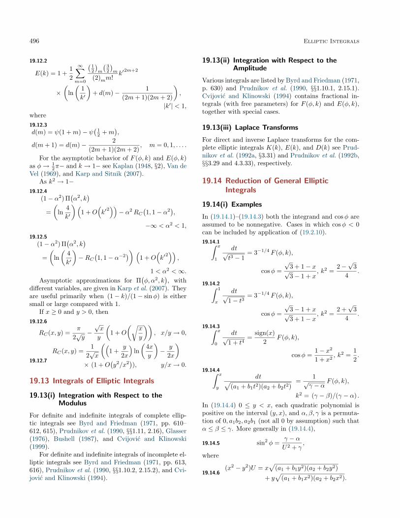
496 Elliptic Integrals
19.12.2
E(k) = 1 +12
∞∑m=0
(12
)m
(32
)m
(2)mm!k′
2m+2
×(
ln(
1k′
)+ d(m)− 1
(2m+ 1)(2m+ 2)
),
|k′| < 1,where19.12.3
d(m) = ψ(1 +m)− ψ(
12 +m
),
d(m+ 1) = d(m)− 2(2m+ 1)(2m+ 2)
, m = 0, 1, . . . .
For the asymptotic behavior of F (φ, k) and E(φ, k)as φ→ 1
2π− and k → 1− see Kaplan (1948, §2), Van deVel (1969), and Karp and Sitnik (2007).
As k2 → 1−19.12.4
(1− α2) Π(α2, k
)=(
ln4k′
)(1 +O
(k′
2))− α2RC
(1, 1− α2
),
−∞ < α2 < 1,
19.12.5
(1− α2) Π(α2, k
)=(
ln(
4k′
)−RC
(1, 1− α−2
)) (1 +O
(k′
2))
,
1 < α2 <∞.Asymptotic approximations for Π
(φ, α2, k
), with
different variables, are given in Karp et al. (2007). Theyare useful primarily when (1− k)/(1− sinφ) is eithersmall or large compared with 1.
If x ≥ 0 and y > 0, then19.12.6
RC(x, y) =π
2√y−√x
y
(1 +O
(√x
y
)), x/y → 0,
19.12.7
RC(x, y) =1
2√x
((1 +
y
2x
)ln(
4xy
)− y
2x
)× (1 +O
(y2/x2
)), y/x→ 0.
19.13 Integrals of Elliptic Integrals
19.13(i) Integration with Respect to theModulus
For definite and indefinite integrals of complete ellip-tic integrals see Byrd and Friedman (1971, pp. 610–612, 615), Prudnikov et al. (1990, §§1.11, 2.16), Glasser(1976), Bushell (1987), and Cvijović and Klinowski(1999).
For definite and indefinite integrals of incomplete el-liptic integrals see Byrd and Friedman (1971, pp. 613,616), Prudnikov et al. (1990, §§1.10.2, 2.15.2), and Cvi-jović and Klinowski (1994).
19.13(ii) Integration with Respect to theAmplitude
Various integrals are listed by Byrd and Friedman (1971,p. 630) and Prudnikov et al. (1990, §§1.10.1, 2.15.1).Cvijović and Klinowski (1994) contains fractional in-tegrals (with free parameters) for F (φ, k) and E(φ, k),together with special cases.
19.13(iii) Laplace Transforms
For direct and inverse Laplace transforms for the com-plete elliptic integrals K(k), E(k), and D(k) see Prud-nikov et al. (1992a, §3.31) and Prudnikov et al. (1992b,§§3.29 and 4.3.33), respectively.
19.14 Reduction of General EllipticIntegrals
19.14(i) Examples
In (19.14.1)–(19.14.3) both the integrand and cosφ areassumed to be nonnegative. Cases in which cosφ < 0can be included by application of (19.2.10).19.14.1∫ x
1
dt√t3 − 1
= 3−1/4 F (φ, k),
cosφ =√
3 + 1− x√3− 1 + x
, k2 =2−√
34
.
19.14.2∫ 1
x
dt√1− t3
= 3−1/4 F (φ, k),
cosφ =√
3− 1 + x√3 + 1− x
, k2 =2 +√
34
.
19.14.3∫ x
0
dt√1 + t4
=sign(x)
2F (φ, k),
cosφ =1− x2
1 + x2, k2 =
12.
19.14.4∫ x
y
dt√(a1 + b1t2)(a2 + b2t2)
=1√γ − α
F (φ, k),
k2 = (γ − β)/(γ − α) .In (19.14.4) 0 ≤ y < x, each quadratic polynomial ispositive on the interval (y, x), and α, β, γ is a permuta-tion of 0, a1b2, a2b1 (not all 0 by assumption) such thatα ≤ β ≤ γ. More generally in (19.14.4),
19.14.5 sin2 φ =γ − αU2 + γ
,
where
19.14.6(x2 − y2)U = x
√(a1 + b1y2)(a2 + b2y2)
+ y√
(a1 + b1x2)(a2 + b2x2).

Symmetric Integrals 497
There are four important special cases of (19.14.4)–(19.14.6), as follows. If y = 0, then
19.14.7 sin2 φ =(γ − α)x2
a1a2 + γx2.
If x =∞, then
19.14.8 sin2 φ =γ − α
b1b2y2 + γ.
If a1 + b1y2 = 0, then
19.14.9 sin2 φ =(γ − α)(x2 − y2)
γ(x2 − y2)− a1(a2 + b2x2).
If a1 + b1x2 = 0, then
19.14.10 sin2 φ =(γ − α)(y2 − x2)
γ(y2 − x2)− a1(a2 + b2y2).
(These four cases include 12 integrals in Abramowitzand Stegun (1964, p. 596).)
19.14(ii) General Case
Legendre (1825–1832) showed that every elliptic in-tegral can be expressed in terms of the three in-tegrals in (19.1.2) supplemented by algebraic, loga-rithmic, and trigonometric functions. The classicalmethod of reducing (19.2.3) to Legendre’s integralsis described in many places, especially Erdélyi et al.(1953b, §13.5), Abramowitz and Stegun (1964, Chapter17), and Labahn and Mutrie (1997, §3). The last refer-ence gives a clear summary of the various steps involvinglinear fractional transformations, partial-fraction de-composition, and recurrence relations. It then improvesthe classical method by first applying Hermite reductionto (19.2.3) to arrive at integrands without multiple polesand uses implicit full partial-fraction decomposition andimplicit root finding to minimize computing with alge-braic extensions. The choice among 21 transformationsfor final reduction to Legendre’s normal form dependson inequalities involving the limits of integration andthe zeros of the cubic or quartic polynomial. A similarremark applies to the transformations given in Erdélyiet al. (1953b, §13.5) and to the choice among explicitreductions in the extensive table of Byrd and Friedman(1971), in which one limit of integration is assumed tobe a branch point of the integrand at which the integralconverges. If no such branch point is accessible from theinterval of integration (for example, if the integrand is(t(3 − t)(4 − t))−3/2 and the interval is [1,2]), then nomethod using this assumption succeeds.
Symmetric Integrals
19.15 Advantages of Symmetry
Elliptic integrals are special cases of a particu-lar multivariate hypergeometric function called Lau-ricella’s FD (Carlson (1961b)). The functionR−a(b1, b2, . . . , bn; z1, z2, . . . , zn) (Carlson (1963)) re-veals the full permutation symmetry that is partiallyhidden in FD, and leads to symmetric standard inte-grals that simplify many aspects of theory, applications,and numerical computation.
Symmetry in x, y, z of RF (x, y, z), RG(x, y, z),and RJ(x, y, z, p) replaces the five transformations(19.7.2), (19.7.4)–(19.7.7) of Legendre’s integrals; com-pare (19.25.17). Symmetry unifies the Landen trans-formations of §19.8(ii) with the Gauss transforma-tions of §19.8(iii), as indicated following (19.22.22) and(19.36.9). (19.21.12) unifies the three transformationsin §19.7(iii) that change the parameter of Legendre’sthird integral.
Symmetry allows the expansion (19.19.7) in a seriesof elementary symmetric functions that gives high pre-cision with relatively few terms and provides the mostefficient method of computing the incomplete integralof the third kind (§19.36(i)).
Symmetry makes possible the reduction theorems of§19.29(i), permitting remarkable compression of tablesof integrals while generalizing the interval of integration.(Compare (19.14.4)–(19.14.10) with (19.29.19), and seethe last paragraph of §19.29(i) and the text following(19.29.15).) These reduction theorems, unknown in theLegendre theory, allow symbolic integration without im-posing conditions on the parameters and the limits ofintegration (see §19.29(ii)).
For the many properties of ellipses and triaxial el-lipsoids that can be represented by elliptic integrals,any symmetry in the semiaxes remains obvious whensymmetric integrals are used (see (19.30.5) and §19.33).For example, the computation of depolarization factorsfor solid ellipsoids is simplified considerably; compare(19.33.7) with Cronemeyer (1991).
19.16 Definitions
19.16(i) Symmetric Integrals
19.16.1 RF (x, y, z) =12
∫ ∞0
dt
s(t),
19.16.2 RJ(x, y, z, p) =32
∫ ∞0
dt
s(t)(t+ p),

498 Elliptic Integrals
19.16.3
RG(x, y, z) =1
4π
∫ 2π
0
∫ π
0
(x sin2 θ cos2 φ+ y sin2 θ sin2 φ
+ z cos2 θ)12 sin θ dθ dφ,
where p (6= 0) is a real or complex constant, and
19.16.4 s(t) =√t+ x
√t+ y
√t+ z.
In (19.16.1) and (19.16.2), x, y, z ∈ C\(−∞, 0] exceptthat one or more of x, y, z may be 0 when the corre-sponding integral converges. In (19.16.2) the Cauchyprincipal value is taken when p is real and negative.In (19.16.3) <x, <y, <z ≥ 0. It should be noted thatthe integrals (19.16.1)–(19.16.3) have been normalizedso that RF (1, 1, 1) = RJ(1, 1, 1, 1) = RG(1, 1, 1) = 1.
A fourth integral that is symmetric in only two vari-ables is defined by
19.16.5 RD(x, y, z) =RJ(x, y, z, z) =32
∫ ∞0
dt
s(t)(t+ z),
with the same conditions on x, y, z as for (19.16.1), butnow z 6= 0.
Just as the elementary function RC(x, y) (§19.2(iv))is the degenerate case
19.16.6 RC(x, y) = RF (x, y, y),
and RD is a degenerate case of RJ , so is RJ a degeneratecase of the hyperelliptic integral,
19.16.732
∫ ∞0
dt∏5j=1
√t+ xj
.
19.16(ii) R−a(b; z)
All elliptic integrals of the form (19.2.3) and many mul-tiple integrals, including (19.16.3), are special cases ofa multivariate hypergeometric function
19.16.8 R−a(b; z) = R−a(b1, . . . , bn; z1, . . . , zn),
which is homogeneous and of degree −a in the z’s, andsymmetric when the same permutation is applied toboth sets of subscripts 1, . . . , n. Thus R−a(b; z) is sym-metric in the variables zj and z` if the parameters bjand b` are equal. The R-function is often used to makea unified statement of a property of several elliptic inte-grals. Before 1969 R−a(b; z) was denoted by R(a; b; z).
19.16.9
R−a(b; z) =1
B(a, a′)
∫ ∞0
ta′−1
n∏j=1
(t+ zj)−bj dt
=1
B(a, a′)
∫ ∞0
ta−1n∏j=1
(1 + tzj)−bj dt,
a, a′ > 0, zj ∈ C\(−∞, 0],
where B(x, y) is the beta function (§5.12) and
19.16.10 a′ = −a+n∑j=1
bj .
19.16.11R−a(b;λz) = λ−aR−a(b; z),R−a(b;x1) = x−a, 1 = (1, . . . , 1).
When n = 4 a useful version of (19.16.9) is given by
19.16.12
R−a(b1, . . . , b4; c− 1, c− k2, c, c− α2
)=
2(sin2 φ)1−a′
B(a, a′)
∫ φ
0
(sin θ)2a−1(sin2 φ− sin2 θ)a′−1
× (cos θ)1−2b1(1− k2 sin2 θ)−b2(1− α2 sin2 θ)
−b4dθ,
where
19.16.13
c = csc2 φ; a, a′ > 0; b3 = a+ a′ − b1 − b2 − b4.
For further information, especially representationof the R-function as a Dirichlet average, see Carlson(1977b).
19.16(iii) Elliptic Cases of R−a(b; z)
R−a(b; z) is an elliptic integral if the z’s are distinctand exactly four of the parameters a, a′, b1, . . . , bn arehalf-odd-integers, the rest are integers, and none of a,a′, a + a′ is zero or a negative integer. The only casesthat are integrals of the first kind are the four in whicheach of a and a′ is either 1
2 or 1 and each bj is 12 . The
only cases that are integrals of the third kind are thosein which at least one bj is a positive integer. All otherelliptic cases are integrals of the second kind.
19.16.14 RF (x, y, z) = R− 12
(12 ,
12 ,
12 ;x, y, z
),
19.16.15 RD(x, y, z) = R− 32
(12 ,
12 ,
32 ;x, y, z
),
19.16.16 RJ(x, y, z, p) = R− 32
(12 ,
12 ,
12 , 1;x, y, z, p
),
19.16.17 RG(x, y, z) = R 12
(12 ,
12 ,
12 ;x, y, z
),
19.16.18 RC(x, y) = R− 12
(12 , 1;x, y
).
When one variable is 0 without destroying convergence,any one of (19.16.14)–(19.16.17) is said to be completeand can be written as an R-function with one less vari-able:
19.16.19
R−a(b1, . . . , bn; 0, z2, . . . , zn)
=B(a, a′ − b1)
B(a, a′)R−a(b2, . . . , bn; z2, . . . , zn),
a+ a′ > 0, a′ > b1.
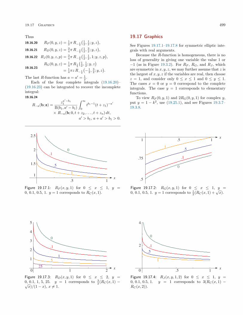
19.17 Graphics 499
Thus19.16.20 RF (0, y, z) = 1
2π R− 12
(12 ,
12 ; y, z
),
19.16.21 RD(0, y, z) = 34π R− 3
2
(12 ,
32 ; y, z
),
19.16.22 RJ(0, y, z, p) = 34π R− 3
2
(12 ,
12 , 1; y, z, p
),
19.16.23RG(0, y, z) = 1
4π R 12
(12 ,
12 ; y, z
)= 1
4πz R− 12
(− 1
2 ,32 ; y, z
).
The last R-function has a = a′ = 12 .
Each of the four complete integrals (19.16.20)–(19.16.23) can be integrated to recover the incompleteintegral:19.16.24
R−a(b; z) =za′−b1
1
B(b1, a′ − b1)
∫ ∞0
tb1−1(t+ z1)−a′
× R−a(b; 0, t+ z2, . . . , t+ zn) dt,a′ > b1, a+ a′ > b1 > 0.
19.17 Graphics
See Figures 19.17.1–19.17.8 for symmetric elliptic inte-grals with real arguments.
Because the R-function is homogeneous, there is noloss of generality in giving one variable the value 1 or−1 (as in Figure 19.3.2). For RF , RG, and RJ , whichare symmetric in x, y, z, we may further assume that z isthe largest of x, y, z if the variables are real, then choosez = 1, and consider only 0 ≤ x ≤ 1 and 0 ≤ y ≤ 1.The cases x = 0 or y = 0 correspond to the completeintegrals. The case y = 1 corresponds to elementaryfunctions.
To view RF (0, y, 1) and 2RG(0, y, 1) for complex y,put y = 1 − k2, use (19.25.1), and see Figures 19.3.7–19.3.8.
Figure 19.17.1: RF (x, y, 1) for 0 ≤ x ≤ 1, y =0, 0.1, 0.5, 1. y = 1 corresponds to RC(x, 1).
Figure 19.17.2: RG(x, y, 1) for 0 ≤ x ≤ 1, y =0, 0.1, 0.5, 1. y = 1 corresponds to 1
2 (RC(x, 1) +√x).
Figure 19.17.3: RD(x, y, 1) for 0 ≤ x ≤ 2, y =0, 0.1, 1, 5, 25. y = 1 corresponds to 3
2 (RC(x, 1) −√x)/(1− x), x 6= 1.
Figure 19.17.4: RJ(x, y, 1, 2) for 0 ≤ x ≤ 1, y =0, 0.1, 0.5, 1. y = 1 corresponds to 3(RC(x, 1) −RC(x, 2)).

500 Elliptic Integrals
Figure 19.17.5: RJ(x, y, 1, 0.5) for 0 ≤ x ≤ 1, y =0, 0.1, 0.5, 1. y = 1 corresponds to 6(RC(x, 0.5) −RC(x, 1)).
x
-4
-8
-12
0.1
.51
0 1.5
Figure 19.17.6: Cauchy principal value ofRJ(x, y, 1,−0.5) for 0 ≤ x ≤ 1, y = 0, 0.1, 0.5, 1.y = 1 corresponds to 2(RC(x,−0.5)−RC(x, 1)).
Figure 19.17.7: Cauchy principal value of RJ(0.5, y, 1, p)for y = 0, 0.01, 0.05, 0.2, 1, −1 ≤ p < 0. y = 1 corre-sponds to 3(RC(0.5, p) − (π/
√8))/(1 − p). As p → 0
the curve for y = 0 has the finite limit −8.10386 . . . ; see(19.20.10).
Figure 19.17.8: RJ(0, y, 1, p), 0 ≤ y ≤ 1, −1 ≤ p ≤ 2.Cauchy principal values are shown when p < 0. Thefunction is asymptotic to 3
2π/√yp as p → 0+, and
to (32/p) ln(16/y) as y → 0+. As p → 0− it has the
limit (−6/y)RG(0, y, 1). When p = 1, it reduces toRD(0, y, 1). If y = 1, then it has the value 3
2π/(p+√p)
when p > 0, and 32π/(p−1) when p < 0. See (19.20.10),
(19.20.11), and (19.20.8) for the cases p→ 0±, y → 0+,and y = 1, respectively.
19.18 Derivatives and DifferentialEquations
19.18(i) Derivatives
19.18.1∂RF (x, y, z)
∂z= − 1
6 RD(x, y, z),
19.18.2d
dxRG(x+ a, x+ b, x+ c) = 1
2 RF (x+ a, x+ b, x+ c).
Let ∂j = ∂/∂zj , and ej be an n-tuple with 1 in the jthplace and 0’s elsewhere. Also define
19.18.3 wj = bj
/ n∑j=1
bj , a′ = −a+n∑j=1
bj .
The next two equations apply to (19.16.14)–(19.16.18)and (19.16.20)–(19.16.23).
19.18.4 ∂j R−a(b; z) = −awj R−a−1(b + ej ; z),

19.19 Taylor and Related Series 501
19.18.5 (zj∂j + bj)R−a(b; z) = wja′R−a(b + ej ; z).
19.18(ii) Differential Equations
19.18.6
(∂
∂x+
∂
∂y+
∂
∂z
)RF (x, y, z) =
−12√xyz
,
19.18.7
(∂
∂x+
∂
∂y+
∂
∂z
)RG(x, y, z) = 1
2 RF (x, y, z).
19.18.8
n∑j=1
∂j R−a(b; z) = −aR−a−1(b; z).
19.18.9(x∂
∂x+ y
∂
∂y+ z
∂
∂z
)RF (x, y, z) = − 1
2 RF (x, y, z),
19.18.10((x− y)
∂2
∂x ∂y+
12
(∂
∂y− ∂
∂x
))RF (x, y, z) = 0,
and two similar equations obtained by permuting x, y, zin (19.18.10).
More concisely, if v = R−a(b; z), then each of(19.16.14)–(19.16.18) and (19.16.20)–(19.16.23) satisfiesEuler’s homogeneity relation:
19.18.11
n∑j=1
zj∂jv = −av,
and also a system of n(n−1)/2 Euler–Poisson differen-tial equations (of which only n− 1 are independent):
19.18.12 (zj∂j + bj)∂lv = (zl∂l + bl)∂jv,
or equivalently,
19.18.13 ((zj − zl)∂j∂l + bj∂l − bl∂j)v = 0.
Here j, l = 1, 2, . . . , n and j 6= l. For group-theoreticalaspects of this system see Carlson (1963, §VI). Ifn = 2, then elimination of ∂2v between (19.18.11) and(19.18.12), followed by the substitution (b1, b2, z1, z2) =(b, c − b, 1 − z, 1), produces the Gauss hypergeometricequation (15.10.1).
The next four differential equations apply tothe complete case of RF and RG in the formR−a
(12 ,
12 ; z1, z2
)(see (19.16.20) and (19.16.23)).
The function w = R−a(
12 ,
12 ;x+ y, x− y
)satisfies
an Euler–Poisson–Darboux equation:
19.18.14∂2w
∂x2 =∂2w
∂y2 +1y
∂w
∂y.
Also W = R−a(
12 ,
12 ; t+ r, t− r
), with r =
√x2 + y2,
satisfies a wave equation:
19.18.15∂2W
∂t2=∂2W
∂x2 +∂2W
∂y2 .
Similarly, the function u = R−a(
12 ,
12 ;x+ iy, x− iy
)satisfies an equation of axially symmetric potential the-ory :
19.18.16∂2u
∂x2 +∂2u
∂y2 +1y
∂u
∂y= 0,
and U = R−a(
12 ,
12 ; z + iρ, z − iρ
), with ρ =
√x2 + y2,
satisfies Laplace’s equation:
19.18.17∂2U
∂x2 +∂2U
∂y2 +∂2U
∂z2 = 0.
19.19 Taylor and Related Series
For N = 0, 1, 2, . . . define the homogeneous hypergeo-metric polynomial
19.19.1 TN (b, z) =∑ (b1)m1
· · · (bn)mnm1! · · ·mn!
zm11 · · · zmnn ,
where the summation extends over all nonnegative in-tegers m1, . . . ,mn whose sum is N . The followingtwo multivariate hypergeometric series apply to eachof the integrals (19.16.14)–(19.16.18) and (19.16.20)–(19.16.23):
19.19.2R−a(b; z) =
∞∑N=0
(a)N(c)N
TN (b,1− z),
c =∑nj=1 bj , |1− zj | < 1,
19.19.3 R−a(b; z) = z−an
∞∑N=0
(a)N(c)N
TN (b1, . . . , bn−1; 1− (z1/zn), . . . , 1− (zn−1/zn)), c =∑nj=1 bj , |1− (zj/zn)| < 1.
If n = 2, then (19.19.3) is a Gauss hypergeometric series(see (19.25.43) and (15.2.1)).
Define the elementary symmetric function Es(z) by
19.19.4n∏j=1
(1 + tzj) =n∑s=0
tsEs(z),
and define the n-tuple 12 = ( 1
2 , . . . ,12 ). Then
19.19.5
TN (12 , z) =
∑(−1)M+N
(12
)M
Em11 (z) · · ·Emnn (z)m1! · · ·mn!
,
where M =∑nj=1mj and the summation extends
over all nonnegative integers m1, . . . ,mn such that∑nj=1 jmj = N .

502 Elliptic Integrals
This form of TN can be applied to (19.16.14)–(19.16.18) and (19.16.20)–(19.16.23) if we use
19.19.6 RJ(x, y, z, p) = R− 32
(12 ,
12 ,
12 ,
12 ,
12 ;x, y, z, p, p
)as well as (19.16.5) and (19.16.6). The number ofterms in TN can be greatly reduced by using variablesZ = 1− (z/A) with A chosen to make E1(Z) = 0. ThenTN has at most one term if N ≤ 5 in the series for RF .For RJ and RD, TN has at most one term if N ≤ 3, andtwo terms if N = 4 or 5.
19.19.7 R−a(
12
; z)
= A−a∞∑N=0
(a)N(12n)N
TN (12,Z),
where
19.19.8A =
1n
n∑j=1
zj , Zj = 1− (zj/A),
E1(Z) = 0, |Zj | < 1.
A special case is given in (19.36.1).
19.20 Special Cases
19.20(i) RF (x, y, z)
In this subsection, and also §§19.20(ii)–19.20(v), thevariables of all R-functions satisfy the constraints spec-ified in §19.16(i) unless other conditions are stated.
19.20.1
RF (x, x, x) = x−1/2,
RF (λx, λy, λz) = λ−1/2RF (x, y, z),RF (x, y, y) = RC(x, y),
RF (0, y, y) = 12πy
−1/2,
RF (0, 0, z) =∞.
The first lemniscate constant is given by
19.20.2
∫ 1
0
dt√1− t4
= RF (0, 1, 2) =
(Γ(
14
))24(2π)1/2
= 1.31102 87771 46059 90523 . . . .
Todd (1975) refers to a proof by T. Schneider that this isa transcendental number. The general lemniscatic caseis
19.20.3 RF (x, a, y) = R− 14
(34 ,
12 ; a2, xy
), a = 1
2 (x+ y).
19.20(ii) RG(x, y, z)
19.20.4
RG(x, x, x) = x1/2,
RG(λx, λy, λz) = λ1/2RG(x, y, z),
RG(0, y, y) = 14πy
1/2,
RG(0, 0, z) = 12z
1/2,
19.20.5 2RG(x, y, y) = y RC(x, y) +√x.
19.20(iii) RJ(x, y, z, p)
19.20.6
RJ(x, x, x, x) = x−3/2,
RJ(λx, λy, λz, λp) = λ−3/2RJ(x, y, z, p),
RJ(x, y, z, z) = RD(x, y, z),
RJ(0, 0, z, p) =∞,
RJ(x, x, x, p) = RD(p, p, x) =3
x− p
(RC(x, p)− 1√
x
),
x 6= p, xp 6= 0.
19.20.7
RJ(x, y, z, p)→ +∞, p→ 0+ or 0−; x, y, z > 0.
19.20.8
RJ(0, y, y, p) =3π
2(y√p+ p
√y)
, p > 0,
RJ(0, y, y,−q) =−3π
2√y(y + q)
, q > 0,
RJ(x, y, y, p) =3
p− y(RC(x, y)−RC(x, p)), p 6= y,
RJ(x, y, y, y) = RD(x, y, y).
19.20.9 RJ(0, y, z,±√yz) = ± 32√yz
RF (0, y, z).
19.20.10
limp→0+
√pRJ(0, y, z, p) =
3π2√yz,
limp→0−
RJ(0, y, z, p) = −RD(0, y, z)−RD(0, z, y)
=−6yz
RG(0, y, z).
19.20.11
RJ(0, y, z, p) ∼ 32p√z
ln(
16zy
), y → 0+; p (6= 0) real.
19.20.12 limp→±∞
pRJ(x, y, z, p) = 3RF (x, y, z).
19.20.13
2(p− x)RJ(x, y, z, p) = 3RF (x, y, z)− 3√xRC
(yz, p2
),
p = x±√
(y − x)(z − x),
where x, y, z may be permuted.When the variables are real and distinct, the vari-
ous cases of RJ(x, y, z, p) are called circular (hyperbolic)cases if (p−x)(p−y)(p−z) is positive (negative), becausethey typically occur in conjunction with inverse circular(hyperbolic) functions. Cases encountered in dynamicalproblems are usually circular; hyperbolic cases includeCauchy principal values. If x, y, z are permuted so that

19.21 Connection Formulas 503
0 ≤ x < y < z, then the Cauchy principal value of RJis given by
19.20.14
(q + z)RJ(x, y, z,−q)= (p− z)RJ(x, y, z, p)− 3RF (x, y, z)
+ 3(
xyz
xy + pq
)1/2RC(xy + pq, pq),
valid when
19.20.15 q > 0, p =z(x+ y + q)− xy
z + q,
or19.20.16 p = wy + (1−w)z, w =
z − xz + q
, 0 < w < 1.
Since x < y < p < z, p is in a hyperbolic region. In thecomplete case (x = 0) (19.20.14) reduces to
19.20.17
(q + z)RJ(0, y, z,−q)= (p− z)RJ(0, y, z, p)− 3RF (0, y, z),
p = z(y + q)/(z + q), w = z/(z + q).
19.20(iv) RD(x, y, z)
19.20.18
RD(x, x, x) = x−3/2,
RD(λx, λy, λz) = λ−3/2RD(x, y, z),
RD(0, y, y) = 34π y
−3/2,
RD(0, 0, z) =∞.
19.20.19 RD(x, y, z) ∼ 3(xyz)−1/2, z/√xy → 0.
19.20.20RD(x, y, y) =
32(y − x)
(RC(x, y)−
√x
y
),
x 6= y, y 6= 0,
19.20.21
RD(x, x, z) =3
z − x
(RC(z, x)− 1√
z
), x 6= z, xz 6= 0.
The second lemniscate constant is given by
19.20.22
∫ 1
0
t2 dt√1− t4
= 13 RD(0, 2, 1) =
(Γ(
34
))2(2π)1/2
= 0.59907 01173 67796 10371 . . . .
Todd (1975) refers to a proof by T. Schneider that thisis a transcendental number. Compare (19.20.2). Thegeneral lemniscatic case is
19.20.23
RD(x, y, a) = R− 34
(54 ,
12 ; a2, xy
), a = 1
2x+ 12y.
19.20(v) R−a(b; z)
Define c =∑nj=1 bj . Then
19.20.24R0(b; z) = 1, RN (b; z) =
N !(c)N
TN (b, z),
N = 0, 1, 2, . . . ,where TN is defined by (19.19.1). Also,
19.20.25 R−c(b; z) =n∏j=1
z−bjj ,
19.20.26R−a(b; z) =
n∏j=1
z−bjj R−a′
(b; z−1
),
a+ a′ = c, z−1 = (z−11 , . . . , z−1
n ).See also (19.16.11) and (19.16.19).
19.21 Connection Formulas
19.21(i) Complete Integrals
Legendre’s relation (19.7.1) can be written
19.21.1
RF (0, z + 1, z)RD(0, z + 1, 1)+RD(0, z + 1, z)RF (0, z + 1, 1) = 3π/(2z),
z ∈ C\(−∞, 0].The case z = 1 shows that the product of the two lem-niscate constants, (19.20.2) and (19.20.22), is π/4.
19.21.2 3RF (0, y, z) = z RD(0, y, z) + y RD(0, z, y).
19.21.3
6RG(0, y, z) = yz(RD(0, y, z) +RD(0, z, y))= 3z RF (0, y, z) + z(y − z)RD(0, y, z).
The complete cases of RF and RG have connectionformulas resulting from those for the Gauss hyperge-ometric function (Erdélyi et al. (1953a, §2.9)). Up-per signs apply if 0 < ph z < π, and lower signs if−π < ph z < 0:
19.21.4 RF (0, z − 1, z) = RF (0, 1− z, 1)∓ iRF (0, z, 1),
19.21.5
2RG(0, z − 1, z) = 2RG(0, 1− z, 1)± i2RG(0, z, 1)+ (z − 1)RF (0, 1− z, 1)∓ izRF (0, z, 1).
Let y, z, and p be positive and distinct, and permutey and z to ensure that y does not lie between z and p.The complete case of RJ can be expressed in terms ofRF and RD:19.21.6
(√rp/z)RJ(0, y, z, p) = (r − 1)RF (0, y, z)RD(p, rz, z)
+RD(0, y, z)RF (p, rz, z),r = (y − p)/(y − z) > 0.
If 0 < p < z and y = z + 1, then as p → 0 (19.21.6)reduces to Legendre’s relation (19.21.1).

504 Elliptic Integrals
19.21(ii) Incomplete Integrals
RD(x, y, z) is symmetric only in x and y, but either(nonzero) x or (nonzero) y can be moved to the thirdposition by using
19.21.7(x− y)RD(y, z, x) + (z − y)RD(x, y, z)
= 3RF (x, y, z)− 3√y/(xz),
or the corresponding equation with x and y inter-changed.
19.21.8RD(y, z, x) +RD(z, x, y) +RD(x, y, z)
= 3(xyz)−1/2,
19.21.9xRD(y, z, x) + y RD(z, x, y) + z RD(x, y, z)
= 3RF (x, y, z).
19.21.10
2RG(x, y, z) = z RF (x, y, z)
− 13 (x− z)(y − z)RD(x, y, z) +
√xy/z,z 6= 0.
Because RG is completely symmetric, x, y, z can bepermuted on the right-hand side of (19.21.10) so that(x − z)(y − z) ≤ 0 if the variables are real, therebyavoiding cancellations when RG is calculated from RFand RD (see §19.36(i)).
19.21.11
6RG(x, y, z) = 3(x+ y + z)RF (x, y, z)
−∑
x2RD(y, z, x)
=∑
x(y + z)RD(y, z, x),
where both summations extend over the three cyclicpermutations of x, y, z.
Connection formulas for R−a(b; z) are given in Carl-son (1977b, pp. 99, 101, and 123–124).
19.21(iii) Change of Parameter of RJ
Let x, y, z be real and nonnegative, with at most one ofthem 0. Change-of-parameter relations can be used toshift the parameter p of RJ from either circular regionto the other, or from either hyperbolic region to theother (§19.20(iii)). The latter case allows evaluation ofCauchy principal values (see (19.20.14)).
19.21.12(p− x)RJ(x, y, z, p) + (q − x)RJ(x, y, z, q)
= 3RF (x, y, z)− 3RC(ξ, η),where19.21.13
(p− x)(q− x) = (y− x)(z − x), ξ = yz/x, η = pq/x,
and x, y, z may be permuted. Also,19.21.14
η − ξ = p+ q− y− z =(p− y)(p− z)
p− x=
(q − y)(q − z)q − x
=(p− y)(q − y)
x− y=
(p− z)(q − z)x− z
.
For each value of p, permutation of x, y, z producesthree values of q, one of which lies in the same region asp and two lie in the other region of the same type. In(19.21.12), if x is the largest (smallest) of x, y, and z,then p and q lie in the same region if it is circular (hy-perbolic); otherwise p and q lie in different regions, bothcircular or both hyperbolic. If x = 0, then ξ = η = ∞and RC(ξ, η) = 0; hence
19.21.15
pRJ(0, y, z, p) + q RJ(0, y, z, q) = 3RF (0, y, z), pq = yz.
19.22 Quadratic Transformations
19.22(i) Complete Integrals
Let <x > 0, <y > 0, a = (x+ y)/2, and p 6= 0. Then
19.22.1
RF(0, x2, y2
)= RF
(0, xy, a2
),
19.22.2
2RG(0, x2, y2
)= 4RG
(0, xy, a2
)− xy RF
(0, xy, a2
),
19.22.3
2y2RD(0, x2, y2
)= 1
4 (y2 − x2)RD(0, xy, a2
)+ 3RF
(0, xy, a2
).
19.22.4
(p2± − p2
∓)RJ(0, x2, y2, p2
)= 2(p2
± − a2)RJ(0, xy, a2, p2
±)
− 3RF(0, xy, a2
)+ 3π/(2p),
where
19.22.5 2p± =√
(p+ x)(p+ y)±√
(p− x)(p− y),
and hence
19.22.6
p+p− = pa, p2+ + p2
− = p2 + xy,
p2+ − p2
− =√
(p2 − x2)(p2 − y2),
4(p2± − a2) = (
√p2 − x2 ±
√p2 − y2)2.
Bartky’s Transformation
19.22.7
2p2RJ(0, x2, y2, p2
)= v+v−RJ
(0, xy, a2, v2
+
)+ 3RF
(0, xy, a2
),
v± = (p2 ± xy)/(2p).
If p = y, then (19.22.7) reduces to (19.22.3), but if p = xor p = y, then both sides of (19.22.4) are 0 by (19.20.9).If x < p < y or y < p < x, then p+ and p− are complexconjugates.

19.22 Quadratic Transformations 505
19.22(ii) Gauss’s Arithmetic-Geometric Mean(AGM)
The AGM, M(a0, g0), of two positive numbers a0 andg0 is defined in §19.8(i). Again, we assume that a0 ≥ g0
(except in (19.22.10)), and define cn =√a2n − g2
n. Then
19.22.82πRF(0, a2
0, g20
)=
1M(a0, g0)
,
19.22.9
4πRG(0, a2
0, g20
)=
1M(a0, g0)
(a2
0 −∞∑n=0
2n−1c2n
)
=1
M(a0, g0)
(a2
1 −∞∑n=2
2n−1c2n
),
and
19.22.10 RD(0, g2
0 , a20
)=
3π4M(a0, g0)a2
0
∞∑n=0
Qn,
where19.22.11 Q0 = 1, Qn+1 = 1
2Qnan − gnan + gn
.
Qn has the same sign as a0 − g0 for n ≥ 1.
19.22.12 RJ(0, g2
0 , a20, p
20
)=
3π4M(a0, g0)p2
0
∞∑n=0
Qn,
where p0 > 0 and
19.22.13pn+1 =
p2n + angn
2pn, εn =
p2n − angnp2n + angn
,
Q0 = 1, Qn+1 = 12Qnεn.
(If p0 = a0, then pn = an and (19.22.13) reduces to(19.22.11).) As n → ∞, pn and εn converge quadrati-cally to M(a0, g0) and 0, respectively, and Qn convergesto 0 faster than quadratically. If the last variable of RJis negative, then the Cauchy principal value is
19.22.14
RJ(0, g2
0 , a20,−q2
0
)=
−3π4M(a0, g0)(q2
0 + a20)
×
(2 +
a20 − g2
0
q20 + g2
0
∞∑n=0
Qn
),
and (19.22.13) still applies, provided that
19.22.15 p20 = a2
0(q20 + g2
0)/(q20 + a2
0).
19.22(iii) Incomplete Integrals
Let x, y, and z have positive real parts, assume p 6= 0,and retain (19.22.5) and (19.22.6). Define
19.22.16a = (x+ y)/2,
2z± =√
(z + x)(z + y)±√
(z − x)(z − y),so that
19.22.17
z+z− = za, z2+ + z2
− = z2 + xy,
z2+ − z2
− =√
(z2 − x2)(z2 − y2),
4(z2± − a2) = (
√z2 − x2 ±
√z2 − y2)2.
Then
19.22.18 RF(x2, y2, z2
)= RF
(a2, z2
−, z2+
),
19.22.19
(z2± − z2
∓)RD(x2, y2, z2
)= 2(z2
± − a2)RD(a2, z2
∓, z2±)
− 3RF(x2, y2, z2
)+ (3/z),
19.22.20
(p2± − p2
∓)RJ(x2, y2, z2, p2
)= 2(p2
± − a2)RJ(a2, z2
+, z2−, p
2±)
− 3RF(x2, y2, z2
)+ 3RC
(z2, p2
),
19.22.212RG
(x2, y2, z2
)= 4RG
(a2, z2
+, z2−)
− xy RF(x2, y2, z2
)− z,
19.22.22 RC(x2, y2
)= RC
(a2, ay
).
If x, y, z are real and positive, then (19.22.18)–(19.22.21) are ascending Landen transformations whenx, y < z (implying a < z− < z+), and descending Gausstransformations when z < x, y (implying z+ < z− < a).Ascent and descent correspond respectively to increaseand decrease of k in Legendre’s notation. DescendingGauss transformations include, as special cases, trans-formations of complete integrals into complete integrals;ascending Landen transformations do not.
If p = x or p = y, then (19.22.20) reduces to 0 = 0by (19.20.13), and if z = x or z = y then (19.22.19)reduces to 0 = 0 by (19.20.20) and (19.22.22). Ifx < z < y or y < z < x, then z+ and z− are com-plex conjugates. However, if x and y are complex con-jugates and z and p are real, then the right-hand sides ofall transformations in §§19.22(i) and 19.22(iii)—except(19.22.3) and (19.22.22)—are free of complex numbersand p2
± − p2∓ = ±|p2 − x2| 6= 0.
The transformations inverse to the ones just de-scribed are the descending Landen transformations andthe ascending Gauss transformations. The equationsinverse to (19.22.5) and (19.22.16) are given by
19.22.23
x+ y = 2a, x− y = (2/a )√
(a2 − z2+)(a2 − z2
−),
z = z+z−/a ,
and the corresponding equations with z, z+, and z− re-placed by p, p+, and p−, respectively. These relationsneed to be used with caution because y is negative when0 < a < z+z−
(z2
+ + z2−)−1/2.

506 Elliptic Integrals
19.23 Integral Representations
In (19.23.1)–(19.23.3) we assume <y > 0 and <z > 0.
19.23.1 RF (0, y, z) =∫ π/2
0
(y cos2 θ + z sin2 θ)−1/2 dθ,
19.23.2 RG(0, y, z) =12
∫ π/2
0
(y cos2 θ + z sin2 θ)1/2 dθ,
19.23.3
RD(0, y, z) = 3∫ π/2
0
(y cos2 θ + z sin2 θ)−3/2 sin2 θ dθ.
19.23.4
RF (0, y, z) =2π
∫ π/2
0
RC(y, z cos2 θ
)dθ
=2π
∫ ∞0
RC(y cosh2 t, z
)dt.
19.23.5
RF (x, y, z) =2π
∫ π/2
0
RC(x, y cos2 θ + z sin2 θ
)dθ,
<y > 0, <z > 0,
19.23.6
4π RF (x, y, z)
=∫ 2π
0
∫ π
0
sin θ dθ dφ(x sin2 θ cos2 φ+ y sin2 θ sin2 φ+ z cos2 θ)1/2
,
where x, y, and z have positive real parts—except thatat most one of them may be 0.
In (19.23.7)–(19.23.10) one or more of the variablesmay be 0 if the integral converges. In (19.23.8) n = 2,and in (19.23.9) n = 3. Also, in (19.23.8) and (19.23.10)B denotes the beta function (§5.12).
19.23.7 RG(x, y, z) =14
∫ ∞0
1√t+ x
√t+ y
√t+ z
(x
t+ x+
y
t+ y+
z
t+ z
)t dt, x, y, z ∈ C\(−∞, 0].
19.23.8 R−a(b; z) =2
B(b1, b2)
∫ π/2
0
(z1 cos2 θ + z2 sin2 θ)−a
(cos θ)2b1−1(sin θ)2b2−1 dθ, b1, b2 > 0; <z1,<z2 > 0.
With l1, l2, l3 denoting any permutation of sin θ cosφ, sin θ sinφ, cos θ,
19.23.9 R−a(b; z) =4 Γ(b1 + b2 + b3)Γ(b1) Γ(b2) Γ(b3)
∫ π/2
0
∫ π/2
0
3∑j=1
zj l2j
−a 3∏j=1
l2bj−1j sin θ dθ dφ, bj > 0, <zj > 0.
19.23.10
R−a(b; z) =1
B(a, a′)
∫ 1
0
ua−1(1− u)a′−1
n∏j=1
(1− u+ uzj)−bj du, a, a′ > 0; a+ a′ =∑nj=1 bj ; zj ∈ C\(−∞, 0].
For generalizations of (19.16.3) and (19.23.8) seeCarlson (1964, (6.2), (6.12), and (6.1)).
19.24 Inequalities
19.24(i) Complete Integrals
The condition y ≤ z for (19.24.1) and (19.24.2) servesonly to identify y as the smaller of the two nonzerovariables of a symmetric function; it does not restrictvalidity.
19.24.1
ln 4 ≤√z RF (0, y, z) + ln
√y/z ≤ 1
2π, 0 < y ≤ z,
19.24.2 12 ≤ z
−1/2RG(0, y, z) ≤ 14π, 0 ≤ y ≤ z,
19.24.3(y3/2 + z3/2
2
)2/3≤ 4πRG(0, y2, z2
)≤(y2 + z2
2
)1/2,
y > 0, z > 0.
If y, z, and p are positive, then
19.24.42√p
(2yz+yp+zp)−1/2 ≤ 43π
RJ(0, y, z, p)≤ (yzp2)−3/8.
Inequalities for RD(0, y, z) are included as the casep = z.
A series of successively sharper inequalities is ob-tained from the AGM process (§19.8(i)) with a0 ≥ g0 >0:19.24.5
1an≤ 2πRF(0, a2
0, g20
)≤ 1gn
, n = 0, 1, 2, . . . ,
where
19.24.6 an+1 = (an + gn)/2, gn+1 =√angn.
Other inequalities can be obtained by applyingCarlson (1966, Theorems 2 and 3) to (19.16.20)–(19.16.23). Approximations and one-sided inequalitiesfor RG(0, y, z) follow from those given in §19.9(i) for thelength L(a, b) of an ellipse with semiaxes a and b, since
19.24.7 L(a, b) = 8RG(0, a2, b2
).

19.25 Relations to Other Functions 507
For x > 0, y > 0, and x 6= y, the complete cases ofRF and RG satisfy
19.24.8RF (x, y, 0)RG(x, y, 0) > 1
8π2,
RF (x, y, 0) + 2RG(x, y, 0) > π.
Also, with the notation of (19.24.6),
19.24.912g2
1 ≤RG(a2
0, g20 , 0)
RF (a20, g
20 , 0)
≤ 12a2
1,
with equality iff a0 = g0.
19.24(ii) Incomplete Integrals
Inequalities for R−a(b; z) in Carlson (1966, Theorems2 and 3) can be applied to (19.16.14)–(19.16.17). Allvariables are positive, and equality occurs iff all vari-ables are equal.
Examples
19.24.103√
x+√y +√z≤ RF (x, y, z) ≤ 1
(xyz)1/6,
19.24.11
(5√
x+√y +√z + 2
√p
)3≤ RJ(x, y, z, p)
≤ (xyzp2)−3/10,
19.24.1213 (√x+√y +√z)
≤ RG(x, y, z) ≤ min
(√x+ y + z
3,x2 + y2 + z2
3√xyz
).
Inequalities for RC(x, y) and RD(x, y, z) are included asspecial cases (see (19.16.6) and (19.16.5)).
Other inequalities for RF (x, y, z) are given in Carl-son (1970).
If a ( 6= 0) is real, all components of b and z are pos-itive, and the components of z are not all equal, then
19.24.13
Ra(b; z)R−a(b; z) > 1, Ra(b; z) +R−a(b; z) > 2;
see Neuman (2003, (2.13)). Special cases with a = ± 12
are (19.24.8) (because of (19.16.20), (19.16.23)), and
19.24.14RF (x, y, z)RG(x, y, z) > 1,
RF (x, y, z) +RG(x, y, z) > 2.
The same reference also gives upper and lower boundsfor symmetric integrals in terms of their elementary de-generate cases. These bounds include a sharper butmore complicated lower bound than that supplied inthe next result:
19.24.15
RC(x, 1
2 (y + z))≤ RF (x, y, z) ≤ RC(x,
√yz), x ≥ 0,
with equality iff y = z.
19.25 Relations to Other Functions
19.25(i) Legendre’s Integrals as SymmetricIntegrals
Let k′2 = 1− k2 and c = csc2 φ. Then19.25.1
K(k) = RF
(0, k′2, 1
), E(k) = 2RG
(0, k′2, 1
),
E(k) = 13k′2(RD
(0, k′2, 1
)+RD
(0, 1, k′2
)),
K(k)− E(k) = k2D(k) = 13k
2RD
(0, k′2, 1
),
E(k)− k′2K(k) = 13k
2k′2RD
(0, 1, k′2
).
19.25.2 Π(α2, k
)−K(k) = 1
3α2RJ
(0, k′2, 1, 1− α2
).
19.25.3 Π(α2, k
)= 1
2π R− 12
(12 ,−
12 , 1; k′2, 1, 1− α2
),
with Cauchy principal value19.25.4
Π(α2, k
)= − 1
3 (k2/α2)RJ(0, 1− k2, 1, 1− (k2/α2)
),
−∞ < k2 < 1 < α2.
19.25.5 F (φ, k) = RF(c− 1, c− k2, c
),
19.25.6∂F (φ, k)∂k
= 13k RD
(c− 1, c, c− k2
).
19.25.7
E(φ, k) = 2RG(c− 1, c− k2, c
)− (c− 1)RF
(c− 1, c− k2, c
)−√
(c− 1)(c− k2)/c,
19.25.8 E(φ, k) = R− 12
(12 ,−
12 ,
32 ; c− 1, c− k2, c
),
19.25.9
E(φ, k)= RF
(c− 1, c− k2, c
)− 1
3k2RD
(c− 1, c− k2, c
),
19.25.10
E(φ, k) = k′2RF(c− 1, c− k2, c
)+ 1
3k2k′
2RD(c− 1, c, c− k2
)+ k2
√(c− 1)/(c(c− k2)), c > k2,
19.25.11E(φ, k) = − 1
3k′2RD
(c− k2, c, c− 1
)+√
(c− k2)/(c(c− 1)), φ 6= 12π.
Equations (19.25.9)–(19.25.11) correspond to three(nonzero) choices for the last variable of RD; see(19.21.7). All terms on the right-hand sides are non-negative when k2 ≤ 0, 0 ≤ k2 ≤ 1, or 1 ≤ k2 ≤ c,respectively.
19.25.12∂E(φ, k)
∂k= − 1
3k RD(c− 1, c− k2, c
).
19.25.13 D(φ, k) = 13 RD
(c− 1, c− k2, c
).
19.25.14
Π(φ, α2, k
)−F (φ, k) = 1
3α2RJ
(c− 1, c− k2, c, c− α2
),
19.25.15
Π(φ, α2, k
)= R− 1
2
(12 ,
12 ,−
12 , 1; c− 1, c− k2, c, c− α2
).

508 Elliptic Integrals
If α2 > c, then the Cauchy principal value is
19.25.16
Π(φ, α2, k
)= − 1
3ω2RJ
(c− 1, c− k2, c, c− ω2
)+
√(c− 1)(c− k2)
(α2 − 1)(1− ω2)
× RC(c(α2 − 1)(1− ω2), (α2 − c)(c− ω2)
),
ω2 = k2/α2.
The transformations in §19.7(ii) result from the sym-metry and homogeneity of functions on the right-handsides of (19.25.5), (19.25.7), and (19.25.14). For exam-ple, if we write (19.25.5) as
19.25.17 F (φ, k) = RF (x, y, z),
with
19.25.18 (x, y, z) = (c− 1, c− k2, c),
then the five nontrivial permutations of x, y, z that leaveRF invariant change k2 (= (z−y)/(z−x)) into 1/k2, k′2,1/k′2, −k2/k′
2, −k′2/k2, and sinφ (=√
(z − x)/z) intok sinφ, −i tanφ, −ik′ tanφ, (k′ sinφ)/
√1− k2 sin2 φ,
−ik sinφ/√
1− k2 sin2 φ. Thus the five permutationsinduce five transformations of Legendre’s integrals (andalso of the Jacobian elliptic functions).
The three changes of parameter of Π(φ, α2, k
)in
§19.7(iii) are unified in (19.21.12) by way of (19.25.14).
19.25(ii) Bulirsch’s Integrals as SymmetricIntegrals
Let r = 1/x2. Then19.25.19
cel(kc, p, a, b) = aRF(0, k2
c , 1)
+ 13 (b− pa)RJ
(0, k2
c , 1, p),
19.25.20
el1(x, kc) = RF(r, r + k2
c , r + 1),
19.25.21
el2(x, kc, a, b) = a el1(x, kc)+ 1
3 (b− a)RD(r, r + k2
c , r + 1),
19.25.22
el3(x, kc, p) = el1(x, kc)+ 1
3 (1− p)RJ(r, r + k2
c , r + 1, r + p).
19.25(iii) Symmetric Integrals as Legendre’sIntegrals
Assume 0 ≤ x ≤ y ≤ z, x < z, and p > 0. Let
19.25.23
φ = arccos√x/z = arcsin
√(z − x)/z ,
k =√z − yz − x
, α2 =z − pz − x
,
with α 6= 0. Then
19.25.24 (z − x)1/2RF (x, y, z) = F (φ, k),
19.25.25
(z − x)3/2RD(x, y, z) = (3/k2)(F (φ, k)− E(φ, k)),
19.25.26
(z−x)3/2RJ(x, y, z, p) = (3/α2)(Π(φ, α2, k
)− F (φ, k)),
19.25.27
2(z − x)−1/2RG(x, y, z) = E(φ, k) + (cotφ)2 F (φ, k)
+ (cotφ)√
1− k2 sin2 φ.
19.25(iv) Theta Functions
For relations of symmetric integrals to theta functions,see §20.9(i).
19.25(v) Jacobian Elliptic Functions
For the notation see §§22.2, 22.15, and 22.16(i).With 0 ≤ k2 ≤ 1 and p, q, r any permutation of the
letters c,d,n, define
19.25.28 ∆(p, q) = ps2 (u, k)− qs2 (u, k) = −∆(q,p),which implies
19.25.29 ∆(n,d) = k2, ∆(d, c) = k′2, ∆(n, c) = 1.
If cs2 (u, k) ≥ 0, then
19.25.30 am (u, k) = RC(cs2 (u, k),ns2 (u, k)
),
19.25.31 u = RF(ps2 (u, k), qs2 (u, k), rs2 (u, k)
);
compare (19.25.35) and (20.9.3).19.25.32
arcps (x, k) = RF(x2, x2 + ∆(q,p), x2 + ∆(r,p)
),
19.25.33
arcsp (x, k) = xRF(1, 1 + ∆(q,p)x2, 1 + ∆(r,p)x2
),
19.25.34arcpq (x, k) =
√wRF
(x2, 1, 1 + ∆(r, q)w
),
w = (1− x2)/
∆(q,p) ,where we assume 0 ≤ x2 ≤ 1 if x = sn, cn, or cd; x2 ≥ 1if x = ns, nc, or dc; x real if x = cs or sc; k′ ≤ x ≤ 1if x = dn; 1 ≤ x ≤ 1/k′ if x = nd; x2 ≥ k′
2 if x = ds;0 ≤ x2 ≤ 1/k′2 if x = sd.
For the use of R-functions with ∆(p, q) in unifyingother properties of Jacobian elliptic functions, see Carl-son (2004, 2006a,b, 2008).
Inversions of 12 elliptic integrals of the firstkind, producing the 12 Jacobian elliptic functions,are combined and simplified by using the propertiesof RF (x, y, z). See (19.29.19), Carlson (2005), and(22.15.11), and compare with Abramowitz and Ste-gun (1964, Eqs. (17.4.41)–(17.4.52)). For analogousintegrals of the second kind, which are not invertiblein terms of single-valued functions, see (19.29.20) and(19.29.21) and compare with Gradshteyn and Ryzhik(2000, §3.153,1–10 and §3.156,1–9).

19.26 Addition Theorems 509
19.25(vi) Weierstrass Elliptic Functions
For the notation see §23.2.
19.25.35 z = RF (℘(z)− e1, ℘(z)− e2, ℘(z)− e3),
provided that
19.25.36 ℘(z)− ej ∈ C\(−∞, 0], j = 1, 2, 3,
and the left-hand side does not vanish for more thanone value of j. Also,19.25.37
ζ(z) + z ℘(z) = 2RG(℘(z)− e1, ℘(z)− e2, ℘(z)− e3).
In (19.25.38) and (19.25.39) j, k, ` is any permuta-tion of the numbers 1, 2, 3.
19.25.38 ωj = RF (0, ej − ek, ej − e`),
19.25.39 ηj + ωjej = 2RG(0, ej − ek, ej − e`).Lastly,
19.25.40 z = σ(z)RF(σ2
1(z), σ22(z), σ2
3(z)),
where19.25.41
σj(z) = exp(−ηjz)σ(z + ωj)/ σ(ωj), j = 1, 2, 3.
19.25(vii) Hypergeometric Function
19.25.42 2F1(a, b; c; z) = R−a(b, c− b; 1− z, 1),
19.25.43
R−a(b1, b2; z1, z2) = z−a2 2F1(a, b1; b1 + b2; 1− (z1/z2)).
For these results and extensions to the Appell functionF1 (§16.13) and Lauricella’s function FD see Carlson(1963). (F1 and FD are equivalent to the R-function of3 and n variables, respectively, but lack full symmetry.)
19.26 Addition Theorems
19.26(i) General Formulas
In this subsection, and also §§19.26(ii) and 19.26(iii), weassume that λ, x, y, z are positive, except that at mostone of x, y, z can be 0.
19.26.1RF (x+ λ, y + λ, z + λ)
+RF (x+ µ, y + µ, z + µ) = RF (x, y, z),
where µ > 0 and19.26.2
x+ µ = λ−2(√
(x+ λ)yz +√x(y + λ)(z + λ)
)2,
with corresponding equations for y + µ and z + µ ob-tained by permuting x, y, z. Also,
19.26.3√z =
ξζ ′ + η′ζ − ξη′√ξηζ ′ +
√ξ′η′ζ
,
where
19.26.4(ξ, η, ζ) = (x+ λ, y + λ, z + λ),
(ξ′, η′, ζ ′) = (x+ µ, y + µ, z + µ),
with√x and
√y obtained by permuting x, y, and z.
(Note that ξζ ′+ η′ζ− ξη′ = ξ′ζ+ ηζ ′− ξ′η.) Equivalentforms of (19.26.2) are given by
19.26.5µ = λ−2
(√xyz +
√(x+ λ)(y + λ)(z + λ)
)2− λ− x− y − z,
and
19.26.6 (λµ−xy−xz− yz)2 = 4xyz(λ+µ+x+ y+ z).
Also,
19.26.7
RD(x+ λ, y + λ, z + λ) +RD(x+ µ, y + µ, z + µ)
= RD(x, y, z)− 3√z(z + λ)(z + µ)
,
19.26.8
2RG(x+ λ, y + λ, z + λ) + 2RG(x+ µ, y + µ, z + µ)= 2RG(x, y, z) + λRF (x+ λ, y + λ, z + λ)
+ µRF (x+ µ, y + µ, z + µ) +√λ+ µ+ x+ y + z.
19.26.9
RJ(x+ λ, y + λ, z + λ, p+ λ)+RJ(x+ µ, y + µ, z + µ, p+ µ)
= RJ(x, y, z, p)− 3RC(γ − δ, γ),
where
19.26.10
γ = p(p+ λ)(p+ µ), δ = (p− x)(p− y)(p− z).Lastly,
19.26.11
RC(x+ λ, y + λ) +RC(x+ µ, y + µ) = RC(x, y),
where λ > 0, y > 0, x ≥ 0, and
19.26.12x+ µ = λ−2(
√x+ λy +
√x(y + λ))2,
y + µ = (y(y + λ)/λ2)(√x+√x+ λ)2.
Equivalent forms of (19.26.11) are given by
19.26.13RC(α2, α2 − θ
)+RC
(β2, β2 − θ
)= RC
(σ2, σ2 − θ
), σ = (αβ + θ)/(α+ β),
where 0 < γ2−θ < γ2 for γ = α, β, σ, except that σ2−θcan be 0, and
19.26.14
(p− y)RC(x, p) + (q − y)RC(x, q)= (η − ξ)RC(ξ, η), x ≥ 0, y ≥ 0; p, q ∈ R\{0},
where
19.26.15(p− x)(q − x) = (y − x)2, ξ = y2/x,
η = pq/x, η − ξ = p+ q − 2y.

510 Elliptic Integrals
19.26(ii) Case x = 0
If x = 0, then λµ = yz. For example,19.26.16
RF (λ, y + λ, z + λ)= RF (0, y, z)−RF (µ, y + µ, z + µ), λµ = yz.
An equivalent version for RC is
19.26.17
√αRC(β, α+ β) +
√β RC(α, α+ β)
= π/2, α, β ∈ C\(−∞, 0), α+ β > 0.
19.26(iii) Duplication Formulas
19.26.18
RF (x, y, z) = 2RF (x+ λ, y + λ, z + λ)
= RF
(x+ λ
4,y + λ
4,z + λ
4
),
where
19.26.19 λ =√x√y +√y√z +√z√x.
19.26.20
RD(x, y, z) = 2RD(x+ λ, y + λ, z + λ) +3√
z(z + λ).
19.26.212RG(x, y, z) = 4RG(x+ λ, y + λ, z + λ)
−λRF (x, y, z)−√x−√y−
√z.
19.26.22RJ(x, y, z, p) = 2RJ(x+ λ, y + λ, z + λ, p+ λ)
+ 3RC(α2, β2
),
where19.26.23
α = p(√x+√y +√z) +
√x√y√z, β =
√p(p+ λ),
β ± α = (√p±√x)(√p±√y)(
√p±√z),
β2 − α2 = (p− x)(p− y)(p− z),either upper or lower signs being taken throughout.
The equations inverse to z+λ = (√z+√x)(√z+√y)
and the two other equations obtained by permutingx, y, z (see (19.26.19)) are
19.26.24z = (ξζ + ηζ − ξη)2/(4ξηζ),
(ξ, η, ζ) = (x+ λ, y + λ, z + λ),and two similar equations obtained by exchanging zwith x (and ζ with ξ), or z with y (and ζ with η).
Next,19.26.25
RC(x, y) = 2RC(x+ λ, y + λ), λ = y + 2√x√y.
Equivalent forms are given by (19.22.22). Also,
19.26.26RC(x2, y2
)= RC
(a2, ay
),
a = (x+ y)/2, <x ≥ 0, <y > 0,and19.26.27
RC(x2, x2 − θ
)= 2RC
(s2, s2 − θ
),
s = x+√x2 − θ, θ 6= x2 or s2.
19.27 Asymptotic Approximations andExpansions
19.27(i) Notation
Throughout this section19.27.1
a = 12 (x+ y), b = 1
2 (y + z), c = 13 (x+ y + z),
f = (xyz)1/3, g = (xy)1/2, h = (yz)1/2.
19.27(ii) RF (x, y, z)
Assume x, y, and z are real and nonnegative and atmost one of them is 0. Then19.27.2
RF (x, y, z) =1
2√z
(ln
8za+ g
)(1 +O
(az
)), a/z → 0.
19.27.3
RF (x, y, z) = RF (0, y, z)− 1√h
(√x
h+O
(xh
)),
x/h→ 0.
19.27(iii) RG(x, y, z)
Assume x, y, and z are real and nonnegative and atmost one of them is 0. Then
19.27.4 RG(x, y, z) =√z
2
(1 +O
(az
lnz
a
)), a/z → 0.
19.27.5
RG(x, y, z) = RG(0, y, z) +√xO(√
x/h)
, x/h→ 0.
19.27.6
RG(0, y, z)
=√z
2+
y
8√z
(ln(
16zy
)− 1) (
1 +O(yz
)),
y/z → 0.
19.27(iv) RD(x, y, z)
Assume x and y are real and nonnegative, at most oneof them is 0, and z > 0. Then19.27.7
RD(x, y, z) =3
2z3/2
(ln(
8za+ g
)− 2)(
1 +O(az
)),
a/z → 0.19.27.8
RD(x, y, z) =3√xyz− 6xy
RG(x, y, 0)(
1 +O
(z
g
)),
z/g → 0.19.27.9
RD(x, y, z) =3√
xz(√y +√z)
(1 +O
(b
xlnx
b
)),
b/x→ 0.
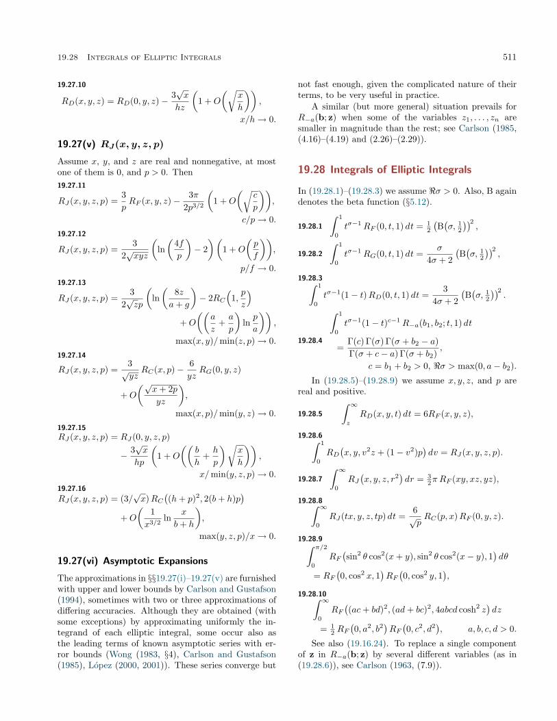
19.28 Integrals of Elliptic Integrals 511
19.27.10
RD(x, y, z) = RD(0, y, z)− 3√x
hz
(1 +O
(√x
h
)),
x/h→ 0.
19.27(v) RJ(x, y, z, p)
Assume x, y, and z are real and nonnegative, at mostone of them is 0, and p > 0. Then19.27.11
RJ(x, y, z, p) =3pRF (x, y, z)− 3π
2p3/2
(1 +O
(√c
p
)),
c/p→ 0.19.27.12
RJ(x, y, z, p) =3
2√xyz
(ln(
4fp
)− 2)(
1 +O
(p
f
)),
p/f → 0.19.27.13
RJ(x, y, z, p) =3
2√zp
(ln(
8za+ g
)− 2RC
(1,p
z
)+O
((a
z+a
p
)lnp
a
)),
max(x, y)/min(z, p)→ 0.19.27.14
RJ(x, y, z, p) =3√yz
RC(x, p)− 6yz
RG(0, y, z)
+O
(√x+ 2pyz
),
max(x, p)/min(y, z)→ 0.19.27.15
RJ(x, y, z, p) = RJ(0, y, z, p)
− 3√x
hp
(1 +O
((b
h+h
p
)√x
h
)),
x/min(y, z, p)→ 0.19.27.16
RJ(x, y, z, p) = (3/√x)RC
((h+ p)2, 2(b+ h)p
)+O
(1
x3/2ln
x
b+ h
),
max(y, z, p)/x→ 0.
19.27(vi) Asymptotic Expansions
The approximations in §§19.27(i)–19.27(v) are furnishedwith upper and lower bounds by Carlson and Gustafson(1994), sometimes with two or three approximations ofdiffering accuracies. Although they are obtained (withsome exceptions) by approximating uniformly the in-tegrand of each elliptic integral, some occur also asthe leading terms of known asymptotic series with er-ror bounds (Wong (1983, §4), Carlson and Gustafson(1985), López (2000, 2001)). These series converge but
not fast enough, given the complicated nature of theirterms, to be very useful in practice.
A similar (but more general) situation prevails forR−a(b; z) when some of the variables z1, . . . , zn aresmaller in magnitude than the rest; see Carlson (1985,(4.16)–(4.19) and (2.26)–(2.29)).
19.28 Integrals of Elliptic Integrals
In (19.28.1)–(19.28.3) we assume <σ > 0. Also, B againdenotes the beta function (§5.12).
19.28.1
∫ 1
0
tσ−1RF (0, t, 1) dt = 12
(B(σ, 1
2
))2,
19.28.2
∫ 1
0
tσ−1RG(0, t, 1) dt =σ
4σ + 2(B(σ, 1
2
))2,
19.28.3∫ 1
0
tσ−1(1− t)RD(0, t, 1) dt =3
4σ + 2(B(σ, 1
2
))2.
19.28.4
∫ 1
0
tσ−1(1− t)c−1R−a(b1, b2; t, 1) dt
=Γ(c) Γ(σ) Γ(σ + b2 − a)Γ(σ + c− a) Γ(σ + b2)
,
c = b1 + b2 > 0, <σ > max(0, a− b2).
In (19.28.5)–(19.28.9) we assume x, y, z, and p arereal and positive.
19.28.5
∫ ∞z
RD(x, y, t) dt = 6RF (x, y, z),
19.28.6∫ 1
0
RD(x, y, v2z + (1− v2)p
)dv = RJ(x, y, z, p).
19.28.7
∫ ∞0
RJ(x, y, z, r2
)dr = 3
2π RF (xy, xz, yz),
19.28.8∫ ∞0
RJ(tx, y, z, tp) dt =6√pRC(p, x)RF (0, y, z).
19.28.9∫ π/2
0
RF(sin2 θ cos2(x+ y), sin2 θ cos2(x− y), 1
)dθ
= RF(0, cos2 x, 1
)RF(0, cos2 y, 1
),
19.28.10∫ ∞0
RF((ac+ bd)2, (ad+ bc)2, 4abcd cosh2 z
)dz
= 12 RF
(0, a2, b2
)RF(0, c2, d2
), a, b, c, d > 0.
See also (19.16.24). To replace a single componentof z in R−a(b; z) by several different variables (as in(19.28.6)), see Carlson (1963, (7.9)).

512 Elliptic Integrals
19.29 Reduction of General EllipticIntegrals
19.29(i) Reduction Theorems
These theorems reduce integrals over a real interval(y, x) of certain integrands containing the square rootof a quartic or cubic polynomial to symmetric integralsover (0,∞) containing the square root of a cubic poly-nomial (compare §19.16(i)). Let
19.29.1Xα =
√aα + bαx, Yα =
√aα + bαy,x > y, 1 ≤ α ≤ 5,
19.29.2 dαβ = aαbβ − aβbα, dαβ 6= 0 if α 6= β,and assume that the line segment with endpoints aα +bαx and aα + bαy lies in C\(−∞, 0) for 1 ≤ α ≤ 4. If
19.29.3 s(t) =4∏
α=1
√aα + bαt
and α, β, γ, δ is any permutation of the numbers1, 2, 3, 4, then
19.29.4
∫ x
y
dt
s(t)= 2RF
(U2
12, U213, U
223
),
where19.29.5
Uαβ = (XαXβYγYδ + YαYβXγXδ)/(x− y),Uαβ = Uβα = Uγδ = Uδγ , U2
αβ − U2αγ = dαδdβγ .
There are only three distinct U ’s with subscripts ≤ 4,and at most one of them can be 0 because the d’s arenonzero. Then19.29.6
Uαβ =√bα√bβYγYδ + YαYβ
√bγ√bδ, x =∞,
Uαβ = XαXβ
√−bγ
√−bδ +
√−bα
√−bβXγXδ,
y = −∞.19.29.7∫ x
y
aα + bαt
aδ + bδt
dt
s(t)= 2
3dαβdαγ RD(U2αβ , U
2αγ , U
2αδ
)+
2XαYαXδYδUαδ
, Uαδ 6= 0.
19.29.8
∫ x
y
aα + bαt
a5 + b5t
dt
s(t)
=23dαβdαγdαδ
dα5RJ(U2
12, U213, U
223, U
2α5
)+ 2RC
(S2α5, Q
2α5
), S2
α5 ∈ C\(−∞, 0),where19.29.9
U2α5 = U2
αβ −dαγdαδdβ5
dα5= U2
βγ −dαβdαγdδ5
dα56= 0,
Sα5 =1
x− y
(XβXγXδ
XαY 2
5 +YβYγYδYα
X25
),
Qα5 =X5Y5
XαYαUα5 6= 0, S2
α5 −Q2α5 =
dβ5dγ5dδ5dα5
.
The Cauchy principal value is taken when U2α5 or Q2
α5
is real and negative. Cubic cases of these formulas areobtained by setting one of the factors in (19.29.3) equalto 1.
The advantages of symmetric integrals for tablesof integrals and symbolic integration are illustrated by(19.29.4) and its cubic case, which replace the 8 + 8 +12 = 28 formulas in Gradshteyn and Ryzhik (2000,3.147, 3.131, 3.152) after taking x2 as the variable of in-tegration in 3.152. Moreover, the requirement that onelimit of integration be a branch point of the integrandis eliminated without doubling the number of standardintegrals in the result. (19.29.7) subsumes all 72 for-mulas in Gradshteyn and Ryzhik (2000, 3.168), and itscubic cases similarly replace the 18 + 36 + 18 = 72 for-mulas in Gradshteyn and Ryzhik (2000, 3.133, 3.142,and 3.141(1-18)). For example, 3.142(2) is included as19.29.10∫ b
u
√a− t
(b− t)(t− c)3dt = − 2
3 (a− b)(b− u)3/2RD
+2
b− c
√(a− u)(b− u)
u− c,
a > b > u > c,where the arguments of the RD function are, in order,(a− b)(u− c), (b− c)(a− u), (a− b)(b− c).
19.29(ii) Reduction to Basic Integrals
(19.2.3) can be written19.29.11
I(m) =∫ x
y
h∏α=1
(aα + bαt)−1/2n∏j=1
(aj + bjt)mj dt,
where x > y, h = 3 or 4, n ≥ h, and mj is an integer.Define
19.29.12 m = (m1, . . . ,mn) =n∑j=1
mjej ,
where ej is an n-tuple with 1 in the jth position and0’s elsewhere. Define also 0 = (0, . . . , 0) and retainthe notation and conditions associated with (19.29.1)and (19.29.2). The integrals in (19.29.4), (19.29.7), and(19.29.8) are I(0), I(eα − eδ), and I(eα − e5), respec-tively.
The only cases of I(m) that are integrals of the firstkind are the two (h = 3 or 4) with m = 0. The onlycases that are integrals of the third kind are those inwhich at least one mj with j > h is a negative integerand those in which h = 4 and
∑nj=1mj is a positive
integer. All other cases are integrals of the second kind.I(m) can be reduced to a linear combination of ba-
sic integrals and algebraic functions. In the cubic case(h = 3) the basic integrals are
19.29.13 I(0); I(−ej), 1 ≤ j ≤ n.

19.29 Reduction of General Elliptic Integrals 513
In the quartic case (h = 4) the basic integrals are
19.29.14I(0); I(−ej), 1 ≤ j ≤ n;I(eα), 1 ≤ α ≤ 4.
Basic integrals of type I(−ej), 1 ≤ j ≤ h, are not lin-early independent, nor are those of type I(ej), 1 ≤ j ≤4.
The reduction of I(m) is carried out by a relation de-rived from partial fractions and by use of two recurrencerelations. These are given in Carlson (1999, (2.19),(3.5), (3.11)) and simplified in Carlson (2002, (1.10),(1.7), (1.8)) by means of modified definitions. Partialfractions provide a reduction to integrals in which mhas at most one nonzero component, and these are thenreduced to basic integrals by the recurrence relations.A special case of Carlson (1999, (2.19)) is given by
19.29.15
bjI(el − ej) = dljI(−ej) + blI(0), j, l = 1, 2, . . . , n,
which shows how to express the basic integral I(−ej)in terms of symmetric integrals by using (19.29.4) andeither (19.29.7) or (19.29.8). The first choice gives aformula that includes the 18+9+18 = 45 formulas inGradshteyn and Ryzhik (2000, 3.133, 3.156, 3.158), andthe second choice includes the 8+8+8+12 = 36 formu-las in Gradshteyn and Ryzhik (2000, 3.151, 3.149, 3.137,3.157) (after setting x2 = t in some cases).
If h = 3, then the recurrence relation (Carlson (1999,(3.5))) has the special case
19.29.16
bβbγI(eα) = dαβdαγI(−eα)
+ 2bα
(s(x)
aα + bαx− s(y)aα + bαy
),
where α, β, γ is any permutation of the numbers 1, 2, 3,and
19.29.17 s(t) =3∏
α=1
√aα + bαt.
(This shows why I(eα) is not needed as a basic integralin the cubic case.) In the quartic case this recurrencerelation has an extra term in I(2eα), and hence I(eα),1 ≤ α ≤ 4, is a basic integral. It can be expressedin terms of symmetric integrals by setting a5 = 1 andb5 = 0 in (19.29.8).
The other recurrence relation is
19.29.18
bqjI(qel) =q∑r=0
(q
r
)brl d
q−rlj I(rej), j, l = 1, 2, . . . , n;
see Carlson (1999, (3.11)). An example that uses(19.29.15)–(19.29.18) is given in §19.34.
For an implementation by James FitzSimons of themethod for reducing I(m) to basic integrals and exten-sive tables of such reductions, see Carlson (1999) andCarlson and FitzSimons (2000).
Another method of reduction is given in Gray(2002). It depends primarily on multivariate recurrencerelations that replace one integral by two or more.
19.29(iii) Examples
The first formula replaces (19.14.4)–(19.14.10). DefineQj(t) = aj + bjt
2, j = 1, 2, and assume both Q’s arepositive for 0 ≤ y < t < x. Then19.29.19∫ x
y
dt√Q1(t)Q2(t)
= RF(U2 + a1b2, U
2 + a2b1, U2),
19.29.20∫ x
y
t2 dt√Q1(t)Q2(t)
= 13a1a2RD
(U2 + a1b2, U
2 + a2b1, U2)
+ (xy/U),and19.29.21∫ x
y
dt
t2√Q1(t)Q2(t)
= 13b1b2RD
(U2 + a1b2, U
2 + a2b1, U2)
+ (xyU)−1,
where19.29.22
(x2 − y2)U = x√Q1(y)Q2(y) + y
√Q1(x)Q2(x).
If both square roots in (19.29.22) are 0, then the inde-terminacy in the two preceding equations can be re-moved by using (19.27.8) to evaluate the integral asRG(a1b2, a2b1, 0) multiplied either by −2/(b1b2) or by−2/(a1a2) in the cases of (19.29.20) or (19.29.21), re-spectively. If x = ∞, then U is found by taking thelimit. For example,19.29.23∫ ∞
y
dt√(t2 + a2)(t2 − b2)
= RF(y2 + a2, y2 − b2, y2
).
Next, for j = 1, 2, define Qj(t) = fj + gjt + hjt2,
and assume both Q’s are positive for y < t < x. If eachhas real zeros, then (19.29.4) may be simpler than
19.29.24
∫ x
y
dt√Q1(t)Q2(t)
= 4RF (U,U +D12 + V,U +D12 − V ),where19.29.25
(x− y)2U = S1S2,
Sj =(√
Qj(x) +√Qj(y)
)2− hj(x− y)2,
Djl = 2fjhl + 2hjfl − gjgl, V =√D2
12 −D11D22.
(The variables of RF are real and nonnegative unlessboth Q’s have real zeros and those of Q1 interlacethose of Q2.) If Q1(t) = (a1 + b1t)(a2 + b2t), whereboth linear factors are positive for y < t < x, and

514 Elliptic Integrals
Q2(t) = f2 + g2t + h2t2, then (19.29.25) is modified
so that
19.29.26
S1 = (X1Y2 + Y1X2)2,
Xj =√aj + bjx, Yj =
√aj + bjy,
D12 = 2a1a2h2 + 2b1b2f2 − (a1b2 + a2b1)g2,
D11 = −(a1b2 − a2b1)2 = −d212,
with other quantities remaining as in (19.29.25). In thecubic case, in which a2 = 1, b2 = 0, (19.29.26) reducesfurther to19.29.27
S1 = (X1 + Y1)2, D12 = 2a1h2 − b1g2, D11 = −b21.For example, because t3− a3 = (t− a)(t2 + at+ a2),
we find that when 0 ≤ a ≤ y < x
19.29.28
∫ x
y
dt√t3 − a3
= 4RF(U,U − 3a+ 2
√3a, U − 3a− 2
√3a),
where19.29.29
(x− y)2U = (√x− a+
√y − a)2
((ξ + η)2 − (x− y)2
),
ξ =√x2 + ax+ a2, η =
√y2 + ay + a2.
Lastly, define Q(t2) = f+gt2+ht4 and assume Q(t2)is positive and monotonic for y < t < x. Then
19.29.30
∫ x
y
dt√Q(t2)
= 2RF(U,U − g + 2
√fh, U − g − 2
√fh),
where19.29.31
(x− y)2U =(√
Q(x2) +√Q(y2)
)2− h(x2 − y2)2.
For example, if 0 ≤ y ≤ x and a4 ≥ 0, then
19.29.32
∫ x
y
dt√t4 + a4
= 2RF(U,U + 2a2, U − 2a2
),
where19.29.33
(x− y)2U =(√
x4 + a4 +√y4 + a4
)2− (x2 − y2)2.
Applications
19.30 Lengths of Plane Curves
19.30(i) Ellipse
The arclength s of the ellipse
19.30.1 x = a sinφ, y = b cosφ, 0 ≤ φ ≤ 2π,
with a > b, is given by
19.30.2 s = a
∫ φ
0
√1− k2 sin2 θ dθ.
When 0 ≤ φ ≤ 12π,
19.30.3
s/a = E(φ, k)
= RF(c− 1, c− k2, c
)− 1
3k2RD
(c− 1, c− k2, c
),
where
19.30.4 k2 = 1− (b2/a2), c = csc2 φ.
Cancellation on the second right-hand side of (19.30.3)can be avoided by use of (19.25.10).
The length of the ellipse is
19.30.5L(a, b) = 4aE(k) = 8aRG
(0, b2/a2, 1
)= 8RG
(0, a2, b2
)= 8abRG
(0, a−2, b−2
),
showing the symmetry in a and b. Approximations andinequalities for L(a, b) are given in §19.9(i).
Let a2 and b2 be replaced respectively by a2 +λ andb2+λ, where λ ∈ (−b2,∞), to produce a family of confo-cal ellipses. As λ increases, the eccentricity k decreasesand the rate of change of arclength for a fixed value ofφ is given by
19.30.6
∂s
∂(1/k)=√a2 − b2 F (φ, k)
=√a2 − b2RF
(c− 1, c− k2, c
),
k2 = (a2 − b2)/(a2 + λ), c = csc2 φ.
19.30(ii) Hyperbola
The arclength s of the hyperbola
19.30.7 x = a√t+ 1, y = b
√t, 0 ≤ t <∞,
is given by
19.30.8 s =12
∫ y2/b2
0
√(a2 + b2)t+ b2
t(t+ 1)dt.
From (19.29.7), with aδ = 1 and bδ = 0,
19.30.9
s = 12I(e1) = − 1
3a2b2RD
(r, r + b2 + a2, r + b2
)+ y
√r + b2 + a2
r + b2, r = b4/y2.
For s in terms of E(φ, k), F (φ, k), and an algebraicterm, see Byrd and Friedman (1971, p. 3). See Carlson(1977b, Ex. 9.4-1 and (9.4-4)) for arclengths of hyper-bolas and ellipses in terms of R−a that differ only in thesign of b2.

19.31 Probability Distributions 515
19.30(iii) Bernoulli’s Lemniscate
For 0 ≤ θ ≤ 14π, the arclength s of Bernoulli’s lemnis-
cate
19.30.10 r2 = 2a2 cos (2θ), 0 ≤ θ ≤ 2π,
is given by
19.30.11
s = 2a2
∫ r
0
dt√4a4 − t4
=√
2a2RF (q − 1, q, q + 1),
q = 2a2/r2 = sec(2θ),
or equivalently,
19.30.12s = aF
(φ, 1/
√2)
,
φ = arcsin√
2/(q + 1) = arccos(tan θ).
The perimeter length P of the lemniscate is given by
19.30.13P = 4
√2a2RF (0, 1, 2) =
√2a2× 5.24411 51 . . .
= 4aK(
1/√
2)
= a× 7.41629 87 . . . .
For other plane curves with arclength representableby an elliptic integral see Greenhill (1892, p. 190) andBowman (1953, pp. 32–33).
19.31 Probability Distributions
RG(x, y, z) and RF (x, y, z) occur as the expectation val-ues, relative to a normal probability distribution in R2
or R3, of the square root or reciprocal square root ofa quadratic form. More generally, let A (= [ar,s]) andB (= [br,s]) be real positive-definite matrices with nrows and n columns, and let λ1, . . . , λn be the eigen-values of AB−1. If x is a column vector with elementsx1, x2, . . . , xn and transpose xT, then
19.31.1 xTAx =n∑r=1
n∑s=1
ar,sxrxs,
and
19.31.2
∫Rn
(xTAx)µ exp(−xTBx
)dx1 · · · dxn
=πn/2 Γ
(µ+ 1
2n)
√det B Γ
(12n) Rµ
(12 , . . . ,
12 ;λ1, . . . , λn
),
µ > − 12n.
§19.16(iii) shows that for n = 3 the incomplete cases ofRF and RG occur when µ = −1/2 and µ = 1/2, respec-tively, while their complete cases occur when n = 2.
For (19.31.2) and generalizations see Carlson(1972b).
19.32 Conformal Map onto a Rectangle
The function
19.32.1 z(p) = RF (p− x1, p− x2, p− x3),
with x1, x2, x3 real constants, has differential
19.32.2dz = −1
2
3∏j=1
(p− xj)−1/2
dp,
=p > 0; 0 < ph(p− xj) < π, j = 1, 2, 3.
If
19.32.3 x1 > x2 > x3,
then z(p) is a Schwartz–Christoffel mapping of the openupper-half p-plane onto the interior of the rectangle inthe z-plane with vertices
19.32.4
z(∞) = 0,
z(x1) = RF (0, x1 − x2, x1 − x3) (> 0),
z(x2) = z(x1) + z(x3),
z(x3) = RF (x3 − x1, x3 − x2, 0)= −i RF (0, x1 − x3, x2 − x3).
As p proceeds along the entire real axis with the upperhalf-plane on the right, z describes the rectangle in theclockwise direction; hence z(x3) is negative imaginary.
For further connections between elliptic integralsand conformal maps, see Bowman (1953, pp. 44–85).
19.33 Triaxial Ellipsoids
19.33(i) Surface Area
The surface area of an ellipsoid with semiaxes a, b, c,and volume V = 4πabc/3 is given by
19.33.1 S = 3V RG(a−2, b−2, c−2
),
or equivalently,
19.33.2
S
2π= c2 +
ab
sinφ(E(φ, k) sin2 φ+ F (φ, k) cos2 φ
),
a ≥ b ≥ c,
where
19.33.3 cosφ =c
a, k2 =
a2(b2 − c2)b2(a2 − c2)
.
Application of (19.16.23) transforms the last quan-tity in (19.30.5) into a two-dimensional analog of(19.33.1).
For additional geometrical properties of ellipsoids(and ellipses), see Carlson (1964, p. 417).

516 Elliptic Integrals
19.33(ii) Potential of a Charged ConductingEllipsoid
If a conducting ellipsoid with semiaxes a, b, c bears anelectric charge Q, then the equipotential surfaces in theexterior region are confocal ellipsoids:
19.33.4x2
a2 + λ+
y2
b2 + λ+
z2
c2 + λ= 1, λ ≥ 0.
The potential is
19.33.5 V (λ) = QRF(a2 + λ, b2 + λ, c2 + λ
),
and the electric capacity C = Q/V (0) is given by
19.33.6 1/C = RF(a2, b2, c2
).
A conducting elliptic disk is included as the casec = 0.
19.33(iii) Depolarization Factors
Let a homogeneous magnetic ellipsoid with semiaxesa, b, c, volume V = 4πabc/3, and susceptibility χ beplaced in a previously uniform magnetic field H parallelto the principal axis with semiaxis c. The external fieldand the induced magnetization together produce a uni-form field inside the ellipsoid with strength H/(1+Lcχ),where Lc is the demagnetizing factor, given in cgs unitsby
19.33.7Lc = 2πabc
∫ ∞0
dλ√(a2 + λ)(b2 + λ)(c2 + λ)3
= V RD(a2, b2, c2
).
The same result holds for a homogeneous dielectricellipsoid in an electric field. By (19.21.8),
19.33.8 La + Lb + Lc = 4π,where La and Lb are obtained from Lc by permutationof a, b, and c. Expressions in terms of Legendre’s inte-grals, numerical tables, and further references are givenby Cronemeyer (1991).
19.33(iv) Self-Energy of an EllipsoidalDistribution
Ellipsoidal distributions of charge or mass are used tomodel certain atomic nuclei and some elliptical galaxies.Let the density of charge or mass be19.33.9
ρ(x, y, z) = f(√
(x2/α2) + (y2/β2) + (z2/γ2)),
where α, β, γ are dimensionless positive constants. Thecontours of constant density are a family of similar,rather than confocal, ellipsoids. In suitable units theself-energy of the distribution is given by19.33.10
U =12
∫R6
ρ(x, y, z)ρ(x′, y′, z′) dx dy dz dx′ dy′ dz′√(x− x′)2 + (y − y′)2 + (z − z′)2
.
Subject to mild conditions on f this becomes
19.33.11 U = 12 (αβγ)2RF
(α2, β2, γ2
) ∫ ∞0
(g(r))2 dr,
where19.33.12 g(r) = 4π
∫ ∞r
f(t)t dt.
19.34 Mutual Inductance of Coaxial Circles
The mutual inductance M of two coaxial circles of ra-dius a and b with centers at a distance h apart is givenin cgs units by19.34.1
c2M
2π= ab
∫ 2π
0
(h2 + a2 + b2 − 2ab cos θ)−1/2 cos θ dθ
= 2ab∫ 1
−1
t dt√(1 + t)(1− t)(a3 − 2abt)
= 2abI(e5),
where c is the speed of light, and in (19.29.11),
19.34.2 a3 = h2 + a2 + b2, a5 = 0, b5 = 1.The method of §19.29(ii) uses (19.29.18), (19.29.16),and (19.29.15) to produce19.34.3
2abI(e5) = a3I(0)− I(e3) = a3I(0)− r2+r
2−I(−e3)
= 2ab(I(0)− r2−I(e1 − e3)),
where a1 + b1t = 1 + t and
19.34.4 r2± = a3 ± 2ab = h2 + (a± b)2
is the square of the maximum (upper signs) or minimum(lower signs) distance between the circles. Applicationof (19.29.4) and (19.29.7) with α = 1, aβ + bβt = 1− t,δ = 3, and aγ + bγt = 1 yields
19.34.53c2
8πabM = 3RF
(0, r2
+, r2−)− 2r2
−RD(0, r2
+, r2−),
or, by (19.21.3),19.34.6
c2
2πM = (r2
+ + r2−)RF
(0, r2
+, r2−)− 4RG
(0, r2
+, r2−).
A simpler form of the result is
19.34.7 M = (2/c2)(πa2)(πb2)R− 32
(32 ,
32 ; r2
+, r2−).
References for other inductance problems solvablein terms of elliptic integrals are given in Grover (1946,pp. 8 and 283).
19.35 Other Applications
19.35(i) Mathematical
Generalizations of elliptic integrals appear in analysisof modular theorems of Ramanujan (Anderson et al.(2000)); analysis of Selberg integrals (Van Diejen andSpiridonov (2001)); use of Legendre’s relation (19.7.1)to compute π to high precision (Borwein and Borwein(1987, p. 26)).

Computation 517
19.35(ii) Physical
Elliptic integrals appear in lattice models of criticalphenomena (Guttmann and Prellberg (1993)); theoriesof layered materials (Parkinson (1969)); fluid dynam-ics (Kida (1981)); string theory (Arutyunov and Stau-dacher (2004)); astrophysics (Dexter and Agol (2009)).
Computation
19.36 Methods of Computation
19.36(i) Duplication Method
Numerical differences between the variables of a sym-metric integral can be reduced in magnitude by succes-sive factors of 4 by repeated applications of the duplica-tion theorem, as shown by (19.26.18). When the differ-ences are moderately small, the iteration is stopped, theelementary symmetric functions of certain differencesare calculated, and a polynomial consisting of a fixednumber of terms of the sum in (19.19.7) is evaluated.For RF the polynomial of degree 7, for example, is
19.36.11− 1
10E2 + 114E3 + 1
24E22 − 3
44E2E3
− 5208E
32 + 3
104E23 + 1
16E22E3,
where the elementary symmetric functions Es are de-fined by (19.19.4). If (19.36.1) is used instead of its firstfive terms, then the factor (3r)−1/6 in Carlson (1995,(2.2)) is changed to (3r)−1/8.
For a polynomial for both RD and RJ see http://dlmf.nist.gov/19.36.i.
Example
Three applications of (19.26.18) yield
19.36.3 RF (1, 2, 4) = RF (z1, z2, z3),where, in the notation of (19.19.7) with a = − 1
2 andn = 3,19.36.4
z1 = 2.10985 99098 8,z3 = 2.15673 49098 8,Z1 = 0.00977 77253 5,
z2 = 2.12548 49098 8,A = 2.13069 32432 1,Z2 = 0.00244 44313 4,
Z3 = −Z1 − Z2 = −0.01222 21566 9,E2 = −1.25480 14× 10−4, E3 = −2.9212× 10⁻⁷.
The first five terms of (19.36.1) suffice for
19.36.5 RF (1, 2, 4) = 0.68508 58166 . . . .All cases of RF , RC , RJ , and RD are computed
by essentially the same procedure (after transformingCauchy principal values by means of (19.20.14) and(19.2.20)). Complex values of the variables are allowed,
with some restrictions in the case of RJ that are suf-ficient but not always necessary. The computation isslowest for complete cases. For details see Carlson(1995, 2002) and Carlson and FitzSimons (2000). Inthe Appendix of the last reference it is shown how tocompute RJ without computing RC more than once.Because of cancellations in (19.26.21) it is advisable tocompute RG from RF and RD by (19.21.10) or else touse §19.36(ii).
Legendre’s integrals can be computed from symmet-ric integrals by using the relations in §19.25(i). Note theremark following (19.25.11). If (19.25.9) is used when0 ≤ k2 ≤ 1, cancellations may lead to loss of significantfigures when k2 is close to 1 and φ > π/4, as shownby Reinsch and Raab (2000). The cancellations can beeliminated, however, by using (19.25.10).
Accurate values of F (φ, k) − E(φ, k) for k2 near 0can be obtained from RD by (19.2.6) and (19.25.13).
19.36(ii) Quadratic Transformations
Complete cases of Legendre’s integrals and symmet-ric integrals can be computed with quadratic conver-gence by the AGM method (including Bartky transfor-mations), using the equations in §19.8(i) and §19.22(ii),respectively.
The incomplete integrals RF (x, y, z) and RG(x, y, z)can be computed by successive transformations in whichtwo of the three variables converge quadratically to acommon value and the integrals reduce to RC , accom-panied by two quadratically convergent series in the caseof RG; compare Carlson (1965, §§5,6). (In Legendre’snotation the modulus k approaches 0 or 1.) Let
19.36.6
2an+1 = an +√a2n − c2n,
2cn+1 = an −√a2n − c2n = c2n/(2an+1),
2tn+1 = tn +√t2n + θc2n,
where n = 0, 1, 2, . . . , and
19.36.7 0 < c0 < a0, t0 ≥ 0, t20 + θa20 ≥ 0, θ = ±1.
Then (19.22.18) implies that
19.36.8 RF(t2n, t
2n + θc2n, t
2n + θa2
n
)is independent of n. As n→∞, cn, an, and tn convergequadratically to limits 0, M , and T , respectively; hence19.36.9
RF(t20, t
20 + θc20, t
20 + θa2
0
)= RF
(T 2, T 2, T 2 + θM2
)= RC
(T 2 + θM2, T 2
).
If t0 = a0 and θ = −1, so that tn = an, then this pro-cedure reduces to the AGM method for the completeintegral.
The step from n to n + 1 is an ascending Landentransformation if θ = 1 (leading ultimately to a hyper-bolic case of RC) or a descending Gauss transformation

518 Elliptic Integrals
if θ = −1 (leading to a circular case of RC). If x, y, andz are permuted so that 0 ≤ x < y < z, then the com-putation of RF (x, y, z) is fastest if we make c20 ≤ a2
0/2by choosing θ = 1 when y < (x+ z)/2 or θ = −1 wheny ≥ (x+ z)/2.
Example
We compute RF (1, 2, 4) by setting θ = 1, t0 = c0 = 1,and a0 =
√3. Then
19.36.10
c23 = 6.65× 10⁻¹², a23 = 2.46209 30206 0 = M2,
t23 = 1.46971 53173 1 = T 2.
Hence19.36.11
RF (1, 2, 4) = RC(T 2 +M2, T 2
)= 0.68508 58166,
in agreement with (19.36.5). Here RC is computed ei-ther by the duplication algorithm in Carlson (1995) orvia (19.2.19).
For an error estimate and the corresponding pro-cedure for RG(x, y, z), see http://dlmf.nist.gov/19.36.ii.
F (φ, k) can be evaluated by using (19.25.5). E(φ, k)can be evaluated by using (19.25.7), and RD by using(19.21.10), but cancellations may become significant.Thompson (1997, pp. 499, 504) uses descending Lan-den transformations for both F (φ, k) and E(φ, k). Asummary for F (φ, k) is given in Gautschi (1975, §3).For computation of K(k) and E(k) with complex k seeFettis and Caslin (1969) and Morita (1978).
(19.22.20) reduces to 0 = 0 if p = x or p = y, and(19.22.19) reduces to 0 = 0 if z = x or z = y. Nearthese points there will be loss of significant figures inthe computation of RJ or RD.
Descending Gauss transformations of Π(φ, α2, k
)(see (19.8.20)) are used in Fettis (1965) to compute alarge table (see §19.37(iii)). This method loses signif-icant figures in ρ if α2 and k2 are nearly equal unlessthey are given exact values—as they can be for tables.If α2 = k2, then the method fails, but the function canbe expressed by (19.6.13) in terms of E(φ, k), for whichNeuman (1969) uses ascending Landen transformations.
Computation of Legendre’s integrals of all threekinds by quadratic transformation is described byCazenave (1969, pp. 128–159, 208–230).
Quadratic transformations can be applied to com-pute Bulirsch’s integrals (§19.2(iii)). The func-tion cel(kc, p, a, b) is computed by successive Bartkytransformations (Bulirsch and Stoer (1968), Bulirsch(1969b)). The function el2(x, kc, a, b) is computed bydescending Landen transformations if x is real, or bydescending Gauss transformations if x is complex (Bu-lirsch (1965a)). Remedies for cancellation when x isreal and near 0 are supplied in Midy (1975). See alsoBulirsch (1969a) and Reinsch and Raab (2000).
Bulirsch (1969a,b) extend Bartky’s transformationto el3(x, kc, p) by expressing it in terms of the firstincomplete integral, a complete integral of the thirdkind, and a more complicated integral to which Bartky’smethod can be applied. The cases k2
c/2 ≤ p < ∞ and−∞ < p < k2
c/2 require different treatment for numeri-cal purposes, and again precautions are needed to avoidcancellations.
19.36(iii) Via Theta Functions
Lee (1990) compares the use of theta functions for com-putation of K(k), E(k), and K(k)− E(k), 0 ≤ k2 ≤ 1,with four other methods. Also, see Todd (1975) for aspecial case of K(k). For computation of Legendre’sintegral of the third kind, see Abramowitz and Stegun(1964, §§17.7 and 17.8, Examples 15, 17, 19, and 20).For integrals of the second and third kinds see Lawden(1989, §§3.4–3.7).
19.36(iv) Other Methods
Numerical quadrature is slower than most methods forthe standard integrals but can be useful for elliptic in-tegrals that have complicated representations in termsof standard integrals. See §3.5.
For series expansions of Legendre’s integrals see§19.5. Faster convergence of power series for K(k) andE(k) can be achieved by using (19.5.1) and (19.5.2) inthe right-hand sides of (19.8.12). A three-part computa-tional procedure for Π
(φ, α2, k
)is described by Franke
(1965) for α2 < 1.When the values of complete integrals are known,
addition theorems with ψ = π/2 (§19.11(ii)) ease thecomputation of functions such as F (φ, k) when 1
2π − φis small and positive. Similarly, §19.26(ii) eases the com-putation of functions such as RF (x, y, z) when x (> 0) issmall compared with min(y, z). These special theoremsare also useful for checking computer codes.
19.37 Tables
19.37(i) Introduction
Only tables published since 1960 are included. For ear-lier tables see Fletcher (1948), Lebedev and Fedorova(1960), and Fletcher et al. (1962).
19.37(ii) Legendre’s Complete Integrals
Functions K(k) and E(k)
Tabulated for k2 = 0(.01)1 to 6D by Byrd and Friedman(1971), to 15D for K(k) and 9D for E(k) by Abramowitzand Stegun (1964, Chapter 17), and to 10D by Fettisand Caslin (1964).

19.38 Approximations 519
Tabulated for k = 0(.01)1 to 10D by Fettis andCaslin (1964), and for k = 0(.02)1 to 7D by Zhang andJin (1996, p. 673).
Tabulated for arcsin k = 0(1◦)90◦ to 6D by Byrdand Friedman (1971) and to 15D by Abramowitz andStegun (1964, Chapter 17).Functions K(k), K′(k), and iK′(k)/K(k)
Tabulated with k = Reiθ for R = 0(.01)1 and θ =0(1◦)90◦ to 11D by Fettis and Caslin (1969).Function exp(−πK′(k)/K(k))(= q(k))
Tabulated for k2 = 0(.01)1 to 6D by Byrd and Friedman(1971) and to 15D by Abramowitz and Stegun (1964,Chapter 17).
Tabulated for arcsin k = 0(1◦)90◦ to 6D by Byrdand Friedman (1971) and to 15D by Abramowitz andStegun (1964, Chapter 17).
Tabulated for k2 = 0(.001)1 to 8D by Bel�ıakov et al.(1962).
19.37(iii) Legendre’s Incomplete Integrals
Functions F (φ, k) and E(φ, k)
Tabulated for φ = 0(5◦)90◦, k2 = 0(.01)1 to 10D byFettis and Caslin (1964).
Tabulated for φ = 0(1◦)90◦, k2 = 0(.01)1 to 7Sby Bel�ıakov et al. (1962). (F (φ, k) is presented asΠ(φ, 0, k).)
Tabulated for φ = 0(5◦)90◦, k = 0(.01)1 to 10D byFettis and Caslin (1964).
Tabulated for φ = 0(5◦)90◦, arcsin k = 0(1◦)90◦
to 6D by Byrd and Friedman (1971), for φ =0(5◦)90◦, arcsin k = 0(2◦)90◦ and 5◦(10◦)85◦ to 8D byAbramowitz and Stegun (1964, Chapter 17), and forφ = 0(10◦)90◦, arcsin k = 0(5◦)90◦ to 9D by Zhang andJin (1996, pp. 674–675).Function Π
`φ,α2, k
´Tabulated (with different notation) for φ = 0(15◦)90◦,α2 = 0(.1)1, arcsin k = 0(15◦)90◦ to 5D by Abramowitzand Stegun (1964, Chapter 17), and for φ = 0(15◦)90◦,α2 = 0(.1)1, arcsin k = 0(15◦)90◦ to 7D by Zhang andJin (1996, pp. 676–677).
Tabulated for φ = 5◦(5◦)80◦(2.5◦)90◦, α2 =−1(.1) − 0.1, 0.1(.1)1, k2 = 0(.05)0.9(.02)1 to 10D byFettis and Caslin (1964) (and warns of inaccuracies inSelfridge and Maxfield (1958) and Paxton and Rollin(1959)).
Tabulated for φ = 0(1◦)90◦, α2 =0(.05)0.85, 0.88(.02)0.94(.01)0.98(.005)1, k2 = 0(.01)1to 7S by Bel�ıakov et al. (1962).
19.37(iv) Symmetric Integrals
Functions RF`x2, 1, y2
´and RG
`x2, 1, y2
´Tabulated for x = 0(.1)1, y = 1(.2)6 to 3D by Nellisand Carlson (1966).
Function RF`a2, b2, c2
´with abc = 1
Tabulated for σ = 0(.05)0.5(.1)1(.2)2(.5)5, cos(3γ) =−1(.2)1 to 5D by Carlson (1961a). Hereσ2 = 2
3 ((ln a)2 + (ln b)2 + (ln c)2), cos(3γ) =(4/σ3)(ln a)(ln b)(ln c), and a, b, c are semiaxes of anellipsoid with the same volume as the unit sphere.
Check Values
For check values of symmetric integrals with real or com-plex variables to 14S see Carlson (1995).
19.38 Approximations
Minimax polynomial approximations (§3.11(i)) forK(k)and E(k) in terms of m = k2 with 0 ≤ m < 1can be found in Abramowitz and Stegun (1964, §17.3)with maximum absolute errors ranging from 4×10⁻⁵ to2×10−8. Approximations of the same type for K(k)and E(k) for 0 < k ≤ 1 are given in Cody (1965a)with maximum absolute errors ranging from 4×10⁻⁵ to4×10−18. Cody (1965b) gives Chebyshev-series expan-sions (§3.11(ii)) with maximum precision 25D.
Approximations for Legendre’s complete or incom-plete integrals of all three kinds, derived by Padé ap-proximation of the square root in the integrand, aregiven in Luke (1968, 1970). They are valid over partsof the complex k and φ planes. The accuracy is con-trolled by the number of terms retained in the approxi-mation; for real variables the number of significant fig-ures appears to be roughly twice the number of termsretained, perhaps even for φ near π/2 with the improve-ments made in the 1970 reference.
19.39 Software
See http://dlmf.nist.gov/19.39.
References
General References
The main references used for writing this chapter areErdélyi et al. (1953b), Byerly (1888), Cazenave (1969),and Byrd and Friedman (1971) for Legendre’s integrals,and Carlson (1977b) for symmetric integrals. For addi-tional bibliographic reading see Cayley (1895), Green-hill (1892), Legendre (1825–1832), Tricomi (1951), andWhittaker and Watson (1927).

520 Elliptic Integrals
Sources
The following list gives the references or other indica-tions of proofs that were used in constructing the varioussections of this chapter. These sources supplement thereferences that are quoted in the text.
§19.2 Bulirsch (1965a, 1969a,b), Bulirsch and Stoer(1968). To prove (19.2.20) evaluate the two partsof the Cauchy principal value (intervals (0,−y−δ)and (−y + δ,∞)) using Carlson (1977b, (8.2-2)),and reduce the first part to RC by Carlson (1977b,(9.8-4)) with B = C. Apply (19.12.7) to bothparts as δ → 0 and combine the two logarithms.For (19.2.21) see (19.16.18) and put cos θ = v in(19.23.8). For (19.2.22) put z = x in (19.23.5) andinterchange x and y.
§19.3 The graphics were produced at NIST.
§19.4 Cazenave (1969, p. 175). (19.4.1)–(19.4.7) followby differentiation of the definitions in §19.2(ii).(19.4.8) agrees also with Edwards (1954, vol. 1,p. 402) and with expansion to first order in k.The term on the right side in Byrd and Friedman(1971, 118.01) has the wrong sign.
§19.5 For (19.5.1)–(19.5.4) put sinφ = 1 and t =√x in (19.2.4)–(19.2.7). Then compare with
Erdélyi et al. (1953a, 2.1.3(10) and 2.1.1(2)) in thefirst three cases, and with Erdélyi et al. (1953a,5.8.2(5) and 5.7.1(6)) in the fourth case. For(19.5.5) and (19.5.6) see Kneser (1927, (12) andp. 218); Byrd and Friedman (1971, 901.00) is in-correct. (19.5.8) and (19.5.9) follow from Borweinand Borwein (1987, (2.1.13) and (2.3.17), respec-tively). For (19.5.10) iterate (19.8.12).
§19.6 For the first line of (19.6.2) put α = k in thefirst line of (19.25.2) and use the last line of(19.25.1). For the second line of (19.6.2), and alsofor (19.6.5), use (19.7.8) and (19.6.15). For thefirst line of (19.6.6) use (19.6.5) and (19.6.2). Formore detail as k2 → 1− see §19.12. For (19.6.7),(19.6.8) use (19.2.4), (19.16.6), and (19.25.5). For(19.6.9), (19.6.10) use (19.2.5). For (19.6.11)–(19.6.14) Byrd and Friedman (1971, 111.01 and111.04, p. 10) also needs α sinφ < 1. Start with(19.25.14). For the second equation of (19.6.12)use (19.20.8). For (19.6.13) use (19.16.5) with(19.25.10) and (19.25.11).
§19.7 Three proofs of (19.7.1) are given in Duren(1991). To prove it from (19.21.1) put z +1 = 1/k2, use homogeneity, and apply thepenultimate equation in (19.25.1) twice. For
(19.7.4)–(19.7.7) see the penultimate paragraphin §19.25(i). (19.7.8)–(19.7.10) follow from thechange of parameter for the symmetric integralof the third kind; see §19.21(iii) and (19.25.14).
§19.8 Cox (1984, 1985), Borwein and Borwein (1987,Chapter 1), Cazenave (1969, pp. 114–127). Toprove the second equality in (19.8.4), put tan θ =√t/g0. (19.8.7) is derived from (19.22.12) and
(19.25.14), and (19.8.9) is derived from (19.6.5)and (19.8.7); see also Carlson (2002). For(19.8.16) and (19.8.17) replace (φ, k) by (φ2, k2),and then (φ1, k1) by (φ, k) in (19.8.11) and(19.8.13). See also Hancock (1958, pp. 74–77) forproof of (19.8.13) and (19.8.17).
§19.9 For (19.9.1) see Erdélyi et al. (1953b,§13.8(9),(11)), (19.9.13), (19.6.12), and (19.6.15).For (19.9.2) and (19.9.3) see Qiu and Vamana-murthy (1996). For (19.9.4) see Barnard et al.(2000, (6)); the first inequality was given earlierby Qiu and Shen (1997, Theorem 2). For (19.9.5)see Lehto and Virtanen (1973, p. 62). For (19.9.6)and (19.9.7) see (19.25.1) and (19.16.21) and thenapply Carlson (1966, (2.15)), in which H < H ′
for 0 < k ≤ 1 in both cases. In (19.9.7) the up-per bound 4/π, which is the smaller of the twowhen k2 ≥ 0.855 . . . , is given by Anderson andVamanamurthy (1985). For (19.9.8) see (19.25.1),Neuman (2003, (4.2)), and (19.24.9). For (19.9.9)see (19.30.5). For (19.9.14) see (19.24.10) and(19.25.5). For (19.9.15) and (19.9.16) see Carlsonand Gustafson (1985, (1.2), (1.22)).
§19.10 For (19.10.1) see (19.2.17). For (19.10.2) use(19.6.8).
§19.11 Byerly (1888, pp. 243–245, 256–258), Edwards(1954, v. 2, pp. 511–513), Cazenave (1969, pp. 83–85). (19.11.5) can be derived from (19.26.9),(19.25.26), and (19.11.1).
§19.12 For (19.12.1) and (19.12.2) see Cayley (1895,p. 54) and Cazenave (1969, pp. 165–169). For(19.12.4) and (19.12.5) use (19.25.2), (19.27.13),and (19.6.5). For (19.12.6) and (19.12.7) see Carl-son and Gustafson (1994, (22),(24)).
§19.14 For (19.14.1)–(19.14.3) see Cazenave (1969,pp. 286,276). For (19.14.4) use (19.29.19) and(19.25.24).
§19.16 See Carlson (1977b, (6.8-6), Ex. 6.8-8, and (5.9-1)). To prove (19.16.12) put t = csc2 θ − csc2 φ inthe first integral in (19.16.9). For (19.16.19) and(19.16.23) see Carlson (1977b, (5.9-19) and (8.3-4)). To derive (19.16.24) exchange subscripts 1

References 521
and n in Carlson (1963, (7.4)), put t = s/z1, anduse (19.16.19).
§19.17 The graphics were produced at NIST.
§19.18 (19.18.1) is derived from (19.16.1), (19.16.5),and (19.18.4). (19.18.2) follows from (19.18.8).For (19.18.4) and (19.18.5) put t = −a andc = a + a′ in Carlson (1977b, (5.9-9),(5.9-10)).(19.18.6) comes from (19.18.8) and (19.20.25). For(19.18.8) and (19.18.11) see Carlson (1977b, (5.9-2)). For (19.18.12)–(19.18.17) see Carlson (1977b,§5.4).
§19.19 To prove (19.19.2) expand the product in(19.23.10) in powers of u. (19.19.3) is derived from(19.16.11) and (19.19.2). For (19.19.5) see Carlson(1979, (A.12)). For (19.19.6) compare (19.16.2)and (19.16.9).
§19.20 In (19.20.2) put t = 1/√s+ 1; alternatively
use (19.29.19). For the second equality replacet4 by t and apply (5.12.1). For (19.20.3) use Carl-son (1977b, Ex. 6.9-5 and p. 309) and (19.25.42).For (19.20.4) use (19.20.5) and (19.16.3). For(19.20.5) put z = y in (19.21.10). For (19.20.6)substitute in (19.16.2) and (19.16.5). In (19.20.7)see (19.27.12) for p → 0+; for p → 0−use (19.20.17) and (19.6.15). In (19.20.8) thethird equation is proved by partial fractions, andalso implies the first two equations by (19.6.15).For (19.20.9) put x = 0 in (19.20.13). For(19.20.10) interchange x and z in (19.27.14) anduse (19.6.15). For (19.20.11) use (19.27.13),(19.20.17), and (19.27.2). For (19.20.12) see(19.27.11) and (19.21.12). For (19.20.13) let q = pin (19.21.12). For (19.20.14) exchange x and z in(19.21.12) and use (19.2.20). For the third equa-tion in (19.20.18) put t = y tan2 θ in (19.16.5); forthe fourth equation see (19.27.7). For (19.20.19)see (19.27.8). For (19.20.20) and (19.20.21) use(19.16.15), (19.16.9), and Carlson (1977b, Table8.5-1). In (19.20.22) put t = 1/
√s+ 1; alterna-
tively use (19.29.20). For the second equality re-place t4 by t and apply (5.12.1). For (19.20.23)use Carlson (1977b, Ex. 6.9-5 and p. 309) and(19.25.42). For (19.20.24)–(19.20.26) see Carlson(1977b, (6.2-1),(6.8-15)).
§19.21 To prove (19.21.1) see the text following(19.21.6), use (19.20.10), and analytic continua-tion. For (19.21.2) put x = 0 in (19.21.9). For(19.21.3) put x = 0 in (19.21.11) and (19.21.10).(19.21.6) is equivalent to Zill and Carlson (1970,(7.15)). For (19.21.8) and (19.21.9) see Carlson(1977b, (5.9-5),(5.9-6)) and (19.20.25). To obtain
(19.21.7) eliminate RD(z, x, y) between (19.21.8)and (19.21.9), which follow from Carlson (1977b,(5.9-5, (6.6-5), and (5.9-6)). For (19.21.10) seeCarlson (1977b, Table 9.3-1). To prove (19.21.11)write xt/(t + x) = x − (x2/(t + x)) in (19.23.7)and similarly for y and z. Then use (19.21.9). For(19.21.12)–(19.21.15) see Zill and Carlson (1970,(4.6)).
§19.22 In (19.22.18), (19.22.21), and (19.22.20), putz = 0 to obtain (19.22.1), (19.22.2), and (19.22.4),respectively. (19.22.3) is derivable from (19.22.2)and (19.21.3), or more directly by putting p =y in (19.22.7). For (19.22.7) see Carlson(1976, (4.14),(4.13)), where (π/4)RL(y, z, p) =RF (0, y, z) − (p/3)RJ(0, y, z, p). For (19.22.8)–(19.22.15) iterate the results given in §19.22(i);see also (19.16.20), (19.16.23), and Carlson (2002,Section 2). For (19.22.18) see Carlson (1964,(5.13)). For (19.22.19) put p = z in (19.22.20).For (19.22.20) see Zill and Carlson (1970, (5.7))and Carlson (1990, (8.5)). For (19.22.21) see Carl-son (1964, (5.16)). For (19.22.22) put z = y in(19.22.18). In the ascending Landen case let k2 =(z2
+ − z2−)/(z2
+ − a2) and k21 = (z2 − y2)/(z2 − x2)
to get the second equation in (19.8.11). In the de-scending Gauss case let k2
1 = (a2 − z2−)/(a2 − z2
+)and k2 = (z2− y2)/(z2−x2) to get the first equa-tion in (19.8.11).
§19.23 For (19.23.8) and (19.23.9) see Carlson (1977b,Exercises 5.9-19, 5.9-20, and p. 306). By§19.16(iii), (19.23.8) implies (19.23.1)–(19.23.3),and (19.23.9) implies (19.23.6). Use (19.23.8) tointegrate over θ in (19.23.6) and then permutevariables to prove (19.23.5). To prove (19.23.4)put z = 0 in (19.23.5), relabel variables, and sub-stitute cos θ = sech t. For (19.23.7) and (19.23.10)see Carlson (1977b, (9.1-9) and (6.8-2), respec-tively).
§19.24 For (19.24.1)–(19.24.3) use (19.9.1) and(19.9.4). For (19.24.4) see (19.16.22) and Carl-son (1966, (2.15)). For (19.24.3) see (19.30.5).(19.24.8) is a special case of (19.24.13). For(19.24.9) see Neuman (2003, (4.2)).
§19.25 (19.25.1), (19.25.2), and (19.25.3) are derivedfrom the incomplete cases. For (19.25.4) put c = 1in (19.25.16). (19.25.5) and (19.25.7) come fromCarlson (1977b, (9.3-2) and (9.3-3)). For (19.25.6)and (19.25.12) apply (19.18.4) to (19.25.5) and(19.25.8), respectively. (19.25.8) and (19.25.15)are special cases of (19.16.12). To get (19.25.9),(19.25.10), and (19.25.11), let (c − 1, c − k2, c) =(x, y, z) and eliminate RG between (19.25.7) and

522 Elliptic Integrals
each of the three forms of (19.25.10) obtainedby permuting x, y and z. For (19.25.13) com-bine (19.2.6) and (19.25.9). For (19.25.14) see Zilland Carlson (1970, (2.5)). For (19.25.16) sub-stitute (19.25.14) in (19.7.8) and use (19.2.20).For (19.25.19)–(19.25.22) rewrite Bulirsch’s inte-grals (§19.2(iii)) in terms of Legendre’s integrals,then use §19.25(i) to convert them to R-functions.For (19.25.24)–(19.25.27) define c = csc2 φ, write(x, y, z, p)/(z − x) = (c− 1, c−k2, c, c−α2), thenuse (19.25.5), (19.25.9), (19.25.14), and (19.25.7)to prove (19.25.24), (19.25.25), (19.25.26), and(19.25.27), respectively. To prove (19.25.29) use(cs,ds,ns) = (cn,dn, 1)/ sn (suppressing vari-ables (u,k)). For (19.25.30) see Carlson (2006a,Comments following proof of Proposition 4.1).For (19.25.31) see Carlson (2004, (1.8)). In(19.25.32), (19.25.33), and (19.25.34), substitutex = ps (u, k), sp (u, k), and pq (u, k), respec-tively, to recover (19.25.31). To prove (19.25.35)use (23.6.36), with z = ℘(w) as prescribed inthe text that follows (23.6.36), substitute u =t + ℘(w) and compare with (19.16.1). Then putz = ωj to obtain (19.25.38). For (19.25.37) and(19.25.39) see Carlson (1964, (3.10) and (3.2)).For (19.25.40) combine Erdélyi et al. (1953b,§§13.12(22), 13.13(22)) and (19.25.35).
§19.26 Addition theorems (and therefore duplicationtheorems) for the symmetric integrals are provedby Zill and Carlson (1970, §8). For other proofsof (19.26.1) see Carlson (1977b, §9.7) and Carl-son (1978, Theorem 3). To prove (19.26.13)use (19.2.9) to show that 2
√θ RC
(σ2, σ2 − θ
)=
ln(
(σ +√θ)/(σ −
√θ))
, then apply this to allthree terms. To prove (19.26.14) put z = y in(19.21.12) and use (19.20.8). For (19.26.17) putθ = −αβ in (19.26.13) and use homogeneity. For(19.26.18)–(19.26.27) put µ = λ in the formulasof §19.26(i). For proofs of (19.26.18) not invokingthe addition theorem, see Carlson (1977b, §9.6)and Carlson (1998, §2). Equations (19.26.25) and(19.26.20) are degenerate cases of (19.26.18) and(19.26.22), respectively.
§19.27 Carlson and Gustafson (1994). For (19.27.2)see Carlson and Gustafson (1985).
§19.28 To prove (19.28.1)–(19.28.3) from (19.28.4) use§19.16(iii). To prove (19.28.4) expand the R-function in powers of 1 − t by (19.19.3), inte-grate term by term, and use Erdélyi et al. (1953a,2.8(46)). (19.28.5) is equivalent to (19.18.1). In(19.28.6) let v =
√u and use Carlson (1963,
(7.9)). In (19.28.7) substitute (19.16.2), changethe order of integration, and use (19.29.4). UseCarlson (1963, (7.11)) and (19.16.20) to prove(19.28.8) and (19.28.10). In the first case Carl-son (1977b, (5.9-21)) is needed; in the sec-ond case put (z1, z2, ζ1, ζ2) = (a2, b2, c2, d2),use Carlson (1977b, (9.8-4)), and substitutet = (ab/cd) exp(2z). To prove (19.28.9) from(19.28.10), put a = exp (ix) = 1/b, c = exp (iy) =1/d, cosh z = 1/ sin θ, and on the right-hand sideuse (19.22.1).
§19.29 For (19.29.4) see Carlson (1998, (3.6)). For(19.29.7), a special case of (19.29.8), see alsoCarlson (1987, (4.14)). For (19.29.8) see Carl-son (1999, (4.10)) and Carlson (1988, (5.6)). For(19.29.10) see Byrd and Friedman (1971, p. 76,Eq. (234.13), and p. 74) for notation. Then useCarlson (2006b, (3.2)) with (p, q, r) = (n, d, c) forreduction to RD. For (19.29.19)–(19.29.33) taket2 as a new variable where appropriate. Then fac-tor quadratic polynomials, use (19.29.4), and ap-ply (19.22.18) to remove any complex quantities.For (19.29.20) use (19.29.7) with aα+ bαt = t andaδ + bδt = 1. For (19.29.21) use (19.29.7) withaα + bαt = 1 and aδ + bδt = t. With regard to(19.29.28) see Carlson (1977a, p. 238).
§19.30 Carlson (1977b, §9.4 and Ex. 8.3-7, with solu-tion on p. 312). For (19.30.5) see (19.25.1). For(19.30.6) use (19.4.6).
§19.32 Carlson (1977b, pp. 234–235). For (19.32.2) use(19.18.6).
§19.33 Carlson (1977b, pp. 271, 313, (9.4-10), andEx. 9.4-3) and Carlson (1961a). For other proofsof (19.33.1) and (19.33.2) see Watson (1935b),Bowman (1953, pp. 31–32), and Carlson (1964,p. 417). For the first equality in (19.33.7) seeBecker and Sauter (1964, p. 106).
§19.34 For (19.34.1) see Becker and Sauter (1964,p. 194). For (19.34.7) see Carlson (1977b, Ex. 9.3-2 and p. 313); alternatively, substitute Carlson(1977b, (9.2-3) and (9.2-2)) in (19.34.6) and useCarlson (1977b, Table 9.3-2).
§19.36 For the quadratic transformations see Carl-son (1965, (3.1), (3.2), Sections 5, 6). Toobtain (19.36.6) and (19.36.8) from (19.22.18),let (x2, y2, z2) = (t2n, t
2n + θc2n, t
2n + θa2
n) and(a2, z2
−, z2+) = (t2n+1, t
2n+1 + θc2n+1, t
2n+1 + θa2
n+1).Then use the expression for z2
±−a2 from (19.22.17)and the definition of a from (19.22.16).

Chapter 20
Theta FunctionsW. P. Reinhardt1 and P. L. Walker2
Notation 52420.1 Special Notation . . . . . . . . . . . . . 524
Properties 52420.2 Definitions and Periodic Properties . . . . 52420.3 Graphics . . . . . . . . . . . . . . . . . . 52520.4 Values at z = 0 . . . . . . . . . . . . . . 52920.5 Infinite Products and Related Results . . 52920.6 Power Series . . . . . . . . . . . . . . . . 53020.7 Identities . . . . . . . . . . . . . . . . . 53020.8 Watson’s Expansions . . . . . . . . . . . 53120.9 Relations to Other Functions . . . . . . . 532
20.10 Integrals . . . . . . . . . . . . . . . . . . 53220.11 Generalizations and Analogs . . . . . . . 532
Applications 53320.12 Mathematical Applications . . . . . . . . 53320.13 Physical Applications . . . . . . . . . . . 533
Computation 53420.14 Methods of Computation . . . . . . . . . 53420.15 Tables . . . . . . . . . . . . . . . . . . . 53420.16 Software . . . . . . . . . . . . . . . . . . 534
References 534
1University of Washington, Seattle, Washington.2American University of Sharjah, Sharjah, United Arab Emirates.Acknowledgments: This chapter is based in part on Abramowitz and Stegun (1964, Chapter 16), by L. M. Milne-Thomson.Copyright c© 2009 National Institute of Standards and Technology. All rights reserved.
523

524 Theta Functions
Notation
20.1 Special Notation
(For other notation see pp. xiv and 873.)m, n integers.z (∈ C) the argument.τ (∈ C) the lattice parameter, =τ > 0.q (∈ C) the nome, q = eiπτ , 0 < |q| < 1. Since τ is
not a single-valued function of q, it isassumed that τ is known, even when q isspecified. Most applications concern therectangular case <τ = 0, =τ > 0, so that0 < q < 1 and τ and q are uniquely related.
qα eiαπτ for α ∈ R (resolving issues of choice ofbranch).
S1/S2 set of all elements of S1, modulo elements ofS2. Thus two elements of S1/S2 areequivalent if they are both in S1 and theirdifference is in S2. (For an example see§20.12(ii).)
The main functions treated in this chapter are thetheta functions θj(z|τ) = θj(z, q) where j = 1, 2, 3, 4and q = eiπτ . When τ is fixed the notation is often ab-breviated in the literature as θj(z), or even as simply θj ,it being then understood that the argument is the pri-mary variable. Sometimes the theta functions are calledthe Jacobian or classical theta functions to distinguishthem from generalizations; compare Chapter 21.
Primes on the θ symbols indicate derivatives withrespect to the argument of the θ function.Other Notations
Jacobi’s original notation: Θ(z|τ), Θ1(z|τ), H(z|τ),H1(z|τ), respectively, for θ4(u|τ), θ3(u|τ), θ1(u|τ),θ2(u|τ), where u = z/ θ2
3(0|τ). Here the symbol H de-notes capital eta. See, for example, Whittaker and Wat-son (1927, p. 479) and Copson (1935, pp. 405, 411).
Neville’s notation: θs(z|τ), θc(z|τ), θd(z|τ),θn(z|τ), respectively, for θ2
3(0|τ) θ1(u|τ)/θ′1(0|τ) ,θ2(u|τ)/θ2(0|τ) , θ3(u|τ)/θ3(0|τ) , θ4(u|τ)/θ4(0|τ) ,where again u = z/ θ2
3(0|τ). This notation simplifiesthe relationship of the theta functions to Jacobian el-liptic functions (§22.2); see Neville (1951).
McKean and Moll’s notation: ϑj(z|τ) = θj(πz|τ),j = 1, 2, 3, 4. See McKean and Moll (1999, p. 125).
Additional notations that have been used in theliterature are summarized in Whittaker and Watson(1927, p. 487).
Properties
20.2 Definitions and Periodic Properties
20.2(i) Fourier Series
20.2.1
θ1(z|τ) = θ1(z, q)
= 2∞∑n=0
(−1)nq(n+ 12 )2 sin((2n+ 1)z),
20.2.2 θ2(z|τ) = θ2(z, q) = 2∞∑n=0
q(n+ 12 )2 cos((2n+ 1)z),
20.2.3 θ3(z|τ) = θ3(z, q) = 1 + 2∞∑n=1
qn2
cos(2nz),
20.2.4 θ4(z|τ) = θ4(z, q) = 1 + 2∞∑n=1
(−1)nqn2
cos(2nz).
Corresponding expansions for θ′j(z|τ), j = 1, 2, 3, 4,can be found by differentiating (20.2.1)–(20.2.4) withrespect to z.
20.2(ii) Periodicity and Quasi-Periodicity
For fixed τ , each θj(z|τ) is an entire function of z withperiod 2π; θ1(z|τ) is odd in z and the others are even.For fixed z, each of θ1(z|τ)/sin z , θ2(z|τ)/cos z , θ3(z|τ),and θ4(z|τ) is an analytic function of τ for =τ > 0, witha natural boundary =τ = 0, and correspondingly, an an-alytic function of q for |q| < 1 with a natural boundary|q| = 1.
The four points (0, π, π + τπ, τπ) are the vertices ofthe fundamental parallelogram in the z-plane; see Figure20.2.1. The points
20.2.5 zm,n = (m+ nτ)π, m,n ∈ Z,
are the lattice points. The theta functions are quasi-periodic on the lattice:20.2.6
θ1(z + (m+ nτ)π|τ) = (−1)m+nq−n2e−2inz θ1(z|τ),
20.2.7
θ2(z + (m+ nτ)π|τ) = (−1)mq−n2e−2inz θ2(z|τ),
20.2.8
θ3(z + (m+ nτ)π|τ) = q−n2e−2inz θ3(z|τ),
20.2.9
θ4(z + (m+ nτ)π|τ) = (−1)nq−n2e−2inz θ4(z|τ).

20.3 Graphics 525
Figure 20.2.1: z-plane. Fundamental parallelogram. Left-hand diagram is the rectangular case (τ purely imaginary);right-hand diagram is the general case. • zeros of θ1(z|τ), � zeros of θ2(z|τ), N zeros of θ3(z|τ), � zeros of θ4(z|τ).
20.2(iii) Translation of the Argument byHalf-Periods
With
20.2.10 M ≡M(z|τ) = eiz+(iπτ/4),
20.2.11θ1(z|τ) =− θ2
(z + 1
2π∣∣τ)=−iM θ4
(z + 1
2πτ∣∣τ)
= −iM θ3
(z + 1
2π + 12πτ
∣∣τ),20.2.12
θ2(z|τ) = θ1
(z + 1
2π∣∣τ) = M θ3
(z + 1
2πτ∣∣τ)
= M θ4
(z + 1
2π + 12πτ
∣∣τ),20.2.13
θ3(z|τ) = θ4
(z + 1
2π∣∣τ) = M θ2
(z + 1
2πτ∣∣τ)
= M θ1
(z + 1
2π + 12πτ
∣∣τ),20.2.14
θ4(z|τ) = θ3
(z + 1
2π∣∣τ) = −iM θ1
(z + 1
2πτ∣∣τ)
= iM θ2
(z + 1
2π + 12πτ
∣∣τ).20.2(iv) z-Zeros
For m,n ∈ Z, the z-zeros of θj(z|τ), j = 1, 2, 3, 4,are (m + nτ)π, (m + 1
2 + nτ)π, (m + 12 + (n + 1
2 )τ)π,(m+ (n+ 1
2 )τ)π respectively.
20.3 Graphics
20.3(i) θ-Functions: Real Variable and RealNome
See Figures 20.3.1–20.3.13.
Figure 20.3.1: θj(πx, 0.15), 0 ≤ x ≤ 2, j = 1, 2, 3, 4.
Figure 20.3.2: θ1(πx, q), 0 ≤ x ≤ 2, q = 0.05, 0.5, 0.7,0.9. For q ≤ qDedekind, θ1(πx, q) is convex in x for0 < x < 1. Here qDedekind = e−πy0 = 0.19 approx-imately, where y = y0 corresponds to the maximumvalue of Dedekind’s eta function η(iy) as depicted inFigure 23.16.1.
Figure 20.3.3: θ2(πx, q), 0 ≤ x ≤ 2, q = 0.05, 0.5, 0.7,0.9.

526 Theta Functions
Figure 20.3.4: θ3(πx, q), 0 ≤ x ≤ 2, q = 0.05, 0.5, 0.7,0.9.
Figure 20.3.5: θ4(πx, q), 0 ≤ x ≤ 2, q = 0.05, 0.5, 0.7,0.9.
�
�
�
Figure 20.3.6: θ1(x, q), 0 ≤ q ≤ 1, x = 0, 0.4, 5, 10, 40.
�
�
Figure 20.3.7: θ2(x, q), 0 ≤ q ≤ 1, x = 0, 0.4, 5, 10, 40.
Figure 20.3.8: θ3(x, q), 0 ≤ q ≤ 1, x = 0, 0.4, 5, 10, 40. Figure 20.3.9: θ4(x, q), 0 ≤ q ≤ 1, x = 0, 0.4, 5, 10, 40.

20.3 Graphics 527
Figure 20.3.10: θ1(πx, q), 0 ≤ x ≤ 2, 0 ≤ q ≤ 0.99. Figure 20.3.11: θ2(πx, q), 0 ≤ x ≤ 2, 0 ≤ q ≤ 0.99.
Figure 20.3.12: θ3(πx, q), 0 ≤ x ≤ 2, 0 ≤ q ≤ 0.99. Figure 20.3.13: θ4(πx, q), 0 ≤ x ≤ 2, 0 ≤ q ≤ 0.99.
20.3(ii) θ-Functions: Complex Variable and Real Nome
See Figures 20.3.14–20.3.17. In these graphics, height corresponds to the absolute value of the function and color tothe phase. See also p. xiv.
Figure 20.3.14: θ1(πx+ iy, 0.12), −1 ≤ x ≤ 1, −1 ≤y ≤ 2.3.
Figure 20.3.15: θ2(πx+ iy, 0.12), −1 ≤ x ≤ 1, −1 ≤y ≤ 2.3.

528 Theta Functions
Figure 20.3.16: θ3(πx+ iy, 0.12), −1 ≤ x ≤ 1, −1 ≤y ≤ 1.5.
Figure 20.3.17: θ4(πx+ iy, 0.12), −1 ≤ x ≤ 1, −1 ≤y ≤ 1.5.
20.3(iii) θ-Functions: Real Variable and Complex Lattice Parameter
See Figures 20.3.18–20.3.21. In these graphics this subsection, height corresponds to the absolute value of the functionand color to the phase. See also p. xiv.
Figure 20.3.18: θ1(0.1|u+ iv), −1 ≤ u ≤ 1, 0.005 ≤ v ≤0.5. The value 0.1 of z is chosen arbitrarily since θ1
vanishes identically when z = 0.
Figure 20.3.19: θ2(0|u+ iv), −1 ≤ u ≤ 1, 0.005 ≤ v ≤0.1.
Figure 20.3.20: θ3(0|u+ iv), −1 ≤ u ≤ 1, 0.005 ≤ v ≤0.1.
Figure 20.3.21: θ4(0|u+ iv), −1 ≤ u ≤ 1, 0.005 ≤ v ≤0.1.

20.4 Values at z = 0 529
20.4 Values at z = 0
20.4(i) Functions and First Derivatives
20.4.1 θ1(0, q) = θ′2(0, q) = θ′3(0, q) = θ′4(0, q) = 0,
20.4.2 θ′1(0, q) = 2q1/4∞∏n=1
(1− q2n
)3,
20.4.3 θ2(0, q) = 2q1/4∞∏n=1
(1− q2n
) (1 + q2n
)2,
20.4.4 θ3(0, q) =∞∏n=1
(1− q2n
) (1 + q2n−1
)2,
20.4.5 θ4(0, q) =∞∏n=1
(1− q2n
) (1− q2n−1
)2.
Jacobi’s Identity
20.4.6 θ′1(0, q) = θ2(0, q) θ3(0, q) θ4(0, q).
20.4(ii) Higher Derivatives
20.4.7 θ′′1 (0, q) = θ′′′2 (0, q) = θ′′′3 (0, q) = θ′′′4 (0, q) = 0.
20.4.8θ′′′1 (0, q)θ′1(0, q)
= −1 + 24∞∑n=1
q2n
(1− q2n)2.
20.4.9θ′′2 (0, q)θ2(0, q)
= −1− 8∞∑n=1
q2n
(1 + q2n)2,
20.4.10θ′′3 (0, q)θ3(0, q)
= −8∞∑n=1
q2n−1
(1 + q2n−1)2,
20.4.11θ′′4 (0, q)θ4(0, q)
= 8∞∑n=1
q2n−1
(1− q2n−1)2.
20.4.12θ′′′1 (0, q)θ′1(0, q)
=θ′′2 (0, q)θ2(0, q)
+θ′′3 (0, q)θ3(0, q)
+θ′′4 (0, q)θ4(0, q)
.
20.5 Infinite Products and Related Results
20.5(i) Single Products
20.5.1
θ1(z, q)
= 2q1/4 sin z∞∏n=1
(1− q2n
)(1− 2q2n cos(2z) + q4n
),
20.5.2
θ2(z, q)
= 2q1/4 cos z∞∏n=1
(1− q2n
)(1 + 2q2n cos(2z) + q4n
),
20.5.3
θ3(z, q) =∞∏n=1
(1− q2n
) (1 + 2q2n−1 cos(2z) + q4n−2
),
20.5.4
θ4(z, q) =∞∏n=1
(1− q2n
) (1− 2q2n−1 cos(2z) + q4n−2
).
20.5.5
θ1(z|τ) = θ′1(0|τ) sin z∞∏n=1
sin(nπτ + z) sin(nπτ − z)sin2(nπτ)
,
20.5.6
θ2(z|τ) = θ2(0|τ) cos z∞∏n=1
cos(nπτ + z) cos(nπτ − z)cos2(nπτ)
,
20.5.7
θ3(z|τ)
= θ3(0|τ)∞∏n=1
cos((n− 1
2 )πτ + z)
cos((n− 1
2 )πτ − z)
cos2((n− 1
2 )πτ) ,
20.5.8
θ4(z|τ)
= θ4(0|τ)∞∏n=1
sin((n− 1
2 )πτ + z)
sin((n− 1
2 )πτ − z)
sin2((n− 1
2 )πτ) .
Jacobi’s Triple Product
20.5.9
θ3(πz|τ) =∞∑
n=−∞p2nqn
2
=∞∏n=1
(1− q2n
) (1 + q2n−1p2
) (1 + q2n−1p−2
),
where p = eiπz, q = eiπτ .
20.5(ii) Logarithmic Derivatives
When |=z| < π=τ ,20.5.10
θ′1(z, q)θ1(z, q)
− cot z = 4 sin(2z)∞∑n=1
q2n
1− 2q2n cos(2z) + q4n
= 4∞∑n=1
q2n
1− q2nsin(2nz),
20.5.11
θ′2(z, q)θ2(z, q)
+ tan z = −4 sin(2z)∞∑n=1
q2n
1 + 2q2n cos(2z) + q4n
= 4∞∑n=1
(−1)nq2n
1− q2nsin(2nz).
The left-hand sides of (20.5.10) and (20.5.11) are re-placed by their limiting values when cot z or tan z areundefined.
When |=z| < 12π=τ ,
20.5.12
θ′3(z, q)θ3(z, q)
= −4 sin(2z)∞∑n=1
q2n−1
1 + 2q2n−1 cos(2z) + q4n−2
= 4∞∑n=1
(−1)nqn
1− q2nsin(2nz),

530 Theta Functions
20.5.13
θ′4(z, q)θ4(z, q)
= 4 sin(2z)∞∑n=1
q2n−1
1− 2q2n−1 cos(2z) + q4n−2
= 4∞∑n=1
qn
1− q2nsin(2nz).
With the given conditions the infinite series in(20.5.10)–(20.5.13) converge absolutely and uniformlyin compact sets in the z-plane.
20.5(iii) Double Products
20.5.14 θ1(z|τ) = z θ′1(0|τ) limN→∞
N∏n=−N
limM→∞
M∏m=−M|m|+|n|6=0
(1 +
z
(m+ nτ)π
),
20.5.15 θ2(z|τ) = θ2(0|τ) limN→∞
N∏n=−N
limM→∞
M∏m=1−M
(1 +
z
(m− 12 + nτ)π
),
20.5.16 θ3(z|τ) = θ3(0|τ) limN→∞
N∏n=1−N
limM→∞
M∏m=1−M
(1 +
z
(m− 12 + (n− 1
2 )τ)π
),
20.5.17 θ4(z|τ) = θ4(0|τ) limN→∞
N∏n=1−N
limM→∞
M∏m=−M
(1 +
z
(m+ (n− 12 )τ)π
).
These double products are not absolutely convergent;hence the order of the limits is important. The ordershown is in accordance with the Eisenstein convention(Walker (1996, §0.3)).
20.6 Power Series
Assume
20.6.1 |πz| < min |zm,n| ,where zm,n is given by (20.2.5) and the minimum is form,n ∈ Z, except m = n = 0. Then
20.6.2 θ1(πz|τ) = πz θ′1(0|τ) exp
− ∞∑j=1
12jδ2j(τ)z2j
,20.6.3 θ2(πz|τ) = θ2(0|τ) exp
− ∞∑j=1
12jα2j(τ)z2j
,20.6.4 θ3(πz|τ) = θ3(0|τ) exp
− ∞∑j=1
12jβ2j(τ)z2j
,20.6.5 θ4(πz|τ) = θ4(0|τ) exp
− ∞∑j=1
12jγ2j(τ)z2j
.Here the coefficients are given by
20.6.6δ2j(τ) =
∞∑n=−∞
∞∑m=−∞|m|+|n|6=0
(m+ nτ)−2j ,
20.6.7 α2j(τ) =∞∑
n=−∞
∞∑m=−∞
(m− 12 + nτ)−2j ,
20.6.8 β2j(τ) =∞∑
n=−∞
∞∑m=−∞
(m− 12 + (n− 1
2 )τ)−2j ,
20.6.9 γ2j(τ) =∞∑
n=−∞
∞∑m=−∞
(m+ (n− 12 )τ)−2j ,
and satisfy
20.6.10α2j(τ) = 22jδ2j(2τ)− δ2j(τ),β2j(τ) = 22jγ2j(2τ)− γ2j(τ).
In the double series the order of summation is impor-tant only when j = 1. For further information on δ2jsee §23.9: since the double sums in (20.6.6) and (23.9.1)are the same, we have δ2n = cn/(2n− 1) when n ≥ 2.
20.7 Identities
20.7(i) Sums of Squares
20.7.1
θ23(0, q) θ2
3(z, q) = θ24(0, q) θ2
4(z, q) + θ22(0, q) θ2
2(z, q),
20.7.2
θ23(0, q) θ2
4(z, q) = θ22(0, q) θ2
1(z, q) + θ24(0, q) θ2
3(z, q),
20.7.3
θ22(0, q) θ2
4(z, q) = θ23(0, q) θ2
1(z, q) + θ24(0, q) θ2
2(z, q),
20.7.4
θ22(0, q) θ2
3(z, q) = θ24(0, q) θ2
1(z, q) + θ23(0, q) θ2
2(z, q).Also
20.7.5 θ43(0, q) = θ4
2(0, q) + θ44(0, q).

20.8 Watson’s Expansions 531
20.7(ii) Addition Formulas
20.7.6θ2
4(0, q) θ1(w + z, q) θ1(w − z, q)= θ2
3(w, q) θ22(z, q)− θ2
2(w, q) θ23(z, q),
20.7.7θ2
4(0, q) θ2(w + z, q) θ2(w − z, q)= θ2
4(w, q) θ22(z, q)− θ2
1(w, q) θ23(z, q),
20.7.8θ2
4(0, q) θ3(w + z, q) θ3(w − z, q)= θ2
4(w, q) θ23(z, q)− θ2
1(w, q) θ22(z, q),
20.7.9θ2
4(0, q) θ4(w + z, q) θ4(w − z, q)= θ2
3(w, q) θ23(z, q)− θ2
2(w, q) θ22(z, q).
For these and similar formulas see Lawden (1989, §1.4)and Whittaker and Watson (1927, pp. 487–488).
20.7(iii) Duplication Formula
20.7.10 θ1(2z, q) = 2θ1(z, q) θ2(z, q) θ3(z, q) θ4(z, q)
θ2(0, q) θ3(0, q) θ4(0, q).
20.7(iv) Transformations of Nome
20.7.11θ1(z, q) θ2(z, q)θ1(2z, q2)
=θ3(z, q) θ4(z, q)θ4(2z, q2)
= θ4
(0, q2
),
20.7.12
θ1
(z, q2
)θ4
(z, q2
)θ1(z, q)
=θ2
(z, q2
)θ3
(z, q2
)θ2(z, q)
= 12 θ2(0, q).
20.7(v) Watson’s Identities
20.7.13
θ1(z, q) θ1(w, q) = θ3
(z + w, q2
)θ2
(z − w, q2
)− θ2
(z + w, q2
)θ3
(z − w, q2
),
20.7.14
θ3(z, q) θ3(w, q) = θ3
(z + w, q2
)θ3
(z − w, q2
)+ θ2
(z + w, q2
)θ2
(z − w, q2
).
20.7(vi) Landen Transformations
With
20.7.15 A ≡ A(τ) = 1/θ4(0|2τ) ,
20.7.16 θ1(2z|2τ) = Aθ1(z|τ) θ2(z|τ),
20.7.17 θ2(2z|2τ) = Aθ1
(14π − z
∣∣τ) θ1
(14π + z
∣∣τ),20.7.18 θ3(2z|2τ) = Aθ3
(14π − z
∣∣τ) θ3
(14π + z
∣∣τ),20.7.19 θ4(2z|2τ) = Aθ3(z|τ) θ4(z|τ).
Next, with
20.7.20 B ≡ B(τ) = 1/(θ3(0|τ) θ4(0|τ) θ3
(14π∣∣τ)) ,
20.7.21 θ1(4z|4τ) = B θ1(z|τ) θ1
(14π − z
∣∣τ) θ1
(14π + z
∣∣τ) θ2(z|τ),
20.7.22 θ2(4z|4τ) = B θ2
(18π − z
∣∣τ) θ2
(18π + z
∣∣τ) θ2
(38π − z
∣∣τ) θ2
(38π + z
∣∣τ),20.7.23 θ3(4z|4τ) = B θ3
(18π − z
∣∣τ) θ3
(18π + z
∣∣τ) θ3
(38π − z
∣∣τ) θ3
(38π + z
∣∣τ),20.7.24 θ4(4z|4τ) = B θ4(z|τ) θ4
(14π − z
∣∣τ) θ4
(14π + z
∣∣τ) θ3(z|τ).
20.7(vii) Derivatives of Ratios of ThetaFunctions
20.7.25d
dz
(θ2(z|τ)θ4(z|τ)
)= −θ
23(0|τ) θ1(z|τ) θ3(z|τ)
θ24(z|τ)
.
See Lawden (1989, pp. 19–20). This reference also givesten additional identities involving permutations of thefour theta functions.
20.7(viii) Transformations of Lattice Parameter
20.7.26 θ1(z|τ + 1) = eiπ/4 θ1(z|τ),
20.7.27 θ2(z|τ + 1) = eiπ/4 θ2(z|τ),
20.7.28 θ3(z|τ + 1) = θ4(z|τ),
20.7.29 θ4(z|τ + 1) = θ3(z|τ).
In the following equations τ ′ = −1/τ , and all squareroots assume their principal values.
20.7.30 (−iτ)1/2 θ1(z|τ) = −i exp(iτ ′z2/π
)θ1(zτ ′|τ ′),
20.7.31 (−iτ)1/2 θ2(z|τ) = exp(iτ ′z2/π
)θ4(zτ ′|τ ′),
20.7.32 (−iτ)1/2 θ3(z|τ) = exp(iτ ′z2/π
)θ3(zτ ′|τ ′),
20.7.33 (−iτ)1/2 θ4(z|τ) = exp(iτ ′z2/π
)θ2(zτ ′|τ ′).
These are examples of modular transformations; see§23.15.
20.8 Watson’s Expansions
20.8.1
θ2(0, q) θ3(z, q) θ4(z, q)θ2(z, q)
= 2∞∑
n=−∞
(−1)nqn2ei2nz
q−ne−iz + qneiz.
See Watson (1935a). This reference and Bellman (1961,pp. 46–47) include other expansions of this type.
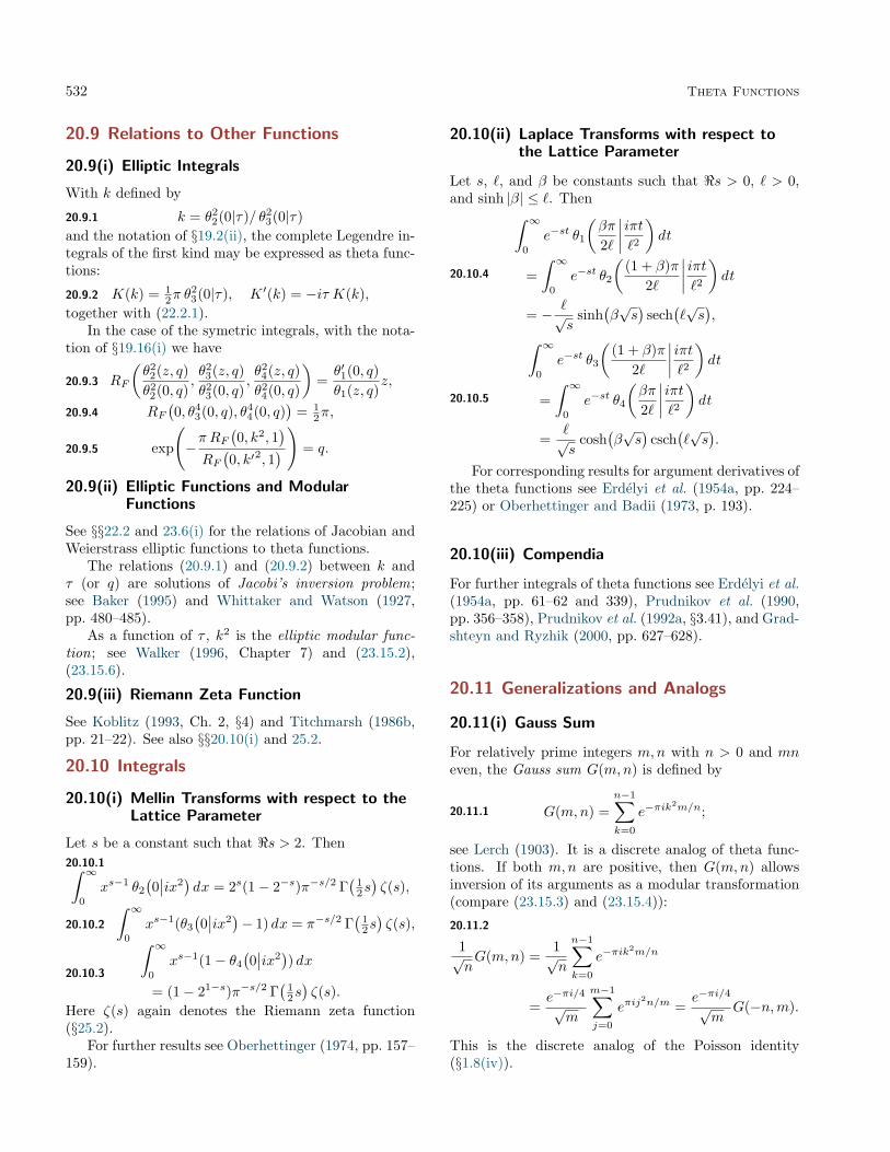
532 Theta Functions
20.9 Relations to Other Functions
20.9(i) Elliptic Integrals
With k defined by
20.9.1 k = θ22(0|τ)/ θ2
3(0|τ)and the notation of §19.2(ii), the complete Legendre in-tegrals of the first kind may be expressed as theta func-tions:
20.9.2 K(k) = 12π θ
23(0|τ), K ′(k) = −iτ K(k),
together with (22.2.1).In the case of the symetric integrals, with the nota-
tion of §19.16(i) we have
20.9.3 RF
(θ2
2(z, q)θ2
2(0, q),θ2
3(z, q)θ2
3(0, q),θ2
4(z, q)θ2
4(0, q)
)=θ′1(0, q)θ1(z, q)
z,
20.9.4 RF(0, θ4
3(0, q), θ44(0, q)
)= 1
2π,
20.9.5 exp
(−π RF
(0, k2, 1
)RF(0, k′2, 1
) ) = q.
20.9(ii) Elliptic Functions and ModularFunctions
See §§22.2 and 23.6(i) for the relations of Jacobian andWeierstrass elliptic functions to theta functions.
The relations (20.9.1) and (20.9.2) between k andτ (or q) are solutions of Jacobi’s inversion problem;see Baker (1995) and Whittaker and Watson (1927,pp. 480–485).
As a function of τ , k2 is the elliptic modular func-tion; see Walker (1996, Chapter 7) and (23.15.2),(23.15.6).
20.9(iii) Riemann Zeta Function
See Koblitz (1993, Ch. 2, §4) and Titchmarsh (1986b,pp. 21–22). See also §§20.10(i) and 25.2.
20.10 Integrals
20.10(i) Mellin Transforms with respect to theLattice Parameter
Let s be a constant such that <s > 2. Then20.10.1∫ ∞
0
xs−1 θ2
(0∣∣ix2
)dx = 2s(1− 2−s)π−s/2 Γ
(12s)ζ(s),
20.10.2
∫ ∞0
xs−1(θ3
(0∣∣ix2
)− 1) dx = π−s/2 Γ
(12s)ζ(s),
20.10.3
∫ ∞0
xs−1(1− θ4
(0∣∣ix2
)) dx
= (1− 21−s)π−s/2 Γ(
12s)ζ(s).
Here ζ(s) again denotes the Riemann zeta function(§25.2).
For further results see Oberhettinger (1974, pp. 157–159).
20.10(ii) Laplace Transforms with respect tothe Lattice Parameter
Let s, `, and β be constants such that <s > 0, ` > 0,and sinh |β| ≤ `. Then
20.10.4
∫ ∞0
e−st θ1
(βπ
2`
∣∣∣∣ iπt`2)dt
=∫ ∞
0
e−st θ2
((1 + β)π
2`
∣∣∣∣ iπt`2)dt
= − `√s
sinh(β√s)
sech(`√s),
20.10.5
∫ ∞0
e−st θ3
((1 + β)π
2`
∣∣∣∣ iπt`2)dt
=∫ ∞
0
e−st θ4
(βπ
2`
∣∣∣∣ iπt`2)dt
=`√s
cosh(β√s)
csch(`√s).
For corresponding results for argument derivatives ofthe theta functions see Erdélyi et al. (1954a, pp. 224–225) or Oberhettinger and Badii (1973, p. 193).
20.10(iii) Compendia
For further integrals of theta functions see Erdélyi et al.(1954a, pp. 61–62 and 339), Prudnikov et al. (1990,pp. 356–358), Prudnikov et al. (1992a, §3.41), and Grad-shteyn and Ryzhik (2000, pp. 627–628).
20.11 Generalizations and Analogs
20.11(i) Gauss Sum
For relatively prime integers m,n with n > 0 and mneven, the Gauss sum G(m,n) is defined by
20.11.1 G(m,n) =n−1∑k=0
e−πik2m/n;
see Lerch (1903). It is a discrete analog of theta func-tions. If both m,n are positive, then G(m,n) allowsinversion of its arguments as a modular transformation(compare (23.15.3) and (23.15.4)):
20.11.2
1√nG(m,n) =
1√n
n−1∑k=0
e−πik2m/n
=e−πi/4√
m
m−1∑j=0
eπij2n/m =
e−πi/4√m
G(−n,m).
This is the discrete analog of the Poisson identity(§1.8(iv)).

Applications 533
20.11(ii) Ramanujan’s Theta Function andq-Series
Ramanujan’s theta function f(a, b) is defined by
20.11.3 f(a, b) =∞∑
n=−∞an(n+1)/2bn(n−1)/2,
where a, b ∈ C and |ab| < 1. With the substitutionsa = qe2iz, b = qe−2iz, with q = eiπτ , we have
20.11.4 f(a, b) = θ3(z|τ).
In the case z = 0 identities for theta functions be-come identities in the complex variable q, with |q| < 1,that involve rational functions, power series, and contin-ued fractions; see Adiga et al. (1985), McKean and Moll(1999, pp. 156–158), and Andrews et al. (1988, §10.7).
20.11(iii) Ramanujan’s Change of Base
As in §20.11(ii), the modulus k of elliptic integrals(§19.2(ii)), Jacobian elliptic functions (§22.2), andWeierstrass elliptic functions (§23.6(ii)) can be ex-panded in q-series via (20.9.1). However, in this caseq is no longer regarded as an independent complex vari-able within the unit circle, because k is related to thevariable τ = τ(k) of the theta functions via (20.9.2).This is Jacobi’s inversion problem of §20.9(ii).
The first of equations (20.9.2) can also be written
20.11.5 2F1
(12 ,
12 ; 1; k2
)= θ2
3(0|τ);
see §19.5. Similar identities can be constructed for2F1
(13 ,
23 ; 1; k2
), 2F1
(14 ,
34 ; 1; k2
), and 2F1
(16 ,
56 ; 1; k2
).
These results are called Ramanujan’s changes of base.Each provides an extension of Jacobi’s inversion prob-lem. See Berndt et al. (1995) and Shen (1998). Forapplications to rapidly convergent expansions for π seeChudnovsky and Chudnovsky (1988), and for applica-tions in the construction of elliptic-hypergeometric se-ries see Rosengren (2004).
20.11(iv) Theta Functions with Characteristics
Multidimensional theta functions with characteristicsare defined in §21.2(ii) and their properties are describedin §§21.3(ii), 21.5(ii), and 21.6. For specialization to theone-dimensional theta functions treated in the presentchapter, see Rauch and Lebowitz (1973) and §21.7(iii).
Applications
20.12 Mathematical Applications
20.12(i) Number Theory
For applications of θ3(0, q) to problems involving sumsof squares of integers see §27.13(iv), and for exten-sions see Estermann (1959), Serre (1973, pp. 106–109),Koblitz (1993, pp. 176–177), and McKean and Moll(1999, pp. 142–143).
For applications of Jacobi’s triple product (20.5.9)to Ramanujan’s τ(n) function and Euler’s pentagonalnumbers see Hardy and Wright (1979, pp. 132–160) andMcKean and Moll (1999, pp. 143–145). For an applica-tion of a generalization in affine root systems see Mac-donald (1972).
20.12(ii) Uniformization and Embedding ofComplex Tori
For the terminology and notation see McKean and Moll(1999, pp. 48–53).
The space of complex tori C/(Z + τZ) (that is,the set of complex numbers z in which two of thesenumbers z1 and z2 are regarded as equivalent if thereexist integers m,n such that z1 − z2 = m + τn) ismapped into the projective space P 3 via the identifica-tion z → (θ1(2z|τ), θ2(2z|τ), θ3(2z|τ), θ4(2z|τ)). Thustheta functions “uniformize” the complex torus. Thisability to uniformize multiply-connected spaces (mani-folds), or multi-sheeted functions of a complex variable(Riemann (1899), Rauch and Lebowitz (1973), Siegel(1988)) has led to applications in string theory (Greenet al. (1988a,b), Krichever and Novikov (1989)), andalso in statistical mechanics (Baxter (1982)).
20.13 Physical Applications
The functions θj(z|τ), j = 1, 2, 3, 4, provide periodicsolutions of the partial differential equation
20.13.1 ∂θ(z|τ)/∂τ = κ ∂2θ(z|τ)/∂z2 ,
with κ = −iπ/4.For τ = it, with α, t, z real, (20.13.1) takes the form
of a real-time t diffusion equation
20.13.2 ∂θ/∂t = α ∂2θ/∂z2 ,
with diffusion constant α = π/4. Let z, α, t ∈ R. Thenthe nonperiodic Gaussian
20.13.3 g(z, t) =√
π
4αtexp(− z2
4αt
)is also a solution of (20.13.2), and it approaches a Diracdelta (§1.17) at t = 0. These two apparently different

534 Theta Functions
solutions differ only in their normalization and bound-ary conditions. From (20.2.3), (20.2.4), (20.7.32), and(20.7.33),
20.13.4
√π
4αt
∞∑n=−∞
e−(nπ+z)2/(4αt) = θ3(z|i4αt/π),
and
20.13.5√π
4αt
∞∑n=−∞
(−1)ne−(nπ+z)2/(4αt) = θ4(z|i4αt/π).
Thus the classical theta functions are “periodized”, or“anti-periodized”, Gaussians; see Bellman (1961, pp. 18,19). Theta-function solutions to the heat diffusion equa-tion with simple boundary conditions are discussed inLawden (1989, pp. 1–3), and with more general bound-ary conditions in Körner (1989, pp. 274–281).
In the singular limit =τ → 0+, the functions θj(z|τ),j = 1, 2, 3, 4, become integral kernels of Feynman pathintegrals (distribution-valued Green’s functions); seeSchulman (1981, pp. 194–195). This allows analytictime propagation of quantum wave-packets in a box, oron a ring, as closed-form solutions of the time-dependentSchrödinger equation.
Computation
20.14 Methods of Computation
The Fourier series of §20.2(i) usually converge rapidlybecause of the factors q(n+ 1
2 )2 or qn2, and provide a
convenient way of calculating values of θj(z|τ). Simi-larly, their z-differentiated forms provide a convenientway of calculating the corresponding derivatives. Forinstance, the first three terms of (20.2.1) give the valueof θ1(2− i|i) (= θ1(2− i, e−π)) to 12 decimal places.
For values of |q| near 1 the transformations of§20.7(viii) can be used to replace τ with a value thathas a larger imaginary part and hence a smaller value of|q|. For instance, to find θ3(z, 0.9) we use (20.7.32) withq = 0.9 = eiπτ , τ = −i ln(0.9)/π. Then τ ′ = −1/τ =−iπ/ ln(0.9) and q′ = eiπτ
′= exp
(π2/ ln(0.9)
)=
(2.07 . . . ) × 10−41. Hence the first term of the series(20.2.3) for θ3(zτ ′|τ ′) suffices for most purposes. Intheory, starting from any value of τ , a finite numberof applications of the transformations τ → τ + 1 andτ → −1/τ will result in a value of τ with =τ ≥
√3/2;
see §23.18. In practice a value with, say, =τ ≥ 1/2,|q| ≤ 0.2, is found quickly and is satisfactory for numer-ical evaluation.
20.15 Tables
Theta functions are tabulated in Jahnke and Emde(1945, p. 45). This reference gives θj(x, q), j = 1, 2, 3, 4,and their logarithmic x-derivatives to 4D for x/π =0(.1)1, α = 0(9◦)90◦, where α is the modular anglegiven by
20.15.1 sinα = θ22(0, q)/ θ2
3(0, q) = k.
Spenceley and Spenceley (1947) tabulatesθ1(x, q)/ θ2(0, q), θ2(x, q)/ θ2(0, q), θ3(x, q)/ θ4(0, q),θ4(x, q)/ θ4(0, q) to 12D for u = 0(1◦)90◦, α = 0(1◦)89◦,where u = 2x/(π θ2
3(0, q)) and α is defined by (20.15.1),together with the corresponding values of θ2(0, q) andθ4(0, q).
Lawden (1989, pp. 270–279) tabulates θj(x, q), j =1, 2, 3, 4, to 5D for x = 0(1◦)90◦, q = 0.1(.1)0.9, andalso q to 5D for k2 = 0(.01)1.
Tables of Neville’s theta functions θs(x, q), θc(x, q),θd(x, q), θn(x, q) (see §20.1) and their logarithmic x-derivatives are given in Abramowitz and Stegun (1964,pp. 582–585) to 9D for ε, α = 0(5◦)90◦, where (in ra-dian measure) ε = x/ θ2
3(0, q) = πx/(2K(k)), and α isdefined by (20.15.1).
For other tables prior to 1961 see Fletcher et al.(1962, pp. 508–514) and Lebedev and Fedorova (1960,pp. 227–230).
20.16 Software
See http://dlmf.nist.gov/20.16.
References
General References
The main references used in writing this chapter areWhittaker and Watson (1927), Lawden (1989), andWalker (1996). For further bibliographic reading seeMcKean and Moll (1999).
Sources
The following list gives the references or other indica-tions of proofs that were used in constructing the varioussections of this chapter. These sources supplement thereferences that are quoted in the text.
§20.2 Whittaker and Watson (1927, pp. 463–465) andLawden (1989, Chapter 1).
§20.3 These graphics were produced at NIST.
§20.4 Lawden (1989, pp. 12–23), Walker (1996, pp. 90–92), and Whittaker and Watson (1927, pp. 470–473). (20.4.1)–(20.4.5) are special cases of(20.5.1)–(20.5.4).

References 535
§20.5 Lawden (1989, pp. 12–23), Walker (1996, pp. 86–98), Whittaker and Watson (1927, pp. 469–473),and Bellman (1961, p. 44). Equations (20.5.14)–(20.5.17) follow from (20.5.5)–(20.5.8) by use ofthe infinite products for the sine and cosine(§4.22).
§20.6 Walker (1996, §3.2) and §23.9. (20.6.2)–(20.6.5) may be derived by termwise expansionin (20.5.14)–(20.5.17). (20.6.10) may be de-rived from (20.6.6) and (20.6.8) by subtractionof terms with even j, in a similar manner to∑∞n=1(−1)n−1n−j = (1− 21−j)
∑∞n=1 n
−j .
§20.7 Lawden (1989, pp. 5–23), Whittaker and Wat-son (1927, pp. 466–477), McKean and Moll (1999,pp. 129–130), Watson (1935a), Bellman (1961,p. 61), and Serre (1973, p. 109). The first equal-ities in (20.7.11) and (20.7.12) follow by transla-tion of z by 1
2π as in (20.2.11)–(20.2.14). Thesecond equalities follow from (20.5.5)–(20.5.8) andthe identity
∏∞n=1(1 + qn)(1− q2n−1) = 1 (Walker
(1996, p. 90)).
§20.9 Walker (1996, p. 156), Whittaker and Wat-son (1927, pp. 480–485), Serre (1973, p. 109),and McKean and Moll (1999, §§3.3, 3.9). For(20.9.3) combination of (20.4.6) and (23.6.5) –
(23.6.7) yields ℘(z) − ej =(v θ′1(0,q) θj+1(v,q)z θ1(v,q) θj+1(0,q)
)2
,
j = 1, 2, 3, where v = πz/(2ω1). Then by ap-plication of (19.25.35) and use of the proper-ties that RF is homogenous and of degree − 1
2in its three variables (§§19.16(ii), 19.16(iii)), wederive z = z θ1(v,q)
v θ′1(0,q) RF
(θ22(v,q)
θ22(0,q),θ23(v,q)
θ23(0,q),θ24(v,q)
θ24(0,q)
).
This equation becomes (20.9.3) when the z’sare cancelled and v is renamed z. For(20.9.4), from (19.25.1) and Erdélyi et al. (1953b,13.20(11)) we have K(k) = RF
(0, θ
44(0,q)
θ43(0,q), 1)
=
θ23(0, q)RF
(0, θ4
3(0, q), θ44(0, q)
), where the sec-
ond equality uses the homogeneity and symme-try of RF . Comparison with (20.9.2) proves(20.9.4). For (20.9.5), by (19.25.1) the left side isexp(−πK(k′)/K(k)), which equals q by Erdélyiet al. (1953b, 13.19(4)).
§20.10 Bellman (1961, pp. 20–24). For (20.10.1) and(20.10.3) use §20.7(viii) with appropriate changesof integration variable. For (20.10.2) use (20.2.3)with z = 0, τ = it, Bellman (1961, pp. 28–32), Koblitz (1993, pp. 70–75), and/or Titchmarsh(1986b, §2.6).
§20.11 Bellman (1961, pp. 38–39), Walker (1996,pp. 181–182), and McKean and Moll (1999,pp. 140–147 and 151–152).
§20.13 Whittaker and Watson (1927, p. 470).


Chapter 21
Multidimensional Theta FunctionsB. Deconinck1
Notation 53821.1 Special Notation . . . . . . . . . . . . . 538
Properties 53821.2 Definitions . . . . . . . . . . . . . . . . . 53821.3 Symmetry and Quasi-Periodicity . . . . . 53921.4 Graphics . . . . . . . . . . . . . . . . . . 53921.5 Modular Transformations . . . . . . . . . 54121.6 Products . . . . . . . . . . . . . . . . . . 542
Applications 54321.7 Riemann Surfaces . . . . . . . . . . . . . 54321.8 Abelian Functions . . . . . . . . . . . . . 54521.9 Integrable Equations . . . . . . . . . . . 545
Computation 54621.10 Methods of Computation . . . . . . . . . 54621.11 Software . . . . . . . . . . . . . . . . . . 546
References 546
1Department of Applied Mathematics, University of Washington, Seattle, Washington.Copyright c© 2009 National Institute of Standards and Technology. All rights reserved.
537

538 Multidimensional Theta Functions
Notation
21.1 Special Notation
(For other notation see pp. xiv and 873.)
g, h positive integers.Zg Z× Z× · · · × Z (g times).Rg R× R× · · · × R (g times).Zg×h set of all g × h matrices with integer
elements.Ω g × g complex, symmetric matrix with =Ω
strictly positive definite, i.e., a Riemannmatrix.
α,β g-dimensional vectors, with all elements in[0, 1), unless stated otherwise.
aj jth element of vector a.Ajk (j, k)th element of matrix A.a · b scalar product of the vectors a and b.a ·Ω · b [Ωa] · b = [Ωb] · a.0g g × g zero matrix.Ig g × g identity matrix.
J2g
[0g Ig−Ig 0g
].
Sg set of g-dimensional vectors with elementsin S.
|S| number of elements of the set S.S1S2 set of all elements of the form
“element of S1 × element of S2”.S1/S2 set of all elements of S1, modulo elements of
S2. Thus two elements of S1/S2 areequivalent if they are both in S1 and theirdifference is in S2. (For an example see§20.12(ii).)
a ◦ b intersection index of a and b, two cycleslying on a closed surface. a ◦ b = 0 if a and bdo not intersect. Otherwise a ◦ b gets anadditive contribution from every intersectionpoint. This contribution is 1 if the basis ofthe tangent vectors of the a and b cycles(§21.7(i)) at the point of intersection ispositively oriented; otherwise it is −1.∮
aω line integral of the differential ω over the
cycle a.
Lowercase boldface letters or numbers are g-dimensional real or complex vectors, either row or col-umn depending on the context. Uppercase boldface let-
ters are g × g real or complex matrices.The main functions treated in this chapter are the
Riemann theta functions θ(z|Ω), and the Riemann thetafunctions with characteristics θ
[αβ
](z|Ω).
The function Θ(φ|B) = θ(φ/(2πi)|B/(2πi)) is alsocommonly used; see, for example, Belokolos et al. (1994,§2.5), Dubrovin (1981), and Fay (1973, Chapter 1).
Properties
21.2 Definitions
21.2(i) Riemann Theta Functions
21.2.1 θ(z|Ω) =∑n∈Zg
e2πi( 12n·Ω·n+n·z).
This g-tuple Fourier series converges absolutely and uni-formly on compact sets of the z and Ω spaces; henceθ(z|Ω) is an analytic function of (each element of) zand (each element of) Ω. θ(z|Ω) is also referred to asa theta function with g components, a g-dimensionaltheta function or as a genus g theta function.
For numerical purposes we use the scaled Riemanntheta function θ̂(z|Ω), defined by (Deconinck et al.(2004)),
21.2.2 θ̂(z|Ω) = e−π[=z]·[=Ω]−1·[=z] θ(z|Ω).
θ̂(z|Ω) is a bounded nonanalytic function of z. Manyapplications involve quotients of Riemann theta func-tions: the exponential factor then disappears.
Example
21.2.3
θ
(z1, z2
∣∣∣∣[ i − 12
− 12 i
])=
∞∑n1=−∞
∞∑n2=−∞
e−π(n21+n2
2)e−iπn1n2e2πi(n1z1+n2z2).
With z1 = x1 + iy1, z2 = x2 + iy2,
21.2.4
θ̂
(x1 + iy1, x2 + iy2
∣∣∣∣[ i − 12
− 12 i
])=
∞∑n1=−∞
∞∑n2=−∞
e−π(n1+y1)2−π(n2+y2)2
× eπi(2n1x1+2n2x2−n1n2).

21.3 Symmetry and Quasi-Periodicity 539
21.2(ii) Riemann Theta Functions withCharacteristics
Let α,β ∈ Rg. Define21.2.5
θ
[α
β
](z|Ω) =
∑n∈Zg
e2πi( 12 [n+α]·Ω·[n+α]+[n+α]·[z+β]).
This function is referred to as a Riemann theta func-
tion with characteristics[αβ
]. It is a translation of the
Riemann theta function (21.2.1), multiplied by an ex-ponential factor:21.2.6
θ
[α
β
](z|Ω) = e2πi( 1
2α·Ω·α+α·[z+β]) θ(z + Ωα+ β|Ω),
and21.2.7 θ
[00
](z|Ω) = θ(z|Ω).
Characteristics whose elements are either 0 or 12 are
called half-period characteristics. For given Ω, there are22g g-dimensional Riemann theta functions with half-period characteristics.
21.2(iii) Relation to Classical Theta Functions
For g = 1, and with the notation of §20.2(i),
21.2.8 θ(z|Ω) = θ3(πz|Ω),
21.2.9 θ1(πz|Ω) = − θ[ 1
212
](z|Ω),
21.2.10 θ2(πz|Ω) = θ
[ 12
0
](z|Ω),
21.2.11 θ3(πz|Ω) = θ
[00
](z|Ω),
21.2.12 θ4(πz|Ω) = θ
[012
](z|Ω).
21.3 Symmetry and Quasi-Periodicity
21.3(i) Riemann Theta Functions
21.3.1 θ(−z|Ω) = θ(z|Ω),
21.3.2 θ(z + m1|Ω) = θ(z|Ω),
when m1 ∈ Zg. Thus θ(z|Ω) is periodic, with period 1,in each element of z. More generally,21.3.3
θ(z + m1 + Ωm2|Ω) = e−2πi( 12m2·Ω·m2+m2·z) θ(z|Ω),
with m1, m2 ∈ Zg. This is the quasi-periodicity prop-erty of the Riemann theta function. It determines theRiemann theta function up to a constant factor. Theset of points m1 + Ωm2 form a g-dimensional lattice,the period lattice of the Riemann theta function.
21.3(ii) Riemann Theta Functions withCharacteristics
Again, with m1, m2 ∈ Zg
21.3.4 θ
[α+ m1
β + m2
](z|Ω) = e2πiα·m1 θ
[α
β
](z|Ω).
Because of this property, the elements of α and β areusually restricted to [0, 1), without loss of generality.
21.3.5
θ
[α
β
](z + m1 + Ωm2|Ω)
= e2πi(α·m1−β·m2− 12m2·Ω·m2−m2·z) θ
[α
β
](z|Ω).
For Riemann theta functions with half-period charac-teristics,
21.3.6 θ
[α
β
](−z|Ω) = (−1)4α·β θ
[α
β
](z|Ω).
See also §20.2(iii) for the case g = 1 and classical thetafunctions.
21.4 Graphics
Figure 21.4.1 provides surfaces of the scaled Riemann theta function θ̂(z|Ω), with
21.4.1 Ω =[1.69098 3006 + 0.95105 6516 i 1.5 + 0.36327 1264 i
1.5 + 0.36327 1264 i 1.30901 6994 + 0.95105 6516 i
].
This Riemann matrix originates from the Riemann surface represented by the algebraic curve µ3 − λ7 + 2λ3µ = 0;compare §21.7(i).

540 Multidimensional Theta Functions
(a1) (b1) (c1)
(a2) (b2) (c2)
(a3) (b3) (c3)
Figure 21.4.1: θ̂(z|Ω) parametrized by (21.4.1). The surface plots are of θ̂(x+ iy, 0|Ω), 0 ≤ x ≤ 1, 0 ≤ y ≤ 5 (suffix1); θ̂(x, y|Ω), 0 ≤ x ≤ 1, 0 ≤ y ≤ 1 (suffix 2); θ̂(ix, iy|Ω), 0 ≤ x ≤ 5, 0 ≤ y ≤ 5 (suffix 3). Shown are the real part(a), the imaginary part (b), and the modulus (c).
For the scaled Riemann theta functions depicted in Figures 21.4.2–21.4.5
21.4.2 Ω1 =[i − 1
2− 1
2 i
],
and
21.4.3 Ω2 =
− 12 + i 1
2 −12 i −
12 −
12 i
12 −
12 i i 0
− 12 −
12 i 0 i
.

21.5 Modular Transformations 541
Figure 21.4.2: <θ̂(x+ iy, 0|Ω1), 0 ≤ x ≤ 1, 0 ≤ y ≤ 5.(The imaginary part looks very similar.)
Figure 21.4.3:∣∣∣θ̂(x+ iy, 0|Ω1)
∣∣∣, 0 ≤ x ≤ 1, 0 ≤ y ≤ 2.
Figure 21.4.4: A real-valued scaled Riemann theta func-tion: θ̂(ix, iy|Ω1), 0 ≤ x ≤ 4, 0 ≤ y ≤ 4. In thiscase, the quasi-periods are commensurable, resulting ina doubly-periodic configuration.
Figure 21.4.5: The real part of a genus 3 scaled Riemanntheta function: <θ̂(x+ iy, 0, 0|Ω2), 0 ≤ x ≤ 1, 0 ≤y ≤ 3. This Riemann matrix originates from the genus3 Riemann surface represented by the algebraic curveµ3 + 2µ− λ4 = 0; compare §21.7(i).
21.5 Modular Transformations
21.5(i) Riemann Theta Functions
Let A, B, C, and D be g × g matrices with integerelements such that
21.5.1 Γ =[A BC D
]is a symplectic matrix, that is,
21.5.2 ΓJ2gΓT = J2g.
Then
21.5.3 det Γ = 1,
and
21.5.4
θ([
[CΩ + D]−1]T
z∣∣∣[AΩ + B][CΩ + D]−1
)= ξ(Γ)
√det[CΩ + D]eπiz·[[CΩ+D]−1C]·z θ(z|Ω).
Here ξ(Γ) is an eighth root of unity, that is, (ξ(Γ))8 = 1.For general Γ, it is difficult to decide which root needs tobe used. The choice depends on Γ, but is independent

542 Multidimensional Theta Functions
of z and Ω. Equation (21.5.4) is the modular transfor-mation property for Riemann theta functions.
The modular transformations form a group underthe composition of such transformations, the modulargroup, which is generated by simpler transformations,for which ξ(Γ) is determinate:
21.5.5 Γ =[A 0g0g [A−1]T
]⇒ θ
(Az∣∣AΩAT
)= θ(z|Ω).
(A invertible with integer elements.)
21.5.6 Γ =[Ig B0g Ig
]⇒ θ(z|Ω + B) = θ(z|Ω).
(B symmetric with integer elements and even diagonalelements.)21.5.7
Γ =[Ig B0g Ig
]⇒ θ(z|Ω + B) = θ
(z + 1
2 diag B∣∣Ω).
(B symmetric with integer elements.) See Heil (1995,p. 24).21.5.8
Γ =[0g −IgIg 0g
]⇒ θ
(Ω−1z
∣∣−Ω−1)
=√
det [−iΩ]eπiz·Ω−1·z θ(z|Ω),
where the square root assumes its principal value.
21.5(ii) Riemann Theta Functions with Characteristics
21.5.9
θ
[Dα−Cβ + 1
2 diag[CDT]−Bα+ Aβ + 1
2 diag[ABT]
]([[CΩ + D]−1
]Tz∣∣∣[AΩ + B][CΩ + D]−1
)= κ(α,β,Γ)
√det[CΩ + D]eπiz·[[CΩ+D]−1C]·z θ
[α
β
](z|Ω),
where κ(α,β,Γ) is a complex number that depends onα, β, and Γ. However, κ(α,β,Γ) is independent ofz and Ω. For explicit results in the case g = 1, see§20.7(viii).
21.6 Products
21.6(i) Riemann Identity
Let T = [Tjk] be an arbitrary h× h orthogonal matrix(that is, TTT = I) with rational elements. Also, let Zbe an arbitrary g × h matrix. Define
21.6.1 K = Zg×hT/(Zg×hT ∩ Zg×h),
that is, K is the set of all g×h matrices that are obtainedby premultiplying T by any g × h matrix with integerelements; two such matrices in K are considered equiva-lent if their difference is a matrix with integer elements.Also, let
21.6.2 D = |TTZh/(TTZh ∩ Zh)|,
that is, D is the number of elements in the set contain-ing all h-dimensional vectors obtained by multiplyingTT on the right by a vector with integer elements. Twosuch vectors are considered equivalent if their difference
is a vector with integer elements. Then
21.6.3
h∏j=1
θ
(h∑k=1
Tjkzk
∣∣∣∣∣Ω)
=1Dg
∑A∈K
∑B∈K
e2πi tr[ 12ATΩA+AT[Z+B]]
×h∏j=1
θ(zj + Ωaj + bj |Ω),
where zj , aj , bj denote respectively the jth columns ofZ, A, B. This is the Riemann identity. On using thetafunctions with characteristics, it becomes21.6.4h∏j=1
θ
[∑hk =1 Tjkck∑hk =1 Tjkdk
]( h∑k=1
Tjkzk
∣∣∣∣∣Ω)
=1Dg
∑A∈K
∑B∈K
e−2πiPhj=1 bj ·cj
h∏j=1
θ
[aj + cjbj + dj
](zj |Ω),
where cj and dj are arbitrary h-dimensional vectors.Many identities involving products of theta functionscan be established using these formulas.
Example
Let h = 4 and
21.6.5 T =
1 1 1 11 1 −1 −11 −1 1 −11 −1 −1 1
.Then

Applications 543
21.6.6
θ
(x + y + u + v
2
∣∣∣∣Ω) θ(x + y − u− v2
∣∣∣∣Ω) θ(x− y + u− v2
∣∣∣∣Ω) θ(x− y − u + v2
∣∣∣∣Ω)=
12g
∑α∈ 1
2 Zg/Zg
∑β∈ 1
2 Zg/Zge2πi(2α·Ω·α+α·[x+y+u+v])
× θ(x + Ωα+ β|Ω) θ(y + Ωα+ β|Ω) θ(u + Ωα+ β|Ω) θ(v + Ωα+ β|Ω),and21.6.7
θ
[ 12 [c1 + c2 + c3 + c4]
12 [d1 + d2 + d3 + d4]
](x + y + u + v
2
∣∣∣∣Ω) θ[ 12 [c1 + c2 − c3 − c4]
12 [d1 + d2 − d3 − d4]
](x + y − u− v
2
∣∣∣∣Ω)× θ
[ 12 [c1 − c2 + c3 − c4]
12 [d1 − d2 + d3 − d4]
](x− y + u− v
2
∣∣∣∣Ω) θ[ 12 [c1 − c2 − c3 + c4]
12 [d1 − d2 − d3 + d4]
](x− y − u + v
2
∣∣∣∣Ω)=
12g
∑α∈ 1
2 Zg/Zg
∑β∈ 1
2 Zg/Zge−2πiβ·[c1+c2+c3+c4] θ
[c1 +αd1 + β
](x|Ω) θ
[c2 +αd2 + β
](y|Ω) θ
[c3 +αd3 + β
](u|Ω) θ
[c4 +αd4 + β
](v|Ω).
21.6(ii) Addition Formulas
Let α, β, γ, δ ∈ Rg. Then
21.6.8
θ
[α
γ
](z1|Ω) θ
[β
δ
](z2|Ω)
=∑
ν∈Zg/(2Zg)
θ
[ 12 [α+ β + ν]
γ + δ
](z1 + z2|2Ω)
× θ
[ 12 [α− β + ν]
γ − δ
](z1 − z2|2Ω).
Thus ν is a g-dimensional vector whose entries are ei-ther 0 or 1. For this result and a generalization seeKoizumi (1976) and Belokolos et al. (1994, pp. 38–41).For addition formulas for classical theta functions see§20.7(ii).
Applications
21.7 Riemann Surfaces
21.7(i) Connection of Riemann ThetaFunctions to Riemann Surfaces
In almost all applications, a Riemann theta function isassociated with a compact Riemann surface. Althoughthere are other ways to represent Riemann surfaces (seee.g. Belokolos et al. (1994, §2.1)), they are obtainablefrom plane algebraic curves (Springer (1957), or Rie-mann (1851)). Consider the set of points in C2 thatsatisfy the equation
21.7.1 P (λ, µ) = 0,where P (λ, µ) is a polynomial in λ and µ that doesnot factor over C2. Equation (21.7.1) determines a
plane algebraic curve in C2, which is made compact byadding its points at infinity. To accomplish this we write(21.7.1) in terms of homogeneous coordinates:
21.7.2 P̃ (λ̃, µ̃, η̃) = 0,by setting λ = λ̃/η̃, µ = µ̃/η̃, and then clearing frac-tions. This compact curve may have singular points,that is, points at which the gradient of P̃ vanishes.Removing the singularities of this curve gives rise toa two-dimensional connected manifold with a complex-analytic structure, that is, a Riemann surface. All com-pact Riemann surfaces can be obtained this way.
Since a Riemann surface Γ is a two-dimensional man-ifold that is orientable (owing to its analytic structure),its only topological invariant is its genus g (the numberof handles in the surface). On this surface, we choose 2gcycles (that is, closed oriented curves, each with at mosta finite number of singular points) aj , bj , j = 1, 2, . . . , g,such that their intersection indices satisfy
21.7.3 aj ◦ ak = 0, bj ◦ bk = 0, aj ◦ bk = δj,k.
For example, Figure 21.7.1 depicts a genus 2 surface.
1 a2
2b1b
a
Figure 21.7.1: A basis of cycles for a genus 2 surface.
On a Riemann surface of genus g, there are g lin-early independent holomorphic differentials ωj , j =
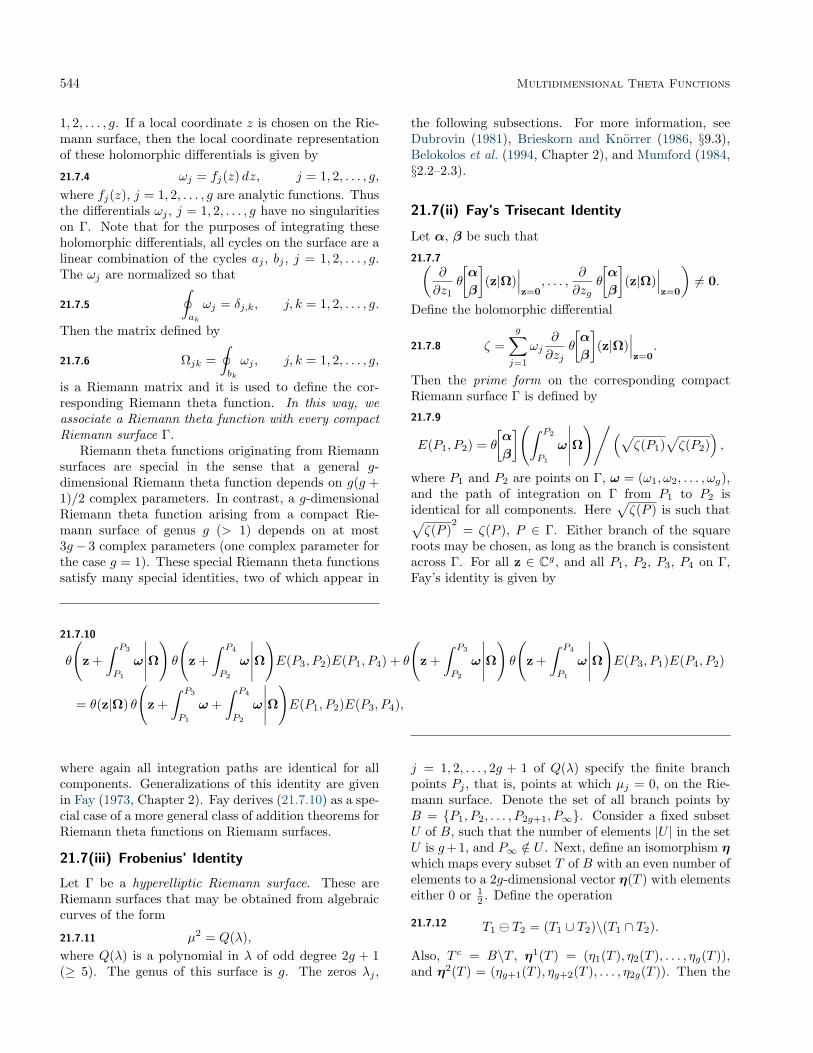
544 Multidimensional Theta Functions
1, 2, . . . , g. If a local coordinate z is chosen on the Rie-mann surface, then the local coordinate representationof these holomorphic differentials is given by
21.7.4 ωj = fj(z) dz, j = 1, 2, . . . , g,where fj(z), j = 1, 2, . . . , g are analytic functions. Thusthe differentials ωj , j = 1, 2, . . . , g have no singularitieson Γ. Note that for the purposes of integrating theseholomorphic differentials, all cycles on the surface are alinear combination of the cycles aj , bj , j = 1, 2, . . . , g.The ωj are normalized so that
21.7.5
∮ak
ωj = δj,k, j, k = 1, 2, . . . , g.
Then the matrix defined by
21.7.6 Ωjk =∮bk
ωj , j, k = 1, 2, . . . , g,
is a Riemann matrix and it is used to define the cor-responding Riemann theta function. In this way, weassociate a Riemann theta function with every compactRiemann surface Γ.
Riemann theta functions originating from Riemannsurfaces are special in the sense that a general g-dimensional Riemann theta function depends on g(g +1)/2 complex parameters. In contrast, a g-dimensionalRiemann theta function arising from a compact Rie-mann surface of genus g (> 1) depends on at most3g− 3 complex parameters (one complex parameter forthe case g = 1). These special Riemann theta functionssatisfy many special identities, two of which appear in
the following subsections. For more information, seeDubrovin (1981), Brieskorn and Knörrer (1986, §9.3),Belokolos et al. (1994, Chapter 2), and Mumford (1984,§2.2–2.3).
21.7(ii) Fay’s Trisecant Identity
Let α, β be such that
21.7.7(∂
∂z1θ
[α
β
](z|Ω)
∣∣∣z=0
, . . . ,∂
∂zgθ
[α
β
](z|Ω)
∣∣∣z=0
)6= 0.
Define the holomorphic differential
21.7.8 ζ =g∑j=1
ωj∂
∂zjθ
[α
β
](z|Ω)
∣∣∣z=0
.
Then the prime form on the corresponding compactRiemann surface Γ is defined by
21.7.9
E(P1, P2) = θ
[α
β
](∫ P2
P1
ω
∣∣∣∣∣Ω)/(√
ζ(P1)√ζ(P2)
),
where P1 and P2 are points on Γ, ω = (ω1, ω2, . . . , ωg),and the path of integration on Γ from P1 to P2 isidentical for all components. Here
√ζ(P ) is such that√
ζ(P )2
= ζ(P ), P ∈ Γ. Either branch of the squareroots may be chosen, as long as the branch is consistentacross Γ. For all z ∈ Cg, and all P1, P2, P3, P4 on Γ,Fay’s identity is given by
21.7.10
θ
(z +
∫ P3
P1
ω
∣∣∣∣∣Ω)θ
(z +
∫ P4
P2
ω
∣∣∣∣∣Ω)E(P3, P2)E(P1, P4) + θ
(z +
∫ P3
P2
ω
∣∣∣∣∣Ω)θ
(z +
∫ P4
P1
ω
∣∣∣∣∣Ω)E(P3, P1)E(P4, P2)
= θ(z|Ω) θ
(z +
∫ P3
P1
ω +∫ P4
P2
ω
∣∣∣∣∣Ω)E(P1, P2)E(P3, P4),
where again all integration paths are identical for allcomponents. Generalizations of this identity are givenin Fay (1973, Chapter 2). Fay derives (21.7.10) as a spe-cial case of a more general class of addition theorems forRiemann theta functions on Riemann surfaces.
21.7(iii) Frobenius’ Identity
Let Γ be a hyperelliptic Riemann surface. These areRiemann surfaces that may be obtained from algebraiccurves of the form
21.7.11 µ2 = Q(λ),where Q(λ) is a polynomial in λ of odd degree 2g + 1(≥ 5). The genus of this surface is g. The zeros λj ,
j = 1, 2, . . . , 2g + 1 of Q(λ) specify the finite branchpoints Pj , that is, points at which µj = 0, on the Rie-mann surface. Denote the set of all branch points byB = {P1, P2, . . . , P2g+1, P∞}. Consider a fixed subsetU of B, such that the number of elements |U | in the setU is g+1, and P∞ /∈ U . Next, define an isomorphism ηwhich maps every subset T of B with an even number ofelements to a 2g-dimensional vector η(T ) with elementseither 0 or 1
2 . Define the operation
21.7.12 T1 T2 = (T1 ∪ T2)\(T1 ∩ T2).
Also, T c = B\T , η1(T ) = (η1(T ), η2(T ), . . . , ηg(T )),and η2(T ) = (ηg+1(T ), ηg+2(T ), . . . , η2g(T )). Then the

21.8 Abelian Functions 545
isomorphism is determined completely by:
21.7.13 η(T ) = η(T c),
21.7.14 η(T1 T2) = η(T1) + η(T2),
21.7.15 4η1(T ) ·η2(T ) = 12 (|T U | − g− 1) (mod 2),
21.7.16
4(η1(T1)·η2(T2)−η2(T1)·η1(T2)) = |T1∩T2| (mod 2).Furthermore, let η(P∞) = 0 and η(Pj) =
η({Pj , P∞}). Then for all zj ∈ Cg, j = 1, 2, 3, 4, suchthat z1 +z2 +z3 +z4 = 0, and for all αj , βj ∈ Rg, suchthat α1 +α2 +α3 +α4 = 0 and β1 +β2 +β3 +β4 = 0,we have Frobenius’ identity :
21.7.17
∑Pj∈U
4∏k=1
θ
[αk + η1(Pj)βk + η2(Pj)
](zk|Ω)
=∑Pj∈Uc
4∏k=1
θ
[αk + η1(Pj)βk + η2(Pj)
](zk|Ω).
21.8 Abelian Functions
An Abelian function is a 2g-fold periodic, meromor-phic function of g complex variables. In consequence,Abelian functions are generalizations of elliptic func-tions (§23.2(iii)) to more than one complex variable.For every Abelian function, there is a positive integer n,such that the Abelian function can be expressed as a ra-tio of linear combinations of products with n factors ofRiemann theta functions with characteristics that sharea common period lattice. For further information seeIgusa (1972, pp. 132–135) and Markushevich (1992).
21.9 Integrable Equations
Riemann theta functions arise in the study of integrabledifferential equations that have applications in manyareas, including fluid mechanics (Ablowitz and Segur(1981, Chapter 4)), magnetic monopoles (Ercolani andSinha (1989)), and string theory (Deligne et al. (1999,Part 3)). Typical examples of such equations are theKorteweg–de Vries equation21.9.1 4ut = 6uux + uxxx,
and the nonlinear Schrödinger equations
21.9.2 iut = − 12uxx ± |u|
2u.
Here, and in what follows, x, y, and t suffixes indicatepartial derivatives.
Particularly important for the use of Riemanntheta functions is the Kadomtsev–Petviashvili (KP)equation, which describes the propagation of two-dimensional, long-wave length surface waves in shallowwater (Ablowitz and Segur (1981, Chapter 4)):
21.9.3 (−4ut + 6uux + uxxx)x + 3uyy = 0.
Here x and y are spatial variables, t is time, andu(x, y, t) is the elevation of the surface wave. All quanti-ties are made dimensionless by a suitable scaling trans-formation. The KP equation has a class of quasi-periodic solutions described by Riemann theta func-tions, given by
21.9.4 u(x, y, t) = c+ 2∂2
∂x2 ln(θ(kx+ ly + ωt+ φ|Ω)),
where c is a complex constant and k, l, ω, and φ areg-dimensional complex vectors; see Krichever (1976).These parameters, including Ω, are not free: they aredetermined by a compact, connected Riemann surface(Krichever (1976)), or alternatively by an appropri-ate initial condition u(x, y, 0) (Deconinck and Segur(1998)). These solutions have been compared success-fully with physical experiments for g = 1, 2 (Wiegel(1960), Hammack et al. (1989), and Hammack et al.(1995)). See Figures 21.9.1 and 21.9.2.
Figure 21.9.1: Two-dimensional periodic waves in a shal-low water wave tank, taken from Hammack et al. (1995,p. 97) by permission of Cambridge University Press.The original caption reads “Mosaic of two overhead pho-tographs, showing surface patterns of waves in shallowwater.”
Figure 21.9.2: Contour plot of a two-phase solution ofEquation (21.9.3). Such a solution is given in terms of aRiemann theta function with two phases; see Krichever(1976), Dubrovin (1981), and Hammack et al. (1995).

546 Multidimensional Theta Functions
Furthermore, the solutions of the KP equation solvethe Schottky problem: this is the question concerningconditions that a Riemann matrix needs to satisfy inorder to be associated with a Riemann surface (Schot-tky (1903)). Following the work of Krichever (1976),Novikov conjectured that the Riemann theta functionin (21.9.4) gives rise to a solution of the KP equation(21.9.3) if, and only if, the theta function originates froma Riemann surface; see Dubrovin (1981, §IV.4). Thefirst part of this conjecture was established in Krichever(1976); the second part was proved in Shiota (1986).
Computation
21.10 Methods of Computation
21.10(i) General Riemann Theta Functions
Although the defining Fourier series (21.2.1) is uni-formly convergent on compact sets, its evaluation iscumbersome when one or more of the eigenvalues of=(Ω) is near zero. Furthermore, for fixed Ω differentterms of the Fourier series dominate for different valuesof z.
To overcome these obstacles, we compute instead thescaled function θ̂(z|Ω) (§21.2(i)) from the expansion
21.10.1
θ̂(z|Ω) =∑
n∈S(ε)
eπi[n−[Y−1y]]·X·[n−[Y−1y]]
× e2πi[n−[Y−1y]]·x e−π[n+[Y−1y]]·Y·[n+[Y−1y]],
where ε is the tolerated maximum absolute error forθ̂(z|Ω). Here X = <(Ω), Y = =(Ω), x = <(z),y = =(z), and
21.10.2
S(ε) ={
m ∈ Zg∣∣∣π [m + [Y−1y]
]·Y
·[m + [Y−1y]
]≤ R(ε)
}.
Thus S(ε) is the set of all integer vectors that are con-tained in an ellipsoid centered at the fractional part ofY−1y, and whose size is determined by the allowed ab-solute error. The value of R(ε) is determined as follows.Let r be the length of the shortest vector of the latticeΛ = {
√πTm|m ∈ Zg}, and TTT = Y be the Cholesky
decomposition of Y (Atkinson (1989, p. 254)). ThenR(ε) is the greater of
√g/2 + r and the smallest posi-
tive root of the equation
21.10.3 Γ(
12g,R
2)/(2grg) = ε.
For the incomplete gamma function Γ(a, z), see §8.2(i).The construction (21.10.2) amounts to determining
all integer vectors in a g-dimensional ellipsoid. For this
purpose it is convenient to have the ellipsoid as sphericalas possible (Siegel (1973, pp. 144–159), Heil (1995)).
Usually, (21.10.1) can also be used for the efficientevaluation of θ̂(z|Ω) for fixed Ω and varying z, by ad-dition of a few vectors to the set S(ε).
21.10(ii) Riemann Theta Functions Associatedwith a Riemann Surface
In addition to evaluating the Fourier series, the mainproblem here is to compute a Riemann matrix originat-ing from a Riemann surface. Various approaches areconsidered in the following references:
• Belokolos et al. (1994, Chapter 5) and referencestherein. Here the Riemann surface is representedby the action of a Schottky group on a region ofthe complex plane. The same representation isused in Gianni et al. (1998).
• Tretkoff and Tretkoff (1984). Here a Hurwitz sys-tem is chosen to represent the Riemann surface.
• Deconinck and van Hoeij (2001). Here a plane al-gebraic curve representation of the Riemann sur-face is used.
21.11 Software
See http://dlmf.nist.gov/21.11.
References
General References
The main references used in writing this chapter areMumford (1983, 1984), Igusa (1972), and Belokoloset al. (1994). For additional bibliographic reading seeDubrovin (1981), Siegel (1971, 1973), and Fay (1973).
Sources
The following list gives the references or other indica-tions of proofs that were used in constructing the varioussections of this chapter. These sources supplement thereferences that are quoted in the text.
§21.3 Mumford (1983, pp. 120–122).
§21.4 These graphics were computed by the author,using the algorithms described in Deconinck et al.(2004).
§21.5 Arnol′d (1997, p. 222), Mumford (1983, pp. 189–210), Igusa (1972, pp. 78–85).

References 547
§21.6 Mumford (1983, pp. 211–216), Dubrovin (1981,pp. 22–23).
§21.7 Mumford (1984, pp. 106–120 and 207–260).
§21.9 Dubrovin (1981), Belokolos et al. (1994).
§21.10 Deconinck et al. (2004).


Chapter 22
Jacobian Elliptic FunctionsW. P. Reinhardt1 and P. L. Walker2
Notation 55022.1 Special Notation . . . . . . . . . . . . . 550
Properties 55022.2 Definitions . . . . . . . . . . . . . . . . . 55022.3 Graphics . . . . . . . . . . . . . . . . . . 55022.4 Periods, Poles, and Zeros . . . . . . . . . 55322.5 Special Values . . . . . . . . . . . . . . . 55422.6 Elementary Identities . . . . . . . . . . . 55622.7 Landen Transformations . . . . . . . . . 55622.8 Addition Theorems . . . . . . . . . . . . 55722.9 Cyclic Identities . . . . . . . . . . . . . . 55822.10 Maclaurin Series . . . . . . . . . . . . . . 55822.11 Fourier and Hyperbolic Series . . . . . . . 55922.12 Expansions in Other Trigonometric Se-
ries and Doubly-Infinite Partial Fractions:Eisenstein Series . . . . . . . . . . . . . . 559
22.13 Derivatives and Differential Equations . . 56022.14 Integrals . . . . . . . . . . . . . . . . . . 56022.15 Inverse Functions . . . . . . . . . . . . . 56122.16 Related Functions . . . . . . . . . . . . . 56122.17 Moduli Outside the Interval [0,1] . . . . . 563
Applications 56322.18 Mathematical Applications . . . . . . . . 56322.19 Physical Applications . . . . . . . . . . . 564
Computation 56622.20 Methods of Computation . . . . . . . . . 56622.21 Tables . . . . . . . . . . . . . . . . . . . 56722.22 Software . . . . . . . . . . . . . . . . . . 567
References 567
1University of Washington, Seattle, Washington.2American University of Sharjah, Sharjah, United Arab Emirates.Acknowledgments: This chapter is based in part on Abramowitz and Stegun (1964, Chapters 16,18) by L. M. Milne-Thomson and
T. H. Southard respectively.Copyright c© 2009 National Institute of Standards and Technology. All rights reserved.
549

550 Jacobian Elliptic Functions
Notation
22.1 Special Notation
(For other notation see pp. xiv and 873.)
x, y real variables.z complex variable.k modulus. Except in §§22.3(iv), 22.17, and
22.19, 0 ≤ k ≤ 1.k′ complementary modulus, k2 + k′
2 = 1. Ifk ∈ [0, 1], then k′ ∈ [0, 1].
K, K ′ K(k), K ′(k) = K(k′) (complete ellipticintegrals of the first kind (§19.2(ii))).
q nome. 0 ≤ q < 1 except in §22.17; see also§20.1.
τ iK ′ /K.
All derivatives are denoted by differentials, notprimes.
The functions treated in this chapter are the threeprincipal Jacobian elliptic functions sn (z, k), cn (z, k),dn (z, k); the nine subsidiary Jacobian elliptic functionscd (z, k), sd (z, k), nd (z, k), dc (z, k), nc (z, k), sc (z, k),ns (z, k), ds (z, k), cs (z, k); the amplitude functionam (x, k); Jacobi’s epsilon and zeta functions E(x, k)and Z(x|k).
The notation sn (z, k), cn (z, k), dn (z, k) is due toGudermann (1838), following Jacobi (1827); that for thesubsidiary functions is due to Glaisher (1882). Othernotations for sn (z, k) are sn(z|m) and sn(z,m) withm = k2; see Abramowitz and Stegun (1964) and Walker(1996). Similarly for the other functions.
Properties
22.2 Definitions
The nome q is given in terms of the modulus k by
22.2.1 q = exp(−πK ′(k)/K(k)),
where K(k), K ′(k) are defined in §19.2(ii). Inversely,
22.2.2 k =θ2
2(0, q)θ2
3(0, q), k′ =
θ24(0, q)θ2
3(0, q), K(k) =
π
2θ2
3(0, q),
where k′ =√
1− k2 and the theta functions are definedin §20.2(i).
With22.2.3 ζ =
πz
2K(k),
22.2.4 sn (z, k) =θ3(0, q)θ2(0, q)
θ1(ζ, q)θ4(ζ, q)
=1
ns (z, k),
22.2.5 cn (z, k) =θ4(0, q)θ2(0, q)
θ2(ζ, q)θ4(ζ, q)
=1
nc (z, k),
22.2.6 dn (z, k) =θ4(0, q)θ3(0, q)
θ3(ζ, q)θ4(ζ, q)
=1
nd (z, k),
22.2.7 sd (z, k) =θ2
3(0, q)θ2(0, q) θ4(0, q)
θ1(ζ, q)θ3(ζ, q)
=1
ds (z, k),
22.2.8 cd (z, k) =θ3(0, q)θ2(0, q)
θ2(ζ, q)θ3(ζ, q)
=1
dc (z, k),
22.2.9 sc (z, k) =θ3(0, q)θ4(0, q)
θ1(ζ, q)θ2(ζ, q)
=1
cs (z, k).
As a function of z, with fixed k, each of the 12 Ja-cobian elliptic functions is doubly periodic, having twoperiods whose ratio is not real. Each is meromorphic inz for fixed k, with simple poles and simple zeros, andeach is meromorphic in k for fixed z. For k ∈ [0, 1], allfunctions are real for z ∈ R.
Glaisher’s Notation
The Jacobian functions are related in the following way.Let p, q, r be any three of the letters s, c, d, n. Then
22.2.10 pq (z, k) =pr (z, k)qr (z, k)
=1
qp (z, k),
with the convention that functions with the same twoletters are replaced by unity; e.g. ss (z, k) = 1.
The six functions containing the letter s in their two-letter name are odd in z; the other six are even in z.
In terms of Neville’s theta functions (§20.1)
22.2.11 pq (z, k) = θp(z|τ)/θq(z|τ) ,where
22.2.12 τ = iK ′(k)/K(k) ,and p, q are any pair of the letters s, c, d, n.
22.3 Graphics
22.3(i) Real Variables: Line Graphs
See Figures 22.3.1–22.3.4 for line graphs of the functionssn (x, k), cn (x, k), dn (x, k), and nd (x, k) for represen-tative values of real x and real k illustrating the neartrigonometric (k = 0), and near hyperbolic (k = 1) lim-its. For corresponding graphs for the other 8 Jacobianelliptic functions see http://dlmf.nist.gov/22.3.i.

22.3 Graphics 551
Figure 22.3.1: k = 0.4, −3K ≤ x ≤ 3K, K = 1.6399 . . . . Figure 22.3.2: k = 0.7, −3K ≤ x ≤ 3K, K = 1.8456 . . . .For cn (x, k) the curve for k = 1/
√2 = 0.70710 . . . is a
boundary between the curves that have an inflectionpoint in the interval 0 ≤ x ≤ 2K(k), and its translates,and those that do not; see Walker (1996, p. 146).
Figure 22.3.3: k = 0.99, −3K ≤ x ≤ 3K, K =3.3566 . . . .
�
Figure 22.3.4: k = 0.999999, −3K ≤ x ≤ 3K, K =7.9474 . . . .
22.3(ii) Real Variables: Surfaces
See Figure 22.3.13 for sn (x, k) as a function of real arguments x and k. The period diverges logarithmically ask → 1−; see §19.12. For the corresponding surfaces for cn (x, k) and dn (x, k) see http://dlmf.nist.gov/22.3.ii.
Figure 22.3.13: sn (x, k) for k = 1− e−n, n = 0 to 20, −5π ≤ x ≤ 5π.

552 Jacobian Elliptic Functions
22.3(iii) Complex z; Real k
In Figure 22.3.16 height corresponds to the absolutevalue of the function and color to the phase. See p. xiv.
Figure 22.3.16: sn (x+ iy, k) for k = 0.99, −3K ≤ x ≤3K, 0 ≤ y ≤ 4K ′. K = 3.3566 . . . , K ′ = 1.5786 . . . .
For the corresponding surfaces for the copolar func-tions cn (z, k) and dn (z, k) and the coperiodic functionscd (z, k), dc (z, k), and ns (z, k) with z = x + iy seehttp://dlmf.nist.gov/22.3.iii.
22.3(iv) Complex k
Figure 22.3.22: <sn (x, k), x = 120, as a function ofk2 = iκ, 0 ≤ κ ≤ 4.
Figure 22.3.23: =sn (x, k), x = 120, as a function ofk2 = iκ, 0 ≤ κ ≤ 4.
In Figures 22.3.24 and 22.3.25, height corresponds to the absolute value of the function and color to the phase.See p. xiv.
Figure 22.3.24: sn (x+ iy, k) for −4 ≤ x ≤ 4, 0 ≤ y ≤8, k = 1 + 1
2 i. K = 1.5149 . . . + i0.5235 . . . , K ′ =1.4620 . . .− i0.3552 . . . .
Figure 22.3.25: sn (5, k) as a function of complex k2,−1 ≤ <(k2) ≤ 3.5, −1 ≤ =(k2) ≤ 1. Compare§22.17(ii).

22.4 Periods, Poles, and Zeros 553
Figure 22.3.26: Density plot of | sn (5, k)| as a functionof complex k2, −10 ≤ <(k2) ≤ 20, −10 ≤ =(k2) ≤10. Grayscale, running from 0 (black) to 10 (white),with |(sn (5, k))| > 10 truncated to 10. White spotscorrespond to poles.
Figure 22.3.27: Density plot of | sn (10, k)| as a functionof complex k2, −10 ≤ <(k2) ≤ 20, −10 ≤ =(k2) ≤10. Grayscale, running from 0 (black) to 10 (white),with | sn (10, k)| > 10 truncated to 10. White spotscorrespond to poles.
For corresponding density plots with arguments 20 and 30 see http://dlmf.nist.gov/22.3.iv.
22.4 Periods, Poles, and Zeros
22.4(i) Distribution
For each Jacobian function, Table 22.4.1 gives its peri-ods in the z-plane in the left column, and the position ofone of its poles in the second row. The other poles are atcongruent points, which is the set of points obtained bymaking translations by 2mK + 2niK ′, where m,n ∈ Z.For example, the poles of sn (z, k), abbreviated as sn inthe following tables, are at z = 2mK + (2n+ 1)iK ′.
Table 22.4.1: Periods and poles of Jacobian elliptic func-tions.
Periodsz-Poles
iK ′ K + iK ′ K 0
4K, 2iK ′ sn cd dc ns
4K, 2K + 2iK ′ cn sd nc ds
2K, 4iK ′ dn nd sc cs
Three functions in the same column of Table 22.4.1are copolar, and four functions in the same row are cope-
riodic.Table 22.4.2 displays the periods and zeros of the
functions in the z-plane in a similar manner to Table22.4.1. Again, one member of each congruent set ofzeros appears in the second row; all others are gener-ated by translations of the form 2mK + 2niK ′, wherem,n ∈ Z.
Table 22.4.2: Periods and zeros of Jacobian elliptic func-tions.
Periodsz-Zeros
0 K K + iK ′ iK ′
4K, 2iK ′ sn cd dc ns
4K, 2K + 2iK ′ sd cn ds nc
2K, 4iK ′ sc cs dn nd
Figure 22.4.1 illustrates the locations in the z-planeof the poles and zeros of the three principal Jaco-bian functions in the rectangle with vertices 0, 2K,2K + 2iK ′, 2iK ′. The other poles and zeros are atthe congruent points.

554 Jacobian Elliptic Functions
(a) sn (z, k) (b) cn (z, k) (c) dn (z, k)Figure 22.4.1: z-plane. Poles ××× and zeros ◦ ◦ ◦ of the principal Jacobian elliptic functions.
22.4(ii) Graphical Interpretation via Glaisher’sNotation
Figure 22.4.2 depicts the fundamental unit cell in thez-plane, with vertices s = 0, c = K, d = K + iK ′,n = iK ′. The set of points z = mK + niK ′, m,n ∈ Z,comprise the lattice for the 12 Jacobian functions; allother lattice unit cells are generated by translation ofthe fundamental unit cell by mK + niK ′, where againm,n ∈ Z.
Figure 22.4.2: z-plane. Fundamental unit cell.
Using the p,q notation of (22.2.10), Figure 22.4.2serves as a mnemonic for the poles, zeros, periods, andhalf-periods of the 12 Jacobian elliptic functions as fol-lows. Let p,q be any two distinct letters from the sets,c,d,n which appear in counterclockwise orientation atthe corners of all lattice unit cells. Then: (a) In anylattice unit cell pq (z, k) has a simple zero at z = pand a simple pole at z = q. (b) The difference betweenp and the nearest q is a half-period of pq (z, k). Thishalf-period will be plus or minus a member of the tripleK, iK ′,K + iK ′; the other two members of this tripleare quarter periods of pq (z, k).
22.4(iii) Translation by Half or Quarter Periods
See Table 22.4.3.For example, sn (z +K, k) = cd (z, k). (The modu-
lus k is suppressed throughout the table.)For the other nine functions see http://dlmf.nist.
gov/22.4.iii.
Table 22.4.3: Half- or quarter-period shifts of variable for the Jacobian elliptic functions.
u
z +K z +K + iK ′ z + iK ′ z + 2K z + 2K + 2iK ′ z + 2iK ′
snu cd z k−1 dc z k−1 ns z − sn z − sn z sn z
cnu −k′ sd z −ik′k−1 nc z −ik−1 ds z − cn z cn z − cn z
dnu k′ nd z ik′ sc z −i cs z dn z −dn z −dn z
22.5 Special Values
22.5(i) Special Values of z
Table 22.5.1 gives the value of each of the functions sn (z, k), cn (z, k), dn (z, k), together with its z-derivative (or at apole, the residue), for values of z that are integer multiples of K, iK ′. For example, at z = K + iK ′, sn (z, k) = 1/k,dsn (z, k)/dz = 0. (The modulus k is suppressed throughout the table.)
For the other nine functions see http://dlmf.nist.gov/22.5.i.

22.5 Special Values 555
Table 22.5.1: Jacobian elliptic function values, together with derivatives or residues, for special values of the variable.
z
0 K K + iK ′ iK ′ 2K 2K + 2iK ′ 2iK ′
sn z 0, 1 1, 0 1/k, 0 ∞, 1/k 0,−1 0,−1 0, 1
cn z 1, 0 0,−k′ −ik′/k, 0 ∞, −i/k −1, 0 1, 0 −1, 0
dn z 1, 0 k′, 0 0, ik′ ∞, −i 1, 0 −1, 0 −1, 0
Table 22.5.2 gives sn (z, k), cn (z, k), dn (z, k) for other special values of z. For example, sn(
12K, k
)= (1+k′)−1/2.
For the other nine functions ratios can be taken; compare (22.2.10).
Table 22.5.2: Other special values of Jacobian elliptic functions.
z
12K
12 (K + iK ′) 1
2 iK′
sn z (1 + k′)−1/2((1 + k)1/2 + i(1− k)1/2
)/(2k)1/2 ik−1/2
cn z (k′/(1 + k′))1/2 (1− i)k′1/2/(2k)1/2 (1 + k)1/2k−1/2
dn z k′1/2
k′1/2((1 + k′)1/2 − i(1− k′)1/2)/21/2 (1 + k)1/2
z
32K
32 (K + iK ′) 3
2 iK′
sn z (1 + k′)−1/2 (1 + i)((1 + k)1/2 − i(1− k)1/2)/(2k1/2) −ik−1/2
cn z −(k′/(1 + k′))1/2 (1− i)k′1/2/(2k)1/2 −(1 + k)1/2k−1/2
dn z k′1/2 (−1 + i)k′1/2((1 + k′)1/2 + i(1− k′)1/2)/2 −(1 + k)1/2
22.5(ii) Limiting Values of k
If k → 0+, then K → π/2 and K ′ →∞; if k → 1−, then K →∞ and K ′ → π/2. In these cases the elliptic functionsdegenerate into elementary trigonometric and hyperbolic functions, respectively. See Tables 22.5.3 and 22.5.4.
Table 22.5.3: Limiting forms of Jacobian elliptic functions as k → 0.
sn (z, k)→ sin z cd (z, k)→ cos z dc (z, k)→ sec z ns (z, k)→ csc z
cn (z, k)→ cos z sd (z, k)→ sin z nc (z, k)→ sec z ds (z, k)→ csc z
dn (z, k)→ 1 nd (z, k)→ 1 sc (z, k)→ tan z cs (z, k)→ cot z
Table 22.5.4: Limiting forms of Jacobian elliptic functions as k → 1.
sn (z, k)→ tanh z cd (z, k)→ 1 dc (z, k)→ 1 ns (z, k)→ coth z
cn (z, k)→ sech z sd (z, k)→ sinh z nc (z, k)→ cosh z ds (z, k)→ csch z
dn (z, k)→ sech z nd (z, k)→ cosh z sc (z, k)→ cosh z cs (z, k)→ csch z
Expansions for K,K ′ as k → 0 or 1 are given in §§19.5, 19.12.For values of K,K ′ when k2 = 1
2 (lemniscatic case) see §23.5(iii), and for k2 = eiπ/3 (equianharmonic case) see§23.5(v).

556 Jacobian Elliptic Functions
22.6 Elementary Identities
22.6(i) Sums of Squares
22.6.1
sn2 (z, k) + cn2 (z, k) = k2 sn2 (z, k) + dn2 (z, k) = 1,
22.6.2 1 + cs2 (z, k) = k2 + ds2 (z, k) = ns2 (z, k),
22.6.3 k′2 sc2 (z, k) + 1 = dc2 (z, k) = k′
2 nc2 (z, k) + k2,
22.6.4
−k2k′2 sd2 (z, k) = k2(cd2 (z, k)−1) = k′
2(1−nd2 (z, k)).
22.6(ii) Double Argument
22.6.5 sn (2z, k) =2 sn (z, k) cn (z, k) dn (z, k)
1− k2 sn4 (z, k),
22.6.6
cn (2z, k) =cn2 (z, k)− sn2 (z, k) dn2 (z, k)
1− k2 sn4 (z, k)
=cn4 (z, k)− k′2 sn4 (z, k)
1− k2 sn4 (z, k),
22.6.7
dn (2z, k) =dn2 (z, k)− k2 sn2 (z, k) dn2 (z, k)
1− k2 sn4 (z, k)
=dn4 (z, k) + k2k′
2 sn4 (z, k)1− k2 sn4 (z, k)
.
For corresponding results for the other nine func-tions see http://dlmf.nist.gov/22.6.ii. See alsoCarlson (2004).
22.6.171− cn (2z, k)1 + cn (2z, k)
=sn2 (z, k) dn2 (z, k)
cn2 (z, k),
22.6.181− dn (2z, k)1 + dn (2z, k)
=k2 sn2 (z, k) cn2 (z, k)
dn2 (z, k).
22.6(iii) Half Argument
22.6.19
sn2(
12z, k
)=
1− cn (z, k)1 + dn (z, k)
=1− dn (z, k)
k2(1 + cn (z, k))
=dn (z, k)− k2 cn (z, k)− k′2
k2(dn (z, k)− cn (z, k)),
22.6.20
cn2(
12z, k
)=−k′2 + dn (z, k) + k2 cn (z, k)
k2(1 + cn (z, k))
=k′
2(1− dn (z, k))k2(dn (z, k)− cn (z, k))
=k′
2(1 + cn (z, k))k′2 + dn (z, k)− k2 cn (z, k)
,
22.6.21
dn2(
12z, k
)=k2 cn (z, k) + dn (z, k) + k′
2
1 + dn (z, k)
=k′
2(1− cn (z, k))dn (z, k)− cn (z, k)
=k′
2(1 + dn (z, k))k′2 + dn (z, k)− k2 cn (z, k)
.
If {p,q,r} is any permutation of {c,d,n}, then
22.6.22
pq2(
12z, k
)=
ps (z, k) + rs (z, k)qs (z, k) + rs (z, k)
=pq (z, k) + rq (z, k)
1 + rq (z, k)=
pr (z, k) + 1qr (z, k) + 1
.
For (22.6.22) and similar results, see Carlson (2004).
22.6(iv) Rotation of Argument (Jacobi’sImaginary Transformation)
Table 22.6.1: Jacobi’s imaginary transformation of Ja-cobian elliptic functions.
sn (iz, k) = i sc (z, k′) dc (iz, k) = dn (z, k′)
cn (iz, k) = nc (z, k′) nc (iz, k) = cn (z, k′)
dn (iz, k) = dc (z, k′) sc (iz, k) = i sn (z, k′)
cd (iz, k) = nd (z, k′) ns (iz, k) = −i cs (z, k′)
sd (iz, k) = i sd (z, k′) ds (iz, k) = −i ds (z, k′)
nd (iz, k) = cd (z, k′) cs (iz, k) = −i ns (z, k′)
22.6(v) Change of Modulus
See §22.17.
22.7 Landen Transformations
22.7(i) Descending Landen Transformation
With22.7.1 k1 =
1− k′
1 + k′,
22.7.2 sn (z, k) =(1 + k1) sn (z/(1 + k1), k1)1 + k1 sn2 (z/(1 + k1), k1)
,
22.7.3
cn (z, k) =cn (z/(1 + k1), k1) dn (z/(1 + k1), k1)
1 + k1 sn2 (z/(1 + k1), k1),
22.7.4 dn (z, k) =dn2 (z/(1 + k1), k1)− (1− k1)1 + k1 − dn2 (z/(1 + k1), k1)
.

22.8 Addition Theorems 557
22.7(ii) Ascending Landen Transformation
With
22.7.5 k2 =2√k
1 + k, k′2 =
1− k1 + k
,
22.7.6
sn (z, k)
=(1 + k′2) sn (z/(1 + k′2), k2) cn (z/(1 + k′2), k2)
dn (z/(1 + k′2), k2),
22.7.7 cn (z, k) =(1 + k′2)(dn2 (z/(1 + k′2), k2)− k′2)
k22 dn (z/(1 + k′2), k2)
,
22.7.8 dn (z, k) =(1− k′2)(dn2 (z/(1 + k′2), k2) + k′2)
k22 dn (z/(1 + k′2), k2)
.
22.7(iii) Generalized Landen Transformations
See Khare and Sukhatme (2004).
22.8 Addition Theorems
22.8(i) Sum of Two Arguments
For u, v ∈ C, and with the common modulus k sup-pressed:
22.8.1 sn (u+ v) =snu cn v dn v + sn v cnudnu
1− k2 sn2 u sn2 v,
22.8.2 cn (u+ v) =cnu cn v − snudnu sn v dn v
1− k2 sn2 u sn2 v,
22.8.3 dn (u+ v) =dnudn v − k2 snu cnu sn v cn v
1− k2 sn2 u sn2 v.
See also Carlson (2004).For the other nine functions see http://dlmf.nist.
gov/22.8.i.
22.8(ii) Alternative Forms for Sum of TwoArguments
For u, v ∈ C, and with the common modulus k sup-pressed:
22.8.13 sn (u+ v) =sn2 u− sn2 v
snu cn v dn v − sn v cnudnu,
22.8.14 sn (u+ v) =snu cnudn v + sn v cn v dnucnu cn v + snudnu sn v dn v
,
22.8.15 cn (u+ v) =snu cnudn v − sn v cn v dnusnu cn v dn v − sn v cnudnu
,
22.8.16 cn (u+ v) =1− sn2 u− sn2 v + k2 sn2 u sn2 v
cnu cn v + snudnu sn v dn v,
22.8.17 dn (u+ v) =snu cn v dnu− sn v cnudn vsnu cn v dn v − sn v cnudnu
,
22.8.18 dn (u+ v) =cnudnu cn v dn v + k′
2 snu sn vcnu cn v + snudnu sn v dn v
.
See also Carlson (2004).
22.8(iii) Special Relations Between Arguments
In the following equations the common modulus k isagain suppressed.
Let
22.8.19 z1 + z2 + z3 + z4 = 0.
Then
22.8.20
∣∣∣∣∣∣∣∣sn z1 cn z1 dn z1 1sn z2 cn z2 dn z2 1sn z3 cn z3 dn z3 1sn z4 cn z4 dn z4 1
∣∣∣∣∣∣∣∣ = 0,
and
22.8.21k′
2 − k′2k2 sn z1 sn z2 sn z3 sn z4
+ k2 cn z1 cn z2 cn z3 cn z4
− dn z1 dn z2 dn z3 dn z4 = 0.
A geometric interpretation of (22.8.20) analogousto that of (23.10.5) is given in Whittaker and Watson(1927, p. 530).
Next, let
22.8.22 z1 + z2 + z3 + z4 = 2K(k).
Then
22.8.23
∣∣∣∣∣∣∣∣sn z1 cn z1 cn z1 dn z1 cn z1 dn z1
sn z2 cn z2 cn z2 dn z2 cn z2 dn z2
sn z3 cn z3 cn z3 dn z3 cn z3 dn z3
sn z4 cn z4 cn z4 dn z4 cn z4 dn z4
∣∣∣∣∣∣∣∣ = 0.
For these and related identities see Copson (1935,pp. 415–416).
If sums/differences of the zj ’s are rational multiplesof K(k), then further relations follow. For instance, if
22.8.24 z1 − z2 = z2 − z3 = 23K(k),
then
22.8.25(dn z2 + dn z3)(dn z3 + dn z1)(dn z1 + dn z2)
dn z1 + dn z2 + dn z3
is independent of z1, z2, z3. Similarly, if
22.8.26 z1 − z2 = z2 − z3 = z3 − z4 = 12K(k),
then
22.8.27 dn z1 dn z3 = dn z2 dn z4 = k′.
Greenhill (1959, pp. 121–130) reviews these results interms of the geometric poristic polygon constructions ofPoncelet. Generalizations are given in §22.9.

558 Jacobian Elliptic Functions
22.9 Cyclic Identities
22.9(i) Notation
The following notation is a generalization of that ofKhare and Sukhatme (2002).
Throughout this subsection m and p are positive in-tegers with 1 ≤ m ≤ p.
22.9.1 s(2)m,p = sn
(z + 2p−1(m− 1)K(k), k
),
22.9.2 c(2)m,p = cn
(z + 2p−1(m− 1)K(k), k
),
22.9.3 d(2)m,p = dn
(z + 2p−1(m− 1)K(k), k
),
22.9.4 s(4)m,p = sn
(z + 4p−1(m− 1)K(k), k
),
22.9.5 c(4)m,p = cn
(z + 4p−1(m− 1)K(k), k
),
22.9.6 d(4)m,p = dn
(z + 4p−1(m− 1)K(k), k
).
In the remainder of this section the rank of an iden-tity is the maximum number of elliptic function factorsin each term in the identity. The value of p determinesthe number of points in the identity. The argument z issuppressed in the above notation, as all cyclic identitiesare independent of z.
22.9(ii) Typical Identities of Rank 2
In this subsection 1 ≤ m ≤ p and 1 ≤ n ≤ p.Three Points
With
22.9.7 κ = dn (2K(k)/3, k),
22.9.8 s(4)1,2s
(4)2,2 + s
(4)2,2s
(4)3,2 + s
(4)3,2s
(4)1,2 =
κ2 − 1k2
,
22.9.9 c(4)1,2c
(4)2,2 + c
(4)2,2c
(4)3,2 + c
(4)3,2c
(4)1,2 = −κ(κ+ 2)
(1 + κ)2,
22.9.10d
(2)1,2d
(2)2,2 + d
(2)2,2d
(2)3,2 + d
(2)3,2d
(2)1,2
= d(4)1,2d
(4)2,2 + d
(4)2,2d
(4)3,2 + d
(4)3,2d
(4)1,2 = κ(κ+ 2).
These identities are cyclic in the sense that each ofthe indices m,n in the first product of, for example, theform s
(4)m,2s
(4)n,2 are simultaneously permuted in the cyclic
order: m→ m+1→ m+2→ · · · p→ 1→ 2→ · · ·m−1;n→ n+ 1→ n+ 2→ · · · p→ 1→ 2→ · · ·n− 1. Manyof the identities that follow also have this property.
22.9(iii) Typical Identities of Rank 3
Two Points
22.9.11
(d
(2)1,2
)2d
(2)2,2 ±
(d
(2)2,2
)2d
(2)1,2 = k′
(d
(2)1,2 ± d
(2)2,2
),
22.9.12 c(2)1,2s
(2)1,2d
(2)2,2 + c
(2)2,2s
(2)2,2d
(2)1,2 = 0.
Three Points
With κ defined as in (22.9.7),
22.9.13 s(4)1,3s
(4)2,3s
(4)3,3 = − 1
1− κ2
(s
(4)1,3 + s
(4)2,3 + s
(4)3,3
),
22.9.14 c(4)1,3c
(4)2,3c
(4)3,3 =
κ2
1− κ2
(c(4)1,3 + c
(4)2,3 + c
(4)3,3
),
22.9.15
d(2)1,3d
(2)2,3d
(2)3,3
=κ2 + k2 − 1
1− κ2
(d
(2)1,3 + d
(2)2,3 + d
(2)3,3
),
22.9.16
s(4)1,3c
(4)2,3c
(4)3,3 + s
(4)2,3c
(4)3,3c
(4)1,3 + s
(4)3,3c
(4)1,3c
(4)2,3
=κ(κ+ 2)1− κ2
(s
(4)1,3 + s
(4)2,3 + s
(4)3,3
).
Four Points
22.9.17
d(2)1,4d
(2)2,4d
(2)3,4 ± d
(2)2,4d
(2)3,4d
(2)4,4 + d
(2)3,4d
(2)4,4d
(2)1,4 ± d
(2)4,4d
(2)1,4d
(2)2,4
= k′(±d(2)
1,4 + d(2)2,4 ± d
(2)3,4 + d
(2)4,4
),
22.9.18
(d
(2)1,4
)2d
(2)3,4 ±
(d
(2)2,4
)2d
(2)4,4 +
(d
(2)3,4
)2d
(2)1,4
±(d
(2)4,4
)2d
(2)2,4 = k′
(d
(2)1,4 ± d
(2)2,4 + d
(2)3,4 ± d
(2)4,4
),
22.9.19c(2)1,4s
(2)1,4d
(2)3,4 + c
(2)3,4s
(2)3,4d
(2)1,4
= c(2)2,4s
(2)2,4d
(2)4,4 + c
(2)4,4s
(2)4,4d
(2)2,4 = 0.
For identities of rank 4 and higher see http://dlmf.nist.gov/22.9.iv.
22.10 Maclaurin Series
22.10(i) Maclaurin Series in z
Initial terms are given by
22.10.1
sn (z, k) = z −(1 + k2
) z3
3!+(1 + 14k2 + k4
) z5
5!
−(1 + 135k2 + 135k4 + k6
) z7
7!+O
(z9),
22.10.2
cn (z, k) = 1− z2
2!+(1 + 4k2
) z4
4!
−(1 + 44k2 + 16k4
) z6
6!+O
(z8),
22.10.3
dn (z, k) = 1− k2 z2
2!+ k2
(4 + k2
) z4
4!
− k2(16 + 44k2 + k4
) z6
6!+O
(z8).
Further terms may be derived by substitutingin the differential equations (22.13.13), (22.13.14),(22.13.15). The full expansions converge when |z| <min (K(k),K ′(k)).

22.11 Fourier and Hyperbolic Series 559
22.10(ii) Maclaurin Series in k and k′
Initial terms are given by22.10.4
sn (z, k) = sin z − k2
4(z − sin z cos z) cos z +O
(k4),
22.10.5
cn (z, k) = cos z +k2
4(z − sin z cos z) sin z +O
(k4),
22.10.6 dn (z, k) = 1− k2
2sin2 z +O
(k4),
22.10.7sn (z, k) = tanh z− k
′2
4(z− sinh z cosh z) sech2 z
+O(k′
4),
22.10.8
cn (z, k) = sech z +k′
2
4(z − sinh z cosh z) tanh z sech z
+O(k′
4),
22.10.9
dn (z, k) = sech z +k′
2
4(z + sinh z cosh z) tanh z sech z
+O(k′
4).
Further terms may be derived from the differen-tial equations (22.13.13), (22.13.14), (22.13.15), or fromthe integral representations of the inverse functions in§22.15(ii). The radius of convergence is the distance tothe origin from the nearest pole in the complex k-planein the case of (22.10.4)–(22.10.6), or complex k′-planein the case of (22.10.7)–(22.10.9); see §22.17.
22.11 Fourier and Hyperbolic Series
Throughout this section q and ζ are defined as in §22.2.If q exp(2|=ζ|) < 1, then
22.11.1 sn (z, k) =2πKk
∞∑n=0
qn+ 12 sin((2n+ 1)ζ)1− q2n+1
,
22.11.2 cn (z, k) =2πKk
∞∑n=0
qn+ 12 cos((2n+ 1)ζ)1 + q2n+1
,
22.11.3 dn (z, k) =π
2K+
2πK
∞∑n=1
qn cos(2nζ)1 + q2n
.
For the other nine functions see http://dlmf.nist.gov/22.11.
Next, with E = E(k) denoting the completeelliptic integral of the second kind (§19.2(ii)) andq exp(2|=ζ|) < 1,22.11.13
sn2 (z, k) =1k2
(1− E
K
)− 2π2
k2K2
∞∑n=1
nqn
1− q2ncos(2nζ).
Similar expansions for cn2 (z, k) and dn2 (z, k) follow im-mediately from (22.6.1).
For further Fourier series see Oberhettinger (1973,pp. 23–27).
A related hyperbolic series is
22.11.14
k2 sn2 (z, k)
=E′
K ′−( π
2K ′)2 ∞∑n=−∞
(sech2
( π
2K ′(z − 2nK )
)),
where E′ = E′(k) is defined by §19.2.9. Again, similarexpansions for cn2 (z, k) and dn2 (z, k) may be derivedvia (22.6.1). See Dunne and Rao (2000).
22.12 Expansions in Other TrigonometricSeries and Doubly-Infinite PartialFractions: Eisenstein Series
With t ∈ C and
22.12.1 τ = iK ′(k)/K(k),
22.12.2
2Kk sn (2Kt, k) =∞∑
n=−∞
π
sin(π(t− (n+ 1
2 )τ))
=∞∑
n=−∞
( ∞∑m=−∞
(−1)m
t−m− (n+ 12 )τ
),
22.12.3
2iKk cn (2Kt, k) =∞∑
n=−∞
(−1)nπsin(π(t− (n+ 1
2 )τ))
=∞∑
n=−∞
( ∞∑m=−∞
(−1)m+n
t−m− (n+ 12 )τ
),
22.12.4
2iK dn (2Kt, k)
= limN→∞
N∑n=−N
(−1)nπ
tan(π(t− (n+ 1
2 )τ))
= limN→∞
N∑n=−N
(−1)n(
limM→∞
M∑m=−M
1t−m− (n+ 1
2 )τ
).
The double sums in (22.12.2)–(22.12.4) are convergentbut not absolutely convergent, hence the order of thesummations is important. Compare §20.5(iii).
For corresponding expansions for the subsidiaryfunctions see http://dlmf.nist.gov/22.12.

560 Jacobian Elliptic Functions
22.13 Derivatives and DifferentialEquations
22.13(i) Derivatives
Table 22.13.1: Derivatives of Jacobian elliptic functionswith respect to variable.
ddz (sn z) = cn z dn z d
dz (dc z) = k′2 sc z nc z
ddz (cn z) = − sn z dn z d
dz (nc z) = sc z dc zddz (dn z) = −k2 sn z cn z d
dz (sc z) = dc z nc zddz (cd z) = −k′2 sd z nd z d
dz (ns z) = −ds z cs zddz (sd z) = cd z nd z d
dz (ds z) = − cs z ns zddz (nd z) = k2 sd z cd z d
dz (cs z) = −ns z ds z
Note that each derivative in Table 22.13.1 is a constantmultiple of the product of the corresponding copolarfunctions. (The modulus k is suppressed throughoutthe table.)
For alternative, and symmetric, formulations ofthese results see Carlson (2004, 2006a).
22.13(ii) First-Order Differential Equations
22.13.1(d
dzsn (z, k)
)2=(1− sn2 (z, k)
) (1− k2 sn2 (z, k)
),
22.13.2(d
dzcn (z, k)
)2=(1− cn2 (z, k)
)(k′
2 + k2 cn2 (z, k)),
22.13.3(d
dzdn (z, k)
)2=(1− dn2 (z, k)
) (dn2 (z, k)− k′2
).
For corresponding equations for the subsidiary functionssee http://dlmf.nist.gov/22.13.ii.
For alternative, and symmetric, formulations ofthese results see Carlson (2006a).
22.13(iii) Second-Order Differential Equations
22.13.13
d2
dz2 sn (z, k) = −(1 + k2) sn (z, k) + 2k2 sn3 (z, k),
22.13.14
d2
dz2 cn (z, k) = −(k′2 − k2) cn (z, k)− 2k2 cn3 (z, k),
22.13.15
d2
dz2 dn (z, k) = (1 + k′2) dn (z, k)− 2 dn3 (z, k).
For corresponding equations for the subsidiary func-tions see http://dlmf.nist.gov/22.13.iii.
For alternative, and symmetric, formulations ofthese results see Carlson (2006a).
22.14 Integrals
22.14(i) Indefinite Integrals of Jacobian EllipticFunctions
With x ∈ R,
22.14.1
∫sn (x, k) dx = k−1 ln(dn (x, k)− k cn (x, k)),
22.14.2
∫cn (x, k) dx = k−1 Arccos(dn (x, k)),
22.14.3
∫dn (x, k) dx = Arcsin(sn (x, k)) = am (x, k).
The branches of the inverse trigonometric functions arechosen so that they are continuous. See §22.16(i) foram (z, k).
For alternative, and symmetric, formulations ofthese results see Carlson (2006a).
For the corresponding results for the subsidiary func-tions see http://dlmf.nist.gov/22.14.i.
22.14(ii) Indefinite Integrals of Powers ofJacobian Elliptic Functions
See §22.16(ii). The indefinite integral of the 3rd powerof a Jacobian function can be expressed as an elemen-tary function of Jacobian functions and a product ofJacobian functions. The indefinite integral of a 4thpower can be expressed as a complete elliptic integral,a polynomial in Jacobian functions, and the integra-tion variable. See Lawden (1989, pp. 87–88). See alsoGradshteyn and Ryzhik (2000, pp. 618–619) and Carl-son (2006a).
For indefinite integrals of squares and products ofeven powers of Jacobian functions in terms of symmet-ric elliptic integrals, see Carlson (2006b).
22.14(iii) Other Indefinite Integrals
In (22.14.13)–(22.14.15), 0 < x < 2K.
22.14.13
∫dx
sn (x, k)= ln
(sn (x, k)
cn (x, k) + dn (x, k)
),
22.14.14
∫cn (x, k) dx
sn (x, k)=
12
ln(
1− dn (x, k)1 + dn (x, k)
),
22.14.15
∫cn (x, k) dxsn2 (x, k)
= −dn (x, k)sn (x, k)
.
For additional results see Gradshteyn and Ryzhik (2000,pp. 619–622) and Lawden (1989, Chapter 3).

22.15 Inverse Functions 561
22.14(iv) Definite Integrals
22.14.16
∫ K(k)
0
ln(sn (t, k)) dt = − 14K′(k)− 1
2K(k) ln k,
22.14.17∫ K(k)
0
ln(cn (t, k)) dt = − 14K′(k) + 1
2K(k) ln(k′/k),
22.14.18
∫ K(k)
0
ln(dn (t, k)) dt = 12K(k) ln k′.
Corresponding results for the subsidiary functionsfollow by subtraction; compare (22.2.10).
22.15 Inverse Functions
22.15(i) Definitions
The inverse Jacobian elliptic functions can be defined inan analogous manner to the inverse trigonometric func-tions (§4.23). With real variables, the solutions of theequations
22.15.1 sn (ξ, k) = x, −1 ≤ x ≤ 1,
22.15.2 cn (η, k) = x, −1 ≤ x ≤ 1,
22.15.3 dn (ζ, k) = x, k′ ≤ x ≤ 1,
are denoted respectively by22.15.4
ξ = arcsn(x, k), η = arccn(x, k), ζ = arcdn(x, k).
Each of these inverse functions is multivalued. The prin-cipal values satisfy
22.15.5 −K ≤ arcsn(x, k) ≤ K,
22.15.6 0 ≤ arccn(x, k) ≤ 2K,
22.15.7 0 ≤ arcdn(x, k) ≤ K,and unless stated otherwise it is assumed that the in-verse functions assume their principal values. The gen-eral solutions of (22.15.1), (22.15.2), (22.15.3) are, re-spectively,
22.15.8 ξ = (−1)m arcsn(x, k) + 2mK,
22.15.9 η = ± arccn(x, k) + 4mK,
22.15.10 ζ = ± arcdn(x, k) + 2mK,
where m ∈ Z.Equations (22.15.1) and (22.15.4), for arcsn(x, k),
are equivalent to (22.15.12) and also to
22.15.11x =
∫ sn (x,k)
0
dt√(1− t2)(1− k2t2)
,
−1 ≤ x ≤ 1, 0 ≤ k ≤ 1.
Similarly with (22.15.13)–(22.15.14) and also the othernine Jacobian elliptic functions.
22.15(ii) Representations as Elliptic Integrals
22.15.12
arcsn(x, k) =∫ x
0
dt√(1− t2)(1− k2t2)
, −1 ≤ x ≤ 1,
22.15.13
arccn(x, k) =∫ 1
x
dt√(1− t2)(k′2 + k2t2)
, −1 ≤ x ≤ 1,
22.15.14
arcdn(x, k) =∫ 1
x
dt√(1− t2)(t2 − k′2)
, k′ ≤ x ≤ 1 .
For the corresponding results for the subsidiary func-tions see http://dlmf.nist.gov/22.15.ii.
The integrals (22.15.12)–(22.15.14) can be regardedas normal forms for representing the inverse functions.Other integrals, for example,∫ b
x
dt√(a2 + t2)(b2 − t2)
can be transformed into normal form by elementarychange of variables. Comprehensive treatments aregiven by Carlson (2005), Lawden (1989, pp. 52–55),Bowman (1953, Chapter IX), and Erdélyi et al. (1953b,pp. 296–301). See also Abramowitz and Stegun (1964,p. 596).
For representations of the inverse functions as sym-metric elliptic integrals see §19.25(v). For power-seriesexpansions see Carlson (2008).
22.16 Related Functions
22.16(i) Jacobi’s Amplitude (am) Function
Definition
22.16.1 am (x, k) = Arcsin(sn (x, k)), x ∈ R,where the inverse sine has its principal value when−K ≤ x ≤ K and is defined by continuity elsewhere.See Figure 22.16.1. am (x, k) is an infinitely differen-tiable function of x.Quasi-Periodicity
22.16.2 am (x+ 2K, k) = am (x, k) + π.
Integral Representation
22.16.3 am (x, k) =∫ x
0
dn (t, k) dt.
Special Values
22.16.4 am (x, 0) = x,
22.16.5 am (x, 1) = gd(x).For the Gudermannian function gd(x) see §4.23(viii).Approximation for Small x
22.16.6 am (x, k) = x− k2x3
3!+ k2
(4 + k2
) x5
5!+O
(x7).

562 Jacobian Elliptic Functions
Approximations for Small k, k′
22.16.7 am (x, k) = x− 14k
2(x− sinx cosx) +O(k4),
22.16.8am (x, k) = gdx− 1
4k′2(x− sinhx coshx) sechx
+O(k′
4).
Fourier Series
With q as in (22.2.1) and ζ = πx/(2K),
22.16.9 am (x, k) =π
2Kx+ 2
∞∑n=1
qn sin(2nζ)n(1 + q2n)
.
Relation to Elliptic Integrals
If −K ≤ x ≤ K, then the following four equations areequivalent:
22.16.10 x = F (φ, k),
22.16.11 am (x, k) = φ,
22.16.12 sn (x, k) = sinφ = sin(am (x, k)),
22.16.13 cn (x, k) = cosφ = cos(am (x, k)).
For F (φ, k) see §19.2(ii).
22.16(ii) Jacobi’s Epsilon Function
Definition
For x ∈ R
22.16.14 E(x, k) =∫ x
0
√1− k2t2
1− t2dt;
compare (19.2.5). See Figure 22.16.2.
Other Integral Representations
22.16.15 E(x, k) = x− k2
∫ x
0
sn2 (t, k) dt,
22.16.16 E(x, k) = k′2x+ k2
∫ x
0
cn2 (t, k) dt,
22.16.17 E(x, k) =∫ x
0
dn2 (t, k) dt.
For corresponding formulas for the subsidiary func-tions see http://dlmf.nist.gov/22.16.ii.
Quasi-Addition and Quasi-Periodic Formulas
22.16.27
E(x1 + x2, k) = E(x1, k) + E(x2, k)− k2 sn (x1, k) sn (x2, k) sn (x1 + x2, k),
22.16.28
E(x+K, k) = E(x, k) + E(k)− k2 sn (x, k) cd (x, k),
22.16.29 E(x+ 2K, k) = E(x, k) + 2E(k).
For E(k) see §19.2(ii).
Relation to Theta Functions
22.16.30 E(x, k) =1
θ23(0, q) θ4(ξ, q)
d
dξθ4(ξ, q) +
E(k)K(k)
x,
where ξ = x/ θ23(0, q). For θj see §20.2(i). For E(k) see
§19.2(ii).
Relation to the Elliptic Integral E(φ, k)
22.16.31 E(am (x, k), k) = E(x, k), −K ≤ x ≤ K.
For E(φ, k) see §19.2(ii). See also (22.16.14).
22.16(iii) Jacobi’s Zeta Function
Definition
With E(k) and K(k) as in §19.2(ii) and x ∈ R,
22.16.32 Z(x|k) = E(x, k)− (E(k)/K(k))x.
See Figure 22.16.3. (Sometimes in the literature Z(x|k)is denoted by Z(am (x, k), k2).)
Properties
Z(x|k) satisfies the same quasi-addition formula as thefunction E(x, k), given by (22.16.27). Also,
22.16.33 Z(x+K|k) = Z(x|k)− k2 sn (x, k) cd (x, k),
22.16.34 Z(x+ 2K|k) = Z(x|k).
22.16(iv) Graphs
Figure 22.16.1: Jacobi’s amplitude function am (x, k) for0 ≤ x ≤ 10π and k = 0.4, 0.7, 0.99, 0.999999. Values ofk greater than 1 are illustrated in Figure 22.19.1.

22.17 Moduli Outside the Interval [0,1] 563
�
Figure 22.16.2: Jacobi’s epsilon function E(x, k) for0 ≤ x ≤ 10π and k = 0.4, 0.7, 0.99, 0.999999. (Thesegraphs are similar to those in Figure 22.16.1; com-pare (22.16.3), (22.16.17), and the graphs of dn (x, k)in §22.3(i).)
Figure 22.16.3: Jacobi’s zeta function Z(x|k) for 0 ≤ x ≤10π and k = 0.4, 0.7, 0.99, 0.999999.
22.17 Moduli Outside the Interval [0,1]
22.17(i) Real or Purely Imaginary Moduli
Jacobian elliptic functions with real moduli in the in-tervals (−∞, 0) and (1,∞), or with purely imaginarymoduli are related to functions with moduli in the in-terval [0, 1] by the following formulas.
First
22.17.1 pq (z, k) = pq (z,−k),
for all twelve functions.Secondly,
22.17.2 sn (z, 1/k) = k sn (z/k, k),
22.17.3 cn (z, 1/k) = dn (z/k, k),
22.17.4 dn (z, 1/k) = cn (z/k, k).
Thirdly, with
22.17.5 k1 =k√
1 + k2, k1k
′1 =
k
1 + k2,
22.17.6 sn (z, ik) = k′1 sd (z/k′1, k1),
22.17.7 cn (z, ik) = cd (z/k′1, k1),
22.17.8 dn (z, ik) = nd (z/k′1, k1).In terms of the coefficients of the power series of
§22.10(i), the above equations are polynomial identitiesin k. In (22.17.5) either value of the square root can bechosen.
22.17(ii) Complex Moduli
When z is fixed each of the twelve Jacobian ellipticfunctions is a meromorphic function of k2. For illus-trations see Figures 22.3.25–22.3.27. In consequence,the formulas in this chapter remain valid when k iscomplex. In particular, the Landen transformationsin §§22.7(i) and 22.7(ii) are valid for all complex val-ues of k, irrespective of which values of
√k and k′ =√
1− k2 are chosen—as long as they are used consis-tently. For proofs of these results and further informa-tion see Walker (2003).
Applications
22.18 Mathematical Applications
22.18(i) Lengths and Parametrization of PlaneCurves
Ellipse
22.18.1(x2/a2
)+(y2/b2
)= 1,
with a ≥ b > 0, is parametrized by
22.18.2 x = a sn (u, k), y = b cn (u, k),where k =
√1− (b2/a2) is the eccentricity, and 0 ≤
u ≤ 4K(k). The arc length l(u) in the first quadrant,measured from u = 0, is
22.18.3 l(u) = a E(u, k),where E(u, k) is Jacobi’s epsilon function (§22.16(ii)).
Lemniscate
In polar coordinates, x = r cosφ, y = r sinφ, the lem-niscate is given by r2 = cos(2φ), 0 ≤ φ ≤ 2π. The arclength l(r), measured from φ = 0, is
22.18.4 l(r) = (1/√
2) arccn(r, 1/√
2).
Inversely:22.18.5 r = cn
(√2l, 1/
√2),
and
22.18.6
x = cn(√
2l, 1/√
2)
dn(√
2l, 1/√
2),
y = cn(√
2l, 1/√
2)
sn(√
2l, 1/√
2)/√
2.

564 Jacobian Elliptic Functions
For these and other examples see Lawden (1989,Chapter 4), Whittaker and Watson (1927, §22.8), andSiegel (1988, pp. 1–7).
22.18(ii) Conformal Mapping
With k ∈ [0, 1] the mapping z → w = sn (z, k) gives aconformal map of the closed rectangle [−K,K]× [0,K ′]onto the half-plane =w ≥ 0, with 0,±K,±K + iK ′, iK ′
mapping to 0,±1,±k−2,∞ respectively. The half-openrectangle (−K,K) × [−K ′,K ′] maps onto C cut alongthe intervals (−∞,−1] and [1,∞). See Akhiezer (1990,Chapter 8) and McKean and Moll (1999, Chapter 2)for discussions of the inverse mapping. Bowman (1953,Chapters V–VI) gives an overview of the use of Jacobianelliptic functions in conformal maps for engineering ap-plications.
22.18(iii) Uniformization and OtherParametrizations
By use of the functions sn and cn, parametrizations ofalgebraic equations, such as
22.18.7ax2y2 + b(x2y + xy2) + c(x2 + y2)
+ 2dxy + e(x+ y) + f = 0,in which a, b, c, d, e, f are real constants, can be achievedin terms of single-valued functions. This circumventsthe cumbersome branch structure of the multivaluedfunctions x(y) or y(x), and constitutes the process ofuniformization; see Siegel (1988, Chapter II). See Bax-ter (1982, p. 471) for an example from statistical me-chanics. Discussion of parametrization of the anglesof spherical trigonometry in terms of Jacobian ellipticfunctions is given in Greenhill (1959, p. 131) and Law-den (1989, §4.4).
22.18(iv) Elliptic Curves and the Jacobi–AbelAddition Theorem
Algebraic curves of the form y2 = P (x), where P isa nonsingular polynomial of degree 3 or 4 (see McK-ean and Moll (1999, §1.10)), are elliptic curves, whichare also considered in §23.20(ii). The special casey2 = (1 − x2)(1 − k2x2) is in Jacobian normal form.For any two points (x1, y1) and (x2, y2) on this curve,their sum (x3, y3), always a third point on the curve, isdefined by the Jacobi–Abel addition law22.18.8
x3 =x1y2 + x2y1
1− k2x21x
22
,
y3 =y1y2 + x2(−(1 + k2)x1 + 2k2x3
1)1− k2x2
1x22
+ x32k2x1y1x
22
1− k2x21x
22
,
a construction due to Abel; see Whittaker and Wat-son (1927, pp. 442, 496–497). This provides an abelian
group structure, and leads to important results in num-ber theory, discussed in an elementary manner by Sil-verman and Tate (1992), and more fully by Koblitz(1993, Chapter 1, especially §1.7) and McKean and Moll(1999, Chapter 3). The existence of this group struc-ture is connected to the Jacobian elliptic functions viathe differential equation (22.13.1). With the identifi-cation x = sn (z, k), y = d(sn (z, k))/dz , the additionlaw (22.18.8) is transformed into the addition theorem(22.8.1); see Akhiezer (1990, pp. 42, 45, 73–74) andMcKean and Moll (1999, §§2.14, 2.16). The theoryof elliptic functions brings together complex analysis,algebraic curves, number theory, and geometry: Lang(1987), Siegel (1988), and Serre (1973).
22.19 Physical Applications
22.19(i) Classical Dynamics: The Pendulum
With appropriate scalings, Newton’s equation of motionfor a pendulum with a mass in a gravitational field con-strained to move in a vertical plane at a fixed distancefrom a fulcrum is
22.19.1d2θ(t)dt2
= − sin θ(t),
θ being the angular displacement from the point of sta-ble equilibrium, θ = 0. The bounded (−π ≤ θ ≤ π)oscillatory solution of (22.19.1) is traditionally written
22.19.2 sin(
12θ(t)
)= sin
(12α)
sn(t, sin
(12α)),
for an initial angular displacement α, with dθ/dt = 0 attime 0; see Lawden (1989, pp. 114–117). The period is4K(sin(
12α))
. The angle α = π is a separatrix, separat-ing oscillatory and unbounded motion. With the sameinitial conditions, if the sign of gravity is reversed thenthe new period is 4K ′
(sin(
12α))
; see Whittaker (1964,§44).
Alternatively, Sala (1989) writes:
22.19.3 θ(t) = 2 am(t,√
2/E),
for the initial conditions θ(0) = 0, the point of stableequilibrium for E = 0, and dθ(t)/dt =
√2E. Here
E = 12 (dθ(t)/dt )2 +1− cos θ(t) is the energy, which is a
first integral of the motion. This formulation gives thebounded and unbounded solutions from the same for-mula (22.19.3), for k ≥ 1 and k ≤ 1, respectively. Also,θ(t) is not restricted to the principal range −π ≤ θ ≤ π.Figure 22.19.1 shows the nature of the solutions θ(t) of(22.19.3) by graphing am (x, k) for both 0 ≤ k ≤ 1, asin Figure 22.16.1, and k ≥ 1, where it is periodic.

22.19 Physical Applications 565
Figure 22.19.1: Jacobi’s amplitude function am (x, k) for0 ≤ x ≤ 10π and k = 0.5, 0.9999, 1.0001, 2. Whenk < 1, am (x, k) increases monotonically indicating thatthe motion of the pendulum is unbounded in θ, cor-responding to free rotation about the fulcrum; com-pare Figure 22.16.1. As k → 1−, plateaus are seenas the motion approaches the separatrix where θ = nπ,n = ±1,±2, ..., at which points the motion is time inde-pendent for k = 1. This corresponds to the pendulumbeing “upside down” at a point of unstable equilibrium.For k > 1, the motion is periodic in x, corresponding tobounded oscillatory motion.
22.19(ii) Classical Dynamics: The QuarticOscillator
Classical motion in one dimension is described by New-ton’s equation
22.19.4d2x(t)dt2
= −dV (x)dx
,
where V (x) is the potential energy, and x(t) is the co-ordinate as a function of time t. The potential
22.19.5 V (x) = ± 12x
2 ± 14βx
4
plays a prototypal role in classical mechanics (Law-den (1989, §5.2)), quantum mechanics (Schulman (1981,Chapter 29)), and quantum field theory (Pokorski(1987, p. 203), Parisi (1988, §14.6)). Its dynamics forpurely imaginary time is connected to the theory of in-stantons (Itzykson and Zuber (1980, p. 572), Schäferand Shuryak (1998)), to WKB theory, and to large-order perturbation theory (Bender and Wu (1973), Si-mon (1982)).
For β real and positive, three of the four possiblecombinations of signs give rise to bounded oscillatorymotions. We consider the case of a particle of mass 1,initially held at rest at displacement a from the originand then released at time t = 0. The subsequent po-sition as a function of time, x(t), for the three casesis given with results expressed in terms of a and thedimensionless parameter η = 1
2βa2.
Case I: V (x) = 12x2 + 1
4βx4
This is an example of Duffing’s equation; see Ablowitzand Clarkson (1991, pp. 150–152) and Lawden (1989,pp. 117–119). The subsequent time evolution is alwaysoscillatory with period 4K(k)/
√1 + η:
22.19.6 x(t) = a cn(√
1 + ηt, 1/√
2 + η−1).
Case II: V (x) = 12x2 − 1
4βx4
There is bounded oscillatory motion near x = 0, withperiod 4K(k)/
√1− η, for initial displacements with
|a| ≤√
1/β:
22.19.7 x(t) = a sn(√
1− ηt, 1/√η−1 − 1
).
As a →√
1/β from below the period diverges sincea = ±
√1/β are points of unstable equilibrium.
Case III: V (x) = −12x2 + 1
4βx4
Two types of oscillatory motion are possible. For an ini-tial displacement with
√1/β ≤ |a| ≤
√2/β, bounded
oscillations take place near one of the two points of sta-ble equilibrium x = ±
√1/β. Such oscillations, of pe-
riod 4K(k)/√η, are given by:
22.19.8 x(t) = a dn(√
ηt,√
2− η−1).
As a →√
2/β from below the period diverges sincex = 0 is a point of unstable equlilibrium. For initialdisplacement with |a| ≥
√2/β the motion extends over
the full range −a ≤ x ≤ a:
22.19.9 x(t) = a cn(√
2η − 1t, 1/√
2− η−1),
with period 4K(k)/√
2η − 1. As |a| →√
2/β fromabove the period again diverges. Both the dn and cnsolutions approach a sech t as a →
√2/β from the ap-
propriate directions.
22.19(iii) Nonlinear ODEs and PDEs
Many nonlinear ordinary and partial differential equa-tions have solutions that may be expressed in terms ofJacobian elliptic functions. These include the time de-pendent, and time independent, nonlinear Schrödingerequations (NLSE) (Drazin and Johnson (1993, Chap-ter 2), Ablowitz and Clarkson (1991, pp. 42, 99)), theKorteweg–de Vries (KdV) equation (Kruskal (1974), Liand Olver (2000)), the sine-Gordon equation, and oth-ers; see Drazin and Johnson (1993, Chapter 2) for anoverview. Such solutions include standing or station-ary waves, periodic cnoidal waves, and single and multi-solitons occurring in diverse physical situations such aswater waves, optical pulses, quantum fluids, and elec-trical impulses (Hasegawa (1989), Carr et al. (2000),Kivshar and Luther-Davies (1998), and Boyd (1998, Ap-pendix D2.2)).

566 Jacobian Elliptic Functions
22.19(iv) Tops
The classical rotation of rigid bodies in free space orabout a fixed point may be described in terms of ellip-tic, or hyperelliptic, functions if the motion is integrable(Audin (1999, Chapter 1)). Hyperelliptic functions u(z)are solutions of the equation z =
∫ u0
(f(x))−1/2 dx,where f(x) is a polynomial of degree higher than 4.Elementary discussions of this topic appear in Lawden(1989, §5.7), Greenhill (1959, pp. 101–103), and Whit-taker (1964, Chapter VI). A more abstract overview isAudin (1999, Chapters III and IV), and a complete dis-cussion of analytical solutions in the elliptic and hyper-elliptic cases appears in Golubev (1960, Chapters V andVII), the original hyperelliptic investigation being dueto Kowalevski (1889).
22.19(v) Other Applications
Numerous other physical or engineering applications in-volving Jacobian elliptic functions, and their inverses, toproblems of classical dynamics, electrostatics, and hy-drodynamics appear in Bowman (1953, Chapters VIIand VIII) and Lawden (1989, Chapter 5). Whittaker(1964, Chapter IV) enumerates the complete class ofone-body classical mechanical problems that are solv-able this way.
Computation
22.20 Methods of Computation
22.20(i) Via Theta Functions
A powerful way of computing the twelve Jacobian el-liptic functions for real or complex values of both theargument z and the modulus k is to use the definitionsin terms of theta functions given in §22.2, obtaining thetheta functions via methods described in §20.14.
22.20(ii) Arithmetic-Geometric Mean
Given real or complex numbers a0, b0, with b0/a0 notreal and negative, define
22.20.1an = 1
2 (an−1 + bn−1) , bn = (an−1bn−1)1/2 ,cn = 1
2 (an−1 − bn−1) ,for n ≥ 1, where the square root is chosen so thatph bn = 1
2 (ph an−1 + ph bn−1), where ph an−1 andph bn−1 are chosen so that their difference is numeri-cally less than π. Then as n → ∞ sequences {an},{bn} converge to a common limit M = M(a0, b0), thearithmetic-geometric mean of a0, b0. And since
22.20.2 max (|an−M | , |bn−M | , |cn|)≤ (const.)×2−2n ,
convergence is very rapid.For x real and k ∈ (0, 1), use (22.20.1) with a0 =
1, b0 = k′ ∈ (0, 1), c0 = k, and continue untilcN is zero to the required accuracy. Next, computeφN , φN−1, . . . , φ0, where
22.20.3 φN = 2NaNx,
22.20.4 φn−1 =12
(φn + arcsin
(cnan
sinφn
)),
and the inverse sine has its principal value (§4.23(ii)).Then
22.20.5
sn (x, k) = sinφ0, cn (x, k) = cosφ0,
dn (x, k) =cosφ0
cos(φ1 − φ0),
and the subsidiary functions can be found using(22.2.10).
See also Wachspress (2000).
Example
To compute sn, cn, dn to 10D when x = 0.8, k = 0.65.Four iterations of (22.20.1) lead to c4 = 6.5 ×
10−12. From (22.20.3) and (22.20.4) we obtainφ1 = 1.40213 91827 and φ0 = 0.76850 92170.Then from (22.20.5), sn (0.8, 0.65) = 0.69506 42165,cn (0.8, 0.65) = 0.71894 76580, dn (0.8, 0.65) =0.89212 34349.
22.20(iii) Landen Transformations
By application of the transformations given in §§22.7(i)and 22.7(ii), k or k′ can always be made sufficently smallto enable the approximations given in §22.10(ii) to beapplied. The rate of convergence is similar to that forthe arithmetic-geometric mean.
Example
To compute dn (x, k) to 6D for x = 0.2, k2 = 0.19,k′ = 0.9.
From (22.7.1), k1 = 119 and x/(1 + k1) =
0.19. From the first two terms in (22.10.6) we finddn(0.19, 1
19
)= 0.999951. Then by using (22.7.4) we
have dn(0.2,√
0.19)
= 0.996253.If needed, the corresponding values of sn and cn
can be found subsequently by applying (22.10.4) and(22.7.2), followed by (22.10.5) and (22.7.3).
22.20(iv) Lattice Calculations
If either τ or q = eiπτ is given, then we usek = θ2
2(0, q)/ θ23(0, q), k′ = θ2
4(0, q)/ θ23(0, q), K =
12π θ
23(0, q), and K ′ = −iτK, obtaining the values of
the theta functions as in §20.14.If k, k′ are given with k2 + k′
2 = 1 and =k′/=k < 0,then K,K ′ can be found from
22.20.6 K =π
2M(1, k′), K ′ =
π
2M(1, k),
using the arithmetic-geometric mean.

22.21 Tables 567
Example 1
If k = k′ = 1/√
2, then three iterations of (22.20.1)give M = 0.84721 30848, and from (22.20.6) K =π/(2M) = 1.85407 46773 —in agreement with the valueof(Γ(
14
))2/ (4√π); compare (23.17.3) and (23.22.2).
Example 2
If k′ = 1 − i, then four iterations of (22.20.1) giveK = 1.23969 74481 + i0.56499 30988.
22.20(v) Inverse Functions
See Wachspress (2000).
22.20(vi) Related Functions
am (x, k) can be computed from its definition (22.16.1)or from its Fourier series (22.16.9). Alternatively, Sala(1989) shows how to apply the arithmetic-geometricmean to compute am (x, k).
Jacobi’s epsilon function can be computed from itsrepresentation (22.16.30) in terms of theta functions andcomplete elliptic integrals; compare §20.14. Jacobi’szeta function can then be found by use of (22.16.32).
22.20(vii) Further References
For additional information on methods of computationfor the Jacobi and related functions, see the introduc-tory sections in the following books: Lawden (1989),Curtis (1964b), Milne-Thomson (1950), and Spenceleyand Spenceley (1947).
22.21 Tables
Spenceley and Spenceley (1947) tabulates sn (Kx, k),cn (Kx, k), dn (Kx, k), am (Kx, k), E(Kx, k) forarcsin k = 1◦(1◦)89◦ and x = 0
(190
)1 to 12D, or 12
decimals of a radian in the case of am (Kx, k).Curtis (1964b) tabulates sn (mK/n, k),
cn (mK/n, k), dn (mK/n, k) for n = 2(1)15, m =1(1)n− 1, and q (not k) = 0(.005)0.35 to 20D.
Lawden (1989, pp. 280–284 and 293–297) tabulatessn (x, k), cn (x, k), dn (x, k), E(x, k), Z(x|k) to 5D fork = 0.1(.1)0.9, x = 0(.1)X, where X ranges from 1.5 to2.2.
Zhang and Jin (1996, p. 678) tabulates sn (Kx, k),cn (Kx, k), dn (Kx, k) for k = 1
4 ,12 and x = 0(.1)4 to
7D.For other tables prior to 1961 see Fletcher et al.
(1962, pp. 500–503) and Lebedev and Fedorova (1960,pp. 221–223).
Tables of theta functions (§20.15) can also be usedto compute the twelve Jacobian elliptic functions by ap-plication of the quotient formulas given in §22.2.
22.22 Software
See http://dlmf.nist.gov/22.22.
References
General References
The main references used for the mathematical proper-ties in this chapter are Bowman (1953), Copson (1935),Lawden (1989), McKean and Moll (1999), Walker(1996), Whittaker and Watson (1927), and for phys-ical applications Drazin and Johnson (1993), Lawden(1989), Walker (1996).
Sources
The following list gives the references or other indica-tions of proofs that were used in constructing the varioussections in this chapter. These sources supplement thereferences that are quoted in the text.
§22.2 Lawden (1989, §2.1), Whittaker and Watson(1927, §22.1), Walker (1996, §§5.1, 6.2), Walker(2003).
§22.3 These graphics were produced at NIST and bythe authors.
§22.4 Lawden (1989, §§2.1, 2.2), Whittaker and Wat-son (1927, §§22.1–22.3), Walker (1996, §6.2).
§22.5 Lawden (1989, §§2.1–2.2, 2.6), Whittaker andWatson (1927, §22.3).
§22.6 Lawden (1989, §§2.4–2.6), Whittaker and Wat-son (1927, §§22.1, 22.4), Walker (1996, §6.2). For(22.6.6) and (22.6.7) set u = v = z in (22.8.2) anduse (22.6.1) repeatedly.
§22.7 Lawden (1989, §3.9), Whittaker and Watson(1927, §22.42), Walker (1996, p. 148).
§22.8 Lawden (1989, §2.4 and p. 43), Whittaker andWatson (1927, §22.2 and p. 530), Walker (1996,§6.2).
§22.9 Khare and Sukhatme (2002), Khare et al. (2003).
§22.10 Lawden (1989, §§2.5, 3.1). The expansions inpowers of k′ follow from those in powers of k byuse of Table 22.6.1 and (4.28.8)–(4.28.10).

568 Jacobian Elliptic Functions
§22.11 Walker (1996, §5.4), Whittaker and Watson(1927, §22.6). For (22.11.13) see Deconinck andKutz (2006, Eq. (48)). The version of this formulain Byrd and Friedman (1971, p. 307, Eq. (911.01))is incorrect; see Tang (1969).
§22.12 For the first right-hand sides of (22.12.2)–(22.12.4) see Lawden (1989, §8.8). The sec-ond right-hand sides of (22.12.2)–(22.12.4) canbe obtained from the corresponding first right-hand sides by substituting, as appropriate, theexpansions π csc(πζ) =
∑∞m=−∞(−1)m/(ζ − m)
or π cot(πζ) = limM→∞∑Mm=−M 1/(ζ −m); com-
pare (4.22.5) and (4.22.3).
§22.13 Lawden (1989, §2.5), Walker (1996, §6.2),Whittaker and Watson (1927, §§22.1–22.2).
(22.13.13)–(22.13.15) are obtained by differentia-tion of (22.13.1)–(22.13.3).
§22.14 Lawden (1989, §2.7), Whittaker and Watson(1927, §§22.5, 22.72).
§22.15 Bowman (1953, Chapter 1), Lawden (1989,§§3.1, 3.2), Whittaker and Watson (1927, §22.72).
§22.16 Lawden (1989, §§3.4–3.6), Walker (1996, §6.5),Whittaker and Watson (1927, §§22.72–22.73).The figures were produced at NIST.
§22.17 Lawden (1989, §3.9).
§22.19 Lawden (1989, §§5.1–5.2). The figure was pro-duced at NIST.
§22.20 Walker (1996, pp. 141–143).

Chapter 23
Weierstrass Elliptic and Modular FunctionsW. P. Reinhardt1 and P. L. Walker2
Notation 57023.1 Special Notation . . . . . . . . . . . . . 570
Weierstrass Elliptic Functions 57023.2 Definitions and Periodic Properties . . . . 57023.3 Differential Equations . . . . . . . . . . . 57123.4 Graphics . . . . . . . . . . . . . . . . . . 57123.5 Special Lattices . . . . . . . . . . . . . . 57423.6 Relations to Other Functions . . . . . . . 57423.7 Quarter Periods . . . . . . . . . . . . . . 57623.8 Trigonometric Series and Products . . . . 57623.9 Laurent and Other Power Series . . . . . 57723.10 Addition Theorems and Other Identities . 57723.11 Integral Representations . . . . . . . . . 57823.12 Asymptotic Approximations . . . . . . . . 57823.13 Zeros . . . . . . . . . . . . . . . . . . . 57923.14 Integrals . . . . . . . . . . . . . . . . . . 579
Modular Functions 57923.15 Definitions . . . . . . . . . . . . . . . . . 57923.16 Graphics . . . . . . . . . . . . . . . . . . 57923.17 Elementary Properties . . . . . . . . . . 58023.18 Modular Transformations . . . . . . . . . 58023.19 Interrelations . . . . . . . . . . . . . . . 581
Applications 58123.20 Mathematical Applications . . . . . . . . 58123.21 Physical Applications . . . . . . . . . . . 582
Computation 58323.22 Methods of Computation . . . . . . . . . 58323.23 Tables . . . . . . . . . . . . . . . . . . . 58423.24 Software . . . . . . . . . . . . . . . . . . 584
References 584
1University of Washington, Seattle, Washington.2American University of Sharjah, Sharjah, United Arab Emirates.Acknowledgments: This chapter is based in part on Abramowitz and Stegun (1964, Chapter 18) by T. H. Southard.Copyright c© 2009 National Institute of Standards and Technology. All rights reserved.
569

570 Weierstrass Elliptic and Modular Functions
Notation
23.1 Special Notation
(For other notation see pp. xiv and 873.)
L lattice in C.`, n integers.m integer, except in §23.20(ii).z = x+ iy complex variable, except in §§23.20(ii),
23.21(iii).[a, b] or (a, b) closed, or open, straight-line segment
joining a and b, whether or not a and bare real.
primes derivatives with respect to the variable,except where indicated otherwise.
K(k), K ′(k) complete elliptic integrals (§19.2(i)).2ω1, 2ω3 lattice generators (=(ω3/ω1) > 0).ω2 −ω1 − ω3.τ = ω3/ω1 lattice parameter (=τ > 0).q = eiπω3/ω1
= eiπτ nome.g2, g3 lattice invariants.e1, e2, e3 zeros of Weierstrass normal cubic
4z3 − g2z − g3.∆ discriminant g3
2 − 27g23 .
nZ set of all integer multiples of n.S1/S2 set of all elements of S1, modulo
elements of S2. Thus two elements ofS1/S2 are equivalent if they are bothin S1 and their difference is in S2. (Foran example see §20.12(ii).)
G×H Cartesian product of groups G and H,that is, the set of all pairs of elements(g, h) with group operation(g1, h1) + (g2, h2) = (g1 + g2, h1 + h2).
The main functions treated in this chapter are theWeierstrass ℘-function ℘(z) = ℘(z|L) = ℘(z; g2, g3); theWeierstrass zeta function ζ(z) = ζ(z|L) = ζ(z; g2, g3);the Weierstrass sigma function σ(z) = σ(z|L) =σ(z; g2, g3); the elliptic modular function λ(τ); Klein’scomplete invariant J(τ); Dedekind’s eta function η(τ).
Other Notations
Whittaker and Watson (1927) requires only =(ω3/ω1) 6=0, instead of =(ω3/ω1) > 0. Abramowitz and Ste-gun (1964, Chapter 18) considers only rectangular andrhombic lattices (§23.5); ω1, ω3 are replaced by ω, ω′ forthe former and by ω2, ω′ for the latter. Silverman andTate (1992) and Koblitz (1993) replace 2ω1 and 2ω3
by ω1 and ω3, respectively. Walker (1996) normalizes2ω1 = 1, 2ω3 = τ , and uses homogeneity (§23.10(iv)).McKean and Moll (1999) replaces 2ω1 and 2ω3 by ω1
and ω2, respectively.
Weierstrass Elliptic Functions
23.2 Definitions and Periodic Properties
23.2(i) Lattices
If ω1 and ω3 are nonzero real or complex numbers suchthat =(ω3/ω1) > 0, then the set of points 2mω1 +2nω3,with m,n ∈ Z, constitutes a lattice L with 2ω1 and 2ω3
lattice generators.The generators of a given lattice L are not unique.
For example, if
23.2.1 ω1 + ω2 + ω3 = 0,
then 2ω2, 2ω3 are generators, as are 2ω2, 2ω1. In gen-eral, if
23.2.2 χ1 = aω1 + bω3, χ3 = cω1 + dω3,
where a, b, c, d are integers, then 2χ1, 2χ3 are generatorsof L iff
23.2.3 ad− bc = 1.
23.2(ii) Weierstrass Elliptic Functions
23.2.4 ℘(z) =1z2
+∑
w∈L\{0}
(1
(z − w2)− 1w2
),
23.2.5 ζ(z) =1z
+∑
w∈L\{0}
(1
z − w+
1w
+z
w2
),
23.2.6 σ(z) = z∏
w∈L\{0}
((1− z
w
)exp(z
w+
z2
2w2
)).
The double series and double product are absolutely anduniformly convergent in compact sets in C that do notinclude lattice points. Hence the order of the terms orfactors is immaterial.
When z /∈ L the functions are related by
23.2.7 ℘(z) = − ζ ′(z),
23.2.8 ζ(z) = σ′(z)/σ(z) .
℘(z) and ζ(z) are meromorphic functions with polesat the lattice points. ℘(z) is even and ζ(z) is odd. Thepoles of ℘(z) are double with residue 0; the poles of ζ(z)are simple with residue 1. The function σ(z) is entireand odd, with simple zeros at the lattice points. Whenit is important to display the lattice with the functionsthey are denoted by ℘(z|L), ζ(z|L), and σ(z|L), respec-tively.

23.3 Differential Equations 571
23.2(iii) Periodicity
If 2ω1, 2ω3 is any pair of generators of L, and ω2 isdefined by (23.2.1), then
23.2.9 ℘(z + 2ωj) = ℘(z), j = 1, 2, 3.Hence ℘(z) is an elliptic function, that is, ℘(z) is mero-morphic and periodic on a lattice; equivalently, ℘(z) ismeromorphic and has two periods whose ratio is notreal. We also have
23.2.10 ℘′(ωj) = 0, j = 1, 2, 3.The function ζ(z) is quasi-periodic: for j = 1, 2, 3,
23.2.11 ζ(z + 2ωj) = ζ(z) + 2ηj ,where
23.2.12 ηj = ζ(ωj).Also,
23.2.13 η1 + η2 + η3 = 0,
23.2.14 η3ω2−η2ω3 = η2ω1−η1ω2 = η1ω3−η3ω1 = 12πi.
For j = 1, 2, 3, the function σ(z) satisfies
23.2.15 σ(z + 2ωj) = −e2ηj(z+ωj) σ(z),
23.2.16 σ′(2ωj) = −e2ηjωj .
More generally, if j = 1, 2, 3, k = 1, 2, 3, j 6= k, andm,n ∈ Z, then23.2.17
σ(z + 2mωj + 2nωk)/σ(z)= (−1)m+n+mn exp((2mηj + 2nηk)(mωj + nωk + z)).
For further quasi-periodic properties of the σ-function see Lawden (1989, §6.2).
23.3 Differential Equations
23.3(i) Invariants, Roots, and Discriminant
The lattice invariants are defined by
23.3.1g2 = 60
∑w∈L\{0}
w−4,
23.3.2g3 = 140
∑w∈L\{0}
w−6.
The lattice roots satisfy the cubic equation
23.3.3 4z3 − g2z − g3 = 0,and are denoted by e1, e2, e3. The discriminant(§1.11(ii)) is given by
23.3.4 ∆ = g32 − 27g2
3 = 16(e2− e3)2(e3− e1)2(e1− e2)2.
In consequence,
23.3.5 e1 + e2 + e3 = 0,
23.3.6 g2 = 2(e21 + e2
2 + e23) = −4(e2e3 + e3e1 + e1e2),
23.3.7 g3 = 4e1e2e3 = 43 (e3
1 + e32 + e3
3).Let g3
2 6= 27g23 , or equivalently ∆ be nonzero, or
e1, e2, e3 be distinct. Given g2 and g3 there is a uniquelattice L such that (23.3.1) and (23.3.2) are satisfied.We may therefore define
23.3.8 ℘(z; g2, g3) = ℘(z|L).Similarly for ζ(z; g2, g3) and σ(z; g2, g3). As functions ofg2 and g3, ℘(z; g2, g3) and ζ(z; g2, g3) are meromorphicand σ(z; g2, g3) is entire.
Conversely, g2, g3, and the set {e1, e2, e3} are deter-mined uniquely by the lattice L independently of thechoice of generators. However, given any pair of gener-ators 2ω1, 2ω3 of L, and with ω2 defined by (23.2.1), wecan identify the ej individually, via
23.3.9 ej = ℘(ωj |L), j = 1, 2, 3.In what follows, it will be assumed that (23.3.9) al-
ways applies.
23.3(ii) Differential Equations and Derivatives
23.3.10 ℘′2(z) = 4℘3(z)− g2 ℘(z)− g3,
23.3.11 ℘′2(z) = 4(℘(z)− e1)(℘(z)− e2)(℘(z)− e3),
23.3.12 ℘′′(z) = 6℘2(z)− 12g2,
23.3.13 ℘′′′(z) = 12℘(z)℘′(z).See also (23.2.7) and (23.2.8).
23.4 Graphics
23.4(i) Real Variables
See Figures 23.4.1–23.4.7 for line graphs of the Weier-strass functions ℘(x), ζ(x), and σ(x), illustrating thelemniscatic and equianharmonic cases. (The figures inthis subsection may be compared with the figures in§22.3(i).)
Figure 23.4.1: ℘(x; g2, 0) for 0 ≤ x ≤ 9, g2 = 0.1, 0.2,0.5, 0.8. (Lemniscatic case.)

572 Weierstrass Elliptic and Modular Functions
Figure 23.4.2: ℘(x; 0, g3) for 0 ≤ x ≤ 9, g3 = 0.1, 0.2,0.5, 0.8. (Equianharmonic case.)
Figure 23.4.3: ζ(x; g2, 0) for 0 ≤ x ≤ 8, g2 = 0.1, 0.2,0.5, 0.8. (Lemniscatic case.)
Figure 23.4.4: ζ(x; 0, g3) for 0 ≤ x ≤ 8, g3 = 0.1, 0.2,0.5, 0.8. (Equianharmonic case.)
Figure 23.4.5: σ(x; g2, 0) for −5 ≤ x ≤ 5, g2 = 0.1, 0.2,0.5, 0.8. (Lemniscatic case.)
Figure 23.4.6: σ(x; 0, g3) for −5 ≤ x ≤ 5, g3 = 0.1, 0.2,0.5, 0.8. (Equianharmonic case.)
Figure 23.4.7: ℘(x) with ω1 = K(k), ω3 = iK ′(k) for0 ≤ x ≤ 9, k2 = 0.2, 0.8, 0.95, 0.99. (Lemniscatic case.)

23.4 Graphics 573
23.4(ii) Complex Variables
See Figures 23.4.8–23.4.12 for surfaces for the Weierstrass functions ℘(z), ζ(z), and σ(z). Height corresponds tothe absolute value of the function and color to the phase. See also p. xiv. (The figures in this subsection may becompared with the figures in §22.3(iii).)
Figure 23.4.8: ℘(x+ iy) with ω1 = K(k), ω3 = iK ′(k)for −2K(k) ≤ x ≤ 2K(k), 0 ≤ y ≤ 6K ′(k), k2 = 0.9.(The scaling makes the lattice appear to be square.)
Figure 23.4.9: ℘(x+ iy; 1, 4i) for −3.8 ≤ x ≤ 3.8,−3.8 ≤ y ≤ 3.8. (The variables are unscaled and thelattice is skew.)
Figure 23.4.10: ζ(x+ iy; 1, 0) for −5 ≤ x ≤ 5, −5 ≤ y ≤5.
Figure 23.4.11: σ(x+ iy; 1, i) for −2.5 ≤ x ≤ 2.5,−2.5 ≤ y ≤ 2.5.

574 Weierstrass Elliptic and Modular Functions
Figure 23.4.12: ℘(3.7; a+ ib, 0) for −5 ≤ a ≤ 3, −4 ≤b ≤ 4. There is a double zero at a = b = 0 and doublepoles on the real axis.
23.5 Special Lattices
23.5(i) Real-Valued Functions
The Weierstrass functions take real values on the realaxis iff the lattice is fixed under complex conjugation:L = L; equivalently, when g2, g3 ∈ R. This happens inthe cases treated in the following four subsections.
23.5(ii) Rectangular Lattice
This occurs when both ω1 and ω3/i are real and posi-tive. Then ∆ > 0 and the parallelogram with verticesat 0, 2ω1, 2ω1 + 2ω3, 2ω3 is a rectangle.
In this case the lattice roots e1, e2, and e3 are realand distinct. When they are identified as in (23.3.9)
23.5.1 e1 > e2 > e3, e1 > 0 > e3.
Also, e2 and g3 have opposite signs unless ω3 = iω1, inwhich event both are zero.
As functions of =ω3, e1 and e2 are decreasing ande3 is increasing.
23.5(iii) Lemniscatic Lattice
This occurs when ω1 is real and positive and ω3 = iω1.The parallelogram 0, 2ω1, 2ω1 + 2ω3, 2ω3 is a square,and
23.5.2 η1 = iη3 = π/(4ω1),
23.5.3 e1 = −e3 =(Γ(
14
))4/(32πω2
1), e2 = 0,
23.5.4 g2 =(Γ(
14
))8/(256π2ω4
1), g3 = 0.Note also that in this case τ = i. In consequence,
23.5.5 k2 = 12 , K(k) = K ′(k) =
(Γ(
14
))2/(4√π) .
23.5(iv) Rhombic Lattice
This occurs when ω1 is real and positive, =ω3 > 0,<ω3 = 1
2ω1, and ∆ < 0. The parallelogram 0, 2ω1−2ω3,2ω1, 2ω3, is a rhombus: see Figure 23.5.1.
The lattice root e1 is real, and e3 = ē2, with =e2 > 0.e1 and g3 have the same sign unless 2ω3 = (1 + i)ω1
when both are zero: the pseudo-lemniscatic case. As afunction of =e3 the root e1 is increasing. For the caseω3 = eπi/3ω1 see §23.5(v).
23.5(v) Equianharmonic Lattice
This occurs when ω1 is real and positive and ω3 =eπi/3ω1. The rhombus 0, 2ω1 − 2ω3, 2ω1, 2ω3 can beregarded as the union of two equilateral triangles: seeFigure 23.5.2.
23.5.6 η1 = eπi/3η3 =π
2√
3ω1
,
and the lattice roots and invariants are given by
23.5.7 e1 = e2πi/3e3 = e−2πi/3e2 =
(Γ(
13
))6214/3π2ω2
1
,
23.5.8 g2 = 0, g3 =
(Γ(
13
))18
(4πω1)6.
Note also that in this case τ = eiπ/3. In consequence,23.5.9
k2 = eiπ/3, K(k) = eiπ/6K ′(k) = eiπ/12 31/4(Γ(
13
))327/3π
.
23.6 Relations to Other Functions
23.6(i) Theta Functions
In this subsection 2ω1, 2ω3 are any pair of generators ofthe lattice L, and the lattice roots e1, e2, e3 are givenby (23.3.9).
23.6.1 q = eiπτ , τ = ω3/ω1.
23.6.2 e1 =π2
12ω21
(θ4
2(0, q) + 2θ44(0, q)
),
23.6.3 e2 =π2
12ω21
(θ4
2(0, q)− θ44(0, q)
),
23.6.4 e3 = − π2
12ω21
(2θ4
2(0, q) + θ44(0, q)
).
23.6.5
℘(z)− e1 =(π θ3(0, q) θ4(0, q) θ2(πz/(2ω1), q)
2ω1 θ1(πz/(2ω1), q)
)2,
23.6.6
℘(z)− e2 =(π θ2(0, q) θ4(0, q) θ3(πz/(2ω1), q)
2ω1 θ1(πz/(2ω1), q)
)2,
23.6.7
℘(z)− e3 =(π θ2(0, q) θ3(0, q) θ4(πz/(2ω1), q)
2ω1 θ1(πz/(2ω1), q)
)2.

23.6 Relations to Other Functions 575
Figure 23.5.1: Rhombic lattice. <(2ω3) = ω1. Figure 23.5.2: Equianharmonic lattice. 2ω3 = eπi/32ω1,2ω1 − 2ω3 = e−πi/32ω1.
23.6.8 η1 = − π2
12ω1
θ′′′1 (0, q)θ′1(0, q)
.
23.6.9 σ(z) = 2ω1 exp(η1z
2
2ω1
)θ1(πz/(2ω1), q)
π θ′1(0, q),
23.6.10 σ(ω1) = 2ω1
exp(
12η1ω1
)θ2(0, q)
π θ′1(0, q),
23.6.11 σ(ω2) = 2ω1iexp(
12η1ω1τ
2)θ3(0, q)
πq1/4 θ′1(0, q),
23.6.12 σ(ω3) = −2ω1
exp(
12η1ω1
)θ4(0, q)
πq1/4 θ′1(0, q).
With z = πu/(2ω1) ,
23.6.13 ζ(u) =η1
ω1u+
π
2ω1
d
dzln θ1(z, q),
23.6.14 ℘(u) =(
π
2ω1
)2(θ′′′1 (0, q)3θ′1(0, q)
− d2
dz2 ln θ1(z, q)),
23.6.15
σ(u+ ωj)σ(ωj)
= exp(ηju+
ηju2
2ω1
)θj+1(z, q)θj+1(0, q)
, j = 1, 2, 3.
For further results for the σ-function see Lawden(1989, §6.2).
23.6(ii) Jacobian Elliptic Functions
Again, in Equations (23.6.16)–(23.6.26), 2ω1, 2ω3 areany pair of generators of the lattice L and e1, e2, e3 aregiven by (23.3.9).
23.6.16 k2 =e2 − e3
e1 − e3, k′
2 =e1 − e2
e1 − e3,
23.6.17K2 = (K(k))2 = ω2
1(e1 − e3),
K ′2 = (K(k′))2 = ω2
3(e3 − e1).
23.6.18 e1 =K2
3ω21
(1 + k′2),
23.6.19 e2 =K2
3ω21
(k2 − k′2),
23.6.20 e3 = −K2
3ω21
(1 + k2).
23.6.21 ℘(z)− e1 =K2
ω21
cs2
(Kz
ω1, k
),
23.6.22 ℘(z)− e2 =K2
ω21
ds2
(Kz
ω1, k
),
23.6.23 ℘(z)− e3 =K2
ω21
ns2
(Kz
ω1, k
).
23.6.24 ℘(z + ω1)− e1 =(Kk′
ω1
)2sc2
(Kz
ω1, k
),
23.6.25 ℘(z + ω2)− e2 = −(Kkk′
ω1
)2sd2
(Kz
ω1, k
),
23.6.26 ℘(z + ω3)− e3 =(Kk
ω1
)2sn2
(Kz
ω1, k
).
In (23.6.27)–(23.6.29) the modulus k is given andK = K(k), K ′ = K(k′) are the corresponding completeelliptic integrals (§19.2(ii)). Also, L1, L2, L3 are the lat-tices with generators (4K , 2iK ′ ), (2K − 2iK ′ , 2K +2iK ′ ), (2K , 4iK ′ ), respectively.
23.6.27 ζ(z|L1)− ζ(z + 2K |L1)+ ζ(2K |L1) = ns (z, k),

576 Weierstrass Elliptic and Modular Functions
23.6.28 ζ(z|L2)− ζ(z + 2K |L2)+ ζ(2K |L2) = ds (z, k),
23.6.29
ζ(z|L3)− ζ(z + 2iK ′ |L3)− ζ(2iK ′ |L3) = cs (z, k).
Similar results for some of the other nine Jacobifunctions can be constructed with the aid of the trans-formations given by Table 22.4.3, or for all nine byreferring to the augmented version of Table 22.4.3 athttp://dlmf.nist.gov/22.4.t3.
For representations of the Jacobi functions sn, cn,and dn as quotients of σ-functions see Lawden (1989,§§6.2, 6.3).
23.6(iii) General Elliptic Functions
For representations of general elliptic functions(§23.2(iii)) in terms of σ(z) and ℘(z) see Lawden (1989,§§8.9, 8.10), and for expansions in terms of ζ(z) seeLawden (1989, §8.11).
23.6(iv) Elliptic Integrals
Rectangular Lattice
Let z be on the perimeter of the rectangle with vertices0, 2ω1, 2ω1 + 2ω3, 2ω3. Then t = ℘(z) is real (§§23.5(i)–23.5(ii)), and
23.6.30z =
12
∫ ∞t
du√(u− e1)(u− e2)(u− e3)
,
t ≥ e1, z ∈ (0, ω1],
23.6.31z − ω1 =
i
2
∫ e1
t
du√(e1 − u)(u− e2)(u− e3)
,
e2 ≤ t ≤ e1, z ∈ [ω1, ω1 + ω3],
23.6.32z − ω3 =
12
∫ t
e3
du√(e1 − u)(e2 − u)(u− e3)
,
e3 ≤ t ≤ e2, z ∈ [ω3, ω1 + ω3],
23.6.33z =
i
2
∫ t
−∞
du√(e1 − u)(e2 − u)(e3 − u)
,
t ≤ e3, z ∈ (0, ω3].
23.6.34
2ω1 =∫ ∞e1
du√(u− e1)(u− e2)(u− e3)
=∫ e2
e3
du√(e1 − u)(e2 − u)(u− e3)
,
23.6.35
2ω3 = i
∫ e1
e2
du√(e1 − u)(u− e2)(u− e3)
= i
∫ e3
−∞
du√(e1 − u)(e2 − u)(e3 − u)
.
For (23.6.30)–(23.6.35) and further identities see Law-den (1989, §6.12).
See also §§19.2(i), 19.14, and Erdélyi et al. (1953b,§13.14).
For relations to symmetric elliptic integrals see§19.25(vi).
General Lattice
Let z be a point of C different from e1, e2, e3, and definew by
23.6.36
w =∫ ∞z
du√4u3 − g2u− g3
=12
∫ ∞z
du√(u− e1)(u− e2)(u− e3)
,
where the integral is taken along any path from z to∞ that does not pass through any of e1, e2, e3. Thenz = ℘(w), where the value of w depends on the choiceof path and determination of the square root; see McK-ean and Moll (1999, pp. 87–88 and §2.5).
23.7 Quarter Periods
23.7.1℘(
12ω1
)= e1 +
√(e1 − e3)(e1 − e2)
= e1 + ω−21 (K(k))2k′,
23.7.2℘(
12ω2
)= e2 − i
√(e1 − e2)(e2 − e3)
= e2 − iω−21 (K(k))2kk′,
23.7.3℘(
12ω3
)= e3 −
√(e1 − e3)(e2 − e3)
= e3 − ω−21 (K(k))2k,
where k, k′ and the square roots are real and positivewhen the lattice is rectangular; otherwise they are de-termined by continuity from the rectangular case.
23.8 Trigonometric Series and Products
23.8(i) Fourier Series
If q = eiπω3/ω1 , =(z/ω1) < 2=(ω3/ω1), and z /∈ L, then
23.8.1
℘(z) +η1
ω1− π2
4ω21
csc2
(πz
2ω1
)= −2π2
ω21
∞∑n=1
nq2n
1− q2ncos(nπz
ω1
),
23.8.2
ζ(z)− η1z
ω1− π
2ω1cot(πz
2ω1
)=
2πω1
∞∑n=1
q2n
1− q2nsin(nπz
ω1
).

23.9 Laurent and Other Power Series 577
23.8(ii) Series of Cosecants and Cotangents
When z /∈ L,
23.8.3 ℘(z) = − η1
ω1+
π2
4ω21
∞∑n=−∞
csc2
(π(z + 2nω3)
2ω1
),
23.8.4 ζ(z) =η1z
ω1+
π
2ω1
∞∑n=−∞
cot(π(z + 2nω3)
2ω1
),
where in (23.8.4) the terms in n and −n are to be brack-eted together (the Eisenstein convention or principalvalue: see Weil (1999, p. 6) or Walker (1996, p. 3)).
23.8.5 η1 =π2
2ω1
(16
+∞∑n=1
csc2
(nπω3
ω1
)),
with similar results for η2 and η3 obtainable by use of(23.2.14).
23.8(iii) Infinite Products
23.8.6 σ(z) =2ω1
πexp(η1z
2
2ω1
)sin(πz
2ω1
) ∞∏n=1
1− 2q2n cos(πz/ω1) + q4n
(1− q2n)2,
23.8.7 σ(z) =2ω1
πexp(η1z
2
2ω1
)sin(πz
2ω1
) ∞∏n=1
sin(π(2nω3 + z)/(2ω1)) sin(π(2nω3 − z)/(2ω1))sin2(πnω3/ω1)
.
23.9 Laurent and Other Power Series
Let z0( 6= 0) be the nearest lattice point to the origin,and define
23.9.1cn = (2n− 1)
∑w∈L\{0}
w−2n, n = 2, 3, 4, . . . .
Then
23.9.2 ℘(z) =1z2
+∞∑n=2
cnz2n−2, 0 < |z| < |z0|,
23.9.3 ζ(z) =1z−∞∑n=2
cn2n− 1
z2n−1, 0 < |z| < |z0|.
Here23.9.4 c2 =
120g2, c3 =
128g3,
23.9.5 cn =3
(2n+ 1)(n− 3)
n−2∑m=2
cmcn−m, n ≥ 4.
Explicit coefficients cn in terms of c2 and c3 are givenup to c19 in Abramowitz and Stegun (1964, p. 636).
For j = 1, 2, 3, and with ej as in §23.3(i),
23.9.6℘(ωj + t) = ej + (3e2
j −5c2)t2 + (10c2ej + 21c3)t4
+ (7c2e2j + 21c3ej + 5c22)t6 +O
(t8),
as t → 0. For the next four terms see Abramowitz andStegun (1964, (18.5.56)). Also, Abramowitz and Ste-gun (1964, (18.5.25)) supplies the first 22 terms in thereverted form of (23.9.2) as 1/℘(z)→ 0.
For z ∈ C23.9.7
σ(z) =∞∑
m,n=0
am,n(10c2)m(56c3)nz4m+6n+1
(4m+ 6n+ 1)!,
where a0,0 = 1, am,n = 0 if either m or n < 0, and
23.9.8am,n = 3(m+ 1)am+1,n−1 + 16
3 (n+ 1)am−2,n+1
− 13 (2m+ 3n− 1)(4m+ 6n− 1)am−1,n.
For am,n with m = 0, 1, . . . , 12 and n = 0, 1, . . . , 8, seeAbramowitz and Stegun (1964, p. 637).
23.10 Addition Theorems and OtherIdentities
23.10(i) Addition Theorems
23.10.1 ℘(u+ v) =14
(℘′(u)− ℘′(v)℘(u)− ℘(v)
)2− ℘(u)− ℘(v),
23.10.2 ζ(u+ v) = ζ(u) + ζ(v) +12ζ ′′(u)− ζ ′′(v)ζ ′(u)− ζ ′(v)
,
23.10.3σ(u+ v)σ(u− v)
σ2(u)σ2(v)= ℘(v)− ℘(u),
23.10.4
σ(u+ v)σ(u− v)σ(x+ y)σ(x− y)+ σ(v + x)σ(v − x)σ(u+ y)σ(u− y)+ σ(x+ u)σ(x− u)σ(v + y)σ(v − y) = 0.
For further addition-type identities for the σ-functionsee Lawden (1989, §6.4).
If u+ v + w = 0, then
23.10.5
∣∣∣∣∣∣1 ℘(u) ℘′(u)1 ℘(v) ℘′(v)1 ℘(w) ℘′(w)
∣∣∣∣∣∣ = 0,
and
23.10.6 (ζ(u)+ ζ(v)+ ζ(w))2 + ζ ′(u)+ ζ ′(v)+ ζ ′(w) = 0.

578 Weierstrass Elliptic and Modular Functions
23.10(ii) Duplication Formulas
23.10.7 ℘(2z) = −2℘(z) +14
(℘′′(z)℘′(z)
)2,
23.10.8
(℘(2z)−e1)℘′2(z) =((℘(z)−e1)2− (e1−e2)(e1−e3)
)2.
(23.10.8) continues to hold when e1, e2, e3 are permutedcyclically.
23.10.9 ζ(2z) = 2 ζ(z) +12ζ ′′′(z)ζ ′′(z)
,
23.10.10 σ(2z) = −℘′(z)σ4(z).
23.10(iii) n-Tuple Formulas
For n = 2, 3, . . . ,
23.10.11 n2 ℘(nz) =n−1∑j=0
n−1∑`=0
℘
(z +
2jnω1 +
2`nω3
),
23.10.12
n ζ(nz) = −n(n− 1)(η1 + η3)
+n−1∑j=0
n−1∑`=0
ζ
(z +
2jnω1 +
2`nω3
),
23.10.13
σ(nz)
= Ane−n(n−1)(η1+η3)z
n−1∏j=0
n−1∏`=0
σ
(z +
2jnω1 +
2`nω3
),
where
23.10.14 An = n
n−1∏j=0
n−1∏`=0` 6=j
1σ((2jω1 + 2`ω3)/n)
.
Equivalently,
23.10.15 An =(π2G2
ω1
)n2−1qn(n−1)/2
in−1exp(− (n− 1)η1
3ω1
((2n− 1)(ω2
1 + ω23) + 3(n− 1)ω1ω3
)),
where
23.10.16 q = eπiω3/ω1 , G =∞∏n=1
(1− q2n).
23.10(iv) Homogeneity
For any nonzero real or complex constant c
23.10.17 ℘(cz|cL) = c−2 ℘(z|L),
23.10.18 ζ(cz|cL) = c−1 ζ(z|L),
23.10.19 σ(cz|cL) = c σ(z|L).
Also, when L is replaced by cL the lattice invariants g2
and g3 are divided by c4 and c6, respectively.For these results and further identities see Lawden
(1989, §6.6) and Apostol (1990, p. 14).
23.11 Integral Representations
Let τ = ω3/ω1 and
23.11.1
f1(s, τ) =cosh2
(12τs)
1− 2e−s cosh(τs) + e−2s,
f2(s, τ) =cos2
(12s)
1− 2eiτs cos s+ e2iτs.
Then
23.11.2℘(z) =
1z2
+ 8∫ ∞
0
s(e−s sinh2
(12zs)f1(s, τ)
+ eiτs sin2(
12zs)f2(s, τ)
)ds,
and
23.11.3ζ(z) =
1z
+∫ ∞
0
(e−s (zs− sinh(zs)) f1(s, τ)
− eiτs (zs− sin(zs)) f2(s, τ))ds,
provided that −1 < <(z + τ) < 1 and |=z| < =τ .
23.12 Asymptotic Approximations
If q (= eπiω3/ω1)→ 0 with ω1 and z fixed, then
23.12.1
℘(z) =π2
4ω21
(−1
3+ csc2
(πz
2ω1
)+ 8
(1− cos
(πz
ω1
))q2 +O
(q4))
,
23.12.2
ζ(z) =π2
4ω21
(z
3+
2ω1
πcot(πz
ω1
)− 8
(z − ω1
πsin(πz
ω1
))q2 +O
(q4))
,
23.12.3
σ(z) =2ω1
πexp(π2z2
24ω21
)sin(πz
2ω1
)×(
1−(π2z2
ω21
− 4 sin2
(πz
2ω1
))q2 +O
(q4))
,
provided that z /∈ L in the case of (23.12.1) and(23.12.2). Also,
23.12.4 η1 =π2
4ω1
(13− 8q2 +O
(q4))
,
with similar results for η2 and η3 obtainable by use of(23.2.14).

23.13 Zeros 579
23.13 Zeros
For information on the zeros of ℘(z) see Eichler andZagier (1982).
23.14 Integrals
23.14.1
∫℘(z) dz = − ζ(z),
23.14.2
∫℘2(z) dz =
16℘′(z) +
112g2z,
23.14.3
∫℘3(z) dz =
1120
℘′′′(z)− 320g2 ζ(z) +
110g3z.
For further integrals see Gröbner and Hofreiter(1949, Vol. 1, pp. 161–162), Gradshteyn and Ryzhik(2000, p. 622), and Prudnikov et al. (1990, pp. 51–52).
Modular Functions
23.15 Definitions
23.15(i) General Modular Functions
In §§23.15–23.19, k and k′ (∈ C) denote the Jacobimodulus and complementary modulus, respectively, andq = eiπτ (=τ > 0) denotes the nome; compare §§20.1and 22.1. Thus
23.15.1 q = exp(−πK
′(k)K(k)
),
23.15.2 k =θ2
2(0, q)θ2
3(0, q), k′ =
θ24(0, q)θ2
3(0, q).
Also A denotes a bilinear transformation on τ , givenby
23.15.3 Aτ =aτ + b
cτ + d,
in which a, b, c, d are integers, with
23.15.4 ad− bc = 1.
The set of all bilinear transformations of this form isdenoted by SL(2,Z) (Serre (1973, p. 77)).
A modular function f(τ) is a function of τ that ismeromorphic in the half-plane =τ > 0, and has theproperty that for all A ∈ SL(2,Z), or for all A belong-ing to a subgroup of SL(2,Z),
23.15.5 f(Aτ) = cA(cτ + d)`f(τ), =τ > 0,
where cA is a constant depending only on A, and ` (thelevel) is an integer or half an odd integer. (Some ref-erences refer to 2` as the level). If, as a function of q,f(τ) is analytic at q = 0, then f(τ) is called a modularform. If, in addition, f(τ) → 0 as q → 0, then f(τ) iscalled a cusp form.
23.15(ii) Functions λ(τ ), J(τ ), η(τ )
Elliptic Modular Function
23.15.6 λ(τ) =θ4
2(0, q)θ4
3(0, q);
compare also (23.15.2).
Klein’s Complete Invariant
23.15.7 J(τ) =
(θ8
2(0, q) + θ83(0, q) + θ8
4(0, q))3
54 (θ′1(0, q))8 ,
where (as in §20.2(i))
23.15.8 θ′1(0, q) = ∂θ1(z, q)/∂z |z=0.
Dedekind’s Eta Function (or Dedekind Modular Function)
23.15.9
η(τ) =(
12 θ′1(0, q)
)1/3 = eiπτ/12 θ3
(12π(1 + τ)
∣∣3τ).In (23.15.9) the branch of the cube root is chosen toagree with the second equality; in particular, when τlies on the positive imaginary axis the cube root is realand positive.
23.16 Graphics
See Figures 23.16.1–23.16.3 for the modular functionsλ, J , and η. In Figures 23.16.2 and 23.16.3, height cor-responds to the absolute value of the function and colorto the phase. See also p. xiv.
Figure 23.16.1: Modular functions λ(iy), J(iy), η(iy) for0 ≤ y ≤ 3. See also Figure 20.3.2.

580 Weierstrass Elliptic and Modular Functions
Figure 23.16.2: Elliptic modular function λ(x+ iy) for−0.25 ≤ x ≤ 0.25, 0.005 ≤ y ≤ 0.1.
Figure 23.16.3: Dedekind’s eta function η(x+ iy) for−0.0625 ≤ x ≤ 0.0625, 0.0001 ≤ y ≤ 0.07.
23.17 Elementary Properties
23.17(i) Special Values
23.17.1 λ(i) = 12 , λ
(eπi/3
)= eπi/3,
23.17.2 J(i) = 1, J(eπi/3
)= 0,
23.17.3
η(i) =Γ(
14
)2π3/4
, η(eπi/3
)=
31/8(Γ(
13
))3/22π
eπi/24.
For further results for J(τ) see Cohen (1993, p. 376).
23.17(ii) Power and Laurent Series
When |q| < 1
23.17.4 λ(τ) = 16q(1− 8q + 44q2 + · · ·),23.17.5
1728J(τ) = q−2 + 744 + 1 96884q2 + 214 93760q4 + · · · ,
23.17.6 η(τ) =∞∑
n=−∞(−1)nq(6n+1)2/12.
In (23.17.5) for terms up to q48 see Zuckerman(1939), and for terms up to q100 see van Wijngaarden(1953). See also Apostol (1990, p. 22).
23.17(iii) Infinite Products
23.17.7 λ(τ) = 16q∞∏n=1
(1 + q2n
1 + q2n−1
)8,
23.17.8 η(τ) = q1/12∞∏n=1
(1− q2n),
with q1/12 = eiπτ/12.
23.18 Modular Transformations
Elliptic Modular Function
λ(Aτ) equals
23.18.1
λ(τ), 1− λ(τ),1
λ(τ),
11− λ(τ)
,λ(τ)
λ(τ)− 1, 1− 1
λ(τ),
according as the elements[a bc d
]of A in (23.15.3) have
the respective forms
23.18.2
[o ee o
],
[e oo e
],
[o eo o
],[
e oo o
],
[o oe o
],
[o oo e
].
Here e and o are generic symbols for even and odd inte-gers, respectively. In particular, if a− 1, b, c, and d− 1are all even, then
23.18.3 λ(Aτ) = λ(τ),
and λ(τ) is a cusp form of level zero for the correspond-ing subgroup of SL(2,Z).
Klein’s Complete Invariant
23.18.4 J(Aτ) = J(τ).
J(τ) is a modular form of level zero for SL(2,Z).

23.19 Interrelations 581
Dedekind’s Eta Function
23.18.5 η(Aτ) = ε(A) (−i(cτ + d))1/2 η(τ),
where the square root has its principal value and
23.18.6 ε(A) = exp(πi
(a+ d
12c+ s(−d, c)
)),
23.18.7 s(d, c) =c−1∑r=1
(r,c)=1
r
c
(dr
c−⌊dr
c
⌋− 1
2
), c > 0.
Here the notation (r, c) = 1 means that the sum is con-fined to those values of r that are relatively prime to c.See §27.14(iii) and Apostol (1990, pp. 48 and 51–53).Note that η(τ) is of level 1
2 .
23.19 Interrelations
23.19.1 λ(τ) = 16
(η2(2τ) η
(12τ)
η3(τ)
)8,
23.19.2 J(τ) =427
(1− λ(τ) + λ2(τ)
)3(λ(τ) (1− λ(τ)))2 ,
23.19.3 J(τ) =g3
2
g32 − 27g2
3
,
where g2, g3 are the invariants of the lattice L with gen-erators 1 and τ ; see §23.3(i).
Also, with ∆ defined as in (23.3.4),
23.19.4 ∆ = (2π)12 η24(τ).
Applications
23.20 Mathematical Applications
23.20(i) Conformal Mappings
Rectangular Lattice
The boundary of the rectangle R, with vertices 0, ω1,ω1 +ω3, ω3, is mapped strictly monotonically by ℘ ontothe real line with 0 → ∞, ω1 → e1, ω1 + ω3 → e2,ω3 → e3, 0 → −∞. There is a unique point z0 ∈[ω1, ω1 + ω3] ∪ [ω1 + ω3, ω3] such that ℘(z0) = 0. Theinterior of R is mapped one-to-one onto the lower half-plane.
Rhombic Lattice
The two pairs of edges [0, ω1]∪ [ω1, 2ω3] and [2ω3, 2ω3−ω1]∪ [2ω3 − ω1, 0] of R are each mapped strictly mono-tonically by ℘ onto the real line, with 0→∞, ω1 → e1,2ω3 → −∞; similarly for the other pair of edges. Foreach pair of edges there is a unique point z0 such that℘(z0) = 0.
The interior of the rectangle with vertices 0, ω1, 2ω3,2ω3 − ω1 is mapped two-to-one onto the lower half-plane. The interior of the rectangle with vertices 0,ω1, 1
2ω1 + ω3, 12ω1 − ω3 is mapped one-to-one onto the
lower half-plane with a cut from e3 to ℘(
12ω1 + ω3
)(=
℘(
12ω1 − ω3
)). The cut is the image of the edge from
12ω1 + ω3 to 1
2ω1 − ω3 and is not a line segment.For examples of conformal mappings of the function
℘(z), see Abramowitz and Stegun (1964, pp. 642–648,654–655, and 659–60).
For conformal mappings via modular functions seeApostol (1990, §2.7).
23.20(ii) Elliptic Curves
An algebraic curve that can be put either into the form
23.20.1 C : y2 = x3 + ax+ b,
or equivalently, on replacing x by x/z and y by y/z(projective coordinates), into the form
23.20.2 C : y2z = x3 + axz2 + bz3,
is an example of an elliptic curve (§22.18(iv)). Here aand b are real or complex constants.
Points P = (x, y) on the curve can be parametrizedby x = ℘(z; g2, g3), 2y = ℘′(z; g2, g3), where g2 = −4aand g3 = −4b: in this case we write P = P (z).The curve C is made into an abelian group (Mac-donald (1968, Chapter 5)) by defining the zero ele-ment o = (0, 1, 0) as the point at infinity, the nega-tive of P = (x, y) by −P = (x,−y), and generallyP1 + P2 + P3 = 0 on the curve iff the points P1, P2,P3 are collinear. It follows from the addition formula(23.10.1) that the points Pj = P (zj), j = 1, 2, 3, havezero sum iff z1 + z2 + z3 ∈ L, so that addition of pointson the curve C corresponds to addition of parameters zjon the torus C/L; see McKean and Moll (1999, §§2.11,2.14).
In terms of (x, y) the addition law can be expressed(x, y) + o = (x, y), (x, y) + (x,−y) = o; otherwise(x1, y1) + (x2, y2) = (x3, y3), where
23.20.3 x3 = m2 − x1 − x2, y3 = −m(x3 − x1)− y1,
and
23.20.4 m =
{(3x2
1 + a)/(2y1), P1 = P2,
(y2 − y1)/(x2 − x1), P1 6= P2.
If a, b ∈ R, then C intersects the plane R2 in a curvethat is connected if ∆ ≡ 4a3 + 27b2 > 0; if ∆ < 0,

582 Weierstrass Elliptic and Modular Functions
then the intersection has two components, one of whichis a closed loop. These cases correspond to rhombicand rectangular lattices, respectively. The addition lawstates that to find the sum of two points, take the thirdintersection with C of the chord joining them (or thetangent if they coincide); then its reflection in the x-axisgives the required sum. The geometric nature of thisconstruction is illustrated in McKean and Moll (1999,§2.14), Koblitz (1993, §§6, 7), and Silverman and Tate(1992, Chapter 1, §§3, 4): each of these references makesa connection with the addition theorem (23.10.1).
If a, b ∈ Q, then by rescaling we may assume a, b ∈Z. Let T denote the set of points on C that are of finiteorder (that is, those points P for which there exists apositive integer n with nP = o), and let I,K be thesets of points with integer and rational coordinates, re-spectively. Then ∅ ⊆ T ⊆ I ⊆ K ⊆ C. Both T,K aresubgroups of C, though I may not be. K always has theform T × Zr (Mordell’s Theorem: Silverman and Tate(1992, Chapter 3, §5)); the determination of r, the rankof K, raises questions of great difficulty, many of whichare still open. Both T and I are finite sets. T musthave one of the forms Z/(nZ), 1 ≤ n ≤ 10 or n = 12, or(Z/(2Z)) × (Z/(2nZ)), 1 ≤ n ≤ 4. To determine T , wemake use of the fact that if (x, y) ∈ T then y2 must bea divisor of ∆; hence there are only a finite number ofpossibilities for y. Values of x are then found as integersolutions of x3 +ax+b−y2 = 0 (in particular x must bea divisor of b−y2). The resulting points are then testedfor finite order as follows. Given P , calculate 2P , 4P ,8P by doubling as above. If any of these quantities iszero, then the point has finite order. If any of 2P , 4P ,8P is not an integer, then the point has infinite order.Otherwise observe any equalities between P , 2P , 4P ,8P , and their negatives. The order of a point (if finiteand not already determined) can have only the values 3,5, 6, 7, 9, 10, or 12, and so can be found from 2P = −P ,4P = −P , 4P = −2P , 8P = P , 8P = −P , 8P = −2P ,or 8P = −4P . If none of these equalities hold, then Phas infinite order.
For extensive tables of elliptic curves see Cremona(1997, pp. 84–340).
23.20(iii) Factorization
§27.16 describes the use of primality testing and factor-ization in cryptography. For applications of the Weier-strass function and the elliptic curve method to theseproblems see Bressoud (1989) and Koblitz (1999).
23.20(iv) Modular and Quintic Equations
The modular equation of degree p, p prime, is an al-gebraic equation in α = λ(pτ) and β = λ(τ). For
p = 2, 3, 5, 7 and with u = α1/4, v = β1/4, the mod-ular equation is as follows:
23.20.5 v8(1 + u8) = 4u4, p = 2,
23.20.6 u4 − v4 + 2uv(1− u2v2) = 0, p = 3,
23.20.7
u6 − v6 + 5u2v2(u2 − v2) + 4uv(1− u4v4) = 0, p = 5,
23.20.8 (1− u8)(1− v8) = (1− uv)8, p = 7.
For further information, including the application of(23.20.7) to the solution of the general quintic equation,see Borwein and Borwein (1987, Chapter 4).
23.20(v) Modular Functions and NumberTheory
For applications of modular functions to number theorysee §27.14(iv) and Apostol (1990). See also Silvermanand Tate (1992), Serre (1973, Part 2, Chapters 6, 7),Koblitz (1993), and Cornell et al. (1997).
23.21 Physical Applications
23.21(i) Classical Dynamics
In §22.19(ii) it is noted that Jacobian elliptic functionsprovide a natural basis of solutions for problems inNewtonian classical dynamics with quartic potentialsin canonical form (1 − x2)(1 − k2x2). The Weierstrassfunction ℘ plays a similar role for cubic potentials incanonical form g3 + g2x − 4x3. See, for example, Law-den (1989, Chapter 7) and Whittaker (1964, Chapters4–6).
23.21(ii) Nonlinear Evolution Equations
Airault et al. (1977) applies the function ℘ to an in-tegrable classical many-body problem, and relates thesolutions to nonlinear partial differential equations. Forapplications to soliton solutions of the Korteweg–deVries (KdV) equation see McKean and Moll (1999,p. 91), Deconinck and Segur (2000), and Walker (1996,§8.1).
23.21(iii) Ellipsoidal Coordinates
Ellipsoidal coordinates (ξ, η, ζ) may be defined as thethree roots ρ of the equation
23.21.1x2
ρ− e1+
y2
ρ− e2+
z2
ρ− e3= 1,

Computation 583
where x, y, z are the corresponding Cartesian coordi-nates and e1, e2, e3 are constants. The Laplacian oper-ator ∇2 (§1.5(ii)) is given by23.21.2
(η − ζ)(ζ − ξ)(ξ − η)∇2 = (ζ − η)f(ξ)f ′(ξ)∂
∂ξ
+ (ξ − ζ)f(η)f ′(η)∂
∂η
+ (η − ξ)f(ζ)f ′(ζ)∂
∂ζ,
where
23.21.3 f(ρ) = 2 ((ρ− e1)(ρ− e2)(ρ− e3))1/2 .Another form is obtained by identifying e1, e2, e3 as
lattice roots (§23.3(i)), and setting
23.21.4 ξ = ℘(u), η = ℘(v), ζ = ℘(w).Then
23.21.5
(℘(v)− ℘(w)) (℘(w)− ℘(u)) (℘(u)− ℘(v))∇2
= (℘(w)− ℘(v))∂2
∂u2 + (℘(u)− ℘(w))∂2
∂v2
+ (℘(v)− ℘(u))∂2
∂w2 .
See also §29.18(ii).
23.21(iv) Modular Functions
Physical applications of modular functions include:
• Quantum field theory. See Witten (1987).
• Statistical mechanics. See Baxter (1982, p. 434)and Itzykson and Drouffe (1989, §9.3).
• String theory. See Green et al. (1988a, §8.2) andPolchinski (1998, §7.2).
Computation
23.22 Methods of Computation
23.22(i) Function Values
Given ω1 and ω3, with =(ω3/ω1) > 0, the nome q iscomputed from q = eiπω3/ω1 . For ℘(z) we apply (23.6.2)and (23.6.5), generating all needed values of the thetafunctions by the methods described in §20.14.
The functions ζ(z) and σ(z) are computed in a simi-lar manner: the former by replacing u and z in (23.6.13)by z and πz/(2ω1), respectively, and also referring to(23.6.8); the latter by applying (23.6.9).
The modular functions λ(τ), J(τ), and η(τ) are alsoobtainable in a similar manner from their definitions in§23.15(ii).
23.22(ii) Lattice Calculations
Starting from Lattice
Suppose that the lattice L is given. Then a pair of gen-erators 2ω1 and 2ω3 can be chosen in an almost canon-ical way as follows. For 2ω1 choose a nonzero point ofL of smallest absolute value. (There will be 2, 4, or 6possible choices.) For 2ω3 choose a nonzero point thatis not a multiple of 2ω1 and is such that =τ > 0 and|τ | is as small as possible, where τ = ω3/ω1. (Therewill be either 1 or 2 possible choices.) This yields a pairof generators that satisfy =τ > 0, |<τ | ≤ 1
2 , |τ | > 1.In consequence, q = eiπω3/ω1 satisfies |q| ≤ e−π
√3/2 =
0.0658 . . . . The corresponding values of e1, e2, e3 arecalculated from (23.6.2)–(23.6.4), then g2 and g3 are ob-tained from (23.3.6) and (23.3.7).
Starting from Invariants
Suppose that the invariants g2 = c, g3 = d, are given,for example in the differential equation (23.3.10) orvia coefficients of an elliptic curve (§23.20(ii)). Thedetermination of suitable generators 2ω1 and 2ω3 isthe classical inversion problem (Whittaker and Wat-son (1927, §21.73), McKean and Moll (1999, §2.12); seealso §20.9(i) and McKean and Moll (1999, §2.16)). Thisproblem is solvable as follows:
(a) In the general case, given by cd 6= 0, we com-pute the roots α, β, γ, say, of the cubic equation4t3−ct−d = 0; see §1.11(iii). These roots are nec-essarily distinct and represent e1, e2, e3 in someorder.
If c and d are real, then e1, e2, e3 can be identifiedvia (23.5.1), and k2, k′2 obtained from (23.6.16).
If c and d are not both real, then we label α, β, γ sothat the triangle with vertices α, β, γ is positivelyoriented and [α, γ] is its longest side (chosen arbi-trarily if there is more than one). In particular, ifα, β, γ are collinear, then we label them so thatβ is on the line segment (α, γ). In consequence,k2 = (β−γ)/(α−γ), k′2 = (α−β)/(α−γ) satisfy=k2 ≥ 0 ≥ =k′2 (with strict inequality unless α,β, γ are collinear); also |k2|, |k′2| ≤ 1.
Finally, on taking the principal square roots of k2
and k′2 we obtain values for k and k′ that lie in
the 1st and 4th quadrants, respectively, and 2ω1,2ω3 are given by
23.22.1
2ω1M(1, k′) = −2iω3M(1, k)
=π
3
√c(2 + k2k′2)(k′2 − k2)
d(1− k2k′2),
where M denotes the arithmetic-geometric mean(see §§19.8(i) and 22.20(ii)). This process yields 2
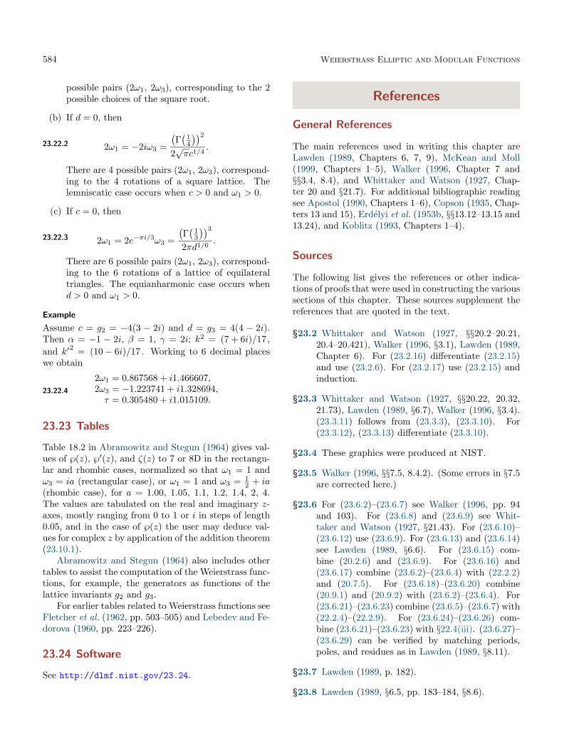
584 Weierstrass Elliptic and Modular Functions
possible pairs (2ω1, 2ω3), corresponding to the 2possible choices of the square root.
(b) If d = 0, then
23.22.2 2ω1 = −2iω3 =
(Γ(
14
))22√πc1/4
.
There are 4 possible pairs (2ω1, 2ω3), correspond-ing to the 4 rotations of a square lattice. Thelemniscatic case occurs when c > 0 and ω1 > 0.
(c) If c = 0, then
23.22.3 2ω1 = 2e−πi/3ω3 =
(Γ(
13
))32πd1/6
.
There are 6 possible pairs (2ω1, 2ω3), correspond-ing to the 6 rotations of a lattice of equilateraltriangles. The equianharmonic case occurs whend > 0 and ω1 > 0.
Example
Assume c = g2 = −4(3 − 2i) and d = g3 = 4(4 − 2i).Then α = −1 − 2i, β = 1, γ = 2i; k2 = (7 + 6i)/17 ,and k′
2 = (10− 6i)/17 . Working to 6 decimal placeswe obtain
23.22.4
2ω1 = 0.867568 + i1.466607,2ω3 = −1.223741 + i1.328694,τ = 0.305480 + i1.015109.
23.23 Tables
Table 18.2 in Abramowitz and Stegun (1964) gives val-ues of ℘(z), ℘′(z), and ζ(z) to 7 or 8D in the rectangu-lar and rhombic cases, normalized so that ω1 = 1 andω3 = ia (rectangular case), or ω1 = 1 and ω3 = 1
2 + ia(rhombic case), for a = 1.00, 1.05, 1.1, 1.2, 1.4, 2, 4.The values are tabulated on the real and imaginary z-axes, mostly ranging from 0 to 1 or i in steps of length0.05, and in the case of ℘(z) the user may deduce val-ues for complex z by application of the addition theorem(23.10.1).
Abramowitz and Stegun (1964) also includes othertables to assist the computation of the Weierstrass func-tions, for example, the generators as functions of thelattice invariants g2 and g3.
For earlier tables related to Weierstrass functions seeFletcher et al. (1962, pp. 503–505) and Lebedev and Fe-dorova (1960, pp. 223–226).
23.24 Software
See http://dlmf.nist.gov/23.24.
References
General References
The main references used in writing this chapter areLawden (1989, Chapters 6, 7, 9), McKean and Moll(1999, Chapters 1–5), Walker (1996, Chapter 7 and§§3.4, 8.4), and Whittaker and Watson (1927, Chap-ter 20 and §21.7). For additional bibliographic readingsee Apostol (1990, Chapters 1–6), Copson (1935, Chap-ters 13 and 15), Erdélyi et al. (1953b, §§13.12–13.15 and13.24), and Koblitz (1993, Chapters 1–4).
Sources
The following list gives the references or other indica-tions of proofs that were used in constructing the varioussections of this chapter. These sources supplement thereferences that are quoted in the text.
§23.2 Whittaker and Watson (1927, §§20.2–20.21,20.4–20.421), Walker (1996, §3.1), Lawden (1989,Chapter 6). For (23.2.16) differentiate (23.2.15)and use (23.2.6). For (23.2.17) use (23.2.15) andinduction.
§23.3 Whittaker and Watson (1927, §§20.22, 20.32,21.73), Lawden (1989, §6.7), Walker (1996, §3.4).(23.3.11) follows from (23.3.3), (23.3.10). For(23.3.12), (23.3.13) differentiate (23.3.10).
§23.4 These graphics were produced at NIST.
§23.5 Walker (1996, §§7.5, 8.4.2). (Some errors in §7.5are corrected here.)
§23.6 For (23.6.2)–(23.6.7) see Walker (1996, pp. 94and 103). For (23.6.8) and (23.6.9) see Whit-taker and Watson (1927, §21.43). For (23.6.10)–(23.6.12) use (23.6.9). For (23.6.13) and (23.6.14)see Lawden (1989, §6.6). For (23.6.15) com-bine (20.2.6) and (23.6.9). For (23.6.16) and(23.6.17) combine (23.6.2)–(23.6.4) with (22.2.2)and (20.7.5). For (23.6.18)–(23.6.20) combine(20.9.1) and (20.9.2) with (23.6.2)–(23.6.4). For(23.6.21)–(23.6.23) combine (23.6.5)–(23.6.7) with(22.2.4)–(22.2.9). For (23.6.24)–(23.6.26) com-bine (23.6.21)–(23.6.23) with §22.4(iii). (23.6.27)–(23.6.29) can be verified by matching periods,poles, and residues as in Lawden (1989, §8.11).
§23.7 Lawden (1989, p. 182).
§23.8 Lawden (1989, §6.5, pp. 183–184, §8.6).

References 585
§23.9 For (23.9.2)–(23.9.5) equate coefficients in(23.2.4), (23.2.5), and also apply (23.10.1),(23.10.2). The first two coefficients in the Maclau-rin expansion (23.9.6) are given by (23.3.9),(23.2.10); the others are obtained from §23.3(ii)combined with (23.9.4). (23.9.7) follows from(23.2.8) and (23.9.3).
§23.10 Whittaker and Watson (1927, §§20.3–20.311,20.41), Lawden (1989, pp. 152–158, 161–162).For (23.10.7), (23.10.9), (23.10.10) let v → uin (23.10.1)–(23.10.3). For (23.10.8) see Walker(1996, p. 83). For (23.10.11) and (23.10.12) com-pare the poles and residues of the two sides.(23.10.13) follows by integration. For (23.10.15)combine (23.10.14), (23.8.7), and (4.21.35).
§23.11 Dienstfrey and Huang (2006).
§23.12 These approximations follow from the expan-sions given in §23.8(ii). For (23.12.4) use Lawden(1989, Eq. 6.2.7) and (20.4.8).
§23.14 To verify these results differentiate and use(23.2.7), §23.3(ii).
§23.15 Apostol (1990, Chapters 1, 2), Walker (1996,Chapter 7), McKean and Moll (1999, Chapters 4,6). For (23.15.9) use (20.5.3) and (23.17.8).
§23.16 These graphics were produced at NIST.
§23.17 Walker (1996, §7.5). For (23.17.4)–(23.17.6)combine §23.15(ii) with the q-expansions of thetheta functions obtained by setting z = 0in §20.2(i). For (23.17.7), (23.17.8) combine(23.15.6), (23.15.9), and (20.5.1)–(20.5.3).
§23.18 See Walker (1996, Chapter 7), Ahlfors (1966,pp. 271–274), and Serre (1973, Chapter 7). For(23.18.4)–(23.18.7) see Apostol (1990, pp. 17, 52).
§23.19 Apostol (1990, Chapters 2, 3), Serre (1973,Chapter 7). (23.19.4) follows from (20.5.3) and(23.17.8).
§23.20 McKean and Moll (1999, §2.8).
§23.21 Jones (1964, pp. 31–33).
§23.22 For (23.22.1) combine (23.6.2)–(23.6.4) and§23.10(iv). (23.22.2) and (23.22.3) follow from(23.5.3) and (23.5.7), respectively.


Chapter 24
Bernoulli and Euler PolynomialsK. Dilcher1
Notation 58824.1 Special Notation . . . . . . . . . . . . . 588
Properties 58824.2 Definitions and Generating Functions . . 58824.3 Graphs . . . . . . . . . . . . . . . . . . . 58924.4 Basic Properties . . . . . . . . . . . . . . 58924.5 Recurrence Relations . . . . . . . . . . . 59124.6 Explicit Formulas . . . . . . . . . . . . . 59124.7 Integral Representations . . . . . . . . . 59224.8 Series Expansions . . . . . . . . . . . . . 59224.9 Inequalities . . . . . . . . . . . . . . . . 59324.10 Arithmetic Properties . . . . . . . . . . . 59324.11 Asymptotic Approximations . . . . . . . . 59324.12 Zeros . . . . . . . . . . . . . . . . . . . 594
24.13 Integrals . . . . . . . . . . . . . . . . . . 59424.14 Sums . . . . . . . . . . . . . . . . . . . 59524.15 Related Sequences of Numbers . . . . . . 59524.16 Generalizations . . . . . . . . . . . . . . 596
Applications 59724.17 Mathematical Applications . . . . . . . . 59724.18 Physical Applications . . . . . . . . . . . 598
Computation 59824.19 Methods of Computation . . . . . . . . . 59824.20 Tables . . . . . . . . . . . . . . . . . . . 59824.21 Software . . . . . . . . . . . . . . . . . . 598
References 598
1Dalhousie University, Halifax, Nova Scotia, Canada.Acknowledgments: This chapter is based in part on Abramowitz and Stegun (1964, Chapter 23) by E. V. Haynsworth and K.
Goldberg.Copyright c© 2009 National Institute of Standards and Technology. All rights reserved.
587

588 Bernoulli and Euler Polynomials
Notation
24.1 Special Notation
(For other notation see pp. xiv and 873.)
j, k, `,m, n integers, nonnegative unless statedotherwise.
t, x real or complex variables.p prime.p |m p divides m.(k,m) greatest common divisor of m,n.(k,m) = 1 k and m relatively prime.
Unless otherwise noted, the formulas in this chapterhold for all values of the variables x and t, and for allnonnegative integers n.
Bernoulli Numbers and Polynomials
The origin of the notation Bn, Bn(x), is not clear. Thepresent notation, as defined in §24.2(i), was used in Lu-cas (1891) and Nörlund (1924), and has become theprevailing notation; see Table 24.2.1. Among variousolder notations, the most common one is
B1 = 16 , B2 = 1
30 , B3 = 142 , B4 = 1
30 , . . . .
It was used in Saalschütz (1893), Nielsen (1923),Schwatt (1962), and Whittaker and Watson (1927).
Euler Numbers and Polynomials
The secant series ((4.19.5)) first occurs in the work ofGregory in 1671. Its coefficients were first studied in Eu-ler (1755); they were called Euler numbers by Raabe in1851. The notations En, En(x), as defined in §24.2(ii),were used in Lucas (1891) and Nörlund (1924).
Other historical remarks on notations can be foundin Cajori (1929, pp. 42–44). Various systems of notationare summarized in Adrian (1959) and D’Ocagne (1904).
Properties
24.2 Definitions and Generating Functions
24.2(i) Bernoulli Numbers and Polynomials
24.2.1t
et − 1=∞∑n=0
Bntn
n!, |t| < 2π.
24.2.2 B2n+1 = 0 , (−1)n+1B2n > 0, n = 1, 2, . . . .
24.2.3text
et − 1=∞∑n=0
Bn(x)tn
n!, |t| < 2π.
24.2.4 Bn = Bn(0),
24.2.5 Bn(x) =n∑k=0
(n
k
)Bk x
n−k.
See also §§4.19 and 4.33.
24.2(ii) Euler Numbers and Polynomials
24.2.62et
e2t + 1=∞∑n=0
Entn
n!, |t| < 1
2π,
24.2.7 E2n+1 = 0 , (−1)nE2n > 0 .
24.2.82ext
et + 1=∞∑n=0
En(x)tn
n!, |t| < π,
24.2.9 En = 2nEn(
12
)= integer,
24.2.10 En(x) =n∑k=0
(n
k
)Ek2k
(x− 12 )n−k.
See also (4.19.5).
24.2(iii) Periodic Bernoulli and Euler Functions
24.2.11 B̃n(x) = Bn(x) , Ẽn(x) = En(x), 0 ≤ x < 1,
24.2.12B̃n(x+ 1) = B̃n(x), Ẽn(x+ 1) = − Ẽn(x),
x ∈ R.

24.3 Graphs 589
24.2(iv) Tables
Table 24.2.1: Bernoulli and Euler numbers.
n Bn En
0 1 1
1 − 12 0
2 16 −1
4 − 130 5
6 142 −61
8 − 130 1385
10 566 −50521
12 − 6912730 27 02765
14 76 −1993 60981
16 − 3617510 1 93915 12145
Table 24.2.2: Bernoulli and Euler polynomials.
n Bn(x) En(x)
0 1 1
1 x− 12 x− 1
2
2 x2 − x+ 16 x2 − x
3 x3 − 32x
2 + 12x x3 − 3
2x2 + 1
4
4 x4 − 2x3 + x2 − 130 x4 − 2x3 + x
5 x5 − 52x
4 + 53x
3 − 16x x5 − 5
2x4 + 5
2x2 − 1
2
For extensions of Tables 24.2.1 and 24.2.2 see http://dlmf.nist.gov/24.2.iv.
24.3 Graphs
Figure 24.3.1: Bernoulli polynomials Bn(x), n =2, 3, . . . , 6.
Figure 24.3.2: Euler polynomials En(x), n = 2, 3, . . . , 6.
24.4 Basic Properties
24.4(i) Difference Equations
24.4.1 Bn(x+ 1)−Bn(x) = nxn−1,
24.4.2 En(x+ 1) + En(x) = 2xn.
24.4(ii) Symmetry
24.4.3 Bn(1− x) = (−1)nBn(x),
24.4.4 En(1− x) = (−1)nEn(x).
24.4.5 (−1)nBn(−x) = Bn(x) + nxn−1,
24.4.6 (−1)n+1En(−x) = En(x)− 2xn.
24.4(iii) Sums of Powers
24.4.7
m∑k=1
kn =Bn+1(m+ 1)−Bn+1
n+ 1,
24.4.8
m∑k=1
(−1)m−kkn =En(m+ 1) + (−1)mEn(0)
2.

590 Bernoulli and Euler Polynomials
24.4.9m−1∑k=0
(a+ dk)n =dn
n+ 1
(Bn+1
(m+
a
d
)−Bn+1
(ad
)),
24.4.10m−1∑k=0
(−1)k(a+ dk)n
=dn
2
((−1)m−1En
(m+
a
d
)+ En
(ad
)).
24.4.11m∑k=1
(k,m)=1
kn =1
n+ 1
n+1∑j=1
(n+ 1j
)
×
∏p|m
(1− pn−j)Bn+1−j
mj .
24.4(iv) Finite Expansions
24.4.12 Bn(x+ h) =n∑k=0
(n
k
)Bk(x)hn−k,
24.4.13 En(x+ h) =n∑k=0
(n
k
)Ek(x)hn−k,
24.4.14 En−1(x) =2n
n∑k=0
(n
k
)(1− 2k)Bk xn−k,
24.4.15
B2n =2n
22n(22n − 1)
n−1∑k=0
(2n− 1
2k
)E2k,
24.4.16
E2n =1
2n+ 1−
n∑k=1
(2n
2k − 1
)22k(22k−1 − 1)B2k
k,
24.4.17
E2n = 1−n∑k=1
(2n
2k − 1
)22k(22k − 1)B2k
2k.
24.4(v) Multiplication Formulas
Raabe’s Theorem
24.4.18 Bn(mx) = mn−1m−1∑k=0
Bn
(x+
k
m
).
Next,
24.4.19En(mx) = − 2mn
n+ 1
m−1∑k=0
(−1)k Bn+1
(x+
k
m
),
m = 2, 4, 6, . . . ,
24.4.20
En(mx) = mnm−1∑k=0
(−1)k En
(x+
k
m
), m = 1, 3, 5, . . . .
24.4.21 Bn(x) = 2n−1(Bn(
12x)
+Bn(
12x+ 1
2
)),
24.4.22 En−1(x) =2n
(Bn(x)− 2nBn
(12x)),
24.4.23 En−1(x) =2n
n
(Bn(
12x+ 1
2
)−Bn
(12x)),
24.4.24
Bn(mx) = mnBn(x) + n
n∑k=1
k−1∑j=0
(−1)j(n
k
)
×
(m−1∑r=1
e2πi(k−j)r/m
(1− e2πir/m)n
)(j +mx)n−1,
n = 1, 2, . . . , m = 2, 3, . . . .
24.4(vi) Special Values
24.4.25 Bn(0) = (−1)nBn(1) = Bn,
24.4.26 En(0) = −En(1) = − 2n+ 1
(2n+1 − 1)Bn+1 .
24.4.27 Bn(
12
)= −(1− 21−n)Bn,
24.4.28 En(
12
)= 2−nEn .
24.4.29 B2n
(13
)= B2n
(23
)= − 1
2 (1− 31−2n)B2n .
24.4.30
E2n−1
(13
)=−E2n−1
(23
)=− (1− 31−2n)(22n − 1)
2nB2n ,
n = 1, 2, . . . .24.4.31
Bn(
14
)= (−1)nBn
(34
)= −1− 21−n
2nBn−
n
4nEn−1 ,
n = 1, 2, . . . .24.4.32
B2n
(16
)= B2n
(56
)= 1
2 (1− 21−2n)(1− 31−2n)B2n,
24.4.33 E2n
(16
)= E2n
(56
)=
1 + 3−2n
22n+1E2n .
24.4(vii) Derivatives
24.4.34d
dxBn(x) = nBn−1(x), n = 1, 2, . . . ,
24.4.35d
dxEn(x) = nEn−1(x), n = 1, 2, . . . .
24.4(viii) Symbolic Operations
Let P (x) denote any polynomial in x, and after expand-ing set (B(x))n = Bn(x) and (E(x))n = En(x). Then
24.4.36 P (B(x) + 1)− P (B(x)) = P ′(x),
24.4.37 Bn(x+ h) = (B(x) + h)n,
24.4.38 P (E(x) + 1) + P (E(x)) = 2P (x),
24.4.39 En(x+ h) = (E(x) + h)n.For these results and also connections with the umbralcalculus see Gessel (2003).

24.5 Recurrence Relations 591
24.4(ix) Relations to Other Functions
For the relation of Bernoulli numbers to the Riemannzeta function see §25.6, and to the Eulerian numbers see(26.14.11).
24.5 Recurrence Relations
24.5(i) Basic Relations
24.5.1
n−1∑k=0
(n
k
)Bk(x) = nxn−1, n = 2, 3, . . . ,
24.5.2
n∑k=0
(n
k
)Ek(x) + En(x) = 2xn, n = 1, 2, . . . .
24.5.3
n−1∑k=0
(n
k
)Bk = 0, n = 2, 3, . . . ,
24.5.4
n∑k=0
(2n2k
)E2k = 0, n = 1, 2, . . . ,
24.5.5
n∑k=0
(n
k
)2k En−k +En = 2.
24.5(ii) Other Identities
24.5.6n∑k=2
(n
k − 2
)Bkk
=1
(n+ 1)(n+ 2)−Bn+1 , n = 2, 3, . . . ,
24.5.7
n∑k=0
(n
k
)Bk
n+ 2− k=Bn+1
n+ 1, n = 1, 2, . . . ,
24.5.8
n∑k=0
22k B2k
(2k)!(2n+ 1− 2k)!=
1(2n)!
, n = 1, 2, . . . .
24.5(iii) Inversion Formulas
In each of (24.5.9) and (24.5.10) the first identity im-plies the second one and vice-versa.
24.5.9 an =n∑k=0
(n
k
)bn−kk + 1
, bn =n∑k=0
(n
k
)Bk an−k.
24.5.10
an =bn/2 c∑k=0
(n
2k
)bn−2k,
bn =bn/2 c∑k=0
(n
2k
)E2k an−2k.
24.6 Explicit Formulas
The identities in this section hold for n = 1, 2, . . . .(24.6.7), (24.6.8), (24.6.10), and (24.6.12) are valid alsofor n = 0.
24.6.1 B2n =2n+1∑k=2
(−1)k−1
k
(2n+ 1k
) k−1∑j=1
j2n,
24.6.2 Bn =1
n+ 1
n∑k=1
k∑j=1
(−1)jjn(n+ 1k − j
)/(n
k
),
24.6.3 B2n =n∑k=1
(k − 1)!k!(2k + 1)!
k∑j=1
(−1)j−1
(2kk + j
)j2n.
24.6.4 E2n =n∑k=1
12k−1
k∑j=1
(−1)j(
2kk − j
)j2n,
24.6.5
E2n =1
2n−1
n−1∑k=0
(−1)n−k(n− k)2nk∑j=0
(2n− 2jk − j
)2j ,
24.6.6
E2n =2n∑k=1
(−1)k
2k−1
(2n+ 1k + 1
) j12k−
12
k∑j=0
(k
j
)(k − 2j)2n.
24.6.7 Bn(x) =n∑k=0
1k + 1
k∑j=0
(−1)j(k
j
)(x+ j)n,
24.6.8 En(x) =12n
n+1∑k=1
k−1∑j=0
(−1)j(n+ 1k
)(x+ j)n.
24.6.9 Bn =n∑k=0
1k + 1
k∑j=0
(−1)j(k
j
)jn,
24.6.10 En =12n
n+1∑k=1
(n+ 1k
) k−1∑j=0
(−1)j(2j + 1)n.
24.6.11 Bn =n
2n(2n − 1)
n∑k=1
k−1∑j=0
(−1)j+1
(n
k
)jn−1,
24.6.12 E2n =2n∑k=0
12k
k∑j=0
(−1)j(k
j
)(1 + 2j)2n.

592 Bernoulli and Euler Polynomials
24.7 Integral Representations
24.7(i) Bernoulli and Euler Numbers
The identities in this subsection hold for n = 1, 2, . . . .(24.7.6) also holds for n = 0.24.7.1
B2n = (−1)n+1 4n1− 21−2n
∫ ∞0
t2n−1
e2πt + 1dt
= (−1)n+1 2n1− 21−2n
∫ ∞0
t2n−1e−πt sech(πt) dt,
24.7.2
B2n = (−1)n+14n∫ ∞
0
t2n−1
e2πt − 1dt
= (−1)n+12n∫ ∞
0
t2n−1e−πt csch(πt) dt,
24.7.3
B2n = (−1)n+1 π
1− 21−2n
∫ ∞0
t2n sech2(πt) dt,
24.7.4
B2n = (−1)n+1π
∫ ∞0
t2n csch2(πt) dt,
24.7.5
B2n = (−1)n2n(2n− 1)
π
∫ ∞0
t2n−2 ln(1− e−2πt
)dt.
24.7.6
E2n = (−1)n22n+1
∫ ∞0
t2n sech(πt) dt.
24.7(ii) Bernoulli and Euler Polynomials
The following four equations hold for 0 < <x < 1.24.7.7
B2n(x) = (−1)n+12n
×∫ ∞
0
cos(2πx)− e−2πt
cosh(2πt)− cos(2πx)t2n−1 dt,
n = 1, 2, . . . ,24.7.8
B2n+1(x) = (−1)n+1(2n+ 1)
×∫ ∞
0
sin(2πx)cosh(2πt)− cos(2πx)
t2n dt.
24.7.9
E2n(x) = (−1)n4∫ ∞
0
sin(πx) cosh(πt)cosh(2πt)− cos(2πx)
t2n dt,
24.7.10
E2n+1(x) = (−1)n+14
×∫ ∞
0
cos(πx) sinh(πt)cosh(2πt)− cos(2πx)
t2n+1 dt.
Mellin–Barnes Integral
24.7.11
Bn(x) =1
2πi
∫ −c+i∞−c−i∞
(x+ t)n(
π
sin(πt)
)2dt, 0 < c < 1.
24.7(iii) Compendia
For further integral representations see Prudnikov et al.(1986a, §§2.3–2.6) and Gradshteyn and Ryzhik (2000,Chapters 3 and 4).
24.8 Series Expansions
24.8(i) Fourier Series
If n = 1, 2, . . . and 0 ≤ x ≤ 1, then
24.8.1 B2n(x) = (−1)n+1 2(2n)!(2π)2n
∞∑k=1
cos(2πkx)k2n
,
24.8.2 B2n+1(x) = (−1)n+1 2(2n+ 1)!(2π)2n+1
∞∑k=1
sin(2πkx)k2n+1
.
The second expansion holds also for n = 0 and 0 < x <1.
If n = 1 with 0 < x < 1, or n = 2, 3, . . . with0 ≤ x ≤ 1, then
24.8.3Bn(x) = − n!
(2πi)n
∞∑k=−∞k 6=0
e2πikx
kn.
If n = 1, 2, . . . and 0 ≤ x ≤ 1, then24.8.4
E2n(x) = (−1)n4(2n)!π2n+1
∞∑k=0
sin((2k + 1)πx)(2k + 1)2n+1
,
24.8.5
E2n−1(x) = (−1)n4(2n− 1)!
π2n
∞∑k=0
cos((2k + 1)πx)(2k + 1)2n
.
24.8(ii) Other Series
24.8.6
B4n+2 = (8n+ 4)∞∑k=1
k4n+1
e2πk − 1, n = 1, 2, . . . ,
24.8.7
B2n =(−1)n+14n
22n − 1
∞∑k=1
k2n−1
eπk + (−1)k+n, n = 2, 3, . . . .
Let αβ = π2. Then
24.8.8
B2n
4n(αn − (−β)n) = αn
∞∑k=1
k2n−1
e2αk − 1
− (−β)n∞∑k=1
k2n−1
e2βk − 1,
n = 2, 3, . . . .
24.8.9
E2n = (−1)n∞∑k=1
k2n
cosh(
12πk
)− 4
∞∑k=0
(−1)k(2k + 1)2n
e2π(2k+1) − 1, n = 1, 2, . . . .

24.9 Inequalities 593
24.9 Inequalities
Except where otherwise noted, the inequalities in thissection hold for n = 1, 2, . . . .
24.9.1 |B2n | > |B2n(x)|, 1 > x > 0,
24.9.2
(2− 21−2n)|B2n | ≥ |B2n(x)−B2n |, 1 ≥ x ≥ 0.
(24.9.3)–(24.9.5) hold for 12 > x > 0.
24.9.3 4−n|E2n | > (−1)nE2n(x) > 0,
24.9.4
2(2n+ 1)!(2π)2n+1
> (−1)n+1B2n+1(x) > 0, n = 2, 3, . . . ,
24.9.5
4(2n− 1)!π2n
22n − 122n − 2
> (−1)nE2n−1(x) > 0.
(24.9.6)–(24.9.7) hold for n = 2, 3, . . . .
24.9.6 5√πn( nπe
)2n> (−1)n+1B2n > 4
√πn( nπe
)2n,
24.9.7
8√n
π
(4nπe
)2n(1+
112n
)> (−1)nE2n > 8
√n
π
(4nπe
)2n.
Lastly,
24.9.8
2(2n)!(2π)2n
11− 2β−2n
≥ (−1)n+1B2n ≥2(2n)!(2π)2n
11− 2−2n
with
24.9.9 β = 2 +ln(1− 6π−2
)ln 2
= 0.6491 . . . .
24.9.10
4n+1(2n)!π2n+1
> (−1)nE2n >4n+1(2n)!π2n+1
11 + 3−1−2n
.
24.10 Arithmetic Properties
24.10(i) Von Staudt–Clausen Theorem
Here and elsewhere in §24.10 the symbol p denotes aprime number.
24.10.1 B2n +∑
(p−1)|2n
1p
= integer,
where the summation is over all p such that p−1 divides2n. The denominator of B2n is the product of all theseprimes p.
24.10.2 pB2n ≡ p− 1 (mod p`+1),
where n ≥ 2, and `(≥ 1) is an arbitrary integer such that(p− 1)p` | 2n. Here and elsewhere two rational numbersare congruent if the modulus divides the numerator oftheir difference.
24.10(ii) Kummer Congruences
24.10.3Bmm≡ Bn
n(mod p),
where m ≡ n 6≡ 0 (mod p− 1).
24.10.4 (1− pm−1)Bmm≡ (1− pn−1)
Bnn
(mod p`+1),
valid when m ≡ n (mod (p−1)p`) and n 6≡ 0 (mod p−1), where `(≥ 0) is a fixed integer.
24.10.5 En ≡ En+p−1 (mod p),where p(> 2) is a prime and n ≥ 2.
24.10.6 E2n ≡ E2n+w (mod 2`),valid for fixed integers `(≥ 0), and for all n(≥ 0) andw(≥ 0) such that 2` | w.
24.10(iii) Voronoi’s Congruence
Let B2n = N2n/D2n , with N2n and D2n relativelyprime and D2n > 0. Then
24.10.7
(b2n − 1)N2n
≡ 2nb2n−1D2n
M−1∑k=1
k2n−1
⌊kb
M
⌋(mod M),
where M(≥ 2) and b are integers, with b relatively primeto M .
For historical notes, generalizations, and applica-tions, see Porubský (1998).
24.10(iv) Factors
With N2n as in §24.10(iii)
24.10.8 N2n ≡ 0 (mod p`),valid for fixed integers `(≥ 1), and for all n(≥ 1) suchthat 2n 6≡ 0 (mod p− 1) and p` | 2n.
24.10.9 E2n ≡
{0 (mod p`) if p ≡ 1 (mod 4),2 (mod p`) if p ≡ 3 (mod 4),
valid for fixed integers `(≥ 1) and for all n(≥ 1) suchthat (p− 1)p`−1 | 2n.
24.11 Asymptotic Approximations
As n→∞
24.11.1 (−1)n+1B2n ∼2(2n)!(2π)2n
,
24.11.2 (−1)n+1B2n ∼ 4√πn( nπe
)2n,
24.11.3 (−1)nE2n ∼22n+2(2n)!π2n+1
,
24.11.4 (−1)nE2n ∼ 8√n
π
(4nπe
)2n.

594 Bernoulli and Euler Polynomials
Also,24.11.5
(−1)bn/2c−1 (2π)n
2(n!)Bn(x)→
{cos(2πx), n even,sin(2πx), n odd,
24.11.6
(−1)b(n+1)/2cπn+1
4(n!)En(x)→
{sin(πx), n even,cos(πx), n odd,
uniformly for x on compact subsets of C.For further results see Temme (1995b) and López
and Temme (1999b).
24.12 Zeros
24.12(i) Bernoulli Polynomials: Real Zeros
In the interval 0 ≤ x ≤ 1 the only zeros ofB2n+1(x), n =1, 2, . . . , are 0, 1
2 , 1, and the only zeros of B2n(x)−B2n,n = 1, 2, . . . , are 0, 1.
For the interval 12 ≤ x < ∞ denote the zeros of
Bn(x) by x(n)j , j = 1, 2, . . . , with
24.12.1 12 ≤ x
(n)1 ≤ x(n)
2 ≤ · · · .
Then the zeros in the interval −∞ < x ≤ 12 are 1−x(n)
j .When n(≥ 2) is even
24.12.234
+1
2n+2π< x
(n)1 <
34
+1
2n+1π,
24.12.3 x(n)1 − 3
4∼ 1
2n+1π, n→∞,
and as n→∞ with m(≥ 1) fixed,
24.12.4 x(n)2m−1 → m− 1
4 , x(n)2m → m+ 1
4 .
When n is odd x(n)1 = 1
2 , x(n)2 = 1 (n ≥ 3), and as
n→∞ with m(≥ 1) fixed,
24.12.5 x(n)2m−1 → m− 1
2 , x(n)2m → m.
Let R(n) be the total number of real zeros of Bn(x).Then R(n) = n when 1 ≤ n ≤ 5, and
24.12.6 R(n) ∼ 2n/(πe), n→∞.
24.12(ii) Euler Polynomials: Real Zeros
For the interval 12 ≤ x < ∞ denote the zeros of En(x)
by y(n)j , j = 1, 2, . . . , with
24.12.7 12 ≤ y
(n)1 ≤ y(n)
2 ≤ · · · .
Then the zeros in the interval −∞ < x ≤ 12 are 1−y(n)
j .
When n(≥ 2) is even y(n)1 = 1, and as n → ∞ with
m(≥ 1) fixed,
24.12.8 y(n)m → m.
When n is odd y(n)1 = 1
2 ,
24.12.932− πn+1
3(n!)< y
(n)2 <
32
, n = 3, 7, 11, . . . ,
24.12.1032< y
(n)2 <
32
+πn+1
3(n!), n = 5, 9, 13, . . . ,
and as n→∞ with m(≥ 1) fixed,
24.12.11 y(n)2m → m− 1
2 .
24.12(iii) Complex Zeros
For complex zeros of Bernoulli and Euler polynomials,see Delange (1987) and Dilcher (1988). A related topicis the irreducibility of Bernoulli and Euler polynomials.For details and references, see Dilcher (1987b), Kimura(1988), or Adelberg (1992).
24.12(iv) Multiple Zeros
Bn(x), n = 1, 2, . . . , has no multiple zeros. The onlypolynomial En(x) with multiple zeros is E5(x) = (x −12 )(x2 − x− 1)2.
24.13 Integrals
24.13(i) Bernoulli Polynomials
24.13.1
∫Bn(t) dt =
Bn+1(t)n+ 1
+ const.,
24.13.2
∫ x+1
x
Bn(t) dt = xn, n = 1, 2, . . . ,
24.13.3
∫ x+(1/2)
x
Bn(t) dt =En(2x)2n+1
,
24.13.4
∫ 1/2
0
Bn(t) dt =1− 2n+1
2nBn+1
n+ 1,
24.13.5
∫ 3/4
1/4
Bn(t) dt =En
22n+1.
For m,n = 1, 2, . . . ,
24.13.6
∫ 1
0
Bn(t)Bm(t) dt =(−1)n−1m!n!
(m+ n)!Bm+n .
24.13(ii) Euler Polynomials
24.13.7
∫En(t) dt =
En+1(t)n+ 1
+ const.,
24.13.8∫ 1
0
En(t) dt = −2En+1(0)n+ 1
=4(2n+2 − 1)
(n+ 1)(n+ 2)Bn+2,
24.13.9∫ 1/2
0
E2n(t) dt = −E2n+1(0)2n+ 1
=2(22n+2 − 1)B2n+2
(2n+ 1)(2n+ 2),
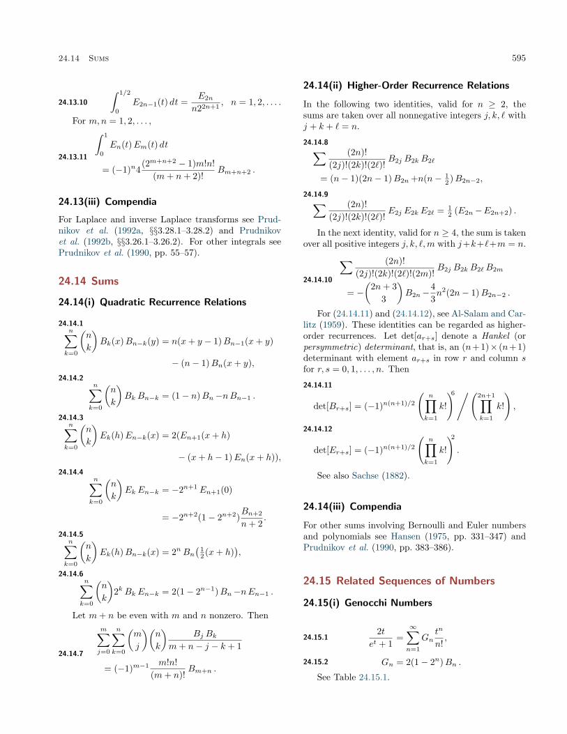
24.14 Sums 595
24.13.10
∫ 1/2
0
E2n−1(t) dt =E2n
n22n+1, n = 1, 2, . . . .
For m,n = 1, 2, . . . ,
24.13.11
∫ 1
0
En(t)Em(t) dt
= (−1)n4(2m+n+2 − 1)m!n!
(m+ n+ 2)!Bm+n+2 .
24.13(iii) Compendia
For Laplace and inverse Laplace transforms see Prud-nikov et al. (1992a, §§3.28.1–3.28.2) and Prudnikovet al. (1992b, §§3.26.1–3.26.2). For other integrals seePrudnikov et al. (1990, pp. 55–57).
24.14 Sums
24.14(i) Quadratic Recurrence Relations
24.14.1n∑k=0
(n
k
)Bk(x)Bn−k(y) = n(x+ y − 1)Bn−1(x+ y)
− (n− 1)Bn(x+ y),
24.14.2n∑k=0
(n
k
)Bk Bn−k = (1− n)Bn−nBn−1 .
24.14.3n∑k=0
(n
k
)Ek(h)En−k(x) = 2(En+1(x+ h)
− (x+ h− 1)En(x+ h)),
24.14.4n∑k=0
(n
k
)Ek En−k = −2n+1En+1(0)
= −2n+2(1− 2n+2)Bn+2
n+ 2.
24.14.5n∑k=0
(n
k
)Ek(h)Bn−k(x) = 2nBn
(12 (x+ h)
),
24.14.6n∑k=0
(n
k
)2k Bk En−k = 2(1− 2n−1)Bn−nEn−1 .
Let m+ n be even with m and n nonzero. Then
24.14.7
m∑j=0
n∑k=0
(m
j
)(n
k
)Bj Bk
m+ n− j − k + 1
= (−1)m−1 m!n!(m+ n)!
Bm+n .
24.14(ii) Higher-Order Recurrence Relations
In the following two identities, valid for n ≥ 2, thesums are taken over all nonnegative integers j, k, ` withj + k + ` = n.
24.14.8∑ (2n)!(2j)!(2k)!(2`)!
B2j B2k B2`
= (n− 1)(2n− 1)B2n +n(n− 12 )B2n−2,
24.14.9∑ (2n)!(2j)!(2k)!(2`)!
E2j E2k E2` = 12 (E2n−E2n+2) .
In the next identity, valid for n ≥ 4, the sum is takenover all positive integers j, k, `,m with j+k+`+m = n.
24.14.10
∑ (2n)!(2j)!(2k)!(2`)!(2m)!
B2j B2k B2`B2m
= −(
2n+ 33
)B2n−
43n2(2n− 1)B2n−2 .
For (24.14.11) and (24.14.12), see Al-Salam and Car-litz (1959). These identities can be regarded as higher-order recurrences. Let det[ar+s] denote a Hankel (orpersymmetric) determinant, that is, an (n+ 1)× (n+ 1)determinant with element ar+s in row r and column sfor r, s = 0, 1, . . . , n. Then
24.14.11
det[Br+s] = (−1)n(n+1)/2
(n∏k=1
k!
)6/(2n+1∏k=1
k!
),
24.14.12
det[Er+s] = (−1)n(n+1)/2
(n∏k=1
k!
)2.
See also Sachse (1882).
24.14(iii) Compendia
For other sums involving Bernoulli and Euler numbersand polynomials see Hansen (1975, pp. 331–347) andPrudnikov et al. (1990, pp. 383–386).
24.15 Related Sequences of Numbers
24.15(i) Genocchi Numbers
24.15.12t
et + 1=∞∑n=1
Gntn
n!,
24.15.2 Gn = 2(1− 2n)Bn .
See Table 24.15.1.

596 Bernoulli and Euler Polynomials
24.15(ii) Tangent Numbers
24.15.3 tan t =∞∑n=0
Tntn
n!,
24.15.4
T2n−1 = (−1)n−1 22n(22n − 1)2n
B2n , n = 1, 2, . . . ,
24.15.5 T2n = 0, n = 0, 1, . . . .
Table 24.15.1: Genocchi and Tangent numbers.
n 0 1 2 3 4 5 6 7 8
Gn 0 1 −1 0 1 0 −3 0 17
Tn 0 1 0 2 0 16 0 272 0
24.15(iii) Stirling Numbers
The Stirling numbers of the first kind s(n,m), and thesecond kind S(n,m), are as defined in §26.8(i).
24.15.6 Bn =n∑k=0
(−1)kk!S(n, k)k + 1
,
24.15.7 Bn =n∑k=0
(−1)k(n+ 1k + 1
)S(n+ k, k)
/(n+ k
k
),
24.15.8
n∑k=0
(−1)n+k s(n+ 1, k + 1)Bk =n!
n+ 1.
In (24.15.9) and (24.15.10) p denotes a prime. SeeHorata (1991).24.15.9
pBnn≡ S(p− 1 + n, p− 1) (mod p2), 1 ≤ n ≤ p− 2,
24.15.10
2n− 14n
p2B2n ≡ S(p+ 2n, p− 1) (mod p3),
2 ≤ 2n ≤ p− 3.
24.15(iv) Fibonacci and Lucas Numbers
The Fibonacci numbers are defined by u0 = 0, u1 = 1,and un+1 = un + un−1, n ≥ 1. The Lucas numbers aredefined by v0 = 2, v1 = 1, and vn+1 = vn+vn−1, n ≥ 1.24.15.11bn/2 c∑k=0
(n
2k
)(59
)kB2k un−2k =
n
6vn−1 +
n
3nv2n−2,
24.15.12bn/2 c∑k=0
(n
2k
)(54
)kE2k vn−2k =
12n−1
.
For further information on the Fibonacci numberssee §26.11.
24.16 Generalizations
24.16(i) Higher-Order Analogs
Polynomials and Numbers of Integer Order
For ` = 0, 1, 2, . . . , Bernoulli and Euler polynomials oforder ` are defined respectively by
24.16.1
(t
et − 1
)̀ext =
∞∑n=0
B(`)n (x)
tn
n!, |t| < 2π,
24.16.2
(2
et + 1
)̀ext =
∞∑n=0
E(`)n (x)
tn
n!, |t| < π.
When x = 0 they reduce to the Bernoulli and Eulernumbers of order `:
24.16.3 B(`)n = B(`)
n (0), E(`)n = E(`)
n (0).
Also for ` = 1, 2, 3, . . . ,
24.16.4
(ln(1 + t)
t
)̀= `
∞∑n=0
B(`+n)n
`+ n
tn
n!, |t| < 1.
For this and other properties see Milne-Thomson (1933,pp. 126–153) or Nörlund (1924, pp. 144–162).
For extensions of B(`)n (x) to complex values of x, n,
and `, and also for uniform asymptotic expansions forlarge x and large n, see Temme (1995b).
Bernoulli Numbers of the Second Kind
24.16.5t
ln(1 + t)=∞∑n=0
bntn, |t| < 1,
24.16.6 n!bn = − 1n− 1
B(n−1)n , n = 2, 3, . . . .
Degenerate Bernoulli Numbers
For sufficiently small |t|,
24.16.7t
(1 + λt) 1/λ − 1=∞∑n=0
βn(λ)tn
n!,
24.16.8
βn(λ) = n!bnλn +bn/2 c∑k=1
n
2kB2k s(n− 1, 2k − 1)λn−2k,
n = 2, 3, . . . .
Here s(n,m) again denotes the Stirling number of thefirst kind.
Nörlund Polynomials
24.16.9
(t
et − 1
)x=∞∑n=0
B(x)n
tn
n!, |t| < 2π.
B(x)n is a polynomial in x of degree n. (This notation is
consistent with (24.16.3) when x = `.)

Applications 597
24.16(ii) Character Analogs
Let χ be a primitive Dirichlet character mod f (see§27.8). Then f is called the conductor of χ. General-ized Bernoulli numbers and polynomials belonging to χare defined by
24.16.10
f∑a=1
χ(a)teat
eft − 1=∞∑n=0
Bn,χtn
n!,
24.16.11 Bn,χ(x) =n∑k=0
(n
k
)Bk,χx
n−k.
Let χ0 be the trivial character and χ4 the unique (non-trivial) character with f = 4; that is, χ4(1) = 1,χ4(3) = −1, χ4(2) = χ4(4) = 0. Then
24.16.12 Bn(x) = Bn,χ0(x− 1),
24.16.13 En(x) = − 21−n
n+ 1Bn+1,χ4(2x− 1).
For further properties see Berndt (1975a).
24.16(iii) Other Generalizations
In no particular order, other generalizations include:Bernoulli numbers and polynomials with arbitrary com-plex index (Butzer et al. (1992)); Euler numbers andpolynomials with arbitrary complex index (Butzer et al.(1994)); q-analogs (Carlitz (1954b), Andrews and Foata(1980)); conjugate Bernoulli and Euler polynomials(Hauss (1997, 1998)); Bernoulli–Hurwitz numbers (Katz(1975)); poly-Bernoulli numbers (Kaneko (1997)); Uni-versal Bernoulli numbers (Clarke (1989)); p-adic in-teger order Bernoulli numbers (Adelberg (1996)); p-adic q-Bernoulli numbers (Kim and Kim (1999)); pe-riodic Bernoulli numbers (Berndt (1975b)); cotangentnumbers (Girstmair (1990a)); Bernoulli–Carlitz num-bers (Goss (1978)); Bernoulli-Padé numbers (Dilcher(2002)); Bernoulli numbers belonging to periodic func-tions (Urbanowicz (1988)); cyclotomic Bernoulli num-bers (Girstmair (1990b)); modified Bernoulli numbers(Zagier (1998)); higher-order Bernoulli and Euler poly-nomials with multiple parameters (Erdélyi et al. (1953a,§§1.13.1, 1.14.1)).
Applications
24.17 Mathematical Applications
24.17(i) Summation
Euler–Maclaurin Summation Formula
See §2.10(i). For a generalization see Olver (1997b,p. 284).
Boole Summation Formula
Let 0 ≤ h ≤ 1 and a,m, and n be integers such thatn > a, m > 0, and f (m)(x) is absolutely integrable over[a, n]. Then with the notation of §24.2(iii)24.17.1n−1∑j=a
(−1)jf(j + h) =12
m−1∑k=0
Ek(h)k!
((−1)n−1f (k)(n)
+ (−1)af (k)(a))
+Rm(n),
where24.17.2
Rm(n) =1
2(m− 1)!
∫ n
a
f (m)(x) Ẽm−1(h− x) dx.
Calculus of Finite Differences
See Milne-Thomson (1933), Nörlund (1924), or Jordan(1965). For a more modern perspective see Grahamet al. (1994).
24.17(ii) Spline Functions
Euler Splines
Let Sn denote the class of functions that have n − 1continuous derivatives on R and are polynomials of de-gree at most n in each interval (k, k + 1), k ∈ Z. Themembers of Sn are called cardinal spline functions. Thefunctions
24.17.3 Sn(x) =Ẽn(x+ 1
2n+ 12
)Ẽn(
12n+ 1
2
) , n = 0, 1, . . . ,
are called Euler splines of degree n. For each n, Sn(x)is the unique bounded function such that Sn(x) ∈ Snand
24.17.4 Sn(k) = (−1)k, k ∈ Z.
The function Sn(x) is also optimal in a certain sense;see Schoenberg (1971).
Bernoulli Monosplines
A function of the form xn − S(x), with S(x) ∈ Sn−1
is called a cardinal monospline of degree n. Again withthe notation of §24.2(iii) define
24.17.5 Mn(x) =
{B̃n(x)−Bn, n even,B̃n(x+ 1
2
), n odd.
Mn(x) is a monospline of degree n, and it follows from(24.4.25) and (24.4.27) that
24.17.6 Mn(k) = 0, k ∈ Z.
For each n = 1, 2, . . . the function Mn(x) is alsothe unique cardinal monospline of degree n satisfying(24.17.6), provided that
24.17.7 Mn(x) = O(|x|γ), x→ ±∞,
for some positive constant γ.

598 Bernoulli and Euler Polynomials
For any n ≥ 2 the function
24.17.8 F (x) = B̃n(x)− 2−nBnis the unique cardinal monospline of degree n havingthe least supremum norm ‖F‖∞ on R (minimality prop-erty).
24.17(iii) Number Theory
Bernoulli and Euler numbers and polynomials occur in:number theory via (24.4.7), (24.4.8), and other identi-ties involving sums of powers; the Riemann zeta func-tion and L-series (§25.15, Apostol (1976), and Irelandand Rosen (1990)); arithmetic of cyclotomic fields andthe classical theory of Fermat’s last theorem (Riben-boim (1979) and Washington (1997)); p-adic analysis(Koblitz (1984, Chapter 2)).
24.18 Physical Applications
Bernoulli polynomials appear in statistical physics(Ordóñez and Driebe (1996)), in discussions of Casimirforces (Li et al. (1991)), and in a study of quark-gluonplasma (Meisinger et al. (2002)).
Euler polynomials also appear in statistical physicsas well as in semi-classical approximations to quan-tum probability distributions (Ballentine and McRae(1998)).
Computation
24.19 Methods of Computation
24.19(i) Bernoulli and Euler Numbers andPolynomials
Equations (24.5.3) and (24.5.4) enable Bn and En to becomputed by recurrence. For higher values of n more ef-ficient methods are available. For example, the tangentnumbers Tn can be generated by simple recurrence rela-tions obtained from (24.15.3), then (24.15.4) is applied.A similar method can be used for the Euler numbersbased on (4.19.5). For details see Knuth and Buckholtz(1967).
Another method is based on the identities
24.19.1 N2n =2(2n)!(2π)2n
∏p−1|2n
p
(∏p
p2n
p2n − 1
),
24.19.2 D2n =∏
p−1|2n
p, B2n =N2n
D2n.
If Ñ2n denotes the right-hand side of (24.19.1) but withthe second product taken only for p ≤
⌊(πe)−12n
⌋+ 1,
then N2n =⌈Ñ2n
⌉for n ≥ 2. For proofs and further
information see Fillebrown (1992).For other information see Chellali (1988) and Zhang
and Jin (1996, pp. 1–11). For algorithms for comput-ing Bn, En, Bn(x), and En(x) see Spanier and Oldham(1987, pp. 37, 41, 171, and 179–180).
24.19(ii) Values of Bn Modulo p
For number-theoretic applications it is important tocompute B2n (mod p) for 2n ≤ p − 3; in particularto find the irregular pairs (2n, p) for which B2n ≡ 0(mod p). We list here three methods, arranged in in-creasing order of efficiency.
• Tanner and Wagstaff (1987) derives a congruence(mod p) for Bernoulli numbers in terms of sumsof powers. See also §24.10(iii).
• Buhler et al. (1992) uses the expansion
24.19.3 t2
cosh t− 1= −2
∞∑n=0
(2n− 1)B2nt2n
(2n)!,
and computes inverses modulo p of the left-handside. Multisectioning techniques are applied in im-plementations. See also Crandall (1996, pp. 116–120).
• A method related to “Stickelberger codes” is ap-plied in Buhler et al. (2001); in particular, itallows for an efficient search for the irregularpairs (2n, p). Discrete Fourier transforms are usedin the computations. See also Crandall (1996,pp. 120–124).
24.20 Tables
Abramowitz and Stegun (1964, Chapter 23) includesexact values of
∑mk=1 k
n, m = 1(1)100, n = 1(1)10;∑∞k=1 k
−n,∑∞k=1(−1)k−1k−n,
∑∞k=0(2k + 1)−n, n =
1, 2, . . . , 20D;∑∞k=0(−1)k(2k+1)−n, n = 1, 2, . . . , 18D.
Wagstaff (1978) gives complete prime factorizationsof Nn and En for n = 20(2)60 and n = 8(2)42, respec-tively. In Wagstaff (2002) these results are extendedto n = 60(2)152 and n = 40(2)88, respectively, withfurther complete and partial factorizations listed up ton = 300 and n = 200, respectively.
For information on tables published before 1961 seeFletcher et al. (1962, v. 1, §4) and Lebedev and Fedorova(1960, Chapters 11 and 14).
24.21 Software
See http://dlmf.nist.gov/24.21.

References 599
References
General References
The main references used in writing this chapter areErdélyi et al. (1953a, Chapter 1), Nörlund (1924, Chap-ter 2), and Nörlund (1922). Introductions to the sub-ject are contained in Dence and Dence (1999) andRademacher (1973); see also Apostol (2008). A com-prehensive bibliography on the topics of this chaptercan be found in Dilcher et al. (1991).
Sources
The following list gives the references or other indica-tions of proofs that were used in constructing the varioussections of this chapter. These sources supplement thereferences that are quoted in the text.
§24.2 Nörlund (1924, Chapter 2), Milne-Thomson(1933, Chapter 6). Tables are from Abramowitzand Stegun (1964, pp. 809–810).
§24.3 These graphs were produced at NIST.
§24.4 Nörlund (1924, Chapter 2), Milne-Thomson(1933, Chapter 6), Howard (1996b), Slavutskĭı(2000), Apostol (2006), Todorov (1991). For(24.4.12)–(24.4.17) use (24.2.3) and (24.2.8). For(24.4.25)–(24.4.33) use §§24.4(ii) and 24.4(v). For(24.4.34) and (24.4.35) use (24.2.3) and (24.2.8).
§24.5 Erdélyi et al. (1953a, Chapter 1), Nörlund (1924,pp. 19 and 24), Apostol (2008), Apostol (1976,p. 275), Riordan (1979, p. 114).
§24.6 Gould (1972, pp. 45–46), Horata (1989), Todorov(1978), Schwatt (1962, p. 270), Carlitz (1961b,p. 134), Todorov (1991, pp. 176–177), Jordan(1965, p. 236).
§24.7 Erdélyi et al. (1953a, Chapter 1), Ramanujan(1927, p. 7), Paris and Kaminski (2001, p. 173).
§24.8 Apostol (1976, p. 267), Erdélyi et al. (1953a,p. 42), Berndt (1975b, pp. 176–178).
§24.9 Olver (1997b, p. 283), Temme (1996a, p. 16),Lehmer (1940, p. 538), Leeming (1989), Alzer(2000). For (24.9.5) use (24.9.8), (24.4.35),(24.2.7), and (24.4.26). For (24.9.10) use (24.4.28)and (24.8.4) with x = 1
2 ; see also Lehmer (1940,p. 538).
§24.10 Ireland and Rosen (1990, Chapter 15), Wash-ington (1997, Chapter 5), Carlitz (1953, p. 167),Ernvall (1979, pp. 36 and 24), Slavutskĭı (1995,1999), Uspensky and Heaslet (1939, p. 261),Ribenboim (1979, p. 105), Girstmair (1990b),Carlitz (1954a).
§24.11 Leeming (1977), Dilcher (1987a).
§24.12 Olver (1997b, p. 283), Inkeri (1959), Leeming(1989), Delange (1991), Lehmer (1940), Dilcher(1988, p. 77), Howard (1976), Delange (1988),Dilcher (2008), Brillhart (1969).
§24.13 Nörlund (1922, p. 143), Apostol (1976, p. 276),Nörlund (1924, pp. 31 and 36). For (24.13.1) and(24.13.2) use (24.4.34) and (24.4.1).
§24.14 Nörlund (1922, pp. 135–142), Carlitz (1961a,p. 992), Dilcher (1996), Sitaramachandrarao andDavis (1986), Huang and Huang (1999).
§24.15 Dumont and Viennot (1980), Graham et al.(1994, Chapter 6), Knuth and Buckholtz (1967),Todorov (1984, pp. 310 and 343), Gould (1972,pp. 44 and 48), Kelisky (1957, pp. 32 and 34).
§24.16 Howard (1996a), Washington (1997, pp. 31–34), Dilcher (1988, pp. 8 and 9).
§24.17 Temme (1996a, pp. 17 and 18), Nörlund(1924, pp. 29–36), Schumaker (1981, pp. 152–153),Schoenberg (1973, pp. 40–41 and 101).
§24.19 For (24.19.3) use (24.2.1).


Chapter 25
Zeta and Related FunctionsT. M. Apostol1
Notation 60225.1 Special Notation . . . . . . . . . . . . . 602
Riemann Zeta Function 60225.2 Definition and Expansions . . . . . . . . 60225.3 Graphics . . . . . . . . . . . . . . . . . . 60325.4 Reflection Formulas . . . . . . . . . . . . 60325.5 Integral Representations . . . . . . . . . 60425.6 Integer Arguments . . . . . . . . . . . . 60525.7 Integrals . . . . . . . . . . . . . . . . . . 60625.8 Sums . . . . . . . . . . . . . . . . . . . 60625.9 Asymptotic Approximations . . . . . . . . 60625.10 Zeros . . . . . . . . . . . . . . . . . . . 606
Related Functions 60725.11 Hurwitz Zeta Function . . . . . . . . . . 607
25.12 Polylogarithms . . . . . . . . . . . . . . 61025.13 Periodic Zeta Function . . . . . . . . . . 61225.14 Lerch’s Transcendent . . . . . . . . . . . 61225.15 Dirichlet L-functions . . . . . . . . . . . 612
Applications 61325.16 Mathematical Applications . . . . . . . . 61325.17 Physical Applications . . . . . . . . . . . 614
Computation 61425.18 Methods of Computation . . . . . . . . . 61425.19 Tables . . . . . . . . . . . . . . . . . . . 61425.20 Approximations . . . . . . . . . . . . . . 61525.21 Software . . . . . . . . . . . . . . . . . . 615
References 615
1California Institute of Technology, Pasadena, California.Copyright c© 2009 National Institute of Standards and Technology. All rights reserved.
601

602 Zeta and Related Functions
Notation
25.1 Special Notation
(For other notation see pp. xiv and 873.)
k,m, n nonnegative integers.p prime number.x real variable.a real or complex parameter.s = σ + it complex variable.z = x+ iy complex variable.γ Euler’s constant (§5.2(ii)).ψ(x) digamma function Γ′(x)/Γ(x) except in
§25.16. See §5.2(i).Bn, Bn(x) Bernoulli number and polynomial
(§24.2(i)).B̃n(x) periodic Bernoulli function Bn(x− bxc).m | n m divides n.primes on function symbols: derivatives with
respect to argument.
The main function treated in this chapter is the Rie-mann zeta function ζ(s). This notation was introducedin Riemann (1859).
The main related functions are the Hurwitz zetafunction ζ(s, a), the dilogarithm Li2(z), the polylog-arithm Lis(z) (also known as Jonquière’s functionφ(z, s)), Lerch’s transcendent Φ(z, s, a), and the Dirich-let L-functions L(s, χ).
Riemann Zeta Function
25.2 Definition and Expansions
25.2(i) Definition
When <s > 1,
25.2.1 ζ(s) =∞∑n=1
1ns.
Elsewhere ζ(s) is defined by analytic continuation. It isa meromorphic function whose only singularity in C isa simple pole at s = 1, with residue 1.
25.2(ii) Other Infinite Series
25.2.2 ζ(s) =1
1− 2−s
∞∑n=0
1(2n+ 1)s
, <s > 1.
25.2.3 ζ(s) =1
1− 21−s
∞∑n=1
(−1)n−1
ns, <s > 0.
25.2.4 ζ(s) =1
s− 1+∞∑n=0
(−1)n
n!γn(s− 1)n, <s > 0,
where
25.2.5 γn = limm→∞
(m∑k=1
(ln k)n
k− (lnm)n+1
n+ 1
).
25.2.6 ζ ′(s) = −∞∑n=2
(lnn)n−s, <s > 1.
25.2.7
ζ(k)(s) = (−1)k∞∑n=2
(lnn)kn−s, <s > 1, k = 1, 2, 3, . . . .
For further expansions of functions similar to(25.2.1) (Dirichlet series) see §27.4. This includes, forexample, 1/ ζ(s).
25.2(iii) Representations by theEuler–Maclaurin Formula
25.2.8ζ(s) =
N∑k=1
1ks
+N1−s
s− 1− s
∫ ∞N
x− bxcxs+1
dx,
<s > 0, N = 1, 2, 3, . . . .
25.2.9
ζ(s) =N∑k=1
1ks
+N1−s
s− 1− 1
2N−s
+n∑k=1
(s+ 2k − 2
2k − 1
)B2k
2kN1−s−2k
−(s+ 2n2n+ 1
)∫ ∞N
B̃2n+1(x)xs+2n+1
dx,
<s > −2n; n,N = 1, 2, 3, . . . .
25.2.10
ζ(s) =1
s− 1+
12
+n∑k=1
(s+ 2k − 2
2k − 1
)B2k
2k
−(s+ 2n2n+ 1
)∫ ∞1
B̃2n+1(x)xs+2n+1
dx,
<s > −2n, n = 1, 2, 3, . . . .
For B2k see §24.2(i), and for B̃n(x) see §24.2(iii).
25.2(iv) Infinite Products
25.2.11 ζ(s) =∏p
(1− p−s)−1, <s > 1,
product over all primes p.
25.2.12 ζ(s) =(2π)se−s−(γs/2)
2(s− 1) Γ(
12s+ 1
) ∏ρ
(1− s
ρ
)es/ρ,
product over zeros ρ of ζ with <ρ > 0 (see §25.10(i)); γis Euler’s constant (§5.2(ii)).

25.3 Graphics 603
25.3 Graphics
Figure 25.3.1: Riemann zeta function ζ(x) and itsderivative ζ ′(x), −20 ≤ x ≤ 10.
�
Figure 25.3.2: Riemann zeta function ζ(x) and itsderivative ζ ′(x), −12 ≤ x ≤ −2.
Figure 25.3.3: Modulus of the Riemann zeta function| ζ(x+ iy)|, −4 ≤ x ≤ 4, −10 ≤ y ≤ 40.
Figure 25.3.4: Z(t), 0 ≤ t ≤ 50. Z(t) and ζ(
12 + it
)have
the same zeros. See §25.10(i).
Figure 25.3.5: Z(t), 1000 ≤ t ≤ 1050.
Figure 25.3.6: Z(t), 10000 ≤ t ≤ 10050.
25.4 Reflection Formulas
For s 6= 0, 1,
25.4.1 ζ(1− s) = 2(2π)−s cos(
12πs
)Γ(s) ζ(s),
25.4.2 ζ(s) = 2(2π)s−1 sin(
12πs
)Γ(1− s) ζ(1− s).
Equivalently,
25.4.3 ξ(s) = ξ(1− s),

604 Zeta and Related Functions
where ξ(s) is Riemann’s ξ-function, defined by:
25.4.4 ξ(s) = 12s(s− 1) Γ
(12s)π−s/2 ζ(s).
For s 6= 0, 1 and k = 1, 2, 3, . . . ,25.4.5
(−1)k ζ(k)(1− s)
=2
(2π)s
k∑m=0
m∑r=0
(k
m
)(m
r
)(<(ck−m) cos
(12πs
)+ =(ck−m) sin
(12πs
))Γ(r)(s) ζ(m−r)(s),
where
25.4.6 c = − ln(2π)− 12πi.
25.5 Integral Representations
25.5(i) In Terms of Elementary Functions
Throughout this subsection s 6= 1.
25.5.1 ζ(s) =1
Γ(s)
∫ ∞0
xs−1
ex − 1dx, <s > 1.
25.5.2 ζ(s) =1
Γ(s+ 1)
∫ ∞0
exxs
(ex − 1)2dx, <s > 1.
25.5.3 ζ(s) =1
(1− 21−s) Γ(s)
∫ ∞0
xs−1
ex + 1dx, <s > 0.
25.5.4ζ(s) =
1(1− 21−s) Γ(s+ 1)
∫ ∞0
exxs
(ex + 1)2dx,
<s > 0.
25.5.5 ζ(s) = −s∫ ∞
0
x− bxc − 12
xs+1dx, −1 < <s < 0.
25.5.6
ζ(s) =12
+1
s− 1+
1Γ(s)
∫ ∞0
(1
ex − 1− 1x
+12
)xs−1
exdx,
<s > −1.
25.5.7ζ(s) =
12
+1
s− 1+
n∑m=1
B2m
(2m)!Γ(s+ 2m− 1)
Γ(s)+
1Γ(s)
∫ ∞0
(1
ex − 1− 1x
+12−
n∑m=1
B2m
(2m)!x2m−1
)xs−1
exdx,
<s > −(2n+ 1), n = 1, 2, 3, . . . .
25.5.8 ζ(s) =1
2(1− 2−s) Γ(s)
∫ ∞0
xs−1
sinhxdx, <s > 1.
25.5.9 ζ(s) =2s−1
Γ(s+ 1)
∫ ∞0
xs
(sinhx)2dx, <s > 1.
25.5.10 ζ(s) =2s−1
1− 21−s
∫ ∞0
cos(s arctanx)(1 + x2)s/2 cosh
(12πx
) dx.25.5.11
ζ(s) =12
+1
s− 1+ 2
∫ ∞0
sin(s arctanx)(1 + x2)s/2(e2πx − 1)
dx.
25.5.12 ζ(s) =2s−1
s− 1− 2s
∫ ∞0
sin(s arctanx)(1 + x2)s/2(eπx + 1)
dx.
25.5(ii) In Terms of Other Functions
25.5.13
ζ(s) =πs/2
s(s− 1) Γ(
12s)
+πs/2
Γ(
12s) ∫ ∞
1
(xs/2 + x(1−s)/2
) ω(x)x
dx,
s 6= 1,where
25.5.14 ω(x) =∞∑n=1
e−n2πx =
12
(θ3(0|ix)− 1) .
For θ3 see §20.2(i). For similar representations involvingother theta functions see Erdélyi et al. (1954a, p. 339).
In (25.5.15)–(25.5.19), 0 < <s < 1, ψ(x) is thedigamma function, and γ is Euler’s constant (§5.2).(25.5.16) is also valid for 0 < <s < 2, s 6= 1.
25.5.15ζ(s) =
1s− 1
+sin(πs)π
×∫ ∞
0
(ln(1 + x)− ψ(1 + x))x−s dx,
25.5.16
ζ(s) =1
s− 1+
sin(πs)π(s− 1)
×∫ ∞
0
(1
1 + x−ψ′(1 + x)
)x1−s dx,
25.5.17 ζ(1 + s) =sin(πs)π
∫ ∞0
(γ+ψ(1 + x))x−s−1 dx,
25.5.18 ζ(1 + s) =sin(πs)πs
∫ ∞0
ψ′(1 + x)x−s dx,
25.5.19
ζ(m+ s) = (−1)m−1 Γ(s) sin(πs)π Γ(m+ s)
×∫ ∞
0
ψ(m)(1 + x)x−s dx,
m = 1, 2, 3, . . . .

25.6 Integer Arguments 605
25.5(iii) Contour Integrals
25.5.20
ζ(s) =Γ(1− s)
2πi
∫ (0+)
−∞
zs−1
e−z − 1dz, s 6= 1, 2, . . . ,
where the integration contour is a loop around the neg-ative real axis; it starts at −∞, encircles the origin oncein the positive direction without enclosing any of thepoints z = ±2πi, ±4πi, . . . , and returns to −∞. Equiv-alently,25.5.21
ζ(s) =Γ(1− s)
2πi(1− 21−s)
∫ (0+)
−∞
zs−1
e−z + 1dz, s 6= 1, 2, . . . .
The contour here is any loop that encircles the originin the positive direction not enclosing any of the points±πi, ±3πi, . . . .
25.6 Integer Arguments
25.6(i) Function Values
25.6.1
ζ(0) = −12, ζ(2) =
π2
6, ζ(4) =
π4
90, ζ(6) =
π6
945.
25.6.2 ζ(2n) =(2π)2n
2(2n)!|B2n| , n = 1, 2, 3, . . . .
25.6.3 ζ(−n) = −Bn+1
n+ 1, n = 1, 2, 3, . . . .
25.6.4 ζ(−2n) = 0, n = 1, 2, 3, . . . .
25.6.5
ζ(k + 1) =1k!
∞∑n1=1
. . .
∞∑nk=1
1n1 · · ·nk(n1 + · · ·+ nk)
,
k = 1, 2, 3, . . . .
25.6.6
ζ(2k + 1) =(−1)k+1(2π)2k+1
2(2k + 1)!
∫ 1
0
B2k+1(t) cot(πt) dt,
k = 1, 2, 3, . . . .
25.6.7 ζ(2) =∫ 1
0
∫ 1
0
11− xy
dx dy.
25.6.8 ζ(2) = 3∞∑k=1
1k2(
2kk
) .25.6.9 ζ(3) =
52
∞∑k=1
(−1)k−1
k3(
2kk
) .25.6.10 ζ(4) =
3617
∞∑k=1
1k4(
2kk
) .25.6(ii) Derivative Values
25.6.11 ζ ′(0) = − 12 ln(2π).
25.6.12 ζ ′′(0) = − 12 (ln(2π))2 + 1
2γ2 − 1
24π2 + γ1,
where γ1 is given by (25.2.5).
With c defined by (25.4.6) and n = 1, 2, 3, . . . ,
25.6.13 (−1)k ζ(k)(−2n) =2(−1)n
(2π)2n+1
k∑m=0
m∑r=0
(k
m
)(m
r
)=(ck−m) Γ(r)(2n+ 1) ζ(m−r)(2n+ 1),
25.6.14 (−1)k ζ(k)(1− 2n) =2(−1)n
(2π)2n
k∑m=0
m∑r=0
(k
m
)(m
r
)<(ck−m) Γ(r)(2n) ζ(m−r)(2n),
25.6.15 ζ ′(2n) =(−1)n+1(2π)2n
2(2n)!(2n ζ ′(1− 2n)− (ψ(2n)− ln(2π))B2n) .
25.6(iii) Recursion Formulas
25.6.16 (n+ 1
2
)ζ(2n) =
n−1∑k=1
ζ(2k) ζ(2n− 2k), n ≥ 2.
25.6.17(n+ 3
4
)ζ(4n+ 2) =
n∑k=1
ζ(2k) ζ(4n+ 2− 2k), n ≥ 1.
25.6.18(n+ 1
4
)ζ(4n) + 1
2 (ζ(2n))2 =n∑k=1
ζ(2k) ζ(4n− 2k),
n ≥ 1.
25.6.19
(m+ n+ 3
2
)ζ(2m+ 2n+ 2)
=
(m∑k=1
+n∑k=1
)ζ(2k) ζ(2m+ 2n+ 2− 2k),
m ≥ 0, n ≥ 0, m+ n ≥ 1.

606 Zeta and Related Functions
25.6.20
12 (22n − 1) ζ(2n) =
n−1∑k=1
(22n−2k − 1) ζ(2n− 2k) ζ(2k),
n ≥ 2.
For related results see Basu and Apostol (2000).
25.7 Integrals
For definite integrals of the Riemann zeta function seePrudnikov et al. (1986b, §2.4), Prudnikov et al. (1992a,§3.2), and Prudnikov et al. (1992b, §3.2).
25.8 Sums
25.8.1
∞∑k=2
(ζ(k)− 1) = 1.
25.8.2
∞∑k=0
Γ(s+ k)(k + 1)!
(ζ(s+ k)− 1)
= Γ(s− 1), s 6= 1, 0,−1,−2, . . . .
25.8.3
∞∑k=0
Γ(s+ k) ζ(s+ k)k! Γ(s)2s+k
= (1− 2−s) ζ(s), s 6= 1.
25.8.4
∞∑k=1
(−1)k
k(ζ(nk)− 1) = ln
n−1∏j=0
Γ(
2− e(2j+1)πi/n),
n = 2, 3, 4, . . . .
25.8.5
∞∑k=2
ζ(k)zk = −γz − z ψ(1− z), |z| < 1.
25.8.6
∞∑k=0
ζ(2k)z2k = − 12πz cot(πz), |z| < 1.
25.8.7
∞∑k=2
ζ(k)k
zk = −γz + ln Γ(1− z), |z| < 1.
25.8.8
∞∑k=1
ζ(2k)k
z2k = ln(
πz
sin(πz)
), |z| < 1.
25.8.9
∞∑k=1
ζ(2k)(2k + 1)22k
=12− 1
2ln 2.
25.8.10
∞∑k=1
ζ(2k)(2k + 1)(2k + 2)22k
=14− 7
4π2ζ(3).
For other sums see Prudnikov et al. (1986b, pp. 648–649), Hansen (1975, pp. 355–357), Ogreid and Osland(1998), and Srivastava and Choi (2001, Chapter 3).
25.9 Asymptotic Approximations
If x ≥ 1, y ≥ 1, 2πxy = t, and 0 ≤ σ ≤ 1, then ast→∞ with σ fixed,
25.9.1
ζ(σ + it) =∑
1≤n≤x
1ns
+ χ(s)∑
1≤n≤y
1n1−s
+O(x−σ
)+O
(yσ−1t
12−σ
),
where s = σ + it and
25.9.2 χ(s) = πs−12 Γ(
12 −
12s)/Γ(
12s).
If σ = 12 , x = y =
√t/(2π), and m = bxc, then
(25.9.1) becomes
25.9.3
ζ(
12 + it
)=
m∑n=1
1n
12 +it
+ χ(
12 + it
) m∑n=1
1n
12−it
+O(t−1/4
).
For other asymptotic approximations see Berry andKeating (1992), Paris and Cang (1997); see also Parisand Kaminski (2001, pp. 380–389).
25.10 Zeros
25.10(i) Distribution
The product representation (25.2.11) implies ζ(s) 6= 0for <s > 1. Also, ζ(s) 6= 0 for <s = 1, a prop-erty first established in Hadamard (1896) and de laVallée Poussin (1896a,b) in the proof of the prime num-ber theorem (25.16.3). The functional equation (25.4.1)implies ζ(−2n) = 0 for n = 1, 2, 3, . . . . These are calledthe trivial zeros. Except for the trivial zeros, ζ(s) 6= 0for <s ≤ 0. In the region 0 < <s < 1, called thecritical strip, ζ(s) has infinitely many zeros, distributedsymmetrically about the real axis and about the criticalline <s = 1
2 . The Riemann hypothesis states that allnontrivial zeros lie on this line.
Calculations relating to the zeros on the critical linemake use of the real-valued function
25.10.1 Z(t) = exp(iϑ(t)) ζ(
12 + it
),
where
25.10.2 ϑ(t) ≡ ph Γ(
14 + 1
2 it)− 1
2 t lnπ
is chosen to make Z(t) real, and ph Γ(
14 + 1
2 it)
assumesits principal value. Because |Z(t)| = | ζ
(12 + it
)|, Z(t)
vanishes at the zeros of ζ(
12 + it
), which can be sepa-
rated by observing sign changes of Z(t). Because Z(t)changes sign infinitely often, ζ
(12 + it
)has infinitely
many zeros with t real.

Related Functions 607
25.10(ii) Riemann–Siegel Formula
Riemann developed a method for counting the totalnumber N(T ) of zeros of ζ(s) in that portion of thecritical strip with 0 < t < T . By comparing N(T )with the number of sign changes of Z(t) we can de-cide whether ζ(s) has any zeros off the line in this re-gion. Sign changes of Z(t) are determined by multiply-ing (25.9.3) by exp(iϑ(t)) to obtain the Riemann–Siegelformula:
25.10.3 Z(t) = 2m∑n=1
cos(ϑ(t)− t lnn)n1/2
+R(t),
where R(t) = O(t−1/4
)as t→∞.
The error term R(t) can be expressed as an asymp-totic series that begins25.10.4
R(t) = (−1)m−1
(2πt
)1/4 cos(t− (2m+ 1)
√2πt− 1
8π)
cos(√
2πt)
+O(t−3/4
).
Riemann also developed a technique for determin-ing further terms. Calculations based on the Riemann–Siegel formula reveal that the first ten billion zeros ofζ(s) in the critical strip are on the critical line (van deLune et al. (1986)). More than one-third of all the ze-ros in the critical strip lie on the critical line (Levinson(1974)).
For further information on the Riemann–Siegel ex-pansion see Berry (1995).
Related Functions
25.11 Hurwitz Zeta Function
25.11(i) Definition
The function ζ(s, a) was introduced in Hurwitz (1882)and defined by the series expansion
25.11.1
ζ(s, a) =∞∑n=0
1(n+ a)s
, <s > 1, a 6= 0,−1,−2, . . . .
ζ(s, a) has a meromorphic continuation in the s-plane, its only singularity in C being a simple pole ats = 1 with residue 1. As a function of a, with s ( 6= 1)fixed, ζ(s, a) is analytic in the half-plane <a > 0. TheRiemann zeta function is a special case:
25.11.2 ζ(s, 1) = ζ(s).
For most purposes it suffices to restrict 0 < <a ≤ 1because of the following straightforward consequencesof (25.11.1):
25.11.3 ζ(s, a) = ζ(s, a+ 1) + a−s,
25.11.4
ζ(s, a) = ζ(s, a+m) +m−1∑n=0
1(n+ a)s
, m = 1, 2, 3, . . . .
Most references treat real a with 0 < a ≤ 1.
25.11(ii) Graphics
Figure 25.11.1: Hurwitz zeta function ζ(x, a), a = 0.3,0.5, 0.8, 1, −20 ≤ x ≤ 10. The curves are almost indis-tinguishable for −14 < x < −1, approximately.
Figure 25.11.2: Hurwitz zeta function ζ(x, a), −19.5 ≤x ≤ 10, 0.02 ≤ a ≤ 1.

608 Zeta and Related Functions
25.11(iii) Representations by the Euler–Maclaurin Formula
25.11.5 ζ(s, a) =N∑n=0
1(n+ a)s
+(N + a)1−s
s− 1− s
∫ ∞N
x− bxc(x+ a)s+1
dx, s 6= 1, <s > 0, a > 0, N = 0, 1, 2, 3, . . . .
25.11.6 ζ(s, a) =1as
(12
+a
s− 1
)− s(s+ 1)
∫ ∞0
B̃2(x)(x+ a)s+2
dx, s 6= 1, <s > −1, a > 0.
25.11.7
ζ(s, a) =1as
+1
(1 + a)s
(12
+1 + a
s− 1
)+
n∑k=1
(s+ 2k − 2
2k − 1
)B2k
2k1
(1 + a)s+2k−1−(s+ 2n2n+ 1
)∫ ∞1
B̃2n+1(x)(x+ a)s+2n+1
dx,
s 6= 1, a > 0, n = 1, 2, 3, . . . , <s > −2n.
For B̃n(x) see §24.2(iii).
25.11(iv) Series Representations
25.11.8ζ(s, 1
2a)
= ζ(s, 1
2a+ 12
)+ 2s
∞∑n=0
(−1)n
(n+ a)s,
<s > 0, s 6= 1, 0 < a ≤ 1.
25.11.9ζ(1− s, a) =
2 Γ(s)(2π)s
∞∑n=1
1ns
cos(
12πs− 2nπa
),
<s > 1, 0 < a ≤ 1.
25.11.10ζ(s, a) =
∞∑n=0
Γ(n+ s)n! Γ(s)
ζ(n+ s)(1− a)n,
s 6= 1, |a− 1| < 1.
When a = 12 , (25.11.10) reduces to (25.8.3); compare
(25.11.11).
25.11(v) Special Values
Throughout this subsection <a > 0.
25.11.11 ζ(s, 1
2
)= (2s − 1) ζ(s), s 6= 1.
25.11.12
ζ(n+ 1, a) =(−1)n+1 ψ(n)(a)
n!, n = 1, 2, 3, . . . .
25.11.13 ζ(0, a) = 12 − a.
25.11.14 ζ(−n, a) = −Bn+1(a)n+ 1
, n = 0, 1, 2, . . . .
25.11.15
ζ(s, ka) = k−sk−1∑n=0
ζ(s, a+
n
k
), s 6= 1, k = 1, 2, 3, . . . .
25.11.16
ζ
(1− s, h
k
)=
2 Γ(s)(2πk)s
k∑r=1
cos(πs
2− 2πrh
k
)ζ(s,r
k
),
s 6= 0, 1; h, k integers, 1 ≤ h ≤ k.
25.11(vi) Derivatives
a-Derivative
25.11.17∂
∂aζ(s, a) = −s ζ(s+ 1, a), s 6= 0, 1; <a > 0.
s-Derivatives
In (25.11.18)–(25.11.24) primes on ζ denote deriva-tives with respect to s. Similarly in §§25.11(viii) and25.11(xii).
25.11.18 ζ ′(0, a) = ln Γ(a)− 12 ln(2π), a > 0.
25.11.19 ζ ′(s, a) = − ln aas
(12
+a
s− 1
)− a1−s
(s− 1)2+ s(s+ 1)
∫ ∞0
B̃2(x) ln(x+ a)(x+ a)s+2
dx− (2s+ 1)∫ ∞
0
B̃2(x)(x+ a)s+2
dx,
<s > −1, s 6= 1, a > 0.
25.11.20
(−1)k ζ(k)(s, a) =(ln a)k
as
(12
+a
s− 1
)+ k!a1−s
k−1∑r=0
(ln a)r
r!(s− 1)k−r+1− s(s+ 1)
∫ ∞0
B̃2(x)(ln(x+ a))k
(x+ a)s+2dx
+ k(2s+ 1)∫ ∞
0
B̃2(x)(ln(x+ a))k−1
(x+ a)s+2dx− k(k − 1)
∫ ∞0
B̃2(x)(ln(x+ a))k−2
(x+ a)s+2dx,
<s > −1, s 6= 1, a > 0.

25.11 Hurwitz Zeta Function 609
25.11.21
ζ ′(
1− 2n,h
k
)=
(ψ(2n)− ln(2πk))B2n(h/k)2n
− (ψ(2n)− ln(2π))B2n
2nk2n+
(−1)n+1π
(2πk)2n
k−1∑r=1
sin(
2πrhk
)ψ(2n−1)
( rk
)+
(−1)n+12 · (2n− 1)!(2πk)2n
k−1∑r=1
cos(
2πrhk
)ζ ′(
2n,r
k
)+ζ ′(1− 2n)
k2n,
where h, k are integers with 1 ≤ h ≤ k and n = 1, 2, 3, . . . .
25.11.22 ζ ′(1− 2n, 1
2
)= −B2n ln 2
n · 4n− (22n−1 − 1) ζ ′(1− 2n)
22n−1, n = 1, 2, 3, . . . .
25.11.23
ζ ′(1− 2n, 1
3
)= − π(9n − 1)B2n
8n√
3(32n−1 − 1)− B2n ln 3
4n · 32n−1−
(−1)n ψ(2n−1)(
13
)2√
3(6π)2n−1−(32n−1 − 1
)ζ ′(1− 2n)
2 · 32n−1, n = 1, 2, 3, . . . .
25.11.24
k−1∑r=1
ζ ′(s,r
k
)= (ks − 1) ζ ′(s) + ks ζ(s) ln k, s 6= 1, k = 1, 2, 3, . . . .
25.11(vii) Integral Representations
25.11.25 ζ(s, a) =1
Γ(s)
∫ ∞0
xs−1e−ax
1− e−xdx, <s > 1, <a > 0.
25.11.26 ζ(s, a) = −s∫ ∞−a
x− bxc − 12
(x+ a)s+1dx, −1 < <s < 0, 0 < a ≤ 1.
25.11.27 ζ(s, a) =12a−s +
a1−s
s− 1+
1Γ(s)
∫ ∞0
(1
ex − 1− 1x
+12
)xs−1
eaxdx, <s > −1, s 6= 1, <a > 0.
25.11.28
ζ(s, a) =12a−s +
a1−s
s− 1+
n∑k=1
Γ(s+ 2k − 1)Γ(s)
B2k
(2k)!a−2k−s+1
+1
Γ(s)
∫ ∞0
(1
ex − 1− 1x
+12−
n∑k=1
B2k
(2k)!x2k−1
)xs−1e−ax dx, <s > −(2n+ 1), s 6= 1, <a > 0.
25.11.29 ζ(s, a) =12a−s +
a1−s
s− 1+ 2
∫ ∞0
sin(s arctan(x/a))(a2 + x2)s/2(e2πx − 1)
dx, s 6= 1, <a > 0.
25.11.30 ζ(s, a) =Γ(1− s)
2πi
∫ (0+)
−∞
eazzs−1
1− ezdz, s 6= 1, <a > 0,
where the integration contour is a loop around the negative real axis as described for (25.5.20).
25.11(viii) Further Integral Representations
25.11.311
Γ(s)
∫ ∞0
xs−1e−ax
2 coshxdx = 4−s
(ζ(s, 1
4 + 14a)− ζ(s, 3
4 + 14a))
, <s > 0, <a > −1.
25.11.32
∫ a
0
xn ψ(x) dx = (−1)n−1 ζ ′(−n) + (−1)nh(n)Bn+1
n+ 1−
n∑k=0
(−1)k(n
k
)h(k)
Bk+1(a)k + 1
an−k
+n∑k=0
(−1)k(n
k
)ζ ′(−k, a)an−k, n = 1, 2, . . . , <a > 0,
where
25.11.33 h(n) =n∑k=1
k−1.
25.11.34 n
∫ a
0
ζ ′(1− n, x) dx = ζ ′(−n, a)− ζ ′(−n) +Bn+1−Bn+1(a)
n(n+ 1), n = 1, 2, . . . , <a > 0.

610 Zeta and Related Functions
25.11(ix) Integrals
See Prudnikov et al. (1990, §2.3), Prudnikov et al.(1992a, §3.2), and Prudnikov et al. (1992b, §3.2).
25.11(x) Further Series Representations
25.11.35∞∑n=0
(−1)n
(n+ a)s
=1
Γ(s)
∫ ∞0
xs−1e−ax
1 + e−xdx
= 2−s(ζ(s, 1
2a)− ζ(s, 1
2 (1 + a)))
,<a > 0, <s > 0; or <a = 0, =a 6= 0, 0 < <s < 1.
When a = 1, (25.11.35) reduces to (25.2.3).
25.11.36
∞∑n=1
χ(n)ns
= k−sk∑r=1
χ(r) ζ(s,r
k
), <s > 1,
where χ(n) is a Dirichlet character (mod k) (§27.8).See also Srivastava and Choi (2001).
25.11(xi) Sums
25.11.37∞∑k=1
(−1)k
kζ(nk, a) = −n ln Γ(a)
+ ln
n−1∏j=0
Γ(a− e(2j+1)πi/n
),
n = 2, 3, 4, . . . , <a ≥ 1.
25.11.38
∞∑k=1
(n+ k
k
)ζ(n+ k + 1, a)zk
=(−1)n
n!
(ψ(n)(a)− ψ(n)(a− z)
),
n = 1, 2, 3, . . . , <a > 0, |z| < |a|.
25.11.39
∞∑k=2
k
2kζ(k + 1, 3
4
)= 8G,
where G is Catalan’s constant :
25.11.40 G =∞∑n=0
(−1)n
(2n+ 1)2= 0.91596 55941 772 . . . .
For further sums see Prudnikov et al. (1990, pp. 396–397) and Hansen (1975, pp. 358–360).
25.11(xii) a-Asymptotic Behavior
As a→ 0 with s (6= 1) fixed,
25.11.41 ζ(s, a+ 1) = ζ(s)− s ζ(s+ 1)a+O(a2).
As β → ±∞ with s fixed, <s > 1,
25.11.42 ζ(s, α+ iβ)→ 0,
uniformly with respect to bounded nonnegative valuesof α.
As a → ∞ in the sector |ph a| ≤ π − δ(< π), withs( 6= 1) and δ fixed, we have the asymptotic expansion25.11.43
ζ(s, a)− a1−s
s− 1− 1
2a−s∼
∞∑k=1
B2k
(2k)!Γ(s+ 2k − 1)
Γ(s)a1−s−2k.
Similarly, as a→∞ in the sector |ph a| ≤ 12π− δ(<
12π),
25.11.44
ζ ′(−1, a)− 112
+14a2 −
(112− 1
2a+
12a2
)ln a
∼ −∞∑k=1
B2k+2
(2k + 2)(2k + 1)2ka−2k,
and
25.11.45
ζ ′(−2, a)− 112a+
19a3−
(16a− 1
2a2 +
13a3
)ln a
∼∞∑k=1
2B2k+2
(2k + 2)(2k + 1)2k(2k − 1)a−(2k−1).
For the more general case ζ ′(−m, a), m = 1, 2, . . . , seeElizalde (1986).
For an exponentially-improved form of (25.11.43) seeParis (2005b).
25.12 Polylogarithms
25.12(i) Dilogarithms
The notation Li2(z) was introduced in Lewin (1981) fora function discussed in Euler (1768) and called the dilog-arithm in Hill (1828):
25.12.1 Li2(z) =∞∑n=1
zn
n2, |z| ≤ 1.
25.12.2 Li2(z) = −∫ z
0
t−1 ln(1− t) dt, z ∈ C\(1,∞).
Other notations and names for Li2(z) include S2(z)(Kölbig et al. (1970)), Spence function Sp(z) (’t Hooftand Veltman (1979)), and L2(z) (Maximon (2003)).
In the complex plane Li2(z) has a branch point atz = 1. The principal branch has a cut along the in-terval [1,∞) and agrees with (25.12.1) when |z| ≤ 1;see also §4.2(i). The remainder of the equations in thissubsection apply to principal branches.25.12.3
Li2(z) + Li2
(z
z − 1
)= −1
2(ln(1− z))2, z ∈ C\[1,∞).
25.12.4
Li2(z) + Li2
(1z
)= −1
6π2 − 1
2(ln(−z))2, z ∈ C\[0,∞).
25.12.5Li2(zm) = m
m−1∑k=0
Li2(ze2πik/m
),
m = 1, 2, 3, . . . , |z| < 1.

25.12 Polylogarithms 611
25.12.6
Li2(x) + Li2(1− x) =16π2− (lnx) ln(1− x), 0 < x < 1.
When z = eiθ, 0 ≤ θ ≤ 2π, (25.12.1) becomes
25.12.7 Li2(eiθ)
=∞∑n=1
cos(nθ)n2
+ i
∞∑n=1
sin(nθ)n2
.
The cosine series in (25.12.7) has the elementary sum
25.12.8
∞∑n=1
cos(nθ)n2
=π2
6− πθ
2+θ2
4.
By (25.12.2)
25.12.9∞∑n=1
sin(nθ)n2
= −∫ θ
0
ln(2 sin
(12x))dx.
The right-hand side is called Clausen’s integral.
For graphics see Figures 25.12.1 and 25.12.2, and forfurther properties see Maximon (2003), Kirillov (1995),Lewin (1981), Nielsen (1909), and Zagier (1989).
� �
�
�
�
Figure 25.12.1: Dilogarithm function Li2(x), −20 ≤ x <1.
Figure 25.12.2: Absolute value of the dilogarithm func-tion |Li2(x+ iy)|, −20 ≤ x ≤ 20, −20 ≤ y ≤ 20. Prin-cipal value. There is a cut along the real axis from 1 to∞.
25.12(ii) Polylogarithms
For real or complex s and z the polylogarithm Lis(z) isdefined by
25.12.10 Lis(z) =∞∑n=1
zn
ns.
For each fixed complex s the series defines an ana-lytic function of z for |z| < 1. The series also convergeswhen |z| = 1, provided that <s > 1. For other values ofz, Lis(z) is defined by analytic continuation.
The notation φ(z, s) was used for Lis(z) in Truesdell(1945) for a series treated in Jonquière (1889), hencethe alternative name Jonquière’s function. The specialcase z = 1 is the Riemann zeta function: ζ(s) = Lis(1).
Integral Representation
25.12.11 Lis(z) =z
Γ(s)
∫ ∞0
xs−1
ex − zdx,
valid when <s > 0 and |ph(1− z)| < π, or <s > 1 andz = 1. (In the latter case (25.12.11) becomes (25.5.1)).
Further properties include25.12.12
Lis(z) = Γ(1− s)(
ln1z
)s−1
+∞∑n=0
ζ(s− n)(ln z)n
n!,
s 6= 1, 2, 3, . . . , | ln z| < 2π,and25.12.13
Lis(e2πia
)+ eπis Lis
(e−2πia
)=
(2π)seπis/2
Γ(s)ζ(1− s, a),
valid when <s > 0, =a > 0 or <s > 1, =a = 0. Whens = 2 and e2πia = z, (25.12.13) becomes (25.12.4).
See also Lewin (1981), Kölbig (1986), Maximon(2003), Prudnikov et al. (1990, §§1.2 and 2.5), Prud-nikov et al. (1992a, §3.3), and Prudnikov et al. (1992b,§3.3).
25.12(iii) Fermi–Dirac and Bose–EinsteinIntegrals
The Fermi–Dirac and Bose–Einstein integrals are de-fined by

612 Zeta and Related Functions
25.12.14 Fs(x) =1
Γ(s+ 1)
∫ ∞0
ts
et−x + 1dt, s > −1,
25.12.15Gs(x) =
1Γ(s+ 1)
∫ ∞0
ts
et−x − 1dt,
s > −1, x < 0; or s > 0, x ≤ 0,
respectively. Sometimes the factor 1/Γ(s+ 1) is omit-ted. See Cloutman (1989) and Gautschi (1993).
In terms of polylogarithms
25.12.16 Fs(x) = −Lis+1(−ex), Gs(x) = Lis+1(ex).
For a uniform asymptotic approximation for Fs(x)see Temme and Olde Daalhuis (1990).
25.13 Periodic Zeta Function
The notation F (x, s) is used for the polylogarithmLis(e2πix
)with x real:
25.13.1 F (x, s) =∞∑n=1
e2πinx
ns,
where <s > 1 if x is an integer, <s > 0 otherwise.F (x, s) is periodic in x with period 1, and equals
ζ(s) when x is an integer. Also,
25.13.2
F (x, s) =Γ(1− s)(2π)1−s
(eπi(1−s)/2 ζ(1− s, x)
+ eπi(s−1)/2 ζ(1− s, 1− x))
,
0 < x < 1, <s > 1,
25.13.3
ζ(1− s, x) =Γ(s)(2π)s
(e−πis/2 F (x, s) + eπis/2 F (−x, s)
),
0 < x < 1, <s > 0.
25.14 Lerch’s Transcendent
25.14(i) Definition
25.14.1Φ(z, s, a) =
∞∑n=0
zn
(a+ n)s,
a 6= 0,−1,−2, . . . , |z| < 1; <s > 1, |z| = 1.
For other values of z, Φ(z, s, a) is defined by analyticcontinuation. This is the notation used in Erdélyiet al. (1953a, p. 27). Lerch (1887) used K(a, x, s) =Φ(e2πix, s, a
).
The Hurwitz zeta function ζ(s, a) (§25.11) and thepolylogarithm Lis(z) (§25.12(ii)) are special cases:
25.14.2 ζ(s, a) = Φ(1, s, a), <s > 1, a 6= 0,−1,−2, . . . ,
25.14.3 Lis(z) = zΦ(z, s, 1), <s > 1, |z| ≤ 1.
25.14(ii) Properties
With the conditions of (25.14.1) and m = 1, 2, 3, . . . ,
25.14.4 Φ(z, s, a) = zm Φ(z, s, a+m) +m−1∑n=0
zn
(a+ n)s.
25.14.5Φ(z, s, a) =
1Γ(s)
∫ ∞0
xs−1e−ax
1− ze−xdx,
<s > 0, <a > 0, z ∈ C\[1,∞).
25.14.6
Φ(z, s, a) =12a−s +
∫ ∞0
zx
(a+ x)sdx
− 2∫ ∞
0
sin(x ln z − s arctan(x/a))(a2 + x2)s/2(e2πx − 1)
dx,
<s > 0 if |z| < 1; <s > 1 if |z| = 1,<a > 0.For these and further properties see Erdélyi et al.(1953a, pp. 27–31).
25.15 Dirichlet L-functions
25.15(i) Definitions and Basic Properties
The notation L(s, χ) was introduced by Dirichlet (1837)for the meromorphic continuation of the function de-fined by the series
25.15.1 L(s, χ) =∞∑n=1
χ(n)ns
, <s > 1,
where χ(n) is a Dirichlet character (mod k) (§27.8).For the principal character χ1 (mod k), L(s, χ1) is an-alytic everywhere except for a simple pole at s = 1 withresidue φ(k)/k, where φ(k) is Euler’s totient function(§27.2). If χ 6= χ1, then L(s, χ) is an entire function ofs.
25.15.2 L(s, χ) =∏p
(1− χ(p)
ps
)−1
, <s > 1,
with the product taken over all primes p, beginning withp = 2. This implies that L(s, χ) 6= 0 if <s > 1.
Equations (25.15.3) and (25.15.4) hold for all s ifχ 6= χ1, and for all s ( 6= 1) if χ = χ1:
25.15.3 L(s, χ) = k−sk−1∑r=1
χ(r) ζ(s,r
k
),
25.15.4 L(s, χ) = L(s, χ0)∏p|k
(1− χ0(p)
ps
),
where χ0 is a primitive character (mod d) for some pos-itive divisor d of k (§27.8).
When χ is a primitive character (mod k) the L-functions satisfy the functional equation:25.15.5
L(1− s, χ) =ks−1 Γ(s)
(2π)s(e−πis/2 + χ(−1)eπis/2
)×G(χ)L(s, χ),

Applications 613
where χ is the complex conjugate of χ, and
25.15.6 G(χ) =k∑r=1
χ(r)e2πir/k.
25.15(ii) Zeros
Since L(s, χ) 6= 0 if <s > 1, (25.15.5) shows that for aprimitive character χ the only zeros of L(s, χ) for <s < 0(the so-called trivial zeros) are as follows:
25.15.7 L(−2n, χ) = 0 if χ(−1) = 1, n = 0, 1, 2, . . . ,25.15.8
L(−2n− 1, χ) = 0 if χ(−1) = −1, n = 0, 1, 2, . . . .There are also infinitely many zeros in the critical
strip 0 ≤ <s ≤ 1, located symmetrically about the criti-cal line <s = 1
2 , but not necessarily symmetrically aboutthe real axis.
25.15.9 L(1, χ) 6= 0 if χ 6= χ1,
where χ1 is the principal character (mod k). This re-sult plays an important role in the proof of Dirichlet’stheorem on primes in arithmetic progressions (§27.11).Related results are:
25.15.10 L(0, χ) =
−1k
k∑r=1
rχ(r), χ 6= χ1,
0, χ = χ1.
Applications
25.16 Mathematical Applications
25.16(i) Distribution of Primes
In studying the distribution of primes p ≤ x, Chebyshev(1851) introduced a function ψ(x) (not to be confused
with the digamma function used elsewhere in this chap-ter), given by
25.16.1 ψ(x) =∞∑m=1
∑pm≤x
ln p,
which is related to the Riemann zeta function by
25.16.2 ψ(x) = x− ζ ′(0)ζ(0)
−∑ρ
xρ
ρ+ o(1), x→∞,
where the sum is taken over the nontrivial zeros ρ ofζ(s).
The prime number theorem (27.2.3) is equivalent tothe statement
25.16.3 ψ(x) = x+ o(x), x→∞.
The Riemann hypothesis is equivalent to the state-ment25.16.4 ψ(x) = x+O
(x
12 +ε)
, x→∞,
for every ε > 0.
25.16(ii) Euler Sums
Euler sums have the form
25.16.5 H(s) =∞∑n=1
h(n)ns
,
where h(n) is given by (25.11.33).H(s) is analytic for <s > 1, and can be extended
meromorphically into the half-plane <s > −2k for ev-ery positive integer k by use of the relations
25.16.6 H(s) = − ζ ′(s) + γ ζ(s) +12ζ(s+ 1) +
k∑r=1
ζ(1− 2r) ζ(s+ 2r) +∞∑n=1
1ns
∫ ∞n
B̃2k+1(x)x2k+2
dx,
25.16.7 H(s) =12ζ(s+ 1) +
ζ(s)s− 1
−k∑r=1
(s+ 2r − 2
2r − 1
)ζ(1− 2r) ζ(s+ 2r)−
(s+ 2k2k + 1
) ∞∑n=1
1n
∫ ∞n
B̃2k+1(x)xs+2k+1
dx.
For integer s (≥ 2), H(s) can be evaluated in termsof the zeta function:
25.16.8 H(2) = 2 ζ(3), H(3) = 54 ζ(4),
25.16.9 H(a) =a+ 2
2ζ(a+ 1)− 1
2
a−2∑r=1
ζ(r + 1) ζ(a− r),
a = 2, 3, 4, . . . .
Also,
25.16.10
H(−2a) =12ζ(1− 2a) = −B2a
4a, a = 1, 2, 3, . . . .
H(s) has a simple pole with residue ζ(1− 2r) (=−B2r /(2r)) at each odd negative integer s = 1 − 2r,r = 1, 2, 3, . . . .

614 Zeta and Related Functions
H(s) is the special case H(s, 1) of the function
25.16.11 H(s, z) =∞∑n=1
1ns
n∑m=1
1mz
, <(s+ z) > 1,
which satisfies the reciprocity law
25.16.12 H(s, z) +H(z, s) = ζ(s) ζ(z) + ζ(s+ z),when both H(s, z) and H(z, s) are finite.
For further properties of H(s, z) see Apostol and Vu(1984). Related results are:
25.16.13
∞∑n=1
(h(n)n
)2=
174ζ(4),
25.16.14
∞∑r=1
r∑k=1
1rk(r + k)
=54ζ(3),
25.16.15
∞∑r=1
r∑k=1
1r2(r + k)
=34ζ(3).
For further generalizations, see Flajolet and Salvy(1998).
25.17 Physical Applications
Analogies exist between the distribution of the zeros ofζ(s) on the critical line and of semiclassical quantumeigenvalues. This relates to a suggestion of Hilbert andPólya that the zeros are eigenvalues of some operator,and the Riemann hypothesis is true if that operator isHermitian. See Armitage (1989), Berry and Keating(1998, 1999), Keating (1993, 1999), and Sarnak (1999).
The zeta function arises in the calculation of thepartition function of ideal quantum gases (both Bose–Einstein and Fermi–Dirac cases), and it determinesthe critical gas temperature and density for the Bose–Einstein condensation phase transition in a dilute gas(Lifshitz and Pitaevskĭı (1980)). Quantum field theoryoften encounters formally divergent sums that need tobe evaluated by a process of regularization: for example,the energy of the electromagnetic vacuum in a confinedspace (Casimir–Polder effect). It has been found pos-sible to perform such regularizations by equating thedivergent sums to zeta functions and associated func-tions (Elizalde (1995)).
Computation
25.18 Methods of Computation
25.18(i) Function Values and Derivatives
The principal tools for computing ζ(s) are the expan-sion (25.2.9) for general values of s, and the Riemann–Siegel formula (25.10.3) (extended to higher terms) for
ζ(
12 + it
). Details are provided in Haselgrove and Miller
(1960). See also Allasia and Besenghi (1989), Butzerand Hauss (1992), Kerimov (1980), and Yeremin et al.(1985). Calculations relating to derivatives of ζ(s)and/or ζ(s, a) can be found in Apostol (1985a), Choud-hury (1995), Miller and Adamchik (1998), and Yereminet al. (1988).
For the Hurwitz zeta function ζ(s, a) see Spanier andOldham (1987, p. 653).
For dilogarithms and polylogarithms see Jacobs andLambert (1972), Osácar et al. (1995), and Spanier andOldham (1987, pp. 231–232).
For Fermi–Dirac and Bose–Einstein integrals seeCloutman (1989), Gautschi (1993), Mohankumar andNatarajan (1997), Natarajan and Mohankumar (1993),Paszkowski (1988, 1991), Pichon (1989), and Sagar(1991a,b).
25.18(ii) Zeros
Most numerical calculations of the Riemann zeta func-tion are concerned with locating zeros of ζ
(12 + it
)in
an effort to prove or disprove the Riemann hypothesis,which states that all nontrivial zeros of ζ(s) lie on thecritical line <s = 1
2 . Calculations to date (2008) havefound no nontrivial zeros off the critical line. For re-cent investigations see, for example, van de Lune et al.(1986) and Odlyzko (1987). For earlier work see Hasel-grove and Miller (1960).
25.19 Tables
• Abramowitz and Stegun (1964) tabulates: ζ(n),n = 2, 3, 4, . . . , 20D (p. 811); Li2(1− x),x = 0(.01)0.5, 9D (p. 1005); f(θ), θ =15◦(1◦)30◦(2◦)90◦(5◦)180◦, f(θ) + θ ln θ, θ =0(1◦)15◦, 6D (p. 1006). Here f(θ) denotesClausen’s integral, given by the right-hand sideof (25.12.9).
• Morris (1979) tabulates Li2(x) (§25.12(i)) for±x = 0.02(.02)1(.1)6 to 30D.
• Cloutman (1989) tabulates Γ(s+ 1)Fs(x), whereFs(x) is the Fermi–Dirac integral (25.12.14), fors = − 1
2 ,12 ,
32 ,
52 , x = −5(.05)25, to 12S.
• Fletcher et al. (1962, §22.1) lists many sources forearlier tables of ζ(s) for both real and complex s.§22.133 gives sources for numerical values of coef-ficients in the Riemann–Siegel formula, §22.15 de-scribes tables of values of ζ(s, a), and §22.17 liststables for some Dirichlet L-functions for real char-acters. For tables of dilogarithms, polylogarithms,and Clausen’s integral see §§22.84–22.858.
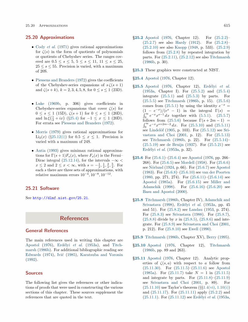
25.20 Approximations 615
25.20 Approximations
• Cody et al. (1971) gives rational approximationsfor ζ(s) in the form of quotients of polynomialsor quotients of Chebyshev series. The ranges cov-ered are 0.5 ≤ s ≤ 5, 5 ≤ s ≤ 11, 11 ≤ s ≤ 25,25 ≤ s ≤ 55. Precision is varied, with a maximumof 20S.
• Piessens and Branders (1972) gives the coefficientsof the Chebyshev-series expansions of s ζ(s+ 1)and ζ(s+ k), k = 2, 3, 4, 5, 8, for 0 ≤ s ≤ 1 (23D).
• Luke (1969b, p. 306) gives coefficients inChebyshev-series expansions that cover ζ(s) for0 ≤ s ≤ 1 (15D), ζ(s+ 1) for 0 ≤ s ≤ 1 (20D),and ln ξ
(12 + ix
)(§25.4) for −1 ≤ x ≤ 1 (20D).
For errata see Piessens and Branders (1972).
• Morris (1979) gives rational approximations forLi2(x) (§25.12(i)) for 0.5 ≤ x ≤ 1. Precision isvaried with a maximum of 24S.
• Antia (1993) gives minimax rational approxima-tions for Γ(s+ 1)Fs(x), where Fs(x) is the Fermi–Dirac integral (25.12.14), for the intervals −∞ <x ≤ 2 and 2 ≤ x < ∞, with s = − 1
2 ,12 ,
32 ,
52 . For
each s there are three sets of approximations, withrelative maximum errors 10−4, 10−8, 10−12.
25.21 Software
See http://dlmf.nist.gov/25.21.
References
General References
The main references used in writing this chapter areApostol (1976), Erdélyi et al. (1953a), and Titch-marsh (1986b). For additional bibliographic reading seeEdwards (1974), Ivić (1985), Karatsuba and Voronin(1992).
Sources
The following list gives the references or other indica-tions of proofs that were used in constructing the varioussections of this chapter. These sources supplement thereferences that are quoted in the text.
§25.2 Apostol (1976, Chapter 12). For (25.2.2)–(25.2.7) see also Hardy (1912). For (25.2.8)–(25.2.10) see also Knopp (1948, p. 533). (25.2.9)follows from (25.2.8) by repeated integration byparts. For (25.2.11), (25.2.12) see also Titchmarsh(1986b, p. 30).
§25.3 These graphics were constructed at NIST.
§25.4 Apostol (1976, Chapter 12).
§25.5 Apostol (1976, Chapter 12), Erdélyi et al.(1953a, Chapter I). For (25.5.2) and (25.5.4)integrate (25.5.1) and (25.5.3) by parts. For(25.5.5) see Titchmarsh (1986b, p. 15). (25.5.6)comes from (25.5.1) by using the identity e−x =(1 − e−x)/(ex − 1) in the integral Γ(s) =∫∞
0e−xxs−1 dx together with (5.5.1). (25.5.7)
follows from (25.5.6) because Γ(s+ 2m− 1) =∫∞0e−xxs+2m−2 dx. For (25.5.10) and (25.5.11)
see Lindelöf (1905, p. 103). For (25.5.12) see Sri-vastava and Choi (2001, p. 12). For (25.5.13)see Titchmarsh (1986b, p. 22). For (25.5.14)–(25.5.19) see de Bruijn (1937). For (25.5.21) seeErdélyi et al. (1953a, p. 32).
§25.6 For (25.6.1)–(25.6.4) see Apostol (1976, pp. 266–268). For (25.6.5) see Mordell (1958). For (25.6.6)see Nörlund (1924, p. 66). For (25.6.7) see Apostol(1983). For (25.6.8)–(25.6.10) see van der Poorten(1980, pp. 271, 274). For (25.6.11)–(25.6.14) seeApostol (1985a). For (25.6.15) see Miller andAdamchik (1998). For (25.6.16)–(25.6.20) seeBasu and Apostol (2000).
§25.8 Titchmarsh (1986b, Chapter IV), Adamchik andSrivastava (1998), Erdélyi et al. (1953a, pp. 45and 51). For (25.8.2) see Landau (1953, p. 274).For (25.8.3) see Srivastava (1988). For (25.8.7),(25.8.8) divide by x in (25.8.5), (25.8.6) and inte-grate. For (25.8.9) see Srivastava and Choi (2001,p. 212). For (25.8.10) see Ewell (1990).
§25.9 Titchmarsh (1986b, Chapter XV), Berry (1995).
§25.10 Apostol (1976, Chapter 12), Titchmarsh(1986b, pp. 89 and 263).
§25.11 Apostol (1976, Chapter 12). Analytic prop-erties of ζ(s, a) with respect to a follow from(25.11.30). For (25.11.5)–(25.11.6) see Apostol(1985a). For (25.11.7) take N = 1 in (25.11.5)and integrate by parts. For (25.11.8)–(25.11.9)see Srivastava and Choi (2001, p. 89). For(25.11.10) use Taylor’s theorem (§§1.4(vi), 1.10(i))and (25.11.17). For (25.11.11) apply (25.2.2) and(25.11.1). For (25.11.12) see Erdélyi et al. (1953a,

616 Zeta and Related Functions
p. 45). For (25.11.13) and (25.11.14) see Apostol(1976, pp. 268, 264). For (25.11.15) use (25.11.1)and analytic continuation. For (25.11.16) seeApostol (1976, p. 263). For (25.11.17) differen-tiate (25.11.1). For (25.11.18) see Erdélyi et al.(1953a, p. 26). For (25.11.19)–(25.11.23) seeApostol (1985a, p. 231) and Miller and Adam-chik (1998). For (25.11.24) use (25.11.15) witha = 1/k, multiply by ks and differentiate.For (25.11.25) see Srivastava and Choi (2001,p. 89) For (25.11.26) see Berndt (1972). For(25.11.27) and (25.11.28) argue as indicated abovefor (25.5.6) and (25.5.7). For (25.11.29) see Lin-delöf (1905, p. 106). For (25.11.30) assume <s >1, collapse the integration path onto the realaxis, apply (25.11.25) and (5.5.3) followed by an-alytic continuation. For (25.11.31) use (25.11.25).For (25.11.32)–(25.11.34) see Adamchik (1998).For (25.11.35) use (25.11.25) and (25.11.8). For
(25.11.36) see Apostol (1976). For (25.11.37)–(25.11.40) see Adamchik and Srivastava (1998).For (25.11.41) and (25.11.42) see Apostol (1952).For (25.11.43) see Paris (2005b). For (25.11.44)and (25.11.45) see Elizalde (1986). The graphicswere constructed at NIST.
§25.12 Erdélyi et al. (1953a, pp. 27, 29), Maximon(2003). For (25.12.13) see Erdélyi et al. (1953a,p. 31) with change of notation. The graphics wereconstructed at NIST.
§25.13 Apostol (1976, Chapter 13).
§25.15 Apostol (1976, Chapter 12), Apostol (1985b).For (25.15.9) see Apostol (1976, pp. 142, 149).
§25.16 Apostol (1976, Chapter 13). For (25.16.2) seeApostol (2000). For (25.16.4) see Ingham (1932,p. 84). For (25.16.5)–(25.16.15) see Apostol andVu (1984) and Basu and Apostol (2000).

Chapter 26
Combinatorial AnalysisD. M. Bressoud1
Notation 61826.1 Special Notation . . . . . . . . . . . . . 618
Properties 61826.2 Basic Definitions . . . . . . . . . . . . . 61826.3 Lattice Paths: Binomial Coefficients . . . 61926.4 Lattice Paths: Multinomial Coefficients
and Set Partitions . . . . . . . . . . . . . 62026.5 Lattice Paths: Catalan Numbers . . . . . 62026.6 Other Lattice Path Numbers . . . . . . . 62126.7 Set Partitions: Bell Numbers . . . . . . . 62326.8 Set Partitions: Stirling Numbers . . . . . 62426.9 Integer Partitions: Restricted Number and
Part Size . . . . . . . . . . . . . . . . . . 62626.10 Integer Partitions: Other Restrictions . . 62726.11 Integer Partitions: Compositions . . . . . 628
26.12 Plane Partitions . . . . . . . . . . . . . . 62926.13 Permutations: Cycle Notation . . . . . . 63126.14 Permutations: Order Notation . . . . . . 63226.15 Permutations: Matrix Notation . . . . . . 63326.16 Multiset Permutations . . . . . . . . . . 63426.17 The Twelvefold Way . . . . . . . . . . . 63426.18 Counting Techniques . . . . . . . . . . . 634
Applications 63526.19 Mathematical Applications . . . . . . . . 63526.20 Physical Applications . . . . . . . . . . . 635
Computation 63526.21 Tables . . . . . . . . . . . . . . . . . . . 63526.22 Software . . . . . . . . . . . . . . . . . . 635
References 635
1Macalester College, Saint Paul, Minnesota.Copyright c© 2009 National Institute of Standards and Technology. All rights reserved.
617

618 Combinatorial Analysis
Notation
26.1 Special Notation
(For other notation see pp. xiv and 873.)
x real variable.h, j, k, `,m, n nonnegative integers.λ integer partition.π plane partition.|A| number of elements of a finite set A.j | k j divides k.(h, k) greatest common divisor of positive
integers h and k.
The main functions treated in this chapter are:(mn
)binomial coefficient.(
mn1,n2,...,nk
)multinomial coefficient.⟨
mn
⟩Eulerian number.[
mn
]q
Gaussian polynomial.
B(n) Bell number.C(n) Catalan number.p(n) number of partitions of n.pk(n) number of partitions of n into at most k
parts.pp(n) number of plane partitions of n.s(n, k) Stirling numbers of the first kind.S(n, k) Stirling numbers of the second kind.
Alternative Notations
Many combinatorics references use the rising and fallingfactorials:
26.1.1xn = x(x+ 1)(x+ 2) · · · (x+ n− 1),xn = x(x− 1)(x− 2) · · · (x− n+ 1).
Other notations for s(n, k), the Stirling numbersof the first kind, include S
(k)n (Abramowitz and Ste-
gun (1964, Chapter 24), Fort (1948)), Skn (Jordan(1939), Moser and Wyman (1958a)),
(n−1k−1
)B
(n)n−k (Milne-
Thomson (1933)), (−1)n−kS1(n − 1, n − k) (Carlitz(1960), Gould (1960)), (−1)n−k
[nk
](Knuth (1992),
Graham et al. (1994), Rosen et al. (2000)).Other notations for S(n, k), the Stirling numbers of
the second kind, include S(k)n (Fort (1948)), Sk
n (Jor-dan (1939)), σkn (Moser and Wyman (1958b)),
(nk
)B
(−k)n−k
(Milne-Thomson (1933)), S2(k, n − k) (Carlitz (1960),Gould (1960)),
{nk
}(Knuth (1992), Graham et al.
(1994), Rosen et al. (2000)), and also an unconventionalsymbol in Abramowitz and Stegun (1964, Chapter 24).
Properties
26.2 Basic Definitions
Permutation
A permutation is a one-to-one and onto function froma non-empty set to itself. If the set consists of the in-tegers 1 through n, a permutation σ can be thoughtof as a rearrangement of these integers where the inte-ger in position j is σ(j). Thus 231 is the permutationσ(1) = 2, σ(2) = 3, σ(3) = 1.
Cycle
Given a finite set S with permutation σ, a cycle is anordered equivalence class of elements of S where j isequivalent to k if there exists an ` = `(j, k) such thatj = σ`(k), where σ1 = σ and σ` is the composition ofσ with σ`−1. It is ordered so that σ(j) follows j. If, forexample, a permutation of the integers 1 through 6 isdenoted by 256413, then the cycles are (1, 2, 5), (3, 6),and (4). Here σ(1) = 2, σ(2) = 5, and σ(5) = 1. Thefunction σ also interchanges 3 and 6, and sends 4 toitself.
Lattice Path
A lattice path is a directed path on the plane integer lat-tice {0, 1, 2, . . .} × {0, 1, 2. . . .}. Unless otherwise speci-fied, it consists of horizontal segments corresponding tothe vector (1, 0) and vertical segments corresponding tothe vector (0, 1). For an example see Figure 26.9.2.
A k-dimensional lattice path is a directed path com-posed of segments that connect vertices in {0, 1, 2, . . . }kso that each segment increases one coordinate by exactlyone unit.
Partition
A partition of a set S is an unordered collection ofpairwise disjoint nonempty sets whose union is S. Asan example, {1, 3, 4}, {2, 6}, {5} is a partition of{1, 2, 3, 4, 5, 6}.
A partition of a nonnegative integer n is an un-ordered collection of positive integers whose sum is n.As an example, {1, 1, 1, 2, 4, 4} is a partition of 13. Thetotal number of partitions of n is denoted by p(n). SeeTable 26.2.1 for n = 0(1)50. For the actual partitions(π) for n = 1(1)5 see Table 26.4.1.
The integers whose sum is n are referred to as theparts in the partition. The example {1, 1, 1, 2, 4, 4} hassix parts, three of which equal 1.

26.3 Lattice Paths: Binomial Coefficients 619
Table 26.2.1: Partitions p(n).
n p(n) n p(n) n p(n)0 1 17 297 34 123101 1 18 385 35 148832 2 19 490 36 179773 3 20 627 37 216374 5 21 792 38 260155 7 22 1002 39 311856 11 23 1255 40 373387 15 24 1575 41 445838 22 25 1958 42 531749 30 26 2436 43 63261
10 42 27 3010 44 7517511 56 28 3718 45 8913412 77 29 4565 46 1 0555813 101 30 5604 47 1 2475414 135 31 6842 48 1 4727315 176 32 8349 49 1 7352516 231 33 10143 50 2 04226
26.3 Lattice Paths: Binomial Coefficients
26.3(i) Definitions(mn
)is the number of ways of choosing n objects from
a collection of m distinct objects without regard to or-der.
(m+nn
)is the number of lattice paths from (0, 0)
to (m,n). The number of lattice paths from (0, 0) to(m,n), m ≤ n, that stay on or above the line y = x is(m+nm
)−(m+nm−1
).
26.3.1
(m
n
)=(
m
m− n
)=
m!(m− n)!n!
, m ≥ n,
26.3.2
(m
n
)= 0, n > m.
For numerical values of(mn
)and
(m+nn
)see Tables
26.3.1 and 26.3.2.
Table 26.3.1: Binomial coefficients(mn
).
mn
0 1 2 3 4 5 6 7 8 9 100 11 1 12 1 2 13 1 3 3 14 1 4 6 4 15 1 5 10 10 5 16 1 6 15 20 15 6 17 1 7 21 35 35 21 7 18 1 8 28 56 70 56 28 8 19 1 9 36 84 126 126 84 36 9 1
10 1 10 45 120 210 252 210 120 45 10 1
Table 26.3.2: Binomial coefficients(m+nm
)for lattice
paths.
mn
0 1 2 3 4 5 6 7 80 1 1 1 1 1 1 1 1 11 1 2 3 4 5 6 7 8 92 1 3 6 10 15 21 28 36 453 1 4 10 20 35 56 84 120 1654 1 5 15 35 70 126 210 330 4955 1 6 21 56 126 252 462 792 12876 1 7 28 84 210 462 924 1716 30037 1 8 36 120 330 792 1716 3432 64358 1 9 45 165 495 1287 3003 6435 12870
26.3(ii) Generating Functions
26.3.3
m∑n=0
(m
n
)xn = (1 + x)m, m = 0, 1, . . . ,
26.3.4
∞∑m=0
(m+ n
m
)xm =
1(1− x)n+1
, |x| < 1.
26.3(iii) Recurrence Relations
26.3.5
(m
n
)=(m− 1n
)+(m− 1n− 1
), m ≥ n ≥ 1,
26.3.6
(m
n
)=m
n
(m− 1n− 1
)=m− n+ 1
n
(m
n− 1
),
m ≥ n ≥ 1,
26.3.7
(m+ 1n+ 1
)=
m∑k=n
(k
n
), m ≥ n ≥ 0,
26.3.8
(m
n
)=
n∑k=0
(m− n− 1 + k
k
), m ≥ n ≥ 0.
26.3(iv) Identities
26.3.9
(n
0
)=(n
n
)= 1,
26.3.10
(m
n
)=
n∑k=0
(−1)n−k(m+ 1k
), m ≥ n ≥ 0,
26.3.11
(2nn
)=
2n(2n− 1)(2n− 3) · · · 3 · 1n!
.
See also §1.2(i).
26.3(v) Limiting Form
26.3.12
(2nn
)∼ 4n√
πn, n→∞.

620 Combinatorial Analysis
26.4 Lattice Paths: MultinomialCoefficients and Set Partitions
26.4(i) Definitions(n
n1,n2,...,nk
)is the number of ways of placing n =
n1 + n2 + · · ·+ nk distinct objects into k labeled boxesso that there are nj objects in the jth box. It is also thenumber of k-dimensional lattice paths from (0, 0, . . . , 0)to (n1, n2, . . . , nk). For k = 0, 1, the multinomial coeffi-cient is defined to be 1. For k = 2
26.4.1
(n1 + n2
n1, n2
)=(n1 + n2
n1
)=(n1 + n2
n2
),
and in general,
26.4.2(n1 + n2 + · · ·+ nkn1, n2, . . . , nk
)=
(n1 + n2 + · · ·+ nk)!n1!n2! · · · nk!
=k−1∏j=1
(nj + nj+1 + · · ·+ nk
nj
).
Table 26.4.1 gives numerical values of multinomi-als and partitions λ,M1,M2,M3 for 1 ≤ m ≤ n ≤ 5.These are given by the following equations in whicha1, a2, . . . , an are nonnegative integers such that
26.4.3 n = a1 + 2a2 + · · ·+ nan,
26.4.4 m = a1 + a2 + · · ·+ an.
λ is a partition of n:
26.4.5 λ = 1a1 , 2a2 , . . . , nan .
M1 is the multinominal coefficient (26.4.2):
26.4.6
M1 =
na1︷ ︸︸ ︷
1, . . . , 1, . . . ,an︷ ︸︸ ︷
n, . . . , n
=
n!(1!)a1(2!)a2 · · · (n!)an
.
M2 is the number of permutations of {1, 2, . . . , n} witha1 cycles of length 1, a2 cycles of length 2, . . . , and ancycles of length n:
26.4.7 M2 =n!
1a1(a1!) 2a2(a2!) · · · nan(an!).
(The empty set is considered to have one permutationconsisting of no cycles.) M3 is the number of set parti-tions of {1, 2, . . . , n} with a1 subsets of size 1, a2 subsetsof size 2, . . . , and an subsets of size n:
26.4.8 M3 =n!
(1!)a1(a1!) (2!)a2(a2!) · · · (n!)an(an!).
For each n all possible values of a1, a2, . . . , an are cov-ered.
Table 26.4.1: Multinomials and partitions.
n m λ M1 M2 M3
1 1 11 1 1 12 1 21 1 1 12 2 12 2 1 13 1 31 1 2 13 2 11, 21 3 3 33 3 13 6 1 14 1 41 1 6 14 2 11, 31 4 8 44 2 22 6 3 34 3 12, 21 12 6 64 4 14 24 1 15 1 51 1 24 15 2 11, 41 5 30 55 2 21, 31 10 20 105 3 12, 31 20 20 105 3 11, 22 30 15 155 4 13, 21 60 10 105 5 15 120 1 1
26.4(ii) Generating Function
26.4.9
(x1 + x2 + · · ·+ xk)n
=∑(
n
n1, n2, . . . , nk
)xn1
1 xn22 · · ·x
nkk ,
where the summation is over all nonnegative integersn1, n2, . . . , nk such that n1 + n2 + · · ·+ nk = n.
26.4(iii) Recurrence Relation
26.4.10(n1 + n2 + · · ·+ nmn1, n2, . . . , nm
)=
m∑k=1
(n1 + n2 + · · ·+ nm − 1
n1, n2, . . . , nk−1, nk − 1, nk+1, . . . , nm
),
n1, n2, . . . , nm ≥ 1.
26.5 Lattice Paths: Catalan Numbers
26.5(i) Definitions
C(n) is the Catalan number. It counts the number oflattice paths from (0, 0) to (n, n) that stay on or abovethe line y = x.26.5.1
C(n) =1
n+ 1
(2nn
)=
12n+ 1
(2n+ 1n
)=(
2nn
)−(
2nn− 1
)=(
2n− 1n
)−(
2n− 1n+ 1
).
(Sixty-six equivalent definitions of C(n) are given inStanley (1999, pp. 219–229).)
See Table 26.5.1.

26.6 Other Lattice Path Numbers 621
Table 26.5.1: Catalan numbers.
n C(n) n C(n) n C(n)0 1 7 429 14 26 744401 1 8 1430 15 96 948452 2 9 4862 16 353 576703 5 10 16796 17 1296 447904 14 11 58786 18 4776 387005 42 12 2 08012 19 17672 631906 132 13 7 42900 20 65641 20420
26.5(ii) Generating Function
26.5.2
∞∑n=0
C(n)xn =1−√
1− 4x2x
, |x| < 14 .
26.5(iii) Recurrence Relations
26.5.3 C(n+ 1) =n∑k=0
C(k)C(n− k),
26.5.4 C(n+ 1) =2(2n+ 1)n+ 2
C(n),
26.5.5 C(n+ 1) =bn/2c∑k=0
(n
2k
)2n−2k C(k).
26.5(iv) Limiting Forms
26.5.6 C(n) ∼ 4n√πn3
, n→∞,
26.5.7 limn→∞
C(n+ 1)C(n)
= 4.
26.6 Other Lattice Path Numbers
26.6(i) Definitions
Dellanoy Number D(m,n)
D(m,n) is the number of paths from (0, 0) to (m,n)that are composed of directed line segments of the form(1, 0), (0, 1), or (1, 1).26.6.1
D(m,n) =n∑k=0
(n
k
)(m+ n− k
n
)=
n∑k=0
2k(m
k
)(n
k
).
See Table 26.6.1.
Table 26.6.1: Dellanoy numbers D(m,n).
mn
0 1 2 3 4 5 6 7 8 9 100 1 1 1 1 1 1 1 1 1 1 11 1 3 5 7 9 11 13 15 17 19 212 1 5 13 25 41 61 85 113 145 181 2213 1 7 25 63 129 231 377 575 833 1159 15614 1 9 41 129 321 681 1289 2241 3649 5641 83615 1 11 61 231 681 1683 3653 7183 13073 22363 363656 1 13 85 377 1289 3653 8989 19825 40081 75517 1 342457 1 15 113 575 2241 7183 19825 48639 1 08545 2 24143 4 339058 1 17 145 833 3649 13073 40081 1 08545 2 65729 5 98417 12 564659 1 19 181 1159 5641 22363 75517 2 24143 5 98417 14 62563 33 17445
10 1 21 221 1561 8361 36365 1 34245 4 33905 12 56465 33 17445 80 97453
Motzkin Number M(n)
M(n) is the number of lattice paths from (0, 0) to (n, n) that stay on or above the line y = x and are composed ofdirected line segments of the form (2, 0), (0, 2), or (1, 1).
26.6.2 M(n) =n∑k=0
(−1)k
n+ 2− k
(n
k
)(2n+ 2− 2kn+ 1− k
).
See Table 26.6.2.
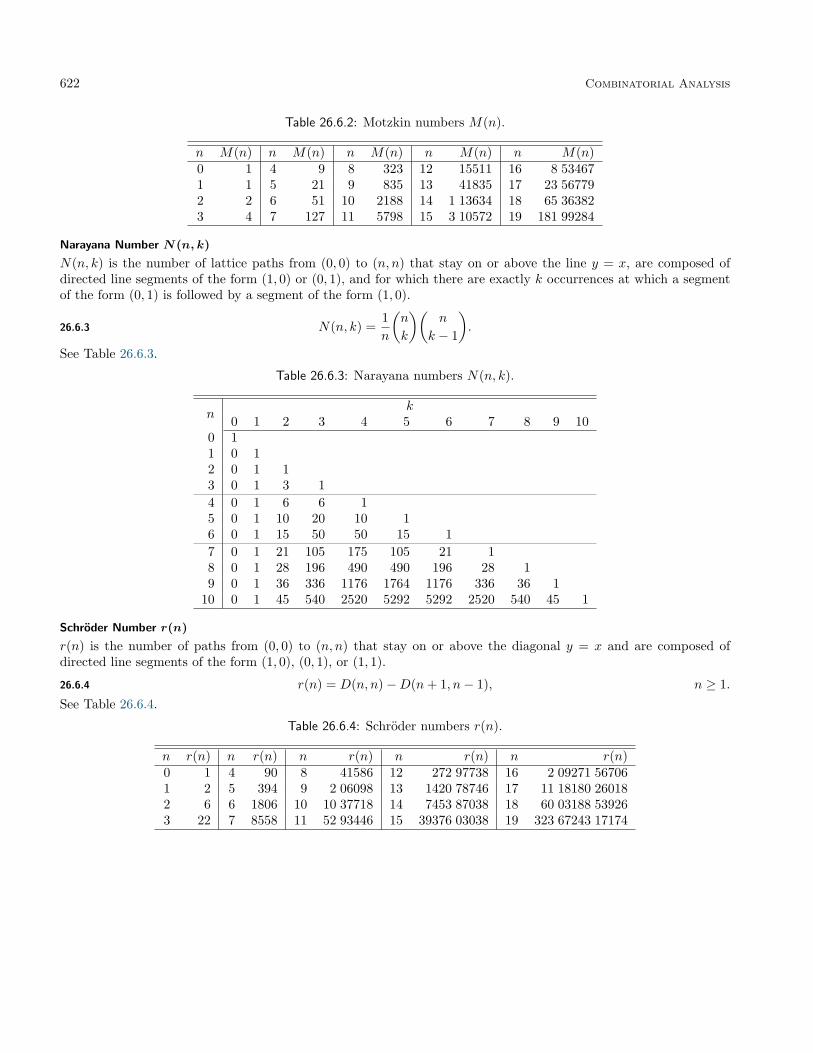
622 Combinatorial Analysis
Table 26.6.2: Motzkin numbers M(n).
n M(n) n M(n) n M(n) n M(n) n M(n)0 1 4 9 8 323 12 15511 16 8 534671 1 5 21 9 835 13 41835 17 23 567792 2 6 51 10 2188 14 1 13634 18 65 363823 4 7 127 11 5798 15 3 10572 19 181 99284
Narayana Number N(n, k)
N(n, k) is the number of lattice paths from (0, 0) to (n, n) that stay on or above the line y = x, are composed ofdirected line segments of the form (1, 0) or (0, 1), and for which there are exactly k occurrences at which a segmentof the form (0, 1) is followed by a segment of the form (1, 0).
26.6.3 N(n, k) =1n
(n
k
)(n
k − 1
).
See Table 26.6.3.
Table 26.6.3: Narayana numbers N(n, k).
nk
0 1 2 3 4 5 6 7 8 9 100 11 0 12 0 1 13 0 1 3 14 0 1 6 6 15 0 1 10 20 10 16 0 1 15 50 50 15 17 0 1 21 105 175 105 21 18 0 1 28 196 490 490 196 28 19 0 1 36 336 1176 1764 1176 336 36 1
10 0 1 45 540 2520 5292 5292 2520 540 45 1
Schröder Number r(n)
r(n) is the number of paths from (0, 0) to (n, n) that stay on or above the diagonal y = x and are composed ofdirected line segments of the form (1, 0), (0, 1), or (1, 1).
26.6.4 r(n) = D(n, n)−D(n+ 1, n− 1), n ≥ 1.See Table 26.6.4.
Table 26.6.4: Schröder numbers r(n).
n r(n) n r(n) n r(n) n r(n) n r(n)0 1 4 90 8 41586 12 272 97738 16 2 09271 567061 2 5 394 9 2 06098 13 1420 78746 17 11 18180 260182 6 6 1806 10 10 37718 14 7453 87038 18 60 03188 539263 22 7 8558 11 52 93446 15 39376 03038 19 323 67243 17174

26.7 Set Partitions: Bell Numbers 623
26.6(ii) Generating Functions
For sufficiently small |x| and |y|,
26.6.5
∞∑m,n=0
D(m,n)xmyn =1
1− x− y − xy,
26.6.6
∞∑n=0
D(n, n)xn =1√
1− 6x+ x2,
26.6.7
∞∑n=0
M(n)xn =1− x−
√1− 2x− 3x2
2x2,
26.6.8
∞∑n,k=1
N(n, k)xnyk
=1− x− xy −
√(1− x− xy)2 − 4x2y
2x,
26.6.9
∞∑n=0
r(n)xn =1− x−
√1− 6x+ x2
2x.
26.6(iii) Recurrence Relations
26.6.10D(m,n) = D(m,n− 1) +D(m− 1, n)
+D(m− 1, n− 1), m,n ≥ 1,
26.6.11M(n) = M(n− 1) +
n∑k=2
M(k − 2)M(n− k),
n ≥ 2.
26.6(iv) Identities
26.6.12 C(n) =n∑k=1
N(n, k),
26.6.13 M(n) =n∑k=0
(−1)k(n
k
)C(n+ 1− k),
26.6.14 C(n) =2n∑k=0
(−1)k(
2nk
)M(2n− k).
26.7 Set Partitions: Bell Numbers
26.7(i) Definitions
B(n) is the number of partitions of {1, 2, . . . , n}. ForS(n, k) see §26.8(i).
26.7.1 B(0) = 1,
26.7.2 B(n) =n∑k=0
S(n, k),
26.7.3 B(n) =m∑k=1
kn
k!
m−k∑j=0
(−1)j
j!, m ≥ n,
26.7.4 B(n) = e−1∞∑k=1
kn
k!= 1 +
⌊e−1
2n∑k=1
kn
k!
⌋.
See Table 26.7.1.
Table 26.7.1: Bell numbers.
n B(n) n B(n)0 1 10 1 159751 1 11 6 785702 2 12 42 135973 5 13 276 444374 15 14 1908 993225 52 15 13829 585456 203 16 1 04801 421477 877 17 8 28648 698048 4140 18 68 20768 061599 21147 19 583 27422 05057
26.7(ii) Generating Function
26.7.5∞∑n=0
B(n)xn
n!= exp(ex − 1).
26.7(iii) Recurrence Relation
26.7.6 B(n+ 1) =n∑k=0
(n
k
)B(n).
26.7(iv) Asymptotic Approximation
26.7.7
B(n) =NneN−n−1
(1 + lnN)1/2
(1 +O
((lnn)1/2
n1/2
)), n→∞,
where
26.7.8 N lnN = n,
or, equivalently, N = eWm(n), with properties of theLambert function Wm(n) given in §4.13. For higherapproximations to B(n) as n→∞ see de Bruijn (1961,pp. 104–108).

624 Combinatorial Analysis
26.8 Set Partitions: Stirling Numbers
26.8(i) Definitions
s(n, k) denotes the Stirling number of the firstkind : (−1)n−k times the number of permutations of{1, 2, . . . , n} with exactly k cycles. See Table 26.8.1.
26.8.1 s(n, n) = 1, n ≥ 0,
26.8.2 s(1, k) = δ1,k,
26.8.3
(−1)n−k s(n, k) =∑
1≤b1<···<bn−k≤n−1
b1b2 · · · bn−k,
n > k ≥ 1.
S(n, k) denotes the Stirling number of the secondkind : the number of partitions of {1, 2, . . . , n} into ex-actly k nonempty subsets. See Table 26.8.2.
26.8.4 S(n, n) = 1, n ≥ 0,
26.8.5 S(n, k) =∑
1c12c2 · · · kck ,
where the summation is over all nonnegative integersc1, c2, . . . , ck such that c1 + c2 + · · ·+ ck = n− k.
26.8.6 S(n, k) =1k!
k∑j=0
(−1)k−j(k
j
)jn.
Table 26.8.1: Stirling numbers of the first kind s(n, k).
nk
0 1 2 3 4 5 6 7 8 9 100 11 0 12 0 −1 13 0 2 −3 14 0 −6 11 −6 15 0 24 −50 35 −10 16 0 −120 274 −225 85 −15 17 0 720 −1764 1624 −735 175 −21 18 0 −5040 13068 −13132 6769 −1960 322 −28 19 0 40320 −1 09584 1 18124 −67284 22449 −4536 546 −36 1
10 0 −3 62880 10 26576 −11 72700 7 23680 −2 69325 6327 −9450 870 −45 1
Table 26.8.2: Stirling numbers of the second kind S(n, k).
nk
0 1 2 3 4 5 6 7 8 9 100 11 0 12 0 1 13 0 1 3 14 0 1 7 6 15 0 1 15 25 10 16 0 1 31 90 65 15 17 0 1 63 301 350 140 21 18 0 1 127 966 1701 1050 266 28 19 0 1 255 3025 7770 6951 2646 462 36 1
10 0 1 511 9330 34105 42525 22827 5880 750 45 1
26.8(ii) Generating Functions
26.8.7n∑k=0
s(n, k)xk = (x− n+ 1)n,
where (x)n is the Pochhammer symbol: x(x+1) · · · (x+n− 1).
26.8.8∞∑n=0
s(n, k)xn
n!=
(ln(1 + x))k
k!, |x| < 1,

26.8 Set Partitions: Stirling Numbers 625
26.8.9
∞∑n,k=0
s(n, k)xn
n!yk = (1 + x)y, |x| < 1.
26.8.10
n∑k=1
S(n, k)(x− k + 1)k = xn,
26.8.11∞∑n=0
S(n, k)xn =xk
(1− x)(1− 2x) · · · (1− kx), |x| < 1/k,
26.8.12
∞∑n=0
S(n, k)xn
n!=
(ex − 1)k
k!,
26.8.13
∞∑n,k=0
S(n, k)xn
n!yk = exp (y(ex − 1)) .
26.8(iii) Special Values
For n ≥ 1,
26.8.14 s(n, 0) = 0, s(n, 1) = (−1)n−1(n− 1)!,
26.8.15 s(n, 2) = (−1)n(n− 1)!(
1 +12
+ · · ·+ 1n− 1
),
26.8.16 − s(n, n− 1) = S(n, n− 1) =(n
2
),
26.8.17 S(n, 0) = 0, S(n, 1) = 1, S(n, 2) = 2n−1 − 1.
26.8(iv) Recurrence Relations
26.8.18 s(n, k) = s(n− 1, k − 1)− (n− 1) s(n− 1, k),
26.8.19
(k
h
)s(n, k) =
n−h∑j=k−h
(n
j
)s(n− j, h) s(j, k − h),
n ≥ k ≥ h,
26.8.20 s(n+ 1, k + 1) = n!n∑j=k
(−1)n−j
j!s(j, k),
26.8.21 s(n+ k + 1, k) = −k∑j=0
(n+ j) s(n+ j, j).
26.8.22 S(n, k) = k S(n− 1, k) + S(n− 1, k − 1),26.8.23(
k
h
)S(n, k) =
n−h∑j=k−h
(n
j
)S(n− j, h)S(j, k − h),
n ≥ k ≥ h,
26.8.24 S(n, k) =n∑j=k
S(j − 1, k − 1)kn−j ,
26.8.25 S(n+ 1, k + 1) =n∑j=k
(n
j
)S(j, k),
26.8.26 S(n+ k + 1, k) =k∑j=0
j S(n+ j, j).
26.8(v) Identities
26.8.27
s(n, n− k)
=k∑j=0
(−1)j(n− 1 + j
k + j
)(n+ k
k − j
)S(k + j, j),
26.8.28
n∑k=1
s(n, k) = 0, n > 1,
26.8.29
n∑k=1
(−1)n−k s(n, k) = n!,
26.8.30
n∑j=k
s(n+ 1, j + 1)nj−k = s(n, k).
26.8.311k!
dk
dxkf(x) =
∞∑n=k
s(n, k)n!
∆nf(x),
when f(x) is analytic for all x, and the series converges,where
26.8.32 ∆f(x) = f(x+ 1)− f(x);
compare §3.6(i).
26.8.33
S(n, n− k)
=k∑j=0
(−1)j(n− 1 + j
k + j
)(n+ k
k − j
)s(k + j, j),
26.8.34
n∑j=0
jkxj =k∑j=0
S(k, j)xjdj
dxj
(1− xn+1
1− x
),
26.8.35
n∑j=0
jk =k∑j=0
j!S(k, j)(n+ 1j + 1
),
26.8.36
n∑k=0
(−1)n−kk!S(n, k) = 1.
26.8.371k!
∆kf(x) =∞∑n=k
S(n, k)n!
dn
dxnf(x),
when f(x) is analytic for all x, and the series converges.Let A and B be the n × n matrices with (j, k)th
elements s(j, k), and S(j, k), respectively. Then
26.8.38 A−1 = B.
26.8.39
n∑j=k
s(j, k)S(n, j) =n∑j=k
s(n, j)S(j, k) = δn,k.
26.8(vi) Relations to Bernoulli Numbers
See §24.15(iii).

626 Combinatorial Analysis
26.8(vii) Asymptotic Approximations
26.8.40
s(n+ 1, k + 1) ∼ (−1)n−kn!k!
(γ + lnn)k, n→∞,
uniformly for k = o(lnn), where γ is Euler’s constant(§5.2(ii)).
26.8.41 s(n+ k, k) ∼ (−1)n
2nn!k2n, k →∞,
n fixed.
26.8.42 S(n, k) ∼ kn
k!, n→∞,
k fixed.26.8.43 S(n+ k, k) ∼ k2n
2nn!, k →∞,
uniformly for n = o(k1/2
).
For asymptotic approximations for s(n+ 1, k + 1)and S(n, k) that apply uniformly for 1 ≤ k ≤ n asn→∞ see Temme (1993).
For other asymptotic approximations and also ex-pansions see Moser and Wyman (1958a) for Stirlingnumbers of the first kind, and Moser and Wyman(1958b), Bleick and Wang (1974) for Stirling numbersof the second kind.
For asymptotic estimates for generalized Stirlingnumbers see Chelluri et al. (2000).
26.9 Integer Partitions: Restricted Numberand Part Size
26.9(i) Definitions
pk(n) denotes the number of partitions of n into at mostk parts. See Table 26.9.1.
26.9.1 pk(n) = p(n), k ≥ n.Unrestricted partitions are covered in §27.14.
Table 26.9.1: Partitions pk(n).
nk
0 1 2 3 4 5 6 7 8 9 100 1 1 1 1 1 1 1 1 1 1 11 0 1 1 1 1 1 1 1 1 1 12 0 1 2 2 2 2 2 2 2 2 23 0 1 2 3 3 3 3 3 3 3 34 0 1 3 4 5 5 5 5 5 5 55 0 1 3 5 6 7 7 7 7 7 76 0 1 4 7 9 10 11 11 11 11 117 0 1 4 8 11 13 14 15 15 15 158 0 1 5 10 15 18 20 21 22 22 229 0 1 5 12 18 23 26 28 29 30 30
10 0 1 6 14 23 30 35 38 40 41 42
A useful representation for a partition is the Ferrersgraph in which the integers in the partition are each
represented by a row of dots. An example is providedin Figure 26.9.1.
• • • • • • •• • • •• • •• • •• ••
Figure 26.9.1: Ferrers graph of the partition 7 + 4 + 3 +3 + 2 + 1.
The conjugate partition is obtained by reflectingthe Ferrers graph across the main diagonal or, equiv-alently, by representing each integer by a column ofdots. The conjugate to the example in Figure 26.9.1 is6 + 5 + 4 + 2 + 1 + 1 + 1. Conjugation establishes a one-to-one correspondence between partitions of n into atmost k parts and partitions of n into parts with largestpart less than or equal to k. It follows that pk(n) alsoequals the number of partitions of n into parts that areless than or equal to k.
pk(≤ m,n) is the number of partitions of n intoat most k parts, each less than or equal to m. It isalso equal to the number of lattice paths from (0, 0) to(m, k) that have exactly n vertices (h, j), 1 ≤ h ≤ m,1 ≤ j ≤ k, above and to the left of the lattice path. SeeFigure 26.9.2.
(0, 0)
(6, 5)
Figure 26.9.2: The partition 5 + 5 + 3 + 2 represented asa lattice path.
Equations (26.9.2)–(26.9.3) are examples of closedforms that can be computed explicitly for any positiveinteger k. See Andrews (1976, p. 81).
26.9.2 p0(n) = 0, n > 0,
26.9.3
p1(n) = 1, p2(n) = 1 + bn/2c ,
p3(n) = 1 +⌊n2 + 6n
12
⌋.
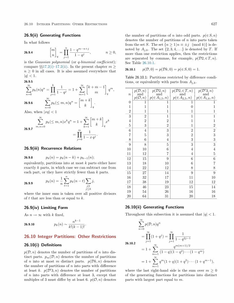
26.10 Integer Partitions: Other Restrictions 627
26.9(ii) Generating Functions
In what follows
26.9.4
[m
n
]q
=n∏j=1
1− qm−n+j
1− qj, n ≥ 0,
is the Gaussian polynomial (or q-binomial coefficient);compare §§17.2(i)–17.2(ii). In the present chapter m ≥n ≥ 0 in all cases. It is also assumed everywhere that|q| < 1.26.9.5∞∑n=0
pk(n)qn =k∏j=1
11− qj
= 1 +∞∑m=1
[k +m− 1
m
]q
qm,
26.9.6
∞∑n=0
pk(≤ m,n)qn =[m+ k
k
]q
.
Also, when |xq| < 1
26.9.7
∞∑m,n=0
pk(≤ m,n)xkqn = 1 +∞∑k=1
[m+ k
k
]q
xk
=m∏j=0
11− x qj
.
26.9(iii) Recurrence Relations
26.9.8 pk(n) = pk(n− k) + pk−1(n);equivalently, partitions into at most k parts either haveexactly k parts, in which case we can subtract one fromeach part, or they have strictly fewer than k parts.
26.9.9pk(n) =
1n
n∑t=1
pk(n− t)∑j|tj≤k
j,
where the inner sum is taken over all positive divisorsof t that are less than or equal to k.
26.9(iv) Limiting Form
As n→∞ with k fixed,
26.9.10 pk(n) ∼ nk−1
k!(k − 1)!.
26.10 Integer Partitions: Other Restrictions
26.10(i) Definitions
p(D, n) denotes the number of partitions of n into dis-tinct parts. pm(D, n) denotes the number of partitionsof n into at most m distinct parts. p(Dk, n) denotesthe number of partitions of n into parts with differenceat least k. p(D′3, n) denotes the number of partitionsof n into parts with difference at least 3, except thatmultiples of 3 must differ by at least 6. p(O, n) denotes
the number of partitions of n into odd parts. p(∈S, n)denotes the number of partitions of n into parts takenfrom the set S. The set {n ≥ 1|n ≡ ±j (mod k)} is de-noted by Aj,k. The set {2, 3, 4, . . .} is denoted by T . Ifmore than one restriction applies, then the restrictionsare separated by commas, for example, p(D2,∈T, n).See Table 26.10.1.
26.10.1 p(D, 0) = p(Dk, 0) = p(∈S, 0) = 1.
Table 26.10.1: Partitions restricted by difference condi-tions, or equivalently with parts from Aj,k.
p(D, n) p(D2, n) p(D2,∈T, n) p(D′3, n)n and and and and
p(O, n) p(∈A1,5, n) p(∈A2,5, n) p(∈A1,6, n)0 1 1 1 11 1 1 0 12 1 1 1 13 2 1 1 14 2 2 1 15 3 2 1 26 4 3 2 27 5 3 2 38 6 4 3 39 8 5 3 3
10 10 6 4 411 12 7 4 512 15 9 6 613 18 10 6 714 22 12 8 815 27 14 9 916 32 17 11 1017 38 19 12 1218 46 23 15 1419 54 26 16 1620 64 31 20 18
26.10(ii) Generating Functions
Throughout this subsection it is assumed that |q| < 1.
26.10.2
∞∑n=0
p(D, n)qn
=∞∏j=1
(1 + qj) =∞∏j=1
11− q2j−1
= 1 +∞∑m=1
qm(m+1)/2
(1− q)(1− q2) · · · (1− qm)
= 1 +∞∑m=1
qm(1 + q)(1 + q2) · · · (1 + qm−1),
where the last right-hand side is the sum over m ≥ 0of the generating functions for partitions into distinctparts with largest part equal to m.

628 Combinatorial Analysis
26.10.3
(1− x)∞∑
m,n=0
pm(≤ k,D, n)xmqn
=k∑
m=0
[k
m
]q
qm(m+1)/2xm =k∏j=1
(1 + x qj),
|x| < 1,
26.10.4∞∑n=0
p(Dk, n)qn = 1 +∞∑m=1
q(km2+(2−k)m)/2
(1− q)(1− q2) · · · (1− qm),
26.10.5
∞∑n=0
p(∈S, n)qn =∏j∈S
11− qj
.
26.10(iii) Recurrence Relations
26.10.6p(D, n) =
1n
n∑t=1
p(D, n− t)∑j|tj odd
j,
where the inner sum is the sum of all positive odd divi-sors of t.
26.10.7
∑(−1)k p
(D, n− 1
2 (3k2 ± k))
=
{(−1)r, n = 3r2 ± r,0, otherwise,
where the sum is over nonnegative integer values of kfor which n− 1
2 (3k2 ± k) ≥ 0.26.10.8∑
(−1)k p(D, n− (3k2 ± k)
)=
{1, n = 1
2 (r2 ± r),0, otherwise,
where the sum is over nonnegative integer values of kfor which n− (3k2 ± k) ≥ 0.
In exact analogy with (26.9.8), we have
26.10.9 pm(D, n) = pm(D, n−m) + pm−1(D, n),
26.10.10 p(Dk, n) =∑
pm(n− 1
2km2 −m+ 1
2km),
where the sum is over nonnegative integer values of mfor which n− 1
2km2 −m+ 1
2km ≥ 0.
26.10.11p(∈S, n) =
1n
n∑t=1
p(∈S, n− t)∑j|tj∈S
j,
where the inner sum is the sum of all positive divisorsof t that are in S.
26.10(iv) Identities
Equations (26.10.13) and (26.10.14) are the Rogers–Ramanujan identities. See also §17.2(vi).
26.10.12 p(D, n) = p(O, n),
26.10.13 p(D2, n) = p(∈ A1,5, n),
26.10.14 p(D2,∈ T, n) = p(∈A2,5, n), T = {2, 3, 4, . . .},
26.10.15 p(D′3, n) = p(∈ A1,6, n).Note that p(D′3, n) ≤ p(D3, n), with strict inequal-
ity for n ≥ 9. It is known that for k > 3, p(Dk, n) ≥p(∈A1,k+3, n), with strict inequality for n sufficientlylarge, provided that k = 2m − 1,m = 3, 4, 5, or k ≥ 32;see Yee (2004).
26.10(v) Limiting Form
26.10.16 p(D, n) ∼ eπ√n/3
(768n3)1/4, n→∞.
26.10(vi) Bessel-Function Expansion
26.10.17
p(D, n)
= π
∞∑k=1
A2k−1(n)(2k − 1)
√24n+ 1
I1
(π
2k − 1
√24n+ 1
72
),
where I1(x) is the modified Bessel function (§10.25(ii)),and
26.10.18Ak(n) =
∑1<h≤k(h,k)=1
eπif(h,k)−(2πinh/k),
with
26.10.19 f(h, k) =k∑j=1
[[2j − 1
2k
]] [[h(2j − 1)
k
]],
and
26.10.20 [[x]] =
{x− bxc − 1
2 , x /∈ Z,0, x ∈ Z.
The quantity Ak(n) is real-valued.
26.11 Integer Partitions: Compositions
A composition is an integer partition in which order istaken into account. For example, there are eight compo-sitions of 4: 4, 3+1, 1+3, 2+2, 2+1+1, 1+2+1, 1+1+2,and 1 + 1 + 1 + 1. c(n) denotes the number of composi-tions of n, and cm(n) is the number of compositions intoexactly m parts. c(∈T, n) is the number of compositionsof n with no 1’s, where again T = {2, 3, 4, . . .}. The in-teger 0 is considered to have one composition consistingof no parts:
26.11.1 c(0) = c(∈T, 0) = 1.Also,
26.11.2 cm(0) = δ0,m,
26.11.3 cm(n) =(n− 1m− 1
),
26.11.4
∞∑n=0
cm(n)qn =qm
(1− q)m.

26.12 Plane Partitions 629
The Fibonacci numbers are determined recursivelyby
26.11.5F0 = 0 , F1 = 1 , Fn = Fn−1 + Fn−2,
n ≥ 2.
26.11.6 c(∈T, n) = Fn−1, n ≥ 1.
Explicitly,
26.11.7 Fn =(1 +
√5)n − (1−
√5)n
2n√
5.
Additional information on Fibonacci numbers canbe found in Rosen et al. (2000, pp. 140–145).
26.12 Plane Partitions
26.12(i) Definitions
A plane partition, π, of a positive integer n, is a par-tition of n in which the parts have been arranged ina 2-dimensional array that is weakly decreasing (non-increasing) across rows and down columns. Differentconfigurations are counted as different plane partitions.As an example, there are six plane partitions of 3:
26.12.1
3 , 2 1 ,21 , 1 1 1 ,
1 11 ,
111
.
An equivalent definition is that a plane partition isa finite subset of N × N × N with the property thatif (r, s, t) ∈ π and (1, 1, 1) ≤ (h, j, k) ≤ (r, s, t), then(h, j, k) must be an element of π. Here (h, j, k) ≤ (r, s, t)means h ≤ r, j ≤ s, and k ≤ t. It is useful to be ableto visualize a plane partition as a pile of blocks, oneblock at each lattice point (h, j, k) ∈ π. For example,Figure 26.12.1 depicts the pile of blocks that representsthe plane partition of 75 given by (26.12.2).
Figure 26.12.1: A plane partition of 75.
26.12.2
6 5 5 4 3 36 4 3 3 16 4 3 1 14 2 2 13 1 11 1 1
The number of plane partitions of n is denoted bypp(n), with pp(0) = 1. See Table 26.12.1.
Table 26.12.1: Plane partitions.
n pp(n) n pp(n) n pp(n)0 1 17 18334 34 281 759551 1 18 29601 35 416 910462 3 19 47330 36 614 849613 6 20 75278 37 903 797844 13 21 1 18794 38 1324 419955 24 22 1 86475 39 1934 875016 48 23 2 90783 40 2818 469237 86 24 4 51194 41 4093 839818 160 25 6 96033 42 5930 012679 282 26 10 68745 43 8566 67495
10 500 27 16 32658 44 12343 6383311 859 28 24 83234 45 17740 7910912 1479 29 37 59612 46 25435 3590213 2485 30 56 68963 47 36379 9303614 4167 31 85 12309 48 51913 0497315 6879 32 127 33429 49 73910 2652216 11297 33 189 74973 50 1 04996 40707
We define the r × s× t box B(r, s, t) as
26.12.3
B(r, s, t) = {(h, j, k) | 1 ≤ h ≤ r, 1 ≤ j ≤ s, 1 ≤ k ≤ t}.Then the number of plane partitions in B(r, s, t) is
26.12.4 ∏(h,j,k)∈B(r,s,t)
h+ j + k − 1h+ j + k − 2
=r∏
h=1
s∏j=1
h+ j + t− 1h+ j − 1
.
A plane partition is symmetric if (h, j, k) ∈ π im-plies that (j, h, k) ∈ π. The number of symmetric planepartitions in B(r, r, t) is
26.12.5
r∏h=1
2h+ t− 12h− 1
∏1 ≤h<j≤r
h+ j + t− 1h+ j − 1
.
A plane partition is cyclically symmetric if (h, j, k) ∈π implies (j, k, h) ∈ π. The plane partition in Fig-ure 26.12.1 is an example of a cyclically symmetric planepartition. The number of cyclically symmetric planepartitions in B(r, r, r) is
26.12.6
r∏h=1
3h− 13h− 2
∏1 ≤h<j≤r
h+ 2j − 1h+ j − 1
,

630 Combinatorial Analysis
or equivalently,
26.12.7
r∏h=1
3h− 13h− 2
r∏j=h
r + h+ j − 12h+ j − 1
.
A plane partition is totally symmetric if it is bothsymmetric and cyclically symmetric. The number oftotally symmetric plane partitions in B(r, r, r) is
26.12.8∏
1≤h≤j≤r
h+ j + r − 1h+ 2j − 2
.
The complement of π ⊆ B(r, s, t) is πc ={(h, j, k) | (r − h + 1, s − j + 1, t − k + 1) /∈ π}. Aplane partition is self-complementary if it is equal to itscomplement. The number of self-complementary planepartitions in B(2r, 2s, 2t) is
26.12.9
r∏h=1
s∏j=1
h+ j + t− 1h+ j − 1
2
;
in B(2r + 1, 2s, 2t) it is
26.12.10 r∏h=1
s∏j=1
h+ j + t− 1h+ j − 1
r+1∏h=1
s∏j=1
h+ j + t− 1h+ j − 1
;
in B(2r + 1, 2s+ 1, 2t) it is
26.12.11r+1∏h=1
s∏j=1
h+ j + t− 1h+ j − 1
r∏h=1
s+1∏j=1
h+ j + t− 1h+ j − 1
.
A plane partition is transpose complement if it isequal to the reflection through the (x, y)-plane of itscomplement. The number of transpose complementplane partitions in B(r, r, 2t) is
26.12.12
(t+ r − 1r − 1
) ∏1≤h≤j≤r−2
h+ j + 2t+ 1h+ j + 1
.
The number of symmetric self-complementary planepartitions in B(2r, 2r, 2t) is
26.12.13
r∏h=1
r∏j=1
h+ j + t− 1h+ j − 1
;
in B(2r + 1, 2r + 1, 2t) it is
26.12.14
r∏h=1
r+1∏j=1
h+ j + t− 1h+ j − 1
.
The number of cyclically symmetric transpose com-plement plane partitions in B(2r, 2r, 2r) is
26.12.15
r−1∏h=0
(3h+ 1) (6h)! (2h)!(4h+ 1)! (4h)!
.
The number of cyclically symmetric self-complementary plane partitions in B(2r, 2r, 2r) is
26.12.16
(r−1∏h=0
(3h+ 1)!(r + h)!
)2.
The number of totally symmetric self-complementary plane partitions in B(2r, 2r, 2r) is
26.12.17
r−1∏h=0
(3h+ 1)!(r + h)!
.
A strict shifted plane partition is an arrangement ofthe parts in a partition so that each row is indented onespace from the previous row and there is weak decreaseacross rows and strict decrease down columns. An ex-ample is given by:
26.12.18
6 6 6 4 33 3
2
A descending plane partition is a strict shifted planepartition in which the number of parts in each row isstrictly less than the largest part in that row and isgreater than or equal to the largest part in the nextrow. The example of a strict shifted plane partitionalso satisfies the conditions of a descending plane par-tition. The number of descending plane partitions inB(r, r, r) is
26.12.19
r−1∏h=0
(3h+ 1)!(r + h)!
.
26.12(ii) Generating Functions
The notation∑π⊆B(r,s,t) denotes the sum over all plane
partitions contained in B(r, s, t), and |π| denotes thenumber of elements in π.
26.12.20∑
π⊆N×N×Nq|π| =
∞∏k=1
1(1− qk)k
,
26.12.21
∑π⊆B(r,s,t)
q|π| =∏
(h,j,k)∈B(r,s,t)
1− qh+j+k−1
1− qh+j+k−2
=r∏
h=1
s∏j=1
1− qh+j+t−1
1− qh+j−1,
26.12.22
∑π⊆B(r,r,t)π symmetric
q|π|
=r∏
h=1
1− q2h+t−1
1− q2h−1
∏1≤h<j≤r
1− q2(h+j+t−1)
1− q2(h+j−1).

26.13 Permutations: Cycle Notation 631
26.12.23
∑π⊆B(r,r,r)
π cyclically symmetric
q|π|
=r∏
h=1
1− q3h−1
1− q3h−2
∏1≤h<j≤r
1− q3(h+2j−1)
1− q3(h+j−1)
=r∏
h=1
1− q3h−1
1− q3h−2
r∏j=h
1− q3(r+h+j−1)
1− q3(2h+j−1)
.
26.12.24 ∑π⊆B(r,r,r)
π descending plane partition
q|π| =∏
1≤h<j≤r
1− qr+h+j−1
1− q2h+j−1.
26.12(iii) Recurrence Relation
26.12.25 pp(n) =1n
n∑j=1
pp(n− j)σ2(j),
where σ2(j) is the sum of the squares of the divisors ofj.
26.12(iv) Limiting Form
As n→∞26.12.26
pp(n) ∼(
ζ(3)211n25
)1/36
exp
(3(ζ(3)n2
4
)1/3+ ζ ′(−1)
),
where ζ is the Riemann ζ-function (§25.2(i)).
26.13 Permutations: Cycle Notation
Sn denotes the set of permutations of {1, 2, . . . , n}. σ ∈Sn is a one-to-one and onto mapping from {1, 2, . . . , n}to itself. An explicit representation of σ can be givenby the 2× n matrix:
26.13.1
[1 2 3 · · · n
σ(1) σ(2) σ(3) · · · σ(n)
].
In cycle notation, the elements in each cycle are putinside parentheses, ordered so that σ(j) immediately fol-lows j or, if j is the last listed element of the cycle, thenσ(j) is the first element of the cycle. The permutation
26.13.2
[1 2 3 4 5 6 7 83 5 2 4 7 8 1 6
]is (1, 3, 2, 5, 7)(4)(6, 8) in cycle notation. Cycles oflength one are fixed points. They are often droppedfrom the cycle notation. In consequence, (26.13.2) canalso be written as (1, 3, 2, 5, 7)(6, 8).
An element of Sn with a1 fixed points, a2 cy-cles of length 2, . . . , an cycles of length n, wheren = a1 + 2a2 + · · · + nan, is said to have cycle type
(a1, a2, . . . , an). The number of elements of Sn withcycle type (a1, a2, . . . , an) is given by (26.4.7).
The Stirling cycle numbers of the first kind, de-noted by
[nk
], count the number of permutations of
{1, 2, . . . , n} with exactly k cycles. They are relatedto Stirling numbers of the first kind by
26.13.3[nk
]= |s(n, k)| .
See §26.8 for generating functions, recurrence relations,identities, and asymptotic approximations.
A derangement is a permutation with no fixedpoints. The derangement number, d(n), is the numberof elements of Sn with no fixed points:
26.13.4 d(n) = n!n∑j=0
(−1)j1j!
=⌊n! + e− 2
e
⌋.
A transposition is a permutation that consists of asingle cycle of length two. An adjacent transpositionis a transposition of two consecutive integers. A per-mutation that consists of a single cycle of length k canbe written as the composition of k − 1 two-cycles (readfrom right to left):
26.13.5
(j1, j2, . . . , jk) = (j1, j2)(j2, j3) · · · (jk−2, jk−1)(jk−1, jk).
Every permutation is a product of transpositions. Apermutation with cycle type (a1, a2, . . . , an) can be writ-ten as a product of a2 + 2a3 + · · · + (n − 1)an =n − (a1 + a2 + · · · + an) transpositions, and no fewer.For the example (26.13.2), this decomposition is givenby (1, 3, 2, 5, 7)(6, 8) = (1, 3)(2, 3)(2, 5)(5, 7)(6, 8).
A permutation is even or odd according to the parityof the number of transpositions. The sign of a permu-tation is + if the permutation is even, − if it is odd.
Every transposition is the product of adjacent trans-positions. If j < k, then (j, k) is a product of 2k−2j−1adjacent transpositions:
26.13.6 (j, k) = (k − 1, k)(k − 2, k − 1) · · · (j + 1, j + 2)
× (j, j + 1)(j + 1, j + 2) · · · (k − 1, k).
Every permutation is a product of adjacent transpo-sitions. Given a permutation σ ∈ Sn, the inversionnumber of σ, denoted inv(σ), is the least number ofadjacent transpositions required to represent σ. Again,for the example (26.13.2) a minimal decomposition intoadjacent transpositions is given by (1, 3, 2, 5, 7)(6, 8) =(2, 3)(1, 2)(4, 5)(3, 4)(2, 3)(3, 4)(4, 5)(6, 7)(5, 6)(7, 8)×(6, 7): inv((1, 3, 2, 5, 7)(6, 8)) = 11.

632 Combinatorial Analysis
26.14 Permutations: Order Notation
26.14(i) Definitions
The set Sn (§26.13) can be viewed as the collec-tion of all ordered lists of elements of {1, 2, . . . , n}:{σ(1)σ(2) · · ·σ(n)}. As an example, 35247816 is an el-ement of S8 . The inversion number is the number ofpairs of elements for which the larger element precedesthe smaller:
26.14.1inv(σ) =
∑1≤j<k≤nσ(j)>σ(k)
1.
Equivalently, this is the sum over 1 ≤ j < n ofthe number of integers less than σ(j) that lie in po-sitions to the right of the jth position: inv(35247816) =2 + 3 + 1 + 1 + 2 + 2 + 0 = 11.
A descent of a permutation is a pair of adjacent ele-ments for which the first is larger than the second. The
permutation 35247816 has two descents: 52 and 81. Themajor index is the sum of all positions that mark thefirst element of a descent:
26.14.2maj(σ) =
∑1≤j<n
σ(j)>σ(j+1)
j.
For example, maj(35247816) = 2 + 6 = 8. The majorindex is also called the greater index of the permutation.
The Eulerian number, denoted⟨nk
⟩, is the number
of permutations in Sn with exactly k descents. An ex-cedance in σ ∈ Sn is a position j for which σ(j) > j. Aweak excedance is a position j for which σ(j) ≥ j. TheEulerian number
⟨nk
⟩is equal to the number of permu-
tations in Sn with exactly k excedances. It is also equalto the number of permutations in Sn with exactly k+1weak excedances. See Table 26.14.1.
Table 26.14.1: Eulerian numbers⟨nk
⟩.
nk
0 1 2 3 4 5 6 7 8 90 11 12 1 13 1 4 14 1 11 11 15 1 26 66 26 16 1 57 302 302 57 17 1 120 1191 2416 1191 120 18 1 247 4293 15619 15619 4293 247 19 1 502 14608 88234 1 56190 88234 14608 502 1
10 1 1013 47840 4 55192 13 10354 13 10354 4 55192 47840 1013 1
26.14(ii) Generating Functions
26.14.3∑σ∈Sn
qinv(σ) =∑σ∈Sn
qmaj(σ) =n∏j=1
1− qj
1− q.
26.14.4∞∑
n,k=0
⟨n
k
⟩xk
tn
n!=
1− xexp((x− 1)t)− x
, |x| < 1, |t| < 1.
26.14.5
n−1∑k=0
⟨n
k
⟩(x+ k
n
)= xn.
26.14(iii) Identities
In this subsection S(n, k) is again the Stirling numberof the second kind (§26.8), and Bm is the mth Bernoulli
number (§24.2(i)).
26.14.6
⟨n
k
⟩=
k∑j=0
(−1)j(n+ 1j
)(k + 1− j)n, n ≥ 1,
26.14.7
⟨n
k
⟩=n−k∑j=0
(−1)n−k−jj!(n− jk
)S(n, j),
26.14.8⟨n
k
⟩= (k + 1)
⟨n− 1k
⟩+(n− k)
⟨n− 1k − 1
⟩, n ≥ 2,
26.14.9
⟨n
k
⟩=⟨
n
n− 1− k
⟩, n ≥ 1,
26.14.10
n−1∑k=0
⟨n
k
⟩= n!, n ≥ 1.

26.15 Permutations: Matrix Notation 633
26.14.11
Bm =m
2m(2m − 1)
m−2∑k=0
(−1)k⟨m− 1k
⟩, m ≥ 2.
26.14.12
S(n,m) =1m!
n−1∑k=0
⟨n
k
⟩(k
n−m
), n ≥ m, n ≥ 1.
26.14(iv) Special Values
26.14.13
⟨0k
⟩= δ0,k,
26.14.14
⟨n
0
⟩= 1,
26.14.15
⟨n
1
⟩= 2n − n− 1, n ≥ 1,
26.14.16
⟨n
2
⟩= 3n − (n+ 1)2n +
(n+ 1
2
), n ≥ 1.
26.15 Permutations: Matrix Notation
The set Sn (§26.13) can be identified with the set ofn× n matrices of 0’s and 1’s with exactly one 1 in eachrow and column. The permutation σ corresponds to thematrix in which there is a 1 at the intersection of rowj with column σ(j), and 0’s in all other positions. Thepermutation 35247816 corresponds to the matrix
26.15.1
0 0 1 0 0 0 0 00 0 0 0 1 0 0 00 1 0 0 0 0 0 00 0 0 1 0 0 0 00 0 0 0 0 0 1 00 0 0 0 0 0 0 11 0 0 0 0 0 0 00 0 0 0 0 1 0 0
The sign of the permutation σ is the sign of the de-terminant of its matrix representation. The inversionnumber of σ is a sum of products of pairs of entries inthe matrix representation of σ:
26.15.2 inv(σ) =∑
aghak`,
where the sum is over 1 ≤ g < k ≤ n and n ≥ h > ` ≥ 1.The matrix represents the placement of n nonat-
tacking rooks on an n × n chessboard, that is, rooksthat share neither a row nor a column with any otherrook. A permutation with restricted position specifies asubset B ⊆ {1, 2, . . . , n} × {1, 2, . . . , n}. If (j, k) ∈ B,then σ(j) 6= k. The number of derangements of n isthe number of permutations with forbidden positionsB = {(1, 1), (2, 2), . . . , (n, n)}.
Let rj(B) be the number of ways of placing j nonat-tacking rooks on the squares of B. Define r0(B) = 1.
For the problem of derangements, rj(B) =(nj
). The
rook polynomial is the generating function for rj(B):
26.15.3 R(x,B) =n∑j=0
rj(B)xj .
If B = B1 ∪ B2, where no element of B1 is in thesame row or column as any element of B2, then
26.15.4 R(x,B) = R(x,B1)R(x,B2).For (j, k) ∈ B, B\[j, k] denotes B after removal ofall elements of the form (j, t) or (t, k), t = 1, 2, . . . , n.B\(j, k) denotes B with the element (j, k) removed.
26.15.5 R(x,B) = xR(x,B\[j, k]) +R(x,B\(j, k)).Nk(B) is the number of permutations in Sn for
which exactly k of the pairs (j, σ(j)) are elements ofB. N(x,B) is the generating function:
26.15.6 N(x,B) =n∑k=0
Nk(B)xk,
and
26.15.7 N(x,B) =n∑k=0
rk(B)(n− k)!(x− 1)k.
The number of permutations that avoid B is
26.15.8 N0(B) ≡ N(0, B) =n∑k=0
(−1)krk(B)(n− k)!.
Example 1
The problème des ménages asks for the number of waysof seating n married couples around a circular tablewith labeled seats so that no men are adjacent, nowomen are adjacent, and no husband and wife are ad-jacent. There are 2(n!) ways to place the wives. LetB = {(j, j), (j, j+1) |1 ≤ j < n}∪{(n, n), (n, 1)}. Then
26.15.9 rk(B) =2n
2n− k
(2n− kk
).
The solution is26.15.10
2(n!)N0(B) = 2(n!)n∑k=0
(−1)k2n
2n− k
(2n− kk
)(n− k)!.
Example 2
The Ferrers board of shape (b1, b2, . . . , bn), 0 ≤ b1 ≤b2 ≤ · · · ≤ bn, is the set B = {(j, k) | 1 ≤ j ≤ n, 1 ≤ k ≤bj}. For this set,
26.15.11
n∑k=0
rn−k(B)(x− k+ 1)k =n∏j=1
(x+ bj − j + 1).
If B is the Ferrers board of shape (0, 1, 2, . . . , n − 1),then
26.15.12
n∑k=0
rn−k(B)(x− k + 1)k = xn,
and therefore by (26.8.10),
26.15.13 rn−k(B) = S(n, k).

634 Combinatorial Analysis
26.16 Multiset Permutations
Let S = {1a1 , 2a2 , . . . , nan} be the multiset that has ajcopies of j, 1 ≤ j ≤ n. SS denotes the set of permuta-tions of S for all distinct orderings of the a1+a2+· · ·+anintegers. The number of elements in SS is the multi-nomial coefficient (§26.4)
(a1+a2+···+ana1,a2,...,an
). Additional in-
formation can be found in Andrews (1976, pp. 39–45).The definitions of inversion number and major in-
dex can be extended to permutations of a multi-set such as 351322453154 ∈ S{12,22,33,42,53}. Thusinv(351322453154) = 4+8+0+3+1+1+2+3+1+0+1 =24, and maj(351322453154) = 2 + 4 + 8 + 9 + 11 = 34.
The q-multinomial coefficient is defined in terms ofGaussian polynomials (§26.9(ii)) by26.16.1[a1 + a2 + · · ·+ ana1, a2, . . . , an
]q
=n−1∏k=1
[ak + ak+1 + · · ·+ an
ak
]q
,
and again with S = {1a1 , 2a2 , . . . , nan} we have
26.16.2∑σ∈SS
qinv(σ) =[a1 + a2 + · · ·+ ana1, a2, . . . , an
]q
,
26.16.3∑σ∈SS
qmaj(σ) =[a1 + a2 + · · ·+ ana1, a2, . . . , an
]q
.
26.17 The Twelvefold Way
The twelvefold way gives the number of mappings ffrom set N of n objects to set K of k objects (puttingballs from set N into boxes in set K). See Table 26.17.1.In this table (k)n is Pochhammer’s symbol, and S(n, k)and pk(n) are defined in §§26.8(i) and 26.9(i).
Table 26.17.1 is reproduced (in modified form) fromStanley (1997, p. 33). See also Example 3 in §26.18.
Table 26.17.1: The twelvefold way.
elements of N elements of K f unrestricted f one-to-one f onto
labeled labeled kn (k − n+ 1)n k!S(n, k)
unlabeled labeled(k + n− 1
n
) (k
n
) (n− 1n− k
)
labeled unlabeledS(n, 1) + S(n, 2)
+ · · ·+ S(n, k)
{1 n ≤ k0 n > k
S(n, k)
unlabeled unlabeled pk(n)
{1 n ≤ k0 n > k
pk(n)− pk−1(n)
26.18 Counting Techniques
Let A1, A2, . . . , An be subsets of a set S that are not necessarily disjoint. Then the number of elements in the setS\(A1 ∪A2 ∪ · · · ∪An) is
26.18.1 |S\(A1 ∪A2 ∪ · · · ∪An)| = |S|+n∑t=1
(−1)t∑
1≤j1<j2<···<jt≤n
|Aj1 ∩Aj2 ∩ · · · ∩Ajt | .
Example 1
The number of positive integers ≤ N that are not divisible by any of the primes p1, p2, . . . , pn (§27.2(i)) is
26.18.2 N +n∑t=1
(−1)t∑
1≤j1<j2<···<jt ≤n
⌊N
pj1pj2 · · · pjt
⌋.

Applications 635
Example 2
With the notation of §26.15, the number of placementsof n nonattacking rooks on an n × n chessboard thatavoid the squares in a specified subset B is
26.18.3 n! +n∑t=1
(−1)trt(B)(n− t)!.
Example 3
The number of ways of placing n labeled objects into klabeled boxes so that at least one object is in each boxis
26.18.4 kn +n∑t=1
(−1)t(k
t
)(k − t)n.
Note that this is also one of the counting problems forwhich a formula is given in Table 26.17.1. Elements ofN are labeled, elements of K are labeled, and f is onto.
For further examples in the use of generating func-tions, see Stanley (1997, 1999) and Wilf (1994). See alsoPólya et al. (1983).
Applications
26.19 Mathematical Applications
Combinatorics has applications to analysis, algebra,and geometry. Examples can be found in Beckenbach(1981), Billera et al. (1996), and Lovász et al. (1995).Partitions and plane partitions have applications to rep-resentation theory (Bressoud (1999), Macdonald (1995),and Sagan (2001)) and to special functions (Andrewset al. (1999) and Gasper and Rahman (2004)).
Other areas of combinatorial analysis include graphtheory, coding theory, and combinatorial designs. Thesehave applications in operations research, probabilitytheory, and statistics. See Graham et al. (1995) andRosen et al. (2000).
26.20 Physical Applications
An English translation of Pólya (1937) on applicationsof combinatorics to chemistry has been published asPólya and Read (1987). Other articles on this subjectare de Bruijn (1981) and Rouvray (1995). The latterreference also describes chemical applications of othercombinatorial techniques.
Applications of combinatorics, especially integer andplane partitions, to counting lattice structures and otherproblems of statistical mechanics, of which the Isingmodel is the principal example, can be found in Mon-troll (1964), Godsil et al. (1995), Baxter (1982), and
Korepin et al. (1993). For an application of statisticalmechanics to combinatorics, see Bressoud (1999).
Other applications to problems in engineering, crys-tallography, biology, and computer science can be foundin Beckenbach (1981) and Graham et al. (1995).
Computation
26.21 Tables
Abramowitz and Stegun (1964, Chapter 24) tabulatesbinomial coefficients
(mn
)for m up to 50 and n up to 25;
extends Table 26.4.1 to n = 10; tabulates Stirling num-bers of the first and second kinds, s(n, k) and S(n, k),for n up to 25 and k up to n; tabulates partitions p(n)and partitions into distinct parts p(D, n) for n up to500.
Andrews (1976) contains tables of the number ofunrestricted partitions, partitions into odd parts, par-titions into parts 6≡ ±2 (mod 5), partitions into parts6≡ ±1 (mod 5), and unrestricted plane partitions up to100. It also contains a table of Gaussian polynomialsup to
[126
]q.
Goldberg et al. (1976) contains tables of binomialcoefficients to n = 100 and Stirling numbers to n = 40.
26.22 Software
See http://dlmf.nist.gov/26.22.
References
General References
Comprehensive references include Graham et al. (1995)and Rosen et al. (2000). Most of this chapter is treatedin detail in Comtet (1974), Riordan (1958), and Stanley(1997, 1999).
Sources
The following list gives the references or other indica-tions of proofs that were used in constructing the varioussections of this chapter. These sources supplement thereferences that are quoted in the text.
§26.2 Table 26.2.1 is from Abramowitz and Stegun(1964, Table 24.5).
§26.3 Comtet (1974, pp. 8–10, 22–23, 292), Riordan(1958, pp. 4–11), and (5.11.7). Tables 26.3.1 and26.3.2 are from Abramowitz and Stegun (1964, Ta-ble 24.1).

636 Combinatorial Analysis
§26.4 Comtet (1974, pp. 28–29). Table 26.4.1 is fromAbramowitz and Stegun (1964, Table 24.2).
§26.5 Comtet (1974, pp. 52–54), Riordan (1979,p. 157). For (26.5.6) and (26.5.7) use (26.3.12)and (26.5.1). Table 26.5.1 was computed by theauthor.
§26.6 Comtet (1974, pp. 80–81), Stanley (1999,pp. 237–241). (26.6.4) is a consequence of André’sreflection principle; see Comtet (1974, pp. 22–23).For (26.6.11) use (26.6.7). Tables 26.6.1–26.6.4were computed by the author.
§26.7 Comtet (1974, pp. 210–211). For (26.7.3) seeWilf (1994, p. 22). For (26.7.7) see de Bruijn(1961, pp. 104–108) and Olver (1997b, pp. 329–331). Table 26.7.1 was computed by the author.
§26.8 Comtet (1974, pp. 206–216), Riordan (1979,pp. 195 and 203–227), Graham et al. (1994,pp. 264–265). For (26.8.31) use (26.8.37) and(26.8.39). For (26.8.40)–(26.8.43) see Jordan(1939, pp. 161–174) (as corrected here). Tables26.8.1 and 26.8.2 are from Abramowitz and Ste-gun (1964, Tables 24.3 and 24.4).
§26.9 Andrews (1976, Chapter 6 and pp. 1–13, 36,47, 81). For (26.9.9) see Bressoud (1999, p. 60,
Eq. (2.23)). Table 26.9.1 was computed by theauthor.
§26.10 Andrews (1976, pp. 5, 11–12, 16–17, 19, 36, 82,97, 104, 116), Bressoud (1999, pp. 60, 78–79). Ta-ble 26.10.1 was computed by the author.
§26.11 Andrews (1976, Chapter 4).
§26.12 Bressoud (1999, pp. 11, 13–18, 22, 57, 197–199(with corrections)), Andrews (1976, p. 199), An-drews (1979, p. 195). Table 26.12.1 was computedby the author.
§26.13 Cameron (1994, pp. 77, 80–84), Stanley (1997,pp. 20–21, 67).
§26.14 Andrews (1976, pp. 39–42), Graham et al.(1994, pp. 267–272), Riordan (1958, pp. 38–39), Stanley (1997, pp. 20–23). For (26.14.10)and (26.14.11) use (26.14.4) and (24.2.1). Table26.14.1 was computed by the author.
§26.15 Stanley (1997, pp. 71–76), Tucker (2006,pp. 335–345).
§26.16 Andrews (1976, pp. 39–45).
§26.18 Riordan (1958, pp. 50–65).

Chapter 27
Functions of Number TheoryT. M. Apostol1
Notation 63827.1 Special Notation . . . . . . . . . . . . . 638
Multiplicative Number Theory 63827.2 Functions . . . . . . . . . . . . . . . . . 63827.3 Multiplicative Properties . . . . . . . . . 64027.4 Euler Products and Dirichlet Series . . . 64027.5 Inversion Formulas . . . . . . . . . . . . 64127.6 Divisor Sums . . . . . . . . . . . . . . . 64127.7 Lambert Series as Generating Functions . 64127.8 Dirichlet Characters . . . . . . . . . . . . 64227.9 Quadratic Characters . . . . . . . . . . . 64227.10 Periodic Number-Theoretic Functions . . 64227.11 Asymptotic Formulas: Partial Sums . . . 64327.12 Asymptotic Formulas: Primes . . . . . . 644
Additive Number Theory 64427.13 Functions . . . . . . . . . . . . . . . . . 64427.14 Unrestricted Partitions . . . . . . . . . . 645
Applications 64727.15 Chinese Remainder Theorem . . . . . . . 64727.16 Cryptography . . . . . . . . . . . . . . . 64727.17 Other Applications . . . . . . . . . . . . 647
Computation 64827.18 Methods of Computation: Primes . . . . 64827.19 Methods of Computation: Factorization . 64827.20 Methods of Computation: Other Number-
Theoretic Functions . . . . . . . . . . . . 64927.21 Tables . . . . . . . . . . . . . . . . . . . 64927.22 Software . . . . . . . . . . . . . . . . . . 649
References 649
1California Institute of Technology, Pasadena, California.Acknowledgments: The author thanks Basil Gordon for comments on an earlier draft, and David Bressoud for providing §§27.12,
27.18, 27.19, and 27.22.Copyright c© 2009 National Institute of Standards and Technology. All rights reserved.
637

638 Functions of Number Theory
Notation
27.1 Special Notation
(For other notation see pp. xiv and 873.)
d, k,m, n positive integers (unless otherwiseindicated).
d | n d divides n.(m,n) greatest common divisor of m,n. If
(m,n) = 1, m and n are called relativelyprime, or coprime.
(d1, . . . , dn) greatest common divisor of d1, . . . , dn.∑d|n,
∏d|n sum, product taken over divisors of n.∑
(m,n)=1 sum taken over m, 1 ≤ m ≤ n and mrelatively prime to n.
p, p1, p2, . . . prime numbers (or primes): integers(> 1) with only two positive integerdivisors, 1 and the number itself.∑
p,∏p sum, product extended over all primes.
x, y real numbers.∑n≤x
∑bxcn=1.
log x natural logarithm of x, written as lnx inother chapters.
ζ(s) Riemann zeta function; see §25.2(i).(n|P ) Jacobi symbol; see §27.9.(n|p) Legendre symbol; see §27.9.
Multiplicative Number Theory
27.2 Functions
27.2(i) Definitions
Functions in this section derive their properties from thefundamental theorem of arithmetic, which states thatevery integer n > 1 can be represented uniquely as aproduct of prime powers,
27.2.1 n =ν(n)∏r=1
parr ,
where p1, p2, . . . , pν(n) are the distinct prime factors ofn, each exponent ar is positive, and ν(n) is the numberof distinct primes dividing n. (ν(1) is defined to be 0.)Euclid’s Elements (Euclid (1908, Book IX, Proposition20)) gives an elegant proof that there are infinitely manyprimes. Tables of primes (§27.21) reveal great irregular-ity in their distribution. They tend to thin out amongthe large integers, but this thinning out is not com-pletely regular. There is great interest in the function
π(x) that counts the number of primes not exceeding x.It can be expressed as a sum over all primes p ≤ x:
27.2.2 π(x) =∑p≤x
1.
Gauss and Legendre conjectured that π(x) is asymp-totic to x/ log x as x→∞:
27.2.3 π(x) ∼ x
log x.
(See Gauss (1863, Band II, pp. 437–477) and Legendre(1808, p. 394).)
This result, first proved in Hadamard (1896) andde la Vallée Poussin (1896a,b), is known as the primenumber theorem. An equivalent form states that thenth prime pn (when the primes are listed in increasingorder) is asymptotic to n log n as n→∞:
27.2.4 pn ∼ n log n.(See also §27.12.) Other examples of number-theoreticfunctions treated in this chapter are as follows.
27.2.5
⌊1n
⌋=
{1, n = 1,0, n > 1.
27.2.6φk(n) =
∑(m,n)=1
mk,
the sum of the kth powers of the positive integers m ≤ nthat are relatively prime to n.
27.2.7 φ(n) = φ0(n).This is the number of positive integers ≤ n that arerelatively prime to n; φ(n) is Euler’s totient.
If (a, n) = 1, then the Euler–Fermat theorem statesthat
27.2.8 aφ(n) ≡ 1 (mod n),and if φ(n) is the smallest positive integer f such thataf ≡ 1 (mod n), then a is a primitive root mod n. Theφ(n) numbers a, a2, . . . , aφ(n) are relatively prime to nand distinct (mod n). Such a set is a reduced residuesystem modulo n.
27.2.9d(n) =
∑d|n
1
is the number of divisors of n and is the divisor func-tion. It is the special case k = 2 of the function dk(n)that counts the number of ways of expressing n as theproduct of k factors, with the order of factors taken intoaccount.
27.2.10σα(n) =
∑d|n
dα,
is the sum of the αth powers of the divisors of n, wherethe exponent α can be real or complex. Note thatσ0(n) = d(n).
27.2.11Jk(n) =
∑((d1,...,dk),n)=1
1,

27.2 Functions 639
is the number of k-tuples of integers ≤ n whose greatestcommon divisor is relatively prime to n. This is Jordan’sfunction. Note that J1(n) = φ(n).
In the following examples, a1, . . . , aν(n) are the ex-ponents in the factorization of n in (27.2.1).
27.2.12 µ(n) =
1, n = 1,(−1)ν(n), a1 = a2 = · · · = aν(n) = 1,0, otherwise.
This is the Möbius function.
27.2.13 λ(n) =
{1, n = 1,(−1)a1+···+aν(n) , n > 1.
This is Liouville’s function.
27.2.14 Λ(n) = log p, n = pa,
where pa is a prime power with a ≥ 1; otherwiseΛ(n) = 0. This is Mangoldt’s function.
27.2(ii) Tables
Table 27.2.1 lists the first 100 prime numbers pn. Ta-ble 27.2.2 tabulates the Euler totient function φ(n), thedivisor function d(n) (= σ0(n)), and the sum of thedivisors σ(n) (= σ1(n)), for n = 1(1)52.
Table 27.2.1: Primes.
n pn pn+10 pn+20 pn+30 pn+40 pn+50 pn+60 pn+70 pn+80 pn+90
1 2 31 73 127 179 233 283 353 419 4672 3 37 79 131 181 239 293 359 421 4793 5 41 83 137 191 241 307 367 431 4874 7 43 89 139 193 251 311 373 433 4915 11 47 97 149 197 257 313 379 439 4996 13 53 101 151 199 263 317 383 443 5037 17 59 103 157 211 269 331 389 449 5098 19 61 107 163 223 271 337 397 457 5219 23 67 109 167 227 277 347 401 461 523
10 29 71 113 173 229 281 349 409 463 541
Table 27.2.2: Functions related to division.
n φ(n) d(n) σ(n) n φ(n) d(n) σ(n) n φ(n) d(n) σ(n) n φ(n) d(n) σ(n)1 1 1 1 14 6 4 24 27 18 4 40 40 16 8 902 1 2 3 15 8 4 24 28 12 6 56 41 40 2 423 2 2 4 16 8 5 31 29 28 2 30 42 12 8 964 2 3 7 17 16 2 18 30 8 8 72 43 42 2 445 4 2 6 18 6 6 39 31 30 2 32 44 20 6 846 2 4 12 19 18 2 20 32 16 6 63 45 24 6 787 6 2 8 20 8 6 42 33 20 4 48 46 22 4 728 4 4 15 21 12 4 32 34 16 4 54 47 46 2 489 6 3 13 22 10 4 36 35 24 4 48 48 16 10 124
10 4 4 18 23 22 2 24 36 12 9 91 49 42 3 5711 10 2 12 24 8 8 60 37 36 2 38 50 20 6 9312 4 6 28 25 20 3 31 38 18 4 60 51 32 4 7213 12 2 14 26 12 4 42 39 24 4 56 52 24 6 98
640 Functions of Number Theory
27.3 Multiplicative Properties
Except for ν(n), Λ(n), pn, and π(x), the functions in§27.2 are multiplicative, which means f(1) = 1 and
27.3.1 f(mn) = f(m)f(n), (m,n) = 1.
If f is multiplicative, then the values f(n) for n > 1are determined by the values at the prime powers.Specifically, if n is factored as in (27.2.1), then
27.3.2 f(n) =ν(n)∏r=1
f(parr ).
In particular,
27.3.3φ(n) = n
∏p|n
(1− p−1),
27.3.4Jk(n) = nk
∏p|n
(1− p−k),
27.3.5 d(n) =ν(n)∏r=1
(1 + ar),
27.3.6 σα(n) =ν(n)∏r=1
pα(1+ar)r − 1pαr − 1
, α 6= 0.
Related multiplicative properties are
27.3.7 σα(m)σα(n) =∑
d|(m,n)
dα σα
(mnd2
),
27.3.8 φ(m)φ(n) = φ(mn)φ((m,n))/ (m,n) .
A function f is completely multiplicative if f(1) = 1and
27.3.9 f(mn) = f(m)f(n), m,n = 1, 2, . . . .
Examples are b1/nc and λ(n), and the Dirichlet char-acters, defined in §27.8.
If f is completely multiplicative, then (27.3.2) be-comes
27.3.10 f(n) =ν(n)∏r=1
(f(pr))ar .
27.4 Euler Products and Dirichlet Series
The fundamental theorem of arithmetic is linked toanalysis through the concept of the Euler product. Ev-ery multiplicative f satisfies the identity
27.4.1
∞∑n=1
f(n) =∏p
(1 +
∞∑r=1
f(pr)
),
if the series on the left is absolutely convergent. In thiscase the infinite product on the right (extended over allprimes p) is also absolutely convergent and is called the
Euler product of the series. If f(n) is completely multi-plicative, then each factor in the product is a geometricseries and the Euler product becomes
27.4.2
∞∑n=1
f(n) =∏p
(1− f(p))−1.
Euler products are used to find series that generatemany functions of multiplicative number theory. Thecompletely multiplicative function f(n) = n−s gives theEuler product representation of the Riemann zeta func-tion ζ(s) (§25.2(i)):
27.4.3 ζ(s) =∞∑n=1
n−s =∏p
(1− p−s)−1, <s > 1.
The Riemann zeta function is the prototype of seriesof the form
27.4.4 F (s) =∞∑n=1
f(n)n−s,
called Dirichlet series with coefficients f(n). The func-tion F (s) is a generating function, or more precisely, aDirichlet generating function, for the coefficients. Thefollowing examples have generating functions related tothe zeta function:
27.4.5
∞∑n=1
µ(n)n−s =1ζ(s)
, <s > 1,
27.4.6
∞∑n=1
φ(n)n−s =ζ(s− 1)ζ(s)
, <s > 2,
27.4.7
∞∑n=1
λ(n)n−s =ζ(2s)ζ(s)
, <s > 1,
27.4.8
∞∑n=1
|µ(n)|n−s =ζ(s)ζ(2s)
, <s > 1,
27.4.9
∞∑n=1
2ν(n)n−s =(ζ(s))2
ζ(2s), <s > 1,
27.4.10
∞∑n=1
dk(n)n−s = (ζ(s))k, <s > 1,
27.4.11∞∑n=1
σα(n)n−s = ζ(s) ζ(s− α), <s > max(1, 1 + <α),
27.4.12
∞∑n=1
Λ(n)n−s = −ζ′(s)ζ(s)
, <s > 1,
27.4.13
∞∑n=2
(log n)n−s = − ζ ′(s), <s > 1.
In (27.4.12) and (27.4.13) ζ ′(s) is the derivative of ζ(s).
27.5 Inversion Formulas 641
27.5 Inversion Formulas
If a Dirichlet series F (s) generates f(n), and G(s) gen-erates g(n), then the product F (s)G(s) generates
27.5.1 h(n) =∑d|n
f(d)g(nd
),
called the Dirichlet product (or convolution) of f andg. The set of all number-theoretic functions f withf(1) 6= 0 forms an abelian group under Dirichlet multi-plication, with the function b1/nc in (27.2.5) as identityelement; see Apostol (1976, p. 129). The multiplicativefunctions are a subgroup of this group. Generating func-tions yield many relations connecting number-theoreticfunctions. For example, the equation ζ(s) ·(1/ζ(s) ) = 1is equivalent to the identity
27.5.2∑d|n
µ(d) =⌊
1n
⌋,
which, in turn, is the basis for the Möbius inversionformula relating sums over divisors:
27.5.3 g(n) =∑d|n
f(d)⇐⇒ f(n) =∑d|n
g(d)µ(nd
).
Special cases of Möbius inversion pairs are:
27.5.4 n =∑d|n
φ(d)⇐⇒ φ(n) =∑d|n
dµ(nd
),
27.5.5 log n =∑d|n
Λ(d)⇐⇒ Λ(n) =∑d|n
(log d)µ(nd
).
Other types of Möbius inversion formulas include:
27.5.6 G(x) =∑n≤x
F(xn
)⇐⇒ F (x) =
∑n≤x
µ(n)G(xn
),
27.5.7
G(x) =∞∑m=1
F (mx)ms
⇐⇒ F (x) =∞∑m=1
µ(m)G(mx)ms
,
27.5.8 g(n) =∏d|n
f(d)⇐⇒ f(n) =∏d|n
(g(nd
))µ(d)
.
For a general theory of Möbius inversion with appli-cations to combinatorial theory see Rota (1964).
27.6 Divisor Sums
Sums of number-theoretic functions extended over divi-sors are of special interest. For example,
27.6.1∑d|n
λ(d) =
{1, n is a square,0, otherwise.
If f is multiplicative, then
27.6.2
∑d|n
µ(d)f(d) =∏p|n
(1− f(p)), n > 1.
Generating functions, Euler products, and Möbiusinversion are used to evaluate many sums extended overdivisors. Examples include:
27.6.3
∑d|n
|µ(d)| = 2ν(n),
27.6.4
∑d2|n
µ(d) = |µ(n)|,
27.6.5∑d|n
|µ(d)|φ(d)
=n
φ(n),
27.6.6∑d|n
φk(d)(nd
)k= 1k + 2k + · · ·+ nk,
27.6.7∑d|n
µ(d)(nd
)k= Jk(n),
27.6.8
∑d|n
Jk(d) = nk.
27.7 Lambert Series as GeneratingFunctions
Lambert series have the form
27.7.1
∞∑n=1
f(n)xn
1− xn.
If |x| < 1, then the quotient xn/(1−xn) is the sum of ageometric series, and when the series (27.7.1) convergesabsolutely it can be rearranged as a power series:
27.7.2
∞∑n=1
f(n)xn
1− xn=∞∑n=1
∑d|n
f(d)xn.
Again with |x| < 1, special cases of (27.7.2) include:
27.7.3
∞∑n=1
µ(n)xn
1− xn= x,
27.7.4
∞∑n=1
φ(n)xn
1− xn=
x
(1− x)2,
27.7.5
∞∑n=1
nαxn
1− xn=∞∑n=1
σα(n)xn,
27.7.6
∞∑n=1
λ(n)xn
1− xn=∞∑n=1
xn2.

642 Functions of Number Theory
27.8 Dirichlet Characters
If k (> 1) is a given integer, then a function χ(n) iscalled a Dirichlet character (mod k) if it is completelymultiplicative, periodic with period k, and vanisheswhen (n, k) > 1. In other words, Dirichlet characters(mod k) satisfy the four conditions:
27.8.1 χ(1) = 1,
27.8.2 χ(mn) = χ(m)χ(n), m,n = 1, 2, . . . ,
27.8.3 χ(n+ k) = χ(n), n = 1, 2, . . . ,
27.8.4 χ(n) = 0, (n, k) > 1.
An example is the principal character (mod k):
27.8.5 χ1(n) =
{1, (n, k) = 1,0, (n, k) > 1.
For any character χ (mod k), χ(n) 6= 0 if and onlyif (n, k) = 1, in which case the Euler–Fermat theorem(27.2.8) implies (χ(n))φ(k) = 1. There are exactly φ(k)different characters (mod k), which can be labeled asχ1, . . . , χφ(k). If χ is a character (mod k), so is its com-plex conjugate χ. If (n, k) = 1, then the characterssatisfy the orthogonality relation
27.8.6
φ(k)∑r=1
χr(m)χr(n) =
{φ(k), m ≡ n (mod k),0, otherwise.
A Dirichlet character χ (mod k) is called primitive(mod k) if for every proper divisor d of k (that is, adivisor d < k), there exists an integer a ≡ 1 (mod d),with (a, k) = 1 and χ(a) 6= 1. If k is prime, then ev-ery nonprincipal character χ (mod k) is primitive. Adivisor d of k is called an induced modulus for χ if
27.8.7 χ(a) = 1 for all a ≡ 1 (mod d), (a, k) = 1.
Every Dirichlet character χ (mod k) is a product
27.8.8 χ(n) = χ0(n)χ1(n),
where χ0 is a character (mod d) for some induced mod-ulus d for χ, and χ1 is the principal character (mod k).A character is real if all its values are real. If k is odd,then the real characters (mod k) are the principal char-acter and the quadratic characters described in the nextsection.
27.9 Quadratic Characters
For an odd prime p, the Legendre symbol (n|p) is de-fined as follows. If p divides n, then the value of (n|p)is 0. If p does not divide n, then (n|p) has the value1 when the quadratic congruence x2 ≡ n (mod p) hasa solution, and the value −1 when this congruence hasno solution. The Legendre symbol (n|p), as a function
of n, is a Dirichlet character (mod p). It is sometimeswritten as (np ). Special values include:
27.9.1 (−1|p) = (−1)(p−1)/2,
27.9.2 (2|p) = (−1)(p2−1)/8.
If p, q are distinct odd primes, then the quadraticreciprocity law states that
27.9.3 (p|q) (q|p) = (−1)(p−1)(q−1)/4.
If an odd integer P has prime factorization P =∏ν(n)r=1 p
arr , then the Jacobi symbol (n|P ) is defined by
(n|P ) =∏ν(n)r=1 (n|pr)ar , with (n|1) = 1. The Jacobi
symbol (n|P ) is a Dirichlet character (mod P ). Both(27.9.1) and (27.9.2) are valid with p replaced by P ; thereciprocity law (27.9.3) holds if p, q are replaced by anytwo relatively prime odd integers P,Q.
27.10 Periodic Number-TheoreticFunctions
If k is a fixed positive integer, then a number-theoreticfunction f is periodic (mod k) if
27.10.1 f(n+ k) = f(n), n = 1, 2, . . . .
Examples are the Dirichlet characters (mod k) and thegreatest common divisor (n, k) regarded as a functionof n.
Every function periodic (mod k) can be expressed asa finite Fourier series of the form
27.10.2 f(n) =k∑
m=1
g(m)e2πimn/k,
where g(m) is also periodic (mod k), and is given by
27.10.3 g(m) =1k
k∑n=1
f(n)e−2πimn/k.
An example is Ramanujan’s sum:
27.10.4 ck(n) =k∑
m=1
χ1(m)e2πimn/k,
where χ1 is the principal character (mod k). This isthe sum of the nth powers of the primitive kth roots ofunity. It can also be expressed in terms of the Möbiusfunction as a divisor sum:
27.10.5 ck(n) =∑d|(n,k)
dµ
(k
d
).
More generally, if f and g are arbitrary, then thesum27.10.6 sk(n) =
∑d|(n,k)
f(d)g(k
d
)

27.11 Asymptotic Formulas: Partial Sums 643
is a periodic function of n (mod k) and has the finiteFourier-series expansion
27.10.7 sk(n) =k∑
m=1
ak(m)e2πimn/k,
where27.10.8 ak(m) =
∑d|(m,k)
g(d)f(k
d
)d
k.
Another generalization of Ramanujan’s sum is theGauss sum G(n, χ) associated with a Dirichlet charac-ter χ (mod k). It is defined by the relation
27.10.9 G(n, χ) =k∑
m=1
χ(m)e2πimn/k.
In particular, G(n, χ1) = ck(n).G(n, χ) is separable for some n if
27.10.10 G(n, χ) = χ(n)G(1, χ).For any Dirichlet character χ (mod k), G(n, χ) is
separable for n if (n, k) = 1, and is separable for everyn if and only if G(n, χ) = 0 whenever (n, k) > 1. For aprimitive character χ (mod k), G(n, χ) is separable forevery n, and
27.10.11 |G(1, χ)|2 = k.
Conversely, if G(n, χ) is separable for every n, thenχ is primitive (mod k).
The finite Fourier expansion of a primitive Dirichletcharacter χ (mod k) has the form
27.10.12 χ(n) =G(1, χ)k
k∑m=1
χ(m)e−2πimn/k.
27.11 Asymptotic Formulas: Partial Sums
The behavior of a number-theoretic function f(n) forlarge n is often difficult to determine because the func-tion values can fluctuate considerably as n increases. Itis more fruitful to study partial sums and seek asymp-totic formulas of the form
27.11.1∑n≤x
f(n) = F (x) +O(g(x)),
where F (x) is a known function of x, and O(g(x)) repre-sents the error, a function of smaller order than F (x) forall x in some prescribed range. For example, Dirichlet(1849) proves that for all x ≥ 1,
27.11.2∑n≤x
d(n) = x log x+ (2γ − 1)x+O(√x),
where γ is Euler’s constant (§5.2(ii)). Dirichlet’s divi-sor problem (unsolved in 2009) is to determine the leastnumber θ0 such that the error term in (27.11.2) is O
(xθ)
for all θ > θ0. Kolesnik (1969) proves that θ0 ≤ 1237 .
Equations (27.11.3)–(27.11.11) list further asymp-totic formulas related to some of the functions listedin §27.2. They are valid for all x ≥ 2. The error termsgiven here are not necessarily the best known.
27.11.3∑n≤x
d(n)n
=12
(log x)2 + 2γ log x+O(1),
where γ again is Euler’s constant.
27.11.4∑n≤x
σ1(n) =π2
12x2 +O(x log x).
27.11.5
∑n≤x
σα(n) =ζ(α+ 1)α+ 1
xα+1 +O(xβ),
α > 0, α 6= 1, β = max(1, α).
27.11.6∑n≤x
φ(n) =3π2x2 +O(x log x).
27.11.7∑n≤x
φ(n)n
=6π2x+O(log x).
27.11.8∑p≤x
1p
= log log x+A+O
(1
log x
),
where A is a constant.
27.11.9
∑p≤x
p≡h (mod k)
1p
=1
φ(k)log log x+B+O
(1
log x
),
where (h, k) = 1, k > 0, and B is a constant dependingon h and k.
27.11.10∑p≤x
log pp
= log x+O(1).
27.11.11
∑p≤x
p≡h (mod k)
log pp
=1
φ(k)log x+O(1),
where (h, k) = 1, k > 0.Letting x → ∞ in (27.11.9) or in (27.11.11) we see
that there are infinitely many primes p ≡ h (mod k) ifh, k are coprime; this is Dirichlet’s theorem on primesin arithmetic progressions.
27.11.12∑n≤x
µ(n) = O(xe−C
√log x
), x→∞,
for some positive constant C,
27.11.13 limx→∞
1x
∑n≤x
µ(n) = 0,
27.11.14 limx→∞
∑n≤x
µ(n)n
= 0,
27.11.15 limx→∞
∑n≤x
µ(n) log nn
= −1.

644 Functions of Number Theory
Each of (27.11.13)–(27.11.15) is equivalent to theprime number theorem (27.2.3). The prime num-ber theorem for arithmetic progressions—an extensionof (27.2.3) and first proved in de la Vallée Poussin(1896a,b)—states that if (h, k) = 1, then the numberof primes p ≤ x with p ≡ h (mod k) is asymptotic tox/(φ(k) log x) as x→∞.
27.12 Asymptotic Formulas: Primes
pn is the nth prime, beginning with p1 = 2. π(x) is thenumber of primes less than or equal to x.
27.12.1 limn→∞
pnn log n
= 1,
27.12.2 pn > n log n, n = 1, 2, . . . .
27.12.3
π(x) = bxc − 1−∑
pj≤√x
⌊x
pj
⌋
+∑r≥2
(−1)r∑
pj1<pj2<···<pjr≤√x
⌊x
pj1pj2 · · · pjr
⌋,
x ≥ 1,where the series terminates when the product of the firstr primes exceeds x.
As x→∞
27.12.4 π(x) ∼∞∑k=1
(k − 1)!x(log x)k
.
Prime Number Theorem
There exists a positive constant c such that27.12.5
|π(x)− li(x)| = O(x exp
(−c√
log x))
, x→∞.
For the logarithmic integral li(x) see (6.2.8). The bestavailable asymptotic error estimate (2009) appears inKorobov (1958) and Vinogradov (1958): there exists apositive constant d such that
27.12.6
|π(x)− li(x)|= O
(x exp
(−d(log x)3/5 (log log x)−1/5
)).
π(x)− li(x) changes sign infinitely often as x→∞;see Littlewood (1914), Bays and Hudson (2000).
The Riemann hypothesis (§25.10(i)) is equivalent tothe statement that for every x ≥ 2657,
27.12.7 |π(x)− li(x)| < 18π√x log x.
If a is relatively prime to the modulus m, then thereare infinitely many primes congruent to a (mod m).
The number of such primes not exceeding x is
27.12.8
x
φ(m)+O
(x exp
(−λ(α)(log x)1/2
)),
m ≤ (log x)α, α > 0,
where λ(α) depends only on α, and φ(m) is the Eulertotient function (§27.2).
A Mersenne prime is a prime of the form 2p − 1.The largest known prime (2009) is the Mersenne prime243,112,609 − 1. For current records online, see http://dlmf.nist.gov/27.12.
A pseudoprime test is a test that correctly identi-fies most composite numbers. For example, if 2n 6≡ 2(mod n), then n is composite. Descriptions and com-parisons of pseudoprime tests are given in Bressoud andWagon (2000, §§2.4, 4.2, and 8.2) and Crandall andPomerance (2005, §§3.4–3.6).
A Carmichael number is a composite number n forwhich bn ≡ b (mod n) for all b ∈ N. There are infinitelymany Carmichael numbers.
Additive Number Theory
27.13 Functions
27.13(i) Introduction
Whereas multiplicative number theory is concernedwith functions arising from prime factorization, addi-tive number theory treats functions related to additionof integers. The basic problem is that of expressing agiven positive integer n as a sum of integers from someprescribed set S whose members are primes, squares,cubes, or other special integers. Each representation ofn as a sum of elements of S is called a partition of n,and the number S(n) of such partitions is often of greatinterest. The subsections that follow describe problemsfrom additive number theory. See also Apostol (1976,Chapter 14) and Apostol and Niven (1994, pp. 33–34).
27.13(ii) Goldbach Conjecture
Every even integer n > 4 is the sum of two odd primes.In this case, S(n) is the number of solutions of the equa-tion n = p + q, where p and q are odd primes. Gold-bach’s assertion is that S(n) ≥ 1 for all even n > 4.This conjecture dates back to 1742 and was undecidedin 2009, although it has been confirmed numerically upto very large numbers. Vinogradov (1937) proves thatevery sufficiently large odd integer is the sum of threeodd primes, and Chen (1966) shows that every suffi-ciently large even integer is the sum of a prime and anumber with no more than two prime factors.
For an online account of the current status of Gold-bach’s conjecture see http://dlmf.nist.gov/27.13.ii.

27.14 Unrestricted Partitions 645
27.13(iii) Waring’s Problem
This problem is named after Edward Waring who, in1770, stated without proof and with limited numericalevidence, that every positive integer n is the sum of foursquares, of nine cubes, of nineteen fourth powers, andso on. Waring’s problem is to find, for each positive in-teger k, whether there is an integer m (depending onlyon k) such that the equation
27.13.1 n = xk1 + xk2 + · · ·+ xkm
has nonnegative integer solutions for all n ≥ 1. Thesmallest m that exists for a given k is denoted byg(k). Similarly, G(k) denotes the smallest m for which(27.13.1) has nonnegative integer solutions for all suffi-ciently large n.
Lagrange (1770) proves that g(2) = 4, and duringthe next 139 years the existence of g(k) was shown fork = 3, 4, 5, 6, 7, 8, 10. Hilbert (1909) proves the exis-tence of g(k) for every k but does not determine itscorresponding numerical value. The exact value of g(k)is now known for every k ≤ 200, 000. For example,g(3) = 9, g(4) = 19, g(5) = 37, g(6) = 73, g(7) = 143,and g(8) = 279. A general formula states that
27.13.2 g(k) ≥ 2k +⌊
3k
2k
⌋− 2,
for all k ≥ 2, with equality if 4 ≤ k ≤ 200, 000. If3k = q2k + r with 0 < r < 2k, then equality holdsin (27.13.2) provided r + q ≤ 2k, a condition that issatisfied with at most a finite number of exceptions.
The existence of G(k) follows from that of g(k) be-cause G(k) ≤ g(k), but only the values G(2) = 4 andG(4) = 16 are known exactly. Some upper boundssmaller than g(k) are known. For example, G(3) ≤ 7,G(5) ≤ 23, G(6) ≤ 36, G(7) ≤ 53, and G(8) ≤ 73.Hardy and Littlewood (1925) conjectures that G(k) <2k + 1 when k is not a power of 2, and that G(k) ≤ 4kwhen k is a power of 2, but the most that is known (in2009) is G(k) < ck log k for some constant c. A surveyis given in Ellison (1971).
27.13(iv) Representation by Squares
For a given integer k ≥ 2 the function rk(n) is definedas the number of solutions of the equation
27.13.3 n = x21 + x2
2 + · · ·+ x2k,
where the xj are integers, positive, negative, or zero,and the order of the summands is taken into account.
Jacobi (1829) notes that r2(n) is the coefficient ofxn in the square of the theta function ϑ(x):
27.13.4 ϑ(x) = 1 + 2∞∑m=1
xm2, |x| < 1.
(In §20.2(i), ϑ(x) is denoted by θ3(0, x).) Thus,
27.13.5 (ϑ(x))2 = 1 +∞∑n=1
r2(n)xn.
One of Jacobi’s identities implies that
27.13.6 (ϑ(x))2 = 1 + 4∞∑n=1
(δ1(n)− δ3(n))xn,
where δ1(n) and δ3(n) are the number of divisors ofn congruent respectively to 1 and 3 (mod 4), and byequating coefficients in (27.13.5) and (27.13.6) Jacobideduced that
27.13.7 r2(n) = 4 (δ1(n)− δ3(n)) .
Hence r2(5) = 8 because both divisors, 1 and 5, arecongruent to 1 (mod 4). In fact, there are four rep-resentations, given by 5 = 22 + 12 = 22 + (−1)2 =(−2)2 + 12 = (−2)2 + (−1)2, and four more with theorder of summands reversed.
By similar methods Jacobi proved that r4(n) =8σ1(n) if n is odd, whereas, if n is even, r4(n) = 24times the sum of the odd divisors of n. Mordell (1917)notes that rk(n) is the coefficient of xn in the power-series expansion of the kth power of the series for ϑ(x).Explicit formulas for rk(n) have been obtained by sim-ilar methods for k = 6, 8, 10, and 12, but they are morecomplicated. Exact formulas for rk(n) have also beenfound for k = 3, 5, and 7, and for all even k ≤ 24.For values of k > 24 the analysis of rk(n) is consider-ably more complicated (see Hardy (1940)). Also, Milne(1996, 2002) announce new infinite families of explicitformulas extending Jacobi’s identities. For more than8 squares, Milne’s identities are not the same as thoseobtained earlier by Mordell and others.
27.14 Unrestricted Partitions
27.14(i) Partition Functions
A fundamental problem studies the number of ways ncan be written as a sum of positive integers ≤ n, thatis, the number of solutions of
27.14.1 n = a1 + a2 + · · · , a1 ≥ a2 ≥ · · · ≥ 1.
The number of summands is unrestricted, repetition isallowed, and the order of the summands is not taken intoaccount. The corresponding unrestricted partition func-tion is denoted by p(n), and the summands are calledparts; see §26.9(i). For example, p(5) = 7 because thereare exactly seven partitions of 5: 5 = 4 + 1 = 3 + 2 =3 + 1 + 1 = 2 + 2 + 1 = 2 + 1 + 1 + 1 = 1 + 1 + 1 + 1 + 1.
The number of partitions of n into at most k partsis denoted by pk(n); again see §26.9(i).

646 Functions of Number Theory
27.14(ii) Generating Functions and Recursions
Euler introduced the reciprocal of the infinite product
27.14.2 f (x) =∞∏m=1
(1− xm), |x| < 1,
as a generating function for the function p(n) defined in§27.14(i):
27.14.31
f (x)=∞∑n=0
p(n)xn,
with p(0) = 1. Euler’s pentagonal number theoremstates that
27.14.4
f (x) = 1− x− x2 + x5 + x7 − x12 − x15 + · · ·
= 1 +∞∑k=1
(−1)k(xω(k) + xω(−k)
),
where the exponents 1, 2, 5, 7, 12, 15, . . . are the pen-tagonal numbers, defined by
27.14.5 ω(±k) = (3k2 ∓ k)/2, k = 1, 2, 3, . . . .Multiplying the power series for f (x) with that for
1/ f (x) and equating coefficients, we obtain the recur-sion formula27.14.6
p(n) =∞∑k=1
(−1)k+1 (p(n− ω(k)) + p(n− ω(−k)))
= p(n− 1) + p(n− 2)− p(n− 5)− p(n− 7) + · · · ,where p(k) is defined to be 0 if k < 0. Logarithmic dif-ferentiation of the generating function 1/ f (x) leads toanother recursion:
27.14.7 n p(n) =n∑k=1
σ1(n) p(n− k),
where σ1(n) is defined by (27.2.10) with α = 1.
27.14(iii) Asymptotic Formulas
These recursions can be used to calculate p(n), whichgrows very rapidly. For example, p(10) = 42, p(100) =1905 69292, and p(200) = 397 29990 29388. For large n
27.14.8 p(n) ∼ eK√n/(4n
√3),
where K = π√
2/3 (Hardy and Ramanujan (1918)).Rademacher (1938) derives a convergent series that alsoprovides an asymptotic expansion for p(n):27.14.9
p(n)
=1
π√
2
∞∑k=1
√kAk(n)
[d
dt
sinh(K√t/k)
√t
]t=n−(1/24)
,
where
27.14.10 Ak(n) =k∑h=1
(h,k)=1
exp(πis(h, k)− 2πin
h
k
),
and s(h, k) is a Dedekind sum given by
27.14.11 s(h, k) =k−1∑r=1
r
k
(hr
k−⌊hr
k
⌋− 1
2
).
27.14(iv) Relation to Modular Functions
Dedekind sums occur in the transformation theory ofthe Dedekind modular function η(τ), defined by
27.14.12 η(τ) = eπiτ/12∞∏n=1
(1− e2πinτ ), =τ > 0.
This is related to the function f (x) in (27.14.2) by
27.14.13 η(τ) = eπiτ/12 f(e2πiτ
).
η(τ) satisfies the following functional equation: ifa, b, c, d are integers with ad− bc = 1 and c > 0, then
27.14.14 η
(aτ + b
cτ + d
)= ε(−i(cτ + d))
12 η(τ),
where ε = exp(πi(((a+ d)/(12c))− s(d, c))) and s(d, c)is given by (27.14.11).
For further properties of the function η(τ) see§§23.15–23.19.
27.14(v) Divisibility Properties
Ramanujan (1921) gives identities that imply divisibil-ity properties of the partition function. For example,the Ramanujan identity
27.14.15 5(f(x5))5
(f (x))6=∞∑n=0
p(5n+ 4)xn
implies p(5n+ 4) ≡ 0 (mod 5). Ramanujan also foundthat p(7n+ 5) ≡ 0 (mod 7) and p(11n+ 6) ≡ 0(mod 11) for all n. After decades of nearly fruitlesssearching for further congruences of this type, it wasbelieved that no others existed, until it was shown inOno (2000) that there are infinitely many. Ono provedthat for every prime q > 3 there are integers a and bsuch that p(an+ b) ≡ 0 (mod q) for all n. For example,p(1575 25693n+ 1 11247) ≡ 0 (mod 13).
27.14(vi) Ramanujan’s Tau Function
The discriminant function ∆(τ) is defined by
27.14.16 ∆(τ) = (2π)12(η(τ))24, =τ > 0,
and satisfies the functional equation
27.14.17 ∆(aτ + b
cτ + d
)= (cτ + d)12 ∆(τ),
if a, b, c, d are integers with ad− bc = 1 and c > 0.The 24th power of η(τ) in (27.14.12) with e2πiτ = x
is an infinite product that generates a power series in

Applications 647
x with integer coefficients called Ramanujan’s tau func-tion τ(n):
27.14.18 x
∞∏n=1
(1− xn)24 =∞∑n=1
τ(n)xn, |x| < 1.
The tau function is multiplicative and satisfies the moregeneral relation:27.14.19
τ(m) τ(n) =∑
d|(m,n)
d11 τ(mnd2
), m,n = 1, 2, . . . .
Lehmer (1947) conjectures that τ(n) is never 0 and ver-ifies this for all n < 21 49286 39999 by studying variouscongruences satisfied by τ(n), for example:
27.14.20 τ(n) ≡ σ11(n) (mod 691).For further information on partitions and generating
functions see Andrews (1976); also §§17.2–17.14, and§§26.9–26.10.
Applications
27.15 Chinese Remainder Theorem
The Chinese remainder theorem states that a system ofcongruences x ≡ a1 (mod m1), . . . , x ≡ ak (mod mk),always has a solution if the moduli are relatively primein pairs; the solution is unique (mod m), where m is theproduct of the moduli.
This theorem is employed to increase efficiency incalculating with large numbers by making use of smallernumbers in most of the calculation. For example, sup-pose a lengthy calculation involves many 10-digit inte-gers. Most of the calculation can be done with five-digitintegers as follows. Choose four relatively prime mod-uli m1,m2,m3, and m4 of five digits each, for example216 − 3, 216 − 1, 216 + 1, and 216 + 3. Their prod-uct m has 20 digits, twice the number of digits in thedata. By the Chinese remainder theorem each integerin the data can be uniquely represented by its residues(mod m1), (mod m2), (mod m3), and (mod m4), re-spectively. Because each residue has no more than fivedigits, the arithmetic can be performed efficiently onthese residues with respect to each of the moduli, yield-ing answers a1 (mod m1), a2 (mod m2), a3 (mod m3),and a4 (mod m4), where each aj has no more than fivedigits. These numbers, in turn, are combined by theChinese remainder theorem to obtain the final result(mod m), which is correct to 20 digits.
Even though the lengthy calculation is repeated fourtimes, once for each modulus, most of it only uses five-digit integers and is accomplished quickly without over-whelming the machine’s memory. Details of a machine
program describing the method together with typicalnumerical results can be found in Newman (1967). Seealso Apostol and Niven (1994, pp. 18–19).
27.16 Cryptography
Applications to cryptography rely on the disparity incomputer time required to find large primes and to fac-tor large integers.
For example, a code maker chooses two large primesp and q of about 100 decimal digits each. Proceduresfor finding such primes require very little computer time.The primes are kept secret but their product n = pq, a200-digit number, is made public. For this reason, theseare often called public key codes. Messages are codedby a method (described below) that requires only theknowledge of n. But to decode, both factors p and qmust be known. With the most efficient computer tech-niques devised to date (2009), factoring a 200-digit num-ber may require billions of years on a single computer.For this reason, the codes are considered unbreakable,at least with the current state of knowledge on factoringlarge numbers.
To code a message by this method, we replace eachletter by two digits, say A = 01, B = 02, . . . , Z = 26,and divide the message into pieces of convenient lengthsmaller than the public value n = pq. Choose a primer that does not divide either p− 1 or q − 1. Like n, theprime r is made public. To code a piece x, raise x to thepower r and reduce xr modulo n to obtain an integer y(the coded form of x) between 1 and n. Thus, y ≡ xr
(mod n) and 1 ≤ y < n.To decode, we must recover x from y. To do this,
let s denote the reciprocal of r modulo φ(n), so thatrs = 1 + t φ(n) for some integer t. (Here φ(n) is Euler’stotient (§27.2).) By the Euler–Fermat theorem (27.2.8),xφ(n) ≡ 1 (mod n); hence xt φ(n) ≡ 1 (mod n). Butys ≡ xrs ≡ x1+t φ(n) ≡ x (mod n), so ys is the sameas x modulo n. In other words, to recover x from y wesimply raise y to the power s and reduce modulo n. If pand q are known, s and ys can be determined (mod n)by straightforward calculations that require only a fewminutes of machine time. But if p and q are not known,the problem of recovering x from y seems insurmount-able.
For further information see Apostol and Niven(1994, p. 24), and for other applications to cryptographysee Menezes et al. (1997) and Schroeder (2006).
27.17 Other Applications
Reed et al. (1990, pp. 458–470) describes a number-theoretic approach to Fourier analysis (called the arith-metic Fourier transform) that uses the Möbius inversion

648 Functions of Number Theory
(27.5.7) to increase efficiency in computing coefficientsof Fourier series.
Congruences are used in constructing perpetual cal-endars, splicing telephone cables, scheduling round-robin tournaments, devising systematic methods forstoring computer files, and generating pseudorandomnumbers. Rosen (2004, Chapters 5 and 10) describesmany of these applications. Apostol and Zuckerman(1951) uses congruences to construct magic squares.
There are also applications of number theory inmany diverse areas, including physics, biology, chem-istry, communications, and art. Schroeder (2006) de-scribes many of these applications, including the de-sign of concert hall ceilings to scatter sound into broadlateral patterns for improved acoustic quality, precisemeasurements of delays of radar echoes from Venus andMercury to confirm one of the relativistic effects pre-dicted by Einstein’s theory of general relativity, and theuse of primes in creating artistic graphical designs.
Computation
27.18 Methods of Computation: Primes
An overview of methods for precise counting of thenumber of primes not exceeding an arbitrary integerx is given in Crandall and Pomerance (2005, §3.7).T. Oliveira e Silva has calculated π(x) for x = 1023, us-ing the combinatorial methods of Lagarias et al. (1985)and Deléglise and Rivat (1996); see Oliveira e Silva(2006). An analytic approach using a contour integralof the Riemann zeta function (§25.2(i)) is discussed inBorwein et al. (2000).
The Sieve of Eratosthenes (Crandall and Pomerance(2005, §3.2)) generates a list of all primes below a givenbound. An alternative procedure is the binary quadraticsieve of Atkin and Bernstein (Crandall and Pomerance(2005, p. 170)).
For small values of n, primality is proven by showingthat n is not divisible by any prime not exceeding
√n.
Two simple algorithms for proving primality re-quire a knowledge of all or part of the factorizationof n − 1, n + 1, or both; see Crandall and Pomerance(2005, §§4.1–4.2). These algorithms are used for test-ing primality of Mersenne numbers, 2n− 1, and Fermatnumbers, 22n + 1.
The APR (Adleman–Pomerance–Rumely) algorithmfor primality testing is based on Jacobi sums. It runs intime O
((log n)c log log log n
). Explanations are given in
Cohen (1993, §9.1) and Crandall and Pomerance (2005,§4.4). A practical version is described in Bosma andvan der Hulst (1990).
The AKS (Agrawal–Kayal–Saxena) algorithm is thefirst deterministic, polynomial-time, primality test.That is to say, it runs in time O((log n)c) for someconstant c. An explanation is given in Crandall andPomerance (2005, §4.5).
The ECPP (Elliptic Curve Primality Proving) algo-rithm handles primes with over 20,000 digits. Explana-tions are given in Cohen (1993, §9.2) and Crandall andPomerance (2005, §7.6).
27.19 Methods of Computation:Factorization
Techniques for factorization of integers fall into threegeneral classes: Deterministic algorithms, Type I prob-abilistic algorithms whose expected running time de-pends on the size of the smallest prime factor, andType II probabilistic algorithms whose expected runningtime depends on the size of the number to be factored.
Deterministic algorithms are slow but are guaran-teed to find the factorization within a known period oftime. Trial division is one example. Fermat’s algorithmis another; see Bressoud (1989, §5.1).
Type I probabilistic algorithms include the Brent–Pollard rho algorithm (also called Monte Carlo method),the Pollard p − 1 algorithm, and the Elliptic CurveMethod (ecm). Descriptions of these algorithms aregiven in Crandall and Pomerance (2005, §§5.2, 5.4, and7.4). As of January 2009 the largest prime factors foundby these methods are a 19-digit prime for Brent–Pollardrho, a 58-digit prime for Pollard p − 1, and a 67-digitprime for ecm.
Type II probabilistic algorithms for factoring n relyon finding a pseudo-random pair of integers (x, y) thatsatisfy x2 ≡ y2 (mod n). These algorithms include theContinued Fraction Algorithm (cfrac), the MultiplePolynomial Quadratic Sieve (mpqs), the General Num-ber Field Sieve (gnfs), and the Special Number FieldSieve (snfs). A description of cfrac is given in Bres-soud and Wagon (2000). Descriptions of mpqs, gnfs,and snfs are given in Crandall and Pomerance (2005,§§6.1 and 6.2). As of January 2009 the snfs holds therecord for the largest integer that has been factored bya Type II probabilistic algorithm, a 307-digit compos-ite integer. The snfs can be applied only to numbersthat are very close to a power of a very small base.The largest composite numbers that have been factoredby other Type II probabilistic algorithms are a 63-digitinteger by cfrac, a 135-digit integer by mpqs, and a182-digit integer by gnfs.
For further information see Crandall and Pomerance(2005) and §26.22.
For current records online, see http://dlmf.nist.gov/27.19.
27.20 Methods of Computation: Other Number-Theoretic Functions 649
27.20 Methods of Computation: OtherNumber-Theoretic Functions
To calculate a multiplicative function it suffices to de-termine its values at the prime powers and then use(27.3.2). For a completely multiplicative function weuse the values at the primes together with (27.3.10).The recursion formulas (27.14.6) and (27.14.7) can beused to calculate the partition function p(n). A similarrecursion formula obtained by differentiating (27.14.18)can be used to calculate Ramanujan’s function τ(n), andthe values can be checked by the congruence (27.14.20).
For further information see Lehmer (1941, pp. 5–83)and Lehmer (1943, pp. 483–492).
27.21 Tables
Lehmer (1914) lists all primes up to 100 06721. Bres-soud and Wagon (2000, pp. 103–104) supplies tables andgraphs that compare π(x), x/log x , and li(x). Glaisher(1940) contains four tables: Table I tabulates, for alln ≤ 104: (a) the canonical factorization of n into pow-ers of primes; (b) the Euler totient φ(n); (c) the divisorfunction d(n); (d) the sum σ(n) of these divisors. Ta-ble II lists all solutions n of the equation f (n) = mfor all m ≤ 2500, where f (n) is defined by (27.14.2).Table III lists all solutions n ≤ 104 of the equationd(n) = m, and Table IV lists all solutions n of theequation σ(n) = m for all m ≤ 104. Table 24.7 ofAbramowitz and Stegun (1964) also lists the factoriza-tions in Glaisher’s Table I(a); Table 24.6 lists φ(n), d(n),and σ(n) for n ≤ 1000; Table 24.8 gives examples ofprimitive roots of all primes ≤ 9973; Table 24.9 lists allprimes that are less than 1 00000.
The partition function p(n) is tabulated in Gupta(1935, 1937), Watson (1937), and Gupta et al. (1958).Tables of the Ramanujan function τ(n) are publishedin Lehmer (1943) and Watson (1949). Lehmer (1941)gives a comprehensive account of tables in the theory ofnumbers, including virtually every table published from1918 to 1941. Those published prior to 1918 are men-tioned in Dickson (1919). The bibliography in Lehmer(1941) gives references to the places in Dickson’s His-tory where the older tables are cited. Lehmer (1941)also has a section that supplies errata and correctionsto all tables cited.
No sequel to Lehmer (1941) exists to date, but manytables of functions of number theory are included in Un-published Mathematical Tables (1944).
27.22 Software
See http://dlmf.nist.gov/27.22.
References
General References
The main references used in writing this chapter areApostol (1976, 1990), and Apostol and Niven (1994).Further information can be found in Andrews (1976),Erdélyi et al. (1955, Chapter XVII), Hardy and Wright(1979), and Niven et al. (1991).
Sources
The following list gives the references or other indica-tions of proofs that were used in constructing the varioussections of this chapter. These sources supplement thereferences quoted in the text.
§27.2 Apostol (1976, Chapter 2). For (27.2.11) seeErdélyi et al. (1955, p. 168). Tables 27.2.1 and27.2.2 are from Abramowitz and Stegun (1964,Tables 24.6 and 24.9).
§27.3 Apostol (1976, Chapter 2).
§27.4 Apostol (1976, Chapter 11). For (27.4.10) seeTitchmarsh (1986b, p. 4).
§27.5 Apostol (1976, Chapter 2 and p. 228). For(27.5.7) use (27.5.2) and formal substitution.
§27.6 Apostol (1976, Chapter 2).
§27.7 Apostol (1990, Chapter 1).
§27.8 Apostol (1976, Chapter 6).
§27.9 Apostol (1976, Chapter 9).
§27.10 Apostol (1976, Chapter 8).
§27.11 Apostol (1976, Chapters 3, 4). For (27.11.12),(27.11.14), and (27.11.15) see Prachar (1957,pp. 71–74).
§27.12 Crandall and Pomerance (2005, pp. 131–152),Davenport (2000), Narkiewicz (2000), Rosser(1939). For (27.12.7) see Schoenfeld (1976) andCrandall and Pomerance (2005, pp. 37, 60).For the proof that there are infinitely manyCarmichael numbers see Alford et al. (1994).
§27.13 Apostol (1976, Chapter 14), Ellison (1971),Grosswald (1985, pp. 8, 32). For (27.13.4) see(20.2.3).
§27.14(ii) Apostol (1976, Chapter 14), Apostol (1990,Chapters 3–5).

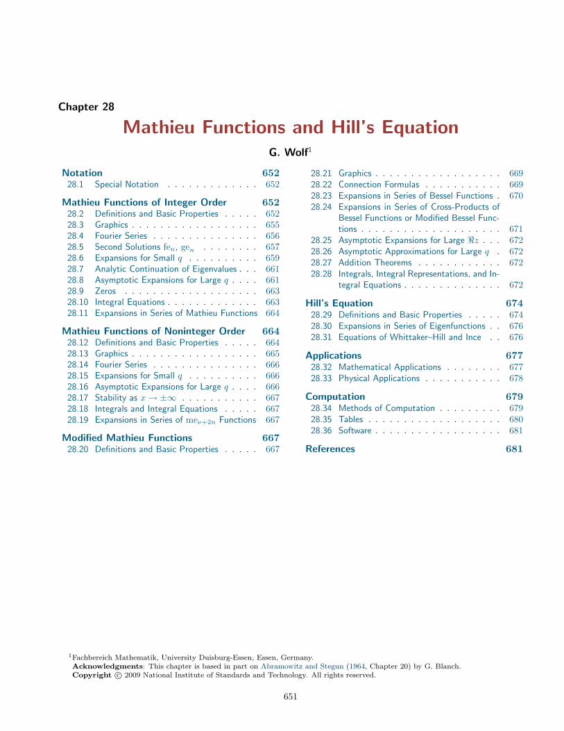
Chapter 28
Mathieu Functions and Hill’s EquationG. Wolf1
Notation 65228.1 Special Notation . . . . . . . . . . . . . 652
Mathieu Functions of Integer Order 65228.2 Definitions and Basic Properties . . . . . 65228.3 Graphics . . . . . . . . . . . . . . . . . . 65528.4 Fourier Series . . . . . . . . . . . . . . . 65628.5 Second Solutions fen, gen . . . . . . . . 65728.6 Expansions for Small q . . . . . . . . . . 65928.7 Analytic Continuation of Eigenvalues . . . 66128.8 Asymptotic Expansions for Large q . . . . 66128.9 Zeros . . . . . . . . . . . . . . . . . . . 66328.10 Integral Equations . . . . . . . . . . . . . 66328.11 Expansions in Series of Mathieu Functions 664
Mathieu Functions of Noninteger Order 66428.12 Definitions and Basic Properties . . . . . 66428.13 Graphics . . . . . . . . . . . . . . . . . . 66528.14 Fourier Series . . . . . . . . . . . . . . . 66628.15 Expansions for Small q . . . . . . . . . . 66628.16 Asymptotic Expansions for Large q . . . . 66628.17 Stability as x→ ±∞ . . . . . . . . . . . 66728.18 Integrals and Integral Equations . . . . . 66728.19 Expansions in Series of meν+2n Functions 667
Modified Mathieu Functions 66728.20 Definitions and Basic Properties . . . . . 667
28.21 Graphics . . . . . . . . . . . . . . . . . . 66928.22 Connection Formulas . . . . . . . . . . . 66928.23 Expansions in Series of Bessel Functions . 67028.24 Expansions in Series of Cross-Products of
Bessel Functions or Modified Bessel Func-tions . . . . . . . . . . . . . . . . . . . . 671
28.25 Asymptotic Expansions for Large <z . . . 67228.26 Asymptotic Approximations for Large q . 67228.27 Addition Theorems . . . . . . . . . . . . 67228.28 Integrals, Integral Representations, and In-
tegral Equations . . . . . . . . . . . . . . 672
Hill’s Equation 67428.29 Definitions and Basic Properties . . . . . 67428.30 Expansions in Series of Eigenfunctions . . 67628.31 Equations of Whittaker–Hill and Ince . . 676
Applications 67728.32 Mathematical Applications . . . . . . . . 67728.33 Physical Applications . . . . . . . . . . . 678
Computation 67928.34 Methods of Computation . . . . . . . . . 67928.35 Tables . . . . . . . . . . . . . . . . . . . 68028.36 Software . . . . . . . . . . . . . . . . . . 681
References 681
1Fachbereich Mathematik, University Duisburg-Essen, Essen, Germany.Acknowledgments: This chapter is based in part on Abramowitz and Stegun (1964, Chapter 20) by G. Blanch.Copyright c© 2009 National Institute of Standards and Technology. All rights reserved.
651

652 Mathieu Functions and Hill’s Equation
Notation
28.1 Special Notation
(For other notation see pp. xiv and 873.)
m,n integers.x, y real variables.z = x+ iy complex variable.ν order of the Mathieu function or modified
Mathieu function. (When ν is an integerit is often replaced by n.)
δ arbitrary small positive number.a, q, h real or complex parameters of Mathieu’s
equation with q = h2.primes unless indicated otherwise, derivatives
with respect to the argument
The main functions treated in this chapter are theMathieu functions
ceν(z, q), seν(z, q), fen(z, q), gen(z, q), meν(z, q),
and the modified Mathieu functions
Ceν(z, q), Seν(z, q), Fen(z, q), Gen(z, q),Meν(z, q), M(j)
ν (z, h), Mc(j)n (z, h), Ms(j)
n (z, h),Ien(z, h), Ion(z, h), Ken(z, h), Kon(z, h).
The functions Mc(j)n (z, h) and Ms(j)
n (z, h) are also knownas the radial Mathieu functions.
The eigenvalues of Mathieu’s equation are denotedby
an(q), bn(q), λν(q).
The notation for the joining factors is
ge,n(h), go,n(h), fe,n(h), fo,n(h).
Alternative notations for the parameters a and q areshown in Table 28.1.1.
Table 28.1.1: Notations for parameters in Mathieu’sequation.
Reference a q
Erdélyi et al. (1955) h θ
Meixner and Schäfke (1954) λ h2
Moon and Spencer (1971) λ q
Strutt (1932) λ h2
Whittaker and Watson (1927) a 8q
Alternative notations for the functions are as follows.
Arscott (1964b) and McLachlan (1947)
Feyn(z, q) =√
12πge,n(h) cen(0, q) Mc(2)
n (z, h),
Me(1,2)n (z, q) =
√12πge,n(h) cen(0, q) Mc(3,4)
n (z, h),
Geyn(z, q) =√
12πgo,n(h) se′n(0, q) Ms(2)
n (z, h),
Ne(1,2)n (z, q) =
√12πgo,n(h) se′n(0, q) Ms(3,4)
n (z, h).
Arscott (1964b) also uses −iµ for ν.
Campbell (1955)
inn = fen, cehn = Cen, inhn = Fen,jnn = gen, sehn = Sen, jnhn = Gen .
Abramowitz and Stegun (1964, Chapter 20)
Fν(z) = Meν(z, q).
NBS (1967)
With s = 4q,
Sen(s, z) =cen(z, q)cen(0, q)
, Son(s, z) =sen(z, q)se′n(0, q)
.
Stratton et al. (1941)
With c = 2√q,
Sen(c, z) =cen(z, q)cen(0, q)
, Son(c, z) =sen(z, q)se′n(0, q)
.
Zhang and Jin (1996)
The radial functions Mc(j)n (z, h) and Ms(j)
n (z, h) are de-noted by Mc(j)
n (z, q) and Ms(j)n (z, q), respectively.
Mathieu Functions of Integer Order
28.2 Definitions and Basic Properties
28.2(i) Mathieu’s Equation
The standard form of Mathieu’s equation with param-eters (a, q) is
28.2.1 w′′ + (a− 2q cos(2z))w = 0.
With ζ = sin2 z we obtain the algebraic form of Math-ieu’s equation
28.2.2
ζ(1− ζ)w′′ + 12
(1− 2ζ)w′ + 1
4 (a− 2q(1− 2ζ))w = 0.
This equation has regular singularities at 0 and 1, bothwith exponents 0 and 1
2 , and an irregular singular pointat∞. With ζ = cos z we obtain another algebraic form:
28.2.3 (1− ζ2)w′′ − ζw′ +(a+ 2q − 4qζ2
)w = 0.

28.2 Definitions and Basic Properties 653
28.2(ii) Basic Solutions wI, wII
Since (28.2.1) has no finite singularities its solutions areentire functions of z. Furthermore, a solution w withgiven initial constant values of w and w′ at a point z0
is an entire function of the three variables z, a, and q.The following three transformations
28.2.4 z → −z; z → z ± π; z → z ± 12π, q → −q;
each leave (28.2.1) unchanged. (28.2.1) possesses a fun-damental pair of solutions wI(z; a, q), wII(z; a, q) calledbasic solutions with
28.2.5
[wI(0; a, q) wII(0; a, q)w′I(0; a, q) w′II(0; a, q)
]=[1 00 1
].
wI(z; a, q) is even and wII(z; a, q) is odd. Other proper-ties are as follows.
28.2.6 W {wI, wII} = 1,
28.2.7wI(z ± π; a, q) = wI(π; a, q)wI(z; a, q)
± w′I(π; a, q)wII(z; a, q),
28.2.8wII(z ± π; a, q) = ±wII(π; a, q)wI(z; a, q)
+ w′II(π; a, q)wII(z; a, q),
28.2.9 wI(π; a, q) = w′II(π; a, q),
28.2.10 wI(π; a, q)− 1 = 2w′I(12π; a, q)wII( 1
2π; a, q),
28.2.11 wI(π; a, q) + 1 = 2wI( 12π; a, q)w′II(
12π; a, q),
28.2.12 w′I(π; a, q) = 2wI( 12π; a, q)w′I(
12π; a, q),
28.2.13 wII(π; a, q) = 2wII( 12π; a, q)w′II(
12π; a, q).
28.2(iii) Floquet’s Theorem and theCharacteristic Exponents
Let ν be any real or complex constant. Then Mathieu’sequation (28.2.1) has a nontrivial solution w(z) suchthat
28.2.14 w(z + π) = eπiνw(z),iff eπiν is an eigenvalue of the matrix
28.2.15
[wI(π; a, q) wII(π; a, q)w′I(π; a, q) w′II(π; a, q)
].
Equivalently,
28.2.16 cos(πν) = wI(π; a, q) = wI(π; a,−q).This is the characteristic equation of Mathieu’s equa-tion (28.2.1). cos(πν) is an entire function ofa, q2. The solutions of (28.2.16) are given by ν =π−1 arccos(wI(π; a, q)). If the inverse cosine takes itsprincipal value (§4.23(ii)), then ν = ν̂, where 0 ≤ <ν̂ ≤1. The general solution of (28.2.16) is ν = ±ν̂ + 2n,where n ∈ Z. Either ν̂ or ν is called a characteristic ex-ponent of (28.2.1). If ν̂ = 0 or 1, or equivalently, ν = n,then ν is a double root of the characteristic equation,otherwise it is a simple root.
28.2(iv) Floquet Solutions
A solution with the pseudoperiodic property (28.2.14)is called a Floquet solution with respect to ν. (28.2.9),(28.2.16), and (28.2.7) give for each solution w(z) of(28.2.1) the connection formula
28.2.17 w(z + π) + w(z − π) = 2 cos(πν)w(z).
Therefore a nontrivial solution w(z) is either a Floquetsolution with respect to ν, or w(z + π) − eiνπw(z) is aFloquet solution with respect to −ν.
If q 6= 0, then for a given value of ν the correspond-ing Floquet solution is unique, except for an arbitraryconstant factor (Theorem of Ince; see also 28.5(i)).
The Fourier series of a Floquet solution
28.2.18 w(z) =∞∑
n=−∞c2ne
i(ν+2n)z
converges absolutely and uniformly in compact subsetsof C. The coefficients c2n satisfy
28.2.19
qc2n+2 −(a− (ν + 2n)2
)c2n + qc2n−2 = 0, n ∈ Z.
Conversely, a nontrivial solution c2n of (28.2.19) thatsatisfies28.2.20 lim
n→±∞|c2n|1/|n| = 0
leads to a Floquet solution.
28.2(v) Eigenvalues an, bn
For given ν and q, equation (28.2.16) determines an in-finite discrete set of values of a, the eigenvalues or char-acteristic values, of Mathieu’s equation. When ν̂ = 0or 1, the notation for the two sets of eigenvalues corre-sponding to each ν̂ is shown in Table 28.2.1, togetherwith the boundary conditions of the associated eigen-value problem. In Table 28.2.1 n = 0, 1, 2, . . . .
Table 28.2.1: Eigenvalues of Mathieu’s equation.
ν̂ Boundary Conditions Eigenvalues
0 w′(0) = w′( 12π) = 0 a2n(q)
1 w′(0) = w( 12π) = 0 a2n+1(q)
1 w(0) = w′( 12π) = 0 b2n+1(q)
0 w(0) = w( 12π) = 0 b2n+2(q)
An equivalent formulation is given by
28.2.21w′I(
12π; a, q) = 0, a = a2n(q),
wI( 12π; a, q) = 0, a = a2n+1(q),
and
28.2.22w′II(
12π; a, q) = 0, a = b2n+1(q),
wII( 12π; a, q) = 0, a = b2n+2(q),

654 Mathieu Functions and Hill’s Equation
where n = 0, 1, 2, . . . . When q = 0,
28.2.23 an(0) = n2, n = 0, 1, 2, . . . ,
28.2.24 bn(0) = n2, n = 1, 2, 3, . . . .
Near q = 0, an(q) and bn(q) can be expanded in powerseries in q (see §28.6(i)); elsewhere they are determinedby analytic continuation (see §28.7). For nonnegativereal values of q, see Figure 28.2.1.
Figure 28.2.1: Eigenvalues an(q), bn(q) of Mathieu’sequation as functions of q for 0 ≤ q ≤ 10, n = 0, 1, 2, 3, 4(a’s), n = 1, 2, 3, 4 (b’s).
Distribution
28.2.25
for q > 0: a0 < b1 < a1 < b2 < a2 < b3 < · · · ,for q < 0: a0 < a1 < b1 < b2 < a2 < a3 < · · · .
Change of Sign of q
28.2.26 a2n(−q) = a2n(q),
28.2.27 a2n+1(−q) = b2n+1(q),
28.2.28 b2n+2(−q) = b2n+2(q).
28.2(vi) Eigenfunctions
Table 28.2.2 gives the notation for the eigenfunctionscorresponding to the eigenvalues in Table 28.2.1. Pe-riod π means that the eigenfunction has the propertyw(z + π) = w(z), whereas antiperiod π means thatw(z + π) = −w(z). Even parity means w(−z) = w(z),and odd parity means w(−z) = −w(z).
Table 28.2.2: Eigenfunctions of Mathieu’s equation.
Eigenvalues Eigenfunctions Periodicity Parity
a2n(q) ce2n(z, q) Period π Even
a2n+1(q) ce2n+1(z, q) Antiperiod π Even
b2n+1(q) se2n+1(z, q) Antiperiod π Odd
b2n+2(q) se2n+2(z, q) Period π Odd
When q = 0,
28.2.29ce0(z, 0) = 1/
√2, cen(z, 0) = cos(nz),
sen(z, 0) = sin(nz), n = 1, 2, 3, . . . .For simple roots q of the corresponding equations
(28.2.21) and (28.2.22), the functions are made uniqueby the normalizations28.2.30∫ 2π
0
(cen(x, q))2 dx = π,
∫ 2π
0
(sen(x, q))2 dx = π,
the ambiguity of sign being resolved by (28.2.29) whenq = 0 and by continuity for the other values of q.
The functions are orthogonal, that is,
28.2.31
∫ 2π
0
cem(x, q) cen(x, q) dx = 0, n 6= m,
28.2.32
∫ 2π
0
sem(x, q) sen(x, q) dx = 0, n 6= m,
28.2.33
∫ 2π
0
cem(x, q) sen(x, q) dx = 0.
For change of sign of q (compare (28.2.4))
28.2.34 ce2n(z,−q) = (−1)n ce2n
(12π − z, q
),
28.2.35 ce2n+1(z,−q) = (−1)n se2n+1
(12π − z, q
),
28.2.36 se2n+1(z,−q) = (−1)n ce2n+1
(12π − z, q
),
28.2.37 se2n+2(z,−q) = (−1)n se2n+2
(12π − z, q
).
For the connection with the basic solutions in§28.2(ii),
28.2.38cen(z, q)cen(0, q)
= wI(z; an(q), q), n = 0, 1, . . . ,
28.2.39sen(z, q)se′n(0, q)
= wII(z; bn(q), q), n = 1, 2, . . . .

28.3 Graphics 655
28.3 Graphics
28.3(i) Line Graphs: Mathieu Functions with Fixed q and Variable x
Even π-Periodic Solutions
Figure 28.3.1: ce2n(x, 1) for 0 ≤ x ≤ π/2, n = 0, 1, 2, 3. Figure 28.3.2: ce2n(x, 10) for 0 ≤ x ≤ π/2, n = 0, 1, 2, 3.
Even π-Antiperiodic Solutions
Figure 28.3.3: ce2n+1(x, 1) for 0 ≤ x ≤ π/2, n =0, 1, 2, 3.
Figure 28.3.4: ce2n+1(x, 10) for 0 ≤ x ≤ π/2, n =0, 1, 2, 3.
Odd π-Antiperiodic Solutions
Figure 28.3.5: se2n+1(x, 1) for 0 ≤ x ≤ π/2, n =0, 1, 2, 3.
Figure 28.3.6: se2n+1(x, 10) for 0 ≤ x ≤ π/2, n =0, 1, 2, 3.

656 Mathieu Functions and Hill’s Equation
Odd π-Periodic Solutions
Figure 28.3.7: se2n(x, 1) for 0 ≤ x ≤ π/2, n = 1, 2, 3, 4.
�
Figure 28.3.8: se2n(x, 10) for 0 ≤ x ≤ π/2, n = 1, 2, 3, 4.
For further graphs see Jahnke et al. (1966, pp. 264–265 and 268–275).
28.3(ii) Surfaces: Mathieu Functions with Variable x and q
Figure 28.3.9: ce0(x, q) for 0 ≤ x ≤ 2π, 0 ≤ q ≤ 10. Figure 28.3.10: se1(x, q) for 0 ≤ x ≤ 2π, 0 ≤ q ≤ 10.
For further graphics see http://dlmf.nist.gov/28.3.ii.
28.4 Fourier Series
28.4(i) Definitions
The Fourier series of the periodic Mathieu functionsconverge absolutely and uniformly on all compact setsin the z-plane. For n = 0, 1, 2, 3, . . . ,
28.4.1 ce2n(z, q) =∞∑m=0
A2n2m(q) cos 2mz,
28.4.2 ce2n+1(z, q) =∞∑m=0
A2n+12m+1(q) cos (2m+ 1)z,
28.4.3 se2n+1(z, q) =∞∑m=0
B2n+12m+1(q) sin (2m+ 1)z,
28.4.4 se2n+2(z, q) =∞∑m=0
B2n+22m+2(q) sin (2m+ 2)z.
28.4(ii) Recurrence Relations
28.4.5
aA0 − qA2 = 0, (a− 4)A2 − q(2A0 +A4) = 0,
(a− 4m2)A2m − q(A2m−2 +A2m+2) = 0,
m = 2, 3, 4, . . . , a = a2n(q), A2m = A2n2m(q).
28.4.6
(a− 1− q)A1 − qA3 = 0,(a− (2m+ 1)2
)A2m+1 − q(A2m−1 +A2m+3) = 0,
m = 1, 2, 3, . . . , a = a2n+1(q), A2m+1 = A2n+12m+1(q).
28.4.7
(a− 1 + q)B1 − qB3 = 0,(a− (2m+ 1)2
)B2m+1 − q(B2m−1 +B2m+3) = 0,
m = 1, 2, 3, . . . , a = b2n+1(q), B2m+1 = B2n+12m+1(q).

28.5 Second Solutions fen, gen 657
28.4.8
(a− 4)B2 − qB4 = 0,(a− 4m2)B2m − q(B2m−2 +B2m+2) = 0,
m = 2, 3, 4, . . . , a = b2n+2(q), B2m+2 = B2n+22m+2(q).
28.4(iii) Normalization
28.4.9 2(A2n
0 (q))2
+∞∑m=1
(A2n
2m(q))2
= 1,
28.4.10
∞∑m=0
(A2n+1
2m+1(q))2
= 1,
28.4.11
∞∑m=0
(B2n+1
2m+1(q))2
= 1,
28.4.12
∞∑m=0
(B2n+2
2m+2(q))2
= 1.
Ambiguities in sign are resolved by (28.4.13)–(28.4.16)when q = 0, and by continuity for the other values of q.
28.4(iv) Case q = 0
28.4.13A0
0(0) = 1/√
2, A2n2n(0) = 1, n > 0,
A2n2m(0) = 0, n 6= m,
28.4.14 A2n+12n+1(0) = 1, A2n+1
2m+1(0) = 0, n 6= m,
28.4.15 B2n+12n+1(0) = 1, B2n+1
2m+1(0) = 0, n 6= m,
28.4.16 B2n+22n+2(0) = 1, B2n+2
2m+2(0) = 0, n 6= m.
28.4(v) Change of Sign of q
28.4.17 A2n2m(−q) = (−1)n−mA2n
2m(q),
28.4.18 B2n+22m+2(−q) = (−1)n−mB2n+2
2m+2(q),
28.4.19 A2n+12m+1(−q) = (−1)n−mB2n+1
2m+1(q),
28.4.20 B2n+12m+1(−q) = (−1)n−mA2n+1
2m+1(q).
28.4(vi) Behavior for Small q
For fixed s = 1, 2, 3, . . . and fixed m = 1, 2, 3, . . . ,
28.4.21 A02s(q) =
((−1)s2(s!)2
(q4
)s+O
(qs+2
))A0
0(q),
28.4.22
Amm+2s(q)Bmm+2s(q)
}=(
(−1)sm!s!(m+ s)!
(q4
)s+O
(qs+1
)){Amm(q),Bmm(q),
28.4.23
Amm−2s(q)Bmm−2s(q)
}=(
(m− s− 1)!s!(m− 1)!
(q4
)s+O
(qs+1
)){Amm(q),Bmm(q).
For further terms and expansions see Meixner andSchäfke (1954, p. 122) and McLachlan (1947, §3.33).
28.4(vii) Asymptotic Forms for Large m
As m→∞, with fixed q ( 6= 0) and fixed n,
28.4.24
A2n2m(q)A2n
0 (q)=
(−1)m
(m!)2
(q4
)m π(1 +O
(m−1
))wII( 1
2π; a2n(q), q),
28.4.25
A2n+12m+1(q)A2n+1
1 (q)=
(−1)m+1((12
)m+1
)2
(q4
)m+1 2(1 +O
(m−1
))w′II(
12π; a2n+1(q), q)
,
28.4.26
B2n+12m+1(q)
B2n+11 (q)
=(−1)m((12
)m+1
)2
(q4
)m+1 2(1 +O
(m−1
))wI( 1
2π; b2n+1(q), q),
28.4.27
B2n+22m (q)
B2n+22 (q)
=(−1)m
(m!)2
(q4
)m qπ(1 +O
(m−1
))w′I(
12π; b2n+2(q), q)
.
For the basic solutions wI and wII see §28.2(ii).
28.5 Second Solutions fen, gen
28.5(i) Definitions
Theorem of Ince (1922)
If a nontrivial solution of Mathieu’s equation with q 6= 0has period π or 2π, then any linearly independent solu-tion cannot have either period.
Second solutions of (28.2.1) are given by
28.5.1 fen(z, q) = Cn(q) (z cen(z, q) + fn(z, q)) ,
when a = an(q), n = 0, 1, 2, . . . , and by
28.5.2 gen(z, q) = Sn(q) (z sen(z, q) + gn(z, q)) ,
when a = bn(q), n = 1, 2, 3, . . . . For m = 0, 1, 2, . . . , wehave28.5.3
f2m(z, q) π-periodic, odd,f2m+1(z, q) π-antiperiodic, odd,
and28.5.4
g2m+1(z, q) π-antiperiodic, even,g2m+2(z, q) π-periodic, even;
compare §28.2(vi). The functions fn(z, q), gn(z, q) areunique.
The factors Cn(q) and Sn(q) in (28.5.1) and (28.5.2)are normalized so that
28.5.5
(Cn(q))2
∫ 2π
0
(fn(x, q))2 dx
= (Sn(q))2
∫ 2π
0
(gn(x, q))2 dx = π.
As q → 0 with n 6= 0, Cn(q) → 0, Sn(q) → 0,Cn(q)fn(z, q) → sinnz, and Sn(q)gn(z, q) → cosnz.This determines the signs of Cn(q) and Sn(q). (Othernormalizations for Cn(q) and Sn(q) can be found in

658 Mathieu Functions and Hill’s Equation
the literature, but most formulas—including connec-tion formulas—are unaffected since fen(z, q)/Cn(q) andgen(z, q)/Sn(q) are invariant.)
28.5.6
C2m(−q) = C2m(q),C2m+1(−q) = S2m+1(q),S2m+2(−q) = S2m+2(q).
For q = 0,
28.5.7fe0(z, 0) = z, fen(z, 0) = sinnz,gen(z, 0) = cosnz, n = 1, 2, 3, . . . ;
compare (28.2.29).As a consequence of the factor z on the right-hand
sides of (28.5.1), (28.5.2), all solutions of Mathieu’s
equation that are linearly independent of the periodicsolutions are unbounded as z → ±∞ on R.
Wronskians
28.5.8 W {cen, fen} = cen(0, q) fe′n(0, q),
28.5.9 W {sen, gen} = − se′n(0, q) gen(0, q).
See (28.22.12) for fe′n(0, q) and gen(0, q).For further information on Cn(q), Sn(q), and expan-
sions of fn(z, q), gn(z, q) in Fourier series or in series ofcen, sen functions, see McLachlan (1947, Chapter VII)or Meixner and Schäfke (1954, §2.72).
28.5(ii) Graphics: Line Graphs of Second Solutions of Mathieu’s Equation
Odd Second Solutions
Figure 28.5.1: fe0(x, 0.5) for 0 ≤ x ≤ 2π and (for com-parison) ce0(x, 0.5).
Figure 28.5.2: fe0(x, 1) for 0 ≤ x ≤ 2π and (for compar-ison) ce0(x, 1).
Figure 28.5.3: fe1(x, 0.5) for 0 ≤ x ≤ 2π and (for com-parison) ce1(x, 0.5).
Figure 28.5.4: fe1(x, 1) for 0 ≤ x ≤ 2π and (for compar-ison) ce1(x, 1).
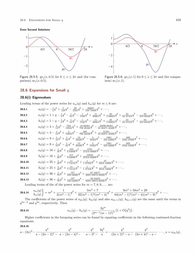
28.6 Expansions for Small q 659
Even Second Solutions
�
Figure 28.5.5: ge1(x, 0.5) for 0 ≤ x ≤ 2π and (for com-parison) se1(x, 0.5).
Figure 28.5.6: ge1(x, 1) for 0 ≤ x ≤ 2π and (for compar-ison) se1(x, 1).
28.6 Expansions for Small q
28.6(i) Eigenvalues
Leading terms of the power series for am(q) and bm(q) for m ≤ 6 are:
28.6.1 a0(q) = − 12q
2 + 7128q
4 − 292304q
6 + 68687188 74368q
8 + · · · ,
28.6.2 a1(q) = 1 + q − 18q
2 − 164q
3 − 11536q
4 + 1136864q
5 + 495 89824q
6 + 5594 37184q
7 − 83353 89440q
8 + · · · ,
28.6.3 b1(q) = 1− q − 18q
2 + 164q
3 − 11536q
4 − 1136864q
5 + 495 89824q
6 − 5594 37184q
7 − 83353 89440q
8 + · · · ,
28.6.4 a2(q) = 4 + 512q
2 − 76313824q
4 + 10 02401796 26240q
6 − 16690 6840145 86471 42400q
8 + · · · ,
28.6.5 b2(q) = 4− 112q
2 + 513824q
4 − 289796 26240q
6 + 2139145 86471 42400q
8 + · · · ,
28.6.6 a3(q) = 9 + 116q
2 + 164q
3 + 1320480q
4 − 516384q
5 − 1961235 92960q
6 − 6091048 57600q
7 + · · · ,
28.6.7 b3(q) = 9 + 116q
2 − 164q
3 + 1320480q
4 + 516384q
5 − 1961235 92960q
6 + 6091048 57600q
7 + · · · ,
28.6.8 a4(q) = 16 + 130q
2 + 4338 64000q
4 − 570127216 00000q
6 + · · · ,
28.6.9 b4(q) = 16 + 130q
2 − 3178 64000q
4 + 1004927216 00000q
6 + · · · ,
28.6.10 a5(q) = 25 + 148q
2 + 117 74144q
4 + 11 47456q
5 + 378918 13888q
6 + · · · ,
28.6.11 b5(q) = 25 + 148q
2 + 117 74144q
4 − 11 47456q
5 + 378918 13888q
6 + · · · ,
28.6.12 a6(q) = 36 + 170q
2 + 187439 04000q
4 + 67 436179293 59872 00000q
6 + · · · ,
28.6.13 b6(q) = 36 + 170q
2 + 187439 04000q
4 − 58 616339293 59872 00000q
6 + · · · .Leading terms of the of the power series for m = 7, 8, 9, . . . are:
28.6.14am(q)bm(q)
}= m2 +
12(m2 − 1)
q2 +5m2 + 7
32(m2 − 1)3(m2 − 4)q4 +
9m4 + 58m2 + 2964(m2 − 1)5(m2 − 4)(m2 − 9)
q6 + · · · .
The coefficients of the power series of a2n(q), b2n(q) and also a2n+1(q), b2n+1(q) are the same until the terms inq2n−2 and q2n, respectively. Then
28.6.15 am(q)− bm(q) =2qm
(2m−1(m− 1)!)2
(1 +O
(q2)).
Higher coefficients in the foregoing series can be found by equating coefficients in the following continued-fractionequations:28.6.16
a−(2n)2−q2
a− (2n− 2)2 −q2
a− (2n− 4)2−· · ·
q2
a− 22 −2q2
a=−
q2
(2n+ 2)2 − a−q2
(2n+ 4)2 − a−· · · , a = a2n(q),

660 Mathieu Functions and Hill’s Equation
28.6.17
a− (2n+ 1)2 −q2
a− (2n− 1)2−· · ·
q2
a− 32 −q2
a− 12 − q= −
q2
(2n+ 3)2 − a−q2
(2n+ 5)2 − a−· · · , a = a2n+1(q),
28.6.18
a− (2n+ 1)2 −q2
a− (2n− 1)2−· · ·
q2
a− 32 −q2
a− 12 + q= −
q2
(2n+ 3)2 − a−q2
(2n+ 5)2 − a−· · · , a = b2n+1(q),
28.6.19
a− (2n+ 2)2 −q2
a− (2n)2 −q2
a− (2n− 2)2−· · ·
q2
a− 22= −
q2
(2n+ 4)2 − a−q2
(2n+ 6)2 − a−· · · , a = b2n+2(q).
Numerical values of the radii of convergence ρ(j)n of the power series (28.6.1)–(28.6.14) for n = 0, 1, . . . , 9 are given
in Table 28.6.1. Here j = 1 for a2n(q), j = 2 for b2n+2(q), and j = 3 for a2n+1(q) and b2n+1(q). (Table 28.6.1 isreproduced from Meixner et al. (1980, §2.4).)
Table 28.6.1: Radii of convergence for power-series expansions of eigenvalues of Mathieu’s equation.
n ρ(1)n ρ
(2)n ρ
(3)n
0 or 1 1.46876 86138 6.92895 47588 3.76995 74940
2 7.26814 68935 16.80308 98254 11.27098 52655
3 16.47116 58923 30.09677 28376 22.85524 71216
4 30.42738 20960 48.13638 18593 38.52292 50099
5 47.80596 57026 69.59879 32769 58.27413 84472
6 69.92930 51764 95.80595 67052 82.10894 36067
7 95.47527 27072 125.43541 1314 110.02736 9210
8 125.76627 89677 159.81025 4642 142.02943 1279
9 159.47921 26694 197.60667 8692 178.11513 940
It is conjectured that for large n, the radii increase in proportion to the square of the eigenvalue number n; seeMeixner et al. (1980, §2.4). It is known that
28.6.20 lim infn→∞
ρ(j)n
n2≥ kk′(K(k))2 = 2.04183 4 . . . ,
where k is the unique root of the equation 2E(k) = K(k) in the interval (0, 1), and k′ =√
1− k2. For E(k) andK(k) see §19.2(ii).
28.6(ii) Functions cen and sen
Leading terms of the power series for the normalized functions are:
28.6.21 2 1/2 ce0(z, q) = 1− 12q cos 2z + 1
32q2 (cos 4z − 2)− 1
128q3(
19 cos 6z − 11 cos 2z
)+ · · · ,
28.6.22ce1(z, q) = cos z − 1
8q cos 3z+ 1
128q2(
23 cos 5z − 2 cos 3z − cos z
)− 1
1024q3(
19 cos 7z − 8
9 cos 5z − 13 cos 3z + 2 cos z
)+ · · · ,
28.6.23se1(z, q) = sin z − 1
8q sin 3z+ 1
128q2(
23 sin 5z + 2 sin 3z − sin z
)− 1
1024q3(
19 sin 7z + 8
9 sin 5z − 13 sin 3z − 2 sin z
)+ · · · ,
28.6.24 ce2(z, q) = cos 2z − 14q(
13 cos 4z − 1
)+ 1
128q2(
13 cos 6z − 76
9 cos 2z)
+ · · · ,
28.6.25 se2(z, q) = sin 2z − 112q sin 4z + 1
128q2(
13 sin 6z − 4
9 sin 2z)
+ · · · .For m = 3, 4, 5, . . . ,
28.6.26
cem(z, q) = cosmz − q
4
(1
m+ 1cos (m+ 2)z − 1
m− 1cos (m− 2)z
)+q2
32
(1
(m+ 1)(m+ 2)cos (m+ 4)z +
1(m− 1)(m− 2)
cos (m− 4)z − 2(m2 + 1)(m2 − 1)2
cosmz)
+ · · · .

28.7 Analytic Continuation of Eigenvalues 661
For the corresponding expansions of sem(z, q) form = 3, 4, 5, . . . change cos to sin everywhere in(28.6.26).
The radii of convergence of the series (28.6.21)–(28.6.26) are the same as the radii of the correspondingseries for an(q) and bn(q); compare Table 28.6.1 and(28.6.20).
28.7 Analytic Continuation of Eigenvalues
As functions of q, an(q) and bn(q) can be continuedanalytically in the complex q-plane. The only singu-larities are algebraic branch points, with an(q) andbn(q) finite at these points. The number of branchpoints is infinite, but countable, and there are no fi-nite limit points. In consequence, the functions can bedefined uniquely by introducing suitable cuts in the q-plane. See Meixner and Schäfke (1954, §2.22). Thebranch points are called the exceptional values, and theother points normal values. The normal values are sim-ple roots of the corresponding equations (28.2.21) and(28.2.22). All real values of q are normal values. To4D the first branch points between a0(q) and a2(q) areat q0 = ±i1.4688 with a0(q0) = a2(q0) = 2.0886, andbetween b2(q) and b4(q) they are at q1 = ±i6.9289 withb2(q1) = b4(q1) = 11.1904. For real q with |q| < |q0|,a0(iq) and a2(iq) are real-valued, whereas for real q with|q| > |q0|, a0(iq) and a2(iq) are complex conjugates.See also Mulholland and Goldstein (1929), Bouwkamp(1948), Meixner et al. (1980), Hunter and Guerrieri(1981), Hunter (1981), and Shivakumar and Xue (1999).
For a visualization of the first branch point of a0(iq̂)and a2(iq̂) see Figure 28.7.1.
Figure 28.7.1: Branch point of the eigenvalues a0(iq̂)and a2(iq̂): 0 ≤ q̂ ≤ 2.5.
All the a2n(q), n = 0, 1, 2, . . . , can be regarded as be-longing to a complete analytic function (in the large).Therefore w′I(
12π; a, q) is irreducible, in the sense that it
cannot be decomposed into a product of entire functions
that contain its zeros; see Meixner et al. (1980, p. 88).Analogous statements hold for a2n+1(q), b2n+1(q), andb2n+2(q), also for n = 0, 1, 2, . . . . Closely connectedwith the preceding statements, we have
28.7.1
∞∑n=0
(a2n(q)− (2n)2
)= 0,
28.7.2
∞∑n=0
(a2n+1(q)− (2n+ 1)2
)= q,
28.7.3
∞∑n=0
(b2n+1(q)− (2n+ 1)2
)= −q,
28.7.4
∞∑n=0
(b2n+2(q)− (2n+ 2)2
)= 0.
28.8 Asymptotic Expansions for Large q
28.8(i) Eigenvalues
Denote h =√q and s = 2m+1. Then as h→ +∞ with
m = 0, 1, 2, . . . ,28.8.1
am(h2)
bm+1
(h2)} ∼ −2h2 + 2sh− 1
8(s2 + 1)− 1
27h(s3 + 3s)
− 1212h2
(5s4 + 34s2 + 9)
− 1217h3
(33s5 + 410s3 + 405s)
− 1220h4
(63s6 + 1260s4 + 2943s2 + 486)
− 1225h5
(527s7 + 15617s5 + 69001s3
+ 41607s) + · · · .For error estimates see Kurz (1979), and for graphicalinterpretation see Figure 28.2.1. Also,
28.8.2
bm+1
(h2)− am
(h2)
=24m+5
m!
(2π
)1/2
hm+( 3/2 )e−4h
×(
1− 6m2 + 14m+ 732h
+O
(1h2
)).
28.8(ii) Sips’ Expansions
Let x = 12π + λh− 1/4 , where λ is a real constant
such that |λ| < 2 1/4 . Also let ξ = 2√h cosx and
Dm(ξ) = e− ξ2/4 Hem(ξ) (§18.3). Then as h→ +∞
28.8.3
cem(x, h2
)= Ĉm (Um(ξ) + Vm(ξ)) ,
sem+1
(x, h2
)sinx
= Ŝm (Um(ξ)− Vm(ξ)) ,
where

662 Mathieu Functions and Hill’s Equation
28.8.4
Um(ξ) ∼ Dm(ξ)− 126h
(Dm+4(ξ)− 4!
(m
4
)Dm−4(ξ)
)+
1213h2
(Dm+8(ξ)− 25(m+ 2)Dm+4(ξ) + 4! 25(m− 1)
(m
4
)Dm−4(ξ) + 8!
(m
8
)Dm−8(ξ)
)+ · · · ,
28.8.5
Vm(ξ) ∼ 124h
(−Dm+2(ξ)−m(m− 1)Dm−2(ξ)
)+
1210h2
(Dm+6(ξ) + (m2 − 25m− 36)Dm+2(ξ)
−m(m− 1)(m2 + 27m− 10)Dm−2(ξ) + 6!(m
6
)Dm−6(ξ)
)+ · · · ,
and
28.8.6 Ĉm ∼(
πh
2(m!)2
)1/4 (1 +
2m+ 18h
+m4 + 2m3 + 263m2 + 262m+ 108
2048h2+ · · ·
)− 1/2
,
28.8.7 Ŝm ∼(
πh
2(m!)2
)1/4 (1− 2m+ 1
8h+m4 + 2m3 − 121m2 − 122m− 84
2048h2+ · · ·
)− 1/2
.
These results are derived formally in Sips (1949, 1959, 1965). See also Meixner and Schäfke (1954, §2.84).
28.8(iii) Goldstein’s Expansions
Let x = 12π − µh
− 1/4 , where µ is a constant such that µ ≥ 1, and s = 2m+ 1. Then as h→ +∞
28.8.8
cem(x, h2
)cem(0, h2)
=2m−( 1/2 )
σm
(W+m(x)(Pm(x)−Qm(x)) +W−m(x)(Pm(x) +Qm(x))
),
sem+1
(x, h2
)se′m+1(0, h2)
=2m−( 1/2 )
τm+1
(W+m(x)(Pm(x)−Qm(x))−W−m(x)(Pm(x) +Qm(x))
),
where
28.8.9 W±m(x) =e±2h sin x
(cosx)m+1
{(cos(
12x+ 1
4π))2m+1
,(sin(
12x+ 1
4π))2m+1
,
and28.8.10 σm ∼ 1 +
s
23h+
4s2 + 327h2
+19s3 + 59s
211h3+ · · · , τm+1 ∼ 2h− 1
4s− 2s2 + 3
26h− 7s3 + 47s
210h2− · · · ,
28.8.11 Pm(x) ∼ 1 +s
23h cos2 x+
1h2
(s4 + 86s2 + 105
211 cos4 x− s4 + 22s2 + 57
211 cos2 x
)+ · · · ,
28.8.12 Qm(x) ∼ sinxcos2 x
(1
25h(s2 + 3) +
129h2
(s3 + 3s+
4s3 + 44scos2 x
))+ · · · .
28.8(iv) Uniform Approximations
Barrett’s Expansions
Barrett (1981) supplies asymptotic approximations fornumerically satisfactory pairs of solutions of both Math-ieu’s equation (28.2.1) and the modified Mathieu equa-tion (28.20.1). The approximations apply when the pa-rameters a and q are real and large, and are uniformwith respect to various regions in the z-plane. Theapproximants are elementary functions, Airy functions,Bessel functions, and parabolic cylinder functions; com-pare §2.8. It is stated that corresponding uniform ap-proximations can be obtained for other solutions, in-cluding the eigensolutions, of the differential equations
by application of the results, but these approximationsare not included.
Dunster’s Approximations
Dunster (1994a) supplies uniform asymptotic approxi-mations for numerically satisfactory pairs of solutionsof Mathieu’s equation (28.2.1). These approximationsapply when q and a are real and q →∞. They are uni-form with respect to a when −2q ≤ a ≤ (2− δ)q, whereδ is an arbitrary constant such that 0 < δ < 4, andalso with respect to z in the semi-infinite strip given by0 ≤ <z ≤ π and =z ≥ 0.
The approximations are expressed in terms of Whit-taker functions Wκ,µ(z) and Mκ,µ(z) with µ = 1
4 ; com-

28.9 Zeros 663
pare §2.8(vi). They are derived by rigorous analysisand accompanied by strict and realistic error bounds.With additional restrictions on z, uniform asymptoticapproximations for solutions of (28.2.1) and (28.20.1)are also obtained in terms of elementary functions by re-expansions of the Whittaker functions; compare §2.8(ii).
Subsequently the asymptotic solutions involving ei-ther elementary or Whittaker functions are identified interms of the Floquet solutions meν(z, q) (§28.12(ii)) andmodified Mathieu functions M(j)
ν (z, h) (§28.20(iii)).For related results see Langer (1934) and Sharples
(1967, 1971).
28.9 Zeros
For real q each of the functions ce2n(z, q), se2n+1(z, q),ce2n+1(z, q), and se2n+2(z, q) has exactly n zeros in0 < z < 1
2π. They are continuous in q. For q → ∞the zeros of ce2n(z, q) and se2n+1(z, q) approach asymp-totically the zeros of He2n
(q1/4(π − 2z)
), and the zeros
of ce2n+1(z, q) and se2n+2(z, q) approach asymptoticallythe zeros of He2n+1
(q1/4(π − 2z)
). Here Hen(z) de-
notes the Hermite polynomial of degree n (§18.3). Fur-thermore, for q > 0 cem(z, q) and sem(z, q) also havepurely imaginary zeros that correspond uniquely to thepurely imaginary z-zeros of Jm
(2√q cos z
)(§10.21(i)),
and they are asymptotically equal as q → 0 and |=z| →∞. There are no zeros within the strip |<z| < 1
2π otherthan those on the real and imaginary axes.
For further details see McLachlan (1947, pp. 234–239) and Meixner and Schäfke (1954, §§2.331, 2.8, 2.81,and 2.85).
28.10 Integral Equations
28.10(i) Equations with Elementary Kernels
With the notation of §28.4 for Fourier coefficients,
28.10.1
2π
∫ π/2
0
cos(2h cos z cos t) ce2n
(t, h2
)dt
=A2n
0 (h2)ce2n
(12π, h
2) ce2n
(z, h2
),
28.10.2
2π
∫ π/2
0
cosh(2h sin z sin t) ce2n
(t, h2
)dt
=A2n
0 (h2)ce2n(0, h2)
ce2n
(z, h2
),
28.10.3
2π
∫ π/2
0
sin(2h cos z cos t) ce2n+1
(t, h2
)dt
= − hA2n+11 (h2)
ce′2n+1
(12π, h
2) ce2n+1
(z, h2
),
28.10.4
2π
∫ π/2
0
cos z cos t cosh(2h sin z sin t) ce2n+1
(t, h2
)dt
=A2n+1
1 (h2)2 ce2n+1(0, h2)
ce2n+1
(z, h2
),
28.10.5
2π
∫ π/2
0
sinh(2h sin z sin t) se2n+1
(t, h2
)dt
=hB2n+1
1 (h2)se′2n+1(0, h2)
se2n+1
(z, h2
),
28.10.6
2π
∫ π/2
0
sin z sin t cos(2h cos z cos t) se2n+1
(t, h2
)dt
=B2n+1
1 (h2)2 se2n+1
(12π, h
2) se2n+1
(z, h2
),
28.10.7
2π
∫ π/2
0
sin z sin t sin(2h cos z cos t) se2n+2
(t, h2
)dt
= − hB2n+22 (h2)
2 se′2n+2
(12π, h
2) se2n+2
(z, h2
),
28.10.8
2π
∫ π/2
0
cos z cos t sinh(2h sin z sin t) se2n+2
(t, h2
)dt
=hB2n+2
2 (h2)2 se′2n+2(0, h2)
se2n+2
(z, h2
).
28.10(ii) Equations with Bessel-FunctionKernels
28.10.9
∫ π/2
0
J0
(2√q(cos2 τ − sin2 ζ)
)ce2n(τ, q) dτ
= wII( 12π; a2n(q), q) ce2n(ζ, q),
28.10.10
∫ π
0
J0(2√q(cos τ + cos ζ)) cen(τ, q) dτ
= wII(π; an(q), q) cen(ζ, q).
28.10(iii) Further Equations
See §28.28. See also Prudnikov et al. (1990, pp. 359–368), Erdélyi et al. (1955, p. 115), and Gradshteyn andRyzhik (2000, pp. 755–759). For relations with variableboundaries see Volkmer (1983).

664 Mathieu Functions and Hill’s Equation
28.11 Expansions in Series of MathieuFunctions
Let f(z) be a 2π-periodic function that is analytic in anopen doubly-infinite strip S that contains the real axis,and q be a normal value (§28.7). Then
28.11.1
f(z) = α0 ce0(z, q) +∞∑n=1
(αn cen(z, q) + βn sen(z, q)) ,
where
28.11.2
αn =1π
∫ 2π
0
f(x) cen(x, q) dx,
βn =1π
∫ 2π
0
f(x) sen(x, q) dx.
The series (28.11.1) converges absolutely and uniformlyon any compact subset of the strip S. See Meixner andSchäfke (1954, §2.28), and for expansions in the caseof the exceptional values of q see Meixner et al. (1980,p. 33).
Examples
With the notation of §28.4,
28.11.3 1 = 2∞∑n=0
A2n0 (q) ce2n(z, q),
28.11.4 cos 2mz =∞∑n=0
A2n2m(q) ce2n(z, q), m 6= 0,
28.11.5 cos (2m+ 1)z =∞∑n=0
A2n+12m+1(q) ce2n+1(z, q),
28.11.6 sin (2m+ 1)z =∞∑n=0
B2n+12m+1(q) se2n+1(z, q),
28.11.7 sin (2m+ 2)z =∞∑n=0
B2n+22m+2(q) se2n+2(z, q).
Mathieu Functions of NonintegerOrder
28.12 Definitions and Basic Properties
28.12(i) Eigenvalues λν+2n(q)
The introduction to the eigenvalues and the functionsof general order proceeds as in §§28.2(i), 28.2(ii), and28.2(iii), except that we now restrict ν̂ 6= 0, 1; equiva-lently ν 6= n. In consequence, for the Floquet solutionsw(z) the factor eπiν in (28.2.14) is no longer ±1.
For given ν (or cos(νπ)) and q, equation (28.2.16)determines an infinite discrete set of values of a, de-noted by λν+2n(q), n = 0,±1,±2, . . . . When q = 0Equation (28.2.16) has simple roots, given by
28.12.1 λν+2n(0) = (ν + 2n)2.
For other values of q, λν+2n(q) is determined by ana-lytic continuation. Without loss of generality, from nowon we replace ν + 2n by ν.
For change of signs of ν and q,
28.12.2 λν(−q) = λν(q) = λ−ν(q).
As in §28.7 values of q for which (28.2.16) has simpleroots λ are called normal values with respect to ν. Forreal values of ν and q all the λν(q) are real, and q isnormal. For graphical interpretation see Figure 28.13.1.To complete the definition we require
28.12.3 λm(q) =
{am(q), m = 0, 1, . . . ,b−m(q), m = −1,−2, . . . .
As a function of ν with fixed q (6= 0), λν(q) is discon-tinuous at ν = ±1,±2, . . . . See Figure 28.13.2.
28.12(ii) Eigenfunctions meν(z, q)
Two eigenfunctions correspond to each eigenvalue a =λν(q). The Floquet solution with respect to ν is denotedby meν(z, q). For q = 0,
28.12.4 meν(z, 0) = eiνz.
The other eigenfunction is meν(−z, q), a Floquet so-lution with respect to −ν with a = λν(q). If q is anormal value of the corresponding equation (28.2.16),then these functions are uniquely determined as ana-lytic functions of z and q by the normalization
28.12.5
∫ π
0
meν(x, q) meν(−x, q) dx = π.
They have the following pseudoperiodic and orthogonal-ity properties:
28.12.6 meν(z + π, q) = eπiν meν(z, q),
28.12.7∫ π
0
meν+2m(x, q) meν+2n(−x, q) dx = 0, m 6= n.
For changes of sign of ν, q, and z,
28.12.8 me−ν(z, q) = meν(−z, q),
28.12.9 meν(z,−q) = eiνπ/2 meν(z − 1
2π, q),
28.12.10 meν(z, q) = meν̄(−z̄, q̄).(28.12.10) is not valid for cuts on the real axis in theq-plane for special complex values of ν; but it remainsvalid for small q; compare §28.7.
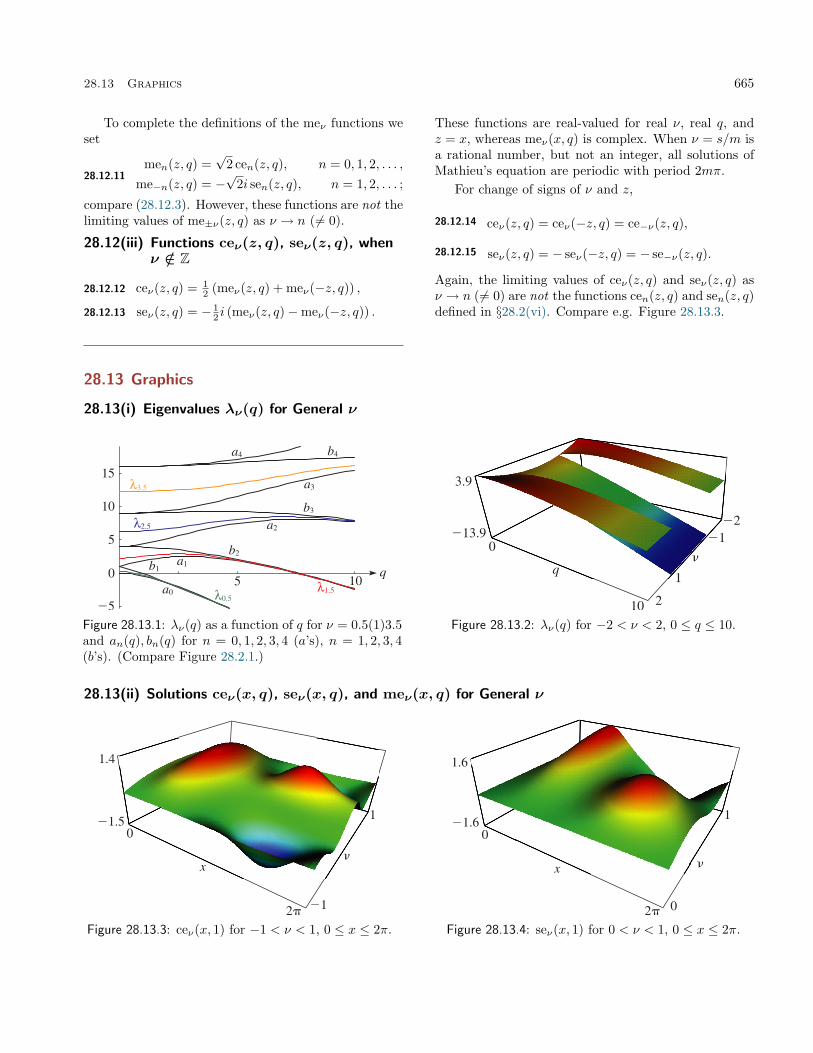
28.13 Graphics 665
To complete the definitions of the meν functions weset
28.12.11men(z, q) =
√2 cen(z, q), n = 0, 1, 2, . . . ,
me−n(z, q) = −√
2i sen(z, q), n = 1, 2, . . . ;
compare (28.12.3). However, these functions are not thelimiting values of me±ν(z, q) as ν → n ( 6= 0).
28.12(iii) Functions ceν(z, q), seν(z, q), whenν /∈ Z
28.12.12 ceν(z, q) = 12 (meν(z, q) + meν(−z, q)) ,
28.12.13 seν(z, q) = − 12 i (meν(z, q)−meν(−z, q)) .
These functions are real-valued for real ν, real q, andz = x, whereas meν(x, q) is complex. When ν = s/m isa rational number, but not an integer, all solutions ofMathieu’s equation are periodic with period 2mπ.
For change of signs of ν and z,
28.12.14 ceν(z, q) = ceν(−z, q) = ce−ν(z, q),
28.12.15 seν(z, q) = − seν(−z, q) = − se−ν(z, q).
Again, the limiting values of ceν(z, q) and seν(z, q) asν → n (6= 0) are not the functions cen(z, q) and sen(z, q)defined in §28.2(vi). Compare e.g. Figure 28.13.3.
28.13 Graphics
28.13(i) Eigenvalues λν(q) for General ν
Figure 28.13.1: λν(q) as a function of q for ν = 0.5(1)3.5and an(q), bn(q) for n = 0, 1, 2, 3, 4 (a’s), n = 1, 2, 3, 4(b’s). (Compare Figure 28.2.1.)
Figure 28.13.2: λν(q) for −2 < ν < 2, 0 ≤ q ≤ 10.
28.13(ii) Solutions ceν(x, q), seν(x, q), and meν(x, q) for General ν
Figure 28.13.3: ceν(x, 1) for −1 < ν < 1, 0 ≤ x ≤ 2π. Figure 28.13.4: seν(x, 1) for 0 < ν < 1, 0 ≤ x ≤ 2π.

666 Mathieu Functions and Hill’s Equation
Figure 28.13.5: meiµ(x, 1) for 0.1 ≤ µ ≤ 0.4, −π ≤ x ≤π.
28.14 Fourier Series
The Fourier series
28.14.1 meν(z, q) =∞∑
m=−∞cν2m(q)ei(ν+2m)z,
28.14.2 ceν(z, q) =∞∑
m=−∞cν2m(q) cos (ν + 2m)z,
28.14.3 seν(z, q) =∞∑
m=−∞cν2m(q) sin (ν + 2m)z,
converge absolutely and uniformly on all compact setsin the z-plane. The coefficients satisfy
28.14.4qc2m+2 −
(a− (ν + 2m)2
)c2m + qc2m−2 = 0,
a = λν(q), c2m = cν2m(q),
and the normalization relation
28.14.5
∞∑m=−∞
(cν2m(q))2 = 1;
compare (28.12.5). Ambiguities in sign are resolved by(28.14.9) when q = 0, and by continuity for other valuesof q.
The rate of convergence is indicated by
28.14.6cν2m(q)cν2m∓2(q)
=−q
4m2
(1 +O
(1m
)), m→ ±∞.
For changes of sign of ν, q, and m,
28.14.7 c−ν−2m(q) = cν2m(q),
28.14.8 cν2m(−q) = (−1)mcν2m(q).
When q = 0,
28.14.9 cν0(0) = 1, cν2m(0) = 0, m 6= 0.
When q → 0 with m (≥ 1) and ν fixed,
28.14.10
cν2m(q) =(
(−1)mqm Γ(ν + 1)m! 22m Γ(ν +m+ 1)
+O(qm+2
))cν0(q).
28.15 Expansions for Small q
28.15(i) Eigenvalues λν(q)
28.15.1
λν(q) = ν2 +1
2(ν2 − 1)q2 +
5ν2 + 732(ν2 − 1)3(ν2 − 4)
q4
+9ν4 + 58ν2 + 29
64(ν2 − 1)5(ν2 − 4)(ν2 − 9)q6 + · · · .
Higher coefficients can be found by equating powersof q in the following continued-fraction equation, witha = λν(q):
28.15.2
a− ν2 −q2
a− (ν + 2)2 −q2
a− (ν + 4)2 −· · ·
=q2
a− (ν − 2)2 −q2
a− (ν − 4)2 −· · · .
28.15(ii) Solutions meν(z, q)
28.15.3
meν(z, q)
= eiνz − q
4
(1
ν + 1ei(ν+2)z − 1
ν − 1ei(ν−2)z
)+q2
32
(1
(ν + 1)(ν + 2)ei(ν+4)z
+1
(ν − 1)(ν − 2)ei(ν−4)z − 2(ν2 + 1)
(ν2 − 1)2eiνz
)+ · · · ;
compare §28.6(ii).
28.16 Asymptotic Expansions for Large q
Let s = 2m + 1, m = 0, 1, 2, . . . , and ν be fixed withm < ν < m+ 1. Then as h(=
√q)→ +∞
28.16.1
λν(h2)∼ −2h2 + 2sh− 1
8(s2 + 1)− 1
27h(s3 + 3s)
− 1212h2
(5s4 + 34s2 + 9)
− 1217h3
(33s5 + 410s3 + 405s)
− 1220h4
(63s6 + 1260s4 + 2943s2 + 486)
− 1225h5
(527s7 + 15617s5 + 69001s3 + 41607s)
+ · · · .For graphical interpretation, see Figures 28.13.1 and28.13.2.
See also §28.8(iv).

28.17 Stability as x→ ±∞ 667
28.17 Stability as x→ ±∞
If all solutions of (28.2.1) are bounded when x → ±∞along the real axis, then the corresponding pair of pa-rameters (a, q) is called stable. All other pairs are un-stable.
For example, positive real values of a with q = 0comprise stable pairs, as do values of a and q that cor-respond to real, but noninteger, values of ν.
However, if =ν 6= 0, then (a, q) always comprises anunstable pair. For example, as x → +∞ one of thesolutions meν(x, q) and meν(−x, q) tends to 0 and theother is unbounded (compare Figure 28.13.5). Also, allnontrivial solutions of (28.2.1) are unbounded on R.
For real a and q (6= 0) the stable regions are the openregions indicated in color in Figure 28.17.1. The bound-ary of each region comprises the characteristic curvesa = an(q) and a = bn(q); compare Figure 28.2.1.
�
Figure 28.17.1: Stability chart for eigenvalues of Math-ieu’s equation (28.2.1).
28.18 Integrals and Integral Equations
See §28.28.
28.19 Expansions in Series of meν+2n
Functions
Let q be a normal value (§28.12(i)) with respect to ν,and f(z) be a function that is analytic on a doubly-infinite open strip S that contains the real axis. Assumealso
28.19.1 f(z + π) = eiνπf(z).Then
28.19.2 f(z) =∞∑
n=−∞fn meν+2n(z, q),
where28.19.3 fn =
1π
∫ π
0
f(z) meν+2n(−z, q) dz.
The series (28.19.2) converges absolutely and uniformlyon compact subsets within S.
Example
28.19.4 eiνz =∞∑
n=−∞cν+2n−2n (q) meν+2n(z, q),
where the coefficients are as in §28.14.
Modified Mathieu Functions
28.20 Definitions and Basic Properties
28.20(i) Modified Mathieu’s Equation
When z is replaced by ±iz, (28.2.1) becomes the modi-fied Mathieu’s equation:
28.20.1 w′′ − (a− 2q cosh(2z))w = 0,with its algebraic form28.20.2
(ζ2 − 1)w′′ + ζw′ +(4qζ2 − 2q − a
)w = 0, ζ = cosh z.
28.20(ii) Solutions Ceν , Seν , Meν , Fen, Gen
28.20.3 Ceν(z, q) = ceν(±iz, q), ν 6= −1,−2, . . . ,
28.20.4 Seν(z, q) = ∓i seν(±iz, q), ν 6= 0,−1, . . . ,
28.20.5 Meν(z, q) = meν(−iz, q),28.20.6 Fen(z, q) = ∓i fen(±iz, q), n = 0, 1, . . . ,
28.20.7 Gen(z, q) = gen(±iz, q), n = 1, 2, . . . .
28.20(iii) Solutions M(j)ν
Assume first that ν is real, q is positive, and a = λν(q);see §28.12(i). Write
28.20.8 h =√q (> 0).
Then from §2.7(ii) it is seen that equation (28.20.2)has independent and unique solutions that are asymp-totic to ζ 1/2 e±2ihζ as ζ → ∞ in the respective sectors|ph(∓iζ)| ≤ 3
2π− δ, δ being an arbitrary small positiveconstant. It follows that (28.20.1) has independent andunique solutions M(3)
ν (z, h), M(4)ν (z, h) such that
28.20.9 M(3)ν (z, h) = H(1)
ν (2h cosh z) (1 +O(sech z)) ,as <z → +∞ with −π + δ ≤ =z ≤ 2π − δ, and
28.20.10 M(4)ν (z, h) = H(2)
ν (2h cosh z) (1 +O(sech z)) ,as <z → +∞ with −2π+ δ ≤ =z ≤ π− δ. See §10.2(ii)for the notation. In addition, there are unique solutionsM(1)ν (z, h), M(2)
ν (z, h) that are real when z is real andhave the properties28.20.11
M(1)ν (z, h) =Jν(2h cosh z)+e|=(2h cosh z)|O
((sech z)3/2
),
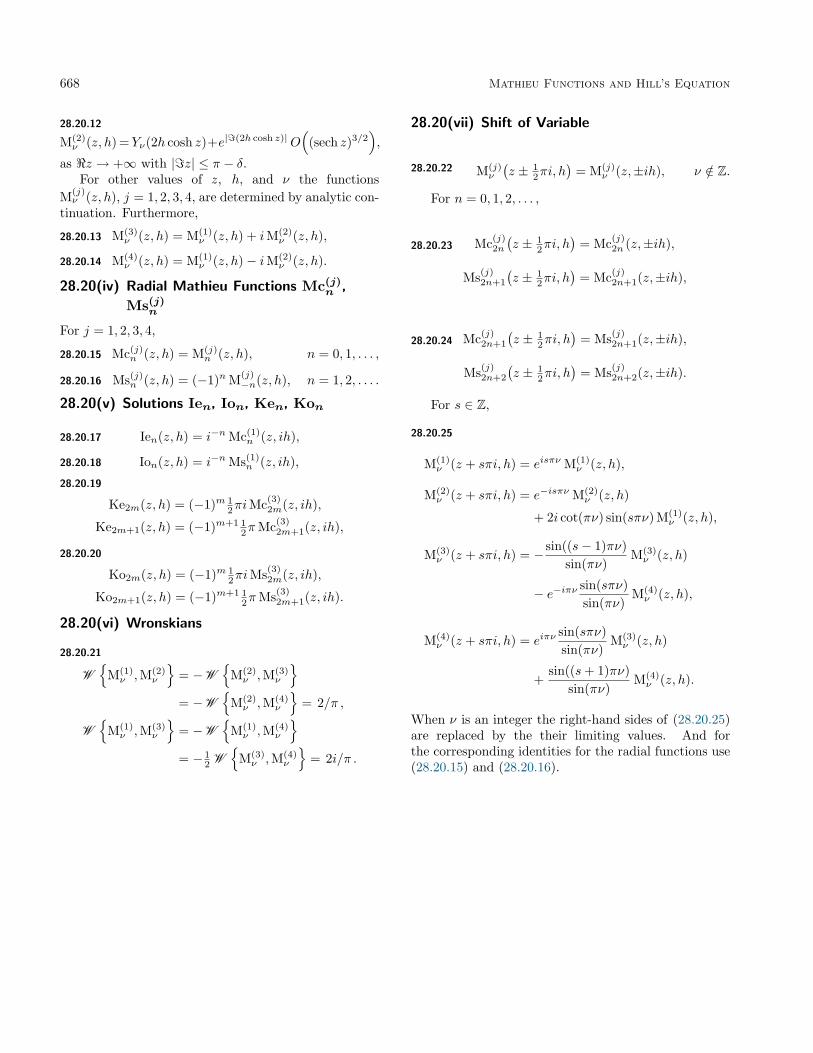
668 Mathieu Functions and Hill’s Equation
28.20.12
M(2)ν (z, h) =Yν(2h cosh z)+e|=(2h cosh z)|O
((sech z)3/2
),
as <z → +∞ with |=z| ≤ π − δ.For other values of z, h, and ν the functions
M(j)ν (z, h), j = 1, 2, 3, 4, are determined by analytic con-
tinuation. Furthermore,
28.20.13 M(3)ν (z, h) = M(1)
ν (z, h) + iM(2)ν (z, h),
28.20.14 M(4)ν (z, h) = M(1)
ν (z, h)− iM(2)ν (z, h).
28.20(iv) Radial Mathieu Functions Mc(j)n ,
Ms(j)n
For j = 1, 2, 3, 4,
28.20.15 Mc(j)n (z, h) = M(j)
n (z, h), n = 0, 1, . . . ,
28.20.16 Ms(j)n (z, h) = (−1)n M(j)
−n(z, h), n = 1, 2, . . . .
28.20(v) Solutions Ien, Ion, Ken, Kon
28.20.17 Ien(z, h) = i−n Mc(1)n (z, ih),
28.20.18 Ion(z, h) = i−n Ms(1)n (z, ih),
28.20.19
Ke2m(z, h) = (−1)m 12πiMc(3)
2m(z, ih),
Ke2m+1(z, h) = (−1)m+1 12πMc(3)
2m+1(z, ih),
28.20.20
Ko2m(z, h) = (−1)m 12πiMs(3)
2m(z, ih),
Ko2m+1(z, h) = (−1)m+1 12πMs(3)
2m+1(z, ih).
28.20(vi) Wronskians
28.20.21
W{
M(1)ν ,M(2)
ν
}= −W
{M(2)ν ,M(3)
ν
}= −W
{M(2)ν ,M(4)
ν
}= 2/π ,
W{
M(1)ν ,M(3)
ν
}= −W
{M(1)ν ,M(4)
ν
}= − 1
2 W{
M(3)ν ,M(4)
ν
}= 2i/π .
28.20(vii) Shift of Variable
28.20.22 M(j)ν
(z ± 1
2πi, h)
= M(j)ν (z,±ih), ν /∈ Z.
For n = 0, 1, 2, . . . ,
28.20.23 Mc(j)2n
(z ± 1
2πi, h)
= Mc(j)2n (z,±ih),
Ms(j)2n+1
(z ± 1
2πi, h)
= Mc(j)2n+1(z,±ih),
28.20.24 Mc(j)2n+1
(z ± 1
2πi, h)
= Ms(j)2n+1(z,±ih),
Ms(j)2n+2
(z ± 1
2πi, h)
= Ms(j)2n+2(z,±ih).
For s ∈ Z,
28.20.25
M(1)ν (z + sπi, h) = eisπν M(1)
ν (z, h),
M(2)ν (z + sπi, h) = e−isπν M(2)
ν (z, h)
+ 2i cot(πν) sin(sπν) M(1)ν (z, h),
M(3)ν (z + sπi, h) = − sin((s− 1)πν)
sin(πν)M(3)ν (z, h)
− e−iπν sin(sπν)sin(πν)
M(4)ν (z, h),
M(4)ν (z + sπi, h) = eiπν
sin(sπν)sin(πν)
M(3)ν (z, h)
+sin((s+ 1)πν)
sin(πν)M(4)ν (z, h).
When ν is an integer the right-hand sides of (28.20.25)are replaced by the their limiting values. And forthe corresponding identities for the radial functions use(28.20.15) and (28.20.16).

28.21 Graphics 669
28.21 Graphics
Radial Mathieu Functions: Surfaces
Figure 28.21.1: Mc(1)0 (x, h) for 0 ≤ h ≤ 3, 0 ≤ x ≤ 2. Figure 28.21.2: Mc(1)
1 (x, h) for 0 ≤ h ≤ 3, 0 ≤ x ≤ 2.
For further graphics see http://dlmf.nist.gov/28.21.
28.22 Connection Formulas
28.22(i) Integer ν
28.22.1
Mc(1)m (z, h) =
√2π
1ge,m(h) cem(0, h2)
Cem(z, h2
),
28.22.2
Ms(1)m (z, h) =
√2π
1go,m(h) se′m(0, h2)
Sem(z, h2
),
28.22.3
Mc(2)m (z, h) =
√2π
1ge,m(h) cem(0, h2)
×(−fe,m(h) Cem
(z, h2
)+
2πCm(h2)
Fem(z, h2
)),
28.22.4
Ms(2)m (z, h) =
√2π
1go,m(h) se′m(0, h2)
×(−fo,m(h) Sem
(z, h2
)− 2πSm(h2)
Gem(z, h2
)).
The joining factors in the above formulas are given by
28.22.5 ge,2m(h) = (−1)m√
2π
ce2m
(12π, h
2)
A2m0 (h2)
,
28.22.6 ge,2m+1(h) = (−1)m+1
√2π
ce′2m+1
(12π, h
2)
hA2m+11 (h2)
,
28.22.7 go,2m+1(h) = (−1)m√
2π
se2m+1
(12π, h
2)
hB2m+11 (h2)
,
28.22.8 go,2m+2(h) = (−1)m+1
√2π
se′2m+2
(12π, h
2)
h2B2m+22 (h2)
,
28.22.9 fe,m(h) = −√π/2ge,m(h) Mc(2)
m (0, h),
28.22.10 fo,m(h) = −√π/2go,m(h) Ms(2)
m
′(0, h),
where Amn (h2), Bmn (h2) are as in §28.4(i), and Cm(h2),Sm(h2) are as in §28.5(i). Furthermore,
28.22.11Mc(2)
m
′(0, h) =
√2/πge,m(h),
Ms(2)m (0, h) = −
√2/πgo,m(h),
28.22.12
fe′m(0, h2
)= 1
2πCm(h2) (ge,m(h))2 cem(0, h2
),
gem(0, h2
)= 1
2πSm(h2) (go,m(h))2 se′m(0, h2
).
28.22(ii) Noninteger ν
28.22.13 M(1)ν (z, h) =
M(1)ν (0, h)
meν(0, h2)Meν
(z, h2
).
Here meν(0, h2
)( 6= 0) is given by (28.14.1) with z = 0,
and M(1)ν (0, h) is given by (28.24.1) with j = 1, z = 0,
and n chosen so that |cν2n(h2)| = max(|cν2`(h2)|), wherethe maximum is taken over all integers `.28.22.14
M(2)ν (z, h) = cot(νπ) M(1)
ν (z, h)− 1sin(νπ)
M(1)−ν(z, h).
See also (28.20.13) and (28.20.14).

670 Mathieu Functions and Hill’s Equation
28.23 Expansions in Series of Bessel Functions
We use the following notations:
28.23.1 C(1)µ = Jµ, C(2)
µ = Yµ, C(3)µ = H(1)
µ , C(4)µ = H(2)
µ ;
compare §10.2(ii). For the coefficients cνn(q) see §28.14. For Amn (q) and Bmn (q) see §28.4.
28.23.2 meν(0, h2
)M(j)ν (z, h) =
∞∑n=−∞
(−1)ncν2n(h2)C(j)ν+2n(2h cosh z),
28.23.3 me′ν(0, h2
)M(j)ν (z, h) = i tanh z
∞∑n=−∞
(−1)n(ν + 2n)cν2n(h2)C(j)ν+2n(2h cosh z),
valid for all z when j = 1, and for <z > 0 and | cosh z| > 1 when j = 2, 3, 4.
28.23.4 meν(
12π, h
2)
M(j)ν (z, h) = eiν π/2
∞∑n=−∞
cν2n(h2)C(j)ν+2n(2h sinh z),
28.23.5 me′ν(
12π, h
2)
M(j)ν (z, h) = ieiν π/2 coth z
∞∑n=−∞
(ν + 2n)cν2n(h2)C(j)ν+2n(2h sinh z),
valid for all z when j = 1, and for <z > 0 and | sinh z| > 1 when j = 2, 3, 4.In the case when ν is an integer
28.23.6 Mc(j)2m(z, h) = (−1)m
(ce2m
(0, h2
))−1∞∑`=0
(−1)`A2m2` (h2)C(j)
2` (2h cosh z),
28.23.7 Mc(j)2m(z, h) = (−1)m
(ce2m
(12π, h
2))−1
∞∑`=0
A2m2` (h2)C(j)
2` (2h sinh z),
28.23.8 Mc(j)2m+1(z, h) = (−1)m
(ce2m+1
(0, h2
))−1∞∑`=0
(−1)`A2m+12`+1 (h2)C(j)
2`+1(2h cosh z),
28.23.9 Mc(j)2m+1(z, h) = (−1)m+1
(ce′2m+1
(12π, h
2))−1
coth z∞∑`=0
(2`+ 1)A2m+12`+1 (h2)C(j)
2`+1(2h sinh z),
28.23.10 Ms(j)2m+1(z, h) = (−1)m
(se′2m+1
(0, h2
))−1tanh z
∞∑`=0
(−1)`(2`+ 1)B2m+12`+1 (h2)C(j)
2`+1(2h cosh z),
28.23.11 Ms(j)2m+1(z, h) = (−1)m
(se2m+1
(12π, h
2))−1
∞∑`=0
B2m+12`+1 (h2)C(j)
2`+1(2h sinh z),
28.23.12 Ms(j)2m+2(z, h) = (−1)m
(se′2m+2
(0, h2
))−1tanh z
∞∑`=0
(−1)`(2`+ 2)B2m+22`+2 (h2)C(j)
2`+2(2h cosh z),
28.23.13 Ms(j)2m+2(z, h) = (−1)m+1
(se′2m+2
(12π, h
2))−1
coth z∞∑`=0
(2`+ 2)B2m+22`+2 (h2)C(j)
2`+2(2h sinh z).
When j = 1, each of the series (28.23.6)–(28.23.13) converges for all z. When j = 2, 3, 4 the series in the even-numbered equations converge for <z > 0 and | cosh z| > 1, and the series in the odd-numbered equations convergefor <z > 0 and | sinh z| > 1.
For proofs and generalizations, see Meixner and Schäfke (1954, §§2.62 and 2.64).

28.24 Expansions in Series of Cross-Products of Bessel Functions or Modified Bessel Functions 671
28.24 Expansions in Series of Cross-Products of Bessel Functions or Modified BesselFunctions
Throughout this section ε0 = 2 and εs = 1, s = 1, 2, 3, . . . .With C(j)
µ , cνn(q), Amn (q), and Bmn (q) as in §28.23,
28.24.1 cν2n(h2) M(j)ν (z, h) =
∞∑`=−∞
(−1)`cν2`(h2) J`−n
(he−z
)C(j)ν+n+`(he
z),
where j = 1, 2, 3, 4 and n ∈ Z.In the case when ν is an integer,
28.24.2 εs Mc(j)2m(z, h) = (−1)m
∞∑`=0
(−1)`A2m
2` (h2)A2m
2s (h2)
(J`−s
(he−z
)C(j)`+s(he
z) + J`+s(he−z
)C(j)`−s(he
z)),
28.24.3 Mc(j)2m+1(z, h) = (−1)m
∞∑`=0
(−1)`A2m+1
2`+1 (h2)
A2m+12s+1 (h2)
(J`−s
(he−z
)C(j)`+s+1(hez) + J`+s+1
(he−z
)C(j)`−s(he
z)),
28.24.4 Ms(j)2m+1(z, h) = (−1)m
∞∑`=0
(−1)`B2m+1
2`+1 (h2)
B2m+12s+1 (h2)
(J`−s
(he−z
)C(j)`+s+1(hez)− J`+s+1
(he−z
)C(j)`−s(he
z)),
28.24.5 Ms(j)2m+2(z, h) = (−1)m
∞∑`=0
(−1)`B2m+2
2`+2 (h2)
B2m+22s+2 (h2)
(J`−s
(he−z
)C(j)`+s+2(hez)− J`+s+2
(he−z
)C(j)`−s(he
z)),
where j = 1, 2, 3, 4, and s = 0, 1, 2, . . . .Also, with In and Kn denoting the modified Bessel functions (§10.25(ii)), and again with s = 0, 1, 2, . . . ,
28.24.6 εs Ie2m(z, h) = (−1)s∞∑`=0
(−1)`A2m
2` (h2)A2m
2s (h2)(I`−s
(he−z
)I`+s(hez) + I`+s
(he−z
)I`−s(hez)
),
28.24.7 Io2m+2(z, h) = (−1)s∞∑`=0
(−1)`B2m+2
2`+2 (h2)
B2m+22s+2 (h2)
(I`−s
(he−z
)I`+s+2(hez)− I`+s+2
(he−z
)I`−s(hez)
),
28.24.8 Ie2m+1(z, h) = (−1)s∞∑`=0
(−1)`B2m+1
2`+1 (h2)
B2m+12s+1 (h2)
(I`−s
(he−z
)I`+s+1(hez) + I`+s+1
(he−z
)I`−s(hez)
),
28.24.9 Io2m+1(z, h) = (−1)s∞∑`=0
(−1)`A2m+1
2`+1 (h2)
A2m+12s+1 (h2)
(I`−s
(he−z
)I`+s+1(hez)− I`+s+1
(he−z
)I`−s(hez)
),
28.24.10 εs Ke2m(z, h) =∞∑`=0
A2m2` (h2)
A2m2s (h2)
(I`−s
(he−z
)K`+s(hez) + I`+s
(he−z
)K`−s(hez)
),
28.24.11 Ko2m+2(z, h) =∞∑`=0
B2m+22`+2 (h2)
B2m+22s+2 (h2)
(I`−s
(he−z
)K`+s+2(hez)− I`+s+2
(he−z
)K`−s(hez)
),
28.24.12 Ke2m+1(z, h) =∞∑`=0
B2m+12`+1 (h2)
B2m+12s+1 (h2)
(I`−s
(he−z
)K`+s+1(hez)− I`+s+1
(he−z
)K`−s(hez)
),
28.24.13 Ko2m+1(z, h) =∞∑`=0
A2m+12`+1 (h2)
A2m+12s+1 (h2)
(I`−s
(he−z
)K`+s+1(hez) + I`+s+1
(he−z
)K`−s(hez)
).
The expansions (28.24.1)–(28.24.13) converge absolutely and uniformly on compact sets of the z-plane.
672 Mathieu Functions and Hill’s Equation
28.25 Asymptotic Expansions for Large <z
For fixed h(6= 0) and fixed ν,
28.25.1
M(3,4)ν (z, h) ∼ e±i(2h cosh z−( 1
2ν+ 14 )π)
(πh(cosh z + 1))12
×∞∑m=0
D±m(∓4ih(cosh z + 1))m
,
where the coefficients are given by
28.25.2 D±−1 = 0, D±0 = 1,and28.25.3
(m+ 1)D±m+1
+((m+ 1
2 )2 ± (m+ 14 )8ih+ 2h2 − a
)D±m
± (m− 12 ) (8ihm)D±m−1 = 0, m ≥ 0.
The upper signs correspond to M(3)ν (z, h) and the lower
signs to M(4)ν (z, h). The expansion (28.25.1) is valid for
M(3)ν (z, h) when
28.25.4 <z → +∞, −π + δ ≤ phh+ =z ≤ 2π − δ,and for M(4)
ν (z, h) when28.25.5 <z → +∞, −2π + δ ≤ phh+ =z ≤ π − δ,
where δ again denotes an arbitrary small positive con-stant.
For proofs and generalizations see Meixner andSchäfke (1954, §2.63).
28.26 Asymptotic Approximations for Largeq
28.26(i) Goldstein’s Expansions
Denote
28.26.1Mc(3)
m (z, h) =eiφ
(πh cosh z) 1/2
× (Fcm(z, h)− iGcm(z, h)) ,
28.26.2iMs(3)
m+1(z, h) =eiφ
(πh cosh z) 1/2
× (Fsm(z, h)− iGsm(z, h)),
where
28.26.3 φ = 2h sinh z −(m+ 1
2
)arctan(sinh z).
Then as h → +∞ with fixed z in <z > 0 and fixeds = 2m+ 1,
28.26.4
Fcm(z, h) ∼ 1 +s
8h cosh2 z+
1211h2
(s4 + 86s2 + 105
cosh4 z− s4 + 22s2 + 57
cosh2 z
)+
1214h3
(−s
5 + 14s3 + 33scosh2 z
− 2s5 + 124s3 + 1122scosh4 z
+3s5 + 290s3 + 1627s
cosh6 z
)+ · · · ,
28.26.5
Gcm(z, h) ∼ sinh zcosh2 z
(s2 + 3
25h+
129h2
(s3 + 3s+
4s3 + 44scosh2 z
)+
1214h3
(5s4 + 34s2 + 9− s6 − 47s4 + 667s2 + 2835
12 cosh2 z+s6 + 505s4 + 12139s2 + 10395
12 cosh4 z
))+ · · · .
The asymptotic expansions of Fsm(z, h) and Gsm(z, h)in the same circumstances are also given by the right-hand sides of (28.26.4) and (28.26.5), respectively.
For additional terms see Goldstein (1927).
28.26(ii) Uniform Approximations
See §28.8(iv). For asymptotic approximations forM(3,4)ν (z, h) see also Naylor (1984, 1987, 1989).
28.27 Addition Theorems
Addition theorems provide important connections be-tween Mathieu functions with different parameters andin different coordinate systems. They are analogous tothe addition theorems for Bessel functions (§10.23(ii))and modified Bessel functions (§10.44(ii)). For a com-prehensive treatment see Meixner et al. (1980, §2.2).
28.28 Integrals, Integral Representations,and Integral Equations
28.28(i) Equations with Elementary Kernels
Let
28.28.1 w = cosh z cos t cosα+ sinh z sin t sinα.
Then
28.28.2
12π
∫ 2π
0
e2ihw cen(t, h2
)dt = in cen
(α, h2
)Mc(1)
n (z, h),
28.28.3
12π
∫ 2π
0
e2ihw sen(t, h2
)dt = in sen
(α, h2
)Ms(1)
n (z, h),

28.28 Integrals, Integral Representations, and Integral Equations 673
28.28.4
ih
π
∫ 2π
0
∂w
∂αe2ihw cen
(t, h2
)dt
= in ce′n(α, h2
)Mc(1)
n (z, h),
28.28.5
ih
π
∫ 2π
0
∂w
∂αe2ihw sen
(t, h2
)dt
= in se′n(α, h2
)Ms(1)
n (z, h).In (28.28.7)–(28.28.9) the paths of integration Lj are
given by
28.28.6
L1 : from − η1 + i∞ to 2π − η1 + i∞,L3 : from − η1 + i∞ to η2 − i∞,L4 : from η2 − i∞ to 2π − η1 + i∞,
where η1 and η2 are real constants.
28.28.7
1π
∫Lje2ihw meν
(t, h2
)dt
= eiνπ/2 meν(α, h2
)M(j)ν (z, h), j = 3, 4,
28.28.8
1π
∫Lj
2ih∂w
∂αe2ihw meν
(t, h2
)dt
= eiνπ/2 me′ν(α, h2
)M(j)ν (z, h), j = 3, 4,
28.28.9
12π
∫L1
e2ihw meν(t, h2
)dt
= eiνπ/2 meν(α, h2
)M(1)ν (z, h).
In (28.28.11)–(28.28.14)
28.28.10 0 < ph(h(cosh z ± 1)) < π.
28.28.11
∫ ∞0
e2ih cosh z cosh t Ceν(t, h2
)dt
= 12πie
iνπ ceν(0, h2
)M(3)ν (z, h),
28.28.12
∫ ∞0
e2ih cosh z cosh t sinh z sinh tSeν(t, h2
)dt
= − π
4heiνπ/2 se′ν
(0, h2
)M(3)ν (z, h),
28.28.13
∫ ∞0
e2ih cosh z cosh t sinh z sinh tFem(t, h2
)dt
= − π
4him fe′m
(0, h2
)Mc(3)
m (z, h),
28.28.14
∫ ∞0
e2ih cosh z cosh t Gem(t, h2
)dt
= 12πi
m+1 gem(0, h2
)Ms(3)
m (z, h).
In particular, when h > 0 the integrals (28.28.11),(28.28.14) converge absolutely and uniformly in the halfstrip <z ≥ 0, 0 ≤ =z ≤ π.
28.28.15
∫ ∞0
cos(2h cos y cosh t) Ce2n
(t, h2
)dt = (−1)n+1 1
2πMc(2)2n (0, h) ce2n
(y, h2
),
28.28.16
∫ ∞0
sin(2h cos y cosh t) Ce2n
(t, h2
)dt = − πA2n
0 (h2)2 ce2n
(12π, h
2) (ce2n
(y, h2
)∓ 2πC2n(h2)
fe2n
(y, h2
)),
where the upper or lower sign is taken according as0 ≤ y ≤ π or π ≤ y ≤ 2π. For A2n
0 (q) and C2n(q)see §§28.4 and 28.5(i).
For details and further equations see Meixner et al.(1980, §2.1.1) and Sips (1970).
28.28(ii) Integrals of Products with BesselFunctions
With the notations of §28.4 for Anm(q) and Bnm(q),§28.14 for cνn(q), and (28.23.1) for C(j)
µ , j = 1, 2, 3, 4,
28.28.17
1π
∫ π
0
C(j)ν+2s(2hR)e−i(ν+2s)φ meν
(t, h2
)dt
= (−1)scν2s(h2) M(j)
ν (z, h), s ∈ Z,where R = R(z, t) and φ = φ(z, t) are analytic functionsfor <z > 0 and real t with
28.28.18R(z, t) =
(12 (cosh(2z) + cos(2t))
)1/2,
R(z, 0) = cosh z,
and
28.28.19e2iφ =
cosh(z + it)cosh(z − it)
,
φ(z, 0) = 0.
In particular, for integer ν and ` = 0, 1, 2, . . . ,
28.28.20
2π
∫ π
0
C(j)2` (2hR) cos(2`φ) ce2m
(t, h2
)dt
= ε`(−1)`+mA2m2` (h2) Mc(j)
2m(z, h),where again ε0 = 2 and ε` = 1, ` = 1, 2, 3, . . . .28.28.21
2π
∫ π
0
C(j)2`+1(2hR) cos((2`+ 1)φ) ce2m+1
(t, h2
)dt
= (−1)`+mA2m+12`+1 (h2) Mc(j)
2m+1(z, h),28.28.22
2π
∫ π
0
C(j)2`+1(2hR) sin((2`+ 1)φ) se2m+1
(t, h2
)dt
= (−1)`+mB2m+12`+1 (h2) Ms(j)
2m+1(z, h),

674 Mathieu Functions and Hill’s Equation
28.28.23
2π
∫ π
0
C(j)2`+2(2hR) sin((2`+ 2)φ) se2m+2
(t, h2
)dt
= (−1)`+mB2m+22`+2 (h2) Ms(j)
2m+2(z, h).
28.28(iii) Integrals of Products of MathieuFunctions of Noninteger Order
With the parameter h suppressed we use the notation28.28.24
D0(ν, µ, z) = M(3)ν (z) M(4)
µ (z)−M(4)ν (z) M(3)
µ (z),
D1(ν, µ, z) = M(3)ν
′(z) M(4)
µ (z)−M(4)ν
′(z) M(3)
µ (z),and assume ν /∈ Z and m ∈ Z. Then28.28.25
sinh zπ2
∫ 2π
0
cos tmeν(t, h2
)me−ν−2m−1
(t, h2
)sinh2 z + sin2 t
dt
= (−1)m+1ihα(0)ν,m D0(ν, ν + 2m+ 1, z),
28.28.26
cosh zπ2
∫ 2π
0
sin tmeν(t, h2
)me−ν−2m−1
(t, h2
)sinh2 z + sin2 t
dt
= (−1)m+1ihα(1)ν,m D0(ν, ν + 2m+ 1, z),
where28.28.27
α(0)ν,m =
12π
∫ 2π
0
cos tmeν(t, h2
)me−ν−2m−1
(t, h2
)dt
= (−1)m2iπ
meν(0, h2
)me−ν−2m−1
(0, h2
)hD0(ν, ν + 2m+ 1, 0)
,
28.28.28
α(1)ν,m =
12π
∫ 2π
0
sin tmeν(t, h2
)me−ν−2m−1
(t, h2
)dt
= (−1)m+1 2iπ
me′ν(0, h2
)me−ν−2m−1
(0, h2
)hD1(ν, ν + 2m+ 1, 0)
.
For further integrals see http://dlmf.nist.gov/28.28.iii.
28.28(iv) Integrals of Products of MathieuFunctions of Integer Order
Again with the parameter h suppressed, let28.28.35
Ds0(n,m, z) = Ms(3)n (z) Ms(4)
m (z)−Ms(4)n (z) Ms(3)
m (z),
Ds1(n,m, z) = Ms(3)n
′(z) Ms(4)
m (z)−Ms(4)n
′(z) Ms(3)
m (z),
Ds2(n,m, z) = Ms(3)n
′(z) Ms(4)
m
′(z)−Ms(4)
n
′(z) Ms(3)
m
′(z).
Then
28.28.36
sinh zπ2
∫ 2π
0
cos t sen(t, h2
)sem
(t, h2
)sinh2 z + sin2 t
dt
= (−1)p+1ihα̂(s)n,m Ds0(n,m, z),
28.28.37
cosh zπ2
∫ 2π
0
sin t se′n(t, h2
)sem
(t, h2
)sinh2 z + sin2 t
dt
= (−1)p+1ihα̂(s)n,m Ds1(n,m, z),
where m− n = 2p+ 1, p ∈ Z; m,n = 1, 2, 3, . . . . Also,
28.28.38
α̂(s)n,m =
12π
∫ 2π
0
cos t sen(t, h2
)sem
(t, h2
)dt
= (−1)p2iπ
se′n(0, h2
)se′m
(0, h2
)hDs2(n,m, 0)
.
For further integrals see http://dlmf.nist.gov/28.28.iv and Schäfke (1983).
28.28(v) Compendia
See Prudnikov et al. (1990, pp. 359–368), Gradshteynand Ryzhik (2000, pp. 755–759), Sips (1970), andMeixner et al. (1980, §2.1.1).
Hill’s Equation
28.29 Definitions and Basic Properties
28.29(i) Hill’s Equation
A generalization of Mathieu’s equation (28.2.1) is Hill’sequation
28.29.1 w′′(z) + (λ+Q(z))w = 0,with28.29.2 Q(z + π) = Q(z),and28.29.3
∫ π
0
Q(z) dz = 0.
Q(z) is either a continuous and real-valued function forz ∈ R or an analytic function of z in a doubly-infiniteopen strip that contains the real axis. π is the minimumperiod of Q.
28.29(ii) Floquet’s Theorem and theCharacteristic Exponent
The basic solutions wI(z, λ), wII(z, λ) are defined in thesame way as in §28.2(ii) (compare (28.2.5), (28.2.6)).Then28.29.4
wI(z + π, λ) = wI(π, λ)wI(z, λ) + w′I(π, λ)wII(z, λ),28.29.5
wII(z + π, λ) = wII(π, λ)wI(z, λ) + w′II(π, λ)wII(z, λ).
Let ν be a real or complex constant satisfying (with-out loss of generality)28.29.6 −1 < <ν ≤ 1throughout this section. Then (28.29.1) has a nontrivialsolution w(z) with the pseudoperiodic property
28.29.7 w(z + π) = eπiνw(z),

28.29 Definitions and Basic Properties 675
iff eπiν is an eigenvalue of the matrix
28.29.8
[wI(π, λ) wII(π, λ)w′I(π, λ) w′II(π, λ)
].
Equivalently,
28.29.9 2 cos(πν) = wI(π, λ) + w′II(π, λ).
This is the characteristic equation of (28.29.1), andcos(πν) is an entire function of λ. Given λ together withthe condition (28.29.6), the solutions ±ν of (28.29.9)are the characteristic exponents of (28.29.1). A solu-tion satisfying (28.29.7) is called a Floquet solution withrespect to ν (or Floquet solution). It has the form
28.29.10 Fν(z) = eiνzPν(z),
where the function Pν(z) is π-periodic.If ν (6= 0, 1) is a solution of (28.29.9), then Fν(z),
F−ν(z) comprise a fundamental pair of solutions of Hill’sequation.
If ν = 0 or 1, then (28.29.1) has a nontrivial solu-tion P (z) which is periodic with period π (when ν = 0)or 2π (when ν = 1). Let w(z) be a solution linearlyindependent of P (z). Then
28.29.11 w(z + π) = (−1)νw(z) + cP (z),
where c is a constant. The case c = 0 is equivalent to
28.29.12
[wI(π, λ) wII(π, λ)w′I(π, λ) w′II(π, λ)
]=[(−1)ν 0
0 (−1)ν
].
The solutions of period π or 2π are exceptional in thefollowing sense. If (28.29.1) has a periodic solution withminimum period nπ, n = 3, 4, . . . , then all solutions areperiodic with period nπ.
Furthermore, for each solution w(z) of (28.29.1)
28.29.13 w(z + π) + w(z − π) = 2 cos(πν)w(z).
A nontrivial solution w(z) is either a Floquet solutionwith respect to ν, or w(z + π) − eiνπw(z) is a Floquetsolution with respect to −ν.
In the symmetric case Q(z) = Q(−z), wI(z, λ) is aneven solution and wII(z, λ) is an odd solution; compare§28.2(ii). (28.29.9) reduces to
28.29.14 cos(πν) = wI(π, λ).
The cases ν = 0 and ν = 1 split into four subcasesas in (28.2.21) and (28.2.22). The π-periodic or π-antiperiodic solutions are multiples of wI(z, λ), wII(z, λ),respectively.
For details and proofs see Magnus and Winkler(1966, §1.3).
28.29(iii) Discriminant and Eigenvalues in theReal Case
Q(x) is assumed to be real-valued throughout this sub-section.
The function
28.29.15 4(λ) = wI(π, λ) + w′II(π, λ)
is called the discriminant of (28.29.1). It is an entirefunction of λ. Its order of growth for |λ| → ∞ is exactly12 ; see Magnus and Winkler (1966, Chapter II, pp. 19–28).
For a given ν, the characteristic equation 4(λ) −2 cos(πν) = 0 has infinitely many roots λ. Conversely,for a given λ, the value of 4(λ) is needed for the com-putation of ν. For this purpose the discriminant canbe expressed as an infinite determinant involving theFourier coefficients of Q(x); see Magnus and Winkler(1966, §2.3, pp. 28–36).
To every equation (28.29.1), there belong two in-creasing infinite sequences of real eigenvalues:
28.29.16 λn, n = 0, 1, 2, . . . , with 4(λn) = 2,
28.29.17 µn, n = 1, 2, 3, . . . , with 4(µn) = −2.
In consequence, (28.29.1) has a solution of period π iffλ = λn, and a solution of period 2π iff λ = µn. Bothλn and µn → ∞ as n → ∞, and interlace according tothe inequalities
28.29.18
λ0 < µ1 ≤ µ2 < λ1 ≤ λ2 < µ3 ≤ µ4 < λ3 ≤ λ4 < · · · .
Assume that the second derivative of Q(x) in(28.29.1) exists and is continuous. Then with
28.29.19 N =1π
∫ π
0
(Q(x))2 dx,
we have for m→∞
28.29.20
µ2m−1 − (2m− 1)2 − N
(4m)2= o(m−2
),
µ2m − (2m− 1)2 − N
(4m)2= o(m−2
),
28.29.21
λ2m−1 − (2m)2 − N
(4m)2= o(m−2
),
λ2m − (2m)2 − N
(4m)2= o(m−2
).
If Q(x) has k continuous derivatives, then as m→∞
28.29.22λ2m − λ2m−1 = o
(1/mk),
µ2m − µ2m−1 = o(
1/mk);
see Hochstadt (1963).For further results, especially when Q(z) is analytic
in a strip, see Weinstein and Keller (1987).

676 Mathieu Functions and Hill’s Equation
28.30 Expansions in Series ofEigenfunctions
28.30(i) Real Variable
Let λ̂m, m = 0, 1, 2, . . . , be the set of characteristic val-ues (28.29.16) and (28.29.17), arranged in their naturalorder (see (28.29.18)), and let wm(x), m = 0, 1, 2, . . . ,be the eigenfunctions, that is, an orthonormal set of2π-periodic solutions; thus
28.30.1 w′′m + (λ̂m +Q(x))wm = 0,
28.30.21
2π
∫ 2π
0
wm(x)wn(x) dx = δm,n.
Then every continuous 2π-periodic function f(x) whosesecond derivative is square-integrable over the interval[0, 2π] can be expanded in a uniformly and absolutelyconvergent series
28.30.3 f(x) =∞∑m=0
fmwm(x),
where
28.30.4 fm =1
2π
∫ 2π
0
f(x)wm(x) dx.
28.30(ii) Complex Variable
For analogous results to those of §28.19, see Schäfke(1960, 1961b), and Meixner et al. (1980, §1.1.11).
28.31 Equations of Whittaker–Hill and Ince
28.31(i) Whittaker–Hill Equation
Hill’s equation with three terms
28.31.1 W ′′ +(A+B cos(2z)− 1
2 (kc)2 cos(4z))W = 0
and constant values of A,B, k, and c, is called the Equa-tion of Whittaker–Hill. It has been discussed in detailby Arscott (1967) for k2 < 0, and by Urwin and Arscott(1970) for k2 > 0.
28.31(ii) Equation of Ince; Ince Polynomials
When k2 < 0, we substitute
28.31.2ξ2 = −4k2c2, A = η − 1
8ξ2, B = −(p+ 1)ξ,
W (z) = w(z) exp(− 1
4ξ cos(2z)),
in (28.31.1). The result is the Equation of Ince:
28.31.3 w′′ + ξ sin(2z)w′ + (η − pξ cos(2z))w = 0.Formal 2π-periodic solutions can be constructed as
Fourier series; compare §28.4:
28.31.4 we,s(z) =∞∑`=0
A2`+s cos (2`+ s)z, s = 0, 1,
28.31.5 wo,s(z) =∞∑`=0
B2`+s sin (2`+ s)z, s = 1, 2,
where the coefficients satisfy
28.31.6−2ηA0 + (2 + p)ξA2 = 0, pξA0 + (4− η)A2 +
(12p+ 2
)ξA4 = 0,
( 12p− `+ 1)ξA2`−2 +
(4`2 − η
)A2` + ( 1
2p+ `+ 1)ξA2`+2 = 0, ` ≥ 2,
28.31.7
(1− η +
(12p+ 1
2
)ξ)A1 +
(12p+ 3
2
)ξA3 = 0,
( 12p− `+ 1
2 )ξA2`−1 +((2`+ 1)2 − η
)A2`+1 + ( 1
2p+ `+ 32 )ξA2`+3 = 0, ` ≥ 1,
28.31.8
(1− η −
(12p+ 1
2
)ξ)B1 +
(12p+ 3
2
)ξB3 = 0,
( 12p− `+ 1
2 )ξB2`−1 +((2`+ 1)2 − η
)B2`+1 + ( 1
2p+ `+ 32 )ξB2`+3 = 0, ` ≥ 1,
28.31.9(4− η)B2 +
(12p+ 2
)ξB4 = 0,
( 12p− `+ 1)ξB2`−2 + (4`2 − η)B2` + ( 1
2p+ `+ 1)ξB2`+2 = 0, ` ≥ 2.
When p is a nonnegative integer, the parameter ηcan be chosen so that solutions of (28.31.3) are trigono-metric polynomials, called Ince polynomials. They aredenoted by
28.31.10C2m
2n (z, ξ) with p = 2n,C2m+1
2n+1 (z, ξ) with p = 2n+ 1,
28.31.11S2m+1
2n+1 (z, ξ) with p = 2n+ 1,S2m+2
2n+2 (z, ξ) with p = 2n+ 2,
and m = 0, 1, . . . , n in all cases.The values of η corresponding to Cmp (z, ξ), Smp (z, ξ)
are denoted by amp (ξ), bmp (ξ), respectively. They are realand distinct, and can be ordered so that Cmp (z, ξ) andSmp (z, ξ) have preciselym zeros, all simple, in 0 ≤ z < π.The normalization is given by28.31.12
1π
∫ 2π
0
(Cmp (x, ξ)
)2dx =
1π
∫ 2π
0
(Smp (x, ξ)
)2dx = 1,

Applications 677
ambiguities in sign being resolved by requiring Cmp (x, ξ)and Smp
′(x, ξ) to be continuous functions of x and posi-tive when x = 0.
For ξ → 0, with x fixed,
28.31.13
C0p(x, ξ)→ 1/
√2, Cmp (x, ξ)→ cos(mx),
Smp (x, ξ)→ sin(mx), m 6= 0; amp (ξ), bmp (ξ)→ m2.
If p → ∞ and ξ → 0 in such a way that pξ → 2q,then in the notation of §§28.2(v) and 28.2(vi)
28.31.14 Cmp (x, ξ)→ cem(x, q), Smp (x, ξ)→ sem(x, q),
28.31.15 amp (ξ)→ am(q), bmp (ξ)→ bm(q).
For proofs and further information, including con-vergence of the series (28.31.4), (28.31.5), see Arscott(1967).
28.31(iii) Paraboloidal Wave Functions
With (28.31.10) and (28.31.11),
28.31.16 hcmp (z, ξ) = e−14 ξ cos(2z)Cmp (z, ξ),
28.31.17 hsmp (z, ξ) = e−14 ξ cos(2z)Smp (z, ξ),
are called paraboloidal wave functions. They satisfy thedifferential equation
28.31.18
w′′ +(η − 1
8ξ2 − (p+ 1)ξ cos(2z) + 1
8ξ2 cos(4z)
)w = 0,
with η = amp (ξ), η = bmp (ξ), respectively.For change of sign of ξ,
28.31.19
hc2m2n (z,−ξ) = (−1)mhc2m
2n ( 12π − z, ξ),
hc2m+12n+1 (z,−ξ) = (−1)mhs2m+1
2n+1 ( 12π − z, ξ),
and
28.31.20
hs2m+12n+1 (z,−ξ) = (−1)mhc2m+1
2n+1 ( 12π − z, ξ),
hs2m+22n+2 (z,−ξ) = (−1)mhs2m+2
2n+2 ( 12π − z, ξ).
For m1 6= m2,
28.31.21
∫ 2π
0
hcm1p (x, ξ)hcm2
p (x, ξ) dx
=∫ 2π
0
hsm1p (x, ξ)hsm2
p (x, ξ) dx = 0.
More important are the double orthogonality relationsfor p1 6= p2 or m1 6= m2 or both, given by
28.31.22∫ u∞
u0
∫ 2π
0
hcm1p1 (u, ξ)hcm1
p1 (v, ξ)hcm2p2 (u, ξ)hcm2
p2 (v, ξ)
× (cos(2u)− cos(2v)) dv du = 0,
and28.31.23∫ u∞
u0
∫ 2π
0
hsm1p1 (u, ξ)hsm1
p1 (v, ξ)hsm2p2 (u, ξ)hsm2
p2 (v, ξ)
× (cos(2u)− cos(2v)) dv du = 0,and also for all p1, p2,m1,m2, given by28.31.24∫ u∞
u0
∫ 2π
0
hcm1p1 (u, ξ)hcm1
p1 (v, ξ)hsm2p2 (u, ξ)hsm2
p2 (v, ξ)
× (cos(2u)− cos(2v)) dv du = 0,where (u0, u∞) = (0, i∞) when ξ > 0, and (u0, u∞) =( 1
2π,12π + i∞) when ξ < 0.
For proofs and further integral equations see Urwin(1964, 1965).
Asymptotic Behavior
For ξ > 0, the functions hcmp (z, ξ), hsmp (z, ξ) behaveasymptotically as multiples of exp
(− 1
4ξ cos(2z))
(cos z)p
as z → ±i∞. All other periodic solutions behave asmultiples of exp
(14ξ cos(2z)
)(cos z)−p−2.
For ξ > 0, the functions hcmp (z,−ξ),hsmp (z,−ξ) behave asymptotically as multiples ofexp(
14ξ cos(2z)
)(cos z)−p−2 as z → 1
2π ± i∞. Allother periodic solutions behave as multiples ofexp(− 1
4ξ cos(2z))
(cos z)p.
Applications
28.32 Mathematical Applications
28.32(i) Elliptical Coordinates and an IntegralRelationship
If the boundary conditions in a physical problem relateto the perimeter of an ellipse, then elliptical coordinatesare convenient. These are given by
28.32.1 x = c cosh ξ cos η, y = c sinh ξ sin η.The two-dimensional wave equation
28.32.2∂2V
∂x2 +∂2V
∂y2 + k2V = 0
then becomes
28.32.3∂2V
∂ξ2 +∂2V
∂η2 +12c2k2(cosh(2ξ)− cos(2η))V = 0.
The separated solutions V (ξ, η) = v(ξ)w(η) can be ob-tained from the modified Mathieu’s equation (28.20.1)for v and from Mathieu’s equation (28.2.1) for w, wherea is the separation constant and q = 1
4c2k2.
This leads to integral equations and an integral re-lation between the solutions of Mathieu’s equation (set-ting ζ = iξ, z = η in (28.32.3)).

678 Mathieu Functions and Hill’s Equation
Let u(ζ) be a solution of Mathieu’s equation (28.2.1)and K(z, ζ) be a solution of
28.32.4∂2K
∂z2 −∂2K
∂ζ2 = 2q (cos(2z)− cos(2ζ))K.
Also let L be a curve (possibly improper) such that thequantity
28.32.5 K(z, ζ)du(ζ)dζ
− u(ζ)∂K(z, ζ)
∂ζapproaches the same value when ζ tends to the end-points of L. Then
28.32.6 w(z) =∫LK(z, ζ)u(ζ) dζ
defines a solution of Mathieu’s equation, provided that(in the case of an improper curve) the integral convergeswith respect to z uniformly on compact subsets of C.
Kernels K can be found, for example, by separat-ing solutions of the wave equation in other systems oforthogonal coordinates. See Schmidt and Wolf (1979).
28.32(ii) Paraboloidal Coordinates
The general paraboloidal coordinate system is linkedwith Cartesian coordinates via28.32.7
x1 = 12c (cosh(2α) + cos(2β)− cosh(2γ)) ,
x2 = 2c coshα cosβ sinh γ, x3 = 2c sinhα sinβ cosh γ,where c is a parameter, 0 ≤ α < ∞, −π < β ≤ π, and0 ≤ γ <∞. When the Helmholtz equation
28.32.8 ∇2V + k2V = 0is separated in this system, each of the separated equa-tions can be reduced to the Whittaker–Hill equation(28.31.1), in which A,B are separation constants. Twoconditions are used to determine A,B. The first is the2π-periodicity of the solutions; the second can be theirasymptotic form. For further information see Arscott(1967) for k2 < 0, and Urwin and Arscott (1970) fork2 > 0.
28.33 Physical Applications
28.33(i) Introduction
Mathieu functions occur in practical applications in twomain categories:
• Boundary-values problems arising from solutionof the two-dimensional wave equation in ellipticalcoordinates. This yields a pair of equations of theform (28.2.1) and (28.20.1), and the appropriatesolution of (28.2.1) is usually a periodic solutionof integer order. See §28.33(ii).
• Initial-value problems, in which only one equation(28.2.1) or (28.20.1) is involved. See §28.33(iii).
28.33(ii) Boundary-Value Problems
Physical problems involving Mathieu functions in-clude vibrational problems in elliptical coordinates; see(28.32.1). We shall derive solutions to the uniform, ho-mogeneous, loss-free, and stretched elliptical ring mem-brane with mass ρ per unit area, and radial tension τper unit arc length. The wave equation
28.33.1∂2W
∂x2 +∂2W
∂y2 −ρ
τ
∂2W
∂t2= 0,
with W (x, y, t) = eiωtV (x, y), reduces to (28.32.2) withk2 = ω2ρ/τ . In elliptical coordinates (28.32.2) becomes(28.32.3). The separated solutions Vn(ξ, η) must be 2π-periodic in η, and have the form28.33.2
Vn(ξ, η) =(cn M(1)
n (ξ,√q) + dn M(2)
n (ξ,√q))
men(η, q),
where q = 14c
2k2 and an(q) or bn(q) is the sepa-ration constant; compare (28.12.11), (28.20.11), and(28.20.12). Here cn and dn are constants. The boundaryconditions for ξ = ξ0 (outer clamp) and ξ = ξ1 (innerclamp) yield the following equation for q:
28.33.3M(1)n (ξ0,
√q) M(2)
n (ξ1,√q)
−M(1)n (ξ1,
√q) M(2)
n (ξ0,√q) = 0.
If we denote the positive solutions q of (28.33.3) byqn,m, then the vibration of the membrane is given byω2n,m = 4qn,mτ
/(c2ρ) . The general solution of the prob-
lem is a superposition of the separated solutions.For a visualization see Gutiérrez-Vega et al. (2003),
and for references to other boundary-value problems see:
• McLachlan (1947, Chapters XVI–XIX) for appli-cations of the wave equation to vibrational sys-tems, electrical and thermal diffusion, electromag-netic wave guides, elliptical cylinders in viscousfluids, and diffraction of sound and electromag-netic waves.
• Meixner and Schäfke (1954, §§4.3, 4.4) for ellipticmembranes and electromagnetic waves.
• Daymond (1955) for vibrating systems.
• Troesch and Troesch (1973) for elliptic mem-branes.
• Alhargan and Judah (1995), Bhattacharyya andShafai (1988), and Shen (1981) for ring antennas.
• Alhargan and Judah (1992), Germey (1964),Ragheb et al. (1991), and Sips (1967) for electro-magnetic waves.
More complete bibliographies will be found inMcLachlan (1947) and Meixner and Schäfke (1954).

Computation 679
28.33(iii) Stability and Initial-Value Problems
If the parameters of a physical system vary periodicallywith time, then the question of stability arises, for ex-ample, a mathematical pendulum whose length variesas cos(2ωt). The equation of motion is given by
28.33.4 w′′(t) + (b− f cos(2ωt))w(t) = 0,
with b, f , and ω positive constants. Substituting z = ωt,a = b
/ω2 , and 2q = f
/ω2 , we obtain Mathieu’s stan-
dard form (28.2.1).As ω runs from 0 to +∞, with b and f fixed, the
point (q, a) moves from ∞ to 0 along the ray L givenby the part of the line a = (2b/f)q that lies in thefirst quadrant of the (q, a)-plane. Hence from §28.17the corresponding Mathieu equation is stable or unsta-ble according as (q, a) is in the intersection of L withthe colored or the uncolored open regions depicted inFigure 28.17.1. In particular, the equation is stable forall sufficiently large values of ω.
For points (q, a) that are at intersections of L withthe characteristic curves a = an(q) or a = bn(q), a pe-riodic solution is possible. However, in response to asmall perturbation at least one solution may becomeunbounded.
References for other initial-value problems include:
• McLachlan (1947, Chapter XV) for amplitude dis-tortion in moving-coil loud-speakers, frequencymodulation, dynamical systems, and vibration ofstretched strings.
• Vedeler (1950) for ships rolling among waves.
• Meixner and Schäfke (1954, §§4.1, 4.2, and 4.7)for quantum mechanical problems and rotation ofmolecules.
• Aly et al. (1975) for scattering theory.
• Hunter and Kuriyan (1976) and Rushchitsky andRushchitska (2000) for wave mechanics.
• Fukui and Horiguchi (1992) for quantum theory.
• Jager (1997, 1998) for relativistic oscillators.
• Torres-Vega et al. (1998) for Mathieu functions inphase space.
Computation
28.34 Methods of Computation
28.34(i) Characteristic Exponents
Methods available for computing the values ofwI(π; a,±q) needed in (28.2.16) include:
(a) Direct numerical integration of the differentialequation (28.2.1), with initial values given by(28.2.5) (§§3.7(ii), 3.7(v)).
(b) Representations for wI(π; a,±q) with limit formu-las for special solutions of the recurrence relations§28.4(ii) for fixed a and q; see Schäfke (1961a).
28.34(ii) Eigenvalues
Methods for computing the eigenvalues an(q), bn(q),and λν(q), defined in §§28.2(v) and 28.12(i), include:
(a) Summation of the power series in §§28.6(i) and28.15(i) when |q| is small.
(b) Use of asymptotic expansions and approximationsfor large q (§§28.8(i), 28.16). See also Zhang andJin (1996, pp. 482–485).
(c) Methods described in §3.7(iv) applied to the dif-ferential equation (28.2.1) with the conditions(28.2.5) and (28.2.16).
(d) Solution of the matrix eigenvalue problem for eachof the five infinite matrices that correspond to thelinear algebraic equations (28.4.5)–(28.4.8) and(28.14.4). See Zhang and Jin (1996, pp. 479–482)and §3.2(iv).
(e) Solution of the continued-fraction equations(28.6.16)–(28.6.19) and (28.15.2) by successive ap-proximation. See Blanch (1966), Shirts (1993),and Meixner and Schäfke (1954, §2.87).
28.34(iii) Floquet Solutions
(a) Summation of the power series in §§28.6(ii) and28.15(ii) when |q| is small.
(b) Use of asymptotic expansions and approximationsfor large q (§§28.8(ii)–28.8(iv)).
Also, once the eigenvalues an(q), bn(q), and λν(q)have been computed the following methods are applica-ble:

680 Mathieu Functions and Hill’s Equation
(c) Solution of (28.2.1) by boundary-value meth-ods; see §3.7(iii). This can be combined with§28.34(ii)(c).
(d) Solution of the systems of linear algebraic equa-tions (28.4.5)–(28.4.8) and (28.14.4), with theconditions (28.4.9)–(28.4.12) and (28.14.5), byboundary-value methods (§3.6) to determine theFourier coefficients. Subsequently, the Fourier se-ries can be summed with the aid of Clenshaw’salgorithm (§3.11(ii)). See Meixner and Schäfke(1954, §2.87). This procedure can be combinedwith §28.34(ii)(d).
28.34(iv) Modified Mathieu Functions
For the modified functions we have:
(a) Numerical summation of the expansions in seriesof Bessel functions (28.24.1)–(28.24.13). These se-ries converge quite rapidly for a wide range of val-ues of q and z.
(b) Direct numerical integration (§3.7) of the differen-tial equation (28.20.1) for moderate values of theparameters.
(c) Use of asymptotic expansions for large z or largeq. See §§28.25 and 28.26.
28.35 Tables
28.35(i) Real Variables
• Blanch and Clemm (1962) includes values ofMc(1)
n
(x,√q)
and Mc(1)n
′(x,√q)
for n = 0(1)15with q = 0(.05)1, x = 0(.02)1. Also Ms(1)
n
(x,√q)
and Ms(1)n
′(x,√q)
for n = 1(1)15 with q =0(.05)1, x = 0(.02)1. Precision is generally 7D.
• Blanch and Clemm (1965) includes values ofMc(2)
n
(x,√q), Mc(2)
n
′(x,√q)
for n = 0(1)7, x =0(.02)1; n = 8(1)15, x = 0(.01)1. AlsoMs(2)
n
(x,√q), Ms(2)
n
′(x,√q)
for n = 1(1)7, x =0(.02)1; n = 8(1)15, x = 0(.01)1. In all casesq = 0(.05)1. Precision is generally 7D. Approxi-mate formulas and graphs are also included.
• Blanch and Rhodes (1955) includes Ben(t),Bon(t), t = 1
2
√q, n = 0(1)15; 8D. The range of t
is 0 to 0.1, with step sizes ranging from 0.002 downto 0.00025. Notation: Ben(t) = an(q)+2q−(4n+2)√q, Bon(t) = bn(q) + 2q − (4n− 2)
√q.
• Ince (1932) includes eigenvalues an, bn, andFourier coefficients for n = 0 or 1(1)6, q =0(1)10(2)20(4)40; 7D. Also cen(x, q), sen(x, q) forq = 0(1)10, x = 1(1)90, corresponding to theeigenvalues in the tables; 5D. Notation: an =ben − 2q, bn = bon − 2q.
• Kirkpatrick (1960) contains tables of the modi-fied functions Cen(x, q), Sen+1(x, q) for n = 0(1)5,q = 1(1)20, x = 0.1(.1)1; 4D or 5D.
• NBS (1967) includes the eigenvalues an(q), bn(q)for n = 0(1)3 with q = 0(.2)20(.5)37(1)100, andn = 4(1)15 with q = 0(2)100; Fourier coeffi-cients for cen(x, q) and sen(x, q) for n = 0(1)15,n = 1(1)15, respectively, and various values of qin the interval [0, 100]; joining factors ge,n(
√q),
fe,n(√q) for n = 0(1)15 with q = 0(.5 to 10)100
(but in a different notation). Also, eigenvalues forlarge values of q. Precision is generally 8D.
• Stratton et al. (1941) includes bn, b′n, and the cor-responding Fourier coefficients for Sen(c, x) andSon(c, x) for n = 0 or 1(1)4, c = 0(.1 or .2)4.5.Precision is mostly 5S. Notation: c = 2
√q, bn =
an + 2q, b′n = bn + 2q, and for Sen(c, x), Son(c, x)see §28.1.
• Zhang and Jin (1996, pp. 521–532) includesthe eigenvalues an(q), bn+1(q) for n = 0(1)4,q = 0(1)50; n = 0(1)20 (a’s) or 19 (b’s),q = 1, 3, 5, 10, 15, 25, 50(50)200. Fourier co-efficients for cen(x, 10), sen+1(x, 10), n =0(1)7. Mathieu functions cen(x, 10), sen+1(x, 10),and their first x-derivatives for n = 0(1)4,x = 0(5◦)90◦. Modified Mathieu functionsMc(j)
n
(x,√
10), Ms(j)
n+1
(x,√
10), and their first x-
derivatives for n = 0(1)4, j = 1, 2, x = 0(.2)4.Precision is mostly 9S.
28.35(ii) Complex Variables
• Blanch and Clemm (1969) includes eigenvaluesan(q), bn(q) for q = ρeiφ, ρ = 0(.5)25, φ =5◦(5◦)90◦, n = 0(1)15; 4D. Also an(q) and bn(q)for q = iρ, ρ = 0(.5)100, n = 0(2)14 andn = 2(2)16, respectively; 8D. Double points forn = 0(1)15; 8D. Graphs are included.
28.35(iii) Zeros
• Blanch and Clemm (1965) includes the first andsecond zeros of Mc(2)
n
(x,√q), Mc(2)
n
′(x,√q)
for
n = 0, 1, and Ms(2)n
(x,√q), Ms(2)
n
′(x,√q)
forn = 1, 2, with q = 0(.05)1; 7D.

28.36 Software 681
• Ince (1932) includes the first zero for cen, sen forn = 2(1)5 or 6, q = 0(1)10(2)40; 4D. This ref-erence also gives zeros of the first derivatives, to-gether with expansions for small q.
• Zhang and Jin (1996, pp. 533–535) includes thezeros (in degrees) of cen(x, 10), sen(x, 10) for n =1(1)10, and the first 5 zeros of Mc(j)
n
(x,√
10),
Ms(j)n
(x,√
10)
for n = 0 or 1(1)8, j = 1, 2. Preci-sion is mostly 9S.
28.35(iv) Further Tables
For other tables prior to 1961 see Fletcher et al. (1962,§2.2) and Lebedev and Fedorova (1960, Chapter 11).
28.36 Software
See http://dlmf.nist.gov/28.36.
References
General References
The main references used in writing this chapter are Ar-scott (1964b), McLachlan (1947), Meixner and Schäfke(1954), and Meixner et al. (1980). For §§28.29–28.30the main source is Magnus and Winkler (1966).
Sources
The following list gives the references or other indica-tions of proofs that were used in constructing the varioussections of this chapter. These sources supplement thereferences that are quoted in the text.
§28.2 Arscott (1964b, Chapter II), Erdélyi et al. (1955,§§16.2, 16.4), McLachlan (1947, Chapter II),Meixner and Schäfke (1954, §2.1), Meixner et al.(1980, Chapter 2). Figure 28.2.1 was produced atNIST.
§28.3 These graphics were produced at NIST.
§28.4 Arscott (1964b, Chapter III), McLachlan (1947,Chapter III), Meixner and Schäfke (1954, §§2.25,2.71), Wolf (2008).
§28.5 Arscott (1964b, §2.4), McLachlan (1947, Chap-ter VII), Meixner and Schäfke (1954, §2.7). Thegraphics were produced at NIST.
§28.6 McLachlan (1947, Chapter II), Meixner andSchäfke (1954, §2.2), Meixner et al. (1980, §2.4),Volkmer (1998).
§28.7 Meixner and Schäfke (1954, §§2.22, 2.25). Figure28.7.1 was provided by the author.
§28.8 Goldstein (1927), Meixner and Schäfke (1954,§§2.33, 2.84).
§28.10 Arscott (1964b, Chapter IV), Meixner andSchäfke (1954, §2.6), Meixner et al. (1980, §2.1.2).
§28.11 Arscott (1964b, §3.9.1).
§28.12 Arscott (1964b, Chapter VI), McLachlan (1947,Chapter IV), Meixner and Schäfke (1954, §2.2).
§28.13 These graphics were produced at NIST.
§28.14 Arscott (1964b, Chapter VI), McLachlan (1947,Chapter IV), Meixner and Schäfke (1954, §2.2).
§28.15 Meixner and Schäfke (1954, §2.2).
§28.16 Meixner and Schäfke (1954, §2.2).
§28.17 Arscott (1964b, §6.2), McLachlan (1947, Chap-ter III), Meixner and Schäfke (1954, §2.3). Figure28.17.1 was recomputed by the author.
§28.19 Meixner and Schäfke (1954, §2.28).
§28.20 Arscott (1964b, Chapter VI), Meixner andSchäfke (1954, §2.4).
§28.21 These graphics were produced at NIST.
§28.22 Meixner and Schäfke (1954, §§2.29, 2.65, 2.73,2.76).
§28.23 Meixner and Schäfke (1954, §2.6).
§28.24 Meixner and Schäfke (1954, §§2.6, 2.7).
§28.26 Goldstein (1927), Meixner and Schäfke (1954,§2.84), NBS (1967, IV).
§28.28 Arscott (1964b, Chapters IV and VI), McLach-lan (1947, Chapters IX and XIV), Meixner andSchäfke (1954, §2.7), Meixner et al. (1980, §2.1),Schäfke (1983). There is a sign error on p. 158 ofthe last reference.
§28.29 Magnus and Winkler (1966, Part I, pp. 1–43),Arscott (1964b, Chapter VII), McLachlan (1947,§6.10).
§28.30 Magnus and Winkler (1966, Part I, §2.5).
§28.31 Arscott (1967), Urwin and Arscott (1970), Ur-win (1964, 1965).
§28.32 Arscott (1967, §§1.3 and 2.6), Meixner andSchäfke (1954, §1.135).


Chapter 29
Lamé FunctionsH. Volkmer1
Notation 68429.1 Special Notation . . . . . . . . . . . . . 684
Lamé Functions 68429.2 Differential Equations . . . . . . . . . . . 68429.3 Definitions and Basic Properties . . . . . 68529.4 Graphics . . . . . . . . . . . . . . . . . . 68629.5 Special Cases and Limiting Forms . . . . 68829.6 Fourier Series . . . . . . . . . . . . . . . 68829.7 Asymptotic Expansions . . . . . . . . . . 68929.8 Integral Equations . . . . . . . . . . . . . 68929.9 Stability . . . . . . . . . . . . . . . . . . 69029.10 Lamé Functions with Imaginary Periods . 69029.11 Lamé Wave Equation . . . . . . . . . . . 690
Lamé Polynomials 69029.12 Definitions . . . . . . . . . . . . . . . . . 690
29.13 Graphics . . . . . . . . . . . . . . . . . . 69129.14 Orthogonality . . . . . . . . . . . . . . . 69229.15 Fourier Series and Chebyshev Series . . . 69229.16 Asymptotic Expansions . . . . . . . . . . 69329.17 Other Solutions . . . . . . . . . . . . . . 693
Applications 69329.18 Mathematical Applications . . . . . . . . 69329.19 Physical Applications . . . . . . . . . . . 694
Computation 69429.20 Methods of Computation . . . . . . . . . 69429.21 Tables . . . . . . . . . . . . . . . . . . . 69429.22 Software . . . . . . . . . . . . . . . . . . 695
References 695
1Department of Mathematical Sciences, University of Wisconsin–Milwaukee, Milwaukee, Wisconsin.Copyright c© 2009 National Institute of Standards and Technology. All rights reserved.
683

684 Lamé Functions
Notation
29.1 Special Notation
(For other notation see pp. xiv and 873.)
m,n, p nonnegative integers.x real variable.z complex variable.h, k, ν real parameters, 0 < k < 1, ν ≥ − 1
2 .k′
√1− k2, 0 < k′ < 1.
K,K ′ complete elliptic integrals of the first kindwith moduli k, k′, respectively (see §19.2(ii)).
All derivatives are denoted by differentials, not byprimes.
The main functions treated in this chapter arethe eigenvalues a2m
ν
(k2), a2m+1
ν
(k2), b2m+1
ν
(k2),
b2m+2ν
(k2), the Lamé functions Ec2m
ν
(z, k2
),
Ec2m+1ν
(z, k2
), Es2m+1
ν
(z, k2
), Es2m+2
ν
(z, k2
), and
the Lamé polynomials uEm2n
(z, k2
), sEm
2n+1
(z, k2
),
cEm2n+1
(z, k2
), dEm
2n+1
(z, k2
), scEm
2n+2
(z, k2
),
sdEm2n+2
(z, k2
), cdEm
2n+2
(z, k2
), scdEm
2n+3
(z, k2
). The
notation for the eigenvalues and functions is due toErdélyi et al. (1955, §15.5.1) and that for the polynomi-als is due to Arscott (1964b, §9.3.2). The normalizationis that of Jansen (1977, §3.1).
Other notations that have been used are as follows:Ince (1940a) interchanges a2m+1
ν
(k2)
with b2m+1ν
(k2).
The relation to the Lamé functions L(m)cν , L(m)
sν of Jansen(1977) is given by
Ec2mν
(z, k2
)= (−1)mL(2m)
cν (ψ, k′2),
Ec2m+1ν
(z, k2
)= (−1)mL(2m+1)
sν (ψ, k′2),
Es2m+1ν
(z, k2
)= (−1)mL(2m+1)
cν (ψ, k′2),
Es2m+2ν
(z, k2
)= (−1)mL(2m+2)
sν (ψ, k′2),
where ψ = am (z, k); see §22.16(i). The relation to theLamé functions Ecmν , Esmν of Ince (1940b) is given by
Ec2mν
(z, k2
)= c2mν (k2)Ec2m
ν (z, k2),
Ec2m+1ν
(z, k2
)= c2m+1
ν (k2)Es2m+1ν (z, k2),
Es2m+1ν
(z, k2
)= s2m+1
ν (k2)Ec2m+1ν (z, k2),
Es2m+2ν
(z, k2
)= s2m+2
ν (k2)Es2m+2ν (z, k2),
where the positive factors cmν (k2) and smν (k2) are deter-mined by
(cmν (k2))2 =4π
∫ K
0
(Ecmν
(x, k2
))2dx,
(smν (k2))2 =4π
∫ K
0
(Esmν
(x, k2
))2dx.
Lamé Functions
29.2 Differential Equations
29.2(i) Lamé’s Equation
29.2.1d2w
dz2 + (h− ν(ν + 1)k2 sn2 (z, k))w = 0,
where k and ν are real parameters such that 0 < k < 1and ν ≥ − 1
2 . For sn (z, k) see §22.2. This equation hasregular singularities at the points 2pK + (2q + 1)iK ′,where p, q ∈ Z, andK,K ′ are the complete elliptic inte-grals of the first kind with moduli k, k′(= (1− k2)1/2),respectively; see §19.2(ii). In general, at each singular-ity each solution of (29.2.1) has a branch point (§2.7(i)).See Figure 29.2.1.
× × × × ×
× × × × ×
× × × × ×
× × × × ×
0
−3iK ′
−2iK ′
−iK ′
iK ′
2iK ′
3iK ′
−4K −2K 2K 4K
Figure 29.2.1: z-plane: singularities ××× of Lamé’sequation.
29.2(ii) Other Forms
29.2.2
d2w
dξ2 +12
(1ξ
+1
ξ − 1+
1ξ − k−2
)dw
dξ
+hk−2 − ν(ν + 1)ξ4ξ(ξ − 1)(ξ − k−2)
w = 0,
where
29.2.3 ξ = sn2 (z, k).
29.2.4(1− k2 cos2 φ)
d2w
dφ2 + k2 cosφ sinφdw
dφ
+ (h− ν(ν + 1)k2 cos2 φ)w = 0,
where
29.2.5 φ = 12π − am (z, k).
For am (z, k) see §22.16(i).

29.3 Definitions and Basic Properties 685
Next, let e1, e2, e3 be any real constants that satisfye1 > e2 > e3 and
29.2.6 e1 + e2 + e3 = 0, (e2 − e3)/(e1 − e3) = k2.
(These constants are not unique.) Then with
29.2.7 g = (e1 − e3)h+ ν(ν + 1)e3,
29.2.8 η = (e1 − e3)−1/2(z − iK ′),we have
29.2.9d2w
dη2 + (g − ν(ν + 1)℘(η))w = 0,
and
29.2.10
d2w
dζ2 +12
(1
ζ − e1+
1ζ − e2
+1
ζ − e3
)dw
dζ
+g − ν(ν + 1)ζ
4(ζ − e1)(ζ − e2)(ζ − e3)w = 0,
where
29.2.11 ζ = ℘(η; g2, g3) = ℘(η),with
29.2.12 g2 = −4(e2e3 + e3e1 + e1e2), g3 = 4e1e2e3.
For the Weierstrass function ℘ see §23.2(ii).Equation (29.2.10) is a special case of Heun’s equa-
tion (31.2.1).
29.3 Definitions and Basic Properties
29.3(i) Eigenvalues
For each pair of values of ν and k there are four in-finite unbounded sets of real eigenvalues h for whichequation (29.2.1) has even or odd solutions with periods2K or 4K. They are denoted by a2m
ν
(k2), a2m+1
ν
(k2),
b2m+1ν
(k2), b2m+2
ν
(k2), where m = 0, 1, 2, . . .; see Ta-
ble 29.3.1.Table 29.3.1: Eigenvalues of Lamé’s equation.
eigenvalue h parity period
a2mν
(k2)
even 2K
a2m+1ν
(k2)
odd 4K
b2m+1ν
(k2)
even 4K
b2m+2ν
(k2)
odd 2K
29.3(ii) Distribution
The eigenvalues interlace according to
29.3.1 amν(k2)< am+1
ν
(k2),
29.3.2 amν(k2)< bm+1
ν
(k2),
29.3.3 bmν(k2)< bm+1
ν
(k2),
29.3.4 bmν(k2)< am+1
ν
(k2).
The eigenvalues coalesce according to
29.3.5 amν(k2)
= bmν(k2), ν = 0, 1, . . . ,m− 1.
If ν is distinct from 0, 1, . . . ,m− 1, then
29.3.6(amν(k2)− bmν
(k2))ν(ν − 1) · · · (ν −m+ 1) > 0.
If ν is a nonnegative integer, then29.3.7
amν(k2)
+ aν−mν
(1− k2
)= ν(ν + 1), m = 0, 1, . . . , ν,
29.3.8
bmν(k2)
+ bν−m+1ν
(1− k2
)= ν(ν + 1), m = 1, 2, . . . , ν.
For the special case k = k′ = 1/√
2 see Erdélyi et al.(1955, §15.5.2).
29.3(iii) Continued Fractions
The quantity
29.3.9 H = 2a2mν
(k2)− ν(ν + 1)k2
satisfies the continued-fraction equation
29.3.10
βp −H −αp−1γp
βp−1 −H −αp−2γp−1
βp−2 −H−· · ·
=αpγp+1
βp+1 −H −αp+1γp+2
βp+2 −H−· · · ,
where p is any nonnegative integer, and
29.3.11 αp =
{(ν − 1)(ν + 2)k2, p = 0,12 (ν − 2p− 1)(ν + 2p+ 2)k2, p ≥ 1,
29.3.12βp = 4p2(2− k2),γp = 1
2 (ν − 2p+ 2)(ν + 2p− 1)k2.
The continued fraction following the second negativesign on the left-hand side of (29.3.10) is finite: it equals0 if p = 0, and if p > 0, then the last denominatoris β0 − H. If ν is a nonnegative integer and 2p ≤ ν,then the continued fraction on the right-hand side of(29.3.10) terminates, and (29.3.10) has only the solu-tions (29.3.9) with 2m ≤ ν. If ν is a nonnegative inte-ger and 2p > ν, then (29.3.10) has only the solutions(29.3.9) with 2m > ν.
For the corresponding continued-fraction equationsfor a2m+1
ν
(k2), b2m+1
ν
(k2), and b2m+2
ν
(k2)
see http://dlmf.nist.gov/29.3.iii.
29.3(iv) Lamé Functions
The eigenfunctions corresponding to the eigenvalues of§29.3(i) are denoted by Ec2m
ν
(z, k2
), Ec2m+1
ν
(z, k2
),
Es2m+1ν
(z, k2
), Es2m+2
ν
(z, k2
). They are called Lamé
functions with real periods and of order ν, or more sim-ply, Lamé functions. See Table 29.3.2. In this tablethe nonnegative integer m corresponds to the numberof zeros of each Lamé function in (0,K), whereas thesuperscripts 2m, 2m + 1, or 2m + 2 correspond to thenumber of zeros in [0, 2K).

686 Lamé Functions
Table 29.3.2: Lamé functions.
boundary conditionseigenvalue
heigenfunction
w(z)parity ofw(z)
parity ofw(z −K)
period ofw(z)
dw/dz |z=0 = dw/dz |z=K = 0 a2mν
(k2)
Ec2mν
(z, k2
)even even 2K
w(0) = dw/dz |z=K = 0 a2m+1ν
(k2)
Ec2m+1ν
(z, k2
)odd even 4K
dw/dz |z=0 = w(K) = 0 b2m+1ν
(k2)
Es2m+1ν
(z, k2
)even odd 4K
w(0) = w(K) = 0 b2m+2ν
(k2)
Es2m+2ν
(z, k2
)odd odd 2K
29.3(v) Normalization
29.3.18
∫ K
0
dn (x, k)(Ec2m
ν
(x, k2
))2dx =
14π,∫ K
0
dn (x, k)(Ec2m+1
ν
(x, k2
))2dx =
14π,∫ K
0
dn (x, k)(Es2m+1
ν
(x, k2
))2dx =
14π,∫ K
0
dn (x, k)(Es2m+2
ν
(x, k2
))2dx =
14π.
For dn (z, k) see §22.2.To complete the definitions, Ecmν
(K, k2
)is positive
and dEsmν(z, k2
)/dz∣∣z=K
is negative.
29.3(vi) Orthogonality
For m 6= p,
29.3.19
∫ K
0
Ec2mν
(x, k2
)Ec2p
ν
(x, k2
)dx = 0,∫ K
0
Ec2m+1ν
(x, k2
)Ec2p+1
ν
(x, k2
)dx = 0,∫ K
0
Es2m+1ν
(x, k2
)Es2p+1
ν
(x, k2
)dx = 0,∫ K
0
Es2m+2ν
(x, k2
)Es2p+2
ν
(x, k2
)dx = 0.
For the values of these integrals when m = p see §29.6.
29.3(vii) Power Series
For power-series expansions of the eigenvalues see Volk-mer (2004b).
29.4 Graphics
29.4(i) Eigenvalues of Lamé’s Equation: LineGraphs
Figure 29.4.1: amν (0.5), bm+1ν (0.5) as functions of ν for
m = 0, 1, 2, 3.

29.4 Graphics 687
Figure 29.4.2: a3ν(0.5)− b3ν(0.5) as a function of ν. Figure 29.4.3: am1.5
(k2), bm+1
1.5
(k2)
as functions of k2 form = 0, 1, 2.
For additional graphs see http://dlmf.nist.gov/29.4.i.
29.4(ii) Eigenvalues of Lamé’s Equation: Surfaces
Figure 29.4.9: a0ν
(k2)
as a function of ν and k2. Figure 29.4.10: b1ν(k2)
as a function of ν and k2.
For additional surfaces see http://dlmf.nist.gov/29.4.ii.
29.4(iii) Lamé Functions: Line Graphs
Figure 29.4.13: Ecm1.5(x, 0.5) for −2K ≤ x ≤ 2K, m =0, 1, 2. K = 1.85407 . . . .
Figure 29.4.14: Esm1.5(x, 0.5) for −2K ≤ x ≤ 2K, m =1, 2, 3. K = 1.85407 . . . .
For additional graphs see http://dlmf.nist.gov/29.4.iii.

688 Lamé Functions
29.4(iv) Lamé Functions: Surfaces
Figure 29.4.25: Ec01.5
(x, k2
)as a function of x and k2. Figure 29.4.26: Es1
1.5
(x, k2
)as a function of x and k2.
For additional surfaces see http://dlmf.nist.gov/29.4.iv.
29.5 Special Cases and Limiting Forms
29.5.1 amν (0) = bmν (0) = m2,
29.5.2 Ec0ν(z, 0) = 2−
12 ,
29.5.3Ecmν (z, 0) = cos
(m( 1
2π − z)), m ≥ 1,
Esmν (z, 0) = sin(m( 1
2π − z)), m ≥ 1.
Let µ = max (ν −m, 0). Then
29.5.4 limk→1−
amν(k2)
= limk→1−
bm+1ν
(k2)
= ν(ν + 1)− µ2,
29.5.5
limk→1−
Ecmν(z, k2
)Ecmν (0, k2)
= limk→1−
Esm+1ν
(z, k2
)Esm+1
ν (0, k2)
=1
(cosh z)µF
(12µ−
12ν,
12µ+ 1
2ν + 12
12
; tanh2 z
),
m even,
29.5.6
limk→1−
Ecmν(z, k2
)dEcmν (z, k2)/dz |z=0
= limk→1−
Esm+1ν
(z, k2
)dEsm+1
ν (z, k2)/dz∣∣z=0
=tanh z
(cosh z)µF
(12µ−
12ν + 1
2 ,12µ+ 1
2ν + 132
; tanh2 z
),
m odd,
where F is the hypergeometric function; see §15.2(i).
If k → 0+ and ν → ∞ in such a way thatk2ν(ν + 1) = 4θ (a positive constant), then
29.5.7lim Ecmν
(z, k2
)= cem
(12π − z, θ
),
lim Esmν(z, k2
)= sem
(12π − z, θ
),
where cem(z, θ) and sem(z, θ) are Mathieu functions; see§28.2(vi).
29.6 Fourier Series
29.6(i) Function Ec2mν
(z, k2
)With φ = 1
2π − am (z, k), as in (29.2.5), we have
29.6.1 Ec2mν
(z, k2
)= 1
2A0 +∞∑p=1
A2p cos(2pφ).
Here
29.6.2 H = 2a2mν
(k2)− ν(ν + 1)k2,
29.6.3 (β0 −H)A0 + α0A2 = 0,
29.6.4
γpA2p−2 + (βp −H)A2p + αpA2p+2 = 0, p ≥ 1,
with αp, βp, and γp as in (29.3.11) and (29.3.12), and
29.6.5 12A
20 +
∞∑p=1
A22p = 1,
29.6.6 12A0 +
∞∑p=1
A2p > 0.

29.7 Asymptotic Expansions 689
When ν 6= 2n, where n is a nonnegative integer, itfollows from §2.9(i) that for any value of H the sys-tem (29.6.4)–(29.6.6) has a unique recessive solutionA0, A2, A4, . . . ; furthermore29.6.7
limp→∞
A2p+2
A2p=
k2
(1 + k′)2, ν 6= 2n, or ν = 2n and m > n.
In addition, if H satisfies (29.6.2), then (29.6.3) applies.In the special case ν = 2n, m = 0, 1, . . . , n, there is
a unique nontrivial solution with the property A2p = 0,p = n + 1, n + 2, . . . . This solution can be con-structed from (29.6.4) by backward recursion, start-ing with A2n+2 = 0 and an arbitrary nonzero value ofA2n, followed by normalization via (29.6.5) and (29.6.6).Consequently, Ec2m
ν
(z, k2
)reduces to a Lamé polyno-
mial; compare §§29.12(i) and 29.15(i).An alternative version of the Fourier series expan-
sion (29.6.1) is given by29.6.8
Ec2mν
(z, k2
)= dn (z, k)
(12C0 +
∞∑p=1
C2p cos(2pφ)
).
Here dn (z, k) is as in §22.2, and
29.6.9 (β0 −H)C0 + α0C2 = 0,
29.6.10
γpC2p−2 + (βp −H)C2p + αpC2p+2 = 0, p ≥ 1,with αp, βp, and γp now defined by
29.6.11
αp =
{ν(ν + 1)k2, p = 0,12 (ν − 2p)(ν + 2p+ 1)k2, p ≥ 1,
βp = 4p2(2− k2),γp = 1
2 (ν − 2p+ 1)(ν + 2p)k2,
and29.6.12(
1− 12k
2)(
12C
20 +
∞∑p=1
C22p
)− 1
2k2∞∑p =0
C2pC2p+2 = 1,
29.6.13 12C0 +
∞∑p =1
C2p > 0,
29.6.14
limp→∞
C2p+2
C2p=
k2
(1 + k′)2,
ν 6= 2n+ 1, or ν = 2n+ 1 and m > n,
29.6.15
12A0C0 +
∞∑p =1
A2pC2p =4π
∫ K
0
(Ec2m
ν
(x, k2
))2dx.
For the corresponding expansions for Ec2m+1ν
(z, k2
),
Es2m+1ν
(z, k2
), and Es2m+2
ν
(z, k2
)see http://dlmf.
nist.gov/29.6.ii.
29.7 Asymptotic Expansions
29.7(i) Eigenvalues
As ν →∞,
29.7.1 amν(k2)∼ pκ− τ0 − τ1κ−1 − τ2κ−2 − · · · ,
where
29.7.2 κ = k(ν(ν + 1))1/2, p = 2m+ 1,
29.7.3 τ0 =123
(1 + k2)(1 + p2),
29.7.4 τ1 =p
26((1 + k2)2(p2 + 3)− 4k2(p2 + 5)).
The same Poincaré expansion holds for bm+1ν
(k2), since
29.7.5
bm+1ν
(k2)− amν
(k2)
= O
(νm+ 3
2
(1− k1 + k
)ν), ν →∞.
See also Volkmer (2004b).For higher terms in (29.7.1) see http://dlmf.nist.
gov/29.7.i.
29.7(ii) Lamé Functions
Müller (1966a,b) found three formal asymptotic expan-sions for a fundamental system of solutions of (29.2.1)(and (29.11.1)) as ν → ∞, one in terms of Jacobianelliptic functions and two in terms of Hermite polyno-mials. In Müller (1966c) it is shown how these expan-sions lead to asymptotic expansions for the Lamé func-tions Ecmν
(z, k2
)and Esmν
(z, k2
). Weinstein and Keller
(1985) give asymptotics for solutions of Hill’s equation(§28.29(i)) that are applicable to the Lamé equation.
29.8 Integral Equations
Let w(z) be any solution of (29.2.1) of period 4K, w2(z)be a linearly independent solution, and W {w,w2} de-note their Wronskian. Also let x be defined by
29.8.1
x = k2 sn (z, k) sn (z1, k) sn (z2, k) sn (z3, k)
− k2
k′2cn (z, k) cn (z1, k) cn (z2, k) cn (z3, k)
+1k′2
dn (z, k) dn (z1, k) dn (z2, k) dn (z3, k),
where z, z1, z2, z3 are real, and sn, cn, dn are the Jaco-bian elliptic functions (§22.2). Then
29.8.2 µw(z1)w(z2)w(z3) =∫ 2K
−2K
Pν(x)w(z) dz,
where Pν(x) is the Ferrers function of the first kind(§14.3(i)),
29.8.3 µ =2στ
W {w,w2},
690 Lamé Functions
and σ (= ±1) and τ are determined by
29.8.4w(z + 2K) = σw(z),w2(z + 2K) = τw(z) + σw2(z).
A special case of (29.8.2) is
29.8.5
Ec2mν
(z1, k
2)w2(K)− w2(−K)dw2(z)/dz |z=0
=∫ K
−KPν(y) Ec2m
ν
(z, k2
)dz,
where29.8.6 y =
1k′
dn (z, k) dn (z1, k).
For results corresponding to (29.8.5) for Ec2m+1ν ,
Es2m+1ν , Es2m+2
ν see http://dlmf.nist.gov/29.8.For further integral equations see Arscott (1964a),
Erdélyi et al. (1955, §15.5.3), Shail (1980), Sleeman(1968a), and Volkmer (1982, 1983, 1984).
29.9 Stability
The Lamé equation (29.2.1) with specified values ofk, h, ν is called stable if all of its solutions are boundedon R; otherwise the equation is called unstable. If ν isnot an integer, then (29.2.1) is unstable iff h ≤ a0
ν
(k2)
or h lies in one of the closed intervals with endpointsamν(k2)
and bmν(k2), m = 1, 2, . . . . If ν is a nonnega-
tive integer, then (29.2.1) is unstable iff h ≤ a0ν
(k2)
orh ∈ [bmν
(k2), amν
(k2)] for some m = 1, 2, . . . , ν.
29.10 Lamé Functions with ImaginaryPeriods
The substitutions
29.10.1 h = ν(ν + 1)− h′,
29.10.2 z′ = i(z −K − iK ′),transform (29.2.1) into
29.10.3d2w
dz′2+ (h′ − ν(ν + 1)k′2 sn2 (z′, k′))w = 0.
In consequence, the functions
29.10.4
Ec2mν
(i(z −K − iK ′), k′2
),
Ec2m+1ν
(i(z −K − iK ′), k′2
),
Es2m+1ν
(i(z −K − iK ′), k′2
),
Es2m+2ν
(i(z −K − iK ′), k′2
),
are solutions of (29.2.1). The first and the fourth func-tions have period 2iK ′; the second and the third haveperiod 4iK ′.
For these results and further information see Erdélyiet al. (1955, §15.5.2).
29.11 Lamé Wave Equation
The Lamé (or ellipsoidal) wave equation is given by29.11.1
d2w
dz2 + (h− ν(ν + 1)k2 sn2 (z, k) + k2ω2 sn4 (z, k))w = 0,
in which ω is another parameter. In the case ω = 0,(29.11.1) reduces to Lamé’s equation (29.2.1).
For properties of the solutions of (29.11.1) see Ar-scott (1956, 1959), Arscott (1964b, Chapter X), Erdélyiet al. (1955, §16.14), Fedoryuk (1989), and Müller(1966a,b,c).
Lamé Polynomials
29.12 Definitions
29.12(i) Elliptic-Function Form
Throughout §§29.12–29.16 the order ν in the differentialequation (29.2.1) is assumed to be a nonnegative integer.
The Lamé functions Ecmν(z, k2
), m = 0, 1, . . . , ν,
and Esmν(z, k2
), m = 1, 2, . . . , ν, are called the Lamé
polynomials. There are eight types of Lamé polynomi-als, defined as follows:
29.12.1 uEm2n
(z, k2
)= Ec2m
2n
(z, k2
),
29.12.2 sEm2n+1
(z, k2
)= Ec2m+1
2n+1
(z, k2
),
29.12.3 cEm2n+1
(z, k2
)= Es2m+1
2n+1
(z, k2
),
29.12.4 dEm2n+1
(z, k2
)= Ec2m
2n+1
(z, k2
),
29.12.5 scEm2n+2
(z, k2
)= Es2m+2
2n+2
(z, k2
),
29.12.6 sdEm2n+2
(z, k2
)= Ec2m+1
2n+2
(z, k2
),
29.12.7 cdEm2n+2
(z, k2
)= Es2m+1
2n+2
(z, k2
),
29.12.8 scdEm2n+3
(z, k2
)= Es2m+2
2n+3
(z, k2
),
where n = 0, 1, 2, . . . , m = 0, 1, 2, . . . , n. These func-tions are polynomials in sn (z, k), cn (z, k), and dn (z, k).In consequence they are doubly-periodic meromorphicfunctions of z.
The superscript m on the left-hand sides of(29.12.1)–(29.12.8) agrees with the number of z-zerosof each Lamé polynomial in the interval (0,K), whilen−m is the number of z-zeros in the open line segmentfromK toK + iK ′.
The prefixes u, s, c, d , sc, sd , cd , scd indicate thetype of the polynomial form of the Lamé polynomial;compare the 3rd and 4th columns in Table 29.12.1. Inthe fourth column the variable z and modulus k of theJacobian elliptic functions have been suppressed, andP (sn2) denotes a polynomial of degree n in sn2 (z, k)(different for each type). For the determination of thecoefficients of the P ’s see §29.15(ii).

29.13 Graphics 691
Table 29.12.1: Lamé polynomials.
νeigenvalue
heigenfunction
w(z)polynomial
formreal
periodimag.period
parity ofw(z)
parity ofw(z −K)
parity ofw(z −K − iK ′)
2n a2mν
(k2)
uEmν
(z, k2
)P (sn2) 2K 2iK ′ even even even
2n+ 1 a2m+1ν
(k2)
sEmν
(z, k2
)snP (sn2) 4K 2iK ′ odd even even
2n+ 1 b2m+1ν
(k2)
cEmν
(z, k2
)cnP (sn2) 4K 4iK ′ even odd even
2n+ 1 a2mν
(k2)
dEmν
(z, k2
)dnP (sn2) 2K 4iK ′ even even odd
2n+ 2 b2m+2ν
(k2)
scEmν
(z, k2
)sn cnP (sn2) 2K 4iK ′ odd odd even
2n+ 2 a2m+1ν
(k2)
sdEmν
(z, k2
)sn dnP (sn2) 4K 4iK ′ odd even odd
2n+ 2 b2m+1ν
(k2)
cdEmν
(z, k2
)cn dnP (sn2) 4K 2iK ′ even odd odd
2n+ 3 b2m+2ν
(k2)
scdEmν
(z, k2
)sn cn dnP (sn2) 2K 2iK ′ odd odd odd
29.12(ii) Algebraic Form
With the substitution ξ = sn2 (z, k) every Lamé poly-nomial in Table 29.12.1 can be written in the form
29.12.9 ξρ(ξ − 1)σ(ξ − k−2)τP (ξ),where ρ, σ, τ are either 0 or 1
2 . The polynomial P (ξ)is of degree n and has m zeros (all simple) in (0, 1)and n−m zeros (all simple) in (1, k−2). The functions(29.12.9) satisfy (29.2.2).
29.12(iii) Zeros
Let ξ1, ξ2, . . . , ξn denote the zeros of the polynomial Pin (29.12.9) arranged according to
29.12.10 0< ξ1 < · · ·< ξm < 1< ξm+1 < · · ·< ξn < k−2.
Then the function29.12.11
g(t1, t2, . . . , tn)
=
(n∏p=1
tρ+ 1
4p |tp − 1|σ+ 1
4 (k−2 − tp)τ+ 14
)∏q<r
(tr − tq),
defined for (t1, t2, . . . , tn) with
29.12.12 0 ≤ t1 ≤ · · · ≤ tm ≤ 1 ≤ tm+1 ≤ · · · ≤ tn ≤ k−2,
attains its absolute maximum iff tj = ξj , j = 1, 2, . . . , n.Moreover,29.12.13
ρ+ 14
ξp+σ + 1
4
ξp − 1+
τ + 14
ξp − k−2+
n∑q=1q 6=p
1ξp − ξq
= 0,
p = 1, 2, . . . , n.This result admits the following electrostatic inter-
pretation: Given three point masses fixed at t = 0,t = 1, and t = k−2 with positive charges ρ + 1
4 , σ + 14 ,
and τ + 14 , respectively, and n movable point masses at
t1, t2, . . . , tn arranged according to (29.12.12) with unitpositive charges, the equilibrium position is attainedwhen tj = ξj for j = 1, 2, . . . , n.
29.13 Graphics
29.13(i) Eigenvalues for Lamé Polynomials
Figure 29.13.1: am2(k2), bm2
(k2)
as functions of k2 form = 0, 1, 2 (a’s), m = 1, 2 (b’s).
For additional graphs see http://dlmf.nist.gov/29.13.i.

692 Lamé Functions
29.13(ii) Lamé Polynomials: Real Variable
Figure 29.13.5: uEm4 (x, 0.1) for −2K ≤ x ≤ 2K,
m = 0, 1, 2. K = 1.61244 . . . .
For additional graphs see http://dlmf.nist.gov/29.13.ii.
29.13(iii) Lamé Polynomials: Complex Variable
Figure 29.13.21: | uE 14(x+ iy, 0.1)| for −3K ≤ x ≤ 3K,
0 ≤ y ≤ 2K ′. K = 1.61244 . . . ,K ′ = 2.57809 . . . .
For additional graphics see http://dlmf.nist.gov/29.13.iii.
29.14 Orthogonality
Lamé polynomials are orthogonal in two ways.First, the orthogonality relations (29.3.19) apply; see§29.12(i). Secondly, the system of functions
29.14.1fmn (s, t) = uEm
2n
(s, k2
)uEm
2n
(K + it, k2
),
n = 0, 1, 2, . . . , m = 0, 1, . . . , n,is orthogonal and complete with respect to the innerproduct
29.14.2 〈g, h〉 =∫ K
0
∫ K′
0
w(s, t)g(s, t)h(s, t) dt ds,
where
29.14.3 w(s, t) = sn2 (K + it, k)− sn2 (s, k).
For the corresponding results for the other seventypes of Lamé polynomials see http://dlmf.nist.gov/29.14.
29.15 Fourier Series and Chebyshev Series
29.15(i) Fourier Coefficients
Polynomial uEm2n`z, k2
´When ν = 2n, m = 0, 1, . . . , n, the Fourier series(29.6.1) terminates:
29.15.1 uEm2n
(z, k2
)= 1
2A0 +n∑p=1
A2p cos(2pφ).
A convenient way of constructing the coefficients, to-gether with the eigenvalues, is as follows. Equations(29.6.4), with p = 1, 2, . . . , n, (29.6.3), and A2n+2 = 0can be cast as an algebraic eigenvalue problem in thefollowing way. Let
29.15.2 M =
β0 α0 0 · · · 0
γ1 β1 α1. . .
...
0. . . . . . . . . 0
.... . . γn−1 βn−1 αn−1
0 · · · 0 γn βn
be the tridiagonal matrix with αp, βp, γp as in (29.3.11),(29.3.12). Let the eigenvalues of M be Hp with
29.15.3 H0 < H1 < · · · < Hn,
and also let
29.15.4 [A0, A2, . . . , A2n]T
be the eigenvector corresponding to Hm and normalizedso that
29.15.5 12A
20 +
n∑p=1
A22p = 1
and
29.15.6 12A0 +
n∑p=1
A2p > 0.
Then
29.15.7 a2mν
(k2)
= 12 (Hm + ν(ν + 1)k2),
and (29.15.1) applies, with φ again defined as in (29.2.5).For the corresponding formulations for the other
seven types of Lamé polynomials see http://dlmf.nist.gov/29.15.i.

29.16 Asymptotic Expansions 693
29.15(ii) Chebyshev Series
The Chebyshev polynomial T of the first kind (§18.3)satisfies cos(pφ) = Tp(cosφ). Since (29.2.5) implies thatcosφ = sn (z, k), (29.15.1) can be rewritten in the form
29.15.43 uEm2n
(z, k2
)= 1
2A0 +n∑p=1
A2p T2p(sn (z, k)).
This determines the polynomial P of degree n for whichuEm
2n
(z, k2
)= P (sn2 (z, k)); compare Table 29.12.1.
The set of coefficients of this polynomial (without nor-malization) can also be found directly as an eigenvectorof an (n + 1) × (n + 1) tridiagonal matrix; see Arscottand Khabaza (1962).
For the corresponding expansions of the other seventypes of Lamé polynomials see http://dlmf.nist.gov/29.15.ii.
For explicit formulas for Lamé polynomials of lowdegree, see Arscott (1964b, p. 205).
29.16 Asymptotic Expansions
Hargrave and Sleeman (1977) give asymptotic approx-imations for Lamé polynomials and their eigenvalues,including error bounds. The approximations for Lamépolynomials hold uniformly on the rectangle 0 ≤ <z ≤K, 0 ≤ =z ≤K ′, when nk and nk′ assume large realvalues. The approximating functions are exponential,trigonometric, and parabolic cylinder functions.
29.17 Other Solutions
29.17(i) Second Solution
If (29.2.1) admits a Lamé polynomial solution E, thena second linearly independent solution F is given by
29.17.1 F (z) = E(z)∫ z
iK′
du
(E(u))2.
For properties of these solutions see Arscott (1964b,§9.7), Erdélyi et al. (1955, §15.5.1), Shail (1980), andSleeman (1966a).
29.17(ii) Algebraic Lamé Functions
Algebraic Lamé functions are solutions of (29.2.1) whenν is half an odd integer. They are algebraic functions ofsn (z, k), cn (z, k), and dn (z, k), and have primitive pe-riod 8K. See Erdélyi (1941c), Ince (1940b), and Lambe(1952).
29.17(iii) Lamé–Wangerin Functions
Lamé–Wangerin functions are solutions of (29.2.1) withthe property that (sn (z, k))1/2w(z) is bounded on theline segment from iK ′ to 2K + iK ′. See Erdélyi et al.(1955, §15.6).
Applications
29.18 Mathematical Applications
29.18(i) Sphero-Conal Coordinates
The wave equation
29.18.1 ∇2u+ ω2u = 0,
when transformed to sphero-conal coordinates r, β, γ:29.18.2
x = kr sn (β, k) sn (γ, k), y = ik
k′r cn (β, k) cn (γ, k),
z =1k′r dn (β, k) dn (γ, k),
with29.18.3
r ≥ 0, β =K + iβ′, 0 ≤ β′ ≤ 2K ′, 0 ≤ γ ≤ 4K,
admits solutions
29.18.4 u(r, β, γ) = u1(r)u2(β)u3(γ),
where u1, u2, u3 satisfy the differential equations
29.18.5d
dr
(r2 du1
dr
)+ (ω2r2 − ν(ν + 1))u1 = 0,
29.18.6d2u2
dβ2 + (h− ν(ν + 1)k2 sn2 (β, k))u2 = 0,
29.18.7d2u3
dγ2 + (h− ν(ν + 1)k2 sn2 (γ, k))u3 = 0,
with separation constants h and ν. (29.18.5) isthe differential equation of spherical Bessel functions(§10.47(i)), and (29.18.6), (29.18.7) agree with the Laméequation (29.2.1).
29.18(ii) Ellipsoidal Coordinates
The wave equation (29.18.1), when transformed to el-lipsoidal coordinates α, β, γ:
29.18.8
x = k sn (α, k) sn (β, k) sn (γ, k),
y = − kk′
cn (α, k) cn (β, k) cn (γ, k),
z =i
kk′dn (α, k) dn (β, k) dn (γ, k),
with29.18.9
α =K + iK ′ − α′, 0 ≤ α′ <K,β =K + iβ′, 0 ≤ β′ ≤ 2K ′, 0 ≤ γ ≤ 4K,
admits solutions
29.18.10 u(α, β, γ) = u1(α)u2(β)u3(γ),
where u1, u2, u3 each satisfy the Lamé wave equation(29.11.1).

694 Lamé Functions
29.18(iii) Spherical and Ellipsoidal Harmonics
See Erdélyi et al. (1955, §15.7).
29.18(iv) Other Applications
Triebel (1965) gives applications of Lamé functions tothe theory of conformal mappings. Patera and Winter-nitz (1973) finds bases for the rotation group.
29.19 Physical Applications
29.19(i) Lamé Functions
Simply-periodic Lamé functions (ν noninteger) can beused to solve boundary-value problems for Laplace’sequation in elliptical cones. For applications in antennaresearch see Jansen (1977). Brack et al. (2001) showsthat Lamé functions occur at bifurcations in chaoticHamiltonian systems. Bronski et al. (2001) uses Laméfunctions in the theory of Bose–Einstein condensates.
29.19(ii) Lamé Polynomials
Ward (1987) computes finite-gap potentials associatedwith the periodic Korteweg–de Vries equation. Shail(1978) treats applications to solutions of elliptic crackand punch problems. Hargrave (1978) studies high fre-quency solutions of the delta wing equation. Macfadyenand Winternitz (1971) finds expansions for the two-body relativistic scattering amplitudes. Roper (1951)solves the linearized supersonic flow equations. Clark-son (1991) solves nonlinear evolution equations. Strutt(1932) describes various applications and provides anextensive list of references.
See also §29.12(iii).
Computation
29.20 Methods of Computation
29.20(i) Lamé Functions
The eigenvalues amν(k2), bmν
(k2), and the Lamé func-
tions Ecmν(z, k2
), Esmν
(z, k2
), can be calculated by di-
rect numerical methods applied to the differential equa-tion (29.2.1); see §3.7. The normalization of Lamé func-tions given in §29.3(v) can be carried out by quadrature(§3.5).
A second approach is to solve the continued-fractionequations typified by (29.3.10) by Newton’s rule orother iterative methods; see §3.8. Initial approxima-tions to the eigenvalues can be found, for example, from
the asymptotic expansions supplied in §29.7(i). Sub-sequently, formulas typified by (29.6.4) can be appliedto compute the coefficients of the Fourier expansionsof the corresponding Lamé functions by backward re-cursion followed by application of formulas typified by(29.6.5) and (29.6.6) to achieve normalization; compare§3.6. (Equation (29.6.3) serves as a check.) The Fourierseries may be summed using Clenshaw’s algorithm; see§3.11(ii). For further information see Jansen (1977).
A third method is to approximate eigenvalues andFourier coefficients of Lamé functions by eigenvaluesand eigenvectors of finite matrices using the methodsof §§3.2(vi) and 3.8(iv). These matrices are the same asthose provided in §29.15(i) for the computation of Lamépolynomials with the difference that n has to be cho-sen sufficiently large. The approximations converge ge-ometrically (§3.8(i)) to the eigenvalues and coefficientsof Lamé functions as n→∞. The numerical computa-tions described in Jansen (1977) are based in part uponthis method.
29.20(ii) Lamé Polynomials
The eigenvalues corresponding to Lamé polynomials arecomputed from eigenvalues of the finite tridiagonal ma-trices M given in §29.15(i), using methods described in§3.2(vi) and Ritter (1998). The corresponding eigen-vectors yield the coefficients in the finite Fourier seriesfor Lamé polynomials. §29.15(i) includes formulas fornormalizing the eigenvectors.
29.20(iii) Zeros
Zeros of Lamé polynomials can be computed by solv-ing the system of equations (29.12.13) by employingNewton’s method; see §3.8(ii). Alternatively, the ze-ros can be found by locating the maximum of functiong in (29.12.11).
29.21 Tables
• Ince (1940a) tabulates the eigenvalues amν(k2),
bm+1ν
(k2)
(with a2m+1ν and b2m+1
ν interchanged)for k2 = 0.1, 0.5, 0.9, ν = − 1
2 , 0(1)25, and m =0, 1, 2, 3. Precision is 4D.
• Arscott and Khabaza (1962) tabulates the co-efficients of the polynomials P in Table 29.12.1(normalized so that the numerically largest coef-ficient is unity, i.e. monic polynomials), and thecorresponding eigenvalues h for k2 = 0.1(.1)0.9,n = 1(1)30. Equations from §29.6 can be usedto transform to the normalization adopted in thischapter. Precision is 6S.

29.22 Software 695
29.22 Software
See http://dlmf.nist.gov/29.22.
References
General References
The main references used in writing this chapter are Ar-scott (1964b), Erdélyi et al. (1955), Ince (1940b), andJansen (1977). For additional bibliographic reading seeHobson (1931), Strutt (1932), and Whittaker and Wat-son (1927).
Sources
The following list gives the references or other indica-tions of proofs that were used in constructing the varioussections of this chapter. These sources supplement thereferences that are quoted in the text.
§29.2 Erdélyi et al. (1955, §15.2).
§29.3 Erdélyi (1941b), Erdélyi et al. (1955, §15.5.1),Ince (1940b), Jansen (1977, §3.1), Magnus andWinkler (1966, §2.1), Volkmer (2004b). For(29.3.19) combine Hochstadt (1964, p. 148) andTable 29.3.2.
§29.4 The graphics were produced at NIST.
§29.5 Erdélyi et al. (1955, §15.5.4), Volkmer (2004b).
§29.6 Erdélyi et al. (1955, §15.5.1), Ince (1940b),Jansen (1977).
§29.7 Ince (1940a), Müller (1966a). For (29.7.5) seeVolkmer (2004b).
§29.8 Erdélyi et al. (1955, §15.5.3), Volkmer (1982,1983).
§29.9 Magnus and Winkler (1966, §2.1).
§29.12 Arscott (1964b, Chapter 9), Whittaker andWatson (1927, Chapter 23).
§29.13 The graphics were produced at NIST.
§29.14 Arscott (1964b, §9.4), Erdélyi et al. (1955,§15.7).
§29.15 The method for constructing the Fourier coeffi-cients follows from §29.6. For the Chebyshev coef-ficients see Arscott (1964b, §9.6.2), Ince (1940a).
§29.18 Arscott (1964b, §9.8.1), Erdélyi et al. (1955,§§15.1.2, 15.1.3, 15.7), Hobson (1931, ChapterXI), Jansen (1977).


Chapter 30
Spheroidal Wave FunctionsH. Volkmer1
Notation 69830.1 Special Notation . . . . . . . . . . . . . 698
Properties 69830.2 Differential Equations . . . . . . . . . . . 69830.3 Eigenvalues . . . . . . . . . . . . . . . . 69830.4 Functions of the First Kind . . . . . . . . 69930.5 Functions of the Second Kind . . . . . . 70030.6 Functions of Complex Argument . . . . . 70030.7 Graphics . . . . . . . . . . . . . . . . . . 70030.8 Expansions in Series of Ferrers Functions 70230.9 Asymptotic Approximations and Expansions 70230.10 Series and Integrals . . . . . . . . . . . . 70330.11 Radial Spheroidal Wave Functions . . . . 703
30.12 Generalized and Coulomb SpheroidalFunctions . . . . . . . . . . . . . . . . . 704
Applications 70430.13 Wave Equation in Prolate Spheroidal Co-
ordinates . . . . . . . . . . . . . . . . . . 70430.14 Wave Equation in Oblate Spheroidal Co-
ordinates . . . . . . . . . . . . . . . . . . 70530.15 Signal Analysis . . . . . . . . . . . . . . 706
Computation 70730.16 Methods of Computation . . . . . . . . . 70730.17 Tables . . . . . . . . . . . . . . . . . . . 70830.18 Software . . . . . . . . . . . . . . . . . . 708
References 708
1Department of Mathematical Sciences, University of Wisconsin-Milwaukee, Milwaukee, Wisconsin.Acknowledgments: This chapter is based in part on Abramowitz and Stegun (1964, Chapter 21) by A. N. Lowan.Copyright c© 2009 National Institute of Standards and Technology. All rights reserved.
697

698 Spheroidal Wave Functions
Notation
30.1 Special Notation
(For other notation see pp. xiv and 873.)
x real variable. Except in §§30.7(iv), 30.11(ii),30.13, and 30.14, −1 < x < 1.
γ2 real parameter (positive, zero, or negative).m order, a nonnegative integer.n degree, an integer n = m,m+ 1,m+ 2, . . . .k integer.δ arbitrary small positive constant.
The main functions treated in this chapter are theeigenvalues λmn
(γ2)
and the spheroidal wave functionsPsmn
(x, γ2
), Qsmn
(x, γ2
), Psmn
(z, γ2
), Qsmn
(z, γ2
), and
Sm(j)n (z, γ), j = 1, 2, 3, 4. These notations are similar to
those used in Arscott (1964b) and Erdélyi et al. (1955).Meixner and Schäfke (1954) use ps, qs, Ps, Qs for Ps,Qs, Ps , Qs , respectively.
Other Notations
Flammer (1957) and Abramowitz and Stegun (1964) useλmn(γ) for λmn
(γ2)
+ γ2, R(j)mn(γ, z) for Sm(j)
n (z, γ), and
30.1.1S(1)mn(γ, x) = dmn(γ) Psmn
(x, γ2
),
S(2)mn(γ, x) = dmn(γ) Qsmn
(x, γ2
),
where dmn(γ) is a normalization constant determinedby
30.1.2
S(1)mn(γ, 0) = (−1)m Pmn (0), n−m even,d
dxS(1)mn(γ, x)
∣∣∣∣x=0
= (−1)md
dxPmn (x)
∣∣∣∣x=0
,
n−m odd.For older notations see Abramowitz and Stegun (1964,§21.11) and Flammer (1957, pp. 14,15).
Properties
30.2 Differential Equations
30.2(i) Spheroidal Differential Equation
30.2.1
d
dz
((1− z2)
dw
dz
)+(λ+ γ2(1− z2)− µ2
1− z2
)w = 0.
This equation has regular singularities at z = ±1 withexponents ± 1
2µ and an irregular singularity of rank 1 atz =∞ (if γ 6= 0). The equation contains three real pa-rameters λ, γ2, and µ. In applications involving prolate
spheroidal coordinates γ2 is positive, in applications in-volving oblate spheroidal coordinates γ2 is negative; see§§30.13, 30.14.
30.2(ii) Other Forms
The Liouville normal form of equation (30.2.1) is
30.2.2d2g
dt2+(λ+
14
+ γ2 sin2 t−µ2 − 1
4
sin2 t
)g = 0,
30.2.3 z = cos t, w(z) = (1− z2)−14 g(t).
With ζ = γz Equation (30.2.1) changes to
30.2.4
(ζ2−γ2)d2w
dζ2 + 2ζdw
dζ+(ζ2−λ−γ2− γ2µ2
ζ2 − γ2
)w = 0.
30.2(iii) Special Cases
If γ = 0, Equation (30.2.1) is the associated Legendredifferential equation; see (14.2.2). If µ2 = 1
4 , Equation(30.2.2) reduces to the Mathieu equation; see (28.2.1). Ifγ = 0, Equation (30.2.4) is satisfied by spherical Besselfunctions; see (10.47.1).
30.3 Eigenvalues
30.3(i) Definition
With µ = m = 0, 1, 2, . . . , the spheroidal wave functionsPsmn
(x, γ2
)are solutions of Equation (30.2.1) which are
bounded on (−1, 1), or equivalently, which are of theform (1 − x2)
12mg(x) where g(z) is an entire function
of z. These solutions exist only for eigenvalues λmn(γ2),
n = m,m+ 1,m+ 2, . . . , of the parameter λ.
30.3(ii) Properties
The eigenvalues λmn(γ2)
are analytic functions of thereal variable γ2 and satisfy
30.3.1 λmm(γ2)< λmm+1
(γ2)< λmm+2
(γ2)< · · · ,
30.3.2 λmn(γ2)
= n(n+ 1)− 12γ
2 +O(n−2
), n→∞,
30.3.3 λmn (0) = n(n+ 1),
30.3.4 −1 <dλmn
(γ2)
d(γ2)< 0.

30.4 Functions of the First Kind 699
30.3(iii) Transcendental Equation
If p is an even nonnegative integer, then the continued-fraction equation
30.3.5
βp − λ−αp−2γp
βp−2 − λ−αp−4γp−2
βp−4 − λ−· · ·
=αpγp+2
βp+2 − λ−αp+2γp+4
βp+4 − λ−· · · ,
where αk, βk, γk are defined by
30.3.6αk = −(k + 1)(k + 2),
βk = (m+ k)(m+ k + 1)− γ2, γk = γ2,
has the solutions λ = λmm+2j
(γ2), j = 0, 1, 2, . . . . If p
is an odd positive integer, then Equation (30.3.5) has
the solutions λ = λmm+2j+1
(γ2), j = 0, 1, 2, . . . . If p = 0
or p = 1, the finite continued-fraction on the left-handside of (30.3.5) equals 0; if p > 1 its last denominator isβ0 − λ or β1 − λ.
For a different choice of αp, βp, γp in (30.3.5) seehttp://dlmf.nist.gov/30.3.iii.
30.3(iv) Power-Series Expansion
30.3.8 λmn(γ2)
=∞∑k=0
`2kγ2k, |γ2| < rmn .
For values of rmn see Meixner et al. (1980, p. 109).
30.3.9
`0 = n(n+ 1), 2`2 = −1− (2m− 1)(2m+ 1)(2n− 1)(2n+ 3)
,
2`4 =(n−m− 1)(n−m)(n+m− 1)(n+m)
(2n− 3)(2n− 1)3(2n+ 1)− (n−m+ 1)(n−m+ 2)(n+m+ 1)(n+m+ 2)
(2n+ 1)(2n+ 3)3(2n+ 5).
For additional coefficients see http://dlmf.nist.gov/30.3.iv.
30.4 Functions of the First Kind
30.4(i) Definitions
The eigenfunctions of (30.2.1) that correspond to theeigenvalues λmn
(γ2)
are denoted by Psmn(x, γ2
), n =
m,m + 1,m + 2, . . . . They are normalized by the con-dition
30.4.1
∫ 1
−1
(Psmn
(x, γ2
))2dx =
22n+ 1
(n+m)!(n−m)!
,
the sign of Psmn(0, γ2
)being (−1)(n+m)/2 when n −m
is even, and the sign of dPsmn(x, γ2
)/dx |x=0 being
(−1)(n+m−1)/2 when n−m is odd.When γ2 > 0 Psmn
(x, γ2
)is the prolate angular
spheroidal wave function, and when γ2 < 0 Psmn(x, γ2
)is the oblate angular spheroidal wave function. If γ = 0,Psmn (x, 0) reduces to the Ferrers function Pmn (x):
30.4.2 Psmn (x, 0) = Pmn (x);compare §14.3(i).
30.4(ii) Elementary Properties
30.4.3 Psmn(−x, γ2
)= (−1)n−m Psmn
(x, γ2
).
Psmn(x, γ2
)has exactly n − m zeros in the interval
−1 < x < 1.
30.4(iii) Power-Series Expansion
30.4.4
Psmn(x, γ2
)= (1− x2)
12m
∞∑k=0
gkxk, −1 ≤ x ≤ 1,
where
30.4.5 αkgk+2 + (βk − λmn(γ2))gk + γkgk−2 = 0
with αk, βk, γk from (30.3.6), and g−1 = g−2 = 0,gk = 0 for even k if n−m is odd and gk = 0 for odd kif n−m is even. Normalization of the coefficients gk iseffected by application of (30.4.1).
30.4(iv) Orthogonality
30.4.6∫ 1
−1
Psmk(x, γ2
)Psmn
(x, γ2
)dx =
22n+ 1
(n+m)!(n−m)!
δk,n.
If f(x) is mean-square integrable on [−1, 1], then for-mally
30.4.7 f(x) =∞∑n=m
cn Psmn(x, γ2
),
where
30.4.8 cn = (n+ 12 )
(n−m)!(n+m)!
∫ 1
−1
f(t) Psmn(t, γ2
)dt.
The expansion (30.4.7) converges in the norm ofL2(−1, 1), that is,
30.4.9 limN→∞
∫ 1
−1
∣∣∣∣∣f(x)−N∑
n=m
cn Psmn(x, γ2
)∣∣∣∣∣2
dx = 0.
It is also equiconvergent with its expansion in Ferrersfunctions (as in (30.4.2)), that is, the difference of cor-responding partial sums converges to 0 uniformly for−1 ≤ x ≤ 1.

700 Spheroidal Wave Functions
30.5 Functions of the Second Kind
Other solutions of (30.2.1) with µ = m, λ = λmn(γ2),
and z = x are
30.5.1 Qsmn(x, γ2
), n = m,m+ 1,m+ 2, . . . .
They satisfy
30.5.2 Qsmn(−x, γ2
)= (−1)n−m+1 Qsmn
(x, γ2
),
and
30.5.3 Qsmn (x, 0) = Qmn (x);
compare §14.3(i). Also,
30.5.4
W{
Psmn(x, γ2
),Qsmn
(x, γ2
)}=
(n+m)!(1− x2)(n−m)!
Amn (γ2)A−mn (γ2) (6= 0),
with A±mn (γ2) as in (30.11.4).For further properties see Meixner and Schäfke
(1954) and §30.8(ii).
30.6 Functions of Complex Argument
The solutions
30.6.1 Psmn(z, γ2
), Qsmn
(z, γ2
),
of (30.2.1) with µ = m and λ = λmn(γ2)
are real whenz ∈ (1,∞), and their principal values (§4.2(i)) are ob-tained by analytic continuation to C \ (−∞, 1].
Relations to Associated Legendre Functions
30.6.2 Psmn (z, 0) = Pmn (z), Qsmn (z, 0) = Qmn (z);
compare §14.3(ii).
Wronskian
30.6.3
W{
Psmn(z, γ2
),Qsmn
(z, γ2
)}=
(−1)m(n+m)!(1− z2)(n−m)!
Amn (γ2)A−mn (γ2),
with A±mn (γ2) as in (30.11.4).
Values on (−1, 1)
30.6.4 Psmn(x± i0, γ2
)= (∓i)m Psmn
(x, γ2
),
30.6.5Qsmn
(x± i0, γ2
)= (∓i)m
(Qsmn
(x, γ2
)∓ 1
2 iπ Psmn(x, γ2
)).
For further properties see Arscott (1964b).For results for Equation (30.2.1) with complex pa-
rameters see Meixner and Schäfke (1954).
30.7 Graphics
30.7(i) Eigenvalues
Figure 30.7.1: Eigenvalues λ0n
(γ2), n = 0, 1, 2, 3, −10 ≤
γ2 ≤ 10.
For additional graphs see http://dlmf.nist.gov/30.7.i.
30.7(ii) Functions of the First Kind
Figure 30.7.5: Ps0n(x, 4), n = 0, 1, 2, 3, −1 ≤ x ≤ 1.
For additional graphs see http://dlmf.nist.gov/30.7.ii.
Figure 30.7.9: Ps02
(x, γ2
), −1 ≤ x ≤ 1, −50 ≤ γ2 ≤ 50.

30.7 Graphics 701
For an additional surface see http://dlmf.nist.gov/30.7.ii.
30.7(iii) Functions of the Second Kind
Figure 30.7.11: Qs0n(x, 4), n = 0, 1, 2, 3, −1 < x < 1.
For additional graphs see http://dlmf.nist.gov/30.7.iii.
Figure 30.7.15: Qs01
(x, γ2
),−1 < x < 1,−10 ≤ γ2 ≤ 10.
30.7(iv) Functions of Complex Argument
Figure 30.7.16: |Ps00(x+ iy, 4)|, −2 ≤ x ≤ 2, −2 ≤ y ≤
2.
For additional surfaces see http://dlmf.nist.gov/30.7.iv.
Figure 30.7.20: |Qs00(x+ iy, 4)|, −2 ≤ x ≤ 2, −2 ≤ y ≤
2.
For an additional surface see http://dlmf.nist.gov/30.7.iv.

702 Spheroidal Wave Functions
30.8 Expansions in Series of FerrersFunctions
30.8(i) Functions of the First Kind
30.8.1 Psmn(x, γ2
)=
∞∑k=−R
(−1)kamn,k(γ2) Pmn+2k(x),
where Pmn+2k(x) is the Ferrers function of the firstkind (§14.3(i)), R =
⌊12 (n−m)
⌋, and the coefficients
amn,k(γ2) are given by
30.8.2
amn,k(γ2) = (−1)k(n+ 2k + 1
2
) (n−m+ 2k)!(n+m+ 2k)!
×∫ 1
−1
Psmn(x, γ2
)Pmn+2k(x) dx.
Let
30.8.3
Ak = −γ2 (n−m+ 2k − 1)(n−m+ 2k)(2n+ 4k − 3)(2n+ 4k − 1)
,
Bk = (n+ 2k)(n+ 2k + 1)
− 2γ2 (n+ 2k)(n+ 2k + 1)− 1 +m2
(2n+ 4k − 1)(2n+ 4k + 3),
Ck = −γ2 (n+m+ 2k + 1)(n+m+ 2k + 2)(2n+ 4k + 3)(2n+ 4k + 5)
.
Then the set of coefficients amn,k(γ2), k = −R,−R +1,−R+ 2, . . . is the solution of the difference equation
30.8.4 Akfk−1 +(Bk − λmn
(γ2))fk + Ckfk+1 = 0,
(note that A−R = 0) that satisfies the normalizing con-dition
30.8.5
∞∑k=−R
amn,k(γ2)a−mn,k (γ2)1
2n+ 4k + 1=
12n+ 1
,
with
30.8.6 a−mn,k (γ2) =(n−m)!(n+m+ 2k)!(n+m)!(n−m+ 2k)!
amn,k(γ2).
Also, as k →∞,
30.8.7k2amn,k(γ2)amn,k−1(γ2)
=γ2
16+O
(1k
),
and
30.8.8λmn(γ2)−Bk
Ak
amn,k(γ2)amn,k−1(γ2)
= 1 +O
(1k4
).
30.8(ii) Functions of the Second Kind
30.8.9
Qsmn(x, γ2
)=−N−1∑k=−∞
(−1)ka′mn,k(γ2) Pmn+2k(x)
+∞∑
k=−N
(−1)kamn,k(γ2) Qmn+2k(x),
where Pmn and Qmn are again the Ferrers functions and
N =⌊
12 (n+m)
⌋. The coefficients amn,k(γ2) satisfy
(30.8.4) for all k when we set amn,k(γ2) = 0 for k < −N .For k ≥ −R they agree with the coefficients definedin §30.8(i). For k = −N,−N + 1, . . . ,−R − 1 theyare determined from (30.8.4) by forward recursion us-ing amn,−N−1(γ2) = 0. The set of coefficients a′mn,k(γ2),k = −N − 1,−N − 2, . . . , is the recessive solution of(30.8.4) as k → −∞ that is normalized by
30.8.10
A−N−1a′mn,−N−2(γ2)
+(B−N−1 − λmn
(γ2))a′mn,−N−1(γ2)
+ C ′amn,−N (γ2) = 0,
with
30.8.11 C ′ =
γ2
4m2 − 1, n−m even,
− γ2
(2m− 1)(2m− 3), n−m odd.
It should be noted that if the forward recursion (30.8.4)beginning with f−N−1 = 0, f−N = 1 leads to f−R = 0,then amn,k(γ2) is undefined for n < −R and Qsmn
(x, γ2
)does not exist.
30.9 Asymptotic Approximations andExpansions
30.9(i) Prolate Spheroidal Wave Functions
As γ2 → +∞, with q = 2(n−m) + 1,
30.9.1 λmn(γ2)∼ −γ2 + γq+ β0 + β1γ
−1 + β2γ−2 + · · · ,
where
30.9.2
8β0 = 8m2− q2− 5, 26β1 =−q3− 11q+ 32m2q,
210β2 = −5(q4 + 26q2 + 21) + 384m2(q2 + 1),
214β3 = −33q5 − 1594q3 − 5621q
+ 128m2(37q3 + 167q)− 2048m4q.
For additional coefficients see http://dlmf.nist.gov/30.9.i.
For the eigenfunctions see Meixner and Schäfke(1954, §3.251) and Müller (1963).
For uniform asymptotic expansions in terms of Airyor Bessel functions for real values of the parameters,complex values of the variable, and with explicit errorbounds see Dunster (1986). See also Miles (1975).

30.10 Series and Integrals 703
30.9(ii) Oblate Spheroidal Wave Functions
As γ2 → −∞, with q = n+ 1 if n−m is even, or q = nif n−m is odd, we have
30.9.4 λmn(γ2)∼ 2q|γ|+ c0 + c1|γ|−1 + c2|γ|−2 + · · · ,
where
30.9.5
2c0 = −q2 − 1 +m2, 8c1 = −q3 − q +m2q,
26c2 = −5q4 − 10q2 − 1 + 2m2(3q2 + 1)−m4,
29c3 =−33q5−114q3−37q+ 2m2(23q3 + 25q)−13m4q.
For additional coefficients see http://dlmf.nist.gov/30.9.ii.
For the eigenfunctions see Meixner and Schäfke(1954, §3.252) and Müller (1962).
For uniform asymptotic expansions in terms of ele-mentary, Airy, or Bessel functions for real values of theparameters, complex values of the variable, and withexplicit error bounds see Dunster (1992, 1995). See alsoJorna and Springer (1971).
30.9(iii) Other Approximations and Expansions
The asymptotic behavior of λmn(γ2)
and amn,k(γ2) asn → ∞ in descending powers of 2n + 1 is derived inMeixner (1944). The cases of large m, and of large mand large |γ|, are studied in Abramowitz (1949). Theasymptotic behavior of Psmn
(x, γ2
)and Qsmn
(x, γ2
)as
x → ±1 is given in Erdélyi et al. (1955, p. 151). Thebehavior of λmn
(γ2)
for complex γ2 and large |λmn(γ2)|
is investigated in Hunter and Guerrieri (1982).
30.10 Series and Integrals
Integrals and integral equations for Psmn(x, γ2
)are given
in Arscott (1964b, §8.6), Erdélyi et al. (1955, §16.13),Flammer (1957, Chapter 5), and Meixner (1951). Forproduct formulas and convolutions see Connett et al.(1993). For an addition theorem, see Meixner andSchäfke (1954, p. 300) and King and Van Buren (1973).For expansions in products of spherical Bessel functions,see Flammer (1957, Chapter 6).
30.11 Radial Spheroidal Wave Functions
30.11(i) Definitions
Denote
30.11.1 ψ(j)k (z) =
( π2z
)12 C(j)
k+ 12(z), j = 1, 2, 3, 4,
where
30.11.2
C(1)ν = Jν , C(2)
ν = Yν , C(3)ν = H(1)
ν , C(4)ν = H(2)
ν ,
with Jν , Yν , H(1)ν , and H
(2)ν as in §10.2(ii). Then solu-
tions of (30.2.1) with µ = m and λ = λmn(γ2)
are givenby
30.11.3
Sm(j)n (z, γ) =
(1− z−2)12m
A−mn (γ2)
∑2k≥m−n
a−mn,k (γ2)ψ(j)n+2k(γz).
Here a−mn,k (γ2) is defined by (30.8.2) and (30.8.6), and
30.11.4 A±mn (γ2) =∑
2k≥∓m−n
(−1)ka±mn,k (γ2) (6= 0).
In (30.11.3) z 6= 0 when j = 1, and |z| > 1 whenj = 2, 3, 4.
Connection Formulas
30.11.5Sm(3)n (z, γ) = Sm(1)
n (z, γ) + i Sm(2)n (z, γ),
Sm(4)n (z, γ) = Sm(1)
n (z, γ)− i Sm(2)n (z, γ).
30.11(ii) Graphics
Figure 30.11.1: S0(1)n (x, 2), n = 0, 1, 1 ≤ x ≤ 10.
For additional graphs see http://dlmf.nist.gov/30.11.ii.
30.11(iii) Asymptotic Behavior
For fixed γ, as z →∞ in the sector |ph z| ≤ π−δ (< π),
30.11.6
Sm(j)n (z, γ) =
{ψ
(j)n (γz) +O
(z−2e|=z|
), j = 1, 2,
ψ(j)n (γz)
(1 +O
(z−1)), j = 3, 4.
For asymptotic expansions in negative powers of zsee Meixner and Schäfke (1954, p. 293).
30.11(iv) Wronskian
30.11.7 W{Sm(1)n (z, γ), Sm(2)
n (z, γ)}
=1
γ(z2 − 1).

704 Spheroidal Wave Functions
30.11(v) Connection with the Ps and QsFunctions
30.11.8 Sm(1)n (z, γ) = Km
n (γ) Psmn(z, γ2
),
30.11.9
Sm(2)n (z, γ) =
(n−m)!(n+m)!
(−1)m+1 Qsmn(z, γ2
)γKm
n (γ)Amn (γ2)A−mn (γ2),
where
30.11.10
Kmn (γ) =
√π
2
(γ2
)m (−1)ma−mn, 12 (m−n)
(γ2)
Γ(
32 +m
)A−mn (γ2) Psmn (0, γ2)
,
n−m even,
or
30.11.11
Kmn (γ) =
√π
2
(γ2
)m+1
×(−1)ma−m
n, 12 (m−n+1)(γ2)
Γ(
52 +m
)A−mn (γ2)( dPsmn (z, γ2)/dz |z=0)
,
n−m odd.
30.11(vi) Integral Representations
When z ∈ C \ (−∞, 1]
30.11.12
A−mn (γ2)Sm(1)n (z, γ)
=12im+nγm
(n−m)!(n+m)!
zm(1− z−2)12m
×∫ 1
−1
e−iγzt(1− t2)12m Psmn
(t, γ2
)dt.
For further relations see Arscott (1964b, §8.6), Con-nett et al. (1993), Erdélyi et al. (1955, §16.13), Meixnerand Schäfke (1954), and Meixner et al. (1980, §3.1).
30.12 Generalized and Coulomb SpheroidalFunctions
Generalized spheroidal wave functions and Coulombspheroidal functions are solutions of the differentialequation
30.12.1
d
dz
((1− z2)
dw
dz
)+(λ+ αz + γ2(1− z2)− µ2
1− z2
)w = 0,
which reduces to (30.2.1) if α = 0. Equation (30.12.1)appears in astrophysics and molecular physics. For thetheory and computation of solutions of (30.12.1) see Fal-loon (2001), Judd (1975), Leaver (1986), and Komarovet al. (1976).
Another generalization is provided by the differentialequation
30.12.2
d
dz
((1− z2)
dw
dz
)+(λ+ γ2(1− z2)
− α(α+ 1)z2
− µ2
1− z2
)w = 0,
which also reduces to (30.2.1) when α = 0. See Leitnerand Meixner (1960), Slepian (1964) with µ = 0, andMeixner et al. (1980).
Applications
30.13 Wave Equation in Prolate SpheroidalCoordinates
30.13(i) Prolate Spheroidal Coordinates
Prolate spheroidal coordinates ξ, η, φ are related toCartesian coordinates x, y, z by
30.13.1x = c
√(ξ2 − 1)(1− η2) cosφ,
y = c√
(ξ2 − 1)(1− η2) sinφ, z = cξη,
where c is a positive constant. The (x, y, z)-space with-out the z-axis corresponds to
30.13.2 1 < ξ <∞, −1 < η < 1, 0 ≤ φ < 2π.
The coordinate surfaces ξ = const. are prolate ellipsoidsof revolution with foci at x = y = 0, z = ±c. The co-ordinate surfaces η = const. are sheets of two-sheetedhyperboloids of revolution with the same foci. The focalline is given by ξ = 1, −1 ≤ η ≤ 1, and the rays ±z ≥ c,x = y = 0 are given by η = ±1, ξ ≥ 1.
30.13(ii) Metric Coefficients
30.13.3 h2ξ =
(∂x
∂ξ
)2+(∂y
∂ξ
)2+(∂z
∂ξ
)2=c2(ξ2 − η2)ξ2 − 1
,
30.13.4 h2η =
(∂x
∂η
)2+(∂y
∂η
)2+(∂z
∂η
)2=c2(ξ2 − η2)
1− η2,
30.13.5h2φ =
(∂x
∂φ
)2+(∂y
∂φ
)2+(∂z
∂φ
)2= c2(ξ2 − 1)(1− η2).

30.14 Wave Equation in Oblate Spheroidal Coordinates 705
30.13(iii) Laplacian
30.13.6
∇2 =1
hξhηhφ
(∂
∂ξ
(hηhφhξ
∂
∂ξ
)+
∂
∂η
(hξhφhη
∂
∂η
)+
∂
∂φ
(hξhηhφ
∂
∂φ
))=
1c2(ξ2 − η2)
(∂
∂ξ
((ξ2 − 1)
∂
∂ξ
)+
∂
∂η
((1− η2)
∂
∂η
)+
ξ2 − η2
(ξ2 − 1)(1− η2)∂2
∂φ2
).
30.13(iv) Separation of Variables
The wave equation
30.13.7 ∇2w + κ2w = 0,
transformed to prolate spheroidal coordinates (ξ, η, φ),admits solutions
30.13.8 w(ξ, η, φ) = w1(ξ)w2(η)w3(φ),
where w1, w2, w3 satisfy the differential equations
30.13.9
d
dξ
((1− ξ2)
dw1
dξ
)+(λ+ γ2(1− ξ2)− µ2
1− ξ2
)w1 = 0,
30.13.10
d
dη
((1−η2)
dw2
dη
)+(λ+γ2(1−η2)− µ2
1− η2
)w2 = 0,
30.13.11d2w3
dφ2 + µ2w3 = 0,
with γ2 = κ2c2 ≥ 0 and separation constants λ and µ2.Equations (30.13.9) and (30.13.10) agree with (30.2.1).
In most applications the solution w has to be asingle-valued function of (x, y, z), which requires µ = m(a nonnegative integer) and
30.13.12 w3(φ) = a3 cos(mφ) + b3 sin(mφ).
Moreover, w has to be bounded along the z-axis awayfrom the focal line: this requires w2(η) to be boundedwhen −1 < η < 1. Then λ = λmn
(γ2)
for somen = m,m + 1,m + 2, . . . , and the general solution of(30.13.10) is
30.13.13 w2(η) = a2 Psmn(η, γ2
)+ b2 Qsmn
(η, γ2
).
The solution of (30.13.9) with µ = m is
30.13.14 w1(ξ) = a1 Sm(1)n (ξ, γ) + b1 S
m(2)n (ξ, γ).
If b1 = b2 = 0, then the function (30.13.8) is a twice-continuously differentiable solution of (30.13.7) in theentire (x, y, z)-space. If b2 = 0, then this property holdsoutside the focal line.
30.13(v) The Interior Dirichlet Problem forProlate Ellipsoids
Equation (30.13.7) for ξ ≤ ξ0, and subject to the bound-ary condition w = 0 on the ellipsoid given by ξ = ξ0,poses an eigenvalue problem with κ2 as spectral param-eter. The eigenvalues are given by c2κ2 = γ2, where γis determined from the condition
30.13.15 Sm(1)n (ξ0, γ) = 0.
The corresponding eigenfunctions are given by(30.13.8), (30.13.14), (30.13.13), (30.13.12), with b1 =b2 = 0. For the Dirichlet boundary-value problem ofthe region ξ1 ≤ ξ ≤ ξ2 between two ellipsoids, theeigenvalues are determined from
30.13.16 w1(ξ1) = w1(ξ2) = 0,with w1 as in (30.13.14). The corresponding eigenfunc-tions are given as before with b2 = 0.
For further applications see Meixner and Schäfke(1954), Meixner et al. (1980) and the references citedtherein; also Ong (1986), Müller et al. (1994), and Xiaoet al. (2001).
30.14 Wave Equation in Oblate SpheroidalCoordinates
30.14(i) Oblate Spheroidal Coordinates
Oblate spheroidal coordinates ξ, η, φ are related toCartesian coordinates x, y, z by
30.14.1x = c
√(ξ2 + 1)(1− η2) cosφ,
y = c√
(ξ2 + 1)(1− η2) sinφ, z = cξη,
where c is a positive constant. The (x, y, z)-space with-out the z-axis and the disk z = 0, x2 + y2 ≤ c2 corre-sponds to
30.14.2 0 < ξ <∞, −1 < η < 1, 0 ≤ φ < 2π.
The coordinate surfaces ξ = const. are oblate ellipsoidsof revolution with focal circle z = 0, x2 + y2 = c2.The coordinate surfaces η = const. are halves of one-sheeted hyperboloids of revolution with the same focalcircle. The disk z = 0, x2 + y2 ≤ c2 is given by ξ = 0,−1 ≤ η ≤ 1, and the rays ±z ≥ 0, x = y = 0 are givenby η = ±1, ξ ≥ 0.
30.14(ii) Metric Coefficients
30.14.3 h2ξ =
c2(ξ2 + η2)1 + ξ2
,
30.14.4 h2η =
c2(ξ2 + η2)1− η2
,
30.14.5 h2φ = c2(ξ2 + 1)(1− η2).

706 Spheroidal Wave Functions
30.14(iii) Laplacian
30.14.6
∇2 =1
c2(ξ2 + η2)
(∂
∂ξ
((ξ2 + 1)
∂
∂ξ
)+
∂
∂η
((1− η2)
∂
∂η
)+
ξ2 + η2
(ξ2 + 1)(1− η2)∂2
∂φ2
).
30.14(iv) Separation of Variables
The wave equation (30.13.7), transformed to oblatespheroidal coordinates (ξ, η, φ), admits solutions of theform (30.13.8), where w1 satisfies the differential equa-tion
30.14.7
d
dξ
((1 + ξ2)
dw1
dξ
)−(λ+ γ2(1 + ξ2)− µ2
1 + ξ2
)w1 = 0,
and w2, w3 satisfy (30.13.10) and (30.13.11), respec-tively, with γ2 = −κ2c2 ≤ 0 and separation constantsλ and µ2. Equation (30.14.7) can be transformed toequation (30.2.1) by the substitution z = ±iξ.
In most applications the solution w has to be asingle-valued function of (x, y, z), which requires µ = m(a nonnegative integer). Moreover, the solution w has tobe bounded along the z-axis: this requires w2(η) to bebounded when −1 < η < 1. Then λ = λmn
(γ2)
for somen = m,m+ 1,m+ 2, . . . , and the solution of (30.13.10)is given by (30.13.13). The solution of (30.14.7) is givenby
30.14.8 w1(ξ) = a1 Sm(1)n (iξ, γ) + b1 S
m(2)n (iξ, γ).
If b1 = b2 = 0, then the function (30.13.8) is a twice-continuously differentiable solution of (30.13.7) in theentire (x, y, z)-space. If b2 = 0, then this property holdsoutside the focal disk.
30.14(v) The Interior Dirichlet Problem forOblate Ellipsoids
Equation (30.13.7) for ξ ≤ ξ0 together with the bound-ary condition w = 0 on the ellipsoid given by ξ = ξ0,poses an eigenvalue problem with κ2 as spectral param-eter. The eigenvalues are given by c2κ2 = −γ2, whereγ2 is determined from the condition
30.14.9 Sm(1)n (iξ0, γ) = 0.
The corresponding eigenfunctions are then given by(30.13.8), (30.14.8), (30.13.13), (30.13.12), with b1 =b2 = 0.
For further applications see Meixner and Schäfke(1954), Meixner et al. (1980) and the references citedtherein; also Kokkorakis and Roumeliotis (1998) and Liet al. (1998).
30.15 Signal Analysis
30.15(i) Scaled Spheroidal Wave Functions
Let τ (> 0) and σ (> 0) be given. Set γ = τσ and define
30.15.1
φn(t) =
√2n+ 1
2τ
√Λn Ps0
n
(t
τ, γ2
), n = 0, 1, 2, . . . ,
30.15.2 Λn =2γπ
(K0n(γ)A0
n(γ2))2
;
see §30.11(v).
30.15(ii) Integral Equation
30.15.3
∫ τ
−τ
sinσ(t− s)π(t− s)
φn(s) ds = Λnφn(t).
30.15(iii) Fourier Transform
30.15.4∫ ∞−∞
e−itωφn(t) dt = (−i)n√
2πτσΛn
φn
( τσω)χσ(ω),
30.15.5
∫ τ
−τe−itωφn(t) dt = (−i)n
√2πτΛnσ
φn
( τσω),
where
30.15.6 χσ(ω) =
{1, |ω| ≤ σ,0, |ω| > σ.
Equations (30.15.4) and (30.15.6) show that the func-tions φn are σ-bandlimited, that is, their Fourier trans-form vanishes outside the interval [−σ, σ].
30.15(iv) Orthogonality
30.15.7
∫ τ
−τφk(t)φn(t) dt = Λnδk,n,
30.15.8
∫ ∞−∞
φk(t)φn(t) dt = δk,n.
The sequence φn, n = 0, 1, 2, . . . forms an orthonormalbasis in the space of σ-bandlimited functions, and, afternormalization, an orthonormal basis in L2(−τ, τ).

Computation 707
30.15(v) Extremal Properties
The maximum (or least upper bound) B of all numbers
30.15.9 β =1
2π
∫ σ
−σ
∣∣∣∣∫ ∞−∞
e−itωf(t) dt∣∣∣∣2 dω
taken over all f ∈ L2(−∞,∞) subject to
30.15.10
∫ ∞−∞|f(t)|2 dt = 1,
∫ τ
−τ|f(t)|2 dt = α,
for (fixed) Λ0 < α ≤ 1, is given by
30.15.11 arccos√
B + arccos√α = arccos
√Λ0,
or equivalently,
30.15.12 B =(√
Λ0α+√
1− Λ0
√1− α
)2.
The corresponding function f is given by
30.15.13
f(t) = aφ0(t)χτ (t) + bφ0(t)(1− χτ (t)),
a =√
α
Λ0, b =
√1− α1− Λ0
.
If 0 < α ≤ Λ0, then B = 1.For further information see Frieden (1971), Lyman
and Edmonson (2001), Papoulis (1977, Chapter 6),Slepian (1983), and Slepian and Pollak (1961).
Computation
30.16 Methods of Computation
30.16(i) Eigenvalues
For small |γ2| we can use the power-series expansion(30.3.8). Schäfke and Groh (1962) gives correspondingerror bounds. If |γ2| is large we can use the asymptoticexpansions in §30.9. Approximations to eigenvalues canbe improved by using the continued-fraction equationsfrom §30.3(iii) and §30.8; see Bouwkamp (1947) andMeixner and Schäfke (1954, §3.93).
Another method is as follows. Let n − m be even.For d sufficiently large, construct the d × d tridiagonalmatrix A = [Aj,k] with nonzero elements
30.16.1
Aj,j = (m+ 2j − 2)(m+ 2j − 1)
− 2γ2 (m+ 2j − 2)(m+ 2j − 1)− 1 +m2
(2m+ 4j − 5)(2m+ 4j − 1),
Aj,j+1 = −γ2 (2m+ 2j − 1)(2m+ 2j)(2m+ 4j − 1)(2m+ 4j + 1)
,
Aj,j−1 = −γ2 (2j − 3)(2j − 2)(2m+ 4j − 7)(2m+ 4j − 5)
,
and real eigenvalues α1,d, α2,d, . . . , αd,d, arranged inascending order of magnitude. Then30.16.2 αj,d+1 ≤ αj,d,and
30.16.3 λmn(γ2)
= limd→∞
αp,d, p =⌊
12 (n−m)
⌋+ 1.
The eigenvalues of A can be computed by methods in-dicated in §§3.2(vi), 3.2(vii). The error satisfies
30.16.4
αp,d − λmn(γ2)
= O
(γ4d
42d+1((m+ 2d− 1)!(m+ 2d+ 1)!)2
),
d→∞.Example
For m = 2, n = 4, γ2 = 10,
30.16.5
α2,2 = 14.18833 246, α2,3 = 13.98002 013,α2,4 = 13.97907 459, α2,5 = 13.97907 345,α2,6 = 13.97907 345,
which yields λ24(10) = 13.97907 345. If n − m is odd,
then (30.16.1) is replaced by
30.16.6
Aj,j = (m+ 2j − 1)(m+ 2j)
− 2γ2 (m+ 2j − 1)(m+ 2j)− 1 +m2
(2m+ 4j − 3)(2m+ 4j + 1),
Aj,j+1 = −γ2 (2m+ 2j)(2m+ 2j + 1)(2m+ 4j + 1)(2m+ 4j + 3)
,
Aj,j−1 = −γ2 (2j − 2)(2j − 1)(2m+ 4j − 5)(2m+ 4j − 3)
.
30.16(ii) Spheroidal Wave Functions of theFirst Kind
If |γ2| is large, then we can use the asymptotic expan-sions referred to in §30.9 to approximate Psmn
(x, γ2
).
If λmn(γ2)
is known, then we can compute Psmn(x, γ2
)(not normalized) by solving the differential equation(30.2.1) numerically with initial conditions w(0) = 1,w′(0) = 0 if n − m is even, or w(0) = 0, w′(0) = 1 ifn−m is odd.
If λmn(γ2)
is known, then Psmn(x, γ2
)can be found
by summing (30.8.1). The coefficients amn,r(γ2) are com-
puted as the recessive solution of (30.8.4) (§3.6), andnormalized via (30.8.5).
A fourth method, based on the expansion (30.8.1), isas follows. Let A be the d×d matrix given by (30.16.1)if n−m is even, or by (30.16.6) if n−m is odd. Form theeigenvector [e1,d, e2,d, . . . , ed,d]T of A associated withthe eigenvalue αp,d, p =
⌊12 (n−m)
⌋+ 1, normalized
according to
30.16.7
d∑j=1
e2j,d
(n+m+ 2j − 2p)!(n−m+ 2j − 2p)!
12n+ 4j − 4p+ 1
=(n+m)!(n−m)!
12n+ 1
.

708 Spheroidal Wave Functions
Then
30.16.8 amn,k(γ2) = limd→∞
ek+p,d,
30.16.9 Psmn(x, γ2
)= limd→∞
d∑j=1
(−1)j−pej,d Pmn+2(j−p)(x).
For error estimates see Volkmer (2004a).
30.16(iii) Radial Spheroidal Wave Functions
The coefficients amn,k(γ2) calculated in §30.16(ii) can
be used to compute Sm(j)n (z, γ), j = 1, 2, 3, 4 from
(30.11.3) as well as the connection coefficients Kmn (γ)
from (30.11.10) and (30.11.11).For another method see Van Buren and Boisvert
(2002).
30.17 Tables
• Stratton et al. (1956) tabulates quantities closelyrelated to λmn
(γ2)
and amn,k(γ2) for 0 ≤ m ≤ 8,m ≤ n ≤ 8, −64 ≤ γ2 ≤ 64. Precision is 7S.
• Flammer (1957) includes 18 tables of eigenvalues,expansion coefficients, spheroidal wave functions,and other related quantities. Precision varies be-tween 4S and 10S.
• Hanish et al. (1970) gives λmn(γ2)
and Sm(j)n (z, γ),
j = 1, 2, and their first derivatives, for 0 ≤ m ≤ 2,m ≤ n ≤ m+ 49, −1600 ≤ γ2 ≤ 1600. The rangeof z is given by 1 ≤ z ≤ 10 if γ2 > 0, or z = −iξ,0 ≤ ξ ≤ 2 if γ2 < 0. Precision is 18S.
• EraŠevskaja et al. (1973, 1976) givesSm(j)(iy,−ic), Sm(j)(z, γ) and their first deriva-tives for j = 1, 2, 0.5 ≤ c ≤ 8, y = 0, 0.5, 1, 1.5,0.5 ≤ γ ≤ 8, z = 1.01, 1.1, 1.4, 1.8. Precision is15S.
• Van Buren et al. (1975) gives λ0n
(γ2), Ps0
n
(x, γ2
)for 0 ≤ n ≤ 49, −1600 ≤ γ2 ≤ 1600, −1 ≤ x ≤ 1.Precision is 8S.
• Zhang and Jin (1996) includes 24 tables of eigen-values, spheroidal wave functions and their deriva-tives. Precision varies between 6S and 8S.
Fletcher et al. (1962, §22.28) provides additional infor-mation on tables prior to 1961.
30.18 Software
See http://dlmf.nist.gov/30.18.
References
General References
The main references used in writing this chapter areArscott (1964b), Erdélyi et al. (1955), Meixner andSchäfke (1954), and Meixner et al. (1980). For addi-tional bibliographic reading see Flammer (1957), Ko-marov et al. (1976), and Stratton et al. (1956).
Sources
The following list gives the references or other indica-tions of proofs that were used in constructing the varioussections of this chapter. These sources supplement thereferences that are quoted in the text.
§30.2 Meixner and Schäfke (1954, §3.1), Arscott(1964b, §8.1).
§30.3 Meixner and Schäfke (1954, §§3.2, 3.531).
§30.4 Meixner and Schäfke (1954, §3.2), Arscott(1964b, §8.2).
§§30.5, 30.6 Meixner and Schäfke (1954, §3.6).
§30.7 These graphics were produced at NIST with theaid of Maple procedures provided by the author.
§30.8 Arscott (1964b, §§8.2, 8.5), Meixner and Schäfke(1954, §§3.542, 3.62).
§30.9 Meixner and Schäfke (1954, §§3.251, 3.252),Müller (1962, 1963).
§30.11 Arscott (1964b, §8.5), Meixner and Schäfke(1954, §§3.64–3.66, 3.84), Erdélyi et al. (1955,§16.11). Figure 30.11.1 was produced at NISTwith the aid of Maple procedures provided by theauthor.
§30.13 Erdélyi et al. (1955, §16.1.2), Meixner andSchäfke (1954, §§1.123, 1.133, Chapter 4).
§30.14 Erdélyi et al. (1955, §16.1.3), Meixner andSchäfke (1954, §§1.124, 1.134, Chapter 4).
§30.15 Frieden (1971, pp. 321–324, §2.10), Meixneret al. (1980, p. 114), Papoulis (1977, pp. 205–210),Slepian (1983).
§30.16 Meixner and Schäfke (1954, §3.93), Volkmer(2004a), Van Buren et al. (1972).

Chapter 31
Heun FunctionsB. D. Sleeman1 and V. B. Kuznetsov2
Notation 71031.1 Special Notation . . . . . . . . . . . . . 710
Properties 71031.2 Differential Equations . . . . . . . . . . . 71031.3 Basic Solutions . . . . . . . . . . . . . . 71131.4 Solutions Analytic at Two Singularities:
Heun Functions . . . . . . . . . . . . . . 71231.5 Solutions Analytic at Three Singularities:
Heun Polynomials . . . . . . . . . . . . . 71231.6 Path-Multiplicative Solutions . . . . . . . 71231.7 Relations to Other Functions . . . . . . . 71331.8 Solutions via Quadratures . . . . . . . . 71331.9 Orthogonality . . . . . . . . . . . . . . . 71431.10 Integral Equations and Representations . 714
31.11 Expansions in Series of HypergeometricFunctions . . . . . . . . . . . . . . . . . 716
31.12 Confluent Forms of Heun’s Equation . . . 71731.13 Asymptotic Approximations . . . . . . . . 71831.14 General Fuchsian Equation . . . . . . . . 71831.15 Stieltjes Polynomials . . . . . . . . . . . 718
Applications 71931.16 Mathematical Applications . . . . . . . . 71931.17 Physical Applications . . . . . . . . . . . 720
Computation 72031.18 Methods of Computation . . . . . . . . . 720
References 721
1Department of Applied Mathematics, University of Leeds, Leeds, United Kingdom.2Department of Applied Mathematics, University of Leeds, Leeds, United Kingdom.Copyright c© 2009 National Institute of Standards and Technology. All rights reserved.
709
710 Heun Functions
Notation
31.1 Special Notation
(For other notation see pp. xiv and 873.)
x, y real variables.z, ζ, w, W complex variables.j, k, `, m, n nonnegative integers.a complex parameter, |a| ≥ 1, a 6= 1.q, α, β, γ, δ, ε, ν complex parameters.
The main functions treated in this chapterare H`(a, q;α, β, γ, δ; z), (s1, s2)Hf m(a, qm;α, β, γ, δ; z),(s1, s2)Hf νm(a, qm;α, β, γ, δ; z), and the polynomialHpn,m(a, qn,m;−n, β, γ, δ; z). These notations were in-troduced by Arscott in Ronveaux (1995, pp. 34–44).Sometimes the parameters are suppressed.
Properties
31.2 Differential Equations
31.2(i) Heun’s Equation
31.2.1
d2w
dz2 +(γ
z+
δ
z − 1+
ε
z − a
)dw
dz+
αβz − qz(z − 1)(z − a)
w
= 0, α+ β + 1 = γ + δ + ε.
This equation has regular singularities at 0, 1, a,∞, withcorresponding exponents {0, 1−γ}, {0, 1−δ}, {0, 1−ε},{α, β}, respectively (§2.7(i)). All other homogeneouslinear differential equations of the second order havingfour regular singularities in the extended complex plane,C ∪ {∞}, can be transformed into (31.2.1).
The parameters play different roles: a is the singu-larity parameter ; α, β, γ, δ, ε are exponent parameters; qis the accessory parameter. The total number of freeparameters is six.
31.2(ii) Normal Form of Heun’s Equation
31.2.2 w(z) = z−γ/2(z − 1)−δ/2(z − a)−ε/2W (z),
31.2.3
d2W
dz2 =(A
z+
B
z − 1+
C
z − a+D
z2+
E
(z − 1)2
+F
(z − a)2
)W ,
A+B + C = 0,
31.2.4
A = −γδ2− γε
2a+q
a, B =
γδ
2− δε
2(a− 1)− q − αβ
a− 1,
C =γε
2a+
δε
2(a− 1)− aαβ − qa(a− 1)
, D = 12γ(
12γ − 1
),
E = 12δ(
12δ − 1
), F = 1
2ε(
12ε− 1
).
31.2(iii) Trigonometric Form
31.2.5 z = sin2 θ,
31.2.6
d2w
dθ2 +(
(2γ − 1) cot θ − (2δ − 1) tan θ
− ε sin(2θ)a− sin2 θ
)dw
dθ+ 4
αβ sin2 θ − qa− sin2 θ
w = 0.
31.2(iv) Doubly-Periodic Forms
Jacobi’s Elliptic Form
With the notation of §22.2 let
31.2.7 a = k−2, z = sn2 (ζ, k).
Then (suppressing the parameter k)
31.2.8
d2w
dζ2 +(
(2γ−1)cn ζ dn ζ
sn ζ−(2δ−1)
sn ζ dn ζcn ζ
− (2ε− 1)k2 sn ζ cn ζdn ζ
)dw
dζ
+ 4k2(αβ sn2 ζ − q)w = 0.
Weierstrass’s Form
With the notation of §§19.2(ii) and 23.2 let
31.2.9
k2 = (e2 − e3)/(e1 − e3),ζ = iK ′ + ξ(e1 − e3)1/2, e1 = ℘(ω1),e2 = ℘(ω2), e3 = ℘(ω3), e1 + e2 + e3 = 0,
where 2ω1 and 2ω3 with =(ω3/ω1) > 0 are generatorsof the lattice L for ℘(z|L). Then
31.2.10w(ξ) = (℘(ξ)− e3)(1−2γ)/4 (℘(ξ)− e2)(1−2δ)/4
× (℘(ξ)− e1)(1−2ε)/4W (ξ),
where W (ξ) satisfies
31.2.11d2W
/dξ2 + (H + b0 ℘(ξ) + b1 ℘(ξ + ω1)
+ b2 ℘(ξ + ω2) + b3 ℘(ξ + ω3))W = 0,
with
31.2.12
b0 = 4αβ − (γ + δ + ε− 12 )(γ + δ + ε− 3
2 ),
b1 = −(ε− 12 )(ε− 3
2 ), b2 = −(δ − 12 )(δ − 3
2 ),
b3 = −(γ − 12 )(γ − 3
2 ),
H = e1(γ + δ − 1)2 + e2(γ + ε− 1)2
+ e3(δ + ε− 1)2 − 4αβe3 − 4q(e2 − e3).

31.3 Basic Solutions 711
31.2(v) Heun’s Equation Automorphisms
F -Homotopic Transformations
w(z) = z1−γw1(z) satisfies (31.2.1) if w1 is a solutionof (31.2.1) with transformed parameters q1 = q+ (aδ+ε)(1 − γ); α1 = α + 1 − γ, β1 = β + 1 − γ, γ1 = 2 − γ.Next, w(z) = (z − 1)1−δw2(z) satisfies (31.2.1) if w2
is a solution of (31.2.1) with transformed parametersq2 = q + aγ(1 − δ); α2 = α + 1 − δ, β2 = β + 1 − δ,δ2 = 2 − δ. Lastly, w(z) = (z − a)1−εw3(z) satisfies(31.2.1) if w3 is a solution of (31.2.1) with transformedparameters q3 = q+γ(1−ε); α3 = α+1−ε, β3 = β+1−ε,ε3 = 2− ε. By composing these three steps, there result23 = 8 possible transformations of the dependent vari-able (including the identity transformation) that pre-serve the form of (31.2.1).
Homographic Transformations
There are 4! = 24 homographies z̃(z) = (Az +B)/(Cz + D) that take 0, 1, a,∞ to some permutationof 0, 1, a′,∞, where a′ may differ from a. If z̃ = z̃(z)is one of the 3! = 6 homographies that map ∞ to ∞,then w(z) = w̃(z̃) satisfies (31.2.1) if w̃(z̃) is a solu-tion of (31.2.1) with z replaced by z̃ and appropriatelytransformed parameters. For example, if z̃ = z/a, thenthe parameters are ã = 1/a, q̃ = q/a; δ̃ = ε, ε̃ = δ.If z̃ = z̃(z) is one of the 4! − 3! = 18 homographiesthat do not map ∞ to ∞, then an appropriate prefac-tor must be included on the right-hand side. For exam-ple, w(z) = (1 − z)−αw̃(z/(z − 1)), which arises fromz̃ = z/(z − 1), satisfies (31.2.1) if w̃(z̃) is a solution of(31.2.1) with z replaced by z̃ and transformed parame-ters ã = a/(a−1), q̃ = −(q−aαγ)/(a−1); β̃ = α+1−δ,
δ̃ = α+ 1− β.
Composite Transformations
There are 8 · 24 = 192 automorphisms of equation(31.2.1) by compositions of F -homotopic and homo-graphic transformations. Each is a substitution of de-pendent and/or independent variables that preservesthe form of (31.2.1). Except for the identity automor-phism, each alters the parameters.
31.3 Basic Solutions
31.3(i) Fuchs–Frobenius Solutions at z = 0
H`(a, q;α, β, γ, δ; z) denotes the solution of (31.2.1) thatcorresponds to the exponent 0 at z = 0 and assumes thevalue 1 there. If the other exponent is not a positive in-teger, that is, if γ 6= 0,−1,−2, . . . , then from §2.7(i)it follows that H`(a, q;α, β, γ, δ; z) exists, is analytic inthe disk |z| < 1, and has the Maclaurin expansion
31.3.1 H`(a, q;α, β, γ, δ; z) =∞∑j=0
cjzj , |z| < 1,
where c0 = 1,
31.3.2 aγc1 − qc0 = 0,
31.3.3 Rjcj+1 − (Qj + q)cj + Pjcj−1 = 0, j ≥ 1,
with
31.3.4
Pj = (j − 1 + α)(j − 1 + β),Qj = j ((j − 1 + γ)(1 + a) + aδ + ε) ,Rj = a(j + 1)(j + γ).
Similarly, if γ 6= 1, 2, 3, . . . , then the solution of (31.2.1) that corresponds to the exponent 1− γ at z = 0 is
31.3.5 z1−γ H`(a, (aδ + ε)(1− γ) + q;α+ 1− γ, β + 1− γ, 2− γ, δ; z).When γ ∈ Z, linearly independent solutions can be constructed as in §2.7(i). In general, one of them has a
logarithmic singularity at z = 0.
31.3(ii) Fuchs–Frobenius Solutions at Other Singularities
With similar restrictions to those given in §31.3(i), the following results apply. Solutions of (31.2.1) correspondingto the exponents 0 and 1− δ at z = 1 are respectively,
31.3.6 H`(1− a, αβ − q;α, β, δ, γ; 1− z),
31.3.7 (1− z)1−δ H`(1− a, ((1− a)γ + ε)(1− δ) + αβ − q;α+ 1− δ, β + 1− δ, 2− δ, γ; 1− z).Solutions of (31.2.1) corresponding to the exponents 0 and 1− ε at z = a are respectively,
31.3.8 H`(
a
a− 1,αβa− qa− 1
;α, β, ε, δ;a− za− 1
),
31.3.9
(a− za− 1
)1−εH`(
a
a− 1,
(a(δ + γ)− γ)(1− ε)a− 1
+αβa− qa− 1
;α+ 1− ε, β + 1− ε, 2− ε, δ; a− za− 1
).

712 Heun Functions
Solutions of (31.2.1) corresponding to the exponents α and β at z =∞ are respectively,
31.3.10 z−α H`(
1a, α (β − ε) +
α
a(β − δ)− q
a;α, α− γ + 1, α− β + 1, δ;
1z
),
31.3.11 z−β H`(
1a, β (α− ε) +
β
a(α− δ)− q
a;β, β − γ + 1, β − α+ 1, δ;
1z
).
31.3(iii) Equivalent Expressions
Solutions (31.3.1) and (31.3.5)–(31.3.11) comprise a set of 8 local solutions of (31.2.1): 2 per singular point. Eachis related to the solution (31.3.1) by one of the automorphisms of §31.2(v). There are 192 automorphisms in all, sothere are 192/8 = 24 equivalent expressions for each of the 8. For example, H`(a, q;α, β, γ, δ; z) is equal to
31.3.12 H`(1/a, q/a;α, β, γ, α+ β + 1− γ − δ; z/a),which arises from the homography z̃ = z/a, and to
31.3.13 (1− z)−α H`(
a
a− 1,−q − aαγ
a− 1;α, α+ 1− δ, γ, α+ 1− β;
z
z − 1
),
which arises from z̃ = z/(z − 1), and also to 21 fur-ther expressions. The full set of 192 local solutions of(31.2.1), equivalent in 8 sets of 24, resembles Kummer’sset of 24 local solutions of the hypergeometric equation,which are equivalent in 4 sets of 6 solutions (§15.10(ii));see Maier (2007).
31.4 Solutions Analytic at TwoSingularities: Heun Functions
For an infinite set of discrete values qm, m =0, 1, 2, . . . , of the accessory parameter q, the functionH`(a, q;α, β, γ, δ; z) is analytic at z = 1, and hence alsothroughout the disk |z| < a. To emphasize this propertythis set of functions is denoted by
31.4.1 (0, 1)Hf m(a, qm;α, β, γ, δ; z), m = 0, 1, 2, . . . .
The eigenvalues qm satisfy the continued-fractionequation
31.4.2 q =aγP1
Q1 + q −R1P2
Q2 + q −R2P3
Q3 + q −· · · ,
in which Pj , Qj , Rj are as in §31.3(i).More generally,
31.4.3 (s1, s2)Hf m(a, qm;α, β, γ, δ; z), m = 0, 1, 2, . . . ,
with (s1, s2) ∈ {0, 1, a,∞}, denotes a set of solutions of(31.2.1), each of which is analytic at s1 and s2. The setqm depends on the choice of s1 and s2.
The solutions (31.4.3) are called the Heun functions.See Ronveaux (1995, pp. 39–41).
31.5 Solutions Analytic at ThreeSingularities: Heun Polynomials
Let α = −n, n = 0, 1, 2, . . . , and qn,m, m = 0, 1, . . . , n,be the eigenvalues of the tridiagonal matrix
31.5.1
0 aγ 0 . . . 0P1 −Q1 R1 . . . 0
0 P2 −Q2
......
.... . . Rn−1
0 0 . . . Pn −Qn
,where Pj , Qj , Rj are again defined as in §31.3(i). Then31.5.2
Hpn,m(a, qn,m;−n, β, γ, δ; z) = H`(a, qn,m;−n, β, γ, δ; z)is a polynomial of degree n, and hence a solution of(31.2.1) that is analytic at all three finite singularities0, 1, a. These solutions are the Heun polynomials. Someproperties are included as special cases of propertiesgiven in §31.15 below.
31.6 Path-Multiplicative Solutions
A further extension of the notation (31.4.1) and (31.4.3)is given by
31.6.1 (s1, s2)Hf νm(a, qm;α, β, γ, δ; z), m = 0, 1, 2, . . . ,with (s1, s2) ∈ {0, 1, a}, but with another set of {qm}.This denotes a set of solutions of (31.2.1) with the prop-erty that if we pass around a simple closed contour inthe z-plane that encircles s1 and s2 once in the positivesense, but not the remaining finite singularity, then thesolution is multiplied by a constant factor e2νπi. Thesesolutions are called path-multiplicative. See Schmidt(1979).

31.7 Relations to Other Functions 713
31.7 Relations to Other Functions
31.7(i) Reductions to the GaussHypergeometric Function
31.7.1
2F1(α, β; γ; z) = H`(1, αβ;α, β, γ, δ; z)= H`(0, 0;α, β, γ, α+ β + 1− γ; z)= H`(a, aαβ;α, β, γ, α+ β + 1− γ; z).
Other reductions of H` to a 2F1, with at least one freeparameter, exist iff the pair (a, p) takes one of a finite
number of values, where q = αβp. Below are threesuch reductions with three and two parameters. Theyare analogous to quadratic and cubic hypergeometrictransformations (§§15.8(iii)–15.8(v)).
31.7.2H`(2, αβ;α, β, γ, α+ β − 2γ + 1; z)
= 2F1
(12α,
12β; γ; 1− (1− z)2
),
31.7.3H`(4, αβ;α, β, 1
2 ,23 (α+ β); z
)= 2F1
(13α,
13β; 1
2 ; 1− (1− z)2(1− 14z)),
31.7.4
H`(
12 + i
√3
2 , αβ( 12 + i
√3
6 );α, β, 13 (α+ β + 1), 1
3 (α+ β + 1); z)
= 2F1
(13α,
13β; 1
3 (α+ β + 1); 1−(
1−(
32 − i
√3
2
)z)3).
For additional reductions, see Maier (2005). Joyce(1994) gives a reduction in which the independent vari-able is transformed not polynomially or rationally, butalgebraically.
31.7(ii) Relations to Lamé Functions
With z = sn2 (ζ, k) and
31.7.5a = k−2, q = − 1
4ah, α = − 12ν,
β = 12 (ν + 1), γ = δ = ε = 1
2 ,
equation (31.2.1) becomes Lamé’s equation with inde-pendent variable ζ; compare (29.2.1) and (31.2.8). Thesolutions (31.3.1) and (31.3.5) transform into even andodd solutions of Lamé’s equation, respectively. Sim-ilar specializations of formulas in §31.3(ii) yield solu-tions in the neighborhoods of the singularities ζ = K ,K + iK ′ , and iK ′ , where K and K ′ are related to kas in §19.2(ii).
31.8 Solutions via Quadratures
For half-odd-integer values of the exponent parameters:31.8.1
β − α = m0 + 12 , γ = −m1 + 1
2 , δ = −m2 + 12 ,
ε = −m3 + 12 , m0,m1,m2,m3 = 0, 1, 2, . . . ,
the Hermite–Darboux method (see Whittaker and Wat-son (1927, pp. 570–572)) can be applied to construct so-lutions of (31.2.1) expressed in quadratures, as follows.
Denote m = (m0,m1,m2,m3) and λ = −4q. Then31.8.2
w±(m;λ; z)
=√
Ψg,N (λ, z)
× exp
(± iν(λ)
2
∫ z
z0
tm1(t− 1)m2(t− a)m3 dt
Ψg,N (λ, t)√t(t− 1)(t− a)
)
are two independent solutions of (31.2.1). HereΨg,N (λ, z) is a polynomial of degree g in λ and of degreeN = m0 +m1 +m2 +m3 in z, that is a solution of thethird-order differential equation satisfied by a productof any two solutions of Heun’s equation. The degree gis given by
31.8.3
g = 12 max
(2 max
0≤k≤3mk, 1 +N
− (1 + (−1)N )(
12 + min
0≤k≤3mk
)).
The variables λ and ν are two coordinates of the associ-ated hyperelliptic (spectral) curve Γ : ν2 =
∏2g+1j=1 (λ −
λj). (This ν is unrelated to the ν in §31.6.) Lastly, λj ,j = 1, 2, . . . , 2g + 1, are the zeros of the Wronskian ofw+(m;λ; z) and w−(m;λ; z).
By automorphisms from §31.2(v), similar solutionsalso exist for m0,m1,m2,m3 ∈ Z, and Ψg,N (λ, z) maybecome a rational function in z. For instance,31.8.4
Ψ1,2 = z2 + λz + a, ν2 = (λ+ a+ 1)(λ2 − 4a),m = (1, 1, 0, 0),
and
31.8.5
Ψ1,−1 =(z3 + (λ+ 3a+ 3)z + a
)/z3,
ν2 = (λ+ 4a+ 4)((λ+ 3a+ 3)2 − 4a
),
m = (1,−2, 0, 0).For m = (m0, 0, 0, 0), these solutions reduce to Her-mite’s solutions (Whittaker and Watson (1927, §23.7))of the Lamé equation in its algebraic form. The curveΓ reflects the finite-gap property of Equation (31.2.1)when the exponent parameters satisfy (31.8.1) for mj ∈Z. When λ = −4q approaches the ends of the gaps,the solution (31.8.2) becomes the corresponding Heunpolynomial. For more details see Smirnov (2002).

714 Heun Functions
The solutions in this section are finite-term Liouvil-lean solutions which can be constructed via Kovacic’salgorithm; see §31.14(ii).
31.9 Orthogonality
31.9(i) Single Orthogonality
With
31.9.1 wm(z) = (0, 1)Hf m(a, qm;α, β, γ, δ; z),we have
31.9.2
∫ (1+,0+,1−,0−)
ζ
tγ−1(1− t)δ−1(t− a)ε−1
×wm(t)wk(t) dt = δm,kθm.
Here ζ is an arbitrary point in the interval (0, 1). Theintegration path begins at z = ζ, encircles z = 1 oncein the positive sense, followed by z = 0 once in thepositive sense, and so on, returning finally to z = ζ.The integration path is called a Pochhammer double-loop contour (compare Figure 5.12.3). The branches ofthe many-valued functions are continuous on the path,and assume their principal values at the beginning.
The normalization constant θm is given by
31.9.3
θm = (1− e2πiγ)(1− e2πiδ)ζγ(1− ζ)δ(ζ − a)ε
× f0(q, ζ)f1(q, ζ)
∂
∂qW {f0(q, ζ), f1(q, ζ)}
∣∣∣∣q=qm
,
where31.9.4
f0(qm, z) = H`(a, qm;α, β, γ, δ; z),f1(qm, z) = H`(1− a, αβ − qm;α, β, δ, γ; 1− z),
and W denotes the Wronskian (§1.13(i)). The right-hand side may be evaluated at any convenient value, orlimiting value, of ζ in (0, 1) since it is independent of ζ.
For corresponding orthogonality relations for Heunfunctions (§31.4) and Heun polynomials (§31.5), seeLambe and Ward (1934), Erdélyi (1944), Sleeman(1966b), and Ronveaux (1995, Part A, pp. 59–64).
31.9(ii) Double Orthogonality
Heun polynomials wj = Hpnj ,mj , j = 1, 2, satisfy
31.9.5
∫L1
∫L2
ρ(s, t)w1(s)w1(t)w2(s)w2(t) ds dt
= 0, |n1 − n2|+ |m1 −m2| 6= 0,
where
31.9.6ρ(s, t) = (s− t)(st)γ−1 ((s− 1)(t− 1))δ−1
× ((s− a)(t− a))ε−1,
and the integration paths L1, L2 are Pochhammerdouble-loop contours encircling distinct pairs of singu-larities {0, 1}, {0, a}, {1, a}.
For further information, including normalizationconstants, see Sleeman (1966b). For bi-orthogonal re-lations for path-multiplicative solutions see Schmidt(1979, §2.2). For other generalizations see Arscott(1964b, pp. 206–207 and 241).
31.10 Integral Equations andRepresentations
31.10(i) Type I
If w(z) is a solution of Heun’s equation, then anothersolution W (z) (possibly a multiple of w(z)) can be rep-resented as
31.10.1 W (z) =∫C
K(z, t)w(t)ρ(t) dt
for a suitable contour C. The weight function is givenby
31.10.2 ρ(t) = tγ−1(t− 1)δ−1(t− a)ε−1,
and the kernel K(z, t) is a solution of the partial differ-ential equation
31.10.3 (Dz −Dt)K = 0,
where Dz is Heun’s operator in the variable z:
31.10.4Dz = z(z−1)(z−a)(∂2
/∂z2 ) + (γ(z−1)(z−a)
+ δz(z − a) + εz(z − 1)) (∂/∂z ) + αβz.
The contour C must be such that
31.10.5 p(t)(∂K∂tw(t)−Kdw(t)
dt
)∣∣∣∣C
= 0,
where
31.10.6 p(t) = tγ(t− 1)δ(t− a)ε.
Kernel Functions
Set
31.10.7 cos θ =(zt
a
)1/2, sin θ cosφ = i
((z − a)(t− a)a(1− a)
)1/2, sin θ sinφ =
((z − 1)(t− 1)
1− a
)1/2.
31.10 Integral Equations and Representations 715
The kernel K must satisfy
31.10.8 sin2 θ
(∂2K∂θ2 +
((1−2γ) tan θ+2(δ+ε− 1
2 ) cot θ) ∂K∂θ−4αβK
)+∂2K∂φ2 +((1−2δ) cotφ−(1−2ε) tanφ)
∂K∂φ
= 0.
The solutions of (31.10.8) are given in terms of the Riemann P -symbol (see §15.11(i)) as
31.10.9 K(θ, φ) = P
0 1 ∞0 1
2 − δ − σ α cos2 θ
1− γ 12 − ε+ σ β
P
0 1 ∞0 0 − 1
2 + δ + σ cos2 φ
1− ε 1− δ − 12 + ε− σ
,where σ is a separation constant. For integral equations satisfied by the Heun polynomial Hpn,m(z) we have σ =12 − δ − j, j = 0, 1, . . . , n.
For suitable choices of the branches of the P -symbols in (31.10.9) and the contour C, we can obtain both integralequations satisfied by Heun functions, as well as the integral representations of a distinct solution of Heun’s equationin terms of a Heun function (polynomial, path-multiplicative solution).
Example 1
Let31.10.10
K(z, t)
= (zt− a)12−δ−σ 2F1
( 12 − δ − σ + α, 1
2 − δ − σ + β
γ;zt
a
)2F1
(− 1
2 + δ + σ,− 12 + ε− σ
δ;a(z − 1)(t− 1)(a− 1)(zt− a)
),
where <γ > 0, <δ > 0, and C be the Pochhammer double-loop contour about 0 and 1 (as in §31.9(i)). Then the inte-gral equation (31.10.1) is satisfied by w(z) = wm(z) andW (z) = κmwm(z), where wm(z) = (0, 1)Hf m(a, qm;α, β, γ, δ; z)and κm is the corresponding eigenvalue.
Example 2
Fuchs–Frobenius solutions Wm(z) = κ̃mz−α H`(1/a, qm;α, α− γ + 1, α− β + 1, δ; 1/z) are represented in terms of
Heun functions wm(z) = (0, 1)Hf m(a, qm;α, β, γ, δ; z) by (31.10.1) with W (z) = Wm(z), w(z) = wm(z), and withkernel chosen from
31.10.11
K(z, t) = (zt− a)12−δ−σ (zt/a )−
12 +δ+σ−α
2F1
( 12 − δ − σ + α, 3
2 − δ − σ + α− γα− β + 1
;a
zt
)
× P
0 1 ∞
0 0 − 12 + δ + σ
(z − a)(t− a)(1− a)(zt− a)
1− ε 1− δ − 12 + ε− σ
.Here κ̃m is a normalization constant and C is the contour of Example 1.
31.10(ii) Type II
If w(z) is a solution of Heun’s equation, then anothersolution W (z) (possibly a multiple of w(z)) can be rep-resented as
31.10.12 W (z) =∫C1
∫C2
K(z; s, t)w(s)w(t)ρ(s, t) ds dt
for suitable contours C1, C2. The weight function is
31.10.13ρ(s, t) = (s− t)(st)γ−1 ((1− s)(1− t))δ−1
× ((1− (s/a))(1− (t/a)))ε−1,
and the kernel K(z; s, t) is a solution of the partial dif-ferential equation
31.10.14 ((t− z)Ds + (z − s)Dt + (s− t)Dz)K = 0,
where Dz is given by (31.10.4). The contours C1, C2
must be chosen so that
31.10.15p(t)
(∂K∂tw(t)−Kdw(t)
dt
)∣∣∣∣C1
= 0,
and
31.10.16p(s)
(∂K∂s
w(s)−Kdw(s)ds
)∣∣∣∣C2
= 0,
where p(t) is given by (31.10.6).
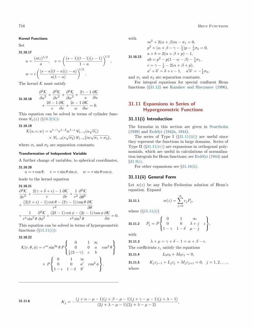
716 Heun Functions
Kernel Functions
Set
31.10.17
u =(stz)1/2
a, v =
((s− 1)(t− 1)(z − 1)
1− a
)1/2,
w = i
((s− a)(t− a)(z − a)
a(1− a)
)1/2.
The kernel K must satisfy
31.10.18
∂2K∂u2 +
∂2K∂v2 +
∂2K∂w2 +
2γ − 1u
∂K∂u
+2δ − 1v
∂K∂v
+2ε− 1w
∂K∂w
= 0.
This equation can be solved in terms of cylinder func-tions Cν(z) (§10.2(ii)):
31.10.19
K(u, v, w) = u1−γv1−δw1−ε C1−γ(u√σ1)
× C1−δ(v√σ2) C1−ε
(iw√σ1 + σ2
),
where σ1 and σ2 are separation constants.
Transformation of Independent Variable
A further change of variables, to spherical coordinates,
31.10.20
u = r cos θ, v = r sin θ sinφ, w = r sin θ cosφ,
leads to the kernel equation
31.10.21
∂2K∂r2 +
2(γ + δ + ε)− 1r
∂K∂r
+1r2
∂2K∂θ2
+(2(δ + ε)− 1) cot θ − (2γ − 1) tan θ
r2
∂K∂θ
+1
r2 sin2 θ
∂2K∂φ2 +
(2δ − 1) cotφ− (2ε− 1) tanφr2 sin2 θ
∂K∂φ
= 0.
This equation can be solved in terms of hypergeometricfunctions (§15.11(i)):
31.10.22
K(r, θ, φ) = rm sin2p θ P
0 1 ∞0 0 a cos2 θ
12 (3− γ) c b
× P
0 1 ∞0 0 a′ cos2 φ
1− ε 1− δ b′
,
with
31.10.23
m2 + 2(α+ β)m− σ1 = 0,p2 + (α+ β − γ − 1
2 )p− 14σ2 = 0,
a+ b = 2(α+ β + p)− 1,ab = p2 − p(1− α− β)− 1
4σ1,
c = γ − 12 − 2(α+ β + p),
a′ + b′ = δ + ε− 1, a′b′ = − 14σ2,
and σ1 and σ2 are separation constants.For integral equations for special confluent Heun
functions (§31.12) see Kazakov and Slavyanov (1996).
31.11 Expansions in Series ofHypergeometric Functions
31.11(i) Introduction
The formulas in this section are given in Svartholm(1939) and Erdélyi (1942a, 1944).
The series of Type I (§31.11(iii)) are useful sincethey represent the functions in large domains. Series ofType II (§31.11(iv)) are expansions in orthogonal poly-nomials, which are useful in calculations of normaliza-tion integrals for Heun functions; see Erdélyi (1944) and§31.9(i).
For other expansions see §31.16(ii).
31.11(ii) General Form
Let w(z) be any Fuchs–Frobenius solution of Heun’sequation. Expand
31.11.1 w(z) =∞∑j=0
cjPj ,
where (§15.11(i))
31.11.2 Pj = P
0 1 ∞0 0 λ+ j z
1− γ 1− δ µ− j
,with
31.11.3 λ+ µ = γ + δ − 1 = α+ β − ε.The coefficients cj satisfy the equations
31.11.4 L0c0 +M0c1 = 0,
31.11.5 Kjcj−1 + Ljcj +Mjcj+1 = 0, j = 1, 2, . . . ,where
31.11.6 Kj = − (j + α− µ− 1)(j + β − µ− 1)(j + γ − µ− 1)(j + λ− 1)(2j + λ− µ− 1)(2j + λ− µ− 2)
,

31.12 Confluent Forms of Heun’s Equation 717
31.11.7
Lj = a(λ+ j)(µ− j)− q +(j + α− µ)(j + β − µ)(j + γ − µ)(j + λ)
(2j + λ− µ)(2j + λ− µ+ 1)
+(j − α+ λ)(j − β + λ)(j − γ + λ)(j − µ)
(2j + λ− µ)(2j + λ− µ− 1),
31.11.8 Mj = − (j − α+ λ+ 1)(j − β + λ+ 1)(j − γ + λ+ 1)(j − µ+ 1)(2j + λ− µ+ 1)(2j + λ− µ+ 2)
.
λ, µ must also satisfy the condition
31.11.9 M−1P−1 = 0.
31.11(iii) Type I
Here
31.11.10 λ = α, µ = β − ε,or
31.11.11 λ = β, µ = α− ε.Then condition (31.11.9) is satisfied.
Every Fuchs–Frobenius solution of Heun’s equation(31.2.1) can be represented by a series of Type I. Forinstance, choose (31.11.10). Then the Fuchs–Frobeniussolution at ∞ belonging to the exponent α has the ex-pansion (31.11.1) with
31.11.12
Pj =Γ(α+ j) Γ(1− γ + α+ j)
Γ(1 + α− β + ε+ 2j)z−α−j
× 2F1
(α+ j, 1− γ + α+ j
1 + α− β + ε+ 2j;
1z
),
and (31.11.1) converges outside the ellipse E in the z-plane with foci at 0, 1, and passing through the thirdfinite singularity at z = a.
Every Heun function (§31.4) can be represented by aseries of Type I convergent in the whole plane cut alonga line joining the two singularities of the Heun function.
For example, consider the Heun function which isanalytic at z = a and has exponent α at ∞. The ex-pansion (31.11.1) with (31.11.12) is convergent in theplane cut along the line joining the two singularitiesz = 0 and z = 1. In this case the accessory parameterq is a root of the continued-fraction equation
31.11.13 (L0/M0)−K1/M1
L1/M1 −K2/M2
L2/M2 −· · · = 0.
The case α = −n for nonnegative integer n correspondsto the Heun polynomial Hpn,m(z).
The expansion (31.11.1) for a Heun function that isassociated with any branch of (31.11.2)—other than amultiple of the right-hand side of (31.11.12)—is conver-gent inside the ellipse E .
31.11(iv) Type II
Here one of the following four pairs of conditions is sat-isfied:31.11.14 λ = γ + δ − 1, µ = 0,
31.11.15 λ = γ, µ = δ − 1,
31.11.16 λ = δ, µ = γ − 1,
31.11.17 λ = 1, µ = γ + δ − 2.
In each case Pj can be expressed in terms of a Ja-cobi polynomial (§18.3). Such series diverge for Fuchs–Frobenius solutions. For Heun functions they are con-vergent inside the ellipse E . Every Heun function canbe represented by a series of Type II.
31.11(v) Doubly-Infinite Series
Schmidt (1979) gives expansions of path-multiplicativesolutions (§31.6) in terms of doubly-infinite series of hy-pergeometric functions.
31.12 Confluent Forms of Heun’s Equation
Confluent forms of Heun’s differential equation (31.2.1)arise when two or more of the regular singularities mergeto form an irregular singularity. This is analogous tothe derivation of the confluent hypergeometric equationfrom the hypergeometric equation in §13.2(i). There arefour standard forms, as follows:
Confluent Heun Equation
31.12.1d2w
dz2 +(γ
z+
δ
z − 1+ ε
)dw
dz+
αz − qz(z − 1)
w = 0.
This has regular singularities at z = 0 and 1, and anirregular singularity of rank 1 at z =∞.
Mathieu functions (Chapter 28), spheroidal wavefunctions (Chapter 30), and Coulomb spheroidal func-tions (§30.12) are special cases of solutions of the con-fluent Heun equation.
Doubly-Confluent Heun Equation
31.12.2d2w
dz2 +(δ
z2+γ
z+ 1)dw
dz+αz − qz2
w = 0.
This has irregular singularities at z = 0 and ∞, each ofrank 1.

718 Heun Functions
Biconfluent Heun Equation
31.12.3d2w
dz2 +(γz
+ δ + z) dwdz
+αz − qz
w = 0.
This has a regular singularity at z = 0, and an irregularsingularity at ∞ of rank 2.
Triconfluent Heun Equation
31.12.4d2w
dz2 + (γ + z) zdw
dz+ (αz − q)w = 0.
This has one singularity, an irregular singularity of rank3 at z =∞.
For properties of the solutions of (31.12.1)–(31.12.4),including connection formulas, see Bühring (1994), Ron-veaux (1995, Parts B,C,D,E), Wolf (1998), Lay andSlavyanov (1998), and Slavyanov and Lay (2000).
31.13 Asymptotic Approximations
For asymptotic approximations for the accessory param-eter eigenvalues qm, see Fedoryuk (1991) and Slavyanov(1996).
For asymptotic approximations of the solutions ofHeun’s equation (31.2.1) when two singularities are closetogether, see Lay and Slavyanov (1999).
For asymptotic approximations of the solutions ofconfluent forms of Heun’s equation in the neighborhoodof irregular singularities, see Komarov et al. (1976),Ronveaux (1995, Parts B,C,D,E), Bogush and Otchik(1997), Slavyanov and Veshev (1997), and Lay et al.(1998).
31.14 General Fuchsian Equation
31.14(i) Definitions
The general second-order Fuchsian equation with N +1regular singularities at z = aj , j = 1, 2, . . . , N , and at∞, is given by31.14.1
d2w
dz2 +
N∑j=1
γjz − aj
dw
dz+
N∑j=1
qjz − aj
w = 0,
∑Nj=1 qj = 0.
The exponents at the finite singularities aj are{0, 1− γj} and those at ∞ are {α, β}, where
31.14.2 α+ β + 1 =N∑j=1
γj , αβ =N∑j=1
ajqj .
The three sets of parameters comprise the singularityparameters aj , the exponent parameters α, β, γj , andthe N − 2 free accessory parameters qj . With a1 = 0and a2 = 1 the total number of free parameters is 3N−3.Heun’s equation (31.2.1) corresponds to N = 3.
Normal Form
31.14.3 w(z) =
N∏j=1
(z − aj)−γj/2W (z),
31.14.4
d2W
dz2 =N∑j=1
(γ̃j
(z − aj)2+
q̃jz − aj
)W ,
∑Nj=1 q̃j = 0,
31.14.5 q̃j =12
N∑k=1k 6=j
γjγkaj − ak
− qj , γ̃j =γj2
(γj2− 1).
31.14(ii) Kovacic’s Algorithm
An algorithm given in Kovacic (1986) determines if agiven (not necessarily Fuchsian) second-order homoge-neous linear differential equation with rational coeffi-cients has solutions expressible in finite terms (Liouvil-lean solutions). The algorithm returns a list of solutionsif they exist.
For applications of Kovacic’s algorithm in spatio-temporal dynamics see Rod and Sleeman (1995).
31.15 Stieltjes Polynomials
31.15(i) Definitions
Stieltjes polynomials are polynomial solutions of theFuchsian equation (31.14.1). Rewrite (31.14.1) in theform31.15.1
d2w
dz2 +
N∑j=1
γjz − aj
dw
dz+
Φ(z)∏Nj =1(z − aj)
w = 0,
where Φ(z) is a polynomial of degree not exceedingN − 2. There exist at most
(n+N−2N−2
)polynomials V (z)
of degree not exceeding N−2 such that for Φ(z) = V (z),(31.15.1) has a polynomial solution w = S(z) of degreen. The V (z) are called Van Vleck polynomials and thecorresponding S(z) Stieltjes polynomials.
31.15(ii) Zeros
If z1, z2, . . . , zn are the zeros of an nth degree Stieltjespolynomial S(z), then every zero zk is either one of theparameters aj or a solution of the system of equations
31.15.2
N∑j=1
γj/2zk − aj
+n∑j=1j 6=k
1zk − zj
= 0, k = 1, 2, . . . , n.
If tk is a zero of the Van Vleck polynomial V (z), cor-responding to an nth degree Stieltjes polynomial S(z),and z′1, z
′2, . . . , z
′n−1 are the zeros of S′(z) (the derivative

Applications 719
of S(z)), then tk is either a zero of S′(z) or a solutionof the equation
31.15.3
N∑j=1
γjtk − aj
+n−1∑j=1
1tk − z′j
= 0.
The system (31.15.2) determines the zk as the pointsof equilibrium of n movable (interacting) particles withunit charges in a field of N particles with the chargesγj/2 fixed at aj . This is the Stieltjes electrostatic inter-pretation.
The zeros zk, k = 1, 2, . . . , n, of the Stieltjes polyno-mial S(z) are the critical points of the function G, thatis, points at which ∂G/∂ζk = 0, k = 1, 2, . . . , n, where
31.15.4
G(ζ1, ζ2, . . . , ζn)
=n∏k=1
N∏`=1
(ζk − a`)γ`/2n∏
j=k+1
(ζk − ζj).
If the following conditions are satisfied:
31.15.5 γj > 0, aj ∈ R, j = 1, 2, . . . , N ,and
31.15.6 aj < aj+1, j = 1, 2, . . . , N − 1,
then there are exactly(n+N−2N−2
)polynomials S(z), each
of which corresponds to each of the(n+N−2N−2
)ways of dis-
tributing its n zeros among N − 1 intervals (aj , aj+1),j = 1, 2, . . . , N − 1. In this case the accessory parame-ters qj are given by
31.15.7 qj = γj
n∑k=1
1zk − aj
, j = 1, 2, . . . , N .
See Marden (1966), Alam (1979), and Al-Rashedand Zaheer (1985) for further results on the locationof the zeros of Stieltjes and Van Vleck polynomials.
31.15(iii) Products of Stieltjes Polynomials
If the exponent and singularity parameters satisfy(31.15.5)–(31.15.6), then for every multi-index m =(m1,m2, . . . ,mN−1), where each mj is a nonnegativeinteger, there is a unique Stieltjes polynomial withmj zeros in the open interval (aj , aj+1) for each j =1, 2, . . . , N − 1. We denote this Stieltjes polynomial bySm(z).
Let Sm(z) and Sl(z) be Stieltjes polynomialscorresponding to two distinct multi-indices m =(m1,m2, . . . ,mN−1) and l = (`1, `2, . . . , `N−1). Theproducts
31.15.8 Sm(z1)Sm(z2) · · ·Sm(zN−1), zj ∈ (aj , aj+1),
31.15.9 Sl(z1)Sl(z2) · · ·Sl(zN−1), zj ∈ (aj , aj+1),are mutually orthogonal over the set Q:
31.15.10 Q = (a1, a2)× (a2, a3)× · · · × (aN−1, aN ),
with respect to the inner product
31.15.11 (f, g)ρ =∫Q
f(z)ḡ(z)ρ(z) dz,
with weight function
31.15.12
ρ(z) =
N−1∏j=1
N∏k=1
|zj − ak|γk−1
N−1∏j<k
(zk − zj)
.
The normalized system of products (31.15.8) forms anorthonormal basis in the Hilbert space L2
ρ(Q). For fur-ther details and for the expansions of analytic functionsin this basis see Volkmer (1999).
Applications
31.16 Mathematical Applications
31.16(i) Uniformization Problem for Heun’sEquation
The main part of Smirnov (1996) consists ofV. I. Smirnov’s 1918 M. Sc. thesis “Inversion problemfor a second-order linear differential equation with foursingular points”. It describes the monodromy group ofHeun’s equation for specific values of the accessory pa-rameter.
31.16(ii) Heun Polynomial Products
Expansions of Heun polynomial products in terms of Ja-cobi polynomial (§18.3) products are derived in Kalninsand Miller (1991a,b, 1993) from the viewpoint of inter-relation between two bases in a Hilbert space:
31.16.1
Hpn,m(x) Hpn,m(y)
=n∑j=0
Aj sin2j θ
×P (γ+δ+2j−1,ε−1)n−j (cos 2θ)P (δ−1,γ−1)
j (cos 2φ),
where n = 0, 1, . . . , m = 0, 1, . . . , n, and
31.16.2 x = sin2 θ cos2 φ, y = sin2 θ sin2 φ.
The coefficients Aj satisfy the relations:
31.16.3 Q0A0 +R0A1 = 0,
31.16.4 PjAj−1 +QjAj +RjAj+1 = 0, j = 1, 2, . . . , n,
where

720 Heun Functions
31.16.5 Pj =(ε− j + n)j(β + j − 1)(γ + δ + j − 2)
(γ + δ + 2j − 3)(γ + δ + 2j − 2),
31.16.6
Qj = −aj(j + γ + δ − 1)− q +(j − n)(j + β)(j + γ)(j + γ + δ − 1)
(2j + γ + δ)(2j + γ + δ − 1)
+(j + n+ γ + δ − 1)j(j + δ − 1)(j − β + γ + δ − 1)
(2j + γ + δ − 1)(2j + γ + δ − 2),
31.16.7 Rj =(n− j)(j + n+ γ + δ)(j + γ)(j + δ)
(γ + δ + 2j)(γ + δ + 2j + 1).
By specifying either θ or φ in (31.16.1) and (31.16.2)we obtain expansions in terms of one variable.
31.17 Physical Applications
31.17(i) Addition of Three Quantum Spins
The problem of adding three quantum spins s, t, andu can be solved by the method of separation of vari-ables, and the solution is given in terms of a productof two Heun functions. We use vector notation [s, t,u](respective scalar (s, t, u)) for any one of the three spinoperators (respective spin values).
Consider the following spectral problem on thesphere S2: x2 = x2
s + x2t + x2
u = R2.31.17.1
J2Ψ(x) ≡ (s + t + u)2Ψ(x) = j(j + 1)Ψ(x),HsΨ(x) ≡ (−2s · t− (2/a )s · u)Ψ(x) = hsΨ(x),
for the common eigenfunction Ψ(x) = Ψ(xs, xt, xu),where a is the coupling parameter of interacting spins.Introduce elliptic coordinates z1 and z2 on S2. Then
31.17.2x2s
zk+
x2t
zk − 1+
x2u
zk − a= 0, k = 1, 2,
with
31.17.3
x2s = R2 z1z2
a, x2
t = R2 (z1 − 1)(z2 − 1)1− a
,
x2u = R2 (z1 − a)(z2 − a)
a(a− 1).
The operators J2 and Hs admit separation of variablesin z1, z2, leading to the following factorization of theeigenfunction Ψ(x):
31.17.4Ψ(x) = (z1z2)−s−
14 ((z1 − 1)(z2 − 1))−t−
14
× ((z1 − a)(z2 − a))−u−14w(z1)w(z2),
where w(z) satisfies Heun’s equation (31.2.1) with a asin (31.17.1) and the other parameters given by31.17.5α = −s− t− u− j − 1, β = j − s− t− u, γ = −2s,δ = −2t, ε = −2u; q = ahs + 2s(at+ u).
For more details about the method of separation ofvariables and relation to special functions see Olevskĭı(1950), Kalnins et al. (1976), Miller (1977), and Kalnins(1986).
31.17(ii) Other Applications
Heun functions appear in the theory of black holes(Kerr (1963), Teukolsky (1972), Chandrasekhar (1984),Suzuki et al. (1998), Kalnins et al. (2000)), lattice sys-tems in statistical mechanics (Joyce (1973, 1994)), dislo-cation theory (Lay and Slavyanov (1999)), and quantumsystems (Bay et al. (1997), Tolstikhin and Matsuzawa(2001)).
For applications of Heun’s equation and functionsin astrophysics see Debosscher (1998) where differentspectral problems for Heun’s equation are also consid-ered. More applications—including those of generalizedspheroidal wave functions and confluent Heun functionsin mathematical physics, astrophysics, and the two-center problem in molecular quantum mechanics—canbe found in Leaver (1986) and Slavyanov and Lay (2000,Chapter 4). For application of biconfluent Heun func-tions in a model of an equatorially trapped Rossby wavein a shear flow in the ocean or atmosphere see Boyd andNatarov (1998).
Computation
31.18 Methods of Computation
Independent solutions of (31.2.1) can be computed inthe neighborhoods of singularities from their Fuchs–Frobenius expansions (§31.3), and elsewhere by numer-ical integration of (31.2.1). Subsequently, the coeffi-cients in the necessary connection formulas can be cal-culated numerically by matching the values of solutionsand their derivatives at suitably chosen values of z; seeLăı (1994) and Lay et al. (1998). Care needs to betaken to choose integration paths in such a way that thewanted solution is growing in magnitude along the pathat least as rapidly as all other solutions (§3.7(ii)). The

References 721
computation of the accessory parameter for the Heunfunctions is carried out via the continued-fraction equa-tions (31.4.2) and (31.11.13) in the same way as for theMathieu, Lamé, and spheroidal wave functions in Chap-ters 28–30.
References
General References
The main references used in writing this chapter areSleeman (1966b) and Ronveaux (1995). For additionalbibliographic reading see Erdélyi et al. (1955).
Sources
The following list gives the references or other indica-tions of proofs that were used in constructing the varioussections of this chapter. These sources supplement thereferences that are quoted in the text.
§31.2 Erdélyi et al. (1955, Chapter XV), Ronveaux(1995, Part A, Chapters 1 and 2).
§31.3 Snow (1952), Ronveaux (1995, Part A, Chapters2 and 3).
§31.4 Erdélyi et al. (1955, Chapter XV), Arscott(1964b, Chapter IX).
§31.5 Erdélyi et al. (1955, Chapter XV), Arscott(1964b, Chapter IX).
§31.7 Ronveaux (1995, Part A, Chapter 1).
§31.9 Becker (1997).
§31.10 Lambe and Ward (1934) Erdélyi (1942b), Va-lent (1986), Sleeman (1969), An error in the lastreference is corrected here.
§31.12 The process of confluence is discussed inInce (1926, Chapter XX). See Decarreau et al.(1978a,b) for the classification of confluent forms.
§31.14 Ince (1926, Chapter XV).
§31.15 Marden (1966).
§31.17 Gaudin (1983), Kuznetsov (1992).


Chapter 32
Painlevé TranscendentsP. A. Clarkson1
Notation 72432.1 Special Notation . . . . . . . . . . . . . 724
Properties 72432.2 Differential Equations . . . . . . . . . . . 72432.3 Graphics . . . . . . . . . . . . . . . . . . 72632.4 Isomonodromy Problems . . . . . . . . . 72832.5 Integral Equations . . . . . . . . . . . . . 72932.6 Hamiltonian Structure . . . . . . . . . . 72932.7 Bäcklund Transformations . . . . . . . . 73032.8 Rational Solutions . . . . . . . . . . . . . 73232.9 Other Elementary Solutions . . . . . . . . 73432.10 Special Function Solutions . . . . . . . . 735
32.11 Asymptotic Approximations for Real Vari-ables . . . . . . . . . . . . . . . . . . . . 736
32.12 Asymptotic Approximations for ComplexVariables . . . . . . . . . . . . . . . . . . 738
Applications 73832.13 Reductions of Partial Differential Equations 73832.14 Combinatorics . . . . . . . . . . . . . . . 73932.15 Orthogonal Polynomials . . . . . . . . . . 73932.16 Physical . . . . . . . . . . . . . . . . . . 739
Computation 73932.17 Methods of Computation . . . . . . . . . 740
References 740
1School of Mathematics, Statistics & Actuarial Science, University of Kent, Canterbury, United Kingdom.Copyright c© 2009 National Institute of Standards and Technology. All rights reserved.
723

724 Painlevé Transcendents
Notation
32.1 Special Notation
(For other notation see pp. xiv and 873.)
m,n integers.x real variable.z complex variable.k real parameter.
Unless otherwise noted, primes indicate derivativeswith respect to the argument.
The functions treated in this chapter are the solu-tions of the Painlevé equations PI–PVI.
Properties
32.2 Differential Equations
32.2(i) Introduction
The six Painlevé equations PI–PVI are as follows:
32.2.1d2w
dz2 = 6w2 + z,
32.2.2d2w
dz2 = 2w3 + zw + α,
32.2.3d2w
dz2 =1w
(dw
dz
)2− 1z
dw
dz+αw2 + β
z+ γw3 +
δ
w,
32.2.4d2w
dz2 =1
2w
(dw
dz
)2+
32w3 + 4zw2 + 2(z2 − α)w +
β
w,
32.2.5d2w
dz2 =(
12w
+1
w − 1
)(dw
dz
)2− 1z
dw
dz+
(w − 1)2
z2
(αw +
β
w
)+γw
z+δw(w + 1)w − 1
,
32.2.6
d2w
dz2 =12
(1w
+1
w − 1+
1w − z
)(dw
dz
)2−(
1z
+1
z − 1+
1w − z
)dw
dz
+w(w − 1)(w − z)
z2(z − 1)2
(α+
βz
w2+γ(z − 1)(w − 1)2
+δz(z − 1)(w − z)2
),
with α, β, γ, and δ arbitrary constants. The solutionsof PI–PVI are called the Painlevé transcendents. Thesix equations are sometimes referred to as the Painlevétranscendents, but in this chapter this term will be usedonly for their solutions.
Let
32.2.7d2w
dz2 = F
(z, w,
dw
dz
),
be a nonlinear second-order differential equation inwhich F is a rational function of w and dw/dz , andis locally analytic in z, that is, analytic except for iso-lated singularities in C. In general the singularities ofthe solutions are movable in the sense that their loca-tion depends on the constants of integration associatedwith the initial or boundary conditions. An equation issaid to have the Painlevé property if all its solutions arefree from movable branch points; the solutions may havemovable poles or movable isolated essential singularities(§1.10(iii)), however.
There are fifty equations with the Painlevé property.They are distinct modulo Möbius (bilinear) transforma-tions32.2.8 W (ζ) =
a(z)w + b(z)c(z)w + d(z)
, ζ = φ(z),
in which a(z), b(z), c(z), d(z), and φ(z) are locally an-
alytic functions. The fifty equations can be reducedto linear equations, solved in terms of elliptic functions(Chapters 22 and 23), or reduced to one of PI–PVI.
For arbitrary values of the parameters α, β, γ, andδ, the general solutions of PI–PVI are transcendental,that is, they cannot be expressed in closed-form ele-mentary functions. However, for special values of theparameters, equations PII–PVI have special solutions interms of elementary functions, or special functions de-fined elsewhere in this Handbook.
32.2(ii) Renormalizations
If γδ 6= 0 in PIII, then set γ = 1 and δ = −1, withoutloss of generality, by rescaling w and z if necessary. Ifγ = 0 and αδ 6= 0 in PIII, then set α = 1 and δ = −1,without loss of generality. Lastly, if δ = 0 and βγ 6= 0,then set β = −1 and γ = 1, without loss of generality.
If δ 6= 0 in PV, then set δ = − 12 , without loss of
generality.
32.2(iii) Alternative Forms
In PIII, if w(z) = ζ−1/2u(ζ) with ζ = z2, then
32.2.9d2u
dζ2 =1u
(du
dζ
)2− 1ζ
du
dζ+u2(α+ γu)
4ζ2+β
4ζ+
δ
4u,

32.2 Differential Equations 725
which is known as P′III.In PIII, if w(z) = exp(−iu(z)), β = −α, and δ = −γ,
then32.2.10
d2u
dz2 +1z
du
dz=
2αz
sinu+ 2γ sin(2u).
In PIV, if w(z) = 2√
2(u(ζ))2 with ζ =√
2z andα = 2ν + 1, then
32.2.11d2u
dζ2 = 3u5 + 2ζu3 +(
14ζ
2 − ν − 12
)u+
β
32u3.
When β = 0 this is a nonlinear harmonic oscillator.In PV, if w(z) = (cothu(ζ))2 with ζ = ln z, then
32.2.12
d2u
dζ2 = − α coshu2(sinhu)3
− β sinhu2(coshu)3
− 14γe
ζ sinh(2u)− 18δe
2ζ sinh(4u).See also Okamoto (1987c), McCoy et al. (1977), Bas-
som et al. (1992), Bassom et al. (1995), and Takasaki(2001).
32.2(iv) Elliptic Form
PVI can be written in the form32.2.13
z(1− z)I
(∫ w
∞
dt√t(t− 1)(t− z)
)=√w(w − 1)(w − z)
×(α+
βz
w2+γ(z − 1)(w − 1)2
+ (δ − 12 )z(z − 1)(w − z)2
),
where
32.2.14 I = z(1− z) d2
dz2 + (1− 2z)d
dz− 1
4.
See Fuchs (1907), Painlevé (1906), Gromak et al. (2002,§42); also Manin (1998).
32.2(v) Symmetric Forms
Let
32.2.15
df1
dz+ f1(f2 − f3) + 2µ1 = 0,
df2
dz+ f2(f3 − f1) + 2µ2 = 0,
df3
dz+ f3(f1 − f2) + 2µ3 = 0,
where µ1, µ2, µ3 are constants, f1, f2, f3 are functionsof z, with
32.2.16 µ1 + µ2 + µ3 = 1,
32.2.17 f1(z) + f2(z) + f3(z) + 2z = 0.Then w(z) = f1(z) satisfies PIV with
32.2.18 (α, β) = (µ3 − µ2,−2µ21).
See Noumi and Yamada (1998).
Next, let
32.2.19
zdf1
dz= f1f3(f2 − f4) + ( 1
2 − µ3)f1 + µ1f3,
zdf2
dz= f2f4(f3 − f1) + ( 1
2 − µ4)f2 + µ2f4,
zdf3
dz= f3f1(f4 − f2) + ( 1
2 − µ1)f3 + µ3f1,
zdf4
dz= f4f2(f1 − f3) + ( 1
2 − µ2)f4 + µ4f2,
where µ1, µ2, µ3, µ4 are constants, f1, f2, f3, f4 arefunctions of z, with32.2.20 µ1 + µ2 + µ3 + µ4 = 1,
32.2.21 f1(z) + f3(z) =√z,
32.2.22 f2(z) + f4(z) =√z.
Then w(z) = 1− (√z/f1(z)) satisfies PV with
32.2.23 (α, β, γ, δ) = (12µ
21,− 1
2µ23, µ4 − µ2,− 1
2 ).
32.2(vi) Coalescence Cascade
PI–PV are obtained from PVI by a coalescence cascade:
32.2.24
PVI −→ PV −→ PIV
↓ ↓PIII −→ PII −→ PI
For example, if in PII
32.2.25 w(z;α) = εW (ζ) +1ε5,
32.2.26 z = ε2ζ − 6ε10
, α =4ε15
,
then32.2.27
d2W
dζ2 = 6W 2 + ζ + ε6(2W 3 + ζW );
thus in the limit as ε→ 0, W (ζ) satisfies PI with z = ζ.If in PIII
32.2.28 w(z;α, β, γ, δ) = 1 + 2εW (ζ; a),
32.2.29z = 1 + ε2ζ, α = − 1
2ε−6,
β = 12ε−6 + 2aε−3, γ = −δ = 1
4ε−6,
then as ε→ 0, W (ζ; a) satisfies PII with z = ζ, α = a.If in PIV
32.2.30 w(z;α, β) = 22/3ε−1W (ζ; a) + ε−3,
32.2.31
z = 2−2/3εζ − ε−3, α = −2a− 12ε−6, β = − 1
2ε−12,
then as ε→ 0, W (ζ; a) satisfies PII with z = ζ, α = a.If in PV
32.2.32 w(z;α, β, γ, δ) = 1 + εζW (ζ; a, b, c, d),
32.2.33z = ζ2, α = 1
4aε−1 + 1
8cε−2,
β = − 18cε−2, γ = 1
4εb, δ = 18ε
2d,
then as ε → 0, W (ζ; a, b, c, d) satisfies PIII with z = ζ,α = a, β = b, γ = c, δ = d.
If in PV
32.2.34 w(z;α, β, γ, δ) = 12
√2εW (ζ; a, b),

726 Painlevé Transcendents
32.2.35z = 1 +
√2εζ, α = 1
2ε−4, β = 1
4b,
γ = −ε−4, δ = aε−2 − 12ε−4,
then as ε→ 0, W (ζ; a, b) satisfies PIV with z = ζ, α = a,β = b.
Lastly, if in PVI
32.2.36 w(z;α, β, γ, δ) = W (ζ; a, b, c, d),
32.2.37 z = 1 + εζ, γ = cε−1 − dε−2, δ = dε−2,
then as ε → 0, W (ζ; a, b, c, d) satisfies PV with z = ζ,α = a, β = b, γ = c, δ = d.
32.3 Graphics
32.3(i) First Painlevé Equation
Plots of solutions wk(x) of PI with wk(0) = 0 and w′k(0) = k for various values of k, and the parabola 6w2 + x = 0.For analytical explanation see §32.11(i).
Figure 32.3.1: wk(x) for −12 ≤ x ≤ 1.33 and k = 0.5,0.75, 1, 1.25, and the parabola 6w2 + x = 0, shown inblack.
Figure 32.3.2: wk(x) for −12 ≤ x ≤ 2.43 and k = −0.5,−0.25, 0, 1, 2, and the parabola 6w2 + x = 0, shown inblack.
Figure 32.3.3: wk(x) for −12 ≤ x ≤ 0.73 and k =1.85185 3, 1.85185 5. The two graphs are indistinguish-able when x exceeds −5.2, approximately. The parabola6w2 + x = 0 is shown in black.
Figure 32.3.4: wk(x) for −12 ≤ x ≤ 2.3 and k =−0.45142 7, −0.45142 8. The two graphs are indis-tinguishable when x exceeds −4.8, approximately. Theparabola 6w2 + x = 0 is shown in black.

32.3 Graphics 727
32.3(ii) Second Painlevé Equation with α = 0
Here wk(x) is the solution of PII with α = 0 and such that
32.3.1 wk(x) ∼ kAi(x), x→ +∞;compare §32.11(ii).
Figure 32.3.5: wk(x) and kAi(x) for −10 ≤ x ≤ 4 withk = 0.5. The two graphs are indistinguishable when xexceeds −0.4, approximately.
Figure 32.3.6: wk(x) for −10 ≤ x ≤ 4 with k = 0.999,1.001. The two graphs are indistinguishable when xexceeds −2.8, approximately. The parabola 2w2 +x = 0is shown in black.
32.3(iii) Fourth Painlevé Equation with β = 0
Here u = uk(x; ν) is the solution of
32.3.2d2u
dx2 = 3u5 + 2xu3 +(
14x
2 − ν − 12
)u,
such that
32.3.3 u ∼ k U(−ν − 1
2 , x), x→ +∞.
The corresponding solution of PIV is given by
32.3.4 w(x) = 2√
2u2k(√
2x, ν),with β = 0, α = 2ν + 1, and32.3.5 w(x) ∼ 2
√2k2 U2
(−ν − 1
2 ,√
2x)
, x→ +∞;
compare (32.2.11) and §32.11(v). If we set d2u/dx2 = 0 in (32.3.2) and solve for u, then
32.3.6 u2 = − 13x±
16
√x2 + 12ν + 6.
Figure 32.3.7: uk(x;− 12 ) for −12 ≤ x ≤ 4 with k =
0.33554 691, 0.33554 692. The two graphs are indis-tinguishable when x exceeds −5.0, approximately. Theparabolas u2 + 1
2x = 0, u2 + 16x = 0 are shown in black
and green, respectively.
Figure 32.3.8: uk(x; 12 ) for −12 ≤ x ≤ 4 with k =
0.47442, 0.47443. The two graphs are indistinguish-able when x exceeds −2.2, approximately. The curvesu2 + 1
3x±16
√x2 + 12 = 0 are shown in green and black,
respectively.

728 Painlevé Transcendents
Figure 32.3.9: uk(x; 32 ) for −12 ≤ x ≤ 4 with k =
0.38736, 0.38737. The two graphs are indistinguish-able when x exceeds −1.0, approximately. The curvesu2 + 1
3x±16
√x2 + 24 = 0 are shown in green and black,
respectively.
Figure 32.3.10: uk(x; 52 ) for −12 ≤ x ≤ 4 with k =
0.24499 2, 0.24499 3. The two graphs are indistinguish-able when x exceeds −0.6, approximately. The curvesu2 + 1
3x±16
√x2 + 36 = 0 are shown in green and black,
respectively.
32.4 Isomonodromy Problems
32.4(i) Definition
PI–PVI can be expressed as the compatibility conditionof a linear system, called an isomonodromy problem orLax pair. Suppose
32.4.1∂Ψ∂λ
= A(z, λ)Ψ,∂Ψ∂z
= B(z, λ)Ψ,
is a linear system in which A and B are matrices and λis independent of z. Then the equation
32.4.2∂2Ψ∂z ∂λ
=∂2Ψ∂λ ∂z
,
is satisfied provided that
32.4.3∂A∂z− ∂B∂λ
+ AB−BA = 0.
(32.4.3) is the compatibility condition of (32.4.1).Isomonodromy problems for Painlevé equations are notunique.
32.4(ii) First Painlevé Equation
PI is the compatibility condition of (32.4.1) with
32.4.4
A(z, λ) = (4λ4 + 2w2 + z)[1 00 −1
]− i(4λ2w + 2w2 + z)
[0 −ii 0
]−(
2λw′ +1
2λ
)[0 11 0
],
32.4.5 B(z, λ) =(λ+
w
λ
)[1 00 −1
]− iw
λ
[0 −ii 0
].
32.4(iii) Second Painlevé Equation
PII is the compatibility condition of (32.4.1) with
32.4.6
A(z, λ) = −i(4λ2 + 2w2 + z)[1 00 −1
]− 2w′
[0 −ii 0
]+(
4λw − α
λ
)[0 11 0
],
32.4.7 B(z, λ) =[−iλ ww iλ
].
See Flaschka and Newell (1980).
32.4(iv) Third Painlevé Equation
The compatibility condition of (32.4.1) with
32.4.8
A(z, λ) =[
14z 00 − 1
4z
]+[− 1
2θ∞ u0
u112θ∞
]1λ
+[
v0 − 14z −v1v0
(v0 − 12z)/v1
14z − v0
]1λ2,
32.4.9
B(z, λ) =[
14 00 − 1
4
]λ+
[0 u0
u1 0
]1z
−[
v0 − 14z −v1v0
(v0 − 12z)/v1
14z − v0
]1zλ,
where θ∞ is an arbitrary constant, is
32.4.10 zu′0 = θ∞u0 − zv0v1,
32.4.11 zu′1 = −θ∞u1 − (z(2v0 − z)/(2v1) ),
32.4.12 zv′0 = 2v0u1v1 + v0 + (u0(2v0 − z)/v1),
32.4.13 zv′1 = 2u0 − 2u1v21 − θ∞v1.
If w = −u0/(v0v1), then
32.4.14 zw′ = (4v0 − z)w2 + (2θ∞ − 1)w + z,

32.5 Integral Equations 729
and w satisfies PIII with32.4.15 (α, β, γ, δ) = (2θ0, 2(1− θ∞), 1,−1) ,where
32.4.16 θ0 =4v0
z
(θ∞
(1− z
4v0
)+z − 2v0
2v0v1u0 +u1v1
).
Note that the right-hand side of the last equation is afirst integral of the system (32.4.10)–(32.4.13).
32.4(v) Other Painlevé Equations
For isomonodromy problems for PIV, PV, and PVI seeJimbo and Miwa (1981).
32.5 Integral Equations
Let K(z, ζ) be the solution of32.5.1
K(z, ζ)
= kAi(z + ζ
2
)+k2
4
∫ ∞z
∫ ∞z
K(z, s) Ai(s+ t
2
)Ai(t+ ζ
2
)ds dt,
where k is a real constant, and Ai(z) is defined in §9.2.Then32.5.2 w(z) = K(z, z),satisfies PII with α = 0 and the boundary condition32.5.3 w(z) ∼ kAi(z), z → +∞.
32.6 Hamiltonian Structure
32.6(i) Introduction
PI–PVI can be written as a Hamiltonian system
32.6.1dq
dz=∂H∂p
,dp
dz= −∂H
∂q,
for suitable (non-autonomous) Hamiltonian functionsH(q, p, z).
32.6(ii) First Painlevé Equation
The Hamiltonian for PI is
32.6.2 HI(q, p, z) = 12p
2 − 2q3 − zq,and so
32.6.3 q′ = p,
32.6.4 p′ = 6q2 + z.
Then q = w satisfies PI. The function32.6.5 σ = HI(q, p, z),defined by (32.6.2) satisfies
32.6.6 (σ′′)2 + 4 (σ′)3 + 2zσ′ − 2σ = 0.Conversely, if σ is a solution of (32.6.6), then
32.6.7 q = −σ′,32.6.8 p = −σ′′,are solutions of (32.6.3) and (32.6.4).
32.6(iii) Second Painlevé Equation
The Hamiltonian for PII is
32.6.9 HII(q, p, z) = 12p
2 − (q2 + 12z)p− (α+ 1
2 )q,
and so
32.6.10 q′ = p− q2 − 12z,
32.6.11 p′ = 2qp+ α+ 12 .
Then q = w satisfies PII and p satisfies
32.6.12 pp′′ = 12 (p′)2 + 2p3 − zp2 − 1
2 (α+ 12 )2.
The function σ(z) = HII(q, p, z) defined by (32.6.9) sat-isfies
32.6.13 (σ′′)2 + 4 (σ′)3 + 2σ′ (zσ′ − σ) = 14 (α+ 1
2 )2.
Conversely, if σ(z) is a solution of (32.6.13), then
32.6.14 q = (4σ′′ + 2α+ 1)/(8σ′) ,
32.6.15 p = −2σ′,
are solutions of (32.6.10) and (32.6.11).
32.6(iv) Third Painlevé Equation
The Hamiltonian for PIII is
32.6.16
zHIII(q, p, z) = q2p2 −(κ∞zq
2 + (2θ0 + 1)q − κ0z)p
+ κ∞(θ0 + θ∞)zq,
and so
32.6.17 zq′ = 2q2p− κ∞zq2 − (2θ0 + 1)q + κ0z,
32.6.18zp′ = −2qp2 + 2κ∞zqp
+ (2θ0 + 1)p− κ∞(θ0 + θ∞)z.
Then q = w satisfies PIII with
32.6.19 (α, β, γ, δ) =(−2κ∞θ∞, 2κ0(θ0 + 1), κ2
∞,−κ20
).
The function
32.6.20 σ = zHIII(q, p, z) + pq + θ20 − 1
2κ0κ∞z2
defined by (32.6.16) satisfies
32.6.21(zσ′′ − σ′)2 + 2
((σ′)2 − κ2
0κ2∞z
2)
(zσ′ − 2σ)
+ 8κ0κ∞θ0θ∞zσ′ = 4κ2
0κ2∞(θ2
0 + θ2∞)z2.
Conversely, if σ is a solution of (32.6.21), then
32.6.22 q =κ0 (zσ′′ − (2θ0 + 1)σ′ + 2κ0κ∞θ∞z)
κ20κ
2∞z
2 − (σ′)2,
32.6.23 p = (σ′ + κ0κ∞z)/(2κ0) ,
are solutions of (32.6.17) and (32.6.18).

730 Painlevé Transcendents
The Hamiltonian for P′III (§32.2(iii)) is
32.6.24ζHIII(q, p, ζ) = q2p2 −
(η∞q
2 + θ0q − η0ζ)p
+ 12η∞(θ0 + θ∞)q,
and so
32.6.25 ζq′ = 2q2p− η∞q2 − θ0q + η0ζ,
32.6.26 ζp′ = −2qp2 + 2η∞qp+ θ0p− 12η∞(θ0 + θ1).
Then q = u satisfies P′III with32.6.27
(α, β, γ, δ) =(−4η∞θ∞, 4η0(θ0 + 1), 4η2
∞,−4η20
).
The function
32.6.28 σ = ζHIII(q, p, ζ) + 14θ
20 − 1
2η0η∞ζ
defined by (32.6.24) satisfies
32.6.29ζ2(σ′′)2 +
(4(σ′)2 − η2
0η2∞)
(ζσ′ − σ)+ η0η∞θ0θ∞σ
′ = 14η
20η
2∞(θ2
0 + θ2∞).
Conversely, if σ is a solution of (32.6.29), then
32.6.30 q =η0 (ζσ′′ − 2θ0σ
′ + η0η∞θ∞)η2
0η2∞ − 4(σ′)2
,
32.6.31 p = (2σ′ + η0η∞ζ)/(2η0) ,are solutions of (32.6.25) and (32.6.26).
The Hamiltonian for PIII with γ = 0 is
32.6.32 zHIII(q, p, z) = q2p2 + (θq − κ0z)p− κ∞zq,and so
32.6.33 zq′ = 2q2p+ θq − κ0z,
32.6.34 zp′ = −2qp2 − θp+ κ∞z.
Then q = w satisfies PIII with
32.6.35 (α, β, γ, δ) =(2κ∞, κ0(θ − 1), 0,−κ2
0
).
The function
32.6.36 σ = zHIII(q, p, z) + pq + 14 (θ + 1)2
defined by (32.6.32) satisfies
32.6.37(zσ′′ − σ′)2 + 2(σ′)2(zσ′ − 2σ)− 4κ0κ∞(θ + 1)θ∞zσ′ = 4κ2
0κ2∞z
2.
Conversely, if σ is a solution of (32.6.37), then
32.6.38 q = κ0 (zσ′′ − θσ′ + 2κ0κ∞z)/
(σ′)2 ,
32.6.39 p = σ′/(2κ0) ,are solutions of (32.6.33) and (32.6.34).
32.6(v) Other Painlevé Equations
For Hamiltonian structure for PIV see Jimbo and Miwa(1981), Okamoto (1986); also Forrester and Witte(2001).
For Hamiltonian structure for PV see Jimbo andMiwa (1981), Okamoto (1987b); also Forrester andWitte (2002).
For Hamiltonian structure for PVI see Jimbo andMiwa (1981) and Okamoto (1987a); also Forrester andWitte (2004).
32.7 Bäcklund Transformations
32.7(i) Definition
With the exception of PI, a Bäcklund transformationrelates a Painlevé transcendent of one type either toanother of the same type but with different values ofthe parameters, or to another type.
32.7(ii) Second Painlevé Equation
Let w = w(z;α) be a solution of PII. Then the trans-formations
32.7.1 S : w(z;−α) = −w,and
32.7.2 T ± : w(z;α± 1) = −w − 2α± 12w2 ± 2w′ + z
,
furnish solutions of PII, provided that α 6= ∓ 12 . PII also
has the special transformation
32.7.3 W (ζ; 12ε) =
2−1/3ε
w(z; 0)d
dzw(z; 0),
or equivalently,32.7.4
w2(z; 0) = 2−1/3
(W 2(ζ; 1
2ε)− εd
dζW (ζ; 1
2ε) + 12ζ
),
with ζ = −21/3z and ε = ±1, where W (ζ; 12ε) satisfies
PII with z = ζ, α = 12ε, and w(z; 0) satisfies PII with
α = 0.The solutions wα = w(z;α), wα±1 = w(z;α ± 1),
satisfy the nonlinear recurrence relation
32.7.5α+ 1
2
wα+1 + wα+
α− 12
wα + wα−1+ 2w2
α + z = 0.
See Fokas et al. (1993).

32.7 Bäcklund Transformations 731
32.7(iii) Third Painlevé Equation
Let wj = w(z;αj , βj , γj , δj), j = 0, 1, 2, be solutions ofPIII with
32.7.6 (α1, β1, γ1, δ1) = (−α0,−β0, γ0, δ0),
32.7.7 (α2, β2, γ2, δ2) = (−β0,−α0,−δ0,−γ0).
Then
32.7.8 S1 : w1 = −w0,
32.7.9 S2 : w2 = 1/w0 .
Next, let Wj = W (z;αj , βj , 1,−1), j = 0, 1, 2, 3, 4,be solutions of PIII with
32.7.10α1 = α3 = α0 + 2, α2 = α4 = α0 − 2,
β1 = β2 = β0 + 2, β3 = β4 = β0 − 2.
Then
32.7.11
T1 : W1 =zW ′0 + zW 2
0 − βW0 −W0 + z
W0(zW ′0 + zW 20 + αW0 +W0 + z)
,
32.7.12
T2 : W2 = − zW ′0 − zW 20 − βW0 −W0 + z
W0(zW ′0 − zW 20 − αW0 +W0 + z)
,
32.7.13
T3 : W3 = − zW ′0 + zW 20 + βW0 −W0 − z
W0(zW ′0 + zW 20 + αW0 +W0 − z)
,
32.7.14
T4 : W4 =zW ′0 − zW 2
0 + βW0 −W0 − zW0(zW ′0 − zW 2
0 − αW0 +W0 − z).
See Milne et al. (1997).If γ = 0 and αδ 6= 0, then set α = 1 and δ = −1,
without loss of generality. Let uj = w(z; 1, βj , 0,−1),j = 0, 5, 6, be solutions of PIII with
32.7.15 β5 = β0 + 2, β6 = β0 − 2.
Then
32.7.16 T5 : u5 = (zu′0 + z − (β0 + 1)u0)/u2
0 ,
32.7.17 T6 : u6 = − (zu′0 − z + (β0 − 1)u0)/u2
0 .
Similar results hold for PIII with δ = 0 and βγ 6= 0.Furthermore,
32.7.18 w(z; a, b, 0, 0) = W 2(ζ; 0, 0, a, b), z = 12ζ
2.
32.7(iv) Fourth Painlevé Equation
Let w0 = w(z;α0, β0) and w±j = w(z;α±j , β±j ), j =
1, 2, 3, 4, be solutions of PIV with
32.7.19
α±1 = 14
(2− 2α0 ± 3
√−2β0
),
β±1 = − 12
(1 + α0 ± 1
2
√−2β0
)2,
α±2 = − 14
(2 + 2α0 ± 3
√−2β0
),
β±2 = − 12
(1− α0 ± 1
2
√−2β0
)2,
α±3 = 32 −
12α0 ∓ 3
4
√−2β0,
β±3 = − 12
(1− α0 ± 1
2
√−2β0
)2,
α±4 = − 32 −
12α0 ∓ 3
4
√−2β0,
β±4 = − 12
(−1− α0 ± 1
2
√−2β0
)2.
Then
32.7.20 T ±1 : w±1 =w′0 − w2
0 − 2zw0 ∓√−2β0
2w0,
32.7.21 T ±2 : w±2 = −w′0 + w2
0 + 2zw0 ∓√−2β0
2w0,
32.7.22 T ±3 : w±3 = w0 +2(1− α0 ∓ 1
2
√−2β0
)w0
w′0 ±√−2β0 + 2zw0 + w2
0
,
32.7.23 T ±4 : w±4 = w0 +2(1 + α0 ± 1
2
√−2β0
)w0
w′0 ∓√−2β0 − 2zw0 − w2
0
,
valid when the denominators are nonzero, and wherethe upper signs or the lower signs are taken throughouteach transformation. See Bassom et al. (1995).
32.7(v) Fifth Painlevé Equation
Let wj(zj) = w(zj ;αj , βj , γj , δj), j = 0, 1, 2, be solu-tions of PV with
32.7.24
z1 = −z0, z2 = z0, (α1, β1, γ1, δ1) = (α0, β0,−γ0, δ0),(α2, β2, γ2, δ2) = (−β0,−α0,−γ0, δ0).
Then32.7.25 S1 : w1(z1) = w(z0),
32.7.26 S2 : w2(z2) = 1/w(z0) .
Let W0 = W (z;α0, β0, γ0,− 12 ) and W1 =
W (z;α1, β1, γ1,− 12 ) be solutions of PV, where
32.7.27
α1 = 18
(γ0 + ε1
(1− ε3
√−2β0 − ε2
√2α0
))2,
β1 = − 18
(γ0 − ε1
(1− ε3
√−2β0 − ε2
√2α0
))2,
γ1 = ε1
(ε3
√−2β0 − ε2
√2α0
),

732 Painlevé Transcendents
and εj = ±1, j = 1, 2, 3, independently. Also let
32.7.28Φ = zW ′0 − ε2
√2α0W
20 + ε3
√−2β0
+(ε2
√2α0 − ε3
√−2β0 + ε1z
)W0,
and assume Φ 6= 0. Then
32.7.29 Tε1,ε2,ε3 : W1 = (Φ− 2ε1zW0)/Φ ,
provided that the numerator on the right-hand side doesnot vanish. Again, since εj = ±1, j = 1, 2, 3, indepen-dently, there are eight distinct transformations of typeTε1,ε2,ε3 .
32.7(vi) Relationship Between the Third andFifth Painlevé Equations
Let w = w(z;α, β, 1,−1) be a solution of PIII and
32.7.30 v = w′ − εw2 + ((1− εα)w/z ),with ε = ±1. Then
32.7.31 W (ζ;α0, β0, γ0, δ0) =v − 1v + 1
, z =√
2ζ,
satisfies PV with32.7.32
(α0, β0, γ0, δ0)=((β − εα+ 2)2/32,−(β + εα− 2)2/32,−ε, 0
).
32.7(vii) Sixth Painlevé Equation
Let wj(zj) = wj(zj ;αj , βj , γj , δj), j = 0, 1, 2, 3, be solu-tions of PVI with32.7.33 z1 = 1/z0,
32.7.34 z2 = 1− z0,
32.7.35 z3 = 1/z0,
32.7.36 (α1, β1, γ1, δ1) = (α0, β0,−δ0 + 12 ,−γ0 + 1
2 ),
32.7.37 (α2, β2, γ2, δ2) = (α0,−γ0,−β0, δ0),
32.7.38 (α3, β3, γ3, δ3) = (−β0,−α0, γ0, δ0).Then32.7.39 S1 : w1(z1) = w0(z0)/z0,
32.7.40 S2 : w2(z2) = 1− w0(z0),
32.7.41 S3 : w3(z3) = 1/w0(z0).
The transformations Sj , for j = 1, 2, 3, generate a groupof order 24. See Iwasaki et al. (1991, p. 127).
Let w(z;α, β, γ, δ) and W (z;A,B,C,D) be solutionsof PVI with
32.7.42 (α, β, γ, δ) =(
12 (θ∞−1)2,− 1
2θ20,
12θ
21,
12 (1−θ2
2)),
32.7.43
(A,B,C,D) =(
12 (Θ∞ − 1)2,− 1
2Θ20,
12Θ2
1,12 (1−Θ2
2)),
and
32.7.44 θj = Θj + 12σ,
for j = 0, 1, 2,∞, where32.7.45
σ = θ0 + θ1 + θ2 + θ∞ − 1 = 1− (Θ0 + Θ1 + Θ2 + Θ∞).Then32.7.46
σ
w −W=
z(z − 1)W ′
W (W − 1)(W − z)+
Θ0
W+
Θ1
W − 1+
Θ2 − 1W − z
=z(z − 1)w′
w(w − 1)(w − z)+θ0
w+
θ1
w − 1+θ2 − 1w − z
.
PVI also has quadratic and quartic transformations.Let w = w(z;α, β, γ, δ) be a solution of PVI. Thequadratic transformation
32.7.47 u1(ζ1) =(1− w)(w − z)
(1 +√z)2w
, ζ1 =(
1−√z
1 +√z
)2,
transforms PVI with α = −β and γ = 12 − δ to PVI with
(α1, β1, γ1, δ1) = (4α,−4γ, 0, 12 ). The quartic transfor-
mation
32.7.48 u2(ζ2) =(w2 − z)2
4w(w − 1)(w − z), ζ2 = z,
transforms PVI with α = −β = γ = 12 − δ to PVI with
(α2, β2, γ2, δ2) = (16α, 0, 0, 12 ). Also,
32.7.49 u3(ζ3) =(
1− z1/4
1 + z1/4
)2(√w + z1/4
√w − z1/4
)2,
32.7.50 ζ3 =(
1− z1/4
1 + z1/4
)4,
transforms PVI with α = β = 0 and γ = 12 − δ to PVI
with α3 = β3 and γ3 = 12 − δ3.
32.7(viii) Affine Weyl Groups
See Okamoto (1986, 1987a,b,c), Sakai (2001), Umemura(2000).
32.8 Rational Solutions
32.8(i) Introduction
PII–PVI possess hierarchies of rational solutions for spe-cial values of the parameters which are generated from“seed solutions” using the Bäcklund transformationsand often can be expressed in the form of determinants.See Airault (1979).

32.8 Rational Solutions 733
32.8(ii) Second Painlevé Equation
Rational solutions of PII exist for α = n(∈ Z) and aregenerated using the seed solution w(z; 0) = 0 and theBäcklund transformations (32.7.1) and (32.7.2). Thefirst four are
32.8.1 w(z; 1) = − 1/z ,
32.8.2 w(z; 2) =1z− 3z2
z3 + 4,
32.8.3 w(z; 3) =3z2
z3 + 4− 6z2(z3 + 10)z6 + 20z3 − 80
,
32.8.4
w(z; 4) = −1z
+6z2(z3 + 10)z6 + 20z3 − 80
− 9z5(z3 + 40)z9 + 60z6 + 11200
.
More generally,
32.8.5 w(z;n) =d
dz
(ln(Qn−1(z)Qn(z)
)),
where the Qn(z) are monic polynomials (coefficient ofhighest power of z is 1) satisfying
32.8.6Qn+1(z)Qn−1(z)
= zQ2n(z) + 4 (Q′n(z))2 − 4Qn(z)Q′′n(z),
with Q0(z) = 1, Q1(z) = z. Thus
32.8.7
Q2(z) = z3 + 4,Q3(z) = z6 + 20z3 − 80,Q4(z) = z10 + 60z7 + 11200z,Q5(z) = z15 + 140z12 + 2800z9 + 78400z6
− 3 13600z3 − 62 72000,Q6(z) = z21 + 280z18 + 18480z15 + 6 27200z12
− 172 48000z9 + 14488 32000z6
+ 1 93177 60000z3 − 3 86355 20000.
Next, let pm(z) be the polynomials defined bypm(z) = 0 for m < 0, and
32.8.8
∞∑m=0
pm(z)λm = exp(zλ− 4
3λ3).
Then for n ≥ 2
32.8.9 w(z;n) =d
dz
(ln(τn−1(z)τn(z)
)),
where τn(z) is the n× n determinant
32.8.10
τn(z) =
∣∣∣∣∣∣∣∣∣p1(z) p3(z) · · · p2n−1(z)p′1(z) p′3(z) · · · p′2n−1(z)
......
. . ....
p(n−1)1 (z) p
(n−1)3 (z) · · · p
(n−1)2n−1 (z)
∣∣∣∣∣∣∣∣∣ .For plots of the zeros of Qn(z) see Clarkson and
Mansfield (2003).
32.8(iii) Third Painlevé Equation
Special rational solutions of PIII are
32.8.11 w(z;µ,−µκ2, λ,−λκ4) = κ,
32.8.12 w(z; 0,−µ, 0, µκ) = κz,
32.8.13 w(z; 2κ+ 3,−2κ+ 1, 1,−1) =z + κ
z + κ+ 1,
with κ, λ, and µ arbitrary constants.In the general case assume γδ 6= 0, so that as in
§32.2(ii) we may set γ = 1 and δ = −1. Then PIII hasrational solutions iff
32.8.14 α± β = 4n,
with n ∈ Z. These solutions have the form
32.8.15 w(z) = Pm(z)/Qm(z) ,
where Pm(z) and Qm(z) are polynomials of degree m,with no common zeros.
For examples and plots see Milne et al. (1997); alsoClarkson (2003a). For determinantal representationssee Kajiwara and Masuda (1999).
32.8(iv) Fourth Painlevé Equation
Special rational solutions of PIV are
32.8.16 w1(z;±2,−2) = ± 1/z ,
32.8.17 w2(z; 0,−2) = −2z,
32.8.18 w3(z; 0,− 29 ) = − 2
3z.
There are also three families of solutions of PIV ofthe form
32.8.19 w1(z;α1, β1) = P1,n−1(z)/Q1,n(z) ,
32.8.20 w2(z;α2, β2) = −2z + (P2,n−1(z)/Q2,n(z) ),
32.8.21 w3(z;α3, β3) = − 23z + (P3,n−1(z)/Q3,n(z) ),
where Pj,n−1(z) and Qj,n(z) are polynomials of degreesn− 1 and n, respectively, with no common zeros.
In general, PIV has rational solutions iff either
32.8.22 α = m, β = −2(1 + 2n−m)2,
or
32.8.23 α = m, β = −2( 13 + 2n−m)2,
with m,n ∈ Z. The rational solutions when the param-eters satisfy (32.8.22) are special cases of §32.10(iv).
For examples and plots see Bassom et al. (1995);also Clarkson (2003b). For determinantal representa-tions see Kajiwara and Ohta (1998) and Noumi andYamada (1999).

734 Painlevé Transcendents
32.8(v) Fifth Painlevé Equation
Special rational solutions of PV are
32.8.24 w(z; 12 ,−
12µ
2, κ(2− µ),− 12κ
2) = κz + µ,
32.8.25 w(z; 12 , κ
2µ, 2κµ, µ) = κ/(z + κ),
32.8.26 w(z; 18 ,−
18 ,−κµ, µ) = (κ+ z)/(κ− z),
with κ and µ arbitrary constants.In the general case assume δ 6= 0, so that as in
§32.2(ii) we may set δ = − 12 . Then PV has a ratio-
nal solution iff one of the following holds with m,n ∈ Zand ε = ±1:
(a) α = 12 (m + εγ)2 and β = − 1
2n2, where n > 0,
m+ n is odd, and α 6= 0 when |m| < n.
(b) α = 12n
2 and β = − 12 (m + εγ)2, where n > 0,
m+ n is odd, and β 6= 0 when |m| < n.
(c) α = 12a
2, β = − 12 (a+n)2, and γ = m, with m+n
even.
(d) α = 12 (b+n)2, β = − 1
2b2, and γ = m, with m+n
even.
(e) α = 18 (2m+ 1)2, β = − 1
8 (2n+ 1)2, and γ /∈ Z.
These rational solutions have the form
32.8.27 w(z) = λz + µ+ (Pn−1(z)/Qn(z) ),where λ, µ are constants, and Pn−1(z), Qn(z) are poly-nomials of degrees n − 1 and n, respectively, with nocommon zeros. Cases (a) and (b) are special cases of§32.10(v).
For examples and plots see Clarkson (2005). For de-terminantal representations see Masuda et al. (2002).For the case δ = 0 see Airault (1979) and Lukaševič(1968).
32.8(vi) Sixth Painlevé Equation
Special rational solutions of PVI are
32.8.28 w(z;µ,−µκ2, 12 ,
12 − µ(κ− 1)2) = κz,
32.8.29 w(z; 0, 0, 2, 0) = κz2,
32.8.30 w(z; 0, 0, 12 ,−
32 ) = κ/z ,
32.8.31 w(z; 0, 0, 2,−4) = κ/z2 ,
32.8.32
w(z; 12 (κ+ µ)2,− 1
2 ,12 (µ− 1)2, 1
2κ(2− κ)) =z
κ+ µz,
with κ and µ arbitrary constants.In the general case, PVI has rational solutions if
32.8.33 a+ b+ c+ d = 2n+ 1,where n ∈ Z, a = ε1
√2α, b = ε2
√−2β, c = ε3
√2γ,
and d = ε4
√1− 2δ, with εj = ±1, j = 1, 2, 3, 4, inde-
pendently, and at least one of a, b, c or d is an integer.These are special cases of §32.10(vi).
32.9 Other Elementary Solutions
32.9(i) Third Painlevé Equation
Elementary nonrational solutions of PIII are
32.9.1 w(z;µ, 0, 0,−µκ3) = κz1/3,
32.9.2
w(z; 0,−2κ, 0, 4κµ− λ2) = z(κ(ln z)2 + λ ln z + µ),
32.9.3 w(z;−ν2λ, 0, ν2(λ2−4κµ), 0) =zν−1
κz2ν + λzν + µ,
with κ, λ, µ, and ν arbitrary constants.In the case γ = 0 and αδ 6= 0 we assume, as in
§32.2(ii), α = 1 and δ = −1. Then PIII has algebraicsolutions iff
32.9.4 β = 2n,with n ∈ Z. These are rational solutions in ζ = z1/3 ofthe form
32.9.5 w(z) = Pn2+1(ζ)/Qn2(ζ) ,where Pn2+1(ζ) and Qn2(ζ) are polynomials of degreesn2 + 1 and n2, respectively, with no common zeros.For examples and plots see Clarkson (2003a) and Milneet al. (1997). Similar results hold when δ = 0 andβγ 6= 0.
PIII with β = δ = 0 has a first integral
32.9.6 z2(w′)2 + 2zww′ = (C + 2αzw + γz2w2)w2,
with C an arbitrary constant, which is solvable byquadrature. A similar result holds when α = γ = 0.PIII with α = β = γ = δ = 0, has the general solutionw(z) = Czµ, with C and µ arbitrary constants.
32.9(ii) Fifth Painlevé Equation
Elementary nonrational solutions of PV are
32.9.7 w(z;µ,− 18 ,−µκ
2, 0) = 1 + κz1/2,
32.9.8 w(z; 0, 0, µ,− 12µ
2) = κ exp(µz),with κ and µ arbitrary constants.
PV, with δ = 0, has algebraic solutions if either
32.9.9 (α, β, γ) = (12µ
2,− 18 (2n− 1)2,−1),
or
32.9.10 (α, β, γ) = ( 18 (2n− 1)2,− 1
2µ2, 1),
with n ∈ Z and µ arbitrary. These are rational solutionsin ζ = z1/2 of the form
32.9.11 w(z) = Pn2−n+1(ζ)/Qn2−n(ζ) ,where Pn2−n+1(ζ) and Qn2−n(ζ) are polynomials of de-grees n2−n+1 and n2−n, respectively, with no commonzeros.
PV, with γ = δ = 0, has a first integral
32.9.12 z2(w′)2 = (w − 1)2(2αw2 + Cw − 2β),

32.10 Special Function Solutions 735
with C an arbitrary constant, which is solvable byquadrature. For examples and plots see Clarkson(2005). PV, with α = β = 0 and γ2 + 2δ = 0, hassolutions w(z) = C exp
(±√−2δz
), with C an arbitrary
constant.
32.9(iii) Sixth Painlevé Equation
An elementary algebraic solution of PVI is
32.9.13 w(z; 12κ
2,− 12κ
2, 12µ
2, 12 (1− µ2)) = z1/2,
with κ and µ arbitrary constants.Dubrovin and Mazzocco (2000) classifies all alge-
braic solutions for the special case of PVI with β = γ =0, δ = 1
2 . For further examples of algebraic solutions seeAndreev and Kitaev (2002), Boalch (2005, 2006), Gro-mak et al. (2002, §48), Hitchin (2003), Masuda (2003),and Mazzocco (2001b).
32.10 Special Function Solutions
32.10(i) Introduction
For certain combinations of the parameters, PII–PVI
have particular solutions expressible in terms of the so-lution of a Riccati differential equation, which can besolved in terms of special functions defined in otherchapters. All solutions of PII–PVI that are expressible interms of special functions satisfy a first-order equationof the form
32.10.1 (w′)n +n−1∑j =0
Fj(w, z)(w′)j = 0,
where Fj(w, z) is polynomial in w with coefficients thatare rational functions of z.
32.10(ii) Second Painlevé Equation
PII has solutions expressible in terms of Airy functions(§9.2) iff
32.10.2 α = n+ 12 ,
with n ∈ Z. For example, if α = 12ε, with ε = ±1, then
the Riccati equation is
32.10.3 εw′ = w2 + 12z,
with solution
32.10.4 w(z; 12ε) = −εφ′(z)/φ(z),
where
32.10.5 φ(z) = C1 Ai(−2−1/3z
)+ C2 Bi
(−2−1/3z
),
with C1, C2 arbitrary constants.
Solutions for other values of α are derived fromw(z;± 1
2 ) by application of the Bäcklund transforma-tions (32.7.1) and (32.7.2). For example,
32.10.6 w(z; 32 ) = Φ− 1
2Φ2 + z,
32.10.7 w(z; 52 ) =
12Φ2 + z
+2zΦ2 + Φ + z2
4Φ3 + 2zΦ− 1,
where Φ = φ′(z)/φ(z), with φ(z) given by (32.10.5).More generally, if n = 1, 2, 3, . . . , then
32.10.8 w(z;n+ 12 ) =
d
dz
(ln(
τn(z)τn+1(z)
)),
where τn(z) is the n× n determinant
32.10.9 τn(z) =
∣∣∣∣∣∣∣∣∣φ(z) φ′(z) · · · φ(n−1)(z)φ′(z) φ′′(z) · · · φ(n)(z)
......
. . ....
φ(n−1)(z) φ(n)(z) · · · φ(2n−2)(z)
∣∣∣∣∣∣∣∣∣ ,and
32.10.10 w(z;−n− 12 ) = −w(z;n+ 1
2 ).
32.10(iii) Third Painlevé Equation
If γδ 6= 0, then as in §32.2(ii) we may set γ = 1 andδ = −1. PIII then has solutions expressible in terms ofBessel functions (§10.2) iff32.10.11 ε1α+ ε2β = 4n+ 2,with n ∈ Z, and ε1 = ±1, ε2 = ±1, independently. Inthe case ε1α+ ε2β = 2, the Riccati equation is
32.10.12 zw′ = ε1zw2 + (αε1 − 1)w + ε2z.
If α 6= ε1, then (32.10.12) has the solution
32.10.13 w(z) = −ε1φ′(z)/φ(z),
where
32.10.14 φ(z) = zν (C1 Jν(ζ) + C2 Yν(ζ)) ,with ζ =
√ε1ε2z, ν = 1
2αε1, and C1, C2 arbitrary con-stants.
For examples and plots see Milne et al. (1997). Fordeterminantal representations see Forrester and Witte(2002) and Okamoto (1987c).
32.10(iv) Fourth Painlevé Equation
PIV has solutions expressible in terms of parabolic cylin-der functions (§12.2) iff either
32.10.15 β = −2(2n+ 1 + εα)2,
or
32.10.16 β = −2n2,
with n ∈ Z and ε = ±1. In the case when n = 0 in(32.10.15), the Riccati equation is
32.10.17 w′ = ε(w2 + 2zw)− 2(1 + εα),which has the solution
32.10.18 w(z) = −εφ′(z)/φ(z),

736 Painlevé Transcendents
where
32.10.19
φ(z) =(C1 U
(a,√
2z)
+ C2 V(a,√
2z))
exp(
12εz
2),
with a = α+ 12ε, and C1, C2 arbitrary constants. When
a+ 12 is zero or a negative integer the U parabolic cylin-
der functions reduce to Hermite polynomials (§18.3)times an exponential function; thus
32.10.20
w(z;−m,−2(m− 1)2) = −H ′m−1(z)Hm−1(z)
, m = 1, 2, 3, . . . ,
and
32.10.21
w(z;−m,−2(m+1)2) =−2z+H ′m(z)Hm(z)
, m = 0, 1, 2, . . . .
If 1 + εα = 0, then (32.10.17) has solutions
32.10.22 w(z) =
2 exp
(z2)
√π (C − i erfc(iz))
, ε = 1,
2 exp(−z2
)√π (C − erfc(z))
, ε = −1,
where C is an arbitrary constant and erfc is the com-plementary error function (§7.2(i)).
For examples and plots see Bassom et al. (1995). Fordeterminantal representations see Forrester and Witte(2001) and Okamoto (1986).
32.10(v) Fifth Painlevé Equation
If δ 6= 0, then as in §32.2(ii) we may set δ = − 12 . PV
then has solutions expressible in terms of Whittakerfunctions (§13.14(i)), iff
32.10.23 a+ b+ ε3γ = 2n+ 1,
or
32.10.24 (a− n)(b− n) = 0,
where n ∈ Z, a = ε1
√2α, and b = ε2
√−2β, with
εj = ±1, j = 1, 2, 3, independently. In the case whenn = 0 in (32.10.23), the Riccati equation is
32.10.25 zw′ = aw2 + (b− a+ ε3z)w − b.If a 6= 0, then (32.10.25) has the solution
32.10.26 w(z) = −zφ′(z)/(aφ(z)),
where
32.10.27 φ(z) =C1Mκ,µ(ζ) + C2Wκ,µ(ζ)
ζ(a−b+1)/2exp(
12ζ),
with ζ = ε3z, κ = 12 (a − b + 1), µ = 1
2 (a + b), and C1,C2 arbitrary constants.
For determinantal representations see Forrester andWitte (2002), Masuda (2004), and Okamoto (1987b).
32.10(vi) Sixth Painlevé Equation
PVI has solutions expressible in terms of hypergeometricfunctions (§15.2(i)) iff32.10.28 a+ b+ c+ d = 2n+ 1,where n ∈ Z, a = ε1
√2α, b = ε2
√−2β, c = ε3
√2γ, and
d = ε4
√1− 2δ, with εj = ±1, j = 1, 2, 3, 4, indepen-
dently. If n = 1, then the Riccati equation is
32.10.29 w′ =aw2
z(z − 1)+
(b+ c)z − a− cz(z − 1)
w − b
z − 1.
If a 6= 0, then (32.10.29) has the solution
32.10.30 w(z) =ζ − 1aφ(ζ)
dφ
dζ, ζ =
11− z
,
where32.10.31
φ(ζ) = C1 F (b,−a; b+ c; ζ) + C2ζ−b+1−c
× F (−a− b− c+ 1,−c+ 1; 2− b− c; ζ),with C1, C2 arbitrary constants.
Next, let Λ = Λ(u, z) be the elliptic function(§§22.15(ii), 23.2(iii)) defined by
32.10.32 u =∫ Λ
0
dt√t(t− 1)(t− z)
,
where the fundamental periods 2φ1 and 2φ2 are lin-early independent functions satisfying the hypergeomet-ric equation
32.10.33 z(1− z)d2φ
dz2 + (1− 2z)dφ
dz− 1
4φ = 0.
Then PVI, with α = β = γ = 0 and δ = 12 , has the
general solution
32.10.34 w(z; 0, 0, 0, 12 ) = Λ(C1φ1 + C2φ2, z),
with C1, C2 arbitrary constants. The solution(32.10.34) is an essentially transcendental function ofboth constants of integration since PVI with α = β =γ = 0 and δ = 1
2 does not admit an algebraic first inte-gral of the form P (z, w,w′, C) = 0, with C a constant.
For determinantal representations see Forrester andWitte (2004) and Masuda (2004).
32.11 Asymptotic Approximations for RealVariables
32.11(i) First Painlevé Equation
There are solutions of (32.2.1) such that
32.11.1w(x) = −
√16 |x|+ d|x|−1/8 sin(φ(x)− θ0)
+ o(|x|−1/8
), x→ −∞,
where
32.11.2 φ(x) = (24)1/4(
45 |x|
5/4 − 58d
2 ln |x|),
and d and θ0 are constants.

32.11 Asymptotic Approximations for Real Variables 737
There are also solutions of (32.2.1) such that
32.11.3 w(x) ∼√
16 |x|, x→ −∞.
Next, for given initial conditions w(0) = 0 andw′(0) = k, with k real, w(x) has at least one pole onthe real axis. There are two special values of k, k1 andk2, with the properties −0.45142 8 < k1 < −0.45142 7,1.85185 3 < k2 < 1.85185 5, and such that:
(a) If k < k1, then w(x) > 0 for x0 < x < 0, where x0
is the first pole on the negative real axis.
(b) If k1 < k < k2, then w(x) oscillates about, and is
asymptotic to, −√
16 |x| as x→ −∞.
(c) If k2 < k, then w(x) changes sign once, from pos-itive to negative, as x passes from x0 to 0.
For illustration see Figures 32.3.1 to 32.3.4, and forfurther information see Joshi and Kitaev (2005), Joshiand Kruskal (1992), Kapaev (1988), Kapaev and Kitaev(1993), and Kitaev (1994).
32.11(ii) Second Painlevé Equation
Consider the special case of PII with α = 0:
32.11.4 w′′ = 2w3 + xw,
with boundary condition
32.11.5 w(x)→ 0, x→ +∞.
Any nontrivial real solution of (32.11.4) that satisfies(32.11.5) is asymptotic to kAi(x), for some nonzeroreal k, where Ai denotes the Airy function (§9.2). Con-versely, for any nonzero real k, there is a unique solu-tion wk(x) of (32.11.4) that is asymptotic to kAi(x) asx→ +∞.
If |k| < 1, then wk(x) exists for all sufficiently large|x| as x→ −∞, and
32.11.6 wk(x) = d|x|−1/4 sin(φ(x)− θ0) + o(|x|−1/4
),
where
32.11.7 φ(x) = 23 |x|
3/2 − 34d
2 ln |x|,and d (6= 0), θ0 are real constants. Connection formulasfor d and θ0 are given by
32.11.8 d2 = −π−1 ln(1− k2
),
32.11.9
θ0 = 32d
2 ln 2 + ph Γ(1− 1
2 id2)
+ 14π(1− 2 sign(k)),
where Γ is the gamma function (§5.2(i)), and the branchof the ph function is immaterial.
If |k| = 1, then
32.11.10 wk(x) ∼ sign(k)√
12 |x|, x→ −∞.
If |k| > 1, then wk(x) has a pole at a finite pointx = c0, dependent on k, and
32.11.11 wk(x) ∼ sign(k)(x− c0)−1, x→ c0+.For illustration see Figures 32.3.5 and 32.3.6, and for
further information see Ablowitz and Clarkson (1991),Bassom et al. (1998), Clarkson and McLeod (1988), De-ift and Zhou (1995), Segur and Ablowitz (1981), andSulĕımanov (1987). For numerical studies see Miles(1978, 1980) and Rosales (1978).
32.11(iii) Modified Second Painlevé Equation
Replacement of w by iw in (32.11.4) gives
32.11.12 w′′ = −2w3 + xw.
Any nontrivial real solution of (32.11.12) satisfies
32.11.13w(x) = d|x|−1/4 sin(φ(x)− χ)
+O(|x|−5/4 ln |x|
), x→ −∞,
where
32.11.14 φ(x) = 23 |x|
3/2 + 34d
2 ln |x|,with d ( 6= 0) and χ arbitrary real constants.
In the case when
32.11.15 χ+ 32d
2 ln 2− 14π − ph Γ
(12 id
2)
= nπ,
with n ∈ Z, we have
32.11.16 w(x) ∼ kAi(x), x→ +∞,where k is a nonzero real constant. The connection for-mulas for k are
32.11.17 d2 = π−1 ln(1 + k2
), sign(k) = (−1)n.
In the generic case
32.11.18 χ+ 32d
2 ln 2− 14π − ph Γ
(12 id
2)6= nπ,
we have
32.11.19w(x) = σ
√12x+ σρ(2x)−1/4 cos(ψ(x) + θ)
+O(x−1
), x→ +∞,
where σ, ρ (> 0), and θ are real constants, and
32.11.20 ψ(x) = 23
√2x3/2 − 3
2ρ2 lnx.
The connection formulas for σ, ρ, and θ are
32.11.21 σ = − sign(=s),
32.11.22 ρ2 = π−1 ln((1 + |s|2)/|2=s|
),
32.11.23 θ = − 34π −
72ρ
2 ln 2 + ph(1 + s2
)+ ph Γ
(iρ2),
where32.11.24
s =(exp(πd2)− 1)1/2
× exp(i(
32d
2 ln 2− 14π + χ− ph Γ
(12 id
2)))
.

738 Painlevé Transcendents
32.11(iv) Third Painlevé Equation
For PIII, with α = −β = 2ν (∈ R) and γ = −δ = 1,32.11.25
w(x)− 1 ∼ −λΓ(ν + 1
2
)2−2νx−ν−(1/2)e−2x, x→ +∞,
where λ is an arbitrary constant such that −1/π < λ <1/π, and
32.11.26 w(x) ∼ Bxσ, x→ 0,where B and σ are arbitrary constants such that B 6=0 and |<σ| < 1. The connection formulas relating(32.11.25) and (32.11.26) are
32.11.27 σ = (2/π) arcsin(πλ),
32.11.28 B = 2−2σ Γ2(
12 (1− σ)
)Γ(
12 (1 + σ) + ν
)Γ2(
12 (1 + σ)
)Γ(
12 (1− σ) + ν
) .See also Abdullaev (1985), Novokshënov (1985),
Its and Novokshënov (1986), Kitaev (1987), Bobenko(1991), Bobenko and Its (1995), Tracy and Widom(1997), and Kitaev and Vartanian (2004).
32.11(v) Fourth Painlevé Equation
Consider PIV with α = 2ν + 1 (∈ R) and β = 0, that is,
32.11.29 w′′ =(w′)2
2w+
32w3 + 4xw2 + 2(x2 − 2ν − 1)w,
and with boundary condition
32.11.30 w(x)→ 0, x→ +∞.Any nontrivial solution of (32.11.29) that satisfies(32.11.30) is asymptotic to hU2
(−ν − 1
2 ,√
2x)
as x →+∞, where h (6= 0) is a constant. Conversely, for anyh (6= 0) there is a unique solution wh(x) of (32.11.29)that is asymptotic to hU2
(−ν − 1
2 ,√
2x)
as x → +∞.Here U denotes the parabolic cylinder function (§12.2).
Now suppose x→ −∞. If 0 ≤ h < h∗, where
32.11.31 h∗ = 1/(
π1/2 Γ(ν + 1)),
then wh(x) has no poles on the real axis. Furthermore,if ν = n = 0, 1, 2, . . . , then
32.11.32 wh(x) ∼ h2nx2n exp(−x2
), x→ −∞.
Alternatively, if ν is not zero or a positive integer, then
32.11.33wh(x) =− 2
3x+ 43d√
3 sin(φ(x)− θ0)+O(x−1
),
x→ −∞,where
32.11.34 φ(x) = 13
√3x2 − 4
3d2√
3 ln(√
2|x|),
and d (> 0) and θ0 are real constants. Connection for-mulas for d and θ0 are given by
32.11.35 d2 = − 14
√3π−1 ln
(1− |µ|2
),
32.11.36θ0 = 1
3d2√
3 ln 3 + 23πν + 7
12π
+ phµ+ ph Γ(− 2
3 i√
3d2),
where
32.11.37 µ = 1 +(
2ihπ3/2 exp(−iπν)/
Γ(−ν)),
and the branch of the ph function is immaterial.Next if h = h∗, then
32.11.38 wh∗(x) ∼ −2x, x→ −∞,and wh∗(x) has no poles on the real axis.
Lastly if h > h∗, then wh(x) has a simple pole onthe real axis, whose location is dependent on h.
For illustration see Figures 32.3.7–32.3.10. In termsof the parameter k that is used in these figures h =23/2k2.
32.12 Asymptotic Approximations forComplex Variables
32.12(i) First Painlevé Equation
See Boutroux (1913), Kapaev and Kitaev (1993), Takei(1995), Costin (1999), Joshi and Kitaev (2001), Kapaev(2004), and Olde Daalhuis (2005b).
32.12(ii) Second Painlevé Equation
See Boutroux (1913), Novokshënov (1990), Kapaev(1991), Joshi and Kruskal (1992), Kitaev (1994), Its andKapaev (2003), and Fokas et al. (2006, Chapter 7).
32.12(iii) Third Painlevé Equation
See Fokas et al. (2006, Chapter 16).
Applications
32.13 Reductions of Partial DifferentialEquations
32.13(i) Korteweg–de Vries and ModifiedKorteweg–de Vries Equations
The modified Korteweg–de Vries (mKdV) equation
32.13.1 vt − 6v2vx + vxxx = 0,has the scaling reduction
32.13.2 z = x(3t)−1/3, v(x, t) = (3t)−1/3w(z),where w(z) satisfies PII with α a constant of integration.
The Korteweg–de Vries (KdV) equation
32.13.3 ut + 6uux + uxxx = 0,has the scaling reduction
32.13.4 z = x(3t)−1/3, u(x, t) = −(3t)−2/3(w′ + w2),where w(z) satisfies PII.

32.14 Combinatorics 739
Equation (32.13.3) also has the similarity reduction
32.13.5 z = x+ 3λt2, u(x, t) = W (z)− λt,where λ is an arbitrary constant and W (z) is express-ible in terms of solutions of PI. See Fokas and Ablowitz(1982) and P. J. Olver (1993b, p. 194).
32.13(ii) Sine-Gordon Equation
The sine-Gordon equation
32.13.6 uxt = sinu,has the scaling reduction
32.13.7 z = xt, u(x, t) = v(z),where v(z) satisfies (32.2.10) with α = 1
2 and γ = 0. Inconsequence if w = exp(−iv), then w(z) satisfies PIII
with α = −β = 12 and γ = δ = 0.
32.13(iii) Boussinesq Equation
The Boussinesq equation
32.13.8 utt = uxx − 6(u2)xx + uxxxx,
has the traveling wave solution
32.13.9 z = x− ct, u(x, t) = v(z),where c is an arbitrary constant and v(z) satisfies
32.13.10 v′′ = 6v2 + (c2 − 1)v +Az +B,
with A and B constants of integration. Dependingwhether A = 0 or A 6= 0, v(z) is expressible in terms ofthe Weierstrass elliptic function (§23.2) or solutions ofPI, respectively.
32.14 Combinatorics
Let SN be the group of permutations π of the numbers1, 2, . . . , N (§26.2). With 1 ≤ m1 < · · · < mn ≤ N ,π(m1),π(m2), . . . ,π(mn) is said to be an increasingsubsequence of π of length n when π(m1) < π(m2) <· · · < π(mn). Let `N (π) be the length of the longestincreasing subsequence of π. Then
32.14.1 limN→∞
Prob
(`N (π)− 2
√N
N1/6≤ s
)= F (s),
where the distribution function F (s) is defined here by
32.14.2 F (s) = exp(−∫ ∞s
(x− s)w2(x) dx),
and w(x) satisfies PII with α = 0 and boundary condi-tions32.14.3 w(x) ∼ Ai(x), x→ +∞,
32.14.4 w(x) ∼√− 1
2x, x→ −∞,
where Ai denotes the Airy function (§9.2).
The distribution function F (s) given by (32.14.2)arises in random matrix theory where it gives the lim-iting distribution for the normalized largest eigenvaluein the Gaussian Unitary Ensemble of n × n Hermitianmatrices; see Tracy and Widom (1994).
See Forrester and Witte (2001, 2002) for other in-stances of Painlevé equations in random matrix theory.
32.15 Orthogonal Polynomials
Let pn(ξ), n = 0, 1, . . . , be the orthonormal set of poly-nomials defined by
32.15.1
∫ ∞−∞
exp(− 1
4ξ4 − zξ2
)pm(ξ)pn(ξ) dξ = δm,n,
with recurrence relation
32.15.2 an+1(z)pn+1(ξ) = ξpn(ξ)− an(z)pn−1(ξ),
for n = 1, 2, . . . ; compare §18.2. Then un(z) = (an(z))2
satisfies the nonlinear recurrence relation
32.15.3 (un+1 + un + un−1)un = n− 2zun,
for n = 1, 2, . . . , and also PIV with α = − 12n and
β = − 12n
2.For this result and applications see Fokas et al.
(1991): in this reference, on the right-hand side ofEq. (1.10), (n + γ)2 should be replaced by n + γ atits first appearance. See also Freud (1976), Brézin et al.(1978), Fokas et al. (1992), and Magnus (1995).
32.16 Physical
Statistical Physics
Statistical physics, especially classical and quantumspin models, has proved to be a major area for researchproblems in the modern theory of Painlevé transcen-dents. For a survey see McCoy (1992). See also McCoyet al. (1977), Jimbo et al. (1980), Essler et al. (1996),and Kanzieper (2002).
Integrable Continuous Dynamical Systems
See Bountis et al. (1982) and Grammaticos et al. (1991).
Other Applications
For the Ising model see Barouch et al. (1973).For applications in 2D quantum gravity and related
aspects of the enumerative topology see Di Francescoet al. (1995). For applications in string theory seeSeiberg and Shih (2005).

740 Painlevé Transcendents
Computation
32.17 Methods of Computation
The Painlevé equations can be integrated by Runge–Kutta methods for ordinary differential equations; see§3.7(v), Butcher (2003), and Hairer et al. (2000). Fornumerical studies of PI see Holmes and Spence (1984)and Noonburg (1995). For numerical studies of PII seeKashevarov (1998, 2004), Miles (1978, 1980), and Ros-ales (1978). For numerical studies of PIV see Bassomet al. (1993).
References
General Reference
The survey article Clarkson (2006) covers all topicstreated in this chapter.
Sources
The following list gives the references or other indica-tions of proofs that were used in constructing the varioussections of this chapter. These sources supplement thereferences that are quoted in the text.
§32.2 Adler (1994), Hille (1976, pp. 439–444), Ince(1926, Chapter XIV), Kruskal and Clarkson(1992), Iwasaki et al. (1991, pp. 119–126), Noumi(2004, pp. 13–23).
§32.3 The graphs were produced at NIST. See also Bas-som et al. (1993).
§32.4 Jimbo and Miwa (1981), Fokas et al. (2006,Chapter 5), Its and Novokshënov (1986).
§32.5 Ablowitz and Clarkson (1991), Ablowitz and Se-gur (1977, 1981).
§32.6 Forrester and Witte (2002), Jimbo and Miwa(1981), Okamoto (1981, 1986, 1987c).
§32.7 Cosgrove (2006), Fokas and Ablowitz (1982),Gambier (1910), Gromak (1975, 1976, 1978,1987), Gromak et al. (2002, §§25,34,39,42,47),Lukaševič (1967a, 1971), Okamoto (1987a).
§32.8 Flaschka and Newell (1980), Gromak (1987),Gromak et al. (2002, §§20,26,35,40), Gromak andLukaševič (1982), Kajiwara and Ohta (1996), Ki-taev et al. (1994), Lukaševič (1967a,b), Mazzocco(2001a), Murata (1985, 1995), Vorob’ev (1965),Yablonskĭı (1959).
§32.9 Gromak et al. (2002, §§33,38), Gromak andLukaševič (1982), Hitchin (1995), Lukaševič(1965, 1967b).
§32.10 Airault (1979), Albrecht et al. (1996), Flaschkaand Newell (1980), Fokas and Yortsos (1981),Gambier (1910), Gromak (1978, 1987), Gro-mak et al. (2002, Chapter 6, §§35,40,44), Gro-mak and Lukaševič (1982), Lukaševič (1965,1967a,b, 1968), Lukaševič and Yablonskĭı (1967),Mansfield and Webster (1998), Okamoto (1986,1987a), Umemura and Watanabe (1998), Watan-abe (1995).
§32.11 Ablowitz and Segur (1977), Bassom et al.(1992), Bender and Orszag (1978, pp. 158–166),Deift and Zhou (1995), Fokas et al. (2006, Chap-ters 9, 10, 14), Hastings and McLeod (1980),Holmes and Spence (1984), Its et al. (1994), Itsand Kapaev (1987, 1998), McCoy et al. (1977).For (32.11.2) see Qin and Lu (2008).
§32.13 Ablowitz and Segur (1977).
§32.14 Baik et al. (1999).

Chapter 33
Coulomb FunctionsI. J. Thompson1
Notation 74233.1 Special Notation . . . . . . . . . . . . . 742
Variables ρ, η 74233.2 Definitions and Basic Properties . . . . . 74233.3 Graphics . . . . . . . . . . . . . . . . . . 74333.4 Recurrence Relations and Derivatives . . 74433.5 Limiting Forms for Small ρ, Small |η|, or
Large ` . . . . . . . . . . . . . . . . . . 74433.6 Power-Series Expansions in ρ . . . . . . . 74533.7 Integral Representations . . . . . . . . . 74533.8 Continued Fractions . . . . . . . . . . . . 74533.9 Expansions in Series of Bessel Functions . 74533.10 Limiting Forms for Large ρ or Large |η| . 74633.11 Asymptotic Expansions for Large ρ . . . . 74733.12 Asymptotic Expansions for Large η . . . . 74733.13 Complex Variable and Parameters . . . . 748
Variables r, ε 74833.14 Definitions and Basic Properties . . . . . 748
33.15 Graphics . . . . . . . . . . . . . . . . . . 74933.16 Connection Formulas . . . . . . . . . . . 75133.17 Recurrence Relations and Derivatives . . 75233.18 Limiting Forms for Large ` . . . . . . . . 75233.19 Power-Series Expansions in r . . . . . . . 75233.20 Expansions for Small |ε| . . . . . . . . . . 75233.21 Asymptotic Approximations for Large |r| . 753
Physical Applications 75333.22 Particle Scattering and Atomic and Molec-
ular Spectra . . . . . . . . . . . . . . . . 753
Computation 75533.23 Methods of Computation . . . . . . . . . 75533.24 Tables . . . . . . . . . . . . . . . . . . . 75533.25 Approximations . . . . . . . . . . . . . . 75633.26 Software . . . . . . . . . . . . . . . . . . 756
References 756
1Lawrence Livermore National Laboratory, Livermore, California.Acknowledgments: This chapter is based in part on Abramowitz and Stegun (1964, Chapter 14) by M. Abramowitz.Copyright c© 2009 National Institute of Standards and Technology. All rights reserved.
741

742 Coulomb Functions
Notation
33.1 Special Notation
(For other notation see pp. xiv and 873.)
k, ` nonnegative integers.r, x real variables.ρ nonnegative real variable.ε, η real parameters.ψ(x) logarithmic derivative of Γ(x); see §5.2(i).δ(x) Dirac delta; see §1.17.primes derivatives with respect to the variable.
The main functions treated in this chapter arefirst the Coulomb radial functions F`(η, ρ), G`(η, ρ),H±` (η, ρ) (Sommerfeld (1928)), which are used in thecase of repulsive Coulomb interactions, and secondly thefunctions f(ε, `; r), h(ε, `; r), s(ε, `; r), c(ε, `; r) (Seaton(1982, 2002)), which are used in the case of attractiveCoulomb interactions.
Alternative Notations
Curtis (1964a): P`(ε, r) = (2` + 1)! f(ε, `; r)/2`+1,Q`(ε, r) = −(2`+ 1)!h(ε, `; r)/(2`+1A(ε, `)).
Greene et al. (1979): f (0)(ε, `; r) = f(ε, `; r),f(ε, `; r) = s(ε, `; r), g(ε, `; r) = c(ε, `; r).
Variables ρ, η
33.2 Definitions and Basic Properties
33.2(i) Coulomb Wave Equation
33.2.1
d2w
dρ2 +(
1− 2ηρ− `(`+ 1)
ρ2
)w = 0, ` = 0, 1, 2, . . . .
This differential equation has a regular singularity atρ = 0 with indices ` + 1 and −`, and an irregu-lar singularity of rank 1 at ρ = ∞ (§§2.7(i), 2.7(ii)).There are two turning points, that is, points at whichd2w
/dρ2 = 0 (§2.8(i)). The outer one is given by
33.2.2 ρtp(η, `) = η + (η2 + `(`+ 1))1/2.
33.2(ii) Regular Solution F`(η, ρ)
The function F`(η, ρ) is recessive (§2.7(iii)) at ρ = 0,and is defined by
33.2.3 F`(η, ρ) = C`(η)2−`−1(∓i)`+1M±iη,`+ 12(±2iρ),
or equivalently33.2.4
F`(η, ρ) = C`(η)ρ`+1e∓iρM(`+ 1∓ iη, 2`+ 2,±2iρ),
where Mκ,µ(z) and M(a, b, z) are defined in §§13.14(i)and 13.2(i), and
33.2.5 C`(η) =2`e−πη/2|Γ(`+ 1 + iη)|
(2`+ 1)!.
The choice of ambiguous signs in (33.2.3) and (33.2.4)is immaterial, provided that either all upper signs aretaken, or all lower signs are taken. This is a consequenceof Kummer’s transformation (§13.2(vii)).
F`(η, ρ) is a real and analytic function of ρ on theopen interval 0 < ρ <∞, and also an analytic functionof η when −∞ < η <∞.
The normalizing constant C`(η) is always positive,and has the alternative form33.2.6
C`(η) =2`(
(2πη/(e2πη − 1))∏`k=1(η2 + k2)
) 1/2
(2`+ 1)!.
33.2(iii) Irregular Solutions G`(η, ρ),H±` (η, ρ)
The functions H±` (η, ρ) are defined by
33.2.7 H±` (η, ρ) = (∓i)`e(πη/2)±i σ`(η)W∓iη,`+ 12(∓2iρ),
or equivalently33.2.8
H±` (η, ρ)
= e±i θ`(η,ρ)(∓2iρ)`+1±iη U(`+ 1± iη, 2`+ 2,∓2iρ),where Wκ,µ(z), U(a, b, z) are defined in §§13.14(i) and13.2(i),
33.2.9 θ`(η, ρ) = ρ− η ln(2ρ)− 12`π + σ`(η),
and
33.2.10 σ`(η) = ph Γ(`+ 1 + iη),the branch of the phase in (33.2.10) being zero whenη = 0 and continuous elsewhere. σ`(η) is the Coulombphase shift.
H+` (η, ρ) and H−` (η, ρ) are complex conjugates, and
their real and imaginary parts are given by
33.2.11H+` (η, ρ) = G`(η, ρ) + i F`(η, ρ),
H−` (η, ρ) = G`(η, ρ)− i F`(η, ρ).As in the case of F`(η, ρ), the solutions H±` (η, ρ) and
G`(η, ρ) are analytic functions of ρ when 0 < ρ < ∞.Also, e∓i σ`(η)H±` (η, ρ) are analytic functions of η when−∞ < η <∞.
33.2(iv) Wronskians and Cross-Product
With arguments η, ρ suppressed,
33.2.12 W {G`, F`} = W{H±` , F`
}= 1.
33.2.13 F`−1G`−F`G`−1 = `/(`2 + η2)1/2, ` ≥ 1.

33.3 Graphics 743
33.3 Graphics
33.3(i) Line Graphs of the Coulomb Radial Functions F`(η, ρ) and G`(η, ρ)
Figure 33.3.1: F`(η, ρ), G`(η, ρ) with ` = 0, η = −2. Figure 33.3.2: F`(η, ρ), G`(η, ρ) with ` = 0, η = 0.
Figure 33.3.3: F`(η, ρ), G`(η, ρ) with ` = 0, η = 2. Theturning point is at ρtp(2, 0) = 4.
Figure 33.3.4: F`(η, ρ), G`(η, ρ) with ` = 0, η = 10. Theturning point is at ρtp(10, 0) = 20.
In Figures 33.3.5 and 33.3.6
33.3.1 M`(η, ρ) = (F 2` (η, ρ) +G2
`(η, ρ))1/2 =∣∣H±` (η, ρ)
∣∣ .
Figure 33.3.5: F`(η, ρ), G`(η, ρ), and M`(η, ρ) with ` =0, η =
√15/2. The turning point is at ρtp
(√15/2, 0
)=
√30 = 5.47 . . . .
Figure 33.3.6: F`(η, ρ), G`(η, ρ), and M`(η, ρ) with ` =5, η = 0. The turning point is at ρtp(0, 5) =
√30 (as in
Figure 33.3.5).

744 Coulomb Functions
33.3(ii) Surfaces of the Coulomb Radial Functions F0(η, ρ) and G0(η, ρ)
Figure 33.3.7: F0(η, ρ), −2 ≤ η ≤ 2, 0 ≤ ρ ≤ 5. Figure 33.3.8: G0(η, ρ), −2 ≤ η ≤ 2, 0 < ρ ≤ 5.
33.4 Recurrence Relations and Derivatives
For ` = 1, 2, 3, . . . , let
33.4.1 R` =
√1 +
η2
`2, S` =
`
ρ+η
`, T` = S` + S`+1.
Then, with X` denoting any of F`(η, ρ), G`(η, ρ), orH±` (η, ρ),
33.4.2 R`X`−1 − T`X` +R`+1X`+1 = 0, ` ≥ 1,
33.4.3 X ′` = R`X`−1 − S`X`, ` ≥ 1,
33.4.4 X ′` = S`+1X` −R`+1X`+1, ` ≥ 0.
33.5 Limiting Forms for Small ρ, Small |η|,or Large `
33.5(i) Small ρ
As ρ→ 0 with η fixed,33.5.1
F`(η, ρ) ∼ C`(η)ρ`+1, F ′`(η, ρ) ∼ (`+ 1)C`(η)ρ`.
33.5.2
G`(η, ρ) ∼ ρ−`
(2`+ 1)C`(η), ` = 0, 1, 2, . . . ,
G′`(η, ρ) ∼ − `ρ−`−1
(2`+ 1)C`(η), ` = 1, 2, 3, . . . .
33.5(ii) η = 0
33.5.3 F`(0, ρ) = ρ j`(ρ), G`(0, ρ) = −ρ y`(ρ).
Equivalently,
33.5.4F`(0, ρ) = (πρ/2)1/2 J`+ 1
2(ρ),
G`(0, ρ) = −(πρ/2)1/2 Y`+ 12(ρ).
For the functions j, y, J, Y see §§10.47(ii), 10.2(ii).
33.5.5
F0(0, ρ) = sin ρ, G0(0, ρ) = cos ρ, H±0 (0, ρ) = e±iρ.
33.5.6 C`(0) =2``!
(2`+ 1)!=
1(2`+ 1)!!
.
33.5(iii) Small |η|
33.5.7 σ0(η) ∼ −γη, η → 0,
where γ is Euler’s constant (§5.2(ii)).
33.5(iv) Large `
As `→∞ with η and ρ (6= 0) fixed,
33.5.8
F`(η, ρ) ∼ C`(η)ρ`+1, G`(η, ρ) ∼ ρ−`
(2`+ 1)C`(η),
33.5.9 C`(η) ∼ e−πη/2
(2`+ 1)!!∼ e−πη/2 e`√
2(2`)`+1.

33.6 Power-Series Expansions in ρ 745
33.6 Power-Series Expansions in ρ
33.6.1 F`(η, ρ) = C`(η)∞∑
k=`+1
A`k(η)ρk,
33.6.2 F ′`(η, ρ) = C`(η)∞∑
k=`+1
kA`k(η)ρk−1,
where A``+1 = 1, A``+2 = η/(`+ 1), and
33.6.3(k + `)(k − `− 1)A`k = 2ηA`k−1 −A`k−2,
k = `+ 3, `+ 4, . . . ,or in terms of the hypergeometric function (§§15.1,15.2(i)),33.6.4
A`k(η)
=(−i)k−`−1
(k − `− 1)! 2F1(`+ 1− k, `+ 1− iη; 2`+ 2; 2).
33.6.5
H±` (η, ρ) =e±i θ`(η,ρ)
(2`+ 1)! Γ(−`+ iη)
( ∞∑k=0
(a)k(2`+ 2)kk!
(∓2iρ)a+k (ln(∓2iρ) +ψ(a+ k)−ψ(1 + k)−ψ(2`+ 2 + k))
−2`+1∑k=1
(2`+ 1)!(k − 1)!(2`+ 1− k)!(1− a)k
(∓2iρ)a−k),
where a = 1 + `± iη and ψ(x) = Γ′(x)/Γ(x) (§5.2(i)).The series (33.6.1), (33.6.2), and (33.6.5) converge
for all finite values of ρ. Corresponding expansions forH±`′(η, ρ) can be obtained by combining (33.6.5) with
(33.4.3) or (33.4.4).
33.7 Integral Representations
33.7.1
F`(η, ρ) =ρ`+12`eiρ−(πη/2)
|Γ(`+ 1 + iη)|
∫ 1
0
e−2iρtt`+iη(1− t)`−iη dt,
33.7.2
H−` (η, ρ) =e−iρρ−`
(2`+ 1)!C`(η)
∫ ∞0
e−tt`−iη(t+ 2iρ)`+iη dt,
33.7.3
H−` (η, ρ)
=−ie−πηρ`+1
(2`+ 1)!C`(η)
∫ ∞0
(exp(−i(ρ tanh t− 2ηt))
(cosh t)2`+2
+ i(1 + t2)` exp(−ρt+ 2η arctan t))dt,
33.7.4
H+` (η, ρ)
=ie−πηρ`+1
(2`+ 1)!C`(η)
∫ −i∞−1
e−iρt(1− t)`−iη(1 + t)`+iη dt.
Noninteger powers in (33.7.1)–(33.7.4) and the arc-tangent assume their principal values (§§4.2(i), 4.2(iv),4.23(ii)).
33.8 Continued Fractions
With arguments η, ρ suppressed,
33.8.1F ′`F`
= S`+1 −R2`+1
T`+1 −R2`+2
T`+2 −· · · .
For R, S, and T see (33.4.1).33.8.2
H±`′
H±`= c± i
ρ
ab
2(ρ− η ± i) +(a+ 1)(b+ 1)
2(ρ− η ± 2i) +· · · ,
where
33.8.3 a = 1 + `± iη, b = −`± iη, c = ±i(1− (η/ρ)).The continued fraction (33.8.1) converges for all finitevalues of ρ, and (33.8.2) converges for all ρ 6= 0.
If we denote u = F ′`/F` and p + iq = H+`
′/H+` ,
then
33.8.4 F` = ±(q−1(u− p)2 + q)−1/2, F ′` = uF`,
33.8.5 G` = q−1(u− p)F`, G′` = q−1(up− p2− q2)F` .The ambiguous sign in (33.8.4) has to agree with thatof the final denominator in (33.8.1) when the continuedfraction has converged to the required precision. Forproofs and further information see Barnett et al. (1974)and Barnett (1996).
33.9 Expansions in Series of BesselFunctions
33.9(i) Spherical Bessel Functions
33.9.1 F`(η, ρ) = ρ
∞∑k=0
ak j`+k(ρ),

746 Coulomb Functions
where the function j is as in §10.47(ii), a−1 = 0,a0 = (2`+ 1)!!C`(η), and
33.9.2
k(k + 2`+ 1)2k + 2`+ 1
ak − 2ηak−1
+(k − 2)(k + 2`− 1)
2k + 2`− 3ak−2 = 0, k = 1, 2, . . . .
The series (33.9.1) converges for all finite values of ηand ρ.
33.9(ii) Bessel Functions and Modified BesselFunctions
In this subsection the functions J, I, and K are as in§§10.2(ii) and 10.25(ii).
With t = 2 |η| ρ,33.9.3
F`(η, ρ) = C`(η)(2`+ 1)!(2η)2`+1
ρ−`∞∑
k=2`+1
bktk/2 Ik
(2√t),
η > 0,
33.9.4
F`(η, ρ) = C`(η)(2`+ 1)!
(2 |η|)2`+1ρ−`
∞∑k=2`+1
bktk/2 Jk
(2√t),
η < 0.Here b2` = b2`+2 = 0, b2`+1 = 1, and
33.9.54η2(k − 2`)bk+1 + kbk−1 + bk−2 = 0,
k = 2`+ 2, 2`+ 3, . . . .The series (33.9.3) and (33.9.4) converge for all finitepositive values of |η| and ρ.
Next, as η → +∞ with ρ (> 0) fixed,33.9.6
G`(η, ρ)
∼ ρ−`
(`+ 12 )λ`(η)C`(η)
∞∑k=2`+1
(−1)kbktk/2Kk
(2√t),
where
33.9.7 λ`(η) ∼∞∑
k=2`+1
(−1)k(k − 1)!bk.
For other asymptotic expansions of G`(η, ρ) seeFröberg (1955, §8) and Humblet (1985).
33.10 Limiting Forms for Large ρ or Large|η|
33.10(i) Large ρ
As ρ→∞ with η fixed,
33.10.1F`(η, ρ) = sin(θ`(η, ρ)) + o(1),G`(η, ρ) = cos(θ`(η, ρ)) + o(1),
33.10.2 H±` (η, ρ) ∼ exp(±i θ`(η, ρ)),where θ`(η, ρ) is defined by (33.2.9).
33.10(ii) Large Positive η
As η →∞ with ρ fixed,
33.10.3
F`(η, ρ) ∼ (2`+ 1)!C`(η)(2η)`+1
(2ηρ) 1/2 I2`+1
((8ηρ) 1/2
),
G`(η, ρ) ∼ 2(2η)`
(2`+ 1)!C`(η)(2ηρ) 1/2 K2`+1
((8ηρ) 1/2
).
In particular, for ` = 0,
33.10.4F0(η, ρ) ∼ e−πη(πρ) 1/2 I1
((8ηρ) 1/2
),
G0(η, ρ) ∼ 2eπη (ρ/π )1/2K1
((8ηρ) 1/2
),
33.10.5F ′0(η, ρ) ∼ e−πη(2πη) 1/2 I0
((8ηρ) 1/2
),
G′0(η, ρ) ∼ −2eπη (2η/π )1/2K0
((8ηρ) 1/2
).
Also,
33.10.6σ0(η) = η(ln η − 1) + 1
4π + o(1),
C0(η) ∼ (2πη)1/2e−πη.
33.10(iii) Large Negative η
As η → −∞ with ρ fixed,
33.10.7
F`(η, ρ) =(2`+ 1)!C`(η)
(−2η)`+1
((−2ηρ) 1/2
× J2`+1
((−8ηρ) 1/2
)+ o(|η| 1/4
)),
G`(η, ρ) = − π(−2η)`
(2`+ 1)!C`(η)
((−2ηρ) 1/2
× Y2`+1
((−8ηρ) 1/2
)+ o(|η| 1/4
)).
In particular, for ` = 0,
33.10.8
F0(η, ρ) = (πρ) 1/2 J1
((−8ηρ) 1/2
)+ o(|η|− 1/4
),
G0(η, ρ) = −(πρ) 1/2 Y1
((−8ηρ) 1/2
)+ o(|η|− 1/4
).
33.10.9
F ′0(η, ρ) = (−2πη) 1/2 J0
((−8ηρ) 1/2
)+ o(|η| 1/4
),
G′0(η, ρ) = −(−2πη) 1/2 Y0
((−8ηρ) 1/2
)+ o(|η| 1/4
).
Also,
33.10.10
σ0(η) = η(ln(−η)−1)− 14π+o(1), C0(η)∼ (−2πη)1/2.

33.11 Asymptotic Expansions for Large ρ 747
33.11 Asymptotic Expansions for Large ρ
For large ρ, with ` and η fixed,
33.11.1 H±` (η, ρ) = e±i θ`(η,ρ)∞∑k=0
(a)k(b)kk!(∓2iρ)k
,
where θ`(η, ρ) is defined by (33.2.9), and a and b aredefined by (33.8.3).
With arguments (η, ρ) suppressed, an equivalent for-mulation is given by
33.11.2 F` = g cos θ` + f sin θ`, G` = f cos θ`− g sin θ`,
33.11.3 F ′` = ĝ cos θ` + f̂ sin θ`, G′` = f̂ cos θ`− ĝ sin θ`,
33.11.4 H±` = e±i θ`(f ± ig),where
33.11.5 f ∼∞∑k=0
fk, g ∼∞∑k=0
gk,
33.11.6 f̂ ∼∞∑k=0
f̂k, ĝ ∼∞∑k=0
ĝk,
33.11.7 gf̂ − fĝ = 1.
Here f0 = 1, g0 = 0, f̂0 = 0, ĝ0 = 1 − (η/ρ), and fork = 0, 1, 2, . . . ,
33.11.8
fk+1 = λkfk − µkgk,gk+1 = λkgk + µkfk,
f̂k+1 = λkf̂k − µkĝk − (fk+1/ρ),
ĝk+1 = λkĝk + µkf̂k − (gk+1/ρ),
where
33.11.9
λk =(2k + 1)η(2k + 2)ρ
, µk =`(`+ 1)− k(k + 1) + η2
(2k + 2)ρ.
33.12 Asymptotic Expansions for Large η
33.12(i) Transition Region
When ` = 0 and η > 0, the outer turning point is givenby ρtp(η, 0) = 2η; compare (33.2.2). Define
33.12.1 x = (2η − ρ)/(2η)1/3, µ = (2η)2/3.
Then as η →∞,
33.12.2F0(η, ρ)G0(η, ρ)
∼ π1/2(2η)1/6
{Ai(x)Bi(x)
(1 +
B1
µ+B2
µ2+ · · ·
)+
Ai′(x)Bi′(x)
(A1
µ+A2
µ2+ · · ·
)},
33.12.3F ′0(η, ρ)G′0(η, ρ)
∼ −π1/2(2η)−1/6
{Ai(x)Bi(x)
(B′1 + xA1
µ+B′2 + xA2
µ2+ · · ·
)+
Ai′(x)Bi′(x)
(B1 +A′1
µ+B2 +A′2µ2
+ · · ·)}
,
uniformly for bounded values of∣∣(ρ− 2η)/η1/3
∣∣. Here Ai and Bi are the Airy functions (§9.2), and
33.12.4 A1 = 15x
2, A2 = 135 (2x3 + 6), A3 = 1
15750 (21x7 + 370x4 + 580x),
33.12.5 B1 = − 15x, B2 = 1
350 (7x5 − 30x2), B3 = 115750 (264x6 − 290x3 − 560).
In particular,
33.12.6F0(η, 2η)
3− 1/2 G0(η, 2η)∼
Γ(
13
)ω1/2
2√π
(1∓ 2
35Γ(
23
)Γ(
13
) 1ω4− 8
20251ω6∓ 5792
46 06875Γ(
23
)Γ(
13
) 1ω10− · · ·
),
33.12.7F ′0(η, 2η)
3− 1/2 G′0(η, 2η)∼
Γ(
23
)2√πω1/2
(±1 +
115
Γ(
13
)Γ(
23
) 1ω2± 2
141751ω6
+1436
23 38875Γ(
13
)Γ(
23
) 1ω8± · · ·
),
where ω = ( 23η)1/3.
For derivations and additional terms in the expan-sions in this subsection see Abramowitz and Rabinowitz(1954) and Fröberg (1955).
33.12(ii) Uniform Expansions
With the substitution ρ = 2ηz, Equation (33.2.1) be-comes
33.12.8d2w
dz2 =(
4η2
(1− zz
)+`(`+ 1)z2
)w.
Then, by application of the results given in §§2.8(iii)and 2.8(iv), two sets of asymptotic expansions can beconstructed for F`(η, ρ) and G`(η, ρ) when η →∞.
The first set is in terms of Airy functions and the ex-pansions are uniform for fixed ` and δ ≤ z <∞, whereδ is an arbitrary small positive constant. They wouldinclude the results of §33.12(i) as a special case.
The second set is in terms of Bessel functions of or-ders 2`+ 1 and 2`+ 2, and they are uniform for fixed `

748 Coulomb Functions
and 0 ≤ z ≤ 1 − δ, where δ again denotes an arbitrarysmall positive constant.
Compare also §33.20(iv).
33.13 Complex Variable and Parameters
The functions F`(η, ρ), G`(η, ρ), and H±` (η, ρ) maybe extended to noninteger values of ` by generalizing(2` + 1)! = Γ(2`+ 2), and supplementing (33.6.5) by aformula derived from (33.2.8) with U(a, b, z) expandedvia (13.2.42).
These functions may also be continued analyticallyto complex values of ρ, η, and `. The quantities C`(η),σ`(η), and R`, given by (33.2.6), (33.2.10), and (33.4.1),respectively, must be defined consistently so that33.13.1
C`(η) = 2`ei σ`(η)−(πη/2) Γ(`+ 1− iη)/Γ(2`+ 2),and
33.13.2 R` = (2`+ 1)C`(η)/C`−1(η).For further information see Dzieciol et al. (1999),
Thompson and Barnett (1986), and Humblet (1984).
Variables r, ε
33.14 Definitions and Basic Properties
33.14(i) Coulomb Wave Equation
Another parametrization of (33.2.1) is given by
33.14.1d2w
dr2 +(ε+
2r− `(`+ 1)
r2
)w = 0,
where
33.14.2 r = −ηρ, ε = 1/η2.
Again, there is a regular singularity at r = 0 withindices `+1 and −`, and an irregular singularity of rank1 at r =∞. When ε > 0 the outer turning point is givenby33.14.3 rtp(ε, `) =
(√1 + ε`(`+ 1)− 1
) /ε;
compare (33.2.2).
33.14(ii) Regular Solution f(ε, `; r)
The function f(ε, `; r) is recessive (§2.7(iii)) at r = 0,and is defined by
33.14.4 f(ε, `; r) = κ`+1Mκ,`+ 12(2r/κ)/(2`+ 1)!,
or equivalently33.14.5
f(ε, `; r)= (2r)`+1e−r/κM(`+ 1− κ, 2`+ 2, 2r/κ)/(2`+ 1)!,
where Mκ,µ(z) and M(a, b, z) are defined in §§13.14(i)and 13.2(i), and
33.14.6 κ =
(−ε)−1/2, ε < 0, r > 0,−(−ε)−1/2, ε < 0, r < 0,±iε−1/2, ε > 0.
The choice of sign in the last line of (33.14.6) is imma-terial: the same function f(ε, `; r) is obtained. This is aconsequence of Kummer’s transformation (§13.2(vii)).
f(ε, `; r) is real and an analytic function of r in theinterval −∞ < r < ∞, and it is also an analytic func-tion of ε when −∞ < ε <∞. This includes ε = 0, hencef(ε, `; r) can be expanded in a convergent power seriesin ε in a neighborhood of ε = 0 (§33.20(ii)).
33.14(iii) Irregular Solution h(ε, `; r)
For nonzero values of ε and r the function h(ε, `; r) isdefined by33.14.7
h(ε, `; r) =Γ(`+ 1− κ)
πκ`
(Wκ,`+ 1
2(2r/κ)
+(−1)`S(ε, r)Γ(`+ 1 + κ)
2(2`+ 1)!Mκ,`+ 1
2(2r/κ)
),
where κ is given by (33.14.6) and
33.14.8 S(ε, r) =
2 cos
(π|ε|−1/2
), ε < 0, r > 0,
0, ε < 0, r < 0,eπε−1/2
, ε > 0, r > 0,e−πε
−1/2, ε > 0, r < 0.
(Again, the choice of the ambiguous sign in the last lineof (33.14.6) is immaterial.)
h(ε, `; r) is real and an analytic function of each of rand ε in the intervals −∞ < r <∞ and −∞ < ε <∞,except when r = 0 or ε = 0.
33.14(iv) Solutions s(ε, `; r) and c(ε, `; r)
The functions s(ε, `; r) and c(ε, `; r) are defined by
33.14.9s(ε, `; r) = (B(ε, `)/2)1/2 f(ε, `; r),c(ε, `; r) = (2B(ε, `))−1/2 h(ε, `; r),
provided that ` < (−ε)−1/2 when ε < 0, where33.14.10
B(ε, `) =
{A(ε, `)
(1− exp
(−2π/ε1/2
))−1, ε > 0,
A(ε, `), ε ≤ 0,and
33.14.11 A(ε, `) =∏̀k=0
(1 + εk2).
An alternative formula for A(ε, `) is
33.14.12 A(ε, `) =Γ(1 + `+ κ)
Γ(κ− `)κ−2`−1,

33.15 Graphics 749
the choice of sign in the last line of (33.14.6) again beingimmaterial.
When ε < 0 and ` > (−ε)−1/2 the quantity A(ε, `)may be negative, causing s(ε, `; r) and c(ε, `; r) to be-come imaginary.
The function s(ε, `; r) has the following properties:
33.14.13
∫ ∞0
s(ε1, `; r) s(ε2, `; r) dr = δ(ε1 − ε2),
where the right-hand side is the Dirac delta (§1.17).When ε = −1/n2, n = ` + 1, ` + 2, . . . , s(ε, `; r) isexp(−r/n) times a polynomial in r, and
33.14.14 φn,`(r) = (−1)`+1+n(2/n3)1/2 s(−1/n2, `; r
)satisfies33.14.15
∫ ∞0
φ2n,`(r) dr = 1.
33.14(v) Wronskians
With arguments ε, `, r suppressed,33.14.16 W {h, f} = 2/π, W {c, s} = 1/π.
33.15 Graphics
33.15(i) Line Graphs of the Coulomb Functionsf(ε, `; r) and h(ε, `; r)
Figure 33.15.1: f(ε, `; r), h(ε, `; r) with ` = 0, ε = 4.
Figure 33.15.2: f(ε, `; r), h(ε, `; r) with ` = 1, ε = 4. Figure 33.15.3: f(ε, `; r), h(ε, `; r) with ` = 0, ε =−1/ν2, ν = 1.5.
Figure 33.15.4: f(ε, `; r), h(ε, `; r) with ` = 0, ε =−1/ν2, ν = 2.
Figure 33.15.5: f(ε, `; r), h(ε, `; r) with ` = 0, ε =−1/ν2, ν = 2.5.

750 Coulomb Functions
33.15(ii) Surfaces of the Coulomb Functions f(ε, `; r), h(ε, `; r), s(ε, `; r), and c(ε, `; r)
Figure 33.15.6: f(ε, `; r) with ` = 0,−2 < ε < 2,−15 <r < 15.
Figure 33.15.7: h(ε, `; r) with ` = 0,−2 < ε < 2,−15 <r < 15.
Figure 33.15.8: f(ε, `; r) with ` = 1,−2 < ε < 2,−15 <r < 15.
Figure 33.15.9: h(ε, `; r) with ` = 1,−2 < ε < 2,−15 <r < 15.
Figure 33.15.10: s(ε, `; r) with ` = 0,−0.15 < ε <0.10, 0 < r < 65.
Figure 33.15.11: c(ε, `; r) with ` = 0,−0.15 < ε <0.10, 0 < r < 65.

33.16 Connection Formulas 751
33.16 Connection Formulas
33.16(i) F` and G` in Terms of f and h
33.16.1 F`(η, ρ) =(2`+ 1)!C`(η)
(−2η)`+1f(1/η2, `;−ηρ
),
33.16.2 G`(η, ρ) =π(−2η)`
(2`+ 1)!C`(η)h(1/η2, `;−ηρ
),
where C`(η) is given by (33.2.5) or (33.2.6).
33.16(ii) f and h in Terms of F` and G` whenε > 0
When ε > 0 denote
33.16.3 τ = ε1/2(> 0),and again define A(ε, `) by (33.14.11) or (33.14.12).Then for r > 0
33.16.4 f(ε, `; r) =(
2πτ
1− e−2π/τ
A(ε, `)
)1/2
F`(−1/τ, τr),
33.16.5 h(ε, `; r) =(
2πτ
A(ε, `)1− e−2π/τ
)1/2
G`(−1/τ, τr).
Alternatively, for r < 033.16.6
f(ε, `; r) = (−1)`+1
(2πτ
e2π/τ − 1A(ε, `)
)1/2
F`(1/τ,−τr),
33.16.7
h(ε, `; r) = (−1)`(
2πτ
A(ε, `)e2π/τ − 1
)1/2
G`(1/τ,−τr).
33.16(iii) f and h in Terms of Wκ,µ(z) whenε < 0
When ε < 0 denote
33.16.8 ν = 1/(−ε)1/2(> 0),
33.16.9
ζ`(ν, r) = Wν,`+ 12(2r/ν),
ξ`(ν, r) = <(eiπνW−ν,`+ 1
2
(eiπ2r/ν
)),
and again define A(ε, `) by (33.14.11) or (33.14.12).Then for r > 0
33.16.10
f(ε, `; r) = (−1)`ν`+1
(−cos(πν)ζ`(ν, r)
Γ(`+ 1 + ν)
+sin(πν) Γ(ν − `)ξ`(ν, r)
π
),
33.16.11
h(ε, `; r) = (−1)`ν`+1A(ε, `)(
sin(πν)ζ`(ν, r)Γ(`+ 1 + ν)
+cos(πν) Γ(ν − `)ξ`(ν, r)
π
).
Alternatively, for r < 0
33.16.12
f(ε, `; r) =(−1)`ν`+1
π
(− πξ`(−ν, r)
Γ(`+ 1 + ν)
+ sin(πν) cos(πν) Γ(ν − `)ζ`(−ν, r)),
33.16.13
h(ε, `; r) = (−1)`ν`+1A(ε, `) Γ(ν − `)ζ`(−ν, r)/π.
33.16(iv) s and c in Terms of F` and G` whenε > 0
When ε > 0, again denote τ by (33.16.3). Then forr > 0
33.16.14s(ε, `; r) = (πτ)−1/2 F`(−1/τ, τr),c(ε, `; r) = (πτ)−1/2G`(−1/τ, τr).
Alternatively, for r < 0
33.16.15s(ε, `; r) = (πτ)−1/2 F`(1/τ,−τr),c(ε, `; r) = (πτ)−1/2G`(1/τ,−τr).
33.16(v) s and c in Terms of Wκ,µ(z) whenε < 0
When ε < 0 denote ν, ζ`(ν, r), and ξ`(ν, r) by (33.16.8)and (33.16.9). Also denote
33.16.16 K(ν, `) =(ν2 Γ(ν + `+ 1) Γ(ν − `)
)−1/2.
Then for r > 0
33.16.17
s(ε, `; r) =(−1)`
2ν1/2
(sin(πν)πK(ν, `)
ξ`(ν, r)
− cos(πν)ν2K(ν, `)ζ`(ν, r)),
c(ε, `; r) =(−1)`
2ν1/2
(cos(πν)πK(ν, `)
ξ`(ν, r)
+ sin(πν)ν2K(ν, `)ζ`(ν, r)).
Alternatively, for r < 0
33.16.18
s(ε, `; r) =(−1)`+1
21/2
(ν3/2
K(ν, `)ξ`(−ν, r)
− sin(πν) cos(πν)πν1/2
K(ν, `)ζ`(−ν, r)),
c(ε, `; r) =(−1)`
π(2ν)1/2K(ν, `)ζ`(−ν, r).

752 Coulomb Functions
33.17 Recurrence Relations and Derivatives
33.17.1 (`+ 1)r f(ε, `− 1; r)− (2`+ 1) (`(`+ 1)− r) f(ε, `; r) + `(1 + (`+ 1)2ε
)r f(ε, `+ 1; r) = 0,
33.17.2 (`+ 1)(1 + `2ε
)r h(ε, `− 1; r)− (2`+ 1) (`(`+ 1)− r)h(ε, `; r) + `r h(ε, `+ 1; r) = 0,
33.17.3 (`+ 1)r f ′(ε, `; r) =((`+ 1)2 − r
)f(ε, `; r)−
(1 + (`+ 1)2ε
)r f(ε, `+ 1; r),
33.17.4 (`+ 1)r h′(ε, `; r) =((`+ 1)2 − r
)h(ε, `; r)− r h(ε, `+ 1; r).
33.18 Limiting Forms for Large `
As `→∞ with ε and r ( 6= 0) fixed,
33.18.1 f(ε, `; r) ∼ (2r)`+1
(2`+ 1)!, h(ε, `; r) ∼ (2`)!
π(2r)`.
33.19 Power-Series Expansions in r
33.19.1 f(ε, `; r) = r`+1∞∑k=0
αkrk,
where
33.19.2
α0 = 2`+1/(2`+ 1)!, α1 = −α0/(`+ 1),k(k + 2`+ 1)αk + 2αk−1 + εαk−2 = 0, k = 2, 3, . . . .
33.19.3
2π h(ε, `; r) =2∑̀k=0
(2`− k)!γkk!
(2r)k−` −∞∑k=0
δkrk+`+1
−A(ε, `) (2 ln |2r/κ|+ <ψ(`+ 1 + κ)+ <ψ(−`+ κ)) f(ε, `; r), r 6= 0.
Here κ is defined by (33.14.6), A(ε, `) is defined by(33.14.11) or (33.14.12), γ0 = 1, γ1 = 1, and
33.19.4
γk−γk−1 + 14 (k− 1)(k− 2`− 2)εγk−2 = 0, k = 2, 3, . . . .
Also,
33.19.5δ0 = (β2`+1 − 2(ψ(2`+ 2) + ψ(1))A(ε, `))α0,
δ1 = (β2`+2 − 2(ψ(2`+ 3) + ψ(2))A(ε, `))α1,
33.19.6k(k + 2`+ 1)δk + 2δk−1 + εδk−2
+ 2(2k + 2`+ 1)A(ε, `)αk = 0, k = 2, 3, . . . ,
with β0 = β1 = 0, and
33.19.7
βk − βk−1
+ 14 (k−1)(k−2`−2)εβk−2+ 1
2 (k−1)εγk−2 = 0,k = 2, 3, . . . .
The expansions (33.19.1) and (33.19.3) converge for allfinite values of r, except r = 0 in the case of (33.19.3).
33.20 Expansions for Small |ε|
33.20(i) Case ε = 0
33.20.1f(0, `; r) = (2r)1/2 J2`+1
(√8r),
h(0, `; r) = −(2r)1/2 Y2`+1
(√8r)
, r > 0,
33.20.2
f(0, `; r) = (−1)`+1(2|r|)1/2 I2`+1
(√8|r|),
h(0, `; r) = (−1)`(2/π)(2|r|)1/2K2`+1
(√8|r|)
,
r < 0.
For the functions J, Y, I, and K see §§10.2(ii), 10.25(ii).
33.20(ii) Power-Series in ε for the RegularSolution
33.20.3 f(ε, `; r) =∞∑k=0
εkFk(`; r),
where
33.20.4
Fk(`; r) =3k∑p=2k
(2r)(p+1)/2Ck,p J2`+1+p
(√8r)
, r > 0,
33.20.5
Fk(`; r)
=3k∑p=2k
(−1)`+1+p(2|r|)(p+1)/2Ck,p I2`+1+p
(√8|r|)
,
r < 0.
The functions J and I are as in §§10.2(ii), 10.25(ii), andthe coefficients Ck,p are given by C0,0 = 1, C1,0 = 0,and
33.20.6
Ck,p = 0, p < 2k or p > 3k,Ck,p = (−(2`+ p)Ck−1,p−2 + Ck−1,p−3) /(4p),
k > 0, 2k ≤ p ≤ 3k.
The series (33.20.3) converges for all r and ε.

33.21 Asymptotic Approximations for Large |r| 753
33.20(iii) Asymptotic Expansion for theIrregular Solution
As ε→ 0 with ` and r fixed,
33.20.7 h(ε, `; r) ∼ −A(ε, `)∞∑k=0
εkHk(`; r),
where A(ε, `) is given by (33.14.11), (33.14.12), and33.20.8
Hk(`; r) =3k∑p=2k
(2r)(p+1)/2Ck,p Y2`+1+p
(√8r)
, r > 0,
33.20.9
Hk(`; r)
= (−1)`+1 2π
3k∑p=2k
(2|r|)(p+1)/2Ck,pK2`+1+p
(√8|r|)
,
r < 0.The functions Y and K are as in §§10.2(ii), 10.25(ii),and the coefficients Ck,p are given by (33.20.6).
33.20(iv) Uniform Asymptotic Expansions
For a comprehensive collection of asymptotic expansionsthat cover f(ε, `; r) and h(ε, `; r) as ε → 0± and areuniform in r, including unbounded values, see Curtis(1964a, §7). These expansions are in terms of elemen-tary functions, Airy functions, and Bessel functions oforders 2`+ 1 and 2`+ 2.
33.21 Asymptotic Approximations for Large|r|
33.21(i) Limiting Forms
We indicate here how to obtain the limiting forms off(ε, `; r), h(ε, `; r), s(ε, `; r), and c(ε, `; r) as r → ±∞,with ε and ` fixed, in the following cases:
(a) When r → ±∞ with ε > 0, Equations (33.16.4)–(33.16.7) are combined with (33.10.1).
(b) When r → ±∞ with ε < 0, Equations(33.16.10)–(33.16.13) are combined with
33.21.1ζ`(ν, r) ∼ e−r/ν(2r/ν)ν ,ξ`(ν, r) ∼ er/ν(2r/ν)−ν , r →∞,
33.21.2ζ`(−ν, r) ∼ er/ν(−2r/ν)−ν ,ξ`(−ν, r) ∼ e−r/ν(−2r/ν)ν , r → −∞.
Corresponding approximations for s(ε, `; r) and c(ε, `; r)as r → ∞ can be obtained via (33.16.17), and asr → −∞ via (33.16.18).
(c) When r → ±∞ with ε = 0, combine (33.20.1),(33.20.2) with §§10.7(ii), 10.30(ii).
33.21(ii) Asymptotic Expansions
For asymptotic expansions of f(ε, `; r) and h(ε, `; r) asr → ±∞ with ε and ` fixed, see Curtis (1964a, §6).
Physical Applications
33.22 Particle Scattering and Atomic andMolecular Spectra
33.22(i) Schrödinger Equation
With e denoting here the elementary charge, theCoulomb potential between two point particles withcharges Z1e, Z2e and masses m1,m2 separated by adistance s is V (s) = Z1Z2e
2/(4πε0s) = Z1Z2αh̄c/s,where Zj are atomic numbers, ε0 is the electric con-stant, α is the fine structure constant, and h̄ is the re-duced Planck’s constant. The reduced mass is m =m1m2/(m1 + m2), and at energy of relative motionE with relative orbital angular momentum `h̄, theSchrödinger equation for the radial wave function w(s)is given by
33.22.1(− h̄2
2m
(d2
ds2 −`(`+ 1)s2
)+Z1Z2αh̄c
s
)w = Ew,
With the substitutions
33.22.2 k = (2mE/h̄2)1/2, Z = mZ1Z2αc/h̄, x = s,
(33.22.1) becomes
33.22.3d2w
dx2 +(
k2 − 2Zx− `(`+ 1)
x2
)w = 0.
33.22(ii) Definitions of Variables
k Scaling
The k-scaled variables ρ and η of §33.2 are given by
33.22.4 ρ = s(2mE/h̄2)1/2, η = Z1Z2αc(m/(2E))1/2.
At positive energies E > 0, ρ ≥ 0, and:
Attractive potentials: Z1Z2 < 0, η < 0.Zero potential (V = 0): Z1Z2 = 0, η = 0.Repulsive potentials: Z1Z2 > 0, η > 0.
Positive-energy functions correspond to processessuch as Rutherford scattering and Coulomb exci-tation of nuclei (Alder et al. (1956)), and atomicphoto-ionization and electron-ion collisions (Bethe andSalpeter (1977)).
At negative energies E < 0 and both ρ and η arepurely imaginary. The negative-energy functions arewidely used in the description of atomic and molecularspectra; see Bethe and Salpeter (1977), Seaton (1983),and Aymar et al. (1996). In these applications, the Z-scaled variables r and ε are more convenient.

754 Coulomb Functions
Z Scaling
The Z-scaled variables r and ε of §33.14 are given by
33.22.5 r = −Z1Z2(mcα/h̄)s, ε = E/(Z21Z
22mc
2α2/2).For Z1Z2 = −1 and m = me, the electron mass,
the scaling factors in (33.22.5) reduce to the Bohr ra-dius, a0 = h̄/(mecα), and to a multiple of the Rydbergconstant,
R∞ = mecα2/(2h̄).
Attractive potentials: Z1Z2 < 0, r > 0.Zero potential (V = 0): Z1Z2 = 0, r = 0.Repulsive potentials: Z1Z2 > 0, r < 0.
ik Scaling
The ik-scaled variables z and κ of §13.2 are given by33.22.6
z = 2is(2mE/h̄2)1/2, κ = iZ1Z2αc(m/(2E))1/2.
Attractive potentials: Z1Z2 < 0, =κ < 0.Zero potential (V = 0): Z1Z2 = 0, κ = 0.Repulsive potentials: Z1Z2 > 0, =κ > 0.
Customary variables are (ε, r) in atomic physics and(η, ρ) in atomic and nuclear physics. Both variable setsmay be used for attractive and repulsive potentials: the(ε, r) set cannot be used for a zero potential because thiswould imply r = 0 for all s, and the (η, ρ) set cannot beused for zero energy E because this would imply ρ = 0always.
33.22(iii) Conversions Between Variables
33.22.7 r = −ηρ, ε = 1/η2, Z from k.
33.22.8 z = 2iρ, κ = iη, ik from k.
33.22.9 ρ = z/(2i), η = κ/i, k from ik.
33.22.10 r = κz/2, ε = −1/κ2, Z from ik.
33.22.11 η = ±ε−1/2, ρ = −r/η, k from Z.
33.22.12 κ = ±(−ε)−1/2, z = 2r/κ, ik from Z.Resolution of the ambiguous signs in (33.22.11),(33.22.12) depends on the sign of Z/k in (33.22.3). Seealso §§33.14(ii), 33.14(iii), 33.22(i), and 33.22(ii).
33.22(iv) Klein–Gordon and Dirac Equations
The relativistic motion of spinless particles in aCoulomb field, as encountered in pionic atoms and pion-nucleon scattering (Backenstoss (1970)) is described bya Klein–Gordon equation equivalent to (33.2.1); seeBarnett (1981a). The motion of a relativistic electron ina Coulomb field, which arises in the theory of the elec-tronic structure of heavy elements (Johnson (2007)), isdescribed by a Dirac equation. The solutions to thisequation are closely related to the Coulomb functions;see Greiner et al. (1985).
33.22(v) Asymptotic Solutions
The Coulomb solutions of the Schrödinger and Klein–Gordon equations are almost always used in the externalregion, outside the range of any non-Coulomb forces orcouplings.
For scattering problems, the interior solution isthen matched to a linear combination of a pair ofCoulomb functions, F`(η, ρ) and G`(η, ρ), or f(ε, `; r)and h(ε, `; r), to determine the scattering S-matrix andalso the correct normalization of the interior wave solu-tions; see Bloch et al. (1951).
For bound-state problems only the exponentially de-caying solution is required, usually taken to be theWhittaker function W−η,`+ 1
2(2ρ). The functions φn,`(r)
defined by (33.14.14) are the hydrogenic bound statesin attractive Coulomb potentials; their polynomial com-ponents are often called associated Laguerre functions;see Christy and Duck (1961) and Bethe and Salpeter(1977).
33.22(vi) Solutions Inside the Turning Point
The penetrability of repulsive Coulomb potential bar-riers is normally expressed in terms of the quantityρ/(F 2
` (η, ρ)+G2`(η, ρ)) (Mott and Massey (1956, pp. 63–
65)). The WKBJ approximations of §33.23(vii) mayalso be used to estimate the penetrability.
33.22(vii) Complex Variables and Parameters
The Coulomb functions given in this chapter are mostcommonly evaluated for real values of ρ, r, η, ε andnonnegative integer values of `, but they may be con-tinued analytically to complex arguments and order `as indicated in §33.13.
Examples of applications to noninteger and/or com-plex variables are as follows.
• Scattering at complex energies. See for exampleMcDonald and Nuttall (1969).
• Searches for resonances as poles of the S-matrix inthe complex half-plane =k < 0. See for exampleCsótó and Hale (1997).
• Regge poles at complex values of `. See for exam-ple Takemasa et al. (1979).
• Eigenstates using complex-rotated coordinatesr → reiθ, so that resonances have square-integrable eigenfunctions. See for example Halleyet al. (1993).
• Solution of relativistic Coulomb equations. See forexample Cooper et al. (1979) and Barnett (1981b).

Computation 755
• Gravitational radiation. See for example Bertiand Cardoso (2006).
For further examples see Humblet (1984).
Computation
33.23 Methods of Computation
33.23(i) Methods for the ConfluentHypergeometric Functions
The methods used for computing the Coulomb functionsdescribed below are similar to those in §13.29.
33.23(ii) Series Solutions
The power-series expansions of §§33.6 and 33.19 con-verge for all finite values of the radii ρ and r, respec-tively, and may be used to compute the regular andirregular solutions. Cancellation errors increase withincreases in ρ and |r|, and may be estimated by com-paring the final sum of the series with the largest par-tial sum. Use of extended-precision arithmetic increasesthe radial range that yields accurate results, but even-tually other methods must be employed, for example,the asymptotic expansions of §§33.11 and 33.21.
33.23(iii) Integration of Defining DifferentialEquations
When numerical values of the Coulomb functions areavailable for some radii, their values for other radii maybe obtained by direct numerical integration of equations(33.2.1) or (33.14.1), provided that the integration iscarried out in a stable direction (§3.7). Thus the reg-ular solutions can be computed from the power-seriesexpansions (§§33.6, 33.19) for small values of the radiiand then integrated in the direction of increasing val-ues of the radii. On the other hand, the irregular solu-tions of §§33.2(iii) and 33.14(iii) need to be integratedin the direction of decreasing radii beginning, for exam-ple, with values obtained from asymptotic expansions(§§33.11 and 33.21).
33.23(iv) Recurrence Relations
In a similar manner to §33.23(iii) the recurrence rela-tions of §§33.4 or 33.17 can be used for a range of valuesof the integer `, provided that the recurrence is carriedout in a stable direction (§3.6). This implies decreas-ing ` for the regular solutions and increasing ` for theirregular solutions of §§33.2(iii) and 33.14(iii).
33.23(v) Continued Fractions
§33.8 supplies continued fractions for F ′` /F` andH±`′/H±` . Combined with the Wronskians (33.2.12),
the values of F`, G`, and their derivatives can be ex-tracted. Inside the turning points, that is, when ρ <ρtp(η, `), there can be a loss of precision by a factor ofapproximately |G` |2.
33.23(vi) Other Numerical Methods
Curtis (1964a, §10) describes the use of series, radialintegration, and other methods to generate the tableslisted in §33.24.
Bardin et al. (1972) describes ten different methodsfor the calculation of F` and G`, valid in different re-gions of the (η, ρ)-plane.
Thompson and Barnett (1985, 1986) and Thompson(2004) use combinations of series, continued fractions,and Padé-accelerated asymptotic expansions (§3.11(iv))for the analytic continuations of Coulomb functions.
Noble (2004) obtains double-precision accuracy forW−η,µ(2ρ) for a wide range of parameters using a com-bination of recurrence techniques, power-series expan-sions, and numerical quadrature; compare (33.2.7).
33.23(vii) WKBJ Approximations
WKBJ approximations (§2.7(iii)) for ρ > ρtp(η, `) arepresented in Hull and Breit (1959) and Seaton andPeach (1962: in Eq. (12) (ρ−c)/c should be (ρ−c)/ρ). Aset of consistent second-order WKBJ formulas is givenby Burgess (1963: in Eq. (16) 3κ2+2 should be 3κ2c+2).Seaton (1984) estimates the accuracies of these approx-imations.
Hull and Breit (1959) and Barnett (1981b) giveWKBJ approximations for F0 and G0 in the region in-side the turning point: ρ < ρtp(η, `).
33.24 Tables
• Abramowitz and Stegun (1964, Chapter 14) tab-ulates F0(η, ρ), G0(η, ρ), F ′0(η, ρ), and G′0(η, ρ)for η = 0.5(.5)20 and ρ = 1(1)20, 5S; C0(η) forη = 0(.05)3, 6S.
• Curtis (1964a) tabulates P`(ε, r), Q`(ε, r) (§33.1),and related functions for ` = 0, 1, 2 and ε =−2(.2)2, with x = 0(.1)4 for ε < 0 and x = 0(.1)10for ε ≥ 0; 6D.
For earlier tables see Hull and Breit (1959) andFletcher et al. (1962, §22.59).

756 Coulomb Functions
33.25 Approximations
Cody and Hillstrom (1970) provides rational approxi-mations of the phase shift σ0(η) = ph Γ(1 + iη) (see(33.2.10)) for the ranges 0 ≤ η ≤ 2, 2 ≤ η ≤ 4, and4 ≤ η ≤ ∞. Maximum relative errors range from1.09×10−20 to 4.24×10⁻¹⁹.
33.26 Software
See http://dlmf.nist.gov/33.26.
References
General References
The main references used in writing this chapter areHull and Breit (1959), Thompson and Barnett (1986),and Seaton (2002). For additional bibliographic readingsee also the General References in Chapter 13.
Sources
The following list gives the references or other indica-tions of proofs that were used in constructing the varioussections of this chapter. These sources supplement thereferences that are quoted in the text.
§33.2 Yost et al. (1936), Hull and Breit (1959, pp. 409–410).
§33.3 These graphics were produced at NIST.
§33.4 Powell (1947).
§33.5 Yost et al. (1936), Hull and Breit (1959, pp. 435–436), Wheeler (1937), Biedenharn et al. (1955).For (33.5.9) combine the second formula in (5.4.2)with (5.11.7).
§33.6 For (33.6.5) use the definition (33.2.8) withU(a, b, z) expanded as in (13.2.9). For (33.6.4)use (33.2.4) with Eq. (1.12) of Buchholz (1969).
§33.7 Hull and Breit (1959, pp. 413–416). For (33.7.1)see also Lowan and Horenstein (1942), withchange of variable ξ = 1 − t in the integral thatfollows Eq. (8). For (33.7.2) see also Hoisingtonand Breit (1938). For (33.7.3) see also Bloch et al.(1950). For (33.7.4) see also Newton (1952).
§33.9 The convergence of (33.9.1) follows from theasymptotic forms, for large k, of ak (obtained byapplication of §2.9(i)) and j`+k(ρ) (obtained from(10.19.1) and (10.47.3)). For (33.9.3) see Yostet al. (1936), Abramowitz (1954), and Humblet(1985). For (33.9.4) see Curtis (1964a, §5.1). For(33.9.6) see Yost et al. (1936) and Abramowitz(1954).
§33.10 Yost et al. (1936), Fröberg (1955), Hum-blet (1984), Humblet (1985, Eqs. 2.10a,b and4.7a,b). For (33.10.6) and (33.10.10) use (33.2.5),(33.2.10), and §5.11(i).
§33.11 Fröberg (1955).
§33.14 Curtis (1964a, pp. ix–xxv), Seaton (1983),Seaton (2002, Eqs. 3, 4, 7, 9, 14, 22, 47, 49,51, 109, 113–116, 122–125, 131, and §2.3). For(33.14.11) and (33.14.12) see Humblet (1985,Eqs. 1.4a,b), Seaton (1982, Eq. 2.4.4).
§33.15 These graphics were produced at NIST.
§33.16 Seaton (2002, Eqs. 104–109, 119–121, 130, 131).(33.16.3)–(33.16.7) are generalizations of Seaton(2002, Eqs. 88, 90, 93, 95). For (33.16.14)and (33.16.15) combine (33.14.9) with (33.16.4)–(33.16.7). For (33.16.17) and (33.16.18) com-bine (33.14.6), (33.14.9)–(33.14.12), (33.16.10)–(33.16.13), and (33.16.16).
§33.17 Seaton (2002, Eqs. 77, 78, 82).
§33.18 Combine (33.5.8) and (33.16.1), (33.16.2). Forf(ε, `; r) (33.19.1) can also be used.
§33.19 Seaton (2002, Eqs. 15–17, 31–48).
§33.20 Seaton (2002, Eqs. 58, 59, 64, 67–70, 96, 98,100, 102 (corrected)).
§33.21 Seaton (2002, Eqs. 104, 107), or apply(13.14.21) to (33.16.9).
§33.23 Stable integration directions for the differen-tial equations are determined by comparison ofthe asymptotic behavior of the solutions as theradii tend to infinity and also as the radii tend tozero (§§33.11, 33.21; §§33.6, 33.19). Stable recur-rence directions for §33.4 are determined by theasymptotic form of F`(η, ρ)/G`(η, ρ) as ` → ∞;see (33.5.8) and (33.5.9). For §33.17 see §33.18.

Chapter 34
3j, 6j, 9j SymbolsL. C. Maximon1
Notation 75834.1 Special Notation . . . . . . . . . . . . . 758
Properties 75834.2 Definition: 3j Symbol . . . . . . . . . . . 75834.3 Basic Properties: 3j Symbol . . . . . . . 75934.4 Definition: 6j Symbol . . . . . . . . . . . 76134.5 Basic Properties: 6j Symbol . . . . . . . 76234.6 Definition: 9j Symbol . . . . . . . . . . . 76334.7 Basic Properties: 9j Symbol . . . . . . . 76434.8 Approximations for Large Parameters . . 76434.9 Graphical Method . . . . . . . . . . . . . 765
34.10 Zeros . . . . . . . . . . . . . . . . . . . 76534.11 Higher-Order 3nj Symbols . . . . . . . . 765
Applications 76534.12 Physical Applications . . . . . . . . . . . 765
Computation 76534.13 Methods of Computation . . . . . . . . . 76534.14 Tables . . . . . . . . . . . . . . . . . . . 76534.15 Software . . . . . . . . . . . . . . . . . . 766
References 766
1Center for Nuclear Studies, Department of Physics, The George Washington University, Washington, D.C.Copyright c© 2009 National Institute of Standards and Technology. All rights reserved.
757

758 3j, 6j, 9j Symbols
Notation
34.1 Special Notation
(For other notation see pp. xiv and 873.)
2j1, 2j2, 2j3, 2l1, 2l2, 2l3 nonnegative integers.r, s, t nonnegative integers.
The main functions treated in this chapter are theWigner 3j, 6j, 9j symbols, respectively,(j1 j2 j3m1 m2 m3
),
{j1 j2 j3l1 l2 l3
},
j11 j12 j13
j21 j22 j23
j31 j32 j33
.The most commonly used alternative notation for
the 3j symbol is the Clebsch–Gordan coefficient(j1 m1 j2 m2|j1 j2 j3 −m3)
= (−1)j1−j2−m3(2j3 + 1)12
(j1 j2 j3m1 m2 m3
);
see Condon and Shortley (1935). For other notations seeEdmonds (1974, pp. 52, 97, 104–105) and Varshalovichet al. (1988, §§8.11, 9.10, 10.10).
Properties
34.2 Definition: 3j Symbol
The quantities j1, j2, j3 in the 3j symbol are called an-gular momenta. Either all of them are nonnegative in-tegers, or one is a nonnegative integer and the other
two are half-odd positive integers. They must form thesides of a triangle (possibly degenerate). They thereforesatisfy the triangle conditions
34.2.1 |jr − js| ≤ jt ≤ jr + js,
where r, s, t is any permutation of 1, 2, 3. The corre-sponding projective quantum numbers m1,m2,m3 aregiven by
34.2.2 mr = −jr,−jr + 1, . . . , jr − 1, jr, r = 1, 2, 3,
and satisfy
34.2.3 m1 +m2 +m3 = 0.
See Figure 34.2.1 for a schematic representation.
Figure 34.2.1: Angular momenta jr and projectivequantum numbers mr, r = 1, 2, 3.
If either of the conditions (34.2.1) or (34.2.3) is not satisfied, then the 3j symbol is zero. When both conditionsare satisfied the 3j symbol can be expressed as the finite sum34.2.4(
j1 j2 j3m1 m2 m3
)= (−1)j1−j2−m3∆(j1j2j3) ((j1 +m1)!(j1 −m1)!(j2 +m2)!(j2 −m2)!(j3 +m3)!(j3 −m3)!)
12
×∑s
(−1)s
s!(j1 + j2 − j3 − s)!(j1 −m1 − s)!(j2 +m2 − s)!(j3 − j2 +m1 + s)!(j3 − j1 −m2 + s)!,
where
34.2.5 ∆(j1j2j3) =(
(j1 + j2 − j3)!(j1 − j2 + j3)!(−j1 + j2 + j3)!(j1 + j2 + j3 + 1)!
)12
,
and the summation is over all nonnegative integers s such that the arguments in the factorials are nonnegative.Equivalently,
34.2.6(j1 j2 j3m1 m2 m3
)= (−1)j2−m1+m3
(j1 + j2 +m3)!(j2 + j3 −m1)!∆(j1j2j3)(j1 + j2 + j3 + 1)!
((j1 +m1)!(j3 −m3)!
(j1 −m1)!(j2 +m2)!(j2 −m2)!(j3 +m3)!
)12
× 3F2(−j1 − j2 − j3 − 1,−j1 +m1,−j3 −m3;−j1 − j2 −m3,−j2 − j3 +m1; 1),where 3F2 is defined as in §16.2.

34.3 Basic Properties: 3j Symbol 759
For alternative expressions for the 3j symbol, written either as a finite sum or as other terminating generalizedhypergeometric series 3F2 of unit argument, see Varshalovich et al. (1988, §§8.21, 8.24–8.26).
34.3 Basic Properties: 3j Symbol
34.3(i) Special Cases
When any one of j1, j2, j3 is equal to 0, 12 , or 1, the 3j symbol has a simple algebraic form. Examples are provided
by
34.3.1
(j j 0m −m 0
)=
(−1)j−m
(2j + 1)12,
34.3.2
(j j 1m −m 0
)= (−1)j−m
2m
(2j(2j + 1)(2j + 2))12
, j ≥ 12 ,
34.3.3
(j j 1m −m− 1 1
)= (−1)j−m
(2(j −m)(j +m+ 1)2j(2j + 1)(2j + 2)
)12
, j ≥ 12 .
For these and other results, and also cases in which any one of j1, j2, j3 is 32 or 2, see Edmonds (1974, pp. 125–127).
Next define34.3.4 J = j1 + j2 + j3.
Then assuming the triangle conditions are satisfied
34.3.5
(j1 j2 j30 0 0
)=
0, J odd,
(−1)12J
((J − 2j1)!(J − 2j2)!(J − 2j3)!
(J + 1)!
) 12 ( 1
2J)!( 1
2J − j1)!( 12J − j2)!( 1
2J − j3)!, J even.
Lastly,
34.3.6
(j1 j2 j1 + j2m1 m2 −m1 −m2
)= (−1)j1−j2+m1+m2
((2j1)!(2j2)!(j1 + j2 +m1 +m2)!(j1 + j2 −m1 −m2)!
(2j1 + 2j2 + 1)!(j1 +m1)!(j1 −m1)!(j2 +m2)!(j2 −m2)!
)12
,
34.3.7
(j1 j2 j3j1 −j1 −m3 m3
)= (−1)−j2+j3+m3
((2j1)!(−j1 + j2 + j3)!(j1 + j2 +m3)!(j3 −m3)!
(j1 + j2 + j3 + 1)!(j1 − j2 + j3)!(j1 + j2 − j3)!(−j1 + j2 −m3)!(j3 +m3)!
)12
.
Again it is assumed that in (34.3.7) the triangle conditions are satisfied.
34.3(ii) Symmetry
Even permutations of columns of a 3j symbol leave it unchanged; odd permutations of columns produce a phasefactor (−1)j1+j2+j3 , for example,
34.3.8
(j1 j2 j3m1 m2 m3
)=(j2 j3 j1m2 m3 m1
)=(j3 j1 j2m3 m1 m2
),
34.3.9
(j1 j2 j3m1 m2 m3
)= (−1)j1+j2+j3
(j2 j1 j3m2 m1 m3
).
Next,
34.3.10
(j1 j2 j3m1 m2 m3
)= (−1)j1+j2+j3
(j1 j2 j3−m1 −m2 −m3
),
34.3.11
(j1 j2 j3m1 m2 m3
)=(
j112 (j2 + j3 +m1) 1
2 (j2 + j3 −m1)j2 − j3 1
2 (j3 − j2 +m1) +m212 (j3 − j2 +m1) +m3
),
34.3.12
(j1 j2 j3m1 m2 m3
)=(
12 (j1 + j2 −m3) 1
2 (j2 + j3 −m1) 12 (j1 + j3 −m2)
j3 − 12 (j1 + j2 +m3) j1 − 1
2 (j2 + j3 +m1) j2 − 12 (j1 + j3 +m2)
).
Equations (34.3.11) and (34.3.12) are called Regge symmetries. Additional symmetries are obtained by applying(34.3.8)–(34.3.10) to (34.3.11)) and (34.3.12). See Srinivasa Rao and Rajeswari (1993, pp. 44–47) and referencesgiven there.
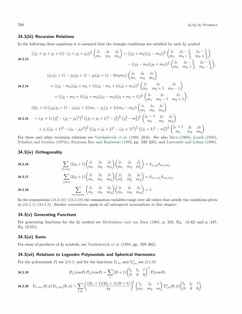
760 3j, 6j, 9j Symbols
34.3(iii) Recursion Relations
In the following three equations it is assumed that the triangle conditions are satisfied by each 3j symbol.
34.3.13
((j1 + j2 + j3 + 1)(−j1 + j2 + j3))12
(j1 j2 j3m1 m2 m3
)= ((j2 +m2)(j3 −m3))
12
(j1 j2 − 1
2 j3 − 12
m1 m2 − 12 m3 + 1
2
)− ((j2 −m2)(j3 +m3))
12
(j1 j2 − 1
2 j3 − 12
m1 m2 + 12 m3 − 1
2
),
34.3.14
(j1(j1 + 1)− j2(j2 + 1)− j3(j3 + 1)− 2m2m3)(j1 j2 j3m1 m2 m3
)= ((j2 −m2)(j2 +m2 + 1)(j3 −m3 + 1)(j3 +m3))
12
(j1 j2 j3m1 m2 + 1 m3 − 1
)+ ((j2 −m2 + 1)(j2 +m2)(j3 −m3)(j3 +m3 + 1))
12
(j1 j2 j3m1 m2 − 1 m3 + 1
),
34.3.15
(2j1 + 1) ((j2(j2 + 1)− j3(j3 + 1))m1 − j1(j1 + 1)(m3 −m2))(j1 j2 j3m1 m2 m3
)= (j1 + 1)
(j21 − (j2 − j3)2
)12((j2 + j3 + 1)2 − j2
1
)12(j21 −m2
1
)12
(j1 − 1 j2 j3m1 m2 m3
)+ j1
((j1 + 1)2 − (j2 − j3)2
)12((j2 + j3 + 1)2 − (j1 + 1)2
)12((j1 + 1)2 −m2
1
)12
(j1 + 1 j2 j3m1 m2 m3
).
For these and other recursion relations see Varshalovich et al. (1988, §8.6). See also Micu (1968), Louck (1958),Schulten and Gordon (1975a), Srinivasa Rao and Rajeswari (1993, pp. 220–225), and Luscombe and Luban (1998).
34.3(iv) Orthogonality
34.3.16∑m1m2
(2j3 + 1)(j1 j2 j3m1 m2 m3
)(j1 j2 j′3m1 m2 m′3
)= δj3,j′3δm3,m′3
,
34.3.17∑j3m3
(2j3 + 1)(j1 j2 j3m1 m2 m3
)(j1 j2 j3m′1 m′2 m3
)= δm1,m′1
δm2,m′2,
34.3.18∑
m1m2m3
(j1 j2 j3m1 m2 m3
)(j1 j2 j3m1 m2 m3
)= 1.
In the summations (34.3.16)–(34.3.18) the summation variables range over all values that satisfy the conditions givenin (34.2.1)–(34.2.3). Similar conventions apply to all subsequent summations in this chapter.
34.3(v) Generating Functions
For generating functions for the 3j symbol see Biedenharn and van Dam (1965, p. 245, Eq. (3.42) and p. 247,Eq. (3.55)).
34.3(vi) Sums
For sums of products of 3j symbols, see Varshalovich et al. (1988, pp. 259–262).
34.3(vii) Relations to Legendre Polynomials and Spherical Harmonics
For the polynomials Pl see §18.3, and for the functions Yl,m and Y ∗l,m see §14.30.
34.3.19 Pl1(cos θ)Pl2(cos θ) =∑l
(2l + 1)(l1 l2 l0 0 0
)2
Pl(cos θ),
34.3.20 Yl1,m1(θ, φ)Yl2,m2(θ, φ) =∑l,m
((2l1 + 1)(2l2 + 1)(2l + 1)
4π
)12(l1 l2 lm1 m2 m
)Y ∗l,m(θ, φ)
(l1 l2 l0 0 0
),

34.4 Definition: 6j Symbol 761
34.3.21
∫ π
0
Pl1(cos θ)Pl2(cos θ)Pl3(cos θ) sin θ dθ = 2(l1 l2 l30 0 0
)2
,
34.3.22
∫ 2π
0
∫ π
0
Yl1,m1(θ, φ)Yl2,m2(θ, φ)Yl3,m3(θ, φ) sin θ dθ dφ
=(
(2l1 + 1)(2l2 + 1)(2l3 + 1)4π
)12(l1 l2 l30 0 0
)(l1 l2 l3m1 m2 m3
).
Equations (34.3.19)–(34.3.22) are particular cases of more general results that relate rotation matrices to 3j symbols,for which see Edmonds (1974, Chapter 4). The left- and right-hand sides of (34.3.22) are known, respectively, asGaunt’s integral and the Gaunt coefficient (Gaunt (1929)).
34.4 Definition: 6j Symbol
The 6j symbol is defined by the following double sum of products of 3j symbols:
34.4.1
{j1 j2 j3l1 l2 l3
}=∑mrm′s
(−1)l1+m′1+l2+m′2+l3+m′3
×(j1 j2 j3m1 m2 m3
)(j1 l2 l3m1 m′2 −m′3
)(l1 j2 l3−m′1 m2 m′3
)(l1 l2 j3m′1 −m′2 m3
),
where the summation is taken over all admissible values of the m’s and m′’s for each of the four 3j symbols; compare(34.2.2) and (34.2.3).
Except in degenerate cases the combination of the triangle inequalities for the four 3j symbols in (34.4.1) is equiv-alent to the existence of a tetrahedron (possibly degenerate) with edges of lengths j1, j2, j3, l1, l2, l3; see Figure 34.4.1.
Figure 34.4.1: Tetrahedron corresponding to 6j symbol.
The 6j symbol can be expressed as the finite sum
34.4.2
{j1 j2 j3l1 l2 l3
}=∑s
(−1)s(s+ 1)!(s− j1 − j2 − j3)!(s− j1 − l2 − l3)!(s− l1 − j2 − l3)!(s− l1 − l2 − j3)!
× 1(j1 + j2 + l1 + l2 − s)!(j2 + j3 + l2 + l3 − s)!(j3 + j1 + l3 + l1 − s)!
,
where the summation is over all nonnegative integers s such that the arguments in the factorials are nonnegative.Equivalently,
34.4.3{j1 j2 j3l1 l2 l3
}= (−1)j1+j3+l1+l3
∆(j1j2j3)∆(j2l1l3)(j1 − j2 + l1 + l2)!(−j2 + j3 + l2 + l3)!(j1 + j3 + l1 + l3 + 1)!∆(j1l2l3)∆(j3l1l2)(j1 − j2 + j3)!(−j2 + l1 + l3)!(j1 + l2 + l3 + 1)!(j3 + l1 + l2 + 1)!
× 4F3
(−j1 + j2 − j3, j2 − l1 − l3,−j1 − l2 − l3 − 1,−j3 − l1 − l2 − 1−j1 + j2 − l1 − l2, j2 − j3 − l2 − l3,−j1 − j3 − l1 − l3 − 1
; 1),
where 4F3 is defined as in §16.2.For alternative expressions for the 6j symbol, written either as a finite sum or as other terminating generalized
hypergeometric series 4F3 of unit argument, see Varshalovich et al. (1988, §§9.2.1, 9.2.3).

762 3j, 6j, 9j Symbols
34.5 Basic Properties: 6j Symbol
34.5(i) Special Cases
In the following equations it is assumed that the triangle inequalities are satisfied and that J is again defined by(34.3.4).
If any lower argument in a 6j symbol is 0, 12 , or 1, then the 6j symbol has a simple algebraic form. Examples are
provided by:
34.5.1
{j1 j2 j30 j3 j2
}=
(−1)J
((2j2 + 1)(2j3 + 1))12,
34.5.2
{j1 j2 j312 j3 − 1
2 j2 + 12
}= (−1)J
((j1 + j3 − j2)(j1 + j2 − j3 + 1)(2j2 + 1)(2j2 + 2)2j3(2j3 + 1)
)12
,
34.5.3
{j1 j2 j312 j3 − 1
2 j2 − 12
}= (−1)J
((j2 + j3 − j1)(j1 + j2 + j3 + 1)
2j2(2j2 + 1)2j3(2j3 + 1)
)12
,
34.5.4
{j1 j2 j31 j3 − 1 j2 − 1
}= (−1)J
(J(J + 1)(J − 2j1)(J − 2j1 − 1)
(2j2 − 1)2j2(2j2 + 1)(2j3 − 1)2j3(2j3 + 1)
)12
,
34.5.5
{j1 j2 j31 j3 − 1 j2
}= (−1)J
(2(J + 1)(J − 2j1)(J − 2j2)(J − 2j3 + 1)
2j2(2j2 + 1)(2j2 + 2)(2j3 − 1)2j3(2j3 + 1)
)12
,
34.5.6
{j1 j2 j31 j3 − 1 j2 + 1
}= (−1)J
((J − 2j2 − 1)(J − 2j2)(J − 2j3 + 1)(J − 2j3 + 2)(2j2 + 1)(2j2 + 2)(2j2 + 3)(2j3 − 1)2j3(2j3 + 1)
)12
,
34.5.7
{j1 j2 j31 j3 j2
}= (−1)J+1 2(j2(j2 + 1) + j3(j3 + 1)− j1(j1 + 1))
(2j2(2j2 + 1)(2j2 + 2)2j3(2j3 + 1)(2j3 + 2))12.
34.5(ii) Symmetry
The 6j symbol is invariant under interchange of any two columns and also under interchange of the upper and lowerarguments in each of any two columns, for example,
34.5.8
{j1 j2 j3l1 l2 l3
}={j2 j1 j3l2 l1 l3
}={j1 l2 l3l1 j2 j3
}.
Next,
34.5.9
{j1 j2 j3l1 l2 l3
}={j1
12 (j2 + l2 + j3 − l3) 1
2 (j2 − l2 + j3 + l3)l1
12 (j2 + l2 − j3 + l3) 1
2 (−j2 + l2 + j3 + l3)
},
34.5.10
{j1 j2 j3l1 l2 l3
}={
12 (j2 + l2 + j3 − l3) 1
2 (j1 − l1 + j3 + l3) 12 (j1 + l1 + j2 − l2)
12 (j2 + l2 − j3 + l3) 1
2 (−j1 + l1 + j3 + l3) 12 (j1 + l1 − j2 + l2)
}.
Equations (34.5.9) and (34.5.10) are called Regge symmetries. Additional symmetries are obtained by applying(34.5.8) to (34.5.9) and (34.5.10). See Srinivasa Rao and Rajeswari (1993, pp. 102–103) and references given there.
34.5(iii) Recursion Relations
In the following equation it is assumed that the triangle conditions are satisfied.
34.5.11
(2j1 + 1) ((J3 + J2 − J1)(L3 + L2 − J1)− 2(J3L3 + J2L2 − J1L1)){j1 j2 j3l1 l2 l3
}= j1E(j1 + 1)
{j1 + 1 j2 j3l1 l2 l3
}+ (j1 + 1)E(j1)
{j1 − 1 j2 j3l1 l2 l3
},
where
34.5.12 Jr = jr(jr + 1), Lr = lr(lr + 1),
34.5.13 E(j) =((j2 − (j2 − j3)2)((j2 + j3 + 1)2 − j2)(j2 − (l2 − l3)2)((l2 + l3 + 1)2 − j2)
)12 .
For further recursion relations see Varshalovich et al. (1988, §9.6) and Edmonds (1974, pp. 98–99).

34.6 Definition: 9j Symbol 763
34.5(iv) Orthogonality
34.5.14∑j3
(2j3 + 1)(2l3 + 1){j1 j2 j3l1 l2 l3
}{j1 j2 j3l1 l2 l′3
}= δl3,l′3 .
34.5(v) Generating Functions
For generating functions for the 6j symbol see Biedenharn and van Dam (1965, p. 255, eq. (4.18)).
34.5(vi) Sums
34.5.15∑j
(−1)j+j′+j′′(2j + 1)
{j1 j2 jj3 j4 j′
}{j1 j2 jj4 j3 j′′
}={j1 j4 j′
j2 j3 j′′
},
34.5.16
(−1)j1+j2+j3+j′1+j′2+l1+l2
{j1 j2 j3l1 l2 l3
}{j′1 j′2 j3l1 l2 l′3
}=∑j
(−1)l3+l′3+j(2j + 1){j1 j′1 jj′2 j2 j3
}{l3 l′3 jj′1 j1 l2
}{l3 l′3 jj′2 j2 l1
}.
Equations (34.5.15) and (34.5.16) are the sum rules. They constitute addition theorems for the 6j symbol.
34.5.17∑j
(2j + 1){j1 j2 jj1 j2 j′
}= (−1)2(j1+j2),
34.5.18∑j
(−1)j1+j2+j(2j + 1){j1 j2 jj2 j1 j′
}=√
(2j1 + 1)(2j2 + 1) δj′,0 ,
34.5.19∑l
{j1 j2 lj2 j1 j
}= 0, 2µ− j odd, µ = min(j1, j2),
34.5.20∑l
(−1)l+j{j1 j2 lj1 j2 j
}=
(−1)2µ
2j + 1, µ = min(j1, j2),
34.5.21∑l
(−1)l+j+j1+j2
{j1 j2 lj2 j1 j
}=
12j + 1
((2j1 − j)!(2j2 + j + 1)!(2j2 − j)!(2j1 + j + 1)!
)12
, j2 ≤ j1,
34.5.22∑l
(−1)l+j+j1+j21
l(l + 1)
{j1 j2 lj2 j1 j
}=
1j1(j1 + 1)− j2(j2 + 1)
((2j1 − j)!(2j2 + j + 1)!(2j2 − j)!(2j1 + j + 1)!
)12
, j2 < j1.
34.5.23
(j1 j2 j3m1 m2 m3
){j1 j2 j3l1 l2 l3
}=
∑m′1m
′2m′3
(−1)l1+l2+l3+m′1+m′2+m′3
(j1 l2 l3m1 m′2 −m′3
)(l1 j2 l3−m′1 m2 m′3
)(l1 l2 j3m′1 −m′2 m3
).
Equation (34.5.23) can be regarded as an alternative definition of the 6j symbol.For other sums see Ginocchio (1991).
34.6 Definition: 9j Symbol
The 9j symbol may be defined either in terms of 3j symbols or equivalently in terms of 6j symbols:
34.6.1
j11 j12 j13
j21 j22 j23
j31 j32 j33
=∑
all mrs
(j11 j12 j13
m11 m12 m13
)(j21 j22 j23
m21 m22 m23
)(j31 j32 j33
m31 m32 m33
)
×(j11 j21 j31
m11 m21 m31
)(j12 j22 j32
m12 m22 m32
)(j13 j23 j33
m13 m23 m33
),
34.6.2
j11 j12 j13
j21 j22 j23
j31 j32 j33
=∑j
(−1)2j(2j + 1){j11 j21 j31
j32 j33 j
}{j12 j22 j32
j21 j j23
}{j13 j23 j33
j j11 j12
}.

764 3j, 6j, 9j Symbols
The 9j symbol may also be written as a finite triple sum equivalent to a terminating generalized hypergeometricseries of three variables with unit arguments. See Srinivasa Rao and Rajeswari (1993, pp. 7 and 125–132) andRosengren (1999).
34.7 Basic Properties: 9j Symbol
34.7(i) Special Case
34.7.1
j11 j12 j13
j21 j22 j13
j31 j31 0
=(−1)j12+j21+j13+j31
((2j13 + 1)(2j31 + 1))12
{j11 j12 j13
j22 j21 j31
}.
34.7(ii) Symmetry
The 9j symbol has symmetry properties with respect to permutation of columns, permutation of rows, and transpo-sition of rows and columns; these relate 72 independent 9j symbols. Even (cyclic) permutations of either columnsor rows, as well as transpositions, leave the 9j symbol unchanged. Odd permutations of columns or rows introducea phase factor (−1)R, where R is the sum of all arguments of the 9j symbol.
For further symmetry properties of the 9j symbol see Edmonds (1974, pp. 102–103) and Varshalovich et al. (1988,§10.4.1).
34.7(iii) Recursion Relations
For recursion relations see Varshalovich et al. (1988, §10.5).
34.7(iv) Orthogonality
34.7.2∑j12 j34
(2j12 + 1)(2j34 + 1)(2j13 + 1)(2j24 + 1)
j1 j2 j12
j3 j4 j34
j13 j24 j
j1 j2 j12
j3 j4 j34
j′13 j′24 j
= δj13,j′13δj24,j′24 .
34.7(v) Generating Functions
For generating functions for the 9j symbol see Biedenharn and van Dam (1965, p. 258, eq. (4.37)).
34.7(vi) Sums
34.7.3∑j13 j24
(−1)2j2+j24+j23−j34(2j13 + 1)(2j24 + 1)
j1 j2 j12
j3 j4 j34
j13 j24 j
j1 j3 j13
j4 j2 j24
j14 j23 j
=
j1 j2 j12
j4 j3 j34
j14 j23 j
.This equation is the sum rule. It constitutes an addition theorem for the 9j symbol.
34.7.4
(j13 j23 j33
m13 m23 m33
)j11 j12 j13
j21 j22 j23
j31 j32 j33
=∑
mr1,mr2,r=1,2,3
(j11 j12 j13
m11 m12 m13
)(j21 j22 j23
m21 m22 m23
)
×(j31 j32 j33
m13 m23 m33
)(j11 j21 j31
m11 m21 m31
)(j12 j22 j32
m12 m22 m32
).
34.7.5∑j′
(2j′ + 1)
j11 j12 j′
j21 j22 j23
j31 j32 j33
{j11 j12 j′
j23 j33 j
}= (−1)2j
{j21 j22 j23
j12 j j32
}{j31 j32 j33
j j11 j21
}.
34.8 Approximations for Large Parameters
For large values of the parameters in the 3j, 6j, and 9j symbols, different asymptotic forms are obtained dependingon which parameters are large. For example,
34.8.1
{j1 j2 j3j2 j1 l3
}= (−1)j1+j2+j3+l3
(4
π(2j1 + 1)(2j2 + 1)(2l3 + 1) sin θ
)12 (
cos((l3 + 1
2 )θ − 14π)
+ o(1))
,
j1, j2, j3 � l3 � 1,

34.9 Graphical Method 765
where
34.8.2 cos θ =j1(j1 + 1) + j2(j2 + 1)− j3(j3 + 1)
2√j1(j1 + 1)j2(j2 + 1)
,
and the symbol o(1) denotes a quantity that tends tozero as the parameters tend to infinity, as in §2.1(i).
Semiclassical (WKBJ) approximations in terms oftrigonometric or exponential functions are given in Var-shalovich et al. (1988, §§8.9, 9.9, 10.7). Uniform ap-proximations in terms of Airy functions for the 3j and6j symbols are given in Schulten and Gordon (1975b).For approximations for the 3j, 6j, and 9j symbols witherror bounds see Flude (1998), Chen et al. (1999), andWatson (1999): these references also cite earlier work.
34.9 Graphical Method
The graphical method establishes a one-to-one corre-spondence between an analytic expression and a dia-gram by assigning a graphical symbol to each functionand operation of the analytic expression. Thus, any an-alytic expression in the theory, for example equations(34.3.16), (34.4.1), (34.5.15), and (34.7.3), may be rep-resented by a diagram; conversely, any diagram rep-resents an analytic equation. For an account of thismethod see Brink and Satchler (1993, Chapter VII).For specific examples of the graphical method of repre-senting sums involving the 3j, 6j, and 9j symbols, seeVarshalovich et al. (1988, Chapters 11, 12) and Lehmanand O’Connell (1973, §3.3).
34.10 Zeros
In a 3j symbol, if the three angular momenta j1, j2, j3 donot satisfy the triangle conditions (34.2.1), or if the pro-jective quantum numbers do not satisfy (34.2.3), thenthe 3j symbol is zero. Similarly the 6j symbol (34.4.1)vanishes when the triangle conditions are not satisfiedby any of the four 3j symbols in the summation. Suchzeros are called trivial zeros. However, the 3j and 6jsymbols may vanish for certain combinations of the an-gular momenta and projective quantum numbers evenwhen the triangle conditions are fulfilled. Such zerosare called nontrivial zeros.
For further information, including examples of non-trivial zeros and extensions to 9j symbols, see Srini-vasa Rao and Rajeswari (1993, pp. 133–215, 294–295,299–310).
34.11 Higher-Order 3nj Symbols
For information on 12j, 15j,..., symbols, see Var-shalovich et al. (1988, §10.12) and Yutsis et al. (1962,pp. 62–65 and 122–153).
Applications
34.12 Physical Applications
The angular momentum coupling coefficients (3j, 6j,and 9j symbols) are essential in the fields of nuclear,atomic, and molecular physics. For applications innuclear structure, see de Shalit and Talmi (1963); inatomic spectroscopy, see Biedenharn and van Dam(1965, pp. 134–200), Judd (1998), Sobelman (1992,Chapter 4), Shore and Menzel (1968, pp. 268–303), andWigner (1959); in molecular spectroscopy and chemi-cal reactions, see Burshtein and Temkin (1994, Chap-ter 5), and Judd (1975). 3j, 6j, and 9j symbols are alsofound in multipole expansions of solutions of the Laplaceand Helmholtz equations; see Carlson and Rushbrooke(1950) and Judd (1976).
Computation
34.13 Methods of Computation
Methods of computation for 3j and 6j symbols includerecursion relations, see Schulten and Gordon (1975a),Luscombe and Luban (1998), and Edmonds (1974, pp.42–45, 48–51, 97–99); summation of single-sum expres-sions for these symbols, see Varshalovich et al. (1988,§§8.2.6, 9.2.1) and Fang and Shriner (1992); evaluationof the generalized hypergeometric functions of unit ar-gument that represent these symbols, see Srinivasa Raoand Venkatesh (1978) and Srinivasa Rao (1981).
For 9j symbols, methods include evaluation of thesingle-sum series (34.6.2), see Fang and Shriner (1992);evaluation of triple-sum series, see Varshalovich et al.(1988, §10.2.1) and Srinivasa Rao et al. (1989). A reviewof methods of computation is given in Srinivasa Rao andRajeswari (1993, Chapter VII, pp. 235–265). See alsoRoothaan and Lai (1997) and references given there.
34.14 Tables
Tables of exact values of the squares of the 3j and 6jsymbols in which all parameters are ≤ 8 are given inRotenberg et al. (1959), together with a bibliography ofearlier tables of 3j, 6j, and 9j symbols on pp. 33–36.
Tables of 3j and 6j symbols in which all parametersare ≤ 17/2 are given in Appel (1968) to 6D. Some se-lected 9j symbols are also given. Other tabulations for3j symbols are listed on pp. 11-12; for 6j symbols onpp. 16-17; for 9j symbols on p. 21.
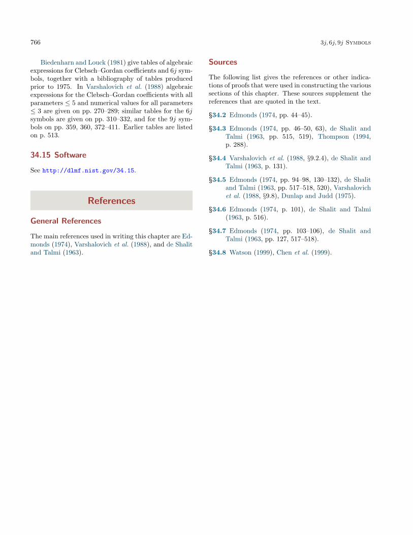
766 3j, 6j, 9j Symbols
Biedenharn and Louck (1981) give tables of algebraicexpressions for Clebsch–Gordan coefficients and 6j sym-bols, together with a bibliography of tables producedprior to 1975. In Varshalovich et al. (1988) algebraicexpressions for the Clebsch–Gordan coefficients with allparameters ≤ 5 and numerical values for all parameters≤ 3 are given on pp. 270–289; similar tables for the 6jsymbols are given on pp. 310–332, and for the 9j sym-bols on pp. 359, 360, 372–411. Earlier tables are listedon p. 513.
34.15 Software
See http://dlmf.nist.gov/34.15.
References
General References
The main references used in writing this chapter are Ed-monds (1974), Varshalovich et al. (1988), and de Shalitand Talmi (1963).
Sources
The following list gives the references or other indica-tions of proofs that were used in constructing the varioussections of this chapter. These sources supplement thereferences that are quoted in the text.
§34.2 Edmonds (1974, pp. 44–45).
§34.3 Edmonds (1974, pp. 46–50, 63), de Shalit andTalmi (1963, pp. 515, 519), Thompson (1994,p. 288).
§34.4 Varshalovich et al. (1988, §9.2.4), de Shalit andTalmi (1963, p. 131).
§34.5 Edmonds (1974, pp. 94–98, 130–132), de Shalitand Talmi (1963, pp. 517–518, 520), Varshalovichet al. (1988, §9.8), Dunlap and Judd (1975).
§34.6 Edmonds (1974, p. 101), de Shalit and Talmi(1963, p. 516).
§34.7 Edmonds (1974, pp. 103–106), de Shalit andTalmi (1963, pp. 127, 517–518).
§34.8 Watson (1999), Chen et al. (1999).

Chapter 35
Functions of Matrix ArgumentD. St. P. Richards1
Notation 76835.1 Special Notation . . . . . . . . . . . . . 768
Properties 76835.2 Laplace Transform . . . . . . . . . . . . 76835.3 Multivariate Gamma and Beta Functions 76835.4 Partitions and Zonal Polynomials . . . . . 76935.5 Bessel Functions of Matrix Argument . . 76935.6 Confluent Hypergeometric Functions of
Matrix Argument . . . . . . . . . . . . . 77035.7 Gaussian Hypergeometric Function of Ma-
trix Argument . . . . . . . . . . . . . . . 771
35.8 Generalized Hypergeometric Functions ofMatrix Argument . . . . . . . . . . . . . 772
Applications 77335.9 Applications . . . . . . . . . . . . . . . . 773
Computation 77335.10 Methods of Computation . . . . . . . . . 77335.11 Tables . . . . . . . . . . . . . . . . . . . 77335.12 Software . . . . . . . . . . . . . . . . . . 773
References 773
1Department of Statistics, Pennsylvania State University.Acknowledgments: With deep gratitude to Ingram Olkin for advice and support regarding the final version of this material.Copyright c© 2009 National Institute of Standards and Technology. All rights reserved.
767

768 Functions of Matrix Argument
Notation
35.1 Special Notation
(For other notation see pp. xiv and 873.)All matrices are of order m×m, unless specified oth-
erwise. All fractional or complex powers are principalvalues.
a, b complex variables.j, k nonnegative integers.m positive integer.[a]κ partitional shifted factorial (§35.4(i)).0 zero matrix.I identity matrix.S space of all real symmetric matrices.S,T,X real symmetric matrices.tr X trace of X.etr(X) exp(tr X).|X| determinant of X (except when m = 1
where it means either determinant orabsolute value, depending on the context).
|(X)j | jth principal minor of X.xj,k (j, k)th element of X.dX
∏1≤j≤k≤m dxj,k.
Ω space of positive-definite real symmetricmatrices.
t1, . . . , tm eigenvalues of T.||T|| spectral norm of T.X > T X−T is positive definite.Z complex symmetric matrix.U,V real and complex parts of Z.f(X) complex-valued function with X ∈ Ω.O(m) space of orthogonal matrices.H orthogonal matrix.dH normalized Haar measure on O(m).Zκ(T) zonal polynomials.
The main functions treated in this chapter arethe multivariate gamma and beta functions, respec-tively Γm(a) and Bm(a, b), and the special functionsof matrix argument: Bessel (of the first kind) Aν(T)and (of the second kind) Bν(T); confluent hyperge-ometric (of the first kind) 1F1(a; b; T) or 1F1
(ab
; T)
and (of the second kind) Ψ(a; b; T); Gaussian hyper-geometric 2F1(a1, a2; b; T) or 2F1
(a1, a2
b; T)
; gener-
alized hypergeometric pFq(a1, . . . , ap; b1, . . . , bq; T) or
pFq
(a1, . . . , apb1, . . . , bq
; T)
.
An alternative notation for the multivariate gammafunction is Πm(a) = Γm
(a+ 1
2 (m+ 1))
(Herz (1955,p. 480)). Related notations for the Bessel func-tions are Jν+ 1
2 (m+1)(T) = Aν(T)/Aν(0) (Faraut and
Korányi (1994, pp. 320–329)), Km(0, . . . , 0, ν|S,T) =|T|ν Bν(ST) (Terras (1988, pp. 49–64)), and Kν(T) =|T|ν Bν(ST) (Faraut and Korányi (1994, pp. 357–358)).
Properties
35.2 Laplace Transform
Definition
For any complex symmetric matrix Z,
35.2.1 g(Z) =∫
Ω
etr(−ZX)f(X) dX,
where the integration variable X ranges over the spaceΩ.
Suppose there exists a constant X0 ∈ Ω such that|f(X)| < etr(−X0X) for all X ∈ Ω. Then (35.2.1) con-verges absolutely on the region <(Z) > X0, and g(Z) isa complex analytic function of all elements zj,k of Z.
Inversion Formula
Assume that∫S |g(Z)| dV converges, and also that
limU→∞∫S |g(Z)| dV = 0. Then
35.2.2 f(X) =1
(2πi)m(m+1)/2
∫etr(ZX)g(Z) dZ,
where the integral is taken over all Z = U + iV suchthat U > X0 and V ranges over S.
Convolution Theorem
If gj is the Laplace transform of fj , j = 1, 2, then g1g2 isthe Laplace transform of the convolution f1 ∗ f2, where
35.2.3 f1 ∗ f2(T) =∫
0<X<T
f1(T−X)f2(X) dX.
35.3 Multivariate Gamma and BetaFunctions
35.3(i) Definitions
35.3.1Γm(a) =
∫Ω
etr(−X)|X|a− 12 (m+1) dX,
<(a) > 12 (m− 1).
35.3.2
Γm(s1, . . . , sm)
=∫
Ω
etr(−X)|X|sm− 12 (m+1)
m−1∏j=1
|(X)j |sj−sj+1 dX,
sj ∈ C, <(sj) > 12 (j − 1), j = 1, . . . ,m.
35.3.3
Bm(a, b) =∫
0<X<I
|X|a− 12 (m+1)|I−X|b− 1
2 (m+1) dX,
<(a),<(b) > 12 (m− 1).

35.4 Partitions and Zonal Polynomials 769
35.3(ii) Properties
35.3.4 Γm(a) = πm(m−1)/4m∏j=1
Γ(a− 1
2 (j − 1)).
35.3.5
Γm(s1, . . . , sm) = πm(m−1)/4m∏j=1
Γ(sj − 1
2 (j − 1)).
35.3.6 Γm(a, . . . , a) = Γm(a).
35.3.7 Bm(a, b) =Γm(a) Γm(b)Γm(a+ b)
.
35.3.8Bm(a, b) =
∫Ω
|X|a− 12 (m+1)|I + X|−(a+b) dX,
<(a),<(b) > 12 (m− 1).
35.4 Partitions and Zonal Polynomials
35.4(i) Definitions
A partition κ = (k1, . . . , km) is a vector of nonnegativeintegers, listed in nonincreasing order. Also, |κ| denotesk1+· · ·+km, the weight of κ; `(κ) denotes the number ofnonzero kj ; a+κ denotes the vector (a+k1, . . . , a+km).
The partitional shifted factorial is given by
35.4.1 [a]κ =Γm(a+ κ)
Γm(a)=
m∏j=1
(a− 1
2 (j − 1))kj,
where (a)k = a(a+ 1) · · · (a+ k − 1).For any partition κ, the zonal polynomial Zκ : S →
R is defined by the properties
35.4.2
Zκ(I) = |κ|! 22|κ| [m/2]κ
∏1≤j<l≤`(κ)
(2kj − 2kl − j + l)
`(κ)∏j=1
(2kj + `(κ)− j)!
and
35.4.3
Zκ(T) = Zκ(I) |T|km∫
O(m)
m−1∏j=1
|(HTH−1)j |kj−kj+1 dH,
T ∈ S.
See Muirhead (1982, pp. 68–72) for the definitionand properties of the Haar measure dH. See Hua(1963, p. 30), Constantine (1963), James (1964), andMacdonald (1995, pp. 425–431) for further informationon (35.4.2) and (35.4.3). Alternative notations for thezonal polynomials are Cκ(T) (Muirhead (1982, pp. 227–239)), Yκ(T) (Takemura (1984, p. 22)), and Φκ(T) (Fa-raut and Korányi (1994, pp. 228–236)).
35.4(ii) Properties
Normalization
35.4.4 Zκ(0) =
{1, κ = (0, . . . , 0),0, κ 6= (0, . . . , 0).
Orthogonal Invariance
35.4.5 Zκ(HTH−1
)= Zκ(T), H ∈ O(m).
Therefore Zκ(T) is a symmetric polynomial in the eigen-values of T.
Summation
For k = 0, 1, 2, . . . ,
35.4.6
∑|κ|=k
Zκ(T) = (tr T)k.
Mean-Value
35.4.7
∫O(m)
Zκ(SHTH−1
)dH =
Zκ(S)Zκ(T)Zκ(I)
.
Laplace and Beta Integrals
For T ∈ Ω and <(a),<(b) > 12 (m− 1),
35.4.8
∫Ω
etr(−TX) |X|a− 12 (m+1) Zκ(X) dX
= Γm(a+ κ) |T|−a Zκ(T−1
),
35.4.9
∫0<X<I
|X|a− 12 (m+1) |I−X|b− 1
2 (m+1) Zκ(TX) dX
=[a]κ
[a+ b]κBm(a, b)Zκ(T).
35.5 Bessel Functions of Matrix Argument
35.5(i) Definitions
35.5.1 Aν(0) =1
Γm(ν + 1
2 (m+ 1)) , ν ∈ C.
35.5.2
Aν(T) =Aν(0)∞∑k=0
(−1)k
k!
∑|κ|=k
1[ν + 1
2 (m+ 1)]κ
Zκ(T),
ν ∈ C, T ∈ S.
35.5.3
Bν(T) =∫
Ω
etr(−(TX + X−1)
)|X|ν− 1
2 (m+1) dX,
ν ∈ C, T ∈ Ω.
35.5(ii) Properties
35.5.4
∫Ω
etr(−TX)|X|ν Aν(SX) dX
= etr(−ST−1
)|T|−ν− 1
2 (m+1),S ∈ S, T ∈ Ω; <(ν) > −1.

770 Functions of Matrix Argument
35.5.5
∫0<X<T
Aν1(S1X)|X|ν1 Aν2(S2(T−X))|T−X|ν2 dX = |T|ν1+ν2+ 12 (m+1)Aν1+ν2+ 1
2 (m+1)((S1 + S2)T),
νj ∈ C, <(νj) > −1, j = 1, 2; S1,S2 ∈ S; T ∈ Ω.
35.5.6 Bν(T) = |T|−ν B−ν(T), ν ∈ C, T ∈ Ω.
35.5.7
∫Ω
Aν1(TX)B−ν2(SX)|X|ν1 dX =1
Aν1+ν2(0)|S|ν2 |T + S|−(ν1+ν2+ 1
2 (m+1)), <(ν1 + ν2) > −1; S,T ∈ Ω.
35.5.8
∫O(m)
etr(SH) dH =A−1/2
(− 1
4SST)
A−1/2(0), S arbitrary.
35.5(iii) Asymptotic Approximations
For asymptotic approximations for Bessel functions of matrix argument, see Herz (1955) and Butler and Wood(2003).
35.6 Confluent Hypergeometric Functions of Matrix Argument
35.6(i) Definitions
35.6.1 1F1
(ab
; T)
=∞∑k=0
1k!
∑|κ|=k
[a]κ[b]κ
Zκ(T).
35.6.2 Ψ(a; b; T) =1
Γm(a)
∫Ω
etr(−TX)|X|a− 12 (m+1) |I + X|b−a−
12 (m+1)
dX, <(a) > 12 (m− 1), T ∈ Ω.
Laguerre Form
35.6.3 L(γ)ν (T) =
Γm(γ + ν + 1
2 (m+ 1))
Γm(γ + 1
2 (m+ 1)) 1F1
(−ν
γ + 12 (m+ 1)
; T)
, <(γ),<(γ + ν) > −1.
35.6(ii) Properties
35.6.4 1F1
(ab
; T)
=1
Bm(a, b− a)
∫0<X<I
etr(TX)|X|a− 12 (m+1)|I−X|b−a− 1
2 (m+1) dX, <(a),<(b− a) > 12 (m− 1).
35.6.5
∫Ω
etr(−TX)|X|b− 12 (m+1)
1F1
(ab
; SX)dX = Γm(b)|I− ST−1|−a|T|−b, T > S, <(b) > 1
2 (m− 1).
35.6.6
Bm(b1, b2)|T|b1+b2− 12 (m+1)
1F1
(a1 + a2
b1 + b2; T)
=∫
0<X<T
|X|b1− 12 (m+1)
1F1
(a1
b1; X)|T−X|b2−
12 (m+1)
1F1
(a2
b2; T−X
)dX, <(b1),<(b2) > 1
2 (m− 1).
35.6.7 1F1
(ab
; T)
= etr(T) 1F1
(b− ab
;−T).
35.6.8
∫Ω
|T|c− 12 (m+1) Ψ(a; b; T) dT =
Γm(c) Γm(a− c) Γm(c− b+ 1
2 (m+ 1))
Γm(a) Γm(a− b+ 1
2 (m+ 1)) ,
<(a) > <(c) + 12 (m− 1) > m− 1, <(c− b) > −1.
35.6(iii) Relations to Bessel Functions of Matrix Argument
35.6.9 lima→∞ 1F1
(a
ν + 12 (m+ 1)
;−a−1T)
=Aν(T)Aν(0)
.
35.6.10 lima→∞
Γm(a) Ψ(a+ ν; ν + 1
2 (m+ 1); a−1T)
= Bν(T).

35.7 Gaussian Hypergeometric Function of Matrix Argument 771
35.6(iv) Asymptotic Approximations
For asymptotic approximations for confluent hypergeometric functions of matrix argument, see Herz (1955) andButler and Wood (2002).
35.7 Gaussian Hypergeometric Function of Matrix Argument
35.7(i) Definition
35.7.1 2F1
(a, b
c; T)
=∞∑k=0
1k!
∑|κ|=k
[a]κ[b]κ[c]κ
Zκ(T), −c+ 12 (j + 1) /∈ N, 1 ≤ j ≤ m; ||T|| < 1.
Jacobi Form
35.7.2 P (γ,δ)ν (T) =
Γm(γ + ν + 1
2 (m+ 1))
Γm(γ + 1
2 (m+ 1)) 2F1
(−ν, γ + δ + ν + 1
2 (m+ 1)γ + 1
2 (m+ 1); T
), 0 < T < I; γ, δ, ν ∈ C; <(γ) > −1.
35.7(ii) Basic Properties
Case m = 2
35.7.3 2F1
(a, b
c;(t1 00 t2
))=∞∑k=0
(a)k(c− a)k(b)k(c− b)kk! (c)2k
(c− 1
2
)k
(t1t2)k 2F1
(a+ k, b+ k
c+ 2k; t1 + t2 − t1t2
).
Confluent Form
35.7.4 limc→∞ 2F1
(a, b
c; I− cT−1
)= |T|b Ψ
(b; b− a+ 1
2 (m+ 1); T).
Integral Representation
35.7.52F1
(a, b
c; T)
=1
Bm(a, c− a)
∫0<X<I
|X|a− 12 (m+1) |I−X|c−a−
12 (m+1)|I−TX|−b dX,
<(a),<(c− a) > 12 (m− 1), 0 < T < I.
Transformations of Parameters
35.7.6
2F1
(a, b
c; T)
= |I−T|c−a−b 2F1
(c− a, c− b
c; T)
= |I−T|−a 2F1
(a, c− b
c;−T(I−T)−1
)= |I−T|−b 2F1
(c− a, b
c;−T(I−T)−1
).
Gauss Formula
35.7.7 2F1
(a, b
c; I)
=Γm(c) Γm(c− a− b)Γm(c− a) Γm(c− b)
, <(c),<(c− a− b) > 12 (m− 1).
Reflection Formula
35.7.8 2F1
(a, b
c; T)
=Γm(c) Γm(c− a− b)Γm(c− a) Γm(c− b) 2F1
(a, b
a+ b− c+ 12 (m+ 1)
; I−T)
, <(c),<(c− a− b) > 12 (m− 1).
35.7(iii) Partial Differential Equations
Let f : Ω→ C (a) be orthogonally invariant, so that f(T) is a symmetric function of t1, . . . , tm, the eigenvalues of thematrix argument T ∈ Ω; (b) be analytic in t1, . . . , tm in a neighborhood of T = 0; (c) satisfy f(0) = 1. Subject tothe conditions (a)–(c), the function f(T) = 2F1(a, b; c; T) is the unique solution of each partial differential equation35.7.9
tj(1− tj)∂2F
∂tj2 −
12
m∑k=1k 6=j
tk(1− tk)tj − tk
∂F
∂tk+
c− 12 (m− 1)−
(a+ b− 1
2 (m− 3))tj +
12
m∑k=1k 6=j
tj(1− tj)tj − tk
∂F
∂tj= abF,
for j = 1, . . . ,m.

772 Functions of Matrix Argument
Systems of partial differential equations for the 0F1
(defined in §35.8) and 1F1 functions of matrix argumentcan be obtained by applying (35.8.9) and (35.8.10) to(35.7.9).
35.7(iv) Asymptotic Approximations
Butler and Wood (2002) applies Laplace’s method(§2.3(iii)) to (35.7.5) to derive uniform asymptotic ap-proximations for the functions
35.7.10 2F1
(αa, αb
αc; T)
and35.7.11 2F1
(a, b
c; I− α−1T
)as α → ∞. These approximations are in terms of ele-mentary functions.
For other asymptotic approximations for Gaussianhypergeometric functions of matrix argument, see Herz(1955), Muirhead (1982, pp. 264–281, 290, 472, 563),and Butler and Wood (2002).
35.8 Generalized Hypergeometric Functionsof Matrix Argument
35.8(i) Definition
Let p and q be nonnegative integers; a1, . . . , ap ∈ C;b1, . . . , bq ∈ C; −bj+ 1
2 (k+1) /∈ N, 1 ≤ j ≤ q, 1 ≤ k ≤ m.The generalized hypergeometric function pFq with ma-trix argument T ∈ S, numerator parameters a1, . . . , ap,and denominator parameters b1, . . . , bq is35.8.1
pFq
(a1, . . . , apb1, . . . , bq
; T)
=∞∑k=0
1k!
∑|κ|=k
[a1]κ · · · [ap]κ[b1]κ · · · [bq]κ
Zκ(T).
Convergence Properties
If −aj + 12 (k+ 1) ∈ N for some j, k satisfying 1 ≤ j ≤ p,
1 ≤ k ≤ m, then the series expansion (35.8.1) termi-nates.
If p ≤ q, then (35.8.1) converges for all T.If p = q + 1, then (35.8.1) converges absolutely for
||T|| < 1 and diverges for ||T|| > 1.If p > q + 1, then (35.8.1) diverges unless it termi-
nates.
35.8(ii) Relations to Other Functions
35.8.2 0F0
(−−
; T)
= etr(T), T ∈ S.
35.8.3
2F1
(a, b
b; T)
= 1F0
(a
−; T)
= |I−T|−a, 0 < T < I.
35.8.4
Aν(T) =1
Γm(ν + 1
2 (m+ 1)) 0F1
(−
ν + 12 (m+ 1)
;−T)
,
T ∈ S.
35.8(iii) 3F2 Case
Kummer Transformation
Let c = b1 + b2 − a1 − a2 − a3. Then
35.8.5
3F2
(a1, a2, a3
b1, b2; I)
=Γm(b2) Γm(c)
Γm(b2 − a3) Γm(c+ a3)
× 3F2
(b1 − a1, b1 − a2, a3
b1, c+ a3; I)
,
<(b2),<(c) > 12 (m− 1).
Pfaff–Saalschutz Formula
Let a1 + a2 + a3 + 12 (m+ 1) = b1 + b2; one of the aj be
a negative integer; <(b1 − a1), <(b1 − a2), <(b1 − a3),<(b1 − a1 − a2 − a3) > 1
2 (m− 1). Then
35.8.6
3F2
(a1, a2, a3
b1, b2; I)
=Γm(b1 − a1) Γm(b1 − a2)Γm(b1) Γm(b1 − a1 − a2)
× Γm(b1 − a3) Γm(b1 − a1 − a2 − a3)Γm(b1 − a1 − a3) Γm(b1 − a2 − a3)
.
Thomae Transformation
Again, let c = b1 + b2 − a1 − a2 − a3. Then
35.8.7
3F2
(a1, a2, a3
b1, b2; I)
=Γm(b1) Γm(b2) Γ(c)
Γm(a1) Γm(c+ a2) Γ(c+ a3)
× 3F2
(b1 − a1, b2 − a2, c
c+ a2, c+ a3; I)
,
<(b1), <(b2), <(c) > 12 (m− 1).
35.8(iv) General Properties
Value at T = 0
35.8.8 pFq
(a1, . . . , apb1, . . . , bq
; 0)
= 1.
Confluence
35.8.9
limγ→∞ p+1Fq
(a1, . . . , ap, γ
b1, . . . , bq; γ−1T
)= pFq
(a1, . . . , apb1, . . . , bq
; T),
35.8.10
limγ→∞ pFq+1
(a1, . . . , apb1, . . . , bq, γ
; γT)
= pFq
(a1, . . . , apb1, . . . , bq
; T).

Applications 773
Invariance
35.8.11
pFq
(a1, . . . , apb1, . . . , bq
; HTH−1
)= pFq
(a1, . . . , apb1, . . . , bq
; T)
,
H ∈ O(m).
Laplace Transform
35.8.12∫Ω
etr(−TX)|X|γ− 12 (m+1)
pFq
(a1, . . . , apb1, . . . , bq
;−X)dX
= Γm(γ)|T|−γ p+1Fq
(a1, . . . , ap, γ
b1, . . . , bq;−T−1
),
<(γ) > 12 (m− 1).
Euler Integral
35.8.13∫0<X<I
|X|a1− 12 (m+1)|I−X|b1−a1− 1
2 (m+1)
× pFq
(a2, . . . , ap+1
b2, . . . , bq+1; TX
)dX
=1
Bm(b1 − a1, a1) p+1Fq+1
(a1, . . . , ap+1
b1, . . . , bq+1; T)
,
<(b1 − a1),<(a1) > 12 (m− 1).
35.8(v) Mellin–Barnes Integrals
Multidimensional Mellin–Barnes integrals are estab-lished in Ding et al. (1996) for the functions pFq andp+1Fp of matrix argument. A similar result for the0F1 function of matrix argument is given in Faraut andKorányi (1994, p. 346). These multidimensional in-tegrals reduce to the classical Mellin–Barnes integrals(§5.19(ii)) in the special case m = 1.
See also Faraut and Korányi (1994, pp. 318–340).
Applications
35.9 Applications
In multivariate statistical analysis based on the mul-tivariate normal distribution, the probability densityfunctions of many random matrices are expressible interms of generalized hypergeometric functions of matrixargument pFq, with p ≤ 2 and q ≤ 1. See James (1964),Muirhead (1982), Takemura (1984), Farrell (1985), andChikuse (2003) for extensive treatments.
For other statistical applications of pFq functionsof matrix argument see Perlman and Olkin (1980),Groeneboom and Truax (2000), Bhaumik and Sarkar(2002), Richards (2004) (monotonicity of power func-tions of multivariate statistical test criteria), Bingham
et al. (1992) (Procrustes analysis), and Phillips (1986)(exact distributions of statistical test criteria). Thesereferences all use results related to the integral formu-las (35.4.7) and (35.5.8).
For applications of the integral representation(35.5.3) see McFarland and Richards (2001, 2002) (sta-tistical estimation of misclassification probabilities fordiscriminating between multivariate normal popula-tions). The asymptotic approximations of §35.7(iv) areapplied in numerous statistical contexts in Butler andWood (2002).
In chemistry, Wei and Eichinger (1993) expressesthe probability density functions of macromolecules interms of generalized hypergeometric functions of matrixargument, and develop asymptotic approximations forthese density functions.
In the nascent area of applications of zonal polyno-mials to the limiting probability distributions of sym-metric random matrices, one of the most comprehensiveaccounts is Rains (1998).
Computation
35.10 Methods of Computation
For small values of ||T|| the zonal polynomial expan-sion given by (35.8.1) can be summed numerically. Forlarge ||T|| the asymptotic approximations referred to in§35.7(iv) are available.
Other methods include numerical quadrature ap-plied to double and multiple integral representations.See Yan (1992) for the 1F1 and 2F1 functions of ma-trix argument in the case m = 2, and Bingham et al.(1992) for Monte Carlo simulation on O(m) applied toa generalization of the integral (35.5.8).
Koev and Edelman (2006) utilizes combinatorialidentities for the zonal polynomials to develop compu-tational algorithms for approximating the series expan-sion (35.8.1). These algorithms are extremely efficient,converge rapidly even for large values of m, and havecomplexity linear in m.
35.11 Tables
Tables of zonal polynomials are given in James (1964)for |κ| ≤ 6, Parkhurst and James (1974) for |κ| ≤ 12,and Muirhead (1982, p. 238) for |κ| ≤ 5. Each tableexpresses the zonal polynomials as linear combinationsof monomial symmetric functions.
35.12 Software
See http://dlmf.nist.gov/35.12.

774 Functions of Matrix Argument
References
General References
The main references used in writing this chapter areHerz (1955), James (1964), Muirhead (1982), Gross andRichards (1987), and Richards (1992). For additionalbibliographic reading see Vilenkin and Klimyk (1992)and Faraut and Korányi (1994).
Sources
The following list gives the references or other indica-tions of proofs that were used in constructing the varioussections in this chapter. These sources supplement thereferences that are quoted in the text.
§35.2 G̊arding (1947), Herz (1955, p. 479), Muirhead(1982, p. 252). See also Siegel (1935), Bochnerand Martin (1948, pp. 90–92, 113–132).
§35.3 Wishart (1928), Ingham (1933), Gindikin (1964),G̊arding (1947), Herz (1955), Olkin (1959).
§35.4 James (1964), Muirhead (1982, Chapter 7),Macdonald (1995, p. 425). See also Constan-tine (1963), Maass (1971, pp. 64–71), Macdonald(1995, pp. 388–439).
§35.5 Herz (1955). See also Bochner (1952), Gross andKunze (1976), Terras (1988, pp. 49–63), Butlerand Wood (2003).
§35.6 Koecher (1954), Muirhead (1978), Muirhead(1982, pp. 264–266, 472–473), Herz (1955). For(35.6.6) apply (35.2.3) and (35.6.5). See alsoShimura (1982).
§35.7 Herz (1955), Muirhead (1982, pp. 264–281, 290,472), Faraut and Korányi (1994, pp. 337–340).For (35.7.8) see Zheng (1997). See also Macdon-ald (1990), Ding et al. (1996), Koornwinder andSprinkhuizen-Kuyper (1978), Gross and Richards(1991).
§35.8 Gross and Richards (1987, 1991), Faraut andKorányi (1994, pp. 318–340), Herz (1955), Muir-head (1982, pp. 259–262), Macdonald (1990),James (1964), Ding et al. (1996).

Chapter 36
Integrals with Coalescing SaddlesM. V. Berry1 and C. J. Howls2
Notation 77636.1 Special Notation . . . . . . . . . . . . . 776
Properties 77636.2 Catastrophes and Canonical Integrals . . 77636.3 Visualizations of Canonical Integrals . . . 77836.4 Bifurcation Sets . . . . . . . . . . . . . . 78136.5 Stokes Sets . . . . . . . . . . . . . . . . 78236.6 Scaling Relations . . . . . . . . . . . . . 78536.7 Zeros . . . . . . . . . . . . . . . . . . . 78536.8 Convergent Series Expansions . . . . . . 78736.9 Integral Identities . . . . . . . . . . . . . 787
36.10 Differential Equations . . . . . . . . . . . 78836.11 Leading-Order Asymptotics . . . . . . . . 789
Applications 78936.12 Uniform Approximation of Integrals . . . 78936.13 Kelvin’s Ship-Wave Pattern . . . . . . . . 79036.14 Other Physical Applications . . . . . . . 791
Computation 79236.15 Methods of Computation . . . . . . . . . 792
References 792
1H H Wills Physics Laboratory, Bristol, United Kingdom.2School of Mathematics, University of Southampton, Southampton, United Kingdom.Copyright c© 2009 National Institute of Standards and Technology. All rights reserved.
775

776 Integrals with Coalescing Saddles
Notation
36.1 Special Notation
(For other notation see pp. xiv and 873.)
l,m, n integers.k, t, s real or complex variables.K codimension.x {x1, x2, . . . , xK}, where x1, x2, . . . , xK are real
parameters; also x1 = x, x2 = y, x3 = z whenK ≤ 3.
Ai, Bi Airy functions (§9.2).∗ complex conjugate.
The main functions covered in this chapter are cus-poid catastrophes ΦK(t; x); umbilic catastrophes withcodimension three Φ(E)(s, t; x), Φ(H)(s, t; x); canonicalintegrals ΨK(x), Ψ(E)(x), Ψ(H)(x); diffraction catastro-phes ΨK(x; k), Ψ(E)(x; k), Ψ(H)(x; k) generated by thecatastrophes. (There is no standard nomenclature forthese functions.)
Properties
36.2 Catastrophes and Canonical Integrals
36.2(i) Definitions
Normal Forms Associated with Canonical Integrals:Cuspoid Catastrophe with Codimension K
36.2.1 ΦK(t; x) = tK+2 +K∑m=1
xmtm.
Special cases: K = 1, fold catastrophe; K = 2, cuspcatastrophe; K = 3, swallowtail catastrophe.
Normal Forms for Umbilic Catastrophes with CodimensionK = 3
36.2.2Φ(E)(s, t; x) = s3 − 3st2 + z(s2 + t2) + yt+ xs,
x = {x, y, z},(elliptic umbilic).
36.2.3Φ(H)(s, t; x) = s3 + t3 + zst+ yt+ xs,
x = {x, y, z},(hyperbolic umbilic).
Canonical Integrals
36.2.4 ΨK(x) =∫ ∞−∞
exp(iΦK(t; x)) dt.
36.2.5 Ψ(U)(x) =∫ ∞−∞
∫ ∞−∞
exp(iΦ(U)(s, t; x)
)ds dt, U = E,H.
36.2.6 Ψ(E)(x) = 2√π/3 exp
(i(
427z
3 + 13xz −
14π)) ∫ ∞ exp(πi/12)
∞ exp(−7πi/12)
exp(i
(u6 + 2zu4 + (z2 + x)u2 +
y2
12u2
))du,
with the contour passing to the lower right of u = 0.
36.2.7
Ψ(E)(x) =4π
31/3exp(i(
227z
3 − 13xz
)) (exp(−iπ
6
)F+(x) + exp
(iπ
6
)F−(x)
),
F±(x) =∫ ∞
0
cos(ry exp
(±iπ
6
))exp(
2ir2z exp(±iπ
3
))Ai(
32/3r2 + 3−1/3 exp(∓iπ
3
) (13z
2 − x))dr.
36.2.8
Ψ(H)(x) = 4√π/6 exp
(i(
127z
3 + 16z(y + x) + 1
4π))
×∫ ∞ exp(πi/12)
∞ exp(5πi/12)
exp(i
(2u6 + 2zu4 +
(12z
2 + x+ y)u2 − (y − x)2
24u2
))du,
with the contour passing to the upper right of u = 0.
36.2.9 Ψ(H)(x) =2π
31/3
∫ ∞ exp(πi/6)
∞ exp(5πi/6)
exp(i(s3 + xs)
)Ai(zs+ y
31/3
)ds.

36.2 Catastrophes and Canonical Integrals 777
Diffraction Catastrophes
36.2.10
ΨK(x; k) =√k
∫ ∞−∞
exp(ikΦK(t; x)) dt, k > 0.
36.2.11
Ψ(U)(x; k) = k
∫ ∞−∞
∫ ∞−∞
exp(ikΦ(U)(s, t; x)
)ds dt,
U = E,H; k > 0.For more extensive lists of normal forms of catas-
trophes (umbilic and beyond) involving two variables(“corank two”) see Arnol’d (1972, 1974, 1975).
36.2(ii) Special Cases
36.2.12 Ψ0 =√π exp
(iπ
4
).
Ψ1 is related to the Airy function (§9.2):
36.2.13 Ψ1(x) =2π
31/3Ai( x
31/3
).
Ψ2 is the Pearcey integral (Pearcey (1946)):
36.2.14
Ψ2(x) = P (x2, x1) =∫ ∞−∞
exp(i(t4 + x2t
2 + x1t))dt.
(Other notations also appear in the literature.)
36.2.15
ΨK(0)
=2
K + 2Γ(
1K + 2
) exp(i
π
2(K + 2)
), K even,
cos(
π
2(K + 2)
), K odd.
36.2.16
Ψ1(0) = 1.54669, Ψ2(0) = 1.67481 + i 0.69373
Ψ3(0) = 1.74646, Ψ4(0) = 1.79222 + i 0.48022.
36.2.17
∂p
∂x1p ΨK(0) =
2K + 2
Γ(p+ 1K + 2
)cos(π
2
(p+ 1K + 2
+ p
)), K odd,
∂2q+1
∂x12q+1 ΨK(0) = 0, K even,
∂2q
∂x12q ΨK(0) =
2K + 2
Γ(
2q + 1K + 2
)exp(iπ
2
(2q + 1K + 2
+ 2q))
, K even.
36.2.18Ψ(E)(0) = 1
3
√π Γ(
16
)= 3.28868,
Ψ(H)(0) = 13 Γ2
(13
)= 2.39224.
36.2.19
Ψ2(0, y) =π
2
√|y|2
exp(−iy
2
8
)(exp(iπ
8
)J− 1/4
(y2
8
)− sign(y) exp
(−iπ
8
)J 1/4
(y2
8
)).
For the Bessel function J see §10.2(ii).36.2.20
Ψ(E)(x, y, 0) = 2π2( 23 )2/3<
(Ai(x+ iy
121/3
)Bi(x− iy121/3
)),
36.2.21 Ψ(H)(x, y, 0) =4π2
32/3Ai( x
31/3
)Ai( y
31/3
).
36.2(iii) Symmetries
36.2.22
Ψ2K(x′) = Ψ2K(x), x′2m+1 = −x2m+1, x′2m = x2m.
36.2.23
Ψ2K+1(x′) = Ψ∗2K+1(x), x′2m+1 = x2m+1, x′2m = −x2m.
36.2.24 Ψ(U)(x, y, z) = Ψ∗(U)(x, y,−z), U = E,H.
36.2.25 Ψ(E)(x,−y, z) = Ψ(E)(x, y, z).
36.2.26
Ψ(E)(− 1
2x∓√
32 y,±
√3
2 x−12y, z
)= Ψ(E)(x, y, z),
(rotation by ± 23π in x, y plane).
36.2.27 Ψ(H)(x, y, z) = Ψ(H)(y, x, z).

778 Integrals with Coalescing Saddles
36.3 Visualizations of Canonical Integrals
36.3(i) Canonical Integrals: Modulus
(a) Density plot. (b) 3D plot.Figure 36.3.1: Modulus of Pearcey integral |Ψ2(x, y)|.
For additional figures see http://dlmf.nist.gov/36.3.i.
(a) Density plot. (b) 3D plot.Figure 36.3.5: Modulus of swallowtail canonical integral function |Ψ3(x, y,−7.5)|.
For additional figures see http://dlmf.nist.gov/36.3.i.

36.3 Visualizations of Canonical Integrals 779
(a) Density plot. (b) 3D plot.
Figure 36.3.8: Modulus of elliptic umbilic canonical integral function |Ψ(E)(x, y, 4)|.
For additional figures see http://dlmf.nist.gov/36.3.i.
(a) Density plot. (b) 3D plot.
Figure 36.3.12: Modulus of hyperbolic umbilic canonical integral function |Ψ(H)(x, y, 3)|.

780 Integrals with Coalescing Saddles
36.3(ii) Canonical Integrals: Phase
In Figure 36.3.13(a) points of confluence of phase contours are zeros of Ψ2(x, y); similarly for other contour plots inthis subsection. In Figure 36.3.13(b) points of confluence of all colors are zeros of Ψ2(x, y); similarly for other densityplots in this subsection.
(a) Contour plot, at intervals of π/4. (b) Density plot.Figure 36.3.13: Phase of Pearcey integral ph Ψ2(x, y).
For additional figures see http://dlmf.nist.gov/36.3.ii.
(a) Contour plot. (b) Density plot.
Figure 36.3.17: Phase of elliptic umbilic canonical integral ph Ψ(E)(x, y, 4).
For additional figures see http://dlmf.nist.gov/36.3.ii.

36.4 Bifurcation Sets 781
(a) Contour plot. (b) Density plot.
Figure 36.3.21: Phase of hyperbolic umbilic canonical integral ph Ψ(H)(x, y, 3).
36.4 Bifurcation Sets
36.4(i) Formulas
Critical Points for Cuspoids
These are real solutions tj(x), 1 ≤ j ≤ jmax(x) ≤ K+1,of36.4.1
∂
∂tΦK(tj(x); x) = 0.
Critical Points for Umbilics
These are real solutions {sj(x), tj(x)}, 1 ≤ j ≤jmax(x) ≤ 4, of
36.4.2
∂
∂sΦ(U)(sj(x), tj(x); x) = 0,
∂
∂tΦ(U)(sj(x), tj(x); x) = 0.
Bifurcation (Catastrophe) Set for Cuspoids
This is the codimension-one surface in x space wherecritical points coalesce, satisfying (36.4.1) and
36.4.3∂2
∂t2ΦK(t; x) = 0.
Bifurcation (Catastrophe) Set for Umbilics
This is the codimension-one surface in x space wherecritical points coalesce, satisfying (36.4.2) and
36.4.4
∂2
∂s2 Φ(U)(s, t; x)∂2
∂t2Φ(U)(s, t; x)
−(
∂2
∂s ∂tΦ(U)(s, t; x)
)2= 0.
Special Cases
K = 1, fold bifurcation set:
36.4.5 x = 0.
K = 2, cusp bifurcation set:
36.4.6 27x2 = −8y3.
K = 3, swallowtail bifurcation set:
36.4.7
x = 3t2(z + 5t2), y = −t(3z + 10t2), −∞ < t <∞.
Swallowtail self-intersection line:
36.4.8 y = 0, z ≤ 0, x = 920z
2.
Swallowtail cusp lines (ribs):
36.4.9 z ≤ 0, x = − 320z
2, 10y2 = −4z3.
Elliptic umbilic bifurcation set (codimension three):for fixed z, the section of the bifurcation set is a three-cusped astroid
36.4.10x = 1
3z2(− cos(2φ)− 2 cosφ),
y = 13z
2(sin(2φ)− 2 sinφ), 0 ≤ φ ≤ 2π.
Elliptic umbilic cusp lines (ribs):
36.4.11 x+ iy = −z2 exp(
23 iπm
), m = 0, 1, 2.
Hyperbolic umbilic bifurcation set (codimensionthree):
36.4.12
x = − 112z
2(exp(2τ)± 2 exp(−τ)),
y = − 112z
2(exp(−2τ)± 2 exp(τ)), −∞ ≤ τ <∞.The + sign labels the cusped sheet; the − sign labelsthe sheet that is smooth for z 6= 0 (see Figure 36.4.4).
Hyperbolic umbilic cusp line (rib):
36.4.13 x = y = − 14z
2.
For derivations of the results in this subsection seePoston and Stewart (1978, Chapter 9).

782 Integrals with Coalescing Saddles
36.4(ii) Visualizations
Figure 36.4.1: Bifurcation set of cusp catastrophe. Figure 36.4.2: Bifurcation set of swallowtail catastrophe.
Figure 36.4.3: Bifurcation set of elliptic umbilic catas-trophe.
Figure 36.4.4: Bifurcation set of hyperbolic umbiliccatastrophe.
36.5 Stokes Sets
36.5(i) Definitions
Stokes sets are surfaces (codimension one) in xspace, across which ΨK(x; k) or Ψ(U)(x; k) acquires anexponentially-small asymptotic contribution (in k), as-sociated with a complex critical point of ΦK or Φ(U).The Stokes sets are defined by the exponential domi-
nance condition:36.5.1
<(ΦK(tj(x); x)− ΦK(tµ(x); x)) = 0,
<(
Φ(U)(sj(x), tj(x); x)− Φ(U)(sµ(x), tµ(x); x))
= 0,
where j denotes a real critical point (36.4.1) or (36.4.2),and µ denotes a critical point with complex t or s, t,connected with j by a steepest-descent path (that is, apath where <Φ = constant) in complex t or (s, t) space.

36.5 Stokes Sets 783
In the following subsections, only Stokes sets involv-ing at least one real saddle are included unless statedotherwise.
36.5(ii) Cuspoids
K = 1. Airy Function
The Stokes set consists of the rays phx = ±2π/3 in thecomplex x-plane.
K = 2. Cusp
The Stokes set is itself a cusped curve, connected to thecusp of the bifurcation set:
36.5.2 y3 = 274
(√27− 5
)x2 = 1.32403x2.
K = 3. Swallowtail
The Stokes set takes different forms for z = 0, z < 0,and z > 0.
For z = 0, the set consists of the two curves
36.5.3 x = B±|y|4/3, B± = 10−1/3(
2x4/3± − 1
2x−2/3±
),
where x± are the two smallest positive roots of the equa-tion
36.5.4 80x5 − 40x4 − 55x3 + 5x2 + 20x− 1 = 0,and36.5.5 B− = −1.69916, B+ = 0.33912.
For z 6= 0, the Stokes set is expressed in terms ofscaled coordinates
36.5.6 X = x/z2, Y = y/|z|3/2,by
36.5.7 X =920
+ 20u4 − Y 2
20u2+ 6u2 sign(z),
where u satisfies the equation
36.5.816u5 − Y 2
10u+ 4u3 sign(z)− 3
10|Y | sign(z)
+ 4t5 + 2t3 sign(z) + |Y |t2 = 0,in which
36.5.9 t = −u+(|Y |10u− u2 − 3
10sign(z)
)1/2.
For z < 0, there are two solutions u, provided that|Y | > ( 2
5 )1/2. They generate a pair of cusp-edged sheetsconnected to the cusped sheets of the swallowtail bifur-cation set (§36.4).
For z > 0 the Stokes set has two sheets. The firstsheet corresponds to x < 0 and is generated as a solu-tion of Equations (36.5.6)–(36.5.9). The second sheetcorresponds to x > 0 and it intersects the bifurca-tion set (§36.4) smoothly along the line generated byX = X1 = 6.95643, |Y | = |Y1| = 6.81337. For |Y | > Y1
the second sheet is generated by a second solution of(36.5.6)–(36.5.9), and for |Y | < Y1 it is generated bythe roots of the polynomial equation
36.5.10 160u6 + 40u4 = Y 2.
36.5(iii) Umbilics
Elliptic Umbilic Stokes Set (Codimension three)
This consists of three separate cusp-edged sheets con-nected to the cusp-edged sheets of the bifurcation set,and related by rotation about the z-axis by 2π/3. Oneof the sheets is symmetrical under reflection in the planey = 0, and is given by
36.5.11x
z2= −1− 12u2 + 8u−
∣∣∣ yz2
∣∣∣ 13 − u(
u(
23 − u
))1/2 .Here u is the root of the equation36.5.12
8u3 − 4u2 −∣∣∣ y3z2
∣∣∣ ( u23 − u
)1/2=
y2
6wz4− 2w3 − 2w2,
with
36.5.13 w = u− 23 +
((23 −u
)2 +∣∣∣ y6z2
∣∣∣ ( 23 − uu
)1/2)1/2,
and such that
36.5.14 0 < u < 16 .
Hyperbolic Umbilic Stokes Set (Codimension three)
This consists of a cusp-edged sheet connected to thecusp-edged sheet of the bifurcation set and intersectingthe smooth sheet of the bifurcation set. With coordi-nates
36.5.15 X = (x− y)/z2, Y = 12 +
((x+ y)/z2
),
the intersection lines with the bifurcation set are gen-erated by |X| = X2 = 0.45148, Y = Y2 = 0.59693.Define
36.5.16
Y (u,X) = 8u− 24u2 +Xu− 1
6(u(u− 1
3
))1/2 ,f(u,X) = 16u3 − 4u2 − 1
6 |X|(
u
u− 13
)1/2.
When |X| > X2 the Stokes set YS(X) is given by
36.5.17 YS(X) = Y (u, |X|),where u is the root of the equation
36.5.18 f(u,X) = f(−u+ 13 , X),
such that u > 13 . This part of the Stokes set connects
two complex saddles.Alternatively, when |X| < X2
36.5.19 YS(X) = Y (−u,−|X|),where u is the positive root of the equation
36.5.20 f(−u,X) =X2
12w+ 4w3 − 2w2,
in which
36.5.21 w = ( 13 + u)
(1−
(1− |X|
12u1/2( 13 + u)3/2
)1/2).

784 Integrals with Coalescing Saddles
36.5(iv) Visualizations
In Figures 36.5.1–36.5.6 the plane is divided into regions by the dashed curves (Stokes sets) and the continuous curves(bifurcation sets). Red and blue numbers in each region correspond, respectively, to the numbers of real and complexcritical points that contribute to the asymptotics of the canonical integral away from the bifurcation sets. In Figure36.5.4 the part of the Stokes surface inside the bifurcation set connects two complex saddles. The distribution ofreal and complex critical points in Figures 36.5.5 and 36.5.6 follows from consistency with Figure 36.5.1 and the factthat there are four real saddles in the inner regions.
Figure 36.5.1: Cusp catastrophe. Figure 36.5.2: Swallowtail catastrophe with z < 0.
Figure 36.5.3: Swallowtail catastrophe with z = 0. Figure 36.5.4: Swallowtail catastrophe with z > 0.

36.6 Scaling Relations 785
Figure 36.5.5: Elliptic umbilic catastrophe with z =constant.
Figure 36.5.6: Hyperbolic umbilic catastrophe with z =constant.
For additional figures see http://dlmf.nist.gov/36.5.iv.
36.6 Scaling Relations
Diffraction Catastrophe Scaling
36.6.1ΨK(x; k) = kβK ΨK(y(k)),
Ψ(U)(x; k) = kβ(U)
Ψ(U)(y(U)(k)
),
where
36.6.2
cuspoids: y(k) = (x1kγ1K , x2k
γ2K , . . . , xKkγKK ) ,
umbilics: y(U)(k) =(xk2/3, yk2/3, zk1/3
).
Indices for k-Scaling of Magnitude of ΨK or Ψ(U)
(Singularity Index)
36.6.3 cuspoids: βK =K
2(K + 2), umbilics: β(U) =
13.
Indices for k-Scaling of Coordinates xm
36.6.4cuspoids: γmK = 1− m
K + 2,
umbilics: γ(U)x = 2
3 , γ(U)y = 2
3 , γ(U)z = 1
3 .
Indices for k-Scaling of x Hypervolume
36.6.5
cuspoids: γK =K∑m=1
γmK =K(K + 3)2(K + 2)
,
umbilics: γ(U) =3∑
m=1
γ(U)m = 5
3 .
Table 36.6.1: Special cases of scaling exponents for cus-poids.
singularity K βK γ1K γ2K γ3K γK
fold 1 16
23 − − 2
3
cusp 2 14
34
12 − 5
4
swallowtail 3 310
45
35
25
95
For the results in this section and more extensivelists of exponents see Berry (1977) and Varčenko (1976).
36.7 Zeros
36.7(i) Fold Canonical Integral
This is the Airy function Ai (§9.2).
36.7(ii) Cusp Canonical Integral
This is (36.2.4) and (36.2.1) with K = 2.The zeros in Table 36.7.1 are points in the x = (x, y)
plane, where ph Ψ2(x) is undetermined. All zeros havey < 0, and fall into two classes. Inside the cusp, that is,for x2 < 8|y|3/27, the zeros form pairs lying in curvedrows. Close to the y-axis the approximate location ofthese zeros is given by
36.7.1
ym = −√
2π(2m+ 1), m = 1, 2, 3, . . . ,
x±m,n =√
2−ym
(2n+ 1
2 + (−1)m 12 ±
14
)π,
m = 1, 2, 3, . . . , n = 0,±1,±2, . . . .

786 Integrals with Coalescing Saddles
Table 36.7.1: Zeros of cusp diffraction catastrophe to 5D.
Zeros{xy
}inside, and zeros
[xy
]outside, the cusp x2 = 8
27 |y|3.
{±0.52768−4.37804
} [±2.35218−1.74360
]{±1.41101−5.55470
} {±2.36094−5.52321
} [±4.42707−3.05791
]{±0.43039−6.64285
} {±3.06389−6.44624
} {±3.95806−6.40312
} [±6.16185−4.03551
]{±1.21605−7.49906
} {±2.02922−7.48629
} {±4.56537−7.19629
} {±5.42206−7.14718
} [±7.72352−4.84817
]{±0.38488−8.31916
} {±2.71193−8.22315
} {±3.49286−8.20326
} {±5.96669−7.85723
} {±6.79538−7.80456
} [±9.17308−5.55831
]
More general asymptotic formulas are given inKaminski and Paris (1999). Just outside the cusp, thatis, for x2 > 8|y|3/27, there is a single row of zeros oneach side. With n = 0, 1, 2, . . . , they are located ap-proximately at
36.7.2
xn = ±(
827
)1/2|yn|3/2(1 + ξn),
yn = −(
3π(8n+ 5)9 + 8ξn
)1/2,
where ξn is the real solution of36.7.3
3π(8n+ 5)9 + 8ξn
ξ3/2n =
2716
(32
)1/2(ln(
1ξn
)+ 3 ln
(32
)).
For a more extensive asymptotic analysis and furthertabulations, see Kaminski and Paris (1999).
36.7(iii) Elliptic Umbilic Canonical Integral
This is (36.2.5) with (36.2.2). The zeros are lines inx = (x, y, z) space where ph Ψ(E)(x) is undetermined.Deep inside the bifurcation set, that is, inside the three-cusped astroid (36.4.10) and close to the part of the z-axis that is far from the origin, the zero contours forman array of rings close to the planes
36.7.4zn = ±3( 1
4π(2n− 12 ))1/3
= 3.48734(n− 14 )1/3, n = 1, 2, 3, . . . .
Near z = zn, and for small x and y, the modulus|Ψ(E)(x)| has the symmetry of a lattice with a rhombo-hedral unit cell that has a mirror plane and an inverse
threefold axis whose z and x repeat distances are givenby36.7.5 ∆z =
9π2z2n
, ∆x =6πzn.
The zeros are approximated by solutions of the equation
36.7.6
exp(−2πi
(z − zn
∆z+
2x∆x
))×
(2 exp
(−6πix
∆x
)cos
(2√
3πy∆x
)+ 1
)=√
3.The rings are almost circular (radii close to (∆x)/9and varying by less than 1%), and almost flat (devi-ating from the planes zn by at most (∆z)/36). Awayfrom the z-axis and approaching the cusp lines (ribs)(36.4.11), the lattice becomes distorted and the rings aredeformed, eventually joining to form “hairpins” whosearms become the pairs of zeros (36.7.1) of the cuspcanonical integral. In the symmetry planes (e.g., y = 0),the number of rings in the mth row, measured from theorigin and before the transition to hairpins, is given by
36.7.7 nmax(m) =⌊
25613 m−
26952
⌋.
Outside the bifurcation set (36.4.10), each rib is flankedby a series of zero lines in the form of curly “antelopehorns” related to the “outside” zeros (36.7.2) of the cuspcanonical integral. There are also three sets of zero linesin the plane z = 0 related by 2π/3 rotation; these arezeros of (36.2.20), whose asymptotic form in polar co-ordinates (x = r cos θ, y = r sin θ) is given by
36.7.8 r = 3
((2n− 1)π4| sin
(32θ)|
)2/3(1 +O
(n−1
)), n→∞.

36.8 Convergent Series Expansions 787
36.7(iv) Swallowtail and Hyperbolic Umbilic Canonical Integrals
The zeros of these functions are curves in x = (x, y, z) space; see Nye (2007) for Φ3 and Nye (2006) for Φ(H).
36.8 Convergent Series Expansions
36.8.1
ΨK(x) =2
K + 2
∞∑n=0
exp(iπ(2n+ 1)2(K + 2)
)Γ(
2n+ 1K + 2
)a2n(x), K even,
ΨK(x) =2
K + 2
∞∑n=0
in cos(π(n(K + 1)− 1)
2(K + 2)
)Γ(n+ 1K + 2
)an(x), K odd,
where
36.8.2 a0(x) = 1, an+1(x) =i
n+ 1
min(n,K−1)∑p=0
(p+ 1)xp+1an−p(x), n = 0, 1, 2, . . . .
For multinomial power series for ΨK(x), see Connor and Curtis (1982).
36.8.3
32/3
4π2Ψ(H)
(31/3x
)= Ai(x) Ai(y)
∞∑n=0
(−3−1/3iz)ncn(x)cn(y)
n!+ Ai(x) Ai′(y)
∞∑n=2
(−3−1/3iz)ncn(x)dn(y)
n!
+ Ai′(x) Ai(y)∞∑n=2
(−3−1/3iz)ndn(x)cn(y)
n!+ Ai′(x) Ai′(y)
∞∑n=1
(−3−1/3iz)ndn(x)dn(y)
n!,
and
36.8.4 Ψ(E)(x) = 2π2
(23
)2/3 ∞∑n=0
(−i(2/3)2/3z
)nn!
<(fn
(x+ iy
121/3,x− iy121/3
)),
where36.8.5
fn(ζ, ζ∗)= cn(ζ)cn(ζ∗) Ai(ζ) Bi(ζ∗) + cn(ζ)dn(ζ∗) Ai(ζ) Bi′(ζ∗) + dn(ζ)cn(ζ∗) Ai′(ζ) Bi(ζ∗) + dn(ζ)dn(ζ∗) Ai′(ζ) Bi′(ζ∗),
with asterisks denoting complex conjugates, and
36.8.6 c0(t) = 1, d0(t) = 0, cn+1(t) = c′n(t) + tdn(t), dn+1(t) = cn(t) + d′n(t).
36.9 Integral Identities
36.9.1 |Ψ1(x)|2 = 25/3
∫ ∞0
Ψ1
(22/3(3u2 + x)
)du;
equivalently,
36.9.2 (Ai(x))2 =22/3
π
∫ ∞0
Ai(
22/3(u2 + x))du.
36.9.3 |Ψ1(x)|2 =
√8π3
∫ ∞0
u−1/2 cos(2u(x+ u2) + 1
4π)du.
36.9.4 |Ψ2(x, y)|2 =∫ ∞
0
(Ψ1
(4u3 + 2uy + x
u1/3
)+ Ψ1
(4u3 + 2uy − x
u1/3
))du
u1/3.
36.9.5 |Ψ2(x, y)|2 = 2∫ ∞
0
cos(2xu) Ψ1
(2u2/3(y + 2u2)
) du
u1/3.
36.9.6 |Ψ3(x, y, z)|2 = 24/5
∫ ∞−∞
Ψ3
(24/5(x+ 2uy + 3u2z + 5u4), 0, 22/5(z + 10u2)
)du.
36.9.7 |Ψ3(x, y, z)|2 =27/4
51/4
∫ ∞0
<
(e2iu(u4+zu2+x) Ψ2
(27/4
51/4yu3/4,
√2u5
(3z + 10u2)
))du
u1/4.
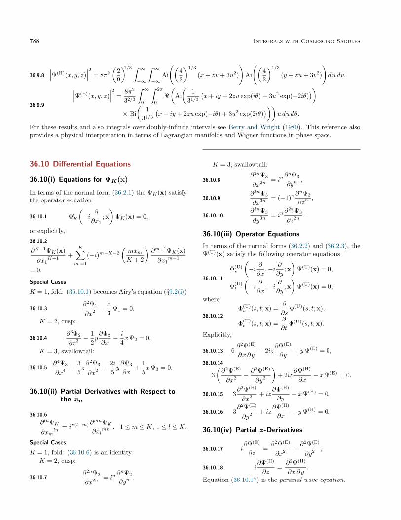
788 Integrals with Coalescing Saddles
36.9.8
∣∣∣Ψ(H)(x, y, z)∣∣∣2 = 8π2
(29
)1/3 ∫ ∞−∞
∫ ∞−∞
Ai
((43
)1/3
(x+ zv + 3u2)
)Ai
((43
)1/3
(y + zu+ 3v2)
)du dv.
36.9.9
∣∣∣Ψ(E)(x, y, z)∣∣∣2 =
8π2
32/3
∫ ∞0
∫ 2π
0
<(
Ai(
131/3
(x+ iy + 2zu exp(iθ) + 3u2 exp(−2iθ)
))× Bi
(1
31/3
(x− iy + 2zu exp(−iθ) + 3u2 exp(2iθ)
)))u du dθ.
For these results and also integrals over doubly-infinite intervals see Berry and Wright (1980). This reference alsoprovides a physical interpretation in terms of Lagrangian manifolds and Wigner functions in phase space.
36.10 Differential Equations
36.10(i) Equations for ΨK(x)
In terms of the normal form (36.2.1) the ΨK(x) satisfythe operator equation
36.10.1 Φ′K
(−i ∂∂x1
; x)
ΨK(x) = 0,
or explicitly,
36.10.2
∂K+1ΨK(x)∂x1
K+1+
K∑m =1
(−i)m−K−2
(mxmK + 2
)∂m−1ΨK(x)∂x1
m−1
= 0.
Special Cases
K = 1, fold: (36.10.1) becomes Airy’s equation (§9.2(i))
36.10.3∂2Ψ1
∂x2 −x
3Ψ1 = 0.
K = 2, cusp:
36.10.4∂3Ψ2
∂x3 −12y∂Ψ2
∂x− i
4xΨ2 = 0.
K = 3, swallowtail:
36.10.5∂4Ψ3
∂x4 −35z∂2Ψ3
∂x2 −2i5y∂Ψ3
∂x+
15xΨ3 = 0.
36.10(ii) Partial Derivatives with Respect tothe xn
36.10.6
∂lnΨK
∂xmln
= in(l−m) ∂mnΨK
∂xlmn , 1 ≤ m ≤ K, 1 ≤ l ≤ K.
Special Cases
K = 1, fold: (36.10.6) is an identity.K = 2, cusp:
36.10.7∂2nΨ2
∂x2n = in∂nΨ2
∂yn.
K = 3, swallowtail:
36.10.8∂2nΨ3
∂x2n = in∂nΨ3
∂yn,
36.10.9∂3nΨ3
∂x3n = (−1)n∂nΨ3
∂zn,
36.10.10∂3nΨ3
∂y3n = in∂2nΨ3
∂z2n .
36.10(iii) Operator Equations
In terms of the normal forms (36.2.2) and (36.2.3), theΨ(U)(x) satisfy the following operator equations
36.10.11
Φ(U)s
(−i ∂∂x,−i ∂
∂y; x)
Ψ(U)(x) = 0,
Φ(U)t
(−i ∂∂x,−i ∂
∂y; x)
Ψ(U)(x) = 0,
where
36.10.12
Φ(U)s (s, t; x) =
∂
∂sΦ(U)(s, t; x),
Φ(U)t (s, t; x) =
∂
∂tΦ(U)(s, t; x).
Explicitly,
36.10.13 6∂2Ψ(E)
∂x ∂y− 2iz
∂Ψ(E)
∂y+ yΨ(E) = 0,
36.10.14
3(∂2Ψ(E)
∂x2 − ∂2Ψ(E)
∂y2
)+ 2iz
∂Ψ(H)
∂x− xΨ(E) = 0.
36.10.15 3∂2Ψ(H)
∂x2 + iz∂Ψ(H)
∂y− xΨ(H) = 0,
36.10.16 3∂2Ψ(H)
∂y2 + iz∂Ψ(H)
∂x− yΨ(H) = 0.
36.10(iv) Partial z-Derivatives
36.10.17 i∂Ψ(E)
∂z=∂2Ψ(E)
∂x2 +∂2Ψ(E)
∂y2 ,
36.10.18 i∂Ψ(H)
∂z=
∂2Ψ(H)
∂x ∂y.
Equation (36.10.17) is the paraxial wave equation.

36.11 Leading-Order Asymptotics 789
36.11 Leading-Order Asymptotics
With real critical points (36.4.1) ordered so that
36.11.1 t1(x) < t2(x) < · · · < tjmax(x),and far from the bifurcation set, the cuspoid canonical integrals are approximated by
36.11.2 ΨK(x) =√
2πjmax(x)∑j=1
exp(i(ΦK(tj(x); x) + 1
4π(−1)j+K+1)) ∣∣∣∣∂2ΦK(tj(x); x)
∂t2
∣∣∣∣−1/2
(1 + o(1)).
Asymptotics along Symmetry Lines
36.11.3 Ψ2(0, y) =
{√π/y
(exp(
14 iπ)
+ o(1)), y → +∞,√
π/|y| exp(− 1
4 iπ) (
1 + i√
2 exp(− 1
4 iy2)
+ o(1)), y → −∞.
36.11.4 Ψ3(x, 0, 0) =√
2π(5|x|3)1/8
{exp(−2√
2(x/5)5/4) (
cos(2√
2(x/5)5/4 − 18π)
+ o(1)), x→ +∞,
cos(4( |x|/5)5/4 − 1
4π)
+ o(1), x→ −∞.
36.11.5 Ψ3(0, y, 0) = Ψ∗3(0,−y, 0) = exp(
14 iπ)√
π/y(
1− (i/√
3) exp(
32 i(2y/5)5/3
)+ o(1)
), y → +∞.
36.11.6 Ψ3(0, 0, z) =Γ(
13
)|z|1/3
√3
+
o(1), z → +∞,2√π51/4
(3|z|)3/4
(cos
(23
(3|z|5
)5/2
− 14π
)+ o(1)
), z → −∞.
36.11.7 Ψ(E)(0, 0, z) =π
z
(i+√
3 exp(
427iz3
)+ o(1)
), z → ±∞,
36.11.8 Ψ(H)(0, 0, z) =2πz
(1− i√
3exp(
127iz3
)+ o(1)
), z → ±∞.
Applications
36.12 Uniform Approximation of Integrals
36.12(i) General Theory for Cuspoids
The canonical integrals (36.2.4) provide a basis for uni-form asymptotic approximations of oscillatory integrals.In the cuspoid case (one integration variable)
36.12.1 I(y, k) =∫ ∞−∞
exp(ikf(u; y))g(u,y) du,
where k is a large real parameter and y = {y1, y2, . . . }is a set of additional (nonasymptotic) parameters. As y
varies as many as K+1 (real or complex) critical pointsof the smooth phase function f can coalesce in clustersof two or more. The function g has a smooth ampli-tude. Also, f is real analytic, and ∂K+2f
/∂uK+2 > 0
for all y such that all K + 1 critical points coincide. If∂K+2f
/∂uK+2 < 0, then we may evaluate the complex
conjugate of I for real values of y and g, and obtain Iby conjugation and analytic continuation. The criticalpoints uj(y), 1 ≤ j ≤ K + 1, are defined by
36.12.2∂
∂uf(uj(y); y) = 0.
The leading-order uniform asymptotic approxima-tion is given by
36.12.3 I(y, k) =exp(ikA(y))k1/(K+2)
K∑m=0
am(y)km/(K+2)
(δm,0 − (1− δm,0) i
∂
∂zm
)ΨK(z(y; k))
(1 +O
(1k
)),

790 Integrals with Coalescing Saddles
where A(y), z(y, k), am(y) are as follows. Define amapping u(t; y) by relating f(u; y) to the normal form(36.2.1) of ΦK(t; x) in the following way:36.12.4 f(u(t,y); y) = A(y) + ΦK(t; x(y)),with the K + 1 functions A(y) and x(y) determined bycorrespondence of the K+1 critical points of f and ΦK .Then36.12.5 f(uj(y); y) = A(y) + ΦK(tj(x(y)); x(y)),where tj(x), 1 ≤ j ≤ K + 1, are the critical points ofΦK , that is, the solutions (real and complex) of (36.4.1).Correspondence between the uj(y) and the tj(x) is es-tablished by the order of critical points along the realaxis when y and x are such that these critical pointsare all real, and by continuation when some or all of thecritical points are complex. The branch for x(y) is suchthat x is real when y is real. In consequence,36.12.6 A(y) = f(u(0,y); y),
36.12.7z(y; k) = {z1(y; k), z2(y; k), . . . , zK(y; k)},zm(y; k) = xm(y)k1−(m/(K+2)),
36.12.8
am(y) =K+1∑n=1
Pmn(y)Gn(y)
(tn(x(y)))m+1K+1∏l=1l 6=n
(tn(x(y))− tl(x(y))),
where
36.12.9
Pmn(y) = (tn(x(y)))K+1
+K∑
l=m+2
l
K + 2xl(y)(tn(x(y)))l−1,
and
36.12.10
Gn(y) = g(tn(y),y)
√∂2ΦK(tn(x(y)); x(y))
/∂t2
∂2f(un(y))/∂u2 .
In (36.12.10), both second derivatives vanish when crit-ical points coalesce, but their ratio remains finite. Thesquare roots are real and positive when y is such that allthe critical points are real, and are defined by analyticcontinuation elsewhere. The quantities am(y) are realfor real y when g is real analytic.
This technique can be applied to generate a hierar-chy of approximations for the diffraction catastrophesΨK(x; k) in (36.2.10) away from x = 0, in terms ofcanonical integrals ΨJ(ξ(x; k)) for J < K. For exam-ple, the diffraction catastrophe Ψ2(x, y; k) defined by(36.2.10), and corresponding to the Pearcey integral(36.2.14), can be approximated by the Airy functionΨ1(ξ(x, y; k)) when k is large, provided that x and yare not small. For details of this example, see Paris(1991).
For further information see Berry and Howls (1993).
36.12(ii) Special Case
For K = 1, with a single parameter y, let the two criti-cal points of f(u; y) be denoted by u±(y), with u+ > u−for those values of y for which these critical points arereal. Then
36.12.11
I(y, k) =∆1/4π
√2
k1/3exp(ikf̃)(( g+√
f ′′++
g−√−f ′′−
)Ai(−k2/3∆
)(1 +O
(1k
))
− i
(g+√f ′′+− g−√
−f ′′−
)Ai′(−k2/3∆
)k1/3∆1/2
(1 +O
(1k
))),
where
36.12.12
f̃ = 12 (f(u+(y), y) + f(u−(y), y)),
g± = g(u±(y), y), f ′′± =∂2
∂u2 f(u±(y), y),
∆ =(
34 (f(u−(y), y)− f(u+(y), y))
)2/3.
For Ai and Ai′ see §9.2. Branches are chosen so that ∆is real and positive if the critical points are real, or realand negative if they are complex. The coefficients of Aiand Ai′ are real if y is real and g is real analytic. Also,∆1/4/
√f ′′+ and ∆1/4/
√−f ′′− are chosen to be positive
real when y is such that both critical points are real,
and by analytic continuation otherwise.
36.12(iii) Additional References
For further information concerning integrals with sev-eral coalescing saddle points see Arnol’d et al. (1988),Berry and Howls (1993, 1994), Bleistein (1967), Duis-termaat (1974), Ludwig (1966), Olde Daalhuis (2000),and Ursell (1972, 1980).
36.13 Kelvin’s Ship-Wave Pattern
A ship moving with constant speed V on deep watergenerates a surface gravity wave. In a reference frame

36.14 Other Physical Applications 791
where the ship is at rest we use polar coordinates r andφ with φ = 0 in the direction of the velocity of the waterrelative to the ship. Then with g denoting the acceler-ation due to gravity, the wave height is approximatelygiven by
36.13.1 z(φ, ρ) =∫ π/2
−π/2cos(ρ
cos(θ + φ)cos2 θ
)dθ,
where
36.13.2 ρ = gr/V 2 .
The integral is of the form of the real part of (36.12.1)with y = φ, u = θ, g = 1, k = ρ, and
36.13.3 f(θ, φ) = −cos(θ + φ)cos2 θ
.
When ρ > 1, that is, everywhere except close tothe ship, the integrand oscillates rapidly. There are twostationary points, given by
36.13.4θ+(φ) = 1
2 (arcsin(3 sinφ)− φ),θ−(φ) = 1
2 (π − φ− arcsin(3 sinφ)).
These coalesce when
36.13.5 |φ| = φc = arcsin(
13
)= 19◦.47122.
This is the angle of the familiar V-shaped wake. Thewake is a caustic of the “rays” defined by the disper-sion relation (“Hamiltonian”) giving the frequency ω asa function of wavevector k:
36.13.6 ω(k) =√gk + V · k.
Here k = |k|, and V is the ship velocity (so thatV = |V|).
The disturbance z(ρ, φ) can be approximated by themethod of uniform asymptotic approximation for thecase of two coalescing stationary points (36.12.11), us-ing the fact that θ±(φ) are real for |φ| < φc and complexfor |φ| > φc. (See also §2.4(v).) Then with the defini-tions (36.12.12), and the real functions
36.13.7
u(φ) =
√∆1/2(φ)
2
(1√f ′′+(φ)
+1√−f ′′−(φ)
),
v(φ) =
√1
2∆1/2(φ)
(1√f ′′+(φ)
− 1√−f ′′−(φ)
),
the disturbance is
36.13.8
z(ρ, φ) = 2π(ρ−1/3u(φ) cos
(ρf̃(φ)
)Ai(−ρ2/3∆(φ)
)× (1 +O(1/ρ))
+ ρ−2/3v(φ) sin(ρf̃(φ)
)Ai′(−ρ2/3∆(φ)
)× (1 +O(1/ρ))
), ρ→∞.
See Figure 36.13.1.
Figure 36.13.1: Kelvin’s ship wave pattern, computedfrom the uniform asymptotic approximation (36.13.8),as a function of x = ρ cosφ, y = ρ sinφ.
For further information see Lord Kelvin (1891, 1905)and Ursell (1960, 1994).
36.14 Other Physical Applications
36.14(i) Caustics
The physical manifestations of bifurcation sets are caus-tics. These are the structurally stable focal singularities(envelopes) of families of rays, on which the intensi-ties of the geometrical (ray) theory diverge. Diffractioncatastrophes describe the (linear) wave amplitudes thatsmooth the geometrical caustic singularities and deco-rate them with interference patterns. See Berry (1969,1976, 1980, 1981), Kravtsov (1964, 1988), and Ludwig(1966).
36.14(ii) Optics
Diffraction catastrophes describe the connection be-tween ray optics and wave optics. Applications includetwinkling starlight, focusing of sunlight by rippling wa-ter (e.g., swimming-pool patterns), and water-droplet“lenses” (e.g., rainbows). See Adler et al. (1997), Berryand Upstill (1980), Marston (1992, 1999), Nye (1999),Walker (1983, 1988, 1989).
36.14(iii) Quantum Mechanics
Diffraction catastrophes describe the “semiclassical”connections between classical orbits and quantum wave-functions, for integrable (non-chaotic) systems. Appli-cations include scattering of elementary particles, atoms

792 Integrals with Coalescing Saddles
and molecules from particles and surfaces, and chemi-cal reactions. See Berry (1966, 1975), Connor (1974,1976), Connor and Farrelly (1981), Trinkaus and Drep-per (1977), and Uzer et al. (1983).
36.14(iv) Acoustics
Applications include the reflection of ultrasound pulses,and acoustical waveguides. See Chapman (1999),Frederickson and Marston (1992, 1994), and Kravtsov(1968).
Computation
36.15 Methods of Computation
36.15(i) Convergent Series
Close to the origin x = 0 of parameter space, the seriesin §36.8 can be used.
36.15(ii) Asymptotics
Far from the bifurcation set, the leading-order asymp-totic formulas of §36.11 reproduce accurately the formof the function, including the geometry of the zeros de-scribed in §36.7. Close to the bifurcation set but farfrom x = 0, the uniform asymptotic approximations of§36.12 can be used.
36.15(iii) Integration along Deformed Contour
Direct numerical evaluation can be carried out alonga contour that runs along the segment of the real t-axis containing all real critical points of Φ and is de-formed outside this range so as to reach infinity alongthe asymptotic valleys of exp(iΦ). (For the umbilics,representations as one-dimensional integrals (§36.2) areused.) For details, see Connor and Curtis (1982) andKirk et al. (2000). There is considerable freedom in thechoice of deformations.
36.15(iv) Integration along Finite Contour
This can be carried out by direct numerical evaluationof canonical integrals along a finite segment of the realaxis including all real critical points of Φ, with contribu-tions from the contour outside this range approximatedby the first terms of an asymptotic series associated withthe endpoints. See Berry et al. (1979).
36.15(v) Differential Equations
For numerical solution of partial differential equationssatisfied by the canonical integrals see Connor et al.(1983).
References
General References
There is no single source covering the material in thischapter. An overview of some of the mathematical anal-ysis is given in Arnol’d (1975, 1986). Many physical ap-plications can be found in Poston and Stewart (1978).For applications to wave physics, especially optics, seeBerry and Upstill (1980).
Sources
The following list gives the references or other indica-tions of proofs that were used in constructing the varioussections of this chapter. These sources supplement thereferences that are quoted in the text.
§36.2 The convergence of the oscillatory integrals(36.2.4)–(36.2.11) can be confirmed by rotatingthe integration paths in the complex plane. For(36.2.6) see Berry et al. (1979). For (36.2.7)shift the s variable in (36.2.5) (with (36.2.2)) toremove the quadratic term, integrate, and thendeform the contour of the remaining t integra-tion. For (36.2.8) see Berry and Howls (1990).For (36.2.9) integrate (36.2.5) (with (36.2.3)) withrespect to t. For (36.2.12) and (36.2.13) use(4.10.11) and (9.5.4), respectively. For (36.2.15)and (36.2.17) use (5.9.1). For (36.2.18) combine(36.2.6), (36.2.8), and (5.9.1) For (36.2.19) use(12.5.1) and (12.14.13). For (36.2.20) see Trinkausand Drepper (1977). For (36.2.21) use (36.2.9).Eqs. (36.2.22)–(36.2.27) follow from the defini-tions given in §36.2(i).
§§36.3, 36.4 The graphics were generated by the au-thors.
§36.5 Wright (1980) and Berry and Howls (1990). Thecommon strategy employed in deriving the for-mulas in this section involves using the critical-point condition (36.4.1) to reduce the order of thecatastrophe polynomials in (36.2.1), then solving(36.5.1) for the imaginary part of the complex crit-ical point in terms of the value of the real criti-cal point, which is itself determined by (36.4.1)and then used to generate the Stokes sets para-metrically. For (36.5.11)–(36.5.21) we also usethe exponents in the representations (36.2.6) and(36.2.8). The graphics were generated by the au-thors. For Figures 36.5.2–36.5.6, Eqs. (36.5.11)–(36.5.21) were used in parametric form x = x(y),and checked against the numerical computations
References 793
in Berry and Howls (1990) (which were based di-rectly on the definitions given in §36.5(i)).
§36.7 Berry et al. (1979). (36.7.2) and (36.7.3) maybe derived by setting to zero the stationary-phaseapproximation (§2.3(iv)) of the Pearcey integralΨ2(x, y) just outside the caustic; this involves onereal saddle and one complex saddle. Table 36.7.1was computed by the authors.
§36.8 Connor (1973) and Connor et al. (1983). For(36.8.1), in the integral (36.2.4) retain the high-est power of t in (36.2.1) in the exponent, expandthe rest of the exponential as a power series int, and evaluate the resulting integrals in termsof gamma functions. For (36.8.3), in the integral(36.2.5) with the polynomial (36.2.3) expand thez-dependent part of the exponential in powers of z,and then repeatedly use the differential equation(9.2.1) to express higher derivatives of the Airyfunction in terms of Ai and Ai′. For (36.8.4), in
the integral (36.2.5) with the polynomial (36.2.2)expand the z-dependent part of the exponential inpowers of z, and then repeatedly use (9.2.1), and(36.2.20).
§36.10 For (36.10.1) to (36.10.10) see Connor et al.(1983). (36.10.11) to (36.10.18) are derived byrepeated differentiations with respect to x, y, orz, in combinations that generate exact derivativesof the exponents in (36.2.5).
§36.11 The formulas in this section are derived by themethod of stationary phase, applied to the realcritical points of the integral representations in§36.2. See §2.3(iv) and also Berry and Howls(1991). For (36.11.4) the integral is exponentiallysmall when x > 0 and the dominant contributionis from a critical point off the real axis.
§36.12 Berry and Howls (1993).
§36.13 The figure was generated by the authors.


Bibliography
A. S. Abdullaev (1985). Asymptotics of solutions of the gen-eralized sine-Gordon equation, the third Painlevé equa-tion and the d’Alembert equation. Dokl. Akad. NaukSSSR 280(2), pp. 265–268. English translation: SovietMath. Dokl. 31(1985), no. 1, pp. 45–47.
M. J. Ablowitz and P. A. Clarkson (1991). Solitons, Nonlin-ear Evolution Equations and Inverse Scattering, Volume149 of London Mathematical Society Lecture Note Series.Cambridge: Cambridge University Press.
M. J. Ablowitz and H. Segur (1977). Exact linearizationof a Painlevé transcendent. Phys. Rev. Lett. 38(20), pp.1103–1106.
M. J. Ablowitz and H. Segur (1981). Solitons and the In-verse Scattering Transform, Volume 4 of SIAM Studies inApplied Mathematics. Philadelphia, PA: Society for In-dustrial and Applied Mathematics (SIAM).
A. Abramov (1960). Tables of ln Γ(z) for Complex Argu-ment. New York: Pergamon Press.
M. Abramowitz (1949). Asymptotic expansions of spheroidalwave functions. J. Math. Phys. Mass. Inst. Tech. 28, pp.195–199.
M. Abramowitz (1954). Regular and irregular Coulomb wavefunctions expressed in terms of Bessel-Clifford functions.J. Math. Physics 33, pp. 111–116.
M. Abramowitz and P. Rabinowitz (1954). Evaluation ofCoulomb wave functions along the transition line. Physi-cal Rev. (2) 96, pp. 77–79.
M. Abramowitz and I. A. Stegun (Eds.) (1964). Handbookof Mathematical Functions with Formulas, Graphs, andMathematical Tables. Number 55 in National Bureau ofStandards Applied Mathematics Series. U.S. GovernmentPrinting Office, Washington, D.C. Corrections appearedin later printings up to the 10th Printing, December, 1972.Reproductions by other publishers, in whole or in part,have been available since 1965.
J.-J. Achenbach (1986). Numerik: Implementierungvon Zylinderfunktionen. Elektrotechnik. Braunschweig-Wiesbaden: Friedr. Vieweg & Sohn.
F. S. Acton (1974). Recurrence relations for the Fres-
nel integralR∞0
exp(−ct) dt√t(1+t2)
and similar integrals. Comm.
ACM 17(8), pp. 480–481.
V. S. Adamchik (1998). Polygamma functions of negativeorder. J. Comput. Appl. Math. 100(2), pp. 191–199.
V. S. Adamchik and H. M. Srivastava (1998). Some series ofthe zeta and related functions. Analysis (Munich) 18(2),pp. 131–144.
A. Adelberg (1992). On the degrees of irreducible factorsof higher order Bernoulli polynomials. Acta Arith. 62(4),pp. 329–342.
A. Adelberg (1996). Congruences of p-adic integer orderBernoulli numbers. J. Number Theory 59(2), pp. 374–388.
C. Adiga, B. C. Berndt, S. Bhargava, and G. N. Wat-son (1985). Chapter 16 of Ramanujan’s second note-book: Theta-functions and q-series. Mem. Amer. Math.Soc. 53(315), pp. v+85.
C. L. Adler, J. A. Lock, B. R. Stone, and C. J. Garcia (1997).High-order interior caustics produced in scattering of a di-agonally incident plane wave by a circular cylinder. J.Opt. Soc. Amer. A 14(6), pp. 1305–1315.
V. È. Adler (1994). Nonlinear chains and Painlevé equa-tions. Phys. D 73(4), pp. 335–351.
P. Adrian (1959). Die Bezeichnungsweise der BernoullischenZahlen. Mitt. Verein. Schweiz. Versicherungsmath. 59, pp.199–206.
M. M. Agrest, S. I. Labakhua, M. M. Rikenglaz, and T. S.Chachibaya (1982). Tablitsy funktsii Struve i integralovot nikh. Moscow: “Nauka”. Translated title: Tables ofStruve Functions and their Integrals.
M. M. Agrest and M. S. Maksimov (1971). Theory of In-complete Cylindrical Functions and Their Applications.Berlin: Springer-Verlag. Translated from the Russian byH. E. Fettis, J. W. Goresh and D. A. Lee, Die Grundlehrender mathematischen Wissenschaften, Band 160.
L. V. Ahlfors (1966). Complex Analysis: An Introduction ofthe Theory of Analytic Functions of One Complex Vari-able (2nd ed.). New York: McGraw-Hill Book Co. Athird edition was published in 1978 by McGraw-Hill, NewYork.
A. R. Ahmadi and S. E. Widnall (1985). Unsteady lifting-line theory as a singular-perturbation problem. J. FluidMech 153, pp. 59–81.
S. Ahmed and M. E. Muldoon (1980). On the zeros ofconfluent hypergeometric functions. III. Characterizationby means of nonlinear equations. Lett. Nuovo Cimento(2) 29(11), pp. 353–358.
795

796 Bibliography
S.-H. Ahn, H.-W. Lee, and H. M. Lee (2001). Lyα line forma-tion in starbursting galaxies. I. Moderately thick, dustless,and static H i media. Astrophysical J. 554, pp. 604–614.
H. Airault (1979). Rational solutions of Painlevé equations.Stud. Appl. Math. 61(1), pp. 31–53.
H. Airault, H. P. McKean, and J. Moser (1977). Ratio-nal and elliptic solutions of the Korteweg-de Vries equa-tion and a related many-body problem. Comm. Pure Appl.Math. 30(1), pp. 95–148.
G. B. Airy (1838). On the intensity of light in the neighbour-hood of a caustic. Trans. Camb. Phil. Soc. 6, pp. 379–402.
G. B. Airy (1849). Supplement to a paper “On the intensityof light in the neighbourhood of a caustic”. Trans. Camb.Phil. Soc. 8, pp. 595–599.
N. I. Akhiezer (1988). Lectures on Integral Transforms,Volume 70 of Translations of Mathematical Monographs.Providence, RI: American Mathematical Society. Trans-lated from the Russian by H. H. McFaden.
N. I. Akhiezer (1990). Elements of the Theory of Ellip-tic Functions, Volume 79 of Translations of MathematicalMonographs. Providence, RI: American Mathematical So-ciety. Translated from the second Russian edition by H.H. McFaden.
A. M. Al-Rashed and N. Zaheer (1985). Zeros of Stieltjesand Van Vleck polynomials and applications. J. Math.Anal. Appl. 110(2), pp. 327–339.
W. A. Al-Salam and L. Carlitz (1959). Some determinants ofBernoulli, Euler and related numbers. Portugal. Math. 18,pp. 91–99.
W. A. Al-Salam and L. Carlitz (1965). Some orthogonalq-polynomials. Math. Nachr. 30, pp. 47–61.
W. A. Al-Salam and M. E. H. Ismail (1994). A q-beta in-tegral on the unit circle and some biorthogonal rationalfunctions. Proc. Amer. Math. Soc. 121(2), pp. 553–561.
M. Alam (1979). Zeros of Stieltjes and Van Vleck polynomi-als. Trans. Amer. Math. Soc. 252, pp. 197–204.
D. W. Albrecht, E. L. Mansfield, and A. E. Milne (1996). Al-gorithms for special integrals of ordinary differential equa-tions. J. Phys. A 29(5), pp. 973–991.
J. R. Albright (1977). Integrals of products of Airy functions.J. Phys. A 10(4), pp. 485–490.
J. R. Albright and E. P. Gavathas (1986). Integrals involvingAiry functions. J. Phys. A 19(13), pp. 2663–2665.
K. Alder, A. Bohr, T. Huus, B. Mottelson, and A. Winther(1956). Study of nuclear structure by electromagnetic ex-citation with accelerated ions. Rev. Mod. Phys. 28, pp.432–542.
G. Alefeld and J. Herzberger (1983). Introduction to IntervalComputations. Computer Science and Applied Mathemat-ics. New York: Academic Press Inc. Translated from theGerman by Jon Rokne.
W. R. Alford, A. Granville, and C. Pomerance (1994). Thereare infinitely many Carmichael numbers. Ann. of Math.(2) 139(3), pp. 703–722.
F. Alhargan and S. Judah (1992). Frequency response char-acteristics of the multiport planar elliptic patch. IEEETrans. Microwave Theory Tech. 40(8), pp. 1726–1730.
F. Alhargan and S. Judah (1995). A general mode theory forthe elliptic disk microstrip antenna. IEEE Trans. Anten-nas and Propagation 43(6), pp. 560–568.
G. Allasia and R. Besenghi (1987a). Numerical calculation ofincomplete gamma functions by the trapezoidal rule. Nu-mer. Math. 50(4), pp. 419–428.
G. Allasia and R. Besenghi (1987b). Numerical computationof Tricomi’s psi function by the trapezoidal rule. Comput-ing 39(3), pp. 271–279.
G. Allasia and R. Besenghi (1989). Numerical Calculation ofthe Riemann Zeta Function and Generalizations by Meansof the Trapezoidal Rule. In C. Brezinski (Ed.), Numeri-cal and Applied Mathematics, Part II (Paris, 1988), Vol-ume 1 of IMACS Ann. Comput. Appl. Math., pp. 467–472.Basel: Baltzer.
G. Allasia and R. Besenghi (1991). Numerical evaluation ofthe Kummer function with complex argument by the trape-zoidal rule. Rend. Sem. Mat. Univ. Politec. Torino 49(3),pp. 315–327.
G. Almkvist and B. Berndt (1988). Gauss, Landen, Ra-manujan, the arithmetic-geometric mean, ellipses, π, andthe Ladies Diary. Amer. Math. Monthly 95(7), pp. 585–608.
Z. Altaç (1996). Integrals involving Bickley and Bessel func-tions in radiative transfer, and generalized exponential in-tegral functions. J. Heat Transfer 118(3), pp. 789–792.
H. H. Aly, H. J. W. Müller-Kirsten, and N. Vahedi-Faridi(1975). Scattering by singular potentials with a perturba-tion – Theoretical introduction to Mathieu functions. J.Mathematical Phys. 16, pp. 961–970. Erratum: samejournal 17 (1975), no. 7, p. 1361.
H. Alzer (1997a). A harmonic mean inequality for thegamma function. J. Comput. Appl. Math. 87(2), pp. 195–198. For corrigendum see same journal v. 90 (1998), no.2, p. 265.
H. Alzer (1997b). On some inequalities for the incompletegamma function. Math. Comp. 66(218), pp. 771–778.
H. Alzer (2000). Sharp bounds for the Bernoulli numbers.Arch. Math. (Basel) 74(3), pp. 207–211.

Bibliography 797
H. Alzer and S.-L. Qiu (2004). Monotonicity theorems andinequalities for the complete elliptic integrals. J. Comput.Appl. Math. 172(2), pp. 289–312.
D. E. Amos (1974). Computation of modified Bessel func-tions and their ratios. Math. Comp. 28(125), pp. 239–251.
D. E. Amos (1980). Computation of exponential integrals.ACM Trans. Math. Software 6(3), pp. 365–377.
D. E. Amos (1983). Uniform asymptotic expansions for ex-ponential integrals En(x) and Bickley functions Kin(x).ACM Trans. Math. Software 9(4), pp. 467–479.
D. E. Amos (1985). A subroutine package for Bessel func-tions of a complex argument and nonnegative order. Tech-nical Report SAND85-1018, Sandia National Laborato-ries, Albuquerque, NM.
D. E. Amos (1989). Repeated integrals and derivatives of KBessel functions. SIAM J. Math. Anal. 20(1), pp. 169–175.
G. D. Anderson, S.-L. Qiu, M. K. Vamanamurthy, andM. Vuorinen (2000). Generalized elliptic integrals andmodular equations. Pacific J. Math. 192(1), pp. 1–37.
G. D. Anderson and M. K. Vamanamurthy (1985). Inequal-ities for elliptic integrals. Publ. Inst. Math. (Beograd)(N.S.) 37(51), pp. 61–63.
G. D. Anderson, M. K. Vamanamurthy, and M. Vuorinen(1990). Functional inequalities for complete elliptic inte-grals and their ratios. SIAM J. Math. Anal. 21(2), pp.536–549.
G. D. Anderson, M. K. Vamanamurthy, and M. Vuorinen(1992a). Functional inequalities for hypergeometric func-tions and complete elliptic integrals. SIAM J. Math.Anal. 23(2), pp. 512–524.
G. D. Anderson, M. K. Vamanamurthy, and M. Vuorinen(1992b). Hypergeometric Functions and Elliptic Integrals.In H. M. Srivastava and S. Owa (Eds.), Current Topicsin Analytic Function Theory, pp. 48–85. River Edge, NJ:World Sci. Publishing.
G. D. Anderson, M. K. Vamanamurthy, and M. K. Vuorinen(1997). Conformal Invariants, Inequalities, and Quasicon-formal Maps. New York: John Wiley & Sons Inc. WithPC diskette, a Wiley-Interscience Publication.
F. V. Andreev and A. V. Kitaev (2002). TransformationsRS2
4(3) of the ranks ≤ 4 and algebraic solutions of thesixth Painlevé equation. Comm. Math. Phys. 228(1), pp.151–176.
G. E. Andrews (1966a). On basic hypergeometric series,mock theta functions, and partitions. II. Quart. J. Math.Oxford Ser. (2) 17, pp. 132–143.
G. E. Andrews (1966b). q-identities of Auluck, Carlitz, andRogers. Duke Math. J. 33(3), pp. 575–581.
G. E. Andrews (1972). Summations and transformationsfor basic Appell series. J. London Math. Soc. (2) 4, pp.618–622.
G. E. Andrews (1974). Applications of basic hypergeometricfunctions. SIAM Rev. 16(4), pp. 441–484.
G. E. Andrews (1976). The Theory of Partitions, Vol-ume 2 of Encyclopedia of Mathematics and its Appli-cations. Reading, MA-London-Amsterdam: Addison-Wesley Publishing Co. Reprinted by Cambridge Univer-sity Press, Cambridge, 1998.
G. E. Andrews (1979). Plane partitions. III. The weak Mac-donald conjecture. Invent. Math. 53(3), pp. 193–225.
G. E. Andrews (1984). Multiple series Rogers-Ramanujantype identities. Pacific J. Math. 114(2), pp. 267–283.
G. E. Andrews (1986). q-Series: Their Development andApplication in Analysis, Number Theory, Combinatorics,Physics, and Computer Algebra, Volume 66 of CBMS Re-gional Conference Series in Mathematics. Providence, RI:Amer. Math. Soc.
G. E. Andrews (1996). Pfaff’s method II: Diverse applica-tions. J. Comput. Appl. Math. 68(1-2), pp. 15–23.
G. E. Andrews (2000). Umbral calculus, Bailey chains, andpentagonal number theorems. J. Combin. Theory Ser.A 91(1-2), pp. 464–475. In memory of Gian-Carlo Rota.
G. E. Andrews (2001). Bailey’s Transform, Lemma, Chainsand Tree. In J. Bustoz, M. E. H. Ismail, and S. K. Suslov(Eds.), Special Functions 2000: Current Perspective andFuture Directions (Tempe, AZ), Volume 30 of NATO Sci.Ser. II Math. Phys. Chem., pp. 1–22. Dordrecht: KluwerAcad. Publ.
G. E. Andrews, R. Askey, and R. Roy (1999). Special Func-tions, Volume 71 of Encyclopedia of Mathematics and itsApplications. Cambridge: Cambridge University Press.
G. E. Andrews, R. A. Askey, B. C. Berndt, and R. A. Rankin(Eds.) (1988). Ramanujan Revisited, Boston, MA. Aca-demic Press Inc.
G. E. Andrews and A. Berkovich (1998). A trinomial ana-logue of Bailey’s lemma and N = 2 superconformal in-variance. Comm. Math. Phys. 192(2), pp. 245–260.
G. E. Andrews and D. Foata (1980). Congruences for the q-secant numbers. European J. Combin. 1(4), pp. 283–287.
G. E. Andrews, I. P. Goulden, and D. M. Jackson (1986).Shanks’ convergence acceleration transform, Padé approx-imants and partitions. J. Combin. Theory Ser. A 43(1),pp. 70–84.
H. M. Antia (1993). Rational function approximations forFermi-Dirac integrals. The Astrophysical Journal Supple-ment Series 84, pp. 101–108. Double-precision Fortran,maximum precision 8D.

798 Bibliography
M. A. Anuta, D. W. Lozier, and P. R. Turner (1996). TheMasPar MP-1 as a computer arithmetic laboratory. J.Res. Nat. Inst. Stand. Technol. 101(2), pp. 165–174.
K. Aomoto (1987). Special value of the hypergeometric func-tion 3F2 and connection formulae among asymptotic ex-pansions. J. Indian Math. Soc. (N.S.) 51, pp. 161–221.
A. Apelblat (1983). Table of Definite and Infinite Integrals,Volume 13 of Physical Sciences Data. Amsterdam: Else-vier Scientific Publishing Co. Table errata: Math. Comp.v. 65 (1996), no. 215, p. 1386.
A. Apelblat (1989). Derivatives and integrals with respectto the order of the Struve functions Hν(x) and Lν(x). J.Math. Anal. Appl. 137(1), pp. 17–36.
A. Apelblat (1991). Integral representation of Kelvin func-tions and their derivatives with respect to the order. Z.Angew. Math. Phys. 42(5), pp. 708–714.
T. M. Apostol (1952). Theorems on generalized Dedekindsums. Pacific J. Math. 2(1), pp. 1–9.
T. M. Apostol (1976). Introduction to Analytic Number The-ory. New York: Springer-Verlag. Undergraduate Texts inMathematics.
T. M. Apostol (1983). A proof that Euler missed: Evaluatingζ(2) the easy way. Math. Intelligencer 5(3), pp. 59–60.
T. M. Apostol (1985a). Formulas for higher derivatives ofthe Riemann zeta function. Math. Comp. 44(169), pp.223–232.
T. M. Apostol (1985b). Note on the trivial zeros of DirichletL-functions. Proc. Amer. Math. Soc. 94(1), pp. 29–30.
T. M. Apostol (1990). Modular Functions and Dirichlet Se-ries in Number Theory (2nd ed.), Volume 41 of GraduateTexts in Mathematics. New York: Springer-Verlag.
T. M. Apostol (2000). A Centennial History of the PrimeNumber Theorem. In Number Theory, Trends Math., pp.1–14. Basel: Birkhäuser.
T. M. Apostol (2006). Bernoulli’s power-sum formulas re-visited. Math. Gaz. 90(518), pp. 276–279.
T. M. Apostol (2008). A primer on Bernoulli numbers andpolynomials. Math. Mag. 81(3), pp. 178–190.
T. M. Apostol and I. Niven (1994). Number Theory. In TheNew Encyclopaedia Britannica (15th ed.), Volume 25, pp.14–37.
T. M. Apostol and T. H. Vu (1984). Dirichlet series relatedto the Riemann zeta function. J. Number Theory 19(1),pp. 85–102.
T. M. Apostol and H. S. Zuckerman (1951). On magicsquares constructed by the uniform step method. Proc.Amer. Math. Soc. 2(4), pp. 557–565.
H. Appel (1968). Numerical Tables for Angular Correla-tion Computations in α-, β- and γ-Spectroscopy: 3j-, 6j-, 9j-Symbols, F- and Γ-Coefficients. Landolt-BörnsteinNumerical Data and Functional Relationships in Scienceand Technology. Springer-Verlag.
G. B. Arfken and H. J. Weber (2005). Mathematical Methodsfor Physicists (6th ed.). Oxford: Elsevier.
J. V. Armitage (1989). The Riemann Hypothesis and theHamiltonian of a Quantum Mechanical System. In M. M.Dodson and J. A. G. Vickers (Eds.), Number Theory andDynamical Systems (York, 1987), Volume 134 of LondonMath. Soc. Lecture Note Ser., pp. 153–172. Cambridge:Cambridge University Press.
B. H. Armstrong (1967). Spectrum line profiles: The Voigtfunction. J. Quant. Spectrosc. Radiat. Transfer 7, pp.61–88.
V. I. Arnol’d (1972). Normal forms of functions near degen-erate critical points, the Weyl groups Ak, Dk, Ek and La-grangian singularities. Funkcional. Anal. i Priložen. 6(4),pp. 3–25. In Russian. English translation: FunctionalAnal. Appl., 6(1973), pp. 254–272.
V. I. Arnol’d (1974). Normal forms of functions in theneighborhood of degenerate critical points. Uspehi Mat.Nauk 29(2(176)), pp. 11–49. Collection of articles dedi-cated to the memory of Ivan Georgievič Petrovskĭı (1901–1973), I. In Russian. English translation: Russian Math.Surveys, 29(1974), no. 2, pp. 10–50.
V. I. Arnol’d (1975). Critical points of smooth functions,and their normal forms. Uspehi Mat. Nauk 30(5(185)),pp. 3–65. In Russian. English translation: Russian Math.Surveys, 30(1975), no. 5, pp. 1–75.
V. I. Arnol’d (1986). Catastrophe Theory (2nd ed.). Berlin:Springer-Verlag. Translated from the Russian by G. S.Wassermann, based on a translation by R. K. Thomas.See also Arnol’d (1992).
V. I. Arnol’d (1992). Catastrophe Theory (3rd ed.). Berlin:Springer-Verlag. Translated from the Russian by G. S.Wassermann, Based on a translation by R. K. Thomas.
V. I. Arnol′d (1997). Mathematical Methods of Classical Me-chanics, Volume 60 of Graduate Texts in Mathematics.New York: Springer-Verlag. Translated from the 1974Russian original by K. Vogtmann and A. Weinstein, Cor-rected reprint of the second (1989) edition.
V. I. Arnol’d, S. M. Gusĕın-Zade, and A. N. Varchenko(1988). Singularities of Differentiable Maps. Vol. II.Boston-Berlin: Birkhäuser. Monodromy and asymptoticsof integrals, Translated from the Russian by Hugh Porte-ous, Translation revised by the authors and James Mon-taldi.
F. M. Arscott (1956). Perturbation solutions of the ellip-soidal wave equation. Quart. J. Math. Oxford Ser. (2) 7,pp. 161–174.

Bibliography 799
F. M. Arscott (1959). A new treatment of the ellipsoidal waveequation. Proc. London Math. Soc. (3) 9, pp. 21–50.
F. M. Arscott (1964a). Integral equations and relations forLamé functions. Quart. J. Math. Oxford Ser. (2) 15, pp.103–115.
F. M. Arscott (1964b). Periodic Differential Equations. AnIntroduction to Mathieu, Lamé, and Allied Functions. In-ternational Series of Monographs in Pure and AppliedMathematics, Vol. 66. New York: Pergamon Press, TheMacmillan Co.
F. M. Arscott (1967). The Whittaker-Hill equation and thewave equation in paraboloidal co-ordinates. Proc. Roy.Soc. Edinburgh Sect. A 67, pp. 265–276.
F. M. Arscott and I. M. Khabaza (1962). Tables of LaméPolynomials. New York: Pergamon Press, The MacmillanCo.
G. Arutyunov and M. Staudacher (2004). Matching higherconserved charges for strings and spins. J. High EnergyPhys. (electronic only, article id. JHEP03(2004)004, 32pp.).
U. M. Ascher, R. M. M. Mattheij, and R. D. Russell (1995).Numerical Solution of Boundary Value Problems for Or-dinary Differential Equations, Volume 13 of Classics inApplied Mathematics. Philadelphia, PA: Society for Indus-trial and Applied Mathematics (SIAM). Corrected reprintof the 1988 original.
U. M. Ascher and L. R. Petzold (1998). Computer Meth-ods for Ordinary Differential Equations and Differential-Algebraic Equations. Philadelphia, PA: Society for Indus-trial and Applied Mathematics (SIAM).
R. Askey (1974). Jacobi polynomials. I. New proofs of Koorn-winder’s Laplace type integral representation and Bate-man’s bilinear sum. SIAM J. Math. Anal. 5, pp. 119–124.
R. Askey (1975). Orthogonal Polynomials and Special Func-tions, Volume 21 of CBMS-NSF Regional Conference Se-ries in Applied Mathematics. Philadelphia, PA: Societyfor Industrial and Applied Mathematics.
R. Askey (1980). Some basic hypergeometric extensionsof integrals of Selberg and Andrews. SIAM J. Math.Anal. 11(6), pp. 938–951.
R. Askey (1982). Commentary on the Paper “Beiträge zurTheorie der Toeplitzschen Form”. In Gábor Szegő, Col-lected Papers. Vol. 1, Contemporary Mathematicians, pp.303–305. MA: Birkhäuser Boston.
R. Askey (1985). Continuous Hahn polynomials. J. Phys.A 18(16), pp. L1017–L1019.
R. Askey (1989). Continuous q-Hermite Polynomials whenq > 1. In q-series and Partitions (Minneapolis, MN,1988), Volume 18 of IMA Vol. Math. Appl., pp. 151–158.New York: Springer.
R. Askey (1990). Graphs as an Aid to Understanding SpecialFunctions. In R. Wong (Ed.), Asymptotic and Computa-tional Analysis, Volume 124 of Lecture Notes in Pure andAppl. Math., pp. 3–33. New York: Dekker.
R. Askey and J. Fitch (1969). Integral representations forJacobi polynomials and some applications. J. Math. Anal.Appl. 26(2), pp. 411–437.
R. Askey and G. Gasper (1976). Positive Jacobi polynomialsums. II. Amer. J. Math. 98(3), pp. 709–737.
R. Askey and M. E. H. Ismail (1984). Recurrence relations,continued fractions, and orthogonal polynomials. Mem.Amer. Math. Soc. 49(300), pp. iv+108.
R. Askey, T. H. Koornwinder, and M. Rahman (1986). Anintegral of products of ultraspherical functions and a q-extension. J. London Math. Soc. (2) 33(1), pp. 133–148.
R. Askey and B. Razban (1972). An integral for Jacobi poly-nomials. Simon Stevin 46, pp. 165–169.
R. Askey and J. Wilson (1985). Some basic hypergeometricorthogonal polynomials that generalize Jacobi polynomials.Mem. Amer. Math. Soc. 54(319), pp. iv+55.
D. Atkinson and P. W. Johnson (1988). Chiral-symmetrybreaking in QCD. I. The infrared domain. Phys. Rev. D(3) 37(8), pp. 2290–2295.
K. E. Atkinson (1989). An Introduction to Numerical Anal-ysis (2nd ed.). New York: John Wiley & Sons Inc.
M. Audin (1999). Spinning Tops: A Course on IntegrableSystems, Volume 51 of Cambridge Studies in AdvancedMathematics. Cambridge: Cambridge University Press.
M. Aymar, C. H. Greene, and E. Luc-Koenig (1996). Multi-channel Rydberg spectroscopy of complex atoms. Reviewsof Modern Physics 68, pp. 1015–1123.
A. W. Babister (1967). Transcendental Functions Satisfy-ing Nonhomogeneous Linear Differential Equations. NewYork: The Macmillan Co.
L. V. Babushkina, M. K. Kerimov, and A. I. Nikitin (1997).New tables of Bessel functions of complex argument. Com-put. Math. Math. Phys. 37(12), pp. 1480–1482. Russianoriginal in Zh. Vychisl. Mat. i Mat. Fiz. 37(1997), no. 12,1526–1528.
G. Backenstoss (1970). Pionic atoms. Annual Review ofNuclear and Particle Science 20, pp. 467–508.
J. Baik, P. Deift, and K. Johansson (1999). On the distri-bution of the length of the longest increasing subsequenceof random permutations. J. Amer. Math. Soc. 12(4), pp.1119–1178.
W. N. Bailey (1928). Products of generalized hypergeometricseries. Proc. London Math. Soc. (2) 28(2), pp. 242–254.

800 Bibliography
W. N. Bailey (1929). Transformations of generalized hyper-geometric series. Proc. London Math. Soc. (2) 29(2), pp.495–502.
W. N. Bailey (1935). Generalized Hypergeometric Series.Cambridge: Cambridge University Press. Reissued byHafner, New York, 1972.
W. N. Bailey (1964). Generalized Hypergeometric Series.New York: Stechert-Hafner, Inc.
G. A. Baker, Jr. and P. Graves-Morris (1996). Padé Approxi-mants (2nd ed.), Volume 59 of Encyclopedia of Mathemat-ics and its Applications. Cambridge: Cambridge Univer-sity Press.
H. F. Baker (1995). Abelian Functions: Abel’s Theorem andthe Allied Theory of Theta Functions. Cambridge: Cam-bridge University Press. Reprint of the 1897 original, witha foreword by Igor Krichever.
P. Baldwin (1985). Zeros of generalized Airy functions.Mathematika 32(1), pp. 104–117.
P. Baldwin (1991). Coefficient functions for an inhomo-geneous turning-point problem. Mathematika 38(2), pp.217–238.
J. S. Ball (2000). Automatic computation of zeros of Besselfunctions and other special functions. SIAM J. Sci. Com-put. 21(4), pp. 1458–1464.
L. E. Ballentine and S. M. McRae (1998). Moment equationsfor probability distributions in classical and quantum me-chanics. Phys. Rev. A 58(3), pp. 1799–1809.
C. B. Balogh (1967). Asymptotic expansions of the modi-fied Bessel function of the third kind of imaginary order.SIAM J. Appl. Math. 15, pp. 1315–1323.
E. Bannai (1990). Orthogonal Polynomials in Coding The-ory and Algebraic Combinatorics. In Orthogonal Polyno-mials (Columbus, OH, 1989), Volume 294 of NATO Adv.Sci. Inst. Ser. C Math. Phys. Sci., pp. 25–53. Dordrecht:Kluwer Acad. Publ.
R. Barakat (1961). Evaluation of the incomplete gammafunction of imaginary argument by Chebyshev polynomi-als. Math. Comp. 15(73), pp. 7–11.
R. Barakat and E. Parshall (1996). Numerical evaluation ofthe zero-order Hankel transform using Filon quadraturephilosophy. Appl. Math. Lett. 9(5), pp. 21–26.
P. Baratella and L. Gatteschi (1988). The Bounds for theError Term of an Asymptotic Approximation of JacobiPolynomials. In Orthogonal Polynomials and Their Ap-plications (Segovia, 1986), Volume 1329 of Lecture Notesin Math., pp. 203–221. Berlin: Springer.
M. N. Barber and B. W. Ninham (1970). Random and Re-stricted Walks: Theory and Applications. New York: Gor-don and Breach.
C. Bardin, Y. Dandeu, L. Gauthier, J. Guillermin, T. Lena,J. M. Pernet, H. H. Wolter, and T. Tamura (1972).Coulomb functions in entire (η, ρ)-plane. Comput. Phys.Comm. 3(2), pp. 73–87.
R. W. Barnard, K. Pearce, and K. C. Richards (2000). Amonotonicity property involving 3F2 and comparisons ofthe classical approximations of elliptical arc length. SIAMJ. Math. Anal. 32(2), pp. 403–419.
R. W. Barnard, K. Pearce, and L. Schovanec (2001). In-equalities for the perimeter of an ellipse. J. Math. Anal.Appl. 260(2), pp. 295–306.
A. R. Barnett (1981a). An algorithm for regular and irregu-lar Coulomb and Bessel functions of real order to machineaccuracy. Comput. Phys. Comm. 21(3), pp. 297–314.
A. R. Barnett (1981b). KLEIN: Coulomb functions for realλ and positive energy to high accuracy. Comput. Phys.Comm. 24(2), pp. 141–159. Double-precision Fortrancode for positive energies.
A. R. Barnett (1996). The Calculation of Spherical BesselFunctions and Coulomb Functions. In K. Bartschat andJ. Hinze (Eds.), Computational Atomic Physics: Electronand Positron Collisions with Atoms and Ions, pp. 181–202. Berlin: Springer. Includes program disk. Double-precision Fortran code for positive energies. Maximum ac-curacy: 15D.
A. R. Barnett, D. H. Feng, J. W. Steed, and L. J. B. Gold-farb (1974). Coulomb wave functions for all real η and ρ.Comput. Phys. Comm. 8(5), pp. 377–395. Single-precisionFortran code for positive energies. For modification seesame journal, 11(1976), p. 141.
E. Barouch, B. M. McCoy, and T. T. Wu (1973). Zero-fieldsusceptibility of the two-dimensional Ising model near Tc.Phys. Rev. Lett. 31, pp. 1409–1411.
G. E. Barr (1968). A note on integrals involving paraboliccylinder functions. SIAM J. Appl. Math. 16(1), pp. 71–74.
R. F. Barrett (1964). Tables of modified Struve functions oforders zero and unity. Part of the Unpublished Mathe-matical Tables. Reviewed in Math. Comp., v. 18 (1964),no. 86, p. 332.
W. Barrett (1981). Mathieu functions of general order: Con-nection formulae, base functions and asymptotic formulae.I–V. Philos. Trans. Roy. Soc. London Ser. A 301, pp. 75–162.
P. Barrucand and D. Dickinson (1968). On the Associ-ated Legendre Polynomials. In Orthogonal Expansions andtheir Continuous Analogues (Proc. Conf., Edwardsville,Ill., 1967), pp. 43–50. Carbondale, Ill.: Southern IllinoisUniv. Press.
D. A. Barry, P. J. Culligan-Hensley, and S. J. Barry (1995).Real values of the W -function. ACM Trans. Math. Soft-ware 21(2), pp. 161–171.

Bibliography 801
W. Bartky (1938). Numerical calculation of a generalizedcomplete elliptic integral. Rev. Mod. Phys. 10, pp. 264–269.
A. O. Barut and L. Girardello (1971). New “coherent”states associated with non-compact groups. Comm. Math.Phys. 21(1), pp. 41–55.
A. P. Bassom, P. A. Clarkson, and A. C. Hicks (1993). Nu-merical studies of the fourth Painlevé equation. IMA J.Appl. Math. 50(2), pp. 167–193.
A. P. Bassom, P. A. Clarkson, and A. C. Hicks (1995).Bäcklund transformations and solution hierarchies for thefourth Painlevé equation. Stud. Appl. Math. 95(1), pp.1–71.
A. P. Bassom, P. A. Clarkson, A. C. Hicks, and J. B. McLeod(1992). Integral equations and exact solutions for thefourth Painlevé equation. Proc. Roy. Soc. London Ser.A 437, pp. 1–24.
A. P. Bassom, P. A. Clarkson, C. K. Law, and J. B.McLeod (1998). Application of uniform asymptotics tothe second Painlevé transcendent. Arch. Rational Mech.Anal. 143(3), pp. 241–271.
A. Basu and T. M. Apostol (2000). A new method for inves-tigating Euler sums. Ramanujan J. 4(4), pp. 397–419.
P. M. Batchelder (1967). An Introduction to Linear Dif-ference Equations. New York: Dover Publications Inc.Unaltered republication of the original 1927 Harvard Uni-versity edition.
H. Bateman (1905). A generalisation of the Legendre poly-nomial. Proc. London Math. Soc. (2) 3(3), pp. 111–123.Reviewed in JFM 36.0512.01.
H. Bateman and R. C. Archibald (1944). A guide to tables ofBessel functions. Mathematical Tables and Other Aids toComputation (now Mathematics of Computation) 1(7),pp. 205–308.
F. L. Bauer, H. Rutishauser, and E. Stiefel (1963). New As-pects in Numerical Quadrature. In Proc. Sympos. Appl.Math., Vol. XV, pp. 199–218. Providence, RI: AmericanMathematical Society.
G. Baxter (1961). Polynomials defined by a difference sys-tem. J. Math. Anal. Appl. 2(2), pp. 223–263.
R. J. Baxter (1981). Rogers-Ramanujan identities in thehard hexagon model. J. Statist. Phys. 26(3), pp. 427–452.
R. J. Baxter (1982). Exactly Solved Models in Statisti-cal Mechanics. London-New York: Academic Press Inc.Reprinted in 1989.
K. Bay, W. Lay, and A. Akopyan (1997). Avoided crossingsof the quartic oscillator. J. Phys. A 30(9), pp. 3057–3067.
C. Bays and R. H. Hudson (2000). A new bound for thesmallest x with π(x) > li(x). Math. Comp. 69(231), pp.1285–1296.
L. P. Bayvel and A. R. Jones (1981). Electromagnetic Scat-tering and its Applications. London: Applied Science Pub-lishers.
E. F. Beckenbach (Ed.) (1981). Applied Combinatorial Math-ematics. Malabar, FL: Robert E. Krieger.
P. A. Becker (1997). Normalization integrals of orthogonalHeun functions. J. Math. Phys. 38(7), pp. 3692–3699.
R. Becker and F. Sauter (1964). Electromagnetic Fields andInteractions, Volume I. New York: Blaisdell. ReplacesAbraham & Becker, Classical Theory of Electricity andMagnetism.
P. Beckmann and A. Spizzichino (1963). The Scattering ofElectromagnetic Waves from Rough Surfaces. New York:Pergamon Press. Reprinted in 1987 by Artech House Pub-lishers, Norwood, Massachusetts.
V. M. Bel�ıakov, R. I. Krav�tsova, and M. G. Rappoport(1962). Tabli�tsy Ellipti �cheski �kh Integralov. Tom I. Mathe-matical tables of the Computing Center of the Academy ofSciences of the USSR]. Moscow: Izdat. Akad. Nauk SSSR.Reviewed in Math. Comp. v. 18(1964), pp. 676–677.
R. Bellman (1961). A Brief Introduction to Theta Func-tions. Athena Series: Selected Topics in Mathematics.New York: Holt, Rinehart and Winston.
E. D. Belokolos, A. I. Bobenko, V. Z. Enol’skii, A. R. Its,and V. B. Matveev (1994). Algebro-geometric Approachto Nonlinear Integrable Problems. Springer Series in Non-linear Dynamics. Berlin: Springer-Verlag.
S. L. Belousov (1962). Tables of Normalized Associated Leg-endre Polynomials. Oxford-New York: Pergamon Press,The Macmillan Co.
C. M. Bender and S. A. Orszag (1978). Advanced Mathe-matical Methods for Scientists and Engineers. New York:McGraw-Hill Book Co. Reprinted by Springer-Verlag,New York, 1999.
C. M. Bender and T. T. Wu (1973). Anharmonic oscillator.II. A study of perturbation theory in large order. Phys.Rev. D 7, pp. 1620–1636.
E. A. Bender (1974). Asymptotic methods in enumeration.SIAM Rev. 16(4), pp. 485–515.
P. Berglund, P. Candelas, X. de la Ossa, and et al. (1994).Periods for Calabi-Yau and Landau-Ginzburg vacua. Nu-clear Phys. B 419(2), pp. 352–403.
A. Berkovich and B. M. McCoy (1998). Rogers-RamanujanIdentities: A Century of Progress from Mathematics toPhysics. In Proceedings of the International Congress ofMathematicians, Vol. III (Berlin, 1998), pp. 163–172.

802 Bibliography
G. D. Bernard and A. Ishimaru (1962). Tables of the Angerand Lommel-Weber Functions. Technical Report 53 andAFCRL 796, University Washington Press, Seattle. Re-viewed in Math. Comp., v. 17 (1963), pp.315–317.
B. C. Berndt (1972). On the Hurwitz zeta-function. RockyMountain J. Math. 2(1), pp. 151–157.
B. C. Berndt (1975a). Character analogues of the Poissonand Euler-MacLaurin summation formulas with applica-tions. J. Number Theory 7(4), pp. 413–445.
B. C. Berndt (1975b). Periodic Bernoulli numbers, sum-mation formulas and applications. In Theory and Appli-cation of Special Functions (Proc. Advanced Sem., Math.Res. Center, Univ. Wisconsin, Madison, Wis., 1975), pp.143–189. New York: Academic Press.
B. C. Berndt (1989). Ramanujan’s Notebooks. Part II. NewYork: Springer-Verlag.
B. C. Berndt (1991). Ramanujan’s Notebooks. Part III.Berlin-New York: Springer-Verlag.
B. C. Berndt, S. Bhargava, and F. G. Garvan (1995).Ramanujan’s theories of elliptic functions to alternativebases. Trans. Amer. Math. Soc. 347(11), pp. 4163–4244.
B. C. Berndt and R. J. Evans (1984). Chapter 13 of Ra-manujan’s second notebook: Integrals and asymptotic ex-pansions. Expo. Math. 2(4), pp. 289–347.
M. V. Berry (1966). Uniform approximation for potentialscattering involving a rainbow. Proc. Phys. Soc. 89(3),pp. 479–490.
M. V. Berry (1969). Uniform approximation: A new conceptin wave theory. Science Progress (Oxford) 57, pp. 43–64.
M. V. Berry (1975). Cusped rainbows and incoherence ef-fects in the rippling-mirror model for particle scatteringfrom surfaces. J. Phys. A 8(4), pp. 566–584.
M. V. Berry (1976). Waves and Thom’s theorem. Advancesin Physics 25(1), pp. 1–26.
M. V. Berry (1977). Focusing and twinkling: Critical ex-ponents from catastrophes in non-Gaussian random shortwaves. J. Phys. A 10(12), pp. 2061–2081.
M. V. Berry (1980). Some Geometric Aspects of Wave Mo-tion: Wavefront Dislocations, Diffraction Catastrophes,Diffractals. In Geometry of the Laplace Operator (Proc.Sympos. Pure Math., Univ. Hawaii, Honolulu, Hawaii,1979), Volume 36, pp. 13–28. Providence, R.I.: Amer.Math. Soc.
M. V. Berry (1981). Singularities in Waves and Rays.In R. Balian, M. Kléman, and J.-P. Poirier (Eds.), LesHouches Lecture Series Session XXXV, Volume 35, pp.453–543. Amsterdam: North-Holland.
M. V. Berry (1989). Uniform asymptotic smoothing ofStokes’s discontinuities. Proc. Roy. Soc. London Ser.A 422, pp. 7–21.
M. V. Berry (1991). Infinitely many Stokes smoothings inthe gamma function. Proc. Roy. Soc. London Ser. A 434,pp. 465–472.
M. V. Berry (1995). The Riemann-Siegel expansion for thezeta function: High orders and remainders. Proc. Roy.Soc. London Ser. A 450, pp. 439–462.
M. V. Berry and C. J. Howls (1990). Stokes surfaces ofdiffraction catastrophes with codimension three. Nonlin-earity 3(2), pp. 281–291.
M. V. Berry and C. J. Howls (1991). Hyperasymptotics forintegrals with saddles. Proc. Roy. Soc. London Ser. A 434,pp. 657–675.
M. V. Berry and C. J. Howls (1993). Unfolding the highorders of asymptotic expansions with coalescing saddles:Singularity theory, crossover and duality. Proc. Roy. Soc.London Ser. A 443, pp. 107–126.
M. V. Berry and C. J. Howls (1994). Overlapping Stokessmoothings: Survival of the error function and canonicalcatastrophe integrals. Proc. Roy. Soc. London Ser. A 444,pp. 201–216.
M. V. Berry and J. P. Keating (1992). A new asymptoticrepresentation for ζ( 1
2+it) and quantum spectral determi-
nants. Proc. Roy. Soc. London Ser. A 437, pp. 151–173.
M. V. Berry and J. P. Keating (1998). H = xp and theRiemann Zeros. In I. V. Lerner, J. P. Keating, and D. E.Khmelnitskii (Eds.), Supersymmetry and Trace Formulae:Chaos and Disorder, pp. 355–367. New York: Plenum.
M. V. Berry and J. P. Keating (1999). The Riemann ze-ros and eigenvalue asymptotics. SIAM Rev. 41(2), pp.236–266.
M. V. Berry, J. F. Nye, and F. J. Wright (1979). The ellipticumbilic diffraction catastrophe. Phil. Trans. Roy. Soc. Ser.A 291(1382), pp. 453–484.
M. V. Berry and C. Upstill (1980). Catastrophe optics: Mor-phologies of caustics and their diffraction patterns. InE. Wolf (Ed.), Progress in Optics, Volume 18, pp. 257–346. Amsterdam: North-Holland.
M. V. Berry and F. J. Wright (1980). Phase-space projectionidentities for diffraction catastrophes. J. Phys. A 13(1),pp. 149–160.
E. Berti and V. Cardoso (2006). Quasinormal ringing ofKerr black holes: The excitation factors. Phys. Rev.D 74(104020), pp. 1–27.
H. A. Bethe and E. E. Salpeter (1977). Quantum Mechan-ics of One- and Two-electron Atoms (Rosetta ed.). NewYork: Plenum Publishing Corp. Reprint (with correc-tions) of the original edition published in 1957 by Springerand Academic Press.

Bibliography 803
F. Bethuel (1998). Vortices in Ginzburg-Landau Equations.In Proceedings of the International Congress of Mathe-maticians, Vol. III (Berlin, 1998), pp. 11–19.
V. Bezvoda, R. Farzan, K. Segeth, and G. Takó (1986). Onnumerical evaluation of integrals involving Bessel func-tions. Apl. Mat. 31(5), pp. 396–410.
A. Bhattacharjie and E. C. G. Sudarshan (1962). A class ofsolvable potentials. Nuovo Cimento (10) 25, pp. 864–879.
A. Bhattacharyya and L. Shafai (1988). Theoretical and ex-perimental investigation of the elliptical annual ring an-tenna. IEEE Trans. Antennas and Propagation 36(11),pp. 1526–1530.
D. K. Bhaumik and S. K. Sarkar (2002). On the power func-tion of the likelihood ratio test for MANOVA. J. Multi-variate Anal. 82(2), pp. 416–421.
W. G. Bickley (1935). Some solutions of the problem offorced convection. Philos. Mag. Series 7 20, pp. 322–343.
W. G. Bickley, L. J. Comrie, J. C. P. Miller, D. H. Sadler,and A. J. Thompson (1952). Bessel Functions. Part II:Functions of Positive Integer Order. British Associa-tion for the Advancement of Science, Mathematical Ta-bles, Volume 10. Cambridge: Cambridge University Press.Reprinted, with corrections, in 1960.
W. G. Bickley and J. Nayler (1935). A short table of thefunctions Kin(x), from n = 1 to n = 16. Phil. Mag. Series7 20, pp. 343–347.
L. C. Biedenharn, R. L. Gluckstern, M. H. Hull, Jr., andG. Breit (1955). Coulomb functions for large charges andsmall velocities. Phys. Rev. (2) 97(2), pp. 542–554.
L. C. Biedenharn and J. D. Louck (1981). Angular Mo-mentum in Quantum Physics: Theory and Application,Volume 8 of Encyclopedia of Mathematics and its Appli-cations. Reading, MA.: Addison-Wesley Publishing Co.
L. C. Biedenharn and H. van Dam (Eds.) (1965). QuantumTheory of Angular Momentum. A Collection of Reprintsand Original Papers. New York: Academic Press.
D. Bierens de Haan (1867). Nouvelles Tables d’IntégralesDéfinies. Leide: P. Engels. Corrected edition printed byHafner Press, 1965.
D. Bierens de Haan (1939). Nouvelles Tables d’IntégralesDéfinies. New York: G.E. Stechert & Co.
L. J. Billera, C. Greene, R. Simion, and R. P. Stanley (Eds.)(1996). Formal Power Series and Algebraic Combina-torics, Volume 24 of DIMACS Series in Discrete Math-ematics and Theoretical Computer Science. Providence,RI: American Mathematical Society.
C. Bingham, T. Chang, and D. Richards (1992). Approxi-mating the matrix Fisher and Bingham distributions: Ap-plications to spherical regression and Procrustes analysis.J. Multivariate Anal. 41(2), pp. 314–337.
Å. Björck (1996). Numerical Methods for Least SquaresProblems. Philadelphia, PA: Society for Industrial andApplied Mathematics (SIAM).
J. M. Blair, C. A. Edwards, and J. H. Johnson (1976). Ratio-nal Chebyshev approximations for the inverse of the errorfunction. Math. Comp. 30(136), pp. 827–830.
J. M. Blair, C. A. Edwards, and J. H. Johnson (1978). Ra-tional Chebyshev approximations for the Bickley functionsKin(x). Math. Comp. 32(143), pp. 876–886.
G. Blanch (1964). Numerical evaluation of continued frac-tions. SIAM Rev. 6(4), pp. 383–421.
G. Blanch (1966). Numerical aspects of Mathieu eigenvalues.Rend. Circ. Mat. Palermo (2) 15, pp. 51–97.
G. Blanch and D. S. Clemm (1962). Tables Relating to theRadial Mathieu Functions. Vol. 1: Functions of the FirstKind. Washington, D.C.: U.S. Government Printing Of-fice.
G. Blanch and D. S. Clemm (1965). Tables Relating to theRadial Mathieu Functions. Vol. 2: Functions of the Sec-ond Kind. Washington, D.C.: U.S. Government PrintingOffice.
G. Blanch and D. S. Clemm (1969). Mathieu’s Equationfor Complex Parameters. Tables of Characteristic Values.Washington, D.C.: U.S. Government Printing Office.
G. Blanch and I. Rhodes (1955). Table of characteristic val-ues of Mathieu’s equation for large values of the parame-ter. J. Washington Acad. Sci. 45(6), pp. 166–196.
W. E. Bleick and P. C. C. Wang (1974). Asymptotics ofStirling numbers of the second kind. Proc. Amer. Math.Soc. 42(2), pp. 575–580. Erratum: same journal v. 48(1975), p. 518.
N. Bleistein (1966). Uniform asymptotic expansions of in-tegrals with stationary point near algebraic singularity.Comm. Pure Appl. Math. 19, pp. 353–370.
N. Bleistein (1967). Uniform asymptotic expansions of in-tegrals with many nearby stationary points and algebraicsingularities. J. Math. Mech. 17, pp. 533–559.
N. Bleistein and R. A. Handelsman (1975). Asymptotic Ex-pansions of Integrals. New York: Holt, Rinehart, andWinston. Reprinted with corrections by Dover Publica-tions Inc., New York, 1986.
I. Bloch, M. H. Hull, Jr., A. A. Broyles, W. G. Bouricius,B. E. Freeman, and G. Breit (1950). Methods of calcula-tion of radial wave functions and new tables of Coulombfunctions. Physical Rev. (2) 80, pp. 553–560.
I. Bloch, M. H. Hull, Jr., A. A. Broyles, W. G. Bouricius,B. E. Freeman, and G. Breit (1951). Coulomb functionsfor reactions of protons and alpha-particles with the lighternuclei. Rev. Modern Physics 23(2), pp. 147–182.

804 Bibliography
R. Bo and R. Wong (1994). Uniform asymptotic expansionof Charlier polynomials. Methods Appl. Anal. 1(3), pp.294–313.
R. Bo and R. Wong (1996). Asymptotic behavior of the Pol-laczek polynomials and their zeros. Stud. Appl. Math. 96,pp. 307–338.
R. Bo and R. Wong (1999). A uniform asymptotic formulafor orthogonal polynomials associated with exp(−x4). J.Approx. Theory 98, pp. 146–166.
P. Boalch (2005). From Klein to Painlevé via Fourier,Laplace and Jimbo. Proc. London Math. Soc. (3) 90(1),pp. 167–208.
P. Boalch (2006). The fifty-two icosahedral solutions toPainlevé VI. J. Reine Angew. Math. 596, pp. 183–214.
A. Bobenko and A. Its (1995). The Painlevé III equation andthe Iwasawa decomposition. Manuscripta Math. 87(3), pp.369–377.
A. I. Bobenko (1991). Constant mean curvature surfaces andintegrable equations. Uspekhi Mat. Nauk 46(4(280)), pp.3–42, 192. In Russian. English translation: Russian Math.Surveys, 46(1991), no. 4, pp. 1–45.
S. Bochner (1952). Bessel functions and modular rela-tions of higher type and hyperbolic differential equations.Comm. Sém. Math. Univ. Lund [Medd. Lunds Univ. Mat.Sem.] 1952(Tome Supplementaire), pp. 12–20.
S. Bochner and W. T. Martin (1948). Several ComplexVariables, Volume 10 of Princeton Mathematical Series.Princeton, N. J.: Princeton University Press.
A. A. Bogush and V. S. Otchik (1997). Problem of twoCoulomb centres at large intercentre separation: Asymp-totic expansions from analytical solutions of the Heunequation. J. Phys. A 30(2), pp. 559–571.
M. Born and E. Wolf (1999). Principles of Optics: Elec-tromagnetic Theory of Propagation, Interference andDiffraction of Light (7th ed.). Cambridge: CambridgeUniversity Press.
J. M. Borwein and P. B. Borwein (1987). Pi and the AGM,A Study in Analytic Number Theory and ComputationalComplexity. Canadian Mathematical Society Series ofMonographs and Advanced Texts. New York: John Wiley& Sons Inc.
J. M. Borwein and P. B. Borwein (1991). A cubic coun-terpart of Jacobi’s identity and the AGM. Trans. Amer.Math. Soc. 323(2), pp. 691–701.
J. M. Borwein, D. M. Bradley, and R. E. Crandall (2000).Computational strategies for the Riemann zeta function.J. Comput. Appl. Math. 121(1-2), pp. 247–296.
J. M. Borwein and R. M. Corless (1999). Emerg-ing tools for experimental mathematics. Amer. Math.Monthly 106(10), pp. 889–909.
J. M. Borwein and I. J. Zucker (1992). Fast evaluation of thegamma function for small rational fractions using com-plete elliptic integrals of the first kind. IMA J. Numer.Anal. 12(4), pp. 519–526.
D. L. Bosley (1996). A technique for the numerical verifi-cation of asymptotic expansions. SIAM Rev. 38(1), pp.128–135.
W. Bosma and M.-P. van der Hulst (1990). Faster Primal-ity Testing. In J.-J. Quisquater and J. Vandewalle (Eds.),Advances in Cryptology—EUROCRYPT ’89 Proceedings,Volume 434 of Lecture Notes in Computer Science, NewYork, pp. 652–656. Springer-Verlag.
T. Bountis, H. Segur, and F. Vivaldi (1982). IntegrableHamiltonian systems and the Painlevé property. Phys.Rev. A (3) 25(3), pp. 1257–1264.
P. Boutroux (1913). Recherches sur les transcendantesde M. Painlevé et l’étude asymptotique des équationsdifférentielles du second ordre. Ann. Sci. École Norm. Sup.(3) 30, pp. 255–375.
C. J. Bouwkamp (1947). On spheroidal wave functions oforder zero. J. Math. Phys. Mass. Inst. Tech. 26, pp. 79–92.
C. J. Bouwkamp (1948). A note on Mathieu func-tions. Proc. Nederl. Akad. Wetensch. 51(7), pp. 891–893=Indagationes Math. 10, 319–321 (1948).
F. Bowman (1953). Introduction to Elliptic Functions withApplications. London: English Universities Press, Ltd.Reprinted by Dover Publications Inc., New York, 1961.
F. Bowman (1958). Introduction to Bessel Functions. NewYork: Dover Publications Inc. Unaltered republication ofthe 1938 edition, published by Longmans, Green and Co.,London-New York.
J. P. Boyd (1998). Weakly Nonlocal Solitary Waves andBeyond-All-Orders Asymptotics, Volume 442 of Mathe-matics and its Applications. Boston-Dordrecht: KluwerAcademic Publishers.
J. P. Boyd and A. Natarov (1998). A Sturm-Liouville eigen-problem of the fourth kind: A critical latitude with equa-torial trapping. Stud. Appl. Math. 101(4), pp. 433–455.
W. G. C. Boyd (1973). The asymptotic analysis of canon-ical problems in high-frequency scattering theory. II. Thecircular and parabolic cylinders. Proc. Cambridge Philos.Soc. 74, pp. 313–332.
W. G. C. Boyd (1987). Asymptotic expansions for the coeffi-cient functions that arise in turning-point problems. Proc.Roy. Soc. London Ser. A 410, pp. 35–60.

Bibliography 805
W. G. C. Boyd (1990a). Asymptotic Expansions forthe Coefficient Functions Associated with Linear Second-order Differential Equations: The Simple Pole Case. InR. Wong (Ed.), Asymptotic and Computational Analy-sis (Winnipeg, MB, 1989), Volume 124 of Lecture Notesin Pure and Applied Mathematics, pp. 53–73. New York:Dekker.
W. G. C. Boyd (1990b). Stieltjes transforms and the Stokesphenomenon. Proc. Roy. Soc. London Ser. A 429, pp.227–246.
W. G. C. Boyd (1993). Error bounds for the method of steep-est descents. Proc. Roy. Soc. London Ser. A 440, pp.493–518.
W. G. C. Boyd (1994). Gamma function asymptotics by anextension of the method of steepest descents. Proc. Roy.Soc. London Ser. A 447, pp. 609–630.
W. G. C. Boyd (1995). Approximations for the late coeffi-cients in asymptotic expansions arising in the method ofsteepest descents. Methods Appl. Anal. 2(4), pp. 475–489.
W. G. C. Boyd and T. M. Dunster (1986). Uniform asymp-totic solutions of a class of second-order linear differentialequations having a turning point and a regular singularity,with an application to Legendre functions. SIAM J. Math.Anal. 17(2), pp. 422–450.
T. H. Boyer (1969). Concerning the zeros of some functionsrelated to Bessel functions. J. Mathematical Phys. 10(9),pp. 1729–1744.
B. L. J. Braaksma and B. Meulenbeld (1967). Integraltransforms with generalized Legendre functions as kernels.Compositio Math. 18, pp. 235–287.
M. Brack, M. Mehta, and K. Tanaka (2001). Occurrence ofperiodic Lamé functions at bifurcations in chaotic Hamil-tonian systems. J. Phys. A 34(40), pp. 8199–8220.
N. Brazel, F. Lawless, and A. Wood (1992). Exponen-tial asymptotics for an eigenvalue of a problem involv-ing parabolic cylinder functions. Proc. Amer. Math.Soc. 114(4), pp. 1025–1032.
R. P. Brent (1976). Fast multiple-precision evaluation of el-ementary functions. J. Assoc. Comput. Mach. 23(2), pp.242–251.
D. Bressoud and S. Wagon (2000). A Course in Compu-tational Number Theory. Emeryville, CA: Key CollegePublishing. With 1 CD-ROM (Windows, Macintosh andUNIX) containing a collection of Mathematica programsfor computations in number theory.
D. M. Bressoud (1989). Factorization and Primality Testing.New York: Springer-Verlag.
D. M. Bressoud (1999). Proofs and Confirmations: TheStory of the Alternating Sign Matrix Conjecture. Cam-bridge: Cambridge University Press.
E. Brézin, C. Itzykson, G. Parisi, and J. B. Zuber (1978).Planar diagrams. Comm. Math. Phys. 59(1), pp. 35–51.
C. Brezinski (1980). Padé-type Approximation and GeneralOrthogonal Polynomials, Volume 50 of International Se-ries of Numerical Mathematics. Basel: Birkhäuser Verlag.
C. Brezinski (1999). Error estimates for the solution of lin-ear systems. SIAM J. Sci. Comput. 21(2), pp. 764–781.
C. Brezinski and M. Redivo Zaglia (1991). ExtrapolationMethods. Theory and Practice, Volume 2 of Studies inComputational Mathematics. Amsterdam: North-HollandPublishing Co. With 1 IBM-PC floppy disk (5.25 inch).
E. Brieskorn and H. Knörrer (1986). Plane Algebraic Curves.Basel: Birkhäuser Verlag. Translated from the German byJohn Stillwell.
J. Brillhart (1969). On the Euler and Bernoulli polynomials.J. Reine Angew. Math. 234, pp. 45–64.
D. M. Brink and G. R. Satchler (1993). Angular Momentum(3rd ed.). Oxford: Oxford University Press.
British Association for the Advancement of Science (1937).Bessel Functions. Part I: Functions of Orders Zero andUnity. Mathematical Tables, Volume 6. Cambridge: Cam-bridge University Press.
J. C. Bronski, L. D. Carr, B. Deconinck, J. N. Kutz,and K. Promislow (2001). Stability of repulsive Bose-Einstein condensates in a periodic potential. Phys. Rev.E (3) 63(036612), pp. 1–11.
J. Brüning (1984). On the asymptotic expansion of someintegrals. Arch. Math. (Basel) 42(3), pp. 253–259.
Yu. A. Brychkov and K. O. Geddes (2005). On the deriva-tives of the Bessel and Struve functions with respect tothe order. Integral Transforms Spec. Funct. 16(3), pp.187–198.
H. Buchholz (1969). The Confluent Hypergeometric Func-tion with Special Emphasis on Its Applications. New York:Springer-Verlag. Translated from the German by H. Licht-bau and K. Wetzel.
J. D. Buckholtz (1963). Concerning an approximation ofCopson. Proc. Amer. Math. Soc. 14(4), pp. 564–568.
J. Buhler, R. Crandall, R. Ernvall, T. Metsänkylä, and M. A.Shokrollahi (2001). Irregular primes and cyclotomic in-variants to 12 million. J. Symbolic Comput. 31(1-2), pp.89–96. Computational algebra and number theory (Mil-waukee, WI, 1996).
J. P. Buhler, R. E. Crandall, and R. W. Sompolski (1992).Irregular primes to one million. Math. Comp. 59(200),pp. 717–722.
W. Bühring (1987a). An analytic continuation of the hyper-geometric series. SIAM J. Math. Anal. 18(3), pp. 884–889.

806 Bibliography
W. Bühring (1987b). The behavior at unit argument of thehypergeometric function 3F2. SIAM J. Math. Anal. 18(5),pp. 1227–1234.
W. Bühring (1988). An analytic continuation formula forthe generalized hypergeometric function. SIAM J. Math.Anal. 19(5), pp. 1249–1251.
W. Bühring (1992). Generalized hypergeometric functionsat unit argument. Proc. Amer. Math. Soc. 114(1), pp.145–153.
W. Bühring (1994). The double confluent Heun equation:Characteristic exponent and connection formulae. Meth-ods Appl. Anal. 1(3), pp. 348–370.
R. Bulirsch (1965a). Numerical calculation of elliptic inte-grals and elliptic functions. Numer. Math. 7(1), pp. 78–90.Algol 60 programs are included for real and complex el-liptic integrals, and for Jacobian elliptic functions of realargument.
R. Bulirsch (1965b). Numerical calculation of elliptic inte-grals and elliptic functions. II. Numer. Math. 7(4), pp.353–354. An improved Algol 60 program for the completeelliptic integral of the third kind is included, but super-seded by a program in Bulirsch (1969b).
R. Bulirsch (1967). Numerical calculation of the sine, cosineand Fresnel integrals. Numer. Math. 9(5), pp. 380–385.Algol 60 procedures for sine, cosine, and 2 Fresnel inte-grals are included.
R. Bulirsch (1969a). An extension of the Bartky-transformation to incomplete elliptic integrals of the thirdkind. Numer. Math. 13(3), pp. 266–284.
R. Bulirsch (1969b). Numerical calculation of elliptic inte-grals and elliptic functions. III. Numer. Math. 13(4), pp.305–315. Algol 60 programs for the incomplete elliptic in-tegral of the third kind, and for a general complete ellipticintegral, are included.
R. Bulirsch and H. Rutishauser (1968). Interpolation undgenäherte Quadratur. In R. Sauer and I. Szabó (Eds.),Mathematische Hilfsmittel des Ingenieurs. Teil III, Vol-ume 141 of Die Grundlehren der mathematischen Wis-senschaften in Einzeldarstellungen, pp. 232–319. Berlin:Springer-Verlag.
R. Bulirsch and J. Stoer (1968). II. Darstellung von Funktio-nen in Rechenautomaten. In R. Sauer and I. Szabó (Eds.),Mathematische Hilfsmittel des Ingenieurs. Teil III. Berlin-New York: Springer-Verlag.
P. S. Bullen (1998). A Dictionary of Inequalities, Volume 97of Pitman Monographs and Surveys in Pure and AppliedMathematics. Harlow: Longman.
J. L. Burchnall and T. W. Chaundy (1940). Expansionsof Appell’s double hypergeometric functions. Quart. J.Math., Oxford Ser. 11, pp. 249–270.
J. L. Burchnall and T. W. Chaundy (1941). Expansions ofAppell’s double hypergeometric functions. II. Quart. J.Math., Oxford Ser. 12, pp. 112–128.
J. L. Burchnall and T. W. Chaundy (1948). The hyper-geometric identities of Cayley, Orr, and Bailey. Proc.London Math. Soc. (2) 50, pp. 56–74.
A. Burgess (1963). The determination of phases and am-plitudes of wave functions. Proc. Phys. Soc. 81(3), pp.442–452.
T. W. Burkhardt and T. Xue (1991). Density profiles inconfined critical systems and conformal invariance. Phys.Rev. Lett. 66(7), pp. 895–898.
W. S. Burnside and A. W. Panton (1960). The Theory ofEquations: With an Introduction to the Theory of BinaryAlgebraic Forms. New York: Dover Publications. Twovolumes. A reproduction of the seventh edition [vol. 1,Longmans, Green, London 1912; vol. 2, Longmans, Green,London 1928].
A. I. Burshtein and S. I. Temkin (1994). Spectroscopy ofMolecular Rotation in Gases and Liquids. Cambridge:Cambridge University Press.
N. M. Burunova (1960). A Guide to Mathematical Tables:Supplement No. 1. New York: Pergamon Press. Sup-plement to “A Guide to Mathematical Tables” by A. V.Lebedev and R. M. Fedorova.
T. Busch, B.-G. Englert, K. Rzażewski, and M. Wilkens(1998). Two cold atoms in a harmonic trap. Found.Phys. 28(4), pp. 549–559.
P. J. Bushell (1987). On a generalization of Barton’s integraland related integrals of complete elliptic integrals. Math.Proc. Cambridge Philos. Soc. 101(1), pp. 1–5.
J. C. Butcher (1987). The Numerical Analysis of OrdinaryDifferential Equations. Runge-Kutta and General LinearMethods. Chichester: John Wiley & Sons Ltd.
J. C. Butcher (2003). Numerical Methods for Ordinary Dif-ferential Equations. Chichester: John Wiley & Sons Ltd.
R. W. Butler and A. T. A. Wood (2002). Laplace approxima-tions for hypergeometric functions with matrix argument.Ann. Statist. 30(4), pp. 1155–1177.
R. W. Butler and A. T. A. Wood (2003). Laplace approxima-tion for Bessel functions of matrix argument. J. Comput.Appl. Math. 155(2), pp. 359–382.
P. L. Butzer, S. Flocke, and M. Hauss (1994). Euler func-tions Eα(z) with complex α and applications. In G. Anas-tassiou and S. T. Rachev (Eds.), Approximation, proba-bility, and related fields (Santa Barbara, CA, 1993), pp.127–150. New York: Plenum Press.
P. L. Butzer and M. Hauss (1992). Riemann zeta func-tion: Rapidly converging series and integral representa-tions. Appl. Math. Lett. 5(2), pp. 83–88.

Bibliography 807
P. L. Butzer, M. Hauss, and M. Leclerc (1992). Bernoullinumbers and polynomials of arbitrary complex indices.Appl. Math. Lett. 5(6), pp. 83–88.
J. G. Byatt-Smith (2000). The Borel transform and its usein the summation of asymptotic expansions. Stud. Appl.Math. 105(2), pp. 83–113.
W. E. Byerly (1888). Elements of the Integral Calculus (2nded.). Boston: Ginn & Co. Reprinted by G. E. Stechert,New York, 1926.
P. F. Byrd and M. D. Friedman (1971). Handbook of Ellip-tic Integrals for Engineers and Scientists (2nd ed.). DieGrundlehren der mathematischen Wissenschaften, Band67. New York: Springer-Verlag. Table errata: Math.Comp. v. 66 (1997), no. 220, p. 1767, v. 36 (1981), no.153, p. 317,319, v. 26 (1972), no. 118, p. 597.
L. G. Cabral-Rosetti and M. A. Sanchis-Lozano (2000). Gen-eralized hypergeometric functions and the evaluation ofscalar one-loop integrals in Feynman diagrams. J. Com-put. Appl. Math. 115(1-2), pp. 93–99.
F. Cajori (1929). A History of Mathematical Notations,Volume II. Chicago: Open Court Publishing Company.Reprinted by Cosimo in 2007.
F. Calogero (1978). Asymptotic behaviour of the zeros ofthe (generalized) Laguerre polynomial Lαn(x) as the indexα→∞ and limiting formula relating Laguerre polynomi-als of large index and large argument to Hermite polyno-mials. Lett. Nuovo Cimento (2) 23(3), pp. 101–102.
J. Camacho, R. Guimerà, and L. A. N. Amaral (2002). An-alytical solution of a model for complex food webs. Phys.Rev. E 65(3), pp. (030901–1)–(030901–4).
P. J. Cameron (1994). Combinatorics: Topics, Techniques,Algorithms. Cambridge: Cambridge University Press.
J. B. Campbell (1980). On Temme’s algorithm for the mod-ified Bessel function of the third kind. ACM Trans. Math.Software 6(4), pp. 581–586.
R. Campbell (1955). Théorie Générale de L’Équation deMathieu et de quelques autres Équations différentielles dela mécanique. Paris: Masson et Cie.
R. G. Campos (1995). A quadrature formula for the Hankeltransform. Numer. Algorithms 9(2), pp. 343–354.
S. M. Candel (1981). An algorithm for the Fourier-Besseltransform. Comput. Phys. Comm. 23(4), pp. 343–353.
L. Carlitz (1953). Some congruences for the Bernoulli num-bers. Amer. J. Math. 75(1), pp. 163–172.
L. Carlitz (1954a). A note on Euler numbers and polynomi-als. Nagoya Math. J. 7, pp. 35–43.
L. Carlitz (1954b). q-Bernoulli and Eulerian numbers.Trans. Amer. Math. Soc. 76(2), pp. 332–350.
L. Carlitz (1958). Expansions of q-Bernoulli numbers. DukeMath. J. 25(2), pp. 355–364.
L. Carlitz (1960). Note on Nörlund’s polynomial B(z)n . Proc.
Amer. Math. Soc. 11(3), pp. 452–455.
L. Carlitz (1961a). A recurrence formula for ζ(2n). Proc.Amer. Math. Soc. 12(6), pp. 991–992.
L. Carlitz (1961b). The Staudt-Clausen theorem. Math.Mag. 34, pp. 131–146.
L. Carlitz (1963). The inverse of the error function. PacificJ. Math. 13(2), pp. 459–470.
R. D. Carlitz (1972, June). Hadronic matter at high density.Phys. Rev. D 5(12), pp. 3231–3242.
B. C. Carlson (1961a). Ellipsoidal distributions of charge ormass. J. Mathematical Phys. 2, pp. 441–450.
B. C. Carlson (1961b). Some series and bounds for incom-plete elliptic integrals. J. Math. and Phys. 40, pp. 125–134.
B. C. Carlson (1963). Lauricella’s hypergeometric functionFD. J. Math. Anal. Appl. 7(3), pp. 452–470.
B. C. Carlson (1964). Normal elliptic integrals of the firstand second kinds. Duke Math. J. 31(3), pp. 405–419.
B. C. Carlson (1965). On computing elliptic integrals andfunctions. J. Math. and Phys. 44, pp. 36–51.
B. C. Carlson (1966). Some inequalities for hypergeometricfunctions. Proc. Amer. Math. Soc. 17(1), pp. 32–39.
B. C. Carlson (1970). Inequalities for a symmetric ellipticintegral. Proc. Amer. Math. Soc. 25(3), pp. 698–703.
B. C. Carlson (1971). New proof of the addition theoremfor Gegenbauer polynomials. SIAM J. Math. Anal. 2, pp.347–351.
B. C. Carlson (1972a). An algorithm for computing loga-rithms and arctangents. Math. Comp. 26(118), pp. 543–549.
B. C. Carlson (1972b). Intégrandes à deux formes quadra-tiques. C. R. Acad. Sci. Paris Sér. A–B 274 (15 May,1972, Sér. A), pp. 1458–1461.
B. C. Carlson (1976). Quadratic transformations of Appellfunctions. SIAM J. Math. Anal. 7(2), pp. 291–304.
B. C. Carlson (1977a). Elliptic integrals of the first kind.SIAM J. Math. Anal. 8(2), pp. 231–242.
B. C. Carlson (1977b). Special Functions of Applied Mathe-matics. New York: Academic Press.
B. C. Carlson (1978). Short proofs of three theorems on el-liptic integrals. SIAM J. Math. Anal. 9(3), pp. 524–528.
B. C. Carlson (1979). Computing elliptic integrals by dupli-cation. Numer. Math. 33(1), pp. 1–16.

808 Bibliography
B. C. Carlson (1985). The hypergeometric function and theR-function near their branch points. Rend. Sem. Mat.Univ. Politec. Torino (Fascicolo Speciale), pp. 63–89.
B. C. Carlson (1987). A table of elliptic integrals of the sec-ond kind. Math. Comp. 49(180), pp. 595–606, S13–S17.
B. C. Carlson (1988). A table of elliptic integrals of the thirdkind. Math. Comp. 51(183), pp. 267–280, S1–S5.
B. C. Carlson (1990). Landen Transformations of Integrals.In R. Wong (Ed.), Asymptotic and Computational Analy-sis (Winnipeg, MB, 1989), Volume 124 of Lecture Notes inPure and Appl. Math., pp. 75–94. New York-Basel: Mar-cel Dekker.
B. C. Carlson (1995). Numerical computation of real or com-plex elliptic integrals. Numer. Algorithms 10(1-2), pp.13–26.
B. C. Carlson (1998). Elliptic Integrals: Symmetry and Sym-bolic Integration. In Tricomi’s Ideas and ContemporaryApplied Mathematics (Rome/Turin, 1997), Volume 147of Atti dei Convegni Lincei, pp. 161–181. Rome: Accad.Naz. Lincei.
B. C. Carlson (1999). Toward symbolic integration of ellipticintegrals. J. Symbolic Comput. 28(6), pp. 739–753.
B. C. Carlson (2002). Three improvements in reduction andcomputation of elliptic integrals. J. Res. Nat. Inst. Stan-dards Tech. 107(5), pp. 413–418.
B. C. Carlson (2004). Symmetry in c, d, n of Jacobian ellip-tic functions. J. Math. Anal. Appl. 299(1), pp. 242–253.
B. C. Carlson (2005). Jacobian elliptic functions as inversesof an integral. J. Comput. Appl. Math. 174(2), pp. 355–359.
B. C. Carlson (2006a). Some reformulated properties of Ja-cobian elliptic functions. J. Math. Anal. Appl. 323(1),pp. 522–529.
B. C. Carlson (2006b). Table of integrals of squared Jacobianelliptic functions and reductions of related hypergeometricR-functions. Math. Comp. 75(255), pp. 1309–1318.
B. C. Carlson (2008). Power series for inverse Jacobian el-liptic functions. Math. Comp. 77(263), pp. 1615–1621.
B. C. Carlson and J. FitzSimons (2000). Reduction theoremsfor elliptic integrands with the square root of two quadraticfactors. J. Comput. Appl. Math. 118(1-2), pp. 71–85.
B. C. Carlson and J. L. Gustafson (1985). Asymptoticexpansion of the first elliptic integral. SIAM J. Math.Anal. 16(5), pp. 1072–1092.
B. C. Carlson and J. L. Gustafson (1994). Asymptotic ap-proximations for symmetric elliptic integrals. SIAM J.Math. Anal. 25(2), pp. 288–303.
B. C. Carlson and G. S. Rushbrooke (1950). On the expan-sion of a Coulomb potential in spherical harmonics. Proc.Cambridge Philos. Soc. 46, pp. 626–633.
L. D. Carr, C. W. Clark, and W. P. Reinhardt (2000).Stationary solutions of the one-dimensional nonlinearSchrödinger equation. I. Case of repulsive nonlinearity.Phys. Rev. A 62(063610), pp. 1–10.
H. S. Carslaw (1930). Introduction to the Theory of Fourier’sSeries and Integrals (3rd ed.). London: Macmillan.Reprinted by Dover, New York, 1950.
H. S. Carslaw and J. C. Jaeger (1959). Conduction of Heatin Solids (2nd ed.). Oxford: Clarendon Press.
J. R. Cash and R. V. M. Zahar (1994). A Unified Approach toRecurrence Algorithms. In R. V. M. Zahar (Ed.), Approxi-mation and Computation (West Lafayette, IN, 1993), Vol-ume 119 of International Series of Computational Math-ematics, pp. 97–120. Boston, MA: Birkhäuser Boston.
A. Cayley (1895). An Elementary Treatise on Elliptic Func-tions. London: George Bell and Sons. Republished byDover Publications, Inc,, New York, 1961. Table erratum:Math. Comp. v. 29 (1975), no. 130, p. 670.
R. Cazenave (1969). Intégrales et Fonctions Elliptiques enVue des Applications. Préface de Henri Villat. Publica-tions Scientifiques et Techniques du Ministère de l’Air,No. 452. Paris: Centre de Documentation de l’Armement.
H. H. Chan (1998). On Ramanujan’s cubic transformationformula for 2F1
`13, 2
3; 1; z
´. Math. Proc. Cambridge Phi-
los. Soc. 124(2), pp. 193–204.
S. Chandrasekhar (1984). The Mathematical Theory of BlackHoles. In General Relativity and Gravitation (Padova,1983), pp. 5–26. Dordrecht: Reidel.
F. Chapeau-Blondeau and A. Monir (2002). Numerical eval-uation of the Lambert W function and application to gen-eration of generalized Gaussian noise with exponent 1/2.IEEE Trans. Signal Process. 50(9), pp. 2160–2165.
C. J. Chapman (1999). Caustics in cylindrical ducts. Proc.Roy. Soc. London Ser. A 455, pp. 2529–2548.
B. W. Char (1980). On Stieltjes’ continued fraction for thegamma function. Math. Comp. 34(150), pp. 547–551.
M. A. Chaudhry, N. M. Temme, and E. J. M. Veling (1996).Asymptotics and closed form of a generalized incompletegamma function. J. Comput. Appl. Math. 67(2), pp. 371–379.
M. A. Chaudhry and S. M. Zubair (1994). Generalized in-complete gamma functions with applications. J. Comput.Appl. Math. 55(1), pp. 99–124.
M. A. Chaudhry and S. M. Zubair (2001). On a Class ofIncomplete Gamma Functions with Applications. BocaRaton, FL: Chapman & Hall/CRC.
T. W. Chaundy (1969). Elementary Differential Equations.Oxford: Clarendon Press.

Bibliography 809
P. L. Chebyshev (1851). Sur la fonction qui déterminela totalité des nombres premiers inférieurs à une limitedonnée. Mem. Ac. Sc. St. Pétersbourg 6, pp. 141–157.
M. Chellali (1988). Accélération de calcul de nombres deBernoulli. J. Number Theory 28(3), pp. 347–362.
R. Chelluri, L. B. Richmond, and N. M. Temme (2000).Asymptotic estimates for generalized Stirling numbers.Analysis (Munich) 20(1), pp. 1–13.
J.-r. Chen (1966). On the representation of a large even in-teger as the sum of a prime and the product of at mosttwo primes. Kexue Tongbao (Foreign Lang. Ed.) 17, pp.385–386.
L.-C. Chen, M. E. H. Ismail, and P. Simeonov (1999).Asymptotics of Racah coefficients and polynomials. J.Phys. A 32(3), pp. 537–553.
Y. Chen and M. E. H. Ismail (1998). Asymptotics of thelargest zeros of some orthogonal polynomials. J. Phys.A 31(25), pp. 5525–5544.
E. W. Cheney (1982). Introduction to Approximation Theory(2nd ed.). New York: Chelsea Publishing Co. Reprintedby AMS Chelsea Publishing, Providence, RI, 1998.
I. Cherednik (1995). Macdonald’s evaluation conjectures anddifference Fourier transform. Invent. Math. 122(1), pp.119–145. Erratum: see same journal 125(1996), no. 2, p.391.
T. M. Cherry (1948). Expansions in terms of parabolic cylin-der functions. Proc. Edinburgh Math. Soc. (2) 8, pp. 50–65.
C. Chester, B. Friedman, and F. Ursell (1957). An exten-sion of the method of steepest descents. Proc. CambridgePhilos. Soc. 53, pp. 599–611.
C. Chiccoli, S. Lorenzutta, and G. Maino (1987). A numeri-cal method for generalized exponential integrals. Comput.Math. Appl. 14(4), pp. 261–268.
C. Chiccoli, S. Lorenzutta, and G. Maino (1988). On theevaluation of generalized exponential integrals Ev(x). J.Comput. Phys. 78(2), pp. 278–287.
C. Chiccoli, S. Lorenzutta, and G. Maino (1990). An al-gorithm for exponential integrals of real order. Comput-ing 45(3), pp. 269–276. Includes Fortran code.
L. Chihara (1987). On the zeros of the Askey-Wilson polyno-mials, with applications to coding theory. SIAM J. Math.Anal. 18(1), pp. 191–207.
T. S. Chihara (1978). An Introduction to Orthogonal Poly-nomials, Volume 13 of Mathematics and its Applications.New York: Gordon and Breach Science Publishers.
T. S. Chihara and M. E. H. Ismail (1993). Extremal measuresfor a system of orthogonal polynomials. Constr. Approx. 9,pp. 111–119.
Y. Chikuse (2003). Statistics on Special Manifolds, Volume174 of Lecture Notes in Statistics. New York: Springer-Verlag.
R. C. Y. Chin and G. W. Hedstrom (1978). A dispersionanalysis for difference schemes: Tables of generalized Airyfunctions. Math. Comp. 32(144), pp. 1163–1170.
B. K. Choudhury (1995). The Riemann zeta-function andits derivatives. Proc. Roy. Soc. London Ser. A 450, pp.477–499.
Y. Chow, L. Gatteschi, and R. Wong (1994). A Bernstein-type inequality for the Jacobi polynomial. Proc. Amer.Math. Soc. 121(3), pp. 703–709.
N. B. Christensen (1990). Optimized fast Hankel transformfilters. Geophysical Prospecting 38(5), pp. 545–568.
J. S. Christiansen and M. E. H. Ismail (2006). A momentproblem and a family of integral evaluations. Trans. Amer.Math. Soc. 358(9), pp. 4071–4097.
R. F. Christy and I. Duck (1961). γ rays from an extranu-clear direct capture process. Nuclear Physics 24(1), pp.89–101.
G. Chrystal (1959). Algebra: An Elementary Textbook forthe Higher Classes of Secondary Schools and for Colleges(6th ed.), Volume 1. New York: Chelsea Publishing Co.A seventh edition (reprinting of the sixth edition) waspublished by AMS Chelsea Publishing Series, AmericanMathematical Society, 1964.
D. V. Chudnovsky and G. V. Chudnovsky (1988). Approx-imations and Complex Multiplication According to Ra-manujan. In G. E. Andrews, R. A. Askey, B. C. Bernd,K. G. Ramanathan, and R. A. Rankin (Eds.), RamanujanRevisited (Urbana-Champaign, Ill., 1987), pp. 375–472.Boston, MA: Academic Press.
C. K. Chui (1988). Multivariate Splines, Volume 54 ofCBMS-NSF Regional Conference Series in Applied Math-ematics. Philadelphia, PA: Society for Industrial and Ap-plied Mathematics (SIAM). With an appendix by HarveyDiamond.
A. Ciarkowski (1989). Uniform asymptotic expansion of anintegral with a saddle point, a pole and a branch point.Proc. Roy. Soc. London Ser. A 426, pp. 273–286.
R. Cicchetti and A. Faraone (2004). Incomplete Hankel andmodified Bessel functions: A class of special functions forelectromagnetics. IEEE Trans. Antennas and Propaga-tion 52(12), pp. 3373–3389.
G. M. Cicuta and E. Montaldi (1975). Remarks on the fullasymptotic expansion of Feynman parametrized integrals.Lett. Nuovo Cimento (2) 13(8), pp. 310–312.
C. W. Clark (1979). Coulomb phase shift. American Journalof Physics 47(8), pp. 683–684.

810 Bibliography
F. Clarke (1989). The universal von Staudt theorems. Trans.Amer. Math. Soc. 315(2), pp. 591–603.
P. A. Clarkson (1991). Nonclassical Symmetry Reductionsand Exact Solutions for Physically Significant NonlinearEvolution Equations. In W. Rozmus and J. A. Tuszynski(Eds.), Nonlinear and Chaotic Phenomena in Plasmas,Solids and Fluids (Edmonton, AB, 1990), pp. 72–79. Sin-gapore: World Scientific Publishing.
P. A. Clarkson (2003a). The third Painlevé equation andassociated special polynomials. J. Phys. A 36(36), pp.9507–9532.
P. A. Clarkson (2003b). The fourth Painlevé equation andassociated special polynomials. J. Math. Phys. 44(11), pp.5350–5374.
P. A. Clarkson (2005). Special polynomials associated withrational solutions of the fifth Painlevé equation. J. Com-put. Appl. Math. 178(1-2), pp. 111–129.
P. A. Clarkson (2006). Painlevé Equations—Nonlinear Spe-cial Functions: Computation and Application. In F. Mar-cellàn and W. van Assche (Eds.), Orthogonal Polynomialsand Special Functions, Volume 1883 of Lecture Notes inMath., pp. 331–411. Berlin: Springer.
P. A. Clarkson and E. L. Mansfield (2003). The secondPainlevé equation, its hierarchy and associated specialpolynomials. Nonlinearity 16(3), pp. R1–R26.
P. A. Clarkson and J. B. McLeod (1988). A connection for-mula for the second Painlevé transcendent. Arch. RationalMech. Anal. 103(2), pp. 97–138.
T. Clausen (1828). Über die Fälle, wenn die Reihe von derForm y = 1+α
1·βγx+α·α+1
1·2 ·β·β+1γ·γ+1
x2+ etc. ein Quadrat von
der Form z = 1+ α′
1· β′
γ′ ·δ′
ε′ x+ α′·α′+11·2 · β
′·β′+1γ′·γ′+1
· δ′·δ′+1ε′·ε′+1
x2+etc. hat. J. Reine Angew. Math. 3, pp. 89–91.
W. W. Clendenin (1966). A method for numerical calculationof Fourier integrals. Numer. Math. 8(5), pp. 422–436.
C. W. Clenshaw (1955). A note on the summation of Cheby-shev series. Math. Tables Aids Comput. 9(51), pp. 118–120.
C. W. Clenshaw (1957). The numerical solution of linear dif-ferential equations in Chebyshev series. Proc. CambridgePhilos. Soc. 53(1), pp. 134–149.
C. W. Clenshaw (1962). Chebyshev Series for Mathemati-cal Functions. National Physical Laboratory Mathemati-cal Tables, Vol. 5. Department of Scientific and IndustrialResearch. London: Her Majesty’s Stationery Office.
C. W. Clenshaw and A. R. Curtis (1960). A method for nu-merical integration on an automatic copmputer. Numer.Math. 2(4), pp. 197–205.
C. W. Clenshaw, D. W. Lozier, F. W. J. Olver, and P. R.Turner (1986). Generalized exponential and logarithmicfunctions. Comput. Math. Appl. Part B 12(5-6), pp.1091–1101.
C. W. Clenshaw and F. W. J. Olver (1984). Beyond floatingpoint. J. Assoc. Comput. Mach. 31(2), pp. 319–328.
C. W. Clenshaw, F. W. J. Olver, and P. R. Turner (1989).Level-Index Arithmetic: An Introductory Survey. In P. R.Turner (Ed.), Numerical Analysis and Parallel Process-ing (Lancaster, 1987), Volume 1397 of Lecture Notes inMath., pp. 95–168. Berlin-Heidelberg: Springer.
L. D. Cloutman (1989). Numerical evaluation of the Fermi-Dirac integrals. The Astrophysical Journal SupplementSeries 71, pp. 677–699. Double-precision Fortran, maxi-mum precision 12D.
J. A. Cochran (1963). Further formulas for calculatingapproximate values of the zeros of certain combinationsof Bessel functions. IEEE Trans. Microwave TheoryTech. 11(6), pp. 546–547.
J. A. Cochran (1964). Remarks on the zeros of cross-productBessel functions. J. Soc. Indust. Appl. Math. 12(3), pp.580–587.
J. A. Cochran (1965). The zeros of Hankel functions as func-tions of their order. Numer. Math. 7(3), pp. 238–250.
J. A. Cochran (1966a). The analyticity of cross-productBessel function zeros. Proc. Cambridge Philos. Soc. 62,pp. 215–226.
J. A. Cochran (1966b). The asymptotic nature of zeros ofcross-product Bessel functions. Quart. J. Mech. Appl.Math. 19(4), pp. 511–522.
J. A. Cochran and J. N. Hoffspiegel (1970). Numerical tech-niques for finding ν-zeros of Hankel functions. Math.Comp. 24(110), pp. 413–422.
W. J. Cody (1965a). Chebyshev approximations for the com-plete elliptic integrals K and E. Math. Comp. 19(89), pp.105–112.
W. J. Cody (1965b). Chebyshev polynomial expansions ofcomplete elliptic integrals. Math. Comp. 19(90), pp. 249–259.
W. J. Cody (1968). Chebyshev approximations for the Fres-nel integrals. Math. Comp. 22(102), pp. 450–453. withMicrofiche Supplement.
W. J. Cody (1969). Rational Chebyshev approximations forthe error function. Math. Comp. 23(107), pp. 631–637.
W. J. Cody (1970). A survey of practical rational and poly-nomial approximation of functions. SIAM Rev. 12(3), pp.400–423.
W. J. Cody and K. E. Hillstrom (1967). Chebyshev approxi-mations for the natural logarithm of the gamma function.Math. Comp. 21(98), pp. 198–203.

Bibliography 811
W. J. Cody and K. E. Hillstrom (1970). Chebyshevapproximations for the Coulomb phase shift. Math.Comp. 24(111), pp. 671–677. Corrigendum: same journal,26(1972), p. 1031.
W. J. Cody, K. E. Hillstrom, and H. C. Thacher, Jr. (1971).Chebyshev approximations for the Riemann zeta function.Math. Comp. 25(115), pp. 537–547.
W. J. Cody, K. A. Paciorek, and H. C. Thacher, Jr. (1970).Chebyshev approximations for Dawson’s integral. Math.Comp. 24(109), pp. 171–178.
W. J. Cody, A. J. Strecok, and H. C. Thacher, Jr. (1973).Chebyshev approximations for the psi function. Math.Comp. 27(121), pp. 123–127.
W. J. Cody and H. C. Thacher, Jr. (1968). Rational Cheby-shev approximations for the exponential integral E1(x).Math. Comp. 22(103), pp. 641–649.
W. J. Cody and H. C. Thacher, Jr. (1969). Chebyshev ap-proximations for the exponential integral Ei(x). Math.Comp. 23(106), pp. 289–303.
W. J. Cody and W. Waite (1980). Software Manual for theElementary Functions. Englewood Cliffs: Prentice-Hall.
H. Cohen (1993). A Course in Computational AlgebraicNumber Theory. Berlin-New York: Springer-Verlag.
J. P. Coleman (1987). Polynomial approximations in thecomplex plane. J. Comput. Appl. Math. 18(2), pp. 193–211.
J. P. Coleman and A. J. Monaghan (1983). Chebyshev expan-sions for the Bessel function Jn(z) in the complex plane.Math. Comp. 40(161), pp. 343–366.
L. Collatz (1960). The Numerical Treatment of DifferentialEquations (3rd ed.), Volume 60 of Die Grundlehren derMathematischen Wissenschaften. Berlin: Springer. Trans-lated by P. G. Williams from a supplemented version ofthe 2d German edition.
D. Colton and R. Kress (1998). Inverse Acoustic and Elec-tromagnetic Scattering Theory (2nd ed.), Volume 93 ofApplied Mathematical Sciences. Berlin: Springer-Verlag.
L. Comtet (1974). Advanced Combinatorics: The Art of Fi-nite and Infinite Expansions (enlarged ed.). Dordrecht:D. Reidel Publishing Co. Revised and enlarged Englishtranslation by D. Reidel of Analyse Combinatoire, TomesI, II, Presses Universitaires de France, Paris, 1970.
S. Conde and S. L. Kalla (1979). The ν-zeros of J−ν(x).Math. Comp. 33(145), pp. 423–426.
S. Conde and S. L. Kalla (1981). On zeros of the hypergeo-metric function. Serdica 7(3), pp. 243–249.
E. U. Condon and G. H. Shortley (1935). The Theory ofAtomic Spectra. Cambridge: Cambridge University Press.Reprinted with corrections in 1991. Transferred to digitalreprinting, 1999.
W. C. Connett, C. Markett, and A. L. Schwartz (1993).Product formulas and convolutions for angular and ra-dial spheroidal wave functions. Trans. Amer. Math.Soc. 338(2), pp. 695–710.
J. N. L. Connor (1973). Evaluation of multidimen-sional canonical integrals in semiclassical collision theory.Molecular Phys. 26(6), pp. 1371–1377.
J. N. L. Connor (1974). Semiclassical theory of molecularcollisions: Many nearly coincident classical trajectories.Molecular Phys. 27(4), pp. 853–866.
J. N. L. Connor (1976). Catastrophes and molecular colli-sions. Molecular Phys. 31(1), pp. 33–55.
J. N. L. Connor and P. R. Curtis (1982). A method for thenumerical evaluation of the oscillatory integrals associatedwith the cuspoid catastrophes: Application to Pearcey’sintegral and its derivatives. J. Phys. A 15(4), pp. 1179–1190.
J. N. L. Connor, P. R. Curtis, and D. Farrelly (1983). A dif-ferential equation method for the numerical evaluation ofthe Airy, Pearcey and swallowtail canonical integrals andtheir derivatives. Molecular Phys. 48(6), pp. 1305–1330.
J. N. L. Connor and D. Farrelly (1981). Molecular colli-sions and cusp catastrophes: Three methods for the cal-culation of Pearcey’s integral and its derivatives. Chem.Phys. Lett. 81(2), pp. 306–310.
J. N. L. Connor and D. C. Mackay (1979). Calculation ofangular distributions in complex angular momentum the-ories of elastic scattering. Molecular Physics 37(6), pp.1703–1712.
A. G. Constantine (1963). Some non-central distribu-tion problems in multivariate analysis. Ann. Math.Statist. 34(4), pp. 1270–1285.
E. D. Constantinides and R. J. Marhefka (1993). Efficientand accurate computation of the incomplete Airy func-tions. Radio Science 28(4), pp. 441–457.
J. W. Cooley and J. W. Tukey (1965). An algorithm forthe machine calculation of complex Fourier series. Math.Comp. 19(90), pp. 297–301.
R. Cools (2003). An encyclopaedia of cubature formulas. J.Complexity 19(3), pp. 445–453. Numerical integrationand its complexity (Oberwolfach, 2001).
F. Cooper, A. Khare, and A. Saxena (2006). Exact ellipticcompactons in generalized Korteweg-de Vries equations.Complexity 11(6), pp. 30–34.

812 Bibliography
M. D. Cooper, R. H. Jeppesen, and M. B. Johnson (1979).Coulomb effects in the Klein-Gordon equation for pions.Phys. Rev. C 20(2), pp. 696–704.
R. B. Cooper (1981). Introduction to Queueing Theory (2nded.). New York: North-Holland Publishing Co.
E. T. Copson (1933). An approximation connected with e−x.Proc. Edinburgh Math. Soc. (2) 3, pp. 201–206.
E. T. Copson (1935). An Introduction to the Theory of Func-tions of a Complex Variable. Oxford: Oxford UniversityPress.
E. T. Copson (1963). On the asymptotic expansion of Airy’sintegral. Proc. Glasgow Math. Assoc. 6, pp. 113–115.
E. T. Copson (1965). Asymptotic Expansions. Number 55in Cambridge Tracts in Mathematics and MathematicalPhysics. New York: Cambridge University Press.
R. M. Corless, G. H. Gonnet, D. E. G. Hare, D. J. Jeffrey,and D. E. Knuth (1996). On the Lambert W function.Adv. Comput. Math. 5(4), pp. 329–359.
R. M. Corless, D. J. Jeffrey, and H. Rasmussen (1992). Nu-merical evaluation of Airy functions with complex argu-ments. J. Comput. Phys. 99(1), pp. 106–114.
G. Cornell, J. H. Silverman, and G. Stevens (Eds.) (1997).Modular Forms and Fermat’s Last Theorem. New York:Springer-Verlag.
H. Cornille and A. Martin (1972). Constraints on the phaseof scattering amplitudes due to positivity. Nuclear Phys.B 49, pp. 413–440.
H. Cornille and A. Martin (1974). Constraints on the phasesof helicity amplitudes due to positivity. Nuclear Phys.B 77, pp. 141–162.
P. Cornille (1972). Computation of Hankel transforms.SIAM Rev. 14(2), pp. 278–285.
M. S. Corrington (1961). Applications of the complex expo-nential integral. Math. Comp. 15(73), pp. 1–6.
C. M. Cosgrove (2006). Chazy’s second-degree Painlevé equa-tions. J. Phys. A 39(39), pp. 11955–11971.
O. Costin (1999). Correlation between pole location andasymptotic behavior for Painlevé I solutions. Comm. PureAppl. Math. 52(4), pp. 461–478.
D. A. Cox (1984). The arithmetic-geometric mean of Gauss.Enseign. Math. (2) 30(3-4), pp. 275–330.
D. A. Cox (1985). Gauss and the arithmetic-geometric mean.Notices Amer. Math. Soc. 32(2), pp. 147–151.
R. Crandall and C. Pomerance (2005). Prime Numbers:A Computational Perspective (2nd ed.). New York:Springer-Verlag.
R. E. Crandall (1996). Topics in Advanced Scientific Com-putation. New York: TELOS/Springer-Verlag.
J. E. Cremona (1997). Algorithms for Modular EllipticCurves (2nd ed.). Cambridge: Cambridge UniversityPress.
J. Crisóstomo, S. Lepe, and J. Saavedra (2004). Quasinormalmodes of the extremal BTZ black hole. Classical QuantumGravity 21(12), pp. 2801–2809.
D. C. Cronemeyer (1991). Demagnetization factors for gen-eral ellipsoids. J. Appl. Phys. 70(6), pp. 2911–2914. Foran erratum concerning availability of tables, see J. Appl.Phys 70(1991)7660.
B. Crstici and G. Tudor (1975). Compléments au traité deD. S. Mitrinović. VII. Sur une inégalité de D. S. Mitri-nović. Univ. Beograd. Publ. Elektrotehn. Fak. Ser. Mat.Fiz. (498-541), pp. 153–154.
A. Cruz, J. Esparza, and J. Sesma (1991). Zeros of the Han-kel function of real order out of the principal Riemannsheet. J. Comput. Appl. Math. 37(1-3), pp. 89–99.
A. Cruz and J. Sesma (1982). Zeros of the Hankel functionof real order and of its derivative. Math. Comp. 39(160),pp. 639–645.
A. Csótó and G. M. Hale (1997). S-matrix and R-matrixdetermination of the low-energy 5He and 5Li resonanceparameters. Phys. Rev. C 55(1), pp. 536–539.
A. R. Curtis (1964a). Coulomb Wave Functions, Volume 11of Roy. Soc. Math. Tables. Cambridge: Cambridge Uni-versity Press.
A. R. Curtis (1964b). Tables of Jacobian Elliptic FunctionsWhose Arguments are Rational Fractions of the QuarterPeriod, Volume 7 of National Physical Laboratory Mathe-matical Tables. London: Her Majesty’s Stationery Office.
A. Cuyt, V. B. Petersen, B. Verdonk, H. Waadeland, andW. B. Jones (2008). Handbook of Continued Fractions forSpecial Functions. New York: Springer.
D. Cvijović and J. Klinowski (1994). On the integration ofincomplete elliptic integrals. Proc. Roy. Soc. London Ser.A 444, pp. 525–532.
D. Cvijović and J. Klinowski (1999). Integrals involving com-plete elliptic integrals. J. Comput. Appl. Math. 106(1),pp. 169–175.
G. M. D’Ariano, C. Macchiavello, and M. G. A. Paris (1994).Detection of the density matrix through optical homodynetomography without filtered back projection. Phys. Rev.A 50(5), pp. 4298–4302.
H. Davenport (2000). Multiplicative Number Theory (3rded.), Volume 74 of Graduate Texts in Mathematics. NewYork: Springer-Verlag. Revised and with a preface byHugh L. Montgomery.

Bibliography 813
B. Davies (1973). Complex zeros of linear combinations ofspherical Bessel functions and their derivatives. SIAM J.Math. Anal. 4(1), pp. 128–133.
B. Davies (1984). Integral Transforms and their Applications(2nd ed.), Volume 25 of Applied Mathematical Sciences.New York: Springer-Verlag.
H. F. Davis and A. D. Snider (1987). Introduction to VectorAnalysis (5th ed.). Boston, MA: Allyn and Bacon Inc.Seventh edition printed by WCB/McGraw-Hill, 1995.
H. T. Davis (1933). Tables of Higher Mathematical Func-tions I. Bloomington, Indiana: Principia Press.
P. J. Davis (1975). Interpolation and Approximation. NewYork: Dover Publications Inc. Republication of the orig-inal 1963 edition (Blaisdell Publishing Co.), with minorcorrections and a new preface and bibliography.
P. J. Davis and P. Rabinowitz (1984). Methods of Numeri-cal Integration (2nd ed.). Computer Science and AppliedMathematics. Orlando, FL: Academic Press Inc.
S. D. Daymond (1955). The principal frequencies of vibrat-ing systems with elliptic boundaries. Quart. J. Mech. Appl.Math. 8(3), pp. 361–372.
C. de Boor (2001). A Practical Guide to Splines (Reviseded.), Volume 27 of Applied Mathematical Sciences. NewYork: Springer-Verlag.
L. de Branges (1985). A proof of the Bieberbach conjecture.Acta Math. 154(1-2), pp. 137–152.
N. G. de Bruijn (1937). Integralen voor de ζ-functie vanRiemann. Mathematica (Zutphen) B5, pp. 170–180. InDutch.
N. G. de Bruijn (1961). Asymptotic Methods in Analysis(2nd ed.). Bibliotheca Mathematica, Vol. IV. Amsterdam:North-Holland Publishing Co.
N. G. de Bruijn (1981). Pólya’s Theory of Counting. InE. F. Beckenbach (Ed.), Applied Combinatorial Mathe-matics, pp. 144–184. Malabar, FL: Robert E. Krieger.
M. G. de Bruin, E. B. Saff, and R. S. Varga (1981a). On thezeros of generalized Bessel polynomials. I. Nederl. Akad.Wetensch. Indag. Math. 84(1), pp. 1–13.
M. G. de Bruin, E. B. Saff, and R. S. Varga (1981b). On thezeros of generalized Bessel polynomials. II. Nederl. Akad.Wetensch. Indag. Math. 84(1), pp. 14–25.
C.-J. de la Vallée Poussin (1896a). Recherches analy-tiques sur la théorie des nombres premiers. Première par-tie. La fonction ζ(s) de Riemann et les nombres pre-miers en général, suivi d’un Appendice sur des réflexionsapplicables à une formule donnée par Riemann. Ann.Soc. Sci. Bruxelles 20, pp. 183–256. Reprinted in Col-lected works/Oeuvres scientifiques, Vol. I, pp. 223–296Académie Royale de Belgique, Brussels, 2000.
C.-J. de la Vallée Poussin (1896b). Recherches analytiquessur la théorie des nombres premiers. Deuxième partie. Lesfonctions de Dirichlet et les nombres premiers de la formelinéaire Mx+N . Ann. Soc. Sci. Bruxelles 20, pp. 281–397.Reprinted in Collected works/Oeuvres scientifiques, Vol.I, pp. 309–425, Académie Royale de Belgique, Brussels,2000.
A. de Shalit and I. Talmi (1963). Nuclear Shell Theory. Pureand Applied Physics, Vol. 14. New York: Academic Press.Reprinted by Dover Publications Inc., New York, 2004.
P. Dean (1966). The constrained quantum mechanical har-monic oscillator. Proc. Cambridge Philos. Soc. 62, pp.277–286.
S. R. Deans (1983). The Radon Transform and Some ofIts Applications. A Wiley-Interscience Publication. NewYork: John Wiley & Sons Inc. Reprinted by Dover in2007.
A. Debosscher (1998). Unification of one-dimensionalFokker-Planck equations beyond hypergeometrics: Factor-izer solution method and eigenvalue schemes. Phys. Rev.E (3) 57(1), pp. 252–275.
A. Decarreau, M.-C. Dumont-Lepage, P. Maroni, A. Robert,and A. Ronveaux (1978a). Formes canoniques deséquations confluentes de l’équation de Heun. Ann. Soc.Sci. Bruxelles Sér. I 92(1-2), pp. 53–78.
A. Decarreau, P. Maroni, and A. Robert (1978b). Sur leséquations confluentes de l’équation de Heun. Ann. Soc.Sci. Bruxelles Sér. I 92(3), pp. 151–189.
B. Deconinck, M. Heil, A. Bobenko, M. van Hoeij, andM. Schmies (2004). Computing Riemann theta functions.Math. Comp. 73(247), pp. 1417–1442.
B. Deconinck and J. N. Kutz (2006). Computing spectra oflinear operators using the Floquet-Fourier-Hill method. J.Comput. Phys. 219(1), pp. 296–321.
B. Deconinck and H. Segur (1998). The KP equation withquasiperiodic initial data. Phys. D 123(1-4), pp. 123–152. Nonlinear waves and solitons in physical systems(Los Alamos, NM, 1997).
B. Deconinck and H. Segur (2000). Pole dynamics for el-liptic solutions of the Korteweg-de Vries equation. Math.Phys. Anal. Geom. 3(1), pp. 49–74.
B. Deconinck and M. van Hoeij (2001). Computing Riemannmatrices of algebraic curves. Phys. D 152/153, pp. 28–46.
P. A. Deift (1998). Orthogonal Polynomials and RandomMatrices: A Riemann-Hilbert Approach, Volume 3 ofCourant Lecture Notes in Mathematics. New York: NewYork University Courant Institute of Mathematical Sci-ences.
P. A. Deift and X. Zhou (1995). Asymptotics for the PainlevéII equation. Comm. Pure Appl. Math. 48(3), pp. 277–337.
814 Bibliography
L. Dekar, L. Chetouani, and T. F. Hammann (1999). Wavefunction for smooth potential and mass step. Phys. Rev.A 59(1), pp. 107–112.
K. Dekker and J. G. Verwer (1984). Stability of Runge-KuttaMethods for Stiff Nonlinear Differential Equations, Vol-ume 2 of CWI Monographs. Amsterdam: North-HollandPublishing Co.
H. Delange (1987). Sur les zéros imaginaires des polynômesde Bernoulli. C. R. Acad. Sci. Paris Sér. I Math. 304(6),pp. 147–150.
H. Delange (1988). On the real roots of Euler polynomials.Monatsh. Math. 106(2), pp. 115–138.
H. Delange (1991). Sur les zéros réels des polynômes deBernoulli. Ann. Inst. Fourier (Grenoble) 41(2), pp. 267–309.
M. Deléglise and J. Rivat (1996). Computing π(x):The Meissel, Lehmer, Lagarias, Miller, Odlyzko method.Math. Comp. 65(213), pp. 235–245.
G. Delic (1979). Chebyshev series for the spherical Besselfunction jl(r). Comput. Phys. Comm. 18(1), pp. 73–86.
P. Deligne, P. Etingof, D. S. Freed, D. Kazhdan, J. W. Mor-gan, and D. R. Morrison (Eds.) (1999). Quantum Fieldsand Strings: A Course for Mathematicians. Vol. 1, 2.Providence, RI: American Mathematical Society. Mate-rial from the Special Year on Quantum Field Theory heldat the Institute for Advanced Study, Princeton, NJ, 1996–1997.
J. B. Dence and T. P. Dence (1999). Elements of the Theoryof Numbers. San Diego, CA: Harcourt/Academic Press.
R. L. Devaney (1986). An Introduction to Chaotic Dynami-cal Systems. Menlo Park, CA: The Benjamin/CummingsPublishing Co. Inc.
J. Dexter and E. Agol (2009). A fast new public code forcomputing photon orbits in a Kerr spacetime. The Astro-physical Journal 696, pp. 1616–1629.
S. C. Dhar (1940). Note on the addition theorem of paraboliccylinder functions. J. Indian Math. Soc. (N. S.) 4, pp. 29–30.
P. Di Francesco, P. Ginsparg, and J. Zinn-Justin (1995). 2Dgravity and random matrices. Phys. Rep. 254(1-2), pp.1–133.
L. E. Dickson (1919). History of the Theory of Numbers (3volumes). Washington, DC: Carnegie Institution of Wash-ington. Reprinted by Chelsea Publishing Co., New York,1966.
A. R. DiDonato (1978). An approximation for ∫∞χ e−t2/2tpdt,
χ > 0, p real. Math. Comp. 32(141), pp. 271–275.
A. R. DiDonato and A. H. Morris (1986). Computation ofthe incomplete gamma function ratios and their inverses.ACM Trans. Math. Software 12(4), pp. 377–393.
P. Dienes (1931). The Taylor Series. Oxford: Oxford Uni-versity Press. Reprinted by Dover Publications Inc., NewYork, 1957.
A. Dienstfrey and J. Huang (2006). Integral representationsfor elliptic functions. J. Math. Anal. Appl. 316(1), pp.142–160.
K. Dilcher (1987a). Asymptotic behaviour of Bernoulli, Eu-ler, and generalized Bernoulli polynomials. J. Approx.Theory 49(4), pp. 321–330.
K. Dilcher (1987b). Irreducibility of certain generalizedBernoulli polynomials belonging to quadratic residue classcharacters. J. Number Theory 25(1), pp. 72–80.
K. Dilcher (1988). Zeros of Bernoulli, generalized Bernoulliand Euler polynomials. Mem. Amer. Math. Soc. 73(386),pp. iv+94.
K. Dilcher (1996). Sums of products of Bernoulli numbers.J. Number Theory 60(1), pp. 23–41.
K. Dilcher (2002). Bernoulli Numbers and Confluent Hyper-geometric Functions. In Number Theory for the Millen-nium, I (Urbana, IL, 2000), pp. 343–363. Natick, MA: A.K. Peters.
K. Dilcher (2008). On multiple zeros of Bernoulli polynomi-als. Acta Arith. 134(2), pp. 149–155.
K. Dilcher, L. Skula, and I. Sh. Slavutskǐı (1991).Bernoulli Numbers. Bibliography (1713–1990), Volume 87of Queen’s Papers in Pure and Applied Mathematics.Kingston, ON: Queen’s University.
A. M. Din (1981). A simple sum formula for Clebsch-Gordancoefficients. Lett. Math. Phys. 5(3), pp. 207–211.
D. Ding (2000). A simplified algorithm for the second-ordersound fields. J. Acoust. Soc. Amer. 108(6), pp. 2759–2764.
H. Ding, K. I. Gross, and D. St. P. Richards (1996). Ra-manujan’s master theorem for symmetric cones. PacificJ. Math. 175(2), pp. 447–490.
R. B. Dingle (1973). Asymptotic Expansions: Their Deriva-tion and Interpretation. London-New York: AcademicPress.
P. G. L. Dirichlet (1837). Beweis des Satzes, dass jede unbe-grenzte arithmetische Progression, deren erstes Glied undDifferenz ganze Zahlen ohne gemeinschaftlichen Factorsind, unendlich viele Primzahlen enthält. Abhandlungender Königlich Preussischen Akademie der Wissenschaftenvon 1837, pp. 45–81. Reprinted in G. Lejeune Dirichlet’sWerke, Band I, pp. 313–342, Reimer, Berlin, 1889 andwith corrections in G. Lejeune Dirichlet’s Werke, AMSChelsea Publishing Series, Providence, RI, 1969.

Bibliography 815
P. G. L. Dirichlet (1849). Über die Bestimmung der mittlerenWerthe in der Zahlentheorie. Abhandlungen der KöniglichPreussischen Akademie der Wissenschaften von 1849, pp.69–83. Reprinted in G. Lejeune Dirichlet’s Werke, BandII, pp. 49–66, Reimer, Berlin, 1897 and with correctionsin G. Lejeune Dirichlet’s Werke, AMS Chelsea PublishingSeries, Providence, RI, 1969.
A. L. Dixon and W. L. Ferrar (1930). Infinite integrals inthe theory of Bessel functions. Quart. J. Math., OxfordSer. 1(1), pp. 122–145.
M. D’Ocagne (1904). Sur une classe de nombres rationnelsréductibles aux nombres de Bernoulli. Bull. Sci. Math.(2) 28, pp. 29–32.
G. Doetsch (1955). Handbuch der Laplace-Transformation.Bd. II. Anwendungen der Laplace-Transformation. 1.Abteilung. Basel und Stuttgart: Birkhäuser Verlag.
G. C. Donovan, J. S. Geronimo, and D. P. Hardin (1999).Orthogonal polynomials and the construction of piecewisepolynomial smooth wavelets. SIAM J. Math. Anal. 30(5),pp. 1029–1056.
B. Döring (1966). Complex zeros of cylinder functions.Math. Comp. 20(94), pp. 215–222. For a numerical er-ror in one of the zeros see Amos (1985).
B. Döring (1971). Über die Doppelnullstellen der Ableitungder Besselfunktion. Angewandte Informatik 13, pp. 402–406.
J. Dougall (1907). On Vandermonde’s theorem, and somemore general expansions. Proc. Edinburgh Math. Soc. 25,pp. 114–132.
P. G. Drazin and R. S. Johnson (1993). Solitons: An Intro-duction. Cambridge Texts in Applied Mathematics. Cam-bridge: Cambridge University Press.
P. G. Drazin and W. H. Reid (1981). Hydrodynamic Stabil-ity. Cambridge: Cambridge University Press. CambridgeMonographs on Mechanics and Applied Mathematics.
B. Dubrovin and M. Mazzocco (2000). Monodromy of certainPainlevé-VI transcendents and reflection groups. Invent.Math. 141(1), pp. 55–147.
B. A. Dubrovin (1981). Theta functions and non-linear equa-tions. Uspekhi Mat. Nauk 36(2(218)), pp. 11–80. With anappendix by I. M. Krichever. In Russian. English transla-tion: Russian Math. Surveys 36(1981), no. 2, pp. 11–92(1982).
J. J. Duistermaat (1974). Oscillatory integrals, Lagrangeimmersions and unfolding of singularities. Comm. PureAppl. Math. 27, pp. 207–281.
D. S. Dummit and R. M. Foote (1999). Abstract Algebra(2nd ed.). Englewood Cliffs, NJ: Prentice Hall Inc.
D. Dumont and G. Viennot (1980). A combinatorial inter-pretation of the Seidel generation of Genocchi numbers.Ann. Discrete Math. 6, pp. 77–87. Combinatorial math-ematics, optimal designs and their applications (Proc.Sympos. Combin. Math. and Optimal Design, ColoradoState Univ., Fort Collins, Colo., 1978).
C. F. Dunkl and Y. Xu (2001). Orthogonal Polynomials ofSeveral Variables, Volume 81 of Encyclopedia of Mathe-matics and its Applications. Cambridge: Cambridge Uni-versity Press.
B. I. Dunlap and B. R. Judd (1975). Novel identities forsimple n-j symbols. J. Mathematical Phys. 16, pp. 318–319.
G. V. Dunne and K. Rao (2000). Lamé instantons.J. High Energy Phys. (electronic only, article id.JHEP01(2000)019, 8 pp.).
T. M. Dunster (1986). Uniform asymptotic expansions forprolate spheroidal functions with large parameters. SIAMJ. Math. Anal. 17(6), pp. 1495–1524.
T. M. Dunster (1989). Uniform asymptotic expansions forWhittaker’s confluent hypergeometric functions. SIAM J.Math. Anal. 20(3), pp. 744–760. (This reference has sev-eral typographical errors.).
T. M. Dunster (1990a). Bessel functions of purely imaginaryorder, with an application to second-order linear differen-tial equations having a large parameter. SIAM J. Math.Anal. 21(4), pp. 995–1018. Errata: In eq. (2.8) replace(x2/4)2 by (x2/4)s. In the second line of eq. (4.7) insertan external factor e−2πij/3 and change the upper limit ofthe sum to n− 1.
T. M. Dunster (1990b). Uniform asymptotic solutions ofsecond-order linear differential equations having a doublepole with complex exponent and a coalescing turning point.SIAM J. Math. Anal. 21(6), pp. 1594–1618.
T. M. Dunster (1991). Conical functions with one or both pa-rameters large. Proc. Roy. Soc. Edinburgh Sect. A 119(3-4), pp. 311–327.
T. M. Dunster (1992). Uniform asymptotic expansions foroblate spheroidal functions I: Positive separation parame-ter λ. Proc. Roy. Soc. Edinburgh Sect. A 121(3-4), pp.303–320.
T. M. Dunster (1994a). Uniform asymptotic approximationof Mathieu functions. Methods Appl. Anal. 1(2), pp. 143–168.
T. M. Dunster (1994b). Uniform asymptotic solutions ofsecond-order linear differential equations having a simplepole and a coalescing turning point in the complex plane.SIAM J. Math. Anal. 25(2), pp. 322–353.
T. M. Dunster (1995). Uniform asymptotic expansions foroblate spheroidal functions II: Negative separation param-eter λ. Proc. Roy. Soc. Edinburgh Sect. A 125(4), pp.719–737.

816 Bibliography
T. M. Dunster (1996a). Asymptotic solutions of second-orderlinear differential equations having almost coalescent turn-ing points, with an application to the incomplete gammafunction. Proc. Roy. Soc. London Ser. A 452, pp. 1331–1349.
T. M. Dunster (1996b). Asymptotics of the generalized expo-nential integral, and error bounds in the uniform asymp-totic smoothing of its Stokes discontinuities. Proc. Roy.Soc. London Ser. A 452, pp. 1351–1367.
T. M. Dunster (1996c). Error bounds for exponentially im-proved asymptotic solutions of ordinary differential equa-tions having irregular singularities of rank one. MethodsAppl. Anal. 3(1), pp. 109–134.
T. M. Dunster (1997). Error analysis in a uniform asymp-totic expansion for the generalised exponential integral. J.Comput. Appl. Math. 80(1), pp. 127–161.
T. M. Dunster (1999). Asymptotic approximations for theJacobi and ultraspherical polynomials, and related func-tions. Methods Appl. Anal. 6(3), pp. 21–56.
T. M. Dunster (2001a). Convergent expansions for solutionsof linear ordinary differential equations having a simpleturning point, with an application to Bessel functions.Stud. Appl. Math. 107(3), pp. 293–323.
T. M. Dunster (2001b). Uniform asymptotic expansions forCharlier polynomials. J. Approx. Theory 112(1), pp. 93–133.
T. M. Dunster (2001c). Uniform asymptotic expansionsfor the reverse generalized Bessel polynomials, and relatedfunctions. SIAM J. Math. Anal. 32(5), pp. 987–1013.
T. M. Dunster (2003a). Uniform asymptotic approximationsfor the Whittaker functions Mκ,iµ(z) and Wκ,iµ(z). Anal.Appl. (Singap.) 1(2), pp. 199–212.
T. M. Dunster (2003b). Uniform asymptotic expansions forassociated Legendre functions of large order. Proc. Roy.Soc. Edinburgh Sect. A 133(4), pp. 807–827.
T. M. Dunster (2004). Convergent expansions for solutionsof linear ordinary differential equations having a simplepole, with an application to associated Legendre functions.Stud. Appl. Math. 113(3), pp. 245–270.
T. M. Dunster (2006). Uniform asymptotic approximationsfor incomplete Riemann zeta functions. J. Comput. Appl.Math. 190(1-2), pp. 339–353.
T. M. Dunster, D. A. Lutz, and R. Schäfke (1993). Con-vergent Liouville-Green expansions for second-order lineardifferential equations, with an application to Bessel func-tions. Proc. Roy. Soc. London Ser. A 440, pp. 37–54.
T. M. Dunster, R. B. Paris, and S. Cang (1998). On thehigh-order coefficients in the uniform asymptotic expan-sion for the incomplete gamma function. Methods Appl.Anal. 5(3), pp. 223–247.
A. J. Durán (1993). Functions with given moments andweight functions for orthogonal polynomials. Rocky Moun-tain J. Math. 23, pp. 87–104.
A. J. Durán and F. A. Grünbaum (2005). A survey on or-thogonal matrix polynomials satisfying second order differ-ential equations. J. Comput. Appl. Math. 178(1-2), pp.169–190.
L. Durand (1975). Nicholson-type Integrals for Productsof Gegenbauer Functions and Related Topics. In R. A.Askey (Ed.), Theory and Application of Special Functions(Proc. Advanced Sem., Math. Res. Center, Univ. Wiscon-sin, Madison, Wis., 1975), pp. 353–374. Math. Res. Cen-ter, Univ. Wisconsin, Publ. No. 35. New York: AcademicPress.
L. Durand (1978). Product formulas and Nicholson-type in-tegrals for Jacobi functions. I. Summary of results. SIAMJ. Math. Anal. 9(1), pp. 76–86.
P. L. Duren (1991). The Legendre Relation for Elliptic In-tegrals. In J. H. Ewing and F. W. Gehring (Eds.), PaulHalmos: Celebrating 50 Years of Mathematics, pp. 305–315. New York: Springer-Verlag.
J. Dutka (1981). The incomplete beta function—a historicalprofile. Arch. Hist. Exact Sci. 24(1), pp. 11–29.
A. Dzieciol, S. Yngve, and P. O. Fröman (1999). Coulombwave functions with complex values of the variable and theparameters. J. Math. Phys. 40(12), pp. 6145–6166.
J. Écalle (1981a). Les fonctions résurgentes. Tome I. Orsay:Université de Paris-Sud Département de Mathématique.
J. Écalle (1981b). Les fonctions résurgentes. Tome II. Orsay:Université de Paris-Sud Département de Mathématique.
C. Eckart (1930). The penetration of a potential barrier byelectrons. Phys. Rev. 35(11), pp. 1303–1309.
A. R. Edmonds (1974). Angular Momentum in Quan-tum Mechanics (3rd printing, with corrections, 2nd ed.).Princeton, NJ: Princeton University Press. Reprinted in1996.
H. M. Edwards (1974). Riemann’s Zeta Function. New York-London: Academic Press,. Pure and Applied Mathemat-ics, Vol. 58. Reprinted by Dover Publications Inc., Mine-ola, NY, 2001.
J. Edwards (1954). A Treatise on the Integral Calculus, Vol-ume 1-2. New York: Chelsea Publishing Co. Originallypublished by Macmillan, 1921-1930.
M. Edwards, D. A. Griggs, P. L. Holman, C. W. Clark, S. L.Rolston, and W. D. Phillips (1999). Properties of a Ra-man atom-laser output coupler. J. Phys. B 32(12), pp.2935–2950.

Bibliography 817
G. P. Egorychev (1984). Integral Representation and theComputation of Combinatorial Sums, Volume 59 of Trans-lations of Mathematical Monographs. Providence, RI:American Mathematical Society. Translated from theRussian by H. H. McFadden, Translation edited by Lev J.Leifman.
U. T. Ehrenmark (1995). The numerical inversion oftwo classes of Kontorovich-Lebedev transform by directquadrature. J. Comput. Appl. Math. 61(1), pp. 43–72.
M. Eichler and D. Zagier (1982). On the zeros of the Weier-strass ℘-function. Math. Ann. 258(4), pp. 399–407.
Á. Elbert (2001). Some recent results on the zeros of Besselfunctions and orthogonal polynomials. J. Comput. Appl.Math. 133(1-2), pp. 65–83.
Á. Elbert and A. Laforgia (1994). Interlacing properties ofthe zeros of Bessel functions. Atti Sem. Mat. Fis. Univ.Modena XLII(2), pp. 525–529.
Á. Elbert and A. Laforgia (1997). An upper bound for thezeros of the derivative of Bessel functions. Rend. Circ.Mat. Palermo (2) 46(1), pp. 123–130.
Á. Elbert and A. Laforgia (2000). Further results on McMa-hon’s asymptotic approximations. J. Phys. A 33(36), pp.6333–6341.
E. Elizalde (1986). An asymptotic expansion for the firstderivative of the generalized Riemann zeta function. Math.Comp. 47(175), pp. 347–350.
E. Elizalde (1995). Ten Physical Applications of SpectralZeta Functions, Volume 35 of Lecture Notes in Physics.New Series m: Monographs. Berlin: Springer-Verlag.
D. Elliott (1971). Uniform asymptotic expansions of theJacobi polynomials and an associated function. Math.Comp. 25(114), pp. 309–315.
D. Elliott (1998). The Euler-Maclaurin formula revisited.J. Austral. Math. Soc. Ser. B 40(E), pp. E27–E76 (elec-tronic).
E. B. Elliott (1903). A formula including Legendre’s EK′ +KE′ − KK′ = 1
2π. Messenger of Math. 33, pp. 31–32.
Errata on p. 45 of the same volume.
W. J. Ellison (1971). Waring’s problem. Amer. Math.Monthly 78(1), pp. 10–36.
S. P. EraŠevskaja, E. A. Ivanov, A. A. Pal’cev, and N. D.Sokolova (1973). Tablicy sferoidal’nyh volnovyh funkciii ih pervyh proizvodnyh. Tom I. Minsk: Izdat. “Naukai Tehnika”. Translated title: Tables of Spheroidal WaveFunctions and Their First Derivatives.
S. P. EraŠevskaja, E. A. Ivanov, A. A. Pal’cev, and N. D.Sokolova (1976). Tablicy sferoidal’nyh volnovyh funkciiiih pervyh proizvodnyh. Tom II. Minsk: Izdat. “Nauka iTehnika”. Edited by V. I. Krylov. Translated title: Tablesof Spheroidal Wave Functions and Their First Deriva-tives.
N. Ercolani and A. Sinha (1989). Monopoles and Baker func-tions. Comm. Math. Phys. 125(3), pp. 385–416.
A. Erdélyi (1941a). Generating functions of certain continu-ous orthogonal systems. Proc. Roy. Soc. Edinburgh. Sect.A. 61, pp. 61–70.
A. Erdélyi (1941b). On Lamé functions. Philos. Mag. (7) 31,pp. 123–130.
A. Erdélyi (1941c). On algebraic Lamé functions. Philos.Mag. (7) 32, pp. 348–350.
A. Erdélyi (1942a). The Fuchsian equation of second orderwith four singularities. Duke Math. J. 9(1), pp. 48–58.
A. Erdélyi (1942b). Integral equations for Heun functions.Quart. J. Math., Oxford Ser. 13, pp. 107–112.
A. Erdélyi (1944). Certain expansions of solutions of theHeun equation. Quart. J. Math., Oxford Ser. 15, pp. 62–69.
A. Erdélyi (1956). Asymptotic Expansions. New York: DoverPublications Inc.
A. Erdélyi, W. Magnus, F. Oberhettinger, and F. G. Tricomi(1953a). Higher Transcendental Functions. Vol. I. NewYork-Toronto-London: McGraw-Hill Book Company, Inc.Reprinted by Robert E. Krieger Publishing Co. Inc., 1981.Table errata: Math. Comp. v. 65 (1996), no. 215, p. 1385,v. 41 (1983), no. 164, p. 778, v. 30 (1976), no. 135, p. 675,v. 25 (1971), no. 115, p. 635, v. 25 (1971), no. 113, p. 199,v. 24 (1970), no. 112, p. 999, v. 24 (1970), no. 110, p. 504.
A. Erdélyi, W. Magnus, F. Oberhettinger, and F. G. Tricomi(1953b). Higher Transcendental Functions. Vol. II. NewYork-Toronto-London: McGraw-Hill Book Company, Inc.Reprinted by Robert E. Krieger Publishing Co. Inc., 1981.Table errata: Math. Comp. v. 41 (1983), no. 164, p. 778,v. 36 (1981), no. 153, p. 315, v. 30 (1976), no. 135, p. 675,v. 29 (1975), no. 130, p. 670, v. 26 (1972), no. 118, p. 598,v. 25 (1971), no. 113, p. 199, v. 24 (1970), no. 109, p. 239.
A. Erdélyi, W. Magnus, F. Oberhettinger, and F. G. Tri-comi (1954a). Tables of Integral Transforms. Vol. I. NewYork-Toronto-London: McGraw-Hill Book Company, Inc.Table errata: Math. Comp. v. 66 (1997), no. 220, p. 1766–1767, v. 65 (1996), no. 215, p. 1384, v. 50 (1988), no. 182,p. 653, v. 41 (1983), no. 164, p. 778–779, v. 27 (1973), no.122, p. 451, v. 26 (1972), no. 118, p. 599, v. 25 (1971), no.113, p. 199, v. 24 (1970), no. 109, p. 239-240.
A. Erdélyi, W. Magnus, F. Oberhettinger, and F. G. Tri-comi (1954b). Tables of Integral Transforms. Vol. II. NewYork-Toronto-London: McGraw-Hill Book Company, Inc.Table errata: Math. Comp. v. 65 (1996), no. 215, p. 1385,v. 41 (1983), no. 164, pp. 779–780, v. 31 (1977), no. 138,p. 614, v. 31 (1977), no. 137, pp. 328–329, v. 26 (1972),no. 118, p. 599, v. 25 (1971), no. 113, p. 199, v. 23 (1969),no. 106, p. 468.

818 Bibliography
A. Erdélyi, W. Magnus, F. Oberhettinger, and F. G. Tricomi(1955). Higher Transcendental Functions. Vol. III. NewYork-Toronto-London: McGraw-Hill Book Company, Inc.Reprinted by Robert E. Krieger Publishing Co. Inc., 1981.Table errata: Math. Comp. v. 41 (1983), no. 164, p. 778.
R. Ernvall (1979). Generalized Bernoulli numbers, gener-alized irregular primes, and class number. Ann. Univ.Turku. Ser. A I 178, pp. 1–72.
F. H. L. Essler, H. Frahm, A. R. Its, and V. E. Korepin(1996). Painlevé transcendent describes quantum correla-tion function of the XXZ antiferromagnet away from thefree-fermion point. J. Phys. A 29(17), pp. 5619–5626.
T. Estermann (1959). On the representations of a numberas a sum of three squares. Proc. London Math. Soc. (3) 9,pp. 575–594.
Euclid (1908). The Thirteen Books of Euclid’s Elements.Cambridge: Cambridge University Press. Translated fromthe text of Heiberg, with introduction and commentary byThomas L. Heath. Reprint of the Cambridge Univeristysecond edition by Dover Publications, Inc., New York,1956.
L. Euler (1768). Institutiones Calculi Integralis, Volume 11of Opera Omnia (1), pp. 110–113. Leipzig-Berlin: B. G.Teubner.
G. A. Evans and J. R. Webster (1999). A comparison of somemethods for the evaluation of highly oscillatory integrals.J. Comput. Appl. Math. 112(1-2), pp. 55–69.
W. D. Evans, W. N. Everitt, K. H. Kwon, and L. L. Little-john (1993). Real orthogonalizing weights for Bessel poly-nomials. J. Comput. Appl. Math. 49(1-3), pp. 51–57.
W. N. Everitt and D. S. Jones (1977). On an integral in-equality. Proc. Roy. Soc. London Ser. A 357, pp. 271–288.
J. A. Ewell (1990). A new series representation for ζ(3).Amer. Math. Monthly 97(3), pp. 219–220.
H. Exton (1983). The asymptotic behaviour of the inhomo-geneous Airy function Hi(z). Math. Chronicle 12, pp.99–104.
B. R. Fabijonas, D. W. Lozier, and F. W. J. Olver (2004).Computation of complex Airy functions and their zeros us-ing asymptotics and the differential equation. ACM Trans.Math. Software 30(4), pp. 471–490.
B. R. Fabijonas and F. W. J. Olver (1999). On the rever-sion of an asymptotic expansion and the zeros of the Airyfunctions. SIAM Rev. 41(4), pp. 762–773.
V. N. Faddeeva and N. M. Terent’ev (1954). Tablicy značenĭı
funkcii w(z) = e−z2(1 + 2i√
π
R z0et
2dt) ot kompleksnogo ar-
gumenta. Moscow: Gosudarstv. Izdat. Tehn.-Teor. Lit. InRussian. English translation, see Faddeyeva and Terent’ev(1961).
V. N. Faddeyeva and N. M. Terent’ev (1961). Tables of Val-
ues of the Function w(z) = e−z2(1 + 2iπ−1/2
R z0et
2dt) for
Complex Argument. Edited by V. A. Fok; translated fromthe Russian by D. G. Fry. Mathematical Tables Series,Vol. 11. Oxford: Pergamon Press.
M. Faierman (1992). Generalized parabolic cylinder func-tions. Asymptotic Anal. 5(6), pp. 517–531.
P. Falloon (2001). Theory and Computation of SpheroidalHarmonics with General Arguments. Master’s thesis, TheUniversity of Western Australia, Department of Physics.Contains Mathematica package for spheroidal wave func-tions of complex arguments with complex parameters.
D. F. Fang and J. F. Shriner, Jr. (1992). A computer pro-gram for the calculation of angular-momentum couplingcoefficients. Comput. Phys. Comm. 70(1), pp. 147–153.Fortran for exact calculation using integers.
J. Faraut and A. Korányi (1994). Analysis on SymmetricCones. Oxford Mathematical Monographs. Oxford-NewYork: The Clarendon Press, Oxford University Press.
R. H. Farrell (1985). Multivariate Calculation. Use of theContinuous Groups. Springer Series in Statistics. NewYork: Springer-Verlag.
J. D. Fay (1973). Theta Functions on Riemann Surfaces.Berlin: Springer-Verlag. Lecture Notes in Mathematics,Vol. 352.
M. V. Fedoryuk (1989). The Lamé wave equation. UspekhiMat. Nauk 44(1(265)), pp. 123–144, 248. In Russian. En-glish translation: Russian Math. Surveys, 44(1989), no.1, pp. 153–180.
M. V. Fedoryuk (1991). Asymptotics of the spectrum of theHeun equation and of Heun functions. Izv. Akad. NaukSSSR Ser. Mat. 55(3), pp. 631–646. In Russian. Englishtranslation: Math. USSR-Izv., 38(1992), no. 3, pp. 621–635 (1992).
S. Fempl (1960). Sur certaines sommes des intégral-cosinus.Bull. Soc. Math. Phys. Serbie 12, pp. 13–20.
C. Ferreira and J. L. López (2001). An asymptotic expansionof the double gamma function. J. Approx. Theory 111(2),pp. 298–314.
C. Ferreira, J. L. López, and E. Pérez Sinuśıa (2005). Incom-plete gamma functions for large values of their variables.Adv. in Appl. Math. 34(3), pp. 467–485.
H. E. Fettis (1965). Calculation of elliptic integrals of thethird kind by means of Gauss’ transformation. Math.Comp. 19(89), pp. 97–104.
H. E. Fettis (1970). On the reciprocal modulus relation forelliptic integrals. SIAM J. Math. Anal. 1(4), pp. 524–526.
H. E. Fettis (1976). Complex roots of sin z = az, cos z = az,and cosh z = az. Math. Comp. 30(135), pp. 541–545.

Bibliography 819
H. E. Fettis and J. C. Caslin (1964, December). Tables ofElliptic Integrals of the First, Second, and Third Kind.Technical Report ARL 64-232, Aerospace Research Lab-oratories, Wright-Patterson Air Force Base, Ohio. Re-viewed in Math. Comp. v. 1919(1965)509. Table erratum:Math. Comp. v. 20 (1966), no. 96, pp. 639-640.
H. E. Fettis and J. C. Caslin (1969, November). A Tableof the Complete Elliptic Integral of the First Kind forComplex Values of the Modulus. Part I. Technical Re-port ARL 69-0172, Aerospace Research Laboratories, Of-fice of Aerospace Research, Wright-Patterson Air ForceBase, Ohio. Table erratum: Math. Comp. v. 36 (1981),no. 153, p. 318. Part II of this report, with the same datebut numbered ARL 69-0173, again puts k = R exp(iθ)but with R as parameter and θ as variable instead of theother way around. Part III, dated May 1970 and num-bered ARL 70-0081, contains tables of auxiliary functionsto help interpolation.
H. E. Fettis and J. C. Caslin (1973). Table errata; Complexzeros of Fresnel integrals. Math. Comp. 27(121), p. 219.Errata in Abramowitz and Stegun (1964).
H. E. Fettis, J. C. Caslin, and K. R. Cramer (1973). Com-plex zeros of the error function and of the complementaryerror function. Math. Comp. 27(122), pp. 401–407.
J. L. Fields (1965). Asymptotic expansions of a class of hy-pergeometric polynomials with respect to the order. III. J.Math. Anal. Appl. 12(3), pp. 593–601.
J. L. Fields (1973). Uniform asymptotic expansions of cer-tain classes of Meijer G-functions for a large parameter.SIAM J. Math. Anal. 4(3), pp. 482–507.
J. L. Fields (1983). Uniform asymptotic expansions of aclass of Meijer G-functions for a large parameter. SIAMJ. Math. Anal. 14(6), pp. 1204–1253.
J. L. Fields and Y. L. Luke (1963a). Asymptotic expansionsof a class of hypergeometric polynomials with respect tothe order. J. Math. Anal. Appl. 6(3), pp. 394–403.
J. L. Fields and Y. L. Luke (1963b). Asymptotic expansionsof a class of hypergeometric polynomials with respect tothe order. II. J. Math. Anal. Appl. 7(3), pp. 440–451.
J. L. Fields and J. Wimp (1961). Expansions of hyper-geometric functions in hypergeometric functions. Math.Comp. 15(76), pp. 390–395.
S. Fillebrown (1992). Faster computation of Bernoulli num-bers. J. Algorithms 13(3), pp. 431–445.
S. R. Finch (2003). Mathematical Constants, Volume 94 ofEncyclopedia of Mathematics and its Applications. Cam-bridge: Cambridge University Press.
N. J. Fine (1988). Basic Hypergeometric Series and Appli-cations, Volume 27 of Mathematical Surveys and Mono-graphs. Providence, RI: American Mathematical Society.With a foreword by George E. Andrews.
G. D. Finn and D. Mugglestone (1965). Tables of the linebroadening function H(a, v). Monthly Notices Roy. As-tronom. Soc. 129, pp. 221–235.
P. Flajolet and A. Odlyzko (1990). Singularity analysis ofgenerating functions. SIAM J. Discrete Math. 3(2), pp.216–240.
P. Flajolet and B. Salvy (1998). Euler sums and contourintegral representations. Experiment. Math. 7(1), pp. 15–35.
C. Flammer (1957). Spheroidal Wave Functions. Stanford,CA: Stanford University Press.
H. Flaschka and A. C. Newell (1980). Monodromy-and spectrum-preserving deformations. I. Comm. Math.Phys. 76(1), pp. 65–116.
A. Fletcher (1948). Guide to tables of elliptic functions.Math. Tables and Other Aids to Computation 3(24), pp.229–281.
A. Fletcher, J. C. P. Miller, L. Rosenhead, and L. J. Com-rie (1962). An Index of Mathematical Tables. Vols. I, II(2nd ed.). Reading, MA: Published for Scientific Comput-ing Service Ltd., London, by Addison-Wesley PublishingCo., Inc. Table errata: Math. Comp. v.27 (1973), p. 1009.
N. Fleury and A. Turbiner (1994). Polynomial relations inthe Heisenberg algebra. J. Math. Phys. 35(11), pp. 6144–6149.
J. P. M. Flude (1998). The Edmonds asymptotic formulasfor the 3j and 6j symbols. J. Math. Phys. 39(7), pp.3906–3915.
V. Fock (1945). Diffraction of radio waves around the earth’ssurface. Acad. Sci. USSR. J. Phys. 9, pp. 255–266.
V. A. Fock (1965). Electromagnetic Diffraction and Propa-gation Problems. International Series of Monographs onElectromagnetic Waves, Vol. 1. Oxford: Pergamon Press.
A. S. Fokas and M. J. Ablowitz (1982). On a unified approachto transformations and elementary solutions of Painlevéequations. J. Math. Phys. 23(11), pp. 2033–2042.
A. S. Fokas, B. Grammaticos, and A. Ramani (1993). Fromcontinuous to discrete Painlevé equations. J. Math. Anal.Appl. 180(2), pp. 342–360.
A. S. Fokas, A. R. Its, A. A. Kapaev, and V. Y. Novok-shenov (2006). Painlevé Transcendents: The Riemann-Hilbert Approach, Volume 128 of Mathematical Surveysand Monographs. Providence, RI: American Mathemati-cal Society.
A. S. Fokas, A. R. Its, and A. V. Kitaev (1991). DiscretePainlevé equations and their appearance in quantum grav-ity. Comm. Math. Phys. 142(2), pp. 313–344.

820 Bibliography
A. S. Fokas, A. R. Its, and X. Zhou (1992). Continuous andDiscrete Painlevé Equations. In D. Levi and P. Winter-nitz (Eds.), Painlevé Transcendents: Their Asymptoticsand Physical Applications, Volume 278 of NATO Adv. Sci.Inst. Ser. B Phys., pp. 33–47. New York: Plenum. Proc.NATO Adv. Res. Workshop, Sainte-Adèle, Canada, 1990.
A. S. Fokas and Y. C. Yortsos (1981). The transforma-tion properties of the sixth Painlevé equation and one-parameter families of solutions. Lett. Nuovo Cimento(2) 30(17), pp. 539–544.
K. W. Ford and J. A. Wheeler (1959a). Semiclassical de-scription of scattering. Ann. Physics 7(3), pp. 259–286.
K. W. Ford and J. A. Wheeler (1959b). Application of semi-classical scattering analysis. Ann. Physics 7(3), pp. 287–322.
W. B. Ford (1960). Studies on Divergent Series and Summa-bility & The Asymptotic Developments of Functions De-fined by Maclaurin Series. New York: Chelsea PublishingCo. Reprint with corrections of two books published orig-inally in 1916 and 1936.
P. J. Forrester and N. S. Witte (2001). Application of theτ -function theory of Painlevé equations to random matri-ces: PIV, PII and the GUE. Comm. Math. Phys. 219(2),pp. 357–398.
P. J. Forrester and N. S. Witte (2002). Application of the τ -function theory of Painlevé equations to random matrices:PV, PIII, the LUE, JUE, and CUE. Comm. Pure Appl.Math. 55(6), pp. 679–727.
P. J. Forrester and N. S. Witte (2004). Application of theτ -function theory of Painlevé equations to random matri-ces: PVI, the JUE, CyUE, cJUE and scaled limits. NagoyaMath. J. 174, pp. 29–114.
R. C. Forrey (1997). Computing the hypergeometric function.J. Comput. Phys. 137(1), pp. 79–100. Double-precisionFortran.
T. Fort (1948). Finite Differences and Difference Equationsin the Real Domain. Oxford: Clarendon Press.
L. Fox (1960). Tables of Weber Parabolic Cylinder Func-tions and Other Functions for Large Arguments. NationalPhysical Laboratory Mathematical Tables, Vol. 4. Depart-ment of Scientific and Industrial Research. London: HerMajesty’s Stationery Office.
L. Fox and I. B. Parker (1968). Chebyshev Polynomials inNumerical Analysis. London: Oxford University Press.Reprinted in 1972 with corrections.
C. H. Franke (1965). Numerical evaluation of the ellipticintegral of the third kind. Math. Comp. 19(91), pp. 494–496.
C. K. Frederickson and P. L. Marston (1992). Transversecusp diffraction catastrophes produced by the reflection ofultrasonic tone bursts from a curved surface in water. J.Acoust. Soc. Amer. 92(5), pp. 2869–2877.
C. K. Frederickson and P. L. Marston (1994). Travel timesurface of a transverse cusp caustic produced by reflectionof acoustical transients from a curved metal surface. J.Acoust. Soc. Amer. 95(2), pp. 650–660.
C. L. Frenzen (1990). Error bounds for a uniform asymptoticexpansion of the Legendre function Q−mn (cosh z). SIAMJ. Math. Anal. 21(2), pp. 523–535.
C. L. Frenzen and R. Wong (1985). A note on asymp-totic evaluation of some Hankel transforms. Math.Comp. 45(172), pp. 537–548.
C. L. Frenzen and R. Wong (1986). Asymptotic expansionsof the Lebesgue constants for Jacobi series. Pacific J.Math. 122(2), pp. 391–415.
C. L. Frenzen and R. Wong (1988). Uniform asymptoticexpansions of Laguerre polynomials. SIAM J. Math.Anal. 19(5), pp. 1232–1248.
A. Fresnel (1818). Mémoire sur la diffraction de la lumière.Mém. de l’Académie des Sciences, pp. 247–382. ŒvresComplètes d’Augustin Fresnel, Paris, 1866.
G. Freud (1976). On the coefficients in the recursion for-mulae of orthogonal polynomials. Proc. Roy. Irish Acad.Sect. A 76(1), pp. 1–6.
B. D. Fried and S. D. Conte (1961). The Plasma Disper-sion Function: The Hilbert Transform of the Gaussian.London-New York: Academic Press. Erratum: Math.Comp. v. 26 (1972), no. 119, p. 814.
B. R. Frieden (1971). Evaluation, design and extrapolationmethods for optical signals, based on use of the prolatefunctions. In E. Wolf (Ed.), Progress in Optics, Volume 9,pp. 311–407. Amsterdam: North-Holland.
F. G. Friedlander (1958). Sound Pulses. Cambridge-NewYork: Cambridge University Press.
C.-E. Fröberg (1955). Numerical treatment of Coulomb wavefunctions. Rev. Mod. Phys. 27(4), pp. 399–411.
R. Fuchs (1907). Über lineare homogene Differentialgle-ichungen zweiter Ordnung mit drei im Endlichen gelege-nen wesentlich singulären Stellen. Math. Ann. 63(3), pp.301–321.
Y. Fukui and T. Horiguchi (1992). Characteristic valuesof the integral equation satisfied by the Mathieu functionsand its application to a system with chirality-pair interac-tion on a one-dimensional lattice. Phys. A 190(3-4), pp.346–362.

Bibliography 821
Y. V. Fyodorov (2005). Introduction to the Random MatrixTheory: Gaussian Unitary Ensemble and Beyond. In Re-cent Perspectives in Random Matrix Theory and NumberTheory, Volume 322 of London Math. Soc. Lecture NoteSer., pp. 31–78. Cambridge: Cambridge Univ. Press.
B. Gabutti (1979). On high precision methods for com-puting integrals involving Bessel functions. Math.Comp. 33(147), pp. 1049–1057.
B. Gabutti (1980). On the generalization of a method forcomputing Bessel function integrals. J. Comput. Appl.Math. 6(2), pp. 167–168.
B. Gabutti and B. Minetti (1981). A new application ofthe discrete Laguerre polynomials in the numerical eval-uation of the Hankel transform of a strongly decreasingeven function. J. Comput. Phys. 42(2), pp. 277–287.
B. Gambier (1910). Sur les équations différentielles du sec-ond ordre et du premier degré dont l’intégrale générale esta points critiques fixes. Acta Math. 33(1), pp. 1–55.
L. G̊arding (1947). The solution of Cauchy’s problem for twototally hyperbolic linear differential equations by means ofRiesz integrals. Ann. of Math. (2) 48(4), pp. 785–826.
I. Gargantini and P. Henrici (1967). A continued fractionalgorithm for the computation of higher transcendentalfunctions in the complex plane. Math. Comp. 21(97), pp.18–29.
G. Gasper (1972). An inequality of Turán type for Jacobipolynomials. Proc. Amer. Math. Soc. 32, pp. 435–439.
G. Gasper (1975). Formulas of the Dirichlet-Mehler Type.In B. Ross (Ed.), Fractional Calculus and its Applica-tions, Volume 457 of Lecture Notes in Math., pp. 207–215.Berlin: Springer.
G. Gasper (1981). Orthogonality of certain functions withrespect to complex valued weights. Canad. J. Math. 33(5),pp. 1261–1270.
G. Gasper and M. Rahman (2004). Basic HypergeometricSeries (Second ed.), Volume 96 of Encyclopedia of Mathe-matics and its Applications. Cambridge: Cambridge Uni-versity Press. With a foreword by Richard Askey.
L. Gatteschi (1987). New inequalities for the zeros of Jacobipolynomials. SIAM J. Math. Anal. 18(6), pp. 1549–1562.
L. Gatteschi (1990). New inequalities for the zeros of con-fluent hypergeometric functions. In Asymptotic and com-putational analysis (Winnipeg, MB, 1989), pp. 175–192.New York: Dekker.
L. Gatteschi (2002). Asymptotics and bounds for the zerosof Laguerre polynomials: A survey. J. Comput. Appl.Math. 144(1-2), pp. 7–27.
M. Gaudin (1983). La fonction d’onde de Bethe. Paris: Mas-son.
J. A. Gaunt (1929). The triplets of helium. Philos. Trans.Roy. Soc. London Ser. A 228, pp. 151–196.
C. F. Gauss (1863). Werke. Band II, pp. 436–447. Königlichen Gesellschaft der Wissenschaften zuGöttingen. Reprinted by Georg Olms Verlag, Hildesheim,1973.
W. Gautschi (1959a). Exponential integralR∞1e−xtt−ndt for
large values of n. J. Res. Nat. Bur. Standards 62, pp. 123–125.
W. Gautschi (1959b). Some elementary inequalities relatingto the gamma and incomplete gamma function. J. Math.Phys. 38(1), pp. 77–81.
W. Gautschi (1961). Recursive computation of the repeatedintegrals of the error function. Math. Comp. 15(75), pp.227–232.
W. Gautschi (1967). Computational aspects of three-termrecurrence relations. SIAM Rev. 9(1), pp. 24–82.
W. Gautschi (1970). Efficient computation of the complexerror function. SIAM J. Numer. Anal. 7(1), pp. 187–198.
W. Gautschi (1974). A harmonic mean inequality for thegamma function. SIAM J. Math. Anal. 5(2), pp. 278–281.
W. Gautschi (1975). Computational Methods in SpecialFunctions – A Survey. In R. A. Askey (Ed.), Theory andApplication of Special Functions (Proc. Advanced Sem.,Math. Res. Center, Univ. Wisconsin, Madison, Wis.,1975), pp. 1–98. Math. Res. Center, Univ. WisconsinPubl., No. 35. New York: Academic Press.
W. Gautschi (1977a). Evaluation of the repeated integrals ofthe coerror function. ACM Trans. Math. Software 3, pp.240–252. For software see Gautschi (1977b).
W. Gautschi (1977b). Algorithm 521: Repeated integralsof the coerror function. ACM Trans. Math. Software 3,pp. 301–302. Single-precision Fortran, maximum accuracy14D.
W. Gautschi (1979a). A computational procedure for incom-plete gamma functions. ACM Trans. Math. Software 5(4),pp. 466–481.
W. Gautschi (1979b). Un procedimento di calcolo per le fun-zioni gamma incomplete. Rend. Sem. Mat. Univ. Politec.Torino 37(1), pp. 1–9.
W. Gautschi (1983). How and how not to check Gaussianquadrature formulae. BIT 23(2), pp. 209–216.
W. Gautschi (1984). Questions of Numerical Condition Re-lated to Polynomials. In G. H. Golub (Ed.), Studies inNumerical Analysis, pp. 140–177. Washington, DC: Math-ematical Association of America.
W. Gautschi (1993). On the computation of generalizedFermi-Dirac and Bose-Einstein integrals. Comput. Phys.Comm. 74(2), pp. 233–238.

822 Bibliography
W. Gautschi (1994). Algorithm 726: ORTHPOL — a pack-age of routines for generating orthogonal polynomials andGauss-type quadrature rules. ACM Trans. Math. Soft-ware 20(1), pp. 21–62. For remark see same journal24(1998), p. 355.
W. Gautschi (1996). Orthogonal Polynomials: Applicationsand Computation. In A. Iserles (Ed.), Acta Numerica,1996, Volume 5 of Acta Numerica, pp. 45–119. Cambridge:Cambridge Univ. Press.
W. Gautschi (1997a). The Computation of Special Functionsby Linear Difference Equations. In S. Elaydi, I. Győri,and G. Ladas (Eds.), Advances in Difference Equations(Veszprém, 1995), pp. 213–243. Amsterdam: Gordon andBreach.
W. Gautschi (1997b). Numerical Analysis. An Introduction.Boston, MA: Birkhäuser Boston Inc.
W. Gautschi (1998). The incomplete gamma functions sinceTricomi. In Tricomi’s Ideas and Contemporary AppliedMathematics (Rome/Turin, 1997), Volume 147 of AttiConvegni Lincei, pp. 203–237. Rome: Accad. Naz. Lin-cei.
W. Gautschi (1999). A note on the recursive calculation ofincomplete gamma functions. ACM Trans. Math. Soft-ware 25(1), pp. 101–107.
W. Gautschi (2002a). Computation of Bessel and Airyfunctions and of related Gaussian quadrature formulae.BIT 42(1), pp. 110–118.
W. Gautschi (2002b). Gauss quadrature approximations tohypergeometric and confluent hypergeometric functions. J.Comput. Appl. Math. 139(1), pp. 173–187.
W. Gautschi (2004). Orthogonal Polynomials: Computationand Approximation. Numerical Mathematics and Scien-tific Computation. New York: Oxford University Press.
W. Gautschi and J. Slavik (1978). On the computation ofmodified Bessel function ratios. Math. Comp. 32(143),pp. 865–875.
M. Gavrila (1967). Elastic scattering of photons by a hydro-gen atom. Phys. Rev. 163(1), pp. 147–155.
I. M. Gel’fand and G. E. Shilov (1964). Generalized Func-tions. Vol. 1: Properties and Operations. New York: Aca-demic Press. Translated from the Russian by Eugene Sale-tan. A paperbound reprinting by the same publisher ap-peared in 1977.
M. Geller and E. W. Ng (1969). A table of integrals of theexponential integral. J. Res. Nat. Bur. Standards Sect.B 73B, pp. 191–210.
M. Geller and E. W. Ng (1971). A table of integrals of theerror function. II. Additions and corrections. J. Res. Nat.Bur. Standards Sect. B 75B, pp. 149–163. See for the firstpart same journal, Sect. B 73, 1-20 (1969).
K. Germey (1964). Die Beugung einer ebenen elektro-manetischen Welle an zwei parallelen unendlich lan-gen idealleitenden Zylindern von elliptischem Querschnitt.Ann. Physik (7) 468, pp. 237–251.
A. Gervois and H. Navelet (1984). Some integrals involvingthree Bessel functions when their arguments satisfy thetriangle inequalities. J. Math. Phys. 25(11), pp. 3350–3356.
A. Gervois and H. Navelet (1985a). Integrals of three Besselfunctions and Legendre functions. I. J. Math. Phys. 26(4),pp. 633–644.
A. Gervois and H. Navelet (1985b). Integrals of threeBessel functions and Legendre functions. II. J. Math.Phys. 26(4), pp. 645–655.
A. Gervois and H. Navelet (1986a). Some integrals involvingthree modified Bessel functions. I. J. Math. Phys. 27(3),pp. 682–687.
A. Gervois and H. Navelet (1986b). Some integrals involvingthree modified Bessel functions. II. J. Math. Phys. 27(3),pp. 688–695.
I. M. Gessel (2003). Applications of the classical umbral cal-culus. Algebra Universalis 49(4), pp. 397–434.
P. Gianni, M. Seppälä, R. Silhol, and B. Trager (1998). Rie-mann surfaces, plane algebraic curves and their periodmatrices. J. Symbolic Comput. 26(6), pp. 789–803.
A. G. Gibbs (1973). Problem 72-21, Laplace transforms ofAiry functions. SIAM Rev. 15(4), pp. 796–798. Problemproposed by P. Smith.
A. Gil and J. Segura (2000). Evaluation of toroidal harmon-ics. Comput. Phys. Comm. 124(1), pp. 104–122.
A. Gil and J. Segura (2003). Computing the zeros and turn-ing points of solutions of second order homogeneous linearODEs. SIAM J. Numer. Anal. 41(3), pp. 827–855.
A. Gil, J. Segura, and N. M. Temme (2000). Computingtoroidal functions for wide ranges of the parameters. J.Comput. Phys. 161(1), pp. 204–217.
A. Gil, J. Segura, and N. M. Temme (2001). On nonoscillat-ing integrals for computing inhomogeneous Airy functions.Math. Comp. 70(235), pp. 1183–1194.
A. Gil, J. Segura, and N. M. Temme (2002a). Computingcomplex Airy functions by numerical quadrature. Numer.Algorithms 30(1), pp. 11–23.
A. Gil, J. Segura, and N. M. Temme (2002b). Evaluation ofthe modified Bessel function of the third kind of imaginaryorders. J. Comput. Phys. 175(2), pp. 398–411.
A. Gil, J. Segura, and N. M. Temme (2003a). Computationof the modified Bessel function of the third kind of imagi-nary orders: Uniform Airy-type asymptotic expansion. J.Comput. Appl. Math. 153(1-2), pp. 225–234.

Bibliography 823
A. Gil, J. Segura, and N. M. Temme (2003b). Computingspecial functions by using quadrature rules. Numer. Algo-rithms 33(1-4), pp. 265–275. International Conference onNumerical Algorithms, Vol. I (Marrakesh, 2001).
A. Gil, J. Segura, and N. M. Temme (2003c). On the zerosof the Scorer functions. J. Approx. Theory 120(2), pp.253–266.
A. Gil, J. Segura, and N. M. Temme (2004a). Computingsolutions of the modified Bessel differential equation forimaginary orders and positive arguments. ACM Trans.Math. Software 30(2), pp. 145–158.
A. Gil, J. Segura, and N. M. Temme (2004b). Integral repre-sentations for computing real parabolic cylinder functions.Numer. Math. 98(1), pp. 105–134.
A. Gil, J. Segura, and N. M. Temme (2006a). The ABC ofhyper recursions. J. Comput. Appl. Math. 190(1-2), pp.270–286.
A. Gil, J. Segura, and N. M. Temme (2006b). Computing thereal parabolic cylinder functions U(a, x), V (a, x). ACMTrans. Math. Software 32(1), pp. 70–101.
A. Gil, J. Segura, and N. M. Temme (2006c). Algorithm 850:Real parabolic cylinder functions U(a, x), V (a, x). ACMTrans. Math. Software 32(1), pp. 102–112.
A. Gil, J. Segura, and N. M. Temme (2007a). NumericalMethods for Special Functions. Philadelphia, PA: Societyfor Industrial and Applied Mathematics (SIAM).
A. Gil, J. Segura, and N. M. Temme (2007b). Numericallysatisfactory solutions of hypergeometric recursions. Math.Comp. 76(259), pp. 1449–1468.
S. G. Gindikin (1964). Analysis in homogeneous domains.Uspehi Mat. Nauk 19(4 (118)), pp. 3–92. In Russian. En-glish translation: Russian Math. Surveys, 19(1964), no.4, pp. 1–89.
J. N. Ginocchio (1991). A new identity for some six-j sym-bols. J. Math. Phys. 32(6), pp. 1430–1432.
K. Girstmair (1990a). Dirichlet convolution of cotangentnumbers and relative class number formulas. Monatsh.Math. 110(3-4), pp. 231–256.
K. Girstmair (1990b). A theorem on the numerators of theBernoulli numbers. Amer. Math. Monthly 97(2), pp. 136–138.
J. W. L. Glaisher (1940). Number-Divisor Tables. BritishAssociation Mathematical Tables, Vol. VIII. Cambridge,England: Cambridge University Press.
M. L. Glasser (1976). Definite integrals of the completeelliptic integral K. J. Res. Nat. Bur. Standards Sect.B 80B(2), pp. 313–323.
M. L. Glasser (1979). A method for evaluating certain Besselintegrals. Z. Angew. Math. Phys. 30(4), pp. 722–723.
C. D. Godsil, M. Grötschel, and D. J. A. Welsh (1995).Combinatorics in Statistical Physics. In R. L. Graham,M. Grötschel, and L. Lovász (Eds.), Handbook of Combi-natorics, Vol. 2, pp. 1925–1954. Amsterdam: Elsevier.
W. M. Y. Goh (1998). Plancherel-Rotach asymptotics forthe Charlier polynomials. Constr. Approx. 14(2), pp. 151–168.
D. Goldberg (1991). What every computer scientist shouldknow about floating-point arithmetic. ACM ComputingSurveys 23(1), pp. 5–48.
K. Goldberg, F. T. Leighton, M. Newman, and S. L. Zuck-erman (1976). Tables of binomial coefficients and Stirlingnumbers. J. Res. Nat. Bur. Standards Sect. B 80B(1), pp.99–171.
S. Goldstein (1927). Mathieu functions. Trans. Camb. Phi-los. Soc. 23, pp. 303–336.
G. H. Golub and C. F. Van Loan (1996). Matrix Computa-tions (3rd ed.). Baltimore, MD: Johns Hopkins UniversityPress.
G. H. Golub and J. H. Welsch (1969). Calculation of Gaussquadrature rules. Math. Comp. 23(106), pp. 221–230.Loose microfiche suppl. A1–A10.
V. V. Golubev (1960). Lectures on Integration of the Equa-tions of Motion of a Rigid Body About a Fixed Point.Translated from the Russian by J. Shorr-Kon. Washing-ton, D. C.: Office of Technical Services, U. S. Departmentof Commerce. Published for the National Science Foun-dation by the Israel Program for Scientific Translations,1960.
E. T. Goodwin (1949a). The evaluation of integrals of
the formR∞−∞ f(x)e−x
2dx. Proc. Cambridge Philos.
Soc. 45(2), pp. 241–245.
E. T. Goodwin (1949b). Recurrence relations for cross-products of Bessel functions. Quart. J. Mech. Appl.Math. 2(1), pp. 72–74.
E. T. Goodwin and J. Staton (1948). Table ofR∞0
e−u2
u+xdu.
Quart. J. Mech. Appl. Math. 1(1), pp. 319–326.
R. G. Gordon (1969). New method for constructing wave-functions for bound states and scattering. J. Chem.Phys. 51, pp. 14–25.
R. G. Gordon (1970). Constructing wavefunctions for non-local potentials. J. Chem. Phys. 52, pp. 6211–6217.
D. Goss (1978). Von Staudt for Fq[T ]. Duke Math. J. 45(4),pp. 885–910.
D. Gottlieb and S. A. Orszag (1977). Numerical Analysisof Spectral Methods: Theory and Applications. Philadel-phia, PA: Society for Industrial and Applied Mathemat-ics. CBMS-NSF Regional Conference Series in AppliedMathematics, No. 26.

824 Bibliography
H. P. W. Gottlieb (1985). On the exceptional zeros of cross-products of derivatives of spherical Bessel functions. Z.Angew. Math. Phys. 36(3), pp. 491–494.
H. W. Gould (1960). Stirling number representation prob-lems. Proc. Amer. Math. Soc. 11(3), pp. 447–451.
H. W. Gould (1972). Explicit formulas for Bernoulli num-bers. Amer. Math. Monthly 79, pp. 44–51.
É. Goursat (1881). Sur l’équation différentielle linéaire, quiadmet pour intégrale la série hypergéométrique. Ann. Sci.École Norm. Sup. (2) 10, pp. 3–142.
É. Goursat (1883). Mémoire sur les fonctions hy-pergéométriques d’ordre supérieur. Ann. Sci. École Norm.Sup. (2) 12, pp. 261–286, 395–430.
J. Grad and E. Zakraǰsek (1973). Method for evaluation ofzeros of Bessel functions. J. Inst. Math. Appl. 11, pp.57–72.
I. S. Gradshteyn and I. M. Ryzhik (2000). Table of Integrals,Series, and Products (6th ed.). San Diego, CA: AcademicPress Inc. Translated from the Russian. Translation editedand with a preface by Alan Jeffrey and Daniel Zwillinger.For a review of the fourth edition (1980), with errata list,see Math. Comp. v. 36 (1981), pp. 310–314. For a reviewof the fifth edition (1994) see Math. Comp. v. 64 (1995),pp. 439–441.
R. L. Graham, M. Grötschel, and L. Lovász (Eds.) (1995).Handbook of Combinatorics. Vols. 1, 2. Amsterdam: El-sevier Science B.V.
R. L. Graham, D. E. Knuth, and O. Patashnik (1994).Concrete Mathematics: A Foundation for Computer Sci-ence (2nd ed.). Reading, MA: Addison-Wesley PublishingCompany.
B. Grammaticos, A. Ramani, and V. Papageorgiou (1991).Do integrable mappings have the Painlevé property? Phys.Rev. Lett. 67(14), pp. 1825–1828.
T. V. Gramtcheff (1981). An application of Airy functions tothe Tricomi problem. Math. Nachr. 102(1), pp. 169–181.
A. Gray, G. B. Mathews, and T. M. MacRobert (1922). ATreatise on Bessel Functions and their Applications toPhysics (2nd ed.). London: Macmillan and Co. Tableerrata: Math. Comp. v. 24 (1970), p. 240, v. 31 (1978),pp. 806 and 1046, and v. 32 (1978), pp. 318. Reprinted byDover Publications Inc., New York, 1966.
J. J. Gray (2000). Linear Differential Equations and GroupTheory from Riemann to Poincaré (2nd ed.). Boston, MA:Birkhäuser Boston Inc.
N. Gray (2002). Automatic reduction of elliptic integrals us-ing Carlson’s relations. Math. Comp. 71(237), pp. 311–318.
M. B. Green, J. H. Schwarz, and E. Witten (1988a). Super-string Theory: Introduction, Vol. 1 (2nd ed.). CambridgeMonographs on Mathematical Physics. Cambridge: Cam-bridge University Press.
M. B. Green, J. H. Schwarz, and E. Witten (1988b). Su-perstring Theory: Loop Amplitudes, Anomalies and Phe-nomenolgy, Vol. 2. (2nd ed.). Cambridge Monographs onMathematical Physics. Cambridge: Cambridge UniversityPress.
C. H. Greene, U. Fano, and G. Strinati (1979). Generalform of the quantum-defect theory. Phys. Rev. A 19(4),pp. 1485–1509.
D. H. Greene and D. E. Knuth (1982). Mathematics for theAnalysis of Algorithms, Volume 1 of Progress in ComputerScience. Boston, MA: Birkhäuser Boston.
A. G. Greenhill (1892). The Applications of Elliptic Func-tions. London: MacMillan. Reprinted by Dover Publica-tions Inc., New York, 1959.
A. G. Greenhill (1959). The Applications of Elliptic Func-tions. New York: Dover Publications Inc. Reprint ofMacmillan, London edition, 1892.
W. Greiner, B. Müller, and J. Rafelski (1985). QuantumElectrodynamics of Strong Fields: With an Introductioninto Modern Relativistic Quantum Mechanics. Texts andMonographs in Physics. Springer.
W. Gröbner and N. Hofreiter (1949). Integraltafel. ErsterTeil. Unbestimmte Integrale. Vienna: Springer-Verlag.Reprintings with corrections appeared in 1961 and 1965.
W. Gröbner and N. Hofreiter (1950). Integraltafel. ZweiterTeil. Bestimmte Integrale. Vienna and Innsbruck:Springer-Verlag. Reprintings with corrections appearedin 1958 and 1961.
P. Groeneboom and D. R. Truax (2000). A monotonicityproperty of the power function of multivariate tests. Indag.Math. (N.S.) 11(2), pp. 209–218.
V. I. Gromak (1975). Theory of Painlevé’s equations. Differ.Uravn. 11(11), pp. 373–376. In Russian. English transla-tion: Differential Equations 11(11), pp. 285–287.
V. I. Gromak (1976). The solutions of Painlevé’s fifth equa-tion. Differ. Uravn. 12(4), pp. 740–742. In Russian. En-glish translation: Differential Equations 12(4), pp. 519–521 (1977).
V. I. Gromak (1978). One-parameter systems of solutionsof Painlevé equations. Differ. Uravn. 14(12), pp. 2131–2135. In Russian. English translation: Differential Equa-tions 14(12), pp. 1510–1513 (1979).
V. I. Gromak (1987). Theory of the fourth Painlevé equation.Differ. Uravn. 23(5), pp. 760–768, 914. In Russian. En-glish translation: Differential Equations 23(5), pp. 506–513.

Bibliography 825
V. I. Gromak, I. Laine, and S. Shimomura (2002). PainlevéDifferential Equations in the Complex Plane, Volume 28of Studies in Mathematics. Berlin-New York: Walter deGruyter & Co.
V. I. Gromak and N. A. Lukaševič (1982). Special classesof solutions of Painlevé equations. Differ. Uravn. 18(3),pp. 419–429. In Russian. English translation: DifferentialEquations 18(3), pp. 317–326.
K. I. Gross and R. A. Kunze (1976). Bessel functions andrepresentation theory. I. J. Functional Analysis 22(2), pp.73–105.
K. I. Gross and D. St. P. Richards (1987). Special functionsof matrix argument. I. Algebraic induction, zonal polyno-mials, and hypergeometric functions. Trans. Amer. Math.Soc. 301(2), pp. 781–811.
K. I. Gross and D. St. P. Richards (1991). Hypergeometricfunctions on complex matrix space. Bull. Amer. Math.Soc. (N.S.) 24(2), pp. 349–355.
E. Grosswald (1978). Bessel Polynomials, Volume 698 of Lec-ture Notes in Mathematics. Berlin-New York: Springer.
E. Grosswald (1985). Representations of Integers as Sumsof Squares. New York: Springer-Verlag.
F. W. Grover (1946). Inductance Calculations. New York:Van Nostrand. Reprinted by Dover, New York, 1962 and2004.
B.-Y. Guo (1998). Spectral Methods and Their Applications.River Edge, NJ-Singapore: World Scientific PublishingCo. Inc.
B. N. Gupta (1970). On Mill’s ratio. Proc. Cambridge Phi-los. Soc. 67, pp. 363–364.
D. P. Gupta and M. E. Muldoon (2000). Riccati equationsand convolution formulae for functions of Rayleigh type.J. Phys. A 33(7), pp. 1363–1368.
H. Gupta (1935). A table of partitions. Proc. London Math.Soc. (2) 39, pp. 142–149.
H. Gupta (1937). A table of partitions. Proc. London Math.Soc. (2) 42, pp. 546–549.
H. Gupta, C. E. Gwyther, and J. C. P. Miller (1958). Tablesof Partitions, Volume 4 of Royal Society Math. Tables.Cambridge University Press.
R. A. Gustafson (1987). Multilateral summation theorems forordinary and basic hypergeometric series in U(n). SIAMJ. Math. Anal. 18(6), pp. 1576–1596.
A. Guthmann (1991). Asymptotische Entwicklungen für un-vollständige Gammafunktionen. Forum Math. 3(2), pp.105–141. Translated title: Asymptotic expansions for in-complete gamma functions.
J. C. Gutiérrez-Vega, R. M. Rodŕıguez-Dagnino, M. A.Meneses-Nava, and S. Chávez-Cerda (2003). Mathieufunctions, a visual approach. Amer. J. Phys. 71(3), pp.233–242.
A. J. Guttmann and T. Prellberg (1993). Staircase poly-gons, elliptic integrals, Heun functions, and lattice Greenfunctions. Phys. Rev. E 47(4), pp. R2233–R2236.
L. Habsieger (1986). La q-conjecture de Macdonald-Morrispour G2. C. R. Acad. Sci. Paris Sér. I Math. 303(6), pp.211–213.
L. Habsieger (1988). Une q-intégrale de Selberg et Askey.SIAM J. Math. Anal. 19(6), pp. 1475–1489.
J. Hadamard (1896). Sur la distribution des zéros de la fonc-tion ζ(s) et ses conséquences arithmétiques. Bull. Soc.Math. France 24, pp. 199–220. Reprinted in Oeuvres deJacques Hadamard. Tomes I, pp. 189–210, Éditions duCentre National de la Recherche Scientifique, Paris, 1968.
P. I. Hadži (1968). Computation of certain integrals thatcontain a probability function. Bul. Akad. Štiince RSSMoldoven 1968(2), pp. 81–104. (errata insert).
P. I. Hadži (1969). Certain integrals that contain a prob-ability function and degenerate hypergeometric functions.Bul. Akad. S̆tiince RSS Moldoven 1969(2), pp. 40–47.
P. I. Hadži (1970). Some integrals that contain a probabilityfunction and hypergeometric functions. Bul. Akad. ŠtiinceRSS Moldoven 1970(1), pp. 49–62.
P. I. Hadži (1972). Certain sums that contain cylindricalfunctions. Bul. Akad. Štiince RSS Moldoven. 1972(3),pp. 75–77, 94.
P. I. Hadži (1973). The Laplace transform for expressionsthat contain a probability function. Bul. Akad. Štiince RSSMoldoven. 1973(2), pp. 78–80, 93.
P. I. Hadži (1975a). Certain integrals that contain a probabil-ity function. Bul. Akad. Štiince RSS Moldoven. 1975(2),pp. 86–88, 95.
P. I. Hadži (1975b). Integrals containing the Fresnelfunctions S(x) and C(x). Bul. Akad. Štiince RSSMoldoven. 1975(3), pp. 48–60, 93.
P. I. Hadži (1976a). Expansions for the probability func-tion in series of Čebyšev polynomials and Bessel func-tions. Bul. Akad. Štiince RSS Moldoven. 1976(1), pp.77–80, 96.
P. I. Hadži (1976b). Integrals that contain a probability func-tion of complicated arguments. Bul. Akad. Štiince RSSMoldoven. 1976(1), pp. 80–84, 96.
P. I. Hadži (1978). Sums with cylindrical functions that re-duce to the probability function and to related functions.Bul. Akad. Shtiintse RSS Moldoven. 1978(3), pp. 80–84,95.
E. Hahn (1980). Asymptotik bei Jacobi-Polynomen undJacobi-Funktionen. Math. Z. 171(3), pp. 201–226.

826 Bibliography
W. Hahn (1949). Über Orthogonalpolynome, die q-Differ-enzengleichungen genügen. Math. Nachr. 2, pp. 4–34.
E. Hairer, S. P. Nørsett, and G. Wanner (1993). Solving Or-dinary Differential Equations. I. Nonstiff Problems (2nded.), Volume 8 of Springer Series in Computational Math-ematics. Berlin: Springer-Verlag. A reprinting with cor-rections appeared in 2000.
E. Hairer, S. P. Nørsett, and G. Wanner (2000). Solving Or-dinary Differential Equations. I. Nonstiff Problems (2nded.). Berlin: Springer-Verlag.
E. Hairer and G. Wanner (1996). Solving Ordinary Differ-ential Equations. II. Stiff and Differential-Algebraic Prob-lems (2nd ed.), Volume 14 of Springer Series in Compu-tational Mathematics. Berlin: Springer-Verlag.
M. H. Halley, D. Delande, and K. T. Taylor (1993). Thecombination of R-matrix and complex coordinate methods:Application to the diamagnetic Rydberg spectra of Ba andSr. J. Phys. B 26(12), pp. 1775–1790.
A. J. S. Hamilton (2001). Formulae for growth factors inexpanding universes containing matter and a cosmologicalconstant. Monthly Notices Roy. Astronom. Soc. 322(2),pp. 419–425.
J. Hammack, D. McCallister, N. Scheffner, and H. Segur(1995). Two-dimensional periodic waves in shallow water.II. Asymmetric waves. J. Fluid Mech. 285, pp. 95–122.
J. Hammack, N. Scheffner, and H. Segur (1989). Two-dimensional periodic waves in shallow water. J. FluidMech. 209, pp. 567–589.
H. Hancock (1958). Elliptic Integrals. New York: DoverPublications Inc. Unaltered reprint of original editionpublished by Wiley, New York, 1917.
R. A. Handelsman and J. S. Lew (1970). Asymptotic ex-pansion of Laplace transforms near the origin. SIAM J.Math. Anal. 1(1), pp. 118–130.
R. A. Handelsman and J. S. Lew (1971). Asymptotic ex-pansion of a class of integral transforms with algebraicallydominated kernels. J. Math. Anal. Appl. 35(2), pp. 405–433.
S. Hanish, R. V. Baier, A. L. Van Buren, and B. J. King(1970). Tables of Radial Spheroidal Wave Functions, Vols.1-3, Prolate, m = 0, 1, 2; Vols. 4-6, Oblate, m = 0, 1, 2.Technical report, Naval Research Laboratory, Washing-ton, D.C. NRL Reports 7088-7093.
E. R. Hansen (1975). A Table of Series and Products. En-glewood Cliffs, NJ: Prentice-Hall. Table erratum: Math.Comp. v.47 (1986), no. 176, p. 767.
E. W. Hansen (1985). Fast Hankel transform algorithm.IEEE Trans. Acoust. Speech Signal Process. 32(3), pp.666–671.
J. Happel and H. Brenner (1973). Low Reynolds Number Hy-drodynamics with Special Applications to Particulate Me-dia (2nd ed.). Leyden: Noordhoff International Publish-ing. The first edition was published in 1965 by Prentice-Hall. The 2nd edition was reissued in 1983 by Springer,and in 1986 by Martinus Nijhoff Publishers (Kluwer Aca-demic Publishers Group).
G. H. Hardy (1912). Note on Dr. Vacca’s series for γ. Quart.J. Math. 43, pp. 215–216.
G. H. Hardy (1940). Ramanujan. Twelve Lectures on Sub-jects Suggested by His Life and Work. Cambridge, Eng-land: Cambridge University Press. Reprinted by ChelseaPublishing Company, New York, 1959.
G. H. Hardy (1949). Divergent Series. Oxford: ClarendonPress. Reprinted by the American Mathematical Societyin 2000.
G. H. Hardy (1952). A Course of Pure Mathematics (10thed.). Cambridge University Press. Numerous reprintingsexist, including the Centenary Edition with Foreword byT. W. Körner (Cambridge Univerity Press, 2008).
G. H. Hardy and J. E. Littlewood (1925). Some problems of“Partitio Numerorum” (VI): Further researches in War-ing’s Problem. Math. Z. 23, pp. 1–37. Reprinted in Col-lected Papers of G. H. Hardy (Including Joint papers withJ. E. Littlewood and others), Vol. I, pp. 469–505, Claren-don Press, Oxford, 1966.
G. H. Hardy, J. E. Littlewood, and G. Pólya (1967). In-equalities (2nd ed.). Cambridge Mathematical Library.Cambridge: Cambridge University Press. Reprint of the1952 edition and reprinted in 1988.
G. H. Hardy and S. Ramanujan (1918). Asymptotic formulaein combinatory analysis. Proc. London Math. Soc. (2) 17,pp. 75–115. Reprinted in Ramanujan (1962, pp. 276–309).
G. H. Hardy and E. M. Wright (1979). An Introduction tothe Theory of Numbers (5th ed.). New York-Oxford: TheClarendon Press Oxford University Press.
B. A. Hargrave (1978). High frequency solutions of the deltawing equations. Proc. Roy. Soc. Edinburgh Sect. A 81(3-4), pp. 299–316.
B. A. Hargrave and B. D. Sleeman (1977). Lamé polynomialsof large order. SIAM J. Math. Anal. 8(5), pp. 800–842.
F. E. Harris (2000). Spherical Bessel expansions ofsine, cosine, and exponential integrals. Appl. Numer.Math. 34(1), pp. 95–98.
F. E. Harris (2002). Analytic evaluation of two-center STOelectron repulsion integrals via ellipsoidal expansion. In-ternat. J. Quantum Chem. 88(6), pp. 701–734.
J. F. Hart, E. W. Cheney, C. L. Lawson, H. J. Maehly, C. K.Mesztenyi, J. R. Rice, H. G. Thacher, Jr., and C. Witzgall(1968). Computer Approximations. SIAM Ser. in Appl.Math. New York: John Wiley & Sons Inc. Reprinted byKrieger Publishing Company, 1978.
Bibliography 827
D. R. Hartree (1936). Some properties and applications ofthe repeated integrals of the error function. Proc. Manch-ester Lit. Philos. Soc. 80, pp. 85–102.
Harvard (1945). Harvard University. Tables of the Mod-ified Hankel Functions of Order One-Third and of theirDerivatives. Cambridge, MA: Harvard University Press.
A. Hasegawa (1989). Optical Solitons in Fibers. Berlin, Ger-many: Springer-Verlag.
C. B. Haselgrove and J. C. P. Miller (1960). Tables of theRiemann Zeta Function. Royal Society Mathematical Ta-bles, Vol. 6. New York: Cambridge University Press.
C. Hastings, Jr. (1955). Approximations for Digital Comput-ers. Princeton, N. J.: Princeton University Press. Assistedby Jeanne T. Hayward and James P. Wong, Jr.
S. P. Hastings and J. B. McLeod (1980). A boundary valueproblem associated with the second Painlevé transcendentand the Korteweg-de Vries equation. Arch. Rational Mech.Anal. 73(1), pp. 31–51.
M. Hauss (1997). An Euler-Maclaurin-type formula involv-ing conjugate Bernoulli polynomials and an application toζ(2m+ 1). Commun. Appl. Anal. 1(1), pp. 15–32.
M. Hauss (1998). A Boole-type Formula involving Conju-gate Euler Polynomials. In P. Butzer, H. T. Jongen,and W. Oberschelp (Eds.), Charlemagne and his Heritage.1200 Years of Civilization and Science in Europe, Vol. 2(Aachen, 1995), pp. 361–375. Turnhout: Brepols Publish-ers.
B. Hayes (2009). The higher arithmetic. American Scien-tist 97, pp. 364–368.
V. B. Headley and V. K. Barwell (1975). On the distri-bution of the zeros of generalized Airy functions. Math.Comp. 29(131), pp. 863–877.
G. J. Heckman (1991). An elementary approach to the hyper-geometric shift operators of Opdam. Invent. Math. 103(2),pp. 341–350.
M. Heil (1995). Numerical Tools for the Study of FiniteGap Solutions of Integrable Systems. Ph. D. thesis, Tech-nischen Universität Berlin. (All relevant material, pluscorrections, are included in Deconinck et al. (2004).).
R. S. Heller (1976). 25D Table of the First One Hundred Val-ues of j0,s,J1(j0,s), j1,s,J0(j1,s) = J0(j′0,s+1),j′1,s,J1(j′1,s).Technical report, Department of Physics, Worcester Poly-technic Institute, Worcester, MA. Ms. of six pages de-posited in the UMT file.
E. Hendriksen and H. van Rossum (1986). OrthogonalLaurent polynomials. Nederl. Akad. Wetensch. Indag.Math. 48(1), pp. 17–36.
P. Henrici (1974). Applied and Computational ComplexAnalysis. Vol. 1: Power Series—Integration—ConformalMapping—Location of Zeros. Pure and Applied Math-ematics. New York: Wiley-Interscience [John Wiley &Sons]. Reprinted in 1988.
P. Henrici (1977). Applied and Computational Com-plex Analysis. Vol. 2: Special Functions—IntegralTransforms—Asymptotics—Continued Fractions. NewYork: Wiley-Interscience [John Wiley & Sons]. Reprintedin 1991.
P. Henrici (1986). Applied and Computational ComplexAnalysis. Vol. 3: Discrete Fourier Analysis—CauchyIntegrals—Construction of Conformal Maps—UnivalentFunctions. Pure and Applied Mathematics. New York:Wiley-Interscience [John Wiley & Sons Inc.]. Reprintedin 1993.
D. R. Herrick and S. O’Connor (1998). Inverse virial symme-try of diatomic potential curves. J. Chem. Phys. 109(1),pp. 11–19.
C. S. Herz (1955). Bessel functions of matrix argument. Ann.of Math. (2) 61(3), pp. 474–523.
H. W. Hethcote (1970). Error bounds for asymptotic ap-proximations of zeros of Hankel functions occurring indiffraction problems. J. Mathematical Phys. 11(8), pp.2501–2504.
D. Hilbert (1909). Beweis für die Darstellbarkeitder ganzen Zahlen durch eine feste Anzahl nter
Potenzen (Waringsches Problem). Nachrichten vonder Gesellschaft der Wissenschaften zu Göttingen,Mathematisch-Physikalische Klasse, pp. 17–36. Also inMath. Annalen (1909), v. 67, pp. 281–300.
F. B. Hildebrand (1974). Introduction to Numerical Analysis(2nd ed.). New York: McGraw-Hill Book Co. Reprintedby Dover Publications Inc., New York, 1987.
C. J. Hill (1828). Über die Integration logarithmisch-rationaler Differentiale. J. Reine Angew. Math. 3, pp.101–159.
E. Hille (1929). Note on some hypergeometric series of higherorder. J. London Math. Soc. 4, pp. 50–54.
E. Hille (1976). Ordinary Differential Equations in the Com-plex Domain. Pure and Applied Mathematics. New York:Wiley-Interscience [John Wiley & Sons]. Reprinted byDover Publications Inc., New York, 1997.
P. Hillion (1997). Diffraction and Weber functions. SIAMJ. Appl. Math. 57(6), pp. 1702–1715.
M. H. Hirata (1975). Flow near the bow of a steadily turningship. J. Fluid Mech. 71(2), pp. 283–291.
N. J. Hitchin (1995). Poncelet Polygons and the PainlevéEquations. In Ramanan (Ed.), Geometry and Analysis(Bombay, 1992), pp. 151–185. Bombay: Tata Inst. Fund.Res.

828 Bibliography
N. J. Hitchin (2003). A lecture on the octahedron. Bull.London Math. Soc. 35(5), pp. 577–600.
E. W. Hobson (1928). A Treatise on Plane and AdvancedTrigonometry (7th ed.). Cambridge University Press.Reprinted by Dover Publications Inc., New York, 2004.
E. W. Hobson (1931). The Theory of Spherical and Ellip-soidal Harmonics. London-New York: Cambridge Uni-versity Press. Reprinted by Chelsea Publishing Company,New York, 1955 and 1965.
H. Hochstadt (1963). Estimates of the stability intervals forHill’s equation. Proc. Amer. Math. Soc. 14(6), pp. 930–932.
H. Hochstadt (1964). Differential Equations: A ModernApproach. New York: Holt, Rinehart and Winston.Reprinted by Dover in 1975.
H. Hochstadt (1971). The Functions of MathematicalPhysics. New York-London-Sydney: Wiley-Interscience[John Wiley & Sons, Inc.]. Pure and Applied Mathemat-ics, Vol. XXIII. Reprinted with corrections by Dover Pub-lications Inc., New York, 1986.
L. E. Hoisington and G. Breit (1938). Calculationof Coulomb wave functions for high energies. Phys.Rev. 54(8), pp. 627–628.
P. Holmes and D. Spence (1984). On a Painlevé-type boundary-value problem. Quart. J. Mech. Appl.Math. 37(4), pp. 525–538.
E. Hopf (1934). Mathematical Problems of Radiative Equi-librium. Cambridge Tracts in Mathematics and Mathe-matical Physics No. 31. Cambridge: Cambridge Univer-sity Press. Reprinted by Stechert-Hafner, Inc., New York,1964.
K. Horata (1989). An explicit formula for Bernoulli num-bers. Rep. Fac. Sci. Technol. Meijo Univ. 29, pp. 1–6.
K. Horata (1991). On congruences involving Bernoulli num-bers and irregular primes. II. Rep. Fac. Sci. Technol. MeijoUniv. 31, pp. 1–8.
F. T. Howard (1976). Roots of the Euler polynomials. PacificJ. Math. 64(1), pp. 181–191.
F. T. Howard (1996a). Explicit formulas for degenerateBernoulli numbers. Discrete Math. 162(1-3), pp. 175–185.
F. T. Howard (1996b). Sums of powers of integers via gen-erating functions. Fibonacci Quart. 34(3), pp. 244–256.
C. J. Howls (1992). Hyperasymptotics for integrals with fi-nite endpoints. Proc. Roy. Soc. London Ser. A 439, pp.373–396.
C. J. Howls, P. J. Langman, and A. B. Olde Daalhuis (2004).On the higher-order Stokes phenomenon. Proc. Roy. Soc.London Ser. A 460, pp. 2285–2303.
C. J. Howls and A. B. Olde Daalhuis (1999). On the resur-gence properties of the uniform asymptotic expansion ofBessel functions of large order. Proc. Roy. Soc. LondonSer. A 455, pp. 3917–3930.
M. Hoyles, S. Kuyucak, and S.-H. Chung (1998). Solutionsof Poisson’s equation in channel-like geometries. Comput.Phys. Comm. 115(1), pp. 45–68.
L. K. Hua (1963). Harmonic Analysis of Functions of SeveralComplex Variables in the Classical Domains, Volume 6 ofTranslations of Mathematical Monographs. Providence,RI: American Mathematical Society. Reprinted in 1979.
I.-C. Huang and S.-Y. Huang (1999). Bernoulli numbersand polynomials via residues. J. Number Theory 76(2),pp. 178–193.
J. H. Hubbard and B. B. Hubbard (2002). Vector Calculus,Linear Algebra, and Differential Forms: A Unified Ap-proach (2nd ed.). Upper Saddle River, NJ: Prentice HallInc.
M. H. Hull, Jr. and G. Breit (1959). Coulomb Wave Func-tions. In S. Flügge (Ed.), Handbuch der Physik, Bd. 41/1,pp. 408–465. Berlin: Springer.
P. Humbert (1920). Sur les fonctions hypercylindriques. C.R. Acad. Sci. Paris Sér. I Math. 171, pp. 490–492.
J. Humblet (1984). Analytical structure and properties ofCoulomb wave functions for real and complex energies.Ann. Physics 155(2), pp. 461–493.
J. Humblet (1985). Bessel function expansions of Coulombwave functions. J. Math. Phys. 26(4), pp. 656–659.
C. Hunter (1981). Two Parametric Eigenvalue Problems ofDifferential Equations. In Spectral Theory of DifferentialOperators (Birmingham, AL, 1981), Volume 55 of North-Holland Math. Stud., pp. 233–241. Amsterdam: North-Holland.
C. Hunter and B. Guerrieri (1981). The eigenvalues ofMathieu’s equation and their branch points. Stud. Appl.Math. 64(2), pp. 113–141.
C. Hunter and B. Guerrieri (1982). The eigenvaluesof the angular spheroidal wave equation. Stud. Appl.Math. 66(3), pp. 217–240.
G. Hunter and M. Kuriyan (1976). Asymptotic expansionsof Mathieu functions in wave mechanics. J. Comput.Phys. 21(3), pp. 319–325.
A. Hurwitz (1882). Einige Eigenschaften der DirichletschenFunctionen F (s) =
P(Dn
) · 1n
, die bei der Bestimmung derKlassenanzahlen binärer quadratischer Formen auftreten.Zeitschrift für Math. u. Physik 27, pp. 86–101.
IEEE (1985). IEEE Standard for Binary Floating-PointArithmetic. The Institute of Electrical and ElectronicsEngineers. ANSI/IEEE Std 754-1985. Reprinted in ACMSIGPLAN Notices v. 22, no. 2 (1987), pp. 9–25.

Bibliography 829
J.-I. Igusa (1972). Theta Functions. New York: Springer-Verlag. Die Grundlehren der mathematischen Wis-senschaften, Band 194.
Y. Ikebe (1975). The zeros of regular Coulomb wave func-tions and of their derivatives. Math. Comp. 29, pp. 878–887.
Y. Ikebe, Y. Kikuchi, and I. Fujishiro (1991). Computingzeros and orders of Bessel functions. J. Comput. Appl.Math. 38(1-3), pp. 169–184.
Y. Ikebe, Y. Kikuchi, I. Fujishiro, N. Asai, K. Takanashi,and M. Harada (1993). The eigenvalue problem for infi-nite compact complex symmetric matrices with applica-tion to the numerical computation of complex zeros ofJ0(z) − iJ1(z) and of Bessel functions Jm(z) of any realorder m. Linear Algebra Appl. 194, pp. 35–70.
M. Ikonomou, P. Köhler, and A. F. Jacob (1995). Compu-tation of integrals over the half-line involving products ofBessel functions, with application to microwave transmis-sion lines. Z. Angew. Math. Mech. 75(12), pp. 917–926.
E. L. Ince (1926). Ordinary Differential Equations. London:Longmans, Green and Co. Reprinted by Dover Publica-tions, New York, 1944, 1956.
E. L. Ince (1932). Tables of the elliptic cylinder functions.Proc. Roy. Soc. Edinburgh Sect. A 52, pp. 355–433.
E. L. Ince (1940a). The periodic Lamé functions. Proc. Roy.Soc. Edinburgh 60, pp. 47–63.
E. L. Ince (1940b). Further investigations into the periodicLamé functions. Proc. Roy. Soc. Edinburgh 60, pp. 83–99.
A. E. Ingham (1932). The Distribution of Prime Num-bers. Cambridge Tracts in Mathematics and Mathemat-ical Physics, No. 30. Cambridge: Cambridge UniversityPress. Reissued with a foreword by R. C. Vaughan in theCambridge Mathematical Library series, 1990.
A. E. Ingham (1933). An integral which occurs in statistics.Proceedings of the Cambridge Philosophical Society 29,pp. 271–276.
K. Inkeri (1959). The real roots of Bernoulli polynomials.Ann. Univ. Turku. Ser. A I 37, pp. 1–20.
K. Ireland and M. Rosen (1990). A Classical Introduction toModern Number Theory (2nd ed.). New York: Springer-Verlag.
A. Iserles (1996). A First Course in the Numerical Analy-sis of Differential Equations. Cambridge Texts in AppliedMathematics, No. 15. Cambridge: Cambridge UniversityPress.
A. Iserles, P. E. Koch, S. P. Nørsett, and J. M. Sanz-Serna(1991). On polynomials orthogonal with respect to certainSobolev inner products. J. Approx. Theory 65(2), pp. 151–175.
A. Iserles, S. P. Nørsett, and S. Olver (2006). Highly Oscil-latory Quadrature: The Story So Far. In A. Bermudezde Castro et al. (Eds.), Numerical Mathematics andAdvanced Applications, pp. 97–118. Berlin: Springer-Verlag. Proceedings of ENuMath, Santiago de Com-postela (2005).
M. E. H. Ismail (1986). Asymptotics of the Askey-Wilsonand q-Jacobi polynomials. SIAM J. Math. Anal. 17(6),pp. 1475–1482.
M. E. H. Ismail (2000a). An electrostatics model for zeros ofgeneral orthogonal polynomials. Pacific J. Math. 193(2),pp. 355–369.
M. E. H. Ismail (2000b). More on electrostatic models forzeros of orthogonal polynomials. Numer. Funct. Anal. Op-tim. 21(1-2), pp. 191–204.
M. E. H. Ismail (2005). Classical and Quantum OrthogonalPolynomials in One Variable, Volume 98 of Encyclopediaof Mathematics and its Applications. Cambridge: Cam-bridge University Press.
M. E. H. Ismail, J. Letessier, G. Valent, and J. Wimp (1990).Two families of associated Wilson polynomials. Canad. J.Math. 42(4), pp. 659–695.
M. E. H. Ismail and X. Li (1992). Bound on the ex-treme zeros of orthogonal polynomials. Proc. Amer. Math.Soc. 115(1), pp. 131–140.
M. E. H. Ismail and D. R. Masson (1991). Two familiesof orthogonal polynomials related to Jacobi polynomials.Rocky Mountain J. Math. 21(1), pp. 359–375.
M. E. H. Ismail and D. R. Masson (1994). q-Hermite poly-nomials, biorthogonal rational functions, and q-beta inte-grals. Trans. Amer. Math. Soc. 346(1), pp. 63–116.
M. E. H. Ismail and M. E. Muldoon (1995). Bounds forthe small real and purely imaginary zeros of Bessel andrelated functions. Methods Appl. Anal. 2(1), pp. 1–21.
A. R. Its, A. S. Fokas, and A. A. Kapaev (1994). Onthe asymptotic analysis of the Painlevé equations via theisomonodromy method. Nonlinearity 7(5), pp. 1291–1325.
A. R. Its and A. A. Kapaev (1987). The method of isomon-odromic deformations and relation formulas for the sec-ond Painlevé transcendent. Izv. Akad. Nauk SSSR Ser.Mat. 51(4), pp. 878–892, 912. In Russian. English trans-lation: Math. USSR-Izv. 31(1988), no. 1, pp. 193–207.
A. R. Its and A. A. Kapaev (1998). Connection formulae forthe fourth Painlevé transcendent; Clarkson-McLeod solu-tion. J. Phys. A 31(17), pp. 4073–4113.
A. R. Its and A. A. Kapaev (2003). Quasi-linear Stokesphenomenon for the second Painlevé transcendent. Non-linearity 16(1), pp. 363–386.

830 Bibliography
A. R. Its and V. Y. Novokshënov (1986). The IsomonodromicDeformation Method in the Theory of Painlevé Equations,Volume 1191 of Lecture Notes in Mathematics. Berlin:Springer-Verlag.
C. Itzykson and J.-M. Drouffe (1989). Statistical Field The-ory: Strong Coupling, Monte Carlo Methods, ConformalField Theory, and Random Systems, Volume 2. Cam-bridge: Cambridge University Press.
C. Itzykson and J. B. Zuber (1980). Quantum Field Theory.International Series in Pure and Applied Physics. NewYork: McGraw-Hill International Book Co. Reprinted byDover, 2006.
A. Ivić (1985). The Riemann Zeta-Function. A Wiley-Interscience Publication. New York: John Wiley & SonsInc. Reprinted by Dover, 2003.
K. Iwasaki, H. Kimura, S. Shimomura, and M. Yoshida(1991). From Gauss to Painlevé: A Modern Theory ofSpecial Functions, Volume 16 of Aspects of MathematicsE. Braunschweig, Germany: Friedr. Vieweg & Sohn.
J. D. Jackson (1999). Classical Electrodynamics (3rd ed.).New York: John Wiley & Sons Inc.
C. G. J. Jacobi (1829). Fundamenta Nova Theoriae Func-tionum Ellipticarum. Regiomonti, Sumptibus fratrumBornträger. Reprinted in Werke, Vol. I, pp. 49–239, Her-ausgegeben von C. W. Borchardt, Berlin, Verlag von G.Reimer, 1881.
D. Jacobs and F. Lambert (1972). On the numerical calcu-lation of polylogarithms. Nordisk Tidskr. Informationsbe-handling (BIT) 12(4), pp. 581–585.
L. Jacobsen, W. B. Jones, and H. Waadeland (1986). Furtherresults on the computation of incomplete gamma func-tions. In W. J. Thron (Ed.), Analytic Theory of ContinuedFractions, II (Pitlochry/Aviemore, 1985), Lecture Notesin Math. 1199, pp. 67–89. Berlin: Springer-Verlag.
L. Jager (1997). Fonctions de Mathieu et polynômes deKlein-Gordon. C. R. Acad. Sci. Paris Sér. I Math. 325(7),pp. 713–716. Translated title: Mathieu functions andKlein-Gordon polynomials.
L. Jager (1998). Fonctions de Mathieu et fonctions propresde l’oscillateur relativiste. Ann. Fac. Sci. Toulouse Math.(6) 7(3), pp. 465–495. Translated title: Mathieu functionsand eigenfunctions of the relativistic oscillator .
D. L. Jagerman (1974). Some properties of the Erlang lossfunction. Bell System Tech. J. 53, pp. 525–551.
E. Jahnke and F. Emde (1945). Tables of Functions withFormulae and Curves (4th ed.). New York: Dover Publi-cations. Contains corrections and enlargements of earliereditions. Originally published by B. G. Teubner, Leipzig,in 1933. In German and English.
E. Jahnke, F. Emde, and F. Lösch (1966). Tafelnhöherer Funktionen (Tables of Higher Functions) (7thed.). Stuttgart: B. G. Teubner. Reprint of sixth edi-tion (McGraw-Hill, New York, 1960) with corrections andupdated bibliography. The sixth edition is a completelyrevised and enlarged version of Jahnke and Emde (1945).In German and English.
A. T. James (1964). Distributions of matrix variates andlatent roots derived from normal samples. Ann. Math.Statist. 35(2), pp. 475–501.
J. K. M. Jansen (1977). Simple-periodic and Non-periodicLamé Functions. Mathematical Centre Tracts, No. 72.Amsterdam: Mathematisch Centrum.
S. Janson, D. E. Knuth, T. Luczak, and B. Pittel (1993).The birth of the giant component. Random Structures Al-gorithms 4(3), pp. 231–358. With an introduction by theeditors.
H. Jeffreys (1928). The effect on Love waves of hetero-geneity in the lower layer. Monthly Notices Roy. As-tronom. Soc. Geophysical Supplement 2, pp. 101–111.
H. Jeffreys and B. S. Jeffreys (1956). Methods of Mathemat-ical Physics (3rd ed.). Cambridge: Cambridge UniversityPress. Reprinted in 1999.
A. J. Jerri (1982). A note on sampling expansion for a trans-form with parabolic cylinder kernel. Inform. Sci. 26(2), pp.155–158.
M. Jimbo and T. Miwa (1981). Monodromy preserving de-formation of linear ordinary differential equations with ra-tional coefficients. II. Phys. D 2(3), pp. 407–448.
M. Jimbo, T. Miwa, Y. Môri, and M. Sato (1980). Densitymatrix of an impenetrable Bose gas and the fifth Painlevétranscendent. Phys. D 1(1), pp. 80–158.
X.-S. Jin and R. Wong (1998). Uniform asymptotic expan-sions for Meixner polynomials. Constr. Approx. 14(1),pp. 113–150.
X.-S. Jin and R. Wong (1999). Asymptotic formulas forthe zeros of the Meixner polynomials. J. Approx. The-ory 96(2), pp. 281–300.
H. K. Johansen and K. Sørensen (1979). Fast Hankel trans-forms. Geophysical Prospecting 27(4), pp. 876–901.
J. H. Johnson and J. M. Blair (1973). REMES2 — a Fortranprogram to calculate rational minimax approximations toa given function. Technical Report AECL-4210, AtomicEnergy of Canada Limited. Chalk River Nuclear Labora-tories, Chalk River, Ontario.
N. L. Johnson, S. Kotz, and N. Balakrishnan (1994). Contin-uous Univariate Distributions (2nd ed.), Volume I. NewYork: John Wiley & Sons Inc.
N. L. Johnson, S. Kotz, and N. Balakrishnan (1995). Contin-uous Univariate Distributions (2nd ed.), Volume II. NewYork: John Wiley & Sons Inc.

Bibliography 831
W. R. Johnson (2007). Atomic Structure Theory: Lectureson Atomic Physics. Berlin and Heidelberg: Springer.
D. S. Jones (1964). The Theory of Electromagnetism. Inter-national Series of Monographs on Pure and Applied Math-ematics, Vol. 47. A Pergamon Press Book. New York: TheMacmillan Co.
D. S. Jones (1972). Asymptotic behavior of integrals. SIAMRev. 14(2), pp. 286–317.
D. S. Jones (1986). Acoustic and Electromagnetic Waves.Oxford Science Publications. New York: The ClarendonPress Oxford University Press.
D. S. Jones (1997). Introduction to Asymptotics: A Treat-ment Using Nonstandard Analysis. River Edge, NJ: WorldScientific Publishing Co. Inc.
D. S. Jones (2001). Asymptotics of the hypergeometric func-tion. Math. Methods Appl. Sci. 24(6), pp. 369–389.
D. S. Jones (2006). Parabolic cylinder functions of large or-der. J. Comput. Appl. Math. 190(1-2), pp. 453–469.
W. B. Jones and W. J. Thron (1974). Numerical stabilityin evaluating continued fractions. Math. Comp. 28(127),pp. 795–810.
W. B. Jones and W. J. Thron (1980). Continued Fractions:Analytic Theory and Applications, Volume 11 of Encyclo-pedia of Mathematics and its Applications. Reading, MA:Addison-Wesley Publishing Co.
W. B. Jones and W. J. Thron (1985). On the computationof incomplete gamma functions in the complex domain. J.Comput. Appl. Math. 12/13, pp. 401–417.
A. Jonquière (1889). Note sur la sérieP∞n=1 x
n/ns. Bull.Soc. Math. France 17, pp. 142–152.
C. Jordan (1939). Calculus of Finite Differences. Budapest:Hungarian Agent Eggenberger Book-Shop. Third editionpublished in 1965 by Chelsea Publishing Co., New York,and American Mathematical Society, AMS Chelsea BookSeries, Providence, RI.
C. Jordan (1965). Calculus of Finite Differences (3rd ed.).Providence, RI: AMS Chelsea.
S. Jorna and C. Springer (1971). Derivation of Green-type,transitional and uniform asymptotic expansions from dif-ferential equations. V. Angular oblate spheroidal wave-functions ps rn(η, h) and qs rn(η, h) for large h. Proc. Roy.Soc. London Ser. A 321, pp. 545–555.
N. Joshi and A. V. Kitaev (2001). On Boutroux’s tritronquéesolutions of the first Painlevé equation. Stud. Appl.Math. 107(3), pp. 253–291.
N. Joshi and A. V. Kitaev (2005). The Dirichlet bound-ary value problem for real solutions of the first Painlevéequation on segments in non-positive semi-axis. J. ReineAngew. Math. 583, pp. 29–86.
N. Joshi and M. D. Kruskal (1992). The Painlevé connec-tion problem: An asymptotic approach. I. Stud. Appl.Math. 86(4), pp. 315–376.
G. S. Joyce (1973). On the simple cubic lattice Green func-tion. Philos. Trans. Roy. Soc. London Ser. A 273, pp.583–610.
G. S. Joyce (1994). On the cubic lattice Green functions.Proc. Roy. Soc. London Ser. A 445, pp. 463–477.
B. R. Judd (1975). Angular Momentum Theory for DiatomicMolecules. New York: Academic Press.
B. R. Judd (1976). Modifications of Coulombic interac-tions by polarizable atoms. Math. Proc. Cambridge Philos.Soc. 80(3), pp. 535–539.
B. R. Judd (1998). Operator Techniques in Atomic Spec-troscopy. Princeton, NJ: Princeton University Press.
G. Julia (1918). Memoire sur l’itération des fonctions ra-tionnelles. J. Math. Pures Appl. 8(1), pp. 47–245.
V. Kac and P. Cheung (2002). Quantum Calculus. Univer-sitext. New York: Springer-Verlag.
K. W. J. Kadell (1988). A proof of Askey’s conjectured q-analogue of Selberg’s integral and a conjecture of Morris.SIAM J. Math. Anal. 19(4), pp. 969–986.
K. W. J. Kadell (1994). A proof of the q-Macdonald-Morrisconjecture for BCn. Mem. Amer. Math. Soc. 108(516),pp. vi+80.
W. Kahan (1987). Branch Cuts for Complex ElementaryFunctions or Much Ado About Nothing’s Sign Bit. InA. Iserles and M. J. D. Powell (Eds.), The State of the Artin Numerical Analysis (Birmingham, 1986), Volume 9 ofInst. Math. Appl. Conf. Ser. New Ser., pp. 165–211. NewYork: Oxford Univ. Press.
K. Kajiwara and T. Masuda (1999). On the Umemurapolynomials for the Painlevé III equation. Phys. Lett.A 260(6), pp. 462–467.
K. Kajiwara and Y. Ohta (1996). Determinant structureof the rational solutions for the Painlevé II equation. J.Math. Phys. 37(9), pp. 4693–4704.
K. Kajiwara and Y. Ohta (1998). Determinant structureof the rational solutions for the Painlevé IV equation. J.Phys. A 31(10), pp. 2431–2446.
A. Kalähne (1907). Über die Wurzeln einiger Zylinder-funktionen und gewisser aus ihnen gebildeter Gleichungen.Zeitschrift für Mathematik und Physik 54, pp. 55–86.
S. L. Kalla (1992). On the evaluation of the Gauss hyper-geometric function. C. R. Acad. Bulgare Sci. 45(6), pp.35–36.
E. G. Kalnins (1986). Separation of Variables for Rieman-nian Spaces of Constant Curvature. Harlow: LongmanScientific & Technical.

832 Bibliography
E. G. Kalnins and W. Miller, Jr. (1991a). Hypergeomet-ric expansions of Heun polynomials. SIAM J. Math.Anal. 22(5), pp. 1450–1459.
E. G. Kalnins and W. Miller, Jr. (1991b). Addendum: “Hy-pergeometric expansions of Heun polynomials”. SIAM J.Math. Anal. 22(6), p. 1803.
E. G. Kalnins and W. Miller, Jr. (1993). Orthogonal Poly-nomials on n-spheres: Gegenbauer, Jacobi and Heun. InTopics in Polynomials of One and Several Variables andtheir Applications, pp. 299–322. River Edge, NJ: WorldSci. Publishing.
E. G. Kalnins, W. Miller, Jr., G. F. Torres del Castillo, andG. C. Williams (2000). Special Functions and Perturba-tions of Black Holes. In Special Functions (Hong Kong,1999), pp. 140–151. River Edge, NJ: World Sci. Publish-ing.
E. G. Kalnins, W. Miller, Jr., and P. Winternitz (1976).The group O(4), separation of variables and the hydrogenatom. SIAM J. Appl. Math. 30(4), pp. 630–664.
J. Kamimoto (1998). On an integral of Hardy and Little-wood. Kyushu J. Math. 52(1), pp. 249–263.
D. Kaminski and R. B. Paris (1999). On the zeroes of thePearcey integral. J. Comput. Appl. Math. 107(1), pp.31–52.
E. Kamke (1977). Differentialgleichungen: Lösungsmethod-en und Lösungen. Teil I. Stuttgart: B. G. Teubner.
M. Kaneko (1997). Poly-Bernoulli numbers. J. Théor. Nom-bres Bordeaux 9(1), pp. 221–228.
E. Kanzieper (2002). Replica field theories, Painlevé tran-scendents, and exact correlation functions. Phys. Rev.Lett. 89(25), pp. (250201–1)–(250201–4).
A. A. Kapaev (1988). Asymptotic behavior of the solu-tions of the Painlevé equation of the first kind. Differ.Uravn. 24(10), pp. 1684–1695. In Russian. English trans-lation: Differential Equations 24(1988), no. 10, pp. 1107–1115 (1989).
A. A. Kapaev (1991). Essential singularity of the Painlevéfunction of the second kind and the nonlinear Stokes phe-nomenon. Zap. Nauchn. Sem. Leningrad. Otdel. Mat.Inst. Steklov. (LOMI) 187, pp. 139–170. English transla-tion: J. Math. Sci. 73(1995), no. 4, pp. 500–517.
A. A. Kapaev (2004). Quasi-linear Stokes phenomenon forthe Painlevé first equation. J. Phys. A 37(46), pp. 11149–11167.
A. A. Kapaev and A. V. Kitaev (1993). Connection formulaefor the first Painlevé transcendent in the complex domain.Lett. Math. Phys. 27(4), pp. 243–252.
N. S. Kapany and J. J. Burke (1972). Optical Waveguides.Quantum Electronics - Principles and Applications. NewYork: Academic Press.
P. L. Kapitsa (1951a). The computation of the sums of neg-ative even powers of roots of Bessel functions. DokladyAkad. Nauk SSSR (N.S.) 77, pp. 561–564.
P. L. Kapitsa (1951b). Heat conduction and diffusion in afluid medium with a periodic flow. I. Determination of thewave transfer coefficient in a tube, slot, and canal. Akad.Nauk SSSR. Žurnal Eksper. Teoret. Fiz. 21, pp. 964–978.
E. L. Kaplan (1948). Auxiliary table for the incomplete el-liptic integrals. J. Math. Physics 27, pp. 11–36.
A. A. Karatsuba and S. M. Voronin (1992). The RiemannZeta-Function, Volume 5 of de Gruyter Expositions inMathematics. Berlin: Walter de Gruyter & Co. Trans-lated from the Russian by Neal Koblitz.
S. Karlin and J. L. McGregor (1961). The Hahn polynomi-als, formulas and an application. Scripta Math. 26, pp.33–46.
D. Karp, A. Savenkova, and S. M. Sitnik (2007). Se-ries expansions for the third incomplete elliptic integralvia partial fraction decompositions. J. Comput. Appl.Math. 207(2), pp. 331–337.
D. Karp and S. M. Sitnik (2007). Asymptotic approxima-tions for the first incomplete elliptic integral near loga-rithmic singularity. J. Comput. Appl. Math. 205(1), pp.186–206.
K. A. Karpov and È. A. Čistova (1964). Tablitsy funktsii Ve-bera. Tom II. Moscow: Vičisl. Centr Akad. Nauk SSSR.
K. A. Karpov and È. A. Čistova (1968). Tablitsy funktsii Ve-bera. Tom III. Moscow: Vyčisl. Centr Akad. Nauk SSSR.
A. V. Kashevarov (1998). The second Painlevé equation inelectric probe theory. Some numerical solutions. Zh. Vy-chisl. Mat. Mat. Fiz. 38(6), pp. 992–1000. In Russian. En-glish translation: Comput. Math. Math. Phys. 38(1998),no. 6, pp. 950–958.
A. V. Kashevarov (2004). The second Painlevé equationin the electrostatic probe theory: Numerical solutions forthe partial absorption of charged particles by the surface.Technical Physics 49(1), pp. 1–7.
C. Kassel (1995). Quantum Groups, Volume 155 of GraduateTexts in Mathematics. New York: Springer-Verlag.
N. M. Katz (1975). The congruences of Clausen-von Staudtand Kummer for Bernoulli-Hurwitz numbers. Math.Ann. 216(1), pp. 1–4.
E. H. Kaufman, Jr. and T. D. Lenker (1986). Linearconvergence and the bisection algorithm. Amer. Math.Monthly 93(1), pp. 48–51.
A. Ya. Kazakov and S. Yu. Slavyanov (1996). Integral equa-tions for special functions of Heun class. Methods Appl.Anal. 3(4), pp. 447–456.

Bibliography 833
N. D. Kazarinoff (1988). Special functions and the Bieber-bach conjecture. Amer. Math. Monthly 95(8), pp. 689–696.
J. Keating (1993). The Riemann Zeta-Function and Quan-tum Chaology. In Quantum Chaos (Varenna, 1991), Proc.Internat. School of Phys. Enrico Fermi, CXIX, pp. 145–185. Amsterdam: North-Holland.
J. P. Keating (1999). Periodic Orbits, Spectral Statistics, andthe Riemann Zeros. In J. P. Keating, D. E. Khmelnitskii,and I. V. Lerner (Eds.), Supersymmetry and Trace Formu-lae: Chaos and Disorder, pp. 1–15. New York: Springer-Verlag.
R. P. Kelisky (1957). On formulas involving both theBernoulli and Fibonacci numbers. Scripta Math. 23, pp.27–35.
M. K. Kerimov (1980). Methods of computing the Riemannzeta-function and some generalizations of it. USSR Com-put. Math. and Math. Phys. 20(6), pp. 212–230.
M. K. Kerimov (1999). The Rayleigh function: Theoryand computational methods. Zh. Vychisl. Mat. Mat.Fiz. 39(12), pp. 1962–2006. Translation in Comput. Math.Math. Phys. 39 (1999), No. 12, pp. 1883–1925.
M. K. Kerimov and S. L. Skorokhodov (1984a). Calculationof modified Bessel functions in a complex domain. Zh.Vychisl. Mat. i Mat. Fiz. 24(5), pp. 650–664. Englishtranslation in U.S.S.R. Computational Math. and Math.Phys. 24(3), pp. 15–24.
M. K. Kerimov and S. L. Skorokhodov (1984b). Calcula-tion of the complex zeros of the modified Bessel functionof the second kind and its derivatives. Zh. Vychisl. Mat.i Mat. Fiz. 24(8), pp. 1150–1163. English translation inU.S.S.R. Computational Math. and Math. Phys. 24(4),pp. 115–123.
M. K. Kerimov and S. L. Skorokhodov (1984c). Evaluationof complex zeros of Bessel functions Jν(z) and Iν(z) andtheir derivatives. Zh. Vychisl. Mat. i Mat. Fiz. 24(10),pp. 1497–1513. English translation in U.S.S.R. Computa-tional Math. and Math. Phys. 24(5), pp. 131–141.
M. K. Kerimov and S. L. Skorokhodov (1985a). Calculationof the complex zeros of a Bessel function of the second kindand its derivatives. Zh. Vychisl. Mat. i Mat. Fiz. 25(10),pp. 1457–1473, 1581. In Russian. English translation:USSR Comput. Math. Math. Phys., 25(1985), no. 5, pp.117–128.
M. K. Kerimov and S. L. Skorokhodov (1985b). Calcula-tion of the complex zeros of Hankel functions and theirderivatives. Zh. Vychisl. Mat. i Mat. Fiz. 25(11), pp.1628–1643, 1741. English translation in U.S.S.R. Compu-tational Math. and Math. Phys. 25(6), pp. 26–36.
M. K. Kerimov and S. L. Skorokhodov (1985c). Calculationof the multiple zeros of the derivatives of the cylindrical
Bessel functions Jν(z) and Yν(z). Zh. Vychisl. Mat. i Mat.Fiz. 25(12), pp. 1749–1760, 1918. English translation inU.S.S.R. Computational Math. and Math. Phys. 25(6),pp. 101–107.
M. K. Kerimov and S. L. Skorokhodov (1986). On mul-tiple zeros of derivatives of Bessel’s cylindrical functions.Dokl. Akad. Nauk SSSR 288(2), pp. 285–288. In Russian.English translation: Soviet Math. Dokl. 33(3), 650–653,(1986).
M. K. Kerimov and S. L. Skorokhodov (1987). On the cal-culation of the multiple complex roots of the derivativesof cylindrical Bessel functions. Zh. Vychisl. Mat. i Mat.Fiz. 27(11), pp. 1628–1639, 1758. English translation inU.S.S.R. Computational Math. and Math. Phys. 27(6),pp. 18–25.
M. K. Kerimov and S. L. Skorokhodov (1988). Multiple com-plex zeros of derivatives of the cylindrical Bessel functions.Dokl. Akad. Nauk SSSR 299(3), pp. 614–618. In Rus-sian. English translation: Soviet Phys. Dokl. 33(3),196–198, (1988).
M. Kerker (1969). The Scattering of Light and Other Elec-tromagnetic Radiation. New York: Academic Press.
A. D. Kerr (1978). An indirect method for evaluating cer-tain infinite integrals. Z. Angew. Math. Phys. 29(3), pp.380–386.
R. P. Kerr (1963). Gravitational field of a spinning massas an example of algebraically special metrics. Phys. Rev.Lett. 11(5), pp. 237–238.
D. Kershaw (1983). Some extensions of W. Gautschi’s in-equalities for the gamma function. Math. Comp. 41(164),pp. 607–611.
S. Kesavan and A. S. Vasudevamurthy (1985). On someboundary element methods for the heat equation. Numer.Math. 46(1), pp. 101–120.
S. H. Khamis (1965). Tables of the Incomplete Gamma Func-tion Ratio: The Chi-square Integral, the Poisson Distribu-tion. Darmstadt: Justus von Liebig Verlag. In cooperationwith W. Rudert.
A. Khare, A. Lakshminarayan, and U. Sukhatme (2003).Cyclic identities for Jacobi elliptic and related functions.J. Math. Phys. 44(4), pp. 1822–1841.
A. Khare and U. Sukhatme (2002). Cyclic identities involv-ing Jacobi elliptic functions. J. Math. Phys. 43(7), pp.3798–3806.
A. Khare and U. Sukhatme (2004). Connecting Jacobi el-liptic functions with different modulus parameters. Pra-mana 63(5), pp. 921–936.
A. I. Kheyfits (2004). Closed-form representations of theLambert W function. Fract. Calc. Appl. Anal. 7(2), pp.177–190.
834 Bibliography
H. Ki and Y.-O. Kim (2000). On the zeros of somegeneralized hypergeometric functions. J. Math. Anal.Appl. 243(2), pp. 249–260.
S. Kida (1981). A vortex filament moving without change ofform. J. Fluid Mech. 112, pp. 397–409.
S. K. Kim (1972). The asymptotic expansion of a hypergeo-metric function 2F2(1, α; ρ1, ρ2; z). Math. Comp. 26(120),p. 963.
T. Kim and H. S. Kim (1999). Remark on p-adic q-Bernoullinumbers. Adv. Stud. Contemp. Math. (Pusan) 1, pp. 127–136. Algebraic number theory (Hapcheon/Saga, 1996).
N. Kimura (1988). On the degree of an irreducible factor ofthe Bernoulli polynomials. Acta Arith. 50(3), pp. 243–249.
B. J. King and A. L. Van Buren (1973). A general additiontheorem for spheroidal wave functions. SIAM J. Math.Anal. 4(1), pp. 149–160.
I. Y. Kireyeva and K. A. Karpov (1961). Tables of Weberfunctions. Vol. I, Volume 15 of Mathematical Tables Se-ries. London-New York: Pergamon Press. Translated byPrasenjit Basu.
A. N. Kirillov (1995). Dilogarithm identities. Progr. Theoret.Phys. Suppl. (118), pp. 61–142.
N. P. Kirk, J. N. L. Connor, and C. A. Hobbs (2000). Anadaptive contour code for the numerical evaluation of theoscillatory cuspoid canonical integrals and their deriva-tives. Computer Physics Comm. 132(1-2), pp. 142–165.
E. T. Kirkpatrick (1960). Tables of values of the modifiedMathieu functions. Math. Comp. 14, pp. 118–129.
A. V. Kitaev (1987). The method of isomonodromicdeformations and the asymptotics of the solutions ofthe “complete” third Painlevé equation. Mat. Sb.(N.S.) 134(176)(3), pp. 421–444, 448. In Russian. En-glish translation: Math. USSR-Sb. 62(1989), no. 2, pp.421–444.
A. V. Kitaev (1994). Elliptic asymptotics of the firstand second Painlevé transcendents. Uspekhi Mat.Nauk 49(1(295)), pp. 77–140. In Russian. English transla-tion: Russian Math. Surveys 49(1994), no. 1, pp. 81–150.
A. V. Kitaev, C. K. Law, and J. B. McLeod (1994). Ra-tional solutions of the fifth Painlevé equation. DifferentialIntegral Equations 7(3-4), pp. 967–1000.
A. V. Kitaev and A. H. Vartanian (2004). Connection for-mulae for asymptotics of solutions of the degenerate thirdPainlevé equation. I. Inverse Problems 20(4), pp. 1165–1206.
Y. Kivshar and B. Luther-Davies (1998). Dark optical soli-tons: Physics and applications. Physics Reports 298(2-3),pp. 81–197.
F. Klein (1894). Vorlesungen über die hypergeometrischeFunktion. Göttingen. Reprint by Springer-Verlag, Berlin,1981, of the 1933 original.
A. Kneser (1927). Neue Untersuchungen einer Reihe ausder Theorie der elliptischen Funktionen. Journal für dieReine und Angenwandte Mathematik 158, pp. 209–218.
H. Kneser (1950). Reelle analytische Lösungen der Gleichungϕ(ϕ(x)) = ex und verwandter Funktionalgleichungen. J.Reine Angew. Math. 187, pp. 56–67.
K. Knopp (1948). Theory and Application of Infinite Series(2nd ed.). New York: Hafner. R. C. Young, translator.
K. Knopp (1964). Theorie und Anwendung der unendlichenReihen (4th ed.). Die Grundlehren der mathematischenWissenschaften, Band 2. Berlin-Heidelberg: Springer-Verlag. A translation by R. C. Young appeared in 1928,Theory and Application of Infinite Series, Blackie, 571pp.
U. J. Knottnerus (1960). Approximation Formulae for Gen-eralized Hypergeometric Functions for Large Values of theParameters. Groningen: J. B. Wolters.
D. E. Knuth (1968). The Art of Computer Programming.Vol. 1: Fundamental Algorithms (1st ed.). Reading, MA-London-Don Mills, Ont: Addison-Wesley Publishing Co.Second printing of second edition by Addison-Wesley Pub-lishing Co., Reading, MA-London-Amsterdam, 1975.
D. E. Knuth (1986). METAFONT: The Program, Volume Dof Computers and Typesetting. Reading, MA: Addison-Wesley.
D. E. Knuth (1992). Two notes on notation. Amer. Math.Monthly 99(5), pp. 403–422.
D. E. Knuth and T. J. Buckholtz (1967). Computa-tion of tangent, Euler, and Bernoulli numbers. Math.Comp. 21(100), pp. 663–688.
N. Koblitz (1984). p-adic Numbers, p-adic Analysis, andZeta-Functions (2nd ed.), Volume 58 of Graduate Textsin Mathematics. New York: Springer-Verlag.
N. Koblitz (1993). Introduction to Elliptic Curves and Mod-ular Forms (2nd ed.), Volume 97 of Graduate Texts inMathematics. New York: Springer-Verlag.
N. Koblitz (1999). Algebraic Aspects of Cryptography.Berlin: Springer-Verlag. Second printing with correc-tions.
M. Koecher (1954). Zur Theorie der Modulformen n-tenGrades. I. Math. Z. 59, pp. 399–416.
J. Koekoek, R. Koekoek, and H. Bavinck (1998). On dif-ferential equations for Sobolev-type Laguerre polynomials.Trans. Amer. Math. Soc. 350(1), pp. 347–393.

Bibliography 835
R. Koekoek and R. F. Swarttouw (1998). The Askey-scheme of hypergeometric orthogonal polynomials and itsq-analogue. Technical Report 98-17, Delft University ofTechnology, Faculty of Information Technology and Sys-tems, Department of Technical Mathematics and Infor-matics. An online version exists.
P. Koev and A. Edelman (2006). The efficient evaluation ofthe hypergeometric function of a matrix argument. Math.Comp. 75(254), pp. 833–846.
D. A. Kofke (2004). Comment on “The incomplete betafunction law for parallel tempering sampling of classicalcanonical systems” [J. Chem. Phys. 120, 4119 (2004)].J. Chem. Phys. 121(2), p. 1167.
S. Koizumi (1976). Theta relations and projective normalityof Abelian varieties. Amer. J. Math. 98(4), pp. 865–889.
G. C. Kokkorakis and J. A. Roumeliotis (1998). Electro-magnetic eigenfrequencies in a spheroidal cavity (calcula-tion by spheroidal eigenvectors). J. Electromagn. WavesAppl. 12(12), pp. 1601–1624.
C. G. Kokologiannaki, P. D. Siafarikas, and C. B. Kouris(1992). On the complex zeros of Hµ(z), J ′µ(z), J ′′µ (z) forreal or complex order. J. Comput. Appl. Math. 40(3), pp.337–344.
K. S. Kölbig (1970). Complex zeros of an incomplete Rie-mann zeta function and of the incomplete gamma func-tion. Math. Comp. 24(111), pp. 679–696.
K. S. Kölbig (1972a). Complex zeros of two incomplete Rie-mann zeta functions. Math. Comp. 26(118), pp. 551–565.
K. S. Kölbig (1972b). On the zeros of the incomplete gammafunction. Math. Comp. 26(119), pp. 751–755.
K. S. Kölbig (1981). A program for computing the coni-cal functions of the first kind Pm− 1
2+iτ(x) for m = 0 and
m = 1. Comput. Phys. Comm. 23(1), pp. 51–61.
K. S. Kölbig (1986). Nielsen’s generalized polylogarithms.SIAM J. Math. Anal. 17(5), pp. 1232–1258.
K. S. Kölbig, J. A. Mignaco, and E. Remiddi (1970). OnNielsen’s generalized polylogarithms and their numeri-cal calculation. Nordisk Tidskr. Informationsbehandling(BIT) 10, pp. 38–73.
G. A. Kolesnik (1969). An improvement of the remainderterm in the divisor problem. Mat. Zametki 6, pp. 545–554.In Russian. English translation: Math. Notes 6(1969), no.5, pp. 784–791.
I. V. Komarov, L. I. Ponomarev, and S. Yu. Slavyanov(1976). Sferoidalnye i kulonovskie sferoidalnye funktsii.Moscow: Izdat. “Nauka”. Translated title: Spheroidaland Coulomb Spheroidal Functions.
E. J. Konopinski (1981). Electromagnetic Fields and Rela-tivistic Particles. International Series in Pure and AppliedPhysics. New York: McGraw-Hill Book Co.
T. H. Koornwinder (1974). Jacobi polynomials. II. An ana-lytic proof of the product formula. SIAM J. Math. Anal. 5,pp. 125–137.
T. H. Koornwinder (1975a). Jacobi polynomials. III. Ananalytic proof of the addition formula. SIAM. J. Math.Anal. 6, pp. 533–543.
T. H. Koornwinder (1975b). A new proof of a Paley-Wienertype theorem for the Jacobi transform. Ark. Mat. 13, pp.145–159.
T. H. Koornwinder (1975c). Two-variable Analogues of theClassical Orthogonal Polynomials. In R. A. Askey (Ed.),Theory and Application of Special Functions, pp. 435–495.New York: Academic Press.
T. H. Koornwinder (1977). The addition formula for La-guerre polynomials. SIAM J. Math. Anal. 8(3), pp. 535–540.
T. H. Koornwinder (1984a). Jacobi Functions and Analysison Noncompact Semisimple Lie Groups. In Special Func-tions: Group Theoretical Aspects and Applications, pp.1–85. Dordrecht: Reidel. Reprinted by Kluwer AcademicPublishers, Boston, 2002.
T. H. Koornwinder (1984b). Orthogonal polynomials withweight function (1−x)α(1+x)β +Mδ(x+1)+Nδ(x−1).Canad. Math. Bull. 27(2), pp. 205–214.
T. H. Koornwinder (1989). Meixner-Pollaczek polynomialsand the Heisenberg algebra. J. Math. Phys. 30(4), pp.767–769.
T. H. Koornwinder (1992). Askey-Wilson Polynomials forRoot Systems of Type BC. In Hypergeometric Functionson Domains of Positivity, Jack Polynomials, and Applica-tions (Tampa, FL, 1991), Volume 138 of Contemp. Math.,pp. 189–204. Providence, RI: Amer. Math. Soc.
T. H. Koornwinder (2006). Lowering and Raising Opera-tors for Some Special Orthogonal Polynomials. In Jack,Hall-Littlewood and Macdonald Polynomials, Volume 417of Contemp. Math., pp. 227–238. Providence, RI: Amer.Math. Soc.
T. H. Koornwinder and I. Sprinkhuizen-Kuyper (1978). Hy-pergeometric functions of 2 × 2 matrix argument are ex-pressible in terms of Appel’s functions F4. Proc. Amer.Math. Soc. 70(1), pp. 39–42.
B. G. Korenev (2002). Bessel Functions and their Applica-tions, Volume 8 of Analytical Methods and Special Func-tions. London-New York: Taylor & Francis Ltd. Trans-lated from the Russian by E. V. Pankratiev.
V. E. Korepin, N. M. Bogoliubov, and A. G. Izergin(1993). Quantum Inverse Scattering Method and Correla-tion Functions. Cambridge: Cambridge University Press.
T. W. Körner (1989). Fourier Analysis (2nd ed.). Cam-bridge: Cambridge University Press.
836 Bibliography
N. M. Korobov (1958). Estimates of trigonometric sumsand their applications. Uspehi Mat. Nauk 13(4 (82)), pp.185–192.
V. Kourganoff (1952). Basic Methods in Transfer Problems.Radiative Equilibrium and Neutron Diffusion. Oxford:Oxford University Press. With the collaboration of I. W.Busbridge.
J. J. Kovacic (1986). An algorithm for solving second or-der linear homogeneous differential equations. J. SymbolicComput. 2(1), pp. 3–43.
S. Kowalevski (1889). Sur le problème de la rotation d’uncorps solide autour d’un point fixe. Acta Math. 12(1), pp.177–232.
Y. A. Kravtsov (1964). Asymptotic solution of Maxwell’sequations near caustics. Izv. Vuz. Radiofiz. 7, pp. 1049–1056.
Y. A. Kravtsov (1968). Two new asymptotic methods in thetheory of wave propagation in inhomogeneous media. Sov.Phys. Acoust. 14, pp. 1–17.
Y. A. Kravtsov (1988). Rays and caustics as physical ob-jects. In E. Wolf (Ed.), Progress in Optics, Volume 26,pp. 227–348. Amsterdam: North-Holland.
R. Kress and E. Martensen (1970). Anwendung der Rechteck-regel auf die reelle Hilberttransformation mit unendlichemIntervall. Z. Angew. Math. Mech. 50(1-4), pp. T61–T64.
E. Kreyszig (1957). On the zeros of the Fresnel integrals.Canad. J. Math. 9, pp. 118–131.
I. M. Krichever (1976). An algebraic-geometrical construc-tion of the Zakharov-Shabat equations and their periodicsolutions. Sov. Math. Doklady 17, pp. 394–397.
I. M. Krichever and S. P. Novikov (1989). Algebras of Vi-rasoro type, the energy-momentum tensor, and operatorexpansions on Riemann surfaces. Funktsional. Anal. iPrilozhen. 23(1), pp. 24–40. In Russian. English trans-lation: Funct. Anal. Appl. 23(1989), no. 1, pp. 19–33.
S. G. Krivoshlykov (1994). Quantum-Theoretical Formalismfor Inhomogeneous Graded-Index Waveguides. Berlin-NewYork: Akademie Verlag.
E. D. Krupnikov and K. S. Kölbig (1997). Some specialcases of the generalized hypergeometric function q+1Fq. J.Comput. Appl. Math. 78(1), pp. 79–95.
M. D. Kruskal (1974). The Korteweg-de Vries Equation andRelated Evolution Equations. In A. C. Newell (Ed.), Non-linear Wave Motion (Proc. AMS-SIAM Summer Sem.,Clarkson Coll. Tech., Potsdam, N.Y., 1972), Lectures inAppl. Math., Vol. 15, pp. 61–83. Providence, RI: Amer.Math. Soc.
M. D. Kruskal and P. A. Clarkson (1992). The Painlevé-Kowalevski and poly-Painlevé tests for integrability. Stud.Appl. Math. 86(2), pp. 87–165.
V. I. Krylov and N. S. Skoblya (1985). A Handbook of Meth-ods of Approximate Fourier Transformation and Inver-sion of the Laplace Transformation. Moscow: Mir. Trans-lated from the Russian by George Yankovsky. Reprint ofthe 1977 translation.
M. Kurz (1979). Fehlerabschätzungen zu asymptotischen En-twicklungen der Eigenwerte und Eigenlösungen der Math-ieuschen Differentialgleichung. Ph. D. thesis, UniversitätDuisburg-Essen, Essen, D 45177.
V. B. Kuznetsov (1992). Equivalence of two graphical calculi.J. Phys. A 25(22), pp. 6005–6026.
V. B. Kuznetsov and S. Sahi (Eds.) (2006). Jack, Hall-Littlewood and Macdonald Polynomials, Volume 417 ofContemporary Mathematics, Providence, RI. AmericanMathematical Society. Proceedings of the workshop heldin Edinburgh, September 23–26, 2003.
K. H. Kwon, L. L. Littlejohn, and G. J. Yoon (2006). Con-struction of differential operators having Bochner-Krallorthogonal polynomials as eigenfunctions. J. Math. Anal.Appl. 324(1), pp. 285–303.
G. Labahn and M. Mutrie (1997). Reduction of Elliptic Inte-grals to Legendre Normal Form. Technical Report 97-21,Department of Computer Science, University of Waterloo,Waterloo, Ontario.
A. Laforgia (1979). On the Zeros of the Derivative of BesselFunctions of Second Kind, Volume 179 of PubblicazioniSerie III [Publication Series III]. Rome: Istituto per leApplicazioni del Calcolo “Mauro Picone” (IAC).
A. Laforgia (1984). Further inequalities for the gamma func-tion. Math. Comp. 42(166), pp. 597–600.
A. Laforgia (1986). Inequalities for Bessel functions. J. Com-put. Appl. Math. 15(1), pp. 75–81.
A. Laforgia (1991). Bounds for modified Bessel functions. J.Comput. Appl. Math. 34(3), pp. 263–267.
A. Laforgia and M. E. Muldoon (1983). Inequalities and ap-proximations for zeros of Bessel functions of small order.SIAM J. Math. Anal. 14(2), pp. 383–388.
A. Laforgia and M. E. Muldoon (1988). Monotonicity prop-erties of zeros of generalized Airy functions. Z. Angew.Math. Phys. 39(2), pp. 267–271.
A. Laforgia and S. Sismondi (1988). Monotonicity resultsand inequalities for the gamma and error functions. J.Comput. Appl. Math. 23(1), pp. 25–33.
J. C. Lagarias, V. S. Miller, and A. M. Odlyzko (1985).Computing π(x): The Meissel-Lehmer method. Math.Comp. 44(170), pp. 537–560.
J. Lagrange (1770). Démonstration d’un Théorémed’Arithmétique. Nouveau Mém. Acad. Roy. Sci. Berlin,pp. 123–133. Reprinted in Oeuvres, Vol. 3, pp. 189–201,Gauthier-Villars, Paris, 1867.

Bibliography 837
V. Lăı (1994). The two-point connection problem for dif-ferential equations of the Heun class. Teoret. Mat.Fiz. 101(3), pp. 360–368. In Russian. English transla-tion: Theoret. and Math. Phys. 101(1994), no. 3, pp.1413–1418 (1995).
H. Lamb (1932). Hydrodynamics (6th ed.). Cambridge:Cambridge University Press. Reprinted in 1993.
C. G. Lambe (1952). Lamé-Wangerin functions. Quart. J.Math., Oxford Ser. (2) 3, pp. 107–114.
C. G. Lambe and D. R. Ward (1934). Some differential equa-tions and associated integral equations. Quart. J. Math.(Oxford) 5, pp. 81–97.
E. Landau (1953). Handbuch der Lehre von der Verteilungder Primzahlen. 2 Bände. New York: Chelsea PublishingCo. 2nd edition, with an appendix by Paul T. Bateman.
L. D. Landau and E. M. Lifshitz (1962). The Classical The-ory of Fields. Oxford: Pergamon Press. Revised secondedition. Course of Theoretical Physics, Vol. 2. Translatedfrom the Russian by Morton Hamermesh.
L. D. Landau and E. M. Lifshitz (1965). Quantum Me-chanics: Non-relativistic Theory. Oxford: PergamonPress Ltd. Revised second edition. Course of Theoreti-cal Physics, Vol. 3. Translated from the Russian by J. B.Sykes and J. S. Bell.
L. D. Landau and E. M. Lifshitz (1987). Fluid Mechanics(2nd ed.). London: Pergamon Press. Course of Theoreti-cal Physics, Vol. 6. Translated from the Russian by J. B.Sykes and W. H. Reid.
L. J. Landau (1999). Ratios of Bessel functions and roots ofαJν(x) + xJ ′ν(x) = 0. J. Math. Anal. Appl. 240(1), pp.174–204.
L. J. Landau (2000). Bessel functions: Monotonicity andbounds. J. London Math. Soc. (2) 61(1), pp. 197–215.
S. Lang (1987). Elliptic Functions (2nd ed.), Volume 112of Graduate Texts in Mathematics. New York: Springer-Verlag. With an appendix by J. Tate.
R. E. Langer (1934). The solutions of the Mathieu equationwith a complex variable and at least one parameter large.Trans. Amer. Math. Soc. 36(3), pp. 637–695.
B. J. Laurenzi (1993). Moment integrals of powers of Airyfunctions. Z. Angew. Math. Phys. 44(5), pp. 891–908.
H. A. Lauwerier (1974). Asymptotic Analysis. Number 54 inMathematical Centre Tracts. Amsterdam: MathematischCentrum.
D. F. Lawden (1989). Elliptic Functions and Applications,Volume 80 of Applied Mathematical Sciences. New York:Springer-Verlag.
W. Lay, K. Bay, and S. Yu. Slavyanov (1998). Asymptoticand numeric study of eigenvalues of the double confluentHeun equation. J. Phys. A 31(42), pp. 8521–8531.
W. Lay and S. Yu. Slavyanov (1998). The central two-pointconnection problem for the Heun class of ODEs. J. Phys.A 31(18), pp. 4249–4261.
W. Lay and S. Yu. Slavyanov (1999). Heun’s equation withnearby singularities. Proc. Roy. Soc. London Ser. A 455,pp. 4347–4361.
D. Le (1985). An efficient derivative-free method for solvingnonlinear equations. ACM Trans. Math. Software 11(3),pp. 250–262. Corrigendum, ibid. 15(3) (1989), 287.
E. W. Leaver (1986). Solutions to a generalized spheroidalwave equation: Teukolsky’s equations in general relativ-ity, and the two-center problem in molecular quantum me-chanics. J. Math. Phys. 27(5), pp. 1238–1265.
A. V. Lebedev and R. M. Fedorova (1960). A Guide to Math-ematical Tables. Amsterdam-New York-Oxford: Perga-mon Press. See also Burunova (1960).
N. N. Lebedev (1965). Special Functions and Their Appli-cations. Englewood Cliffs, N.J.: Prentice-Hall Inc. R. A.Silverman, translator and editor; reprinted by Dover, NewYork, 1972.
N. N. Lebedev, I. P. Skalskaya, and Y. S. Uflyand (1965).Problems of Mathematical Physics. Revised, enlargedand corrected English edition; translated and edited byRichard A. Silverman. With a supplement by Edward L.Reiss. Englewood Cliffs, NJ: Prentice-Hall Inc. Repub-lished as Worked Problems in Applied Mathematics byDover Publications, New York, 1979.
J. LeCaine (1945). A table of integrals involving the functionsEn(x). National Research Council of Canada, Division ofAtomic Energy, Document no. MT-131 (NRC 1553).
D. K. Lee (1990). Application of theta functions for numeri-cal evaluation of complete elliptic integrals of the first andsecond kinds. Comput. Phys. Comm. 60(3), pp. 319–327.
S.-Y. Lee (1980). The inhomogeneous Airy functions, Gi(z)and Hi(z). J. Chem. Phys. 72(1), pp. 332–336.
D. J. Leeming (1977). An asymptotic estimate for theBernoulli and Euler numbers. Canad. Math. Bull. 20(1),pp. 109–111.
D. J. Leeming (1989). The real zeros of the Bernoulli poly-nomials. J. Approx. Theory 58(2), pp. 124–150.
A. M. Legendre (1808). Essai sur la Théorie des Nombres(2nd ed.). Paris: Courcier.
A. M. Legendre (1825–1832). Traité des fonctions elliptiqueset des intégrales Eulériennes. Paris: Huzard-Courcier.vol.1, 1825; vol.2, 1826; three supplements, 1828–1832.
D. R. Lehman and J. S. O’Connell (1973). Graphical Re-coupling of Angular Momenta. Technical report, NationalBureau of Standards, Washington, D.C. Monograph 136.

838 Bibliography
D. R. Lehman, W. C. Parke, and L. C. Maximon (1981).Numerical evaluation of integrals containing a spheri-cal Bessel function by product integration. J. Math.Phys. 22(7), pp. 1399–1413.
D. H. Lehmer (1940). On the maxima and minima ofBernoulli polynomials. Amer. Math. Monthly 47(8), pp.533–538.
D. H. Lehmer (1941). Guide to Tables in the Theory of Num-bers. Bulletin of the National Research Council, No. 105.Washington, D. C.: National Research Council. Reprintedin 1961.
D. H. Lehmer (1943). Ramanujan’s function τ(n). DukeMath. J. 10(3), pp. 483–492.
D. H. Lehmer (1947). The vanishing of Ramanujan’s func-tion τ(n). Duke Math. J. 14(2), pp. 429–433.
D. N. Lehmer (1914). List of Prime Numbers from 1 to10,006,721. Publ. No. 165. Washington, DC: CarnegieInstitution of Washington.
J. Lehner (1941). A partition function connected with themodulus five. Duke Math. J. 8(4), pp. 631–655.
O. Lehto and K. I. Virtanen (1973). Quasiconformal Map-pings in the Plane (2nd ed.). New York: Springer-Verlag. Translated from the German by K. W. Lucas, DieGrundlehren der mathematischen Wissenschaften, Band126.
A. Leitner and J. Meixner (1960). Eine Verallgemeinerungder Sphäroidfunktionen. Arch. Math. 11, pp. 29–39.
D. A. Leonard (1982). Orthogonal polynomials, duality andassociation schemes. SIAM J. Math. Anal. 13(4), pp.656–663.
N. L. Lepe (1985). Functions on a parabolic cylinder with anegative integer index. Differ. Uravn. 21(11), pp. 2001–2003, 2024. In Russian.
J. Lepowsky and S. Milne (1978). Lie algebraic approachesto classical partition identities. Adv. in Math. 29(1), pp.15–59.
J. Lepowsky and R. L. Wilson (1982). A Lie theoretic inter-pretation and proof of the Rogers-Ramanujan identities.Adv. in Math. 45(1), pp. 21–72.
M. Lerch (1887). Note sur la fonction K(w, x, s) =P∞k=0
e2kπix
(w+k)s. Acta Math. 11(1-4), pp. 19–24.
M. Lerch (1903). Zur Theorie der Gaußschen Summen.Math. Ann. 57(4), pp. 554–567.
J. Letessier (1995). Co-recursive associated Jacobi polyno-mials. J. Comput. Appl. Math. 57(1-2), pp. 203–213.
J. Letessier, G. Valent, and J. Wimp (1994). Some Differ-ential Equations Satisfied by Hypergeometric Functions.In Approximation and Computation (West Lafayette, IN,1993), Volume 119 of Internat. Ser. Numer. Math., pp.371–381. Boston, MA: Birkhäuser Boston.
C. Leubner and H. Ritsch (1986). A note on the uniformasymptotic expansion of integrals with coalescing endpointand saddle points. J. Phys. A 19(3), pp. 329–335.
K. V. Leung and S. S. Ghaderpanah (1979). An applica-tion of the finite element approximation method to findthe complex zeros of the modified Bessel function Kn(z).Math. Comp. 33(148), pp. 1299–1306.
L. Levey and L. B. Felsen (1969). On incomplete Airy func-tions and their application to diffraction problems. RadioSci. 4(10), pp. 959–969.
E. Levin and D. S. Lubinsky (2001). Orthogonal Polynomi-als for Exponential Weights. CMS Books in Mathemat-ics/Ouvrages de Mathématiques de la SMC, 4. New York:Springer-Verlag.
H. Levine and J. Schwinger (1948). On the theory of diffrac-tion by an aperture in an infinite plane screen. I. Phys.Rev. 74(8), pp. 958–974.
N. Levinson (1974). More than one third of zeros ofRiemann’s zeta-function are on σ = 1
2. Advances in
Math. 13(4), pp. 383–436.
N. Levinson and R. M. Redheffer (1970). Complex Variables.San Francisco, CA: Holden-Day Inc.
J. S. Lew (1994). On the Darling-Mandelbrot probability den-sity and the zeros of some incomplete gamma functions.Constr. Approx. 10(1), pp. 15–30.
S. Lewanowicz (1985). Recurrence relations for hypergeomet-ric functions of unit argument. Math. Comp. 45(172), pp.521–535.
S. Lewanowicz (1987). Corrigenda: “Recurrence relationsfor hypergeometric functions of unit argument” [Math.Comp. 45 (1985), no. 172, 521–535; MR 86m:33004].Math. Comp. 48(178), p. 853.
S. Lewanowicz (1991). Evaluation of Bessel function in-tegrals with algebraic singularities. J. Comput. Appl.Math. 37(1-3), pp. 101–112.
L. Lewin (1981). Polylogarithms and Associated Functions.New York: North-Holland Publishing Co. With a fore-word by A. J. Van der Poorten.
J. T. Lewis and M. E. Muldoon (1977). Monotonicity andconvexity properties of zeros of Bessel functions. SIAM J.Math. Anal. 8(1), pp. 171–178.
L.-W. Li, T. S. Yeo, P. S. Kooi, and M. S. Leong (1998).Microwave specific attenuation by oblate spheroidal rain-drops: An exact analysis of TCS’s in terms of spheroidalwave functions. J. Electromagn. Waves Appl. 12(6), pp.709–711.

Bibliography 839
X. Li, X. Shi, and J. Zhang (1991). Generalized Riemann ζ-function regularization and Casimir energy for a piecewiseuniform string. Phys. Rev. D 44(2), pp. 560–562.
X. Li and R. Wong (1994). Error bounds for asymp-totic expansions of Laplace convolutions. SIAM J. Math.Anal. 25(6), pp. 1537–1553.
X. Li and R. Wong (2000). A uniform asymptotic expansionfor Krawtchouk polynomials. J. Approx. Theory 106(1),pp. 155–184.
X. Li and R. Wong (2001). On the asymptotics of theMeixner-Pollaczek polynomials and their zeros. Constr.Approx. 17(1), pp. 59–90.
Y. A. Li and P. J. Olver (2000). Well-posedness and blow-up solutions for an integrable nonlinearly dispersive modelwave equation. J. Differential Equations 162(1), pp. 27–63.
Y. T. Li and R. Wong (2008). Integral and series represen-tations of the Dirac delta function. Commun. Pure Appl.Anal. 7(2), pp. 229–247.
E. M. Lifshitz and L. P. Pitaevskĭı (1980). StatisticalPhysics, Part 2: Theory of the Condensed State. Oxford:Pergamon Press. Course of Theoretical Physics , Vol. 9.Translated from the Russian by J. B. Sykes and M. J.Kearsley.
M. J. Lighthill (1958). An Introduction to Fourier Analysisand Generalised Functions. Cambridge Monographs onMechanics and Applied Mathematics. New York: Cam-bridge University Press.
E. Lindelöf (1905). Le Calcul des Résidus et ses Applica-tions à la Théorie des Fonctions. Paris: Gauthier-Villars.Reprinted by Éditions Jacques Gabay, Sceaux, 1989.
P. Linz and T. E. Kropp (1973). A note on the computationof integrals involving products of trigonometric and Besselfunctions. Math. Comp. 27(124), pp. 871–872.
J. E. Littlewood (1914). Sur la distribution des nombrespremiers. Comptes Rendus de l’Academie des Sciences,Paris 158, pp. 1869–1872.
I. M. Longman (1956). Note on a method for computing in-finite integrals of oscillatory functions. Proc. CambridgePhilos. Soc. 52(4), pp. 764–768.
J. L. López (1999). Asymptotic expansions of the Whit-taker functions for large order parameter. Methods Appl.Anal. 6(2), pp. 249–256. Dedicated to Richard A. Askeyon the occasion of his 65th birthday, Part II.
J. L. López (2000). Asymptotic expansions of symmetricstandard elliptic integrals. SIAM J. Math. Anal. 31(4),pp. 754–775.
J. L. López (2001). Uniform asymptotic expansions of sym-metric elliptic integrals. Constr. Approx. 17(4), pp. 535–559.
J. L. López and N. M. Temme (1999a). Approximation oforthogonal polynomials in terms of Hermite polynomials.Methods Appl. Anal. 6(2), pp. 131–146.
J. L. López and N. M. Temme (1999b). Hermite polynomi-als in asymptotic representations of generalized Bernoulli,Euler, Bessel, and Buchholz polynomials. J. Math. Anal.Appl. 239(2), pp. 457–477.
L. Lorch (1984). Inequalities for ultraspherical polynomialsand the gamma function. J. Approx. Theory 40(2), pp.115–120.
L. Lorch (1990). Monotonicity in terms of order of the zerosof the derivatives of Bessel functions. Proc. Amer. Math.Soc. 108(2), pp. 387–389.
L. Lorch (1992). On Bessel functions of equal order and ar-gument. Rend. Sem. Mat. Univ. Politec. Torino 50(2), pp.209–216 (1993).
L. Lorch (1993). Some inequalities for the first positive ze-ros of Bessel functions. SIAM J. Math. Anal. 24(3), pp.814–823.
L. Lorch (1995). The zeros of the third derivative ofBessel functions of order less than one. Methods Appl.Anal. 2(2), pp. 147–159.
L. Lorch (2002). Comparison of a pair of upper bounds for aratio of gamma functions. Math. Balkanica (N.S.) 16(1-4), pp. 195–202.
L. Lorch, M. E. Muldoon, and P. Szego (1970). Higher mono-tonicity properties of certain Sturm-Liouville functions.III. Canad. J. Math. 22, pp. 1238–1265.
L. Lorch, M. E. Muldoon, and P. Szego (1972). Higher mono-tonicity properties of certain Sturm-Liouville functions.IV. Canad. J. Math. 24, pp. 349–368.
L. Lorch and P. Szego (1963). Higher monotonicity proper-ties of certain Sturm-Liouville functions. Acta Math. 109,pp. 55–73.
L. Lorch and P. Szego (1964). Monotonicity of the differ-ences of zeros of Bessel functions as a function of order.Proc. Amer. Math. Soc. 15(1), pp. 91–96.
L. Lorch and P. Szego (1990). On the points of inflec-tion of Bessel functions of positive order. I. Canad. J.Math. 42(5), pp. 933–948. Corrigenda see same journal,42(6), p. 1132.
L. Lorch and P. Szego (1995). Monotonicity of the zeros ofthe third derivative of Bessel functions. Methods Appl.Anal. 2(1), pp. 103–111.
Lord Kelvin (1891). Popular Lectures and Addresses, Vol-ume 3, pp. 481–488. London: Macmillan.
Lord Kelvin (1905). Deep water ship-waves. Phil. Mag. 9,pp. 733–757.

840 Bibliography
Lord Rayleigh (1945). The Theory of Sound (2nd ed.). NewYork: Dover Publications. Photographic reproduction ofthe 1929 reprint of the edition of 1894–1896, published byMacmillan, London.
H. A. Lorentz, A. Einstein, H. Minkowski, and H. Weyl(1923). The Principle of Relativity: A Collection of Orig-inal Memoirs on the Special and General Theory of Rela-tivity. London: Methuen and Co., Ltd. Translated fromDas Relativitätsprinzip by W. Perrett and G. B. Jeffery.Reprinted by Dover Publications Inc., New York, 1952.
L. Lorentzen and H. Waadeland (1992). Continued Fractionswith Applications. Studies in Computational Mathemat-ics. Amsterdam: North-Holland Publishing Co.
J. D. Louck (1958). New recursion relation for the Clebsch-Gordan coefficients. Phys. Rev. (2) 110(4), pp. 815–816.
L. Lovász, L. Pyber, D. J. A. Welsh, and G. M. Ziegler(1995). Combinatorics in Pure Mathematics. In R. L.Graham, M. Grötschel, and L. Lovász (Eds.), Handbookof Combinatorics, Vol. 2, pp. 2039–2082. Amsterdam: El-sevier.
E. R. Love (1970). Changing the order of integration. J. Aus-tral. Math. Soc. 11, pp. 421–432. An addendum appearsin Vol. 14, pp. 383-384, of the same journal.
E. R. Love (1972a). Addendum to: “Changing the order ofintegration”. J. Austral. Math. Soc. 14, pp. 383–384.
E. R. Love (1972b). Two index laws for fractional integralsand derivatives. J. Austral. Math. Soc. 14, pp. 385–410.
A. N. Lowan and W. Horenstein (1942). On the functionH(m,a, x) = exp(−ix)F (m+1−ia, 2m+2; 2ix). J. Math.Phys. Mass. Inst. Tech. 21, pp. 264–283.
T. A. Lowdon (1970). Integral representation of the Hankelfunction in terms of parabolic cylinder functions. Quart.J. Mech. Appl. Math. 23(3), pp. 315–327.
D. W. Lozier (1980). Numerical Solution of Linear Differ-ence Equations. NBSIR 80-1976, National Bureau of Stan-dards, Gaithersburg, MD 20899. (Available from NationalTechnical Information Service, Springfield, VA 22161.).
D. W. Lozier (1993). An underflow-induced graphics fail-ure solved by SLI arithmetic. In E. E. Swartzlander, Jr.,M. J. Irwin, and G. A. Jullien (Eds.), IEEE Symposiumon Computer Arithmetic, Washington, D.C., pp. 10–17.IEEE Computer Society Press.
D. W. Lozier and F. W. J. Olver (1993). Airy and BesselFunctions by Parallel Integration of ODEs. In R. F. Sin-covec, D. E. Keyes, M. R. Leuze, L. R. Petzold, and D. A.Reed (Eds.), Proceedings of the Sixth SIAM Conferenceon Parallel Processing for Scientific Computing, Philadel-phia, PA, pp. 530–538. Society for Industrial and AppliedMathematics (SIAM).
D. W. Lozier and F. W. J. Olver (1994). Numerical Evalua-tion of Special Functions. In Mathematics of Computation1943–1993: A Half-Century of Computational Mathemat-ics (Vancouver, BC, 1993), Volume 48 of Proc. Sympos.Appl. Math., pp. 79–125. Providence, RI: Amer. Math.Soc. An updated version exists online.
É. Lucas (1891). Théorie des nombres. Tome I: Le calculdes nombres entiers, le calcul des nombres rationnels, ladivisibilité arithmétique. Paris: Gauthier-Villars.
S. K. Lucas (1995). Evaluating infinite integrals involvingproducts of Bessel functions of arbitrary order. J. Com-put. Appl. Math. 64(3), pp. 269–282.
S. K. Lucas and H. A. Stone (1995). Evaluating infinite in-tegrals involving Bessel functions of arbitrary order. J.Comput. Appl. Math. 64(3), pp. 217–231.
D. Ludwig (1966). Uniform asymptotic expansions at a caus-tic. Comm. Pure Appl. Math. 19, pp. 215–250.
N. A. Lukaševič (1965). Elementary solutions of certainPainlevé equations. Differ. Uravn. 1(3), pp. 731–735. InRussian. English translation: Differential Equations 1(3),pp. 561–564.
N. A. Lukaševič (1967a). Theory of the fourth Painlevé equa-tion. Differ. Uravn. 3(5), pp. 771–780. In Russian. Englishtranslation: Differential Equations 3(5), pp. 395–399.
N. A. Lukaševič (1967b). On the theory of Painlevé’s thirdequation. Differ. Uravn. 3(11), pp. 1913–1923. In Rus-sian. English translation: Differential Equations 3(11),pp. 994–999.
N. A. Lukaševič (1968). Solutions of the fifth Painlevé equa-tion. Differ. Uravn. 4(8), pp. 1413–1420. In Russian.English translation: Differential Equations 4(8), pp. 732–735.
N. A. Lukaševič (1971). The second Painlevé equation. Dif-fer. Uravn. 7(6), pp. 1124–1125. In Russian. English trans-lation: Differential Equations 7(6), pp. 853–854.
N. A. Lukaševič and A. I. Yablonskĭı (1967). On a set of so-lutions of the sixth Painlevé equation. Differ. Uravn. 3(3),pp. 520–523. In Russian. English translation: DifferentialEquations 3(3), pp. 264–266.
Y. L. Luke (1959). Expansion of the confluent hypergeomet-ric function in series of Bessel functions. Math. TablesAids Comput. 13(68), pp. 261–271.
Y. L. Luke (1962). Integrals of Bessel Functions. New York:McGraw-Hill Book Co., Inc.
Y. L. Luke (1968). Approximations for elliptic integrals.Math. Comp. 22(103), pp. 627–634.
Y. L. Luke (1969a). The Special Functions and their Ap-proximations, Vol. 1. New York: Academic Press.
Y. L. Luke (1969b). The Special Functions and their Ap-proximations. Vol. 2. New York: Academic Press.

Bibliography 841
Y. L. Luke (1970). Further approximations for elliptic inte-grals. Math. Comp. 24(109), pp. 191–198.
Y. L. Luke (1971a). Miniaturized tables of Bessel functions.Math. Comp. 25(114), pp. 323–330.
Y. L. Luke (1971b). Miniaturized tables of Bessel functions.II. Math. Comp. 25(116), pp. 789–795 and D14–E13. ForCorrigendum see same journal 26(120), pp. A1–A7.
Y. L. Luke (1972). Miniaturized tables of Bessel functions.III. Math. Comp. 26(117), pp. 237–240 and A14–B5.
Y. L. Luke (1975). Mathematical Functions and their Ap-proximations. New York: Academic Press Inc.
Y. L. Luke (1977a). Algorithms for rational approxima-tions for a confluent hypergeometric function. UtilitasMath. 11, pp. 123–151.
Y. L. Luke (1977b). Algorithms for the Computation ofMathematical Functions. New York: Academic Press.
Y. L. Luke and J. Wimp (1963). Jacobi polynomial ex-pansions of a generalized hypergeometric function over asemi-infinite ray. Math. Comp. 17(84), pp. 395–404.
J. Lund (1985). Bessel transforms and rational extrapola-tion. Numer. Math. 47(1), pp. 1–14.
J. H. Luscombe and M. Luban (1998). Simplified recur-sive algorithm for Wigner 3j and 6j symbols. Phys. Rev.E 57(6), pp. 7274–7277.
W. Luther (1995). Highly accurate tables for elementaryfunctions. BIT 35(3), pp. 352–360.
R. J. Lyman and W. W. Edmonson (2001). Linear predic-tion of bandlimited processes with flat spectral densities.IEEE Trans. Signal Process. 49(7), pp. 1564–1569.
J. N. Lyness (1971). Adjusted forms of the Fourier coeffi-cient asymptotic expansion and applications in numericalquadrature. Math. Comp. 25(113), pp. 87–104.
J. N. Lyness (1985). Integrating some infinite oscillatingtails. J. Comput. Appl. Math. 12/13, pp. 109–117.
H. Maass (1971). Siegel’s modular forms and Dirichlet se-ries, Volume 216 of Lecture Notes in Mathematics. Berlin:Springer-Verlag.
D. A. MacDonald (1989). The roots of J0(z) − i J1(z) = 0.Quart. Appl. Math. 47(2), pp. 375–378.
D. A. MacDonald (1997). On the computation of zeroes ofJn(z) − iJn+1(z) = 0. Quart. Appl. Math. 55(4), pp.623–633.
I. D. Macdonald (1968). The Theory of Groups. Oxford:Clarendon Press. Reprinted in 1988 by Krieger Publish-ing Co., Malabar, FL.
I. G. Macdonald (1972). Affine root systems and Dedekind’sη-function. Invent. Math. 15(2), pp. 91–143.
I. G. Macdonald (1982). Some conjectures for root systems.SIAM J. Math. Anal. 13(6), pp. 988–1007.
I. G. Macdonald (1990). Hypergeometric Functions. Un-published Lecture Notes, University of London. An onlineversion exists.
I. G. Macdonald (1995). Symmetric Functions and HallPolynomials (2nd ed.). New York-Oxford: The Claren-don Press, Oxford University Press. With contributionsby A. Zelevinsky. Paperback version published by OxfordUniversity Press, July 1999.
I. G. Macdonald (1998). Symmetric Functions and Orthogo-nal Polynomials, Volume 12 of University Lecture Series.Providence, RI: American Mathematical Society.
I. G. Macdonald (2000). Orthogonal polynomials associatedwith root systems. Sém. Lothar. Combin. 45, pp. Art.B45a, 40 pp. (electronic).
I. G. Macdonald (2003). Affine Hecke Algebras and Or-thogonal Polynomials, Volume 157 of Cambridge Tracts inMathematics. Cambridge: Cambridge University Press.
R. L. Mace and M. A. Hellberg (1995). A dispersion functionfor plasmas containing superthermal particles. Physics ofPlasmas 2(6), pp. 2098–2109.
N. W. Macfadyen and P. Winternitz (1971). Crossingsymmetric expansions of physical scattering amplitudes:The O(2, 1) group and Lamé functions. J. MathematicalPhys. 12, pp. 281–293.
A. J. MacLeod (1993). Chebyshev expansions for modifiedStruve and related functions. Math. Comp. 60(202), pp.735–747.
A. J. MacLeod (1994). Computation of inhomogeneous Airyfunctions. J. Comput. Appl. Math. 53(1), pp. 109–116.
A. J. MacLeod (1996). Rational approximations, softwareand test methods for sine and cosine integrals. Numer.Algorithms 12(3-4), pp. 259–272. Includes Fortran code,maximum accuracy 20S.
A. J. MacLeod (2002a). Asymptotic expansions for thezeros of certain special functions. J. Comput. Appl.Math. 145(2), pp. 261–267.
A. J. MacLeod (2002b). The efficient computation ofsome generalised exponential integrals. J. Comput. Appl.Math. 148(2), pp. 363–374.
T. M. MacRobert (1967). Spherical Harmonics. An Elemen-tary Treatise on Harmonic Functions with Applications(3rd ed.), Volume 98 of International Series of Mono-graphs in Pure and Applied Mathematics. Oxford: Perg-amon Press.
A. P. Magnus (1995). Painlevé-type differential equationsfor the recurrence coefficients of semi-classical orthogonalpolynomials. J. Comput. Appl. Math. 57(1-2), pp. 215–237.

842 Bibliography
W. Magnus (1941). Zur Theorie des zylindrisch-parabolischen Spiegels. Z. Physik 118, pp. 343–356.
W. Magnus, F. Oberhettinger, and R. P. Soni (1966). For-mulas and Theorems for the Special Functions of Math-ematical Physics (3rd ed.). New York-Berlin: Springer-Verlag. Table errata: Math. Comp. v. 23 (1969), p. 471,v. 24 (1970), pp. 240 and 505, v. 25 (1971), no. 113, p.201, v. 29 (1975), no. 130, p. 672, v. 30 (1976), no. 135,pp. 677–678, v. 32 (1978), no. 141, pp. 319–320, v. 36(1981), no. 153, pp. 315–317, and v. 41 (1983), no. 164,pp. 775–776.
W. Magnus and S. Winkler (1966). Hill’s Equation. Inter-science Tracts in Pure and Applied Mathematics, No. 20.New York-London-Sydney: Interscience Publishers JohnWiley & Sons. Reprinted by Dover Publications, Inc.,New York, 1979.
K. Mahler (1930). Über die Nullstellen der unvollständigenGammafunktionen. Rend. del Circ. Matem. Palermo 54,pp. 1–41.
R. S. Maier (2005). On reducing the Heun equation to thehypergeometric equation. J. Differential Equations 213(1),pp. 171–203.
R. S. Maier (2007). The 192 solutions of the Heun equation.Math. Comp. 76(258), pp. 811–843.
H. Majima, K. Matsumoto, and N. Takayama (2000).Quadratic relations for confluent hypergeometric func-tions. Tohoku Math. J. (2) 52(4), pp. 489–513.
S. Makinouchi (1966). Zeros of Bessel functions Jν (x) andYν (x) accurate to twenty-nine significant digits. Technol-ogy Reports of the Osaka University 16(685), pp. 1–44.
Yu. I. Manin (1998). Sixth Painlevé Equation, Univer-sal Elliptic Curve, and Mirror of P2. In A. Khovan-skii, A. Varchenko, and V. Vassiliev (Eds.), Geometry ofDifferential Equations, Volume 186 of Amer. Math. Soc.Transl. Ser. 2, pp. 131–151. Providence, RI: Amer. Math.Soc.
E. L. Mansfield and H. N. Webster (1998). On one-parameterfamilies of Painlevé III. Stud. Appl. Math. 101(3), pp.321–341.
F. Marcellán, M. Alfaro, and M. L. Rezola (1993). Orthog-onal polynomials on Sobolev spaces: Old and new direc-tions. J. Comput. Appl. Math. 48(1-2), pp. 113–131.
M. Marden (1966). Geometry of Polynomials (2nd ed.).Providence, RI: American Mathematical Society.
O. I. Marichev (1983). Handbook of Integral Transformsof Higher Transcendental Functions: Theory and Algo-rithmic Tables. Chichester/New York: Ellis HorwoodLtd./John Wiley & Sons, Inc. Edited by F. D. Gakhov,Translated from the Russian by L. W. Longdon.
O. I. Marichev (1984). On the Representation of Meijer’sG-Function in the Vicinity of Singular Unity. In ComplexAnalysis and Applications ’81 (Varna, 1981), pp. 383–398. Sofia: Publ. House Bulgar. Acad. Sci.
S. M. Markov (1981). On the interval computation of ele-mentary functions. C. R. Acad. Bulgare Sci. 34(3), pp.319–322.
A. I. Markushevich (1983). The Theory of Analytic Func-tions: A Brief Course. Moscow: “Mir”. Translated fromthe Russian by Eugene Yankovsky.
A. I. Markushevich (1985). Theory of Functions of a Com-plex Variable. Vols. I, II, III. New York: Chelsea Publish-ing Co. Translated and edited by Richard A. Silverman.
A. I. Markushevich (1992). Introduction to the ClassicalTheory of Abelian Functions. Providence, RI: AmericanMathematical Society. Translated from the 1979 Russianoriginal by G. Bluher.
P. Maroni (1995). An integral representation for the Besselform. J. Comput. Appl. Math. 57(1-2), pp. 251–260.
J. E. Marsden and A. J. Tromba (1996). Vector Calculus(4th ed.). New York: W. H. Freeman & Company. Fifthedition printed in 2003.
P. L. Marston (1992). A. D. Pierce and R. N. Thurston(Eds.). Geometrical and Catastrophe Optics Methods inScattering, Volume 21, pp. 1–234. New York: AcademicPress.
P. L. Marston (1999). Catastrophe optics of spheroidal dropsand generalized rainbows. J. Quantit. Spec. and Rad.Trans. 63, pp. 341–351.
B. Martić (1978). Note sur certaines inégalités d’intégrales.Akad. Nauka Umjet. Bosne Hercegov. Rad. Odjelj. Prirod.Mat. Nauka 61(17), pp. 165–168.
P. Mart́ın, R. Pérez, and A. L. Guerrero (1992). Two-point quasi-fractional approximations to the Airy functionAi(x). J. Comput. Phys. 99(2), pp. 337–340. There is anerror in Eq. (5): the second term in parentheses needs tobe multiplied by x.
J. Martinek, H. P. Thielman, and E. C. Huebschman (1966).On the zeros of cross-product Bessel functions. J. Math.Mech. 16, pp. 447–452.
J. C. Mason and D. C. Handscomb (2003). Chebyshev Poly-nomials. Boca Raton, FL: Chapman & Hall/CRC.
D. R. Masson (1991). Associated Wilson polynomials. Con-str. Approx. 7(4), pp. 521–534.
T. Masuda (2003). On a class of algebraic solutions to thePainlevé VI equation, its determinant formula and coales-cence cascade. Funkcial. Ekvac. 46(1), pp. 121–171.
T. Masuda (2004). Classical transcendental solutions of thePainlevé equations and their degeneration. Tohoku Math.J. (2) 56(4), pp. 467–490.

Bibliography 843
T. Masuda, Y. Ohta, and K. Kajiwara (2002). A determi-nant formula for a class of rational solutions of PainlevéV equation. Nagoya Math. J. 168, pp. 1–25.
A. M. Mathai (1993). A Handbook of Generalized SpecialFunctions for Statistical and Physical Sciences. OxfordScience Publications. New York: The Clarendon PressOxford University Press.
F. Matta and A. Reichel (1971). Uniform computation ofthe error function and other related functions. Math.Comp. 25(114), pp. 339–344.
D. W. Matula and P. Kornerup (1980). Foundations of Fi-nite Precision Rational Arithmetic. In G. Alefeld andR. D. Grigorieff (Eds.), Fundamentals of Numerical Com-putation (Computer-oriented Numerical Analysis), Vol-ume 2 of Comput. Suppl., Vienna, pp. 85–111. Springer.
L. C. Maximon (1955). On the evaluation of indefiniteintegrals involving the special functions: Application ofmethod. Quart. Appl. Math. 13, pp. 84–93.
L. C. Maximon (1991). On the evaluation of the integral overthe product of two spherical Bessel functions. J. Math.Phys. 32(3), pp. 642–648.
L. C. Maximon (2003). The dilogarithm function for com-plex argument. Proc. Roy. Soc. London Ser. A 459, pp.2807–2819.
M. Mazzocco (2001a). Rational solutions of the Painlevé VIequation. J. Phys. A 34(11), pp. 2281–2294.
M. Mazzocco (2001b). Picard and Chazy solutions to thePainlevé VI equation. Math. Ann. 321(1), pp. 157–195.
R. C. McCann (1977). Inequalities for the zeros of Besselfunctions. SIAM J. Math. Anal. 8(1), pp. 166–170.
J. P. McClure and R. Wong (1978). Explicit error termsfor asymptotic expansions of Stieltjes transforms. J. Inst.Math. Appl. 22(2), pp. 129–145.
J. P. McClure and R. Wong (1979). Exact remaindersfor asymptotic expansions of fractional integrals. J. Inst.Math. Appl. 24(2), pp. 139–147.
J. P. McClure and R. Wong (1987). Asymptotic expansionof a multiple integral. SIAM J. Math. Anal. 18(6), pp.1630–1637.
B. M. McCoy (1992). Spin Systems, Statistical Mechanicsand Painlevé Functions. In D. Levi and P. Winternitz(Eds.), Painlevé Transcendents: Their Asymptotics andPhysical Applications, Volume 278 of NATO Adv. Sci.Inst. Ser. B Phys., pp. 377–391. New York: Plenum. Proc.NATO Adv. Res. Workshop, Sainte-Adèle, Canada, 1990.
B. M. McCoy, C. A. Tracy, and T. T. Wu (1977). Painlevéfunctions of the third kind. J. Mathematical Phys. 18(5),pp. 1058–1092.
F. A. McDonald and J. Nuttall (1969). Complex-energymethod for elastic e-H scattering above the ionizationthreshold. Phys. Rev. Lett. 23(7), pp. 361–363.
J. N. McDonald and N. A. Weiss (1999). A Course in RealAnalysis. San Diego, CA: Academic Press Inc.
H. R. McFarland, III and D. St. P. Richards (2001). Exactmisclassification probabilities for plug-in normal quadraticdiscriminant functions. I. The equal-means case. J. Mul-tivariate Anal. 77(1), pp. 21–53.
H. R. McFarland, III and D. St. P. Richards (2002). Exactmisclassification probabilities for plug-in normal quadraticdiscriminant functions. II. The heterogeneous case. J.Multivariate Anal. 82(2), pp. 299–330.
H. McKean and V. Moll (1999). Elliptic Curves. Cambridge:Cambridge University Press. Reprint with corrections oforiginal edition, published in 1997 by Cambridge Univer-sity Press.
N. M. McLachlan and A. L. Meyers (1936). The ster andstei functions. Phil. Mag. Series 7 21(140), pp. 425–436.
N. W. McLachlan (1934). Loud Speakers: Theory, Perfor-mance, Testing and Design. New York: Oxford UniversityPress. Reprinted, with corrections, by Dover PublicationsInc., 1960.
N. W. McLachlan (1947). Theory and Application of Math-ieu Functions. Oxford: Clarendon Press. Corrected re-publication by Dover Publications, Inc., New York, 1964.
N. W. McLachlan (1961). Bessel Functions for Engineers(2nd ed.). Oxford: Clarendon Press. The first edition waspublished in 1934 by Clarendon Press. The second editionwas published originally in 1955.
J. McMahon (1894/95). On the roots of the Bessel and cer-tain related functions. Ann. of Math. 9(1-6), pp. 23–30.
J. M. McNamee (2007). Numerical Methods for Roots ofPolynomials. Part I, Volume 14 of Studies in Computa-tional Mathematics. Amsterdam: Elsevier.
F. Mechel (1966). Calculation of the modified Bessel func-tions of the second kind with complex argument. Math.Comp. 20(95), pp. 407–412.
V. Meden and K. Schönhammer (1992). Spectral functionsfor the Tomonaga-Luttinger model. Phys. Rev. B 46(24),pp. 15753–15760.
D. S. Meek and D. J. Walton (1992). Clothoid spline tran-sition spirals. Math. Comp. 59(199), pp. 117–133.
R. Mehrem, J. T. Londergan, and M. H. Macfarlane (1991).Analytic expressions for integrals of products of sphericalBessel functions. J. Phys. A 24(7), pp. 1435–1453.
M. L. Mehta (2004). Random Matrices (3rd ed.), Volume142 of Pure and Applied Mathematics (Amsterdam). Am-sterdam: Elsevier/Academic Press.

844 Bibliography
C. S. Meijer (1946). On the G-function. VII, VIII. Nederl.Akad. Wetensch., Proc. 49, pp. 1063–1072, 1165–1175 =Indagationes Math. 8, 661–670, 713–723 (1946).
J. W. Meijer and N. H. G. Baken (1987). The exponen-tial integral distribution. Statist. Probab. Lett. 5(3), pp.209–211.
G. Meinardus (1967). Approximation of Functions: Theoryand Numerical Methods, Volume 13 of Springer Tractsin Natural Philosophy. New York: Springer-Verlag. Ex-panded translation from the German edition. Translatedby Larry L. Schumaker.
P. N. Meisinger, T. R. Miller, and M. C. Ogilvie (2002).Phenomenological equations of state for the quark-gluonplasma. Phys. Rev. D 65(3), pp. (034009–1)–(034009–10).
J. Meixner (1944). Die Laméschen Wellenfunktionen desDrehellipsoids. Forschungsbericht no. 1952, ZWB. En-glish translation: Lamé wave functions of the ellipsoidof revolution appeared as NACA Technical MemorandumNo. 1224, 1949.
J. Meixner (1951). Klassifikation, Bezeichnung und Eigen-schaften der Sphäroidfunktionen. Math. Nachr. 5, pp. 1–18.
J. Meixner and F. W. Schäfke (1954). Mathieusche Funk-tionen und Sphäroidfunktionen mit Anwendungen aufphysikalische und technische Probleme. Die Grundlehrender mathematischen Wissenschaften in Einzeldarstellun-gen mit besonderer Berücksichtigung der Anwendungsge-biete, Band LXXI. Berlin: Springer-Verlag.
J. Meixner, F. W. Schäfke, and G. Wolf (1980). MathieuFunctions and Spheroidal Functions and Their Mathemat-ical Foundations: Further Studies, Volume 837 of Lec-ture Notes in Mathematics. Berlin-New York: Springer-Verlag.
A. J. Menezes, P. C. van Oorschot, and S. A. Vanstone(1997). Handbook of Applied Cryptography. Boca Raton,FL: CRC Press. With a foreword by Ronald L. Rivest.
A. McD. Mercer (1992). The zeros of az2 J ′′ν (z) + bz J ′ν(z) +c Jν(z) as functions of order. Internat. J. Math. Math.Sci. 15(2), pp. 319–322.
X. Merrheim (1994). The computation of elementary func-tions in radix 2p. Computing 53(3-4), pp. 219–232. Inter-national Symposium on Scientific Computing, ComputerArithmetic and Validated Numerics (Vienna, 1993).
A. Messiah (1961). Quantum Mechanics. Vol. I. Amster-dam: North-Holland Publishing Co. Translated from theFrench by G. M. Temmer.
R. Metzler, J. Klafter, and J. Jortner (1999). Hierarchies andlogarithmic oscillations in the temporal relaxation patternsof proteins and other complex systems. Proc. Nat. Acad.Sci. U .S. A. 96(20), pp. 11085–11089.
A. Michaeli (1996). Asymptotic analysis of edge-excited cur-rents on a convex face of a perfectly conducting wedge un-der overlapping penumbra region conditions. IEEE Trans.Antennas and Propagation 44(1), pp. 97–101.
C. Micu and E. Papp (2005). Applying q-Laguerre poly-nomials to the derivation of q-deformed energies of os-cillator and Coulomb systems. Romanian Reports inPhysics 57(1), pp. 25–34.
M. Micu (1968). Recursion relations for the 3-j symbols.Nuclear Physics A 113(1), pp. 215–220.
P. Midy (1975). An improved calculation of the general el-liptic integral of the second kind in the neighbourhood ofx = 0. Numer. Math. 25(1), pp. 99–101.
G. J. Miel (1981). Evaluation of complex logarithms andrelated functions. SIAM J. Numer. Anal. 18(4), pp. 744–750.
J. W. Miles (1975). Asymptotic approximations for prolatespheroidal wave functions. Studies in Appl. Math. 54(4),pp. 315–349.
J. W. Miles (1978). On the second Painlevé transcendent.Proc. Roy. Soc. London Ser. A 361, pp. 277–291.
J. W. Miles (1980). The Second Painlevé Transcendent: ANonlinear Airy Function. In Mechanics Today, Volume 5,pp. 297–313. Oxford: Pergamon.
M. S. Milgram (1985). The generalized integro-exponentialfunction. Math. Comp. 44(170), pp. 443–458.
A. R. Miller (1997). A class of generalized hypergeometricsummations. J. Comput. Appl. Math. 87(1), pp. 79–85.
A. R. Miller (2003). On a Kummer-type transformation forthe generalized hypergeometric function 2F2. J. Comput.Appl. Math. 157(2), pp. 507–509.
G. F. Miller (1960). Tables of Generalized Exponential In-tegrals. NPL Mathematical Tables, Vol. III. London: HerMajesty’s Stationery Office.
G. F. Miller (1966). On the convergence of the Chebyshev se-ries for functions possessing a singularity in the range ofrepresentation. SIAM J. Numer. Anal. 3(3), pp. 390–409.
J. Miller and V. S. Adamchik (1998). Derivatives of theHurwitz zeta function for rational arguments. J. Comput.Appl. Math. 100(2), pp. 201–206.
J. C. P. Miller (1946). The Airy Integral, Giving Tables ofSolutions of the Differential Equation y′′ = xy. BritishAssociation for the Advancement of Science, Mathemati-cal Tables Part-Vol. B. Cambridge: Cambridge UniversityPress.
J. C. P. Miller (1950). On the choice of standard solutions fora homogeneous linear differential equation of the secondorder. Quart. J. Mech. Appl. Math. 3(2), pp. 225–235.

Bibliography 845
J. C. P. Miller (1952). On the choice of standard solutions toWeber’s equation. Proc. Cambridge Philos. Soc. 48, pp.428–435.
J. C. P. Miller (Ed.) (1955). Tables of Weber Parabolic Cylin-der Functions. London: Her Majesty’s Stationery Office.
W. Miller, Jr. (1974). Lie theory and separation of vari-ables. I: Parabolic cylinder coordinates. SIAM J. Math.Anal. 5(4), pp. 626–643.
W. Miller, Jr. (1977). Symmetry and Separation of Variables.Reading, MA-London-Amsterdam: Addison-Wesley Pub-lishing Co. Encyclopedia of Mathematics and its Appli-cations, Vol. 4.
J. P. Mills (1926). Table of the ratio: Area to bounding or-dinate, for any portion of normal curve. Biometrika 18,pp. 395–400.
A. E. Milne, P. A. Clarkson, and A. P. Bassom (1997).Bäcklund transformations and solution hierarchies for thethird Painlevé equation. Stud. Appl. Math. 98(2), pp.139–194.
S. C. Milne (1985a). A q-analog of the 5F4(; ; 1) summationtheorem for hypergeometric series well-poised in SU(n).Adv. in Math. 57(1), pp. 14–33.
S. C. Milne (1985b). An elementary proof of the Macdonald
identities for A(1)l . Adv. in Math. 57(1), pp. 34–70.
S. C. Milne (1985c). A new symmetry related to SU(n) forclassical basic hypergeometric series. Adv. in Math. 57(1),pp. 71–90.
S. C. Milne (1985d). A q-analog of hypergeometric serieswell-poised in SU(n) and invariant G-functions. Adv. inMath. 58(1), pp. 1–60.
S. C. Milne (1988). A q-analog of the Gauss summa-tion theorem for hypergeometric series in U(n). Adv. inMath. 72(1), pp. 59–131.
S. C. Milne (1994). A q-analog of a Whipple’s transformationfor hypergeometric series in U(n). Adv. Math. 108(1), pp.1–76.
S. C. Milne (1996). New infinite families of exact sums ofsquares formulas, Jacobi elliptic functions, and Ramanu-jan’s tau function. Proc. Nat. Acad. Sci. U.S.A. 93(26),pp. 15004–15008.
S. C. Milne (1997). Balanced 3Θ2 summation theorems forU(n) basic hypergeometric series. Adv. Math. 131(1), pp.93–187.
S. C. Milne (2002). Infinite families of exact sums of squaresformulas, Jacobi elliptic functions, continued fractions,and Schur functions. Ramanujan J. 6(1), pp. 7–149.
S. C. Milne and G. M. Lilly (1992). The Al and ClBailey transform and lemma. Bull. Amer. Math. Soc.(N.S.) 26(2), pp. 258–263.
L. M. Milne-Thomson (1933). The Calculus of Finite Dif-ferences. London: Macmillan and Co. Ltd. Reprintedin 1951 by Macmillan, and in 1981 by Chelsea Publish-ing Co., New York, and American Mathematical Society,AMS Chelsea Book Series, Providence, RI.
L. M. Milne-Thomson (1950). Jacobian Elliptic FunctionTables. New York: Dover Publications Inc.
A. C. G. Mitchell and M. W. Zemansky (1961). ResonanceRadiation and Excited Atoms (2nd ed.). Cambridge, Eng-land: Cambridge Univerity Press. Reprinted by Cam-bridge University Press in 1971.
D. S. Mitrinović (1964). Elementary Inequalities. Gronin-gen: P. Noordhoff Ltd. In cooperation with E. S. Barnes,D. C. B. Marsh, J. R. M. Radok. Tutorial Text, No. 1.
D. S. Mitrinović (1970). Analytic Inequalities. New York:Springer-Verlag. Addenda: Univ. Beograd. Publ. Elek-trotehn. Fak. Ser. Mat. Fiz., no. 634–677 (1979), pp. 3–24and no. 577-598 (1977), pp. 3–10.
D. S. Moak (1981). The q-analogue of the Laguerre polyno-mials. J. Math. Anal. Appl. 81(1), pp. 20–47.
D. S. Moak (1984). The q-analogue of Stirling’s formula.Rocky Mountain J. Math. 14(2), pp. 403–413.
S. Moch, P. Uwer, and S. Weinzierl (2002). Nested sums, ex-pansion of transcendental functions, and multiscale mul-tiloop integrals. J. Math. Phys. 43(6), pp. 3363–3386.
V. P. Modenov and A. V. Filonov (1986). Calculation of ze-ros of cylindrical functions and their derivatives. VestnikMoskov. Univ. Ser. XV Vychisl. Mat. Kibernet. (2), pp.63–64, 71. In Russian.
N. Mohankumar and A. Natarajan (1997). The accurateevaluation of a particular Fermi-Dirac integral. Comput.Phys. Comm. 101(1-2), pp. 47–53.
E. W. Montroll (1964). Lattice Statistics. In E. F. Beck-enbach (Ed.), Applied Combinatorial Mathematics, Uni-versity of California Engineering and Physical SciencesExtension Series, pp. 96–143. New York-London-Sydney:John Wiley and Sons, Inc. Reprinted by Robert E. KriegerPublishing Co. in 1981.
P. Moon and D. E. Spencer (1971). Field Theory Hand-book. Including Coordinate Systems, Differential Equa-tions and Their Solutions (2nd ed.). Berlin: Springer-Verlag. Reprinted in 1988.
R. E. Moore (1979). Methods and Applications of IntervalAnalysis, Volume 2 of SIAM Studies in Applied Mathe-matics. Philadelphia, PA: Society for Industrial and Ap-plied Mathematics (SIAM).
L. J. Mordell (1917). On the representation of numbers asa sum of 2r squares. Quarterly Journal of Math. 48, pp.93–104.

846 Bibliography
L. J. Mordell (1958). On the evaluation of some multipleseries. J. London Math. Soc. (2) 33, pp. 368–371.
G. W. Morgenthaler and H. Reismann (1963). Zeros of firstderivatives of Bessel functions of the first kind, J ′n (x),21 ≤ n ≤ 51, 0 ≤ x ≤ 100. J. Res. Nat. Bur. StandardsSect. B 67B(3), pp. 181–183.
T. Morita (1978). Calculation of the complete elliptic in-tegrals with complex modulus. Numer. Math. 29(2), pp.233–236. An Algol procedure for calculating the completeelliptic integrals of the first and the second kind with com-plex modulus k is included.
R. Morris (1979). The dilogarithm function of a real argu-ment. Math. Comp. 33(146), pp. 778–787.
P. M. Morse and H. Feshbach (1953a). Methods of Theo-retical Physics, Volume 1. New York: McGraw-Hill BookCo.
P. M. Morse and H. Feshbach (1953b). Methods of Theo-retical Physics, Volume 2. New York: McGraw-Hill BookCo.
L. Moser and M. Wyman (1958a). Asymptotic developmentof the Stirling numbers of the first kind. J. London Math.Soc. 33, pp. 133–146.
L. Moser and M. Wyman (1958b). Stirling numbers of thesecond kind. Duke Math. J. 25(1), pp. 29–43.
S. L. B. Moshier (1989). Methods and Programs for Math-ematical Functions. Chichester: Ellis Horwood Ltd. In-cludes diskette.
N. F. Mott and H. S. W. Massey (1956). Theory of AtomicCollisions (3rd ed.). Oxford: Oxford Univ. Press. Two-volume paperback version reprinted in 1987.
R. J. Muirhead (1978). Latent roots and matrix variates: Areview of some asymptotic results. Ann. Statist. 6(1), pp.5–33.
R. J. Muirhead (1982). Aspects of Multivariate StatisticalTheory. New York: John Wiley & Sons Inc.
M. E. Muldoon (1970). Singular integrals whose kernelsinvolve certain Sturm-Liouville functions. I. J. Math.Mech. 19(10), pp. 855–873.
M. E. Muldoon (1977). Higher monotonicity properties ofcertain Sturm-Liouville functions. V. Proc. Roy. Soc. Ed-inburgh Sect. A 77(1-2), pp. 23–37.
M. E. Muldoon (1979). On the zeros of a cross-productof Bessel functions of different orders. Z. Angew. Math.Mech. 59(6), pp. 272–273.
M. E. Muldoon (1981). The variation with respect to order ofzeros of Bessel functions. Rend. Sem. Mat. Univ. Politec.Torino 39(2), pp. 15–25.
H. P. Mulholland and S. Goldstein (1929). The characteris-tic numbers of the Mathieu equation with purely imaginaryparameter. Phil. Mag. Series 7 8(53), pp. 834–840.
D. Müller, B. G. Kelly, and J. J. O’Brien (1994). Spher-oidal eigenfunctions of the tidal equation. Phys. Rev.Lett. 73(11), pp. 1557–1560.
H. J. W. Müller (1962). Asymptotic expansions of oblatespheroidal wave functions and their characteristic num-bers. J. Reine Angew. Math. 211, pp. 33–47.
H. J. W. Müller (1963). Asymptotic expansions of prolatespheroidal wave functions and their characteristic num-bers. J. Reine Angew. Math. 212, pp. 26–48.
H. J. W. Müller (1966a). Asymptotic expansions of ellip-soidal wave functions and their characteristic numbers.Math. Nachr. 31, pp. 89–101.
H. J. W. Müller (1966b). Asymptotic expansions of el-lipsoidal wave functions in terms of Hermite functions.Math. Nachr. 32, pp. 49–62.
H. J. W. Müller (1966c). On asymptotic expansions of ellip-soidal wave functions. Math. Nachr. 32, pp. 157–172.
J.-M. Muller (1997). Elementary Functions: Algorithms andImplementation. Boston, MA: Birkhäuser Boston Inc. A2nd edition was published in 2006.
K. H. Müller (1988). Elastodynamics in parabolic cylinders.Z. Angew. Math. Phys. 39(5), pp. 748–752.
D. Mumford (1983). Tata Lectures on Theta. I. Boston,MA: Birkhäuser Boston Inc.
D. Mumford (1984). Tata Lectures on Theta. II. Boston,MA: Birkhäuser Boston Inc. Jacobian theta functions anddifferential equations.
Y. Murata (1985). Rational solutions of the second and thefourth Painlevé equations. Funkcial. Ekvac. 28(1), pp.1–32.
Y. Murata (1995). Classical solutions of the third Painlevéequation. Nagoya Math. J. 139, pp. 37–65.
L. A. Muravĕı (1976). Zeros of the function Ai′(z)−σAi(z).Differential Equations 11, pp. 797–811.
B. T. M. Murphy and A. D. Wood (1997). Hyperasymp-totic solutions of second-order ordinary differential equa-tions with a singularity of arbitrary integer rank. MethodsAppl. Anal. 4(3), pp. 250–260.
J. Murzewski and A. Sowa (1972). Tables of the functionsof the parabolic cylinder for negative integer parameters.Zastos. Mat. 13, pp. 261–273.
A. Nakamura (1996). Toda equation and its solutions in spe-cial functions. J. Phys. Soc. Japan 65(6), pp. 1589–1597.
W. Narkiewicz (2000). The Development of Prime NumberTheory: From Euclid to Hardy and Littlewood. Berlin:Springer-Verlag.

Bibliography 847
A. Natarajan and N. Mohankumar (1993). On the numer-ical evaluation of the generalised Fermi-Dirac integrals.Comput. Phys. Comm. 76(1), pp. 48–50.
National Bureau of Standards (1944). Tables of LagrangianInterpolation Coefficients. New York: Columbia Univer-sity Press. Technical Director: Arnold N. Lowan.
National Physical Laboratory (1961). Modern ComputingMethods (2nd ed.). Notes on Applied Science, No. 16.London: Her Majesty’s Stationery Office.
D. Naylor (1984). On simplified asymptotic formulas for aclass of Mathieu functions. SIAM J. Math. Anal. 15(6),pp. 1205–1213.
D. Naylor (1987). On a simplified asymptotic formula forthe Mathieu function of the third kind. SIAM J. Math.Anal. 18(6), pp. 1616–1629.
D. Naylor (1989). On an integral transform involving a classof Mathieu functions. SIAM J. Math. Anal. 20(6), pp.1500–1513.
D. Naylor (1990). On an asymptotic expansion of theKontorovich-Lebedev transform. Applicable Anal. 39(4),pp. 249–263.
D. Naylor (1996). On an asymptotic expansion ofthe Kontorovich-Lebedev transform. Methods Appl.Anal. 3(1), pp. 98–108.
NBS (1958). National Bureau of Standards. Integrals ofAiry Functions. Number 52 in National Bureau of Stan-dards Applied Mathematics Series. Washington, D.C.:U.S. Government Printing Office.
NBS (1967). National Bureau of Standards. Tables Relat-ing to Mathieu Functions: Characteristic Values, Coeffi-cients, and Joining Factors (2nd ed.). Number 59 in Na-tional Bureau of Standards Applied Mathematics Series.Washington, D.C.: U.S. Government Printing Office.
J. Negro, L. M. Nieto, and O. Rosas-Ortiz (2000). Conflu-ent hypergeometric equations and related solvable poten-tials in quantum mechanics. J. Math. Phys. 41(12), pp.7964–7996.
W. J. Nellis and B. C. Carlson (1966). Reduction and evalu-ation of elliptic integrals. Math. Comp. 20(94), pp. 223–231.
G. Németh (1992). Mathematical Approximation of SpecialFunctions. Commack, NY: Nova Science Publishers Inc.Ten papers on Chebyshev expansions.
J. J. Nestor (1984). Uniform Asymptotic Approximations ofSolutions of Second-order Linear Differential Equations,with a Coalescing Simple Turning Point and Simple Pole.Ph. D. thesis, University of Maryland, College Park, MD.
E. Neuman (1969). On the calculation of elliptic integrals ofthe second and third kinds. Zastos. Mat. 11, pp. 91–94.
E. Neuman (2003). Bounds for symmetric elliptic integrals.J. Approx. Theory 122(2), pp. 249–259.
E. Neuman (2004). Inequalities involving Bessel functions ofthe first kind. JIPAM. J. Inequal. Pure Appl. Math. 5(4),pp. Article 94, 4 pp. (electronic).
P. Nevai (1986). Géza Freud, orthogonal polynomials andChristoffel functions. A case study. J. Approx. The-ory 48(1), pp. 3–167.
E. H. Neville (1951). Jacobian Elliptic Functions (2nd ed.).Oxford: Clarendon Press.
J. N. Newman (1984). Approximations for the Bessel andStruve functions. Math. Comp. 43(168), pp. 551–556.
M. Newman (1967). Solving equations exactly. J. Res. Nat.Bur. Standards Sect. B 71B, pp. 171–179.
T. D. Newton (1952). Coulomb Functions for Large Valuesof the Parameter η. Technical report, Atomic Energy ofCanada Limited, Chalk River, Ontario. Rep. CRT-526.
E. W. Ng and M. Geller (1969). A table of integrals of theerror functions. J. Res. Nat. Bur. Standards Sect B. 73B,pp. 1–20. See for additions and corrections same journal,Sect. B 75, 149–163 (1975).
N. Nielsen (1906a). Handbuch der Theorie der Gammafunk-tion. Leipzig: B. G. Teubner. For a reprint with correc-tions see Nielsen (1965).
N. Nielsen (1906b). Theorie des Integrallogarithmus und ver-wandter Transzendenten. Leipzig: B. G. Teubner. For areprint with corrections see Nielsen (1965).
N. Nielsen (1909). Der Eulersche Dilogarithmus und seineVerallgemeinerungen. Nova Acta Leopoldina 90, pp. 123–212.
N. Nielsen (1923). Traité Élémentaire des Nombres deBernoulli. Paris: Gauthier-Villars.
N. Nielsen (1965). Die Gammafunktion. Band I. Handbuchder Theorie der Gammafunktion. Band II. Theorie desIntegrallogarithmus und verwandter Transzendenten. NewYork: Chelsea Publishing Co. Both books are textuallyunaltered except for correction of errata.
Y. Nievergelt (1995). Bisection hardly ever converges lin-early. Numer. Math. 70(1), pp. 111–118.
A. F. Nikiforov and V. B. Uvarov (1988). Special Functionsof Mathematical Physics: A Unified Introduction with Ap-plications. Basel: Birkhäuser Verlag. Translated from theRussian and with a preface by Ralph P. Boas, with a fore-word by A. A. Samarskĭı.
I. Niven, H. S. Zuckerman, and H. L. Montgomery (1991).An Introduction to the Theory of Numbers (5th ed.). NewYork: John Wiley & Sons Inc.
C. J. Noble (2004). Evaluation of negative energy Coulomb(Whittaker) functions. Comput. Phys. Comm. 159(1), pp.55–62. Double-precision Fortran-90 code.

848 Bibliography
V. A. Noonburg (1995). A separating surface for thePainlevé differential equation x′′ = x2− t. J. Math. Anal.Appl. 193(3), pp. 817–831.
N. E. Nörlund (1922). Mémoire sur les polynomes deBernoulli. Acta Math. 43, pp. 121–196.
N. E. Nörlund (1924). Vorlesungen über Differenzenrech-nung. Berlin: Springer-Verlag. Reprinted 1954 by ChelseaPublishing Company, New York.
N. E. Nørlund (1955). Hypergeometric functions. ActaMath. 94, pp. 289–349.
L. N. Nosova and S. A. Tumarkin (1965). Tables of Gener-alized Airy Functions for the Asymptotic Solution of theDifferential Equations ε(py′)′ + (q + εr)y = f . Oxford:Pergamon Press. D. E. Brown, translator.
M. Noumi (2004). Painlevé Equations through Symmetry,Volume 223 of Translations of Mathematical Monographs.Providence, RI: American Mathematical Society. Trans-lated from the 2000 Japanese original by the author.
M. Noumi and Y. Yamada (1998). Affine Weyl groups, dis-crete dynamical systems and Painlevé equations. Comm.Math. Phys. 199(2), pp. 281–295.
M. Noumi and Y. Yamada (1999). Symmetries in the fourthPainlevé equation and Okamoto polynomials. NagoyaMath. J. 153, pp. 53–86.
V. Y. Novokshënov (1985). The asymptotic behavior of thegeneral real solution of the third Painlevé equation. Dokl.Akad. Nauk SSSR 283(5), pp. 1161–1165. In Russian.English translation: Sov. Math., Dokl. 30(1988), no. 8,pp. 666–668.
V. Y. Novokshënov (1990). The Boutroux ansatz for the sec-ond Painlevé equation in the complex domain. Izv. Akad.Nauk SSSR Ser. Mat. 54(6), pp. 1229–1251. In Russian.English translation: Math. USSR-Izv. 37(1991), no. 3, pp.587–609.
H. M. Nussenzveig (1965). High-frequency scattering by animpenetrable sphere. Ann. Physics 34(1), pp. 23–95.
J. F. Nye (1999). Natural Focusing and Fine Structure ofLight: Caustics and Wave Dislocations. Bristol: Instituteof Physics Publishing.
J. F. Nye (2006). Dislocation lines in the hyperbolic umbilicdiffraction catastrophe. Proc. Roy. Soc. Lond. Ser. A 462,pp. 2299–2313.
J. F. Nye (2007). Dislocation lines in the swallowtail diffrac-tion catastrophe. Proc. Roy. Soc. Lond. Ser. A 463, pp.343–355.
F. Oberhettinger (1972). Tables of Bessel Transforms.Berlin-New York: Springer-Verlag. Table errata: Math.Comp. v. 65 (1996), no. 215, p. 1386.
F. Oberhettinger (1973). Fourier Expansions. A Collectionof Formulas. New York-London: Academic Press.
F. Oberhettinger (1974). Tables of Mellin Transforms.Berlin-New York: Springer-Verlag.
F. Oberhettinger (1990). Tables of Fourier Transforms andFourier Transforms of Distributions. Berlin: Springer-Verlag.
F. Oberhettinger and L. Badii (1973). Tables of LaplaceTransforms. Berlin-New York: Springer-Verlag. Tableerrata: Math. Comp. v. 50 (1988), no. 182, pp. 653–654.
F. Oberhettinger and T. P. Higgins (1961). Tables of Lebe-dev, Mehler and Generalized Mehler Transforms. Mathe-matical Note 246, Boeing Scientific Research Lab, Seattle.
A. M. Odlyzko (1987). On the distribution of spacings be-tween zeros of the zeta function. Math. Comp. 48(177),pp. 273–308.
A. M. Odlyzko (1995). Asymptotic Enumeration Methods.In L. Lovász, R. L. Graham, and M. Grötschel (Eds.),Handbook of Combinatorics, Vol. 2, pp. 1063–1229. Ams-terdam: Elsevier.
O. M. Ogreid and P. Osland (1998). Summing one- and two-dimensional series related to the Euler series. J. Comput.Appl. Math. 98(2), pp. 245–271.
K. Okamoto (1981). On the τ -function of the Painlevé equa-tions. Phys. D 2(3), pp. 525–535.
K. Okamoto (1986). Studies on the Painlevé equations. III.Second and fourth Painlevé equations, PII and PIV. Math.Ann. 275(2), pp. 221–255.
K. Okamoto (1987a). Studies on the Painlevé equations.I. Sixth Painlevé equation PVI. Ann. Mat. Pura Appl.(4) 146, pp. 337–381.
K. Okamoto (1987b). Studies on the Painlevé equations. II.Fifth Painlevé equation PV. Japan. J. Math. (N.S.) 13(1),pp. 47–76.
K. Okamoto (1987c). Studies on the Painlevé equations. IV.Third Painlevé equation PIII. Funkcial. Ekvac. 30(2-3),pp. 305–332.
S. Okui (1974). Complete elliptic integrals resulting frominfinite integrals of Bessel functions. J. Res. Nat. Bur.Standards Sect. B 78B(3), pp. 113–135.
S. Okui (1975). Complete elliptic integrals resulting from in-finite integrals of Bessel functions. II. J. Res. Nat. Bur.Standards Sect. B 79B(3-4), pp. 137–170.
A. B. Olde Daalhuis (1994). Asymptotic expansions for q-gamma, q-exponential, and q-Bessel functions. J. Math.Anal. Appl. 186(3), pp. 896–913.
A. B. Olde Daalhuis (1995). Hyperasymptotic solutions ofsecond-order linear differential equations. II. MethodsAppl. Anal. 2(2), pp. 198–211.

Bibliography 849
A. B. Olde Daalhuis (1996). Hyperterminants. I. J. Comput.Appl. Math. 76(1-2), pp. 255–264.
A. B. Olde Daalhuis (1998a). Hyperasymptotic solutions ofhigher order linear differential equations with a singular-ity of rank one. Proc. Roy. Soc. London Ser. A 454, pp.1–29.
A. B. Olde Daalhuis (1998b). Hyperterminants. II. J. Com-put. Appl. Math. 89(1), pp. 87–95.
A. B. Olde Daalhuis (1998c). On the resurgence proper-ties of the uniform asymptotic expansion of the incompletegamma function. Methods Appl. Anal. 5(4), pp. 425–438.
A. B. Olde Daalhuis (2000). On the asymptotics for latecoefficients in uniform asymptotic expansions of integralswith coalescing saddles. Methods Appl. Anal. 7(4), pp.727–745.
A. B. Olde Daalhuis (2003a). Uniform asymptotic expan-sions for hypergeometric functions with large parameters.I. Analysis and Applications (Singapore) 1(1), pp. 111–120.
A. B. Olde Daalhuis (2003b). Uniform asymptotic expan-sions for hypergeometric functions with large parameters.II. Analysis and Applications (Singapore) 1(1), pp. 121–128.
A. B. Olde Daalhuis (2004a). Inverse factorial-series so-lutions of difference equations. Proc. Edinb. Math. Soc.(2) 47(2), pp. 421–448.
A. B. Olde Daalhuis (2004b). On higher-order Stokes phe-nomena of an inhomogeneous linear ordinary differentialequation. J. Comput. Appl. Math. 169(1), pp. 235–246.
A. B. Olde Daalhuis (2005a). Hyperasymptotics for nonlin-ear ODEs. I. A Riccati equation. Proc. R. Soc. Lond. Ser.A Math. Phys. Eng. Sci. 461(2060), pp. 2503–2520.
A. B. Olde Daalhuis (2005b). Hyperasymptotics for nonlin-ear ODEs. II. The first Painlevé equation and a second-order Riccati equation. Proc. R. Soc. Lond. Ser. A Math.Phys. Eng. Sci. 461(2062), pp. 3005–3021.
A. B. Olde Daalhuis (2010). Uniform asymptotic expansionsfor hypergeometric functions with large parameters. III.Analysis and Applications (Singapore). In press.
A. B. Olde Daalhuis and F. W. J. Olver (1994). Exponen-tially improved asymptotic solutions of ordinary differen-tial equations. II Irregular singularities of rank one. Proc.Roy. Soc. London Ser. A 445, pp. 39–56.
A. B. Olde Daalhuis and F. W. J. Olver (1995a). Hy-perasymptotic solutions of second-order linear differentialequations. I. Methods Appl. Anal. 2(2), pp. 173–197.
A. B. Olde Daalhuis and F. W. J. Olver (1995b). On the cal-culation of Stokes multipliers for linear differential equa-tions of the second order. Methods Appl. Anal. 2(3), pp.348–367.
A. B. Olde Daalhuis and F. W. J. Olver (1998). On theasymptotic and numerical solution of linear ordinary dif-ferential equations. SIAM Rev. 40(3), pp. 463–495.
A. B. Olde Daalhuis and N. M. Temme (1994). Uni-form Airy-type expansions of integrals. SIAM J. Math.Anal. 25(2), pp. 304–321.
M. N. Olevskĭı (1950). Triorthogonal systems in spaces ofconstant curvature in which the equation ∆2u + λu = 0allows a complete separation of variables. Mat. SbornikN.S. 27(69)(3), pp. 379–426. In Russian.
T. Oliveira e Silva (2006). Computing π(x): The combina-torial method. Revista do DETUA 4(6), pp. 759–768.
J. Oliver (1977). An error analysis of the modified Clenshawmethod for evaluating Chebyshev and Fourier series. J.Inst. Math. Appl. 20(3), pp. 379–391.
I. Olkin (1959). A class of integral identities with matrixargument. Duke Math. J. 26(2), pp. 207–213.
F. W. J. Olver (1950). A new method for the evaluationof zeros of Bessel functions and of other solutions ofsecond-order differential equations. Proc. Cambridge Phi-los. Soc. 46(4), pp. 570–580.
F. W. J. Olver (1951). A further method for the evaluationof zeros of Bessel functions and some new asymptotic ex-pansions for zeros of functions of large order. Proc. Cam-bridge Philos. Soc. 47, pp. 699–712.
F. W. J. Olver (1952). Some new asymptotic expansions forBessel functions of large orders. Proc. Cambridge Philos.Soc. 48(3), pp. 414–427.
F. W. J. Olver (1954). The asymptotic expansion of Besselfunctions of large order. Philos. Trans. Roy. Soc. London.Ser. A. 247, pp. 328–368.
F. W. J. Olver (1959). Uniform asymptotic expansions forWeber parabolic cylinder functions of large orders. J. Res.Nat. Bur. Standards Sect. B 63B, pp. 131–169.
F. W. J. Olver (Ed.) (1960). Bessel Functions. Part III:Zeros and Associated Values. Royal Society Mathemati-cal Tables, Volume 7. Cambridge-New York: CambridgeUniversity Press.
F. W. J. Olver (1962). Tables for Bessel Functions of Moder-ate or Large Orders. National Physical Laboratory Math-ematical Tables, Vol. 6. Department of Scientific and In-dustrial Research. London: Her Majesty’s Stationery Of-fice.
F. W. J. Olver (1964a). Error analysis of Miller’s recurrencealgorithm. Math. Comp. 18(85), pp. 65–74.
F. W. J. Olver (1964b). Error bounds for asymptotic ex-pansions in turning-point problems. J. Soc. Indust. Appl.Math. 12(1), pp. 200–214.

850 Bibliography
F. W. J. Olver (1965). On the asymptotic solution of second-order differential equations having an irregular singularityof rank one, with an application to Whittaker functions.J. Soc. Indust. Appl. Math. Ser. B Numer. Anal. 2(2), pp.225–243.
F. W. J. Olver (1967a). Numerical solution of second-orderlinear difference equations. J. Res. Nat. Bur. StandardsSect. B 71B, pp. 111–129.
F. W. J. Olver (1967b). Bounds for the solutions of second-order linear difference equations. J. Res. Nat. Bur. Stan-dards Sect. B 71B(4), pp. 161–166.
F. W. J. Olver (1970). A paradox in asymptotics. SIAM J.Math. Anal. 1(4), pp. 533–534.
F. W. J. Olver (1974). Error bounds for stationary phaseapproximations. SIAM J. Math. Anal. 5(1), pp. 19–29.
F. W. J. Olver (1975a). Second-order linear differential equa-tions with two turning points. Philos. Trans. Roy. Soc.London Ser. A 278, pp. 137–174.
F. W. J. Olver (1975b). Legendre functions with both param-eters large. Philos. Trans. Roy. Soc. London Ser. A 278,pp. 175–185.
F. W. J. Olver (1976). Improved error bounds for second-order differential equations with two turning points. J.Res. Nat. Bur. Standards Sect. B 80B(4), pp. 437–440.
F. W. J. Olver (1977a). Connection formulas for second-order differential equations with multiple turning points.SIAM J. Math. Anal. 8(1), pp. 127–154.
F. W. J. Olver (1977b). Connection formulas for second-order differential equations having an arbitrary number ofturning points of arbitrary multiplicities. SIAM J. Math.Anal. 8(4), pp. 673–700.
F. W. J. Olver (1977c). Second-order differential equationswith fractional transition points. Trans. Amer. Math.Soc. 226, pp. 227–241.
F. W. J. Olver (1978). General connection formulae forLiouville-Green approximations in the complex plane. Phi-los. Trans. Roy. Soc. London Ser. A 289, pp. 501–548.
F. W. J. Olver (1980a). Asymptotic approximations and er-ror bounds. SIAM Rev. 22(2), pp. 188–203.
F. W. J. Olver (1980b). Whittaker functions with bothparameters large: Uniform approximations in terms ofparabolic cylinder functions. Proc. Roy. Soc. EdinburghSect. A 86(3-4), pp. 213–234.
F. W. J. Olver (1983). Error Analysis of Complex Arith-metic. In H. Werner, L. Wuytack, E. Ng, and H. J.Bünger (Eds.), Computational Aspects of Complex Anal-ysis (Braunlage, 1982), Volume 102 of NATO Adv. Sci.Inst. Ser. C: Math. Phys. Sci., pp. 279–292. Dordrecht-Boston, MA: D. Reidel.
F. W. J. Olver (1991a). Uniform, exponentially improved,asymptotic expansions for the generalized exponential in-tegral. SIAM J. Math. Anal. 22(5), pp. 1460–1474.
F. W. J. Olver (1991b). Uniform, exponentially improved,asymptotic expansions for the confluent hypergeometricfunction and other integral transforms. SIAM J. Math.Anal. 22(5), pp. 1475–1489.
F. W. J. Olver (1993a). Exponentially-improved asymptoticsolutions of ordinary differential equations I: The conflu-ent hypergeometric function. SIAM J. Math. Anal. 24(3),pp. 756–767.
F. W. J. Olver (1994a). Asymptotic expansions of the coeffi-cients in asymptotic series solutions of linear differentialequations. Methods Appl. Anal. 1(1), pp. 1–13.
F. W. J. Olver (1994b). The Generalized Exponential Inte-gral. In R. V. M. Zahar (Ed.), Approximation and Com-putation (West Lafayette, IN, 1993), Volume 119 of Inter-national Series of Numerical Mathematics, pp. 497–510.Boston, MA: Birkhäuser Boston.
F. W. J. Olver (1995). On an asymptotic expansion of aratio of gamma functions. Proc. Roy. Irish Acad. Sect.A 95(1), pp. 5–9.
F. W. J. Olver (1997a). Asymptotic solutions of linear or-dinary differential equations at an irregular singularity ofrank unity. Methods Appl. Anal. 4(4), pp. 375–403.
F. W. J. Olver (1997b). Asymptotics and Special Functions.Wellesley, MA: A. K. Peters. Reprint, with corrections,of original Academic Press edition, 1974.
F. W. J. Olver (1999). On the uniqueness of asymptoticsolutions of linear differential equations. Methods Appl.Anal. 6(2), pp. 165–174.
F. W. J. Olver and J. M. Smith (1983). Associated Legen-dre functions on the cut. J. Comput. Phys. 51(3), pp.502–518.
F. W. J. Olver and D. J. Sookne (1972). Note on backwardrecurrence algorithms. Math. Comp. 26(120), pp. 941–947.
F. W. J. Olver and F. Stenger (1965). Error bounds forasymptotic solutions of second-order differential equationshaving an irregular singularity of arbitrary rank. J. Soc.Indust. Appl. Math. Ser. B Numer. Anal. 2(2), pp. 244–249.
P. J. Olver (1993b). Applications of Lie Groups to Differen-tial Equations (2nd ed.), Volume 107 of Graduate Textsin Mathematics. New York: Springer-Verlag.
M. K. Ong (1986). A closed form solution of the s-waveBethe-Goldstone equation with an infinite repulsive core.J. Math. Phys. 27(4), pp. 1154–1158.
K. Ono (2000). Distribution of the partition function modulom. Ann. of Math. (2) 151(1), pp. 293–307.
Bibliography 851
G. E. Ordóñez and D. J. Driebe (1996). Spectral decom-position of tent maps using symmetry considerations. J.Statist. Phys. 84(1-2), pp. 269–276.
J. M. Ortega and W. C. Rheinboldt (1970). Iterative Solu-tion of Nonlinear Equations in Several Variables. NewYork: Academic Press. Reprinted in 2000 by the So-ciety for Industrial and Applied Mathematics (SIAM),Philadelphia, Pennsylvania.
C. Osácar, J. Palacián, and M. Palacios (1995). Numericalevaluation of the dilogarithm of complex argument. Celes-tial Mech. Dynam. Astronom. 62(1), pp. 93–98.
A. M. Ostrowski (1973). Solution of Equations in Euclideanand Banach Spaces, Volume 9 of Pure and Applied Mathe-matics. New York-London: Academic Press. Third editionof Solution of equations and systems of equations.
R. H. Ott (1985). Scattering by a parabolic cylinder—a uni-form asymptotic expansion. J. Math. Phys. 26(4), pp.854–860.
M. L. Overton (2001). Numerical Computing with IEEEFloating Point Arithmetic. Philadelphia, PA: Society forIndustrial and Applied Mathematics (SIAM). Includingone theorem, one rule of thumb, and one hundred and oneexercises.
V. I. Pagurova (1961). Tables of the Exponential IntegralEν(x) =
R∞1e−xuu−νdu. New York: Pergamon Press.
V. I. Pagurova (1963). Tablitsy nepolnoi gamma-funktsii.Moscow: Vyčisl. Centr Akad. Nauk SSSR. In Russian.Translated title: Tables of the Incomplete Gamma Func-tion.
V. I. Pagurova (1965). An asymptotic formula for the incom-plete gamma function. Ž. Vyčisl. Mat. i Mat. Fiz. 5, pp.118–121. English translation in U.S.S.R. ComputationalMath. and Math. Phys. 5(1), pp. 162–166.
P. Painlevé (1906). Sur les équations différentielles du secondordre à points critiques fixès. C.R. Acad. Sc. Paris 143,pp. 1111–1117.
E. Pairman (1919). Tables of Digamma and Trigamma Func-tions. In K. Pearson (Ed.), Tracts for Computers, No. 1.Cambridge Univ. Press.
B. V. Pal′tsev (1999). On two-sided estimates, uniform withrespect to the real argument and index, for modified Besselfunctions. Mat. Zametki 65(5), pp. 681–692. Englishtranslation in Math. Notes 65 (1999) pp. 571-581.
D. J. Panow (1955). Formelsammlung zur numerischen Be-handlung partieller Differentialgleichungen nach dem Dif-ferenzenverfahren. Berlin: Akademie-Verlag.
A. Papoulis (1977). Signal Analysis. New York: McGraw-Hill.
R. B. Paris (1984). An inequality for the Bessel functionJν(νx). SIAM J. Math. Anal. 15(1), pp. 203–205.
R. B. Paris (1991). The asymptotic behaviour of Pearcey’sintegral for complex variables. Proc. Roy. Soc. LondonSer. A 432, pp. 391–426.
R. B. Paris (1992a). Smoothing of the Stokes phenomenonfor high-order differential equations. Proc. Roy. Soc. Lon-don Ser. A 436, pp. 165–186.
R. B. Paris (1992b). Smoothing of the Stokes phe-nomenon using Mellin-Barnes integrals. J. Comput. Appl.Math. 41(1-2), pp. 117–133.
R. B. Paris (2001a). On the use of Hadamard expansions inhyperasymptotic evaluation. I. Real variables. Proc. Roy.Soc. London Ser. A 457(2016), pp. 2835–2853.
R. B. Paris (2001b). On the use of Hadamard expansions inhyperasymptotic evaluation. II. Complex variables. Proc.Roy. Soc. London Ser. A 457, pp. 2855–2869.
R. B. Paris (2002a). Error bounds for the uniform asymptoticexpansion of the incomplete gamma function. J. Comput.Appl. Math. 147(1), pp. 215–231.
R. B. Paris (2002b). A uniform asymptotic expansionfor the incomplete gamma function. J. Comput. Appl.Math. 148(2), pp. 323–339.
R. B. Paris (2002c). Exponential asymptotics of the Mittag-Leffler function. Proc. Roy. Soc. London Ser. A 458, pp.3041–3052.
R. B. Paris (2003). The asymptotic expansion of a gen-eralised incomplete gamma function. J. Comput. Appl.Math. 151(2), pp. 297–306.
R. B. Paris (2004). Exactification of the method of steepestdescents: The Bessel functions of large order and argu-ment. Proc. Roy. Soc. London Ser. A 460, pp. 2737–2759.
R. B. Paris (2005a). A Kummer-type transformationfor a 2F2 hypergeometric function. J. Comput. Appl.Math. 173(2), pp. 379–382.
R. B. Paris (2005b). The Stokes phenomenon associated withthe Hurwitz zeta function ζ(s, a). Proc. Roy. Soc. LondonSer. A 461, pp. 297–304.
R. B. Paris and S. Cang (1997). An asymptotic representa-tion for ζ( 1
2+it). Methods Appl. Anal. 4(4), pp. 449–470.
R. B. Paris and D. Kaminski (2001). Asymptotics andMellin-Barnes Integrals. Cambridge: Cambridge Univer-sity Press.
R. B. Paris and W. N.-C. Sy (1983). Influence of equilibriumshear flow along the magnetic field on the resistive tearinginstability. Phys. Fluids 26(10), pp. 2966–2975.
R. B. Paris and A. D. Wood (1995). Stokes phenomenondemystified. Bull. Inst. Math. Appl. 31(1-2), pp. 21–28.
G. Parisi (1988). Statistical Field Theory. Reading, MA:Addison-Wesley.

852 Bibliography
A. M. Parkhurst and A. T. James (1974). Zonal Polyno-mials of Order 1 Through 12. In H. L. Harter and D. B.Owen (Eds.), Selected Tables in Mathematical Statistics,Volume 2, pp. 199–388. Providence, RI: Amer. Math. Soc.
J. B. Parkinson (1969). Optical properties of layer antifer-romagnets with K2NiF4 structure. J. Phys. C: Solid StatePhysics 2(11), pp. 2012–2021.
R. Parnes (1972). Complex zeros of the modified Bessel func-tion Kn(Z). Math. Comp. 26(120), pp. 949–953.
P. I. Pastro (1985). Orthogonal polynomials and some q-betaintegrals of Ramanujan. J. Math. Anal. Appl. 112(2), pp.517–540.
S. Paszkowski (1988). Evaluation of Fermi-Dirac Integral. InA. Cuyt (Ed.), Nonlinear Numerical Methods and Ratio-nal Approximation (Wilrijk, 1987), Volume 43 of Mathe-matics and Its Applications, pp. 435–444. Dordrecht: Rei-del.
S. Paszkowski (1991). Evaluation of the Fermi-Dirac integralof half-integer order. Zastos. Mat. 21(2), pp. 289–301.
J. K. Patel and C. B. Read (1982). Handbook of the Nor-mal Distribution, Volume 40 of Statistics: Textbooks andMonographs. New York: Marcel Dekker Inc. A revisedand expanded 2nd edition was published in 1996.
J. Patera and P. Winternitz (1973). A new basis for the rep-resentation of the rotation group. Lamé and Heun polyno-mials. J. Mathematical Phys. 14(8), pp. 1130–1139.
A. R. Paterson (1983). A First Course in Fluid Dynamics.Cambridge: Cambridge University Press.
F. A. Paxton and J. E. Rollin (1959, June). Tables ofthe Incomplete Elliptic Integrals of the First and ThirdKind. Technical report, Curtiss-Wright Corp., ResearchDivision, Quehanna, PA. Reviewed in Math. Comp.14(1960)209-210.
T. Pearcey (1946). The structure of an electromagnetic fieldin the neighbourhood of a cusp of a caustic. Philos. Mag.(7) 37, pp. 311–317.
K. Pearson (Ed.) (1965). Tables of the Incomplete Γ-function. Cambridge: Biometrika Office, Cambridge Uni-versity Press.
K. Pearson (Ed.) (1968). Tables of the Incomplete Beta-function (2nd ed.). Cambridge: Published for theBiometrika Trustees at the Cambridge University Press.
T. G. Pedersen (2003). Variational approach to excitons incarbon nanotubes. Phys. Rev. B 67(7), pp. (073401–1)–(073401–4).
M. D. Perlman and I. Olkin (1980). Unbiasedness of invari-ant tests for MANOVA and other multivariate problems.Ann. Statist. 8(6), pp. 1326–1341.
G. Petiau (1955). La Théorie des Fonctions de BesselExposée en vue de ses Applications à la PhysiqueMathématique. Paris: Centre National de la RechercheScientifique.
M. S. Petković and L. D. Petković (1998). Complex IntervalArithmetic and its Applications, Volume 105 of Mathemat-ical Research. Berlin: Wiley-VCH Verlag Berlin GmbH.
M. Petkovšek, H. S. Wilf, and D. Zeilberger (1996). A = B.Wellesley, MA: A K Peters Ltd. With a separately avail-able computer disk.
E. Petropoulou (2000). Bounds for ratios of modified Besselfunctions. Integral Transform. Spec. Funct. 9(4), pp. 293–298.
P. C. B. Phillips (1986). The exact distribution of the Waldstatistic. Econometrica 54(4), pp. 881–895.
B. Pichon (1989). Numerical calculation of the generalizedFermi-Dirac integrals. Comput. Phys. Comm. 55(2), pp.127–136.
R. Piessens (1984). Chebyshev series approximations for thezeros of the Bessel functions. J. Comput. Phys. 53(1), pp.188–192.
R. Piessens (1990). On the computation of zeros and turn-ing points of Bessel functions. Bull. Soc. Math. Grèce(N.S.) 31, pp. 117–122.
R. Piessens and S. Ahmed (1986). Approximation forthe turning points of Bessel functions. J. Comput.Phys. 64(1), pp. 253–257.
R. Piessens and M. Branders (1972). Chebyshev polyno-mial expansions of the Riemann zeta function. Math.Comp. 26(120), pp. G1–G5.
R. Piessens and M. Branders (1983). Modified Clenshaw-Curtis method for the computation of Bessel function in-tegrals. BIT 23(3), pp. 370–381.
R. Piessens and M. Branders (1985). A survey of numericalmethods for the computation of Bessel function integrals.Rend. Sem. Mat. Univ. Politec. Torino (Special Issue), pp.249–265. International conference on special functions:theory and computation (Turin, 1984).
A. Pinkus and S. Zafrany (1997). Fourier Series and IntegralTransforms. Cambridge: Cambridge University Press.
G. Pittaluga and L. Sacripante (1991). Inequalities for thezeros of the Airy functions. SIAM J. Math. Anal. 22(1),pp. 260–267.
S. Pokorski (1987). Gauge Field Theories. Cambridge Mono-graphs on Mathematical Physics. Cambridge: CambridgeUniversity Press.
J. Polchinski (1998). String Theory: An Introduction tothe Bosonic String, Vol. I. Cambridge Monographs onMathematical Physics. Cambridge: Cambridge UniversityPress.

Bibliography 853
G. Pólya (1937). Kombinatorische Anzahlbestimmungen fürGruppen, Graphen und chemische Verbindungen. ActaMathematica 68, pp. 145–254.
G. Pólya and R. C. Read (1987). Combinatorial Enumera-tion of Groups, Graphs, and Chemical Compounds. NewYork: Springer-Verlag. Pólya’s contribution translatedfrom the German by Dorothee Aeppli.
G. Pólya, R. E. Tarjan, and D. R. Woods (1983). Noteson Introductory Combinatorics, Volume 4 of Progress inComputer Science. Boston, MA: Birkhäuser Boston Inc.
A. Poquérusse and S. Alexiou (1999). Fast analytic formu-las for the modified Bessel functions of imaginary orderfor spectral line broadening calculations. J. Quantit. Spec.and Rad. Trans. 62(4), pp. 389–395.
S. Porubský (1998). Voronoi type congruences for Bernoullinumbers. In P. Engel and H. Syta (Eds.), Voronoi’s Im-pact on Modern Science. Book I. Kyiv: Institute of Math-ematics of the National Academy of Sciences of Ukraine.
T. Poston and I. Stewart (1978). Catastrophe Theory andits Applications. London: Pitman. Reprinted by Dover in1996.
J. L. Powell (1947). Recurrence formulas for Coulomb wavefunctions. Physical Rev. (2) 72(7), pp. 626–627.
M. J. D. Powell (1967). On the maximum errors of polyno-mial approximations defined by interpolation and by leastsquares criteria. Comput. J. 9(4), pp. 404–407.
K. Prachar (1957). Primzahlverteilung, Volume 91 of DieGrundlehren der mathematischen Wissenschaften. Berlin-Göttingen-Heidelberg: Springer-Verlag. Reprinted in1978.
S. Pratt (2007). Comoving coordinate system for relativistichydrodynamics. Phy. Rev. C 75, pp. (024907–1)–(024907–10).
T. Prellberg and A. L. Owczarek (1995). Stacking models ofvesicles and compact clusters. J. Statist. Phys. 80(3–4),pp. 755–779.
P. J. Prince (1975). Algorithm 498: Airy functions us-ing Chebyshev series approximations. ACM Trans. Math.Software 1(4), pp. 372–379.
M. H. Protter and C. B. Morrey, Jr. (1991). A First Coursein Real Analysis (2nd ed.). Undergraduate Texts in Math-ematics. New York: Springer-Verlag.
A. P. Prudnikov, Yu. A. Brychkov, and O. I. Marichev(1986a). Integrals and Series: Elementary Functions, Vol.1. New York: Gordon & Breach Science Publishers. Trans-lated from the Russian and with a preface by N. M. Queen.Table errata: Math. Comp. v. 66 (1997), no. 220, pp.1765–1766, Math. Comp. v. 65 (1996), no. 215, pp. 1380–1381 .
A. P. Prudnikov, Yu. A. Brychkov, and O. I. Marichev(1986b). Integrals and Series: Special Functions, Vol. 2.New York: Gordon & Breach Science Publishers. A sec-ond edition was published in 1988. Table errata: Math.Comp. v. 65 (1996), no. 215, pp. 1382–1383.
A. P. Prudnikov, Yu. A. Brychkov, and O. I. Marichev(1990). Integrals and Series: More Special Functions, Vol.3. New York: Gordon and Breach Science Publishers.Translated from the Russian by G. G. Gould. Table erra-tum Math. Comp. v. 65 (1996), no. 215, p. 1384.
A. P. Prudnikov, Yu. A. Brychkov, and O. I. Marichev(1992a). Integrals and Series: Direct Laplace Transforms,Vol. 4. New York: Gordon and Breach Science Publish-ers. Table erratum: Math. Comp. v. 66 (1997), no. 220,p. 1766.
A. P. Prudnikov, Yu. A. Brychkov, and O. I. Marichev(1992b). Integrals and Series: Inverse Laplace Trans-forms, Vol. 5. New York: Gordon and Breach SciencePublishers.
J. D. Pryce (1993). Numerical Solution of Sturm-LiouvilleProblems. Monographs on Numerical Analysis. New York:The Clarendon Press, Oxford University Press.
M. Puoskari (1988). A method for computing Bessel functionintegrals. J. Comput. Phys. 75(2), pp. 334–344.
F. Qi and J.-Q. Mei (1999). Some inequalities of the incom-plete gamma and related functions. Z. Anal. Anwendun-gen 18(3), pp. 793–799.
H.-z. Qin and Y.-m. Lu (2008). A note on an open problemabout the first Painlevé equation. Acta Math. Appl. Sin.Engl. Ser. 24(2), pp. 203–210.
S.-L. Qiu and J.-M. Shen (1997). On two problems concern-ing means. J. Hangzhou Inst. Elec. Engrg. 17, pp. 1–7.In Chinese.
S.-L. Qiu and M. K. Vamanamurthy (1996). Sharp estimatesfor complete elliptic integrals. SIAM J. Math. Anal. 27(3),pp. 823–834.
W.-Y. Qiu and R. Wong (2000). Uniform asymptotic expan-sions of a double integral: Coalescence of two stationarypoints. Proc. Roy. Soc. London Ser. A 456, pp. 407–431.
W.-Y. Qiu and R. Wong (2004). Asymptotic expansion of theKrawtchouk polynomials and their zeros. Comput. Meth-ods Funct. Theory 4(1), pp. 189–226.
C. K. Qu and R. Wong (1999). “Best possible” upper andlower bounds for the zeros of the Bessel function Jν(x).Trans. Amer. Math. Soc. 351(7), pp. 2833–2859.
H. Rademacher (1938). On the partition function p(n). Proc.London Math. Soc. (2) 43(4), pp. 241–254.
H. Rademacher (1973). Topics in Analytic Number Theory.New York: Springer-Verlag. Edited by E. Grosswald, J.Lehner and M. Newman, Die Grundlehren der mathema-tischen Wissenschaften, Band 169.
854 Bibliography
H. A. Ragheb, L. Shafai, and M. Hamid (1991). Plane wavescattering by a conducting elliptic cylinder coated by anonconfocal dielectric. IEEE Trans. Antennas and Prop-agation 39(2), pp. 218–223.
M. Rahman (2001). The Associated Classical OrthogonalPolynomials. In Special Functions 2000: Current Per-spective and Future Directions (Tempe, AZ), Volume 30of NATO Sci. Ser. II Math. Phys. Chem., pp. 255–279.Dordrecht: Kluwer Acad. Publ.
E. M. Rains (1998). Normal limit theorems for symmetricrandom matrices. Probab. Theory Related Fields 112(3),pp. 411–423.
E. D. Rainville (1960). Special Functions. New York: TheMacmillan Co.
A. Ralston (1965). Rational Chebyshev approximation byRemes’ algorithms. Numer. Math. 7(4), pp. 322–330.
S. Ramanujan (1921). Congruence properties of partitions.Math. Z. 9(1-2), pp. 147–153.
S. Ramanujan (1927). Some properties of Bernoulli’s num-bers (J. Indian Math. Soc. 3 (1911), 219–234.). In Col-lected Papers. Cambridge University Press.
S. Ramanujan (1962). Collected Papers of Srinivasa Ra-manujan. New York: Chelsea Publishing Co. Reprintedwith commentary by Bruce Berndt, AMS Chelsea Pub-lishing Series, American Mathematical Society (2000).
Ju. M. Rappoport (1979). Tablitsy modifitsirovannykh funk-tsii Besselya K 1
2+iβ(x). Moscow: “Nauka”. In Rus-
sian. Translated title: Tables of Modified Bessel FunctionsK 1
2+iβ(x).
H. E. Rauch and A. Lebowitz (1973). Elliptic Functions,Theta Functions, and Riemann Surfaces. Baltimore, MD:The Williams & Wilkins Co.
J. Raynal (1979). On the definition and properties of gener-alized 6-j symbols. J. Math. Phys. 20(12), pp. 2398–2415.
M. Razaz and J. L. Schonfelder (1980). High precisionChebyshev expansions for Airy functions and their deriva-tives. Technical report, University of Birmingham Com-puter Centre.
M. Razaz and J. L. Schonfelder (1981). Remark on Algo-rithm 498: Airy functions using Chebyshev series approx-imations. ACM Trans. Math. Software 7(3), pp. 404–405.
I. S. Reed, D. W. Tufts, X. Yu, T. K. Truong, M. T. Shih,and X. Yin (1990). Fourier analysis and signal process-ing by use of the Möbius inversion formula. IEEE Trans.Acoustics, Speech, Signal Processing 38, pp. 458–470.
W. H. Reid (1972). Composite approximations to the solu-tions of the Orr-Sommerfeld equation. Studies in Appl.Math. 51, pp. 341–368.
W. H. Reid (1974a). Uniform asymptotic approximationsto the solutions of the Orr-Sommerfeld equation. I. PlaneCouette flow. Studies in Appl. Math. 53, pp. 91–110.
W. H. Reid (1974b). Uniform asymptotic approximationsto the solutions of the Orr-Sommerfeld equation. II. Thegeneral theory. Studies in Appl. Math. 53, pp. 217–224.
W. H. Reid (1995). Integral representations for products ofAiry functions. Z. Angew. Math. Phys. 46(2), pp. 159–170.
W. H. Reid (1997a). Integral representations for productsof Airy functions. II. Cubic products. Z. Angew. Math.Phys. 48(4), pp. 646–655.
W. H. Reid (1997b). Integral representations for products ofAiry functions. III. Quartic products. Z. Angew. Math.Phys. 48(4), pp. 656–664.
K.-D. Reinsch and W. Raab (2000). Elliptic Integrals ofthe First and Second Kind – Comparison of Bulirsch’sand Carlson’s Algorithms for Numerical Calculation. InC. Dunkl, M. Ismail, and R. Wong (Eds.), Special Func-tions (Hong Kong, 1999), pp. 293–308. River Edge, NJ-Singapore 912805: World Sci. Publishing.
F. E. Relton (1965). Applied Bessel Functions. New York:Dover Publications Inc. Reprint of original Blackie & SonLimited, London, 1946.
G. F. Remenets (1973). Computation of Hankel (Bessel)functions of complex index and argument by numerical in-tegration of a Schläfli contour integral. Ž. Vyčisl. Mat. iMat. Fiz. 13, pp. 1415–1424, 1636. English translation inU.S.S.R. Computational Math. and Math. Phys. 13(6),pp. 58–67.
E. Y. Remez (1957). General Computation Methods ofChebyshev Approximation. The Problems with Linear RealParameters. Kiev: Publishing House of the Academy ofScience of the Ukrainian SSR. English translation, AEC-TR-4491, United States Atomic Energy Commission.
P. Ribenboim (1979). 13 Lectures on Fermat’s Last Theo-rem. New York: Springer-Verlag.
S. O. Rice (1954). Diffraction of plane radio waves by aparabolic cylinder. Calculation of shadows behind hills.Bell System Tech. J. 33, pp. 417–504.
D. St. P. Richards (Ed.) (1992). Hypergeometric Functionson Domains of Positivity, Jack Polynomials, and Appli-cations, Volume 138 of Contemporary Mathematics, Prov-idence, RI. American Mathematical Society.
D. St. P. Richards (2004). Total positivity properties of gen-eralized hypergeometric functions of matrix argument. J.Statist. Phys. 116(1-4), pp. 907–922.
È. Y. Riekstynš (1991). Asymptotics and Bounds of theRoots of Equations (Russian). Riga: Zinatne.

Bibliography 855
B. Riemann (1851). Grundlagen für eine allgemeine Theorieder Functionen einer veränderlichen complexen Grösse.Inauguraldissertation, Göttingen.
B. Riemann (1859). Über die Anzahl der Primzahlen untereiner gegebenen Grösse. Monats. Berlin Akad. November1859, pp. 671–680. Reprinted in Gesammelte Mathematis-che Werke, pp. 145–155, published by Dover Publications,New York, N.Y. 1953.
B. Riemann (1899). Elliptische Functionen. Leipzig: Teub-ner. Based on notes of lectures by B. Riemann editedand published by H. Stahl. Reprinted by UMI Books onDemand (Ann Arbor, MI, USA).
J. Riordan (1958). An Introduction to Combinatorial Anal-ysis. New York: John Wiley & Sons Inc. Reprinted byPrinceton University Press, Princeton, NJ, 1980 and reis-sued by Dover Publications Inc., New York, 2002.
J. Riordan (1979). Combinatorial Identities. Huntington,NY: Robert E. Krieger Publishing Co. Reprint of the1968 original with corrections.
S. Ritter (1998). On the computation of Lamé functions,of eigenvalues and eigenfunctions of some potential oper-ators. Z. Angew. Math. Mech. 78(1), pp. 66–72.
T. J. Rivlin (1969). An Introduction to the Approximationof Functions. Waltham, MA-Toronto-London: BlaisdellPublishing Co. (Ginn and Co.). Corrected reprint byDover Publications, Inc., New York, 1981.
L. Robin (1957). Fonctions sphériques de Legendre et fonc-tions sphéröıdales. Tome I. Paris: Gauthier-Villars.Préface de H. Villat.
L. Robin (1958). Fonctions sphériques de Legendre et fonc-tions sphéröıdales. Tome II. Paris: Gauthier-Villars.
L. Robin (1959). Fonctions sphériques de Legendre et fonc-tions sphéröıdales. Tome III. Collection Technique et Sci-entifique du C. N. E. T. Gauthier-Villars, Paris.
H. P. Robinson (1972). Roots of tanx = x. 10 typewrittenpages deposited in the UMT file at Lawrence BerkeleyLaboratory, University of California, Berkeley, CA.
M. Robnik (1980). An extremum property of the n-dimensional sphere. J. Phys. A 13(10), pp. L349–L351.
D. L. Rod and B. D. Sleeman (1995). Complexity in spatio-temporal dynamics. Proc. Roy. Soc. Edinburgh Sect.A 125(5), pp. 959–974.
M. D. Rogers (2005). Partial fractions expansions andidentities for products of Bessel functions. J. Math.Phys. 46(4), pp. 043509–1–043509–18.
A. Ronveaux (Ed.) (1995). Heun’s Differential Equations.New York: The Clarendon Press Oxford University Press.
C. C. J. Roothaan and S.-T. Lai (1997). Calculation of 3n-jsymbols by Labarthe’s method. International Journal ofQuantum Chemistry 63(1), pp. 57–64.
G. M. Roper (1951). Some Applications of the Lamé Func-tion Solutions of the Linearised Supersonic Flow Equa-tions. Technical Reports and Memoranda 2865, Aeronau-tical Research Council (Great Britain). Reprinted by HerMajesty’s Stationery Office, London, 1962.
R. R. Rosales (1978). The similarity solution for theKorteweg-de Vries equation and the related Painlevé tran-scendent. Proc. Roy. Soc. London Ser. A 361, pp. 265–275.
K. H. Rosen (2004). Elementary Number Theory and itsApplications (5th ed.). Reading, MA: Addison-Wesley.
K. H. Rosen, J. G. Michaels, J. L. Gross, J. W. Gross-man, and D. R. Shier (Eds.) (2000). Handbook of Discreteand Combinatorial Mathematics. Boca Raton, FL: CRCPress.
P. A. Rosenberg and L. P. McNamee (1976). Precisioncontrolled trigonometric algorithms. Appl. Math. Com-put. 2(4), pp. 335–352.
H. Rosengren (1999). Another proof of the triple sum for-mula for Wigner 9j-symbols. J. Math. Phys. 40(12), pp.6689–6691.
H. Rosengren (2004). Elliptic hypergeometric series on rootsystems. Adv. Math. 181(2), pp. 417–447.
J. B. Rosser (1939). The n-th prime is greater than n logn.Proceedings of the London Mathematical Society 45, pp.21–44.
G.-C. Rota (1964). On the foundations of combinatorial the-ory. I. Theory of Möbius functions. Z. Wahrscheinlichkeit-stheorie und Verw. Gebiete 2, pp. 340–368.
M. Rotenberg, R. Bivins, N. Metropolis, and J. K. Wooten,Jr. (1959). The 3-j and 6-j Symbols. Cambridge, MA:The Technology Press, MIT.
M. Rothman (1954a). The problem of an infinite plate underan inclined loading, with tables of the integrals of Ai(±x)and Bi(±x). Quart. J. Mech. Appl. Math. 7(1), pp. 1–7.
M. Rothman (1954b). Tables of the integrals and differentialcoefficients of Gi(+x) and Hi(−x). Quart. J. Mech. Appl.Math. 7(3), pp. 379–384.
K. Rottbrand (2000). Finite-sum rules for Macdonald’sfunctions and Hankel’s symbols. Integral Transform. Spec.Funct. 10(2), pp. 115–124.
D. H. Rouvray (1995). Combinatorics in Chemistry. In R. L.Graham, M. Grötschel, and L. Lovász (Eds.), Handbookof Combinatorics, Vol. 2, pp. 1955–1981. Amsterdam: El-sevier.
W. Rudin (1973). Functional Analysis. New York: McGraw-Hill Book Co. McGraw-Hill Series in Higher Mathemat-ics.

856 Bibliography
W. Rudin (1976). Principles of Mathematical Analysis (3rded.). New York: McGraw-Hill Book Co. InternationalSeries in Pure and Applied Mathematics.
H.-J. Runckel (1971). On the zeros of the hypergeometricfunction. Math. Ann. 191(1), pp. 53–58.
J. Rushchitsky and S. Rushchitska (2000). On Simple Waveswith Profiles in the form of some Special Functions—Chebyshev-Hermite, Mathieu, Whittaker—in Two-phaseMedia. In Differential Operators and Related Topics,Vol. I (Odessa, 1997), Volume 117 of Operator Theory:Advances and Applications, pp. 313–322. Basel-Berlin-Boston: Birkhäuser.
A. Russell (1909). The effective resistance and inductanceof a concentric main, and methods of computing the berand bei and allied functions. Philos. Mag. (6) 17, pp.524–552.
H. Rutishauser (1957). Der Quotienten-Differenzen-Algorithmus. Mitteilungen aus dem Institut für Ange-wandte Mathematik an der Eidgenössischen Technis-chen Hochschule in Zürich, No. 7. Basel/Stuttgart:Birkhäuser.
L. Saalschütz (1893). Vorlesungen über die Bernoulli-schen Zahlen, ihren Zusammenhang mit den Secanten-Coefficienten und ihre wichtigeren Anwendungen. Berlin:Springer-Verlag.
A. Sachse (1882). Über die Darstellung der Bernoullischenund Eulerschen Zahlen durch Determinanten. Archiv fürMathematik und Physik 68, pp. 427–432.
B. E. Sagan (2001). The Symmetric Group: Representa-tions, Combinatorial Algorithms, and Symmetric Func-tions (2nd ed.), Volume 203 of Graduate Texts in Math-ematics. New York: Springer-Verlag. First edition pub-lished by Wadsworth & Brooks/Cole Advanced Books &Software, 1991.
R. P. Sagar (1991a). A Gaussian quadrature for the calcula-tion of generalized Fermi-Dirac integrals. Comput. Phys.Comm. 66(2-3), pp. 271–275.
R. P. Sagar (1991b). On the evaluation of the Fermi-Diracintegrals. Astrophys. J. 376(1, part 1), pp. 364–366.
H. Sakai (2001). Rational surfaces associated with affine rootsystems and geometry of the Painlevé equations. Comm.Math. Phys. 220(1), pp. 165–229.
K. L. Sala (1989). Transformations of the Jacobian am-plitude function and its calculation via the arithmetic-geometric mean. SIAM J. Math. Anal. 20(6), pp. 1514–1528.
L. Z. Salchev and V. B. Popov (1976). A property of thezeros of cross-product Bessel functions of different orders.Z. Angew. Math. Mech. 56(2), pp. 120–121.
H. E. Salzer (1955). Orthogonal polynomials arising inthe numerical evaluation of inverse Laplace transforms.Math. Tables Aids Comput. 9(52), pp. 164–177.
P. Sarnak (1999). Quantum Chaos, Symmetry and ZetaFunctions. Lecture I, Quantum Chaos. In R. Bott (Ed.),Current Developments in Mathematics, 1997 (Cambridge,MA), pp. 127–144. Boston, MA: International Press.
T. Schäfer and E. V. Shuryak (1998). Instantons in QCD.Rev. Modern Phys. 70(2), pp. 323–425.
F. W. Schäfke (1960). Reihenentwicklungen analytischerFunktionen nach Biorthogonalsystemen spezieller Funk-tionen. I. Math. Z. 74, pp. 436–470.
F. W. Schäfke (1961a). Ein Verfahren zur Berechnung descharakteristischen Exponenten der Mathieuschen Differ-entialgleichung I. Numer. Math. 3(1), pp. 30–38.
F. W. Schäfke (1961b). Reihenentwicklungen analytischerFunktionen nach Biorthogonalsystemen spezieller Funk-tionen. II. Math. Z. 75, pp. 154–191.
F. W. Schäfke (1983). Über einige Integrale mit Produktenvon Mathieu-Funktionen. Arch. Math. (Basel) 41(2), pp.152–162.
F. W. Schäfke and A. Finsterer (1990). On Lindelöf ’s errorbound for Stirling’s series. J. Reine Angew. Math. 404,pp. 135–139.
F. W. Schäfke and H. Groh (1962). Zur Berechnungder Eigenwerte der Sphäroiddifferentialgleichung. Numer.Math. 4, pp. 310–312.
C. W. Schelin (1983). Calculator function approximation.Amer. Math. Monthly 90(5), pp. 317–325.
J. L. Schiff (1999). The Laplace Transform: Theory andApplications. Undergraduate Texts in Mathematics. NewYork: Springer-Verlag.
T. Schmelzer and L. N. Trefethen (2007). Computing thegamma function using contour integrals and rational ap-proximations. SIAM J. Numer. Anal. 45(2), pp. 558–571.
D. Schmidt (1979). Die Lösung der linearen Differentialgle-ichung 2. Ordnung um zwei einfache Singularitäten durchReihen nach hypergeometrischen Funktionen. J. ReineAngew. Math. 309, pp. 127–148.
D. Schmidt and G. Wolf (1979). A method of generating in-tegral relations by the simultaneous separability of gener-alized Schrödinger equations. SIAM J. Math. Anal. 10(4),pp. 823–838.
I. J. Schoenberg (1971). Norm inequalities for a certain classof C∞ functions. Israel J. Math. 10, pp. 364–372.
I. J. Schoenberg (1973). Cardinal Spline Interpolation.Philadelphia, PA: Society for Industrial and AppliedMathematics. Conference Board of the Mathematical Sci-ences Regional Conference Series in Applied Mathematics,No. 12.

Bibliography 857
L. Schoenfeld (1976). Sharper bounds for the Chebyshevfunctions θ(x) and ψ(x). II. Math. Comp. 30(134), pp.337–360. For corrigendum see same journal v. 30 (1976),no. 136, p. 900.
J. L. Schonfelder (1978). Chebyshev expansions for the errorand related functions. Math. Comp. 32(144), pp. 1232–1240.
J. L. Schonfelder (1980). Very high accuracy Chebyshevexpansions for the basic trigonometric functions. Math.Comp. 34(149), pp. 237–244.
F. Schottky (1903). Über die Moduln der Thetafunctionen.Acta Math. 27(1), pp. 235–288.
M. R. Schroeder (2006). Number Theory in Scienceand Communication: With Applications in Cryptogra-phy, Physics, Digital Information, Computing, and Self-Similarity (4th ed.). Berlin: Springer-Verlag. Volume 7in Springer Series in Information Sciences.
L. S. Schulman (1981). Techniques and Applications of PathIntegration. New York: John Wiley & Sons Inc. Reprintedby Dover in 2005.
K. Schulten and R. G. Gordon (1975a). Exact recur-sive evaluation of 3j- and 6j-coefficients for quantum-mechanical coupling of angular momenta. J. Mathemati-cal Phys. 16(10), pp. 1961–1970.
K. Schulten and R. G. Gordon (1975b). Semiclassicalapproximations to 3j- and 6j-coefficients for quantum-mechanical coupling of angular momenta. J. Mathemati-cal Phys. 16(10), pp. 1971–1988.
Z. Schulten, D. G. M. Anderson, and R. G. Gordon (1979).An algorithm for the evaluation of the complex Airy func-tions. J. Comput. Phys. 31(1), pp. 60–75.
L. L. Schumaker (1981). Spline Functions: Basic The-ory. New York: John Wiley & Sons Inc. Pure andApplied Mathematics, A Wiley-Interscience Publication.Reprinted by Robert E. Krieger Publishing Co. Inc., 1993.
R. Schürer (2004). Adaptive Quasi-Monte Carlo Integra-tion Based on MISER and VEGAS. In Monte Carlo andQuasi-Monte Carlo Methods 2002, pp. 393–406. Berlin:Springer.
I. J. Schwatt (1962). An Introduction to the Operations withSeries (2nd ed.). New York: Chelsea Publishing Co. Thisis a reprint, with corrections, of the first edition [Univer-sity of Pennsylvania Press, Philadelphia, Pa., 1924].
R. S. Scorer (1950). Numerical evaluation of integrals of theform I =
R x2x1f(x)eiφ(x) dx and the tabulation of the func-
tion Gi(z) = (1/π)R∞0
sin(uz + 13u3) du. Quart. J. Mech.
Appl. Math. 3(1), pp. 107–112.
J. B. Seaborn (1991). Hypergeometric Functions and TheirApplications, Volume 8 of Texts in Applied Mathematics.New York: Springer-Verlag.
M. J. Seaton (1982). Coulomb functions analytic in the en-ergy. Comput. Phys. Comm. 25(1), pp. 87–95. Double-precision Fortran code.
M. J. Seaton (1983). Quantum defect theory. Rep. Prog.Phys. 46(2), pp. 167–257.
M. J. Seaton (1984). The accuracy of iterated JWBK approx-imations for Coulomb radial functions. Comput. Phys.Comm. 32(2), pp. 115–119.
M. J. Seaton (2002). Coulomb functions for attractive andrepulsive potentials and for positive and negative energies.Comput. Phys. Comm. 146(2), pp. 225–249.
M. J. Seaton and G. Peach (1962). The determination ofphases of wave functions. Proc. Phys. Soc. 79(6), pp.1296–1297.
J. D. Secada (1999). Numerical evaluation of the Hankeltransform. Comput. Phys. Comm. 116(2-3), pp. 278–294.
H. Segur and M. J. Ablowitz (1981). Asymptotic solutionsof nonlinear evolution equations and a Painlevé transcen-dent. Phys. D 3(1-2), pp. 165–184.
J. Segura (1998). A global Newton method for the zeros ofcylinder functions. Numer. Algorithms 18(3-4), pp. 259–276.
J. Segura (2001). Bounds on differences of adjacent zeros ofBessel functions and iterative relations between consecu-tive zeros. Math. Comp. 70(235), pp. 1205–1220.
J. Segura (2002). The zeros of special functions from a fixedpoint method. SIAM J. Numer. Anal. 40(1), pp. 114–133.
J. Segura and A. Gil (1999). Evaluation of associated Leg-endre functions off the cut and parabolic cylinder func-tions. Electron. Trans. Numer. Anal. 9, pp. 137–146. Or-thogonal polynomials: numerical and symbolic algorithms(Leganés, 1998).
N. Seiberg and D. Shih (2005). Flux vacua and branes of theminimal superstring. J. High Energy Phys. Electronic.E-print number: hep-th/0412315. 38 pp.
R. G. Selfridge and J. E. Maxfield (1958). A Table of theIncomplete Elliptic Integral of the Third Kind. New York:Dover Publications Inc.
J.-P. Serre (1973). A Course in Arithmetic, Volume 7 ofGraduate Texts in Mathematics. New York: Springer-Verlag. Translated from the French.
R. Shail (1978). Lamé polynomial solutions to some ellipticcrack and punch problems. Internat. J. Engrg. Sci. 16(8),pp. 551–563.
R. Shail (1980). On integral representations for Lamé andother special functions. SIAM J. Math. Anal. 11(4), pp.702–723.

858 Bibliography
H. Shanker (1939). On the expansion of the parabolic cylin-der function in a series of the product of two paraboliccylinder functions. J. Indian Math. Soc. (N. S.) 3, pp.226–230.
H. Shanker (1940a). On integral representation of Weber’sparabolic cylinder function and its expansion into an infi-nite series. J. Indian Math. Soc. (N. S.) 4, pp. 34–38.
H. Shanker (1940b). On certain integrals and expansionsinvolving Weber’s parabolic cylinder functions. J. IndianMath. Soc. (N. S.) 4, pp. 158–166.
H. Shanker (1940c). On the expansion of the product of twoparabolic cylinder functions of non integral order. Proc.Benares Math. Soc. (N. S.) 2, pp. 61–68.
D. Shanks (1955). Non-linear transformations of divergentand slowly convergent sequences. J. Math. Phys. 34, pp.1–42.
G. Shanmugam (1978). Parabolic Cylinder Functions andtheir Application in Symmetric Two-centre Shell Model.In Proceedings of the Conference on Mathematical Analy-sis and its Applications (Inst. Engrs., Mysore, 1977), Vol-ume 91 of Matscience Rep., Aarhus, pp. P81–P89. AarhusUniv.
J. Shao and P. Hänggi (1998). Decoherent dynamics of atwo-level system coupled to a sea of spins. Phys. Rev.Lett. 81(26), pp. 5710–5713.
O. A. Sharafeddin, H. F. Bowen, D. J. Kouri, and D. K.Hoffman (1992). Numerical evaluation of spherical Besseltransforms via fast Fourier transforms. J. Comput.Phys. 100(2), pp. 294–296.
A. Sharples (1967). Uniform asymptotic forms of modifiedMathieu functions. Quart. J. Mech. Appl. Math. 20(3),pp. 365–380.
A. Sharples (1971). Uniform asymptotic expansions of mod-ified Mathieu functions. J. Reine Angew. Math. 247, pp.1–17.
I. Shavitt (1963). The Gaussian Function in Calculationsof Statistical Mechanics and Quantum Mechanics. InB. Alder, S. Fernbach, and M. Rotenberg (Eds.), Meth-ods in Computational Physics: Advances in Research andApplications, Volume 2, pp. 1–45. New York: AcademicPress.
I. Shavitt and M. Karplus (1965). Gaussian-transformmethod for molecular integrals. I. Formulation for energyintegrals. J. Chem. Phys. 43(2), pp. 398–414.
D. C. Shaw (1985). Perturbational results for diffractionof water-waves by nearly-vertical barriers. IMA J. Appl.Math. 34(1), pp. 99–117.
N. T. Shawagfeh (1992). The Laplace transforms of productsof Airy functions. Dirāsāt Ser. B Pure Appl. Sci. 19(2),pp. 7–11.
L. Shen (1981). The elliptical microstrip antenna with cir-cular polarization. IEEE Trans. Antennas and Propaga-tion 29(1), pp. 90–94.
L.-C. Shen (1998). On an identity of Ramanujan based onthe hypergeometric series 2F1
`13, 2
3; 1
2;x´. J. Number The-
ory 69(2), pp. 125–134.
M. M. Shepherd and J. G. Laframboise (1981). Chebyshevapproximation of (1 + 2x) exp(x2) erfcx in 0 ≤ x < ∞.Math. Comp. 36(153), pp. 249–253.
M. E. Sherry (1959). The zeros and maxima of the Airyfunction and its first derivative to 25 significant figures.Report afcrc-tr-59-135, astia document no. ad214568, AirResearch and Development Command, U.S. Air Force,Bedford, MA. Available from U.S. Department of Com-merce, Office of Technical Services, Washington, D.C.
G. Shimura (1982). Confluent hypergeometric functions ontube domains. Math. Ann. 260(3), pp. 269–302.
T. Shiota (1986). Characterization of Jacobian varieties interms of soliton equations. Invent. Math. 83(2), pp. 333–382.
R. B. Shirts (1993). The computation of eigenvalues andsolutions of Mathieu’s differential equation for nonintegerorder. ACM Trans. Math. Software 19(3), pp. 377–390.
P. N. Shivakumar and R. Wong (1988). Error bounds fora uniform asymptotic expansion of the Legendre functionP−mn (cosh z). Quart. Appl. Math. 46(3), pp. 473–488.
P. N. Shivakumar and J. Xue (1999). On the double pointsof a Mathieu equation. J. Comput. Appl. Math. 107(1),pp. 111–125.
B. W. Shore and D. H. Menzel (1968). Principles of AtomicSpectra. New York: John Wiley & Sons Ltd.
A. Sidi (1997). Computation of infinite integrals in-volving Bessel functions of arbitrary order by the D-transformation. J. Comput. Appl. Math. 78(1), pp. 125–130.
A. Sidi (2003). Practical Extrapolation Methods: Theoryand Applications, Volume 10 of Cambridge Monographson Applied and Computational Mathematics. Cambridge:Cambridge University Press.
A. Sidi (2004). Euler-Maclaurin expansions for integralswith endpoint singularities: A new perspective. Numer.Math. 98(2), pp. 371–387.
C. L. Siegel (1935). Über die analytische Theorie derquadratischen Formen. Ann. of Math. (2) 36(3), pp. 527–606.
C. L. Siegel (1971). Topics in Complex Function Theory.Vol. II: Automorphic Functions and Abelian Integrals. In-terscience Tracts in Pure and Applied Mathematics, No.25. New York: Wiley-Interscience [John Wiley & Sons

Bibliography 859
Inc.]. Translated from the original German by A. Shen-itzer and M. Tretkoff. Reprinted by John Wiley & Sons,New York, 1988.
C. L. Siegel (1973). Topics in Complex Function Theory.Vol. III: Abelian Functions and Modular Functions of Sev-eral Variables. Interscience Tracts in Pure and AppliedMathematics, No. 25. New York-London-Sydney: Wiley-Interscience, [John Wiley & Sons, Inc]. Translated fromthe original German by E. Gottschling and M. Tretkoff.Reprinted by John Wiley & Sons, New York, 1989.
C. L. Siegel (1988). Topics in Complex Function Theory.Vol. I: Elliptic Functions and Uniformization Theory. Wi-ley Classics Library. New York: John Wiley & Sons Inc.Translated from the German by A. Shenitzer and D. Soli-tar. Reprint of the 1969 edition, a Wiley-Interscience Pub-lication.
K. M. Siegel (1953). An inequality involving Bessel func-tions of argument nearly equal to their order. Proc. Amer.Math. Soc. 4(6), pp. 858–859.
K. M. Siegel and F. B. Sleator (1954). Inequalities involvingcylindrical functions of nearly equal argument and order.Proc. Amer. Math. Soc. 5(3), pp. 337–344.
C. E. Siewert and E. E. Burniston (1973). Exact analyticalsolutions of zez = a. J. Math. Anal. Appl. 43(3), pp.626–632.
J. H. Silverman and J. Tate (1992). Rational Points on El-liptic Curves. Undergraduate Texts in Mathematics. NewYork: Springer-Verlag.
R. A. Silverman (1967). Introductory Complex Analysis. En-glewood Cliffs, N.J.: Prentice-Hall, Inc. Reprinted byDover Publications Inc. 1972.
G. F. Simmons (1972). Differential Equations with Applica-tions and Historical Notes. New York: McGraw-Hill BookCo. International Series in Pure and Applied Mathemat-ics.
B. Simon (1982). Large orders and summability of eigen-value perturbation theory: A mathematical overview. Int.J. Quantum Chem. 21, pp. 3–25.
B. Simon (2005a). Orthogonal Polynomials on the UnitCircle. Part 1: Classical Theory, Volume 54 of Ameri-can Mathematical Society Colloquium Publications. Prov-idence, RI: American Mathematical Society.
B. Simon (2005b). Orthogonal Polynomials on the UnitCircle. Part 2: Spectral Theory, Volume 54 of Ameri-can Mathematical Society Colloquium Publications. Prov-idence, RI: American Mathematical Society.
R. Sips (1949). Représentation asymptotique des fonctionsde Mathieu et des fonctions d’onde sphéroidales. Trans.Amer. Math. Soc. 66(1), pp. 93–134.
R. Sips (1959). Représentation asymptotique des fonctionsde Mathieu et des fonctions sphéroidales. II. Trans. Amer.Math. Soc. 90(2), pp. 340–368.
R. Sips (1965). Représentation asymptotique de la solutiongénérale de l’équation de Mathieu-Hill. Acad. Roy. Belg.Bull. Cl. Sci. (5) 51(11), pp. 1415–1446.
R. Sips (1967). Répartition du courant alternatif dans unconducteur cylindrique de section elliptique. Acad. Roy.Belg. Bull. Cl. Sci. (5) 53(8), pp. 861–878.
R. Sips (1970). Quelques intégrales définies discontinues con-tenant des fonctions de Mathieu. Acad. Roy. Belg. Bull.Cl. Sci. (5) 56(5), pp. 475–491.
R. Sitaramachandrarao and B. Davis (1986). Some identitiesinvolving the Riemann zeta function. II. Indian J. PureAppl. Math. 17(10), pp. 1175–1186.
S. L. Skorokhodov (1985). On the calculation of complexzeros of the modified Bessel function of the second kind.Dokl. Akad. Nauk SSSR 280(2), pp. 296–299. Englishtranslation in Soviet Math. Dokl. 31(1), pp. 78–81.
H. Skovgaard (1954). On inequalities of the Turán type.Math. Scand. 2, pp. 65–73.
H. Skovgaard (1966). Uniform Asymptotic Expansions ofConfluent Hypergeometric Functions and Whittaker Func-tions, Volume 1965 of Doctoral dissertation, University ofCopenhagen. Copenhagen: Jul. Gjellerups Forlag.
J. C. Slater (1942). Microwave Transmission. New York:McGraw-Hill Book Co. Reprinted by Dover PublicationsInc., New York, 1960.
L. J. Slater (1960). Confluent Hypergeometric Functions.Cambridge-New York: Cambridge University Press. Ta-ble errata: Math. Comp. v. 30 (1976), no. 135, 677–678.
L. J. Slater (1966). Generalized Hypergeometric Functions.Cambridge: Cambridge University Press.
D. V. Slavić (1974). Complements to asymptotic de-velopment of sine cosine integrals, and auxiliary func-tions. Univ. Beograd. Publ. Elecktrotehn. Fak., Ser. Mat.Fiz. 461–497, pp. 185–191.
I. Sh. Slavutskĭı (1995). Staudt and arithmetical propertiesof Bernoulli numbers. Historia Sci. (2) 5(1), pp. 69–74.
I. Sh. Slavutskĭı (1999). About von Staudt congruencesfor Bernoulli numbers. Comment. Math. Univ. St.Paul. 48(2), pp. 137–144.
I. Sh. Slavutskĭı (2000). On the generalized Bernoullinumbers that belong to unequal characters. Rev. Mat.Iberoamericana 16(3), pp. 459–475.
S. Yu. Slavyanov (1996). Asymptotic Solutions of theOne-dimensional Schrödinger Equation. Providence, RI:American Mathematical Society. Translated from the1990 Russian original by Vadim Khidekel.

860 Bibliography
S. Yu. Slavyanov and W. Lay (2000). Special Functions:A Unified Theory Based on Singularities. Oxford Mathe-matical Monographs. Oxford: Oxford University Press.
S. Yu. Slavyanov and N. A. Veshev (1997). Structure ofavoided crossings for eigenvalues related to equations ofHeun’s class. J. Phys. A 30(2), pp. 673–687.
B. D. Sleeman (1966a). The expansion of Lamé functionsinto series of associated Legendre functions of the secondkind. Proc. Cambridge Philos. Soc. 62, pp. 441–452.
B. D. Sleeman (1966b). Some Boundary Value ProblemsAssociated with the Heun Equation. Ph. D. thesis, Lon-don University. Available from the library, University ofSurrey, UK.
B. D. Sleeman (1968a). Integral equations and relationsfor Lamé functions and ellipsoidal wave functions. Proc.Cambridge Philos. Soc. 64, pp. 113–126.
B. D. Sleeman (1968b). On parabolic cylinder functions. J.Inst. Math. Appl. 4(1), pp. 106–112.
B. D. Sleeman (1969). Non-linear integral equations forHeun functions. Proc. Edinburgh Math. Soc. (2) 16, pp.281–289.
D. Slepian (1964). Prolate spheroidal wave functions,Fourier analysis and uncertainity. IV. Extensions tomany dimensions; generalized prolate spheroidal func-tions. Bell System Tech. J. 43, pp. 3009–3057.
D. Slepian (1983). Some comments on Fourier analysis, un-certainty and modeling. SIAM Rev. 25(3), pp. 379–393.
D. Slepian and H. O. Pollak (1961). Prolate spheroidal wavefunctions, Fourier analysis and uncertainty. I. Bell Sys-tem Tech. J. 40, pp. 43–63.
N. J. A. Sloane (2003). The On-Line Encyclopedia of IntegerSequences. Notices Amer. Math. Soc. 50(8), pp. 912–915.
W. M. Smart (1962). Text-book on Spherical Astronomy.Fifth edition. Cambridge: Cambridge University Press.
A. D. Smirnov (1960). Tables of Airy Functions and SpecialConfluent Hypergeometric Functions. New York: Perga-mon Press. Translated from the Russian by D. G. Fry.
A. O. Smirnov (2002). Elliptic Solitons and Heun’s Equa-tion. In V. B. Kuznetsov (Ed.), The Kowalevski Prop-erty (Leeds, UK, 2000), Volume 32 of CRM Proc. LectureNotes, pp. 287–306. Providence, RI: Amer. Math. Soc.
V. I. Smirnov (1996). Izbrannye Trudy. Analiticheskayateoriya obyknovennykh differentsialnykh uravnenii. St.Petersburg: Izdatel’ stvo Sankt-Peterburgskogo Univer-siteta. In Russian. Translated title: Selected Works. An-alytic Theory of Ordinary Differential Equations.
D. M. Smith (1989). Efficient multiple-precision evaluationof elementary functions. Math. Comp. 52(185), pp. 131–134.
D. R. Smith (1986). Liouville-Green approximations via theRiccati transformation. J. Math. Anal. Appl. 116(1), pp.147–165.
D. R. Smith (1990). A Riccati approach to the Airy equa-tion. In R. Wong (Ed.), Asymptotic and computationalanalysis (Winnipeg, MB, 1989), pp. 403–415. New York:Marcel Dekker.
F. C. Smith (1939a). On the logarithmic solutions of thegeneralized hypergeometric equation when p = q+ 1. Bull.Amer. Math. Soc. 45(8), pp. 629–636.
F. C. Smith (1939b). Relations among the fundamental so-lutions of the generalized hypergeometric equation whenp = q + 1. II. Logarithmic cases. Bull. Amer. Math.Soc. 45(12), pp. 927–935.
G. S. Smith (1997). An Introduction to Classical Electro-magnetic Radiation. Cambridge-New York: CambridgeUniversity Press.
I. N. Sneddon (1966). Mixed Boundary Value Problems inPotential Theory. Amsterdam: North-Holland PublishingCo.
I. N. Sneddon (1972). The Use of Integral Transforms. NewYork: McGraw-Hill.
C. Snow (1952). Hypergeometric and Legendre Functionswith Applications to Integral Equations of Potential The-ory. National Bureau of Standards Applied Mathemat-ics Series, No. 19. Washington, D. C.: U. S. GovernmentPrinting Office.
W. V. Snyder (1993). Algorithm 723: Fresnel integrals. ACMTrans. Math. Software 19(4), pp. 452–456. Single- anddouble-precision Fortran, maximum accuracy 16D. For re-marks see same journal v. 22 (1996), p. 498-500 and v. 26(2000), p. 617.
I. I. Sobelman (1992). Atomic Spectra and Radiative Transi-tions (2nd ed.). Berlin: Springer-Verlag. A second print-ing with corrections was published in 1996.
A. Sommerfeld (1928). Atombau und Spektrallinien. Braun-schweig: Vieweg. English translation: Wave Mechanicspublished by Methuen, London, 1930.
K. Soni (1980). Exact error terms in the asymptotic ex-pansion of a class of integral transforms. I. Oscillatorykernels. SIAM J. Math. Anal. 11(5), pp. 828–841.
D. Sornette (1998). Multiplicative processes and power laws.Phys. Rev. E 57(4), pp. 4811–4813.
J. Spanier and K. B. Oldham (1987). An Atlas of Functions.Washington: Hemisphere Pub. Corp.
G. W. Spenceley and R. M. Spenceley (1947). SmithsonianElliptic Functions Tables. Smithsonian Miscellaneous Col-lections, v. 109 (Publication 3863). Washington, D. C.:The Smithsonian Institution.

Bibliography 861
R. Spigler (1980). Some results on the zeros of cylindricalfunctions and of their derivatives. Rend. Sem. Mat. Univ.Politec. Torino 38(1), pp. 67–85.
R. Spigler and M. Vianello (1992). Liouville-Green approx-imations for a class of linear oscillatory difference equa-tions of the second order. J. Comput. Appl. Math. 41(1-2), pp. 105–116.
R. Spigler and M. Vianello (1997). A Survey on theLiouville-Green (WKB) Approximation for Linear Differ-ence Equations of the Second Order. In S. Elaydi, I. Győri,and G. Ladas (Eds.), Advances in Difference Equations(Veszprém, 1995), pp. 567–577. Amsterdam: Gordon andBreach.
R. Spigler, M. Vianello, and F. Locatelli (1999). Liouville-Green-Olver approximations for complex difference equa-tions. J. Approx. Theory 96(2), pp. 301–322.
R. Spira (1971). Calculation of the gamma function by Stir-ling’s formula. Math. Comp. 25(114), pp. 317–322.
V. P. Spiridonov (2002). An elliptic incarnation of the Baileychain. Int. Math. Res. Not. (37), pp. 1945–1977.
G. Springer (1957). Introduction to Riemann Surfaces.Reading, Massachusetts: Addison-Wesley PublishingCompany. A second edition was published in 1981(Chelsea Publishing Co., New York, and AMS ChelseaBook Series, American Mathematical Society, Providence,Rhode Island).
K. Srinivasa Rao (1981). Computation of angular momen-tum coefficients using sets of generalized hypergeometricfunctions. Comput. Phys. Comm. 22(2-3), pp. 297–302.
K. Srinivasa Rao and V. Rajeswari (1993). Quantum Theoryof Angular Momentum: Selected Topics. Berlin: Springer-Verlag. Fortran programs comparing methods for the cal-culation of Clebsch–Gordan coefficients, and of 6j and 9jsymbols, are given on pp. 266–292.
K. Srinivasa Rao, V. Rajeswari, and C. B. Chiu (1989). Anew Fortran program for the 9-j angular momentum co-efficient. Comput. Phys. Comm. 56(2), pp. 231–248.
K. Srinivasa Rao and K. Venkatesh (1978). New Fortran pro-grams for angular momentum coefficients. Comput. Phys.Comm. 15(3-4), pp. 227–235.
H. M. Srivastava (1988). Sums of certain series of the Rie-mann zeta function. J. Math. Anal. Appl. 134(1), pp.129–140.
H. M. Srivastava and J. Choi (2001). Series Associated withthe Zeta and Related Functions. Dordrecht: Kluwer Aca-demic Publishers.
F. D. Stacey (1977). Physics of the Earth (2nd ed.). NewYork: John Wiley & Sons, Inc. Fourth edition publishedin 2008 by Cambridge University Press.
A. Stankiewicz (1968). Tables of the integro-exponentialfunctions. Acta Astronom. 18, pp. 289–311.
R. P. Stanley (1989). Some combinatorial properties of Jacksymmetric functions. Adv. Math. 77(1), pp. 76–115.
R. P. Stanley (1997). Enumerative Combinatorics. Vol.1. Cambridge: Cambridge University Press. Correctedreprint of the 1986 original.
R. P. Stanley (1999). Enumerative Combinatorics. Vol. 2.Cambridge: Cambridge University Press.
I. A. Stegun and R. Zucker (1974). Automatic computingmethods for special functions. II. The exponential integralEn(x). J. Res. Nat. Bur. Standards Sect. B 78B, pp.199–216. Double-precision Fortran, maximum accuracy16S.
E. M. Stein and R. Shakarchi (2003). Fourier Analysis: AnIntroduction, Volume 1 of Princeton Lectures in Analysis.Oxford-Princeton, NJ: Princeton University Press.
J. Steinig (1970). The real zeros of Struve’s function. SIAMJ. Math. Anal. 1(3), pp. 365–375.
J. Steinig (1972). The sign of Lommel’s function. Trans.Amer. Math. Soc. 163, pp. 123–129.
F. Stenger (1966a). Error bounds for asymptotic solutionsof differential equations. I. The distinct eigenvalue case.J. Res. Nat. Bur. Standards Sect. B 70B, pp. 167–186.
F. Stenger (1966b). Error bounds for asymptotic solutionsof differential equations. II. The general case. J. Res. Nat.Bur. Standards Sect. B 70B, pp. 187–210.
F. Stenger (1993). Numerical Methods Based on Sinc andAnalytic Functions, Volume 20 of Springer Series in Com-putational Mathematics. New York: Springer-Verlag.
G. W. Stewart (2001). Matrix Algorithms. Vol. 2: Eigensys-tems. Philadelphia, PA: Society for Industrial and AppliedMathematics (SIAM).
A. N. Stokes (1980). A stable quotient-difference algorithm.Math. Comp. 34(150), pp. 515–519.
J. A. Stratton, P. M. Morse, L. J. Chu, and R. A. Hutner(1941). Elliptic Cylinder and Spheroidal Wave Functions,Including Tables of Separation Constants and Coefficients.New York: John Wiley and Sons, Inc.
J. A. Stratton, P. M. Morse, L. J. Chu, J. D. C. Little, andF. J. Corbató (1956). Spheroidal Wave Functions: In-cluding Tables of Separation Constants and Coefficients.New York: Technology Press of M. I. T. and John Wiley& Sons, Inc.
A. Strecok (1968). On the calculation of the inverse of theerror function. Math. Comp. 22(101), pp. 144–158.
R. S. Strichartz (1994). A Guide to Distribution Theory andFourier Transforms. Studies in Advanced Mathematics.Boca Raton, FL: CRC Press.
862 Bibliography
A. H. Stroud (1971). Approximate Calculation of MultipleIntegrals. Englewood Cliffs, N.J.: Prentice-Hall Inc.
A. H. Stroud and D. Secrest (1966). Gaussian QuadratureFormulas. Englewood Cliffs, NJ: Prentice-Hall Inc.
M. J. O. Strutt (1932). Lamésche, Mathieusche, undverwandte Funktionen in Physik und Technik. Berlin:Springer. Reprinted by J. W. Edwards, Ann Arbor, MI,1944.
B. I. Sulĕımanov (1987). The relation between asymptoticproperties of the second Painlevé equation in different di-rections towards infinity. Differ. Uravn. 23(5), pp. 834–842. In Russian. English translation: Differential Equa-tions 23(1987), no. 5, pp. 569–576.
W. F. Sun (1996). Uniform asymptotic expansions of Her-mite polynomials. M. Phil. thesis, City University of HongKong.
S. K. Suslov (2003). An Introduction to Basic Fourier Series,Volume 9 of Developments in Mathematics. Dordrecht:Kluwer Academic Publishers.
H. Suzuki, E. Takasugi, and H. Umetsu (1998). Perturba-tions of Kerr-de Sitter black holes and Heun’s equations.Progr. Theoret. Phys. 100(3), pp. 491–505.
N. Svartholm (1939). Die Lösung der Fuchsschen Differ-entialgleichung zweiter Ordnung durch hypergeometrischePolynome. Math. Ann. 116(1), pp. 413–421.
C. A. Swanson and V. B. Headley (1967). An extension ofAiry’s equation. SIAM J. Appl. Math. 15(6), pp. 1400–1412.
C. E. Synolakis (1988). On the roots of f(z) = J0(z)−i J1(z).Quart. Appl. Math. 46(1), pp. 105–107.
O. Szász (1950). On the relative extrema of ultrasphericalpolynomials. Boll. Un. Mat. Ital. (3) 5, pp. 125–127.
O. Szász (1951). On the relative extrema of the Hermite or-thogonal functions. J. Indian Math. Soc. (N.S.) 15, pp.129–134.
G. Szegö (1933). Asymptotische Entwicklungen der Jacobis-chen Polynome. Schr. der König. Gelehr. Gesell. Natur-wiss. Kl. 10, pp. 33–112.
G. Szegö (1948). On an inequality of P. Turán concerningLegendre polynomials. Bull. Amer. Math. Soc. 54, pp.401–405.
G. Szegö (1967). Orthogonal Polynomials (3rd ed.). NewYork: American Mathematical Society. American Math-ematical Society Colloquium Publications, Vol. 23.
G. Szegö (1975). Orthogonal Polynomials (4th ed.), VolumeXXIII of Colloquium Publications. Providence, RI: Amer-ican Mathematical Society.
G. ’t Hooft and M. Veltman (1979). Scalar one-loop inte-grals. Nuclear Phys. B 153(3-4), pp. 365–401.
K. Takasaki (2001). Painlevé-Calogero correspondence revis-ited. J. Math. Phys. 42(3), pp. 1443–1473.
Y. Takei (1995). On the connection formula for the firstPainlevé equation—from the viewpoint of the exact WKBanalysis. Sūrikaisekikenkyūsho Kōkyūroku (931), pp. 70–99. Painlevé functions and asymptotic analysis (Japanese)(Kyoto, 1995).
T. Takemasa, T. Tamura, and H. H. Wolter (1979). Coulombfunctions with complex angular momenta. Comput. Phys.Comm. 17(4), pp. 351–355. Single-precision Fortrancode.
A. Takemura (1984). Zonal Polynomials. Institute of Math-ematical Statistics Lecture Notes—Monograph Series, 4.Hayward, CA: Institute of Mathematical Statistics.
I. C. Tang (1969). Some definite integrals and Fourier seriesfor Jacobian elliptic functions. Z. Angew. Math. Mech. 49,pp. 95–96.
J. W. Tanner and S. S. Wagstaff, Jr. (1987). New congru-ences for the Bernoulli numbers. Math. Comp. 48(177),pp. 341–350.
J. G. Taylor (1978). Error bounds for the Liouville-Greenapproximation to initial-value problems. Z. Angew. Math.Mech. 58(12), pp. 529–537.
J. G. Taylor (1982). Improved error bounds for theLiouville-Green (or WKB) approximation. J. Math. Anal.Appl. 85(1), pp. 79–89.
N. M. Temme (1975). On the numerical evaluation of themodified Bessel function of the third kind. J. Comput.Phys. 19(3), pp. 324–337. Algol program.
N. M. Temme (1978). Uniform asymptotic expansionsof confluent hypergeometric functions. J. Inst. Math.Appl. 22(2), pp. 215–223.
N. M. Temme (1979a). An algorithm with ALGOL 60 pro-gram for the computation of the zeros of ordinary Besselfunctions and those of their derivatives. J. Comput.Phys. 32(2), pp. 270–279.
N. M. Temme (1979b). The asymptotic expansion of the in-complete gamma functions. SIAM J. Math. Anal. 10(4),pp. 757–766.
N. M. Temme (1983). The numerical computation of theconfluent hypergeometric function U(a, b, z). Numer.Math. 41(1), pp. 63–82. Algol 60 variable-precision pro-cedures are included.
N. M. Temme (1985). Laplace type integrals: Transforma-tion to standard form and uniform asymptotic expansions.Quart. Appl. Math. 43(1), pp. 103–123.
N. M. Temme (1986). Laguerre polynomials: Asymptoticsfor large degree. Technical Report AM-R8610, CWI, Am-sterdam, The Netherlands.

Bibliography 863
N. M. Temme (1987). On the computation of the incompletegamma functions for large values of the parameters. InAlgorithms for approximation (Shrivenham, 1985), Vol-ume 10 of Inst. Math. Appl. Conf. Ser. New Ser., pp.479–489. New York: Oxford Univ. Press.
N. M. Temme (1990a). Asymptotic estimates for Laguerrepolynomials. Z. Angew. Math. Phys. 41(1), pp. 114–126.
N. M. Temme (1990b). Uniform asymptotic expansions of aclass of integrals in terms of modified Bessel functions,with application to confluent hypergeometric functions.SIAM J. Math. Anal. 21(1), pp. 241–261.
N. M. Temme (1992a). Asymptotic inversion of incompletegamma functions. Math. Comp. 58(198), pp. 755–764.
N. M. Temme (1992b). Asymptotic inversion of the incom-plete beta function. J. Comput. Appl. Math. 41(1-2), pp.145–157. Asymptotic methods in analysis and combina-torics.
N. M. Temme (1993). Asymptotic estimates of Stirling num-bers. Stud. Appl. Math. 89(3), pp. 233–243.
N. M. Temme (1994a). Computational aspects of incom-plete gamma functions with large complex parameters. InR. V. M. Zahar (Ed.), Approximation and Computation.A Festschrift in Honor of Walter Gautschi., Volume 119 ofInternational Series of Numerical Mathematics, pp. 551–562. Boston, MA: Birkhäuser Boston.
N. M. Temme (1994b). Steepest descent paths for integralsdefining the modified Bessel functions of imaginary order.Methods Appl. Anal. 1(1), pp. 14–24.
N. M. Temme (1995a). Asymptotics of zeros of incompletegamma functions. Ann. Numer. Math. 2(1-4), pp. 415–423. Special functions (Torino, 1993).
N. M. Temme (1995b). Bernoulli polynomials old and new:Generalizations and asymptotics. CWI Quarterly 8(1),pp. 47–66.
N. M. Temme (1995c). Uniform asymptotic expansions ofintegrals: A selection of problems. J. Comput. Appl.Math. 65(1-3), pp. 395–417.
N. M. Temme (1996a). Special Functions: An Introductionto the Classical Functions of Mathematical Physics. NewYork: John Wiley & Sons Inc.
N. M. Temme (1996b). Uniform asymptotics for the incom-plete gamma functions starting from negative values of theparameters. Methods Appl. Anal. 3(3), pp. 335–344.
N. M. Temme (1997). Numerical algorithms for uni-form Airy-type asymptotic expansions. Numer. Algo-rithms 15(2), pp. 207–225.
N. M. Temme (2000). Numerical and asymptotic as-pects of parabolic cylinder functions. J. Comput. Appl.Math. 121(1-2), pp. 221–246. Numerical analysis in the20th century, Vol. I, Approximation theory.
N. M. Temme (2003). Large parameter cases of the Gausshypergeometric function. J. Comput. Appl. Math. 153(1-2), pp. 441–462.
N. M. Temme and J. L. López (2001). The Askey schemefor hypergeometric orthogonal polynomials viewed fromasymptotic analysis. J. Comput. Appl. Math. 133(1-2),pp. 623–633.
N. M. Temme and A. B. Olde Daalhuis (1990). Uniformasymptotic approximation of Fermi-Dirac integrals. J.Comput. Appl. Math. 31(3), pp. 383–387.
A. Terras (1988). Harmonic Analysis on Symmetric Spacesand Applications. II. Berlin: Springer-Verlag.
A. Terras (1999). Fourier Analysis on Finite Groups andApplications, Volume 43 of London Mathematical SocietyStudent Texts. Cambridge: Cambridge University Press.
S. A. Teukolsky (1972). Rotating black holes: Separable waveequations for gravitational and electromagnetic perturba-tions. Phys. Rev. Lett. 29(16), pp. 1114–1118.
I. J. Thompson (2004). Erratum to “COULCC: A continued-fraction algorithm for Coulomb functions of complex orderwith complex arguments”. Comput. Phys. Comm. 159(3),pp. 241–242.
I. J. Thompson and A. R. Barnett (1985). COULCC:A continued-fraction algorithm for Coulomb functions ofcomplex order with complex arguments. Comput. Phys.Comm. 36(4), pp. 363–372. Double-precision Fortran,minimum accuracy: 14D. See also Thompson (2004).
I. J. Thompson and A. R. Barnett (1986). Coulomb andBessel functions of complex arguments and order. J. Com-put. Phys. 64(2), pp. 490–509.
W. J. Thompson (1994). Angular Momentum: An IllustratedGuide to Rotational Symmetries for Physical Systems. AWiley-Interscience Publication. New York: John Wiley &Sons Inc. With 1 Macintosh floppy disk (3.5 inch; DD).Programs for the calculation of 3j, 6j, 9j symbols are in-cluded.
W. J. Thompson (1997). Atlas for Computing MathematicalFunctions: An Illustrated Guide for Practitioners. NewYork: John Wiley & Sons Inc. With CD-ROM contain-ing a large collection of mathematical function softwarewritten in Fortran 90 and Mathematica (an edition withthe same software in C and Mathematica exists also). Thefunctions are computed for real variables only. Maximumaccuracy 12D.
E. C. Titchmarsh (1962). The Theory of Functions (2nded.). Oxford: Oxford University Press.
E. C. Titchmarsh (1986a). Introduction to the Theory ofFourier Integrals (Third ed.). New York: Chelsea Pub-lishing Co. Original edition was published in 1937 by Ox-ford University Press. Expanded bibliography and someimprovements were made for the second and third edi-tions.

864 Bibliography
E. C. Titchmarsh (1986b). The Theory of the Riemann Zeta-Function (2nd ed.). New York-Oxford: The ClarendonPress Oxford University Press. Edited and with a prefaceby D. R. Heath-Brown.
J. Todd (1954). Evaluation of the exponential integral forlarge complex arguments. J. Research Nat. Bur. Stan-dards 52, pp. 313–317.
J. Todd (1975). The lemniscate constants. Comm.ACM 18(1), pp. 14–19. Collection of articles honoringAlston S. Householder. For corrigendum see same journalv. 18 (1975), no. 8, p. 462.
P. G. Todorov (1978). Une nouvelle représentation explicitedes nombres d’Euler. C. R. Acad. Sci. Paris Sér. A-B 286(19), pp. A807–A809.
P. G. Todorov (1984). On the theory of the Bernoulli poly-nomials and numbers. J. Math. Anal. Appl. 104(2), pp.309–350.
P. G. Todorov (1991). Explicit formulas for the Bernoulliand Euler polynomials and numbers. Abh. Math. Sem.Univ. Hamburg 61, pp. 175–180.
O. I. Tolstikhin and M. Matsuzawa (2001). Hypersphericalelliptic harmonics and their relation to the Heun equation.Phys. Rev. A 63(032510), pp. 1–8.
G. P. Tolstov (1962). Fourier Series. Englewood Cliffs,N.J.: Prentice-Hall Inc. Translated from the Russian byRichard A. Silverman. Second English edition publishedby Dover Publications Inc., New York, 1976.
R. F. Tooper and J. Mark (1968). Simplified calculation ofEi(x) for positive arguments, and a short table of Shi(x).Math. Comp. 22(102), pp. 448–449.
G. Torres-Vega, J. D. Morales-Guzmán, and A. Zúñiga-Segundo (1998). Special functions in phase space: Mathieufunctions. J. Phys. A 31(31), pp. 6725–6739.
C. A. Tracy and H. Widom (1994). Level-spacing distribu-tions and the Airy kernel. Comm. Math. Phys. 159(1),pp. 151–174.
C. A. Tracy and H. Widom (1997). On exact solutions to thecylindrical Poisson-Boltzmann equation with applicationsto polyelectrolytes. Phys. A 244(1-4), pp. 402–413.
J. F. Traub (1964). Iterative Methods for the Solution ofEquations. Prentice-Hall Series in Automatic Computa-tion. Englewood Cliffs, NJ: Prentice-Hall Inc.
L. N. Trefethen (2008). Is Gauss quadrature better thanClenshaw-Curtis? SIAM Rev. 50(1), pp. 67–87.
L. N. Trefethen and D. Bau, III (1997). Numerical LinearAlgebra. Philadelphia, PA: Society for Industrial and Ap-plied Mathematics (SIAM).
C. L. Tretkoff and M. D. Tretkoff (1984). CombinatorialGroup Theory, Riemann Surfaces and Differential Equa-tions. In Contributions to Group Theory, Volume 33of Contemp. Math., pp. 467–519. Providence, RI: Amer.Math. Soc.
M. J. Tretter and G. W. Walster (1980). Further com-ments on the computation of modified Bessel function ra-tios. Math. Comp. 35(151), pp. 937–939.
F. G. Tricomi (1947). Sugli zeri delle funzioni di cui siconosce una rappresentazione asintotica. Ann. Mat. PuraAppl. (4) 26, pp. 283–300.
F. G. Tricomi (1949). Sul comportamento asintotico dell’n-esimo polinomio di Laguerre nell’intorno dell’ascissa 4n.Comment. Math. Helv. 22, pp. 150–167.
F. G. Tricomi (1950a). Über die Abzählung der Nullstellender konfluenten hypergeometrischen Funktionen. Math.Z. 52, pp. 669–675.
F. G. Tricomi (1950b). Asymptotische Eigenschaften der un-vollständigen Gammafunktion. Math. Z. 53, pp. 136–148.
F. G. Tricomi (1951). Funzioni Ellittiche (2nd ed.). Bologna:Nicola Zanichelli Editore. German edition (M. Krafft,Ed.) Akad. Verlag., Leipzig, 1948.
F. G. Tricomi (1954). Funzioni ipergeometriche confluenti.Roma: Edizioni Cremonese.
H. Triebel (1965). Über die Lamésche Differentialgleichung.Math. Nachr. 30, pp. 137–154.
H. Trinkaus and F. Drepper (1977). On the analysis ofdiffraction catastrophes. J. Phys. A 10, pp. L11–L16.
B. A. Troesch and H. R. Troesch (1973). Eigenfrequenciesof an elliptic membrane. Math. Comp. 27(124), pp. 755–765.
C. Truesdell (1945). On a function which occurs in the the-ory of the structure of polymers. Ann. of Math. (2) 46,pp. 144–157.
C. Truesdell (1948). An Essay Toward a Unified Theory ofSpecial Functions. Annals of Mathematics Studies, no. 18.Princeton, N. J.: Princeton University Press.
P.-H. Tseng and T.-C. Lee (1998). Numerical evaluation ofexponential integral: Theis well function approximation.Journal of Hydrology 205(1-2), pp. 38–51.
E. O. Tuck (1964). Some methods for flows past blunt slenderbodies. J. Fluid Mech. 18, pp. 619–635.
A. Tucker (2006). Applied Combinatorics (5th ed.). NewYork: John Wiley and Sons.
S. A. Tumarkin (1959). Asymptotic solution of a linearnonhomogeneous second order differential equation witha transition point and its application to the computationsof toroidal shells and propeller blades. J. Appl. Math.Mech. 23, pp. 1549–1565.

Bibliography 865
A. A. Tuẑilin (1971). Theory of the Fresnel integral. USSRComput. Math. and Math. Phys. 9(4), pp. 271–279.Translation of the paper in Zh. Vychisl. Mat. Mat. Fiz.,Vol. 9, No. 4, 938-944, 1969.
H. Umemura (2000). On the transformation group of thesecond Painlevé equation. Nagoya Math. J. 157, pp. 15–46.
H. Umemura and H. Watanabe (1998). Solutions of the thirdPainlevé equation. I. Nagoya Math. J. 151, pp. 1–24.
Unpublished Mathematical Tables (1944). Mathematicsof Computation Unpublished Mathematical Tables Col-lection. Archives of American Mathematics, Center forAmerican History, The University of Texas at Austin.Covers 1944–1994. An online guide is arranged chrono-logically by date of issuance within Mathematics of Com-putation.
J. Urbanowicz (1988). On the equation f(1)1k+f(2)2k+· · ·+f(x)xk +R(x) = By2. Acta Arith. 51(4), pp. 349–368.
F. Ursell (1960). On Kelvin’s ship-wave pattern. J. FluidMech. 8(3), pp. 418–431.
F. Ursell (1972). Integrals with a large parameter. Severalnearly coincident saddle-points. Proc. Cambridge Philos.Soc. 72, pp. 49–65.
F. Ursell (1980). Integrals with a large parameter: A doublecomplex integral with four nearly coincident saddle-points.Math. Proc. Cambridge Philos. Soc. 87(2), pp. 249–273.
F. Ursell (1984). Integrals with a large parameter: Legen-dre functions of large degree and fixed order. Math. Proc.Cambridge Philos. Soc. 95(2), pp. 367–380.
F. Ursell (1994). Ship Hydrodynamics, Water Waves andAsymptotics, Volume 2 of Collected works of F. Ursell,1946-1992. Singapore: World Scientific.
K. M. Urwin (1964). Integral equations for paraboloidal wavefunctions. I. Quart. J. Math. Oxford Ser. (2) 15, pp. 309–315.
K. M. Urwin (1965). Integral equations for the paraboloidalwave functions. II. Quart. J. Math. Oxford Ser. (2) 16,pp. 257–262.
K. M. Urwin and F. M. Arscott (1970). Theory of theWhittaker-Hill equation. Proc. Roy. Soc. Edinburgh Sect.A 69, pp. 28–44.
J. V. Uspensky and M. A. Heaslet (1939). Elementary Num-ber Theory. New York: McGraw-Hill Book Company, Inc.
T. Uzer, J. T. Muckerman, and M. S. Child (1983). Col-lisions and umbilic catastrophes. The hyperbolic umbiliccanonical diffraction integral. Molecular Phys. 50(6), pp.1215–1230.
G. Valent (1986). An integral transform involving Heun func-tions and a related eigenvalue problem. SIAM J. Math.Anal. 17(3), pp. 688–703.
O. Vallée and M. Soares (2004). Airy Functions and Appli-cations to Physics. London-Singapore: Imperial CollegePress. Distributed by World Scientific, Singapore.
A. L. Van Buren, R. V. Baier, S. Hanish, and B. J. King(1972). Calculation of spheroidal wave functions. J.Acoust. Soc. Amer. 51, pp. 414–416.
A. L. Van Buren and J. E. Boisvert (2002). Accurate calcula-tion of prolate spheroidal radial functions of the first kindand their first derivatives. Quart. Appl. Math. 60(3), pp.589–599.
A. L. Van Buren, B. J. King, R. V. Baier, and S. Han-ish (1975). Tables of Angular Spheroidal Wave Functions,Vol. 1, Prolate, m = 0; Vol. 2, Oblate, m=0. Washington,D.C.: Naval Res. Lab. Reports.
H. C. van de Hulst (1957). Light Scattering by Small Parti-cles. New York: John Wiley and Sons. Inc.
H. C. van de Hulst (1980). Multiple Light Scattering, Vol-ume 1. New York: Academic Press.
J. van de Lune, H. J. J. te Riele, and D. T. Winter (1986).On the zeros of the Riemann zeta function in the criticalstrip. IV. Math. Comp. 46(174), pp. 667–681.
H. Van de Vel (1969). On the series expansion method forcomputing incomplete elliptic integrals of the first and sec-ond kinds. Math. Comp. 23(105), pp. 61–69.
C. G. van der Laan and N. M. Temme (1984). Calculationof Special Functions: The Gamma Function, the Expo-nential Integrals and Error-Like Functions, Volume 10 ofCWI Tract. Amsterdam: Stichting Mathematisch Cen-trum, Centrum voor Wiskunde en Informatica.
A. J. van der Poorten (1980). Some Wonderful Formulas. . . an Introduction to Polylogarithms. In R. Ribenboim(Ed.), Proceedings of the Queen’s Number Theory Confer-ence, 1979 (Kingston, Ont., 1979), Volume 54 of Queen’sPapers in Pure and Appl. Math., Kingston, Ont., pp. 269–286. Queen’s University.
B. L. van der Waerden (1951). On the method of saddlepoints. Appl. Sci. Research B. 2, pp. 33–45.
J. F. Van Diejen and V. P. Spiridonov (2001). Modularhypergeometric residue sums of elliptic Selberg integrals.Lett. Math. Phys. 58(3), pp. 223–238.
C. Van Loan (1992). Computational Frameworks for theFast Fourier Transform, Volume 10 of Frontiers in Ap-plied Mathematics. Philadelphia, PA: Society for Indus-trial and Applied Mathematics (SIAM).
B. Ph. van Milligen and A. López Fraguas (1994). Expansionof vacuum magnetic fields in toroidal harmonics. Comput.Phys. Comm. 81(1-2), pp. 74–90.

866 Bibliography
A. van Wijngaarden (1953). On the coefficients of the mod-ular invariant J(τ). Nederl. Akad. Wetensch. Proc. Ser.A. 56 = Indagationes Math. 15 56, pp. 389–400.
A. N. Varčenko (1976). Newton polyhedra and estimates ofoscillatory integrals. Funkcional. Anal. i Priložen. 10(3),pp. 13–38. English translation in Functional Anal. Appl.18 (1976), pp. 175-196.
R. S. Varma (1941). An infinite series of Weber’s paraboliccylinder functions. Proc. Benares Math. Soc. (N.S.) 3, p.37.
D. A. Varshalovich, A. N. Moskalev, and V. K. Khersonskĭı(1988). Quantum Theory of Angular Momentum. Singa-pore: World Scientific Publishing Co. Inc.
A. N. Vavreck and W. Thompson, Jr. (1984). Some novelinfinite series of spherical Bessel functions. Quart. Appl.Math. 42(3), pp. 321–324.
G. Vedeler (1950). A Mathieu equation for ships rollingamong waves. I, II. Norske Vid. Selsk. Forh., Trond-heim 22(25–26), pp. 113–123.
R. Vein and P. Dale (1999). Determinants and Their Appli-cations in Mathematical Physics, Volume 134 of AppliedMathematical Sciences. New York: Springer-Verlag.
G. Veneziano (1968). Construction of a crossing-symmetric,Regge-behaved amplitude for linearly rising trajectories. IlNuovo Cimento A 57(1), pp. 190–197.
P. Verbeeck (1970). Rational approximations for exponentialintegrals En(x). Acad. Roy. Belg. Bull. Cl. Sci. (5) 56, pp.1064–1072.
R. Vidūnas (2005). Transformations of some Gauss hyper-geometric functions. J. Comput. Appl. Math. 178(1-2),pp. 473–487.
R. Vidūnas and N. M. Temme (2002). Symbolic evaluation ofcoefficients in Airy-type asymptotic expansions. J. Math.Anal. Appl. 269(1), pp. 317–331.
L. Vietoris (1983). Dritter Beweis der die unvollständigeGammafunktion betreffenden Lochsschen Ungleichungen.Österreich. Akad. Wiss. Math.-Natur. Kl. Sitzungsber.II 192(1-3), pp. 83–91.
N. Ja. Vilenkin (1968). Special Functions and the Theory ofGroup Representations. Providence, RI: American Math-ematical Society.
N. Ja. Vilenkin and A. U. Klimyk (1991). Representationof Lie Groups and Special Functions. Volume 1: SimplestLie Groups, Special Functions and Integral Transforms,Volume 72 of Mathematics and its Applications (SovietSeries). Dordrecht: Kluwer Academic Publishers Group.Translated from the Russian by V. A. Groza and A. A.Groza.
N. Ja. Vilenkin and A. U. Klimyk (1992). Representationof Lie Groups and Special Functions. Volume 3: Classicaland Quantum Groups and Special Functions, Volume 75of Mathematics and its Applications (Soviet Series). Dor-drecht: Kluwer Academic Publishers Group. Translatedfrom the Russian by V. A. Groza and A. A. Groza.
N. Ja. Vilenkin and A. U. Klimyk (1993). Representation ofLie Groups and Special Functions. Volume 2: Class I Rep-resentations, Special Functions, and Integral Transforms,Volume 74 of Mathematics and its Applications (SovietSeries). Dordrecht: Kluwer Academic Publishers Group.Translated from the Russian by V. A. Groza and A. A.Groza.
I. M. Vinogradov (1937). Representation of an odd numberas a sum of three primes (Russian). Dokl. Akad. NaukSSSR 15, pp. 169–172.
I. M. Vinogradov (1958). A new estimate of the functionζ(1 + it). Izv. Akad. Nauk SSSR. Ser. Mat. 22, pp. 161–164.
N. Virchenko and I. Fedotova (2001). Generalized Associ-ated Legendre Functions and their Applications. Singa-pore: World Scientific Publishing Co. Inc.
H. Volkmer (1982). Integral relations for Lamé functions.SIAM J. Math. Anal. 13(6), pp. 978–987.
H. Volkmer (1983). Integralgleichungen für periodis-che Lösungen Hill’scher Differentialgleichungen. Analy-sis 3(1-4), pp. 189–203.
H. Volkmer (1984). Integral representations for products ofLamé functions by use of fundamental solutions. SIAM J.Math. Anal. 15(3), pp. 559–569.
H. Volkmer (1998). On the growth of convergence radiifor the eigenvalues of the Mathieu equation. Math.Nachr. 192, pp. 239–253.
H. Volkmer (1999). Expansions in products of Heine-Stieltjespolynomials. Constr. Approx. 15(4), pp. 467–480.
H. Volkmer (2004a). Error estimates for Rayleigh-Ritzapproximations of eigenvalues and eigenfunctions of theMathieu and spheroidal wave equation. Constr. Ap-prox. 20(1), pp. 39–54.
H. Volkmer (2004b). Four remarks on eigenvalues of Lamé’sequation. Anal. Appl. (Singap.) 2(2), pp. 161–175.
A. P. Vorob’ev (1965). On the rational solutions of the sec-ond Painlevé equation. Differ. Uravn. 1(1), pp. 79–81. InRussian. English translation: Differential Equations 1(1),pp. 58–59.
M. N. Vrahatis, T. N. Grapsa, O. Ragos, and F. A.Zafiropoulos (1997a). On the localization and compu-tation of zeros of Bessel functions. Z. Angew. Math.Mech. 77(6), pp. 467–475.

Bibliography 867
M. N. Vrahatis, O. Ragos, T. Skiniotis, F. A. Zafiropoulos,and T. N. Grapsa (1997b). The topological degree theoryfor the localization and computation of complex zeros ofBessel functions. Numer. Funct. Anal. Optim. 18(1-2),pp. 227–234.
E. L. Wachspress (2000). Evaluating elliptic functions andtheir inverses. Comput. Math. Appl. 39(3-4), pp. 131–136.
E. Wagner (1986). Asymptotische Darstellungen der hy-pergeometrischen Funktion für große Parameter unter-schiedlicher Größenordnung. Z. Anal. Anwendungen 5(3),pp. 265–276.
E. Wagner (1988). Asymptotische Entwicklungen der hy-pergeometrischen Funktion F (a, b, c, z) für |c| → ∞ undkonstante Werte a, b und z. Demonstratio Math. 21(2),pp. 441–458.
E. Wagner (1990). Asymptotische Entwicklungender Gaußschen hypergeometrischen Funktion fürunbeschränkte Parameter. Z. Anal. Anwendungen 9(4),pp. 351–360.
S. S. Wagstaff, Jr. (1978). The irregular primes to 125000.Math. Comp. 32(142), pp. 583–591.
S. S. Wagstaff, Jr. (2002). Prime Divisors of the Bernoulliand Euler Numbers. In Number Theory for the Millen-nium, III (Urbana, IL, 2000), pp. 357–374. Natick, MA:A. K. Peters.
J. Waldvogel (2006). Fast construction of the Fejér andClenshaw-Curtis quadrature rules. BIT 46(1), pp. 195–202.
J. Walker (1983). Caustics: Mathematical curves generatedby light shined through rippled plastic. Scientific Ameri-can 249, pp. 146–153.
J. Walker (1988). Shadows cast on the bottom of a pool arenot like other shadows. Why? Scientific American 259,pp. 86–89.
J. Walker (1989). A drop of water becomes a gateway intothe world of catastrophe optics. Scientific American 261,pp. 120–123.
P. L. Walker (1991). Infinitely differentiable generalized loga-rithmic and exponential functions. Math. Comp. 57(196),pp. 723–733.
P. L. Walker (1996). Elliptic Functions. A Constructive Ap-proach. Chichester-New York: John Wiley & Sons Ltd.
P. L. Walker (2003). The analyticity of Jacobian functionswith respect to the parameter k. Proc. Roy. Soc. LondonSer A 459, pp. 2569–2574.
P. L. Walker (2007). The zeros of Euler’s psi function andits derivatives. J. Math. Anal. Appl. 332(1), pp. 607–616.
H. S. Wall (1948). Analytic Theory of Continued Fractions.New York: D. Van Nostrand Company, Inc. Reprinted byChelsea Publishing, New York, 1973 and AMS ChelseaPublishing, Providence, RI, 2000.
Z. Wang and R. Wong (2002). Uniform asymptotic expansionof Jν(νa) via a difference equation. Numer. Math. 91(1),pp. 147–193.
Z. Wang and R. Wong (2003). Asymptotic expansions forsecond-order linear difference equations with a turningpoint. Numer. Math. 94(1), pp. 147–194.
Z. Wang and R. Wong (2005). Linear difference equationswith transition points. Math. Comp. 74(250), pp. 629–653.
Z. Wang and R. Wong (2006). Uniform asymptotics of theStieltjes-Wigert polynomials via the Riemann-Hilbert ap-proach. J. Math. Pures Appl. (9) 85(5), pp. 698–718.
Z. X. Wang and D. R. Guo (1989). Special Functions. Sin-gapore: World Scientific Publishing Co. Inc. Translatedfrom the Chinese by Guo and X. J. Xia.
R. S. Ward (1987). The Nahm equations, finite-gap poten-tials and Lamé functions. J. Phys. A 20(10), pp. 2679–2683.
S. O. Warnaar (1998). A note on the trinomial analogueof Bailey’s lemma. J. Combin. Theory Ser. A 81(1), pp.114–118.
L. C. Washington (1997). Introduction to Cyclotomic Fields(2nd ed.). New York: Springer-Verlag.
W. Wasow (1965). Asymptotic Expansions for OrdinaryDifferential Equations. New York-London-Sydney: Inter-science Publishers John Wiley & Sons, Inc. Reprinted byKrieger, New York, 1976 and Dover, New York, 1987.
W. Wasow (1985). Linear Turning Point Theory. Ap-plied Mathematical Sciences No. 54. New York: Springer-Verlag.
H. Watanabe (1995). Solutions of the fifth Painlevé equation.I. Hokkaido Math. J. 24(2), pp. 231–267.
B. M. Watrasiewicz (1967). Some useful integrals of Si(x),Ci(x) and related integrals. Optica Acta 14(3), pp. 317–322.
G. N. Watson (1910). The cubic transformation of the hyper-geometric function. Quart. J. Pure and Applied Math. 41,pp. 70–79.
G. N. Watson (1935a). Generating functions of class-numbers. Compositio Math. 1, pp. 39–68.
G. N. Watson (1935b). The surface of an ellipsoid. Quart.J. Math., Oxford Ser. 6, pp. 280–287.
G. N. Watson (1937). Two tables of partitions. Proc. LondonMath. Soc. (2) 42, pp. 550–556.

868 Bibliography
G. N. Watson (1944). A Treatise on the Theory of BesselFunctions (2nd ed.). Cambridge, England: CambridgeUniversity Press. Reprinted in 1995.
G. N. Watson (1949). A table of Ramanujan’s function τ(n).Proc. London Math. Soc. (2) 51, pp. 1–13.
J. K. G. Watson (1999). Asymptotic approximations for cer-tain 6-j and 9-j symbols. J. Phys. A 32(39), pp. 6901–6902.
J. V. Wehausen and E. V. Laitone (1960). Surface Waves. InHandbuch der Physik, Vol. 9, Part 3, pp. 446–778. Berlin:Springer-Verlag.
G. Wei and B. E. Eichinger (1993). Asymptotic expan-sions of some matrix argument hypergeometric functions,with applications to macromolecules. Ann. Inst. Statist.Math. 45(3), pp. 467–475.
A. Weil (1999). Elliptic Functions According to Eisensteinand Kronecker. Classics in Mathematics. Berlin: Springer-Verlag. Reprint of the 1976 original.
M. I. Weinstein and J. B. Keller (1985). Hill’s equation witha large potential. SIAM J. Appl. Math. 45(2), pp. 200–214.
M. I. Weinstein and J. B. Keller (1987). Asymptotic behav-ior of stability regions for Hill’s equation. SIAM J. Appl.Math. 47(5), pp. 941–958.
G. Weiss (1965). Harmonic Analysis. In I. I. Hirschman,Jr. (Ed.), Studies in Real and Complex Analysis, Studiesin Mathematics, Vol. 3, pp. 124–178. Buffalo, NY: TheMathematical Association of America.
E. J. Weniger (1989). Nonlinear sequence transformationsfor the acceleration of convergence and the summation ofdivergent series. Computer Physics Reports 10(5-6), pp.189–371.
E. J. Weniger (1996). Computation of the Whittaker functionof the second kind by summing its divergent asymptotic se-ries with the help of nonlinear sequence transformations.Computers in Physics 10(5), pp. 496–503.
E. J. Weniger (2003). A rational approximant for thedigamma function. Numer. Algorithms 33(1-4), pp. 499–507. International Conference on Numerical Algorithms,Vol. I (Marrakesh, 2001).
E. J. Weniger (2007). Asymptotic Approximations to Trun-cation Errors of Series Representations for Special Func-tions. In A. Iske and J. Levesley (Eds.), Algorithmsfor Approximation, pp. 331–348. Berlin-Heidelberg-NewYork: Springer-Verlag.
E. J. Weniger and J. Č́ıžek (1990). Rational approximationsfor the modified Bessel function of the second kind. Com-put. Phys. Comm. 59(3), pp. 471–493.
H. Werner, J. Stoer, and W. Bommas (1967). RationalChebyshev approximation. Numer. Math. 10(4), pp. 289–306.
J. A. Wheeler (1937). Wave functions for large argumentsby the amplitude-phase method. Phys. Rev. 52, pp. 1123–1127.
A. D. Wheelon (1968). Tables of Summable Series and In-tegrals Involving Bessel Functions. San Francisco, CA:Holden-Day.
F. J. W. Whipple (1927). Some transformations of gener-alized hypergeometric series. Proc. London Math. Soc.(2) 26(2), pp. 257–272.
C. S. Whitehead (1911). On a generalization of the functionsber x, bei x, ker x, kei x. Quart. J. Pure Appl. Math. 42,pp. 316–342.
G. B. Whitham (1974). Linear and Nonlinear Waves. NewYork: John Wiley & Sons. Reprinted in 1999.
E. T. Whittaker (1902). On the functions associated withthe parabolic cylinder in harmonic analysis. Proc. Lon-don Math. Soc. 35, pp. 417–427.
E. T. Whittaker (1964). A Treatise on the Analytical Dy-namics of Particles and Rigid Bodies (4th ed.). Cam-bridge: Cambridge University Press. Reprinted in 1988.
E. T. Whittaker and G. N. Watson (1927). A Course ofModern Analysis (4th ed.). Cambridge University Press.Reprinted in 1996. Table errata: Math. Comp. v. 36(1981), no. 153, p. 319.
D. V. Widder (1941). The Laplace Transform. PrincetonMathematical Series, v. 6. Princeton, NJ: Princeton Uni-versity Press.
D. V. Widder (1979). The Airy transform. Amer. Math.Monthly 86(4), pp. 271–277.
R. L. Wiegel (1960). A presentation of cnoidal wave theoryfor practical application. J. Fluid Mech. 7(2), pp. 273–286.
E. P. Wigner (1959). Group Theory and its Application to theQuantum Mechanics of Atomic Spectra. Pure and AppliedPhysics. Vol. 5. New York: Academic Press. Expandedand improved ed. Translated from the German by J. J.Griffin.
H. S. Wilf (1994). generatingfunctionology (2nd ed.). Boston,MA: Academic Press Inc. A 3rd edition was published in2006 by A.K. Peters, Ltd., Wellesley, MA.
H. S. Wilf and D. Zeilberger (1992a). An algorithmicproof theory for hypergeometric (ordinary and “q”) multi-sum/integral identities. Invent. Math. 108, pp. 575–633.
H. S. Wilf and D. Zeilberger (1992b). Rational function cer-tification of multisum/integral/“q” identities. Bull. Amer.Math. Soc. (N.S.) 27(1), pp. 148–153.

Bibliography 869
J. H. Wilkinson (1988). The Algebraic Eigenvalue Problem.Monographs on Numerical Analysis. Oxford Science Pub-lications. Oxford: The Clarendon Press, Oxford Univer-sity Press. Paperback reprint of original edition, publishedin 1965 by Clarendon Press, Oxford.
C. A. Wills, J. M. Blair, and P. L. Ragde (1982). RationalChebyshev approximations for the Bessel functions J0(x),J1(x), Y0(x), Y1(x). Math. Comp. 39(160), pp. 617–623.Tables on microfiche.
J. A. Wilson (1978). Hypergeometric Series, Recurrence Re-lations and Some New Orthogonal Polynomials. Ph. D.thesis, University of Wisconsin, Madison, WI.
J. A. Wilson (1980). Some hypergeometric orthogonal poly-nomials. SIAM J. Math. Anal. 11(4), pp. 690–701.
J. A. Wilson (1991). Asymptotics for the 4F3 polynomials.J. Approx. Theory 66(1), pp. 58–71.
J. Wimp (1964). A class of integral transforms. Proc. Edin-burgh Math. Soc. (2) 14, pp. 33–40.
J. Wimp (1965). On the zeros of a confluent hypergeometricfunction. Proc. Amer. Math. Soc. 16(2), pp. 281–283.
J. Wimp (1968). Recursion formulae for hypergeometricfunctions. Math. Comp. 22(102), pp. 363–373.
J. Wimp (1981). Sequence Transformations and their Appli-cations, Volume 154 of Mathematics in Science and Engi-neering. New York: Academic Press Inc.
J. Wimp (1984). Computation with Recurrence Relations.Boston, MA: Pitman.
J. Wimp (1985). Some explicit Padé approximants for thefunction Φ′/Φ and a related quadrature formula involvingBessel functions. SIAM J. Math. Anal. 16(4), pp. 887–895.
J. Wimp (1987). Explicit formulas for the associatedJacobi polynomials and some applications. Canad. J.Math. 39(4), pp. 983–1000.
J. Wishart (1928). The generalised product moment distri-bution in samples from a normal multivariate population.Biometrika 20A, pp. 32–52.
E. Witten (1987). Elliptic genera and quantum field theory.Comm. Math. Phys. 109(4), pp. 525–536.
G. Wolf (1998). On the central connection problem for thedouble confluent Heun equation. Math. Nachr. 195, pp.267–276.
G. Wolf (2008). On the asymptotic behavior of the Fouriercoefficients of Mathieu functions. J. Res. Nat. Inst. Stan-dards Tech. 113(1), pp. 11–15.
R. Wong (1973a). An asymptotic expansion of Wk,m(z) withlarge variable and parameters. Math. Comp. 27(122), pp.429–436.
R. Wong (1973b). On uniform asymptotic expansion of defi-nite integrals. J. Approximation Theory 7(1), pp. 76–86.
R. Wong (1976). Error bounds for asymptotic expansions ofHankel transforms. SIAM J. Math. Anal. 7(6), pp. 799–808.
R. Wong (1977). Asymptotic expansions of Hankel trans-forms of functions with logarithmic singularities. Comput.Math. Appl. 3(4), pp. 271–286.
R. Wong (1979). Explicit error terms for asymptotic expan-sions of Mellin convolutions. J. Math. Anal. Appl. 72(2),pp. 740–756.
R. Wong (1981). Asymptotic expansions of the Kontorovich-Lebedev transform. Appl. Anal. 12(3), pp. 161–172.
R. Wong (1982). Quadrature formulas for oscillatory integraltransforms. Numer. Math. 39(3), pp. 351–360.
R. Wong (1983). Applications of some recent results inasymptotic expansions. Congr. Numer. 37, pp. 145–182.
R. Wong (1989). Asymptotic Approximations of Integrals.Boston-New York: Academic Press Inc. Reprinted withcorrections by SIAM, Philadelphia, PA, 2001.
R. Wong (1995). Error bounds for asymptotic approxima-tions of special functions. Ann. Numer. Math. 2(1-4), pp.181–197. Special functions (Torino, 1993).
R. Wong and T. Lang (1990). Asymptotic behaviour of theinflection points of Bessel functions. Proc. Roy. Soc. Lon-don Ser. A 431, pp. 509–518.
R. Wong and T. Lang (1991). On the points of inflec-tion of Bessel functions of positive order. II. Canad. J.Math. 43(3), pp. 628–651.
R. Wong and H. Li (1992a). Asymptotic expansions forsecond-order linear difference equations. J. Comput. Appl.Math. 41(1-2), pp. 65–94.
R. Wong and H. Li (1992b). Asymptotic expansions forsecond-order linear difference equations. II. Stud. Appl.Math. 87(4), pp. 289–324.
R. Wong and J. F. Lin (1978). Asymptotic expansions ofFourier transforms of functions with logarithmic singu-larities. J. Math. Anal. Appl. 64(1), pp. 173–180.
R. Wong and M. Wyman (1974). The method of Darboux.J. Approximation Theory 10(2), pp. 159–171.
R. Wong and H. Y. Zhang (2007). Asymptotic solutionsof a fourth order differential equation. Stud. Appl.Math. 118(2), pp. 133–152.
R. Wong and J.-M. Zhang (1994a). Asymptotic monotonic-ity of the relative extrema of Jacobi polynomials. Canad.J. Math. 46(6), pp. 1318–1337.
R. Wong and J.-M. Zhang (1994b). On the relative extrema
of the Jacobi polynomials P(0,−1)n (x). SIAM J. Math.
Anal. 25(2), pp. 776–811.

870 Bibliography
R. Wong and J.-M. Zhang (1997). Asymptotic expansionsof the generalized Bessel polynomials. J. Comput. Appl.Math. 85(1), pp. 87–112.
R. Wong and Y.-Q. Zhao (1999a). Smoothing of Stokes’s dis-continuity for the generalized Bessel function. Proc. Roy.Soc. London Ser. A 455, pp. 1381–1400.
R. Wong and Y.-Q. Zhao (1999b). Smoothing of Stokes’sdiscontinuity for the generalized Bessel function. II. Proc.Roy. Soc. London Ser. A 455, pp. 3065–3084.
R. Wong and Y.-Q. Zhao (2002a). Exponential asymptoticsof the Mittag-Leffler function. Constr. Approx. 18(3), pp.355–385.
R. Wong and Y.-Q. Zhao (2002b). Gevrey asymptotics andStieltjes transforms of algebraically decaying functions.Proc. Roy. Soc. London Ser. A 458, pp. 625–644.
R. Wong and Y.-Q. Zhao (2003). Estimates for the errorterm in a uniform asymptotic expansion of the Jacobipolynomials. Anal. Appl. (Singap.) 1(2), pp. 213–241.
R. Wong and Y.-Q. Zhao (2004). Uniform asymptotic ex-pansion of the Jacobi polynomials in a complex domain.Proc. Roy. Soc. London Ser. A 460, pp. 2569–2586.
R. Wong and Y.-Q. Zhao (2005). On a uniform treatment ofDarboux’s method. Constr. Approx. 21(2), pp. 225–255.
P. M. Woodward and A. M. Woodward (1946). Four-figuretables of the Airy function in the complex plane. Philos.Mag. (7) 37, pp. 236–261.
J. W. Wrench, Jr. (1968). Concerning two series for thegamma function. Math. Comp. 22(103), pp. 617–626.
E. M. Wright (1935). The asymptotic expansion of the gen-eralized Bessel function. Proc. London Math. Soc. (2) 38,pp. 257–270.
E. M. Wright (1940a). The asymptotic expansion of thegeneralized hypergeometric function. Proc. London Math.Soc. (2) 46, pp. 389–408.
E. M. Wright (1940b). The generalized Bessel function oforder greater than one. Quart. J. Math., Oxford Ser. 11,pp. 36–48.
F. J. Wright (1980). The Stokes set of the cusp diffractioncatastrophe. J. Phys. A 13(9), pp. 2913–2928.
C. Y. Wu (1982). A series of inequalities for Mills’s ratio.Acta Math. Sinica 25(6), pp. 660–670.
P. Wynn (1966). Upon systems of recursions which obtainamong the quotients of the Padé table. Numer. Math. 8(3),pp. 264–269.
H. Xiao, V. Rokhlin, and N. Yarvin (2001). Prolate spher-oidal wavefunctions, quadrature and interpolation. InverseProblems 17(4), pp. 805–838. Special issue to celebratePierre Sabatier’s 65th birthday (Montpellier, 2000).
A. I. Yablonskĭı (1959). On rational solutions of the secondPainlevé equation. Vesti Akad. Navuk. BSSR Ser. Fiz.Tkh. Nauk. 3, pp. 30–35.
G. D. Yakovleva (1969). Tables of Airy Functions and TheirDerivatives. Moscow: Izdat. Nauka.
Z. M. Yan (1992). Generalized Hypergeometric Functionsand Laguerre Polynomials in Two Variables. In Hyperge-ometric Functions on Domains of Positivity, Jack Polyno-mials, and Applications (Tampa, FL, 1991), Volume 138of Contemporary Mathematics, pp. 239–259. Providence,RI: Amer. Math. Soc.
A. J. Yee (2004). Partitions with difference conditions andAlder’s conjecture. Proc. Natl. Acad. Sci. USA 101(47),pp. 16417–16418.
A. Yu. Yeremin, I. E. Kaporin, and M. K. Kerimov (1985).The calculation of the Riemann zeta function in thecomplex domain. USSR Comput. Math. and Math.Phys. 25(2), pp. 111–119.
A. Yu. Yeremin, I. E. Kaporin, and M. K. Kerimov (1988).Computation of the derivatives of the Riemann zeta-function in the complex domain. USSR Comput. Math.and Math. Phys. 28(4), pp. 115–124. Includes Fortranprograms.
F. L. Yost, J. A. Wheeler, and G. Breit (1936). Coulombwave functions in repulsive fields. Phys. Rev. 49(2), pp.174–189.
A. Young and A. Kirk (1964). Bessel Functions. Part IV:Kelvin Functions. Royal Society Mathematical Tables,Volume 10. Cambridge-New York: Cambridge UniversityPress.
D. M. Young and R. T. Gregory (1988). A Survey of Numer-ical Mathematics. Vol. II. New York: Dover PublicationsInc. Corrected reprint of the 1973 original, published byAddison-Wesley.
A. P. Yutsis, I. B. Levinson, and V. V. Vanagas (1962).Mathematical Apparatus of the Theory of Angular Mo-mentum. Jerusalem: Israel Program for Scientific Trans-lations for National Science Foundation and the NationalAeronautics and Space Administration. Translated fromthe Russian by A. Sen and R. N. Sen.
F. A. Zafiropoulos, T. N. Grapsa, O. Ragos, and M. N. Vra-hatis (1996). On the Computation of Zeros of Bessel andBessel-related Functions. In D. Bainov (Ed.), Proceed-ings of the Sixth International Colloquium on DifferentialEquations (Plovdiv, Bulgaria, 1995), Utrecht, pp. 409–416. VSP.
D. Zagier (1989). The Dilogarithm Function in Geometryand Number Theory. In R. Askey et al. (Eds.), NumberTheory and Related Topics (Bombay, 1988), Volume 12 ofTata Inst. Fund. Res. Stud. Math., pp. 231–249. Bom-bay/Oxford: Tata Inst. Fund. Res./Oxford UniversityPress.
Bibliography 871
D. Zagier (1998). A modified Bernoulli number. Nieuw Arch.Wisk. (4) 16(1-2), pp. 63–72.
R. Zanovello (1975). Sul calcolo numerico della funzione diStruve Hν(z). Rend. Sem. Mat. Univ. e Politec. Torino 32,pp. 251–269.
R. Zanovello (1977). Integrali di funzioni di Anger, Webered Airy-Hardy. Rend. Sem. Mat. Univ. Padova 58, pp.275–285.
R. Zanovello (1978). Su un integrale definito del prodotto didue funzioni di Struve. Atti Accad. Sci. Torino Cl. Sci.Fis. Mat. Natur. 112(1-2), pp. 63–81.
R. Zanovello (1995). Numerical analysis of Struve functionswith applications to other special functions. Ann. Numer.Math. 2(1-4), pp. 199–208.
A. Zarzo, J. S. Dehesa, and R. J. Yañez (1995). Distributionof zeros of Gauss and Kummer hypergeometric functions.A semiclassical approach. Ann. Numer. Math. 2(1-4), pp.457–472.
D. Zeilberger and D. M. Bressoud (1985). A proof of An-drews’ q-Dyson conjecture. Discrete Math. 54(2), pp. 201–224.
J. Zhang (1996). A note on the τ -method approximationsfor the Bessel functions Y0(z) and Y1(z). Comput. Math.Appl. 31(9), pp. 63–70.
J. Zhang and J. A. Belward (1997). Chebyshev series ap-proximations for the Bessel function Yn(z) of complex ar-gument. Appl. Math. Comput. 88(2-3), pp. 275–286.
J. M. Zhang, X. C. Li, and C. K. Qu (1996). Error boundsfor asymptotic solutions of second-order linear differenceequations. J. Comput. Appl. Math. 71(2), pp. 191–212.
S. Zhang and J. Jin (1996). Computation of Special Func-tions. New York: John Wiley & Sons Inc. Includesdiskette containing a large collection of mathematicalfunction software written in Fortran. Implementation indouble precision. Maximum accuracy 16S.
Q. Zheng (1997). Generalized Watson Transforms and Ap-plications to Group Representations. Ph. D. thesis, Uni-versity of Vermont, Burlington,VT.
Ya. M. Zhilĕıkin and A. B. Kukarkin (1995). A fast Fourier-Bessel transform algorithm. Zh. Vychisl. Mat. i Mat.Fiz. 35(7), pp. 1128–1133. English translation in Com-put. Math. Math. Phys. 35(7), pp. 901–905.
D. G. Zill and B. C. Carlson (1970). Symmetric elliptic in-tegrals of the third kind. Math. Comp. 24(109), pp. 199–214.
A. Ziv (1991). Fast evaluation of elementary mathemati-cal functions with correctly rounded last bit. ACM Trans.Math. Software 17(3), pp. 410–423.
I. J. Zucker (1979). The summation of series of hyperbolicfunctions. SIAM J. Math. Anal. 10(1), pp. 192–206.
H. S. Zuckerman (1939). The computation of the smallercoefficients of J(τ). Bull. Amer. Math. Soc. 45(12), pp.917–919.
M. I. Žurina and L. N. Karmazina (1963). Tablitsy funktsiiLezhandra P 1
−1/2+iτ (x). Vyčisl. Centr Akad. Nauk SSSR,Moscow. Translated title: Tables of the Legendre func-tions P 1
−1/2+iτ (x).
M. I. Žurina and L. N. Karmazina (1964). Tables of theLegendre functions P− 1/2+iτ (x). Part I. Translated byD. E. Brown. Mathematical Tables Series, Vol. 22. Ox-ford: Pergamon Press. Translation of Žurina and Kar-mazina, Tablitsy funktsii Lezhandra P−1/2+iτ (x). Tom I,Izdat. Akad. Nauk SSSR, Moscow, 1960.
M. I. Žurina and L. N. Karmazina (1965). Tables of theLegendre functions P−1/2+iτ (x). Part II. Translated byPrasenjit Basu. Mathematical Tables Series, Vol. 38. APergamon Press Book. New York: The Macmillan Co.Translation of Žurina and Karmazina, Tablitsy funktsiiLezhandra P−1/2+iτ (x). Tom II, Izdat. Akad. Nauk SSSR,Moscow, 1962.
M. I. Žurina and L. N. Karmazina (1966). Tables and formu-lae for the spherical functions Pm−1/2+iτ (z). Translated byE. L. Albasiny. Oxford: Pergamon Press. Translation ofŽurina and Karmazina, Tablitsy i formuly dlya sferich-eskikh funktsii Pm−1/2+iτ (z), Vyčisl. Centr Akad NaukSSSR, Moscow. 1962.
M. I. Žurina and L. N. Karmazina (1967). Tablitsy mod-ifitsirovannykh funktsii Besselya s mnimym indeksomKiτ (x). Vyčisl. Centr Akad. Nauk SSSR, Moscow. Trans-lated title: Tables of the Modified Bessel Functions withImaginary Index Kiτ (x).
M. I. Žurina and L. N. Osipova (1964). Tablitsy vyrozhden-noi gipergeometricheskoi funktsii. Moscow: Vyčisl. CentrAkad. Nauk SSSR. Translated title: Tables of the conflu-ent hypergeometric function.


Notations
!n!q: q-factorial . . . . . . . . . . . . . . . . . . . . . . . . . . . . . . . . . . 145
·a · b: vector dot (or scalar) product . . . . . . . . . . . . . . . 9
∗f ∗ g: convolution for Fourier transforms . . . . . . . . . 27f ∗ g: convolution for Laplace transforms . . . . . . . . . 28f ∗ g: convolution for Mellin transforms . . . . . . . . . . 29f ∗ g: convolution product . . . . . . . . . . . . . . . . . . . . . . . 53
×G×H: Cartesian product of groups G and H . . .570
×a× b: vector cross product. . . . . . . . . . . . . . . . . . . . . . . .9
/
S1/S2: set of all elements of S1 modulo elements ofS2 . . . . . . . . . . . . . . . . . . . . . . . . . . . . . . . . . . . . . . . . . . . . 538
∼asymptotic equality . . . . . . . . . . . . . . . . . . . . . . . . . . . . . . 42
∇del operator . . . . . . . . . . . . . . . . . . . . . . . . . . . . . . . . . . . . . .10
∇2
Laplacian . . . . . . . . . . . . . . . . . . . . . . . . . . . . . . . . . . . . . . . . . 7Laplacian for cylindrical coordinates . . . . . . . . . . . . . . .7Laplacian for polar coordinates . . . . . . . . . . . . . . . . . . . . 7Laplacian for spherical coordinates . . . . . . . . . . . . . . . . 8
∇fgradient of differentiable scalar function f . . . . . . . . 10
∇× Fcurl of vector-valued function F . . . . . . . . . . . . . . . . . . 10
∇ · Fdivergence of vector-valued function F. . . . . . . . . . . .10∫ b
a
Cauchy principal value . . . . . . . . . . . . . . . . . . . . . . . . . . . . 6∫ (b+)
a
loop integral in C: path begins at a, encircles b oncein the positive sense, and returns to a. . . . . . . . . 139∫ (1+,0+,1−,0−)
P
Pochhammer’s loop integral . . . . . . . . . . . . . . . . . . . . . 142∫· · · dqxq-integral . . . . . . . . . . . . . . . . . . . . . . . . . . . . . . . . . . . . . . . 422
z
complex conjugate . . . . . . . . . . . . . . . . . . . . . . . . . . . . . . . 15|z|
modulus (or absolute value) . . . . . . . . . . . . . . . . . . . . . . 15‖a‖
magnitude of vector . . . . . . . . . . . . . . . . . . . . . . . . . . . . . . . 9‖A‖pp-norm of a matrix . . . . . . . . . . . . . . . . . . . . . . . . . . . . . . . 74
‖x‖2Euclidean norm of a vector . . . . . . . . . . . . . . . . . . . . . . . 74
‖x‖pp-norm of a vector . . . . . . . . . . . . . . . . . . . . . . . . . . . . . . . 74
‖x‖∞infinity (or maximum) norm of a vector . . . . . . . . . . 74
f(c+)limit on right (or from above) . . . . . . . . . . . . . . . . . . . . . 4
f(c−)limit on left (or from below) . . . . . . . . . . . . . . . . . . . . . . . 4
f [n](z)nth q-derivative . . . . . . . . . . . . . . . . . . . . . . . . . . . . . . . . . 421
xn
falling factorial. . . . . . . . . . . . . . . . . . . . . . . . . . . . . . . . . .618xn
rising factorial . . . . . . . . . . . . . . . . . . . . . . . . . . . . . . . . . . 618
b0+a1b1+
a2b2+ ···
continued fraction . . . . . . . . . . . . . . . . . . . . . . . . . . . . . . . . 24(n|P )
Jacobi symbol . . . . . . . . . . . . . . . . . . . . . . . . . . . . . . . . . . 642(n|p)
Legendre symbol . . . . . . . . . . . . . . . . . . . . . . . . . . . . . . . . 642(a; q)nq-factorial (or q-shifted factorial) . . . . . . . . . . . 145, 420
(a; q)νq-shifted factorial (generalized) . . . . . . . . . . . . . . . . . .420
(a; q)∞q-shifted factorial . . . . . . . . . . . . . . . . . . . . . . . . . . . . . . . 420
(a1, a2, . . . , ar; q)nmultiple q-shifted factorial . . . . . . . . . . . . . . . . . . . . . . 420
(a1, a2, . . . , ar; q)∞multiple q-shifted factorial . . . . . . . . . . . . . . . . . . . . . . 420
873

874 Notations
(j1 m1 j2 m2|j1 j2 j3 −m3)Clebsch–Gordan coefficient . . . . . . . . . . . . . . . . . . . . . . 758(
mn
)binomial coefficient . . . . . . . . . . . . . . . . . . . . . . . . . . . 2, 619(
n1+n2+···+nkn1,n2,...,nk
)multinomial coefficient . . . . . . . . . . . . . . . . . . . . . . . . . . 620(j1 j2 j3m1 m2 m3
)3j symbol. . . . . . . . . . . . . . . . . . . . . . . . . . . . . . . . . . . . . . .758
〈Λ, φ〉distribution . . . . . . . . . . . . . . . . . . . . . . . . . . . . . . . . . . . . . . 35
〈f, φ〉tempered distribution . . . . . . . . . . . . . . . . . . . . . . . . . . . . 52
〈δ, φ〉Dirac delta distribution . . . . . . . . . . . . . . . . . . . . . . . . . . 36⟨nk
⟩Eulerian number . . . . . . . . . . . . . . . . . . . . . . . . . . . . . . . . 632
[z0, z1, . . . , zn]divided difference . . . . . . . . . . . . . . . . . . . . . . . . . . . . . . . . 76
[a]κpartitional shifted factorial . . . . . . . . . . . . . . . . . . . . . . 769
[p/q]fPadé approximant . . . . . . . . . . . . . . . . . . . . . . . . . . . . . . . 98[nk
]Stirling cycle number . . . . . . . . . . . . . . . . . . . . . . . . . . . 631[nm
]q
q-binomial coefficient (or Gaussian polynomial). . . . . . . . . . . . . . . . . . . . . . . . . . . . . . . . . . . . . . . . . .421, 627[
a1+a2+···+ana1,a2,...,an
]q
q-multinomial coefficient . . . . . . . . . . . . . . . . . . . . . . . . 634{. . .}
sequence, asymptotic sequence (or scale), or enumer-able set . . . . . . . . . . . . . . . . . . . . . . . . . . . . . . . . . . . . . . . . 43
{z, ζ}Schwarzian derivative . . . . . . . . . . . . . . . . . . . . . . . . . . . . 27{j1 j2 j3l1 l2 l3
}6j symbol. . . . . . . . . . . . . . . . . . . . . . . . . . . . . . . . . . . . . . .761j11 j12 j13
j21 j22 j23
j31 j32 j33
9j symbol. . . . . . . . . . . . . . . . . . . . . . . . . . . . . . . . . . . . . . .763
A
Glaisher’s constant . . . . . . . . . . . . . . . . . . . . . . . . . . . . . .144Aν(z)
Anger–Weber function . . . . . . . . . . . . . . . . . . . . . . . . . . 295
Aν(T)Bessel function of matrix argument (first kind) . . 769
An(z)generalized Airy function. . . . . . . . . . . . . . . . . . . . . . . .206
Ak(z, p)generalized Airy function. . . . . . . . . . . . . . . . . . . . . . . .207
Am,s(q)q-Euler number . . . . . . . . . . . . . . . . . . . . . . . . . . . . . . . . . 422
am,s(q)q-Stirling number . . . . . . . . . . . . . . . . . . . . . . . . . . . . . . . 422
Ai(z)Airy function . . . . . . . . . . . . . . . . . . . . . . . . . . . . . . . . . . . 194
am (x, k)Jacobi’s amplitude function . . . . . . . . . . . . . . . . . . . . . 561
arccd(x, k)inverse Jacobian elliptic function . . . . . . . . . . . . . . . . 561
arccn(x, k)inverse Jacobian elliptic function . . . . . . . . . . . . . . . . 561
Arccos zgeneral arccosine function . . . . . . . . . . . . . . . . . . . . . . . 118
arccos zarccosine function . . . . . . . . . . . . . . . . . . . . . . . . . . . . . . . 119
Arccosh zgeneral inverse hyperbolic cosine function . . . . . . . 127
arccosh zinverse hyperbolic cosine function . . . . . . . . . . . . . . . 127
Arccot zgeneral arccotangent function . . . . . . . . . . . . . . . . . . . 118
arccot zarccotangent function . . . . . . . . . . . . . . . . . . . . . . . . . . . 119
Arccoth zgeneral inverse hyperbolic cotangent function. . . .127
arccoth zinverse hyperbolic cotangent function . . . . . . . . . . . 127
arccs(x, k)inverse Jacobian elliptic function . . . . . . . . . . . . . . . . 561
Arccsc zgeneral arccosecant function. . . . . . . . . . . . . . . . . . . . .118
arccsc zarccosecant function . . . . . . . . . . . . . . . . . . . . . . . . . . . . 119
Arccsch zgeneral inverse hyperbolic cosecant function . . . . . 127
arccsch zinverse hyperbolic cosecant function . . . . . . . . . . . . . 127
arcdc(x, k)inverse Jacobian elliptic function . . . . . . . . . . . . . . . . 561

Notations 875
arcdn(x, k)inverse Jacobian elliptic function . . . . . . . . . . . . . . . . 561
arcds(x, k)inverse Jacobian elliptic function . . . . . . . . . . . . . . . . 561
arcnc(x, k)inverse Jacobian elliptic function . . . . . . . . . . . . . . . . 561
arcnd(x, k)inverse Jacobian elliptic function . . . . . . . . . . . . . . . . 561
arcns(x, k)inverse Jacobian elliptic function . . . . . . . . . . . . . . . . 561
arcsc(x, k)inverse Jacobian elliptic function . . . . . . . . . . . . . . . . 561
arcsd(x, k)inverse Jacobian elliptic function . . . . . . . . . . . . . . . . 561
Arcsec zgeneral arcsecant function . . . . . . . . . . . . . . . . . . . . . . . 118
arcsec zarcsecant function. . . . . . . . . . . . . . . . . . . . . . . . . . . . . . .119
Arcsech zgeneral inverse hyperbolic secant function . . . . . . . 127
arcsech zinverse hyperbolic secant function . . . . . . . . . . . . . . . 127
Arcsin zgeneral arcsine function . . . . . . . . . . . . . . . . . . . . . . . . . 118
arcsin zarcsine function . . . . . . . . . . . . . . . . . . . . . . . . . . . . . . . . . 119
Arcsinh zgeneral inverse hyperbolic sine function . . . . . . . . . 127
arcsinh zinverse hyperbolic sine function . . . . . . . . . . . . . . . . . 127
arcsn(x, k)inverse Jacobian elliptic function . . . . . . . . . . . . . . . . 561
Arctan zgeneral arctangent function . . . . . . . . . . . . . . . . . . . . . 118
arctan zarctangent function . . . . . . . . . . . . . . . . . . . . . . . . . . . . . 119
Arctanh zgeneral inverse hyperbolic tangent function . . . . . . 127
arctanh zinverse hyperbolic tangent function. . . . . . . . . . . . . .127
Bn
Bernoulli numbers . . . . . . . . . . . . . . . . . . . . . . . . . . . . . . 588B
(`)n
generalized Bernoulli numbers. . . . . . . . . . . . . . . . . . .596
B(x)n
Nörlund polynomials . . . . . . . . . . . . . . . . . . . . . . . . . . . . 596
B(n)Bell number . . . . . . . . . . . . . . . . . . . . . . . . . . . . . . . . . . . . 623
Bn(x)Bernoulli polynomials . . . . . . . . . . . . . . . . . . . . . . . . . . . 588
Bν(T)Bessel function of matrix argument (second kind)
. . . . . . . . . . . . . . . . . . . . . . . . . . . . . . . . . . . . . . . . . . . . . . 769Bn(z)
generalized Airy function. . . . . . . . . . . . . . . . . . . . . . . .206B̃n(x)
periodic Bernoulli functions . . . . . . . . . . . . . . . . . . . . . 588Bk(z, p)
generalized Airy function. . . . . . . . . . . . . . . . . . . . . . . .207
B(`)n (x)generalized Bernoulli polynomials . . . . . . . . . . . . . . . 596
B(a, b)beta function . . . . . . . . . . . . . . . . . . . . . . . . . . . . . . . . . . . 142
Bm(a, b)multivariate beta function. . . . . . . . . . . . . . . . . . . . . . .768
Bx(a, b)incomplete beta function . . . . . . . . . . . . . . . . . . . . . . . . 183
Bq(a, b)q-beta function . . . . . . . . . . . . . . . . . . . . . . . . . . . . . . . . . 145
beiν(x)Kelvin function . . . . . . . . . . . . . . . . . . . . . . . . . . . . . . . . . 267
berν(x)Kelvin function . . . . . . . . . . . . . . . . . . . . . . . . . . . . . . . . . 267
βn(x, q)q-Bernoulli polynomial . . . . . . . . . . . . . . . . . . . . . . . . . . 422
Bi(z)Airy function . . . . . . . . . . . . . . . . . . . . . . . . . . . . . . . . . . . 194
C(n)Catalan number . . . . . . . . . . . . . . . . . . . . . . . . . . . . . . . . 620
C (I) or C (a, b)continuous on an interval I or (a, b) . . . . . . . . . . . . . . . 4
Cn (I) or Cn (a, b)continuously differentiable n times on an interval I or
(a, b) . . . . . . . . . . . . . . . . . . . . . . . . . . . . . . . . . . . . . . . . . . . .5C∞ (I) or C∞ (a, b)
infinitely differentiable on an interval I or (a, b) . . . 5χ(n)
Dirichlet character . . . . . . . . . . . . . . . . . . . . . . . . . . . . . . 642C(z)
Fresnel integral . . . . . . . . . . . . . . . . . . . . . . . . . . . . . . . . . 160χ(n)
ratio of gamma functions. . . . . . . . . . . . . . . . . . . . . . . .198

876 Notations
c(n)number of compositions of n . . . . . . . . . . . . . . . . . . . . 628
Cν(z)cylinder function . . . . . . . . . . . . . . . . . . . . . . . . . . . . . . . . 218
C`(η)normalizing constant for Coulomb radial functions
. . . . . . . . . . . . . . . . . . . . . . . . . . . . . . . . . . . . . . . . . . . . . . 742cm(n)
number of compositions of n into exactly m parts. . . . . . . . . . . . . . . . . . . . . . . . . . . . . . . . . . . . . . . . . . . . . . 628
ck(n)Ramanujan’s sum . . . . . . . . . . . . . . . . . . . . . . . . . . . . . . . 642
C(λ)α (z)Gegenbauer function . . . . . . . . . . . . . . . . . . . . . . . . . . . . 394
C(λ)n (x)ultraspherical (or Gegenbauer) polynomial . . . . . . 439
c(condition, n)restricted number of compositions of n . . . . . . . . . . 628
Cn(x, a)Charlier polynomial . . . . . . . . . . . . . . . . . . . . . . . . . . . . . 462
Cmn (z, ξ)Ince polynomials . . . . . . . . . . . . . . . . . . . . . . . . . . . . . . . . 676
c(ε, `; r)irregular Coulomb function. . . . . . . . . . . . . . . . . . . . . .748
C(f, h)(x)cardinal function . . . . . . . . . . . . . . . . . . . . . . . . . . . . . . . . . 77
Cn(x;β | q)continuous q-ultraspherical polynomial . . . . . . . . . . 473
cd (z, k)Jacobian elliptic function . . . . . . . . . . . . . . . . . . . . . . . 550
cdEm2n+2
(z, k2
)Lamé polynomial . . . . . . . . . . . . . . . . . . . . . . . . . . . . . . . 690
Ceν(z, q)modified Mathieu function . . . . . . . . . . . . . . . . . . . . . . 667
ceν(z, q)Mathieu function of noninteger order . . . . . . . . . . . . 665
cen(z, q)Mathieu function . . . . . . . . . . . . . . . . . . . . . . . . . . . . . . . 654
cEm2n+1
(z, k2
)Lamé polynomial . . . . . . . . . . . . . . . . . . . . . . . . . . . . . . . 690
cel(kc, p, a, b)Bulirsch’s complete elliptic integral . . . . . . . . . . . . . .487
Chi(z)hyperbolic cosine integral . . . . . . . . . . . . . . . . . . . . . . . 150
Ci(z)cosine integral . . . . . . . . . . . . . . . . . . . . . . . . . . . . . . . . . . 150
Ci(a, z)generalized cosine integral . . . . . . . . . . . . . . . . . . . . . . .188
ci(a, z)generalized cosine integral . . . . . . . . . . . . . . . . . . . . . . .188
Cin(z)cosine integral . . . . . . . . . . . . . . . . . . . . . . . . . . . . . . . . . . 150
cn (z, k)Jacobian elliptic function . . . . . . . . . . . . . . . . . . . . . . . 550
cos zcosine function . . . . . . . . . . . . . . . . . . . . . . . . . . . . . . . . . . 112
Cosq(x)q-cosine function . . . . . . . . . . . . . . . . . . . . . . . . . . . . . . . . 422
cosq(x)q-cosine function . . . . . . . . . . . . . . . . . . . . . . . . . . . . . . . . 422
cosh zhyperbolic cosine function. . . . . . . . . . . . . . . . . . . . . . .123
cot zcotangent function . . . . . . . . . . . . . . . . . . . . . . . . . . . . . . 112
coth zhyperbolic cotangent function . . . . . . . . . . . . . . . . . . . 123
cs (z, k)Jacobian elliptic function . . . . . . . . . . . . . . . . . . . . . . . 550
csc zcosecant function . . . . . . . . . . . . . . . . . . . . . . . . . . . . . . . 112
csch zhyperbolic cosecant function . . . . . . . . . . . . . . . . . . . . 123
curlof vector-valued function . . . . . . . . . . . . . . . . . . . . . . . . . 10
D(I)test function space . . . . . . . . . . . . . . . . . . . . . . . . . . . . . . . 35
D(k)complete elliptic integral of Legendre’s type . . . . . 487
d(n)divisor function . . . . . . . . . . . . . . . . . . . . . . . . . . . . . . . . . 638
d(n)derangement number. . . . . . . . . . . . . . . . . . . . . . . . . . . .631
Dqq-differential operator . . . . . . . . . . . . . . . . . . . . . . . . . . . 421
Dν(z)parabolic cylinder function . . . . . . . . . . . . . . . . . . . . . . 304
dk(n)divisor function . . . . . . . . . . . . . . . . . . . . . . . . . . . . . . . . . 638
dqx
q-differential . . . . . . . . . . . . . . . . . . . . . . . . . . . . . . . . . . . . 422Dα
fractional derivative . . . . . . . . . . . . . . . . . . . . . . . . . . . . . . 35

Notations 877
D(m,n)Dellanoy number. . . . . . . . . . . . . . . . . . . . . . . . . . . . . . . .621
D(φ, k)incomplete elliptic integral of Legendre’s type . . . 486
Dj(ν, µ, z)cross-products of modified Mathieu functions and
their derivatives . . . . . . . . . . . . . . . . . . . . . . . . . . . . . . 674dc (z, k)
Jacobian elliptic function . . . . . . . . . . . . . . . . . . . . . . . 550∂(f,g)∂(x,y)
Jacobian . . . . . . . . . . . . . . . . . . . . . . . . . . . . . . . . . . . . . . . . . . 9dEm
2n+1
(z, k2
)Lamé polynomial . . . . . . . . . . . . . . . . . . . . . . . . . . . . . . . 690
∆(τ)discriminant function . . . . . . . . . . . . . . . . . . . . . . . . . . . 646
δ(x− a)Dirac delta (or Dirac delta function) . . . . . . . . . . . . . 37
divdivergence of vector-valued function . . . . . . . . . . . . . . 10
dn (z, k)Jacobian elliptic function . . . . . . . . . . . . . . . . . . . . . . . 550
ds (z, k)Jacobian elliptic function . . . . . . . . . . . . . . . . . . . . . . . 550
Dsj(n,m, z)cross-products of radial Mathieu functions and their
derivatives . . . . . . . . . . . . . . . . . . . . . . . . . . . . . . . . . . . . 674
e
base of exponential function. . . . . . . . . . . . . . . . . . . . .105En
Euler numbers . . . . . . . . . . . . . . . . . . . . . . . . . . . . . . . . . . 588E
(`)n
generalized Euler numbers . . . . . . . . . . . . . . . . . . . . . . 596E(k)
Legendre’s complete elliptic integral of the secondkind . . . . . . . . . . . . . . . . . . . . . . . . . . . . . . . . . . . . . . . . . . 487
η(τ)Dedekind’s eta function (or Dedekind modular func-
tion) . . . . . . . . . . . . . . . . . . . . . . . . . . . . . . . . . . . . . 579, 646Es(z)
elementary symmetric function . . . . . . . . . . . . . . . . . . 501En(x)
Euler polynomials . . . . . . . . . . . . . . . . . . . . . . . . . . . . . . .588E1(z)
exponential integral . . . . . . . . . . . . . . . . . . . . . . . . . . . . . 150Ep(z)
generalized exponential integral . . . . . . . . . . . . . . . . . 185
Ea,b(z)Mittag-Leffler function . . . . . . . . . . . . . . . . . . . . . . . . . . 261
Eq(x)q-exponential function . . . . . . . . . . . . . . . . . . . . . . . . . . 422
Eν(z)Weber function . . . . . . . . . . . . . . . . . . . . . . . . . . . . . . . . . 295
eq(x)q-exponential function . . . . . . . . . . . . . . . . . . . . . . . . . . 422
Ẽn(x)periodic Euler functions . . . . . . . . . . . . . . . . . . . . . . . . . 588
E(`)n (x)generalized Euler polynomials . . . . . . . . . . . . . . . . . . . 596
E(φ, k)Legendre’s incomplete elliptic integral of the second
kind . . . . . . . . . . . . . . . . . . . . . . . . . . . . . . . . . . . . . . . . . . 486Ecmν
(z, k2
)Lamé function . . . . . . . . . . . . . . . . . . . . . . . . . . . . . . . . . . 685
Ei(x)exponential integral . . . . . . . . . . . . . . . . . . . . . . . . . . . . . 150
Ein(z)complementary exponential integral . . . . . . . . . . . . . 150
el1(x, kc)Bulirsch’s incomplete elliptic integral of the first kind
. . . . . . . . . . . . . . . . . . . . . . . . . . . . . . . . . . . . . . . . . . . . . . 487el2(x, kc, a, b)
Bulirsch’s incomplete elliptic integral of the secondkind . . . . . . . . . . . . . . . . . . . . . . . . . . . . . . . . . . . . . . . . . . 487
el3(x, kc, p)Bulirsch’s incomplete elliptic integral of the third kind
. . . . . . . . . . . . . . . . . . . . . . . . . . . . . . . . . . . . . . . . . . . . . . 487env Ai(x)
envelope of Airy function. . . . . . . . . . . . . . . . . . . . . . . . .59env Bi(x)
envelope of Airy function. . . . . . . . . . . . . . . . . . . . . . . . .59env Jν(x)
envelope of Bessel function . . . . . . . . . . . . . . . . . . . . . . . 61env Yν(x)
envelope of Bessel function . . . . . . . . . . . . . . . . . . . . . . . 61envU(−c, x)
envelope of parabolic cylinder function . . . . . . . . . . 367envU(−c, x)
envelope of parabolic cylinder function . . . . . . . . . . 367εjk`
Levi-Civita symbol . . . . . . . . . . . . . . . . . . . . . . . . . . . . . . . 10E(x, k)
Jacobi’s epsilon function . . . . . . . . . . . . . . . . . . . . . . . . 562

878 Notations
erf zerror function . . . . . . . . . . . . . . . . . . . . . . . . . . . . . . . . . . . 160
erfc zcomplementary error function . . . . . . . . . . . . . . . . . . . 160
Esmν(z, k2
)Lamé function . . . . . . . . . . . . . . . . . . . . . . . . . . . . . . . . . . 685
exp zexponential function . . . . . . . . . . . . . . . . . . . . . . . . . . . . 105
Fn
Fibonacci number . . . . . . . . . . . . . . . . . . . . . . . . . . . . . . . 629FD
Lauricella’s multivariate hypergeometric function. . . . . . . . . . . . . . . . . . . . . . . . . . . . . . . . . . . . . . . . . . . . . . 497
F (z)Dawson’s integral . . . . . . . . . . . . . . . . . . . . . . . . . . . . . . . 160
F(z)Fresnel integral . . . . . . . . . . . . . . . . . . . . . . . . . . . . . . . . . 160
Fs(x)Fermi–Dirac integral . . . . . . . . . . . . . . . . . . . . . . . . . . . . 612
Fc(x)Fourier cosine transform . . . . . . . . . . . . . . . . . . . . . . . . . 27
Fs(x)Fourier sine transform. . . . . . . . . . . . . . . . . . . . . . . . . . . .27
Fp(z)terminant function . . . . . . . . . . . . . . . . . . . . . . . . . . . . . . 189
fe,m(h)joining factor for radial Mathieu functions. . . . . . .669
fo,m(h)joining factor for radial Mathieu functions. . . . . . .669
F (x)Fourier transform . . . . . . . . . . . . . . . . . . . . . . . . . . . . . . . . 27
F (φ, k)Legendre’s incomplete elliptic integral of the first kind
. . . . . . . . . . . . . . . . . . . . . . . . . . . . . . . . . . . . . . . . . . . . . . 486F (x, s)
periodic zeta function . . . . . . . . . . . . . . . . . . . . . . . . . . . 612F`(η, ρ)
regular Coulomb radial function. . . . . . . . . . . . . . . . .742
F(a,bc ; z
)hypergeometric function . . . . . . . . . . . . . . . . . . . . . . . . 384
F (a, b; c; z)hypergeometric function . . . . . . . . . . . . . . . . . . . . . . . . 384
F(a,bc ; z
)Olver’s hypergeometric function . . . . . . . . . . . . . . . . . 384
F(a, b; c; z)Olver’s hypergeometric function . . . . . . . . . . . . . . . . . 384
f(ε, `; r)regular Coulomb function . . . . . . . . . . . . . . . . . . . . . . . 748
1F1
(ab ; T
)confluent hypergeometric function of matrix argu-
ment (first kind) . . . . . . . . . . . . . . . . . . . . . . . . . . . . . . 770
1F1(a; b; T)confluent hypergeometric function of matrix argu-
ment (first kind) . . . . . . . . . . . . . . . . . . . . . . . . . 768, 770
2F1
(a,bc ; T
)hypergeometric function of matrix argument . . . . 771
2F1(a, b; c; T)hypergeometric function of matrix argument
. . . . . . . . . . . . . . . . . . . . . . . . . . . . . . . . . . . . . . . . . .768, 771
2F1(a, b; c; z)hypergeometric function . . . . . . . . . . . . . . . . . . . . . . . . 384
pFq(
ab ; z)
generalized hypergeometric function . . . . . . . . 404, 408
pFq
(a1,...,apb1,...,bq
; z)
generalized hypergeometric function . . . . . . . . 404, 408
pFq
(a1,a2,...,apb1,b2,...,bq
; T)
generalized hypergeometric function of matrix argu-ment . . . . . . . . . . . . . . . . . . . . . . . . . . . . . . . . . . . . . . . . . 772
pFq(a; b; z)generalized hypergeometric function . . . . . . . . 404, 408
pFq(a1, . . . , ap; b1, . . . , bq; z)generalized hypergeometric function . . . . . . . . 404, 408
pFq(a1, a2, . . . , ap; b1, b2, . . . , bq; T)generalized hypergeometric function of matrix argu-
ment. . . . . . . . . . . . . . . . . . . . . . . . . . . . . . . . . . . . .768, 772
2F1(a, b; c; z)Olver’s hypergeometric function . . . . . . . . . . . . . . . . . 384
pFq(
ab ; z)
scaled (or Olver’s) generalized hypergeometric func-tion . . . . . . . . . . . . . . . . . . . . . . . . . . . . . . . . . . . . . . . . . . 405
F1(α;β, β′; γ;x, y)Appell function . . . . . . . . . . . . . . . . . . . . . . . . . . . . . . . . . 413
F2(α;β, β′; γ, γ′;x, y)Appell function . . . . . . . . . . . . . . . . . . . . . . . . . . . . . . . . . 413
F3(α, α′;β, β′; γ;x, y)Appell function . . . . . . . . . . . . . . . . . . . . . . . . . . . . . . . . . 413
F4(α;β; γ, γ′;x, y)Appell function . . . . . . . . . . . . . . . . . . . . . . . . . . . . . . . . . 413
Fen(z, q)modified Mathieu function . . . . . . . . . . . . . . . . . . . . . . 667
fen(z, q)second solution, Mathieu’s equation . . . . . . . . . . . . . 657

Notations 879
Gn
Genocchi numbers . . . . . . . . . . . . . . . . . . . . . . . . . . . . . . 595G(z)
Barnes’ G-function (or double gamma function) . . 144G(z)
Goodwin–Staton integral . . . . . . . . . . . . . . . . . . . . . . . .160G(k)
Waring’s function . . . . . . . . . . . . . . . . . . . . . . . . . . . . . . . 645g(k)
Waring’s function . . . . . . . . . . . . . . . . . . . . . . . . . . . . . . . 645Gs(x)
Bose–Einstein integral . . . . . . . . . . . . . . . . . . . . . . . . . . 612Gp(z)
product of gamma and incomplete gamma functions. . . . . . . . . . . . . . . . . . . . . . . . . . . . . . . . . . . . . . . . . .199, 230
ge,m(h)joining factor for radial Mathieu functions. . . . . . .669
go,m(h)joining factor for radial Mathieu functions. . . . . . .669
G(n, χ)Gauss sum . . . . . . . . . . . . . . . . . . . . . . . . . . . . . . . . . . . . . . 643
G`(η, ρ)irregular Coulomb radial function . . . . . . . . . . . . . . . 742
Gm,np,q
(z; a1,...,ap
b1,...,bq
)Meijer G-function . . . . . . . . . . . . . . . . . . . . . . . . . . . . . . . 415
Gm,np,q (z; a; b)Meijer G-function . . . . . . . . . . . . . . . . . . . . . . . . . . . . . . . 415
γ
Euler’s constant. . . . . . . . . . . . . . . . . . . . . . . . . . . . . . . . .136Γ(z)
gamma function . . . . . . . . . . . . . . . . . . . . . . . . . . . . . . . . 136Γm(a)
multivariate gamma function . . . . . . . . . . . . . . . . . . . . 768Γq(z)q-gamma function. . . . . . . . . . . . . . . . . . . . . . . . . . . . . . .145
Γ(a, z)incomplete gamma function . . . . . . . . . . . . . . . . . . . . . 174
γ(a, z)incomplete gamma function . . . . . . . . . . . . . . . . . . . . . 174
γ∗(a, z)incomplete gamma function . . . . . . . . . . . . . . . . . . . . . 174
gdxGudermannian function . . . . . . . . . . . . . . . . . . . . . . . . . 121
gd−1(x)inverse Gudermannian function . . . . . . . . . . . . . . . . . 121
Gen(z, q)modified Mathieu function . . . . . . . . . . . . . . . . . . . . . . 667
gen(z, q)second solution, Mathieu’s equation . . . . . . . . . . . . . 657
Gi(z)Scorer function (inhomogeneous Airy function) . . 204
gradgradient of differentiable scalar function . . . . . . . . . . 10
H(s)Euler sums. . . . . . . . . . . . . . . . . . . . . . . . . . . . . . . . . . . . . .613
H(x)Heaviside function . . . . . . . . . . . . . . . . . . . . . . . . . . . . . . . 36
Hn(x)Hermite polynomial . . . . . . . . . . . . . . . . . . . . . . . . . . . . . 439
Hν(z)Struve function . . . . . . . . . . . . . . . . . . . . . . . . . . . . . . . . . 288
Hen(x)Hermite polynomial . . . . . . . . . . . . . . . . . . . . . . . . . . . . . 439
H(1)ν (z)Bessel function of the third kind (or Hankel function)
. . . . . . . . . . . . . . . . . . . . . . . . . . . . . . . . . . . . . . . . . . . . . . 217H
(2)ν (z)Bessel function of the third kind (or Hankel function)
. . . . . . . . . . . . . . . . . . . . . . . . . . . . . . . . . . . . . . . . . . . . . . 217h
(1)n (z)spherical Bessel function of the third kind . . . . . . . 262
h(2)n (z)spherical Bessel function of the third kind . . . . . . . 262
H(s, z)generalized Euler sums . . . . . . . . . . . . . . . . . . . . . . . . . . 614
H (f ;x)Hilbert transform . . . . . . . . . . . . . . . . . . . . . . . . . . . . . . . . 29
H(a, u)line-broadening function . . . . . . . . . . . . . . . . . . . . . . . . 167
Hn(x | q)continuous q-Hermite polynomial . . . . . . . . . . . . . . . .473
hn(x | q)continuous q−1-Hermite polynomial . . . . . . . . . . . . . 473
hn(x; q)discrete q-Hermite I polynomial . . . . . . . . . . . . . . . . . 471
h̃n(x; q)discrete q-Hermite II polynomial . . . . . . . . . . . . . . . . 472
H±` (η, ρ)irregular Coulomb radial functions . . . . . . . . . . . . . . 742
h(ε, `; r)irregular Coulomb function. . . . . . . . . . . . . . . . . . . . . .748

880 Notations
pHq
(a1,...,apb1,...,bq
; z)
bilateral hypergeometric function . . . . . . . . . . . . . . . 408hcmp (z, ξ)
paraboloidal wave function . . . . . . . . . . . . . . . . . . . . . . 677(s1, s2)Hf m(a, qm;α, β, γ, δ; z)
Heun functions. . . . . . . . . . . . . . . . . . . . . . . . . . . . . . . . . .712(s1, s2)Hf νm(a, qm;α, β, γ, δ; z)
path-multiplicative solutions of Heun’s equation . . 712Hhn(z)
probability function . . . . . . . . . . . . . . . . . . . . . . . . 167, 308Hi(z)
Scorer function (inhomogeneous Airy function) . . 204H`(a, q;α, β, γ, δ; z)
Heun functions. . . . . . . . . . . . . . . . . . . . . . . . . . . . . . . . . .711Hpn,m(a, qn,m;−n, β, γ, δ; z)
Heun polynomials . . . . . . . . . . . . . . . . . . . . . . . . . . . . . . . 712hsmp (z, ξ)
paraboloidal wave function . . . . . . . . . . . . . . . . . . . . . . 677
Iα
fractional integral . . . . . . . . . . . . . . . . . . . . . . . . . . . . 35, 53I(m)
general elliptic integral . . . . . . . . . . . . . . . . . . . . . . . . . . 512Iν(z)
modified Bessel function . . . . . . . . . . . . . . . . . . . . . . . . 249Ĩν(x)
modified Bessel function of imaginary order . . . . . 261
i(1)n (z)
modified spherical Bessel function . . . . . . . . . . . . . . . 262
i(2)n (z)
modified spherical Bessel function . . . . . . . . . . . . . . . 262Ix(a, b)
incomplete beta function . . . . . . . . . . . . . . . . . . . . . . . . 183idem(χ1;χ2, . . . , χn)
idem function . . . . . . . . . . . . . . . . . . . . . . . . . . . . . . . . . . . 420Ien(z, h)
modified Mathieu function . . . . . . . . . . . . . . . . . . . . . . 668inerfc(z)
repeated integrals of the complementary error func-tion . . . . . . . . . . . . . . . . . . . . . . . . . . . . . . . . . . . . . . . . . . 167
invinversion number. . . . . . . . . . . . . . . . . . . . . . . . . . . . . . . .632
inverf xinverse error function . . . . . . . . . . . . . . . . . . . . . . . . . . . 166
inverfcxinverse complementary error function . . . . . . . . . . . 166
Ion(z, h)modified Mathieu function . . . . . . . . . . . . . . . . . . . . . . 668
jν,m
zeros of the Bessel function Jν(x) . . . . . . . . . . . . . . . 235j′ν,m
zeros of the Bessel function derivative J ′ν(x) . . . . . 235J(τ)
Klein’s complete invariant. . . . . . . . . . . . . . . . . . . . . . .579Jν(z)
Anger function . . . . . . . . . . . . . . . . . . . . . . . . . . . . . . . . . . 295Jν(z)
Bessel function of the first kind . . . . . . . . . . . . . . . . . 217J̃ν(x)
Bessel function of imaginary order . . . . . . . . . . . . . . 248Jk(n)
Jordan’s function . . . . . . . . . . . . . . . . . . . . . . . . . . . . . . . 638jn(z)
spherical Bessel function of the first kind . . . . . . . . 262
K(k)Legendre’s complete elliptic integral of the first kind
. . . . . . . . . . . . . . . . . . . . . . . . . . . . . . . . . . . . . . . . . . . . . . 487κ(λ)
condition number . . . . . . . . . . . . . . . . . . . . . . . . . . . . . . . . 75Kν(z)
modified Bessel function . . . . . . . . . . . . . . . . . . . . . . . . 249K̃ν(x)
modified Bessel function of imaginary order . . . . . 261Kν(z)
Struve function . . . . . . . . . . . . . . . . . . . . . . . . . . . . . . . . . 288kn(z)
modified spherical Bessel function . . . . . . . . . . . . . . . 262Kn(x; p,N)
Krawtchouk polynomial . . . . . . . . . . . . . . . . . . . . . . . . . 462Ken(z, h)
modified Mathieu function . . . . . . . . . . . . . . . . . . . . . . 668keiν(x)
Kelvin function . . . . . . . . . . . . . . . . . . . . . . . . . . . . . . . . . 268kerν(x)
Kelvin function . . . . . . . . . . . . . . . . . . . . . . . . . . . . . . . . . 268Kiα(x)
Bickley function . . . . . . . . . . . . . . . . . . . . . . . . . . . . . . . . 259Kon(z, h)
modified Mathieu function . . . . . . . . . . . . . . . . . . . . . . 668
Llattice in C . . . . . . . . . . . . . . . . . . . . . . . . . . . . . . . . . . . . . 570

Notations 881
Ln
Lebesgue constant . . . . . . . . . . . . . . . . . . . . . . . . . . . . . . . 13Ln(x)
Laguerre polynomial . . . . . . . . . . . . . . . . . . . . . . . 436, 439Lν(z)
modified Struve function . . . . . . . . . . . . . . . . . . . . . . . . 288L
(α)n (x)Laguerre (or generalized Laguerre) polynomial . . 439
L(s, χ)Dirichlet L-function . . . . . . . . . . . . . . . . . . . . . . . . . . . . . 612
L (f ; s)Laplace transform. . . . . . . . . . . . . . . . . . . . . . . . . . . . . . . . 28
L(α)n (x; q)q-Laguerre polynomial . . . . . . . . . . . . . . . . . . . . . . . . . . 471
λ(τ)elliptic modular function . . . . . . . . . . . . . . . . . . . . . . . . 579
Λ(n)Mangoldt’s function. . . . . . . . . . . . . . . . . . . . . . . . . . . . .639
λ(n)Liouville’s function. . . . . . . . . . . . . . . . . . . . . . . . . . . . . .639
li(x)logarithmic integral . . . . . . . . . . . . . . . . . . . . . . . . . . . . . 150
Li2(z)dilogarithm . . . . . . . . . . . . . . . . . . . . . . . . . . . . . . . . . . . . . 610
Lis(z)polylogarithm. . . . . . . . . . . . . . . . . . . . . . . . . . . . . . . . . . . 611
Ln zgeneral logarithm function . . . . . . . . . . . . . . . . . . . . . . 104
ln zprincipal branch of logarithm function . . . . . . . . . . 104
log xlogarithm to base e (Chapter 27 only) . . . . . . . . . . . 105
log10 z
common logarithm . . . . . . . . . . . . . . . . . . . . . . . . . . . . . . 105loga z
logarithm to general base a . . . . . . . . . . . . . . . . . . . . . 105
M(x)Mills’ ratio . . . . . . . . . . . . . . . . . . . . . . . . . . . . . . . . . . . . . .163
M(n)Motzkin number . . . . . . . . . . . . . . . . . . . . . . . . . . . . . . . . 621
Mν(z)modified Struve function . . . . . . . . . . . . . . . . . . . . . . . . 288
Mκ,µ(z)Whittaker confluent hypergeometric function . . . . 334
M(a, g)arithmetic-geometric mean . . . . . . . . . . . . . . . . . . . . . . 492
M (f ; s)Mellin transform . . . . . . . . . . . . . . . . . . . . . . . . . . . . . . . . . 29
M(j)ν (z, h)modified Mathieu function . . . . . . . . . . . . . . . . . . . . . . 667
M(a, b, z)Kummer confluent hypergeometric function . . . . . 322
M(a, b, z)Olver’s confluent hypergeometric function . . . . . . . 322
Mn(x;β, c)Meixner polynomial . . . . . . . . . . . . . . . . . . . . . . . . . . . . . 462
majmajor index. . . . . . . . . . . . . . . . . . . . . . . . . . . . . . . . . . . . .632
Mc(j)n (z, h)
radial Mathieu function . . . . . . . . . . . . . . . . . . . . . . . . . 668Meν(z, q)
modified Mathieu function . . . . . . . . . . . . . . . . . . . . . . 667meν(z, q)
Mathieu function of noninteger order . . . . . . . . . . . . 664men(z, q)
Mathieu function . . . . . . . . . . . . . . . . . . . . . . . . . . . . . . . 665Ms(j)
n (z, h)radial Mathieu function . . . . . . . . . . . . . . . . . . . . . . . . . 668
µ(n)Möbius function . . . . . . . . . . . . . . . . . . . . . . . . . . . . . . . . 639
Nwinding number. . . . . . . . . . . . . . . . . . . . . . . . . . . . . . . . . .16
N(n, k)Narayana number . . . . . . . . . . . . . . . . . . . . . . . . . . . . . . . 622
nc (z, k)Jacobian elliptic function . . . . . . . . . . . . . . . . . . . . . . . 550
nd (z, k)Jacobian elliptic function . . . . . . . . . . . . . . . . . . . . . . . 550
ns (z, k)Jacobian elliptic function . . . . . . . . . . . . . . . . . . . . . . . 550
ν(n)number of distinct primes dividing n . . . . . . . . . . . . 638
O(x)order not exceeding . . . . . . . . . . . . . . . . . . . . . . . . . . . . . . 42
o(x)order less than . . . . . . . . . . . . . . . . . . . . . . . . . . . . . . . . . . . 42
On(x)Neumann’s polynomial . . . . . . . . . . . . . . . . . . . . . . . . . . 247
PI, PII, PIII, P′III, PIV, PV, PVI
Painlevé transcendents . . . . . . . . . . . . . . . . . . . . . . . . . . 724p(condition, n)
restricted number of partions of n . . . . . . . . . . . . . . . 627

882 Notations
P
α β γa1 b1 c1 za2 b2 c2
Riemann’s P -symbol for solutions of the generalized
hypergeometric differential equation . . . . . . . . . . 396℘(z) (= ℘(z|L) = ℘(z; g2, g3))
Weierstrass ℘-function . . . . . . . . . . . . . . . . . . . . . . . . . . 570p(n)
total number of partitions of n . . . . . . . . . . . . . . . . . . 618Pν(x): Pµν (x) with µ = 0 . . . . . . . . . . . . . . . . . . . . 352, 353Pn(x)
Legendre polynomial . . . . . . . . . . . . . . . . . . . . . . . . . . . . 439Pν(z): Pµν (z) with µ = 0 . . . . . . . . . . . . . . . 352, 353, 375pk(n)
number of partitions of n into at most k parts. . .626Pµν (x)
Ferrers function of the first kind . . . . . . . . . . . . . . . . 353Pµν (z)
associated Legendre function of the first kind. . . . . . . . . . . . . . . . . . . . . . . . . . . . . . . . . . . . . . . . . .353, 375
P ∗n(x)shifted Legendre polynomial . . . . . . . . . . . . . . . . . . . . 439
P(α,β)n (x)Jacobi polynomial . . . . . . . . . . . . . . . . . . . . . . . . . . . . . . 439
P−µ− 12 +iτ
(x)
conical function . . . . . . . . . . . . . . . . . . . . . . . . . . . . . . . . . 372P (a, z)
normalized incomplete gamma function . . . . . . . . . 174Pn(x; c)
associated Legendre polynomial . . . . . . . . . . . . . . . . . 474pk(≤ m,n)
number of partitions of n into at most k parts, eachless than or equal to m . . . . . . . . . . . . . . . . . . . . . . . 626
pk(D, n)number of partitions of n into at most k distinct parts
. . . . . . . . . . . . . . . . . . . . . . . . . . . . . . . . . . . . . . . . . . . . . . 627P
(α,β)n (x; c)associated Jacobi polynomial . . . . . . . . . . . . . . . . . . . . 474
P(λ)n (x;φ)Meixner–Pollaczek polynomial . . . . . . . . . . . . . . . . . . 462
Pα,β,γm,n (x, y)triangle polynomial . . . . . . . . . . . . . . . . . . . . . . . . . . . . . 478
P(λ)n (x; a, b)Pollaczek polynomial . . . . . . . . . . . . . . . . . . . . . . . . . . . .476
pn(x; a, b; q)little q-Jacobi polynomial . . . . . . . . . . . . . . . . . . . . . . . 471
P(α,β)n (x; c, d; q)big q-Jacobi polynomial . . . . . . . . . . . . . . . . . . . . . . . . . 471
pn(x; a, b, a, b
)continuous Hahn polynomial . . . . . . . . . . . . . . . . . . . . 462
Pn(x; a, b, c; q)big q-Jacobi polynomial . . . . . . . . . . . . . . . . . . . . . . . . . 471
pn(x; a, b, c, d | q)Askey–Wilson polynomial . . . . . . . . . . . . . . . . . . . . . . . 472
phphase . . . . . . . . . . . . . . . . . . . . . . . . . . . . . . . . . . . . . . . . . . . . 15
φ(n)Euler’s totient . . . . . . . . . . . . . . . . . . . . . . . . . . . . . . . . . . 638
Φ1(t; x)fold catastrophe. . . . . . . . . . . . . . . . . . . . . . . . . . . . . . . . .776
Φ2(t; x)cusp catastrophe . . . . . . . . . . . . . . . . . . . . . . . . . . . . . . . . 776
Φ3(t; x)swallowtail catastrophe . . . . . . . . . . . . . . . . . . . . . . . . . 776
ΦK(t; x)cuspoid catastrophe . . . . . . . . . . . . . . . . . . . . . . . . . . . . . 776
φk(n)sum of powers of integers relatively prime to n . . 638
φ(α,β)λ (t)Jacobi function . . . . . . . . . . . . . . . . . . . . . . . . . . . . . . . . . 394
Φ(E)(s, t; x)elliptic umbilic catastrophe. . . . . . . . . . . . . . . . . . . . . .776
Φ(H)(s, t; x)hyperbolic umbilic catastrophe . . . . . . . . . . . . . . . . . . 776
φ(ρ, β; z)generalized Bessel function . . . . . . . . . . . . . . . . . . . . . . 261
Φ(z, s, a)Lerch’s transcendent . . . . . . . . . . . . . . . . . . . . . . . . . . . . 612
Φ(1)(a; b, b′; c;x, y)first q-Appell function. . . . . . . . . . . . . . . . . . . . . . . . . . .423
Φ(2)(a; b, b′; c, c′;x, y)second q-Appell function . . . . . . . . . . . . . . . . . . . . . . . . 423
Φ(3)(a, a′; b, b′; c;x, y)third q-Appell function. . . . . . . . . . . . . . . . . . . . . . . . . .423
Φ(4)(a; b; c, c′;x, y)fourth q-Appell function . . . . . . . . . . . . . . . . . . . . . . . . 423
r+1φs
(a0,a1,...,arb1,b2,...,bs
; q, z)
basic hypergeometric (or q-hypergeometric) function. . . . . . . . . . . . . . . . . . . . . . . . . . . . . . . . . . . . . . . . . . . . . . 423
r+1φs(a0, a1, . . . , ar; b1, b2, . . . , bs; q, z)basic hypergeometric (or q-hypergeometric) function
. . . . . . . . . . . . . . . . . . . . . . . . . . . . . . . . . . . . . . . . . . . . . . 423

Notations 883
π
set of plane partitions . . . . . . . . . . . . . . . . . . . . . . . . . . . 629π(x)
number of primes not exceeding x . . . . . . . . . . . . . . . 638Π(α2, k
)Legendre’s complete elliptic integral of the third kind
. . . . . . . . . . . . . . . . . . . . . . . . . . . . . . . . . . . . . . . . . . . . . . 487Π(φ, α2, k
)Legendre’s incomplete elliptic integral of the third
kind . . . . . . . . . . . . . . . . . . . . . . . . . . . . . . . . . . . . . . . . . . 487pp(n)
number of plane partitions of n . . . . . . . . . . . . . . . . . 629pq (z, k)
generic Jacobian elliptic function . . . . . . . . . . . . . . . . 550Psmn
(z, γ2
)spheroidal wave function of complex argument . . 700
Psmn(x, γ2
)spheroidal wave function of the first kind . . . . . . . . 699
ψ(x)Chebyshev ψ-function . . . . . . . . . . . . . . . . . . . . . . . . . . . 613
ψ(z)psi (or digamma) function . . . . . . . . . . . . . . . . . . . . . . 136
Ψ2(x)Pearcey integral. . . . . . . . . . . . . . . . . . . . . . . . . . . . . . . . .777
ΨK(x)canonical integral . . . . . . . . . . . . . . . . . . . . . . . . . . . . . . . 776
ψ(n)(z)polygamma functions . . . . . . . . . . . . . . . . . . . . . . . . . . . 144
Ψ(E)(x)canonical integral . . . . . . . . . . . . . . . . . . . . . . . . . . . . . . . 776
Ψ(H)(x)canonical integral . . . . . . . . . . . . . . . . . . . . . . . . . . . . . . . 776
Ψ3(x; k)swallowtail canonical integral function . . . . . . 777, 778
ΨK(x; k)diffraction catastrophe . . . . . . . . . . . . . . . . . . . . . . . . . . 777
Ψ(E)(x; k)elliptic umbilic canonical integral function
. . . . . . . . . . . . . . . . . . . . . . . . . . . . . . . . . . . . . 777, 779, 780Ψ(H)(x; k)
hyperbolic umbilic canonical integral function. . . . . . . . . . . . . . . . . . . . . . . . . . . . . . . . . . . . . 777, 779, 781
Ψ(a; b; T)confluent hypergeometric function of matrix argu-
ment (second kind) . . . . . . . . . . . . . . . . . . . . . . 768, 770
rψs
(a1,a2,...,arb1,b2,...,bs
; q, z)
bilateral basic hypergeometric (or bilateral q-hyper-
geometric) function . . . . . . . . . . . . . . . . . . . . . . . . . . . 423
rψs(a1, a2, . . . , ar; b1, b2, . . . , bs; q, z)bilateral basic hypergeometric (or bilateral q-hyper-
geometric) function . . . . . . . . . . . . . . . . . . . . . . . . . . . 423
Qν(x): Qµν (x) with µ = 0 . . . . . . . . . . . . . . . . . . . . 352, 353
Qn(x;α, β,N)Hahn polynomial . . . . . . . . . . . . . . . . . . . . . . . . . . . . . . . 462
Qν(z): Qµν (z) with µ = 0 . . . . . . . . . . . . . . . 352, 354, 375Qµν (x)Ferrers function of the second kind . . . . . . . . . . . . . . 353
Qµν (z)associated Legendre function of the second kind
. . . . . . . . . . . . . . . . . . . . . . . . . . . . . . . . . . . . . . . . . .354, 375Qµν (z)Olver’s associated Legendre function . . . . . . . 354, 375
Q̂−µ− 12 +iτ
(x)
conical function . . . . . . . . . . . . . . . . . . . . . . . . . . . . . . . . . 372Q(a, z)
normalized incomplete gamma function . . . . . . . . . 174Qn(x; a, b | q)
Al-Salam–Chihara polynomial . . . . . . . . . . . . . . . . . . .473Qn(x; a, b | q−1
)q−1-Al-Salam–Chihara polynomial . . . . . . . . . . . . . . 473
Qn(x;α, β,N ; q)q-Hahn polynomial . . . . . . . . . . . . . . . . . . . . . . . . . . . . . .470
Qsmn(z, γ2
)spheroidal wave function of complex argument . . 700
Qsmn(x, γ2
)spheroidal wave function of the second kind . . . . . 700
r(n)Schröder number . . . . . . . . . . . . . . . . . . . . . . . . . . . . . . . .622
rtp(ε, `)outer turning point for Coulomb functions . . . . . . 748
R(α)m,n(z)disk polynomial . . . . . . . . . . . . . . . . . . . . . . . . . . . . . . . . . 477
R−a(b1, b2, . . . , bn; z1, z2, . . . , zn)multivariate hypergeometric function . . . . . . . . . . . . 498
R−a(b; z)multivariate hypergeometric function . . . . . . . . . . . . 498
Rn(x; γ, δ,N)dual Hahn polynomial . . . . . . . . . . . . . . . . . . . . . . . . . . 467
Rn(x;α, β, γ, δ)Racah polynomial . . . . . . . . . . . . . . . . . . . . . . . . . . . . . . .467
Rn(x;α, β, γ, δ | q)q-Racah polynomial . . . . . . . . . . . . . . . . . . . . . . . . . . . . . 474

884 Notations
RC(x, y)Carlson’s elliptic integral with two variables . . . . . 487
RD(x, y, z)elliptic integral symmetric in only two variables . . 498
RF (x, y, z)symmetric elliptic integral of first kind . . . . . . . . . . 497
RG(x, y, z)symmetric elliptic integral of second kind. . . . . . . .498
ρtp(η, `)outer turning point for Coulomb radial functions
. . . . . . . . . . . . . . . . . . . . . . . . . . . . . . . . . . . . . . . . . . . . . . 742RJ(x, y, z, p)
symmetric elliptic integral of third kind . . . . . . . . . 497
Sn
set of permutations of {1, 2, . . . , n} . . . . . . . . . . . . . . 631S(z)
Fresnel integral . . . . . . . . . . . . . . . . . . . . . . . . . . . . . . . . . 160Sµ,ν(z)
Lommel function . . . . . . . . . . . . . . . . . . . . . . . . . . . . . . . . 295sµ,ν(z)
Lommel function . . . . . . . . . . . . . . . . . . . . . . . . . . . . . . . . 294Sm(j)n (z, γ)radial spheroidal wave function. . . . . . . . . . . . . . . . . .703
S (f ; s)Stieltjes transform . . . . . . . . . . . . . . . . . . . . . . . . . . . . . . . 29
S(n, k)Stirling number of the second kind . . . . . . . . . . . . . . 624
s(n, k)Stirling number of the first kind. . . . . . . . . . . . . . . . . 624
Sn(x; q)Stieltjes–Wigert polynomial . . . . . . . . . . . . . . . . . . . . . 471
Smn (z, ξ)Ince polynomials . . . . . . . . . . . . . . . . . . . . . . . . . . . . . . . . 676
s(ε, `; r)regular Coulomb function . . . . . . . . . . . . . . . . . . . . . . . 748
S(k, h)(x)Sinc function. . . . . . . . . . . . . . . . . . . . . . . . . . . . . . . . . . . . .77
Sn(x; a, b, c)continuous dual Hahn polynomial . . . . . . . . . . . . . . . 467
sc (z, k)Jacobian elliptic function . . . . . . . . . . . . . . . . . . . . . . . 550
scdEm2n+3
(z, k2
)Lamé polynomial . . . . . . . . . . . . . . . . . . . . . . . . . . . . . . . 690
scEm2n+2
(z, k2
)Lamé polynomial . . . . . . . . . . . . . . . . . . . . . . . . . . . . . . . 690
sd (z, k)Jacobian elliptic function . . . . . . . . . . . . . . . . . . . . . . . 550
sdEm2n+2
(z, k2
)Lamé polynomial . . . . . . . . . . . . . . . . . . . . . . . . . . . . . . . 690
Seν(z, q)modified Mathieu function . . . . . . . . . . . . . . . . . . . . . . 667
seν(z, q)Mathieu function of noninteger order . . . . . . . . . . . . 665
sen(z, q)Mathieu function . . . . . . . . . . . . . . . . . . . . . . . . . . . . . . . 654
sEm2n+1
(z, k2
)Lamé polynomial . . . . . . . . . . . . . . . . . . . . . . . . . . . . . . . 690
sec zsecant function. . . . . . . . . . . . . . . . . . . . . . . . . . . . . . . . . .112
sech zhyperbolic secant function . . . . . . . . . . . . . . . . . . . . . . 123
Shi(z)hyperbolic sine integral . . . . . . . . . . . . . . . . . . . . . . . . . 150
Si(z)sine integral. . . . . . . . . . . . . . . . . . . . . . . . . . . . . . . . . . . . .150
si(z)sine integral. . . . . . . . . . . . . . . . . . . . . . . . . . . . . . . . . . . . .150
Si(a, z)generalized sine integral . . . . . . . . . . . . . . . . . . . . . . . . . 188
si(a, z)generalized sine integral . . . . . . . . . . . . . . . . . . . . . . . . . 188
σn(ν)Rayleigh function . . . . . . . . . . . . . . . . . . . . . . . . . . . . . . . 240
σ`(η)Coulomb phase shift . . . . . . . . . . . . . . . . . . . . . . . . . . . . 742
σα(n)sum of powers of divisors of n . . . . . . . . . . . . . . . . . . . 638
σ(z) (= σ(z|L) = σ(z; g2, g3))Weierstrass sigma function . . . . . . . . . . . . . . . . . . . . . . 570
sin zsine function . . . . . . . . . . . . . . . . . . . . . . . . . . . . . . . . . . . . 112
Sinq(x)q-sine function . . . . . . . . . . . . . . . . . . . . . . . . . . . . . . . . . . 422
sinq(x)q-sine function . . . . . . . . . . . . . . . . . . . . . . . . . . . . . . . . . . 422
sinh zhyperbolic sine function . . . . . . . . . . . . . . . . . . . . . . . . . 123
sn (z, k)Jacobian elliptic function . . . . . . . . . . . . . . . . . . . . . . . 550
Tn
tangent numbers . . . . . . . . . . . . . . . . . . . . . . . . . . . . . . . . 596

Notations 885
Tn(x)Chebyshev polynomial of the first kind . . . . . . . . . . 439
T ∗n(x)shifted Chebyshev polynomial of the first kind . . 439
tan ztangent function . . . . . . . . . . . . . . . . . . . . . . . . . . . . . . . . 112
tanh zhyperbolic tangent function . . . . . . . . . . . . . . . . . . . . . 123
τ(n)Ramanujan’s tau function . . . . . . . . . . . . . . . . . . . . . . . 647
θj(z|τ)theta function . . . . . . . . . . . . . . . . . . . . . . . . . . . . . . . . . . 524
θj(z, q)theta function . . . . . . . . . . . . . . . . . . . . . . . . . . . . . . . . . . 524
θ(z|Ω)Riemann theta function . . . . . . . . . . . . . . . . . . . . . . . . . 538
θ̂(z|Ω)scaled Riemann theta function . . . . . . . . . . . . . . . . . . 538
θ[αβ
](z|Ω)
Riemann theta function with characteristics . . . . . 539
Un(x)Chebyshev polynomial of the second kind . . . . . . . 439
Um(t)generalized Airy function. . . . . . . . . . . . . . . . . . . . . . . .207
U∗n(x)shifted Chebyshev polynomial of the second kind
. . . . . . . . . . . . . . . . . . . . . . . . . . . . . . . . . . . . . . . . . . . . . . 439U(a, z)
parabolic cylinder function . . . . . . . . . . . . . . . . . . . . . . 304U(x, t)
Voigt function . . . . . . . . . . . . . . . . . . . . . . . . . . . . . . . . . . 167U(a, x)
parabolic cylinder function . . . . . . . . . . . . . . . . . . . . . . 305U(a, b, z)
Kummer confluent hypergeometric function . . . . . 322uEm
2n
(z, k2
)Lamé polynomial . . . . . . . . . . . . . . . . . . . . . . . . . . . . . . . 690
Va,b(f)total variation. . . . . . . . . . . . . . . . . . . . . . . . . . . . . . . . . . . . .6
Vn(x)Chebyshev polynomial of the third kind . . . . . . . . . 439
Vm(t)generalized Airy function. . . . . . . . . . . . . . . . . . . . . . . .207
V m(t)generalized Airy function. . . . . . . . . . . . . . . . . . . . . . . .207
V (a, z)parabolic cylinder function . . . . . . . . . . . . . . . . . . . . . . 304
V(x, t)Voigt function . . . . . . . . . . . . . . . . . . . . . . . . . . . . . . . . . . 167
W
Wronskian . . . . . . . . . . . . . . . . . . . . . . . . . . . . . . . . . . . . . . . 26W (x)
Lambert W -function . . . . . . . . . . . . . . . . . . . . . . . . . . . . 111w(z)
complementary error function . . . . . . . . . . . . . . . . . . . 160Wn(x)
Chebyshev polynomial of the fourth kind. . . . . . . .439Wp(x)
principal branch of Lambert W -function . . . . . . . . 111Wm(x)
nonprincipal branch of Lambert W -function . . . . . 111Wκ,µ(z)
Whittaker confluent hypergeometric function . . . . 334W (a, x)
parabolic cylinder function . . . . . . . . . . . . . . . . . . . . . . 314wI(z, λ)
basic solution, Hill’s equation . . . . . . . . . . . . . . . . . . . 674wII(z, λ)
basic solution, Hill’s equation . . . . . . . . . . . . . . . . . . . 674wI(z; a, q)
basic solution, Mathieu’s equation. . . . . . . . . . . . . . .653wII(z; a, q)
basic solution, Mathieu’s equation. . . . . . . . . . . . . . .653Wn(x; a, b, c, d)
Wilson polynomial . . . . . . . . . . . . . . . . . . . . . . . . . . . . . . 467
ξ(s)Riemann’s ξ-function . . . . . . . . . . . . . . . . . . . . . . . . . . . 604
yν,m
zeros of the Bessel function Yν(x) . . . . . . . . . . . . . . . 235y′ν,m
zeros of the Bessel function derivative Y ′ν(x) . . . . . 235Yν(z)
Bessel function of the second kind. . . . . . . . . . . . . . . 217Ỹν(x)
Bessel function of imaginary order . . . . . . . . . . . . . . 248yn(z)
spherical Bessel function of the second kind . . . . . 262yn(x; a)
Bessel polynomial . . . . . . . . . . . . . . . . . . . . . . . . . . . . . . . 476Yl,m(θ, φ)
spherical harmonic . . . . . . . . . . . . . . . . . . . . . . . . . . . . . . 378

886 Notations
Y ml (θ, φ)surface harmonic of the first kind . . . . . . . . . . . . . . . 378
Zν(z)modified cylinder function . . . . . . . . . . . . . . . . . . . . . . 249
Zκ(T)zonal polynomial . . . . . . . . . . . . . . . . . . . . . . . . . . . . . . . .769
za
power function . . . . . . . . . . . . . . . . . . . . . . . . . . . . . . . . . . 105
Z(x|k)Jacobi’s zeta function . . . . . . . . . . . . . . . . . . . . . . . . . . . 562
ζ(s)Riemann zeta function . . . . . . . . . . . . . . . . . . . . . . . . . . 602
ζx(s)incomplete Riemann zeta function. . . . . . . . . . . . . . .189
ζ(s, a)Hurwitz zeta function . . . . . . . . . . . . . . . . . . . . . . . . . . . 607
ζ(z) (= ζ(z|L) = ζ(z; g2, g3))Weierstrass zeta function. . . . . . . . . . . . . . . . . . . . . . . .570

Index
Abel means . . . . . . . . . . . . . . . . . . . . . . . . . . . . . . . . . . . . . . . . 33Abel summability . . . . . . . . . . . . . . . . . . . . . . . . . . . . . . .33, 34Abel–Plana formula . . . . . . . . . . . . . . . . . . . . . . . . . . . . . . . . 63Abelian functions . . . . . . . . . . . . . . . . . . . . . . . . . . . . . . . . . 545absolute error . . . . . . . . . . . . . . . . . . . . . . . . . . . . . . . . . . . . . . 73acceleration of convergence
definition . . . . . . . . . . . . . . . . . . . . . . . . . . . . . . . . . . . . . . . . 93for sequences . . . . . . . . . . . . . . . . . . . . . . . . . . . . . . . . . 93–94for series . . . . . . . . . . . . . . . . . . . . . . . . . . . . . . . . . . . . . 93–94limit-preserving . . . . . . . . . . . . . . . . . . . . . . . . . . . . . . . . . . 93
accumulation point . . . . . . . . . . . . . . . . . . . . . . . . . . . . . . . . . 15acoustics
canonical integrals . . . . . . . . . . . . . . . . . . . . . . . . . . . . . . 792additive number theory . . . . . . . . . . . . . . . . . . . . . . . 644–647
Dedekind modular function . . . . . . . . . . . . . . . . . . . . . 646Dedekind sum . . . . . . . . . . . . . . . . . . . . . . . . . . . . . . . . . . 646discriminant function . . . . . . . . . . . . . . . . . . . . . . . . . . . 646Euler’s pentagonal number theorem . . . . . . . . . . . . . 646Goldbach conjecture . . . . . . . . . . . . . . . . . . . . . . . . . . . . 644Jacobi’s identities . . . . . . . . . . . . . . . . . . . . . . . . . . . . . . . 645notation . . . . . . . . . . . . . . . . . . . . . . . . . . . . . . . . . . . . . . . . 638partition function . . . . . . . . . . . . . . . . . . . . . . . . . . . . . . . 644
unrestricted . . . . . . . . . . . . . . . . . . . . . . . . . . . . . . . . . . 645Ramanujan’s identity . . . . . . . . . . . . . . . . . . . . . . . . . . . 646Ramanujan’s tau function . . . . . . . . . . . . . . . . . . . . . . . 646representation by squares . . . . . . . . . . . . . . . . . . . . . . . 645Waring’s problem . . . . . . . . . . . . . . . . . . . . . . . . . . . . . . . 645
aerodynamicsStruve functions . . . . . . . . . . . . . . . . . . . . . . . . . . . . . . . . 298
affine Weyl groupsPainlevé equations . . . . . . . . . . . . . . . . . . . . . . . . . . . . . . 732
Airy functions . . . . . . . . . . . . . . . . . . . . . . . . . . . . . . . . . . . . 194analytic properties . . . . . . . . . . . . . . . . . . . . . . . . . . . . . . 194applications
mathematical . . . . . . . . . . . . . . . . . . . . . . . . . . . . . . . . . 208physical . . . . . . . . . . . . . . . . . . . . . . . . . . . . . . . . . . . . . . 209ship waves . . . . . . . . . . . . . . . . . . . . . . . . . . . . . . . . . . . . 790
approximationsexpansions in Chebyshev series . . . . . . . . . . . . . . . 211in terms of elementary functions . . . . . . . . . . . . . . 211in the complex plane. . . . . . . . . . . . . . . . . . . . . . . . . .212
asymptotic expansions . . . . . . . . . . . . . . . . . . . . . .198–199error bounds. . . . . . . . . . . . . . . . . . . . . . . . . . . . . . . . . .199exponentially-improved . . . . . . . . . . . . . . . . . . . . . . . 199
computation. . . . . . . . . . . . . . . . . . . . . . . . . . . . . . . .209–210connection formulas . . . . . . . . . . . . . . . . . . . . . . . . . . . . . 194definitions . . . . . . . . . . . . . . . . . . . . . . . . . . . . . . . . . . . . . . 194differential equation . . . . . . . . . . . . . . . . . . . . . . . . . . . . . 194
for products . . . . . . . . . . . . . . . . . . . . . . . . . . . . . . . . . . 203initial values . . . . . . . . . . . . . . . . . . . . . . . . . . . . . . . . . . 194numerically satisfactory solutions . . . . . . . . . . . . . 194Riccati form . . . . . . . . . . . . . . . . . . . . . . . . . . . . . . . . . . 194
Dirac delta . . . . . . . . . . . . . . . . . . . . . . . . . . . . . . . . . . . . . . .38envelope functions . . . . . . . . . . . . . . . . . . . . . . . . . . . . . . . 59generalized. . . . . . . . . . .see generalized Airy functions.graphics . . . . . . . . . . . . . . . . . . . . . . . . . . . . . . . . . . . . . . . . 195incomplete . . . . . . . . . . . . . . . . . . . . . . . . . . . . . . . . . . . . . . 208integral identities . . . . . . . . . . . . . . . . . . . . . . . . . . . . . . . 787integral representations. . . . . . . . . . . . . . . . . . . . .196, 203integrals
approximations . . . . . . . . . . . . . . . . . . . . . . . . . . 211, 212asymptotic approximations . . . . . . . . . . . . . . . . . . . 202definite . . . . . . . . . . . . . . . . . . . . . . . . . . . . . . . . . . . . . . . 202indefinite . . . . . . . . . . . . . . . . . . . . . . . . . . . . . . . . . . . . . 202of products . . . . . . . . . . . . . . . . . . . . . . . . . . . . . . . . . . . 204repeated . . . . . . . . . . . . . . . . . . . . . . . . . . . . . . . . . . . . . . 203tables . . . . . . . . . . . . . . . . . . . . . . . . . . . . . . . . . . . . . . . . 211
Laplace transforms. . . . . . . . . . . . . . . . . . . . . . . . . . . . . .203Maclaurin series . . . . . . . . . . . . . . . . . . . . . . . . . . . . . . . . 196Mellin transform . . . . . . . . . . . . . . . . . . . . . . . . . . . . . . . . 203modulus and phase
asymptotic expansions . . . . . . . . . . . . . . . . . . . . . . . . 200definitions . . . . . . . . . . . . . . . . . . . . . . . . . . . . . . . . . . . . 199graphs . . . . . . . . . . . . . . . . . . . . . . . . . . . . . . . . . . . . . . . . 195identities . . . . . . . . . . . . . . . . . . . . . . . . . . . . . . . . . . . . . 200monotonicity . . . . . . . . . . . . . . . . . . . . . . . . . . . . . . . . . 200relation to Bessel functions . . . . . . . . . . . . . . . . . . . 199relation to zeros . . . . . . . . . . . . . . . . . . . . . . . . . . . . . . 200
notation . . . . . . . . . . . . . . . . . . . . . . . . . . . . . . . . . . . . . . . . 194products
differential equation . . . . . . . . . . . . . . . . . . . . . . . . . . 203integral representations . . . . . . . . . . . . . . . . . . . . . . . 203integrals . . . . . . . . . . . . . . . . . . . . . . . . . . . . . . . . . . . . . . 204Wronskian . . . . . . . . . . . . . . . . . . . . . . . . . . . . . . . . . . . . 203
relation to umbilics . . . . . . . . . . . . . . . . . . . . . . . . . . . . . 777relations to other functions
Bessel functions . . . . . . . . . . . . . . . . . . . . . . . . . . 196–197confluent hypergeometric functions . . 197, 328, 338Hankel functions . . . . . . . . . . . . . . . . . . . . . . . . . 196–197modified Bessel functions . . . . . . . . . . . . . . . . .196–197
Stieltjes transforms . . . . . . . . . . . . . . . . . . . . . . . . . . . . . 203tables
complex variables . . . . . . . . . . . . . . . . . . . . . . . . . . . . . 210integrals . . . . . . . . . . . . . . . . . . . . . . . . . . . . . . . . . . . . . . 211real variables . . . . . . . . . . . . . . . . . . . . . . . . . . . . . . . . . 210zeros . . . . . . . . . . . . . . . . . . . . . . . . . . . . . . . . 201–202, 211
887

888 Index
Wronskians . . . . . . . . . . . . . . . . . . . . . . . . . . . . . . . . . . . . . 194zeros
asymptotic expansions . . . . . . . . . . . . . . . . . . . . . . . . 201computation . . . . . . . . . . . . . . . . . . . . . . . . . . . . . . 76, 210differentiation . . . . . . . . . . . . . . . . . . . . . . . . . . . . . . . . 200relation to modulus and phase . . . . . . . . . . . . . . . . 200tables . . . . . . . . . . . . . . . . . . . . . . . . . . . . . . . 201–202, 211
Airy transform . . . . . . . . . . . . . . . . . . . . . . . . . . . . . . . . . . . . 203Airy’s equation
. . . . . . . . . . see Airy functions, differential equation.Aitken’s ∆2-process
for sequences . . . . . . . . . . . . . . . . . . . . . . . . . . . . . . . . . . . . . 93iterated . . . . . . . . . . . . . . . . . . . . . . . . . . . . . . . . . . . . . . . . . . 93
Al-Salam–Chihara polynomials . . . . . . . . . . . . . . . . . . . . 473algebraic curves
Riemann surface . . . . . . . . . . . . . . . . . . . . . . 543, 544, 546algebraic equations
parametrization via Jacobian elliptic functions . . 563spherical trigonometry . . . . . . . . . . . . . . . . . . . . . . . . 564uniformization . . . . . . . . . . . . . . . . . . . . . . . . . . . . . . . . 564
algebraic Lamé functions . . . . . . . . . . . . . . . . . . . . . . . . . . 693alternant
determinant . . . . . . . . . . . . . . . . . . . . . . . . . . . . . . . . . . . . . . . 3amplitude (am) function . . . . . . . . . . . . . . . . . . . . . . . . . . 561
applications . . . . . . . . . . . . . . . . . . . . . . . . . . . . . . . . . . . . . 564approximations
small k, k′ . . . . . . . . . . . . . . . . . . . . . . . . . . . . . . . . . . . . 562small x . . . . . . . . . . . . . . . . . . . . . . . . . . . . . . . . . . . . . . . 561
computation . . . . . . . . . . . . . . . . . . . . . . . . . . . . . . . . . . . . 567definition . . . . . . . . . . . . . . . . . . . . . . . . . . . . . . . . . . . . . . . 561Fourier series . . . . . . . . . . . . . . . . . . . . . . . . . . . . . . . . . . . 562integral representation . . . . . . . . . . . . . . . . . . . . . . . . . . 561quasi-periodicity . . . . . . . . . . . . . . . . . . . . . . . . . . . . . . . . 561relation to elliptic integrals . . . . . . . . . . . . . . . . . . . . . .562relation to Gudermannian function . . . . . . . . . . . . . . 562special values . . . . . . . . . . . . . . . . . . . . . . . . . . . . . . . . . . . 561tables . . . . . . . . . . . . . . . . . . . . . . . . . . . . . . . . . . . . . . . . . . . 567
analytic continuation . . . . . . . . . . . . . . . . . . . . . . . . . . . . . . . 19by reflection . . . . . . . . . . . . . . . . . . . . . . . . . . . . . . . . . . . . . 19
analytic function . . . . . . . . . . . . . . . . . . . . . . . . . . . . . . . . . . . 16at infinity . . . . . . . . . . . . . . . . . . . . . . . . . . . . . . . . . . . . . . . . 17in a domain . . . . . . . . . . . . . . . . . . . . . . . . . . . . . . . . . . . . . . 16singularities . . . . . . . . . . . . . . . . . . . . . . . . . . . . . . . . . . . . . . 19zeros . . . . . . . . . . . . . . . . . . . . . . . . . . . . . . . . . . . . . . . . . . . . . 19
Anger function. . . . . . . . . . . .see Anger–Weber functions.Anger–Weber functions . . . . . . . . . . . . . . . . . . . . . . . . . . . 295
analytic properties . . . . . . . . . . . . . . . . . . . . . . . . . . . . . . 295asymptotic expansions
large argument . . . . . . . . . . . . . . . . . . . . . . . . . . . . . . . 297large order. . . . . . . . . . . . . . . . . . . . . . . . . . . . . . . . . . . .298
computation . . . . . . . . . . . . . . . . . . . . . . . . . . . . . . . . 87, 299definitions . . . . . . . . . . . . . . . . . . . . . . . . . . . . . . . . . . . . . . 295derivatives . . . . . . . . . . . . . . . . . . . . . . . . . . . . . . . . . . . . . . 297differential equation . . . . . . . . . . . . . . . . . . . . . . . . . . . . . 295
graphics . . . . . . . . . . . . . . . . . . . . . . . . . . . . . . . . . . . . . . . . 296incomplete . . . . . . . . . . . . . . . . . . . . . . . . . . . . . . . . . . . . . . 300integral representations . . . . . . . . . . . . . . . . . . . . . . . . . 295integrals . . . . . . . . . . . . . . . . . . . . . . . . . . . . . . . . . . . . . . . . 297interrelations . . . . . . . . . . . . . . . . . . . . . . . . . . . . . . . . . . . 296Maclaurin series . . . . . . . . . . . . . . . . . . . . . . . . . . . . . . . . 296notation . . . . . . . . . . . . . . . . . . . . . . . . . . . . . . . . . . . . . . . . 288order . . . . . . . . . . . . . . . . . . . . . . . . . . . . . . . . . . . . . . . . . . . 288recurrence relations . . . . . . . . . . . . . . . . . . . . . . . . . . . . . 297relations to other functions
Fresnel integrals . . . . . . . . . . . . . . . . . . . . . . . . . . . . . . 297Lommel functions. . . . . . . . . . . . . . . . . . . . . . . . . . . . .296Struve functions . . . . . . . . . . . . . . . . . . . . . . . . . . . . . . 297
series expansionspower series . . . . . . . . . . . . . . . . . . . . . . . . . . . . . . . . . . 296products of Bessel functions . . . . . . . . . . . . . . . . . . 297
special values . . . . . . . . . . . . . . . . . . . . . . . . . . . . . . . . . . . 297sums. . . . . . . . . . . . . . . . . . . . . . . . . . . . . . . . . . . . . . . . . . . .297tables . . . . . . . . . . . . . . . . . . . . . . . . . . . . . . . . . . . . . . . . . . . 299
angle between arcs . . . . . . . . . . . . . . . . . . . . . . . . . . . . . . . . . 17angular momenta . . . . . . . . . . . . . . . . . . . . . . . . . . . . . . . . . 758angular momentum
generalized hypergeometric functions . . . . . . . . . . . . 418angular momentum coupling coefficients
. . . . . see 3j symbols, 6j symbols, and 9j symbols.angular momentum operator
spherical coordinates . . . . . . . . . . . . . . . . . . . . . . . . . . . . 379annulus . . . . . . . . . . . . . . . . . . . . . . . . . . . . . . . . . . . . . . . . . . . . 19antenna research
Lamé functions . . . . . . . . . . . . . . . . . . . . . . . . . . . . . . . . . 694Appell functions . . . . . . . . . . . . . . . . . . . . . . . . . . . . . . . . . . 412
analytic continuation. . . . . . . . . . . . . . . . . . . . . . . . . . . .414applications
physical . . . . . . . . . . . . . . . . . . . . . . . . . . . . . . . . . . . . . . 417computation . . . . . . . . . . . . . . . . . . . . . . . . . . . . . . . . . . . . 418definition . . . . . . . . . . . . . . . . . . . . . . . . . . . . . . . . . . . 412–413integral representations . . . . . . . . . . . . . . . . . . . . . . . . . 414integrals . . . . . . . . . . . . . . . . . . . . . . . . . . . . . . . . . . . . . . . . 414
inverse Laplace transform. . . . . . . . . . . . . . . . . . . . . 414notation . . . . . . . . . . . . . . . . . . . . . . . . . . . . . . . . . . . . . . . . 412partial differential equations . . . . . . . . . . . . . . . . . . . . 413relation to Legendre’s elliptic integrals . . . . . . . . . . 490relation to symmetric elliptic integrals. . . . . . . . . . .509relations to hypergeometric functions. . . . . . . . . . . .414transformations of variables . . . . . . . . . . . . . . . . 414–415
quadratic . . . . . . . . . . . . . . . . . . . . . . . . . . . . . . . . . . . . . 415reduction formulas . . . . . . . . . . . . . . . . . . . . . . . . . . . . 414
approximation techniquesChebyshev-series expansions . . . . . . . . . . . . . . . . . . . . . 97least squares. . . . . . . . . . . . . . . . . . . . . . . . . . . . . . . . .99–100minimax polynomials . . . . . . . . . . . . . . . . . . . . . . . . . . . . 96minimax rational functions . . . . . . . . . . . . . . . . . . . . . . . 97Padé . . . . . . . . . . . . . . . . . . . . . . . . . . . . . . . . . . . . . . . . . 98–99splines . . . . . . . . . . . . . . . . . . . . . . . . . . . . . . . . . . . . . . . . . . 100

Index 889
arc lengthJacobian elliptic functions. . . . . . . . . . . . . . . . . . . . . . .563
arc(s) . . . . . . . . . . . . . . . . . . . . . . . . . . . . . . . . . . . . . . . . . . . . . . 16angle between . . . . . . . . . . . . . . . . . . . . . . . . . . . . . . . . . . . . 17
area of triangle . . . . . . . . . . . . . . . . . . . . . . . . . . . . . . . . . . . . 246argument principle . . . . . . . . . . . . . . . . see phase principle.arithmetic Fourier transform . . . . . . . . . . . . . . . . . . . . . . 647arithmetic mean . . . . . . . . . . . . . . . . . . . . . . . . . . . . . . . . . 3, 13arithmetic progression . . . . . . . . . . . . . . . . . . . . . . . . . . . . . . . 2arithmetic-geometric mean. . . . . . . . . . . . . . . . . . . . . . . .492
hypergeometric function . . . . . . . . . . . . . . . . . . . . . . . . 400integral representations . . . . . . . . . . . . . . . . . . . . . . . . . 492Jacobian elliptic functions. . . . . . . . . . . . . . . . . . . . . . .566Legendre’s elliptic integrals . . . . . . . . . . . . . . . . . 492–493symmetric elliptic integrals . . . . . . . . . . . . . . . . . . . . . .505
arithmeticscomplex. . . . . . . . . . . . . . . . . . . . . . . . . . . . . . . . . . . . . . . . . .73exact rational . . . . . . . . . . . . . . . . . . . . . . . . . . . . . . . . . . . . 72floating-point . . . . . . . . . . . . . . . . . . . . . . . . . . . . . . . . . . . . 72interval . . . . . . . . . . . . . . . . . . . . . . . . . . . . . . . . . . . . . . . . . . 72level-index . . . . . . . . . . . . . . . . . . . . . . . . . . . . . . . . . . . . . . . 73
Askey polynomials . . . . . . . . . . . . . . . . . . . . . . . . . . . . . . . . 475Askey scheme for orthogonal polynomials . . . . . . . . . .464Askey–Gasper inequality
Jacobi polynomials . . . . . . . . . . . . . . . . . . . . . . . . . . . . . .478Askey–Wilson class orthogonal polynomials . . . 472–474
as eigenfunctions of a q-difference operator . . . . . . 472asymptotic approximations. . . . . . . . . . . . . . . . . . . . . .474interrelations with other orthogonal polynomials
. . . . . . . . . . . . . . . . . . . . . . . . . . . . . . . . . . . . . . . . . . . . . . 464orthogonality properties . . . . . . . . . . . . . . . . . . . . . . . . .472representation as q-hypergeometric functions
. . . . . . . . . . . . . . . . . . . . . . . . . . . . . . . . . . . . . . . . . . 472–474Askey–Wilson polynomials . . . . . . . . . . . . . . . . . . . . . . . . 472
asymptotic approximations. . . . . . . . . . . . . . . . . . . . . .474relation to q-hypergeometric functions . . . . . . 472–474
associated Anger–Weber function. . . . . . . . . . . . . . . . . . . . . . see Anger–Weber functions.
associated Laguerre functions . . . . . . . . . . . . . . . . . . . . . 754associated Legendre equation . . . . . . . . . . . . . . . . . 352, 375
exponent pairs . . . . . . . . . . . . . . . . . . . . . . . . . . . . . . . . . . 352numerically satisfactory solutions . . . . . . . . . . .352, 375singularities . . . . . . . . . . . . . . . . . . . . . . . . . . . . . . . . . . . . . 352standard solutions . . . . . . . . . . . . . . . . . . . . . 352, 354, 375
associated Legendre functions . . . . . . . . . . . . . . . . . . . . .352. . . . . . . . . . . . . . . . . . . . . . . . . . see also Ferrers functions.addition theorems . . . . . . . . . . . . . . . . . . . . . . . . . . 370, 377analytic continuation. . . . . . . . . . . . . . . . . . . . . . . . . . . .376analytic properties . . . . . . . . . . . . . . . . . . . . . . . . . . . . . . 375applications . . . . . . . . . . . . . . . . . . . . . . . . . . . . . . . . 378–379asymptotic approximations
. . . . . . . . . . see uniform asymptotic approximations.behavior at singularities . . . . . . . . . . . . . . . . . . . . 361, 375computation . . . . . . . . . . . . . . . . . . . . . . . . . . . . . . . . . . . . 379
connection formulas . . . . . . . . . . . . . . . . . . . . . . . . 362, 375continued fractions . . . . . . . . . . . . . . . . . . . . . . . . . . . . . . 364cross-products . . . . . . . . . . . . . . . . . . . . . . . . . . . . . . . . . . 353definitions . . . . . . . . . . . . . . . . . . . . . . . . . . . . . 353–354, 375degree . . . . . . . . . . . . . . . . . . . . . . . . . . . . . . . . . . . . . . . . . . 352derivatives . . . . . . . . . . . . . . . . . . . . . . . . . . . . . . . . . . . . . . 362
with respect to degree or order. . . . . . . . . . . . . . . .363differential equation
. . . . . . . . . . . . . . . . see associated Legendre equation.expansions in series of. . . . . . . . . . . . . . . . . . . . . . . . . . .370generalized. . . . . . . . . . . . . . . . . . . . . . . . . . . . . . . . . . . . . .378generating functions. . . . . . . . . . . . . . . . . . . . . . . .361, 375graphics . . . . . . . . . . . . . . . . . . . . . . . . . . 357–359, 375–376Heine’s formula . . . . . . . . . . . . . . . . . . . . . . . . . . . . . . . . . 377hypergeometric representations . . . . . . . . 353–354, 375integer degree and order . . . . . . . . . . . . . . . 360–361, 375integer order . . . . . . . . . . . . . . . . . . . . . . . . . . . . . . . 360, 375integral representations. . . . . . . . . . . . . . . . . . . . .363, 377integrals
definite . . . . . . . . . . . . . . . . . . . . . . . . . . . . . . . . . . . . . . . 369Laplace transforms . . . . . . . . . . . . . . . . . . . . . . . . . . . 370Mellin transforms . . . . . . . . . . . . . . . . . . . . . . . . . . . . . 370products . . . . . . . . . . . . . . . . . . . . . . . . . . . . . . . . . . . . . .369
notation . . . . . . . . . . . . . . . . . . . . . . . . . . . . . . . . . . . . . . . . 352of the first kind . . . . . . . . . . . . . . . . . . . . . . . . . . . . . . . . . 353of the second kind . . . . . . . . . . . . . . . . . . . . . . . . . . . . . . 354Olver’s . . . . . . . . . . . . . . . . . . . . . . . . . . . . . . . . . . . . . 354, 375order . . . . . . . . . . . . . . . . . . . . . . . . . . . . . . . . . . . . . . . . . . . 352orthogonality . . . . . . . . . . . . . . . . . . . . . . . . . . . . . . . . . . . 369principal values (or branches) . . . . . . . . . . . . . . . . . . . 375recurrence relations . . . . . . . . . . . . . . . . . . . . . . . . 362, 375relations to other functions
elliptic integrals . . . . . . . . . . . . . . . . . . . . . . . . . . . . . . 360Gegenbauer function . . . . . . . . . . . . . . . . . . . . . . . . . . 355hypergeometric function. . . . . . . . . . . . .353, 354, 394Jacobi function . . . . . . . . . . . . . . . . . . . . . . . . . . . . . . . 355Legendre polynomials . . . . . . . . . . . . . . . . . . . . . . . . . 360
Rodrigues-type formulas . . . . . . . . . . . . . . . . . . . . . . . . 360special values . . . . . . . . . . . . . . . . . . . . . . . . . . . . . . 359, 360sums . . . . . . . . . . . . . . . . . . . . . . . . . . . . . . . . . . 370–371, 377tables . . . . . . . . . . . . . . . . . . . . . . . . . . . . . . . . . . . . . . . . . . . 380uniform asymptotic approximations
large degree . . . . . . . . . . . . . . . . . . . . . . . . . 366–368, 377large order . . . . . . . . . . . . . . . . . . . . . . . . . . 365–366, 377
values on the cut. . . . . . . . . . . . . . . . . . . . . . . . . . . . . . . .376Whipple’s formula . . . . . . . . . . . . . . . . . . . . . . . . . . . . . . 362Wronskians . . . . . . . . . . . . . . . . . . . . . . . . . . . . 352–353, 375zeros . . . . . . . . . . . . . . . . . . . . . . . . . . . . . . . . . . . . . . . 368, 377
associated orthogonal polynomials . . . . . . . . . . . . . . . . . 474corecursive . . . . . . . . . . . . . . . . . . . . . . . . . . . . . . . . . . . . . . 474Jacobi . . . . . . . . . . . . . . . . . . . . . . . . . . . . . . . . . . . . . . . . . . 474Legendre. . . . . . . . . . . . . . . . . . . . . . . . . . . . . . . . . . . . . . . .474
astrophysicserror functions and Voigt functions . . . . . . . . . . . . . . 169

890 Index
Heun functions and Heun’s equation . . . . . . . . . . . . 720asymptotic and order symbols . . . . . . . . . . . . . . . . . . . . . . 42
definition . . . . . . . . . . . . . . . . . . . . . . . . . . . . . . . . . . . . . . . . 42differentiation . . . . . . . . . . . . . . . . . . . . . . . . . . . . . . . . . . . . 42integration . . . . . . . . . . . . . . . . . . . . . . . . . . . . . . . . . . . . . . . 42
asymptotic approximations and expansions . . . . see alsoasymptotic approximations of integrals, asymptoticapproximations of sums and sequences, asymptoticsolutions of difference equations, asymptotic solu-tions of differential equations, and asymptotic so-lutions of transcendental equations.
algebraic operations . . . . . . . . . . . . . . . . . . . . . . . . . . . . . . 42cases of failure. . . . . . . . . . . . . . . . . . . . . . . . . . . . . . . .52, 66differentiation . . . . . . . . . . . . . . . . . . . . . . . . . . . . . . . . . . . . 42double asymptotic properties
Bessel functions . . . . . . . . . . . . . . . . . . . . . . . . . . . . . . 258Hankel functions . . . . . . . . . . . . . . . . . . . . . . . . . . . . . .258Kelvin functions . . . . . . . . . . . . . . . . . . . . . . . . . . . . . . 273modified Bessel functions . . . . . . . . . . . . . . . . . . . . . 257parabolic cylinder functions . . . . . . . . . . . . . . . . . . . 311
exponentially-improved expansions . . . . . . . . . . . . 67–69generalized . . . . . . . . . . . . . . . . . . . . . . . . . . . . . . . . . . . . . . . 43hyperasymptotic expansions . . . . . . . . . . . . . . . . . . . . . . 68improved accuracy via numerical transformations
. . . . . . . . . . . . . . . . . . . . . . . . . . . . . . . . . . . . . . . . . . . . . . . 69integration . . . . . . . . . . . . . . . . . . . . . . . . . . . . . . . . . . . . . . . 42logarithms of . . . . . . . . . . . . . . . . . . . . . . . . . . . . . . . . . . . . .42null . . . . . . . . . . . . . . . . . . . . . . . . . . . . . . . . . . . . . . . . . . . . . . 42numerical use of . . . . . . . . . . . . . . . . . . . . . . . . . . . . . . 66, 69Poincaré type . . . . . . . . . . . . . . . . . . . . . . . . . . . . . . . . . . . . 42powers of . . . . . . . . . . . . . . . . . . . . . . . . . . . . . . . . . . . . . . . . 42re-expansion of remainder terms . . . . . . . . . . . . . . 67–69reversion of . . . . . . . . . . . . . . . . . . . . . . . . . . . . . . . . . . . . . . 43Stokes phenomenon . . . . . . . . . . . . . . . . . . . . . . . . . . . . . . 67substitution of . . . . . . . . . . . . . . . . . . . . . . . . . . . . . . . . . . . 42uniform . . . . . . . . . . . . . . . . . . . . . . . . . . . . . . . . . . . . . . . . . . 43uniqueness . . . . . . . . . . . . . . . . . . . . . . . . . . . . . . . . . . . . . . . 42via connection formulas . . . . . . . . . . . . . . . . . . . . . . . . . . 66
asymptotic approximations of integrals . . . . . . . . . . 43–55Bleistein’s method . . . . . . . . . . . . . . . . . . . . . . . . . . . . . . . 45Chester–Friedman–Ursell method . . . . . . . . . . . . . . . . 48coalescing critical points . . . . . . . . . . . . . . . . . . . . . . . . . 48coalescing peak and endpoint. . . . . . . . . . . . . . . . . . . . .45coalescing saddle points . . . . . . . . . . . . . . . . . . . . . . . . . . 48distributional methods . . . . . . . . . . . . . . . . . . . . . . . . 51–55Fourier integrals . . . . . . . . . . . . . . . . . . . . . . . . . . . . . . . . . 44Haar’s method . . . . . . . . . . . . . . . . . . . . . . . . . . . . . . . . . . . 46integration by parts . . . . . . . . . . . . . . . . . . . . . . . . . . . . . . 43inverse Laplace transforms . . . . . . . . . . . . . . . . . . . . 46–47Laplace transforms . . . . . . . . . . . . . . . . . . . . . . . . . . . . . . . 43Laplace’s method . . . . . . . . . . . . . . . . . . . . . . . . . 44–45, 47Mellin transform methods . . . . . . . . . . . . . . . . . . . . . . . . 48
extensions . . . . . . . . . . . . . . . . . . . . . . . . . . . . . . . . . . 49–51method of stationary phase . . . . . . . . . . . . . . . . . . . . . . 45
extensions . . . . . . . . . . . . . . . . . . . . . . . . . . . . . . . . . . . . . 45method of steepest descents . . . . . . . . . . . . . . . . . . . . . . 47multidimensional integrals. . . . . . . . . . . . . . . . . . . . . . . .51Stieltjes transforms . . . . . . . . . . . . . . . . . . . . . . . . . . . 52–53
generalized . . . . . . . . . . . . . . . . . . . . . . . . . . . . . . . . . . . . 53Watson’s lemma . . . . . . . . . . . . . . . . . . . . . . . . . . . . . . 44, 46
generalized . . . . . . . . . . . . . . . . . . . . . . . . . . . . . . . . . . . . 44asymptotic approximations of sums and sequences
. . . . . . . . . . . . . . . . . . . . . . . . . . . . . . . . . . . . . . . . . . . . 63–66Abel–Plana formula . . . . . . . . . . . . . . . . . . . . . . . . . . . . . . 63Darboux’s method . . . . . . . . . . . . . . . . . . . . . . . . . . . . 65–66entire functions . . . . . . . . . . . . . . . . . . . . . . . . . . . . . . . . . . 64Euler–Maclaurin formula . . . . . . . . . . . . . . . . . . . . . . . . . 63summation by parts . . . . . . . . . . . . . . . . . . . . . . . . . . . . . . 63
asymptotic scale or sequence . . . . . . . . . . . . . . . . . . . . . . . 43asymptotic solutions of difference equations . . . . . 61–63
characteristic equation . . . . . . . . . . . . . . . . . . . . . . . . . . . 62coincident characteristic values . . . . . . . . . . . . . . . . . . . 62Liouville–Green (or WKBJ) type approximations
. . . . . . . . . . . . . . . . . . . . . . . . . . . . . . . . . . . . . . . . . . . . . . . 62transition points . . . . . . . . . . . . . . . . . . . . . . . . . . . . . . . . . 63turning points. . . . . . . . . . . . . . . . . . . . . . . . . . . . . . . . . . . .63with a parameter . . . . . . . . . . . . . . . . . . . . . . . . . . . . . 62–63
asymptotic solutions of differential equations . . . . 55–61characteristic equation . . . . . . . . . . . . . . . . . . . . . . . . . . . 56coincident characteristic values . . . . . . . . . . . . . . . . . . . 57error-control function . . . . . . . . . . . . . . . . . . . . . . . . . . . . 57Fabry’s transformation . . . . . . . . . . . . . . . . . . . . . . . . . . . 57irregular singularities of rank 1 . . . . . . . . . . . . . . . . . . . 56Liouville–Green approximation theorem . . . . . . . . . . 57Liouville–Green (or WKBJ) approximations . . . . . . 57numerically satisfactory solutions. . . . . . . . . . . . . . . . .58resurgence . . . . . . . . . . . . . . . . . . . . . . . . . . . . . . . . . . . . 57, 68with a parameter . . . . . . . . . . . . . . . . . . . . . . . . . . . . . 58–61
classification of cases . . . . . . . . . . . . . . . . . . . . . . . . . . .58coalescing transition points . . . . . . . . . . . . . . . . . . . . 61connection formulas across transition points . . . . 61in terms of Airy functions . . . . . . . . . . . . . . . . . . . . . .59in terms of Bessel functions of fixed order. . .60–61in terms of Bessel functions of variable order . . . 61in terms of elementary functions . . . . . . . . . . . . . . . 59Liouville transformation . . . . . . . . . . . . . . . . . . . . . . . 58transition points . . . . . . . . . . . . . . . . . . . . . . . . . . . . . . . 58turning points . . . . . . . . . . . . . . . . . . . . . . . . . . . . . . . . . 58
asymptotic solutions of transcendental equations. . . .43Lagrange’s formula . . . . . . . . . . . . . . . . . . . . . . . . . . . . . . . 43
atomic photo-ionizationCoulomb functions . . . . . . . . . . . . . . . . . . . . . . . . . . . . . . 753
atomic physicsCoulomb functions . . . . . . . . . . . . . . . . . . . . . . . . . . . . . . 754error functions . . . . . . . . . . . . . . . . . . . . . . . . . . . . . . . . . . 169
atomic spectraCoulomb functions . . . . . . . . . . . . . . . . . . . . . . . . . . . . . . 753
atomic spectroscopy

Index 891
3j, 6j, 9j symbols. . . . . . . . . . . . . . . . . . . . . . . . . . . . . . . .765attractive potentials
Coulomb functions . . . . . . . . . . . . . . . . . . . . . . . . . 753, 754auxiliary functions for Fresnel integrals
approximations . . . . . . . . . . . . . . . . . . . . . . . . . . . . . . . . . 170asymptotic expansions . . . . . . . . . . . . . . . . . . . . . . . . . . 164computation . . . . . . . . . . . . . . . . . . . . . . . . . . . . . . . . . . . . 169definitions . . . . . . . . . . . . . . . . . . . . . . . . . . . . . . . . . . . . . . 160derivatives . . . . . . . . . . . . . . . . . . . . . . . . . . . . . . . . . . . . . . 164integral representations . . . . . . . . . . . . . . . . . . . . . . . . . 163
Mellin–Barnes integrals . . . . . . . . . . . . . . . . . . . . . . . 163symmetry . . . . . . . . . . . . . . . . . . . . . . . . . . . . . . . . . . . . . . . 162
auxiliary functions for sine and cosine integralsanalytic continuation. . . . . . . . . . . . . . . . . . . . . . . . . . . .151approximations . . . . . . . . . . . . . . . . . . . . . . . . . . . . . . . . . 156asymptotic expansions . . . . . . . . . . . . . . . . . . . . . . . . . . 153
exponentially-improved . . . . . . . . . . . . . . . . . . . . . . . 154Chebyshev-series expansions . . . . . . . . . . . . . . . . . . . . 157computation . . . . . . . . . . . . . . . . . . . . . . . . . . . . . . . . . . . . 156definition . . . . . . . . . . . . . . . . . . . . . . . . . . . . . . . . . . . . . . . 150integral representations . . . . . . . . . . . . . . . . . . . . . . . . . 152principal values . . . . . . . . . . . . . . . . . . . . . . . . . . . . . . . . . 151relation to confluent hypergeometric functions . . .153tables . . . . . . . . . . . . . . . . . . . . . . . . . . . . . . . . . . . . . . . . . . . 156
axially symmetric potential theory . . . . . . . . . . . . . . . . 501
Bäcklund transformationsclassical orthogonal polynomials . . . . . . . . . . . . . . . . .478Painlevé transcendents . . . . . . . . . . . . . . . . . . . . . 730–732
backward recursion . . . . . . . . . . . . . . . . . . . . . . . . . . . . . . . . . 85Bailey’s 2F1(−1) sumq-analog . . . . . . . . . . . . . . . . . . . . . . . . . . . . . . . . . . . . . . . . 426
Bailey’s 4F3(1) sumq-analogs (first and second) . . . . . . . . . . . . . . . . . . . . . 427
Bailey’s 2ψ2 transformationsbilateral q-hypergeometric function. . . . . . . . . . . . . .429
Bailey’s bilateral summationsbilateral q-hypergeometric function. . . . . . . . . . . . . .427
bandlimited functions . . . . . . . . . . . . . . . . . . . . . . . . . . . . . 706Barnes’ beta integral . . . . . . . . . . . . . . . . . . . . . . . . . . . . . . 143Barnes’ G-function
asymptotic expansion . . . . . . . . . . . . . . . . . . . . . . . . . . . 144definition . . . . . . . . . . . . . . . . . . . . . . . . . . . . . . . . . . . . . . . 144infinite product . . . . . . . . . . . . . . . . . . . . . . . . . . . . . . . . . 144integral representation . . . . . . . . . . . . . . . . . . . . . . . . . . 144recurrence relation . . . . . . . . . . . . . . . . . . . . . . . . . . . . . . 144
Barnes’ integralFerrers functions . . . . . . . . . . . . . . . . . . . . . . . . . . . . . . . . 369
Bartky’s transformationBulirsch’s elliptic integrals . . . . . . . . . . . . . . . . . . . . . . 487symmetric elliptic integrals . . . . . . . . . . . . . . . . . . . . . .504
basic elliptic integrals . . . . . . . . . . . . . . . . . . . . . . . . . . . . . 512basic hypergeometric functions. . .see bilateral q-hyper-
geometric function and q-hypergeometric function.Basset’s integral
modified Bessel functions . . . . . . . . . . . . . . . . . . . . . . . 253Bell numbers
asymptotic approximations. . . . . . . . . . . . . . . . . . . . . .623definition . . . . . . . . . . . . . . . . . . . . . . . . . . . . . . . . . . . . . . . 623generating function . . . . . . . . . . . . . . . . . . . . . . . . . . . . . 623recurrence relation . . . . . . . . . . . . . . . . . . . . . . . . . . . . . . 623table . . . . . . . . . . . . . . . . . . . . . . . . . . . . . . . . . . . . . . . . . . . .623
Bernoulli monosplines . . . . . . . . . . . . . . . . . . . . . . . . . . . . . 597Bernoulli numbers . . . . . . . . . . . . . . . . . . . . . . . . . . . . . . . . 588
arithmetic properties . . . . . . . . . . . . . . . . . . . . . . . . . . . .593asymptotic approximations. . . . . . . . . . . . . . . . . . . . . .593computation . . . . . . . . . . . . . . . . . . . . . . . . . . . . . . . . . . . . 598definition . . . . . . . . . . . . . . . . . . . . . . . . . . . . . . . . . . . . . . . 588degenerate . . . . . . . . . . . . . . . . . . . . . . . . . . . . . . . . . . . . . . 596explicit formulas . . . . . . . . . . . . . . . . . . . . . . . . . . . . . . . . 591factors . . . . . . . . . . . . . . . . . . . . . . . . . . . . . . . . . . . . . . . . . . 593finite expansions . . . . . . . . . . . . . . . . . . . . . . . . . . . . . . . . 590generalizations . . . . . . . . . . . . . . . . . . . . . . . . . . . . . 596, 597generating function . . . . . . . . . . . . . . . . . . . . . . . . . . . . . 588identities. . . . . . . . . . . . . . . . . . . . . . . . . . . . . . . . . . . . . . . .591inequalities . . . . . . . . . . . . . . . . . . . . . . . . . . . . . . . . . . . . . 593integral representations . . . . . . . . . . . . . . . . . . . . . . . . . 592inversion formulas. . . . . . . . . . . . . . . . . . . . . . . . . . . . . . .591irregular pairs. . . . . . . . . . . . . . . . . . . . . . . . . . . . . . . . . . .598Kummer congruences . . . . . . . . . . . . . . . . . . . . . . . . . . . 593notation . . . . . . . . . . . . . . . . . . . . . . . . . . . . . . . . . . . . . . . . 588of the second kind . . . . . . . . . . . . . . . . . . . . . . . . . . . . . . 596recurrence relations
linear . . . . . . . . . . . . . . . . . . . . . . . . . . . . . . . . . . . . . . . . . 591quadratic and higher order. . . . . . . . . . . . . . . . . . . .595
relations toEulerian numbers . . . . . . . . . . . . . . . . . . . . . . . . . . . . . 591Genocchi numbers . . . . . . . . . . . . . . . . . . . . . . . . . . . . 595Stirling numbers . . . . . . . . . . . . . . . . . . . . . . . . . . . . . . 596tangent numbers . . . . . . . . . . . . . . . . . . . . . . . . . . . . . .596
sums. . . . . . . . . . . . . . . . . . . . . . . . . . . . . . . . . . . . . . . . . . . .595tables . . . . . . . . . . . . . . . . . . . . . . . . . . . . . . . . . . . . . . 589, 598
Bernoulli polynomials . . . . . . . . . . . . . . . . . . . . . . . . . . . . .588applications
mathematical . . . . . . . . . . . . . . . . . . . . . . . . . . . . 597–598physical . . . . . . . . . . . . . . . . . . . . . . . . . . . . . . . . . . . . . . 598
asymptotic approximations. . . . . . . . . . . . . . . . . . . . . .593computation . . . . . . . . . . . . . . . . . . . . . . . . . . . . . . . . . . . . 598definitions . . . . . . . . . . . . . . . . . . . . . . . . . . . . . . . . . . . . . . 588derivative . . . . . . . . . . . . . . . . . . . . . . . . . . . . . . . . . . . . . . . 590difference equation . . . . . . . . . . . . . . . . . . . . . . . . . . . . . . 589explicit formulas . . . . . . . . . . . . . . . . . . . . . . . . . . . . . . . . 591finite expansions . . . . . . . . . . . . . . . . . . . . . . . . . . . . . . . . 590generalized . . . . . . . . . . . . . . . . . . . . . . . . . . . . . . . . . 596, 597generating function . . . . . . . . . . . . . . . . . . . . . . . . . . . . . 588graphs . . . . . . . . . . . . . . . . . . . . . . . . . . . . . . . . . . . . . . . . . . 589inequalities . . . . . . . . . . . . . . . . . . . . . . . . . . . . . . . . . . . . . 593infinite series expansions
Fourier . . . . . . . . . . . . . . . . . . . . . . . . . . . . . . . . . . . . . . . 592

892 Index
other . . . . . . . . . . . . . . . . . . . . . . . . . . . . . . . . . . . . . . . . . 592integral representations . . . . . . . . . . . . . . . . . . . . . . . . . 592integrals . . . . . . . . . . . . . . . . . . . . . . . . . . . . . . . . . . . . . . . . 594
compendia . . . . . . . . . . . . . . . . . . . . . . . . . . . . . . . . . . . .595Laplace transforms. . . . . . . . . . . . . . . . . . . . . . . . . . . . . .595multiplication formulas. . . . . . . . . . . . . . . . . . . . . . . . . .590notation . . . . . . . . . . . . . . . . . . . . . . . . . . . . . . . . . . . . . . . . 588recurrence relations
linear . . . . . . . . . . . . . . . . . . . . . . . . . . . . . . . . . . . . . . . . . 591quadratic . . . . . . . . . . . . . . . . . . . . . . . . . . . . . . . . . . . . . 595
relation to Eulerian numbers . . . . . . . . . . . . . . . . . . . . 591relation to Riemann zeta function . . . . . . . . . . . . . . . 591representation as sums of powers . . . . . . . . . . . . . . . . 589special values . . . . . . . . . . . . . . . . . . . . . . . . . . . . . . . . . . . 590sums. . . . . . . . . . . . . . . . . . . . . . . . . . . . . . . . . . . . . . . . . . . .595symbolic operations . . . . . . . . . . . . . . . . . . . . . . . . . . . . . 590symmetry . . . . . . . . . . . . . . . . . . . . . . . . . . . . . . . . . . . . . . . 589tables . . . . . . . . . . . . . . . . . . . . . . . . . . . . . . . . . . . . . . . . . . . 589zeros
complex . . . . . . . . . . . . . . . . . . . . . . . . . . . . . . . . . . . . . . 594multiple . . . . . . . . . . . . . . . . . . . . . . . . . . . . . . . . . . . . . . 594real . . . . . . . . . . . . . . . . . . . . . . . . . . . . . . . . . . . . . . . . . . .594
Bernoulli’s lemniscate . . . . . . . . . . . . . . . . . . . . . . . . . . . . . 515Bernstein–Szegö polynomials . . . . . . . . . . . . . . . . . . . . . . 474Bessel functions . . . . . . . . . . . . . . . . . . . . . . . . . . . . . . . . . . 217
. . . . . . . . . . . . . . . . . . . . . . . . . . . . . . see also cylinder func-tions, Hankel functions, Kelvin functions, modifiedBessel functions, and spherical Bessel functions.
addition theorems. . . . . . . . . . . . . . . . . . . . . . . . . . . . . . .246analytic continuation. . . . . . . . . . . . . . . . . . . . . . . . . . . .226applications
asymptotic solutions of differential equations. . . . . . . . . . . . . . . . . . . . . . . . . . . . . . . . . . . . . . . . . . 274–275electromagnetic scattering . . . . . . . . . . . . . . . . . . . . 275Helmholtz equation . . . . . . . . . . . . . . . . . . . . . . . . . . . 275Laplace’s equation . . . . . . . . . . . . . . . . . . . . . . . . . . . . 275oscillation of chains . . . . . . . . . . . . . . . . . . . . . . . . . . . 275oscillation of plates . . . . . . . . . . . . . . . . . . . . . . . . . . . 276wave equation . . . . . . . . . . . . . . . . . . . . . . . . . . . . . . . . 275
approximations . . . . . . . . . . . . . . . . . . . . . . . . . . . . . . . . . 281asymptotic expansions for large argument . . 228–230
error bounds . . . . . . . . . . . . . . . . . . . . . . . . . . . . . 229–230exponentially-improved . . . . . . . . . . . . . . . . . . . . . . . 230
asymptotic expansions for large order . . . . . . .231–235asymptotic forms . . . . . . . . . . . . . . . . . . . . . . . . . . . . . 231Debye’s expansions . . . . . . . . . . . . . . . . . . . . . . . 231–232double asymptotic properties. . . . . . . . . . . . .235, 258resurgence properties of coefficients . . . . . . . . . . . 233transition region . . . . . . . . . . . . . . . . . . . . . . . . . . . . . . 232uniform . . . . . . . . . . . . . . . . . . . . . . . . . . . . . . . . . . 232–235
branch conventions. . . . . . . . . . . . . . . . . . . . . . . . . . . . . .218computation. . . . . . . . . . . . . . . . . . . . . . . . . . . . . . . .276–277computation by quadrature . . . . . . . . . . . . . . . . . . . . . . 83computation by recursion . . . . . . . . . . . . . . . . . . . . . . . . 87
connection formulas . . . . . . . . . . . . . . . . . . . . . . . . . . . . . 222contiguous . . . . . . . . . . . . . . . . . . . . . . . . . . . . . . . . . . . . . . 235continued fractions . . . . . . . . . . . . . . . . . . . . . . . . . . . . . . 226cross-products. . . . . . . . . . . . . . . . . . . . . . . . . . . . . .222, 223
zeros . . . . . . . . . . . . . . . . . . . . . . . . . . . . . . . . . . . . . . . . . 238definite integrals . . . . . . . . . . . . . . . . . . . . . . . . . . . . . . . . 203definitions . . . . . . . . . . . . . . . . . . . . . . . . . . . . . . . . . . 217–218derivatives
asymptotic expansions for large argument . . . . . 229asymptotic expansions for large order . . . . 231–232explicit forms . . . . . . . . . . . . . . . . . . . . . . . . . . . . . . . . . 222uniform asymptotic expansions for large order. . . . . . . . . . . . . . . . . . . . . . . . . . . . . . . . . . . . . . . . . . . . . . 232with respect to order . . . . . . . . . . . . . . . . . . . . . 227–228zeros . . . . . . . . . . . . . . . . see zeros of Bessel functions.
differential equations . . . . . . . . . . . . . . . . . . . . . . . 217, 226. . . . . . . . . . . . . . . . . . . . . . . . see also Bessel’s equation.
Dirac delta . . . . . . . . . . . . . . . . . . . . . . . . . . . . . . . . . . . . . . .38envelope functions . . . . . . . . . . . . . . . . . . . . . . . . . . . . . . . 61expansions in partial fractions. . . . . . . . . . . . . . . . . . .247expansions in series of . . . . . . . . . . . . . . . . . . . . . . 247–248Fourier–Bessel expansion . . . . . . . . . . . . . . . . . . . . . . . . 248generalized. . . . . . . . . . . . . . . . . . . . . . . . . . . . . . . . . . . . . .261generating functions . . . . . . . . . . . . . . . . . . . . . . . . . . . . 226graphics . . . . . . . . . . . . . . . . . . . . . . . . . . . . . . . . . . . . 218–222incomplete . . . . . . . . . . . . . . . . . . . . . . . . . . . . . . . . . . . . . . 261inequalities . . . . . . . . . . . . . . . . . . . . . . . . . . . . . . . . . . . . . 227infinite integrals . . . . . . . . . . . . . . . . . . . . . . . . . . . . . . . . 448infinite products . . . . . . . . . . . . . . . . . . . . . . . . . . . . . . . . 235integral representations
along the real line . . . . . . . . . . . . . . . . . . . . . . . . 223–224compendia . . . . . . . . . . . . . . . . . . . . . . . . . . . . . . . . . . . .226contour integrals . . . . . . . . . . . . . . . . . . . . . . . . . 224–225Mellin–Barnes type . . . . . . . . . . . . . . . . . . . . . . . . . . . 225products . . . . . . . . . . . . . . . . . . . . . . . . . . . . . . . . . . . . . .225
integrals . . . . . see also integrals of Bessel and Hankelfunctions and Hankel transforms.approximations . . . . . . . . . . . . . . . . . . . . . . . . . . . . . . . 281computation . . . . . . . . . . . . . . . . . . . . . . . . . . . . . . . . . . 277tables . . . . . . . . . . . . . . . . . . . . . . . . . . . . . . . . . . . . 279, 280
limiting forms. . . . . . . . . . . . . . . . . . . . . . . . . . . . . . . . . . .223minimax rational approximation . . . . . . . . . . . . . . . . . 98modulus and phase functions
asymptotic expansions for large argument . . . . . 231basic properties . . . . . . . . . . . . . . . . . . . . . . . . . . . . . . . 230definitions . . . . . . . . . . . . . . . . . . . . . . . . . . . . . . . . . . . . 230graphics . . . . . . . . . . . . . . . . . . . . . . . . . . . . . . . . . . . . . . 218relation to zeros . . . . . . . . . . . . . . . . . . . . . . . . . . . . . . 235
monotonicity. . . . . . . . . . . . . . . . . . . . . . . . . . . . . . . . . . . .227multiplication theorem . . . . . . . . . . . . . . . . . . . . . . . . . . 246notation . . . . . . . . . . . . . . . . . . . . . . . . . . . . . . . . . . . . . . . . 217of imaginary argument
. . . . . . . . . . . . . . . . . . . . see modified Bessel functions.of imaginary order

Index 893
applications . . . . . . . . . . . . . . . . . . . . . . . . . . . . . . . . . . 248definitions . . . . . . . . . . . . . . . . . . . . . . . . . . . . . . . . . . . . 248graphs . . . . . . . . . . . . . . . . . . . . . . . . . . . . . . . . . . . 221–222limiting forms . . . . . . . . . . . . . . . . . . . . . . . . . . . . . . . . 248numerically satisfactory pairs . . . . . . . . . . . . . . . . . 248uniform asymptotic expansions for large order. . . . . . . . . . . . . . . . . . . . . . . . . . . . . . . . . . . . . . . . . . . . . . 248zeros . . . . . . . . . . . . . . . . . . . . . . . . . . . . . . . . . . . . . . . . . 248
of matrix argument . . . . . . . . . . . . . . . . . . . . . . . . . . . . .769applications . . . . . . . . . . . . . . . . . . . . . . . . . . . . . . . . . . 773asymptotic approximations . . . . . . . . . . . . . . . . . . . 770definitions . . . . . . . . . . . . . . . . . . . . . . . . . . . . . . . . . . . . 769notation . . . . . . . . . . . . . . . . . . . . . . . . . . . . . . . . . . . . . . 768of the first and second kinds . . . . . . . . . . . . . . . . . . 768properties . . . . . . . . . . . . . . . . . . . . . . . . . . . . . . . . . . . . 769relations to confluent hypergeometric functions ofmatrix argument . . . . . . . . . . . . . . . . . . . . . . . . . . . . . 770
of the first, second, and third kinds . . . . . . . . . 217–218orthogonality. . . . . . . . . . . . . . . . . . . . . . . . . . . . . . .243, 244power series . . . . . . . . . . . . . . . . . . . . . . . . . . . . . . . . . . . . .223principal branches (or values). . . . . . . . . . . . . . .217–218recurrence relations. . . . . . . . . . . . . . . . . . . . . . . . .222–223relations to other functions
Airy functions. . . . . . . . . . . . . . . . . . . . . . . . . . . .196–197confluent hypergeometric functions . . . . . . . . . . . 228elementary functions . . . . . . . . . . . . . . . . . . . . . . . . . .228generalized Airy functions . . . . . . . . . . . . . . . . . . . . 206generalized hypergeometric functions. . . . . . . . . .228parabolic cylinder functions . . . . . . . . . . . . . . 228, 315
sums . . . . . . . . . . . . . . . . . . . . . . . . . . . . . . . . . . . . . . . 246–248addition theorems . . . . . . . . . . . . . . . . . . . . . . . . 246–247compendia . . . . . . . . . . . . . . . . . . . . . . . . . . . . . . . . . . . .248expansions in series of Bessel functions . . . 247–248multiplication theorem. . . . . . . . . . . . . . . . . . . . . . . .246
tables . . . . . . . . . . . . . . . . . . . . . . . . . . . . . . . . . . . . . . 278–279Wronskians . . . . . . . . . . . . . . . . . . . . . . . . . . . . . . . . . . . . . 222zeros . . . . . . . . . . . . . . . . . . see zeros of Bessel functions.
Bessel polynomials . . . . . . . . . . . . . . . . . . . . . . . . . . . 264, 476asymptotic expansions . . . . . . . . . . . . . . . . . . . . . . . . . . 476definition . . . . . . . . . . . . . . . . . . . . . . . . . . . . . . . . . . . . . . . 476differential equations . . . . . . . . . . . . . . . . . . . . . . . . . . . . 476generalized. . . . . . . . . . . . . . . . . . . . . . . . . . . . . . . . . . . . . .476orthogonality properties . . . . . . . . . . . . . . . . . . . . . . . . .476recurrence relations . . . . . . . . . . . . . . . . . . . . . . . . . . . . . 476relations to other functions
complex orthogonal polynomials . . . . . . . . . . . . . . . 83confluent hypergeometric functions . . . . . . . . . . . 476generalized hypergeometric functions. . . . . . . . . .476Jacobi polynomials . . . . . . . . . . . . . . . . . . . . . . . . . . . 476
Bessel transform . . . . . . . . . . . . . . . . see Hankel transform.Bessel’s equation . . . . . . . . . . . . . . . . . . . . . . . . . . . . . . . . . . 217
inhomogeneous forms . . . . . . . . . . . . . . . . . . 288, 294, 295numerically satisfactory solutions . . . . . . . . . . . . . . . 218singularities . . . . . . . . . . . . . . . . . . . . . . . . . . . . . . . . . . . . . 217
standard solutions . . . . . . . . . . . . . . . . . . . . . . . . . . 217–218Bessel’s inequality
Fourier series. . . . . . . . . . . . . . . . . . . . . . . . . . . . . . . . . . . . .13Bessel’s integral
Bessel functions . . . . . . . . . . . . . . . . . . . . . . . . . . . . . . . . . 223best uniform polynomial approximation . . . . . . . . . . . . 96best uniform rational approximation . . . . . . . . . . . . . . . . 97beta distribution
incomplete beta functions . . . . . . . . . . . . . . . . . . . . . . . 189beta function . . . . . . . . . . . . . . . . . . . . . . . . . . . . . . . . . . . . . 142
. . . . . . . . . . . . . . . . . see also incomplete beta functions.applications
physical . . . . . . . . . . . . . . . . . . . . . . . . . . . . . . . . . . 145–146definition . . . . . . . . . . . . . . . . . . . . . . . . . . . . . . . . . . . . . . . 142integral representations . . . . . . . . . . . . . . . . . . . . . . . . . 142
multidimensional . . . . . . . . . . . . . . . . . . . . . . . . . . . . . 143integrals . . . . . . . . . . . . . . . . . . . . . . . . . . . . . . . . . . . . . . . . 143multivariate. . . . . . . . . .see multivariate beta function.
beta integrals . . . . . . . . . . . . . . . . . . . . . . . . . . . . . . . . . 142–143Bickley function . . . . . . . . . . . . . . . . . . . . . . . . . . . . . . . . . . . 259
applications . . . . . . . . . . . . . . . . . . . . . . . . . . . . . . . . . . . . . 276approximations . . . . . . . . . . . . . . . . . . . . . . . . . . . . . . . . . 281
biconfluent Heun equation. . . . . . . . . . . . . . . . . . . . . . . . .718application to Rossby waves. . . . . . . . . . . . . . . . . . . . .720
Bieberbach conjecture . . . . . . . . . . . . . . . . . . . . . . . . 417, 479Jacobi polynomials . . . . . . . . . . . . . . . . . . . . . . . . . . . . . .479
bifurcation sets . . . . . . . . . . . . . . . . . . . . . . . . . . . . . . . . . . . .781visualizations . . . . . . . . . . . . . . . . . . . . . . . . . . . . . . . . . . . 782
big q-Jacobi polynomials . . . . . . . . . . . . . . . . . . . . . . . . . . 471bilateral basic hypergeometric function
. . . . . . . . . . see bilateral q-hypergeometric function.bilateral hypergeometric function . . . . . . . . . . . . . . . . . . 408bilateral q-hypergeometric function
Bailey’s 2ψ2 transformations . . . . . . . . . . . . . . . . . . . . 429Bailey’s bilateral summations . . . . . . . . . . . . . . . . . . . 427computation . . . . . . . . . . . . . . . . . . . . . . . . . . . . . . . . . . . . 432definition . . . . . . . . . . . . . . . . . . . . . . . . . . . . . . . . . . . . . . . 423notation . . . . . . . . . . . . . . . . . . . . . . . . . . . . . . . . . . . . . . . . 420Ramanujan’s 1ψ1 summation. . . . . . . . . . . . . . . . . . . .427special cases . . . . . . . . . . . . . . . . . . . . . . . . . . . . . . . . 427–428transformations . . . . . . . . . . . . . . . . . . . . . . . . . . . . . . . . . 432
bilateral series. . . . . . . . . . . . . . . . . . . . . . . . . . . . . . . . . . . . .408bilinear transformation . . . . . . . . . . . . . . . . . . . . . . . . . . . . . 17
cross ratio . . . . . . . . . . . . . . . . . . . . . . . . . . . . . . . . . . . . . . . 17SL(2,Z) . . . . . . . . . . . . . . . . . . . . . . . . . . . . . . . . . . . . . . . . 579
binary number system . . . . . . . . . . . . . . . . . . . . . . . . . . . . . . 72binary quadratic sieve
number theory . . . . . . . . . . . . . . . . . . . . . . . . . . . . . . . . . . 648Binet’s formula
gamma function . . . . . . . . . . . . . . . . . . . . . . . . . . . . . . . . 140binomial coefficients
definitions . . . . . . . . . . . . . . . . . . . . . . . . . . . . . . . . . . . . . . 619generating functions . . . . . . . . . . . . . . . . . . . . . . . . . . . . 619identities. . . . . . . . . . . . . . . . . . . . . . . . . . . . . . . . . . . . . . . .619

894 Index
limiting form. . . . . . . . . . . . . . . . . . . . . . . . . . . . . . . . . . . .619recurrence relations . . . . . . . . . . . . . . . . . . . . . . . . . . . . . 619relation to lattice paths . . . . . . . . . . . . . . . . . . . . . . . . . 619tables . . . . . . . . . . . . . . . . . . . . . . . . . . . . . . . . . . . . . . 619, 635
binomial expansion . . . . . . . . . . . . . . . . . . . . . . . . . . . . . . . . 108binomial theorem. . . . . . . . . . . . . . . . . . . . . . . . . . . . . . . . . . . . 2binomials . . . . . . . . . . . . . . . . . . . . . . . . . . . . . . . . . . . . . . . . . . . .2black holes
Heun functions. . . . . . . . . . . . . . . . . . . . . . . . . . . . . . . . . .720Bohr radius
Coulomb functions . . . . . . . . . . . . . . . . . . . . . . . . . . . . . . 754Bohr-Mollerup theorem
gamma function . . . . . . . . . . . . . . . . . . . . . . . . . . . . . . . . 138q-gamma function. . . . . . . . . . . . . . . . . . . . . . . . . . . . . . .145
Boole summation formula . . . . . . . . . . . . . . . . . . . . . . . . . 597Borel summability . . . . . . . . . . . . . . . . . . . . . . . . . . . . . . . . . . 33Borel transform theory
applications to asymptotic expansions . . . . . . . . . . . . 68Bose–Einstein condensates
Lamé functions . . . . . . . . . . . . . . . . . . . . . . . . . . . . . . . . . 694Bose–Einstein integrals
computation . . . . . . . . . . . . . . . . . . . . . . . . . . . . . . . . . . . . 614definition . . . . . . . . . . . . . . . . . . . . . . . . . . . . . . . . . . . . . . . 611relation to polylogarithms. . . . . . . . . . . . . . . . . . . . . . . 612
Bose–Einstein phase transition . . . . . . . . . . . . . . . . . . . . 614bound-state problems
hydrogenic . . . . . . . . . . . . . . . . . . . . . . . . . . . . . . . . . . . . . . 754Whittaker functions. . . . . . . . . . . . . . . . . . . . . . . . . . . . .754
boundary points . . . . . . . . . . . . . . . . . . . . . . . . . . . . . . . . 11, 15boundary-value methods or problems
difference equations . . . . . . . . . . . . . . . . . . . . . . . . . . 86, 87ordinary differential equations . . . . . . . . . . . . . . . . . . . . 88parabolic cylinder functions . . . . . . . . . . . . . . . . . . . . . 317
bounded variation . . . . . . . . . . . . . . . . . . . . . . . . . . . . . . . . . . . 6Boussinesq equation
Painlevé transcendents . . . . . . . . . . . . . . . . . . . . . . . . . . 739box
plane partitions . . . . . . . . . . . . . . . . . . . . . . . . . . . . . . . . . 629branch
of multivalued function . . . . . . . . . . . . . . . . . . . . . . 20, 104construction . . . . . . . . . . . . . . . . . . . . . . . . . . . . . . . . . . . 20example . . . . . . . . . . . . . . . . . . . . . . . . . . . . . . . . . . . . . . . 20
branch cut . . . . . . . . . . . . . . . . . . . . . . . . . . . . . . . . . . . . . . . . 104branch point . . . . . . . . . . . . . . . . . . . . . . . . . . . . . . . . . . . . . . . 20
movable . . . . . . . . . . . . . . . . . . . . . . . . . . . . . . . . . . . . . . . . 724Bromwich integral . . . . . . . . . . . . . . . . . . . . . . . . . . . . . . . . . . 83Bulirsch’s elliptic integrals . . . . . . . . . . . . . . . . . . . . . . . . 487
computation . . . . . . . . . . . . . . . . . . . . . . . . . . . . . . . . . . . . 518first, second, and third kinds . . . . . . . . . . . . . . . . . . . . 486notation . . . . . . . . . . . . . . . . . . . . . . . . . . . . . . . . . . . . . . . . 486relation to symmetric elliptic integrals. . . . . . . . . . .508
calculuscomplex variable . . . . . . . . . . . . . . . . . . . . . . . . . . . . . .14–18one variable . . . . . . . . . . . . . . . . . . . . . . . . . . . . . . . . . . . . .4–7
two or more variables . . . . . . . . . . . . . . . . . . . . . . . . . . . 7–9calculus of finite differences. . . . . . . . . . . . . . . . . . . . . . . .597canonical integrals . . . . . . . . . . . . . . . . . . . . . . . . . . . . . . . . 776
applicationsacoustics . . . . . . . . . . . . . . . . . . . . . . . . . . . . . . . . . . . . . 792caustics. . . . . . . . . . . . . . . . . . . . . . . . . . . . . . . . . . . . . . .791integrals with coalescing critical points . . . 789–790optics . . . . . . . . . . . . . . . . . . . . . . . . . . . . . . . . . . . . . . . . 791quantum mechanics . . . . . . . . . . . . . . . . . . . . . . . . . . .791
asymptotic approximations . . . . . . . . . . . . . . . . . 789–790computation . . . . . . . . . . . . . . . . . . . . . . . . . . . . . . . . . . . . 792convergent series . . . . . . . . . . . . . . . . . . . . . . . . . . . . . . . . 787definitions . . . . . . . . . . . . . . . . . . . . . . . . . . . . . . . . . . . . . . 776differential equations . . . . . . . . . . . . . . . . . . . . . . . . . . . . 788integral identities . . . . . . . . . . . . . . . . . . . . . . . . . . . 787–788notation . . . . . . . . . . . . . . . . . . . . . . . . . . . . . . . . . . . . . . . . 776relations to other functions
Airy function . . . . . . . . . . . . . . . . . . . . . . . . . . . . . . . . . 777Pearcey integral . . . . . . . . . . . . . . . . . . . . . . . . . . . . . . 777
special cases . . . . . . . . . . . . . . . . . . . . . . . . . . . . . . . . . . . . 777symmetries . . . . . . . . . . . . . . . . . . . . . . . . . . . . . . . . . . . . . 777visualizations of modulus . . . . . . . . . . . . . . . . . . . 778–779visualizations of phase . . . . . . . . . . . . . . . . . . . . . . 780–781zeros . . . . . . . . . . . . . . . . . . . . . . . . . . . . . . . . . . . . . . . 785–787
cardinal function . . . . . . . . . . . . . . . . . . . . . . . . . . . . . . . . . . . 77cardinal monosplines. . . . . . . . . . . . . . . . . . . . . . . . . .597–598cardinal spline functions . . . . . . . . . . . . . . . . . . . . . . . . . . .597Carmichael numbers
number theory . . . . . . . . . . . . . . . . . . . . . . . . . . . . . . . . . . 644Casimir forces
Bernoulli polynomials . . . . . . . . . . . . . . . . . . . . . . . . . . . 598Casimir–Polder effect
Riemann zeta function . . . . . . . . . . . . . . . . . . . . . . . . . . 614Catalan numbers
definitions . . . . . . . . . . . . . . . . . . . . . . . . . . . . . . . . . . . . . . 620generating function . . . . . . . . . . . . . . . . . . . . . . . . . . . . . 621identities. . . . . . . . . . . . . . . . . . . . . . . . . . . . . . . . . . . . . . . .623limiting forms. . . . . . . . . . . . . . . . . . . . . . . . . . . . . . . . . . .621recurrence relations . . . . . . . . . . . . . . . . . . . . . . . . . . . . . 621relation to lattice paths . . . . . . . . . . . . . . . . . . . . . . . . . 620table . . . . . . . . . . . . . . . . . . . . . . . . . . . . . . . . . . . . . . . . . . . .621
Catalan’s constantRiemann zeta function . . . . . . . . . . . . . . . . . . . . . . . . . . 610
Cauchy determinant . . . . . . . . . . . . . . . . . . . . . . . . . . . . . . . . . 4Cauchy principal values
integrals . . . . . . . . . . . . . . . . . . . . . . . . . . . . . . . . . . . . . . . . . . 6Cauchy’s integral formula . . . . . . . . . . . . . . . . . . . . . . . . . . 16
for derivatives . . . . . . . . . . . . . . . . . . . . . . . . . . . . . . . . . . . . 16Cauchy’s theorem . . . . . . . . . . . . . . . . . . . . . . . . . . . . . . . . . . 16Cauchy–Riemann equations . . . . . . . . . . . . . . . . . . . . . . . . 16Cauchy–Schwarz inequalities for sums and integrals
. . . . . . . . . . . . . . . . . . . . . . . . . . . . . . . . . . . . . . . . . . . . 12, 13caustics
Airy functions . . . . . . . . . . . . . . . . . . . . . . . . . . . . . . . . . . 209

Index 895
canonical integrals . . . . . . . . . . . . . . . . . . . . . . . . . . . . . . 791Cayley’s identity for Schwarzian derivatives . . . . . . . . . 27central differences in imaginary direction . . . . . . . . . . 436Cesàro means . . . . . . . . . . . . . . . . . . . . . . . . . . . . . . . . . . . . . . 33Cesàro summability. . . . . . . . . . . . . . . . . . . . . . . . . . . . .33, 34chain rule
for derivatives . . . . . . . . . . . . . . . . . . . . . . . . . . . . . . . . . . 5, 7characteristic equation
difference equations . . . . . . . . . . . . . . . . . . . . . . . . . . . . . . 62differential equations . . . . . . . . . . . . . . . . . . . . . . . . . . . . . 56
characteristicsRiemann theta functions . . . . . . . . . . . . . . . . . . . . . . . . 539
charactersnumber theory
Dirichlet . . . . . . . . . . . . . . . . . . . . . . . . . . . . . . . . . . . . . . 642induced modulus . . . . . . . . . . . . . . . . . . . . . . . . . . . . . 642orthogonality relation . . . . . . . . . . . . . . . . . . . . . . . . . 642primitive . . . . . . . . . . . . . . . . . . . . . . . . . . . . . . . . . . . . . 642principal . . . . . . . . . . . . . . . . . . . . . . . . . . . . . . . . . . . . . .642quadratic Jacobi symbol . . . . . . . . . . . . . . . . . . . . . . 642quadratic Legendre symbol . . . . . . . . . . . . . . . . . . . 642real . . . . . . . . . . . . . . . . . . . . . . . . . . . . . . . . . . . . . . . . . . .642
Charlier polynomials. . . . . . . . . . . . . see Hahn class orthogonal polynomials.
Chebyshev ψ-function . . . . . . . . . . . . . . . . . . . . . . . . . . . . . 613Chebyshev polynomials . . . . . . . . . . . . . . . . . . . . . . . . . . . 438
. . see also Chebyshev-series expansions and classicalorthogonal polynomials.
applicationsapproximation theory . . . . . . . . . . . . . . . . . . . . . . . . . 478solutions of differential equations . . . . . . . . . . . . . 478
computation . . . . . . . . . . . . . . . . . . . . . . . . . . . . . . . . . . . . 479continued fractions . . . . . . . . . . . . . . . . . . . . . . . . . . . . . . 450definition . . . . . . . . . . . . . . . . . . . . . . . . . . . . . . . . . . . . . . . 439derivatives . . . . . . . . . . . . . . . . . . . . . . . . . . . . . . . . . . . . . . 447differential equations . . . . . . . . . . . . . . . . . . . . . . . . . . . . 445dilated . . . . . . . . . . . . . . . . . . . . . . . . . . . . . . . . . . . . . . . . . . 437expansions in series of . . . . . . . . . . . . . . . . . . 96, 459, 461explicit representations . . . . . . . . . . . . . . . . . . . . . 442–443generating functions . . . . . . . . . . . . . . . . . . . . . . . . . . . . 449graphs . . . . . . . . . . . . . . . . . . . . . . . . . . . . . . . . . . . . . . . . . . 440inequalities . . . . . . . . . . . . . . . . . . . . . . . . . . . . . . . . . . . . . 450integral representations . . . . . . . . . . . . . . . . . . . . . . . . . 448integrals . . . . . . . . . . . . . . . . . . . . . . . . . . . . . . . . . . . . . . . . 458interrelations with other classical orthogonal polyno-
mials. . . . . . . . . . . . . . . . . . . . . . . . . . . . . . . . . . . . .444–445leading coefficients . . . . . . . . . . . . . . . . . . . . . . . . . . . . . . 439linearization formula . . . . . . . . . . . . . . . . . . . . . . . . . . . . 460local maxima and minima. . . . . . . . . . . . . . . . . . . . . . . 451normalization . . . . . . . . . . . . . . . . . . . . . . . . . . . . . . . . . . . 439notation . . . . . . . . . . . . . . . . . . . . . . . . . . . . . . . . . . . . . . . . 436of the first, second, third, and fourth kinds . . . . . . 439orthogonality properties
with respect to integration . . . . . . . . . . . . . . . . 96, 439
with respect to summation . . . . . . . . . . . . . . . . 97, 440recurrence relations . . . . . . . . . . . . . . . . . . . . . . . . . 96, 446relations to other functions
hypergeometric function . . . . . . . . . . . . . . . . . . . . . . 394Jacobi polynomials . . . . . . . . . . . . . . . . . . . . . . . . . . . 444trigonometric functions . . . . . . . . . . . . . . . . . . . . . . . 442
Rodrigues formula . . . . . . . . . . . . . . . . . . . . . . . . . . . . . . 442scaled. . . . . . . . . . . . . . . . . . . . . . . . . . . . . . . . . . . . . . . . . . .478shifted . . . . . . . . . . . . . . . . . . . . . . . . . . . . . . . . . . . . . 437, 439special values . . . . . . . . . . . . . . . . . . . . . . . . . . . . . . . . . . . 444symmetry . . . . . . . . . . . . . . . . . . . . . . . . . . . . . . . . . . . . . . . 444tables . . . . . . . . . . . . . . . . . . . . . . . . . . . . . . . . . . . . . . . . . . . 480
of coefficients . . . . . . . . . . . . . . . . . . . . . . . . . . . . . . . . . 440upper bounds . . . . . . . . . . . . . . . . . . . . . . . . . . . . . . . . . . . 451weight functions . . . . . . . . . . . . . . . . . . . . . . . . . . . . . . . . 439zeros . . . . . . . . . . . . . . . . . . . . . . . . . . . . . . . . . . . . . . . 438, 440
Chebyshev-series expansionscomplex variables . . . . . . . . . . . . . . . . . . . . . . . . . . . . . . . . 97computation of coefficients . . . . . . . . . . . . . . . . . . . . . . . 97relation to minimax polynomials . . . . . . . . . . . . . . . . . 97summation . . . . . . . . . . . . . . . . . . . . . . . . . . . . . . . . . . . . . . . 97
chemical reactions3j, 6j, 9j symbols. . . . . . . . . . . . . . . . . . . . . . . . . . . . . . . .765
chi-square distribution functionincomplete gamma functions . . . . . . . . . . . . . . . . . . . . 189
Chinese remainder theoremnumber theory . . . . . . . . . . . . . . . . . . . . . . . . . . . . . . . . . . 647
Christoffel coefficients (or numbers) . . . . . . . . . see Gaussquadrature, Christoffel coefficients (or numbers)
Christoffel-Darboux formulaclassical orthogonal polynomials . . . . . . . . . . . . . . . . .438confluent form . . . . . . . . . . . . . . . . . . . . . . . . . . . . . . . . . . 438
Chu–Vandermonde identityhypergeometric function . . . . . . . . . . . . . . . . . . . . . . . . 387
circular trigonometric functions. . . . . . . . . . . . . . . . . . . . . . see trigonometric functions.
classical dynamicsJacobian elliptic functions. . . . . . . . . . . . . . . . . . . . . . .566Weierstrass elliptic functions . . . . . . . . . . . . . . . . . . . . 582
classical orthogonal polynomials . . . . . . . . . . . . . . . . . . 438addition theorems. . . . . . . . . . . . . . . . . . . . . . . . . . . . . . .459applications
approximation theory . . . . . . . . . . . . . . . . . . . . . . . . . 478Bieberbach conjecture . . . . . . . . . . . . . . . . . . . . . . . . 479integrable systems . . . . . . . . . . . . . . . . . . . . . . . . . . . . 478numerical solution of differential equations . . . . 478physical . . . . . . . . . . . . . . . . . . . . . . . . . . . . . . . . . . . . . . 479quadrature . . . . . . . . . . . . . . . . . . . . . . . . . . . . . . . . . . . 478quantum mechanics . . . . . . . . . . . . . . . . . . . . . . . . . . .479Radon transform . . . . . . . . . . . . . . . . . . . . . . . . . . . . . 479random matrix theory . . . . . . . . . . . . . . . . . . . . . . . . 479Riemann–Hilbert problems . . . . . . . . . . . . . . . . . . . 479
asymptotic approximations . . . . . . . . . . . . . . . . . 451–454computation . . . . . . . . . . . . . . . . . . . . . . . . . . . . . . . . . . . . 479

896 Index
connection formulas . . . . . . . . . . . . . . . . . . . . . . . . . . . . . 460contiguous relations . . . . . . . . . . . . . . . . . . . . . . . . . . . . . 446continued fractions . . . . . . . . . . . . . . . . . . . . . . . . . . . . . . 450definitions . . . . . . . . . . . . . . . . . . . . . . . . . . . . . . . . . . 438–439derivatives . . . . . . . . . . . . . . . . . . . . . . . . . . . . . . . . . 446–447differential equations . . . . . . . . . . . . . . . . . . . . . . . . . . . . 445expansions in series of . . . . . . . . . . . . . . . . . . . . . . 459–461explicit representations . . . . . . . . . . . . . . . . . . . . . 442–443Fourier transforms. . . . . . . . . . . . . . . . . . . . . . . . . .456–457generating functions . . . . . . . . . . . . . . . . . . . . . . . . . . . . 449in two or more variables . . . . . . . . . . . . . . . . . . . . . . . . 477inequalities
local maxima and minima . . . . . . . . . . . . . . . . 450–451Turan-type . . . . . . . . . . . . . . . . . . . . . . . . . . . . . . . . . . . 450upper bounds . . . . . . . . . . . . . . . . . . . . . . . . . . . . . . . . .450
integral representations . . . . . . . . . . . . . . . . . . . . . 447–448for products . . . . . . . . . . . . . . . . . . . . . . . . . . . . . . . . . . 455
integrals . . . . . . . . . . . . . . . . . . . . . . . . . . . . . . . . . . . .455–459compendia . . . . . . . . . . . . . . . . . . . . . . . . . . . . . . . . . . . .459
interrelationslimiting forms . . . . . . . . . . . . . . . . . . . . . . . . . . . . . . . . 445linear . . . . . . . . . . . . . . . . . . . . . . . . . . . . . . . . . . . . . . . . . 444quadratic . . . . . . . . . . . . . . . . . . . . . . . . . . . . . . . . . . . . . 445with other orthogonal polynomials . . . . . . . . . . . . 464
Laplace transforms. . . . . . . . . . . . . . . . . . . . . . . . . . . . . .457leading coefficients . . . . . . . . . . . . . . . . . . . . . . . . . . . . . . 439limiting forms
Mehler–Heine type formulas . . . . . . . . . . . . . . . . . . 449linearization formulas . . . . . . . . . . . . . . . . . . . . . . . . . . . 460local maxima and minima . . . . . . . . . . . . . . . . . . 450–451Mellin transforms . . . . . . . . . . . . . . . . . . . . . . . . . . . . . . . 457multiplication theorems . . . . . . . . . . . . . . . . . . . . . . . . . 460normalization . . . . . . . . . . . . . . . . . . . . . . . . . . . . . . . . . . . 439notations . . . . . . . . . . . . . . . . . . . . . . . . . . . . . . . . . . . . . . . 436orthogonality properties . . . . . . . . . . . . . . . . . . . . 439, 443parameter constraints . . . . . . . . . . . . . . . . . . . . . . 439, 443Poisson kernels. . . . . . . . . . . . . . . . . . . . . . . . . . . . . . . . . .461recurrence relations . . . . . . . . . . . . . . . . . . . . . . . . . . . . . 446relations to other functions
confluent hypergeometric functions . . . . . . . . . . . 442generalized hypergeometric functions. . . . . . . . . .442hypergeometric function . . . . . . . . . . . . . 393–394, 442
sums . . . . . . . . . . . . . . . . . . . . . . . . . . . . . . . . . . . . . . . 459–461Bateman-type . . . . . . . . . . . . . . . . . . . . . . . . . . . . . . . . 461compendia . . . . . . . . . . . . . . . . . . . . . . . . . . . . . . . . . . . .461
tables . . . . . . . . . . . . . . . . . . . . . . . . . . . . . . . . . . . . . . . . . . . 480of coefficients . . . . . . . . . . . . . . . . . . . . . . . . . . . . . . . . . 440
upper bounds . . . . . . . . . . . . . . . . . . . . . . . . . . . . . . . . . . . 450weight functions . . . . . . . . . . . . . . . . . . . . . . . . . . . . . . . . 439zeros
asymptotic approximations . . . . . . . . . . . . . . . 454–455distribution . . . . . . . . . . . . . . . . . . . . . . . . . . . . . . . . . . . 438inequalities . . . . . . . . . . . . . . . . . . . . . . . . . . . . . . . . . . . 454
classical theta functions . . . . . . . . . . . see theta functions.
Clausen’s integral . . . . . . . . . . . . . . . . . . . . . . . . . . . . . . . . . 611tables . . . . . . . . . . . . . . . . . . . . . . . . . . . . . . . . . . . . . . . . . . . 614
Clebsch–Gordan coefficients . . . . . . . . . . . see 3j symbols.relation to generalized hypergeometric functions
. . . . . . . . . . . . . . . . . . . . . . . . . . . . . . . . . . . . . . . . . . . . . . 418Clenshaw’s algorithm
Chebyshev series . . . . . . . . . . . . . . . . . . . . . . . . . . . . . . . . . 97classical orthogonal polynomials . . . . . . . . . . . . . . . . .480
Clenshaw–Curtis quadrature formula. . . . . . . . . . . .79, 82comparison with Gauss quadrature . . . . . . . . . . . . . . . 80
closed point set . . . . . . . . . . . . . . . . . . . . . . . . . . . . . . . . . 11, 15closure
of interval . . . . . . . . . . . . . . . . . . . . . . . . . . . . . . . . . . . . . . . . . 6of point sets in complex plane . . . . . . . . . . . . . . . . . . . . 15
coalescing saddle points . . . . . . . . . . . . . . . . . . . . . . .789–790coaxial circles
symmetric elliptic integrals . . . . . . . . . . . . . . . . . . . . . .516coding theory
combinatorics . . . . . . . . . . . . . . . . . . . . . . . . . . . . . . . . . . . 635Krawtchouk and q-Racah polynomials . . . . . . . . . . .479
cofactor . . . . . . . . . . . . . . . . . . . . . . . . . . . . . see determinants.coherent states
generalizedconfluent hypergeometric functions . . . . . . . . . . . 346
cols . . . . . . . . . . . . . . . . . . . . . . . . . . . . . . . . . see saddle points.combinatorial design . . . . . . . . . . . . . . . . . . . . . . . . . . . . . . 635combinatorics . . . . . . . . . . . . . . . . . . . . . . . . . . . . . . . . . . . . .618
applications . . . . . . . . . . . . . . . . . . . . . . . . . . . . . . . . . . . . . 635mathematical . . . . . . . . . . . . . . . . . . . . . . . . . . . . . . . . . 635physical . . . . . . . . . . . . . . . . . . . . . . . . . . . . . . . . . . . . . . 635
generalized hypergeometric functions . . . . . . . . . . . . 417hypergeometric identities. . . . . . . . . . . . . . . . . . . . . . . .400Painlevé transcendents . . . . . . . . . . . . . . . . . . . . . . . . . . 739
compact set . . . . . . . . . . . . . . . . . . . . . . . . . . . . . . . . . . . . . . . . 18complementary error function. . . . . .see error functions.complementary exponential integral
. . . . . . . . . . . . . . . . . . . . . . . . .see exponential integrals.completely multiplicative functions . . . . . . . . . . . . . . . . 640complex numbers
arithmetic operations . . . . . . . . . . . . . . . . . . . . . . . . . . . . 15complex conjugates . . . . . . . . . . . . . . . . . . . . . . . . . . . . . . 15DeMoivre’s theorem. . . . . . . . . . . . . . . . . . . . . . . . . . . . . .15imaginary part . . . . . . . . . . . . . . . . . . . . . . . . . . . . . . . . . . . 14modulus . . . . . . . . . . . . . . . . . . . . . . . . . . . . . . . . . . . . . . . . . 15phase . . . . . . . . . . . . . . . . . . . . . . . . . . . . . . . . . . . . . . . . . . . . 15polar representation . . . . . . . . . . . . . . . . . . . . . . . . . . . . . . 14powers . . . . . . . . . . . . . . . . . . . . . . . . . . . . . . . . . . . . . . . . . . . 15real part . . . . . . . . . . . . . . . . . . . . . . . . . . . . . . . . . . . . . . . . . 14triangle inequality. . . . . . . . . . . . . . . . . . . . . . . . . . . . . . . .15
complex physical systemsincomplete gamma functions . . . . . . . . . . . . . . . . . . . . 189
complex toritheta functions. . . . . . . . . . . . . . . . . . . . . . . . . . . . . . . . . .533
computer arithmetic

Index 897
generalized exponentials and logarithms . . . . . . . . . 131computer-aided design
Cornu’s spiral . . . . . . . . . . . . . . . . . . . . . . . . . . . . . . . . . . . 169conductor
generalized Bernoulli polynomials . . . . . . . . . . . . . . . 597confluent Heun equation. . . . . . . . . . . . . . . . . . . . . . . . . . .717
applications . . . . . . . . . . . . . . . . . . . . . . . . . . . . . . . . . . . . . 720properties of solutions. . . . . . . . . . . . . . . . . . . . . . . . . . .718special cases . . . . . . . . . . . . . . . . . . . . . . . . . . . . . . . . . . . . 717
confluent hypergeometric functions . . see also Kummerfunctions and Whittaker functions.
of matrix argument . . . . . . . . . . . . . . . . . . . . . . . . . . . . .770asymptotic approximations . . . . . . . . . . . . . . . . . . . 771computation . . . . . . . . . . . . . . . . . . . . . . . . . . . . . . . . . . 773definition . . . . . . . . . . . . . . . . . . . . . . . . . . . . . . . . . . . . . 770first kind . . . . . . . . . . . . . . . . . . . . . . . . . . . . . . . . . . . . . 768Laguerre form . . . . . . . . . . . . . . . . . . . . . . . . . . . . . . . . 770notation . . . . . . . . . . . . . . . . . . . . . . . . . . . . . . . . . . . . . . 768properties . . . . . . . . . . . . . . . . . . . . . . . . . . . . . . . . . . . . 770relations to Bessel functions of matrix argument. . . . . . . . . . . . . . . . . . . . . . . . . . . . . . . . . . . . . . . . . . . . . . 770second kind. . . . . . . . . . . . . . . . . . . . . . . . . . . . . . . . . . .768
relations to other functionsAiry functions . . . . . . . . . . . . . . . . . . . . . . . . . . . . . . . . 197Bessel and Hankel functions . . . . . . . . . . . . . . . . . . 228classical orthogonal polynomials . . . . . . . . . . . . . . 442Coulomb functions . . . . . . . . . . . . . . . . . . . . . . . 742, 748error functions . . . . . . . . . . . . . . . . . . . . . . . . . . . . . . . . 164exponential integrals . . . . . . . . . . . . . . . . . . . . . . . . . . 153generalized Bessel polynomials . . . . . . . . . . . . . . . . 476generalized exponential integral . . . . . . . . . . . . . . . 186Hahn class orthogonal polynomials . . . . . . . . . . . .466modified Bessel functions . . . . . . . . . . . . . . . . . . . . . 255parabolic cylinder functions . . . . . . . . . . . . . . 308, 315repeated integrals of error functions . . . . . . . . . . .167sine and cosine integrals . . . . . . . . . . . . . . . . . . . . . . 153
conformal mapping . . . . . . . . . . . . . . . . . . . . . . . . . . . . . 16–17generalized hypergeometric functions . . . . . . . . . . . . 417hypergeometric function . . . . . . . . . . . . . . . . . . . . . . . . 399Jacobian elliptic functions. . . . . . . . . . . . . . . . . . . . . . .564modular functions. . . . . . . . . . . . . . . . . . . . . . . . . . . . . . .581symmetric elliptic integrals . . . . . . . . . . . . . . . . . . . . . .515Weierstrass elliptic functions . . . . . . . . . . . . . . . . . . . . 581
congruence of rational numbers . . . . . . . . . . . . . . . . . . . .593conical functions . . . . . . . . . . . . . . . . . . . . . . . . . . . . . . . . . .372
applications . . . . . . . . . . . . . . . . . . . . . . . . . . . . . . . . . . . . . 379asymptotic approximations
large degree . . . . . . . . . . . . . . . . . . . . . . . . . . . . . . . . . . 374large order. . . . . . . . . . . . . . . . . . . . . . . . . . . . . . . . . . . .374
behavior at singularities . . . . . . . . . . . . . . . . . . . . . . . . .373connection formulas . . . . . . . . . . . . . . . . . . . . . . . . . . . . . 372definitions . . . . . . . . . . . . . . . . . . . . . . . . . . . . . . . . . . . . . . 372degree . . . . . . . . . . . . . . . . . . . . . . . . . . . . . . . . . . . . . . . . . . 352differential equation . . . . . . . . . . . . . . . . . . . . . . . . . . . . . 372
generalized Mehler–Fock transformation . . . . . . . . . 373graphics . . . . . . . . . . . . . . . . . . . . . . . . . . . . . . . . . . . . . . . . 373integral representation . . . . . . . . . . . . . . . . . . . . . . . . . . 373integrals with respect to degree . . . . . . . . . . . . . . . . . 375notation . . . . . . . . . . . . . . . . . . . . . . . . . . . . . . . . . . . 352, 372order . . . . . . . . . . . . . . . . . . . . . . . . . . . . . . . . . . . . . . . . . . . 352tables . . . . . . . . . . . . . . . . . . . . . . . . . . . . . . . . . . . . . . . . . . . 380trigonometric expansion. . . . . . . . . . . . . . . . . . . . . . . . .373Wronskians . . . . . . . . . . . . . . . . . . . . . . . . . . . . . . . . . . . . . 372zeros . . . . . . . . . . . . . . . . . . . . . . . . . . . . . . . . . . . . . . . . . . . .375
connected point set . . . . . . . . . . . . . . . . . . . . . . . . . . . . . . . . .15constants
roots of . . . . . . . . . . . . . . . . . . . . . . . . . . . . . . . . . . . . . . . . . . 23continued fractions . . . . . . . . . . . . . . . . . . . . . . . . . . . . . . 24–25
applications . . . . . . . . . . . . . . . . . . . . . . . . . . . . . . . . . . . . . . 25approximants . . . . . . . . . . . . . . . . . . . . . . . . . . . . . . . . . . . . 24canonical denominator (or numerator) . . . . . . . . . . . .24contraction. . . . . . . . . . . . . . . . . . . . . . . . . . . . . . . . . . . . . . .25convergence . . . . . . . . . . . . . . . . . . . . . . . . . . . . . . . . . . . . . . 25convergents . . . . . . . . . . . . . . . . . . . . . . . . . . . . . . . . . . . . . . 24
existence of . . . . . . . . . . . . . . . . . . . . . . . . . . . . . . . . . . . . 25determinant formula . . . . . . . . . . . . . . . . . . . . . . . . . . . . . 24equivalent . . . . . . . . . . . . . . . . . . . . . . . . . . . . . . . . . . . . . . . . 24even part . . . . . . . . . . . . . . . . . . . . . . . . . . . . . . . . . . . . . . . . 25extension . . . . . . . . . . . . . . . . . . . . . . . . . . . . . . . . . . . . . . . . 25fractional transformations . . . . . . . . . . . . . . . . . . . . . . . . 25J-fraction . . . . . . . . . . . . . . . . . . . . . . . . . . . . . . . . . . . . . . . . 95Jacobi fraction . . . . . . . . . . . . . . . . . . . . . . . . . . . . . . . . . . . 95
associated . . . . . . . . . . . . . . . . . . . . . . . . . . . . . . . . . . . . . 95notation . . . . . . . . . . . . . . . . . . . . . . . . . . . . . . . . . . . . . . . . . 24numerical evaluation
backward recurrence . . . . . . . . . . . . . . . . . . . . . . . . . . . 95forward recurrence . . . . . . . . . . . . . . . . . . . . . . . . . . . . . 95forward series recurrence . . . . . . . . . . . . . . . . . . . . . . . 96
odd part . . . . . . . . . . . . . . . . . . . . . . . . . . . . . . . . . . . . . . . . . 25Pringsheim’s theorem . . . . . . . . . . . . . . . . . . . . . . . . . . . . 25quotient-difference algorithm . . . . . . . . . . . . . . . . . . . . . 95recurrence relations . . . . . . . . . . . . . . . . . . . . . . . . . . . . . . 24relation to power series . . . . . . . . . . . . . . . . . . . . . . . 94, 95S-fraction . . . . . . . . . . . . . . . . . . . . . . . . . . . . . . . . . . . . . . . . 95series . . . . . . . . . . . . . . . . . . . . . . . . . . . . . . . . . . . . . . . . . . . . 24Stieltjes fraction . . . . . . . . . . . . . . . . . . . . . . . . . . . . . . . . . 95Van Vleck’s theorem . . . . . . . . . . . . . . . . . . . . . . . . . . . . . 25
continuous dual Hahn polynomials. . . . . . . . . . . see Wilson class orthogonal polynomials.
continuous dynamical systems and mappingsPainlevé transcendents . . . . . . . . . . . . . . . . . . . . . . . . . . 739
continuous functionat a point . . . . . . . . . . . . . . . . . . . . . . . . . . . . . . . . . . . 4, 7, 15notation. . . . . . . . . . . . . . . . . . . . . . . . . . . . . . . . . . . . . . . . . . .4of two variables . . . . . . . . . . . . . . . . . . . . . . . . . . . . . . . .7, 15on a point set . . . . . . . . . . . . . . . . . . . . . . . . . . . . . . . . . . . . . 7on a region. . . . . . . . . . . . . . . . . . . . . . . . . . . . . . . . . . . . . . .15on an interval . . . . . . . . . . . . . . . . . . . . . . . . . . . . . . . . . . . . . 4

898 Index
on the left (or right). . . . . . . . . . . . . . . . . . . . . . . . . . . . . . .4piecewise . . . . . . . . . . . . . . . . . . . . . . . . . . . . . . . . . . . . . . . 4, 7removable discontinuity . . . . . . . . . . . . . . . . . . . . . . . . . . . 4sectionally . . . . . . . . . . . . . . . . . . . . . . . . . . . . . . . . . . . . . . . . 4simple discontinuity . . . . . . . . . . . . . . . . . . . . . . . . . . . . . . . 4
continuous Hahn polynomials. . . . . . . . . . . . . see Hahn class orthogonal polynomials.
continuous q-Hermite polynomials . . . . . . . . . . . . . . . . . 473continuous q−1-Hermite polynomials. . . . . . . . . . . . . . .473
asymptotic approximations to zeros . . . . . . . . . . . . . 474continuous q-ultraspherical polynomials . . . . . . . . . . . 473contour . . . . . . . . . . . . . . . . . . . . . . . . . . . . . . . . . . . . . . . . . . . . 16
simple . . . . . . . . . . . . . . . . . . . . . . . . . . . . . . . . . . . . . . . . . . . 16simple closed . . . . . . . . . . . . . . . . . . . . . . . . . . . . . . . . . . . . . 16
convergenceacceleration . . . . . . . . . see acceleration of convergence.cubic. . . . . . . . . . . . . . . . . . . . . . . . . . . . . . . . . . . . . . . . . . . . .90geometric . . . . . . . . . . . . . . . . . . . . . . . . . . . . . . . . . . . . . . . . 90linear . . . . . . . . . . . . . . . . . . . . . . . . . . . . . . . . . . . . . . . . . . . . 90local . . . . . . . . . . . . . . . . . . . . . . . . . . . . . . . . . . . . . . . . . . . . . 90of the pth order . . . . . . . . . . . . . . . . . . . . . . . . . . . . . . . . . . 90quadratic . . . . . . . . . . . . . . . . . . . . . . . . . . . . . . . . . . . . . . . . 90
convex functions . . . . . . . . . . . . . . . . . . . . . . . . . . . . . . . . . . . . .7coordinate systems
cylindrical. . . . . . . . . . . . . . . . . . . . . . . . . . . . . . . . . . . . . . . . .7ellipsoidal . . . . . . . . . . . . . . . . . . . . . . . . . . . . . . . . . . 582, 693elliptic . . . . . . . . . . . . . . . . . . . . . . . . . . . . . . . . . . . . . . . . . . 720elliptical . . . . . . . . . . . . . . . . . . . . . . . . . . . . . . . . . . . .677–678oblate spheroidal . . . . . . . . . . . . . . . . . . . . . . . . . . . . . . . .705parabolic cylinder . . . . . . . . . . . . . . . . . . . . . . . . . . . . . . . 317paraboloid of revolution . . . . . . . . . . . . . . . . . . . . . . . . . 317paraboloidal . . . . . . . . . . . . . . . . . . . . . . . . . . . . . . . 346, 678polar . . . . . . . . . . . . . . . . . . . . . . . . . . . . . . . . . . . . . . . . . . . . . . 7projective . . . . . . . . . . . . . . . . . . . . . . . . . . . . . . . . . . . . . . . 581prolate spheroidal . . . . . . . . . . . . . . . . . . . . . . . . . . . . . . . 704spherical (or spherical polar) . . . . . . . . . . . . . . . . . . . . . . 8sphero-conal . . . . . . . . . . . . . . . . . . . . . . . . . . . . . . . . . . . . 693toroidal . . . . . . . . . . . . . . . . . . . . . . . . . . . . . . . . . . . . 371, 379
Cornu’s spiral . . . . . . . . . . . . . . . . . . . . . . . . . . . . . . . . . . . . 168applications . . . . . . . . . . . . . . . . . . . . . . . . . . . . . . . . . . . . . 169connection with Fresnel integrals . . . . . . . . . . . . . . . . 168
cosecant function . . . . . . . . . see trigonometric functions.cosine function . . . . . . . . . . . . see trigonometric functions.cosine integrals . . . . . . . . . . . . . . . . . . . . . . . . . . . . . . . . . . . 150
analytic continuation. . . . . . . . . . . . . . . . . . . . . . . . . . . .151applications . . . . . . . . . . . . . . . . . . . . . . . . . . . . . . . . . . . . . 155approximations . . . . . . . . . . . . . . . . . . . . . . . . . . . . . . . . . 156asymptotic expansions . . . . . . . . . . . . . . . . . . . . . . . . . . 153
exponentially-improved . . . . . . . . . . . . . . . . . . . . . . . 154auxiliary functions . . . see auxiliary functions for sine
and cosine integrals.Chebyshev-series expansions . . . . . . . . . . . . . . . . 156–157computation . . . . . . . . . . . . . . . . . . . . . . . . . . . . . . . . . . . . 155definition . . . . . . . . . . . . . . . . . . . . . . . . . . . . . . . . . . . . . . . 150
expansion in spherical Bessel functions . . . . . . . . . . 153generalized . . . . . . . . . . . . . . . . . . . . . . . . . . . . . . . . . 188–189graphics . . . . . . . . . . . . . . . . . . . . . . . . . . . . . . . . . . . . . . . . 151hyperbolic analog . . . . . . . . . . . . . . . . . . . . . . . . . . . . . . . 150
analytic continuation . . . . . . . . . . . . . . . . . . . . . . . . . 151integral representations . . . . . . . . . . . . . . . . . . . . . . . . . 152integrals . . . . . . . . . . . . . . . . . . . . . . . . . . . . . . . . . . . . . . . . 154Laplace transform. . . . . . . . . . . . . . . . . . . . . . . . . . . . . . .154notation . . . . . . . . . . . . . . . . . . . . . . . . . . . . . . . . . . . . . . . . 150power series . . . . . . . . . . . . . . . . . . . . . . . . . . . . . . . . . . . . .151principal value . . . . . . . . . . . . . . . . . . . . . . . . . . . . . . . . . . 150relations to exponential integrals . . . . . . . . . . . . . . . . 151sums. . . . . . . . . . . . . . . . . . . . . . . . . . . . . . . . . . . . . . . . . . . .154tables . . . . . . . . . . . . . . . . . . . . . . . . . . . . . . . . . . . . . . . . . . . 156value at infinity . . . . . . . . . . . . . . . . . . . . . . . . . . . . . . . . . 150zeros . . . . . . . . . . . . . . . . . . . . . . . . . . . . . . . . . . . . . . . . . . . .154
asymptotic expansion . . . . . . . . . . . . . . . . . . . . . . . . . 154computation . . . . . . . . . . . . . . . . . . . . . . . . . . . . . . . . . . 156
cosmologyconfluent hypergeometric functions . . . . . . . . . . . . . . 346incomplete beta functions . . . . . . . . . . . . . . . . . . . . . . . 189
cotangent function . . . . . . . . see trigonometric functions.Coulomb excitation of nuclei . . . . . . . . . . . . . . . . . . . . . . 753Coulomb field . . . . . . . . . . . . . . . . . . . . . . . . . . . . . . . . . . . . . 754Coulomb functions
Dirac delta . . . . . . . . . . . . . . . . . . . . . . . . . . . . . . . . . . . . . . .38Coulomb functions: variables ρ, η . . . . . . . . . . . . . . . . . 742
analytic properties . . . . . . . . . . . . . . . . . . . . . . . . . . . . . . 742applications . . . . . . . . . . . . . . . . . . . . . . . . . . . . . . . . 753–755asymptotic expansions
large η . . . . . . . . . . . . . . . . . . . . . . . . . . . . . . . . . . . . . . . .747large ρ . . . . . . . . . . . . . . . . . . . . . . . . . . . . . . . . . . . . . . . .747uniform expansions. . . . . . . . . . . . . . . . . . . . . . .747–748
case η = 0 . . . . . . . . . . . . . . . . . . . . . . . . . . . . . . . . . . . . . . 744complex variable and parameters . . . . . . . . . . . 748, 754computation . . . . . . . . . . . . . . . . . . . . . . . . . . . . . . . . . . . . 755continued fractions . . . . . . . . . . . . . . . . . . . . . . . . . . . . . . 745conversions between variables and parameters . . . 754cross-product . . . . . . . . . . . . . . . . . . . . . . . . . . . . . . . . . . . 742definitions . . . . . . . . . . . . . . . . . . . . . . . . . . . . . . . . . . . . . . 742derivatives . . . . . . . . . . . . . . . . . . . . . . . . . . . . . . . . . . . . . . 744expansions in Airy functions . . . . . . . . . . . . . . . . . . . . 747expansions in Bessel functions. . . . . . . . . . . . . . . . . . .746expansions in modified Bessel functions . . . . . . . . . 746expansions in spherical Bessel functions . . . . . . . . . 745functions F`(η, ρ), G`(η, ρ), H±` (η, ρ) . . . . . . . . . . . . . 742graphics . . . . . . . . . . . . . . . . . . . . . . . . . . . . . . . . . . . . 743–744integral representations . . . . . . . . . . . . . . . . . . . . . . . . . 745limiting forms
large ` . . . . . . . . . . . . . . . . . . . . . . . . . . . . . . . . . . . . . . . . 744large |η| . . . . . . . . . . . . . . . . . . . . . . . . . . . . . . . . . . . . . . 746large ρ . . . . . . . . . . . . . . . . . . . . . . . . . . . . . . . . . . . 746, 747small |η| . . . . . . . . . . . . . . . . . . . . . . . . . . . . . . . . . . . . . . 744small ρ . . . . . . . . . . . . . . . . . . . . . . . . . . . . . . . . . . . . . . . 744

Index 899
normalizing constant . . . . . . . . . . . . . . . . . . . . . . . . . . . . 742phase shift (or phase) . . . . . . . . . . . . . . . . . . . . . . 742, 756power-series expansions in ρ . . . . . . . . . . . . . . . . . . . . .745recurrence relations . . . . . . . . . . . . . . . . . . . . . . . . . . . . . 744relations to other functions
confluent hypergeometric functions . . . . . . . . . . . 742Coulomb functions with variables r, ε . . . . . . . . . 751Whittaker functions . . . . . . . . . . . . . . . . . . . . . . . . . . 742
scaling of variables and parameters . . . . . . . . . 753, 754tables . . . . . . . . . . . . . . . . . . . . . . . . . . . . . . . . . . . . . . . . . . . 755transition region . . . . . . . . . . . . . . . . . . . . . . . . . . . . . . . . 747WKBJ approximations . . . . . . . . . . . . . . . . . . . . . . . . . .755Wronskians . . . . . . . . . . . . . . . . . . . . . . . . . . . . . . . . . . . . . 742
Coulomb functions: variables r, ε . . . . . . . . . . . . . . . . . .748analytic properties . . . . . . . . . . . . . . . . . . . . . . . . . . . . . . 748applications . . . . . . . . . . . . . . . . . . . . . . . . . . . . . . . . 753–755asymptotic approximations and expansions for large|r| . . . . . . . . . . . . . . . . . . . . . . . . . . . . . . . . . . . . . . . . . . . . 753
asymptotic expansions as ε→ 0 . . . . . . . . . . . . . . . . . 753uniform. . . . . . . . . . . . . . . . . . . . . . . . . . . . . . . . . . . . . . .753
case ε = 0. . . . . . . . . . . . . . . . . . . . . . . . . . . . . . . . . . . . . . . 752complex variables and parameters . . . . . . . . . . . . . . . 754computation . . . . . . . . . . . . . . . . . . . . . . . . . . . . . . . . . . . . 755conversions between variables and parameters . . . 754definitions . . . . . . . . . . . . . . . . . . . . . . . . . . . . . . . . . . . . . . 748derivatives . . . . . . . . . . . . . . . . . . . . . . . . . . . . . . . . . . . . . . 752expansions in Airy functions . . . . . . . . . . . . . . . . . . . . 753expansions in Bessel functions . . . . . . . . . . . . . . 752, 753expansions in modified Bessel functions. . . . .752, 753functions f(ε, `; r), h(ε, `; r) . . . . . . . . . . . . . . . . . . . . . .748functions s(ε, `; r), c(ε, `; r) . . . . . . . . . . . . . . . . . . . . . . 748graphics . . . . . . . . . . . . . . . . . . . . . . . . . . . . . . . . . . . . 749–750integral representations for Dirac delta . . . . . . . . . . 749limiting forms for large ` . . . . . . . . . . . . . . . . . . . . . . . . 752power-series expansions in ε . . . . . . . . . . . . . . . . . . . . . 752power-series expansions in r . . . . . . . . . . . . . . . . . . . . .752recurrence relations . . . . . . . . . . . . . . . . . . . . . . . . . . . . . 752relations to other functions
confluent hypergeometric functions . . . . . . . . . . . 748Coulomb functions with variables ρ, η . . . . . . . . . 751Whittaker functions. . . . . . . . . . . . . . . . . . . . . .748, 751
scaling of variables and parameters . . . . . . . . . 753, 754tables . . . . . . . . . . . . . . . . . . . . . . . . . . . . . . . . . . . . . . . . . . . 755Wronskians . . . . . . . . . . . . . . . . . . . . . . . . . . . . . . . . . . . . . 749
Coulomb phase shift . . . . . . . . . . . . . . . . 145, 742, 755, 756Coulomb potential barriers . . . . . . . . . . . . . . . . . . . . . . . . 754Coulomb potentials . . . . . . . . . . . . . . . . . . . . . . . . . . . 753–754q-hypergeometric function. . . . . . . . . . . . . . . . . . . . . . .432
Coulomb radial functions. . . . . . . . . . . . see Coulomb functions: variables ρ, η.
Coulomb spheroidal functions . . . . . . . . . . . . . . . . . . . . . 704as confluent Heun functions . . . . . . . . . . . . . . . . . . . . . 717
Coulomb wave equationirregular solutions . . . . . . . . . . . . . . . . . . . . . . . . . . 742, 748
regular solutions . . . . . . . . . . . . . . . . . . . . . . . . . . . 742, 748singularities . . . . . . . . . . . . . . . . . . . . . . . . . . . . . . . . 742, 748turning points . . . . . . . . . . . . . . . . . . . . . . . . . 742, 748, 754
Coulomb wave functions . . see Coulomb functions: vari-ables ρ, η and Coulomb functions: variables r, ε.
counting techniques . . . . . . . . . . . . . . . . . . . . . . . . . . . . . . . 634critical phenomena
elliptic integrals . . . . . . . . . . . . . . . . . . . . . . . . . . . . . . . . . 517hypergeometric function . . . . . . . . . . . . . . . . . . . . . . . . 400
critical points . . . . . . . . . . . . . . . . . . . . . . . . . . . . . . . . . . . . .781coalescing . . . . . . . . . . . . . . . . . . . . . . . . . . . . . . . . . . 789–790
cross ratio . . . . . . . . . . . . . . . . . . . . . . . . . . . . . . . . . . . . . . . . . . 17cryptography. . . . . . . . . . . . . . . . . . . . . . . . . . . . . . . . . . . . . .647
Weierstrass elliptic functions . . . . . . . . . . . . . . . . . . . . 582cubature
for disks and squares . . . . . . . . . . . . . . . . . . . . . . . . . 84–85cubic equation. . . . . . . . . . . . . . . . . . . . . . . . . . . . . . . . . . . . . .23
resolvent . . . . . . . . . . . . . . . . . . . . . . . . . . . . . . . . . . . . . . . . . 23cubic equations
solutions as trigonometric and hyperbolic functions. . . . . . . . . . . . . . . . . . . . . . . . . . . . . . . . . . . . . . . . . . . . . . 131
curvepiecewise differentiable . . . . . . . . . . . . . . . . . . . . . . . . . . . 11simple closed . . . . . . . . . . . . . . . . . . . . . . . . . . . . . . . . . . . . . 11
cusp bifurcation setformula . . . . . . . . . . . . . . . . . . . . . . . . . . . . . . . . . . . . . . . . . 781picture . . . . . . . . . . . . . . . . . . . . . . . . . . . . . . . . . . . . . . . . . .782
cusp canonical integral . . . . . . . . . . . . . . . . . . . . . . . 776, 785zeros . . . . . . . . . . . . . . . . . . . . . . . . . . . . . . . . . . . . . . . . . . . .785
table . . . . . . . . . . . . . . . . . . . . . . . . . . . . . . . . . . . . . . . . . 786cusp catastophe . . . . . . . . . . . . . . . . . . . . . . . . . . . . . .776, 784cuspoids
normal forms . . . . . . . . . . . . . . . . . . . . . . . . . . . . . . . . . . . 776cut . . . . . . . . . . . . . . . . . . . . . . . . . . . . . . . . . . . . . . . . . . . . . . . . . 20
domain . . . . . . . . . . . . . . . . . . . . . . . . . . . . . . . . . . . . . . . . . . 20neighborhood . . . . . . . . . . . . . . . . . . . . . . . . . . . . . . . . . . . . 20
cycle . . . . . . . . . . . . . . . . . . . . . . . . . . . . . . . . . . . . . . . . . . . . . . 618Riemann surface . . . . . . . . . . . . . . . . . . . . . . . . . . . . . . . . 543
cyclic identitiesJacobian elliptic functions. . . . . . . . . . . . . . . . . . . . . . .558
cyclotomic fieldsBernoulli and Euler polynomials . . . . . . . . . . . . . . . . 598
cylinder functionsaddition theorems. . . . . . . . . . . . . . . . . . . . . . . . . . . . . . .246definition . . . . . . . . . . . . . . . . . . . . . . . . . . . . . . . . . . . . . . . 218derivatives . . . . . . . . . . . . . . . . . . . . . . . . . . . . . . . . . . . . . . 222differential equations . . . . . . . . . . . . . . . . . . . . . . . 217, 226integrals . . . . . . . . . . . . . . . . . . . . . . . . . . . . . . . . . . . .240–241multiplication theorem . . . . . . . . . . . . . . . . . . . . . . . . . . 246recurrence relations . . . . . . . . . . . . . . . . . . . . . . . . . . . . . 222zeros. . . . . . . . . . . . . . . . .see zeros of cylinder functions.
cylindrical coordinates . . . . . . . . . . . . . . . . . . . . . . . . . . . . . . . 7cylindrical polar coordinates
. . . . . . . . . . . . . . . . . . . . . . . see cylindrical coordinates.

900 Index
Darboux’s methodasymptotic approximations of sums and sequences
. . . . . . . . . . . . . . . . . . . . . . . . . . . . . . . . . . . . . . . . . . . . 65–66Dawson’s integral . . . . . . . . . . . . . . . . . . . . . . . . . . . . . . . . .160
applications . . . . . . . . . . . . . . . . . . . . . . . . . . . . . . . . . . . . . 169approximations . . . . . . . . . . . . . . . . . . . . . . . . . . . . . . . . . 170computation . . . . . . . . . . . . . . . . . . . . . . . . . . . . . . . . . . . . 169definition . . . . . . . . . . . . . . . . . . . . . . . . . . . . . . . . . . . . . . . 160generalized. . . . . . . . . . . . . . . . . . . . . . . . . . . . . . . . . . . . . .166graphics . . . . . . . . . . . . . . . . . . . . . . . . . . . . . . . . . . . . . . . . 161integral representation . . . . . . . . . . . . . . . . . . . . . . . . . . 162notation . . . . . . . . . . . . . . . . . . . . . . . . . . . . . . . . . . . . . . . . 160relation to error functions . . . . . . . . . . . . . . . . . . . . . . . 162relation to parabolic cylinder functions . . . . . . . . . . 308tables . . . . . . . . . . . . . . . . . . . . . . . . . . . . . . . . . . . . . . . . . . . 169
de Branges–Wilson beta integral . . . . . . . . . . . . . . . . . . 143De Moivre’s theorem
trigonometric functions . . . . . . . . . . . . . . . . . . . . . . . . . 118Dedekind modular function. . . . . . . . . . . . . . . . . . . . . . . .646
functional equation . . . . . . . . . . . . . . . . . . . . . . . . . . . . . 646Dedekind sums
number theory . . . . . . . . . . . . . . . . . . . . . . . . . . . . . . . . . . 646Dedekind’s eta function . . . . . . . . see modular functions.Dedekind’s modular function . . . see modular functions.del operator . . . . . . . . . . . . . . . . . . . . . . . . . . . . . . . . . . . . . . . . 10Dellanoy numbers
definition . . . . . . . . . . . . . . . . . . . . . . . . . . . . . . . . . . . . . . . 621generating functions . . . . . . . . . . . . . . . . . . . . . . . . . . . . 623recurrence relation . . . . . . . . . . . . . . . . . . . . . . . . . . . . . . 623relation to lattice paths . . . . . . . . . . . . . . . . . . . . . . . . . 621table . . . . . . . . . . . . . . . . . . . . . . . . . . . . . . . . . . . . . . . . . . . .621
delta sequence . . . . . . . . . . . . . . . . . . . . . . . . . . . . . . . . . . . . . .37delta wing equation
Lamé polynomials . . . . . . . . . . . . . . . . . . . . . . . . . . . . . . 694derivatives
chain rule. . . . . . . . . . . . . . . . . . . . . . . . . . . . . . . . . . . . . . .5, 7definition . . . . . . . . . . . . . . . . . . . . . . . . . . . . . . . . . . . . . . . 5, 7distributional . . . . . . . . . . . . . . . . . . . . . . . . . . . . . . . . . . . . 36Faà di Bruno’s formula . . . . . . . . . . . . . . . . . . . . . . . . . . . . 5Jacobian . . . . . . . . . . . . . . . . . . . . . . . . . . . . . . . . . . . . . . . . . . 9L’Hôpital’s rule . . . . . . . . . . . . . . . . . . . . . . . . . . . . . . . . . . . 5left-hand . . . . . . . . . . . . . . . . . . . . . . . . . . . . . . . . . . . . . . . . . 14Leibniz’s formula . . . . . . . . . . . . . . . . . . . . . . . . . . . . . . . . . . 5mean value theorem . . . . . . . . . . . . . . . . . . . . . . . . . . . . . . . 5notation . . . . . . . . . . . . . . . . . . . . . . . . . . . . . . . . . . . . . . . . 5, 7of distribution . . . . . . . . . . . . . . . . . . . . . . . . . . . . . . . . . . . 35partial . . . . . . . . . . . . . . . . . . . . . . . . . . . . . . . . . . . . . . . . . . . . 7right-hand . . . . . . . . . . . . . . . . . . . . . . . . . . . . . . . . . . . . . . . 14
Descartes’ rule of signs (for polynomials) . . . . . . . . . . . 22determinants
alternants . . . . . . . . . . . . . . . . . . . . . . . . . . . . . . . . . . . . . . . . . 3Cauchy . . . . . . . . . . . . . . . . . . . . . . . . . . . . . . . . . . . . . . . . . . . 4circulant . . . . . . . . . . . . . . . . . . . . . . . . . . . . . . . . . . . . . . . . . . 4cofactor . . . . . . . . . . . . . . . . . . . . . . . . . . . . . . . . . . . . . . . . . . . 3
definition. . . . . . . . . . . . . . . . . . . . . . . . . . . . . . . . . . . . . . . . . .3Hadamard’s inequality . . . . . . . . . . . . . . . . . . . . . . . . . . . . 3Hankel . . . . . . . . . . . . . . . . . . . . . . . . . . . . . . . . . . . . . . 93, 595inequalities . . . . . . . . . . . . . . . . . . . . . . . . . . . . . . . . . . . . . . . . 3infinite
convergence . . . . . . . . . . . . . . . . . . . . . . . . . . . . . . . . . . . . . 4Hill’s type . . . . . . . . . . . . . . . . . . . . . . . . . . . . . . . . . . . . . . 4
Krattenthaler’s formula . . . . . . . . . . . . . . . . . . . . . . . . . . . 4minor . . . . . . . . . . . . . . . . . . . . . . . . . . . . . . . . . . . . . . . . . . . . . 3notation. . . . . . . . . . . . . . . . . . . . . . . . . . . . . . . . . . . . . . . . . . .3persymmetric . . . . . . . . . . . . . . . . . . . . . . . . . . . . . . . . . . . 595properties . . . . . . . . . . . . . . . . . . . . . . . . . . . . . . . . . . . . . . . . . 3Vandermonde . . . . . . . . . . . . . . . . . . . . . . . . . . . . . . . . . . . . . 3
diatomic moleculeshypergeometric function . . . . . . . . . . . . . . . . . . . . . . . . 400
difference equationsasymptotic solutions
. . see asymptotic solutions of difference equations.distinguished solutions . . . . . . . . . . . . . . . . . . . . . . . . . . . 85minimal solutions . . . . . . . . . . . . . . . . . . . . . . . . . . . . . . . . 85numerical solution . . . . . . . . . . . . . . . . . . . . . . . . . . . . 85–88
backward recursion method . . . . . . . . . . . . . . . . 85, 86boundary-value methods . . . . . . . . . . . . . . . . . . . 86, 87homogeneous equations . . . . . . . . . . . . . . . . . . . . . 85–86inhomogeneous equations . . . . . . . . . . . . . . . . . . . . . . 86normalizing factor . . . . . . . . . . . . . . . . . . . . . . . . . . . . . 86stability . . . . . . . . . . . . . . . . . . . . . . . . . . . . . . . . . . . . . . . 85
recessive solutions . . . . . . . . . . . . . . . . . . . . . . . . . . . . . . . . 85difference operators . . . . . . . . . . . . . . . . . . . . . . . . . . . . . . . 436
backward . . . . . . . . . . . . . . . . . . . . . . . . . . . . . . . . . . . . . . . 436central in imaginary direction . . . . . . . . . . . . . . . . . . . 436forward . . . . . . . . . . . . . . . . . . . . . . . . . . . . . . . . . . . . . . . . . 436
differentiable functions . . . . . . . . . . . . . . . . . . . . . . . . . . . 5, 15differential equations
asymptotic solutions . . . . . see asymptotic solutions ofdifferential equations.
change of variableselimination of first derivative . . . . . . . . . . . . . . . . . . .26Liouville transformation . . . . . . . . . . . . . . . . . . . . . . . 26point at infinity . . . . . . . . . . . . . . . . . . . . . . . . . . . . . . . .26
classification of singularities . . . . . . . . . . . . . . . . . 56, 409closed-form solutions . . . . . . . . . . . . . . . . . . . . . . . . . . . . . 27dominant solutions . . . . . . . . . . . . . . . . . . . . . . . . . . . . . . . 57Fuchs–Frobenius theory . . . . . . . . . . . . . . . . . . . . . . . . . . 55homogeneous . . . . . . . . . . . . . . . . . . . . . . . . . . . . . . . . . 26, 88indices differing by an integer . . . . . . . . . . . . . . . . . . . . 56indicial equation . . . . . . . . . . . . . . . . . . . . . . . . . . . . . . . . . 56inhomogeneous . . . . . . . . . . . . . . . . . . . . . . . . . . . . . . . 26, 88
solution by variation of parameters. . . . . . . . . . . . .26irregular singularity . . . . . . . . . . . . . . . . . . . . . . . . . . . . . . 56nonhomogeneous . . . . . . . . . . . . . . . .see inhomogeneous.numerical solution
boundary-value problems . . . . . . . . . . . . . . . . . . . . . . 88eigenfunctions . . . . . . . . . . . . . . . . . . . . . . . . . . . . . . . . . 89

Index 901
eigenvalues . . . . . . . . . . . . . . . . . . . . . . . . . . . . . . . . . . . . 89initial-value problems . . . . . . . . . . . . . . . . . . . . . . . . . . 88Runge–Kutta method . . . . . . . . . . . . . . . . . . . . . . 89–90stability . . . . . . . . . . . . . . . . . . . . . . . . . . . . . . . . . . . . . . . 88Sturm–Liouville eigenvalue problems . . . . . . . . . . . 89Taylor-series methods . . . . . . . . . . . . . . . . . . . . . . 88–89
numerically satisfactory solutions. . . . . . . . . . . . . . . . .58of arbitrary order . . . . . . . . . . . . . . . . . . . . . . . . . . . . . . . 409ordinary point. . . . . . . . . . . . . . . . . . . . . . . . . . . . . . .55, 409rank of singularity . . . . . . . . . . . . . . . . . . . . . . . . . . . . . . . 56recessive solutions . . . . . . . . . . . . . . . . . . . . . . . . . . . . . . . . 57regular singularity. . . . . . . . . . . . . . . . . . . . . . . . . . . . . . . .56Schwarzian derivative . . . . . . . . . . . . . . . . . . . . . . . . . . . . 27solutions
existence. . . . . . . . . . . . . . . . . . . . . . . . . . . . . . . . . . . . . . .25fundamental pair . . . . . . . . . . . . . . . . . . . . . . . . . . . . . . 26in series of Chebyshev polynomials . . . . . . . 478, 480in series of classical orthogonal polynomials . . . 479linearly independent . . . . . . . . . . . . . . . . . . . . . . . . . . . 26products . . . . . . . . . . . . . . . . . . . . . . . . . . . . . . . . . . . . . . . 27Wronskian . . . . . . . . . . . . . . . . . . . . . . . . . . . . . . . . . . . . . 26
subdominant solutions . . . . . . . see recessive solutions.with a parameter. . . . . . . . . . . . . . . . . . . . . . . . . . . . . . . . .26
differentiationCauchy–Riemann equations . . . . . . . . . . . . . . . . . . . . . . 16numerical
analytic functions . . . . . . . . . . . . . . . . . . . . . . . . . . . . . . 77Lagrange’s formula for equally-spaced nodes . . . 77partial derivatives. . . . . . . . . . . . . . . . . . . . . . . . . . . . . .78
of integrals . . . . . . . . . . . . . . . . . . . . . . . . . . . . . . . . . . . . 8, 21partial . . . . . . . . . . . . . . . . . . . . . . . . . . . . . . . . . . . . . . . . . . . . 7
diffraction catastrophes . . . . . . . . . . . . . . . . . . . . . . 777, 789notation . . . . . . . . . . . . . . . . . . . . . . . . . . . . . . . . . . . . . . . . 776scaling laws . . . . . . . . . . . . . . . . . . . . . . . . . . . . . . . . . . . . . 785
diffraction of lightFresnel integrals and Cornu’s spiral . . . . . . . . .161, 169
diffraction problemsMathieu functions. . . . . . . . . . . . . . . . . . . . . . . . . . . . . . .678
diffusion equationstheta functions. . . . . . . . . . . . . . . . . . . . . . . . . . . . . . . . . .533
diffusion problemsMathieu functions. . . . . . . . . . . . . . . . . . . . . . . . . . . . . . .678
digamma function . . . . . . . . . . . . . . . . . . . . see psi function.dilogarithms
analytic properties . . . . . . . . . . . . . . . . . . . . . . . . . . . . . . 610approximations . . . . . . . . . . . . . . . . . . . . . . . . . . . . . . . . . 615computation . . . . . . . . . . . . . . . . . . . . . . . . . . . . . . . . . . . . 614definition . . . . . . . . . . . . . . . . . . . . . . . . . . . . . . . . . . . . . . . 610graphics . . . . . . . . . . . . . . . . . . . . . . . . . . . . . . . . . . . . . . . . 611principal branch (or value) . . . . . . . . . . . . . . . . . . . . . . 610tables . . . . . . . . . . . . . . . . . . . . . . . . . . . . . . . . . . . . . . . . . . . 614
Dirac delta . . . . . . . . . . . . . . . . . . . . . . . . . . . . . . . . . . . . . 37–38delta sequences . . . . . . . . . . . . . . . . . . . . . . . . . . . . . . . 37–38integral representations
Airy functions . . . . . . . . . . . . . . . . . . . . . . . . . . . . . . . . . 38Bessel functions. . . . . . . . . . . . . . . . . . . . . . . . . . . . . . . .38Coulomb functions . . . . . . . . . . . . . . . . . . . . . . . . . . . . . 38Fourier . . . . . . . . . . . . . . . . . . . . . . . . . . . . . . . . . . . . . 37–38spherical Bessel functions . . . . . . . . . . . . . . . . . . . . . . 38
mathematical definitions . . . . . . . . . . . . . . . . . . . . . . . . . 38series representations
Fourier . . . . . . . . . . . . . . . . . . . . . . . . . . . . . . . . . . . . . . . . 38Hermite polynomials . . . . . . . . . . . . . . . . . . . . . . . . . . . 38Laguerre polynomials . . . . . . . . . . . . . . . . . . . . . . . . . . 38Legendre polynomials . . . . . . . . . . . . . . . . . . . . . . . . . . 38spherical harmonics . . . . . . . . . . . . . . . . . . . . . . . . . . . . 38
Dirac delta distribution. . . . . . . . . . . . . . . . . . . . . . . . . . . . .53Dirac delta function . . . . . . . . . . . . . . . . . . . see Dirac delta.Dirac equation
Coulomb functions . . . . . . . . . . . . . . . . . . . . . . . . . . . . . . 754Dirichlet L-functions
analytic properties . . . . . . . . . . . . . . . . . . . . . . . . . . . . . . 612definition . . . . . . . . . . . . . . . . . . . . . . . . . . . . . . . . . . . . . . . 612functional equation . . . . . . . . . . . . . . . . . . . . . . . . . . . . . 612infinite products . . . . . . . . . . . . . . . . . . . . . . . . . . . . . . . . 612tables . . . . . . . . . . . . . . . . . . . . . . . . . . . . . . . . . . . . . . . . . . . 614zeros . . . . . . . . . . . . . . . . . . . . . . . . . . . . . . . . . . . . . . . . . . . .613
Dirichlet characters . . . . . . . . . . . . . . . . . . . . . . . . . . . . . . . 642Gauss sum . . . . . . . . . . . . . . . . . . . . . . . . . . . . . . . . . . . . . . 643
Dirichlet problemwith toroidal symmetry . . . . . . . . . . . . . . . . . . . . . . . . . 379
Dirichlet product (or convolution) . . . . . . . . . . . . . . . . . 641Dirichlet series . . . . . . . . . . . . . . . . . . . . . . . . . . . . . . . 602, 640
generating function . . . . . . . . . . . . . . . . . . . . . . . . . . . . . 640Dirichlet’s divisor problem
number theory . . . . . . . . . . . . . . . . . . . . . . . . . . . . . . . . . . 643Dirichlet’s theorem
prime numbers in arithmetic progression . . . . . . . . 643discontinuity . . . . . . . . . . . . . . . . . . . . . . . . . . . . . . . . . . . . . . . . 4discrete Fourier transform . . . . . . . . . . . . . . . . . . . . . . . . . . 99discrete q-Hermite I and II polynomials. . . . . . . . . . . .471discriminant
of a polynomial . . . . . . . . . . . . . . . . . . . . . . . . . . . . . . . . . . 22discriminant function
number theory . . . . . . . . . . . . . . . . . . . . . . . . . . . . . . . . . . 646functional equation . . . . . . . . . . . . . . . . . . . . . . . . . . . 646
diskaround infinity . . . . . . . . . . . . . . . . . . . . . . . . . . . . . . . . . . . 16open . . . . . . . . . . . . . . . . . . . . . . . . . . . . . . . . . . . . . . . . . . . . . 15
disk polynomials . . . . . . . . . . . . . . . . . . . . . . . . . . . . . . . . . . 477dislocation theory
Heun functions. . . . . . . . . . . . . . . . . . . . . . . . . . . . . . . . . .720distribution function
Painlevé transcendents . . . . . . . . . . . . . . . . . . . . . . . . . . 739distribution functions
connection withincomplete beta functions . . . . . . . . . . . . . . . . . . . . . 189incomplete gamma functions . . . . . . . . . . . . . . . . . . 189

902 Index
distributional derivative . . . . . . . . . . . . . . . . . . . . . . . . . . . . 36distributions . . . . . . . . . . . . . . . . . . . . . . . . . . . . . . . . . . . . 35–37
convergence . . . . . . . . . . . . . . . . . . . . . . . . . . . . . . . . . . 35, 36convolutions . . . . . . . . . . . . . . . . . . . . . . . . . . . . . . . . . . . . . 54derivatives . . . . . . . . . . . . . . . . . . . . . . . . . . . . . . . . . . . . . . . 35Dirac delta . . . . . . . . . . . . . . . . . . . . . . . . . . . . . . . . . . . . . . .36distributional derivative . . . . . . . . . . . . . . . . . . . . . . . . . . 36Fourier transforms . . . . . . . . . . . . . . . . . . . . . . . . . . . . . . . 37Heaviside function . . . . . . . . . . . . . . . . . . . . . . . . . . . . . . . 36linear functionals. . . . . . . . . . . . . . . . . . . . . . . . . . . . . . . . .35of derivatives. . . . . . . . . . . . . . . . . . . . . . . . . . . . . . . . . . . . .52regular . . . . . . . . . . . . . . . . . . . . . . . . . . . . . . . . . . . . . . . . . . . 35regularization . . . . . . . . . . . . . . . . . . . . . . . . . . . . . . . . . . . . 55several variables . . . . . . . . . . . . . . . . . . . . . . . . . . . . . . 36–37singular . . . . . . . . . . . . . . . . . . . . . . . . . . . . . . . . . . . . . . . . . . 35support . . . . . . . . . . . . . . . . . . . . . . . . . . . . . . . . . . . . . . . . . . 35tempered . . . . . . . . . . . . see tempered distributions., 52test function space . . . . . . . . . . . . . . . . . . . . . . . . . . . . . . . 35test functions . . . . . . . . . . . . . . . . . . . . . . . . . . . . . . . . . . . . 35
convergence. . . . . . . . . . . . . . . . . . . . . . . . . . . . . . . . . . . .35divergence theorem
. . see Gauss’s theorem for vector-valued functions.divergent integrals . . . . . . . . . . . . . . . . . . . . . . . . . . . . . . . . . .51
regularization . . . . . . . . . . . . . . . . . . . . . . . . . . . . . . . . . . . . 55divided differences
definition . . . . . . . . . . . . . . . . . . . . . . . . . . . . . . . . . . . . . . . . 76integral representation . . . . . . . . . . . . . . . . . . . . . . . . . . . 76
divisor functionnumber theory . . . . . . . . . . . . . . . . . . . . . . . . . . . . . . . . . . 638
Dixon’s 3F2(1) sumq-analog . . . . . . . . . . . . . . . . . . . . . . . . . . . . . . . . . . . . . . . . 426
Dixon’s sumF. H. Jackson’s q-analog . . . . . . . . . . . . . . . . . . . . . . . . 426
domain . . . . . . . . . . . . . . . . . . . . . . . . . . . . . . . . . . . . . . . . . . . . . 15closed . . . . . . . . . . . . . . . . . . . . . . . . . . . . . . . . . . . . . . . . . . . . 15cut. . . . . . . . . . . . . . . . . . . . . . . . . . . . . . . . . . . . . . . . . . . . . . .20simply-connected. . . . . . . . . . . . . . . . . . . . . . . . . . . . . . . . .25
dominated convergence theoreminfinite series . . . . . . . . . . . . . . . . . . . . . . . . . . . . . . . . . . . . . 18
double gamma function . . . . . . . see Barnes’ G-function.double integrals . . . . . . . . . . . . . . . . . . . . . . . . . . . . . . . . . . . 8–9
change of order of integration . . . . . . . . . . . . . . . . . . . . . 9change of variables . . . . . . . . . . . . . . . . . . . . . . . . . . . . . . . . 9infinite . . . . . . . . . . . . . . . . . . . . . . . . . . . . . . . . . . . . . . . . . . . . 9
double sequence . . . . . . . . . . . . . . . . . . . . . . . . . . . . . . . . . . . . 18convergence . . . . . . . . . . . . . . . . . . . . . . . . . . . . . . . . . . . . . . 18
double series . . . . . . . . . . . . . . . . . . . . . . . . . . . . . . . . . . . . . . . 18convergence . . . . . . . . . . . . . . . . . . . . . . . . . . . . . . . . . . . . . . 18
doubly-confluent Heun equation . . . . . . . . . . . . . . . . . . . 717Dougall’s 7F6(1) sum
F. H. Jackson’s q-analog . . . . . . . . . . . . . . . . . . . . . . . . 427Dougall’s bilateral sum . . . . . . . . . . . . . . . . . . . . . . . . . . . . 387Dougall’s expansion
associated Legendre functions . . . . . . . . . . . . . . . . . . . 371
dual Hahn polynomials. . . . . . . . . . . see Wilson class orthogonal polynomials.
Duffing’s equationJacobian elliptic functions. . . . . . . . . . . . . . . . . . . . . . .565
dynamical systemsMathieu functions. . . . . . . . . . . . . . . . . . . . . . . . . . . . . . .679Painlevé transcendents . . . . . . . . . . . . . . . . . . . . . . . . . . 739
Dyson’s integralgamma function . . . . . . . . . . . . . . . . . . . . . . . . . . . . . . . . 144
ecological systemsincomplete gamma functions . . . . . . . . . . . . . . . . . . . . 189
Einstein summation convention for vectors. . . . . . . . . .10Eisenstein convention . . . . . . . . . . . . . . . . . . . . . . . . . . . . . 577Eisenstein series
Jacobian elliptic functions. . . . . . . . . . . . . . . . . . . . . . .559electric particle field
Stieltjes electrostatic interpretation . . . . . . . . . . . . . 719electromagnetic scattering
Bessel functions and spherical Bessel functions . . 275electromagnetic theory
sine and cosine integrals . . . . . . . . . . . . . . . . . . . . . . . . 155electromagnetic waves
Mathieu functions. . . . . . . . . . . . . . . . . . . . . . . . . . . . . . .678electron-ion collisions
Coulomb functions . . . . . . . . . . . . . . . . . . . . . . . . . . . . . . 753electronic structure of heavy elements
Coulomb functions . . . . . . . . . . . . . . . . . . . . . . . . . . . . . . 754electrostatics
Jacobian elliptic functions. . . . . . . . . . . . . . . . . . . . . . .566zeros of classical orthogonal polynomials . . . . . . . . 479
elementary functions. . . . . . . . . . . . .see exponential func-tion, hyperbolic functions, inverse hyperbolic func-tions, inverse trigonometric functions, Lambert W -function, logarithm function, power function, andtrigonometric functions.
relation to RC-function . . . . . . . . . . . . . . . . . . . . . . . . . 495elementary particle physics
conical functions . . . . . . . . . . . . . . . . . . . . . . . . . . . . . . . . 379ellipse
elliptic integrals . . . . . . . . . . . . . . . . . . . . . . . . . . . . . . . . . 514ellipse arc length
Jacobian elliptic functions. . . . . . . . . . . . . . . . . . . . . . .563ellipsoid
capacity . . . . . . . . . . . . . . . . . . . . . . . . . . . . . . . . . . . . . . . . 516depolarization . . . . . . . . . . . . . . . . . . . . . . . . . . . . . . 497, 516potential . . . . . . . . . . . . . . . . . . . . . . . . . . . . . . . . . . . . . . . . 516self-energy . . . . . . . . . . . . . . . . . . . . . . . . . . . . . . . . . . . . . . 516surface area . . . . . . . . . . . . . . . . . . . . . . . . . . . . . . . . . . . . . 515triaxial . . . . . . . . . . . . . . . . . . . . . . . . . . . . . . . . . . . . . . . . . 515
ellipsoidal coordinates . . . . . . . . . . . . . . . . . . . . . . . . . . . . . 693Weierstrass elliptic functions . . . . . . . . . . . . . . . . . . . . 582
ellipsoidal harmonicsLamé polynomials . . . . . . . . . . . . . . . . . . . . . . . . . . . . . . 694
ellipsoidal wave equation . . . . . see Lamé wave equation.

Index 903
elliptic coordinates . . . . . . . . . . . . . . . . . . . . . . . . . . . . . . . . 720elliptic crack and punch problems
Lamé polynomials . . . . . . . . . . . . . . . . . . . . . . . . . . . . . . 694elliptic curves . . . . . . . . . . . . . . . . . . . . . . . . . . . . . . . . . . . . . 564
addition law . . . . . . . . . . . . . . . . . . . . . . . . . . . . . . . . . . . . 581definition . . . . . . . . . . . . . . . . . . . . . . . . . . . . . . . . . . . . . . . 581Jacobi–Abel addition theorem. . . . . . . . . . . . . . . . . . .564Jacobian normal form . . . . . . . . . . . . . . . . . . . . . . . . . . . 564Mordell’s theorem. . . . . . . . . . . . . . . . . . . . . . . . . . . . . . .582tables . . . . . . . . . . . . . . . . . . . . . . . . . . . . . . . . . . . . . . . . . . . 582Weierstrass elliptic functions . . . . . . . . . . . . . . . . . . . . 581
elliptic functions . . . see also Jacobian elliptic functionsand Weierstrass elliptic functions.
general. . . . . . . . . . . . . . . . . . . . . . . . . . . . . . . . . . . . . . . . . .571representation as Weierstrass elliptic functions. . . . . . . . . . . . . . . . . . . . . . . . . . . . . . . . . . . . . . . . . . . . . . 576
Weierstrass . . . . . . . . see Weierstrass elliptic functions.elliptic integrals . . see basic elliptic integrals, Bulirsch’s
elliptic integrals, general elliptic integrals, general-izations of elliptic integrals, Legendre’s elliptic in-tegrals, and symmetric elliptic integrals.
completequasiconformal mapping . . . . . . . . . . . . . . . . . . . . . . 399
relations to other functionsassociated Legendre functions . . . . . . . . . . . . . . . . . 360Ferrers functions . . . . . . . . . . . . . . . . . . . . . . . . . . . . . .360Weierstrass elliptic functions . . . . . . . . . . . . . . . . . . 576
elliptic modular function . . . . . . . see modular functions.elliptic umbilic bifurcation set
formula . . . . . . . . . . . . . . . . . . . . . . . . . . . . . . . . . . . . . . . . . 781picture . . . . . . . . . . . . . . . . . . . . . . . . . . . . . . . . . . . . . . . . . .782
elliptic umbilic canonical integral . . . . . . . . . . . . . . . . . 776asymptotic approximations . . . . . . . . . . . . . . . . . 789–790convergent series . . . . . . . . . . . . . . . . . . . . . . . . . . . . . . . . 787differential equations . . . . . . . . . . . . . . . . . . . . . . . . . . . . 788formulas for Stokes set . . . . . . . . . . . . . . . . . . . . . . . . . . 783integral identity . . . . . . . . . . . . . . . . . . . . . . . . . . . . . . . . . 788pictures of modulus . . . . . . . . . . . . . . . . . . . . . . . . . . . . . 779pictures of phase . . . . . . . . . . . . . . . . . . . . . . . . . . . . . . . . 780scaling laws . . . . . . . . . . . . . . . . . . . . . . . . . . . . . . . . . . . . . 785zeros . . . . . . . . . . . . . . . . . . . . . . . . . . . . . . . . . . . . . . . . . . . .786
elliptic umbilic catastrophe. . . . . . . . . . . . . . . . . . .776, 785elliptical coordinates
Mathieu functions . . . . . . . . . . . . . . . . . . . . . . . . . . 677–678entire functions. . . . . . . . . . . . . . . . . . . . . . . . . . . . . . . . . . . . .16
asymptotic expansions . . . . . . . . . . . . . . . . . . . . . . . . . . . 64Liouville’s theorem . . . . . . . . . . . . . . . . . . . . . . . . . . . . . . . 16
enumerative topologyPainlevé transcendents . . . . . . . . . . . . . . . . . . . . . . . . . . 739
epsilon function . . . . . . . . . . see Jacobi’s epsilon function.equation of Ince . . see Hill’s equation, equation of Ince.equiconvergent . . . . . . . . . . . . . . . . . . . . . . . . . . . . . . . . . . . . 699Erlang loss function
incomplete gamma functions . . . . . . . . . . . . . . . . . . . . 189
error-control functiondifferential equations . . . . . . . . . . . . . . . . . . . . . . . . . . . . . 57
error functions . . . . . . . . . . . . . . . . . . . . . . . . . . . . . . . . . . . .160applications
asymptotic approximation of integrals . . . . . . . . 168physics . . . . . . . . . . . . . . . . . . . . . . . . . . . . . . . . . . . . . . . 169statistics. . . . . . . . . . . . . . . . . . . . . . . . . . . . . . . . . . . . . .169Stokes phenomenon . . . . . . . . . . . . . . . . . . . . . . . . . . . 168
approximations . . . . . . . . . . . . . . . . . . . . . . . . . . . . . . . . . 170asymptotic expansions . . . . . . . . . . . . . . . . . . . . . . . . . . 164
exponentially-improved . . . . . . . . . . . . . . . . . . . . . . . 164computation . . . . . . . . . . . . . . . . . . . . . . . . . . . . . 83–84, 169continued fractions . . . . . . . . . . . . . . . . . . . . . . . . . . . . . . 163definitions . . . . . . . . . . . . . . . . . . . . . . . . . . . . . . . . . . . . . . 160derivatives . . . . . . . . . . . . . . . . . . . . . . . . . . . . . . . . . . . . . . 163expansions in spherical Bessel functions . . . . . . . . . 162generalized. . . . . . . . . . . . . . . . . . . . . . . . . . . . . . . . . . . . . .166graphics. . . . . . . . . . . . . . . . . . . . . . . . . . . . . . . . . . . .160, 161inequalities . . . . . . . . . . . . . . . . . . . . . . . . . . . . . . . . . . . . . 163integral representations . . . . . . . . . . . . . . . . . . . . . 162–163integrals
Fourier transform . . . . . . . . . . . . . . . . . . . . . . . . . . . . . 166Laplace transforms . . . . . . . . . . . . . . . . . . . . . . . . . . . 166
interrelations . . . . . . . . . . . . . . . . . . . . . . . . . . . . . . . . . . . 162inverse functions . . . . . . . . . . . . . . . . . . . . . . . . . . . . . . . . 166
asymptotic expansions . . . . . . . . . . . . . . . . . . . . . . . . 166computation . . . . . . . . . . . . . . . . . . . . . . . . . . . . . . . . . . 169power-series expansions . . . . . . . . . . . . . . . . . . . . . . . 166
notation . . . . . . . . . . . . . . . . . . . . . . . . . . . . . . . . . . . . . . . . 160power-series expansions . . . . . . . . . . . . . . . . . . . . . . . . . 162relations to other functions
confluent hypergeometric functions . . 164, 328, 338Dawson’s integral . . . . . . . . . . . . . . . . . . . . . . . . . . . . . 162Fresnel integrals . . . . . . . . . . . . . . . . . . . . . . . . . . . . . . 162generalized exponential integrals . . . . . . . . . . . . . . 164incomplete gamma functions . . . . . . . . . . . . . . . . . . 164parabolic cylinder functions . . . . . . . . . . . . . . . . . . . 308probability functions . . . . . . . . . . . . . . . . . . . . . . . . . .160Voigt functions . . . . . . . . . . . . . . . . . . . . . . . . . . . . . . . 167
repeated integrals of . . . .see repeated integrals of thecomplementary error function.
sums. . . . . . . . . . . . . . . . . . . . . . . . . . . . . . . . . . . . . . . . . . . .166tables . . . . . . . . . . . . . . . . . . . . . . . . . . . . . . . . . . . . . . 169, 170values at infinity . . . . . . . . . . . . . . . . . . . . . . . . . . . . . . . . 160zeros . . . . . . . . . . . . . . . . . . . . . . . . . . . . . . . . . . . . . . . . . . . .165
asymptotic expansions . . . . . . . . . . . . . . . . . . . . . . . . 165tables . . . . . . . . . . . . . . . . . . . . . . . . . . . . . . . . . . . . 165, 170
error measuresabsolute error . . . . . . . . . . . . . . . . . . . . . . . . . . . . . . . . . . . . 73complex arithmetic. . . . . . . . . . . . . . . . . . . . . . . . . . . . . . .73mollified error . . . . . . . . . . . . . . . . . . . . . . . . . . . . . . . . . . . . 73relative error . . . . . . . . . . . . . . . . . . . . . . . . . . . . . . . . . . . . . 73relative precision . . . . . . . . . . . . . . . . . . . . . . . . . . . . . . . . . 73
error term. . . . . . . . . . . . . . . . . . . . . . . . . . . . . . . . . . . . . . . . . . 43
904 Index
essential singularity . . . . . . . . . . . . . . . . . . . . . . . . . . . . . . . . 19. . . . . . . . . . . . . . . see also isolated essential singularity.
eta function . . . . . . . . . . . . . . see Dedekind’s eta function.Euler–Maclaurin formula . . . . . . . . . . . . . . . . . . . . . . . . . . . 63
extensions. . . . . . . . . . . . . . . . . . . . . . . . . . . . . . . . . . . . . . . .63generalization . . . . . . . . . . . . . . . . . . . . . . . . . . . . . . . . . . . 597
Euler numbers . . . . . . . . . . . . . . . . . . . . . . . . . . . . . . . . . . . . 588arithmetic properties . . . . . . . . . . . . . . . . . . . . . . . . . . . .593asymptotic approximations. . . . . . . . . . . . . . . . . . . . . .593computation . . . . . . . . . . . . . . . . . . . . . . . . . . . . . . . . . . . . 598definition . . . . . . . . . . . . . . . . . . . . . . . . . . . . . . . . . . . . . . . 588explicit formulas . . . . . . . . . . . . . . . . . . . . . . . . . . . . . . . . 591factors . . . . . . . . . . . . . . . . . . . . . . . . . . . . . . . . . . . . . . . . . . 593finite expansions . . . . . . . . . . . . . . . . . . . . . . . . . . . . . . . . 590generalizations . . . . . . . . . . . . . . . . . . . . . . . . . . . . . 596, 597generating function . . . . . . . . . . . . . . . . . . . . . . . . . . . . . 588identities. . . . . . . . . . . . . . . . . . . . . . . . . . . . . . . . . . . . . . . .591inequalities . . . . . . . . . . . . . . . . . . . . . . . . . . . . . . . . . . . . . 593integral representation . . . . . . . . . . . . . . . . . . . . . . . . . . 592inversion formulas. . . . . . . . . . . . . . . . . . . . . . . . . . . . . . .591Kummer congruences . . . . . . . . . . . . . . . . . . . . . . . . . . . 593notation . . . . . . . . . . . . . . . . . . . . . . . . . . . . . . . . . . . . . . . . 588recurrence relations
linear . . . . . . . . . . . . . . . . . . . . . . . . . . . . . . . . . . . . . . . . . 591quadratic and higher order. . . . . . . . . . . . . . . . . . . .595
sums. . . . . . . . . . . . . . . . . . . . . . . . . . . . . . . . . . . . . . . . . . . .595tables . . . . . . . . . . . . . . . . . . . . . . . . . . . . . . . . . . . . . . 589, 598
Euler polynomials . . . . . . . . . . . . . . . . . . . . . . . . . . . . . . . . 588applications
mathematical . . . . . . . . . . . . . . . . . . . . . . . . . . . . 597–598physical . . . . . . . . . . . . . . . . . . . . . . . . . . . . . . . . . . . . . . 598
asymptotic approximations. . . . . . . . . . . . . . . . . . . . . .593computation . . . . . . . . . . . . . . . . . . . . . . . . . . . . . . . . . . . . 598definition . . . . . . . . . . . . . . . . . . . . . . . . . . . . . . . . . . . . . . . 588derivative . . . . . . . . . . . . . . . . . . . . . . . . . . . . . . . . . . . . . . . 590difference equation . . . . . . . . . . . . . . . . . . . . . . . . . . . . . . 589explicit formulas . . . . . . . . . . . . . . . . . . . . . . . . . . . . . . . . 591finite expansions . . . . . . . . . . . . . . . . . . . . . . . . . . . . . . . . 590generalized . . . . . . . . . . . . . . . . . . . . . . . . . . . . . . . . . 596, 597generating function . . . . . . . . . . . . . . . . . . . . . . . . . . . . . 588graphs . . . . . . . . . . . . . . . . . . . . . . . . . . . . . . . . . . . . . . . . . . 589inequalities . . . . . . . . . . . . . . . . . . . . . . . . . . . . . . . . . . . . . 593infinite series expansions
Fourier . . . . . . . . . . . . . . . . . . . . . . . . . . . . . . . . . . . . . . . 592other . . . . . . . . . . . . . . . . . . . . . . . . . . . . . . . . . . . . . . . . . 592
integral representations . . . . . . . . . . . . . . . . . . . . . . . . . 592integrals . . . . . . . . . . . . . . . . . . . . . . . . . . . . . . . . . . . . . . . . 594
compendia . . . . . . . . . . . . . . . . . . . . . . . . . . . . . . . . . . . .595Laplace transforms. . . . . . . . . . . . . . . . . . . . . . . . . . . . . .595multiplication formulas. . . . . . . . . . . . . . . . . . . . . . . . . .590notation . . . . . . . . . . . . . . . . . . . . . . . . . . . . . . . . . . . . . . . . 588recurrence relations
linear . . . . . . . . . . . . . . . . . . . . . . . . . . . . . . . . . . . . . . . . . 591quadratic . . . . . . . . . . . . . . . . . . . . . . . . . . . . . . . . . . . . . 595
representations as sums of powers . . . . . . . . . . . . . . . 589special values . . . . . . . . . . . . . . . . . . . . . . . . . . . . . . . . . . . 590sums. . . . . . . . . . . . . . . . . . . . . . . . . . . . . . . . . . . . . . . . . . . .595symbolic operations . . . . . . . . . . . . . . . . . . . . . . . . . . . . . 590symmetry . . . . . . . . . . . . . . . . . . . . . . . . . . . . . . . . . . . . . . . 589tables . . . . . . . . . . . . . . . . . . . . . . . . . . . . . . . . . . . . . . . . . . . 589zeros
complex . . . . . . . . . . . . . . . . . . . . . . . . . . . . . . . . . . . . . . 594multiple . . . . . . . . . . . . . . . . . . . . . . . . . . . . . . . . . . . . . . 594real . . . . . . . . . . . . . . . . . . . . . . . . . . . . . . . . . . . . . . . . . . .594
Euler productnumber theory . . . . . . . . . . . . . . . . . . . . . . . . . . . . . . . . . . 640
Euler splines . . . . . . . . . . . . . . . . . . . . . . . . . . . . . . . . . . . . . . 597Euler sums
Riemann zeta function . . . . . . . . . . . . . . . . . . . . . . . . . . 613reciprocity law. . . . . . . . . . . . . . . . . . . . . . . . . . . . . . . .614
Euler’s beta integral . . . . . . . . . . . . . . . . . . . . . . . . . . . . . . .142Euler’s constant . . . . . . . . . . . . . . . . . . . . . . . . . . . . . . . . . . . 136
integral representations . . . . . . . . . . . . . . . . . . . . . . . . . 140Euler’s homogeneity relation
symmetric elliptic integrals . . . . . . . . . . . . . . . . . . . . . .501Euler’s integral
gamma function . . . . . . . . . . . . . . . . . . . . . . . . . . . . . . . . 136Euler’s pentagonal number theorem
number theory . . . . . . . . . . . . . . . . . . . . . . . . . . . . . . . . . . 646Euler’s sumsq-hypergeometric function . . . . . . . . . . . . . . . . . . 423, 424
Euler’s totientnumber theory . . . . . . . . . . . . . . . . . . . . . . . . . . . . . . . . . . 638
Euler’s transformationapplied to asymptotic expansions. . . . . . . . . . . . . . . . .69of series . . . . . . . . . . . . . . . . . . . . . . . . . . . . . . . . . . . . . . . . . . 93
Euler–Fermat theoremnumber theory . . . . . . . . . . . . . . . . . . . . . . . . . . . . . 638, 647
Euler–Poisson differential equations . . . . . . . . . . . . . . . 501Euler–Poisson–Darboux equation
symmetric elliptic integrals . . . . . . . . . . . . . . . . . . . . . .501Euler–Tricomi equation
Airy functions . . . . . . . . . . . . . . . . . . . . . . . . . . . . . . . . . . 209Eulerian numbers
definition . . . . . . . . . . . . . . . . . . . . . . . . . . . . . . . . . . . . . . . 632generating functions . . . . . . . . . . . . . . . . . . . . . . . . . . . . 632identities. . . . . . . . . . . . . . . . . . . . . . . . . . . . . . . . . . . . . . . .632notation . . . . . . . . . . . . . . . . . . . . . . . . . . . . . . . . . . . . . . . . 632relation to Bernoulli numbers . . . . . . . . . . . . . . . . . . . 591relation to permutations . . . . . . . . . . . . . . . . . . . . . . . . 632special values . . . . . . . . . . . . . . . . . . . . . . . . . . . . . . . . . . . 633table . . . . . . . . . . . . . . . . . . . . . . . . . . . . . . . . . . . . . . . . . . . .632
evolution equationsLamé polynomials . . . . . . . . . . . . . . . . . . . . . . . . . . . . . . 694
exact rational arithmetic . . . . . . . . . . . . . . . . . . . . . . . . . . . 72exponential function . . . . . . . . . . . . . . . . . . . . . . . . . . . . . . 105
analytic properties . . . . . . . . . . . . . . . . . . . . . . . . . . . . . . 105approximations . . . . . . . . . . . . . . . . . . . . . . . . . . . . . . . . . 132

Index 905
Chebyshev-series expansions . . . . . . . . . . . . . . . . . . . . 132computation . . . . . . . . . . . . . . . . . . . . . . . . . . . . . . . . . . . . 131conformal maps . . . . . . . . . . . . . . . . . . . . . . . . . . . . . . . . . 106continued fractions . . . . . . . . . . . . . . . . . . . . . . . . . . . . . . 110definition . . . . . . . . . . . . . . . . . . . . . . . . . . . . . . . . . . . . . . . 105derivatives . . . . . . . . . . . . . . . . . . . . . . . . . . . . . . . . . . . . . . 109differential equation . . . . . . . . . . . . . . . . . . . . . . . . . . . . . 109generalized. . . . . . . . . . . . . . . . . . . . . . . . . . . . . . . . . . . . . .111graphics
complex argument . . . . . . . . . . . . . . . . . . . . . . . . . . . . 107real argument . . . . . . . . . . . . . . . . . . . . . . . . . . . . . . . . 106
identities. . . . . . . . . . . . . . . . . . . . . . . . . . . . . . . . . . . . . . . .109inequalities . . . . . . . . . . . . . . . . . . . . . . . . . . . . . . . . . . . . . 108integrals . . . . . . . . . . . . . . . . . . . . . . . . . . . . . . . . . . . . . . . . 110limits . . . . . . . . . . . . . . . . . . . . . . . . . . . . . . . . . . . . . . . . . . . 107notation . . . . . . . . . . . . . . . . . . . . . . . . . . . . . . . . . . . . . . . . 104periodicity . . . . . . . . . . . . . . . . . . . . . . . . . . . . . . . . . . . . . . 105power series . . . . . . . . . . . . . . . . . . . . . . . . . . . . . . . . . . . . .105special values . . . . . . . . . . . . . . . . . . . . . . . . . . . . . . . . . . . 107sums. . . . . . . . . . . . . . . . . . . . . . . . . . . . . . . . . . . . . . . . . . . .110tables . . . . . . . . . . . . . . . . . . . . . . . . . . . . . . . . . . . . . . . . . . . 132zeros . . . . . . . . . . . . . . . . . . . . . . . . . . . . . . . . . . . . . . . . . . . .105
exponential growth . . . . . . . . . . . . . . . . . . . . . . . . . . . . . . . . . 28exponential integrals . . . . . . . . . . . . . . . . . . . . . . . . . . . . . .150
analytic continuation. . . . . . . . . . . . . . . . . . . . . . . . . . . .151applications . . . . . . . . . . . . . . . . . . . . . . . . . . . . . . . . . . . . . 155approximations . . . . . . . . . . . . . . . . . . . . . . . . . . . . . . . . . 156asymptotic expansions . . . . . . . . . . . . . . . . . . . . . . . . . . 153
exponentially-improved . . . . . . . . . . . . . . . . . . . . . . . 153re-expansion of remainder term . . . . . . . . . . . . . . . 153
Chebyshev-series expansions. . . . . . . . . . . . . . . .156, 157computation . . . . . . . . . . . . . . . . . . . . . . . . . . . . . . . . . . . . 155continued fraction. . . . . . . . . . . . . . . . . . . . . . . . . . . . . . .153definition . . . . . . . . . . . . . . . . . . . . . . . . . . . . . . . . . . . . . . . 150expansion in inverse factorials . . . . . . . . . . . . . . . . . . . 153expansions in modified spherical Bessel functions
. . . . . . . . . . . . . . . . . . . . . . . . . . . . . . . . . . . . . . . . . . . . . . 153generalized. . . . . . . . . . . . . . . . . . . . . . . . . . . . . . . . . . . . . .185graphics . . . . . . . . . . . . . . . . . . . . . . . . . . . . . . . . . . . . . . . . 151inequalities . . . . . . . . . . . . . . . . . . . . . . . . . . . . . . . . . . . . . 152integral representations . . . . . . . . . . . . . . . . . . . . . . . . . 152integrals . . . . . . . . . . . . . . . . . . . . . . . . . . . . . . . . . . . . . . . . 154interrelations . . . . . . . . . . . . . . . . . . . . . . . . . . . . . . . 150, 151Laplace transform. . . . . . . . . . . . . . . . . . . . . . . . . . . . . . .154notation . . . . . . . . . . . . . . . . . . . . . . . . . . . . . . . . . . . . . . . . 150power series . . . . . . . . . . . . . . . . . . . . . . . . . . . . . . . . . . . . .151principal value . . . . . . . . . . . . . . . . . . . . . . . . . . . . . . . . . . 150relations to other functions
confluent hypergeometric functions . . . . . . . . . . . 153incomplete gamma function . . . . . . . . . . . . . . . . . . . 153logarithmic integral . . . . . . . . . . . . . . . . . . . . . . . . . . . 150sine and cosine integrals . . . . . . . . . . . . . . . . . . . . . . 151
small argument . . . . . . . . . . . . . . . . . . . . . . . . . . . . . . . . . . 51tables . . . . . . . . . . . . . . . . . . . . . . . . . . . . . . . . . . . . . . . . . . . 156
zeros . . . . . . . . . . . . . . . . . . . . . . . . . . . . . . . . . . . . . . . . . . . .154extended complex plane . . . . . . . . . . . . . . . . . . . . . . . . . . . . 16
Faà di Bruno’s formulafor derivatives . . . . . . . . . . . . . . . . . . . . . . . . . . . . . . . . . . . . . 5
Fabry’s transformationdifferential equations . . . . . . . . . . . . . . . . . . . . . . . . . . . . . 57
factorials (rising or falling) . . . . . . . . . . . . . . . . . . . . . . . . 618factorization
of integers . . . . . . . . . . . . . . . . . . . . . . . . . . . . . . . . . . . . . . 648via Weierstrass elliptic functions . . . . . . . . . . . . . . 582
Faddeeva function . . . . . . . . . . . . . . . . . . . . . . . . . . . . . . . . . 169fast Fourier transform . . . . . . . . . . . . . . . . . . . . . . . . . . . . . 100Fay’s trisecant identity
Riemann theta functions with characteristics . . . . 544generalizations . . . . . . . . . . . . . . . . . . . . . . . . . . . . . . . .544
Fejér kernelFourier integral . . . . . . . . . . . . . . . . . . . . . . . . . . . . . . . . . . 34Fourier series. . . . . . . . . . . . . . . . . . . . . . . . . . . . . . . . . . . . .33
Fermat numbersnumber theory . . . . . . . . . . . . . . . . . . . . . . . . . . . . . . . . . . 648
Fermat’s last theoremBernoulli and Euler numbers and polynomials . . . 598
Fermi–Dirac integralsapproximations . . . . . . . . . . . . . . . . . . . . . . . . . . . . . . . . . 615computation . . . . . . . . . . . . . . . . . . . . . . . . . . . . . . . . . . . . 614definition . . . . . . . . . . . . . . . . . . . . . . . . . . . . . . . . . . . . . . . 611relation to polylogarithms. . . . . . . . . . . . . . . . . . . . . . . 612tables . . . . . . . . . . . . . . . . . . . . . . . . . . . . . . . . . . . . . . . . . . . 614uniform asymptotic approximation . . . . . . . . . . . . . . 612
Ferrers board . . . . . . . . . . . . . . . . . . . . . . . . . . . . . . . . . . . . . 633Ferrers function
of the first kindintegral equation for Lamé functions . . . . . . . . . . 689
Ferrers functions . . . . . . . . . . . . . . . . . . . . . . . . . . . . . . . . . .352addition theorems. . . . . . . . . . . . . . . . . . . . . . . . . . . . . . .370analytic continuation. . . . . . . . . . . . . . . . . . . . . . . . . . . .376applications
spherical harmonics . . . . . . . . . . . . . . . . . . . . . . 378–379spheroidal harmonics . . . . . . . . . . . . . . . . . . . . . . . . . 378
asymptotic approximations. . . . . . . . . . see uniform asymptotic approximations.
behavior at singularities . . . . . . . . . . . . . . . . . . . . 361–362computation . . . . . . . . . . . . . . . . . . . . . . . . . . . . . . . . . . . . 379connection formulas . . . . . . . . . . . . . . . . . . . . . . . . . . . . . 362cross-products . . . . . . . . . . . . . . . . . . . . . . . . . . . . . . . . . . 352definitions . . . . . . . . . . . . . . . . . . . . . . . . . . . . . . . . . . 353–354degree . . . . . . . . . . . . . . . . . . . . . . . . . . . . . . . . . . . . . . . . . . 352derivatives . . . . . . . . . . . . . . . . . . . . . . . . . . . . . . . . . . . . . . 362
with respect to degree or order. . . . . . . . . . . . . . . .363differential equation
. . . . . . . . . . . . . . . . see associated Legendre equation.generating functions . . . . . . . . . . . . . . . . . . . . . . . . . . . . 361graphics . . . . . . . . . . . . . . . . . . . . . . . . . . . . . . . . . . . . 355–357integer degree and order . . . . . . . . . . . . . . . . . . . . 360–361

906 Index
integer order . . . . . . . . . . . . . . . . . . . . . . . . . . . . . . . . . . . . 360integral representations . . . . . . . . . . . . . . . . . . . . . . . . . 363integrals
definite . . . . . . . . . . . . . . . . . . . . . . . . . . . . . . . . . . . . . . . 369indefinite . . . . . . . . . . . . . . . . . . . . . . . . . . . . . . . . . . . . . 368Laplace transforms . . . . . . . . . . . . . . . . . . . . . . . . . . . 370Mellin transforms . . . . . . . . . . . . . . . . . . . . . . . . . . . . . 370orthogonality properties . . . . . . . . . . . . . . . . . . . . . . 369
notation . . . . . . . . . . . . . . . . . . . . . . . . . . . . . . . . . . . . . . . . 352of the first kind . . . . . . . . . . . . . . . . . . . . . . . . . . . . . . . . . 353of the second kind . . . . . . . . . . . . . . . . . . . . . . . . . . . . . . 353order . . . . . . . . . . . . . . . . . . . . . . . . . . . . . . . . . . . . . . . . . . . 352orthogonality . . . . . . . . . . . . . . . . . . . . . . . . . . . . . . . . . . . 369recurrence relations . . . . . . . . . . . . . . . . . . . . . . . . . . . . . 362reflection formulas . . . . . . . . . . . . . . . . . . . . . . . . . . . . . . 361relations to other functions
elliptic integrals . . . . . . . . . . . . . . . . . . . . . . . . . . . . . . 360hypergeometric function. . . . . . . . . . . . .353, 354, 394Legendre polynomials . . . . . . . . . . . . . . . . . . . . . . . . . 360ultraspherical polynomials . . . . . . . . . . . . . . . . . . . . 448
Rodrigues-type formulas . . . . . . . . . . . . . . . . . . . . . . . . 360special values . . . . . . . . . . . . . . . . . . . . . . . . . . . . . . .359–360sums . . . . . . . . . . . . . . . . . . . . . . . . . . . . . . . . . . . . . . . 370–371tables . . . . . . . . . . . . . . . . . . . . . . . . . . . . . . . . . . . . . . . . . . . 380trigonometric expansions . . . . . . . . . . . . . . . . . . . . . . . . 364uniform asymptotic approximations
large degree . . . . . . . . . . . . . . . . . . . . . . . . . . . . . . 366–368large order . . . . . . . . . . . . . . . . . . . . . . . . . . . . . . . 365–366
Wronskians. . . . . . . . . . . . . . . . . . . . . . . . . . . . . . . . .352–353zeros . . . . . . . . . . . . . . . . . . . . . . . . . . . . . . . . . . . . . . . . . . . .368
Ferrers graph. . . . . . . . . . . . . . . . . . . . . . . . . . . . . . . . . . . . . .626Feynman diagrams
Appell functions . . . . . . . . . . . . . . . . . . . . . . . . . . . . . . . . 417Feynman path integrals
theta functions. . . . . . . . . . . . . . . . . . . . . . . . . . . . . . . . . .534Fibonacci numbers . . . . . . . . . . . . . . . . . . . . . . . . . . . 596, 629fine structure constant
Coulomb functions . . . . . . . . . . . . . . . . . . . . . . . . . . . . . . 753finite Fourier series
number theory . . . . . . . . . . . . . . . . . . . . . . . . . . . . . . . . . . 643fixed point . . . . . . . . . . . . . . . . . . . . . . . . . . . . . . . . . . . . . . . . . 90floating-point arithmetic
bits . . . . . . . . . . . . . . . . . . . . . . . . . . . . . . . . . . . . . . . . . . . . . . 72format width . . . . . . . . . . . . . . . . . . . . . . . . . . . . . . . . . . 72significant . . . . . . . . . . . . . . . . . . . . . . . . . . . . . . . . . . . . . 72
double precision . . . . . . . . . . . . . . . . . . . . . . . . . . . . . . . . . . 72exponent . . . . . . . . . . . . . . . . . . . . . . . . . . . . . . . . . . . . . . . . . 72fractional part . . . . . . . . . . . . . . . . . . . . . . . . . . . . . . . . . . . 72IEEE standard . . . . . . . . . . . . . . . . . . . . . . . . . . . . . . . . . . . 72machine epsilon . . . . . . . . . . . . . . . . . . . . . . . . . . . . . . . . . . 72machine number . . . . . . . . . . . . . . . . . . . . . . . . . . . . . . . . . 72machine precision . . . . . . . . . . . . . . . . . . . . . . . . . . . . . . . . 72overflow. . . . . . . . . . . . . . . . . . . . . . . . . . . . . . . . . . . . . . . . . .72rounding
by chopping . . . . . . . . . . . . . . . . . . . . . . . . . . . . . . . . . . . 72down . . . . . . . . . . . . . . . . . . . . . . . . . . . . . . . . . . . . . . . . . . 72symmetric . . . . . . . . . . . . . . . . . . . . . . . . . . . . . . . . . . . . . 72to nearest machine number . . . . . . . . . . . . . . . . . . . . 72
significand . . . . . . . . . . . . . . . . . . . . . . . . . . . . . . . . . . . . . . . 72single precision . . . . . . . . . . . . . . . . . . . . . . . . . . . . . . . . . . .72underflow . . . . . . . . . . . . . . . . . . . . . . . . . . . . . . . . . . . . . . . . 72
Floquet solutionsHill’s equation . . . . . . . . . . . . . . . . . . . . . . . . . . . . . . . . . . 675Mathieu’s equation . . . . . . . . . . . . . . . . . . . . . . . . . . . . . 653
Floquet’s theoremHill’s equation . . . . . . . . . . . . . . . . . . . . . . . . . . . . . . . . . . 674Mathieu’s equation . . . . . . . . . . . . . . . . . . . . . . . . . . . . . 653
fluid dynamicselliptic integrals . . . . . . . . . . . . . . . . . . . . . . . . . . . . . . . . . 517Legendre polynomials . . . . . . . . . . . . . . . . . . . . . . . . . . . 479Riemann theta functions . . . . . . . . . . . . . . . . . . . . . . . . 545Struve functions . . . . . . . . . . . . . . . . . . . . . . . . . . . . . . . . 298
fold canonical integral. . . . . . . . . . . . . . . . . . . . . . . .776, 785bifurcation set . . . . . . . . . . . . . . . . . . . . . . . . . . . . . . . . . . 781differential equation . . . . . . . . . . . . . . . . . . . . . . . . . . . . . 788integral identity . . . . . . . . . . . . . . . . . . . . . . . . . . . . . . . . . 787relation to Airy function . . . . . . . . . . . . . . . . . . . . . . . . 777zeros . . . . . . . . . . . . . . . . . . . . . . . . . . . . . . . . . . . . . . . . . . . .785
fold catastrophe. . . . . . . . . . . . . . . . . . . . . . . . . . . . . .776, 785Fourier cosine and sine transforms
definition . . . . . . . . . . . . . . . . . . . . . . . . . . . . . . . . . . . . . . . . 27generalized. . . . . . . . . . . . . . . . . . . . . . . . . . . . . . . . . . . . . .400inversion . . . . . . . . . . . . . . . . . . . . . . . . . . . . . . . . . . . . . . . . . 28Parseval’s formula. . . . . . . . . . . . . . . . . . . . . . . . . . . . . . . .28tables . . . . . . . . . . . . . . . . . . . . . . . . . . . . . . . . . . . . . . . . 31, 32
Fourier integralasymptotic expansions . . . . . . . . . . . . . . . . . . . . . . . . 44, 45Dirac delta . . . . . . . . . . . . . . . . . . . . . . . . . . . . . . . . . . . . . . .38Fejér kernel . . . . . . . . . . . . . . . . . . . . . . . . . . . . . . . . . . . . . . 34Poisson kernel. . . . . . . . . . . . . . . . . . . . . . . . . . . . . . . . . . . .34summability . . . . . . . . . . . . . . . . . . . . . . . . . . . . . . . . . . . . . 34
Fourier series . . . . . . . . . . . . . . . . . . . . . . . . . . . . . . . . . . . 13–14Bessel’s inequality. . . . . . . . . . . . . . . . . . . . . . . . . . . . . . . .13coefficients . . . . . . . . . . . . . . . . . . . . . . . . . . . . . . . . . . . . . . . 13compendia . . . . . . . . . . . . . . . . . . . . . . . . . . . . . . . . . . . . . . . 14convergence . . . . . . . . . . . . . . . . . . . . . . . . . . . . . . . . . . . . . . 14definition . . . . . . . . . . . . . . . . . . . . . . . . . . . . . . . . . . . . . . . . 13differentiation . . . . . . . . . . . . . . . . . . . . . . . . . . . . . . . . . . . . 14Dirac delta . . . . . . . . . . . . . . . . . . . . . . . . . . . . . . . . . . . . . . .38Fejér kernel . . . . . . . . . . . . . . . . . . . . . . . . . . . . . . . . . . . . . . 33finite
number theory. . . . . . . . . . . . . . . . . . . . . . . . . . . . . . . .643integration . . . . . . . . . . . . . . . . . . . . . . . . . . . . . . . . . . . . . . . 14Parseval’s formula. . . . . . . . . . . . . . . . . . . . . . . . . . . . . . . .14Poisson kernel. . . . . . . . . . . . . . . . . . . . . . . . . . . . . . . . . . . .34Poisson’s summation formula . . . . . . . . . . . . . . . . . . . . .14properties . . . . . . . . . . . . . . . . . . . . . . . . . . . . . . . . . . . . . . . . 13summability . . . . . . . . . . . . . . . . . . . . . . . . . . . . . . . . . . 33–34

Index 907
uniqueness . . . . . . . . . . . . . . . . . . . . . . . . . . . . . . . . . . . . . . . 13Fourier transform . . . . . . . . . . . . . . . . . . . . . . . . . . . . . . . 27–28
convergence . . . . . . . . . . . . . . . . . . . . . . . . . . . . . . . . . . . . . . 27convolution . . . . . . . . . . . . . . . . . . . . . . . . . . . . . . . . . . . . . . 27definitions . . . . . . . . . . . . . . . . . . . . . . . . . . . . . . . . . . . . . . . 27discrete . . . . . . . . . . . . . . . . . . . . . . . . . . . . . . . . . . . . . . . . . . 99distributions . . . . . . . . . . . . . . . . . . . . . . . . . . . . . . . . . . . . . 37fast . . . . . . . . . . . . . . . . . . . . . . . . . . . . . . . . . . . . . . . . . . . . . 100group
hypergeometric function . . . . . . . . . . . . . . . . . . . . . . 400inversion . . . . . . . . . . . . . . . . . . . . . . . . . . . . . . . . . . . . . . . . . 27Parseval’s formula. . . . . . . . . . . . . . . . . . . . . . . . . . . . . . . .27tables . . . . . . . . . . . . . . . . . . . . . . . . . . . . . . . . . . . . . . . . 30, 32tempered distributions . . . . . . . . . . . . . . . . . . . . . . . . . . . 37uniqueness . . . . . . . . . . . . . . . . . . . . . . . . . . . . . . . . . . . . . . . 27
Fourier–Bessel expansionBessel functions . . . . . . . . . . . . . . . . . . . . . . . . . . . . . . . . . 248
computation . . . . . . . . . . . . . . . . . . . . . . . . . . . . . . . . . . 278Fourier-series expansions
nonuniformity of convergence . . . . . . . . . . . . . . . . . . . 155piecewise continuous functions . . . . . . . . . . . . . . . . . . 155
fractals . . . . . . . . . . . . . . . . . . . . . . . . . . . . . . . . . . . . . . . . . . . . . 92fractional derivatives . . . . . . . . . . . . . . . . . . . . . . . . . . . . . . . 35fractional integrals . . . . . . . . . . . . . . . . . . . . . . . . . . . . . . . . . 35
asymptotic expansions . . . . . . . . . . . . . . . . . . . . . . . . 53–55definition . . . . . . . . . . . . . . . . . . . . . . . . . . . . . . . . . . . . . . . . 53
fractional linear transformation. . . . . . . . . . . . . . . . . . . . . . see bilinear transformation.
Fresnel integrals . . . . . . . . . . . . . . . . . . . . . . . . . . . . . . . . . . 160applications
Cornu’s spiral . . . . . . . . . . . . . . . . . . . . . . . . . . . . . . . . 168interference patterns . . . . . . . . . . . . . . . . . . . . . . . . . . 161physics and astronomy. . . . . . . . . . . . . . . . . . . . . . . . 169probability theory . . . . . . . . . . . . . . . . . . . . . . . . . . . . 169statistics. . . . . . . . . . . . . . . . . . . . . . . . . . . . . . . . . . . . . .169
approximations . . . . . . . . . . . . . . . . . . . . . . . . . . . . . . . . . 170asymptotic expansions . . . . . . . . . . . . . . . . . . . . . . . . . . 164
exponentially-improved . . . . . . . . . . . . . . . . . . . . . . . 164auxiliary functions
. . . . . . see auxiliary functions for Fresnel integrals.computation . . . . . . . . . . . . . . . . . . . . . . . . . . . . . . . . . . . . 169definition . . . . . . . . . . . . . . . . . . . . . . . . . . . . . . . . . . . . . . . 160expansions in spherical Bessel functions . . . . . . . . . 162graphics . . . . . . . . . . . . . . . . . . . . . . . . . . . . . . . . . . . . . . . . 161integrals
Laplace transforms . . . . . . . . . . . . . . . . . . . . . . . . . . . 166interrelations . . . . . . . . . . . . . . . . . . . . . . . . . . . . . . . . . . . 162notation . . . . . . . . . . . . . . . . . . . . . . . . . . . . . . . . . . . . . . . . 160power-series expansions . . . . . . . . . . . . . . . . . . . . . . . . . 162relations to other functions
Anger–Weber functions . . . . . . . . . . . . . . . . . . . . . . . 297auxiliary functions . . . . . . . . . . . . . . . . . . . . . . . 160, 162confluent hypergeometric functions . . . . . . . . . . . 164error functions . . . . . . . . . . . . . . . . . . . . . . . . . . . . . . . . 162
generalized hypergeometric functions. . . . . . . . . .164symmetry . . . . . . . . . . . . . . . . . . . . . . . . . . . . . . . . . . . . . . . 161tables . . . . . . . . . . . . . . . . . . . . . . . . . . . . . . . . . . . . . . . . . . . 169values at infinity . . . . . . . . . . . . . . . . . . . . . . . . . . . . . . . . 160zeros . . . . . . . . . . . . . . . . . . . . . . . . . . . . . . . . . . . . . . . . . . . .165
asymptotic expansions . . . . . . . . . . . . . . . . . . . . . . . . 165tables . . . . . . . . . . . . . . . . . . . . . . . . . . . . . . . . . . . . . . . . 165
Freud weight function . . . . . . . . . . . . . . . . . . . . . . . . . . . . . 475Frobenius’ identity
Riemann theta functions with characteristics . . . . 544Fuchsian equation
classification of parameters . . . . . . . . . . . . . . . . . . . . . . 718definitions . . . . . . . . . . . . . . . . . . . . . . . . . . . . . . . . . . . . . . 718normal form . . . . . . . . . . . . . . . . . . . . . . . . . . . . . . . . . . . . 718polynomial solutions . . . . . . . . . . . . . . . . . . . . . . . . . . . . 718relation to Heun’s equation . . . . . . . . . . . . . . . . . . . . . 718
functionsanalytic . . . . . . . . . . . . . . . . . . . . . . . see analytic function.analytically continued . . . . . . . . . . . . . . . . . . . . . . . . . . . . 19continuous . . . . . . . . . . . . . . . . . see continuous function.continuously differentiable . . . . . . . . . . . . . . . . . . . . . . 5, 7convex . . . . . . . . . . . . . . . . . . . . . . . . . . . . . . . . . . . . . . . . . . . . 7decreasing. . . . . . . . . . . . . . . . . . . . . . . . . . . . . . . . . . . . . . . . .4defined by contour integrals . . . . . . . . . . . . . . . . . . . . . . 21differentiable . . . . . . . . . . . . . . . . . . . . . . . . . . . . . . . . . . . . . . 5entire . . . . . . . . . . . . . . . . . . . . . . . . . . see entire functions.harmonic . . . . . . . . . . . . . . . . . . . . . . . . . . . . . . . . . . . . . . . . 16holomorphic . . . . . . . . . . . . . . . . . . see analytic function.increasing . . . . . . . . . . . . . . . . . . . . . . . . . . . . . . . . . . . . . . . . . 4inverse . . . . . . . . . . . . . . . . . . . . . . . . . . . . . . . . . . . . . . . . . . . 21limits . . . . . . . . . . . . . . . . . . . . . . . . see limits of functions.many-valued . . . . . . . . . . . . . . see multivalued function.meromorphic . . . . . . . . . . . . . . . . . . . . . . . . . . . . . . . . . . . . . 19monotonic . . . . . . . . . . . . . . . . . . . . . . . . . . . . . . . . . . . . . . . . 4multivalued . . . . . . . . . . . . . . . see multivalued function.nondecreasing . . . . . . . . . . . . . . . . . . . . . . . . . . . . . . . . . . . . . 4nonincreasing . . . . . . . . . . . . . . . . . . . . . . . . . . . . . . . . . . . . . 4of a complex variable . . . . . . . . . . . . . . . . . . . . . . . . . 18–22of bounded variation . . . . . . . . . . . . . . . . . . . . . . . . . . . . . . 6of compact support . . . . . . . . . . . . . . . . . . . . . . . . . . . . . . 35of matrix argument
. . . . . . . . . . . . . . . . see functions of matrix argument.strictly decreasing . . . . . . . . . . . . . . . . . . . . . . . . . . . . . . . . . 4strictly increasing . . . . . . . . . . . . . . . . . . . . . . . . . . . . . . . . . 4strictly monotonic . . . . . . . . . . . . . . . . . . . . . . . . . . . . . . . . . 4support of . . . . . . . . . . . . . . . . . . . . . . . . . . . . . . . . . . . . . . . 35vector-valued . . . . . . . . . . . . . . . . . . . . . . . . . . . . . . . . . 10–11
functions of matrix argument . . . . . . . . . . . . . . . . . . . . . 768Laplace transform. . . . . . . . . . . . . . . . . . . . . . . . . . . . . . .768orthogonal invariance . . . . . . . . . . . . . . . . . . . . . . . . . . . 771
fundamental theorem of arithmetic . . . . . . . . . . . . . . . . 638fundamental theorem of calculus . . . . . . . . . . . . . . . . . . . . . 6
gamma distributionincomplete gamma functions . . . . . . . . . . . . . . . . . . . . 189

908 Index
gamma function . . . . . . . . . . . . . . . . . . . . . . . . . . . . . . . . . . 136. . . . . . . . . . . . . . see also incomplete gamma functions.analytic properties . . . . . . . . . . . . . . . . . . . . . . . . . . . . . . 136applications
mathematical . . . . . . . . . . . . . . . . . . . . . . . . . . . . . . . . . 145physical . . . . . . . . . . . . . . . . . . . . . . . . . . . . . . . . . . 145–146
approximationsChebyshev series. . . . . . . . . . . . . . . . . . . . . . . . . . . . . .147complex variables . . . . . . . . . . . . . . . . . . . . . . . . . . . . . 147rational . . . . . . . . . . . . . . . . . . . . . . . . . . . . . . . . . . 146, 147
asymptotic expansions . . . . . . . . . . . . . . . . . . . . . .140–142error bounds. . . . . . . . . . . . . . . . . . . . . . . . . . . . . . . . . .141exponentially-improved . . . . . . . . . . . . . . . . . . . . . . . 141for ratios . . . . . . . . . . . . . . . . . . . . . . . . . . . . . . . . . . . . . 141
Bohr-Mollerup theorem . . . . . . . . . . . . . . . . . . . . . . . . . 138computation . . . . . . . . . . . . . . . . . . . . . . . . . . . . . . . . . . . . 146continued fraction. . . . . . . . . . . . . . . . . . . . . . . . . . . . . . .140definition . . . . . . . . . . . . . . . . . . . . . . . . . . . . . . . . . . . . . . . 136duplication formula . . . . . . . . . . . . . . . . . . . . . . . . . . . . . 138Euler’s integral . . . . . . . . . . . . . . . . . . . . . . . . . . . . . . . . . 136extrema
asymptotic approximation . . . . . . . . . . . . . . . . . . . . 138table of . . . . . . . . . . . . . . . . . . . . . . . . . . . . . . . . . . . . . . . 138
Gauss’s multiplication formula . . . . . . . . . . . . . . . . . . 138graphics . . . . . . . . . . . . . . . . . . . . . . . . . . . . . . . . . . . . 136–137inequalities . . . . . . . . . . . . . . . . . . . . . . . . . . . . . . . . . . . . . 138infinite products . . . . . . . . . . . . . . . . . . . . . . . . . . . . . . . . 139integral representations. . . . . . .139–140, 143–144, 188
for derivatives . . . . . . . . . . . . . . . . . . . . . . . . . . . . . . . . 140multidimensional . . . . . . . . . . . . . . . . . . . . . . . . . 143–144
logarithmcontinued fraction . . . . . . . . . . . . . . . . . . . . . . . . . . . . 140convexity . . . . . . . . . . . . . . . . . . . . . . . . . . . . . . . . 136, 138graphics . . . . . . . . . . . . . . . . . . . . . . . . . . . . . . . . . . . . . . 136integral representations . . . . . . . . . . . . . . . . . . . . . . . 140Taylor series . . . . . . . . . . . . . . . . . . . . . . . . . . . . . . . . . . 139
maxima and minima . . . . . . . . . . . . . . . . . . . . . . . . . . . . 138multiplication formulas. . . . . . . . . . . . . . . . . . . . . . . . . .138multivariate . . . . . . .see multivariate gamma function.notation . . . . . . . . . . . . . . . . . . . . . . . . . . . . . . . . . . . . . . . . 136reciprocal
analytic properties . . . . . . . . . . . . . . . . . . . . . . . . . . . . 136graphics . . . . . . . . . . . . . . . . . . . . . . . . . . . . . . . . . 136, 137Maclaurin series . . . . . . . . . . . . . . . . . . . . . . . . . . . . . . 139zeros . . . . . . . . . . . . . . . . . . . . . . . . . . . . . . . . . . . . . . . . . 136
recurrence relation . . . . . . . . . . . . . . . . . . . . . . . . . . . . . . 138reflection formula . . . . . . . . . . . . . . . . . . . . . . . . . . . . . . . 138relations to hypergeometric function . . . . . . . . . . . . 387scaled. . . . . . . . . . . . . . . . . . . . . . . . . . . . . . . . . . . . . . . . . . .185special values . . . . . . . . . . . . . . . . . . . . . . . . . . . . . . . . . . . 137tables . . . . . . . . . . . . . . . . . . . . . . . . . . . . . . . . . . . . . . . . . . . 146
Gaunt coefficient3j symbol. . . . . . . . . . . . . . . . . . . . . . . . . . . . . . . . . . . . . . .761
Gaunt’s integral
3j symbol. . . . . . . . . . . . . . . . . . . . . . . . . . . . . . . . . . . . . . .761Gauss quadrature . . . . . . . . . . . . . . . . . . . . . . . . . . . . . . . 80–83
Christoffel coefficients (or numbers) . . . . . . . . . . . . . . 80comparison with Clenshaw–Curtis formula . . . . . . . 80eigenvalue/eigenvector characterization . . . . . . . . . . . 82for contour integrals. . . . . . . . . . . . . . . . . . . . . . . . . . . . . .83Gauss–Chebyshev formula. . . . . . . . . . . . . . . . . . . . . . . .80Gauss–Hermite formula . . . . . . . . . . . . . . . . . . . . . . . . . . 81Gauss–Jacobi formula . . . . . . . . . . . . . . . . . . . . . . . . . . . . 80Gauss–Laguerre formula . . . . . . . . . . . . . . . . . . . . . . 80–81
generalized . . . . . . . . . . . . . . . . . . . . . . . . . . . . . . . . . . . . 80Gauss–Legendre formula . . . . . . . . . . . . . . . . . . . . . . . . . 80logarithmic weight function . . . . . . . . . . . . . . . . . . . 81–82nodes . . . . . . . . . . . . . . . . . . . . . . . . . . . . . . . . . . . . . . . . . . . . 80
tables . . . . . . . . . . . . . . . . . . . . . . . . . . . . . . . . . . . . . . 80–83remainder terms . . . . . . . . . . . . . . . . . . . . . . . . . . . . . . . . . 80weight functions . . . . . . . . . . . . . . . . . . . . . . . . . . . . . . . . . 80
tables . . . . . . . . . . . . . . . . . . . . . . . . . . . . . . . . . . . . . . 80–83Gauss series
hypergeometric function . . . . . . . . . . . . . . . . . . . . . . . . 384convergence . . . . . . . . . . . . . . . . . . . . . . . . . . . . . . . . . . 384
Gauss sumsnumber theory
Dirichlet character . . . . . . . . . . . . . . . . . . . . . . . . . . . . 643separable . . . . . . . . . . . . . . . . . . . . . . . . . . . . . . . . . . . . . 643
theta functions. . . . . . . . . . . . . . . . . . . . . . . . . . . . . . . . . .532Gauss’s 2F1(−1) sumq-analog . . . . . . . . . . . . . . . . . . . . . . . . . . . . . . . . . . . . . . . . 426
Gauss’s theorem for vector-valued functions . . . . . . . . 12Gauss–Christoffel quadrature . . . see Gauss quadrature.Gaussian
nonperiodic . . . . . . . . . . . . . . . . . . . . . . . . . . . . . . . . . . . . . 533Gaussian elimination . . . . . . . . . . . . . . . . . . . . . . . . . . . . 73–74
back substitution. . . . . . . . . . . . . . . . . . . . . . . . . . . . . . . . .73forward elimination . . . . . . . . . . . . . . . . . . . . . . . . . . . . . . 73iterative refinement . . . . . . . . . . . . . . . . . . . . . . . . . . . . . . 74multipliers . . . . . . . . . . . . . . . . . . . . . . . . . . . . . . . . . . . . . . . 73partial pivoting . . . . . . . . . . . . . . . . . . . . . . . . . . . . . . . . . . 73pivot (or pivot element) . . . . . . . . . . . . . . . . . . . . . . . . . . 73residual vector . . . . . . . . . . . . . . . . . . . . . . . . . . . . . . . . . . . 74triangular decomposition . . . . . . . . . . . . . . . . . . . . . . . . . 73tridiagonal systems. . . . . . . . . . . . . . . . . . . . . . . . . . . . . . .74
Gaussian hypergeometric function. . . . . . . . . . . . . . . . .see also hypergeometric function.
of matrix argument . . . . . . . . . . . . . . . . . . . . . . . . . . . . .771applications . . . . . . . . . . . . . . . . . . . . . . . . . . . . . . . . . . 773asymptotic approximations . . . . . . . . . . . . . . . . . . . 772basic properties . . . . . . . . . . . . . . . . . . . . . . . . . . . . . . . 771case m = 2 . . . . . . . . . . . . . . . . . . . . . . . . . . . . . . . . . . . 771computation . . . . . . . . . . . . . . . . . . . . . . . . . . . . . . . . . . 773confluent form . . . . . . . . . . . . . . . . . . . . . . . . . . . . . . . . 771definition . . . . . . . . . . . . . . . . . . . . . . . . . . . . . . . . . . . . . 771Gauss formula . . . . . . . . . . . . . . . . . . . . . . . . . . . . . . . . 771integral representation . . . . . . . . . . . . . . . . . . . . . . . . 771

Index 909
Jacobi form. . . . . . . . . . . . . . . . . . . . . . . . . . . . . . . . . . .771notation . . . . . . . . . . . . . . . . . . . . . . . . . . . . . . . . . . . . . . 768partial differential equations . . . . . . . . . . . . . .771–772reflection formula . . . . . . . . . . . . . . . . . . . . . . . . . . . . . 771transformations of parameters . . . . . . . . . . . . . . . . 771
Gaussian noiseLambert W -function . . . . . . . . . . . . . . . . . . . . . . . . . . . . 131
Gaussian polynomialsdefinition . . . . . . . . . . . . . . . . . . . . . . . . . . . . . . . . . . . . . . . 627tables . . . . . . . . . . . . . . . . . . . . . . . . . . . . . . . . . . . . . . . . . . . 635
Gaussian probability functions . . . . . . . . . . . . . . . . . . . . 160Gaussian unitary ensemble
Painlevé transcendents . . . . . . . . . . . . . . . . . . . . . . . . . . 739Gegenbauer function
definition . . . . . . . . . . . . . . . . . . . . . . . . . . . . . . . . . . . . . . . 394relation to associated Legendre functions . . . . . . . . 355relation to hypergeometric function . . . . . . . . . . . . . 394
Gegenbauer polynomials. . . . see ultraspherical polynomials and also classical
orthogonal polynomials.Gegenbauer’s addition theorem
Bessel functions . . . . . . . . . . . . . . . . . . . . . . . . . . . . . . . . . 247modified Bessel functions . . . . . . . . . . . . . . . . . . . . . . . 261
general elliptic integrals . . . . . . . . . . . . . . . . . . . . . . . . . . .486reduction to basic elliptic integrals . . . . . . . . . . . . . . 512reduction to Legendre’s elliptic integrals . . . . 496–497reduction to symmetric elliptic integrals . . . . 512–514
general orthogonal polynomials . . . . . . . . . . . . . . . . . . . 437computation . . . . . . . . . . . . . . . . . . . . . . . . . . . . . . . . . . . . 479difference operators . . . . . . . . . . . . . . . . . . . . . . . . . . . . . 437monic . . . . . . . . . . . . . . . . . . . . . . . . . . . . . . . . . . . . . . . . . . .438on finite point sets . . . . . . . . . . . . . . . . . . . . . . . . . . . . . . 437on intervals . . . . . . . . . . . . . . . . . . . . . . . . . . . . . . . . . . . . . 437orthonormal . . . . . . . . . . . . . . . . . . . . . . . . . . . . . . . . . . . . 438recurrence relations . . . . . . . . . . . . . . . . . . . . . . . . . . . . . 438sums of products . . . . . . . . . . . . . . . . . . . . . . . . . . . . . . . .438weight functions . . . . . . . . . . . . . . . . . . . . . . . . . . . . . . . . 437x-difference operators . . . . . . . . . . . . . . . . . . . . . . . . . . . 437zeros . . . . . . . . . . . . . . . . . . . . . . . . . . . . . . . . . . . . . . . . . . . .438
generalizations of elliptic integrals . . . . . . . . . . . . . . . . . 516generalized Airy functions
from differential equation . . . . . . . . . . . . . . . . . . . 206–207asymptotic approximations . . . . . . . . . . . . . . . . . . . 206definitions . . . . . . . . . . . . . . . . . . . . . . . . . . . . . . . 206, 207relation to Bessel functions . . . . . . . . . . . . . . . . . . . 206relation to modified Bessel functions . . . . . . . . . . 206tables . . . . . . . . . . . . . . . . . . . . . . . . . . . . . . . . . . . . . . . . 211
from integral representations . . . . . . . . . . . . . . . 207–208connection formulas . . . . . . . . . . . . . . . . . . . . . . . . . . 208definitions . . . . . . . . . . . . . . . . . . . . . . . . . . . . . . . . . . . . 207difference equation. . . . . . . . . . . . . . . . . . . . . . . . . . . .208differential equation . . . . . . . . . . . . . . . . . . . . . . . . . . 208
generalized exponential integral . . . . . . . . . . . . . . . . . . . 185analytic continuation. . . . . . . . . . . . . . . . . . . . . . . . . . . .187
applicationsmathematical . . . . . . . . . . . . . . . . . . . . . . . . . . . . . . . . . 189physical . . . . . . . . . . . . . . . . . . . . . . . . . . . . . . . . . . . . . . 189
approximations . . . . . . . . . . . . . . . . . . . . . . . . . . . . . . . . . 191asymptotic expansions
exponentially-improved . . . . . . . . . . . . . . . . . . . . . . . 187large parameter . . . . . . . . . . . . . . . . . . . . . . . . . . . . . . .187large variable . . . . . . . . . . . . . . . . . . . . . . . . . . . . . . . . . 187
Chebyshev-series expansions . . . . . . . . . . . . . . . . . . . . 191computation . . . . . . . . . . . . . . . . . . . . . . . . . . . . . . . . . . . . 190continued fraction. . . . . . . . . . . . . . . . . . . . . . . . . . . . . . .187definition . . . . . . . . . . . . . . . . . . . . . . . . . . . . . . . . . . . . . . . 185derivatives . . . . . . . . . . . . . . . . . . . . . . . . . . . . . . . . . . . . . . 186further generalizations . . . . . . . . . . . . . . . . . . . . . . . . . . 187graphics . . . . . . . . . . . . . . . . . . . . . . . . . . . . . . . . . . . . 185–186inequalities . . . . . . . . . . . . . . . . . . . . . . . . . . . . . . . . . . . . . 187integral representations . . . . . . . . . . . . . . . . . . . . . . . . . 185
Mellin–Barnes type . . . . . . . . . . . . . . . . . . . . . . . . . . . 185integrals . . . . . . . . . . . . . . . . . . . . . . . . . . . . . . . . . . . . . . . . 187notation . . . . . . . . . . . . . . . . . . . . . . . . . . . . . . . . . . . . . . . . 174of large argument . . . . . . . . . . . . . . . . . . . . . . . . . . . . . . . . 66principal values . . . . . . . . . . . . . . . . . . . . . . . . . . . . . . . . . 185recurrence relation . . . . . . . . . . . . . . . . . . . . . . . . . . . . . . 186relations to other functions
confluent hypergeometric functions . . . . . . . . . . . 186error functions . . . . . . . . . . . . . . . . . . . . . . . . . . . . . . . . 164incomplete gamma functions . . . . . . . . . . . . . . . . . . 185
series expansions . . . . . . . . . . . . . . . . . . . . . . . . . . . . . . . . 186special values . . . . . . . . . . . . . . . . . . . . . . . . . . . . . . . . . . . 186tables . . . . . . . . . . . . . . . . . . . . . . . . . . . . . . . . . . . . . . . . . . . 190
generalized exponentials . . . . . . . . . . . . . . . . . . . . . . . . . . . 111generalized functions
distributions . . . . . . . . . . . . . . . . . . . . . . . . . . . . . . . . . . . . . 55generalized hypergeometric differential equation . . . 409
confluence of singularities . . . . . . . . . . . . . . . . . . . . . . . 410connection formula. . . . . . . . . . . . . . . . . . . . . . . . . . . . . .410fundamental solutions . . . . . . . . . . . . . . . . . . . . . . . . . . . 409singularities . . . . . . . . . . . . . . . . . . . . . . . . . . . . . . . . . . . . . 409
generalized hypergeometric function 0F2
definition . . . . . . . . . . . . . . . . . . . . . . . . . . . . . . . . . . 404, 408of large argument . . . . . . . . . . . . . . . . . . . . . . . . . . . . . . . . 64
generalized hypergeometric functions. . . . . . . . . . . . . .404analytic continuation. . . . . . . . . . . . . . . . . . . . . . . . . . . .408analytic properties . . . . . . . . . . . . . . . . . . . . 404, 405, 408applications
mathematical . . . . . . . . . . . . . . . . . . . . . . . . . . . . . . . . . 417physical . . . . . . . . . . . . . . . . . . . . . . . . . . . . . . . . . . . . . . 417
approximations . . . . . . . . . . . . . . . . . . . . . . . . . . . . . . . . . 418argument unity . . . . . . . . . . . . . . . . . . . . . . . . . . . . . . . . . 405as functions of parameters . . . . . . . . . . . . . . . . . . . . . . 405asymptotic expansions
formal series . . . . . . . . . . . . . . . . . . . . . . . . . . . . . . . . . . 411large parameters . . . . . . . . . . . . . . . . . . . . . . . . . . . . . . 412large variable . . . . . . . . . . . . . . . . . . . . . . . . . . . . . . . . . 411

910 Index
small variable. . . . . . . . . . . . . . . . . . . . . . . . . . . . . . . . .408balanced . . . . . . . . . . . . . . . . . . . . . . . . . . . . . . . . . . . . . . . . 405bilateral series . . . . . . . . . . . . . . . . . . . . . . . . . . . . . . . . . . 408
Dougall’s bilateral sum . . . . . . . . . . . . . . . . . . . . . . . 408computation . . . . . . . . . . . . . . . . . . . . . . . . . . . . . . . . . . . . 418contiguous balanced series . . . . . . . . . . . . . . . . . . . . . . 407contiguous functions . . . . . . . . . . . . . . . . . . . . . . . . . . . . 405contiguous relations . . . . . . . . . . . . . . . . . . . . . . . . . . . . . 407continued fractions . . . . . . . . . . . . . . . . . . . . . . . . . . . . . . 407definitions. . . . . . . . . . . . . . . . . . . . . . . . . . . . . . . . . .404, 408derivatives . . . . . . . . . . . . . . . . . . . . . . . . . . . . . . . . . . . . . . 405differential equation . . . . . . . . . . . . . . . . . see generalized
hypergeometric differential equation.Dixon’s well-poised sum. . . . . . . . . . . . . . . . . . . . . . . . .406Dougall’s bilateral sum. . . . . . . . . . . . . . . . . . . . . . . . . .408Dougall’s very well-poised sum . . . . . . . . . . . . . . . . . . 406Džrbasjan’s sum . . . . . . . . . . . . . . . . . . . . . . . . . . . . . . . . 406expansions in series of. . . . . . . . . . . . . . . . . . . . . . . . . . .410extensions of Kummer’s relations. . . . . . . . . . . . . . . .407identities. . . . . . . . . . . . . . . . . . . . . . . . . . . . . . . . . . . . . . . .407integral representations . . . . . . . . . . . . . . . . . . . . . . . . . 408integrals . . . . . . . . . . . . . . . . . . . . . . . . . . . . . . . . . . . . . . . . 408
inverse Laplace transform. . . . . . . . . . . . . . . . . . . . . 408Laplace transform . . . . . . . . . . . . . . . . . . . . . . . . . . . . 408
k-balanced . . . . . . . . . . . . . . . . . . . . . . . . . . . . . . . . . . . . . . 405Kummer-type transformations. . . . . . . . . . . . . .407, 409monodromy . . . . . . . . . . . . . . . . . . . . . . . . . . . . . . . . . . . . . 417notation . . . . . . . . . . . . . . . . . . . . . . . . . . . . . . . . . . . . . . . . 404of matrix argument . . . . . . . . . . . . . . . . . . . . . . . . . . . . .772
applications . . . . . . . . . . . . . . . . . . . . . . . . . . . . . . . . . . 773computation . . . . . . . . . . . . . . . . . . . . . . . . . . . . . . . . . . 773confluence . . . . . . . . . . . . . . . . . . . . . . . . . . . . . . . . . . . . 772convergence properties . . . . . . . . . . . . . . . . . . . . . . . . 772definition . . . . . . . . . . . . . . . . . . . . . . . . . . . . . . . . . . . . . 772Euler integral . . . . . . . . . . . . . . . . . . . . . . . . . . . . . . . . . 773expansion in zonal polynomials . . . . . . . . . . . . . . . 772general properties. . . . . . . . . . . . . . . . . . . . . . . . . . . . .772invariance . . . . . . . . . . . . . . . . . . . . . . . . . . . . . . . . . . . . 773Kummer transformation . . . . . . . . . . . . . . . . . . . . . . 772Laplace transform . . . . . . . . . . . . . . . . . . . . . . . . . . . . 773Mellin–Barnes integrals . . . . . . . . . . . . . . . . . . . . . . . 773notation . . . . . . . . . . . . . . . . . . . . . . . . . . . . . . . . . . . . . . 768Pfaff–Saalschutz formula . . . . . . . . . . . . . . . . . . . . . . 772relations to other functions . . . . . . . . . . . . . . . . . . . 772Thomae transformation . . . . . . . . . . . . . . . . . . . . . . . 7723F2 case . . . . . . . . . . . . . . . . . . . . . . . . . . . . . . . . . . . . . . 772value at T = 0. . . . . . . . . . . . . . . . . . . . . . . . . . . . . . . .772
Pfaff–Saalschütz balanced sum . . . . . . . . . . . . . . . . . . 406polynomial cases . . . . . . . . . . . . . . . . . . . . . . . . . . . . . . . . 404principal branch (value) . . . . . . . . . . . . . . . . . . . . . . . . . 404products . . . . . . . . . . . . . . . . . . . . . . . . . . . . . . . . . . . . . . . . 412recurrence relations . . . . . . . . . . . . . . . . . . . . . . . . . . . . . 407relations to other functions
associated Jacobi polynomials. . . . . . . . . . . . . . . . .474
Bessel functions . . . . . . . . . . . . . . . . . . . . . . . . . . . . . . 228classical orthogonal polynomials . . . . . . . . . . . . . . 442Fresnel integrals . . . . . . . . . . . . . . . . . . . . . . . . . . . . . . 164generalized Bessel polynomials . . . . . . . . . . . . . . . . 476Hahn class orthogonal polynomials . . . . . . . . . . . .463Kummer functions . . . . . . . . . . . . . . . . . . . . . . . . . . . . 328Meijer G-function. . . . . . . . . . . . . . . . . . . . . . . . . . . . .416modified Bessel functions . . . . . . . . . . . . . . . . . . . . . 255orthogonal polynomials and other functions . . . 4093j, 6j, 9j symbols . . . . . . . . . . . . . . . . . . . . . . . . 407, 418Wilson class orthogonal polynomials . . . . . . . . . . 468
Rogers–Dougall very well-poised sum. . . . . . . . . . . .406Saalschützian . . . . . . . . . . . . . . . . . . . . . . . . . . . . . . . . . . . 405terminating . . . . . . . . . . . . . . . . . . . . . . . . . . . . . . . . . . . . . 404transformation of variable . . . . . . . . . . . . . . . . . . . . . . . 408
cubic . . . . . . . . . . . . . . . . . . . . . . . . . . . . . . . . . . . . . . . . . 409quadratic . . . . . . . . . . . . . . . . . . . . . . . . . . . . . . . . . . . . . 408
very well-poised . . . . . . . . . . . . . . . . . . . . . . . . . . . . . . . . . 405Watson’s sum . . . . . . . . . . . . . . . . . . . . . . . . . . . . . . . . . . . 406well-poised . . . . . . . . . . . . . . . . . . . . . . . . . . . . . . . . . . . . . . 405Whipple’s sum . . . . . . . . . . . . . . . . . . . . . . . . . . . . . . . . . . 406Whipple’s transformation . . . . . . . . . . . . . . . . . . . . . . . 407with two variables . . . . . . . . . . . . . . . . . . . . . . . . . . 412–415zeros . . . . . . . . . . . . . . . . . . . . . . . . . . . . . . . . . . . . . . . . . . . .410
generalized hypergeometric series . . . . . . . . . . . . . . . . . . 404generalized integrals
asymptotic expansions . . . . . . . . . . . . . . . . . . . . . . . . . . . 52generalized logarithms . . . . . . . . . . . . . . . . . . . . . . . . . 73, 111
applications . . . . . . . . . . . . . . . . . . . . . . . . . . . . . . . . . . . . . 131generalized precision. . . . . . . . . . . . . . . . . . . . . . . . . . . . . . . .73generalized sine and cosine integrals . . . . . . . . . . . . . . 188
analytic properties . . . . . . . . . . . . . . . . . . . . . . . . . . . . . . 188asymptotic expansions for large variable . . . . . . . . .189auxiliary functions . . . . . . . . . . . . . . . . . . . . . . . . . . . . . . 189
asymptotic expansions for large variable . . . . . . 189integral representations . . . . . . . . . . . . . . . . . . . . . . . 189
computation . . . . . . . . . . . . . . . . . . . . . . . . . . . . . . . . . . . . 190definitions
general values . . . . . . . . . . . . . . . . . . . . . . . . . . . . . . . . 188principal values . . . . . . . . . . . . . . . . . . . . . . . . . . . . . . . 188
expansions in series of spherical Bessel functions . . 188integral representations . . . . . . . . . . . . . . . . . . . . . . . . . 188interrelations . . . . . . . . . . . . . . . . . . . . . . . . . . . . . . . . . . . 188notation . . . . . . . . . . . . . . . . . . . . . . . . . . . . . . . . . . . . . . . . 174power-series expansions . . . . . . . . . . . . . . . . . . . . . . . . . 188relation to sine and cosine integrals . . . . . . . . . . . . . 188special values . . . . . . . . . . . . . . . . . . . . . . . . . . . . . . . . . . . 188
Genocchi numbers. . . . . . . . . . . . . . . . . . . . . . . . . . . . . . . . .595table . . . . . . . . . . . . . . . . . . . . . . . . . . . . . . . . . . . . . . . . . . . .596
genusRiemann surface . . . . . . . . . . . . . . . . . . . . . . . . . . . . . . . . 543
geometric mean . . . . . . . . . . . . . . . . . . . . . . . . . . . . . . . . . . 3, 13geometric progression (or series) . . . . . . . . . . . . . . . . . . . . . 2geophysics

Index 911
spherical harmonics . . . . . . . . . . . . . . . . . . . . . . . . . . . . . 379Gibbs phenomenon
sine integral. . . . . . . . . . . . . . . . . . . . . . . . . . . . . . . . . . . . .154Glaisher’s constant . . . . . . . . . . . . . . . . . . . . . . . . . . . . 63, 144Glaisher’s notation
Jacobian elliptic functions. . . . . . . . . . . . . . . . . . . . . . .550Goldbach conjecture
number theory . . . . . . . . . . . . . . . . . . . . . . . . . . . . . . . . . . 644Goodwin–Staton integral
asymptotic expansion . . . . . . . . . . . . . . . . . . . . . . . . . . . 164computation . . . . . . . . . . . . . . . . . . . . . . . . . . . . . . . . . . . . 169definition . . . . . . . . . . . . . . . . . . . . . . . . . . . . . . . . . . . . . . . 160relations to Dawson’s integral and exponential inte-
gral. . . . . . . . . . . . . . . . . . . . . . . . . . . . . . . . . . . . . . . . . . .162Graf’s addition theorem
Bessel functions . . . . . . . . . . . . . . . . . . . . . . . . . . . . . . . . . 247modified Bessel functions . . . . . . . . . . . . . . . . . . . . . . . 261
Gram–Schmidt procedurefor least squares approximation . . . . . . . . . . . . . . . . . . 99
graph theorycombinatorics . . . . . . . . . . . . . . . . . . . . . . . . . . . . . . . . . . . 635
gravitational radiationCoulomb functions . . . . . . . . . . . . . . . . . . . . . . . . . . . . . . 755
Green’s theorem for vector-valued functionsthree dimensions . . . . . . . . . . . . . . . . . . . . . . . . . . . . . . . . . 12two dimensions. . . . . . . . . . . . . . . . . . . . . . . . . . . . . . . . . . .11
group representationsorthogonal polynomials . . . . . . . . . . . . . . . . . . . . . . . . . 479
group theoryhypergeometric function . . . . . . . . . . . . . . . . . . . . . . . . 400
Gudermannian function . . . . . . . . . . . . . . . . . . . . . . . . . . . 121inverse . . . . . . . . . . . . . . . . . . . . . . . . . . . . . . . . . . . . . . . . . . 121relation to RC-function . . . . . . . . . . . . . . . . . . . . . . . . . 495relation to amplitude (am) function . . . . . . . . . . . . . 561tables . . . . . . . . . . . . . . . . . . . . . . . . . . . . . . . . . . . . . . . . . . . 132
Haar measure . . . . . . . . . . . . . . . . . . . . . . . . . . . . . . . . . . . . . 769Hadamard’s inequality for determinants . . . . . . . . . . . . . 3Hahn class orthogonal polynomials . . . . . . . . . . . .462–467
asymptotic approximations . . . . . . . . . . . . . . . . . 466–467computation . . . . . . . . . . . . . . . . . . . . . . . . . . . . . . . . . . . . 479definitions . . . . . . . . . . . . . . . . . . . . . . . . . . . . . . . . . . . . . . 462difference equations on variable . . . . . . . . . . . . . . . . . 465differences . . . . . . . . . . . . . . . . . . . . . . . . . . . . . . . . . . . . . . 465dualities . . . . . . . . . . . . . . . . . . . . . . . . . . . . . . . . . . . . . . . . 463generating functions . . . . . . . . . . . . . . . . . . . . . . . . . . . . 466interrelations with other orthogonal polynomials
. . . . . . . . . . . . . . . . . . . . . . . . . . . . . . . . . . . . . . . . . .463, 464leading coefficients . . . . . . . . . . . . . . . . . . . . . . . . . . . . . . 462limit relations . . . . . . . . . . . . . . . . . . . . . . . . . . . . . . . . . . . 463normalizations . . . . . . . . . . . . . . . . . . . . . . . . . . . . . . . . . . 462notation . . . . . . . . . . . . . . . . . . . . . . . . . . . . . . . . . . . . . . . . 436orthogonality properties . . . . . . . . . . . . . . . . . . . . . . . . .462recurrence relations . . . . . . . . . . . . . . . . . . . . . . . . . . . . . 464
relations to confluent hypergeometric functions andgeneralized hypergeometric functions . . . . . 328, 463
relations to hypergeometric function. . . . . . . .394, 463Rodrigues formula . . . . . . . . . . . . . . . . . . . . . . . . . . . . . . 462special cases . . . . . . . . . . . . . . . . . . . . . . . . . . . . . . . . . . . . 463weight functions . . . . . . . . . . . . . . . . . . . . . . . . . . . . . . . . 462
Hahn polynomials. . . . . . . . . . .see Hahn class orthogonal polynomials.
Hamiltonian systemschaotic
Lamé functions . . . . . . . . . . . . . . . . . . . . . . . . . . . . . . . 694handle
Riemann surface . . . . . . . . . . . . . . . . . . . . . . . . . . . . . . . . 543Hankel functions . . . . . . . . . . . . . . . . . . . . . . . . . . . . . . . . . .217
addition theorems . . . . . . . . . . . . . . . . . . . . . . . . . . 246–247analytic continuation. . . . . . . . . . . . . . . . . . . . . . . . . . . .226approximations . . . . . . . . . . . . . . . . . . . . . . . . . . . . . . . . . 281asymptotic expansions for large argument . . 229–230
error bounds . . . . . . . . . . . . . . . . . . . . . . . . . . . . . 229–230exponentially-improved . . . . . . . . . . . . . . . . . . . . . . . 230
asymptotic expansions for large order . . . . . . .231–235asymptotic forms . . . . . . . . . . . . . . . . . . . . . . . . . . . . . 231double asymptotic properties. . . . . . . . . . . . .235, 258transition region . . . . . . . . . . . . . . . . . . . . . . . . . . . . . . 232uniform . . . . . . . . . . . . . . . . . . . . . . . . . . . . . . . . . . 232–235
branch conventions. . . . . . . . . . . . . . . . . . . . . . . . . . . . . .218computation. . . . . . . . . . . . . . . . . . . . . . . . . . . . . . . .276–277connection formulas . . . . . . . . . . . . . . . . . . . . . . . . . . . . . 222cross-product . . . . . . . . . . . . . . . . . . . . . . . . . . . . . . . . . . . 222definitions . . . . . . . . . . . . . . . . . . . . . . . . . . . . . . . . . . . . . . 217derivatives . . . . . . . . . . . . . . . . . . . . . . . . . . . . . . . . . . . . . . 222
asymptotic expansions for large argument . . . . . 229asymptotic expansions for large order . . . . 231–232uniform asymptotic expansions for large order. . . . . . . . . . . . . . . . . . . . . . . . . . . . . . . . . . . . . . . . . . . . . . 233zeros . . . . . . . . . . . . . . . . . . . . . . . . . . . . . . . . . . . . . . . . . 238
differential equations . . . . . . . . . . . . . . . . . . . . . . . . . . . . 217. . . . . . . . . . . . . . . . . . . . . . . . see also Bessel’s equation.
graphics . . . . . . . . . . . . . . . . . . . . . . . . . . . . . . . . . . . . 220–221incomplete . . . . . . . . . . . . . . . . . . . . . . . . . . . . . . . . . . . . . . 262integral representations
along real line . . . . . . . . . . . . . . . . . . . . . . . . . . . . . . . . 224compendia . . . . . . . . . . . . . . . . . . . . . . . . . . . . . . . . . . . .226contour integrals . . . . . . . . . . . . . . . . . . . . . . . . . . . . . .224
integrals. . . . . .see integrals of Bessel and Hankel functions.
limiting forms . . . . . . . . . . . . . . . . . . . . . . . . . . . . . . 217, 223multiplication theorem . . . . . . . . . . . . . . . . . . . . . . . . . . 246notation . . . . . . . . . . . . . . . . . . . . . . . . . . . . . . . . . . . . . . . . 217power series . . . . . . . . . . . . . . . . . . . . . . . . . . . . . . . . . . . . .223principal branches (or values) . . . . . . . . . . . . . . . . . . . 217recurrence relations . . . . . . . . . . . . . . . . . . . . . . . . . . . . . 222relations to other functions
Airy functions. . . . . . . . . . . . . . . . . . . . . . . . . . . .196–197

912 Index
confluent hypergeometric functions . . . . . . . . . . . 228elementary functions . . . . . . . . . . . . . . . . . . . . . . . . . .228
Wronskians . . . . . . . . . . . . . . . . . . . . . . . . . . . . . . . . . . . . . 222zeros . . . . . . . . . . . . . . . . . . . . . . . . . . . . . . . . . . . . . . . . . . . .238
computation . . . . . . . . . . . . . . . . . . . . . . . . . . . . . . . . . . 277tables . . . . . . . . . . . . . . . . . . . . . . . . . . . . . . . . . . . . . . . . 279with respect to order (ν-zeros) . . . . . . . . . . . . . . . . 240
Hankel transform. . . . . . . . . . . . . . . . . . . . . . . . . . . . . . . . . .246computation . . . . . . . . . . . . . . . . . . . . . . . . . . . . . . . . . . . . 277
Hankel’s expansionsfor Bessel and Hankel functions . . . . . . . . . . . . .228–229for modified Bessel functions . . . . . . . . . . . . . . . . . . . . 255
Hankel’s integralsBessel functions and Hankel functions . . . . . . . . . . . 226
Hankel’s inversion theoremBessel functions . . . . . . . . . . . . . . . . . . . . . . . . . . . . . . . . . 246
Hankel’s loop integralgamma function . . . . . . . . . . . . . . . . . . . . . . . . . . . . . . . . 139
harmonic analysishypergeometric function . . . . . . . . . . . . . . . . . . . . . . . . 399
harmonic functions . . . . . . . . . . . . . . . . . . . . . . . . . . . . . . . . . 16maximum modulus . . . . . . . . . . . . . . . . . . . . . . . . . . . . . . . 20mean value property . . . . . . . . . . . . . . . . . . . . . . . . . . . . . 16Poisson integral . . . . . . . . . . . . . . . . . . . . . . . . . . . . . . . . . . 16
harmonic mean . . . . . . . . . . . . . . . . . . . . . . . . . . . . . . . . . . 3, 13harmonic oscillators
Hermite polynomials . . . . . . . . . . . . . . . . . . . . . . . . . . . . 479q-hypergeometric function. . . . . . . . . . . . . . . . . . . . . . .432
harmonic trapping potentialsparabolic cylinder functions . . . . . . . . . . . . . . . . . . . . . 317
heat conduction in liquidsRayleigh function . . . . . . . . . . . . . . . . . . . . . . . . . . . . . . . 276
heat theoryconical functions . . . . . . . . . . . . . . . . . . . . . . . . . . . . . . . . 379
Heaviside function . . . . . . . . . . . . . . . . . . . . . . . . . . . . . . 36, 54derivative . . . . . . . . . . . . . . . . . . . . . . . . . . . . . . . . . . . . . . . . 36
Heine’s formulaassociated Legendre functions . . . . . . . . . . . . . . . . . . . 377
Heine’s integralLegendre functions . . . . . . . . . . . . . . . . . . . . . . . . . . . . . . 364
Helmholtz equation3j, 6j, 9j symbols. . . . . . . . . . . . . . . . . . . . . . . . . . . . . . . .765associated Legendre functions . . . . . . . . . . . . . . . . . . . 379Bessel functions and modified Bessel functions . . 275parabolic cylinder functions . . . . . . . . . . . . . . . . . . . . . 317paraboloidal coordinates . . . . . . . . . . . . . . . . . . . . . . . . 678
Hermite polynomials . . . . . . . . . . . . . . . . . . . . . . . . . . . . . .438. . . . . . . . . . . see also classical orthogonal polynomials.addition theorem. . . . . . . . . . . . . . . . . . . . . . . . . . . . . . . .460applications
integrable systems . . . . . . . . . . . . . . . . . . . . . . . . . . . . 478random matrix theory . . . . . . . . . . . . . . . . . . . . . . . . 479Schrödinger equation . . . . . . . . . . . . . . . . . . . . . . . . . 479
asymptotic approximations. . . . . . . . . . . . . . . . . . . . . .453
computation . . . . . . . . . . . . . . . . . . . . . . . . . . . . . . . . . . . . 479continued fractions . . . . . . . . . . . . . . . . . . . . . . . . . . . . . . 450definitions . . . . . . . . . . . . . . . . . . . . . . . . . . . . . . . . . . . . . . 439derivatives . . . . . . . . . . . . . . . . . . . . . . . . . . . . . . . . . . . . . . 447differential equations . . . . . . . . . . . . . . . . . . . . . . . . . . . . 445Dirac delta . . . . . . . . . . . . . . . . . . . . . . . . . . . . . . . . . . . . . . .38expansions in series of . . . . . . . . . . . . . . . . . . . . . . 459–461explicit representations . . . . . . . . . . . . . . . . . . . . . 442–443Fourier transforms . . . . . . . . . . . . . . . . . . . . . . . . . . . . . . 457generating functions . . . . . . . . . . . . . . . . . . . . . . . . . . . . 450graphs . . . . . . . . . . . . . . . . . . . . . . . . . . . . . . . . . . . . . . . . . . 441inequalities . . . . . . . . . . . . . . . . . . . . . . . . . . . . . . . . .450, 451
Turan-type . . . . . . . . . . . . . . . . . . . . . . . . . . . . . . . . . . . 450integral representations. . . . . . . . . . . . . . . . . . . . .447, 448integrals . . . . . . . . . . . . . . . . . . . . . . . . . . . . . . . 455, 457–459
indefinite . . . . . . . . . . . . . . . . . . . . . . . . . . . . . . . . . . . . . 455Nicholson-type. . . . . . . . . . . . . . . . . . . . . . . . . . . . . . . .455
interrelations with other orthogonal polynomials. . . . . . . . . . . . . . . . . . . . . . . . . . . . . . . . 444–445, 463, 464
Laplace transform. . . . . . . . . . . . . . . . . . . . . . . . . . . . . . .457leading coefficients . . . . . . . . . . . . . . . . . . . . . . . . . . . . . . 439limiting forms as trigonometric functions . . . . . . . . 449linearization formulas . . . . . . . . . . . . . . . . . . . . . . . . . . . 461local maxima and minima. . . . . . . . . . . . . . . . . . . . . . . 451Mellin transform . . . . . . . . . . . . . . . . . . . . . . . . . . . . . . . . 458monic . . . . . . . . . . . . . . . . . . . . . . . . . . . . . . . . . . . . . . . 81, 441multiplication theorem . . . . . . . . . . . . . . . . . . . . . . . . . . 460normalizations . . . . . . . . . . . . . . . . . . . . . . . . . . . . . . . . . . 439notation . . . . . . . . . . . . . . . . . . . . . . . . . . . . . . . . . . . . . . . . 436orthogonality properties . . . . . . . . . . . . . . . . . . . . . . . . .439Poisson kernels. . . . . . . . . . . . . . . . . . . . . . . . . . . . . . . . . .461recurrence relations . . . . . . . . . . . . . . . . . . . . . . . . . . . . . 446relations to other functions
confluent hypergeometric functions . . 328, 338, 449derivatives of the error function . . . . . . . . . . . . . . . 163generalized hypergeometric functions. . . . . . . . . .443parabolic cylinder functions . . . . . . . . . . . . . . . . . . . 308repeated integrals of the complementary error func-tion . . . . . . . . . . . . . . . . . . . . . . . . . . . . . . . . . . . . . . . . . . 167
Rodrigues formula . . . . . . . . . . . . . . . . . . . . . . . . . . . . . . 442special values . . . . . . . . . . . . . . . . . . . . . . . . . . . . . . . . . . . 444symmetry . . . . . . . . . . . . . . . . . . . . . . . . . . . . . . . . . . . . . . . 444tables . . . . . . . . . . . . . . . . . . . . . . . . . . . . . . . . . . . . . . . . . . . 480
of coefficients . . . . . . . . . . . . . . . . . . . . . . . . . . . . . . . . . 440of zeros . . . . . . . . . . . . . . . . . . . . . . . . . . . . . . . . . . . . . . . . 81
upper bounds . . . . . . . . . . . . . . . . . . . . . . . . . . . . . . . . . . . 450zeros . . . . . . . . . . . . . . . . . . . . . . . . . . . . . . . . . . . . . . . 438, 455
asymptotic behavior . . . . . . . . . . . . . . . . . . . . . . . . . . 455tables . . . . . . . . . . . . . . . . . . . . . . . . . . . . . . . . . . . . . . . . . .81
Hermite–Darboux methodHeun functions. . . . . . . . . . . . . . . . . . . . . . . . . . . . . . . . . .713
Hermitian matricesGaussian unitary ensemble
limiting distribution of eigenvalues . . . . . . . . . . . . 739

Index 913
Heun equation . . . . . . . . . . . . . . . . . . . see Heun’s equation.Heun functions . . . . . . . . . . . . . . . . . . . . . . . . . . . . . . . . . . . 710
applicationsmathematical . . . . . . . . . . . . . . . . . . . . . . . . . . . . 719–720physical . . . . . . . . . . . . . . . . . . . . . . . . . . . . . . . . . . . . . . 720
asymptotic approximations. . . . . . . . . . . . . . . . . . . . . .718computation . . . . . . . . . . . . . . . . . . . . . . . . . . . . . . . . . . . . 720definition . . . . . . . . . . . . . . . . . . . . . . . . . . . . . . . . . . . . . . . 712differential equation. . . . . . . . . . . .see Heun’s equation.expansions in series of
hypergeometric functions . . . . . . . . . . . . . . . . . 716–717orthogonal polynomials . . . . . . . . . . . . . . . . . . . . . . . 717
integral equations and representations . . . . . . 714–716notation . . . . . . . . . . . . . . . . . . . . . . . . . . . . . . . . . . . . . . . . 710orthogonality
double . . . . . . . . . . . . . . . . . . . . . . . . . . . . . . . . . . . . . . . . 714single . . . . . . . . . . . . . . . . . . . . . . . . . . . . . . . . . . . . . . . . . 714
relations to hypergeometric function . . . . . . . . . . . . 713relations to Lamé functions . . . . . . . . . . . . . . . . . . . . . 713
Heun polynomials . . . . . . . . . . . . . . . . . . . . . . . . . . . . . . . . 712applications . . . . . . . . . . . . . . . . . . . . . . . . . . . . . . . . . . . . . 719definitions . . . . . . . . . . . . . . . . . . . . . . . . . . . . . . . . . . . . . . 712integral equations and representations . . . . . . . . . . . 715notation . . . . . . . . . . . . . . . . . . . . . . . . . . . . . . . . . . . . . . . . 712orthogonality . . . . . . . . . . . . . . . . . . . . . . . . . . . . . . . . . . . 714products . . . . . . . . . . . . . . . . . . . . . . . . . . . . . . . . . . . . . . . . 719
Heun’s equation . . . . . . . . . . . . . . . . . . . . . . . . . . . . . . . . . . 710accessory parameter. . . . . . . . . . . . . . . . . . . . . . . . . . . . .710
asymptotic approximations . . . . . . . . . . . . . . . . . . . 718applications . . . . . . . . . . . . . . . . . . . . . . . . . . . . . . . . . . . . . 718
mathematical . . . . . . . . . . . . . . . . . . . . . . . . . . . . 719–720physical . . . . . . . . . . . . . . . . . . . . . . . . . . . . . . . . . . . . . . 720
asymptotic approximationseigenvalues of accessory parameters . . . . . . . . . . . 718solutions near irregular singularities . . . . . . . . . . .718solutions of confluent forms . . . . . . . . . . . . . . . . . . . 718solutions with coalescing singularities . . . . . . . . . 718
automorphisms . . . . . . . . . . . . . . . . . . . . . . . . . . . . . 711–713composite . . . . . . . . . . . . . . . . . . . . . . . . . . . . . . . . . . . . 711F -homotopic transformations . . . . . . . . . . . . . . . . . 711homographic transformations . . . . . . . . . . . . . . . . . 711
basic solutionsequivalent expressions . . . . . . . . . . . . . . . . . . . . . . . . 712Fuchs–Frobenius . . . . . . . . . . . . . . . . . . . . . . . . . . . . . . 711
biconfluent . . . . . . . . . . . . . . . . . . . . . . . . . . . . . . . . . . . . . .718classification of parameters . . . . . . . . . . . . . . . . . . . . . . 710computation of solutions . . . . . . . . . . . . . . . . . . . . . . . . 720confluent forms . . . . . . . . . . . . . . . . . . . . . . . . . . . . . 717–718
asymptotic approximations . . . . . . . . . . . . . . . . . . . 718integral equations. . . . . . . . . . . . . . . . . . . . . . . . . . . . .716special cases . . . . . . . . . . . . . . . . . . . . . . . . . . . . . . . . . . 717
doubly-confluent . . . . . . . . . . . . . . . . . . . . . . . . . . . . . . . . 717doubly-periodic forms
Jacobi’s elliptic . . . . . . . . . . . . . . . . . . . . . . . . . . . . . . . 710
Weierstrass’s . . . . . . . . . . . . . . . . . . . . . . . . . . . . . . . . . 710eigenvalues of accessory parameter . . . . . . . . . . . . . . 712expansions of solutions in series of
hypergeometric functions . . . . . . . . . . . . . . . . . 716–717orthogonal polynomials . . . . . . . . . . . . . . . . . . . . . . . 717
exponent parameters . . . . . . . . . . . . . . . . . . . . . . . . . . . . 710integral equations . . . . . . . . . . . . . . . . . . . . . . . . . . 714–716integral representation of solutions. . . . . . . . . .714–716
kernel functions . . . . . . . . . . . . . . . . . . . . . . . . . . 714, 716separation constant . . . . . . . . . . . . . . . . . . . . . . . . . . . 714
inversion problem . . . . . . . . . . . . . . . . . . . . . . . . . . . . . . . 719Jacobi’s elliptic form . . . . . . . . . . . . . . . . . . . . . . . . . . . . 710Liouvillean solutions . . . . . . . . . . . . . . . . . . . . . . . . . . . . 713monodromy group . . . . . . . . . . . . . . . . . . . . . . . . . . . . . . 719normal form . . . . . . . . . . . . . . . . . . . . . . . . . . . . . . . . . . . . 710parameters
classification . . . . . . . . . . . . . . . . . . . . . . . . . . . . . . . . . . 710path-multiplicative solutions . . . . . . . . . . . . . . . . . . . . 712
biorthogonality . . . . . . . . . . . . . . . . . . . . . . . . . . . . . . . 714expansions in series of hypergeometric functions. . . . . . . . . . . . . . . . . . . . . . . . . . . . . . . . . . . . . . . . . . . . . . 717
relation to Fuchsian equation . . . . . . . . . . . . . . . . . . . 718relation to Lamé’s equation . . . . . . . . . . . . . . . . . . . . . 685separation of variables . . . . . . . . . . . . . . . . . . . . . . . . . . 720singularities . . . . . . . . . . . . . . . . . . . . . . . . . . . . . . . . . . . . . 710singularity parameter . . . . . . . . . . . . . . . . . . . . . . . . . . . 710solutions analytic at three singularities
. . . . . . . . . . . . . . . . . . . . . . . . . . . see Heun polynomials.solutions analytic at two singularities
. . . . . . . . . . . . . . . . . . . . . . . . . . . . . . see Heun functions.solutions via quadratures. . . . . . . . . . . . . . . . . . . . . . . .713triconfluent . . . . . . . . . . . . . . . . . . . . . . . . . . . . . . . . . . . . . 718trigonometric form . . . . . . . . . . . . . . . . . . . . . . . . . . . . . . 710uniformization problem . . . . . . . . . . . . . . . . . . . . . . . . . 719Weierstrass’s form . . . . . . . . . . . . . . . . . . . . . . . . . . . . . . 710
Heun’s operator . . . . . . . . . . . . . . . . . . . . . . . . . . . . . . . . . . . 714hexadecimal number system . . . . . . . . . . . . . . . . . . . . . . . . 72high-frequency scattering
parabolic cylinder functions . . . . . . . . . . . . . . . . . . . . . 317higher-order 3nj symbols . . . . . . . . . . . . . . . . . . . . . . . . . . 765highway design
Cornu’s spiral . . . . . . . . . . . . . . . . . . . . . . . . . . . . . . . . . . . 169Hilbert space
interrelation between basesHeun polynomial products . . . . . . . . . . . . . . . 719–720
L2ρ(Q) orthonormal basis . . . . . . . . . . . . . . . . . . . . . . . . 719
Hilbert transformcomputation . . . . . . . . . . . . . . . . . . . . . . . . . . . . . . . . . . . . . 84definition . . . . . . . . . . . . . . . . . . . . . . . . . . . . . . . . . . . . . . . . 29Fourier transform of. . . . . . . . . . . . . . . . . . . . . . . . . . . . . .29inequalities. . . . . . . . . . . . . . . . . . . . . . . . . . . . . . . . . . . . . . .29inversion . . . . . . . . . . . . . . . . . . . . . . . . . . . . . . . . . . . . . . . . . 29
Hill’s equation . . . . . . . . . . . . . . . . . . . . . . . . . . . . . . . . . . . . 674. . . . . . . . . . . . . . . . . . . see also Whittaker–Hill equation.

914 Index
antiperiodic solutions . . . . . . . . . . . . . . . . . . . . . . . . . . . 675basic solutions . . . . . . . . . . . . . . . . . . . . . . . . . . . . . . . . . . 674characteristic equation . . . . . . . . . . . . . . . . . . . . . . . . . . 675characteristic exponents . . . . . . . . . . . . . . . . . . . . . . . . . 675definition . . . . . . . . . . . . . . . . . . . . . . . . . . . . . . . . . . . . . . . 674discriminant . . . . . . . . . . . . . . . . . . . . . . . . . . . . . . . . . . . . 675eigenfunctions . . . . . . . . . . . . . . . . . . . . . . . . . . . . . . . . . . 676eigenvalues. . . . . . . . . . . . . . . . . . . . . . . . . . . . . . . . . . . . . .675equation of Ince. . . . . . . . . . . . . . . . . . . . . . . . . . . . . . . . .676
Fourier-series solutions. . . . . . . . . . . . . . . . . . . . . . . .676polynomial solutions . . . . . . . . see Ince polynomials.
expansions in series of eigenfunctions . . . . . . . . . . . . 676Floquet solutions . . . . . . . . . . . . . . . . . . . . . . . . . . . . . . . 675Floquet’s theorem. . . . . . . . . . . . . . . . . . . . . . . . . . . . . . .674periodic solutions . . . . . . . . . . . . . . . . . . . . . . . . . . . . . . . 675pseudoperiodic solutions . . . . . . . . . . . . . . . . . . . . . . . . 674real case . . . . . . . . . . . . . . . . . . . . . . . . . . . . . . . . . . . . . . . . 675separation constants . . . . . . . . . . . . . . . . . . . . . . . 677, 678symmetric case . . . . . . . . . . . . . . . . . . . . . . . . . . . . . . . . . 675
Hölder’s inequalities for sums and integrals . . . . . 12, 13holomorphic function . . . . . . . . . . . . see analytic function.homogeneous harmonic polynomials . . . . . . . . . . . . . . . 379homographic transformation
. . . . . . . . . . . . . . . . . . . . . . see bilinear transformation.Horner’s scheme for polynomials . . . . . . . . . . . . . . . . . . . . 22
extended . . . . . . . . . . . . . . . . . . . . . . . . . . . . . . . . . . . . . . . . . 22Hurwitz criterion for stable polynomials . . . . . . . . . . . . 23Hurwitz system
Riemann surface . . . . . . . . . . . . . . . . . . . . . . . . . . . . . . . . 546Hurwitz zeta function. . . . . . . . . . . . . . . . . . . . . . . . . . . . .607
analytic properties . . . . . . . . . . . . . . . . . . . . . . . . . . . . . . 607asymptotic expansions for large parameter . . . . . . 610computation . . . . . . . . . . . . . . . . . . . . . . . . . . . . . . . . . . . . 614definition . . . . . . . . . . . . . . . . . . . . . . . . . . . . . . . . . . . . . . . 607derivatives . . . . . . . . . . . . . . . . . . . . . . . . . . . . . . . . . . . . . . 608
asymptotic expansions for large parameter . . . . 610graphics . . . . . . . . . . . . . . . . . . . . . . . . . . . . . . . . . . . . 607–608integral representations . . . . . . . . . . . . . . . . . . . . . . . . . 609integrals . . . . . . . . . . . . . . . . . . . . . . . . . . . . . . . . . . . . . . . . 610relations to other functions
Lerch’s transcendent . . . . . . . . . . . . . . . . . . . . . . . . . . 612periodic zeta function. . . . . . . . . . . . . . . . . . . . . . . . .612polylogarithms. . . . . . . . . . . . . . . . . . . . . . . . . . . . . . . .611Riemann zeta function . . . . . . . . . . . . . . . . . . . . . . . . 607
representations by Euler–Maclaurin formula . . . . . 608series representations . . . . . . . . . . . . . . . . . . . . . . . 608, 610special values . . . . . . . . . . . . . . . . . . . . . . . . . . . . . . . . . . . 608sums. . . . . . . . . . . . . . . . . . . . . . . . . . . . . . . . . . . . . . . . . . . .610tables . . . . . . . . . . . . . . . . . . . . . . . . . . . . . . . . . . . . . . . . . . . 614
hydrodynamicsJacobian elliptic functions. . . . . . . . . . . . . . . . . . . . . . .566
hyperasymptotic expansions . . . . . . . . . . . . . . . . . . . . . . . . 68hyperbola
elliptic integrals . . . . . . . . . . . . . . . . . . . . . . . . . . . . . . . . . 514
hyperbolic cosecant function . . see hyperbolic functions.hyperbolic cosine function . . . .see hyperbolic functions.hyperbolic cotangent function
. . . . . . . . . . . . . . . . . . . . . . . . . see hyperbolic functions.hyperbolic functions . . . . . . . . . . . . . . . . . . . . . . . . . . . . . . 123
addition formulas . . . . . . . . . . . . . . . . . . . . . . . . . . . . . . . 125analytic properties . . . . . . . . . . . . . . . . . . . . . . . . . . . . . . 123approximations . . . . . . . . . . . . . . . . . . . . . . . . . . . . . . . . . 132computation . . . . . . . . . . . . . . . . . . . . . . . . . . . . . . . . . . . . 132conformal maps . . . . . . . . . . . . . . . . . . . . . . . . . . . . . . . . . 124continued fractions . . . . . . . . . . . . . . . . . . . . . . . . . . . . . . 129definitions . . . . . . . . . . . . . . . . . . . . . . . . . . . . . . . . . . . . . . 123derivatives . . . . . . . . . . . . . . . . . . . . . . . . . . . . . . . . . . . . . . 125differential equations . . . . . . . . . . . . . . . . . . . . . . . . . . . . 125elementary properties . . . . . . . . . . . . . . . . . . . . . . . . . . . 124graphics
complex argument . . . . . . . . . . . . . . . . . . . . . . . . . . . . 124real argument . . . . . . . . . . . . . . . . . . . . . . . . . . . . 123–124
identities. . . . . . . . . . . . . . . . . . . . . . . . . . . . . . . . . . . . . . . .125inequalities . . . . . . . . . . . . . . . . . . . . . . . . . . . . . . . . . . . . . 125infinite products . . . . . . . . . . . . . . . . . . . . . . . . . . . . . . . . 126integrals
definite . . . . . . . . . . . . . . . . . . . . . . . . . . . . . . . . . . . . . . . 130indefinite . . . . . . . . . . . . . . . . . . . . . . . . . . . . . . . . . . . . . 130
inverse . . . . . . . . . . . . . see inverse hyperbolic functions.Laurent series . . . . . . . . . . . . . . . . . . . . . . . . . . . . . . . . . . . 125limits . . . . . . . . . . . . . . . . . . . . . . . . . . . . . . . . . . . . . . . . . . . 125Maclaurin series . . . . . . . . . . . . . . . . . . . . . . . . . . . . . . . . 125moduli . . . . . . . . . . . . . . . . . . . . . . . . . . . . . . . . . . . . . . . . . . 126multiples of argument . . . . . . . . . . . . . . . . . . . . . . . . . . . 126notation . . . . . . . . . . . . . . . . . . . . . . . . . . . . . . . . . . . . . . . . 104partial fractions . . . . . . . . . . . . . . . . . . . . . . . . . . . . . . . . . 126periodicity . . . . . . . . . . . . . . . . . . . . . . . . . . . . . . . . . . . . . . 123poles. . . . . . . . . . . . . . . . . . . . . . . . . . . . . . . . . . . . . . . . . . . .123real and imaginary parts . . . . . . . . . . . . . . . . . . . . . . . . 126relations to trigonometric functions . . . . . . . . . . . . . 123special values . . . . . . . . . . . . . . . . . . . . . . . . . . . . . . . . . . . 125squares and products . . . . . . . . . . . . . . . . . . . . . . . . . . . 126sums. . . . . . . . . . . . . . . . . . . . . . . . . . . . . . . . . . . . . . . . . . . .130tables . . . . . . . . . . . . . . . . . . . . . . . . . . . . . . . . . . . . . . . . . . . 132zeros . . . . . . . . . . . . . . . . . . . . . . . . . . . . . . . . . . . . . . . . . . . .123
hyperbolic secant function . . . see hyperbolic functions.hyperbolic sine function . . . . . . see hyperbolic functions.hyperbolic tangent function . . see hyperbolic functions.hyperbolic trigonometric functions
. . . . . . . . . . . . . . . . . . . . . . . . . see hyperbolic functions.hyperbolic umbilic bifurcation set
formula . . . . . . . . . . . . . . . . . . . . . . . . . . . . . . . . . . . . . . . . . 781picture . . . . . . . . . . . . . . . . . . . . . . . . . . . . . . . . . . . . . . . . . .782
hyperbolic umbilic canonical integral . . . . . . . . . . . . . .776asymptotic approximations . . . . . . . . . . . . . . . . . 789–790convergent series . . . . . . . . . . . . . . . . . . . . . . . . . . . . . . . . 787differential equations . . . . . . . . . . . . . . . . . . . . . . . . . . . . 788formulas for Stokes set . . . . . . . . . . . . . . . . . . . . . . . . . . 783

Index 915
integral identity . . . . . . . . . . . . . . . . . . . . . . . . . . . . . . . . . 787pictures of modulus . . . . . . . . . . . . . . . . . . . . . . . . . . . . . 779pictures of phase . . . . . . . . . . . . . . . . . . . . . . . . . . . . . . . . 781scaling laws . . . . . . . . . . . . . . . . . . . . . . . . . . . . . . . . . . . . . 785zeros . . . . . . . . . . . . . . . . . . . . . . . . . . . . . . . . . . . . . . . . . . . .787
hyperbolic umbilic catastrophe . . . . . . . . . . . . . . . 776, 785hyperelliptic functions . . . . . . . . . . . . . . . . . . . . . . . . . . . . . 566hyperelliptic integrals . . . . . . . . . . . . . . . . . . . . . . . . . . . . . 498hypergeometric differential equation . . . . . . . . . . . . . . 394
equivalent equation for contiguous functions . . . . . 388fundamental solutions . . . . . . . . . . . . . . . . . . . . . . 394–395Kummer’s solutions . . . . . . . . . . . . . . . . . . . . . . . . . . . . . 395singularities . . . . . . . . . . . . . . . . . . . . . . . . . . . . . . . . . . . . . 395
hypergeometric equation. . . . . . . . . see hypergeometric differential equation.
hypergeometric function . . . . . . . . . . . . . . . . . . . . . . . . . . 384. . . . . . . . . see also Gaussian hypergeometric function.analytic properties . . . . . . . . . . . . . . . . . . . . . . . . . . . . . . 384applications
mathematical . . . . . . . . . . . . . . . . . . . . . . . . . . . . . . . . . 399physical . . . . . . . . . . . . . . . . . . . . . . . . . . . . . . . . . . . . . . 400
asymptotic approximationslarge a (or b) and c . . . . . . . . . . . . . . . . . . . . . . 397, 398large a and b . . . . . . . . . . . . . . . . . . . . . . . . . . . . .397, 398large a or b . . . . . . . . . . . . . . . . . . . . . . . . . . . . . . . . . . . 398large a, b, and c . . . . . . . . . . . . . . . . . . . . . . . . . . . . . . 398large c . . . . . . . . . . . . . . . . . . . . . . . . . . . . . . . . . . . 396–398large variable . . . . . . . . . . . . . . . . . . . . . . . . . . . . . . . . . 396
branch points . . . . . . . . . . . . . . . . . . . . . . . . . . . . . . . . . . . 384computation . . . . . . . . . . . . . . . . . . . . . . . . . . . . . . . . . . . . 400contiguous . . . . . . . . . . . . . . . . . . . . . . . . . . . . . . . . . . . . . . 388continued fractions . . . . . . . . . . . . . . . . . . . . . . . . . . . . . . 389definition . . . . . . . . . . . . . . . . . . . . . . . . . . . . . . . . . . . . . . . 384derivatives . . . . . . . . . . . . . . . . . . . . . . . . . . . . . . . . . 387–388Fourier transforms . . . . . . . . . . . . . . . . . . . . . . . . . . . . . . 398graphics . . . . . . . . . . . . . . . . . . . . . . . . . . . . . . . . . . . . 385–386Hankel transforms . . . . . . . . . . . . . . . . . . . . . . . . . . . . . . 398integral representations . . . . . . . . . . . . . . . . . . . . . 388–389
Mellin–Barnes type . . . . . . . . . . . . . . . . . . . . . . 388–389integrals . . . . . . . . . . . . . . . . . . . . . 326, 327, 337, 398–399
compendia . . . . . . . . . . . . . . . . . . . . . . . . . . . . . . . 398–399Laplace transforms. . . . . . . . . . . . . . . . . . . . . . . . . . . . . .398Maclaurin series . . . . . . . . . . . . . . . . . . . . . . . . . . . . . . . . 384Mellin transform . . . . . . . . . . . . . . . . . . . . . . . . . . . . . . . . 398multivariate. . . . . . . . . . . . . . . . . . . . . . . . . . . . . . . . . . . . .498notation . . . . . . . . . . . . . . . . . . . . . . . . . . . . . . . . . . . . . . . . 384Olver’s . . . . . . . . . . . . . . . . . . . . . . . . . . . . . . . . . . . . . . . . . .384polynomial cases . . . . . . . . . . . . . . . . . . . . . . . . . . . . . . . . 385principal value (or branch) . . . . . . . . . . . . . . . . . . . . . . 384products
series expansions. . . . . . . . . . . . . . . . . . . . . . . . . . . . . .399recurrence relations . . . . . . . . . . . . . . . . . . . . . . . . . . . . . 388relations to other functions
associated Legendre functions . . . . . . . 353, 354, 394
classical orthogonal polynomials . . . . . . . . . . . . . . 442elementary functions . . . . . . . . . . . . . . . . . . . . . . . . . .386Ferrers functions . . . . . . . . . . . . . . . . . . . . 353, 354, 394gamma function . . . . . . . . . . . . . . . . . . . . . . . . . . . . . . 387Gegenbauer function . . . . . . . . . . . . . . . . . . . . . . . . . . 394Hahn class orthogonal polynomials . . . . . . . . . . . .463Heun functions . . . . . . . . . . . . . . . . . . . . . . . . . . . . . . . 713incomplete beta functions . . . . . . . . . . . . . . . . . . . . . 183Jacobi function . . . . . . . . . . . . . . . . . . . . . . . . . . . . . . . 394orthogonal polynomials. . . . . . . . . . . . . . . . . . .393–394Painlevé transcendents. . . . . . . . . . . . . . . . . . . . . . . .399Pollaczek polynomials . . . . . . . . . . . . . . . . . . . . . . . . 476psi function. . . . . . . . . . . . . . . . . . . . . . . . . . . . . . . . . . .387symmetric elliptic integrals . . . . . . . . . . . . . . . . . . . 509Szegö–Askey polynomials . . . . . . . . . . . . . . . . . . . . . 475Wilson class orthogonal polynomials . . . . . . . . . . 469
singularities . . . . . . . . . . . . . . . . . . . . . . . . . . . . . . . . . . . . . 384special cases
argument ±1 . . . . . . . . . . . . . . . . . . . . . . . . . . . . . . . . . 387argument a fraction. . . . . . . . . . . . . . . . . . . . . . . . . . .387arguments e±iπ/3 . . . . . . . . . . . . . . . . . . . . . . . . 387, 400elementary functions . . . . . . . . . . . . . . . . . . . . . 386–387
sums. . . . . . . . . . . . . . . . . . . . . . . . . . . . . . . . . . . . . . . . . . . .399compendia . . . . . . . . . . . . . . . . . . . . . . . . . . . . . . . . . . . .399
transformation of variablecubic . . . . . . . . . . . . . . . . . . . . . . . . . . . . . . . . . . . . . . . . . 393linear . . . . . . . . . . . . . . . . . . . . . . . . . . . . . . . 390–391, 400quadratic . . . . . . . . . . . . . . . . . . . . . . . . . . . . . . . . 391–393
with two variables . . . . . . . . . . . . . see Appell functions.Wronskians . . . . . . . . . . . . . . . . . . . . . . . . . . . . . . . . . . . . . 395zeros . . . . . . . . . . . . . . . . . . . . . . . . . . . . . . . . . . . . . . . . . . . .398
hypergeometric functions of matrix argument. . . . see confluent hypergeometric functions of ma-trix argument, Gaussian hypergeometric functionsof matrix argument, and generalized hypergeomet-ric functions of matrix argument.
hypergeometric R-function . . . . . . . . . . . . . . . . . . . . . . . .498derivative . . . . . . . . . . . . . . . . . . . . . . . . . . . . . . . . . . . . . . . 500differential equation . . . . . . . . . . . . . . . . . . . . . . . . . . . . . 501elliptic cases . . . . . . . . . . . . . . . . . . . . . . . . . . . . . . . . . . . . 498integral representations . . . . . . . . . . . . . . . . . . . . . . . . . 498
implicit function theorem . . . . . . . . . . . . . . . . . . . . . . . . . . . . 7Ince polynomials . . . . . . . . . . . . . . . . . . . . . . . . . . . . . . . . . . 676
normalization . . . . . . . . . . . . . . . . . . . . . . . . . . . . . . . . . . . 676zeros . . . . . . . . . . . . . . . . . . . . . . . . . . . . . . . . . . . . . . . . . . . .676
Ince’s equation . . . see Hill’s equation, equation of Ince.Ince’s theorem . . . . . . . . . . . . . . . . . . . see Theorem of Ince.incomplete Airy functions . . . . . . . . . . . . . . . . . . . . . . . . . 208incomplete beta functions . . . . . . . . . . . . . . . . . . . . . . . . .183
applicationsphysical . . . . . . . . . . . . . . . . . . . . . . . . . . . . . . . . . . . . . . 189statistical . . . . . . . . . . . . . . . . . . . . . . . . . . . . . . . . . . . . . 189
asymptotic expansions for large parametersgeneral case . . . . . . . . . . . . . . . . . . . . . . . . . . . . . . . . . . 185

916 Index
inverse function. . . . . . . . . . . . . . . . . . . . . . . . . . . . . . .185symmetric case . . . . . . . . . . . . . . . . . . . . . . . . . . . . . . . 184
basic properties . . . . . . . . . . . . . . . . . . . . . . . . . . . . . . . . . 183continued fraction. . . . . . . . . . . . . . . . . . . . . . . . . . . . . . .184historical profile. . . . . . . . . . . . . . . . . . . . . . . . . . . . . . . . .183integral representation . . . . . . . . . . . . . . . . . . . . . . . . . . 183inverse function . . . . . . . . . . . . . . . . . . . . . . . . . . . . . . . . . 185notation . . . . . . . . . . . . . . . . . . . . . . . . . . . . . . . . . . . . . . . . 174recurrence relations . . . . . . . . . . . . . . . . . . . . . . . . . . . . . 183relation to hypergeometric function . . . . . . . . . . . . . 183sums. . . . . . . . . . . . . . . . . . . . . . . . . . . . . . . . . . . . . . . . . . . .184tables . . . . . . . . . . . . . . . . . . . . . . . . . . . . . . . . . . . . . . . . . . . 190
incomplete gamma functions . . . . . . . . . . . . . . . . . . . . . . 174analytic continuation. . . . . . . . . . . . . . . . . . . . . . . . . . . .174applications
mathematical . . . . . . . . . . . . . . . . . . . . . . . . . . . . . . . . . 189physical . . . . . . . . . . . . . . . . . . . . . . . . . . . . . . . . . . . . . . 189statistical . . . . . . . . . . . . . . . . . . . . . . . . . . . . . . . . . . . . . 189
approximations . . . . . . . . . . . . . . . . . . . . . . . . . . . . . . . . . 191asymptotic approximations and expansions
exponentially-improved . . . . . . . . . . . . . . . . . . 179, 181for inverse function . . . . . . . . . . . . . . . . . . . . . . . . . . . 182large variable and/or large parameter. . . . . . . . . . . . . . . . . . . . . . . . . . . . . . . . . . . . . 179–180, 182uniform for large parameter . . . . . . . . . . . . . . 181, 182
basic properties . . . . . . . . . . . . . . . . . . . . . . . . . . . . . . . . . 174Chebyshev-series expansions . . . . . . . . . . . . . . . . . . . . 191computation . . . . . . . . . . . . . . . . . . . . . . . . . . . . . . . . . . . . 190continued fraction. . . . . . . . . . . . . . . . . . . . . . . . . . . . . . .179definitions
general values . . . . . . . . . . . . . . . . . . . . . . . . . . . . . . . . 174principal values . . . . . . . . . . . . . . . . . . . . . . . . . . . . . . . 174
derivatives . . . . . . . . . . . . . . . . . . . . . . . . . . . . . . . . . . . . . . 178differential equations . . . . . . . . . . . . . . . . . . . . . . . . . . . . 174expansions in series of
Bessel functions . . . . . . . . . . . . . . . . . . . . . . . . . . . . . . 178Laguerre polynomials . . . . . . . . . . . . . . . . . . . . . . . . . 178modified spherical Bessel functions . . . . . . . . . . . . 178
generalizations . . . . . . . . . . . . . . . . . . . . . . . . . . . . . . . . . . 183graphics
complex argument . . . . . . . . . . . . . . . . . . . . . . . . . . . . 176real variables . . . . . . . . . . . . . . . . . . . . . . . . . . . . . 175–176
inequalities . . . . . . . . . . . . . . . . . . . . . . . . . . . . . . . . . . . . . 179integral representations
along real line . . . . . . . . . . . . . . . . . . . . . . . . . . . . . . . . 177compendia . . . . . . . . . . . . . . . . . . . . . . . . . . . . . . . . . . . .178contour integrals . . . . . . . . . . . . . . . . . . . . . . . . . . . . . .177Mellin–Barnes type . . . . . . . . . . . . . . . . . . . . . . . . . . . 177
integrals . . . . . . . . . . . . . . . . . . . . . . . . . . . . . . . . . . . . . . . . 182monotonicity properties . . . . . . . . . . . . . . . . . . . . . . . . . 176normalized . . . . . . . . . . . . . . . . . . . . . . . . . . . . . . . . . . . . . . 174notation . . . . . . . . . . . . . . . . . . . . . . . . . . . . . . . . . . . . . . . . 174of imaginary argument . . . . . . . . . . . . . . . . . . . . . . . . . . 177Padé approximant . . . . . . . . . . . . . . . . . . . . . . . . . . . . . . 179
power-series expansions . . . . . . . . . . . . . . . . . . . . . . . . . 178principal values . . . . . . . . . . . . . . . . . . . . . . . . . . . . . . . . . 174recurrence relations . . . . . . . . . . . . . . . . . . . . . . . . . . . . . 178relations to other functions
confluent hypergeometric functions . . 177, 328, 338error functions . . . . . . . . . . . . . . . . . . . . . . . . . . . . . . . . 164exponential integrals . . . . . . . . . . . . . . . . . . . . . . . . . . 153generalized exponential integral . . . . . . . . . . . . . . . 185incomplete Riemann zeta function . . . . . . . . . . . . 189
special values . . . . . . . . . . . . . . . . . . . . . . . . . . . . . . . . . . . 176sums. . . . . . . . . . . . . . . . . . . . . . . . . . . . . . . . . . . . . . . . . . . .183tables . . . . . . . . . . . . . . . . . . . . . . . . . . . . . . . . . . . . . . . . . . . 190zeros . . . . . . . . . . . . . . . . . . . . . . . . . . . . . . . . . . . . . . . . . . . .182
incomplete Riemann zeta function . . . . . . . . . . . . . . . . . 189asymptotic approximations. . . . . . . . . . . . . . . . . . . . . .189expansions in series of incomplete gamma functions
. . . . . . . . . . . . . . . . . . . . . . . . . . . . . . . . . . . . . . . . . . . . . . 189zeros . . . . . . . . . . . . . . . . . . . . . . . . . . . . . . . . . . . . . . . . . . . .189
inductancesymmetric elliptic integrals . . . . . . . . . . . . . . . . . . . . . .516
inequalitiesmeans. . . . . . . . . . . . . . . . . . . . . . . . . . . . . . . . . . . . . . . . . . . .13sums and integrals
Cauchy–Schwarz . . . . . . . . . . . . . . . . . . . . . . . . . . . 12, 13Hölder’s . . . . . . . . . . . . . . . . . . . . . . . . . . . . . . . . . . . .12, 13Jensen’s . . . . . . . . . . . . . . . . . . . . . . . . . . . . . . . . . . . . . . . 13Minkowski’s . . . . . . . . . . . . . . . . . . . . . . . . . . . . . . . . 12, 13
infinite partial fractions . . . . . . . . . . . . . . . . . . . . . . . . . . . . 22Mittag-Leffler’s expansion . . . . . . . . . . . . . . . . . . . . . . . . 22
infinite productsconvergence . . . . . . . . . . . . . . . . . . . . . . . . . . . . . . . . . . . . . . 21
absolute . . . . . . . . . . . . . . . . . . . . . . . . . . . . . . . . . . . . . . . 21uniform. . . . . . . . . . . . . . . . . . . . . . . . . . . . . . . . . . . . . . . . 21
M -test for uniform convergence . . . . . . . . . . . . . . . . . . 21relation to infinite partial fractions . . . . . . . . . . . . . . . 22Weierstrass product . . . . . . . . . . . . . . . . . . . . . . . . . . . . . . 22
infinite sequencesconvergence . . . . . . . . . . . . . . . . . . . . . . . . . . . . . . . . . . . . . . 17
absolute . . . . . . . . . . . . . . . . . . . . . . . . . . . . . . . . . . . . . . . 17pointwise . . . . . . . . . . . . . . . . . . . . . . . . . . . . . . . . . . . . . . 17uniform. . . . . . . . . . . . . . . . . . . . . . . . . . . . . . . . . . . . . . . . 17
double . . . . . . . . . . . . . . . . . . . . . . . . . . . . . . . . . . . . . . . . . . . 18convergence. . . . . . . . . . . . . . . . . . . . . . . . . . . . . . . . . . . .18relation to infinite double series . . . . . . . . . . . . . . . . 18
infinite series. . . . . . . . . . . . . . . . . . . . . . . . . . . . . . . see also power series.convergence . . . . . . . . . . . . . . . . . . . . . . . . . . . . . . . . . . . . . . 17
absolute . . . . . . . . . . . . . . . . . . . . . . . . . . . . . . . . . . . . . . . 17pointwise . . . . . . . . . . . . . . . . . . . . . . . . . . . . . . . . . . . . . . 17uniform. . . . . . . . . . . . . . . . . . . . . . . . . . . . . . . . . . . . . . . . 17Weierstrass M -test. . . . . . . . . . . . . . . . . . . . . . . . . . . . .17
divergent. . . . . . . . . . . . . . . . . . . . . . . . . . . . . . . . . . . . . . . . .17dominated convergence theorem . . . . . . . . . . . . . . . . . . 18double . . . . . . . . . . . . . . . . . . . . . . . . . . . . . . . . . . . . . . . . . . . 18

Index 917
doubly-infinite . . . . . . . . . . . . . . . . . . . . . . . . . . . . . . . . . . . 17summability methods . . . . . . . . . . . . . . . . . . . . . . . . . 33–34term-by-term integration . . . . . . . . . . . . . . . . . . . . . . . . . 18
inhomogeneous Airy functions . . . . see Scorer functions.initial-value problems
Mathieu functions. . . . . . . . . . . . . . . . . . . . . . . . . . . . . . .679integrable differential equations
Riemann theta functions . . . . . . . . . . . . . . . . . . . 545–546integrable equations
. . . . . . . . . . . . . . see integrable differential equations.integral equations
Painlevé transcendents . . . . . . . . . . . . . . . . . . . . . . . . . . 729integral transforms . . . . . . . . . . . . . . . . . . . . . . . . . . . . . . . . .27
. . . . . . . . . . . . . . . . . . . . . see also Fourier cosine and sinetransforms, Fourier transform, Jacobi transform,Hankel (or Bessel) transform, Hilbert transform,Kontorovich–Lebedev transform, Laplace trans-form, Mellin transform, spherical Bessel transform,and Stieltjes transform.
compendia . . . . . . . . . . . . . . . . . . . . . . . . . . . . . . . . . . . . . . . 32in terms of parabolic cylinder functions . . . . . . . . . 317in terms of Whittaker functions . . . . . . . . . . . . . . . . . 344
integralsasymptotic approximations
. . . . . . .see asymptotic approximations of integrals.Cauchy principal values . . . . . . . . . . . . . . . . . . . . . . . . . . . 6change of variables . . . . . . . . . . . . . . . . . . . . . . . . . . . . . . . . 6convergence . . . . . . . . . . . . . . . . . . . . . . . . . . . . . . . . . . . . . . . 6
absolute . . . . . . . . . . . . . . . . . . . . . . . . . . . . . . . . . . . . . . . . 6uniform . . . . . . . . . . . . . . . . . . . . . . . . . . . . . . . . . . . . . 8, 21
convolution product . . . . . . . . . . . . . . . . . . . . . . . . . . . . . . 53definite. . . . . . . . . . . . . . . . . . . . . . . . . . . . . . . . . . . . . . . . . . . .5differentiation . . . . . . . . . . . . . . . . . . . . . . . . . . . . . . . . . . 6, 8double . . . . . . . . . . . . . . . . . . . . . . . . . see double integrals.fundamental theorem of calculus . . . . . . . . . . . . . . . . . . 6generalized . . . . . . . . . . . . . . . . . . . . . . . . . . . . . . . . . . . . . . . 52indefinite . . . . . . . . . . . . . . . . . . . . . . . . . . . . . . . . . . . . . . . . . .5infinite . . . . . . . . . . . . . . . . . . . . . . . . . . . . . . . . . . . . . . 6, 9, 16Jensen’s inequality . . . . . . . . . . . . . . . . . . . . . . . . . . . . . . . 13line . . . . . . . . . . . . . . . . . . . . . . . . . . . . . . . . . . . . . . . . . . . . . . 11mean value theorems
first . . . . . . . . . . . . . . . . . . . . . . . . . . . . . . . . . . . . . . . . . . . . .6second . . . . . . . . . . . . . . . . . . . . . . . . . . . . . . . . . . . . . . . . . . 6
multiple . . . . . . . . . . . . . . . . . . . . . . . . . . . . . . . . . . . . . . . . . . . 8over parametrized surface . . . . . . . . . . . . . . . . . . . . . . . . 12path . . . . . . . . . . . . . . . . . . . . . . . . . . . . . . . . . . . . . . . . . . . . . 11repeated . . . . . . . . . . . . . . . . . . . . . . . . . . . . . . . . . . . . . . . . . . 6square-integrable . . . . . . . . . . . . . . . . . . . . . . . . . . . . . . . . . . 6summability methods . . . . . . . . . . . . . . . . . . . . . . . . . 34–35tables . . . . . . . . . . . . . . . . . . . . . . . . . . . . . . . . . . . . . . . . . . . . . 5with coalescing saddle points . . . . . . . . . . . . . . . 789–790
integrals of Bessel and Hankel functionscompendia . . . . . . . . . . . . . . . . . . . . . . . . . . . . . . . . . . . . . . 246convolutions . . . . . . . . . . . . . . . . . . . . . . . . . . . . . . . . . . . . 242
fractional . . . . . . . . . . . . . . . . . . . . . . . . . . . . . . . . . . . . . . . 243Hankel (or Bessel) transform . . . . . . . . . . . . . . . . . . . . 246indefinite . . . . . . . . . . . . . . . . . . . . . . . . . . . . . . . . . . . 240–241orthogonal properties . . . . . . . . . . . . . . . . . . . . . . 243, 244over finite intervals . . . . . . . . . . . . . . . . . . . . . . . . . 241–243over infinite intervals . . . . . . . . . . . . . . . . . . 243–246, 326products . . . . . . . . . . . . . . . . . . . . . . . . . . . . . . . . . . . 241–246
triple . . . . . . . . . . . . . . . . . . . . . . . . . . . . . . . . . . . . . . . . . 245trigonometric arguments . . . . . . . . . . . . . . . . . . . . . . . . 241
integrals of modified Bessel functionscompendia . . . . . . . . . . . . . . . . . . . . . . . . . . . . . . . . . . . . . . 261computation . . . . . . . . . . . . . . . . . . . . . . . . . . . . . . . . . . . . 277fractional . . . . . . . . . . . . . . . . . . . . . . . . . . . . . . . . . . . . . . . 259indefinite . . . . . . . . . . . . . . . . . . . . . . . . . . . . . . . . . . . . . . . 258Kontorovich–Lebedev transform. . . . . . . . . . . . . . . . .260over finite intervals. . . . . . . . . . . . . . . . . . . . . . . . . . . . . .258over infinite intervals . . . . . . . . . 205, 258–260, 326, 337products . . . . . . . . . . . . . . . . . . . . . . . . . . . . . . . . . . . . . . . . 260tables . . . . . . . . . . . . . . . . . . . . . . . . . . . . . . . . . . . . . . . . . . . 279
integration . . . . . . . . . . . . . . . . . . . . . . . . . . . . . . . . . . . . . . . 5, 16by parts . . . . . . . . . . . . . . . . . . . . . . . . . . . . . . . . . . . . . . . . . . .5numerical . . . . . . . . . . see cubature, Gauss quadrature,
Monte-Carlo methods, and quadrature.term by term . . . . . . . . . . . . . . . . . . . . . . . . . . . . . . . . . . . . 18
interaction potentialshypergeometric function . . . . . . . . . . . . . . . . . . . . . . . . 400
interior Dirichlet problemfor oblate spheroids . . . . . . . . . . . . . . . . . . . . . . . . . . . . . 706for prolate spheroids . . . . . . . . . . . . . . . . . . . . . . . . . . . . 705
interior points . . . . . . . . . . . . . . . . . . . . . . . . . . . . . . . . . . . . . . 15interpolation . . . . . . . . . . . . . . . . . . . . . . . . . . . . . . . . 75–77, 91
. . . . . . . . . . . . . . . . . . . . see also Lagrange interpolation.based on Chebyshev points . . . . . . . . . . . . . . . . . . . . . . . 77based on Sinc functions . . . . . . . . . . . . . . . . . . . . . . . . . . 77bivariate . . . . . . . . . . . . . . . . . . . . . . . . . . . . . . . . . . . . . . . . . 77convergence properties . . . . . . . . . . . . . . . . . . . . . . . . . . . 77Hermite . . . . . . . . . . . . . . . . . . . . . . . . . . . . . . . . . . . . . . . . . . 77inverse . . . . . . . . . . . . . . . . . . . . . . . . . . . . . . . . . . . . . . . . . . . 76inverse linear . . . . . . . . . . . . . . . . . . . . . . . . . . . . . . . . . . . . .91linear . . . . . . . . . . . . . . . . . . . . . . . . . . . . . . . . . . . . . . . . . . . . 76rational . . . . . . . . . . . . . . . . . . . . . . . . . . . . . . . . . . . . . . . . . . 77spline . . . . . . . . . . . . . . . . . . . . . . . . . . . . . . . . . . . . . . . . . . . . 77trigonometric . . . . . . . . . . . . . . . . . . . . . . . . . . . . . . . . . . . . 77
intervalclosure . . . . . . . . . . . . . . . . . . . . . . . . . . . . . . . . . . . . . . . . . . . . 6
interval arithmetic. . . . . . . . . . . . . . . . . . . . . . . . . . . . . . . . . .72inverse function . . . . . . . . . . . . . . . . . . . . . . . . . . . . . . . . . . . . 21
Lagrange inversion theorem . . . . . . . . . . . . . . . . . . . . . . 21extended. . . . . . . . . . . . . . . . . . . . . . . . . . . . . . . . . . . . . . .21
inverse Gudermannian function. . . . . . . . . . . . . . . . . . . .121relation to Legendre’s elliptic integrals . . . . . . . . . . 491relation to RC-function . . . . . . . . . . . . . . . . . . . . . . . . . 491
inverse hyperbolic functions . . . . . . . . . . . . . . . . . . . . . . .127addition formulas . . . . . . . . . . . . . . . . . . . . . . . . . . . . . . . 129

918 Index
analytic properties . . . . . . . . . . . . . . . . . . . . . . . . . . . . . . 127approximations . . . . . . . . . . . . . . . . . . . . . . . . . . . . . . . . . 132branch cuts . . . . . . . . . . . . . . . . . . . . . . . . . . . . . . . . . . . . . 127branch points . . . . . . . . . . . . . . . . . . . . . . . . . . . . . . . . . . . 127Chebyshev-series expansions . . . . . . . . . . . . . . . . . . . . 132computation . . . . . . . . . . . . . . . . . . . . . . . . . . . . . . . . . . . . 132conformal maps . . . . . . . . . . . . . . . . . . . . . . . . . . . . . . . . . 124continued fractions . . . . . . . . . . . . . . . . . . . . . . . . . . . . . . 129definitions . . . . . . . . . . . . . . . . . . . . . . . . . . . . . . . . . . . . . . 127derivatives . . . . . . . . . . . . . . . . . . . . . . . . . . . . . . . . . . . . . . 129fundamental property . . . . . . . . . . . . . . . . . . . . . . . . . . . 128general values . . . . . . . . . . . . . . . . . . . . . . . . . . . . . . . . . . . 127graphics
complex argument . . . . . . . . . . . . . . . . . . . . . . . . . . . . 124real argument . . . . . . . . . . . . . . . . . . . . . . . . . . . . 123–124
integrals . . . . . . . . . . . . . . . . . . . . . . . . . . . . . . . . . . . . . . . . 129interrelations . . . . . . . . . . . . . . . . . . . . . . . . . . . . . . . . . . . 128logarithmic forms . . . . . . . . . . . . . . . . . . . . . . . . . . . . . . . 128notation . . . . . . . . . . . . . . . . . . . . . . . . . . . . . . . . . . . . . . . . 104power series . . . . . . . . . . . . . . . . . . . . . . . . . . . . . . . . . . . . .129principal values . . . . . . . . . . . . . . . . . . . . . . . . . . . . . . . . . 127reflection formulas . . . . . . . . . . . . . . . . . . . . . . . . . . . . . . 128tables . . . . . . . . . . . . . . . . . . . . . . . . . . . . . . . . . . . . . . . . . . . 132values on the cuts . . . . . . . . . . . . . . . . . . . . . . . . . . . . . . . 128
inverse incomplete beta function. . . . . . . . . . . . . . . . . . .185inverse incomplete gamma function . . . . . . . . . . . . . . . . 182inverse Jacobian elliptic functions . . . . . . . . . . . . . . . . . 561
applications . . . . . . . . . . . . . . . . . . . . . . . . . . . . . . . . . . . . . 563as Legendre’s elliptic integrals . . . . . . . . . . . . . . . . . . .561as symmetric elliptic integrals . . . . . . . . . . . . . . . . . . . 561computation . . . . . . . . . . . . . . . . . . . . . . . . . . . . . . . . . . . . 567definitions . . . . . . . . . . . . . . . . . . . . . . . . . . . . . . . . . . . . . . 561equivalent forms . . . . . . . . . . . . . . . . . . . . . . . . . . . . . . . . 561normal forms . . . . . . . . . . . . . . . . . . . . . . . . . . . . . . . . . . . 561notation . . . . . . . . . . . . . . . . . . . . . . . . . . . . . . . . . . . . . . . . 561power-series expansions . . . . . . . . . . . . . . . . . . . . . . . . . 561principal values . . . . . . . . . . . . . . . . . . . . . . . . . . . . . . . . . 561
inverse Laplace transformsasymptotic expansions . . . . . . . . . . . . . . . . . . . . . . . . 46–47
inverse trigonometric functions. . . . . . . . . . . . . . . . . . . .118addition formulas . . . . . . . . . . . . . . . . . . . . . . . . . . . . . . . 121analytic properties . . . . . . . . . . . . . . . . . . . . . . . . . . . . . . 119approximations . . . . . . . . . . . . . . . . . . . . . . . . . . . . . . . . . 132branch cuts . . . . . . . . . . . . . . . . . . . . . . . . . . . . . . . . . . . . . 119branch points . . . . . . . . . . . . . . . . . . . . . . . . . . . . . . . . . . . 119Chebyshev-series expansions . . . . . . . . . . . . . . . . . . . . 132computation . . . . . . . . . . . . . . . . . . . . . . . . . . . . . . . . . . . . 132conformal maps . . . . . . . . . . . . . . . . . . . . . . . . . . . . . . . . . 113continued fractions . . . . . . . . . . . . . . . . . . . . . . . . . . . . . . 121definitions . . . . . . . . . . . . . . . . . . . . . . . . . . . . . . . . . . . . . . 118derivatives . . . . . . . . . . . . . . . . . . . . . . . . . . . . . . . . . . . . . . 121fundamental property . . . . . . . . . . . . . . . . . . . . . . . . . . . 120general values . . . . . . . . . . . . . . . . . . . . . . . . . . . . . . . . . . . 118graphics
complex argument . . . . . . . . . . . . . . . . . . . . . . . 113–115real argument . . . . . . . . . . . . . . . . . . . . . . . . . . . . . . . . 112
integrals . . . . . . . . . . . . . . . . . . . . . . . . . . . . . . . . . . . . . . . . 122interrelations . . . . . . . . . . . . . . . . . . . . . . . . . . . . . . . . . . . 120logarithmic forms. . . . . . . . . . . . . . . . . . . . . . . . . . .119–120notation . . . . . . . . . . . . . . . . . . . . . . . . . . . . . . . . . . . . . . . . 104power series . . . . . . . . . . . . . . . . . . . . . . . . . . . . . . . . . . . . .121principal values . . . . . . . . . . . . . . . . . . . . . . . . . . . . . . . . . 119real and imaginary parts . . . . . . . . . . . . . . . . . . . . . . . . 120reflection formulas . . . . . . . . . . . . . . . . . . . . . . . . . . . . . . 119special values . . . . . . . . . . . . . . . . . . . . . . . . . . . . . . . . . . . 120sums. . . . . . . . . . . . . . . . . . . . . . . . . . . . . . . . . . . . . . . . . . . .123tables . . . . . . . . . . . . . . . . . . . . . . . . . . . . . . . . . . . . . . . . . . . 132values on the cuts . . . . . . . . . . . . . . . . . . . . . . . . . . 119–120
Ising modelAppell functions . . . . . . . . . . . . . . . . . . . . . . . . . . . . . . . . 417combinatorics . . . . . . . . . . . . . . . . . . . . . . . . . . . . . . . . . . . 635generalized hypergeometric functions . . . . . . . . . . . . 417Painlevé transcendents . . . . . . . . . . . . . . . . . . . . . . . . . . 739
isolated essential singularity . . . . . . . . . . . . . . . . . . . . . . . . 19. . . . . . . . . . . . . . . . . . . . . . . see also essential singularity.
movable . . . . . . . . . . . . . . . . . . . . . . . . . . . . . . . . . . . . . . . . 724isolated singularity . . . . . . . . . . . . . . . . . . . . . . . . . . . . . . . . . 19iterative methods
Bairstow’s method (for zeros of polynomials) . . . . . 91bisection method . . . . . . . . . . . . . . . . . . . . . . . . . . . . . . . . . 91convergence
cubic . . . . . . . . . . . . . . . . . . . . . . . . . . . . . . . . . . . . . . . . . . 90geometric . . . . . . . . . . . . . . . . . . . . . . . . . . . . . . . . . . . . . . 90linear . . . . . . . . . . . . . . . . . . . . . . . . . . . . . . . . . . . . . . . . . . 90local . . . . . . . . . . . . . . . . . . . . . . . . . . . . . . . . . . . . . . . . . . . 90logarithmic . . . . . . . . . . . . . . . . . . . . . . . . . . . . . . . . . . . . 94of the pth order . . . . . . . . . . . . . . . . . . . . . . . . . . . . . . . . 90quadratic . . . . . . . . . . . . . . . . . . . . . . . . . . . . . . . . . . . . . . 90
eigenvalue methods . . . . . . . . . . . . . . . . . . . . . . . . . . . . . . 91fixed-point methods . . . . . . . . . . . . . . . . . . . . . . . . . . . . . . 92Halley’s rule . . . . . . . . . . . . . . . . . . . . . . . . . . . . . . . . . . . . . 92Newton’s rule (or method) . . . . . . . . . . . . . . . . . . . . . . . 90regula falsi . . . . . . . . . . . . . . . . . . . . . . . . . . . . . . . . . . . . . . . 91secant method . . . . . . . . . . . . . . . . . . . . . . . . . . . . . . . . . . . 91Steffensen’s method . . . . . . . . . . . . . . . . . . . . . . . . . . . . . . 91
Jacobi fraction (J-fraction) . . . . . . . . . . . . . . . . . . . . . . . . . 95Jacobi function
applications . . . . . . . . . . . . . . . . . . . . . . . . . . . . . . . . . . . . . 399definition . . . . . . . . . . . . . . . . . . . . . . . . . . . . . . . . . . . . . . . 394relations to other functions
associated Legendre functions . . . . . . . . . . . . . . . . . 355conical functions . . . . . . . . . . . . . . . . . . . . . . . . . . . . . . 379hypergeometric function . . . . . . . . . . . . . . . . . . . . . . 394
Jacobi polynomials . . . . . . . . . . . . . . . . . . . . . . . . . . . . . . . 438. . . . . . . . . . . see also classical orthogonal polynomials.applications
Bieberbach conjecture . . . . . . . . . . . . . . . . . . . . . . . . 479associated. . . . . . . . . . . . . . . . . . . . . . . . . . . . . . . . . . . . . . .474

Index 919
asymptotic approximations . . . . . . . . . . . . . . . . . 451–452Bateman-type sums . . . . . . . . . . . . . . . . . . . . . . . . . . . . . 461computation . . . . . . . . . . . . . . . . . . . . . . . . . . . . . . . . . . . . 479definition . . . . . . . . . . . . . . . . . . . . . . . . . . . . . . . . . . . . . . . 439derivatives . . . . . . . . . . . . . . . . . . . . . . . . . . . . . . . . . . . . . . 446differential equations . . . . . . . . . . . . . . . . . . . . . . . . . . . . 445expansions in series of . . . . . . . . . . . . . . . . . . . . . . 459–461Fourier transform . . . . . . . . . . . . . . . . . . . . . . . . . . . . . . . 456generating functions . . . . . . . . . . . . . . . . . . . . . . . . . . . . 449graphs . . . . . . . . . . . . . . . . . . . . . . . . . . . . . . . . . . . . . . . . . . 440inequalities . . . . . . . . . . . . . . . . . . . . . . . . . . . . . . . . .450, 451
Szegö–Szász . . . . . . . . . . . . . . . . . . . . . . . . . . . . . . . . . . 451Turan-type . . . . . . . . . . . . . . . . . . . . . . . . . . . . . . . . . . . 450
integral representations. . . . . . . . . . . . . . . . . . . . .447, 448integrals . . . . . . . . . . . . . . . . . . . . . . . . . . . . . . . 455–457, 459
fractional . . . . . . . . . . . . . . . . . . . . . . . . . . . . . . . . . . . . . 456indefinite . . . . . . . . . . . . . . . . . . . . . . . . . . . . . . . . . . . . . 455
interrelations with other orthogonal polynomials. . . . . . . . . . . . . . . . . . . . . . . . . . . . . . . . 444–445, 463, 464
Laplace transform. . . . . . . . . . . . . . . . . . . . . . . . . . . . . . .457leading coefficients . . . . . . . . . . . . . . . . . . . . . . . . . . . . . . 439limiting form
as Bessel functions . . . . . . . . . . . . . . . . . . . . . . . . . . . . 449as Bessel polynomials . . . . . . . . . . . . . . . . . . . . . . . . . 476
limits to monomials . . . . . . . . . . . . . . . . . . . . . . . . . . . . . 444local maxima and minima . . . . . . . . . . . . . . . . . . 450–451Mellin transform . . . . . . . . . . . . . . . . . . . . . . . . . . . . . . . . 457monic . . . . . . . . . . . . . . . . . . . . . . . . . . . . . . . . . . . . . . . . . . . . 80normalization . . . . . . . . . . . . . . . . . . . . . . . . . . . . . . . . . . . 439notation . . . . . . . . . . . . . . . . . . . . . . . . . . . . . . . . . . . . . . . . 436orthogonality properties . . . . . . . . . . . . . . . . . . . . . . . . .439parameter constraint . . . . . . . . . . . . . . . . . . . . . . . 439, 443recurrence relations . . . . . . . . . . . . . . . . . . . . . . . . . . . . . 446relations to other functions
hypergeometric function . . . . . . . . . . . . . . . . . 393, 442orthogonal polynomials on the triangle . . . . . . . .478
Rodrigues formula . . . . . . . . . . . . . . . . . . . . . . . . . . . . . . 442shifted . . . . . . . . . . . . . . . . . . . . . . . . . . . . . . . . . . . . . . . . . . 437special values . . . . . . . . . . . . . . . . . . . . . . . . . . . . . . . . . . . 444symmetry . . . . . . . . . . . . . . . . . . . . . . . . . . . . . . . . . . . . . . . 444tables of coefficients . . . . . . . . . . . . . . . . . . . . . . . . . . . . . 440upper bounds . . . . . . . . . . . . . . . . . . . . . . . . . . . . . . . . . . . 450weight function . . . . . . . . . . . . . . . . . . . . . . . . . . . . . . . . . 439zeros . . . . . . . . . . . . . . . . . . . . . . . . . . . . . . . . . . . . . . . 438, 454
asymptotic approximations . . . . . . . . . . . . . . . . . . . 454Jacobi symbol
number theory . . . . . . . . . . . . . . . . . . . . . . . . . . . . . . . . . . 642Jacobi transform . . . . . . . . . . . . . . . . . . . . . . . . . . . . . 379, 394
inversion . . . . . . . . . . . . . . . . . . . . . . . . . . . . . . . . . . . . . . . . 394Jacobi’s amplitude function
. . . . . . . . . . . . . . . . . . . . . see amplitude (am) function.Jacobi’s epsilon function . . . . . . . . . . . . . . . . . . . . . . . . . . 562
applications . . . . . . . . . . . . . . . . . . . . . . . . . . . . . . . . . . . . . 563computation . . . . . . . . . . . . . . . . . . . . . . . . . . . . . . . . . . . . 567
definition . . . . . . . . . . . . . . . . . . . . . . . . . . . . . . . . . . . . . . . 562graphs . . . . . . . . . . . . . . . . . . . . . . . . . . . . . . . . . . . . . . . . . . 563integral representations . . . . . . . . . . . . . . . . . . . . . . . . . 562quasi-addition formula . . . . . . . . . . . . . . . . . . . . . . . . . . 562quasi-periodicity . . . . . . . . . . . . . . . . . . . . . . . . . . . . . . . . 562relation to Legendre’s elliptic integrals . . . . . . . . . . 562relation to theta functions . . . . . . . . . . . . . . . . . . . . . . 562tables . . . . . . . . . . . . . . . . . . . . . . . . . . . . . . . . . . . . . . . . . . . 567
Jacobi’s identitiesnumber theory . . . . . . . . . . . . . . . . . . . . . . . . . . . . . . . . . . 645
Jacobi’s imaginary transformation . . . . . . . . . . . . . . . . . 556Jacobi’s inversion problem for elliptic functions . . . . 532Jacobi’s nome
power-series expansion . . . . . . . . . . . . . . . . . . . . . . . . . . 490Jacobi’s theta functions . . . . . . . . . . . see theta functions.Jacobi’s triple product . . . . . . . . . . . . . . . . . . . . . . . . . . . . 529q-version . . . . . . . . . . . . . . . . . . . . . . . . . . . . . . . . . . . . . . . . 427
Jacobi’s zeta function . . . . . . . . . . . . . . . . . . . . . . . . . . . . .562computation . . . . . . . . . . . . . . . . . . . . . . . . . . . . . . . . . . . . 567definition . . . . . . . . . . . . . . . . . . . . . . . . . . . . . . . . . . . . . . . 562graphs . . . . . . . . . . . . . . . . . . . . . . . . . . . . . . . . . . . . . . . . . . 563quasi-addition formula . . . . . . . . . . . . . . . . . . . . . . . . . . 562tables . . . . . . . . . . . . . . . . . . . . . . . . . . . . . . . . . . . . . . . . . . . 567
Jacobi–Abel addition theoremJacobian elliptic functions. . . . . . . . . . . . . . . . . . . . . . .564
Jacobi-type polynomials . . . . . . . . . . . . . . . . . . . . . . . . . . . 477Jacobian . . . . . . . . . . . . . . . . . . . . . . . . . . . . . . . . . . . . . . . . . . . . 9Jacobian elliptic functions . . . . . . . . . . . . . . . . . . . . . . . . 550
addition theorems. . . . . . . . . . . . . . . . . . . . . . . . . . . . . . .557analytic properties . . . . . . . . . . . . . . . . . . . . . . . . . 550, 563applications
mathematical . . . . . . . . . . . . . . . . . . . . . . . . . . . . 563–564physical . . . . . . . . . . . . . . . . . . . . . . . . . . . . . . . . . . 564–566
change of modulus . . . . . . . . . . . . . . . . . . . . . . . . . . . . . . 563computation. . . . . . . . . . . . . . . . . . . . . . . . . . . . . . . .566–567congruent points . . . . . . . . . . . . . . . . . . . . . . . . . . . . . . . . 553coperiodic . . . . . . . . . . . . . . . . . . . . . . . . . . . . . . . . . . . . . . 553copolar . . . . . . . . . . . . . . . . . . . . . . . . . . . . . . . . . . . . . . . . . 553cyclic identities
notation . . . . . . . . . . . . . . . . . . . . . . . . . . . . . . . . . . . . . . 558points . . . . . . . . . . . . . . . . . . . . . . . . . . . . . . . . . . . . . . . . 558rank . . . . . . . . . . . . . . . . . . . . . . . . . . . . . . . . . . . . . . . . . . 558simultaneously permuted . . . . . . . . . . . . . . . . . . . . . 558
definitions . . . . . . . . . . . . . . . . . . . . . . . . . . . . . . . . . . . . . . 550derivatives . . . . . . . . . . . . . . . . . . . . . . . . . . . . . . . . . . . . . . 560differential equations
first-order . . . . . . . . . . . . . . . . . . . . . . . . . . . . . . . . . . . . 560second-order . . . . . . . . . . . . . . . . . . . . . . . . . . . . . . . . . . 560
double argument . . . . . . . . . . . . . . . . . . . . . . . . . . . . . . . . 556Eisenstein series . . . . . . . . . . . . . . . . . . . . . . . . . . . . . . . . 559elementary identities . . . . . . . . . . . . . . . . . . . . . . . . . . . . 556equianharmonic case . . . . . . . . . . . . . . . . . . . . . . . . . . . . 555expansions in doubly-infinite partial fractions . . . 559Fourier series . . . . . . . . . . . . . . . . . . . . . . . . . . . . . . . . . . . 559

920 Index
for squares. . . . . . . . . . . . . . . . . . . . . . . . . . . . . . . . . . . .559fundamental unit cell . . . . . . . . . . . . . . . . . . . . . . . . . . . 554Glaisher’s notation . . . . . . . . . . . . . . . . . . . . . . . . . 550, 554graphical interpretation via Glaisher’s notation . . 554graphics
complex modulus . . . . . . . . . . . . . . . . . . . . . . . . 552–553complex variable . . . . . . . . . . . . . . . . . . . . . . . . . . . . . .552real variable. . . . . . . . . . . . . . . . . . . . . . . . . . . . . .550–552
half argument . . . . . . . . . . . . . . . . . . . . . . . . . . . . . . . . . . . 556hyperbolic series for squares. . . . . . . . . . . . . . . . . . . . .559integrals
definite . . . . . . . . . . . . . . . . . . . . . . . . . . . . . . . . . . . . . . . 561indefinite . . . . . . . . . . . . . . . . . . . . . . . . . . . . . . . . . . . . . 560of squares . . . . . . . . . . . . . . . . . . . . . . . . . . . . . . . . . . . . 562
interrelations . . . . . . . . . . . . . . . . . . . . . . . . . . . . . . . . . . . 508inverse . . . . . . . see inverse Jacobian elliptic functions.Jacobi’s imaginary transformation. . . . . . . . . . . . . . .556Landen transformations
ascending . . . . . . . . . . . . . . . . . . . . . . . . . . . 557, 563, 566descending . . . . . . . . . . . . . . . . . . . . . . . . . . 556, 563, 566generalized . . . . . . . . . . . . . . . . . . . . . . . . . . . . . . . . . . . 557theta functions . . . . . . . . . . . . . . . . . . . . . . . . . . . . . . . 531
lattice . . . . . . . . . . . . . . . . . . . . . . . . . . . . . . . . . . . . . . . . . . 554computation . . . . . . . . . . . . . . . . . . . . . . . . . . . . . . . . . . 566
lemniscatic case . . . . . . . . . . . . . . . . . . . . . . . . . . . . . . . . . 555limiting forms as k → 0 or k → 1 . . . . . . . . . . . . . . . . 555Maclaurin series
in k, k′ . . . . . . . . . . . . . . . . . . . . . . . . . . . . . . . . . . . . . . . 559in z . . . . . . . . . . . . . . . . . . . . . . . . . . . . . . . . . . . . . . . . . . 558
modulus . . . . . . . . . . . . . . . . . . . . . . . . . . . . . . . . . . . . . . . .550change of . . . . . . . . . . . . . . . . . . . . . . . . . . . . . . . . . . . . . 563complex. . . . . . . . . . . . . . . . . . . . . . . . . . . . .552, 553, 563limiting values . . . . . . . . . . . . . . . . . . . . . . . . . . . . . . . . 555outside the interval [0, 1] . . . . . . . . . . . . . . . . . . . . . . 563purely imaginary . . . . . . . . . . . . . . . . . . . . . . . . . . . . . 563real . . . . . . . . . . . . . . . . . . . . . . . . . . . . . . . . . . . . . . . . . . .563
nome . . . . . . . . . . . . . . . . . . . . . . . . . . . . . . . . . . . . . . . . . . . 550notation . . . . . . . . . . . . . . . . . . . . . . . . . . . . . . . . . . . . . . . . 550periods . . . . . . . . . . . . . . . . . . . . . . . . . . . . . . . . 550, 553–554poles . . . . . . . . . . . . . . . . . . . . . . . . . . . . . . . . . . . . . . . 553–554poristic polygon constructions . . . . . . . . . . . . . . . . . . . 557principal . . . . . . . . . . . . . . . . . . . . . . . . . . . . . . . . . . . . . . . . 550relations to other functions
symmetric elliptic integrals . . . . . . . . . . . . . . . . . . . 508theta functions . . . . . . . . . . . . . . . . . . . . . . . . . . . . . . . 550Weierstrass elliptic functions . . . . . . . . . . . . . . . . . . 575
rotation of argument . . . . . . . . . . . . . . . . . . . . . . . . . . . . 556special values of the variable . . . . . . . . . . . 554–555, 557subsidiary. . . . . . . . . . . . . . . . . . . . . . . . . . . . . . . . . . . . . . .550sums of squares . . . . . . . . . . . . . . . . . . . . . . . . . . . . . . . . . 556tables . . . . . . . . . . . . . . . . . . . . . . . . . . . . . . . . . . . . . . . . . . . 567translation of variable . . . . . . . . . . . . . . . . . . . . . . . . . . . 554trigonometric series expansions . . . . . . . . . . . . . . . . . .559zeros . . . . . . . . . . . . . . . . . . . . . . . . . . . . . . . . . . . . . . . . . . . .553
Jensen’s inequality for integrals . . . . . . . . . . . . . . . . . . . . .13Jonquière’s function . . . . . . . . . . . . . . . see polylogarithms.Jordan curve theorem . . . . . . . . . . . . . . . . . . . . . . . . . . . . . . 16Jordan’s function
number theory . . . . . . . . . . . . . . . . . . . . . . . . . . . . . . . . . . 638Jordan’s inequality
sine function . . . . . . . . . . . . . . . . . . . . . . . . . . . . . . . . . . . . 116Julia sets . . . . . . . . . . . . . . . . . . . . . . . . . . . . . . . . . . . . . . . . . . . 92
Kadomtsev–Petviashvili equationRiemann theta functions . . . . . . . . . . . . . . . . . . . . . . . . 545
Kapteyn’s inequalityBessel functions . . . . . . . . . . . . . . . . . . . . . . . . . . . . . . . . . 227
Kelvin functions . . . . . . . . . . . . . . . . . . . . . . . . . . . . . . . . . . 267applications . . . . . . . . . . . . . . . . . . . . . . . . . . . . . . . . . . . . . 276approximations . . . . . . . . . . . . . . . . . . . . . . . . . . . . . . . . . 281asymptotic expansions for large argument . . . . . . . 271
cross-products and sums of squares . . . . . . . . . . . 271exponentially-small contributions . . . . . . . . . . . . . 271
asymptotic expansions for large order . . . see uniformasymptotic expansions for large order.
computation. . . . . . . . . . . . . . . . . . . . . . . . . . . . . . . .276–277cross-products . . . . . . . . . . . . . . . . . . . . . . . . . . . . . . . . . . 269definitions . . . . . . . . . . . . . . . . . . . . . . . . . . . . . . . . . . . . . . 267derivatives . . . . . . . . . . . . . . . . . . . . . . . . . . . . . . . . . . . . . . 269
with respect to order . . . . . . . . . . . . . . . . . . . . . . . . . 269differential equations . . . . . . . . . . . . . . . . . . . . . . . . . . . . 268expansions in series of Bessel functions . . . . . . . . . . 270graphs . . . . . . . . . . . . . . . . . . . . . . . . . . . . . . . . . . . . . . . . . . 268integral representations . . . . . . . . . . . . . . . . . . . . . . . . . 269integrals
compendia . . . . . . . . . . . . . . . . . . . . . . . . . . . . . . . . . . . .274definite . . . . . . . . . . . . . . . . . . . . . . . . . . . . . . . . . . . . . . . 274indefinite . . . . . . . . . . . . . . . . . . . . . . . . . . . . . . . . . . . . . 274Laplace transforms . . . . . . . . . . . . . . . . . . . . . . . . . . . 274
modulus and phase functionsasymptotic expansions for large argument . . . . . 272definitions . . . . . . . . . . . . . . . . . . . . . . . . . . . . . . . . . . . . 272properties . . . . . . . . . . . . . . . . . . . . . . . . . . . . . . . . . . . . 272
notation . . . . . . . . . . . . . . . . . . . . . . . . . . . . . . . . . . . . . . . . 217orders ± 1
2 . . . . . . . . . . . . . . . . . . . . . . . . . . . . . . . . . . . . . . .268power series . . . . . . . . . . . . . . . . . . . . . . . . . . . . . . . . 269–270
compendia . . . . . . . . . . . . . . . . . . . . . . . . . . . . . . . . . . . .270cross-products and sums of squares . . . . . . . . . . . 270
recurrence relations . . . . . . . . . . . . . . . . . . . . . . . . . . . . . 269reflection formulas for arguments and orders . . . . 268uniform asymptotic expansions for large order . . .273
double asymptotic property . . . . . . . . . . . . . . . . . . . 273exponentially-small contributions . . . . . . . . . . . . . 273
zerosasymptotic approximations for large zeros. . . . .273computation . . . . . . . . . . . . . . . . . . . . . . . . . . . . . . . . . . 277tables . . . . . . . . . . . . . . . . . . . . . . . . . . . . . . . . . . . . . . . . 281
Kelvin’s ship-wave pattern . . . . . . . . . . . . . . . . . . . . 790–791kernel equations

Index 921
Heun’s equation . . . . . . . . . . . . . . . . . . . . . . . . . . . . 715, 716kernel functions
Heun’s equation . . . . . . . . . . . . . . . . . . . . . . . . . . . . 715, 716Klein’s complete invariant . . . . . . see modular functions.Klein–Gordon equation
Coulomb functions . . . . . . . . . . . . . . . . . . . . . . . . . . . . . . 754Kontorovich–Lebedev transform
modified Bessel functions . . . . . . . . . . . . . . . . . . . . . . . 260computation . . . . . . . . . . . . . . . . . . . . . . . . . . . . . . . . . . 278
Korteweg–de Vries equationAiry functions . . . . . . . . . . . . . . . . . . . . . . . . . . . . . . . . . . 209Jacobian elliptic functions. . . . . . . . . . . . . . . . . . . . . . .565Lamé polynomials . . . . . . . . . . . . . . . . . . . . . . . . . . . . . . 694Painlevé transcendents . . . . . . . . . . . . . . . . . . . . . . . . . . 738Riemann theta functions . . . . . . . . . . . . . . . . . . . . . . . . 545Weierstrass elliptic functions . . . . . . . . . . . . . . . . . . . . 582
Kovacic’s algorithm . . . . . . . . . . . . . . . . . . . . . . . . . . 713, 718KP equation . . . . see Kadomtsev–Petviashvili equation.Krattenthaler’s formula for determinants . . . . . . . . . . . . 4Krawtchouk polynomials
. . . . . . . . see also Hahn class orthogonal polynomials.applications
coding theory . . . . . . . . . . . . . . . . . . . . . . . . . . . . . . . . .479relation to hypergeometric function . . . . . . . . . . . . . 394
Kummer congruencesBernoulli and Euler numbers . . . . . . . . . . . . . . . . . . . . 593
Kummer functions . . . . . . . . . . . . . . . . . . . . . . . . . . . . . . . . 322. . . . . . . . see also confluent hypergeometric functions.addition theorems. . . . . . . . . . . . . . . . . . . . . . . . . . . . . . .333analytic continuation. . . . . . . . . . . . . . . . . . . . . . . . . . . .323analytical properties . . . . . . . . . . . . . . . . . . . . . . . . . . . . 322applications
physical . . . . . . . . . . . . . . . . . . . . . . . . . . . . . . . . . . . . . . 346approximations . . . . . . . . . . . . . . . . . . . . . . . . . . . . . . . . . 347asymptotic approximations for large parameters
large a . . . . . . . . . . . . . . . . . . . . . . . . . . . . . . . . . . . 330–331large b . . . . . . . . . . . . . . . . . . . . . . . . . . . . . . . . . . . . . . . . 330uniform . . . . . . . . . . . . . . . . . . . . . . . . . . . . . . . . . . 330–331
asymptotic expansions for large argument . . 328–329error bounds. . . . . . . . . . . . . . . . . . . . . . . . . . . . . . . . . .329exponentially-improved . . . . . . . . . . . . . . . . . . . . . . . 329hyperasymptotic . . . . . . . . . . . . . . . . . . . . . . . . . . . . . . 329
Chebyshev-series expansions . . . . . . . . . . . . . . . . . . . . 347computation. . . . . . . . . . . . . . . . . . . . . . . . . . . . . . . .346–347connection formulas . . . . . . . . . . . . . . . . . . . . . . . . . . . . . 325continued fractions . . . . . . . . . . . . . . . . . . . . . . . . . . . . . . 327definitions . . . . . . . . . . . . . . . . . . . . . . . . . . . . . . . . . . . . . . 322derivatives . . . . . . . . . . . . . . . . . . . . . . . . . . . . . . . . . 325–326differential equation . . . . . . . . . see Kummer’s equationinteger parameters. . . . . . . . . . . . . . . . . . . . . . . . . .322–323integral representations
along the real line . . . . . . . . . . . . . . . . . . . . . . . . . . . . 326contour integrals . . . . . . . . . . . . . . . . . . . . . . . . . 326–327Mellin–Barnes type . . . . . . . . . . . . . . . . . . . . . . . . . . . 327
integralsalong the real line . . . . . . . . . . . . . . . . . . . . . . . . . . . . 326compendia . . . . . . . . . . . . . . . . . . . . . . . . . . . . . . . . . . . .333Fourier transforms . . . . . . . . . . . . . . . . . . . . . . . . . . . . 332Hankel transforms. . . . . . . . . . . . . . . . . . . . . . . .332–333indefinite . . . . . . . . . . . . . . . . . . . . . . . . . . . . . . . . . . . . . 332Laplace transforms . . . . . . . . . . . . . . . . . . . . . . . . . . . 332Mellin transforms . . . . . . . . . . . . . . . . . . . . . . . . . . . . . 332
interrelations . . . . . . . . . . . . . . . . . . . . . . . . . . . . . . . 322, 325Kummer’s transformations . . . . . . . . . . . . . . . . . . . . . . 325limiting forms
as z → 0 . . . . . . . . . . . . . . . . . . . . . . . . . . . . . . . . . . . . . . 323as z →∞ . . . . . . . . . . . . . . . . . . . . . . . . . . . . . . . . . . . . .323
Maclaurin series . . . . . . . . . . . . . . . . . . . . . . . . . . . . . . . . 322multiplication theorems . . . . . . . . . . . . . . . . . . . . . . . . . 334notation . . . . . . . . . . . . . . . . . . . . . . . . . . . . . . . . . . . . . . . . 322polynomial cases . . . . . . . . . . . . . . . . . . . . . . . . . . . 322, 323principal branches (or values) . . . . . . . . . . . . . . . . . . . 322products . . . . . . . . . . . . . . . . . . . . . . . . . . . . . . . . . . . . . . . . 333recurrence relations . . . . . . . . . . . . . . . . . . . . . . . . . . . . . 325relations to other functions
Airy functions . . . . . . . . . . . . . . . . . . . . . . . . . . . . . . . . 328elementary functions . . . . . . . . . . . . . . . . . . . . . . . . . .327error functions . . . . . . . . . . . . . . . . . . . . . . . . . . . . . . . . 328generalized hypergeometric functions. . . . . . . . . .328incomplete gamma functions . . . . . . . . . . . . . . . . . . 328modified Bessel functions . . . . . . . . . . . . . . . . . . . . . 328orthogonal polynomials . . . . . . . . . . . . . . . . . . . . . . . 328parabolic cylinder functions . . . . . . . . . . . . . . . . . . . 328Whittaker functions . . . . . . . . . . . . . . . . . . . . . . . . . . 334
series expansionsaddition theorems . . . . . . . . . . . . . . . . . . . . . . . . . . . . 333in modified Bessel functions. . . . . . . . . . . . . . . . . . .333Maclaurin . . . . . . . . . . . . . . . . . . . . . . . . . . . . . . . . . . . . 322multiplication theorems . . . . . . . . . . . . . . . . . . . . . . . 334
tables . . . . . . . . . . . . . . . . . . . . . . . . . . . . . . . . . . . . . . . . . . . 347Wronskians . . . . . . . . . . . . . . . . . . . . . . . . . . . . . . . . . . . . . 324zeros
asymptotic approximations . . . . . . . . . . . . . . . . . . . 331distribution . . . . . . . . . . . . . . . . . . . . . . . . . . . . . . . . . . . 331inequalities . . . . . . . . . . . . . . . . . . . . . . . . . . . . . . . . . . . 331number of . . . . . . . . . . . . . . . . . . . . . . . . . . . . . . . . . . . . 331
Kummer’s equation . . . . . . . . . . . . . . . . . . . . . . . . . . . . . . . 322equivalent form . . . . . . . . . . . . . . . . . . . . . . . . . . . . . . . . . 325fundamental solutions . . . . . . . . . . . . . . . . . . . . . . 323–324numerically satisfactory solutions . . . . . . . . . . . 323–324relation to hypergeometric differential equation . . 322relation to Whittaker’s equation . . . . . . . . . . . . . . . . 334standard solutions . . . . . . . . . . . . . . . . . . . . . . . . . . . . . . 322
Kummer’s transformationsfor 3F2 hypergeometric functions of matrix argument
. . . . . . . . . . . . . . . . . . . . . . . . . . . . . . . . . . . . . . . . . . . . . . 772for confluent hypergeometric functions . . . . . . . . . . 325
L’Hôpital’s rule for derivatives . . . . . . . . . . . . . . . . . . . . . . . 5

922 Index
Lagrange interpolation . . . . . . . . . . . . . . . . . . . . . . . . . . 75–76abscissas . . . . . . . . . . . . . . . . . . . . . . . . . . . . . . . . . . . . . . . . . 75coefficients . . . . . . . . . . . . . . . . . . . . . . . . . . . . . . . . . . . . . . . 75equally-spaced nodes. . . . . . . . . . . . . . . . . . . . . . . . . .75–76error term . . . . . . . . . . . . . . . . . . . . . . . . . . . . . . . . . . . . . . . 75formula . . . . . . . . . . . . . . . . . . . . . . . . . . . . . . . . . . . . . . . . . . 75Newton’s interpolation formula . . . . . . . . . . . . . . . . . . . 76nodal polynomials. . . . . . . . . . . . . . . . . . . . . . . . . . . . . . . .75nodes . . . . . . . . . . . . . . . . . . . . . . . . . . . . . . . . . . . . . . . . . . . . 75polynomial . . . . . . . . . . . . . . . . . . . . . . . . . . . . . . . . . . . . . . . 75remainder terms . . . . . . . . . . . . . . . . . . . . . . . . . . . . . . 75–76via divided differences . . . . . . . . . . . . . . . . . . . . . . . . . . . . 76
Lagrange inversion theorem . . . . . . . . . . . . . . . . . . . . . . . . 21extended . . . . . . . . . . . . . . . . . . . . . . . . . . . . . . . . . . . . . . . . . 21
Lagrange’s formula for reversion of series . . . . . . . . . . . 43Laguerre functions
associated. . . . . . . . . . . . . . . . . . . . . . . . . . . . . . . . . . . . . . .754Laguerre polynomials . . . . . . . . . . . . . . . . . . . . . . . . . . . . . 438
. . . . . . . . . . . see also classical orthogonal polynomials.addition theorem. . . . . . . . . . . . . . . . . . . . . . . . . . . . . . . .460applications
Schrödinger equation . . . . . . . . . . . . . . . . . . . . . . . . . 479asymptotic approximations . . . . . . . . . . . . . . . . . 452–453computation . . . . . . . . . . . . . . . . . . . . . . . . . . . . . . . . . . . . 479continued fraction. . . . . . . . . . . . . . . . . . . . . . . . . . . . . . .450derivatives . . . . . . . . . . . . . . . . . . . . . . . . . . . . . . . . . . . . . . 447differential equations . . . . . . . . . . . . . . . . . . . . . . . . . . . . 445Dirac delta . . . . . . . . . . . . . . . . . . . . . . . . . . . . . . . . . . . . . . .38expansions in series of . . . . . . . . . . . . . . . . . . . . . . 459, 460explicit representations . . . . . . . . . . . . . . . . . . . . . 442–443Fourier transforms . . . . . . . . . . . . . . . . . . . . . . . . . . . . . . 457generalized. . . . . . . . . . . . . . . . . . . . . . . . . . . . . . . . . . . . . .436generating functions . . . . . . . . . . . . . . . . . . . . . . . . . . . . 449graphics . . . . . . . . . . . . . . . . . . . . . . . . . . . . . . . . . . . . . . . . 441inequalities . . . . . . . . . . . . . . . . . . . . . . . . . . . . . . . . .450, 451
Turan-type . . . . . . . . . . . . . . . . . . . . . . . . . . . . . . . . . . . 450integral representations. . . . . . . . . . . . . . . . . . . . .447, 448integrals . . . . . . . . . . . . . . . . . . . . . . . . . . . . . . . . . . . .455–457
fractional . . . . . . . . . . . . . . . . . . . . . . . . . . . . . . . . . . . . . 456indefinite . . . . . . . . . . . . . . . . . . . . . . . . . . . . . . . . . . . . . 455
interrelations with other orthogonal polynomials. . . . . . . . . . . . . . . . . . . . . . . . . . . . . . . . . . . . . 445, 463, 464
Laplace transform. . . . . . . . . . . . . . . . . . . . . . . . . . . . . . .457leading coefficients . . . . . . . . . . . . . . . . . . . . . . . . . . . . . . 439limiting form as a Bessel function . . . . . . . . . . . . . . . 449limits to monomials . . . . . . . . . . . . . . . . . . . . . . . . . . . . . 444local maxima and minima. . . . . . . . . . . . . . . . . . . . . . . 451Mellin transform . . . . . . . . . . . . . . . . . . . . . . . . . . . . . . . . 458monic . . . . . . . . . . . . . . . . . . . . . . . . . . . . . . . . . . . . . . . . . . . . 80multiplication theorem . . . . . . . . . . . . . . . . . . . . . . . . . . 460normalization . . . . . . . . . . . . . . . . . . . . . . . . . . . . . . . . . . . 439notation . . . . . . . . . . . . . . . . . . . . . . . . . . . . . . . . . . . . . . . . 436orthogonality properties . . . . . . . . . . . . . . . . . . . . . . . . .439parameter constraint . . . . . . . . . . . . . . . . . . . . . . . 439, 443
Poisson kernels. . . . . . . . . . . . . . . . . . . . . . . . . . . . . . . . . .461recurrence relations . . . . . . . . . . . . . . . . . . . . . . . . . . . . . 446relation to confluent hypergeometric functions
. . . . . . . . . . . . . . . . . . . . . . . . . . . . . . . . 328, 338, 443, 448Rodrigues formula . . . . . . . . . . . . . . . . . . . . . . . . . . . . . . 442tables . . . . . . . . . . . . . . . . . . . . . . . . . . . . . . . . . . . . . . . . . . . 480
of coefficients . . . . . . . . . . . . . . . . . . . . . . . . . . . . . . . . . 440of zeros . . . . . . . . . . . . . . . . . . . . . . . . . . . . . . . . . . . . . . . . 81
tables of zeros. . . . . . . . . . . . . . . . . . . . . . . . . . . . . . . . . . . .81upper bounds . . . . . . . . . . . . . . . . . . . . . . . . . . . . . . . . . . . 450value at z = 0. . . . . . . . . . . . . . . . . . . . . . . . . . . . . . . . . . .443weight function . . . . . . . . . . . . . . . . . . . . . . . . . . . . . . . . . 439zeros . . . . . . . . . . . . . . . . . . . . . . . . . . . . . . . . . . . . . . . 438, 454
asymptotic behavior . . . . . . . . . . . . . . . . . . . . . . . . . . 454tables . . . . . . . . . . . . . . . . . . . . . . . . . . . . . . . . . . . . . . . . . .81
Lamé functions . . . . . . . . . . . . . . . . . . . . . . . . . . . . . . . . . . . 684algebraic . . . . . . . . . . . . . . . . . . . . . . . . . . . . . . . . . . . . . . . . 693applications
conformal mapping . . . . . . . . . . . . . . . . . . . . . . . . . . . 694physical . . . . . . . . . . . . . . . . . . . . . . . . . . . . . . . . . . . . . . 694rotation group . . . . . . . . . . . . . . . . . . . . . . . . . . . . . . . . 694sphero-conal coordinates . . . . . . . . . . . . . . . . . . . . . . 693
asymptotic expansions . . . . . . . . . . . . . . . . . . . . . . . . . . 689computation . . . . . . . . . . . . . . . . . . . . . . . . . . . . . . . . . . . . 694definition . . . . . . . . . . . . . . . . . . . . . . . . . . . . . . . . . . . . . . . 685differential equation . . . . . . . . . . . see Lamé’s equation.eigenvalues
asymptotic expansions . . . . . . . . . . . . . . . . . . . . . . . . 689coalescence . . . . . . . . . . . . . . . . . . . . . . . . . . . . . . . . . . . 685computation . . . . . . . . . . . . . . . . . . . . . . . . . . . . . . . . . . 694continued-fraction equation . . . . . . . . . . . . . . . . . . . 685definition . . . . . . . . . . . . . . . . . . . . . . . . . . . . . . . . . . . . . 685distribution . . . . . . . . . . . . . . . . . . . . . . . . . . . . . . . . . . . 685graphics. . . . . . . . . . . . . . . . . . . . . . . . . . . . . . . . . .686–687interlacing . . . . . . . . . . . . . . . . . . . . . . . . . . . . . . . . . . . . 685limiting forms . . . . . . . . . . . . . . . . . . . . . . . . . . . . . . . . 688notation . . . . . . . . . . . . . . . . . . . . . . . . . . . . . . . . . . . . . . 684parity . . . . . . . . . . . . . . . . . . . . . . . . . . . . . . . . . . . . . . . . 685periods . . . . . . . . . . . . . . . . . . . . . . . . . . . . . . . . . . . . . . . 685power-series expansions . . . . . . . . . . . . . . . . . . . . . . . 686special cases . . . . . . . . . . . . . . . . . . . . . . . . . . . . . . . . . . 688tables . . . . . . . . . . . . . . . . . . . . . . . . . . . . . . . . . . . . . . . . 694
Fourier series . . . . . . . . . . . . . . . . . . . . . . . . . . . . . . . 688–689graphics . . . . . . . . . . . . . . . . . . . . . . . . . . . . . . . . . . . . 687–688integral equations . . . . . . . . . . . . . . . . . . . . . . . . . . . . . . . 689limiting forms. . . . . . . . . . . . . . . . . . . . . . . . . . . . . . . . . . .688normalization . . . . . . . . . . . . . . . . . . . . . . . . . . . . . . . . . . . 686notation . . . . . . . . . . . . . . . . . . . . . . . . . . . . . . . . . . . . . . . . 684order . . . . . . . . . . . . . . . . . . . . . . . . . . . . . . . . . . . . . . . . . . . 685orthogonality . . . . . . . . . . . . . . . . . . . . . . . . . . . . . . . . . . . 686parity . . . . . . . . . . . . . . . . . . . . . . . . . . . . . . . . . . . . . . . . . . .686period . . . . . . . . . . . . . . . . . . . . . . . . . . . . . . . . . . . . . . . . . . 686relations to Heun functions. . . . . . . . . . . . . . . . . . . . . .713relations to Lamé polynomials . . . . . . . . . . . . . . 689, 690

Index 923
special cases . . . . . . . . . . . . . . . . . . . . . . . . . . . . . . . . . . . . 688with imaginary periods. . . . . . . . . . . . . . . . . . . . . . . . . .690with real periods . . . . . . . . . . . . . . . . . . . . . . . . . . . . . . . . 685zeros . . . . . . . . . . . . . . . . . . . . . . . . . . . . . . . . . . . . . . . . . . . .685
Lamé polynomials . . . . . . . . . . . . . . . . . . . . . . . . . . . . . . . . 690algebraic form . . . . . . . . . . . . . . . . . . . . . . . . . . . . . . . . . . 691applications
ellipsoidal harmonics. . . . . . . . . . . . . . . . . . . . . . . . . .694physical. . . . . . . . . . . . . . . . . . . . . . . . . . . . . . . . . .691, 694spherical harmonics . . . . . . . . . . . . . . . . . . . . . . . . . . . 694
asymptotic expansions . . . . . . . . . . . . . . . . . . . . . . . . . . 693Chebyshev series . . . . . . . . . . . . . . . . . . . . . . . . . . . . . . . . 693coefficients . . . . . . . . . . . . . . . . . . . . . . . . . . . . . . . . . . . . . . 694computation . . . . . . . . . . . . . . . . . . . . . . . . . . . . . . . . . . . . 694definition . . . . . . . . . . . . . . . . . . . . . . . . . . . . . . . . . . . . . . . 690eigenvalues
asymptotic expansions . . . . . . . . . . . . . . . . . . . . . . . . 693computation . . . . . . . . . . . . . . . . . . . . . . . . . . . . . . . . . . 694graphics . . . . . . . . . . . . . . . . . . . . . . . . . . . . . . . . . . . . . . 691
elliptic-function form. . . . . . . . . . . . . . . . . . . . . . . . . . . .690explicit formulas . . . . . . . . . . . . . . . . . . . . . . . . . . . . . . . . 693Fourier series . . . . . . . . . . . . . . . . . . . . . . . . . . . . . . . . . . . 692graphics . . . . . . . . . . . . . . . . . . . . . . . . . . . . . . . . . . . . . . . . 692notation. . . . . . . . . . . . . . . . . . . . . . . . . . . . . . .684, 690, 691orthogonality . . . . . . . . . . . . . . . . . . . . . . . . . . . . . . . . . . . 692periodicity . . . . . . . . . . . . . . . . . . . . . . . . . . . . . . . . . . . . . . 690relation to Lamé functions . . . . . . . . . . . . . . . . . 689, 690tables . . . . . . . . . . . . . . . . . . . . . . . . . . . . . . . . . . . . . . . . . . . 694zeros . . . . . . . . . . . . . . . . . . . . . . . . . . . . . . . . . . . . . . . . . . . .690
computation . . . . . . . . . . . . . . . . . . . . . . . . . . . . . . . . . . 694electrostatic interpretation . . . . . . . . . . . . . . . . . . . . 691
Lamé wave equation. . . . . . . . . . . . . . . . . . . . . . . . . . . . . . .690Lamé’s equation . . . . . . . . . . . . . . . . . . . . . . . . . . . . . . . . . . 684
algebraic form . . . . . . . . . . . . . . . . . . . . . . . . . . . . . . . . . . 684eigenfunctions . . . . . . . . . . . . . . . . . . . . . . . . . . . . . . . . . . 686eigenvalues . . . . . . . . . see Lamé functions, eigenvalues.Jacobian elliptic-function form . . . . . . . . . . . . . . . . . . 684other forms. . . . . . . . . . . . . . . . . . . . . . . . . . . . . . . . .684–685relation to Heun’s equation . . . . . . . . . . . . . . . . . . . . . 685second solution . . . . . . . . . . . . . . . . . . . . . . . . . . . . . . . . . 693singularities . . . . . . . . . . . . . . . . . . . . . . . . . . . . . . . . . . . . . 684stability . . . . . . . . . . . . . . . . . . . . . . . . . . . . . . . . . . . . . . . . 690trigonometric form . . . . . . . . . . . . . . . . . . . . . . . . . . . . . . 684Weierstrass elliptic-function form. . . . . . . . . . . . . . . .685
Lamé–Wangerin functions . . . . . . . . . . . . . . . . . . . . . . . . . 693Lambert W -function . . . . . . . . . . . . . . . . . . . . . . . . . . . . . .111
applications . . . . . . . . . . . . . . . . . . . . . . . . . . . . . . . . . . . . . 131asymptotic expansions . . . . . . . . . . . . . . . . . . . . . . . . . . 111computation . . . . . . . . . . . . . . . . . . . . . . . . . . . . . . . . . . . . 132definition . . . . . . . . . . . . . . . . . . . . . . . . . . . . . . . . . . . . . . . 111graphs . . . . . . . . . . . . . . . . . . . . . . . . . . . . . . . . . . . . . . . . . . 111integral representations . . . . . . . . . . . . . . . . . . . . . . . . . 111notation . . . . . . . . . . . . . . . . . . . . . . . . . . . . . . . . . . . . . . . . 111principal branch . . . . . . . . . . . . . . . . . . . . . . . . . . . . . . . . 111
other branches . . . . . . . . . . . . . . . . . . . . . . . . . . . . . . . . 111properties . . . . . . . . . . . . . . . . . . . . . . . . . . . . . . . . . . . . . . .111
Lambert seriesnumber theory . . . . . . . . . . . . . . . . . . . . . . . . . . . . . . . . . . 641
Lanczos tridiagonalization of a symmetric matrix . . . 75Lanczos vectors . . . . . . . . . . . . . . . . . . . . . . . . . . . . . . . . . . . . 75Landen transformations
Jacobian elliptic functions . . . . . . . . 556, 557, 563, 566theta functions. . . . . . . . . . . . . . . . . . . . . . . . . . . . . . . . . .531
Laplace equation3j, 6j, 9j symbols. . . . . . . . . . . . . . . . . . . . . . . . . . . . . . . .765
Laplace transformanalyticity . . . . . . . . . . . . . . . . . . . . . . . . . . . . . . . . . . . . . . . 28asymptotic expansions for large parameters
. . . . . . . . . . . . . . . . . . . . . . . . . . . . . . . . . . . . . . . . 43, 44, 46asymptotic expansions for small parameters . . . . . . 51convergence . . . . . . . . . . . . . . . . . . . . . . . . . . . . . . . . . . . . . . 28convolution . . . . . . . . . . . . . . . . . . . . . . . . . . . . . . . . . . . . . . 28definition . . . . . . . . . . . . . . . . . . . . . . . . . . . . . . . . . . . . . . . . 28derivatives . . . . . . . . . . . . . . . . . . . . . . . . . . . . . . . . . . . . . . . 28differentiation . . . . . . . . . . . . . . . . . . . . . . . . . . . . . . . . . . . . 28for functions of matrix argument . . . . . . . . . . . . . . . . 768
analytic properties . . . . . . . . . . . . . . . . . . . . . . . . . . . . 768convolution theorem . . . . . . . . . . . . . . . . . . . . . . . . . . 768definition . . . . . . . . . . . . . . . . . . . . . . . . . . . . . . . . . . . . . 768inversion formula . . . . . . . . . . . . . . . . . . . . . . . . . . . . . 768
integration . . . . . . . . . . . . . . . . . . . . . . . . . . . . . . . . . . . . . . . 28inversion . . . . . . . . . . . . . . . . . . . . . . . . . . . . . . . . . . . . . . . . . 28notation . . . . . . . . . . . . . . . . . . . . . . . . . . . . . . . . . . . . . . . . . 28numerical inversion . . . . . . . . . . . . . . . . . . . . . . . 83–84, 99of periodic functions . . . . . . . . . . . . . . . . . . . . . . . . . . . . . 28tables . . . . . . . . . . . . . . . . . . . . . . . . . . . . . . . . . . . . . . . . . . . . 32translation . . . . . . . . . . . . . . . . . . . . . . . . . . . . . . . . . . . . . . . 28uniqueness . . . . . . . . . . . . . . . . . . . . . . . . . . . . . . . . . . . . . . . 29
Laplace’s equationBessel functions . . . . . . . . . . . . . . . . . . . . . . . . . . . . . . . . . 275for elliptical cones. . . . . . . . . . . . . . . . . . . . . . . . . . . . . . .694spherical coordinates . . . . . . . . . . . . . . . . . . . . . . . . . . . . 379symmetric elliptic integrals . . . . . . . . . . . . . . . . . . . . . .501toroidal coordinates . . . . . . . . . . . . . . . . . . . . . . . . . . . . . 379
Laplace’s method for asymptotic expansions of integrals. . . . . . . . . . . . . . . . . . . . . . . . . . . . . . . . . . . . . . . . . . . . 44, 47
Laplacian . . . . . . . . . . . . . . . . . . . . . . . . . . . . . . . . . . . . . . . . . . . 7cylindrical coordinates . . . . . . . . . . . . . . . . . . . . . . . . . . . . 7ellipsoidal coordinates . . . . . . . . . . . . . . . . . . . . . . . . . . .583numerical approximations . . . . . . . . . . . . . . . . . . . . . . . . 78oblate spheroidal coordinates. . . . . . . . . . . . . . . . . . . .706parabolic cylinder coordinates . . . . . . . . . . . . . . . . . . . 317polar coordinates . . . . . . . . . . . . . . . . . . . . . . . . . . . . . . . . . .7prolate spheroidal coordinates . . . . . . . . . . . . . . . . . . . 705spherical coordinates . . . . . . . . . . . . . . . . . . . . . . . . . . . . . . 8
latticefor elliptic functions
. . . . . . . . . see Weierstrass elliptic functions, lattice.

924 Index
lattice models of critical phenomenaelliptic integrals . . . . . . . . . . . . . . . . . . . . . . . . . . . . . . . . . 517
lattice parametertheta functions. . . . . . . . . . . . . . . . . . . . . . . . . . . . . . . . . .524
lattice paths . . . . . . . . . . . . . . . . . . . . . . . . . . . . . . . . . . 618–623definition . . . . . . . . . . . . . . . . . . . . . . . . . . . . . . . . . . . . . . . 618k-dimensional . . . . . . . . . . . . . . . . . . . . . . . . . . . . . . . . . . . 618
lattice walksAppell functions . . . . . . . . . . . . . . . . . . . . . . . . . . . . . . . . 417generalized hypergeometric functions . . . . . . . . . . . . 417
Laurent series . . . . . . . . . . . . . . . . . . . . . . . . . . . . . . . . . . . . . . 19asymptotic approximations for coefficients . . . . . . . . 65
Lauricella’s functionrelation to symmetric elliptic integrals. . . . . . . . . . .509
Lax pairsclassical orthogonal polynomials . . . . . . . . . . . . . . . . .478Painlevé transcendents . . . . . . . . . . . . . . . . . . . . . . . . . . 728
layered materialselliptic integrals . . . . . . . . . . . . . . . . . . . . . . . . . . . . . . . . . 517
least squares approximations . . . . . . . . . . . . . . . . . . . 99–100conditioning . . . . . . . . . . . . . . . . . . . . . . . . . . . . . . . . . . . . . 99normal equations. . . . . . . . . . . . . . . . . . . . . . . . . . . . . . . . .99orthogonal functions with respect to weighted sum-
mation . . . . . . . . . . . . . . . . . . . . . . . . . . . . . . . . . . . . . . . . 99Lebesgue constants . . . . . . . . . . . . . . . . . . . . . . . . . . . . . 13, 97
asymptotic behavior . . . . . . . . . . . . . . . . . . . . . . . . . . . . . 13Legendre functions . . . . . . . . . . . . . . . . . . . . . . . . . . . . . . . . 352
. . see also associated Legendre functions and Ferrersfunctions.
complex degree . . . . . . . . . . . . . . . . . . . . . . . . . . . . . . . . . 379Legendre functions on the cut . . . see Ferrers functions.Legendre polynomials . . . . . . . . . . . . . . . . . . . . . . . . . . . . .438
. . . . . . . . . . . see also classical orthogonal polynomials.addition theorem. . . . . . . . . . . . . . . . . . . . . . . . . . . . . . . .459applications
Schrödinger equation . . . . . . . . . . . . . . . . . . . . . . . . . 479associated. . . . . . . . . . . . . . . . . . . . . . . . . . . . . . . . . . . . . . .474asymptotic approximations. . . . . . . . . . . . . . . . . . . . . .452computation . . . . . . . . . . . . . . . . . . . . . . . . . . . . . . . . . . . . 479continued fraction. . . . . . . . . . . . . . . . . . . . . . . . . . . . . . .450definition . . . . . . . . . . . . . . . . . . . . . . . . . . . . . . . . . . . . . . . 439differential equation . . . . . . . . . . . . . . . . . . . . . . . . . . . . . 445Dirac delta . . . . . . . . . . . . . . . . . . . . . . . . . . . . . . . . . . . . . . .38expansions in series of . . . . . . . . . . . . . . . . . . . . . . 459, 461explicit representations . . . . . . . . . . . . . . . . . . . . . 442–443Fourier transforms . . . . . . . . . . . . . . . . . . . . . . . . . . . . . . 456generating functions . . . . . . . . . . . . . . . . . . . . . . . . . . . . 449graphs . . . . . . . . . . . . . . . . . . . . . . . . . . . . . . . . . . . . . . . . . . 441inequalities . . . . . . . . . . . . . . . . . . . . . . . . . . . . . . . . . . . . . 450
Turan-type . . . . . . . . . . . . . . . . . . . . . . . . . . . . . . . . . . . 450integral representations. . . . . . . . . . . . . . . . . . . . .447, 448
for products . . . . . . . . . . . . . . . . . . . . . . . . . . . . . . . . . . 455integrals . . . . . . . . . . . . . . . . . . . . . . . . . . . . . . . . . . . 455, 458
Nicholson-type. . . . . . . . . . . . . . . . . . . . . . . . . . . . . . . .455
interrelations with other orthogonal polynomials. . . . . . . . . . . . . . . . . . . . . . . . . . . . . . . . . . . . . . . . . . . . . . 444
large degree . . . . . . . . . . . . . . . . . . . . . . . . . . . . . . . . . . . . . . 65leading coefficients . . . . . . . . . . . . . . . . . . . . . . . . . . . . . . 439Mellin transforms . . . . . . . . . . . . . . . . . . . . . . . . . . . . . . . 458monic . . . . . . . . . . . . . . . . . . . . . . . . . . . . . . . . . . . . . . . . . . . . 80normalization . . . . . . . . . . . . . . . . . . . . . . . . . . . . . . . . . . . 439notation . . . . . . . . . . . . . . . . . . . . . . . . . . . . . . . . . . . . . . . . 436orthogonality properties . . . . . . . . . . . . . . . . . . . . . . . . .439recurrence relations . . . . . . . . . . . . . . . . . . . . . . . . . . . . . 446relations to other functions
associated Legendre functions . . . . . . . . . . . . . . . . . 360Ferrers functions . . . . . . . . . . . . . . . . . . . . . . . . . . . . . .360hypergeometric function . . . . . . . . . . . . . . . . . . . . . . 3943j symbols . . . . . . . . . . . . . . . . . . . . . . . . . . . . . . . 760–761
Rodrigues formula . . . . . . . . . . . . . . . . . . . . . . . . . . . . . . 442shifted . . . . . . . . . . . . . . . . . . . . . . . . . . . . . . . . . . . . . 436, 439special values . . . . . . . . . . . . . . . . . . . . . . . . . . . . . . . . . . . 444symmetry . . . . . . . . . . . . . . . . . . . . . . . . . . . . . . . . . . . . . . . 444tables . . . . . . . . . . . . . . . . . . . . . . . . . . . . . . . . . . . . . . . . . . . 480
of coefficients . . . . . . . . . . . . . . . . . . . . . . . . . . . . . . . . . 440of zeros . . . . . . . . . . . . . . . . . . . . . . . . . . . . . . . . . . . . . . . . 80
value at argument zero . . . . . . . . . . . . . . . . . . . . . . . . . . 285weight function . . . . . . . . . . . . . . . . . . . . . . . . . . . . . . . . . 439zeros . . . . . . . . . . . . . . . . . . . . . . . . . . . . . . . . . . . . . . . 438, 454
tables . . . . . . . . . . . . . . . . . . . . . . . . . . . . . . . . . . . . . . . . . .80Legendre symbol
prime numbers . . . . . . . . . . . . . . . . . . . . . . . . . . . . . . . . . . 642Legendre’s elliptic integrals . . . . . . . . . . . . . . . . . . . . . . . 486
addition theorem. . . . . . . . . . . . . . . . . . . . . . . . . . . . . . . .495applications
mathematical . . . . . . . . . . . . . . . . . . . . . . . . . . . . 514–516physical . . . . . . . . . . . . . . . . . . . . . . . . . . . . . . . . . . . . . . 517
approximations (except asymptotic) . . . . . . . . . . . . . 519arithmetic-geometric mean . . . . . . . . . . . . . . . . . . . . . . 492asymptotic approximations. . . . . . . . . . . . . . . . . . . . . .495change of amplitude. . . . . . . . . . . . . . . . . . . . . . . . . . . . .492change of modulus . . . . . . . . . . . . . . . . . . . . . . . . . . . . . . 492change of parameter . . . . . . . . . . . . . . . . . . . . . . . . . . . . 492circular cases . . . . . . . . . . . . . . . . . . . . . . . . . . . . . . .487, 492complete . . . . . . . . . . . . . . . . . . . . . . . . . . . . . . . . . . . . . . . . 487computation. . . . . . . . . . . . . . . . . . . . . . . . . . . . . . . .517–518connection formulas . . . . . . . . . . . . . . . . . . . . . . . . . . . . . 491derivatives . . . . . . . . . . . . . . . . . . . . . . . . . . . . . . . . . . . . . . 490differential equations . . . . . . . . . . . . . . . . . . . . . . . . . . . . 490duplication formulas . . . . . . . . . . . . . . . . . . . . . . . . . . . . 495first, second, and third kinds . . . . . . . . . . . . . . . . . . . . 486Gauss transformation . . . . . . . . . . . . . . . . . . . . . . . . . . . 493graphics . . . . . . . . . . . . . . . . . . . . . . . . . . . . . . . . . . . . 488–489hyperbolic cases . . . . . . . . . . . . . . . . . . . . . . . . . . . . 487, 492imaginary-argument transformations . . . . . . . . . . . . 492imaginary-modulus transformations . . . . . . . . . . . . . 492incomplete . . . . . . . . . . . . . . . . . . . . . . . . . . . . . . . . . . . . . . 486inequalities
Index 925
complete integrals . . . . . . . . . . . . . . . . . . . . . . . . . . . . 494incomplete integrals . . . . . . . . . . . . . . . . . . . . . . . . . . 494
integrationwith respect to amplitude. . . . . . . . . . . . . . . . . . . . .496with respect to modulus . . . . . . . . . . . . . . . . . . . . . . 496
Landen transformationsascending . . . . . . . . . . . . . . . . . . . . . . . . . . . . . . . . . . . . . 493descending. . . . . . . . . . . . . . . . . . . . . . . . . . . . . . . . . . . .493
Laplace transforms. . . . . . . . . . . . . . . . . . . . . . . . . . . . . .496limiting values . . . . . . . . . . . . . . . . . . . . . . . . . . . . . . . . . . 491notation . . . . . . . . . . . . . . . . . . . . . . . . . . . . . . . . . . . . . . . . 486power-series expansions . . . . . . . . . . . . . . . . . . . . . . . . . 490quadratic transformations . . . . . . . . . . . . . . . . . . . . . . . 492reciprocal-modulus transformation . . . . . . . . . . . . . . 492reduction of general elliptic integrals . . . . . . . .496–497relations to other functions
am function . . . . . . . . . . . . . . . . . . . . . . . . . . . . . . . . . . 562Appell functions . . . . . . . . . . . . . . . . . . . . . . . . . . . . . . 490inverse Gudermannian function . . . . . . . . . . . . . . . 491inverse Jacobian elliptic functions . . . . . . . . . . . . . 561Jacobi’s epsilon function . . . . . . . . . . . . . . . . . . . . . . 562Jacobi’s zeta function . . . . . . . . . . . . . . . . . . . . . . . . . 562Jacobian elliptic functions . . . . . . . . . . . . . . . . . . . . 494symmetric elliptic integrals. . . . . . . . . . . . . . .507, 508theta functions . . . . . . . . . . . . . . . . . . . . . . . . . . . . . . . 494Weierstrass elliptic functions . . . . . . . . . . . . . . . . . . 494
special cases . . . . . . . . . . . . . . . . . . . . . . . . . . . . . . . . . . . . 491tables . . . . . . . . . . . . . . . . . . . . . . . . . . . . . . . . . . . . . . 518–519
Legendre’s equation . . . . . . . . . . . . . . . . . . . . . . . . . . . . . . . 352standard solutions . . . . . . . . . . . . . . . . . . . . . . . . . . . . . . 352
Legendre’s relationLegendre’s elliptic integrals . . . . . . . . . . . . . . . . . . . . . 492
Legendre’s relation for the hypergeometric functiongeneralized. . . . . . . . . . . . . . . . . . . . . . . . . . . . . . . . . . . . . .399
Leibniz’s formula for derivatives . . . . . . . . . . . . . . . . . . . . . 5lemniscate arc length . . . . . . . . . . . . . . . . . . . . . . . . . . . . . . 563lemniscate constants . . . . . . . . . . . . . . . . . . . . . . . . . .502, 503lengths of plane curves
Bernoulli’s lemniscate . . . . . . . . . . . . . . . . . . . . . . . . . . . 515ellipse. . . . . . . . . . . . . . . . . . . . . . . . . . . . . . . . . . . . . . . . . . .514hyperbola . . . . . . . . . . . . . . . . . . . . . . . . . . . . . . . . . . . . . . . 514
Lerch’s transcendentdefinition . . . . . . . . . . . . . . . . . . . . . . . . . . . . . . . . . . . . . . . 612properties . . . . . . . . . . . . . . . . . . . . . . . . . . . . . . . . . . . . . . .612relation to Hurwitz zeta function . . . . . . . . . . . . . . . . 612relation to polylogarithms. . . . . . . . . . . . . . . . . . . . . . . 612
level-index arithmetic . . . . . . . . . . . . . . . . . . . . . . . . . . . . . . 73Levi-Civita symbol for vectors . . . . . . . . . . . . . . . . . . . . . . 10Levin’s transformations
application to asymptotic expansions . . . . . . . . . . . . . 69for sequences . . . . . . . . . . . . . . . . . . . . . . . . . . . . . . . . . . . . . 94
Lie algebrasq-series . . . . . . . . . . . . . . . . . . . . . . . . . . . . . . . . . . . . . . . . . 432
light absorption
Voigt functions . . . . . . . . . . . . . . . . . . . . . . . . . . . . . . . . . 169limit points (or limiting points) . . . . . . . . . . . . . . . . . . . . .15limits of functions
of a complex variable. . . . . . . . . . . . . . . . . . . . . . . . . . . . .15of one variable . . . . . . . . . . . . . . . . . . . . . . . . . . . . . . . . . . . . 4of two complex variables . . . . . . . . . . . . . . . . . . . . . . . . . 15of two variables . . . . . . . . . . . . . . . . . . . . . . . . . . . . . . . . . . . 7
line broadening function . . . . . . . . . . . . . . . . . . . . . . . . . . . 167linear algebra . . . . . . . . . . . . . . . . . . . . . . . . . . . . . . . . . . . 73–75
. . . . . . . . . . . . . . . . . . . . . . see also Gaussian elimination.condition numbers . . . . . . . . . . . . . . . . . . . . . . . . . . . . 74, 75conditioning of linear systems . . . . . . . . . . . . . . . . . . . . 74error bounds . . . . . . . . . . . . . . . . . . . . . . . . . . . . . . . . . . . . . 74
a posteriori . . . . . . . . . . . . . . . . . . . . . . . . . . . . . . . . . . . . 74norms
Euclidean . . . . . . . . . . . . . . . . . . . . . . . . . . . . . . . . . . . . . . 74of arbitrary order . . . . . . . . . . . . . . . . . . . . . . . . . . . . . . 74of matrices. . . . . . . . . . . . . . . . . . . . . . . . . . . . . . . . . . . . .74of vectors . . . . . . . . . . . . . . . . . . . . . . . . . . . . . . . . . . . . . . 74
linear functional . . . . . . . . . . . . . . . . . . . . . . . . . . . . . . . . . . . . 35linear transformation . . . . . . . . . . . . . . . . . . . . . . . . . . . . . . . 17Liouville transformation for differential equations
. . . . . . . . . . . . . . . . . . . . . . . . . . . . . . . . . . . . . . . . . . . . 26, 58Liouville’s function
number theory . . . . . . . . . . . . . . . . . . . . . . . . . . . . . . . . . . 639Liouville’s theorem for entire functions . . . . . . . . . . . . . 16Liouville–Green (or WKBJ) approximation . . . . . . . . . 57
for difference equations . . . . . . . . . . . . . . . . . . . . . . . . . . .62little q-Jacobi polynomials . . . . . . . . . . . . . . . . . . . . . . . . .471local maxima and minima . . . . . . . . . . . . . . . . . . . . . . . . . 450locally analytic . . . . . . . . . . . . . . . . . . . . . . . . . . . . . . . . . . . . 724locally integrable . . . . . . . . . . . . . . . . . . . . . . . . . . . . . . . . . . . 48logarithm function . . . . . . . . . . . . . . . . . . . . . . . . . . . . . . . . 104
analytic properties . . . . . . . . . . . . . . . . . . . . . . . . . . . . . . 104approximations . . . . . . . . . . . . . . . . . . . . . . . . . . . . . . . . . 132branch cut . . . . . . . . . . . . . . . . . . . . . . . . . . . . . . . . . . . . . . 104Briggs . . . . . . . . . . . . . . . . . . . . . . . . . . . . . . . . . . . . . . . . . . 105Chebyshev-series expansions . . . . . . . . . . . . . . . . . . . . 132common . . . . . . . . . . . . . . . . . . . . . . . . . . . . . . . . . . . . . . . . 105computation . . . . . . . . . . . . . . . . . . . . . . . . . . . . . . . . . . . . 131conformal maps . . . . . . . . . . . . . . . . . . . . . . . . . . . . . . . . . 106continued fractions . . . . . . . . . . . . . . . . . . . . . . . . . . . . . . 109definition . . . . . . . . . . . . . . . . . . . . . . . . . . . . . . . . . . . . . . . 104derivatives . . . . . . . . . . . . . . . . . . . . . . . . . . . . . . . . . . . . . . 108differential equations . . . . . . . . . . . . . . . . . . . . . . . . . . . . 109general base . . . . . . . . . . . . . . . . . . . . . . . . . . . . . . . . . . . . 105general value. . . . . . . . . . . . . . . . . . . . . . . . . . . . . . . . . . . .104generalized. . . . . . . . . . . . . . . . . . . . . . . . . . . . . . . . . . . . . .111graphics
complex argument . . . . . . . . . . . . . . . . . . . . . . . . . . . . 107real argument . . . . . . . . . . . . . . . . . . . . . . . . . . . . . . . . 106
hyperbolic . . . . . . . . . . . . . . . . . . . . . . . . . . . . . . . . . . . . . . 105identities. . . . . . . . . . . . . . . . . . . . . . . . . . . . . . . . . . . . . . . .109inequalities . . . . . . . . . . . . . . . . . . . . . . . . . . . . . . . . . . . . . 108

926 Index
integrals . . . . . . . . . . . . . . . . . . . . . . . . . . . . . . . . . . . . . . . . 110limits . . . . . . . . . . . . . . . . . . . . . . . . . . . . . . . . . . . . . . . . . . . 107Napierian . . . . . . . . . . . . . . . . . . . . . . . . . . . . . . . . . . . . . . . 105natural . . . . . . . . . . . . . . . . . . . . . . . . . . . . . . . . . . . . . . . . . 105notation . . . . . . . . . . . . . . . . . . . . . . . . . . . . . . . . . . . . . . . . 104power series . . . . . . . . . . . . . . . . . . . . . . . . . . . . . . . . . . . . .108principal value . . . . . . . . . . . . . . . . . . . . . . . . . . . . . . . . . . 104real and imaginary parts . . . . . . . . . . . . . . . . . . . . . . . . 104special values . . . . . . . . . . . . . . . . . . . . . . . . . . . . . . . . . . . 107sums. . . . . . . . . . . . . . . . . . . . . . . . . . . . . . . . . . . . . . . . . . . .110tables . . . . . . . . . . . . . . . . . . . . . . . . . . . . . . . . . . . . . . . . . . . 132values on the cut. . . . . . . . . . . . . . . . . . . . . . . . . . . . . . . .104zeros . . . . . . . . . . . . . . . . . . . . . . . . . . . . . . . . . . . . . . . . . . . .104
logarithmic integral . . . . . . . . . . . . . . . . . . . . . . . . . . . . . . . 150asymptotic expansion . . . . . . . . . . . . . . . . . . . . . . . . . . . 153definition . . . . . . . . . . . . . . . . . . . . . . . . . . . . . . . . . . . . . . . 150graph . . . . . . . . . . . . . . . . . . . . . . . . . . . . . . . . . . . . . . . . . . . 155notation . . . . . . . . . . . . . . . . . . . . . . . . . . . . . . . . . . . . . . . . 150number-theoretic significance. . . . . . . . . . . . . . . . . . . .155relation to exponential integrals . . . . . . . . . . . . . . . . . 150
Lommel functions. . . . . . . . . . . . . . . . . . . . . . . . . . . . . . . . .294asymptotic expansions for large argument . . . . . . . 295computation . . . . . . . . . . . . . . . . . . . . . . . . . . . . . . . . . . . . 299definitions . . . . . . . . . . . . . . . . . . . . . . . . . . . . . . . . . . 294–295differential equation . . . . . . . . . . . . . . . . . . . . . . . . . . . . . 294integral representations . . . . . . . . . . . . . . . . . . . . . . . . . 295integrals . . . . . . . . . . . . . . . . . . . . . . . . . . . . . . . . . . . . . . . . 295notation . . . . . . . . . . . . . . . . . . . . . . . . . . . . . . . . . . . . . . . . 288power series . . . . . . . . . . . . . . . . . . . . . . . . . . . . . . . . . . . . .294reflection formulas . . . . . . . . . . . . . . . . . . . . . . . . . . . . . . 295relation to Anger–Weber functions . . . . . . . . . . . . . . 296series expansions
Bessel functions . . . . . . . . . . . . . . . . . . . . . . . . . . . . . . 295power series . . . . . . . . . . . . . . . . . . . . . . . . . . . . . . . . . . 294
Lucas numbers . . . . . . . . . . . . . . . . . . . . . . . . . . . . . . . . . . . . 596
M -test for uniform convergenceinfinite products . . . . . . . . . . . . . . . . . . . . . . . . . . . . . . . . . 21infinite series . . . . . . . . . . . . . . . . . . . . . . . . . . . . . . . . . . . . . 17
magic squaresnumber theory . . . . . . . . . . . . . . . . . . . . . . . . . . . . . . . . . . 648
magnetic monopolesRiemann theta functions . . . . . . . . . . . . . . . . . . . . . . . . 545
Mangoldt’s functionnumber theory . . . . . . . . . . . . . . . . . . . . . . . . . . . . . . . . . . 639
many-body systemsconfluent hypergeometric functions . . . . . . . . . . . . . . 346
many-valued function . . . . . . . . see multivalued function.mathematical constants . . . . . . . . . . . . . . . . . . . . . . . . . . . 100Mathieu functions . . . . . . . . . . . . . . . . . . . . . . . . . . . 652, 664
. . . . . .see also Mathieu’s equation, modified Mathieufunctions, and radial Mathieu functions.
analytic properties . . . . . . . . . . . . . . . . . . . . 653, 661, 665antiperiodicity . . . . . . . . . . . . . . . . . . . . . . . . . . . . . . . . . . 654applications
mathematical . . . . . . . . . . . . . . . . . . . . . . . . . . . . 677–678physical . . . . . . . . . . . . . . . . . . . . . . . . . . . . . . . . . . 678–679
asymptotic expansions for large q. . see also uniform asymptotic approximations forlarge parameters.Goldstein’s . . . . . . . . . . . . . . . . . . . . . . . . . . . . . . . . . . . 662Sips’ . . . . . . . . . . . . . . . . . . . . . . . . . . . . . . . . . . . . . . . . . .661
computation. . . . . . . . . . . . . . . . . . . . . . . . . . . . . . . .679–680connection formulas . . . . . . . . . . . . . . . . . . . . . . . . . . . . . 665definitions . . . . . . . . . . . . . . . . . . . . . . . . . . . . . . . . . . . . . . 664differential equation . . . . . . . . . . . . . . . . . . . . . . . . . . . . . 652expansions in series of . . . . . . . . . . . . . . . . . . . . . . 664, 667Fourier coefficients
asymptotic forms for small q . . . . . . . . . . . . . 657, 666asymptotic forms of higher coefficients . . . . . . . . 657normalization . . . . . . . . . . . . . . . . . . . . . . . . . . . . 657, 666recurrence relations . . . . . . . . . . . . . . . . . . . . . . 656, 666reflection properties in q . . . . . . . . . . . . . . . . . . . . . . 657tables . . . . . . . . . . . . . . . . . . . . . . . . . . . . . . . . . . . . . . . . 680values at q = 0 . . . . . . . . . . . . . . . . . . . . . . . . . . . . . . . 657
Fourier series . . . . . . . . . . . . . . . . . . . . . . . . . . 653, 656, 666graphics . . . . . . . . . . . . . . . . . . . . . . . . . . . . . . . 655–656, 665integral equations
compendia . . . . . . . . . . . . . . . . . . . . . . . . . . . . . . . . . . . .663variable boundaries . . . . . . . . . . . . . . . . . . . . . . . . . . . 663with Bessel-function kernels. . . . . . . . . . . . . . . . . . .663with elementary kernels . . . . . . . . . . . . . . . . . . 663, 672
integral representations . . . . . . . . . . . . . . . . . . . . . . . . . 672compendia . . . . . . . . . . . . . . . . . . . . . . . . . . . . . . . . . . . .674
integralscompendia . . . . . . . . . . . . . . . . . . . . . . . . . . . . . . . . . . . .674of products . . . . . . . . . . . . . . . . . . . . . . . . . . . . . . . . . . . 674of products with Bessel functions . . . . . . . . . 673–674
irreducibility . . . . . . . . . . . . . . . . . . . . . . . . . . . . . . . . . . . . 661limiting forms as order tends to integers . . . . . . . . .665normalization . . . . . . . . . . . . . . . . . . . . . . . . . . . . . . 654, 664notation . . . . . . . . . . . . . . . . . . . . . . . . . . . . . . . . . . . . . . . . 652of integer order . . . . . . . . . . . . . . . . . . . . . . . . . . . . . . . . .654of noninteger order . . . . . . . . . . . . . . . . . . . . . . . . . . . . . 664orthogonality. . . . . . . . . . . . . . . . . . . . . . . . . . . . . . .654, 664parity . . . . . . . . . . . . . . . . . . . . . . . . . . . . . . . . . . . . . . . . . . .654periodicity . . . . . . . . . . . . . . . . . . . . . . . . . . . . . . . . . 654, 664power series in q . . . . . . . . . . . . . . . . . . . . . . . . . . . 660, 666pseudoperiodicity . . . . . . . . . . . . . . . . . . . . . . . . . . 653, 664reflection properties in ν . . . . . . . . . . . . . . . . . . . . . . . . 664reflection properties in q . . . . . . . . . . . . . . . 654, 664, 665reflection properties in z . . . . . . . . . . . . . . . . . . . . . . . . 664relations to other functions
basic solutions of Mathieu’s equation . . . . . . . . . 654confluent Heun functions . . . . . . . . . . . . . . . . . . . . . 717modified Mathieu functions . . . . . . . . . . . . . . . . . . . 667
tables . . . . . . . . . . . . . . . . . . . . . . . . . . . . . . . . . . . . . . . . . . . 680uniform asymptotic approximations for large param-
eters

Index 927
Barrett’s . . . . . . . . . . . . . . . . . . . . . . . . . . . . . . . . . . . . . 662Dunster’s . . . . . . . . . . . . . . . . . . . . . . . . . . . . . . . . 662–663
values at q = 0 . . . . . . . . . . . . . . . . . . . . . . . . . . . . . . . . . . 654Wronskians . . . . . . . . . . . . . . . . . . . . . . . . . . . . . . . . . . . . . 658zeros . . . . . . . . . . . . . . . . . . . . . . . . . . . . . . . . . . . . . . . . . . . .663
tables . . . . . . . . . . . . . . . . . . . . . . . . . . . . . . . . . . . . . . . . 680Mathieu’s equation . . . . . . . . . . . . . . . . . . . . . . . . . . . . . . . 652
algebraic form . . . . . . . . . . . . . . . . . . . . . . . . . . . . . . . . . . 652basic solutions . . . . . . . . . . . . . . . . . . . . . . . . . . . . . . . . . . 653
relation to eigenfunctions . . . . . . . . . . . . . . . . . . . . . 654characteristic equation . . . . . . . . . . . . . . . . . . . . . . . . . . 653characteristic exponents . . . . . . . . . . . . . . . . . . . . . . . . . 653
computation . . . . . . . . . . . . . . . . . . . . . . . . . . . . . . . . . . 679eigenfunctions . . . . . . . . . . . . . . . see Mathieu functions.eigenvalues (or characteristic values) . . . . . . . . . . . . 653
analytic continuation . . . . . . . . . . . . . . . . . . . . . . . . . 661analytic properties . . . . . . . . . . . . . . . . . . . . . . . . . . . . 661asymptotic expansions for large q . . . . . . . . 661, 666branch points . . . . . . . . . . . . . . . . . . . . . . . . . . . . . . . . . 661characteristic curves . . . . . . . . . . . . . . . . . . . . . . . . . . 667computation . . . . . . . . . . . . . . . . . . . . . . . . . . . . . . . . . . 679continued-fraction equations . . . . . . . . . . . . . 659, 666distribution . . . . . . . . . . . . . . . . . . . . . . . . . . . . . . 654, 664exceptional values . . . . . . . . . . . . . . . . . . . . . . . . . . . . 661graphics . . . . . . . . . . . . . . . . . . . . . . . . . . . . . . . . . 654, 665normal values . . . . . . . . . . . . . . . . . . . . . . . . . . . . 661, 664notation . . . . . . . . . . . . . . . . . . . . . . . . . . . . 652, 653, 664power-series expansions in q . . . . . . . . . 659–660, 666reflection properties in ν . . . . . . . . . . . . . . . . . . . . . . 664reflection properties in q . . . . . . . . . . . . . . . . . 654, 664tables . . . . . . . . . . . . . . . . . . . . . . . . . . . . . . . . . . . . . . . . 680
Floquet solutions . . . . . . . . . . . . . . . . . . . . . . . . . . . . . . . 653computation . . . . . . . . . . . . . . . . . . . . . . . . . . . . . . . . . . 679Fourier-series expansions . . . . . . . . . . . . . . . . . . . . . .653uniqueness . . . . . . . . . . . . . . . . . . . . . . . . . . . . . . . . . . . .653
Floquet’s theorem. . . . . . . . . . . . . . . . . . . . . . . . . . . . . . .653parameters
definition . . . . . . . . . . . . . . . . . . . . . . . . . . . . . . . . . . . . . 652stability chart . . . . . . . . . . . . . . . . . . . . . . . . . . . . . . . . 667stable pairs . . . . . . . . . . . . . . . . . . . . . . . . . . . . . . . . . . . 667stable regions . . . . . . . . . . . . . . . . . . . . . . . . . . . . . . . . . 667unstable pairs . . . . . . . . . . . . . . . . . . . . . . . . . . . . . . . . 667
second solutionsantiperiodicity . . . . . . . . . . . . . . . . . . . . . . . . . . . . . . . . 657definitions . . . . . . . . . . . . . . . . . . . . . . . . . . . . . . . . . . . . 657expansions in Mathieu functions . . . . . . . . . . . . . . 658Fourier series . . . . . . . . . . . . . . . . . . . . . . . . . . . . . . . . . 658graphics . . . . . . . . . . . . . . . . . . . . . . . . . . . . . . . . . . . . . . 658normalization . . . . . . . . . . . . . . . . . . . . . . . . . . . . . . . . . 657notation . . . . . . . . . . . . . . . . . . . . . . . . . . . . . . . . . . . . . . 652periodicity . . . . . . . . . . . . . . . . . . . . . . . . . . . . . . . . . . . . 657reflection properties in q . . . . . . . . . . . . . . . . . . . . . . 658values at q = 0 . . . . . . . . . . . . . . . . . . . . . . . . . . . . . . . 658
singularities . . . . . . . . . . . . . . . . . . . . . . . . . . . . . . . . . . . . . 652
standard form . . . . . . . . . . . . . . . . . . . . . . . . . . . . . . . . . . 652Theorem of Ince . . . . . . . . . . . . . . . . . . . . . . . . . . . 653, 657transformations . . . . . . . . . . . . . . . . . . . . . . . . . . . . . . . . . 653
matrix. . . . . . . . . . . . . . . . . . . . . . . . . . . . . see also linear algebra.
augmented . . . . . . . . . . . . . . . . . . . . . . . . . . . . . . . . . . . . . . . 73characteristic polynomial . . . . . . . . . . . . . . . . . . . . . . . . . 74condition number . . . . . . . . . . . . . . . . . . . . . . . . . . . . . . . . 74eigenvalues . . . . . . . . . . . . . . . . . . . . . . . . . . . . . . . . . . . 74–75
characteristic polynomial . . . . . . . . . . . . . . . . . . . . . . 74computation . . . . . . . . . . . . . . . . . . . . . . . . . . . . . . . . . . . 75condition numbers . . . . . . . . . . . . . . . . . . . . . . . . . . . . . 75conditioning . . . . . . . . . . . . . . . . . . . . . . . . . . . . . . . . . . . 75multiplicity . . . . . . . . . . . . . . . . . . . . . . . . . . . . . . . . . . . . 74
eigenvectorsleft . . . . . . . . . . . . . . . . . . . . . . . . . . . . . . . . . . . . . . . . . . . . 74normalized. . . . . . . . . . . . . . . . . . . . . . . . . . . . . . . . . . . . .74right . . . . . . . . . . . . . . . . . . . . . . . . . . . . . . . . . . . . . . . . . . . 74
equivalent. . . . . . . . . . . . . . . . . . . . . . . . . . . . . . . . . . . . . . .542factorization . . . . . . . . . . . . . . . . . . . . . . . . . . . . . . . . . . . . . 73Jacobi . . . . . . . . . . . . . . . . . . . . . . . . . . . . . . . . . . . . . . . . . . . 82nondefective . . . . . . . . . . . . . . . . . . . . . . . . . . . . . . . . . . . . . 74norms. . . . . . . . . . . . . . . . . . . . . . . . . . . . . . . . . . . . . . . . . . . .74Riemann . . . . . . . . . . . . . . . . . . . . . . . . . . . . . . . . . . . . . . . . 538symmetric
tridiagonalization . . . . . . . . . . . . . . . . . . . . . . . . . . . . . . 75symplectic . . . . . . . . . . . . . . . . . . . . . . . . . . . . . . . . . . . . . . 541triangular decomposition . . . . . . . . . . . . . . . . . . . . . . . . . 73tridiagonal . . . . . . . . . . . . . . . . . . . . . . . . . . . . . . . . . . . . . . . 74
maximum . . . . . . . . . . . . . . . . . . . . . . . . . . . . . . . . . . . . . . . . . . . 7local . . . . . . . . . . . . . . . . . . . . . . . . . . . . . . . . . . . . . . . . . . . . 5, 8
maximum-modulus principleanalytic functions . . . . . . . . . . . . . . . . . . . . . . . . . . . . . . . . 20harmonic functions . . . . . . . . . . . . . . . . . . . . . . . . . . . . . . . 20Schwarz’s lemma . . . . . . . . . . . . . . . . . . . . . . . . . . . . . . . . . 20
McKean and Moll’s theta functions . . . . . . . . . . . . . . . . 524McMahon’s asymptotic expansions
zeros of Bessel functions . . . . . . . . . . . . . . . . . . . . . . . . 236error bounds. . . . . . . . . . . . . . . . . . . . . . . . . . . . . . . . . .236
mean value property for harmonic functions . . . . . . . . 16mean value theorems
differentiable functions . . . . . . . . . . . . . . . . . . . . . . . . . . . . 5integrals . . . . . . . . . . . . . . . . . . . . . . . . . . . . . . . . . . . . . . . . . . 6
means. . . . . . . . . . . . . . . . . . . . . . . . . . . . . . . . . . . . . . . .see Abelmeans, arithmetic mean, Cesàro means, geometricmean, harmonic mean, and weighted means.
measure . . . . . . . . . . . . . . . . . . . . . . . . . . . . . . . . . . . . . . . . . . . 437theory . . . . . . . . . . . . . . . . . . . . . . . . . . . . . . . . . . . . . . . . . . 437
Mehler functions . . . . . . . . . . . . . . . . see conical functions.Mehler–Dirichlet formula
Ferrers functions . . . . . . . . . . . . . . . . . . . . . . . . . . . . . . . . 363Mehler–Fock transformation . . . . . . . . . . . . . . . . . . 373, 379
generalized . . . . . . . . . . . . . . . . . . . . . . . . . . . . . . . . . 373, 379Mehler–Sonine integrals

928 Index
Bessel and Hankel functions . . . . . . . . . . . . . . . . . . . . . 224Meijer G-function. . . . . . . . . . . . . . . . . . . . . . . . . . . . . . . . .415
approximations . . . . . . . . . . . . . . . . . . . . . . . . . . . . . . . . . 418asymptotic expansions . . . . . . . . . . . . . . . . . . . . . . . . . . 417differential equation . . . . . . . . . . . . . . . . . . . . . . . . . . . . . 417identities. . . . . . . . . . . . . . . . . . . . . . . . . . . . . . . . . . . . . . . .416integral representations . . . . . . . . . . . . . . . . . . . . . . . . . 415integrals . . . . . . . . . . . . . . . . . . . . . . . . . . . . . . . . . . . . . . . . 416notation . . . . . . . . . . . . . . . . . . . . . . . . . . . . . . . . . . . . . . . . 415relation to generalized hypergeometric function
. . . . . . . . . . . . . . . . . . . . . . . . . . . . . . . . . . . . . . . . . . 415–416special cases . . . . . . . . . . . . . . . . . . . . . . . . . . . . . . . . . . . . 416sums. . . . . . . . . . . . . . . . . . . . . . . . . . . . . . . . . . . . . . . . . . . .416
Meixner polynomials. . . . . . . . . . . . . see Hahn class orthogonal polynomials.relation to hypergeometric function . . . . . . . . . . . . . 394
Meixner–Pollaczek polynomials. . . . . . . . . . . . . see Hahn class orthogonal polynomials.relation to hypergeometric function . . . . . . . . . . . . . 394
Mellin transformanalytic properties . . . . . . . . . . . . . . . . . . . . . . . . . . . . . . . 48analyticity . . . . . . . . . . . . . . . . . . . . . . . . . . . . . . . . . . . . . . . 29convergence . . . . . . . . . . . . . . . . . . . . . . . . . . . . . . . . . . . . . . 29convolution . . . . . . . . . . . . . . . . . . . . . . . . . . . . . . . . . . . . . . 29convolution integrals . . . . . . . . . . . . . . . . . . . . . . . . . . . . . 49definition . . . . . . . . . . . . . . . . . . . . . . . . . . . . . . . . . . . . . 29, 48inversion . . . . . . . . . . . . . . . . . . . . . . . . . . . . . . . . . . . . . 29, 48notation . . . . . . . . . . . . . . . . . . . . . . . . . . . . . . . . . . . . . . . . . 29Parseval-type formulas . . . . . . . . . . . . . . . . . . . . . . . . . . . 29tables . . . . . . . . . . . . . . . . . . . . . . . . . . . . . . . . . . . . . . . . . . . . 32
Mellin–Barnes integrals . . . . . . . . . . . . . . . . . . . . . . . . . . . 145meromorphic function . . . . . . . . . . . . . . . . . . . . . . . . . . . . . . 19Mersenne numbers
number theory . . . . . . . . . . . . . . . . . . . . . . . . . . . . . . . . . . 648Mersenne prime
number theory . . . . . . . . . . . . . . . . . . . . . . . . . . . . . . . . . . 644method of stationary phase
asymptotic approximations of integrals . . . . . . . . . . . 45metric coefficients
for oblate spheroidal coordinates . . . . . . . . . . . . . . . . 705for prolate spheroidal coordinates . . . . . . . . . . . . . . . 704
Mill’s ratio for complementary error function . . . . . . 163inequalities . . . . . . . . . . . . . . . . . . . . . . . . . . . . . . . . . . . . . 163
Miller’s algorithmdifference equations . . . . . . . . . . . . . . . . . . . . . . . . . . . 85–87
minimax polynomial approximations. . . . . . . . . . . . . . . .96computation of coefficients . . . . . . . . . . . . . . . . . . . . . . . 96
minimax rational approximations . . . . . . . . . . . . . . . . . . . 97computation of coefficients . . . . . . . . . . . . . . . . . . . . . . . 98type . . . . . . . . . . . . . . . . . . . . . . . . . . . . . . . . . . . . . . . . . . . . . 97weight function . . . . . . . . . . . . . . . . . . . . . . . . . . . . . . . . . . 97
minimum. . . . . . . . . . . . . . . . . . . . . . . . . . . . . . . . . . . . . . . . . . . . 7local . . . . . . . . . . . . . . . . . . . . . . . . . . . . . . . . . . . . . . . . . . . . 5, 8
Minkowski’s inequalities for sums and series . . . . .12, 13
minor . . . . . . . . . . . . . . . . . . . . . . . . . . . . . . . see determinants.Mittag-Leffler function . . . . . . . . . . . . . . . . . . . . . . . . . . . . 261Mittag-Leffler’s expansion
infinite partial fractions . . . . . . . . . . . . . . . . . . . . . . . . . . 22Möbius transformation . . . . see bilinear transformation.Möbius function
number theory . . . . . . . . . . . . . . . . . . . . . . . . . . . . . . . . . . 639Möbius inversion formulas
number theory . . . . . . . . . . . . . . . . . . . . . . . . . . . . . . . . . . 641modified Bessel functions . . . . . . . . . . . . . . . . . . . . . . . . . 248
addition theorems. . . . . . . . . . . . . . . . . . . . . . . . . . . . . . .260analytic continuation. . . . . . . . . . . . . . . . . . . . . . . . . . . .253applications
asymptotic solutions of differential equations . . 274wave equation . . . . . . . . . . . . . . . . . . . . . . . . . . . . . . . . 275
approximations . . . . . . . . . . . . . . . . . . . . . . . . . . . . . . . . . 281asymptotic expansions for large argument . . 255–256
error bounds . . . . . . . . . . . . . . . . . . . . . . . . . . . . . 255, 256exponentially-improved . . . . . . . . . . . . . . . . . . . . . . . 256for derivatives with respect to order. . . . . . . . . . .255for products . . . . . . . . . . . . . . . . . . . . . . . . . . . . . . . . . . 255
asymptotic expansions for large order . . . . . . .256–258asymptotic forms . . . . . . . . . . . . . . . . . . . . . . . . . . . . . 256double asymptotic properties . . . . . . . . . . . . . 257–258in inverse factorial series . . . . . . . . . . . . . . . . . . . . . . 257uniform . . . . . . . . . . . . . . . . . . . . . . . . . . . . . . . . . . 256–257
branch conventions. . . . . . . . . . . . . . . . . . . . . . . . . . . . . .249computation. . . . . . . . . . . . . . . . . . . . . . . . . . . . . . . .276–277connection formulas . . . . . . . . . . . . . . . . . . . . . . . . . . . . . 251continued fractions . . . . . . . . . . . . . . . . . . . . . . . . . . . . . . 253cross-products . . . . . . . . . . . . . . . . . . . . . . . . . . . . . . . . . . 251definitions . . . . . . . . . . . . . . . . . . . . . . . . . . . . . . . . . . . . . . 248derivatives
asymptotic expansions for large argument . . . . . 255explicit forms . . . . . . . . . . . . . . . . . . . . . . . . . . . . . . . . . 252uniform asymptotic expansions for large order. . . . . . . . . . . . . . . . . . . . . . . . . . . . . . . . . . . . . . . . . . 256–257
derivatives with respect to order . . . . . . . . . . . . . . . . 254asymptotic expansion for large argument. . . . . .255
differential equations . . . . . . . . . . . . . . . . . . . . . . . 248, 254. . . . . . . . . . . . . . .see also modified Bessel’s equation.
generating function . . . . . . . . . . . . . . . . . . . . . . . . . . . . . 254graphics . . . . . . . . . . . . . . . . . . . . . . . . . . . . . . . . . . . . . . . . 249hyperasymptotic expansions. . . . . . . . . . . . . . . . . . . . .276incomplete . . . . . . . . . . . . . . . . . . . . . . . . . . . . . . . . . . . . . . 262inequalities . . . . . . . . . . . . . . . . . . . . . . . . . . . . . . . . . . . . . 254integral representations
along real line . . . . . . . . . . . . . . . . . . . . . . . . . . . . 252–253compendia . . . . . . . . . . . . . . . . . . . . . . . . . . . . . . . . . . . .253contour integrals . . . . . . . . . . . . . . . . . . . . . . . . . . . . . .253Mellin–Barnes type . . . . . . . . . . . . . . . . . . . . . . . . . . . 253products . . . . . . . . . . . . . . . . . . . . . . . . . . . . . . . . . . . . . .253
integrals . . see integrals of modified Bessel functions.limiting forms. . . . . . . . . . . . . . . . . . . . . . . . . . . . . . . . . . .252

Index 929
monotonicity. . . . . . . . . . . . . . . . . . . . . . . . . . . . . . . . . . . .254multiplication theorem . . . . . . . . . . . . . . . . . . . . . . . . . . 260notation . . . . . . . . . . . . . . . . . . . . . . . . . . . . . . . . . . . . . . . . 217of imaginary order
approximations . . . . . . . . . . . . . . . . . . . . . . . . . . . . . . . 281computation . . . . . . . . . . . . . . . . . . . . . . . . . . . . . . . . . . 278definitions . . . . . . . . . . . . . . . . . . . . . . . . . . . . . . . . . . . . 261graphs . . . . . . . . . . . . . . . . . . . . . . . . . . . . . . . . . . . 250, 251limiting forms . . . . . . . . . . . . . . . . . . . . . . . . . . . . . . . . 261numerically satisfactory pairs . . . . . . . . . . . . . . . . . 261tables . . . . . . . . . . . . . . . . . . . . . . . . . . . . . . . . . . . . . . . . 280uniform asymptotic expansions for large order. . . . . . . . . . . . . . . . . . . . . . . . . . . . . . . . . . . . . . . . . . . . . . 261zeros . . . . . . . . . . . . . . . . . . . . . . . . . . . . . . . . . . . . . . . . . 261
power series . . . . . . . . . . . . . . . . . . . . . . . . . . . . . . . . . . . . .252principal branches (or values) . . . . . . . . . . . . . . . . . . . 249recurrence relations . . . . . . . . . . . . . . . . . . . . . . . . . . . . . 251relations to other functions
Airy functions . . . . . . . . . . . . . . . . . . . . . . . . . . . . . . . . 197confluent hypergeometric functions . . 255, 328, 338elementary functions . . . . . . . . . . . . . . . . . . . . . . . . . .254generalized Airy functions . . . . . . . . . . . . . . . . . . . . 206generalized hypergeometric functions. . . . . . . . . .255parabolic cylinder functions . . . . . . . . . . . . . . 255, 308
sumsaddition theorems . . . . . . . . . . . . . . . . . . . . . . . . . . . . 260compendia . . . . . . . . . . . . . . . . . . . . . . . . . . . . . . . . . . . .261expansions in series of . . . . . . . . . . . . . . . . . . . . . . . . 261multiplication theorem. . . . . . . . . . . . . . . . . . . . . . . .260
tables . . . . . . . . . . . . . . . . . . . . . . . . . . . . . . . . . . . . . . . . . . . 279Wronskians . . . . . . . . . . . . . . . . . . . . . . . . . . . . . . . . . . . . . 251zeros . . . . . . . . . . . . . . . . . . . . . . . . . . . . . . . . . . . . . . . . . . . .258
computation . . . . . . . . . . . . . . . . . . . . . . . . . . . . . . . . . . 277tables . . . . . . . . . . . . . . . . . . . . . . . . . . . . . . . . . . . . . . . . 280
modified Bessel’s equation . . . . . . . . . . . . . . . . . . . . . . . . . 248inhomogeneous forms . . . . . . . . . . . . . . . . . . . . . . 288, 295numerically satisfactory solutions . . . . . . . . . . . . . . . 249singularities . . . . . . . . . . . . . . . . . . . . . . . . . . . . . . . . . . . . . 248standard solutions . . . . . . . . . . . . . . . . . . . . . . . . . . . . . . 249
modified Korteweg–de Vries equationPainlevé transcendents . . . . . . . . . . . . . . . . . . . . . . . . . . 738
modified Mathieu functions . . . . . . . . . . . . . . . . . . . . . . . 667. . . . . . . . . . . . . . . . . . see also radial Mathieu functions.
addition theorems. . . . . . . . . . . . . . . . . . . . . . . . . . . . . . .672analytic continuation. . . . . . . . . . . . . . . . . . . . . . . . . . . .668applications
mathematical . . . . . . . . . . . . . . . . . . . . . . . . . . . . . . . . . 677physical . . . . . . . . . . . . . . . . . . . . . . . . . . . . . . . . . . 678–679
asymptotic approximations. . see also uniform asymptotic approximations forlarge parameters.for large <z . . . . . . . . . . . . . . . . . . . . . . . . . . . . . . 667, 672for large q . . . . . . . . . . . . . . . . . . . . . . . . . . . . . . . . . . . . 672
computation . . . . . . . . . . . . . . . . . . . . . . . . . . . . . . . . . . . . 680
connection formulas . . . . . . . . . . . . . . . . . . . . . . . . 667, 669definitions . . . . . . . . . . . . . . . . . . . . . . . . . . . . . . . . . . . . . . 667differential equation . . . . . . . . . . . . . . . . . . . . . . . . . . . . . 667expansions in series of
Bessel functions . . . . . . . . . . . . . . . . . . . . . . . . . . . . . . 670cross-products of Bessel functions and modifiedBessel functions . . . . . . . . . . . . . . . . . . . . . . . . . . . . . . 671
graphics . . . . . . . . . . . . . . . . . . . . . . . . . . . . . . . . . . . . . . . . 669integral representations . . . . . . . . . . . . . . . . . . . . . 672–674
compendia . . . . . . . . . . . . . . . . . . . . . . . . . . . . . . . . . . . .674of cross-products . . . . . . . . . . . . . . . . . . . . . . . . . . . . . 674
integrals . . . . . . . . . . . . . . . . . . . . . . . . . . . . . . . . . . . . . . . . 672compendia . . . . . . . . . . . . . . . . . . . . . . . . . . . . . . . . . . . .674
joining factors . . . . . . . . . . . . . . . . . . . . . . . . . . . . . .652, 669tables . . . . . . . . . . . . . . . . . . . . . . . . . . . . . . . . . . . . . . . . 680
notation . . . . . . . . . . . . . . . . . . . . . . . . . . . . . . . . . . . . . . . . 652relation to Mathieu functions . . . . . . . . . . . . . . . . . . . 667shift of variable . . . . . . . . . . . . . . . . . . . . . . . . . . . . . . . . . 668tables . . . . . . . . . . . . . . . . . . . . . . . . . . . . . . . . . . . . . . . . . . . 680uniform asymptotic approximations for large param-
eters . . . . . . . . . . . . . . . . . . . . . . . . . . . . . . . . . . . . . 662, 672Wronskians . . . . . . . . . . . . . . . . . . . . . . . . . . . . . . . . . . . . . 668zeros
tables . . . . . . . . . . . . . . . . . . . . . . . . . . . . . . . . . . . . . . . . 680modified Mathieu’s equation . . . . . . . . . . . . . . . . . . . . . . 667
algebraic form . . . . . . . . . . . . . . . . . . . . . . . . . . . . . . . . . . 667modified spherical Bessel functions
. . . . . . . . . . . . . . . . . . . . see spherical Bessel functions.modified Struve functions . . . . see Struve functions and
modified Struve functions.modified Struve’s equation . . . see Struve functions and
modified Struve functions, differential equations.modular equations
modular functions. . . . . . . . . . . . . . . . . . . . . . . . . . . . . . .582modular functions . . . . . . . . . . . . . . . . . . . . . . . . . . . . . . . . 579
analytic properties . . . . . . . . . . . . . . . . . . . . . . . . . . . . . . 579applications
mathematical . . . . . . . . . . . . . . . . . . . . . . . . . . . . 581–582physical . . . . . . . . . . . . . . . . . . . . . . . . . . . . . . . . . . 582–583
computation . . . . . . . . . . . . . . . . . . . . . . . . . . . . . . . . . . . . 583cusp form . . . . . . . . . . . . . . . . . . . . . . . . . . . . . . . . . . . . . . . 579definitions . . . . . . . . . . . . . . . . . . . . . . . . . . . . . . . . . . . . . . 579elementary properties . . . . . . . . . . . . . . . . . . . . . . . . . . . 580general. . . . . . . . . . . . . . . . . . . . . . . . . . . . . . . . . . . . . . . . . .579graphics . . . . . . . . . . . . . . . . . . . . . . . . . . . . . . . . . . . . . . . . 579infinite products . . . . . . . . . . . . . . . . . . . . . . . . . . . . . . . . 580interrelations . . . . . . . . . . . . . . . . . . . . . . . . . . . . . . . . . . . 581Laurent series . . . . . . . . . . . . . . . . . . . . . . . . . . . . . . . . . . . 580level . . . . . . . . . . . . . . . . . . . . . . . . . . . . . . . . . . . . . . . . . . . . 579modular form . . . . . . . . . . . . . . . . . . . . . . . . . . . . . . . . . . . 579modular transformations . . . . . . . . . . . . . . . . . . . . . . . . 580notation . . . . . . . . . . . . . . . . . . . . . . . . . . . . . . . . . . . 570, 579power series . . . . . . . . . . . . . . . . . . . . . . . . . . . . . . . . . . . . .580relations to theta functions . . . . . . . . . . . . 525, 532, 579

930 Index
special values . . . . . . . . . . . . . . . . . . . . . . . . . . . . . . . . . . . 580modular theorems
generalized elliptic integrals . . . . . . . . . . . . . . . . . . . . . 516molecular spectra
Coulomb functions . . . . . . . . . . . . . . . . . . . . . . . . . . . . . . 753molecular spectroscopy
3j, 6j, 9j symbols. . . . . . . . . . . . . . . . . . . . . . . . . . . . . . . .765mollified error . . . . . . . . . . . . . . . . . . . . . . . . . . . . . . . . . . . . . . 73moment functionals . . . . . . . . . . . . . . . . . . . . . . . . . . . . . . . 476monic polynomial . . . . . . . . . . . . . . . . . . . . . . . . . . . . . . .22, 80monodromy groups
Heun functions. . . . . . . . . . . . . . . . . . . . . . . . . . . . . . . . . .719hypergeometric function . . . . . . . . . . . . . . . . . . . . . . . . 400
monosplinesBernoulli. . . . . . . . . . . . . . . . . . . . . . . . . . . . . . . . . . . . . . . .597cardinal . . . . . . . . . . . . . . . . . . . . . . . . . . . . . . . . . . . . . . . . .597
monotonicity . . . . . . . . . . . . . . . . . . . . . . . . . . . . . . . . . . . . . . . . 4Monte Carlo sampling . . . . . . . . . . . . . . . . . . . . . . . . . . . . . 189Monte-Carlo methods
for multidimensional integrals . . . . . . . . . . . . . . . . . . . . 84Mordell’s theorem . . . . . . . . . . . . . . . . . . . . . . . . . . . . . . . . . 582
elliptic curves . . . . . . . . . . . . . . . . . . . . . . . . . . . . . . . . . . . 581Motzkin numbers
definition . . . . . . . . . . . . . . . . . . . . . . . . . . . . . . . . . . . . . . . 621generating function . . . . . . . . . . . . . . . . . . . . . . . . . . . . . 623identities. . . . . . . . . . . . . . . . . . . . . . . . . . . . . . . . . . . . . . . .623recurrence relation . . . . . . . . . . . . . . . . . . . . . . . . . . . . . . 623relation to lattice paths . . . . . . . . . . . . . . . . . . . . . . . . . 621table . . . . . . . . . . . . . . . . . . . . . . . . . . . . . . . . . . . . . . . . . . . .622
multidimensional theta functions. . . . . . . see Riemann theta functions and Riemanntheta functions with characteristics.
multinomial coefficientsdefinitions . . . . . . . . . . . . . . . . . . . . . . . . . . . . . . . . . . . . . . 620generating function . . . . . . . . . . . . . . . . . . . . . . . . . . . . . 620recurrence relation . . . . . . . . . . . . . . . . . . . . . . . . . . . . . . 620relation to lattice paths . . . . . . . . . . . . . . . . . . . . . . . . . 620table . . . . . . . . . . . . . . . . . . . . . . . . . . . . . . . . . . . . . . . . . . . .620
multiple orthogonal polynomials . . . . . . . . . . . . . . . . . . . 477multiplicative functions . . . . . . . . . . . . . . . . . . . . . . . . . . . 640multiplicative number theory . . . . . . . . . . . . . . . . . 638–644
completely multiplicative functions . . . . . . . . . . . . . . 640Dirichlet series . . . . . . . . . . . . . . . . . . . . . . . . . . . . . . . . . . 640Euler product . . . . . . . . . . . . . . . . . . . . . . . . . . . . . . . . . . . 640fundamental theorem of arithmetic . . . . . . . . . . . . . . 638multiplicative functions . . . . . . . . . . . . . . . . . . . . . . . . . 640notation . . . . . . . . . . . . . . . . . . . . . . . . . . . . . . . . . . . . . . . . 638primitive roots . . . . . . . . . . . . . . . . . . . . . . . . . . . . . . . . . . 638
multivalued function . . . . . . . . . . . . . . . . . . . . . . . . . . . . . . . 20branch . . . . . . . . . . . . . . . . . . . . . . . . . . . . . . . . . . . . . . 20, 104branch cut . . . . . . . . . . . . . . . . . . . . . . . . . . . . . . . . . . . . . . 104principal value . . . . . . . . . . . . . . . . . . . . . . . . . . . . . . . . . . 104
closed definition . . . . . . . . . . . . . . . . . . . . . . . . . . . . . . 104multivariate beta function
definition . . . . . . . . . . . . . . . . . . . . . . . . . . . . . . . . . . . . . . . 768notation . . . . . . . . . . . . . . . . . . . . . . . . . . . . . . . . . . . . . . . . 768properties . . . . . . . . . . . . . . . . . . . . . . . . . . . . . . . . . . . . . . .769
multivariate gamma functiondefinition . . . . . . . . . . . . . . . . . . . . . . . . . . . . . . . . . . . . . . . 768notation . . . . . . . . . . . . . . . . . . . . . . . . . . . . . . . . . . . . . . . . 768properties . . . . . . . . . . . . . . . . . . . . . . . . . . . . . . . . . . . . . . .769
multivariate hypergeometric function . . . . . . . . . . . . . . 498mutual inductance of coaxial circles
elliptic integrals . . . . . . . . . . . . . . . . . . . . . . . . . . . . . . . . . 516
n-dimensional spheregamma function . . . . . . . . . . . . . . . . . . . . . . . . . . . . . . . . 145
Nörlund polynomials . . . . . . . . . . . . . . . . . . . . . . . . . . . . . . 596nanotubes
Struve functions . . . . . . . . . . . . . . . . . . . . . . . . . . . . . . . . 298Narayana numbers
definition . . . . . . . . . . . . . . . . . . . . . . . . . . . . . . . . . . . . . . . 622generating function . . . . . . . . . . . . . . . . . . . . . . . . . . . . . 623identity . . . . . . . . . . . . . . . . . . . . . . . . . . . . . . . . . . . . . . . . . 623relation to lattice paths . . . . . . . . . . . . . . . . . . . . . . . . . 622table . . . . . . . . . . . . . . . . . . . . . . . . . . . . . . . . . . . . . . . . . . . .622
negative definiteTaylor series . . . . . . . . . . . . . . . . . . . . . . . . . . . . . . . . . . . . . . 8
neighborhood . . . . . . . . . . . . . . . . . . . . . . . . . . . . . . . . . . . . 7, 15cut. . . . . . . . . . . . . . . . . . . . . . . . . . . . . . . . . . . . . . . . . . . . . . .20of infinity . . . . . . . . . . . . . . . . . . . . . . . . . . . . . . . . . . . . . . . . 16punctured. . . . . . . . . . . . . . . . . . . . . . . . . . . . . . . . . . . . . . . .19
Neumann’s addition theoremBessel functions . . . . . . . . . . . . . . . . . . . . . . . . . . . . . . . . . 246modified Bessel functions . . . . . . . . . . . . . . . . . . . . . . . 260
Neumann’s expansionBessel functions . . . . . . . . . . . . . . . . . . . . . . . . . . . . . . . . . 247
Neumann’s integralBessel functions . . . . . . . . . . . . . . . . . . . . . . . . . . . . . . . . . 224Legendre functions . . . . . . . . . . . . . . . . . . . . . . . . . . . . . . 364
Neumann’s polynomialBessel functions . . . . . . . . . . . . . . . . . . . . . . . . . . . . . . . . . 247
Neumann-type expansionsmodified Bessel functions . . . . . . . . . . . . . . . . . . . . . . . 261
Neville’s theta functions . . . . . . . . . . . . . . . . . . . . . . . . . . . 524relations to Jacobian elliptic functions. . . . . . . . . . .550
Newton’s interpolation formula . . . . . . . . . . . . . . . . . . . . . 76Newton’s rule (or method) . . . . . . . . . . . . . . . . . . . . . . . . . 90
convergence . . . . . . . . . . . . . . . . . . . . . . . . . . . . . . . . . . . . . . 90Nicholson’s integral
Bessel functions . . . . . . . . . . . . . . . . . . . . . . . . . . . . . . . . . 225Nicholson-type integral
parabolic cylinder functions . . . . . . . . . . . . . . . . . . . . . 3139j symbols . . . . . . . . . . . . . . . . . . . . . . . . . . . . . . . . . . . . . . . 763
addition theorem. . . . . . . . . . . . . . . . . . . . . . . . . . . . . . . .764applications . . . . . . . . . . . . . . . . . . . . . . . . . . . . . . . . . . . . . 765approximations for large parameters . . . . . . . . . . . . 764computation . . . . . . . . . . . . . . . . . . . . . . . . . . . . . . . . . . . . 765definition . . . . . . . . . . . . . . . . . . . . . . . . . . . . . . . . . . . . . . . 763

Index 931
generating functions . . . . . . . . . . . . . . . . . . . . . . . . . . . . 764graphical method . . . . . . . . . . . . . . . . . . . . . . . . . . . . . . . 765notation . . . . . . . . . . . . . . . . . . . . . . . . . . . . . . . . . . . . . . . . 758orthogonality . . . . . . . . . . . . . . . . . . . . . . . . . . . . . . . . . . . 764recursion relations . . . . . . . . . . . . . . . . . . . . . . . . . . . . . . 764representation as
finite sum of 6j symbols . . . . . . . . . . . . . . . . . . . . . . 763finite sum of 3j symbols . . . . . . . . . . . . . . . . . . . . . . 763generalized hypergeometric functions. . . . . . . . . .764
special case . . . . . . . . . . . . . . . . . . . . . . . . . . . . . . . . . . . . . 764sum rule . . . . . . . . . . . . . . . . . . . . . . . . . . . . . . . . . . . . . . . . 764summation convention . . . . . . . . . . . . . . . . . . . . . . . . . . 760sums. . . . . . . . . . . . . . . . . . . . . . . . . . . . . . . . . . . . . . . . . . . .764symmetry . . . . . . . . . . . . . . . . . . . . . . . . . . . . . . . . . . . . . . . 764tables . . . . . . . . . . . . . . . . . . . . . . . . . . . . . . . . . . . . . . . . . . . 765zeros . . . . . . . . . . . . . . . . . . . . . . . . . . . . . . . . . . . . . . . . . . . .765
nodal polynomials . . . . . . . . . . . . . . . . . . . . . . . . . . . . . . . . . . 75nodes . . . . . . . . . . . . . . . . . . . . . . . . . . . . . . . . . . . . . . . . . . . 79, 80nome
Jacobi’s . . . . . . . . . . . . . . . . . . . . . . . . . . . . . . . . . . . . . . . . . 490Jacobian elliptic functions. . . . . . . . . . . . . . . . . . . . . . .550theta functions. . . . . . . . . . . . . . . . . . . . . . . . . . . . . . . . . .524Weierstrass elliptic functions . . . . . . . . . . . . . . . . . . . . 570
nonlinear equationsfixed points . . . . . . . . . . . . . . . . . . . . . . . . . . . . . . . . . . . . . . 90numerical solutions
iterative methods . . . . . . . . . . . . . . . . . . . . . . . . . . .90–92systems . . . . . . . . . . . . . . . . . . . . . . . . . . . . . . . . . . . . . . . . . . 92
nonlinear evolution equationsWeierstrass elliptic functions . . . . . . . . . . . . . . . . . . . . 582
nonlinear harmonic oscillatorPainlevé equations . . . . . . . . . . . . . . . . . . . . . . . . . . . . . . 725
nonlinear ordinary differential equationsJacobian elliptic functions. . . . . . . . . . . . . . . . . . . . . . .565
nonlinear partial differential equationsJacobian elliptic functions. . . . . . . . . . . . . . . . . . . . . . .565
normal probability functions . . . . . . . . . . . . . . . . . . . . . . 160Novikov’s conjecture
Riemann theta functions . . . . . . . . . . . . . . . . . . . . . . . . 546nuclear physics
Coulomb functions . . . . . . . . . . . . . . . . . . . . . . . . . . . . . . 754nuclear structure
3j, 6j, 9j symbols. . . . . . . . . . . . . . . . . . . . . . . . . . . . . . . .765number theory . . . . . . . see also additive number theory,
multiplicative number theory, and prime numbers.Bernoulli and Euler numbers and polynomials . . . 598generalized hypergeometric functions . . . . . . . . . . . . 417Jacobian elliptic functions. . . . . . . . . . . . . . . . . . . . . . .564modular functions. . . . . . . . . . . . . . . . . . . . . . . . . . . . . . .582theta functions. . . . . . . . . . . . . . . . . . . . . . . . . . . . . . . . . .533Weierstrass elliptic functions . . . . . . . . . . . . . . . . . . . . 582
number-theoretic functions. . . . . . . . . . . . . . . . . . . .638–643completely multiplicative. . . . . . . . . . . . . . . . . . . . . . . .640computation . . . . . . . . . . . . . . . . . . . . . . . . . . . . . . . . . . . . 649
Dirichlet character . . . . . . . . . . . . . . . . . . . . . . . . . . . . . . 642induced modulus . . . . . . . . . . . . . . . . . . . . . . . . . . . . . 642Legendre symbol. . . . . . . . . . . . . . . . . . . . . . . . . . . . . .642primitive . . . . . . . . . . . . . . . . . . . . . . . . . . . . . . . . . . . . . 642principal . . . . . . . . . . . . . . . . . . . . . . . . . . . . . . . . . . . . . .642
Dirichlet divisor problem. . . . . . . . . . . . . . . . . . . . . . . . 643divisor function . . . . . . . . . . . . . . . . . . . . . . . . . . . . . . . . . 638divisor sums . . . . . . . . . . . . . . . . . . . . . . . . . . . . . . . . . . . . 641inversion formulas. . . . . . . . . . . . . . . . . . . . . . . . . . . . . . .641Lambert series . . . . . . . . . . . . . . . . . . . . . . . . . . . . . . . . . . 641Möbius inversion . . . . . . . . . . . . . . . . . . . . . . . . . . . 641, 647
pairs . . . . . . . . . . . . . . . . . . . . . . . . . . . . . . . . . . . . . . . . . 641multiplicative . . . . . . . . . . . . . . . . . . . . . . . . . . . . . . . . . . . 640orthogonality . . . . . . . . . . . . . . . . . . . . . . . . . . . . . . . . . . . 642periodic . . . . . . . . . . . . . . . . . . . . . . . . . . . . . . . . . . . . . . . . .642Ramanujan’s sum . . . . . . . . . . . . . . . . . . . . . . . . . . . . . . . 642tables . . . . . . . . . . . . . . . . . . . . . . . . . . . . . . . . . . . . . . . . . . . 649
numerical differentiation. . . . . . . . . . . . . . . . . . . . see differentiation, numerical.
oblate spheroidal coordinates . . . . . . . . . . . . . . . . . . . . . . 705Laplacian . . . . . . . . . . . . . . . . . . . . . . . . . . . . . . . . . . . . . . . 706metric coefficients . . . . . . . . . . . . . . . . . . . . . . . . . . . . . . . 705
Olver’s algorithmdifference equations . . . . . . . . . . . . . . . . . . . . . . . . . . . 86–87
Olver’s associated Legendre function. . . . . . . . . .354, 375Olver’s confluent hypergeometric function . . . . . . . . . 322Olver’s hypergeometric function . . . . . . . . . . . . . . 353, 384OP’s . . . . . . . . . . . . . . . . . . . . . . see orthogonal polynomials.open disks around infinity . . . . . . . . . . . . . . . . . . . . . . . . . . 16open point set . . . . . . . . . . . . . . . . . . . . . . . . . . . . . . . . . . 11, 15optical diffraction
Struve functions . . . . . . . . . . . . . . . . . . . . . . . . . . . . . . . . 298optics
canonical integrals . . . . . . . . . . . . . . . . . . . . . . . . . . . . . . 791Orr–Sommerfeld equation
Airy functions . . . . . . . . . . . . . . . . . . . . . . . . . . . . . . . . . . 209orthogonal matrix polynomials . . . . . . . . . . . . . . . . . . . . 477orthogonal polynomials
complex. . . . . . . . . . . . . . . . . . . . . . . . . . . . . . . . . . . . . . . . . .83Painlevé transcendents . . . . . . . . . . . . . . . . . . . . . . . . . . 739relations to confluent hypergeometric functions
. . . . . . . . . . . . . . . . . . . . . . . . . . . . . . . . . . . . . . . . . .328, 338relations to hypergeometric function . . . . . . . . 393–394
orthogonal polynomials associated with root systems. . . . . . . . . . . . . . . . . . . . . . . . . . . . . . . . . . . . . . . . . . . . . . 478
orthogonal polynomials on the triangle . . . . . . . . . . . . 478orthogonal polynomials on the unit circle
. . . . . . see polynomials orthogonal on the unit circle.orthogonal polynomials with Freud weights . . . . . . . . 475oscillations of chains
Bessel functions . . . . . . . . . . . . . . . . . . . . . . . . . . . . . . . . . 275oscillations of plates
Bessel functions . . . . . . . . . . . . . . . . . . . . . . . . . . . . . . . . . 276℘-function . . . . . . . . . . . see Weierstrass elliptic functions.

932 Index
packing analysisincomplete beta functions . . . . . . . . . . . . . . . . . . . . . . . 189
Padé approximations . . . . . . . . . . . . . . . . . . . . . . . . . . . .98–99computation of coefficients . . . . . . . . . . . . . . . . . . . . . . . 98convergence . . . . . . . . . . . . . . . . . . . . . . . . . . . . . . . . . . . . . . 98Padé table . . . . . . . . . . . . . . . . . . . . . . . . . . . . . . . . . . . . . . . 98
Painlevé equations . . . . . . . . . . . . . . . . . . . . . . . . . . . . . . . .724. . . . . . . . . . . . . . . . . . . . see also Painlevé transcendents.affine Weyl groups . . . . . . . . . . . . . . . . . . . . . . . . . . . . . . 732alternative forms . . . . . . . . . . . . . . . . . . . . . . . . . . . . . . . . 724Bäcklund transformations . . . . . . . . . . . . . . . . . . 730–732coalescence cascade . . . . . . . . . . . . . . . . . . . . . . . . . . . . . 725compatibility conditions . . . . . . . . . . . . . . . . . . . . 728–729elementary solutions . . . . . . . . . . . . . . . . . . . . . . . . 732–735elliptic form. . . . . . . . . . . . . . . . . . . . . . . . . . . . . . . . . . . . .725graphs of solutions . . . . . . . . . . . . . . . . . . . . . . . . . 726–728Hamiltonian structure . . . . . . . . . . . . . . . . . . . . . . 729–730interrelations . . . . . . . . . . . . . . . . . . . . . . . . . . . . . . . 730–732isomonodromy problems . . . . . . . . . . . . . . . . . . . . . . . . 728
compatibility condition . . . . . . . . . . . . . . . . . . . . . . . 728Lax pair . . . . . . . . . . . . . . . . . . . . . . . . . . . . . . . . . . . . . . . . 728rational solutions . . . . . . . . . . . . . . . . . . . . . . . . . . . 732–734renormalizations . . . . . . . . . . . . . . . . . . . . . . . . . . . . . . . . 724special function solutions . . . . . . . . . . . . . . . . . . . 735–736
Airy functions . . . . . . . . . . . . . . . . . . . . . . . . . . . . . . . . 735Bessel functions . . . . . . . . . . . . . . . . . . . . . . . . . . . . . . 735Hermite polynomials . . . . . . . . . . . . . . . . . . . . . . . . . .735hypergeometric function . . . . . . . . . . . . . . . . . 399, 736parabolic cylinder functions . . . . . . . . . . . . . . . . . . . 735Whittaker functions . . . . . . . . . . . . . . . . . . . . . . . . . . 736
symmetric forms . . . . . . . . . . . . . . . . . . . . . . . . . . . . . . . . 725Painlevé property . . . . . . . . . . . . . . . . . . . . . . . . . . . . . . . . . 724
applications . . . . . . . . . . . . . . . . . . . . . . . . . . . . . . . . . . . . . 739Painlevé transcendents . . . . . . . . . . . . . . . . . . . . . . . . . . . .724
. . . . . . . . . . . . . . . . . . . . . . . . see also Painlevé equations.applications . . . . . . . . . . . . . . . . . . . . . . . . . . . . . . . . . . . . . 738
Boussinesq equation . . . . . . . . . . . . . . . . . . . . . . . . . . 739combinatorics. . . . . . . . . . . . . . . . . . . . . . . . . . . . . . . . .739enumerative topology . . . . . . . . . . . . . . . . . . . . . . . . . 739integrable continuous dynamical systems . . . . . . 739integral equations. . . . . . . . . . . . . . . . . . . . . . . . . . . . .729Ising model . . . . . . . . . . . . . . . . . . . . . . . . . . . . . . . . . . . 739Korteweg–de Vries equation. . . . . . . . . . . . . . . . . . .738modified Korteweg–de Vries equation . . . . . . . . . 738orthogonal polynomials . . . . . . . . . . . . . . . . . . . . . . . 739partial differential equations . . . . . . . . . . . . . .738–739quantum gravity . . . . . . . . . . . . . . . . . . . . . . . . . . . . . . 739sine-Gordon equation . . . . . . . . . . . . . . . . . . . . . . . . . 739statistical physics . . . . . . . . . . . . . . . . . . . . . . . . . . . . . 739string theory . . . . . . . . . . . . . . . . . . . . . . . . . . . . . . . . . 739
asymptotic approximations . . . . . . . . . . . . . . . . . 736–738complex variables . . . . . . . . . . . . . . . . . . . . . . . . . . . . . 738real variables . . . . . . . . . . . . . . . . . . . . . . . . . . . . . 736–738
Bäcklund transformations . . . . . . . . . . . . . . . . . . 730–732
computation . . . . . . . . . . . . . . . . . . . . . . . . . . . . . . . . . . . . 740differential equations for . . . . . . . . . . . . . . . . . . . . . . . . 724graphs . . . . . . . . . . . . . . . . . . . . . . . . . . . . . . . . . . . . . 726–728Hamiltonians . . . . . . . . . . . . . . . . . . . . . . . . . . . . . . . 729–730Lax pair . . . . . . . . . . . . . . . . . . . . . . . . . . . . . . . . . . . . . . . . 728notation . . . . . . . . . . . . . . . . . . . . . . . . . . . . . . . 724, 730–732
parabolic cylinder functions . . . . . . . . . . . . . . . . . 304, 314addition theorems. . . . . . . . . . . . . . . . . . . . . . . . . . . . . . .313applications
mathematical . . . . . . . . . . . . . . . . . . . . . . . . . . . . . . . . . 317physical . . . . . . . . . . . . . . . . . . . . . . . . . . . . . . . . . . . . . . 317
approximations . . . . . . . . . . . . . . . . . . . . . . . . . . . . . . . . . 318asymptotic expansions for large parameter . . see uni-
form asymptotic expansions for large parameter.asymptotic expansions for large variable . . . . 309, 315
exponentially-improved . . . . . . . . . . . . . . . . . . 309, 317computation . . . . . . . . . . . . . . . . . . . . . . . . . . . . . . . . . . . . 318connection formulas . . . . . . . . . . . . . . . . . . . . . . . . 304, 315continued fraction. . . . . . . . . . . . . . . . . . . . . . . . . . . . . . .308definitions . . . . . . . . . . . . . . . . . . . . . . . . . . . . . 304, 305, 314derivatives . . . . . . . . . . . . . . . . . . . . . . . . . . . . . . . . . . . . . . 309differential equations . . . . . . . . . . . . . . . . . . . . . . . . . . . . 304
numerically satisfactory solutions . . . . . . . . 304, 314standard solutions . . . . . . . . . . . . . . . . . . . . . . . . . . . . 304
envelope functions . . . . . . . . . . . . . . . . . . . . . . . . . . . . . . 367expansions in Chebyshev series . . . . . . . . . . . . . . . . . . 318generalized. . . . . . . . . . . . . . . . . . . . . . . . . . . . . . . . . . . . . .317graphics
complex variables . . . . . . . . . . . . . . . . . . . . . . . . . . . . . 306real variables . . . . . . . . . . . . . . . . . . . . . . . . 305–306, 314
Hermite polynomial case . . . . . . . . . . . . . . . . . . . 304, 308integral representations
along the real line. . . . . . . . . . . . . . . . . . . . . . . .307, 315compendia . . . . . . . . . . . . . . . . . . . . . . . . . . . . . . . . . . . .308contour integrals . . . . . . . . . . . . . . . . . . . . . . . . . . . . . .307Mellin–Barnes type . . . . . . . . . . . . . . . . . . . . . . . . . . . 308
integral transforms . . . . . . . . . . . . . . . . . . . . . . . . . . . . . . 317integrals . . . . . . . . . . . . . . . . . . . . . . . . . . . . . . . . . . . . . . . . 313
asymptotic methods . . . . . . . . . . . . . . . . . . . . . . . . . . 317compendia . . . . . . . . . . . . . . . . . . . . . . . . . . . . . . . . . . . .313Nicholson-type. . . . . . . . . . . . . . . . . . . . . . . . . . . . . . . .313
modulus and phase functions . . . . . . . . . . . . . . . 305, 316notation . . . . . . . . . . . . . . . . . . . . . . . . . . . . . . . . . . . . . . . . 304orthogonality . . . . . . . . . . . . . . . . . . . . . . . . . . . . . . . . . . . 317power-series expansions . . . . . . . . . . . . . . . . . . . . 307, 315recurrence relations . . . . . . . . . . . . . . . . . . . . . . . . . . . . . 309reflection formulas . . . . . . . . . . . . . . . . . . . . . . . . . . . . . . 304relations to other functions
Bessel functions . . . . . . . . . . . . . . . . . . . . . . . . . .228, 315confluent hypergeometric functions. . . . . . . . . . . . . . . . . . . . . . . . . . . . . . . . 308, 315, 328, 338error and related functions . . . . . . . . . . . . . . . . . . . . 308Hermite polynomials . . . . . . . . . . . . . . . . . . . . . . . . . .308modified Bessel functions . . . . . . . . . . . . . . . . 255, 308

Index 933
probability functions . . . . . . . . . . . . . . . . . . . . . . . . . .308repeated integrals of the complementary error func-tion . . . . . . . . . . . . . . . . . . . . . . . . . . . . . . . . . . . . . . . . . . 167
sums. . . . . . . . . . . . . . . . . . . . . . . . . . . . . . . . . . . . . . . . . . . .313tables . . . . . . . . . . . . . . . . . . . . . . . . . . . . . . . . . . . . . . . . . . . 318uniform asymptotic expansions for large parameter
. . . . . . . . . . . . . . . . . . . . . . . . . . . . . . . . 309–312, 315–316double asymptotic property . . . . . . . . . . . . . . . . . . . 311in terms of Airy functions . . . . . . . . . . . 311–312, 316in terms of elementary functions . . . . . 310–311, 316modified expansions in terms of Airy functions. . . . . . . . . . . . . . . . . . . . . . . . . . . . . . . . . . . . . . . . . . . . . . 312modified expansions in terms of elementary func-tions . . . . . . . . . . . . . . . . . . . . . . . . . . . . . . . . . . . . . . . . . 311
values at z = 0 . . . . . . . . . . . . . . . . . . . . . . . . . . . . . 304, 314Wronskians . . . . . . . . . . . . . . . . . . . . . . . . . . . . . . . . 304, 314zeros
asymptotic expansions for large parameter . . . . 313asymptotic expansions for large variable . . 312, 317distribution . . . . . . . . . . . . . . . . . . . . . . . . . . . . . . . . . . . 312
paraboloidal coordinateswave equation . . . . . . . . . . . . . . . . . . . . . . . . . . . . . . . . . . 346Whittaker–Hill equation . . . . . . . . . . . . . . . . . . . . . . . . 678
paraboloidal wave functions . . . . . . . . . . . . . . . . . . . . . . . 677asymptotic behavior for large variable . . . . . . . . . . . 677orthogonality properties . . . . . . . . . . . . . . . . . . . . . . . . .677reflection properties . . . . . . . . . . . . . . . . . . . . . . . . . . . . . 677
parallelepipedvolume. . . . . . . . . . . . . . . . . . . . . . . . . . . . . . . . . . . . . . . . . . .10
parallelogramarea. . . . . . . . . . . . . . . . . . . . . . . . . . . . . . . . . . . . . . . . . . . . . .10
parametrization of algebraic equationsJacobian elliptic functions. . . . . . . . . . . . . . . . . . . . . . .563
parametrized surfacesarea. . . . . . . . . . . . . . . . . . . . . . . . . . . . . . . . . . . . . . . . . . . . . .11integral over . . . . . . . . . . . . . . . . . . . . . . . . . . . . . . . . . . . . . 12of revolution . . . . . . . . . . . . . . . . . . . . . . . . . . . . . . . . . . . . . 12orientation . . . . . . . . . . . . . . . . . . . . . . . . . . . . . . . . . . . . . . . 12smooth . . . . . . . . . . . . . . . . . . . . . . . . . . . . . . . . . . . . . . . . . . 11sphere . . . . . . . . . . . . . . . . . . . . . . . . . . . . . . . . . . . . . . . . . . . 11tangent vector . . . . . . . . . . . . . . . . . . . . . . . . . . . . . . . . . . . 11
paraxial wave equation . . . . . . . . . . . . . . . . . . . . . . . . . . . . 788Parseval’s formula
Fourier cosine and sine transforms. . . . . . . . . . . . . . . .28Fourier series. . . . . . . . . . . . . . . . . . . . . . . . . . . . . . . . . . . . .14Fourier transform . . . . . . . . . . . . . . . . . . . . . . . . . . . . . . . . 27
Parseval-type formulasMellin transform . . . . . . . . . . . . . . . . . . . . . . . . . . . . . 29, 49
partial derivative . . . . . . . . . . . . . . . . . . . . . . . . . . . . . . . . . . . . 7partial differential equations
nonlinearWeierstrass elliptic functions . . . . . . . . . . . . . . . . . . 582
Painlevé transcendents . . . . . . . . . . . . . . . . . . . . . . . . . . 738spectral methods. . . . . . . . . . . . . . . . . . . . . . . . . . . . . . . .479
partial differentiation . . . . . . . . . . . . . . . . . . . . . . . . . . . . . . . . 7partial fractions . . . . . . . . . . . . . . . . . . . . . . . . . . . . . . . . . . . . . 2
. . . . . . . . . . . . . . . . . . . see also infinite partial fractions.particle scattering
Coulomb functions . . . . . . . . . . . . . . . . . . . . . . . . . . . . . . 753partition . . . . . . . . . . . . . . . . . . . . . . . see partition function.partition function
asymptotic expansion . . . . . . . . . . . . . . . . . . . . . . . . . . . 646calculation . . . . . . . . . . . . . . . . . . . . . . . . . . . . . . . . . . . . . . 646divisibility . . . . . . . . . . . . . . . . . . . . . . . . . . . . . . . . . . . . . . 646generating function . . . . . . . . . . . . . . . . . . . . . . . . . . . . . 646hadronic matter. . . . . . . . . . . . . . . . . . . . . . . . . . . . . . . . .146parts. . . . . . . . . . . . . . . . . . . . . . . . . . . . . . . . . . . . . . . . . . . .645Ramanujan congruences. . . . . . . . . . . . . . . . . . . . . . . . .646unrestricted . . . . . . . . . . . . . . . . . . . . . . . . . . . . . . . . . . . . . 645
partitional shifted factorial . . . . . . . . . . . . . . . . . . . . . . . . 769partitions. . . . . . . . . . . . . . . . . . . . . . .618–620, 624–631, 769
applications . . . . . . . . . . . . . . . . . . . . . . . . . . . . . . . . . . . . . 635compositions . . . . . . . . . . . . . . . . . . . . . . . . . . . . . . . . . . . . 628conjugate . . . . . . . . . . . . . . . . . . . . . . . . . . . . . . . . . . . . . . . 626definition . . . . . . . . . . . . . . . . . . . . . . . . . . . . . . . . . . . . . . . 618of a set . . . . . . . . . . . . . . . . . . . . . . . . . . . 618–620, 624–626of integers . . . . . . . . . . . . . . . . . . . . . . . . . . . . . 618, 626–628parts. . . . . . . . . . . . . . . . . . . . . . . . . . . . . . . . . . . . . . . . . . . .618plane. . . . . . . . . . . . . . . . . . . . . . . . . . .see plane partitions.restricted . . . . . . . . . . . see restricted integer partitions.tables . . . . . . . . . . . . . . . . . . . . . . . . . . . . . . . . . 619, 629, 635weight of. . . . . . . . . . . . . . . . . . . . . . . . . . . . . . . . . . . . . . . .769
pathintegrals of vector-valued functions . . . . . . . . . . . . . . . 11
length . . . . . . . . . . . . . . . . . . . . . . . . . . . . . . . . . . . . . . . . . 11PCFs. . . . . . . . . . . . . . . . .see parabolic cylinder functions.Pearcey integral . . . . . . . . . . . . . . . . . . . . . . . . . . . . . . . . . . 777
asymptotic approximations . . . . . . . . . . . . . . . . . 789–790convergent series . . . . . . . . . . . . . . . . . . . . . . . . . . . . . . . . 787definition . . . . . . . . . . . . . . . . . . . . . . . . . . . . . . . . . . . . . . . 777differential equation . . . . . . . . . . . . . . . . . . . . . . . . . . . . . 788formula for Stokes set . . . . . . . . . . . . . . . . . . . . . . . . . . . 783integral identities . . . . . . . . . . . . . . . . . . . . . . . . . . . . . . . 787picture of Stokes set . . . . . . . . . . . . . . . . . . . . . . . . . . . . 784pictures of modulus . . . . . . . . . . . . . . . . . . . . . . . . . . . . . 778pictures of phase . . . . . . . . . . . . . . . . . . . . . . . . . . . . . . . . 780scaling laws . . . . . . . . . . . . . . . . . . . . . . . . . . . . . . . . . . . . . 785zeros . . . . . . . . . . . . . . . . . . . . . . . . . . . . . . . . . . . . . . . . . . . .785
table . . . . . . . . . . . . . . . . . . . . . . . . . . . . . . . . . . . . . . . . . 786pendulum
amplitude (am) function . . . . . . . . . . . . . . . . . . . . . . . . 564Jacobian elliptic functions. . . . . . . . . . . . . . . . . . . . . . .564Mathieu functions. . . . . . . . . . . . . . . . . . . . . . . . . . . . . . .679
pentagonal numbersnumber theory . . . . . . . . . . . . . . . . . . . . . . . . . . . . . . . . . . 646
periodic Bernoulli functions . . . . . . . . . . . . . . . . . . . . . . . 588periodic Euler functions . . . . . . . . . . . . . . . . . . . . . . . . . . . 588periodic zeta function

934 Index
relation to Hurwitz zeta function . . . . . . . . . . . . . . . . 612relation to polylogarithms. . . . . . . . . . . . . . . . . . . . . . . 612
permutations . . . . . . . . . . . . . . . . . . . . . . . . . . . . 618, 631–634adjacent transposition. . . . . . . . . . . . . . . . . . . . . . . . . . .631cycle notation. . . . . . . . . . . . . . . . . . . . . . . . . . . . . . . . . . .631definition . . . . . . . . . . . . . . . . . . . . . . . . . . . . . . . . . . . . . . . 618derangement . . . . . . . . . . . . . . . . . . . . . . . . . . . . . . . . . . . . 631derangement number. . . . . . . . . . . . . . . . . . . . . . . . . . . .631descent . . . . . . . . . . . . . . . . . . . . . . . . . . . . . . . . . . . . . . . . . 632even or odd . . . . . . . . . . . . . . . . . . . . . . . . . . . . . . . . . . . . . 631excedance . . . . . . . . . . . . . . . . . . . . . . . . . . . . . . . . . . . . . . . 632
weak . . . . . . . . . . . . . . . . . . . . . . . . . . . . . . . . . . . . . . . . . 632fixed points . . . . . . . . . . . . . . . . . . . . . . . . . . . . . . . . . . . . . 631generating function . . . . . . . . . . . . . . . . . . . . . . . . . . . . . 632greater index . . . . . . . . . . . . . . . . . . . . . . . . . . . . . . . . . . . 632identities. . . . . . . . . . . . . . . . . . . . . . . . . . . . . . . . . . . . . . . .632inversion numbers . . . . . . . . . . . . . . . . . . . . . . . . . . 631–634major index . . . . . . . . . . . . . . . . . . . . . . . . . . . . . . . . 632, 634matrix notation . . . . . . . . . . . . . . . . . . . . . . . . . . . . . . . . . 633multiset. . . . . . . . . . . . . . . . . . . . . . . . . . . . . . . . . . . . . . . . .634order notation . . . . . . . . . . . . . . . . . . . . . . . . . . . . . . . . . . 632restricted position. . . . . . . . . . . . . . . . . . . . . . . . . . . . . . .633sign . . . . . . . . . . . . . . . . . . . . . . . . . . . . . . . . . . . . . . . . 631, 633special values . . . . . . . . . . . . . . . . . . . . . . . . . . . . . . . . . . . 633transpositions . . . . . . . . . . . . . . . . . . . . . . . . . . . . . . . . . . . 631twelvefold way . . . . . . . . . . . . . . . . . . . . . . . . . . . . . . . . . . 634
Pfaff–Saalschutz formula3F2 functions of matrix argument . . . . . . . . . . . . . . . 772
phase principle . . . . . . . . . . . . . . . . . . . . . . . . . . . . . . . . . 20, 92photon scattering
hypergeometric function . . . . . . . . . . . . . . . . . . . . . . . . 400pi
computation to high precision via elliptic integrals. . . . . . . . . . . . . . . . . . . . . . . . . . . . . . . . . . . . . . . . . . . . . . 516
Picard’s theorem . . . . . . . . . . . . . . . . . . . . . . . . . . . . . . . . . . . 19Picard–Fuchs equations
generalized hypergeometric functions . . . . . . . . . . . . 417piecewise continuous . . . . . . . . . . . . . . . . . . . . . . . . . . . . . . . . .4piecewise differentiable curve . . . . . . . . . . . . . . . . . . . . . . . 11pion-nucleon scattering
Coulomb functions . . . . . . . . . . . . . . . . . . . . . . . . . . . . . . 754pionic atoms
Coulomb functions . . . . . . . . . . . . . . . . . . . . . . . . . . . . . . 754plane algebraic curves . . . . . . . . . . . . see algebraic curves.plane curves
elliptic integrals . . . . . . . . . . . . . . . . . . . . . . . . . . . . 514–515Jacobian elliptic functions. . . . . . . . . . . . . . . . . . . . . . .563
plane partitionsapplications . . . . . . . . . . . . . . . . . . . . . . . . . . . . . . . . . . . . . 635complementary . . . . . . . . . . . . . . . . . . . . . . . . . . . . . . . . . 630definitions . . . . . . . . . . . . . . . . . . . . . . . . . . . . . . . . . . . . . . 629descending . . . . . . . . . . . . . . . . . . . . . . . . . . . . . . . . . . . . . . 630generating functions . . . . . . . . . . . . . . . . . . . . . . . . . . . . 630limiting form. . . . . . . . . . . . . . . . . . . . . . . . . . . . . . . . . . . .631
recurrence relation . . . . . . . . . . . . . . . . . . . . . . . . . . . . . . 631strict shifted . . . . . . . . . . . . . . . . . . . . . . . . . . . . . . . . . . . . 630symmetric . . . . . . . . . . . . . . . . . . . . . . . . . . . . . . . . . . . . . . 629table . . . . . . . . . . . . . . . . . . . . . . . . . . . . . . . . . . . . . . . . . . . .629
plane polar coordinates . . . . . . . . . see polar coordinates.plasma dispersion function . . . . . . . . . . . . . . . . . . . . . . . . 169plasma waves
error functions . . . . . . . . . . . . . . . . . . . . . . . . . . . . . . . . . . 169plasmas
hypergeometric function . . . . . . . . . . . . . . . . . . . . . . . . 400Pochhammer double-loop contour . . . . . . . . 326, 389, 714Pochhammer’s integral
beta function . . . . . . . . . . . . . . . . . . . . . . . . . . . . . . . . . . . 142Heun functions. . . . . . . . . . . . . . . . . . . . . . . . . . . . . . . . . .714
Pochhammer’s symbol. . . . . . . . . . . . . . . . . . . . . . . . . . . . .136point sets in complex plane
closed . . . . . . . . . . . . . . . . . . . . . . . . . . . . . . . . . . . . . . . . . . . . 15closure . . . . . . . . . . . . . . . . . . . . . . . . . . . . . . . . . . . . . . . . . . . 15compact . . . . . . . . . . . . . . . . . . . . . . . . . . . . . . . . . . . . . . . . . 18connected . . . . . . . . . . . . . . . . . . . . . . . . . . . . . . . . . . . . . . . . 15domain . . . . . . . . . . . . . . . . . . . . . . . . . . . . . . . . . . . . . . . . . . 15
exterior . . . . . . . . . . . . . . . . . . . . . . . . . . . . . . . . . . . . . . . . 16interior . . . . . . . . . . . . . . . . . . . . . . . . . . . . . . . . . . . . . . . . 16
open . . . . . . . . . . . . . . . . . . . . . . . . . . . . . . . . . . . . . . . . . . . . . 15region. . . . . . . . . . . . . . . . . . . . . . . . . . . . . . . . . . . . . . . . . . . .15
points in complex planeaccumulation. . . . . . . . . . . . . . . . . . . . . . . . . . . . . . . . . . . . .15at infinity . . . . . . . . . . . . . . . . . . . . . . . . . . . . . . . . . . . . . . . . 16boundary . . . . . . . . . . . . . . . . . . . . . . . . . . . . . . . . . . . . . . . . 15interior . . . . . . . . . . . . . . . . . . . . . . . . . . . . . . . . . . . . . . . . . . 15limit (or limiting) . . . . . . . . . . . . . . . . . . . . . . . . . . . . . . . . 15
Poisson identitydiscrete analog . . . . . . . . . . . . . . . . . . . . . . . . . . . . . . . . . . 532
Gauss sum. . . . . . . . . . . . . . . . . . . . . . . . . . . . . . . . . . . .532Poisson integral . . . . . . . . . . . . . . . . . . . . . . . . . . . . . . . . .16, 34
conjugate . . . . . . . . . . . . . . . . . . . . . . . . . . . . . . . . . . . . . . . . 34harmonic functions . . . . . . . . . . . . . . . . . . . . . . . . . . . . . . . 16
Poisson kernel . . . . . . . . . . . . . . . . . . . . . . . . . . . . . . . . . . . . . . 33Fourier integral . . . . . . . . . . . . . . . . . . . . . . . . . . . . . . . . . . 34Fourier series. . . . . . . . . . . . . . . . . . . . . . . . . . . . . . . . . . . . .33
Poisson’s equationin channel-like geometries . . . . . . . . . . . . . . . . . . . . . . . 379
Poisson’s integralBessel functions . . . . . . . . . . . . . . . . . . . . . . . . . . . . . . . . . 224
Poisson’s summation formulaFourier series. . . . . . . . . . . . . . . . . . . . . . . . . . . . . . . . . . . . .14
polar coordinates . . . . . . . . . . . . . . . . . . . . . . . . . . . . . . . . . . . . 7polar representation
complex numbers . . . . . . . . . . . . . . . . . . . . . . . . . . . . . . . . 14pole . . . . . . . . . . . . . . . . . . . . . . . . . . . . . . . . . . . . . . . . . . . . . . . . 19
movable . . . . . . . . . . . . . . . . . . . . . . . . . . . . . . . . . . . . . . . . 724multiplicity . . . . . . . . . . . . . . . . . . . . . . . . . . . . . . . . . . . . . . 19order. . . . . . . . . . . . . . . . . . . . . . . . . . . . . . . . . . . . . . . . . . . . .19
Pollaczek polynomials . . . . . . . . . . . . . . . . . . . . . . . . . . . . . 476

Index 935
definition . . . . . . . . . . . . . . . . . . . . . . . . . . . . . . . . . . . . . . . 476expansions in series of. . . . . . . . . . . . . . . . . . . . . . . . . . .477orthogonality properties . . . . . . . . . . . . . . . . . . . . . . . . .477relation to hypergeometric function . . . . . . . . . . . . . 476relations to other orthogonal polynomials . . . . . . . 477
polygamma functions . . . . . . . . . . . . . . . . . . . . . . . . . . . . . 144computation . . . . . . . . . . . . . . . . . . . . . . . . . . . . . . . . . . . . 146continued fractions . . . . . . . . . . . . . . . . . . . . . . . . . . . . . . 144definition . . . . . . . . . . . . . . . . . . . . . . . . . . . . . . . . . . . . . . . 144properties . . . . . . . . . . . . . . . . . . . . . . . . . . . . . . . . . . . . . . .144special values . . . . . . . . . . . . . . . . . . . . . . . . . . . . . . . . . . . 144sums. . . . . . . . . . . . . . . . . . . . . . . . . . . . . . . . . . . . . . . . . . . .144tables . . . . . . . . . . . . . . . . . . . . . . . . . . . . . . . . . . . . . . . . . . . 146
polylogarithms. . . . . . . . . . . . . . . . . . . . . . . . . . . . . . . . . . . .611analytic properties . . . . . . . . . . . . . . . . . . . . . . . . . . . . . . 611computation . . . . . . . . . . . . . . . . . . . . . . . . . . . . . . . . . . . . 614definitions . . . . . . . . . . . . . . . . . . . . . . . . . . . . . . . . . . . . . . 611integral representations . . . . . . . . . . . . . . . . . . . . . . . . . 611relations to other functions
Fermi–Dirac integrals . . . . . . . . . . . . . . . . . . . . . . . . . 612Lerch’s transcendent . . . . . . . . . . . . . . . . . . . . . . . . . . 612periodic zeta function. . . . . . . . . . . . . . . . . . . . . . . . .612Riemann zeta function . . . . . . . . . . . . . . . . . . . . . . . . 611
series expansions . . . . . . . . . . . . . . . . . . . . . . . . . . . . . . . . 611tables . . . . . . . . . . . . . . . . . . . . . . . . . . . . . . . . . . . . . . . . . . . 614
polynomialscharacteristic . . . . . . . . . . . . . . . . . . . . . . . . . . . . . . . . . . . . 74deflation . . . . . . . . . . . . . . . . . . . . . . . . . . . . . . . . . . . . . . . . . 91discriminant . . . . . . . . . . . . . . . . . . . . . . . . . . . . . . . . . . . . . 22monic . . . . . . . . . . . . . . . . . . . . . . . . . . . . . . . . . . . . . . . . 22, 80nodal . . . . . . . . . . . . . . . . . . . . . . . . . . . . . . . . . . . . . . . . . . . . 75stable . . . . . . . . . . . . . . . . . . . . . . . see stable polynomials.Wilkinson’s . . . . . . . . . . . . . . . . . . . . . . . . . . . . . . . . . . . . . . 92zeros . . . . . . . . . . . . . . . . . . . . . . see zeros of polynomials.zonal. . . . . . . . . . . . . . . . . . . . . . . . .see zonal polynomials.
polynomials orthogonal on the unit circle . . . . . 475–476biorthogonal . . . . . . . . . . . . . . . . . . . . . . . . . . . . . . . . . . . . 476connection with orthogonal polynomials on the line
. . . . . . . . . . . . . . . . . . . . . . . . . . . . . . . . . . . . . . . . . . . . . . 475definition . . . . . . . . . . . . . . . . . . . . . . . . . . . . . . . . . . . . . . . 475recurrence relations . . . . . . . . . . . . . . . . . . . . . . . . . . . . . 475special cases . . . . . . . . . . . . . . . . . . . . . . . . . . . . . . . . . . . . 475
population biologyincomplete gamma functions . . . . . . . . . . . . . . . . . . . . 189
poristic polygon constructions of PonceletJacobian elliptic functions. . . . . . . . . . . . . . . . . . . . . . .557
positive definiteTaylor series . . . . . . . . . . . . . . . . . . . . . . . . . . . . . . . . . . . . . . 8
potential theoryconical functions . . . . . . . . . . . . . . . . . . . . . . . . . . . . . . . . 379symmetric elliptic integrals . . . . . . . . . . . . . . . . . 501, 516
power function. . . . . . . . . . . . . . . . . . . . . . . . . . . . . . . . . . . .105analytic properties . . . . . . . . . . . . . . . . . . . . . . . . . . . . . . 105branch cut . . . . . . . . . . . . . . . . . . . . . . . . . . . . . . . . . . . . . . 104
definition . . . . . . . . . . . . . . . . . . . . . . . . . . . . . . . . . . . . . . . 105derivatives . . . . . . . . . . . . . . . . . . . . . . . . . . . . . . . . . . . . . . 109general bases. . . . . . . . . . . . . . . . . . . . . . . . . . . . . . . . . . . .105general value. . . . . . . . . . . . . . . . . . . . . . . . . . . . . . . . . . . .105identities. . . . . . . . . . . . . . . . . . . . . . . . . . . . . . . . . . . . . . . .109limits . . . . . . . . . . . . . . . . . . . . . . . . . . . . . . . . . . . . . . . . . . . 107modulus . . . . . . . . . . . . . . . . . . . . . . . . . . . . . . . . . . . . . . . . 105notation . . . . . . . . . . . . . . . . . . . . . . . . . . . . . . . . . . . . . . . . 105phase . . . . . . . . . . . . . . . . . . . . . . . . . . . . . . . . . . . . . . . . . . . 105principal value . . . . . . . . . . . . . . . . . . . . . . . . . . . . . . . . . . 105special values . . . . . . . . . . . . . . . . . . . . . . . . . . . . . . . . . . . 107
power seriesaddition. . . . . . . . . . . . . . . . . . . . . . . . . . . . . . . . . . . . . . . . . .17convergence . . . . . . . . . . . . . . . . . . . . . . . . . . . . . . . . . . . . . . 17
circle of . . . . . . . . . . . . . . . . . . . . . . . . . . . . . . . . . . . . . . . . 17radius of . . . . . . . . . . . . . . . . . . . . . . . . . . . . . . . . . . . . . . . 17
differentiation . . . . . . . . . . . . . . . . . . . . . . . . . . . . . . . . . . . . 18multiplication . . . . . . . . . . . . . . . . . . . . . . . . . . . . . . . . . . . . 17of logarithms. . . . . . . . . . . . . . . . . . . . . . . . . . . . . . . . . . . . .18of powers . . . . . . . . . . . . . . . . . . . . . . . . . . . . . . . . . . . . . . . . 18of reciprocals. . . . . . . . . . . . . . . . . . . . . . . . . . . . . . . . . . . . .18subtraction . . . . . . . . . . . . . . . . . . . . . . . . . . . . . . . . . . . . . . 17
primality testingWeierstrass elliptic functions . . . . . . . . . . . . . . . . . . . . 582
prime number theorem . . . . . . . . . . . . . . . . . . 638, 643, 644equivalent statement . . . . . . . . . . . . . . . . . . . . . . . . . . . . 613
prime numbersapplications . . . . . . . . . . . . . . . . . . . . . . . . . . . . . . . . . . . . . 647asymptotic formula . . . . . . . . . . . . . . . . . . . . . . . . . . . . . 644computation. . . . . . . . . . . . . . . . . . . . . . . . . . . . . . . .648–649counting . . . . . . . . . . . . . . . . . . . . . . . . . . . . . . . . . . . . . . . . 648cryptography . . . . . . . . . . . . . . . . . . . . . . . . . . . . . . . . . . . 647distribution . . . . . . . . . . . . . . . . . . . . . . . . . . . . . . . . 613, 638
asymptotic estimate . . . . . . . . . . . . . . . . . . . . . . . . . . 638Euler–Fermat theorem . . . . . . . . . . . . . . . . . . . . . . . . . . 638in arithmetic progressions
Dirichlet’s theorem. . . . . . . . . . . . . . . . . . . . . . .613, 643Jacobi symbol . . . . . . . . . . . . . . . . . . . . . . . . . . . . . . . . . . 642largest known . . . . . . . . . . . . . . . . . . . . . . . . . . . . . . . . . . . 644Legendre symbol . . . . . . . . . . . . . . . . . . . . . . . . . . . . . . . . 642Mersenne prime . . . . . . . . . . . . . . . . . . . . . . . . . . . . 644, 648prime number theorem . . . . . . . . . . . . . . . . 638, 643, 644quadratic reciprocity law . . . . . . . . . . . . . . . . . . . . . . . . 642relation to logarithmic integral . . . . . . . . . . . . . . . . . . 155tables . . . . . . . . . . . . . . . . . . . . . . . . . . . . . . . . . . . . . . 639, 649
primes . . . . . . . . . . . . . . . . . . . . . . . . . . . . see prime numbers.primitive Dirichlet characters
relation to generalized Bernoulli polynomials . . . . 597principal branches . . . . . . . . . . . . . . . . see principal values.principal values . . . . . . . . . . . . . . . . . . . . . . . . . . . . . . . . . . . 104
. . . . . . . . . . . . . . . . . . . see also Cauchy principal values.closed definition. . . . . . . . . . . . . . . . . . . . . . . . . . . . . . . . .104
principle of the argument. . . . . . . . . .see phase principle.Pringsheim’s theorem for continued fractions . . . . . . . 25

936 Index
probability distributionsymmetric elliptic integrals . . . . . . . . . . . . . . . . . . . . . .515
probability functions. . . . . . . . . . . . . . . . . . . . .160, 167, 308Gaussian. . . . . . . . . . . . . . . . . . . . . . . . . . . . . . . . . . . . . . . .160normal . . . . . . . . . . . . . . . . . . . . . . . . . . . . . . . . . . . . . . . . . .160relations to other functions
error functions . . . . . . . . . . . . . . . . . . . . . . . . . . . . . . . . 160parabolic cylinder functions . . . . . . . . . . . . . . . . . . . 308repeated integrals of the complementary error func-tion. . . . . . . . . . . . . . . . . . . . . . . . . . . . . . . . . . . . . .167, 308
problème des ménages . . . . . . . . . . . . . . . . . . . . . . . . . . . . . 633projective coordinates . . . . . . . . . . . . . . . . . . . . . . . . . . . . . 581projective quantum numbers
3j symbols . . . . . . . . . . . . . . . . . . . . . . . . . . . . . . . . . . . . . . 758prolate spheroidal coordinates . . . . . . . . . . . . . . . . . . . . . 704
Laplacian . . . . . . . . . . . . . . . . . . . . . . . . . . . . . . . . . . . . . . . 705metric coefficients . . . . . . . . . . . . . . . . . . . . . . . . . . . . . . . 704
Prym’s functions . . . . . . . . . . . . . . . . . . . . . . . . . . . . . . . . . . 174pseudoperiodic solutions
of Hill’s equation. . . . . . . . . . . . . . . . . . . . . . . . . . . . . . . .674of Mathieu’s equation . . . . . . . . . . . . . . . . . . . . . . 653, 664
pseudoprime test . . . . . . . . . . . . . . . . . . . . . . . . . . . . . . . . . . 644pseudorandom numbers . . . . . . . . . . . . . . . . . . . . . . . . . . . 648psi function. . . . . . . . . . . . . . . . . . . . . . . . . . . . . . . . . . . . . . .136
analytic properties . . . . . . . . . . . . . . . . . . . . . . . . . . . . . . 136applications
mathematical . . . . . . . . . . . . . . . . . . . . . . . . . . . . . . . . . 145approximations
Chebyshev series. . . . . . . . . . . . . . . . . . . . . . . . . . . . . .147complex variable . . . . . . . . . . . . . . . . . . . . . . . . . . . . . .147rational . . . . . . . . . . . . . . . . . . . . . . . . . . . . . . . . . . 146, 147
asymptotic expansion . . . . . . . . . . . . . . . . . . . . . . . . . . . 140computation . . . . . . . . . . . . . . . . . . . . . . . . . . . . . . . . . . . . 146continued fractions . . . . . . . . . . . . . . . . . . . . . . . . . . . . . . 140definition . . . . . . . . . . . . . . . . . . . . . . . . . . . . . . . . . . . . . . . 136expansions in partial fractions. . . . . . . . . . . . . . . . . . .139graphics. . . . . . . . . . . . . . . . . . . . . . . . . . . . . . . . . . . .136, 137inequalities . . . . . . . . . . . . . . . . . . . . . . . . . . . . . . . . . . . . . 138integral representations . . . . . . . . . . . . . . . . . . . . . . . . . 140multiplication formula . . . . . . . . . . . . . . . . . . . . . . . . . . 138notation . . . . . . . . . . . . . . . . . . . . . . . . . . . . . . . . . . . . . . . . 136recurrence relation . . . . . . . . . . . . . . . . . . . . . . . . . . . . . . 138reflection formula . . . . . . . . . . . . . . . . . . . . . . . . . . . . . . . 138relation to hypergeometric function . . . . . . . . . . . . . 387special values . . . . . . . . . . . . . . . . . . . . . . . . . . . . . . . . . . . 137tables . . . . . . . . . . . . . . . . . . . . . . . . . . . . . . . . . . . . . . . . . . . 146Taylor series . . . . . . . . . . . . . . . . . . . . . . . . . . . . . . . . . . . . 139zeros . . . . . . . . . . . . . . . . . . . . . . . . . . . . . . . . . . . . . . . . . . . .136
asymptotic approximation . . . . . . . . . . . . . . . . . . . . 138table of . . . . . . . . . . . . . . . . . . . . . . . . . . . . . . . . . . . . . . . 138
public key codes. . . . . . . . . . . . . . . . . . . . . . . . . . . . . . . . . . .647punctured neighborhood. . . . . . . . . . . . . . . . . . . . . . . . . . . .19
q-beta function . . . . . . . . . . . . . . . . . . . . . . . . . . . . . . . . . . . . 145q-factorials . . . . . . . . . . . . . . . . . . . . . . . . . . . . . . . . . . . . . . . . 145
q-gamma function . . . . . . . . . . . . . . . . . . . . . . . . . . . . . . . . . 145q-Appell functions . . . . . . . . . . . . . . . . . . . . . . . . . . . . . . . . .423
transformations . . . . . . . . . . . . . . . . . . . . . . . . . . . . . . . . . 430q-Bernoulli polynomials . . . . . . . . . . . . . . . . . . . . . . . . . . . 422q-binomial coefficient . . . . . . . . . . . . . . . . . . . . . . . . . 421, 627q-binomial series . . . . . . . . . . . . . . . . . . . . . . . . . . . . . . . . . . 423q-binomial theorem . . . . . . . . . . . . . . . . . . . . . . . . . . . 421, 424q-calculus. . . . . . . . . . . . . . . . . . . . . . . . . . . . . . . . . . . . .420–422q-cosine function . . . . . . . . . . . . . . . . . . . . . . . . . . . . . . . . . . 422q-derivatives . . . . . . . . . . . . . . . . . . . . . . . . . . . . . . . . . . . . . . 421q-differential equations . . . . . . . . . . . . . . . . . . . . . . . . . . . . 425q-Dyson conjecture . . . . . . . . . . . . . . . . . . . . . . . . . . . . . . . . 431q-elementary functions. . . . . . . . . . . . . . . . . . . . . . . .422, 432q-Euler numbers . . . . . . . . . . . . . . . . . . . . . . . . . . . . . . . . . . 422q-exponential function . . . . . . . . . . . . . . . . . . . . . . . . . . . . . 422
applications . . . . . . . . . . . . . . . . . . . . . . . . . . . . . . . . . . . . . 432q-hypergeometric function . . . . . . . . . . . . . . . . . . . . . . . . 420
Andrews–Askey sum . . . . . . . . . . . . . . . . . . . . . . . 424, 426Andrews’ q-Dyson conjecture. . . . . . . . . . . . . . . . . . . .431applications
mathematical . . . . . . . . . . . . . . . . . . . . . . . . . . . . . . . . . 432physical . . . . . . . . . . . . . . . . . . . . . . . . . . . . . . . . . . . . . . 432
Bailey chain . . . . . . . . . . . . . . . . . . . . . . . . . . . . . . . . . . . . 430Bailey lemma
strong . . . . . . . . . . . . . . . . . . . . . . . . . . . . . . . . . . . . . . . . 430weak . . . . . . . . . . . . . . . . . . . . . . . . . . . . . . . . . . . . . . . . . 430
Bailey pairs . . . . . . . . . . . . . . . . . . . . . . . . . . . . . . . . . . . . . 430Bailey transform . . . . . . . . . . . . . . . . . . . . . . . . . . . . . . . . 430Bailey’s 2F1(−1) sumq-analog . . . . . . . . . . . . . . . . . . . . . . . . . . . . . . . . . . . . . . 426
Bailey’s 4F3(1) sumq-analogs (first and second) . . . . . . . . . . . . . . . . . . . 427
Bailey’s transformation of very-well-poised 8φ7 . . 429Bailey–Daum q-Kummer sum . . . . . . . . . . . . . . . . . . . 424balanced series . . . . . . . . . . . . . . . . . . . . . . . . . . . . . . . . . . 423bibasic sums and series. . . . . . . . . . . . . . . . . . . . . . . . . .429bilateral . . . . see bilateral q-hypergeometric function.Cauchy’s sum . . . . . . . . . . . . . . . . . . . . . . . . . . . . . . . . . . . 424Chu–Vandermonde sums (first and second)q-analogs . . . . . . . . . . . . . . . . . . . . . . . . . . . . . . . . . . . . . 424
computation . . . . . . . . . . . . . . . . . . . . . . . . . . . . . . . . . . . . 432constant term identities . . . . . . . . . . . . . . . . . . . . . . . . . 431contiguous relations (Heine’s) . . . . . . . . . . . . . . . . . . . 425continued fractions . . . . . . . . . . . . . . . . . . . . . . . . . . . . . . 426definition . . . . . . . . . . . . . . . . . . . . . . . . . . . . . . . . . . . . . . . 423differential equations . . . . . . . . . . . . . . . . . . . . . . . . . . . . 425Dixon’s 3F2(1) sumq-analog . . . . . . . . . . . . . . . . . . . . . . . . . . . . . . . . . . . . . . 426
Dixon’s sumF. H. Jackson’s q-analog . . . . . . . . . . . . . . . . . . . . . . 426
Dougall’s 7F6(1) sumF. H. Jackson’s q-analog . . . . . . . . . . . . . . . . . . . . . . 427
Euler’s sums (first, second, third) . . . . . . . . . . 423, 424F. H. Jackson’s transformations . . . . . . . . . . . . . . . . . 428

Index 937
Fine’s transformations (first, second, third). . . . . .424Gauss’s 2F1(−1) sumq-analog . . . . . . . . . . . . . . . . . . . . . . . . . . . . . . . . . . . . . . 426
generalizations . . . . . . . . . . . . . . . . . . . . . . . . . . . . . . . . . . 432Heine’s transformations (first, second, third) . . . . 424idem function . . . . . . . . . . . . . . . . . . . . . . . . . . . . . . 420, 429integral representations . . . . . . . . . . . . . . . . . . . . . . . . . 426integrals . . . . . . . . . . . . . . . . . . . . . . . . . . . . . . . . . . . . . . . . 431k-balanced series . . . . . . . . . . . . . . . . . . . . . . . . . . . . . . . . 423mixed base Heine-type transformations . . . . . . . . . .429nearly-poised . . . . . . . . . . . . . . . . . . . . . . . . . . . . . . . . . . . 423notation . . . . . . . . . . . . . . . . . . . . . . . . . . . . . . . . . . . . . . . . 420q-Pfaff–Saalschütz sum. . . . . . . . . . . . . . . . . . . . . . . . . .426q-Saalschütz sum
nonterminating form. . . . . . . . . . . . . . . . . . . . . . . . . . 426q-Sheppard identity . . . . . . . . . . . . . . . . . . . . . . . . . . . . . 428quintuple product identity . . . . . . . . . . . . . . . . . . . . . . 427Ramanujan’s integrals . . . . . . . . . . . . . . . . . . . . . . . . . . 431relations to other functions
Askey–Wilson class orthogonal polynomials. . . . . . . . . . . . . . . . . . . . . . . . . . . . . . . . . . . . . . . . . . 472–474q-Hahn class orthogonal polynomials . . . . . 470–472
Rogers–Fine identity . . . . . . . . . . . . . . . . . . . . . . . . . . . . 424Saalschützian series . . . . . . . . . . . . . . . . . . . . . . . . . . . . . 423Sears’ balanced 4φ3 transformation. . . . . . . . . . . . . .428special cases . . . . . . . . . . . . . . . . . . . . . . . . . . . . . . . . . . . . 426three-term 2φ1 transformation . . . . . . . . . . . . . . . . . . 425transformations . . . . . . . . . . . . . . . . . . . . . . . . . . . . . . . . . 428Vandermonde sum
nonterminating q-version. . . . . . . . . . . . . . . . . . . . . .425very-well-poised . . . . . . . . . . . . . . . . . . . . . . . . . . . . . . . . . 423well-poised . . . . . . . . . . . . . . . . . . . . . . . . . . . . . . . . . . . . . . 423Zeilberger–Bressoud theorem. . . . . . . . . . . . . . . . . . . . 431
q-Hahn class orthogonal polynomials . . . . . . . . . . 470–472as eigenvalues of q-difference operator . . . . . . . . . . . 470asymptotic approximations. . . . . . . . . . . . . . . . . . . . . .474orthogonality properties . . . . . . . . . . . . . . . . . . . . . . . . .470relation to q-hypergeometric function . . . . . . . 470–472
q-Hahn polynomials . . . . . . . . . . . . . . . . . . . . . . . . . . . . . . . 470q-hypergeometric orthogonal polynomials . . . . . . . . . . 470q-integrals. . . . . . . . . . . . . . . . . . . . . . . . . . . . . . . . . . . . . . . . .422q-Laguerre polynomials . . . . . . . . . . . . . . . . . . . . . . . . . . . .471
applications . . . . . . . . . . . . . . . . . . . . . . . . . . . . . . . . . . . . . 432asymptotic approximations to zeros . . . . . . . . . . . . . 474
q-Leibniz rule . . . . . . . . . . . . . . . . . . . . . . . . . . . . . . . . . . . . . 421q-multinomial coefficient . . . . . . . . . . . . . . . . . . . . . . . . . . 634q-Pochhammer symbol . . . . . . . . . . . . . . . . . . . . . . . . . . . . 436q-product . . . . . . . . . . . . . . . . . . . . . . . . . . . . . . . . . . . . . . . . . 436q-Racah polynomials . . . . . . . . . . . . . . . . . . . . . . . . . . . . . . 474
applicationscoding theory . . . . . . . . . . . . . . . . . . . . . . . . . . . . . . . . .479
relation to q-hypergeometric function . . . . . . . . . . . 474q-series
classification . . . . . . . . . . . . . . . . . . . . . . . . . . . . . . . . . . . . 423
q-sine function . . . . . . . . . . . . . . . . . . . . . . . . . . . . . . . . . . . . 422q-Stirling numbers . . . . . . . . . . . . . . . . . . . . . . . . . . . . . . . . 422q−1-Al-Salam–Chihara polynomials . . . . . . . . . . . . . . . . 473quadratic characters
number theory . . . . . . . . . . . . . . . . . . . . . . . . . . . . . . . . . . 642quadratic equations . . . . . . . . . . . . . . . . . . . . . . . . . . . . . . . . 23quadratic reciprocity law
number theory . . . . . . . . . . . . . . . . . . . . . . . . . . . . . . . . . . 642quadrature . . . . . . . . . . . . . . . . . . . . . . . . . . . . . . . . . . . . . .78–84
contour integrals . . . . . . . . . . . . . . . . . . . . . . . . . . . . . .83–84interpolatory rules (or formulas)
. . . . . . . . . . . . . . . . . . . . . . . see also Gauss quadrature.Clenshaw–Curtis . . . . . . . . . . . . . . . . . . . . . . . . . . . . . . . 79closed . . . . . . . . . . . . . . . . . . . . . . . . . . . . . . . . . . . . . . . . . 79error term . . . . . . . . . . . . . . . . . . . . . . . . . . . . . . . . . . . . . 79Fejér’s . . . . . . . . . . . . . . . . . . . . . . . . . . . . . . . . . . . . . . . . . 79midpoint . . . . . . . . . . . . . . . . . . . . . . . . . . . . . . . . . . . . . . 79Newton–Cotes . . . . . . . . . . . . . . . . . . . . . . . . . . . . . . . . . 79nodes . . . . . . . . . . . . . . . . . . . . . . . . . . . . . . . . . . . . . . . . . . 79open . . . . . . . . . . . . . . . . . . . . . . . . . . . . . . . . . . . . . . . . . . . 79weight function . . . . . . . . . . . . . . . . . . . . . . . . . . . . . . . . 79
oscillatory integralsClenshaw–Curtis formula (extended) . . . . . . . . . . . 82Filon’s rule . . . . . . . . . . . . . . . . . . . . . . . . . . . . . . . . . . . . 82Longman’s method . . . . . . . . . . . . . . . . . . . . . . . . . . . . 82multidimensional . . . . . . . . . . . . . . . . . . . . . . . . . . . . . . 82
Romberg integration . . . . . . . . . . . . . . . . . . . . . . . . . . . . . 79Simpson’s rule
composite . . . . . . . . . . . . . . . . . . . . . . . . . . . . . . . . . . 78, 79elementary. . . . . . . . . . . . . . . . . . . . . . . . . . . . . . . . . . . . .79
steepest-descent paths . . . . . . . . . . . . . . . . . . . . . . . . 83–84trapezoidal rule
composite . . . . . . . . . . . . . . . . . . . . . . . . . . . . . . 78, 79, 84elementary . . . . . . . . . . . . . . . . . . . . . . . . . . . . . . . . . 78, 79improved . . . . . . . . . . . . . . . . . . . . . . . . . . . . . . . . . . . . . . 78
via classical orthogonal polynomials . . . . . . . . . . . . . 478quantum chemistry
generalized exponential integral . . . . . . . . . . . . . . . . . 190incomplete gamma functions . . . . . . . . . . . . . . . . . . . . 189
quantum chromo-dynamicshypergeometric function . . . . . . . . . . . . . . . . . . . . . . . . 400
quantum field theorymodular functions. . . . . . . . . . . . . . . . . . . . . . . . . . . . . . .582Riemann zeta function . . . . . . . . . . . . . . . . . . . . . . . . . . 614
quantum gravityPainlevé transcendents . . . . . . . . . . . . . . . . . . . . . . . . . . 739
quantum groupsq-series . . . . . . . . . . . . . . . . . . . . . . . . . . . . . . . . . . . . . . . . . 432
quantum mechanicsassociated Legendre functions . . . . . . . . . . . . . . . . . . . 379canonical integrals . . . . . . . . . . . . . . . . . . . . . . . . . . . . . . 791classical orthogonal polynomials . . . . . . . . . . . . . . . . .479Heun functions. . . . . . . . . . . . . . . . . . . . . . . . . . . . . . . . . .720Mathieu functions. . . . . . . . . . . . . . . . . . . . . . . . . . . . . . .679

938 Index
nonrelativisticgamma function . . . . . . . . . . . . . . . . . . . . . . . . . . . . . . 145
parabolic cylinder functions . . . . . . . . . . . . . . . . . . . . . 317Struve functions . . . . . . . . . . . . . . . . . . . . . . . . . . . . . . . . 298Whittaker functions. . . . . . . . . . . . . . . . . . . . . . . . . . . . .346
quantum probability distributionsEuler polynomials . . . . . . . . . . . . . . . . . . . . . . . . . . . . . . .598
quantum scatteringhypergeometric function . . . . . . . . . . . . . . . . . . . . . . . . 400
quantum spin modelsPainlevé transcendents . . . . . . . . . . . . . . . . . . . . . . . . . . 739
quantum spinsHeun’s equation. . . . . . . . . . . . . . . . . . . . . . . . . . . . . . . . .720
quantum systemsHeun’s equation. . . . . . . . . . . . . . . . . . . . . . . . . . . . . . . . .720
quantum wave-packetstheta functions. . . . . . . . . . . . . . . . . . . . . . . . . . . . . . . . . .534
quark-gluon plasmaBernoulli polynomials . . . . . . . . . . . . . . . . . . . . . . . . . . . 598
quartic equations . . . . . . . . . . . . . . . . . . . . . . . . . . . . . . . . . . . 23quartic oscillator
Jacobian elliptic functions. . . . . . . . . . . . . . . . . . . . . . .565quasiconformal mapping
complete elliptic integrals . . . . . . . . . . . . . . . . . . . . . . . 399hypergeometric function . . . . . . . . . . . . . . . . . . . . . . . . 399
queueing theoryincomplete gamma functions . . . . . . . . . . . . . . . . . . . . 189
quintic equationsmodular functions. . . . . . . . . . . . . . . . . . . . . . . . . . . . . . .582
quotient-difference algorithm . . . . . . . . . . . . . . . . . . . . . . . 95rhombus rule . . . . . . . . . . . . . . . . . . . . . . . . . . . . . . . . . . . . .95stability . . . . . . . . . . . . . . . . . . . . . . . . . . . . . . . . . . . . . . . . . .95
quotient-difference scheme . . . . . . . . . . . . . . . . . . . . . . . . . . 95
Raabe’s theoremBernoulli polynomials . . . . . . . . . . . . . . . . . . . . . . . . . . . 590
Racah polynomials . . . . . . . . . . . . . . . . . . . . . . . . . . . . . . . . 407. . . . . . . . . . . see Wilson class orthogonal polynomials.
radial Mathieu functions . . . . . . . . . . . . . . . . . . . . . . . . . . 668. . . . . . . . . . . . . . . .see also modified Mathieu functions.definitions . . . . . . . . . . . . . . . . . . . . . . . . . . . . . . . . . . . . . . 668expansions in series of Bessel functions . . . . . . . . . . 670expansions in series of cross-products of Bessel func-
tions and modified Bessel functions . . . . . . .671–672graphics . . . . . . . . . . . . . . . . . . . . . . . . . . . . . . . . . . . . . . . . 669integral representations . . . . . . . . . . . . . . . . . . . . . 672–674
compendia . . . . . . . . . . . . . . . . . . . . . . . . . . . . . . . . . . . .674of cross-products . . . . . . . . . . . . . . . . . . . . . . . . . . . . . 674
joining factors . . . . . . . . . . . . . . . . . . . . . . . . . . . . . .652, 669notation . . . . . . . . . . . . . . . . . . . . . . . . . . . . . . . . . . . . . . . . 652relation to modified Mathieu functions . . . . . . . . . . 668shift of variable . . . . . . . . . . . . . . . . . . . . . . . . . . . . . . . . . 668
radial spheroidal wave functions . . . . . . . . . . . . . . . . . . 703applications . . . . . . . . . . . . . . . . . . . . . . . . . . . . . . . . . . . . . 706asymptotic behavior for large variable . . . . . . . . . . . 703
computation . . . . . . . . . . . . . . . . . . . . . . . . . . . . . . . . . . . . 708connection formulas . . . . . . . . . . . . . . . . . . . . . . . . . . . . . 703connection with spheroidal wave functions. . . . . . .704definitions . . . . . . . . . . . . . . . . . . . . . . . . . . . . . . . . . . . . . . 703graphics . . . . . . . . . . . . . . . . . . . . . . . . . . . . . . . . . . . . . . . . 703integral representation . . . . . . . . . . . . . . . . . . . . . . . . . . 704tables . . . . . . . . . . . . . . . . . . . . . . . . . . . . . . . . . . . . . . . . . . . 708Wronskian . . . . . . . . . . . . . . . . . . . . . . . . . . . . . . . . . . . . . . 703
radiative equilibriumgeneralized exponential integral . . . . . . . . . . . . . . . . . 190
Radon transformclassical orthogonal polynomials . . . . . . . . . . . . . . . . .479
railroad track designCornu’s spiral . . . . . . . . . . . . . . . . . . . . . . . . . . . . . . . . . . . 169
rainbowAiry functions . . . . . . . . . . . . . . . . . . . . . . . . . . . . . . . . . . 209
Ramanujan’s 1ψ1 summationbilateral q-hypergeometric function. . . . . . . . . . . . . .427
Ramanujan’s beta integral. . . . . . . . . . . . . . . . . . . . . . . . .143Ramanujan’s cubic transformation
hypergeometric function . . . . . . . . . . . . . . . . . . . . . . . . 393Ramanujan’s partition identity
number theory . . . . . . . . . . . . . . . . . . . . . . . . . . . . . . . . . . 646Ramanujan’s sum
number theory . . . . . . . . . . . . . . . . . . . . . . . . . . . . . . . . . . 643Ramanujan’s tau function
number theory . . . . . . . . . . . . . . . . . . . . . . . . . . . . . 646–647random graphs
generalized hypergeometric functions . . . . . . . . . . . . 417random matrix theory
Hermite polynomials . . . . . . . . . . . . . . . . . . . . . . . . . . . . 479Painlevé transcendents . . . . . . . . . . . . . . . . . . . . . . . . . . 739
random walks . . . . . . . . . . . . . . . . . . . . . . . . . . . . . . . . . . . . . 417rational arithmetics . . . . . . . . . . . . . . . . . . . . . . . . . . . . . . . . 72
exact . . . . . . . . . . . . . . . . . . . . . . . . . . . . . . . . . . . . . . . . . . . . 72rational functions
summation. . . . . . . . . . . . . . . . . . . . . . . . . . . . . . . . . . . . . .145Rayleigh function . . . . . . . . . . . . . . . . . . . . . . . . . . . . . . . . . 240
applications . . . . . . . . . . . . . . . . . . . . . . . . . . . . . . . . . . . . . 276RC-function . . . . . . . . . . . . . . . . . . . . . . . . . . . . . . . . . . . . . . 487
asymptotic approximations. . . . . . . . . . . . . . . . . . . . . .496limiting values . . . . . . . . . . . . . . . . . . . . . . . . . . . . . . . . . . 491relation to elementary functions . . . . . . . . . . . . . . . . . 495relation to Gudermannian function . . . . . . . . . . . . . . 495relation to inverse Gudermannian function . . . . . . 491special values . . . . . . . . . . . . . . . . . . . . . . . . . . . . . . . . . . . 491
reduced Planck’s constant . . . . . . . . . . . . . . . 379, 479, 753reduced residue system
number theory . . . . . . . . . . . . . . . . . . . . . . . . . . . . . . . . . . 638reductions of partial differential equations
Painlevé transcendents . . . . . . . . . . . . . . . . . . . . . . . . . . 738Regge poles
Coulomb functions . . . . . . . . . . . . . . . . . . . . . . . . . . . . . . 754Regge symmetries

Index 939
6j symbols . . . . . . . . . . . . . . . . . . . . . . . . . . . . . . . . . . . . . . 7623j symbols . . . . . . . . . . . . . . . . . . . . . . . . . . . . . . . . . . . . . . 759
region . . . . . . . . . . . . . . . . . . . . . . . . . . . . . . . . . . . . . . . . . . . . . . 15regularization
distributional methods . . . . . . . . . . . . . . . . . . . . . . . . . . . 55relative error . . . . . . . . . . . . . . . . . . . . . . . . . . . . . . . . . . . . . . . 73relative precision . . . . . . . . . . . . . . . . . . . . . . . . . . . . . . . . . . . 73relativistic Coulomb equations. . . . . . . . . . . . . . . . . . . . .754relaxation times for proteins
incomplete gamma functions . . . . . . . . . . . . . . . . . . . . 189Remez’s second algorithm
minimax rational approximations. . . . . . . . . . . . . . . . .98removable singularity . . . . . . . . . . . . . . . . . . . . . . . . . . . . . . . 19repeated integrals of the complementary error function
. . . . . . . . . . . . . . . . . . . . . . . . . . . . . . . . . . . . . . . . . . . . . .167applications . . . . . . . . . . . . . . . . . . . . . . . . . . . . . . . . . . . . . 169asymptotic expansions . . . . . . . . . . . . . . . . . . . . . . . . . . 167computation . . . . . . . . . . . . . . . . . . . . . . . . . . . . . . . . . . . . 169continued fractions . . . . . . . . . . . . . . . . . . . . . . . . . . . . . . 167definition . . . . . . . . . . . . . . . . . . . . . . . . . . . . . . . . . . . . . . . 167derivatives . . . . . . . . . . . . . . . . . . . . . . . . . . . . . . . . . . . . . . 167differential equation . . . . . . . . . . . . . . . . . . . . . . . . . . . . . 167graphics . . . . . . . . . . . . . . . . . . . . . . . . . . . . . . . . . . . . . . . . 167power-series expansion . . . . . . . . . . . . . . . . . . . . . . . . . . 167recurrence relations . . . . . . . . . . . . . . . . . . . . . . . . . . . . . 167relations to other functions
confluent hypergeometric functions . . . . . . . . . . . 167Hermite polynomials . . . . . . . . . . . . . . . . . . . . . . . . . .167parabolic cylinder functions . . . . . . . . . . . . . . 167, 308probability functions . . . . . . . . . . . . . . . . . . . . . 167, 308
scaled. . . . . . . . . . . . . . . . . . . . . . . . . . . . . . . . . . . . . . . . . . .167tables . . . . . . . . . . . . . . . . . . . . . . . . . . . . . . . . . . . . . . . . . . . 169
representation theorypartitions . . . . . . . . . . . . . . . . . . . . . . . . . . . . . . . . . . . . . . . 635
repulsive potentialsCoulomb functions . . . . . . . . . . . . . . . . . . . . . . . . . 753, 754
residue . . . . . . . . . . . . . . . . . . . . . . . . . . . . . . . . . . . . . . . . . . . . . 19theorem. . . . . . . . . . . . . . . . . . . . . . . . . . . . . . . . . . . . . . . . . .19
resistive MHD instability theoryStruve functions . . . . . . . . . . . . . . . . . . . . . . . . . . . . . . . . 298
resolvent cubic equation . . . . . . . . . . . . . . . . . . . . . . . . . . . . 23resonances
Coulomb functions . . . . . . . . . . . . . . . . . . . . . . . . . . . . . . 754restricted integer partitions
Bessel-function expansion . . . . . . . . . . . . . . . . . . . . . . . 628conjugate . . . . . . . . . . . . . . . . . . . . . . . . . . . . . . . . . . . . . . . 626generating functions . . . . . . . . . . . . . . . . . . . . . . . . . . . . 627identities. . . . . . . . . . . . . . . . . . . . . . . . . . . . . . . . . . . . . . . .628limiting form. . . . . . . . . . . . . . . . . . . . . . . . . . . . . . . 627, 628notation . . . . . . . . . . . . . . . . . . . . . . . . . . . . . . . . . . . 626, 627recurrence relations . . . . . . . . . . . . . . . . . . . . . . . . 627, 628relation to lattice paths . . . . . . . . . . . . . . . . . . . . . . . . . 626tables . . . . . . . . . . . . . . . . . . . . . . . . . . . . . . . . . . . . . . 626, 627
resurgence
asymptotic solutions of differential equations . . . . . 57reversion of series . . . . . . . . . . . . . . . . . . . . . . . . . . . . . . . . . . 43Riccati–Bessel functions . . . . . . . . . . . . . . . . . . . . . . . . . . . 240
zeros . . . . . . . . . . . . . . . . . . . . . . . . . . . . . . . . . . . . . . . . . . . .240Riemann hypothesis . . . . . . . . . . . . . . . . . . . . . . . . . . . . . . . 606
equivalent statements . . . . . . . . . . . . . . . . . 613, 614, 644Riemann identity
Riemann theta functions . . . . . . . . . . . . . . . . . . . . . . . . 542Riemann theta functions with characteristics . . . . 542
Riemann matrix. . . . . . . . . . . . . . . . . . . . . . . . . . . . . . . . . . .538computation . . . . . . . . . . . . . . . . . . . . . . . . . . . . . . . . . . . . 546
Riemann surface . . . . . . . . . . . . . . . . . . . . . . . . . . . . . . . . . . 543connection with Riemann theta functions . . .543, 546cycles . . . . . . . . . . . . . . . . . . . . . . . . . . . . . . . . . . . . . . . . . . . 543definition . . . . . . . . . . . . . . . . . . . . . . . . . . . . . . . . . . . . . . . 543genus . . . . . . . . . . . . . . . . . . . . . . . . . . . . . . . . . . . . . . . . . . . 543handle . . . . . . . . . . . . . . . . . . . . . . . . . . . . . . . . . . . . . . . . . . 543holomorphic differentials . . . . . . . . . . . . . . . . . . . . . . . . 543hyperelliptic . . . . . . . . . . . . . . . . . . . . . . . . . . . . . . . . . . . . 544intersection indices . . . . . . . . . . . . . . . . . . . . . . . . . 538, 543prime form. . . . . . . . . . . . . . . . . . . . . . . . . . . . . . . . . . . . . .544representation via Hurwitz system . . . . . . . . . . . . . . 546representation via plane algebraic curve . . . . . . . . . 546representation via Schottky group . . . . . . . . . . . . . . . 546
Riemann theta functions . . . . . . . . . . . . . . . . . . . . . . . . . .538analytic properties . . . . . . . . . . . . . . . . . . . . . . . . . . . . . . 538applications . . . . . . . . . . . . . . . . . . . . . . . . . . . . . . . . 543–546components . . . . . . . . . . . . . . . . . . . . . . . . . . . . . . . . . . . . . 538computation . . . . . . . . . . . . . . . . . . . . . . . . . . . . . . . . . . . . 546definition . . . . . . . . . . . . . . . . . . . . . . . . . . . . . . . . . . . . . . . 538dimension. . . . . . . . . . . . . . . . . . . . . . . . . . . . . . . . . . . . . . .538genus . . . . . . . . . . . . . . . . . . . . . . . . . . . . . . . . . . . . . . . . . . . 538graphics . . . . . . . . . . . . . . . . . . . . . . . . . . . . . . . . . . . . 539–541modular group . . . . . . . . . . . . . . . . . . . . . . . . . . . . . . . . . . 542modular transformations . . . . . . . . . . . . . . . . . . . 541–542notation . . . . . . . . . . . . . . . . . . . . . . . . . . . . . . . . . . . . . . . . 538period lattice . . . . . . . . . . . . . . . . . . . . . . . . . . . . . . . . . . . 539products . . . . . . . . . . . . . . . . . . . . . . . . . . . . . . . . . . . . . . . . 542quasi-periodicity . . . . . . . . . . . . . . . . . . . . . . . . . . . . . . . . 539relation to classical theta functions . . . . . . . . . . . . . . 539Riemann identity . . . . . . . . . . . . . . . . . . . . . . . . . . . . . . . 542scaled . . . . . . . . . . . . . . . . . . . . . . . . . . . . . . . . . . . . . . 538, 546symmetry . . . . . . . . . . . . . . . . . . . . . . . . . . . . . . . . . . . . . . . 539
Riemann theta functions with characteristics . . . . . .539addition formulas . . . . . . . . . . . . . . . . . . . . . . . . . . . . . . . 543applications
Abelian functions . . . . . . . . . . . . . . . . . . . . . . . . . . . . . 545characteristics . . . . . . . . . . . . . . . . . . . . . . . . . . . . . . . . . . 539
half-period. . . . . . . . . . . . . . . . . . . . . . . . . . . . . . . . . . . .539modular transformations . . . . . . . . . . . . . . . . . . . . . . . . 542notation . . . . . . . . . . . . . . . . . . . . . . . . . . . . . . . . . . . . . . . . 538quasi-periodicity . . . . . . . . . . . . . . . . . . . . . . . . . . . . . . . . 539Riemann identity . . . . . . . . . . . . . . . . . . . . . . . . . . . . . . . 542symmetry . . . . . . . . . . . . . . . . . . . . . . . . . . . . . . . . . . . . . . . 539

940 Index
Riemann zeta function . . . . . . . . . . . . . . . . . . . . . . . . . . . .602analytic properties . . . . . . . . . . . . . . . . . . . . . . . . . . . . . . 602applications
mathematical . . . . . . . . . . . . . . . . . . . . . . . . . . . . . . . . . 613physical . . . . . . . . . . . . . . . . . . . . . . . . . . . . . . . . . . . . . . 614
approximations . . . . . . . . . . . . . . . . . . . . . . . . . . . . . . . . . 615asymptotic . . . . . . . . . . . . . . . . . . . . . . . . . . . . . . . . . . . 606
Chebyshev series . . . . . . . . . . . . . . . . . . . . . . . . . . . . . . . . 615computation . . . . . . . . . . . . . . . . . . . . . . . . . . . . . . . . . . . . 614connection with incomplete gamma functions. . . .189critical line . . . . . . . . . . . . . . . . . . . . . . . . . . . . . . . . . . . . . 606critical strip . . . . . . . . . . . . . . . . . . . . . . . . . . . . . . . . . . . . 606definition . . . . . . . . . . . . . . . . . . . . . . . . . . . . . . . . . . . . . . . 602derivatives . . . . . . . . . . . . . . . . . . . . . . . . . . . . . . . . . . . . . . 602
integer arguments . . . . . . . . . . . . . . . . . . . . . . . . . . . . 605series expansions. . . . . . . . . . . . . . . . . . . . . . . . . . . . . .602
Euler-product representation . . . . . . . . . . . . . . . . . . . . 640graphics . . . . . . . . . . . . . . . . . . . . . . . . . . . . . . . . . . . . . . . . 603incomplete . . . . . . . . . . . . . . . . . . . . . . . . . . . . . . . . . . . . . . 189infinite products . . . . . . . . . . . . . . . . . . . . . . . . . . . . . . . . 602integer argument . . . . . . . . . . . . . . . . . . . . . . . . . . . . . . . .605integral representations
along the real line . . . . . . . . . . . . . . . . . . . . . . . . . . . . 604contour integrals . . . . . . . . . . . . . . . . . . . . . . . . . . . . . .605
integrals . . . . . . . . . . . . . . . . . . . . . . . . . . . . . . . . . . . . . . . . 606notation . . . . . . . . . . . . . . . . . . . . . . . . . . . . . . . . . . . . . . . . 602recursion formulas . . . . . . . . . . . . . . . . . . . . . . . . . . . . . . 605reflection formulas . . . . . . . . . . . . . . . . . . . . . . . . . . . . . . 603relations to other functions
Bernoulli and Euler numbers and polynomials. . . . . . . . . . . . . . . . . . . . . . . . . . . . . . . . . . . . . . . . . .598, 605Hurwitz zeta function. . . . . . . . . . . . . . . . . . . . . . . . .607polylogarithms. . . . . . . . . . . . . . . . . . . . . . . . . . . . . . . .611
representations by Euler–Maclaurin formula . . . . . 602series expansions . . . . . . . . . . . . . . . . . . . . . . . . . . . . . . . . 602sums. . . . . . . . . . . . . . . . . . . . . . . . . . . . . . . . . . . . . . . . . . . .606tables . . . . . . . . . . . . . . . . . . . . . . . . . . . . . . . . . . . . . . . . . . . 614zeros
computation . . . . . . . . . . . . . . . . . . . . . . . . . . . . . . . . . . 614counting . . . . . . . . . . . . . . . . . . . . . . . . . . . . . . . . . 607, 614distribution . . . . . . . . . . . . . . . . . . . . . . . . . . . . . . . . . . . 606on critical line or strip . . . . . . . . . . . . . . . . . . . 606, 614relation to quantum eigenvalues. . . . . . . . . . . . . . .614Riemann hypothesis . . . . . . . . . . . . . . . . . . . . . . . . . . 606trivial . . . . . . . . . . . . . . . . . . . . . . . . . . . . . . . . . . . . . . . . 606
Riemann’s ξ-function . . . . . . . . . . . . . . . . . . . . . . . . . . . . . . 603approximations . . . . . . . . . . . . . . . . . . . . . . . . . . . . . . . . . 615
Riemann’s differential equationgeneral form . . . . . . . . . . . . . . . . . . . . . . . . . . . . . . . . . . . . 396reduction to hypergeometric differential equation
. . . . . . . . . . . . . . . . . . . . . . . . . . . . . . . . . . . . . . . . . . . . . . 396singularities . . . . . . . . . . . . . . . . . . . . . . . . . . . . . . . . . . . . . 396solutionsP -symbol notation . . . . . . . . . . . . . . . . . . . . . . . . . . . .396
transformations . . . . . . . . . . . . . . . . . . . . . . . . . . . . . . . 396Riemann–Hilbert problems
classical orthogonal polynomials . . . . . . . . . . . . . . . . .479Riemann–Lebesgue lemma. . . . . . . . . . . . . . . . . . . . . . . . . .14Riemann–Siegel formula . . . . . . . . . . . . . . . . . . . . . . . . . . . 607
coefficients . . . . . . . . . . . . . . . . . . . . . . . . . . . . . . . . . . . . . . 614Riemann’s P -symbol . . . . . . . . . . . . . . . . . . . . . . . . . . . . . . 396ring functions. . . . . . . . . . . . . . . . . . .see toroidal functions.Ritt’s theorem
differentiation of asymptotic approximations . . . . . 42robot trajectory planning
Cornu’s spiral . . . . . . . . . . . . . . . . . . . . . . . . . . . . . . . . . . . 169Rodrigues formulas
classical orthogonal polynomials . . . . . . . . . . . . . . . . .442Hahn class orthogonal polynomials . . . . . . . . . . . . . . 462
Rogers polynomials. . . . . . . . see continuous q-ultraspherical polynomials.
Rogers–Ramanujan identities . . . . . . . . . . . . . . . . . 422, 430constant term. . . . . . . . . . . . . . . . . . . . . . . . . . . . . . . . . . . 431partitions . . . . . . . . . . . . . . . . . . . . . . . . . . . . . . . . . . . . . . . 628
Rogers–Szegö polynomials . . . . . . . . . . . . . . . . . . . . . . . . . 475rolling of ships
Mathieu functions. . . . . . . . . . . . . . . . . . . . . . . . . . . . . . .679rook polynomial . . . . . . . . . . . . . . . . . . . . . . . . . . . . . . . . . . . 633roots
of equations . . . . . . . . . . . . . . . . . . . . . . . . . . . . . . . . . . . . . . 90Rossby waves
biconfluent Heun functions . . . . . . . . . . . . . . . . . . . . . . 720rotation matrices
relation to 3j symbols. . . . . . . . . . . . . . . . . . . . . . . . . . .761Rouché’s theorem. . . . . . . . . . . . . . . . . . . . . . . . . . . . . . . 20, 92round-robin tournaments . . . . . . . . . . . . . . . . . . . . . . . . . . 648Runge–Kutta methods
ordinary differential equations . . . . . . . . . . . . . . . . 89–90Rutherford scattering
Coulomb functions . . . . . . . . . . . . . . . . . . . . . . . . . . . . . . 753gamma function . . . . . . . . . . . . . . . . . . . . . . . . . . . . . . . . 145
Rydberg constantCoulomb functions . . . . . . . . . . . . . . . . . . . . . . . . . . . . . . 754
S-matrix scatteringCoulomb functions . . . . . . . . . . . . . . . . . . . . . . . . . . . . . . 754
saddle points . . . . . . . . . . . . . . . . . . . . . . . . . . . . . . . . . . . . . . . 47coalescing. . . . . . . . . . . . . . . . . . . . . . . . . . . . . . .48, 789–790
sampling expansionsparabolic cylinder functions . . . . . . . . . . . . . . . . . . . . . 317
scaled gamma function . . . . . . . . . . . . . . . . . . . . . . . . . . . . 185scaled Riemann theta functions
computation . . . . . . . . . . . . . . . . . . . . . . . . . . . . . . . . . . . . 546definition . . . . . . . . . . . . . . . . . . . . . . . . . . . . . . . . . . . . . . . 538
scaled spheroidal wave functions . . . . . . . . . . . . . . 706–707bandlimited . . . . . . . . . . . . . . . . . . . . . . . . . . . . . . . . . . . . . 706extremal properties . . . . . . . . . . . . . . . . . . . . . . . . . . . . . 707Fourier transform . . . . . . . . . . . . . . . . . . . . . . . . . . . . . . . 706integral equation . . . . . . . . . . . . . . . . . . . . . . . . . . . . . . . . 706

Index 941
orthogonality . . . . . . . . . . . . . . . . . . . . . . . . . . . . . . . . . . . 706scaling laws
for diffraction catastrophes . . . . . . . . . . . . . . . . . . . . . . 785scattering problems
associated Legendre functions . . . . . . . . . . . . . . . . . . . 379Coulomb functions . . . . . . . . . . . . . . . . . . . . . . . . . 753–755
scattering theoryMathieu functions. . . . . . . . . . . . . . . . . . . . . . . . . . . . . . .679
Schläfli’s integralsBessel functions . . . . . . . . . . . . . . . . . . . . . . . . . . . . 224, 225
Schläfli–Sommerfeld integralsBessel and Hankel functions . . . . . . . . . . . . . . . . . . . . . 224
Schläfli-type integralsKelvin functions . . . . . . . . . . . . . . . . . . . . . . . . . . . . . . . . 269
Schottky groupRiemann surface . . . . . . . . . . . . . . . . . . . . . . . . . . . . . . . . 546
Schottky problemRiemann surface . . . . . . . . . . . . . . . . . . . . . . . . . . . . . . . . 545
Schröder numbersdefinition . . . . . . . . . . . . . . . . . . . . . . . . . . . . . . . . . . . . . . . 622generating function . . . . . . . . . . . . . . . . . . . . . . . . . . . . . 623relation to lattice paths . . . . . . . . . . . . . . . . . . . . . . . . . 622table . . . . . . . . . . . . . . . . . . . . . . . . . . . . . . . . . . . . . . . . . . . .622
Schrödinger equationAiry functions . . . . . . . . . . . . . . . . . . . . . . . . . . . . . . . . . . 209Coulomb functions . . . . . . . . . . . . . . . . . . . . . . . . . 753–755nonlinear
Jacobian elliptic functions . . . . . . . . . . . . . . . . . . . . 565Riemann theta functions . . . . . . . . . . . . . . . . . . . . . . 545
q-deformed quantum mechanical . . . . . . . . . . . . . . . . 432solutions in terms of classical orthogonal polynomials
. . . . . . . . . . . . . . . . . . . . . . . . . . . . . . . . . . . . . . . . . . . . . . 479theta functions. . . . . . . . . . . . . . . . . . . . . . . . . . . . . . . . . .534
Schwarz reflection principle . . . . . . . . . . . . . . . . . . . . . . . . . 19Schwarz’s lemma . . . . . . . . . . . . . . . . . . . . . . . . . . . . . . . . . . . 20Schwarzian derivative. . . . . . . . . . . . . . . . . . . . . . . . . . . . . . .27Scorer functions . . . . . . . . . . . . . . . . . . . . . . . . . . . . . . . . . . 204
analytic properties . . . . . . . . . . . . . . . . . . . . . . . . . . . . . . 204applications . . . . . . . . . . . . . . . . . . . . . . . . . . . . . . . . . . . . . 209approximations
expansions in Chebyshev series . . . . . . . . . . . . . . . 212asymptotic expansions . . . . . . . . . . . . . . . . . . . . . . . . . . 205computation . . . . . . . . . . . . . . . . . . . . . . . . . . . . . . . . . . . . 210computation by quadrature . . . . . . . . . . . . . . . . . . . . . . 84connection formulas . . . . . . . . . . . . . . . . . . . . . . . . . . . . . 205definition . . . . . . . . . . . . . . . . . . . . . . . . . . . . . . . . . . . . . . . 204differential equation . . . . . . . . . . . . . . . . . . . . . . . . . . . . . 204
initial values . . . . . . . . . . . . . . . . . . . . . . . . . . . . . . . . . . 204numerically satisfactory solutions . . . . . . . . . . . . . 204standard solutions . . . . . . . . . . . . . . . . . . . . . . . . . . . . 204
graphs . . . . . . . . . . . . . . . . . . . . . . . . . . . . . . . . . . . . . . . . . . 204integral representations . . . . . . . . . . . . . . . . . . . . . 204–205integrals
asymptotic expansions . . . . . . . . . . . . . . . . . . . . . . . . 206
tables . . . . . . . . . . . . . . . . . . . . . . . . . . . . . . . . . . . . . . . . 211Maclaurin series . . . . . . . . . . . . . . . . . . . . . . . . . . . . . . . . 205notation . . . . . . . . . . . . . . . . . . . . . . . . . . . . . . . . . . . . . . . . 194tables . . . . . . . . . . . . . . . . . . . . . . . . . . . . . . . . . . . . . . . . . . . 211zeros . . . . . . . . . . . . . . . . . . . . . . . . . . . . . . . . . . . . . . . . . . . .206
computation . . . . . . . . . . . . . . . . . . . . . . . . . . . . . . . . . . 210tables . . . . . . . . . . . . . . . . . . . . . . . . . . . . . . . . . . . . . . . . 211
secant function. . . . . . . . . . . .see trigonometric functions.sectorial harmonics . . . . . . . . . . . . . . . . . . . . . . . . . . . . . . . . 378Selberg integrals
generalized elliptic integrals . . . . . . . . . . . . . . . . . . . . . 516Selberg-type integrals
gamma function . . . . . . . . . . . . . . . . . . . . . . . . . . . . . . . . 143separable Gauss sum
number theory . . . . . . . . . . . . . . . . . . . . . . . . . . . . . . . . . . 643Shanks’ transformation
for sequences . . . . . . . . . . . . . . . . . . . . . . . . . . . . . . . . . . . . . 93ship wave . . . . . . . . . . . . . . . . . . . . . . . . . . . . . . . . . . . . . 790–791sieve of Eratosthenes
prime numbers . . . . . . . . . . . . . . . . . . . . . . . . . . . . . . . . . . 648sigma function . . . . . . .see Weierstrass elliptic functions.signal analysis
spheroidal wave functions. . . . . . . . . . . . . . . . . . .706–707simple closed contour . . . . . . . . . . . . . . . . . . . . . . . . . . . . . . . 16simple closed curve . . . . . . . . . . . . . . . . . . . . . . . . . . . . . . . . . 11simple discontinuity . . . . . . . . . . . . . . . . . . . . . . . . . . . . . . . . . 4simple zero . . . . . . . . . . . . . . . . . . . . . . . . . . . . . . . . . . . . . . . . . 19simply-connected domain . . . . . . . . . . . . . . . . . . . . . . . . . . . 25Sinc function . . . . . . . . . . . . . . . . . . . . . . . . . . . . . . . . . . . . . . . 77sine function . . . . . . . . . . . . . . see trigonometric functions.sine integrals . . . . . . . . . . . . . . . . . . . . . . . . . . . . . . . . . . . . . 150
applicationsGibbs phenomenon . . . . . . . . . . . . . . . . . . . . . . . . . . . 154physical . . . . . . . . . . . . . . . . . . . . . . . . . . . . . . . . . . . . . . 155
approximations . . . . . . . . . . . . . . . . . . . . . . . . . . . . . . . . . 156asymptotic expansions . . . . . . . . . . . . . . . . . . . . . . . . . . 153
exponentially-improved . . . . . . . . . . . . . . . . . . . . . . . 154auxiliary functions . . . see auxiliary functions for sine
and cosine integrals.Chebyshev-series expansions . . . . . . . . . . . . . . . . 156–157computation . . . . . . . . . . . . . . . . . . . . . . . . . . . . . . . . . . . . 155definition . . . . . . . . . . . . . . . . . . . . . . . . . . . . . . . . . . . . . . . 150expansion in spherical Bessel functions . . . . . . . . . . 153generalized . . . . . . . . . . . . . . . . . . . . . . . . . . . . . . . . . 188–189graphics . . . . . . . . . . . . . . . . . . . . . . . . . . . . . . . . . . . . . . . . 151hyperbolic analog . . . . . . . . . . . . . . . . . . . . . . . . . . . . . . . 150integral representations . . . . . . . . . . . . . . . . . . . . . . . . . 152integrals . . . . . . . . . . . . . . . . . . . . . . . . . . . . . . . . . . . . . . . . 154Laplace transform. . . . . . . . . . . . . . . . . . . . . . . . . . . . . . .154maxima and minima . . . . . . . . . . . . . . . . . . . . . . . . . . . . 155notation . . . . . . . . . . . . . . . . . . . . . . . . . . . . . . . . . . . . . . . . 150power series . . . . . . . . . . . . . . . . . . . . . . . . . . . . . . . . . . . . .151relations to exponential integrals . . . . . . . . . . . . . . . . 151sums. . . . . . . . . . . . . . . . . . . . . . . . . . . . . . . . . . . . . . . . . . . .154

942 Index
tables . . . . . . . . . . . . . . . . . . . . . . . . . . . . . . . . . . . . . . . . . . . 156value at infinity . . . . . . . . . . . . . . . . . . . . . . . . . . . . . . . . . 150zeros . . . . . . . . . . . . . . . . . . . . . . . . . . . . . . . . . . . . . . . . . . . .154
asymptotic expansion . . . . . . . . . . . . . . . . . . . . . . . . . 154computation . . . . . . . . . . . . . . . . . . . . . . . . . . . . . . . . . . 156
sine-Gordon equationJacobian elliptic functions. . . . . . . . . . . . . . . . . . . . . . .565Painlevé transcendents . . . . . . . . . . . . . . . . . . . . . . . . . . 739
singularitiesmovable . . . . . . . . . . . . . . . . . . . . . . . . . . . . . . . . . . . . . . . . 724
singularitybranch point . . . . . . . . . . . . . . . . . . . . . . . . . . . . . . . . . . . . . 20essential . . . . . . . . . . . . . . . . . . . . . . . . . . . . . . . . . . . . . . . . . 19isolated . . . . . . . . . . . . . . . . . . . . . . . . . . . . . . . . . . . . . . . . . . 19isolated essential . . . . . . . . . . . . . . . . . . . . . . . . . . . . . . . . . 19pole . . . . . . . . . . . . . . . . . . . . . . . . . . . . . . . . . . . . . . . . . . . . . .19removable . . . . . . . . . . . . . . . . . . . . . . . . . . . . . . . . . . . . . 4, 19
6j symbols . . . . . . . . . . . . . . . . . . . . . . . . . . . . . . . . . . . . . . . 761addition theorem. . . . . . . . . . . . . . . . . . . . . . . . . . . . . . . .763applications . . . . . . . . . . . . . . . . . . . . . . . . . . . . . . . . . . . . . 765approximations for large parameters . . . . . . . . . . . . 764computation . . . . . . . . . . . . . . . . . . . . . . . . . . . . . . . . . . . . 765definition . . . . . . . . . . . . . . . . . . . . . . . . . . . . . . . . . . . . . . . 761
alternative . . . . . . . . . . . . . . . . . . . . . . . . . . . . . . . . . . . . 763generating functions . . . . . . . . . . . . . . . . . . . . . . . . . . . . 763graphical method . . . . . . . . . . . . . . . . . . . . . . . . . . . . . . . 765notation . . . . . . . . . . . . . . . . . . . . . . . . . . . . . . . . . . . . . . . . 758orthogonality . . . . . . . . . . . . . . . . . . . . . . . . . . . . . . . . . . . 763recursion relations . . . . . . . . . . . . . . . . . . . . . . . . . . . . . . 762Regge symmetries . . . . . . . . . . . . . . . . . . . . . . . . . . . . . . .762representation as
finite sum of algebraic quantities . . . . . . . . . . . . . . 762finite sum of 3j symbols . . . . . . . . . . . . . . . . . . . . . . 761generalized hypergeometric functions. . . . . . . . . .761
special cases . . . . . . . . . . . . . . . . . . . . . . . . . . . . . . . . . . . . 762sum rules . . . . . . . . . . . . . . . . . . . . . . . . . . . . . . . . . . . . . . . 763summation convention . . . . . . . . . . . . . . . . . . . . . . . . . . 760sums. . . . . . . . . . . . . . . . . . . . . . . . . . . . . . . . . . . . . . . . . . . .763symmetry . . . . . . . . . . . . . . . . . . . . . . . . . . . . . . . . . . . . . . . 762tables . . . . . . . . . . . . . . . . . . . . . . . . . . . . . . . . . . . . . . . . . . . 765zeros . . . . . . . . . . . . . . . . . . . . . . . . . . . . . . . . . . . . . . . . . . . .765
SL(2,Z) bilinear transformation . . . . . . . . . . . . . . . . . . . 579Sobolev polynomials. . . . . . . . . . . . . . . . . . . . . . . . . . . . . . .477soliton theory
classical orthogonal polynomials . . . . . . . . . . . . . . . . .478solitons
Jacobian elliptic functions. . . . . . . . . . . . . . . . . . . . . . .565Weierstrass elliptic functions . . . . . . . . . . . . . . . . . . . . 582
spatio-temporal dynamicsHeun functions. . . . . . . . . . . . . . . . . . . . . . . . . . . . . . . . . .718
spectral problemsHeun’s equation. . . . . . . . . . . . . . . . . . . . . . . . . . . . . . . . .720separation of variables . . . . . . . . . . . . . . . . . . . . . . . . . . 720
spherical Bessel functions . . . . . . . . . . . . . . . . . . . . . . . . . 262
addition theorems. . . . . . . . . . . . . . . . . . . . . . . . . . . . . . .267analytic properties . . . . . . . . . . . . . . . . . . . . . . . . . . . . . . 262applications
electromagnetic scattering . . . . . . . . . . . . . . . . . . . . 276Helmholtz equation . . . . . . . . . . . . . . . . . . . . . . . . . . . 276wave equation . . . . . . . . . . . . . . . . . . . . . . . . . . . . . . . . 276
approximations . . . . . . . . . . . . . . . . . . . . . . . . . . . . . . . . . 281asymptotic approximations for large order . . . . . . . see
uniform asymptotic expansions for large ordercomputation. . . . . . . . . . . . . . . . . . . . . . . . . . . . . . . .276–277continued fractions . . . . . . . . . . . . . . . . . . . . . . . . . . . . . . 266cross-products . . . . . . . . . . . . . . . . . . . . . . . . . . . . . . . . . . 265definitions . . . . . . . . . . . . . . . . . . . . . . . . . . . . . . . . . . . . . . 262derivatives . . . . . . . . . . . . . . . . . . . . . . . . . . . . . . . . . . . . . . 265
zeros. . . . . . . . . . . . . . . . . . . . . . . . . . . . . . . . . . . . .266, 280differential equations . . . . . . . . . . . . . . . . . . . . . . . . . . . . 262
numerically satisfactory solutions . . . . . . . . . . . . . 262singularities . . . . . . . . . . . . . . . . . . . . . . . . . . . . . . . . . . 262standard solutions . . . . . . . . . . . . . . . . . . . . . . . . . . . . 262
Dirac delta . . . . . . . . . . . . . . . . . . . . . . . . . . . . . . . . . . . . . . .38duplication formulas . . . . . . . . . . . . . . . . . . . . . . . . . . . . 267explicit formulas
modified functions . . . . . . . . . . . . . . . . . . . . . . . . . . . . 264sums or differences of squares . . . . . . . . . . . . . . . . . 264unmodified functions . . . . . . . . . . . . . . . . . . . . . . . . . 264
generating functions . . . . . . . . . . . . . . . . . . . . . . . . . . . . 266graphs . . . . . . . . . . . . . . . . . . . . . . . . . . . . . . . . . . . . . . . . . . 262integral representations . . . . . . . . . . . . . . . . . . . . . . . . . 266integrals . . . . . . . . . . . . . . . . . . . . . . . . . . . . . . . . . . . . . . . . 267
computation . . . . . . . . . . . . . . . . . . . . . . . . . . . . . . . . . . 278interrelations . . . . . . . . . . . . . . . . . . . . . . . . . . . . . . . . . . . 262limiting forms. . . . . . . . . . . . . . . . . . . . . . . . . . . . . . . . . . .265modified . . . . . . . . . . . . . . . . . . . . . . . . . . . . . . . . . . . . . . . . 262notation . . . . . . . . . . . . . . . . . . . . . . . . . . . . . . . . . . . . . . . . 217of the first, second, and third kinds . . . . . . . . . . . . . 262power series . . . . . . . . . . . . . . . . . . . . . . . . . . . . . . . . . . . . .265Rayleigh’s formulas . . . . . . . . . . . . . . . . . . . . . . . . . . . . . 264recurrence relations . . . . . . . . . . . . . . . . . . . . . . . . . . . . . 265reflection formulas . . . . . . . . . . . . . . . . . . . . . . . . . . . . . . 262sums. . . . . . . . . . . . . . . . . . . . . . . . . . . . . . . . . . . . . . . . . . . .267
addition theorems . . . . . . . . . . . . . . . . . . . . . . . . . . . . 267compendia . . . . . . . . . . . . . . . . . . . . . . . . . . . . . . . . . . . .267duplication formulas . . . . . . . . . . . . . . . . . . . . . . . . . . 267
tables . . . . . . . . . . . . . . . . . . . . . . . . . . . . . . . . . . . . . . . . . . . 280uniform asymptotic expansions for large order . . .266Wronskians . . . . . . . . . . . . . . . . . . . . . . . . . . . . . . . . . . . . . 265zeros . . . . . . . . . . . . . . . . . . . . . . . . . . . . . . . . . . . . . . . . . . . .266
spherical Bessel transform . . . . . . . . . . . . . . . . . . . . . . . . . 278computation . . . . . . . . . . . . . . . . . . . . . . . . . . . . . . . . . . . . 278
spherical coordinates . . . . . . . . . . . . . . . . . . . . . . . . . . . . . . . . 8spherical harmonics . . . . . . . . . . . . . . . . . . . . . . . . . . . . . . .378
addition theorem. . . . . . . . . . . . . . . . . . . . . . . . . . . . . . . .379applications . . . . . . . . . . . . . . . . . . . . . . . . . . . . . . . . . . . . . 379basic properties . . . . . . . . . . . . . . . . . . . . . . . . . . . . 378–379

Index 943
definitions . . . . . . . . . . . . . . . . . . . . . . . . . . . . . . . . . . . . . . 378Dirac delta . . . . . . . . . . . . . . . . . . . . . . . . . . . . . . . . . . . . . . .38distributional completeness. . . . . . . . . . . . . . . . . . . . . .379Lamé polynomials . . . . . . . . . . . . . . . . . . . . . . . . . . . . . . 694relation to 3j symbols. . . . . . . . . . . . . . . . . . . . . . . . . . .760sums. . . . . . . . . . . . . . . . . . . . . . . . . . . . . . . . . . . . . . . . . . . .379zonal . . . . . . . . . . . . . . . . . . . . . . . . . . . . . . . . . . . . . . . . . . . 479
spherical polar coordinates . . see spherical coordinates.spherical triangles
solution of . . . . . . . . . . . . . . . . . . . . . . . . . . . . . . . . . . . . . . 131spherical trigonometry
Jacobian elliptic functions. . . . . . . . . . . . . . . . . . . . . . .564sphero-conal coordinates . . . . . . . . . . . . . . . . . . . . . . . . . . 693spheroidal coordinates . . . . . . . . . . . see oblate spheroidal
coordinates and prolate spheroidal coordinates.spheroidal differential equation. . . . . . . . . . . . . . . . . . . .698
eigenvalues . . . . . . . . . . . . . . . . . . . . . . . . . . . . . . . . . 698–699asymptotic behavior. . . . . . . . . . . . . . . . . . . . . .702–703computation . . . . . . . . . . . . . . . . . . . . . . . . . . . . . . . . . . 707continued-fraction equation . . . . . . . . . . . . . . . . . . . 699graphics . . . . . . . . . . . . . . . . . . . . . . . . . . . . . . . . . . . . . . 700power-series expansion . . . . . . . . . . . . . . . . . . . . . . . . 699tables . . . . . . . . . . . . . . . . . . . . . . . . . . . . . . . . . . . . . . . . 708
Liouville normal form . . . . . . . . . . . . . . . . . . . . . . . . . . . 698singularities . . . . . . . . . . . . . . . . . . . . . . . . . . . . . . . . . . . . . 698special cases . . . . . . . . . . . . . . . . . . . . . . . . . . . . . . . . . . . . 698with complex parameter . . . . . . . . . . . . . . . . . . . . . . . . 700
spheroidal harmonicsoblate. . . . . . . . . . . . . . . . . . . . . . . . . . . . . . . . . . . . . . . . . . .378prolate . . . . . . . . . . . . . . . . . . . . . . . . . . . . . . . . . . . . . . . . . .378
spheroidal wave functions . . . . . . . . . . . . . . . . . . . . . . . . . 698addition theorem. . . . . . . . . . . . . . . . . . . . . . . . . . . . . . . .703applications
signal analysis. . . . . . . . . . . . . . . . . . . . . . . . . . . .706–707wave equation . . . . . . . . . . . . . . . . . . . . . . . . . . . . 704–706
approximations . . . . . . . . . . . . . . . . . . . . . . . . . . . . . . . . . 703as confluent Heun functions . . . . . . . . . . . . . . . . . . . . . 717asymptotic behavior
as x→ ±1 . . . . . . . . . . . . . . . . . . . . . . . . . . . . . . . . . . . . 703for large
∣∣γ2∣∣ . . . . . . . . . . . . . . . . . . . . . . . . . . . . . 702–703
computation. . . . . . . . . . . . . . . . . . . . . . . . . . . . . . . .707–708convolutions . . . . . . . . . . . . . . . . . . . . . . . . . . . . . . . . . . . . 703Coulomb. . . . . . . . . . . . . . . . . . . . . . . . . . . . . . . . . . . . . . . . 704definitions. . . . . . . . . . . . . . . . . . . . . . . . . . . . . . . . . .699, 700differential equation . . . . . . . . . . . . . . . . . . . . . . . . . . . . . 698eigenvalues. . . . . . . . . . . . . . . . . . . . . . . . . . . . . . . . . . . . . .698elementary properties . . . . . . . . . . . . . . . . . . . . . . . . . . . 699expansions in series of Ferrers functions . . . . . . . . . 702
asymptotic behavior of coefficients . . . . . . . . . . . . 702tables of coefficients . . . . . . . . . . . . . . . . . . . . . . . . . . 708
expansions in series of spherical Bessel functions . . 703Fourier transform . . . . . . . . . . . . . . . . . . . . . . . . . . . . . . . 706generalized. . . . . . . . . . . . . . . . . . . . . . . . . . . . . . . . . . . . . .704graphics . . . . . . . . . . . . . . . . . . . . . . . . . . . . . . . . . . . . 700–701
integral equations . . . . . . . . . . . . . . . . . . . . . . . . . . 703, 706integrals . . . . . . . . . . . . . . . . . . . . . . . . . . . . . . . . . . . . . . . . 703notation . . . . . . . . . . . . . . . . . . . . . . . . . . . . . . . . . . . . . . . . 698oblate angular . . . . . . . . . . . . . . . . . . . . . . . . . . . . . . . . . . 699of complex argument . . . . . . . . . . . . . . . . . . . . . . . . . . . . 700of the first kind . . . . . . . . . . . . . . . . . . . . . . . . . . . . . . . . . 699of the second kind . . . . . . . . . . . . . . . . . . . . . . . . . . . . . . 700orthogonality . . . . . . . . . . . . . . . . . . . . . . . . . . . . . . . . . . . 699other notations . . . . . . . . . . . . . . . . . . . . . . . . . . . . . . . . . 698power-series expansions . . . . . . . . . . . . . . . . . . . . . . . . . 699products . . . . . . . . . . . . . . . . . . . . . . . . . . . . . . . . . . . . . . . . 703prolate angular . . . . . . . . . . . . . . . . . . . . . . . . . . . . . . . . . 699radial . . . . . . . . . . . . . . . . . . . . . . . . . . . . . . . . . . . . . . . . . . . 703scaled. . . . . . . . . . . . . . . . . . . . . . . . . . . . . . . . . . . . . . . . . . .706tables . . . . . . . . . . . . . . . . . . . . . . . . . . . . . . . . . . . . . . . . . . . 708with complex parameters . . . . . . . . . . . . . . . . . . . . . . . 700zeros . . . . . . . . . . . . . . . . . . . . . . . . . . . . . . . . . . . . . . . . . . . .699
spline functionsBernoulli monosplines . . . . . . . . . . . . . . . . . . . . . . . . . . . 597cardinal monosplines . . . . . . . . . . . . . . . . . . . . . . . . . . . . 597cardinal splines . . . . . . . . . . . . . . . . . . . . . . . . . . . . . . . . . 597Euler splines . . . . . . . . . . . . . . . . . . . . . . . . . . . . . . . . . . . . 597
splinesBézier curves . . . . . . . . . . . . . . . . . . . . . . . . . . . . . . . . . . . 100definitions . . . . . . . . . . . . . . . . . . . . . . . . . . . . . . . . . . . . . . 100
square-integrable function . . . . . . . . . . . . . . . . . . . . . . . . . . . 6stability problems
Mathieu functions. . . . . . . . . . . . . . . . . . . . . . . . . . . . . . .679stable polynomials. . . . . . . . . . . . . . . . . . . . . . . . . . . . . . . . . .23
Hurwitz criterion. . . . . . . . . . . . . . . . . . . . . . . . . . . . . . . . .23statistical analysis
multivariatefunctions of matrix argument . . . . . . . . . . . . . . . . . 773
statistical applicationsfunctions of matrix argument . . . . . . . . . . . . . . . . . . . 773
statistical mechanicsapplication to combinatorics . . . . . . . . . . . . . . . . . . . . 635Heun functions. . . . . . . . . . . . . . . . . . . . . . . . . . . . . . . . . .720incomplete beta functions . . . . . . . . . . . . . . . . . . . . . . . 189Jacobian elliptic functions. . . . . . . . . . . . . . . . . . . . . . .564modular functions. . . . . . . . . . . . . . . . . . . . . . . . . . . . . . .582q-hypergeometric function. . . . . . . . . . . . . . . . . . . . . . .432solvable models . . . . . . . . . . . . . . . . . . . . . . . . . . . . . . . . . 146theta functions. . . . . . . . . . . . . . . . . . . . . . . . . . . . . . . . . .533
statistical physicsBernoulli and Euler polynomials . . . . . . . . . . . . . . . . 598Painlevé transcendents . . . . . . . . . . . . . . . . . . . . . . . . . . 739
Steed’s algorithmfor continued fractions . . . . . . . . . . . . . . . . . . . . . . . . . . . 96
steepest-descent pathsnumerical integration . . . . . . . . . . . . . . . . . . . . . . . . . 83–84
Stickelberger codesBernoulli numbers . . . . . . . . . . . . . . . . . . . . . . . . . . . . . . 598
Stieltjes fraction (S-fraction) . . . . . . . . . . . . . . . . . . . . . . . 95

944 Index
Stieltjes polynomialsdefinition . . . . . . . . . . . . . . . . . . . . . . . . . . . . . . . . . . . . . . . 718orthogonality . . . . . . . . . . . . . . . . . . . . . . . . . . . . . . . . . . . 719products . . . . . . . . . . . . . . . . . . . . . . . . . . . . . . . . . . . . . . . . 719zeros . . . . . . . . . . . . . . . . . . . . . . . . . . . . . . . . . . . . . . . . . . . .718
electrostatic interpretation . . . . . . . . . . . . . . . . . . . . 719Stieltjes transform
analyticity . . . . . . . . . . . . . . . . . . . . . . . . . . . . . . . . . . . . . . . 30asymptotic expansions . . . . . . . . . . . . . . . . . . . . . . . . 52–53convergence . . . . . . . . . . . . . . . . . . . . . . . . . . . . . . . . . . . . . . 29definition . . . . . . . . . . . . . . . . . . . . . . . . . . . . . . . . . . . . . 29, 52derivatives . . . . . . . . . . . . . . . . . . . . . . . . . . . . . . . . . . . . . . . 30generalized . . . . . . . . . . . . . . . . . . . . . . . . . . . . . . . . . . . . . . . 53inversion . . . . . . . . . . . . . . . . . . . . . . . . . . . . . . . . . . . . . . . . . 30representation as double Laplace transform. . . . . . . 30
Stieltjes–Wigert polynomials . . . . . . . . . . . . . . . . . . . . . . 471asymptotic approximations. . . . . . . . . . . . . . . . . . . . . .474
Stirling cycle numbers . . . . . . . . . . . . . . . . . . . . . . . . . . . . . 631Stirling numbers (first and second kinds)
asymptotic approximations. . . . . . . . . . . . . . . . . . . . . .626definitions . . . . . . . . . . . . . . . . . . . . . . . . . . . . . . . . . . . . . . 624generalized. . . . . . . . . . . . . . . . . . . . . . . . . . . . . . . . . . . . . .626generating functions . . . . . . . . . . . . . . . . . . . . . . . . . . . . 624identities. . . . . . . . . . . . . . . . . . . . . . . . . . . . . . . . . . . . . . . .625notations . . . . . . . . . . . . . . . . . . . . . . . . . . . . . . . . . . . . . . . 618recurrence relations . . . . . . . . . . . . . . . . . . . . . . . . . . . . . 625relations to Bernoulli numbers . . . . . . . . . . . . . . . . . . 596special values . . . . . . . . . . . . . . . . . . . . . . . . . . . . . . . . . . . 625tables . . . . . . . . . . . . . . . . . . . . . . . . . . . . . . . . . . . . . . 624, 635
Stirling’s formula . . . . . . . . . . . . . . . . . . . . . . . . . . . . . . . . . .141Stirling’s series . . . . . . . . . . . . . . . . . . . . . . . . . . . . . . . . . . . . 141Stokes line . . . . . . . . . . . . . . . . . . . . . . . . . . . . . . . . . . . . . . . . . 68Stokes multipliers . . . . . . . . . . . . . . . . . . . . . . . . . . . . . . . . . . 57Stokes phenomenon . . . . . . . . . . . . . . . . . . . . . . . . . . . . . . . . 67
complementary error function . . . . . . . . . . . . . . . . . . . 164incomplete gamma functions . . . . . . . . . . . . . . . . . . . . 189smoothing of . . . . . . . . . . . . . . . . . . . . . . . . . . . . . . . . . . . . . 67
Stokes sets. . . . . . . . . . . . . . . . . . . . . . . . . . . . . . . . . . . .782–785cuspoids . . . . . . . . . . . . . . . . . . . . . . . . . . . . . . . . . . . . . . . . 783definitions . . . . . . . . . . . . . . . . . . . . . . . . . . . . . . . . . . . . . . 782umbilics . . . . . . . . . . . . . . . . . . . . . . . . . . . . . . . . . . . . . . . . 783visualizations . . . . . . . . . . . . . . . . . . . . . . . . . . . . . . . 784–785
Stokes’ theorem for vector-valued functions . . . . . . . . . 12string theory
beta function . . . . . . . . . . . . . . . . . . . . . . . . . . . . . . . . . . . 146elliptic integrals . . . . . . . . . . . . . . . . . . . . . . . . . . . . . . . . . 517modular functions. . . . . . . . . . . . . . . . . . . . . . . . . . . . . . .582Painlevé transcendents . . . . . . . . . . . . . . . . . . . . . . . . . . 739Riemann theta functions . . . . . . . . . . . . . . . . . . . . . . . . 545theta functions. . . . . . . . . . . . . . . . . . . . . . . . . . . . . . . . . .533
Struve functions . . . . see Struve functions and modifiedStruve functions.
Struve functions and modified Struve functions . . . 288analytic continuation. . . . . . . . . . . . . . . . . . . . . . . . . . . .291
applicationsphysical . . . . . . . . . . . . . . . . . . . . . . . . . . . . . . . . . . . . . . 298
approximations . . . . . . . . . . . . . . . . . . . . . . . . . . . . . . . . . 300argument xe±3πi/4 . . . . . . . . . . . . . . . . . . . . . . . . . . . . . . 294asymptotic expansions
generalized . . . . . . . . . . . . . . . . . . . . . . . . . . . . . . . . . . . 293large argument . . . . . . . . . . . . . . . . . . . . . . . . . . . . . . . 293large order. . . . . . . . . . . . . . . . . . . . . . . . . . . . . . . . . . . .293remainder terms . . . . . . . . . . . . . . . . . . . . . . . . . . . . . . 293
computation . . . . . . . . . . . . . . . . . . . . . . . . . . . . . . . . . . . . 299definitions . . . . . . . . . . . . . . . . . . . . . . . . . . . . . . . . . . . . . . 288derivatives . . . . . . . . . . . . . . . . . . . . . . . . . . . . . . . . . . . . . . 292
with respect to order . . . . . . . . . . . . . . . . . . . . . . . . . 292differential equations . . . . . . . . . . . . . . . . . . . . . . . . . . . . 288
numerically satisfactory solutions . . . . . . . . . . . . . 288particular solutions . . . . . . . . . . . . . . . . . . . . . . . . . . . 288
graphics . . . . . . . . . . . . . . . . . . . . . . . . . . . . . . . . . . . . 289–291half-integer orders . . . . . . . . . . . . . . . . . . . . . . . . . . . . . . 291incomplete . . . . . . . . . . . . . . . . . . . . . . . . . . . . . . . . . . . . . . 300inequalities . . . . . . . . . . . . . . . . . . . . . . . . . . . . . . . . . . . . . 291integral representations
along real line . . . . . . . . . . . . . . . . . . . . . . . . . . . . . . . . 292compendia . . . . . . . . . . . . . . . . . . . . . . . . . . . . . . . . . . . .293contour integrals . . . . . . . . . . . . . . . . . . . . . . . . . . . . . .292Mellin–Barnes type . . . . . . . . . . . . . . . . . . . . . . . . . . . 293
integralscompendia . . . . . . . . . . . . . . . . . . . . . . . . . . . . . . . . . . . .294definite . . . . . . . . . . . . . . . . . . . . . . . . . . . . . . . . . . . . . . . 294indefinite. . . . . . . . . . . . . . . . . . . . . . . . . . . . . . . . .293–294Laplace transforms . . . . . . . . . . . . . . . . . . . . . . . . . . . 294products . . . . . . . . . . . . . . . . . . . . . . . . . . . . . . . . . . . . . .294tables . . . . . . . . . . . . . . . . . . . . . . . . . . . . . . . . . . . . . . . . 299with respect to order . . . . . . . . . . . . . . . . . . . . . . . . . 294
Kelvin-function analogs . . . . . . . . . . . . . . . . . . . . . . . . . 294notation . . . . . . . . . . . . . . . . . . . . . . . . . . . . . . . . . . . . . . . . 288order . . . . . . . . . . . . . . . . . . . . . . . . . . . . . . . . . . . . . . . . . . . 288power series . . . . . . . . . . . . . . . . . . . . . . . . . . . . . . . . . . . . .288principal values . . . . . . . . . . . . . . . . . . . . . . . . . . . . . . . . . 288recurrence relations . . . . . . . . . . . . . . . . . . . . . . . . . . . . . 292relations to Anger–Weber functions . . . . . . . . . . . . . 297series expansions
Bessel functions . . . . . . . . . . . . . . . . . . . . . . . . . . . . . . 292Chebyshev. . . . . . . . . . . . . . . . . . . . . . . . . . . . . . . . . . . .300power series . . . . . . . . . . . . . . . . . . . . . . . . . . . . . . . . . . 288
sums. . . . . . . . . . . . . . . . . . . . . . . . . . . . . . . . . . . . . . . . . . . .294tables . . . . . . . . . . . . . . . . . . . . . . . . . . . . . . . . . . . . . . . . . . . 299zeros . . . . . . . . . . . . . . . . . . . . . . . . . . . . . . . . . . . . . . . . . . . .292
Struve’s equation . . . see Struve functions and modifiedStruve functions, differential equations.
Sturm–Liouville eigenvalue problemsordinary differential equations . . . . . . . . . . . . . . . . . . . . 89
summability methods for integralsAbel . . . . . . . . . . . . . . . . . . . . . . . . . . . . . . . . . . . . . . . . . . . . . 34Cesàro . . . . . . . . . . . . . . . . . . . . . . . . . . . . . . . . . . . . . . . . . . . 34

Index 945
Fourier integralsconjugate Poisson integral . . . . . . . . . . . . . . . . . . . . . 34Fejér kernel . . . . . . . . . . . . . . . . . . . . . . . . . . . . . . . . . . . . 34Poisson integral . . . . . . . . . . . . . . . . . . . . . . . . . . . . . . . . 34Poisson kernel . . . . . . . . . . . . . . . . . . . . . . . . . . . . . . . . . 34
fractional derivatives . . . . . . . . . . . . . . . . . . . . . . . . . . . . . 35fractional integrals . . . . . . . . . . . . . . . . . . . . . . . . . . . . . . . 35
summability methods for seriesAbel . . . . . . . . . . . . . . . . . . . . . . . . . . . . . . . . . . . . . . . . . . . . . 33Borel . . . . . . . . . . . . . . . . . . . . . . . . . . . . . . . . . . . . . . . . . . . . 33Cesàro . . . . . . . . . . . . . . . . . . . . . . . . . . . . . . . . . . . . . . . . . . . 33
general . . . . . . . . . . . . . . . . . . . . . . . . . . . . . . . . . . . . . . . . 33convergence . . . . . . . . . . . . . . . . . . . . . . . . . . . . . . . . . . . . . . 33Fourier series
Abel means . . . . . . . . . . . . . . . . . . . . . . . . . . . . . . . . . . . . 33Cesàro means . . . . . . . . . . . . . . . . . . . . . . . . . . . . . . . . . . 33Fejér kernel . . . . . . . . . . . . . . . . . . . . . . . . . . . . . . . . . . . . 33Poisson kernel . . . . . . . . . . . . . . . . . . . . . . . . . . . . . . . . . 33
regular . . . . . . . . . . . . . . . . . . . . . . . . . . . . . . . . . . . . . . . . . . . 33Tauberian theorems . . . . . . . . . . . . . . . . . . . . . . . . . . . . . . 35
summation by parts . . . . . . . . . . . . . . . . . . . . . . . . . . . . . . . . 63summation formulas
Boole . . . . . . . . . . . . . . . . . . . . . . . . . . . . . . . . . . . . . . . . . . . 597Euler–Maclaurin . . . . . . . . . . . . . . . . . . . . . . . . . . . . . . . . 597
sums of powersas Bernoulli or Euler polynomials . . . . . . . . . . . . . . . 589tables . . . . . . . . . . . . . . . . . . . . . . . . . . . . . . . . . . . . . . . . . . . 598
supersonic flowLamé polynomials . . . . . . . . . . . . . . . . . . . . . . . . . . . . . . 694
supportof a function . . . . . . . . . . . . . . . . . . . . . . . . . . . . . . . . . . . . . 35
surface . . . . . . . . . . . . . . . . . . . . . see parametrized surfaces.surface harmonics of the first kind . . . . . . . . . . . . . . . . . 378surface-wave problems
Struve functions . . . . . . . . . . . . . . . . . . . . . . . . . . . . . . . . 298swallowtail bifurcation set
formula . . . . . . . . . . . . . . . . . . . . . . . . . . . . . . . . . . . . . . . . . 781picture . . . . . . . . . . . . . . . . . . . . . . . . . . . . . . . . . . . . . . . . . .782
swallowtail canonical integral . . . . . . . . . . . . . . . . . . . . . 776asymptotic approximations . . . . . . . . . . . . . . . . . 789–790convergent series . . . . . . . . . . . . . . . . . . . . . . . . . . . . . . . . 787differential equations . . . . . . . . . . . . . . . . . . . . . . . . . . . . 788formulas for Stokes set . . . . . . . . . . . . . . . . . . . . . . . . . . 783integral identities . . . . . . . . . . . . . . . . . . . . . . . . . . . . . . . 787picture of Stokes set . . . . . . . . . . . . . . . . . . . . . . . . . . . . 784pictures of modulus . . . . . . . . . . . . . . . . . . . . . . . . . . . . . 778scaling laws . . . . . . . . . . . . . . . . . . . . . . . . . . . . . . . . . . . . . 785zeros . . . . . . . . . . . . . . . . . . . . . . . . . . . . . . . . . . . . . . . . . . . .787
swallowtail catastrophe . . . . . . . . . . . . . . . . . . . . . . 776, 784symmetric elliptic integrals . . . . . . . . . . . . . . . . . . . . . . . 497
addition theorems . . . . . . . . . . . . . . . . . . . . . . . . . . 509–510advantages of symmetry . . . . . . . . . . . . . . . . . . . . . . . . 497applications
mathematical . . . . . . . . . . . . . . . . . . . . . . . . . . . . 514–516
physical . . . . . . . . . . . . . . . . . . . . . . . . . . . . . . . . . . 516–517statistical . . . . . . . . . . . . . . . . . . . . . . . . . . . . . . . . . . . . . 515
arithmetic-geometric mean . . . . . . . . . . . . . . . . . . . . . . 505asymptotic approximations and expansions
. . . . . . . . . . . . . . . . . . . . . . . . . . . . . . . . . . . . . . 53, 510–511Bartky’s transformation. . . . . . . . . . . . . . . . . . . . . . . . .504change of parameter of RJ . . . . . . . . . . . . . . . . . . . . . . 504circular cases . . . . . . . . . . . . . . . . . . . . . . . . . . . . . . . 502–504complete . . . . . . . . . . . . . . . . . . . . . . . . . . . . . . . . . . . . . . . . 486computation. . . . . . . . . . . . . . . . . . . . . . . . . . . . . . . .517–519connection formulas . . . . . . . . . . . . . . . . . . . . . . . . . . . . . 503degree . . . . . . . . . . . . . . . . . . . . . . . . . . . . . . . . . . . . . . . . . . 498derivatives . . . . . . . . . . . . . . . . . . . . . . . . . . . . . . . . . . . . . . 500differential equations . . . . . . . . . . . . . . . . . . . . . . . . . . . . 501duplication formulas . . . . . . . . . . . . . . . . . . . . . . . . . . . . 510elliptic cases of R−a(b; z) . . . . . . . . . . . . . . . . . . . . . . . 498first, second, and third kinds . . . . . . . . . . . . . . . . . . . . 486Gauss transformations . . . . . . . . . . . . . . . . . . . . . 497, 505general lemniscatic case . . . . . . . . . . . . . . . . . . . . 502, 503graphics . . . . . . . . . . . . . . . . . . . . . . . . . . . . . . . . . . . . 499–500hyperbolic cases . . . . . . . . . . . . . . . . . . . . . . . . . . . . 502–504inequalities
complete integrals . . . . . . . . . . . . . . . . . . . . . . . . 506–507incomplete integrals . . . . . . . . . . . . . . . . . . . . . . . . . . 507
integral representations . . . . . . . . . . . . . . . . . . . . . . . . . 506integrals of. . . . . . . . . . . . . . . . . . . . . . . . . . . . . . . . . . . . . .511Landen transformations . . . . . . . . . . . . . . . . . . . . 497, 505notation . . . . . . . . . . . . . . . . . . . . . . . . . . . . . . . . . . . . . . . . 486permutation symmetry . . . . . . . . . . . . . . . . . . . . . 497, 498power-series expansions. . . . . . . . . . . . . . . . . . . . .501–502reduction of general elliptic integrals . . . . . . . .512–514relations to other functions
Appell functions . . . . . . . . . . . . . . . . . . . . . . . . . . . . . . 509Bulirsch’s elliptic integrals . . . . . . . . . . . . . . . . . . . . 508hypergeometric function . . . . . . . . . . . . . . . . . . . . . . 509Jacobian elliptic functions . . . . . . . . . . . . . . . . . . . . 508Lauricella’s function . . . . . . . . . . . . . . . . . . . . . . . . . . 509Legendre’s elliptic integrals . . . . . . . . . . . . . . 507, 508theta functions . . . . . . . . . . . . . . . . . . . . . . . . . . . . . . . 508Weierstrass elliptic functions . . . . . . . . . . . . . . . . . . 509
special cases . . . . . . . . . . . . . . . . . . . . . . . . . . . . . . . . 502–503tables . . . . . . . . . . . . . . . . . . . . . . . . . . . . . . . . . . . . . . . . . . . 519transformations replaced by symmetry
. . . . . . . . . . . . . . . . . . . . . . . . . . . . . . . . . . . . . 497, 505, 508symmetries
of canonical integrals . . . . . . . . . . . . . . . . . . . . . . . . . . . .777Szegö–Askey polynomials. . . . . . . . . . . . . . . . . . . . . . . . . .475Szegö–Szász inequality
Jacobi polynomials . . . . . . . . . . . . . . . . . . . . . . . . . . . . . .451
tangent function . . . . . . . . . . see trigonometric functions.tangent numbers . . . . . . . . . . . . . . . . . . . . . . . . . . . . . . . . . . 596
tables . . . . . . . . . . . . . . . . . . . . . . . . . . . . . . . . . . . . . . . . . . . 596Taylor series. . . . . . . . . . . . . . . . . . . . . . . . . . . . . . . . . . . . . . . .18
asymptotic approximations for coefficients . . . . . . . . 65

946 Index
Taylor’s theoremone variable . . . . . . . . . . . . . . . . . . . . . . . . . . . . . . . . . . . 6, 18two variables . . . . . . . . . . . . . . . . . . . . . . . . . . . . . . . . . . . . . . 8
tempered distributions . . . . . . . . . . . . . . . . . . . . . . . . . . 36, 52convergence . . . . . . . . . . . . . . . . . . . . . . . . . . . . . . . . . . . . . . 36Fourier transform . . . . . . . . . . . . . . . . . . . . . . . . . . . . . . . . 37
term-by-term integration . . . . . . . . . . . . . . . . . . . . . . . . . . . 18terminant function . . . . . . . . . . . . . . . . . . . . . . . . . . . . . . . . . 68
incomplete gamma functions . . . . . . . . . . . . . . . . . . . . 189tesseral harmonics . . . . . . . . . . . . . . . . . . . . . . . . . . . . . . . . .378test functions
distributions . . . . . . . . . . . . . . . . . . . . . . . . . . . . . . . . . . . . . 35Theorem of Ince
Mathieu’s equation . . . . . . . . . . . . . . . . . . . . . . . . . 653, 657theta functions . . . . . . . . . . . . . . . . . . . . . . . . . . . . . . . . . . . 524
addition formulas . . . . . . . . . . . . . . . . . . . . . . . . . . . . . . . 531applications
mathematical . . . . . . . . . . . . . . . . . . . . . . . . . . . . . . . . . 533physical . . . . . . . . . . . . . . . . . . . . . . . . . . . . . . . . . . . . . . 533
computation . . . . . . . . . . . . . . . . . . . . . . . . . . . . . . . . . . . . 534derivatives . . . . . . . . . . . . . . . . . . . . . . . . . . . . . . . . . 529–530
of ratios . . . . . . . . . . . . . . . . . . . . . . . . . . . . . . . . . . . . . . 531discrete analog . . . . . . . . . . . . . . . . . . . . . . . . . . . . . . . . . . 532double products. . . . . . . . . . . . . . . . . . . . . . . . . . . . . . . . .530duplication formula . . . . . . . . . . . . . . . . . . . . . . . . . . . . . 531Fourier series . . . . . . . . . . . . . . . . . . . . . . . . . . . . . . . . . . . 524fundamental parallelogram . . . . . . . . . . . . . . . . . . . . . . 524generalizations . . . . . . . . . . . . . . . . . . . . . . . . . . . . . . . . . . 532graphics
complex variables . . . . . . . . . . . . . . . . . . . . . . . . 527–529real variables . . . . . . . . . . . . . . . . . . . . . . . . . . . . . 525–527
infinite products . . . . . . . . . . . . . . . . . . . . . . . . . . . . 529–530integrals . . . . . . . . . . . . . . . . . . . . . . . . . . . . . . . . . . . . . . . . 532Jacobi’s identity . . . . . . . . . . . . . . . . . . . . . . . . . . . . . . . . 529Jacobi’s inversion formula . . . . . . . . . . . . . . . . . . 532, 533Jacobi’s original notation . . . . . . . . . . . . . . . . . . . . . . . 524Jacobi’s triple product . . . . . . . . . . . . . . . . . . . . . . . . . . 529Landen transformation . . . . . . . . . . . . . . . . . . . . . . . . . . 531Laplace transform with respect to lattice parameter
. . . . . . . . . . . . . . . . . . . . . . . . . . . . . . . . . . . . . . . . . . . . . . 532lattice parameter. . . . . . . . . . . . . . . . . . . . . . . . . . . . . . . .524
transformation of . . . . . . . . . . . . . . . . . . . . . . . . . . . . . 531lattice points. . . . . . . . . . . . . . . . . . . . . . . . . . . . . . . . . . . .524limit forms as =τ → 0+ . . . . . . . . . . . . . . . . . . . . . . . . . 534McKean and Moll’s . . . . . . . . . . . . . . . . . . . . . . . . . . . . . 524Mellin transform with respect to lattice parameter
. . . . . . . . . . . . . . . . . . . . . . . . . . . . . . . . . . . . . . . . . . . . . . 532modular transformations . . . . . . . . . . . . . . . . . . . . . . . . 531multidimensional . . . . . . . . . . . . . . . . . . . see Chapter 21.Neville’s . . . . . . . . . . . . . . . . . . . . . . . . . . . . . . . . . . . 524, 550nome . . . . . . . . . . . . . . . . . . . . . . . . . . . . . . . . . . . . . . . . . . . 524
rectangular case . . . . . . . . . . . . . . . . . . . . . . . . . . . . . . 524transformation of . . . . . . . . . . . . . . . . . . . . . . . . . . . . . 531
notation . . . . . . . . . . . . . . . . . . . . . . . . . . . . . . . . . . . . . . . . 524
periodicity . . . . . . . . . . . . . . . . . . . . . . . . . . . . . . . . . . . . . . 524power series . . . . . . . . . . . . . . . . . . . . . . . . . . . . . . . . . . . . .530quasi-periodicity . . . . . . . . . . . . . . . . . . . . . . . . . . . . . . . . 524Ramanujan’s . . . . . . . . . . . . . . . . . . . . . . . . . . . . . . . . . . . .533Ramanujan’s change of base . . . . . . . . . . . . . . . . . . . . 533rectangular case. . . . . . . . . . . . . . . . . . . . . . . . . . . . . . . . .524relations to other functions
Dedekind’s eta function . . . . . . . . . . . . . . . . . . . . . . . 525elliptic integrals . . . . . . . . . . . . . . . . . . . . . . . . . . . . . . 532elliptic modular function . . . . . . . . . . . . . . . . . . . . . . 532Jacobi’s epsilon function . . . . . . . . . . . . . . . . . . . . . . 562Jacobian elliptic functions. . . . . . . . . . . . . . . .532, 550modular functions . . . . . . . . . . . . . . . . . . . . . . . . . . . . 579Riemann zeta function . . . . . . . . . . . . . . . . . . . . . . . . 532symmetric elliptic integrals . . . . . . . . . . . . . . . . . . . 508Weierstrass elliptic functions . . . . . . . . . . . . . 532, 574
Riemann . . . . . . . . . . . . . . . . . . . . . . . . . . . . . . . . . . . . . . . . 538Riemann with characteristics . . . . . . . . . . . . . . . . . . . .539sums of squares . . . . . . . . . . . . . . . . . . . . . . . . . . . . . . . . . 530tables . . . . . . . . . . . . . . . . . . . . . . . . . . . . . . . . . . . . . . . . . . . 534translation by half-periods . . . . . . . . . . . . . . . . . . . . . . 525values at z = 0. . . . . . . . . . . . . . . . . . . . . . . . . . . . . . . . . . 529Watson’s expansions . . . . . . . . . . . . . . . . . . . . . . . . . . . . 531Watson’s identities . . . . . . . . . . . . . . . . . . . . . . . . . . . . . . 531with characteristics . . . . . . . . . . . . . . . . . . . . . . . . . . . . . 533zeros . . . . . . . . . . . . . . . . . . . . . . . . . . . . . . . . . . . . . . . . . . . .525
Thomae transformation3F2 functions of matrix argument . . . . . . . . . . . . . . . 772
3j, 6j, 9j symbolsrelation to generalized hypergeometric functions
. . . . . . . . . . . . . . . . . . . . . . . . . . . . . . . . . . . . . . . . . .407, 4183j symbols . . . . . . . . . . . . . . . . . . . . . . . . . . . . . . . . . . . . . . . 758
angular momenta . . . . . . . . . . . . . . . . . . . . . . . . . . . . . . . 758applications . . . . . . . . . . . . . . . . . . . . . . . . . . . . . . . . . . . . . 765approximations for large parameters . . . . . . . . . . . . 764computation . . . . . . . . . . . . . . . . . . . . . . . . . . . . . . . . . . . . 765definition . . . . . . . . . . . . . . . . . . . . . . . . . . . . . . . . . . . . . . . 758Gaunt coefficient . . . . . . . . . . . . . . . . . . . . . . . . . . . . . . . . 761Gaunt’s integral. . . . . . . . . . . . . . . . . . . . . . . . . . . . . . . . .761generating functions . . . . . . . . . . . . . . . . . . . . . . . . . . . . 760graphical method . . . . . . . . . . . . . . . . . . . . . . . . . . . . . . . 765notation . . . . . . . . . . . . . . . . . . . . . . . . . . . . . . . . . . . . . . . . 758orthogonality . . . . . . . . . . . . . . . . . . . . . . . . . . . . . . . . . . . 760projective quantum numbers . . . . . . . . . . . . . . . . . . . . 758recursion relations . . . . . . . . . . . . . . . . . . . . . . . . . . . . . . 760Regge symmetries . . . . . . . . . . . . . . . . . . . . . . . . . . . . . . .759relations to other functions
Legendre functions. . . . . . . . . . . . . . . . . . . . . . . . . . . .760rotation matrices . . . . . . . . . . . . . . . . . . . . . . . . . . . . . 761spherical harmonics . . . . . . . . . . . . . . . . . . . . . . . . . . . 760
representation asfinite sum of algebraic quantities . . . . . . . . . . . . . . 758generalized hypergeometric functions. . . . . . . . . .758
special cases . . . . . . . . . . . . . . . . . . . . . . . . . . . . . . . . . . . . 759

Index 947
summation convention . . . . . . . . . . . . . . . . . . . . . . . . . . 760sums. . . . . . . . . . . . . . . . . . . . . . . . . . . . . . . . . . . . . . . . . . . .760symmetry . . . . . . . . . . . . . . . . . . . . . . . . . . . . . . . . . . . . . . . 759tables . . . . . . . . . . . . . . . . . . . . . . . . . . . . . . . . . . . . . . . . . . . 765triangle conditions . . . . . . . . . . . . . . . . . . . . . . . . . . . . . . 758zeros . . . . . . . . . . . . . . . . . . . . . . . . . . . . . . . . . . . . . . . . . . . .765
Toda equationHermite polynomials . . . . . . . . . . . . . . . . . . . . . . . . . . . . 478
tomographyconfluent hypergeometric functions . . . . . . . . . . . . . . 346
topsJacobian elliptic, or hyperelliptic, integrals . . . . . . 566
toroidal coordinates . . . . . . . . . . . . . . . . . . . . . . . . . . 371, 379toroidal functions . . . . . . . . . . . . . . . . . . . . . . . . . . . . . . . . . 371
applications . . . . . . . . . . . . . . . . . . . . . . . . . . . . . . . . . . . . . 379definitions . . . . . . . . . . . . . . . . . . . . . . . . . . . . . . . . . . . . . . 371hypergeometric representations. . . . . . . . . . . . . . . . . .371integral representations . . . . . . . . . . . . . . . . . . . . . . . . . 371sums. . . . . . . . . . . . . . . . . . . . . . . . . . . . . . . . . . . . . . . . . . . .372Whipple’s formula . . . . . . . . . . . . . . . . . . . . . . . . . . . . . . 372
toruscomplex . . . . . . . . . . . . . . . . . . . . . . . . . . . . . . . . . . . . . . . . 533
transcendental equationsasymptotic solutions . . . . . . . . . . . . . . . . . . . . . . . . . . . . . 43
transcendental functions. . . . . . . . . . . . . . . . . . . . . . . . . . .724transition points . . . . . . . . . . . . . . . . . . . . . . . . . . . . . . . . 58, 63transport equilibrium
generalized exponential integral . . . . . . . . . . . . . . . . . 190triangle conditions
3j symbols . . . . . . . . . . . . . . . . . . . . . . . . . . . . . . . . . . . . . . 758triangle inequality . . . . . . . . . . . . . . . . . . . . . . . . . . . . . . . . . . 15triangles
solution of . . . . . . . . . . . . . . . . . . . . . . . . . . . . . . . . . . . . . . 130triangular matrices
confluent hypergeometric functions . . . . . . . . . . . . . . 345triconfluent Heun equation . . . . . . . . . . . . . . . . . . . . . . . . 718trigonometric functions . . . . . . . . . . . . . . . . . . . . . . . . . . . 112
addition formulas . . . . . . . . . . . . . . . . . . . . . . . . . . . . . . . 117analytic properties . . . . . . . . . . . . . . . . . . . . . . . . . . . . . . 112applications
cubic equations . . . . . . . . . . . . . . . . . . . . . . . . . . . . . . . 131solution of triangles and spherical triangles . . . 130
approximations . . . . . . . . . . . . . . . . . . . . . . . . . . . . . . . . . 132Chebyshev-series expansions . . . . . . . . . . . . . . . . . . . . 132computation . . . . . . . . . . . . . . . . . . . . . . . . . . . . . . . . . . . . 131conformal maps . . . . . . . . . . . . . . . . . . . . . . . . . . . . . . . . . 113continued fractions . . . . . . . . . . . . . . . . . . . . . . . . . . . . . . 121definitions . . . . . . . . . . . . . . . . . . . . . . . . . . . . . . . . . . . . . . 112derivatives . . . . . . . . . . . . . . . . . . . . . . . . . . . . . . . . . . . . . . 117differential equations . . . . . . . . . . . . . . . . . . . . . . . . . . . . 117elementary properties . . . . . . . . . . . . . . . . . . . . . . 115–116graphics
complex argument . . . . . . . . . . . . . . . . . . . . . . . 113–115real argument . . . . . . . . . . . . . . . . . . . . . . . . . . . . . . . . 112
identities. . . . . . . . . . . . . . . . . . . . . . . . . . . . . . . . . . . . . . . .117inequalities . . . . . . . . . . . . . . . . . . . . . . . . . . . . . . . . . . . . . 116infinite products . . . . . . . . . . . . . . . . . . . . . . . . . . . . . . . . 118integrals
definite . . . . . . . . . . . . . . . . . . . . . . . . . . . . . . . . . . . . . . . 122indefinite . . . . . . . . . . . . . . . . . . . . . . . . . . . . . . . . . . . . . 122
inverse . . . . . . . . . . see inverse trigonometric functions.Laurent series . . . . . . . . . . . . . . . . . . . . . . . . . . . . . . . . . . . 116limits . . . . . . . . . . . . . . . . . . . . . . . . . . . . . . . . . . . . . . . . . . . 116Maclaurin series . . . . . . . . . . . . . . . . . . . . . . . . . . . . . . . . 116moduli . . . . . . . . . . . . . . . . . . . . . . . . . . . . . . . . . . . . . . . . . . 118multiples of argument . . . . . . . . . . . . . . . . . . . . . . . . . . . 118notation . . . . . . . . . . . . . . . . . . . . . . . . . . . . . . . . . . . . . . . . 104orthogonality . . . . . . . . . . . . . . . . . . . . . . . . . . . . . . . . . . . 122partial fractions . . . . . . . . . . . . . . . . . . . . . . . . . . . . . . . . . 118periodicity . . . . . . . . . . . . . . . . . . . . . . . . . . . . . . . . . . . . . . 112poles. . . . . . . . . . . . . . . . . . . . . . . . . . . . . . . . . . . . . . . . . . . .123real and imaginary parts . . . . . . . . . . . . . . . . . . . . . . . . 118relations to hyperbolic functions . . . . . . . . . . . . . . . . 123special values . . . . . . . . . . . . . . . . . . . . . . . . . . . . . . . . . . . 116squares and products . . . . . . . . . . . . . . . . . . . . . . . . . . . 117sums. . . . . . . . . . . . . . . . . . . . . . . . . . . . . . . . . . . . . . . . . . . .123tables . . . . . . . . . . . . . . . . . . . . . . . . . . . . . . . . . . . . . . . . . . . 132zeros . . . . . . . . . . . . . . . . . . . . . . . . . . . . . . . . . . . . . . . . . . . .112
triple integrals . . . . . . . . . . . . . . . . . . . . . . . . . . . . . . . . . . . . . . .9truncated exponential series . . . . . . . . . . . . . . . . . . . . . . . 180turning points . . . . . . . . . . . . . . . . . . . . . . . . . . . . . . . . . . 58, 63
fractional or multiple . . . . . . . . . . . . . . . . . . . . . . . . . . . . .61two-body relativistic scattering
Lamé polynomials . . . . . . . . . . . . . . . . . . . . . . . . . . . . . . 694
ultraspherical polynomials . . . . . . . . . . . . . . . . . . . . . . . . 438. . . . . . . . . . . see also classical orthogonal polynomials.addition theorem. . . . . . . . . . . . . . . . . . . . . . . . . . . . . . . .459applications
zonal spherical harmonics . . . . . . . . . . . . . . . . . . . . . 479asymptotic approximations. . . . . . . . . . . . . . . . . . . . . .452case λ = 0 . . . . . . . . . . . . . . . . . . . . . . . . . . . . . . . . . . . . . . 437computation . . . . . . . . . . . . . . . . . . . . . . . . . . . . . . . . . . . . 479definition . . . . . . . . . . . . . . . . . . . . . . . . . . . . . . . . . . . . . . . 439derivatives . . . . . . . . . . . . . . . . . . . . . . . . . . . . . . . . . . . . . . 446differential equation . . . . . . . . . . . . . . . . . . . . . . . . . . . . . 445expansions in series of . . . . . . . . . . . . . . . . . . . . . . 460, 461Fourier transforms . . . . . . . . . . . . . . . . . . . . . . . . . . . . . . 456generating functions . . . . . . . . . . . . . . . . . . . . . . . . . . . . 449inequalities . . . . . . . . . . . . . . . . . . . . . . . . . . . . . . . . . . . . . 450integral representations. . . . . . . . . . . . . . . . . . . . .447, 448
for products . . . . . . . . . . . . . . . . . . . . . . . . . . . . . . . . . . 455integrals . . . . . . . . . . . . . . . . . . . . . . . . . . . . . . . . . . . . . . . . 456interrelations with other orthogonal polynomials
. . . . . . . . . . . . . . . . . . . . . . . . . . . . . . . . . . . . . 444–445, 448leading coefficients . . . . . . . . . . . . . . . . . . . . . . . . . . . . . . 439limits to monomials . . . . . . . . . . . . . . . . . . . . . . . . . . . . . 444linearization formula . . . . . . . . . . . . . . . . . . . . . . . . . . . . 460Mellin transform . . . . . . . . . . . . . . . . . . . . . . . . . . . . . . . . 458

948 Index
normalization . . . . . . . . . . . . . . . . . . . . . . . . . . . . . . . . . . . 439notation . . . . . . . . . . . . . . . . . . . . . . . . . . . . . . . . . . . 436, 437orthogonality property . . . . . . . . . . . . . . . . . . . . . . . . . . 439parameter constraint . . . . . . . . . . . . . . . . . . . . . . . 439, 443recurrence relations . . . . . . . . . . . . . . . . . . . . . . . . . . . . . 446relations to other functions
Ferrers functions . . . . . . . . . . . . . . . . . . . . . . . . . . . . . .448hypergeometric function . . . . . . . . . . . . . . . . . 393, 442
Rodrigues formula . . . . . . . . . . . . . . . . . . . . . . . . . . . . . . 442special values . . . . . . . . . . . . . . . . . . . . . . . . . . . . . . . . . . . 444symmetry . . . . . . . . . . . . . . . . . . . . . . . . . . . . . . . . . . . . . . . 444tables of coefficients . . . . . . . . . . . . . . . . . . . . . . . . . . . . . 440upper bound . . . . . . . . . . . . . . . . . . . . . . . . . . . . . . . . . . . . 450weight function . . . . . . . . . . . . . . . . . . . . . . . . . . . . . . . . . 439zeros . . . . . . . . . . . . . . . . . . . . . . . . . . . . . . . . . . . . . . . 438, 454
umbilicsnormal forms . . . . . . . . . . . . . . . . . . . . . . . . . . . . . . . . . . . 776
umbral calculusBernoulli and Euler polynomials . . . . . . . . . . . . . . . . 590
uniformizationalgebraic equations via Jacobian elliptic functions
. . . . . . . . . . . . . . . . . . . . . . . . . . . . . . . . . . . . . . . . . . . . . . 564unity
roots of . . . . . . . . . . . . . . . . . . . . . . . . . . . . . . . . . . . . . . . . . . 23
vacuum magnetic fieldstoroidal functions . . . . . . . . . . . . . . . . . . . . . . . . . . . . . . . 379
validated computing . . . . . . . . . . . . . . . . . . . . . . . . . . . . . . . . 72Van Vleck polynomials
definition . . . . . . . . . . . . . . . . . . . . . . . . . . . . . . . . . . . . . . . 718zeros . . . . . . . . . . . . . . . . . . . . . . . . . . . . . . . . . . . . . . . . . . . .718
Van Vleck’s theorem for continued fractions . . . . . . . . 25Vandermondian . . . . . . . . . . . . . . . . . . . . . . . . . . . . . . . . . . . . . 3variation of parameters
inhomogeneous differential equations . . . . . . . . . . . . . 26variation of real or complex functions . . . . . . . . . . . . . . . . 6
bounded . . . . . . . . . . . . . . . . . . . . . . . . . . . . . . . . . . . . . . . . . . 6total . . . . . . . . . . . . . . . . . . . . . . . . . . . . . . . . . . . . . . . . . . . . . . 6
variational operator . . . . . . . . . . . . . . . . . . . . . . . . . . . . . . . . 44vector
equivalent. . . . . . . . . . . . . . . . . . . . . . . . . . . . . . . . . . . . . . .542norms. . . . . . . . . . . . . . . . . . . . . . . . . . . . . . . . . . . . . . . . . . . .74
vector-valued functions . . . . . . . . . . . . . . . . . . . . . . . . . . . 9–12. . . . . . . . . . . . . . . . . . . . . see also parametrized surfaces.curl . . . . . . . . . . . . . . . . . . . . . . . . . . . . . . . . . . . . . . . . . . . . . . 10del operator . . . . . . . . . . . . . . . . . . . . . . . . . . . . . . . . . . . . . .10divergence . . . . . . . . . . . . . . . . . . . . . . . . . . . . . . . . . . . . . . . 10divergence (or Gauss’s) theorem. . . . . . . . . . . . . . . . . . 12gradient. . . . . . . . . . . . . . . . . . . . . . . . . . . . . . . . . . . . . . . . . .10Green’s theorem
three dimensions . . . . . . . . . . . . . . . . . . . . . . . . . . . . . . . 12two dimensions . . . . . . . . . . . . . . . . . . . . . . . . . . . . . . . . 11
line integral . . . . . . . . . . . . . . . . . . . . . . . . . . . . . . . . . . . . . . 11path integral . . . . . . . . . . . . . . . . . . . . . . . . . . . . . . . . . . . . . 11reparametrization of integration paths
orientation-preserving . . . . . . . . . . . . . . . . . . . . . . . . . . 11orientation-reversing . . . . . . . . . . . . . . . . . . . . . . . . . . . 11
Stokes’ theorem . . . . . . . . . . . . . . . . . . . . . . . . . . . . . . . . . . 12vectors . . . . . . . . . . . . . . . . . . . . . . . . . . . . . . . . . . . . . . . . . . . . . . 9
. . . . . . . . . . . . . . . . . . . . see also vector-valued functions.angle . . . . . . . . . . . . . . . . . . . . . . . . . . . . . . . . . . . . . . . . . . . . . . 9cross product . . . . . . . . . . . . . . . . . . . . . . . . . . . . . . . . . . . . . 9
right-hand rule . . . . . . . . . . . . . . . . . . . . . . . . . . . . . . . . 10dot product . . . . . . . . . . . . . . . . . . . . . . . . . . . . . . . . . . . . . . . 9Einstein summation convention . . . . . . . . . . . . . . . . . . 10Levi-Civita symbol . . . . . . . . . . . . . . . . . . . . . . . . . . . . . . . 10magnitude . . . . . . . . . . . . . . . . . . . . . . . . . . . . . . . . . . . . . . . . 9notations . . . . . . . . . . . . . . . . . . . . . . . . . . . . . . . . . . . . . . 9, 10right-hand rule for cross products . . . . . . . . . . . . . . . . 10scalar product . . . . . . . . . . . . . . . . . . . . . see dot product.unit . . . . . . . . . . . . . . . . . . . . . . . . . . . . . . . . . . . . . . . . . . . . . . . 9vector product. . . . . . . . . . . . . . . . . . . .see cross product.
vibrational problemsMathieu functions. . . . . . . . . . . . . . . . . . . . . . . . . . . . . . .678
Voigt functionsapplications . . . . . . . . . . . . . . . . . . . . . . . . . . . . . . . . . . . . . 169computation . . . . . . . . . . . . . . . . . . . . . . . . . . . . . . . . . . . . 169definition . . . . . . . . . . . . . . . . . . . . . . . . . . . . . . . . . . . . . . . 167graphs . . . . . . . . . . . . . . . . . . . . . . . . . . . . . . . . . . . . . . . . . . 168properties . . . . . . . . . . . . . . . . . . . . . . . . . . . . . . . . . . . . . . .168relation to line broadening function . . . . . . . . . . . . . 167tables . . . . . . . . . . . . . . . . . . . . . . . . . . . . . . . . . . . . . . . . . . . 169
von Staudt–Clausen theoremBernoulli numbers . . . . . . . . . . . . . . . . . . . . . . . . . . . . . . 593
Voronoi’s congruenceBernoulli numbers . . . . . . . . . . . . . . . . . . . . . . . . . . . . . . 593
Waring’s problemnumber theory . . . . . . . . . . . . . . . . . . . . . . . . . . . . . . . . . . 645
water wavesKelvin’s ship-wave pattern. . . . . . . . . . . . . . . . . .790–791Riemann theta functions . . . . . . . . . . . . . . . . . . . . . . . . 545Struve functions . . . . . . . . . . . . . . . . . . . . . . . . . . . . . . . . 298
Watson integralsAppell functions . . . . . . . . . . . . . . . . . . . . . . . . . . . . . . . . 417generalized hypergeometric functions . . . . . . . . . . . . 417
Watson’s 3F2 sumAndrews’ terminating q-analog . . . . . . . . . . . . . . . . . . 427Gasper–Rahman q-analog . . . . . . . . . . . . . . . . . . . . . . . 426
Watson’s expansionstheta functions. . . . . . . . . . . . . . . . . . . . . . . . . . . . . . . . . .531
Watson’s identitiestheta functions. . . . . . . . . . . . . . . . . . . . . . . . . . . . . . . . . .531
Watson’s lemmaasymptotic expansions of integrals . . . . . . . . . . . . 44, 46
Watson’s sumgeneralized hypergeometric functions . . . . . . . . . . . . 406
wave acousticsgeneralized exponential integral . . . . . . . . . . . . . . . . . 190
wave equation

Index 949
. . . . . . . . . . . . . . . . . . . . . . . . . . . . . . . see also water waves.Bessel functions and modified Bessel functions . . 276confluent hypergeometric functions . . . . . . . . . . . . . . 346ellipsoidal coordinates . . . . . . . . . . . . . . . . . . . . . . . . . . .693Mathieu functions. . . . . . . . . . . . . . . . . . . . . . . . . . . . . . .678oblate spheroidal coordinates . . . . . . . . . . . . . . . 705–706paraboloidal coordinates . . . . . . . . . . . . . . . . . . . . . . . . 346prolate spheroidal coordinates . . . . . . . . . . . . . . 704–705separation constants . . . . . . . . . . . . . . . . . . . . . . . . . . . . 693spherical Bessel functions . . . . . . . . . . . . . . . . . . . . . . . 276sphero-conal coordinates . . . . . . . . . . . . . . . . . . . . . . . . 693symmetric elliptic integrals . . . . . . . . . . . . . . . . . . . . . .501
wave functionsparaboloidal . . . . . . . . . . . . . . . . . . . . . . . . . . . . . . . . . . . . 677
waveguides . . . . . . . . . . . . . . . . . . . . . . . . . . . . . . . . . . . . . . . . 275Weber function . . . . . . . . . . . see Anger–Weber functions.Weber parabolic cylinder functions
. . . . . . . . . . . . . . . . . .see parabolic cylinder functions.Weber’s function
. . . . . . . . . . see Bessel functions of the second kind.Weber–Schafheitlin discontinuous integrals
Bessel functions . . . . . . . . . . . . . . . . . . . . . . . . . . . . . . . . . 244Weierstrass M -test
. . . . . . . . . . . . . . see M -test for uniform convergence.Weierstrass elliptic functions . . . . . . . . . . . . . . . . . . . . . .570
addition theorems. . . . . . . . . . . . . . . . . . . . . . . . . . . . . . .577analytic properties . . . . . . . . . . . . . . . . . . . . . . . . . . . . . . 570applications
mathematical . . . . . . . . . . . . . . . . . . . . . . . . . . . . . . . . . 581physical . . . . . . . . . . . . . . . . . . . . . . . . . . . . . . . . . . 582–583
asymptotic approximations. . . . . . . . . . . . . . . . . . . . . .578computation . . . . . . . . . . . . . . . . . . . . . . . . . . . . . . . . . . . . 583definitions . . . . . . . . . . . . . . . . . . . . . . . . . . . . . . . . . . . . . . 570derivatives . . . . . . . . . . . . . . . . . . . . . . . . . . . . . . . . . . . . . . 571differential equations . . . . . . . . . . . . . . . . . . . . . . . . . . . . 571discriminant . . . . . . . . . . . . . . . . . . . . . . . . . . . . . . . . . . . . 571duplication formulas . . . . . . . . . . . . . . . . . . . . . . . . . . . . 578equianharmonic case . . . . . . . . . . . . . . . . . . . 571–572, 574Fourier series . . . . . . . . . . . . . . . . . . . . . . . . . . . . . . . . . . . 576graphics
complex variables . . . . . . . . . . . . . . . . . . . . . . . . 573–574real variables . . . . . . . . . . . . . . . . . . . . . . . . . . . . . 571–572
homogeneity . . . . . . . . . . . . . . . . . . . . . . . . . . . . . . . . . . . . 578infinite products . . . . . . . . . . . . . . . . . . . . . . . . . . . . . . . . 577integral representations . . . . . . . . . . . . . . . . . . . . . . . . . 578integrals . . . . . . . . . . . . . . . . . . . . . . . . . . . . . . . . . . . . . . . . 579lattice . . . . . . . . . . . . . . . . . . . . . . . . . . . . . . . . . . . . . . . . . . 570
computation . . . . . . . . . . . . . . . . . . . . . . . . . . . . . . . . . . 583equianharmonic. . . . . . . . . . . . . . . . . . . . . . . . . . . . . . .574generators . . . . . . . . . . . . . . . . . . . . . . . . . . . . . . . . . . . . 570invariants . . . . . . . . . . . . . . . . . . . . . . . . . . . . . . . . . . . . .571lemniscatic . . . . . . . . . . . . . . . . . . . . . . . . . . 571–572, 574notation . . . . . . . . . . . . . . . . . . . . . . . . . . . . . . . . . . . . . . 570points . . . . . . . . . . . . . . . . . . . . . . . . . . . . . . . . . . . . . . . . 570
pseudo-lemniscatic . . . . . . . . . . . . . . . . . . . . . . . . . . . . 574rectangular . . . . . . . . . . . . . . . . . . . . . . . . . . . . . . . . . . . 574rhombic . . . . . . . . . . . . . . . . . . . . . . . . . . . . . . . . . . . . . . 574roots . . . . . . . . . . . . . . . . . . . . . . . . . . . . . . . . . . . . . . . . . 571
Laurent series . . . . . . . . . . . . . . . . . . . . . . . . . . . . . . . . . . . 577lemniscatic case . . . . . . . . . . . . . . . . . . . . . . . 571–572, 574n-tuple formulas . . . . . . . . . . . . . . . . . . . . . . . . . . . . . . . . 578notation . . . . . . . . . . . . . . . . . . . . . . . . . . . . . . . . . . . . . . . . 570periodicity . . . . . . . . . . . . . . . . . . . . . . . . . . . . . . . . . . . . . . 571poles. . . . . . . . . . . . . . . . . . . . . . . . . . . . . . . . . . . . . . . . . . . .570power series . . . . . . . . . . . . . . . . . . . . . . . . . . . . . . . . . . . . .577principal value . . . . . . . . . . . . . . . . . . . . . . . . . . . . . . . . . . 577pseudo-lemniscatic case . . . . . . . . . . . . . . . . . . . . . . . . . 574quarter periods . . . . . . . . . . . . . . . . . . . . . . . . . . . . . . . . . 576quasi-periodicity . . . . . . . . . . . . . . . . . . . . . . . . . . . . . . . . 571relations to other functions
elliptic integrals . . . . . . . . . . . . . . . . . . . . . . . . . . . . . . 576general elliptic functions . . . . . . . . . . . . . . . . . . . . . . 576Jacobian elliptic functions . . . . . . . . . . . . . . . . . . . . 575symmetric elliptic integrals . . . . . . . . . . . . . . . . . . . 509theta functions . . . . . . . . . . . . . . . . . . . . . . . . . . . . . . . 574
rhombic case . . . . . . . . . . . . . . . . . . . . . . . . . . . . . . . . . . . . 574series of cosecants or cotangents . . . . . . . . . . . . . . . . .577tables . . . . . . . . . . . . . . . . . . . . . . . . . . . . . . . . . . . . . . . . . . . 584zeros . . . . . . . . . . . . . . . . . . . . . . . . . . . . . . . . . . . . . . . 570, 579
Weierstrass ℘-function. . . . . . . . . . . . . . . . . see Weierstrass elliptic functions.
Weierstrass product . . . . . . . . . . . . . . . . . . . . . . . . . . . . . . . . 22Weierstrass sigma function
. . . . . . . . . . . . . . . . . see Weierstrass elliptic functions.Weierstrass zeta function
. . . . . . . . . . . . . . . . . see Weierstrass elliptic functions.weight functions
cubature. . . . . . . . . . . . . . . . . . . . . . . . . . . . . . . . . . . . . .84–85definition. . . . . . . . . . . . . . . . . . . . . . . . . . . . . . . . . . . .79, 437Freud . . . . . . . . . . . . . . . . . . . . . . . . . . . . . . . . . . . . . . . . . . . 475least squares approximations . . . . . . . . . . . . . . . . . . . . . 99logarithmic . . . . . . . . . . . . . . . . . . . . . . . . . . . . . . . . . . . 81–82minimax rational approximations. . . . . . . . . . . . . . . . .97quadrature . . . . . . . . . . . . . . . . . . . . . . . . . . . . . . . . . . . 79–80
weighted means . . . . . . . . . . . . . . . . . . . . . . . . . . . . . . . . . . . . . 3Weniger’s transformation
for sequences . . . . . . . . . . . . . . . . . . . . . . . . . . . . . . . . . . . . . 94Whipple’s 3F2 sum
Gasper–Rahman q-analog . . . . . . . . . . . . . . . . . . . . . . . 427Whipple’s formula
associated Legendre functions . . . . . . . . . . . . . . . . . . . 362toroidal functions . . . . . . . . . . . . . . . . . . . . . . . . . . . . . . . 372
Whipple’s sumgeneralized hypergeometric functions . . . . . . . . . . . . 406
Whipple’s theoremWatson’s q-analog. . . . . . . . . . . . . . . . . . . . . . . . . . . . . . .429
Whipple’s transformationgeneralized hypergeometric functions . . . . . . . . . . . . 407

950 Index
Whittaker functions . . . . . . . . . . . . . . . . . . . . . . . . . . . . . . 334. . . . . . . . see also confluent hypergeometric functions.addition theorems. . . . . . . . . . . . . . . . . . . . . . . . . . . . . . .345analytic continuation. . . . . . . . . . . . . . . . . . . . . . . . . . . .334analytical properties . . . . . . . . . . . . . . . . . . . . . . . . . . . . 334applications
Coulomb functions. . . . . . . . . . . . . . . . . . . . . . . . . . . .346groups of triangular matrices . . . . . . . . . . . . . . . . . 345physical. . . . . . . . . . . . . . . . . . . . . . . . . . . . . . . . . .346, 754uniform asymptotic solutions of differential equa-tions . . . . . . . . . . . . . . . . . . . . . . . . . . . . . . . . . . . . . . . . . 345
asymptotic approximations for large parametersimaginary κ and/or µ . . . . . . . . . . . . . . . . . . . . . . . . .340large κ . . . . . . . . . . . . . . . . . . . . . . . . . . . . . . . . . . . 341–342large µ . . . . . . . . . . . . . . . . . . . . . . . . . . . . . . . . . . . 339–341uniform . . . . . . . . . . . . . . . . . . . . . . . . . . . . . . . . . . 339–342
asymptotic expansions for large argument . . . . . . . 339error bounds. . . . . . . . . . . . . . . . . . . . . . . . . . . . . . . . . .339exponentially-improved . . . . . . . . . . . . . . . . . . . . . . . 339
computation . . . . . . . . . . . . . . . . . . . . . . . . . . . . . . . . . . . . 346connection formulas . . . . . . . . . . . . . . . . . . . . . . . . . . . . . 335continued fractions . . . . . . . . . . . . . . . . . . . . . . . . . . . . . . 338definitions . . . . . . . . . . . . . . . . . . . . . . . . . . . . . . . . . . . . . . 334derivatives . . . . . . . . . . . . . . . . . . . . . . . . . . . . . . . . . . . . . . 336differential equation. . . . . . .see Whittaker’s equation.expansions in series of. . . . . . . . . . . . . . . . . . . . . . . . . . .344integral representations
along the real line . . . . . . . . . . . . . . . . . . . . . . . . . . . . 337contour integrals . . . . . . . . . . . . . . . . . . . . . . . . . . . . . .337Mellin–Barnes type . . . . . . . . . . . . . . . . . . . . . . . . . . . 337
integral transforms in terms of . . . . . . . . . . . . . . . . . . 344integrals . . . . . . . . . . . . . . . . . . . . . . . . . . . . . . . . . . . . . . . . 337
compendia . . . . . . . . . . . . . . . . . . . . . . . . . . . . . . . . . . . .344Fourier transforms . . . . . . . . . . . . . . . . . . . . . . . . . . . . 343Hankel transforms. . . . . . . . . . . . . . . . . . . . . . . .343–344Laplace transforms . . . . . . . . . . . . . . . . . . . . . . . . . . . 343Mellin transforms . . . . . . . . . . . . . . . . . . . . . . . . . . . . . 343
interrelations . . . . . . . . . . . . . . . . . . . . . . . . . . . . . . . . . . . 335large argument . . . . . . . . . . . . . . . . . . . . . . . . . . . . . . . . . . . 69limiting forms
as z → 0 . . . . . . . . . . . . . . . . . . . . . . . . . . . . . . . . . . . . . . 335as z →∞ . . . . . . . . . . . . . . . . . . . . . . . . . . . . . . . . . . . . .335
multiplication theorems . . . . . . . . . . . . . . . . . . . . . . . . . 345notation . . . . . . . . . . . . . . . . . . . . . . . . . . . . . . . . . . . . . . . . 322power series . . . . . . . . . . . . . . . . . . . . . . . . . . . . . . . . . . . . .334principal branches (or values) . . . . . . . . . . . . . . . . . . . 334products . . . . . . . . . . . . . . . . . . . . . . . . . . . . . . . . . . . . . . . . 345recurrence relations . . . . . . . . . . . . . . . . . . . . . . . . . . . . . 336relations to other functions
Airy functions . . . . . . . . . . . . . . . . . . . . . . . . . . . . . . . . 338Coulomb functions . . . . . . . . . . . . . . . . . . 742, 748, 751elementary functions . . . . . . . . . . . . . . . . . . . . . . . . . .338error functions . . . . . . . . . . . . . . . . . . . . . . . . . . . . . . . . 338incomplete gamma functions . . . . . . . . . . . . . . . . . . 338
Kummer functions . . . . . . . . . . . . . . . . . . . . . . . . . . . . 334modified Bessel functions . . . . . . . . . . . . . . . . . . . . . 338orthogonal polynomials . . . . . . . . . . . . . . . . . . . . . . . 338parabolic cylinder functions . . . . . . . . . . . . . . . . . . . 338
series expansions . . . . . . . . . . . . . . . . . . . . . . . . . . . 344–345addition theorems . . . . . . . . . . . . . . . . . . . . . . . . . . . . 345in Bessel functions or modified Bessel functions. . . . . . . . . . . . . . . . . . . . . . . . . . . . . . . . . . . . . . . . . . . . . . 344multiplication theorems . . . . . . . . . . . . . . . . . . . . . . . 345power . . . . . . . . . . . . . . . . . . . . . . . . . . . . . . . . . . . . . . . . 334
Wronskians . . . . . . . . . . . . . . . . . . . . . . . . . . . . . . . . . . . . . 335zeros
asymptotic approximations . . . . . . . . . . . . . . . . . . . 343distribution . . . . . . . . . . . . . . . . . . . . . . . . . . . . . . . . . . . 342inequalities . . . . . . . . . . . . . . . . . . . . . . . . . . . . . . . . . . . 343number of . . . . . . . . . . . . . . . . . . . . . . . . . . . . . . . . . . . . 343
Whittaker’s equation . . . . . . . . . . . . . . . . . . . . . . . . . . . . . . 334fundamental solutions . . . . . . . . . . . . . . . . . . . . . . . . . . . 335numerically satisfactory solutions . . . . . . . . . . . . . . . 335relation to Kummer’s equation . . . . . . . . . . . . . . . . . . 334standard solutions . . . . . . . . . . . . . . . . . . . . . . . . . . . . . . 334
Whittaker–Hill equation . . . . . . . . . . . . . . . . . . . . . . . . . . . 676applications . . . . . . . . . . . . . . . . . . . . . . . . . . . . . . . . . . . . . 678
separation constants . . . . . . . . . . . . . . . . . . . . . . . . . . 678Wigner 3j, 6j, 9j symbols
. . . . . see 3j symbols, 6j symbols, and 9j symbols.Wilf–Zeilberger algorithm
applied to generalized hypergeometric functions . . 407Wilkinson’s polynomial . . . . . . . . . . . . . . . . . . . . . . . . . . . . . 92Wilson class orthogonal polynomials . . . . . . . . . . 467–470
asymptotic approximations. . . . . . . . . . . . . . . . . . . . . .470definitions . . . . . . . . . . . . . . . . . . . . . . . . . . . . . . . . . . . . . . 467differences . . . . . . . . . . . . . . . . . . . . . . . . . . . . . . . . . . . . . . 469dualities . . . . . . . . . . . . . . . . . . . . . . . . . . . . . . . . . . . . . . . . 463generating functions . . . . . . . . . . . . . . . . . . . . . . . . . . . . 469interrelations with other orthogonal polynomials
. . . . . . . . . . . . . . . . . . . . . . . . . . . . . . . . . . . . . 464, 468–469leading coefficients . . . . . . . . . . . . . . . . . . . . . . . . . . . . . . 468normalizations . . . . . . . . . . . . . . . . . . . . . . . . . . . . . 467–468notation . . . . . . . . . . . . . . . . . . . . . . . . . . . . . . . . . . . . . . . . 436orthogonality properties . . . . . . . . . . . . . . . . . . . . . . . . .467relation to generalized hypergeometric functions
. . . . . . . . . . . . . . . . . . . . . . . . . . . . . . . . . . . . . . . . . . 468–469transformations of variable . . . . . . . . . . . . . . . . . . . . . . 467weight functions . . . . . . . . . . . . . . . . . . . . . . . . . . . . 467–468
Wilson polynomials. . . . . . . . . . . see Wilson class orthogonal polynomials.
winding numberof closed contour . . . . . . . . . . . . . . . . . . . . . . . . . . . . . . . . . 16
WKB or WKBJ approximation. . see Liouville–Green (or WKBJ) approximation.
Wronskiandifferential equations . . . . . . . . . . . . . . . . . . . . . . . . . . . . . 26
Wynn’s cross rule

Index 951
for Padé approximations . . . . . . . . . . . . . . . . . . . . . . . . . 98Wynn’s epsilon algorithm
for sequences . . . . . . . . . . . . . . . . . . . . . . . . . . . . . . . . . . . . . 93
zero potentialCoulomb functions . . . . . . . . . . . . . . . . . . . . . . . . . 753, 754
zeros of analytic functionscomputation . . . . . . . . . . . . . . . . . . . . . . . . . . . . . . . . . . 90–92conditioning . . . . . . . . . . . . . . . . . . . . . . . . . . . . . . . . . . . . . 92multiplicity . . . . . . . . . . . . . . . . . . . . . . . . . . . . . . . . . . .19, 90simple . . . . . . . . . . . . . . . . . . . . . . . . . . . . . . . . . . . . . . . . . . . 90
zeros of Bessel functions (including derivatives)analytic properties . . . . . . . . . . . . . . . . . . . . . . . . . . . . . . 235approximations . . . . . . . . . . . . . . . . . . . . . . . . . . . . . . . . . 281asymptotic expansions for large order
uniform. . . . . . . . . . . . . . . . . . . . . . . . . . . . . . . . . . . . . . .237asymptotic expansions for large zeros . . . . . . . . . . . 236
error bounds. . . . . . . . . . . . . . . . . . . . . . . . . . . . . . . . . .236bounds . . . . . . . . . . . . . . . . . . . . . . . . . . . . . . . . . . . . . . . . . 236common . . . . . . . . . . . . . . . . . . . . . . . . . . . . . . . . . . . . . . . . 235complex. . . . . . . . . . . . . . . . . . . . . . . . . . . . . . . . . . . .235, 238computation . . . . . . . . . . . . . . . . . . . . . . . . . . . . . . . . . . . . 277distribution. . . . . . . . . . . . . . . . . . . . . . . . . . . .235, 238–240double . . . . . . . . . . . . . . . . . . . . . . . . . . . . . . . . . . . . . . . . . . 235interlacing . . . . . . . . . . . . . . . . . . . . . . . . . . . . . . . . . . . . . . 235monotonicity. . . . . . . . . . . . . . . . . . . . . . . . . . . . . . . . . . . .236notation . . . . . . . . . . . . . . . . . . . . . . . . . . . . . . . . . . . . . . . . 235of cross-products . . . . . . . . . . . . . . . . . . . . . . . . . . . . . . . . 238
asymptotic expansions . . . . . . . . . . . . . . . . . . . . . . . . 238purely imaginary . . . . . . . . . . . . . . . . . . . . . . . . . . . 235, 236relation to inverse phase functions. . . . . . . . . . . . . . .235tables . . . . . . . . . . . . . . . . . . . . . . . . . . . . . . . . . . . . . . 132, 278with respect to order (ν-zeros) . . . . . . . . . . . . . . . . . . 240
zeros of cylinder functions (including derivatives). . . . . . . . . . . . . . . . . . . . . . . . . . . . . . . . . . . . . . . . . . 235–237
analytic properties . . . . . . . . . . . . . . . . . . . . . . . . . . . . . . 235asymptotic expansions for large order
uniform. . . . . . . . . . . . . . . . . . . . . . . . . . . . . . . . . . . . . . .236
asymptotic expansions for large zeros . . . . . . . . . . . 236forward differences . . . . . . . . . . . . . . . . . . . . . . . . . . . . . . 235interlacing . . . . . . . . . . . . . . . . . . . . . . . . . . . . . . . . . . . . . . 235monotonicity. . . . . . . . . . . . . . . . . . . . . . . . . . . . . . . . . . . .236relation to inverse phase functions. . . . . . . . . . . . . . .235
zeros of polynomials. . . . . . . . . . . . . . . . . . . . . . . . see also stable polynomials.
computation . . . . . . . . . . . . . . . . . . . . . . . . . . . . . . . . . . 91–92conditioning . . . . . . . . . . . . . . . . . . . . . . . . . . . . . . . . . . . . . 92degrees two, three, four . . . . . . . . . . . . . . . . . . . . . . . . . . 23Descartes’ rule of signs . . . . . . . . . . . . . . . . . . . . . . . . . . . 22discriminant . . . . . . . . . . . . . . . . . . . . . . . . . . . . . . . . . . . . . 22distribution . . . . . . . . . . . . . . . . . . . . . . . . . . . . . . . . . . . . . . 22division algorithm. . . . . . . . . . . . . . . . . . . . . . . . . . . . . . . . 22elementary properties . . . . . . . . . . . . . . . . . . . . . . . . . . . . 22elementary symmetric functions . . . . . . . . . . . . . . . . . . 22explicit formulas . . . . . . . . . . . . . . . . . . . . . . . . . . . . . . . . . 91Horner’s scheme. . . . . . . . . . . . . . . . . . . . . . . . . . . . . . . . . .22
extended. . . . . . . . . . . . . . . . . . . . . . . . . . . . . . . . . . . . . . .22resolvent cubic . . . . . . . . . . . . . . . . . . . . . . . . . . . . . . . . . . . 23roots of constants . . . . . . . . . . . . . . . . . . . . . . . . . . . . . . . . 23roots of unity . . . . . . . . . . . . . . . . . . . . . . . . . . . . . . . . . . . . 23
zeta function . . . . . . . . . . . . . . . see Hurwitz zeta function,Jacobi’s zeta function, periodic zeta function, Rie-mann zeta function, and Weierstrass zeta function.
zonal polynomials. . . . . . . . . . . . . . . . . . . . . . . . . . . . . . . . .769applications . . . . . . . . . . . . . . . . . . . . . . . . . . . . . . . . . . . . . 773beta integral . . . . . . . . . . . . . . . . . . . . . . . . . . . . . . . . . . . . 769definition . . . . . . . . . . . . . . . . . . . . . . . . . . . . . . . . . . . . . . . 769Laplace integral . . . . . . . . . . . . . . . . . . . . . . . . . . . . . . . . . 769mean-value . . . . . . . . . . . . . . . . . . . . . . . . . . . . . . . . . . . . . 769normalization . . . . . . . . . . . . . . . . . . . . . . . . . . . . . . . . . . . 769notation . . . . . . . . . . . . . . . . . . . . . . . . . . . . . . . . . . . . . . . . 769orthogonality . . . . . . . . . . . . . . . . . . . . . . . . . . . . . . . . . . . 769summation. . . . . . . . . . . . . . . . . . . . . . . . . . . . . . . . . . . . . .769tables . . . . . . . . . . . . . . . . . . . . . . . . . . . . . . . . . . . . . . . . . . . 773
zonal spherical harmonicsultraspherical polynomials . . . . . . . . . . . . . . . . . . . . . . 479