NAT L INST. OF STAND & TECH R.I.C.

NIST

PUBLICATIONS

Allies AAtam

NIST Special Publication 949

Ninth International Conference onComputer Technology in Welding

T. Siewert

C. Pollock

Editors

N0.949

2000

rhe National Institute of Standards and Technology was established in 1988 by Congress to "assist industry in

the development of technology . . . needed to improve product quality, to modernize manufacturing processes,

to ensure product reliability . . . and to facilitate rapid commercialization ... of products based on new scientific

discoveries."

NIST, originally founded as the National Bureau of Standards in 1901, works to strengthen U.S. industry's

competitiveness; advance science and engineering; and improve public health, safety, and the environment. One

of the agency's basic functions is to develop, maintain, and retain custody of the national standards of

measurement, and provide the means and methods for comparing standards used in science, engineering,

manufacturing, commerce, industry, and education with the standards adopted or recognized by the Federal

Government.

As an agency of the U.S. Commerce Department's Technology Administration, NIST conducts basic and

applied research in the physical sciences and engineering, and develops measurement techniques, test

methods, standards, and related services. The Institute does generic and precompetitive work on new and

advanced technologies. NIST's research facilities are located at Gaithersburg, MD 20899, and at Boulder, CO 80303.

Major technical operating units and their principal activities are listed below. For more information contact the

Publications and Program Inquiries Desk, 301-975-3058.

Office of the Director• National Quality Program

• International and Academic Affairs

Technology Services• Standards Services

• Technology Partnerships

• Measurement Services

• Information Services

Advanced Technology Program• Economic Assessment

• Information Technology and Applications

• Chemistry and Life Sciences

• Materials and Manufacturing Technology

• Electronics and Photonics Technology

Manufacturing Extension PartnershipProgram• Regional Programs

• National Programs

• Program Development

Electronics and Electrical EngineeringLaboratory• Microelectronics

• Law Enforcement Standards

• Electricity

• Semiconductor Electronics

• Radio-Frequency Technology'

• Electromagnetic Technology'

• Optoelectronics'

Materials Science and EngineeringLaboratory• Intelligent Processing of Materials

^

• Ceramics

• Materials Reliability'

• Polymers

• Metallurgy

• NIST Center for Neutron Research

Chemical Science and TechnologyLaboratory• Biotechnology

• Physical and Chemical Properties^

• Analytical Chemistry

• Process Measurements

• Surface and Microanalysis Science

Physics Laboratory• Electron and Optical Physics

• Atomic Physics

• Optical Technology

• Ionizing Radiation

• Time and Frequency'

• Quantum Physics'

Manufacturing EngineeringLaboratory• Precision Engineering

• Automated Production Technology

• Intelligent Systems

• Fabrication Technology

• Manufacturing Systems Integration

Building and Fire ResearchLaboratory• Applied Economics

• Structures

• Building Materials

• Building Environment

• Fire Safety Engineering

• Fire Science

Information Technology Laboratory• Mathematical and Computational Sciences^

• Advanced Network Technologies

• Computer Security

• Information Access and User Interfaces

• High Performance Systems and Services

• Distributed Computing and Information Services

• Software Diagnostics and Conformance Testing

• Statistical Engineering

'At Boulder, CO 80303.

^Some elements at Boulder, CO.

NIST Special Publication 949

Ninth International Conference onComputer Technology in Welding

T. Siewert

Mateirlas Reliability Division

Materrials Science and Engineering Laboratory

National Institute ofStandards and Technology

Boulder, CO 80303-3328

C. Pollock

American Welding Society

Miami, FL 33126

Sponsored by

American Welding Society

The Welding Institute

National Institute of Standards and Technology

May 2000

T) J

U.S. Department of Commerce

William M. Daley, Secretary

Technology Administration

Dr Cheryl L. Shavers, Under Secretary ofCommercefor Technology

National Institute of Standards and Technology

Raymond G. Kammer, Director

Certain commercial entities, equipment, or materials may be identified in this

document in order to describe an experimental procedure or concept adequately.

Such identification is not intended to imply recommendation or endorsement by the

National Institute of Standards and Technology, nor is it intended to imply that the

entities, materials, or equipment are necessarily the best available for the purpose.

National Institute of Standards and Technology Special Publication 949

Natl. Inst. Stand. Technol. Spec. Publ. 949, 523 pages (May 2000)

CODEN: NSPUE2

U.S. GOVERNMENT PRINTING OFFICEWASHINGTON: 2000

For sale by the Superintendent of Documents

U.S. Government Printing Office

Washington, DC 20402-9325

CONTENTS

Preface vii

TRACK A: MODELING

Chair: D. Barborak, The Ohio State University, Columbus, Ohio

Session Al: Resistance Welding Simulation

Al-1 Real Time Visualization of Welding State in Spot Welding

K. Matsuyama, MIT, Cambridge, Massachusetts 3

A 1-2 Finite Element Modeling of Resistance Spot and Projection Welding Processes

W. Zhang and L. Kristensen, Technical University of Denmark, Lyngby, Denmark 15

A 1-3 Finite Element Modeling of Resistance Upset Welding

B. Palotas and D. Malgin, Technical University of Budapest, Budapest, Hungary 24

Session A2: Simulation ofGMAW and RWA2- 1 MAGSIM and SPOTSIM— Simulation ofGMA- and Spot Welding for Training and

Industrial Applications

U. Dilthey, A. Brandenburg, H.-C. Bohlmann, and R. Sattler, ISF Welding Institute,

Aachen University, Germany, and W. Sudnik, W. Erofeew, and R. Kudinow,

ComHighTech Institute, Tula University, Russia 37

A2-2 WELDSIM— An Advanced Simulation Model for Aluminum Welding

O.R. Myhr and A.O. Kluken, Hydro Raufoss Automotive Technical Center, Raufoss,

Norway, H.G. Fjaer, S. Klokkenhaug, and E.J. Holm, Institute for Energy

Technology, Kjeller, Norway, and 0. Grong, Norwegian University of Science and

Technology, Trondheim, Norway 52

A2-3 Dynamic Modeling of Electrode Melting Rate in the GMAW Process

Z. Bingul, G.E. Cook, and A.M. Strauss, Vanderbilt University, Nashville, Tennessee...64

A2-4 Empirical Models for GMAW Fillet Weld Profiles

D. Barborak, R. Richardson, and D. Farson, The Ohio State University, Columbus,

Ohio, and H. Ludewig, Caterpillar Inc., Peoria, Illinois 76

Session A3: Weld Shape and Distortion Modeling

A3-1 Numerical and Experimental Study on the Transport Phenomena in Plasma Arc

Welding

H.G. Fan, R. Kovacevic, B. Zheng, and H.J. Wang, Southern Methodist University,

Dallas, Texas 91

A3 -2 Prevention of Out-of-Plane Deformation Generated by Fillet Welding

Y.C. Kim, K.H. Chang, and K. Horikawa, Osaka University, Osaka, Japan 101

A3-3 Thermo-Mechanical Computer Modeling of Residual Stress and Distortion During

Welding Process

Y.J. Chao and X. Qi, University of South Carolina, Columbia, South Carolina 109

iii

A3 -4 Finite Element Modeling of Angular Distortion in Stiffened Thin-Section Panels

W. Cheng, J.R. Dydo, Z. Feng, Y. Chen, and J.S. Crompton, Edison Welding

Institute, Columbus, Ohio 120

Chair: T. Siewert, NIST, Boulder, Colorado

Session A4: SolidificationAVeld Composition Modeling

A4-1 The Use of Computerized Thermodynamic Databases for Solidification Modeling of

Fusion Welds in Multi-Component Alloys

J.N. DuPont and B.D. Newbury, Lehigh University, Bethlehem, Permsylvania, and

C.V. Robino and G.A. Knorovsky, Sandia National Laboratories, Albuquerque,

New Mexico 133

A4-2 Modeling of Multipass Weldments

E.A. Metzbower, U.S. Naval Research Laboratory, Washington, D.C 144

A4-3 Computer Modeling of Metallurgical Technologies

M. Zinigrad, College of Judea and Samaria, Ariel, Israel, and

V. Mazurovsky, Chisumim Ltd., Ariel, Israel 164

Session A5: General Modeling

B5-1 The Effect of Weld Metal on the Geometry Relations in C(T) and SE(B) Fracture

Specimens

J.R. Donoso and F. Labbe, Universidad Tecnica Federico Santa Maria, Valparaiso,

Chile 175

Session A6: Welding Documentation

A6- 1 Video Monitoring and Control of the LENS Process

W.H. Hofmeister, Vanderbilt University, Nashville, Tennessee, and D.O. MacCallum

and G.A. Knorovsky, Sandia National Laboratories, Albuquerque, New Mexico 187

A6-2 Implementing a QA/QC System that Complies with ISO 3834

E. Engh, 4X Software, Osteras, Norway 197

A6-3 Development of Ultra-Narrow Gap GMA Welding Process by Numerical Simulation

T. Nakamura and K. Hiraoka, National Research Institute for Metals, Tsukuba-shi,

Ibaraki, Japan 201

TRACK B WELD SENSING AND CONTROL

Chair: J. E. Jones, N. A. Technologies Co., Golden, Colorado

Session Bl: Real-Time Weld Sensing and Control Systems: GMAW Arc Quality

Monitoring I

Bl-1 EBSIM - A Simulation Tool for Electron Beam Welding

U. Dilthey, A. Brandenburg, S. Bohm, and T. Welters, ISF-Welding Institute, Aachen

University, Aachen, Germany, and S. Iljin and G. Turichin, State Technical

University, St. Petersburg, Russia 213

iv

Bl-2 Industrial Fault Detection and Arc Stability Measurement Using Welding Signatures

P.W. Hughes, P. Gillespie, and S.W. Simpson, Welding Technologies Innovations,

Sydney, Australia 226

Bl-3 Application of Vision Sensor for Welding Automation in Shipbuilding

W.-S. Yoo and S.-J. Na, KAIST, Taejon, Korea, and J.-W. Yoon, Samsung Heavy

Ind. Co. Ltd., Kyungnam, Korea, and'Y.-S. Han, Daewoo Heavy Ind. Co., Kyungnam,

Korea 236

B 1 -4 Internet Based Management of Data from Welding Sensors

T.P. Quinn, NIST, Boulder, Colorado 247

Session B2: Real-Time Weld Sensing and Control Systems: GMAW Arc Quality

Monitoring II

B2-1 The Use of an Integrated Multiple Neural Network Structure for Simultaneous

Prediction of Weld Shape, Mechanical Properties, and Distortion in 6063-T6 and

6082-T6 Aluminum Assemblies

0. Gundersen, SINTEF Materials Technology, Trondheim, Norway, A.O. Kluken and

O.R. Myhr, Hydro Raufoss Automotive Technical Center, Raufoss, Norway, and J.E.

Jones, V. Rhoades, J. Day, J.C. Jones, and B. Krygowski, Native American

Technologies Company, Golden, Colorado 255

B2-2 Spatter Monitoring for Short Circuit Metal Transfer in GMAWS.K. Kang and S.-J. Na, KAIST, Taejon, Korea 301

B2-3 Acoustic Identification of the GMAW Process

A.M. Mansoor, Ainsworth Technologies, Cambridge, Ontario, Canada, and

J. P. Huissoon, University of Waterloo, Waterloo, Canada 312

Session B3: Real-Time Weld Sensing and Control Systems: GMAW Arc Quality

Monitoring III

B3-1 Development of Adaptive Control of Arc Welding by Image Processing

T. Maeda and Y. Ichiyama, Nippon Steel Company, Chiba, Japan 327

B3-2 Adaptive Voltage Control in GTAWP. Koseeyapom, G.E. Cook, and A.M. Strauss, Vanderbilt University, Nashville,

Tennessee 337

B3-3 Weld Surface Undulation Characteristics in the Pulsed GMA Welding Process

S. Rajasekaran, Amrita Institute of Technology and Science, Tamil Nadu, India 349

Chair: L. Flitter, NSWC, Carderock Division, NSWC, Bethesda, Maryland

Session B4: Real-Time Weld Sensing and Control Systems: GMAW Droplet Control

and Weld Process Automation

B4-1 A Novel Control Approach for the Droplet Detachment in GMA Welding of Steel

B. Zheng and R. Kovacevic, Southern Methodist University, Dallas, Texas 363

B4-2 High Performance Parallel Digital Signal Processors Applied to Welding

D.A. Hartman, Los Alamos National Laboratory, Los Alamos, New Mexico,

and G.E. Cook, Vanderbilt University, Nashville, Tennessee 374

B4-3 Wave Designer^^'^: Pulsed GMAW Online Waveform Editor and Soft Oscilloscope

C. Hsu, The Lincoln Electric Company, Cleveland, Ohio 392

V

B4-4 Fully Automatic GMAW Installation

A. Kolasa and P. Cegielski, Warsaw University of Technology, Warsaw, Poland 401

B4-5 A Welding Cell that Supports Remote Collaboration

J. Gilsinn, W. Rippey, J. Falco, R. Russell, and K. Stouffer, NIST, Gaithersburg,

Maryland, and T.P. Quinn, NIST, Boulder, Colorado 408

Session B5: Real-Time Weld Sensing and Control Systems: Weld Process Automation— Communication and Interfaces

B5-1 On-line Sensing of Laser Surface Modification Process by Computer Vision

D. Hu, M. Labudovic, and R. Kovacevic, Southern Methodist University,

Dallas, Texas 417

B5-2 American Welding Society's Committee on the Computerization of Welding

Information (A9)

L. Flitter, NSWC, Carderock Division, Bethesda, Maryland 425

B5-3 A Method for Optimization of Welding Processes

P.E. Murray, Idaho National Engineering and Environmental Laboratory,

Idaho Falls, Idaho 452

Chair: A. Brightmore, TWI, Abington, Cambridge, UKSession B6: Welding Documents and Database Applications

B6-1 Benefits to be Gained from Computerizing the Management of Fabrication

A. Brightmore and M. Bernasek, TWI, Abington, Cambridge, UK 465

B6-2 Heat and Material Flow Modeling of the Friction Stir Welding Process

C.B. Smith and J.S. Noruk, Tower Automotive, Milwaukee, Wisconsin,

G.B. Bendzsak and T.H. North, University of Toronto, Toronto, Canada,

J.F. Hinrichs, The Welding Link, Menomonee Falls, Wisconsin, and

R.J. Heideman, A.O. Smith, Corporate Technology, Milwaukee, Wisconsin 475

Tutorials

Tl Developing an Effective Web Page (computer presentation)

T.P. Quinn, NIST, Boulder, Colorado 489

T2 Networking of Welding Applications (computer presentation)

W. Rippey, and J. Gilsinn, NIST, Gaithersburg, Maryland, and L. Flitter, Carderock

Division, NSWC, Bethesda, Maryland 510

Appendix A: Participants in Ninth International Conference on Computer Technology

in Welding

A.l Speakers 529

A.2 Attendees 533

vi

Preface

This is the proceedings of the ninth conference in this series. It was held September 28 to 30, 1999

in Detroit, Michigan, under the sponsorship of the American Welding Society, NIST, and The

Welding Institute. There were 57 papers grouped into sessions on resistance weld simulation,

simulation of gas metal arc welding, modeling of weld shape and distortion, modeling of

solidification, general modeling, welding documentation, sensing and control of arc quality, droplet

control and process automation, automation communication and interfaces, and documentation and

database applications. The large number ofpapers required the papers to be divided into two parallel

tracks: a modeling track, and a sensing and control track. In addition, there were tutorials on weld

cell communication issues and on web page design. This proceedings includes the 39 printed

manuscripts that were submitted (including the viewgraphs trom the two tutorials. Additional copies

are available from NTIS (National Technical Information Service) or GPO as NIST Special

Publication 949.

The first U.S. workshop on computerization of welding data was held in 1986, under the sponsorship

of the American Welding Institute (AWI) and the then National Bureau of Standards (now. National

Institute of Standards and Technology—NIST). The workshop produced a list of national needs in

welding data, a list designed to guide database developers. The proceedings of that first workshop

are available from NTIS as NIST Special Publication 742.

There had been sufficient advances in database activity by 1988 to justify a second meeting, this time

as a joint workshop-conference under the sponsorship of AWI, NIST, and the American Welding

Society (AWS). The scope was expanded to include a conference on the latest developments and

a preconference tutorial to provide novices with a background in common computer applications.

The conference was attended by 61 managers, welding engineers, and computer professionals. The

proceedings of the workshop and conference are available from NTIS as NIST Special Publication

781.

By 1990, the welding database activity had grown large enough to justify another conference on this

topic, again sponsored by AWI, AWS, and NIST. It consisted of a series of tutorials, a keynote

presentation, and technical sessions on the topics: off-line planning, real-time welding information,

data systems and standards, and industrial applications. The conference included demonstrations

of welding software, and was followed by a meeting of the AWS Committee on Computerization

of Welding Data.

The fourth conference, held during November 1992 in Orlando, Florida, was truly an international

conference; speakers representing' 10 countries presented papers on the topics of standards,

applications, quality and NDE, sensing, control, and databases. Once again, a preconference tutorial

was organized and taught by AWI personnel covering PC networks, expert systems, neural networks,

Windows and the Excel Spreadsheet, and databases. The conference also included a keynote

presentation, tabletop exhibits, and hands-on demonstrations of welding software. The AWSCommittee on Computerization of Welding Data met following the Conference. These proceedings

are available from AWS (Code: CP- 1 192).

vii

The fifth conference, held August 1994 in Golden, Colorado, continued the trend of growth in size

and scope. It consisted of 3 1 papers (by 69 authors) on the topics of quality control, off-line

planning and simulation, commercial software systems, control and automation, welding

optimization, data acquisition and sensors, application case studies, welder and procedure

qualification systems, weld prediction and control, and large-scale systems. This year the

preconference tutorials were on the topics of computing platforms, sensing and data acquisition, and

line plarming for welding automation. These tutorials were taught by experts fi-om AMET, NIST,

CSM, Ford Research Laboratory, and ABB Robotics. The conference was cosponsored by AWS,the Colorado School of Mines, NIST, and AWI. The conference proceedings are available from

AWS (code: CP-794).

The sixth conference was held June 9-12, 1996, in the 'Heart of Europe,' where Belgium, Germany,

and the Netherlands converge in the Limberg region. The Technical Program was aimed to embrace

all known facets of computing practice as applied to welded fabrication and manufacturing. Expert

advice was provided in process selection, consumable selection, and welding procedure generation

and interpretation of standards. Proceedings are available through Woodhead Publishing Ltd. (see

below).

The seventh conference was held July 8-12, 1997, in San Francisco, California, and was presented

in conjunction with the American Welding Society, The Welding Institute and the National Institute

of Standards and Technology. Attendees were able to observe how computers can be used for more

than just databases. In addition to tutorials, the following were covered: case studies, controls and

controllers, sensing, process automation, modeling heat and fluid flow, modeling thermomechanical

effects, and modeling residual stress or mechanical effects. Also covered were the Internet and

networked systems in the welding industry. Additional copies of the proceedings are available from

NTIS as NIST Special Publication 923

.

The eighth conference was held June 22 to 24, 1998 in Liverpool, U.K., and was sponsored by The

Welding Institute. The significant advances in technologies such as expert systems, neural networks,

and the internet, were highlighted in tutorial sessions. The 35 papers were grouped into sessions on:

sensors/vision, modeling and control, modeling of process and joint properties, modeling and

simulation, education and training, and quality control and quality assurance.

viii

To order the NIST Special Publications, contact:

Superintendent of Documents or

Government Printing Office

Washington, DC 20402

(202) 512-1800

http://www.access.gpo.gov/

'National Technical Information Service

Springfield, VA 22161

(703) 487-4650

http://www.ntis.gov/

To order the 1992 and 1994 proceedings, contact:

Order Department

American Welding Society

550 N.W. LeJeune Road

Miami, Florida 33126

(800) 334-9353 (or (305) 443-9353, Ext. 280)

To order the 1996 or 1998 proceedings, contact:

Woodhead Publishing Ltd.

Abington Hall, Abington

Cambridge CBl 6AHEngland

+44(0)1223 891358

Except where attributed to NIST authors, the content of individual sections of this volume has neither been reviewed

nor edited by the National Institute of Standards and Technology. NIST therefore accepts no responsibility for

comments or recommendations therein. The mention of trade names in this volume neither constitutes nor implies any

endorsement or recommendation by the National Institute of Standards and Technology.

Acknowledgment: The editors wish to express their appreciation to those who helped run the

conference and to prepare these proceedings: Gladys Santana, Marilyn Levine, and Martica Ventura,

American Welding Society, and Vonnie Ciaranello, National Institute of Standards and Technology.

ix

Session Al: Resistance Welding Simulation

I

t

REAL TIME VISUALIZATION OF WELDING STATEIN SPOT WELDING

K. Matsuyama*^

ABSTRACT

A high-speed numerical simulation algorithm was developed to establish a phenomenon-based

quality monitoring/state sensing system for resistance spot welds. The system can show

temperature distribution patterns in weld part and in electrode tips besides the information on the

weld size. In the system, contact diameters at electrode-plate interfaces and at faying surfaces are

estimated with dynamic resistance values between electrode tips to calculate the current

distribution in workpieces. Then, the temperature distribution is computed by a new scheme with

finite differential method (FDM). The calculations are repeated at every short welding period

during each welding to simulate the nugget formation process on computer memories. Then the

computation speed has been remarkably improved by using a pre-calculated chart for estimation of

the current distribution in workpieces, and by improving the CPU speed with a new personal

computer, so that a real time quality monitoring system has been realized even by using a

numerical simulation algorithm. In the present report, the procedure how to improve the

calculation speed without reducing the accuracy.

INTRODUCTION

Recently, many reports regarding neural networks have been presented to estimate and evaluate

the weld quality without non-destructive tests (Ref 1-4). The author has also investigated the

neural network leaning system, and reported it two years ago (Ref 5). The Neuro-Fuzzy

technique is remarkably effective to shorten the treatment time, so that the system can easily apply

to real time quality monitoring and control systems because the equations used for estimation are

quite simple after learning, and there is no difficulty to learn the relation with experimental data.

The learning results, however, only apply to estimation only for direct measured results. This

means that the procedure only apply to the estimation of weld size and/or weld strength if the

teaching was achieved for the parameters.

On the contrary, the phenomenon-based simulation with mathematical model can give results of

not only weld sizes but also temperature distributions and its heat cycle although longer treatment

time is required than that with the Neuro-Fuzzy system. If the treatment speed could be improved,

these temperature information is useful and helpful to control the welding process, estimate

cooling rate of the spot welds, optimize weld condition in real time and so on.

The original three-dimensional model, however, needs 30 to 60 min for the treatment with an old

type of personal computer implemented Intel i80386/80387 which is a latest one at that time.

The system can be applied not only for zinc-coated steel sheets (Ref6-7) but also aluminum alloy

ones (Ref 8). So, the author has closely considered the governing factors and processes of the

* MIT, Mechanical Engineering Dept., 77 Massachusetts Ave., Room 35-237, Cambridge. MA 021 39, USA

3

welding phenomena in resistance spot welding. Then, the procedure has been improved and

optimized for realizing a real time working system as a virtual welding machine with the

numerical simulator concept.

Then, a new real time working system was realized to estimate nugget formation process with a

latest type of personal computer implemented a Pentium CPU, where the two monitoring

parameters of welding current and welding voltage are measured as the input data. Anapplication as an adaptive control system of welding condition has been reported at the last AWSconference to suppress expulsion occurrence and reduce welding power input (Ref 9). In the

present paper, the principle of the high-speed calculation system, its algorithm and the adaptability

have been described with some experimental data.

KEYWORDSResistance spot welding. Quality monitoring. Numerical simulation. Real time monitoring.

Phenomenon model. Heat conduction equation.

PRINCEPLE OF THE ORIGINAL MONITORING SYSTEM WITHA THREE-DIMENTIONAL MODEL AND ITS PROBLEM

Original phenomenon-based quality monitoring

and state sensing system (Ref 7) had been

developed as a three-dimensional model based

on a fully simulation procedure reported at the

7th international conference on computer

technology in welding (Ref 10). In the

phenomenon-based system, the contact

diameters at plate-electrode interfaces and at

faying surface were estimated with the dynamic

resistance curve deduced by the calculation with

dynamic voltage between tips and welding

Currentpath

•'; PlateLi

C///////// dc ///////m

Electrode

( Start )

Read dataMaterial constant

Profile of electrode tips

Plate thickness •• AT

I t=0 I

Pick up voltage between tips

and welding current v^, ./

[Calculation of contact diameter ; c^g .c/^|

Calculation of potential distribution

[Calculation of current density|

jColculation of tempurature diStibutcon|

[Estimation o( nugget diameter • dn

LOutput

dr.. c/c d.

Modification of material constant

( End )

(a) Definition of the weld part (b) A flow chart to simulate the welding process

Fig. 1 A quality monitoring system with three-dimensional numerical simulator

4

current wave forms which are measured through A/D converter mounted into a personal computer.

The calculations of the current distribution and temperature rise in the workpieces and electrode

tips have been achieved with the same algorithm Used in the fully numerical simulation procedure

for the nugget formation process by using a flow stress model described in the above document

(Ref 10). The flowchart and some definition of the parameters used are shown in Fig. 1.

Welding voltage and welding current are measured as the input data to get the dynamic resistance

curve. Then, contact diameters are estimated in an idea of that the contact diameter de can be

decided with the dynamic resistance value and resistivity of weld part yielded by temperature

distribution in the weld part under an assumption that the difference between "dc" and "de" is

constant (Ref 11). After that, potential distribution within the workpiece and the electrode tips is

calculated by a finite differential method based on the Laplace equation described in Eqs. (1) and

(2) to get the current distribution. Then, temperature rise within the workpiece and the electrode

tips is computed by another finite differential method deduced from the thermal conductance

equation shown in Eq, (3) by the Crank-Nicolson method.

V (k VI/) = 0(1)

/c : Electric conductivity (S/ca)V : Electric potential ( V

)

<y = I a: grad V| (2)

6 : Current density (A/cn^)

Co— = v(/c vr) + p [2)

K : Tberoal conductivity ( J/s'co'K.)

C : Specific heat ( J/g*K) <y :Current density(A/co')

T : Teaperature (*C) a : Density (g/cm')'

p : Electric resistivity (a^'Co) t :Tioe (s)

The nugget formation process is estimated by repeating the above procedure in each short welding

period At. Typical monitoring results with the above three-dimensional model are shown in Fig.2.

In the present cases, the time period At was setup in quarter cycle of power line frequency.

Fig.2 (a) shows relationships between the estimated and experimental results where zinc coated

steel sheets were used for the test piece. The monitoring system works well not only for newelectrode tips but also for used tip condition after 2000 welds. The system with the fully three-

dimensional model is apphcable to the case of that there is shunting current flowing into the pre-

spot welds as shown in Fig. 2 (b). The monitoring results and the measured ones have a good

agreement with each other within a small error less than 0.5VT(t: plate thickness in mm unit).

The system, however, has a demerit that needs long duration to get monitoring results. For

example, if an old personal computer machine implemented the Intel i80386/i80387 CPUs that run

in 33MHz of front bus speed was used for the calculation, 30 to 60 min of calculation time was

5

/=3.8-13.2kAP = imH/=4-20cyclesh =0.8mmt(Galvannealed

45/45)

• Expulsion

0 2 4 6 8

Estimated value ^fT^rT\<t>)

5200

1500)

uc 100nU)

Vl

o0„

££ 6

4

w01

2

£0

5

50R-typeBphase O.C.

ld,-d,)/h =0.6/, « 15mm

/«9.9kA

/) =0.8mmt(5PCC)

With shunting current o Experimental

Without

-i—I ] I'

10 15Time / (cycles)

20

(a) (b)

Fig. 2 Adaptability of a phenomenon-based quality monitoring system with numerical simulator

needed to get the monitoring results. Even if a latest CUP one would be hired for the calculation,

the time is remarkably improved but the value is longer than 30 s. This means that specification

of the original system is not sufficient to use for the real time monitoring system. It is only

effective for researches to understand what phenomena occurs during welding. So, the author has

tried to make a new high-speed version with the same concept of using numerical simulator in

order to get temperature information beside the nugget size one.

EXAMINATION OF THE PROCEDURE TO REALIZE A fflGH SPEED VERSION

In the above three-dimensional model, much time has been spent for the estimation of contact

diameters and current distribution, and the calculation of the temperature rise in electrode. So,

these routines were examined to shorten the treatment time.

Routine for the current distribution in workpicccThe current distribution pattern along radial direction can be calculated with the three-dimensional

model as shown in Fig.3 (a). The calculation was carried out where the contact diameter "de" at

electrode-plate interface and "dc" at faying surface are equal, and plate thickness "h" is 0.8mm.

The solid line indicates the distribution pattern across the faying surface or electrode-plate

interface. The broken line shows the calculated result across mid plane in each stacked plate.

The ordinate indicates a non-dimensional current density divided by a value defined in the figure.

The abscissa corresponds to the radius from the center axis of electrode tips.

Both lines almost coincide with each other because the plate thickness of workpiece in resistance

spot welding is relatively thin if the value would be compared with the contact diameters dc or de.

Such a feature can be also recognized in another setting conditions. This suggests that the current

density along the plate thickness direction could be supposed not to change in workpieces along

thickness direction. It also means that the deviation can be supposed to be negligible for the

estimation of contact diameters and the calculation of temperature rise, if adequate correction

factor could be given for estimation of the current density in the weld part.

6

(a) (b)

Fig. 3 Estimation of current density with a pre-calculated chart to improve the simulation speed

The examined results for evaluation of the correction factors are shown in Fig. 3 (b). The

calculations were carried out in various contact diameter and various temperature distribution

conditions in order to find the fringing effect and some influences of resistivity distribution in the

weld part. Moreover, in the calculation it was defined that the dc is larger then the de, and the

difference is constant that is 0.625 times of plate thickness. The ratio is normal in the contact

condition for resistance spot welding bare steel sheets. Those calculated results are plotted as

hatched zone in the figure. The ordinate also indicates the non-dimensional current density at the

center of weld, and the abscissa displays a non-dimensional contact diameter d/2h. The value "d"

was defined with an equation; d = (dc+de)/2.

There is a good correlation between the mean contact diameter d and the non-dimensional current

density S/Sq. This suggests that the current density in welding zone can be simply estimated with

the midpoint of the hatched zone as a function of the mean contact diameter, so that it could be

realized to reduce the treatment time remarkably. This means that the procedure with the finite

differential method for computation of the potential distribution within workpiece and electrode

tips can be omitted from the flowchart shown in Fig. 1.

Routine for the temperature rise in electrode tip

The outer size of electrode tip is larger than the weld size. For example, in case of making a

nugget of 5 mm<|) for 0.8mm thickness steel sheets, big outer diameter electrode tips of 16 mm^ to

19 mmcj) are usually used, and the cooling end length is longer than 10 mm. The latter value of

length is more than 5 to 10 times of the plate thickness for the automotive body. Then, it seems

to be effective to reduce the calculation time if the mesh number in electrode tips could be

decreased because the calculation time increases to be proportional to three powers of mesh

numbers.

7

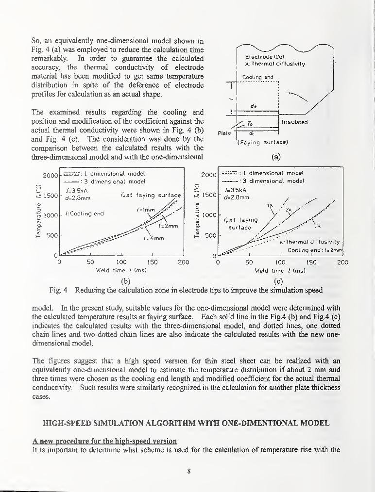
So, an equivalently one-dimensional model shown in

Fig. 4 (a) was employed to reduce the calculation time

remarkably. In order to guarantee the calculated

accuracy, the thermal conductivity of electrode

material has been modified to get same temperature

distribution in spite of the deference of electrode

profiles for calculation as an actual shape.

The examined results regarding the cooling end

position and modification of the coefficient against the

actual thermal conductivity were shown in Fig. 4 (b)

and Fig. 4 (c). The consideration was done by the

comparison between the calculated results with the

three-dimensional model and with the one-dimensional

Electrode (Cu)

K:Thermal diffusivity

PlateJ

(Faying surface)

(a)

2000

p^ 1500

2 1000

£^ 500

0

-zZ-.^il:": 1 dimensional model

:3 dimensional model

/=3.5kA/"oat faying surface" cfe2.8mm

_ /:Cool ing end

^ / = ^mm

1 1

2000 .^.-iTI- : 1 dimensional model

: 3 dimensional model

0 50 100 150

Weld time / (ms)

200

K:Thermol diffusivily

Cooling end : / = 2mm

50 100 150

Weld time / (ms)

200

(b) (c)

Fig. 4 Reducing the calculation zone in electrode tips to improve the simulation speed

model. In the present study, suitable values for the one-dimensional model were determined with

the calculated temperature results at faying surface. Each solid line in the Fig.4 (b) and Fig.4 (c)

indicates the calculated results with the three-dimensional model, and dotted lines, one dotted

chain lines and two dotted chain lines are also indicate the calculated results with the new one-

dimensional model.

The figures suggest that a high speed version for thin steel sheet can be realized with an

equivalently one-dimensional model to estimate the temperature distribution if about 2 mm and

three times were chosen as the cooling end length and modified coefficient for the actual thermal

conductivity. Such results were similarly recognized in the calculation for another plate thickness

cases.

fflGH-SPEED SIMULATION ALGORTTBDM WITH ONE-DIMENTIONAL MODEL

A new procedure for the high-speed version

It is important to determine what scheme is used for the calculation of temperature rise with the

8

I

finite differential method, and how to estimate correct current distribution by the correction

because the resistivity remarkably changes as a function of the weld part temperature.

So, the author has developed a new one-dimensional procedure under some considerations where

the contact diameter is remarkably larger than the plate thickness, and potential value at electrode-

plate interface is almost constant in spite of the surface position, and changes only depending on

the welding state. While, the previous idea, that the contact diameter should increase in

accordance with softening the weld region, has been kept for an important concept to get highly

accurate results.

A mesh system shown in Fig. 5 was used for the calculation of current distribution and

temperature rise in workpieces and electrode tips.

The current density is estimated in

some assumptions that the value can

be calculated with sum of the

resistance in each set of the elements

along the plate thickness direction,

and that the potential at the electrode-

plate interface is constant.

The temperature rise at each time step

is calculated with a tridiagonal matrix

method for the each set of elements

located along the plate thickness

direction to reduce the computing time.

Then, a few elements were arranged in

electrode tip to consider the effect of

electrode materials and cooling end in

electrode. The effect of heat loss

toward radial direction has been

adjusted by using another calculation

along radius direction with the same

tridiagonal matrix method.

The effect of fringing current in the workpiece has been considered by using a modified current

distribution pattern as shown with the one-dotted chain line indicated in Fig. 3 (a).

Simulation algorithm for the high-speed version

A flowchart for the simulation with new procedures is almost same as that shown in Fig. 1(b).

Only details of each routine are modified according to the description in the previous section.

In the new procedure, contact diameters are also estimated with temperature information for

previous time step, so that the current distribution is determined from the resistance value of each

set of elements located along the z-axis of plate thickness direction. The temperature rise is

computed with two step calculation procedure. First, temperature distribution along the z-axis is

calciilated. Then, the calculated results are adjusted with another calculation along the radial axis.

/

Cooling end ( /"= D"P7

Electrode(Cu)

Fig. 5 Mesh system in the high-speed version

9

After both the temperature calculations and a treatment for latent heat, the temperature distribution

within workpiece and electrode tips is determined to estimate the nugget size. Thus, the

calculations are repeated after modification of the material properties for the workpieces in each

time step of the calculation.

Exammatiion of the applicability

A computed result with the newalgorithm is shown in Fig. 6.

Broken line indicates the result with

the high-seed version of one

dimensional model. The solid line

in the figure indicates a calculated

result with the previous three-

dimensional model described in the

other report (Ref 6, 7).

Both lines well coincide with each

other. This means that the high-

speed version can be applicable for

estimation of the nugget growth

pattern in resistance spot welding.

8

s 7£

-§6

£

- 3

a, 9

i 1

/=9.0kA

/7=0.8mmt

c/.= 4.5mm

3 dimensional model

1 dimensional model

50 100 150 200

V/eld lime t (ms)

250 300

Fig. 6 Comparison of simulated residts with

the three-dimensional and high speed versions

I. Nugget monitoring with simulator

35

0 0 0

0.5 0 0

1 0 0

1.5 0 0

2 0 0

2.5 0 0

3 0 0

3.5 0 0

4 0 0

4.5 0 0

5 0.3108434 0 03

5.5 0.5 0.07

6 0.5216108 0.07

6.5 0.55 0.07

7 0.5743687 0.07

7.5 0.6062032 0.09

8 0.6 0.09

8.5 0.6 0.09

r Ooss section

Weld lime (cycle) :

|

Nugget dia.(mm);j

PoneUalionlmm):| qT

65

55

?—

r

Dn

Pn

3 4 5 6

W»ld time (cjrcU)Stafl sampling

and

calculation

Fig. 7 User interface screen for real time quality monitoring with the high-speed version

10

In addition, the simulation program has been made as a dynamic link library that can be linked to

any programs run on the Window 95/98. An interface sample with Microsoft visual Basic is

shown in the Fig. 7. The program can show input data to the simulation program which wasconverted from measuring data of welding current and welding voltage during welding, simulated

results of nugget formation process, and nugget shape at each time step which can be controlled

with a scroll bar appeared on the display. The engine part for simulation as the dynamic link

library can be run in almost twice of the actual nugget formation speed. For example, welding of

150 ms can be simulated only in 60 ms with a personal computer mounted Pentium II of 233MHzwhere the front bus speed is 66 MHz. Of course, the DLL program can give the calculated

results of temperature distribution not only in workpieces but also in electrode tips.

ADAPTABILITY OF THE fflGH SPEED VERION

Measuring system of monitoring parameters

A voltage between tips and a welding current are measured for the monitoring parameters. Anexample of the system is schematically shown in Fig. 8. The welding current was picked up with

a non-inductive shunt in the present study. But the value can be also got by a welding current

meter with a toroidal coil, which is usually used for the resistance welding current meter. In the

present study, the voltage between tips was picked up from both electrode tips although it can be

measured at the electrode tip holders. And then, these monitoring parameters were recorded on

computer memories through an A/D converter of 12bit type. The sampling rate ofA/D converter

was setup in 500 Samples/s in the present case to yield the input data for the simulator.

Examination of the adaptability

The adaptability of new algorithm was examined for zinc coated steel sheets with a H.F.D.C. spot

welding machine. Dome type specified in JIS (Tip end shape is 6mm(j), 50mmR) was selected for

electrode tips because the shape has been ordinarily used in all Japanese automotive companies.

The voltage drop in the electrode tips was corrected as a tip resistance value. The value can be

previously measured without workpieces. In the present case, the value was abnost 1 5 iiQ as the

Nooinducliveshunt

Current

VoUogebetween tips

A/0 converter

Personol computer

21Display

I |6

i ^

CL XI

01 01

I 1Z 2

Dome-type

Inverter O.C.

/=6.0kA

/'=2.0kN

/>=0.8mmt o Exper ..-nental

(Galvannoalcd)

50 100 150 200

Weld time / (m?)

250 300

Fig. 8 Sensing system used for the measurement

of the welding current and voltage between tips

Fig. 9 Adaptability of the high-speed

version for nugget size monitoring

11

Experimental value d^, (mmjS). p«, (mm) Experimental value o'n. (mm?«). (mmj

(a) by the high-speed version (b) by the three-dimensional model

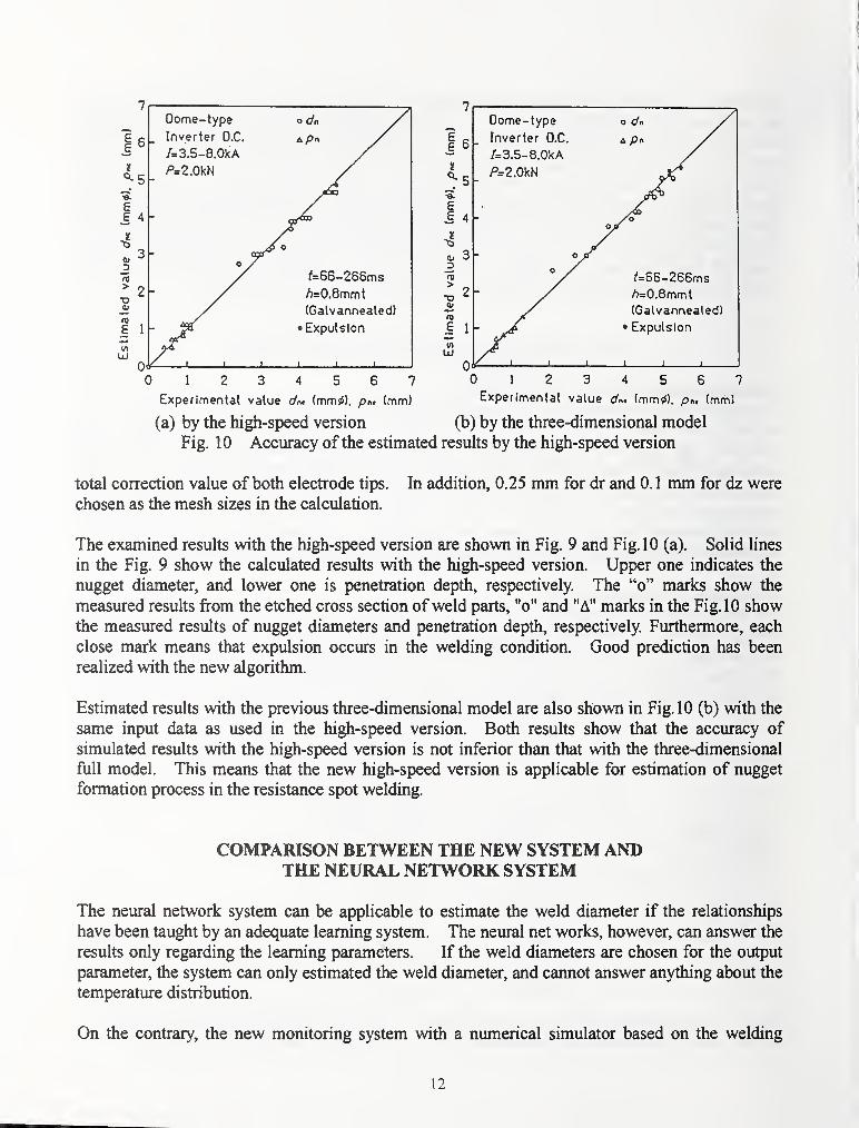
Fig. 10 Accuracy of the estimated results by the high-speed version

total correction value of both electrode tips. In addition, 0.25 mm for dr and 0. 1 mm for dz were

chosen as the mesh sizes in the calculation.

The examined results with the high-speed version are shown in Fig. 9 and Fig. 10 (a). Solid lines

in the Fig. 9 show the calculated results with the high-speed version. Upper one indicates the

nugget diameter, and lower one is penetration depth, respectively. The "o" marks show the

measured results from the etched cross section of weld parts, "o" and "A" marks in the Fig. 10 showthe measured results of nugget diameters and penetration depth, respectively. Furthermore, each

close mark means that expulsion occurs in the welding condition. Good prediction has been

realized with the new algorithm.

Estimated results with the previous three-dimensional model are also shown in Fig. 10 (b) with the

same input data as used in the high-speed version. Both results show that the accuracy of

simulated results with the high-speed version is not inferior than that with the three-dimensional

fiill model. This means that the new high-speed version is applicable for estimation of nugget

formation process in the resistance spot welding.

COMPARISON BETWEEN THE NEW SYSTEM ANDTHE NEURAL NETWORK SYSTEM

The neural network system can be applicable to estimate the weld diameter if the relationships

have been taught by an adequate learning system. The neural net works, however, can answer the

results only regarding the learning parameters. If the weld diameters are chosen for the output

parameter, the system can only estimated the weld diameter, and cannot answer anything about the

temperature distribution.

On the contrary, the new monitoring system with a numerical simulator based on the welding

12

!

I

i

I

On the contrary, the new monitoring system with a numerical simulator based on the welding

phenomena can estimated the temperature and current distributions besides the weld diameters

even though the optimization of the system was achieved only by using the weld diameters as the

output parameter This feature caused by that the new system involves a heat conduction

equation as the estimation engine. Therefore, the system has a week point that requires higher

CUP power than that for the neural network system. The problem, however, has been resolved

by using high-speed algorithm described here.

The features are shown in Table 1 comparing the results for neural networks. Most important

point is that the new system can give users temperature values in workpieces and electrode tips

during welding in real time. Such a property must not realized by using neural networks

Table 1 Comparison between the new system and the neural network system

Items by simulation technique by neural network technique

Engine Numerical simulator Non-linear equations

Merits Wide adaptability

All phenomena can be estimated

Easily high speed treatment

Relatively high accurate estimation

Demerit High CPU power required

Optimization required

Narrow adaptability

Teaching process required

Where the new system based on the

numerical simulator is installed as the

monitoring system, not only the

temperature distribution during

welding, but also the cooling

temperature patterns in the weld part

can be estimated only by sensing the

welding current and welding voltage

wave forms.

A typical result estimated a cooling

process is shown in Fig. 11. Themarks "o" and "A" indicate the

estimated temperature values at the

center part of a nugget and in the HAZzone at faying surface of weld part,

respectively when two stack plates of

0.8 mm steel sheets were used as the

workpieces.

The data are plotted on a CCTdiagram (Ref 12) after Ac3 point in

cooling duration. Both marks are

located near one curve, and the estimated results agreed with another research results (Ref 12).

This suggests that the system is also applicable to estimate the welding state after current flowing

1000

- AC3

800 -

Oo^—

^

gop.

600

400

/

O ; At the center point

a; At r =2.5 mm point

at faying surface

I I I mill I ' 1 ""I ' t I It.200

0.001 0.01 0.1 I

Time after Acs point / (s)

Fig. 11 An example applying to estimation

of cooling process by the new monitoring

system assisted by a numerical simulator

10

13

SUMMARY AND CONCLUSIONS

The treatment time to obtain the simulated results has been remarkably reduced by using the newhigh-speed version without decreasing the simulated accuracy to realize the real-time quality

monitoring with a phenomenon-based system.

The new system can show the temperature distribution in weld part besides the weld nugget size in

real time. And it is applicable to estimate the welding state not only in two stack cases, that are

usually setup in laboratory, but also in three or four stack cases, which are usually used in

automotive works. Furthermore, the system can be also applied to the resistance spot welding

aluminum alloy sheets in addition to the steel ones with and without coated zinc on the surface

although the details have omitted here because of the limitation of pages described.

REFERENCES

1. M. Jou, R.W.Messle, Jr., C.J.Li; A Fuzzy Logic Control System for Resistance Spot Welding

Based on a Neural Network Model, Proc, of Sheet Metal Welding Conference (1994)

2. D.Spinella; Using Fuzzy Logic to Determine Operating Parameters for Resistance Spot

Welding Aluminum, Proc. of Sheet Metal Welding Conference (1994)

3. J.D.Brown, C.P.Jobling, N.T.Williams; Optimisation of Signal Inputs to a Neural Network for

Modeling Spot Welding of Zinc Coated Steels, HW, Doc. No. Ill- 1117-98(1998)

4. G.Monari, O.Dieraert, H.Oberel, G.Dreyflis; Prediction of Spot Welding Diameter using

Neural Networks, nw. Doc. No.III-1108-98( 1998)

5. K.Matsuyama; Nugget size sensing of spot weld based on neural network learning. Proc. of

Seventh International Conference on Computer Technology in Welding, (1997), pp486-495

6. K. Matsuyama, H. Sato, Y. Nishiu, K. Nishiguchi; Computer-Aided Monitoring System of

Nugget formation Process, Proc. of5WS ofJIW in Makuhari, pp577-5 82(1 990)

7. K. MATSUYAM et al.; Model reference type monitoring system to estimate nugget and

contact diameters in resistance spot welding (in Japanese), Technical Commission on Joining

and Material Processing for Light Structures ofJWS, MP-5-88 (1988)

8. K. Matsuyama; Numerical Simulation of Nugget Formation Process in Spot Welding

Aluminum Alloys and its Application to the Quality Monitoring, I.I.W., Doc, No. HI-1060-96

(1996)

9. M. Ryudou, Y. Gotoh, K. Fujii, K. Matsuyama; Development of Inprocess Control System for

Resistance Spot Welding, Proc. of AWS Conference on Resistance Welding; Theory and

Applications held in Chicago (1997- 10)

10. K, Matsuyama; Modeling of Nugget Formation Process in Resistance Spot Welding, Proc. of

Seventh International Conference on Computer Technology in Welding, (1997), pp435-446

11. NAKANE et al; A Study on Determination of Suitable Welding Conditions in Spot Welding

(in Japanese), J. of the Japan Welding Society, Vol.42(1973), No.3, p5012. M.V. Li et al.; Analysis of Microstructure Evolution snd Residual Stress Development in

Resistance Spot Welds ofHigh Strength Steels, Proc. ofSMWC VIII in Detroit, (1998-10)

14

FINITE ELEMENT MODELINGOF RESISTANCE SPOT AND PROJECTION WELDING PROCESSES

W. Zhang and L. Kristensen

ABSTRACT

Based on long time engineering expertise on resistance welding and close collaboration with

industry, a unique finite element program, SORPAS, is developed for simulation of resistance

projection and spot welding processes. In order to make the program directly applicable by

engineers to simulate industrial problems, all the important parameters involved in resistance

welding have been considered and implemented into the program. With the specially designed

Windows 95/98/NT graphic user interface, engineers (even without prior knowledge of the finite

element method) are able to quickly learn and easily operate the program for implementing the

practical parameters, rurming simulations, displaying the simulated results and analyzing the

dynamic welding processes. With the four-fold coupling of the electrical, thermal, metallurgical

and mechanical models as well as the user-friendly facility for flexible geometric design of

workpieces and electrodes, the program can be readily applied for product development or rapid

prototyping and process analysis in industry applying resistance welding. After simulation, the

dynamic process parameters are graphically displayed. The distributions of temperature, current,

stress, strain and strain rate in the materials are displayed in color, which can be animated like a

slow-motion video. In the past two years, the program has been extensively verified and applied

by engineers in industry and students at universities.

KEYWORDS: Resistance welding, FEM modeling, rapid prototyping, process analysis

INTRODUCTION

Resistance welding including spot welding of metal sheets and projection welding of more

complex components is widely applied for joining similar as well as dissimilar metals in various

industries, e.g. automotive, aeronautic, electronic and metal working industries. The process is,

however, very difficult to understand and complicated to manage in production, which involves

interactions of electrical, thermal, metallurgical and mechanical phenomena. In order to design new

products, to select appropriate welding machines or to optimize process settings in industry, a

large number of running-in experiments have to be carried out with a method of trial and error.

This increases the product costs and results in substantial delay in the onset of production.

Another important aspect is the difficulties in identification of the causes for arbitrary

Department of Manufacturing Engineering

Technical University of Denmark, Building 425

DK-2800 Lyngby, DENMARK

15

fluctuations in product quality due to the very fast process time (0.02-0.5 seconds) resulting in

problems monitoring the welding process parameters. There have been keen interests expressed

by engineers in various industries to obtain advanced development tools that are able to extend

the working capacity and skills of engineers thereby to reduce the development costs and time for

product design or rapid prototyping and optimization of production lines.

Among resistance welding processes spot welding and projection welding are the most commonones as illustrated in Fig. 1. Current, force and time are the basic process parameters. Plastic

deformation of metals is often involved, especially in projection welding due to collapse of the

projection part.

Force Current Force Current

Electrode ^^^^^^^^^H Electrode

Electrode ^^^^^^^^H Electrode

(a) Spot welding (b) Projection welding

Fig. 1 : Variants ofthe resistance weldingprocesses.

In order to facilitate industrial applications of resistance welding, numerical modeling of

resistance welding processes applying the finite element method (FEM) has been carried out at

the Technical University of Denmark in the past five years. Considering the physical process of

resistance welding, the numerical modeling tasks have been divided into four models, namely an

electrical model, a thermal model, a metallurgical model and a mechanical model. The electrical,

thermal and metallurgical models are simultaneously coupled considering the dynamics of the

process parameters and the influence of temperature on the properties of materials. The mechanical

model is coupled stepwise with the other models for development of the stress distribution and the

deformation of the workpieces and the electrodes.

Considering engineers as direct end users, an integrated software system, named SORPAS, has

been developed for Windows 95/98/NT. An engineering language familiar to engineers is used in

the graphic user interface. The simulation can be easily operated and the progress is dynamically

indicated and easily controlled. A post-processor is developed for display of process parameters

and animated distributions of electric current, temperature, stress and strain in both workpieces

and electrodes. Large plastic deformation is modeled in the program that can thereby be applied

for spot welding as well as projection welding. Due to the fact that the program is developed in

close contact with industry, practical aspects of the processes have been thoroughly considered in

the program. The software system has been applied in several European companies for evaluation

16

of the geometry and material combination of the product, the main process parameters and also

for determination of the required type and capacity of welding machines. Examples are presented

for demonstration of the applications of the program.

PARAMETERS IN RESISTANCE WELDING

In order to obtain industrial relevant numerical results, it is very important to understand the

process of resistance welding completely and systematically. The practical process of resistance

welding involves not only the workpieces and the electrodes, but also the machine characteristics

and the dynamic features of the process. In order to make realistic and applicable simulations of

the resistance welding process all important parameters should be considered.

ElectrodesGeometry, Materials

InterfacesElectrical, Therinal

Mechanical Properties

MachineElectrical, Mechanical

Characteristics

Dynamics, Stability

Productivity

Fig. 2: System ofparameters in resistance welding.

Fig. 2 illustrates the system of parameters in resistance welding, which is classified into five

groups, namely the workpieces, the electrodes, the contact interfaces, the machine characteristics

and the process features.

The workpieces are the products to be manufactured applying resistance welding. Parameters

related to the workpieces include the geometry and the material properties, the weld nugget

formation and the resulting weld quality. The electrodes are applied to conduct the welding

current to the workpieces to be welded. Parameters related to the electrodes include the geometry

and the material properties, the cooling passage and the lifetime. The electrodes influence the

heat development and eventually the nugget formation in the workpieces. The lifetime of

electrodes has a vital importance in production especially in automatic production lines. Another

important group of parameters is the contact interfaces between the workpieces and between the

workpieces and the electrodes. Parameters related to the interfaces are the electrical contact

resistivity, the thermal contact conductivity and the friction if relative movement (sliding) occurs

at the interface. All these parameters are dynamic and dependent on many other factors. These

make the contact properties very difficult to handle both in practice and in theoretical modeling.

However, they have great influence on the weld nugget formation and the resulting weld quality.

17

Without careful consideration and reliable modeling of the contact properties, it will be difficult

to obtain accurate numerical results.

Besides the parameters directly in connection with the workpieces, parameters related to the

welding machine and the process are also important. The welding machine decides how the

energy is delivered to the electrodes and the workpieces. For example, alternating current (AC)

welding machines will have different dynamics in energy delivery comparing to condensator

discharge (CD) welding machines. Furthermore, each individual welding machine will have its

own electrical and mechanical characteristics including its dynamic response to a rapid current

variance and a sudden mechanical movement. The dynamic characteristics of the process

parameters such as the welding current and the welding force are very important, too. Stability of

the process indicates how sensitive the weld quality is to the variation in the process parameters

since the process parameters may be disturbed by many factors in industrial production.

Productivity is another factor. A low welding current and a long welding time may result in a

similar welding result as a high current and a short time. For stability reason the former case maybe preferred but for productivity reason the latter case is preferable. The changing properties of

the electrodes along with the number of welds have also great influence to the dynamic behaviors

of the welding machines and processes.

PROCESS STAGES OF RESISTANCE WELDING

In order to carry out the numerical modeling, the physical processes of resistance welding should be

first understood. Considering the process parameters and the behaviors of materials, the process of

resistance welding is divided into three stages, which are squeezing stage, welding stage and

holding stage.

In the squeezing stage, the metals to be welded are brought into contact by applying a welding force

to the joint. The contacting workpieces may be plastically deformed especially in projection

welding, but the welding current is not applied in this stage. In the welding stage, the welding

current is applied to the joint and heat is generated at the interfaces and in the workpieces and

electrodes while the weld force is still applied. Due to increase of temperature, the material

properties are changed and deformation of the contacting materials is accelerated. If the welding

time is long enough, melting occurs in the workpieces while deformation of materials continues. In

the holding stage, the current is switched off thus heat generation is stopped, but the welding force

is still applied to maintain the weld. As temperature decreases due to heat transfer, the melted metal

returns to solid state. Welding force will be released when there is no risk of damaging the welds.

FINITE ELEMENT MODELING OF RESISTANCE WELDING

According to the basic parameters and the physical processes occurring in resistance welding,

resistance welding is simulated with four numerical models: an electrical model, a thermal model, a

metallurgical model and a mechanical model. The electrical model calculates the distributions of

the voltage and the current as well as the heat generation in materials and electrodes. The thermal

18

model calculates the heat transfer and the temperature distribution. The metallurgical model

calculates the phase transformation and the material properties dependent on temperature. The

mechanical model calculates the deformation and geometry of materials, the stress distribution and

the contact properties at interfaces.

These models are strongly interrelated to each other and they are all influenced by the dynamic

behaviors of the materials, the interfaces, the machines and the processes. In order to make an

efficient simulation, a simultaneous coupling is made for electrical, thermal and metallurgical

models, whereas the mechanical model is coupled stepwise with the others, see Fig. 3. In this way,

convergence of the models can be easily achieved while the accuracy of solutions is maintained.

Input

Mechanical model

Fully coupled

Electrical model

Thermal model &Metallurgical model

Output

Q.0)4-'

(A

z

Fig. 3: Algorithm for dynamic coupling of the numerical models in FEM modeling of

resistance welding.

IMPLEMENTATION OF PRACTICAL PARAMETERS

In order to simulate a resistance welding process, the geometry and material properties of the

workpieces and the electrodes have to be specified. The material properties are temperature

dependent, which include the electric resistivity, thermal conductivity, heat capacity and flow

stress etc.. To obtain industrial relevant results some other practical parameters have also to be

considered.

Dynamics of Process Parameters

Dynamics of the process parameters such as the welding current and the welding force during

welding is very important in resistance welding especially in projection welding due to a very

short welding time. In order to simulate an actual process, the slope-up of the welding current

(how it rises from zero to a specified level) and the follow-up of the electrode (how it reacts to a

sudden collapse of workpiece due to softening of materials) are determined as functions of the

welding time.

19

I

Types of Resistance Welding Machines

The type of the welding machine is normally defined by the type of its power source. There are

basically three types of welding machines, i.e. the direct current (DC) welding machines, the

alternating current (AC) welding machines and the condensator discharge (CD) welding

machines. The mid-frequency (or inverter) welding machines may be treated as a DC machine.

The impulsed welding machines can also be derived as variations of the DC machines. *

In simulations, the input of electrical power may be defined either by a dynamic curve of the\

welding voltage or by current. The welding current in a DC machine is directly defined as a

function of the welding time taking into account the slope-up and slope-down of the welding

current while switching on and off. The welding current in an AC machine is defined by a sine

function combined with a profile curve for the slope-up and slope-down of the current as well as

the efficiency by phase shifting. The welding current in a CD machine is simulated with a slope-

up curve and a discharge curve of the welding voltage.

By consideration of the actual process and machine characteristics in the simulations in a way

similar to the practice, the program is made very easy for engineers to understand and to operate.

Contact Properties at Interfaces

The contact properties are as mentioned earlier very important although difficult to handle in

resistance welding processes. The most important ones are the electric contact resistivity, the

thermal contact conductivity and the friction conditions at the interface. For instance, in

simulations, the contact resistivity pcontact the interfaces is modelled according to the real

area of contact between surface asperities and the influence of surface contaminant films:

where cry^Q-ff

is the flow stress of the softer metal which is a function of the temperature, strain

and strain rate, cJcn is the normal contact pressure at the interface, p is the resistivity and the

subscripts 1 and 2 indicate the two metals in contact. An extra term is introduced in the equation

to include the influence of surface contaminant films, which is determined as a function of

temperature.

APPLICATIONS OF SORPAS

Based on the numerical models and in-depth engineering expertise, an integrated software

system, SORPAS, has been developed for finite element modeling of resistance welding, which

include a graphic user interface for data input and automatic mesh generation, simulation

operations and graphical display of simulation results. The user interface has been made in an

20

engineering language familiar to engineers. The parameters required for simulation are similar to

the parameters needed for a numerical controlled welding machine.

The program is released to several European manufacturing companies for applications in product

design and process analysis. It is proved by a number of industrial applications that the program can

be applied for the following analyses:

• Evaluation of the weld nugget formation and location influenced by the geometry and

material combination of the weld products.

• Evaluation of the electrode design influenced by the geometry and material properties of

the electrodes in connection with the weld quality, e.g. the heat balance etc.

• Evaluation of the welding results responding to the adjustment of basic process

parameters in order for improving the product quality.

• Comparison of the welding results of the same weld combination obtained with different

machines in order to select the optimal machine type and capacity.

• Evaluation of the lifetime of electrodes by estimation of the heat transfer and

temperature development as well as the stress distribution in the electrodes

Two examples, one for spot welding and one for projection welding, are given below to show the

general applications of the program.

Fig. 4 shows an example of spot welding a 1 mm stainless steel sheet to a 2 mm mild steel sheet,

where the numerical result (on the right side) is compared with the experimental observation (on

the left side). It is shown that the formation of the weld nugget in the stainless steel and the mild

steel obtained by numerical simulation is similar to the one obtained by experiment. It is also

found that an indentation of the electrodes into the workpieces occurred both in the experiment

and in the simulation.

(Molten)

- 1500.0

- 1352.0

- 1204.0

- 10560

908 0

760.0

612 0

4R4 0

- 5160

- 1680

- 20 0

Fig. 4: Comparison ofnumerical and experimental resultsfor spot welding ofstainless

steel (upper part) to mild steel (lower part).

21

Fig. 5 shows a comparison of the simulation results with the micrographs of projection welding

stainless steel to stainless steel. It is seen that the deformation of the material and the

development of the contact area in projection welding is simulated similarly as seen in the

micrographs. This example demonstrates that the program is able to simulate large deformation

whereby also applicable for modeling the process of projection welding.

Fig. 5: Comparison ofthe simulation results with the micrographs ofprojection welding

stainless steel to stainless steel.

CONCLUSIONS

A unique finite element program, SORPAS, has been developed for simulation of resistance

projection and spot welding processes. Results of simulation showed that the program is able to

successfully demonstrate the influence of the main process parameters as well as the geometry and

the material properties of workpieces and electrodes considering also the practical aspects such as

the dynamics of the process and the welding machine characteristics. The program is thus

applicable for quantitative analysis and understanding of resistance welding processes as a

development tool for welding engineers to more efficiently design new products and to optimize

process settings applying resistance welding.

REFERENCES

1. Roberts, D. K.; Roberts, J. E.; and Wells, A. A. 1958. Fundamental Resistance Welding

Investigations. British Welding Journal (3): 1 17 to 126.

2. Archer, G. R. 1960. Calculations for Temperature Response in Spot Welding. Welding

Journal (8): 327-s to 330-s.

3. Greenwood, J. A. 1961. Temperatures in Spot Welding. British Welding Journal (3): 316 to

322.

22

4. Rice, W.; and Funk, E. J. 1967. An Analytical Investigation of the Temperature Distributions

during Resistance Welding. Welding Journal (4); 175-s to 186-s.

5. Cho, H. S.; and Cho, Y. J. 1989. A Study of the Thermal Behaviour in Resistance Spot

Welds. Weldins Journal (6): 236-s to 244-s.

6. Nied, H. A. 1984. The Finite Element Modelling of the Resistance Spot Welding Process.

Weldin2 Journal (4): 123-sto 132-s.

7. Tsai, C. L.; Jammal, O. A.; Papritan, J. C; and Dickinson, D. W. 1992. Modelling of

Resistance Spot Weld Nugget Growth. Welding Journal (2): 47-s to 54-s.

8. Browne, D. J.; Chandler, H. W.; Evans, J. T. and Wen, J. 1995. Computer Simulation of

Resistance Spot Welding in Aluminium: Part I. Welding Journal (10): 339-s to 344-s.

9. Browne, D. J.; Chandler, H. W.; Evans, J. T.; James, P. S.; Wen, J.; and Newton, C. J. 1995.

Computer Simulation of Resistance Spot Welding in Aluminium: Part II. Welding Journal

(12): 417-s to 422-s.

10. Zhang, W. and Kristensen, T. F. 1997. Finite Element Modeling of Resistance Welding

Processes, Proc. 8th Int. Conf. on Joining ofMaterials - JOM-8 , Helsinger, Denmark, 226 to

233.

11. Zhang, W.; Jensen H. H. and Bay N. 1997. Finite Element Modeling of Spot Welding Similar

and Dissimilar Metals, Proc. 7th International Conference on Computer Technology in

Welding, San Francisco, USA, 364 to 373.

12. Zhang, W.; and Bay N. 1998. Finite Element Modeling Aided Process Design in Resistance

Welding, Proc. 8th Int. Conf. on Computer Technology in Welding, Liverpool, UK, S36.1 to

11.

13. Zhang, W. 1998. A Finite Element Program for Simulation of Resistance Welding Processes,

Int. Conf. on Education, Training, Certification and Accreditation in Welding, Helsingor,

Denmark.

14. Zhang, W. 1999. Finite Element Simulation of Resistance Welding, Pore. 9th Int. Conf. on

Joining ofMaterials - JOM-9, Helsing0r, Denmark, 54 to 59.

15. Kristensen, L.; Zhang, W. and Bay, N. 1999. Influence of Geometric Parameters on Weld

Quality in Resistance Projection Welding. Proc. 9th Int. Conf. on Joining of Materials -

JOM-9, Helsing0r, Denmark, 1 12 to 1 17.

23

FINITE ELEMENT MODELING OF RESISTANCE UPSET WELDING

B. Palotas - D. Malgin

ABSTRACT

The resistant upset welding is a widely applied procedure in the technical practice. The quality of

products welded by this procedure depends on the welding parameters, because the resistance

upset welding is a fully mechanized procedure. In order to increase the reliability of welding

parameters the Computer Aided Process Planning can be used, especially in the case of flilly

mechanized procedures, so thus in the case of upset resistance welding as well. The paper shows

the resistance upset welding procedure with main welding parameters and a possibility of the

process parameters planning aided by computer. There are many literature which give formulas

for calculation of welding parameters of upset welding, but these formulas are generally based

on empirical investigations. The paper tries to give the method of parameters calculation on the

physical bases. After the application of analytical solutions for temperature distribution, the finite

element modeling of plastic deformation is shown. The results of paper can be applied in the

technical practice.

INTRODUCTION

The quality of welded structures is depended on the quality of welds. The quality of welds might

be increased by application of fially mechanized welding procedures, because the human factors

can be minimized.

The resistance upset welding is a ftiUy mechanized welding procedure, so it is widely applied

procedure of mass production in the technical practice. The wrong welding parameter setting

might produce many welding defects during mass production, so the correct welding parameter

setting is especially important in the case of ftilly mechanized welding procedures.

The human factors should be also taken into consideration in the welding parameter planning.

The Computer Aided Welding Parameter Planning can close out the human factors in the

welding parameter calculation, so it is an important way of process planning.

The possibility of Computer Aided Process Planning is a reality of our days, but reliable

mathematical models are required.

The resistance upset welding is based on plastic deformation of elements, so the plastic

deformation theories can be used for its modeling.

The resistance heating of elements can be written by analytical equations, but the modeling of

plastic deformation is very difficult by the analytical methods.

The finite element modeling of plastic deformation gives applicable results for technical practice.

The paper will show the resistance upset welding procedure, gives the welding parameters and

calculation methods of them.

The block - diagram of welding parameters calculation of resistance upset welding concluded by

paper might give a base of Computer Aided Process Planning of this procedure.

The mathematical modeling of resistance upset welding might give a base of modeling of other

resistance welding procedures or other pressure welding procedures.

24

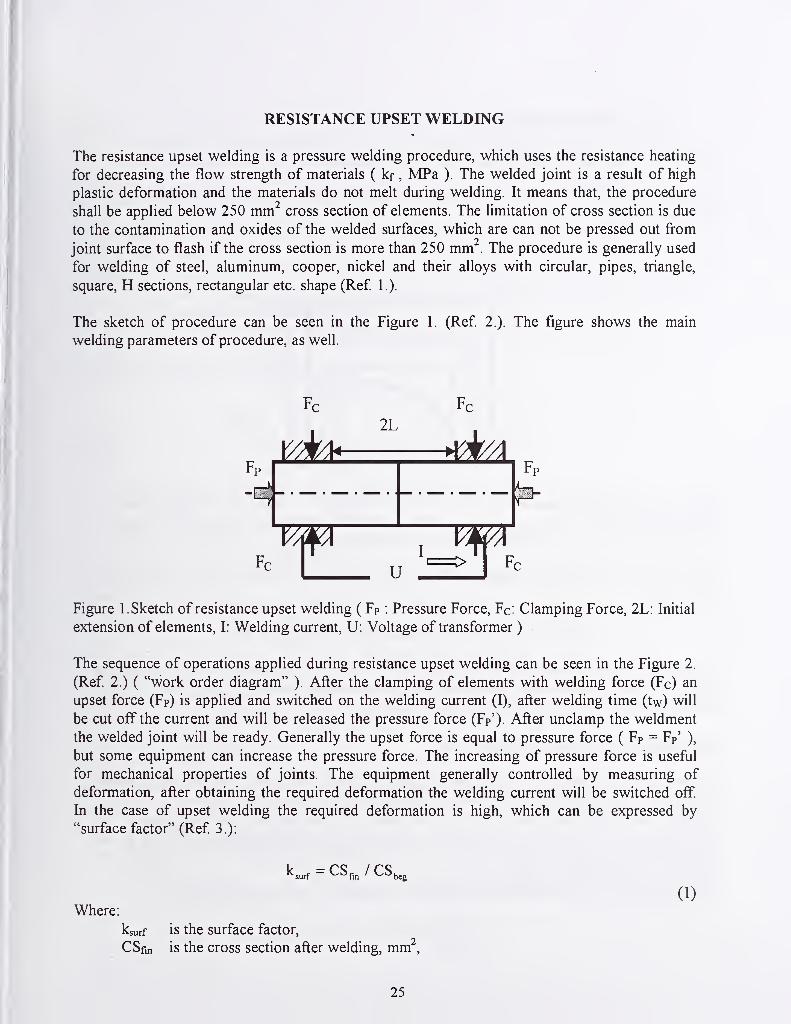
RESISTANCE UPSET WELDING

The resistance upset welding is a pressure welding procedure, which uses the resistance heating

for decreasing the flow strength of materials ( kf , MPa ). The welded joint is a result of high

plastic deformation and the materials do not melt during welding. It means that, the procedure

shall be applied below 250 mm'^ cross section of elements. The limitation of cross section is due

to the contamination and oxides of the welded surfaces, which are can not be pressed out from

joint surface to flash if the cross section is more than 250 mm . The procedure is generally used

for welding of steel, aluminum, cooper, nickel and their alloys with circular, pipes, triangle,

square, H sections, rectangular etc. shape (Ref 1.).

The sketch of procedure can be seen in the Figure 1. (Ref 2.). The figure shows the main

welding parameters of procedure, as well.

Fc Fc

Figure 1. Sketch of resistance upset welding ( Fp : Pressure Force, Fc: Clamping Force, 2L: Initial

extension of elements, I: Welding current, U: Voltage of transformer ) .

The sequence of operations applied during resistance upset welding can be seen in the Figure 2.

(Ref 2.) ( "work order diagram" ). After the clamping of elements with welding force (Fc) an

upset force (Fp) is applied and switched on the welding current (I), after welding time (tw) will

be cut off the current and will be released the pressure force (Fp'). After unclamp the weldment

the welded joint will be ready. Generally the upset force is equal to pressure force ( Fp = Fp' ),

but some equipment can increase the pressure force. The increasing of pressure force is usefiil

for mechanical properties of joints. The equipment generally controlled by measuring of

deformation, after obtaining the required deformation the welding current will be switched off

In the case of upset welding the required deformation is high, which can be expressed by

"surface factor" (Ref 3 ):

^surf - ^^fin I CS^eg

(1)

Where:

ksurf is the surface factor,

CSfin is the cross section after welding, mm^.

25

2CSbig is the cross section before welding, mm .

The required deformation is high, ksurf ^ 4 given by Ref 3

.

The high deformation given by (1) shows that, the most important parameter of upset welding is

the pressure force.

Figure 3. Work Order Diagram of Resistance Upset Welding ( Fc: clamping force, F?: pressure

force (upset force), F?': pressure force, I: welding current, AL: changing of length of elements,

tpre: pre-pressure time, tw: welding time, tpost: post-pressure time )

We try to give a solution for calculation of welding parameters of resistance upset welding in the

followings.

The main parameters of upset welding are the welding current, the welding time and the pressure

force. The other parameters are not effected the weld quality directly ( Fc, tpre, tpost )• The ALparameter will be calculated by finite element modeling.

The Welding Current and Welding Time

On the base of Rosenthal's or Rikalyn's theory of heat conductivity written for welding

conditions, we can calculate the temperature distribution as it follows (Ref 3. ) :

We take into consideration the heating of an infinite rod with constant, uniform current. Wesuppose that, the temperature is constant in a plane and the resistant heating occurred in the

connected surfaces of elements in momentary. After heating of elements, the rods conduct the

heat by heat conduction.

We suppose that, the thermo-physical properties are depended on temperature linearly.

Parameters

CALCULATION OF WELDING PARAMETERS

P ^ Po

cy {cy\

(2)

26

Where:

po and (cy)o are the electrical resistance and specific heat at T = 0 °C,

P is the temperature coefficient of (p/cy).

The temperature of rod can be written as follows:

T(x,t) = Ti(t) + T2(x,t)

(3)

Where:

Ti (t) is the temperature of infinite rod, heated by current, and its resistance depends on

only its material and temperature linearly,

T2 ( X, t ) is the temperature of infinite rod heated by momentary local heat source.

The uniform heating is as follows:

(4)

Where:

wo is the initial rate of heating, °C/s

J is the current density. A/cm .

The T2 ( X, t ) temperature can be calculated by following equation:

(5)

^2(^.0=-

—

?! ^exp pw^t-

r „2 \X

Here:

(6)

_k^X*c*y

(7)

Q2 is the summa heat in the specific cross section arised during welding,

c*, X*, a* are the average values of specific heat, heat conductivity and temperature

conductivity during welding,

k is an efficiency factor takes into consideration the material, pressure and efficiency of

heating. It is 2.6 ... 3.0 for carbon steel, 0.07 ... 0.08 for stainless steel, 0.34 ... 0.36 for

aluminum and 0.14 ... 0.15 for cooper. If the pressure is higher, then the smaller values

of k should be used.

27

The temperature distribution is given in Figure 3. calculated by above written equations. The

temperature is calculated for short extension of elements, but in the case of long extension the

temperature distribution is different from one given in Figure3.

If the extension of elements were too long, then possible buckling would occur. In order to avoid

the buckling, the 2L = 2d where d is the diameter of elements or typical dimension of elements.

In the case of resistance upset welding the maximum temperature of elements is ( Tmax = (0.8 ...

0.9) Tmeiting ) in the plane of connection.

From temperature we can calculate the welding current, welding time and we can use it in the

plastic deformation modeling.

Plane of clamping

Figure 3. Temperature distribution at the resistance upset welding

The welding current and welding time can be calculated by iteration from Tmax ,using the

equations (2) ... (7).

The beginning welding current density (Jo) and beginning welding time (two) used in the iteration

can be calculated from Table 1. (Ref 3. ).

A, mm"^ Jo, A/mm tvvO, S

25 200 0.6

50 160 0.8

100 140 1.0

250 90 1.5

Table 1 . Beginning welding current density and welding time

The required welding current density and welding time have to give the specified Tmax, using

iteration by computer this parameters can be calculated easy.

The Pressure Force

Finite Element Method (FEM) can model the pressure force (FP) required for plastic

deformation.

We show the FEM modeling for unalloyed carbon steel ( type is CI 5 by Hungarian Standard ).

Geometrical data of model is shown in the Figure 4.

28

We used the MARC/AutoForge 2.2.0 software for FEM modeling, the materials were given as

elasto-plastic materials.

The initial condition of modeling is given in the Figure 5.

The force distribution can be seen in the Figure 6.

The results of modeling gave that, the required Pressure Force is 55kN for ksurf ^ 2.15 when the

diameter of deformed element is 22mm. The applied pressure rate was 12m/s. The AL = 5 .5 mmat both side.

1230 °C

^^^^

Figure 4. Initial geometrical data ofFEM modeling

Inc

Time

AngleO.OOOe+OCQ.OOOe+OC

1.230e+03

_ 1.117e+03

3.910e+02

.780e+02

5.520e+02

^.390e+02

3.260e+02

2 .130e+02

l.OOOe+02

jobl

TefTiper-dtufe t

Figure 5. Initial temperature condition ofFEM model

Xmarc

29

Icasel

Body 3 Force X (xlOOOO)

01 20

.519

i

4

.8

X 1011V 12

4. 15"v. 16

——

^

18

;i

^ 22\ 23

ZS. 29

L

,32 33 34

35

5.52

Body 3 Pos X

Figure 6. Force distribution in the case of ksurf 2. 15

The strain distribution is given in the Figure 7., and the Figure 8. shows the temperature

distribution at the moment of ksurf =2.15.

The results of FEM modeling show that, the Finite Element Method can be used for calculation

of pressure force and length changing required by resistance upset welding.

Principle, the resistance heating can be also modeled by FEM and we would like to carry out the

complex modeling of resistance upset welding in the future.

Our results proved that, the pressure welding procedures could be modeled as plastic

deformation procedures.

COMPUTER AIDED PROCESS PLANING OF RESISTANCE UPSET WELDING

On the base of above written, we have prepared the flowchart of CAP? of Resistance Upset

Welding. The flowchart is given in the Figure 9.

30

Inc :

Time :

Angle:

35

M .66?e-04

O.OOOe+00

1.19Se*00

„ 9.b85e-01

6.3B7e-Cl

2.39Se-Cl

-1.6b8e-C5

Icasel

Total Equivalent Plastic Strain

Figure 7. The strain distribution in the case of ksurf = 2, 15

Inc ; 35

Time : •4.667e-04

Angle: O.OOOetOC

9.120etC2

i 6.800st02

4 . 481e*02

2.162e+02

TeripenatLipe t

-I =*x

Figure 8. The temperature distribution in the case of ksurf = 2. 15

31

[ STARTj

Base Material

Geometrical data

Table 1. I

Equation

(2)... (7)

Materials properties

Mechanical

Thermal

J — Jo, tw — tv

Temperature

distribution

Tn

c(T)

X(T)

P(T)

aCT)

Materials

database

rj= j+

1

tw = tw + 0.01

J = J-

1

tw = tw-0.01

y

FEM modeling

of plastic deformation < FEMmodeling

software

Materials

Nmodel

Fp, J, tw, ALtpre, tpost

Fc

tpre> tpost > Fc

^ STOPJ

Figure 9. Flowchart of Resistance Upset Welding CAPP

32

The parameter calculation starts with input of geometrical data and base materials specification.

Materials database gives the required data of materials, the calculation of temperature

distribution gives the welding current density and welding time, by iteration. The FEM modeling

of plastic deformation gives the required pressure force and length changing of elements. The

output of calculation gives the welding parameters.

CONCLUSION

The Resistance Upset Welding is a fully mechanized procedure and the calculation of welding

paramxCters by computer is possible and reasonable in our time.

Analytical and Finite Element Method can calculate the welding parameters.

We suggest using an analytical model for calculation of heating parameters and FEM model for

required pressure force calculation in the case of resistance upset welding.

The FEM modeling can be used for all pressure welding procedure.

We would like to calculate all welding parameters of Resistance Upset Welding on the base of

FEM modeling in the future.

REFERENCES

1. O'Brien, R. L. Editor, 1991. Welding Handbook. Volume 2. Welding Processes : 955

Miami: American Welding Society

2. Buranszky, J. I. Editor, 1985. Welding Handbook : 969 Budapest: Muszaki Konyvkiado

( In Hungarian

)

3. Orlov, B.D. 1980 . Resistance Welding : 410 Budapest: Muszaki Konyvkiado

( In Hungarian

)

33

Session A2: Simulation ofGMAW and RW

\

MAGSIM AND SPOTSIM - SIMULATION OF GMA- AND SPOT WELDINGFOR TRAINING AND INDUSTRIAL APPLICATION

Authors: Prof. Dr.-Ing. U. Dilthey, Dr.-Ing. A. Brandenburg,

DipL-Ing. H.-C. Bohlmann, Dipl. -Inf. R. Sattler

ISF-Welding Institute, Aachen University, Germany,

Prof. Dr.-Ing. habil. W. Sudnik, Dr.-Ing. W. Erofeew, Dipl.-Ing. R. Kudinow,

ComHighTech Institute, Tula University, Russia

Abstract: Simulation systems allow a close inspection of the relation

between welding parameters and the resulting weld seam. So such systems

are very useful in education ofweld staff as well as production and planning.

In training the influence of variations of parameters can be investigated

without the need for real welding experiments. In the design phase

requirements of the welding process can be taken into account without

several iteration cycles. By estimating a good parameter set for the given

welding task the set up phase for a new production cycle can be reduced.

Simulation systems were developed for GMA welding as well as spot

welding. MAGSIM calculates the weld shape and the temperature cycle of a

unpulsed and pulsed GMA welding process for a butt weld as well as fillet

welds. A graphical display of the cross section of the weld shape and a three

dimensional visualisation allow a close inspection of the weld result. The

seam is classified according to the European Standard EN25817. The

simulation system takes 50 different parameters including parameters into

account.

The SPOTSIM software is a program simulating the process of resistance

spot welding (RSW) which includes a material data bank relating to the

thermo-physical and thermo-mechanical qualities of the steels as well as a

data bank concerning the welding-machines and electrodes. The mathe-

matical model of the process is a system of differential equations of the

electronic potential, the thermal energy and the equation of the plastic

, deformation of the metal depending on the power of the electrodes and the

temporal alteration of the welding current By this simulation it is possible to

calculate the measurements of the weld nugget, of the electrode indentation

and the sheet separation.

1.0 INTRODUCTION

The determination of optimal welding parameters is still a difficult task for both spot

welding and GMA welding. Based on experimental data and a statistical analysis the

result of the welding process can be estimated quite good. This approach works only in

determined valid boundaries and doesn't consider important details like contact-tube

distance, length of hose assembly, characteristic ofpower source, dimensions of the gap,

and so on. Another cause for the non-exact reproducibility of such predictions are the

37

neglected influences of the chosen measuring methods, e.g. the location of voltage

measuring points.

A simulation of the weld formation under consideration of all influences would

considerably diminish the efforts for the determination of suitable process parameters.

Non-experts would also be able to produce solutions for specific welding tasks by

means of a computer dialogue. By variations of welding parameters the relations

between welding parameters and the result can be investigated. In addition based on

simulation systems the knowledge of the physical and chemical processes in the

welding process can be extended and verified.

To achieve a detailed description of the weld formation which is also in accordance to

the process mechanisms, extensive mathematical models are necessary, which, however,

can only be solved by numerical methods.

2.0 MAGSIM

The computer program MAGSIM was published already 1993 as a simulation system

for GMA welding processes. It was designed for running on standard personal

computers using the MSDOS operating system. The main goal for MAGSIM is the fast

simulation of the weld shape and the classification of the result according to the Euro-

pean standard EN 25817. For the simulation ofGMA welding processes a mathematical

model [1,2] and a simulation software [3,4] were developed. It simulates the physical

processes of the electric welding circuit and the arc as well as the formation of the

temperature field and the bead surface numerically. The particular algorithms are based

upon physical laws, numerical mathematics and verification adjustment. They allow the

analysis of real welding processes regarding up to 50 parameter values, the optimisation

of welding parameters for given tasks and the diagnosis of butt joint welding processes

[5,6]. The model is self-consistent so that no additional assumptions (e.g. the efficiency

of the arc) are necessary. Aside of the estimation of the weld shape it can be used for the

optimisation of the welding parameter.

The program MAGSIM2 extends the simulation capabilities of MAGSIM to pulse arc

processes, fillet welds, additional mixed gases with O2 components and high-alloy

steels. It allows the calculation of the arc efficiency and the part of drop heat regarding

of all pulse parameters including current leading and trailing edge. The mathematical

38

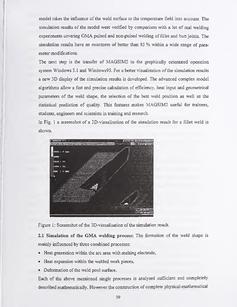
model takes the influence of the weld surface to the temperature field into account. The

simulation results of the model were verified by comparison with a lot of real welding

experiments covering GMA pulsed and non-pulsed welding of fillet and butt joints. The

simulation results have an exactness of better than 85 % within a wide range of para-

meter modifications.

The next step is the transfer of MAGSIM2 to the graphically orientated operation

system Windows 3.1 and Windows95. For a better visualisation of the simulation results

a new 3D display of the simulation results is developed. The advanced complex model

algorithms allow a fast and precise calculation of efficiency, heat input and geometrical

parameters of the weld shape, the selection of the best weld position as well as the

statistical prediction of quality. This features makes MAGSIM2 useful for trainees,

students, engineers and scientists in training and research.

In Fig. 1 a screenshot of a 3D-visualisation of the simulation result for a fillet weld is

shown.

Figure 1 : Screenshot of the 3D-visualisation of the simulation result.

2.1 Simulation of the GMA welding process: The formation of the weld shape is

mainly influenced by three combined processes:

• Heat generation within the arc area with melting electrode,

• Heat expansion within the welded work pieces,

• Deformation of the weld pool surface.

Each of the above mentioned single processes is analysed sufficient and completely

described mathematically. However the construction of complete physical-mathematical

39

models describing the welding processes and their numerical realisation is very complex

already for plain joint geometry like butt joints. It is about the necessity of solving the

very non-linear coupled three-dimensional temperature problem at the uncovered

surface.

Essers and Walter [7] have shown by experiment that the enthalpy of the separated

metallic drops sets the common area of the seam cross-section, while their dynamic

effect to the metallic molten bath effects the depth of the melting zone. Tsao and Wu [8]

have examined the two-dimensional process of spot welding regarding a volume source

and the flow of the molten metal. Kumar and Bhaduri [9] have developed a three-

dimensional model of the transient temperature field regarding the kinetic energy and

enthalpy of the drops coming from the electrode. The enthalpy of the drops is regarded

as a volume source.

[10] describes the development of a three-dimensional mathematical model for the

formation of the melting pool surface in fillet welds including the numerical solution of

the two differential equations describing the heat transfer and the static balance of the

three forces arc pressure, gravity and surface tension. The heat flow depends on the

configuration of the melting pool and vice versa, so the solution of this coupled problem

had to be iterative. The change of the co-ordinates of the uncovered surface caused by

the iterations was regarded by supplement or removal of the control volume within the

simulation zone. For the solution of this task Sudnik proposes deformed adaptive

numerical networks [11].

The numerical simulation of the two-dimensional temperature field and the analj^ic

description of the seam cross-section profile for GMA welding of fillet welds regarding

deformations as undercuts and excessive distorted weld shapes was published in [12].

The analytic solution of the non-stationary three-dimensional temperature distribution

for a sheet with normal source distribution and the following transformation for the T

joint is described in [13]. The arc heat source is described using an elliptical Gaussian

distribution. The adjustment of the calculation results for correspondence of melfing

zone and HAZ with the welding experiments was done by adaptation of the concen-

tration coefficients.

For the easy selection and optimisation of adequate welding procedures a computer

program for the simulation of temperature distribution and weld seam formation for

given tasks ofGMA welding with various welding positions is introduced [14].

40

2.2 Physical-mathematical model of the process for fillet welds: The wide propaga-

tion of the welding of fillet welds (T and overlap joint) required the expansion of the

base model and the simulation software. The' model description and there simulation are

made more difficult for the welding of fillet welds by serious interrelationships:

• The UI diagram of the arc required for the model differs near the irmer edge of the

groove from that used for the butt joint model,

• the efficiency of the arc is actually higher for the fillet weld model, because the

surfaces of the groove sides are heated more by the radiation of the arc stream,

• the share of the molten base metal within the seam is more than 50 %. This fact

requires a more precise description of the superficial heat source of the arc with

melting electrode,

• a widespread hypothesis about the normal circular power density distribution of the

arc has to be extended to a hypothesis of a normal elliptical distribution,

• the existence of a gap - even a gap width of zero - effects a dissymmetry of the

temperature field relative to the heat source axis and excludes the calculation of only

one symmetric half of the welding zone,

• the melting pool when welding T and overlap joints in horizontal position is not

symmetric to the gravity vector. Therefore its components have been taken into

consideration for the differential equation describing the melting pool surface,

• The modelling of the pulsed spray arc with frequencies above 100 Hz requires a more

accurate description of the electrode drop force.

The general physical-mathematical model can be divided into four partial models:

• work piece

• heat source for pulsed and non-pulsed welding

• temperature field v^thin the work pieces to be welded

• deformation of the weld pool surface

The partial model of the work piece describes parameters of the base material like the

enthalphy etc. Experiences with the numerical modelling of arc welding processes have

shovm that for the correct consideration of the phase transition heat at melting and

crystallisation it is better to the use the equation for the energy transmission instead of

the temperature.

Three heat sources for the welding process have to be distinguished: the power of the

41

anode which includes the heating of the wire, the cathode zone and the arc stream. The

energy of the arc stream is only partially used for the process depending of the depth of

the crater. For the pulsed arc process the power of the arc results from the calculation of

the integrate average value of the instantaneous arc power over one period t^^^. The

partial model of the pulsed arc allows the calculation of the arc efficiency and the part of

drop heat in consideration of all parameters of the pulsed power source including the

leading and trailing pulse edges [15].

The equation of the stationary thermal conduction of the temperature model is described

for movements along the x-axis of the medium in Cartesian co-ordinates. The z-axis is

identical with the axis of the wire electrode and the y-axis is perpendicular to the xy-

plane. The boundary conditions at the outer surface of the joint describe the thermal heat

flows of the hot spot the arc stream q^q^ as well as the thermal radiation flowing

off, the heat convection and the vaporisation. The heat flow of the hot spot is described

by an elliptical probability curve. The boundary condition for the second surface is

given by the loss of energy by radiation and vaporisation.

The melting pool surface is changed in shape by the electromagnetic and gas kinetic arc

influence of the falling drops and the gravity which is balanced by the forces of the

surface tension. The surface shape is calculated by the equation for the balance of the

above mentioned forces [1]. The front part of the melting pool is identical with the base

material. For the rear part of the melting pool the boundary conditions reflect the

parallelism of the crystallisation surface of the x-axis. When turning the work pieces

with their co-ordinate system by the angle 0 the term of the hydrostatic pressure

changes to a sum of the components pgZ/Cos0 + pgTsin©, in which Y is a co-ordinate

of a spot at the melting pool surface.

2.3 Realisation: The numerical approximation of the three-dimensional model is done

by the finite difference method applied to a regular net with the dimensions 80 x 80 x

100 mm with the mesh width Ax = Ay = Az = 0.2 mm. The widths were adapted

additionally for the minimisation of inaccuracies of the stepped approximation. The heat

transfer is calculated neglecting the molecular heat transfer along the axis ox. The

algorithm of the numerical solution is based upon the use of efficient methods for

solving of three-dimensional problems - the local one-dimensional pattern.

After finding the surface Zi(x,y) the simulation area for the partial model of the

temperature field is specified more exact and then the calculation procedure is repeated.

42

For a precise determination of the weld shape 2-3 repetitions are necessary.

Knowing the surface of the molten metal, the co-ordinates of the seam surface can be

used as a first approximation for the boundary surface of the simulation zone for the

partial model of the temperature field. The selection of the start approximation of the

surface mostly allows a solution for the melt surface of the model in one cycle of

temperature field calculation.

2.4 Verification of the Simulation Results: The important verification of the

simulation software was done by the comparison of the calculation results with the

polished sections of welding experiments. The extensive verification experiments

needed for the extended welding tasks ofMAGSIM2 were done at the Welding Institute

(ISF) Aachen using the steel St37-2 for butt welds and fillet welds with different

parameters and seam types. A good correspondence of the simulation results compared

to the experimental outcome is obtained for the melting pool parameters and the HAZ

area for a T joint, Fig. 2, 3.

a) b)

Figure 2: Comparison of welding experiment and its simulation for pulsed MAGwelding, butt weld (thickness 2 mm), D^= 1 .2 mm, Z^. = 1 5 mm, Iq = 40 A,

Up = 35,5 V, CORGON 18

a) = 7,1 m/min, fp = 1 75 Hz, = 1 .3 1 m/min,

b) = 4.4 m/min, fp = 100 Hz, v^ = 0.91 m/min

2/18/11

Figure 3: Comparison of welding experiment and its simulation for steel St37-2, fillet

weld (thickness 2 + 2 mm), D^=\.2 mm, Zk = 1 1 mm, torch angle 45°,

inclination neutral, v^ = 0,7 m/min, v^= 4 m/min (I = 1 85 A), U = 1 9 V,

CORGON 18

43

3.0 SPOTSIM

According to the DVS-leaflet 2916 the criterions of quahty of resistance spot welding

are the diameter of the weld nugget, the zone of the heat-influence, the electrode

indentation as well as the joint-gap between the sheets. These depend on the welding

parameters of the process, which are adjustable on the welding-machine, and the shape

of the electrodes. The experimental estimation of quality can be carried out with the

help of the computer model of the process. Already in 1949 Gelmann [16] formulated

the first model of the process of resistance spot welding as a system of differential

equations of the electric potential and the heat conductivity. The two-dimensional

distribution of temperature concerning steel was determined numerically by Greenwood

[17]. Ruge and Hildebrandt [18] determined it for aluminium. Tschakalew [19]

developed an axis-symmetrical model based on the numerical solution of the differential

equation of the heat conductivity. By means of the method of finite elements Nixed [20]

took into consideration the deformation of the welded workpieces. Wei and Ho [21]

applied the instationary model of the heat conductivity on the studies of the

measurements of the weld nuggets with different currents, different types of electrodes

and varying thickness of sheets. Sudnik and Erofeew [22] developed the coupled

numerical model of the process based on the system of differential equations of the

mechanical balance of the electrode force and the plastic deformation of the workpiece.

In the edge conditions of the equation of the electric potential the ohmic and the

inductive resistances of the welding machine were taken into consideration. During the

development of the model [22] Erofeew and Kudinow [23] additionally considered the

formation conditions of the gap and the probability of spatter. The programs for

resistance spot welding were developed by means of the commercially accessible soft-

ware ANSYS [24] and SYSWELD [25].

In the present model the welding current adjustment by phase shift by means of the

input of the retardation angle of the control and the ignition of the thyristors. To

simulate real conditions data banks for resistance welding machines and electrode types

exist. In order to test the model a series of verification welds of steel sheets with a

thickness up to 1,2 mm has been executed. As a result the software SPOTSIM was

developed for the IBM PC under MS DOS.

44

3.1 The mathematical model: The basis of the model is a system of differential

equations in a cylindric coordinate system of the electric potential and the thermal

energy and the integral equation of the plastic deformation of the welding zone.

Alternating current welding machines roughly grade the effective value of the current by

the open-circuit voltage Ull of the welding transformer and shift it infinitely variable

by the regulation of the phase displacement a of the thyristors. In the edge conditions of

the differential equation of the potential the momentary voltage between the electrodes

of the machine uee is taken account of. For the determination of this parameter the

welding current and the resistance ReE between the electrodes is calculated from the

solution of the differential equation of the potential [22].

R + Rsincor - sin(a - cp ) exp(-r ^

— —) (1)

when CO equals the circular frequency of the sinus current, L equals the inductivity of the

welding current circuit, Rm equals the inner resistance of the machine, cp equals the

efficiency factor of the welding current circuit, cp = arctan(coL/(RM"'"REE))^ t equals the

time, a equals the displacement of the phase angle and t] equals the time since the

starting of the thyristor.

The solution of the differential equation of the potential takes into consideration the

influence of the temperature on the resistances of the material and the electrode tip and

calculates the specific density of the generation of heat. The temperature distribution is

determined by the solution of the non-linear equation of the energy with observance of

the thermal conductivity and the phase transitions [22,23].

The electrode geometry for the calculation of the plastic deformation is described by the

tip radius Ri according to ISO 5821. Concerning resistance spot welding the density of

the generation of heat and the speed of temperature rise depends on the contact between

the sheets. This contact zone increases significantly during the welding process due to

the strength reduction of the metal. In the molten area the strength of the metal equals

zero and the inner pressure equals the deformation resistance on the periphery of the

softened zone. In the model it is assumed that the contact pressure between the sheets

derives from the deformation resistance a(T) on the edge of the softened area. By this

device it is possible to determine the momentary value of the tip radius rK by the

45

temperature distribution T(r) and the electrode force Fel by means of the iterative

solution of the integral equation [22,23].

2^''fa(r }^'- = /^/:/, (2)

The depth e of the electrode indentation derives from the momentary value of the tip

radius between the working pieces and the electrode radius Rj

e = R,-^R}-rj^-^-, (3)

The thermal expansion and the plastic deformation lead to the formation of the gap

width X between the working pieces:

^ = £l±£l+ ja,r^, (4)^ 0

when ei and e2 as depths of the upper and lower electrode indentation, aX as coefficient

of the thermal expansion.

3.2 Numerical Approximation: The solution of the differential equations is produced

by means of the fmite-differences-method. The instationary process of resistance spot

welding with alternating current welding machines is calculated with a width A

t = 0.5 ms in consideration of current variations. With every pace the equations of the

electrical potential, the energies and the plastic deformations are solved. The edge

condition Ull of the equation of the current-depending electrical potential and the

current derive from this equation; thus the solution is calculated iteratively. Thereby the

distribution of density of the generation of heat is determined. The distribution of

temperature derives from the solution of the instationary equations of the energy. After-

wards the integral equation is solved and the tip radiuses of the current moment are

determined. These values are used to solve the equations of the next pace.

3.3 Calculation algorithm: After all parameters are chosen from the data banks, the

starting conditions are calculated (Tab. 1). The main cycle of the calculation includes a

solution of the two differential equations and a solution of one integral equation for

every pace in time.

The edge conditions of the potential equations consider the variations of the sinus

voltage between the electrodes. The iterative solution of the potential equation is

executed in consideration of the non-linearity of the specific resistance. Concerning the

46

solution of the energy equation for the very small time pace the non-linearity of the

temperature-depending heat conductivity can be neglected. The calculation of the plastic

deformation with a variable tip radius rK is -continued until the correspondence of the

calculated and the adjusted electrode force is reached. The calculation process is

repeated for the next time pace.

Selection of sheet thickness and alloying.

Selection from the data banks of:

thermo-physical properties of the material,

mechanical properties of the material,

parameters of the machine,

parameters of the electrodes,

parameters of the process; no load voltage Ull,

welding time tg,

electrode force Fe|,

phase shift of the thyristors a

starting conditions: t=0, H=Ho, rK'=''K,0. REE=REE,0. i^'O

t=t + dt

calculation of the tip resistance pkCO-

calculation of the edge conditions of the potential differential

equation and momentary value of electrode voltage

uEE=f(L'LL. REE> Zm, i, a ).

N=0, Un(PK.rK) = Un(PK,rK)

repeat n=n+l

solution of the differential equation of the potential u(

PK. TK),

calculation of the welding current and of the electric

resistance between the electrodes ReE-

Until |un - Un- l<eu

solution of the differential equation of energy, determination of

temperature and measurements of the weld nugget

repeat TC =rK + dr

solution of the integral equation of the piastical

deformation in the contact area with the radius rK and

determination of the electrode force F[viod. of

gap-width between the workpieces and of the

electrode indentation

Until IFMod -

'

-ell <er

Until t<ts

record of results of the simulation

Table 1 : Scheme of the algorithm

3.4 The data banks: The data bank concerning material contains information about

enthalpy, heat conductivity, density, specific resistance and deformation resistance of

steels. The properties of the steels can be entered at 6 degrees which are freely to choose

for the temperatures from 20 to approximately 2000°C. The data concerning the

alternating current machines contain power, short circuit current, power factor, scope of

adjustment of the electrode force as well as the primary no load voltage of the trans-

47

formators. Information about the standardised electrodes are the measurements of the tip

radiuses and the material. These data can easily be completed and edited by the user.

3.5 Possibilities of the model: The model calculates the momentary value of the

welding current, the weld nugget diameter, the resistance (Fig. 4), the temperature

(Fig. 5), the sheet gap and the tip diameter between the work pieces depending on the

chosen steels, the sheet thickness, the electrode geometry and material geometry as well

as the welding parameters. Furthermore the model is able to determine a welding lobe of

parameters after determination of the range and limits. That way the user has the

possibility to choose appropriate welding parameters depending on the input of the

problem.

400 14 I

Figure 4: Resistance and nugget diameter. Figure 5: Simulation of thermal field of

a spot weld Simulation

3.6 Parameter study and verification: For the validation of the correctness of the

calculations a series of experiments is executed. The material chosen for the

experiments was St 12 with a sheet thickness of 1,2 mm. The experiments were carried

out on a alternating current machine of the type Schlatter Selekta P3 with the electrodes

G 16X20 (CuCrZr). The welding current was altered between 5 and 10 kA. Electrode

forces from 1 ,5 to 4 kN and welding times from 6 to 1 8 periods were chosen as fiirther

welding parameters. Comparisons between the cross-section of the welded joints and

the calculated geometries are exposed in Fig. 6.

0.06 0.12 0.18 =11.6 Uc-welding time, s

48

I1

i

\ 1 ! 1 11

0 1 2 3 456 mm 8

Figure 6: Comparison of welding nugget in cross-section and simulation, Stl2, 1,2 mm,F,,=4 kN, Ull=14 V, ts=18 Per, (j)=108<'

4.0 HARD- AND SOFTWARE DEMANDS

To run the programs the following hard- and software is required: at least IBM PC 386

with a mathematical coprocessor or higher, operating system MS-DOS and a VGA-

graphical interface. The programs, which are programmed with Borland Pascal 7.0 in an

object-orientated way, is mouse and menu controlled. This way simulation systems

allow the direct evaluation of the simulation results and a better understanding by

visualisation. The time required for the calculation of one simulation on a PC Pentium

with a clock-frequency of 200 MHz is about 1 0 seconds.

5.0 SUMMARY

With the support of the data banks SPOTSIM proves to be a device which eases

considerably the engineer practice of production planning in the field of resistance spot

welding. By the calculated results the expenses and costs concerning operations

scheduling and production can be reduced drastically in comparison to the usual

proceedings. The verification has shown that the model simulates sufficiently accurate

the welding current, the voltage, the measurements of the weld nugget and the welding

zone, the deformation of the working piece surface and the variation of the gap width

between the working pieces.

Especially in the field of education and teaching the effects of resistance welding, as

there are the formation of the weld nugget during the process of welding, the influence

of the welding parameters and of the measurements and types of the electrodes on the

49

geometry of the weld nugget, which can otherwise only difficulty or even not be shown,

can with the support of SPOTSIM be demonstrated in a clear and vivid manner.

Therefore the simulation systems are not only recommended for the use in the engineer-

ing practice, but also for the education for a better understanding of the quantitative and

qualitative proceedings of the process of GMA and resistance spot welding and its

optimisation.

Acknowledgement: The investigations and results reported in this paper were promoted

partly by the German society „Deutsche Forschungsgemeinschaft DFG". The authors

wish to record their thanks for this funding.

6.0 LITERATURE

[1] Sudnik W. A. 1991 Untersuchung von SchmelzschweiBtechnologien anhand

physikalisch-mathematischer Modelle. SchweiBen und Schneiden 43 (10). S. 588

-590.

[2] Dilthey U., Habedank G., Reichel T., Sudnik W. A. and Iwanow A. W. 1993

Numerical Simulation of the metal-arc active gas welding process. 45 (3). E50 -

E53.

[3] Dilthey U., Reichel T., Sudnik W. A., Iwanow A. W., Mokrow O. A. and

Habedank G. 1993 MAGSIM - Anforderungsgerechtes MAG-SchweiBen von

Diinnblechteilen mit Unterstutzung durch die Computersimulation. DVS Berichte

156, DVS Verlag, Dusseldorf, S. 87-91.

[4] Habedank G., Dilthey U. and Sudnik W 1996 MAGSIM and SPOTSIM - PCaided simulation ofGMA and spot welding processes for educational purposes

and production scheduling. 6th Intemational Conference on Computer

Technology in Welding, Lanaken, Belgium, 9-12 June 1996. Abington

Publishing, UK.

[5] Dilthey U., Habedank G., Reichel T., Sudnik W. A. and Mokrow O. A. 1 994

Analytical system for metal arc active gas welding of thin walled steel sheet in

conformance with requirement. Welding and Cutting 46 (2). p. E24 / E25.

[6] Dilthey U., Habedank G., Reichel T., Sudnik W. A. and Mokrow O. A. 1 996

Numerical process diagnosis for weld seam formation in active-gas metal-arc

welding of light gauge steel sheet. Welding and Cutting. 48 (12). P. E234 - E 236.

[7] Essers W.G. and Walter R. 1981 Heat transfer and penetration mechanisms with

GMA and Plasma-GMA welding. Welding Journal. 60 (2) Pp. 37s - 42s.

[8] Tsao K. S. and Wu C. S. 1 988 Fluid flow and heat transfer in GMA weld pools.

Welding Journal 67(3), pp. 70s-75s.

[9] Kumar S. and Bhaduri S.C. 1994 Three-dimensional finite element modelling og

gas metal arc welding. Metall. Mater. Trans. B, Vol. 25B, pp. 435-441.

50

[10] Ohji T., Nishiguchi K. 1983 Mathematical modelling of a molten pool in arc

welding of thin plate. Technology Reports of Osaka University, Vol 33 No 1688

pp. 65-43.

[1 1] Sudnik W. A. 1985 Digitale und experimentelle Temperaturverteilung in der

SchweiBzone bei Einwirkimg des defokussierten Energiestromes. DVS Berichte

99, DVS Verlag, Diisseldorf, S. 58-61.

[12] Hyeong-Soon Moon and Suck-Joo. 1997 Prediction of weld defect in horizontal

fillet welding using numerical analysis and current measurement. ASM Int. Eur.

Conf. Weld. And Join. Sci. And Technol., Madrid, 10-12 March, 1997: BookProc. Brussels, p 463 - 471

.

[13] Jeong S. K. and Cho H. S. 1997 An analytical solution to predict the transient

temperature distribution in fillet arc welds. Welding Journal. 76(6) Pp. 223s-232s.

[14] WeiB D; Schmidt J; Franz U; Cronacher F; Quaissa B. Simulation von

Temperaturverteilung und Nahtausbildung beim SchweiBen von Blechen in

unterschiedlicher Position. DVS-Berichte, 156 (1993) S. 140-143.

[15] Dilthey U., Sudnik W., Iwanow A., Roosen S. and Habedank G. A study on

mathematical modelling of effective heat input in pulsed GMA welding of steels

with experimental verification (under preparation).

[16] Gelmann A. S. Elektrisches WiderstandspreBschweiBen. Moskau: Maschgiz,

1949. 499 s.(in Russisch)

[17] Greenwood J. A. Temperatures in Spot Welding // British Welding Journal, 1961.

Vol. 8. P. 316-322.

[18] Ruge J. und Hildebrand P. EinfluB von Temperaturverteilung und Werkstoff-

eigenschaf-ten auf das Haften der Elektroden beim WPS von Aluminium und

Aluminiumlegierungen. SchweiBen und Schneiden. 16(1964), H. 4, S.l 15/124.

[19] Chakalev A. A. Et al. Evaluation of the thermal state of the metal in spot welding

with the help of the computer. Welding Production. 20 (1973), H. 10. S. 9/12.

[20] Nied H. A. The Finite Element Modelling of the Resistance Spot Welding Process

// Welding Journal, 1984. Vol. 63. P. 123-132.

[21] Wei P.S., Ho C.Y. Axisymmetric Nugget Growth During Resistance Spot

Welding // Modem Machinebuilding, 1990. Vol. 10. P. 10-17.

[22] Sudnik W. A., Erofeew W. A. Berechnungen der SchweiBprozesses mit

Computem. Tula: Technische Universitat, 1986. 100 S. (in Russisch).

[23] Erofeew W. A., Kudinow R. A. Computermodell des WPSs fur die Qualitats-

analyse von Verbindungen. In: CAD und Expertensysteme in der SchweiBtechnik.

Tula: Technische Universitat, 1995. S. 84/92 (in Russisch).

[24] Greitmann M.J., Kessler A. Qualitatssicherung durch ProzeBanalyse bei Wider-

standpunktschweiBen von Aluminium. SchweiBen und Schneiden. 48(1996), H.l.

S. 11/17

[25] N. N. Resistance welding. SYSWELD + Apphcation. Fa Framasoft + CSI.

51

WELDSIM - AN ADVANCED SIMULATION MODEL FOR ALUMINIUM WELDING

O. R. Myhr H. G. Fjaer ^**\ S. Klokkehaug ^**\ E. J. Holm ^**\ 0. Grongand A. O. Kluken

ABSTRACT

This article illustrates the applications of an advanced simulation model, WELDSIM, for

prediction of microstructure evolution, residual stresses and distortions during welding of age

hardening aluminium alloys. The model consists of three components, i.e. a numerical heat

flow model, a microstructure model, and a mechanical model that are sequentially coupled. Acomparison with experiments shows that the model predicts adequately the temperature and

local strength distribution as well as the thermally induced deformations. In the present paper

the versatility of WELDSIM is illustrated in different numerical examples pertaining to

welding of critical components for automotive applications.

INTRODUCTION

High volume production of aluminium based components for the automotive industry

represents a growing market for aluminium consumption. This market is a challenge to serve

due to its extreme focus on quality, consistency and productivity. In large-scale production of

automotive parts it is essential that the different components fit together during assembly.

This means that the dimensional tolerances have to be very tight. Since thermally induced

deformations are unavoidable in fusion welding, these will usually represent the most difficult

problem to overcome in joining of automotive parts in aluminium. Other typical problems

associated with welding are cracking, porosity, lack of fusion and degradation of the base

material due to softening of the HAZ.

Simulations represent a means of controlling the welding process since the method offers the

possibility to test out how different designs, geometries and welding parameters affect the

resulting properties. The development of useful and reliable software for weld simulations

requires insight into different scientific disciplines like physical metallurgy, continuum

mechanics as well as numerical methods and finite element analyses. During the last few

years significant progress has been made in the understanding of physical processes that take

place during welding of aluminium alloys. A synthesis of that knowledge has, in turn, been

consolidated into a process model, WELDSIM, which provides a mathematical description of

Hydro Raufoss Automotive Technical Centre, N-2831, Raufoss, NorwayInstitute for Energy Technology, N-2007 Kjeller, NorwayNorwegian University of Science and Technology, N-7491 Trondheim, Norway

52

the relation between the main welding variables and the subsequent weld properties, based on

sound physical principles. The present paper illustrates different applications of this computer

program and shows some examples where the model has been applied to provide practical

guidelines for welding of specific components for automotive applications.

GENERAL OUTLINE OF MODEL

The different input and output of WELDSIM are shown in Fig. 1. Alloy composition and

temper condition must be specified as well as the geometry of the welded component. The

fixture design is represented in the model by appropriate mechanical boundary conditions.

The welding parameters are accounted for by specifying the net heat input, the spatial heat

distribution, and the time dependent position of the heat source for the different weld

segments.

The main outputs from WELDSIM are illustrated by means of symbols in the figure, and

include the evolution of temperature, microstructure and strength, as well as thermally

induced deformations and stress fields.

• BASE MATERIALCOMPOSITION

• BASE MATERIALTEMPER

• GEOMETRY

> FIXTURE DESIGN

• WELDINGPARAMETERS

• WELDINGSEQUENCE

WELDSIM

/ • TEMPERATURES

• MICROSTRUCTURE

• STRENGTH

• DISTORTIONS

• STRESSES

Fig. 1 . Schematic diagram showing the main input and output of WELDSIM.

COMPONENTS OF WELDSIM

The process model consists of three components, i.e. a numerical heat flow model, a

microstructure model, and a mechanical model that are sequentially coupled. The coupling

between the different models is shown in Fig. 2. According to the assumptions, the imposed

temperature field influences both the microstructure evolution and the stress-deformation

fields. At the same time there is a link between the microstructure model and the mechanical

53

model taking into account the important effect of heat affected zone (HAZ) softening on the

strain relaxation during cooling. In the following, a brief outline of the different components

ofWELDSIM is provided. Further details are give in Refs.[l-31.

Fig. 2. Schematic diagram illustrating the coupling between the different submodels in

WELDSIM.

Thermal modelThe thermal model solves the three dimensional, time dependent heat conduction equation by

a finite element technique. The heat released by the welding arc is represented by an ellipsoid

volume distributed source, where the heat distribution is calibrated against measurements of

the weld pool geometry. In order to account for the metal deposition from the filler wire,

elements that are part of the weld reinforcement are activated when they are approached by

the heat source. An example of output from the thermal model is given in Fig. 3(a), which

compares calculated and measured thermal cycles during robotic GMA welding of a T-joint.

The element mesh and dimensions are shown in Figs. 3(b) and (c). This component will be

used in different case studies throughout the paper.

400 J_l I L_l L . . . I J I L

Measured

O 300 -

0 —I—I—n—I—I—I—

r

10 20

T—|—1—I—I—I—I—I—

r

30 400 50

Time(s)

(a)

54

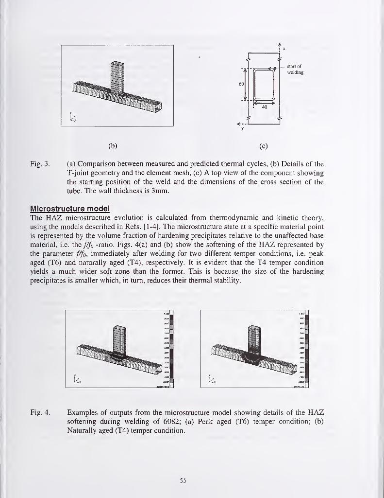
(br (c)

Fig. 3. (a) Comparison between measured and predicted thermal cycles, (b) Details of the

T-joint geometry and the element mesh, (c) A top view of the component showing

the starting position of the weld and the dimensions of the cross section of the

tube. The wall thickness is 3mm.

Microstructure modelThe HAZ microstructure evolution is calculated from thermodynamic and kinetic theory,

using the models described in Refs. [1-4]. The microstructure state at a specific material point

is represented by the volume fraction of hardening precipitates relative to the unaffected base

material, i.e. the f/fo -ratio. Figs. 4(a) and (b) show the softening of the HAZ represented by

the parameter immediately after welding for two different temper conditions, i.e. peak

aged (T6) and naturally aged (T4), respectively. It is evident that the T4 temper condition

yields a much wider soft zone than the former. This is because the size of the hardening

precipitates is smaller which, in turn, reduces their thermal stability.

Fig. 4. Examples of outputs from the microstructure model showing details of the HAZsoftening during welding of 6082; (a) Peak aged (T6) temper condition; (b)

Naturally aged (T4) temper condition.

55

In WELDSIM the parameter f/fo represents the instantaneous state of the microstructure at

each material point of the solution domain and is transmitted to the mechanical model as

illustrated in Fig. 2. This parameter is conveniently transformed to an equivalent base material

strength, e.g. the local hardness or yield strength, which are easier to measure in a weldment

than the internal microstructure parameter /^fo- Fig. 5 shows a comparison between measured

and predicted hardness values in different surface positions across the weld HAZ of the

horizontal member (i.e. the chord) of the T-joint. It is obvious that the observed asymmetry in

the hardness distribution, resulting from a corresponding asymmetry in the thermal field, is

adequately predicted by WELDSIM.

Calculated

W-l 11

11

11

11

11

11-

200 220 240 260 280 300

X(mm)

Fig. 5. Comparison between measured and predicted hardness profiles in different

positions across the upper horizontal 5 ..Tace of the chord after prolonged room

temperature ageing. (Alloy: 6082-T6).

Mechanical modelIn the mechanical model, isotropic elastic-viscoplastic material behaviour is assumed. In the

applied constitutive equations for viscoplastic flow, the flow stress is expressed as a function

of the temperature, the microstructure parameter f/fo, a hardening parameter, and the

viscoplastic strain rate. The material dependent constants entering the constitutive equations

are determined on the basis of experiments carried out in a weld thermal simulator. Here the

samples were tensile tested at different temperatures and strain rates for different starting

microstructures.

The governing equations are solved by a finite element method. The elements in the weld

regions are activated when the temperature has dropped below the coherency temperature

after passage of the weld heat source. At the interface between the welded parts, no gap is

allowed to form, but tangential slip is permitted prior to local solidification.

PREDICTIONS OF DISTORTIONS

Fig. 6 shows a schematic representation of the sequence of deformations taking place during

welding of a T-joint. The vertical displacement is, at first, in the upward direction as shown in

Fig. 6(a). This is due to thermal expansion of the heated material adjacent to the weld. The

56

direction is, however, reversed during cooling as the material contracts. Eventually, the

deformation becomes as shown in Fig. 6(b). By means of WELDSIM the evolution of this

vertical distortion with time can be calculated with a high degree of accuracy, as illustrated by

the plots in Fig. 7. This means that the mechanical model is sufficiently relevant and

comprehensive to be used in numerical case studies to simulate how changes in the welding

conditions affect the evolution of the distortions.

Fig. 6. Schematic diagrams illustrating the evolution of thermally induced distortions

during welding of a T-joint. (a) Before completion of the weld, and (b) After

completion of the weld.

§ 0.5

o0 0.0

^ -0.5

03o

"S -1.0>

-1.5

0 50 100 150 200

Time(s)

Fig. 7. Comparison between measured and predicted vertical deflections at the centre of

the side wall of the horizontal tube (i.e. the chord). Alloy: 6082-T4.

Effect of weld travel speedFig. 8 illustrates how the weld travel speed affects the vertical deflection at the centre of the

horizontal tube when all other parameters are fixed in the simulations. In general, an increase

in the travel speed will tend to narrow the width of the soft zone where the plastic strains

build up. Since these plastic strains are the cause of the deformations, one would expect that

the increase in the travel speed should result in smaller deflections. This is also in accordance

with the WELDSIM predictions as shown in Fig. 8.

J I I I I I I I I I I I I I I I I I I I I L

T—I—I—I—I—I—I—I—i—I

—

I—

I

—I—I—I—I—I—I—1—I—i—

r

57

Fig. 8. Calculated vertical deflection at the centre of the side wall of the horizontal tube

(i.e. the chord) for two different weld travel speeds.

Effect of wall thickness

The wall thickness of the tubes used in the T-joint has a significant effect on the distortions.

This is seen from Fig. 9. It follows that the end deflection of the horizontal tube is reduced

when the wall thickness increases. This is due to a corresponding increase in the stiffness

resulting from the larger wall thickness.

t 1 1 1 t 1 1 1 1 1 1 1 1 1 1 1 1 1 1 1 1 1 1

0.53mm wall thickness :

0.0 1\

l\

4mm wall thickness -

5mm wall thickness -_

-0.5

-1.0 -_

-1.5 -_

0 100 200 300 400 500

Time(s)

Fig. 9. Calculated vertical deflection at the centre of the side wall of the horizontal tube

(i.e. the chord) for three different tube wall thicknesses.

Effect of welding sequenceWELDSIM has also been used to simulate how different welding sequences affect the course

of the deformations. The different welding conditions examined are summarised in Fig. 10.

The possibility of splitting up the weld length into smaller parts that are welded successively

is investigated. Also a consideration of changing the start and stop positions is included. The

results of the simulations are presented in Table 1 . Generally speaking, smaller distortions are

expected when the weld length is split up into smaller parts. Moreover, it seems to be an

advantage to start at the centre of the short side of the tube compared with the centre of the

long side. This follows from a comparison of Sequence 3 and 2 in Fig. 10 and Table 1,

respectively.

58

Sequence

1

^start/stop

^ start/stop

Sequence

1

Sequence

3

^tart/stop

top

Sequence

4

Sequence

5

I

stop

stop Sequence

6start

K--

Fig. 10. Schematic representation of the different welding sequences applied in the

simulations.

Table 1. Calculated vertical end deflections for the different welding sequences shown in

Fig. 10.

Sequence # End deflection [mm]

1 1.27

2 1.33

3 1.09

4 1.02

5 1.26

6 0.88

Effect of welding fixture

The effect of three different welding fixtures on the resulting deflections were simulated by

manipulating the mechanical boundary conditions (BC). Fig. 1 1 illustrates the different

boundary conditions applied, while Table 2 shows the results from the simulations with

respect to the final vertical deflection. Note that BC 1 is the standard set-up used in the

simulations if nothing else is stated. In the BC 1 set-up, the horizontal tube (i.e. the chord) is

fixed vertically to the base at both ends throughout the whole simulation, while horizontal

displacement at one of the ends is allowed, as shown in Fig. 1 1 . Considering BC 2, no vertical

displacements are allowed for at the bottom of the chord during welding. However, when the

welding stops, this restriction is immediately relaxed and the further deformations take place

with boundary conditions identical to BC 1 . In practice, this corresponds to a situation wherethe components are heavily clamped during the welding operation and then suddenly released

allowing the component to deform freely during the cooling stage. As shown in Table 2, this

represents the worst case with respect to the end deformations because the rigid clampingduring the welding stage introduces severe plastic yielding in a large domain of the HAZ. Theresulting driving force for deformation will then act over a correspondingly large part of the

HAZ.

59

The BC 3 case is initially identical to BC 2, but here the constraints are maintained until the

whole component has cooled down. This corresponds to a situation where the component is

kept heavily clamped in the fixture for a long time after welding is completed. This results in

the smallest end distortion among the three cases investigated, since the deformations taking

place during the cooling will be suppressed .

BC 2: Immediately

after welding

BC 3: After cooling

Fig. 1 1 . Schematic illustration of different mechanical boundary conditions (BC) applied

in the simulations.

Table 2. Calculated vertical end deflections for different mechanical boundary conditions.

Boundary condition (BC) End deflection [mm]

BC 1 1.30

BC2 1.56

BC3 1.06

Effect of base material

Different alloys respond differently to the imposed temperature field from the heating source

during heating and cooling. WELDSIM accounts for the microstructure reactions within the

material during welding, and can therefore be used to investigate their resulting effects on

deformations. Fig. 12 shows the vertical deflection during welding and cooling for the alloys

6082, 7108 and 6063, all assumed to be in the initial peak aged (T6) condition. It is evident

that the end-deformation is smaller for the latter alloy compared with the former two. This can

be attributed to the lower yield stress of the material in the fully reverted (soft) condition. The

significance of HAZ softening will be further discussed in the following section.

60

—1—1—1—1—1—1—1—1—1—1 1 1 1 1 1 1 1 1 1 1'

0.5 -

n 6082-T6 :

0.0 -1 6063-T6 :

1 7108-T6j

-0.5 - \ -

V\ N

-1.0^

-1.5-;

—I—1—1—1—1—1—1—1—1—1—1—1—I—1—1—1—1—r—r—1—1—1—1—t—

0 100 200 300 400 500

Time(s)

Fig. 12. Calculated vertical deflection at the centre of the side wall of the horizontal tube

(i.e. the chord) for three different base materials.

SIGNIFICANCE OF THE HAZ SOFTENING

In simulations dealing with welding of age hardening aluminium alloys, it is essential to

include the softening of the HAZ which takes place during welding due to the reversion of

hardening precipitates. As an illustration of principles, we shall consider the same problem as

in Ref. [5], where thermal strains in a fully constrained bar induce uniaxial stresses and plastic

flow. Fig. 13 shows schematically how a material point within the HAZ responds to a thermal

cycle reaching a peak temperature of approximately 400°C when the effect of reversion is

either included (Case A) or ignored (Case B). Also shown in the figure are curves

representing the yield stress as a function of temperature for two extreme situations where the

relative volume fraction of hardening particles is kept at its maximum and minimum level

during the heating and cooling cycle, corresponding to f/fo=\ and 0, respectively. A more

realistic stress-temperature curve for a typical evolution of f/fo is also indicated in the figure.

Initially, the compressive stress increases during heating due to thermo-elastic behavior. After

the yield limit is reached, the compressive stress decreases more rapidly with temperature in

Case A than in Case B due to the reversion.

400

300

« 200D.

— 100</>

v>

2 0CO

1-100

=1-200

-300

-400

0 100 200 300 400 500

Temperature [°C]

Fig. 13. Schematic diagram showing the stress evolution in a material point within the HAZundergoing a thermal cycle under uniaxial constraint. Softening due to reversion of

hardening precipitates is accounted for in Case A, but not in Case B.

61

The most striking difference occurs between Case A and B is during the cooling stage, where

the stresses go from compression to tension. In Case A the residual stresses will soon follow

the tensile flow stress curve for the fully reverted material (f/fo=0), and accordingly a low

residual stress of approximately 100 MPa is obtained. In Case B the situation will be different,

since no softening due to reversion is assumed. This results in a longer thermo-elastic

transition from compression to tension. Eventually, the flow stress curve for the unaffected

base material (f/fo=\) is reached, and a residual stress of about 300 MPa is obtained. The latter

value represents a tremendous overestimation.

In WELDSIM the important effect of the HAZ softening due to reversion of hardening

precipitates is fully accounted for. Fig. 14 shows that the calculated residual stresses are

qualitatively very different when reversion is either included or ignored, corresponding to

case A and B, respectively. Also the calculated distortions will be significantly overestimated

if reversion of the hardening precipitates is ignored in the simulation. This is shown in Fig.

15.

).I5 0.20 0.30 0.35

X- Ms (m)

(a) (b)

Fig. 14. Calculated longitudinal components of the residual stresses near the upper surface

of the chord; (a) Inclusion of reversion of hardening particles (i.e. Case A); (b) Noconsideration of reversion of hardening particles (i.e. Case B). Alloy 6082-T6

>

0.5 -

0 0.0

^ -0.5 •

CO

Case ACase B

s

100 200

Time(s)

r300

T400 500

Fig. 15. Calculated vertical deflection at the centre of the side wall of the horizontal tube

(i.e. the chord). Case A: Inclusion of reversion of hardening particles. Case B: Noconsideration of reversion of hardening particles. Alloy 6082-T6

62

SUMMARY

In this article the apphcations of a newly developed process model {WELDSIM) for welding

of age-hardening aluminium alloys is illustrated. It is shown that the model predicts

adequately the temperature and the local strength distribution as well as the thermally induced

deformations. The model has been applied in different case studies pertaining to welding of

hollow extruded profiles for automotive applications. It has been demonstrated that the model

is capable of accounting for a wide range of different welding conditions, including variations

in the weld travel speed, the tube wall thickness, the base material composition as well as the

welding sequence and the fixture design. Moreover, the local softening of the heat affected

zone is shown to have a significant effect on the simulated stress distribution and

deformations. Hence due consideration must be given to the HAZ microstructure evolution in

the weld simulations. It is believed that the present model is sufficiently comprehensive and

flexible to be applied as a tool in manufacturing and design of welded components in

aluminium where the mechanical integrity is of particular concern.

ACKNOWLEDGEMENTS

The authors wish to acknowledge the financial support of Hydro Raufoss Automotive

Strucmres and The Research Council of Norway. Moreover, thanks are due to Dr. J. Strid at

Hydro Raufoss Automotive Technical Centre for his contributions to this article.

REFERENCES

1. O. R. Myhr, 0.Grong, S.Klokkehaug, H.G.Fjaer and A.O.Kluken. 1997. Science andTechnology of Welding and Joining , Vol. 2, No. 6, 245-254.

2. O. R. Myhr, S. Klokkehaug, 0. Grong, H. G. Fjaer and A. O. Kluken. 1998. Welding.

Journal Vol. 77, No. 7, 286-292.

3. O. R. Myhr, S.Klokkehaug, H.G.Fjaer, 0.Grong and A.O.Kluken. 1998: Proceedings of

the 5th International Conference on Trends in Welding Research. Georgia, USA.4. 0. Grong: Metallurgical modelling of welding . Second Edition 1997, London (UK),

The Institute of Materials.

5. H. Murakawa, Y. Luc and Y. Ueda. 1998: in Mathematical modelling of weldphenomena . Ed. H. Cerjak, Vol 4, 597-619.

63

DYNAMIC MODELING OF ELECTRODE MELTING RATEIN THE GMAW PROCESS

Z. Binguf, G. E. Cook*, and A. M. Strauss*

ABSTRACT

A model has been developed correlating the anode temperature profile with the dynamic melting

rate in gas metal arc welding. Components of this model are identified, as the electrode melting

rate, temperature-dependent resistivity of the electrode and arc voltage. The differential

equations describing the dynamic behavior of the electrode extension were derived from mass

continuity and energy relations. The temperature of the electrode extension was determined by

conductive heat transfer and joule heating. One-dimensional solutions of temperature and heat

content were used to obtain the dynamic melting rate equation. The purpose of the present paper

is to provide quantitative analyses, concentrating on the thermal behavior and the electrical

characteristics of the arc welding system, to aid in a fundamental understanding of the process,

and to develop a dynamic model that may be used in adaptive control. The model is tested by

comparing simulations to experimental results.

INTRODUCTION

The variables of the welding process can be separated into two categories [1]: direct weld

parameters (DWP) and indirect weld parameters (IWP) as shown Figure 1. The disturbance

parameters can be varied on line during welding to affect change in the DWP so they must be

controlled by the other indirect welding parameters. Since a nonlinear relationship exits between

the highly coupled direct and indirect weld parameters, the coefficients of the differential

equations that relate the direct and indirect weld parameters vary as a function of operating

conditions.

Arc stability is essential for good quality welds. Ensuring maximum arc stability is a function of

many factors, selecting satisfactory welding parameters, maintaining the same parameters in

production, monitoring internal and external changes in the process, correcting them,

maintaining uniform metal transfer, chemical composition of the material being melted, and

dynamic characteristics of the power source and process variables. Abnormal changes in the

process variables can result in an unstable arc (spatter and fiame). To reduce the spatter and fume,

feedback control systems with the added capability of self-adjustment are necessary to maintain

a stable arc over the operating range of the process.

Electrode melting rate is one of the most important parameters in the gas metal arc welding

(GMAW) process because arc stability depends on how closely the electrode feed rate and the

electrode melting rate are balanced to maintain a constant arc length. For constant potential

GMAW, arc length regulation is an inherent part of the "self-regulation" characteristic [19]

inherent with this mode of operation. While instabilities may occur with this mode [3-5], it is an

easy matter to choose stable zones of operation. For constant current and pulsed current GMAW

*Welding Automation Laboratory, Vanderbilt University, Nashville, TN

64

however, arc-length regulation must

be provided by sensing and

controlling the voltage [6]. Design

and testing of the arc-length

regulation system requires an accurate

dynamic melting rate model.

rwp

Disturbance

Parameters

Electrode Extension

Arc Length

Current

Voltage

Wire FeedRate

Travel

Speed

CTWD

WELDPROCESS

Penetration

Ductility

Incomplete Fusion

Porosity

Lesnewich [7] conducted extensive

experimentation with GMA welding

of mild steel and empirically derived

his well-known equation expressing

the steady-state relationship between

current, electrode diameter, and

mehing rate. Halmoy [8] used an

energy balance to derive a result of the

same form as Lesnewich, and he

calculated the "effective anode

heating voltage" and the temperature

of the discharged droplets. Other authors [9-15] have contributed to our general knowledge and

use of the melting rate relationships for both constant potential and pulsed current GMAW.While there has been limited work describing dynamic melting rate relationships [16-18], most

of the efforts have been based, at least in part, on steady-state conditions. Unfortunately, in most

cases these conditions become unacceptable for practical control purposes.

i DWP

Bead Width

Figure 1 . Input and output variables of welding process

A good understanding of arc physics is the most important step to develop the dynamic melting

rate model based on relationships between the energy, mass transfer and heat transfer. The

electrical energy supplies the arc energy, which generates the heat at the anode and cathode

regions and within the plasma column. Mathematical modeling of the welding system is

complicated because of the complex distribution of temperature throughout the system Adistributed-parameter model governed by partial differential equations or nonlinear differential

equations with appropriate boundary conditions is required for a precise analysis of the system.

MATHEMATICAL MODEL

The mathematical model developed here

of the GMAW process consists of three

components, the melting rate model, the

electrode resistivity model, and the arc

voltage model. A schematic diagram of

the model is shown in Figure 2.

Melting Rate Model

Developing an explicit melting rate model

which explains the relationship in arc

current and electrode extension for a

Current

Density

J -

Wire Feed

Rate

Rale Model

UAre VoltageModel

Dynamic Resistivity J|Mod«4 ^^^Resistivity

Figure 2. Schematic diagram of the GMAW model.

65

z=L, T = Z0

L

given wire size and wire composition is

important to global control of the process

variables. The melting rate is determined by the

balance between energy and mass entering and

leaving the electrode. The arc can be considered

to be a moving energy (heat) source in the z

direction. Therefore, energy conservation and

mass conservation theories can be applied by

specifying the boundary conditions and initial

conditions. The difficulties arising in the

modeling of the electrode are mainly due to the

complex nature of the boundary conditions.

However, treating the electrode and the arc

column as separate blocks helps to eliminate

these boundary conditions [2]. This is illustrated

in Figure 3. The assumptions made for the

model are that the heat dissipation losses due to

convection, vaporization and radiation, and the

influence of metal droplets are negligible. These assumptions don't affect the model accuracy's

because many authors [8-10] have shown that the convective heat produced by the electric

current is the major part of the energy transferred to the anode from the welding arc. Based on

the above assumptions, the conservation equations are expressed in terms of the z-axis as

follows:

z=0, T = T,^ H

Figure 3. Temperature and energy along

electrode extension.

Mass continuity:

d_

dzAfY)

d1dz

V— = 0dt dz

Conservation ofEnergy:

(1)

^J^^(\)-Cp(l)piJ) h Vdt dz

(2)

The energy equation contains a Joule heating term. The boundary conditions are:

r = ro

r = r,mdT

~d^= 0

2=1

z = 0 (3)

Combining the mass continuity equation and the energy equation, the damped nonlinear heat

equation can be obtained as follows.

66

d_

dzX{T)

dz+ j^^(r) = o (4)

Heat transfer and temperature

distributions during welding are complex

and a solution to the equations is

dependent on the thermal conductivity,

specific heat and density of the mass as a

function of temperature. To find

analytical solutions to the equations, it is

therefore helpful to eliminate the

relationship between temperature and the

above variables by means of defining a

new variable, which serves as a bridge

between them. The heating effect, called

the heat content is defined as:

Resistance (ohm-mm)

Heat Content (J/mm )

Si-Mn — Blainless -*- mild

Figure 4. Resistivity vs. heat content for

typical wires.

X{J) dT

V dz(5)

Replacing the parenthesis expression with // v in Equation 4 yields an equivalent first order

nonlinear differential equation given by:

dH(6)

dz V

The resistivity versus heat content is shown for three representative electrode wire materials in

Figure 4. The curves may be approximated with two straight lines about the knee of the curve.

The resistivity can be written in terms of heat content as,

0(//)jaiH+bi H<Hc

(7)

where He (4 J/mm ) is heat content at the Curie temperature. From Equation 6, the heat content

as a function of time can be written as:

dHdt

= -J^O(r) (8)

The desired relationship between heat content, time and current density can be obtained by

rearranging and integrating Equation 8 over time.

dH

0 ^{H)\J^dt (9)

67

where Hi is the Joule heating energy per unit volume of wire. The left side of Equation 9 is

called the action integral [16]. It is dominant in the dynamic behavior of the process. Equation 9

shows that the heat content based on temperature and temperature history is related to the current

density and current density history. Substitution of Equation 7 into Equation 9 gives:

dH

0 +^2W H>H, (10)

This equation can be solved for the Joule heating energy

a\

«2H >H,

(11)

The total heat content along the electrode extension is composed of the following elements:

(12)

where Ha is called the anode heat content and is derived using Equation 5. This equation is still

valid at the electrode tip, but the mehing rate instead of wire feed rate must be used in the

equation. Therefore, Equation 5 can be written as:

(13)

By using the chain rule, the temperature as a ftinction time and z can be expressed in the

following form:

<^T{z,t) _ dT dH ^dT dt(14)

dz dH dz dt dz

The melting wire is assumed to have constant melting temperature at the anode tip so that dT/dt

is considered to be zero. After substituting Equations 6 and 13 into Equation 14, the heat content

at the anode tip becomes:

H ^{T)A{T)J^ dT

dH(15)

m

In order to formulate the anode heat content in terms of current density and melting rate, the

above equation associated with the boundary conditions is rearranged and integrated over H and

T.

68

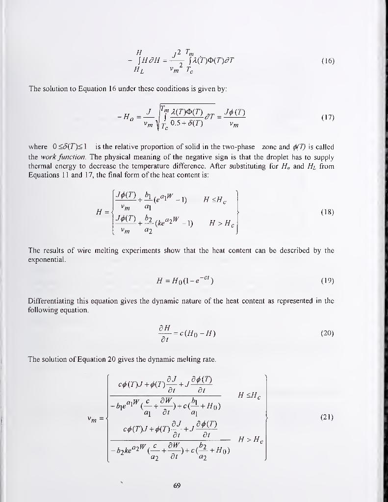
H J 2 T^i

(16)

The solution to Equation 16 under these conditions is given by:

-H^^^ fj^jTmT) ^^^J(f,{T)

(17)

m

where 0 <5{T)< 1 is the relative proportion of solid in the two-phase zone and (j)(T) is called

the work function. The physical meaning of the negative sign is that the droplet has to supply

thermal energy to decrease the temperature difference. After substituting for Ha and Hl from

Equations 1 1 and 17, the final form of the heat content is:

H ^1^ + ^(yt.^2^-l) H>H,(18)

The results of wire melting experiments show that the heat content can be described by the

exponential.

H^H^{\-e-'') (19)

Differentiating this equation gives the dynamic nature of the heat content as represented in the

following equation.

dH~d7

-c(Ho-H) (20)

The solution of Equation 20 gives the dynamic melting rate.

c<p {T)J + (f>{T)— + Jdt ot

7 a^W , c dW. .b\ „ ^- Z^ie^l'" (— + --) + c (-L + //o

)

a\ ot a\

c<t>{T)J + (t>{J)— + Jot ot

-bike"^ (— +— ) + c(-^ + //o)^2 ^2

H<H,

H >H.

(21)

69

320

^310c^ 300i_

O 290o< 280

270

!!!!!!!!!

i i i 1 i i i i i

- Simulatitbn result

QQ ..6xp.eri.mknta.l reiu.lt.

1.2 1.4 1.6 1.

Time (s)

Figure 5. Simulation and experimental results for 30A increase in arc current.

Shepard's burn-off rate model [16] is also derived from this equation under appropriate

simplifying assumptions. He assumed that the work function is constant and the heat content for

the wire is above He {4 J/mm^ ). It is concluded from his assumptions that the power is dissipated

in a constant potential drop in the arc. By using his assumptions, the equation reduces to:

kiJ H >H,X-kjW

Under steady state conditions, this equation reduces to Lesnewich's equation [7].

- + k2LJ

(22)

(23)

Electrode Voltage Model

The current changes in the GMAW process cause significant temperature changes along the

electrode extension. These changes lead to a temperature-dependent resistance which produces

the electrode voltage drop. The basic equation for the resistance is given by:

(24)

70

1 1.5 2 2.5 3 3.5

Time (s)

1 1.5 2 2.5 3 3.5

Time (s)

Figure 6. Electrode voltage drop and comparison of simulation and experimental results for total

voltage.

The voltage drop is the product of the welding current and resistance of the electrode extension.

Vl-IRl (25)

Arc Voltage Model

There have been a number of models for the arc voltage model in the gas tungsten arc welding

(GTAW) and the GMAW processes. These models show that as the welding current is increased,

the relationship between the voltage and current is approximately linear. The arc voltage drop

can be modeled as

Varc-V^+R^I + EJ (26)

where Ra defines the current dependency of the arc voltage and Ea defines the length dependency

of the arc. The total voltage can be obtained by adding the electrode voltage drop and arc voltage

drop.

71

0^ 0 8 ' i i ' ' ^

1 1.5 2 2.5 3 3.5

Time (s)

Figure 7. Dynamic action integral and resistivity.

EXPERIMENTAL PROCEDURES

Welding experiments were structured to examine the dynamic nature of the electrode extension

and arc length from both electrical signal measurements and a high-speed video system (2000

frames/s). A 1.2mm (0.045") diameter ER705-2 steel wire and Argon+5%CO^ shielding gas

were used. The contact-tip-to-work distance (CTWD) was 20mm (3/4") and the travel speed was

set at 6 mm/s. The current and voltage signals were collected at 5000Hz. Using a constant

current power source with electrode positive, both square wave and sinusoidal perturbations, of

variable amplitude (20 A, 30 A and 40 A peak-to peak), were superimposed on the current to

allow measurement of changes in the electrode extension, arc length, and total vohage. The

square wave perturbations provided a direct measure of the time response of the electrode

melting.

RESULTS AND DISCUSSION

The model was tested by introducing 30A step changes to the arc current, as the wire feed rate

was constant at 140 mm/s. Comparison of the experimental and simulation resuhs is shown in

Figure 5. The electrode extension settles from an initial value of 13.5mm to 9.5mm in 0.4s.

Similarly, the arc vohage changes from 33.5 V to 36.5 V. The effect of electrode vohage drop

changes on the dynamic behavior of the process can be seen in Figure 6. As shown, the vohage

suddenly decreases to about 2.3 V and increases to about 4. 1 V during the current transition. This

72

shows that the electrode voltage drop is a significant factor in the dynamic response of the

process. Figure 7 shows the dynamic behavior of the action integral and resistivity. From the

figure, it can be seen that the resistivity of the wire can not be assumed to be constant during the

current transition.

180

9 10 11 12 13

Electrode Extension (mm)

1 1.5 2 2.5

Time (s)

Figure 8. Phase plain analysis and dynamic melting rate.

In order to examine motion

trajectories corresponding to

various initial conditions and

information concerning the

system stability, a phase plane

analysis was made. As seen in

Figure 8, the initial point

(13.5mm) for the electrode

extension is moved to another

point (9.5mm) in the phase

plane. Oscillatory behavior of

the curve results from the

dynamic resistance changes in

the electrode extension.

Figure 9 illustrates the

relationship between droplet

frequency and arc current. The

500

450

400

uc

350

Q)

Ul 300

8-250

200

,0"

... ©r'

Wire feedrate= 140 mm/s\A/ire= 1.2mm mild steel ^Shielding gas=Argon +5%CO^

150240

-I L-

250 260 270 280 290

Arc Current (A)

300 310 320

Figure 9. Relationship between droplet frequency and arc

current.

73

droplet frequency increases markedly at the transition from globular to drop spray transfer, and

at the transition from drop spray transfer to streaming spray transfer.

An interesting aspect of the high-speed video

system used in capturing the experimental

electrode extension dynamics is its ability to

capture the power source and droplet

dynamics as well. Power spectrum analysis of

a single pixel corresponding to the high-speed

video is illustrated in Figure 10. As seen, the

frequency components are at 120Hz, 240Hzand 320Hz. These results match results of the

same analysis for the arc current. The high-

speed video system has been shown to be

capable of capturing the dynamics of the

power supply and the process itself, and it

can also be used to detect the droplet transfer

frequency.

;0:.6:a

0.00 _i

100,0 150 0 200,0 250,0 300,0 350.0 400J:

Figure 10. Power spectral density of the pixel

of high-speed films

CONCLUSIONS

A dynamic model of the GMAW process has been developed and tested by comparing

simulations to experimental results. The model is applicable to both constant potential and

constant current modes (including pulse current) of the GMAW process. The dynamic model

developed in this work is essential to development of a truly adaptive arc length regulation with

the pulsed current GMAW process.

P

X

o

J

V

NOMENCLATURE

Density {g / mm^ )

Thermal conductivity ( W/(mm K) ) To

Work function ( F)

Resistivity of wire ( Q mm )

Current density {A / mm'^

)

Wire feed rate ( mm / s)

Melting rate ( mm / s)

Cp Specific heat capacity {J / (g K))

H Heat content {J/mm )

Ho Melting heat content {J/mm^

)

WVl

Varc

ki2

anhn

Ha

Hl

T

Melting temperature (K)

Initial temperature {K)

Action integral {J / ( f2mm'^ ) )

Voltage drop along electrode extension (V)

Arc voltage drop (V)

Coefficients of Lesnewich's equation

Coefficients of the resistivity

Anode heating content ( J/mm )

Joule heating content (J /mm )

Temperature {K)

74

REFERENCES

1. Cook, G. E., Andersen K. and Barrett R.J. 1992. Keynote Address. Feedback and

Adaptive Control in Welding. International Trends in Welding Science and Technology ^

ASM International, 891-s to 903 -s.

2. P. Zhu and J.J. Lowke; 1993. Theoretical study of the melting of the cathode tip of a free

burning arc in argon for various conical angles. J. Phys. D: Appl Phys, (26): 1073-1079.

3. Halmoy, E., Pulsating Welding Arc, SINTEF Report STF16-A7902L Trondheim,

Netherlands.

4. Bingul, Z.1996. Stability Considerations for the Gas Metal Arc Welding Process , M.S.

Thesis, Vanderbilt University.

5. Bingul, Z., Cook, G. E., Barnett, R. J., Strauss, A. M., and Wells, B. S., 1998. AnInvestigation of Constant Potential GMAW Instability Behavior, 5**^ International

Conference on Trends in Welding Research.

6. Cook, G. E., 1998. Decoupling of Weld Variables for Improved Automatic Control,

International Conference on Trends in Welding Research.

7. Lesnewich, A., 1958. Control of Melting Rate and Metal Transfer in Gas-Shielded Metal-

Arc Welding; Part 1 - Control of Electrode Melting Rate, Welding Journal 37 (8): 343-s

to353-s.

8. Halmoy, E., 1979. Wire melting rate, droplet temperature, and effective anode melting

potential, Proc. Int. Conf On Arc Physics and Weld Pool Behavior , The Welding

Institute, Cambridge, UK.

9. Wilson, J. L. and Claussen, G. E., 1956. The Effect of I^R Heating on Electrode Melting

Rate, Welding Journal 35(1): 1-sto 8-s.

10. Waszink, J. H. and van den Heuvel, G. J. P. M., 1982. Heat Generation and Heat Flow mthe Filler Metal in GMA Welding, Welding Journal 61(8): 269-s to 282-s.

11. Quintino, L. and Allum, C. J., 1984. Pulsed GMAW Interactions Between Process

Parameters, Part 1," Welding andMetal Fabrication ^ March.

12. Amin, M., 1983. Pulse current parameters for arc stability and controlled metal transfer in

arc welding, Metal Construction , May.

13. Amin, M., 1986. Microcomputer control of synergic pulsed MIG welding," Metal

Construction , April.

14. Smati, Z., 1986. Automatic pulsed MIG welding. Metal Construction , January.

15. Richardson, M. I., Bucknall, P. W., and Stares, I., 1994. The Influence of Power Source

Dynamics on Wire Melting Rate in Pulsed GMAW Welding, Welding Journal, 73(2): 32-

s to 37-s.

16. Shepard, M E., 1991. Modeling of Self-Regulation in Gas-Metal Arc Welding , Ph.D.

Dissertation.

17. Quinn, T. P. and Madigan, R. B., 1993. Dynamic Model of Electrode Extension for Gas

Metal Arc Welding, International Trends in Welding Science and Technology, ASMInternational, 1003- 1008, 1993.

18. Mao, W. and Ushio, M., 1997. Measurement and theoretical investigation of arc sensor

sensitivity in dynamic state during gas metal arc welding," Science and Technology of

Welding and Joining. 2(5): 191-198.

19. Shepard, M. E. and Cook, G. E., 1993 . A Frequency-Domain Model of Self-Regulation in

Gas-Metal Arc Welding, International Trends in Welding Science and Technology, Eds:

S. A. David and J. M. Vitek, ASM International, 899-903.

75

EMPIRICAL MODELS FOR GMAW FILLET WELD PROFILES

D. Barborak', R. Richardson', D. Farson', and H. Ludewig*

ABSTRACT

Response Surface Methodology (RSM) with regression modeling was utilized to develop process

models for use in a closed-loop multivariate weld geometry control system. A D-Optimal

experimental design of 140 single-pass GMAW fillet welds was conducted with twelve process

variables. This Resolution V experimental matrix allowed all main and two-factor effects to be

determined without confounding. The ranges for these factors were centered around an optimal

welding procedure developed from screening experiments in order to develop a locally accurate

model. The response variables measured were various aspects of the welds' profile including leg

lengths, convexity/concavity, theoretical throat and weld toe angles. Analysis of Variance

(ANOVA) and correlation was used to identify important process inputs and linear least-sqaures

regression was used to fit input/output relationships. A second-order quadratic equation was

developed for each geometric weld feature. These equations were then embedded into software

that allowed visualization of the process behavior through Dynamic Response Surface (DRS)

plots. These dynamic response surface plots were used to study the effects of commonlyencountered disturbing inputs such as variations in root gap or CTWD.

KEYWORDS

GMAW, Fillet Weld, Weld Geometry, Weld Profile, Modeling, Design-of-Experiments, Least

Squares Regression, Response Surface Methodology

INTRODUCTION

The basic objectives of applying closed-loop control in automated GMAW applications is to

ensure that the desired weld properties are achieved i.e. desired weld geometry, microstructure,

mechanical properties and minimal discontinuities. For most automated applications, open-loop

control alone is not sufficient to overcome variations in these properties due to a variety of

disturbances. Closed-loop control is desired to overcome these deficiencies. From the

standpoint of feedback control, the GMA welding process present three principle challenges:

1 . In most cases, the relationships between the process inputs and outputs are non-linear.

2. The process inputs and outputs are generally highly related.

3. Not all ofthe disturbing inputs nor their effects on process outputs are known.

A relatively straightforward approach to closed-loop control system design for welding is to

manipulate one process input (such as travel speed or wire feed speed) to control the value of one

weld property. In this single-variable control, the other weld properties may fluctuate. This

technique is not suitable for weld geometry control because of the highly coupled nature of the

The Ohio State University

Caterpillar Inc.

76

welding process inputs that affect weld geometry. Therefore a multivariate control system is

required for weld geometry control. The challenge of a multivariable closed-loop control system

design is to use a process model to design a control law which maintains the response of the

process to within pre-specified tolerance limits despite the effects of uncertainty in the system.

GMAW Models

Theoretical process models for the Gas Tungsten Arc Welding (GTAW) Process has been the

focus of the majority of research in physical studies and model development for arc welding.

The principle reason is the lessor number of process inputs and cleaner experimental

environment for GTAW as compared to the consumable electrode processes such as GMAW.With the GTAW process, plasma arc physics and weld pool dynamics can be studied with the

heat source separated from metal transfer. Also, the experimental conditions are cleaner than

with consumable electrode processes where experimental measurements must deal with smoke,

spatter, and increased sensory noise due to the mass transfer of metal across the arc.

Only recently have the principals of analytical models from GTAW been extended to the

consumable electrode processes such as GMAW. The advances include the modeling of heat-

flow, microstructural evolution, thermal and residual stresses, and distortion based on the

welding parameters. However, accurate theoretical models for weld geometry, profile, or shape

do not exist due to the compUcated nature of weld pool phenomena such as fluid flow and effects

of electro-hydrodynamics for consumable arc welding processes.

Even with accurate theoretical models, a distinguishing characteristic of process models used for

control purposes is they must be computable in real-time. Thus, most of the numerical models

such as finite element or finite difference methods cannot be applied. Another important aspect

of models utilized for control is they generally need to provide both static and dynamic process

information.

There has been research focused on developing empirical models for weld geometry. These

models derive the relationships between process inputs and outputs with model coefficients

chosen to minimize the error between the model prediction and experimental data. The majority

ofthis research has focused on the development of static linear regression models. These models

are typically developed using statistical experimental design techniques' to predict weld

geometry during steady state conditions. Examples of this research include modeling bead-on-2 3

plate weld geometry '

, and modeling the geometry of consumable electrode processes other than

GMAW*'^'^'^. a few specific studies on modeling fillet weld geometry have been conducted^'^.

The development of a robust multivariate control system for weld geometry requires an accurate

model with both statics and dynamics. PreUminary work on dynamic models has been

conducted using system identification techniques'^ that can predict weld geometry changes

during transient conditions. These studies measured the response of the weld pool and final weld• 11 12

shape in real-time to step changes inputs and sinusoidal inputs to the welding parameters '.

77

RESULTS AND DISCUSSION

In this work, experiments were conducted in three phases with an initial screening experiment,

main experimental run, then augmented experimental runs. The data analysis consisted of

several techniques including Analysis of Variance, Regression Modeling, and Response Surface

Methodology.

Experimental Setup

Tests were conducted with a 6-axis articulated arm welding robot interfaced with a 600 amppower supply. A non-restrained welding fixture was utilized to hold the T-joint in a flat IF or

downhand position during welding. Tests were conducted with a standard 0.052 inch( 1.32mm)

diameter ER70-S3 wire with 90%Argon- 10%CO2 shielding gas. The material was standard

ASTM A36 steel in various thickness' with the T-joint configured from 24 x 12 inch(61 x 15cm)

plates.

A data acquisition system was utilized to verify voltage, current, and wire feed speed during

welding. All welds were scanned with a laser-based machine vision metrology sensor to digitize

the solidified weld profile. Once the weld surface was digitized, a machine vision algorithm then

calculated various geometric features of the weld face along its length. These features and their

description are as follows:

• Leg Lengths - the distance from the joint root to the weld toe.

• Theoretical Throat - the distance from the beginning of the joint root perpendicular to

the hypotenuse of the largest right triangle that can be inscribed within the cross

section of the fillet weld.

• Convexity/Concavity - the maximum distance from the face of the weld

perpendicular to a line joining the weld toes.

• Toe Angles - the angle formed at the junction of the weld face and the base metal.

Because these variables are being used in the development of a weld geometry control system,

the individual leg lengths and toe angels were combined to form a "additive leg length",

"differential leg length", "additive toe angle" and "differential toe angle". These variables

provide a better picture of the symmetry and magnitude of each weld feature to model for the

control system. Geometry weld features such as penetration profile and sidewall ftision were

ignored because they could not be directly measured in real-time for use in control. A summaryof the response variable nomenclature for the experiments is shown in Table 1

.

Table 1 Response Variables.

Description Notation Units

Additive Leg Length ALL mmDifferential Leg Length DLL mmAdditive Toe Angle ATA degrees

Differential Toe Angle DTA degrees

Theoretical Throat TT mmConvexity/Concavity CVCC mm

78

Experimental Design

The Design of Experiments (DOE) approach was chosen because the data involved has

experimental error and contains process noise. Therefore, statistical analysis is the only

objective approach to the analysis. To use Response Surface Methodology, all factors had to be

varied with at least three levels in order to allow non-linearity's in the model. Also, to know the

main effects and two-factor interactions without aliasing and confounding, the experimental

design had to be of resolution V. This allowed construction of a fiiU quadratic model for each

response variable. An initial screening experiment was performed to fmd a baseline welding

procedure that produced acceptable welds with the desired geometric shape. Based on the results

of the screening experiment thirteen factors were chosen. In order to reduce the number of

experimental runs to be conducted. Voltage and Wire Feed Speed were treated as covariates i.e.

they were varied together linearly, and were combined to form what was called the Power

Setting Pair (PSP). Also, the three weaving parameters were combined to form a block in the

experimental design.

For the experiment, the twelve factors were to be varied in a combination of three levels each in

order to form a full quadratic model. This required that at least 91 (l+2*12+12(12-l)/2 = 91)

distinct tests or runs be conducted. Various experimental designs are compared in Table 2.

While it is recommended that a standard design such as the Central Composite (CCD) or Box-

Behhnken (BBD) be used, this is not usually practical for welding applications because of the

large number of experiments required. An alternative is to use a saturated or nearly saturated

design that requires near the minimal amount of runs as calculated above. These design types

include the small-composite (SCD), Koshal designs, hybrid designs, or optimal designs. The D-

optimal design criteria*^''*''^ was used here because it produces the absolute minimum number of

experiments required to estimate the second order model with a resolution of V. By adding nine

center points, the initial experimental design totaled 1 00 tests.

Table 2 Experimental Designs and Their Required Number of Tests.

Design Notation # Tests

Full Factorial Design 3.2 531,441

Res.V Central Composite Design 2'^+2*l2+5 4125

Res.IV Central Composite Design 212-1+2*12+5 2077

Box-Behnken Design 2'* 12+5 101

D-optimal Design D*^ 91

After analysis of the data from the original experimental design, it was decided to augment the

experimental matrix by adding an additional 41 tests. This augmentation accounted for slower

travel speeds down to 7 inches/minute, while the original experimental matrix went no slower

than 10 inches/minute. The GMAW variables with their corresponding ranges and levels utilized

for the experiment are shown in Table 3

79

Table 3 DOE Variables, Range and Levels.

Variable Notation Range Units Factor Levels

Voltage PSP 31.5 to 34.5 volts 3

Wire Feed Speed PSP 375 to 425 inches/minute 3

Travel Speed TS 7 to 12 inches/minute 5

Torch Offset TO -1.3 to 1.3 mm 3

Root Gap GAP Oto 1.25 mm 2

Plate Thickness PT 6 to 24 mm 4

CTWD CTWD 25 to 30 mm 2

Travel Angle TA -15 to -5 degrees 3

Work Angle WA -5 to 5 degrees 3

Part Angle PA 6 to 10 degrees 3

Weave Amplitude WVA Oto 8 mm 3

Weave Frequency WVF Oto 1 Hz. 3

Weave Dwell WVD 0 to 0.2 seconds 3

Factor Significance

In order to determine which variables significantly affected the various weld geometry, features

two techniques namely ANOVA and Correlation analysis were utilized. The confidence interval

was chosen to be 95% (a=0.05) to provide a 95% or more certainty that a variable significantly

affects a response. Analysis of Variance or ANOVA techniques help to determine the effects of

a parameter on a response by partitioning the total variance into its component parts. Variance

analysis permits the differentiation between significant and insignificant parameters where

comparison of means plays a key role. The correlation coefficient is a measure of the degree of

linear relationship between two variables or a factor and response.

A summary of the response variables, and the significant factors is shown in Table 4. The main

significance level was 95%, with factors showing at least 90% significant in parenthesis. Someof the cause-and-effect relations are intuitive such as the effect of Power Setting Pair (PSP), and

Travel Speed (TS) on Additive Leg Length (ALL). Other relations such as the absence of Torch

Offset (TO) affect on Differential Leg Length (DLL), and Differential Toe Angle (DTA).

Experience would say that any offset of the torch from the weld centerline should affect weld

symmetry, which would show up in these responses.

Table 4 Significant Factors.

Response Variable Significant Factor, a=0.05(a=0.1)

ALL PSP, TS, GAP, PT, (WEAVE)DLL TS, GAP, PT, WA, (PA)

ATA TS, GAP, PT, PA, (TA)

DTA GAP, (TS), (PT), (PA)

TT PSP, TS, PA, (TO)

CVCC TS, GAP, PT, TA, PA, (WEAVE)

80

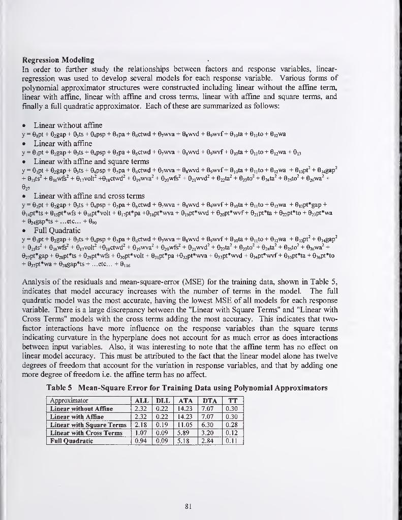
Regression Modeling

In order to further study the relationships between factors and response variables, linear-

regression was used to develop several models for each response variable. Various forms of

polynomial approximator structures were constructed including linear without the aflfine term,

linear with aflfine, linear with affine and cross terms, linear with afflne and square terms, and

finally a full quadratic approximator. Each of these are summarized as follows:

• Linear without aflfine

y = 0ipt + Szgap + Qsts + Q^psp + Q^pa + GeCtwd + Qjwva + Ggwvd + 09wvf + Giota + Guto + 0i2wa

• Linear with affine

y = 9ipt + 62gap + Gats + 94psp + Sspa + Sgctwd + Qywva + Ggwvd + Ggwvf + Giota + Guto + G,2wa + G13

• Linear with aflfine and square terms

y = Gipt + G2gap + Gsts + G4psp + Gspa + GeCtwd + Qjwva + Ggwvd + Ggwvf + Giota + Guto + G^wa + Gispt^ + Gngap^

+ Gijts^ + 0i6wfs^ + Gnvolt^ +Gi8Ctwd^ + Gigwva^ + Gjowfs^ + G2iwvd^ + G22ta^ + G23to^ + G24ta^ + 62510^ + 026wa^ +

627

• Linear with aflfine and cross terms

y = 9ipt + G2gap + Gsts + G4psp + Gspa + GeCtwd + Gywva + GgWvd + Ggwvf+ Giota + Guto + G^wa + Gi3pt*gap +

Gi4pt*ts + Gi5pt*wfs + Gi6pt*volt + Gi7pt*pa +Gi8pt*wva + Gi9pt*wvd + 02opt*wvf+ G2ipt*ta + G22pt*to + G23pt*wa

+ G24gap*ts + ...etc... + G90

• Full Quadratic

y = Gipt + G2gap + Gsts + G4psp + Gspa + GeCtwd + Gywva + GgWvd + G9wvf + Giota + Guto + G^wa + Gupt^ + Gi4gap^

+ Gists^ + Giewfs^ + Gnvolt^ +Gi8Ctwd^ + Gigwva^ + G2owfs^ + Gjiwvd^ + G22ta^ + G23to^ + G24ta^ + G25to^ + G26wa^ +

G27pt*gap + G28pt*ts + G29pt*wfs + G3opt*volt + G3ipt*pa +G32pt*wva + G33pt*wvd + G34pt*wvf+ G35pt*ta + 036pt*to

+ G37pt*wa + G38gap*ts + ...etc... + Que

Analysis of the residuals and mean-square-error (MSE) for the framing data, shown in Table 5,

indicates that model accuracy increases with the number of terms in the model. The full

quadratic model was the most accurate, havmg the lowest MSE of all models for each response

variable. There is a large discrepancy between the "Linear with Square Terms" and "Linear with

Cross Terms" models with the cross terms adding the most accuracy. This indicates that two-

factor interactions have more influence on the response variables than the square terms

indicating curvature m the hyperplane does not account for as much error as does interactions

between mput variables. Also, it was interesting to note that the aflfine term has no effect on

linear model accuracy. This must be attributed to the fact that the linear model alone has twelve

degrees of freedom that account for the variation in response variables, and that by adding one

more degree of freedom i.e. the aflfine term has no affect.

Table 5 Mean-Square Error for Training Data using Polynomial Approximators

Approximator ALL DLL ATA DTA TTLinear without Affine 2.32 0.22 14.23 7.07 0.30

Linear with Affine 2.32 0.22 14.23 7.07 0.30

Linear with Square Terms 2.18 0.19 11.05 6.30 0.28

Linear with Cross Terms 1.07 0.09 5.89 3.20 0.12

Full Quadratic 0.94 0.09 5.18 2.84 0.11

81

Dynamic Response Surface Software

Response Surface Methodology (RSM) is a collection of statistical and mathematical techniques

usefiil for studying process behavior. RSM shows graphically, the relationship between the

process inputs and process outputs. Because of its graphical nature, only three dimensions or

less can be visualized at one time i.e. the effect of two input variables and their interaction on a

single response variable or process output. Higher order relations (i.e. greater than three degrees

of freedom) are simplified to 3 dimensions for visualization. First order models are used for

linear approximations while higher order models such as a full quadratic can show curvature.

While such models are reasonably accurate for a small experimental region such as the 141 run

DOE, they can be quite inaccurate over larger experimental regions such as in broader screening

experiments.

In order to aid in the visualization of the complex relationships between variables such as in

welding. Dynamic Response Surface (DRS) software was developed using Matlab^"^. The DRSsoftware contained a graphical user interface that allowed the user to generate the 3-D response

surface of any two process inputs and process response variables (Figure 1). Then the user can

manipulate the other process inputs to see their effect on the chosen relationship. The fiiU

quadratic models developed in the previous section were incorporated in the DRS software.

Figure 1 shows the relationship between Additive Leg Length (ALL), Power Pair (PP), and

Travel Speed (TS). The response surface basically indicates that the higher the wire feed speed

or slower the travel speed, the larger the leg lengths become, as would be expected from

experience.

The graphical user interface of the DRS software (Figure 1) shows all of the process input

variables on the left, the response surface plot in the middle, and the modeled process response

variables on the right. The user can choose any variables to plot by choosing its corresponding

check box. The controls allow the user to manipulate the other variables in the model to see the

effect on the chosen response surface. Another software feature is the optimized search were the

software will search within the model region for the optimized welding procedure based on the

constraints chosen by the user. The search method utilized is steepest descent gradient.

82

4 I

Fillet Weld Model (c)1 998-39 The Ohio State Univers

Ste Edit loote vyn(*3w befp

mora

Vottaqa:

WFS.

1 PowerPoir 3

J J10 Travd Speed 12

''J J J-13 Torch Offset 13

rjj J ll

0 Giso 1-25

6 Plate Thickness 24

r A

25 CTWD

r J J-15 Trawel Anqle

-5 WorkAnqle

r J J6 PertAnqle

0 WsoveMiplitude 8

0 Weave Frequency 1

D Weave Dwell 0.2

±J30

J-5

ll

5

J10

1315

I4O0

24

i27.7

-15

Response Surfece

Quit!I

Rip Axis!|OPTIMAL

|

AdditivB Leq Lenqth

! 20.4

OifferentiQl Leq Lenqth

rI 0.49

Additive Toe Anqle

r 1279.'

Differential Toe Anqle

r j 4.24

Theoretical Thto«»t

r [TtT

Conve»ty^Concevity

ri0.40

Figure 1 DRS response surface for Additive Toe Angle as a function of Power Pair and

Travel Speed.

The some of the response surfaces such as Figure 1 appear very linear, other response surfaces

such as shown in Figure 2 are highly non linear. In Figure 2, the Differential Leg Length (DLL)

is plotted as a function of Torch Offset (TO) and Work Angle (WA). This response surface

basically indicates that the fiirther the Torch Offset or Work Angle are from the center position

in the joint, the more asymmetric the weld becomes as their leg lengths differ. In fact, for all

combinations of Torch Offset and Work Angle with all other parameters held fixed at their

current values, one leg is always larger than the other. This was a trend present within most of

the experimental region. It should be noted that the range for Torch Offset and Work Angle

during these experiments were fixed relatively small, and that extreme values of either would

certainly skew the weld symmetry in the corresponding opposite direction. The fact that this

trend was present throughout most of the experimental region leads the belief that other

phenomena is affecting the weld symmetry.

83

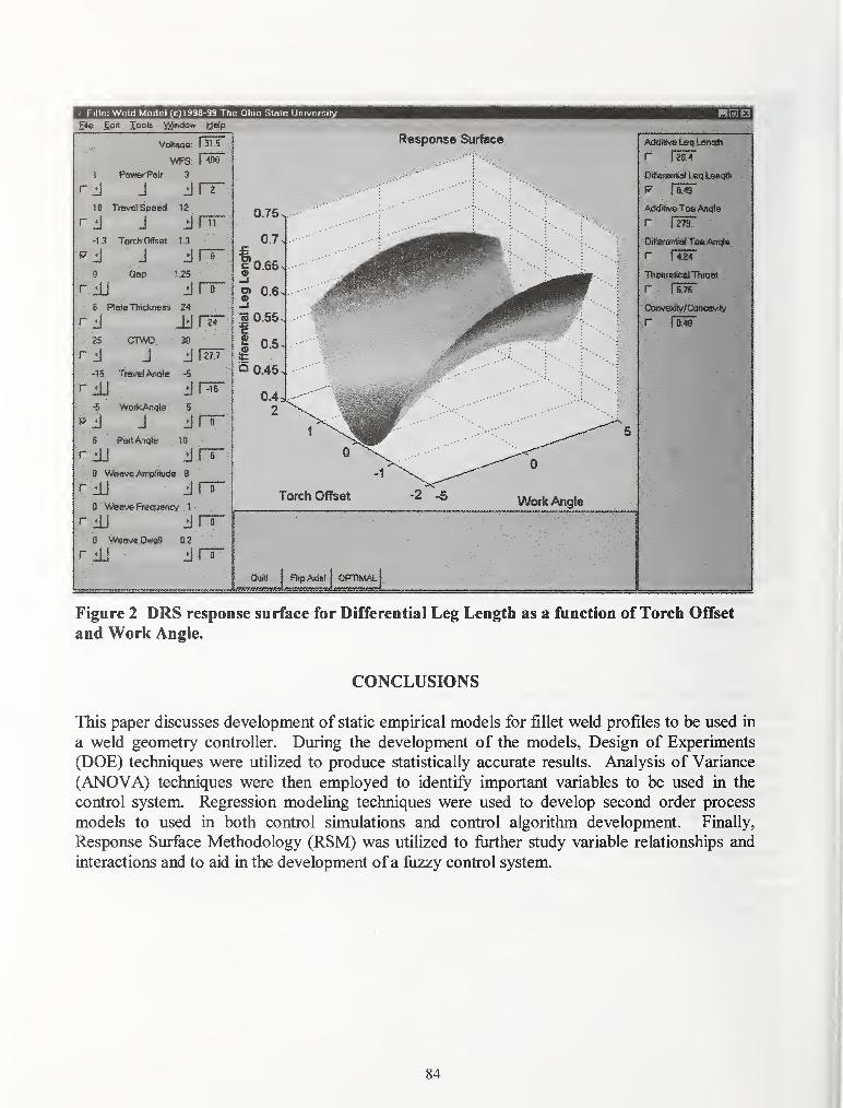
Bte £dtt Tosts ^wdGw lielp

Vottaqe:

WFS:

1 PowerPttir 3

J10 Travel Speed

r J J-T3 Torch Offset

^ J JGao

!31S

: 400

0

1-3

J1.25

J6 Plate Thickness 24

±1CTWD

Treivel Anqle

25

-15

-5

S

WofkArtcite

JPartAnqle

30

Jj

-5

Jj

5

10

277

-IS

0 Weave Amplitude 8

0 Weave Frequencv 1

Response Surface

0.75

0.7

to.65IB—I

g> 0.6-J

S 0.55

I 0.5

Q 0.45

Additive Leq Lentjfh

r rioT

DifferenW Leq Lenqth

W f 0.49

Additive Toe Anqle

r 1 279.

DifierenSal Toe Anqls

r 1 4.24

Theoretical Throat

r rsTs"

Convexitv/Concavity

ri 0.40

Figure 2 DRS response surface for Differential Leg Length as a function of Torch OfTset

and Work Angle.

CONCLUSIONS

This paper discusses development of static empirical models for fillet weld profiles to be used in

a weld geometry controller. During the development of the models. Design of Experiments

(DOE) techniques were utilized to produce statistically accurate results. Analysis of Variance

(ANOVA) techniques were then employed to identify important variables to be used in the

control system Regression modeling techniques were used to develop second order process

models to used in both control simulations and control algorithm development. Finally,

Response Surface Methodology (RSM) was utilized to further study variable relationships and

interactions and to aid in the development of a flizzy control system.

84

REFERENCES.

^ Montgomery, D.C. 1997. "Design and Analysis of Experiments", ISBN #0471157465, John Wiley &Sons Inc.

^ Kim, I.S., Siores, E., and Basu, A. 1993. "Relationships Between Process Parameters and Weld BeadGeometry for GMAW Process", Proc. 41^. WTIA/AINDT Fabocn/Fabfair Conf . Wollongong Astralia.

^ Kumar, R.S., and Pannar, R.S. 1986. "Weld Bead Geometry Prediction for Pulse MIG Welding", Proc.

Int. Conf. on Advances in Welding Science and Technology . ASM International.

'* McConnell, I.A., and McPherson, N.A. 1997. "The Application of Statistical Process Design to a FCAWProcess", Welding Journal, 76(10)412s-416s.

^ Raveendra, J., and Pannar, R.S. 1987. Mathematical Models to Predict Weld Bead Geometry for Flux

Cored Arc Welding", Metal Construction . 19(1)31 R-35R.

^ McGlone, J.C., 1982. "Weld Bead Geometry Prediction - A Review", Metal Construction . 14(7)378-384.

^ Salter, G.R., and Doherty, J. 1981. "Procedure Selection for Arc Welding", Metal Construction .

13(9)544-550.

® Moon, H-S., and Na, S-J. 1996. "A Neuro-Fuzzy Approach to Select Welding Conditions for WeldingQuality Improvement in Horizontal Fillet Welding", Journal of Manufacturing Systems . 15(6)392-403.

^ Barton, D.J. 1997. 'The Effect of GMA Process Variables on Weld Quality", Proc. SAE Conf. onEarthmoving Industry , paper #981522, Society of Automotive Engineers.

^° Ljung, L 1999. "System Identification - Theory for the User", ISBN# 0136566952, Prentice-Hall Inc.

" Hale, M.B. and Hardt, D.E. 1990. "Multivariable Geometry Control of Welding - Part I: Process

Modeling", Proc. Svmp. On Manufacturing Process Modeling and Control . ASME.

Hellinga, M.C., Huissoon, J. P., and Ken", H.W. 1996. "Identifying Weld Pool Dynamics for GMAW'.Proc. 6"^

Int. Conf. on Computer Technology in Welding . TWI.

Atkinson, A.C. and Donev, A.N. 1992. "Optimum Experimental Designs". Oxford Science Publications .

'^^Nguyen, N-K. and Miller, A.J. 1992. "A Review of Some Exchange Algorithms for Constructing

Discrete D-Optimal Designs", Computational Statistics and Data Analysis 14(1992)489^98.

Mitchell, T.J. 1974. "An Algorithm for the Construction of D-Optimal Experimental Design",

Technometrics 16(2)203-219.

85

APPENDIX

ALL = 35.4 + 2.85*psp - 2.65*ts + 3.96*to - 0.52*gap - 0.417*pt - 0.122*ctwd - 0.058*ta +

0.567*wa + 0.83*pa - 1.15*wva + 25.3*wvf - 2.9*wvd - 0 . 267*psp*psp + 0.133*ts*ts + 0.432*to*to +

0.0113*pt*pt + 0.0017*ta*ta - 0.0070*wa*wa - 0.120*pa*pa + 0 . 0172*wva*wva - 11.8*wvf*wvf +

0.0109*psp*ts + 0.039*psp*to - 0 . 097*psp*gap - 0 . 0112*psp*pt - 0 . 0268*psp*ctwd - 0 . 0315*psp*ta -

0.0166-*psp-*wa - 0.0665*psp*pa + 0 . 0909*psp-*wva - 0 . 766*psp-*wvf - 0.37*psp*wvd - 0.0646*ts*to -

0.013*ts*gap - 0.0079*ts*pt - 0 . 0288*ts*ctwd + 0.0196*ts*ta - 0.0105*ts*wa + 0.0289*ts*pa +

0 . 0272*ts*wva - 0.403*ts*wvf - 0.83*ts*wvd - 0.552*to*gap - 0.0067*to*pt - 0 . 0655*to*ctwd +

0.0007*to*ta + 0.122*to*wa - 0.139*to*pa - 0 . 0331*to*wva + 0.001*to*wvf - 0.61*to*wvd -

0.0685*gap*pt + 0 . 001*gap*ctwd - 0 . 0110*gap*ta - 0 . 0467*gap*wa + 0.266*gap*pa - 0 . 169*gap*wva +

0 . 647*gap*wvf + 3.54*gap*wvd + 0 . 0071*pt*ctwd + 0 . 001 69*pt*ta + 0 . 00322*pt*wa + 0.0056*pt*pa -

0 . 00588*pt*wva - 0 . 0444*pt*wvf - 0.248*pt*wvd - 0. 0094 *ctwd*ta - 0 . 0176*ctwd*wa + 0 . 0331*ctwd*pa- 0 . 0015*ctwd*wva - 0 . 152*ctwd*wvf - 0 . 326*ctwd*wvd - 0 . 00385*ta*wa + 0.0230*ta*pa -

0.0122*ta*wva - 0.015*ta*wvf + 0.394*ta*wvd - 0.0081*wa*pa - 0 . 0011*wa*wva - 0.036*wa*wvf +

0.055*wa*wvd - 0 . 0088*pa*wva - 0.335*pa*wvf + 1.47*pa*wvd + 0 . 739*wva*wvf + 1.65*wva*wvd -

3.29*wvf*wvd

DLL = 1.29 + 0.23*psp - 0.115*ts - 0.318*to - 0.29*gap + 0.137*pt + 0.092-'ctwd - 0.102*ta +

0.057*wa - 0.818*pa - 0.520*wva + 7.36*wvf - 5.57*wvd + 0 . 034*psp*psp + 0.0064*ts*ts +

0.0952*to*to - 0.00178*pt*pt - 0 . 00399*ta*ta - 0 . 00239*wa*wa + 0.0435*pa*pa + 0 . 0131*wva*wva -

5.17*wvf*wvf + 0.0139*psp*ts + 0 . 0445*psp*to + 0 . 0623*psp*gap + 0 . 00556*psp*pt - 0 . 0224*psp*ctwd- 0.0008*psp*ta - 0 . 0110*psp*wa + 0 . 0063-*psp*pa + 0 . 0005*psp*wva - 0 . 074*psp*wvf + 0 . 006*psp*wvd+ 0.0822*ts*to + 0 . 0692*ts*gap - 0 . 00357*ts*pt + 0 . 0069*ts*ctwd + 0 . 00966*ts*ta - 0 . 00426*ts*wa -

0.0217*ts*pa + 0 . 0012*ts*wva - 0.029*ts*wvf - 0.220*ts*wvd + 0.181*to*gap + 0 . 00716*to*pt -

0.0112*to*ctwd + 0.0157*to*ta - 0 . 00434*to*wa - 0.0489*to*pa - 0 . 0081*to*wva + 0.048*to*wvf +

0.410*to*wvd - 0.0059*gap*pt - 0 . 0243*gap*ctwd - 0 . 0064*gap*ta + 0 . 0202*gap*wa + 0 . 0001-*gap*pa +

0 . 0129*gap*wva - 0 . 258*gap*wvf + 1.20*gap*wvd - 0 . 00376*pt*ctwd - 0 . 00101*pt*ta - 0 . 00105*pt*wa +

0.00523*pt*pa - 0 . 00315*pt*wva - 0 . 0015*pt*wvf - 0.071*pt*wvd - 0 . 00034*ctwd*ta + 0 . 00347*ctwd*wa- 0.0014*ctwd*pa - 0. 00089*ctwd*wva - 0. 0835*ctwd*wvf + 0 . 304*ctwd*wvd + 0 . 00245*ta*wa -

0.0101*ta*pa - 0 . 00598*ta*wva + 0 . 0535*ta*wvf + 0.113*ta*wvd - 0 . 00268*wa*pa + 0 . 00250*wa*wva -

0.0248*wa*wvf + 0.056*wa*wvd + 0 . 0060*pa*wva + 0.171*pa*wvf - 0.052*pa*wvd + 0 . 384*wva*wvf +

0.011*wva*wvd + 1.06*wvf*wvd

ATA = 342 - 8.9*psp - 9.53*ts - 2.42*to - 4.1*gap - 2.30*pt - 0.11*ctwd - 1.98*ta - 0.32*wa +

4.51*pa + 0.40*wva - 15.1*wvf - 71.0*wvd + 0.76*psp*psp + 0.304*ts*ts - 0.554*to*to +

0.0233*pt*pt - 0.0673*ta*ta + 0.0319*wa*wa - 0.325*pa*pa - 0 . 014 6*wa*wva + 11.4*wvf*wvf +

0.286*psp*ts - 0.184*psp*to + 0 . 161*psp*gap - 0 . 0058*psp*pt - 0 . 027*psp*ctwd - 0 . 137*psp*ta -

0.108*psp*wa + 0.122*psp*pa + 0 . 119*psp*wva - 0.47*psp*wvf + 3.22*psp*wvd - 0.208*ts*to -

0.818*ts*gap - 0.0010*ts*pt - 0 . 007*ts*ctwd - 0.0444*ts*ta - 0.0408*ts*wa + 0.096*ts*pa +

0.078*ts*wva + 0.96*ts*wvf + 3.87*ts*wvd + 0.723*to*gap - 0.0173*to*pt + 0 . 151*to*ctwd +

0.0504*to*ta - 0.0840*to*wa + 0.134*to*pa - 0.020*to*wva + 0.80*to*wvf + 0.67*to*wvd +

0.103*gap*pt + 0 . 372*gap*ctwd - 0.086*gap*ta + 0.051*gap*wa - 0.227*gap*pa - 0 . 014*gap*wva -

1.39*gap*wvf - 0.19*gap*wvd + 0 . 0339*pt*ctwd - 0.0015*pt*ta - 0.0090*pt*wa + 0.0460*pt*pa +

0 . 0194*pt*wva - 0.122*pt*wvf + 1.01*pt*wvd + 0 . 0340*ctwd*ta + 0 . 0215*ctwd*wa + 0.014*ctwd*pa -

0.0148*ctwd*wva - 0 . 294*ctwd*wvf - 0 . 24*ctwd*wvd + 0.0066*ta*wa + 0.0438*ta*pa + 0 . 0237*ta*wva -

0.248*ta*wvf + 0.19*ta*wvd + 0.0293*wa*pa + 0 . 04 65*wa*wva + 0.118*wa*wvf - l.ll*wa*wvd -

0.007*pa*wva + 0.371*pa*wvf + 1.76*pa*wvd - 1.03*wva*wvf - 0.31*wva*wvd - 14.2*wvf*wvd

DTA = 27.4 + 6.04*psp - 3.33*ts + 2.80*to - 9.33*gap + 0.367*pt - 0.12*ctwd - 0.27*ta + 1.22*wa -

3.11*pa - 1.07*wva + 22.3*wvf - 73.1*wvd - 1.05*psp*psp + 0.074*ts*ts + 0.416*to*to +

0.0091*pt*pt - 0.0181*ta*ta - 0.0344*wa*wa + 0.160*pa*pa + 0 . 0479*wva*wva - 19.6*wvf*wvf +

0.143*psp*ts + 0.375*psp*to + 0 . 686*psp*gap + 0 . 0385*psp*pt - 0 . 172*psp*ctwd - 0 . 0385*psp*ta -

0.0767*psp*wa + 0.038*psp*pa + 0.049*psp*VA7-a - 0.52*psp*wvf - 1.40*psp*wvd + 0.400*ts*to +

0.479*ts*gap - 0.0351*ts*pt + 0 . 107*ts*ctwd + 0.0329*ts*ta - 0.0331*ts*wa - 0.146*ts*pa +

0.0272*ts*wva - 0.085*ts*wvf + 0.97*ts*wvd + 0.903*to*gap + 0.0325*to*pt - 0 . 180*to*ctwd +

0.0746*to*ta - 0.0663*to*wa - 0.346*to*pa - 0 . 0456*to*wva + 0.424*to*wvf + 1.73*to*wvd -

0.055*gap*pt - 0 . 025*gap*ctwd - 0.069*gap*ta + 0.102*gap*wa + 0.383*gap*pa - 0 . 04 l*gap*wva -

1.24*gap*wvf + 12.4*gap*wvd - 0 . 0205*pt*ctwd - 0 . 00500*pt*ta - 0 . 00217*pt*wa + 0.0269*pt*pa -

0.0233*pt*wva - 0.006*pt*wvf - 0.500*pt*wvd + 0 . 0033*ctwd*ta - 0 . 0032*ctwd*wa - 0 . 0102*ctwd*pa -

0 . 0470*ctwd*wva - 0 . 218*ctwd*vfvf + 2 . 50*ctwd*wvd + 0.0164*ta*wa - 0.0500*ta*pa - 0 . 0403*ta*wva +

0.200*ta*wvf + 0.428*ta*wvd - 0.0311*wa*pa + 0 . 0206*wa*wva - 0.208*wa*wvf - 0.301*wa*wvd +

0.0143*pa*wva + 0.876*pa*wvf + 0.02*pa*wvd + 1.84*wva*wvf - 0.51*wva*wvd + 8.6*wvf*wvd

86

TT = 8.25 + 1.59*psp - 0.375*ts + 1.52*to - 0.21*gap - 0.005*pt - 0.064*ctwd + 0.045*ta +0.244*wa + 0.060*pa - 0.431*wva + 9.67*wvf + 1.8*wvd - 0 . 187*psp*psp + 0.0260*ts*ts + 0.162*to*to+ 0.00299*pt*pt + 0.00291*ta*ta - 0 . 00323*wa*wa - 0.0302*pa*pa + 0 . 00716*wva*wva - 4.83*wvf*wvf -

0.0036*psp*ts + 0.0283*psp*to - G . 0501*psp*gap - 0 . 00305*psp*pt - 0 . 0074 *psp*ctwcl - 0 . 0019*psp*ta+ 0.0009*psp*wa - 0 . 0310*psp*pa + 0 . 0238*psp*wva - 0 . 229*psp*wvf - 0 . 297*psp*wvd - 0.0087*ts*to +

0.0306*ts*gap - 0 . 00232*ts*pt - 0 . 0089*ts*ctwd + 0 . 00842*ts*ta - 0 . 0024 6*ts*wa + 0.0074*ts*pa +

0.0070*ts*wva - 0.173*ts*wvf - 0.595*ts*wvd - 0.237*to*gap - 0 . 00268*to*pt - 0 . 0300*to*ctwd +

0.0005*to*ta + 0.0452*to*wa - 0.0556*to*pa - 0 . 0102*to*wva - 0.055*to*wvf - 0.250*to*wvd -

0.0309*gap*pt - 0 . 0118*gap*ctwd - 0 . 0054*gap*ta - 0 . 0226*gap*wa + 0.120*gap*pa - 0 . 0652*gap*wva +0.349*gap*wvf + 1.12*gap*wvd + 0 . 00027*pt*ctwd + 0 . 00105*pt*ta + 0 . 00193*pt*wa - 0 . 00184 *pt*pa -

0.00238*pt*wva - 0 . 0184*pt*wvf - 0.130*pt*wvd - 0 . 004 62*ctwd*ta - 0 . 00866*ctwd*wa +

0.0139*ctwd*pa - 0 . 00068*ctwd*wva - 0 . 0335*ctwd*wvf - 0 . 073*ctwd*wvd - 0 . 00185*ta*wa +

0.00678*ta*pa - 0 . 00653*ta*wva + 0 . 0127*ta*wvf + 0.110*ta*wvd - 0 . 00303*wa*pa - 0 . 00363*wa*wva -

0.0146*wa*wvf + 0.067*wa*wvd - 0 . 0036*pa*wva - 0.146*pa*wvf + 0.524*pa*wvd + 0 . 319*wva*wvf +

0 . 581*wva*wvd - 0.12*wvf*wvd

CVCC = 1.86 - 0.112*psp - 0.347*ts + 0.234*to + 0.193*gap - 0.122*pt + 0.0105*ctwd - 0.0592*ta +0.0155*wa + 0.284*pa - 0.046*wva + 1.52*wvf - 1.98*wvd + 0 . 0102*psp*psp + 0.0159*ts*ts +

0.0281*to*to + 0.00159*pt*pt - 0 . 00203*ta*ta + 0 . 00019*wa*wa - 0.0218*pa*pa + 0 . 00066*wva*vfva -

0.585*wvf*wvf + 0.0078*psp*ts - 0 . 0127*psp*to - 0 . 0122*psp*gap - 0 . 00157*psp*pt -

0.00420*psp*ctwd - 0.00838*psp*ta - 0 . 00617*psp*wa + 0 . 0028*psp*pa + 0 . 0107*psp*wva -

0.0527*psp*wvf + 0 . 106*psp*wvd - 0.0157*ts*to - 0 . 0206*ts*gap - 0 . 00051*ts*pt -

0.00293*ts*ctwd + 0 . 00063*ts*ta - 0 . 00139*ts*wa + 0 . 00540*ts*pa + 0 . 00144*ts*wva + 0 . 0031*ts*wvf+ 0.092*ts*wvd - 0.0147*to*gap + 0 . 00024*to*pt + 0 . 00043*to*ctwd - 0 . 00007*to*ta + 0 . 00776*to*wa- 0.0077*to*pa - 0.00376*to*wva + 0 . 0279*to*wvf - 0.025*to*wvd - 0 . 00280*gap*pt + 0 . 0051*gap*ctwd+ 0 . 00145*gap*ta - 0 . 00144*gap*wa - 0 . 0008*gap*pa - 0 . 0118*gap*wva - 0.017*gap*wvf +

0.254*gap*wvd + 0 . 00215*pt*ctwd + 0. 000301*pt*ta + 0 . 000031*pt*wa + 0 . 00227*pt*pa +

0.00021*pt*vrva - 0.00397*pt*wvf + 0 . 0088*pt*wvd - 0. 00015*ctwd*ta - 0 . 00010*ctwd*wa +

0.00071*ctwd*pa - 0. 00024 *ctwd*wva - 0 . 0277*ctwd*wvf - 0 . 070*ctwd*wvd - 0 . 000268*ta*wa +

0 . 00240*ta*pa + 0 . 00018*ta*wva - 0 . 0094*ta*wvf + 0 . 0436*ta*wvd - 0.00075*wa*pa +

0.00156*wa*wva + 0 . 0032*wa*wvf - 0 . 0175*wa*wvd - 0 . 00077*pa*wva - 0 . 0033*pa*wvf + 0.196*pa*wvd +

0 . 0140*wva*wvf + 0.122*wva*wvd - 0.63*wvf*wvd

87

I

Session A3: Weld Shape and Distortion Modeling

NUMERICAL AND EXPERIMENTAL STUDY ON THE TRANSPORT PHENOMENAIN THE PLASMA ARC WELDING

H. G. Fan, R. Kovacevic, B. Zheng, H. J. Wang

ABSTRACT

A mathematical model is developed to describe the heat transfer and fluid flow in stationary

keyhole plasma arc welding. Using the Volume of Fluid (VOF) method, the processes of heating,

melting, collapsing and subsequent solidifying in the molten pool are dynamically studied. The

predicted results have been compared with the experimental weld and keyhole shape. Theoretical

predictions and experimental results are in close agreement, suggesting the theoretical treatment

of the model is good.

Keywords: Plasma welding. Numerical simulation, Keyhole mode.

INTRODUCTION

In plasma arc welding, a constricting plasma arc is used as the concentrated energy source to

melt the workpiece. Due to its high energy density, and its high velocity plasma jet, the plasma

arc welding process can produce deeper weld penetrations, faster travel speeds, and reduced

thermal distortions when compared with gas tungsten arc welding \ Plasma arc welding fusion

can be categorized as either melt-in or keyhole mode. The keyhole mode is the primary attribute

of plasma arc welding that makes it so attractive. In the keyhole-welding mode, as shown in

Figure 1, the plasma jet completely penetrates the weld pool, forming a symmetric, funnel-

shaped cavity called a keyhole, and a similarly shaped liquid-solid metal phase boundary. Somemathematical models on the prediction of weld and keyhole shapes have been developed for

electron beam and laser beam welding. But the mechanism of keyhole formation in these

processes is different from that in the plasma arc welding process. In plasma arc welding the

keyhole is produced and maintained mainly by the pressure of the arc plasma, rather than by the

recoil pressure of the evaporating metal as in electron beam and laser welding. Up to the present,

the most comprehensive models of plasma arc welding are Rubinsky's two-dimensional (2D)

and three-dimensional (3D) finite element simulation^ '^. The 2D quasi-stationary model neglects

surface tension effects and simplifies the pool geometry by assuming flat upper and lower free

surfaces and a keyhole of constant radius. The developed 3D steady model is used to predict the

weld pool shape based on heat transfer and fluid flow, while the keyhole shape is assumed

according to experimental results. Currently, theoretical study on the transient development of

the keyhole shape in plasma arc welding has not been found in the open literature.

In this paper, a two-dimensional, transient model is developed to describe the heat transfer and

fluid flow in keyhole plasma arc welding. In the model, the weld pool surface is depressed by the

arc pressure, and the fluid flow in the molten pool is induced by surface tension gradient,

electromagnetic force, and buoyancy force. The VOF (Volume of Fluid), modified to include

heat transfer and the electromagnetic force, was used to track the transient deformed shape of the

Department of Mechanical Engineering, southern Methodist University, PO Box 750337, Dallas, TX, 75275

91

weld pool surface. The processes of heating, melting, collapsing and subsequent solidifying are

simulated in the keyhole plasma arc welding. Experiments have been done with AISI 304

stainless steel. The resultant weld and keyhole shapes have been compared with the predicted

ones, which are in good agreement. This study may enhance our understanding of the heat

transfer related phenomena during plasma arc welding.

Shielding gas Plasma gas

Figure 1. Schematic of plasma arc and weld pool.

MATHEMATICAL FORMULATION

Governing Equations

In order to simplify the mathematical model, the following assumptions have been made:

(1) the welding process is restricted to the stationary plasma arc welding, and the system is

assumed to be axisymmetric;

(2) laminar flow is assumed;

(3) the thermophysical properties, listed in Table 1, are assumed to be constant;

(4) the fluid in the pool is driven by a combination of buoyancy, electromagnetic, and surface

tension forces; however, plasma jet shear is neglected;

92

Table 1. Physical Properties of the Workpiece

Symbol Value Symbol Value

B p 7200 kg/m^

Y 1.2 N/m 1.26x10-^ H/m0.006 kg/m.s a 7.7x1O^mho/m

dy/dT 10"^ N/m.K e 0.9

Cp 753 J/kg.K AH 2.47x10^ J/kg

T, 1723 K Ts 1523 Kk 20 W/m.K Kmax 10^

Based on the above assumptions, the governing differential equations used to describe

heat and fluid flow in the weld pool can be expressed as follows:

Equation ofmass continuity:

1 dini) dw ^z—^ +— = 0

r dr dz(1)

Conservation of radial momentum:

d , ^ \ d , du^ d , du^— (pu) + -—(pruu-jur—) +—(puw-ju—) =at r or or ai ai

dp \ d , du. - M d , dv\). . _-—^-—{^r—)-ln—^—{^—)-]^B,-Ku

dr r or dr r az or

(2)

Conservation of axial momentum:

— (yOw) +—

-

dt r drpruw-fir—

dr

dw\ d(dz

dvpww- IJ,

—dz

dP Id, du, d , dM^ „ . „ ^ ,

oz r or dz az az

(3)

The temperature-dependent drag term which represents fluid flow in the mushy zone is

incorporated into the momentum equation via -Ku and -Kw where

0 T>Ti

K = \K^AT,-T)/{T,-T^) T^<T<T,

oo T<T(4)

93

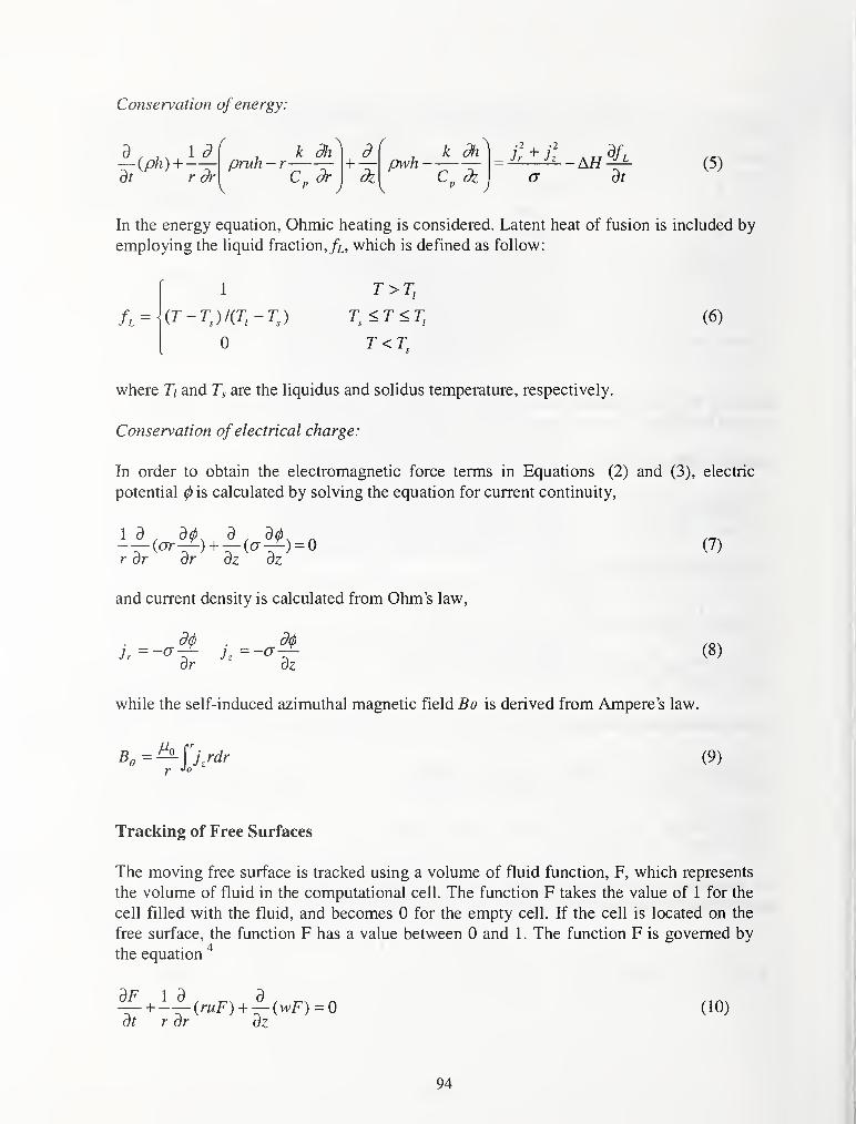
Conservation of energy:

ot r or

k dhpruh -r——

C dr+

, k dhpwh-——C di

A// (5)

In the energy equation, Ohmic heating is considered. Latent heat of fusion is included by

employing the liquid fraction, /a, which is defined as follow:

1

(r-rj/(r,-7;)

0

T^<T<Ti

T<T(6)

where Ti and Ts are the liquidus and solidus temperature, respectively.

Conservation of electrical charge:

In order to obtain the electromagnetic force terms in Equations (2) and (3), electric

potential (p is calculated by solving the equation for current continuity,

(or—-) +— (cr—) = 0r dr dr dz dz

and current density is calculated from Ohm's law.

(7)

d0 . d(l)

or oz(8)

while the self-induced azimuthal magnetic field Be is derived from Ampere's law.

5. = ^jfrdry Jo

(9)

Tracking of Free Surfaces

The moving free surface is tracked using a volume of fluid function, F, which represents

the volume of fluid in the computational cell. The function F takes the value of 1 for the

cell filled with the fluid, and becomes 0 for the empty cell. If the cell is located on the

free surface, the function F has a value between 0 and 1. The function F is governed by

the equation

^ +^f(™F) + f(wf) = 0at r dr dz

(10)

94

Boundary Conditions

Boundary conditionsfor momentum

The boundary conditions needed to specify the fluid flow problem are:

(1) symmetry about the centerline

(2) no slip at the solid boundaries

(3) at the free surface, the plasma arc pressure Pare can be approximated by

Cc=^n.xexp(-^) (11)

where Pmax is calculated by -^p^rc^^lrc 'using values of Parc and Varc determined earlier^. The

Marangoni force due to the variation of the surface tension coefficient with temperature is

described by

= —^ = — (12)dn dT ds

The plasma arc pressure Pare and the Marangoni force are included by adding source terms to

the momentum equation. The method used is detailed in Ref. 6, which is called Continuum

Surface Force (CSF) model.

Boundary conditions for thermal energy

The boundary conditions pertaining to the heat-transfer problem are

(1) symmetry about the axial centerline

(2) at the free surface of the molten pool, the heat flux from the welding arc is assumed to obey a

Gaussian-type distribution of the form

-.f = |^exp(-^)-^(7-r,) (13)dn Lm„ 2r

where /i^ is a combined heat transfer coefficient for the radiate and convective boundary

expressed in the following equation^

^ =24.1xlO"'£T'" (14)

95

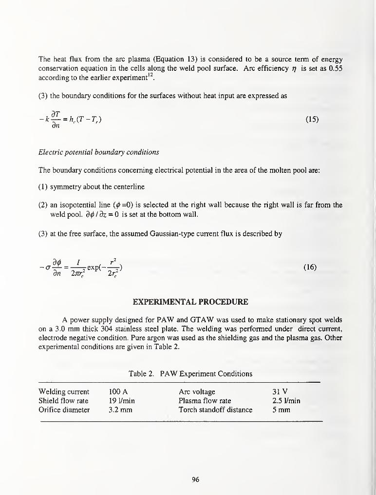
The heat flux from the arc plasma (Equation 13) is considered to be a source term of energy

conservation equation in the cells along the weld pool surface. Arc efficiency rj is set as 0.55

according to the earlier experiment'^.

(3) the boundary conditions for the surfaces without heat input are expressed as

dn= KiT-T^) (15)

Electric potential boundary conditions

The boundary conditions concerning electrical potential in the area of the molten pool are:

(1) symmetry about the centerline

(2) an isopotential line (0 =0) is selected at the right wall because the right wall is far from the

weld pool. d(l>ldz = 0 is set at the bottom wall.

(3) at the free surface, the assumed Gaussian-type current flux is described by

A power supply designed for PAW and GTAW was used to make stationary spot welds

on a 3.0 mm thick 304 stainless steel plate. The welding was performed under direct current,

electrode negative condition. Pure argon was used as the shielding gas and the plasma gas. Other

experimental conditions are given in Table 2.

d(j) _ I

dn iTtr'^

(16)

EXPERIMENTAL PROCEDURE

Table 2. PAW Experiment Conditions

Welding current

Shield flow rate

Orifice diameter

100 A19 1/min

3.2 mm

Arc voltage

Plasma flow rate

Torch standoff distance

31 V2.5 1/min

5 mm

96

RESULTS AND DISCUSSION

The development of keyhole in plasma arc welding is presented in Figure 2. The surface profile

of the weld pool is determined by the arc pressure, gravitational force and surface tension acting

on the weld pool. In the partially penetrated weld pool, the molten metal is pushed out by arc

pressure; thus, the pool surface is depressed in the center and humped at the pool boundary. Ahole with V-shape cross section is formed before full penetration because of the high-velocity,

concentrated plasma arc. Since the plasma arc in the cone hole heats the base metal, the liquid-

solid boundary has shown a similar V-shape. Around 2.62s, the molten pool is fully penetrated.

The molten metal is held by surface tension. In the newly developed bottom surface, surface

tension also tends to form a shape that minimizes the surface energy. As shown in Figure 2, a

keyhole with X-shape cross section is developed at t = 2.69 s.

The keyhole is collapsed after the arc is extinguished. At t=2.71s in Figure 2b, the fluid is

accelerated into the hole, causing the hole to fill soon. At t = 2.72s, the inward flows impinge in

the center; thus, the top part fluid moves upward and the bottom part moves downward. At t =

2.73s, the top part of the pool which overpasses the equilibrium begins to move downward. The

downward flow is dominant in the weld pool at t = 2.74s. Meanwhile, influenced by surface

tension, the flow direction of the bottom part begins to change. It is obvious that the upward flow

from the bottom will affect the flow in the top. Then, the upward flow is dominant at t = 2.76s.

At t = 2.77s and 2.79s, it is seen that the flow directions in the weld pool change again. The weld

pool oscillation will continue until equilibrium is achieved or the weld pool is solidified.

The temperature distribution is shown in Figure 2a. The keyhole is developed so fast that the

highest temperature appears near the top surface, although the heat flux from arc plasma is

higher in the center of the weld pool. This is because the high temperature molten metal is

always pushed toward the top surface by plasma arc; furthermore, the central pool always

approaches first and is cooled by the low temperature base metal. After the collapse of the

molten pool, the high temperature molten metal from the top moves to the center which result in

a higher temperature distribution at the center. In the process of solidification, the higher

temperature fluid remains near to the top and the bottom surface. Finally, the solidification is

completed near the bottom surface, because heat loss is mainly from the surrounding base metal.

The experimental results have been shown in Figure 3. The reasonable agreement between the

predicted and experimentally observed fusion zone shape and size is obtained. Figure 3b shows

the weld shape after bum through. This helps to understand the keyhole shape under the

influence of the plasma arc. The cross section of the bum through weld is nearly X-shape, which

agrees well with the predicted results.

97

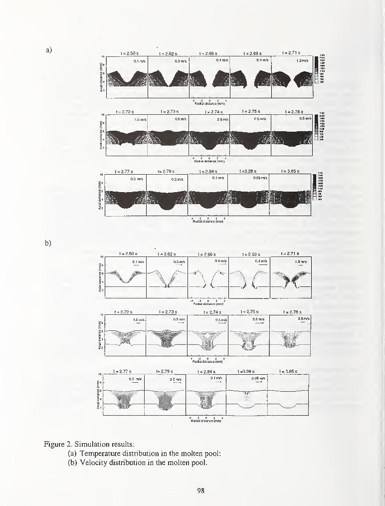
-4 -2 0 2 4

Radial distance (mm)

t = 2.72 s t = 2.73 s t = 2.74 s t = 2.75 s . t = 2.76 s10

1.0 m/s 0,5 m/s 0.5 m/s 0.5 m/s 0.5 m/s

-4 -2 0 2 4

Radial distance (mm)

t = 2.77 s t= 2.79 s t = 2.84 s t =3.28 S t = 3.85 s

• 4 -2 0 2 4

Radial distance (mm)

b)

t = 2.50 s t = 2.62 s I = 2.66 s I = 2.69 s t = 2.71 s

0.1 m/s 0.3 m/s 0.4 m/s 0.4 m/s 1.0 m/s

JX—

-

I = 2.72 s t = 2.73 s

-4-2024Radlat distance (mm)

I = 2.74 s t = 2.75 s t = 2.76 s

1.0 m/s 0.5 m/s 0-5 m/s 0.5 m/s 0.5 m/s

-III-

I = 2.77 s t= 2.79 s

4 .2 0 2 4

Radial distance (mm)

t = 2.84 s I =3.28 s t = 3.85 s

0.) nVs

Figure 2. Simulation results:

(a) Temperature distribution in the molten pool:

(b) Velocity distribution in the molten pool.

98

(a)

Figure 3. (a) Resultant weld shape

(b) Keyhole shape after bum through

CONCLUSION

A two-dimensional heat and fluid flow model has been developed to analyze keyhole formation

and collapse in stationary plasma arc. The keyhole with a X-shape cross-section has been

predicted and observed.

The weld pool oscillation could be triggered after the collapse of the molten pool. In the fully

penetrated weld, the addition of a free bottom surface results in a more significant weld pool

oscillation, and the bottom and the top surface oscillation have close connections. The weld pool

oscillation will continue until the equilibrium or solidification has been achieved.

The calculated temperature distribution during keyhole formation reveals that the highest

temperature appears near the top of the molten pool. After the keyhole collapse, the fluid

temperature around the periphery is lower than the temperature at the center. Heat lose is mainly

from the base metal, thus, solidification is initiated at the solid-liquid interface and advance

toward the center. In the process of solidification, the higher temperature remains near to the

bottom.

99

REFERENCE

1. Fuerschloach, P.W.; and Knorousky, G.A. 1991. Weldins Journal 70(10): 287 to 297s.

2. Hsu J.F.; and Rubinsky, B. 1998 Int. J. Heat Mass Transfer 31(1): 1409 to 1421.

3. Keanini, R.G.; and Rubinsky, B. 1993. Three-dimensional simulation of the plasma arc

welding process. Int. J. Heat Mass Transfer 36(13): 3283 to 3298.

4. Nichols, B.D.; Hirt C.W.; and Hotchkiss R.S. 1980. SOLA-VOF: A solution algorithm for

transient fluid flow with multiple free boundaries. Report LA-8355. Los Alamos Scientific

Laboratory.

5. Metcalfe J.C.; and Quigeley, M.B.C. 1975. Heat tranfer in plasma arc weldin g. WeldimJournal 54(3): 93 to 103.

6. Kothe, D.B.; Mjolsness R.C.; and Torrey M.D. 1991. RIPPLE: A computer program for

incompressible flows with free surfaces. Report LA-12007-MS. Los Alamos Scientific

Laboratory.

1. Goldak, J.; Bibby, M.; Moore, J.; and Patel, B. 1986. Metallurgical Transaction B 17B: 587

to 600.

8. Evans, D.W., Huang D., McClure J.C.; and Nunes A.C. 1998. Weldins Journal 77(2): 53 to

58.

100

PREVENTION OF OUT-OF-PLANE DEFORMATION GENERATEDBY FILLET WELDING

Y. C. Kim*, K. H. Chang** and K. Horikawa*

ABSTRACT

The validity of the preset distortion method was confirmed. The prevention accuracy of out-of-

plane deformation by the preset distortion was determined by the prediction accuracy of welding

deformation. Angular distortion could be prevented by heating two points on the flange under the

welding heat source or one point on the flange under the web in order to reduce the temperature

gradient for the thickness direction of the flange. Residual stress a ^ was a little larger with

heating from the opposite side comparing to without heating. Considering the manufacture site,

the prevention of angular distortion was investigated for the one point heating from the opposite

side. If the heating temperature became higher, the heating width may be narrow. However, the

maximum heating temperature from the opposite side should be 650-700°C. Angular distortion

could prevent by controlling the heating width from the opposite side for any flange thickness.

KEY WORDS: (Fillet Welding)(Welding Distortion)(Distortion Prevention)(Preset Distortion)

(Angular Distortion Prevention)(Residual Stress)(FEM Modelling)

INTRODUCTION

Fillet welding was performed in constructing the steel structures such as ships, the deck plate of

bridges which were assembled by plates and stiffeners. Welding deformation is necessarily

generated by fillet welding. As out-of-plane deformation in welding deformation lowers the

constructing accuracy and the appearance of the steel structures, it is generally reformed.

The reformation often causes the obstruction in manufacture, that is the increment of the

manufacturing time and the standstill of the manufacturing systems. The reformation influences

the strength of the structures directly or indirectly (Ref 1). So, it is required that the system,

which controls and prevents welding deformation before welding, is constructed (Ref 2, 3).

Concerning to this, the authors found the characteristics and the production mechanism of out-

of-plane deformation generated by butt welding with the initial deflection and by fillet welding

(Ref 4, 5). The effects of the welding conditions on out-of-plane deformation and residual stress

were elucidated. At the same time, the generality of the production mechanisms for out-of-plane

deformation was investigated together with the validity (Ref 4-6).

In this paper, the validity of the preset distortion, which has been well known as a prevention

method of out-of-plane deformation, is investigated. The conditions, which should be satisfied to

prevent welding out-of-plane deformation by preset distortion method, are found. On the other

hand, the prevention method of angular distortion is proposed and the validity is shown.

Joining & Welding Research Institute, Osaka University, Japan

* Graduate student, Osaka University, Japan

101

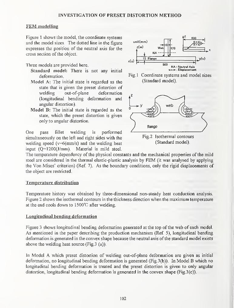
INVESTIGATION OF PRESET DISTORTION METHOD

FEM modelling

Figure 1 shows the model, the coordinate systems

and the model sizes. The dotted line in the figure

expresses the position of the neutral axis for the

cross section of the object.

Three models are provided here.

Standard model: There is not any initial

deformation.

Model A: The initial state is regarded as the

state that is given the preset distortion of

welding out-of-plane deformation

(longitudinal bending deformation and

angular distortion).

Model B: The initial state is regarded as the

state, which the preset distortion is given

only to angular distortion.

One pass fillet welding is performed

simultaneously on the left and right sides with the

welding speed (v=6(mm/s) and the welding heat

input (Q=1200(J/mm). Material is mild steel.

The temperature dependency of the physical constants and the mechanical properties of the mild

steel are considered in the thermal elastic-plastic analysis by FEM (it was analysed by applying

the Von Mises' criterion) (Ref 7). As the boundary conditions, only the rigid displacements of

the object are restricted.

Temperature distribution

Temperature history was obtained by three-dimensional non-steady heat conduction analysis.

Figure 2 shows the isothermal contours in the thickness direction when the maximum temperature

at the end cools down to 1500°C after welding.

Longitudinal bending deformation

Figure 3 shows longitudinal bending deformation generated at the top of the web of each model.

As mentioned in the paper describing the production mechanism (Ref 5), longitudinal bending

deformation is generated in the convex shape because the neutral axis ofthe standard model exists

above the welding heat source (Fig. 3 (a)).

In Model A which preset distortion of welding out-of-plane deformation are given as initial

deformation, no longitudinal bending deformation is generated (Fig. 3(b)). In Model B which no

longitudinal bending deformation is treated and the preset distortion is given to only angular

distortion, longitudinal bending deformation is generated in the convex shape (Fig.3(c)).

unit(mm)

z(w)

1 NA

x(u)

19

120

600 ^

1 5 Flange

500

v(v)

NA : Neutral Axisu.v.w ; Displacement

Fig. 1 Coordinate systems and model sizes

(Standard model).

Fig. 2 Isothermal contours

(Standard model).

102

0.6

0.4

0.2

-0.4

-0.6

Welding deformation

at the top of weby= 250 (mm)

200 400

x(mm)

(a) Standard model.

600

EE

+-<

c0)

Ea>oJSQ.

Welding deformation

at X = 0 (mm)

250

x(mm)

(a) Standard model.

500

-0.4

-0.6

preset distortion

after welding

at the top of weby= 250 (mm)

200 400

x(mm)

(b) Model A.

600

E£

*->

c<x>

E(1)

oJOaS2

b

preset distortion

after welding

at X = 0 (mm)

250

y(mm)

(b) Model A.

500

0.6

0.4

0,2

-0.4

-0.6

preset distortion

after welding

at the top of web

y= 250 (mm)

6000 200 400

x(mm)

(c) Model B.

Fig. 3 Longitudinal bending deformation

EE

c

Eu

aw

preset distortion

after welding

at X = 0 (mm)

250

y(mm)

(C) Model B.

Fig.4 Angular distortion.

500

103

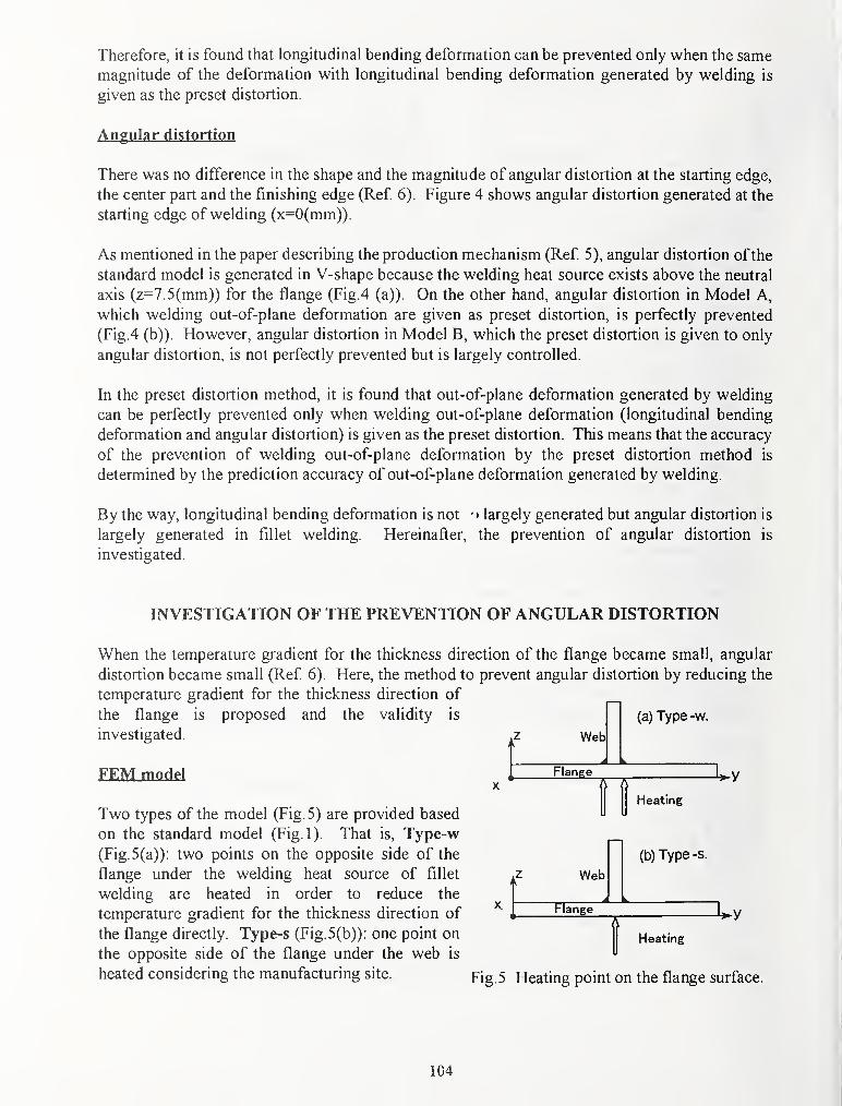
Therefore, it is found that longitudinal bending deformation can be prevented only when the same

magnitude of the deformation with longitudinal bending deformation generated by welding is

given as the preset distortion.

Angular distortion

There was no difference in the shape and the magnitude of angular distortion at the starting edge,

the center part and the finishing edge (Ref 6). Figure 4 shows angular distortion generated at the

starting edge of welding (x=0(mm)).

As mentioned in the paper describing the production mechanism (Ref 5), angular distortion ofthe

standard model is generated in V-shape because the welding heat source exists above the neutral

axis (z=7.5(mm)) for the flange (Fig.4 (a)). On the other hand, angular distortion in Model A,

which welding out-of-plane deformation are given as preset distortion, is perfectly prevented

(Fig.4 (b)). However, angular distortion in Model B, which the preset distortion is given to only

angular distortion, is not perfectly prevented but is largely controlled.

In the preset distortion method, it is found that out-of-plane deformation generated by welding

can be perfectly prevented only when welding out-of-plane deformation (longitudinal bending

deformation and angular distortion) is given as the preset distortion. This means that the accuracy

of the prevention of welding out-of-plane deformation by the preset distortion method is

determined by the prediction accuracy of out-of-plane deformation generated by welding.

By the way, longitudinal bending deformation is not ' • largely generated but angular distortion is

largely generated in fillet welding. Hereinafter, the prevention of angular distortion is

investigated.

INVESTIGATION OF THE PREVENTION OF ANGULAR DISTORTION

When the temperature gradient for the thickness direction of the flange became small, angular

distortion became small (Ref 6). Here, the method to prevent angular distortion by reducing the

temperature gradient for the thickness direction of

the flange is proposed and the validity is

investigated.

FEM model

Two types of the model (Fig. 5) are provided based

on the standard model (Fig.l). That is, Type-w

(Fig. 5(a)): two points on the opposite side of the

flange under the welding heat source of fillet

welding are heated in order to reduce the

temperature gradient for the thickness direction of

the flange directly. Type-s (Fig. 5(b)): one point on

the opposite side of the flange under the web is

heated considering the manufacturing site.

Web

(a) Type -w.

Flange

Web

Flange

Heating

(b)Type-s.

Heating

Fig. 5 Heating point on the flange surface.

104

Heating from the opposite side of the flange is performed with the same time and speed as

welding.

Temperature

Temperature history of welding was obtained by three-dimensional non-steady heat conduction

analysis. Figure 6 shows the isothermal contours for the thickness direction in Type-w and

Type-s when the maximum temperature at the end cools down to 1500°C after welding.

These isothermal contours consequently

correspond to the heating temperature where

angular distortion can prevent. The maximumtemperature from the opposite side is 550°C in

Type-w and is 700°C in Type-s, respectively.

It can be known that the temperature gradient for

the thickness direction of the flange becomes

small directly in Type-w.

Angular distortion

Figure 7 shows angular distortion generated at the

central position (x=300(mm)).

Angular distortion can be prevented both in

Type-w and Type-s. It is found that reducing the

temperature gradient for the thickness direction of

the flange with heating from the opposite side of

the flange can prevent angular distortion. So, the

validity is confirmed. In the same way, the

applicability of the prevention of angular

distortion is variously investigated (Ref 8).

Considering the manufacturing site, Type-s is

more useful than Type-w. The heating

temperature and the heating width from the

opposite side to be necessary for the change ofthe

flange thickness are investigated by using Type-s.

Residual stress

It was found that heating from the opposite side

can prevent angular distortion. Therefore, it is

necessary to know the influence of heating from

the opposite side on residual stress.

(a) Type -w.

(b) Type-s.

Fig. 6 Isothermal contours with heating at the

opposite side of the welding surface.

EE

Jc0)

E0)

uJ5aw

4

3

2

1

0

-1

-2

-3

-4

Standard Model

Type-w

Type-s

at X = 300 (mm)

250

y(mm)

500

Fig. 7 Angular distortion with heating at the

opposite side of the welding surface.

105

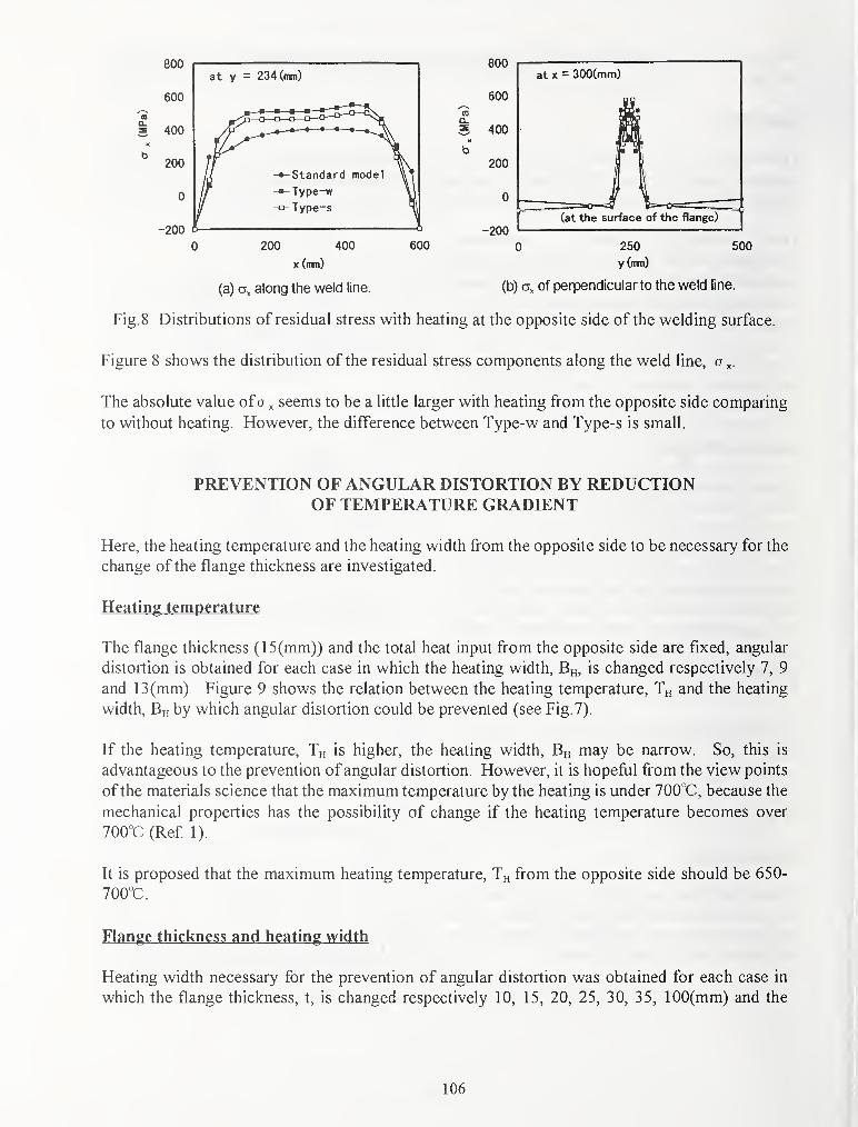
at y = 234 (mm)

to

800

600

400

200

0

-200

at X = 300(mm)

(at the surface of the flange)

200 400

X (mm)

(a) along the weld line.

600 250

y (mm)

500

(b) of perpendicular to the weld line.

Fig. 8 Distributions of residual stress with heating at the opposite side of the welding surface.

Figure 8 shows the distribution of the residual stress components along the weld line, o ^.

The absolute value of o ^ seems to be a little larger with heating from the opposite side comparing

to without heating. However, the difference between Type-w and Type-s is small.

PREVENTION OF ANGULAR DISTORTION BY REDUCTIONOF TEMPERATURE GRADIENT

Here, the heating temperature and the heating width from the opposite side to be necessary for the

change of the flange thickness are investigated.

Heating temperature

The flange thickness (15(mm)) and the total heat input from the opposite side are fixed, angular

distortion is obtained for each case in which the heating width, Bh, is changed respectively 7, 9

and 13 (mm). Figure 9 shows the relation between the heating temperature, Th and the heating

width, Bh by which angular distortion could be prevented (see Fig. 7).

If the heating temperature, Th is higher, the heating width, Bh may be narrow. So, this is

advantageous to the prevention of angular distortion. However, it is hopeful from the view points

of the materials science that the maximum temperature by the heating is under 700°C, because the

mechanical properties has the possibility of change if the heating temperature becomes over

700°C (Ref 1).

It is proposed that the maximum heating temperature, Th from the opposite side should be 650-

700°C.

Flange thickness and heating width

Heating width necessary for the prevention of angular distortion was obtained for each case in

which the flange thickness, t, is changed respectively 10, 15, 20, 25, 30, 35, lOO(mm) and the

106

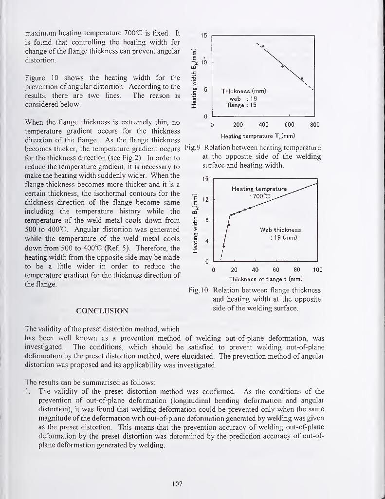
maximum heating temperature 700°C is fixed. It

is found that controlling the heating width for

change of the flange thickness can prevent angular

distortion.

Figure 10 shows the heating width for the

prevention of angular distortion. According to the

results, there are two lines. The reason is

considered below.

When the flange thickness is extremely thin, no

temperature gradient occurs for the thickness

direction of the flange. As the flange thickness

becomes thicker, the temperature gradient occurs

for the thickness direction (see Fig. 2). In order to

reduce the temperature gradient, it is necessary to

make the heating width suddenly wider. When the

flange thickness becomes more thicker and it is a

certain thickness, the isothermal contours for the

thickness direction of the flange become same

including the temperature history while the

temperature of the weld metal cools down from

500 to 400°C. Angular distortion was generated

while the temperature of the weld metal cools

down from 500 to 400°C (Ref 5). Therefore, the

heating width from the opposite side may be madeto be a little wider in order to reduce the

temperature gradient for the thickness direction of

the flange.

CONCLUSION

E

X00

-D

'+->

(0

15

10

Thickness (mm)

web :19flange : 1

5

Fig.9

0 200 400 600 800

Heating temprature T^(mm)

Relation between heating temperature

at the opposite side of the welding

surface and heating width.

16

12EE.

Xm^ 8D

TO0)

X

Heating temprature

: 700°C

Web thickness

: 1 9 (mm)

0 20 40 60 80

Thickness of flange t (mm)

100

Fig. 10 Relation between flange thickness

and heating width at the opposite

side of the welding surface.

The validity of the preset distortion method, which

has been well known as a prevention method of welding out-of-plane deformation, was

investigated. The conditions, which should be satisfied to prevent welding out-of-plane

deformation by the preset distortion method, were elucidated. The prevention method of angular

distortion was proposed and its applicability was investigated.

The results can be summarised as follows:

1. The validity of the preset distortion method was confirmed. As the conditions of the

prevention of out-of-plane deformation (longitudinal bending deformation and angular

distortion), it was found that welding deformation could be prevented only when the same

magnitude of the deformation with out-of-plane deformation generated by welding was given

as the preset distortion. This means that the prevention accuracy of welding out-of-plane

deformation by the preset distortion was determined by the predicfion accuracy of out-of-

plane deformation generated by welding.

107

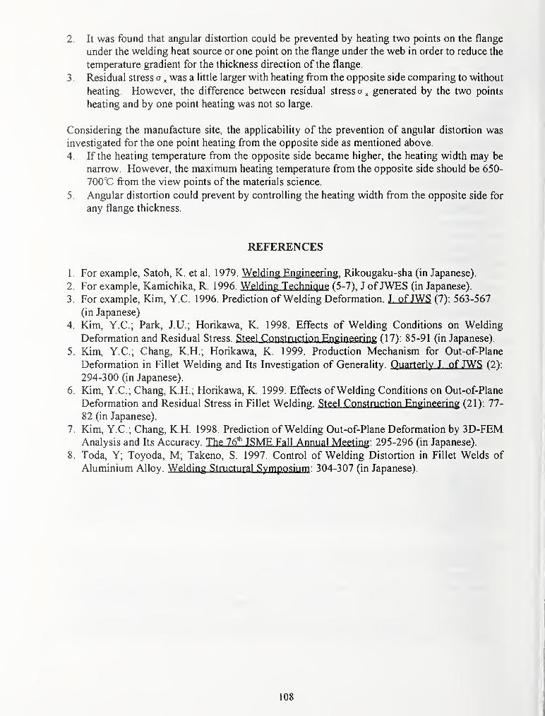
2. It was found that angular distortion could be prevented by heating two points on the flange

under the welding heat source or one point on the flange under the web in order to reduce the

temperature gradient for the thickness direction of the flange.

3 . Residual stress a ^ was a little larger with heating from the opposite side comparing to without

heating. However, the difference between residual stress o ^ generated by the two points

heating and by one point heating was not so large.

Considering the manufacture site, the applicability of the prevention of angular distortion was

investigated for the one point heating from the opposite side as mentioned above.

4. If the heating temperature from the opposite side became higher, the heating width may be

narrow. However, the maximum heating temperature from the opposite side should be 650-

700°C from the view points of the materials science.

5. Angular distortion could prevent by controlling the heating width from the opposite side for

any flange thickness.

REFERENCES

1. For example, Satoh, K. et al. 1979. Welding Engineering . Rikougaku-sha (in Japanese).

2. For example, Kamichika, R. 1996. Welding Technique (5-7), J ofJWES (in Japanese).

3. For example, Kim, Y.C. 1996. Prediction of Welding Deformation. J. ofJWS (7): 563-567

(in Japanese)

4. Kim, Y.C; Park, J.U.; Horikawa, K. 1998. Effects of Welding Conditions on Welding

Deformation and Residual Stress. Steel Construction Engineering (17): 85-91 (in Japanese).

5. Kim, Y.C; Chang, K.H.; Horikawa, K. 1999. Production Mechanism for Out-of-Plane

Deformation in Fillet Welding and Its Investigation of Generality. Quarterly J. of JWS (2):

294-300 (in Japanese).

6. Kim, Y.C; Chang, K.H.; Horikawa, K. 1999. Effects of Welding Conditions on Out-of-Plane

Deformation and Residual Stress in Fillet Welding. Steel Construction Engineering (21): 77-

82 (in Japanese).

7. Kim, Y.C; Chang, K.H. 1998. Prediction of Welding Out-of-Plane Deformation by 3D-FEMAnalysis and Its Accuracy. The 76*^ JSME Fall Annual Meeting : 295-296 (in Japanese).

8. Toda, Y; Toyoda, M; Takeno, S. 1997. Control of Welding Distortion in Fillet Welds of

Aluminium Alloy. Welding Structural Symposium : 304-307 (in Japanese).

108

THERMO-MECHANICAL COMPUTER MODELING OF RESIDUAL STRESS ANDDISTORTION DURING WELDING PROCESS

Y. J. Chao and X. Qi

Department of Mechanical Engineering, University of South Carolina

Tel: (803)777-5869; Fax: (803)777-0106; Chao@sc.edu

ABASTRACT

A three-dimensional finite element simulation of welding process is presented. A de-coupled

heat transfer and thermo-mechanical analysis is adopted for the determination of residual

stress and distortion. Special features for the welding process are developed in the modeling

to reduce the computational cost and time of the analysis. A butt-welded aluminum plate was

analyzed and the results are compared with experimental data. The good comparison for both

the residual stress distribution and the distortion verifies the modeling procedures. It is further

shown that the full three-dimensional model can reveal more realistic results, which cannot be

obtained by the simplified two-dimensional simulation. In addition, the efficiency of the code

in computational time is demonstrated.

INTODUCTION

Welding is a popular joining method used in many industries, e.g. from offshore drilling

platform to electronic packaging. By going through heating, melting and solidification

processes, two workpieces are joined together using torch, laser, electron beam or other heat

sources. The highly localized, transient heat input and extremely non-uniform temperature

fields in both heating and cooling processes cause non-uniform thermal expansion and

contraction, and thus plastic deformation in the weld and its neighborhood. Consequently,

residual stress, strain and distortion of the welded structure are developed. The residual stress

in the weld region affects the service life of the structure, e.g. stress corrosion cracking of the

weld, and the distortion directly influence the fabrication of the structure. Thus, control of

residual stress and distortion from the welding process is extremely important in the

manufacturing and construction industry. Besides the determination of the residual stress and

distortion of the welded structure, modeling effort for the welding process can also be used to

incorporate the welding procedures and pattern into the design evaluation, optimization and

manufacturing of the structures.

Due to its complexity, analytical solutions to the welding process can rarely address the

practical manufacturing processes. Numerical solutions, on the other hand, can provide more

detailed results and address more realistic problems. Hibbitt and Marcal (Ref. 1) marks the

first step in applying a two-dimensional finite element analysis (FEA) to predict residual

stress in a weldment. Most modeling efforts in the 70' s and 80' s are for two-dimensional or

simple three-dimensional geometries due to the limitations from the computer, i.e. time and

109

cost. With the rapid advancement in computing speed from modem computers, numerical

modeling of practical welding processes now becomes feasible. Recently, three-dimensional

modeling using commercial finite element codes are reported by Tekriwal and Mazumder(Ref. 2), Michaleris and DeBiccari (Ref. 3), and Dong, et al (Ref. 4) among others. Brown

and Song (Refs. 5,6) used three-dimensional models to demonstrate the inadequacy of using

two-dimensional models for the determination of distortions due to welding process. In

particular they demonstrated that the fixture used for the welding process in general cannot be

modeled as a two-dimensional case and thus a two-dimensional model could give erroneous

distortion results. Dike, et al (Ref. 7) pointed out the two-dimensional models cannot

account for restraint and solidification effects and significantly underpredicts the distortion of

multi-pass welds.

Note that in using the commercial finite element codes, many user subroutines must be added

to handle the special features of the welding process, e.g. melting and annealing, which are

usually not accounted for in the general-purpose finite element codes. In this paper we first

demonstrate a numerical modeling procedure which includes advanced features to improve

the computational efficiency. The modeling procedure was then developed into a FEA code

for the welding process simulation. The developed FEA program is three-dimensional and

runs on PC platform. A flow chart of a complete modeling of the welding process involving a

heat transfer analysis and a subsequent thermo-mechanical analysis is shown in fig.l. Amoving heat source is modeled first to generate the temperature fields at various time steps

during the welding process and then the temperature history is used for the calculation of the

thermal stresses and displacement fields during and after the welding process. Unique

features of the welding process are built into the code and appropriate convergence can be

controlled by the user with flexibility. The computer code is developed in order to study the

welding process and for practical engineering applications.

Welding process Thermophysical Numerical

variables data variables

Finite Element Models ( 2D & 3D Solid Elements )

Weld Heat Flow Simulation

Thermomechanical Simulation

Figure 1 Flow chart of the welding process modeling

In the following sections we first outline the basic principles of the finite element analysis,

then discuss special features of the code, present the results from the modeling of a gas metal

arc welding (GMAW) of a rectangular Aluminum plate, and finally compare the analytical

110

results to experimental data. Further results are presented to show that why a three-

dimensional modeling is needed for the simulation of practical welding problems. Adiscussion is then given to conclude the paper.

FINITE ELEMENT FORMULATION

It has been shown by Argyris, et al (Ref. 8) and Papazoglou and Masubuchi (Ref. 9) that the

difference between a coupled and de-coupled analysis for residual stress and distortion in a

welding process is very small. Therefore, we have adopted a de-coupled finite element

analysis; i.e. a thermo-mechanical stress analysis following an independent heat transfer

analysis.

The finite element formulation and solver follow the standard procedures and can be found in

many textbooks (Ref. 10, Ref. 11). In the heat transfer analysis, the differential equations

governing the transient heat conduction problems can be obtained by using the first and

second law of thermodynamics. A moving heat source is formulated into the code to simulate

the movement of the torch. The temperature history at each finite element node is determined

and stored for the subsequent thermo-mechanical stress analysis. The basic mechanics

formulation starts from the constitutive equation, in incremental (differential) form for the

thermal elastic-plastic material, i.e. de'"'"' = de'"^''' + de"'""'' + de"'"^' + de"''" . The creep

strain is for modeling the post-weld heat treatment used to reduce or alter the distortion and

the residual stress pattern of the welded structure. The finite element formulation uses a rate

independent plasticity model with kinematic hardening to model the reverse plasticity and

Bauschinger effect. Either power law or linear relation for the uniaxial stress-strain curve

beyond the yielding can be used for the non-linear material behavior. Von Mises yield

criterion with an associated flow rule is used to determine the onset of yielding and the

amount of incremental plastic strain.

SPECIAL FEATURES TO IMPROVE THE COMPUTATION SPEED ANDACCURACY

One of the drawbacks of using the commercial finite element codes for modeling welding

process is the slow speed and the lack of unique features of the welding process in the codes.

In order to improve the computation speed, several strategies are introduced in our welding

process simulation and built into the code. These include

1 . A moving heat source to simulate the movement of the torch

2. Flexibility in convergence tolerance

3. Using an appropriate cut-off temperature

4. Appropriate weight factor for elastic to plastic transition

111

5. Dummy elements used for multi-pass welding

6. Flexibility in finite element meshes

7. Using adjustable time and temperature increments in the iteration

The details of these computational strategies are discussed elsewhere and are not reported

here due to the length limit of the current paper.

MODELING OF ALUMINUM PLATES JOINED BY GMAW

This section reports results from modeling a butt joint by gas metal arc welding (GMAW).The numerical results from our analysis are compared with the experimental data by Cancis et.

al. (Ref. 12). In addition, results that can only be obtained from a three-dimensional analysis

and cannot generally be obtained by the simplified two-dimensional analysis are reported.

Figure 2 shows the geometry and welding configuration of the problem under consideration.

A half model was used in the simulation due to symmetry. The FEM model consists of 4040

nodes and 2700 (8 nodes) solid elements in the heat transfer analysis, and 2040 nodes and

1350 solid elements in the thermo-mechanical analysis. Figure 3 shows the FEA mesh for the

thermo-mechanical analysis. The material is the aluminum alloy A/5083-O with the thermo-

mechanical properties shown in fig. 4 (Ref. 12). A cut-off temperature 550^C was used in the

computation. The electricity provided to the GMAW process is 23.4 Volt and 170 Amp, AGaussian distribution with an effective arc radius of 7 mm and efficiency of 64% is used to

simulate the heat flux applied to the workpiece. The heat is applied in the Z=0 plane and

moves along the +X-direction with a speed of 1 1 mm/sec, as shown in figure 2. The total

welding time lasts 23 seconds.

welding nozzle ^maw: 23.4V • 170A

I) .0.64

Figure 2 Configuration of the model

112

Figure 3 FEA mesh in the thermo-mechanical model

Figure 4 Thermo-mechanical properties of the aluminum alloy A/5083-O

(640*^C is the melting temperature)

RESULTS FROM THE THERMO-MECHANICAL ANALYSIS AND COMPARISONTO THE EXPERIMENTAL DATA

Residual Stresses

Residual stresses Gxx, Cyy, <Jxy at the centroids of the elements along a section in the middle of the

plate (X, Y, Z) = (122.5, Y, 1) mm are shown in Fig.5 along with the experimental data. It is

shown in Fig. 5 that the analytical results compare well with the test data.

113

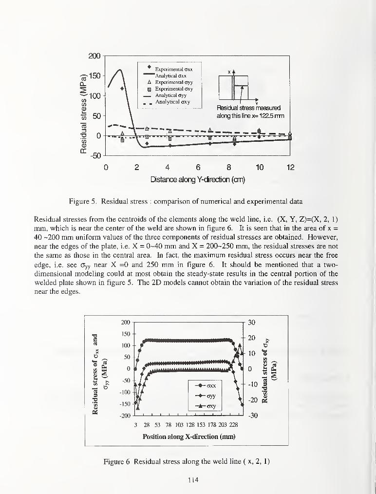
Figure 5. Residual stress : comparison of numerical and experimental data

Residual stresses from the centroids of the elements along the weld line, i.e. (X, Y, Z)=(X, 2, 1)

mm, which is near the center of the weld are shown in figure 6. It is seen that in the area of x =

40 -200 mm uniform values of the three components of residual stresses are obtained. However,

near the edges of the plate, i.e. X = 0-40 mm and X = 200-250 mm, the residual stresses are not

the same as those in the central area. In fact, the maximum residual stress occurs near the free

edge, i.e. see cjyy near X =0 and 250 mm in figure 6. It should be mentioned that a two-

dimensional modeling could at most obtain the steady-state results in the central portion of the

welded plate shown in figure 5. The 2D models cannot obtain the variation of the residual stress

near the edges.

c

in,^

IS

IHIMimUMMMIIIIIlH'"""*

J I I L J I I I I

30

28 53 78 103 128 153 178 203 228

Position along X-direction (mm)

Figure 6 Residual stress along the weld line ( x, 2, 1)

114

Figure 7 shows the residual stress distributions along the Y-direction in three sections; one at

X=7.5 mm near the starting edge, one in the central part X= 122.5 mm and one at X= 242.5 mmnear the finishing edge. Again, significant difference in the residual stress distribution in the

three sections is present.

The maximum tensile residual stress appears to be parallel to the weld and near the weld as can

be seen from Figures 5 and 7. This Gxx has a maximum value of 161 MPa, which is slightly

higher than the yield stress of the material at room temperature Oys = 145.1 MPa.

Distortion

Due to the highly localized, transient heating and hence non-uniform heat distribution in the

workpiece, the plate exhibits complicated distortion during the welding. Fig. 8 shows the

distorted plate during and after welding. One half of the plate is modeled and shown in Fig. 8.

Recall that the torch moves at 1 1 mm/second; thus, the torch is at X= 55 mm as t = 5 seconds for

figure 10(a), X= 165 mm as t = 15 seconds for figure 10(b). And, figure 10 (c) demonstrates the

deformed workpiece right after the welding was completed (i.e. t=23 seconds), while Fig. 10 (d)

is after the workpiece completely cooled down to room

200atZ=1,X=122.5 mmatZ=1,X=7.5mm

atZ=1, X=242.Smm

atZ=1, X=122.5 mmatZ=1, X=7.5 mmatZ=1, X=242.S mmatZ=1, X=122.5 mmatZ=1, X=7.5 mmatZ=1,X=242.5 mm

Y-measured from the center of the weld (cm)

Figure 7 Residual stresses at three different sections along the Y-direction

temperature. Note that the distortion is magnified by 100 times in figure 8. The final deformed

shape of the originally flat plate is a warped surface resembling a double-curvatured plate. The

maximum residual distortion (or warpage) in the out of plane or Z-direction is about 2.2 mm in

this case.

115

(a) time = 5 seconds (b) time = 15 seconds

(c) time = 23 seconds (d) time = after cooling to room temperature

Figure 8 Distorted shape of the plate during and after the welding process

(Magnification of distortion: x 100)

The distribution of the longitudinal strains in the welding direction, Exx , along the line in the

center of the plate (X, Y,Z) = ( 125, Y, 0 mm) is shown in Fig. 9. Fig. 9 indicates that the

longitudinal strain, which is transverse to the weld line is non-uniform with the maximumcompressive strain at the weld-line. The resulted shrinkage along the weld-line (X, 0, 0) for the

plate is about 0.18 mm, while there is almost no shrinkage at the edges (X, 180, 0 mm). Note

that modeling using a plane strain assumption has been used by many researchers to study the

steady-state welding process, which may seem to be valid in the central part of the plate, e.g. a

cross section of the plate. The results in Fig. 9 cannot be obtained by a plane strain model and

indicate that the plane strain model is not realistic.

116

O.E-fOO

-1.E-04c

I -2.E-04(0

5 -3.E-04c§ -4.E-04

1* -5.E-04o"* -6.E-04

-7.E-04

0 50 100 150 200

Distance along Y-direction (mm)

Figure 9 The longitudinal strains 8xx along the line in the center of

the plate, (125, Y, 0) mm

The computed shrinkage in the transverse direction, the longitudinal direction, as well as the

angular distortion (3 are also compared with available empirical predictions from open literature.

The comparison is very good and is reported elsewhere (Ref. 13).

COMPUTATION SPEED

In order to study the computational speed for various features discussed previously, several cases

were carried out. Table 1 shows the total time required to complete the analyses for the six cases.

The FEM code was compiled and linked using VISUAL FORTRAN on the MS developer

studio. Cases 1-5 were carried out on a PC platform with Pentium II 266MHz, 128M RAM.Case 6 was on a Pentium III 450 MHz and 256M RAM. Case 1 includes all the special features

for the code as discussed previously. The other cases have the same features in Case 1 except

that (1) in Case 2 the tolerance limit for the residual force is 1/5 of that used in Case 1, (2) in

Case 3 the melting point of the material (640°C) was used as the cut-off temperature instead of

550°C used in case 1, (3) in Case 4 the FEA mesh in the heat transfer analysis was again used in

the thermo-mechanical analysis, (4) in Case 5 a smaller time increment and a larger temperature

increment were used in the thermo-mechanical analysis, and (5) in case 6 same input files as case

1 were used but with a better computer. Note that all five cases yield similar results for the

residual stress and distortion and the difference is of little physical significance.

The data shown in table 1 indicates that the special features in the code can indeed increase the

cortiputational speed for the analysis. It is noted although adopting a cut-off temperature of

550 C only improve the speed slightly as shown by Case 3 in Table 1, it is because the

workpiece is made of Aluminum alloy. For steel, however, the saving in computation could be

significant since the cut-off temperature can be substantially less than the melting temperature.

In Case 4, approximately one-half of the number of nodes used for the heat transfer analysis

(4040 nodes) was used in the thermo-mecahnical stress analysis (2040 nodes) and the time-

saving is significant.

117

Table 1 Comparison of computational time for various cases

Case number 1

(the basic case)2 3 4 5 6

Time (hours) 18 36 20 45 24 9

% of the basic case 100 200 111 250 133 50

Many welding processes require more complex modeling effort such the latent heat effect,

complex heat source models, local coordinate transformation, phase transformation, micro-

structure evolution, reduced integration (for mesh locking), large deformation (for buckling

analysis), dummy element (for multi-pass welding), and fixture relief after welding. These

features are either implemented into our code already or in the process of inclusion to study more

complicated welding processes.

CONCLUSIONS

A three-dimensional finite element simulation of GMAW process is presented. The analysis

adopts a de-coupled heat transfer and thermo-mechanical analysis for the determination of

residual stress and distortion. Special features for the welding process are developed in the

finite element model to reduce the computational time of the analysis. A butt-welded aluminum

plate was analyzed and the numerical results compared well with the available experimental data.

It is further demonstrated that the full three-dimensional model can reveal more realistic results,

which generally cannot be obtained by the simplified two-dimensional simulation.

Three-dimensional modeling of welding process is time consuming, however, essential for

practical problems. The butt-welded plate analyzed in the paper took about 9 hours to complete

both the heat transfer and thermo-mechanical analyses on a Pentium 450 MHz PC with 256 MBRAM. This computation speed for such a three-dimensional problem is very efficient compared

to any of the published results the authors are aware of. This high efficiency is achieved

primarily by incorporating the special computational techniques into the code. With efficient

computational code such as the current one available, modeling of welding process can then be

applied to more practical problems to address the fabrication process of welded structures.

ACKNOWLEDEMENT

This work is a part of the research program in structural joints, sponsored by the NSFCooperative Agreement No. EPS-9630167 at the University of South Carolina. The support

from NSF is greatly appreciated.

REFERENCES

1. Hibbitt, H.D.; and Marcal, P.V. 1973. A Numerical Thermo-Mechanical Model of the

Welding and Subsequent Loading of a Fabricated Structure. Computers and Structures

3(5): 1145toll74.

118

2. Tekriwal, P.; and Mazumder, J. 1991. Transient and Residual Thermal Strain-Stress

Analysis of GMAW. ASME Journal of Engineerins Materials and Technology 113(7):

336 to 343.

3. Michaleris, P.; and DeBiccari, A. 1997. Prediction of Welding Distortion. Welding

Journal 76(4): 172stol81s.

4. Dong, Y.; Hong, J.K.; Tsai, C.L.; and Dong, P. 1997. Finite element Modeling of

Residual Stresses in Austenitic Stainless Steel Pipe Girth Welds. Welding Journal

76(10): 442s to 449s.

5. Brown, S. and Song, H. 1992. Finite Element Simulation of Welding Large Structures.

ASME Journal of Engineering for Industry 1 14: 441 to 451.

6. Brown, S. and Song, H. 1992. Implications of Three Dimensional Numerical

Simulations of Welding of Large Structures, Welding Research Supplement, Welding

Journal 71(2): 55 to 62.

7. Dike, J.; Cadden, C; Corderman, R.; Schultz, C. and McAninch, M. 1995. Finite

Element Modeling of Multipass GMA Welds in Steel Plates. Proceedings of the 4^^

International Conference of Trends in Welding Research , Gatlinburg, TN, June 4-8.

8. Arrgyris, J.H.; Szimmat, J. and William, K.J. 1982. Computational aspects of welding

stress analysis. Computer Methods in Applied Mechanical Engineering , 33: 635 to 666.

9. Papazoglou, V.J. and Masubuchi, K. 1982. Numerical Analysis of Thermal Stresses

during Welding Including Phase Transformation Effects. ASME Journal of Pressure

Vessel Technolosy , 104: 198 to 203.

10. Karlsson, L, 1986. Thermal Stresses in Welding. Chapter 5, Thermal Stresses I, VolumeI of Thermal Stress , editor R.B. Hetnarski, Elsevier Science Publishers.

11. Chao, Y. J.; Qi, X. 1999. Three-Dimensional Modeling of Gas Metal Arc Welding

Process. Transaction of NAMRC XXVII , North American Manufacturing Research

Institution:MR99- 1 64.

12. Canas, J.; Picon, R.; Paris, F.; Blazquez, A. and Marin, J.C. 1996. A Simplified

Numerical Analysis of Residual Stresses in Aluminum Welded Plates. Computers &Structures 58(1): 59 to 69.

13. Chao, Y.J. and Qi, X., "Thermo-mechanical Modeling of Residual Stress and Distortion

during Welding Process," Fracture, Fatigue and Weld Residual Stresses, ASME 1999

PVP-Vol ???.

119

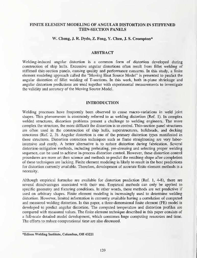
FINITE ELEMENT MODELING OF ANGULAR DISTORTION IN STIFFENEDTHIN-SECTION PANELS

W. Cheng, J. R. Dydo, Z. Feng, Y. Chen, J. S. Crompton*

ABSTRACT

Welding-induced angular distortion is a common form of distortion developed during

construction of ship hulls. Excessive angular distortions often result from fillet welding of

stiffened thin-section panels, causing quality and performance concerns. In this study, a finite

element modeling approach called the "Moving Heat Source Model" is presented to predict the

angular distortion of fillet welding of T-sections. In this work, both in-plane shrinkage and

angular distortion predictions are used together with experimental measurements to investigate

the validity and accuracy of the Moving Source Model.

INTRODUCTION

Welding processes have frequently been observed to cause macro-variations in weld joint

shapes. This phenomenon is commonly referred to as welding distortion (Ref. 1). In complex

welded structures, distortion problems present a challenge to welding engineers. The more

complex the structure, the more difficult the distortion is to control. Thin-section panel structures

are often used in the construction of ship hulls, superstructures, bulkheads, and decking

structures (Ref. 2, 3). Angular distortion is one of the primary distortion types manifested in

these structures. Distortion correction techniques such as flame straightening are very labor-

intensive and costly. A better alternative is to reduce distortion during fabrication. Several

distortion-mitigation methods, including preheating, pre-stressing and selecting proper welding

sequence, can be used to achieve in-process distortion control. However, these distortion control

procedures are more art then science and methods to predict the resulting shape after completion

of these techniques are lacking. Finite element modeling is likely to result in the best predictions

for distortion currently available. Therefore, development of accurate finite element methods is a

necessity.

Although empirical formulae are available for distortion prediction (Ref. 1, 4-8), there are

several disadvantages associated with their use. Empirical methods can only be applied to

specific geometry and fixturing conditions. In other words, these methods are not predictive if

used on arbitrary shapes. Finite element modeling is increasingly used to determine welding

distortion. However, limited information is currently available having a correlation of computed

and measured welding distortion. In this paper, a three-dimensional finite element (FE) model is

developed to predict angular distortion. The computed temperature and distortion profiles are

compared with measured values. The finite element technique described in this paper consists of

a full-scale detailed model development, which consumes huge computing resources and time.

The efforts to reduce computational time are also discussed.

*Edison Welding Institute, Columbus, OH 43221

120

PREDICTION OF WELDING DISTORTION USING THE "MOVING SOURCEMODEL"

The moving source model is formulated and verified for two different configurations. The first

verification is for in-plane shrinkage of a butt joint. The finite element results are compared with

the published experimental data (Ref. 9) to verify the validity of the model. After this

verification, the finite element model is used to predict the angular distortion in a stiffened thin

panel typical of a ship hull. The predicted results are also compared with the experimental

measurements.

Finite Element Model

Typically, a GMAW or FCAW process is used to produce dual fillet welds on T-sections of

thickness commonly used in shipyard for thin-section panel fabrications. A three-dimensional

finite element model is described that simulates the transient, nonlinear thermomechanical

deformation process associated with welding. The motion of welding arc and the associated filler

metal deposition processes are simulated in the model. Thermo-elasto-plastic analyses are

performed using the commercial code ABAQUS enhanced with USER subroutines. The thermal

and elastic-plastic analyses are decoupled and solved independently.

The temperature fields during welding are computed based on the welding process conditions.

The welding heat input is applied using the "double ellipsoid" heat source model (Ref. 10),

where the heat generated by welding is simulated with a power density moving along with the

torch. The double ellipsoid model is implemented via a user subroutine DFLUX in ABAQUS.The method described in (Ref. 10) is used directly. The total heat input Q is evaluated from the

following expression:

Q = TiVI (1)

where r| is the process efficiency, V is the voltage, and I is the current. The process efficiency is

determined by a trial and error approach such that the computed fusion zone matches the actual

one. A process efficiency of 90% is found to give the best correlation of computed and observed

fusion zones in both in-plane shrinkage and angular distortion studies. Temperature-dependent

material properties including thermal conductivity, specific heat are used. Convection boundary

conditions are used for all free surfaces in the thermal analysis.

In the mechanical analysis, the calculated transient temperature fields are used as the thermal

loading for the thermomechanical deformation computations performed using ABAQUSenhanced with user defined subroutines. The user subroutines are used to deal with the materials

behavior at elevated temperatures and simulate the filler metal addition process (Ref. 11).

The FE mesh of the Butt Joint is illustrated in Figure la. The model consists of 15880 elements

and 19603 nodes. The joint has a dimension of 24 inch X 24 inch and plate thickness is 2-3/4

inch. It is a multipass weld, using 4 passes, as shown in Figure lb. The FE mesh used for the Tee

Joint is shown in Figure 2, which contains 21600 elements and 26487 nodes. The joint is

symmetric, therefore, a half model with symmetry boundary conditions is used in the FE model.

Heat conduction 8-node linear brick elements (ABAQUS DC3D8) are used in the thermal

121

analyses and reduced integration 8-node linear brick elements (ABAQUS C3D8R) in the

mechanical analyses for both joints.

Experimental Procedure

The in-plane shrinkage resulted from multipass GMA welding were reported in the literature by

J. Dike, et al (Ref. 9). The double-fillet Tee Joint was welded with FCAW. The experimental set-

up is illustrated in Figure 3. The bottom plate measures 20 inch x 20 inch and the height of the

stiffener is 8 inches. During welding the two torches traveled simultaneously on both sides of the

stiffener to maintain symmetry about the stiffener. The FCAW process used 24 V, 245 A, and 14

in/min travel speed. The fillet size is nominal 1/4 inch. To obtain the thermal response during

welding, the thermocouples are placed beneath the weld bead and on the surface of the plate. Theplate and stiffener are tack welded together before welding. As shown in Figure 3, two brackets

mounted on the stiffener are used to support the joint and prevent any rigid body motion. Figure

3 also indicates the LVDT's used to record the real-time displacement of the plate are positioned

beneath the plate. In addition to the thermocouple and LVDT data, the temperature and

displacement fields were measured using both thermal and stereoscopic imaging systems.

RESULTS AND DISCUSSIONS

For the in-plane shrinkage study, the comparison of cumulative average in-plane shrinkage for 4

passes using FE analysis and experiment is shown in Figure 4. The FE analysis gives a

reasonably accurate prediction of shrinkage resulted from the first pass but also accurately

predicts significant additional shrinkage subsequently.

The fillet weld results are given in Figures 5 through 12. The temperature history, weld bead

shape, transient and final out-of-plane displacements are predicted for the fillet welds with

different welding parameters. The FE predictions are shown in good agreement with the

experimental measurement results. The predicted and observed bead shapes are demonstrated in

Figure 5. The calculated transient temperature fields are verified with both thermocouple and

thermal imaging results. The thermocouple data was compared directly to the nodal temperatures

as predicted by the finite element analysis, as illustrated in Figure 6. In addition thermographic

plots were obtained of the underside of the test plate for comparison as well, see Figures 7

through 9. The predicted final out-of-plane displacement fields during welding are compared

with stereographic mapping results, Figures 10 and 11. The calculated out-of-plane (angular)

displacement history is compared with measurement using LVDTs, as shown in Figure 12.

Both FE modeling and experiment measurements show that the primary distortion mode is

angular distortion for the cases studied. The FE model is capable of accurately simulating the

angular distortion of the welds. Parametric studies using the FE model reveals that, in order to

adequately simulate the angular distortion, it is critical to properly simulate the accumulated

structural rigidity changes along the weld line caused by the continuous deposition of the fillet

metal during welding. Other factors significantly influencing the magnitude of distortion include

weld bead shape and the heat input levels.

122

ACKNOWLEDGEMENT

The authors wish to thank the US Navy and the Manufacturing Technology Program

(MANTECH) for their sponsorship of this research.

The United States Navy, Department of Defense, Navy Joining Center, nor Edison Welding

Institute, nor its subcontractors, nor any of their employees, makes any warranty, express or

implied, or assumes any legal liability or responsibility for the accuracy, completeness, or

usefulness of any information, apparatus, product or process disclosed in this report, or

represents that its use would not infringe privately owned rights. Reference herein to any specific

commercial product, process, or service by trade name, trademark, manufacturer, or otherwise,

does not necessarily constitute or imply its endorsement, recommendation, or favoring by the

United States Government or any agency thereof. The views and opinions of authors expressed

herein do not state or reflect those of the United States Government or any agency thereof.

REFERENCES

1. Masubuchi, K. 1980. Analysis of Welded Structures : 235-240^ Pergamon Press.

2. Michaleris, P.; and DeBiccari, A. 1996. A Predictive Technique for Buckling Analysis of

Thin Section Panels Due to Welding. Journal of Ship Production 12(4): 269-275.

3. Conrardy, C; and Dull, R. 1997, Control of Distortion in Thin Ship Panels. Journal of Ship

Production 13(2): 83-92.

4. Watanabe, M.; and Satoh, K. 1961. Effect of Welding Conditions on the Shrinkage

Distortion in Welded Structures. Welding Journal 40(8): 377s to 384s.

5. Spraragen, W.; and Cordov, M. 1944. Shrinkage Distortion in Welding. Welding Journal

23(11): 545s to 559s.

6. Spraragen, W.; and Ettinger, W. 1950. Shrinkage Distortion in Welding. Welding Journal

29(6): 292s to 294s.

7. Goglio, L.; and Gola, M. 1993. Shrinkage in Butt Welded Joints: Measurement and

Prediction. Welding International 7(10): 776-787.

8. Kumose, T.; Yoshida, T.; Abbe, T.; and Onoue, H. 1954. Prediction of Angular Distortion

Caused by One-Pass Fillet Welding. Welding Journal 33(10): 945s to 956s.

9. Dike, J.; Cadden, C; Corderman, R.; Schultz, C; and McAninch, M. 1995. Finite Element

Modeling of Multipass GMA Welds in Steel Plates. Proc. 4th International Conference on

Trends in Welding Research : 1-9.

10. Goldak, J.; Chakravarti, A.; and Bibby, M. 1984. A New Finite element Model for Welding

Heat Sources. Metallurgical Transactions B 15(6): 299-305.

11. Feng, Z.; Wang, X. L.; Spooner, S.; Goodwin, G. M.; Maziasz, P. J.; Hubbard, C. R.; and

Zacharia, T. 1996. A Finite Element Model for Residual Stress in Repair Welds. Residual

Stress in Design, Fabrication, Assessment and Repair , ASME PVP Volume 327: 11 9- 125.

123

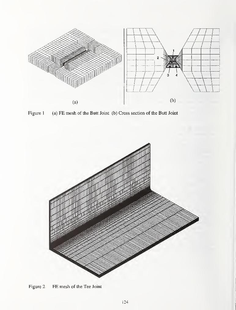
Figure 3 Experimental set-up of welding of stiffened panels (Tee Joints). Plate size (20x 20

in.), stiffener Height (8 in.), thickness (1/2 in.)

Average In-Plane Shrinkage from 3-D FE Analysis and Experiment

Pass Number

Figure 4 Comparison of cumulative average in-plane shrinkage for 4 passes from FE analysis

and Experiment (Ref. 9)

125

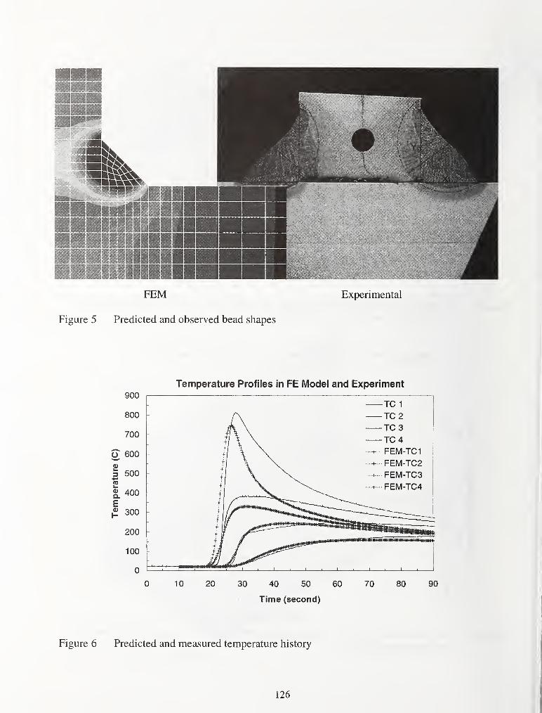
Temperature Profiles in FE Model and Experiment900

I

0 10 20 30 40 50 60 70 80 90

Time (second)

Figure 6 Predicted and measured temperature history

126

Figure 7 Thermographic Plot Depicting the Temperature Distribution on the Bottom of the

Plate with Torch Near Mid-Length of Travel

r RESTART PILE = iilC2-liaw9(l-nt STEP 1 IW-KEMEWT 1766

TIKE (-tiMPLETED IH THIS STEP B5.7 TC/TAL ACCUMULATED TIME H5.7

ABAuttS VD<SlrMi 5.7-6 DATB> 14-AIKJ*195H TIMBi OO.S'JiJB

Figure 9 Predicted temperature field on the bottom of plate at near end of welding

Time

:

1800 seconds

200

•g-IBO

E.

>•

50 ^^^^^^^^^^^^^^^^

50 100 150 200X [mm]

250 300

mm mftflBfflBlfHrftlltllHI! lllltllWiHBHiV8 0.2539 aB89+ 0.9243 1.2804 1.5969 1.9315 2.2670 2.8025 2.9380

Figure 10 Measured Out-of-Plane Displacement After Cooling

128

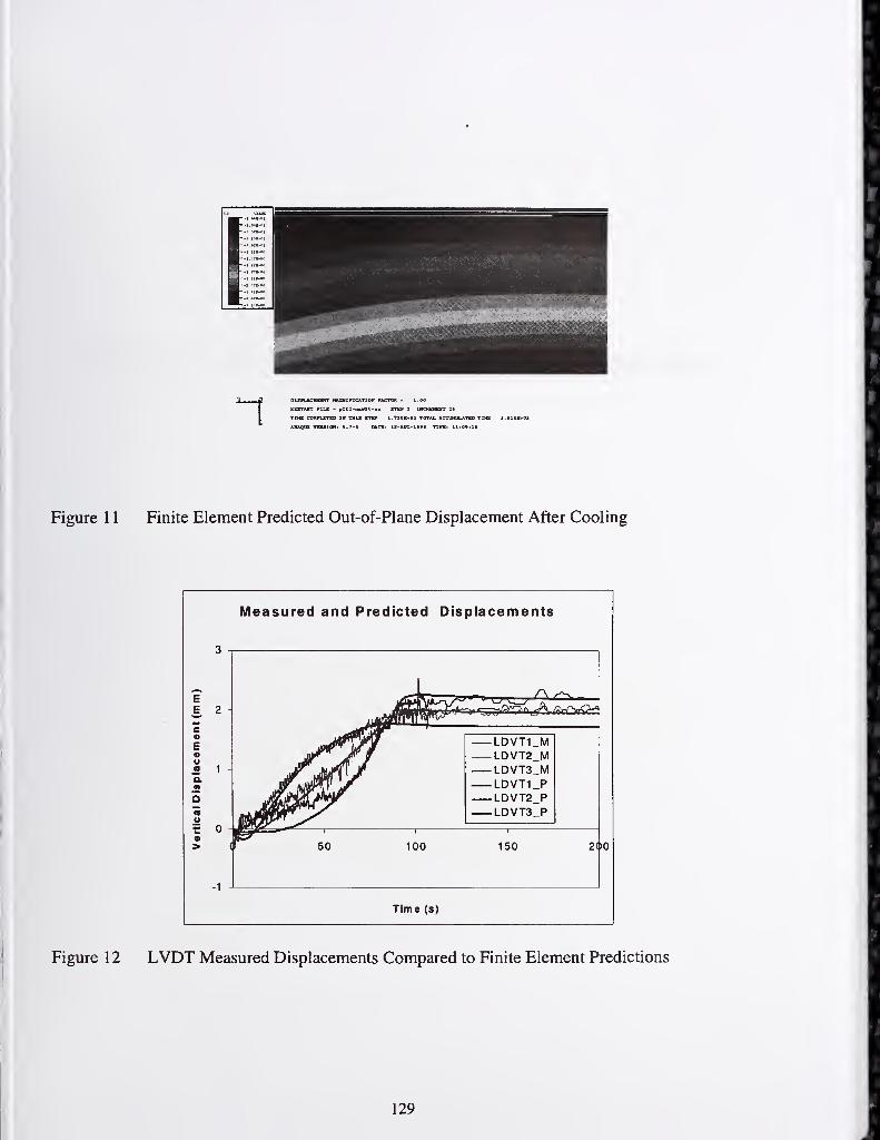
DISPIACBfBNT WUJlnncJkTIOH FACTOR 1.00

RSSTWtT PILE - pU2-n»w90-*B STEP 2 tKCHBHEMT 2S

TIME COHPLETED IN THIS STW 1.130B*03 TOTAL ACCTMULATBD TIMB

ABAgtS VERSIOIIi S.7-C OATSi 1I-AUC-199S TIHBi tlt09ilS

Figure 1 1 Finite Element Predicted Out-of-Plane Displacement After Cooling

Measured and Predicted Displacements

Time (s)

200

Figure 12 LVDT Measured Displacements Compared to Finite Element Predictions

129

Session A4: SolidificationAVeld Composition

Modeling

it

THE USE OF COMPUTERIZED THERMODYNAMIC DATABASESFOR SOLIDIFICATION MODELING OF FUSION WELDS

IN MULTI-COMPONENT ALLOYS

J.N. DuPont \ B.D. Newbury \ C.V. Robino ^ and G.A. Knorovsky ^

ABSTRACT

Most engineering alloys contain numerous alloying elements and their solidification behavior

can not typically be modeled with existing binary and ternary phase diagrams. There has recently

been considerable progress in the development of thermodynamic software programs for

calculating solidification parameters and phase diagrams of multi-component systems. These

routines can potentially provide useful input data that are needed in muhi-component

solidification models. However, these thermodynamic routines require validation before they can

be confidently applied to simulations of alloys over a wide range of composition. In this article, a

preliminary assessment of the accuracy of the Thermo-Calc NiFe Superalloy database is

presented. The database validation is conducted by comparing calculated phase diagram

quantities to experimental measurements available in the literature. Comparisons are provided in

terms of calculated and measured liquidus and solidus temperatures and slopes, equilibrium

distribution coefficients, and multi-component phase diagrams. Reasonable agreement is

observed among the comparisons made to date. Examples are provided which illustrate how the

database can be used to approximate the solidification sequence and final segregation patterns in

multi-component alloys. An additional example of the coupling of calculated phase diagrams to

solute redistribution computations in a commercial eight component Ni base superalloy is also

presented.

1. Lehigh University, Bethlehem, PA2. Sandia National Laboratories, Albuquerque, NM

133

EVTRODUCTION

The microstructure of fusion welds in engineering alloys is dependent on the redistribution of

solute (microsegregation) during solidification as well as the form of the phase diagram.

Previous studies conducted to fundamentally quantify the relation between alloy composition,

microsegregation, and weld microstructure often utilized binary alloy systems (Refs. 1,2). This

approach is convenient because the alloy parameters required for microsegregation calculations

(e.g., liquidus temperature, distribution coefficient, eutectic temperature and composition) can be

determined directly from the binary phase diagram. However, many alloys of engineering

significance contain numerous solute additions, and can undergo one or more eutectic-type

reactions over a broad temperature and composition range. In this case, microsegregation

calculations require the knowledge of multi-component phase diagrams and the distribution

coefficients for all solutes which significantly affect development of the final microstructure. In

addition, when a eutectic-type reaction occurs over an appreciable temperature and composition

range, it then becomes necessary to know two distribution coefficients for each important solute;

one which describes solute partitioning between the liquid and primary solid phase, and a second

which describes partitioning between the liquid and secondary solid phase within the eutectic

constituent. The lack of such information restricts solute redistribution modeling of multi-

component alloys.

In recent years there has been considerable progress in the development of thermodynamic

software programs for calculating solidification parameters and phase diagrams of muhi-

component systems (Ref 3). This progress is likely to lead to more frequent use of solute

redistribution models and their application to alloy systems containing many elements. In view

of this fact, it is useful to consider how such thermodynamic databases can be integrated into

modeling efforts directed at understanding weldability phenomenon. In this article, preliminary

results of an assessment of the accuracy of the Thermo-Calc thermodynamic routine for

modeling solidification of nickel base superalloys will be presented. An example on the

integration of thermodynamic calculations and solute redistribution models for the purpose of

modeling microstructural evolution in alloy IN 718 will also be provided.

APPROACH

Some of the nickel base alloys of primary interest in this work are summarized in Table 1 along

with their chemical composition. The table also includes references to previous work which

investigated the solidification behavior of these alloys through differential thermal analysis

(DTA) and microstructural characterization techniques. DTA has been used to determine the

liquidus and solidus temperatures as well as the temperatures of eutectic-like reactions which

occur near the end of solidification. Phase identification of secondary constituents has been

conducted using electron microscopy. The combination ofDTA data with microscopy resuhs has

been used to experimentally determine the solidification reaction sequences and the details of the

procedures can be found within the references cited. In the current study the Thermo-Calc

routine was used in conjunction with the NiFe Superalloy database (Ref 4) to estimate various

phase diagram quantities and solidification reaction sequences for comparison to the

experimental data. This database has been shown to provide accurate descriptions of solid-solid

134

phase equilibria in multi-component Ni base alloys (Ret 4), but an assessment for modeling

solidification reactions has not yet been reported.

Table 1. Concentration of major elements of some of the alloys under investigation. All values in

weight percent.

Alloy Composition Ref

Fe Ni Cr Mo Other

C-22 3.17 Bal 21.22 13.43 3.29 W 5

C-276 5.44 Bal 15.83 15.56 3.93W 5

IN 718 18.2 Bal 18.2 3.1 5.2Nb-0.04C 6

IN 625 2.4 Bal 22.7 9.6 Range of Nb,Si, and C 7

Experimental 11-45 Bal 19.0 Range of Nb,Si, and C 8

RESULTS AND DISCUSSION

Reaction Temperatures and Phase Diagrams

Liquidus and solidus slopes are important for solidification modeling as they can be used to

provide values for the equilibrium distribution coefficients. Experimental measurement of these

quantities can be accomplished by measuring the liquidus and solidus temperatures with DTA on

homogeneous, single phase alloys with systematic variations in composition (Refs. 7,9).

Although this approach is effective, it is also quite time consuming. Direct calculation of liquidus

and solidus temperatures through thermodynamic databases would thus provide a useful

technique for minimizing the extent of experimental measurements. Figure 1 compares the

measured and calculated Hquidus and solidus temperatures for the alloys listed in Table 1 in

addition to data on other alloys reported in the literature, and the agreement is reasonable. These

Figure 1. Comparison of calculated and measured liquidus (a) and solidus (b) temperatures.

135

calculations can easily be extended to determine the liquidus and solidus temperatures over a

range of composition for a particular alloying element, and an example is shown in Figure 2 for a

five component alloy (Ni-llFe-19Cr-0.02C-XNb). The liquidus and solidus slopes with respect

to Nb in this system have been measured to be -8.3 and -17.9°C/wt% Nb, respectively. The

calculated slopes are in reasonable agreement with these values (-1 1 and -24°C/wt%). The

equilibrium distribution coefficient for Nb, which is given by the ratio of liquidus to solidus

slope, has also been measured for this system and is 0.46. This is in excellent agreement with the

value of 0.46 obtained from the slopes given in Figure 2.

1500

1450

^1400

2^13503ul300

E1250

^1200

1150

11000.0 2.0 4.0 6.0 8.0 10.0 12.0

We ight Pe rc e ntNb

Figure 2. Calculated variation in liquidus and solidus temperature as a function ofNb content for

Ni-llFe-19Cr-0.02C-XNb alloys.

Phase diagrams are needed in order to follow the progression of reactions over the entire

solidification range. Various experimental measurements of multi-component equilibria have

been reported, and these are usually portrayed by using simplified binary or ternary-like

diagrams. These experimentally derived diagrams are useful for database validation. Knorovsky

et al. presented a binary-like phase diagram for EST 718. This alloy exhibits a three step

solidification reaction according 1: L -> y, 2: L -> (y + NbC), 3: L -> (y + Laves). The L -> (y +

NbC) reaction occurs over a relatively wide temperature range and forms a small amount of the

y/NbC eutectic-type constituent. The L -> (y + Laves) reaction occurs over a small temperature

interval and the y/Laves accounts for most of the eutectic-type constituent in the as-solidified

microstructure. Neglecting the small amount of y/NbC that forms, Knorovsky et al. developed a

binary-like eutectic phase diagram at solidification temperatures that includes the primary L ->

y and eutectic-type L -> (y + Laves) reactions. Key temperature/composition points on the

diagram were determined by a combination of DTA and electron microscopy. Their diagram is

compared to a calculated diagram for IN 718 in Figure 3. The calculated liquidus line and L ->

(y + Laves) reaction composition are in reasonable agreement with experimental values. The

calculated solidus line is 75-100 °C below the experimental line, and the calculated eutectic

temperature is approximately 50 °C below the measured value. The difference in solidus values

could, in part, be attributed to the sample used in the DTA measurements. These samples

136

contained a combination ofNbC and austenite. The presence ofNbC depletes the austenite ofNband C relative to the bulk composition of the alloy. Since the solidus slopes for Nb and C are

negative (Refs. 7,9), this reduction in Nb and C would increase the effective solidus temperature

of the austenite. Additional comparisons are, however, needed to confirm this effect.

1500

1400

cT 1300

U 1200

1100

H1000

900

- Khorovsky et al.

- ThanB-Calc

0.0 5.0 10.0 15.0 20.0 25.0

Weight PercentNb

Figure 3. Comparison of measured and calculated binary-like phase diagram for IN 718.

0.6

0.5

10 0.4

c

1 0.3Q.

EoO 0.2;o'5

o-

^ 0.1

NbC

\-4 experimental

calculated—X

\ Laves

Y v\ J\ ^V ^

10 20Liquid Composition Nb wt %

30

Figure 4. Comparison of measured and calculated ternary-like liquidus projection for Fe-Ni-Cr-

Nb-Si-C alloys.

137

The small amount of y/NbC which forms in the IN 718 investigated by Knorovsky et al. can be

attributed to it's low carbon content (~ 0.04 wt%). However, it has been shown (Refs. 7,9) that

the amount of y/NbC constituent that forms in Nb bearing superalloys will increase significantly

with relatively minor increases in carbon content. In this case, binary-like diagrams that account

for only one eutectic-type reaction must be replaced by ternary-like liquidus surfaces. A y-Nb-C

liquidus surface has recently been reported for Fe-Ni-Cr-Nb-Si-C alloys and is reproduced in

Figure 4 along with a calculated version for the same alloy system. The general shape of this

diagram is very similar to that reported for the simple Ni-Nb-C ternary system (Ref 10), except

that the Ni^Nb phase is replaced by the Laves phase (because of the presence of Fe and Cr).

Ternary solute redistribution models (Refs. 11,12) require a priori knowledge of the slope of the

two fold saturation line and the liquid composition at which the L -> (y + NbC) reaction is

replaced by the L -> (y + Laves) reaction. Reference to Figure 4 indicates these values are in

reasonable agreement, indicating that the calculated liquidus surface should provide sufficiently

accurate input values for solidification models. This will be assessed in more detail under the

section on "Coupling of Solidification Models and Calculated Phase Diagrams".

Reaction Sequences and Elemental Partitioning

The sequence of solidification reactions and final microsegregation patterns depend on both the

shape of the phase diagram and the solute redistribution behavior. For example, a binary alloy

that is below the maximum solid solubility and solidifying under equilibrium conditions exhibits

only a primary solidification reaction, since the liquid is consumed before the eutectic

composition is reached. Immediately after solidification the alloy is single phase with uniform

composition. However, under "Scheil-type" conditions (Ref 13), where the diffusivity of solute

in the solid is negligible, the liquid will become progressively enriched in solute until the eutectic

composition is reached, thus initiating a eutectic reaction as solidification terminates

isothermally (for a simple binary system). In this case, the as-solidified microstructure contains

cored primary dendrites and interdendritic eutectic. In many alloys of engineering importance,

however, some solid state redistribution is possible. Thus, in the general case, the reaction

sequence and distribution of alloying elements cannot be accurately estimated until both the

kinetic and thermodynamic considerations are understood. For these situations, calculated phase

diagrams must be integrated with more complex solute redistribution models. An example of this

integration for muhi-component alloys exhibiting both Scheil-type and more complex

solidification behavior are given below.

Considering Scheil-type solidification first, it has been shown that microstructural evolution

during solidification in many nickel based alloys is controlled by subtitutional alloying elements

which exhibit negligible diffusion in the primary austenite constituent (Ref 5). For these alloys,

a simple Scheil simulation can be easily coupled to phase equilibria calculations to approximate

the sequence of solidification reactions and final segregation patterns. Computationally, this

coupling is accomplished sequentially by using the Scheil equation and re-setting the nominal

alloy composition to that of the liquid composition from the previous temperature step. This

ensures the liquid composition will always reach a local minimum on the liquidus surface, as

expected from the Scheil equation. The corresponding fraction liquid is determined by the

product of the fraction liquid from the previous and current temperature steps. Under the

assumptions of negligible diffusivity, this approach can be used to compute the fractions and

138

compositions of solid and liquid during solidification without the need for any kinetic data. The

Thermo-Calc application contains a module for making these calculations.

1400

1380 -

_ 1360O

I 1340

|- 1320

1300

1280

^.1382 — Gamma

- Gamma + Sigma

\ 1310

\^C-22

\ 1290

a

0.5 1

Weight Fraction Solid

1.5

1400

1380 -

o 1360 -

1340-

s

Temf1320 -

1300

1280

namma

Gamma +

1391 \ P

1309 1

C-276

b1299

0.5 1

Weight Fraction Solid

1.5

Figure 5. Scheil simulations for alloys C-22 and C-276.

a

0,2 0.4 0.6 0.8

Weight Fraction Gamma

2 3 4 5 6 7 8

POSITION (MICRONS)9 10

Figure 6. Comparison of calculated (a) and measured (b) segregation patterns for Ni, Cr, and Moin alloy C-22.

139

Microstructural evolution of fusion welds in Hastelloy alloys C-22 and C-276 has been shown to

be governed primarily by partitioning of Mo and Cr (Ref 5). These subtitutional elements

exhibit negligible solid state diffusion during the time frames associated with the cooling rates of

conventional arc welds (Ref 5,8). The final segregation pattern of Mo is of particular interest

since welds in these alloys are known to be susceptible to localized corrosion attack at the Mo-depleted dendrite cores (Ref 14). Figure 5 shows a Scheil simulation for these alloys. For

Hastelloy C-22, the simulations predict a two step solidification reaction consisting of L -> y

followed by L -> (y + a) which initiates at 1310 °C. For the C-276 alloy, a reaction sequence of

L -> y followed by L -> (y + P) initiating at 1309 "C is predicted. These solidification sequences

are in agreement to those experimentally observed by Cieslak et al, with the exception that the

final reactions occur at 1285 °C in each alloy. Figure 6a shows the calculated concentrations of

Ni, Cr, and Mo in austenite as a function of fraction solid in Hastelloy C-22. Since solid state

diffusion is assumed to be negligible, these resuhs are analogous to the final distribution of

solute that should exist across the dendritic substructure, where the fraction solid (fraction

gamma in the figure) is equal to zero at the dendrite core and equal to one at the center of two

neighboring dendrites. Figure 6b shows the experimentally measured segregation patterns of Ni,

Cr, and Mo across the dendritic substructure in Hastelloy C-22 (Ref 5). The segregation profiles

in Figures 6a and 6b are comparable in terms of both segregation direction and magnitudes

(assuming constant density across the range of compositions estimated). Similar results were

obtained for the C-276 alloy.

Coupling of Solidification Models and Calculated Phase Diagrams

As indicated above, conditions exist where the solidification behavior can not be estimated with

a simple Scheil-type analysis because one or more of the important solutes do not obey the

assumption of negligible solid state diffusion. In these cases, the solidification path must be

calculated with a more complex solute redistribution model and combined with the pertinent

liquidus surface to understand the solidification behavior. The binary-like diagram presented for

alloy IN 718 in Figure 3 is useflil for alloy compositions (heats) with low carbon contents that

form negligible quantities of y/NbC. In higher carbon alloys, the L -> (y + NbC) reaction will

occur over an appreciably larger temperature range, and y/NbC will account for a large fraction

of the total eutectic-type constituent present in the final microstructure. The binary-like diagram

can not account for this additional reaction, and higher order diagrams are needed to represent

the multiple eutectic reactions. In this final section, an example is presented where a calculated

ternary-like liquidus projection is combined with a solute redistribution model to understand the

influence of composition on the solidification behavior of alloy IN 718.

Table 2 lists the chemical composition of five heats of IN 718 that contain variations in the Nband C concentrations. Figure 7 shows typical DTA cooling curves for Heats 1 and 5, where the

three step L -> y, L -> (y + NbC), L -> (y + Laves) reaction sequence is displayed for each alloy.

However, note that a seemingly small change in carbon content from 0.04 to 0.09 wt% increases

the L -> (y + NbC) start temperature by an average of 36 °C. These experimentally determined

reaction start temperatures are summarized in Table 2. In agreement with previous results (Ref

6), the L -> (y + Laves) reaction occurs near 1200 °C over a relatively small temperature interval.

Figure 8 shows a calculated ternary-like liquidus projection for IN 718. This diagram was

computed by determining the position of the lines of two-fold saturation which separate the y,

140

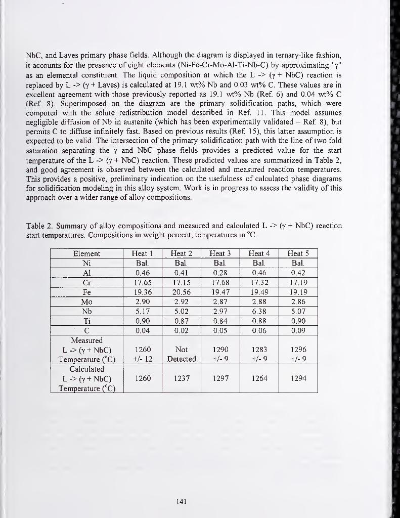
NbC, and Laves primary phase fields. Although the diagram is displayed in ternary-like fashion,

it accounts for the presence of eight elements (Ni-Fe-Cr-Mo-Al-Ti-Nb-C) by approximating "y"

as an elemental constituent. The liquid composition at which the L -> (y + NbC) reaction is

replaced by L -> (y + Laves) is calculated at 19.1 wt% Nb and 0.03 wt% C. These values are in

excellent agreement with those previously reported as 19.1 wt% Nb (Ref 6) and 0.04 wt% C(Ref 8). Superimposed on the diagram are the primary solidification paths, which were

computed with the solute redistribution model described in Ref 11. This model assumes

negligible diffusion of Nb in austenite (which has been experimentally validated - Ref 8), but

permits C to diffuse infinitely fast. Based on previous resuhs (Ref 15), this latter assumption is

expected to be valid. The intersection of the primary solidification path with the line of two fold

saturation separating the y and NbC phase fields provides a predicted value for the start

temperature of the L -> (y + NbC) reaction. These predicted values are summarized in Table 2,

and good agreement is observed between the calculated and measured reaction temperatures.

This provides a positive, preliminary indication on the usefulness of calculated phase diagrams

for solidification modeling in this alloy system. Work is in progress to assess the validity of this

approach over a wider range of alloy compositions.

Table 2. Summary of alloy compositions and measured and calculated L -> (y + NbC) reaction

start temperatures. Compositions in weight percent, temperatures in °C.

Element Heat 1 Heat 2 Heat 3 Heat 4 Heat 5

Ni Bal. Bal. Bal. Bal. Bal.

Al 0.46 0.41 0.28 0.46 0.42

Cr 17.65 17.15 17.68 17.32 17.19

Fe 19.36 20.56 19.47 19.49 19.19

Mo 2.90 2.92 2.87 2.88 2.86

Nb 5.17 5.02 2.97 6.38 5.07

Ti 0.90 0.87 0.84 0.88 0.90

C 0.04 0.02 0.05 0.06 0.09

Measured

L -> (y + NbC) 1260 Not 1290 1283 1296

Temperature (°C) +/- 12 Detected +1-9 +1-9 +1-9

Calculated

L -> (y + NbC) 1260 1237 1297 1264 1294

Temperature (°C)

141

Figure 7. DTA cooling curves for Heat 1 (a) and Heat 5 (b).

0.4 1

o 0.3

Calculated L -> y + NbCV Start Temperatures

\ NbC

\ 1294 -C

y \ / 1297 °C

^ \ 1264 °C

yf >sr^^1260°C/

Heat^/ \ ^1237 °C

>1Heat1„--—"^^^X^/

Laves

-'^eat2

0 5 10 15 20 25

Liquid Composition, wt. % Nb

Figure 8. Calculated ternary-like liquidus projection and solidification paths for five different

heats ofalloy IN 718.

SUMMARY

A preliminary assessment on the applicability of the Thermo-Calc NiFe Superalloy database to

solidification problems in complex muhi-component alloys has been conducted. To this point,

the validation has been conducted by comparing calculated phase diagram quantities to

experimental measurements available in the literature. The comparisons indicate the database

provides useful estimates of phase equilibrium information that is needed as inputs for

solidification models. Work is in progress to extend the validation study to a wider range of alloy

compositions and to couple the calculated thermodynamic information to more realistic solute

redistribution models.

142

ACKNOWLEDGEMENTS

This work was performed at Lehigh University under contract to Sandia National Laboratories.

Sandia is a muhiprogram laboratory operated by Sandia Corporation, a Lockheed Martin

Company, for the United States Department of Energy under Contract No. DE-AC04-95AL85000.

REFERENCES

1. T.W. Clyne and G.J. Davies, Proceedings Solidification and Casting ofMetals, July 18-21,

1977, TMS, 275-278.

2. J.A. Brooks, Proceedings of Weldability ofMaterials, October 8-12, 1990, ASM, 41-48.

3. B. Sundman, B. Jansson, and J O. Anderson, CALPHAD, 1985, 9, 153-190,

4. N. Saunders, Siiperalloys 1996, R.D. Kissinger etal. (eds.), TMS, Warrendale, PA, p. lOL

5. M.J. Cieslak, T.J. Headley, and A.D. Romig, Metallurgical and Materials Transactions, Vol.

17A, 1986, p. 2035.

6. G.A. Knorovsky, M.J. Cieslak, T.J. Headley, A.D. Romig, Jr., and W.F. Hammetter, Metall.

Trans. A, 1989, Vol. 20A, pp. 2149-2158.

7. M.J. Cieslak, T.J. Headley, T. Kollie, and A.D. Romig, Jr., Metall. Trans. A, 1988, Vol.

19A, pp. 2319-2331.

8. J.N. DuPont, C.V. Robino, A.R. Marder, M R. Notis, and J. R. Michael, Metallurgical and

Material Transactions A, 1998, Vol. 29A, pp. 2785-2796.

9. J.N. DuPont, C.V. Robino, and A.R. Marder, Science and Technology of Welding and

Joining, Vol 4, No. 1, pp. 1-14, 1999.

10. H.H. Stadelmaier and M.L. Fiedler, Z Metallkd., 1975, vol. 66 (4), pp. 224-225.

11. J.N. DuPont, C.V. Robino, and A.R. Marder, Acta Materialia, 1998, vol. 46 (13), pp.

4781-4790.

12. R. Mehrabian and M.C. Flemings, Metallurgical Transactions A, 1970, Vol. 1, pp. 455-464.

13. E. Scheil, Z. Metallk, 1942, Vol. 34, p. 70.

14. CD. Lundin, W. Liu, G. Zhou, and C.Y. Qiao, (1998), Unmixed Zones in Arc Welds:

Significance on Corrosion Resistance of High Molybdenum Stainless Steels, Welding

Research Council, Bulletin No. 428, January, WRC, New York, NY.15. T.W. Clyne and W. Kurz, Metall. Trans. A, 1981, Vol. 12A, pp. 965-971.

16. T. J. Lienert, Conference Proceedings Weldability ofMaterials. Edited by R.A. Patterson

and K.W. Mahin. October 8-12, 1990, ASM 1990, pp. 159-165.

17. M.J. Cieslak, T.J. Headley, G.A. Knorovsky, A.D. Romig, Jr., and T. Kollie, Metallurgical

Transactions A, Vol. 21 A, February 1990, pp. 479-488.

18. C.V. Robino, JR. Michael, and M.J. Cieslak, Science and Technology of Welding andJoining, Vol. 2, No. 5, pp. 220-230.

143

Modeling of Multipass WeldmentsE. A. Metzbower

US Naval Research Laboratory

Code 6320Washington DC 20375-5320

Abstract

Computer programs have been developed that present a realistic cross section of a gas metalarc weld. Experimental data derived from bead-on-plate welds at different heat inputs are

used to calculate the width, penetration, and weld bead re-enforcement. Typical computercalculated cross sections are shown for a single V weld configuration. A methodology to

determine the temperature at any point in the weld after each subsequent pass is developed.

Introduction

This is a preliminary report on a program that has been initiated to model the

microstructural development in multipass welds. The impetus for this work lies in a similar

effort on laser beam welding. In that effort the hardness, properties, and microstructure of

the fusion and heat-affected zones were modeled and calculated with surprisingly goodresults. By knowing the composition of the steel, the thermal profile resulting from laser

beam welding, and the grain size of the base plate, the volume fraction of the microstructures

and consequently the hardness and properties of the fusion and heat-affected zones weredetermined.

Reed and Bhadeshia (1) reported on a computer program that they developed to estimate the

cooling conditions that exist in various regions of a multipass weld. Their effort wasdirected towards the shielded metal arc welding of 21/4CrlMo multipass welds which are

used to join l/2CrMoV steam pipes in modem steam-generating power plants. This report

utilizes their concepts for gas metal arc welding of naval structures.

Bead-on-Plate Welds

Data on bead-on-plate welds was provided by the David Taylor Naval Research andDevelopment Center (DNSRDC) (2) and is given in Table 1 . The data is for five different

heat inputs, ranging from 1 .6 to 4.9 kJ/mm (40 to 120 kJ/in). This data was used to

calculated the weld width, height, depth of penetration, and weld bead area as a function of

the heat input. Figure 1 shows the correlation between the weld width and the heat input, E(=Volts * Amps/Welding Speed). Figure 2 shows a similar plot for depth of penetration as

a function of E. Expressions were also obtained for weld bead area and weld bead height as

a function of E.

Table 1 . Experimental Bead-on-Plate Data

Heat

Input

Current Voltage WeldingSpeed

Width Depth Height Total

Area

KJ/mm Amps Volts mm/s mm mm mm 2mm1.6 250 24.8 3.89 14.0 4.4 3.2 55.0

2.8 310 32.0 3.60 19.0 6.3 3.3 72.7

3.1 300 28.5 2.75 19.0 5.9 3.8 87.8

3.9 413 32.0 3.39 23.0 8.0 4.0 115.9

4.9 490 35.0 3.51 25.0 10.0 3.8 138.8

144

26-Welding Data

:" 'y L' slg/Ve V L'sVaVx" r=" i.VsVel" "e":24--

22+

20"

1 8+

1 64-

1 4-

1 2-

o

o ^ o

1 .5 2.5 3 3.5 4E, kJ/mm

Figure 1 Bead-on-plate width as a function of heat input.

'"I ""I'

'

I ""I "" I

4.5

11-

1 0-

9-

8'

7'

6'

5'

4

Welding Data1 I I I I

IJ44 "+"\

1 1 1

1

y = 1.3944 + 1.7013X R= 0.9796I

I I I II

I

0.97963

o

1.5 2.5 3 3.5 4 4.5E, kJ/mm

Figure 2 Depth of penetration as a function of heat input.

The bead-on-plate weld consist of a reinforcement above the top of the plate. This

reinforcement can be characterized as a spherical cap. Knowing the width of the bead-on-

145

i

Height

T

Figure 3. Thedrawing depicts

the geometry of

the cross section of the bead-on-plate weld.

plate weld and the area of the fusion zone, the half angle of the spherical cap can be

calculated. This geometrical arrangement is shown in Fig. 3.

Rosenthal's (3,4) equations for heat flow around a finite heat source moving at constant

speed across the surface of a plate have been modified by several authors (5,6). One such

modification by Ashby and Easterling (5) modifies the time by including the additional time

require for the source to transverse a given point and modifies the height by replacing the

real source by an apparent source above the plate. These modifications result in the

following equations for heat flow

T-To = exp/-X f(5±5q)! + jL] 1

27tA[t(t+to

4a (t+to),

Where T is the temperature, t is the time, X is the thermal conductivity, a is thermal

diffusivity, q is the watts (current * amps), v is the welding speed, and rt is the radius of the

source.

By solving these equations with the appropriate thermodynamic values, a bead-on-plate

profile can be constructed at any heat input. Figure 4 depicts a bead-on-plate weld

calculated at 1.6 kJ/mm. The various degrees of shading represent the temperatures that are

146

Figure 4. Bead-on-plate weld computed at 1 .6 kJ/mm.

obtained in these regions. These temperatures range from above the melting point of the

steel down to about 850 °C below which no transformations are expected. The programperforms an iterative calculation on the heat input (essentially modifying the efficient of the

process) so that good agreement is reached between the depth and width of the weld as

calculated from the modified Rosenthal equation and the depth and width of the

Fig.4. Single V weld after one pass.

147

experimental bead-on-plate welds fabricated at various heat inputs. The program presently

allows only a few weld geometries to be calculated: bead-on-plate, single V, and double V.

The angle of the V is input for the program.

Fig. 5. Single V weld after ten passes.

Fig. 6 Single V pass after completion (21 passes).

In calculating a multipass weld, a significant variable is the amount of overlap between

adjacent passes. If this input value is incorrect, the resulting cross section will have holes in

148

A cknowldegemntit. Thus the program has been run with an array of overlaps until the

cross section is dense and the number of passes is appropriate. If the overlap is too great,

the cross section appears distorted. The geometry of the addition of each pass is critical in

filling the single V. The geometrical factors have been explained by Reed and Bhadeshia

(1). An example of a single V weld with a heat input of 40 kJ/mm is shown in Fig. 5 after

a single pass, in Fig. 6 after 10 passes, and in Fig. 7 after completion (21 passes). Each of

these passes contains a fmger penetration, which would occur at these voltages, but is

artificially added to the calculation. Again the variations in color or shading are an

indication of the temperature regimes last experienced in the calculation. The small square

in the middle represents the point in the weld where the complete thermal history is knownfrom the program. Figure 8 shows the thermal profile obtained from the program at

different peak temperatures. The program can calculate the peak temperature experienced

2

I

1800

1600

1400

1200

1000

800

600

400

200

1 I 1 ) 1 I 1 t r 1r 1 r 1 1 1 [ 1 1 T 1 1 1 1 1 1 T T 1

1 r T 1

-i /-^ Vs. ; i

r ^N;iL : :

1 1 I 1 1 1 t 1 1 1 t 1 1 1 , , , , i , , , , i , , , , i , , , ,

~

10 15 20

Time, s

25 30 35

Fig. 8 Thermal profiles based on different peak temperatures.

by any point in the weld. The succession of peak temperatures gives an approximation of

the tempering that occurs by subsequent passes. Depending on the location of the point of

interest, a subsequent pass may completely austenitize the point.

Future Work

A series of welds of A36, HSAL65 , and HSLAIOO have been fabricated at three different

heat inputs of 1 .0, 1 .6, and 2.0 kJ/mm (25, 40, and 50 kJ/in) under the direction of R. Wongat the Naval Surface Warfare Center, Carderock Division. These gas metal arc welds are

approximately twenty four inches long, have a single V, 60° configuration and were made

such that each subsequent pass was indexed (7) about two inches from the prior pass. In

this manner the microstructural evolution of each pass will be examined. Macro and

microstructural evaluation of these welds has begun. Hardness maps will be constructed.

Tempering will be studied using a dilatometer.

149

Acknowledgement

This work was supported by the Office of Naval Research.

References

1 . R. C. Reed and H. K. D. H. Bhadeshia, Acta metall. mater. 42, 3663 (1994)

2. G. L. Franke, David Taylor Research and Development Center, private communication

3. D. Rosenthal, Weld. J. Res. Suppl. 20, 220s (1941)

4. 4. D. Rosenthal, Trans. ASME 68, 849 (1946)

5. M. F. Ashby and K. E. Easterling, Acta metall. 32, 1935 (1984).

6. J. C. Ion, K. E. Easterling, and M. F. Ashby, Acta metall. 32 1949 (1984)

7. R. Wong, Naval Surface Warfare Center, Carderock Division, private communication

150

DEEP PENETRATION WEL0

- .^-.CHARACTEBISnCS. „.i.

-2S 0

TEMPERATURE (C)

COMPIt^ »«CISION HIGH VOIUMC ASSFMfll Y

requires hiqh speed wehUng wWi low heat tnpm

«rfvicr. at Itte RMnponant crqurte-i a tough weWMfli co«8iig rare causes » h»rH and bcHMc wrid

Itic assembly caiiiiol Ue bulk iM-dtrd

\|

toss

T T-T DUGHAM

"f

T

EMP

linimte

1 sec IOC TIMt

151

152

rv: W»i

CAM POWER (KW)

450 r

400

3S0CO

J 300

1 250

> 200oE$

150111 100

50

0-7

^^^^^

o , t

a.

OISTANCK

SCHEMATIC OF TEMPERATURES iN LBW

CONCLUSION

The potential cost savings of heavy - section

laser welding is si^ficant. The technology

appears to be at hand. It is now our challenge

to soive the complementary probiems to

expedite implementation.

LASER BEAM WELDING OF STRUCTURAL ALLOYS

GOOD PENETRATIONFAST WELDING SPEEDSDEMANDS AUTOMATIONGOOD MECHANICAL PROPERTIES R<xiu«*i<w af iS'iftct-wses tcHJ&hnetss

Addition of Ni j«cr«eiw» U>w icmpcrasuce fraciure toughness

L*!M!f aiTength easier (o *tW

£»siorjion L-i minimal Ir I.BW

Low C, fciw ^ a)(('y;,>iMV!-bes( mwhaoica) prt^^fritrs

Can OiUjiliiic har/Sit:;;*s (uMt*) ar.d hcal-a)lcc*i<l /ixira

153

^

—

.—^

^—_

LASER BEAM WELDINGPROCESS PARAMETERS

MATtntAI. THICKNESS l>OWER SPEED HEAT INPUTkW m<n/M)c<i|>ml kJimm(kJ:in.>

A3* S!.») ( 21 m .» i 7,31

« t.m 10 .O i14.»)

12 1») 1) M (33t t3 {23 ffi

13 « EtSI 2.n iss.O)

HV-80 a t 211 8 » im -32 i «.1l

n f -5) 11 13 «3(» .» 121.51

6(25) S 23 !sa 3S 1 asi

MV 1M 6im • 21 m .38 i 9 7)

1i (.5 i 13 W !MJ 10 i26.«f

1? ! S > m 13 '.301 n (1SS)

LASER BEAM WELDINGMECHANICAL PROPERTIES

YIELD ULTIMATE ELONGATION/MATERIAL THICKNESS STREN(3TH STUIUQTM HARDNESS

mm {in.) Mp« (Mil Mp« (k«l) * Be

AS 6 I S] 278 I 40) 442 ( 841 23

9 (.38) 2» 1 31) 428 ( 82! 22 -vM12 1 .51 278 1 W) 448 ( 881 24

U I.S3I 2S» < 39) 438 1 83) SMV«I » (.251 21 I Ml 745 11881 25 42

12 ( ,EI (27 1 911 7SZ (IDS! 24 43

HV-IOO « I.2S) 887 (toil 78» (1101 20 41

Hy-i3B e 1.251 986 (1MI 1022 f14S) 13 4012 1 -SI 962 (1381 987 1143) 19 40

154

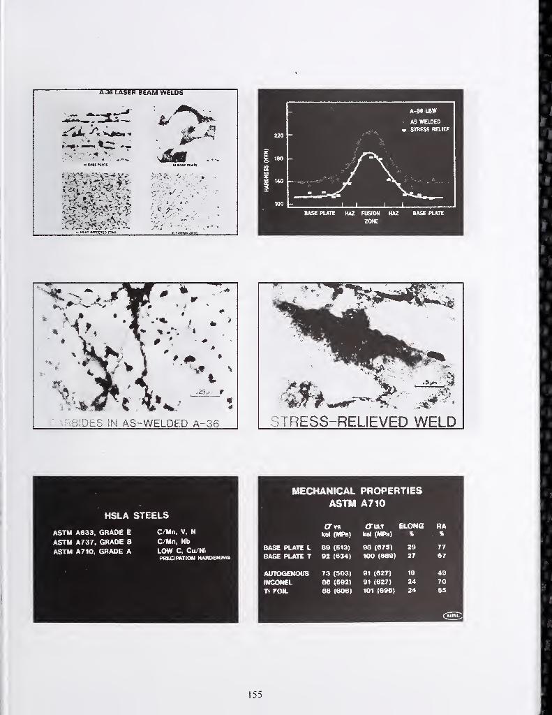
LASER BEAM WeLbi

HSLA STEELS

ASTM A633, GRADE E C/Mn. V, N

ASTM A737, GRADE B C/Mn, Nb

ASTM A710, GRADE A LOW C, Cu/NIPflECimTION HMROENINQ

jTRESS-RELIEVED WELD

MECHANICAL PROPERTIESASTM A710

<Tt8 OTULT ELONG RAkal (MPB) M (MPa) % . %

BASE PLATI L ae (813) 08 (678) 29 77

BASE PLATE T 82 (634) 100 (680) 27 67

AUTOGENOUS 73 (503) 91 (627) 19 40

tNCONEL ae (602) 91 (627) 24 70

Tl FO«L 88 (606) 101 (606) 24

155

156

157

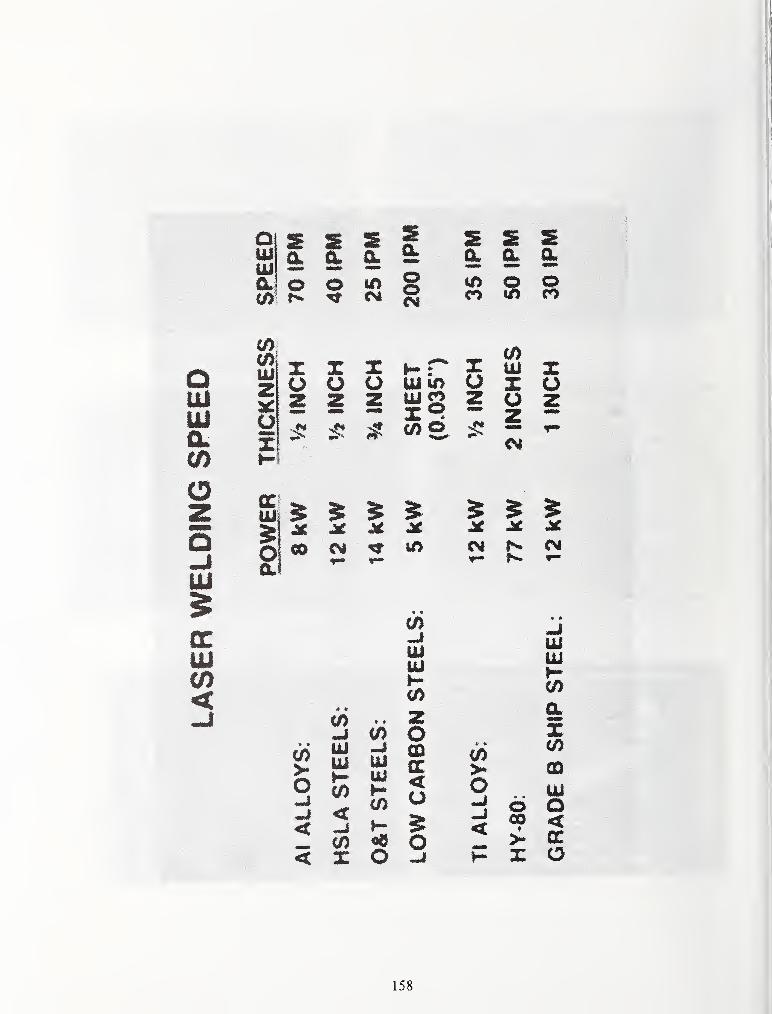
oUJ

HEStum

o-«?r CM

oo

s s sa a a.

ID Q OCO in CO

ft

o

UiZoX

Xu

X Xo oz z

25 3^

<

00

>o•J

<

-JUJ

UJ touj{2Xo

5 ? 5CM tn

UIU(

iA

W OUJ UJ q:. ... ^

o

o<

X o

Xo

o

<

COui

o

CM

XOz

5 5 5^ jtf ^CM N <MIT— f*.

UJUi

CD

O OCO <

H X O

158

DEEP PENETRATION WELDGHARACTEmSTICS ^

D smov

—~~.— .- . » «•

ADVANTAGES OF LASER WELDING

ULTRA FAST WELDING SPEEDS

GOOD PENETRATION

SIMPLE GEOMETRY

LOW DISTORTION

GOOD MECHANICAL PROPERTIES

EXCEPTIONAL FRACTURE RESISTANCE

OcMANDS AUTOMATION

159

160

LASER WELDING

MATERIAL SELECTION FOR LASER WELDING

SAMPLE PREPARATIONA) JOINT DESIGNB) FIT UP TOLERANCEC) O-EANING OF WORKPIECES

MAJOR LASER PROCESS PARAMETERSA) POWER AND TRAVEL SPEEDB) WELD PROTECTION GASC) FOCUSING OPTICSD) FOCAL POINT POSITION

POST-VretD INSPECTIONA) DESTRUCTIVE TESTINGB) NON-DESTRUCTIVE TESTING

LASER WELDING OF MATERIALSCOMMON STEELS

MATERIAL SUITABILITY POSSIBLE PnOBLEMS COMMENTS

LOWCARBOH(fllMHCO)

STtEt

LOW 1, POBOSITY2. BRITTIEI«SS3- OMPSEDICTAaiLITV

POOR BESUtTS DOE lOIFKXUSIOMS, DEOASINa

LOWCARBON(ALUttmUHKNXEO)STEEL

EXCELLEKT LESS THAN 0 3%CAHSON COWrGNT

MEOIVW/HK3HCARBONAND ALLOYSTEEL

EXCELLEHT V STRESS CRACKINQ.COHTH0U.A01E 8V PRE-ANO/OR POST-nCATINO

PRE -MEAT TEUP. DGI>ENOENTON nBOKNEJiS.I'EHETRATIONRULE Of TMUNB:o.3\ < ECC' < o.ev-

200-SOO "C

O.e* < ECC: 'C

DISSIMILAf!STEELS

EXCeiLEHT 1. STRESS CHACKIMO,COMTROtLASLE BV l>m£-

AM}/0« POST-HCATmO

OEPEMDEMT OH ECC OFALLOT m WELD ZONE ASQETEiaVNEO BY DILUTIONAHALYSiS.

OPTIMIZATION OF LASER WELDING

POWER DENSITY

TRAVEL SPEED

GAS SHIELDING

PLASMA CONTROL

WELDMENT PROPERTIES

FUSION METALLURGY

162

380

/O 300E

ui 240X 1 Itir .3 180Z

iflHU-60 -20 20 60 100

TCMPERATUHE (°C)

?5 r-i'

• LBW BL-T *LBW-SH

i:

163

COMPUTER MODELING OF METALLURICAL TECHNOLOGIES

M. Zinigrad*, V. Mazurovsky**

ABSTRACT

The principles of the mathematical modeling of metallurgical welding processes are considered.

The essence of the proposed method is the application of fundamental equations of physical

chemistry to the analysis of the complex chemical processes that take place between the metallic,

oxide, and gaseous phases in weld zone and shape the final composition of the weld metal. Themethod is used to develop a mathematical model of a flux-core arc welding process. The model

permits prediction of the composition of the weld metal (the direct problem) as a function of the

composition of the starting materials, i.e., the metal strip, the base metal, and the flux powder

components, and as a fianction of the technological parameters of the process. The solution of the

inverse problem, in which the input parameters are the technological characteristics and the

composition of the strip, the base metal, and the weld metal, and the output parameter, i.e., the

parameter sought, is the ratio between the core materials in the wire, is also possible. In this case,

a computer program based on the model yields a new formula for a flux-cored wire over the

course of a few minutes.

KEY WORDS

Mathematical modeling, welding and surfacing, flux-cored wire, composition optimization.

INTRODUCTION

The complexity of welding processes stems form the simultaneous occurrence of a large number

of physical and chemical processes involving liquid, solid, and gaseous phases. The special

features of these processes include a high temperature, intense stirring of the phases,

nonstationary mass transport, and thermal fluxes. The course of a process is determined by a

large number of parameters, which often depend on one another.

The methods of mathematical modeling are being employed with increasing frequency for just

such complex systems (Refs. 1-14). The use of mathematical methods reduces the duration,

tediousness, and cost of an investigation. Moreover, computer experiments often provide a result,

which is extremely difficult or totally impossible to obtain by empirical means on a real object.

A model is essentially a simplified system, which reflects isolated, but the most significant

aspects of the real object. The more parameters the model takes into account, the more universal

and faithfiil to that object it is.

* The College of Judea and Samaria, Ariel, Israel

" Chisumim Ltd., Ariel, Israel

164

Modeling involves a search for a mathematical dependence between the input and output

parameters of the system being studied. Either industrial welding processes (Refs. 1, 5, 6, 8, 9,

and 11), the formation of the weld metal and its properties (Refs. 4, 7, 10, and 12), or the

physiochemical and metallurgical processes shaping the composition (Refs. 2, 3, 13, and 14-17)

are modeled

ESSENCE OF THE PROPOSED APPROACH

The possibility of predicting the composition of a product is important for any technological

process, since it permits prediction of the outcome of a technology already in the planning stage.

The solution of this problem takes on special importance for welding technologies because of the

high speed of the process, the high temperatures, and the short lifetime of the liquid pool. The

principal chemical reactions shaping the final composition of the weld metal take place on the

boundary between the metallic and oxide liquid phases, as well as in their interactions with the

gas. The interaction between the phases during welding usually represents a large set of parallel

and conjugate reactions, whose rates are interrelated. The main problem arising in calculations of

the dependence of the composition of phases on time is associated with the difficulty in

determining the rates of these reactions. If these rates can be determined, the concentration of

any element in a volume of a particular phase can be found using the simple relation

where V is the volume of the phase in which the element is located, A is the surface area of

the interface, C^.. is the concentration of the particular element, and V^^ is the rate of its passage

from one phase to another.

The plus and minus signs show the direction of passage of the element: the minus sign

corresponds to a decrease in concentration, and the plus sign corresponds to an increase.

If we confine ourselves to small time intervals (At), during which the rates can be considered

constant, Eq. (1) can be simplified:

V,,^±—^--, (2)

This equation permits finding the value of AC^^ and, consequently, the concentration C^. at any

moment in time.

Thus, the problem of predicting the composition reduces to selecting a simple and reliable

method for calculating the rates of passage of all elements through an interface.

165

Let us utilize our previously developed method (Ref. 18) for finding these rates. The essential

idea of the method is that the entire set of chemical reactions taking place on an interface is

described by the equations of chemical reactions with a single common reactant. For metal

materials based on iron, we choose iron oxide FeO as such a reactant and write the equation of

the reaction in the form:

-[E,] + (FeO) ^ -iE.pj + Fe, (3)m m

where [£,] is any element in the metallic phase, (£",^0^) is its oxide in the oxide phase, and n

and m are stoichiometric coefficients.

The method, which was described in detail in Ref 18, permits determination of the rates of

passage of elements through an interface F^.^ . It consequently makes it possible to calculate the

variation of the concentration of each element [£,] in the metallic phase and the concentration of

the corresponding oxide {E^O^) in the slag phase.

The advantage of such an approach lies in the fact that the calculation results do not depend on

which specific reactions among all the possible ones are considered. It is sufficient that they be

algebraically independent, include all the necessary components, and contain one commonreactant. This is associated with the essence of the method itself, which permits determination of

the fluxes of reactants toward and away from the phase boundary, rather than the rates proper.

MATHEMATICAL MODEL OF A FLUX-CORED WELDING PROCESS

This paper discusses the results of the development of a quantitative mathematical model of a

flux-core welding (surfacing) process.

Let us consider the sources shaping the composition of the weld metal for the technology chosen.

The scheme of the technological process is presented in Fig. 1.

It is expedient to consider the shaping of the composition in two stages of the process: the drop

stage and the pool stage.

The final composition of the drop is determined by the concentrations in each of the powdered

components in the wire [£,1'^^ and, accordingly, by the melting rates of these components V^^,

the concentration of each element the metal cladding [Et]b and its melting rate Vt, as well as by

the rates of passage of the elements through the interface V^^ of the drop (3) and the slag film (4)

on its surface, which can be calculated in accordance with the methods described above. The

values of F^^and Vb are found from empirical relations as functions of the technological

parameters of the process.

166

Welding Direction

Figure 1 . The technological scheme ofwelding process.

1 - metal tube; 2 - flux (powder mixture); 3 - drop of liquid metal; 4 - slag film; 5 - metal pool;

6 - molten slag pool; 7 - weld metal; 8 - base metal; 9 - slag crust (layer of solid slag)

Thus, the concentration of the /-th element in the drop at any moment in time t [E^ ]^ , can be

calculated from the equation

V, At +f^Vl,[EXAT + V,^ -M,^ .^.-Ar-lOO

{E,, (4)

where Ad is the surface area of the liquid drop, / labels the type of powder, L is the number of

types, M^^ is the molecular weight of the element, and is the mass of the metal drop at the

time T.

167

The final drop composition thus calculated [Ei]ci is used to calculate the concentration of the i-th

element in the weld pool at any time x. The composition of the pool and therefore the

composition of the weld metal are determined by the concentrations of the elements in the liquid

drop [E,]d and accordingly by the rate of descent of the drops into the liquid pool V^, the

concentration of each element in the base metal [E,]bm, the melting rate of the base metal, and, as

in the case of the drop stage, by the rate of passage of each element through the interface

between the metal (5) and slag (6) pools.

In accordance with the foregoing, the expression for calculating the concentration of element / in

the weld metal can be written in the form

V, At + V,^-[EJ,„.At + V,^-M,^-A^-At-\00L^J =

, (5)

where Ap is the area of the interface between the metal and the slag, and nip is the mass of the

weld pool at the time x.

The system of equations (4) and (5), together with the expressions for calculating taken from

Ref 18, comprise a mathematical model, which describes the interaction between the phases in

an industrial flux-core welding (surfacing) process.

USmG THE MATHEMATICAL MODEL TO DEVELOP NEW

FLUX-CORED WmE COMPOSITIONS

A computer program for PC computers has been written in Microsoft EXCEL and Visual Basic

for Windows using the model developed.

This program can be used to determine the composition of a flux-cored wire that ensures the

formation of a weld metal with an assigned chemical composition. In this case, the output

parameter is the new formula of the flux-cored wire. The input parameters are the chemical

compositions of the starting materials, the physicochemical characteristics of the interacting

phases and processes taking place between them, and the technological parameters.

Let us analyze the stages of operation of the program in the case of the development of a new

formula for a self-shielded flux-cored wire.

We assume that our task is to develop a new electrode for obtaining a welding joint with an

assigned composition and required properties. The chemical composition of the base metal,

which is needed for the calculation, is stored in the database together with the composition of

other standard materials.

At the first step we enter the technological parameters in accordance with the welding procedure

selected.

168

We must ensure that the weld metal has a definite composition. We enter the chemical

composition of the weld metal that must be obtained.

Element C Si Mn Cr V Ti Al Fe

Concentration,

wt. %0.1 0.15 1.2 0.1 0.012 0.40 0.8 B

Table 1 . Required weld metal composition

The next and most important step is optimization of the flux composition. The required weld

composition can clearly be obtained with different combinations of components in the flux. The

database contains the chemical compositions of various components, which should be utilized in

selecting the optimal flux composition.

The program has to establish the flux composition that provides the required weld metal

composition and to select the most inexpensive variant among them. The weldability should be

optimized as well.

The program also includes a special module, which provides an evaluation and optimization of

the mechanical properties of the weld metal having the composition obtained.

This obviously requires a large number of iterations to perform calculations with all possible

component ratios.

In particular, four flux compositions were found for the case under consideration, and one of

them was specified as flux, which provides the required joint composition with the lowest

production costs. The results of the calculation (both the optimal composition and the other three

compositions) are stored in the database of the program. The program presents the optimal flux

composition. Such a flux provides the solution of the problem posed, i.e., the required joint

composition. This composition agrees well with the one we assigned when we posed the

problem.

Element C Si Mn Cr V Ti Al Fe

Concentration,

wt. %0.09 0.18 1.12 0.09 0.016 0.42 0.71 B

Table 2. Predicted weld metal composition

It would be naive to think that we can get a new electrode just from PC. What we do is

narrowing the area of search an extent that by conducting only a few welding experiments we

will be able to get the desired composition.

169

This advantage acquires special importance in the case when we deal with components that have

never been used in the welding materials production. In such a case even the most highly skilled

and experienced technologist can not know what the influence of this or that component will be.

In the case at hand the approximate time for the calculations and optimization was 1 5 to 20 min.

Very short series of welding experiments was carried out to adjust the composition to the real

technological conditions. The result is a new formula for an electrode that provides an assigned

joint composition and is 40% less costly than the existing formulas owing to the employment of

alternative materials and optimization of the composition.

The flux-cored electrode with a new flux was produced. Welding was carried out. The actual

weld metal composition (obtained using a spectroscopic method) is presented in Table 3.

Element C Si Mn Cr V Ti Al Fe

Concentration,

wt. %0.08 0.18 1.32 0.11 0.013 0.38 0.62 B

Table 3. Experimental weld metal composition

INDUSTRIAL APPLICATION

In 1997, we founded a new R&D company, Chisumim Ltd., to implement the development

techniques described above.

Chisumim specializes in utilizing our unique scientific methods for formulating the optimal

composition of welding materials and optimizing welding and hard-facing technologies.

Chisumim is developing new materials for hard-facing machine parts in various industries.

Another of Chisumim' s projects (which is being financed by GM-UMI Technology R&D, a joint

venture of General Motors and Universal Motors Israel) is the development of a tailor-made

flux-cored welding wire intended for improving the course and efficiency of welding processes

in GM.

REFERENCES

1. Ducharme R., Kapadia P., Dowden J,, Williams K, Steen W. 1994. An integrated

mathematical model for the welding of thick sheets of metal with a continuous CO2 laser.

Laser Inst Am. 11: 97-sto 105-s.

2. Boronenkov V., Salamatov A., Zhadkevich M. 1991. A mathematical model of the

physico-chemical processes in electron beam remelting. Proc. -All-Union conference,

170

Novokuznetsk: 21-22.

3. Schwerdtfeger K., Werner W., Pateisky G., Modeling of chemical reactions occurring

during electroslag remelting. Iron and Steel 3: 135-s to 143-s.

4. Davydov Yu., Boronenkov V., Salamatov A. 1992. Prediction of the weld formation of

variable composition based on modehng of metallurgical processes. Autom. Svarka 7-8:

23-s to 26-s.

5. Norrish J., Gray D. 1992 Computer simulation and off-line programming in integrated

welding systems. Weld. Met. Fabr. 60, 3: 119-sto 122-s.

6. Kozlovsky S. 1990. Modeling of the interaction of parts in the contact area in spot

welding. Isv. VUZ. Mashinostr .9. 89-s to 94-s.

7. Grigorenko V., Kiselev O., Chemyshov G. 1994. Mathematical model and its practical

evaluation for weld formation. Svar. Proizvod. 2: 30-s to 32-s.

8. Tsybulkin G. 1994. Mathematical models in adaptive control of arc welding. Autom.

Svarka. 1 : 24-s to 27-s.

9. Cerjak H., Easterling K. E. 1993. Mathematical modeling of weld phenomena. 369

London

10. Vitek J., Zacharia T., David S., Rappaz M., Boather H. 1994. Modeling of single-crystal

laser-weld microstructures, Proc. Laser mater process symp. TMS, USA: 213-220.

11. Dowden J., Ducharme R., Kapadia P., Clucas A. 1994. A mathematical model for the

penetration depth in welding with continuous CO2 lasers. Laser Inst. Am. 79, 451-460.

12. Grong O., Kluken A.O. 1992. Microstructure and properties of steel weld metals. KeyEng.Mater: 47-93.

13. Mitra U., Eagar T.W. 1991. Slag-metal reactions during welding. Metall. Trans. (B),

vol.22, No 1: 65-100.

14. Olson D. L., Lui S., Edwards G. R. 1993. Physical metallurgical concerns in the modeling

of weld metal transformations. Math. Modell. Weld. Phenom.: 89-108.

15. Zinigrad M,, Zalomov N., Mazurovsky V., Aksyutin O. 1997. Creating new welding

materials on the basis of metallurgical processes modeling. Proc. 7^ int. conf on

computer technology in welding. USA,, ed. T. Siewert: 291-297. NIST spec, publ.923.

16. Zinigrad M., Mazurovsky V. 1996. Modeling of metallurgical welding processes for the

purpose of creating new welding materials. Proc. International conf on modeling and

simulation in metallurgical eng. and materials science, Beijing, China, eds. Yu zonsen,

Xiao Zeqiang, Xie Xishan: 669-673. Metallurgical Industry Press.

17. Zinigrad M., Mazurovsky V., Zalomov N., Aksyutin O. 1998. Computer approach to the

development of welding materials. Proc. 8^ International conf Computer Technology in

Welding. pp.S20-l - S20-9, Cambrige University, TWI.

18. Boronenkov V., Shanchurov S., Zinigrad M. 1979. Kinetics of the interaction of

multicomponent metal with slag under diffusion conditions. Izvestiya Ac. Nauk USSR.

Metal, 6, 21-27.

171

I

I

Session A5: General Modeling

i

THE EFFECT OF WELD METAL ON THE GEOMETRY RELATIONS IN

C(T) AND SE(B) FRACTURE SPECIMENS

J.R. Donoso* and F. Labbef

ABSTRACT

The geometry relations in C(T) and SE(B) fracture specimens with weld metal in the ligament are

analyzed. For this purpose, ASTM A 588 Grade A steel fracture specimens welded with AWSE8018-G electrodes were modeled by a two-dimensional non-linear finite element code,

considering different defr)rmation behavior for the base metal (BM) and the weld metal (WM). Adegree of overmatching of 1.4 between weld metal and base metal, various volume fractions of

WM, and no dilution effects were also considered in the model. The geometry characteristics

analyzed are: the relation between crack-mouth opening displacement (cmod) and load-line

displacement; the value of rjpi needed for the evaluation of J; and the position of the apparent

center of rotation in the ligament, related to the evaluation of CTOD. The numerical results

obtained for the modeled specimens were compared to experimental load vs. load-line

displacement results obtained on blunt-notched, small ligament size (0.30 < bAV < 0.50) weld

metal fracture specimens. In addition, a comparison was done with theoretical values of r|pi for

BM specimens obtained from the Common Format Equation parameters of Donoso and Landes.

The effects of crack length and volume fraction ofWM on the geometry relations are analyzed and

discussed in terms of the constraint imposed by the overmatched weld metal.

KEYWORDS

Elastic-Plastic fracture; fracture toughness; finite element modeling

INTRODUCTION

The application of ductile fracture mechanics to the evaluation of fracture toughness in materials

rests primarily upon two widely used approaches: J and CTOD. Both parameters have been

extensively used, and become the subject of standards; e.g. ASTM standards E 813 and E 1290

[Refs.l, 2]. Both standards are explicitly intended to be used with homogeneous materials;

however, weldments may be included in their scope of application. On the other hand, BSStandard 5762 [Ref 3] has been followed up with a proposal for the assessment of defects in

fiasion welded joints [Ref 4] based on the CTOD approach. Apparently, the evaluation of

toughness of welds by using CTOD seems to be more reliable than taking the overall specimen

deformation behavior, as does the evaluation of J [Ref 5].

* Materials Science Department, Universidad Tecnica Federico Santa Maria, Valparaiso, CHILE

t Mechanical Engineering Department. Universidad Tecnica Federico Santa Maria, Valparaiso, CHILE.

175

The latter argument places J in disadvantage in relation with CTOD measurements, whenevaluating the properties of a weld. The material property variations in welded joints (base metal,

BM; weld metal, WM, and heat aflfected zone, HAZ) are overcome by making all measurements in

the "mouth" of the crack (cmod), thus representing local behavior in the vicinity of the crack. In

the case of J evaluations of a transversely loaded weld, measurements of load-line displacement

are made that may be affected by the difference in mechanical properties of the various

components of the joint (BM, WM and HAZ), much in the sense of a rule-of-mixtures resuh for

the displacement. Such a problem is, obviously, not present in a specimen made of a single

(homogeneous) material. Let us recall that The Ji^ standard [Ref 1] requires its evaluation as the

sum of an elastic and a plastic contribution:

J = Jel + Jpl (1)

where the elastic part is calculated as

= Jei = Tr(l -v^) (2)

-2

E

for plane strain conditions!, and Jpi is of the form

in which b is the uncracked ligament, B is the specimen thickness, r|pi is a factor, and the integral

term represents the area under the load vs. plastic displacement record.

Recently, Donoso and Landes [Ref 6] showed that J may be written in one single term as

•'^^'P^^t (4)Bb

where v^ is total displacement (elastic + plastic), r|pi = r\Q\ = r|, and the area under the curve is the

total area. In Eq. 3, the plastic eta factor, r|pi, may be computed as [Ref 7]:

^b^pi

— = dlogG/dlog(b/W) (5)G

where G is the calibration function of the geometry of the specimen employed for the J evaluation.

From the Common Format Equation (CFE) analysis of Donoso and Landes [Ref 8] it may be

shown that ripj is equal to the exponent m of the equation for G:

G = C B W (bAV)m (6)

In Eq. (6), B and W are the specimen thickness and width, respectively, and C and m are the

coefficient and exponent characteristic of the geometry of the specimen. Values of C and m are

available for planar fracture testing specimens: C(T), SE(B), SENT, DENT, and M(T) [Ref 8].

In this context, the accurate description of the behavior of a weld metal fracture test specimen, in

terms of both load line displacement, and rjpj, should be of great significance for the evaluation of

J, as a measure of fracture toughness in welds. On the other hand, the evaluation of the plastic

176

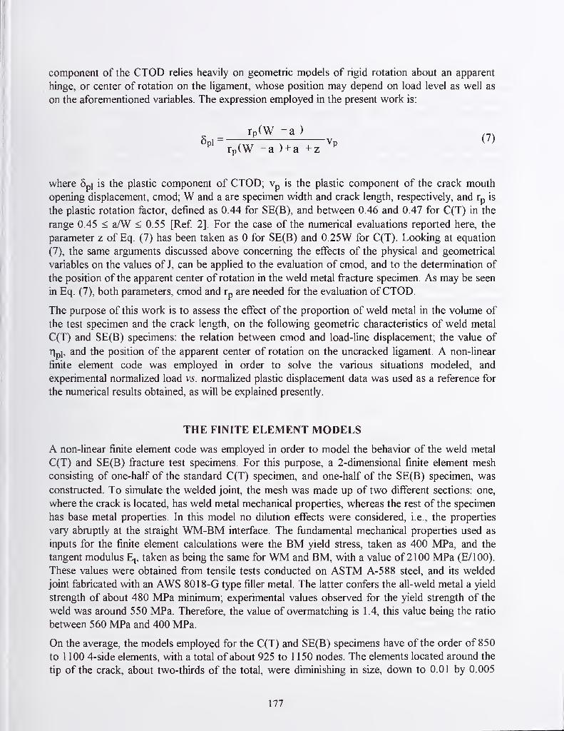
component of the CTOD relies heavily on geometric mpdels of rigid rotation about an apparent

hinge, or center of rotation on the ligament, whose position may depend on load level as well as

on the aforementioned variables. The expression employed in the present work is:

rp(W -a )

where 5pi is the plastic component of CTOD; Vp is the plastic component of the crack mouth

opening displacement, cmod; W and a are specimen width and crack length, respectively, and rp is

the plastic rotation factor, defined as 0.44 for SE(B), and between 0.46 and 0.47 for C(T) in the

range 0.45 < aAV < 0.55 [Ref 2]. For the case of the numerical evaluations reported here, the

parameter z of Eq. (7) has been taken as 0 for SE(B) and 0.25W for C(T). Looking at equation

(7), the same arguments discussed above concerning the effects of the physical and geometrical

variables on the values of J, can be applied to the evaluation of cmod, and to the determination of

the position of the apparent center of rotation in the weld metal fi"acture specimen. As may be seen

in Eq. (7), both parameters, cmod and rp are needed for the evaluation ofCTOD.

The purpose of this work is to assess the effect of the proportion of weld metal in the volume of

the test specimen and the crack length, on the following geometric characteristics of weld metal

C(T) and SE(B) specimens: the relation between cmod and load-line displacement; the value of

r|pj, and the position of the apparent center of rotation on the uncracked ligament. A non-linear

finite element code was employed in order to solve the various situations modeled, and

experimental normalized load vs. normalized plastic displacement data was used as a reference for

the numerical results obtained, as will be explained presently.

THE FINITE ELEMENT MODELS

A non-linear finite element code was employed in order to model the behavior of the weld metal

C(T) and SE(B) fi-acture test specimens. For this purpose, a 2-dimensional finite element mesh

consisting of one-half of the standard C(T) specimen, and one-half of the SE(B) specimen, was

constructed. To simulate the welded joint, the mesh was made up of two diflferent sections: one,

where the crack is located, has weld metal mechanical properties, whereas the rest of the specimen

has base metal properties. In this model no dilution effects were considered, i.e., the properties

vary abruptly at the straight WM-BM interface. The fiandamental mechanical properties used as

inputs for the finite element calculations were the BM yield stress, taken as 400 MPa, and the

tangent modulus E^, taken as being the same for WM and BM, with a value of 2100 MPa (E/lOO).

These values were obtained ft-om tensile tests conducted on ASTM A-588 steel, and its welded

joint fabricated with an AWS 8018-G type filler metal. The latter confers the all-weld metal a yield

strength of about 480 MPa minimum; experimental values observed for the yield strength of the

weld was around 550 MPa. Therefore, the value of overmatching is 1.4, this value being the ratio

between 560 MPa and 400 MPa.

On the average, the models employed for the C(T) and SE(B) specimens have of the order of 850

to 1 100 4-side elements, with a total of about 925 to 1 150 nodes. The elements located around the

tip of the crack, about two-thirds of the total, were diminishing in size, down to 0.01 by 0.005

177

mm. the smallest. The tip of the crack was given a radius of curvature of 0.03 mm. The scheme

employed considered von Mises yield criterion, bilinear behavior (i.e., the hardening was

considered to be linear beyond limit load), and total Lagrangian formulation. All finite element

computations were made under plane strain conditions, for the selected crack lengths employed.

The output generated was load vs. load line displacement; load vs. cmod; displacements of the

nodes along the crack, and hoop stresses normal to the ligament. The parameters used to analyze

the results were: the ratio ofWM to total volume of the specimen, R, and the ligament size, bAV.

For the ratio R ofWM to specimen volume, values of 1/4, 1/3, and 1/2 were employed, being

chosen as representative of most practical cases of manual metal arc weld joints. Finally, in

relation to the uncracked ligament, numerical calculations were made for b/W values of 0.5, 0.4,

and 0.3. These values represent normalized crack lengths a/W of 0.5, 0.6, and 0.7, respectively,

which correspond to what is normally termed "deep cracks".

Figure 1 shows a schematic of both the C(T) specimen and part of the SE(B) specimen.

Dimensions are proportional to the standard IT, with 25 mm thickness (1"), as per ASTM [Ref

1]. Therefore, W = 50 mm for both geometry. Crack length, a, and ligament size, b, are also

shown in this schematic. In Figure 1, p denotes the WM portion of the specimen, whereas qdenotes the whole of the specimen. Therefore, the volume ratio has been defined as R = p/q.

< w H

Figure 1 . Schematic of the C(T) and part of the SE(B) specimens.

Figure 2, on the other hand, shows the portion of interest of the finite element model for both

specimens, with the detail at the crack tip. As pointed out above, the radius of curvature at the

crack tip is of the order of 0.03 mm. Elements surrounding the center of curvature are of the order

of 0.01 by 0.005 mm.

178

Figure 2. Details ofthe mesh surrounding the crack tip; r is radius at the tip.

RESULTS AND DISCUSSION

Figure 3 shows plots of normalized load vs. normalized plastic component of the load-line

displacement for C(T) specimens with bAV = 0.5 (a) and 0.3 (b), respectively. Figure 4 shows

similar data for SE(B) specimens. Normalized load is computed from the CFE form for the load:

P = {Q*} {B W C (bAV)m) {a* (w^Y^^}

from which normalized load, P^, is:

PN = P/G = (Q*){a*(vN)^/"}

(8)

(9)

800

600

_o

izedj400

"«

o2

200

0

^ o o -e-—©-e

—

—

e

—e-©- ©-

C(T), bAV = 0.5

-e-Exp X R = 1/4

A R =

1

1/3 O R = 1/2

1

800

0,00 0,01 0,02 0,03 0,04 0,05

Normalized plastic displacement

Oh

^ 600

II 400

O200

0

C(D,bAV=0.3

-©-Exp.

A R=l/3

X R=l/4

0,00 0,01 0,02 0,03 0,04 0,05

Normalized plastic displacement

(a) (b)

Figure 3 . Normalized load V5:. normalized plastic displacement, C(T) specimens.

179

800

§ 600

-a

o^ 400u

CO

g 200

0

SE(B),b/W = 0.5

-S— E?f).

A R=l/3

X R=l/4

O R=l/2

0,00 0,01 0,02 0,03 0,04 0,05

Nonnalized plastic displacement

(a)

uN

800

600

400

200

SE(B),b/W=0.3

A R=l/3

X R = 1/4

0 R-1/2

0 -I 1 ^ 11

0,00 0,01 0,02 0,03 0,04 0,05

Normalized plastic displacement

(b)

Figure 4. Normalized load v^-. normalized plastic displacement, SE(B) specimens.

For both geometry, normalized displacement is the plastic component of the load line divided by

W. In all four figures there is one experimental curve included for comparison. The main feature of

these plots is that whereas the SE(B) data normalize onto one single curve regardless of the

ligament size and WM volume fraction, the C(T) data show a distinct difference [Ref 9]. In fact,

for bAV = 0.30 (deeply cracked specimen), all numerical curves are coincident. For bAV = 0.50,

however, R plays a dominant role on the behavior. The meaning of this is straightforward: a J

computation with a C(T) specimen, for which the load-line displacement is required, may become

dependent on the amount of weld metal present in the specimen. The same would not occur when

using a SE(B) weld metal fracture specimen.

Notwithstanding the fact that R appears to affect the load vs. load-line displacement behavior of

the C(T) specimen, the relation between the latter variable and the cmod is not influenced by the

presence of weld metal. Figure 5 shows vll - cmod curves for the C(T) and SE(B) geometries.

The C(T) curves are little influenced by the ligament size, and for each value of b/W, there is no

influence of R. The SE(B) curves, on the other hand, show a larger influence of ligament size, and

no influence of amount of WM. The ratios of cmod to vlL' are listed in Table 1 for both

geometries, obtained by linear regressions. These values are listed together with the GE-EPRI

Handbook values for n = 10 [Ref 10], and the absolute relative differences A, in %.

Table 1 . Values ofC = cmod / vll ^(T) and SE(B) specimens

bAV CC(T) C C(T), EPRI A, % C SE(B) ^ SE(B), EPRI A,%

0.3 1.302 1.300 0.15 0.835 0.843 0.60

0.4 1.315 1.324 1.07 0.766 0.781 1.96

0.5 1.338 1.347 0.67 0.702 0.718 1.70

180

0,0 0,5 1.0 1.5

Load line displacement, mm

(a)

2,0 0.0 0,5 1,0

Load line displacement, mm1,5

(b)

Figure 5. cmod v^'. load line displacement, v^l.

The differences between the EPRI C, ratios and those calculated from the obtained numerical

values, are not siginificant, considering that the former are computed with a power law code, and

the latter are based on a rigid rotation. Thus, these results could be taken to imply that the

presence of weld metal in a fracture C(T) or SE(B) specimen does not alter the ratio between

cmod and v^l. However, as was discussed in relation with Figures 3 and 4, the value of R does

have an influence on the C(T) load vs. load-line displacement behavior, and therefore, may affect

the J values.

The relation between cmod and vll ^n^y be further used to determine the location of the apparent

center of rotation. The idea of a point about which the two halves of the specimen rotate in a rigid

fashion has been employed for a long time in relation with CTOD evaluations, as shown by Eq.

(7). For SE(B) specimens and small angles of rotation, Kirk and Hackett [Ref 11], based on a

rigid rotation model, suggest the following relation between cmod and vll:

^ =^ = l_P(b/W)VLL

(10)

where P = 1- rp. On the same grounds, one can propose a similar relation for the C(T) specimen

cmod 1.25-P(b/W)

VLL 1-P(b/W)

From Eqs. (10) and (11), the following expressions relate P to Q:

p-(i-0/(b/w)

for SE(B), and

(;-i.2513=(C-l)(b/W)

(11)

(12)

(13)

181

for C(T). Table 2 lists the values of (3 and rp from the values for each geometry and ligament size,

with the El 290 suggested values [Ref 2] included for comparison.

Table 2. Values of (3 and rp for WM C(T) and SE(B) specimens

bAV P, C(T) rp , C(T) rp, E1290 P, SE(B) rp,SE(B) rp, E1290

0.3 0.555 0.445 0.435 0.550 0.450 0.44

0.4 0.515 0.485 0.449 0.585 0.415 0.44

0.5 0.520 0.480 0.465 0.596 0.404 0.44

The rp values obtained in this work for the WM C(T) specimens are fairly consistent with those

used in El 290. For the SE(B) specimens, on the other hand, a value of 0.6 has been used for P[Ref 1 1], implying an rp of 0.4, whereas El 290 suggests a value of rp of 0.44. In summary, the

values obtained in this work seem to indicate that the presence ofWM does not affect the position

of the apparent center of rotation for either geometry. Thus, the suggested values of rp given in

El 290 may as well be used for evaluating CTOD in weld metal fracture specimens of the C(T) and

SE(B) types.

The other issue of importance is the value of r\pi for welds: according to Eqs. (5) and (6), ripj is

equal to m. Therefore, the evaluation ofm serves two purposes: the G function for the geometry,

and the coefficient of the J integral of Eq. (3). The value of m is obtained from the variation of

limit load with ligament size, according to Eq. (5), expressed in the following form [Ref 12]:

ripi= dlog G / dlog (bAV) = dlog (P^/BWOq) / dlog (bAV) ( 1 4)

Thus, a log-log plot of normalized limit load, Pg/BWao ^^^^ hfW, will give the value of r|pi = m.

Figure 6 show this type of plot, for R = 1/3. For the C(T) geometry, there is a slight effect of R;

values are listed in Table 3, in which the CFE value of 2.236 is included for comparison.

5,0

4.2 H ^ ^ ^

1

-0,6 -0,5 -0,4 -0,3 -0,2

log (b/W)

Figure 6. Normalized limit load vs. ligament size, C(T) and SE(B) specimens.

182

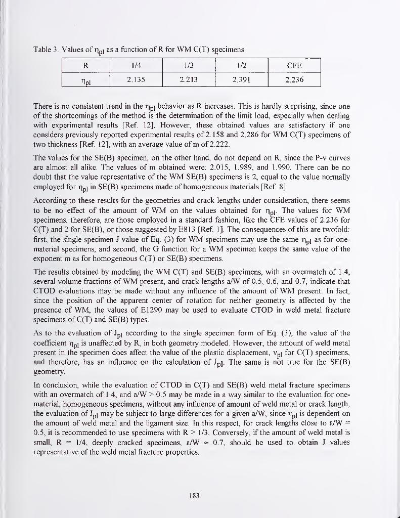
Table 3. Values of ripi as a function ofR for WM C(T) sfjecimens

R 1/4 1/3 1/2 CFE

npi 2.135 2.213 2.391 2.236

There is no consistent trend in the ripj behavior as R increases. This is hardly surprising, since one

of the shortcomings of the method is the determination of the limit load, especially when dealing

with experimental results [Ref 12]. However, these obtained values are satisfactory if one

considers previously reported experimental resuhs of 2.158 and 2.286 for WM C(T) specimens of

two thickness [Ref 12], with an average value ofm of 2.222.

The values for the SE(B) specimen, on the other hand, do not depend on R, since the P-v curves

are almost all alike. The values of m obtained were: 2.015, 1.989, and 1.990. There can be no

doubt that the value representative of the WM SE(B) specimens is 2, equal to the value normally

employed for rjpj in SE(B) specimens made of homogeneous materials [Ref 8],

According to these results for the geometries and crack lengths under consideration, there seems

to be no effect of the amount of WM on the values obtained for r|p|. The values for WMspecimens, therefore, are those employed in a standard fashion, like the CFE values of 2.236 for

C(T) and 2 for SE(B), or those suggested by E813 [Ref 1]. The consequences of this are twofold:

first, the single specimen J value of Eq. (3) for WM specimens may use the same ripj as for one-

material specimens, and second, the G function for a WM specimen keeps the same value of the

exponent m as for homogeneous C(T) or SE(B) specimens.

The results obtained by modeling the WM C(T) and SE(B) specimens, with an overmatch of 1.4,

several volume fractions ofWM present, and crack lengths a/W of 0.5, 0.6, and 0.7, indicate that

CTOD evaluations may be made without any influence of the amount of WM present. In fact,

since the position of the apparent center of rotation for neither geometry is affected by the

presence of WM, the values of El 290 may be used to evaluate CTOD in weld metal fracture

specimens of C(T) and SE(B) types.

As to the evaluation of Jpj according to the single specimen form of Eq. (3), the value of the

coefficient r|pi is unaffected by R, in both geometry modeled. However, the amount of weld metal

present in the specimen does affect the value of the plastic displacement, Vpj for C(T) specimens,

and therefore, has an influence on the calculation of Jpj. The same is not true for the SE(B)

geometry.

In conclusion, while the evaluation of CTOD in C(T) and SE(B) weld metal fracture specimens

with an overmatch of 1.4, and a/W > 0.5 may be made in a way similar to the evaluation for one-

material, homogeneous specimens, without any influence of amount of weld metal or crack length,

the evaluation of Jpj may be subject to large differences for a given aAV, since Vpi is dependent on

the amount of weld metal and the ligament size. In this respect, for crack lengths close to a/W =

0.5, it is recommended to use specimens with R > 1/3. Conversely, if the amount of weld metal is

small, R = 1/4, deeply cracked specimens, a/W « 0.7, should be used to obtain J values

representative of the weld metal fracture properties.

183

ACKNOWLEDGMENTS

This work was supported by FONDECYT-CHILE, Project No. 1980169.

REFERENCES

1. ASTM Standard E 813-89, 1991. Standard Test Method for % A Measure of Fracture

Toughness, Annual Book of ASTM Standards, Vol. 03.PL American Society for Testing and

Materials, 713-727.

2. ASTM Standard E 1290-89, 1991. Standard Test Method for Crack-Tip Opening

Displacement (CTOD) Fracture Toughness Measurement, Annual Book of ASTM Standards.

Vol. 03.01 . American Society for Testing and Materials, 924-939.

3. BS 5762: 1979. Methods for Crack Tip Opening Displacement (COD) Testing, British

Standards Institution. London.

4. BS PD 6493: 1980. Guidance on Some Methods for the Derivation of Acceptance Levels for

Defects in Fusion Welded Joints, British Standards Institution, London.

5. International Institute of Welding, 1990. IIW Guidance on Assessment of the Fitness for

Purpose of Welded Structures. Draft for Development. IIW/IIS-SST-1 157-90 .

6. Donoso, J.R.; Landes, J.D. 1998. A Unifying Principle for Evaluating Fracture Toughness in

the Elastic and Plastic Regimes with Planar Fracture Specimens, 30^ ASTM National

Svmposium on Fatigue and Fracture Mechanics . St. Louis, MO.

7. Sharobeam M.W. and Landes J.D., 1991. The Load Separation Criterion and Methodology in

Ductile Fracture Mechanics, International Journal ofFracture , Vol. 37, 81-104.

8. Donoso, J.R.; Landes, J.D. 1994. Common Format for Developing Calibration Curves in

Elastic-Plastic Fracture Mechanics, Engineering Fracture Mechanics, Vol. 47, 5, 619-628.

9. Donoso, J R.; Labbe, F.and Mora, C. 1994. The Effect of the Yield Stress Mismatch on the

Calibration Curves of Weld Metal Fracture Specimens, International Conference Proceedings

on Modeling and Control of Joining Processes . Ed. Thomas Zacharia: 566-573, American

Welding Society.

10. Kumar, V., German, M.D., y Shih, C.F. 1981. An Engineering Approach for Elastic-Plastic

Fracture Analysis, NP 1931, EPRI Project 1237-1 .

11. Kirk, M.T. and Hackett, E.M. 1988. An Evaluation of J-R Curve Testing Using Three-Point

Bend Specimens. Fracture Mechanics: Eighteenth Symposium. ASTM STP 945. Eds. D.T.

Read and R.P. Reed: 347-373. American Society for Testing and Materials.

12. Donoso, J., Labbe, F. and Mora, C. 1993. Evaluation of Plastic Eta Factors in Weld Metal

Fracture Specimens: A Comparison Between Limit Load and Common Format Solutions.

Engineering Fracture Mechanics. Vol. 44, 4, 515-520.

184

Session A6: Welding Documentation

VIDEO MONITORING AND CONTROL OF THE LENS PROCESS

William H. Hofmeister\ Danny O. MacCallum^, Gerald A. Knorovsky^

ABSTRACT

The LENS (Laser Engineered Net Shaping) process has significant potential impact to the

manufacturing community in producing near-net shape rapid prototypes, tooling and

customized small lot parts. LENS has its roots in stereolithography and weld surfacing.

Parts are built up in layers by delivering powder carried in an inert gas stream directed

via nozzles to a laser-produced molten pool. A robust implementation of this technology

requires a thorough understanding of how the thermal history during part fabrication

influences the dimensions, microstructure and properties of the part. This understanding,

in combination with effective closed loop feedback control of the process, and modeling

of the part to be formed, is required to ensure routine fabrication of components with

appropriate properties Thermal behavior at high temperatures (above 800°C) can be

readily monitored by visible light radiation pyrometry. In this work a high speed digital

camera with a narrow bandpass optical filter was used to obtain thermal images of the

LENS process zone. The thermal imaging system was incorporated into the optical path

of the laser so that the melt pool and adjacent areas of the part could be monitored

without intrusive hardware add-ons at the lens/powder nozzle/process zone vicinity. The

output of the digital camera was collected by a frame grabber card in a personal computer

(PC). Characteristics of the melt pool were evaluated and then used as inputs to a

Proportional-Integral-Derivative (PID) control algorithm also running on the PC. The

output of the PID algorithm was then used to control the laser power. Running the closed

loop control resulted in significant stabilization of the melt pool size during simulated

fabrication experiments. We will describe the equipment, algorithms, experiments and

results obtained from LENS-formed simple shapes of 316 Stainless Steel.

INTRODUCTION

LENS (Laser Engineered Net Shaping) is a process for building solid metallic structures

by injecting fine powder into a laser-sustained fusion zone. LENS has its roots in

stereolithography and weld surfacing. Parts are built up in layers by delivering powder

carried in an inert gas stream directed via nozzles to a laser-produced molten pool. The

powder (which is preheated by the laser beam) melts in the fusion zone, adding to its

' Dept. of Chemical Engineering, Vanderbilt University, Nashville TN 37235

^ Joining, Coating & Net Shaping Dept., Sandia National Laboratories, Albuquerque, NM 87185-0367

187

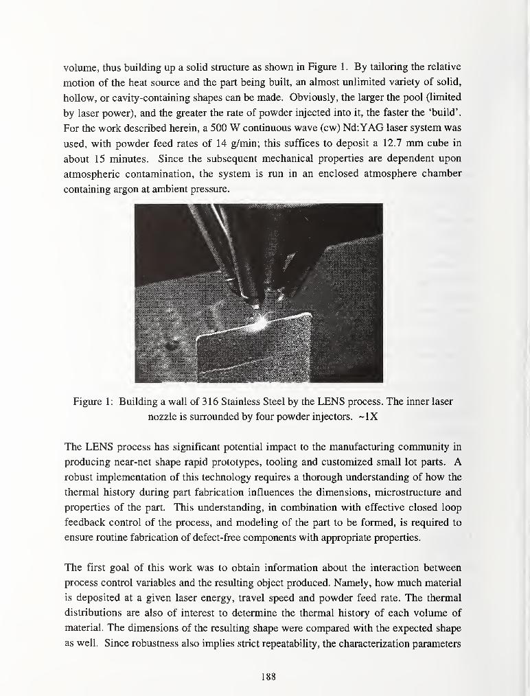
volume, thus building up a solid structure as shown in Figure 1 . By tailoring the relative

motion of the heat source and the part being built, an almost unlimited variety of solid,

hollow, or cavity-containing shapes can be made. Obviously, the larger the pool (limited

by laser power), and the greater the rate of powder injected into it, the faster the 'build'.

For the work described herein, a 500 W continuous wave (cw) Nd:YAG laser system was

used, with powder feed rates of 14 g/min; this suffices to deposit a 12.7 mm cube in

about 15 minutes. Since the subsequent mechanical properties are dependent upon

atmospheric contamination, the system is run in an enclosed atmosphere chamber

containing argon at ambient pressure.

Figure 1: Building a wall of 316 Stainless Steel by the LENS process. The inner laser

nozzle is surrounded by four powder injectors. -IX

The LENS process has significant potential impact to the manufacturing community in

producing near-net shape rapid prototypes, tooling and customized small lot parts. Arobust implementation of this technology requires a thorough understanding of how the

thermal history during part fabrication influences the dimensions, microstructure and

properties of the part. This understanding, in combination with effective closed loop

feedback control of the process, and modeling of the part to be formed, is required to

ensure routine fabrication of defect-free components with appropriate properties.

The first goal of this work was to obtain information about the interaction between

process control variables and the resulting object produced. Namely, how much material

is deposited at a given laser energy, travel speed and powder feed rate. The thermal

distributions are also of interest to determine the thermal history of each volume of

material. The dimensions of the resulting shape were compared with the expected shape

as well. Since robustness also implies strict repeatability, the characterization parameters

188

were used in implementation of feedback control of the process, initially to obtain high

fidelity shape generation and ultimately microstructural control.

EXPERIMENTAL PROCEDURES

Temperature fields at high temperatures (above 800°C) can be readily monitored by

visible light radiation pyrometry.' In this work a high speed digital camera with a narrow

bandpass optical filter (the laser radiation must be filtered out!) was used to obtain

thermal images of the LENS process zone. All pixels of the video camera were

calibrated with a NIST traceable tungsten strip lamp to determine the effective

wavelength of the camera, lenses, and filter set. During the experiments, an in situ

calibration was performed by observing the freezing of a 3 mm ball of the deposited

material.The temperature uncertainty is +/-7K. The thermal imaging system was

incorporated into the optical path of the laser (as shown in Figure 2) so that the melt pool

and adjacent areas of the part could be monitored without intrusive hardware add-ons at

the lens/powder nozzle/process zone vicinity. The output of the digital camera was

collected by a frame grabber card in a personal computer (PC).

filter

High Speed

Video

CameraData PC

turning mirror (1 064 nm)

IHeating Laser

I

viewport

laser >

objective C-

lens

;

I LENS' glovebox

workpiece

1

Figure 2: Video monitoring set-up and schematic of optical path modifications.

After converting the intensity data to temperature vs location maps, characteristics of the

melt pool and local temperature conditions were evaluated as a function of the build

189

parameters (laser power and scanning speed). These included the length and width of the

molten zone, its area, and temperature gradients at the liquid/solid interface. The area was

later used as an input to a Proportional-Integral-Derivative (PID) controller also running

on the PC which controlled the laser output power. Additional information was also

needed, such as whether a boundary or a fill pass was being made, and whether the laser

shutter was open or closed. This information was obtained from the X-Y-Z table/lens

height controller, running on a separate PC. The output of the PID algorithm was then

used to control the laser power in such a manner as to maintain the projected area of the

molten zone constant. All manipulations to the intensity data were performed using

LabView software.

The ranges of power and travel speed investigated are shown in Figure 3; where the

resulting isotherm area of the melt pool is plotted. As is expected from the different heat

sink conditions, the isotherm area for a given set of conditions changes markedly

depending upon whether one is building a line, at the border of a solid, or at the interior

of a solid. As may be seen, the isotherm area decreased in that order, with the fill

condition having less than half the isotherm area of a line build at equivalent conditions.

(W) 460 (mm/s)

Figure 3: Melt isotherm area as a function of laser power and travel speed.

VIDEO MONITORING RESULTS & DISCUSSION

In order to determine if the melt isotherm video measurements were correctly calibrated,

a number of runs were subjected to metallographic verification. These are noted in Figure

190

4 for the line build data. As can be seen, the video and metallographic pool width results

both increase with absorbed laser energy (laser power times absorptivity divided by the

travel velocity; with 0.35 used for absorptivity), and are in excellent agreement at low

values of absorbed energy; however, at higher values the agreement deteriorates and the

width measured by microstructural analysis is smaller than the width indicated by video.

A smooth relation was found for the video-measured pool length shown in Figure 5. The

melt pool area isotherm also smoothly increased with absorbed energy as shown in

Figure 6, with a linear fit of the relation of the isotherm area to absorbed energy.

Metallography of the bead cross-sections for the 7.62 mm/s travel speed builds, allowed

calculation of the bead height and volume. This ratio (0.76) was found to be constant at a

given travel velocity, independent of laser power. Assuming that the bead height-to-width

ratio was constant and 0.73 for the 5.93mm/s builds, and 0.89 for the 9.32 mm/s

conditions allowed all three volume vs absorbed energy to be brought into concurrence as

shown in Figure 7. This corresponds with having a relatively taller bead at slower

speeds. In welding, it is common for slower speed pools to be more isotropic is shape,

with faster speeds leading to more elongated pools.

EE

T3

OOQ.

1.7 n-

1.5 -

1.3 -

1.1 -

0.9 -

0.7 -

0.5 -

if

.15.93 mm/s

• 7.62 mm/s

A 9.31 mm/s

O micro measure (7.62 mm/s)

0 5 10 15 20 25 30

Absorbed Energy (J/mm)

Figure 4: Melt pool width vs absorbed laser energy, line build.

The cooling rate at the liquid/solid interface, derived from the temperature gradient and

travel speed product, showed a greater amount of scatter, but generally decreased as the

absorbed energy increased. It may be noted that the cooling rate is in excess of 500K/s

even at the absorbed energy values. This is conducive to fme solidification structures.

191

EE

O)c0)

ooOL

2.1 H

1.9

1.7 -

1.5 -

1.3 -

1.1-

0.9

0.7 ^

0.5

i

5.93 mm/s

• 7.62 mm/s

A 9.31 mm/s

5 10 15 20

Absorbed Energy (J/mm)

25 30

Figure 5: Melt pool length vs absorbed laser energy, line build.

2.5

EE,

0)

E3O>"oo0- 0.5

2 -

1.5 -

1-

0

5.93 mm/s 1

• 7.62 mm/s

A 9.31 mm/s • 1

10 20

Absorbed Energy (J/mm)

30

Figure 6: Pool melt isotherm area vs absorbed laser energy, line build.

CONTROL RESULTS AND DISCUSSION

The fusion zone thermal boundary conditions change appreciably during a part build. In

the initial stages the substrate is at ambient temperature and is a significant heat sink. As

192

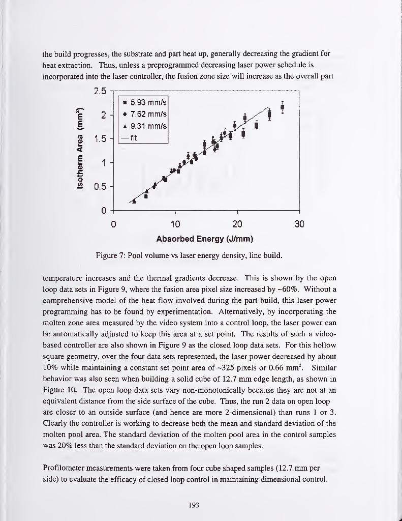
the build progresses, the substrate and part heat up, generally decreasing the gradient for

heat extraction. Thus, unless a preprogrammed decreasing laser power schedule is

incorporated into the laser controller, the fusion zone size will increase as the overall part

2.5

2 -

1.5 -

1-

EE,

(0

<E

4-*

o(0i2 0.5 -

0

0 10 20

Absorbed Energy (J/mm)

Figure 7: Pool volume vs laser energy density, line build.

30

temperature increases and the thermal gradients decrease. This is shown by the open

loop data sets in Figure 9, where the fusion area pixel size increased by -60%. Without a

comprehensive model of the heat flow involved during the part build, this laser power

programming has to be found by experimentation. Alternatively, by incorporating the

molten zone area measured by the video system into a control loop, the laser power can

be automatically adjusted to keep this area at a set point. The results of such a video-

based controller are also shown in Figure 9 as the closed loop data sets. For this hollow

square geometry, over the four data sets represented, the laser power decreased by about

10% while maintaining a constant set point area of -325 pixels or 0.66 mm^. Similar

behavior was also seen when building a solid cube of 12.7 mm edge length, as shown in

Figure 10. The open loop data sets vary non-monotonically because they are not at an

equivalent distance from the side surface of the cube. Thus, the run 2 data on open loop

are closer to an outside surface (and hence are more 2-dimensional) than runs 1 or 3.

Clearly the controller is working to decrease both the mean cind standard deviation of the

molten pool area. The standard deviation of the molten pool area in the control samples

was 20% less than the standard deviation on the open loop samples.

Profilometer measurements were taken from four cube shaped samples (12.7 mm per

side) to evaluate the efficacy of closed loop control in maintaining dimensional control.

193

Table 1 summarizes the measurements of cube height for the samples, open loop, closed

loop with border set point of 320 pixels and fill set point of 265 pixels, closed loop with a

border set point of 200 pixels, and a duplicate of the previous condition with different

5000

4500

2" 4000

^ 3500

1^ 3000(0

« 2500

^ 2000O)

= 1500O

O 1000

500 H

0

.1

5.93 mm/s

7.62 mm/s

A 9.31 mm/s

mm I

10 15 20

Absorbed Energy (J/mm)

25 30

W<DXa(00)

Eo

O0)

Figure 8: Cooling rate at liquid/solid interface vs energy density

450

400 -

350 -

300 -

250 -

200 -

150 -

100

50 H

0

open loop

closed loop

X laser current in closed loop

2 3

Data Set Number

48

+ 45r-Q)(0

+ 42Oc-I-Io339

- 36

33

Figure 9: Variability of laser power and molten zone area at various times during open

and closed loop builds of a hollow square (wall build). Laser current is proportional to

laser power. Each data set averages 20 seconds of data.

194

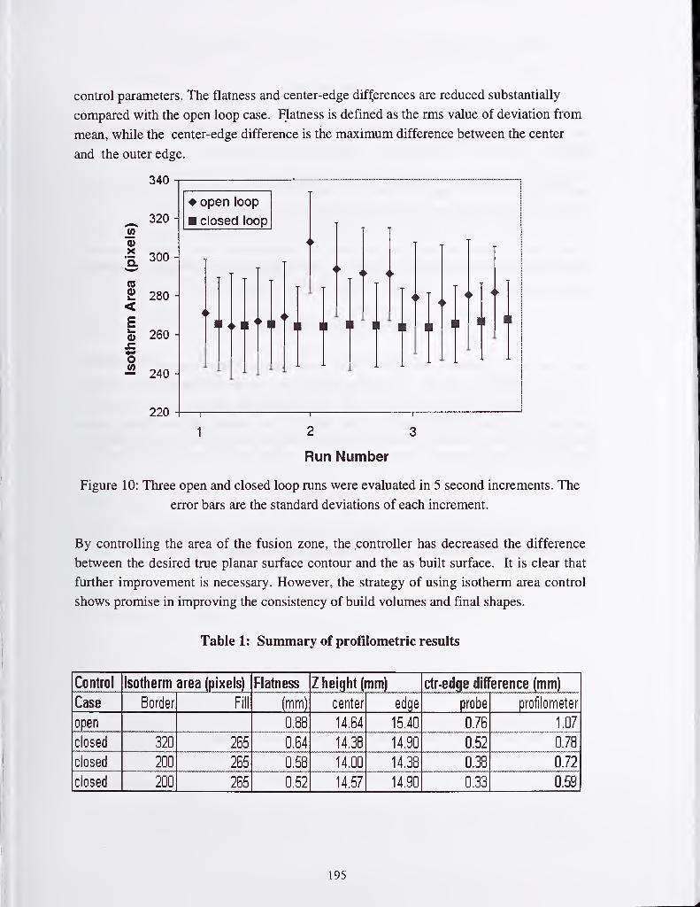
control parameters. The flatness and center-edge differences are reduced substantially

compared with the open loop case. Flatness is defined as the rms value of deviation from

mean, while the center-edge difference is the maximum difference between the center

and the outer edge.

oX'5.

340

320 -

S 300

(0

£ 280<E

4-1

o^ 240

260

220

open loop

closed loop

Run Number

Figure 10: Three open and closed loop runs were evaluated in 5 second increments. The

error bars are the standard deviations of each increment.

By controlling the area of the fusion zone, the controller has decreased the difference

between the desired true planar surface contour and the as built surface. It is clear that

further improvement is necessary. However, the strategy of using isotherm area control

shows promise in improving the consistency of build volumes and final shapes.

Table 1: Summary of profilometric results

Control Isotherm area (pixels) Flatness Z height (mm) ctr-edge dif erence (mm)

Case Border Fill (mm) center edge probe profilometer

o£en 0.88 14.64 15.40 0.76 1.07

closed 320 265 0.64 14.38 14.90 0.52 0.78

closed 200 265 0.58 14.00 14.38 0.38 0.72

closed 200 265 0.52 14.57 14.90 0.33 0.59

195

CONCLUSIONS

Thermal video imaging via visible radiation is a powerful tool for understanding

gradients, cooling rates, and parameter scaling of the LENS process.

Based upon our monitoring experiments we found that the pool length, width, area and

volume scales well with absorbed energy (absorptivity x laser power / velocity).

Control from PC-based thermal imaging based on isotherm area works, giving consistent

isotherm areas with less variance. Set point control of the fusion zone area also improved

dimensional accuracy of a simple cubic shape relative to open loop process operation.

ACKNOWLEDGEMENTS

This work was supported by the United States Department of Energy under Contract DE-

AC04-94AL85000. Sandia is a multiprogram laboratory operated by Sandia Corporation,

a Lockheed Martin Company, for the United States Department of Energy. The work was

performed for the LENS CRADA. The authors also thank Melissa Wert, John

Smugeresky, Joel A. Philliber, Michelle Griffith, Don Greene and Mark Ensz for help in

performing the experiments.

REFERENCE

1. G.D. Nutter in Applications of Radiation Thermometry. ASTM STP 895 . J.C.

Richmond and D.P. DeWitt, Eds., ASTM, Philadelphia, 1985, pp 3-23.

196

IniplenicnfaHoii of a QA/QC sysfeni that complies to ISO 3834.

E. Engh, 4X Software, Norway

Tiitrodiiclioii.

As the global production scenario is growing and the rapid requirements for high quality

products are being focused, most people clearly see the needs for a common QA/QCstrategy in their companies.

For global fabricators it is of the utmost importance that their product quality is reliable

even if their final product must consist of products from their facilities all over the world.

For medium sized and small companies it is a growing demand or more reliable products

and better quality, reduced costs and reduced time to market.

Being able to manage the production and its quality to the right level will be an important

competitive factor in the years to come.

Background.

Competitive fabricators in Europe, US and Canada cannot compete on labor intensive

fabrication unless this fabrication can have a high degree of technology. We have had an

ever lasting story of labor intensive products with low technological content that has been

wiped out from our fabrication sphere. Fabrication of standard vessels for crude oil, bulk

and so forth. Boilers with low working pressure are another example.

Due to our background and history we must face that we have to add an additional value

to the products in form of technology and quality to be able to survive in the competitive

marketplace.

The competitive window we can achieve through technology and quality we must use to

stretch our goals and limits further on. One of the typical competitive advantages we can

have is time to market as one ff production and small series production becomes moretypical.

Quality management and quality control in all phases of a product life cycle will therefore

be more and more important.

Quality records

Still a lot of fabricators thinks that fabrication records are the same as quality

management. To be able to document what has happened is far from being able to monitor

the fabrication and taking corrective actions.

With a shorter turn around time it is not of interest to find out three weeks later what

happened, you need to know it now so that you can avoid consequential damages or a

complete destruction of parts.

Quality Management.

With Quality Management we mean that you should be able to monitor the production

constantly so that immediate action can be taken when necessary. In Quality Management

197

we see a management Dedication to quality in all phases of the production and that this

management dedication is understood and accepted at all levels in the organization.

ISO 900 series of standards are a good tool to drive the organization in the right direction.

ISO 3834 completes the ISO 9000 series with fabrication expertise and know how. This is

of special importance for fabricators where welding is an important fabrication method.

Over the last two to three years we have seen an increasing interest from fabricators to

implement the ISO 3834 standard as well as an increasing demand for using this standard

as reference in other standard, specification, product standards and European directives.

Iniplenientiiig a Quality nianagenient system.

Two key factors for success has been:

Management focus and dedication to the implementation.

Always an underestimated factor. An implementation will always take time. Costs can be

estimated wrong or the time for the implementation can be longer than expected. This is

actually quite normal. Unforeseen problems in the organization can take longer time to

solve.'

Motivation and dedication of the personnel participating in the implementation.

This also a key factor to a success. You cannot order a person to change, you must

motivate him or her. Motivated people in the organization will be a driving force for

change and a positive resource of knowhow and ideas.

However very often job functions and tasks have to be reorganized. Such changes must be

cared for and supported at all levels.

The human factor is the most valuable resource in implementing a Quality Management

system and that is very often forgotten. It has to be planned for in such a way that you

can utilize this resource.

Tools

A Quality Management system must also consist of the necessary tools that will enable

the users to access the data they need fro verification purpose. They also need tools to be

able to establish the required routines and procedures.

A set of tools has been developed to cope with the requirements of ISO 3834, XWELD,QMWELD and XQUALITY.

XWELD

This tool enables the welding engineer to create documentation of any PQR (or WPAR)including test documentation. Based on an approved PQR he can develop one or moreWPS fro production. Procedures can be stored and retrieved or manipulated fro alterations

and so forth. The system have input verification on essential variables as well as a

powerful drawing tool for generating weld sequences and layer disposition.

198

QMWELD

A tool for tracing all activities related to a weld. This means it follows the weld through

the production process, from engineering to final product. In this system a weld is

connected to a drawing. Then associated information is connected to the weld, like

material information, information about extent of control. From production additional

information is added, like which WPS was used, which welders carried out the job and at

what time.

The qualification of the welder is verified to see if the certificate is valid for tlie Joint.

This means that a system for administrating certificates are included as well as a system

for updating the certificates.

Coming to the Quality Control department, the welds are controlled with non-destructive

methods, like RT, UT ,MT and so forth.

The system is used for this control and reports are automatically generated when a defect

is found. The reports must be signed off and they are then stored with reference to the

weld.

Since all production data is stored, then a set of valuable statistics can be generated. Like

production status, remaining work, scope of work for each department and so forth.

Implementation.

This part of the system will usually involve at least four departments, engineering or

design, welding engineering, production and Quality Control.

The implementation will focus on the fui\ction and process flow. Usually we carry out an

overall training showing the process in order to have full acceptance for the process

understanding and process flow. An important factor in this part of the implementation is

getting acceptance fro the interdepartemental dependencies and also to highlight any

ciianges in the organization if necessary.

After the first training session, then department oriented training will take place. This

means that we follow the fabrication process and carry out a job-function related training.

Again, the implementation takes into consideration the effect every department has on the

final product and their relations.

Other QA activities.

So far we have been concentration on welding only. But in order to achieve a first class

product, the rest of the QA process must be planned and documented. For this purpose weuse XQUALITY.

XQUALITY

A tool for generating control plan at different levels. First a main Control Plan is

developed to meet the contractual requirements. And agreed to with the client. Then these

control plans are broken down to detailed control activities. These activities can span over

the whole product development cycles to the material reception.

Logical connections are developed between the control activities to ensure that we have

199

consistency in the planning activities.

Sign off routines are standardized and reports are generated automatically if the result

from a control is not acceptable.

Implementation.

Implementing XQUALITY in an organization means that we suddenly have to train a high

number of employees, from material reception to shop floor control. AS training schedule

is then developed to cope with the fact that most people in production need to have access

to this tool.

Necessary thin clients or other hardware are implemented in the production facilities. Wealso encourage the client to let people that are responsible for a control activity, also

report the result from the control itself.

Conclusion.

Implementing a QA/QC system in an organization has been done in a number of

fabrication sites. The implementation has focused on following the production process and

thematically concentrating on the tasks for each department. The overall process

understanding is important and has to be understood in each department.

Being able to follow the process and as a consequence see their own part in such a

process is motivating factor for the user.

An implementation must be based on a management commitment. If this commitment is

not present, then an implementation is likely to fail. But the users are also the key factor

to success. Their understanding, motivation and cooperation must be stimulated. If we.

Through such an implementation, can create a positive teamwork, then the implementation

will be a success.

200

DEVELOPMENT OF ULTRA-NARROW GAP GMA WELDING PROCESSBY NUMERICAL SIMULATION

T. Nakamura* and K. Hiraoka**

ABSTRACT

To obtain high quality welded joints with the HAZ width which is as narrow as possible

by controlling the arc heat input distribution, an ultra-narrow gap GMA welding (UNGW)

process with less than 5mm gap width has been developed. In the UNGW process, the arc

heat pole at the groove wall is made widely oscillate in the direction of thickness. The heat

input density is reduced by the UNGW process, and the heat input density is smaller than that

of conventional GMA welding. The arc heat pole is dominated by wire melting tip position in

GMAW process, and the wire melting tip can be represented by wire extension. The wire

extension is a function of wire feed speed and wire melting speed which is determined by

welding current and wire polarity. If the wire feed speed is constant, the wire extension can

be controlled by DC pulse current or AC current.

In order to determine optimum welding conditions without defects in the UNGWprocess, a numerical simulation of the wire melting tip behavior is carried out in the pulsed

DC and AC arcs. As the results, excellent welding joints with the maximum melted area

width 6mm and HAZ width l~2mm, can be obtained by using the newly developed pulsed-

UNGW system.

KEYWORD

Ultra-narrow gap welding

Electrode melting speed

Oscillation

Wire extension

DC pulse arc

AC arc

Process simulation

GMA(I)

(11)

(III)

(IV)

(V)

(VI)

(VII)

(VIII)

* NATINAL RESEARCH INSTITUTE FOR METALS, JAPAN

** NATINAL RESEARCH INSTITUTE FOR METALS, JAPAN

201

1. INTRODUCTION

Narrow gap welding (NGW) possesses many advantages than conventional welding

method such as higher mechanical properties of welded joints, higher productivity, lower

residual stress and higher cost effectiveness, and various NGW techniques have been

developed.

On the other hand, as decreasing the gap width, weld defects such as incomplete fusion

at groove side-wall easily occur. In most narrow gap GMAW processes, therefore, the

weaving techniques of the arc heat across the groove gap had been developed. Usually, small

current and multi-pass welding process has been applied in NGW with the gap width from 7

to 15mm (Ref.l, Ref. 2).

It can be expected that if the groove gap becomes narrower than the diameter of higher

current arc heat source, the mechanical weaving system is not necessary to be applied.

However, narrow gap causes the increase of the hydrostatic head of molten metal, and

thus inducing the incomplete fusion at groove side-wall. As the decrease in gap width, the

phenomena become seriously. Under 7mm narrow gap the unstable arc phenomena, that the

arc irregularly goes up at the groove wall, appears remarkably.

In this report, a new NGW process with less than 5mm gap is proposed by means of the

numerical simulation of GMA welding process.

2. ULTRA-NARROW GAPGMA WELDING

2.1 Principle of ultra-narrow gap GMAW process

In the ultra narrow gap welding (UNGW) with less than 5mm gap, the bead height per

welding pass increases, and the arc is unstable so that the arc pole irregularly perturbates up-

to-downwards along the groove wall. To sustain the arc stable and obtain weld joint without

defects such as lucks of fusion and undercuts of bead surface, the arc pole behavior and the

arc heat input along the groove wall corresponding with a bead height have to be regularly

controlled and distributed respectively.

In this report a new GMA process is proposed to control the arc pole and regularly

oscillated up-to-downwards along the groove wall by welding current form (Ref.3).

The arc pole is dominated by wire melting tip position in the GMAW process, and the

wire melting tip can be represented by the wire extension. The wire extension L is regarded

as a function of wire melting speed v„ and wire feed speed Vf . The relationship between wire

extension L and wire melting speed is given by

dL

Tr"'-"" (1)

In the GMAW process, the wire feed speed is recognizes to be constant as conventional

GMA welding. Because the extension is determined by the melting speed which depends on

202

welding current and the electric polarity of the wire, the position of the melting wire tip

corresponding with the arc pole can be oscillated along the groove wall in DC pulse current

or AC current welding system.

DC pulse current process is shown in Fig. 1. In the high current pulse period, the wire

melting speed v„, which is larger than the mean wire melting speed, is larger than the wire

feed speed v^. As the dLldt given by equation (1) becomes negative, the wire extension

decreases and then the position of wire tip moves up from position Al to position A2. Next,

in the low base current period, as the wire melting speed v„ becomes smaller than the wire

feed speed v^, the wire extension increases, and the wire tip moves from A2 point to the

bottom A3. Current

metal

Figure 1. DC pulse arc welding process of UNGW

Figure 2 shows AC arc welding process. The wire melting speed during the electrode

negative (EN) is about 1.7 to 3 times the wire melting during the electrode positive (EP) at

the same welding current (Ref. 4). In the EN period, the wire melting speed becomes

larger than the wire feed speeds Vf, thus the extension becomes shorter and the wire tip moves

from the bottom position Al to the upper position A2. In the EP period, the wire melting

speed becomes smaller than wire feed speeds Vf and the wire tip moves from A2 position to

the bottom position A3.

Weld

metal

Figure 2. AC arc welding process for UNGW

203

The results suggest that the position of the melting wire tip corresponding with the arc

pole can be oscillated along the groove wall in DC pulse current or AC current welding

system.

2.2 Numerical stimulation for ultra-narrow gap welding process

In the numerical simulation, many factors are considered such as the energy balance of

droplet, heat input from arc to droplet, heat transfer from droplet to wire, joule's heating at

wire extension, hydrostatic potential of molten metal at arc pole above the molten pool, arc

pressure and balance of GMA welding electric circuit. Here, the vibration of molten pool and

surface profile of the molten metal are not considered. Halm(t)y's expressions described in

stable state are utilized, although the wire melting behavior is not exactly stable in DC pulse

process and AC process.

From equation (2), the welding current is calculated in GMA welding circuit shown in

Fig.3.

E^V,^V,^R,-I^.L,-^^ (2)

Where E is voltage of power supply, is arc voltage, is voltage drop of wire

extension, is resistance of welding circuit and is inductance of welding circuit.

Wire

Wire feeder

Figure 3. Schematic illustration of GMA welding circuit

The following constrained condition for an ultra narrow gap welding is applied. If the arc

length is longer than W/2, where W is the width of groove gap, arc occurs between wire tip

and groove wall, and if the arc length is smaller than W/2, arc occurs between wire tip and

molten pool. Moreover, in the UNGW process which satisfies equation (2), the arc length is

calculated by considering the balance of current determined arc force and hydrostatic

potential of molten pool.

Figure 4 shows the flowchart of the ultra-narrow gap welding simulation process by

204

using equations (1), (2) and Halm(j)y's equations (Ref. 5, Ref. 6). In Fig. 4, the voltage drop of

wire extension and wire melting speed v„ are derived from Halm(j)y's equations.

According to the procedure of the flowchart, the optimum welding conditions for the

ultra-narrow gap welding are obtained.

( Start )

' Welding current : /„

Electrode stickout : Lg

LWire feed speed : \/,

Arc Characterstic

in Ultra- NarrowGap

Resistance of welding circuit:

Inductance of welding circuit

:

Characteristic of

power supply

E

Heat content of

electrode stickout

3

Energy balance

at the electrode tip

Voltage drop of

electrode stickout

y, =-

/

Wire melting speed

Tv„ =

4) : Anode heating

J potential

: Heat content

of droplet

Differential equation for GMA welding circuit

E = V,+V,+R,UL,-^ (2)at

Differential equation for the stickout

= (1)

Welding current:/

Electrode stickout : L

rind")

Figure 4. Flowchart ofUNGW simulation process

Z2 Simulation results

In order to find out the optimum welding conditions, the relationship between wire tip

position and electric current waveform is described by the numerical UNGW simulation.

Firstly, DC pulse process was simulated by means of the square pulse current waveform

for the plate 19mm thickness with 5mm I-gap groove. Fig. 5 shows the simulated behavior of

the wire melting tip with in the following welding parameters;

pulse peak duration time Tp = 0.06s, pulse base duration time Tf, = 0.3s,

no load voltage of power source for peak voltage is 40V,

no load voltage of power source for base voltage of power source is 34V,

205

external characteristics of power source is OV/A,

average current 4^ is 380A.

(a) Relationship between pulse current (b) Behavior of wire tip

and position of wire tip

Figure 5. Results of simulation of wire tip position

From the wire feed speed computed in these welding conditions, the throat thickness of

deposited metal is calculated and is about 10mm. The wire tip can be located near the groove

bottom from (D), (E) to (A) as shown in Fig. 5(b).

Because the arc pole varies below the groove bottom, the arc heat can be distributed

along the groove wall through the throat thickness and the groove bottom can be melt

enough.

E

<

M-o

IDD

"5.

E<

Vp=40~42VVg=34~35Vl.„=380A

20

Frequency f (Hz)

Figure 6. The effect of DC pulse frequency on amplitude of wire tip

Figure 6 shows the relationship between pulse frequency / and oscillation amplitude of

the wire tip ziZ in DC pulse arcs in which the ratio of peak time Tp to base time T^, retains

206

1/5. The amplitude decreases as increasing the pulse frequency. In the UNGW process,

the low frequency of less than 5Hz is effective to obtain the amplitude z\Z corresponding

with the throat thickness of the bead.

40

S 20(D

O)

5 0o> -20

-40

600

< 400

I200

i 0uo)-200

1 -400

^ -600

20,9-

£ 15

I E° E10

1

I 5

a.

0

Figure 7, Simulation results ofAC arc welding

The UNGW process by AC arc is simulated in Fig. 7. As mentioned in section 2.1, the

wire tip can be oscillated along the groove wall as the same as DC pulse process. For the high

current 600A during positive wire polarity, further, the wire tip can move to the groove

bottom, because the wire melting speed during positive wire polarity is smaller than that

during negative wire polarity. The melting efficiency of base metal in negative wire polarity

is generally higher than that in positive wire polarity.

AC process, therefore, can effectively transfer the arc heat to the groove bottom and be

more effective to prevent of the incomplete fusion at the comer of groove than DC pulse

process.

From all the simulated results, the distribution of arc heat input in the new UNGWprocess can be controlled by selecting electric current waveform.

3. EXPERIMENTAL RESULTS

Figure 8 shows the simulated relationship between the ratio of peak current to base

current 7^/ and melting wire tip position Z. The , A and • marks show the maximum

upper position Zmax, the minimum lower position Zmin and the mean position Zav in wire tip

207

oscillation, respectively. From the simulated results, it is found that the position of wire tip

increases with Ipl 1^-

The ultra-narrow gap GMA welding with 5mm I-gap is carried out with the welding

conditions Ipl Ib= 1-31 and Ip/ !(, = 1.47 which are determined by the numerical simulation of

UNGW. Fig. 9 shows the cross-section of penetration obtained in case of 7^ / 4 = 1.31 and 7^/

7^ = 1.47. Compared with the bead for 7^/ 7^, = 1.31, the position of the maximum bead width

for Ipl lb = 1A7 at first pass moves upwards. Further, in second pass welding of Ip/ Ib = 1-47,

incomplete fusion lacks occur at both comers of bead bottom.

From the results, it can be experimentally found that the mean heated zone moves

upward as increasing the ratio Ip/ lb- This experimental tendency agrees qualitatively with the

simulated results. Therefore, the developed numerical simulation is useful to determine many

welding parameters in the UNGW process.

JNQ.

20

15

10

1—1—I—I—I—I—I—I—r—I—I—I—I I I I—I—I—I—I I I—I—I—I—I II

I I I II

I—

n

- (Results of simulation)

Z,^ =380 A

i_r=0.06s

r;=o.3 s ''

% 5

coV;« 0OQ.

: DC

ZminJ I I 1 I I 1 I I I I I I I 1 I I I I t 1 I I I I I I 1 I I I 1 I ' ' I 1 1 I L.

C D

Zmax

1.0 1.1 1.2 1.3 1.4 1.5 1.6 1.7 1.8

IZmin

Figure 8. Effect of the ratio of peak current to base current on wire tip position

19mm

(a)Ipllh =1.31

Tp =0.06s

Th =0.3s

Ip =A12A

lb =361A

lav =380A

i^) Ipllb =1.47

Tp =0.06s

Tb =0.3s

Ip =522A

lb =355A

lav =380A

Figure 9. Bead cross-section of UNGW joints

208

Figure 10 schematically shows an example of the cross-sections of UNGW joints in

optimum welding conditions. Maximum width of molten zone is 6 mm and it is confirmed

that the base metal can be slightly melted and the one side width of HAZ can be minimized

within 1 to 2 mm. The oscillation control of arc pole along the groove wall by current

waveforms reduces the density of arc heat input in the UNGW process.

Furthermore, the welded joint with 10mm in the thickness can be formed by 2 welding

passes.

From the all facts mentioned above, a higher-efficient GMA process producing higher-

quality joints have been developed.

i i

CD

5

J

Maximum width of

melted area

HAZ

Weld metal

DC pulse arc process :

r = 0.06s. r = 0.3s, / = 380A . 45cm/minp b av

Wire diameter w.= 1.6mm Shielding gas : CO,

Unit : mm

(a) Shape of ultra-narrow gap groove (b) Schematic cross section of welded joint

Figure 10. Results of ultra-narrow gap DC pulse arc welding

4. CONCLUSIONS

The ultra-narrow gap GMAW process with less than 5mm gap width is proposed to

obtain high quality welded joints with the HAZ as narrow as possible. In the UNGW process,

in order to control the arc heat input distribution and to achieve stable arc welding without

weld defects. The behavior of arc pole along groove wall was discussed by the numerical

simulation of arc current waveforms. The conclusions are summarized as follows.

(1) It is found from the numerical simulation process that under the correlation between the

wire melting speed and wire feed speed, the wire tip oscillating behavior along the ultra-

narrow gap groove wall can be controlled by arc current waveform of DC pulse orAC arc.

The wire melting speed is dominated by arc current.

(2) Welding parameters determined by numerical simulation leads to good experimental

results. The numerical simulation of the new UNGW process in which is effective to find

optimal conditions by considering many factors in ultra-narrow gap arc phenomena.

209

(3) A welded joint with the width of HAZ l'^2 mm and the maximum width of penetration 6

mm can be obtained by the UNGW. The oscillation of arc pole along the groove wall can

reduce the density of arc heat input.

(4) Further, a higher-efficient GMA process which can achieve deposited metal height of

about 10mm per welding pass without weld defects is developed.

REFERENCES

1. Malinm,V. 1987. Monograph on Narrow-Gap Welding Technology. WRC Bulletin 323

2. Hori,K. and Haneda,M. 1999. Narrow Gap Arc Welding. Journal of J.W.S. 68(3): 41-62

3. Nakamura,T. and Hiraoka,K. 1998. Development of Ultra-Narrow Gap Welding Process.

Preprints of the National meeting of J.W.S . 62: 82-83

4. Lancaster, J. F. 1984. The Physics of Welding : 225-226. PERGAMON PRESS.

5. Budapest, 1996. Simulation and Instabilities in GMAW and SAW, The International

Institute of welding. Halm<t)y, E. IIW Doc.212-895-96

6. London, 1979. Wire melting rate droplet temperature and effective anode melting

potential. Conf. on Arc Physics and Weld Pool Behavior. Halm^y, E. : 49-59.

i

210

Session Bl: Real-Time Weld Sensing and

Control Systems: GMAW Arc Quality

Monitoring I

.1

EBSIM -A SIMULATION TOOL FOR ELECTRON BEAM WELDING

Authors: Prof. Dr.-Ing. U. Dilthey, Dr.-Ing. A. Brandenburg, Dipl.-Ing. S. Bohm,

T. Welters

ISF-Welding Institute, Aachen University; Germany,

Dr. S. Iljin, Dr. G. Turichin

State Technical University, St. Petersburg, Russia

Abstract:

During a research cooperation between the ISF Welding Institute Aachen and the St.

Petersburg State Technical University a software for forecasting the electron beam

welding process with vapour capillary was developed. In this paper the new computer

program is presented. AU input and output data are described and the simulation algo-

rithms are explained. A short introduction into some physical aspects of the model is also

given. It is shown which influence quantities are not neglected in contrast to some other

already existing models. In order to evaluate the performance of the simulation algo-

rithm, a comparison between the simulated welding results and real welding experiments

is carried out. For some materials the newly developed model gives results with a varia-

tion from the real experiments of less than 1 0%.

1.0 INTRODUCTION

One of the most important characteristics of electron beam welding which helped to in-

crease the industrial acceptance of this welding method is the high reproducibility of the

welding results. This is supported by the possibility of controlling the welding parameters

automatically. New legal rules concerning quality insurance require extra efforts specially

in mass production which are very easy to fiiLfiU for electron beam welding.

Because of the huge amount and type of welding parameters and the complexity of the

welding tasks it is necessary to carry out welding experiments to find out the correct

parameters. But these experiments are time consuming and therefore, costly. It is impos-

sible to replace these experiments by computer simulations without a physical model.

Although different models were developed during the last 30 years industry did not ac-

cept these models for practical use.

The problem with all these models is that they are only suitable for a restricted type of

materials, certain welding machines and small intervals of parameters. The reason for this

is that the welding process itself was not modelled carefiilly enough until now. To de-

scribe the welding process and the melt pool exactly gasdynamical and hydrodynamical

processes must be taken into account. It is also necessary to take the absorption and re-

flection of electrons in the capillary and above the workpiece into consideration.

213

2.0 MODELLING

overview

It is well known that an electron beam with sufiBcient beam power is capable of pro-

ducting a narrow and deep capillary in the workpiece. This capillary is surrounded by

liquid metal and is filled with metal vapour which partly escapes fi"om the capillary. Be-

cause of the movement of the capillary through the workpiece the weld seam is pro-

duced. In the following the process of electron beam welding is divided into separate

processes:

• scattering of the beam at the vapour jet above the capillary

• absorption and reflection ofthe electron beam at the surface ofthe capillary

• heat transport in the molten metal

• hydrodynamic processes in the molten metal

• dynamic ofthe vapour

Each single process is described exactly but not all processes are solved satisfactory and

the combination of all processes to an overall-model is not yet done suflBciently.

Beam data measured by DIABEAMor beam power, acc volt., beam cur

,

beam diam,ar^le of apertur, focus material

distance

^

Energie/ coupling

\ (absorption and

\ reflection)

Heattransfer

(conduction andconvetion) ^

Vapourjet out of the

capiliary

Equations and coefficients

Boundary conditions

v„ material material

Figure 1 : Aspects ofthe physical model

214

To sum up it can be said that it is necessary to solve a certain number of single problems

which are closely related. By assuming certain parameters it is even possible to solve

connected problems analytically (e.g. to calculate the radius of the capillary when solving

the heat source problem). The solution of the problem depends in that case on these pa-

rameters. By solving all essential separate problems a system of equations for these pa-

rameters is generated. This represents a model of the welding process. But only the use

of several simplifications which are connected with the physical process leads to a solu-

tion of the problem. In the following some separate processes are listed:

scattering above the workpiece

During electron beam welding a vapour-filled capOlary is produced inside the workpiece.

Because of the different pressures in the capillary and the surrounding vacuum the va-

pour pours out and accumulates above the workpiece. Due to the scattering of electrons

at the vapour atoms the power density distribution and distribution of angles is changed.

Therefore, the focussing parameters are also changed. This effect has to be analysed

when the vapour density distribution is described. This cannot be reached by making use

of the conventional equations for gas dynamic problems because in this case the transi-

tion from the gas dynamic fluid to free movement of molecules is not possible. The exact

problem can only be solved by using the kinetic Boltzmann equation (1).

scattering in the capillary

The interaction between the electron beam and the vapour above the workpiece and in-

side the capillary leads to a broadening of the beam (2), a reduction of power density and

results in a change of the angle in which the electrons arrive at the surface of the work-

piece. On the other hand this results in a change of the absorbed power. For the descrip-

tion of the scattering effect (1) it is helpfiil to use an approximation of the Boltzmann

equation for small and very fast particles and small angles. This assumption can be made

because the speed of the gas molecules is much smaller than the speed of the electrons

and no kinetic energy is exchanged during the impact, and the electrons are scattered

back in a small angle,

energy coupling

The problem of decreasing power density with increasing depth during deep penetration

electron beam welding consists of two independent separate problems. In the first part

the electron absorption coefficient and the energy of the particle flow in the interval of

angles between 1 to 10 degrees have to be calculated. The second part deals with the

215

determination of the energy distribution at the surface of the capillary which depends on

the reflection of electrons.

The first problem can be solved by using the Monte-Carlo method (3). This method can

be applied as long as the electron beam responds to classical laws of mechanics and the

electrons move on different trajectories. When collisions occur the electrons change their

direction of movement and during ionization of the metal atoms and the formation of

plasma the electrons loose their energy. The angels at the collisions and the length be-

tween the collisions are considered as random variables with probability distributions

given by the theory of scattering in quantum mechanics.

The local reflection of the electrons at the capillary wall leads to a new distribution of the

delivered energy in the depth and the capillary circumference.

Using the results of the Monte-Carlo method the whole surface of the capillary does not

effect the electrons like a mirror. Instead the electrons are distributed at an average re-

flection angle. At a cylinder shaped reflecting surface, the electron distribution after a

multiple reflection and the resulting energy distribution are very difficult to determine. To

simplify this the angle between the arriving electrons and the capillary wall increases

rapidly after multiple reflections. Therefore the reflection coeflBcient is also increasing.

This means that to obtain a good approximation it is enough to take into account only

the first reflection.

gas dynamics

For the model ofvapour forming it is assumed that the vapour inside the capillary is satu-

rated. It is also assumed that the momentum of the vapour fi-om the outer limits of the

Knudsen-layers is not perpendicular but parallel to the surface. In other words: perpen-

dicular to the surface, the ,Jiydrodynamic" speed at the outer limits of the Knudsen-layer

is equal to zero. In that case existing models for vapour forming deliver „zero" for the

value of the vapour flow. A one-dimensional approximation is used for the description of

the movement of the vapour through the capillary (velocity, pressure, density and tem-

perature of the vapour flow are a function of one coordinate „z" in the direction of the

axis of the capillary). The equations of the model are conservation equations regarding

mass, impact and energy flow.

heat and mass transport

Heat and hydrodynamic processes in the area of electron beam welding with deep pene-

tration are very complex. The problem consists of two separate problems: on the one

216

hand the heat transfer and on the other hand the mass transfer. Both problems are closely

related. Therefore, the solution of the hydrodynamic problem results into values for co-

efficients of the equation of heat transfer. The solution of the heat problem determines

the boundary conditions for the hydrodynamic equation. The problem is complex be-

cause of non-linear physical quantities like viscosity, thermal conductivity etc. There are

also non-linear geometric quantities which are directly generated from the solution.

geometry ofthe workpiece

A completely allocation of the geometry of the workpiece is only possible at the expense

of a considerable computational effort. Since the above described calculations are carried

out in a personal computer, some simplifications must take place:

According to the division of the workpiece into different calculation layers during the

calculation of the capillary the virtual heat sources are also divided because of the heat

reflection at the layer boundaries. For the reflection every layer for calculation of the

primary heat source is regarded as a 3-dimensional point-shaped heat source which im-

ages are calculated. Only the first reflections at the workpiece boundaries are taken into

account. To calculate the temperature at a certain point in the workpiece it is necessary

to consider on one hand the influence of the primary heat source and on the other hand

every single virtual heat source.

3.0 PRACTICAL REALISATION

Development ofthe simulation software

The simulation algorithm was built with the help of the experience gained during the

project. The purpose of this realisation was a strongly modular program. This has the

advantage that it can react on new demands also during the development ofthe program.

User interface

The practical applicability is one of the main aspects of the software. The purpose is to

supply the user with a tool which requires no specific knowledge. The complete product

can be run on a usual PC. It eliminates the need of investing on expensive hardware. The

current program version is fuUy developed for Windows 95® under the programming

environment Borland Delphi 2.0® and is a 32bit program, which can use aU potentialities

of the graphical environment of Windows 95®. The whole application can be operated to

a large extent through a system of object oriented context menus. For instance it is pos-

sible to change the system of coordinates by regulating the cut ofwhole view.

217

DIABEAMmanual input of

the beam data

beam data

minimal approx.

of the beam

geometry of the

melt pool

MATERIAL-EXPLORER

material database

simulation

algorithm

beamparameter

thermocycles geometry of the

capillary

mechanical techno-

logical properties

Figure 2: Schematic of the program

In order to increase the user's overview of the simulation process and results, it was at-

tempted to make the program environment possibly modular. One set of input parame-

ters, which consists of materials, beam, some other welding and simulation parameters,

leads to only one set of output data. The output also has a modular structure. One part

plots dimension and temperature parameters which describe real appearance and behav-

iour of welding joint. Furthermore, it is possible to output the parameters, that are not

connected to the description of the welding joint, but characterize the behaviour of the

simulation algorithm.

Input data

The calculation algorithm needs a lot of information concerning material, for example

heat conductivity, atomic number or data about chemical compounds. In order to make it

easy for the user, specific physical parameters ofmaterial are saved in a material database

which contains parameters of typical materials. Using a special program, this database

can be upgraded. When a new calculation starts, the user chooses fi-om the list of materi-

als the desired material.

In order to calculate the energy distribution it is necessary to have data on the electron

218

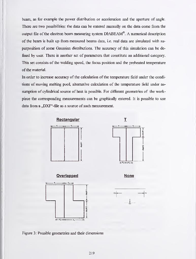
beam, as for example the power distribution or acceleration and the aperture of angle.

There are two possibilities: the data can be entered manually on the data come from the

output file of the electron beam measuring system DI'ABEAM®. A numerical description

of the beam is built up from measured beams data, i.e. real data are simulated with su-

perposition of some Gaussian distributions. The accuracy of this simulation can be de-

fined by user. There is another set of parameters that constitute an additional category.

This set consists of the welding speed, the focus position and the preheated temperature

ofthe material.

In order to increase accuracy of the calculation of the temperature field under the condi-

tions of moving melting pool, alternative calculation of the temperature field under as-

sumption of cylindrical source of heat is possible. For different geometries of the work-

piece the corresponding measurements can be graphically entered. It is possible to use

data from a ,J)XF"-file as a source of such measurement.

Rectangular

-d, Bj« d2- -d, cj„ dj

Ho-dj-t^o-d^-i,)

Overlapped

d3-p+.

None

Figure 3 : Possible geometries and their dimensions

219

Output data

The most interesting data obtained during the simulation are plotted on the screen. Plot-

ted data concern the weld geometry or for example the temperature cycles or isotherms.

Data referring to the temperature of capillary or the mean convergence of the angle of

electron beam which describe the stability eind convergence of the algorithm can also be

obtained. All output results can be set up and switched on and off in an option's menu, in

order to minimise the calculation time and only determine the necessary results.

The application calculates both a side view and a frontal view of the melt pool, so that it

is possible to obtain information about the cross and longitudinal dimensions of the melt

pool of the stationary heat source. Figure 4. This view and calculation of the dimensions

is not limited to the dimension of the melt pool, but it can be used for the determination

of any thermo-cycles. Furthermore, it is possible to export the temperature field in vari-

ous formats like EXCEL® spreadsheets or text files.

Figure 4: Output ofthe cross and longitudinal section of a simulated seam

If it is interesting to know the thermo cycle in a special point, for example to obtain the

tg/s-time the program also calculates the temperature cycle. It is not only possible to fix a

time area but also a temperature area. To give the user a clear picture of the geometry of

the melt pool it is possible to calculate a 3-dimensional view of the melt pool.

220

4.0 EXPERIMENT AND RESULTS

Description ofthe experiments

Experiments ofmany penetrated weldings and not folly penetrated weldings were carried

out. The welding parameters were changed in the area of 6-18kW, 90-150kV and 2-

25mm/s. The main materials were high-temperature resistant steel X20CrMoV12.1 and

the fine grain steel EStE355. All experiments were performed with an electron beam

machine with 150kV/30kW and horizontal gun at the ISF Welding Institute, Aachen.

Description ofthe simulation parameters used

The parameters used for the simulation are the measured distribution of beam densities,

which are read directly jfrom the DIABEAM measurement file (4) and approximated af-

terwards, the angle of aperture, weld velocity, the acceleration voltage and the beam

current. If the measurement of the beam density distribution is not desired or not avail-

able, it is possible to input one diameter of the electron beam. In this case it is also neces-

sary to add the percentage of the beam power included in this diameter. The geometry of

the workpiece is not so important because simulation and experiments show that the in-

fluence of the workpiece borders is not so significant.

Interpretation ofthe simulation results

Corresponding to the welding experiments and using the welding parameters and the

measured beams data fi-om DIABEAM for each case, all weldings were simulated. Due

to the differences between the reality and the simulation of the weld depths it is not easy

to compare different widths in various weld depths (e.g. the 10%-width at S=45mm not

equal to the 10%-width at S=40mm). It should be remarked that in the simulation the

penetration depth is higher compared to the weld experiments. The average error is less

than 10%. The error occuring at the simulation of the melted area is less than at the

simulation of the weld depth. But both simulations lead to bigger quantities. It is obvious

that the simulation of the material EStE 355 at 18kW produces an average error about

20%. Such a large error is due to the Humping-Efifect and the Spiking-Effect. To reduce

the amount of variations of the welding parameters the 1 8kW weldings experiments were

also performed with surface focused beam. However, this leads to an unstable weld pool

and a strong Humping-Efifect.

221

Figure 5: View of the upper bead of a EStE 355 weld sample (1) and view ofthe longi-

tudinal section (r). The weld parameters are 150kV, 18kW, 15mm/s, surface

focused. The Humping-Effect Eind the Spiking-Eflfect are good to recognise.

The difference between the minimal and maximal depth of the weld is about 7

mm.

The welding experiments with an acceleration of 90kV were not carried out because the

beam measurement system could not be used successfully at this acceleration voltage.

The simulation results are slightly worse than the error of measurement at the determina-

tion of the real seam geometry. At the measurement of the seam geometry problems oc-

cur which are produced by the dynamic behaviour of the weldings like Spiking or

Humping. The distinction between heat affected zone and melt pool is in spite of a good

chemical etching partially possible. In addition inaccuracies of the measurement and of

the interpretation do occur. Depending on the material and on the welding parameters,

errors can be as large as 20%.

Variation ofthe materialparameters

Although the accuracy of the simulation can be increased, it is interesting to know the

relation between material parameters and the results. The material parameters heat ca-

pacity, heat conductivity and boiling heat and the consideration of the alloy elements

influence the simulation results more strongly than other material parameters. The speci-

fication of physical material parameters is critical. The literature gives partly varying val-

ues. For parameters of some materials like the surface tension it is not possible to deter-

mine the values by experiments or only in a small limited temperature interval. The con-

tent of the alloys can also fluctuate. The effects on the welding results are not neglect-

222

able. The used material parameters should not be interpreted as absolutely fixed values.

So it is interesting to analyse the influence of changes in the material parameters on the

welding results.

In a first step the values ofthe heat capacity, the heat conductivity and the boiling heat of

the materiel X20CrMoV12.1 were changed in an area of +/- 10%. Here it was possible

to see that increasing the value of the boiling heat reduces the weld depth and increases

the melted area. Increasing the value of the heat conductivity or heat capacity the simu-

lated weld depth and the melted area decrease. It should be noted that by optimising the

material parameters the quality of the simulation can be increased.

5.0 SUMMARY

In the fi-ame of a cooperation project between the Technical University St. Petersburg,

Russia and the ISF Aachen, Germany the simulation program EBSim was developed. It

combines a simulation algorithm with a user fiiendly interface. Simulation results like the

shape of the melt pool and additional information like the thermo cycles can be obtained

graphically. This program makes use of databases that store the large amount of input

parameters, specially the material parameters, so it is easy to use for non specialists too.

The comparison of the simulation results of EBSim and experimental results of not fiilly

penetrated welds of the materials X20CrMoV12.1 (1.4922) and EStE 355 (1.1106)

showed that the prediction of the weld depth and the melted area is in keeping with the

trend. The electron beam welding process is quite good researched in the mostly parts.

The combination of the results of the individual physical phenomena is connected with

some practical problems. On the one hand, the complete evaluation of all differential

equations describing the system is not possible under current computing power. On the

other hand, the determination ofmany boundary values of the simulation like the surface

tension in dependency of the temperature is uncertain. Furthermore, the experimental

verification of the simulation results is complicated by various factors:

- the simulation of aU physical phenomena is very complex. This makes the verification of

the individual parts more complex;

- an experimental verification of all parameter dependencies needs thousands of experi-

mental weldings;

- the determination of the experimental values is not error fi-ee. For example, the deter-

223

mination ofthe weld deepth is influenced by Spiking and Humping-EfiFects;

- the determination of the geometry of the beam, specially the determination of the angle

of aperture, is not error free. The geometry of the beam is important for the process of

energy coupling. SmaU fluctuations of the machine parameters during the welding leads

to measurable changes ofthe welding;

- the presented model solves the physical problem on a static way, so that a prediction of

the dynamical behaviour ofthe capillary and the weld seam is not possible.

In spite of some problems this paper shows that it is possible to develop a fundamental

and in a wide area quantitatively correct description (in comparison to the error of the

measurement of the experimental results) of the electron beam process. So is the predic-

tion of the welding results for material close to iron better than the prediction of high

alloyed materials. This shows that a further development for other materials is neces-

sary.

Acknowledgements:

The model described in this paper is partly accrued in a common project of the ISF

Aachen and the CL&PT, TU St. Petersburg, St. Petersburg, Russia. The project was

financed by the DFG (Deutsche Forschungsgemeinschaft). Both institutes wish to record

their thanks for this funding of the DFG project ('Mathematische Simulation des Elek-

tronenstrahl-SchweiBprozesses und der sich einstellenden mechanischen und metallurgis-

chen Kennwerte der SchweiBung', Projekt Nr.:436RUS113/55) to the BMBF (Bundes-

miniesterium fur Bildung und Forschung). WINDOWS 95 and EXCEL are trademarks

ofMICROSOFT and DELPHI 2.0 is a trademark ofBORLAND INTERNATIONAL.

6.0 LITERATURE

[1] U. Dilthey, S. Bohm, T. Welters, S. Ilyin, G. Turichin:

EBSIM - New Simulation Software for Electron Beam Welding with Deep

Penetration

IIW Doc. No. IV-669-97

[2] V. Bashenko, E. Mitkevich, G. Turichin, D. Ivanov:

Energy absorption law in cavity in EBW

2nd Int. Conf on EBW, Varna, Bulgaria, 1988, pp460-463

224

[3] A.F. Akkermaiin, U.M. Nikituschev, W.A. Botwin:

Problem des Transfers von schnellen Elektronen in Stofife mit der Monte-Carlo-

Methode

[4] U. Dilthey, S. Bohm, M. Dobner, G. Trager:

Comparability, Reproducability and Portability of the Electron Beam Technology

Using New Tools of the DIABEAM Measurement Device

IIW Doc. No. IV-650-96

225

INDUSTRIAL FAULT DETECTION AND ARC STABILITY MEASUREMENTUSING WELDING SIGNATURES

P W Hughes, P GUIespie, SW Simpson

ABSTRACT

The use of signature images for on-line analysis of arc welding electrical data in industrial

applications is described. Welding signature images are data objects or structures that can be

manipulated to yield on-line information about welding processes. Although numerically

intensive mathematical processing is required, this is hiddenfrom the end-user. Arc stability

is gauged by an inner product comparison ofan on-line signature image with the immediately

preceding signatures. Similarly, welding quality is gauged by an inner product comparison of

a reference signature image with an on-line signature image, and welding faults can be

detected. Industrial applications including applications where conditions vary during a weld

are described.

KEYWORDS

welding signatures, information processing, on-line fault detection, welding quality, arc

stability, WeldPrint.

INTRODUCTION

Signal processing of arc welding data to produce signature images is being used for on-line

fault detection and process improvement in fully automatic industrial welding applications.

The ability to detect faults in real time without time consuming post production analysis

allows the manufacturing process to be halted as soon as a fault occurs. This saves rework and

greatly accelerates process improvement.

Compared to other forms of sensing arc conditions such as acoustic or optical, electrical

sensing offers distinct advantages in that costly diagnostic equipment is not needed and the

necessary equipment can be located remotely. The measurement technique is robust enough

for most industrial environments and is non-intrusive.

In the following section, generation of signature images from sampled electrical data is

discussed, including the mathematical framework for manipulating the signatures. These

signatures are used to quantify the stability of the arc and the quality of the welds produced.

Signature tracking, a technique to allow for expected variations in conditions during a

welding run, is outlined.

Industrial applications using Stability, Quality and Tracking for fault detection and process

improvement are then described.

226

GENERATION OF WELDING SIGNATURE IMAGES

Welding signature images are statistical data objects generated from blocks of sampled

welding data. Data collection is via non-invasive electrical measurement - generally the

welding voltage or current. Typically 2000 to 4000 data points are collected in 0.25-0.5

seconds. The data object is filtered to remove statistical noise resulting from the finite sample

size, and then remapped and scaled non-linearly to generate a signature image, which

enhances the information about the welding arc and weld pool that is available in the data

block during that time period.

Vector space operations are defined for the data objects, specifically an inner product that

leads to a definition of length and permits manipulation and comparison of signature images.

WELDING ARC STABILITY

The comparison of successive signature images acquired from a welding process allows

quantification of arc stability. The stability can be defined as how closely the signature at a

given time matches what would be predicted from the signatures recorded immediately before.

A perfect match will give an inner product of unity, or 100%.

Until now, welding arc stability has proven difficult to quantify for different welding

processes. Stability in the ordinary electrical sense is inappropriate in gas metal arc welding.

For example, the well-known process of short arc metal transfer is technically an unstable

non-linear (limit cycle) oscillation.

Tests verifying that signature images do in fact give a measure that relates to the phenomena

occurring during welding and, in particular, during the metal transfer process, have been

performed. A laser shadowgraph arrangement (ref 1) was used to record droplet images with a

video camera and computer image analysis was employed to determine the droplet diameter

distribution in a gas metal arc weld. Figure 1 plots average stability (open circles) measured

for a set of welding runs at different wire feed rates. The welds were steel bead-on-plate with

wire diameter 0.9mm, voltage 30V and 20mm contact tip-to-workpiece separation.

Approximately 200 droplets were analysed for each run. The mean droplet diameter is also

plotted in Figure 1 (solid circles). At wire feed rates from 150mm/s to 160mm/s the average

droplet size moves downwards from a size greater than the wire diameter to a size smaller

than the wire diameter, and this corresponds to the transition from globular to spray metal

transfer.

227

120 140 160 180

wfr (mm/s)

Figure 1. Measured stability (open circles), average droplet diameter (solid circles) and

standard deviation of droplet diameters (open squares) as a Sanction ofwire feed speed.

Relating the stability measurements (open circles) to the transfer regime as indicated by the

droplet diameter (solid circles) in Figure 1, it can be seen that the stability is much lower for

globular transfer, around 92%, compared to spray transfer, where it is around 99%. This

agrees with common experience in welding. However the stability measurement shows a

surprising feature: instead of a smooth increase in stability through the transition from

150mm/s to 160mm/s, there is a stability peak before the transition where the stability rises to

99.5%, still in the globular transfer region. Confirmation that this point does in fact represent

a very stable operating condition comes from the calculated standard deviations of the droplet

diameter distributions, which measure the spread of droplet sizes in metal transfer. Figure 1

also plots the standard deviation of the droplet diameters divided by the average diameter

expressed as a percentage (open squares). The curve shows a pronounced minimum in the

standard deviation at 150mm/s, the same point as the stability maximum. The good

agreement demonstrates that weld stability measurement correlates closely with the physical

phenomena taking place during welding and is a valuable diagnostic welding tool.

Example of Using Stability Measurement for Process Improvement

Figures 2a, 2b and 2c below show the voltage, current and stability average over 5 welds

made on an automotive component by a robot using GMAW to make a lap joint between the

top and bottom sections. The welding is done with 1.2mm solid wire and Argon/C02 gas

mixture.

228

AVERAGE VOLTAGE

30

10 2 0 30 40 50 60 7 0

AVERAGE CURRENT

300

Figure 2. Average over 5 welds made on automotive components by a robot using GMAW.(a) Voltage, (b) Current and (c) Stability

Routine destructive testing has found deficiencies in these welds from time to time, probably

associated with fit-up and electrical interference from the stop-start welding being done on

the same component by other robots. The procedure is altered at 29 seconds, and again at 47

seconds to minimise these problems, but they still persist.

It is not obvious from examination of the voltage and current traces where these welds will be

most prone to problems. The two points where the procedure changes are readily identified. It

can be seen from the stability trace that apart from the above two points, the arc is quite

unstable at 27 seconds and between 39 and 42 seconds. The arc is also potentially unstable at

53 and 60 seconds. The lack of arc stability means poor reproducibility and an unreliable

process. With the information on precisely where this is likely to occur, the fit-up, torch

position and earthing arrangements can be ahered and improvements verified.

229

SIGNATURE IMAGES TO MEASURE QUALITY

The simplest approach to measure quahty and detect fauhs is to compare a reference signature

image with data collected on-line. The resuhant inner product x 100% can be described as the

(instantaneous) weld quality, provided the reference is a good quality weld. When the

signature images differ, the quality falls below 100% and a sufficient difference can be

described as a fault. A typical level below which an event would be described as a fault is

85%.

Laboratory Example of How Quality Measurement Works

Figure 3(a) shows the result of reducing the gas flow in short-arc welding. Here, the reference

signature was collected during the first one second of welding after a trigger delay of one

second to allow the wire to feed down and a stable arc to be established. The weld is steel

bead-on-plate with 1.2mm wire, a 20mm contact tip-to-work separation and a current of 190A.

At time 17s during the run, the gas flow was reduced from 26 litres per minute to 12 litres per

minute. Although there is no observable change in the average voltage of each data block

(Figure 3b), there is a change in the details of the waveform (Figure 3a). This leads to a

difference between the measured signature image and the reference after time 17s, which is

indicated by a deterioration in the weld quality (Figure 3c). It can also be seen that the weld

quality is not constant, suggesting that the welding is less stable after 17s. A point to note in

this comparison with a reference signature image is that there is an assumption that the

reference is representative of a good weld, and changes from the reference in any direction in

signature image space represent a deterioration in weld quality and eventually a fault. If, for

example, a fault were present during the initial one second period when the reference signature

image was recorded, subsequent welding would be (incorrectly) compared with the faulty

reference.

Nevertheless, using a reference at the start of a long welding run does have advantages in

terms of simplicity. A more reliable method of making a comparison is to record a reference

signature image or series of signature images for a qualified welding procedure under goodwelding conditions. In this case it is possible to inspect and test the resultant welds to ensure

that the signature images represent good welding. Such reference sequences can then be

recalled for comparison on-line during production welding.

230

30V -I

^ 20V -f

> 10VH

22V'

g'21VH

> 20V ^

19V

1 ^

200 400 600 800 1000

Sample points

J I I I L(b)

-1—|——1—I—I—I—I—I—I—I—I—I

—

Os 5s 10s 15s 20s 25s 30sarc-on time

100%

(0

a 90%-

^ 80%-T ' 1 ' 1 r—(—I 1^—1 r

Os 5s 10s 15s 20s 25s 30sarc-on time

Figure 3. Effect of Gas Flow on Weld Quality, (a) Sampled block of 1000 data points; (b)

average voltage for each block through welding run; (c) welding quality calculated from

signature images (see text).

Industrial Example of Process Improvement Using Quality Measurement

At a Welded Beam Plant, the signal imaging quality measurement has been used to fine-tune

the welding process, which led to a 6% increase in throughput.

The plant uses two H Master welding stations. Two fillet welds are completed on one side of

the I beam in one pass through the first station before the beam is turned over and the two

fillet welds on the other side are completed in one pass through the other station. All four

fillet welds are performed with tandem arc (lead wire AC, trailing wire DC) submerged arc

welding.

231

QUALITYAC WIRE RIGHT SIDE No2 STATION (Same Reffileas 4a)

(0

B 0.8-

0 5 10 1 5 20 2 5 30 35 40 45

Time (seconds)

Figure 4 (a) Quality as measured on the AC wire on the left side of the second welding

station, (b) Quality as measured on the AC wire on the right of the same station using

the same reference file.

As can be seen from the above quality measures, the welding is very consistent on both sides.

This is the result of process improvements made using WeldPrint, the commercially available

form of signature image analysis, to identify problems with earthing and voltage control,

leading to the redesign of both and the establishment of a maintenance program. This was not

possible by simply measuring voltage and current. Changes in the target settings of 0.25 vohs

were demonstrated to affect the quality measure and the actual welding performance, even

though this was only a fraction of the fluctuations occurring during normal welding.

WELD TRACKING USING SIGNATURE IMAGES

Where the intended welding conditions are steady state, the measurement of quality and

stability are adequate. However, frequently in industrial situations the conditions are changed

by design during the weld. This could be for example where a weld overlaps at the end of a

circumferential weld, or due to programmed changes to welding parameters. In these

circumstances the changes which are expected should not show as a fault or deterioration in

quality. At the same time, the quality needs to be measured for the entire weld.

232

VOLTAGE

40

- II 111]^\

I I I I I I I I I I I I 1 I I1 1

1 I I I1 1—I

1 I I

11 I I

10 20 30 40 50 60 70

Time (seconds)

CURRENT

300

I 100 ir » ' ' '

I1—1—1 1 1 1—I

1 I 1 -I—1—1 1 r

10 20 X 40 50 60

Hme (seconds)

70 80

QUALITY WITHOUT TRACKING: AUTOMATIC REFERENCE

=i 0.5 .

T r

Y ^10 20 30 40 50

Time (seconds)

60 70 80

1 -,

QUALITY WITH TRACKING : PREVIOUS WELD AS REFERENCE

Quality

0.9 .

0.8 -

0 7

10 20 30 40 50 60

Time (seconds)

70 80

Figures 5 Robotic GMAW on automotive component with two procedure changes (a) Vohage

(b) Current (c) Quality measured with automatic reference and without tracking and (d)

Quality measured using previous weld as reference and with tracking.

233

To accommodate this requirement, tracking has been developed. Mathematically, a linear

subspace is defined from the acceptable signatures, and the measured signature is divided into

a component orthogonal to the subspace and a component within the subspace. Anycomponent orthogonal to the subspace represents an error component, while the component

within the subspace represents an error if it does not lie on the line or "track" between the

acceptable signatures.

The data in the above figures is again from the automotive industry where components are

being welded by robots using GMAW. Figures 5(a) and 5(b) are the current and vohage traces

of a weld and the parameter changes at 35 seconds and 55 seconds are apparent. Figure 5(c)

and 5(d) show the quality measured without tracking and with tracking.

With the previous weld as the reference, it is possible to measure the quality of this weld

relative to the previous weld along the entire length using tracking, even though the welding

goes from spray transfer to short arc and back to spray.

i CONCLUSIONS

This paper has described several current industrial applications of welding signature images.

The key advantages of signature image analysis are:

(i) robustness, ability to extract data features, and immunity from noise since the basis of the

inner product operations is cross correlation, and

(ii) it requires only a simple training process (or none at all) and has the ability to generalise to

a wide range of industrial situations

Welding signature images offer a fault detection capability in a range of welding processes,

including robotic weld sequences where fully automated operation will become increasingly

important in coming years. Tracking expected changes during welding allows the technique to

be extended from simple welding processes operating under fixed conditions to very complex

welding procedures. Welding arc stability from signature images provides a new quantitative

process measurement tool, which is being used for process improvement and welding

procedure development.

Although the information processing embodied in signature image analysis is relatively

sophisticated, this complexity is hidden from the end user. The key to successftil application

of information technology in welding in coming years will be a convenient user interface

which allows the welding engineer to focus on the welding task and not the monitoring and

control hardware and software.

Future developments of signature imaging include automatic identification of the cause of

faults and interfaces to control the welding process.

234

ACKNOWLEDGMENT

The authors gratefully acknowledge financial support from the Australian Research Council.

REFERENCES

1. S.W. Simpson, P. Zhu, S. Law, J. Baba, and M. Rados, "Metal Transfer Modes in Gas

Metal Arc Welding", International Institute of Welding Asian Pacific Welding Congress -

Productivity Beyond 2000, Auckland, 3, 1319-1326, February 1996.

235

APPLICATION OF VISION SENSOR FORWELDING AUTOMATION IN SHIPBUILDING

W.-S.Yoo*, S.-J.Na*, J.-W.Yoon**, Y.-S.Han***

ABSTRACT

For welding automation in shipbuilding it is necessary to compensate for such complications

as workpiece shape errors, setting errors, jig errors and weldment distortions. At the same

time it is also required to track the weld seam accurately to stabilize welding quality and

improve productivity. Recently developed automatic welding systems can simultaneously

perform both seam tracking and adaptive control of welding conditions based on information

obtained from either a single sensor or combined sensors.

Among various sensors the vision sensor is probably the most powerful form of sensory

feedback, because it can provide a 3-D geometry information in detail and can be used with

workpieces of arbitrary shape without requiring any contact or interfering with the

manufacturing process.

In this paper three examples are presented to demonstrate the research effort on application of

vision sensor to welding automation for shipbuilding in Korea.

INTRODUCTION

In a variety of robot applications in manufacturing, sensing of the exact location and

orientation of a workpiece, and its detailed surface geometry is needed for the robot guidance.

Among various sensors of contact and non-contact type, the vision sensor is probably the

most powerful form of sensory feedback because it can provide a 3-D geometry information

of workpieces. Applications of vision sensors are spreading into many areas of

manufacturing processes due to the fact that the price of vision sensor components such as

CCD camera, diode laser and DSP board becomes lower and lower.

The active vision sensor based on optical triangulation is classified into two types according

to the beam characteristics: projected sheet of light or scanned point beam (Ref. 1).

Although the vision sensor with projected sheet of light is largely influenced by arc noise and

the preprocessing time of image is considerably long, it is widely used because it is relatively

cheap and its construction is simple (Ref. 2-5). In spite of the complex structure and

relatively high price, the application of vision sensor with a scanned point beam increases

steadily, because the effect of arc noise is low and the preprocessing time of captured image is

relatively short (Ref 6-8). In addition to that, this type of laser vision sensor provides a

possibility of real time control of the observation zone.

Dept. of Mech. Eng., KAIST, Yusong-gu, Taejon, Korea

Samsung Heavy Ind. Co. Ltd., Shinhyun-up, Kyungnam, Korea

Daewoo Heavy Ind. Co. Ltd., Jangseungpo-up, Kyungnam, Korea

236

VISION SENSOR

Figure 1 shows the classification of 3-D vision sensing methods based on the principle of

operation. In the industrial environment, the proximity of objects allows the active direct

measurement method based on optical triangulation to be used more widely than other

methods including passive stereo vision type or time-of-flight method. Applications of

indirect measurement methods are highly limited because of the harsh environment of

welding such as high temperature arc plasma, spatter and welding fume.

Active direct measurement systems replace one of the cameras in the stereo vision system

with a source of controlled illumination called structured light. The term 'structured light'

refers to a pattern of lines, triangles, or grids projected on the surface being measured.

Commonly, the structured light may be projected serially on the surface by scanning a

collimated laser beam or it can be a sheet of light generated by fanning a laser beam through a

cylindrical lens. Figure 2. Many systems based on scanning a beam of light use a mirror

attached to a galvanometer whose oscillation is controlled by a microcomputer. 1-D CCDcell is used in this system to capture the light reflected from the object surface, while 2-D

CCD cell is used in systems based on a sheet of light.

LASER VISION SENSOR FOR PRE-ASSEMBLING OF STIFFENERS

The block assembly production method, a result of the development in welding technology, is

the most common method of shipbuilding today. Common block assembly process is

composed of several production phases such as manufacturing of flat and curved panels, pre-

assembling of stiffeners on plate, assembling of the pre-assembled parts in sections,

assembling of blocks and erection of blocks in the building dock.

One of big shipyards in Korea has devoted a few years to developing an automatic welding

system for pre-assembling of stiffeners on plate. The developed system is equipped with a

gantry type welding station on which two 6-axis articulated welding robots are suspended to

trace two fillet joints of stiffeners simultaneously, Figure 3. This welding gantry covers a

working area of 9m x 22m and is designed to allow a positional repeatability of ±0.1mmaccuracy. Inverter type welding power sources with 500A/42V capability were integrated

into the automatic welding system with flux-cored wire of 1 .2mm diameter and shielding gas

of 100% CO,.

The laser vision sensor was designed, manufactured and implemented for automatic welding

in pre-assembling of stiffeners by cooperative research effort of the industry and KAIST. It

was based on optical triangulation of the projected sheet of light with lateral field of view of

51mm(resolution: 0.03mm - 0.1mm) and depth of field of 143mm(resolution: 0.15mm -

0.24mm). The sensor was mounted on only one of two articulated welding robots, because

the geometrical information of one joint can be also used to define the other joint of stiffeners,

Figure 4. It was attached to a two-axis device whose motion is controlled to avoid the

collision of sensor with weldments.

The developed sensor was calibrated by using a block of predefined geometry and could

237

process up to 10 image frames per second. The captured image of the sheet of reflected laser

beam was thinned to produce lines. The intersection points of lines were then calculated to

determine the weld seam point and the size of gap between plate and stiffener. Various joint

types such as fillet, V-groove, I-butt and lap joint could be identified according to the

geometrical data obtained. Fuzzy logic and neural network algorithms were incorporated

into the main program for the adaptive control of welding parameters. The laser vision

system could carry out various functions such as seam tracking, recognition of weld start/end

point, gap sensing and adaptive control of welding condition, multi-pass welding and weld

bead sensing. Figure 5.

LASER VISION SENSOR FOR CORRUGATED MEMBRANES

The development of an automatic welding process of the LNG tanker is necessary to meet

demands for consistent weld quality and precise welding, and consequently to provide a

secure transport of LNG. The vision sensor is suitable for automatic welding of membrane

type LNG tanker because of its high resolution without affecting the surface condition of thin

corrugated membranes and its relatively low cost.

The automatic welding system is equipped with a portable robot. It moves in two rectilinear

coordinates (horizontal and vertical), and rotates by a torch rotation mechanism. Figure 6.

The device of torch rotation has a unique structure to keep the torch tip end at a constant

position, while the torch angle changes continuously to maintain the welding torch

substantially perpendicular to the surface of workpiece. The vision sensor is mounted at a side

of torch holder, and consequently its motion is the same as that of the torch.

The vision sensor was based on optical triangulation of projected sheet of laser beam with

lateral field of view of 35mm(resolution at center: 0.037mm) and depth of field of 35mm(average resolution: 0.070mm). The image data of the workpiece surface captured by the

vision sensor were processed to give information on the height and slope of corrugated

membranes. In this study it was assumed that the corrugated panel has a considerably good

straight side, so that the sensor-based weld line tracking can be neglected.

For weldments with complicated shape like the corrugated membrane it is difficult to

determine the proper configuration of sensory system because of the rotating motion of torch

and sensor which will result in very fast change of laser illumination line. Many of data

points can be missed, because they are located out of the field of view of the sensor or the

laser beam reflected from the weldment surface does not reach the camera due to the

interference with workpiece. The sensor configuration in relation to the relative location of

camera and laser, and separate angle between them was optimized to give the best

measurement efficiency.

The specular surface of corrugated panels causes the multi-reflection of projected laser sheet,

and adversely affects the recognition of weld line height. Figure 7. The image of specular

reflection shown in right side of the figure can be brighter than that of original pattern. This

phenomenon occurs severely especially at the start and end of steep corrugation. The

original pattern of the projected laser beam was extracted from the raw image data by using

238

the continuity of corrugated panels in height variation. The initial image was that captured

just before the start of corrugation, because the flat part did not cause multi-reflection and

consequently any disturbances in raw image data.

LASER VISION SENSOR FOR BLOCK ASSEMBLY

Design of a conceptual mobile platform-manipulator welding system is discussed in this

section. This system is equipped with a wheeled mobile platform, a manipulator with

articulated arms and a laser vision sensor, Figure 8. The mobile platform has two

independent driving wheels at the center of each side and two passive castor wheels at the

center of front and rear of the platform, while the manipulator has 6 degrees of freedom.

The vision sensor attached on the mobile platform has one degree of freedom in vertical

direction. Robotic welding operations require trajectory control of the welding torch

mounted on the end-effector of the robot. Welding of two vertical plates on a flat plate is

considered to investigate the application of a laser vision sensor for automatic seam tracking.

The laser vision sensor is based on optical triangulation of scanned point beam, because its

measurement area can be easily controlled according to the welding condition. Its depth of

measurement range was 890 mm with average resolution of 0.87 mm. The range of lateral

measurement and scanning rate of the sensor are variable with a maximum value of 50 ° and

80 Hz respectively. These two sensor parameters and the sampling rate will determine the

sensor resolution in lateral direction.

Figure 9 shows some typical image patterns captured at various sensor positions to find

feature points of PI to P5. At first some characteristic features should be extracted from the

image data to identify the pattern categories. For this purpose several parameters were

tested and it was revealed that the sum of coordinates of each image pixel and the maximumdifference of coordinates of two consecutive pixels are the most appropriate to differentiate

the image pattern from each other. Figure 10.

A neural network using two beforementioned parameters as inputs and two hidden layers was

developed to find the pattern type as output. Back propagation algorithm was adopted to

teach the neural network by using the geometrical patterns determined by simulations.

Three image patterns of the weld seam (pattern 1-1, 1-2 and 1-3) were almost identical after

the characteristic features, so that they were classified in one group at the stage of neural

network, Table 1 . For the pattern 2, 3 and 4 the image data were processed using the line

segmentation method to determine the distinctive feature. This feature of each pattern can

be then used to find the weld seam or its end position for automatic welding system.

For the image pattern 1-1, 1-2 and 1-3, the intersecting point of two line segments was firstly

determined. It was then transformed into the three dimensional space to differentiate the

pattern type of weld seam. Finally the image data were processed to find the weld line for

automatic seam tracking.

239

CONCLUSIONS

Laser vision sensors with the principle of active direct measurement were developed for

automatic welding of shipbuilding industries in Korea. The cooperative research between

industry and research institute was essential, since the laser vision sensor should compose the

whole automatic welding system.

Two of three laser vision sensors presented in this paper were based on optical triangulation of

projected sheet of laser beam. The third one was the type of scanned point beam, because its

measurement range and resolution can be easily controlled. The laser vision system could

carry out various functions such as seam tracking, recognition of weld start/end point, gap

sensing and adaptive control of welding condition, multi-pass welding and weld bead sensing.

REFERENCES

L Lee, C.W.; and Na, S.-J. 1993. Vision sensor for welding automation. Journal of the

Korean Welding Society 11(3): 10-21

2. Clocksin, W.F.; Bromley, J.S.E.; Davey, P.G.; Vidler, A.R.; and Morgan, C.G. 1985.

An implementation of model-based visual feedback for robotic arc welding of thin

sheet steel. The International Journal ofRobotics Research 4(1): 13-26

3. Richardson, R.W. 1986. Robotic weld joint tracking systems - theory and

implementation methods. Welding Journal 65(1 1): 43-51

4. Agapakis, J.E.; Katz, J.M.; Koifman, M.; Epstein, G.N.; Friedman, J.M.; Eyring,

D.O.; and Rutishauser, H.J. 1986. Joint tracking and adaptive robotic welding using

vision sensing of the weld joint geometry. Welding Journal 65(1 1): 33-41

5. Niepold, R.; and Brummer, F. 1987. PASS - a visual sensor for seam tracking and

on-line process parameter control in arc welding applications. Robotic Welding : IFS

Ltd.: 129-140

6. Oomen, G.L.; and Verbeek, W.J.RA. 1987. A real-time optical profile sensor for

robot arc welding. Robotic Welding : IFS Ltd.: 117-128

7. Bjorkelund, M. 1987. A true seam tracker for arc welding. Robotic Welding : IFS

Ltd.: 167-177

8. Nitzan, D. 1988. Three-dimensional vision structure for robot applications. IEEETrans, on PAMI \ m\. 291-309

240

Table 1 Output of neural network for captured images

Output of Neural Network

Yi Y2 Y3 Y4

Captured Image 1-1 0.989871 0.000000 0.011705 0.000005

Captured Image 1 -2 0.931313 0.000000 0.095693 0.000008

Captured Image 1 -3 0.990139 0.000000 0.011015 0.000005

Captured Image 2 0.006624 0.920713 0.016061 0.029989

Captured Image 3 0.009474 0.012195 0.970208 0.023555

Captured Image 4 0.014312 0.000000 0.000816 0.990243

241

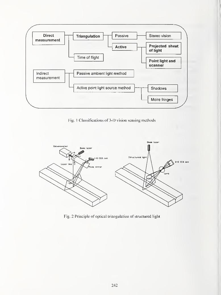
Direct

measurementTriangulation Passive Stereo vision

Active

Time of flight

Projected slieet

of light

Point liglit andscanner

Indirect

measurementPassive ambient light method

Active point light source method Shadov\/s

Moire fringes

Fig. 1 Classifications of 3-D vision sensing methods

242

243

Fig. 5 Functions of laser vision sensor for pre-assembly of stiffeners

Main Body

Torch

CCD Camera

n Diode Laser

rLNG lank Corrugation

Fig.6 Schematic diagram of the automatic welding system for corrugated membranes

244

Fig. 7 Multi-reflections on corrugated panel of LNG tank

P4

1 0

ig. 9 Feature points and typical images of vision sensor

pattern 1-1

pattern 1-2

pattern 1-3

pattern 2

pattern 3

pattern 4

0.1 0.2 0.3 0.4 0.5 0.6 0.7 0.8 0.9

Sum. of pixel coordinates

10 11 1.2 1.3

Fig. 1 0 Characteristic parameters for neural network

246

INTERNET BASED MANAGEMENT OF DATA FROM WELDING SENSORS*

T.P. Quinn*

ABSTRACT

This paper describes a case study of data management for the data generated during sensing of

welding processes. Real-time sensors can produce large amounts of data for weld documentation

or control. The data can also be made available to a geographically remote station to allow

informed decisions to be made about the productivity of a welding station or to troubleshoot

problems of a welding station. The arc sensing monitor (ASM), a through-the-arc sensing

system, was used to demonstrate a possible solution. The ASM outputs seven different quality

measures thirty-two times a second. Based on the quality measures, the ASM decides whether

there has been a defect. The ASM was modified to make the data and defect decisions available

via Internet protocols. A data client collected the information and pushed it into a standard

database. An applet accesses the database from a web browser or as a stand-alone application.

The welding engineer can use the applet to identify the defective welds and plot the quality

measures from any location on the Internet, either off-line or as the weld is being made. The

scheme of storing the data in a standard database architecture allows simple scripts to be

developed to query any aspect of the data.

INTRODUCTION

This paper presents a recipe for managing large amounts of weld-sensing data using Internet

technologies. In 1991, the National Research Council (NRC) outlined the needs for

manufacturing research (Ref 1). The NRC decided that one of the principal needs for

deployment of intelligent-manufacturing control is the effective acquisition, correlation, and

presentation of manufacturing data. Many welding sensors have been developed over the past

decade (for examples, see Refs. 2-10), and many produce large amounts of data that can be used

to document parts, to do statistical process control, and to troubleshoot welding lines. However,

as the NRC pointed out, the data must be presented to the welding engineer in a manner so that

s/he can predict when process disruptions are about to occur and can learn from process

disruptions if they do occur. If the welding engineer is not located near the welding station, it

becomes imperative that the data from the welding station be accessible remotely. The engineer

can save down time on the line and can better recognize trends in the data if the data are

available at his/her current location immediately.

The growing use of Internet protocols has not bypassed manufacturing. Many equipment

suppliers for factory automation now offer Internet communication facilities. Researchers are

also developing data management solutions using Internet protocols: Gower et al. demonstrated

the use of a Internet protocols in controlling a a semiconductor processing cell remotely (Ref

* Product of the National Institute of Standards and Technology, not subject to US copyright.

' National Institute of Standards and Technology, Boulder CO 80303

247

11). Bertocco et al. described a client-server system for controlling electronic instrumentation

over the Internet (Ref. 12). Adams et al. used Internet protocols to control and collect data for

toxic exposure tests (Ref 13).

In the research presented here, I used Internet and database standards to gather and consolidate

the data produced by a through-the-arc sensing system of gas metal arc welding.

METHODS

The through-the-arc system has been described in Refs. 5,14. The arc sensing monitor (ASM)

calculates seven quality variables and, once every ^ s decides whether defects have occurred.

The ASM is a PC-based system that is attached to an Intranet. The ASM can be controlled from

the network using Transmission Control Protocol and Internet Protocol (TCP/IP), the standard

protocols used for the Internet.

The scheme utilizes four independent modules: the sensor, the database server, the web server,

and the engineer's workstation. The sensor in the weld cell (in this case the ASM) connects to a

database server located somewhere across the network. The ASM acts as a TCP/IP streaming

socket host and listens for connections on a specified port (Ref. 15) - Figure 1. The "database

tender," a program running on the database server, connects to the ASM socket, and after each

weld, the quality variables are sent over the socket. The database tender also receives the

configuration parameters for the ASM. The data are buffered by the database tender so that the

ASM can be ready for the next weld. Once the data transmission is complete the database tender

parses the data and places it in the database. The database is accessed through an Open DataBase

Connectivity (ODBC) manager. ODBC allows the database tender to interact with the database

using SQL, a widely used programming language. The database tender can also configure the

ASM remotely by changing the configuration parameters of the ASM.

The database is relational and is arranged in four tables: defective welds, quality parameters,

graphing indices, and configuration constants. The name of the weld and the time and date of its

creation are used as keys for organizing the tables. The defects table shows whether the weld has

defects or not. The quality parameters table contains all the time indexed quality parameters for

each weld. The configuration table stores the setup parameters needed for the ASM, which

includes such things as the sampling frequency and current scale. The graphing indices are used

so that the visualization program can quickly plot the quality parameters and the thresholds on

the quality parameters without recomputing.

A visualization program written in Java'^'^^ runs on the Engineers Workstation but is served from

the web server. The visualization program also accesses the database through the ODBCmanager.

248

Welding

Cell

ODBC

<

Database Server

Engineer's Workstation

Figure 1: The architecture for the data-handling scheme.

The visualization program can be run as a stand-alone application or in a browser on the

engineer's workstation. The program displays to the welding engineer a table of the welds made.

The defective welds are checkmarked (Figure 2). The welding engineer can plot a time-series of

any of the quality parameters by highlighting the weld s/he is interested in and clicking on the

appropriate button.

249

^Applet Frame mASM Weld Database

4 J_«J_*J -J •d ><J lJ 3 I sWELDID

1DateTimeOfWeld DEFECTS •^

7 expo. 60 [l 5/99 10:28:14 AM r8 expo. 61 1 5/99 11 :02:16 AM sn r-

Record 8 of 18

Arc Condition No.

40

30

20

10

0.7 1.7 2.7 3.7

Time s

Push Button to View Graph

Average Current|

AverageVoltage

i

Arc Condition

Short FrequencyI

Pulse Frequency

Current Trend

Voltage Trend

Average Resistance

Plotted Weld id Out ofTolerence Limit

Figure 2: The visualization program's user interface.

RESULTS AND DISCUSSION

The scheme was implemented and used in combination with other web-based technology to

demonstrate remote collaboration (Ref. 16). Welds were made in Gaithersburg, Maryland and

reviewed in Boulder, Colorado and in St. Louis, Missouri. The welds joined a mounting bracket

to the shaft of an automotive suspension strut. Two, 2 s welds were made with an approximately

1 s delay between welds. In both cases, the network speed was adequate to transmit the data

between welds and have the ASM be ready to process the next weld. Approximately 3 KB of

data need to be transmitted for each second of weld. An Intranet connection implemented at

ISDN bit-rates (128000 bits/s) could transmit the data from a 2 s weld in 0.375 s.

The web server, the engineering workstation, and the database server need not be running on

three different computers-in this implementation, they all ran on a single PC. The ODBCmanager was included in the operating system, and the run-time engine for the visualization

program was downloaded from the Internet without cost. Wizards to manage the database were

available in common, office-productivity software (Ref. 17). Queries to the database that are not

programmed into the visualization tool can easily be constructed using the same software.

The advantages of this scheme are the following: (1) The data are available remotely, allowing

production welding lines to be monitored and troubleshot by a central staff. (2) Large amounts of

250

data generated in the cell can more easily be handled on machines that are designed to be

database servers. (3) The process of developing user-specific ways to view the data can take

advantage of the large number of relatively low-cost tools already developed for databases. (4)

The visualization program can be run on virtually any platform. A disadvantage is that a reliable

TCP/IP-based network must be installed in the factory.

SUMMARY

A data-management system was developed for a through-the-arc sensing system. The sensor

reports its data over a TCP/IP network to a program that buffers the data, then places it in a

database. The database is accessed with the standard ODBC protocol. Weld engineers can use a

visualization program that also accesses the database through the ODBC protocol. The engineers

can then monitor and troubleshoot the welding station. The visualization program is written in a

generic programming language that can run on almost any platform. The large amounts of data

are managed easily using generic or specific scripts developed for databases.

REFERENCES

1. Committee on Analysis of Research Directions and Needs in U.S. Manufacturing. 1991.

The Competitive Edge - Research Prioritiesfor U.S. Manufacturing. Washington:

National Research Council, pp. 25-53.

2. Araya, T., and Saukawa, S. 1992. Recent Activities on Sensing and Adaptive Control of

Arc Welding. Proc. 3rd International Conference on Trends in Welding Research, eds. S.

A. David and J. M. Vitek, pp. 833-842, ASM International.

3. Smartt, H. B. 1992. Intelligent Sensing and Control of Arc Welding. Proc. 3rd

International Conference on Trends in Welding Research, eds. S. A. David and J. M.

Vitek, pp. 843-851, ASM International.

4. Sicard, P., and Levine, M. D. 1988. An Approach to an Expert Robot Welding System.

IEEE Transactions on Systems, Man, and Cybernetics 18 (2):204-222.

5. Quinn, T. P., Smith, C, McCowan, C. N., Blachowiac, E., and Madigan, R. B. 1999. Arc

Sensing for Defects in Constant-Voltage Gas-Metal-Arc Welding. Welding Journal (in

press).

6. Hanright, J. 1986. Robotic Arc Welding under Active Control - A Survey of Current

Technology. Welding Journal 65 (ll):19-24.

7. Richardson, R. W. 1986. Robotic Weld Joint Tracking Systems - Theory and

Implementation Methods. Welding Journal 65 (1 1):43-51.

8. Madigan, R. B., Quinn, T. P., and Siewert, T. A. 1995. Control ofGas-Metal-Arc

Welding Using Arc-Light Sensing. Gaithersburg, MD: National Institute of Standards and

Technology, Report No. NISTIR 5037, p. 9.

9. Johnson, J. A., Carlson, N. M., Smartt, H. B., and Clark, D. E. 1991. Process Control of

GMAW: Sensing of Metal Transfer Mode. Welding Journal 70 (4):91s-99s.

10. Song, J.-B., and Hardt, D. E. 1993. Closed-Loop Control of Weld Depth Using AThermally Based Depth Estimator. Welding Journal 72 (10):471s-478s.

251

11. Gower, A., Boning, D., and Mcllrath, M. 1996. A Flexible, Distributed, Architecture for

Semiconducter Process Control and Experimentation. Proc. Intl. Symposium on

Intelligent Systems and Advanced Manufacturing, SPIE Proc.

12. Bertocco, M., Ferraris, F., Offelli, C, and Parvis, M. 1998. A Client-Server Archetecture

for Distributed Measurement Systems. IEEE Transactions on Intrumentation and

Measurement {5):\\A3>-\\A%.

13. Adams, D., Swannack, R., and Peterson, M. 1999. Remote Control of Instrumentation

Via Ethernet. Scientific Computing and Instrumentation 16 (9):46-48.

14. Quinn, T. P., and Madigan, R. B. 1998. Sensing of Arc Welding Process Characteristics

for Welding Process Control. United States Patent No. 5,756,967.

15. Quinn, B., and Shute, D. 1996. Windows Sockets Network Programming. Reading:

Addison-Wesley.

16. Gilsinn, J., Rippey, W., Falco, J., Quinn, T. P., Russel, B., and Stouffer, K. 1999. AWelding Cell that Supports Remote Collaboration. Proc. Ninth International Conference

on Computer Technology in Welding.

17. Microsoft. \991 . Microsoft Access®: Microsoii.

" Trade names are used only to specify adequately the techniques used. Such identification implies neither

endorsement by NIST that the particular technique is the best available for the purpose.

252

Session B2: Real-Time Weld Sensing andControl Systems: GMAW Arc Quality

Monitoring II

The Use of an Integrated Multiple Neural Network Structure

for Simultaneous Prediction of Weld Shape, Mechanical

Properties, and Distortion in 6063-T6 and 6082-T6 AluminiumAssemblies

0. Gundersen\ A. O. Kluken^ 0. R. Myhi^, J. E. Jones^ V. Rhoades^ J. Day^ J. C.

Jones^, B. Krygowski^

^ SINTEF Materials Technology

N-7465 Trondheim, Norway

^ Hydro Raufoss Automotive Technical Centre ASP. O. Box 41

N-2831 Raufoss, Norway

^ Native American Technologies Company1317 Washington Ave. - Suite 1

Golden, Colorado 80401

ABSTRACT

Neural networks are parameterised non-linear mathematical models well suited for pattern

classification and non-linear function approximation. These kinds of models are empirical models

and in the training process, the unknown parameters are adjusted until the non-linear response of

the network fits the data according to a specified performance criterion. Neural networks offer

certain advantages in weld modelling. However, in the past, such models did not provide all of

the information that is usually necessary to completely design a welded assembly and optimise the

welding operation. In this work, a neural network structure for simultaneous prediction of weld

shape, mechanical properties and distortions of welded aluminium assemblies is presented. The

experimental approach is well described and extensive information about the neural network

concept used in this work is also provided. In a simulation case, it is shown that optimisation of

individual weld properties may easily cause other properties to fall outside the acceptable range

(SPC-limits). It is also shown that the model can be used for optimisation of multiple properties.

255

1. INTRODUCTION

As the demands of the manufacturing environment continue to increase and time-to-market for

products experiences a continual contraction, better computer tools are necessary. The is need for

a design system that is capable of virtual manufacturing to provide the capability to "manufacture"

a product in the computer, just as it would be produced on the shop floor. Such a system should

provide virtual manufacturing that is simultaneous with the design process, so that the

manufacturability of designs can be verified without investment in expensive production

equipment.

Higher strength heat treatable aluminium alloys exhibit degradation of the metallurgical properties

in the heat affected zone (HAZ) of arc welds. Arc welded automotive space fi^ame assemblies

produced using these alloys will have the overall strength limited by the HAZ properties.

Additionally, distortions from the welding process can cause difficulties with the fit-up of other

components of the automobile.

Robotic welding of aluminium space frame assemblies demands that the process be optimised.

Such optimisation should focus not only on the weld engineering shape parameters, such as depth

of penetration, or weld size, but also consider to minimise distortions in the final assembly as well

as to maximise the strength of the weld HAZ. Previously, each of these has been modelled

separately and most frequently by using different kinds of models. Also, there have been no

reports of a comprehensive model that allows for complete optimisation of the welding process to

meet the specifications of the weld itself, while simultaneously minimising distortions and

maximising HAZ properties.

Previous work conducted at Native American Technologies Company (NATech) and by others

have shown that neural networks provide certain advantages in weld modelling. Until now,

however, neural network models as well as other types of models have not provided all the

information that is necessary to completely design the welded assembly and at the same time be

used as an aid for optimisation of the welding operation. The present study describes the

development of a multiple neural network structure for prediction of multiple properties of

aluminium weldments. The study presents results obtained in a project conducted by Hydro

Raufoss Automotive Technical Centre (HRTC) in cooperation with NaTech; a company that has

specialised in development of neural networks for welding applications. SINTEF Materials

Technology (SINTEF) played the role as a third party consultant during the whole project.

HRTC's main objective was to study the potentials of using neural network modelling in

computer assisted welding procedure development.

The welds were made from extrusions of two aluminium alloys, both in the peak aged temper

condition. The extrusions of square tubing were heat treated to the same property levels. Material

thickness varied fi^om 2 to 5 mm. Pulsed gas metal arc (GMA) welds were produced according to

a set of experiments derived fi^om an experimental design technique optimised for neural network

modelling. Included in this part of the work was also some initial screening experiments to

become familiar with the operation ranges of the different welding parameters. The screening

experiments were embedded into the experimental design matrix. The neural networks were

256

trained using the P/NA^ neural network concept developed at NATech [1,4,6]. Each of the neural

network prototype models was tested by the use of an exclusive statistical method used for

determination of the upper error bound in the models as well as confidence levels for the

predicted information. This method, known as guided experimentation was used to generate

additional experimental data in regions of the parametric space where refinement of the neural

network models was needed.

The refined neural networks are integrated into a single software Graphical User Interface (GUI)

that provides the ability to simultaneously observe weld shape, weld mechanical properties and

distortions for a T - connection structural assembly. The experimental approach and neural

network modelling concept are thoroughly described and the capabilities of the neural network

structure as a complete knowledge source for engineering design and process optimisation is

demonstrated. The software system also provides a set of exclusion rules which prevents the user

and the built in optimisation routine from selecting weldmg parameters that belong to a region in

which the welding process will not operate.

The rest of the article is organised as described in the following. At first, some characteristic

features of aluminium space frame weldments along with their traditional modelling approaches

are presented. Then, a unified approach to neural network modelling is described and important

phases of the development work is classified. Relevant properties of the aluminium alloys and

different approaches in experimental design are then described. Also, a brief introduction into

neural networks is presented along with a thorough description of the neural network concept

used in this work. Then, some general features of the computer model are summarised before the

presentation of a simulation study related with optimisation ofweldment properties. Finally, some

ideas about fiature use of neural networks in the field of weld modelling are given before the

concluding remarks at the end of the paper.

2. SPACE FRAME WELDMENTS:MODELLING OF CHARACTERISTIC FEATURES

In this section, some important problems related to welding of automotive space frame

components in aluminium are presented. These include predictions of weld bead shape, strength

distribution and weld distortions. For each of these features, the basic mechanisms will briefly be

explained along with descriptions of the different modelling approaches that are most frequently

used for modelling these phenomena. It will be shown that traditionally, different modelling

approaches are used depending on which feature of the weld that is focussed on. This is in

contrast with the approach described in this work where the same neural network modelling

approach is used to describe different features of the weldment.

2.1 Weld Bead Shape

There is a growing interest for simulation programmes that can predict the detailed geometry of

the weld bead. Based on the bead geometry, geometric data of the bead can be defined and used

for assessment of weld quality. If such programmes are sufficiently accurate, they can be applied

as a tool in welding procedure development. Work with procedure development has traditionally

257

been a discipline of trial and error, which is costly and time consuming. By bringing simulation

tools into use, the task of developing a welding procedure becomes more systematic and

predictable. Different techniques based on both empirical modelling techniques and physical

principles have been used for describing the weld bead shape or associated bead parameters. The

reader should note that most of the references cited in this subsection deals with studies of steel

weldments, but the principles discussed will also be applicable in welding of aluminium.

Linear and non-linear regression techniques have been used for modelling the relationship

between welding parameters and geometric data for description of the bead [1, 2]. As opposed to

these traditional regression type models which have been used for direct prediction of weld

geometry parameters, neural networks have been used for prediction of the whole weld bead [4,

5]. Then, weld geometry and engineering parameters can be derived with basis in the predicted

whole bead shape. It has been shown that this approach yields a much more accurate prediction

since many of the geometry parameters are not continuous as the weld shape varies, but the bead

shape varies in a "smooth" way as the welding parameters are varied [Klein 94; obtain ref from

JJ]. The neural network which is used as a non-linear empirical model is capable of sufficient

multi-dimensionality to describe the entire weld bead shape; the neural network concept used in

this work is described in section 5.0 on neural networks.

Physical modelling techniques have also been used for modelling the shape of the weld bead. The

mechanisms that determine the weld pool shape are very complex and include fluid flow, droplet

detachment and metal transfer phenomena. For the majority of cases, the Peclet number is high

enough to introduce significant effect from the convective heat transfer on the weld pool shape

[7]. The driving forces for convection in the weld pool depend on the kind of heat source used. In

arc welding, electromagnetic forces will contribute to the weld pool circulation but in laser driven

welds such forces are absent. Thus, in arc welds, forces due to the surface tension temperature

gradient (Marangoni effect), the buoyancy force, the electromagnetic body (Lorenz) force and

aerodynamic drag forces contribute to the convective flow in the pool [8, 9, 10,11]. Models of

this kind are frequently based on finite volume and finite difference techniques but finite element

approaches are also applied in modelling ofweld pool convection.

Finite element based models have been extensively used for prediction of residual stresses in

welds. Details of the weld may have impact on the residual stresses in regions close to the weld

but are not critical for proper prediction of the residual stresses in the heat affected zone. In such

models, the approximate shape of the weld is implemented by using an appropriate heat source

model to account for the heat power distribution in the weld pool [12]. In an even simpler

approach, analytical models with distributions of elementary point heat sources and the method of

images have been used for a qualitative prediction ofweld bead shape [13].

Even though physically based models have become increasingly sophisticated and can account for

several of the mechanisms that influence weld shape, they are still not useful for most production

applications since they usually require many hours to run, which is far too slow for real-time

simulations. If experimental data for weld shape are available, neural networks offer an alternative

method for modelling the weld shape since these models are capable of capturing all of the

258

complexity of the manufacturing process. Such empirically based models represent a completely

different approach to weld bead modelling compared with the physically based models.

2.2 Weld Mechanical Properties

The structural strength of 6XXX (i.e. Al-Mg-Si) alloys can not be fiilly utilised in welded

automotive space frame assemblies since the HAZ is significantly softer than the unaffected base

material. This strength loss is caused by a sequence of unfavourable metallurgical reactions taking

place in the HAZ as a result of the high temperatures imposed by the welding arc.

During welding, reversion of hardening P"(Mg2Si)-precipitates will occur to an increasing extent

within the peak temperature range from about 220-500°C. At the same time, non-hardening

P'(Mg2Si) precipitates can nucleate and grow at dispersoids. Fig. 1(a) shows the corresponding

hardness drop across the HAZ immediately after welding. It follows from Fig. 1(b) that this

strength loss is not permanent, but will gradually become smaller as excess solute starts to

recombine and form GP-zones during subsequent natural aging. The recovery process is almost

completed after 1-2 weeks, and the resulting hardness profile will then be as shown in Fig. 1(b)

from which it is apparent that the minimum hardness will be located at some distance from the

weld fusion line. The corresponding yield stress at this position is an important value in

engineering design since it defines the overall strength of the assembly.

Different types of models can be applied to predict the HAZ strength distribution. Myhr and

Grong have derived physically based models which simulates the microstructure evolution during

welding, and these have been successfially applied to predict the effect of different welding and

material combinations on the resulting HAZ strength [8-11, 14, 15]. The microstructure model is

derived by considering the P" particle dissolution (particle reversion model) during welding which

leads to strength loss. A natural ageing model accounts for the subsequent reprecipitation of GP-

zones during storing at room temperature which leads to strength recovery. In the model,

equations are established for the relative volume fraction fp(fp,o of the strengthening particles; fp is

the actual volume fraction of precipitates and fp,o is the volume fraction of precipitates in the

(artificially aged) base material. In the next paragraph, it is shown that the quantity fp/fp,o can be

related to the strength ofthe weldment.

The high strength values ofAA6XXX alloys are due to the presence of the P" particles. The net

precipitation strength increment Aap due to artificial hardening can be calculated from an equation

originally derived by Kelly and Nicholson [16] that states:

Now, if the relative volume fraction Xp =fp/fp,o is introduced, the strength increment can be

expressed by

(1)

Ac, oc XJ^_, (2)

259

Aap reaches its maximum when Xp= 1; i.e. when the maximum number of precipitates are present

in the aluminium matrix. Thus

(3)

<3p,min denotes the intrinsic strength of the aluminium matrix after complete particle dissolution

while (5p,max is the original base material strength in the artificially aged condition. As a rough

estimate, the yield strength can be estimated fi^om the hardness value by a linear relationship [17]

for certain alloys. For AA6082 alloys of the kind studied in this work, the following relationship

between hardness and yield strength can be used [15]:

This kind of linear relationship cannot in general be expected to be valid for all types ofAA6XXXalloys. In principle, however, we see that hardness, strength and volume fraction of

strengthening precipitates are related properties and information about strength and

precipitation reaction kinetics can be obtained via hardness measurement. Such measurement

are much easier to perform than measurement of the actual particle volume Abactions. Hardness

measurements constitute the experimental basis for the microstructure model. In this work,

hardness measurements are used as the basis for calculation of the minimum strength in the HAZof the weldment.

Thermally induced distortions caused by the steep thermal gradients associated with welding may

represent a serious problem in keeping the dimensional tolerances within the specified limits of

welded automotive components. Fig. 2 shows schematically the sequence of deformations taking

place during welding of a typical T-joint of a space fi"ame assembly. The vertical displacement is

initially in the upward direction as shown in Fig. 2(a). This is due to thermal expansion of the

heated material adjacent to the weld. The direction is however reversed during cooling when the

material contracts, and the final deformation will usually be as shown in Fig. 2(b).

Finite element (FE) modelling techniques can be applied to calculate such deformations. Accurate

predictions require that the softening of the HAZ, as described in Section 2.2, is accounted for in

the mechanical model which calculates the evolution of stresses and strains during welding. If this

effect is ignored, the result will be a significant overestimation of the residual stress level in the

HAZ [18]. FE-models where the microstructure evolution is accounted for by internal state

variables have recently been developed for different types of aluminium alloys [19,20,22,23].

These models have been demonstrated to be capable of predicting how different base materials,

welding parameters and sequences affect the resuhing deformations, and they are also very

flexible with respect to the geometric design which can readily be changed for each newsimulation. The disadvantage is, however, that each simulation requires a substantial computer

time that implies that such models at present cannot be used as an interactive tool.

a^3.0HV-4S.l (4)

2.3 Weld Distortions and Residual Stresses

260

The cornerstone in these simulations is the microstructure model. Myhr et. al use only the

reversion model to describe the evolution of microstructure over the weld cycle; the natural

ageing modelling is needed to describe strengthening processes in the material after welding is

completed. The reversion model operates together with a constitutive equation for the mechanical

behaviour of the material. The constitutive equation relates the effective flow stress a also to

other critical parameters in the system;

cr = (TJ V

\J p,o

f

= F(T)Gf

'

y p.o p.o J

8p\ J

(5)

Myhr et. al used this constitutive equation which takes into account the dependency of the flow

stress on the effective (equivalent) viscoplastic strain rate. Also, strain hardening is taken into

account by a separate function that depends both on microstructure and the strain hardening

parameter (j). Above a certain temperature 2} during heating, the subsequent deformation during

cooling will have no memory about its initial deformation. Thus, pure creep ((|)= 0) is assumed

until the temperature falls below 7}. Below a lower temperature To, the hardening parameter

evolves in the same way as the effective (equivalent) viscoplastic strain rate. Between

temperatures To and 7} there is a linear decay of (j) to zero. Isotropic elastic-viscoplastic material

behaviour was assumed in the calculations [20].

3. A UNIFIED APPROACH TO NEURAL NETWORK MODELLING

The concept used for developing the neural networks presented in this work constitutes a part of

a systematic approach to neural network modelling. As basis for this approach, it is realised that

the prediction performance of the neural networks is dependent on the quality of the

experimental data. Data of satisfactory quality is a prerequisite for the development of a

successful neural network model. Also, it is realised that experimental work most frequently is an

expensive part of a modelling project and it should be aimed to keep to number of experiments to

a minimum as well as exploiting already available information in an optimal manner. Finally, it

should be possible to return to the experimental planning phase and add new input parameters

without having to redo the previous work done in experimental planning. Next, training of the

neural networks should be as efficient as possible and modifications of the neural network model

should be done without having to redo the work already spent during initial training of the neural

networks. This has lead to the development of a methodology for neural network modelling that

typically involves the following phases (tasks):

1. Brainstorming and Planning. The objective of this phase is to gain understanding of

the process to be modelled. This involves discussions to decide which are the relevant

input and output parameters to be considered. Decisions about the discretisation

(number of levels) of the input parameters will also be taken.

2. Experimental Design: Based on the information provided in the previous phase, a

design of experiments (DOE) will be performed by the use of suitable software. This

gives a matrix of experiments listed in randomised order to be conducted in the next

261

phase. If experimental information already is available, the software can be loaded with

this information. Then, a design matrix is generated which includes the already

available experiments.

3. Experimental Work: This phase involves the main part of the experimental work and

preparation of the weld samples. This usually includes a set of screening experiments.

Such experiments are needed to become familiar with the operation range of the input

parameters. Due to such information, one may sometimes need to involve more input

parameters to extend the experimental design matrix.

4. Sample Preparation: This may involve metallographic preparation of the samples and

different types of materials testing.

5. Preparation of Data for Neural Network Training: The samples and information

obtained from the previous phase are used to generate a neural network training - file

in electronic format.

6. Training & Analysis of the Prototype Model: This phase involves both initial training

and testing of the prototype model to point out domains in the input parameter space

that gives predictions with an error larger than accepted for the current application.

Then, guided experiments are planned to generate additional information to improve

the performance of the model in the uncertain regions of the input parameter space.

Also, at this stage, work will start with development of a Window's based Graphical

User Interface (GUI) for the neural network software model.

7. Execution of "Guided Experiments": This phase involves execution of the guided

experiments and preparation of the samples.

8. Refinement of the Neural Network Model: The information obtained from guided

experiments is used for refinement (improvement) of the prediction performance of the

neural network.

At best, guided experimentation only has to be executed once. In general, however, several stages

of guided experimentation may be needed to achieve a neural network model with the desired

predictive capabilities.

The following two sections of this study include descriptions of the experimental approach and

the neural network concept (training and testing) respectively. Information about the guided

experiments is given in section 4.3 although guided experimentation may be considered to belong

to the task of testing the neural networks as described in section 5.6.

4. MATERIALS, EXPERIMENTAL DESIGN AND WELDING PROCEDURE

This section is related with the experimental approach used in this study. A thorough description

of the experimental planning methodology is given along with information about the welding

procedure applied during the experiments.

4.1 Materials

The welds studied in this work were made from hot extrusions of two aluminium alloys AA6063and AA6082; each alloy in the peak aged temper condition (T6). These alloys belong to the

.262

AA6XXX series that contains on the order of (0.5-1.3)% magnesium and (0.4-1.4)% silicon.

AA6082 has a significantly higher yield strength than AA6063 (typically 300 MPa and 220 MPa,

respectively). Such alloys are made by DC-casting and subsequent homogenisation at

temperatures between 530 and 580°C. Subsequently, the metal is extruded and cooled. Then, for

the extrusions to achieve the desired properties, the extrusions are age hardened at temperatures

between 160 and 185°C for 3 to 6 hours. Age hardening is performed over a limited period of

time to avoid overaging; i.e. reduction of the strength of the material. The hardening process

during ageing ofhot extrudedAA6XXX alloys is described in Appendix A.

4.2 Introduction to Experimental Design

The following subsection gives a review of the principles of experimental design. The material

presented is mainly based on [24, 25, 26].

Experimental design (Design Of Experiments; DOE) deals with methods for experimental

planning that support the user in efficiently obtaining the relevant characteristics of the process.

The ideas involved in experimental design are relatively simple but in many cases the statistics

involved can be quite difficult. However, such methods are also available to the non-expert via

software packages that have built - in routines for a wide variety of design techniques. The output

from this process is an experimental design matrix with information on the set of experiments to

be conducted.

The keyword in experimental design is planning. Typical decisions that have to be made include:

• Specify the goal of the experiment

• Classify input- and output variables

• Clearly specify assumptions about the process

This is in contrast with the technique often used in traditional experimentation: Frequently, one

tends to vary the process input parameters in an unsystematic way; using the results of one run to

give guidelines for how to perform the next run. By following this approach, no insight into the

coupled influence of the input parameters on the process outputs can be achieved. Thus, when

there is no systematic planning of the experiments, there is always a risk of loosing knowledge

about a certain important feature of the process and may result in reinforcing false assumptions

due to confounding effects in the non-randomized data.

Most experimental designs allow for the estimation of the desired coefficients in the model with

fewer {less than full factorial) than the full set of experiments that would be included in a full

factorial design. There is, however, a trade-off between the number of runs, the number of

estimated terms and the quality of the estimation (i.e. the estimated model parameters).

In the literature, two groups of experimental designs are classified. Classical designs have

desirable statistical properties that make the analysis of the experimental data quite easy.

Unfortunately, these designs are applicable only to certain problems and they are inflexible about

the number of runs and the factor settings they need. Taguchi designs, full factorial designs.

263

fractional factorial designs, Box-Behnken designs, central composite designs and orthogonal

arrays belong to the classical designs. Constraints on the region of operability of the factors and

other special features of the design situation may prevent the use of classical designs. In such

cases, the use of an optimal design technique is the only alternative. The optimal designs

constitute to the second group. These designs are non-orthogonal. There are several types of

optimal designs (A, D, G and V optimal) each named after the optimisation criterion used to

determine the set of experimental runs. According to the criterion, the amount of information in

the experiments is maximised.

In this work, experimental design was used to support the process of establishing a complex

model based on neural networks. NATech has long experience in using experimental design for

neural network modelling. In a study performed at NATech, several classical design methods and

optimal designs were examined to determine the best experimental approach for neural network

modelling. The initial study included a two level Box-Behnken design and a Taguchi design with

three levels. The result of this work clearly indicated that the Taguchi design provided a much

better model than the Box-Behnken design.

As part of a continuing overall plan for testing and verification of neural networks, a series of

tests were conducted to evaluate the effectiveness ofvarious other experimental designs, currently

used for statistical modelling. These designs included both three and four level D-Optimal

designs. Depending on the number of factors, these designs required similar numbers of

experiments as the Taguchi designs. The neural networks generated with the four level D-

Optimal designs performed better than neural networks generated fi^om other designs.

However, based on the results of the tests, it was concluded that there could be an improvement

on the D-Optimal design of experiments. The result of this work was an "N-Optimal" design

method that is optimised for neural network development.

4.3 N-Optimal Experimental Design

A refined D-optimal design technique called N-optimal design optimised for neural network

applications was developed [1]. The N-optimal design provides the maximum likelihood of

minimising the error in the neural network while simultaneously using a minimum number of

experiments. Cost of experimentation can often be a significant part of the development cost of a

neural network, so reduction of the number of experiments is a primary criterion in the N-Optimal

design method. When combined with Guided Experimentation (described in Section 4.4), a

neural network can be trained to an acceptable error level. Also, the N-optimal design gives the

user the opportunity to add factors and add data fi"om new experiments without having to redo

the whole design. Furthermore, the design method is capable of excluding parts of the input

parameter space which correspond to possible invalid parameter settings for the process. In the

neural network software, these socalled exclusion rules keep track of these omitted regions of the

input parameters.

In addition to using a good design of experiments, it is important to carefiilly document each

conducted experiment. One should keep track of error sources and also register special features

264

observed during the experiments. Based on this documentation, sources of error can be traced and

possible bad experiments removed from the data set used to train the neural network. Also,

accurate and repeatable measurements are necessary to derive a neural network model that

provides an accurate representation of the process that is modelled.

Much effort has been spent at NATech to develop an experimentation methodology in which the

objective is to minimise the amount of experimental work. This can be achieved if one is able to

select only the specific data points that completely represent the underlying process. This reduces

experimentation costs, network training difificuhies and the risk of network overtraining

(overfitting) and hidden node generation. This experimentation methodology is called Guided

Experimentation. The method includes three steps. At first, an N-optimal design gives the least

possible number of experiments that is needed to train the neural network model. However, one

may often need to perform some screening experiments but these experiments may be included in

the set ofN-optimal experiments. Secondly, another group of experiments is selected based on the

value of a statistical parameter called the S-parameter. The S-parameter described in section 5.6 is

a specially designed maximum likelihood estimator that has shovm to be conservative; the error in

the S-parameter is never less than the error in the neural network. Also, it conforms to the student

t statistical distribution. Depending on the accepted error level in the neural network, the value of

the S-parameter as evaluated on the original N-optimal data set can be used to pinpoint the

regions in the parameter space that needs more information about characteristics of the process.

The experimental data obtained during the guided experimentation stage are used for so-called

refinement of the neural network model to embed into the model the new amount of information

represented by the guided experiments. In reality, this is an iterative process that in practical work

only has to be repeated once. Then, training, testing and verification of the neural network model

is based on the original N-optimal data set and the additional guided experiments. This is a unique

feature of the Guided Experimentation methodology that contributes to reducing the amount of

experimental work.

4.4 Guided Experimentation

A neural network can be thought of, in an analogy, as a "wet blanket" that is to be draped over a

set of data points in space. It is pinned at each of the points, but is free to conform to any shape

in the regions between points. Using this analogy, it is clear that the first logical conclusion would

be that the better "pinned" the neural network, the more accurate will be the resulting model.

Stated differently, "if a large set of data points will produce a good neural network, a very large

set of data points will produce an even better neural network". "This "more is better" syndrome is

generally accepted throughout the neural network community.

However, on closer analysis, the problem is really one of selecting the specific data points that

represent the underlying process completely. There are actually two methods of achieving this

"completeness" of coverage of the process operating space. The first is based on the premise that

if there are a sufficiently large number of data points, then the probability is higher that all of the

process behaviours will be represented in the neural network training set. This approach is ofl;en

cited as the only approach that is usefiil for training neural networks.

265

However, if it was possible to select only the data points that exactly represented the process, and

no more, then several advantages would accrue. First, since experiments are always costly, this

approach will yield a cost reduction. Secondly, the neural network training time and difficulties

will be reduced if the training data set is smaller. Third, as the number of training examples

increases, the likelihood of over training also increases as well as the likelihood of too manyhidden nodes required to map the training examples. Guided experimentation provides a method

for achieving these results by near optimum selection of the necessary training data points while

also minimising the number of unnecessary data points.

The technique developed for this guided experimentation approach consists of a set of steps.

First, an initial neural network is developed using the data generated from a very small

experimental design. In the second step, the next experiment or group of experiments to be

conducted is selected. The selection criterion is to maximise the amount of expected decrease in

overall error of the neural network. The S-parameter method for testing the network is described

in the next section. Third, by using the refinement technique of the P/NA^ neural network

structure (see description in the next section) together with the associated training algorithm, the

network is modified to represent the new data without disturbing the basic neural network

structure that was already trained. Fourth, this process is repeated until the neural network is

within an error bound that is reasonable for the problem (considering experimental error, cost

trade-off, etc.). Usually one loop of Guided Experimentation gives a model with satisfactory

prediction performance.

4.5 Experimental Design in this Study

For derivation of the model presented in this work, screening experiments were performed to

determine the exclusion regions in the input parameter space and determine the operation ranges

for the critical factors. Also, the screening experiments contributed to determine the significant

input parameters to be considered. The exclusion regions correspond to parameter combinations

that do not work in practice during welding. As an example, it was shown that welding of thin

materials (thickness 2 and 3 mm) has to occur at different parameter settings than the parameters

used for the thick materials (thickness 4 and 5 mm). The ability to treat such exclusion regions is a

unique feature of all of the Optimal design methodologies. In this study, approximately 150

experiments were included in the set of N-optimal experiments and 20 additional experiments

were recommended by the use of guided experimentation. Altogether thirteen input parameters

were considered and seven of these were four level parameters.

4.6 Welding Procedure

The parts used in the weldments were produced from extrusions of square tubing. The gage

thickness of the extruded profiles varied between 2.0 mm and 5.0 mm. The weld was a T-fiUet

joint around the circumference of a butted tube end in a T-connection of a square tubular

structural assembly. The weld configuration is shown in Fig. 3. The welding experiments were

conducted in a robotic welding fixture, in which weld distortion was monitored during the

welding process by using a LVDT {Linear Variable Displacement Transducer) to determine the

amount of deflection of the chord. The weld was produced as two fillet welds, one starting at one

266

comer of the abutting hollow profile, along one side, around an adjacent comer and along a

second side to the opposite comer. The second weld started at the same point as the first weld

and progressing along the sides not included in the first weld and terminating at the same point as

the first weld as shown in Fig. 4. The welds were deposited using a 4043 (AlSi5) filler wire and

two different shielding gas compositions (pure argon and 70%Ar/30% He, respectively). The

welding parameters included wire feed rate, weld travel speed, vohage, pulsing parameters, torch

offset and a "ramp parameter" which represented a decreased heat input set of parameters for the

second weld to accommodate the pre-heat caused by the first weld. All of the welding parameters

were recorded electronically during each welding experiment. As noted before, the experiments

were conducted in two phases. The first phase included the screening experiments and the set of

experiments as suggested by the experimental design software. Then, the guided experimentation

procedure was performed according to judgement of the S-parameter to provide data for

refinement of the neural network model in regions of the parameter space where the model

predictions are not within the accepted error bounds.

All of the welds were sectioned at eight locations along the length of the weld producing nearly

900 samples. These samples were metallographically prepared and the etched weld cross-section

was captured using a video camera into a PC computer. The weld shape was quantified and

stored electronically, using a special multiple spline fit program, to produce data for the neural

network models. The graphical measurement screen used for capturing the weld cross section

images is shown in Fig. 8.

To be able to monitor the degradation of the mechanical properties in the heat affected zone of

the welds, the method described previously in section 2.2 of this paper which relates hardness to

strength was applied. The method has been previously published and shown good correlation

when used for weld strength prediction. Microhardness profiles were taken on multiple sections of

each weld, to determine the hardness through the HAZ, as a function of the distance along the

centerline of the material progressing away fi*om the location of the. The resulting data set

included approximately 10000 hardness readings.

5. FEATURES OF NEURAL NETWORK MODELS

This section is devoted to the neural networks. After the introduction, some features of

perceptrons, feedforward neural networks and the backpropagation training algorithm are

reviewed. Then, some limitations of the standard backpropagation method are stated before

presentation of NATech's neural network concept applied in this work. Finally, testing of neural

networks is discussed before the section is closed with a description of the neural networks

developed in this study.

5.1 Introduction

A neural network is an empirical approach to process modelling. Such empirical models may be

developed from various sources of data, both real and virtual. In general, however, experimental

data from actual process operation is the best source of information for developing a neural

network model to be used in planning and controlling the production process. Therefore, the

267

quality of the neural network model is a direct fiinction of the quality of the data set. Carefully

designed experiments are the key to producing high quality neural network models.

Neural networks are not a new technology, but a newly applied technology. This work does not

intend to give a survey of different kinds of neural networks; the reader is referred to other

publication for this kind of discussion [1, 3 - 9]. A brief review, however, of some of the most

widely used networks is given in the next subsection. Neural networks (NN)' are an attempt to

develop computer systems that emulate the neural reasoning behaviour of biological neural

systems (e.g. the human brain). As such they are, mathematically, loosely based on the internal

ftinctioning of biological neural networks. For the interested reader. Chapter 1 in Bose and

Liang's book [27] gives a description of the relationships between (artificial) neural networks and

neuroscience.

Numerous examples of the application of neural networks can be found in the literature [30, 31,

32, 33]. In aerospace, neural networks have been use in applications like autopilots and aircraft

control systems. In banking and finance, where neural nets are used very extensively they have

been used for check reading, currency price predictions, loan approval, and for buy/sell decisions

for stocks and other securities. Several applications like visual quality inspection systems, dynamic

modelling, analysis of weld quality and chemical products can be mentioned in manufacturing.

Other important application areas are defence, robotics, telecommunications and entertainment.

A neural network consists of a series of nodes (neurons) and weighted connections (axons) that,

when presented with a specific input pattern, can associate specific output patterns. The operation

characteristics of a neuron are shown in Fig. 5 and a typical architecture of a neural network is

shown in Fig. 6. In essence, the neural network represents a highly complex, non-linear,

mathematical relationship or transform. However, it is not necessary for the developer of such a

system to understand the basic underlying physical or scientific principles of a process in order to

develop an accurate ANS based process model. Thus, in this way it is quite different from other

mathematical modelling approaches such as the Finite Element Analysis (FEA) method and more

like the traditional statistical or regression type models. The primary difference between neural

networks and statistical methods, however, is that neural networks are efficient at extracting

patterns from data sets and the data need not be structured in orthogonal arrays. Usually,

mathematical flinctions that resemble step fiinctions have been used as transfer fijnctions in neural

networks. Due to computational reasons, the sigmoid function shown in 1 IZ has frequently been

used.

The challenges in neural network development are to decide how many nodes and connections are

needed to model a specific process, how to configure them, and to determine the specific values

of the connection weights and the transfer functions that exist within the network. There is no

direct known correspondence between the network parameters, it's operation, and the problem to

be modelled by the network. One of the most successful approaches that has yielded reasonable

results in developing networks is known as the "backpropagation" method. This method is

described in sections 5.3 and 5.4 below.

' Sometimes also known as Artificial Neural Systems (ANS) or Artificial Neural Networks (ANN).

268

5.2 Perceptrons and Feedforward Neural Networks

Neural networks may be classified into static- and dynamic networks. Static networks are

characterised by node equations that are without memory and delays; i.e. the output of the neural

network is only dependent on the current input value to the node. Among others, the perceptrons

(single and multilayered layered) neural networks belong to the group of static networks:

In the simplest form, perceptrons are one-layered neural networks with nodes that have a hard

limit transfer function. This simple architecture places limitations on the computational power of

the perceptron. The perceptron learning rule is used to train these single layered networks.

Perceptrons may be coupled in series to form multilayer perceptrons (MLP). If one allows the

transfer function to be more general than the hard limit flinction, such MLP networks are also

denoted multilayer feedforward neural networks. Among the static networks, the MPL - or

feedforward neural networks are most widely used. Such multilayer networks often use a log-

sigmoid transfer function. If a linear transfer fijnction is used at the output neurons, the network is

capable of generating outputs of any value.

If a linear transfer function is used, training can be done by using the Widrow-HofiF algorithm. It

should be noted that any multilayered network with linear transfer functions can be represented by

an equivalent single layered network with linear transfer functions. This is an inherent property of

the linear functions.

The backpropagation training algorithm was created by generalising the Widrow-Hoff learning

rule to multiple layer networks with nonlinear differentiable transfer functions. Standard

backpropagation is a gradient descent algorithm. By using the standard backpropagation training

rule, it may be difficult to obtain a solution. Even more, if one is able to find the optimal set of

weight parameters, the convergence may be slow. Numerous modifications of the standard

backpropagation method can be found in the literature.

The learning rules described so far belong to the group of supervised learning rules. This means

that they are presented with a set of example input-output pairs (Xi,di) and then trained to

implement a nonlinear mapping that matches the training examples (datapoints) as close as

possible.

During learning, the outputs of a supervised neural net are used to approximate supplied target

(output) values from supplied input variables. By generalization, however, is meant the ability of

the neural network to approximate output datafrom input variables that are not in the training

set. Generalization is a measure of how well the neural network performs on the actual problem

once training is completed; i.e. how good is the prediction performance of the network? The

following conditions are typically necessary (but not sufficient) for good generalization:

• The function that the network tries to learn is in some sense smooth.

• The training data set must be a sufficiently large and representative subset of all cases

that the network is supposed to generalize over.

• The network is large enough.

269

In a MLP (feedforward) network, the number of training samples should be approximately ten

times the number of weights to achieve satisfactory generalization properies (i.e. avoid

overtraining/overfitting). Other features of generalization are discussed by Hush [34].

Since, in general, a neural network performs a highly non-linear transformation from inputs to

outputs of the network, it is possible also to 'overfit' the training data: The network behaves

correctly for the training data but prediction based on test data may lead to very bad prediction

properties. Such a network is unable to generalize properly; the situation is denoted overtraining

or overfitting. Overtraining can be handled by Bayesian regularisation theory. Application of

Bayesian neural networks is described by Cool and MacKay [35], [36]. Another method used to

improve generalization is the Early-Stopping technique described in section 5.6.

A neural network that is not sufficiently complex can fail to detect fully the signal in a complicated

data set. This leads to underfitting; i.e. the model performs badly for the training data points as

well as for the test points.

5.3 The Back Propagation Training Algorithm

In the back propagation method, "training" of the neural network is a search for a network

configuration that offers minimum error for all of the data points (examples) in the "training set".

The method assumes that the search in weight space for a functioning network configuration can

be accomplished as an iterative search using the error gradient (i.e. slope of the error surface).

That is, a series of moves are accomplished on the multi-dimensional error surface using

approximately the maximum mean squared error gradient direction as the move direction to a new

set of weight values, at each iteration (training cycle). The error in the network is defined as the

difference between the desired output representation and the actual output given the current

weight matrix values. By calculating the maximum gradient of the mean squared error for any

given training example (set of input and corresponding output patterns), the weights are adjusted

so that the net moves along that gradient direction in each presentation of the training example to

the network. Using this procedure, the network slowly "learns" to associate all of the training

example input patterns with the correct corresponding output patterns by finding a global

minimum on the error surface. A mathematical formulation of the backpropagation algorithm can

be found in Hush's article [34].

5.4 Limitations of Back Propagation

This "basic" back propagation learning process has several significant drawbacks. First, the

optimum configuration (i.e. number and relative location of hidden layers of nodes) cannot be

pre-determined by any known method and, yet, needs to be pre-assigned by using an "educated

guess" in order to use this procedure. Since the node configuration can significantly affect the

operation of the network, this will at best lead to a long series of training re-starts and at worse to

no useful network at all. Secondly, the training process is very slow and no known methodforpredetermining the learning rate (gain term) will consistently choose an optimum value. As with

any search approach, taking steps that are too large will result in overshoot and an inability to find

the minimum and steps that are too small will lead to very long search times. Third, it has been

270

shown that it generally requires a larger network to "learn" a problem than is required to solve

the problem. There are techniques for trimming nodes or connections from a large network, but

there is no known method of reducing the size the size of the network after training that will

guarantee optimal net performance. Finally, learning instabilities exist in nearly every problem

that will cause the network to stop learning (converging); at least three types of learning

instabilities have been shown to exist. One ofthese instability types is known as a local minimum.

This occurs when a "low" spot is reached on the error surface that is not the lowest error position.

Using a geographic analogy, if you are sitting at the bottom of a lake, your local surroundings

appear to go up in every direction. If your objective is to always move downward, you will be

stuck. However, if you stop at that point, you will never find the bottom of the ocean (i.e. the

absolute minimum error point on the surface). This problem has been studied, but for complex

processes, it is often difficult to overcome this problem when using the traditional back

propagation method.

5.5 A Novel Neural Network Concept

A new method developed at NATech for training neural networks has been shown to overcome

many of the known problems with the back propagation method described above. The

mathematical construct of a neural network is inherently good at zero-one or on-oflf, type

problems (e.g. signal classification). Although the fimctions typically used as the nodal transfer

fijnction in a neural network are continuous fimctions, they are designed to produce output values

that are not close to one or zero only in a very small range of input values. This problem persists

in making it difficult to produce accurate continuous valued fianctional relationships with neural

networks. Fig. 7 shows a neural network trained using an error gradient descent type method

(e.g. back propagation). This neural network contains a relationship that is very similar to that of

the underiying fiinction that was used to generate the training points. However, there is some

error in the neural network due, in part, to the transfer Sanction - particularly at points located

some distance from the training points. For many modelling applications, particularly where the

slope of the response surface is important, this neural network has an unacceptably high error

rate.

When the back propagation neural network is "pushed" to converge to very low error levels, or

when an excessive number of hidden layer nodes are added in an effort to produce low error, the

result is "over training". Fig. 8 illustrates the condition of over training. For many real problems,

particularly complex process models, the back propagation method will produce either a low

accuracy neural network, similar to the example shown in Fig. 7, or an overtrained (overfitted)

neural network similar to the example shown in Fig. 8.

A new neural network architecture was developed that permits the development of highly

accurate continuous valued models. This new neural network configuration, known as the

Progressive Neural Network (P/NA), has a completely different hidden node structure than that of

the commonly used networks. It is not possible to train this type of neural network using back

propagation. The third type of this Progressive Neural Network, known as P/NA^, is capable of

highly accurate representation of continuous valued fimctions, as illustrated in Fig. 9.

271

Also, a new training algorithm (the D/NA; Delta/Neural-Activity Algorithm) [37] has been

developed for the P/NA^ neural network structure to provide accurate modelling of continuous

valued processes and very fast convergence of the neural network during training. By combining

dynamic self - configuration of the neural network together with avoidance of learning

instabilities, an operating network is virtually guaranteedfor allproblems. The network's ability

to dynamically configure itselfduring training willproduce a network size nearly optimalfor the

problem under study. Finally, the P/NA^ networks have good generalization properties and are

not hampered with the over-training problems. The resulting neural network structure is ideally

suited for all complex non-linear modelling problems, and provides a universal solution to

empirical modelling with accurate prediction capabilities.

The P/NA^ neural network structure with the D/NA training algorithm also has the ability to

"refme" the neural network. That is, additional data points can be used to make minor

adjustments to the neural network without affecting the overall network structure and without

having to re-start the training process. When approximate models of the process already exist,

the neural network can be trained to emulate the behaviour of the existing models (e.g. the finite

element models) by using outputs from the existing models as basis for neural network training.

Then the network can be refined using a very small number of additional data points from

experiments (see guided experimentation below), reducing the cost of experimentation.

5.6 Testing of Neural Networks

In order to develop a level of confidence for a neural network model, it is necessary to thoroughly

test the network. Testing and verification provide information that can be used in design and

production process planning.

A variety of testing methods are currently used to test and verify the performance of neural

network models. Three principal techniques are frequently applied alone or in combination. The

first method, known as Train-Test-Verify requires three independent data sets. The first data set

is used to train the neural network, the second data set is used to determine the effectiveness of

the training process and determine when over training is eminent, and the third data set is used to

verify the performance of the neural network. Training is stopped when the prediction error

related to the test data set starts to increase while at the same time the error related to the training

set still is decreasing. This situation is demonstrated in Fig. 10. This method of training neural

networks is referred to as Early-Stopping.

The Jack-Knife and Boot-Strap methods require less excess data than the Train-Test-Verify

method, but all three techniques require additional data in excess of that necessary to train the

neural network. All experimentation costs resources, both fiscal and personnel, so the more

excess data that is required, the higher the cost of developing the neural network.

NATech's methodology for training, testing, and verifying the performance of a neural network,

does not require any additional data, other than the original neural network training set. This

method, when coupled with the N-Optimal experimental design and Guided Experimentation to

272

pinpoint the specific data needed to characterise the process, ofifers the most cost effective

approach to producing an accurate neural network model.

This method involves the use of a maximum likelihood estimator of the neural net predicted

outputs, called the S-Parameter. This estimator has been shown to be a conservative estimator;

that is, the error in the S-Parameter values is never less than the error in the outputs of the neural

network. Additionally, it has been possible to show mathematically that the S-Parameter is a

statistic that is t-distributed; it conforms to the student t statistical distribution. Finally, the

calculation of the S-Parameter does not require any additional data beyond the amount

necessary to train the neural network.

Fig. 11, 12 and 13 illustrates the use of the S-parameter. Fig. 11 shows a neural network

developed specifically to have a very poor representation of the underlying function used to

generate the training samples. Fig. 12 shows a neural network for which the confidence level is

approximately 2 a. The confidence level is approximately 99.5% as determined expected for that

size of the confidence interval. Note that the value of a is estimated by sampling the output

prediction of the neural network at random positions and comparing those values to the values of

the known underlying function. This approach is used in testing the S-parameter, but in practice

one does not know the underlying function (i.e. the process response) since that is the objective of

using the neural network. Fig. 13 shows a neural network developed using the N-optimal

experimental design method, applying Gruided Experimentation, and trained with the P/NA^ neural

network exhibits high accuracy and a corresponding high level of confidence predicted by the S-

parameter test.

5.7 Development of the Neural Networks in this Study

The neural networks were trained using the P/NA^ neural network described previously in this

section. Each neural network was tested using the statistical S-parameter method, to determine

the upper bound of the error in the model, and confidence levels for the predicted information.

Then the multiple neural networks were integrated into a single soflware interface that provides

the ability to simuhaneously observe the weld shape, weld mechanical properties, and weld

distortion predictions for the T-joint structural assembly. The software system also includes a

search engine for simultaneously optimising the weld shape parameters and weld strength, while

minimising distortion in the welded assembly. One should be aware that the multiple neural

network structure consists of individual networks for the weld shape, weld mechanical properties,

and weld distortion predictions. It has been more flexible to perform the model development by

considering stand alone network structures for the individual phenomena rather than developing

one comprehensive structure for all the different outputs. For the user, however, it appears as if

one is dealing with only one neural network structure.

Training of the neural network for weld shape was relatively straight forward; NATech has long

experience with neural networks for prediction of weld shape. Also, the use of a specially

developed spline based (Windows compatible) software NAMeS for capturing the weld cross

section pictures makes it possible to efficiently generate the weld shape training file. The

273

performance of the weld shape network is very good. Figure 14 shows the NAMeS software

interface used for producing the weld shape data for training the neural network model.

Training of the hardness neural network was challenging. In general, the position in HAZ for the

minimum value of hardness is varying. Initially, the network was trained to predict both position

of the minimum hardness value as well as the value itself This was very difficult to achieve; in fact

even more data would have been needed to accompUsh this. The problem was solved by

associating the minimum value of hardness with a fixed position and let one of the output

parameters of the hardness neural network be the shape of this normaUsed hardness curve. The

actual position of the minimum value is easy to determine from the measurements and this

position is modelled as the second output variable of the hardness neural network. Then by

coupling this information with the predicted (i.e. normalised) hardness curve, it is possible to

display a modified hardness curve that takes into account the actual position of the hardness

minimum value as well as the correct minimum value. Also, this modification of the hardness

neural network made significant improvement of the convergence rate of the training process for

the hardness network.

The simplest network to train was in fact the deformation neural network. The predictions are

very close to the measured deformation curves and the mean prediction-error is in the order of

4%. The network is able to predict the time dependent deformation during progress of the

welding cycle. The time axis is discretised such that 512 outputs are used in the deformation

neural network. The LVDT used to measure the displacement of the part during and following the

welding process produced a signal that contained a significant amount of noise. Additionally, the

LVDT was not set at zero for the start of each weld, due to variation in the exact shape of the

square tube profiles that were welded. Consequently, for the training process to operate well,

some pre-processing of the deformation data was needed. The deformation curves were

corrected with a certain offset value; individually determined for each curve. Sudden jumps on the

curve (i.e. obvious outlier points caused by noise in the LVDT data) were removed from the

database and moving average filtering was done on the resulting curve by taking into account five

points on each side of the actual time position along the curve. Training of the neural network

was simple and convergence was obtained within 5 minutes ofthe onset of training.

Is it in general possible to determine when the training process should be stopped? Obviously the

error in the neural network can never be less than the error in the experimental data themselves;

i.e. the quality of the network predictions depends on the quality of the data. Therefore, there is a

certain threshold value for the prediction error of the network; the error should not be reduced

below this threshold since one then starts to correct errors that are intrinsically present in the data

themselves. Thus, the training process is stopped according to experience gained through a

number of neural network modelling - projects. Replicates are included in the designed

experiment, and statistical analysis of the results from those replicates is used to produce an

estimate of the error inherent in the experimental data.

274

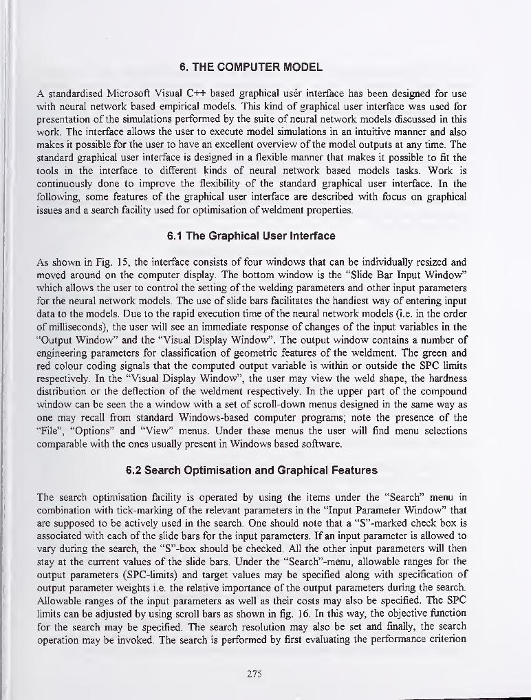
6. THE COMPUTER MODEL

A standardised Microsoft Visual C++ based graphical user interface has been designed for use

with neural network based empirical models. This kind of graphical user interface was used for

presentation of the simulations performed by the suite of neural network models discussed in this

work. The interface allows the user to execute model simulations in an intuitive manner and also

makes it possible for the user to have an excellent overview of the model outputs at any time. The

standard graphical user interface is designed in a flexible manner that makes it possible to fit the

tools in the interface to different kinds of neural network based models tasks. Work is

continuously done to improve the flexibility of the standard graphical user interface. In the

following, some features of the graphical user interface are described with focus on graphical

issues and a search facility used for optimisation ofweldment properties.

6.1 The Graphical User Interface

As shown in Fig. 15, the interface consists of four windows that can be individually resized and

moved around on the computer display. The bottom window is the "Slide Bar Input Window"which allows the user to control the setting of the welding parameters and other input parameters

for the neural network models. The use of slide bars facilitates the handiest way of entering input

data to the models. Due to the rapid execution time ofthe neural network models (i.e. in the order

of milliseconds), the user will see an immediate response of changes of the input variables in the

"Output Window" and the "Visual Display Window". The output window contains a number of

engineering parameters for classification of geometric features of the weldment. The green and

red colour coding signals that the computed output variable is within or outside the SPC limits

respectively. In the "Visual Display Window", the user may view the weld shape, the hardness

distribution or the deflection of the weldment respectively. In the upper part of the compound

window can be seen the a window v^th a set of scroll-down menus designed in the same way as

one may recall fi-om standard Windows-based computer programs; note the presence of the

"File", "Options" and "View" menus. Under these menus the user will find menu selections

comparable with the ones usually present in Windows based software.

6.2 Search Optimisation and Graphical Features

The search optimisation facility is operated by using the items under the "Search" menu in

combination with tick-marking of the relevant parameters in the "Input Parameter Window" that

are supposed to be actively used in the search. One should note that a "S"-marked check box is

associated with each of the slide bars for the input parameters. If an input parameter is allowed to

vary during the search, the "S"-box should be checked. All the other input parameters will then

stay at the current values of the slide bars. Under the "Search"-menu, allowable ranges for the

output parameters (SPC-limits) and target values may be specified along with specification of

output parameter weights i.e. the relative importance of the output parameters during the search.

Allowable ranges of the input parameters as well as their costs may also be specified. The SPC

limits can be adjusted by using scroll bars as shown in fig. 16. In this way, the objective fiinction

for the search may be specified. The search resolution may also be set and finally, the search

operation may be invoked. The search is performed by first evaluating the performance criterion

275

over the whole input parameter domain according to the selected resolution. Then a gradient-

based search is executed in the part of the input domain that so far has got the most optimal

solution. When the search is completed, the input parameters are set to the optimal values and the

optimal solution presented in the "Output-" and "Visual Display" windows.

The graphical features under the "DynaGraph (TM)" menu may then be used to display the result

of the search. Menu items for setting of SPC-limits and resolution are also available here. Also,

the type of surface to be displayed can be selected and it is possible to select the axes of the

graph. Then by invoking the "Generate Graph" item under the "DynaGrraph (TM)"-menu, the

response surface corresponding to the current input parameter setting will be presented. Note that

the "DynaGraph (TM)" menu may be used for graphical display of the outputs of the neural

networks at any stage during exercise with the software. An example of such a response surface is

displayed in Fig. 17.

7. APPLICATION OF THE MODEL

The search engine of the neural network model was applied for optimising the properties of the

welded T-joint. In order to carry out a search, the SPC-limits for each separate output parameter

must be defined. In the present work, the SPC-limits for the weld bead shape were set according

to an internal weld quality standard. The other SPC-limits were approximated fi-om typical

performance requirements for similar types of welded aluminium joints. Additionally, an output

weight number can be devoted to each separate output parameter in order to rate their relative

importance in the performance criterion.

7.1 Optimisation of Individual Properties

First, the model was used to optimise individual properties. This was done by assigning a high

value of the output weight number for the specific property to be optimised. Similar searches

were then successively performed for the individual properties listed below:

Case 1 : Optimisation of productivity (maximise weld travel speed).

Case 2: Optimisation of fatigue properties (maximise weld toe angles).

Case 3: Optimisation ofHAZ strength (maximise yield and tensile strength).

Case 4: Optimisation of distortions (minimise weld distortion).

The results fi^om these search operations are summarised in Table 1 . It is evident fi"om the table

that optimising just one property at a time is not a method that can be recommended since other

properties than the optimised one will be neglected in the search and, as a result, they will easily

fall outside the defined SPC-limits.

7.2 Overall Optimisation of Properties

In practice, welding of aluminium space fi^ame assemblies demands that the process be optimised

for a number of different properties. In the present case, this means that one has to seek the best

trade-offbetween the different output parameters in the neural network model. This can be

276

Table 1. Results from the neural network models search engine. Plus and minus signs indicate

that the specific property is within or outside the defined SPC-limits, respectively.

Property Case 1 Case 2 Case 3 Case 4 Case 5

Weld shape + +

Fatigue + +

HAZ strength + +

Distortion + +

Productivity ( m/min) 1.26 0.99 0.99 0.99 1.05

achieved by investigating the response surfaces of the output parameters to obtain a better

impression of the sensitivity between different input and output parameters. Also manipulation

with the output weight numbers for the different properties is an efficient way of "compromising"

between the different properties. By utihsing these techniques, Case 5 in Table 1 was obtained. As

can be seen, this specific combination of welding parameters results in properties that are all

within the SPC-limits. Moreover, a slight increase in productivity is also observed for this case

compared with case 2, 3, and 4.

Figs. 18, 19 and 20 show examples of visual outputs from the graphical user interface which

display the weld shape, the weld distortions, and the HAZ strength distribution. All figures are

from Case 5. As seen from Fig. 18, the actual choice of the interactive changeable control

parameters will produce a weld where all the critical geometrical shape parameters are within the

defined SPC-limits (i.e. green colours).

Figure 19 shows two different curves for the HAZ hardness distribution across the brace and

cord, respectively. These curves are qualitatively very similar to the schematic diagrams shown in

Fig. 3, which indicates that dissolution and reprecipitation of hardening particles are the governing

mechanisms determining the HAZ strength as explained in Section 2.2. The important strength

parameters from an engineering design point of view are the minimum values for yield and tensile

strength which are both within the specifications for the chosen set of control parameters.

Figure 20 shows the time variation of the vertical deflection of the chord during welding. Apositive value on the y-axis corresponds to thermal expansion of the material adjacent to the weld

during heating and a corresponding global deflection as shown schematically in Fig. 2(a).

Contrary, a negative value corresponds to the situation shown in Fig. 2(b) and is associated with

thermal contraction during cooling. The two peaks in the curve arises because the material is

given enough time to cool significantly in the 10 seconds time period after the first weld is finished

and before the second weld is started. As seen from Fig. 20, the selected set of process

parameters yields an end distortion of only 0.098 mm which correspond to 0.51 mm/meter length

of the profile.

277

8. FUTURE APPLICATIONS OF NEURAL NETWORK MODELS

Traditionally, neural network models are trained with basis in data sets provided from

experimental work performed in the laboratory. Neural networks, however, are also capable of

using data generated by other sources of information. A very interesting possibility is to use the

results from FE-calculations as the basic input data for training neural network models. Such FE-

calculations may take hours to complete, but when the data provided from such calculations are

used for training of neural networks one will obtain a model that is capable of providing the same

results within milliseconds of execution time. Such a combination of models utiHses the neural

network model's advantage of rapid calculations with the FE-modelling technique's capability to

test completely new geometric designs. Examples of neural network models based on FE-

calculations already exist in the literature [39], and others must be expected to arrive in the future.

Another application of neural networks is their use in control. The neural network is a non-linear

model, that can be operated in real-time on very fast digital signal processor (DSP) hardware.

The neural network is often generated as a feedforward model; that is, the inputs are the

controlled or measured parameters of the process operation, and the outputs are the outcome of

the process. Generally, model based controllers are developed by inverting a feedforward model

to produce a feedback model, which is then used to set the operating parameters of the process.

In many cases, it may not be possible to construct a feedback model because of the relationships

that exist in the process data. For example, if two different sets of input parameters can produce

identical outputs, it is easy to produce a feedforward model, but will be impossible to produce a

complete feedback model. Methods have been developed to operate a control system, using a

feedforward model, and these are being applied with neural network based control system for

welding [40].

9. CONCLUSIONS

In this work, the powerful non-linear prediction capability of neural networks is exploited in a

neural network based computer model for simultaneous prediction of shape, properties and

distortions of aluminium weldments. The model includes a search engine for optimisation of these

characteristics of the weldment. A set of exclusion rule assist during usage of the software both in

manual operation as well as automatic search to generate output only from combinations of input

parameters that are physically realistic. However, the quality of the model predictions relies

entirely on quality of the experimental data used as basis for training and testing the neural

networks. Accurate work during the data collection is therefore a prerequisite for a model of

acceptable prediction performance.

To assist in the data collection part of the work, an experimental design methodology specially

formulated for neural network model development was used to suggest the set of experiments to

be conducted. This technique of experimental planning is based on the theory of optimal designs

with an objective to minimise the number of experiments needed to derive the empirical neural

network based model. This is very attractive since in most cases, experimental work in the

industry is costly and time consuming.

278

It should also be noted that all the information generated during experimental work is used for

training the socalled P/NA^ neural networks; i.e. there is no need to divide the database into test-

and verification datasets in addition to the training set. In fact, this is an exclusive feature of the

neural network concept used in this work. In the concept, testing and verification of the neural

networks are done by the use of a novel statistical method that determines the upper error bound

in the model predictions. In this way, the analyst will be informed about possible sub-domains in

the input parameter space that causes predictions with an error outside the accepted error bound.

Then it is possible to collect more experimental data in this domain and continue training of the

neural network to improve the prediction performance in this (these) domain(s). Note that training

of the network can be continued with basis in the solution that so far has been determined. Thus,

there is no need to start retraining the network with the weights reinitialised to all random

numbers.

The use of the neural network has shovm that simultaneous optimisation of weldment properties

is possible but also that other properties may fall outside the SPC-Umits if optimisation is focussed

on only one weldment property. This kind of neural network based computer model puts new

perspectives into the use of computer based tools as basis for virtual design and manufacturing as

used in the industry. This is due both to the systematic approach used for derivation of the models

as well as the short runtimes and powerfial prediction capabilities of such models. Costs of model

development efforts are predictable and as the model becomes available it virtually allows the user

to weld on the computer. Finally, one should also be aware that the data used for training the

neural networks can be obtained fi'om traditional experimental works as well as be generated fi-om

the output of finite element based simulations. In this way, the rapid runtimes of empirically based

neural network models is exploited to generate predictions that could also be obtained fi-om first

principles finite elements models but then usually afl;er hours of execution time.

ACKNOWLEDGEMENTS

The authors are gratefijl to Hydro Raufoss Automotive Technical Centre AS for giving the

opportunity to publish the results presented in this work

279

APPENDIX AThe AA6XXX Aluminium Alloy Series

The welds studied in this work were made from hot extrusions of two age hardenable aluminium

alloys AA6063 and AA6082; each alloy in the peak aged temper condition (T6). These alloys

belong to the AA6XXX. Age hardening of such alloys is performed over a limited period of time

to avoid overaging; i.e. reduction of the strength of the material.

According to the phase diagram these alloys will in the single - phase region (at high temperature)

consist of the phase a which contains aluminium with a mixture ofMg and Si in solid solution.

The two phase region (at lower temperature) is a mixture of a and an intermetallic phase p. The

solubility ofMg and Si in the aluminium matrix decreases with temperature but the elements will

remain in solid solution if the alloy is rapidly quenched from the higher temperature down to room

temperature. If then, the alloy is heated to a certain temperature, artificial ageing of AA6XXXalloys will occur according to the following (ageing) sequence:

Supersaturated a -> GPl zones -> /3"(Mg^Si) needles -> P'iMg^Si) rods P equil.

This operation leads to precipitation hardening of the alloy. GPl represents the socalled Guinier-

Preston zones which most possible are spheres ofMg and Si. P" represent an intermediate very

fine needle shaped precipitate structure along the <100> directions in the aluminium matrix.

P" precipitates are the main strengthening contributing particles in the AA6XXX-alloys. The next

intermediate P' precipitates are more coarse, partly coherent rods which do not contribute to

strengthening of the material since their number density is too low. The maximum strength is

achieved for a certain number density and size of P". If the alloy is held (aged) for very long times

at a given temperature, strength will be lost due to formation of completely incoherent equilibrium

precipitates P (i.e. the interparticle spacing is increased). This effect is known as overageing. The

presence of the very fine, needle shaped P" precipitates contributes to high yield strength values

in the artificially aged T6 condition. The AA6XXX alloys are weldable, but as discussed in section

2.2, they suffer from severe softening in the heat affected zone because of dissolution of the P"precipitates during the weld thermal cycle. Total recovery of the strength of the HAZ is not

possible (without performing a completely new solution heat treatment) due to formation of non-

strengthening P' particles during the cooling leg of the thermal cycle. However, strength recovery

after welding may be enhanced by artifical ageing.

280

APPENDIX BEXPERIMENTAL DESIGN

A typical exercise in experimental design has to go through the following phases:

Define the problem

Specify the type of model to be used

Select type of Experimental Design

Run the experiments

Analyse/ use the data (to determine the unknown model parameters)

Interpret the results

In this appendix, items one to four on the Ust are discussed in sequence. Then, some features of

Taguchi and D-optimal designs are discussed.

B.1 Define the problem

It is of great importance to have knowledge about the behaviour of the process and also to decide

which features of the process that one wants to study. Typical ingredients in this step are as

follows:

1 . Identify input variables (input parameters, factors)

2. Classify the nature of the input variables:

• Qualitative parameters, i.e. parameters that only can take discrete values .

• Quantitative parameters, i.e. parameters that varies continuously .

3 . Which factors (input variables) can be controlled in an experiment?

4. Decide the level of each factor (i.e. select values for the qualitative parameters and

discretise the qualitative parameters).

5. Identify process output parameters (output parameters are called response variables).

In a process with a lot of input parameters, it may be a challenge to extract the important ones.

This can be done by screening - experiments to obtain information of the process. Also, these

screening experiments can help as an aid to determine the operation range for each factor. The

screening experiments performed in the T-joint project served both these purposes: Due to the

result of the screening experiments, it was decided to introduce the vohage as an input variable.

Screening experiments were also needed to set the right values for the range of the parameters

(i.e. the minimum and maximum values of the input parameters). Even more, the range of a

typical quantitative parameter (i.e. vohage, wire feed rate etc.) was dependent on the value of

typical qualitative parameters like material thickness.

It should be noted that there is a trade-off between the number of factors to be included in the

model and the number of experiments.

281

B.2 Select the Model

The number of levels for each factor (i.e. the number of values that are considered for each

parameter) must be determined according to the type of model we want to use and the nature of

the process that is studied. To determine second order effects, one at least needs three levels for

each factor. In the N-Optimal design, a minimum of at least four levels is recommended for each

quantitative (continuous) factor.

The type of model depends on the characteristics of the process. If second order effects are

present in the process, a second order (quadratic) model must be used. In some cases, even higher

order models are needed; i.e. cubic models or higher. It should be noted that the size of the

experimental design matrix depends on the complexity of the chosen model.

In general, the simplest possible model should be selected. Quite frequently linear models with

possible interaction terms are used. Nonlinear models may also be applied but often a nonlinear

transformation is used so that linear regression still can be used to obtain the unknown

coefficients in the model.

B.3 Select Experimental Design Methodology

The experimental design methodology is an aid for determining the actual set of experiments to be

performed. The following has impact on the selection of the experimental design technique:

• The experimental objective

• The number of factors

• The type of factors

• The terms in the model

Quite frequently, the levels of a factor are scaled for ease of use in designing the experiments. The

scaling is a linear transformation and is also called a standardisation. Two level factors are often

coded by (-1) for the low level and (+1) for the high level respectively. For three level factors,

codes -1,0 and +1 (or 0, 1 an 2) are used.

A special feature of some experimental designs is that they are orthogonal, i.e. the correlation

between the factors is zero. Orthogonality lets the desired effects be measured independently of

each other. This means that the influence of each factor can be tested without the influence fi"om

other factors.

The number of possible experimental designs that may be chosen in a certain case may depend on

whether the factors are qualitative or quantitative.

Experimental designs can be described by the ability to identify the effects considered in the model

(i.e. distinguish between the different terms in the model). Confounding happens when two effects

cannot be distinguished from one another. In a design of resolution R, no p-factor effect is

confounded with any other effect containing less than (R-p) factors. A design of resolution R=in

282

does not confound main effects (i.e. terms depending linearly on one factor) with one another but

does confound main effects with two factor interactions. A design of resolution R=rV does not

confound main effects and two-factor interactions but does confound two-factor interactions with

other two factor interactions. Characteristics for higher order resolutions may also be specified.

B.4 Run the Experiments

The result of the experimental design is a matrix of experiments. The execution of the

experimental matrix should be randomized to minimize the chance of obtaining experimental

results that are biased by possible factors that are not considered in the experiment. Often, the

experimental design software package will give a list ofrandomized runs for the experiment.

B.5 Taguchi Designs

Taguchi designs [39] belong to the classical designs. These designs, originally developed by

Genichi Taguchi, were primarily designed for identification of significant process factors i.e. main

effects. The designs rely heavily on orthogonality. Thus the designs are simple and allow for

reproducibility and cost effective conduction of experimental work. Unfortunately, these designs

do not allow for identification of all interaction terms due to confounded effects since the designs

generally have resolution R = HI. The Taguchi analysis generally can be used to determine the

settings for the process that results in the best outcome. The prediction equations generally

associated with Taguchi designs basically gives an overall predicted value by using differences

fi^om the mean value.

Research performed at NATech, has shown that Taguchi type of designs are the second best

alternatives for performing experimental designs to be used in association with neural network

modelling. This is probably due to the fact that the designs are well suited for determining the

main effects in the process. Also the cost efficiency and reproducibility of the method are

important factors which makes the Taguchi design suited for designing experiments to be used

with neural networks.

B.6 Optimal Experimental Designs

Classical experimental designs are often the most elegant and powerfiil tools for solving practical

engineering problems. They are based on a standard geometrical formulation or they constitute a

subset of all possible designs (i.e. fractional factorial design). Unfortunately, restrictions on

sample size (i.e. sample size; number of experiments, should be as low as possible), constraints on

the region of operability for the factors and other special features of the design situation may

prevent the use of the classical designs. In such cases, the use of an optimal design technique is

the only ahemative. According to a certain criterion, these designs maximise the amount of

information in an experiment. It should be noted that the optimality of an optimal design is closely

linked to the criterion used for the design. If the criterion is changed, redesign according to the

new criterion has to be done to achieve optimality.

283

B.6.1 D Optimal Design

D-optimal design is based on a design criterion that maximises the amount of information in the

design. The criterion is expressed as finding the maximum value of the determinant of the matrix

where X is the design matrix. A definition of the design matrix X is given below. How does

the determinant of )^X, measure the information in a design? The mathematical objective of D-

optimal design is to determine good values of the unknown model parameters (contained in the

vector 0; described in the next subsection). The noise in the process introduces uncertainty in the

estimated values of the parameters. One way to express this uncertainty is by a region in the space

of the parameters, which is likely to contain the true but still unknown parameters ^. The idea in

D-optimal design is to minimise the volume of this region.

D-optimal designs can handle mixed level experiments; i.e. the factors do not need to run with the

same number of levels. D-optimal designs are also attractive in that they often need fewer runs

compared to standard classical designs. The reduced number of runs is a very important feature in

industrial settings where the runs may be very expensive.

Two effects of using the determinant as the criterion for D-optimal design should be stated.

Firstly, in design situations were all the factors are quantitative (i.e. varies continuously), the D-

optimal design places the experimental runs on the edges and vertices of the factors' region of

operability.

Once there are enough runs to completely determine the unknown parameters in the model, the

algorithm for D-optimal design tends to replicate runs that are already included in the design

rather than adding completely new experiments. Then, there is generally very few runs that can be

used to assess the possible lack of fit of the apriori model and the experimenter relies heavily on

the correctness of the model. In the standard D-optimal design, the data are mostly taken fi-om the

boundaries of the factors' operation range. Obviously then, interpolation inside the operation

ranges of the factors may give predictions which do not compare well to reality if the model is

invalid.

B.6.2 Mathematical Theory for Optimal Designs

St. John [26] gives a very brief introduction to the field of optimal design by the use of a

mathematical formalism for stating the optimal criterion used for G- and D- optimal design. In the

simplest case, a linear regression model of the following type is considered [26]:

>',=/'fe)^ + ^, (1)

where i= 1, n. n is the number of experiments (observations), yi is the responses

(observations). /fx^ (p x 1) is a vector that depends on the form of the selected response flinction.

X, (q x 1) a vector of predictor variables. 8i is a noise term; the process noise is assumed to be

noncorrelated (i.e. the variance is a^) and have zero mean value. ^ (p x 1) is a vector of unknownmodel parameters. The model can be expressed in matrix notation as follows

284

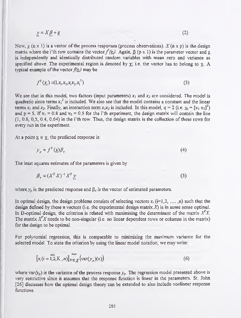
y-xp_+s (2)

Now, (n X 1) is a vector of the process responses (process observations). X (n x p) is the design

matrix where the i'th row contains the vectorf(Xj). Again, 0 (p x 1) is the parameter vector and s

is independently and identically distributed random variables with mean zero and variance as

specified above. The experimental region is denoted by x; i e. the vector has to belong to X- Atypical example of the vectorf(Xi) may be

/^te)=(1.^.^2.^^2.^') (3)

We see that in this model, two factors (input parameters) Xi and X2 are considered. The model is

quadratic smce terms is included. We also see that the model contains a constant and the linear

terms x; and X2. Finally, an interaction term XiX2 is included. In this model, q = 2 (i.e. 2fi = [xi X2]'^)

and p = 5. If xi = 0.8 and X2 = 0.5 for the i'th experiment, the design matrix will contain the line

(1, 0.8, 0,5, 0.4, 0.64) in the i'th row. Thus, the design matrix is the collection of these rows for

every run in the experiment.

At a point x g x, the predicted response is:

y,-fi^)Pe (4)

The least squares estimates of the parameters is given by

P^^iX'XyX'y (5)

where yp is the predicted response and Pe is the vector of estimated parameters.

In optimal design, the design problems consists of selecting vectors x, (i=l,2, .... ,n) such that the

design defined by these n vectors (i.e. the experimental design matrix^ is in some sense optimal.

In D-optimal design, the criterion is related with maximising the determinant of the matrix )^X.

The matrix needs to be non-singular (i.e. no linear dependent rows or columns in the matrix)

for the design to be optimal.

For polynomial regression, this is comparable to minimising the maximum variance for the

selected model. To state the criterion by using the linear model notation, we may write:

_ min / \

[x,(/ = 1,2,K ,«)]xE;^(varCy^)(x)) (6)

where y^r(y^ is the variance of the process response yp. The regression model presented above is

very restrictive since it assumes that the response function is linear in the parameters. St. John

[26] discusses how the optimal design theory can be extended to also include nonlinear response

functions.

285

REFERENCES

1. D. R. WHITE and J. E. JONES: 'The use of Neural Networks for Automotive Body Applications',

IBEC '96: International Body Engineering Conference & Exposition, 1996.

2. L. J. YANG, M. J. BIBBY and R. S. CHANDEL: 'Modelling the submerged -arc welding process

using linear regression equations' in S. A. David and J, M. Vitek ed.. International Trends in

Welding Science and Technology: Proceedings ofthe 3rd International Conference on Trends in

Welding Research, ASM International, Gatlinburg, Tennessee, USA, June 1-5, 1992, pp. 411-415.

3. IS. KIM and A. BASU: 'A study of influence ofwelding process variables on GMAW,Transactions ofMechanical Engineering, Australia, 1995, 20(1), 35-41.

4. J. JONES: 'Weld Parameter Modelling', in S. A. David and J, M. Vitek ed, International Trends in

Welding Science and Technology: Proceedings ofthe 3rd International Conference on Trends in

Welding Research, ASM International, Gatlinburg, Termessee, USA, Jime 1-5, 1992, pp. 895-899.

5. X. XU, et. al.: 'The use ofNeural Network Technology in Welding and Materials Applications', in

T. Zacharia ed, Modelling and Control ofJoining Processes, American Welding Society, Orlando,

Florida, December 8-10, 1993, 203-214.

6 KLEIN, C. F., "Case Study of a Neural Network Model of a Automobile Seat Structural Weld",T.

A. Siewert ed., 'Computerization ofWelding Information IV. Proceedings, International

Conference', November 3-6, 1993, Orlando, Florida, USA

7. J. SZEKELY: Keynote address: 'The mathematical modeling of arc welding operation', in S. A.

David and J, M. Vitek ed., Advances in Welding Science and Technology: Proceedings ofthe 3rd

International Conference on Trends in Welding Research, ASM International, Gatlinburg,

Tennessee, USA, 18-22 May, 1986, pp. 3-14.

8. Y. H. WANG and S. KOU: 'Driving forces for convection in weld pools', in S. A. David and J, M.

Vitek ed.. Advances in Welding Science and Technology: Proceedings ofthe 3rd International

Conference on Trends in Welding Research, ASM International, Gatlinburg, Tennessee, USA, 18-

22 May, 1986, pp. 65-70.

9. T. ZACHARIA, A. H. ERASLAN, D. K. AIDUN and S. A. DAVID: 'Three dimensional model for

arc welding process'. Metallurgical Transactions, 1989, 20B, 645-659.

10. A. MATSUNAWA and S. YOKOYA: 'Fluid flow and its effect of penetration shape in stationary

arc welds', in S. A. David and J, M. Vitek ed, Recent Trends in Welding Science and Technology:

Proceedings ofthe 2nd International Conference on Trends in Welding Research, ASMInternational, Gatlinburg, Tennessee, USA, 14-18 May, 1989, pp. 31-35.

1 1 . MATSUNAWA, A., Keynote Address: 'Modeling of heat and fluid flow in arc welding', in S. A.

David and J, M. Vitek ed.. International Trends in Welding Science and Technology: Proceedings

ofthe 3rd International Conference on Trends in Welding Research, ASM International,

Gatlinburg, Tennessee, USA June 1-5, 1992, pp. 3-16.

286

12. J. GOLDAK: Keynote address: 'Modeling Thermal Stresses and Distortions in Welds', in S. A.

David and J, M. Vitek ed, Recent Trends in Welding Science and Technology: Proceedings ofthe

2nd International Conference on Trends in Welding Research, ASM International, Gatlinburg,

Tennessee, USA, May 14-18, 1989, 71-82.

13 . A. KELLY and R. B. NICHOLSON: 'Precipitation Hardening',Progress in Materials Science,

Vol. 10, Pergamon Press, London, 1963.

14. 0. R. MYHR, 0. GRONG: 'Process Modelling Applied to 6082-T6 Aluminium Weldments-I.

Reaction Kinetics', ActaMetall. Mater., 1991, 39 (11), 1991, 2693-2702.

15. 0. R. MYHR, 0. GRONG: 'Process Modelling Applied to 6082-T6 Aluminium Weldments-H.

Applications ofthe Model, ActaMetall. Mater., 1991, 39 (11), 1991, 2703-2708.

16. 0. T. MIDLING: M.Sc. Thesis, The Norwegian Institute of Technology, Trondheim, 1988.

17. 0. GRONG: 'Metallurgical Modelling of Welding', 2nd Ed.' The Institute of Materials, The

University Press, Cambridge, 1997.

18. O. R. MYHR, 0. GRONG, S. KLOKKEHAUG, H. G. FJ^R and A. O. BCLUKEN: 'Process

Model for Welding of Al-Mg-Si Extrusions. Part I: Precipitate Stability', Science and Technology of

Welding and Joining, 1997, 2 (6), 245-254.

19. 0. R. MYHR, S. KLOKKEHAUG, 0. GRONG, H. G. FJ^R and A. 0. KLUKEN: 'Modelling of

Microstructure Evolution, Residual Stresses and Deformations in 6082-T6 Aluminium Weldments',

Welding Journal, 11 (7), July 1998, 286-292

20. 0. R. MYHR, S. KLOKKEHAUG, H. G. FJvER, 0. GRONG and A. 0. KLUKEN: 'Modelling of

Microstructure Evolution and Residual Stresses in Processing and Welding of 6082 and 7108

Aluminium Alloys', The 5th International Conference on Trends in Welding Research, Georgia,

USA, 1-5 June 1998.

21. G O. RADING and J. T. BERRY. 'A Model for Heat-Affected Zone Hardness Profiles in Al-Li-X

Alloys', Welding Journal, 11 (9), September 1998, 383-387.

22. E. SARRAZIN: Ph. D. Thesis, Ecole Polytechnique, Palaiseau, France, 1995.

23. D. RADAJ, H. HAEUSER and S. BRAUN: Nimierische Simulation von Eigenspannungen und

Verzug bei Schweissverbindungen aus AlMgSi-Legierungen, Konstruktion, 1998, 50, 30-38.

24. A. C. ATKINSON and A. N. DONEV: 'Optimum Experimental Design; Clarendon Press, Oxford,

1992.

25. S R. SCHMIDT and R. G. LAUNSBY: 'Understanding Industrial Designed Experiments' 4th

Edition, Air Academy Press, Colorado Springs, 1997.

26. R. C. ST. JOHN and N. R. DRAPER: 'D-optimality for Regression Designs: A Review',

Technometrics, 17 (1), 1975.

287

27. X. N. K. BOSE and P. LIANG: Neural Network Fundamentals with Graphs, Algorithms, and

Applications, McGraw-Hill International Editions, Elecrtical Engineering Series, 1996.

28. R. IRVING: 'Successful Welding Operations: Aren't They Top Management ResponsibiUty',

Welding Journal, May 1994, 33-35.

29. W. W. McCULLOCH and W. PITTS: 'A Logical Calculus of the Ideas Imminent in Nervous

Activity', Bulletin ofMathematics Biophysics, 5, 1943, 115-133.

30. B. WIDROW and M. E. Hoff: 'Adaptive Switching Circuits', 1960 IRE WESCON Convention

Record, part 4, New York Institute of Radio Engineeris, pp. 96-104, 1960.

31. K. ASAKAWA and H. TAGAKI: 'Neural networks in Japan', Communications ofthe ACM, 1994,

37 (2), 106-112.

32. H. DEMUTH and M. BEALE: 'Neural Network Toolbox for use with MATLAB', Version 3,

User's Guide, January 1998.

33. DARPA Neural Network Study, Lexington, MA: M.I.T. Lincohi Laboratory, 1988.

34. D. R. HUSH and B. G. HORNE: 'Progress in Supervised Neural Networks, IEEE Signal Processing

Magazine, 8-36, January 1993.

35. T. COOL, H. K. D. H. BHADESHIA and D. J. C. MACKAY: 'Modelling the Mechanical

Properties in the HAZ ofPower Plant Steels I: Bayesian Neural Network Analysis ofProof

Strength', in H. Cerjak ed., 'Mathematical Modelling ofWeld Phenomena 3, Materials Modelling

Series, The Institute of Materials , The University Press, Cambridge, UK, 1997, pp. 403-442.

36. D. C. J. MACKAY: 'A Practical Bayesian Framework for Backprop Networks', J. E. Moody, S. J.

Hanson and R. P. Lippman ed, Advances in Neural Information Processing Systems, 4, 839-846,

1997.

37. JONES, J, "A Radar Signal Processing Application of Neural Networks", Report, Colorado School

of Mines No. TI8604, submitted to Texas Instruments, May 1986.

38. JONES, J., "A Neural Network Model of the Friction Soldering Process", Report, N. A.

Technologies Co. #94231, submitted to Ford Motor Company, February, 1996.

39. R. K. ROY: 'A Primer on the Taguchi Method', Society of Manufacturing Engineers, 1990.

40. D. WHITE, J. A. CHARMEIN, J. E. JONES, K. LIU: 'Integrated Control of Welding with Neural

Network based Process Control Methods', T. A. Siewert ed., 'Computerization of Welding

Information FV. Proceedings, International Conference', November 3-6, 1993, Orlando, Florida,

USA, 310-324.

41. W. W. McCULLOCH and W. PITTS: 'A Logical Calculus of the Ideas Imminent in Nervous

Activity', Bulletin of Mathematics Biophysics, 5, 1943, 115-133.

288

42. F. ROSENBLATT: Principles ofNeurodynamics, Spartan Books, New York, 1962.

43. D. E. RUMELHART, D. E. HINTON and R. J. WILLIAMS: 'Learning Internal Representation by

Error Propagation', in Parallel Distributed Processing, Vol. 1, MIT Press, Cambridge, MA., pp.

318-362, 1986.

44. D. B. PARKER: 'Learning Logic', Invention Report S81-64, File 1, Office of Technology

Licensing, Stanford University, Stanford, CA, 1982.

289

Peak temperature

500°C ~ 220°C

COVi0c"S(0

X

Fully

reverted

region

HAZhardness

immediately

after welding

- Peak temperature

500°C ~ 220X

Natural

ageing

\

^ Resulting

HAZhardness

Distance from fusion line Distance from fusion line

(a) (b)

Figure 1. Schematic diagrams showing the HAZ hardness distribution immediately after welding

of peak aged (T6) Al-Mg-Si alloys; (a). Hardness distribution following prolonged room

temperature aging; (b). (FromRef /6/).

Figure 2. Schematic diagram of deformations in welding of a T-joint. (a) During welding, and (b)

after welding is completed.

290

291

weighted mput Sfgnai

Ex««yt^ tmrssfsr function fCp*w -^h^

Send result to OMl?l?<»Mr nodes

Pw 1

The Axon

Resting

Triggerirtg

* NsoTGiraitsniitfefs dls<ang&potmHal to -5&mVF ii ing

* SofSwn/potassmm Stsw reversal (-^50

* OecJffca^ pQtfittSM praim^M&s down Men

Figure 5: The operation characteristics of a neuron.

292

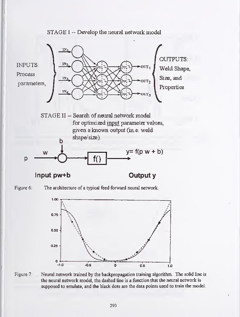
STAGE I ~ Develop the neureil network model

INPUTS:

Process

pai'ametei's.

I OOLT,

OUT

OUTPUTS:

I Weld Shape,

I Size, aiid

I Pi-operties

STAGE II — Search of neiiral network model

for optimized input paiiainetei' values,

given a known output (in,e. weld

w

ushape/'size).

f()

y= f(p w + b)

Input pw+b Output y

Figure 6: The architecture of a typical feed forward neural network.

t.oo

0.75 -

0.50

0.25 -

Figure 7: Neural network trained by the backpropagation training algorithm. The solid line is

the neural network model, the dashed line is a function that the neural network is

supposed to emulate, and the black dots are the data points used to train the model.

293

Figure 8. Diagram showing the performance of a backpropagation neural network trained to

4 % error. The overtraining effect is present. This is expressed by good fit in the

datapoints but the overall performance of the network is bad.

1.00

0.S0

0^5

ij

11

ij

\ • Training points

\ PNA output

\ Otsved Output

Figure 9: P/NA^ neural network. The underlying function and training data are the same as

for the neural networks shown in figures 7 and 8. The neural network model was

trained using the N. A. Technologies P/NA^ algorithm to a mean error of

approximately 1%.

294

Prediction

Error

# iterations

Stop

Training

Figure 10. Neural network prediction error for training and test data sets as a function of thenumber of training cycles. Training eventually leads to a low prediction error forthe training data set. At the same time, the prediction error increases for the test setand the generalisation capability of the neural network starts to decrease.

CONFIDENCE INTERVAL: [0, 0.04]

CONFIDENCE LEVEL: 1.2%MODEL vs. ACTUALFUNCTION STD. DEVIAT.: 0.1 1 52

Figure 11: A neural network developed specifically to have a very poor representation of theunderlying function used to generate the training samples.

295

x-axli

CONFIDENCE INTERVAL: [0, 0.04]

CONFIDENCE LEVEL: 98.6%MODEL vs. ACTUALFUNCTION STD. DEVIAT.: 0.0231

Figure 12: A neural network for which the confidence level is approximately 2a. The

confidence level is approximately 99.5% as determined expected for that size of the

confidence interval.

1.0 J

0.8 •

0.6 -

w

0.4

0.2

0 -1 . 1 • .

0 0.2 0.4 0.6 o.a 1.0

x-axIs

CONFIDENCE INTERVAL: [0, 0.04]

CONFIDENCE LEVEL: 99.999%MODEL vs. ACTUALFUNCTION STD. DEVIAT.: 0.0135

Figure 13: A neural network trained with the P/NA^ neural network exhibits high accuracy and

a corresponding high level of confidence predicted by the S-parameter test

296

:>^9'-i-^NAH __________ P'll'SES.'i

Figure 14: The NAMeS GUI for measurement ofweld shapes.

297

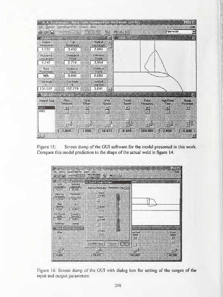
N . A. T echnologies - Norsk Hydro Aluminum Fillel Weld Model (3.0 fi2);

;

i.-'-. J Fillet Weld

HutCTjii-it

not wvinl< 7A/

|__

fnr, f.n/

s| 3.^33

Th«K*

I0 000

ToeAnde

S—IjS7.779

I3.954

s| 0.000

3.841

6082

Figure 1 5 : Screen dump of the GUI software for the model presented in this work.

Compare this model prediction to the shape ofthe actual weld in figure 14.

Figure 16: Screen dump of the GUI with dialog box for setting of the ranges of the

input and output parameters.

298

Dyna Gidph(TMJ

Figure 17: Screen dump of a typical response surface window. The red colour

represents values of the response variable (effective throat) not within

the specified SPC-limits.

Figure 18. Screen dump of the graphical user interface that visualises the weld

bead shape and selected output values.

299

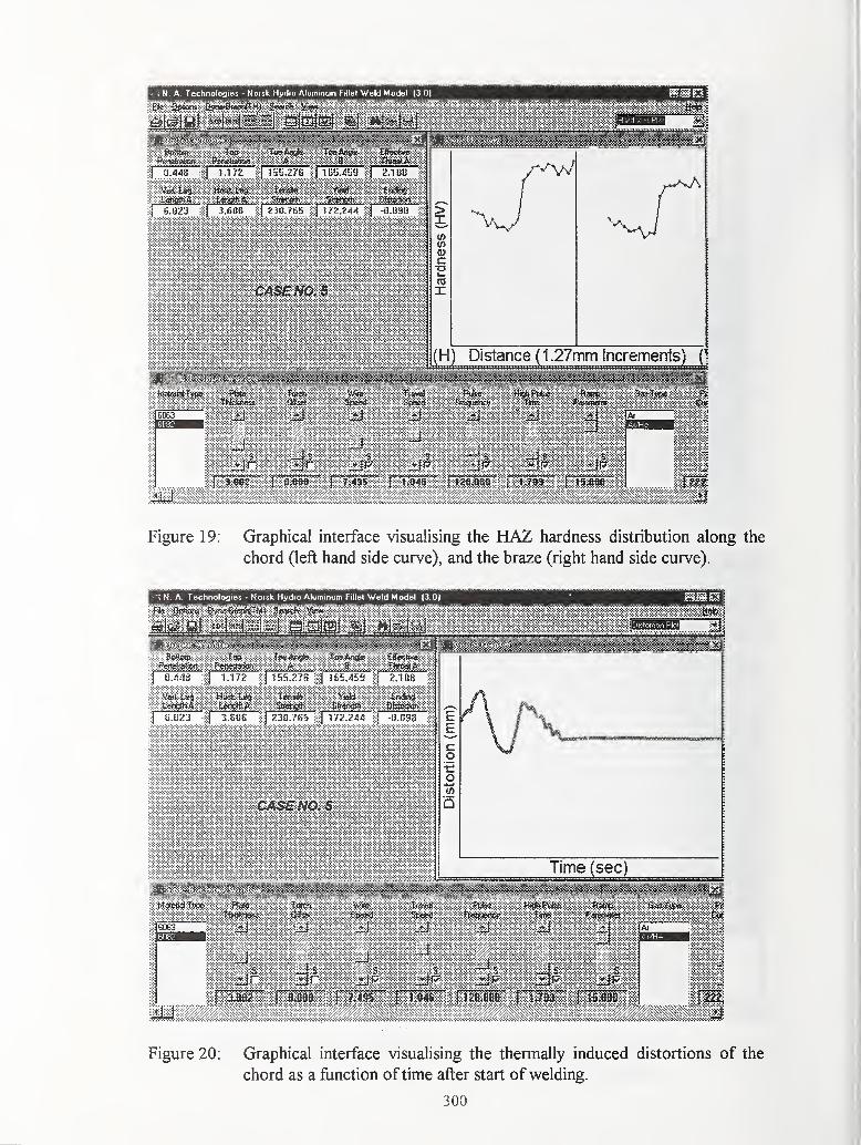
; N. A. Technologies - Norsk Hydio Aluminum Fillel Weld Model (3 D)

Figure 19: Graphical interface visualising the HAZ hardness distribution along the

chord (left hand side curve), and the braze (right hand side curve).

N. A. Technologies - Norsk Hydro Aluminum Fillet Weld Model (3.0)

3i

Tof-Anglv Ts»At)s^ SSiiicbvsSaSatn Top-

Cltfi j 1 i7? jli^R ?7R J 165.'1b9

j? 108

t-"-^-^,

i^f^^.e^**^

ti.Ei2J 3.606 55 230.765 ^ m.HA i{ -0.093

6063

^3r

Time (sec)

Hi.

Figure 20; Graphical interface visuaHsing the thermally induced distortions of the

chord as a function of time after start ofwelding.

300

SPATTER MONITORING FORSHORT CIRCUIT METAL TRANSFER IN GMAW

S. K. Kang* and S.-J. Na*

ABSTRACT

Quantitative analysis regarding the effect of waveform parameters of arc welding current on

spatter generation was conducted using a microcomputer-based experimental data analyzing

system. Statistical data derived from welding experiments showed that qualitative

relationships can be obtained between spatter generation and some parameters of welding

current. By using the multiple regression analysis method, two indices predicting the spatter

and big spatter generation during a fixed welding time were developed. Neural networks

were also used to estimate the spatter and big spatter generation. It was revealed that the

indices and the neural networks could predict the spatter and big spatter generation to a

certain extent in comparison with experimental data of spatter generation.

INTRODUCTION

In recent years the development of semi-automation, automation and robotization techniques

for welding has been remarkable. GMAW with active shielding gas such as CO2 and Ar-

CO2 using these developments now has a major role in arc welding practice as an alternative

to manual metal arc welding, although it still has some problems such as spatter and fume

generation. The occurrence of spatter in GMA welding has a number of detrimental effects

such as: 1) obstruction of the shielding gas due to its adhesion at nozzle inside, 2) increase in

number of operations because of the need to remove spatter, and 3) danger of bums and fires.

Consequently various preventive measures are considered in terms of many factors such as

welding conditions, filler wire materials and welding power sources.

Spatter reduction in pulsed COj-shielded arc welding has been studied with special reference

to waveform control of the power source and chemical composition of the welding wire (Ref

1). Inverter-controlled power source with high-speed control capability was used in one

study to control the welding current and voltage for spatter reduction in CO2 arc welding (Ref

2-3). Using a newly developed inverter controlled pulsed MAG welding machine, a newcurrent waveform control system was developed to reduce spatter (Ref. 4). Other studies

were conducted on spatter reduction in MAG welding from the viewpoint of welding

materials such as filler wire and shielding gas (Ref 5-6).

A great amount of work has been done to investigate the phenomena and mechanisms of

spatter generation in short circuit metal transfer mode (Ref 7). The mechanisms of spatter

generation obtained can be summarized as follows: 1) Electric explosion - Under the action of

magnetic force produced by high short circuit current, the metal bridge shrinks in cross

section and the density of short circuit current increases further. The metal bridge is

*Dept. of Mech. Eng., KAIST, Yusong-gu, Taejon, Korea

301

overheated and evaporated, resulting in metal explosion. 2) Gas explosion - Surplus oxygen

and carbon in the melted metal react intensively with each other in high temperature arc,

which results in violent evolution or explosion of CO gas. 3) Gas impact - Atmospheric gas

heats and expands due to abrupt arc initiation after short-circuiting. The melted metal in the

weld pool and remaining drop are blown off through this gas impact. 4) Instantaneous short-

circuiting - Instantaneous short-circuiting refers to short-circuiting of a very short duration

without metal transfer. As the thin metal bridge breaks, a small quantity of spatter may be

produced.

In this paper, the parameters affecting spatter generation were selected based on previous

papers and tested by preparatory welding experiments. Spatter indices and neural networks

were developed to estimate the spatter and big spatter generation during a fixed welding time.

EXPERIMENTAL PROCEDURE

Experimental Equipment

Figure 1 shows the experimental apparatus composed of three parts. The first part consists

of several welding machines having different characteristics. The second one is a welding

table to move the welding torch in three directions. The third is a microcomputer to acquire

and analyze the welding current and arc voltage signal through a PC-Lab card with 330 kHzsampling frequency. Programs were developed to analyze the waveform of welding current

and arc voltage.

Welding Experiments

Bead-on-plate welding was carried out on the workpiece of 12 mm thickness using inverter

controlled power sources. Solid wire of 1 .2 mm diameter was used with a stick-out length of

1 5mm. The shielding gas was Ar 80% and CO2 20% with a flow rate of 20 liter/min, and the

welding speed 360 mm/min. The range of welding current was between 150 A and 250 A,

and that of arc voltage between 20 V and 32 V, which covers the range of short circuit metal

transfer mode. Welding experiment was conducted by varying the welding voltage, while

the welding current was fixed. Figure 2 shows the typical relationship between arc voltage

and spatter and big spatter generation, which reveals that spatter and big spatter generation

increases with increasing arc voltage. The sampling frequency for waveform data was 10

kHz, and data were measured during 0.8 sec. intervals.

Parameter Selection

There are several parameters to be considered for estimating the spatter generation At short

circuit breakage, metal vapor explodes and spatter occurs. If peak current is high, the

amount of metal vapor will be large and heavy spatter will be caused by explosion. If the

short-circuiting time is long, the peak current will become large, resulting in increase of

spatter generation. When short-circuiting bridge is formed, the complete contact is not made

immediately after contact due to surface disturbances such as oxidants. Welding current

passes through small points of real contact, which will cause overheating. It was shown that

302

the welding current at short circuit start and its increasing rate after short-circuiting are related

to spatter generation (Ref. 6).

While the welding arc exists, the electrode melts and droplet is formed at the end of electrode.

If the arcing time is long, a lot of electrode will melt and the electrode droplet will becomelarge. The large droplet can be the source of instability and result in spatter generation.

Based on the above explanation, five parameters were selected to analyze the spatter

generation. They are peak current (Ip), arcing time (TJ, short-circuiting time (T^), current

slope at short circuit start (SJ and current at short circuit start (Q, as shown in Figure 3.

RESULTS AND DISCUSSION

Relationship between Waveform Parameters and Spatter Generation

Figure 4 shows the common relationship between Ip and spatter generation. Spatter

generation increases with increasing Ip, which coincides with the previous research (7).

Figure 5 shows that spatter generation increases with increasing T^. The main mechanism of

spatter generation is believed to be the explosion of metal vapor. Because metal vapor

explosion is less influenced by Tg than by Ip, the correlation coefficient between T^ and spatter

generation is lower than that between Ip and spatter generation, Table 1. Figure 6 reveals

that spatter generation increases with increasing I3, while it shows the highest correlation

coefficient with spatter generation.

Figure 7 shows that spatter generation increases with increasing 85. This is probably due to

the fact that the longer the period of controlling I^ to a low value, the more regular and

uniform the short circuit state becomes. Figure 8 shows the relationship between Tj and

spatter generation, which reveals no particular correlation. While short circuit is formed,

many factors - the inductance of welding machine, T^ and the diameter of short-circuiting

bridge - influence the welding current rise. It seems to be difficult to analyze the influence

of Tj on spatter generation in general.

A big spatter was defined as a spatter whose diameter is larger than the electrode diameter

(1.2 mm). Big spatters adhere strongly to the nozzle and base metal while small spatters are

easily removed with a blow or touch. Figure 4 shows the relationship between Ip and big

spatter generation. Big spatter generation is more dependent on the size of droplet than the

explosion of metal vapor. Therefore the correlation coefficient between Ip and big spatter

generation is lower than that between T^ and spatter generation.

Figure 5 reveals that big spatter generation increases with increasing T^. It is generally

considered that the size of shattered particles is dependent on that of droplets. A big droplet

generates shattered particles larger than those of a small droplet. Therefore it is considered

that a large amount of big spatter is generated from a large diameter of short-circuiting bridge.

The main parameter resulting in a large diameter of short-circuiting bridge is large T^, and

consequently the correlation coefficient of Tg with big spatter is the highest among the

parameters considered, Table 2. Figure 6 and 7 show the relationship between big spatter

303

and Is and respectively. It was also revealed that the effect of \ and S3 on big spatter

generation is less than that on spatter generation. Figure 8 shows that there is no particular

correlation between and big spatter generation, like that between and spatter generation.

Index and Neural Network

By analysis of the relationships between parameters and spatter generation, it was found that

the parameters tested are influencing the spatter and big spatter generation in various ways.

For spatter generation Ip and I^ are the dominant parameters, and and are the secondary

ones, while for big spatter generation is the dominant parameter, and Ip and I^ are the

secondary ones. In order to estimate spatter and big spatter generation, it is necessary to

analyze and synthesize the contribution of each parameter. In this purpose, the indices and

neural networks were developed for spatter and big spatter generation. The index expresses

the direct relationship between parameters and spatter generation, while the neural network

possesses the robustness and ability to extract an underlying pattern from noisy or erratic data.

The ability of neural networks to train on representative test data enables the complex and

nonlinear relationships to be interpreted, without time consuming construction of a complete

model of the process.

Spatter

Multiple regression analysis was performed to develop an index of Ip, T^, S^ and I^ to estimate

the spatter generation during a fixed time. The developed spatter index is as follows.

5 = 7.9446-10"'^ •/ +3.46523-10"^ -r +0.0045-5 +0.00578-7 -0.82705p ass

The neural network consisted of 4 inputs (Ip, T^, S^ and IJ, 2 hidden layers and 1 output

(spatter generation). 53 representative conditions were selected from welding experiments

to teach the neural network. In order to test the performance of the neural network, the

experimental data not used in teaching stage were used.

Figure 9 shows the relationship between real spatter generation and spatter generation

estimated by the index and neural network. The correlation coefficient of the index was 0.80,

while that of the neural network was slightly higher (0.86).

Big Spatter

The big spatter index was developed by multiple regression analysis, neglecting the effect of

short circuit time (TJ and current slope at short circuit start (S^). The developed big spatter

index is as follows.

5 = 1.02871-10"^ -7p + 5.07155 -10"^-7; +9.89649 10"' -7, -0.03696

The neural network consisted of 3 inputs, 2 hidden layers and 1 output. Ip, T^ and I^ are the

input variables and big spatter generation is the output. 56 representative values were

304

selected to teach the neural network, and the data not used at the learning stage were used to

test its performance.

Figure 10 shows the relationship between the real big spatter generation and big spatter

generation estimated by the index and neural network. The correlation coefficient of big

spatter generation was 0.77 and 0.76 for the index and neural network respectively, which

were slightly lower than those for spatter generation

CONCLUSIONS

To investigate the spatter generation, a waveform analysis system for welding current and arc

voltage was developed using a microcomputer. Based on previous studies related to spatter

generation, five waveform parameters of welding current were selected. Using these

parameters, the indices and neural networks were developed to quantitatively estimate the

spatter and big spatter generation for short circuit metal transfer in CO2 welding.

Spatter and big spatter generation were influenced by current waveform parameters in various

ways. Peak current and current at short circuit start were the dominant parameters for spatter

generation, while arcing time was dominant in big spatter estimation. Short-circuiting time

could be neglected in estimating the spatter and big spatter generation, because its correlation

coefficient was substantially low. For big spatter generation, the current slope at short

circuit start could be additionally neglected.

The indices and neural networks could predict the spatter and big spatter generation to a

certain extent in comparison with the experimental data. Especially spatter generation

estimated by the neural network developed was in fairly good agreement with experimental

data. In general, the estimation accuracy of big spatter was relatively low, both by the index

and neural network, when compared to that of spatter generation.

REFERENCES

1. Ito, T.; Koshiishi, F.; Sato, M.; Suga, T.; and Ushio, M. 1998. Study of spatter reduction

in pulsed CO2 shielded arc welding. Welding International 12(5): 366-371.

2. Mita, T. 1988. Reducing spatter in CO2 gas shielded arc welding - waveform control.

Quarterly Journal ofthe.Japan Welding Society 6(2): 209-214.

3. Maruyama, Y.; Sato, M.; and Hida, Y. 1990. Waveform control in gas shielded arc

welding. Welding International 4(9): 677-683.

4. Yamamoto, H.; Harada, S.; and Yasuda, T. 1990. The development of welding current

control systems for spatter reduction. Welding International 4(5): 398-407.

5. Suga, T. 1992. Spatter reduction in MAG welding - consumables aspects. Welding

International 6(1): 16-19.

6. Mita, T. 1991. Spatter reduction - power source consideration. Welding International

5(11): 847-850.

7. Chen, J.H.; Sun, J.C.; and Fan, D. 1996. Study on the mechanism of spatter produced by

basic welding electrodes. Welding Journal 75(10): 311s - 316s.

305

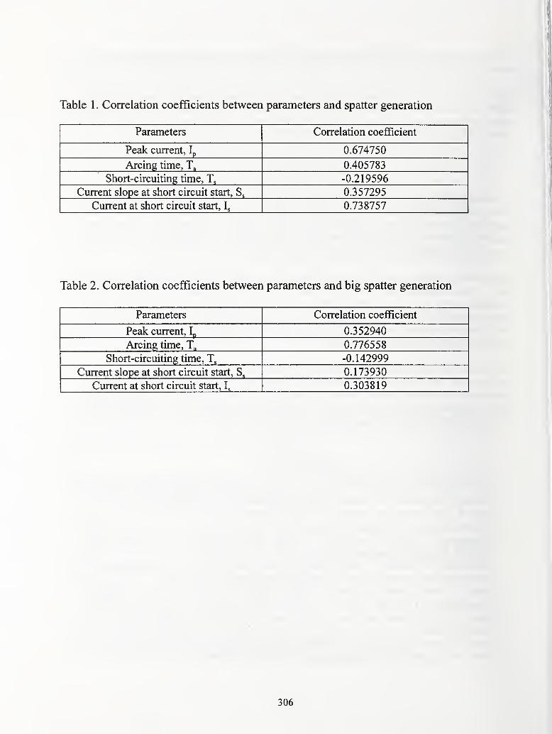
Table 1 . Correlation coefficients between parameters and spatter generation

Parameters Correlation coefficient

Peak current, Ip 0.674750

Arcing time, 0.405783

Short-circuiting time, T, -0.219596

Current slope at short circuit start, S, 0.357295

Current at short circuit start, 0.738757

Table 2. Correlation coefficients between parameters and big spatter generation

Parameters Correlation coefficient

Peak current, Ip 0.352940

Arcing time, T^ 0.776558

Short-circuiting time, T^ -0.142999

Current slope at short circuit start, S^ 0.173930

Current at short circuit start, I, 0.303819

306

Power supply

ComputerFast A/DConverter

Data files Output1—

r

Figure 1 . Welding waveform analysis system

27 28

voltage[V]

32

Figure 2. Relationship between spatter and big spatter generation and arc voltage

307

Is

Ta>K >

Tstim e

Figure 3. Waveform parameters for analysis

0.8

0.7

0.6

0.5 -

" 0.4

^ 0.3

0.2

0.1 -I

0.0

A spatter

T big spatter

200

T

250 300 350

peak current[A]

400

Figure 4. Relationship between spatter and big spatter generation and

peak current (Ip)

308

0.8

0.7

0.6 -

0.5 -

D)" 0.4x:

^ 0.3

0.2 -

0.1 -

0.0

A spatter

T big spatter

20 40—I

—

60

arcing time[msec]

—1—

80 100

Figure 5. Relationship between spatter and big spatter generation

and arcing time (TJ

160 180 200 220 240

current at short circuit start[A]

260

Figure 6. Relationship between spatter and big spatter generation and current at short

circuit start (IJ

309

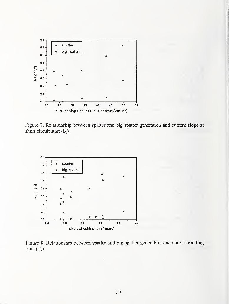
0.8

0.7

0.6

0.5

0.4

I0.3 -

0.2 -I

0.1

0.0

A spatter

big spatter

A A

A

20 25 30 35 40 45 50

current slope at short circuit start[A/msec]

55

Figure 7. Relationship between spatter and big spatter generation and current slope at

short circuit start (Sj)

0.8

0.7

0.6

0.5

" 0.4 4

I0.3 -

0.2 -I

0.1

0.0

2.5

A spatter

big spatter

A

A

-t*

A

A

—

r

4.03.0 3.5

short circuiting time[msec]

—I

—

4.5 5.0

Figure 8. Relationship between spatter and big spatter generation and short-circuiting

time (T,)

310

3.0

TO 2 .5 -

2 .0 -

0)ts(0

Q.(A

T30)

(0

E

S 1.0

O) 0.5 -

0.0

• spatter index

A neural network

V0.0 0.5 1.0 1.5 2 0 2 5

weight of real spatter[g]

3.0 3.5

Figure 9. Relationship between estimated and real spatter generation

0(0

Q.

1.0

0.8 -

• big spatter Index

A neural network

0 2 0 4 0.6 0.1

weight of real big spatter[g]

1 .0

Figure 10. Relationship between estimated and real big spatter generation

311

ACOUSTIC IDENTIFICATION OF THE GMAW PROCESS

A.M. Mansoor* & J.P. Huissoon^

ABSTRACT

In this study, a high speed data acquisition system was developed to record and

analyse the arc sound produced during GMA welding. The recorded data was

processed to obtain time domain, frequency domain and time-frequency domain

descriptors. Relationships between these descriptors and the originating weld

parameter levels and metal transfer mode were investigated, as were relationships

between the electrical power supplied to the weld and the arc sound. Results

indicate that the arc sound exhibits distinct characteristics for each welding mode.

The occurrence of spatter and short circuits was also found to be clearly

detectable in the arc sound record.

Keywords: Arc acoustics, automation, metal transfer mode, sound spectra

INTRODUCTION

The automation of Gas Metal Arc welding applications is often desirable due to the somewhat

unpleasant working conditions that the process creates. If properly implemented, automation can

increase productivity and weld quality while simultaneously improving the work environment.

However in general, automation efforts are usually most successful in applications where

relatively little skill is required for the manual operation, and least successful when a high level

of skill is required. The skill level required is often related to hand-eye co-ordination (sensing

and feedback control) and the experience necessary to be proficient at the job (learning the

appropriate controller "transfer function"). Gas Metal Arc welding can be difficult to automate

properly, since replicating the level of skill required to produce a quality weld by an automatic

machine relies heavily on an understanding of the relationship between feedback from the

process and actions to be taken in response.

Skilled manual welders represent extremely sophisticated and effective feedback control

systems. Visual, audio and tactile feedback cues are sensed, and a sophisticated non-linear

adaptive controller processes these data and recruits muscles in response. In developing feedback

control systems for automated welding, it is useful to study the sources of feedback utilised by

skilled manual welders. One such source of feedback is the arc sound produced during welding

[1,2]. This study was undertaken in an effort to determine if and how this sound can be used as a

source of feedback in automated GMA welding.

EXPERIMENTAL SETUP

The experimental equipment is comprised of a computer controlled GMA welding system,

synchronised with a data acquisition system for collecting acoustic data while welding. This

system is depicted schematically in Figure 1

.

' Ainsworth Technologies, Cambridge, Ontario; ^ Dept. of Mechanical Engineering, University of Waterloo

312

+x

3-Axis Table

WeldingPSU

0FEEDBACK

X-Axis EncoderY-Axis EncoderZ-Axis Encoder

Control PC

FEEDBACK

Welding VoltageWelding Current

SETPOINTS

Welding VoltageWire Feed Rate

Figure 1 . Schematic of experimental test equipment

The welding system consists of a Fronius 500A welding power source and wire feed unit, and a

three axis motion control system. This welding system provides computer control of the wire

feed rate (WFR), the torch travel speed (TS), the contact tube to workpiece distance (CTWD)and the welding voltage at the contact tube. The shielding gas flow rate (SGF) was manually set,

and a standard Ar-15 shielding gas composition was used.

The data acquisition system consists of sound level meter (SLM) with an analog output, low pass

anti-aliasing filtering and pre-amplification circuitry, shielding for the SLM and circuitry, a

Datel® PC-414A high-speed multi-channel analog input board, and a host 80486 based PC. The

data acquisition system is depicted in Figure 2.

313

Aluminium

WeldingPSU—

ICurrent LEM

iVoltage LEM

0 PC-414ABoard

Figure 2. Schematic of Sound Level Meter (SLM) and data acquisition system

The sound level meter (SLM) can measure sound levels from 50dB to 126dB with an accuracy of

±2dB, and was set to the C weighted frequency response. The output from the SLM is

conditioned with a 6th order Butterworth low pass filter with a break frequency of lOkHz, so that

the frequency range considered is 32Hz to lOkHz. The conditioned SLM analog output was

connected to one channel of the analog input board. The SLM and conditioning circuitry were

shielded from RF and EM noise by placing these in an electrically grounded steel casing. The

SLM was positioned 2m behind the welding torch, and at a height of 20 cm above the seam of

the weld. Since the 3-axis welding table moves the workpiece with respect to the stationary

welding torch, this arrangement maintains the SLM at a constant distance from the arc.

Voltage and current measurements were obtained using LEM® isolation sensors, and connected

to the analog input board. The PC-414A analog input board simultaneously samples the input

channels and provides 12-bit resolution at up to 350kHz per channel. In this application, the

acoustic, welding voltage and current signals were sampled at 40kHz. An 8Mb RAM drive

enabled up to 35 seconds of continuous data to be recorded.

In preliminary experiments, it was found that there were significant noise sources besides the

welding arc. These included the power supply unit, the motors on the 3-axis table, ventilation

and shielding gas flow. The sound from these background sources was measured and found to

314

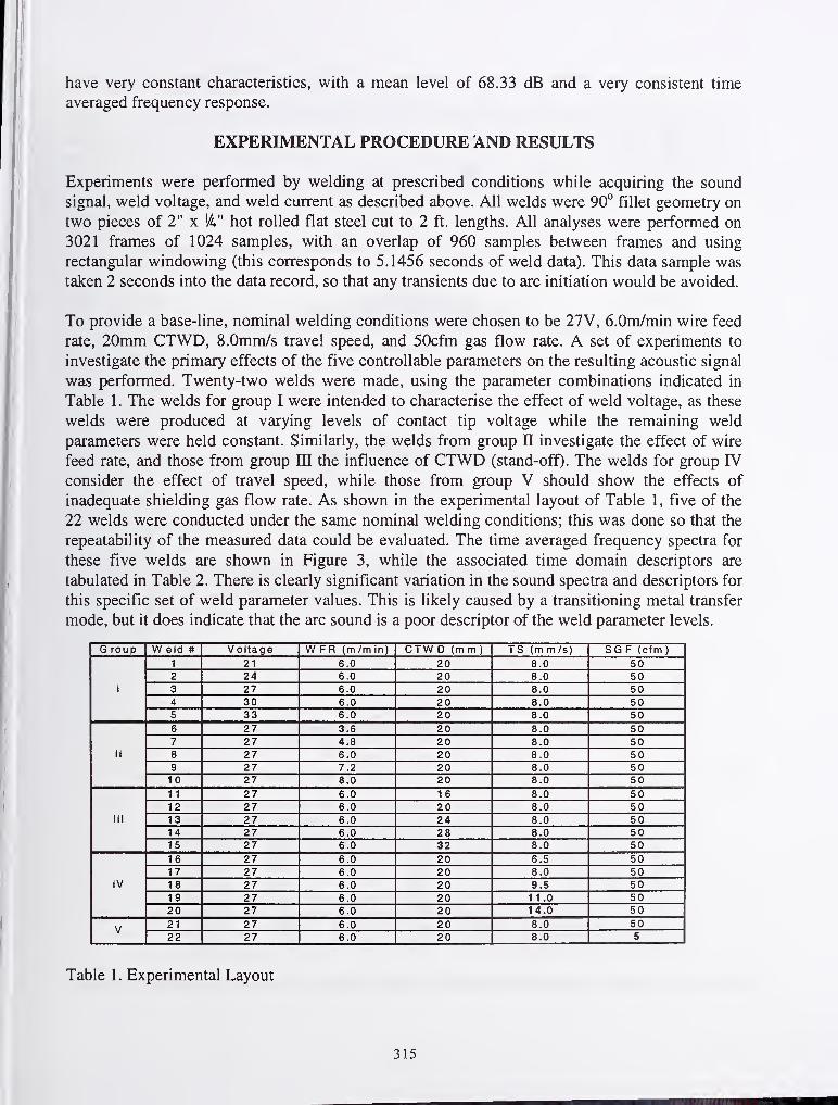
have very constant characteristics, with a mean level of 68.33 dB and a very consistent time

averaged frequency response.

EXPERIMENTAL PROCEDURE AND RESULTS

Experiments were performed by welding at prescribed conditions while acquiring the sound

signal, weld voltage, and weld current as described above. All welds were 90° fillet geometry on

two pieces of 2" x 'A" hot rolled flat steel cut to 2 ft. lengths. All analyses were performed on

3021 frames of 1024 samples, with an overlap of 960 samples between frames and using

rectangular windowing (this corresponds to 5.1456 seconds of weld data). This data sample was

taken 2 seconds into the data record, so that any transients due to arc initiation would be avoided.

To provide a base-line, nominal welding conditions were chosen to be 27V, 6.0m/min wire feed

rate, 20mm CTWD, 8.0mm/s travel speed, and 50cfm gas flow rate. A set of experiments to

investigate the primary effects of the five controllable parameters on the resulting acoustic signal

was performed. Twenty-two welds were made, using the parameter combinations indicated in

Table 1 . The welds for group I were intended to characterise the effect of weld voltage, as these

welds were produced at varying levels of contact tip voltage while the remaining weld

parameters were held constant. Similarly, the welds from group n investigate the effect of wire

feed rate, and those from group IQ the influence of CTWD (stand-off). The welds for group IV

consider the effect of travel speed, while those from group V should show the effects of

inadequate shielding gas flow rate. As shown in the experimental layout of Table 1 , five of the

22 welds were conducted under the same nominal welding conditions; this was done so that the

repeatability of the measured data could be evaluated. The time averaged frequency spectra for

these five welds are shown in Figure 3, while the associated time domain descriptors are

tabulated in Table 2. There is clearly significant variation in the sound spectra and descriptors for

this specific set of weld parameter values. This is likely caused by a transitioning metal transfer

mode, but it does indicate that the arc sound is a poor descriptor of the weld parameter levels.

G roup W eld # Voltage W FR (m/m in) CTW D (m m ) TS (m m /s) SGF (cfm)

1

1 21 6.0 20 8.0 502 24 6.0 20 8.0 503 27 6.0 20 8.0 504 30 6.0 20 8.0 505 33 6.0 20 8.0 50

II

6 27 3.6 20 8.0 507 27 4.8 20 8.0 508 27 6.0 20 8.0 509 27 7.2 20 8.0 501 0 27 8.0 20 8.0 50

III

1 1 27 6.0 16 8.0 501 2 27 6.0 20 8.0 501 3 27 6.0 24 8.0 501 4 27 6.0 28 8.0 501 5 27 6.0 32 8.0 50

IV

1 6 27 6.0 20 6.5 501 7 27 6.0 20 8.0 501 8 27 6.0 20 9.5 501 9 27 6.0 20 1 1 .0 5020 27 6.0 20 14.0 50

V21 27 6.0 20 8.0 5022 27 6.0 20 8.0 5

Table 1 . Experimental Layout

315

Volt.=27 V, WFR=6.0 m/min, T.S=8.0 mm/s, CTWD=20mm, SGF=50 cfm

0.15

1.25 2.5 3.75 5 6.25 7.5Frequency (kHz)

8.75 10

1.25 2.5 3.75 5 6.25 7.5Frequency (kHz)

8.75 10

1.25 2.5

0.15

1.25 2.5

Ma A/*

3.75 5 6.25Frequency (kHz)

8.75

0.15 ^

0 1.25 2.5 3.75 5 6.25 7.5 8.75 10Frequency (kHz)

Figure 3. Time averaged frequency spectra for five welds at the nominal parameter levels

Weld

3 8 12 17 21

Mean Sound Level (V) 0.147 0.231 0.363 0.225 0.326

Peak Sound Level (V) 2.28 3.83 3.83 3.37 3.2

Standard Dev. (V) 0.128 0.209 0.321 0.198 0.278

Coeff . of Variation (%) 87.1 90.5 88.4 88 85.3

Mean Sound Level (dB) 79.43 83.29 86.96 83.01 86.28

Peak Sound Level (db) 107.08 111.57 111.59 110.47 110.02

Table 2. Time domain sound descriptors for five welds conducted with the same parameter levels

316

Arc Sound vs. Metal Transfer Mode

The metal transfer mode is the characteristic most commonly associated with arc sound. Three

sets of welding parameters that resulted in spray transfer, globular transfer and short arc transfer

were experimentally determined. Using these parameters, five welds were performed in each

transfer mode. Typical sound records for each transfer mode are shown on a compressed time

scale in Figure 4. These records are consistent with those reported in other studies [3,4].

SPRAY TRANSFER

12 -r

8 --

s3

l\O.

3os_l(0

-8

-12

GLOBULAR TRANSFER

0.5 1.5 2 2.5 3

Time (s)

3.5 4.5

SHORT ARC TRANSFER

Figure 4. Typical Compressed Sound Records for each Transfer Mode

317

From Figure 4 it is clear that the time domain characteristics vary significantly with transfer

mode. Spray transfer produces a low amplitude signal, while globular and short arc transfer

produce louder signals. The sound from short arc transfer is distinguished from that of spray and

globular transfer by abrupt short spikes in the sound signal, these spikes being associated with

the occurrence of a short circuit. In order to summarise the nature of the acquired sound signals,

time domain descriptor values were calculated. Three of these descriptors: Peak Sound level,

Coefficient of Variation and Maximum Rise are plotted versus transfer mode in Figures 5, 6 and

7. The Maximum Rise is found as the largest absolute difference between consecutive samples in

a sound record. These Figures show that the values of all three of the plotted time descriptors

increase from spray to globular to short arc transfer.

Peak Sound Level vs Transfer Mode125

^ 120ID

? 115 +

S 110 +

DC(/)

ns<uQ.

105

100 -

95 -

90 —

X X X X

I Short Arc X Globular O Spray

Figure 5. Peak Sound Levels vs. Transfer Mode

Coefficient of Variation vs Transfer Mode100

95

90

85

80 -

75 -

70

O o

I Short Arc X Globular O Spray

Figure 6. Coefficient of Variation of Sound Level vs. Transfer Mode

Time averaged frequency spectra were found for each of the five sound records associated with

each transfer mode. These spectra are plotted in Figures 8, 9 and 10. From these plots it can be

seen that even though the frequency spectra from a given transfer mode exhibit some variation,

the general shape of the spectra is quite consistent. Spray transfer exhibits an almost monotone

spectrum, while globular and short arc transfer exhibit more broad-band signals. The spectra for

globular and short arc transfer are similar, but smaller amplitudes and spectra with a more

trapezoidal shape can distinguish the short arc spectra.

318

«

E 6(BCO

o«

I 2

Max. Rise vs Transfer Mode

9

X X X X ^

I Short Arc X Globular O Spray

Figure 7. Max. Rise vs. Transfer Mode

s 0.15 - -

COBa> 0.1 -

•0

3 0.05 -

0 -

3.75 5 6.25Frequency (kHz)

8.75

s 0.15

eo> 0.1 -

en

3 0.05 -

CO

1.25 3.75 5 6.25Frequency (kHz)

0.15 -

s 0.1 -

•m

SLM0.05 -

1 .2S 2.5 3.75 5 6.25Frequency (kHz)

7.5 8.75 10

'c5

g, 0.1 +wa| 0.05CO

0

1.25 2.5 3.75 5 6.25Frequency (kHz)

7.5 8.75 10

3.75 5 6.25Frequency (kHz)

10

Figure 8. Time Averaged Frequency Spectra for Sound from Spray Transfer

319

0 1.25 2.5 3.75 5 6.25 7.5 8.75 10Frequency (kHz)

1.25 2.5 3.75 5 6.25Frequency (kHz)

8.75 10

1.25 3.75 5 6.25Frequency (kHz)

8.75

1.25 3.75 5 6.25Frequency (kHz)

8.75

0.15 -

0.1

3 0.05 •

iiiTiiiili^iiiii

1.25 2.5 3.75 5 6.25Frequency (kHz)

8.75 10

Figure 9. Time Averaged Frequency Spectra for Sound from Globular Transfer

Comparison of Arc sound and Power

The relationship between the sound produced by an electrical arc and the electrical power

supplied to the arc can be expressed as [5,6] :

SAt) = k^(V(t)Iit))at

where SJt) is the amplitude of the sound signal at time t,

V(t) is the voltage across the arc at time t,

I(t) is the current flowing through the arc at time t,

kisa. constant of proportionality .

320

S 0.15

1.25 2.5 3.75 5 6.25Frequency (kHz)

7.5 8.75 10

3.75 5 6.25Frequency (kHz)

10

0.15

0.1 -

S 0.05 - -

1.25 2.5 3.75 5 6.25Frequency (kHz)

7.5 8.75 10

1.25 2.5 3.75 5 6.25Frequency (kHz)

7.5 8.75 10

3.75 5 6.25Frequency (kHz)

Figure 10. Time Averaged Frequency Spectra for Sound from Short Arc Transfer

There is evidence that this relationship also holds for the GTA welding arc [7]. To investigate

this relationship for the GMA welding arc, the sound and power derivative signals for welds

were compared in the time and frequency domains. The electrical power supplied to the arc was

calculated as the product of the measured welding current and voltage (an over-estimate since the

voltage was measured at the contact tube). The power signal was then differentiated using a 2nd

order backward finite difference equation. The time domain sound and electrical power

derivative signals did not exhibit a great deal of similarity for either spray or globular transfer,

although for short arc, a similar periodicity was evident. As seen in Figure 11(a), the power

321

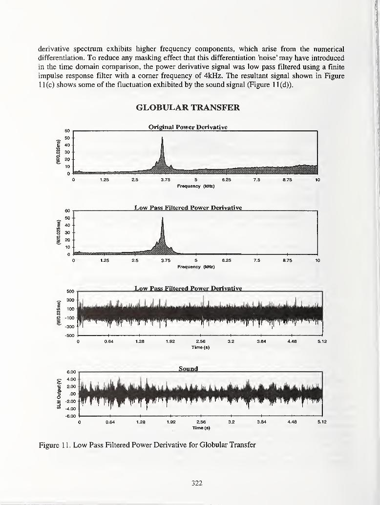
derivative spectrum exhibits higher frequency components, which arise from the numerical

differentiation. To reduce any masking effect that this differentiation 'noise' may have introduced

in the time domain comparison, the power derivative signal was low pass filtered using a finite

impulse response filter with a comer frequency of 4kHz. The resultant signal shown in Figure

1 1(c) shows some of the fluctuation exhibited by the sound signal (Figure 1 1(d)).

GLOBULAR TRANSFER

Original Power Derivative

0 1.25 2.5 3.75 5 6.25 7.5 8.75 10

Frequency (kHz)

Low Pass Filtered Power Derivative

0 1.25 2.5 3.75 5 6.25 7.5 8.75 10

Frequency (kHz)

Low Pass Filtered Power Derivative

Time (s)

Time (s)

Figure 1 1 . Low Pass Filtered Power Derivative for Globular Transfer

322

CONCLUSIONS

The results of this study indicate that the arc sound produced during the GMA welding process

can be used as a source of process feedback. Specifically, this study has shown that the metal

transfer mode, and events such as the occurrence of spatter or short circuit can be discerned from

the arc sound. Such feedback has potential applications in monitoring the GMA welding process.

FUTURE WORK

Further work in this area will concentrate on incorporating the arc sound descriptors developed

in this study into a weld monitoring system. This system would acquire the sound from the arc

and calculate time domain, frequency domain and frequency-time domain descriptors. These

descriptors would then be further analysed using a set of heuristics or a pattern recognition tool

such as a neural network to extract useful information about the weld process. Possible

applications are spatter detection and automatic arc tuning.

REFERENCES

1. Arata, Y.; Inoue, K.; Futama, M.; and Toh, T. 1979. Investigation on Welding Arc Sound

(Report n). Evaluation by Hearing Acuity and Some Characteristics of Arc Sound.

Transactions ofJWRI 8(2): 3-38

2. Wu, C. 1992. Microcomputer Based Welder Training Simulator. Computers in Industry 20:

321-325.

3. Morita, T.; Ogawa, Y.; and Sumitomo, T. 1995. Analysis of Acoustic Signals on Welding and

Cutting. Proc. 14th Int. Conf. on Offshore Mechanics and Arctic Engineering (ASME), Part 3:

547-52.

4. Blumschein, E.; Werner, C; Blumschein, J.; and Schik, U. 1996. A Concept for Cognitive

Control of Welding Processes. Proc. 6th Int. Conf. on Computers in Welding,paper 33

5. Dadgar, H.; Pilorget, A.; and Fitaire, M. 1977. Acoustic Noise Excited by Electric Arcs. IEEEInt. Conf. on Plasma Science: Conference Record - Abstracts, R.P.I., 1 17.

6. Drouet, M.; and Nadeau, F. 1982. Acoustic Measurement of the Arc Voltage Applicable to

Arc Welding and Arc Furnaces. J. Phys E: Sci. Instrum . 15.

7. Kaskinen, P.; and Mueller, G. 1986. Acoustic Arc Length Control. Proc. Int. Conf. on Trends

in Welding Research , 763-765.

323

Session B3: Real-Time Weld Sensing andControl Systems: GMAW Arc Quality

Monitoring III

DEVELOPMENT OF ADAPTIVE CONTROL OF ARC WELDINGBY IMAGE PROCESSING

T.Maeda, Y.Ichiyama

ABSTRACT

Sensing welding circumstances during welding is essential for seam-tracking and in-process

controls of automatic arc welding. Among many types of sensing, visual sensing is influenced to

a less extent by the change in welding conditions and provides much more information than

other sensing. However, miss-operation in processing of visual sensing may take place due to

noises caused by arc light and others, and visual sensing devices are costly. From these reasons,

the use of visual sensors have been less popular than arc sensors.

The authors have developed a system of image measuring of a weld molten pool. The newly

developed system has enabled to avoid the external interference such as arc light fluctuation and

spattering during welding. This development has been achieved by, 1) reduction of relative

intensity of arc light through improved optical processing; 2) detection of the location of the

electrode wire through processing images by the camera with a trigger high-speed shutter; 3)

averaging images by integration and stabilization of data processing through an algorithm using

a weighting function.

A control of the shape of a back-bead reinforcement in one-side narrow gap welding is important.

This image processing has accomplished not only preferable seam-tacking but also the

improvement of quality of deposited weld metal through a control of the surface shape of a

molten pool. The in-line control system with this image processing is to be applied for one-side

GMAW narrow gap welding in which a control of the shape of a back-bead reinforcement is

significantly important.

INTRODUCTION

There has been an increasing demand for an in-line control of automated arc welding in steel

welded constructions. Laser sensors have recently been used to measure the groove shape and

control the position of a welding torch so that the preferable quality of deposited metal can be

327

obtained. However, some difficulties arise in controlling the torch position when the welding

condition fluctuates. For example, it is almost impossible for the laser sensor to correct the torch

position when the welding wire is bent. Furthermore, the laser sensing is inappropriate in

optimizing back-bead welding such encountered with pipe girth welding.

This study is dealt with a technology of image processing and an in-line control in narrow gap

arc welding with a torch weaving with high speed. This technology is featured by a computer-

aided vision system enabling in-process detection of the electrode wire position and the

geometry of a molten weld pool. This system is ready to be applied to automatic all-position

welding such as pipeline construction welding.

: ; IN-LINE WELDING DATA ACQUISITION SYSTEM

An in-line data acquisition system equipped with a visual sensor consists of a CCD camera, an

image processor and sensors other than the CCD camera. The real time data acquisition is

essential in in-line sensing of dynamic welding situation. The system presently studied enabled

to concurrently acquire images of the molten pool, arc light, welding sound, arc voltage, and

welding current. Because of their huge data size, image data of the molten pool were compressed

into a moving picture format (MOTION-JPEG) and then the compressed data were stored as a

Video for Windows format (AVI file) in the computer. The image data of the molten pool and

acquisition data for arc light, welding sound, arc voltage, and welding current were stored in a

precisely synchronous manner as a text file in the computer.

Fig. 1 shows the composition of a multiple-sensing system for the in-line processing developed

in the present study. The software in the system enabled to display pool images and measured

data either graphically or in an image manner ( still picture or moving picture), and either

independently or synchronously. The text data of arc voltage, welding current, welding sound

and others were analyzed by some application software (e.g. EXEL, MATLAB). The

development of the visual sensing method and the image measurement of the molten pool is

mainly focused in the present paper.

328

Measurement

Data of Image

tControl of Welding

Fig.l Multiple Sensing System of Welding Process

329

IMAGE PROCESSING OF MOTLEN POOL

Selection of Optical Band-Pass Filter

A visual sensor, which acquires the image of a molten pool and a weaving electrode wire, was

installed at an angle forward a welding torch as shown in Fig. 1 . Brightness of arc light is much

more intense than radiation from the molten pool. It is, thus, difficult to acquire the processing-

possible images of the molten pool unless some measures are taken. The arc spectrums of

GMAW with 80%Ar and 20% COj mixture shielding gas were measured and it was found that

there are two high intensity groups: one around 400 to 500nm wavelength due to Fe and another

from 700 to 900nm due to Ar as shown in Fig. 2.

2.00E-04

1.50E-04 -

§ 1.00E-04

5.00E-05

O.OOE+00

[ Spectrum Measurement ]

11

1 1

JkIdIII0.3 0.4 0.5 0.6 0.7 0.8 0.9 1

WavelengthC m)

.1 1.2 1.3

Fig.2 Measured Spectrum(GMAW, Ar 80%+C02 20%

)

For a comparison purpose, a detailed spectrum of Ar according to the database(Ref.4) as shown

in Fig.3 was referred to. From a Plank's radiation formula, the peak intensity of radiation from

the molten pool is considered to range between 1 ,200 and 1 ,600nm. However, the sensitive range

of the CCD device is not higher than 1 ,000nm. So, it is desired to view a weld region through an

optical band-pass filter whose the center wavelength is near l,000nm.

However, when the center wavelength of a band-pass filter is too close to l,000nm, the

330

sensitivity of the CCD drops and poor acquisition of pool images results. Finally, a filter with the

center wavelength of 955nm was used in the present study and the significant interference with

detectable spectrums of the molten pool due to Ar spectrum could be avoided.

I

i

[ Ar Spectrum (800~ lOOOnm) ]

4I

E

800 820 840 860 880 900 920 940 960 980 1000

Wavelength (nm)

I

I

Fig.3 Spectrum data from "Wavelength Table"

Acquisition of Molten Pool Image

A CCD camera with an electronic trigger shutter was used to apply the present system to in-line

processing of welding with an electrode wire weaving as fast as 10 to 50Hz speed. The camera

with a normal synchronous shutter is unable to acquire the images of the pulsating pool and the

fast weaving electrode wire. In this study, a CCD camera was employed which was provided

with an electronic shutter operating with external trigger signals at arbitrarily selected timing.

The timing was selected so as to coincide with the center position of wire weaving.

Fig. 4 shows trigger shutter timing in this system. Then, it became possible to obtain still images

even under the condition of high speed weaving and detect the wire position in a weld groove

and the wire shape within the molten pool image. Through keeping the distance between the wire

position and the center of the molten pool zero, the torch position was satisfactorily controlled at

the center of the welding pool all the time.

33)

r:t (T) (f) (i (]) (T)

Synchronous

Signal

Trigger

Pulse

Exposure

Timing

Image

Data

Fig.4 Exposure Timing and External Trigger synchronized with torch weaving

Algorithm of Image Acquisition and Image Analysis

The algorithm of image acquisition of a molten pool is divided into three stages: an averaging

process by image integration; detection of characteristic points of a welding pool; and analysis

of the shape of a welding pool.

Arc light intensity fluctuates very often due to droplets transfer into the molten pool and the

brightness of molten pool images frequently changes because the molten pool is reflected by arc

light. Fig. 5 shows a dark arc image with pool radiation alone and a bright arc image with pool

radiation and arc reflection. This brightness fluctuation results in incorrect acquired images. To

solve this problem, a frame averaging process by image integration was introduced.

As shown in Fig. 6, the integration of several video frames followed by bit shifting made it

possible to average noise images and reduce disturbing images. The image integration processing

was done in real time by the image processor.

332

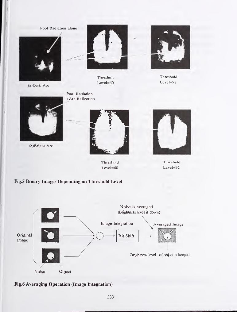
(a)Dark Arc

Threshold

Level=60

Pool Radiation

+Arc Reflection

(b)Bright Arc

Threshold

Level=92

Threshold

Level=60

Threshold

Level=92

Fig.5 Binary Images Depending on Threshold Level

Originali

Image

Noise Object

Noise is averaged

(Brightness level is down)

Averaged Image

Bit Shift

.0

Brightness level of object is keeped

Fig.6 Averaging Operation (Image Integration)

333

The images of a weld region were acquired by the CCD camera and then, the position of the side

edges of a molten pool and the center of an electrode wire were determined by the smoothed

differentiation of the brightness along the line perpendicular to the welding direction. Fig. 7

shows a newly developed image processing algorithm.

Width of molten pool(=Width of groove)

Differential

of intensity

on line

Weighting

function

Result of

operation

Molten Pool Electrode Wire

Measurement Line

Scannig Direction

i

Fig.7 Pool Edge Detection with Weighting Function

334

As mentioned above, acquired images by the CCD camera equipped with a high-speed shutter

considerably fluctuates in their brightness. In order to accomplish stable detection of the

characteristic points of the pool image, a dynamic threshold level or gray level in the data

acquisition was set up instead of a fixed threshold level.

Furthermore, the weighting function, W(x) corresponding to the groove size was prepared as

shown in Fig.7 and then the values of differentiated brightness, D(i) and W(x) were multiplied.

This multiplication facilitated the avoidance of external interference due to arc light and spatters.

As a result, the developed algorithm enabled stable detection of the characteristic points of a

molten pool so that satisfactory seam tracking could be performed.

Result of Seam-Tracking Control Test

The authors conducted seam-tracking tests using the image-processing algorithm developed in

the present study. A work piece was machined with a narrow gap with a bevel angle of 10 degree

and a root gap of 7mm. It was set at an angle toward the travel direction, i.e., 2.5mm per 170mm-

travel direction, as shown in Fig. 8. GMAW was conducted under the conditions of 80%Ar and

20%CO2 shielding gas, solid electrode wire, 20cm/min of travel velocity and 30Hz weaving

frequency. During testing, zero distance was kept between the wire position and the center of a

molten pool, and it was found that the torch position was constantly controlled at a satisfactory

level along the groove center line, as shown in Fig. 9.

Carriage Travelling Axis(Y)

I

Fig.8 Relative Directions of Carriage Travel and Welding Groove

335

0 50 100

travelling position(mm)

Fig.9 Result of Seam-Tracking Control by Image Processing

SUMMARY

150

tracking position

center of groove

An in-line control system for all-position narrow gap welding was developed, which measures

images of a molten weld pool. The image measurement developed in the present study was

characterized by being less susceptible to the external influences such as spattering during

welding. This development was achieved by: 1) reduction of relative intensity of arc light

through improved optical processing; 2) detection of the location of the electrode wire through

processing images by the camera with a high-speed trigger shutter; 3) averaging images by

integration and stabilization of data processing through an algorithm with a weighting function.

REFERNCES

1 . Inoue,K. 1 98 1 . Image processing for on-line detection of welding process(2"'* report).

Yousetsu gakkai shi/ VOL.50,NO. 1 1 , 1 1 1 8- 1 1 24

2. Li,Y,Wu,L.,Middle,J.E.,1993. Machine Vision Analysis of the Welding Region and Its

Application to Seam Tracking in Arc Welding. Proc Inst Mech Eng Part BA'^OL.207,

NO.4,275-283

3. Maeda,T.,Makabe,T.Jchiyama,Y.,1997. Development of an On-line Visual Sensing System

for Molten Pool Measurement , Yousetu gakkai kouen gaiyouA^OL.6 1,8-9

4. Phelps,F.M.,1982. M.I.T. wavelength tables, vol.2 2 ed. 4 ed.

336

ADAPTIVE VOLTAGE CONTROL IN GTAW

P. Koseeyaporn *, G. E. Cook A. M. JStrauss*

ABSTRACT

Automatic voltage control (AVC) systems are commonly used in gas tungsten arc welding

(GTAW) to maintain constant arc length. Although AVCs usually perform adequately in most

operating circumstances, there are conditions during which the traditional systems cause

problems because the arc voltage-to-arc length gain, Karc, a feed forward gain, is not constant but

varies with the nominal values of the arc current and voltage. Thus, an AVC that has a fixed

voltage set point will not maintain a fixed arc length if the arc current changes. In this paper an

adaptive controller is introduced that is capable of "identifying" the arc sensitivity characteristic

and adjusting the controller in real time for optimum response without any a priori knowledge of

the current/gain relationship.

INTRODUCTION

Automatic voltage control (AVC) systems are commonly used in gas tungsten arc welding

(GTAW) to maintain constant arc length. Although AVCs usually perform adequately in most

operating circumstances, there are conditions during which the traditional systems cause

problems and sometimes fail totally in providing acceptable position control. Bjorgvinsson [1]

has traced these problems to two significant characteristics of the welding arc that are not

accounted for in traditional AVCs:

1) The arc voltage-to-arc length gain, Karc, is not constant but varies with the nominal values of

the arc current and voltage. In the closed-loop AVC system, this arc sensitivity affects the

dynamic response of the system since it is one of the parameters forming the forward loop of

the AVC.

2) The arc voltage-to-gap relationship is not constant but varies with current. Thus, an AVCthat has a fixed voltage set point will not maintain a fixed arc length if the arc current

changes.

The unstable phenomena fi'equently observed with AVCs occur primarily at the operating

conditions that are significantly different fi^om "normal" welding conditions, such as when the

welding current is pulsed between primary and secondary current levels or at low currents

experienced during upslope and downslope. If an AVC is tuned for the optimum response at

normal welding current levels, then at the lower currents experienced during upslope and

downslope the position control may become oscillatory sometimes driving the torch into the

weld pool. To avoid these instability problems the AVC is fi^equently turned off in practice

during the critical current sloping portions of the weld cycle. However, it is widely known that

control of the cooling rate of the weld during termination is important if cracks in the weld seam

are to be avoided. A simple disabling of the AVC during welding initiation and termination

deprives the welder of full control over the welding heat during that period. Although the

Department of Electrical & Computer Engineering, Vanderbilt University, Nashville, TN 37235* Department of Mechanical Engineering, Vanderbilt University, Nashville, TN 37235

337

welding current is sloped down, voltage is not as well controlled, and the result is the so-called

"tail-out" cracking. Therefore, a means of maintaining control of the arc gap, independent of

current, is needed. Bjorgvinsson, Cook, and Andersen address the first characteristic by

introducing a gain scheduling adaptive control law [2]. This system is based on use of a lookup

table or empirical relationship between arc sensitivity and current. While the gain scheduling

adaptive controller employed by Bjorgvinsson has been demonstrated to work well under

controlled conditions, the functional relationship between arc sensitivity and current is dependent

on a number of parameters that are difficult to preprogram. In this paper an adaptive controller is

introduced that is capable of "identifying" the arc sensitivity characteristic and adjusting the

controller in real time for optimum response without any a priori knowledge of the current

sensitivity relationship. It is thus capable of providing stable operation at all points. Ability to

control the arc voltage in a stable manner at all welding currents also permits addressing the

second characteristic. The voltage reference is varied as the current changes, e.g., decreases

during weld termination, in such a manner as to maintain an appropriate weld pool width to

depth ratio and maintain an optimum weld pool shape [3-4]. In this research, fuzzy logic control

was used to estimate the required voltage reference setpoint to maintain the weld pool

geometrical characteristics [5]. While both characteristics of the welding arc are accounted for

in the results described in this paper, the adaptive control aspect of the first characteristic is the

paper's primary focus.

TRADITONAL CLOSED-LOOP SYSTEM VERSUS ADAPTIVE CONTROL

To control the gas tungsten arc welding (GTAW) system with a constant current power source

(see Figure 1.), an automatic voltage control (AVC) is typically used to control the arc voltage in

order to maintain a desired arc length. However, it is known that the arc voltage-to-gap

relationship is not constant but varies with current [1,2]. Thus, an AVC that has a fixed voltage

set point will not maintain a fixed arc length if the arc current changes. The traditional AVCdesign uses a fixed arc voltage-to-arc length gain, Karc, as shown in the closed-loop AVC block

diagram in Figure 2. Although not shown in the simplified block diagram, rate feedback would

normally be employed for improved response characteristics. To prevent the system from being

unstable when the arc current changes, adaptive control [6] is used to identify the arc voltage

gain in the closed-loop system, as shown in Figure 3, and produce compensatory changes in the

controller.

ServoMotor

Welding

Torch

ShieldingGas

I

Tungsten k T

N Electrode I I

I I

I rWaterCoolantArc

Workpiece

ShieldingGas

ConstantCurrentPowerSource

WorkClamp

K.

s(s+a)

Figure 1. GTAW system with AVC. Figure 2. Traditional closed-loop AVC.

338

DESIGN OF THE ADAPTIVE CONTROL

In this paper, the adaptive controller, shown in Figure 3,'is used to identify the gains in the

model-based portion of the partitioned control system [7] used to control the arc voltage. Theadaptive controller provides stable control of the system even when the input current is changed

over a wide range.

The transfer function of the dc servomotor used for control of the arc length (and hence arc

voltage) is given by

Using L^K^^^=V^ 'm (1), we may express the corresponding differential equation as

V, + ay„ - KKv_s a s arc m

1 aLetting c.^ = and = — , we may rewrite the open-loop equation as,

K,K KK„,„s arc

C2^a+C,Va=^m- (2)

Both and vary inversely as Karc, which is a nonlinear function of the welding current and

arc voltage. Thus, when the current/voltage dependence of Karc is taken into account, the open-

loop dynamics of the system relating arc voltage to servo drive voltage is a nonlinear second-

order differential equation.

The partitioning scheme [4] employed here partitions the controller into a model-based portion

and a servo portion. The model-based portion appears in a control law of the form

^n.=CCVm+P, (3)

where a and p are functions or constants chosen such that if v„ is taken as the new input to the

system, the system appears as a simple linear second-order system,

v.- v.. (4)

Equating (1) and (2),

C2^a+c,v^=av\„+ P . (5)

Clearly, in order to make the system appear as the linear system given by (3) at the v„ input, a

and p must be chosen as

(6)

339

Referring to Figure 3, c, and are estimates of c^and c^, respectively. We choose the

proportional-pius-derivative control law

^m=^2^!„+^A. (7)

where - v^^^ + K^e + K^e , and e = v^^^ -. From Figure 3, we see that

^.^'^ref+KJ + K^e, (8)

and

K=^2^'n,+^,t- (9)

Equating (9) to the open-loop dynamics of the system, as expressed by (2), and substituting (8)

into the right-hand side of (9), we obtain

Rearranging,

^2V + ^2 [KJ + K^e] = c,v^ + (c, - c, >>,

.

Subtracting c^v^ from both sides,

or

c^e + c^lKJ + K^e] = c^v^ + c,v^,

where the parameter errors are ?2 - ^2 ~ ^2 ^1 - ^1 ~ ^1

The desired error equation is then,

e + K^e + K^e = ^^'[c^v, + c,vj . (10)

If the model-based portion of the controller equals exactly the system parameters, then c, and

are zero, and the error disappears. In this case, is chosen to provide the desired closed-loop

stiffness and is chosen to provide the desired damping, e.g., critical damping, C, = \. When

the model parameters are not known exactly, the mismatch between actual and modeled

parameters will cause servo error, possibly resulting in an oscillatory or unstable system, in the

absence of adaptive control. With adaptation, the servo error may be used to drive the adaptation

scheme, as shown in Figure 3, which attempts to update the values of the model parameters until

the error disappears. Equation (10) may be rewritten in the form,

e+K^e + Ke = c-'W{v,v)^ (11)

340

where O'^2 -^2 "^2'

,andPr(v^,vJ = [v^ vj

The adaptive law computes how to change the parameter estimates as a function of the filtered

servo error signal (see Figure 4),

e

==2

f

! t

(3, =c,

f

Figure 3. The welding system with an adaptive controller. Figure 4. The adaptive law.

EXs)={s + \i/)e(s),

where vj/ is a positive constant.

Substituting the Laplace transform of the error equation (11),

s +K..s + K_

(12)

(13)

Based on the strictly positive real (SPR) lemma [8] and Lyapunov stability theory [9], we choose

(14)

where F = diagiy^ y^) and is nonnegative.

Equation (14) provides the parameter updates in the "identification paradigm" of the adaptive

system. The adaptation law, including the error filter, is shown in the block diagram of Figure 4.

FUZZY LOGIC SELECTION OF VOLTAGE SETPOINT

During initiation of the weld, the welding current is typically ramped linearly from a low value,

e.g., 10 amperes, or less, to the weld value, e.g., 50-400 amperes, or more. During termination of

the weld, the welding current is typically ramped linearly fi^om the weld value back down to a

low value. During both ofthese critical portions ofthe weld, it is important that desired

341

Figure 5. The welding system with an adaptive

controller and FLC for setpoint selection.

ARCVOLTAGE

1^

POWER SOURCECURRENT

CONTROLLER

lebn A/D12btt[VA

ISA

Bus

CONTROL PC

1-^

ISA

Bus

MONITORING &RECORDING PC

Figure 6. Hardware interfacing block

diagram.

geometrical characteristics of the weld pool are maintained [10-13]. To accomplish this, it is not

only necessary that the AVC be operative and stable, but it is also necessary that the reference

(setpoint) voltage be changed as the current changes. This is because the arc voltage-to-gap

relationship is not constant but varies with current [1]. Since the arc length can not easily be

measured, it is difficult to continuously set the voltage reference to the correct value to obtain a

specific arc length required for the desired weld pool geometry. The required relationship could

be determined experimentally [3-4], but this relationship varies as a function of a number of

variables. In this research the required voltage was chosen by means of a fuzzy logic control

(FLC) system.

The FLC is only operative when the welding current larc is below a reference value Iref In

addition to larc and Iref, inputs to the FLC are the relative arc length error {Lref - Lore) and the

derivative of the error. The relative arc length error was measured with a linear transducer

connected between the AVC servo mount and the welding torch.

Membership functions of the FLC were composed of the input error, the velocity error, and an

output (vref). The shape of the membership functions was selected as triangular for faster control.

A center-of-gravity deflizzification scheme was applied [14]. Each of the negative and positive

fuzzy sets was assigned three values (large, medium, and small), so there was a total of forty-

nine rules. Example rules are as follows:

If the error is negative large and the velocity error is negative large, then the output is

negative large.

If the error is positive small and the velocity error is negative small, then the output is

positive small.

When larc ^ Iref, thc FLC incrcascs or decreases the arc length by adding its output to the fixed

weld vohage level. When larc Iref, the FLC has no output, and the system operates in the

constant arc voltage mode. The adaptive AVC with FLC selection of voltage reference is shown

in Figure 5.

342

IMPLEMENTATION

To implement and test the adaptive AVC system, both software and hardware components were

required. The control algorithms were written in C++ on a personal computer (PC) allowing the

user to conveniently change the parameters during the experiments under a Graphic User

Interface (GUI) environment. Monitoring and recording programs were also required to obtain

data fi"om the system during its real-time control.

The hardware used in the research included a data acquisition system, isolator, welding power

supply, control PC, monitoring and recording PC, and linear variable differential transformer

(LVDT). The hardware interfacing block diagram is shown in Figure 6. The hardware can be

classified into two groups: interfacing devices, and power and control devices.

Referring to Figure 6, the DMM-16 data acquisition board [15] was used to send and receive the

data composed of the arc voltage, the relative arc length (LVDT) and the arc current to the

control PC. Two input channels were connected to the voltage pickup for arc voltage

measurement and the LVDT for relative arc length measurement. An output channel was linked

to the power source current controller. Two of the output channels were employed to drive the

reversible servomotor, one used for positive output and another for negative output. All of the

input channels have 16-bit resolution with a 2 kHz maximum sampling rate per channel for

single mode operation. The output channels have 12-bit resolution with the same sampling rate.

Another data acquisition board, 5516DMA [16], was used to capture the analog signals for use

by the monitoring and recording PC. Three channels of this board were employed. One is linked

to the arc length signal, and the others are connected to the arc current and arc voltage signals.

Magnetic isolators [17] were utilized to prevent the power signals from disturbing sensitive

devices such as the PCs and data acquisition boards. A class-H welding power source [18-19]

provided constant current output control. The power source can deliver output current from 0 to

500A at a voltage from 0 to 45 volts.

Figure 7. The dialog-based control program. Figure 8. Monitoring/recording program.

343

All of the control schemes, including a digital non-adaptive AVC and adaptive AVC, were

implemented by programming under a graphic user interface (GUI) based on Microsoft's Visual

C++ platform language [20]. For some programs in which an algorithm was needed to run

concurrently with other tasks, the thread program feature was applied [20]. The dialog features

were used for conveniently allowing the user to adjust the parameters during experimental

implementation (see Figure 7). The document and viewing features were used to graphically

display the input/output signals and to enable data recording with adjustable resolution (see

Figure 8). Control programs used for real-time control consisted of an automatic arc starter

program, a digital non-adaptive AVC program, an adaptive AVC program, and a utility program

used to move the welding torch to a specified position [5].

EXPERIMENTAL RESULTSDynamic response tests

To test the dynamic response of the AVC system with and without adaptive control, a copper

stepped-plate was used, as shown in Figure 9. Tests were conducted at 30 amperes and 100

amperes. The travel speed was 2. 12 mm/sec. The shielding gas was argon with a flow rate of 25

cfh. The tungsten electrode was 1.65-mm diameter. The gain of the digital non-adaptive AVCwas set for optimum response at 100A. The response is shown in Figure 10. With the same gain

setting, the experiment was repeated at 3 OA. The results are shown in Figure 11. As can be

seen, the response at this lower current was quite oscillatory. This is consistent with

experimental resuhs that show the arc voltage-to-arc length, Karc, increases at the lower currents

[1]. The increase in Karc reduces the damping ratio according to (see Figure 2)

I' I

Weldingxc-i Torchi i

(| J Direction

Imm.

Figure 9. Step-plate experiment.

14

> 12

I

11 1 1 1 1 ! 1 1 1

0 2 4 6 8 10 12 14

2

a: .il 1 1 1 1 1 1 1

0 2 4 6 8 10 12 14

Seconds

Figure 10. Digital non-adaptive AVC response

with Iarc=100A.

0 2 4 6 8 10 12 14

mmmm0 2 4 6 8 10 12 14

Seconds

Figure 1 1 . Digital non-adaptive AVC response

with Iarc=30A.

344

VIS 13

>

I 12

_ 2

eE

-El

i 0

S -1

6 8 10 12 14

10 12 14

Figure 12. Adaptive AVC response with

Iarc=30A.

15

2 ^*

5 13

>

11

0 2 4 6

0 2 4 6

10 12 14

10 12 14

Figure 13. Adaptive AVC response with

Iarc=100A.

a.

leading to the oscillatory response observed in Figure 10. The response of the adaptive AVCsystem is shown in Figure 12 for BOA and in Figure 13 for lOOA. As can be seen, at 30A, there

is an initial oscillation but that is quickly damped out as the adaptive system adjusts the model-

based parameters to match the system. At lOOA, the response is optimum as in the non-adaptive

case.

Figure 14. AVC ramping down current result.

ffl 20

1 15

H< 1001 23456789 10

Figure 15. Adaptive ramping down current

result.

Ramping down current tests

These experiments were conducted to test the ability of the non-adaptive AVC and the adaptive

AVC to control the arc voltage when the welding current varied from lOOA to a minimum level

at weld termination. The tests were conducted with an arc voltage of 13V at the welding level of

lOOA. A copper test plate was utilized without travel speed. The results of the non-adaptive AVC

345

tests are shown in Figure 14. As can be seen, when the current decreased to a sufficiently small

value, the welding torch was uncontrollable and the tungsten electrode suddenly touched the

workpiece. This behavior was due to the oscillatory state of the closed-loop system at the low

current. In comparison, the result of the same test with the adaptive AVC is shown in Figure 15.

In this case stability is maintained throughout the downsloping period. Furthermore, below a

preset reference current of 70A, the FLC system varied the arc voltage in a manner necessary to

maintain a reasonably constant energy density at the arc resulting in consistent weld pool

geometry throughout the downsloping period.

DISCUSSION AND CONCLUSIONS

The primary focus of this paper was on design of an adaptive AVC system that would provide

stable voltage control over the full range of expected operating currents for the GTA welding

process. This is important in many welding applications where it is essential to control the arc

voltage throughout the current upsloping period at the weld initiation and the current

downsloping period at weld termination. Traditionally designed AVCs have been unable to meet

this requirement, simply being switched off during the ramping periods of the weld program. For

many applications, this is unacceptable because it results in weld cracking, particularly at the

weld termination. Ability to control the arc voltage throughout the ramping periods is also

important because it is necessary to vary the reference (setpoint) voltage in such a manner as to

maintain approximately constant energy density during these critical periods of the weld in order

to maintain a weld geometry that is least susceptible to cracking.

The adaptive control system design presented in this paper, in combination with the fuzzy logic

voltage setpoint controller, proved to robustly satisfy both of the requirements for full-range arc

voltage control. In tests in which the current was ramped down from a lOOA weld level to a

minimum level of approximately 5A, the adaptive controller maintained stable control, and the

fuzzy logic setpoint varied the setpoint voltage in such a manner as to maintain a reasonable arc

length. This results in maintenance of the desired weld pool geometry for minimumsusceptibility to cracking.

For argon shielding gas, as employed in this research, the arc voltage-to-arc length gain, Karc,

increases by a factor of approximately six when the current decreases from 100A to 5A [1], as in

the weld termination tests reported in this paper. Without adaptive control this would lead to an

approximate twenty-five percent overshoot for a step change in input. Additionally, a traditional

AVC would attempt to maintain constant voltage throughout the ramping down period. With a

voltage of 13V at lOOA the arc length would be approximately 4 mm. At 5A, a 13V arc is

approximately 0.9 mm long. When this short arc length requirement is coupled with the

oscillatory state of the feedback system, it is understandable that the traditional AVC design

fails. The adaptive AVC system reported in this paper maintains optimum dynamic response

characteristics throughout the range of current. The FLC setpoint controller increases the

reference voltage at the low currents to realize a more reasonable arc length. The two systems

act in combination to provide greatly improved weld initiation and termination control.

In conclusion, the application described in this paper requires adaptive control for proper

operation. This is because of the large changes in system gain as operating conditions change.

346

While gain-scheduling adaptive control has been shown to work [2], the many variables that

affect the gain schedule render this method problematic for general usage. The adaptive control

scheme proposed in this paper provides the real-time identification and control needed for

trouble-free operation. The authors have no doubt that other adaptive control schemes, such as a

model reference adaptive system (MRAS) approach, would work also.

REFERENCES

1. Bjorgvinsson, J. B., Adaptive Voltage Control in Gas Tungsten Arc Welding. M.S. Thesis,

Vanderbilt University, 1992.

2. Bjorgvinsson, J. B., Cook, G. E., and Andersen, K., "Microprocessor-Based Arc Voltage

Control for Gas Tungsten Arc Welding Using Gain Scheduling," IEEE Transactions on

Industry Applications , Vol. 29(2), pp 250-255, March/April 1993.

3. Yizhang Liu, George. E. Cook, R. Joel Barnett, and James F. Springfield, "PC-Based Arc

Ignition and Arc Length Control System for Gas Tungsten Arc Welding," IEEE Trans. OnIndustry Applications , vol. 28, 5, pp. 11 60-1 165, Sept./Oct. 1992.

4. R. Joel Barnett, Kristinn Andersen, George E. Cook, and Alvin M. Strauss, "Weld Quality

Enhancement Using Precision Multi-Parameter Control in Gas Tungsten Arc Welding,"

International Trends in Welding Science and Technology , S. A. David and J. M. Vitek, Eds.

Materials Park, Ohio: ASM International, 1993, pp. 981-985.

5. Poolsak Koseeyapom, Adaptive Voltage Control in Gas Tungsten Arc Welding , M.S. Thesis,

Vanderbilt University, May 1999.

6. Astrom, K.J. and Wittenmark, B., Adaptive Control , Addison-Wesley, Reading,

Massachusetts, 2"'* Edition, 1995.

7. Craig, J. J., Adaptive Control of Mechanical Manipulators , Addison-Wesley, Reading,

Massachusetts, 1988.

8. Kumpati S. Narendra and Anuradha M. Annaswamy, Stable Adaptive Systems, New Jersey:

Prentice Hall, 1989, pp. 63-65.

9. William L. Brogan, Modem Control Theory, New York: Quantum Publishers, Inc., 1974, pp.

262-282.

10. M. Lu and S. Kou, "Power and Current Distributions in Gas Tungsten Arcs," Welding

Journal vol. 67, no. 2, pp. 29s-34s, 1988.

11. W. F. Savage and A. H. Aronson, "Preferred Orientation in the Weld Fusion Zone," Welding

Journal vol. 45, no. 2, pp. 85s-89s, 1966.

12. L. A. Weeter, C. E. Albright, and W. H. Jones, "Development of a Weldability Test for

Pulsed Laser Beam Welding," Welding Journal vol. 65, no. 3, pp. 51s-62s, 1986.

13. Fukuhisa Matsuda, "Solidification Crack Susceptibility of Weld Metal," Recent Trends in

Welding Science and Technology, S. A. David and J. M. Vitek, Eds. Materials Park, Ohio:

ASM International, 1990, pp. 127-136.

14. B. Kosko, Fuzzy Engineering , New Jersey: Prentice Hall Inc., 1997.

15. Diamond-mm-16 PC/104 Format 16-bit Analog I/O Module User Manual Vl.O, California:

Diamond Systems Corporation, 1997.

16. User Documentation for 5516DMA Multi-Function Data Acquisition Board. Massachusetts:

American Data Acquisition Corporation.

347

17. User's Manual. The 3B Series Signal Conditioning I/O Subsystem. Massachusetts: Analog

Devices Inc., 1986.

18. Hussam El-Dean E. H. Eassa, Electric Arc Welding Control with a High Performance Power

Source. "Ph.D. Dissertation, Vanderbilt University, 1983.

19. Kristinn Andersen, George E. Cook, Robert J. Bamett, and E. H. Eassa, "A Class-H

Amplifier Power Source Used as a High-Performance Welding Research Tool," Recent

Trends in Welding Science and Technology. S. A. David and J. M. Vitek, Eds. Materials

Park, Ohio: ASM International, 1990, pp. 973-978.

20. Microsoft Visual Studio 97 Development System - Enterprise Edition.

348

WELD SURFACE UNDULATION CHARACTERISTICS IN THE PULSED GMAWELDING PROCESS

S. Rajasekaran

ABSTRACT. The weld surface quality in pulsed current gas metal arc welding (GMAW-P)process is mainly influenced by the pulse parameters. Selection of the most suitable combination

of pulse parameters is very difficult due to the complex interdependence of the parameters of

pulsed current. Therefore effect of the pulse parameters on weld surface characteristics has been

studied for different types of droplet detachments, namely background detachment, one droplet

detachment per peak, two droplets detachment per peak and three droplets detachment per peak.

The suitable type of droplet detachment for welding, using 1.2 mm diameter of ER 5356 filler

metal, has been selected on the b^sis of measuring the surface characteristics of the weld usiiig a

computerized measuring system based on a Linear Variable Differential Transformer. Onedroplet detachment per peak was considered to be capable of providing smoother weld surface

than other types of droplet detachments. The peak energy was found to be low for background

detachments.

KEY WORDS: Al-Mg Alloys Welding, Droplet Detachment, Pulsed Current Gas Metal Arc

Welding, Pulse Parameters, Weld Surface Undulation, Weld Characteristics, Weld Quality.

INTRODUCTION

Aluminium and its alloys are widely used in the transportation industry, where lightweight,

corrosion resistance and high fatigue strength are the desired properties. Pulsed current gas metal

arc welding process (GMAW-P) is widely used to weld many Al-Mg alloys components of

spacecraft, automobile, ship, air craft, rail road, bridges, oil tanks, pipe lines, structures,

cryogenic storage tanks, marine, unfired pressure vessels, T.V towers, missile components and

drilling rigs. Al-Mg alloys offer maximum resistance to atmospheric, salt water and alkaline

corrosion (Ref. 1). The GMAW-P may be considered a potential process for the welding Al-Mg

alloys, where the dilution can be controlled more precisely than other conventional welding

processes.

The pulsed current gas metal arc welding process has recently gained wide attention in welding

industry, due to its comparatively low heat input and precise control over the thermal cycle (Ref

2). Because, In pulsed current gas metal arc welding process, spray transfer or more precisely

controlled droplet transfer is obtained at low average current. This condition provides a smaller

and controlled weld pool, which allows welding of thin materials in all positions (Ref 3,4).

Detachment of molten metal droplets from the filler metal, its transfer across the arc and its flow

S. RAJASEKARAN, formerly a Research Scholar, Department of Mechanical Engineering, Indian Institute of

Technology-Bombay, Mumbai 400 076, India, is presently an Assistant Professor, Department of Production

Engineering, Amrita Institute of Technology and Science, Coimbatore 641 105, Tamil Nadu, India.

349

into the weld pool are defined as metal transfer characteristics. Droplet detachment

characteristics are defined as (a) the size of molten droplet (b) instance and duration at which

detachment takes place arid (c) number of droplet detachments per pulse.

The superiority of the GMAW-P process is mainly related to the nature of metal deposition

governed by the pulse parameters viz. peak current (Ip), peak duration (Tp), background current

(Ib) and background duration (Tq) (Ref. 5). Selection of the most suitable combination of pulse

parameters is very difficult due to the complex interdependence of the above parameters of

pulsed current (Refs. 3, 6-8). To resolve this problem, studies have been carried out for different

types of droplet detachments, namely background detachment, one droplet detachment per peak,

two droplets detachment per peak and three droplets detachment per peak, by varying pulse cycle

time.

Depending on the parameters of GMAW-P (Fig. 1) process either a single droplet or multiple

droplets may get detached. If it is a single droplet, this detachment may occur either in peak

duration or background duration and if it is multiple droplet detachment, the same may occur in

peak duration. This difference in the tin.ing of droplet detachment affects the uniformity in weld

surface undulation and overall quality of the weld (Ref. 9). These characteristics have been

investigated in this study. Experiments were conducted at fixed value of Wp, Ig and Tg to

establish the relationship between Ip and Tp for different types of droplet detachments. In order to

obtain different type of droplet detachments, pulse cycle time was allowed to vary. For this, it

was not assumed that the molten droplet diameter is equal to the diameter of weld metal. In

addition to obtaining the above relationship between Ip and Tp, further studies have been carried

out to select a suitable type of droplet detachment to obtain good quality welds.

[]0

y^^""^^*^METAL

® ,® ®

Ztr

cc3U

iB

Ip

TIME,T ( ms)

Ip-Peak current (A); IB-Background current (A)

Tp-Peak duration (ms); Te-Background duration (ms)

T-Pulse cycle time (ms); T=Tp+Tb; Pulse Frequency, Fpu=l/T

Iav -Average current (A); Iav = (Ip Tp + Ib Tb) / (Tp + Tb)

Ij-Spray current level (A); Above Ix-Spray metal transfer

Below It- Globular metal transfer

1,2,3 and 4- Stages of metal transfer

Fig. 1 Pulsed current metal transfer

350

Objective

The objective of this investigation was to determine the suitable combination of pulse parameters

to obtain a good quality weld surface.

EXPERIMENTAL WORK

Materials

The welding was carried out with a diameter of 1.2 mm ER 5356 Al-Mg wire. To study the weld

surface characteristics of the ER 5356 Al-Mg alloy, welding was done on the compatible AA5083 Al-Mg alloy of 6.0 mm thickness base metal. Argon gas having a commercial purity of

99.97 % and a flow rate of20 L/min was used throughout the welding as shielding gas.

Welding Equipment

Fig. 2 shows the schematic layout of the experimental set-up of GMAW-P. A transistorized

welding power supply - Transarc Fronius 500 was used for carrying out welding operations in

pulsed current, operating with a constant voltage output characteristics. In the pulsed current

mode, peak voltage, background voltage, peak duration, cycle time and wire feed speed can be

varied over a range of 10 to 40 V, 10 to 30 V, 1 to 15 ms, 3.3 to 50 ms and 0 to 300 mm/s,

respectively.

Directly setting the levels at peak and background current is not possible in the above welding

power supply. Hence, levels of peak and background voltage were adjusted by trial and error to

obtain the desired peak and background current levels, and measured using a high-speed double

channel digital storage oscilloscope. Wire feed speed, peak duration and cycle time could be

independently adjusted using the power supply control.

Filters for Voltage and Current Signals

The problem of high frequency noise and process noise in the signals of voltage and current was

discussed with the manufacturer of welding power supply and eliminated from the signals using

two 5 kHz low-pass passive filters as shown in Fig. 2. These filters permit frequencies below 5

kHz to pass and reject all other frequencies, which are above 5 kHz. Since expected molten

droplet frequency is well within 5 kHz, droplet detachment phenomena could be clearly studied

from the blips on the waveform of pulsed voltage.

Instrumentation

Currents during welding were sensed from the RTR-B control PCB - plug x - 102 of power

supply as shown in Fig.2. Voltage levels were sensed between the base metal and the contact tip

and they are used as measure of arc voltage (Ref 10, 11). Sufficient time was allowed during

351

welding to reach a stable welding condition. For this, delay time was set in the oscilloscope and

then instantaneous current and voltage were monitored and recorded simultaneously with a high

speed double channel digital storage oscilloscope (Gould 4072) through 5 kHz low-pass passive

filters (Fig. 2).

Levels of peak current were measured on the pulsed current waveform for every pulse cycle time

and average peak current level was taken as a measure of peak current. Levels of background

current were measured on the captured pulsed current waveform for every pulse cycle time and

the average background current level was taken as a measure of background current. Droplet

detachment was observed from the blips on the waveform of pulsed voltage. There are variations

in the peak voltage values along peak duration except those due to the intentional pulsing. The

reason for variations is that when the droplet is transferred, the instantaneous arc voltage will

momentarily increase and form blips on the peak voltage levels along the peak duration (Ref. 6,

12). Droplet detachment time and the number of droplet detachments were obtained fi^om pulsed

voltage traces.

The total area of the cap^ared waveform of the pulsed current was measured by usirs a waveform

processor of the oscilloscope. Average current was calculated by dividing the total area of the

current waveform by total time duration, which corresponded to the measured area of the

waveform. Similarly, average voltage was calculated by dividing the total area of the pulsed

voltage waveform by the corresponding total time.

1 ) Argon gas cylinder

2) Regulator with flow meter

3) Filler metal reel

4) Filler metal feed rollers

5) Water cooling unit

6) Transistorized welding

power supply

7) RTR-B control PCBplug X 1 02

8) Power supply control unit

for setting parameters

9) Workpiece lead

10) Torch

11) Torch switch

12) Contact tip

13) Gas nozzle

14) Filler metal

15) Base metal

16) 5kHz low pass passive filter

for voltage signal

1 7) 5 kHz low pass passive

filter for current signal

1 8) Double channel digital

storage oscilloscope

1 9) Internal color digital plotter

20) Waveform processor

21) GP-IB interface

22) Personal computer

Fig. 2 Experimental set-up of the pulsed current gas metal arc welding

352

Welding Procedure

Filler metal was connected to the direct-current-electrode-positive (DCEP) polarity. Prior to

welding, the base metal surface was mechanically cleaned. Welding torch was mounted on four-

wheeled variable speed tractor (Esab A2 Mini trac). It was moved above the base metal and

welding was carried out (down hand type) in the rolling direction of base metal. The torch-to-

work-angle was maintained at 90° and contact tip-to-work distance at 1 5 mm. Proper guiding was

ensured and proper alignment was made for moving the variable-speed tractor with welding torch

over the base metal. This set-up ensures constant gap between the contact tip and base metal

throughout the welding operation; this ensures that the current levels are the same throughout the

length of a weld. The suitable parameters of the pulsed current and the type of droplet

detachment were selected on the basis of weld surface quality. Method of measurements of this

quality parameter is detailed below:

Quality Parameters and their Measurements

Measuring the surface characteristics of the weld using a computerized measuring system based

on a Linear Variable Differential Transformer (Sylvac) (Fig. 3) carried out a quantitative

evaluation of the quality of weld. The workpiece was mounted on an X-Y measuring table using

a specially designed and fabricated fixture. The workpiece was aligned properly and moved

under a LVDT probe, in the direction of welding. LVDT probe with a standard contact point of

2 mm diameter carbide ball was used (Fig. 3). A sample length of weld used was 25 mm.Fluctuations on the top of the weld surface were displayed numerically on the digital-indicating

unit of a LVDT (1 micron accuracy). All the displayed digital output values were transferred to a

personal computer through a data acquisition card and analyzed statistically to calculate the

standard deviation (a) and coefficient of variation (C.V). The weld surface undulation profile

with lesser standard deviation and coefficient of variation was considered to be good fi"om the

standpoint of smooth weld surface.

RESULTS AND DISCUSSION

Limiting Peak Current d p) and Peak Duration (Tp)

Experiments were conducted at fixed value of Wp = 1 00 mm/s, Ws = 1 0 mm/s Ig = 20 A and

Tg = 6 ms to establish the relationship between Ip and Tp for different types of droplet

detachments, namely background detachment, one droplet detachment, two droplets detachment

and three droplets detachment per peak, respectively (Ref. 13). For this, levels of Ip were kept

above the spray current level (Refs. 14-17), and Ip and Tp were allowed to vary (Figs. 4-7). To

obtain the above types of droplet detachments, pulse cycle time was allowed to vary. For this, it

was not assumed in this study that molten droplet diameter would be equal to the diameter of

weld metal.

353

1) Base

2) X-Y measuring table with

micrometer

3) Fixture

4) LVDT probe (P 25)

Fig. 3 Schematic layout of the

(LVDT) experimental

undulations.

5) Welded workpiece

6) Measuring stand

7) LVDT Digital indicating unit (D 50)

8) Interface (PCL 208)

9) Personal computer

linear variable differential transformer

set-up to measure weld surface

300

200 z

TIME (ms)

Ip = 240.5 A; Tp = 3.0 ms; Ib = 20 A;

TB=6ms (WeldNo: WE 1);

Scale: X-axis: 5 ms/div;

Y-axis: 5 V/div and 50 A/div

Fig. 4 Typical arc voltage and current

traces, indicating background detachment.

TIME (ms)

Ip= 196.8 A; Tp= 5.0 ms; Ib= 20 A;

TB=6ms (Weld No: WE 4);

Scale: X-axis: 10 ms/div;

Y-axis: 5 V/div and 50 A/div

Fig. 5 Typical arc voltage and

current traces, indicating one

droplet detachment per peak

354

, —I 1 1 1 1 1 1 1

—

iVQLTAGE SPKE INDICATING ORO,PLrr OeTACHMENT-f—

300

200 ~

100

TIME (ms)

Ip= 230.3 A; Tp= 5.0 ms; Ib= 20 A;

TB=6ms (Weld No: WE 6);

Scale: X-axis: 10 ms/div;

Y-axis: 5 V/div and 50 A/div

Fig. 6 Typical arc voltage and

current traces, indicating two

droplets detachment per peak.

TIME (ms)

Ip= 172.7 A; Tp= 10.0 ms; Ib= 20 A;

TB=6ms (Weld No: WE 11);

Scale: X-axis: 20 ms/div;

Y-axis: 5 V/div and 50 A/div

Fig. 7 Typical arc voltage and

current traces, indicating three

droplets detachment per peak

The values of Ip and Tp were grouped according to the type of droplet detachment and plotted on

the logarithmic scale (Fig. 8). Slope between Ip and Tp was found to be -1.7 for all type of droplet

detachments, i.e. Tp a Ip . Amin (Ref 6) found the slope as -2.3 for 1.6 mm diameter of pure

aluminum filler metal, and Trindade and Allum (Ref. 14) found the slope as -2.0 for the filler

metal diameter of 1 .2 mm pure aluminum. However, Araya, Endo, Imamiya, Ando and Sejima

(Ref. 18) found the slope as -1.54 for the filler metal diameter of 1.6 mm ER 4043 Al-Si alloys.

This shows that the slope varies depending on chemical composition and diameter of filler metal.

The relationship between Ip and Tp can be expressed as follows:

I.1.7

Tp = Kv1.7

equation (1)

Where Ky is a constant called detachment parameter. The values of constant vary depending on

the droplet volume to be detached from a given filler metal and diameter. In this investigation,

Al-Mg alloy weld surface characteristics, produced by the GMAW-P process were studied with

respect to the pulse parameters viz. peak current (Ip), peak duration (Tp), background current (Ig)

and background duration (Tb).

Selection of Suitable Pulse Parameter Combinations and Suitable Type of Droplet

Detachment

Weld surface undulation criterion has been considered for selection of the suitable pulse

parameter combinations to obtain good quality weld. Also, on the basis of the above criterion, the

suitable type of droplet detachment was recommended among the four different types of droplet

detachments viz. background detachment, one droplet detachment, two droplets detachment and

three droplets detachment per peak (Figs. 4-7) (per peak is applicable only to one droplet

detachment, two droplets detachment and three droplets detachment).

355

woo P

< 600a. 500

*-zUJ 300aO 200

<IS

100

A B C D

A - BACKGRCXJND DETACHMENTB - ONE DROPLET DETACHMENT PER PEAKC - TWO DROPLETS DETACHMENT PER PEAKD- THREE DROPLETS DETACHMENT PER PEAK

SLOPE = -1.7

2 3 4 5 6 7 6910

PEAK DURATION , Tp ( ms)

20

Wp = 6 m/min *, Ig= 20 A}Tg=- 6 ms

Type of droplet detachment

A- Background detachment

B- One droplet detachment per peak

C- Two droplets detachment per peak

D- Three droplets detachment per peak

Fig. 8 Relationship between Ip and Tp for different

types of droplet detachments.

Relationship

Ip^-^ Tp = 34 A'-^s

Ip'-^ Tp = 40 A'-^s

Ip'-^ Tp = 50 A'-^s

I p'-^ Tp = 62 A 1.7

Uniformity in Weld Surface Undulation

Typical weld surface undulation as revealed by LVDT traverse is shown in Fig. 9. The standard

deviation and the coefficient of variation of the weld surface undulation were calculated for four

types of droplet detachments viz. background detachment, one droplet detachment per peak, two

droplets detachment per peak and three droplets detachment per peak and given in Table 1.

Different types of droplet detachments were produced at various combinations of pulsed current.

The lowest standard deviation and the lowest coefficient of variation were observed for the weld

nos. WE 1, WE 4, WE 6 and WE 1 1 which were produced at different welding conditions viz.

background detachment, and one droplet detachment, two droplets detachment and three droplets

detachment per peak, respectively. Among these four types of droplet detachments, the lowest

standard deviation (0.0553) and the lowest coefficient of variation (0.0252) were found for the

weld made with one droplet detachment per peak (Weld No. WE 4). Smaller the standard

deviation and the coefficient of variation, the smoother the weld surface. Hence, one droplet

detachment per peak was considered to be capable of providing smoother weld surface than other

types of droplet detachments. Based on this, the following corresponding parameters of the

pulsed current were found to be more suitable than other combinations of pulsed current. Ip =

196.8 A; Tp= 5.0 ms; Ib= 20 A; Tb= 6 ms; Wf= 100 mm/s; Iav= 99.7 A and Ws= 10.0 mm/s.However, standard deviation and coefficient of variation of the weld made with background

detachment (Weld No. WE 1) was found to be second in the order of smooth weld surface.

Peak Energy

The peak energy was determined for the various droplet detachment conditions and given in

Table 1 . Peak energy required for background detachment is less, but one droplet detachment per

356

E 2'3

X

J 2-2

11

L 1 J1 1

1 1

1 1

1

r ^ 1

l\ /^ _L ^1 1

I

J1

1

•

1 1

1

1

1

1

~"

1

1

1

0 50 laO 15.0 20.0 25.0

WELD LENGTH, L (mm)

Minimum value: 2.077 Standard deviation : 0.0553Maximum value: 2.292 Coefficient of variation : 0.0252Arithmetic mean: 2.197

Ip = 196.8 A; Tp = 5 ms; Ib = 20 A; Tb = 6.0 ms;Wf= 100 mm/s; Ws= 10.0 mm/s

Fig. 9 Typical weld surface undulation recorded by LVDT (Weld No: WE 4);

AO -

q:

>oir

z

<tua

30

20

I I I I J

A B C D

NUMBER OF DROPLET DETACHMENTS PER PEAK

A - Background detachment C - Two droplets detachment per

peak

B - One droplet detachment per peak D - Three droplets detachment per peak

Fig. 10 Relationship between peak energy and number of droplet

detachments per peak

357

peak, two droplets detachment per peak and three droplets detachment per peak conditions

require high peak energy, in increasing order. The rearon is that the combination of the highest Ip

and the lowest Tp is used during background detachments and results in low peak energy. Hence,

background detachment is preferable (Fig. 10).

CONCLUSIONS

The most significant findings of this study can be summarized as follows:

1 . The slope between Ip and Tp was found to be -1 .7 for all type of droplet detachments, i.e. Tp aIp '^. Slope varies depending on chemical composition and diameter of weld metal. The

relationship between Ip and Tp can be expressed as follows:

Ip'^ Tp = Kv s

Where Ky is a constant called as detachment parameter. The values of constant vary

depending on the droplet volume to be detached fi^om a given filler metal and diameter.

2. A smoother weld surface was observed for the welds made with one droplet detachment per

peak (Weld No. WE 4) than background detachment, two droplets detachment per peak and

three droplets detachment per peak conditions.

3. Peak energy required for background detachment is less, but the peak energy required for

other types of droplet detachments is high, i.e. one droplet detachment per peak, two droplets

detachment per peak and three droplets detachment per peak conditions require high peak

energy, in increasing order.

REFERENCES

1. Donald S. C; and Wilbur, R. V. 1986. Physical metallurgy for engineers : Second Edn, 423-

439 New Delhi: Affiliated East-West Press Private Limited.

2. Smillie, S. 1989. Corrosion resistant synergic MIG overlaying. Joining and Materials Aug:

387 to 389.

3. Brosilow, R. 1984. Welding better with pulsed power. Weldin2 Design and Fabrication . 57

(10): 57 to 70.

4. Pixley, M. 1999. The microprocessor revolution-synergic pulsed MIG/MAG welding.

Welding and Metal Fabrication 67. (2): 17-18.

5. Ueguri,S; Hara,K; and Komura, H. 1985. Study of Metal Transfer in Pulsed GMA Welding.

Welding JournaL 64 (8): 242-s to 250-s.

6. Amin, M. 1983. Pulsed current parameters for arc stability and controlled metal transfer in

arc welding. Metal Construction 15 (5): 272 to 278.

358

7. Kim, Y.S; and Eager, T.W. 1993. Metal transfer in pulsed current gas metal arc welding.

Welding Journal 72 (7): 279-s to 287-s.

8. Pan, J.L; Zhang, R.H; Ou, Z.M; Wu, Z.Q; and Chen, Q. 1989. Adaptive control GMAwelding - A new technique for quality control. Welding Journal. 68 (3): 73 to 76.

9. Wang, Q.L; Li, PJ; Zhang, L; Li, Q; and Jiang, W.Y. 1994. A new close - loop droplet

transfer control system in the pulsed GMAW. Advanced Techniques and Low Cost

Automation. 217 - 226. Beijing.

10. Needham, J.C 1985. What do you mean by voltage?. 77;g Welding Institute Research

Bulletin. Sept: 311 to 316.

11. Street, J.A. 1987. Practical measurement of voltage and current in arc welding. Metal

Construction . 19 (1 1): 646 to 648.

12. OTDrien R. L. (Editor). 1991. Welding handbook. Vol.2 :l 15-123. Miami: American Welding

Society.

13. Trindade, E.N; and Allum, C.J. 1984. Characteristics in steady and pulsed current GMAW.Welding and Metal Fabrication . 52 (8): 264 to 272.

14. Allum, C.J. 1985. Welding technology data: Pulsed MIG welding. Sheet no:65. Welding and

Metal Fabrication . 53 (1): 24 to 30.

15. Daggett,E.H; and Zircher,W.E. 1970. New developments in pulsed spray welding. Welding

Journal. 49 (10) : 780 to 787.

16. Needham, J.C. 1966. Pulsed current for gas shielded arc welding. IEEE Transactions on

Industry and General Applications. VIGA-2, (3): 225 to 233.

17. Middleton, P; and Norrish, J. 1990. Progress in controlled transfer welding. Welding and

Metal Fabrication. 58 (9): 497 to 504.

18. Araya, T; Endo, T; Imamiya, H; Ando, B; and Sejima,I. 1981. Transistor-controlled pulse

MIG welding of aluminium alloys. IIW Doc . XII-C- 19-81: 1 to 19.

LIST OF SYMBOLS

c.v Coefficient of Variation T Pulse cycle time

DCEP Direct Current Electrode Tb Background duration

Positive To Droplet detachment time

GMAW-P Pulsed Current Gas Tp Peak duration

Metal Arc Welding V Voltage

I Welding current Vb Background voltage

Ib Background current Vd Droplet volume

Ip Peak current Vp Peak voltage

I AV Average current Average arc voltage

Kv Detachment parameter Wp Wire feed speed

LVDT Linear Variable Differential Ws Welding speed

Transformer Standard deviation

Mg Magnesium

359

Weld Ip Tp (a) (a) TY W.S.U P.E

No. (A) (ms) Iav

(A)

Vav(V)

(J)

WE 1 240.5 3.0 96.0 18.6 A 0.061 1<'^

0.0283<'"

16.7

WE2 211.5 4.0 96.4 19.1 A 0.0714

0.0334

19.5

WE 3 226.0 4.0 101.8 18.2 B 0.0616

0.0300

21.3

WE4 196.8 5.0 99.7 18.1 B 0.0553

0.0252

22.5

WE5 180.5 6.0 99.4 18.6 B 0.1540

0.0657

24.7

WE6 230.3 5.0 109.4 18.3 C 0.0756

0.0352

26.5

WE 7 207.8 6.0 109.5 18.3 C 0.0976

0.0406

29.6

WE 8 160.0 9.0 105.7 18.7 c 0.0792

0.0320

32.8

WE9 192.9 8.0 109.8 19.9 D 0.0736

0.0291

36.9

WE 10 180.2 9.0 109.2 19.6 D 0.0992

0.0432

38.3

WE 11 172.7 10.0 104.6 20.2 D 0.0740

0.0318

40.8

Table 1. Types of Droplet Detachment, and Statistical Analysis ofWeld Surface Undulation

(a)Measured value TY:Type of droplet detachment

(b)Average value A:Background detachment, Ip'^ Tp = 34.0 a'^ s

(c)Standard deviation B:One droplet detachment per peak, Ip Tp = 40.0 A s

17 17(d)Coefficient of variation; C:Two droplets detachment per peak, Ip Tp=50.0 A ' s

17 17Ib=20 a D:Three droplets detachment per peak, Ip Tp=62 A s

Tg = 6 ms P.E: Peak Energy = Ip x Tp x Vp (J)

Wp = 1 00 mm/s W.S.U: Weld Surface Undulation

Ws= 10 mm/s

360

Session B4: Real-Time Weld Sensing andControl Systems: GMAW Droplet Control and

Weld Process Automation

I

til

I

A Novel Control Approach

for the Droplet Detachment in GMA Welding of Steel

Bing Zheng and Radovan Kovacevic

Southern Methodist University, Dallas, TX 75275

ABSTRACT

Projected spray in one droplet per pulse (ODPP) mode in combination with closed loop

feedback control of droplet detachment is the most effective approach to guarantee high weld

quality for gas metal arc welding (GMAW) of steel in argon-rich shielding. Three groups of

experiments are performed according to the different welding current wave forms in this paper:

pure square wave, square wave combined with sine wave (combined wave), and pure sine wave.

Compared with the pure square wave form, the combined wave form can generate a weld bead

with narrower and shallower penetration (the width and depth are respectively 3.048 mm and

0.228 mm). The direction of the droplet is still very straight even though the corresponding

frequency of the droplet transfer is as low as 1 8 Hz. In pure sine wave form pulsed GMAW, the

droplet is forced to oscillate once (the oscillation cycle equals the pulse cycle) at the wire tip and

then detaches smoothly. The process is accompanied with a harmoniously characteristic sound.

The images also show that the droplet is forced to oscillate twice (the oscillation cycle equals

half of the pulsed cycle) at the wire tip and then detaches in square wave form or combined wave

form pulsed GMAW. Careful selection of parameters is also required to generate more

oscillations for the droplet at the tip of the wire before it detaches. The cross section of a weld

bead show that the penetration profile can be greatly improved using a combined waveform. The

results achieved are beneficial for the investigation of the mass and heat control in GMA welding

of thin materials.

Key Words: GMAW, Penetration profile. Droplet detachment. Metal transfer. Oscillation,

Projected spray

INTRODUCTION

In a gas metal arc welding (GMAW) process with argon-rich shielding, a consumable

electrode wire is fed, melted, and transferred to the weld pool to form a weld bead. This

technology featuring different metal transfer modes of globular, projected spray, streaming, and

rotation [1] is one of the most attractive arc welding technologies in manufacturing industry due

to its high deposition rate, deep penetration, and low cost. If the welding material is steel, the

above metal transfer modes can be observed in sequence when the welding current increases [2-

4]. The critical welding current making the metal transfer mode changeable is defined as

transition current, such as spray transition current [2]. Usually, the high weld quality can be

achieved using the projected spray transfer mode of one droplet per pulse (ODPP) because of

that mode's flexible controllability of the droplet detachment and the better adjustability of the

operational process parameters in pulsed GMA welding [2, 5-8]. However, as the parameters are

363

selected mainly for control of the droplet detachment, regulation of the penetration profile of a

bead is usually unachievable.

According to the static force balance theory [9-11], the forces promoting the droplet

detachment in flat welding position consist of electromagnetic force resulting from the welding

current, gravity, and plasma gas drag force; while the force resisting the droplet detachment is

the surface tension. When the forces promoting the droplet detachment are equal to or greater

than the surface tension, the droplet will detach from the tip of the electrode wire. Based on this

theory and the analysis of the approaches used, the controlling strategies may be categorized into

two types: electrical and mechanical. Previous research on feedback control for the droplet

detachment is electrically or mechanically implemented using voltage, current, light, or vision

sensing of an arc [5-8, 12]. Since electrically controlling the electromagnetic force inside the

droplet and arc is reliable and fast, most of the investigations on droplet detachment control

focused on this approach. With the electrical approach, the droplet detachment is controlled

mostly by the adjustment of the dynamic parameters, such as the pulse current, background

current, pulse duration time, and pulse frequency. According to the theories of both the static

force balance and the pinch instability, the ODPP approach characterizing approximately the

same droplet diameter as that of a wire can be electrically achieved only when the welding

current during a pulse period is above the transition current. The droplet may detach during the

period of the pulse current or during the period of the background current in a cycle, depending

on different combinations of the parameters. The melting rate of the electrode wire (or wire

feeding speed) is directly proportional to the frequency of the welding current pulse: the higher

the frequency, the higher both the average welding current and the melting rate. Therefore, the

mass and heat transferred to the workpiece may be flexibly controlled by the regulation of the

average welding current. The mechanical approach applies the inertia principle in physics for a

moving object: the droplet at the wire tip will keep moving along its axis towards the weld pool

because of the action of inertia generated when the wire feeding speed is suddenly reversed or

stopped. The inertia force acting on the droplet is beneficial in promoting its detachment [14-

17,18]. For the mechanical approach, the droplet detachment occurs even if the welding current

is below the transition current. So, the heat transferred to the workpiece is even lower than that

of the electrical approach because of the lower average current used. However, compared with

the electrical approach, besides the bulky wire feeder and limited applications, the mechanical

approach has a slow control response and short wire feeding length from a wire feeder to the

torch.

In ODPP ofGMA welding of steel, during the pulse period, the droplet gradually grows to a

certain size. This length of time may be defined as the growing period. Besides growth, the

droplet at the tip of the electrode wire may also oscillate vertically (or with a horizontal

component oscillation) at random frequencies (multi-resonant oscillation) because of the forces

acting on the droplet. Previous researches paid almost all attention to the droplet growth and

detachment, but little attention to the oscillation of the droplet at the tip of the wire in the range

of projected spray transfer. However, the investigation of this oscillation may be beneficial to

both the droplet detachment control and the penetration profile regulation.

This paper intends to: 1 . explore new approaches for controlling the droplet detachment in

GMA welding of steel, which may improve the GMA welding process for rapid prototyping of

metallic parts; 2. examine the droplet oscillation using different welding current wave forms in

the range ofODPP, which may be beneficial to the welding of thin materials.

364

EXPERIMENT PROCEDURE

A PC-controlled, inverter welding power

source with a data acquisition system and a

wire feeder are used. A high frame rate digital

camera with adjustable frame rate and a frame

grabber is used for monitoring the droplet

based on the principle of the back-

illuminating light from a He-Ne laser. Current

and voltage sensors, as well as a computer

controlled spectrometer are integrated with

the system. A CNC three-linear positioning

system with three-dimensional movements is

also controlled by another PC-Pentium II.

Due to the fact that the droplet at the

wire tip may oscillate before detachment, a

sine wave form signal with a widely

adjustable range of frequencies is integrated

with the developed computer controlled pulse

generating circuit. This can make the droplet

oscillate under a given frequency that is the

same as the frequency of a sine wave form

current during the background period of a

cycle. The schematic for the welding current

control wave form is shown in Fig. 1. The

electrode wire is 1.2-mm-diameter steel

(AWS standard ER 70S) and the shielding gas

is argon-rich (Ar-COi). Bead-on-plate welds

are made on 6.0 mm thick mild steel plates.

c d^«

C9C

tb

Time

•E *tp

3

C

«>

5

tb

Time

«i—3U

c

«>

5.

Timec

Fig. 1 Schematic of Welding Current

Control Wave Form

a. pure square wave

b. square wave combined sine wave

c. pure sine wave

RESULTS and DISCUSSION

The evaluation of the difference between the pure square wave form and the combined wave

form is done by using the ODPP transfer mode with the same droplet detachment frequency,

while maintaining as little energy input from the welding power source as possible. Three groups

of experiments with droplet detachment frequencies of 50 Hz, 25 Hz, and 18 Hz are maderespectively according to the five groups of parameters in Table 1 (from No. 1 to No. 5). The

corresponding images for the droplet detachment in a cycle of pulse are shown respectively in

Fig. 2, Fig. 3, and Fig. 4. For the droplet transfer frequencies of 50 Hz and 25 Hz, the detachment

instant of the combined wave form is during the period of a pulse (tp in Fig. 1 ) in a cycle, which

is the same as in the case of the corresponding pure square wave form applied. This can be

verified by the step increase of the arc light intensity on the consecutive images. The detachment

instant for the combined wave form with the frequency of 18 Hz is also during the pulse period.

The photo of a weld bead with the detachment frequency of 1 8 Hz using the combined wave

form is shown in Fig. 5. Since the energy input is low, the ODPP approach with a detachment

365

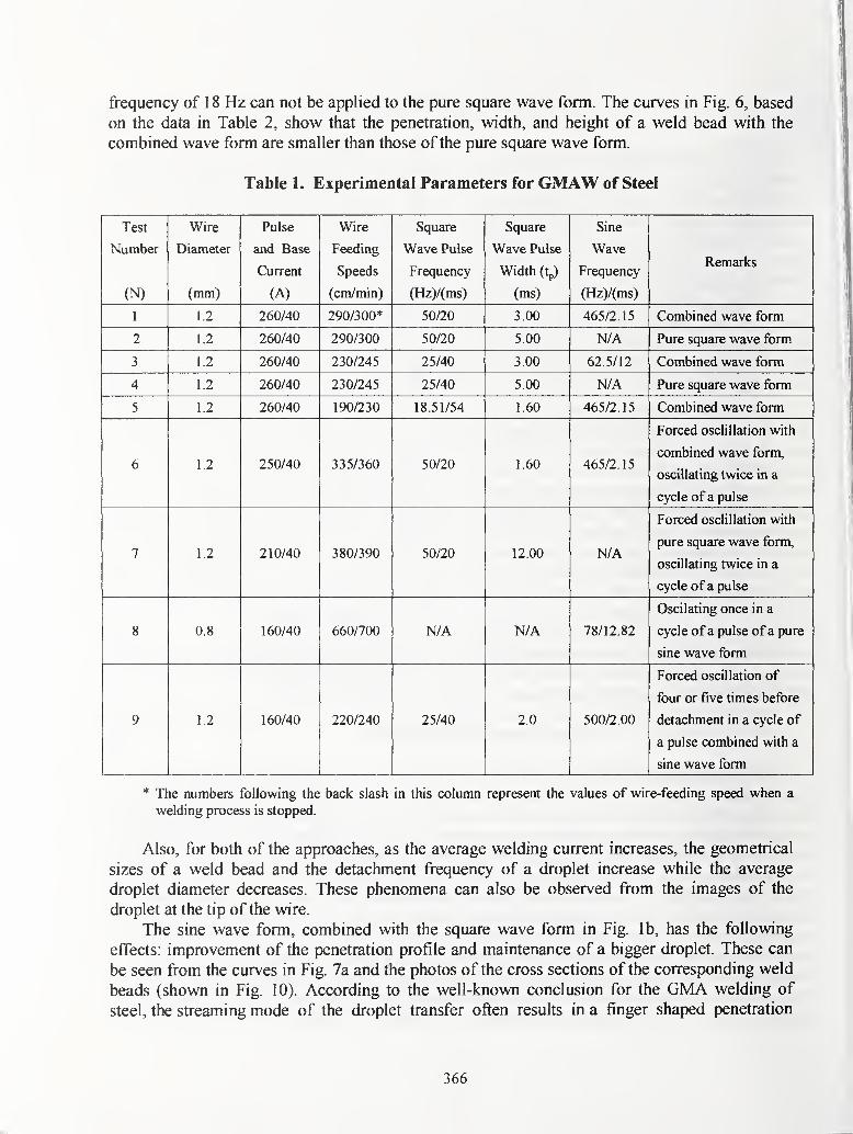
frequency of 1 8 Hz can not be applied to the pure square wave form. The curves in Fig. 6, based

on the data in Table 2, show that the penetration, width, and height of a weld bead with the

combined wave form are smaller than those of the pure square wave form.

Table 1. Experimental Parameters for GMAW of Steel

Test

Number

(N)

Wire

Diameter

(mm)

Pulse

and Base

Current

(A)

Wire

Feeding

Speeds

(cmi/min)

Square

Wave Pulse

Frequency

(rizy/^msj

Square

Wave Pulse

Width (tp)

(ms)

Sine

Wave

Frequency

(rlz;/(ms)

Remarks

1 1.2 260/40 290/300* 50/20 3.00 465/2.15 Combined wave form

2 1.2 260/40 290/300 50/20 5.00 N/A Pure square wave form

3 1.2 260/40 230/245 25/40 3.00 62.5/12 Combined wave form

4 1.2 260/40 230/245 25/40 5.00 N/A Pure square wave form

5 1.2 260/40 190/230 18.51/54 1.60 465/2.15 Combined wave form

6 1.2 250/40 335/360 50/20 1.60 465/2.15

Forced osclillation with

combined wave form,

oscillating twice in a

cycle of a pulse

7 1.2 210/40 380/390 50/20 12.00 N/A

Forced osclillation with

pure square wave form,

oscillating twice in a

cycle of a pulse

8 0.8 160/40 660/700 N/A N/A 78/12.82

Oscilating once in a

cycle of a pulse of a pure

sine wave form

9 1.2 160/40 220/240 25/40 2.0 500/2.00

Forced oscillation of

four or five times before

detachment in a cycle of

a pulse combined with a

sine wave form

* The numbers following the back slash in this column represent the values of wire-feeding speed when a

welding process is stopped.

Also, for both of the approaches, as the average welding current increases, the geometrical

sizes of a weld bead and the detachment frequency of a droplet increase while the average

droplet diameter decreases. These phenomena can also be observed from the images of the

droplet at the tip of the wire.

The sine wave form, combined with the square wave form in Fig. lb, has the following

effects; improvement of the penetration profile and maintenance of a bigger droplet. These can

be seen from the curves in Fig. 7a and the photos of the cross sections of the corresponding weld

beads (shown in Fig. 10). According to the well-known conclusion for the GMA welding of

steel, the streaming mode of the droplet transfer often results in a finger shaped penetration

366

Fig. 2 Images of Droplet Detachment with Frequency of 50 Hz (frame rate: 409 frames/second)

a. combination of square wave form with sine wave form for current control

b. pure square wave form for current control

fiS hi U U h'i f.

I

# 1wWW WWWSi ir

Fig. 3 Images of Droplet Detachment with Frequency of 25 Hz (frame rate: 409 frames/second)

a. combination of square wave form with sine wave form for current control

b. pure square wave form for current control

Ip=260A Ii,=40A %if=190 cm/niiiL

Psqf=18Hz Ptir=l^«nis Prif*4«SHz

12 30.1998

Fig. 4 Images of Droplet Detachment Fig. 5 Photos of Weld Bead with Detachment

with Frequency of 18 Hz (frame rate: Frequency of 18 Hz409 frames/second)

profile, compared with the projected spray transfer mode. So, the projected spray transfer mode

is preferred and widely applied to production. However, it was found in our work that a finger

shaped, deep penetration can also be generated if the detachment frequency in ODPP mode is

above 50 Hz, even though it is not as severe as in the case of streaming mode when the average

367

welding current is below 100 A. When the droplet transfer frequency decreases to 25 Hz, the

penetration profile is much more uniform and shallow using the combined wave-form approach.

The probable reason for this is that the bigger droplet, associated with the applied higher average

welding current and long background time, will bring more heat to the molten pool without

deeper and stronger droplet impingement to the molten pool. The heat convection in the weld

pool may also make the heat inside it more evenly be distributed. From the above results, it can

also be observed that in order to improve the penetration profile, the droplet transfer frequency in

ODPP mode has to be below 25 Hz, which is very crucial to the parts made in the GMAW based

rapid prototyping.

Table 2 Sizes ofWeld Bead, Average Current, and Average Droplet Diameter

Test Penetration Average welding Wire length Diameter

Number depth Width Height current per droplet of the droplet

(N) (mm) (mm) (mm) (A) (mm/d) (mm)

1 0.6858 5.4356 1.6256 97 0.9668 1.014

2 0.7366 5.3594 1.7272 95 0.9668 1.014

3 0.2524 3.9116 1.4224 90 1.5364 1.154

4 0.2686 4.1500 1.6764 84 1.5364 1.154

5 0.2280 3.0480 1.2700 56 1.7235 1.230

6 1.0668 6.0452 1.8288 80 1.1170 1.206

7 1.5240 7.1120 1.7780 142 1.2667 1.110

8 0.9144 6.0452 1.8796 120 1.7600 1.587

9 N/A N/A N/A 58 0.7333 1.166

The random oscillation of the droplet was observed and analyzed mostly in the range of

globular transfer mode where the droplet suspends at the tip of the wire for a comparatively

longer time because the elecfromagnetic force inside the droplet is smaller than the surface

tension [9-11]. This type of oscillation is not controllable and thus not a candidate for droplet

detachment control. A so-called active control for the droplet detachment was developed by

Radovan Kovacevic and his research team at the University of Kentucky using a high frame rate

camera as a vision sensor to detect the vertical coordinate of the droplet along the axis of the

wire [12-13]. This process first experiences a growth period preset in advance to develop a

droplet with a certain size at around 240 A for a 1.2-mm-diameter wire, which is higher than the

transition current. Then the current is cut down to a low level (40 A) to excite a damped droplet

oscillation at the tip of the wire. When the droplet nearly finishes the oscillation of a first cycle

and goes down-wards, a high welding current pulse (higher than 250 A) is applied. Thus, the

inertia generated by the oscillation and the electromagnetic force generated by the high welding

current both act on the droplet to promote it to detach from the tip of the wire. After the above

high current pulse is applied, the background period of a preset time is initiated with a current of

40 A. When the background period terminates, the next cycle repeats the same process.

Actually, in a pulsed GMA welding process with the ODPP mode, the droplet can detach in

the range of either the pulse period or the base period. There is a possibility that the droplet is

forced to detach at the instant of the front edge of the next welding current pulse. Thus, a current

pulse is not only used as a growth period for providing the arc with the heat to melt the wire and

368

EE

c0)a.

aCO0)

5

1

0.90.80.70.60.50.40.30.20.1

0 ;,„„;;

50 60 70 80 90 100Average welding current (A)

a

form a new droplet, but also as a detachment pulse by generating electromagnetic force for the

previous droplet to promote it transfer to the weld pool. To verify this, two approaches of an

open loop control with induced oscillation are examined: pure square wave form and combined

wave form. The images of the electrode-droplet in a pulse cycle of 50 Hz are shown in Fig. 8.

The results show that each droplet will oscillate

twice before it detaches at the instant of the front

edge of the next welding current pulse (verified by

the intensity increase of the arc light from the

images) and that the combined wave form can

generate a more stable droplet transfer process and an

improved penetration profile. For instance, in the Fig.

8b, the first frame shows that the droplet is ready to

detach. After it detaches at the instant of the second

frame, a new droplet forms and moves upward and

downward from frame 2 to frame 6. This is the first

cycle of the oscillation for this new droplet. From

frame 7 to frame 12, the droplet has another cycle of

oscillation, and then detaches at the instant of frame

14. The droplet at the tip of the wire will be forced to

oscillate at this frequency. During the droplet

oscillation, although the heat generated in the acting

period of a sine wave-form current is less than that of

a square pulse with the same magnitude and acting

time as a sine wave pulse, it still continuously melts

the wire. This type of melting effect should be

considered when the dynamic parameters are selected

for the forced multiple oscillations. The droplet

oscillation using pure sine wave form can also been

observed from Fig. 9.

A natural oscillation frequency for a given

droplet depends on its size. When this natural

oscillation frequency equals that of a periodically

varied external force applied on the droplet, a

resonance may occur. In this case, the droplet maydetach if the magnitude of the resonance is high

enough.

50 60 70 80 90 100Average welding current (A)

50 60 70 80 90 100Average welding current (A)

The experiment is designed to verify the

feasibility of a droplet resonance-based detachment

control. The corresponding parameters and the

images of the droplet are given for the experiment

No. 9 in Table 2 and in Fig. 11, respectively. The

wire is melted under the heating of the pulse current

of 160 A to form a certain size droplet, and then the

current is cut down to the base current of 40 A. After

that, a sine wave-form current is applied to the

droplet with the magnitude of 260 A and the

frequency of 500 Hz.

Fig. 6. Geometrical Sizes of the WeldBead versus Average Welding

Current (corresponding to the

experiments of No. 1-5 in

Table 2)

a. weld penetration b. weld bead

width c. weld bead height

• pure square wave form

combined wave form

369

> Average welding current (A) Average welding current (A)

a b

Fig. 7 Droplet Diameter and Detachment Frequency versus Average Welding Current

(for the Experiments of No. 1-5 in Table 2)

a. average droplet diameter b. droplet detachment frequency

• pure square wave form combined wave form

a b

Fig. 8 Images of Forced Droplet Oscillation with Detachment

Frequency of 50 Hz Corresponding to Fig. 11

(frame rate: 606 frames/second)

a. combination of square wave form with sine wave form for current control

b. pure square wave form for current control

This promotes the droplet to

continuously grow as it oscillates. Whenthe droplet detaches, the welding current is

cut down to the base current. At the end of

base current period, a new following cycle

repeats the same process. It can be seen

fi-om Fig. 1 1 that the arc is maintained and

the wire melted from frame I to frame 7.

From frame 8 to frame 12, the droplet

finishes the first cvcle of oscillation.

Fig. 9 Images of Forced Droplet Oscillation

with Detachment Frequency of 75.5 Hz(frame rate: 606 frames/second)

370

b

e f

Fig. 10. Cross Sections of the Weld Bead for the Experiments of No. 1-5 and No. 8

in Table 2

a. combined wave form of 50 Hz b. pure square wave form of 50 Hzc. combined wave form of25 Hz d. pure square wave form of25 Hze. combined wave form of 18 Hz f pure sine wave form of 75 Hz

371

From frame 12 to frame 15, the

droplet makes the second oscillation.

During the time from frame 15 to

frame 18, the droplet oscillates the

third time. The droplet also makes

the fourth oscillation from frame 18

to frame 21, and then detaches at the

instant between frame 22 and frame

23. The frequency of the droplet

oscillation (496 Hz, acquired by

counting the numbers of image

frames and making simple

calculation) is nearly the same as

that of a sine wave form pulse (500

Hz). Compared with the droplet

oscillation, the sine wave-form

current has just two and a half

cycles. Therefore, in this case, the

droplet can oscillate only twice

based on the sine wave-form

frequency and one induced

oscillation resulting from the cutting

down of the current after the square

wave-form pulse.

Fig. 1 1 Images of Droplet Resonance Oscillation

Corresponding to Fig. 15 (frame rate: 595

frames/second)

The fourth oscillation and the detachment of the droplet indicate that the droplet resonance

occurs because ofthe effect ofthe inertia generated by the forced multiple oscillation.

CONCLUSION

Droplet detachment confrol is crucial to control the mass and heat transferred to the parts in

gas metal arc welding process. To maintain a stable welding process, the one droplet per pulse

mode for metal fransfer is recommended. An output current with the shape of a square waveform combined with a sine wave form can widen the operational range of the welding parameters

for one droplet per pulse mode and highly improve the weld penetration profile. To achieve

optimal results, the droplet transfer frequency should be maintained below 25 Hz.

Droplet oscillation can be implemented and controlled in the range of the one droplet per

pulse transfer mode. The pure sine wave form approach can generate one forced droplet

oscillation before its detachment, which is associated with a harmoniously characteristic sound.

The welding current with the pure square wave form can generate two forced droplet

oscillations. The larger number of forced droplet oscillations can be beneficial using the

combination of the square wave-form current with the sine wave-form current with which the

control of the droplet detachment and the regulation ofthe penetration profile can be guaranteed.

372

REFERENCE

[I] Lancaster, J. F., Ed. The Physics of Welding, 2nd ed. Edition. New York, Pergamon Press.

1986.

[2] AWS. Welding Handbook. Vol. 2. American Welding Society, Miami, Fla. 1991

[3] Y.S. Kim and T. W. Eagar. Analysis of Metal Transfer in Gas Metal Arc Welding.

Welding Journal, 6: 269-278. 1993.

[4] L. A. Jones, T. W. Eagar, and J H. Lang. Images of a Steel Electrode in Ar-2%02Shielding during Constant Gas Metal Arc Welding. Welding Journal, 4: 269 to 278. 1998.

[5] Q. L. Wang and P. J. Li. Arc Light Sensing of Droplet Transfer and Its Analysis in Pulsed

GMAW Process. Welding Journal, 11. 458s to 469s. 1997

[6] J. A. Johnson, N. M. Carlson, and H. B. Smartt. Detection of Metal Transfer Mode in

GMAW. Proc. 2nd International Conf on Trends in Welding Res., 5: 377 to 381,

Gatlinburg, Tenn. 1989.

[7] R. B. Madigan, T. P. Quinn, and T. A. Siewert. Sensing Droplet Detachment and Electrode

Extension for Control of Gas Metal Arc Welding. Proc. 3^^^ International Conf on Trends in

Welding Res., 1 1: 999 to 1002, Gatlinburg, Tenn. 1989.

[8] ESAB Group. Size and Shape of the Liquid Droplet at the Molten Tip of an Arc Electrode.

Journal of Physics, 4: 1433 to 1442. 1994.

[9] J. C. Amson. An Analysis of the Gas-shielded Consumable Metal Arc Welding System.

British Welding Journal, 41(4): 232 to 249. 1962.

[10] J. W. Greene. An Analysis of Transfer in Gas-shielded Welding Arcs. Trans. AIEE Part 2,

7:194 to 203. 1960.

[II] J. H. Waszink and L. H. J. Graat. Experiment Investigation of the Forces Acting on a

Droplet ofWeld Metal. Welding Journal, 62(4): 109s to 116s. 1983.

[12] R. Kovacevic, L. G. Er, and Y. M. Zhang. Achieving Projected Spray Based on Excited

Droplet Oscillation. The Second World Congress on Intelligent Manufacturing Progresses

and Systems, Budapest, Hungary. 6: 10 to 13. 1997.

[13] Y. M. Zhang, L. G. Er, and R. Kovacevic. Active Metal Transfer Control by Monitoring

Excited Droplet Oscillation. Welding Journal, 77(9): 388s to 395s. 1998.

[14] Z. Dubon. A Device for Interrupted Electrode Wire Feed during Arc Welding.

Czechoslovakian Priority Certificate No. 116243. 10, 1965.

[15] B. E. Paton et al.. Controlling the Arc Welding Process by Programming the Electrode Wire

Feed Rate. Automatic Welding, 30(1): 1 to 4. 1977.

[16] V. P. Dmitrienko. Calculation of the Speed of Movement of the Electrode Tip during

Welding with Mechanical Control of Metal Transfer. Automatic Welding, 32(2): 1 to 4.

1977.

[17] L. A. Jones, T. W. Eagar, and J. H. Lang. Investigation of Droplet Detachment Control in

Gas Metal Arc Welding. Proceedings of the 3' International Conference on Trends in

Welding Research. Gatlinburg, TN. 6: 1009 to 1013. 1992.

[18] S. Y. Yang. Projected Droplet Transfer Control with Additional Mechanical Forces (AMF)

in MIG/MAG Welding Process. Ph. D. Dissertation, Harbin Institute of Technology. 1998.

373

HIGH PERFORMANCE PARALLEL DIGITAL SIGNAL PROCESSORS APPLIED TOWELDING

D.A. Hartman and G.E. Cook «

ABSTRACT

Increasingly affordable digital signal processors are providing engineers with expanded capabilities

and design flexibility when developing a process monitoring or control system. Microprocessors, and

digital signal processors (DSP) in particular, are narrowing the performance gap between analog- and

software-based implementations of control systems. In addition to bandwidth improvements, micro-

processors afford the engineer with additional benefits, such as environmental invulnerability, repro-

duceability, and adaptability. Finally, a software-based approach allows an engineer to supplement and

enhance new or existing control algorithms with intelligent techniques.

This paper presents the development of a parallel DSP platform for weld process monitoring and

control. Four Texas Instrument's TMS320C40 parallel DSPs are interconnected to provide hard real-time

process monitoring and control. A Pentium class PC serves as the host computer for the parallel-based

platform. Real-time control, on-line process data visualization (time and frequency), data logging, and

dynamic reconfigurability are just a few of the benefits available in this system.

An application involving the control of penetration in the gas tungsten arc (GTA) welding process is

discussed. Intelligent methods, such as neural networks and fuzzy logic, applied to control and signal

detection are presented. The system provides an excellent development, test, and verification platform

prior to implementing on an embedded processor.

INTRODUCTION

Digital signal processing continues to extend the functionality and capabilities of software-based control

systems. Although it may not be obvious why it is desirable to migrate from analog-based control applica-

tions to software-based systems, consider the following advantages:

• Environmentally invulnerable: In general, analog circuitry is subject to behavior variations depending

on environmental factors, such as temperature. Digital systems, on the other hand, are essentially

immune to such environmental effects.

• Reproducible: Analog circuitry depends on the combination of interconnected components each of

which deviates to some degree from its nominal behavior. Consequently, expensive and hard to find

*This work was supported, in part, by the American Welding Society Foundation under a graduate research fellowship, 1995-

1998. The author gratefully acknowledges an AWS Nashville section gift from Kirby Welding Supply.

^D.A. Hartman is a technical staff member of the Metallurgy Group in the Materials Science and Technology Division of Los

Alamos National Laboratory, P.O. Box 1663, Mail Stop G770, Los Alamos, New Mexico 87545. E-mail: hartman@lanl.gov.

*^G.E. Cook is with the Welding Automation Laboratory at Vanderbilt University, Electrical and Computer Engineering Depart-

ment, Box 1824-B, Nashville, Tennessee, 37235.

374

components, such as precision resistors, are necessary if the design engineer must duplicate an analog-

based circuit to within very tight tolerances.

• Adaptable: Modifying the characteristics of an analog circuit, such as a filter, is not easily accom-

plished. Implementing a filter digitally, however, using a microprocessor enables the engineer to

quickly and easily change the characteristics of the system.

Analog-based systems will always exceed their digital counterparts in terms of speed. However, micropro-

cessors, and digital signal processors specifically, are narrowing the performance gap such that more and

more applications are easily and effectively accomplished in software.

This paper presents the development of a parallel digital signal processing system for weld process moni-

toring and control. Information regarding the difficulty of automating the welding process, the objectives

for feedback control of the welding process, and intelligent techniques that can help overcome some of the

difficulties is presented in the Background section. A brief introduction into parallel hardware architectures

is then provided. Finally, the framework for and the implementation of a distributed GTAW penetration

control system is presented.

BACKGROUND

Manual vs. Automated Welding

In a typical manual welding situation, a human operator can observe the sights and sounds emanating from

the welding process, assess the weld pool with respect to its desired state, and make minor changes in the

weld parameters under his immediate control (weld current, voltage, travel speed and electrode orientation

with respect to the joint path) in an effort to maintain the desired state of the weld. Adapting these sight

and sound inputs to machine control and making the appropriate decisions is a challenging task. The human

operator makes decisions from his inputs based primarily on past learned experience. For instance, when a

weld is performed in the vertical position a seasoned welder knows that when the weld pool gets too large the

liquid will run out of the pool leaving a crater. Acquiring the skill and knowledge to perform complicated

tasks, such as full-penetration vertical-up or overhead welds, are the result of countless hours of practice

through acquired rule of thumb techniques. Explaining this knowledge verbally involving precise visual

cues to another human being or to a knowledge engineer is practically impossible.

Attempting to emulate the flexibility and adaptability of the human welder though mechanization is a non-

trivial task. Providing a weld controller with sight and sound input is straightforward; however, making

appropriate decisions from these inputs concerning control of the weld is not. In an attempt to circumvent

a machine's lack of human intuition and decision-making capabilities, in-process welding control systems

have incorporated feedback of welding characteristics which are unobservable to humans, such as thermog-

raphy or ultrasonics, and utilized sophisticated control algorithms that involve accurate sensing feedback in

an effort to maintain a tight tolerance on the welding process conditions.

Ultimately, most welding automation techniques did not evolve from traditional manual methods. Instead

control engineers have applied conventional quantitative techniques of system analysis through the use of

difference, differential, and integral equations to model and control the mechanized aspects of welding.

Such an approach requires mathematical formalism and formal truths.

Applications involving through-the-arc sensing, such as automatic voltage control and seam tracking, have

been met with a great amount of success such that they have found their way into commercial use. These

375

systems, arc voltage control and seam tracking in particular, have been successful for a variety of reasons.

Clearly, the sensing technique is low cost, reliable, and nonintrusive. Their success, however, is directly

correlated to their performance. Both of these systems are mechanistic systems, that is, they are physical

systems that are governed, in this case, by electromagnetic laws. These laws are well understood and are

therefore strategically and efficiently applied to both the sensor feedback information and to the control laws

within the closed-loop feedback path.

More complex systems such as bead geometry or penetration control are well understood phenomena that

can be accurately modeled from a theoretical standpoint; however, there are simply too many parameters

involved in the models that require precise process feedback information that in-process implementation is

impractical. As the complexity of the system increases the ability for the control technique to make precise

and significant statements about its behavior decreases. Conventional quantitative techniques are inherently

unsuitable for such complex systems.

The ability of a skilled human welder to assess and control bead geometry, for example, is not due to

a fundamental understanding of the laws of physics. Instead of applying a mechanistic approach to the

control of the weld pool, a seasoned welder applies a more humanistic approach in which the feedback

information is not based on precision and formal truths but rather on imprecision and partial truths. Clearly,

fully automated welding robots will require a marriage between mechanistic approaches for phenomena

that is physically well understood and mathematically feasible for both sensors and control algorithms and

humanistic approaches for phenomena that are otherwise infeasible to implement using conventional control

techniques due to the required complexity resulting in a diminished accuracy.

Feedback Control of Fusion Welding

The objectives for feedback control of fusion welding are to continuously sense and control (1) the placement

of the heat source with respect to the joint, (2) the geometry of the weld reinforcement and fusion zone, (3)

the mechanical properties of the completed weld, (4) the microstructural evolution during solidification and

cooling, and (5) the discontinuity formation (Ref. 1). The first objective, more commonly known as seam

or joint tracking, is a well established and commercially successful adaptation to the mechanized fusion

process (Refs. 2-5). Difficulties in sensing and controlling the geometry of the weld reinforcement and

fusion zone area is an ongoing research topic (Ref. 6). Furthermore, regulating the geometrical properties

of the welded joint will, in turn, influence the mechanical properties of the joint. Sensing and controlling

the mechanical properties and the microstructure, such as centerline cooling rate and the heat affected zone,

are topics of current, albeit relatively new, research interest (Refs. 7-9). Finally, the on-line identification of

discontinuities, such as porosity and incomplete sidewall fusion, have been investigated in (Refs. 10-12).

The replacement of the human operator by a welding robot is particularly susceptible in its ability to handle

process variations and disturbances. The flexibility and judgement inherent in a human welder has yet to be

transferred successfully to a mechanical system. Nevertheless, techniques such as neural networks, fuzzy

logic, expert systems, and genetic algorithms; multiple feedback sensing; and distributed, autonomous, and

hierarchical control coupled with conventional control methods are the first step in an attempt to mimic

human intuition and capabilities.

Intelligent Techniques for the Control of Complex Systems

Although intelligent techniques have been successfully demonstrated to effectively replace and, in certain

cases, even exceed conventional control methods, intelligent techniques can, more importantly, complement,

376

Modeling Techniques

Fuzzy vs. Neural

Figure 1 : Fuzzy or neural modeling techniques should be chosen depending on what type of knowledge is

available about the process.

enhance, and extend conventional control methods through the use of supervisory agents (Refs. 13-16) and

through the use of hierarchical (Refs. 17-19), distributed (Refs. 20,21), and autonomous (Refs. 22,23) con-

trol methods. Processes that (1) were too complex to understand or represent simply, (2) contained large

unpredictable environmental disturbances, or (3) involved nonlinear, time varying, or stochastic character-

istics are now being approached with intelligent control methods in a practical and viable manner. Fur-

thermore, unlike conventional methods which rely on mechanistic approaches, intelligent techniques can

emulate humanistic approaches in an attempt to control non-deterministic processes.

Although other equally effective intelligent techniques are available, this paper will limit its focus to the

application of fuzzy and neural network methods for the control of a complex process, and specifically the

control of the depth of penetration in gas tungsten arc welding (GTAW). Choosing between a neural or

fuzzy modeling technique should be based on what type of knowledge is available about the process (see

Figure 1). Questions, such as, "Is the process well understood and the inputs and outputs of the system

hard to quantify?" or "Is the process ill-defined and the inputs and outputs of the system precise and easily

quantifiable?", must be addressed prior to committing to an intelligent technique.

In general, fuzzy modeling techniques excel when an intuition-based, or humanistic, understanding of the

process is available. Consequently, precise information regarding the process's inputs and outputs is not

required. Fuzzy logic attempts to solve a problem in the same manner that a human might typically solve

a problem: linguistically using rules of thumb. That is, when a human is asked to explain the solution to

certain types of problems they (1) quantify the information used to make decisions in terms of imprecise

values or categories and (2) they justify their actions in terms of if-then rules. For example, the amount of

pressure that a person applies to the brakes of a car while approaching a stop sign at an intersection is based

on information such as speed, distance, visibility, and road traction. Instead of mapping exact values, such as

45 MPH and 72.5 feet to speed and distance, respectively, in order to determine the brake pressure a human

applies imprecise concepts such as "fast" or "slow", "near" or "far", "clear" or "foggy", and "good" or "bad"

to quantify speed, distance, visibility, and road traction respectively. Furthermore, concepts such as visibility

and road traction which are extremely hard to quantify precisely are nonetheless critical to ensuring that the

car will stop at the proper location. Conventional control techniques that are typically applied to computer

decision making processes would inevitably fall short in achieving a robust design due to the inability to

377

Network Archifecfure

feed-forward:

' single or multilayer perceptron or

• radial basis function networl<.

recurrent:

' competitive network,

• Kohenen's Self Organizing Map,

• Hopfieid network, or

• ART models.

Learning Paradigm

unsupervised,

supervised, or

Itybrid.

Error Correction Rule

error correction,

Boltzmann,

Hebbian, or

competitive.

Figure 2: Commonly used methods for network architecture, learning paradigm, and error correction rules.

formulate an exact mathematical relationship for brake pressure involving all the necessary variables.

Neural networks, on the other hand, are well adept at mapping the input-output relationships of a process

when the process is not well understood or too complex to implement using an analytical solution. Unlike

fuzzy logic which employs ambiguity, a neural network requires precise values for both its input and its

output nodes. Developing a neural network involves selecting a network architecture, a learning paradigm,

and an error correction rule. Figure 2 illustrates some of the more commonly used methods for each of

these selections. Clearly, extensive knowledge of the problem is required to in order to match the problem

with the architecture, the learning paradigm, and the error correction mechanism (Ref. 24). Furthermore,

constructing a training set that appropriately represents the problem to be modeled can be rather challenging,

if not impossible, to obtain. Finally, ensuring that the training data and the training mechanism produce a

network mapping capable of generalizing rather than memorizing is critical to the successful application for

modeling and control.

When compared to other modeling methodologies, neural networks have certain drawbacks as well as ad-

vantages. The most notable drawback is the lack of comprehension of the physics of the process. Relating

the qualitative effects of the network structure or parameters to the process parameters is usually impossible.

On the other hand, most physical models resort to substantial simplifications of the process and therefore

trade accuracy for comprehensibility. The advantages of neural models include relative accuracy and gen-

erality. If the training data for a neural network is general enough, spanning the entire ranges of process

parameters, the resulting model will capture the complexion of the process, including nonlinearities and

parameter cross couplings, over the same ranges. Model development is much simpler than for most other

models. Instead of theoretical analysis and development for a new model the neural network tailors itself

to the training data. Finally, the neural network can calculate its result relatively fast, as the input data is

propagated once through the network in the application mode.

Microprocessor-Based Monitoring and Control

When high speed, deterministic control is required most control engineers resort to a programmable logic

controller (PLC). PLCs fit a very large class of control problems very well; in particular, PLCs excel at

mechanistic processes, such as machine control. Most importantly, the simple and specialized nature of a

PLC enables it to perform most tasks effectively, cheaply, and reliably.

A traditional PLC-based design is inappropriate when developing a control system for a complex, non-

deterministic process, such as those found in welding. A microprocessor-based development environment,

on the other hand, presents an ideal platform for the investigation and deployment of modeling and control

378

Processor Core

1 Address Bus {

1 J

Memory

Processor Core

J 1

IDota BusT

Memory A Memory B

(a) Von Neumanin memory architecture. (b) Harvard memory architecture.

Figure 3: Microprocessor architectures.

techniques that extend beyond conventional control-based methods. In addition to providing an operator

interface in which valuable process information can be viewed in real time, microprocessor-based control

environments can provide software reconfigurability enabling different control strategies to be created, de-

bugged, and evaluated.

PARALLELISM AND HIGH-PERFORMANCE COMPUTING

Parallelism can be architecturally characterized as a spectrum of different hardware configurations or de-

signs involving, in one extreme, distributed network computing and, in the other extreme, simple bit-serial

multiprocessing. Distributed network computing involves the loose interconnection of isolated and sepa-

rated computing systems through a communication transport mechanism, such as Ethernet or, more recently,

asynchronous transfer mode (ATM) networks. At the other extreme, the bit-serial processor, although of lit-

tle value by itself, when coupled together into upwards of tens of thousands of processing elements (PEs)

can achieve massive processing power (Ref. 25).

An intermediate approach to parallelism, and the path chosen for this research, involves using a micro-

processor device as a building block with other microprocessor devices to construct a parallel computing

network. Rather than waiting on a single processor to accomplish a set of tasks in series, we can distribute

these tasks to a number of different processors. Each processor can execute its operations concurrently.

Unlike a uniprocessor implementation, this results in a more accurate reflection of the real world in which

many activities, or "processes", are happening concurrently.

Introduced in the late 1980's, the first commercially successful, general-purpose microprocessor that ad-

dressed the issues of parallel processing (communication, scheduling, scaling) was the Inmos Transputer

(Ref. 26). The Transputer chip is a single-chip computer with a processor, local memory, and communi-

cation link interfaces. This general purpose processor (GPP) uses a von Neumann architecture in which

the central processor is connected by a single data bus to memory (see Figure 3(a)). Concurrency within

the single processor is handled by a processor scheduler implemented into the chip's microcode for fast

379

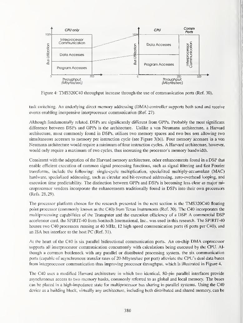
100%

CPU only CPU Comm

IntGrprocGSSorCommunication

'Jization

Data Accesses

interprocessor

Communication

Data Accesses

Program AccessesProgram Accesses

CQ

k.

Tiirougtiput(Mbytes/sec)

Tlirougliput(Mbytes/sec)

320

Figure 4: TMS320C40 throughput increase through the use of communication ports (Ref. 30).

task switching. An underlying direct memory addressing (DMA) controller supports both send and receive

events enabling inexpensive interprocessor communication (Ref. 27).

Although fundamentally related, DSPs are significantly different from GPPs. Probably the most significant

difference between DSPs and GPPs is the architecture. Unlike a von Neumann architecture, a Harvard

architecture, most commonly found in DSPs, utilizes two memory spaces and two bus sets allowing two

simultaneous accesses to memory per instruction cycle (see Figure 3(b)). Four memory accesses in a von

Neumann architecture would require a minimum of four instruction cycles. A Harvard architecture, however,

would only require a maximum of two cycles, thus increasing the processor's memory bandwidth.

Consistent with the adaptation of the Harvard memory architecture, other enhancements found in a DSP that

enable efficient execution of common signal processing functions, such as signal filtering and fast Fourier

transforms, include the following: single-cycle multiplication, specialized multiply-accumulate (MAC)

hardware, specialized addressing, such as circular and bit-reversed addressing, zero-overhead looping, and

execution time predictability. The distinction between GPPs and DSPs is becoming less clear as major mi-

croprocessor vendors incorporate the enhancements traditionally found in DSPs into their own processors

(Refs. 28,29).

The processor platform chosen for the research presented in the next section is the TMS320C40 floating

point processor (commonly known as the C40) from Texas Instruments (Ref. 30). The C40 incorporates the

multiprocessing capabilities of the Transputer and the execution efficiency of a DSP. A commercial DSPaccelerator card, the SPIRIT-40 from Sonitech International, Inc., was used in this research. The SPIRIT-40

houses two C40 processors running at 40 MHz, 12 high speed communication ports (6 ports per C40), and

an ISA bus interface to the host PC (Ref. 31).

At the heart of the C40 is six parallel bidirectional communication ports. An on-chip DMA coprocessor

supports all interprocessor communication concurrently with calculations being executed by the CPU. Al-

though a common bottleneck with any parallel or distributed processing system, the six communication

ports (capable of asynchronous transfer rates of 20-Mbytes/sec per port) alleviate the CPU's dual data buses

from interprocessor communication thus improving processor throughput, which is illustrated in Figure 4.

The C40 uses a modified Harvard architecture in which two identical, 80-pin parallel interfaces provide

asynchronous access to two memory banks, commonly referred to as global and local memory. The buses

can be placed in a high-impedance state for multiprocessor bus sharing in parallel systems. Using the C40

device as a building block, virtually any architecture, including both distributed and shared memory, can be

380

(Processor) [Processor)

CQcrie 1 icoerce

Main Memory I/O

(a) Centralized shared memory. (b) Distributed memory.

Figure 5: Memory architectures.

defined to solve computationally intensive problems (Ref. 32). Any number of C40 processors can be linked

together through the communication ports or the multi-port data bus interfaces thereby enabling an engineer

to custom tailor the size of the processing system and its level of performance.

The interconnection of microprocessors can fall into two classes depending on the memory organization and

the interconnect strategy (Ref. 33). What constitutes a small or large number of processors will inevitably

change over time. Therefore, parallel machines are typically referred to by their memory organization:

shared or distributed.

A centralized shared-memory architecture (see Figure 5(a)) can be classified in many ways. At its most basic

level, a centralized shared-memory architecture involves multiple processors^ sharing a single centralized

memory via a bus. However, such an architecture is not restricted to public memory rather it may also

involve some public and some private memory. Because a single main memory must share access to a group

of processors, the scale of a centralized shared-memory parallel machine is limited.

A distributed-memory architecture (see Figure 5(b)) can support larger processor counts by physically dis-

tributing the memory among the processors. Memory bandwidth increases and the latency between accesses

decreases because each processor has access to its own private memory. Transmitting data between proces-

sors is more complex and has a higher latency in a distributed memory architecture because the processors

no longer share a single centralized memory. Consequently, the key disadvantage for a distributed-memory

architecture is interprocessor communication.

Although a vast array of memory configurations and system architectures using the C40 can be configured

to solve virtually any kind of computationally intensive problem, the parallel architecture chosen for this

research was restricted to a distributed-memory architecture which is hard-wired into SPIRIT-40. In partic-

ular, the SPIRIT-40 houses two C40s (labeled 0 and 1) that are hardwired through communication ports 3

and 0, respectively. Two single cycle dual-access RAM blocks (global and local) are accessible privately to

each processor. The global RAM block is also accessible to the host PC through the ISA bus. A functional

block diagram detailing the configuration is provided in Figure 6.

'Most computer scientists draw a distinction between multiprocessors and multicomputers. A parallel machine consists of

multiprocessors if the replication of processors within the parallel framework does not alter the relationship between the processor(s)

and other components, such as memory or I/O. A multicomputer system consists of individual, whole microprocessors (processor

and memory) in which some form of communication network must be added to exchange data.

381

Global RAM

SPIRIT-40Block Diagram

ISA InterfaceLogic

( PC Host ISA Bus )

Figure 6: Simplified SPIRIT-40 block diagram.

WELD POOL OSCILLATION MONITORING AND PENETRATION CONTROL

Weld pool oscillation sensing was first proposed by Hardt, et al. (Ref. 34) as a method of sensing pool

geometry, and hence penetration, for closed-loop feedback control of the depth of penetration. The funda-

mental concept is based on the fluid dynamics of the molten region in the weldment which is constrained

by a solid container (i.e., the unmelted workpiece) and by surface tension forces. External excitation of the

weld puddle's surface will result in pool oscillations that are a function of (1) the external force, (2) the

properties of the molten region, (3) the surface tension, and (4) the shape of the container.

Implementing penetration control using pool oscillation sensing involves (1) excitation, (2) detection, and

(3) control. Excitation of the weld puddle is most commonly initiated through the modulation of the welding

current which thereby induces a change in the arc pressure on the pool's surface. Detection of the pool's

fundamental mode of vibration requires (1) sensing the fluctuations in either the arc voltage or arc light and

(2) extracting the fundamental mode of oscillation from the sensed fluctuations. Finally, control of the total

heat input, either through current or travel speed or both, into the the workpiece can take on many differ-

ent control algorithms involving either traditional, adaptive, or intelligent techniques or some combination

thereof (Ref. 6).

System Objectives

The successful implementation of the closed-loop, single input (weld pool oscillation frequency), single

output (welding current) controller requires not only the implementation of each of these functionally in-

dependent components, but also the ability for each of the components to cooperatively interact with one

another. The system was modeled after work performed by Andersen in (Ref. 35). The following three

items detail the requirements set forth by Andersen:

• Excitation: An improved method for inducing the molten weld pool into motion using a phase-locked

loop (PLL) technique was developed by Andersen. The synchronized pulsing scheme provided a

reliable means of sustaining weld pool vibration without introducing surface wave interference or

compromising the response time of the controller. Although the design was sufficient for preliminary

feasibility studies, a more robust excitation system was needed to accommodate changes in pool

frequency, harmonic mode competition, and chaotic surface wave interaction. A software-based,

dynamically reconfigurable, PLL was implemented enabling superior tracking performance over a

wider range of resonant frequency conditions (Ref 36).

382

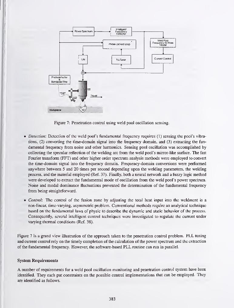
Figure 7: Penetration control using weld pool oscillation sensing.

• Detection: Detection of the weld pool's fundamental frequency requires (1) sensing the pool's vibra-

tions, (2) converting the time-domain signal into the frequency domain, and (3) extracting the fun-

damental frequency from noise and other harmonics. Sensing pool oscillation was accomplished by

collecting the specular reflection of the welding arc from the weld pool's mirror-like surface. The fast

Fourier transform (FFT) and other higher order spectrum analysis methods were employed to convert

the time-domain signal into the frequency domain. Frequency-domain conversions were performed

anywhere between 5 and 20 times per second depending upon the welding parameters, the welding

process, and the material employed (Ref. 37). Finally, both a neural network and a fuzzy logic method

were developed to extract the fundamental mode of oscillation from the weld pool's power spectrum.

Noise and modal dominance fluctuations prevented the determination of the fundamental frequency

from being straightforward.

• Control: The control of the fusion zone by adjusting the total heat input into the weldment is a

non-linear, time-varying, asymmetric problem. Conventional methods require an analytical technique

based on the fundamental laws of physic to describe the dynamic and static behavior of the process.

Consequently, several intelligent control techniques were investigated to regulate the current under

varying thermal conditions (Ref. 38).

Figure 7 is a grand view illustration of the approach taken to the penetration control problem. PLL tuning

and current control rely on the timely completion of the calculation of the power spectrum and the extraction

of the fundamental frequency. However, the software-based PLL routine can run in parallel.

System Requirements

A number of requirements for a weld pool oscillation monitoring and penetration control system have been

identified. They each put constraints on the possible control implementations that can be employed. They

are identified as follows.

383

• Extensibility: The system should evolve as the researcher gains additional insight into and knowledge

of the physical process. Therefore, modifications and improvements to the system throughout the

development cycle can be expected. Furthermore, the system should be capable of hosting a variety

of different detection and control algorithms. Extensibility can be facilitated through careful planning

and modular design.

• Speed: The system must be fast. The reaction time of a typical GTAW process requires that the

system respond within a 10 Hz frequency window (Refs. 1,39). More importantly, power spectrums,

intelligent frequency detection, current control, and phase-locked loop activities all must be performed

within this window.

• Visual Feedback: A thorough understanding of the physical process is essential in developing an

accurate, responsive, and reliable control system. Although an extensive amount of research has been

conducted in the area of weld pool oscillation and penetration control there are still unresolved issues.

In particular, Andersen notes that the PLL circuit fails to perform adequately during the transition from

partial to full penetration. Real-time observation of the physical process through time and frequency-

based analysis of the feedback signals can provide insight that off-line viewing of the data might

otherwise fail to uncover.

• Reliability and Fault Tolerance: The system must operate in a manufacturing environment.

• Safety: The system must be safe. The welding operator must be able to manually override any process

.parameters or controller decisions. Consequently, the controller's interface must provide the operator

with intimate details of the process and control information.

• Cost: The system must be economically feasible.

Achieving real-time monitoring and control in addition to fulfilling the previously mentioned requirements

must involve a combination of hardware and software components. A parallel digital signal processor plat-

form built around the Texas Instrument's TMS320C40 (C40) processor was used to facilitate modularity,

hence extensibility, and to provide the response time, hence speed, necessary from a GTA welding control

system.

Rather than relying on one serial processor to handle all of the operations of each component within our

system, we can distribute the operations to a number of different processors. Therefore, using a modular

design approach in conjunction with a parallel microprocessor environment enables the researcher to add

and subtract components from the system without disrupting the entire system as a whole. Consequently, the

development process can be naturally decomposed into a variety of functional components. Each component

can be tested and verified to ensure both accuracy and reliability, hence ensuring a robust system.

An Intel-based Pentium computer was used to host the graphical user interface (GUI) necessary for the

welding operator. The interface enables real-time display (time and frequency) of process parameters and

feedback signals. Most importantly, the GUI contains numerous controls which allow the operator to man-

ually control and override (if necessary) any process parameters or control variables.

Parallel DSP Platform

Table 1 summarizes the actions required, the methods employed, and the response time objectives needed

in order to implement the controller. In addition to the functional components listed in Table 1, the parallel

384

Table 1: Real-time control actions for penetration control.

Requirement Method Employed Response Time

Excitation Software-based PLL 400 - 2000 HzOn-line tuning of the PLL 5 - 20 Hz

Detection FFT or other spectrum analysis method 5 - 20 HzExtracting the fundamental frequency 5 - 20 Hz

Control Fuzzy or neural control method 5 - 20 Hz

DSP platform must be able to interface with a data acquisition card for I/O and a personal computer (PC)

for data logging, operator interface, and data visualization. In addition to real-time data display, the welding

engineer must be able to manually override all computer controlled welding operations.

Clearly, the requirements imply very high computational costs. Consequently, a single processor imple-

mentation would be infeasible. Therefore, in order to guarantee a system-wide, real-time response from the

controller the tasks were distributed onto separate microprocessors.

Two SPIRIT-40 boards were used in this research providing a total of four (4) C40s. The decomposition

of the problem was therefore limited to only four DSP processors and one host (Intel Pentium) processor.

Since shared memory only exists between the host PC and a C40, a message passing dichotomy was used

to exchange information between the DSP processors.

The parallel machine design was based on a collection of loosely-coupled processes. The processes are

therefore statically bound to a processor at compile-time. Consequently, parallelization was achieved using a

functional decomposition of the problem (see Figure 8). The communication ports were hard-wired between

C40s to facilitate communication between the processes.

Although a loosely coupled system is generally more difficult in ensuring optimal throughput of the system

(Ref. 40), the primary objective in the design of the system was performance. Other factors such as maxi-

mizing processor utilization, cost, and programmability are important, however, they were not the primary

objective. Therefore, in order to guarantee a real-time response the tasks were distributed across the four

DSP processors in such a manner to ensure that all processing take place within some specified amount

of time at every instance. Figure 8 illustrates the functional decomposition of the problem taken in this

research.

Ultimately, the system performance as a whole depends on the timely completion of each individual task.

Due to the sequential nature of the problem, any shortcoming in performance of an individual task (i.e.

decreased response time) will inevitably result in deteriorated system performance as a whole. Therefore,

careful attention was taken in determining the required CPU time necessary for completing each task.

PC Host Interface

Due to the nondeterministic nature of the welding process, the asymmetric behavior of the heat transfer

characteristics, and the chaotic interaction of the surface waves of the molten weld pool a PC-based inter-

face, capable of real-time display of the process's measurable variables, was deemed necessary. On-line

interrogation of most aspects of the penetration control system provided a debugging environment for the

excitation, detection, and control algorithms of the system. Although off-line (or post process) inspection

of the data is necessary for sufficiently validating the reliability and stability of the control system, on-line

process monitoring enabled the control engineer to not only watch the process data but to correlate it with

385

smn-40 r spim-46

Base address: 0x031 Oh ii

Base oddress: Ox0300h

Global RAM: 256 Kbytei j

Global RAM: 1Mbyte

Local RAM: 256 Kbyte ii

Local RAM: 1 Mbyte

Figure 8: Interprocessor communication layout,

the sights and sounds emanating from the process.

UnUke a deterministic control system in which an analytical model is available, an intelligent control tech-

nique relies on either extensive training data, such as a neural network, or human-based intuition, such as a

fuzzy logic approach, in order to derive a model. The PC-based interface facilitated this need by (1) being

capable of storing large amounts of data and (2) serving as a learning tool for the development of human

insight into the complex nature of the process.

Figure 9 is a typical screen capture during a penetration control welding experiment. Both time- and

frequency-domain information of all the measurable process variables can be displayed in real-time. Most

importantly, the control engineer can change different parameters of the process, such as the welding current,

pulse frequency, travel speed, etc., and watch their effect upon the process. Experimenting in this manner

can enable one to extend their understanding of the process beyond a traditional model-based understanding

that one might obtain strictly through a mathematical presentation of the process.

Figures 10(a) through 10(f) illustrate the different control views available to the operator. The fuzzy logic

control (FLC) view and the FLC tuner view (see Figures 10(a) and 10(b), respectively) enable the operator

to change the controller's set-point, gain, etc. and compare the overall performance of the controller relative

to its desired performance. The PC interface also empowers the operator with control over the synchronized

pulsing capabilities (see Figure 10(c)). Presented in Figure 10(d), manually changing the PLL's configura-

tion can be performed on-line. Finally, both the frequency-to-mass model and the fundamental frequency

detection method can be modified on-line (see Figures 10(e) and 10(f), respectively).

CONCLUSIONS

The advent of microprocessors and PC-based control environments has enabled engineers in all disciplines

to employ control methods that extend beyond those of conventional-based control. Intelligent techniques,

such as fuzzy logic, neural networks, etc., can provide an engineer with additional tools to tackle complex

processes that can not be represented in a tractable and analytical fashion. Furthermore, intelligent control

methodologies, such as hierarchical, distributed, and autonomous control, can complement and enhance,

386

Figure 9: Penetration control main window.

rather than replace, conventional-based control algorithms in an attempt to improve the robustness and

dynamic range that a controller can perform within.

387

K'Welding Conliol

Computai Contra)

f" ON OFF

Background Cutrant: 2G9 A Mawran Curent 25Q 0 A

-7I

CuionCooliol |pv(s»)aupu| WeWModd] Mode Daieclion|Fl£Ti«i| ConflarttiLiJ

r OK OFF

Mods 1 Fiequency- 0 0 Hz

FFT Souoi Opdcai Piobs I

nedFiKuwcy 450 Hi MmCurertChjuiga ii

Chance wi Ema. de; Ch^njw h Cuient. (Jc

m Welding Conlfol

Compute) Conboi

r- ON OFF

BackgiDund Curientij

MawmumCufent:

Cunent Conbol [ Piised Oupu | WeW Mo<W j Mode Oet«cbon L50i™| Constant EjJjJ

r OH OFF

P Retponte time (rise «id fait 14

OwarviurvlerthootlS:)

StMdy ital© ott ov. un pt}:

r* Setting time. Jtl

"0.0000

Desired

5OQOO"

~ o.oodb" aisbo

; 0.0000 aoooo ai5tio

VwT

Fte$«tGonMaliH DcHsnloedGanMatiK

(a) (b)

pWelding Conliol

Ccmputaj Conbol

r ON OFF

BacJ^yound CuirenIij J

r ON

P SirchiDrizDdPiiwig r Inldlgeni PUiku

Pojk Curat '

100,0 AJj

p PdteWldlh: 0 002515 »ec

• Puis« Fioquenc?.i 60 0 Hz -^j r DutyC/cle 150831 X d

P AouolFre.^. 7.0 Hi -^j dP BkickWIdih 'OCOSOOO sec. -fj F Mecti Ptiajo 5hft I1O0 deg HP OftedAnfi 19 77 J ,

r ElecPhassSMt 0.0 des

.,2^111.. ill,

iiiil

Welding Control

BackgtDU^ Current:

Computer Contjol

r ON OFF

WeWModell Mode Oeteotion]aCIunoil Con«t»nt EaJtaliiiil rWI-Xa<fiouaiin| Mr «

|>

OesCT?)tiDn 1 Unit 1 VariaUeName VA» 1-

Consider No«se' Y/N ConsKletNcwe 0

Cente< Irequercy (mm] 200000e^1Center frequency |ma«) IHzI _w0_maj< l.OOOOOe.002

Dempr^laclOf ri/a z 7.00000»ail

Lock lenge |H!| wL 1 OOOOOe^ —

1

TiansrT«55>on BW m Bl QOOOOOe^OOON<xso BW IHzi BL aoooooa^ooo

SNR ot the rpul signal n/a SNR. Z00000e>000

SNR ot the loop n/a SNRL 400000a>000

Fiequeixji langc Irran) |H!| w2 mn OOOOOOe^OOO

Frequercy range |maj<| (Hil _»2_max 0000000*000 »

Racelcti*t«PU.Pai«ft(

R netLPFOiipul HejelPaPaiam(

(c) (d)

PWeldtng Conliol

Computet Conttot

<" ON OFF

Backflrot«JCij«ent: > 269 A -f| Mawnun Cuient 250 0 A -yj

Cment ControlIPiisedOutotl f^eid Modell[ ModeOetedionl aCTi»iai| ComiartEjjLiJ

ModdRotatkmshps

Modal Mode 2 Mode 3

IHzl" SdO" ' 970 " -rj 123.1 -rj

M1M2 M1M3 M2M3

: 1940 " " Z4S3" -jj ^ ' ^69 -^j

SaveI

Reset

n/a

Oetoclion Methwfe

r Wi«*wedSeat*

P Fuz^ Logic

r Meual rietnok

Ftoqoenrgr Detection Re«ukl

Save 1 Retat

Corr^tieiCortiot

ON <^ OFF

Batiground Current 26.9 ^i^j Ma»r*wi&^ent: 2^Ai^

Cunent ControlIPiJjedOulW

IWeld Model ;

"Wo<feT?ie<arr||FIX Tuw I

ConstantEjUr

SvvdQueli^

Reset Fuztjr Er^jinaj

Model Mode2 Mode3

Frequerxy: 0 0 1 tto i 0.0"

ConHdence: " 00 ] do !^00

(e) (f)

Figure 10: Penetration control interface.

388

References

[1] G.E. Cook, K. Andersen, and R.J. Bamett. Feedback and adaptive control in welding. In S.A. David

and J.M. Vitek, editors. Recent Trends in Welding Science and Technology, Proceedings of the 2nd In-

ternational Conference on Trends in Welding Research, pages 891-903, Gatlinburg, Tennessee, USA,May 14-18, 1989. ASM International.

[2] G.E. Cook, G.M. Merrick, U.A. Schneider, and W.R. Rosenberger. Weld tracking/electric arc sensing.

United States Patent 4,336,440. Westinghouse Electric Corporation, Pittsburg, Pennsylvania, June 22,

1982.

[3] G.E. Cook. Apparatus and method for sensing a workpiece with an electrical arc. United States Patent

4,531,192. CRC Welding Systems, Inc., Nashville, Tennessee, July 23, 1985.

[4] B. Butler. Joint tracking automation triples propane cylinder production. Welding Journal, 71(8):61-

63, August 1992.

[5] Joint tracking robot system transforms company's welding production. Welding Journal, 73(3):68-69,

March 1994.

[6] Daniel Anthony Hartman. Modal Analysis of GTA Weld Pools for Penetration Control. PhD thesis,

Vanderbilt University, December 1999.

[7] W.E. Lukens and R.A. Morris. Infrared temperature sensing of cooling rates for arc welding control.

Welding Journal, 61(l):27s-33s, January 1982.

[8] C.C. Doumanidis and D.E. Hardt. A model for in-process control of thermal properties during welding.

Transactions of the ASME: Journal of Dynamic Systems, Measurement, and Control, lll(l):40-50,

March 1989.

[9] D.R. DeLapp, R.J. Bamett, G.E. Cook, A.M. Strauss, and D.A. Hartman. An investigation into the

local solidification rate of the GTA weld pool. In H.B. Smartt, J.A. Johnson, and S.A. David, editors.

Trends in Welding Research, Proceedings of the 5th International Conference, page to be published,

Callaway Gardens, Georgia, USA, June 1-5, 1998. ASM International.

[10] N.M. Carlson, J.A. Johnson, and D.C. Kunerth. Control of GMAW: Detection of discontinuities in the

weld pool. Welding Journal, 69(7):257s-263s, July 1990.

[11] CD. Sorensen and T.W. Eagar. Digital signal processing as a diagnostic tool for gas tungsten arc

welding. In S.A. David, editor, Advances in Welding Science and Technology, Proceedings of an In-

ternational Conference on Trends in Welding Research, pages 467^72, Gatlinburg, Tennessee, USA,

May 18-22, 1986. ASM International.

[12] T.P. Quinn, R.B. Madigan, C.B. Smith, and E.G. Blachowiak. Weld defect decisions using through-the-

arc sensor data. In T. Siewert, editor, N1ST Special Publication 923, Seventh International Conference

on Computer Technology in Welding, pages 496-502, San Fransisco, California, July 8-11, 1997. Na-

tional Institute of Standards and Technology.

[13] Jon Zumberge and Kevin M. Passino. A case study in intelligent vs. conventional control for a process

control experiment. In Proceedings of the 1996 IEEE International Symposium on Intelligent Control,

pages 37^2, Dearborn, Michigan, September 15-18 1996.

389

[14] K.M. Passino. Toward bridging the perceived gap between conventional control and intelligent control.

In M.M. Gupta and N.K. Sinha, editors, Intelligent Control Systems: Theory and Applications, pages

3-27. IEEE Press, New York, NY, 1996.

[15] S. Chiu. Developing commercial applications of intelligent control. IEEE Control Systems, 17(2):94-

97, April 1997.

[16] S. Chiu. Using fuzzy logic in control applications: Beyond fuzzy pid control. IEEE Control Systems,

18(5): 100-105, October 1998.

[17] G.V.S. Raju, Jun Zhou, and Roger A. Kisner. Hierarchical fuzzy control. In C.J. Harris, editor.

Advances in Intelligent Control, pages 243-258. Taylor & Francis, London; Bristol, PA, 1994.

[18] V.G. Moudgal, K.M. Passino, and S. Yurkovich. Rule-based control for a flexible-link robot. IEEE

.J

Transactions on Control Systems Technology, 2(4):392-405, December 1994.

[19] M. Sugeno, I. Hirano, S. Nakamura, and S. Kotsu. Development of an intelligent unmanned helicopter.

In Proceedings of the 1995 IEEE International Conference on Fuzzy Systems, Part 5 (of 5), pages 33-

34, Yokohama, Japan, March 20-24 1995.

[20] S.A.K. Zaidi and A.H. Levis. Algorithmic design of distributed intelligence system architectures. In

Madan M. Gupta and Naresh K. Sinha, editors. Intelligent Control Systems, Theory and Applications,

pages 101-126. IEEE Press, New York, NY, 1996.

[21] R.R. Brooks and S.S. Iyengar. Robust distributed computing and sensing algorithm. Computer,

29(6):53-60, June 1996.

[22] K.M. Passino. Intelligent control for autonomous systems. IEEE Spectrum, 32(6):55-62, June 1995.

[23] P.J. Antsaklis, M. Lemmon, and J.A. Stiver. Learning to be autonomous. In M.M. Gupta and N.K.

Sinha, editors. Intelligent Control Systems: Theory and Applications. IEEE Press, New York, NY,

1996.

[24] M. Brown and C.J. Harris. Neural networks for modelling and control. In C.J. Harris, editor. Advances

in Intelligent Control, pages 17-55. Taylor & Francis, London; Bristol, PA, 1994.

[25] K.E. Batcher. Design of a massively parallel processor. IEEE Transactions on Computers, C-

29(9):836-840, September 1980.

[26] D. Pountain. The transputer strikes back. Byte, (8):265-275, August 1991.

[27] Inmos, Berkeley, CA. The Transputer Databook, 1989.

[28] Microprocessors return to DSP: The technology battle. EDN, pages S31-S35, June 20, 1996.

[29] T. Fliegel. Trimedia: Separate but better? MacWorld, 14(2):46, February 1997.

[30] Texas Instruments, Inc., Houston, Texas. TMS320C40 User's Guide, 1992.

[31] Sonitech International, Inc., Wellesley, Massachusets. SPIRITED ISA User's Guide, Revision 3.0,

1995.

[32] R. Simar, Jr., P. Koeppen, J. Leach, S. Marshall, D. Francis, G. Mekras, J. Rosenstrauch, and S. Ander-

son. Floating-point processors join forces in parallel processing architectures. IEEE Micro, 12(8):60-

69, August 1992.

390

[33] D.A. Patterson and J.L. Hennessy. Computer Architecture: A Quantitative Approach. Morgan Kauf-

mann Publishers, Inc., San Fransisco, California, 1996.

[34] D.E. Hardt, K.M. Masubichi, H.M Paynter, E. Unkel, J. Convert!, and M. Zachsenhouse. Improvement

of fusion welding through modeling, measurement, and real-time control. In International Conference

on Welding Technology for Energy Applications, pages 281-299, Gatlinburg, Tennessee, USA, May1982.

[35] Kristinn Andersen. Synchronous Weld Pool Oscillation for Monitoring and Control. PhD thesis,

Vanderbilt University, May 1993.

[36] D.A. Hartman, D.R. DeLapp, G.E. Cook, and R.J. Bamett. Intelligent fusion control throughout vary-

ing thermal regions. In 34th Annual Meeting - IEEE Industry Applications Society, page to be pub-

lished, October 3-7, 1999.

[37] G.E. Cook, K. Andersen, and R.J. Bamett. Welding and bonding. In R.C. Dorf, editor. The Electrical

Engineering Handbook, pages 2223-2237. CRC Press, Inc., Boca Raton, PL, 1993.

[38] D.A. Hartman, D.R. DeLapp, G.E. Cook, and R.J. Bamett. Intelligent control in arc welding. In

Cihan H. Dagli, Joydeep Ghosh, Anna L. Buczak, Okan Ersoy, and Mark J. Embrechts, editors. Smart

Engineering System Design: Neural Networks, Fuzzy Logic, Evolutionary Programming, Complex

Systems and Data Mining, page to be published, New York, NY, November 7-10, 1999. ASME Press.

[39] A. Suzuki, D.E. Hardt, and L. Valvani. Application of adaptive control theory to on-line GTA weld

geometry regulation. Transactions of the ASME: Journal of Dynamic Systems, Measurement, and

Control, 113(1):93-103, March 1991.

[40] R.N. Ibbett and N.P. Topham. Architecture ofHigh Performance Computers, Volume II: Array Proces-

sors and Multiprocessor Systems. Springer-Verlag New York, Inc., New York, NY, 1989.

391

WAVE DESIGNER™:PULSED GMAW ONLINE WAVEFORM EDITOR AND SOFT OSCILLOSCOPE

C. HSU*

ABSTRACT

A Java™ powered GMAW tool is introduced which allows graphical manipulation of current

waveforms and arc characteristics with a live welding arc. Objectives of arc stability weld

quality and productivity can be balanced and optimized for given welding conditions and

manufacturing requirements.

In pulsed GMAW process and surface tension transfer® (STT®) process, the tool is used to

refine arc starting, short clearing, droplet growth and detachment, pinch force control, heat input,

arc length, bead profile, puddle following, and arc end tip conditioning.

The program also can monitor and analyze the actual waveforms of critical welding parameters

at high resolution, including directly measurable electrical signals (such as arc current and

voltage), derived signals (such as arc impedance, power and energy), and process state switching

conditions (such as short circuit clearing and plasma boost). Furthermore, the apparatus is

capable of recording welding signals and signatures in a data acquisition system without special

sensors or instrumentation.

KEYWORDS

Process control, waveform control, pulse welding, GMAW, Surface Tension Transfer, short-

circuiting, droplet transfer, arc start, arc end, data acquisition, heat input, arc physics,

microprocessor controlled welding, arc signals, arc monitor

INTRODUCTION

Waveform Control Technology"^"^ in gas metal arc welding such as advanced pulse welding and

low spatter, controlled short-circuiting process produces high quality welds in broader operating

conditions than traditional constant potential (CV) and short-circuiting process. However, the

flexibility of waveform control introduces a large set of parameters to make a good weld with a

stable process. These parameters must be adjusted for given welding conditions and joint design

to meet weld specification and production rate.

Welding conditions and specifications vary depending on industry, application, plant location,

work center layout, etc. For example, a procedure optimized for 90% Argon and 10% C02 gas

blend does not well work in Europe, where the common gas mix has 18% C02 or other gas

blends. A boom mounted wire feeder has longer cables, which affects output inductance and

actual pulse ramp rate at the arc. Wire type, size and its manufacturing affect the transition

* Lincoln Electric, Cleveland, Ohio

392

between globular and spray transfer. Higher welding speeds require shorter arc lengths, for

puddles to follow. Other examples include position (effect of gravity), material type, weldment

surface treatment, joint design, preparation and accessibility, heat sinking condition, grounding,

tooling and fixture, etc. Weld specifications are application dependent, which include penetration

profile, surface profile, tolerance of defect and discontinuity, distortion, and mechanical

properties. Trade-offs are often made between quality and productivity.

In order to make the "controls" or the user interface friendly, commercial equipment

manufacturers offer "synergic" or "one-knob" procedures for selected materials and wire sizes,

with limited flexibility for adjustments. Due to factorial explosion of possibilities, it is not

practical to offer a procedure for every combination of welding condition and requirement.

Therefore, these procedures are developed with "typical" welding conditions, and with the goal

of seeking process compromise for wide coverage instead of optimization. Additionally, hard-

wired or hard-coded power sources are not ready to take advantage of new materials or newconstmiables coming to the market, in terms of cost savings and quality improvements.

Wave Designer is tool to put the degree of flexibility back into the hands of a welding engineer.

It is a graphical program to harness Waveform Control Technology and to customize arc

characteristics, in order to achieve optimum weld quality and productivity. It is first

implemented on Lincoln Electric PowerWave® 455 and 455/STT system.

GRAPHICAL WAVEFORM EDITOR

Wave Designer allows graphical manipulation of waveform while welding. It starts with a pre-

built template (Fig. 1). This template is drawn on the screen and contains a set of "hot spots",

which can be picked up or selected by an input device (such as a mouse or keyboard). These hot

spots can be moved around on the screen by the input device and dropped or placed to a newlocation on the screen. As the hot spots are moved about on the screen, new waveforms are

plotted on the screen to reflect the altered wave shape, and the new set of welding parameters are

calculated and sent to the power source, which are reflected in the arc immediately.

The graphical editor also contains a panel of individual variables to manipulate the controlling

parameters discretely. The variable field list contains characteristics of the waveform and other

process parameters. Each field has a numerical window where the parameter can be typed in

directly and a scrollbar where the parameter can be slid or incremented in small and large steps,

and a "soft lock" mechanism to lock out unintentional altering. There are also relationships

between these parameters such as that one parameter can not exceed the other, and frequency is a

function of peak time and background time, etc. The editor ensures that when a change is made,

all the minimum/maximum limits are met with the target and spontaneous parameters and all

internal relationships are held valid. The waveform and the parameter panel are linked to each

other so that changes made to one automatically update the other.

393

iWave Designei Pio Off Line - pulse. swf

i^.Ih Til il rtint Hi-I|i

B—

H

—

1

J1 u

B V

Pulse Waveform Editor

Wire Feed Speed m

Ramp Up Rate

Ramp Oversfioat Va

Peak Amps

Peah Time ms

Tailout Time

Tailout Speed

StepofT Amps

Backgrd Amps

Backgrd Time

1.4

75

S5

3.3

Frequency 147.1

400

200

12 15 18 21 20. 27 30AV

J:^

10 158 700

25 SO

Fig. 1 OnlineWavefomi Editor

SOFT OSCILLOSCOPE AND ANALYZER

The program also accomplishes functions of an oscilloscope (ArcScope'^'^) without additional

sensors, probes or special I/O boards (e.g. A/D converter). It uses the welding power source

itself to sample the data. Arc signals such as current and voltage are sampled at 40 KHz by the

power source, filtered at 10 KHz, and plotted on the screen during welding. High quality arc

signals are acquired with special mechanism to block out inverter switching noise. In addition to

physical signals, ArcScope also captures software signals such as estimated arc length, machine

control logic, current and voltage regulation, etc.

FIG. 2 shows a simultaneously sampled or computed group of signals of a pulse process. Five

simultaneously sampled traces are displayed: arc voltage, arc current, voltage derivative,

impedance, and current derivative. The time scale is displayed in milliseconds.

ArcScope extends traditional scope functions by computing and plotting derived signals on the

fly. Examples include the arc impedance and instantaneous power. The behavior of adaptive

loop to contact tip to work distance (CTWD) variations is also sampled and displayed. Such

behavior scales the dynamics to adapt to the changes in CTWD. Actual pulse frequency in a

394

pulsed GMAW or shorting frequency in a short-arc or surface tension transfer process is also

calculated and displayed in real-time. Average current and voltage are sampled at a fixed rate

and the welding time and accumulated energy input are displayed on the left.

^Wave Designer: Pio. Off Line - sit. swf [modified]:: nix

ARC SCOPEM Live Update

Browse >

Browse <

Pause

Configure

OJ) KJ

0.0 Sec 306.8 ms, 147.1 Hz, /

Piatus

2070.2 Joule

Fig 2. ArcScope is a soft oscilloscope using welding equipment to sample process signals

ArcScope provides an on-screen measurement and analysis tool. A reference bar (near 20 msmark in Fig. 2) can be picked up and moved across the sampled waveform and the numerical

data of all channels are updated. Furthermore, if the mouse is pressed at a spot near the reference

bar, the differential time to the reference bar, the frequency and joule energy integrated under the

power curve are computed and displayed.

Traces of voltage, current, power, and machine control logic can be logged, and waveform

parameters can be exported, to text and html files. It provides the storing of welding signals and

signatures of waveform for documentation, viewing and analysis, with Wave Designer or other

tools such as spreadsheets and web browsers.

395

DEVELOPING PULSED GMAW WAVEFORM

Waveform is developed at a specific wire feed speed called "work-point". First, a base

waveform is designed at a fixed CTWD. Secondly, dynamics to adapt to CTWD variations are

chosen. Many work-points make up a table of waveforms. Waveform for a wire speed that falls

in between work-points will be linearly interpolated from the table by the machine. Fig. 3

illustrates a basic waveform for pulsed GMAW process.

PEAK TIME TAILOUT

% OVERSHOOT

STEP-OFFAMPS

BACKGROUND AMPS

BACKGROUNDTIME

1/FREQUENCY

Fig. 3 Pulsed GMAW parameters to define a base waveform

Waveform variables are adjusted with objectives of process stability, arc length, heat input, bead

profile, and defect elimination. Ramp up rate contributes to the formation of droplet, arc force

applied to the weld pool, and ability to cut through mill scale. Peak current is set to be higher

than the spray transition current. Together with peak time, they facilitate melting and pinching

off the droplet and propel it towards the weld pool. Tail-out speed and time offer control of heat

input. Background current keeps the arc lit. Between pulses, frequency is usually set to achieve

single droplet transfer per pulse, with droplet size compatible with wire size to avoid spatter.

The ratio of peak and background current affects power density, which in turn can affect weld

width to depth aspect ratio and weld susceptibility to defects. Area under the waveform must be

properly set to achieve desired melt-off rate.

Adaptive control parameters determine how waveform is adjusted to compensate for a change in

stickout. The variables subject to CTWD adaptation include peak current, peak time, step-off

and background current, and background time. Wire feed speed has a great influence on droplet

forming and transfer physics and thus CTWD adaptation strategy. At low speeds, frequency maybe used. At high speeds, peak current may be used. Both may be used in the midrange of wire

speeds.

396

§ Starl Control - PulseQQ

STRIKEPEAK AMPS

OPENCIRCUIT-

VOLTS

ARCSTRIKE

START TIME-

AVERAGESTARTAMPS

STARTVOLTS

Start Control

For Wire Feed Speed 150

Stage 1 : Wire Run In

Open Circuit Volt 48.0

Stage 2 : Striking Pulse

Strike Peak Time

Strike Peak Arrips

2,0

550.0

Stage 3 ; Arc Length Control

Start Volt

Start Time

28.0

50

Stage 4 : Current Control

Start Amps 50

Fig. 4 Arc start control for pulsed GMAW process

Arc start, short clearing and arc end behavior can also be tailored to specific welding conditions.

Fig. 4 shows start control, which is broken down into four stages. First is wire run in at open

circuit voltage. Second a striking pulse is applied when the wire touches the workpiece. In stage

3 it regulates on voltage to establish an arc length and finally it switches over to current

regulation. Fig. 5 shows a simple short clearing cycle, where voltage is used to detect a short,

followed by electromagnetic pinch current ramp, and voltage is monitored for arc re-

establishment. Fig. 6 shows the last pulse applied to eject any droplet before extinguishing the

arc, so that the wire tip is conditioned for reliable arc start next time.

PINCH CURRENTRISE PLATE

AMPS

VOLTS

SHORTDETECT-VOLTS

ARCREESTABLISH

VOLTS

Shorting Control

Shorting Control

For Wire Feed Speed 50

Short Detect Volt

Pinch Current Rise Rate

Arc Restablish Volt

55.18

15

27850036

Fig. 5 Short clearing control for pulsed GMAW process

397

END AMPS End Conditioning

End Conditioning

For Wire Feed Speed 50

End Amp

End Time

Amp * Time

550.0

2.5

1375.0

Fig. 6 End tip conditioning control for pulsed GMAW process

From a "global" perspective, Wave Designer provides productivity tools, such as parameter

interpolation and extrapolation among selected work-points.

DEVELOPING STT WAVEFORM

Key parameters of an STT waveform are shown in Fig. 7. As in the case of pulsed GMAW, the

waveform is developed for a given wire feed speed and CTWD.

CDmcrLU

>

PINCH STARTlate\^

BACKGROUND AMPSZDo

1

dV/dt

CAl

PEAK TIME

PEAK AMPS

TAILOUTSPEED

TIME

Fig. 7 STT parameters to define a base waveform

STT is a low spatter short circuiting transfer process that cuts back pinch force when liquid

bridge is about to break into an arc (Ref. 1). A background current between 50 to 100 amps

398

maintains the arc and contributes to plate heating. After the electrode initially shorts to the weld

pool, the current is immediately reduced for about 0.75 millisecond to ensure a solid short.

Pinch current is then applied to squeeze molten metal down the pool while monitoring derivative

of voltage (dV/dt). When liquid bridge is about to break, dV/dt increases sharply and power

source reacts by cutting back current to 50 amps. Immediately following the arc establishment, a

peak current is applied to produce plasma force pushing down the weld pool. Finally

exponential tail-out and background are adjusted to regulate heat input.

SUMMARY

This paper introduces a Java program designed for pulsed GMAW and Surface Tension Transfer

(STT) welding process development. It includes graphical online editors for controlling power

source waveform and dynamics while welding, and an integral software oscilloscope to monitor

actual welding signals.

In order to optimize for weld quality and process stability, the dynamics of welding power source

must be developed for given welding conditions, such as material, wire size, wire feed speed, gas

composition, cable inductance, and travel speed, etc. The dynamics of pulsed GMAW process

are the commanded current waveform, the arc start behavior, the adaptive response to CTWDfluctuations, the reaction to a short, etc. A simple waveform is consisted of ramp up rate and

time, peak amps and time, ramp down rate and time, and background amps and time. Since these

large number of parameters are interrelated and difficult to master, equipment manufacturers

often provide sets of pre-defined dynamics for specific conditions. Unfortunately, these factory-

set characteristics often do not meet the needs of changing conditions in your welding

applications.

To expedite pulsed GMAW weld development. Wave Designer is used to modify commandedwave shapes and monitor actual wave shapes, online with a computer controlled welding powersource. A welding engineer can use a mouse to alter the waveform by grabbing and movingmany graphical elements of a template and the results is shown both on screen and in the arc

instantly. When one parameter is changed, many interrelated parameters are spontaneously

changed to maintain a valid waveform.

While controlling the output of the power source, Wave Designer also serves many functions of

an oscilloscope at the same time. It uses the power source itself as sensors, and graphically plots

welding signals sampled at 10 KHz. The signals include arc current, voltage, instantaneous

power, CTWD indicator, arc impedance, and the time derivative of above signals. It has mousedriven measurement capability. On a per weld basis, it also keeps track of average voltage,

current, power, pulse or shorting frequency (for pulse or short-arc welding respectively), and

accumulated weld energy and time.

Once a waveform is properly designed for a custom application, it can be stored in the non-

volatile memory of the welding power source for production. It can also control and monitor a

power source at a remote location, by employing two modems and telephone service. It has

import and export features to work with commercial programs such as spreadsheets and Webbrowsers.

399

ACKNOWLEDGMENTS

The author wishes to express his sincere appreciation to Steve Peters and Bruce Fulmer for their

work on pulsed GMAW; Russ Myers on ArcScope; Heath Suraba on STT; Dave Barton, Jeff

Nadzam and Lisa Rini on field beta tests; and George Blankenship for his support and

contribution to the project. All are Lincoln Electric employees.

REFERENCES

1. Stava, E. K., "The Surface-Tension-Transfer Power Source: A New Low-Spatter Arc Welding

Machine", Welding Journal, January 1993, pp. 25-29

Wave Designer, ArcScope and Waveform Control Technology are trademarks of Lincoln

Electric. Power Wave, Surface Tension Transfer and STT are registered trademarks of Lincoln

Electric. Java is a trademark of Sun Microsystems.

400

FULLY AUTOMATIC GMAW INSTALLATION

A. Kolasa*, P. Cegielski*

ABSTRACT

The general concept of a welding robotic installation, that has been designed and implemented in

industries in collaboration of the Department of Welding Engineering of Warsaw University of

Technology and Zaklady Automatyki Przemyslowej ZAP S.A. in Ostrow Wlkp. is described. The

installation consists of commercially available two major component parts: industrial robot Irp-6

and synergic, microprocessor controlled MIG/MAG equipment Optymag 500R and is additionally

equipped with a number of auxiliary units. All the system components have been manufactured in

Poland. Some examples of an industrial applications in Polish industries are also presented.

INTRODUCTION

Automation of manufacturing and/or assembly processes used to be thought to be most applicable

to the automotive industry and other highly productive industries, but it is now realised that it can

be a feasible means of increasing productivity and quality in many types of manufacturing

operations. In recent years, it has become particularly attractive to the welding operations. Beside

a number of advantages resulted from an automated welding system application, such as

increased productivity and high repeatability, a significant improvement of an operator natural

environment is a vital factor. A human labour from the role of a direct manufacturer is replaced

by the role of operator and/or supervisor. In the case of welding processes the removal of manfrom dangerous and hazardous environment is of great importance. On the other hand an

automation of welding processes creates high requirements to be met by both personnel and the

equipment used. The most significant of them are:

• high dimensional accuracy of parts to be joined,

• high professional skill of personnel involved,

• high accuracy, repeatability and stability of welding parameters and welding conditions.

The optimal solution of an automated welding system should be simple in operation, reliable, safe

for operators and equipment, as well as of low cost. The MIG/MAG welding robotic system being

presented in this paper meets all the above requirements. The system has been designed,

manufactured and implemented as a result of the co-operation between Department of Welding

Engineering of Warsaw University of Technology and Zaklady Automatyki Przemyslowej ZAPS.A. in Ostrow Wielkopolski

* Department of Welding Engineering, Warsaw University of Technology, Narbutta St. 85, 02-524 Warsaw,

Poland

401

ROBOTIC WELDING SYSTEM CONFIGURATION

Preliminary assumptions

The basic configuration of the MIG/MAG welding installation consists of the following

component parts: industrial robot Irp-6 with the robot control unit USR-6, welding MIG/MAGequipment Optymag 500R, positioning table PH-2-100 with work fixtures, torch cleaner andother necessary accessories, that make the entire system fully productive. All component devices

are controlled from the robot controller by the use of digital input/outputs. In case of complexapplication or the use of the installation as a part of a flexible manufacturing system a central

master controller can be easily applied.

The robot that was used in the presented installation is of an anthropomorphic type, manufactured

by Zaklady Automatyki Przemyslowej ZAP S.A. in Poland. It consists of three major component

systems: the supplying system, the mechanical system (manipulator), and the controller. It has

five servo-driven motion axes (fig. 5) with repeatability less than ± 0.20 mm and the handling

capacity of 6.0 kg. Its controller consists of microcomputer, memory units and binary

input/outputs for connection with other system devices and motion axes control modules.

640

Fig. 1 . Dimensions

and working range of

Irp-6 robot [2].

The semiautomatic synergic MIG/MAG welding equipment, of the commercial name Optymag

500R [3], manufactured by Zaklady Urz^dzen Technologicznych Bester in Bielawa, Poland has

been selected and adopted for the installation. It can be used for welding low-carbon and low-

alloyed steels with an active shielding gases as well as stainless steels and aluminium alloys with

inert shielding gases. The microprocessor controlled synergic power source can supply both

constant and pulsed welding current up to 500 amps with an option to store up to 49 sets of

welding parameters, referred to as welding programs. The power source is equipped with separate

wire feeder PDE-3W and water cooled machine welding torch.

These two commercial machines, i.e. the robot and the welding equipment have been connected

together as well as the constructed installation has been equipped with all necessary auxiliary

devices to make it fully productive. Additionally it has been assumed that the installation should

be simple in both construction and operation, be reliable, be low-cost, and be safe for the

operator, all installation equipment and welding processes performed. To reach these project

objectives, the following tasks have been undertaken:

402

• the adaptation of welding equipment for continuous duty and the design and implementation of

an interface connecting it with the robotic controller,

• the completion of auxiliary devices, such as positioning table, torch cleaning device, electrode

wire cutter, etc.

• the design and manufacturing of a positioning table,

• the design and manufacturing of necessary auxiliary devices, such as a torch cleaner, electrode

wire tip cutter, etc.

The installation has been presented on the 7th conference of this type in 1997 and described in the

conference proceedings. Since than the rebuilding of the robot as well as updating changes of

other installation components have been done.

The rebuilding of the robot Irp-6

Comparing to the former structure of the robot [1], the significant changes of the control system,

the software and the manipulator structure have been implemented. The entire electronic package

has been modernised and the widely used standard of an open VME bus has been applied. The

system is controlled by 32-bit microprocessor. Due to these changes the number of advantages

have been achieved, such as: increased reliability, non-failure operation, noise immunity as well

as easier operation of external axes, that enables both their simple connection in any flexible

manufacturing systems and operation in a network. As a result the dynamics of the robot

manipulator has been improved and motion speed of each axe has been increased around 20%.

The new control system is based on real-time operation system, the enables the robot reaction

with no delay, multipurpose and concurrent operation of the entire system. In order to

visualisation and control the programme being just running, the touch-screen has been applied.

Independently of the standard programming unit it enables alternatively the edition of another

control programme. Both programme software can be run together or separately, depending on

the choice of the operator.

Control system of the installation

The basic component parts of the robotic arc welding system are an industrial robot and welding

apparatus. All industrial robots are equipped with a microprocessor control system owing both

programming and data memory units. Similarly, recent welding power supplies are also

controlled by microcomputer systems with its own programming and memory units. Therefore

modem robotic welding installations become integrated multicomputer systems [4]. In order to

assure proper communication between these microcomputer controllers, they must be connected

with an interface using their own input and output systems [1, 5, 6].

The interface is used to transmit signals between them, that control and supervise the welding

process. Those signals could be of either control and/or alarm mode. Signals of the first kind are

used to select proper welding parameters and directly control tool and work motion devices,

while signals of the second kind have to warn each of the components against any malfunctions

that might occur and cause a defence reaction, usually the interface is located in and integrated

with the robot controller or welding equipment controller.

The control unit of the welding power source allows a direct access to any set of parameters

stored in a memory by simply pointing out the number of the welding program. The robotic

403

controller was equipped with 16 digital output/inputs that could be easily used for this purpose.

Such a solution made the interface structure simple and low-cost in manufacturing. The designed

interface uses two-directional digital signals for mutual communication between the robotic

controller and the welding equipment. Assisted with relevant software the robotic controller

played the master role in the controlling and the supervising of the system operation. Control

signals are limited to the most significant for the MIG/MAG process (fig. 2) as follows.

Welder control OPTYMAG 500R(Interface)

Robot control IRp-6

WIRE EXTENSION

WELDING START ^WELDING JPROGRAM

(4 lines)

"(J

-g) +24V

-t) OV

In 22

Out?

-P) Outs

Out 6

Out 4

Out 3

^) Out 2

p)0ut1

Cable 12x0.34x7000mm

')Option: POWER SOURCE ERROR

Fig. 2. Block diagram of the robot controller and welding equipment controller interface.

The "No arc" signal is generated by the currant flow sensor after a sudden welding arc

extinguishing and effects a reset of both the power source and the wire feeder. This signal is also

used as a confirmation signal of the arc ignition while the welding operation is being initiated.

The „time out" is set on 2.2 sec.

The "Error " signal is sent from the robotic controller that monitors all malfunctions and resets

the power source and the wire feeder, i.e. the welding operation may be resumed once the error

has been remedied and a new start instruction has been given. This signal may be generated by

any of the following malfunctions:

(i) overtemperature; if the duty cycle is exceeded or if the cooling system malfunctions,

(ii) no program; if the program selector does not act correctly or the parameters set is

incomplete,

(iii) power on reset; for 2 sec. after the power source is switched on,

(iv) robot reset; if an emergency stop command is given for the robot.

The "Wire extension" signal is used for wire inching after the welding operation in order to cut

off the end of the wire to a required length by an automatic wire cutting unit.

The "Welding start" signal actuates the power source, the wire feeder and the shielding gas

valve.

404

The "Welding program" signal is used for selection by the robot control unit through the

interface of one out of fifteen sets of parameters which are stored in the welding power source

memory. This signal is coded on four lines and decoded on one-out-of-fifteen basis.

Additionally to the "no arc " signal, it is planned to increase the number of welding equipment

emergency signals for such signals as "no water", "no gas", "no wire", and "thermal

overloading" . After modification this join signal will be called the "power source error".

Continuously controlled positioning table

The two-stand positioning table PH-2-100 (fig. 3) is

used for spatial positioning of the work to the

position most convenient to welding and turn it

when required with the welding speed, The stand

change of 180 deg. is done by the pneumatically

driven rotation around the vertical axe of the

positioner while the work rotates around the

horizontal axe driven by the electrical motor. The

positioning table design allows for assembling

other positioner structures using the same

component subassemblies. The hoisting capacity of

the positioning table is 100 kg, positioning

accuracy ±0.2 mm, dimensions 2400 x 1800 x

1775.

Fig. 3. Positioning table PH-2-100

Together with described above updating changes of the component parts of the installation, the

controller of the positioning table has been improved as well. Two new options have been added,

i.e. ''partition" and ""rotation". Both enable the partition of one turn of the table into as many as

up to 99 parts, the option that can be used in all cases when the same kind of parts are

manufactured repeatable and they can be located round the table. By rotating the table from one

part to another the manufacturing programme is repeated for each manufacturing part.

Auxiliary devices

The robotic welding installation requires a number of component devices, such as electrode wire

tip cutter (fig. 4a), mechanical torch cleaner with lubrication of the gas nozzle or anticollision

torch holder (fig. 4b). The installation can be optionally equipped with a base trunk traverse, band

conveyors for works transportation or other auxiliary devices regarding to a certain application

and arrangement of the job being done.

405

a) b)

Welding gun

Fig. 4. Auxiliary devices: a) electrode wire tip cutter UT-2, (b) anticollision welding

torch holder

EXAMPLES OF APPLICATION

Fig. 5 shows the basic arrangement of the robotic MIG/MAG welding system. Such arrangement

has been implemented in one automobile factory for welding the rear bridge housing of a delivery

truck.

^

Fig. 5. Typical robotic MIG/MAGwelding arrangement:

( 1 ) Irp-6 robot,

(2) robot controller USR-6,

(3) welding power source Optymag

500R,

(4) positioning table PH-2-100,

(5) welding torch cleaner,

(6) positioning table controller.

Another, interesting example of not typical application of the robotic welding system is

automatic rebuilding of worn-out parts (fig. 6). In this case the system is controlled and

supervised by the master controller. The work is fixed on the positioning table 3. Next, the laser

scanner placed in the robot wrist identifies the part and by scanning its surface measures the

depth of worn out material. The measurement data is compared by the master controller with the

reference contour of the part and the system automatically generates the surfacing programme

406

and next supervises it until the part gains its nominal dimensions. Once the job is done, the next

part is fixed and the process is being repeated.

The several application of given above kind have been already implemented in Polish industries.

Fig. 6. Robotic surfacing arrangement

for automated rebuilding of machine

parts:

(1) ]ip-6 robot,

(2) welding power source Optymag

500R,

(3) positioning table PZP-3-150,

(4) anticollision torch holder,

(5) robot controller USR-6 with

master controller SN-1,

(6) work fixture,

(7) laser sensor SLS 5000,

(8) positioning table controller,

(9) torch cleaner with wire tip cutter.

SUMMARY

Presented here the concept of the robotic installation is a compromise between the requirements

concerning the industrial robot - welding equipment system employed to a typical welding

application and the technical specification of these two component parts. The implementation of

the installation done so far approved the correctness of the design assumptions and practical

solutions. The flexibility of the installation allows various kind of application since any

modification of the system components is very simple and can be easily implemented.

The presented here automatic GMAW installation due to its programming abilities, visualisation

of the job being performed and relatively low price seems to be interesting proposal not only for

industrial application but for teaching purposes as well.

REFERENCES

1. Kolasa A., Cegielski P. "Fully Automatic GMAW System", Proceedings of Seventh

International Conference on Computer Technology in Welding, San Francisco 8-11. 07.1997.

2. Industrial Robot Irp-6. Operating manual, Zaklady Automatyki Przemystowej ZAP S.A.

Ostrow Wielkopolski (in Polish).

3. Optymag 500. Operating manual, Zaklady Urz^dzen Technologicznych Bester, Bielawa (in

Polish)

4. Misiurewicz P. "Podstawy techniki mikroprocesorowej" WNT, Warsaw, 1991 (in Polish).

5. Roboter Interface TSST 153. Operating manual, Fronius Schweissmachinen, Austria.

6. Robot Welding System A30A. ASEA Pamphlet, Vasteras, Sweden.

407

Ninth International Conference on Computer Technology in Welding

September 28-30, 1999, Detroit, MI

A Welding Cell That Supports Remote Collaboration

Jim Gilsinn, Bill Rippey, Joe Falco, Tim Quimi, Bob Russell, Keith Stouffer

National Institute of Standards and Technology

Intelligent Systems Division

http://www.isd.cme.nist.gov/

Abstract

Discrete part manufacturers using robotic arc welding cells often have several more

geographically distributed plants than welding experts. This ratio often leads to costly downtimes

due to both logistic and communication deficiencies between weld engineers and the production

site. The ability for engineers to remotely access welding cells from their home office to

anywhere in the world can yield several benefits. These include quicker response time to

problems, improved weld quality, increased production line reliability, and reduced travel time for

weld engineers. We describe the NIST testbed technology and infrastructure for remote

manufacturing that has been applied and demonstrated on a robotic welding cell where valuable

process data can be made available to remotely located engineers in real-time or near real-time.

Remote access to cell information is made possible by open-architecture interfaces that tie the

robot controller, weld controller, and cell controller together. The welding cell allows remote

access through the internet via: an audio/video system for communicating with the operator, a

pan/tilt/zoom camera inside the welding cell for viewing the cell in operation and inspecting parts

after a weld, a real-time display for welding process data, a web-based graphic simulation of the

robot arm driven by real-time motion commands, and an intelligent monitoring system with an

internet accessible welding database. The cell incorporates multiple weld monitoring systems

with data logging capability to capture process variables during a weld.

Keywordsweld cells, monitoring, remote collaboration, World-Wide-Web, internet, weld sensing, interface

specifications

INTRODUCTION

Discrete part manufacturers using robotic arc welding cells often have several more

geographically distributed plants than welding experts. This ratio often leads to costly

downtimes due to both logistic and communication deficiencies between weld engineers and the

production site. The ability for engineers to remotely access welding cells from their homeoffice to anywhere in the world can yield several benefits. These include quicker response time

to problems, improved weld quality, increased production line reliability, and reduced travel time

for weld engineers. The NIST testbed enables remote collaboration by providing access to the

weld cell information via the internet. The data can be accessed remotely with close to the same

ease an on-site.

Data produced by cell controllers and dedicated weld monitors can be accessed and displayed

over the internet using a combination of general purpose web browsers and special-purpose

programs. The welding cell allows remote access through the internet via: an audio/video

system for communicating with the operator, a pan/tilt/zoom camera inside the welding cell for

viewing the cell in operation and inspecting parts after a weld, a real-time display for welding

process data, a web-based graphic simulation of the robot arm driven by real-time motion

commands, and an intelligent monitoring system with an internet accessible welding database.

408

Ninth International Conference on Computer Technology in Welding

September 28-30, 1999, Detroit, MI

The cell incorporates multiple weld monitoring systems with data logging capability to capture

process variables during a weld.

WELD CELL ARCHITECTURE

Figure 1 shows the current architecture of the NIST Gas Metal Arc Welding (GMAW) cell.

Three controllers form the framework of the cell: a robot controller that controls the robot, an

intelligent welding controller that controls the welding process, and a cell controller that oversees

the welding cell and interprets the weld program. Other elements of the architecture deal mostly

with monitoring sensors and storing weld data.

OfT-Lliie

Figure I - NIST GMAW Cell Architecture

The robot controller controls the robot joint actions to produce the commanded torch path and

orientation. The robot controller also makes some of its internal control data available to the

World Model [1] and to a web server though open architecture interfaces. Real-time torch

location and orientation data is useful when combined with weld process data to relate weld

process variables to part geometry.

The intelligent welding controller has three sub-controllers: the audio/video controller, the weld

process controller, and the wire snipper controller. The audio/video controller handles the

microphones and cameras for observing the weld from remote locations. The weld process

controller operates the welding equipment to produce the desired weld. The wire snipper

controller trims the welding wire to a known length. Through-the-arc sensors feed weld process

data back to the intelligent welding controller.

The cell controller supervises the welding cell. It interprets the weld program and sends

commands to the robot and intelligent welding controllers and monitors their status. It also

409

Ninth International Conference on Computer Technology in Welding

September 28-30, 1999, Detroit, MI

handles the operator interaction. All commands from the user to cell components go through the

cell controller.

The other cell elements monitor sensors and log data to local files. The world model data

consists of all data in the welding cell that is shared between controllers and elements. These

include torch position, arc voltage, arc current, error states, etc. The data logger accesses all of

this data and stores it in local welding data files.

Monitoring Systems

Monitoring systems gather sensor data at high rates (1-10 kHz), and at minimum, store the data.

Filtering and averaging calculations reduce the amount of data that needs to be supplied to other

systems, both in real-time and in database files. Some monitors compare real-time data to limits

and report alarms when the limits are exceeded. The primary sensors used in weld monitoring

systems measure arc voltage and current. Additional sensors may measure wire feed speed,

shielding gas flow rate, coolant flow, etc. Data from these sensors are used to model weld

quality.

The NIST GMAW cell architecture in Figure 1 shows weld sensors that feed into an embedded

monitoring system. NIST's monitoring system uses arc voltage and current sensors to determine

weld quality. The voltage sensor is attached to the power supply output terminals. The current

sensor is a hall effect current transducer surrounding the electrode cable.

We also incorporate two standalone monitoring systems into our GMAW cell: the Arc-Sensing

Module (ASM) [4] developed by the Materials Reliability Division at NIST, and the ARCAgent-2000 [2] developed by Impact Engineering'. Both systems measure voltage at the power supply

output terminals. The ASM uses the same hall effect sensor data as the embedded monitoring

system, but the ARCAgent uses a current sensor in-line with the power cable. The ARCAgent-2000 also has the capability to use wire feed speed and gas flow sensors, but neither is used in

this implementation.

While a weld is being performed, the embedded system records voltage, current, and torch

position. The ASM records voltage, current, and time. After the weld has been completed, it

computes a modeled arc quality index. The ARCAgent records voltage, current, and time. It

filters the data and produces average values and analysis of the electrical characteristics of the

weld such as pulse frequency and average voltage.

All three monitoring systems store their data to their own respective files. These files can be

stored and retrieved at a later time if a particular weld needs to be analyzed. Currently all three

are implemented on different PC platforms and store to local disks. A near fiiture issue is to

improve the integration of these files.

* DISCLAIMER: Certain commercial equipment, instruments, or materials are identified in this paper to specify the

experimental procedure adequately. Such identification is not intended to imply recommendation or endorsement by

the National Institute of Standards and Technology, nor is it intended to imply that the materials or equipment

identified are necessarily the best available for the purpose.

410

Ninth International Conference on Computer Technology in Welding

September 28-30, 1999, Detroit, MI

Intra-Cell Communications

Real-time communications between processes in the cell employ a NIST communications utility

called the Communications Management System (CMS) and a software API called the Neutral

Message Language (NML). [9] CMS uses a shared memory model of communications that has

been implemented over many different media, including shared memory, dual port RAM, and

ethemet. NML is a software interface that utilizes CMS communications, allowing a user to

send messages between software modules easily. In addition to allowing intra-cell

communications, NML also allows servers to access the data from anywhere over the internet.

Internet Interfaces

Figure 2 shows how the welding testbed interfaces to the internet. The pan/tilt camera is a

conmiercial product that has an embedded web server. It exports images at about 1 Hz, and can

accept aiming and zooming commands. A web-based interface to the server is used to

communicate with the weld cam. Anyone on the internet running a general purpose browser can

view images and control the camera. Figure 3 shows a top view of the welding table and robot

arm with torch.

f \ audio

PC- NelMeeting(audio/video)

Communicaiioa

Produciion Welding Cell

CMS/NMLWebSerwer

iSiimiUiitKitSi

Rciil-Tirnc

Aji; Suasing

Moduk(ASM)

Weld

Internet

PC- NelMeeting

(audio/vidcol

- Web Browser(WsldCam.Simulalion.

Real-TimeDala)

- User Interface

(ASM)

Video

Welding Engineer's Offiix

Figure 2 - Internet Interfaces to the NIST Welding Testbed

The stationary camera is attached to a low cost commercial video board. NetMeeting software

from Microsoft' integrates video from the board and audio from a microphone. Two way

communication is possible with someone else anywhere on the internet via NetMeeting.

The cell web server connects to the intra-cell NML interfaces, and makes their information

accessible. This allows internet processes to read intra-cell data using TCP/IP protocol. Typical

data rates are 20 Hz for torch position and process data.

411

Ninth International Conference on Computer Technology in Welding

September 28-30, 1999, Detroit, MI

Figure 3 - Live Video Feedfrom Weld Camera

The Arc Sensing Monitor has a custom interface to the internet that employs TCP/IP socket

protocol. The remote user interfaces to this custom interface, allowing them to download a

database of welding information. This weld database contains raw sensor data as well as

processed data such as weld quality and estimated pulse frequency. Due to the ASM's custom

interface, it is not possible to access the weld database through a general purpose web browser at

this time.

Figure 4 - JAVA Strip Chart Graph

The embedded monitoring system has added capabilities to remotely access to the data. While a

weld is being performed, the system allows the process variables to be remotely viewed in real-

time with a JAVA strip chart graph as seen in Figure 4. This graph shows real-time data that can

give an experienced welder a feel for what is happening with the weld as it is being performed.

NIST has also developed technology to overlay recorded process data onto a three dimensional

model of the part to give the operator a better view of where possible defects may have occurred.

Figure 5 shows an automotive strut part with voltage and current displayed as lines in a 3D plot.

This display is possible due to sharing of data between the welding and robot controllers and the

synchronization of the two data streams by the cell controller.

412

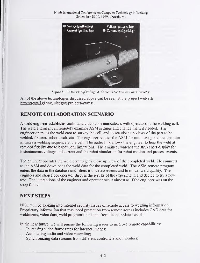
Ninth International Conference on Computer Technology in Welding

September 28-30, 1999, Detroit, MI

Figure 5 - VRML Plot of Voltage & Current Overlaid on Part Geometry

All of the above technologies discussed above can be seen at the project web site

http://www.isd.cme.nist.gov/projects/awms/ .

REMOTE COLLABORATION SCENARIO

A weld engineer establishes audio and video communications with operators at the welding cell.

The weld engineer can remotely examine ASM settings and change them if needed. The

engineer operates the weld cam to survey the cell, and to see close up views of the part to be

welded, fixtures, robot torch, etc. The engineer readies the ASM for monitoring and the operator

initiates a welding sequence at the cell. The audio link allows the engineer to hear the weld at

reduced fidelity due to bandwidth limitations. The engineer watches the strip chart display for

instantaneous voltage and current and the robot simulation for robot motion and process events.

The engineer operates the weld cam to get a close up view of the completed weld. He connects

to the ASM and downloads the weld data for the completed weld. The ASM remote program

enters the data in the database and filters it to detect events and to model weld quality. The

engineer and shop floor operator discuss the results of the experiment, and decide to try a newtest. The interactions of the engineer and operator occur almost as if the engineer was on the

shop floor.

NEXT STEPS

NIST will be looking into internet security issues of remote access to welding information.

Proprietary information that may need protection from remote access includes CAD data for

weldments, video data, weld programs, and data from the completed welds.

In the near future, we will pursue the following issues to improve remote capabilities:

- Increasing video frame rates for internet images;

- Automating audio and video recording;

- Synchronizing data streams from different controllers and monitors;

413

Ninth International Conference on Computer Technology in Welding

September 28-30, 1999, Detroit, MI

Centralizing world model data acquisition to simplify interfaces for external access;

Integrating the testbed with higher level collaborative tools [10];

Automating co-display of part geometry and sensor model data (Figure 5);

- Incorporating the commercial monitor in remote access, either by adapting interfaces

ourselves or using modifications made by the vendor;

Exploring standard interfaces both for integration of cell components and for remote access;

Editing the weld program remotely; and

- Initiating cell events, like cycle start, remotely.

NIST is working as a member of the AWS-A9 committee on Computerization of Welding

Information to develop a specification for the exchange of welding information between

intelligent systems. The NIST testbed will be used to test specifications while they are still in

draft stages. One current working document is the Arc Welding Activity Model (available at

http://www.isd.cme.nist.gov/projects/awms/aws/ ).

REFERENCES

[1] Albus, J., "A Reference Model Architecture for Design and Implementation of Intelligent

Control in Large and Complex Systems," International Journal of Intelligent Control

and Svstems . Vol. 1, No. 1, 15-30, 1996.

[2] Impact Engineering, ARCAgent-2000 Networking Overview , 1998.

[3] Madigan, R.B., Quinn, T.P., Siewert, T.A., Control of Gas-Metal-Arc Welding Using Arc-

Light Sensing , NIST Internal Report 5037, 1995.

[4] Quinn, T.P., Madigan, R.B., Sensing of Arc Welding Process Characteristics for Welding

Process Control , U.S. Patent Number 5,756,967, 1998.

[5] Quinn, T.P., Madigan, R.B., Siewert, T.A., "An Electrode Extension Model for Gas Metal

Arc Welding," Welding Journal Vol. 73 (10): 241s-248s, 1994.

[6] Quinn, T.P., Madigan, R.B., Smith, C.B., Blachowiak, E.G., "Weld Defect Decisions Using

Through-The-Arc Sensor Data," Proc. of Seventh International Conf. on Computer

Technology in Welding , NIST Special Publication 923, ed. Siewert, T., 1997.

[7] Rippey, W.G., Proceedings ofNIST Workshop: Industry Needs in Welding Research and

Standards Development , NIST Internal Report 5822, 1996.

[8] Rippey, W.G., Falco, J.A., "The NIST Automated Arc Welding Testbed," Proc. of Seventh

International Conf. on Computer Technology in Welding , 1997.

[9] Shackleford, W., Proctor, P., Real-Time Control Systems Library - Software and

Documentation , Online Documentation, http://www.isd.cme.nist.gov/projects/rcs_lib/ .

[10] Steves, M., Knutilla, A., "Collaborative Technologies for Global Manufacturing," Proc. OfASME International Mechanical Engineering Congress and Exposition (IMECE):

Symposium on Manufacturing Logistics in a Global Economy , 1999.

414

Session B5: Real-Time Weld Sensing and

Control Systems: Weld Process Automation

Communication and Interfaces

ON-LINE SENSING OF LASER SURFACE MODIFICATION PROCESS BYCOMPUTER VISION

D. Hu, M. Labudovic and R. Kovacevic

ABSTRACT

Laser surface modification with alloying or re-melting often has unstable results. To achieve on-

line control, process sensing is the key technology. This paper introduces molten pool imaging as

laser processing feedback. Well-contrasted molten pool images are acquired in experiences

eliminating the strong light from spatter and plasma. The image shows a clear correlation with

laser power absorbed by bulk material, which can be used to provide molten depth on-line

estimation in laser surface modification with constant scan velocity. An algorithm for real time

image processing is developed. The algorithm shows a robust and high-speed performance.

Keywords: Laser surface modification. Computer vision, Image processing. Neural network.

INTRODUCTION

Laser surface modification comprises a family of methods such as transformation hardening,

melting, alloying and cladding. It allows a user to build a part with totally different properties in

surface layer from bulk material. The surface layer can obtain high wear, fatigue or erosion

resistance while the bulk material can still keep its original properties such as good strength.

The theory of laser surface modification is based on rapid thermal cycling due to the excellent

characteristic of laser that can produce more concentrated heat energy on the part. A high cooling

rate can be reached while the heat conducts into the cold bulk material, which results in a self-

quenching process. This self-quenching process produces microstructure refinement, phase

transformation or formation of supersaturated solid solution

One typical application of laser surface modification is the thermochemical treatment to the

surface of titanium which has excellent mechanical and chemical properties such as high

strength, good biocompatibility and high corrosion resistance but with low resistance to sliding

and abrasive wear. When nitrogen is blown into the molten pool produced by laser on titanium

material a thin golden layer of titanium-nitride forms which shows great hardness (HV=2000-

3000 kg/mm^), high melting temperature, high temperature stability and low electrical

sensitivity^. But irregular qualities are often produced because the processes are too sensitive to

the processing parameters, such as input laser power and scanning velocity. For example, under

certain conditions a 10% fluctuation in laser absorption will cause a 50% change in molten

depth. Therefore, real-time control of the process is required to produce more stable and

repeatable molten depth and adapt to the complex shape of the part.

Accurate and reliable process sensing and feedback is the key to achieve such successful control.

Owing to the complex interaction between laser and material, there are several kinds of sensors

to be used in laser welding to monitor the welding process (e.g., plasma detector, acoustic sensor.

Department of Mechanical Engineering, Southern Methodist University, PO Box 750337, Dallas, TX, 75275

417

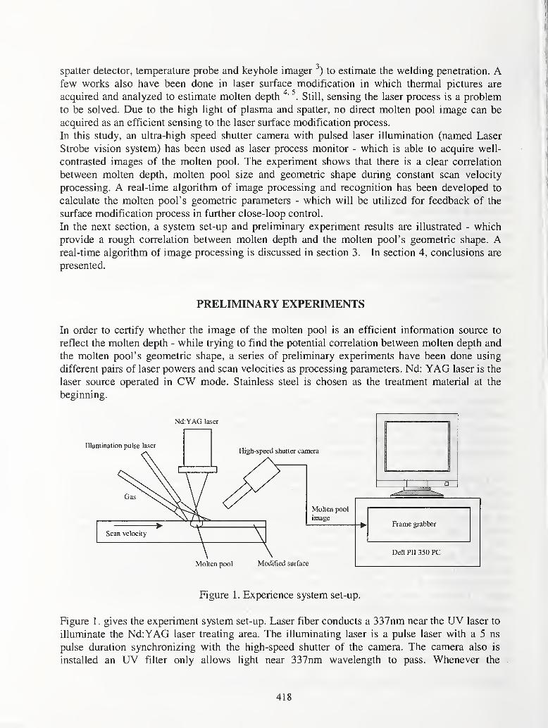
spatter detector, temperature probe and keyhole imager ^) to estimate the welding penetration. Afew works also have been done in laser surface modification in which thermal pictures are

acquired and analyzed to estimate molten depth ^. Still, sensing the laser process is a problem

to be solved. Due to the high light of plasma and spatter, no direct molten pool image can be

acquired as an efficient sensing to the laser surface modification process.

In this study, an ultra-high speed shutter camera with pulsed laser illumination (named Laser

Strobe vision system) has been used as laser process monitor - which is able to acquire well-

contrasted images of the molten pool. The experiment shows that there is a clear correlation

between molten depth, molten pool size and geometric shape during constant scan velocity

processing. A real-time algorithm of image processing and recognition has been developed to

calculate the molten pool's geometric parameters - which will be utilized for feedback of the

surface modification process in further close-loop control.

In the next section, a system set-up and preliminary experiment results are illustrated - which

provide a rough correlation between molten depth and the molten pool's geometric shape. Areal-time algorithm of image processing is discussed in section 3. In section 4, conclusions are

presented.

PRELIMINARY EXPERIMENTS

In order to certify whether the image of the molten pool is an efficient information source to

reflect the molten depth - while trying to find the potential correlation between molten depth and

the molten pool's geometric shape, a series of preliminary experiments have been done using

different pairs of laser powers and scan velocities as processing parameters. Nd: YAG laser is the

laser source operated in CW mode. Stainless steel is chosen as the treatment material at the

beginning.

' I 1

Nd:YAG laser u , 1

Illumination pulse laser

Molten pool Modified surface

Figure 1. Experience system set-up.

Figure 1. gives the experiment system set-up. Laser fiber conducts a 337nm near the UV laser to

illuminate the Nd:YAG laser treating area. The illuminating laser is a pulse laser with a 5 ns

pulse duration synchronizing with the high-speed shutter of the camera. The camera also is

installed an UV filter only allows light near 337nm wavelength to pass. Whenever the

418

illuminating laser is triggered, the camera shutter is open 50 ns to capture an image. During the

illumination period, the intensity of the illuminating laser can cover the spatter and plasma light.

Due to reflecting of the mirror-like molten pool, a well-contrasted image of the molten pool can

be obtained. Nitrogen is used as the alloying gas while it also blows away the plasma generated

from the molten pool.

A frame grabber installed on a PII 350 PC computer acquires images from the high-speed shutter

camera at 30 Hz. Real-time image processing, recognition, molten depth estimation and close-

loop control will be completed on the same computer. The experiment results are shown in

Figure 2. and Figure 3.

-1 '1

' 1 '1

' 1—

2 4 6 8 10

Scan Velocity (mm/s)

(a) Depth of the modified surface vs. scan velocity for different laser output power.

(b) Structure of modified surface.

Figure 2. Laser surface modification results.

419

Laser power=1200W

Laser Power=950W

Laser Power=830W

Laser Power=570W

v=2.5 mm/s v=5mm/s v=10mm/s

Figure. 3 Images of the molten pool under different laser powers and scan velocities.

By a laser strobe lighting camera, well-contrasted molten pool images can be acquired whose

qualities are good enough for further image processing. From data in Figure 2, the depth of the

modified surface shows more sensitivity to absorbed laser power than to scan velocity. For

example, processing started with parameters of 1200W laser power and 2.5mm/s scan velocity.

Decreasing the laser power 50% or increasing the scan speed 3 times will form almost the same

variation of depth in the molten pool. Comparing the images in Figure 3 with data in Figure 2,

the molten pool images are also seen to reflect more signs of variation in laser power than in scan

velocity. Using constant scan velocity in processing, the geometric shape of the molten pool

changes prominently with the variation of laser power. When laser power is decreased, the size

of the pool shrinks and the angle at the front end is smaller. In contrast, changing the scan

420

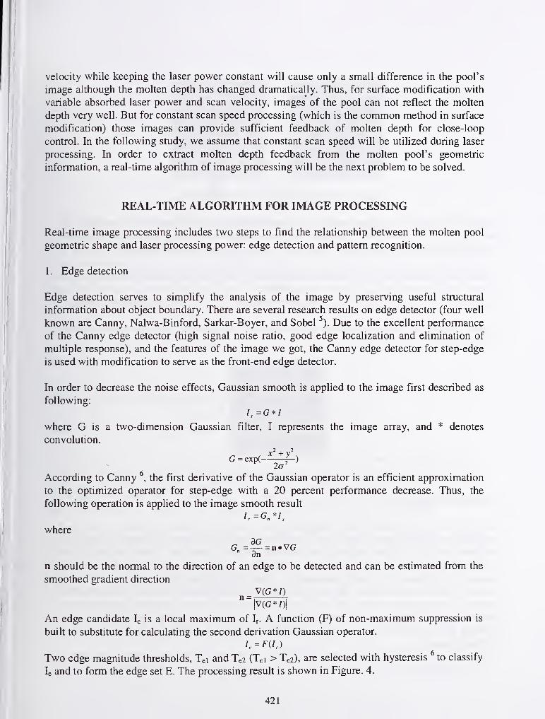
velocity while keeping the laser power constant will cause only a small difference in the pool's

image although the molten depth has changed dramatically. Thus, for surface modification with

variable absorbed laser power and scan velocity, images of the pool can not reflect the molten

depth very well. But for constant scan speed processing (which is the common method in surface

modification) those images can provide sufficient feedback of molten depth for close-loop

control. In the following study, we assume that constant scan speed will be utilized during laser

processing. In order to extract molten depth feedback from the molten pool's geometric

information, a real-time algorithm of image processing will be the next problem to be solved.

REAL-TIME ALGORITHM FOR IMAGE PROCESSING

Real-time image processing includes two steps to find the relationship between the molten pool

geometric shape and laser processing power: edge detection and pattern recognition.

1 . Edge detection

Edge detection serves to simplify the analysis of the image by preserving useful structural

information about object boundary. There are several research results on edge detector (four well

known are Canny, Nalwa-Binford, Sarkar-Boyer, and Sobel ^). Due to the excellent performance

of the Canny edge detector (high signal noise ratio, good edge localization and elimination of

multiple response), and the features of the image we got, the Canny edge detector for step-edge

is used with modification to serve as the front-end edge detector.

In order to decrease the noise effects, Gaussian smooth is applied to the image first described as

following:

= G * /

where G is a two-dimension Gaussian filter, I represents the image array, and * denotes

convolution.

G = exp(

—

la

According to Canny ^, the first derivative of the Gaussian operator is an efficient approximation

to the optimized operator for step-edge with a 20 percent performance decrease. Thus, the

following operation is applied to the image smooth result

/ =G */r n s

where

G„=|^ = n.VG

n should be the normal to the direction of an edge to be detected and can be estimated from the

smoothed gradient direction

_ V(G*/)

""|V(G*/)|

An edge candidate le is a local maximum of Ir. A function (F) of non-maximum suppression is

built to substitute for calculating the second derivation Gaussian operator.

Two edge magnitude thresholds, Tei and Ta (Tei > Te2), are selected with hysteresis ^ to classify

le and to form the edge set E. The processing result is shown in Figure. 4.

421

Figure 4. Processing result of the edge detector.

In order to eliminate the edges caused by the heat-effected zone, two gray level thresholds, Tgi

and Tg2 (Tgi <Tg2), also with hysteresis, are used combined with edge magnitude thresholds,

based on the original image histogram analysis. The process is defined as following:

If Ie(x, y)>Tei and I(x, y)<Tgi, (x, y)GE, break=FALSE, x±A, y±A; A is a small increase.

If Ie(x, y)<Te2 or I(x, y)>Tg2, (x, y)£E, break=TRUE;

If Tei>Ie(x, y)>Te2 and Tg2>I(x, y)>Tgi and break=FALSE, (x, y) eE, otherwise break=TRUE;

Figure 5 shows that the extra edges are greatly reduced. The edge set E is the data source of next

step recognition.

Figure 5. Final processing result of the edge detector.

2. Pattern recognition

The purpose of the molten pool recognition is to classify the geometric shape of the pool

according to molten depth. In this study, a template-matching method is selected to satisfy the

requirements of real time. Because the positions of laser head and camera are fixed, one

dimension optimization searching which has very fast recognition speed is enough for two-

dimension recognition. For each processing of certain segment laser power, one template must

be built. Then a look-up table can link template and molten depth. Because it is difficult to

extract one accurate analytic model for the geometric shape of the molten pool, Self-Organized

Feature Map (SOFM) is utilized to construct such a recognition template by the associate

learning neural network, due to the good performance of SOFM in distributing weight according

to training patterns.

422

The structure of neural network is shown in Figure 6. The input patterns (p) are 2x1 vectors,

which are positions of the edges of one set of the moltei) pool detected in the above section. Aweight matrix will be trained to distribute weight vectors according to the position of the edges

and to be the recognition template of that set of molten pool.

Input Feature Map

caw

n

hFigure?. Structure of the neural network of SOFM.

Here the set of images with processing parameters of 1200W-laser power and 5mm/s scan

velocity is selected to illustrate the template training process in detail. N images of this set are

chosen as the training input pattern. The 2-D positions of the edges of the molten pool will be

operated by OR set operation to construct input pattern set. The input pattern set is described as

follows:N

1=1

where Pj is the input pattern set for one segment of laser processing power and Ej is edge set of

one image.

A program is developed to train the SOFM using the Kohonen rule with neighborhood. The

training algorithm is described in the following equation ^.

,w(n) = (1 - a). w(n) + otpin) i G N., (d)

where N^(d) = {j,dy <d} , i* represents the wining neuron, and a is the learning rate.

The trained weight matrix (w) will be the recognition template. Because the weight matrix wclassifies the edges according to their position, in order to get correct template that can fit the

contour of edges of N images, enough number of initial classifications must be selected to avoid

the "average" effect. The training result (template) is shown in Figure 8. The template

constructed by SOFM can represent the geometric shape of the molten pool very well.

The algorithm combining the modified Canny and template matching constructed by the SFOMneural network method shows good performance in time consuming and robust. On the computer

described in section 2, it will take 60ms to complete such image processing. It can classify

images formed by different segments of laser processing power, from which sufficient

information can be extracted by building a look-up table.

CONCLUSION

Well-contrasted molten pool images of laser surface modification can be obtained by a Laser

Strobe vision system. Both images and molten depth are more sensitive to the change of laser

423

power absorbed by bulk material than by scan velocity. The computer vision can be used as an

efficient method for sensing laser surface modification with constant scan velocity. An algorithm

for real-time image processing is developed combining modified Canny and template matching

constructed by SFOM neural network method. The algorithm shows very robust performance

and fast speed in testing on different images. Molten depth estimation modeling and close-loop

control for laser surface modification will be the further research.

Learning rate is 0.8. Input pattern repeating times is 1. Neighborhood size is 0 9.

250 , , , , , , , , , ,,

200

150

100

50 I I I I I 1 1 1 I I

20 40 60 80 100 120 140 160 180 200 220

Figure 8. Recognition template trained by SFOM(Laser power=1200W, scan velocity=5mm/s).

REFERENCE

1. Heuvelman, C.J.; Konig, W.; and et al. 1992. Surface treatment techniques by laser beammachining. Annals of the CIRP 41(2): 657 to 666.

2. Romer, G.W.; Hoeksman, M.; and Meijer, J. 1997. Industrial imaging controls laser surface

treatment. Photonics Spectra 31(11): 104-109.

3. Tu, J.F.; Lankalapalli, K.N.; Gartner, M.; and Leong, K.H. 1997. On-line estimation of laser

weld penetration. Transaction of the ASME: Journal of dynamic system, measurement, and

control 119: 791-801.

4. Derouet, H.; Coste, F.; Sabatier, L.; and Fabbro, R. 1996. Real time control of surface

treatments with liquid phase (molten depth on-line estimation). Proceedings of SPIE 2789:

264 to 272.

5. Heath, M.; Sarkar, S.; Sanocki, T.; and Bowyer, K. 1998. Comparison of edge detectors-A

methodology and initial study. Computer vision and image understanding 69 (1): 38 to 54.

6. Canny, J. 1986. A computational approach to edge detector. IEEE transactions on pattern

analysis and machine intelligence PAMI-8 (6): 679 to 698.

7. Hagan, M. T.; Demuth, H. B.; and Beale M. Neural Network Design 1995. PWS publishing

company, USA.

424

o

>^ N

o

o

O

o

ao

o

I5X)

OO

O

ON

(N

a^—

>

425

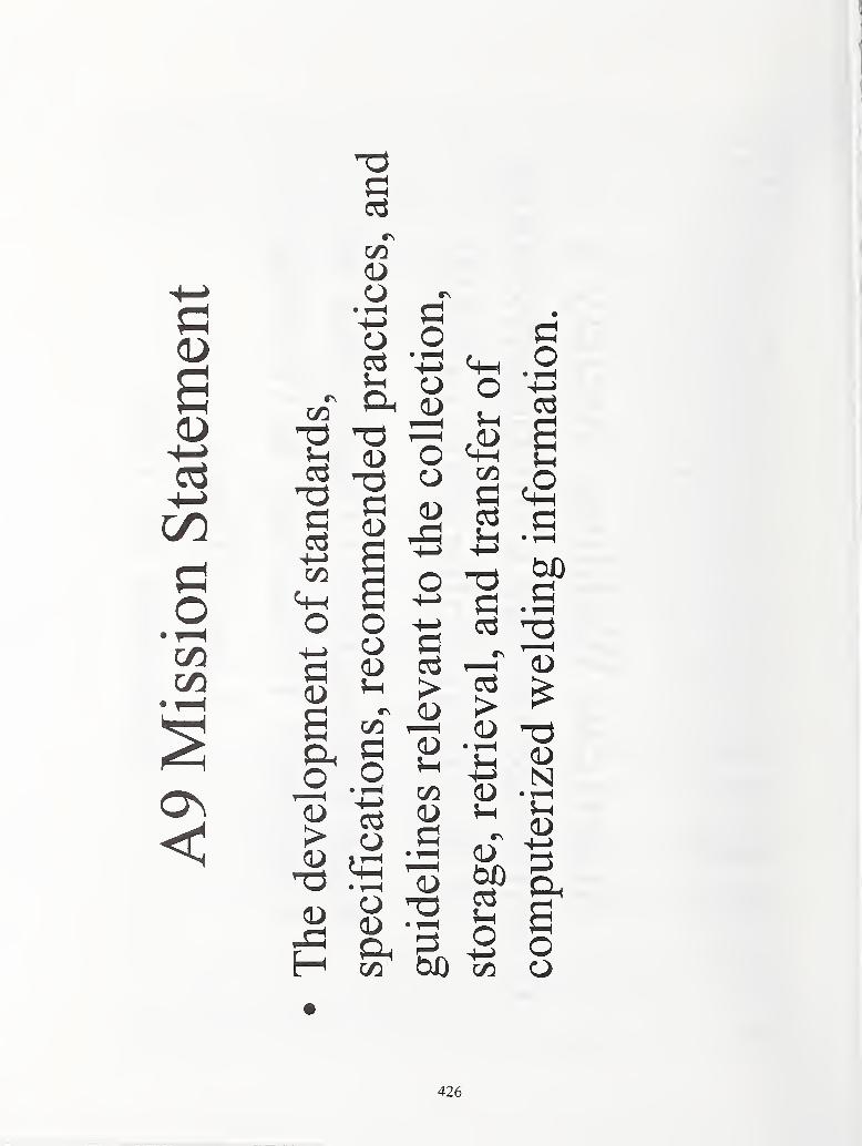
o

426

00

Nl

O

CI.

OS oH

427

CO

Oh

o

Q

OU<

o

N

Ouo

0^

C/3

OJj J-(

o

$-1

-a

03

s 1i ^O ;h

U Oh

I

a.oPh

(L)

N• 1—

I

<D't—

>

aoU

13

o

op c/5

S -§

Q §o 1;:!

^ 1Xw

=3

o

c o

(/5

0^ O< ^

>• 1-H

o

(/I

O

o

15• 1-H

;-H

(D

2 c/^

;-H 4-»

< ^<L>

N• 1—

(

Vhoo

;-H

cd^

^3

cd^—

>

o. 1-H

cd

(N s

O

o

;3

Oh

o

Oo

on

Q

o

^73

CO

as

o

in

CO

o>

h-1

Q

o

Oo

GO

13

O

uI

428

?? N

i-H

^ oc3

o

a

2 §Oh >

c3

a

2 o(D CO

^ 2^

^3

c« OX)

o

CO

o OO

o0-)

oX

ao o

COa.)

o

V. O

429

<3-)

>

<PQ

<"S

u

C/3

oo

CD

o

b boQ .Si

5

^3 bo

5 ^

Co" ^t>0

CO S

l>3

GO

< ^

Co ^

<^

CO ^^ "I g

430

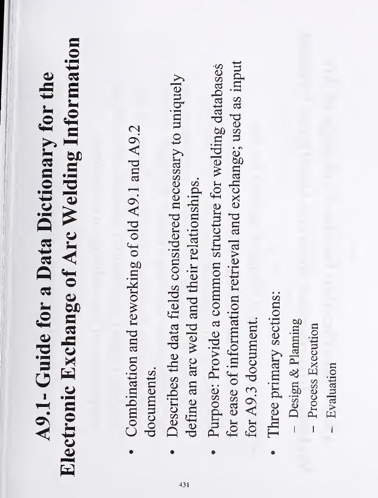
O

£ s

i (DJ)

S3

^ 2

(NOn

odo

o

O

SoU -6

0-)

aoo H ^ ^

PLh <iH «

oo o

o

g wEl ^

oC/3 O

O

Q £ W

431

4>

Oo

B

a ^C3

CD

GO^

c3

0-)

> GO

GO C (UO c3 a>

X (U

o o o

(U S^ ^ ^S o o

o

^ O

o

0-)

CO O

^o a>

0-)

GO

0-)

C O

H a> (D

CD oo

o• ^™

oC/5

0-)

2 a

c/0

c3

0-) 3

Oh

c3

43

432

433

434

OPh

a

O

O-I—CO

bD O

S o

> >

oId

no

a

4^

O

O

o O

^ l-H S

C/3

O <3->

a s

o ^

^ o

o ^Ph

O

s a

B B

o ^

in

O

o

(DOo

tan

•

• 1—1

GO

aOa

td oo o

3 c

ao ^

C/3

(U O X)CD

. 1—1

>r-(

> ao

1I

O (U

435

oO

o

O•^oa.C/5

CD

• 1-H

o

oI

o

o

t5

O

oo

• 1-H

o oo pq

.a phOh O

> <u

00

2

O

O CO

o

ao

CZ5

Oh• 1—

H

O

<u o

o .t^

CO

C/5 ^

WD iS

Oo

CO

O0-)

o

° I>

Q

o

o .So bp

(U -ft

0) CO

^ Ia B

CL CJ

t ^I I I I

436

>

<

Q

O

2 o£ o

> B

3 o

« c3

C3 <^

COGO

>CIS

so

;^ o

>O 0-)

cs

OB

j:^ CO

o

S ^ oSCO ^ Oh

C3

CO

S53

437

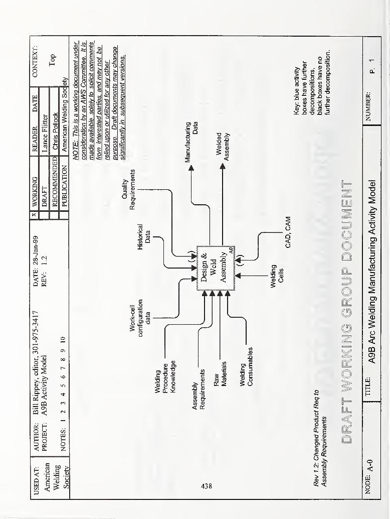
HXmHOu

<Q

a!

O

o

C3)

Cj>

CCO

I

00

^ >

On

O)-(

O T3O

>;.^<u >C1.-X3

OS

oa;a.

OS

00

r-

VO

ir>

CO

00

HO

<QUD

•S I I

^ ^ ^

.1?CO ^

is: ^

wco

tooQ.

c

to o

>< ^O T3

£

Oj TO ^a ^PQ

438

u3 CO

tfsi -Q

"<- ?

(D

o

>o<c

o

cCD

c

<CQ

<

QO

UiHZoo

WH<Q

Q<

O

05

I

CCO—

>

00

l-(

o

2 <

<

HOUO

ooo0.

O"qwQZw

o

lii ..

< UiQ 52

I

On

O

CI. u

<QUonD

ocn

TOC

0

cCDO'k-

0)

E<

COuHO

60

'oo00

TO

CD O

439

<Q

WQ<

X

8i

<DO

o_o

oDl

Q(JLl

Q

oU

o>I

c(0-j>

00CM

[ii

H<Q

I

On

O

>

T3

'-8

O

3^ >

UPQ1—1

O

o

c

c(0o0)

E<

as

00

00UHO2;

c

C

SO

c

DcCDCoCD

cCD

EO§it:

2Q

to

& £

Qj CO

CD 0)

:^ -D CU

0 OO

5o

D.5

(0(D

>^ c5 .2£cu oCO (;=

« oQ. ^CO

oQ JOCO

CO C.9? flj

lb CO

|Eo(U

cCD

Q.

'rt

wcCD

>> E

< a:

CO

W

>«x>E(D(O(O

<cD)CO0)

Q

3WQO

440

X

Zou

H<a

<

OiCj)

c(0—

}

00

w ..

^ >< dJQ 2

I

On

Omt-T

>

s<

HUU1—1

ooiCU

OS

00

m

m

00uHO

<QUonD

o•c

u o

co

^ TOX) OE<D OW Q)CA Q.< CO

441

HXwHou

wH<Q

Q

O

O)

cCO—J

I

CO<N

diH<Q

*r)

asI

o

O T3•ti o

>;.^

Oh O

ED

<

HU

oa;Oh

o_o

o

O

oCO

cnc

ON

oo

C/3

UiHO

<QU00D

60

U o

c w

OJ o

442

H2OU

a<

aO<

pH

O

cCO

« ^CM —

.

W ..

>< ClJ

Q o2

I

o

o

2^ >

2^ OSOQ <

HU1—1

O

o_goa.

w

O

Q

o

oCO

c

CTs

OO

in

r<-)

t/3

uHO

<QCOD

00

CO

Wpa

W S-

CD Co oE =

||CM ^

ct: 05

Si cC3) OC .b:CD-C C

0O

coO

> Q. CO —

tii

OO

443

444

tSX)

a S

u

u

ao

I

^ o .2

WD 2s s

^ W ^

^ s

< 2

o

^ fH C/3

c « g

i<U O

13O ^H 1^

^ O

O

CO

aCO

O

COGO

O0-)

0->

C3

GO

&1oo

o&

c; ^

^ OO

O C

Oh 0^

O ^

t3

s OOc3

a

C3

13

in

a

bD

445

446

O

o

00

O

C/3

O

Vh

cd cd

s >

^

c3

C/3

^ oo c3 7^

a, ^^ CO O

cd

•j

V

.s ^

C/5^—

>

GOoo

CO

O4U

bX)

oo

o

oo o

I

c3

OX

cd

O

cd bX)

a OCd O

o ^

o ^

td ^ sbx) >^ -a

fli ^X (D <D

^ bn

2i -a

cd

bX)

• ^1cd

CIS

^ s

^ S <i>

O O wC Sh c3

447

ooOh

a

O

o

§

o

1 ^

J3

oo

O

OOh

(/3

O

M I—

I

o B ^

o

X o

c3 (D-I—

>

C/5

0-)

3

oO

O

oOhen

• 1-H

448

C/3

^3a

OOh

OS

aso

oOhc/5

O

Q

gO

aoO

o

449

• 1-H

OJ-H

^c3 H

oo

oa • 1-H

0)

00 S 2

I

BBoU

Q

<

Oo

>

o1-H

(/3 >

X)o o

C/5

Ooo

s• 1-H^—

»

• 1-H

13

C5O

c/3

O• 1-H

oo

^ ^Q W

450

oUo

O

U

J3

o

o do

ao

O

o

oo

^ <

O00

OO

o

cy3

513

o o

C/)

>o

c/3

o

o

om•

X

in

OnI

o00

oc3

O00

q

Ic/3

oo

CO

s

o

>O

g

CO

^ ;i Vo ON

451

A METHOD FOR OPTIMIZINGWELDING PROCESSES

P. E. Murray'

ABSTRACT

Arc Welder, a Windows-based software application, is developed to accurately, efficiently, and

reliably simulate the gas metal arc welding process, and to select welding parameters for optimal

control of the process variables that affect weld quality. In this paper we describe Arc Welder

and how it is used to select welding parameters. We also describe plans to integrate Arc Welder,

drawing software, and an optimization algorithm into a comprehensive software product for

ensuring weld quality and enhancing productivity in the welding industry.

INTRODUCTION

Ensuring weld quality and enhancing productivity are important in the welding industry,

especially for automatic and robotic welding used in the automotive and ship building industries.

Optimal welding procedures and parameters ensure the quality of the weld and reliability of the

welding process while minimizing the cost of fabrication. Currently, designing the joint,

selecting the welding technique, choosing the welding consumables, and optimizing the welding

parameters are independent tasks. Furthermore, welding procedures are often developed with the

aid of handbooks and manufacturers' recommendations that are based on a large amount of

empirical data, and welding parameters are often found by a process of trial and error.

Consequently, the welding process may not be optimal in regard to weld quality and cost. Tointegrate these disparate design processes, we are developing a method to select the optimal

welding procedure and parameters for satisfying the numerous constraints on the weld process.

Currently, analytical models, simplified numerical models, and empirical methods are used to

establish relationships between welding parameters, weld bead geometry, weld quality, and

productivity, and to select welding parameters leading to an optimal process. Several notable

examples may be found in Refs. 1-4; a related approach that is entirely empirical is described in

Ref 5. But all of these models are based on simplifying assumptions and empirical data

—

analytical models have deficiencies stemming from simplifying assumptions and empirical

models are valid only for the processes and consumables used to validate the model.

Nonetheless, empirical models have an important function in welding engineering, because the

complexity of the weld process usually precludes detailed numerical simulation. Recently, a

numerical approach has been used to simulate thermal phenomena occurring during welding, and

to optimize welding parameters for controlling weld bead geometry and productivity (Ref 6).

Although numerical modeling has gained acceptance in the welding research community,

empirical modeling is still the current practice in welding engineering.

' Applied Materials and Technology Department, Idaho National Engineering and Environmental Laboratory, Idaho

Falls, ID 83415-2210.

452

In this paper, we report on the first phase of a project to accurately, efficiently, and reliably

simulate the gas metal arc welding process. We developed a computer program called Arc

Welder that can find the operating conditions that lead to a desired weld process and thereby

identify the optimal welding procedure. Arc Welder performs the calculations in an integrated

and efficient manner; provides menu items to select the base metal, type of joint, welding

consumables, and welding parameters; and includes a graphical user interface for Windows95/98/NT operating systems (Figure 1). Arc Welder may be used to identify a range of operating

conditions, establish limits on welding parameters, assess the effect of changes in welding

consumables, find the welding parameters that lead to desired operating conditions, and optimize

the parameters to satisfy constraints on the process variables that affect weld quality and

productivity. These constraints stem from the need to reduce weld defects, reduce the extent of

distortion, meet the requirements on mechanical properties, and to increase productivity by

reducing the number of passes needed to fill the joint and increasing the rate of deposition.

Optimization is done by simulating the welding process for selected welding consumables and a

range ofwelding parameters, and applying the constraints to find the optimal welding procedure.

In this paper, we show examples of determination of welding parameters for optimal control of

arc length and depth of fusion to ensure arc stability and adequate joint penetration.

MiAfc Welding Simulato

Figure 1. The user interface ofArc Welder.

453

DESCRIPTION OFARC WELDER

Arc Welder simulates gas metal arc welding using a constant voltage power supply. Several

models are used to assess the relationship between welding parameters and process variables that

affect weld quality, using controllable operating conditions and welding consumables as inputs

to the models. Welding parameters include voltage, current, travel speed, wire feed speed, wire

diameter, and standoff distance; process variables include heat input, cooling rate, weld metal

geometry, base metal dilution, rate of transfer of droplets, arc length, and electrode extension.

The rate of transfer of droplets is used to ascertain the mode of mass transfer, i.e., short arc,

globular, or spray.

The relationships between voltage, current, arc length, melting rate, and electrode extension are

included in Arc Welder. As an example, consider a welding procedure using a stainless steel

electrode and gas shielding consisting of 98% A12 and 2% O2. The correlation between voltage,

current, and arc length is shown in Figure 2, and the correlation between melting rate, current,

and electrode extension given by Lesnewich (Ref 7) is shown in Figure 3 . These relationships

are used to compute the arc voltage, current, arc length, and electrode extension. Arc Welder also

identifies the limiting conditions of "short" and "long" arc length and thereby checks for a stable

arc. In this manner. Arc Welder may be used to determine the welding parameters that lead to a

stable operating condition.

4 6 8 10 12

Arc Length (mm)

Figure 2. Correlation between arc length, voltage, and current, using stainless steel electrodes (0.9 and 1.2 mmdiameter), and 98% Ar2 and 2% O2 shielding gas.

454

1.0E-05

8.0E-06

6.0E-06

—

U)

c(1)

t

O

^ 4.0E-06(0

0^

O)c=1 2.0E-06

O.OE+00

^ Experimental Data

Theoretical o

y = 4E-07X + 3E-06

R^ = 0.8189

0.0 2.0 4.0 6.0

Electrode Voltage Drop (v)

8.0 10.0

Figure 3. Correlation between melting rate, current, and electrode extension using stainless steel electrodes (0.9 and

1.2 mm diameter), and 98% Ar2 and 2% O2 shielding gas.

Arc Welder also includes a model of the depth of fusion, which is used extensively in the

examples given in the next section. A complete description of this model and the validation

performed in the case of stainless steel base metal may be found in Murray and Scotti (Ref 8).

Other models in Arc Welder include a correlation between welding parameters and the rate of

transfer of droplets by Murray (Ref 9), the heat transfer solution of Rosenthal (Ref 10) as

expanded upon by Christensen et al. (Ref 11), and the centerline cooling rate formula of Adams(Ref 12). Arc Welder may be used to compute joint penetration, weld width, reinforcement

height, and base metal dilution.

The current version ofArc Welder is for a butt weld in the flat position, but it will be extended to

include other joint designs. The user may select mild steel, stainless steel, or aluminum; an

option to select other alloys may be provided in a later version. Arc Welder has been validated

only for selected consumables, but will be extended to include other filler metals and shielding

gases. The program provides a view of the base metal, weld metal, arc, electrode, droplet, and

contact tip, as shown in Figure 1. The user has the option to "run" the process by simulating

transfer of droplets from the consumable electrode. The user also has the options to save a given

set of welding parameters in a file, open a file containing welding parameters saved previously,

and print a bitmap image of the client area of the window. A future version of Arc Welder mayinclude additional base metals, consumables, power supplies, joint designs, and welding

techniques.

455

SELECTING PARAMETERS WITHARC WELDER

As an example, consider the problem of computing the welding parameters that lead to a stable

arc. The short arc limit for a 1.2 mm diameter stainless steel electrode is shown in Figure 4; the

long arc limit is shown in Figure 5. These limiting conditions determine the range of arc voltage

needed to sustain a stable arc. Using these results, the user may select the welding parameters

that lead to a desired arc length.

Next consider the problem of computing the depth of fusion to ensure that joint penetration is

adequate. The depth of fiision in stainless steel, using a 1.2 mm diameter stainless steel electrode,

gas shielding consisting of 98% Ar2 and 2% O2, and a filler metal deposition equal to 0.2 g/mmis shown in Figure 6. We assume that 4 mm is the desired depth. The operating conditions

needed to obtain the desired depth are shown in Figure 7. The simulations identify the range of

vohage, wire feed speed, and standoff distance, and their effect on arc length and heat input.

To identify the optimal operating conditions, the user selects particular objectives and constraints

that must be satisfied. For example, suppose that the user wants an arc length equal to 6 mm. The

results shown in Figure 7 may be used to find the optimal operating points. In particular, weselect specific values of arc voltage, wire feed speed, and standoff distance that lead to the

desired arc length while maintaining desired values of filler metal deposition and depth of fusion.

A few of these operating points and the effect on current are computed and given below.

Arc Voltage (v) Wire Feed Speed (mm/s) StandoffDistance (mm) Current (A)

25.3 155 13 25727 170 16 24828.5 185 19 240

In the preceding example. Arc Welder was used to identify a range of stable welding parameters,

and to find the welding parameters that lead to desired operating conditions. Specific welding

parameters were found by controlling arc length, depth of fusion, and filler metal deposition,

leading to arc stability, adequate weld bead size, and adequate joint penetration. Arc Welder maybe used to select welding parameters for controlling other process variables that affect weld

quality. In this manner. Arc Welder may be used to develop optimal welding procedures.

FUTURE WORK

Arc Welder is the basis for comprehensive software that the welding industry can use to obtain

an optimal weld process specification. The comprehensive software will incorporate simulation

and optimization methods to compute the optimal weld process; these methods will satisfy

requirements on accuracy, validity, and performance that are essential for improving quality and

productivity in welding. In the next phase of this project, we will explore ways to achieve an

efficient simulation and optimization of the gas metal arc welding process. We are especially

interested in determining welding parameters for controlling arc length, weld metal geometry,

and rate of metal transfer because these process variables are important factors in weld quality.

Other variables that affect weld quality include heat input, cooling rate, and base metal dilution.

456

Figure 4. Short arc limit for 1.2 mm diameter stainless steel electrode.

457

Figure 6. Depth of fusion in stainless steel, using 1.2 mm diameter stainless steel electrode, 16 mm standoff, 0.2

g/mm deposit.

Wire Feed Speed (mtn/s)

(a) Voltage, wire feed speed, and standoff.

Figure 7. Operating points needed to obtain 4 mm depth of fiision, using 1.2 mm diameter stainless steel electrode,

0.2 g/mm deposit.

458

EE

£c

<

standoff (mm)

Wire Feed Speed (mm/s)

(b) Arc length, wire feed speed, and standoff.

E

I

3ac

eX

1500

1200

900-

600-

300'

Standoff (mm)

Wire Feed Speed (mm/s) 250

(c) Heat input, wire feed speed, and standoff.

Figure 7. Continued

459

In the next phase of the project, we will develop a method of optimization in the manner of

inverse design. That is, we will specify constraints on the process variables affecting weld

quality, such as minimum and maximum weld bead size and maximum heat input, and find the

welding parameters that satisfy these constraints and maximize productivity. A diagram of the

flow of data in weld process simulation and optimization is shown in Figure 8. This approach

will lead to reduced occurrence of defects, enhanced productivity, and improved weld quality.

We also plan to build software that integrates Arc Welder and a computer-aided-design method

for drawing a weld joint. The implementation will be compatible with common drawing objects

such as bitmaps and will include a user interface compatible with Windows 95/98/NT. Weenvision engineering software used on a desktop workstation in which Arc Welder, drawing

software, and an optimization algorithm are used in an efficient manner to obtain a weld process

that is optimal in regard to quality and productivity.

Voltage

Current

Travel Speed

Wire Feed Speed

Wire Diameter

StandoffDistance

Base Material

Base Thickness

Joint Type and Design

Welding Consumables

Welding Technique

Optimize Weld Parameters

to Ensure Weld Quality

and Productivity

Weld Process Simulation

Using ARC WELDER

Weld Metal Geometry

Base Metal Dilution

Heat Input

Cooling Rate

Arc Length

Droplet Transfer

Figure 8. The flow of data in weld process simulation and optimization.

460

II

I

i

ACKNOWLEDGMENT

This work was supported by the U.S. Department of Energy, Office of Science, Office of Basic

Energy Sciences, under DOE Idaho Operations Office Contract DE-AC07-94ID13223.

!

i REFERENCES

1. Salter, G. R., and Doherty, J. 1981. Procedure Selection for Arc Welding. Metal

I

Construction 13(9): 544-550.

2. White, D., and Jones, J. 1997. Process Modeling with Neural Networks for Pulsed GMAWBraze Welds. JOM49(9): 49-53.

3. Eisler, G. R., and Fuerschbach, P. W. 1997. SOAR: An Extensible Suite of Codes for WeldAnalysis and Optimal Weld Schedules. Proc. 7th Intl. Conf. on Computer Technology in

Welding, July 9-11, San Francisco, CA. Ed. T. A. Siewert, pp. 257-268. NIST.

4. Mitchiner, J. L.; Kleban, S. D.; Hess, B. V.; Mahin, K. W.; and Messink, D. 1995.

SmartWeld: A Knowledge-Based Approach to Welding. Technical Report SAND-96-1372C.

5. Harwig, D. D. 1997. The ARCWISE Technique for Increasing Productivity in Arc Welding.

Presented at the International Conference on Advances in Welding Technology, Sept. 17-19,

Columbus, OH.

6. Dilthey, U., Roosen, S., and Sudnik, V. 1997. MAGSIM and SPOTSIM: PC Aided

Simulation ofGMA and Spot Welding Processes. Proc. 7th Intl. Conf. on Computer

Technology in Welding, July 9-11, San Francisco, CA. Ed. T. A. Siewert, pp. 548-561. NIST.

7. Lesnewich, A. 1958. Control ofMelting Rate and Metal Transfer in Gas Shielded Metal Arc

Welding: Control of Electrode Melting Rate. Welding J. Res. (Suppl.) 37: 343s-353s.

8. Murray, P. and Scotti, A 1999. Depth ofPenetration in Gras Metal Arc Welding. Science andTechnology of Welding and Joining 4(2) : 112-117.

9. Murray, P. 1999. Stability ofDroplets in Gras Metal Arc Welding. Science and Technology of

Welding and Joining: in press.

10. Rosenthal, D. 1946. The Theory ofMoving Sources ofHeat and its Application to Metal

Treatments. Trans. ASME 68: 849-866.

11. Christensen, N.; Davies, V. de L.; and Gjermundsen, K. 1965. Distribution of Temperatures

in Arc Welding. British Welding J. 2: 54-75.

12. Adams, C. M. 1958. Cooling Rates and Peak Temperatures in Fusion Welding. Welding J.

Res. (Suppl.) 37: 210s-215s.

461

Session B6: Welding Documents and Database

Applications

BENEFITS TO BE GAINED FROM COMPUTERIZING THE MANAGEMENT OF FABRICATION

A D Brightmore and M Bernasek"

ABSTRACT

Welding engineers have managed welding procedures and welder performance qualifications

using computers for some years now and have been gaining benefits such as :

- readily accessible information : no more searching through large amounts of paper.

- easy development of procedures and qualifications through on-screen editing.

- professional looking documentation.

- advance warning of expiry.

Most fabricators now have local or wide area networks and sharing information between key

personnel is easier than it has ever been. This paper describes the benefits that can be gained

from use of computers to integrate management of procedures and qualifications with production

weld information and quality control data. Such integrated systems can give :

- instant progress reporting, important perhaps for stage payments.

- automatic assignment of procedures and personnel, ensuring qualifications are up to date.

- automatic generation of progress reports, including testing percentages and repair rates, etc.

- automatic update of WPQs, based on satisfactory production welds.

- automatic generation of documentation packs.

- instant traceability between production welds and procedures, qualifications and QC data.

- efficient archiving of fabrication information.

- satisfaction of QA requirements.

The paper also describes some of the difficulties in developing such systems, and the pitfalls to

be wary of.

KEYWORDS

WPS, PQR, WPQ, Welding procedure, ASME DC, EN 288/287, Software, Production welding

INTRODUCTION

Computers have always been good at storing large amounts of data and sorting and searching

through that data, making them suitable for pure database applications. Such applications have

depended on the user being able to identify parameters for searching easily, or with minor help

from the software. In welding, such systems have been used for managing welding procedures

and welder performance qualifications and to date, most have had limited, if any, 'expertise'.

The problem with building expertise into software is that it is necessary to have a deep

understanding of both software development, and the technology being computerized. In our

465

industry, this might include a knowledge of many subjects, including metallurgy, engineering,

production, quality control and standards. Standards are particularly important as many aspects

of fabrication are specified via national and international standards, such as ASME IX, AWSD 1 . 1 , EN 287/288 and ISO 9000.

Software houses with no depth of welding expertise or engineers with no depth of software

development skills both find it difficult to develop expert welding systems. It may be possible for

individual engineers to develop software, but long term support is at best difficult, and in most

cases impossible. For storage of large amounts of information, where considerable time is

invested in entering the data, long term support is critical.

In addition, most existing software systems in the fabrication industry are tools for individuals,

not large parts of organizations, because until recently, most organizations have simply not had

the infrastructure to allow information to be distributed electronically. The widespread use of

email has been one of the main driving forces behind the move of most fabricators to use local

and wide area networks. It is now possible to share welding procedures or welder approvals

across a company via a multi-user software system.

Even so, welding procedures and welder performance qualifications are usually managed by one

or two key personnel. The information may be made available across a company, but usually

only in a read-only form. By using local and wide area networks, it is now possible to

computerize, and integrate database systems, so maximum benefits can be gained. This paper

describes the benefits of computerizing welding procedures and performance qualifications, as

well as the integration of these with systems of wider scope to manage all aspects of fabrication.

Practical examples are used to illustrate how such software can be used in practice.

Welding Procedures and Welder Performance Qualifications

The management of welding procedures is one of the most time-consuming jobs of a welding

engineer. Creating, verifying and approving new procedures, and checking, adapting and

approving existing procedures takes a long time. Consequently, this was one of the first welding

engineering tasks to be computerised. TWI's Weldspec and Computer Engineering's Welding

Pro-Write are examples of such software.

Much of this job is administrative. That is, the management of paper welding procedures

involved a lot of time with a typewriter and liquid paper. Creating or modifying procedures was

very cumbersome. Searching for existing procedures for new production welds was a very time-

consuming task and required expert skills.

The first welding procedure database management systems were simply electronic filing

cabinets. They used the speed of data-sorting that computers could offer to make searching for

existing procedures much quicker. The ease with which documents could be copied and edited to

create new documents meant that this task could be undertaken much faster. What they could not

do very easily, however, was to give the welding engineer much help when creating new

procedures for new applications.

466

The problem was that the sources of such information are wide and disparate. They comprise

standards (welding and application), consumable and parent material handbooks, technical

literature and, most difficult of all to computerise, experience. To build all this into a computer

program would be, at best, very time-consuming, and impossible without a wide knowledge of

the sources available.

TWI and C-spec have collaborated to develop a new version of Weldspec (version 4). Weldspec

4 has been designed to give the welding engineer help in writing and drafting new welding

procedures while still giving the benefits of speed and editing of existing procedures, in a full 32-

bit Windows application. The development of the program has required expertise in a large

number of factors, including :

World-wide welding and application standards, from such organizations as ASME, AWS,European Standards, API etc.

Industry practice in developing, qualifying and using welding procedures.

Typical interactions between customer, fabricator and inspector.

Welding engineering and metallurgy.

Software development and knowledge representation techniques.

The representation of knowledge is important because software based on knowledge and

recommendations from standards needs to be frequently updated (ASME IX is updated every

year). Knowledge that is hard coded within software is difficult to change. Weldspec'

s

knowledge-base is stored externally to the main program in an easily modified format, making

updating more simple.

Management of welder performance qualifications is very similar to welding procedures, in that

their administration is defined by standards. Thus, the variables which must be recorded, the

extent of approval given by a test and the destructive and non-destructive test regimes are

specified in national and international standards.

However, unlike welding procedures, WPQs are only valid for a specified time without practice

or additional testing. Certificates expire, so the date of expiry becomes another key variable, so

the fast sorting capability of computers is even more beneficial.

TWI and C-spec have collaborated in development of Welderqual 4, which integrates seamlessly

with Weldspec 4. For example, the two programs use a shared database of welder details and

WPQs can be created directly from welding procedures.

Production Welding and Quality Control

467

The management of welding procedures and performance qualifications, as described above, can

give great benefits in saving time and reducing errors. However, if this is integrated with

software to manage production welding and quality control, the benefits can be multiplied.

The Problems

Most fabricators work in a compartmentalized way. The functions of design, engineering,

production and quality control are discrete and communication is often difficult. This can give a

number of problems

:

It is accepted that any error in the design stage of a fabrication can be very expensive to rectify

once a weld has been completed. The concept of simultaneous engineering, where all personnel

can contribute at all stages of manufacture, is particularly relevant to fabrication.

It is difficult to monitor fabrication, as paperwork can take a long time to circulate. This means

that problems can become serious before they are identified.

The sheer weight of paperwork can make it very difficult to update welder performance

qualifications based on satisfactory production welds. Many fabricators retest welders

unnecessarily. Also, it can be very difficult to identify those welders whose qualifications are

close to expiring.

Similarly, it can be very difficult and extremely time consuming to collate project data books,

simply because of the amount of paper.

The Solution

An integrated software system such as Welding Co-ordinator can overcome all the problems

listed above. Welding Co-ordinator is designed to be used live to manage fabrication as it is

progressing. It is usually based around an electronic 'weld map', or 'weld data sheet' or 'weld

schedule', into which data are entered as welds are designed, engineered, welded and tested. The

weld map would also usually have some space for approval, either weld by weld, or once a

project or structure has been completed. Figure 1 . shows an example of part of a weld map, for a

fabricator in the power generation industry, and figure 2. shows an example of the system as used

in the chemical process industry.

Data are usually entered into the system from four functions :

At the design stage, where information such as the weld ID number and other design parameters

(material type, thickness, joint type, etc) are entered.

At welding engineering, where a procedure is assigned. It may also be possible to identify

suitable welders or classes of welders qualified to make the weld, although this is more likely to

be done at the production stage.

468

At production, where the completion of a weld is registered (usually by entering the date) and

visual inspection carried out and approved.

At quality control, where acceptance of the weld is registered. This may be simply by typing test

report numbers into the system, or it may be done with live links to NDTspec or similar systems.

It should be stressed that these data should be entered live into the system, as fabrication

progresses.

As well as solving the problems identified above, the system can give a number of other benefits,

including the following :

Instant progress reporting. Anyone with access to the system can see how fabrication is

progressing. This may be simply by looking at the weld data sheet on screen, or by explicitly-

programmed progress reports. These can identify bottlenecks (e.g. by comparing the number of

welds completed with the number of welds radiographed), or help to produce reports for stage

payments in large projects.

Automatic assignment of welding procedures and welders. If enough information is supplied at

the design stage, the system has everything it needs to automatically search through Weldspec's

database of procedures for suitable WPSs. This may be a single WPS or a number from which to

choose. It is important to recognise that this can be done simply with a click of a mouse button.

Also, having chosen a suitable WPS, the system can search through Welderqual's database of

WPQs to identify suitably-qualified welders. If necessary, the system can list welders in order of

expiry date of their certificates so maximum benefit can be made of extending their

qualifications.

Automatic production of test requisitions. The system illustrated in figure 2 automatically

produces NDT requisitions, based on the NDT requirements for the project. These can be

selected either manually, or the system could 'randomly' select welds for testing.

Automatic generation of test percentages and repair rates. The system can produce reports on

repair rates per welder (to identify training requirements) by procedure (to highlight defect-prone

procedures) or any other measure, providing the relevant data are recorded. Figure 3 is a printed

report showing the number of welds of different sizes produced by each welder on a project.

Automatic update of WPQs. This is a very time consuming task on paper and may be impossible

due to the amount of paperwork. However, it is ideally suited for computerisation because it is a

simple data sort and test function. The integration between Welding Co-ordinator and

Welderqual makes it possible for the system to update all WPQs in a project, based on

satisfactory production welds.

Automatic generation of document packs on completion of a project. This can also be a very

time-consuming task manually, but again is ideally suited for computerisation. On the click of a

button, the system can print the weld data sheets for a project, along with all the WPSs used

(with backup PQRs if necessary) and all the WPQs. In addition, if NDTspec has been used to

469

report testing, the system can print relevant NDT reports as well. Alternatively, this information

can be archived on CD, which obviously takes less space.

Instant traceability between production welds information and the back-up information. Thus, if

the inspector wants to see a WPS that was used on a weld, or wants to see proof that the welder

was suitably qualified, this can be done on the click of a button. This facility can also be useful

after a number of years of service. If a defect is found in a structure, it is possible to access the

original WPS (for repair purposes), or the NDT report (to see if evidence of the defect was

present at testing).

Satisfaction of QA requirements. There can be no doubt that the use of a system such as Welding

Co-ordinator can help to satisfy the most stringent of QA requirements.

Problems and Pitfalls

If all the above seems too good to be true, there are paybacks and pitfalls, as described below :

For any customised software, it is critical to get the requirements of all personnel who will use

the system identified at an early stage, and approved by all concerned. In practice, the software

developer and the fabricator will collaborate in producing a list of requirements (WHAT the

system will do) and both parties will sign this document. This is a base line from which the

system is designed and developed, and is used to measure the quality of the software produced. It

works for both the fabricator and the system developer.

The production of a requirements document can be a time-consuming process, and the timescale

and cost of the system can only be estimated after this has been generated, so it is an important

stage in development.

A system such as Welding Co-ordinator affects may people, as it is, by its nature, a multi-user

program. Any form of change is often resisted, so it is important to identify all the potential users

of the system and involve them in the requirements analysis stage. Any users not involved in this

stage can claim the system does not do what they want. This may be because it makes their job

harder, or can be used an excuse to avoid change.

From a system developer's point of view, it is important to find a champion of the system within

the fabricator's organisation. This person can help to promote the system in the absence of the

developer. This person should either have a senior position, or be well respected.

It is very tempting to develop the system to be too prescriptive. For example, it is possible to

develop the Welding Co-ordinator system to only allow the selection of welders who are

registered in Welderqual as being qualified. In practice, however, the qualification test may have

been taken, but the NDT results may not have been received. Prohibiting selection of that welder

would not be correct in such circumstances.

470

Arguments often arise between QA/QC personnel and engineering staff on how prescriptive to

make the system. Experience shows that it is preferable to err on the non-prescriptive side, at

least in the early stages of system implementation. It is always possible to modify the system.

ACKNOWLEDGEMENTS

The authors would like to thank ABB Power Construction Ltd (Derby, UK) for their permission

to reproduce parts of their system within this paper.

FIGURES

Figure 1. A Weld Data Sheet from a Welding Co-ordinator used by a fabricator in the power

generation industry.

Figure 2. A Fabrication Inspection Record from a fabricator in the chemical process industry.

Figures 3. A printed report showing numbers of welds of different sizes produced by welders on

a project.

471

S5 5 t

E EO «

472

' o i i i §

d a lu < ,,

2 S X " oo I " 3 o< 3 a z ua- z 3 o 1-

oQ£OOUJ

ZOI-oUia(0zzg

ism

i3 I5 §

1 isz ji

-J 1s gnil

0.

3CALI

'LAN

0tn

sa. o o o

3 3 2 3; 3

s 2

«• i i i

i '

< < < < < < < < < <

9 3

s ^ ;^ ^

473

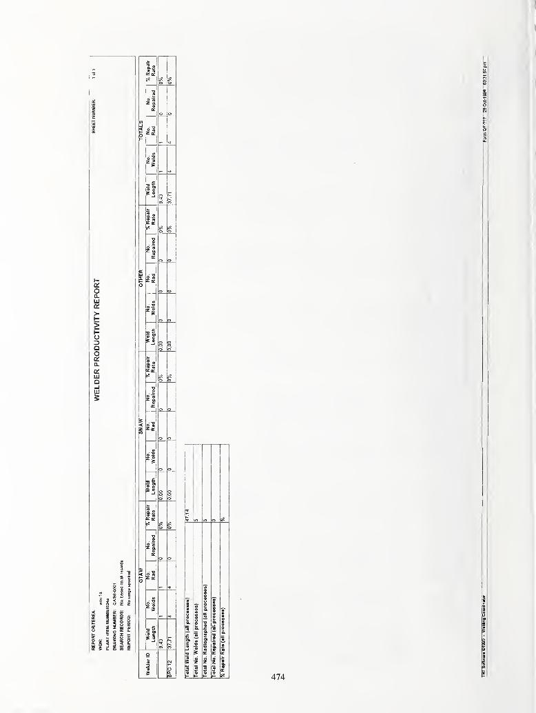
oa.tu

>

o

Q.

q:UiQ_1Ui

2 ?

1 1

s §

t- 5 o a:

^ 2 °= 9! S 2 £0. O 01 GC

ffl

go

o o

D9

i%«a:

1

o o

vt-I

< On0

j

r-

s

<P IS

r a:

o1

at

•

Kj

o2

—

~—

W

o o

—

? «i o oo o

•5

Q. ®

^1

5?

1 1

o o1

•oo

S"^z .9q:

s<

1

1

—

S z a:,

o o

»

» J5 go oo oo o

^ o

oa

S'Sz a.

1

o o

< o"gZ|£

to

£9Toi r)

9a r>j

"5 OQ.m 414

HEAT AND MATERIAL FLOW MODELING OF THEFRICTION STIRWELDING PROCESS

C. B. Smith*, G. B. Bendzsak', T. H. North', J. F. Hinrichs®, J. S. Noruk*, R. J. Heideman^

ABSTRACT

To gain an improved understanding of the friction stir welding (FSW) process, a heat and

material flow model has been developed to determine the material flow, temperature distribution,

and process loads (forces and torque) during the FSW of aluminum. Inputs to the model are the

weld tool geometry, tool position, travel speed and rotation speed. Pursuant to the development

of the FSW model, there was no information regarding material properties of aluminum at

elevated temperatures (e.g. viscosity and boundary conditions). These material properties are

essential information for the model to accurately predict the heat and material flow.

The first phase of model development was to determine these unknown material properties. This

paper describes the specific model development and experiments used to determine these

material properties. Further experiments are also described, which were used to confirm the

accuracy of the model. The second phase of the modeling effort used the material property and

boundary condition information acquired from the first phase to develop a full three-dimensional

model of the friction stir welding process.

INTRODUCTION

Friction stir welding is a solid phase joining process that was invented in 1991 by TWI (The

Welding Institute) in Cambridge, U.K. (Ref 1, 2). FSW has been primarily used to join

Aluminum alloys, but has also been used to join numerous other materials (Ref 3). For joining

aluminum alloys, FSW has several advantages over fusion joining processes, which are most

commonly used to join aluminum. These advantages include; 1) FSW is an autogeneous process

requiring no consumables, 2) improved tensile joint efficiency, 3) improved fatigue strength, 4)

reduced distortion as a result of lower heat input, 5) safety improvements (no arc radiation,

fumes, etc.), and 6), improved process uptime as a result of being a more robust process (Ref 3).

However, these advantages do not come without any challenges. The two most prohibiting

challenges are the relatively large forces required and the slower travel speed when compared to

a fusion joining process, such as Gas Metal Arc Welding (GMAW).

For the automotive industry, the advantages of FSW represent a chance to significantly lower

aluminum joining costs. The cost advantage can be fully realized, if travel speeds are increased

' Tower Automotive, Advanced Technology - Process, Milwaukee, WI, USA* University of Toronto, Toronto, ON, Canada® The Welding Link, Menomonee Falls, WI, USA" A.O. Smith Corporate Technology, Milwaukee, WI, USA

475

and process loads are decreased (reduces capital costs). In the initial development of the FSWprocess, travel speeds have been reported to be in the range of 0.25 meters / minute (10 IPM) for

6 mm thick butt welds of 6061 Aluminum (Ref 4). Whereas, travel speeds of 0.75 to 1.5

meters / minute (30-60 IPM) in lap welds of 3 to 4 mm material are common for the GMAWprocess, which is the most common joining process for aluminum in the automotive structures

business. Although, the compared travel speeds are not for the same material thickness nor joint

configuration, a FSW tool to perform a butt weld on 6 mm thick material is similar in geometry

to an FSW tool for a lap penetration weld on 3 to 4 mm thick material.

Decreasing the process loads of FSW is also an important goal, as there is a need to be able to

perform FSW on an industrial robot. There are two critical reasons for being able to perform

FSW on a robot; both are related to decreasing the costs of FSW. First, there is a definite need

to be able to perform FSW along three-dimensional paths. Industrial robots are ideal for

generating three-dimensional paths; however, their load capability is limited. Still, it has been

shown that a low-cost standard industrial robot can indeed perform three-dimensional FSW (Ref

5). However, FSW can only be performed on aluminum within a limited thickness range (up to 3

mm). Thus, custom machines will likely be required, if loads are not decreased. Unfortunately,

custom equipment costs are much higher than standard industrial robot costs. Secondly, there is

the automotive industry's familiarity with industrial robots. New and unknown equipment raises

operating, maintenance, and training costs.

Furthermore, GMAW is the preferred alternative to FSW and is generally performed by

industrial robots. Thus, when comparing FSW to GMAW, the limitation of only being able to

perform FSW on a custom machine may mean GMAW is more cost competitive, especially

considering the added cost of FSW will be primarily in capital equipment. Therefore, load

reductions are necessary for FSW to be performed on a standard industrial robot. This will make

FSW more cost competitive and will allow for wider acceptance in the automotive industry.

It was perceived that tool design (tool material, tool geometry, coatings) was the most promising

area for process optimization to achieve the goal of reducing the loads and increasing the travels

speeds during FSW welding. One approach to solve this problem is a trial and error tool design

process. Due to the significant cost of testing, even one tool design, it can be prohibitively

expensive to exhaustively study a wide range of tool designs for their FSW feasibility. Testing

of one tool design would include a weld parameter development study, tensile testing, and

fatigue testing. Secondly, there is little guarantee that an optimal tool design has been achieved.

Another approach is to develop a completely theoretical model. This has the obvious problem of

not having any validation and can easily yield incorrect results. Therefore the project team at

Tower Automotive decided the best approach was to develop a process model of the fiiction stir

welding process with a significant amount of experimental validation. With an accurate and

valid process model, optimal weld parameters and tool designs could be determined.

It is also noted that relatively little information is available regarding material flow

characteristics, which control weld quality. Again, a trial and error experimental approach

followed by metallurgical analysis of many welds could yield information about these aspects.

476

but the effort could also be overwhelming. It was perceived that a process model could also

yield more information about material mixing, defect presence, and retained oxide films.

The specific objective was to develop a model, which was physics based, with no assumptions

regarding heat generation and material flow characteristics. This was based primarily on the fact

that in FSW welds, the area of material flow is relatively small. If broad assumptions were maderegarding the heat generation or material flow, then we were likely to miss important

characteristics of FSW welds. The inputs to the model include tool design, tool position, tool

rotation speed, and travel speed. The outputs include required forces and torque, temperature

distribution, and material flow profiles. It was also decided that this model development should

entail significant experimentation to aid in model development and confirmation of model

output.

The model development was divided into two distinct phases. The first phase was to develop

unknown material properties and boundary conditions that would be required to accurately

predict the flow profiles in actual friction stir welds. To determine these properties a two-

dimensional system (physical experiment and model) was setup, which is equivalent to an

infinite sea viscometer. The second phase was to develop a three-dimensional model of the

actual welding process. This paper describes results obtained from the first phase of the project,

including the material properties of aluminum that are critical to the successful implementation

of a full three-dimensional model of the fhction stir welding process. The three-dimensional

modeling effort is also briefly described.

TEXT

When investigating a specific approach to modeling of the fiiction stir welding process, two

basic approaches were considered. The first approach is to model the heat generation through

fiiction and subsequently model the material flow. An alternative is to develop a physics based

model using equations of fluid mechanics to describe the material flow. Heat generation is then

assumed to be via viscous heat dissipation of mechanical energy.

Both approaches to the modeling of the fiiction stir welding process were investigated. It was

concluded that the use of fluid mechanics to model material flow and the heat generation via

associated viscous heat dissipation was most likely to achieve positive results. Questions arose

as to how and whether friction could be used to explain high temperature phenomena (Ref 6, 7)

and the details of the material flow that occurs during FSW. In a literature review, it was

determined that the rotary fiiction welding (FW) process has been modeled using a fluid

mechanics approach (Ref 8, 9, 10), as well as the aluminum extrusion process (Ref 1 1). It was

determined that observed material flow patterns could be replicated using fluid mechanics,

lending credence to this approach. One material flow pattern that could be observed in rotary

fiiction welding in both the model and the actual process is spiral defect formation, indicating

that a fluid flow based approach could be used to model the material flow in actual welds.

Another important aspect of the rotary welding research was the geometry of the actual samples

in relation to the geometry of the FSW tool that is effective for joining aluminum between 3 mm

477

and 6 mm. In the work by North and Bendzsak, the rotary friction welded tubes were 19 mm in

diameter and were welded at 1000 to 2000 RPM, which is in the neighborhood of the tool

diameter and parameters used for FSW of aluminum in the above thickness range.

Since it was known that the principles of fluid mechanics had been successfully employed to

model the FW process with similar parameters to that used for FSW of 6061 aluminum, the fluid

mechanics approach was used in this modeling effort. The Navier-Stokes equations are used to

describe fluid mechanics and equate rate of change of momentum due to convection with the

addition of applied force due to pressure gradients and rate of change of momentum due to

diffusion. (Ref. 12)

p FDt

pressure shear

— + (V«V)F = --VP + ^V^Fdt p p

Equation 1

where p is the material density, V is the velocity vector, P is the pressure, and // is the viscosity.

The heat generation then is a balance between convection and diffusion or

dT dT

dt

+ V— + V-dT

dz^

1 d_

r dr

where

krdT

dr. dz

k^[ dZj

edVa

dzJ

dr Equation 2

where, Cp is heat capacity, T is temperature, ju is viscosity, k is thermal conductivity, and r and z

are the independent geometry variables.

Of major importance is the existence of the viscosity term in the heat generation equation, which

means the heat generation is self-consistent with the fluid mechanics equations. Thus, if these

equations are used as is, without any correction factors, this modeling approach will only work

correctly, if and only if, viscous heat dissipation is the source of the heat generation and the

equations of fluid mechanics can be used to model the FSW process. The following assumptions

have been made regarding the FSW process in this modeling effort:

1) Non-Newtonian flow

2) Viscosity is a function of temperature and shear rate

3) Material velocity equal to tool velocity at tool material interface and decreases linearly to the

edge of the material flow zone

4) Maximum temperature is solidus temperature

478

5) Zero heat transfer into surroundings (tool and samples insulated)

In the first phase, the objective was to determine material properties of the aluminum at elevated

temperatures. This information could then be used in the full three-dimensional model. Tosimplify the process of determining the material properties an axi-symmetric two-dimensional

model and experimental system were developed, which we refer to as an infinite sea viscometer

system. The experimental system is depicted in Figure 1

.

Insulated Tool

Thermo-

couples

ifRotation Speed

Plunge RateAluminum

Sample

Holding

Fixture (not

shown)Insulator

Figure 1 : Schematic of Two-Dimensional

Axi-Symmetric Experimental System.

Desired TCLocation

Thermocouple Closest

to Material Flow Zone

1.25 mm

0.88 mm

Figure 2: Schematic of Thermocouple

Location Closest to Tool.

The system consisted of a 100 mm diameter by 12.7 mm thick 6061-T6 disk located rigidly

within a fixture. The fixture was partially fabricated of a ceramic insulator (aluminum silicate),

so as to surround the aluminum in order to eliminate the heat transfer into the fixture. The

fixture was then mounted to a six-axis load cell, which measured the three force components and

three torque components. An array of Type K thermocouples was mounted into the mid-

thickness portion of the aluminum disk via 1.25 mm diameter holes drilled to the center of the

plate. To determine the temperature as close as possible to the material flow zone, the

thermocouple closest to the material flow zone was inserted into a hole that was drilled at a 45°

angle fi^om the surface, as shown in Figure 2. The objective was to insure that any effect on the

material flow as a result of the hole was negligible. The tool used in the experiments had a

smooth profiled 5 mm diameter pin and no shoulder, and was partially comprised of a ceramic

insulator. The tool had a ceramic insulator to eliminate heat transfer up into the shank of the

tool, in order to provide another simplification to the model.

In the experimental system, force, torque and temperature data were collected using a 16-channel

data acquisition system, as the tool was plunged into the center of the aluminum disk at a

specified and controlled rate. The data in the initial experiments were collected at a 20 Hz rate.

It should be noted that the thermocouple signal conditioning equipment employed a 4 Hz filter.

Therefore, useful higher frequency information could only be gleaned from the force and torque

data. In the initial experiments, a tool with a 5 mm cylindrical pin (with 3.75 mm radius

spherical bottom) was plunged into the aluminum to a depth of 5.56 mm at a rate of 0.25

millimeters per second at 1 100 RPM.

479

The torque data (converted to power) were then entered into the corresponding two-dimensional

model. The model then performed an iterative process to determine the viscosity of aluminum as

a function of shear rate and temperature. In addition to a viscosity curve, the model outputted the

material flow profile and temperature distribution. If a correct viscosity curve were outputted,

then the model's temperature and material flow profiles should match the actual temperature data

and material flow profile.

Using the viscosity curve that was determined, the model was then used to determine a

temperature history of the area surrounding the tool and within the tool. Figure 3 shows the

temperature distribution at 17 sec. and Figure 4 shows the experimental data profiles. The

temperature profile of the thermocouple closest to the rotating pin is shown in Figure 4, along

with the associated torque and thrust force.

to Tool), Force, & Torque vs. TimeFigure 3 : Model Temperature Profile

In the initial work to determine material properties, it was found that there were large variations

in the outputted viscosity curves based on small changes in the inputted thermocouple location.

By observing the above plots it can be seen that the model predicts a very large temperature

gradient near the stir weld tool. Thus, the exact location of the thennocouple is very important

for the model to predict accurate viscosity curves. Given the fact that the thermocouples closest

to the tool were inserted into holes that were 1.25 mm in diameter at a 45° angle to the surface,

the precise thermocouple location was unknown, as can be seen in Figure 2. Based on this early

finding, further experiments were executed, in which the samples were X-rayed (to determine

thermocouple location) prior to being cut for mounting. This did prove to be an effective means

of determining the location of the thermocouple. However, the thermocouple tended to favor the

lowest point of the hole, which was not the closest point to the tool.

As a result of this, several new methods of thermocouple placement were attempted in which the

goal was to obtain a temperature closer to the material flow zone. The experiments executed

with the improved method for placing the thermocouple close to the tool were run with the same

480

parameters as all of the previous experiments. After completion of the experiments, the samples

were X-rayed to determine the precise location ofjhe thermocouple nearest the tool.

Unfortunately, all attempts showed that material flowed into the hole in which the thermocouple

was placed, pushing the thermocouple much further away from the tool than was intended. This

is illustrated in Figure 5. As a result, future tests with thermocouples in the samples, did not

concentrate on getting a thermocouple near the tool-material interface. In the end, the solution

was to place the thermocouple in the tool, 200 microns from the tool's end.

Figure 5: Cross-Section Showing Thermocouple Displacement

At the same time, an observation was made with regard to the model in that a reasonable

viscosity curve could not be derived from data within the first few seconds of the plunge of the

tool into the aluminum. Also, based on what was believed to be a reasonable viscosity curve, the

model did not predict the existence of any material flow in the first few seconds. Furthermore,

the model did not predict material flow that completely surrounded the tool until six seconds. To

examine these model predictions a series of experimental tests were ran in which the plunge of

the tool was stopped at one-second increments. In these experiments, the thermocouple was

placed in the tool.

After completing the experiments, the samples were mounted, polished, and etched. A cross-

section of the plunge after two seconds is shown in Figure 6 and a cross section of the plunge

after six seconds is shown in Figure 7. These pictures indicate that the situation two seconds into

the plunge is similar to that produced during sliding wear testing and the plasticized material

completely encapsulates the base of the tool by six seconds. These phenomena can also be partly

confirmed through visual observation. Particles similar to machining chips were often observed

within the first couple seconds of the plunge in these tests and during FSW. Thereafter material

can be seen extruding from the bottom of the tool.

Of further interest are the temperature profiles at two and six seconds. Given that the material

flow begins after approximately 2 seconds and completely encapsulates the tool at 6 seconds, a

temperature of 200° C appears to be a critical temperature where material flow begins. It is seen

that the temperature at 2 seconds achieves a maximum of approximately 200° C and at 6 seconds

481

the temperature all around the tool-material interface is at or above 200° C, as indicated by

model predictions. This temperature coincides with a large increase in the effective friction

coefficient at 200° C where a rotating aluminum cylinder is forced against a steel counterface

during sliding wear testing (Ref 6). Furthermore, in their experiments Singh and Alpas (Ref 6)

reported material flow characteristics and recrystalized grains in the regions with temperatures

exceeding 200° C; these are characteristic features ofFSW joints.

Figure 6: Cross-Section & Temperature after

Two seconds

Material Flow

Heat Affected &Deformed Mat.

{ ft

^ li.'. ' -Kyi,.'' i.U.'u . ii

Figure 7: Cross-Section and Temperature

after Six Seconds

These observations have important implications for the FSW. For 6061-T6 material these are:

A) Heating is derived from friction and numerous adhesions and seizure events at the beginning

of the plunging process.

B) After initial heating, it is believed that the heat generation is through viscous heat dissipation

of mechanical energy. This implies that there is no slipping. This statement is essentially

correct for the rotation speed and with the tool design used in these experiments. The model

482

assumes that the material flow rate at the contact point of the tool and the material, is the tool

velocity. If this were not the case, then the model would not predict correct results.

For the model to be credible, it should also predict accurate temperature profiles. The theoretical

and actual temperature at the center of the tool, 200 microns from the bottom, is plotted in Figure

8. Though it is not displayed, the measured temperature, during the experiment, peaks at 400° C.

This is approximately 100° C higher than that measured in the early experiments with the

thermocouple placed in the angled hole. From the model output after 20 seconds into the plunge

it can be seen that the model predicts a temperature of 410° C while the measured value is 350°

C. Over the whole profile the temperature curves are in fairly good agreement, with slopes and

slope changes matching well. For a couple of reasons, it would expected that the measured

temperature, if there were any deviation, would be lower than the theoretical values. First, the

adhesive and the air in the hole in the tool would act to insulate the thermocouple. Another

source of error is the assumption of zero heat transfer out of the sample. The insulators

significantly decreased conduction into the fixture and tool shank, but could not eliminate it.

Theoretical vs Experimental Temperature History

( Tenperature measured 200 microns from tooi tip

)

500

„ 400o

£

I 300

I^ 200o

100

5 10 15 20PiunoeTime (Sec)

Figure 8: Actual versus Theoretical Temperature Profile (In Tool) at 11 00 RPM

With the model predicting behavior that was seen in the time step plunge experiments,

confidence in the model's output was achieved for the specific parameters of these experiments.

However, the model must also be able to predict the various FSW characteristics using other

weld parameter settings. Thus, to fijrther develop the material property parameters, a set of

experiments was executed using a range of other rotational speeds (900, 1300, and 1500 RPM).

As previously, the model was used to predict viscosity curves, material flow profiles, and

temperature distribution with the torque (power), plunge rate, and rotation speed as inputs.

From this work, viscosity curves were generated and are shown in Figure 9.

These results can be compared with a theoretical situation where the viscosity relation is well

known (Ref 7, 12). This situation involves a stationary pin surrounded by a fluid, which are

both encapsulated by a rotadng cylinder. Since the rotafing cylinder is also concentric with the

pin, this geometry mimics plunging of the pin into the aluminum work-piece, except the rotating

features are reversed. The viscosity values in Figure 9 correlate well with this theoretical

situation, giving credence to the results that were obtained by using the model.

483

Viscosity-time dependence

Plunge Time (sec)

Figure 9: Relative Viscosity at Various Rotation Speeds

Figure 10: 3-D Model and Corresponding Cross-Section (Plan View < 1 mm offBottom of Pin)

After determining the viscosity of 6061-T6 as a function of temperature and shear rate, this was

used as an input to the three-dimensional model (STIR-3D) of the FSW process. STIR-3D uses

tool geometry, alloy, rotation speed, tool position, and travel speed as inputs and outputs the

material flow profiles, process loads, and temperature distributions. STIR-3D is currently

operating for tools with smooth geometry on the pin, but the goal is to develop a model capable

of predicting FSW characteristics for tools having complex geometry. The model will use CADdata as the input and output material flow profiles and temperature distributions in an easy and

understandable graphical format. Once the model is able to predict FSW characteristics, the

eventual goal is to be able to optimize the tool geometry in order to minimize loads and

maximize travel speed.

Initial development of the STIR-3D model involved the simulation of FSW welding using a 5

mm diameter vertical smooth pin (using welding parameters comprising a rotational speed of

1200 RPM and a travel speed of 0.25 m/sec). The program solves for the 3D distributions of

velocity and pressure within the weld region as ftanction of viscosity obtained during plunge

testing. Figure 10 compares the flow profile produced by STIR-3D and those in a FSW weld.

484

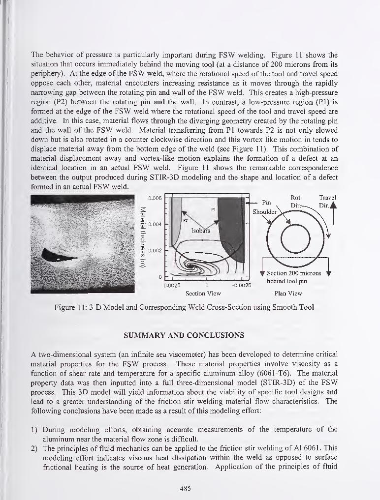
The behavior of pressure is particularly important during FSW welding. Figure 1 1 shows the

situation that occurs immediately behind the moving toQl (at a distance of 200 microns from its

periphery). At the edge of the FSW weld, where the rotational speed of the tool and travel speed

oppose each other, material encounters increasing resistance as it moves through the rapidly

narrowing gap between the rotating pin and wall of the FSW weld. This creates a high-pressure

region (P2) between the rotating pin and the wall. In contrast, a low-pressure region (PI) is

formed at the edge of the FSW weld where the rotational speed of the tool and travel speed are

additive. In this case, material flows through the diverging geometry created by the rotating pin

and the wall of the FSW weld. Material transferring from PI towards P2 is not only slowed

down but is also rotated in a counter clockwise direction and this vortex like motion in tends to

displace material away from the bottom edge of the weld (see Figure 11). This combination of

material displacement away and vortex-like motion explains the formation of a defect at an

identical location in an actual FSW weld. Figure 11 shows the remarkable correspondence

between the output produced during STIR-3D modeling and the shape and location of a defect

formed in an actual FSW weld.

Figure 1 1 : 3-D Model and Corresponding Weld Cross-Section using Smooth Tool

SUMMARY AND CONCLUSIONS

A two-dimensional system (an infinite sea viscometer) has been developed to determine critical

material properties for the FSW process. These material properties involve viscosity as a

frmction of shear rate and temperature for a specific aluminum alloy (6061-T6). The material

property data was then inputted into a fiill three-dimensional model (STIR-3D) of the FSWprocess. This 3D model will yield information about the viability of specific tool designs and

lead to a greater understanding of the fiiction stir welding material flow characteristics. The

following conclusions have been made as a result of this modeling effort:

1) During modeling efforts, obtaining accurate measurements of the temperature of the

aluminum near the material flow zone is difficult.

2) The principles of fluid mechanics can be applied to the fiiction stir welding of Al 6061. This

modeling effort indicates viscous heat dissipation within the weld as opposed to surface

fiicfional heating is the source of heat generafion. Application of the principles of fluid

485

mechanics to the FSW process will eventually allow for prediction of mixing with the weld,

prediction of oxide inclusions, and prediction of weld defects.

3) An infinite sea viscometer system (2D experimental and associated model) predicts critical

material properties that can be used for modeling of the FSW process. Given only the power

input, rotation speed, plunge rate, and viscosity, the infinite sea viscometer model was able to

predict accurately flow profiles and temperature distributions during plunge testing.

4) Plunge testing has shown that the temperature is nearly isothermal within 250 microns of the

tool and that the effect of shear rate on viscosity is large.

ACKNOWLEDGEMENTS

The authors would like to acknowledge technical support fi-om Wade Crusan, Tim DeShazer, and

Rich Claxton at Tower Automotive and Steve Carian and Terry Allen at A. O. Smith Corp. The

authors would also like to acknowledge funding support fi"om NIST (Project #70NAB5H)

REFERENCES

1. Thomas, W.M.; et al. 1991. Friction Stir Butt Welding. U.S. Patent No. 5,460,317.

2. Dawes, C.J.; and Thomas, W.M. 1996. Friction Stir Process Welds Aluminum Alloys,

Welding Journal: 75 (3): 41.

3. Nicholas, E.D.; and Kallee, S.W. 1998. Causing a Stir in the Future. Welding & Joining (2):

18-21.

4. Dawes, C. J. 1994. Development of the New Friction Stir Technique for Welding Aluminum- Phase I Report, TWI GSP 5651: (7): 13.

5. Broman, R. E.; Smith, C. B.; Noruk, J. S.; and McDonald, W. M. Challenges of Robotic

Welding ofAluminum Structures. Proc. of 38^ International Conf. of Metallurgists

6. Singh, J.; and Alpas, A.P. 1996 High Temperature Wear and Deformation Processing Metal

Matrix Composites. Metallurgical & Material Transactions: 27A: 1-13.

7. North, T.H.; Bendzsak G. B.; Smith C. B.; Hinrichs J.F.; Noruk, J. S.; and Heideman, R. J.

1999. Submitted to Welding Journal.:

8. Bendzsak, G. B.; North, T. H.; and Li, Z. 1997. Numerical Model for Steady-State Flow in

Friction Welding. Acta Metallurgical Material. 45 (4): 1735-1745.

9. Bendzsak, G. B.; and North, T. H. 1997. Numerical Modeling of Fluid Dynamics and Heat

Transfer in Friction Welding. Proc. International Seminar of Numerical Analysis of

Weldability . ed. H. Czerjack.

10. Bendzsak, G.B.; and North, T. H. 1997. Modeling of Fluid Dynamics and Heat Transfer in

Friction Welding. Trans. Japan welding Research . 25 (2): 171-184.

11. Bryant, A.J; Dixon, W; Fielding, A.P; and Macey, G. 1999. Isothermal Extrusion. Light

Metal Age : 78 (2): 8-36.

12. Bird, R.R; Stewart, W.E.; and Lightfood, E.N. 1960. Transport Phenomena . 95 New York,

NY: John Wiley and Sons.

486

Tutorials

Ph

j^

r •

o

O

H1—

1

It

o• 1—1

Ct

:^

489

C/3

Q

H

• ^

>

Q

Co

Si

oo

3 I

>3

Ik

O

>PQ

I

I

aooGO

s ^_J i

02 Oo

o

H—

>

a.

GO

I

o

a

Uh-I

490

c3

Oh

Ph o

O

CD

a

O

O1^

c2

• I—

I

ID^73

>Hi 200

ooC3

o

491

492

oc3

1o

Oh

C/3

aOhoOho

o j3

a• rH

§C/3

493

Oc/3 a

a

O

494

O

• •

H

Q

Oh

CD

o

O ^Q. CO

P o

o

o

oIT)

Io<N

c/:i

Oo

OaoQ

495

496

497

03

• 1—

(

aoo

>

o

o>cd o

N

O

oU

498

i

499

p.

Aoo(D oo

O =„ ^3

2 i ^

^ a ^ .2

c/3 V Q

502

in

C/5

•J

503

I

C/3

Oh

504

!/3 (1^

^ C3

OOh

oO

4t:

(A

505

H

c/5

O• 1—1

>

O

O

C/3

^3

s

M-H

H

>

506

HOt/i

CD5-1 }-(

C3o

42

Oh

507

0-)

o

0-)

o

oa.

• I—

I

O

u 8

,-4->

M—

I

o

s

O

GO

H

Oh

ao

o

o

oU tin

O• 1—1

• i-H

-4—

»

OS

• ^

o

508

g

O

O

oc3O

ID

E(Doa

>^

i

510

O

C/5

o

O

C39h c3

N

511

N

u

O

u

o>^

S ®

-0 o

oC/3

O

I"

o

CO

o

512

o

o

c3

o

o

Oh

o

C3

«4Ho o

B ^

Ooaoo

13 .S ^o

o

o ^

oC/3

13 ^O

oo

513

o

Id

Oo

o

o

514

o

o

O

oIdN

O

03

o

C/3

3

so

<

C/3

.3

Do o

515

0'

o

CO

o

o(J

Oo

Oooo

O

o

C3

Q

ao

Co ^^ -a

CD

I I

(30

Oo

516

s—

>

o

C/2

oa.O

Ph

C/5

Oo

O

517

518

« o

o

>

o

i

o

N

C/5

o

o

o

§

ID<D

1/5

1 C/5

o^ ^ ^

in

O

519

o

o

iw

O

OoI

CDa

a a

520

o

in

.2

o

o

aeg

>o

o

o .2

o

CO

o00

o00

o

c2

O

B>o

O00

<2

• I-H

>o

oX• 1-H

oCD

Oh

O

CO

OQ

521

522

o

o

Oh

C/5

C/3

O

O

C/5

OCQ

t>0

Oc3

bp

Q

Q+->

o

o

(30 5^

cCD

c3

1)

3oo

•^

I

OO

(20

bOo

;-( o

O• l-H

00

CO

OO

ooo

v7r • 1-HCO43C/5

524

o

Z

W o

<D O

o o

^ O

o

o+->

Oh

O

$-1

PQ

o

o

c/5

oio

§

oo

I

CD

Oh OCO h-H

C/5

o

§o

• 1—

I

>o

Oo

o

525

i

O

o

N

O

oc/3

CO)

O

526

Appendix A: Participants in Ninth

International Conference on ComputerTechnology in Welding

Appendix A.l: Speakers at the Ninth International Conference on Computer Technology

in Welding, September 28-30, 1999, Detroit, Michigan

Mr. Darren M. Barborak

Graduate Research Associate

The Ohio State University

1248 Arthur E. Adams Drive

Columbus, OH 43221

Mr. Zafer Bingul

PhD Candidate

Vanderbilt University

349 Normandy Circle

Nashville, TN 37209

Dr. Annette Brandenburg

Dr.-Ing.

ISF— Welding Institute Aachen

Ponstrasse 49

52062 Aachen 1 Germany

Mr. Andy Brightmore

Manager, Software Development

TWITechnology Transfer Department

Cambridge CBl 6ALUnited Kingdom

Dr. Bill Y.J. Chao

Professor

University of South Carolina

Dept. ofMechanical Engineering

Columbia, SC 29208

Dr. Pawel Cegielski

Assistant Professor

Warsaw University of Technology

Institute ofMaterials Processing

Welding Department

85 Narbutta Street

02-524 Warsaw, Poland

Dr. Juan R. Donoso

Professor

Universidad Tecnica Federica Santa Maria

Avenida Espana 1680

Valparaiso, Chile

Dr. John N. Dupont

Assistant Professor

Materials Science & Engineering

Lehigh University

5 East Packer Avenue

Bethlehem, PA 18015

Dr. James R. Dydo

Senior Engineer

EWI1250 Arthur E. Adams Drive

Columbus, OH 43221

Mr. Erik EnghGeneral Manager

4X Software ASGrini Neringspark 1

N-1361 Osteras, Norway

Mr. Lance A. Flitter

Computer Scientist

NSWC9500 MacArthur Boulevard

Bethesda,MD 20817-5700

Mr. James D. Gilsinn

Electronics Engineer

NISTIntelligent Systems Division

100 Bureau Drive, Stop 8230

Gaithersburg, MD 20899-8230

529

Appendix A.1: Speakers at the Ninth International Conference on Computer Technology

in Welding, September 28-30, 1999, Detroit, Michigan

Dr. Dariusz Golanski

Assistant Professor

Warsaw University ofTechnology

Institute ofMaterials Processing

Welding Department

85 Narbutta Street

02-524 Warsaw, Poland

Dr. Daniel A. Hartman

Los Alamos National Laboratory

PO Box 1663, Mail Stop G770Los Alamos, NM 87545

Mr. Chris Hsu

Senior Project Engineer

The Lincoln Electric Company

22801 St. Clair Avenue

Cleveland, OH 44117

Mr. Peter W. Hughes

Technical Director

Welding Technology Innovations Pty Ltd.

PO Box 97

Botany, NSW, 2019, Australia

Dr. Jan Paul Huisson

Associate Professor

University ofWaterloo

Dept. ofMechanical Engineering

Waterloo, Ontario N2L 3G1 Canada

Dr. Jerald E. Jones

Chief Scientist

NA Technology Company1317 Washington Avenue

Suite 1

Golden, CO 80401

Dr. You Chul KimAssociate Professor

JWRI, Osaka University

11-1, Mihogaoka

Ibaraki, Osaka 567-0047, Japan

Mr. Gerald A. Knorovsky

Sr. Member of Technical Staff

Sandia National Lab

1515 Eubank S.E., Mail Stop 0367

Albuquerque, NM 87123

Mr. Poolsak KoseyapomVanderbilt University

Box 1826, Station B.

Nashville, TN 37235

Dr. Radovan Kovacevic

Professor

Mechancial Engineering Dept.

Southern Methodist University

3160 SMU Boulevard

Dallas, TX 75205

Mr. John Lapham

Engineering Manager

Robotic Workspace Technologies, Inc.

17105 San Carlos Boulevard

Suite A-6151

Fort Myers, FL 33931

Mr. Danny O. MacCallum

PTNGMaterials Joining Department

PO Box 5800, Mail Stop 0367

Albuquerque, NM 87185-0367

530

Appendix A.1: Speakers at the Ninth International Conference on Computer Technology

in Welding, September 28-30, 1999, Detroit, Michigan

Mr. Tsuyoshi MaedaWelding & Joining Research Center

Nippon Steel Corporation

20-1 Shintomi

Futtsu, Chiba, 293-8511 Japan

Dr. Kin-ichi Matsuyama

Visiting Professor

MIT, Mechanical Engineering

77 Massachusetts Avenue

Room 35-231

Cambridge, MA 02139

Dr. Edward A. Metzbower

Branch HeadNaval Research Laboratory

Code 6320

Washington, DC 20375-5320

Dr. Paul E. Murray

Advisory Engineer

Lockheed Martin Idaho Technologies

PO Box 1625

Idaho FaUs, ID 83415-2210

Dr. Ole Runar Myhr

Research Scientist

Hydro Raufoss Automotive

PO Box 41

N-2831 Raufoss, Norway

Dr. S.-J. NaProfessor

KAIST373-1, Kusongdong, Yusonggu

Taejon, 305-701 Korea

Mr. Terumi NakamuraNational Research Center for Metals

1-2-1 Sengen,

Tukuba-shi Ibaraki 305-0047 Japan

Dr. BelaPalotas

Associated Professor

Technical University ofBudapest

Bertalan L. U. F.

Budapest, H-1521, Hungary

Dr. Timothy P. Quinn

Mechanical Engineer

NIST- Mail Code 853

Materials Reliability Division

325 Broadway

Boulder, CO 80303

Dr. S. Rajasekara

Assistant Professor

Dept. ofProduction Engineering

Amrita Institute ofTechnology & Science

Ettimadai Post, Coimbatore 641 105

Tamil Nadu, India

Mr. William G. Rippey

Electrical Engineer

NISTIntelligent Systems Division

Manufacturing Engineering Laboratory

100 Bureau Drive, Stop 8230

Gaithersburg, MD 20899-8230

Dr. Thomas A. Siewert

Deputy Chief

NIST -Mail Code 853

Materials Reliability Division

325 Broadway

Boulder, CO 80303

531

Appendix A.l: Speakers at the Ninth International Conference on Computer Technology

in Welding, September 28-30, 1999, Detroit, Michigan

Mr. Christopher B. Smith

Sr. Mechanical Engineer

Tower Automotive

3533 N. 27th Street

Milwaukee, WI 53216

Dr. Wenqi Zhang

Associate Professor

Department ofManufacturing Engineering

Technical University ofDenmark

Building 425

2800 Lyngby, Denmark

Prof Michael Zinigrad

Professor

The College ofJudea & Samaria

Ariel, Israel, 44837

532

Appendix A.2: Attendees of the Ninth International Conference on Computer Technology

in Welding, September 28-30, 1999, Detroit, Michigan

Mr. Pat Brousset

Ingenieur Systeme

Framatome Technologies

Plant Component Repair Equipements de

Soudage

3315 Old Forest Road/PO Box 10935

Lynchburg, VA 24506-0935

Mr. Dave Cottle

Weldmg Engineer

DC Fabricators

801 W. Front Street

Florence, NJ 08053

Mr. Eric Halloran

617 Bradley Street

Dubuque, lA 52003

Mr. Dan Hayden

StafiF Scientist

GM R&D Center

30500 Mound Road

Warren, MI 48090

Mr. Timothy Heston

Assistant Editor

American Welding Society

550NWLeJeuneRoadMiami, FL 33126

Mr. CarlF. Klein

Manager New Technology

Johnson Controls, Inc.

Automotive Systems Group

49200 Halyard Drive/PO Box 8010

Plymouth, MI 48170

Siri Klokkehaug

Research Scientist

Institute for Energy Technology

Materials and Corrosion Technology Dept.

PO Box 40

N-2007 Kjeller, Norway

Dr. Amt O. Kluken

Head of Joining Technology Group

Hydro Raufoss Automotive Research Center

PO Box 41

N-283 1 Raufoss, Norway

Dr. Kishore N. Lakalapalli

Product Development Engineer

FANUC Robotics North America

3900 W.Hamlin RoadRochester Hills, MI 48309-3253

Dr. Lin Li

Advanced Welding Engineer

Hydro Raufoss Automotive

365 West 24th Street

HoUand, MI 49423

Mr. John F. Negri

APEX Technical School

635 Avenue ofthe Americas

Manhattan, NY 10011

Mr. Alan R. Nywening

Ingersoll Rand

942 Memorial Parkway

Phillipsburg, NJ 08865

Mr. Juan E. Ochoa

109 South Summit Avenue

Gaithersburg, MD 20877

533

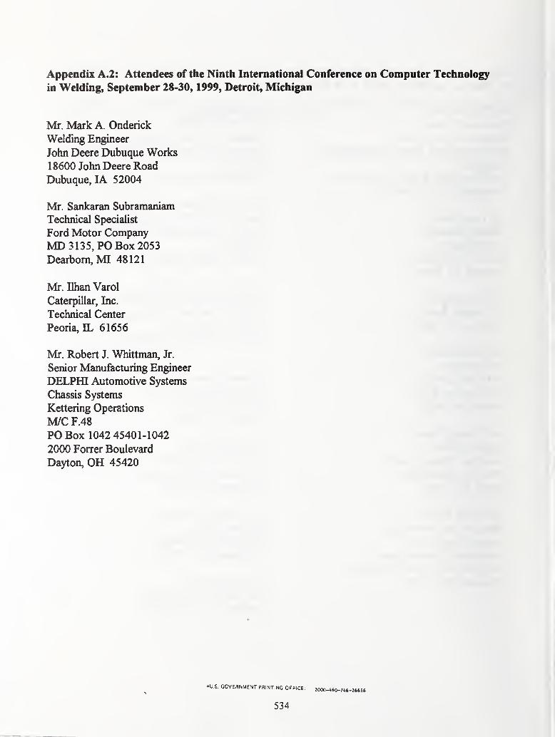
Appendix A.2: Attendees of the Ninth International Conference on Computer Technology

in Welding, September 28-30, 1999, Detroit, Michigan

Mr. Mark A. Onderick

Welding Engineer

John Deere Dubuque Works

18600 John Deere Road

Dubuque, lA 52004

Mr. Sankaran Subramaniam

Technical Specialist

Ford Motor CompanyMD3135,PO Box 2053

Dearborn, MI 48121

Mr. Dhan Varol

Caterpillar, Inc.

Technical Center

Peoria, DL 61656

Mr. Robert J. Whittman, Jr.

Senior Manufacturing Engineer

DELPHI Automotive Systems

Chassis Systems

Kettering Operations

M/C F.48

PO Box 1042 45401-1042

2000 Forrer Boulevard

Dayton, OH 45420

^U.S. GOVERNMENT PRINTING OFFICE: 2000-460-746-26656

534

Technical Publications

Periodical

Journal of Research of the National Institute of Standards and Technology—Reports NIST research

and development in those disciplines of the physical and engineering sciences in which the Institute is

active. These include physics, chemistry, engineering, mathematics, and computer sciences. Papers cover a

broad range of subjects, with major emphasis on measurement methodology and the basic technology

underlying standardization. Also included from time to time are survey articles on topics closely related to

the Institute's technical and scientific programs. Issued six times a year.

Nonperiodicals

Monographs—Major contributions to the technical literature on various subjects related to the

Institute's scientific and technical activities.

Handbooks—Recommended codes of engineering and industrial practice (including safety codes) devel-

oped in cooperation with interested industries, professional organizations, and regulatory bodies.

Special Publications—Include proceedings of conferences sponsored by NIST, NIST annual reports, and

other special publications appropriate to this grouping such as wall charts, pocket cards, and bibliographies.

National Standard Reference Data Series—Provides quantitative data on the physical and chemical

properties of materials, compiled from the world's literature and critically evaluated. Developed under a

worldwide program coordinated by NIST under the authority of the National Standard Data Act (Public

Law 90-396). NOTE: The Journal of Physical and Chemical Reference Data (JPCRD) is published

bimonthly for NIST by the American Chemical Society (ACS) and the American Institute of Physics (AIP).

Subscriptions, reprints, and supplements are available from ACS, 1 155 Sixteenth St., NW, Washington, DC20056.

Building Science Series—Disseminates technical information developed at the Institute on building

materials, components, systems, and whole structures. The series presents research results, test methods, and

performance criteria related to the structural and environmental functions and the durability and safety

characteristics of building elements and systems.

Technical Notes—Studies or reports which are complete in themselves but restrictive in their treatment of

a subject. Analogous to monographs but not so comprehensive in scope or definitive in treatment of the

subject area. Often serve as a vehicle for final reports of work performed at NIST under the sponsorship of

other government agencies.

Voluntary Product Standards—Developed under procedures published by the Department of Commercein Part 10, Title 15, of the Code of Federal Regulations. The standards establish nationally recognized

requirements for products, and provide all concerned interests with a basis for common understanding of

the characteristics of the products. NIST administers this program in support of the efforts of private-sector

standardizing organizations.

Order the following NIST publications—FIPS and NISTIRs—from the National Technical Information

Service, Springfield, VA 22161.

Federal Information Processing Standards Publications (FIPS PUB)—Publications in this series

collectively constitute the Federal Information Processing Standards Register. The Register serves as the

official source of information in the Federal Government regarding standards issued by NIST pursuant to

the Federal Property and Administrative Services Act of 1949 as amended. Public Law 89-306 (79 Stat.

1 127), and as implemented by Executive Order 1 1717 (38 FR 12315, dated May 11, 1973) and Part 6 of

Title 15 CFR (Code of Federal Regulations).

NIST Interagency or Internal Reports (NISTIR)—The series includes interim or final reports on work

performed by NI^ for outside sponsors (both government and nongovernment). In general, initial

distribution is handled by the sponsor; public distribution is handled by sales through the National Technical

Information Service, Springfield, VA 22161, in hard copy, electronic media, or microfiche form. NISTIR's

may also report results of NIST projects of transitory or limited interest, including those that will be

published subsequently in more comprehensive form.

U.S. Department of CommerceNational Institute of Standards and Tech325 BroadwayBoulder, Colorado 80303-3328

Official BusinessPenalty for Private Use, $300