Proc. R. Soc. B (2005) 272, 2203–2210

doi:10.1098/rspb.2005.3212

New insights into butterfly–environmentrelationships using partitioning methods

Risto K. Heikkinen*, Miska Luoto, Mikko Kuussaari and Juha Poyry

Finnish Environment Institute, Research Programme for Biodiversity, PO Box 140, 00251 Helsinki, Finland

Published online 31 August 2005

*Autho

ReceivedAccepted

Variation partitioning and hierarchical partitioning are novel statistical approaches that provide deeper

understanding of the importance of different explanatory variables for biodiversity patterns than traditional

regression methods. Using these methods, the variation in occupancy and abundance of the clouded apollo

butterfly (Parnassius mnemosyne L.) was decomposed into independent and joint effects of larval and adult

food resources, microclimate and habitat quantity. The independent effect of habitat quantity variables

(habitat area and connectivity) captured the largest fraction of the variation in the clouded apollo patterns,

but habitat connectivity had a major contribution only for occupancy data. The independent effects of

resources and microclimate were higher on butterfly abundance than on occupancy. However, a

considerable amount of variation in the butterfly patterns was accounted for by the joint effects of

predictors and may thus be causally related to two or all three groups of variables. Abundance of the

butterfly in the surroundings of the focal grid cell had a significant effect in all analyses, independently of

the effects of other predictors. Our results encourage wider applications of partitioning methods in

biodiversity studies.

Keywords: autocovariate; collinearity; connectivity; habitat quality; Parnassius mnemosyne;

semi-natural grasslands

1. INTRODUCTIONConclusions about the determinants of biodiversity

patterns in ecological studies are often derived from

correlative multiple regression settings. However, identi-

fication of the predictor variables most probably affecting

the variation in the response variable by commonly used

regression methods can be problematic, particularly if

predictor variables are significantly intercorrelated

(Chevan & Sutherland 1991; Mac Nally 2000; Graham

2003).

Multicollinearity among predictors may result in the

exclusion of ecologically more causal variables from

multiple regression models if other intercorrelated

variables explain the variation in response variable better

in statistical terms (Mac Nally 2000). There are currently

many approaches available for tackling collinearity

problems. In studies aiming at predictive regression

analysis, valuable insights can be developed by methods

such as sequential regression and structural equation

modelling (Graham 2003). Collinearity can also be

addressed by variation partitioning (Borcard et al.

1992) and hierarchical partitioning methods (Chevan &

Sutherland 1991; Mac Nally 2000). These techniques

aim to provide understanding of the probable causalities

and explanatory powers of predictors in multivariate

datasets, not at generating a predictive equation (Watson&

Peterson 1999). In this study, we focus on variation

partitioning and hierarchical partitioning methods.

These methods can provide new insights into species–

environment relationships by decomposing the variation

in response variable(s) into independent components

which reflect the relative importances of individual

r for correspondence (risto.heikkinen@ymparisto.fi).

31 May 200512 June 2005

2203

predictors or groups of predictors and their joint effects

(Liu 1997; Anderson & Gribble 1998; Watson & Peterson

1999; Mac Nally 2000; Lichstein et al. 2002; Cushman &

McGarigal 2004; Gibson et al. 2004; Heikkinen et al.

2004).

Butterfly–environment studies have often relied on

traditional regression methods: relationships between

species richness or abundance of butterflies and the

environment have commonly been examined with (step-

wise) regression techniques (e.g. Clausen et al. 2001;

Krauss et al. 2003; Maes et al. 2003), and single species

occupancy patterns using (stepwise) logistic-regression

(e.g. Hill et al. 1996; Dennis & Eales 1997, 1999; Cowley

et al. 2000; Thomas et al. 2001; Fleishman et al. 2002;

WallisDeVries 2004). Both variation and hierarchical

partitioning methods have rarely been applied in assessing

the contributions of different environmental variables to

studied butterfly patterns (but see Mac Nally et al. 2003;

Sawchik et al. 2003; Cleary & Gennert 2004). This is

surprising, because butterflies have been used as model

taxa in ecological and population biological, e.g. metapo-

pulation studies which have compared the explanatory

power of two or more groups of predictor variables to

explain the variation in species abundance or occupancy,

e.g. landscape factors versus local factors (Krauss et al.

2003; Bergman et al. 2004), or habitat patch size

and isolation versus habitat quality factors (Thomas

et al. 2001; Fleishman et al. 2002; Anthes et al. 2003;

WallisDeVries 2004). Such study designs may provide

insufficient information concerning the relative

importance of predictors when traditional regression

methods are employed to model species–environment

data affected by multicollinearity (cf. Mac Nally 2000;

Heikkinen et al. 2004).

q 2005 The Royal Society

2204 R. K. Heikkinen and others Butterfly–environment relationships

Heikkinen et al. (2004) showed that both variation

partitioning and hierarchical partitioning approaches can

provide important insights into bird abundance–environ-

ment relationships. Here, we present the first simul-

taneous application of two partitioning methods to explain

the occupancy and abundance patterns of a single

butterfly species. We explored the relative importance of

predictors representing three ecological groups of vari-

ables (larval and adult food resources, microclimate,

habitat quantity) in explaining the spatial variation of the

threatened clouded apollo butterfly (Parnassius mnemosyne

L.) in southwestern Finland. Using data on P. mnemosyne

recorded in a 50!50 m grid system we determined the

independent and joint effects of predictor variables on the

variation in occupancy and abundance of the butterfly.

Specifically, we asked the following questions: (i) How

great are the independent contributions of the three

groups of predictors in explaining the occupancy and

abundance of the clouded apollo? (ii) Do the relative

importances of the predictor groups differ between the

variation partitioning results for the butterfly occupancy

and abundance? (iii) How great are the joint contributions

of the explanatory variables? (iv) Which variables have the

highest independent correlations with the occupancy and

abundance of the butterfly in hierarchical partitioning?

Furthermore, we explored whether the spatial autocorre-

lation in the clouded apollo abundance (‘autocovariate’,

i.e. the abundance of butterfly individuals in the

surroundings of the focal grid square; see Augustin et al.

1996; Ferrier et al. 2002) exerts an independent,

significant effect on the butterfly patterns even if the

effects of other factors are controlled.

2. MATERIAL AND METHODSThe study area and material are described in detail in Luoto

et al. (2001) and here we provide only a brief description.

(a) Study area

The study area is situated in an agriculturally dominated

landscape in southwestern Finland (608N 32 0–608N 36 0,

23819 0–23830 0E). The landscape is generally characterized

by flat agricultural plains, scattered forest-covered hills and

steep-sided river valleys along the river Rekijoki. Coniferous

forest (Norway spruce Picea abies and Scots pine Pinus

sylvestris) is the main forest type in the area. Deciduous forests

(birches Betula pendula and Betula pubescens, grey alder Alnus

incana and trembling aspen Populus tremula) and semi-natural

grasslands are found on the slopes of river valleys.

(b) Study species

The clouded apollo (P. mnemosyne) is a palearctic butterfly

which is classified as threatened in Finland (Rassi et al. 2001)

and elsewhere in Europe (Konvicka &Kuras 1999; van Swaay

& Warren 1999). In Finland, the clouded apollo is a rare

inhabitant of traditionally managed flower-rich semi-natural

meadows and pastures accompanied by deciduous forest

patches abundant withCorydalis solida, the larval host plant of

the butterfly (Luoto et al. 2001).

(c) Butterfly survey

In 1999 the distribution of P. mnemosyne was surveyed in a

total of 2408 grid squares, 50!50 m in size, within a 6 km2

study area. All parts of the study area were visited at least five

Proc. R. Soc. B (2005)

times during the adult flight season. In each grid square the

potentially suitable habitat was thoroughly sampled using

mark–release–recapture method (Luoto et al. 2001). The

sampling effort varied between different parts of the study

area. However, the results of Luoto et al. (2001) showed that

the impact of study effort on modelling results was small,

particularly when spatial autocorrelation (autocovariate) was

considered simultaneously, as was also done here. From the

survey results we produced two variables measuring the

distribution and abundance of the butterfly. Distribution was

measured for each of the 2408 grid squares as a binary

variable, presence (O0 observations) or absence (0 obser-

vations) of butterflies during the whole flight season. For each

of the 349 grid cells (‘core’ set of grid cells), where the

butterfly was present its abundance was measured as the total

number of butterflies observed during all visits divided by the

number of visits in each grid square.

(d) Environmental variables

Eight environmental predictor variables were recorded for

each of the 2408 0.25 ha grid squares. Data for the ninth

environmental variable, the abundance of nectar plants, was

available only for the core set of 349 grid squares. These

variables were assigned into three groups: (i) habitat quantity

(habitat area and connectivity), (ii) resource and (iii)

microclimate variables. An additional predictor was the

‘autocovariate’, which incorporated the effect of the butterfly

abundance in the surroundings into the analysis.

The four habitat area variables included were the amount

of agricultural land, semi-natural grassland, deciduous and

mixed forest and coniferous forest in each of the 0.25 ha grid

squares. The distribution of these habitats was defined from

aerial low altitude black and white photographs (1 : 7500

scale) and from topographic maps, and verified in the field

(Luoto et al. 2001).

Habitat connectivity was measured only for semi-natural

grasslands, the habitat for P. mnemosyne (Luoto et al. 2001).

Connectivity (S) to semi-natural grasslands in the surround-

ings of grid square i was measured as follows (Hanski 1994):

Si ZX

jsi

expðKadijÞAj ; ð2:1Þ

where Aj is the area of semi-natural grassland (in ha) in the

square, and dij is the distance between squares i and j. The

dispersal kernel a was set as 1 based on mark–recapture data

on the movements of the butterfly in the study area

(Kuussaari & Luoto, unpublished work). Connectivity of

the focal cell to semi-natural grasslands in adjacent grid cells

was measured up to 330 m, which matches closely with the

observed average dispersal distance of P. mnemosyne in boreal

areas (Valimaki & Itamies 2003).

The two resource variables were the abundances of nectar

plants and larval host plants. The average density of host

plant (C. solida) shoots per square metre was estimated from

each grid square in April–May. The abundance of the nectar

plants (Anthriscus sylvestris, Geranium sylvaticum, Trifolium

spp.,Vicia cracca,Vicia sepium,Ranunculus spp.) was recorded

only from the core set of 349 grid squares using a scale from 0

to 10 (0Zno nectar plants, 10Znectar plants extremely

abundant) in June.

The two variables reflecting microclimate were radiation

and average wind speed. Following Luoto et al. (2001), an

estimate of maximum theoretical solar radiation for each grid

square was produced using a computer model of clear sky

habitat (H)9.2%

a

resources (R)3.5%

b

undetermined variation (U)75.0%

d4.3%

g3.0%

c3.5%

microclimate (M)

e1.2%

f0.5%

habitat (H)26.4%

a

resources (R)1.4%

b

undetermined variation (U)41.4%

d17.3%

g9.8%

c2.2%

microclimate (M)

e2.2%

f0.3%

(a) (b)

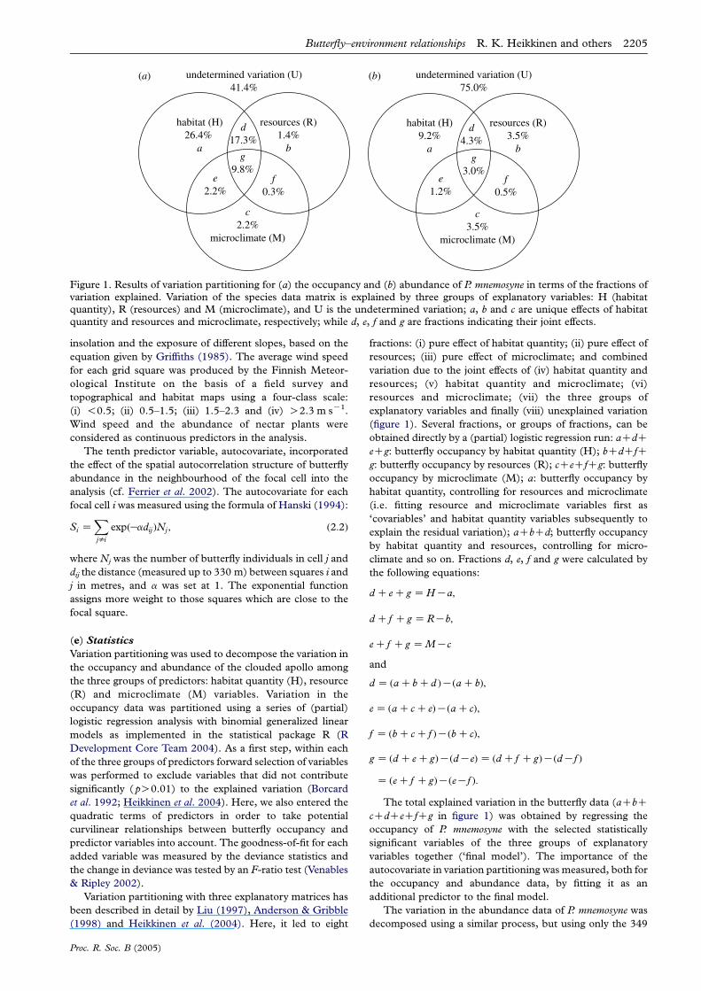
Figure 1. Results of variation partitioning for (a) the occupancy and (b) abundance of P. mnemosyne in terms of the fractions ofvariation explained. Variation of the species data matrix is explained by three groups of explanatory variables: H (habitatquantity), R (resources) and M (microclimate), and U is the undetermined variation; a, b and c are unique effects of habitatquantity and resources and microclimate, respectively; while d, e, f and g are fractions indicating their joint effects.

Butterfly–environment relationships R. K. Heikkinen and others 2205

insolation and the exposure of different slopes, based on the

equation given by Griffiths (1985). The average wind speed

for each grid square was produced by the Finnish Meteor-

ological Institute on the basis of a field survey and

topographical and habitat maps using a four-class scale:

(i) !0.5; (ii) 0.5–1.5; (iii) 1.5–2.3 and (iv) O2.3 m sK1.

Wind speed and the abundance of nectar plants were

considered as continuous predictors in the analysis.

The tenth predictor variable, autocovariate, incorporated

the effect of the spatial autocorrelation structure of butterfly

abundance in the neighbourhood of the focal cell into the

analysis (cf. Ferrier et al. 2002). The autocovariate for each

focal cell i was measured using the formula of Hanski (1994):

Si ZX

jsi

expðKadijÞNj ; ð2:2Þ

where Nj was the number of butterfly individuals in cell j and

dij the distance (measured up to 330 m) between squares i and

j in metres, and a was set at 1. The exponential function

assigns more weight to those squares which are close to the

focal square.

(e) Statistics

Variation partitioning was used to decompose the variation in

the occupancy and abundance of the clouded apollo among

the three groups of predictors: habitat quantity (H), resource

(R) and microclimate (M) variables. Variation in the

occupancy data was partitioned using a series of (partial)

logistic regression analysis with binomial generalized linear

models as implemented in the statistical package R (R

Development Core Team 2004). As a first step, within each

of the three groups of predictors forward selection of variables

was performed to exclude variables that did not contribute

significantly ( pO0.01) to the explained variation (Borcard

et al. 1992; Heikkinen et al. 2004). Here, we also entered the

quadratic terms of predictors in order to take potential

curvilinear relationships between butterfly occupancy and

predictor variables into account. The goodness-of-fit for each

added variable was measured by the deviance statistics and

the change in deviance was tested by an F-ratio test (Venables

& Ripley 2002).

Variation partitioning with three explanatory matrices has

been described in detail by Liu (1997), Anderson & Gribble

(1998) and Heikkinen et al. (2004). Here, it led to eight

Proc. R. Soc. B (2005)

fractions: (i) pure effect of habitat quantity; (ii) pure effect of

resources; (iii) pure effect of microclimate; and combined

variation due to the joint effects of (iv) habitat quantity and

resources; (v) habitat quantity and microclimate; (vi)

resources and microclimate; (vii) the three groups of

explanatory variables and finally (viii) unexplained variation

(figure 1). Several fractions, or groups of fractions, can be

obtained directly by a (partial) logistic regression run: aCdC

eCg: butterfly occupancy by habitat quantity (H); bCdCfC

g: butterfly occupancy by resources (R); cCeCfCg: butterfly

occupancy by microclimate (M); a: butterfly occupancy by

habitat quantity, controlling for resources and microclimate

(i.e. fitting resource and microclimate variables first as

‘covariables’ and habitat quantity variables subsequently to

explain the residual variation); aCbCd; butterfly occupancy

by habitat quantity and resources, controlling for micro-

climate and so on. Fractions d, e, f and g were calculated by

the following equations:

dCeCg ZHKa;

dC f Cg ZRKb;

eC f Cg ZMKc

and

d Z ðaCbCd ÞKðaCbÞ;

eZ ðaCcCeÞKðaCcÞ;

f Z ðbCcC f ÞKðbCcÞ;

g Z ðdCeCgÞKðdKeÞZ ðdC f CgÞKðdKf Þ

Z ðeC f CgÞKðeKf Þ:

The total explained variation in the butterfly data (aCbC

cCdCeCfCg in figure 1) was obtained by regressing the

occupancy of P. mnemosyne with the selected statistically

significant variables of the three groups of explanatory

variables together (‘final model’). The importance of the

autocovariate in variation partitioning was measured, both for

the occupancy and abundance data, by fitting it as an

additional predictor to the final model.

The variation in the abundance data of P. mnemosyne was

decomposed using a similar process, but using only the 349

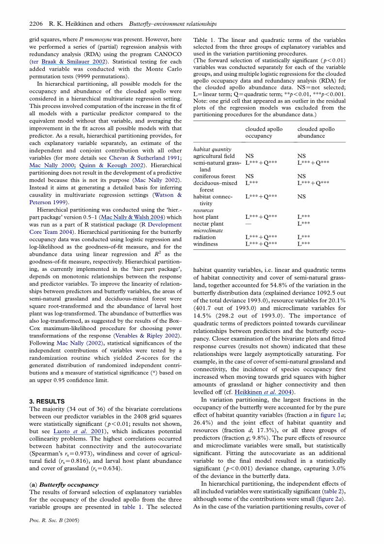
Table 1. The linear and quadratic terms of the variablesselected from the three groups of explanatory variables andused in the variation partitioning procedures.(The forward selection of statistically significant ( p!0.01)variables was conducted separately for each of the variablegroups, and using multiple logistic regressions for the cloudedapollo occupancy data and redundancy analysis (RDA) forthe clouded apollo abundance data. NSZnot selected;LZlinear term; QZquadratic term; **p!0.01, ***p!0.001.Note: one grid cell that appeared as an outlier in the residualplots of the regression models was excluded from thepartitioning procedures for the abundance data.)

clouded apollooccupancy

clouded apolloabundance

habitat quantityagricultural field NS NSsemi-natural grass-

landL***CQ*** L***CQ***

coniferous forest NS NSdeciduous–mixed

forestL*** L***CQ***

habitat connec-tivity

L***CQ*** NS

resourceshost plant L***CQ*** L***nectar plant — L***microclimateradiation L***CQ*** L***windiness L***CQ*** L***

2206 R. K. Heikkinen and others Butterfly–environment relationships

grid squares, where P. nmemosyne was present. However, here

we performed a series of (partial) regression analysis with

redundancy analysis (RDA) using the program CANOCO

(ter Braak & Smilauer 2002). Statistical testing for each

added variable was conducted with the Monte Carlo

permutation tests (9999 permutations).

In hierarchical partitioning, all possible models for the

occupancy and abundance of the clouded apollo were

considered in a hierarchical multivariate regression setting.

This process involved computation of the increase in the fit of

all models with a particular predictor compared to the

equivalent model without that variable, and averaging the

improvement in the fit across all possible models with that

predictor. As a result, hierarchical partitioning provides, for

each explanatory variable separately, an estimate of the

independent and conjoint contribution with all other

variables (for more details see Chevan & Sutherland 1991;

Mac Nally 2000; Quinn & Keough 2002). Hierarchical

partitioning does not result in the development of a predictive

model because this is not its purpose (Mac Nally 2002).

Instead it aims at generating a detailed basis for inferring

causality in multivariate regression settings (Watson &

Peterson 1999).

Hierarchical partitioning was conducted using the ‘hier.-

part package’ version 0.5–1 (Mac Nally &Walsh 2004) which

was run as a part of R statistical package (R Development

Core Team 2004). Hierarchical partitioning for the butterfly

occupancy data was conducted using logistic regression and

log-likelihood as the goodness-of-fit measure, and for the

abundance data using linear regression and R2 as the

goodness-of-fit measure, respectively. Hierarchical partition-

ing, as currently implemented in the ‘hier.part package’,

depends on monotonic relationships between the response

and predictor variables. To improve the linearity of relation-

ships between predictors and butterfly variables, the areas of

semi-natural grassland and deciduous-mixed forest were

square root-transformed and the abundance of larval host

plant was log-transformed. The abundance of butterflies was

also log-transformed, as suggested by the results of the Box–

Cox maximum-likelihood procedure for choosing power

transformations of the response (Venables & Ripley 2002).

Following Mac Nally (2002), statistical significances of the

independent contributions of variables were tested by a

randomization routine which yielded Z-scores for the

generated distribution of randomized independent contri-

butions and a measure of statistical significance (*) based on

an upper 0.95 confidence limit.

3. RESULTSThe majority (34 out of 36) of the bivariate correlations

between our predictor variables in the 2408 grid squares

were statistically significant ( p!0.01; results not shown,

but see Luoto et al. 2001), which indicates potential

collinearity problems. The highest correlations occurred

between habitat connectivity and the autocovariate

(Spearman’s rsZ0.973), windiness and cover of agricul-

tural field (rsZ0.816), and larval host plant abundance

and cover of grassland (rsZ0.634).

(a) Butterfly occupancy

The results of forward selection of explanatory variables

for the occupancy of the clouded apollo from the three

variable groups are presented in table 1. The selected

Proc. R. Soc. B (2005)

habitat quantity variables, i.e. linear and quadratic terms

of habitat connectivity and cover of semi-natural grass-

land, together accounted for 54.8% of the variation in the

butterfly distribution data (explained deviance 1092.5 out

of the total deviance 1993.0), resource variables for 20.1%

(401.7 out of 1993.0) and microclimate variables for

14.5% (298.2 out of 1993.0). The importance of

quadratic terms of predictors pointed towards curvilinear

relationships between predictors and the butterfly occu-

pancy. Closer examination of the bivariate plots and fitted

response curves (results not shown) indicated that these

relationships were largely asymptotically saturating. For

example, in the case of cover of semi-natural grassland and

connectivity, the incidence of species occupancy first

increased when moving towards grid squares with higher

amounts of grassland or higher connectivity and then

levelled off (cf. Heikkinen et al. 2004).

In variation partitioning, the largest fractions in the

occupancy of the butterfly were accounted for by the pure

effect of habitat quantity variables (fraction a in figure 1a;

26.4%) and the joint effect of habitat quantity and

resources (fraction d; 17.3%), or all three groups of

predictors (fraction g; 9.8%). The pure effects of resource

and microclimate variables were small, but statistically

significant. Fitting the autocovariate as an additional

variable to the final model resulted in a statistically

significant ( p!0.001) deviance change, capturing 3.0%

of the deviance in the butterfly data.

In hierarchical partitioning, the independent effects of

all included variables were statistically significant (table 2),

although some of the contributions were small (figure 2a).

As in the case of the variation partitioning results, cover of

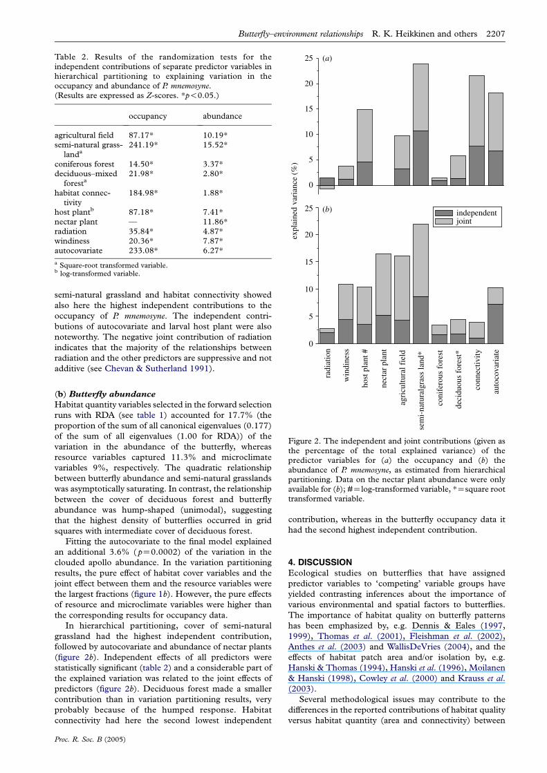
Table 2. Results of the randomization tests for theindependent contributions of separate predictor variables inhierarchical partitioning to explaining variation in theoccupancy and abundance of P. mnemosyne.(Results are expressed as Z-scores. *p!0.05.)

occupancy abundance

agricultural field 87.17* 10.19*semi-natural grass-

landa241.19* 15.52*

coniferous forest 14.50* 3.37*deciduous–mixed

foresta21.98* 2.80*

habitat connec-tivity

184.98* 1.88*

host plantb 87.18* 7.41*nectar plant — 11.86*radiation 35.84* 4.87*windiness 20.36* 7.87*autocovariate 233.08* 6.27*

a Square-root transformed variable.b log-transformed variable.

ral f

ield

s la

nd*

s fo

rest

for

est*

adia

tion

indi

ness

pla

nt #

ar p

lant

ectiv

ity

ovar

iate

independentjoint

0

5

10

15

20

25

0

5

10

15

20

25

expl

aine

d va

rian

ce (

%)

(a)

(b)

Butterfly–environment relationships R. K. Heikkinen and others 2207

semi-natural grassland and habitat connectivity showed

also here the highest independent contributions to the

occupancy of P. mnemosyne. The independent contri-

butions of autocovariate and larval host plant were also

noteworthy. The negative joint contribution of radiation

indicates that the majority of the relationships between

radiation and the other predictors are suppressive and not

additive (see Chevan & Sutherland 1991).

agri

cultu

sem

i-na

tura

lgra

s

coni

fero

u

deci

duou

sr w

host

nect

conn

auto

c

Figure 2. The independent and joint contributions (given asthe percentage of the total explained variance) of thepredictor variables for (a) the occupancy and (b) theabundance of P. mnemosyne, as estimated from hierarchicalpartitioning. Data on the nectar plant abundance were onlyavailable for (b); #Zlog-transformed variable, *Zsquare roottransformed variable.

(b) Butterfly abundance

Habitat quantity variables selected in the forward selection

runs with RDA (see table 1) accounted for 17.7% (the

proportion of the sum of all canonical eigenvalues (0.177)

of the sum of all eigenvalues (1.00 for RDA)) of the

variation in the abundance of the butterfly, whereas

resource variables captured 11.3% and microclimate

variables 9%, respectively. The quadratic relationship

between butterfly abundance and semi-natural grasslands

was asymptotically saturating. In contrast, the relationship

between the cover of deciduous forest and butterfly

abundance was hump-shaped (unimodal), suggesting

that the highest density of butterflies occurred in grid

squares with intermediate cover of deciduous forest.

Fitting the autocovariate to the final model explained

an additional 3.6% ( pZ0.0002) of the variation in the

clouded apollo abundance. In the variation partitioning

results, the pure effect of habitat cover variables and the

joint effect between them and the resource variables were

the largest fractions (figure 1b). However, the pure effects

of resource and microclimate variables were higher than

the corresponding results for occupancy data.

In hierarchical partitioning, cover of semi-natural

grassland had the highest independent contribution,

followed by autocovariate and abundance of nectar plants

(figure 2b). Independent effects of all predictors were

statistically significant (table 2) and a considerable part of

the explained variation was related to the joint effects of

predictors (figure 2b). Deciduous forest made a smaller

contribution than in variation partitioning results, very

probably because of the humped response. Habitat

connectivity had here the second lowest independent

Proc. R. Soc. B (2005)

contribution, whereas in the butterfly occupancy data it

had the second highest independent contribution.

4. DISCUSSIONEcological studies on butterflies that have assigned

predictor variables to ‘competing’ variable groups have

yielded contrasting inferences about the importance of

various environmental and spatial factors to butterflies.

The importance of habitat quality on butterfly patterns

has been emphasized by, e.g. Dennis & Eales (1997,

1999), Thomas et al. (2001), Fleishman et al. (2002),

Anthes et al. (2003) and WallisDeVries (2004), and the

effects of habitat patch area and/or isolation by, e.g.

Hanski & Thomas (1994), Hanski et al. (1996), Moilanen

& Hanski (1998), Cowley et al. (2000) and Krauss et al.

(2003).

Several methodological issues may contribute to the

differences in the reported contributions of habitat quality

versus habitat quantity (area and connectivity) between

2208 R. K. Heikkinen and others Butterfly–environment relationships

different studies, two of which are discussed here. First,

the discrepancies between studies may stem from the

varying efficiency of the connectivity or isolation measures

employed in different modelling exercises. The connec-

tivity index Si used in this study is currently considered

superior to more simple isolation measures such as

distance to the nearest patch (Moilanen & Nieminen

2002). Thus, the role of connectivity may have been

underestimated in studies based on simple isolation

indices (e.g. Thomas et al. 2001).

Second, a large number of butterfly studies have

employed traditional regression techniques, which may

have distorted inferences about the relative importance of

explanatory variables. This is because traditional

regression approaches do not provide separate measures

of the amounts of variation explained independently and

jointly by two or more variables or groups of variables.

Due to collinearity among explanatory variables, the

variables selected for the model will inevitably pick up

some of the explanatory power of, and thereby downplay

the importance of the other intercorrelated variables.

Variation and hierarchical partitioning methods used in

this study provide measures of the independent and joint

explanatory capacities of single predictors or groups of

predictors (Mac Nally 2000; Cushman & McGarigal

2004). Overall, the results of the two methods were in our

case similar, and the variables highlighted as significant by

the two approaches were the same. Our results for the

occupancy of P. mnemosyne indicate a dominant indepen-

dent contribution of habitat quantity and only a very small

independent contribution of resources and microclimate.

This supports the conclusions of Hanski et al. (1996),

Cowley et al. (2000), Krauss et al. (2003) and Bergman

et al. (2004) on the importance of habitat area and

connectivity. Moilanen & Hanski (1998) reported that

adding information on habitat quality did not greatly

improve the goodness-of-fit of the incidence function

models (based on patch area and isolation) for the patch

occupancy and density of Melitaea cinxia.

However, almost half (27.1 of 59.6%) of the total

explained variation of the clouded apollo occupancy in our

variation partitioning results was related to the joint

variation between habitat quantity and resources, or to

the joint variation between all three groups of variables.

The amount of joint contributions of predictors was also

notable in hierarchical partitioning. The shared variation

in variation partitioning results may be related to the

variation in resources, as well as to microclimate or habitat

area and connectivity. If we consider larval host plant

abundance as the most potential causal explanatory

variable for the joint variation, the total relative import-

ance of resources increases more than tenfold from the

pure effect of resources. It is noteworthy that modelling

exercises where resource variables are entered only as

additional predictors after all the statistically significant

habitat quantity variables will give only an estimation of

the pure effect of resources, and vice versa.

Habitat quantity (area of semi-natural grassland and

deciduous-mixed forest) also had the highest independent

fraction in the variation partitioning of the clouded apollo

abundance data (see also Luoto et al. 2001, 2002).

However, connectivity of semi-natural grasslands made a

minor contribution to the abundance of the butterfly both

in variation and hierarchical partitioning, possibly because

Proc. R. Soc. B (2005)

in our study area semi-natural grasslands often occur in a

riverside corridor system and not as clearly separated

distinct patches.

Resource variables (host-plant and nectar-plant abun-

dance) and microclimate had a relatively higher indepen-

dent importance for the abundance than for the

occupancy patterns of P. mnemosyne. The proportions of

joint contributions of predictors on butterfly abundance

were also notable. The importance of the amounts of

larval host plant and adult nectar sources for butterfly

abundance (or occupancy) has been demonstrated by

numerous studies (e.g. Dennis 1992; Loertscher et al.

1995; Clausen et al. 2001; Thomas et al. 2001; Fleishman

et al. 2002; Anthes et al. 2003; Auckland et al. 2004;

WallisDeVries 2004).

The contribution of microclimate reflects the fact that

in our study area the clouded apollo occurs most

abundantly in sheltered river valleys with warm micro-

climate and low wind speed. This is not surprising because

our study area is at the northern margin of the European

distribution of P. mnemosyne. The importance of micro-

climate for butterfly abundance has been emphasized by

many other butterfly studies (e.g. Thomas et al. 1999;

Clausen et al. 2001).

The abundance of the butterfly in the surroundings

(autocovariate) appeared as a significant predictor in all

our partitioning analyses. Thus, the number of butterfly

individuals in the surroundings of the focal square had an

explanatory power, which was independent of the effects

of other variables, including connectivity of semi-natural

grasslands, and this effect should be taken into account in

modelling. The importance of the autocovariate may

reflect occurrences of sites with favourable amounts of

resources or sheltered patches in the surroundings, or the

behaviour of P. mnemosyne. The latter assumption is

supported by the results of Valimaki & Itamies (2003),

who reported that the most important single factor

explaining the number of immigrating P. mnemosyne

individuals was the butterfly density in the target patch.

To reiterate, our results show that habitat quantity, i.e.

habitat connectivity and particularly habitat area, have a

major effect on the clouded apollo occupancy. Resource

andmicroclimate variables made substantial contributions

to the abundance of P. mnemosyne, but their independent

impact on the occupancy patterns was small. This suggests

that the components of habitat quality become increas-

ingly important for butterflies when examining the finer-

scale variation of abundance, whereas habitat quantity and

spatial arrangement of habitat patches may largely

determine the species distribution patterns in a wider

landscape. Nevertheless, in our results a considerable

amount of variation in the butterfly patterns was related to

joint effects of explanatory variables. Whether this

variation is ultimately more causally related to habitat

quantity, resources or microclimate can only by assessed

by experimental work or by accumulating information

from new similar study settings. Overall, the considerable

amount of conjoined contributions suggests that the

relative importance of different competing predictors

may have been insufficiently scrutinized in several earlier

butterfly studies.

In conclusion, our study shows that variation and

hierarchical partitioning methods provide deeper insights

into biodiversity–environment relationships than

Butterfly–environment relationships R. K. Heikkinen and others 2209

traditional regression methods, particularly if used in a

complementary manner. A potential shortcoming of

hierarchical partitioning is that the importance of

polynomial variables cannot be assessed by this method.

Asymptotic relationships between explanatory and

response variables can be improved by taking transform-

ation of the variables, as was done in our study. However,

in the case of humped relationships (here P. mnemosyne

abundance versus deciduous forest), improving the

linearity between response variables and predictors is

difficult, if not impossible. Under such circumstances

hierarchical partitioning is a less powerful method than

variation partitioning, in which the model fit can be

improved by including polynomial terms (Heikkinen et al.

2004). A possible weak point in variation partitioning is

the potential of collinearity problems during the forward

selection within the groups of predictor variables. In such

cases, hierarchical partitioning can be used in confirming

whether the predictors selected in variation partitioning

are among the most likely causal variables (cf. Gibson et al.

2004). Hitherto both partitioning methods have been

applied only sporadically in butterfly studies (but see Mac

Nally et al. 2003; Sawchik et al. 2003; Cleary & Gennert

2004). We conclude that when applied with caution,

butterfly ecology and biodiversity–environment studies in

general would benefit from a wider application of the

partitioning methods.

We thank B. Schroder and an anonymous referee for valuablecomments. Different parts of this research were funded by theEC FP6 Integrated Project ALARM (GOCE-CT-2003-506675).

REFERENCESAnderson, M. J. & Gribble, N. A. 1998 Partitioning the

variation among spatial, temporal and environmental

components in a multivariate data set. Aust. J. Ecol. 23,

158–167.

Anthes, N., Fartmann, T., Hermann, G. & Kaule, G. 2003

Combining larval habitat quality and metapopulation

structure—the key for successful management of pre-

alpine Euphydryas aurinia colonies. J. Insect Conserv. 7,

175–185. (doi:10.1023/A:1027330422958.)

Auckland, J. N., Debinski, D. M. & Clarke, W. R. 2004

Survival, movement, and resource use of the butterfly

Parnassius clodius. Ecol. Entomol. 29, 139–149. (doi:10.

1111/j.0307-6946.2004.00581.x.)

Augustin, N., Mugglestone, M. A. & Buckland, S. T. 1996

An autologistic model for spatial distribution of wildlife.

J. Appl. Ecol. 33, 339–347.Bergman, K.-O., Askling, J., Ekberg, O., Ignell, H.,

Wahlman, H. & Milberg, P. 2004 Landscape effects on

butterfly assemblages in an agricultural region. Ecography

27, 619–628. (doi:10.1111/j.0906-7590.2004.03906.x.)

Borcard, D., Legendre, P. & Drapeau, P. 1992 Partialling out

the spatial component of ecological variation. Ecology 73,

1045–1055.

Chevan, A. & Sutherland, M. 1991 Hierarchical partitioning.

Am. Stat. 45, 90–96.Clausen, H. D., Holbeck, H. B. & Reddersen, J. 2001 Factors

influencing abundance of butterflies and burnet moths in

the uncultivated habitats of an organic farm in Denmark.

Biol. Conserv. 98, 167–178. (doi:10.1016/S0006-3207

(00)00151-8.)

Proc. R. Soc. B (2005)

Cleary, D. F. R. & Gennert, M. J. 2004 Changes in rain forest

butterfly diversity following major ENSO-induced fires in

Borneo. Global Ecol. Biogeogr. 13, 129–140. (doi:10.1111/

j.1466-882X.2004.00074.x.)

Cowley, M. J. R., Wilson, R. J., Leon-Cortes, J. L., Gutierrez,

D., Bulman, C. R. & Thomas, C. D. 2000 Habitat-based

statistical models for predicting the spatial distribution of

butterflies and day-flying moths in fragmented landscape.

J. Appl. Ecol. 37, 60–72. (doi:10.1046/j.1365-2664.2000.

00526.x.)

Cushman, S. A. & McGarigal, K. 2004 Hierarchical analysis

of forest bird species–environment relationships in the

Oregon coast range. Ecol. Appl. 14, 1090–1105.Dennis, R. L. H. (ed.) 1992 The ecology of butterflies in Britain.

Oxford, UK: Oxford University Press.

Dennis, R. L. H. & Eales, H. T. 1997 Patch occupancy in

Coenonympha tullia (Muller, 1764) (Lepidoptera: Satyr-

inae): habitat quality matters as much as patch size and

isolation. J. Insect Conserv. 1, 167–176. (doi:10.1023/

A:1018455714879.)

Dennis, R. L. H. & Eales, H. T. 1999 Probability of site

occupancy in the large heath butterfly Coenonympha tulliadetermined from geographical and ecological data. Biol.

Conserv. 87, 295–301. (doi:10.1016/S0006-

3207(98)00080-9.)

Ferrier, S., Watson, G., Pearce, J. & Drielsma, M. 2002

Extended statistical approaches to modeling spatial

pattern in biodiversity: the north-east New South Wales

experience. I. Species-level modeling. Biodivers. Conserv.

11, 2275–2307. (doi:10.1023/A:1021302930424.)

Fleishman, E., Ray, C., Sjogren-Gulve, P., Boggs, C. L. &

Murphy, D. D. 2002 Assessing the roles of patch quality,

area, and isolation in predicting metapopulation

dynamics. Conserv. Biol. 16, 706–716. (doi:10.1046/j.

1523-1739.2002.00539.x.)

Gibson, L. A., Wilson, B. A., Cahill, D. M. & Hill, J. 2004

Spatial prediction of rufous bristlebird habitat in a coastal

heathland: a GIS-based approach. J. Appl. Ecol. 41,

213–223. (doi:10.1111/j.0021-8901.2004.00896.x.)

Graham,M. 2003 Confronting multicollinearity in ecological

multiple regression. Ecology 84, 2809–2815.

Griffiths, J. F. 1985 Climatology. In Handbook of applied

meteorology (ed. D. D. Houghton), pp. 62–132. New York:

Wiley.

Hanski, I. 1994 A practical model of metapopulation

dynamics. J. Anim. Ecol. 63, 151–162.Hanski, I. & Thomas, C. D. 1994 Metapopulation dynamics

and conservation: a spatially explicit model applied to

butterflies. Biol. Conserv. 68, 167–180. (doi:10.1016/

0006-3207(94)90348-4.)

Hanski, I., Moilanen, A., Pakkala, T. & Kuussaari, M. 1996

The quantitative incidence function model and persist-

ence of an endangered butterfly metapopulation. Conserv.

Biol. 10, 578–590. (doi:10.1046/j.1523-1739.1996.

10020578.x.)

Heikkinen, R. K., Luoto, M., Virkkala, R. & Rainio, K. 2004

Effects of habitat cover, landscape structure and spatial

variables on the abundance of birds in an agricultural-

forest mosaic. J. Appl. Ecol. 41, 824–835. (doi:10.1111/j.

0021-8901.2004.00938.x.)

Hill, J. K., Thomas, C. D. & Lewis, O. T. 1996 Effects of

habitat patch size and isolation on dispersal by Hesperia

comma butterflies: implications for metapopulation struc-

ture. J. Anim. Ecol. 65, 725–735.Konvicka, M. & Kuras, T. 1999 Population structure,

behaviour and selection of oviposition sites of an

endangered butterfly, Parnassius mnemosyne, in Litovelske

Pomoravi, Czech Republic. J. Insect Conserv. 3, 211–223.

(doi:10.1023/A:1009641618795.)

2210 R. K. Heikkinen and others Butterfly–environment relationships

Krauss, J., Steffan-Dewenter, I. & Tscharntke, T. 2003 Howdoes landscape context contribute to effects of habitatfragmentation on diversity and population density ofbutterflies? J. Biogeogr. 30, 889–900. (doi:10.1046/j.1365-2699.2003.00878.x.)

Lichstein, J. W., Simons, T. R., Shriner, S. A. & Franzreb,K. E. 2002 Spatial autocorrelation and autoregressivemodels in ecology. Ecol. Monogr. 72, 445–463.

Liu, Q. 1997 Variation partitioning by partial redundancyanalysis (RDA). Environmetrics 8, 75–85. (doi:10.1002/(SICI)1099-095X(199703)8:2!75::AID-ENV250O3.0.CO;2-N.)

Loertscher, M., Erhardt, A. & Zettel, J. 1995 Microdistribu-tion of butterflies in a mosaic-like habitat: the role ofnectar sources. Ecography 18, 15–26.

Luoto, M., Kuussaari, M., Rita, H., Salminen, J. & vonBonsdorff, T. 2001 Determinants of distribution andabundance in the clouded apollo butterfly: a landscapeecological approach. Ecography 24, 601–617. (doi:10.1034/j.1600-0587.2001.d01-215.x.)

Luoto, M., Kuussaari, M. & Toivonen, T. 2002 Modellingbutterfly distribution based on remote sensing data.J. Biogeogr. 29, 1027–1037. (doi:10.1046/j.1365-2699.2002.00728.x.)

Mac Nally, R. 2000 Regression and model-building inconservation biology, biogeography and ecology: Thedistinction between—and reconciliation of—‘predictive’and explanatory models. Biodivers. Conserv. 9, 655–671.(doi:10.1023/A:1008985925162.)

Mac Nally, R. 2002 Multiple regression and inference inecology and conservation biology: further commentson identifying important predictor variables. Biodivers.Conserv.11, 1397–1401. (doi:10.1023/A:1016250716679.)

Mac Nally, R. & Walsh, C. J. 2004 Hierarchical partitioningpublic-domain software. Biodivers. Conserv. 13, 659–660.(doi:10.1023/B:BIOC.0000009515.11717.0b.)

Mac Nally, R., Fleishman, E., Fay, J. P. & Murphy, D. D.2003 Modelling butterfly species richness using mesoscaleenvironmental variables: model construction and vali-dation for mountain ranges in the Great Basin of westernNorth America. Biol. Conserv. 110, 21–31. (doi:10.1016/S0006-3207(02)00172-6.)

Maes, D., Gilbert, M., Titeux, N., Goffart, P. & Dennis,R. L. H. 2003 Prediction of butterfly diversity hotspots inBelgium: a comparison of statistically focused and landuse-focused models. J. Biogeogr. 30, 1907–1920. (doi:10.1046/j.0305-0270.2003.00976.x.)

Moilanen, A. & Hanski, I. 1998 Metapopulation dynamics:effects of habitat quality and landscape structure. Ecology79, 2503–2515.

Moilanen, A. & Nieminen, M. 2002 Simple connectivitymeasures in spatial ecology. Ecology 83, 1131–1145.

Proc. R. Soc. B (2005)

Quinn, G. P. & Keough, M. J. 2002 Experimental design and

data analysis for biologists. Cambridge, UK: Cambridge

University Press.

R Development Core Team 2004 R: a language and

environment for statistical computing. Vienna, Austria:

R Foundation for Statistical Computing. See http://www.

R-project.org.

Rassi, P., Alanen, A., Kanerva, T. & Mannerkoski, I. (ed.s)

2001 The 2000 Red List of Finnish species. The II Committee

for the monitoring of threatened species in Finland (In Finnish

with English Summary). Helsinki, Finland: Ministry of

the Environment & Finnish Environment Institute.

Sawchik, J., Dufrene, M. & Lebrun, P. 2003 Estimation

of habitat quality based on plant community, and effects

of isolation in a network of butterfly habitat patches.

Acta Oecol. 24, 25–33. (doi:10.1016/S1146-609X(02)

00005-X.)

ter Braak, C. J. F. & Smilauer, P. 2002 CANOCO reference

manual and canodraw for windows user’s guide: software for

canonical community ordination (version 4.5). Ithaca, NY,

USA: Microcomputer Power.

Thomas, J. A., Rose, R. J., Clarke, R. T., Thomas, C. D. &

Webb, N. R. 1999 Intraspecific variation in habitat

availability among ectothermic animals near their climatic

limits and their centres of range. Funct. Ecol. 13(Suppl. 1),

55–64. (doi:10.1046/j.1365-2435.1999.00008.x.)

Thomas, J. A., Bourn, N. A. D., Clarke, R. T., Stewart, K. E.,

Simcox, D. J., Pearman, G. S., Curtis, R. & Goodger, B.

2001 The quality and isolation of habitat patches both

determine where butterflies persist in fragmented land-

scapes. Proc. R. Soc. B 268, 1791–1796. (doi:10.1098/

rspb.2001.1693.)

van Swaay, C. A. M. & Warren, M. S. 1999 Red Data Book of

European Butterflies (Rhopalocera). Nature and environment

99. Strasbourg: Council of Europe Publishing.

Valimaki, P. & Itamies, J. 2003 Migration of the clouded

Apollo butterfly Parnassius mnemosyne in a network of

suitable habitats—effects of patch characteristics.Ecography

26, 679–691. (doi:10.1034/j.1600-0587.2003.03551.x.)

Venables, W. N. & Ripley, B. D. 2002 Modern applied statistics

with S. Berlin: Springer.

WallisDeVries, M. F. 2004 A quantitative conservation

approach for the endangered butterfly Maculinea alcon.

Conserv. Biol. 18, 489–499.

Watson, D. M. & Peterson, A. T. 1999 Determinants of

diversity in a naturally fragmented landscape: humid

montane forest avifaunas of Mesoamerica. Ecography 22,

582–589.

As this paper exceeds the maximum length normally permitted, theauthors have agreed to contribute to production costs.