New Hierarchical Production Planning Design for Glass

Container Industry

February 21, 2006

Abstract

Inspired by a case study, this paper deals with the production planning and schedul-ing problem of the glass container industry. This is a multi-facility production system,where each facility (plant) has a set of furnaces where the glass is produced in order tomeet the demand, being afterwards distributed to a set of parallel molding machines.Due to huge setup times involved in a color changeover, manufacturers adopt their ownmix of furnaces and machines to meet the needs of their customers as flexibly and ef-ficiently as possible. The monolithic approach to model this system results in a verylarge and complex optimization problem. We discuss the inadequation of the traditionalhierarchical production planning to approach this complex production process, arguingthat it doesn’t model correctly the inherent production dynamics of this intensive cap-ital industry. Therefore, we design a new HPP system tailored to the glass containerindustry. A two-level hierarchy is proposed, allowing for better coordination and co-herency between long and short-term levels. The optimization problems for both levelshave been formulated, as well as for the monolithic approach. The complexity of thesemodels is assessed by means of an industrial real instance.

Keywords: HPP, glass container industry, production planning and scheduling, color changeover

1 Introduction

The glass industry is extremely diverse, both on the products made and on the manufactur-ing techniques employed. According to the Directive 96/61/EC [EuropeanComission, 2001],glass industry has eight sectors and each sector is a separate industry in its own right, eachproducing very different products and facing different challenges.

The glass container production is the largest sector of the EU glass industry, represent-ing around 60% of the total glass production. This sector covers the production of glasspackaging, i.e., bottles and jars (mass-production items). Flat glass, fueled by demand forbuilding and automotive glass, is the second largest sector of the glass industry in the EU(22%). Float glass is the main type of flat glass. Final products are not directly producedafter the melting stage. Instead, ribbons of glass are cut into different sized panels that arestocked and afterwards cut into smaller rectangular items according to the requirements.Therefore, a two-dimensional cutting stock problem arises in this sector [Al-Khayyal et al.,

1

2001]. Among the smallest sectors of the glass industry in terms of tonnage are the con-tinuous filament glass fibre (1.8%) and the domestic glass (3.6%). The items of the formerare converted into other products, have a relative high value to mass ratio and are read-ily transported. Therefore, this sector has a wide diverse customer base when comparedto the container one. Furthermore, melters are smaller [Randhawa and Rai, 1995]. Theproducts of the latter cover ovenware, drinking glasses and giftware (high value ware), andhere operations are relatively labor intensive and produce . Energy costs constitute a muchlower of overall costs than for the larger melters. The molding machines can be automaticor manual. This industry works under a make-to-order policy (see [Alvarez-Valdes et al.,2005] and [He et al., 1996]).

Driven by a real industrial case, we will focus hereafter on the glass container productionplanning problem. Although the production system is multi-site, for the sake of managerialefficiency the production planning and scheduling functions are centralized and performedby a single scheduler. The short-term planning and scheduling of this industry have beentreated with several approaches, however they assume the same hierarchical design, in linewith the three-level traditional one. We present a new two-level hierarchical design toimprove conceptual deficiencies of traditional approach, that reflect the specificities of theglass container manufacturing environment. Consistency and coordination between the twolevels are guaranteed by anticipation, instruction and reaction mechanisms. Both monolithicand hierarchical approaches are modeled, revealing the main drawbacks of the former.

This paper is organized as follows. After presenting the production process and analyzingits main constraints (§2), we propose a hierarchical approach for production planning inSection §3. The planning problem is decomposed into two sub-problems, namely longterm (§3.1) and short term (§3.2). The optimization problems for both levels have beenformulated, as well as for the monolithic approach (§3.3). The complexity of these modelsis assessed by means of a real instance (§3.4) and in subsection §3.5 some remarks are madeabout hierarchical interdependencies. Finally, in §4 we present some conclusions.

2 The glass container production process

2.1 An overview

The glass container manufacturing process includes three main sub-processes (namely theglass production, the containers manufacturing and the palletizing) and one supportingsub-process (the decoration).

The manufacturing process begins with the mixture of raw materials (mainly sand),including the recycling glass (’cullet’). The mixture of different quantities of raw mate-rials determines the color of the glass (typically amber, flint or green). The mixture istransported into the furnace where it is melted at around 1500◦C. Since the batch materialtakes about 24 hours to pass through the melting stage, the furnace capacity is measuredin melted tonnes per day. The energy source in this process is natural gas. The glass pasteis cut into gobs and distributed by the feeders to a set of parallel independent section (IS)glass moulding machines that shape the finished product at 600◦C. Each moulding machinehas four main characteristics: the number of individual sections (container making unitsassembled side by side), the number of mould cavities per section, i.e., the number of gobs

2

to be formed in parallel (in a double-gob machine two gobs are shaped at the same timewithin a section), the center distance, i.e., the distance between the molds in a double-gobor triple-gob machine (either 41/4 inches, 5in, 51/2in or 61/4in) and the type of manufac-turing process. There are two main processes: the ’blow-blow’ (BB) technique, in whichcompressed air is used in a pre-mould to give the container its general form, before being, inthe final mould, blown to its final shape, and the ’press and-blow’ (PS) technique, that dif-fers from BB in the first stage, where the initial shape is obtained with a press before beingsubsequently blown to its final shape (see Figure 1, withdrawn from [EuropeanComission,2001] . There are some variants of these standard techniques. For example, the well known’narrow-neck press-and-blow’ (NNPB) is a variant of the PS process.

Figure 1: Press and blow forming and blow and blow forming

The formed containers are then passed through a reheating kiln (’lehr’) used to coolthe glass evenly, in order to improve its strength. With a surface finishing process, thecontainers are given some additional protection from scratches and their resistance to breakis also improved. A conveyor belt then moves the containers through a strict automaticinspection. Containers found to be defective are discarded and melted down in the furnaceas ’cullet’. Once they have been quality approved, the containers are packed on pallets (thefinal product to be warehoused or shipped) at the end of the production lines. Figure 2illustrates a typical production facility layout.

The decoration sub-process doesn’t fit the core business of the glass container companiesand usually takes place in dedicated facilities adjacent to the glass container productionlines.

3

Figure 2: Glass container production process layout

2.2 The main constraints

Glass container industry works under a make-to-stock policy (MTS), serving extremelydynamic markets. Sales of glass containers have two main characteristics: a high seasonalityand a high variability [Paul, 1979]. Since production capacity remains almost constant, thehigh seasonality leads to occasional production incapacities to face demand. The highdemand variability for any product is caused by the nature of the final end product withthe further complication of being an intermediary process. Therefore, most of demandquantities are based on monthly demand forecasts for each product. Nevertheless, largercustomers tend to indicate more often their requirements.

Usually, a glass container company has several plants (spread over one or more coun-tries). The container is typically manufactured closer to the end use due to transportationcosts. Therefore, the location of the production sites constraints the glass container poten-tial market. Imports and exports tend to be fairly limited in EU since glass container isproduced in almost all Member States [EuropeanComission, 2001]. The plants distinguishthemselves by the technologies employed and by the number and capacity of their furnaces.The number of furnaces and the color campaign schedules strangulate the production flexi-bility. Only one color of glass can be produced at any time in each furnace. Machines servedby the same furnace produce only one color of glass at a time. In addition, there are high se-quence dependent setup times involved in a color changeover (may reach four days), clearly

4

inducing color long runs and, therefore, furnace color’s specialization. Consequently, MTSpolicy is not only driven by demand seasonality, but also by the need to meet customer’sneeds until the next production run of the container in order to minimize lost productioncapacity due to changeovers. The furnace color’s specialization can be, sometimes, relaxeddue to commercial demands. Nevertheless, color is likely to remain constant in the mediumterm.

Furnaces are operated continuously (except when they are being repaired) and machinelines operate on a 24 hour basis for seven days a week. Therefore, there is little freedomfor varying output to match fluctuations in demand. Furnace output can vary to a limitedextent: it is possible to run furnaces somewhat above the rated output by boosting (heatingby electricity to supplement the normal natural gas heating process) and below maximumcapacity, but the savings in costs are minimal. Due to economies of scale in natural gasconsumption and to feeders’ setup, machine idleness is not allowed. This type of machinebalancing constraint forces machines fed by the same furnace to process for the same amountof time. Each machine can only run one product at a time. Furthermore, the number ofmould equipments may also limit the number of machines on which a product can beallocated at the same.

From the four characteristics of a moulding machine (Figure 3) referred in the previoussection, the number of both individual sections and gobs to be formed in parallel deter-mine the maximum throughput of the machine, whilst the center distance and the typeof manufacturing process features restrict the set of products that can be allocated to amachine.

Figure 3: A triple-gob moulding machine with 12 sections

The production rate of a product on a machine cannot be pre-specified to a pair machine-product, because it is not constant. It depends not only on the characteristics of both prod-uct and machine, but also on the products that are produced on neighbors machines (i.e.,that are fed by the same furnace). One major advantage of IS machines is the possibility ofindependently stop the sections. Moreover, some flexible machines allow different numberof gobs to be formed in parallel (e.g., the same machine may run a double or triple gob).If the mix of products demands too much from the furnace output (above its daily capac-ity), at least one machine has to be either sectioned (stopping some machine sections) or,if possible, its number of gobs to be formed in parallel decreased and, therefore, changingthe processing time of that job. Thus, we are dealing with controllable discrete processingtimes. The interrelation between machines of the same furnace cannot be neglected. How-ever, notice that the processing time of each product per section of each machine is constant

5

(called cavity rate).There is also a sequence dependent setup time in a product changeover on a machine

(even if it is minor when compared with the major setups of a color changeover).The overall efficiency of the production is measured as a ”pack to melt” ratio, i.e., the

tonnage of containers packed (for shipment) as a percentage of the tonnage of glass meltedin the furnace (typically varies between 85% and 94%).

Additionally, there are other industrial constraints concerning the scheduling of productchangeovers, since they are undertook by teams of highly skilled workers. Therefore, de-pending on the plants, there might be restrictions to the maximum number of changeoversallowable per day or per week, or to the period in which a changeover might occur (forinstance, only being possible on working days or daily shifts).

3 The production planning system

Glass making long term slow growth and the fact that we are dealing with an intensivecapital mature industry, lead to a strong focus on improving efficiencies and reducing costsin order to remain competitive and, subsequently, on the production planning process. Ingeneral terms, production can be defined as a process of converting raw materials intofinished products [Bukh, 1994]. The complexity of the glass container production system(incorporates almost all the traditional machine scheduling constraints in addition to theones related with the furnaces), the dynamic and stochastic nature of this production en-vironment, as well as the frequent interdependencies between decisions that are made atand affect different organizational echelons (the person in charge of sequencing productson a machine is not one that will decide the assignment of glass colors to plants) make itdifficult to manage the production planning decision-making process with a single quantita-tive model. Despite the strong dependency of these decision levels requiring an integratedprocedure that would minimize sub-optimization, the result of a monolithic entity wouldbe a large scale model, difficult to assemble, optimize and interpret, neglecting establishedorganizational structures [Vicens et al., 2001]. A classical approach to handle this multi-level decision making process is Hierarchical Production Planning - HPP [Hax and Meal,1975]. HPP recognizes the differences and contrasts of the decision categories introducedby [Anthony, 1965] strategic planning, tactical planning and operational control -, and par-titions a large scale production planning problem into smaller manageable sub-problems.HPP uses the aggregation and the desegregation of information along the several linkedhierarchical levels: decisions primarily taken poses constraints on the subsequent detaileddecisions that, in turn, give feed-back to evaluate the quality of higher level action. Thenumber of hierarchical levels and the variables aggregation types within each hierarchicallevel determine the design of a HPP system.

In [Richard, 1997] and [Chevalier et al., 1996] present similar planning systems for glasscontainer industry with the three classical levels: strategic, tactical and operational, usingthe three aggregation categories listed in [Boskma, 1982]- products, resources and time. Atthe strategic level, glass color aggregated demand (in tonnage) is assigned to furnaces perperiod, in a 12 months rolling horizon, with the objective of minimizing a cost function(sum of raw materials, melting process, transportation and stock costs). At the middlelevel, products are scheduled on machines period by period in each color campaign, and

6

product lot sizes are calculated. At the lower level, products are scheduled on machines ona daily basis on a short term: 3 to 6 months. The main objective is demand satisfactionwith minimum stocks. This hierarchical system induces a scheduling of the color campaignssituated between the strategic and tactical levels, since in the former they are assigned tofurnaces and, in the latter, their length is calculated. However, this interrelationship is notfully analyzed since the extremely high color changeover costs of this industry would needto be considered. According to [Richard, 1997], the introduction of those costs would resultin a non-linear problem, not possible to be solved until optimality.

In [Daheur and Jacquet-Lagreze, 1996] a production scheduling system is proposed for3 successive months, and it consists of two stages: a ”lot-sizing procedure”, in which thescheduler calculates the appropriate product quantity to be manufactured and determines atarget period (regarding inventory levels), followed by a ”machine-loading and scheduling”procedure, that tries to find an available machine with the right characteristics to processeach lot previously defined, giving the precise date for its production. Furnaces are herebyconsidered to be mono-color for a long period. The timetables for color campaigns are inputdata of this production planning system. It can be deduced that, with this architecture, atleast 3 hierarchical levels (the paper doesn’t refer the number of hierarchical levels used toschedule color campaigns) are need to analyze the whole production planning problem.

[Richard and Proust, 2000] focus on the short-term planning. The authors consider thatthe middle term production plan output fixes colors campaigns, assigns a set of commercialdemands to plants and computes the production load of each furnace. The objective of theshort-term planning step is to assign products to machines, maximizing a financial crite-rion: ”total production margin”. The authors argue that they deal with lot sizing problem,despite not including inventory levels. Moreover, this level doesn’t scope with sequencinglots on machines, and the authors limit the analysis to one furnace. For ”industrial prob-lems”, the size of an instance led the authors to propose an hierarchical approach to theshort-term planning. In a first stage products are aggregated in macro-products, that areassigned to machines to minimize sequence independent changeover costs and, in a secondstage, a financial criterion is maximized in order to assign products to machines, satisfyingthe aggregate plan output.

[T’Kindt et al., 2001] also deals with the short-term production planning problem. Theinputs of this level are the same considered in [Richard and Proust, 2000]. In addition tothe financial criterion, another criterion based on the idle time of a machine (representingthe balancing constraint) is incorporated in the model to schedule products on parallelmachines. In [Paul, 1979] jobs are scheduled and sequenced on machines using differentdispatching rules, towards the minimization of both the mean tardiness of jobs and thenumber of stockouts. Lot dimension is calculated based on the gross requirements to meetthe following two-periods of forecast demand. The input data of this problem are the colorcampaigns timetables and the assignment of products to furnaces.

[Paul, 1979], [Daheur and Jacquet-Lagreze, 1996], [Richard and Proust, 2000] and [T’Kindtet al., 2001] assume the same input data for the short-term planning process: color cam-paigns scheduled per furnace and products assigned to furnaces. That input is used toschedule products on machines in the short-term planning. [Richard, 1997] and [Chevalieret al., 1996] also propose a HPP whereas in one level products are assigned to furnaces and,downstream, products are scheduled on machines.

7

In our opinion, none of those HPPs reflect entirely the container glass production envi-ronment. We believe that, with those designs, the feasibility of an upstream level plan maylead to the infeasibility of a downstream plan. The high setup times involved in both colorand manufacturing process changeovers make the number of machines in each furnace andthe technologies employed on each machine vital to the desired production flexibility. Theadequacy of machine equipment to face demand is critical due to the machine balancingconstraint demanding no idle times on machines. Therefore, the color campaign schedul-ing decision is highly related with the assignment of products on machines. Even if themachine balancing constraint is slightly relaxed, good local solutions in both subproblemswould lead to poor overall performance. Naturally, integrating both subproblems in thesame level would increase the difficulty to compute and optimize it.

The production planning process will be decomposed into two broad levels: long-termplanning, with a tactical nature, and short-term planning, more operational. The factorsthat determined the contents of each decision level were the planning horizon (12 monthsfor long-term level and 12 weeks for short-term one), the lead time (short-term level de-mands a daily plan making, whilst long-term few plans per month), the decision making(different decision-makers involved in both levels) and the production process environment.Regarding the manufacturing process, the production planning is only constrained by thehot area (see Figure 2) of the semi continuous manufacturing process, which includes theglass production (the continuous part) and the containers manufacturing (the discrete part).Usually, there is enough capacity downstream of the moulding machines to process all thework coming from upstream. Even if some problems arise at the end of the production line(packaging area), the conveyor belt have some buffer areas to temporarily stock intermedi-ate products, avoiding the stoppage of any moulding machine. The hot production processarea can be considered as a single operation type (single level), the transformation of themolten glass into a finished product. This feature will be taken into account in the followingsections.

3.1 Long-term level

The output of the long-term planning (see Figure 4) is a monthly production plan to a 12months rolling horizon, in which color campaigns are scheduled. Moreover, it determinesthe number of days per month that each product will be produced on a specific machine.

This output is ambitious, in a sense that we are dealing in the same level with transportsrouting, color scheduling, lot-sizing and machine loading procedures. At this level we arenot dealing yet with product sequencing problem and even the lot sizing procedure is notcomplete, since at the lower level, for instance, it is possible to schedule within a colorcampaign two or more production runs of the same product (job splitting), or to join twolots to be produced in one run (job batching).

The specific management objectives in this level include meeting customer demands,minimizing inventory investment (above safety stocks) and transportation costs, and max-imizing the utilization of production facilities. Firstly, customer satisfaction has to duedelivery commitments. When production capacity is not enough to meet gross require-ments, it is necessary to manage priorities by ranking customers’ importance, typically in

8

Figure 4: Long-term production planning output

A, B or C. Secondly, regarding transportation costs, customers are aggregated in pre-definedgeographic areas. Thirdly, the minimization of the costly stocks can be achieved based onshorter color campaigns. Finally, maximizing the throughput (furnace utilization) can bedone by both maximizing the (monthly aggregated) melted tonnage and minimizing thesequence dependent setup times. Considering that the only characteristics that are intrin-sic to a container are its color and manufacturing process, it is assumed that, at this level,products sharing the same color and manufacturing process have negligible setup times.Along with the gob setup, the color and manufacturing process setups are the most diffi-cult changeovers and require significant (major) setup times (and consequently setup costs,as we are dealing with an intensive capital industry). Since glass industry furnaces areusually dedicated to a small set of colors, and machines to manufacturing processes, it isessential to define color campaigns and manufacturing process sub-campaigns (within eachcolor campaign). Despite manufacturing process sub-campaigns not being defined yet inthis level, the number of manufacturing processes required to produce products on each ma-chine within each color campaign is taken into account at the objective function of this level.Machines are considered to be producing at their fastest production rate (consequently, gobchangeovers are not taken into account at this level).

A final remark about the granularity of information used in this problem: from the threeaggregation categories listed in [Boskma, 1982] products, resources and time, we use a time

9

aggregation mechanism, aggregating micro-periods (days) in macro-periods (months). Re-garding resources aggregation, it is not advisable, as referred before, to aggregate machinesinto furnaces, because of the strong machine-balancing constraint, that would generateunfeasible solutions in the lower level. Since we are planning finished products (the endproduct of the hot zone) instead of final products (decorated and palletized finished prod-ucts), there is a slight product aggregation (the same finished product may be decorated orpalletized in different ways, generating more than one final product). A stronger productaggregation is tempting due to common technology and intrinsic characteristics, like colorand manufacturing process families. However, a certain family could contain products tobe distributed to customers from different regions, not allowing the establishment of logisticcosts to that family. Consequently, products could be filtered by customers’ geographicalclusters. However, those sub-families could contain products to be shipped to customersranked differently according to their importance to the company (used to prioritize produc-tion in case of scarce capacity). In addition to color, manufacturing process and geographicalcluster, it could be added a customer ranking filter. With these sequential filters, the totalnumber of families would be large, not reducing as intended the problem complexity anddimension (for our case study, we would have 8 colors * 3 manufacturing processes * 10geographical clusters * 3 customers importance levels = 720 families). Nevertheless, we areonly considering major setups and, therefore, the concept of product family is disseminatedhere. Unfortunately, as referred in [Merce et al., 1997], we are not taking advantage of thefact that product families demand forecasts are more realistic and reliable than the relateddetailed data (due to error compensation).

Notice that the first two months of the long-term planning should be frozen. Such periodis forced by the expected time that takes from the requisition to availability of a new set ofmolds in the facilities.

In order to state the long-term production planning model, the following notation is used.

Indices:

i, j product (i, j = 1, ..., N)

l, u product color (l, u = 1, ..., L)

m product manufacturing process (m = 1, ..., M)

t macro-period (t = 1, ..., T )

p plants (p = 1, ..., P )

y furnaces

0@y = 1, ...,

Xp

|Yp|

1A

k, g machines

0@k = 1, ...,

Xy

|Ky|

1A

v demand locations (v = 1, ..., V )

Parameters:

10

nk total number of mould cavities of machine k

ηk machine k efficiencyYp set of furnaces of plant p

|Yp| number of furnaces of plant p

Ky set of machines fed by furnace y

|Ky| number of machines fed by furnace y

Flm set of products sharing color l and manufacturing process m

Tr set of triples (m, l, k), such as a product with color l and manufacturingprocess m cannot be assigned to machine k

hit holding cost of carrying one unit of stock of product i fromperiod t to t + 1

git penalty cost of carrying one unit of backlog of product i fromperiod t to t + 1

stlu time needed to set up a furnace from color l to color u (hours)ctluy cost incurred to set up furnace y from color l to color u

A fixed charge incurred whenever a manufacturing process is setup on amachine

ripvt cost incurred to ship one unit of product i from plant p to demandlocation v in period t

divt demand for product i at location v at the end of period t (tonnes)Cyt capacity of furnace y in period t (tonnes)

Mikt = min

8>>><>>>:

Cyt · nkXg∈Ky

ng

,Xvt

divt +Xp

I−ipt −Xp

I+ipt

9>>>=>>>;

; upper bound of Xikt

Decision variables:

Xikt quantity of product i produced on machine k in period t (tonnes)Wipvt quantity of product i shipped from plant p to demand location v

in period t

I+ipt stock of product i at plant p at the end of period t

I−ipt backlog of product i at plant p at the end of period t

αlyt

(1, if the furnace is setup for color l at the beginning of period t

0, otherwise

βlyt

(1, if the furnace is setup for color l at the end of period t

0, otherwise

Qmlkt

8><>:

1, if manufacturing process m is used within color campaign l onmachine k in period t

0, otherwise

Tluyt

8><>:

1, if a setup occurs on the furnace y configuration state from color l

to color u in period t

0, otherwise

11

Using the above notation, a mixed linear programming can be formulated as follows.

MinimizeXluyt

ctlu · Tluyt +Xit

hit · I+ipt +

Xit

git · I−ipt +Xipvt

Wipvt · ripvt + A ·Xmlkt

Qmlkt (1)

subject to

I+ipt − I−ipt = I+

ip(t−1) − I−ip(t−1) +X

k∈Ky∈Yp

Xikt −Xv

Wipvt , ∀i, p, t (2)

Xp

Wipvt = divt , ∀i, v, t (3)

Xk∈Ky

Xi

Xikt

ηk+X

l

Xu

stlu · Tluyt ≤ Cyt , ∀y, t (4)

Xikt ≤ Mikt ·Qmlkt , ∀i ∈ Flm, l, m, k, t (5)Xi

Xikt

ηk · nk=

Xi

Xigt

ηg · ng, ∀

(k, g) ∈ Ky,

k 6= g, y, t(6)

Xikt ≤ Mikt ·

Xu

Tulyt

!, ∀i ∈ Flm, k ∈ Ky, l, m, y, t (7)

Xikt ≤ Mikt ·

Xu

Tluyt

!, ∀i ∈ Flm, k ∈ Ky, l, m, y, t (8)

Xi∈Flm

Xk∈Ky

Xikt ≤ Mikt ·

0@X

u

Tluyt −Xu 6=l

Tulyt + 2− αlyt − βlyt

1A , ∀l, m, y, t (9)

Xl

αlyt = 1 , ∀y, t (10)

Xl

βlyt = 1 , ∀y, t (11)

αlyt = βly(t−1) , ∀l, y, t (12)Tluyt + Tulyt ≤ αlyt + βlyt + 1 , ∀l, u, y, t (13)αlyt +

Xu

Tulyt = βlyt +Xu

Tluyt , ∀l, y, t (14)X

t

Qmlkt = 0 , ∀(m, l, k) ∈ Tr (15)

Xikt, Wipvt, I+ipt, I

−ipt, αlyt, βlyt ≥ 0 ; Tluyt, Qlmkt ∈ {0, 1} (16)

The objective function (1) minimizes the sum of sequence-dependent setup (color changeover)costs, inventory holding and backlog costs, plus transportation and manufacturing processcosts. We hereby assume that the same product is not supplied to more than one type of

12

customer. It seems to be a fair assumption since big customers tend to demand exclusiveitems, whilst standard products are typically shipped to smaller customers.

Constraints (2) represent the inventory balances, accounting for backorders. These con-straints assure that after being produced, a product is either held in inventory or transferredto a demand location to immediately meet demand. No other additional stocking locationsare considered in this model. The prioritization of customers’ demand is accomplished bysetting different values to parameter git according to their importance.

The set of constrains (3) guarantee that demand is satisfied by the shipments. Con-straints (4) ensure that the total glass production on each furnace and in each period doesnot exceed the available melting capacity. Constraints (5) allow us to detect whether or nota color/manufacturing process family is produced. Constraints (6) represent an approxima-tion to the machine balancing condition. These constraints along with constraints (4) limitthe amount of production that can be allocate to a machine.

Constraints (7)-(14) determine the sequence of color runs on each furnace in each periodand keep track of the furnace configuration state by knowing the color that a furnace isready to process (color setup carryover information is thereby tracked).

A color campaign l only takes place if both�Tulyt

�, known as an output setup, and�

Tluyt

�, an input setup, equal 1. This condition is guaranteed by constraints (7) and (8).

In some particular cases, the color campaigns may only be sequenced with constrains (9).Constrains (10) and (11) ensure that α and β are one for exactly one color in a given period,i.e., ensure a furnace to be setup for a color run at the beginning and at the end of eachperiod. Constraints (12) maintain and carry the setup configuration state of the furnaceinto the next period. Constraints (13) avoid sub-tours of two configuration states for twodifferent colors, by forcing at least one of the variables α and β to equal 1. At least one ofthese variables is also forced to be 1 if a phantom setup occurs

�Tllyt = 1

�. Constraints (14)

ensure a balanced network flow of the machine configuration states.Technological constraints (15) prevent some color/manufacturing process campaigns to

run on machine k. Finally, constraints (16) represent the integrality and non-negativityconstraints.

3.2 Short-term level

The output of this stage is a daily production plan to a 12 weeks rolling horizon. This plansequences the products in the processors for a time interval that is somewhat larger thanthe frozen period of the long-term planning, and gives the precise date (day) for each lotto be produced. It is impracticable (or, at least, not desirable) to change production plansin the current week, therefore the first one is always frozen. Figure 5 illustrates a partialproduction plan for the short-term production planning.

The input data of this level are the timetables for the color campaigns on furnacesand the assignment of products on furnaces. Despite the long-term output suggesting theproduction number of days per month of products on machines, short-term sequencingprocedure may anticipate or postpone the starting or finishing dates of a lot to a differentmonth and will only consider the furnace where the product will be produced. Therefore, themachine loading long-term output won’t be considered as an input of this level in order to

13

Figure 5: Short-term level (partial) output

increase search flexibility for feasible plans (strangulated by machine balancing constraint).This short-term analysis will be conducted furnace by furnace.

The short-term management objectives encompass the satisfaction of customers’ duedates (on a weekly basis), and the maximization of the resources utilization. The last ob-jective can be done by both maximizing the furnaces’ daily melted tonnage and minimizingproduct (major and minor) setup times (not negligible even for products sharing the samecolor and manufacturing process).

Hereby, production plan has to satisfy additional constraints. Remember that machinesof the same furnace are not independent of one another since they share (consume) the sameresource. If the products mix demands to much from the furnace (above its daily capacity),it may be necessary to either stop some machine sectors or change (if possible) the numberof gobs to be formed in parallel. The processing time of products manufactured in thosesituations is naturally larger. Contrarily, if the mix of products in a certain day pulls toolittle melted glass from the furnace (usually happens when the products are lightweight),the natural gas consumption economies of scale are minimum and, therefore, it can leadto prohibitive industrial costs. Remember that in the long term level it was assumedthat each machine was working at its full speed. The number of mould equipments mayalso limit the number of machines on which a product can be allocated at the same time(researchers usually don’t allow job splitting because it would require the duplication ofexpensive equipments).

Moreover, additional commercial constraints have to be taken into account, like theneed for a safety stock demanded by large customers. Products may also be prioritized percustomer importance (A, B or C).

In addition to industrial and marketing constraints, the short-term planning processhas also to respect management rules of the different production sites like, for instance, thechanging of a lot on a machine being possible only on week days or the number of changesper week (and/or per day) limited per facility.

From scheduling theory, the problem underneath this level is one of scheduling n jobson m machines in parallel subject to a resource constraint (not independent of one anotherdue to furnace considerations), with controllable processing times.

The short-term level problem adopts a decomposition-based approach in which the over-all planning problem is solved by considering the furnaces independently.

14

The lower level is represented by the following MILP planning and scheduling model,which is solved furnace by furnace for 12 weeks. Notice that each model only incorporatesa subset of products defined at the upper level.

Indices:

s micro-period

s = 1, ...,X

t

|St|

!

Parameters:

St set of micro-periods belonging to macro-period t

|St| number of micro-periods belonging to macro-period t

D set of pairs (i, k), such as product i cannot be allocated to machine k

CRi cavity rate of product i (number of containers formed per mold cavity per day)pi weight of one unit of product i

sijk setup time of a changeover from product i to product j on machine k

(expressed in tonnes)cijk cost incurred to set up machine k from product i to color j

Cd micro-period capacity of the furnace (tonnes)lit penalty cost for shortage of one unit of product i in macro-period t

λ conversion factor

Decision variables:

Y kis

(1, if product i is assigned to machine k in micro-period s

0, otherwise

Zkijs

8><>:

1, if product j is scheduled immediately after product i on machine k

in micro-period s

0, otherwiseNk

is number of mold cavities of machine k producing in micro-period s

Shit shortage of product i in macro-period t

Iit stock of product i at the end of macro-period t

Minimize

Xijks

cijk · Zkijs +

Xit

lit · Shit − λ ·Xiks

Nkis · CRi · pi (17)

15

subject to

Iit = Ii(t−1) +Xk

Xs∈St

0@Nk

is · CRi · pi −X

j

Zkijs · sijk

1A− (dtit − Shit) , ∀i, t (18)

Shit ≤ dit , ∀i, t (19)Xik

Nkis · CRi · pi ≤ Cd , ∀s (20)

Nkis ≤ nk · Y k

is , ∀i, k, s (21)

Xi

Nkis ≤ nk , ∀k, s (22)

Xi

Nkis ≥ ε , ∀k, s (23)

Xi

Y kis = 1 , ∀k, s (24)

Xk

Y kis ≤ 1 , ∀i, s (25)

Y kis ≥ Zk

ijs , ∀ (i 6= j) , k, s (26)Y k

is + Y ki(s−1) ≤ Zk

ijs + 1 , ∀ (i 6= j) , k, s (27)Xk

Y kis +

Xk

Y kjs ≤ 1 , ∀i ∈ Fl·, j 6∈ Fl·, s (28)

Xs

Y kis = 0 , ∀(i, k) ∈ D (29)

Iit, Shit ≥ 0 ; Nkis int. ; Y k

is, Zkijs ∈ {0, 1} (30)

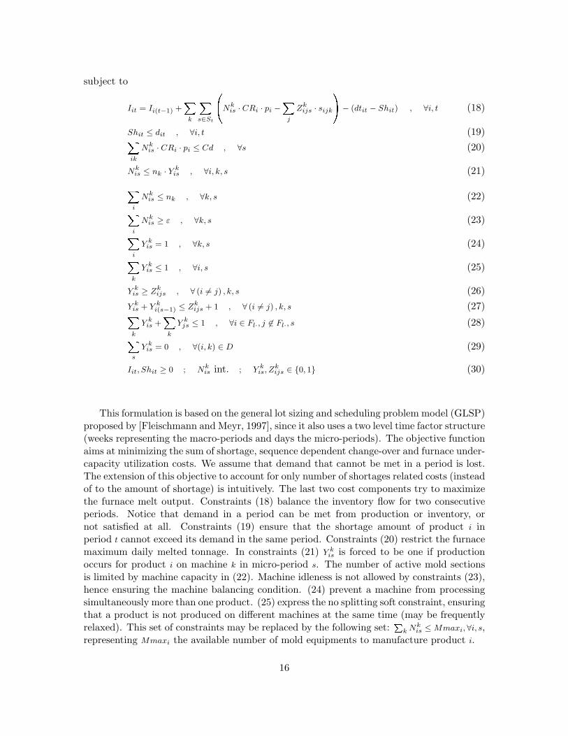
This formulation is based on the general lot sizing and scheduling problem model (GLSP)proposed by [Fleischmann and Meyr, 1997], since it also uses a two level time factor structure(weeks representing the macro-periods and days the micro-periods). The objective functionaims at minimizing the sum of shortage, sequence dependent change-over and furnace under-capacity utilization costs. We assume that demand that cannot be met in a period is lost.The extension of this objective to account for only number of shortages related costs (insteadof to the amount of shortage) is intuitively. The last two cost components try to maximizethe furnace melt output. Constraints (18) balance the inventory flow for two consecutiveperiods. Notice that demand in a period can be met from production or inventory, ornot satisfied at all. Constraints (19) ensure that the shortage amount of product i inperiod t cannot exceed its demand in the same period. Constraints (20) restrict the furnacemaximum daily melted tonnage. In constraints (21) Y k

is is forced to be one if productionoccurs for product i on machine k in micro-period s. The number of active mold sectionsis limited by machine capacity in (22). Machine idleness is not allowed by constraints (23),hence ensuring the machine balancing condition. (24) prevent a machine from processingsimultaneously more than one product. (25) express the no splitting soft constraint, ensuringthat a product is not produced on different machines at the same time (may be frequentlyrelaxed). This set of constraints may be replaced by the following set:

Pk Nk

is ≤ Mmaxi,∀i, s,representing Mmaxi the available number of mold equipments to manufacture product i.

16

Constraints (26) and (27) guarantee the coherency between variables Y kis and Zk

ijs. Eachfurnace and its associated machines can only produce one glass’ color at a time. Thiscolor constraint is expressed by (28). Technological constraints (29) prevent a productto be assigned to some machines. Finally, equations (30) represent the integrality andnon-negativity constraints.

Other operations constraints such as the maximum number of moulding changing perweek per facility or the maximum number of mould changing per day can be easily modeled.

3.3 Monolithic model

In order to state a monolithic model to the glass container production planning and schedul-ing problem, the planning horizon is decomposed into two sections (Figure 6).

• the first section has 12 macro-periods (t = 1, ..., 12), each one equivalent to a week.Each macro-period is divided into a variable number (|St|) of micro-periods (days).

• the second section includes 9 macro-periods (t = 13, ..., 21), each one equivalent to amonth.

Figure 6: Partition of the planning horizon

According to the notation proposed by [Fleischmann and Meyr, 1997], ft and lt repre-sent the first and the last micro-periods of macro-period t, respectively. This time structureallow us to integrate in a single model the specific features of both levels described earlier,and does not require detailed information for the entire horizon (eg., demand figures). Wewill generalize this framework considering that the planning horizon has T macro-periods,and the last bucket of the first section corresponds to macro-period (week) t′.

Parameters: K =Xy

|Ky|

Decision variables:

Shipt shortage of product i on plant p in macro-period t

17

Minimize

NXi=1

NXj=1

KXk=1

lt′Xs=1

cijk · Zkijs +

NXi=1

PXp=1

t′Xt=1

lit · Shipt − λ ·NX

i=1

KXk=1

lt′Xs=1

Nkis · CRi · pi+

LXl=1

LXu=1

YXy=1

TXt=t′+1

ctlu · Tluyt +

NXi=1

TXt=t′+1

�hit · I+

ipt + git · I−ipt

�+

NXi=1

PXp=1

VXv=1

TXt=1

Wipvt · ripvt + A ·MX

m=1

LXl=1

KXk=1

TXt=t′+1

Qmlkt

(31)

subject to

I+ipt = I+

ip(t−1)+

KXk∈Ky∈Yp

ltXs=ft

0@Nk

is · CRi · pi −NX

j=1

Zkijs · sijk

1A−

VX

v=1

Wipvt − Shipt

!,∀i = 1, ..., N p = 1, ..., P t = 1, ...t′

(32)

I+ipt − I−ipt = I+

ip(t−1) − I−ip(t−1) +

KXk∈Ky∈Yp

Xikt −VX

v=1

Wipvt,∀i = 1, ..., N p = 1, ..., P

t = t′ + 1, ..., T(33)

Shit ≤ dit , ∀i = 1, ..., N t = 1, ..., t′ (34)PX

p=1

Wipvt = divt , ∀i = 1, ..., N v = 1, ..., V t = 1, ..., T (35)

NXi=1

KXk=1

Nkis · CRi · pi ≤ Cd , ∀s = 1, ..., lt′ (36)

Nkis ≤ nk · Y k

is , ∀i = 1, ..., N k = 1, ..., K s = 1, ..., lt′ (37)NX

i=1

Nkis ≤ nk , ∀k = 1, ..., K s = 1, ..., lt′ (38)

NXi=1

Nkis ≥ ε , ∀k = 1, ..., K s = 1, ..., lt′ (39)

NXi=1

Y kis = 1 , ∀k = 1, ..., K s = 1, ..., lt′ (40)

KXk=1

Y kis ≤ 1 , ∀i = 1, ..., N s = 1, ..., lt′ (41)

Y kis ≥ Zk

ijs , ∀i, j (i 6= j) = 1, ..., N k = 1, ..., K s = 1, ..., lt′ (42)Y k

is + Y ki(s−1) ≤ Zk

ijs + 1 , ∀i, j (i 6= j) = 1, ..., N k = 1, ..., K s = 1, ..., lt′ (43)(44)

18

KXk=1

Y kis +

KXk=1

Y kjs ≤ 1 , ∀i ∈ Fl· j 6∈ Fl· s = 1, ..., lt′ (45)

Xk∈Ky

NXi=1

Xikt

ηk+

LXl=1

LXu=1

stlu · Tluyt ≤ Cyt , ∀y = 1, ..., Y t = t′ + 1, ..., T (46)

lt′Xs=1

Y kis = 0 , ∀(i, k) ∈ D (47)

Xikt ≤ Mikt ·Qmlkt , ∀i ∈ Flm l = 1, ..., L m = 1, ..., M k = 1, ..., K t = t′ + 1, ..., T (48)NX

i=1

Xikt

ηk · nk=

NXi=1

Xigt

ηg · ng, ∀

(k, g) ∈ Ky

k 6= g y = 1, ..., Y t = t′ + 1, ..., T(49)

Xikt ≤ Mikt ·

LX

u=1

Tulyt

!, ∀

i ∈ Flm k ∈ Ky l = 1, ..., Lm = 1, ..., M

y = 1, ..., Y t = t′ + 1, ..., T(50)

Xikt ≤ Mikt ·

LX

u=1

Tluyt

!, ∀

i ∈ Flm, k ∈ Ky l = 1, ..., L m = 1, ..., M

y = 1, ..., Y t = t′ + 1, ..., T(51)

Xi∈Flm

Xk∈Ky

Xikt ≤ Mikt ·

0@ LX

u=1

Tluyt −LX

u=1(u 6=l)

Tulyt + 2− αlyt − βlyt

1A,∀

l = 1, ..., L

m = 1, ..., M

y = 1, ..., Y

t = t′ + 1, ..., T

(52)

LXl=1

αlyt = 1 , ∀y = 1, ..., Y t = t′ + 1, .., T (53)

LXl=1

βlyt = 1 , ∀y = 1, ..., Y t = t′ + 1, ..., T (54)

αlyt = βly(t−1) , ∀l = 1, ..., L y = 1, ..., Y t = t′ + 1, ..., T (55)

βlyt′ =

Xi∈Fl·

Xk∈Ky

Y kilt′

|Ky|, ∀l = 1, ..., L y = 1, ..., Y (56)

Tluyt + Tulyt ≤ αlyt + βlyt + 1 , ∀l = 1, ..., L u = 1, ..., U y = 1, ..., Y t = t′ + 1, ..., T (57)

αlyt +

UXu=1

Tulyt = βlyt +

UXu=1

Tluyt , ∀l = 1, ..., L y = 1, ..., Y t = t′ + 1, ..., T (58)

Xt=1

Qmlkt = 0 , ∀(m, l, k) ∈ Tr (59)

Xikt, Wipvt, Shipt, I+ipt, I

−ipt, αlyt, βlyt ≥ 0 ; Nk

is int. ; Tluyt, Qlmkt, Zkijs ∈ {0, 1} (60)

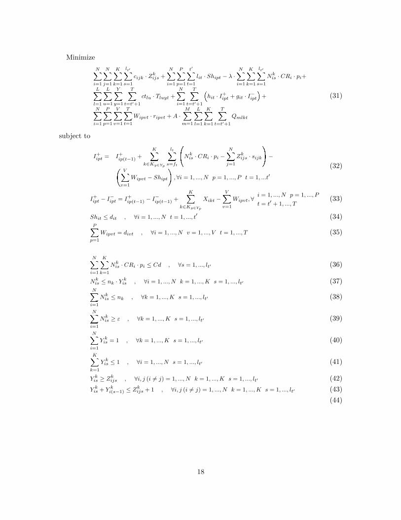
This formulation integrates the short-term and long-term models stated before, withsome adjustments. The new set of constraints (56) is added to define each furnace setupcolor at the beginning of period t′+1 in accordance to the color of the last product producedin period t′.

19

3.4 Models benchmark for case study

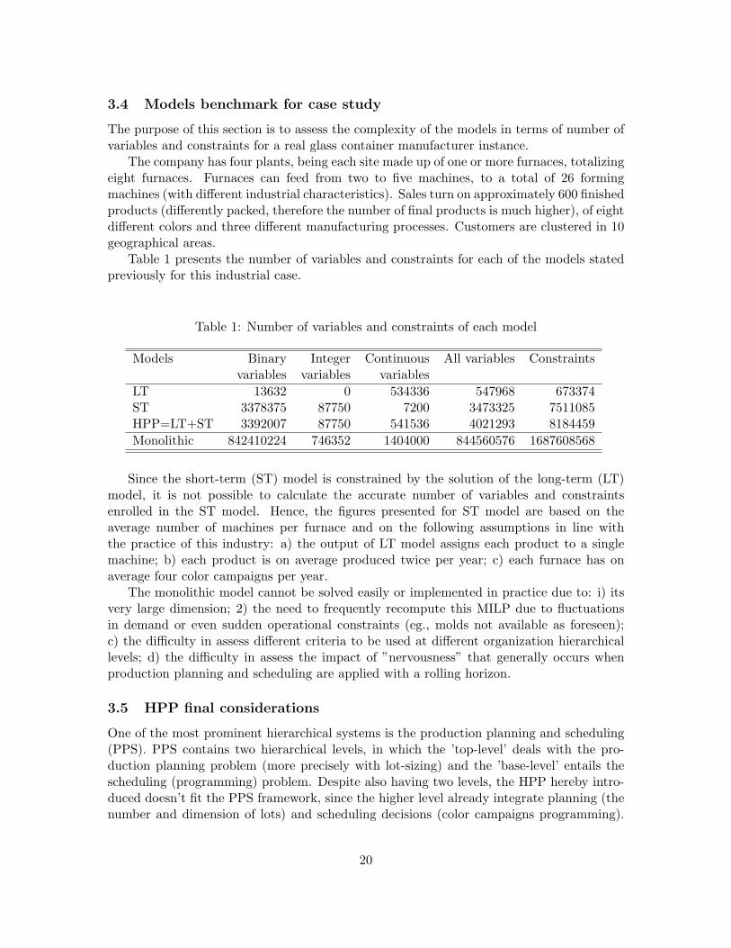
The purpose of this section is to assess the complexity of the models in terms of number ofvariables and constraints for a real glass container manufacturer instance.

The company has four plants, being each site made up of one or more furnaces, totalizingeight furnaces. Furnaces can feed from two to five machines, to a total of 26 formingmachines (with different industrial characteristics). Sales turn on approximately 600 finishedproducts (differently packed, therefore the number of final products is much higher), of eightdifferent colors and three different manufacturing processes. Customers are clustered in 10geographical areas.

Table 1 presents the number of variables and constraints for each of the models statedpreviously for this industrial case.

Table 1: Number of variables and constraints of each model

Models Binary Integer Continuous All variables Constraintsvariables variables variables

LT 13632 0 534336 547968 673374ST 3378375 87750 7200 3473325 7511085HPP=LT+ST 3392007 87750 541536 4021293 8184459Monolithic 842410224 746352 1404000 844560576 1687608568

Since the short-term (ST) model is constrained by the solution of the long-term (LT)model, it is not possible to calculate the accurate number of variables and constraintsenrolled in the ST model. Hence, the figures presented for ST model are based on theaverage number of machines per furnace and on the following assumptions in line withthe practice of this industry: a) the output of LT model assigns each product to a singlemachine; b) each product is on average produced twice per year; c) each furnace has onaverage four color campaigns per year.

The monolithic model cannot be solved easily or implemented in practice due to: i) itsvery large dimension; 2) the need to frequently recompute this MILP due to fluctuationsin demand or even sudden operational constraints (eg., molds not available as foreseen);c) the difficulty in assess different criteria to be used at different organization hierarchicallevels; d) the difficulty in assess the impact of ”nervousness” that generally occurs whenproduction planning and scheduling are applied with a rolling horizon.

3.5 HPP final considerations

One of the most prominent hierarchical systems is the production planning and scheduling(PPS). PPS contains two hierarchical levels, in which the ’top-level’ deals with the pro-duction planning problem (more precisely with lot-sizing) and the ’base-level’ entails thescheduling (programming) problem. Despite also having two levels, the HPP hereby intro-duced doesn’t fit the PPS framework, since the higher level already integrate planning (thenumber and dimension of lots) and scheduling decisions (color campaigns programming).

20

The lower level is similar to the PPS ’base-level’. Figure 7 summarizes the relations betweenboth levels, indicating on the left hand side the different criteria of both levels and on theright hand side different information situations.

Figure 7: Glass container hierarchical planning structure

Production planning is usually performed on a rolling horizon basis. Hence, despitethe long-term level being computed over 12 months, only a part of it (over the 12 weeksshort-term horizon) is implemented. Figure 7 uses the conceptual framework proposed in[Schneeweiss, 1995], distinguishing three different stages of hierarchical interdependencies:anticipation, instruction and reaction. In finding a feasible solution, the long-term leveltakes into account the most relevant characteristics of the short-term level, namely the ma-chine balancing constraint and the average machine efficiency (considering already productchangeovers average setup times). This bottom-up influence is crucial to the future feasi-bility of the short-term production plans. The output of the long-term level will naturallyinfluence the short-term level (top-down influence). Remember that base level analysis isconducted furnace by furnace. Finally, in the reaction stage (also a bottom-up influence,but in this case as a feedback one) the base-level reacts to the top-level’s instruction. Thelength of the color campaign is updated in the lower level. This information is given back tothe upper level, that has to recompute its long-term plans based on the actual state of thesystem. If there is no feasible solution in the short-term planning, the decision maker hasto manipulate the input data of the long-term level (intensifying the feedforward influenceof the anticipation).

21

4 Conclusions

This paper presents a new hierarchical design for solving the production planning problemof the glass container industry. We tried to show that the hierarchical structures used sofar on the container glass industry are traditional approaches that don’t take advantageof the specificities of its production environment. Due to huge impact of production plansin management (and industrial) key performance indicators, glass container productionplanning has received some attention in recent years. However, researchers have assumedthe standard hierarchical procedure, and analyzed mainly the scheduling of short-termlevel. The overall consistency between planning and scheduling decisions, despite beingrecognized for some time [Dauzere-Peres and Lasserre, 2002], has not received attentionin this industry. The large impact of the color campaign scheduling on the downstreamprocess demands an output for the long-term level as coherent as possible in relation tolower level decisions. We hereby propose a two level HPP system. The authors believe thatwith this new hierarchical approach the output of the long-term level (the one that clearlyinfluence the industrial costs) is much more reliable than the traditional ones.

References

F. Al-Khayyal, P. Griffin, and N. Smith. Solution of a large-scale tewo-stage decision andscheduling problem using decomposition. European Journal of Operational Research, 132:453–465, 2001.

R. Alvarez-Valdes, A. Fuertes, J. Tamarit, G. Gimnez, and R. Ramos. A heuristic toschedule flexible job-shop in a glass factory. European Journal of Operational Research,165:525–534, 2005.

R. N. Anthony. Planning and control systems: A framework for analysis. Technical report,Harvard University Graduate School of Business, 1965.

K. Boskma. Aggregation and the design of models for medium-term planning of production.European Journal of Operational Research, 10(3):244–249, 1982.

P. Bukh. A bibliography of hierarchical production planning tecniques, methodology, andapllications - version 2. Technical report, Institute of Management, University of Aarhus,1994.

J. Chevalier, J. Barrier, and P. Richard. Production planning in the glass industry. InWorkshop on Production Planning and Control, pages 282–285, Mons, 1996.

L. Daheur and E. Jacquet-Lagreze. A glass bottle production scheduling system usinga mixed integer programming formulation. In Workshop on Production Planning andControl, pages 161–164, Mons, 1996.

S. Dauzere-Peres and J. Lasserre. On the importance of sequencing decisions in productionplanning and scheduling. International Transactions in Operational Research, 9(6):779–793, 2002.

22

EuropeanComission. Best available techniques in the glass manufacturing industry. Tech-nical report, 2001.

B. Fleischmann and H. Meyr. The general lotsizing and scheduling problem. Or Spektrum,19(1):11–21, 1997.

A. Hax and H. C. Meal. Hierarchical Integration of Production Planning and Scheduling,volume 1 of Logistics. M. A. Geisler Ed, Amsterdam:North Holland, 1975.

D. W. He, A. Kusiak, and A. Artiba. A scheduling problem in glass manufacturing. IIETransactions, 28(2):129–139, 1996.

C. Merce, G. Hetreux, and G. Fontan. A hierarchical production planning based on an ag-gregation of time. Technical report, Laboratoire d’Analyse et d’Architecture des Systme,1997.

R. J. Paul. Production scheduling problem in the glass-container industry. OperationsResearch, 27(2):290–302, 1979.

S. Randhawa and N. Rai. A scheduling decision aid in glass fiber manufacturing. Computersand Industrial Engineering, 29(1):255–259, 1995.

P. Richard. Contribution des rseaux de Petri l’tude de problmes de recherche oprationnelle.Docteur, Universite Francois Rabelais Tours, 1997.

P. Richard and C. Proust. Maximizing benefits in short-term planning in bottle-glass in-dustry. International Journal of Production Economics, 64(1-3):11–19, 2000.

C. Schneeweiss. Hierarchical structures in organizations - a conceptual-framework. EuropeanJournal of Operational Research, 86(1):4–31, 1995.

V. T’Kindt, J. C. Billaut, and C. Proust. Solving a bicriteria scheduling problem on un-related parallel machines occurring in the glass bottle industry. European Journal ofOperational Research, 135(1):42–49, 2001.

E. Vicens, M. E. Alemany, C. Andres, and J. J. Guarch. A design and application method-ology for hierarchical production planning decision support systems in an enterprise in-tegration context. International Journal of Production Economics, 74(1-3):5–20, 2001.

23