Documentol 07/07/2005

SIGIR 2005

» +Introduction -Compression - Transmission -Searching

+Word-based compression: +Huffman-based:

-Moffat, -PH, TH -compression (30^), -searching (BM o no).

+End-Tagged Dense Codes -Definition -Encoding schema (1 byte, 2 bytes, 3 bytes) -Only the rank position is needed to encode. -Simple on-the-fly encoding/decoding -Compression ratio (30^), searchin (BM)

+Dynamic ETDC -Using on-the-fly algorithms -Use of "c new" escape-symbol to introduce new words. -Example: transmitting 1) an existing word, 2) a new

word. ^

> >> > ' tnCA'v^. ^^j re,(.2t^ . » + DLETDC ^ ^ » -Giving more stability to codes to allow searching » +The c_swap code: » -Many exchanges at the beginning. » -Decreasing as compression progresses. » +Searching.,c K^r,,,^l,^ iP^, » +Multipattern M-searches. » -Beginnina: searching for codes ( c_new and c_swap) and plain » words. » -Middle: Searching for both "escape codes", codes, and words » -End: Searching for c_swap and codes ( not plain-words). » » » +Experimental Results » » -Texts and Computer used » » -Swaps vs New Words: quizás poner sólo unha gráfica con swaps en el eje » vertical, frente al número de palabras del vocabulario, y marcando algunos » puntos ( sobre la gráfica), y la proporción de swaps-Vs-words. » » -Compression ratio (Gráfico de Barras como en mi tesis, únicamente » para el corpus AP) » -Compression efficiency ( Gráfico de Barras. corpus AP) » -Decompression efficiency ( Gráfico de Barras. corpus AP) » -Searches. » » » +Conclusions » » ----------------------------------------------­» ----------------------------------------------­» Posibles preguntas ... » ^por que usar un c swap de 3 bytes y un c_new de 3 bytes? ^que hacer si » hay máis de 2,100,000 palabras y por tanto se precisan códigos de 4 bytes » ? » » En las búsquedas... cuando se encuentra un código » -^cómo saber si es válido? --> precedido por un stopper » -situación [C NEW)[ASCII-WORD[\0)][CODE], (el \0 funciona como

1

Documentol 07/07/2005

» stopper para validar)

^ ^a(^ ^,o^ ^`^^t ^ ^-^C S^^ S6^ 2003

O - i 2^

2

'r

Universidade da Coruña Departamento de Computación

New Compression Codes for Text Databases

Tese Doutoral

Doutorando:

Directores: Antonio Fariña Martínez

Nieves R. Brisaboa e Gonzalo Navarro

A Coruña, Abril de 2005

Ph. D. Thesis supervised by

Tese doutoral dirixida por

Nieves Rodríguez Brisaboa

Departamento de Computación

Facultade de Informática

Universidade da Coruña

15071 A Coruña (España)

Tel: +34 981 167000 ext. 1243

Fax: +34 981 167160

brisaboa@udc.es

Gonzalo Navarro

Centro de Investigación de la Web

Departamento de Ciencias de la Computación

Universidad de Chile

Blanco Encalada 2120 Santiago (Chile)

Tel: ^-56 2 6892736

Fax: +56 2 6895531

gnavarro@dcc.uchile.cl

Aos meus pais e irmáns

Aos meus sobriños

Acknowledgements

I consider that it is fair to thank my PhD supervisors: Nieves and Gonzalo.

Without any kind of doubt, the research I have been doing during the last years

would not have been the same without their assistance. Their knowledge and

experience, their unconditional dedication, their tireless support (and patience),

their advice,... were always useful and showed me the way to follow. Thank you for

your professionalism and particularly thank you for your friendship.

On the other hand, I would not have reached this point without the support of

my family. They always gave me the strength to carry on fighting for those things

I longed for, and they were always close to me both in the good and in the bad

moments. They all form a very important part of my life. First of all, this thesis

is a gift that I want to dedicate to the most combative and strong people I have

ever met: thank you mum and dad. My parents (Felicidad and Manolo) taught

me the virtues of honesty, the importance of trusting people, and the importance

of not giving up even if the future is riddled with hard obstacles to overcome. My

lifelong brother and sisters (Arosa, Manu, and María) and the newest ones (Marina

e Lexo) are not "simply" brothers, they are the mirror I have always looked to

improve myself as a person. I want to thank my nephew and nieces (Lexo, María,

and Paula), who are my great weakness, for making me feel the greatest uncle in

the world week after week. Finally, thanks also to you, Luisa, for your love and for

all those wonderful moments we have already shared, and those that I hope will

come.

For innumerable issues, I want to give thanks to my partners at the LBD: Miguel,

J.R., Jose, Toni, Penabad, Ángeles, mon, Eva, Fran, Luis, Sebas, Raquel, Cris,

David, Eloy, and Marisa. Their support and comradeship, their friendship, and the

fact of belonging to the tight-knit circle we all have built make going to work easier

every day. Even though they are not "formally" a part of the LBD, I want also

to give thanks to Rosa F. Esteller by her unselfish help during the writing of this

thesis, and to Susana Ladra for the good ideas she gave me.

I am also very grateful to all those people who offered me their friendship and

hospitality when I was far from home. Particularly thanks to: (F^om Zaragoza)

Júlvez, Edu, Yolanda, Merse, Mínguez, Diego, Montesano, Campos, Dani,... (F^om

Santiago) Diego, Andrés, Betina, Heikki,...

And finally, thanks to all the others I did not mentioned but know that they have a part in this work.

Agradecementos

Creo que é xusto darlles as grazas aos meus directores de tese: Nieves e Gonzalo.

Sen dúbida algunha, a investigación que levei a cabo durante estes últimos anos non

tería sido a mesma sen a súa colaboración. Os seus coñecementos e experiencia, a súa

adicación sen condicións, o seu apoio incansábel (e paciencia), os seus consellos,...

sempre me serviron de apoio e me marcaron o camiño que debía seguir. Grazas

pola vosa profesionalidade e sobre todo grazas pola vosa amizade.

Por outra banda, eu non tería chegado ata aquí sen ó apoio da miña familia. Eles

sempre me alentaron a loitar por aquilo que anhelaba, e sempre estiveron alí tanto

nos bos como nos malos momentos. Todos eles forman unha parte moi importante

da miña vida. Ante todo, esta tese é un regalo que lles quero adicar ás dúas persoas

máis loitadoras e fortes que coñezo: grazas mamá e papá. Meus pais (Felicidad

e Manolo) ensináronme as virtudes da honestidade, a importancia de confiar nas

persoas, e a non desanimar aínda que o futuro estivese plagado de duros obstáculos

que salvar. Os meus irmáns de toda a vida (Arosa, Manu e María) e os máis

novos (Marina e Lexo) non son "simplemente" irmáns, son o espello no que sempre

me mirei para tratar de superarme e mellorar como persoa. Aos meus sobriños e

grandes debilidades (Lexo, María e Paula) quérolles agradecer que me fagan sentir

semana a semana o"tío" máis grande do mundo. Por último, grazas a ti, Luisa,

polo teu amor e por todos eses maravillosos momentos que xa compartimos, e os

que espero virán.

Teño moito que agradecer tamén aos meus compañeiros do LBD: Miguel, J.R.,

Jose, Toni, Penabad, Ángeles, Mon, Eva, Fran, Luis, Sebas, Raquel, Cris, David,

Eloy e Marisa. O seu apoio e compañeirismo, a súa amizade e o•formar parte desta

grande "piña" que construímos entre todos, fan que ir traballar cada día sexa moito

máis sinxelo. Se ben "formalmente" non son parte LBD, é tamén de agradecer a

axuda desinteresada que durante a escritura desta tese me prestou Rosa F. Esteller,

e as boas ideas que me aportou Susana Ladra.

Tamén lles estou moi agradecido a todas aquelas persoas que me brindaron

a súa amizade e que tan ben me acolleron cando estiven lonxe do meu fogar.

Especialmente grazas a: (De Zaragoza) Júlvez, Edu, Yolanda, Merse, Mínguez,

Diego, Montesano, Campos, Dani,... (De Santiago) Diego, Andrés, Betina, Heikki,...

E xa para rematar, gracias a todos os demais que non citei, mais sabedes que

tamén tedes a vosa parte neste traballo.

Abstract

Text databases are growing in the last years due to the widespread use of digital libraries, document databases and mainly because of the continuous growing of the Web. Compression comes up as an ideal solution that permits to reduce both

storage requirements and input/output operations. Therefore, it is useful when

transmitting data through a network.

Even though compression appeared in the first half of the 20th century, in the last

decade, new Huffman-based compression techniques appeared. Those techniques

use words as the symbols to be compressed. They do not only improve the

compression ratio obtained by other well-known methods (e.g. Ziv-Lempel), but

also allow to efficiently perform searches inside the compressed text avoiding the

need for decompression before the search. As a result, those searches are much faster than searches inside plain text.

Following the idea of word-based compression, in this thesis, we developed four

new compression techniques that make up a new family of compressors. They are

based in the utilization of dense codes. Among these four techniques, the first two

ones are semi-static techniques and the others are dynamic methods. They are

called: End-Tagged Dense Code, (s, c)-Dense Code, Dynamic End-Tagged Dense

Code, and Dynamic (s, c)-Dense Code.

Moreover, in this thesis, we have implemented a first prototype of a word-based

byte-oriented dynamic Huffman compressor. This technique was developed with

the aim of having a competitive technique to compare against our two dynamic

methods.

Our empirical results, obtained from the systematic empirical validation of

our compressors in real corpora, show that our techniques become a fundamental

contribution in the area of compression. Since these techniques compress more,

and more efficiently than other widely used compressors (e.g. gzip, compress, etc.),

they can be applied to both Text R.etrieval systems and to systems oriented to data

transmission.

It is remarkable that the research done in this thesis introduces a new family

of compressors that is based on the use of dense codes. Even though we have only

explored the beginning of this new family, the obtained results are so good that we

hope that future works permit us to develop more compressors from this family.

Resumo

As bases de datos textuais están a medrar nos últimos anos debido á proliferación

de bibliotecas dixitais, bases de datos documentais, e sobre todo polo grande

crecemento continuado que a Web está a manter. A compresión xurde como

a solución ideal que permite reducir espazo de armacenamento e operacións de

entrada/saída, co conseguinte beneficio para a transmisión de información a través

dunha rede.

Se ben a compresión nace na primeira parte do século XX, na pasada década

aparecen novas técnicas de compresión baseadas en Huffman que usan as palabras

como os símbolos a comprimir. Estas novas técnicas non só melloran a capacidade

de compresión doutros métodos moi coñecidos (p.ex: Ziv-Lempel), senón que

ademais permiten realizar buscas dentro do texto comprimido, sen necesidade de

descomprimilo, dun xeito moito máis rápido que cando ditas buscas se fan sobre o

texto plano.

Seguindo coa idea da compresión baseada en palabras, nesta tese desenvolvéronse

catro novas técnicas de compresión que inician unha nova familia de compresores

baseados na utilización de códigos densos. Destas catro técnicas, dúas son semi­

estáticas e dúas son dinámicas. Os seus nomes son: End-Tagged Dense Code,

(s, c)-Dense Code, Dynamic End-Tagged Dense Code e Dynamic (s, c)-Dense Code.

Ademais, nesta tese implementouse por primeira vez un compresor dinámico

orientado a bytes e baseado en palabras que usa Huffman como esquema de

codificación. Nós desenvolvemos este compresor para termos unha técnica

competitiva e baseada en Huffman coa que comparar as nosas dúas técnicas

dinámicas.

Os resultados empíricos obtidos da validación experimental sistemática dos nosos

compresores contra corpus reais demostran que estes supoñen unha aportación

fundamental no campo da compresión tanto para sistemas orientados a Text

R.etrieval como para sistemas orientados á transmisión de datos, xa que os

nosos compresores comprimen máis e máis eficientemente que moitos dos actuais

compresores en uso (gzip, compress, etc.).

Hai que salientar que a investigación realizada nesta tese inicia unha nova familia

de compresores baseados en códigos densos cuxas posibilidades están apenas a ser

albiscadas, polo que esperamos que traballos futuros nos permitan desenvolver novos

compresores desta familia.

Contents

Contents

1 Introduction­ 1

1.1 Text Compression . . . . . . . . . . . . . . . . . . . . . . . . . . . . 1

1.1.1 Compression for space saving and efficient retrieval ...... 3

1.1.2 Compression for file transmission . . . . . . . . . . . . . . . . 5

1.2 Open problems faced in this thesis . . . . . . . . . . . . . . . . . . . 6

1.3 Contributions of the thesis . . . . . . . . . . . . . . . . . . . . . . . . 7

1.4 Outline . . . . . . . . . . . . . . . . . . . . . . . . . . . . . . . . . . 11

2 Basic concepts­ 13

2.1 Concepts of Information Theory . . . . . . . . . . . . . . . . . . . . 13

2.1.1 Kraft's inequality . . . . . . . . . . . . . . . . . . . . . . . . . 15

2.2 Redundancy and compression . . . . . . . . . . . . . . . . . . . . . . 16

2.3 Entropy in context-dependent messages . . . . . . . . . . . . . . . . 17

2.4 Characterization of natural language text . . . . . . . . . . . . . . . 18

2.4.1 Heaps' law . . . . . . . . . . . . . . . . . . . . . . . . . . . . 18

2.4.2 Zipf's law and Zipf-Mandelbrot's law . . . . . . . . . . . . . . 19

2.5 Classification of text compression techniques . . . . . . . . . . . . . . 21

2.6­ Measuring the efficiency of compression techniques . . . . . . . . . . 23

xvii

Contents

2.7 Experimental framework . . . . . . . . . . . . . . . . . . . . . . . . . . 24

2.8 Notation . . . . . . . . . . . . . . . . . . . . . . . . . . . . . . . . . . 26

I Semi-static compression 27

3 Compressed Text Databases 29

3.1 Motivation . . . . . ... . . . . . . . . . . . . . . . . . . . . . . . . . 29

3.2 Inverted indexes . . . . . . . . . . . . . . . . . . . . . . . . . . . . . 30

3.3 Compression schemes for Text Databases . . . . . . . . . . . . . . . 33

3.4 Pattern matching . . . . . . . . . . . . . . . . . . . . . . . . . . . . . 34

3.4.1 Boyer-Moore algorithm . . . . . . . . . . . . . . . . . . . . . 36

3.4.2 Horspool algorithm . . . . . . . . . . . . . . . . . . . . . . . . 38

3.4.3 Shift-Or algorithm . . . . . . . . . . . . . . . . . . . . . . . . 40

3.5 Summary ................................. 42

4 Semi-static text compression techniques 45

4.1 Classic Huffman Code . . . . . . . . . . . . . . . . . . . . . . . . . . 45

4.1.1 Building a Huffman tree . . . . . . . . . . . . . . . . . . . . . 46

4.1.2 Canonical Huffman tree . . . . . . . . . . . . . . . . . . . . . 47

4.2 Word-Based Huffman compression . . . . . . . . . . . . . . . . . . . 50

4.2.1 Plain Huffman and Tagged Huffman Codes . . . . . . . . . . 51

4.3 Searching Huffman compressed text . . . . . . . . . . . . . . . . . . 53

4.3.1 Searching Plain Huffman Code . . . . . . . . . . . . . . . . . 53

4.3.2 Searching Tagged Huffman Code . . . . . . . . . . . . . . . . 56

4.4 Other techniques . . . . . . . . . . . . . . . . . . . . . . . . . . . . . 58

4.4.1 Byte Pair Encoding . . . . . . . . . . . . . . . . . . . . . . . 58

xviii

Contents

4.4.2 Burrows-Wheeler Transform . . . . . . . . . . . . . . . . . . . 60

4.5 Summary . . . . . . . . . . . . . . . . . . . . . . . . . . . . . . . . . 65

5 End-Tagged Dense Code 67

5.1 Motivation . . . . . . . . . . . . . . . . . . . . . . . . . . . . . . . . 67

5.2 End-Tagged Dense Code . . . . . . . . . . . . . . . . . . . . . . . . . 68

5.3 Encoding and decoding algorithms . . . . . . . . . . . . . . . . . . . 71

5.3.1 Encoding algorithm . . . . . . . . . . . . . . . . . . . . . . . 71

5.3.2 Decoding algorithm . . . . . . . . . . . . . . . . . . . . . . . 74

5.4 Searching End-Tagged Dense Code . . . . . . . . . . . . . . . . . . . 75

5.5 Empirical results . . . . . . . . . . . . . . . . . . . . . . . . . . . . . 75

5.5.1 Compression ratio . . . . . . . . . . . . . . . . . . . . . . . . 76

5.5.2 Encoding and compression times . . . . . . . . . . . . . . . . 76

5.5.3 Decompression time . . . . . . . . . . . . . . . . . . . . . . . 78

5.5.4 Search time . . . . . . . . . . . . . . . . . . . . . . . . . . . . 79

5.6 Summary . . . . . . . . . . . . . . . . . . . . . . . . . . . . . . . . . 82

6 (s, c)-Dense Code 83

6.1 Motivation . . . . . . . . . . . . . . . . . . . . . . . . . . . . . . . . 83

6.2 (s, c)-Dense Code . . . . . . . . . . . . . . . . . . . . . . . . . . . . . 85

6.3 Optimal s and c values . . . . . . . . . . . . . . . . . . . . . . . . . . 89

6.3.1 Feasibility of using binary search in natural language corpora 92

6.3.2 Algorithm to find the optimal s and c values ......... 95

6.4 Encoding and decoding algorithms . . . . . . . . . . . . . . . . . . . 98

6.4.1 Encoding algorithm . . . . . . . . . . . . . . . . . . . . . . . 98

6.4.2 Decoding algorithm . . . . . . . . . . . . . . . . . . . . . . . 99

xix

Contents

6.5 Searching (s, c)-Dense Code . . . . . . . . . . . . . . . . . . . . . . . 100

6.6 Empirical results . . . . . . . . . . . . . . . . . . . . . . . . . . . . . 101

6.6.1 Compression ratio . . . . . . . . . . . . . . . . . . . . . . . . 101

6.6.2 Encoding and compression times . . . . . . . . . . . . . . . . 102

6.6.3 Decompression time . . . . . . . . . . . . . . . . . . . . . . . 106

6.6.4 Search time . . . . . . . . . . . . . . . . . . . . . . . . . . . . 107

6.7 Summary . . . . . . . . . . . . . . . . . . . . . . . . . . . . . . . . . 109

7 New bounds on D-ary Huffman coding 111

7.1 Motivation . . . . . . . . . . . . . . . . . . . . . . . . . . . . . . . . 111

7.2 Using End-Tagged Dense Code to bound Huffman Compression ... 112

7.3 Bounding Plain Huffman with (s, c)-Dense Code . . . . . . . . . . . 112

7.4 Analytical entropy-based bounds . . . . . . . . . . . . . . . . . . . . 113

7.5 Analytical bounds with (s, c)-Dense Code . . . . . . . . . . . . . . . 115

7.5.1 Upper bound . . . . . . . . . . . . . . . . . . . . . . . . . . . 115

7.5.2 Lower bound . . . . . . . . . . . . . . . . . . . . . . . . . . . 117

7.6 Applying bounds to real text collections . . . . . . . . . . . . . . . . 119

7.7 Applying bounds to theoretical text collections . . . . . . . . . . . . 119

7.8 Summary . . . . . . . . . . . . . . . . . . . . . . . . . . . . . . . . . 120

II Adaptive compression 123

8 Dynamic text compression techniques 125

8.1 Introduction . . . . . . . . . . . . . . . . . . . . . . . . . . . . . . . . 126

8.2 Statistical dynamic codes . . . . . . . . . . . . . . . . . . . . . . . . 127

8.2.1 Dynamic Huffman codes . . . . . . . . . . . . . . . . . . . . . 129

Contents

8.2.2 Arithmetic codes . . . . . . . . . . . . . . . . . . . . . . . . . 130

8.3 Prediction by Partial Matching . . . . . . . . . . . . . . . . . . . . . 132

8.4 Dictionary techniques . . . . . . . . . . . . . . . . . . . . . . . . 134

8.4.1 LZ77 ................................ 135

8.4.2 LZ78 ................................ 136

8.4.3 LZW . . . . . . . . . . . . . . . . . . . . . . . . . . . . . . . . 137

8.4.4 Comparing dictionary techniques . . . . . . . . . . . . . . . . 139

8.5 Summary . . . . . . . . . . . . . . . . . . . . . . . . . . . . . . . . . 139

9 Dynamic byte-oriented word-based Huffman code 141

9.1 Motivation . . . . . . . . . . . . . . . . . . . . . . . . . . . . . . . . 141

9.2 Word-based dynamic Huffman codes . . . . . . . . . . . . . . . . . . 142

9.3 Method overview . . . . . . . . . . . . . . . . . . . . . . . . . . . . . 144

9.4 Data structures . . . . . . . . . . . . . . . . . . . . . . . . . . . . . . 146

9.4.1 Definition of the tree data structures . . . . . . . . . . . . . . 146

9.4.2 List of blocks . . . . . . . . . . . . . . . . . . . . . . . . . . . 148

9.5 Huffman tree update algorithm . . . . . . . . . . . . . . . . . . . . . 153

9.6 Empirical results . . . . . . . . . . . . . . . . . . . . . . . . . . . . . 156

9.6.1 Character- versus word-oriented HufTman . . . . . . . . . . . 157

9.6.2 Semi-static Vs dynamic approach . . . . . . . . . . . . . . . . 158

9.7 Summary . . . . . . . . . . . . . . . . . . . . . . . . . . . . . . . . . 160

10 Dynamic End-Tagged Dense Code 163

10.1 Motivation . . . . . . . . . . . . . . . . . . . . . . . . . . . . . . . . 163

10.2 Method overview . . . . . . . . . . . . . . . . . . . . . . . . . . . . . 165

10.3 Data structures . . . . . . . . . . . . . . . . . . . . . . . . . . . . . . 166

^

Contents

10.3.1 Sender's data structures . . . . . . . . . . . . . . . . . . . . . 167

10.3.2 R.eceiver's data structures . . . . . . . . . . . . . . . . . . . . 168

10.4 Sender's and receiver's pseudo-code . . . . . . . . . . . . . . . . . . 169

10.5 Empirical results . . . . . . . . . . . . . . . . . . . . . . . . . . . . . 171

10.5.1 Semi-static Vs dynamic approach . . . . . . . . . . . . . . . . 171

10.5.2 Dynamic ETDC Vs dynamic Huffman . . . . . . . . . . . . . 172

10.6 Summary . . . . . . . . . . . . . . . . . . . . . . . . . . . . . . . . . 173

11 Dynamic (s, c)-Dense Code 177

11.1 Motivation . . . . . . . . . . . . . . . . . . . . . . . . . . . . . . . . 178

11.2 Dynamic (s, c)-Dense Codes . . . . . . . . . . . . . . . . . . . . . . . 178

11.3 Maintaining optimal the s and c values: Connting Bytes approach . 179

11.3.1 Pseudo-code for the Counting Bytes approach ......... 181

11.4 Maintaining optimal the s and c values: Ranges approach ...... 183

11.4.1 General description of the R.anges approach . . . . . . . . . . 185

11.4.2 Implementation . . . . . . . . . . . . . . . . . . . . . . . . . . 188

11.5 Empirical results . . . . . . . . . . . . . . . . . . . . . . . . . . . . . 191

11.5.1 Dynamic approaches: compression ratio and time performance 192

11.5.2 Semi-static Vs dynamic approach . . . . . . . . . . . . . . . . 193

11.5.3 Comparison against other adaptive compressors ........ 196

11.6 Summary . . . . . . . . . . . . . . . . . . . . . . . . . . . . . . . . . 200

12 Conclusions and )^ture Work 201

12.1 Main contributions . . . . . . . . . . . . . . . . . . . . . . . . . . . . 203

12.2 Future work . . . . . . . . . . . . . . . . . . . . . . . . . . . . . . . . 204

xxii

Contents

A Publications and Other Research Results Related to the Thesis 207

A.1 Publications . . . . . . . . . . . . . . . . . . . . . . . . . . . . . . . . 207

A.1.1 International Conferences . . . . . . . . . . . . . . . . . . . . 207

A.1.2 National Conferences . . . . . . . . . . . . . . . . . . . . . . . 208

A.1.3 Journals and Book Chapters . . . . . . . . . . . . . . . . . . 208

A.2 Submitted papers . . . . . . . . . . . . . . . . . . . . . . . . . . . . . 209

A.2.1 International Journals . . . . . . . . . . . . . . . . . . . . . . 209

A.2.2 International Conferences . . . . . . . . . . . . . . . . . . . . 209

A.3 Research Stays . . . . . . . . . . . . . . . . . . . . . . . . . . . . . . 209

Bibliography 210

List of Tables

List of Tables

2.1 Parameters for Heaps' law in the experimental framework. ...... 18

2.2 Description of the collections used . . . . . . . . . . . . . . . . . . . . 25

4.1 Codes for a uniform distribution . . . . . . . . . . . . . . . . . . . . . 54

4.2 Codes for an exponential distribution . . . . . . . . . . . . . . . . . . 54

5.1 Codeword format in Tagged Huffman and End-Tagged Dense Code. 68

5.2 Code assignment in End-Tagged Dense Code . . . . . . . . . . . . . . 70

5.3 Codes for a uniform distribution . . . . . . . . . . . . . . . . . . . . . 72

5.4 Codes for an exponential distribution . . . . . . . . . . . . . . . . . . 72

5.5 Comparison of compression ratios . . . . . . . . . . . . . . . . . . . . 76

5.6 Code generation time comparison . . . . . . . . . . . . . . . . . . . . 77

5.7 Compression speed comparison . . . . . . . . . . . . . . . . . . . . . . 78

5.8 Decompression speed comparison . . . . . . . . . . . . . . . . . . . . . 79

5.9 Searching time comparison . . . . . . . . . . . . . . . . . . . . . . . . 80

5.10 Searching time comparison . . . . . . . . . . . . . . . . . . . . . . . . 81

5.11 Searching for random patterns: time comparison. . . . . . . . . . . . 81

6.1 Code assignment in (s, c)-Dense Code . . . . . . . . . . . . . . . . . . 87

List of Tables

6.2 Comparative example among compression methods, for b=3. .... 89

6.3 Size of compressed text for an artificial distribution. ......... 92

6.4 Values of Wk for k E [1..6] . . . . . . . . . . . . . . . . . . . . . . . . 93

6.5 Comparison of compression ratio . . . . . . . . . . . . . . . . . . . . . 101

6.6 Code generation time comparison . . . . . . . . . . . . . . . . . . . . 104

6.7 Compression speed comparison . . . . . . . . . . . . . . . . . . . . . . 105

6.8 Decompression speed comparison . . . . . . . . . . . . . . . . . . . . . 107

6.9 Searching time comparison . . . . . . . . . . . . . . . . . . . . . . . . 108

6.10 Searching for random patterns: time comparison. . . . . . . . . . . . 109

7.1 Redundancy in real corpora . . . . . . . . . . . . . . . . . . . . . . 120

8.1 Compression of "abbabcabbbbc", E={a, b, c}, using LZW. ..... 138

9.1 Word-based Vs character-based dynamic approaches. . . . . . . . . . 158

9.2 Compression ratio of dynamic versus semi-static versions. ...... 158

9.3 Compression and decompression speed comparison. . . . . . . . . . . 159

10.1 Compression ratios of dynamic versus semi-static techniques. .... 171

10.2 Comparison in speed of ETDC and Dynamic ETDC. ......... 172

10.3 Comparison of compression and decompression time. ......... 173

11.1 Subintervals inside the interval [Wk , W^+1), for 1 < k< 4. ...... 187

11.2 Comparison among our three dynamic techniques. . . . . . . . . . . 193

11.3 Compression ratio of dynamic versus semi-static techniques. . .... 194

11.4 Time performance in semi-static and dynamic approaches. ...... 195

11.5 Comparison against gzip, bzip,2, and arithmetic technique. ... ... 197

xxvi

List of Figures

List of Figures

1.1 Comparison of semi-static techniques on a corpus of 564 Mbytes. .. 9

1.2 Comparison of dynamic techniques on a corpus of 564 Mbytes. ... 10

2.1 Distinct types of codes . . . . . . . . . . . . . . . . . . . . . . . . . . 15

2.2 Heaps' law for AP (top) and FT94 (bottom) text corpora. ...... 19

2.3 Comparison of Zipf-Mandelbrot's law against Zipf's law. ....... 20

3.1 Structure of an inverted index . . . . . . . . . . . . . . . . . . . . . . 31

3.2 Boyer-Moore elements description . . . . . . . . . . . . . . . . . . . . 36

3.3 Example of Boyer-Moore searching . . . . . . . . . . . . . . . . . . . . 37

3.4 Horspool's elements description . . . . . . . . . . . . . . . . . . . . . . 38

3.5 Pseudo-code for Horspool algorithm . . . . . . . . . . . . . . . . . . . 39

3.6 Example of Horspool searching . . . . . . . . . . . . . . . . . . . . . . 40

3.7 Example of Shift-Or searching . . . . . . . . . . . . . . . . . . . . . . 42

4.1 Building a classic Hufñnan tree . . . . . . . . . . . . . . . . . . . . . 48

4.2 Example of canonical Huffman tree . . . . . . . . . . . . . . . . . . . 49

4.3 Shapes of non-optimal (a) and optimal (b) Huffman trees. ...... 51

4.4 Example of false matchings in Plain Huffman . . . . . . . . . . . . . . 52

XXVll

List of Figures

4.5 Plain and Tagged Huffman trees for a uniform distribution. ..... 55

4.6 Plain and Tagged Huffman trees for an exponential distribution. .. 55

4.7 Searching Plain Huffman compressed text for pattern "red hot". .. 56

4.8 Compression process in Byte Pair Encoding . . . . . . . . . . . . . . . 59

4.9 Direct Burrows-Wheeler Transform . . . . . . . . . . . . . . . . . . . 61

4.10 Whole compression process using BWT, MTF, and RLE-0. ..... 64

5.1 Searching End-Tagged Dense Code . . . . . . . . . . . . . . . . . . . . 75

6.1 128 versus 230 stoppers with a vocabulary of 5, 000 words. ...... 84

. 6.2 Compressed text sizes and compression ratios for different s values. . 90

6.3 Size of the compressed text for different s values. ........... 91

6.4 Vocabulary extraction and encoding phases . . . . . . . . . . . . . . . 103

6.5 Comparison of "dense" and Huffman-based codes. . . . . . . . . . . 110

7.1 Comparison of Tagged Huffman and End-Tagged Dense Code. .... 113

7.2 Bounds using Zipf-Mandelbrot's law . . . . . . . . . . . . . . . . . . . 121

8.1 Sender and receiver processes in statistical dynamic text compression. 128

8.2 Arithmetic compression for the text AABC! . . . . . . . . . . . . . . 131

8.3 Compression using LZ77 . . . . . . . . . . . . . . . . . . . . . . . . . 135

8.4 Compression of the text "abbabcabbbbc" using LZ78. ........ 137

9.1 Dynamic process to maintain a well-formed 4-ary Huffman tree. ... 145

9.2 Use of the data structure to represent a Huffman tree. ........ 149

9.3 Increasing the frequency of word e . . . . . . . . . . . . . . . . . . . 150

9.4 Distinct situations of increasing the frequency of a node. ...... 150

xxviii

List of Figures

9.5­ Huffman tree Data structure using a list of blocks. .......... 152

10.1­ Transmission of "the rose rose is beautiful beautiful" .... 165

10.2 Transmission of words­ C, C, D and D having transmitted ABABB

earlier . . . . . . . . . . . . . . . . . . . . . . . . . . . . . . . . . . . . 169

10.3­ Reception of c3i c3, c4D# and c4 having previously received

cl A#c2 B #cl c2 c2 c3 C # . . . . . . . . . . . . . . . . . . . . . . . . . . 170

10.4­ Dynamic ETDC sender pseudo-code . . . . . . . . . . . . . . . . . . . 174

10.5­ Dynamic ETDC receiver pseudo-code . . . . . . . . . . . . . . . . . . 175

11.1­ Algorithm to change parameters s and c . . . . . . . . . . . . . . . . . 182

11.2­ Ranges defined by W^-1, Wk and W^+1 . . . . . . . . . . . . . . . . 183

11.3 Evolution of s as the vocabulary grows . . . . . . . . . . . . . . . . . 186

11.4 Intervals and subintervals, penalties and bonus . . . . . . . . . . . . . 188

11.5­ Algorithm to change parameters s and c . . . . . . . . . . . . . . . . . 191

11.6 Progression of compression and decompression speed. ......... 196

11.7 Summarized empirical results for the FT^1LL corpus. ........ 199

1

Introduction

1.1 Text Compression

Compression techniques exploit redundancies in the data to represent them using

less space [BCW90]. The amount of document collections has grown rapidly in

the last years, mainly due to the widespread use of Digital Libraries, Document

Databases, office automation systems, and the Web. These collections usually

contain text, images (that are often associated with the text) and even multimedia

information such as music and video.

For example, a digital newspaper treats a huge amount of news a day. Each

article is composed of some text and it often encloses one or more photos, audio

files, and even videos. If we consider a Digital Library that allows access to antique

books, it is necessary to maintain not only digital photos of the books, which permits

to appreciate the shape of the original copies, but also the text itself, which allows

to perform searches about their content.

This work does not deal with the management of Document Databases in

general. It is focused on natural language Text Databases. That is, we considered

documents that contain only text. Text content is specially important if we consider

the necessity of retrieving some elements from a document collection. R,etrieval

systems usually allow users to ask for documents containing some text (i.e. "I want

documents which include the word com•pressio^e"), but they do not usually permit

to ask for other types of data.

1

1. Introd uction

Current Text Databases contain hundreds of gigabytes and the Web is measured in terabytes. Although the capacity of new devices to store data grows fast and

the associated costs decrease, the size of text collections increases faster. Moreover,

CPU speed grows much faster than that of secondary memory devices and networks,

so storing data in compressed form reduces not only space, but also the ^/o time

and the network bandwidth needed to transmit it. Therefore, compression is more

and more convenient, even at the expense of some extra CPU time. For example, if we consider the low bandwidth wireless communications in hand-held devices,

compression reduces transmission time and makes transmission faster and cheaper.

A Text Database is not only a large collection of documents. It is also composed

of a set of structures that guarantee efficient retrieval of the relevant documents. Among them, inverted indexes [BYR,N99, WMB99] are the most widely used retrieval structures.

Inverted indexes store information about all the relevant terms in the Text

Database, and basically associate those terms with the positions where they appear

inside the Text Database. Depending on the level of granularity of the index, that position can be either an offset inside a document (word addressing inde^es or standard inverted indexes), a document (docvment addressing indexes) or a block (block addressing. indexes). Standard inverted indexes are usually large (they store

one pointer per text word), therefore they are expensive in space requirements.

Memory utilization can be reduced by using block addressing indexes. These indexes

are smaller than standard indexes because they point to blocks instead of exact word positions. Of course the price to pay is the need for sequential text scanning of the pointed blocks.

Using compression along with block addressing indexes usually improves their

performance. If the text is compressed with a technique that allows direct searching

for words in the compressed text, then the index size is reduced because the text size is decreased, and therefore, the number of documents that can be held in a block increases. Moreover, the search inside candidate text blocks is much faster. Notice

that using these two techniques together, as in [NMN+00], the index is used just as

a device to filter out some blocks that do not contain the word we are looking for.

This index schema was first proposed in Glimpse [MW94], a widely known system

that uses a block addressing index. On the other hand, compression techniques

can be also used to compress the inverted indexes themselves, as suggested in

[NMN+00, SWYZ02], achieving very good results.

Summarizing, compression techniques have become attractive methods that can

be used in Text Databases to save both space and transmission time. These two

goals of compression techniques correspond to two distinct compression scenarios

2

1.1. Text Compression

that are described next.

1.1.1 Compression for space saving and eíficient retrieval

Decreasing the space needed to store data is important. However, if the compression

scheme does not allow us to search directly the compressed text, then the retrieval

over such compressed documents will be less efficient due to the necessity of

decompressing them before the search. Moreover, even if the search is done via

an index (and especially in either block or document addressing indexes) some text

scanning is needed in the search process [MW94, NMN+00]. Basically, compression

techniques are well-suited for Text Retrieval systems iff: i) they achieve good

compression ratio, ii) they maintain good search capabilities and iii) they permit

direct access to the compressed text, what enables decompressing random parts of

the compressed text without having to process it from the beginning.

Classic compression techniques, like the well-known algorithms of Ziv and

Lempel [ZL77, ZL78] or classic Huffman [Huf52], permit to search for words directly

on the compressed text [NT00, MFTS98]. Empirical results showed that searching

the plain version of the texts can take half the time of decompressing that text and

then searching it. However, the compressed search is twice as slow as just searching

the uncompressed version of the text. Classic Huffman yields poor compression

ratio (over 60%). Other techniques such as Byte-Pair Encoding [Gag94] obtain

competitive search performance [TSM+Ol, SMT+00] but still poor compression on

natural language texts (around 50%).

Classic Huffman techniques are character-based statistical two-^ass techniques.

Statistical compression techniques split the original text into symbolsl and replace

those symbols with a codeword in the compressed text. Compression is achieved

by assigning shorter codewords to more frequent symbols. These techniques need

a model that assigns a frequency to each original symbol, and an encoding scheme

that assigns a codeword to each symbol depending on its frequency. R,eturning to

character based Huffman, a first pass over the text to compress gathers symbols and

computes their frequencies. Then a codeword is assigned to each symbol following

a Huffman encoding scheme. In the second pass, those codewords are used to

compress the text. The compressed text is stored along with a header where the

correspondence between the source symboLs and codewords is represented. This

header will be needed at decompression time.

lif the source text is split into chazacters, the compression technique is said to be a chazacter­based one. If words aze considered as the base symbols we call them word-based techniques.

3

1. Introduction

An excellent idea to compress natural language text is given by Moffat in [Mof89],

where it is suggested that words, rather than characters, should be the source

symbols to compress. A compression scheme using a semi-static word-based model

and Huffman coding achieves very good compression ratio (about 25-30%). This

improvement is due to the more biased word frequency distribution with respect

to the character frequency distribution. Moreover, since in Information Retrieval

(IR) words are the atoms of the search, these compression schemes are particularly suitable for IR.

In [MNZBY00], Moura et al. presented a compression technique called Plain Hu,ffman Code a word-based byte-oriented optimal prefix2 code. They also showed

how to search for either a word or phrase into a text compressed with a word-based

Huffman code without decompressing it, in such a way that the search can be up

to eight times faster than searching the plain uncompressed text. One of the keys

of the efficiency is that the codewords are sequences of bytes rather than bits.

Another technique, called Tagged Huffman Code, was presented in [MNZBY00]. It differs from Plain Huffman in that Tagged Huffman reserves a bit of each byte

to signal the beginning of a codeword. Hence, only 7 bits of each byte are used for

the Huffman code. Notice that the use of a Huffman code over the remaining 7 bits is mandatory, as the flag is not useful by itself to make the code a prefix code.

Direct searches [MNZBY00] over Tagged Huffman, are possible by compressing

the pattern and then searching for it in the compressed text using any classical

string matching algorithm. In Plain Huffman this is not possible, as the codeword

could occur in the text and yet not correspond to the pattern. The problem is that

the concatenation of parts of two adjacent codewords may contain the codeword of

another source symbol. This cannot happen in Tagged Huffman Code because of

the bit that distinguishes the first byte of each codeword. For this reason, searching

with Plain Huffman requires inspecting all the bytes of the compressed text, while

the fast Boyer-Moore type searching [BM77] (that is, skipping bytes) is possible over Tagged Huffman Code.

Another important advantage of using flag bits is that they make Tagged Huffman a self-synchronizing3 code. As a result, Tagged Huffman permits direct access to the compressed text. That is, it is feasible to access a compressed text, to find the beginning of the current codeword (synchronization), and to start

decompressing the text without the necessity of processing it from the beginning.

2A prefix code generates codewords that are never prefix of a larger codeword. This is interesting

since it makes decompression simpler and faster.

3Given a compressed text, it is possible to easily find the beginning of a codeword by only looking for a byte with its flag bit set to 1.

4

1.1. Text Compression

The flag bit in Tagged Huffman Code has a price in terms of compression

performance: the loss of compression ratio is approximately 3.5 percentage points.

Although Huffman is the optimal prefix code, Tagged Huffman Code largely

underutilizes the representation. Thus, there are a many bit combinations in each

byte that are not used, to guarantee the code to be a prefix code.

1.1.2 Compression for file transmission

File transmission is another interesting scenario where compression techniques are

very suitable. Note that when a user requests some documents from a Text

Database, these documents are first located, and then they are usually downloaded

through a slow network to the user's computer.

In general, transmission of compressed data is usually composed of four

processes: compression, transmission, reception, and decompression. The first two

are carried out by a sender process and the last two by a receiver. This is the typical

situation of a downloadable zipped document available through a Web page.

There are several interesting real-time transmission scenarios, where compression

and transmission should take place concurrently with reception and decompression.

That is, the sender should be able to start the transmission of compressed data

without preprocessing the whole text, and simultaneously, the receiver should start

reception and decompression as the text arrives.

Real-time transmission is handled with so-called dynamic or adaptive

compression techniques. Such techniques perform a single pass over the text (so

they are also called one-pass), therefore the compression and transmission take place

as the source data is read. Notice that this is not possible in two-pass techniques,

since compression cannot start until the first pass over the whole text has been

completed. Unfortunately, this restriction makes two-pass codes unsuitable for real­

time transmission.

In the case of dynamic codes, searching capabilities are not crucial as in the case

of semi-static compression methods used in IR systems.

The first interesting statistical adaptive techniques were presented by Faller

and Gallager in [Fa173, Ga178]. Such techniques are based on Huffman codes.

Those methods were later improved in [Knu85, Vit87]. Since they are one-pass

techniques, the frequency of symbols and the codeword assignment is computed

and updated on-the-fly during the whole transmission process, by both sender and

receiver. However, those methods were character- rather than word-oriented, and

5

1.­ Introduction

thus their compression ratios on natural language were poor (around 60%).

Currently, the most widely used adaptive compression techniques (i.e. gzip, com­press,...) belong to the Ziv-Lempel family [BCW90]. They obtain good compres­

sion and decompression speed, however, when applied to natural language text, the

compression ratios achieved by Ziv-Lempel are not that good (around 40%). Other

techniques such as PPM [CW84] or arithmetic encoding [Abr63, WNC87, MNW98]

obtain better compression ratios, but they are not time-efficient.

1.2 Open problems faced in this thesis

Some open problems are interesting in both text compression for efficient retrieval and dynamic compression fields. Among them we want to. emphasize the two problems that were tackled in this thesis:

1.­ Developing compression techniques well-suited to be integrated into Text

Retrieval Systems to improve their performance. Those compression techniques should join good compression ratio and good searching capabilities.

We considered that developing new codes yielding compression ratios close to

those of Plain Huffman while maintaining the good Tagged Huffman direct search capabilities, would be interesting.

2.­ Developing powerful dynamic compression techniques well-suited for its

application to natural language texts. Such techniques should be well-suited

for its use in real-time transmission scenarios. Good compression ratio, and

efficient compression and decompression processes are additional properties

that those techniques should yield. It is well-known that adaptive Huffman­

based techniques obtain poor compression ratios (they are character based)

and are slow. Nowadays, there exist dynamic compression techniques that

obtain good compression ratios, but they are slow. There are also other time-efficient dynamic techniques, but unfortunately, they do not obtain good compression ratios. Therefore, developing an efficient adaptive compression

technique for natural language texts, joining good compression ratio and good

compression and decompression speed, was also a relevant problem.

6

1.3. Contributions of the thesis

1.3 Contributions of the thesis

The first task developed in this thesis was a word-based byte-oriented statistical

two-pass compression technique called End-Tagged Dense Code. This code signals

the last byte of each codeword instead of the first (as Tagged Huffman does). By

signaling the last byte, the rest of the bits can be used in all their 128 combinations

and the code is still a prefix code. Hence, 128i codewords of length i can be built.

The last byte of each codeword can use 128 possible bit combinations (i.e those

values from 128 to 255) and the rest of the bytes use the remaining byte values

(i.e values from 0 to 127). As a result, End-Tagged Dense Code is a"dense"

code. That is, all possible combinations of bits are used for the bytes of a given

codeword. Compression ratio becomes closer to the compression ratio obtained by

Plain Huffman Code. This code not only retains the ability of being searchable with

any string matching algorithm (i.e. algorithms following the Boyer-Moore strategy),

but it is also extremely simple to build (using a sequential assignment of codewords)

and permits a more compact representation of the vocabulary (there is no need to

store anything except the ranked vocabulary with words ordered by frequency).

Thus, the advantages over Tagged Huffman Code are (i) better compression ratios,

(ii) same searching possibilities, (iii) simpler and faster coding, and (iv) simpler

and smaller vocabulary representation.

However, we show that it is possible to improve End-Tagged Dense Code

compression ratio even more while maintaining all its good searchability features.

(s, c)-Dense Code, a generalization of End-Tagged Dense Code, improves its

compression ratio by tuning two parameters, s and c, to the word frequency

distribution in the corpus to be compressed. These two parameters are: the number

of values (stoppers) in a byte that are used to mark the end of a codeword (s values)

and the number of values (continuers) used in the remaining bytes (256 - s= c).

As a result, (s, c)-Dense Code compresses strictly better than End-Tagged Dense

Code and Tagged Huffman Code, reaching compression ratios directly comparable

with Plain Huffman Code. At the same time, (s, c)-Dense Codes retain all the

simplicity and direct search and direct access capabilities of End-Tagged Dense

Code and Tagged Huffman Code. As addition, both End-Tagged Dense code and

(s, c)-Dense Code permit to derive interesting analytical lower and upper bounds

to the compression that is obtained by D-ary Huffman codes.

In the text transmission field, our goals were to introduce dynamism into word­

based semi-static techniques. With this aim, three word-based dynamic techniques

were developed.

We extended both End-Tagged Dense Code and (s, c)-Dense Code to build

7

1.­ Introduction

two new adaptive techniques: Dynamic End-Tagged Dense Code and Dynamic

(s, c)-Dense Code. Their loss of compression is negligible with respect to the semi­static version while compression speed is even better in the dynamic version of our

compressors. This makes up an excellent alternative for adaptive natural language

text compression.

A dynamic word-based Huffman method was also built to compare it with both

Dynamic End-Tagged Dense code and Dynamic (s, c)-Dense Code. This Dynamic

word-based Huffman technique is also described in detail because it turns out to be

an interesting contribution. Since it is a Huffman method, it compresses slightly

better than Dynamic (s, c)-Dense Code and Dynamic End-Tagged Dense Code, but

it is much slower in both compression and decompression.

Specifically, the contributions of this work are:

1.­ The development of the End-Tagged Dense Code. It always improves the

compression ratio with respect to Tagged Huffman Code, and maintains its

good features: i) easy and fast decompression of any portion of compressed

text, ii) direct searches in the compressed text for any kind of pattern with

a Boyer-Moore approach. Empirical results comparing End-Tagged Dense

Code with other well-known and powerful codes such as Tagged Huffman and

Plain Huffman are also presented. End-Tagged Dense Code improves Tagged

Huffman by more than 2.5 percentage points and is only 1 percentage point

worse than Plain Huffman. Moreover, it is shown that End-Tagged Dense

Code is faster to build than Huffman-based techniques, and it is also faster to

search than Tagged Huffman and Plain Huffman.

2.­ The development of the (s, c)-Dense Code, a powerful generalization of End-

Tagged Dense Code. It adapts better its encoding schema to the source

word frequency distribution. (s, c)-Dense Code improves the compression

ratio obtained by End-Tagged Dense Code by about 0.6 percentage points

and maintains its good features: direct search capabilities, random access

and fast decompression. We also provide empirical results comparing (s, c)-

Dense Code with End-Tagged Dense Code, Tagged Huffman and Plain

Huffman. With respect to Huffman-based techniques, (s, c)-Dense Code

improves Tagged Huffman compression ratio by more than 3 percentage

points, and its compression ratio is only 0.3 percentage points, in average,

worse than the compression ratio obtained by Plain Huffman. Finally, it is

also shown that (s, c)-Dense Code is faster to build and to search than the

Huffman-based techniques. It is also faster in searches than End-Tagged Dense

8

1.3. Contributions of the thesis

Code, but it results slightly slower during the encoding phase. Figure 1.1

illustrates those results on an experimental setup explained in Séction 2.7.

o Plain Huffman

^t Tagged Huffmana 34 0 q (s,c)-Dense Code ^° 33­ 0 End-Tagged Dense Codec0 ^y 32m ñ ó 31fq O U I 30^^

100 120 140 160 180 200 220 240 260 encroding time (msec)

o Plain Huffman a° 34 ^ Tagged Huffman 0

q (s,c)-Dense Code^^ 33 0­ End-Tagged Dense Codec

y 32 m 0 ñ31 OE 0 ° 30

2.4­ 2.45 2.5 2.55 2.6 2.65 2.7 2.75 search time (sec)

Figure 1.1: Comparison of semi-static techniques on a corpus of 564 Mbytes.

3.­ The derivation of new bounds for a D-ary Huffman code. Given a word

frequency distribution, (s, c)-Dense Code (and End-Tagged Dense Code) can

be used to provide lower and upper bounds for the avernge codeword length

of a D-ary Huffman code. We obtained new bounds for Huffman techniques

assuming that words in a natural language text follow a Zipf-Mandelbrot

distribution.

4.­ The development of a word-based byte-oriented Dynamic Huffman method,

which had never been implemented before (to the best of our knowledge).

This is an interesting dynamic compression alternative for natural language

text.

5.­ Thé adaptation of End-Tagged Dense Code to real-time transmission by

de"veloping the Dynamic End-Tagged Dense Code. It has only a 0.1%

compression ratio overhead with respect to the semi-static End-Tagged Dense

Code. The dynamic version is even faster at compression than the semi-static

approach (around 10%), but it is much slower in decompression.

6.­ The adaptation of (s, c)-Dense Code to real-time transmission by developing

9

1. Introduction

45 O Dynamic PH^

0 40 x ^ Dynamic (s,c)-Dense Code m O Dynamic End-Tagged Dense Code

3 N

35

^ É 30

Qo

-^- Arithmetic encoder x gzip -f ^ bzip2 -b

Ú fi 25' .0 100 200 300 400 500 600 700 800

compression time (sec)

45 O Dynamic PH

^ ^ Dynamic (s,c)-Dense Code0 40.^ x

0 Dynamic End-Tagged Dense Code

c + Arithmetic encoder 0N

35 x gzip -f ul Q, ^ ^ bzip2 -b É 30 0

^ 25 0 50 100 150 200 250

decompression time (sec)

Figure 1.2: Comparison of dynamic techniques on a corpus of 564 Mbytes.

the Dynamic (s, c)-Dense Code. It has at most a 0.04% overhead in

compression ratio with respect to the semi-static version of (s, c)-Dense Code.

Moreover, Dynamic (s, c)-Dense Code is a bit slower (around 5%) than the

Dynamic End-Tagged Dense Code, but it improves the compression ratio of

the Dynamic End-Tagged Dense Code by about 0.7 percentage points.

Both Dynamic End-Tagged Dense Code and Dynamic (s, c)-Dense Code

compress more than 6.5 Mbytes per second and achieve compression ratios about

30 - 35%: Comparing these results against gzip, our methods get an improvement in compression ratio of about 7- 8 percentage points and around 10% in compression time. However, they are slower at decompression than gzip. On the other hand, Dynamic (s, c)-Dense Code and End-Tagged Dense Code lose compression power

with respect to bzip2 and arithmetic coding4, but they are much faster to. build and

decompress. Figure 1.2 illustrates our results.

4The arithmetic encoder uses a bit-oriented coding method, whereas our techniques are byte­

oriented. Therefore, our methods obtain an improvement in compression and decompression speed,

which implies some loss of compression ratio.

10

1.4. Outline

1.4 Outline

First, in Chapter 2, some basic concepts about compression, as well as a taxonomy

of compression techniques, are presented. After that, following the classification

of compression techniques, into well-suited to text retrieval and well-suited to

transmission, the remainder of this thesis is organized in two parts.

Part one is focused on semi-static or two-pass statistical compression

techniques. In Chapter 3, Compressed Text Databases, as well as the Text Retrieval

systems that allow recovering documents from a Text Database, are presented. We

also show how compression can be integrated into those systems. Since searches

are an important part of those systems, we also introduce the pattern matching

problem an describe some useful string matching algorithms.

In Chapter 4, a review of some classical text compression techniques is given.

In particular, character-oriented classic Huffman code [Huf52] is reviewed. Then

our discussion is focused on the word-oriented Plain Huffman and Tagged Huffman

codes [MNZBY00], since these codes are the main competitors of End-Tagged Dense

Code and (s, c)-Dense Code. Next, it is described how to search a text compressed

with a word-oriented Huffman technique. Finally, other techniques such as Byte

Pair Encoding and the Burrows-Wheeler Transform are briefly described.

In Chapter 5, End-Tagged Dense Code is fully described and tested. Chap­

ter 6 presents the (s, c)-Dense Code. Empirical results regarding compression ratio,

encoding time, and also compression and decompression time are presented. (s, c)-

Dense Code is compared with both End-Tagged Dense Code and Huffman-based

techniques. Finally, analytical results which yield new upper and lower bounds on

the average code length of a D-ary Huffman coding are shown in Chapter 7.

Part two focuses on dynamic or one-pass compression. An introduction of

classic dynamic techniques, paying special attention to dynamic Huffman codes, is

addressed in Chapter S. That chapter also includes a review of arithmetic codes,

dictionary-based techniques and the predictive approach PPM.

Chapter 9 describes dynamic word-based byte-oriented Huffman code. Empirical

results comparing this code and a character-based dynamic Huffman code are shown.

We also compare our new dynamic Huffman-based technique with its semi-static

counterpart, the Plain Huffman Code.

Chapter 10 presents the dynamic version of End-Tagged Dense Code. Its

compression/decompression processes are described and compared with Huffman­

11

1. Introduction

based ones.

Chapter 11 focuses on dynamic (s, c)-Dense Code. This new dynamic technique

is described, and special attention is paid to show how the s and c parameters are

adapted during compression. Empirical results of systematic experiments over real

corpora, comparing all the presented techniques against well-known and commonly used compression methods such as gzip, bzip2 and an arithmetic compressor are presented.

Finally, Chapter 12 presents the conclusions of this work. Some future lines of work are also suggested.

To complete the thesis, Appendix A enumerates the publications and research activities related to this thesis.

With the exception of our word-based dynamic Huffman code, presented in

Chapter 9, that was developed to have a good dynamic HufEman code to compare

with, all the remaining four codes presented form a new family of compressors.

That is, End-Tagged Dense Code, (s, c)-Dense Code, and their dynamic versions, are "dense" codes. The fact of being dense gives them interesting compression properties. Hence, we consider that this new family of statistical compressors for

natural language text is promising and need to be explored further as we explain in Section "Future work".

12

2

Basic concepts

This chapter presents the basic concepts that are needed for a better understanding

of this thesis. A brief description of several concepts related to Information Theory

are shown first. In Section 2.4, some well-known laws that characterize natural

language text are presented: Heaps's law is shown in Section 2.4.1, and Zipf's law

and Zipf-Mandelbrot's law are described in Section 2.4.2. Then a taxonomy of

compression techniques is provided in Section 2.5. Some measure units that can

be used to compare compression techniques are presented in Section 2.6. Finally,

the experimental framework used to empirically test our compression techniques

is presented in Section 2.7 and the notation used along this thesis is given in

Section 2.8.

2.1 Concepts of Information Theory

Text compression techniques divide the source text into small portions that are

then represented using less space [BCW90, WMB99, BYRN99]. The basic units

into which the text to be compressed is partitioned are called source symbols. The

vocabulary is the set of all the n distinct source symbols that appear in the text.

^An eucodi^eg scheme or code defines how each source symbol is encoded. That is,

how it is mapped to a codeword. This codeword is composed by one or more target

symbols from a target alphabet T. The number of elements of the target alphabet

is commonly D= 2 (binary code, T= {0,1}). D determines the number of bits

(b) that are needed to represent a symbol in T. If codewords are sequences of bits

13

2. Basic concepts

(bit-oriented codewords) then b= 1 and D= 21. If codewords are sequences of

bytes (byte-oriented codewords) then b= 8 and D= 28.

Compression consists of substituting each source symbol that appears in the

source text by a codeword. That codeword is associated to that source symbol by the encoding scheme. The process of recovering the source symbol that corresponds to a given codeword is called decoding.

A code is a distinct code if each codeword is distinguishable from every other. A code is said to be uniquely decodable if every codeword is identifiable from a sequence of codewords. Let us consider a vocabulary of three symbols A, B, C, and let us assume that the encoding scheme maps: A H 0, B H 1, C ^--> 11. Then such code is a distinct code since the mapping from source symbols to codewords is one to one, but it is not uniquely decodable because the sequence 11 can be decoded

as BB or as C. For example, the mapping A ^--> 1, B^ 10, C^ 100 is uniquely decodable. However, a lookahead is needed during decoding. A bit 1 is decoded as A if it is followed by another 1. The sequence 10 is decoded as B, if it is followed by another 1. Finally the sequence 100 is always decoded as C.

A uniquely decodable code is called a prefix code (or prefix-free code) if no

codeword is a proper prefix of another codeword. Given a vocabulary with source symbols A, B, C, the mapping: A H 0, B H 10, C H 110 produces a prefi,^ code.

Prefix codes are instantaneously decodable. That is, an encoded message can be partitioned into codewords without the need of using a lookahead. This property

is important, since it enables decoding a codeword without having to inspect

the following codewords in the encoded message. This improves decompression speed. For example, the encoded message 010110010010 is decoded univocally as ABCABAB.

A prefix code is said to be a minimal prefix code if, being ^ a proper prefix of some codeword, then ^a is either a codeword or a proper prefix of a codeword, for each target symbol cx in the target alphabet T. For example, the code that maps:

A^--> 0, B^ 10 and C t--> 110 is not a minimal prefix code because 11 is a proper

prefix of 110, but 111 is neither a codeword nor a prefix of a longer codeword. If the map C ^--> 110 is replaced by C^-> 11 then the code becomes a minimal prefi^ code. The minimality property avoids the use of codewords longer than needed.

Figure 2.1 exemplifies the types of codes described above.

14

2.1. Concepts of Information Theory

Distinct code Uniquely decodable code Prefix code Minimal prefix code

Figure 2.1: Distinct types of codes.

2.1.1 Kraft's inequality

To find a prefix code with some codeword lengths, it is important to know in which

situations it is feasible to find such a code. Kraft's theorem [Kra49) presented in

1949, gives some information about that feasibility.

Theorem 2.1 There e^ists a binary prefi,^ éode with codewords {cl, c2i ..., c^ } and

with corresponding codeword lengths {ll, l2i ..., l,^} if and only if ^i 1 2-l^ < 1.

That is, if Kraft's inequality is satisfied, then a prefix code with those codeword

lengths {ll, l2, ..., ln} exists. However, note that this does not imply that any code

which satisfies Kraft's inequality is a prefix code.

For example, on the one hand, the uniquely decodable code in Figure 2.1 has

codeword lengths {1, 2, 3} and satisfies Kraft's inequality since 2-1 + 2-2 + 2-3 = ĝ < 1, but it is not a prefix code. On the other hand, using those codeword lengths

we can build a prefix code: A^--> 0, B^--> 10, C F--^ 110 as it is shown in Figure 2.1.

Moreover, it is also clear that in the case of non-prefix codes, Kraft's inequality

can be unsatisfied. For example, in the distinct code in Figure 2.1 we have:

2-1 + 2-1 + 2-2 = 4> 1. Note that it is not possible to obtain a prefix code

with codeword lengths {1,1, 2}, since either the first or the second codeword would

be a prefix of the third one.

Note also that when ^i12-^^ = 1, the codeword length is minimal, therefore

a minimal prefix code exists.

15

2. Basic concepts

2.2 Redundancy and compression

Compression techniques are based on reducing the redundancy in the source

messages, while maintaining the source information. In [Abr63] a measure of the information content in a source symbol xi was defined as I(xi) _- logD p(xi), where D is the number of symbols of the target alphabet (D = 2, if a bit-oriented technique is used) and p(xi) is the probability of occurrence of a symbol xi. This definition assumes that p(xi) does not depend on the symbols that appeared previously. F^om the definition of^I(xi), it can be seen that:

• If p(xi) is high (p(xi) -> 1) then the information content of xi is almost zero since the occurrence of x2 gives very little information.

• If p(xi) is low (p(xi) -^ 0) then xi is a source symbol which does not usually appear. In this situation, the occurrence of xi has high information content.

In association with the information content of a symbol xi, the average information content of the source vocabulary can be computed by weighting the information content of each source symbol xz by its probability of occurrence p(xi). The following expression yields:

^

H = - ^p(x^) logDp(x^) ^=i

Such expression is called the entropy of the source [SW49]. The entropy gives a

lower bound to the number of target symbols that will be required to encode the whole source text.

As shown, compression techniques try to reduce the redundancy of the source messages. Having l(x^) as the length of the codeword assigned to symbol xi, redundancy can be defined as follows:

R= ^..i ^ p(xi)l(xi) - H =^Z ^ p(xi)l(xi) -^.i ^-p(xi) logDp(xi)

Therefore, redundancy is a measure of the difference between the average codeword length and the entropy. Since entropy takes a fixed value for a given

distribution of probabilities, a good code has to reduce the average codeword length.

A code is said to be a minimum redundancy code if it has minimum codeword length.

16

2.3. Entropy in context-dependent messages

2.3 Entropy in context-dependent messages

Definitions in previous section treat source symbols assuming independence in their

occurrences. However, it is usually possible to model the probability of the next

source symbol x;, in a more precise way, by using the source symbols that have

appeared before x=.

The context of a source symbol xi is defined as a fixed length sequence of source

symbols that precede xt.

Depending on the length of the context used, different models of the source text

can be made. When that context is formed by m symbols, it is said that an m-order

model is used.

In a zero-order model, the probability of a source symbol xti is obtained from its

number of occurrences. When an m-order model is used to obtain that probability,

the obtained compression is better than when a lower-order model is used.

Depending on the order of the model, the entroPy expression varies:

•­ Base-order models. In this case, it is considered that all the source symbols

are independent and their frequency is uniform. Then H_1 = logD n.

•­ Zero-order models. In this case, all the source symbols are independent

and their frequency consists of their number of occurrences. Therefore,

Ho = - ^Z i P(xti) logDp(xi)•

•­ First-order models. The probability of occurrence of the symbol x j

conditioned by the previous occurrence of the symbol xti is denoted by Pxi ^x;

and the entroPy is computed as: Hl =-^í1 P(xi) ^^ 1 Px;lx: 1ogD(Px;lx:)•

• Second-order models.­ The probability of occurrence of the symbol xk

conditioned by the previous occurrence of the sequence xixj is denoted by

Pxk ^xi x^ and the entroPy is computed as:

H2 =-^i=17^(xi) ^j1 Pxi^x: ^k=1 Pyk^xi y^ logD(Pxk^x;,x:)•

•­ Higher-order models follow the same idea.

Several distinct m-order models can be combined to estimate the probability

of the next source symbol. In this situation, it is mandatory to choose a method

that describes how the probability estimation is done. In [CW84, Mof90, BCW90],

a technique called Prediction 6y Partiad Matching (PPM), which combines several

finite-context models of order 0 to m, is described.

17

2. Basic concepts

CORPUS ^^ K ^ Q ^ ^ CÓRPUS K 1 FT91 2.003 0.560 CALGARY 1.040 0.630 FT92 2.409 0.535 CR 2.604 0.512 FT93 2.427 0.532 ZIFF 2.011 0.546 FT94 2.352 0.535 AP 2.928 0.493 ALL^T 2.169 0.548 ALL 0.640 0.624

Table 2.1: Parameters for Heaps' law in the experimental framework.

2.4 Characterization of natural language text

In natural language text compression, it is interesting to know how many different

source symbols can appear for a given text, and also to be able to estimate the

frequency of those symbols. In this section we present Heaps' law, which gives an approximation of how a vocabulary grows as the size of a text collection increases. We also show Zipf's law and Zipf-Mandelbrot's law. They give an estimation of the word frequency distribution for a natural language text.

2.4.1 Heaps' law

Heaps' law establishes that the relationship between the number of words in a natural language text (N) and the number of different words (n) in that text (that is, words in the vocabulary) is given by the expression n= aNQ, where a and ,Q are free parameters empirically determined. In English text corpora, it typically holds that 10<c^<100and0.4<^<0.6.

For natural language text corpora, Heaps's law also predicts the vocabulary size (n) from the size of the text in bytes (tSize), such that, n= K x tSizeQ. In Section 2.7, we describe ten corpora that are used in our experimental framework. Figure 2.2 illustrates the relationship between n and tSize for two of those text corpora: AP Newshire 1998 (AP) and Financial Times 1994 (FT94). In corpus AP, it holds that n = 2.928 x tSizeo.4s3 and in corpus FT94, n = 2.352 x tSizeo.53s Table 2.1 shows the parameters K and ,Q for all the corpora in the experimental framework.

The parameter Q depends on the homogeneity of the corpus: the larger the ,0, the

more heterogenous the corpus. Therefore, larger values of ,Q imply a faster growth of the vocabulary size. For example, we have estimated from the growth of the vocabulary size in AP and FT94 corpora that, to have a vocabulary with 2, 000, 000

words, AP corpus should have 700 Gbytes of text and FT94 corpus around 120 Gbytes.

18

2.4. Characterization of natural language text

x 105 AP: K= 2.928, ^= 0.493

^ 2.5

N a^ 2

_^ 1.5 ^ m 1 U 0 0.5

0 0.5 1 1.5 2

size of text x 108 x 105 FT94: K= 2.352, R= 0.535

Ñ 2.5

^ 2

^ 1.5 ^ ^ 1 U ^ 0.5

0 2 4 6 8 10 12 14 16 18

size of text x 10'

Figure 2.2: Heaps' law for AP (top) and FT94 (bottom) text corpora.

2.4.2 Zipf's law and Zipf-Mandelbrot's law

Zipf's Law [Zip49] gives a good estimation for the word frequency distribution in

natural language texts. It is well-known [BCW90] that, in natural language, the

probability of occurrence of words in a vocabulary closely follows Zipf's Law. That is:

Az p: _ ^

i

Where i is the rank of a word in the vocabulary (i = 1.. n), B is a constant that depends on the analyzed text (1 < B< 2), and AZ = - is a

.>0 1/i S^B) normalization factorl.

In [Man53] it is provided a modification of Zipf's law that is called Zipf­

Mandelbrot's law. This law modifies Zipf's distribution by adding a new parameter

C, which also depends on the text, in such a way that the probability of the ith

most frequent word in a vocabulary is given by the following expression:

A 7^^ _

(C + i)B

Mandelbrot's modification fits more adequately than the original Zipf's

1^(x) _^^^0 1/ix is known as the Zeta function.

19

2. Basic concepts

distribution the region corresponding to the more frequent words (i < 100) [Mon01].

The generalized Mandelbrot's law can be rewritten as follows:

pZ - (1 ^- Ci)B

where the parameter C needs to be adjusted to fit the data and cannot tend to zero.

In this case, the normalization factoí A, which depends on the two parameters C and B, is defined as:

A _ 1 _ 1

^c(B)^^>i ^í+ĝZ^

Figure 2.3 shows the real probability distribution of the first 500 words in

the ALL corpus (see Section 2.7). The probabilities estimated by assuming Zipf­

Mandelbrot's law with C= 0.75 and the optimal value of the parameter B(B = 1.46)

and with other values for both B and C are also shown. Finally, the estimation

given by Zipf's law (B = 1.67) is also shown. It can be seen that Zipf-Mandelbrot's

distribution gives a better estimation of the real probabilities of the source symbols

than Zipf's distribution.

Real 1.6­ Zipf-Mandelbrot: C=0.75, 9=1.46

• _ • - • Zipf-Mandelbrot: C=5.00, 0=1.46

^ 1.4­ • • • • • • • Zipf-Mandelbrot: C=0.75, 9=1.80 ^- zipf: e=1 s7

É y 1.2 m p^

Ñ 1

O

•' n o ^ m a Q 0.6n n_

a 0.4

0.2

100 200 300 400 500 i= rank in vocabulary of source symbol

Figure 2.3: Comparison of Zipf-Mandelbrot's law against Zipf's law.

20

2.5. Classification of text compression techniques

2.5 Classification of text compression techniques

Text compression is based on processing the source data to represent them in

such a way that space requirements decrease [BCW90]. As a result, the source

information is maintained, but its redundancy is reduced. Decompressors act over

the compressed data to recover the original data.

In some scenarios (such as image or sound compression), some loss of source

information can be permitted during compression because human visual/auditive

sensibility cannot detect small differences between both the original and the

decompressed data. In those cases, it is said that lossy compression techniques are used. However, if text compression is carried out, lossless techniques are needed. This is because it is mandatory to recover the same original text after decompression.

In order to compress a text, it is first necessary to divide the input text into

symbols and to compute their probability. This process creates a representation of the text. Then an encoding scheme is used to assign a codeword to each symbol

according to that representation. For example, both Plain Huffman and End-Tagged

Dense Code use the same word-based zero-order model2 but they use different

encoding schemes (these are described in Sections 4.2 and 5.2 respectively).

The correspondence between symbols and codewords has also to be known by

the decompressor, in order to be able to recover the original source data. Depending

on the model used, compression techniques can be classified as using:

• Static or non-adaptive models.­ The assignment of frequencies to each source

symbol is fixed. They have probability tables previously computed (usually

based on experience) that are used during the encoding process. Since those

probabilities are fixed, they can match badly with source data in general, so

thesé techniques are usually suitable only in specific scenarios. Examples of

this approach are the JPEG image standard or the Morse code.

•­ Semi-static models. They are usually used along with two-pass techniques.

These methods perform a first pass over the source text in order to obtain the

probabilities of all the distinct source symbols that compose the vocabulary.

Then those probabilities remain fixed and are used during the second pass,

where the source text is processed again and each source symbol is assigned

a codeword whose length depends on its probability.

ZThat is, both of them divide the source text into words ( word-based model), and the probability of those words is given by their number of occurrences (zero-order model).

21

2. Basic concepts

These techniques present two main disadvantages. The first one is that the

source text has to be processed twice, and therefore encoding cannot start

before the whole first pass has been completed. As a result, it is impossible to

apply semi-static techniques to compress text streams. The second problem

relies on the necessity of providing the vocabulary and the probabilities (or

the codewords), obtained by the compressor during the first pass, to the

decompressor. Even though this overhead is not a problem when large texts

(compared to their vocabulary) are compressed3, it causes an important loss

of compression ratio when semi-static techniques are applied to small texts.

Huffman-based codes [Huf52] are the main representatives of compressors that

use a semi-static model.

•­ Dynamic or adaptive models. Compression techniques using dynamic models

are commonly known as one-pass techniques. Instead of performing a initial

pass to obtain the probabilities of the source symbols, these techniques

commonly start with an initial empty vocabulary. Then the source text is

read one symbol at a time. Each time a symbol is read, it is encoded using

the current frequency distribution and its number of occurrences is increased.

Obviously when a new symbol is read, it is appended to the vocabulary. The

compression process adapts the codeword of each symbol to its frequency as

compression progresses.

In one-pass techniques, the decompressor adapts the mapping between

symbols and codewords in the same way the compressor does. This adaptation

can be done by just taking account of the sequence of symbols that were

already decoded. As a consequence, it is not needed to explicitly include

that mapping apart from the compressed data. This property gives one-pass

techniqv,es their main advantage: their ability to compress streams of text.

Techniques such as the Ziv-Lempel family [ZL77, ZL78, We184], arithmetic

encoding4 [Abr63, WNC87, MNW98] and PPM [CW84] are well-known

dynamic compression techniques.

Another classification of compression techniques can be done depending on how

the encoding process takes place. Two families are defined: statistical and dictionary

based techniques.

• Statistical methods assign to each source symbol a codeword whose length

3As Heaps' law shows (see Section 2.4.2), in a word-based model the size of the vocabulary is

negligible compared to the compressed text size. 4Arithmetic encoding is typically used along with a dynamic model, even when static and

semi-static models are also applicable.

22

2.6. Measuring the efficiency of compression techniques

depends on the probability of the source symbol. Compression is obtained

because shorter codes are assigned to the more frequent symbols. Some typical

statistical techniques are the Huffman codes and arithmetic methods.

•­ Dictionary techniques build a dictionary during the compression, storing the

last appeared phrases (sequences of source symbols). Encoding is performed

by substituting those phrases by small frxed length pointers to their position

in the dictionary. Compression is achieved as the result of substituting large

phrases by a small fi,^ed length pointer. Compression methods from the Ziv-

Lempel family are the most commonly used dictionary techniques.

2.6­ Measuring the efficiency of compression

techniques

In order to measure the efficiency of a compression technique, two basic concerns

have to be taken into account: the performance of the algorithms involved and the

compression achieved.

The complexity of compression and decompression algorithms gives an idea of

how a technique will behave, but it is also necessary to obtain empirical results that

permit comparing directly the performance of such technique with other methods

in real scenarios. Performance is measured in time and in speed:

•­ Compression and decompression times are usually measured in seconds or

milliseconds.

•­ Compression and decompression speed measure the throughput achieved.

Common speed units are, Kbytes per second and Mbytes per second.

Assuming that i is the size of the input text (in bytes), that the compressed

text occupies o bytes, and that bt is the average number of bits used to represent a

symbol in the source text (since the source alphabet contains typically characters, it

often holds that b= = 8), there are several ways to measure the compression achieved

by a compression technique. The most usual measures are:

•­ Compression ratio represents the percentage that the compressed text

occupies with respect to the original text size. It is computed as:

compression ratio = f x 100

23

2. Basic concepts

•­ Compression rate indicates the decrease of space needed by the compressed

text with respect to the source text. It is computed as:

compression rate = 100 - compression ratio = ii° x 100

•­ Bits per symbol (bps). It compares the number of bits that are needed to

represent a source symbol against the number of bits used to represent its

codeword. It is computed as:

bps = ° x bi

It is interesting to point out the apparently obvious difference between absolute

and relative measures when comparing two compression techniques. Next example

clarifies both measurements.

Example 2.1 Let us assume two compression methods Ma and Mb that are applied

to a text collection of 100 Mbytes, such that Ma compresses the text collection to

45 Mbytes and Mb to 50 Mbytes. Therefore, the compression ratios are 45%o and 50% respectively. As a result, we will say that M^ improves M6 by 5 percentage

points (absolute measurement). However, notice that Ma does not improve M6 by 5%. Using relative measurements, since 10 = 100 - 4s x ioo ^,e will sa that M50 y a improves M6 by 10%.

2.7 Experimental framework

Several experiments were performed in this thesis in order to validate the

compression achieved by the compression techniques that we developed and to

compare our techniques with their competitors. All tests were carried out on an

isolated dual Intel®Pentium®-III 800 Mhz system, with 768 MB SDRAM-100Mhz.

It ran Debian GNU/Linux (kernel version 2.2.19). The compiler used was gcc

version 3.3.3 20040429 and -09 compiler optimizations were set.

Time results (implied in compression, decompression and search speed) measure

CPU user time. That is, those measures include only the amount of time the

computer spends with the program, but the time needed to access files is excluded.

Due to small variations in the running times, an average calculated from 5 runs was

taken for most of the experiments. With respect to the compression effectiveness,

compression ratio was measured.

24

2.7. Experimental framework

Several text collections of varied sizes were chosen for this research. As a representative for short texts, we used the Calgary corpus5. We also used some large text collections from the Text REtrieval Conference6 (TREC). From TREC-2, both AP Newswire 1988 and Ziff Data 1989-1990 corpora were used. From TREC-4, we

used Congressional Record 1993, and Financial Times 1991, 1992, 1993, and 1994.

Finally, two larger collections, ALL^T and ALL, were used. ALL.FT includes all texts from Financial Times collection, whereas ALL collection is composed by Calgary corpus and all texts from TREC-2 and TREC-4.

Table 2.2 shows, for each corpus used, the size (in bytes), the number of words

(N), and the number of different words; that is, the number of words in the

vocabulary (n). The fifth column in that table shows the parameter B from Zipf's

law. Finally, the last three columns show the parameter B from Zipf-Mandelbrot's

law, assuming that C takes the values 0.75, 1.00, and 1.25 respectively.

CORPUS size (bytes) #words(N) voc.(n) BZ;pf BZ,y BZM BZM

CALGARY 2,131,045 528,611 30,995 1.270 1.343 1.302 1.272 FT91 14,749,355 3,135,383 75,681 1.450 1.390 1.352 1.323 CR 51,085,545 10,230,907 117,713 1.634 1.422 1.384 1.355

FT92 175,449,235 36,803,204 284,892 1.631 1.443 1.408 1.381 ZIFF 185,220,215 40,866,492 237,622 1.744 1.462 1.425 1.398 FT93 197,586,294 42,063,804 291,427 1.647 1.451 1.416 1.389 FT94 203,783,923 43,335,126 295,018 1.649 1.453 1.417 1.391 AP 250,714,271 53,349,620 269,141 1.852 1.458 1.422 1.395 ALL^T 591,568,807 124,971,944 577,352 1.648 1.472 1.435 1.412 ALL 1,080,719,883 229,596,845 886,190 1.672 1.465 1.432 1.408

Table 2.2: Description of the collections used.

For all the compression methods that use a word-based model, the spaceless

word model [MNZBY00] was used to model the separators. A separator is the text

between two contiguous words, and it must be coded too. In the spaceless word

model, if the separator following a word is a single white space, we just encode

the word, otherwise both the word and the separator are encoded. Hence, the

vocabulary is formed by all the different words and all the different separators,

excluding the single white space.

We also use for comparison some well-known compressors such as:

•­ Gzip version 1.3.5 (2002-09-30). It is a patent free (under the terms of GNU

General Public License, http://www.gnu.org) compression utility from the

Ziv-Lempel 77 family.

sUR.L: http://www.datarcompression.info/Corpora/CalgazyCorpus/

6TReC is an international conference where standazd and well-known real corpora aze used to

test Text Retrieval Systems. More information can be found at http://trec.nist.gov/

25

2. Basic concepts

•­ Bzip2, which is a freely available (http://sources.redhat.com/bzip2/), patent

free data compressor. It uses the Burrows-Wheeler Transform along with

Huffman coding. We used bzip2 version 1.0.2. (2001-12-30).

•­ An aritmetic compressor [CMN+99] that uses an adaptive zero-order word­based model.

2.8 Notation

We collect here most of the notation used throughout the thesis:

5ymbol­ Definition

n Number of words in the vocabulary

N Number of words in the source text

b Number of bits needed to represent a symbol from

the target alphabet. b= i for a bit-oriented code

and b= 8 for a byte-oriented code.

D Number of symbols in the target alphabet. D= 2 for

a binary code and D= 256 for a byte-oriented code

s, c Number of stoppers (s) and continuers (c)

pi Probability of the ith most frequent source symbol

k^ Codeword length when the number of stoppers is x

Wk Number of words that can be encoded with up to k

bytes using s as the number of stoppers

HD (X ), Hó , H -^i pi logD pí (entropy implied by distribution X)

E6 Average codeword length for a 2b-ary End-Tagged

Dense Code

Ld(s, c) Average codeword length for (s, c)-Dense Code

Tb Average codeword length for a 2b-ary Tagged Huffman

Lh(D) Average codeword length for a D-ary Plain Huffman

26

Part I

Semi-static compression

3

Compressed Text Databases

This chapter describes some of the structures and algorithms used to work with

Text Databases, specially inverted indexes. We also introduce the importance of

having efficient Text Retrieval Systems in order to recover relevant data stored

inside Text Databases. The main advantages that compression techniques provide

to Text Retrieval Systems, and the way those techniques can be integrated into

their inverted indexes to improve performance, are also shown.

Finally, the problem of text searching is introduced, and some commonly used

pattern matching algorithms such as Boyer-Moore, Horspool, and Shift-Or are

presented.

3.1 Motivation

A Docu^nent Database can be seen as a very large collection of documents and a set

of tools that permit managing it and searching it efficiently.

Libraries can be used as an analogy of a Document Database. They store many

books, and a user can go there to find information related to an issue of interest.

However, this user usually does not have enough time to review all books in the

library in order to find that information. Therefore, it is necessary to give the user

some kind of tool (e.g. a catalog) which enables him/her finding rapidly the most

relevant books.

A Digitad Library, the set of articles published by a digital newspaper, or the Web

29

3. Compressed Text Databases

in general, are examples of Document Databases. Since the number of documents­

stored is very large, the amount of space needed to store them is also enormous

(and it usually increases along time). The use of compression techniques reduces

the size of the documents, and consequently the amount of time needed to transfer

them from secondary memory or across a network, at the expense of some CPU time

needed for compression, and especially, decompression.

However, not only saving storage space is important. A Text R.etrieval System

working on a Text Database has to provide efficient search and retrieval of documents. Inverted inde^es are the most commonly used retrieval structures in

occidental languages. In a traditional library, a simple catalog which associates some keywords with each document is usually used as retrieval structure. In Text

Databases, a full text model is used; that is, all the words that appear in each document are indexed (not only a few keywords). Therefore any word appearing

at least once in any document can be searched and a more effective retrieval of

documents will be achieved.

3.2 Inverted indexes

An inverted index is a data structure that permits fast retrieval of all the positions in a Text Database where a search term appears.

Basically, an inverted index maintains a terrras vector or vocabnlary in which all terms (usually words) are stored. For each of those terms ti, a list of occurrences that keeps all the Positions where ti appears is also stored.

Note that depending on the granularity used, the length of the list of occurrences may vary. If the level of granularity used iĝ coarse (e.g. the index tells the documents

where each term appears) then the list of occurrences is much smaller than when

the granularity is fine (the index tells the exact positions within documents for each

term). Note that a term may appear lots of times in the same document, and

with fine granularity, each occurrence has to be stored inside the inverted index.

Therefore, the coarser the granularity, the smaller the size of the whole index. Using

coarse granularity improves some searches [WMB99, BYR.N99] and increases the

possibilities of maintaining the whole index in memory, but if the exact occurrence

positions are needed (for example for a proximity search), it will be necessary to

perform a sequential scan of the pointed document or block.

For example, in Figure 3.1 the list of occurrences for the term "compression"

stores 4 pointers. Each pointer references the exact location (document and offset

30

3.2. Inverted indexes

terms list

t, P^ ^ PZ ^ Ps ^ PQ^

compression • :'

^ ^^ ^^^ , ^;^ .tit­ ^^

c^.^^ é^a^ m ^^^ ene ^Me^np ^^.^^4^+­ ^ ooamerm ane mairteireA6 ^,

^mages by lan H. ^^^ ^• mmnresslon ro e^oac ndoessing

T^ ^^ N aedm d^aatasw^en, a^ ^rnerred ^ndm^s.n+oIFA. end com^;m^áa rocare^aed na co^o Nava^o.c. eaa. ^^ Ea^o m r.^w.a.

^ ^á nvden riamac. aweuea ey .. rwó ZMarii anaDoc 1­ Rimdo B^

^ma (r.^r ^ess

Doc 2 Doc 3 .......... Doc n

Figure 3.1: Structure of an inverted index.

inside it) of the term. If the level of granularity used for the list of occurrences had

been the document, only 3 pointers would have been needed, since "compression"

only appears inside three documents.

Searches in the inverted index start by finding in the vocabulary the search

term. This initial search can be speeded up by using any suitable data structure

such as hash tables or tries. This takes O(m) time (being m the size of the searched

pattern). Binary search is also feasible if a lexicographically ordered vocabulary is

maintained. Binary search is cheaper in memory requirements and competitive in

performance, since it takes O(logn) time. Finally, the list of occurrences is used to

access documents.

Sometimes (e.g. with approximate searching), more than one term in the

vocabulary matches the searched pattern. In this case, the initial search delivers

several lists of occurrences that will be traversed in a synchronized way.

The list of occurrences is used in a different way depending on the granularity

of the index:

1.­ word level (word-addressing indexes): In this case, all terms that match the

searched pattern are located in the vocabulary. Then the list of occurrences

indicates not only the documents, but also the offset inside the documents

where those terms appear.

2.­ document level (document indexes): The list of occurrences points directly

to documents. However, to find the exact position where a term appears

31

3. Compressed Text Databases

in a document it is necessary to sequentially search for it in all the pointed

documents.

3. level of block­ (block addressing indexes) [MW94, NMN+00]. In this case the list of occurrences points to blocks, and a block can hold several documents.

Hence, all searches require inspecting all the text in those pointed blocks in

order to know in which documents the search pattern appears. Thus, there is

a space-time trade-off regarding the block size.

Block addressing indexes take special advantage of compression. Since a

compressed document requires less space, more documents can be held in

the same block. This reduces considerably the size of the inverted index.

When word addressing indexes are used, all searches can be performed in the

index, and it is only necessary to access to the pointed documents to retrieve

them. Single word searches are immediately solved since the index points to all

documents where a word appears. Searching for phrase patterns (finding a sequence

of words in the text) involves looking for all the words that compose the pattern,

in the vocabulary of the index. Then their lists of occurrences are traversed in a

synchronized way to check if the words in the phrase pattern appear together in the

text. Finally the pointed documents are returned.

In the case of document addressing indexes, single word patterns can be also

searched directly in the index. However, in block addressing indexes, the index

points to blocks, not to documents. Therefore, it is necessary to scan the pointed

blocks to know if a word appears in a given document inside the block.

It is also possible to perform phrase queries using word addressing or block

addressing inverted indexes. For example, let us assume we want to find all the

places where the phrase "text databases" appears, that is, the positions were "text"

and "databases" appear together and "text" precedes to "databases" . In this case,

the index can be used to select those candidate documents/blocks where both words

appear, but only a sequential search can tell whether the sequence "text databases"

occurs.

As a result, in the case of document and block addressing indexes, which are

those providing best space usage, keeping the text in compressed form saves not

only space and transmission time for results, but also disk time for searching. In

addition, direct searching the compressed text without decompressing it saves cPu

time.

Compression has been used along with inverted inde^es with good results

[NMN+00, ZM95]. Text compression techniques must have some characteristics for

32

3.3. Compression schemes for Text Databases

this symbiosis to be productive. These characteristics are explained in Section 3.3.

3.3 Compression schemes for Text Databases

Not all compression techniques are suitable for use along with Text Databases.

Compression schemes have to permit two main operations: direct access and direct

search in the compressed text. ^

- Direct access. The direct access property refers to the possibility of going

to a random part of a compressed text and start decompressing from there

on, avoiding to process it from the beginning. Decompression is needed for

presenting results, that is, to visualize the resulting documents.

Sometimes, we are interested in retrieving only a small context of the searched

term. For example, a Web search engine presents to the user a list of relevant

links and a small snippet of the document as the context where the searched

term appears.

If the compression scheme does not permit direct access, once a document

has been located via the index, it is necessary to start decompressing the

document (or a collection of texts if several documents were compressed as a

whole) from the beginning.

However, if the compression scheme permits direct access, it is possible to

have a word addressing inverted inde^ over the compressed text. In such case,

the index returns the position inside the compressed document, and only a

small portion of the compressed text, around the searched term, has to be

decompressed.

Finally, when the user chooses one link, the whole document has to be

delivered to him/her and therefore the decompression of the document is

mandatory. Again, if the compressed document is inside a compressed text

collection, direct access avoids the necessity of starting decompression from

the beginning of the compressed data.

- Direct search. This property is related to the feasibility of searching inside

the compressed text without having to decompress it first.

The ability to perform direct searches inside the compressed text is interesting

because it permits to maintain the text in compressed form all the time, and

decompression is only needed to present the retrieved documents. This saves

cPU time.

33

3. Compressed Text Databases

For example, if a Web server answers a few requests per second, the search

time is negligible with respect to the time needed to transfer a Web page from

the server to a client. Therefore differences in time between performing direct

searches or performing decompression first will be small. However, in the case

of a Web server accepting many queries per second, the extra CPU time needed

to decompress documents before the search slows down the system, causing

search time to become too long.

When a compression scheme supports direct searches, given a pattern, it is

possible to search for the compressed pattern directly into the compressed text

with a(general or specialized) sequential string matching algorithm. Direct

searches over text compressed with some techniques [MNZBY00] can actually

improve the search performance. For example, using word-based Huffman,

Moura et al. [MNZBY00] found that searching the compressed text is up to

8 times faster for approximate searches than searches on uncompressed text.

The use of a compression scheme allowing direct search permits to maintain

the text in compressed form all the time, and to use block addressing indexes

that point to compressed blocks, as it is shown in [NMN+00].

To sum up, the use of compression techniques which permit direct search and

direct access turns out to be very useful. It enables maintaining the text in a

compressed form all the time (which saves space), but it aIso improves the efficiency

of Text Retrieval Systems.

There exist specialized search algorithms that enable direct searching the text

compressed with techniques such as Ziv-Lempel [NT00, ABF96, FT95, NR04] and

Byte Pair Encoding [Man94, STF+99].

There are also other compression techniques that enable compressing the

search pattern and then performing a scan through the text to look for the

compressed pattern. These compression techniques, which permit direct searching

the compressed text [MNZBY00] are based on the one-to-one association between

a codeword and an input symbol.

3.4 Pattern matching

The pattern matching problem consists basically in finding all the occurrences of

a given pattern p in a larger text t [BM77, KMP77, Sun90]. In this section, the

length of the pattern p will be denoted by m and the text length is represented as

34

3.4. Pattern matching

^.­ Finally, the text t is composed of symbols from an alphabet which is denoted as

E.

Search patterns can be classified as follows:

i)­ Exact words. I.e. "car", "dog", etc.

ii)­ Prefixes and suffixes. All words that start with a specified prefix or those

which end with a given sufñx are searched. For example patterns "under-"

and "-ation" aim to search for words such as under^round, undercooked, and

generation, imagination, respectively.

iii)­ Substrings. They obtain all words containing a sequence of characters. The

pattern "-sio-" represents words such as: compression, passion, etc.

iv)­ Alphabetical ranges. They represent all the terms contained in a given range

(assuming an alphabetical order). For example, [a, b) returns words starting

with an 'a', and (zodiac, zone] returns words such as zombie and zone.

v)­ Patterns allowing errorsl. For example "hot" with one error, returns words

with an edit distance less or equal than 1 with respect to hot, i.e. hot, hit,

hat, pot, rot, hop, shot.

vi)­ Regular expressions. They consist of words that can be built from an initial

set of strings and three operators: union (el^e2), concatenation (ele2) and

repetition zero of more times (e*) of other regular expressions el, e2, e. For

example, (red)*(car^bike)(0^1)* returns terms such as: car, car0, carl, car01,

bike, redbike, ...

In this section, we are only interested in presenting the simpler string matching

problem, that is, how to search for a single pattern inside a text. Three well-known

and useful string matching techniques are presented. For more information about

other pattern matching techniques and how to search for several patterns (multiple

string matching) see [NR02].

The first technique shown is the Boyer-Moore [BM77] algorithm. It is briefly

described here because it is the main representative of a family of fast pattern

matching algorithms that is commonly used to search compressed text. In our

1The approximate string matching problem consists of finding all substrings in a text t that are

close to the pattern p under some measure of closeness. The most common measure of closeness

in Text Databases is known as the edit distance. A string p is said to be of distance k to a string q

if we can transform p into q with a sequence of k insertions of single characters in azbitrary places

in p, deletions of single characters in p, or substitutions of characters.

35

3. Compressed Text Databases

Text (t) m

1 shiftPattem (p) ^ n. u ^^

Figure 3.2: Boyer-Moore elements description.

empirical tests, we use a simpler variant of the Boyer-Moore algorithm called Horspool algorithm [Hor80]. The third technique is named Shift-Or algorithm, and it constitutes the base of the plain filterless algorithm which is used to search Plain Huffman code, as shown in Section 4.3.

3.4.1 Boyer-Moore algorithm

This algorithm uses a search window corresponding to the search pattern that is

moved along the text. The algorithm starts by aligning the pattern p with the

leftmost part of the text t, and then it compares right-to-left the pattern to the

text in the window until they match (or until a difference between the pattern and

the text in the window appears). In each step, the longest possible safe-shift to the

right of the window is performed.

Let us assume that a maximal suffix µ of the search window is also a suffix of

the pattern, and that the character Q from the text in the window does not match

with character a in the pattern. Figure 3.2 shows thosé elements. Then three shift functions are pre-computed:

Sl : If the suffix µ appears in another position in p, then Sl is the distance from a to the next occurrence of µ which is not preceded by cx backwards in the pattern. If µ does not occur again in p then Sl = m. That is, ól computes, for

each sufE'ix of the pattern, the distance to the position of its next occurrence backwards in p.

a2­ : If the suffix µ does not appear in any text position, then suffixes v of µ are taken into account, since they could also be a prefix of the pattern in next

step. In such a case, the length of the longest prefix v of p that is also a sufFix of µ is assigned to ó2.

b3 : It is associated to the distance from the rightmost occurrence of ^ in the

pattern to the end. If Q does not appear in p, then 83 = m. This shift function is used because if the search window is shifted with Sl, and Q is not aligned

36

3.4. Pattern matching

pattern EXAMPLE

text HERE IS A SIMPLE EXAMPLE

0 EXAMPLE

1 EXAMPLE

2 EXAMPLE

3 EXAMPLE

4 EXAMPLE

Figure 3.3: Example of Boyer-Moore searching.

with another existing v in the pattern, then we will perform an unnecessary

verification of the new search window in the next step.

Having obtained bl, ó2i and 83 the algorithm computes two values:

M= max(ól, b3) and min(M, m- SZ). The last value is used to slide the search

window before the next iteration. However, note that when a full match of the

pattern is found inside the text, only the b2 function is used.

An example of the way Boyer-Moore type searching works is shown in

Example 3.1 and can also be followed in Figure 3.3.

Example 3.1 Let us search for the pattern `EXAMPLE' inside the text

`HERE IS A SIMPLE EXAMPLE'. In step 0, the search window contains `HERE IS'.

Since ` E' #` S' then o=` S' , a=` E' and µ= e (empty string) . We have Sl = 1,

ó2 = 0 and ^3 = m= 7, hence the pattern is shifted 7 positions to the right.

In step 1, the search window contains ` A SIMP'. Since `E'^`P' then Q=`P',

a=`E' and µ= e. We have fil = l, S2 = 0 and b3 = 2(`P' appears 2 positions

backwards in the pattern), hence the pattern is shifted 2 positions to the right.

In step 2, the search window contains ` SIMPLE' . Then v=` I' , a=` A' and

µ=`MPLE' . We have bl = 7, b2 = 1(since the longest prefix of the pattern that is

a suffix in µ is `E' ) and ó3 = 7. Therefore the pattern is shifted min(7, 7- 1) = 6

positions to the right.

In step 3, the search window contains `E EXAMP'. Since `E'#`P' then v=`P',

a=`E' and µ= e. We set 81 = 1, SZ = 0 and b3 = 2(`P' appears 2 positions

backwards in the pattern), hence the pattern is shifted 2 positions to the right.

Finally, the pattern and the search window match in step 4. Since b2 = 1, the

pattern is shifted 7- 1= 6 positions to the right and the process ends. q

37

3. Compressed Text Databases

The Boyer-Moore search is O(m^) time in the worst case. On average, its complexity is sublinear. That is, in general its performance is better when the

number of elements of the alphabet (^E^) is larger, since the probability of matches

between the symbo)s of the pattern and those of the search window becomes smaller,

which results in large shifts of the search window. This is interesting when Boyer-

Moore is applied to compressed text, where the size of the alphabet is high (usually

256 if a byte-oriented technique is used).

Variations of the initial Boyer-Moore algorithm such as the Horspool algorithm and the Sunday variation are deĝcribed in [Hor80, Sun90, NR02].

3.4.2 Horspool algorithm

Horspool technique [Hor80] is a simplified version of the Boyer-Moore algorithm. It works well if the alphabet is large in comparison with the length of the search

pattern. Therefore it is useful, for instance, when a byte-oriented compressed text is

searched, since the alphabet has 256 symbols uniformly distributed, and the pattern usually has not more than 4 bytes.

Text (t)

Pattem (p) safe shiñ

^ . v

no ^ in this part

Figure 3.4: Horspool's elements description.

Horspool is distinguished from the classic Boyer-Moore algorithm by using a

unique shift function. For each position in the search window, it compares its last

character (,Q in Figure 3.4) with the last character of the pattern. If they match,

the search window is verified backwards against the pattern until the whole pattern

matches or we fail in a character (v in Figure 3.4). Then whether there is a match

or not, the search window is shifted according to the next occurrence of the letter

,^ in the pattern.

Horspool algorithm consists of two parts: An initial preprocessing part and the searching phase.

1. Preprocessing phase. It computes the shift function. That is, it computes the

38

3.4. Pattern matching

shift that corresponds to any symbol in the alphabet (E) used. If (3 is the final

letter of the search window, the number of positions that the search window

will be shifted when the backwards verification stops, is given by the distance

from the last occurrence of Q in the pattern p to the end of the pattern. If

a symbol ^c E E does not occur in p then the shift associated to ^c is m (the

length of p).

2.­ Searching phase. The text is traversed, and each time the pattern is aligned

to the search window, a backwards verification is performed. Then the search

window is shifted and the process continues.

Pseudo-code for the Horspool algorithm is given in Figure 3.5. Note that the

preprocessing phase computes the shifts and stores them in a vector denoted by sv.

For each symbol r^ E E, sv[^^ keeps the shift associated to rc.

Preprocessing phase(p)

(1) //input p= plpzp3 ... P,,, : the searched pattern

(2) //output sv: a vector containing the shifts for each symbol

(3) for r^ E E

(4) sv[^c] <- m;

(5) for i E 1... m- 1

(6) sv[pi] ^- m - i;

(7) return sv;

Searching phase(p, t, sv)

(1) //input p= plpz ... pm: the searched pattern.

(2) //input t= tltz ... ta: the text to be searched for p.

(3) //input sv: the vector that keeps the pre-computed shifts.

(4) pos ^ 0;

(5) while pos < a - m

(6) j ^- m;

(7) while j > 0 and tQOe+j = pj

(g) .^ ^ .^ - li (9) if j = 0 then

(10) occurrence appeared at position pos -}- 1;

(11) pOS ^- poS+S17[tpos^}-m]i

Figure 3.5: Pseudo-code for Horspool algorithm.

An example of how Horspool algorithm works is shown in Example 3.2. It is

illustrated in Figure 3.6.

39

3. Compressed Text Databases

6 5 4 3 2 7 7 7SV ^ E^X A M;^ L H I,S _

______T_ •­`- _h_^__^_

pattern EXAMPLE ^ _^ '^--- _ _^ ; ^^n ^:^ ^-^.

text HERE S A S I P E EX P E

0 EXAMPLE

1 EXAMPLE

Z EXAMPLE

g EXAMPLE

4 EXAMPLE

Figure 3.6: Example of Horspool seazching.

Example 3.2 Let us search for the pattern `EXAMPLE' inside the text

`HERE IS A SIMPLE EXAMPLE'.

Once the preprocessing phase ends, and vector sv contains the shifts that

correspond to each symbol in E _{E, X, A, M, P, L, H, I, S, _}, the searching

phase can start (see Figure 3.6).

In step 0, the search window contains `HERE IS' . Since `E' #`S' then Q=`S'

and Q=` S' , then a match cannot occur, so the search window is shifted by

sv[S] = 7.

In step 1, the search window contains ` A SIMP' . Since `E' ^ P' then a=`P' and ,Q =`P'. We shift the search window sv[P] = 2 positions to the right.

In step 2, the search window contains ` SIMPLE' . Then the ba ĝkwards verification fails with Q=` I' . Since ^3 =` E' , a shift of sv [E] = 6 positions is done.

In step 3, the search window contains `E EXAMP' . Since ` E' ^` P' then Q=` P'

and ^3 =`P'. We shift the search window by sv[P] = 2 positions to the right.

The pattern and the search window match in step 4. Then the pattern is shifted

sv[E] = 6 positions to the right and the searching phase finishes. q

3.4.3 Shift-Or algorithm

The Shift-Or algorithm [WM92, BYG92] uses bitwise techniques. The algorithm

acts as a nondeterministic automaton that searches for the pattern in the text. Its

40

3.4. Pattern matching

key idea is to maintain a set with all the prefixes of the pattern p that match a

suffix of the text read. This set is represented via a bit mask D= d,,,,, d„i_1i ..., dl

(note that d^ represents the ith least significative bit in D).

We put a zero in D^ iff pl ... p^ is a sufñx of the text read tl ... ti. If Dm = 0 then

a match is reported. When reading the next character in the text, it is necessary to

compute a new set of prefixes D'. Position j+ 1 in D' will be set to "0" iff D^ = 0

(pl ... p^ was a sufFix of tl ... ti) and ti+l = p^+l. If the search pattern is not larger

than the word size w of the computer (current architectures have w = 32 or w= 64

bits), then the bit mask fits completely in a cPU register. In such case, the new set

D' is computed in constant time by using bitwise operations. Therefore Shift-Or

algorithm is very efñcient.

Being m the size of the pattern and ^E^ the number of characters in the alphabet

E, the algorithm starts building a table B of size (^E^ x m), that keeps a bit mask

B[^] = b^,, ... bl for each character ^ in E. The bit mask in B[^c] will have a"0" in

its jth position if p^ _ ^c. If p^ ^^ then B[^]^ ^ 1. That is,

J 0 if p^ = Ei B[Ez]; = t 1 otherwise

Example 3.3 Filling the B table, when the pattern `abbc' is being searched inside

the text `abcabx'.

pattern = c b b a

B [a] _ 1 1 1 0

B [b] _ 1 0 0 1

B[c]= 0 1 1 1

B [^] _ 1 1 1 1 3 2

Notice that, since letter `a' only appears in the lst position of the pattern

(starting numbering from right to left), the element B[a]1 is set to zero. The

remaining elements of B[a] are set to 1. q

Once table B has been initialized, the search algorithm proceeds. The ^nask

register p of size m is initialized with ones. A match of the current input character

with the pattern, will be represented with a zero. Next, letters from the text are

processed. Each time a letter ^c from the text is read, D is updated as follows:

41

3. Compressed Text Databases

ELPMAXE pattem EXAMPLE

teXt THIS-IS-AN-EXAMPLE 111101111111

111011111 111

01111 1111111

1011 11111111

1111 0 111111

110111 111111

111 101111111

12 read E 11

10

1 1 1 00111 1

11

11

1 01

D«1 B 1 1

D 11111101111111 6 1111100 D«111111 1 11110 D«1

13. read X 1 1 1 1 1 0 1 B x 6 read I 111111 B 1

1111101D6D 1111111

D«1 0 1

1 1

0 0

1 1

1 1

1111 11111

01

13

D«1 ^A1Bs

14. ^adA D 1111011 E1111111 6

1 readT 1 1 1 1

1 1 11

01

1 1

1111111 110 D«1 11111 0 11110 1s read ­ 11111 B 1 11011115. ^adM

DD 1111111 D

2 read H 11

11

11

1 1 1 1

0 1

D«1 1111011111110 D«1 1 10111 B P11110 1 B 11 16. ^adP

D 1111111 D 1101111 E

1111110 D«1 D«1 3 read I 1 1 1 1 1 1 1 B 1 1 ^ read N

11

00 1

01

1 1

1 11B N 1 ^ read L

D 1111111 R D 6 D

1 1 1

1 1

1 1

0 1

1 1

1 1

11

11

1 0 1

1 1

1 1

0 0 1

1 1

1 1

1 1

1 0 0

D«1 B 18 read E4 read S

D 1111111 1111111 ^ D 0111111

Match found

Figure 3.7: Example of Shift-Or searching.

D f- (D « 1) ^ B[^], where '^' indicates a bitwise oR and B[^] is the bit mask that corresponds to ^. A match is detected when D[m] = 0.

Figure 3.7 shows how Shift-Or algorithm searches for the pattern `EXAMPLE'

inside the text `THIS-IS-AN-EXAMPLE'.

Assuming that the pattern length is no longer than the memory-word size of

the machine (m <_ w), the space and time complexity of the preprocessing phase (building B table) is O(m+z). The time complexity of the search phase is O(^m/w) in the worst case, being O(^) on average. Therefore, it is independent of the alphabet size and the pattern length.

3.5 Summary

In this chapter, we introduced Text Databases, and the necessity of maintaining some kind of structure to allow an efficient retrieval of documents inside a Text Database. A brief description of the inverted inde^ structure was also presented.

Special attention was paid to block addressing inverted inde^es. It was shown

42

3.5. Summary

how compression can be used along with this kind of inverted index to improve its

performance. Some characteristics (direct access and direct search capabilities) that

compression techniques must have in order to be suitable for these kind of inverted

indexes were also described.

Finally, since the use of compression along with block addressing indexes usually

requires searching the compressed text for a pattern, the pattern matching problem

was presented, and three commonly used string matching techniques, the Boyer-

Moore, the Horspool variant, and the Shift-Or algorithms, were also described.

43

4

Semi-static text compression

techniques

The chapter •starts by presenting the classic Huffman algorithm [Huf52], which is

the base of a new word-based generation of codes that appeared in the nineties.

Section 4.2, presents a brief description of some of the most interesting natural

language text compression codes used nowadays. Special attention is paid to the

techniques called Plain Hu,^man and Tagged Hufj^man. Section 4.3 shows how

searches can be performed directly inside the text compressed with Pla,in Huffman

or Tagged Huffman code. The chapter ends with the description of other two

techniques: Byte Pair Encoding (BPE) and Burrows-Wheeler 7'rnnsform (BWT).

BPE is a compression technique that enables efficient search and decoding. BWT

is an algorithm that transforms a text to another more compressible one.

4.1 Classic Huffman Code

Classic Huffman appeared in 1952 [Huf52]. It is a statistical semi-static technique

commonly used as a character-based bit-oriented code. The codes it generates

are prefi,^ codes. This method produced an important break point in compression

techniques. Several Huffman-based compression techniques where developed since

that date [Ga178, Knu85, Vit87, MNZBY00].

Being a semi-static technique, two passes over the input text are performed: In

45

4.­ Semi-static text compression techniques

the first pass, the frequency of each symbol is computed. Once the frequencies of

all source symbols are known, Huffman algorithm builds a tree that is used in the

encoding process as explained next. This tree is the basis of the encoding scheme.

In the second pass, each source symbol is encoded and output. Using the Huffman

tree, shorter codes are assigned to more frequent source symbols.

The compressed file must include a header representing the vocabulary and

information enough to enable the decompressor to know the shape of the Huffman

tree used during compression.

4.1.1 Building a HufFman tree

The classic Huffman tree is binary: Source symbols are assigned to the leaf nodes

of the tree, and their position (level) in the tree depends on their probability.

Moreover, the number of occurrences of a node in a higher level can never be

smaller than the number of occurrences of a node placed in a lower level.

A Huffman tree is built through the following process:

1.­ A set of nodes is created, one node for each distinct source symbol. Each leaf

node stores a source symbol and its frequency.

2.­ The two least frequent nodes X and Y are taken out of the set of nodes.

3.­ A new internal node P is added to the set of nodes. P is set as the parent of

the nodes X and Y in the tree, and its frequency is computed as the sum of

the frequencies of those two nodes.

4.­ Steps 2) and 3) are repeated while two or more nodes remain in the set of

nodes. When the whole process finishes, the unique node that remains in the

set is the root of the Huffman tree (and its frequency is the sum of occurrences

of all the source symbols).

Once the Huffman tree has been built, it is possible to begin the compression

process. The left branch of a node is set to 0 and the right branch is set to 1. The

path from the root of the tree to the leaf node where a symbol appears gives the

(binary) codeword of that symbol.

Example 4.1 Building a Huffman tree from 5 input symbols: {a, b, c, d, e} with

frequencies 40, 20, 20, 15 and 5 respectively.

46

4.1. Classic Huffman Code

Figure 4.1 shows the process step by step. In the first step, a list of nodes

associated to the input symbols: {a, b, c, d, e} is created. In step two, the two

least frequent nodes are chosen, and they are joined into a new internal node whose

frequency is 20, that is, the sum of frequencies of d and e. In step three, the currently

least frequent nodes b, c and the internal node just created could be chosen (all have

the same frequency). In this case, we choose the internal node and c, and join them

in a new internal node of frequency 40 that is added to the set. Note that if b

had been chosen, a distinct Huffman tree would have been generated (more than

one Huffman tree exist usually). Next, b and the previous internal node are joined

into a new internal node, its frequency being 60. In the last step, only two nodes

remained to be chosen. These two nodes are set as children of the root node. Then

the branches of the Huffman tree are labelled and codewords are assigned to the

symbols, as it is shown in the table in Figure 4.1. q

Assuming that the source symbols are already sorted, the cost of building a character

oriented Huffman tree is O(n) [MK95] where n is the number of symbols (leaf nodes)

in the tree.

To decompress a compressed text, the shape of the Huffman tree used during

compression has to be known. The decompression algorithm reads one bit at a

time. The value of such bit permits choosing either the right or the left branch of

an internal node. When a leaf is reached, a symbol has been recognized and it is

output. Then the decompressor goes back to the root of the tree and restarts the

process.

4.1.2 Canonical HufFman tree

In 1964, Schwartz and Kallick [SK64] defined the concept of canonical Hu)^`rn.an

code. In essence, the idea is that Huffman's algorithm is only needed to compute

the length of the codewords that will be mapped to each source symbol. Once those

lengths are known, codewords can be assigned in several ways.

Intuitively, a canonical code builds the prefix code tree from left to right in

increasing order of depth. At each level, leaves are placed in the first position

available (from left to right). Figure 4.2 shows the canonical Huffman tree for

Example 4.1.

The canonical code has some important properties:

. Codewords are assigned to symboLs in increasing length where the lengths are

47

4. Semi-static text compression techniques

Building the tree

input symbol ^ Code assigned a ^ 0

b ^ 11

c -^ 100 d ^ 1010

e ^ 1011

Figure 4.1: Building a classic Huffman tree.

48

4.1. Classic Huffman Code

0,15 0,05

Figure 4.2: Example of canonical Huffman tree.

given by Huffman's algorithm.

. Codewords of a given length are consecutive binary numbers.

•­ The first codeword c^ of length l is related to the last codeword of length l-1

by the equation c` = 2(ct_1 + 1).

Given Figure 4.2, where codeword lengths are respectively 1, 2, 3, 4, and 5, the

codewords obtained are: 0, 10, 110, 1110 and 1111.

The main advantage of the canonical representation is that it is possible

to represent the Huffman tree by only using the lengths of the codewords.

Therefore, the vocabulary needed for decompression will only require storing: i)

the list of symbols of the vocabulary, ii) the minimum and ma^imum codeword

length values and iii) the number of codes of each length. For example, the

header of a compressed text using the Huffman tree in Figure 4.2 would be:

<a, b, c, d, e><1, 4><1, 1, l, 2>.

As a result, keeping the shape of the canonical Huffman tree of n words takes

O(h) integers, where h corresponds to the height of the Huffman tree. Moreover,

canonical codes reduce also the memory requirements needed during compression

and decompression.

Implementation details of canonical Huffman codes can be seen in [HL90]. Even

when the canonical representation was defined for a bit-oriented Huffman approaçh,

it can be also defined for a byte-oriented approach. More details about how a byte­

oriented canonical Huffman code can be built appear in [MK95, MT96].

49

4. Semi-static text compression techniques

4.2 Word-Based Huffman compression

The traditional implementations of the Huffman code are character-based, that is,

they use characters as the symbols of the alphabet. Therefore, compression is poor

because the distribution of frequencies of characters in natural language texts is

not much biased. A brilliant idea proposed by Moffat in [Mof89] is to use the

words in the text as the symbols to be compressed. This idea works well because a

text is more compressible when regarded as a sequence of words rather than one of

characters, since in natural language text the word frequency distribution is much

more biased than that of characters. Character-based Huffman methods are able to

reduce English texts to approximately 60% of their original size, while word-based

Huffman methods are able to reduce them to 25% - 30% of their original size.

The use of words as the basic symbols to be compressed meets the requirements

of IR systems. Since words are the basic atoms in such systems, the table of

symbols of an inverted index coincides with the vocabulary of the compressor,

which makes it easier and faster to integrate compression with inverted indexes

[WMB99, NMN+00, ZMNBY00] (the vocabulary of the compressor is needed during

search and decompression).

In [MNZBY00], two compression techniques that use this strategy combined

with a Huffman code are presented. They are called Plain Huffman and Tagged

Huffman.

As it was shown in Section 4.1, the basic method proposed by Huffman is mostly

used as a binary code, that is, each symbol in the original text is coded as a sequence

of bits. In [MNZBY00], they modified the code assignment such that a sequence

of bytes instead of bits is associated with each word in the text. Experimental

results have shown that, in natural language, there is only a small degradation in

the compression ratio (less than 5 percentage points) by using bytes instead of bits.

In exchange, decompression and searching are faster with byte-oriented Huffman

codes because no bit manipulations are necessary.

Building a 2b-ary Huffman tree is similar to the construction of a binary Huffman

tree. The main difference stands in the start point of the process, in the number of

nodes R that have to be chosen in the first iteration of the process. R was defined

in [MNZBY00], as follows:

R= 1-^ ((n - 26) mod (2b - 1))

Then, in the following iterations of the process, 2b nodes are taken and set as

children of a new internal node, until only 26 available nodes remain to be chosen.

50

4.2. Word-Based Huffman compression

(a) (b)

Figure 4.3: Shapes of non-optimal (a) and optimal (b) Huffman trees.

In general the number of iterations needed to build a 2b-ary Huffman tree can be

bounded as ^ 2^ ^ .

Note that the expression for R given in [MNZBY00] is not optimal. If we

consider a byte-oriented Huffman tree (b = 8) with 511 leaves, that expression

gives: R= 1+((511 - 256) mod ( 255)) = 1. Therefore the Huffman tree would

have the shape in Figure 4.3(a), and it is easy to see that such a Huffman tree is not

optimal, whereas the tree shown in Figure 4.3(b) is. In order to solve this problem,

we propose the following expression to compute the right R value:

n if n < 26 (only 1 level in the tree)

R= 1+((n - 26) mod (26 - 1)) if (n - 26) mod (2b - 1) > 0

26 if (n - 26) mod (26 - 1) = 0

4.2.1 Plain Huffman and Tagged Huíiman Codes

The two compression schemes presented in [MNZBY00] are called Plain Hu^`man

and Tagged Huj^nan. Being word-oriented, both Plain Huffman and Tagged

Huffman codes allow to easily search for words in the compressed text without

decompressing it, in such a way that the search can be up to eight times faster

for certain queries [MNZBY00]. This idea has been carried on further, up to a

full integration between inverted indexes and word-based compression schemes,

opening the door to a brand new family of low-overhead indexing methods for

natural language texts (WMB99, NMN+00, ZMNBY00].

In [MNZBY00], they call Plain Huffrnan Code the one we have already

described, that is, a word-based byte-oriented Huffman code. Plain Huffman obtains

compression ratios around 30%-35% when applied to compression of English texts.

51

4. Semi-static text compression techniques

Original message: to be or not to be good

Plain Huffman Code Tagged Huffman Code word re codeword word re codeword

to 2 00 to 2

be 2 01 be 2 1 ^ 00

or 1 10 or 1 1 01 00

not 1 11 00 not 1 1 01 01 00

good 1 11 01 good 1 01 01 01

Compressed text 00 01 10 -1 01(^ 00 01 1101 10 1100 110100 11010100 10 1100 11010101

To be or not to be good To be or not to be good

False matching: when searching for "to"

Figure 4.4: Example of false matchings in Plain Huffman.

Pla,in Huffman Code does not permit direct searching the compressed text

by simply compressing the pattern and then using any classical string matching

algorithm. This does not work because the pattern could occur in the text and yet

not correspond to our codeword. The problem is that the concatenation of parts

of two codewords may form the codeword of another vocabulary word. Therefore,

to search for a word in a text compressed with the Plain Huffman scheme, it is

necessary to read it one byte at a time. Starting in the root of the Huffman tree, the

Huffman tree is traversed top-down until a leaf node is found (each byte read permits

choosing a branch during the traversal). Once the algorithm gets to a leaf node,

the word associated to that leaf node is the word that corresponds to the codeword

just read (so it can be compared with the searched word). Then, the algorithm

starts again at the root of the tree, reading the next byte in the compressed text.

Searches over Plain Huffman code are explained in detail in Section 4.3.1.

The second code proposed in [MNZBY00] is called Tagged Huffman Code, which

avoids that problem in searches. This technique is like the previous one, differing

only in that the first bit of each byte is reserved to flag the first byte of a codeword.

Hence, only 7 bits of each byte are used for the Huffman code. Note that the use of

a Huffman code over the remaining 7 bits is mandatory, as the flag bit is not useful

by itself to make the code a prefix code.

Therefore, due to the use of the flag bit in each byte, no spurious matchings

can happen in Tagged Huffman Code. For this reason, Boyer-Moore type searching

(that is, skipping bytes, Section 3.4.1) is possible over Tagged Huffman Code. See

Figure 4.4 for an example of how false matchings can happen in Plain Huffman

Code. Notice that, in the example, special "bytes" of two bits are used (b = 2).

52

4.3. Searching Huffman compressed text

Tagged Huffman Code has a price in terms of compression performance:

full bytes are stored, but only 7 bits are used for coding. Hence, the

compressed file grows approximately by 11%. As a compensation, Tagged Huffman

searches compressed text much faster than Plain Huffman because Boyer-Moore

type searching algorithms can be used over Tagged Huffman, as explained in

Section 4.3.2.

The differences among the codes generated by the Plain Huffman Code and

Tagged Huffman Code are shown in the following example.

Example 4.2 Assume that the vocabulary has 17 words, with uniform distribution

(p,; = 1^17) in Table 4.1 and with exponential distribution (pz = 1^21) in Table 4.2.

The resulting canonical Plain Huffman and Tagged Huffman trees are shown in

Figure 4.5 and Figure 4.6.

For the sake of simplicity, in this example, we consider that the used "bytes" are

formed by only three bits. Hence, Tagged Huffman Code uses one bit for the flag

and two for the code (this makes it look worse than it is). Flag bits are underlined

in Table 4.1 and Table 4.2. q

4.3 Searching Huffman compressed text

As mentioned in the previous section, both Plain Huffman and Tagged Huffman

techniques enable searching the compressed text without decompressing it.

However, as shown there, no false matchings can occur in Tagged Huffman

compressed text, but they can take place with Plain Huffman. Therefore searches

over Tagged Huffman codes are simpler and faster that those over Plain Huffman.

4.3.1 Searching Plain Huíiman Code

Two basic search methods were proposed in [MNZBY00]. The first technique is

known as plai^e filterless. A preprocessing phase starts by searching for and marking

in the vocabulary those words that match the search pattern (exact and complex

searches are treated in the same way). In order to handle phrase patterns, a bit

mask is also associated to each word. This bit mask indicates which element(s)

of the pattern match(es) that word (that is, the position of the element(s) inside

the pattern), and permits building a non-deterministic automaton that permits

53

4. Semi-static text compression techniques

Word Probab. Plain Huffman Tagged Huffman

A 1/17 000 100 000 B 1/17 001 100 001 C 1/17 O10 100 O10 D 1/17 O11 100 O11 E 1/17 100 101 000 F 1/17 101 101 001 G 1/17 110 000 101 O10 H 1/17 110 001 101 O11

I 1/17 110 O10 110 000 J 1/17 110 O11 110 001 K 1/17 110 100 110 O10 L 1/17 110 101 110 O11

M 1/17 110 110 111 000 N 1/17 110 111 111 QO1

O 1/17 111 000 111 O10

P 1/17 111 001 111 011000 Q 1/17 111 O10 111 Oll 001

Table 4.1: Codes for a uniform distribution.

Word Probab. Plain Huffman Tagged Huffman

A 1/2 000 100 B 1/4 001 101

C 1/8 O10 110 D 1/16 O11 111 000 E 1/32 100 111 QO1 F 1/64 101 111 010 G 1/128 110 111 O11 000 H 1/256 111 000 111 011 001 I 1/512 111 001 111 Oll O10 J 1/1024 111 010 111 011 011 000 K 1/2048 111 Oll 111 Qll Q11 QOl

L 1/4096 111 100 111 011 011 010 M 1/8192 111 101 111 Oll O11 Oll Q00 N 1/16384 111 110 111 011 011 011 001 O 1/ 32768 111 111 000 111 Ol l O l l Ol l O 10 P 1/65536 111 111 001 111 Oll Oll Oll Qll Q00

Q 1/65536 111 111010 111 011 011 011 011001

Table 4.2: Codes for an exponential distribution.

54

4.3. Sea,rching Huffma^n compressed text

^, o, , o, , o, o, , o, o,

(A) Tagged Huffman

Figure 4.5: Plain and Tagged Huffman trees for a uniform distribution.

Figure 4.6: Plain and Tagged Huffman trees for an exponential distribution.

55

4. Semi-static teJCt compression techniques

1Q

^1^ '^

L red hot

l

^ Huffman tree

^ ^ ^^ vocabulary mask

automaton

Figure 4.7: Searching Plain Huffman compressed text for pattern "red hot".

recognizing the pattern. This automaton is simulated by the Shift-Or (Section 3.4.3)

algorithm as shown in [BYG92].

After the preprocessing phase, the compressed text is explored one byte at a

time. Each byte permits choosing a branch to traverse the Huffman tree downwards.

When a leaf is reached, its bit mask is sent to the automaton, which will move from

a state to another depending on the bit mask received. Figure 4.7 shows how the

pattern "red hot" is searched, assuming that the codeword of "red" is [255], and

that of "hot" is [127] [201] [0] .

This is quite efficient, but not as much as the second choice, named plain fclter,

which compresses the pattern and uses any classical string matching strategy, such

as Boyer-Moore. For this second, faster choice to be of use, it is necessary to ensure

that no spurious occurrences are found, so the filterless algorithm is applied in a

region where the possible match was found. To avoid processing the text from the

beginning, texts are divided in small blocks during compression, in such a way that

no codeword crosses a block boundary. Therefore, the filterless algorithm can start

the validation of a match from the beginning of the block where that match takes

place (blocks act as synchronization marks). This algorithm also supports complex

patterns that are searched by using a multi-pattern matching technique. However,

its efficiency may be reduced because a large number of matches, found directly by

plain filter, may have to be checked by the filterless algorithm.

4.3.2 Searching Tagged Hufiman Code

The algorithm to search for a pattern (a word, a phrase, etc.) under Tagged Huffman

Code consists basically of two phases: compressing the pattern and then searching

for it in the compressed text.

56

4.3. Searching Huffman compressed text

In the first phase "compressing the pattern" each element that compose the

search pattern is found in the vocabulary. Then, the compressed codeword/s for

the pattern is/are obtained. If a word in the pattern is not found in the vocabulary,

then it cannot appear in the compressed text.

If the pattern is a word or phrase composed of single words, then the search in

the vocabulary can be efficiently performed by using the appropriate data structures (i.e. a hash table). However, in the case of approximate or complex patterns (see

Section 3.4), each element of the pattern (if there is more than one word) can be

associated with several words in the vocabulary. To find all the words that match the

pattern in the vocabulary, a sequential search is performed, and a list of codewords

is held for each of the elements of the pattern.

The second phase "searching for the compressed pattern" depends also on the

type of search being performed. For an exact search, the codeword of the pattern is

searched in the compressed text using any classical string matching algorithm with

no modifications (i.e. the Boyer-Moore algorithm presented in Section 3.4.1). This

technique is called direct search [MNZBY00, ZMNBY00]. In the case of approximate

or complex searches of one pattern, the problem of finding the codewords in the

compressed text can be treated with a multi-pattern matching technique.

In the case of phrase patterns two situations are possible: The simplest case

consists of searching for the single words that compose a phrase, so their codewords

are obtained and concatenated. Finally this large concatenated-codeword is

searched as if it were a single codeword. The second situation takes place when

the elements of the phrase pattern are complex patterns, therefore more than one

codeword can be associated to each element of that phrase pattern. The algorithm

needs to create, for each one of the elements in the phrase pattern, a list with all

its codewords. Then the elements of one of the lists are searched in the compressed

text. As a heuristic, the list Lt associated to element i of the pattern is chosen so

that the minimal length of the codewords in Li is maximized [BYRN99]. Each time

a match occurs, the rest of the lists are used to validate if that match belongs to an

occurrence of the entire pattern. Note that the heuristic used is based on the idea

of choosing the list whose codewords are longer, hence the number of validatiores needed will be small.

Notice that the efficiency of the previous technique gets worse when searching

for frequent words, because in this situation the number of matches that occur is

high, and hence many validations against the other lists have to be performed.

In [MNZBY00], they compare searching Tagged Huffman and Plain Huffman

57

4. Semi-static te}ct compression techniques

compressed text against searching the uncompressed text. The results show that

searching a compressed text for a single pattern is twice as fast as searching the

uncompressed text, and that searching the compressed text for complex patterns

can be up to eight times faster than searching the uncompressed text. These results

have two reasons: i) the size of the searched data that in compressed searches is

about 30% of the size of the uncompressed text, and ii) the vocabulary can be used

to improve the searches for complex patterns. Since a major part of the work is

done in the vocabulary, the scan of the text during the search is faster. Hence,

compression not only saves space, but it also improves the search speed over text

collections. As a result, keeping documents in compressed form and decompressing

them only for presentation process seems to be very interesting.

4.4 Other techniques

In this section, two more techniques are presented. The first one is a simple

compression technique, called Byte Pair Encoding, which offers competitive

decompression speed (at the expense of bad compression ratio). The second

technique is called Burrows-Wheeler Transform, an algorithm to transform an

original text (or string) to another which is more compressible.

4.4.1 Byte Pair Encoding

Byte Pair Encoding (BPE) [Gag94], is a simple text compression technique based

on pattern substitution. It is based on finding the most frequently occurring pair of

adjacent letters in the text and then substituting them by a unique character that

does not appear in the text. This operation is repeated until: i) Either all the 256

possible values of a byte are used (hence no more substitutions can be done), or ii)

no more frequent adjacent pairs can be found (that is, all pairs appear only once).

Each time a substitution of a pair takes place, a hash table (also known as

substitution table) is also modified either to add the new substitution pair or to

increase its number of occurrences. The substitution table is necessary during

decompression, hence the compressed file is composed of two parts: the substitution

table and the packed data. An example of the compression process is given in Figure

4.8.

This algorithm can be considered to be multi-pass, since the number of passes

over the text is not fixed, but depends on the text. The algorithm works well if

58

4.4. Other techniques

YIZ U V

^ A X W V Y W VIU AIW V

A A X B Y B U V B A X

A B U V B C

Figure 4.8: Compression process in Byte Pair Encoding.

the whole text is kept in memory. This technique could obtain poor compression

when compressing large binary files where the number of unused byte values could

be small, and therefore the substitution process would finish prematurely.

Those two problems (memory usage and not enough free byte values) can be

avoided by partitioning the text into blocks and then compressing each block

separately. This has the advantage that the substitution table can be locally adapted

to the text in the block. However, for each compressed block, the substitution table

has to be included along with the packed data, which worsens the compression ratio.

The three main advantages of BPE are: i) the high decompression speed reached

(competitive with respect to gzip), ii) the possibility of partial decompression (which

only needs to know the substitutions made during compression), and iii) the fact

that it is byte-oriented. These three properties make BPE very interesting when

performing compressed pattern matching. In [STF+99], two different approaches

to search BPE compressed text are presented: a brute force and a Shift-Or based

technique.

The main disadvantages of BPE are: i) very slow compression, and ii) bad

compression ratio (comparable with character-based Huffman).

To improve compression speed, some modifications of the initial algorithm

[Gag94] were proposed. In [STF+99], they achieved better compression speed than

gzip and compress at the expense of a small lose in compression ratio. Basically,

they compute the substitution table for the first block of the text, and then use it

for the remainder blocks. ­

59

4. Semi-static text compression techniques

A word-based BPE is described in [Wan03]. This technique was proposed to efficiently permit both phrase-based browsing and searching of large document

collections. In this scenario, two main factors are important: efñcient decoding and

a separate dictionary stream.

The compression algorithm is not efficient in compression time and demands

large amounts of inemory. Due to the high memory requirements, the source

text is separated into individual blocks prior to compression. Then compression is performed on each block (as a result the compressed data and a vocabulary

which contains phrases of words is obtained). Finally a post-processing merge stage combines the blocks in sequential phases.

They proposed two versions of word-based BPE. The first, which aims to

obtain good compression ratio but does not enable phrose-browsingl is fast at decompression (comparable with gzip) but it is very slow at compression (about 10

times slower than gzip). Its main advantage is its good compression ratio (about 20­

25%). The second variant is almost twice slower than the former at decompression

time, and obtains worse compression ratio (about 28%). Its main advantage is the

possibility of performing phrase-browsing.

4.4.2 Burrows-Wheeler 1^ansform

The Burrows-Wheeler Transform (BWT) was designed by Wheeler in 1983, though

it was not published until 1994 in [BW94]. It is not a compression technique, but

an algorithm to transform an original text (or string) to another more compressible

with certain techniques.

This algorithm is reversible. Given a string S, BWT transforms it to a new string TS such that TS contains the same data of S, but in a different order, and

from TS (and little extra information) an Inverse BWT recovers the original source

string S.

1Phrase browsing [Wan03] is a retrieval strategy that helps users to contextualize their query.

This is done by first offering some phrases taken from the collection that include the answer to

their query (this phrases give some context) and then allowing the user: i) to extend some of those

phrases to obtain a larger context, or ii) to access the document that include a given phrase. As

a result, the collection of documents can be órowsed (by extending some contexts) and explored

(by entering a given document).

60

4.4. Other techniques

S M M abraca

1 aabrac caabra ^ 2I ^caa^^ l^ L = "caraab"

"abraca"

M is 3 acaabr racaab

3 Row 4

rac ( bwt I= 1

built 5 bracaa sorting 5

Figure 4.9: Direct Burrows-Wheeler 1^ansform.

Computing BWT

Let S be a string of length N. The algorithm starts building a matrix MNxnr, such

that S appears in the first row, the second row contains S» 1(S circularly shifted

one position to the right), and so on.

The second step consists of sorting alphabetically all the rows of the matrix,

keeping track of their original position. Note that one of the rows of the sorted

matrix corresponds to the initial string S. Let us call I the row containing string

S.

After the sorting, the first column of M is labelled F and the last one is labelled

L. Two properties hold: i) F contains all characters in S, but now they are sorted

alphabetically, and ii) character j in L precedes (in S) the string contained at row

j•

The result of the BWT consists of the string composed of all characters in column

L of M, and the value I. That is, BWT(S) ^(L, I). An example of how BWT is

applied over the string `abraca' is shown in Figure 4.9.

Computing Inverse BWT

The inverse BWT (IBWT) algorithm uses the output (L, I) of the BWT algorithm

to reconstruct its input, that is, the string S of length N. IBWT consists of three

phases.

In the first phase, the column F of the matrix M is rebuilt. This is done

by alphabetically sorting the string L. In the example shown in Figure 4.9, L=

`caraab'. Hence, after sorting L, F= `aaabcr' is obtained.

61

4. Semi-static text compression techniques

In the second phase, the strings F and L are used to calculate a vector T that

indicates the correspondence between the characters of the two strings. That is, if L[j] is the kth occurrence of the character `c' in L, then T[j] = i, such that F[i] is the kth occurrence of `c' in F. Therefore vector T represents a correspondence between the elements of F and the elements of L.

Example 4.3 Note that the first occurrence of `c'= L[0] in F happens in position

4, hence T[0] = 4. The first occurrence of `a'= L[1] is F[0], therefore T[1] = 0, etc.

Position 0 1 2 3 4 5

L= c a r a a b

F= a a a b c r

T= 4 0 5 1 2 3

q ^

From the definition of T, it can also be seen that F[T[j]] = L[j]. This property is interesting because it will enable recovering the source string S.

In the last phase, the source text S is obtained using the index I, and the vectors L and T. The process that recovers the original text S starts by performing:

p I;^ i F-- 0;

Then N iterations are performed in order to recover the N elements of S as follows:

SN_i_1 ^ L[^];

p <--- T [p]; i ^ i+l;

Example 4.4 Having L= ` caraab' , T= [4, 0, 5, 1, 2, 3] and I= 1, the process starts with p^ 1 and i 4- 0. Hence the first iteration makes S5 ^ L[1] _`a';

p^ T[1] = 0; i^-- 1. The second iteration makes S4 ^ L[0] _ `c'; p^ T[0] = 4;

i^ 2, and so on. Notice that the string S is built right-to-left. q

62

4.4. Other techniques

Using BWT in text compression

To see why applying BWT leads to a more effective compression, let us consider the

example of the letter `t' in the word `the', and assume a source English text S

containing many instances of `the' . When the rows in M are sorted, all those rows

starting with `he ' will appear together. A large proportion of them are likely to

end in (i.e. be preceded by) `t'. Hence, one region of the text L will contain a very

large number of `t' characters, along with other characters that can precede `he'

in English, such as space, ` s' ,`T' , and ` S' . The same argument can be applied

to all characters in all words, so any localized region of the string L will contain a

large number of a few distinct characters.

The overall effect is that the probability that a character `t' will occur at a

given point in L is very high if `t' occurs near that point in L, and it is low

otherwise. This property is exactly the one needed for effective compression by a

move-to-front (MTF) encoder [BSTW86], which encodes an instance of character

`t' by the count of distinct characters seen since the last previous occurrence of

`t'. Basically, a MTF encoder keeps a list Z with all characters in the alphabet

used. Each time a character c is processed, c is searched in Z, and the position

j such as Z^ = c is output. Then Z^ is moved to the front of Z(by shifting the

characters Zti, i= 0.. j- 1 to the positions 1.. j and setting Zo = c). Therefore, if

the next character in L is again the same character c, it will be replaced by a 0 in

R(where R is a list of numbers generated by the MTF encoder).

As a result, consecutive repetitions of a character will become consecutive zeros

in the vector R, and consecutive repetitions of a small set of characters will produce

an output dominated by low numbers. For example, for some sequences taken

from Calgary corpus the percentage of zeros in the sequence R may reach 90%. In

[BWC89] they showed that the sequence of numbers in R will contain 60% zeros on

average.

To sum up, once BWT has been applied over a source text S, and the

transformed string L and the I value have been obtained, it is possible to apply

a MTF encoder to transform L into a sequence of numbers R. The sequence R

will be much more compressible than the initial text S. R is usually compressed

using either a Huffman-based or an arithmetic encoder. However, since zero is the

dominant symbol in R, there are many long runs in the sequence R consisting of

zeros, called zero-runs. This led Wheeler to propose another transform called Ze^-

Run T'nznsform, which is also known as RLE-0, to treat 0-runs in a special way. It

was not published by Wheeler but reported by Fenwick in [Fen96]. Experimental

results [BK00] indicate that the application of the RLE-0 transforrrc indeed improves

63

4. Semi-static teact compression techniques

S bwl I I cmtl S

RIe-0 Huffman or BYV I ^--ĝ + MTF RLE-0 Arithmetic

encoder I output

Figure 4.10: Whole compression process using BWT, MTF, and R.L^O.

the compression ratio, obtaining compression ratios around 20-25%.

Figure 4.10 summarizes the whole compression process of a text S when BWT, MTF and RLE-0 transforms are applied.

For decompression, the process starts by decompressing the compressed data

(using the corresponding technique applied in compression) and then applying the

IBWT process to obtain the plain text S.

Compressed indexes based on BWT

In [FM00, FMO1] Ferragina and Manzini presented the FM-index, a compression

technique that produces a compressed file which can be used as a text retrieval

index. It is a sort of self-indexing2 tool that carefully combines the Burrows-Wheeler

algorithm and the sufñx array3 data structure [MM93]. The base of FM-index is

the existence of an implicit suffix array in the sorted rows of matrix M that is

used by BWT. Ferragina and Manzini increased the information kept by BWT in

order to support efficient random access to the compressed data without having to

uncompress all of it at search time.

Basically two search operations are allowed by the FM-index:

• count operation returns the number of occurrences of a pattern p in a text t

by taking advantage of two properties of matrix M: a) all the sufñxes of the

text t prefixed by a pattern p appear in consecutive rows in M, and b) the

set of those rows starts in position iniP and ends in endP, such that iniP is

the lexicographic position of the string p among all the sorted rows of M and

endP indicates the last row that is prefixed by p.

• locate obtains, given a row index i in M, the starting position in the text t of

the suffix that corresponds to the row M[i].

ZThe structure of the compressed file makes it easier to search for a pattern. 3A suffix array is a data structure that maintains lexicographically sorted all the suffíxes that

appear in a text.

64

4.5. Summary

The FM-index achieves compression ratios close to those of the best compressors

(e.g. bzip,2) and permits fast counting of the pattern occurrences, while the cost of

its retrieval is reasonable when the number of occurrences is low. More details can

be found in [FM00, FMO1].

BWT in a word-based approach

As it was shown, Burrows-Wheeler Transform is ty.pically applied to obtain

improved character-based compression (e.g. bzip,2). A word-based approach has

been considered in [MI04]. In that paper, Moffat and Isal proposed a compression

mechanism composed of four transformations: i) parsing the input text into a

sequence of spaceless words, representing them by integer indexes into a dictionary

of strings; ii) applying the BWT to the sequence of integers obtained; iii) applying

a recency-rank4 transformation to the BWT output to obtain a more compressible

sequence of integers; and iv) applying a Huffman-based or an arithmetic encoder to

that output sequence. The resulting code obtained good compression (compression

ratio about 20%) at the expense of compression and decompression speed (more

than twice slower than bzip2, which is already slow).

4.5 Summary

In this chapter, an introduction to the classical Huffman technique as well as a

description of the mechanism to build a Huffman tree, and its representation via

a canonical tree, were shown. A special emphasis was put in the description of

the two word-based Huffman techniques that appeared in [MNZBY00], since those

techniques use the same word-based statistical approach of the semi-static codes we

develop in this thesis.(Chapters 5 and 6). In Section 4.3, we describe how to search

directly into a text compressed with Tagged Huffman and Plain Huffman.

Finally, two further techniques were presented: Byte Pair Encoding, a

compression scheme based on pattern substitution, and the Burrows-Wheeler

Transform, a technique to transform a text into a more compressible one.

4The recency-rank operations aze carried out in an elegant manner using a splay tree[ST85].

The simple MTF algorithm is not suitable if words, instead of characters, aze considered. In a

chazacter enviroment, a lineaz seazch on the MTF list is both simple to implement and economical

in operation. However, in a word-based BWT, the alphabet of source symbols is very lazge and

locality is less pronounced, so sequential seazch is not feasible.

65

5

End-Tagged Dense Code

This chapter explains in detail the End-Tagged Dense Code. This is the first original

compression technique developed in collaboration between the Database Laboratory

of the University of A Coruña and the Department of Computer Science of the

University of Chile. Some preliminary ideas about this compression technique were

presented in [BINP03]. In this thesis, the whole procedure was developed from these

initial ideas, and efficient implementations of the compressor, decompressor, and

search algorithms were made. We also carried out an analytical study (presented

in Chapter 7) where it is shown how to use End-Tagged Dense Code to bound

Huffman compression ratio assuming that words in the natural language text follow

Zipf-Mandelbrot's Law [Man53].

In Section 5.1, the motivation of the End-Tagged Dense Code is presented. Next,

the way End-Tagged Dense Code works is described in Section 5.2. Later, encoding

and decoding mechanisms are explained and pseudo-code is given in Section 5.3.

Section 5.4 is focused on searches, explaining how to use Boyer-Moore type searching

over End-Tagged Dense Code. In Section 5.5, some empirical results comparing

End-Tagged Dense Code against Plain Huffman and Tagged Huffman are given.

Finally, some conclusions about End-Tagged Dense Code are shown in Section 5.6.

5.1 Motivation

As it has been already pointed out in Section 4.2, Tagged Huffman has two good

properties that Plain Huffman does not have: direct search capabilities and direct

67

5. End-Tagged Dense Code

#Bytes Tagged Huffman Code End-Tagged Dense Code

1 lxxxxxxx lxxxxxxx

2 lx^oooooc Oxx^oaacx O^oooaocx l^oaoaooc 3 lx^oaoooc O^ooooocx O^oaooooc O^oooooac O^ooooooc l^oooaocx

n lx^oooc^oc Oxxxxxxx ... O^ooooacx O^aoc^oooc ... 0}0oooooc lx^oooooc

Table 5.1: Codeword format in Tagged Huffman and End-Tagged Dense Code.

access. Being a prefix code, Tagged Huffman does not make use of all the possible

combinations of bits in each byte. Moreover, the use of a flag bit implies that its

compression ratio is not optimal.

End-Tagged Dense Code uses, as Plain and Tagged Huffman do, a semi-static statistical word-based model, but it is not based on Huffman at all. Its interest

lies in that it improves Tagged Huffman compression ratio and keeps all the good

features of Tagged Huffman code:

• It is a prefi^ codel.

•­ As Tagged Huffman code, it enables fast decompression of arbitrary portions

of the text by using a flag bit in all the bytes that compose a codeword.

• It permits to use Boyer-Moore type searching algorithms (see Section 3.4.1)

directly on the compressed text.

Besides, encoding and decoding with End-Tagged Dense Code are simpler and

faster than with Plain Huffman and Tagged Huffman.

5.2 End-Tagged Dense Code

End-Tagged Dense Code starts with a seemingly dull change of Tagged Huffman

Code. Instead of using the flag bit to signal the beginning of a codeword, the flag bit is used to signal the end of a codeword. That is, the flag bit is 0 for the first

bit of any byte of a codeword except for the last one, which has a 1 in its more

significative bit. This difference can be observed in Table 5.1.

lEven though it is a prefix code, End-Tagged Dense Code (as Plain Huffman) is not a su,^x code

as Tagged Huffman is. Therefore, even though it permits Boyer-Moore type searching algorithms,

when a match is found, a check over the previous byte is needed. A full explanation is presented

in Section 5.4.

68

5.2. End-Tagged Dense Code

This change has surprising consequences. Now the flag bit is enough to ensure

that the code is a prefix code regardless of the contents of the other 7 bits of each

byte. To see this, consider two codewords X and Y, being X shorter than Y

( ^ X ^< ^Y ^). X cannot be a prefix of Y because the last byte of X has its flag bit

in 1, while the ^X^-th byte of Y has its flag bit in 0. This fact can be easily seen in

Table 5.1.

At this point, there is no need at all to use Huffman coding over the remaining 7

bits to get a prefi^ code. Therefore it is possible to use all the possible combinations

of 7 bits in all the bytes, as long as the flag bit is used to mark the last byte of the

codeword.

The encoding process is simpler and faster than Huffman, since no tree has to

be built. Notice that we are not restricted to use symbols of 8 bits to form the

codewords. It is possible to use symbols of b bits. Therefore, End-Tagged Dense

Code is defined as follows:

Definition 5.1 Given source symbols with decreasing probabilities {p2}o<t<n the

corresponding codeword using the End-Tagged Dense Code is formed by a sequence

of symbols of b bits, all of them representing digits in base 2b-1 (that is, from 0 to

26-1 - 1), e^cept the last one which has a value between 26-1 and 26 - 1, and the

assignment is done in a sequential fashion.

Specifically, being k the number of bytes in each codeword (k > 1) then:

1 2(b-1)(k-1) - 1 6 1 2(b-1)^ - 162 26_1 - 1 < i< 2­ 2b-i - 1

The codeword corresponding to symbol i is obtained as the number x written in base (6-1)k- 6 1

26-1, where x= i- 2^, and adding 2b-1 to the last digit.

That is, using symbols of 8 bits, the encoding process can be described as follows:

•­ Words iñ the vocabulary are decreasingly ranked by number of occurrences.

•­ Codewords 128 to 255 (10000000 to 11111111) are given to the first 128 words

in the vocabulary. That is, to words ranked from 0 to 27 - 1.

•­ Words ranked from 27 = 128 to 2^27+27-1 = 16511 are assigned sequentially

to two-byte codewords. The first byte of each codeword has a value in the

range [0,127] and the second in range [128, 255].

•­ Word 16512 is assigned a tree-byte codeword, and so on.

69

5. End-Tagged Dense Code

Word rank codeword assigned # Bytes # words

0 10000000 1 1 10000001 1 2 10000010 1 2^

27-1=127 11111111 1 2 = 128 00000000:10000000 2

129 00000000:10000001 2

130 00000000:10000010 2

255 00000000:11111111 2 256 00000001:10000000 2 2^27 257 00000001:10000001 2

258 00000001:10000010 2

2^2^ + 27 - 1= 16511 01111111:11111111 2

2 2 + 2 = 16512 00000000:00000000:10000000 3

16513 00000000:00000000:10000001 3 16514 00000000:00000000:10000010 3 (2^)3

(2^)3 -^- (2^)2 + 2^ - 1 01111111:01111111:11111111 3

Table 5.2: Code assignment in End-Tagged Dense Code.

As it can be seen in Table 5.2, the computation of codes is extremely simple: It

is only necessary to order the vocabulary by word frequency and then sequentially

assign the codewords. Hence the coding phase will be faster than using Huffman

because obtaining the codes is simpler.

What is perhaps less obvious is that the code dépends on the rank of the words,

not on their actual frequency. That is, if we have four words A, B, C, D (ranked i... i+ 3) with frequencies 0.36, 0.22, 0.22, and 0.20, respectively, then the code

will be the same as if their frequencies were 0.9, 0.09, 0.009, and 0.001.

In Example 5.1, the differences among the codes generated by Plain Huffman

Code, Tagged Huffman Code and End-Tagged Dense Code, are shown. For the

sake of simplicity we consider that the "bytes" used are formed by only three bits

(b = 3).

Example 5.1 A vocabulary of 17 words is used. Table 5.3 shows the codeword

assigned to each word assuming that the frequencies of those words in the text

follow a uniform distribution (pi = 1/17). In Table 5.4 an exponential distribution

(pi = 1/2i) is assumed.

70

5.3. Encoding and decoding algorithms

Assuming "bytes" of three bits, Tagged Huffman and End-Tagged Dense Code

use one bit for the flag and two for the code (this makes them look worse than they

are). Flag bits are underlined. Plain Huffman uses all the three bits to the code.

Notice that in the case of End-Tagged Dense Code, the code assignment is the

same independently of the distribution of frequencies of the words in the vocabulary.

q

5.3 Encoding and decoding algorithms

5.3.1 Encoding algorithm

The encoding process is rather simple, as it was shown in the previous section.

There are two available encoding algorithms: sequential encoding and on-the-fly

encoding.

The sequential encoding algorithm computes the codewords for all the words

in the sorted vocabulary and stores them in a vector that we call codeBook. Its

pseudo-code is presented next.

SequentialEncode (codeBook, n)

(1) //input n: number of codewords that will be generated

(2) firstKBytes «- 0; //rank of the first word encoded with k bytes

(3) numKBytes ^- 128; //number of k-byte codewords

(4) p^ 0; //current codeword being generated

(5) k<- 1; //size of the current codeword

(6) while p< n //n codewords are generated

(7) paux ^- p- f irstKBytes; //relative position inside k-byte codewords

(8) while (p < n) and (paux < numKBytes) //k-byte codewords are computed

(9) codeóook[pJ.code[k - 1] f- (paux mod 128) + 128; //leftmost byte (10) paux ^- paux div 128;

(11) for i^- k- 2 downto 0

(12) codeóook[p].code[i] ^- paux mod 128; (13) paux ^- paux div 128;

(14) P ^ P+1; (15) paux f-- p - firstKBytes;

(16) k f- k+l; (17) firstKBytes ^- f irstKBytes + numKBytes;

(18) numKBytes ^- numKBytes x 128;

Notice that, the operations: mod 128, div 128, -^ 128 and x 128 that

71

5. End-Tagged Dense Code

Word Probab. Plain Huffman Tagged Huffman End-Tagged Dense Code

A 1/17 000 100 000 100 B 1/17 001 100 001 101 C 1/17 O10 100 O10 110

D 1/17 O11 100 Q11 111 E 1/17 100 101 000 000 100 F 1/17 101 101 001 000 101 G 1/17 110 000 101 O10 000 110 H 1/17 110 001 101 O11 000 111 I 1/17 110 O10 110 000 001 100 J 1/17 110 O11 110 QO1 001 101 K 1/17 110 100 110 O10 001 110 L 1/17 110 101 110 O11 001 111

M 1/17 110 110 111 Q00 Q10 100 N 1/17 110 111 111 001 O10 101

O 1/17 111 000 111 O10 O10 110

P 1/17 111 001 111 011000 010 111 Q 1/17 111 O10 111 Oll 001 Oll 100

Table 5.3: Codes for a uniform distribution.

Word Probab. Plain Huffman Tagged Huffman End-Tagged Dense Code

A 1/2 000 100 100 B 1/4 001 101 101 C 1/8 O10 110 110 D 1/16 O11 111 000 111

E 1/32 100 111 001 000 100 F 1/64 101 111 O10 000 101 G 1/128 110 111 Q11 000 000 110 H 1/256 111 000 111 011 001 000 111 I 1/512 111 001 111 Oll Q10 001 100 J 1/1024 111 010 111 011 011 000 001 101 K 1/2048 111 011 111 011 011 001 001 110 L 1/4096 111 100 111 Oll Qll O10 001 111 M 1/8192 111 101 111 011 011 011000 010 100 N 1/16384 111 110 111 011 011 011001 010 101 O 1/32768 111 111 000 111 011 011 011010 010 110 P 1/65536 111 111001 111 011 011 011011000 010 111 Q 1/65536 111 111010 111 011 Oll 011011001 011 100

Table 5.4: Codes for an exponential distribution.

72

5.3. Encoding and decoding algorithms

were included above to increase readability, can be made through faster bitwise

operations using the following translation table:

operation bitwise operation

x mod 128 -+ x andy Ollllll

x+ 128 -. x ory 1000000 x div 128 -. x» 7 x x 128 -. x« 7

Storing the codewords in an structure such as a codebook can be avoided. Given

a word rank i, we can obtain on-the-fly its Q-byte codeword in O(P) = O(logi) time.

Considering that the codes are assigned in a sequential way, once words have been

sorted by frequency in the vocabulary, an on-the-fly encoding algorithm can also be

used. Next, the pseudo-code for the on-the-fly encoding algorithm is shown. The

algorithm outputs the bytes of each codeword one at a time from right to left. That

is, it begins outputting the least significative bytes first.

Encode (i)

(1) //input i: rank of the word being encoded 0< i < n, - 1

(2) output ((i ^nod 128) + 128); //rightmost byte

(3) i ^- i div 128; (4) while i> 0// remainder bytes

(5) i .- i - 1;

(6) output (i ^reod 128);

(7) i ^ i div 128;

However, in practice, it is faster to sequentially compute the codewords for the

whole words iil the vocabulary (in O(n) time) in such a way that the assignment

word-codeword is pre-computed before the second pass of the compression starts

(immediately after words in the vocabulary are ranked by frequency). As in any

other two-pass statistical compression technique, after compressing the text, it is

necessary to store the vocabulary along with the compressed text in order to be

able to decompress it later.

Notice that there is no need to store neither the codewords (in any form such

as a tree) nor the frequencies in the compressed file. It is enough to store the plain

words sorted by frequency. Therefore, the vocabulary will be slightly smaller than

in the case of the Huffman code, where some information about the shape of the

tree must be stored (even when a canonical Huffman tree is used).

73

5. End-Tagged Dense Code

5.3.2 Decoding algorithm

The first step to decompress a compressed text is to load the words that compose

the vocabulary in a vector. Since these words were stored sorted by frequency

along with the compressed text during compression, the vocabulary is recovered

already sorted by frequency. Once the sorted vocabulary is obtained the decoding

of codewords can begin.

In order to obtain the word wi that corresponds to a given codeword ci, the

decoder can run a simple computation to obtain the rank of the word i from the codeword c.L. Then, using the value i, the corresponding word can be obtained from vocabulary[i]. A code ci of 2 bytes can be decoded in O(P) = O(log i) time.

The algorithm inputs a codeword x, and iterates over each byte of x. The

last byte of the codeword has the tag byte to 1, so its value is greater than 127. This permits to distinguish the end of the codeword. After the iteration, a position i is returned, and the decoded word is obtained from vocabulary[i]. For example, decoding a four bytes codeword x= xlx2x3x4 to obtain the rank i of the corresponding word is basically done as follows:

i =(((xl x 128) + x2) x 128) + x3) x 128) -}- (x4 - 128) + base[4]

Where base is a table such that, being k the codeword length, base[k] _ (^j=1 12H^-1) - 1 indicates the rank in the vocabulary of the first word encoded with k bytes.

The pseudo-code for the decode algorithm is shown next.

Decode (base, x) (1) //input x: the codeword to be decoded

(2) //output i: the position of the decoded word in the ranked vocabulary (3) i f- 0; (4) k^ 1; // byte of the codeword (5) while x[k] < 128 (6) i ^-- i x 128+x[k]; (7) k ^- k + 1; (8) i^- i x 128 + x[k] - 128;

(9) i ^ i + base[k];

(10) return i;

74

5.4. Searching End-Tagged Dense Code

pattem O10 110 iMemiediate byte last byte

llo nnm m^^ mi n c^ i t^i; oi o I l oCompressed text ^'^^.---- .

false rtratch ^ valid match

Figure 5.1: Searching End-Tagged Dense Code.

5.4 Searching End-Tagged Dense Code

As it was shown in Section 5.2, End-Tagged Dense Code uses a flag bit to mark the

end of a codeword. For this reason, the concatenation of bytes from two consecutive

codewords cannot produce a false matching. Therefore, as in Tagged Huffman, it is

feasible to use a Boyer-Moore type searching which permits to skip some bytes of

the codewords. However, it has to be taken into account that the End-Tagged Dense

Code, is not a su^i.x free code (a codeword can be the suñix of another codeword),

while Tagged Huffman is. Hence, each time a matching of the whole pattern occurs

in the text, it is mandatory to check whether the byte preceding the first matched

byte has either a value in the range [26-1, 26 - 1] (it is the last byte of the previous

codeword) or a value in the range [0, 2b-1-1] (it is not the last byte of the previous

codeword but a part of the current codeword, which is longer than the pattern). If

that value is greater than or equal to 2b-1, then a valid match has to be reported.

However, if it is smaller than 2b-1, then the match is not valid since it does not

correspond to the searched codeword, but to the suffix of a larger codeword, so

the process continues. An example of how false matchings can be detected (using

"bytes" of three bits) is presented in Figure 5.1.

This overhead in searches is negligible because checking the previous byte is

only needed when a matching is detected, and it is not necessary during the search

phase. As it is shown in Section 5.5.4, this small disadvantage with respect to

Tagged Huffman (which is both a prefix and a suffix code) is compensated because

the size of the compressed text is smaller in End-Tagged Dense Code than in Tagged

Huffman.

5.5 Empirical results

The text collections described in Section 2.7 were compressed using Plain Huffman,

End-Tagged Dense Code and Tagged Huffman. The spaceless word model

[MNZBY00] was used to create the vocabulary. In the remainder of this section we

75

5. End-Tagged Dense Code

provide comparisons among the three compression techniques in both compression

ratio, encoding and compression time, and decompression time.

5.5.1 Compression ratio

Table 5.5 shows the compression ratio obtained by the mentioned codes.

The size of the compressed vocabulary was excluded from the results. This size

is negligible and^ similar in all cases, although a bit smaller in End-Tagged Dense

Code because orily the ordered list of words is needed.

The second column of the table contains the original size (in bytes) of the

processed corpus, the third column indicates the number of words in the vocabulary,

and the following three columns the compression ratio for each method. Finally, the

last two columns show the differences (in percentage points) between End-Tagged

Dense Code and Plain Huffman, and between End-Tagged Dense Code and Tagged

Huffman respectively.

CORPUS Original Size ^n PH ETDC TH ETDC-PH TH-ETDC

CALGARY 2,131,045 30,995 34.76 35.92 38.91 1.16 2.99 FT91 14,749,355 75,681 30.26 31.15 33.58 0.89 2.43 CR 51,085,545 117,713 29.21 30.10 32.43 0.89 2.33 FT92 175,449,235 284,892 30.49 31.31 34.08 0.82 2.77 ZIFF 185,220,215 237,622 31.83 32.72 35.33 0.89 2.61 FT93 197,586,294 291,427 30.61 31.49 34.30 0.88 2.81 FT94 203,783,923 295,018 30.57 31.46 34.28 0.89 2.82 AP 250,714,271 269,141 31.32 32.14 34.72 0.82 2.58 ALL^T 591,568,807 577,352 30.73 31.56 34.16 0.83 2.60 ALL 1,080,719,883 886,190 32.05 32.88 35.60 0.83 2.72

Table 5.5: Comparison of compression ratios.

As it can be seen, Plain Huffman gets the best compression ratio (as expected

since it is an optimal prefix code) and End-Tagged Dense Code always obtains

better results than Tagged Huffman, with an improvement of up to 2.5 percentage

points. In fact, End-Tagged Dense Code is worse than Plain Huffman only by less

than 1 percentage point on average.

5.5.2 Encoding ánd compression times

Table 5.6 compares the code generation time for both End-Tagged Dense Code and

Plain Huffman, that is, the time needed to assign a codeword to each word in the

sorted vocabulary. A detailed description of how those processes were implemented

76

5.5. Empirical results

is presented in Section 6.6.2, where it is also shown how the implementation of our

next compression method (the (s, c)-Dense Code) is done.

The first column in Table 5.6 indicates the corpus processed. Columns two and

three show the number of words in the whole text and the number of words in the

vocabulary respectively. The fourth and fifth columns give the encoding time (in

milliseconds) for both End-Tagged Dense Code and Plain Huffman. Finally, the

last column shows the gain (in percentage) of End-Tagged Dense Code with respect

to Plain Huffman.

CORPUS #words n ETDC Plain DIFF

(msec) (msec) (%)

CALGARY 528,611 30,995 4.233 11.133 61.98 FT91 3,135,383 75,681 11.977 26.500 54.81 CR 10,230,907 117,713 21.053 49.833 57.75 FT92 36,803,204 284,892 52.397 129.817 59.64 ZIFF 40,866,492 237,622 44.373 105.900 58.10 FT93 42,063,804 291,427 52.813 133.350 60.40 FT94 43,335,126 295,018 52.980 134.367 60.57 AP 53,349,620 269,141 50.073 121.900 58.92 ALL^T 124,971,944 577,352 103.727 260.800 60.23 ALL 229,596,845 886,190 165.417 402.875 58.94

Table 5.6: Code generation time comparison.

The results indicate that End-Tagged Dense Code is about 60% faster than Plain

Huffman in the code ^generation phase. Note that the overall complexity is O(n) in

both methods. However, from a sorted vocabulary, End-Tagged Dense Code can

immediately start code assignment, while Plain Huffman has to deal with the prior

process of building a canonical Huffman tree. In the case of Tagged Huffman, results

are similar to Plain Huffman but it is slightly slower because longer codewords are

generated.

Note that vocabulary extraction, vocabulary sorting, and compression phases

are common for both End-Tagged Dense Code and Plain Huffman. Unfortunately,

those processes consume much more time than encoding. On the other hand, Plain

Huffman has to output2 less bytes than End-Tagged Dense Code. As a result,

compression time and compression speed are more or less the same in both methods,

as the next table shows.

Table 5.7 compares End-Tagged Dense Code with Plain Huffman in compression

time. The third and fourth columns contain the user time (in seconds) needed to

compress each corpus in our experimental framework. Compression speed, measured

ZThe user time does not take into account the time spent in I/O system calls. However, it includes the time needed to manage the operations with I/O buffers implied in both compression and decompression processes.

77

5. End-Tagged Dense Code

CORPUS Size Compr. time (sec) Compr. speed (Kbytes/sec) (bytes) ETDC PH ETDC PH DIFF(%)

CALGARY 2,131,045 0.393 0.415 5,417.91 5,135.05 5.508 FT91 14,749,355 2.482 2.500 5,943.33 5,899.74 0.739

CR 51,085,545 7.988 7.990 6,395.46 6,393.69 0.028 FT92 175,449,235 29.230 29.243 6,002.37 5,999.80 0.043 ZIFF 185,220,215 30.368 30.354 6,099.29 6,101.95 -0.094 FT93 197,586,294 32.783 32.915 6,027.12 6,002.93 0.403 FT94 203,783,923 33.763 33.874 6,035.81 6,015.98 0.330 AP 250,714,271 42.357 42.641 5,919.06 5,879.62 0.671

ALL^T 591,568,807 100.469 99.889 5,888.10 5,922.28 -0.577 ALL 1,080,719,883 191.763 191.396 5,635.70 5,646.53 -0.192

Table 5.7: Compression speed comparison.

in Kbytes per second, is shown in columns five and six. The last column shows

the gain (in percentage) of compression speed of End-Tagged Dense Code with

respect to Plain Huffman. These results show that both techniques have similar

compression speed because, although End-Tagged Dense Code outputs more data

than Plain Huffman, its faster encoding process compensates the time needed to

output longer codewords.

5.5.3 Decompression time

The decompression process is almost identical for Plain Huffman and End-Tagged

Dense Code. The process starts by loading the words of the vocabulary into a

vector V. In order to decode a codeword, Plain Huffman needs also to load two

vectors: base and f irst which implicitly represent a canonical Huffman tree. Next,

the compressed text is read and each codeword is replaced by its corresponding

uncompressed word. Given a codeword C, a simple decoding algorithm obtains the

position i of the word in the vocabulary, such that V[i] is the uncompressed word

that corresponds to codeword C. Decompression takes O(v) time, being v the size

in bytes of the compressed text.

Plain Huffman and End-Tagged Dense Code were compared in decompression

speed using all the text corpora in our experimental framework. Table 5.8 shows the

results obtained. The size of the compressed text is shown in columns two and three.

The next two columns present decompression time (in seconds). The sixth and the

seventh columns show decompression speed (in Kbytes per second) and the last one

shows the gain (in percentage) of decompression speed of End-Tagged Dense Code

with respect to Plain Huffman. Decompression speed is almost identical (about 23

Mbytes/sec) in both cases.

78

5.5. Empirical results

CORPUS Compresaed Toxt Size (bytes) Decompr. time (eec) Decompreea. apeed (Kbytea/eec)

ETDC PH ETDC PH ETDC PH DIFF o

CALGARY 785,394 740,878 0.085 0.088 25,071.12 24,125.04 3.774

FT91 4,594,427 4,462,813 0.570 0.577 25,876.06 25,576.92 1.156

CR 15,374,717 14,923,086 1.928 1.903 28,530.29 26,851.80 -1.212

FT92 54,930,885 53,499,958 7.561 7.773 23,204.16 22,573.08 2.720

ZIFF 80,612,615 58,957,431 7.953 8.263 23,289.77 22,414.71 3.757

FT93 62,228,340 60,483,65b 8.694 8.408 22,727.40 23,506.19 -3.427

FT94 64,112,806 62,303,279 8.463 8.638 24,080.82 23,596.34 2.012

AP 80,569,810 78,528,845 11.233 11.040 22,318.78 22,709.63 -1.751

ALL_FT 186,722,027 181,808,938 24.500 24.798 24,145.67 23,855.99 1.200

ALL 355,297,805 346,370,713 46.352 45.699 23,315.50 23,848.88 -1.430

Table 5.8: Decompression speed comparison.

5.5.4 Search time

As we introduced in Section 5.4, End-Tagged Dense Code is not a su„^ code. This

implies that each time a match ocurrs during the traversal of the compressed text,

it has to be checked if it is a valid ^aatch or not. This is accomplished by inspecting

the previous byte and checking whether it is the last byte of a codeword (that is, a

value greater than 127 = 26-1 - 1).

Empirical results regarding direct search time in End-Tagged Dense Code and

Tagged Huffman are presented in Table 5.9. The compressed text has been searched

by first compressing the pattern and then performing a traversal through the

compressed file to detect all the matches of the compressed pattern inside it.

This traversal was carried out by applying Horspool pattern matching algorithm

(Section 3.4.2).

R,esults shown in Table 5.9 compare the time needed to search for a single word

pattern in three different corpora: FT91, AP, and ALL. We carefully chose those

words in order to search for the most frequent words and for the least frequent

words that are assigned 1, 2, and 3 bytes codewords when they are encoded with

both Tagged Huffman and End-Tagged Dense Code. Note that in the case of End-

Tagged Dense Code, all words were encoded with at most 3 bytes, while in Tagged

Huffman, codewords of 4 bytes were needed to encode some words in corpora AP

and ALL.

Table 5.9 contains three sub-tables, one sub-table corresponding to each corpus.

They are organized as follows: The three first columns give the length of the

codeword associated to the word being searched, the word itself and the number of

occurrences of that word in the text. Columns four and five give the searching time

(in seconds) for both techniques, and finally the last column gives the decrease of

time (in percentage) of End-Tagged Dense Code with respect to Tagged Huffman.

Empirical results show that searching End-Tagged Dense Code for a k-byte

79

5. End-Tagged Dense Code

codeword is faster (up to 7%) than searching Tagged Huffman. Therefore, the

^" extra comparison that is needed in End-Tagged Dense Code is compensated by its

better compression ratio (which implies that a shorter file has to be traversed during

searches). ^

FT91

code length word occurrences ETDC TH DIFF

(sec) (sec) (%)

1 the 126,869 0.071 0.075 5.106 1 market 4,941 0.063 0.066 4.972 2 But 2,754 0.034 0.035 2.173 2 Maria 39 _ 0.031 0.033 5.946 3 bells 7 0.023 0.024 1.634 3 citadels 1 0.022 0.023 3.489

AP code length word occurrences ETDC TH DIFF

(sec) (sec) (%)

1 the 1,970,841 1.236 1.308 5.498 1 percent 80,331 1.094 1.158 5.559

2 new 40,347 0.572 0.615 6.927 2 Platinum 634 0.567 0.598 5.282 3 Chang 143 0.401 0.407 1.304 3 Lectures 5 0.369 0.398 7.215

ALL code length word occurrences ETDC TH DIFF

(sec) (sec) (%)

1 the 8,205,778 5.452 5.759 5.331 1 were 356,144 5.048 5.182 2.596 2 over 202,706 2.737 2.859 4.279 2 predecessor 2,775 2.666 2.736 2.558 3 resilience 612 1.779 1.858 4.257 3 behooves 22 1.667 1.701 2.009

Table 5.9: Searching time comparison.

It is also interesting to note that, since a Boyer-Moore-type searching is used,

longer patterns are found faster. As a result, a word that is encoded with 4 bytes by

Tagged Huffman is found much faster than the same word (which is encoded with 3 bytes) in End-Tagged Dense Code. Table 5.10 shows these results. For example, in

corpus ALL, 779, 375 words (87.95%) are encoded with 4 bytes in Tagged Huffman.

Table 5.11 shows the results of searching for random words appearing at least

twice in each corpus. We took 10, 000 random samples (words) from the vocabulary

of each corpus and then we searched for them. Average-search-time (time and

standard deviation (v) are given for each compression technique. The second and

third columns in that table, show the average-time and the standard deviation for

End-Tagged Dense Code. Average-time and standard deviation for Tagged Huffman

are shown in columns 4 and 5. Finally, the last column shows the difference of search

80

5.5. Empirical results

AP code length word occurrences ETDC TH DIFF

(sec) (sec) (%)

34 Carelly 0.367 0.300 -22.474

I34 Britany 1 0.370 0.295 -24.336

ALL code length word occurrences ETDC TH DIFF

(sec) (sec) (°yo)

34 predate 22 1.677 1.389 -20.810 43- Fezzani 1 1.641 1.387 -18.320

(.)these codeworde havo 3 bytes in ETDC and 4 bytes in TH.

Table 5.10: Searching time comparison.

time, in percentage points, between Tagged Huffman and End-Tagged Dense Code.

In general, End-Tagged Dense Code obtains the best results when searching for

random single-word patterns. Only in the largest texts, Tagged Huffman obtains

the best search time. As we have already explained, this is because the number of

long codewords in Tagged Huffman is larger than in End-Tagged Dense Code. Since

the longer the codeword, the faster the search using Boyer-Moore type algorithms,

a trade-off between compression ratio and search speed exists.

Even though Tagged Huffman is faster in searches for random codewords in large

texts, End-Tagged Dense Code is always faster when codewords of a given length

are searched.

CORPUS ETDC TH DIFF (%) time o time a

CALGARY 0.005 0.017 0.005 0.020 0.000 FT91 0.024 0.006 0.024 0.005 0.000

CR 0.073 0.016 0.077 0.012 5.479 FT92 0.257 0.044 0.267 0.046 3.891 ZIFF 0.283 0.047 0.292 0.052 3.180 FT93 0.291 0.045 0.299 0.052 2.749 FT94 0.300 0.047 0.306 0.059 2.000

AP 0.382 0.066 0.380 0.048 -0.524 ALL_FT 0.867 0.101 0.760 0.141 - 12.341

ALL 1.650 0.195 1.390 0.250 - 15.758

Table 5.11: Searching for random patterns: time comparison.

81

5. End-Tagged Dense Code

5.6 Summary

End-Tagged Dense Code, a simple and fast technique for compressing natural

language texts databases, was presented. Its compression scheme is not based on

Huffman at all, but it generates prefi^ codes by using a tag bit that indicates whether

each byte is the last of the codeword or not. Being a Tagged code, direct access,

searching the compressed text, and direct decompression are possible.

Empirical results show that the compression obtained is very good. It achieves

less than one percentage point of compression ratio overhead with respect to Plain

Huffman, and improves that of Tagged Huffman by about 2.5 percentage points.

Moreover, compression speed is similar in both End-Tagged Dense Code and Plain

Huffman, but encoding is faster (about 60%), because the encoding algorithm is

simpler. In decompression, End-Tagged Dense Code is slightly faster than Plain

Huffman. Being faster that Plain Huffman guarantees that End-Tagged Dense

Code is also faster than Tagged Huffman since both encoding time and compression

ratio are better in Plain Huffman than in Tagged Huffman [MNZBY00].

With respect to searches, we compared End-Tagged Dense Code with Tagged

Huffman because Plain Huffman permits neither direct search nor direct access.

We found that pattern matching of k-byte codewords over End-Tagged Dense

Code is around 5 percentage points faster than in Tagged Huffman. Only random

searches in large text collections are faster in Tagged Huffman due to its worse

compression ratio. The worse the compression ratio, the longer the search patterns,

and consequently, the faster the search.

82

6

(s, c)-Dense Code

The second contribution of this thesis is presented in this chapter. It consists of

a new word-based byte-oriented statistical two-Pass technique called (s, c)-Dense

Code, which generalizes the End-Tagged Dense Code technique described in the

previous chapter.

This chapter is structured as follows: First, the key idea and the motivation of

the (s, c)-Dense Code are shown in Section 6.1. In Section 6.2, the new technique is

defined and described. Next, procedures to obtain optimal s and c parameters are

presented, encoding and decoding processes are explained, and their pseudo-code is

given. Section 6.5 is focused on how direct searches can be performed over this code.

In Section 6.6, empirical results comparing (s, c)-Dense Code against End-Tagged

Dense Code, Plain Huffman and Tagged Huffman are also shown. The chapter ends

with some conclusions.

6.1 Motivation

End-Tagged Dense Code has been described in Chapter 5. This technique uses a

semi-static statistical word-based model as the Plain Huffman and Tagged Huffman

codes [MNZBY00] do, but it is not based on Huffman at all.

In Section 5.5 it is shown that End-Tagged Dense Code improves the Tagged

Huf&nan compression ratio by more than 2.5 percentage points. However, its

difference with respect to Plain Huffman is still about 1 percentage point.

83

6. (s, c)-Dense Code

` ' ^ n=5,000

128 230 128 128 + 128x128 = 16,512

230 230 + 230x26 = 6,210

Figure 6.1: 128 versus 230 stoppers with a vocabulary of 5, 000 words.

As it is shown in Chapter 5, End-Tagged Dense Code uses 2b-1 digits, from 0

to 2b-1 - 1, for the bytes that do not end a codeword, and it uses the other 26-1

digits, from 26-1 to 26 - 1, for the last byte of the codeword. Let us call continners the former digits and stop^pers the latter. The question that arises now is whether

that proportion between the number of continuers and stoppers is the optimal one;

that is, for a given corpus with a specific word frequency distribution, we want to

know the optimal number of continuers and stoppers. It will probably be different

than 26-1. This idea has been previously pointed out in [RTT02], and it is the

basic difference between End-Tagged Dense Code and (s, c)-Dense Code, as it will

be explained later. In [RTT02], an encoding scheme using stoppers and continuers

is presented on a character-based source alphabet, but the goal of those authors

was to have a code where searches could be performed very efficiently. Their idea

was to create a code where each codeword could be split into two parts in such a

way that searches could be performed using only one part of the codewords.

Example 6.1 illustrates the advantages of using a variable rather than a fixed

number of stoppers and continuers.

Example 6.1 Let us suppose that 5,000 distinct words compose the vocabulary of

the text to compress. Assume also that bytes are used to form the codewords, so ^ b=8.

If End-Tagged Dense Code is used, that is, if the number of stoppers and

84

6.2. (s, c)-Dense Code

continuers is 27 = 128, there will be 128 codewords of one byte, and the rest of

the words would have codewords of two bytes, since 128 + 1282 = 16, 512. That is,

16, 512 is the number of words that can be encoded with codewords of one or two

bytes. Therefore, there would be 16, 512 - 5, 000 = 11, 512 unused codewords of two

bytes.

If the number of stoppers chosen is 230 (so the number of continuers is

256-230 = 26), then 230+230x 26 = 6, 210 words can be encoded with codewords of

only one or two bytes. Therefore the whole 5, 000 words can be assigned codewords

of 1 or 2 bytes in the following way: the 230 most frequent words are assigned

one-byte codewords and the remainder 5, 000 - 230 = 4, 770 words are assigned

two-byte codewords.

It can be seen that words from 1 to 128 and words ranked from 231 to 5, 000

are assigned codewords of the same length in both schemes. However words from

129 to 230 are assigned shorter codewords when using 230 stoppers instead of only

128. Figure 6.1 describes this scenario.­ q

As a result, it seems appropriate to adapt the number of stoppers and continuers

to:

• The size of the vocabulary (n). It is possible to maximize the available number

of short codewords depending on n.

•­ The word frequency distribution of the vocabulary. Intuitively, if that

distribution presents a very steep slope (that is, if it is very biased), it can

be desirable to increase the number of words that can be encoded with short

codewords (so a high number of stoppers should be chosen). However, this

will imply that the less frequent words are encoded with longer codewords,

which does not matter since the gain in the most frequent words compensates

the loss of compression in the least frequent words. When that distribution is

more uniform, it is preferable to reduce the longest-codeword length, in order

to avoid losing compression in the least frequent words.

6.2 (s, c)-Dense Code

We define (s, c) stop-cont codes as follows.

Definition 6.1 Given sov.rce symbols with probabilities {p;}o<;<+^ an (s, c) stop­

cont code (where c and s are integers larger than zero) assigns to each source symbol

85

6. (s, c)-Dense Code

i­ a unique target code formed by a sequence of zero or more digits in base c added to s(that is, from s to s-}- c- 1). That sequence is terminated by a base-s digit (between 0 and s - 1).

It should be clear that a stop-cont coding is just a base-c numerical

representation, yet adding s to each digit, with the exception that the last digit

is in base s, between 0 and s- 1. Continuers are digits between s and s+ c- 1 and

stoppers are digits between 0 and s- l. The next property clearly follows.

Property 6.1 Any (s, c) stop-cont code is a prefix code.

Proof If one code were a prefix of the other, since the shorter code must have a

final digit of value lower than s, then the longer code must have an intermediate

digit which is not in base c plus s. This is a contradiction. q

Among all the possible (s, c) stop-cont codes for a given probability distribution, the dense code is the one that minimizes the average codeword length. This is because

a dense code uses all the possible combinations of bits in each byte. That is, codes

can be assigned sequentially to the ranked symbols.

Definition 6.2 Given source symbols with decreasing probabilities {pz}o<i^n, the

corresponding (s, c)-Dense Code ((s, c)-DC) is an (s, c) stop-cont code where the

codewords are assigned as follows: Let k be the number of bytes in each codeword,

which is always > 1, then k will be such that

Ck-1 - 1 Ck - 1 s <ti<s c-1 c-1

Thus, the code corresponding to source symbol i is formed by k-1 digits in base

c added to s and a final base-s digit. If k= 1 then the code is simply the stopper i.

Otherwise the code is formed by the number ( x/s^ written in base c, and adding s

to each digit (they are base-c digits which are then added to s), followed by x mod s,k-1s^c_i s.where x= i -

That is, using symbols of 8 bits (b = 8), the encoding process can be described as follows:

•­ One-byte codewords from 0 to s- 1 are given to the first s words in the

vocabulary.

86

6.2. (s, c)-Dense Code

•­ Words ranked from s to s+sc-1 are assigned sequentially two-byte codewords.

The first byte of each codeword has a value in the range [s, s + c- 1] and the

second in range [0, s- 1].

•­ Words from s+ sc to s+ sc + sc2 - 1 are assigned tree-byte codewords, and so on.

Word rank codeword assigned # bytes # wórds

0 [0] 1

1 [1] 1

2 [2] 1 s

s - 1 [s-1]­ 1

s [s][0] 2

s + 1 [s][1]­ 2

s + 2 [s] [a]­ 2

s+ s- 1 [s] [s-1] 2 sc

s + s (s+l][o] 2 s+s+l [s+l][ll 2

s + sc - 1 [s+o-l] [s-1] a

s -I- sc [s] [s] [0] 3 s+sc-^ 1 [s][s][1] 3 s+ sc -f- 2 [s] [s] [2] 3 sc2

s+sc+sc2-1 [s+c-1][s+c-1][s-1] 3

Table 6.1: Code assignment in (s, c)-Dense Code.

Table 6.1 summarizes this process. Next, we provide another example of how

codewords are assigned. ^

Example 6.2 The codes assigned to symbols i E 0... 15 by a(2,3)-DC are as

follows: (0), (1), (2,0), (2,1), (3,0), (3,1), (4,0), (4,1), (2,2,0), (2,2,1), (2,3,0), (2,3,1),

(2,4,0), (2,4,1), (3,2,0) and (3,2,1). q

Notice that the code does not depend on the exact symbol probabilities, but

only on their ordering by frequency. We now prove that the dense coding is an

optimal stop-cont coding.

Property 6.2 The average length of an (s, c)-dense code is minimal urith resPect

to any other (s,c) stoP-cont code.

87

6. (s, c)-Dense Code

Proof Let us consider an arbitrary (s, c) stop-cont code, and let us write all the

possible codewords in numerical order, as in Example 6.2, together with the symbol

they encode, if any. Then it is clear that (i) any unused code in the middle could

be used to represent the source symbol with longest codeword, hence a compact

assignment of target symbols is optimal; and (ii) if a less probable symbol with

a shorter code is swapped with a more probable symbol with a longer code then

the average code length decreases, and hence sorting the symbols by decreasing

frequency is optimal. q

Since sck-1 different codewords can be coded using k digits, let us call

k ck-1Wk = ^ scj-1 = s (6.1)

c- 1 j=1

(where Wó = 0) the number of source symbols that can be coded with up to k

digits. Let us also call

Wk

ĝk = ^ pj (6.2)

^=Wk-1-^1

the sum of probabilities of source symbols coded with k digits by an (s, c)-DC.

Then, the average codeword length, Ld(s, c), for the (s, c)-DC is

Ke K9 Wk

Ld(S, c) _ ^ ^.f^ _ ^ k pj^ k=1 k=1 j=Wk_1-^1

Kg-1 Wk+l Ke-1 WKe

= 1 + ^ k ^ pj = 1 + ^ ^ pj (6.3) k=1 j=Wk+1 k=1 j=Wk+1

where K^ _ ^log^2b_xi (1 +^^Zb ^^-1^)l, and n is the number of symbols in the

vocabulary.

It is clear from Definition 6.2 that the End-Tagged Dense Code is a(26-1,2b-1)-

DC and therefore (s,c)-DC can be seen as a generalization of the End-Tagged Dense

Code where s and c are adjusted to optimize the compression for the distribution

of frequencies and the size of the vocabulary.

Moreover, recall from Chapter 5^that (2b-1,26-1)-DC is more efñcient than

Tagged Huffman over b bits. This is because Tagged Huffman is essentially a (26-1,26-1) (non dense) stop-cont code, while the End-Tagged Dense Code is a (2b-1,2b-1)-Dense Code.

88

6.3. Optimal s and c values

Fl^eq X bytes Rank Word Freq PH (8,2)-DC ETDC TH PH (8,2)-DC ETDC TH

O A 0.200 [0] [0] [4] 0.20 0.20 0.20 0.20[4] 1 B 0.200 [1] [1] [5] [5] 0.20 0.20 0.20 0.20 2 C 0.150 [2] [2j [8] [8] 0.15 0.15 0.15 0.15

3 D 0.150 [3] [3] [^] [^][0] 0.15 0.15 0.15 0.30

4 E 0.140 [4] [4] [0][4] [^][1[ 0.14 0.14 0.28 0.28 5 F 0.090 [5] [5] [0][5] [^J[2] 0.09 0.09 0.18 0.18 6 G 0.040 [8) [8][0] [0][8] [^]!3][0] 0.04 0.08 0.08 0.12 7 H 0.020 [^][O] [8J[1] [0][^] [^][3][1] 0.04 0.04 0.04 0.06 8 I 0.005 [^][1] [8][2] [1][4] [^][3][2] 0.01 0.01 0.01 0.035 9 J 0.005 [^][2] [8][3] [1][5] [^][3][3] O.Ol 0.01 O.Ol 0.015

average codeword length 1.03 1.07 1.80 1.62

Table 6.2: Comparative example among compression methods, for 6=3.

Example 6.3 Table 6.2 shows the codewords assigned to a small set of words

ordered by frequency when using Plain Huffman (P.H.), (6,,ĝ)-DC, End-Tagged

Dense Code (ETDC) which is a(4,4)-DC, and Tagged Huffman (TH). Digits of

three bits (instead of bytes) are used for simplicity (b=3), and therefore s-}- c= 8.

The last four columns present the products of the number of bytes by the frequency

for each word, and its sum (the average codeword length) is shown in the last row.

It is easy to see that, for this example, Plain Huffman and the (6,2)-Dense

Code are better than the (4,4)-Dense Code (ETDC) and therefore they are also

better than Tagged Huffman. Notice that (6,2)-Dense Code is better than (4,4)-

Dense Code because it takes advantage of the distribution of frequencies and of

the number of words in the vocabulary. However, the values (6,2) for s and c are

not the optimal ones since a(7,1)-Dense Code obtains, in this example, an optimal

compressed text having the same result than Plain Huffman. q

The problem now consists of finding the s and c values (assuming a fixed b where

26 = s+c) that minimize the size of the compressed text for a specific word frequency

distribution.

6.3 Optimal s and c values

The key advantage of this method with respect to End-Tagged Dense Code is the

ability to use the optimal s and c values. In all the real text corpora used in our

experiments, the size of the compressed text, as a function of s, has only one local

minimum. See Figures 6.2 and 6.3, where optimal s values are shown for some real

corpora, as well as the curves where it can be seen that a unique minimum exits.

In Figure 6.2, the size of the compressed texts and the compression ratios are

shown as a function of the values of s, for ZIFF and AP corpora. As it is also shown

89

6. (s, c)-Dense Code

in the table of Figure 6.2, the optimal s value for ZIFF corpus is 198, while for the

AP corpus the best compression ratio is achieved with s= 189. That table shows

sizes and compression ratios when values of s close to the optimum are used over

these two corpus.

41 Ap Newswire

40 ^ ZIFF Data

,.., 39

ó ó 38

^ 37 c Ñ 36 ^ ^ 35 a

p 34U

33

32

31

50 100 150 200 250 s value

s valuo Ap Newewire Corpue ZIFF Corpue

ratio(%) eize(bytes) ratio(%) eize(bytea)

188 31.5927 79,207,309 32.0433 59,350,593 187 31.5917 79,204,745 32.0391 59,342,810 188 31.5910 79,202,982 32.0355 59,336,069

18B 91.6908 79,202,069 32.0321 59,329,848 190 31.5907 79,202,351 32.0290 59,324,149

191 31.5912 79,203,574 32.0283 59,319,106 192 31.5921 79,205,733 32.0239 59,314,667

195 31.5974 79,219,144 32.0188 59,305,267 198 31.8002 79,226,218 32.0179 59,303,599

197 31.6036 79,234,671 32.0174 59,302,677 198 31.8074 79,244,243 31.017d b9,302,609 199 31.6117 79,254,929 32.0178 59,303,324

200 31.8186 79,287,125 32.0188 59,304,790 201 31.6220 79,280,683 32.0198 59,307,119

Figure 6.2: Compressed text sizes and compression ratios for different s values.

Note that, when s is very small, the number of high frequency words encoded

with one byte is also very small (s words are encoded with just one byte) but in

this case, c is large and therefore words with low frequency will be encoded with

few bytes: sc words will be encoded with two bytes, sc2 words will be encoded with

3 bytes, sc3 with 4 bytes, and so on.

^ It is clear that, as s grows, more high frequency words will be encoded with one

byte, so we improve the compression of those words. But at the same time, as s

grows, more low frequency words will need more bytes to be encoded, so we lose

compression in those words.

90

6.3. Optimal s and c values

Figure 6.3: Size of the compressed text for different s values.

At some point, the compression lost in the last words is larger than the

compression gained in words at the beginning, and therefore the global compression

ratio decreases. That point gives us the optimal s value. It is easy to see in Figure 6.3

that, around of the optimal value, the compression is relatively insensitive to the

exact value of s. This fact causes the smooth bottom part of the curve.

A binary search algorithm, which computes the best s and c values, takes

advantage of this property. It is not necessary to check all the values of s because

the shape of the distribution of compression ratios as a function of s is known.

Therefore the search is led towards the area where compression ratio is best.

However, the property of the existence of a unique minimum does not always

hold. We have produced artificial distributions where more than one local minima

exist. A distribution with 2 local minima is given in Example 6.4. However,

although a sequential search for the optimal s and c values would be theoretically

necessary, a binary search will, in real cases, find the best s and c values. In all

the real natural language corpora checked, only one local minimum appeared (we

explain in Section 6.3.1 the reasons why this occurs). On the other hand, the bottom

of the curve is very smooth, which means that even if an s value that is not exactly

the optimal one is chosen, the loss of compression ratio will be very small.

Example 6.4 Consider a text with N = 50, 000 words, and n = 5, 000 distinct

91

6. (s, c)-Dense Code

value average codeword length ompressed text aize (bytea)

(1 X 0.4014 X 1) }(1 X 0.044 X 6) }(2 x 0.044 X 3) 7 }(2 X 0.0001 X 50) }(2 X 0.00004 X 10) 85,316

}(3 x 0.00004 X 567) }(4 x 0.00004 x 4,363) = 1.70632

(1 x 0.4014 x 1) }(1 x 0.044 X 7) }(2 X 0.044 x 2) 8 }(2 x 0.0001 x 50) }(2 x 0.00004 X 12) 83,868

}(3 x 0.00004 X 512) }(4 x 0.00004 X 4,098) _

}(5 X 0.00004 X 320) = 1.87718

(1 X 0.4014 X 1) }(1 X 0.044 X B) }(2 X 0.044 X 1) 9 }(2 X 0.0001 X 50) }(2 X 0.00004 X 12) 83,960

}(3 X 0.00004 x 441) }(4 X 0.00004 X 3,087) _ }(5 X 0.00004 X 1,400) = 1.87920

(1 x 0.4014 X 1) }(1 X 0.044 X 9) }(2 X 0.0001 X 50) 30 }(2 X 0.00004 X 30) }(3 X 0.00004 X 360) 89,960

}(4 X 0.00004 x 2,160) _}(5 X 0.00004 x 2,410) = 1.67900

(1 X 0.4014 X 1) }(1 X 0.044 X 9) }(1 X 0.0001 X 1) 11 }(2 X 0.0001 X 49) }(2 X 0.00004 X 6) 85,879

}(3 x 0.00004 x 275) }(4 x 0.00004 X 1,375) _ }(5 x 0.00004 X 3,284) - 1.71758

Table 6.3: Size of compressed text for an artificial distribution.

words. An artificial distribution of the probability of occurrence pi for all words i, i E l..n in the text is defined as follows:

0.4014 if i=0 _ 0.044 if i E [1..9]

pZ 0.0001 if i E[10..59] 0.00004 if i E [60..4999J

If the text is compressed using (s, c)-Dense Code and assuming that b= 4 (therefore, s+ c= 26 = 16), the distribution of the size of the compressed text depending on the value of s used to encode words has two local minima. The first minimum occurs when s= c= 8 and the second one when s= 10 and c= 6. This situation can be observed in Table 6.3. q

6.3.1­ Feasibility of using binary search in natural language corpora

To understand why only a local minimum was found in all our experiments it is

necessary to remember some properties of natural language text.

F^om the Heaps' law (see Section 2.4.1) it is easy to conclude that the number of

different words that can be found in a natural language text grows very slowly when

very large texts are used. In fact, the ALL corpus, a very large text (1,080,719,883

bytes), contains only 886,190 different words.

The other property, which is leading us to find just one minimum value of s,

is derived from the fact that we always use bytes (b = 8) as basic symbols of the

92

6.3. Optimal s a.nd c values

s w w w w w w 1 1 256 65,281 18,711,881 4.E}09 1.E}17

10 10 2,470 607,630 150,082,150 4.E}10 9.E}17

20 20 4,740 1,118,860 265,117,700 6.E}10 1.E}18

30 30 6,830 1,539,090 349,368,850 8.E}10 2.E}18

40 40 8,680 1,874,920 408,849,000 9.E}30 7.E-^18

50 50 30,350 2,132,150 441,344,750 9.E+10 2.E}18

60 60 11,820 2,318,780 458,399,800 9.E}10 2.E}18

70 70 13,090 2,434,810 455,296,450 8.E}10 2.E}18

80 80 14,160 2,492,240 441,112,400 8.E}10 1.E}18

90 90 15,030 7,495,070 418,881,750 7.E}10 1.E}18

100 300 15,700 2,449,300 384,524,500 B.E}30 9.E}17

110 130 16,170 2,360,930 347,040,850 S.E}30 7.E}17

120 120 16,440 2,235,960 306,310,200 4.E}10 6.E}17

127 127 18,510 2,129,917 276,872,827 4.E}10 S.E}17

128 128 18,612 2,113,664 272,848,272 3.E}10 4.E}17 129 129 18,512 2,097,153 268,419,201 3.E}10 4.E}17

130 130 18,510 2,080,390 264,193,150 3.E}10 4.E}17 140 140 18,380 1,900,220 222,309,500 3.E}10 3.E}17 150 150 16,050 1,701,450 182,039,250 2.E}10 2.E}17

160 180 15,520 1,490,080 144,522,400 1.E}30 1.E}17

170 170 14,790 1,272,110 110,858,950 1.E-}-10 8.E}18

180 180 13,860 1,053,540 81,308,900 8.Et09 S.E}16

190 190 12,730 840,370 56,292,250 4.E}09 2.E}16 200 200 11,400 638,800 38,369,000 2.E}09 1.E}18

230 210 9,870 454,230 21,339,150 1.E}09 S.E}10 220 220 8,140 293,260 30,842,700 390,907,660 1.E}10

230 230 6,210 161,890 4,359,850 113,662,090 3.E}09

240 240 4,080 65,520 1,110,000 17,883,120 286,314,480

250 250 1,750 10,750 73,750 460,750 2,791,750

255 266 530 785 1,275 2,040 3,060

Table 6.4: Values of Wk for k E[1..6].

codewords. See Table 6.4 to understand how the Wi evolve, assuming that b= 8.

The maximum number of words that can be encoded with 6 bytes is found when

the value of s is around 40. In the same way, the maximum number of words that

can be encoded with 5, 4, and 3 bytes is reached when the value of s is respectively

around of 50, 60 and 90. Finally, the value of s that maximizes the number of words

encoded with 2 bytes is s= c= 128, but the number of words encoded with just

one byte grows when s is increased.

Notice that compression clearly improves, even if a huge vocabulary of 2 million

words is considered, when s increases from s= 1 until s= 128. Only vocabularies

with more than 2.5 million words can lose compression if s grows from s= 90 up

to s= 120. This happens because those words that can be encoded with 3-byte

codewords for s= 90, would need 4-byte codewords when s increases. However, as

it has been already pointed out, we never obtained a vocabulary with more than

886,190 words in all the real texts used, and that number of words is encoded with

just 3 bytes with any s< 187.

Therefore, in our experiments the space trade-off depends on the sum of the

probability of the words encoded with only 1 byte, against the sum of the probability

of words encoded with 2 bytes. The remaining words were always encoded with 3

bytes.

93

6. (s, c)-Dense Code

The size of the compressed text for two consecutive values of s, let us call them T3 and T3+1, are respectively:

Wi -1 W2 -1 W3 -1

Ta = 1 ^ pi + 2 ^ 7^i + 3 ^ pi i=0 Wi i=W2

Wi+l-1 W2+1-1 W3+'-1

Ts+l = 1 ^ pi + 2 ^ 1^i + 3 ^ pi . i-^ Z-wi+l Z-W2}1

Two different situations happen depending on whether s> c or s<_ c. When s< c the size of Ts is always greater than the size of T3+1 because the number of words

that are encoded with both one and two bytes grows when s increases. Therefore

as the value of s is increased, compression is improved until the value s= c= 128 is

reached. Of course, this holds because after s= 15 all the words in the vocabulary

are encoded with up to 3 bytes, hence variations in the number of words that could

be encoded with 4, 5 or more bytes do not affect the compression achieved.

For s values beyond s= c(s > c), compression increases when the value s+ 1

is used instead of s iff:

Wi+l-1 W2-1

^ pi > ^ pi that is, e e^i= i i=w2+

s+s^-i

ps > pi^ i=(3+1)+(s+i)(^-1)

It is clear that, for each successive value of s, ps decreases while 3+3C-1 9 ^+9 -1

pi grows, since words are decreasingly sorted^i=(s+l)+(3+1)(^-i) pi =^s^+^ by frequency, and each interval [W2+1, WZ - 1] is larger than the former. That is:

(W2 -1)-WZ+i > (W2-1-1)-WZ

(s+sc-1)-((s+l)+(s+l)(c-1))> ((s-1)+(s-1)(c+l)-1)-s-sc

1 > -1 WZ -1

As a consequence, once s reaches a value such that ps <^i-W2}1 pi, successive

values of s will also produce a loss of compression. Such loss of compression will be

bigger in each successive step.

To sum up, we can affirm that a unique optimal value of s will be found in

practice, even if a huge natural language text is compressed. Moreover, that optimal

value of s will be larger than 128, that is, s> c.

94

6.3. Optimal s and c values

6.3.2 Algorithm to find the optimal s and c values

This section presents both the binary and sequential algorithms developed to obtain

the optimal s and c values for a given vocabulary.

Both algorithms BinaryFindBestS() and SequentialFindBestS() need to

compute the size (in bytes) of the compressed text for any given s and c values, in

order to choose the best ones. This size is computed by another algorithm called

computeSizeS().

In turn, computeSizeS() uses a list of accumulated frequencies acc^ previously

computed to efficiently obtain the size of the compressed text. The size of the

compressed text can be computed for any given s and c values, as follows:

xe-i size^bytesl = acc[s] -I- ^ k (acc[W^] - acc[W^_1]) -{­

k=2

-}- K3 (acc[n] - acc[WKa_1])

where K^ _^log^2ó_xl (1 + n^26 2x-1111. The formula for size can be reexpressed as follows: J I

xa-i

size = acc[s] + ^ k (acc[W^] - acc[W^_1]) + k=2

K9acc[n] - K9acc[WK,_1]

= Wi + 2acc[WZ ] - 2acc[Wi ] + 3acc[W3 ] - 3acc[W2 ] + • • • +

(K9 - 1)acc[Wi{,-1] - (Ks - 1)acc[Wit,-z] +

Ksacc[n] - Ksacc[WK,_1]

_ - acc[Wi ] - acc[WZ] - . .. - acc[Wi{a-1] + K9acc[n]

x°-i = acc[n] + ^ (acc[n] - acc[Wk])

k=1

The pseudo-code of computeSizeS() is as follows:

95

6. (s, c)-Dense Code

computeSizeS (s, c, acc)

(1) //inputs: s, c and acc, the vector of accumulated frequencies (2) //output: the length of the compressed text using s and c (3) k^- 1; n f- nuyreber ofpositions in vector ^acc^; (4) total ^- acc[n]; (5) Lef t ^- ^m,in(s, n); (6) while Le f t< ^t

(7) total ^- total + (acc[n] - acc[Left]);

(8) Left «- Left+sck; (9) /c t- k + 1; (10) return total;

Notice that the complexity of computing the size of the compressed text for a specific value of s is O(log^ n), except for c= 1, in which case it is O(n/s) _ O(n/26).

Sequential search

Sequentially searching the best s and c values consists of computing the size of

the compressed text for each possible s value and then choosing the s value that minimizes the compressed text size.

SequentialFindBestS (b, acc)

(1) //inputs: b value (2b = c^- s) and acc, the vector of accumulated frequencies (2) //output: The best s and c values

(3) sizeBestS t- oo; (4) for i= 1 to 26 - 1

(5) sixeS f- compateSizeS(i, 2b - i, acc); (6) if sizeS < sizeBestS then (7) bestS ^- i; (8) sizeBestS ^-- sizeS; (9) bestC ^ 2b - bestS; (10) return bestS, bestC;

Since this algorithm calls co^nputeSizeS() for each s E[1..26 - 1], the cost of sequential search is:

2b-1 26-1

O 2b ^- ^ logi n = O 2b ^- log2 n ^ l01 i = O\ 26 + 2b log2 nli-a z=2 gz

Note that f Since lolx = Sĝ (^ ),HE ^ O,261o^x ^^?=21 lol i^ Jib-l lodzx•g2 ^2 g2 g

96

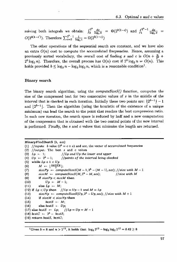
6.3. Optimal s and c values

solving both integrals we obtain: f2 b 1 g2 x =®(2b(1-E)) and fi b-1 1 g2 y=

O(26(1-É 1). Therefore ^t=21 iOg2 t-^(26(1-E))

The other operations of the sequential search are constant, and we have also

an extra O(n) cost to compute the accumulated frequencies. Hence, assuming a

previously sorted vocabulary, the overall cost of finding s and c is O(n +^+

261og2 n). Therefore, the overall process has O(n) cost if 2b log2 n= O(n). This

holds provided b< log2 n - log2 log2 n, which is a reasonable conditionl.

Binary search

The binary search algorithm, using the computeSizeS() function, computes the

size of the compressed text for two consecutive values of s in the middle of the

interval that is checked in each iteration. Initially these two points are: ^26-1 J- 1

and L26-1J. Then the algorithm (using the heuristic of the existence of a unique

minimum) can lead the search to the point that reaches the best compression ratio.

In each new iteration, the search space is reduced by half and a new computation

of the compression that is obtained with the two central points of the new interval

is performed. Finally, the s and c values that minimize the length are returned.

BinaryFindBestS (b, acc) (1) //inputs: b value (26 = c+s) and acc, the vector of accumulated frequencies (2) //output: The best s and c values

(3) Lp «- 1; //Lp and Up the lower and upper (4) Up ^--- 2b - 1; //points of the interval óeing checked

(5) while Lp + 1 < Up

(6) M t- L`PZUPJ; (7) sizePp ^- computeSizeS(M - 1, 26 -(M - 1), acc); //size with M- 1

(8) sizeM ^- computeSizeS(M, 26 - M, acc); //size with M

(9) if sizePp < sizeM then

(10) Up <-- M - 1;

(11) else Lp ^- M; (12) if Lp < Up then //Lp = Up - 1 and M= Lp (13) sizeNp .- coniputeSizeS(Up, 26 - Up, acc); //size with M-^ 1

(14) if sizeM < sizeNp then

(15) óestS f- M; (16) else óestS ^-- Up; (17) else óestS ^- Lp; //Lp = Up = M- 1

(18) bestC F- 26 - bestS;

(19) return óestS, bestC;

1Given 6= 8 and n> 212, it holds that: Iog2 212 - log2 log2 212 = 8.42 > 8

97

6. (s, c)-Dense Code

The most expensive possible sequence of calls to the computeSizeS algorithm occurs

if the optimal s and c values are s= 255 and c= 1. In that case, computeSizeS() is called for the sequence of values c= 26-1, c= 26-2, c= 2b-3,. .., c= 1. Therefore,

in the worst case, the cost of the BinaryFindBestS() algorithm is:

6-1 n b-1 n 1 n 2b + ^ log2b_; n 2b + log2 n ^ b_ i = O( 2b + log n log b)

z-i í-i

The other operations of the binary search are constant, and we have also an extra O(n) cost to compute the accumulated frequencies. Hence the overall cost of

finding s and c is O(n+log(n) log(b)). Since the maximum b of interest is such that

b=^log2 n^ (because at this point we can code each symbol using a single stopper),

the cost of optimization algorithm is at most O(n + log(n) loglog(n)) = O(n),

assuming that the vocabulary is already sorted. Therefore, the cost of computing

the optimal s and c values is totally negligible, and computing the accumulated

frequencies becomes the most time-consuming operation.

6.4 Encoding and decoding algorithms

Once the optimal s and c values for a given vocabulary are known, it is feasible to

perform code generation. This encoding is usually done in a sequential fashion as

shown in Table 6.1. However, an on-the-fly encoding process is also available as it

happened in the case of End-Tagged Dense Code. Given a word rank i, its ^-byte

codeword, can be easily computed in O(P) = O(log i) time.

Again, there is no need to store the codewords (in any form such as a tree) nor

the frequencies in the compressed file. It is enough to store the plain words sorted

by frequency and the value of s used in the compression process. Therefore, the

vocabulary will be slightly smaller than in the case of a Huffman code, where some

information about the shape of the tree must be stored (even when a canonical

Huffman tree is used).

6.4.1 Encoding algorithm

The following pseudo-code presents the on-the-fly encoding algorithm. The

algorithm outputs the bytes of each codeword one at a time from right

to left. That is, it begins outputting the least significative bytes first.

98

6.4. Encoding and decoding algorithms

Encode (i)

(1) //input: i, the rank of the word in the vocabulary

(2) //output: the codeword Ci from right to left

(3) output i mod s;

(4) x ^- i div s;

(5) while x > 0

(6) x ^- x - 1;

(7) output(x mod c) -}- s;

(8) x ^- x div c;

A more efficient implementation of the on-the-fly encode algorithm that

computes a codeword and returns also the codeword length k is also given next.

This algorithm is the one we used when an on-the-fly encoding algorithm is needed

(see Section 11.2).

Encode (i)

(1) //input: i, the rank of the word in the vocabulazy

(2) //output: the codeword C2 from right to left, and its length k

(3) k ^- 1;

(4) if i > s (5) output i mod s;

(6) x ^- (i div s) - 1;

(7) while x > c

(8) output (a mod c) ^- s;

(9) x ^- (x div c) - 1;

(10) k ^- k -^ 1;

(11) output x -1- s;

(12) k ^- k -}- 1;

(13) else output i;

(14) return k;

6.4.2 Decoding algorithm

The first step of decompression is to load the words that compose the vocabulary to

a vector. Since these words were saved ordered by frequency along with the s value

and the ĝompressed text during compression, the vocabulary of the decompressor

is recovered already sorted by frequency. Once the sorted vocabulary is loaded, the

decoding of codewords can begin.

In order to obtain the word wi that corresponds to a given codeword ct, the

decoder can run a simple computation to obtain, from the codeword, the rank of

the word i. Then, using the value i, it obtains the word from the vocabulary sorted

99

6. (s, c)-Dense Code

by frequency. A code c; of 2 bytes can be decoded in O(P) = O(log^ i) time2 as follows:

The decoder uses a base table. This table indicates the rank of the first word

of the vocabulary that is encoded with k bytes (k >_ 1). Therefore base[1] = 0, base[2] = s, base[3] = s+ sc,... base[k] = base[l^ - 1] + sck-2.

The decode algorithm receives a codeword x, and iterates over each byte of x. The end of the codeword can be easily recognized because its value is smaller

than s. After the iteration, the value i holds the relative position of the word wi

among all the words of k bytes. Then the base table is used, and the final value is i^ i+ base[k]. As a result, a position i is returned, and the decoded word wi is obtained from vocabulary[i].

Decode (base, x) (1) //input: x, the codeword to be decoded and the base table

(2) //output: i, the position of the decoded word in the ranked vocabulary

(3) i ^- 0;

(4) k^- 1; // number of bytes of the codeword

(5) while x[k] > s

(6) i^- i x c+ (x[k] - s); (7) k ^- k -}- 1;

(8) i^- i x s-I- x[k];

(9) i <-- i -}- óase[k];

(10) return i;

6.5 Searching (s, c)-Dense Code

Searches over (s, c)-Dense Code are performed as in the case of End-Tagged Dense

Code. As it was explained in Section 5.4, the search pattern is encoded and then

searched through the compressed text using a Boyer-Moore type algorithm. A valid

match is detected if the compressed pattern is found in the compressed text and it

is preceded by a stopper.

The only différence between both techniques is the definition of the stopper and the continwer concepts. In End-Tagged Dense Code continuers and stoppers were

defined as byte values in the ranges [0, 26-1 - 1] and [26-1, 26 - 1] respectively,

whereas in (s, c)-Dense Code stoppers belong to the range [0, s- 1] and continuers

are byte values in the range [s, 2b - 1].

ZDecoding takes O(log^ i) time if c> 1. If c= 1, it takes O(i/26)

100

6.6. Empirical results

CORPUS Original Size PH (s,c)-DC ETDC TH DIFFl DIFF2

CALGARY 2,131,045 34.76 (197,59) 35.13 35.92 38.91 0.37 0.79 FT91 14,749,355 30.26 (193,63) 30.50 31.15 33.58 0.24 0.65 CR 51,085,545 29.21 (195,61) 29.45 30.10 32.43 0.24 0.65 FT92 175,449,235 30.49 (193,63) 30.71 31.31 34.08 0.22 0.60 ZIFF 185,220,215 31.83 (198,58) 32.02 32.72 35.33 0.19 0.70 FT93 197,586,294 30.61 (195,61) 30.81 31.49 34.30 0.20 0.68 FT94 203,783,923 30.57 (195,61) 30.77 31.46 34.28 0.20 0.69 AP 250,714,271 31.32 (189,67) 31.59 32.14 34.72 0.27 0.55 ALL^T 591,568,807 30.73 (196,60) 30.88 31.56 34.16 0.15 0.68 ALL 1,080,719,883 32.05 (188,68) 32.24 32.88 35.60 0.19 0.64 (*)DIFFl shows the value (s, c)-DC - PH. (*)DIFFZ shows the value ETDC -(s, c)-DC.

Table 6.5: Comparison of compression ratio.

6.6 Empirical results

All the text collections in the experimental framework described in Section 2.7 were

used. We compressed them applying Plain Huffman (PH), (s,c)-Dense Code ((s, c)-

DC), End-Tagged Dense Code (ETDC) and Tagged Huffman (TH), using bytes

(b = 8) as the target alfabet.

In Section 6.6.1, we compare the compression ratio achieved by each technique.

In Section 6.6.2, we focus on time performance, comparing encoding time and

compression time among the four techniques. Finally, in Section 6.6.3 we also

compare the decompression speed obtained by (s, c)-Dense Code, End-Tagged Dense

Code, Plain Huffman, and Tagged Huffman.

6.6.1 Compression ratio

Table 6.5 shows the compression ratio obtained by the different codes. We excluded

the size of the compressed vocabulary in the results (this size is negligible and

similar in all cases, although a bit smaller in (s, c)-DC and ETDC because only the

sorted words are needed).

The second column of the table contains the original size of the processed corpus,

the following four columns give the compression ratio for each method, the seventh

column shows the small loss of compression of (s, c)-DC with respect to Plain

Huffman, and the last column shows the difference between (s, c)-DC and End-

Tagged Dense Code. The fourth column, which refers to (s, c)-DC, also gives the

optimal (s, c) values.

As it can be seen in Table 6.5, Plain Huffman gets the best compression ratio

101

6.­ (s, c)-Dense Code

(as expected since it is an optimal prefix code). End-Tagged Dense Code always

obtains better results than Tagged Huffman, with an improvement of up to 2.5

percentage points, as it was shown in Section 5.5.1. (s, c)-DC improves ETDC

compression ratio by around 0.6 percentage points (as expected, since ETDC is a

(128, 128)-DC), and it is worse than the optimal Plain Huffman only by less than

0.3 percentage points on average.

6.6.2 Encoding and compression times

As shown in the previous section, (s, c)-DC compression ratios are very close to the

Plain Huffman ones. In this section we compare the (s, c)-DC and Plain Huffman

encoding phases and measure code generation time and compression time. We also

include End-Tagged Dense Code in the comparison because it is even simpler to

build than (s, c)-Dense Code. In the case of Tagged Huffman, it works exactly as

Plain Huffman, with the only difference of generating 2b-1-ary trees instead of 26­

ary trees as Plain Huffman does. This provokes a ne ĝligible loss of encoding speed,

but worsens compression speed noticeably.

The model used for compressing a corpus in our experiments is described in

Figure 6.4. It consists of three main phases.

1.­ The first phase is vocabulary extraction. The corpus is processed once in order

to obtain all distinct words in it (n) and their number of occurrences. The

result is a list of pairs (word, f requency), which is then sorted by f requency.

This phase is identical for Plain Huffman, (s, c)-Dense Code, and End-Tagged

Dense Code.

2. In the second phase­ (encoding) each word in the vocabulary is assigned a

codeword that minimizes average codeword length. This process is different

for each method:

• The Plain Huffman encoding phase is split into two main parts:­ Creating

the Hu,f,^man tree uses the Huffman algorithm to build a tree where each

leaf corresponds to one of the n words in the vocabulary, and the number

of internal nodes is at most ^2^^. Then, starting from the root of the

tree, the depth of each leaf is computed. Further details of this first part

can be found in [MK95, MT96]. Code assignment starts at the bottom

of the tree (longest codewords) and goes through all leaf nodes. Nodes

in the same level are given codewords sequentially, and a jump of level

is determined by using the previously computed leaf depths. During

102

6.6. Empirical results

Vocabulary extraction

File processing wordi Words vector ^ID ^

Increasin fre uenc sortin Decreasin fre uenc sortin

t I n 1 n

Encoding

Huffman (s-c) DC To

Creating Huffman Vee Search for optimal (s,c) values m

C /Q^,, y Aaximulated list ^

N ^ fm ^^ C^I Ci ^ O•• V. Find t3est S c a> rn y ó

Sequential code generatior^^ ^C ' O• •o

Sequential code 9eneretion

U ® ^

T^

word

Hash table

Compression phase i

Figure 6.4: Vocabulary extraction and encoding phases.

this process, two vectors base and first, needed for fast decompression,

are also initialized: base[l] = x if x is the first node of the lth level,

and first[l] = y if y is the first codeword of l bytes. Encoding takes

O([n + n/26] +[n/2b] +[n/26 + n])=0(n) time overall.

The same analysis can be applied to Tagged Huffman, in that çase,

encoding cost is O([n + n/26-1] +[n/2b-1] +[n/2b-1 + n])=0(n)

time overall.

•­ The (s, c)-DC encoding phase has also two parts: The first computes

the list of accumulated frequencies and searches for the optimal s and

c values. Its cost is O(n + log(n) loglog(n)) = O(n). After getting the

optimal s and c values, (s, c) sequential encoding is performed. The

overall cost is O(n).

Therefore, both Plain Huffman and (s, c)-Dense Code, run in linear

time once the vocabulary is sorted. However, Huffman's constant is in

practice larger because it involves more operations than just adding up

103

6. (s, c)-Dense Code

CORPUB #worde n ETDC (e.c)-DC PH DIFFl DIFF2 (meec) (maec) (msec) (%) (%)

CALGARY 528,811 30,995 4.233 8.150 11.133 31.186 44.780 FT91 3,135,383 75,681 11.977 15.350 26.500 21.97B 42.076 CR 10,230,907 117,713 21.053 25.750 49.833 18.^39 48.328 FT92 38,803,204 291,427 52.397 69.000 129.817 24.083 48.848 ZIFF 40,868,492 284,892 44.373 58.650 105.900 21.871 48.608 FT93 42,083,804 295,018 52.813 69.725 133.350 24.266 47.713 FT94 43,335,126 289,141 52.980 71.800 134.367 78.008 48.713 AP 53,349,820 237,622 50.073 64.700 121.900 2Z.807 48.924 ALL^`T 124,971,944 577,352 103.727 142.875 260.800 27.400 46.217 ALL 229,598,845 888,190 185.417 216.225 402.875 23.498 48.330

(')DIFFl ehowe the gain of ETDC over (s, c)-DC. (')DIFF2 ehowe the gain of (s, c)-DC over PH.

Table 6.6: Code generation time comparison.

frequencies.

•­ The encoding phase is even simpler in ETDC than in (s, c)-Dense Code,

because ETDC does not have to search for the optimal s and c values

(they are fixed to 128). Therefore only the sequential code generation

phase is performed. It costs O(n) time overall.

In all cases, the result of the encoding section is a hash table of pairs

(word, codeword).

3.­ The third phase, compression, processes again the whole source text. For

each input word, the compression process looks for it inside the hash table

and outputs its corresponding codeword.

Given that the vocabulary extraction phase, the process of building the hash table

of pairs, and the compression phase are present in Plain Huffman, ETDC and (s, c)-

DC, we first measured only code generation time (Tl -To in Figure 6.4), to compare

the three techniques. Lastly, we also measure the time needed to complete the whole

compression process.

Encoding time comparison

Table 6.6 shows the results obtained regarding to code generation time. The first

column indicates the corpus processed, the second the number of words in the

corpus, and the third the number of distinct words in the vocabulary. The fourth,

fifth, and sixth columns give the encoding time (in milliseconds) for ETDC, (s, c)-

DC, and Plain Huffman respectively. The seventh column presents the gain (in

percentage) of ETDC over (s, c)-DC. Finally, the last column shows the gain (in

percentage) of (s, c)-DC over Plain Huffman.

ETDC takes advantage of its simpler encoding phase with respect to (s, c)-DC,

104

6.6. Empirical results

and reduces its encoding time by about 25%. This difference corresponds exactly to

the amount of time needed to compute the optimal s and c values, and corresponds

mainly to the process of computing the vector of accumulated frequencies. With

respect to Plain Huffman, ETDC decreases the encoding time by about 60%.

(s, c)-DC code generation process is always about 45% faster than Plain

Huffman. Although the encoding is in both methods O(n) under reasonable

conditions, (s, c)-DC performs simpler operations. Computing the list of

accumulated frequencies and searching for the best (s, c) pair only involve elemental

operations, while the process of building a canonical Huffman tree has to deal with

the tree structure.

Compression time comparison

As it happened in the previous chapter (where we compared End-Tagged Dense

Code with Plain Huffman), the advantage obtained in encoding time with respect

to Plain Huffman, is compensated by the better compression ratio of Plain Huff­

man. As a result, differences in compression speed among our "dense" techniques

and the Huffman-based methods are minimal as it is shown in Table 6.7.

CORPU9 Compr. time (aec) Compr. 3peed (Kbytea/aec)

PH (s, c)-DC ETDC TH PH (s, -DC ETDC TH

CALGARY 0.415 0.405 0.393 0.415 5,135.05 5,261.84 b,417.91 5,135.05

FT91 2.500 2.493 2.462 2.503 5,899.74 5,915.52 5,943.33 5,891.89

CR 7.990 7.958 7.968 8.040 8,393.89 8,420.81 8,395.46 8,353.92

FT92 29.243 29.339 29.230 29.438 5,999.60 5,980.12 8,002.37 5,980.45

ZIFF 30.354 30.620 30.388 30.725 8,301.95 8,048.99 8,099.29 8,028.32

FT93 32.915 33.031 32.783 33.203 6,002.93 5,981.77 6,027.12 b,950.80

FT94 33.874 33.717 33.783 33.700 6,015.98 8,044.01 8,035.81 6,047.00

AP 42.841 42.878 42.357 42.683 5,879.82 5,874.83 5,919.08 5,878.b7

ALL_FT 99.689 100.570 100.469 101.471 5,922.28 5,882.16 5,888.30 5,829.92

ALL 191.398 191.809 191.783 192.353 5,848.53 5,834.36 5,835.70 5,818.42

a) compression time and compression speed.

CORPUS (e, c)-DC - PH (%) (s, c)-DC - ETDC (%) (s, c)-DC - TH (%) ^

CALGARY 2.489 -2.861 2.489

FT91 0.287 -0.468 0.401 CR 0.424 0.396 1.053

FT92 -0.328 -0.371 0.330

ZIFF -0.888 -0.825 0.343

FT93 -0.352 -0.753 0.520

FT94 0.488 0.138 0.010

AP -0.081 -0.747 0.033

ALL^T -0.877 -0.101 0.898

ALL -0.215 -0.024 0.284

erences w^t respect to s, c­ .

Table 6.7: Compression speed comparison.

Table 6.7.a) gives results for each technique with respect to compression time and

compression speed. The first column in that table indicates the corpus processed.

The following four columns show compression time (in seconds) and the last four

105

6. (s, c)-Dense Code

columns show the compression speed (in Kbytes per second) for Plain Huffman;

(s, c)-DC, ETDC, and Tagged Huffman respectively.

Table 6.7.b) compares ETDC, Plain Huffman, and Tagged Huffman against

(s, c)-DC. Columns from two to four show the gain (in percentage) in compression

speed of (s, c)-DC over the other techniques. Positive values mean that (s, c)-DC

is better than the others. Although differences among the four techniques are very

small, it can be seen that End-Tagged Dense Code is the fastest technique, and that

Plain Huffman is slightly faster in compression than (s, c)-DC. It is also shown that

Tagged Huffman is beaten by its competitors in all corpora.

It is interesting to note that, even having a worse compression ratio than (s, c)-

DC, ETDC is faster. This advantage of ETDC arises because it can use fast bitwise

operations, whereas (s, c)-DC needs to use slower division and modulus operations.

6.6.3 Decompression time

The decompression process is almost identical for the Huffman-based techniques

and (s, c)-DC (ETDC is decompressed assuming that it is a(128,128)-DC). The

process starts by loading the words of the vocabulary into a vector V. For decoding

a codeword, (s, c)-DC also needs the value of s used in compression, whereas Plain

Huffman and Tagged Huffman need to load the vectors base and f irst. Next,

the compressed text is read and each codeword is replaced by its corresponding

uncompressed word. Since it is possible to detect the end of a codeword by using either the s value (in (s, c)-DC) or the f irst vector (in Plain and Tagged Huffman),

decompression is performed codeword-wise. Given a codeword C, a simple decoding

algorithm obtains the position i of the word in the vocabulary, such that V[i] is the

uncompressed word that corresponds to codeword C. Decompression takes O(v)

time, being v the size (in bytes) of the compressed text.

All the corpora in our experimental framework were decompressed using

Plain Huffman, (s, c)-DC, ETDC, and Tagged Huffman. Results in Table 6.8.a)

compare decompression time and decompression speed for the four techniques. The

first column shows the corpus being decompressed. Next four columns present

decompression time (in seconds) for each method, and columns from the sixth to

the ninth show decompression speed (in Kbytes per second).

Table 6.8.b) compares ETDC, Plain Huffman, and Tagged Huffman against

(s, c)-DC. The first column shows the corpus being decompressed and the remainder

three columns in that table show the gain (in percentage) in decompression speed

of (s, c)-DC over Plain Huffman, End-Tagged Dense Code, and Tagged Huffman

106

6.6. Empirical results

CORPUS Deoompr. time (eec) Decompr. Speed (Kbytea/aec) PH (s, c)-DC ETDC TH PH (s, c)-DC ETDC TH

CALGARY 0.088 0.097 0.085 0.092 24,125.04 22,045.29 25,071.12 23,247.76 FT91 0.577 0.603 0.570 0.575 25,576.92 24,446.44 25,876.06 25,651.05

CR 1.903 1.971 1.926 1.988 26,651.80 25,917.13 26,530.29 25,964.70 FT92 7.773 7.592 7.561 7.801 22,573.08 23,109.75 23,204.18 22,489.89 ZIFF 8.263 7.988 7.953 8.081 22,414.71 23,187.95 23,289.77 22,919.24 FT93 6.406 8.437 8.694 8.657 23,506.19 23,418.83 22,727.40 22,824.75 FT94 6.636 8.690 8.463 8.825 23,596.34 23,450.39 24,080.82 23,091.66

AP 11.040 11.404 11.233 11.637 22,709.63 21,985.25 22,318.78 21,544.31 ALL_FT 24.798 25.118 24.500 26.280 23,855.99 23,552.06 24,145.87 22,510.23

ALL 45.699 46.698 46.352 47.156 23,648.88 23,142.74 23,315.50 22,916.11

a compresslon tlme an compresslon spee .

CORPUS (e, c)-DC - PH (%) (s, c)-DC - ETDC (%) (s, c)-DC - TH (%)

CALGARY -8.621 -12.069 -5.172 FT91 -4.420 -5.525 -4.696 CR -3.481 -2.311 -0.183

FT92 2.378 -0.407 2.756

ZIFF 3.450 -0.437 1.172 FT93 -0.373 3.041 2.602 FT94 -0.619 -2.618 1.554 AP -3.190 -1.494 2.047

ALL_FT -1.274 -2.458 4.628 ALL -2.140 -0.741 0.980

^ erences w^t respect to s, c- .

Table 6.8: Decompression speed comparison.

respectively. It can be seen that Both End-Tagged Dense Code and Plain Huffman

are a bit faster in decompression than (s, c)-Dense Code, whereas Tagged Huffman

is clearly the slower technique in decompression.

6.6.4 Search time

Empirical results shown in Section 5.5.4 give End-Tagged Dense Code a little

advantage (2 - 7%) in search speed with respect to Tagged Huffman, when fixed­

length codewords are searched.

The algorithm to search in (s, c)-Dense Code is exactly the same as in ETDC.

The same good results can be expected, but improved from the fact that (s, c)-

Dense Code obtains better compression than ETDC, and therefore the text to be

scanned is shorter.

We present in Table 6.9 the results of searching for some single word patterns in

the ALL compressed corpus. The first three columns give the length of the codeword

assóciated to the word that is being searched, the word itself and the number of

occurrences of that word in the text. Columns four, five, and six show the search

time (in seconds) for the three techniques. The last two columns give the decrease of

search time (in percentage) of (s, c)-Dense Code with respect to End-Tagged Dense

Code and Tagged Huffinan respectively.

107

6. (s, c)-Dense Code

The words searched in the experiments are the most and least frequent words

that are encoded with 1, 2, or 3 bytes with the three compression techniques.

code length word occur. (s, c)-DC ETDC TH DIFFl DIFFZ (sec) (sec) (sec) (%) (%)

1 the 8,205,778 5.308 5.452 5.759 2.636 7.826 1 were 356,144 4.701 5.048 5.182 6.856 9.273 2 sales 88,442 2.526 2.679 2.800 5.711 9.779 2 predecessor 2,775 2.520 2.666 2.736 5.476 7.895 3 resilience 612 1.671 1.779 1.858 6.061 10.059 3 behooves 22 1.613 1.667 1.701 3.245 5.189

DIFFl and DIFF2 show the gain of (s, c)-DC with respect to ETDC and TH respectively.

Table 6.9: Searching time comparison.

It can be seen that, due to the better compression ratio, (s, c)-Dense Code

overcomes End-Tagged Dense Code in searches, achieving a decrease of search time

up to 6%. Therefore, it also overcomes Tagged Huffman search speed in about 5-10

percentage points.

Results for random searches are given in Table 6.10. 10, 000 random words,

appearing at least twice in a corpus, were randomly taken from each corpus

and their corresponding codeword was searched inside the compressed corpus.

The second and third columns in that table, show the average-time (time and the standard deviation (Q) respectively for (s, c)-Dense Code. Average-time and

standard deviation for End-Tagged Dense Code and Tagged Huffman are shown in

columns 4 to 7. Finally, the last two columns show the difference (in percentage)

between (s, c)-Dense Code and Tagged Huffman, and between (s, c)-Dense Code

and End-Tagged Dense Code respectively.

Tagged Huffman improves its search results when searching for random single­

word patterns in large corpus. As we have already explained in Section 5.5.4,

Tagged Huffman uses longer codewords than End-Tagged Dense Code and (s, c)-

Dense Code. This gives it a small advantage when those codewords are searched

using a Boyer-Moore type searching algorithm. However, note that (s, c)-Dense

Code obtains better results than Tagged Huffman in general, with an improvement

around 7 percentage points. In practice, Tagged Huffman only improves (s, c)-Dense

Code in the large FT^LL and ALL collections, where it takes advantage of using

many long codewords.

With respect to End-Tagged Dense Code, (s, c)-Dense Code obtains an

advantage of about 2- 3 percentage points in all corpus.

108

6.7. Summary

CORPUS (s, c)-DC ETDC TH DIFF (%)

TH - ETDC ­time a time a time a s c-DC s c-DC

FT91 0.023 0.006 0.024 0.006 0.024 0.005 4.348 4.348 CR 0.072 0.015 0.073 0.016 0.077 0.012 6.944 1.389

FT92 0.250 0.038 0.257 0.044 0.267 0.046 6.800 2.800 ZIFF 0.275 0.041 0.283 0.047 0.292 0.052 6.182 2.909

^ FT93 0.283 0.049 0.291 0.045 0.299 0.052 5.654 2.827 FT94 0.291 0.039 0.300 0.047 0.306 0.059 5.155 3.093

AP 0.376 0.056 0.382 0.066 0.380 0.048 1.064 1.596 ALL^T 0.844 0.091 0.867 0.101 0.760 0.141 -9.953 2.725

ALL 1.610 0.176 1.650 0.195 1.390 0.250 -13.665 2.484

Table 6.10: Searching for random patterns: time comparison.

6.7 Summary

(s, c)-Dense Code, a simple method for compressing natural language Text

Databases with several advantages over the existing techniques was presented. This

technique is a generalization of the previously presented End-Tagged Dense Code,

and improves its compression ratio by adjusting the parameters s and c to the

distribution of frequencies of the text to be compressed.0

Some empirical results comparing (s, c)-DC with Huffman codes are shown.

In compression ratio, our new code is strictly better than Tagged Huffman Code

(by 3.5 percentage points in practice), and it is only 0.3 percentage points worse

than the optimal Plain Huffman Code. The new code is simpler to build than

Huffman Codes and can be built in around half the time. In compression and

decompression speed, (s, c)-DC is slightly slower than End-Tagged Dense Code

and Plain Huffman, however differences are minimal. This makes (s, c)-DC a real

alternative to Plain Huffman in situations where a simple, fast and good compression

method is required. Moreover, as in Tagged Huffman, (s, c)-DC enables fast direct

searches on the compressed text, which improves Plain Huffman searching efficiency

and capabilities. However, searches in Tagged Huffman are around 5-10% slower

than in (s, c)-DC. Tagged Huffman is only faster than (s, c)-Dense Code when we

perform random searches inside very large texts (the random words are encoded

with longer codewords in Tagged Huffman).

Figure 6.5 summarizes compression ratio, encoding time, compression and

decompression time, and search time for the different methods. In that figure,

the measures obtained in the AP corpus are shown normalized to the worst value.

Moreover, since we show compression ratio and time comparisons, the lower the

value in a bar, the better the compression techniques.

109

6. (s, c)-Dense Code

a0 r iv E 100 % Ñ

O 3 a^ t

° 80 % Ú

Tagged Huffmarj ETDC (s,c)-DC Plain Huffman

d 0. NN

L_

3 ÓU % N m f0

ĝ NU

N

a 40 %

compr. ratio encod. time compr. time decomp. time search time

Figure 6.5: Comparison of "dense" and Huffman-based codes.

Note that Plain Huffman remains interesting because it has the better

compression ratio. However, Tagged Huffman has been overcome by both End-

Tagged Dense Code and (s, c)-Dense Code in all concerns: compression ratio,

encoding speed, compression and decompression speed, and search speed.

110

7

New bounds on D-ary

Huffman coding

7.1 Motivation

Bounding the compression that a D-ary Huffman code achieves is an interesting

problem. In this chapter, we provide new analytical bounds that can be obtained

by using End-Tagged Dense Code and (s, c)-Dense Code. The new bounds permit

us to approximate the compression achieved by a D-ary Huffman code without

having to run HufFinan's algorithm.

Section 7.2 and Section 7.3 explain how the average codeword length of End-

Tagged Dense code and (s, c)-Dense code can be used to bound Huffman. In

Section 7.4, we describe how the zero-order entropy (Hó ) permits bounding

Huffman compression.

An interesting contribution of (s, c)-Dense Code is that analytical bounds

for a D-ary Huffman code can be obtained for different distributions of symbol

frequencies. In Section 7.5, an interesting distribution, called Zipf-Mandelbrot's

distribution, is assumed and analytical bounds to D-ary Huffman are obtained.

Finally, the new bounds obtained are applied to real and theoretical text collections

in Sections 7.6 and 7.7.

111

7. New bounds on D-ary HufFinan coding

7.2­ Using End-Tagged Dense Code to bound

HufFinan Compression

An interesting property of End-Tagged Dense Code is that it can be used as a

bound for the compression that can be obtained with a Huffman code. As shown

in Section 5.2, End-Tagged Dense Code uses all the possible combinations of all

bits, except for the first bit, that is used as a flag as in the Tagged Huffman Code.

Therefore, calling Eb the average codeword length of the End-Tagged Dense Code

that uses symbols of b bits, and defining Lh(2b) and Tb respectively as the average

codeword length of Plain Huffman and Tagged Huffman (with symbols of b bits)

we have:

Eb+l <_ Lh(2b) < Eb < T6 < Eb_1

It is easy to see that Eb+l < Lh(26) since End-Tagged Dense Code, with b+ 1

bits, uses all the 26 combinations of b+ 1- 1 bits, while in Plain Huffman some of

the 2b combinations of b bits are not used. The same reasoning can be applied to see tliat Eb < T6.

On the other hand, Eb is a prefix code of b bits and Huffman is the optimal prefix

code using b bits, thus it holds that Lh(2b) <_ Eb. To understand that Tb < E6_1 it

is only needed to consider Tagged Huffman over b bits as a Huffman code over b-1

bits, and therefore it is always better than End-Tagged Dense Code over b- 1 bits.

Figure 7.1 shows the shape of a Tagged Huffman tree. It is also shown how

the shape of a tree representing the codewords generated by End-Tagged Dense

Code would be. It can be seen that End-Tagged Dense Code achieves a smaller

compressed text size than Tagged Huffman, since an internal node will have 256

children: 128 internal nodes and also 128 leaf nodes. However, in Tagged Huffman,

an internal node can have less than 128 children, some of them (z) will be leaves

and the others, at most (128 - z), will be internal nodes. Therefore End-Tagged

Dense Code has, at least, the same number of codewords of a given length l than

Tagged Huffman (where l corresponds to a level in the tree).

7.3­ Bounding Plain Huífman with (s, c)-Dense

Code

In this section, it is shown that the average codeword length of a D-ary Huffman

code (Lh(D)) can be lower and upper bounded by the average codeword length

112

7.4. Analytical entropy-based bounds

1 0 1 0^ ^

1 z-1 1 127 ^

1 z ^ 0 xxxxxxx 0 0 ^1 xxxxxxx

1 127 0 xxxxxxx 0 127 1 xxxxxxx1 Tagged Huffman End-Tagged Dense Code

z leaves (128 - z) 1281eaves 128 internal nodes internal nodes

Figure 7.1: Comparison of Tagged Huffman and End-Tagged Dense Code.

(Ld(s, c)) that is obtained by (s, c)-Dense Code. For the upper bound we use Ld(s, c)

for some values such that D= s+c, and for the lower bound we use Ld(s, c), having

2D=s+c.

As shown in Section 6.2, (s, c)-Dense Code is a prefix code, and it is well-known

that Huffman [Huf52] is the optimal prefix code. Therefore, Ld(s, c) _> Lh(D).

Moreover a D-ary Huffman code can be seen as a (D, D) stop-cont code provided

that D is added to all digits in a codeword, except the last one. Therefore, Lh(D)

cannot be smaller than the average codeword length of a(D, D)-Dense Code.

Therefore, Ld(D, D) < Lh(D) clearly holds.

Summarizing, (s, c)-Dense Code provides new bounds to a D-ary Huffman code

in the following way:

Ld(D, D) < Lh(D) < Ld(s, c) for any D= s+ c (7.1)

7.4 Analytical entropy-based bounds

F^om the Noisedess Coding Theorern [SW49] it holds that H° < Lh(D) < Hó + 1,

where D= 2 and, as we showed in Section 2.2,

Hó =-^^ i 7^(x:) logD p(^i)

113

7. New bounds on D-ary Huffman coding

is the D-ary zero-order entropy of the words in the vocabulary. Therefore H° is a lower bound of Lh(D).

If Zipf-Mandelbrot's law (see Section 2.4.2) is assumed, Hó can be computed as follows:

1 _ A 1HD0 ^ p^ logD -^( ) B logD A

- +^1+ Ci (1i>^ pi i>^

logD A logD (1 + Ci)B

A i^ [ (1 + Ci)B + (1 + Ci)B ]

A AB logD (1 + Ci)- logD A ^ (1 +

Ci)B + ^ (1 + Ci)ei>1 i>1

logD (1 + Ci) - logD A^ pi + A9 ^

(1 + Ci)ei>^ i>^

logD (1 + Ci) - logD A+ AB ^

(1 ^- Ci)Bi>1

- ln 1+Ci-BA ln A^i>1 (1-}-Ci) ­

ln D

From Equation 2.2, it is known that: A= 1-^ 1 At this point weE>^^,-+^ Cc (B) '

resort to derivation of ^c(B) with respect to Bl

^C(e) - ^ -(1 + Ci)B ln(1 + Ci) - ^ - ln(1 + Ci)

(1 + Ci)ze ( 1 + Ci)ei>1 i>1

And then we substitute in (7.2):

HD = -Bçc(B)^ĝ (B) -^ çc(B) -Bç^ +1n^C(e) 0 ln D ln D

Then a lower bound to Lh(D) based on the entropy value is:

-Bç-^ +ln c(B)Cc(B) ^ Lh(D) > (7.3)ln D

and an upper bound is obtained as:

L (D)h < -B S^ + ln ^c (B)

Hó + 1= 1+ SQ(B^D 7 4. )(

114

7.5. Analytical bounds wit6 (s, c)-Dense Code

7.5 Analytical bounds with (s, c)-Dense Code

F^om Equation 6.3 the average codeword length of (s, c)-Dense Code for a given

distribution of word frequencies which follows Zipf-Mandelbrot's law is:

Ld (s , c)=1+^ ^ 7 í =1+A^ ^ 1 (7 . 5) (1+C2)8

k>1í>Wk-}-1 k>1 i>Wk+l

Note that f(i) _ ^1+^, having C > 0, B> 1 and i>_ 1, is a continuous,

positive and decreasing function. Therefore the series ^í>1 f(z) _^í>1 ií+ĝ^ converges if B > 1 since ^í>1 ^1+^ < ^ ^í>1 ^.

By applying the Integration Theorem, fi ° f(x)dx exists, and it is possible to

bound the series ^^ n+l fk as follows: fi+l f(x)dx <^k>í+l fk < fí°O f(x)dx.

As a result, from 7.5 it is obtained:

Ld(s, c) < 1+ l4 ^ f dx (7 .6)(1 + Cx)e

k>1 Wk

Ld(s,c) > 1 + A ^ f^ dx (7 . 7) Wk+l (1+Cx)B

k>1

7.5.1 Upper bound

As shown in Equation 7.1, it is possible to achieve an upper bound to Lh(D) using

Ld(s, c). We use Equation 7.6 and operate in the summation. Note that we assume

c> 1. The case c= 1 is treated later.

^ °O 1 dx - ^ (1 + Cx)-8+11 °° - ^ -1

(1 + Cx)B C(-B + 1) J C(1 - B)(1 + CW^ )B-1k>1 ^Wk k>1 Wk k>1

1 ^ 1 e-1C(B - 1) k>1 (1 +CS il)

1 (c - 1)B-1^` 1

C(B - 1) se-1 3 r c-1k>1 \^-^ + C(ck - 1)/l e-1

1 (c - 1)A-1 1 1 (7.8)

^ C(B - 1) se-1 Ce-1 ^(ck - 1)B-1

115

7. New bounds on D-ary Huffman coding

Equation 7.8 can be simplified, since:

^ (c^ _ll)e-i - ^ ^k(B-1)(1 - ^)B-1^>1 l^^(1 - ^))B-1k>1

1-B 11 1 < ^ ck(B-1)(1 - ĝ )B-1 = ^1 - ^^

C ^ c^(B-1)

1^ 1-e ^ -^ 1\ i-e ci-e 1-- ^ 1-- J,

c 1- ^^ c 1- cl-e

(c - 1)i-e

1 - ci-e

From Equations 7.6, 7.8, and 7.9 it is obtained that:

) 1 1 1 1Ld(s, c

< 1+ AC(B - 1) sB-1 Ce-i 1_ ci-e

1 (7.10)

= 1 + CB (B - 1) ^c(B) sB-1 (1 - cl-B) _ ^9

Such equation represents an upper bound for Ld(s, c). Therefore in order to obtain

a minimal upper bound we substitute c= D- s and then we resort to differentiation in s.

a^9 - ^se-i((1 - B)(D - s)-e) + (B - 1)sB-z(1 - (D - s)1-B)^

ás CB (B - 1) Cc(B) s(A-1)z [1- (D - s)i-e]z

And now we solve for á• = 0, that is:

0 sA-1(1 - B)(D - s)-B + (B - 1)se-z(1 - (D - s)1-B)

since, 0< c< D and B> 1

0 se-z(1 - B) [s(D - s)-e - (1 - (D - s)(1-B)/J

0 = s(D - s)-B - (1 - (D - s)1-B)

1= s(D - s)-e +(D - s)(D - s)-B

1 = (D - s)-B [(D - s) + s]

1 = (D - s)-BD

D-s = Dé

s= D- D^, is the s value that gives the best upper bound.

Then we obtain that the optimal c value is: c= D- s= D é.

116

7.5. Analytical bounds with (s, c)-Dense Code

Therefore, a minimal upper bound for Ld(s, c) is obtained by substituting the

optimal s and c values in Equation 7.10, that is:

1 min Ld(s, c) < 1 + (7.11)

s CB(B - 1)^c(e)(D - Dé )A-1(1 - D'-o-1)

If we assume c= 1 then Wk = k(D - 1), hence from Equation 7.6 we obtain:

^ O° 1 dx - 1 1 1 ^ 1 (7.12)

r^>i ^Wk (1 + Cx)B B- 1 CB (D - 1)B-1 ^>i ke-i

Since the summation above diverges if 1< B< 2, no upper bound is obtained for

c= 1 and 1< B< 2. However, given B> 2,

(7.13)^ ke-i = 1 + ^ kel-i < 1 + J ^ kl-Bdk = B - 2i

Therefore, from Equations 7.6, 7.12, and 7.13 an upper bound is obtained as:

1 Ld(U - 1,1) < 1 + (7.14)

(B - 2) ^c(B) CB (D - 1)B-1 ' B > 2

7.5.2 Lower bound

Similarly to the way the upper bound was obtained, it is also possible to obtain a

lower bound. Using Equation 7.7 we have:

Ld(s,c) > 1+A^ fWk+l (1+Cx)edx

For c= 1 the compression obtained by (s, c)-Dense Code is poor, so it is not possible

to guarantee that it will obtain a lower bound to Lh(D). However, assuming c> 1

we obtain:

dx = (1 + Cx)-e+i l ^^ 1

^Wk+l ( 1 + Cx)B C(-6 + 1) J Wk+^ 1 -1 1 1

e-iC(1 - B) [1 + C(Wk + 1)]B-1 C(B - 1) [1 + C(s i + 1)]

(c - 1)B-1 1

C(6 - 1) [(c - 1) + C(s(ck - 1) + (c - 1))]B-1

117

7. New bounds on D-ary Huffman coding

Therefore we obtain that:

Ld(s, c) > 1+ A^(c - 1)B-1 ( 1 (7.15)^i (B - 1) ^lC - 1) + Ci (S(Ck - 1) + (C - 1))]B-1k>1

At this point, note that given c> 1, s> 1 and k> 1

(c - 1) + c(s(ck - 1) + (c - 1)) _ (c - 1)(1 + C) + Cs(ck - 1) <

< (ck - 1)(1 ^- C) + Cs(ck - 1) _ (ck - 1)(1 + C + Cs) then

^(c - 1) + C(s(ck - 1) + (c - 1)^ B 1 < ^(ck - 1) (1 + C + Cs)^ e-1

and

1 1

[(C - 1) + C[S(Ck - 1) + (C - 1)]]B-1 > [(Ck - 1)(1 + C + CS)]B-1

As a result, Equation 7.15 can be transformed into:

Ld(s, c) > 1+ A^ (c - 1)B-1 1

k>i C(B - 1) ((1 + C+ Cs)(ck - 1)]e-1

> 1+A(c 1)e-i 1 1 ^ (ck)B-iC(9 - 1) (1 + C + Cs)B-i

e-i ci-e(c - 1)

- 1+ ^c(B) C(B - 1) (1 + C+ Cs)e-1 1- cl-e (1 _ 1)e-i11+ ^

^C(6) C(B - 1) (1 + C + Cs)e-1 1_ cl-B

Summarizing, we have obtained a lower bound to Ld(s, c)

1- ^)BB1Ld(s,c) > 1+ (7.16)1 e 1(^C(B) C(B - 1) (1 + C+ Cs) - 1- c-

Since Equation 7.1, it is known that Ld(D, D) is a lower bound of Lh(D), thus the

following Equation gives a lower bound for a D-ary Huffman code.

(1 - 1 )e-'Ld^D D^ > 1 + °

^C(B) C(B - 1) (1 + C + CD)B-1 ( 1 _ D1-e)

118

7.6. Applying bounds to real text collections

7.6­ Applying bounds to real text collections

We have obtained the optimal parameters B and C from Zipf-Mandelbrot's law

that approximate the word frequency distribution for all the text collections in

our experimental framework. This was made by first choosing suitable values of C(0.75, 1.00, and 1.25), and then applying regression to obtain the best value of B. Then, assuming Zipf-Mandelbrot's distributions with those parameters, we ran

Huffman's algorithm to obtain the average codeword length for a D-ary Huffman code (Lh(D)). Finally we also computed the empirical and analytical bounds shown through this chapter.

Table 7.1 compares the redundancy (see Section 2.2) obtained by our bounds

and the redundancy of the D-ary Huffman code when they are applied to the largest

corpora in our experimental framework. Columns two and three in that table show,

respectively, the parameters C and B used to characterize the word frequencies in

each corpus. The lower bounds are shown in the fourth and fifth columns: the fourth

one gives the redundancy obtained by the (D, D)-Dense Code (Ld(D, D) - Hó ),

and the fifth column shows the redundancy obtained by the analytical lower bound ([Eq. 7.17] - Hó ). The sixth column from the table shows the redundancy of the

D-ary Huffman code (Lh(D) - Hó ). The last two columns show, respectively,

the redundancy obtained by the empirical upper bound (Ld(s, c) - Hó ) and the analytical upper bound ([Eq. 7.11] - H° ).

It can be seen that very tight upper and lower bounds aze obtained by running

(s, c)-Dense Code and (D, D)-Dense Code respectively. Moreover, it is shown that

the analytical bounds work fine, obtaining values very close to the empirical bounds.

7.7­ Applying bounds to theoretical text collec­

tions

In this section we use theoretical Zipf-Mandelbrot's word frequency distributions

and show the behavior of the bounds presented. In Figure 7.2, assuming Zipf­

Mandelbrot's law and having n, = 10, 000, 000 and C= 1.0 we show the bounds

obtained for different values of the parameter 8. Both the empirical upper bound

(obtained by rnnning (s, c)-Dense Code) and the analytical upper bound are very

tight. In fact, the empirical upper bound is so tight that it becomes almost

indistinguishable with respect to the D-ary Huffman. In the case of the lower

bounds, they are not so tight as the upper bounds aze, but they permit predicting

119

7. New bounds on D-ary Huffman coding

CORPUS Z-M param. Redundancy C B An. Low (D, D)-DC D-ary Huff (s, c)-DC An. Up

ZIFF 0.75 1.462 0.270 0.293 0.313 0.313 0.327 FT93 0.75 1.451 0.262 0.286 0.307 0.308 0.323 FT94 0.75 1.453 0.264 0.287 0.308 0.309 0.323

AP 0.75 1.458 0.267 0.290 0.311 0.311 0.325 FTALL 0.75 1.472 0.272 0.297 0.317 0.317 0.326

ALL 0.75 1.465 0.266 0.293 0.314 0.314 0.322

ZIFF 1.00 1.425 0.274 0.295 0.317 0.318 0.337 FT93 1.00 1.416 0.267 0.289 0.312 0.313 0.333 FT94 1.00 1.417 0.267 0.289 0.312 0.313 0.333

AP 1.00 1.422 0.271 0.292 0.315 0.316 0.335 FT^1LL 1.00 1.438 0.277 0.301 0.323 0.323 0.336

ALL 1.00 1.432 0.271 0.297 0.320 0.320 0.332

ZIFF 1.25 1.398 0.275 0.294 0.318 0.319 0.344 FT93 1.25 1.389 0.268 0.287 0.313 0.314 0.340 FT94 1.25 1.391 0.269 0.288 0.314 0.315 0.341

AP 1.25 1.395 0.272 0.291 0.316 0.317 0.342 FT^1LL 1.25 1.412 0.277 0.301 0.325 0.325 0.341

ALL 1.25 1.408 0.272 0.297 0.322 0.323 0.338

Table 7.1: R,edundancy in real corpora

the average codeword length of a D-ary Huffman code with little error.

It can be seen that, when low values of B are used, the redundancy obtained

is low. However, differences between the lower and upper bounds and the

redundancy of Huffman are maximal. As B increases, more biased Zipf-Mandelbrot's

distributions are generated, and the bounds obtained are tighter than those obtained

with lower values of B.

7.8 Summary

In this chapter we presented how the compression ratio that is obtained by a D-ary

Huffman code can be lower and upper bounded by both End-Tagged Dense Code

and (s, c)-Dense Code. We first showed that these new techniques are so simple and

fast that they can be run to approximate the average codeword length of a D-ary

Huffman code, avoiding running the slower Huffman algorithm.

Then, we presented analytical bounds, assuming that Zipf-Mandelbrot's law

predicts the word frequency distribution in natural language texts. First, we showed

bounds that are based on the zero-order entropy. Finally, we provided analytical

upper and lower bounds based on (s, c)-Dense Code.

These analytical results are important for compressed Text Databases, because

they permit to predict their compressed size from an analytical model of a word

120

7.8. Summary

Redundancy for n=10^ and C= 1.0 0.5

0.45

0.4 ^ U C N ^ C

^ 0.35 m ¢

0.3

0.25

1.4 1.45 1.5 1.55 1.6 1.65 e

Figure 7.2: Bounds using Zipf-Mandelbrot's law.

distribution in some language.

121

Part II

Adaptive compression

8

Dynamic text compression

techniques

In this chapter, a brief description of the state of the art in dynamic text compression

techniques is presented. First, the motivation of adaptive versus semi-static

techniques is discussed. Then, the two most popular and well-known families of

dynamic techniques are described: statistical and dictionary-based compressors.

The first family of dynamic compressors is composed of statistical techniques.

The general way of working of dynamic statistical codes is explained, and the two

main representatives of this kind of dynamic methods are described in Section 8.2.

The first technique is called dynamic character oriented Huffman, and it is described

in Section 8.2.1. Dynamic character oriented Huffman is the basis of the dynamic

word-based Huffman technique presented in Chapter 9. The other statistical

technique, known as dynamic arithmetic compression, is introduced in Section 8.2.2.

In Section 8.3, a predictive technique called Prediction by Partial Matching

(PPM) is presented. Finally, Section 8.4 starts with a brief description of dictionary

techniques and later presents the variants of the Ziv-Lempel family, one of the most

widespread compression families, and the basis of common programs such as gzip,

compress, and arj.

125

8. Dynamic text compression techniques

8.1 Introduction

Transmission of compressed data is usually composed of four processes:

compression, transmission, reception, and decompression. The first two are carried

out by a sender process and the last two by a receiver. This structure can be

seen for example, when a user downloads a zip file from a website. The file,

which was previously compressed in the server, is transmitted in compressed form

when the user downloads it. Finally, once the transmission has finished, it can be

decompressed. This transmission scheme can also be extrapolated to the scenario

of a file being compressed or decompressed from disk. In this case, the compressor

acts as a sender and the decompressor acts as the receiver.

There are several interesting real-time transmission scenarios where the

compression, transmission, reception, and decompression processes should take place concurrently. That is, the sender should be able to start the transmission of

compressed data without preprocessing the whole text, and simultaneously the receiver should start the reception and decompression of the text as it arrives.

Real-time transmission is usually of interest when communicating over a

network. In the case of natural language text, this kind of compression can be

applied, for example, in the following scenarios:

• Interactive services such as remote talk/chat protocols, where messages

are exchanged during the whole communication process. Instantaneous

transmission and reception are needed, and they take place in an interactive

way. Therefore, it is not feasible to delay the beginning of the transmission of

data until the whole text is known.

• Transmission of­ Web pages. Installing a browser plug-in to handle

decompression enables the exchange of compressed pages between a server

and a client along time in a more efficient way.

•­ Wireless communication with hand-held devices with little bandwidth.

Real-time transmission is handled by dynamic or adaptive compression

techniques. As in the case of semi-static methods, these techniques pursue several

goals such as good compression ratio, and fast compression and decompression.

However, whereas in semi-static techniques the features of direct access and direct

search were interesting, in dynamic techniques it is crucial to be able to manage

streams of text.

Currently, the most widely used adaptive compression techniques belong to the

126

8.2. Statistical dynamic codes

Ziv-Lempel family [ZL77, ZL78, We184]. When applied to natural language text,

however, the compression ratios achieved by Ziv-Lempel are not that good (around

40%). Their advantages are compression speed and, mainly, decompression speed.

Other adaptive techniques like Arithmetic Encoding [Abr63, WNC87, MNW98]

or Prediction by Partial Matching (PPM) [BCW84] have proven to be competitive

regarding compression ratio. However, they are not time-efficient.

Classic Huffman code [Huf52] is a well-known two-pass method. Making it

dynamic was first proposed in [Fa173, Ga178]. This method was later improved in

[Knu85, Vit87]. However, being character-based, the compression ratios achieved

were not good. It is interesting to point out that the adaptive Huffman-based

techniques can be extrapolated to a word-based approach. Such a technique is

presented in Chapter 9.

This chapter shows the most common adaptive compression techniques. These

techniques will be used in Chapter 11 to experimentally test the dynamic

compression techniques developed in this thesis.

8.2 Statistical dynamic codes

Statistical dynamic compression techniques are also called one-pass. Symbol

frequencies are collected as the text is read, and consequently, the mapping between

symbols and codewords is updated as compression progresses. The receiver acts in

the same way as the sender. It computes symbol frequencies and updates the

correspondence between codewords and symbols each time a codeword is received.

In particular, dynamic statistical compressors model the text using the

information about source symbol frequencies, that is, f(s2) is the number of times

that the source symbol st appears in the text (read up to now).

In order to maintain the vocabulary up-to-date, dyñamic techniques need a data

structure to keep all symbols s^ and their frequencies f(si) up to now. Such data

structure is used by the encoding/decoding scheme, and it is continuously updated

during compression/decompression. For each new source symbol, if it is already

in the vocabulary, its frequency is increased by 1. If it is not, it is inserted in the

vocabulary and its frequency is set to 1. After reading each symbol, the vocabulary

is updated and rearranged if necessary, so that the codeword assigned to any source

symbol may change.

To let the sender inform the receiver about new source symbols that appear in

127

8. Dynamic text compression techniques

Sender ( ) (1) Vocaóulary ^­ {C^ew-Symbol}i

(2) Initialize CodeBook;

(3) while (true)

(4) read s from the text;

(5) if s ^ Vocaóulary then

(6)­ send CRew-Symboli send s in plain form;

Vocabu,lary ^- Vocaóulary U {s};

(9)­ f(s) (10) else (11)­ send CodeBook(s);

(12)­ f(s) <- f(s) + 1;

(13) Update CodeBoo%;

Receiver ( )

Vocaóulary ^- {i'.^ew-Symóol}; Initialize CodeBook;

while (true)

receive C;

lf C. = C^,ew-Symbol then

receive s in plain form;

Vocabulary ^ Vocaóulary U {s};

f (s) ^- 1;

else (10)­ s ^- CodeBook-1(C); (11)­ f(s) ^ f(s) -F 1; (12) output s;

(13) Update CodeBook;

Figure 8.1: Sender and receiver processes in statistical dynamic text compression.

the text, a special source symbol new-Symbol (whose frequency is zero by definition)

is always held in the vocabulary. The sender transmits the new-Symbol codeword

each time a new symbol arises in the source text. Then, the sender encodes the

source symbol in plain form (e.g., using ASCII code for words) so that the receiver

can insert it in its vocabulary.

Figure 8.1 depicts the sender and receiver processes, highlighting the symmetry

of the scheme. CodeBook stands for the mapping between symbols and codewords,

and permits to assign codewords to source symbols or vice versa. Note that new-

Symbol is always the least frequent symbol of the CodeBook.

128

8.2. Statistical dynamic codes

8.2.1 Dynamic HufFman codes

In [Fa173, Ga178], an adaptive character-oriented Huffman code algorithm was

presented. It was later improved in [Knu85], being named FGK algorithm. FGK

is the basis of the UNIX compact command.

FGK maintains a Huffman tree for the source text already read. The tree is

adapted each time a symbol is read to keep it optimal. It is maintained both by

the sender, to determine the code corresponding to a given source symbol, and by

the receiver, to do the opposite.

Thus, the Huffman tree acts as the CodeBook of Figure 8.1. Consequently, it

is initialized with a unique special node called zeroNode (corresponding to new-

Symbol), and it is updated every time a new source symbol is inserted in the

vocabulary or when a frequency is increased. The codeword for a source symbol

corresponds to the path from the tree root to the leaf corresponding to that symbol.

Any leaf insertion or frequency change may require reorganizing the tree to restore

its optimality.

The main challenge of Dynamic Huffman is how to reorganize the Huffman tree

efficiently upon leaf insertions and frequency increments. This is a complex and

potentially time-consuming process that must be carried out both by the sender

and the receiver.

The basis of the FGK algorithm is the sibling property defined by Gallager in

[Ga178].

Definition 8.1 A binary code tree has the sibling property if each node (except the

root) has a sibling and if all nodes can be listed in decreasing weight order, with each

node adjacent to its sibling.

Gallager also proved that a binary prefix code is a Huffman code iff the code tree

has the sibling property.

Using the sibling p^perty, the main achievement of FGK is to ensure that the

tree can be updated by doing only a constant amount of work per node in the path

from the affected leaf to the tree root. Calling l(si) the path length from the leaf

of source symbol si to the root, and f(s^) its frequency, the overall cost of the

algorithm FGK is ^ f(si)l(si), which is exactly the length of the compressed text

measured in number of target symbols.

In (Vit87] an improvement upon FGK denominated algorithm A was presented.

129

8. Dynamic text compression techniques

An implementation of A can be found in [Vit89]. The main difference with respect to FGK is that algorithm A uses a different method to update the tree, which not

only minimizes ^ f(si)l(si) (compressed text length) but also the external path

length (^l(si)), and the height of the tree (maxl(si)). Moreover, algorithm A

reduces to 1 the number of exchanges in which a node is moved upwards in the

tree during an update of the tree. Although these improvements do not modify the

complexity of the whole algorithm, they give algorithm A advantage in compression ratio and speed over FGK, and even over static Huffman for small messages. Results

presented in [Vit87] show that adaptive Huffman methods are directly comparable

to classic Huffmán in compression ratio.

8.2.2 Arithmetic codes

Arithmetic coding was first presented in the sixties in [Abr63]. Being statistical, it

uses the probabilities of the source symbols in order to obtain compression.

Distinct models can be used to calculate, for a given context, the probability

of the next source symbol. Therefore static, semi-static, and adaptive arithmetic codes are available. The key idea of this technique is to represent a sequence of

source symbols using a unique real number in the range [0,1). As the message to

be encoded becomes larger, the interval needed to represent it becomes narrower,

and therefore, the number of bits needed to represent it grows.

Basically an arithmetic encoder works with a list of the n symbols of the

vocabulary and their probabilities. The initial interval is [0,1). When a new source

symbol is processed, the interval is reduced in accordance with the current symbol

probability and the interval becomes a narrower range that represents the input

sequence of symbols already processed.

We present in Example 8.1 a semi-static arithmetic compressor to explain how

arithmetic compression works. Note that making it dynamic consists only of

adapting the frequency of the source symbols each time one of them is processed.

Example 8.1 Let us compress the message "AABC! " using a semi-static model.

In the first phase, the compressor creates the vocabulary, which is composed of four

symbols: 'A', 'B', 'C' and '!'. Their frequencies are: 0.4, 0.2, 0.2 and 0.2 respectively.

Therefore, in the initial state, any number in the interval [0, 0.4) represents symbol

'A', and intervals [0.4, 0.6), [0.6, 0.8) and [0.8, 1) represent symbols 'B', 'C', and '!'

respectively.

Since the first symbol to encode is 'A', the interval [0,1) is reduced to [0, 0.4).

130

8.2. Statistical dynamic codes

Next possible sub-intervals are [0, 0.16), [0.16, 0.24), [0.24, 0.32), and [0.32, 0.4).

They would represent the sequences 'AA', 'AB', 'AC' or 'A!'. Figure 8.2 represents

graphically the intervals of the whole process. Since the next symbol is again 'A',

the current working-interval is reduced to [0, 0.16). Note that the size of this interval

depends on the probability of the sequence encoded; that is: 0.4 x 0.4 = 0.16.

To encode the next source symbol 'B', the new interval is reduced to [0.064, 0.096),

because the sequence 'AAB' has probability of 0.032 = 0.096 - 0.064.

After processing 'C', the range becomes [0.0832, 0.0896), and the probability

associated to 'AABC' is 0.0064.

Finally, the possible sub-intervals are [0.0832, 0.08576), [0.08576, 0.08704), [0.08704,

0.08832), and [0.08832, 0.0896). Since '!' was the last symbol of the vocabulary, any

number in the interval [0.08832, 0.0896) represents the message 'AABC!'. Therefore,

the encoder generates the number that can be encoded with less bits inside that

interval. q

The decompressor only has to know the vocabulary used, the probabilities of

the source symbols and the number of symbols transmitted. From the compressed

data, it can detect the intervals used in the encoding phase and from these intervals,

it recovers the source symbols.

A B C ! o, o,s o,a 1

A I B I C I^^I 0 0.24 0.32 0.4

A I B I C 1 0 64 0.0$6. 0.128 0.16

A I B I C I !^I 0.064 0.0768 ^6832 0.08^6 0.096

^ _B ^ C ^^ 0.0832 0.08576 0.08704 0.08832 0.0896

Figure 8.2: Arithmetic compression for the text AABC!.

In general, arithmetic compression improves Huffman compression ratios. When

131

8. Dynamic text compression techniques

static or semi-static models are used, compression and decompression speed are not

competitive with respect to Huffman-based techniques. Moreover, they have the

disadvantage that decompression and searches cannot be performed directly in the

compressed text because it is represented by a single number, so decompression

is mandatory before a search can be performed. As a result, arithmetic coding is

not useful in environments where text retrieval capabilities are needed. However, it

becomes a good alternative to adaptive Huffman codes. In [WNC87], an adaptive

character based arithmetic technique is compared with the UNIX compact algorithm

(which is based on FGK dynamic Huffman). In this case arithmetic encoding is

faster in both compression and decompression processes, and it also achieves better

compression ratio.

Several modifications of the basic arithmetic algorithm improving its

performance and/or using distinct models have been made. In [WNC87], Witten,

Neal, and Cleary presented an arithmetic encoder based on the use of integer

arithmetic. In [MNW98], Moffat et al. made improvements focused on avoiding

using multiplications and divisions that could be replaced with faster shift/add

operations. Moreover, the code from [CMN+99] (based on [MNW98]) is of public

domain and it has been used in our tests.

8.3 Prediction by Partial Matching

Prediction by Partial Matching technique (PPM) was first presented in 1984 by

Cleary and Witten [CW84].

PPM is an adaptive statistical data compression technique based on context

modelling and prediction. Basically, PPM uses sequences of previous symbols in

the source symbol stream to predict the frequency of the next symbol, and then

it applies an arithmetic technique [WNC87, MNW95] to encode that symbol using

the predicted frequency.

PPM is based on using the last m characters from the input stream to predict

the probability of the next one. This is the reason why it is called a finite-conte^t

model of order m. That is, a finite-context model of order 2 will use only the two

previous symbols to predict the frequency of the next symbol.

PPM çombines several finite-context models of order m, in such a way that

m takes the values from 0 to M(M is the maximum context length). For each

finite-context model, PPM takes account of all m-length sequences Si that have

previously appeared. Moreover, for each of those sequences Si, all characters that

132

8.3. Prediction by Partial Matching

have followed Si, as well as the number of times they have appeared, are kept. The

number of times a character followed an m-length sequence is used to predict the

probability of the incoming character in the model of order m. Therefore, for each

of the finite-context models used, a separate predicted probability distribution is

obtained.

The maximum context length (that is, the length of a sequence of symbols that

are considered in the highest-order model) is usually 5. It was shown [CW84, Mof90]

that increasing the context length beyond 5- 6 symbols does not usually improve

compression ratio.

The M+ 1 probability distributions are blended into a single one, and arithmetic

coding is used to encode the current character using that distribution. In general,

the probability predicted by the highest-order model (the M-order model) is used.

However, if a novel character is found in this context (no M-length sequence precedes

the new character), then it is not possible to encode the new character using the given M-order model, and it is necessary to try the ( M - 1)-order model. In this

case, an escape symbol is transmitted to warn the decoder that a change from an M

to an (M - 1)-order model occurs. The process continues until it reaches a model where the incoming symbol is not novel (and then that symbol can be encoded

with the frequency predicted by the model). To ensure that the process always finishes, a(-1)-order model is assumed to exist. This bottom-level model predicts

all characters si from the source alphabet ( E) with the same probability, that is

p(s^) = É '

Notice that each time a model shift (from m to m- 1) occurs due to a novel symbol in the context model of order m, the probability given to the escape symbol

in the m-order model needs to be combined with the probability that the (m - 1)­order model assigns to the symbol being encoded.

We call w the symbol whose probability is being predicted, p„^(w) the probability

that the m-order model assigns to w and e,,,, the probability assigned to the escape

symbol by the m-order model. Two situations can arise:

1.­ w can be predicted by the M-order model. In this case w is encoded using the

probability p(w) = p,^(w).

2.­ w can be predicted by an m-order model (m < M). Then the probability used

to encode w is p(w) = p„1(w) x^^m^-1 e^'

Distinct methods can be used to assign probabilities both to the escape symbol

and to a novel source symbol. For example, PPMA [CW84) uses a method called A,

133

8. Dynamic text compression techniques

which makes p,,, (w) = 1+ m and e,,,,, = l+^m , where c.,,,, (w) is the number of times

that the character w appeared in the m-order model, and c,,, is the total count of

characters that were first predicted by an m-order model. PPMC [Mof^JO] is the

first popular PPM variant because PPM algorithms require a significant amount of

memory and previous computers were not powerful enough. PPMC uses method C

to assign probabilities. It sets e,,, _^-, and p,,,, (w)^m _ ^^m -dm i x ^m i"i^m ^ where d^ is

the number of distinct characters that were first predicted by the m-order model.

Choosing a method to assign probabilities to the escape symbol constitutes an

interesting problem called the zero-order,frequency problem. Distinct methods have been proposed: Methods A and B [CW84], method C[Mof90], method D [How93] and

method X [WB91]. A description and a comparison of the those available methods can be found in [MT02].

Recent PPM implementations obtain good compression results. As shown in

[CTW95], PPMC uses 2.48 bits per character (bpc) to encode the Calgary corpus

and another variant PPM* (or PPMX)[CTW95] needs only 2.34 bpc (less than 30%

in compression ratio). However, compression and decompression speed are not so

good (5 times slower than gzip in compression).

Nowadays, the main competitor of PPM in compression ratio is bzip2. In

[WMB99], it is shown that PPM and bzip2 compression ratio and compression

speed are quite similar (with a small advantage to PPM). However, bzip,2 is 3 times

faster than PPM in decompression. These reasons (similar compression, but worse

decompression) and the fact that bzip2 has become a well-known and widespread

compression technique, led us to use bzip,2 instead of PPM in our tests.

8.4 Dictionary techniques

Dictionary techniques do not take into account the statistics of the number of

occurrences of symbols in a text. They are based on building a dictionary where

substrings are stored, in such a way that each substring is assigned a codeword

(usually the codeword is given by its position in the dictionary). Each time a

substring is read from the source stream, it is searched in the dictionary, and the

substring is substituted by its codeword. Compression is achieved because the

substituted substrings are usually larger than their codewords.

Dictionary techniques are the most commonly used compression techniques. In fact, the Ziv-Lempel family [ZL77] is the most representative Dictionary technique, and its two main variants LZ77 [ZL77] and LZ78 [ZL78] are the base of several

134

8.4. Dictionary techniques

outout Step 5 in detailstep 1 a b b a b c a b b b b c <OOa>

^ ____ n

^ " ^---y Current positionstep 2 :a b b a b c a b b b b c <OOb>

, oRaet = 3

step 3 a'b b a b c a b b b b c a b ".b: ^ ^1 cs ^ _' b

step 4 a' b: b: ': a b c a b b b b c sliding window ' ^J

Step 5 a?b''b a b o` a b b b b c <32b>­ ^=2 *,r

Step6 a b b a b c a!b b b b c < 2 2 c >''^^_c----------- - -" __

Figure 8.3: Compression using LZ77.

common compression programs. For example, programs such as gzip, pkzip and arj

are based on LZ77, and LZ78 is the base of the UNIX program compress.

8.4.1 LZ??

This is the first technique that Abraham Lempel and Jacob Ziv presented in 1977

[ZL77]. LZ77 uses the dictionary strategy. It has a dictionary that is composed of

the n last characters already processed (n is a fixed value) and is commonly called

the sliding window.

Compression starts with an empty sliding window. In each step of the

compression process, the largest substring w that already appeared in the window

is read. That is, characters wo, wl, ..., w^ after the window are read as long as

the substring w=' wo, wl, ..., wk can be found in the window. Assume that

U is the next character after w. Then the compressor outputs the triplet <

position, length, U >, and the window is slid by k+ 1 positions. If w= e(án

empty string) then the triplet < 0, 0, U> is output. The position element of the

triplet represents the backwards offset with respect to the end of the window where

w appears, and the length element corresponds to the size of the w substring (that

is, k).

Example 8.2 Let us compress the text "abbabcabbbbc" using LZ77 technique

assuming a sliding window of only 5 bytes. The process, summarized in Figure 8.3,

consists of the following six steps:

l.­ The window starts with no characters, so ' a' is not in the dictionary and

< 0, 0, a> is output. Then, the window is slid by 1 character to the right, so

the window will contain (-,-,-,-,'a').

135

8.­ Dynamic text compression techniques

2.­ Next ' b' is read, it is not in the dictionary and < 0, 0, b> is output. Then the window is slid again by 1 position.­ Hence the new window contains

-^-> > 'a' 'b'>­ )•

3.­ A new ' b' is read. It was already in the last position of the window, but the string 'ba' was not in the vocabulary yet. Therefore w=' b' , U=' a' and < 1, 1, a> is output. The window is slid by ^w^ -^ 1= 2 positions, so it becomes (- ,'a','b','b','a').

4.­ The next substring is ' b' , but ' bc' does not appear in the sliding window, so w=' b' , U = ' c' and < 2,1, c> is output. After sliding the window by ^w^ -I- 1= 2 positions, it contains ( 'b','b','a','b','c').

5.­ The process continues reading ' abb' , such as ' ab' is a prefix in the window, and < 3, 2, b> is output. The new window contains ( 'b','c','a','b','b').

6.­ Finally, since ' bb' is a new recognized substring but ' bbc' does not appear

in the sliding window, < 2, 2, c> is output. q

During decompression the window holds the last decoded elements. Given a triplet < position, length, nextChar >, the decompressor outputs length characters starting position elements before the end of the window and finally it also outputs nextchar. Notice that the vocabulary is quite small (it can be kept in cache in a current processor), and the decoding process implies only one array lookup. Therefore, decompression is very fast.

In general, a minimum substring size (usually 3 characters) is used to avoid the

substitution of small prefixes. Moreover, the length of the sliding window has a

fixed value. A higher value permits finding larger substrings in the sliding window.

^However, that implies that a larger pointer will also be needed to represent the

position element of the triplet. In general, the position element is represented by

12 bits (hence the sliding window has 4096 bytes at most), and 4 bits are used for

the length element. That is, 2 bytes are needed to represent both position and

length.

8.4.2 LZ78

Instead of a window that contains the last processed text, LZ78 technique [ZL78]

builds a dictionary that holds all phrasesl recognized in the text. This dictionary is

efficiently searched via a trie data structure in such a way that a node li in the trie

lA phrase is just a substring of the source text.

136

8.4. Dictionary techniques

step input output Dictionary

1 a (O,a) entryl = "a"

1 2 2 3

b ba

(O,b) (2,a)

entry2 = "b" entrY3 = "ba"

b c b 4 bc (2,c) entry4 = "bc" 5 3 4 6 5 ab (l,b) entry5 = "ab"

6 bb (2,b) entrys = "bb" Trie structure 7 bc (4,s) -

Figure 8.4: Compression of the text "abbabcabbbbc" using LZ78.

stores a pointer i to a dictionary entry (entryz), and the path from the root of the

trie to node li spells out the letters of entry;,. That is, the labels in the branches of

the trie correspond to the letters of entryz.

LZ78 has simple encoding and decoding procedures. Basically encoding consists of:

i)­ From the current position in the text, the longest entry in the vocabulary

(entryz) that matches with the following characters in the text is found.

ii)­ The pair (i, U) is output (where U is the character that follows entryz in the

text) .

iii)­ The new phrase (entryt+U) is appended to the dictionary.

Figure 8.4 explains how to compress the text "abbabcabbbbc" using LZ78

technique.

Decoding is done in a symmetric form to encoding, this time the trie has to be

traversed upwards, and a vector representation is preferable.

Compression in LZ78 is faster than in LZ77, but decompression is slower because

the decompressor needs to store the phrases. However, this technique results

interesting and a variant of LZ78 called LZW is widely used.

8.4.3 LZW

LZW is a variant of LZ78 proposed by Welch in 1984 [We184]. LZW is widely

used: the Unix compress program and the GIF image format use this technique

to achieve compression. The main difference of LZW with respect to LZ78 is that

137

8. Dynamic text compression techniques

input next character output Dictionary

entryo = "a"

entryl = "b"

entry2 = "c"

a b 0 entry3 = "ab"

b b 1 entry4 = "bb" b a 1 entry5 = "ba"

ab c 3 entrys = "abc" c a 2 entry7 = "ca"

ab b 3 entry$ _ "abb" bb b 4 entry9 = "bbb" b c 1 entrylo = "bc"

c e 2 -

Table 8.1: Compression of "abbabcabbbbc", E={a, b, c}, using LZW.

LZW only outputs a list of pointers, while LZ78 outputs also characters explicitly. LZW avoids outputtiñg those characters explicitly by initializing the dictionary with

phrases that include all the characters from the source alphabet (for example, the

128 nsCii values) and taking the last character as the first of the next phrase.

The encoding process starts with the initial dictionary. FYom the input, the

longest phrase wowl ... w^ that exists in the dictionary is searched (note that, since

all characters belong to the dictionary, phrases are always found in the dictionary).

Suppose that the entry in the dictionary which corresponds to that phrase is i

(that is, phrasei = wowl ... w^ and the phrase wowl ... w^wk+l did not appear in the dictionary previously). Then i is output and a new phrase, formed as the

concatenation of phrasei and the next character in the input w^+l, is added to the

dictionary (that is, the phrase wowl ... w^w^+l). Then the process iterates reading the next characters wk+2wk+3 ... w^w^+,,,, from the input and searching again for

the longest phrase in the dictionary which contains wk+lwk+zw^+s ••• w^+,,,.. An

example describing the whole compression process is shown in Table 8.1.

Since a maximum dictionary size has to be defined, some decision has to be

taken when all the available entries in the dictionary are already used:

• Do not permit more entries and continue compression with the current

dictionary.

•­ Use a least-recently-vsed policy to discard entries when a new entry has to be

added.

138

8.5. Summary

•­ Delete the whole dictionary and start again with an empty one (which has

only the initial entries, that is,the symbols of the alphabet).

•­ Continue monitoring the compression ratio, and drop the dictionary when

compression decreases.

8.4.4 Comparing dictionary techniques

Two Ziv-Lempel based techniques are widely used. The most used is gzip (based on

LZ77) and the second is compress (based on LZW). As it is shown in [WMB99], gzip

achieves better compression ratio (around 35-40%) and decompression speed than

compress (compression ratio around 40%). However, compress is a bit faster in

compression. Gzip was used in our tests as a representative of dictionary-based

techniques. We decided to use gzip instead of compress because it has better

compression ratio in natural language texts.

8.5 Summary

In this chapter, the state of the art in dynamic text compression techniques has been

reviewed. Special attention was paid to statistical methods such as Huffman-based

ones. Arithmetic compression, as well as a predictive model such as Prediction by

Partial Matching technique, were shown. Finally, a brief review of Ziv-Lempel based

compressors, the most commonly used compression family, was also presented.

139

9

Dynamic byte-oriented

word-based Huffman code

A dynamic byte-oriented word-based Huffman code is presented in this chapter.

This is a practical contribution of this thesis. Even though we developed and

implemented this technique in order to compare it against the Dynamic End-

Tagged Dense Code and Dynamic (s, c)-Dense Code, presented in Chapters 10

and 11 respectively, the results achieved in compression ratio, as well as in

compression^decompression speed, make this a competitive adaptive technique, and

hence a valuable contribution by itself.

We start with the motivation of developing a word-based byte-oriented Huffman

code. Next, some properties and definitions on the code are shown. The technique is

described in Section 9.3. Later, the data structures used and the update algorithm

that enables maintaining a well-formed Huffman tree dynamically are shown. In

Section 9.6, some empirical results compare our Dynamic word-based Huffman Code

against the well-known character-based approach. Finally, the new dynamic code

is also compared against its semi-static counterpart, the Plain Huffman Code.

9.1 Motivation

We have already presented in Section 8.2.1 some variants of dynamic Huffman­based techniques. However, those methods are character-oriented, and thus their

141

9. Dynamic byte-oriented word-based Huffman code

compression ratios on natural language is poor (around 60%).

It was also shown in Section 4.2 that new semi-static word-based Huffman

compression techniques for natural language appeared in the last years. The first

ones [Mof89] are bit-oriented techniques and achieve compression ratios around

25%. Tagged Huffman and Plain Huffman codes [MNZBY00] use a byte- rather

than bit-oriented coding alphabet, what speeds up decompression and search at the

expense of a small loss in compression ratio (under 5 percentage points).

Two-pass codes, unfortunately, are not suitable for real-time transmission.

Hence, developing a fast adaptive compression technique with good compression

ratio for natural language texts is a relevant problem.

In this chapter, a dynamic word-based byte-oriented Huffman method is

presented. It retains the advantages of the semi-static word-based techniques

(compression ratio around 30%-35% in large texts) and the real-time facilities of the

dynamic character-based bit-oriented Huffman techniques. Moreover, being byte­

rather than bit-oriented, compression and decompression speed are competitive.

9.2 Word-based dynamic Huffman codes

We developed a word-based byte-oriented version of the algorithm FGK which

satisfies two necessary conditions: i) only one pass over the text is performed, and ii)

it is needed to maintain a well-formed 26-ary Huffman tree during the compression

process.

As the number of different text words is much larger than the number of

distinct characters, several challenges arise to manage such a large vocabulary. The

original FGK algorithm pays little attention to these issues because of its underlying

assumption that the source alphabet is not very large.

For example, our sender must maintain a hash table that permits fast searching

for a word si, in order to obtain its corresponding tree leaf and its current frequency.

In the character-oriented approach, this can be done by simply using an array

indexed by character.

However, the most important difference between our word-based version and

the original FGK is the fact that our codewords are byte- rather than bit-oriented.

Although this necessarily implies some loss in compression ratio, it gives a decisive

advantage in efFiciency. R.ecall that the algorithm complexity corresponds to the

number of target symbols in the compressed text. A bit-oriented approach requires

142

9.2. Word-based dynamic Huffman codes

time proportional to the number of bits in the compressed text, while ours requires

time proportional to the number of bytes. Hence byte-coding could be up to 8 times

faster.

Being byte-oriented implies that each internal node can have up to 26 children in

the resulting Huffman tree, instead of 2 as in a binary tree. This requires extending

FGK algorithm in several aspects. In particular, some parent/child information

that is made implicit by an appropriate node numbering, must be made explicit

when the tree arity exceeds 2. So each node must store pointers to its first and

last child. Also, the process of restructuring thé tree each time a source symbol is

processed, is more complex in general.

The sibling property (Definition 8.1) was redefined for its use in a byte-oriented

Huffman code as follows:

Definition 9.1 A 26-ary code tree has the sibling property if each node (except the

root and the zeroNode and its siblings), has 26 - 1 siblings, and if all nodes can be

listed in decreasing frequency order, with each node adjacent to its siblings.

Recall that the zeroNode is a special zero-frequency node that is used in dynamic

codes to introduce those symbols that have not yet appeared.

Intuitively, it can be seen that in a 26-ary well-formed Huffman tree all internal

nodes have 26 children. However the parent of the zeroNode can have less than 2b

children. In fact, if n is the number of symbols (leaves) in a 2b-ary Huffman tree

(including the zeroNode), the parent of the zeroNode has exactly R child-nodes

(see Section 4.2).

Note that the zeroNode and its R- 1 siblings are the least frequent leaf nodes

of the tree.

Property 9.1 To achieve a dynamic word-based, byte-oriented Hu,^`'man code it is

only needed to maintain two conditions:

- All nodes of the Hu„Q'man tree (both interaal and leaf nodes) remain sorted

by frequency. In this ranking the root is the most frequent node, and the

zeroNode is the least frequent node.

- All the siblings of a node remain adjacent.

To maintain the conditions needed by Property 9.1, a node-numbering method

was considered. It ranks nodes in the following way:

143

9. Dynamic byte-oriented word-based Huffman code

- Nodes in the top levels of the tree precede nodes in the bottom levels.

- For a given level of the tree, nodes are ranked left-to-right. Therefore the

left-most node of a level precedes all nodes in that level.

9.3 Method overview

The compressor/sender and decompressor/receiver algorithms follow the general

guidelines shown in Figure 8.1. Considering that general scheme, the main issue

that has to be taken into account is how to maintain the Codebook up to date, after

insertions of new words, or when the frequency of a word is increased.

In this case, the Codebook is a 2b-ary Huffman tree for the words processed up

to a given moment of the compression/decompression process.

This Huffman tree is used by both the encoder and the decoder to handle the encoding of a word and also the decoding of a codeword. In the encoding process, a

codeword is given by the path from the root of the tree to the leaf node where that

word is placed. The process of decoding a codeword starts in the root of the tree,

and each byte value in the codeword specifies the child node that has to be chosen

in the next step in a top-down traversal of the tree. A word is recognized each time

a leaf node is reached.

Once a encoding/decoding of a word si has been carried out, the tree has to be

updated. If sz was already in the tree, the frequency of the leaf node q representing

si has to be increased, taking into account that the order by frequency of nodes

must be maintained. To achieve this, the first node t in the node-numbering such

that f requency9 = f reqv,encyt is located. Next step is to exchange nodes q and

t. After that, q's frequency can be increased (without altering the order of nodes).

Finally the increase of frequency has to be promoted to q's parent. The process

continues until the root of the tree is reached.

If si was not in the Huffman tree, a new node q representing si has to be added

(with frequency = 1). Two situations can occur: i) if zeroNode has less than 2b-1

siblings then q is added as a new sibling of the zeroNode. ii) If the zeroNode has

26 - 1 siblings then a new internal node p is created in the position of zeroNode

and both q and zeroNode are set as children of p. In both cases the increase of

frequency has to be promoted to the ancestors of q.

Figure 9.1 shows how a 4-ary Huffman tree is maintained by the adaptive process

when the sequence "aaaaaaaaabbbbbbbbcddddddcccccceeefg" is transmitted.

144

9.3. Method overview

- a aaaaaaaa b

0 1 9 10

0 1 0 0 19 9 0

- a - a - a b ­

^ Initial state 2 New letter a Increase weight a New letter

bbbbbbb c d d

19 2p17 18

9 8 0 9 0 9 . 1 9 1

a b c a b da b - a b c ­, ,

d - c ­

s Increase weight s New letter ^ New letter a Increase weight

dddd ccccc c e 29 3124 30

B 9 6 9 6 9 7

a b d ^ a b d ` a b c a b c '_' 1 8 6 8 D

c - c - d - d e -

s Increase weight ^o Increase weight ti Incn;ase weight ^z New letter

e e f g ^ , 35

33 34

1 9 9 7

ci9 9 7 1 9 7 a b a b c a b c a b c 3 ^

8 0 8 0 3 0 d e fd e - d e - d e f - D

9 ­^s Increase weight ia lncrease weight is New letter ts New letter

Figure 9.1: Dynamic process to maintain a well-formed 4ary Huffman tree.

145

9. Dynamic byte-oriented word-based Huffman code

The first box shows the initial state of the Huffman tree. The only nodes in the tree are the zeroNode and the root node. In step 2, a new node 'a' is inserted into the tree as a sibling of the zeroNode (as the parent of the zeroNode has enough space to hold 'a', no extra internal nodes have to be added). In step 7, node 'd' is

added. As the zeroNode has already 26 - 1= 3 siblings, a new internal node is

created. In the eighth box, increasing the frequency of node 'd' implies an exchange

with node 'c' (needed to maintain the ordered list of nodes). In step 13, the increase

of frequency of node 'e' cause an exchange between the parent of 'e' and node 'c'.

9.4 Data structures

In this section, the data structures that support this code are presented. Two main

parts arise: i) A data structure that supports the Huffman tree, and enables fast

lexicographical searches (given a word, find the node representing it in the tree); and ii) A blocks data structure that, given a frequency value x, enables finding efficiently the first node q whose frequency is x in the ordered list of nodes.

9.4.1 Definition of the tree data structures

Assume that the maximum number of distinct words that will be encoded is n. That is, n is the maximum number of leaf nodes of the Huffman tree and the number

of internal nodes is at most ^n/(2b - 1)l. Let us call N= n-}- ^n/(26 - 1)l, the maximum number of nodes in the tree.

The Huffman tree is represented by three different data structures: i) a node index that enables the management of both leaves and internal nodes independently

of their type, ii) an internal nodes data structure, and iii) a hash table that holds the

words of the vocabulary (and hence the leaf nodes of the tree). Two more variables,

zeroNode and maxlnternalNode, handle respectively the first free position in the node index and the first free position in the internal nodes data structure. Figure 9.2 presents all those data structures and their relationships.

Node Index

As shown, this data structure keeps up to N nodes (both internal and leaf nodes).

It consists of four arrays, all of them with N elements:

146

9.4. Data structures

• nodeType[q) ='I', 1<_ q< N iff the node with the qth highest frequency of the

Huffman tree is an internal node. If it is a leaf node then nodeType [q] _'L'.

. freq[q] = w, 1 < q< N. Depending on the value nodeType[q]:

- If nodeType[q]­ _'L' then freq[q] = w indicates that the number of

occurrences of the node with the qth highest frequency in the tree is

w.

- If nodeType[q] _'I' then freq[q] = w represents the summation of the

frequencies of all the leaf nodes located in the subtree whose root is the

node with the qth highest frequency in the tree.

• parent[q]­ = j, 1< q< N and 1< j< ^n/(2b - 1)l, iff the internal node with

the jth highest frequency is the parent of node q. In the case of the root of

the tree, that is, the first node in the node index, parent[1] = 1.

• relPos[q] = j, 1< q< N. Depending on the value nodeType[q]:

- If nodeType[q]­ _'I' then relPos[q] = j, 1<_ j<_ ^n/(26 - 1)1 means

that the node with the qth highest frequency of the tree corresponds to

the internal node that is stored in the jth position of the internal nodes

data structure.

- If nodeType[q]­ _'L' then relPos[q] = j, 1< j< nextPrime(2n) means

that the node with the qth highest frequency of the tree corresponds to

the leaf node stored in the hash table in the jth position.

Internal nodes data structure

It stores the data that algorithms need for the internal nodes. As shown, the

maximum number of internal nodes is ^n/(26 - 1)l. Three vectors are used:

•­ minChild[i] = q, 1<_ i<^n/(26 - 1)l, 1<_ q< N, iff the first (most frequent)

child of internal node i is held in the qth position of the node index.

•­ maxChild[i] = q, 1<_ i<_ ^n/(26 - 1)1, 1<_ q< N, iff the last (least frequent) child of the internal node i is located in the qth position of the node index.

Note that it always holds that maxChild[i] - minChild[i] = 26 - 1(except if i is the parent of the zeroNode, where the number of children of i can be smaller than 26).

• inodePos[i]­ = q, 1<_ i<_ ^n/(26 - 1)l, 1<_ q< N. It means that the ith

internal node is the qth node of the node index.

147

9. Dynamic byte-oriented word-based Huffman code

Hash table to hold leaf nodes

It is used to store the words of the vocabulary so that they can be located quickly.

The hash table has two vectors.

•­ word[i] = w, 1< i<_ nextPrime(2n). That is, a word w, is in position i in the hash table. This happens if and only if: i) i= fhash(w) and words[i] = Null before adding w into the tree, or ii) i' = fha9h(w), words[i'] ^ w and i = solveCollision(i', w).

We are using closed-hashing. The hash function uses a fast bit-wise approachl. The function solveCollision(i', w) repeats the instructions

i F- ((i -^ jump) mod ht_size); i' ^ i;

until i is a free slot in the hash table, where nextPrime(2n) = ht^ize and jump is a small prime number (101 in this case).

• lnodePos[i]­ = q, 1<_ i<_ nextPrime(2n), 1<_ q< N. It means that the word in the position i in the hash table corresponds to the qth node of the node index.

Figure 9.2 shows how the tree data structures are used assuming a 4-ary tree. In

the right part, the tree of step 12 in Figure 9.1 is shown. On the left, those vectors

that represent the tree are shown.

Notice that the tree data structures just defined are enough to maintain all nodes

in the Huffman tree sorted by frequency. In fact, the first position in the node index

stores the root of the tree (the most frequent node), the second position holds the

most frequent node among the remainder ones, and so on. However, with only those

data structures it is time-expensive to find the first node of a given frequency in the node index, since either a binary or a sequential search should be made. Remember

that, as explained in Section 9.3, finding the first node with a given frequency is

needed, at least once, when updating the tree. In order to improve the performance

of such search process the following list of blocks structure is used.

9.4.2 List of blocks

Using the idea pointed in [Knu85, Vit87] nodes with the same frequency are joined

into blocks and a list of blocks is maintained sorted in decreasing order of frequency.

1The Justin Zobel's bit-wise hash function used is available at the website

http: //www.cs.rmit.edu.au/ ĝugh/zhw-ipl.html.

148

9.4. Data structures

zeroNode = 8NODEINDEX

reJFos 1 8 17 3 2 11 14 -

nodeType I L L L I L L L

31 9 8 7 7 6 1

1 1 1 1 1 2 2 2 31

1 2 3 4 5 6 9 10 11 12 1'INT^RNAL NO[^! 0

Id

iNode 1 s IastlntemalNode = ĝ1 2 3 4

LEAV^S HASN TAB wond c a d e b

INodePos 4 2 6 7 3

9 10 11 12 13 14 15 16 17

Figure 9.2: Use of the data structure to represent a Huffman tree.

We define block^ as the block that groups all the nodes with j occurrences. We also define top^ and last^ nodes respectively as the first and last nodes in the node index that are members of block^.

The main advantage of maintaining a list of blocks, is that it can be easily

maintained sorted in constant time. Assume that a word wti, belonging to block b„

is being processed. The number of occurrences of the leaf node qz that represents

wi needs to be increased. That is, it is necessary to promote the node q;, from block b^ to block b^+l, which basically implies two operations:

• Exchange­ q;, with top^. Notice that top^ is the first node in the node index that belongs to the block b^ .

• Set last^+l to q; and top^ to qi + 1.

Figure 9.3 illustrates the process of changing a given node e from block b4 to

block bs. In Figure 9.3(B) it is shown how e is exchanged with d, the top of its block b4. Finally, e is set as the last node of bs in Figure 9.3(C).

When a node wi is processed, several situations can take place depending on the

state of the tree and the state of sorted list of blocks:

A. w; was not in the tree: In this case, wi is added to the tree, and set as the

last node of bl. See Figure 9.4(A).

149

9. Dynamic byte-oriented word-based Huffman code

a ^ toP ,­ a ^P a

b ^ b last b5

^ b­ b

last

(A)

Figure 9.3: Increasing the frequency of word e.

y y a ma a mP .^ .^

b b ^ a mv a ma ^a b5 ^ast bs b b ^

C to C m la bj^t last bj+t

d ias b, d ia

b, c d

m

i bj

c

d e e

f ® f

(A)­ (B)

y y a mP a y .^

mp b b bl^a a mc a ma m bt 3 ^ast

b b mv

C C bj^1 la b1'3 la bt^3

^ C C d ^as bj d m­ m m b.bj d >+t

ias bj d e e­ ^asi ^ast

(C)­ (D)

Figure 9.4: Distinct situations of increasing the frequency of a node.

150

9.4. Data structures

B. wti is the unique node in b^ and b^+l exists. Since­ wi is the only node in b^, it is also the top of b^. When w2 is promoted to block b^+l, the block b^ becomes empty and has to be removed from the list of blocks. This scenario is shown in Figure 9.4(B).

C. wi belongs to b^ and b^+l does not exist. If there are two or more nodes in b^ then block b^+l has to be added to the list of blocks (see Figure 9.4(C)), and then we operate as in case A.

D. wi is the unique node of b^ and b^+l does not exist. Therefore b^ is turned into block b^+l, and neither insertions nor deletions of blocks are needed, as it is shown in Figure 9.4(D).

Implementation

Six vectors and a variable called availableBlock define the list of blocks data structure. The first vector is called nodelnBlock and stores information on nodes.

The other five vectors hold information that is associated to blocks and permits

maintaining a list of blocks. Those vectors are defined as follows:

• nodeInBlock[q]­ = i, 1< q< N, if and only if the node ranked q in the node index belongs to block i. That is, for each node in the node inde^, the vector nodelnBlock indicates in which block it appears.

• topBlock[i]­ = q, 1<_ i<_ N, if and only if the node ranked q in the node index is the top of block bi.

• lastBlock[i] = q,­ 1<_ i<_ N, if and only if the node ranked q in the node index is the last node of block bi.

•­ freq[i] = w, 1_< i<_ N, if and only if the frequency of words in block bt is w. Notice that now the frequency value of a node is not explicitly associated to

it, since it can be obtained quickly. For example, the number of occurrences of a node q can be obtained as freq[nodelnBlock[q]]. As a result, the field f req from the node index is no longer necessary.

• nextBlock[i]­ = nb, 1 < i<_ N, if and only if block bnb follows block b;, in the list of blocks. Since we are interested in maintaining also a list of unused blocks, this vector is initialized as:

nextBlock[i] ^ i-^ 1; i E 1..N - 1

151

9. Dynamic byte-oriented word-based Huffman code

LIST OF BLOCKS topBlodc 7 6 1 - 2 4 3 8

IastBlodc 7 6 1 , '2 5 3 8

nextBlodc

prevlousBlodc

2

8

6

1

8 ^

5;

9

-

3

7

7

2

, 5

i6

1

3

10 11 12

-

-

-

List of blocks

1

1

6

2

31;

3;

-

4

9

5

7 - - - -

NOD INDEX

nodelnBlock 3 5 7; 6 6 21 1 8

n;IPos 1 8 17i 3 2 11i 14 -

nodeType I L Li L I Lj L L

parent

minChild

naxChild

nodeP^

vuord

- 1 1; 1 1 ^^ 2 2

1 2 3^4 Sf'6 7 INTERNAL NODES 2

5

1

6

8

5

8 9

IastlntemalNode = 2

1 2 3 4 LEAVES HASH TABLE

c a

10 11

d

12

e b

nodePos 4 2 6 7 3

1 2 3 4 5 6 7 8 9 10 11 12 13 14 15 16 17

Figure 9.5: Huffman tree Data structure using a list of blocks.

• previousBlock[i]­ = nb, 1 <_ i<_ N, if and only if block b^b precedes bi in the

list of blocks. Notice that if nextBlock[x] = y therefore it always holds that

prevBlock[y] = x (except for the unused blocks). That is, we are maintaining

a circular list of used blocks.

• availableBlock indicates the first block that is unused.­ All unused blocks

are linked together in a list using nextBlock array, and availableBlock is

the header of that list. At the beginning of the process, availableBlock is

initialized to 1.

The data structure presented in Figure 9.2 is integrated with the list of blocks

as shown in Figure 9.5. It can be observed that each node (from the node index)

is associated to one block through vector nodelnBlock. Moreover, it is immediate

how to obtain both the top and the last node for a given block. Notice also that

152

9.5. Huffman tree update algorithm

a double-linked circular list of blocks is maintained through vectors ne^tBlock and previousBlock. Being double-linked it makes simple both deletions and insertions

of blocks. Finally it is also shown that the unused blocks are also kept in a simple

list, and that variable availableBlock always points to the first block in such list.

As additional implementation details, notice that, since it is necessary to reserve

memory to hold the data structures used in our compressors and decompressors,

we first obtained the size of the vocabulary (n) for each corpus. The experimental

versions of our compressors and decompressors use n as a fixed parameter that

permits to allocate enough memory to hold their data structures. However, the

final versions of the programs should be able to use growing structures. For

example, they can use Heaps' law to estimate an initial n from the size of the

text to be compressed. Later, if data structures need to grow then the size of those

structures can be duplicated (rehashing should be needed in the hash table) and

then the compression/decompression process would continue. Using Heaps' law,

the estimation n= 4 x(text size in bytes)0^6 became useful for all corpora in our

experimental framework.

9.5 HufFinan tree update algorithm

The compressor/sender and decompressor/receiver algorithms use the general

guidelines shown in Figure 8.1.

The update algorithm is presented next. It assumes that q is the rank in the

node inde^ of the node whose frequency has to be increased (or q= zeroNode if a

new word is being added to the tree).

update(q)

(1) findNode(q); //it sets q as the node to be increased

(2) while q# 1 do //bottom-up traversal of the tree

(3) top ^-- tapBloc%[nodelnBlock[q]]; (4) if q ^ top then

(5) if nodeType[q] _' L' then //q is a leaf node (6) if nodeType[top] _' L' then (7) exchangeNodesLL (q, top);

(8) else exchangeNodesIL (q, tap); (9) else //q is an internal node

(10) if nodeType[tap] _' L' then (11) exchangeNodeslL (top, q); (12) else exchangeNodesII (top, q);

153

9. Dynamic byte-oriented word-based Huffman code

(13) q ^- top;

(14) increaseBlock(q); //it changes node q from block 6j to block bj+l

(15) freq(1] ^ freq[1] + 1; //root's frequency

How to exchange two nodes depends on their type. Next three algorithms enable

exchanging either two leaves, two internal nodes or a leaf with an internal node.

exchangeNodesLL(leafi, leafj)

(1) lNodePos[relPos[leaf;]] ^ lNodePos[relPos(leafj]];

(2) relPos[leafi] H relPos[leafj];

exchangeNodesIL(leaf, internal) (1) lNodePos[relPos[leaf]] .-. iNodePos[relPos[internal]]; (2) relPos[leaf] .-+ relPos[internal]; (3) nodeType[leaf] H nodeType[internal];

exchangeNodesII(i, j) (1) iNodePos[relPos[i]] ^ iNodePos[relPos[j]];

(2) relPos[i] <--^ relPos[j];

Procedure findNode() is shown next. Each time a new symbol si is transmitted

(in this case q= zeroNode), a new node qs^ needs to be added to the Huffman

tree. If the node pq = parent[q] has less than 26 children (line 4), then it is enough

to add qs^ as a sibling of q. However, if the node parent[q] haĝ already 26 children

(line 37) then it is needed to first replace q by a new internal node npq (therefore

npq is set as a child of pq), and later qs; and q are set as children of npq.

The algorithm findNode() deals with the operations needed to add such new

symbol sti to the tree. Notice that each call to findNode() sets the node q as the

node that will be moved from block bj = nodelnBlock[q] to block bj+l later.

findNode(q) (1 ) 6q ^-- nodelnBlock[q]; (2 ) if q = zeroNode then

(3 ) p9 <-- parent[q]; (4 ) if (maaChild[pq] - minChild[pq]) < 26 - 1 then //pq has less than 26

154

9.5. Huffman tree update algorithm

(5 )

(6 )

(7 )

(8 )

(9 ) (10)

(11)

(12)

(13)

(14)

(15)

(16)

(17)

(18)

(19)

(20)

(21)

(22)

(23)

(24)

(25)

(26)

(27)

(28)

(29)

(30)

(31)

(32)

(33)

(34)

(35)

(36)

(37) else

(38)

(39)

(40)

(41)

(42)

(43)

(`^) (45)

(46)

(47)

(48)

(49)

(50)

(51)

(52)

(53)

(54)

(55)

nbq F-- nextBlock[bq]; //children, so it has enough space to hold q.

if freq[nbq] = 1 then //block "1" already exists

nodelnBlock[q] .- 1;

nodelnBlock[q+l] ^- 0;

lastBlock[1] .- q;

lastBlock[0] ^- q + 1;

topBlock[0] f-- q + 1;

else //block "1" did not exists so it is created bq7 ^- availableBlock; availableBlock ^ nextBlock[availableBlock];

nextBlock[bqI] ^- nextBlock[bq];

previousBlock[bq7] ^- previov,sBlock[nbq];

nextBlock[bq] t-- bql;

previousBlock[nbq] ^- bql;

freq[bqI] ^- 1;

nodelnBlock[q] ^- 1;

nodelnBlock[q + 1] ^- 0;

topBlock[bq7] .- q;

lastBlock[bqI] ^- q; ^ topBlock(bq] f- q + 1; lastBlock[bq] f- q + 1;

//q is added to the tree

addr t- fhash(sz)i word[addr] ^- s=;

lNodePos[addr] <- q;

relPos[q] t-- addr;

nodeType[q] ^- ^L^;

parent[q] .- pq;

zeroNode ^- zeroNode + 1;

nodeType[zeroNode] ^- 'L^;

parent[zeroNode] ^- pq;

^m,axChild[pq] f- ^naxChild(pq] + 1;

//a new internal node has to be created in position zeroNode

lastlntNode ^- lastlntNode + 1;

npq ^- lastlntNode;

relPos[q] ^- npq;

nodeType[q] ^- 'I';

parent(q] ^- pq;

mánChild[npq] ^- q + 1;

^naxChild[npq] ^- q + 2;

iNodePos[npq] ^- q;

nbq ^- nextBlock[bq];

if freq[nbq] = 1 then //block "1" already exists

nodelnBlock[q] ^- 1;

nodelnBlock[q + 1] ^-- 1;

nodelnBlock[q + 2] ^- 0;

lastBlock[1] ^- q + 1;

lastBlock[0] ^- q + 2;

topBlock[0] ^- q + 2;

else //block "1" does not exist yet óql ^- avaitableBlock;

155

9. Dynamic byte-oriented word-based Huffman code

(56) availableBlock ^- nextBlock[availableBlock]; (57) nextBlock[bq7] ^- nextBlock[bq]; (58) previousBlock[bqI] «- previousBlock[nbq]; (59) nextBlock[bq] ^--­ bql; (60) previousBlock[nbq] ^- 6qI;

(61) freq[bq7] ^-- 1;

(62) nodelnBlock[q] ^--- 1;

(63) nodelnBlock[q + 1] .- 1;

(64) nodelnBlock[q + 2] f- 0;

(65) topBlock[bqI] ^- q•,

(66) lastBlock[bqI] ^-­ q + 1;

(67) topBlock[bq] ^ q + 2;

(68) lastBlock[bq] ^ q + 2;

(69) q ^- q + 1;

(70) addr ^­ ,fhash(^rrentWord);

(71) word[addr] f- currentWord;

(72) lNodePos[addr] ^ q•,

(73) relPos[q] .- addr;

(74) nodeType(q] ^- 'L';

(75) parent[q] .- npq;

(76) zeroNode ^- zeroNode + 2;

(77) nodeType[zeroNode] ^ 'L';

(78) parent[zeroNode] ^- npq;

(79) q <- intNodes[pq].nodePos;

(80) else //q is not the zeroNode, so it is already the node to be increased

Note that the function fhash(currentWord) used in lines 27 and 70 returns the

position inside the hash table where currentWord should be placed. Note also that

in the case of the decompressor, as it needs only an array of words, rather than a

hash table, these lines should be replaced by next two instructions:

addr <- ne^tFreeWord; ne^tFreeWord ^ nextFreeWord -^ 1;

where ne^tFreeWord stores the next available free position in words vector.

The last procedure used in update() is called increaseBlock(q). This procedure

is called in each step of the bottom-up traversal of the Huffman tree. It increases

the frequency of the node q and sets q to point to its parent, next level upward in

the tree.

9.6 Empirical results

We compressed the texts shown in Section 2.7 to test the compression ratio

and time performance of the character-based FGK algorithm (using the compact

156

9.6. Empirical results

increaseBlock(q)

(1 ) bq ^- nodelnBlock[q];

(2 ) nbq ^-- nextBlock[bq];

(3 ) if freq[nbq] _ (freq[bq] + 1) then (4 ) nodelnBlock[q] ^- nbq; (5 ) lastBlock[nbq] ^--- q; (6 ) if lastBlock[bq] = q then //q's old block disappears (7 ) previousBlock[nbq] ^- previousBlock[bq];

(8 ) nextBlock(^ireviov,sBlock[bq]] .- nbq; (9 ) nextBlock[bq] t- availableBlock; (10) availableBlock ^- bq; (11) else topBlock[bq] ^- q -}- 1;

(12) else //Next block does not exist

(13) if lastBlock[bq] = q then (14) freq[bq] .- freq[bq] + 1;

(15) else

(16) b ^- availableBlock; (17) availableBlock ^- nextBlock[availableBlock]; (18) nextBlock[bq] <--- b; (19) previov,sBlock[b] .- bq;

(20) nextBlock[b] f- nbq;

(21) previousBlock[nbq] .- b;

(22) tópslock[bq] «- q + 1;

(23) topBlock[b] ^ q;

(24) lastBlock[b] ^--- q; (25) freq[b] «- freq[bq] + 1;

(26) nodelnBlock[q] «- b;

(27) q ^- iNodePos[parent[q]];

command) against the dynamic word-based byte-oriented Huffman code described in this chapter. That comparison is shown in Section 9.6.1. In Section 9.6.2,

we also compare our dynamic word-based byte-oriented Huffman code against Plain Huffman (semi-static code) in compression ratio, and compression and decompression speed.

9.6.1 Character- versus word-oriented Huffman

Table 9.1 compares the compression ratio and compression speed of both techniques.

As expected, the word-based technique reduces the compression ratio of the

character-based dynamic Huffman by half. Compression speed is also increased.

The dynamic word-based byte-oriented Huffman (DynPH) reduces FGK algorith^rt

compression time in about 8.5 times. Note that, for using bytes instead of bits

157

9. Dynamic byte-oriented word-based Huffman code

and for improving the compression ratio by half, the compression time should have

been reduced up to 16 times, but it was reduced only by 8.5 times. This happened

because a 46% overhead arises as the result of using more complex algorithms.

CORPUS O SIZE Dyn PH FGK algorithm bytea bytea ratlo time (aee) bytea ratto tlme(aec)

CALGARY 2,131,045 991,911 46.548 0.342 1,315,774 61.743 3.270 FT91 14,749,355 5,123,739 34.739 2.322 9,309,215 61.780 20.020 CR 51,085,545 15,888,830 31.102 7.506 31,398,726 61.463 71.010

FT92 175,449,235 56,185,629 32.024 29.214 108,420,880 61.798 259.125 ZIFF 185,220,215 60,928,765 32.895 30.218 117,703,299 63.548 264.570 FT93 197,588,294 83,238,059 32.005 32.506 124,501,989 83.011 272.375 FT94 203,783,923 65,128,588 31.959 33.310 128,274,442 62.948 276.210 AP 250,714,271 80,984,800 32.294 43.228 155,030,899 81.828 381.120

ALL^T 591,568,807 187,586,995 31.710 103.354 370,551,380 62.639 832.134 ALL 1,080,719,883 355,005,679 32.849 209.476 678,267,443 62.763 1,523.890

Table 9.1: Word-based Vs character-based dynamic approaches.

9.6.2 Semi-static Vs dynamic approach

Table 9.2 compares the compression ratio of Plain Huffman (semi-static version)

with that of the dynamic version presented in this chapter. The first four columns

in that table indicate respectively the corpus, the size (in bytes), the size of the

vocabulary, and the number of words in the whole text. The fifth and sixth columns

show the compression ratio obtained by the semi-static and dynamic techniques

respectively. Finally, the last column shows the gain (in percentage) of the semi­

static code with respect to the dynamic one.

CORPUS TEXT 3IZE n #worde eemí-atatic dynamic dlfi bytee ratlo% ratlo% ratlo%

CA LGARY 2,131,045 30,995 528,811 46.238 46.546 0.308 FT91 14,749,355 75,681 3,135,383 34.828 34.739 0.111 CR 51,085,545 117,713 30,230,907 31.057 31.102 0.046

FT92 175,449,235 284,892 36,803,204 32.000 32.024 0.024 ZIFF 185,220,215 237,622 40,868,492 32.878 32.895 0.019 FT93 197,586,294 291,427 42,083,804 31.983 32.005 0.022 FT94 203,783,923 295,018 43,335,128 31.937 31.959 0.022 AP 250,714,271 269,141 53,349,620 32.272 32.294 0.021

A LL_FT 591,568,807 577,352 124,971,944 31.698 31.730 0.014 ALL 1,080,719,883 886,190 229,598,845 32.830 32.849 0.019

Table 9.2: Compression ratio of dynamic versus semi-static versions.

It can be seen that adding dynamism to Plain Huffman produces a negligible

loss of compression ratio (under 0.05 percentage points in general).

We also measured the compression and decompression speed of our dynamic

version to compare it with Plain Huffman. Table 9.3 shows the results obtained.

The first column indicates the corpus processed, and the second, the number of

words in the source text. Observe that the number of words in the source text (or

158

9.6. Empirical results

the number of codewords in a compressed text) corresponds exactly with the number

of times that the update algorithm is called during compression and decompression processes. Columns three and four in Table 9.3 show, respectively, the time (in

seconds) needed to run the semi-static and the dynamic compressor over each

corpus. The gain of compression speed (in percentage) obtained by the semi-static

compressor with respect to the dynamic one, is given in the fifth column. The

sixth and seventh columns in that table show decompression time (in seconds), and

the last one shows the gain in decompression speed of Plain Huffman against the dynamic version of the code.

CORPUS #worda Compresalon time (eec) Decompreealon time (aec) ml-atatic dynamic ditP % mi-aLatlc dynamlo diff %

CALGARY 528,611 0.415 0.342 -21.345 0.088 0.216 59.105 FT91 3,135,383 2.500 2.322 -7.666 0.577 1.554 62.891 CA 10,230,907 7.990 7.506 -6.448 1.903 5.376 64.611

FT92 36,803,204 29.243 29.214 -0.098 7.773 21.728 84.225 ZIFF 40,866,492 30.354 30.218 -0.451 8.263 21.592 61.730 FT93 42,083,804 32.915 32.506 -1.258 8.406 23.398 64.075 FT94 43,335,126 33.874 33.310 -1.692 8.836 23.802 83.716

AP 53,349,620 42.641 43.228 1.357 11.040 32.164 65.697 ALL^T 124,971,944 99.889 103.354 3.353 24.798 75.934 87.343

ALL 229,598,845 191.398 209.476 8.631 45.699 161.448 71.695

Table 9.3: Compression and decompression speed comparison.

As shown in Section 6.6.2, the semi-static technique processes twice each corpus during compression. After the first pass each word in the vocabulary is given a codeword. That association remains fixed during the second pass, where the

compressor has only to substitute each source word by its corresponding symbol.

In the dynamic compressor, the source text is processed only once. However, the

association word-codeword (given by the Huffman tree) varies as the compression progresses. Each time a source word is processed, it has to be encoded using the

current Huffman tree. This tree is then updated to maintain it optimal. As a result,

both the encoding and the update algorithms are performed as many times as words exist in the source text.

In small corpora, the dynamic compressor takes advantage of performing a

unique pass over the text. However, as the size of the corpora increases, the cost of

performing two passes is compensated by the large number of times that the encod­

ing and the update algorithms are called in the dynamic compressor. This happens

mainly because calls to the update algorithm become more and more expensive (the

height of the Huffman tree increases) as the vocabulary grows.

R.egarding decompression, the semi-static technique is much simpler. It loads the

whole vocabulary first (and the shape of the Huffman tree used in compression) and

then it has only to decode each codeword to obtain its corresponding uncompressed

word. On the other hand, the dynamic decompressor starts with an empty Huffman

159

9. Dynamic byte-oriented word-based Huflman code

tree, that must be updated each time a codeword is decoded. Since updating the

dynamic Huffman tree is a complex task, the decompression speed obtained by the

semi-static code overcomes that of the dynamic decompressor by up to 71%. (It

becomes almost 4 times faster than the dynamic one).

More empirical results comparing the Dynamic word-based byte-oriented

Huffman technique explained in this chapter against several well-known compression

techniques, are also presented in Section 11.5.

9.7 Summary

Our dynamic word-based byte-oriented Huffman code and the data structures that

support efficiently the update process of the Huffman tree in each step of both

compression and decompression processes were presented.

Word-based Huffman codes are known to obtain good compression. For this

sake, we adapted an existing character-based Huffman algorithm to obtain a word­

based one. Our new dynamic Huffman code can handle very large sets of source

words and produces a byte-oriented output. The latter decision sacrifices some

compression ratio in exchange for an 8-fold improvement in time performance. The

resulting algorithm obtains a compression ratio very similar to its semi-static version

(only 0.05 percentage points off).

Regarding compression speed, the new dynamic technique is faster than Plain

Huffman in small- and medium-sized texts. However, compression speed worsens

as the size of the text collection increases. In the case of decompression speed,

the dynamic decompressor obtains acceptable results, but, as expected, it is much

slower than Plain Huffman.

Some empirical results comparing the new technique with the FGK algorithm,

a good character-based dynamic HufFinan method, were presented. Those results

show that our implementation clearly improves the compression ratio and largely

reduces the compression time achieved by the character-based FGK algorithm.

As a result, we have obtained an adaptive natural language text compressor

that obtains 30%-32% compression ratio for large texts, and compresses more than

5 Mbytes per second on a standard PC. Empirical results also show its good

performance when compared against other compressors such as gzip, bzip,2 and arithmetic encoding (see Section 11.5 for more details).

Having set the efficiency of this algorithm, we will use it as a competitive

160

9.7. Summary

compression technique to show that the dynamic versions of both End-Tagged

Dense Code and (s, c)-Dense Code are, as their two-pass versions, good alternatives

to Huffman compression techniques, because of their competitive compression

ratio, compression and decompression speed, and also, due to the easiness of their

implementation.

161

10

Dynamic End-Tagged Dense

Code

This chapter presents a dynamic version of the End-Tagged Dense Code. First,

the motivation of this new technique is explained. Then, its basis are presented in

Section 10.2. The data structures needed to make it an efficient adaptive technique,

are explained in Section 10.3. Section 10.4 presents pseudo-code for both compressor

and decompressor processes. It includes the algorithms to adapt the model used

when a source symbol is processed. In Section 10.5, some empirical results are

given. We first compare both the dynamic and the semi-static versions of End-

Tagged Dense Code in compression ratio and time performance. Then, we also

compare the new dynamic code with the Dynamic Huffman code shown in the

previous chapter. Finally, some conclusions regarding to this new technique are

given.

10.1 Motivation

In Chapter 9, a good word-based byte-oriented dynamic Huffman code was

presented. That code joins the good compression ratios achieved by the word­

based semi-static statistical Huffman methods (in this case, Plain Huffman method

[MNZBY00]) with the advantages of adaptive compression techniques in file

transmission scenarios. The resulting code permits real-time transmission of data

and achieves compression ratios very close to those of the semi-static version of the

163

10. Dynamic End-Tagged Dense Code

code.

However, this algorithm is rather complex to implement and the update of

the Huffman tree is time-consuming. Each time a symbol si is processed, it is

required to perform a full bottom-up traversal of the tree to update the weights of

all the ancestors of si until reaching the root (and at each level, reorganizations can

happen).

In Chapter 5, we described End-Tagged Dense Code, a statistical word-based

compression technique (not using Huffman). End-Tagged Dense Code was shown

to be a good alternative to word-based Huffman due to several features:

• It is very simple to build since only a list of words ranked by frequency is

needed by both the encoding and decoding processes.

• End-Tagged Dense Code is faster than Huffman-based codes. Code generation

process is about 50 - 60% faster than in the case of Plain Huffman, while

compression and decompression speed are similar in both cases.

•­ The loss of compression ratio compared against the Plain Huffman code is

small (about 1 percentage point).

• It enables to use direct searches inside the compressed text.

For the first three reasons it is interesting to develop a Dynamic End-Tagged

Dense Code. This new code [BFNP04^ is shown in the next sections of this chapter.

It improves the compression/decompression speed of the dynamic Huffman-based

technique (about 20%-24% faster in compression and 45% in decompression), at the

expense of a small loss of compression ratio (one percentage point).

It is interesting to point out that the semi-static End-Tagged Dense Code is much

faster than Plain Huffman in code generation phase (about 60%), but since this

phase is a very small part of the overall two-pass compression process, differences in

compression time between both techniques do not exist. However, when dynamic

techniques are considered, encoding is a very significative part of the overall process,

hence differences in time between Dynamic End-Tagged Dense Code and Dynamic

Huffman are substantial.

164

10.2. Method overview

B es=36 Plain text t h e r o s e r o s e i s b e a u t i f u I b e a u t i f u I

Input order 0 1 2 3 4 5 6 Word parsed the rose rose is beautiful beautiful In vocabula . no no yes no no yes

Data sent 1C lthe CZ rose ^C 1 C3 is C4bea^bt„i C4

1 l^_ 1 the ^ 1 th^ 1 1 rose Z 1 rose Z 1 rose Z 1 rose z VoCabulary

z _ 2 _ y lrose^ 2 the ^ 2 the ^ 2 the ^state 2 ^a^^ 3 - 3 - 3 - 3 - 3 is ^ 3 is ^ 3 is ^

4 - 4 - 4 - 4 - 4 - 4 beautifiil 4 the ^

B es = 28 Compressed text c, t h e ^ r o s e ^ c, i s c, b e a u t i f u I # c.

Figure 10.1: Tra,nsmission of "the rose rose is beautiful beautiful" .

10.2 Method overview

In this Section it is shown how ETDC can be made dynamic. Considering again

the general scheme of Figure 8.1, the main issue is how to maintain the CodeBook

up to date upon insertions of new source symbols and frequency increments.

In the case of ETDC, the CodeBook consists essentially of one structure

that keeps the vocabulary ordered by frequency. Since we maintain such sorted

vocabulary upon insertions and frequency changes, we can encode any source symbol

or decode any target symbol by using the on-the-fly encode and decode procedures

explained in Section 5.3.

Figure 10.1 shows how the compressor operates. At first (step 0), no words

have been read so new-Symbol is the only word in the vocabulary (it is implicitly

placed at position 1). In step 1, a new symbol "the" is read. Since it is not in the

vocabulary, Cl (the codeword of new-Symbol) is sent, followed by "the" in plain

form (bytes 't' ,' h' ,' e' and some terminator '#' ). Then "the" is added to

the vocabulary with frequency 1, at position 1. Implicitly, new-Symbol has been

displaced to position 2. Step 2 shows the transmission of "rose", which was not yet

in the vocabulary. In step 3, "rose" is read again. Since it was in the vocabulary at

position 2, only the codeword C2 is sent. Now, "rose" becomes more frequent than

"the", so it moves upwards in the ordered vocabulary. Note that a hypothetical new

occurrence of "rose" would be transmitted as Cl, while it was sent as CZ in step 3.

In steps 4 and 5, two more new words, "is" and "beautiful", are transmitted and

added to the vocabulary. Finally, in step 6, "beautiful" is read again, and when

its frequency is updated it becomes more frequent than "is" and "the". Therefore,

165

10. Dynamic End-Tagged Dense Code

it moves upwards in the vocabulary by means of an exchange with "the" (which is

the first word in its block of frequencies).

The receiver works similarly to the sender. It receives a codeword Ci, and

decodes it. As a result of decoding Ci, a symbol SZ is obtained. If Ci corresponds

to the new-Sy7rcbol, then the receiver knows that a new word si will be received in

plain form next, so si is received and added to the vocabulary. When Ci corresponds

to a word s2 that is already in the vocabulary, the receiver only has to increase its

frequency and usually to reorder the vocabulary. R.eordering the vocabulary only

implies (when needed), to exchange the word si with the first word with the same

frequency of si.

The main challenge is how to efficiently maintain the vocabulary sorted. In

Section 10.3 it is shown how to do this with a complexity equal to the number of

source symbols transmitted. This is always lower than FGK complexity, because

at least one target symbol must be transmitted for each source symbol, and usually

several more.

Essentially, we must be able to identify blocks of words with the same frequency

in the ordered vocabulary, and be able to fast promote a word to the next block when

its frequency increases. Promoting a.word wi with frequency f to next frequency

blocks f+ 1 consists of:

• Sliding­ wi over all words whose frequency is f. This operation implies two

operations:

- Locating the first ranked word in the ordered vocabulary whose frequency

is f. This word is called top f.

-­ Exchanging wi with top p

• Increasing the frequency of wi

The data structures and the way they are used to efficiently maintain the

vocabulary sorted are shown next.

10.3 Data structures

As with word-based dynamic Huffman (Chapter 9), the sender maintains a hash

table that permits fast searching for a source word sz. The hash table is also used

to obtain the rank i in the vocabulary vector (remember that to encode a word

166

10.3. Data structures

si only its rank i is needed), as well as its current frequency fq (which is used to

rapidly find the position of the word top f^).

The receiver does not need to maintain a hash table to hold words. It only needs

to use a word vector, because the decoding process uses the codeword to directly

obtain the rank value i that can be used to index the word vector. Finding a word

lexicographically is not necessary.

Let n be the vocabulary size, F the maximum frequency value for any word in •

the vocabulary (it is estimated heuristically). The data structures used by both the

sender and the receiver, as well as their functionality, are shown next.

10.3.1 Sender's data structures

The following three main data structures, shown in Figure 10.2, are needed:

• A hash table of words keeps in word the source word, in poslnUoc the rank (or

position) of the word in the ordered vocabulary, and in freq its frequency. Both

word, poslnUoc, and freq are H-element arrays (having H= nextPrime(2n)).

• In the­ poslnHT array, each position represents a specific word of the

vocabulary. Words are not explicitly represented, but a pointer to the woTd

vector in the hash table is stored. poslnHT is an n-element vector. This vector

keeps words ordered by frequency. That is, poslnHT[1] points to the most

frequent word, poslnHT[2] to the second most frequent word, and so on.

•­ Array top is defined as an F-element array. Each position represents a

frequency value implicitly. That is, top[1] is associated to words with frequency

equal to 1, top[2] represents words with frequency 2, an so on. For each

possible frequency, top vector keeps a pointer to the entry in poslnHT that

represent the rank of the first word with that frequency.

Two more variables, new-Symbol and maxFreq, are needed. new-Symbol holds the

first free position in the vocabulary (in poslnHT) and maxFreq the first free position

that appears at the end of the top vector.

Using the F-element vector top may require a large amount of inemory. However,

since top maintains an implicit list of blocks structure, it results faster and simpler

than maintaining an explicit list of blocks as in the dynamic Huffinan technique

presented in Chapter 9. Besides, if inemory requirements need to be reduced, it is

167

10. Dynamic End-Tagged Dense Code

also possible to substitute this F-element top vector by a set of 6 vectors of size n, to maintain an explicit list of blocks in the same way that it was presented in Section 9.4.2.

The highest frequency value, which was obtained in our experiments with the

largest corpus (ALL), was F= 8, 205, 778. In this corpus, the number of words in

the vocabulary was n= 885, 873. Therefore the space requirements to keep vector

top is 8, 205, 778 x 4 bytes = 32, 823,112 bytes ^ 31 Mbytes, while using an explicit list of blocks need 6 x 885, 873 x 4 bytes = 21, 260, 852 bytes ^ 20 Mbytes. Both

are comparable and perfectly reasonable for current computers.

Notice that using the slower approach (the explicit list of blocks) is mandatory in

the case of our dynamic Huffman technique, since in this case F would correspond to

the root f requency, that is, the number of words in the source text. Therefore the

amount of inemory required to keep the top vector would be too large. For example,

using the faster approach (a unique top vector with F elements) in the ALL corpus,

which has 229, 596, 845 words, would need 229, 596, 845 x 4= 918, 387, 380 bytes

^ 876 Mbytes!!

10.3.2 Receiver's data structures

The following three vectors are needed:

•­ A word vector that keeps the source words. Its size is n.

.­ A, freq vector that keeps the frequency of each word. That is, f req[i] = f, if

the number of occurrences of the word stored in word[i] is f. As the word

array, this vector can keep up to n elements.

•­ Array top. As it happened in the sender, this array gives, for each possible

frequency, the word position of the first word with that frequency. It has also

F positions.

Variables new-Symbol and moxFreq are also needed by the receiver. All the

structures needed by the receiver are represented in Figure 10.3.

Next section explains the way both sender and receiver work, and how

they use the data structures presented to make sending/compression and

reception/decompression processes efñcient.

168

10.4. Sender's and receiver's pseudo-code

ABABBCC ABABBCCC word C A B word C

poslnVoc 3 2 1 poslnVoc 2 3 1

L freq 2 2 3 freq 3 2 3 fi 1 2 3 4 5 6 7 8

m^ ? top - - 3 1 maxFr^ q =4 top - - ^ 1 - maxFreq = 4

0 0 1 2 3 4

E^ poslnHT ^ ^ poslnHT newSymbol = 4newSymbol = 31 1^Z 3 4 5 / 1 2 3 4 5

word poslnVoc

freq

ABABBCCCD D C

4 32 1 23

2 51 3 4 6

B 1

3 7 8

word poslnVoc

freq

ABABBCCCDD D 4

2 1 2

C 2

3 3 4

A 3

5 6

B 1

3 7 8

top -0

4 1

^ 2

1 3

-4

maxFreq = 4 top -0

-1

^ 2

1 3

-4

ma^cFreq = 4

poslnHT 1 3 4 5

newSymbol = 5 poslnHT 1 2 3 4 5

newSymbol = 5

Figure 10.2: Transmission of words C, C, D and D having transmitted ABABB earlier.

10.4 Sender's and receiver's pseudo-code

When the sender reads word si, it uses the hash function to obtain its position p

in the hash table, so that fhash(si) = p and therefore word[^] = si. After reading

f= freq[^i], it increments freq[p]. The position of si in the vocabulary array is also

obtained as i= poslnVoc[p] (the codeword C; can be computed and sent using the

on-the-fly algorithm shown in page 73). Now, word si must be promoted to the next

block. For this sake, sender's algorithm finds the head of its block j= top[ f] and

the corresponding position h of the word in the hash table h= poslnHT[j]. Now,

it is necessary to swap words i and j in the vector poslnHT. The swapping requires

exchanging poslnHT[j] = h with poslnHT[i] = p, setting poslnVoc[p] = j and

setting poslnVoc[h] = i. Once the swapping is done, we promote j to the next

block by setting top[ f]= j+ 1.

If st turns out to be a new word, we set word[^] = s^, freq[^i] = 0, and

poslnVoc[p] =new-Symbol. Then exactly the above procedure is followed with

f= 0 and i=new-Symbol. Finally new-Symbol is also increased.

Figure 10.2 explains the way the sender works and how its data structures are

used.

The receiver works very similarly to the sender, but it is even simpler. Given

169

10. Dynamic End-Tagged Dense Code

C^A#CpB#C^CpCpC3C#C CtA#CpB#C^CpCpC3C#C C^

word B A C ^ word B C A v v a freq 3 2 2 0 freq 3 2 3 3 1 2 3 4 5 6

newSymbol = 4 n a

^ top o top - - ^ ^ - maxFreq = 4

rn rn 0 1 2 3 4

C^A#CpB#C^CpC2C3C#C3C C ^ C tA#C2B#Ct CyCpC3C#C3CgC4D#,C^

word B C A D word B C A D y N U freq 3 2 1 U freq 3 3 2 2 3 1 2 3 4 5 6 3 1 2 3 4 5 6

newSymbol = 5 newSymbol = 5 o.^^ ^ top - 4 3 1 - maxFreq = 4 top maxFreq = 4 rn 0 1 2 3 4 0 1 2 3 4

Figure 10.3: Reception of c3, ca, c4D# and c4 having previously received

C 1 i1 #C2 B# C l Cz C2 C3 Ci #.

a codeword Ci, the receiver decodes it using the decode algorithm in page 74,

obtaining the position i such as decode(Ci) = i and word[i] contains the word sí

that corresponds to Ci. Therefore word[i] can be output. Next the receiver sets

f= freq[i] and then increases freq[i]. In order to promote si in the vocabulary,

j= top[f] is located. In next step word[i] and word[j], as well as freq[i] and

freq[j], are swapped. Finally j is promoted to the group of frequency f+ 1 by

setting top[f] = j + 1.

If i= new-Symbol then a new word st is being transmitted in plain form. We set

word[i] = si, freq[i] = 0, and again the previous process is performed with f= 0

and i=new-Symbol. Finally new-Symbol is also increased.

Figure 10.3 gives an example of how the receiver works.

Pseudo-code for both sender and receiver processes is shown in Figures 10.4

and 10.5. Notice that implementing Dynamic ETDC is simpler than building

dynamic word-based Huffman. In fact, our implementation of the Huffman tree

update (Section 9.5) takes about 120 C source code lines, while the update procedure

takes less than 20 lines in Dynamic ETDC.

170

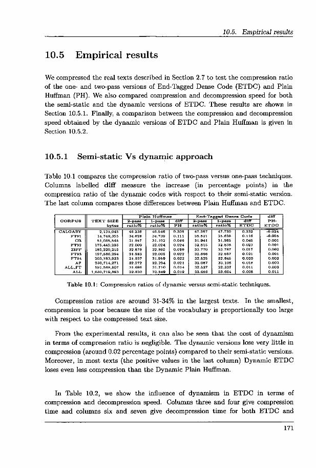
10.5. Empirical results

10.5 Empirical results

We compressed the real texts described in Section 2.7 to test the compression ratio

of the one- and two-pass versions of End-Tagged Dense Code (ETDC) and Plain

Huffman (PH). We also compared compression and decompression speed for both

the semi-static and the dynamic versions of ETDC. These results are shown in

Section 10.5.1. Finally, a comparison between the compression and decompression

speed obtained by the dynamic versions of ETDC and Plain Huffman is given in

Section 10.5.2.

10.5.1 Semi-static Vs dynamic approach

Table 10.1 compares the compression ratio of two-pass versus one-pass techniques.

Columns labelled diff ineasure the increase (in percentage points) in the

compression ratio of the dynamic codes with respect to their semi-static version.

The last column compares those differences between Plain Huffman and ETDC.

Plafn Huffman End-Tagged Denae Code dlff CORPU3 TEXT 3IZE 2-pesa 1-peae diff 2-paee 1-peea diff PH­

bytea ratío o ratlo o PH raLio o ratlo o ETDC ETDC

CALGARY 2,131,045­ 46.238 46.548 0.308 47.397 47.730 0.332 -0.024

FT91 14,749,355 34.828 34.739 0.111 35.521 35.638 0.118 -0.005

CR 51,085,545 31.057 31.102 0.046 31.941 31.985 0.045 0.001

FT92 175,449,235 32.000 32.024 0.024 32.815 32.838 0.023 0.001

ZIFF 185,220,21b 32.878 32.895 0.019 33.770 33.787 0.017 0.002

FT93 197,586,294 31.983 32.005 0.022 32.866 32.887 0.021 0.001

FT94 203,783,923 31.937 31.959 0.022 32.825 32.845 0.020 0.002

AP 250,714,271 32.272 32.294 0.021 33.087 33.306 0.018 0.003 ALL^T 591,568,807 31.698 31.710 0.014 32.527 32.537 0.011 0.003

ALL 1,080,719,883 32.830 32.849 0.019 33.858 33.664 0.008 0.011

Table 10.1: Compression ratios of dynamic versus semi-static techniques.

Compression ratios are around 31-34% in the largest texts. In the smallest,

compression is poor because the size of the vocabulary is proportionally too large

with respect to the compressed text size.

From the experimental results, it can also be seen that the cost of dynamism

in terms of compression ratio is negligible. The dynamic versions lose very little in

compression (around 0.02 percentage points) compared to their semi-static versions.

Moreover, in most texts (the positive values in the last column) Dynamic ETDC

loses even less compression than the Dynamic Plain Huffman.

In Table 10.2, we show the influence of dynamism in ETDC in terms of

compression and decompression speed. Columns three and four give compression

time and columns six and seven give decompression time for both ETDC and

171

10. Dynamic End-Tagged Dense Code

CORPUS TEXT 3IZE Comprosalon time (eec) Decompreseion tlme (aec) bytea 2-pasa 1-pase dlff %) 2-pesa 1-pane diH (%)

CALGARY 2,131,045 0.393 0.288 46.584 0.085 0.122 -30.137 FT91 14,749,355 2.482 1.788 38.770 0.570 0.847 -32.877 CR 51,065,545 7.988 8.050 32.029 1.928 3.033 -36.520

FT92 175,449,235 29.230 22.905 27.614 7.b81 11.603 -34.837 ZIFF 185,220,215 30.368 24.042 26.312 7.953 11.888 -33.104 FT93 197,586,294 32.783 25.505 28.535 8.694 12.675 -31.410 FT94 203,783,923 33.763 28.385 27.961 8.463 13.013 -34.971

A P 250,714,271 42.357 33.700 25.889 11.233 16.923 -33.622 ALL_FT 591,568,807 100.469 79.307 26.684 24.500 39.970 -38.704

A LL 1,080,719,883 191.763 157.277 21.927 46.352 81.893 -43.400

Table 10.2: Comparison in speed of ETDC and Dynamic ETDC.

Dynamic ETDC respectively (in seconds). The fifth column shows the increment of

compression time (in percentage) obtained by the semi-static code with respect to

the Dynamic ETDC. Finally, the last column in that table presents (in percentage)

the difference in decompression time between ETDC and the dynamic method,

showing that ETDC is faster.

In all the corpora used, the compression speed obtained by the Dynamic ETDC is much better (at least 21%) than that of the 2-pass approach. As it happened in

the previous chapter, differences between both approaches decrease as the size of the

source texts grows. However, the update algorithm is now so simple and fast that

those distances in time decrease with a very gentle slope. This becomes an important

advantage over the dynamic Huffman technique presentéd in the previous chapter.

In that case, as the size of the corpora increased, differences between Plain Huffman

and the dynamic Huffman-based technique decreased so fast that, in the two largest

corpora, the dynamic compressor was overcome. by the semi-static compressor. In

decompression speed, the semi-static ETDC clearly overcomes the results obtained

by the dynamic technique. Indeed, it reduces the time needed in decompression by

the Dynamic ETDC in more than 31%.

10.5.2 Dynamic ETDC Vs dynamic Huíiman

As it happened in the semi-static versions of the two codes, compression ratio

is around 30%-35% in both Dynamic ETDC and Dynamic PH. As expected, the

compression ratio obtained by Dynamic ETDC is around 1 percentage point worse

than that of Dynamic PH. Those compression ratios are shown in Table 10.1.

Compression and decompression time for both Dynamic ETDC and Dynamic

PH are compared in Table 10.3. Columns labelled diff show (in percentage) the

advantage in time of Dynamic ETDC with respect to Dynamic PH. In compression,

Dynamic ETDC is 20%-25% faster than Dynamic PH. If we consider decompression,

the simpler decompression mechanism of Dynamic ETDC makes it much faster than

172

10.6. Summary

CORPUS Compression time (sec) Decompression time (sec) Dyn PH DETDC diff (%) Dyn PH DETDC diff(%)

CALGARY 0.342 0.268 21.540 0.216 0.122 43.673 FT91 2.322 1.788 22.983 1.554 0.847 45.517 CR 7.506 6.050 19.398 5.376 3.033 43.576 FT92 29.214 22.905 21.596 21.726 11.603 46.592 ZIFF 30.218 24.042 20.439 21.592 11.888 44.941 FT93 32.506 25.505 21.538 23.398 12.675 45.829 FT94 33.310 26.385 20.790 23.802 13.013 45.327 AP 43.228 33.700 22.041 32.184 16.923 47.417 ALL^T 103.354 79.307 23.267 75.934 39.970 47.362 ALL 209.476 157.277 24.919 161.448 81.893 49.276

Table 10.3: Comparison of compression and decompression time.

Dynamic PH. As a result, an improvement of about 45% is achieved.

More empirical results, comparing the one-pass version of ETDC with other

well-known compression techniques, are shown in Section 11.5.

10.6 Summary

We adapted End-Tagged Dense Code (ETDC) to obtain a dynamic version of that

compressor. The resulting dynamic version is much simpler than the Huffman-based

one (proposed in Chapter 9). This is because maintaining an ordered list of words is much simpler than adapting a Huffman tree (and less operations are performed).

As a result, Dynamic ETDC is 20%-25% faster than Dynamic PH in compression,

compressing typically 7 Mbytes per second. In decompression, Dynamic ETDC is

about 45% faster than Dynamic PH.

Comparing Dynamic ETDC with the semi-static version, the compression ratio

is only 0.02% larger than with semi-static ETDC and 1% larger than with Huffman.

In compression speed, Dynamic ETDC is faster (more than 20%) than the semi­

static version of ETDC, but it is slower in decompression (around 30%-35%).

173

10. Dynamic End-Tagged Dense Code

Sender main algorithm ( )

(1) new-Symbol <-- 1;

(2) top[0] ^-- new-Symbol;

(3) maxFreq ^--- 1;

(4) while more words left

(5) read si from text;

(6) if (si ^ word) then

(7) 7^ ^ .fhaeh(Si)i (8) i ^- new-Symbol;

(9) send (encode(i));

(10) send si in plain form;

(11) else

(12) i ^ poslnVoc[p];

(13) send (encode(i));

(14) update();

Sender update ( )

(1) if i=new-Symbol then // new word (2) word[p] ^- si;

(3) freq[p] ^ 0; (4) poslnVoc[p] ^- new-Symbol ; (5) poslnHT[new-Symbolf ^- p,

(6) new-Symbod ^-- new-Symbol ^- 1;

(7) ĝ ^- fre4^]; (8) freq[p] f- freq(p] + 1;

(9) f ^ top[f]; (10) h ^- poslnHT[j]; (11) poslnHT[i] H poslnHT[j];

(12) poslnVoc[fi] ^-- 7;

(13) poslnVoc[h] ^- i;

(14) taP[.Í] ~ .9 + 1, (15) if maxFreq = f 1- 1 then

(16) top[f ^- 1] ^- 1;

(17) maxFreq ^- maxFreq -^ 1;

Figure 10.4: Dynamic ETDC sender pseudo-code.

174

10.6. Summary

Receiver main algorithm ( )

new-Symbol .- 1;

top[0] ^- new-Symbol;

maxFreq ^- 1;

while more codewords remain

i .- decode(c;);

if i =new-Symbol then

receive si in platin form;

output si;

else

output word[i];

update();

Receiver update ( ) (1) if i=new-Symbol then // new word

(2) word[i] ^- s;;

(3) freq[i] ^- 0;

(4) new-Symbol ^- new-Symbol + 1;

(5) f ^ fTe9[i]> (6) freq[i] t-- freq[i] ^- 1;

(7) j ^- taP[f]^

(8) fTeq[z] ~ fTe4^7]; (9) word[i] ^ word[j]; (10) top[f] ^- j + 1; (11) if maxFreq = f-{- 1 then

(12) top[f ^- 1] ^- 1;

(13) maxFreq ^ maxFreq -^ 1;

Figure 10.5: Dynamic E`I'DC receiver pseudo-code.

175

11

Dynamic (s, c)-Dense Code

This chapter presents the last contribution of this thesis: a new adaptive

compression technique called Dyna^rcic (s,c)-Dense Code (D-SCDC). D-SCDC is

the dynamic version of the (s, c)-Dense Code presented in Chapter 6, and at the

same time, it is a generalization of the Dynamic End-Tagged Dense Code, in which

not only the vocabulary is maintained sorted dynamically, but also the s and c

parameters can vary along the compression/decompression processes in order to

achieve a better compression.

The chapter is structured as follows: First the motivation of this new technique

is introduced. Section 11.2 describes Dynamic (s, c)-Dense Code. It shows the

similarities between the data structures of Dynamic End-Tagged Dense Code and

those of Dynamic (s, c)-Dense Code, as well as the differences that arise due to the

need to adapt the parameters s and c. Then, two approaches to maintain s and c

parameters optimal are presented: the simplest one is shown in Section 11.3 and

the most efficient approach is shown in Section 11.4. Section 11.5 shows empirical

results where the three new dynamic techniques developed are compared with their

corresponding two-pass versions, as well as with other well-known compressors such

as gzip, bzip2 and an adaptive arithmetic compressor [MNW98]. Lastly, some

conclusions are presented in Section 11.6.

177

I1. Dynamic (s, c)-Dense Code

11.1 Motivation

In the previous two chapters, two dynamic word-based byte-oriented techniques

were defined: the Dynamic word-based byte-oriented Huffman and the Dynamic

End-Tagged Dense Code.

The first one is based on Plain Huffman. It achieves better compression

than the Dynamic End-Tagged Dense Code (ETDC) (about 1 percentage point in

compression ratio). However, it is slower in compression and decompression (about

20%-25% and 45% respectively for large texts).

As shown in Chapter 6, (s, c)-Dense Code [BFNE03] is a compression technique

that generalizes End-Tagged Dense Code and obtains compression ratios very close

to those of the optimal Plain Huffman Code while using faster and easier-to-program algorithms.

In this chapter, we build an adaptive version of (s, c)-Dense Code. It consists of

an extension to Dynamic ETDC where the number of byte values that signal the

end of a codeword can be adapted to optimize compression, instead of being fixed

at 128 as in Dynamic ETDC.

11.2 Dynamic (s, c)-Dense Codes

Based on Dynamic ETDC, Dynamic ( s, c)-DC also uses the scheme presented in Figure 8.1. The CodeBook is essentially the vocabulary sorted by frequency, and the on-the-fly encode and decode procedures, explained in Section 6.4, are used.

The main difference with respect to Dynamic ETDC is that, at each step of

the compression/decompression processes, it is mandatory not only to maintain

the vocabulary sorted, but also to check whether the current value of s(and

consequently the c value) remains optimal or if it should change.

The úpdate() algorithm to maintain the sorted list of words is the same used in

the case of Dynamic End-Tagged Dense Code (see Figures 10.4 and 10.5). However,

the test for a possible change of the s value is new and it has to be performed after

calling the update process.

Both encoder and decoder start with s= 256. This s value is optimal for the

first 255 words of the vocabulary, because it permits encoding all of them with just

one byte. When the 256th word arrives, s has to be decreased by 1 since a two­

178

11.3. Maintaining optimal the s and c values: Counting Bytes approach

byte codeword is needed. F^om this point on, the optimal s and c values will be

heuristically estimated.

Two different approaches can be used to keep the optimal values of s and c.

The first one, more intuitive, is presented in Section 11.3. It is called counting bytes approach. The second alternative, called ranges approach is shown in Section 11.4.

It gives a more efficient way to maintain optimal the s and c parameters.

11.3­ Maintaining optimal the s and c values:

Countirag Bytes approach

The simplest approach to estimate the optimal s and c values as the

compression/decompression progresses is based on comparing the size of the

compressed text depending on the s and c values used to encode it.

Notice that this approach does not pretend to obtain the absolute optimal s

value, but only to follow an efficient heuristical and easy-to-implement approach

that still produces a good compression. The general idea is to compare the number

of bytes that would be added to the compressed text if the current word wi would have been encoded using s- 1, s, and s+ 1. Of course, the value of s, such that it minimizes the size of the compressed text, must be obtained. If the number

of bytes needed to encode the word wi becomes smaller by using either s- 1 or

s+ 1 instead of s, then we update the value of s. Therefore, in each step of the compression/decompression process, the value of s changes at most by one.

Three variables are needed: prev, so and next. The prev variable stores the size of

the compressed text assuming that the value s-1 was used in the encoding/decoding

process. In the same way, so and next accumulate the size of the compressed text,

assuming that it was encoded using the current s and the s+ 1 values respectively.

At the beginning, the three variables are initialized to zero. Each time a word wi

is processed, prev, so and next are increased.

Let countBytes(s_value, i) be the function that computes the number of bytes

needed to encode the ith word of the vocabulary with s= s_value and c=

256 - s_value. Then, intuitively, the three variables are increased as follows:

• prev f- prev -}- countBytes(s - 1, i)

• so <- so + countBytes(s, i)

• next <- next + countBytes(s -^ 1, i)

179

I1. Dynamic (s, c)-Dense Code

A change of the s value takes place if prev < so or if next < so. If prev < so

then s- 1 becomes the new value of s(s ^ s- 1). On the other hand, if next < so

then s is increased (s <- s+l). Notice that it is impossible that both prev and next

become smaller than so at the same time, as it is proved in the next two lemmas.

Lemma 11.1 (s - 1)(c + 1)n > sc^ ^ sc^ >(s + 1)(c - 1)^ bn > 1

Proof We prove it by induction in n. For n= 1 we have:

(s - 1)(c -^ 1) > sc ^ sc > (s -}- 1)(c - 1)

from this we get that s> c-^ 1^ s> c- 1, which clearly holds. Now we assume that:

(s - 1)(c + 1)n > scn ^ scn > (s + 1)(c - 1)n

and we prove it for n+ 1

(s - 1)(c + 1)^(c + 1) > sc^`c ^ scnc > (s + 1)(c - 1)^(c - 1)

that is

c(s - 1)(c -^ 1)^` + (s - 1)(c -^ 1)^ > sc^`c ^ sc^c > c(s + 1)(c - 1)^` - (s -^ 1)(c - 1)n

which clearly holds by applying the Induction Hypothesis.

Lemma 11.2 W,^-1 > Wñ ^ Wñ > Wñ+l bn > 2

Proof We prove it by induction in n. For n= 2 we have:

(s-1)+(s-1)(c^-1)>s+sc^s+sc>(s-}-1)-^(s-^1)(c-1)

from this we get that s> c+ 2^ s> c, which clearly holds. Now we assume that:

W^-1 > W,^ ^ W,^ > Wñ+l

and we prove it for n+ 1

Wñ-1+(s-1)(c+l)n>Wñ+sc^^W,^+scn>Wñ+l+(s+l)(c-1)^

which holds by the Induction Hypothesis and Lemma 11.1. q

180

11.3. Maintaining optimal the s and c values: Counting Bytes approach

Therefore, it is impossible that prev < so > next, and hence we can easily

decide in which direction s must be modified. Each time the parameter s changes,

the values prev, so, and next are initialized again, and then the process continues.

This initialization depends on the change of s that takes place. In order to keep the

history of the process we do not initialize the three values to zero, but we use the

previous values. Of course, one of the three values (either prev or next, depending

on the direction of the change of s) is unknown and we set it to the same value of

so. Summarizing:

- If s is increased then prev 4- so and so f- next (next does not change).

10 6 5 6 5 5

prev next prev s0 next

- If s is decreased then next ^ so and so ^ prev (prev does not change).

20 20 20 21

prev a0 next prev sp next

There are other alternatives for this basic algorithm. For example, it would be

possible to use an e value as a threshold for the change of s. That is, the value of

s would change only if prev + e< so or next + e< so. In this way, less changes

would take place and the algorithm would be a little faster, but the compression

ratio would not be so good.

Another possible choice would be to initialize the three variables prev, so, and next to zero each time the value of s changes. This choice would make

the algorithm free from the previous history. This approach can be interesting in

natural language documents where the vocabulary, and consequently its frequency

distribution, changes frequently along the text. On the other hand, assuming

that the document is rather homogeneous, keeping the previous knowledge seems

interesting. We do that by initializing so with the value of either prev or next and

then keeping the former value of so in either next or prev respectively, depending

on whether we are increasing or decreasing the value of s.

11.3.1 Pseudo-code for the Counting Bytes approach

Two main procedures are used in this counting bytes approach to check whether the

s and c values should change after having processed a new source symbol. The first

one is the already described countBytes() algorithm.

181

11. Dynamic (s, c)-Dense Code

countBytes Algorithm (si, iPos) //Caleu,lates the length of the codeword assigned to a word ranked iPos

//Using s;, as value of s

(1) k ^- 1;

(2) last ^ sí;

(3) Pot ^ si^ (4) ci ^- 256 - s;;

(5) while last < iPos

(6) Pot ^- pot X c;,;

(7) last f- last + pot;

(8) k ^- k + 1;

(9) return k;

TakeIntoAccount Algorithm (s, c, i) //It changes, if needed, the s and c valv,es

(1) prev <- countBytes (s - 1, i);

(2) sp ^- countBytes (s, i);

(3) if prev < sp then

(4) s^ s- 1; //s is decreased

(5) c ^- c -F 1;

(6) next ^- sp;

(7) so ^-- prev;

(8) else

(9) next ^ countBytes (s + 1, i);

(10) if next < sp then

(11) s.- s-{- 1; //s is increased

(12) c E- c - 1;

(13) prev ^- sp;

(14) sp f- next;

Figure 11.1: Algorithm to change parameters s and c.

The second procedure, called TakelntoAccount(), is invoked after each call to

the update() procedure. It first uses countBytes() to increase prev, so and next.

Then, it checks either if prev < so or if next < so, and changes the s value used in

compression or decompression if necessary.

The pseudo-code for both algorithms is shown in Figure 11.1. Notice that

the countBytes() algorithm is called at least twice in each execution of the

TakelntoAccount() algorithm. The cost of countBytes() depends on the ma^imum

codeword length. It is O(log^(n)) if c> 1, and O(Zĝ5) if c= 1. However, in practice

the value c= 1 is only used when the size of the vocabulary is between 256 and

510 (the c value increases rapidly while the first thousands of words are processed).

Since the maximum codeword length for s= 255, c= 1 and n< 510 is 2, it can be

182

11.4. Maintaining optimal the s and c values: R,anges approach

considered that the cost of countBytes() is O(log^(n)).

Since TakelntoAccount() is called N times (being N the number of source words), the cost of the whole process is O(N log^(n)). Actually, this is proportional to the

number of bytes of the compressed stream.

As a result, maintaining optimal the s and c values can be done quite eíficiently.

It can also be seen that the countBytes() algorithm takes an important part of the

time spent by TakelntoAccount(). In the following section, a more efficient way to

maintain optimal the s and c values is presented. It consists of a more sophisticated

alternative that avoids using countBytes(), by using some knowledge about how the values W^ behave.

11.4­ Maintaining optimal the s and c values:

Ranges approach

This approach is based on an interesting property that arises from the definition of Wk in Section 6.2. The key idea is to use the ranges defined by thé different W^ , for 128 <_ s<_ 256 and 1<_ k<_ 4, in the rank of the words of the vocabulary. These ranges .indicate the number of bytes k that are needed to encode a word wi, (i is the rank in the vocabulary for wi) using s - 1, s, and s+ 1 stoppers. That is,

these ranges allow us to know, for any word wi and using a specific s value, whether

encoding that word with s- 1 or s+ 1 stoppers would produce codewords with

equal, more, or less bytes. The main difference with the previous approach is that

now it is not necessary to use the time-consuming CountBytes(s, i) procedure to know the number of bytes of the codeword associated to wi if s- 1 or s+ 1 were used instead of s.

^ "^ ^ . .., . ^. p" w3 w3 '

Q w; ' w,' w;" w2'w^ w^'­ v^P."w^° w:'

Figure 11.2: Ranges defined by Wk-1, Wk and Wk+l.

We do not consider values of s smaller than 128 because, as shown in

Section 6.3.1, those values never improve compression ratios in natural language

applications were the number of words in the vocabulary is never large enough to

183

11. Dynamic (s, c)-Dense Code

take advantage of the large amount of words that can be encoded with 4, 5, 6, or

more bytes. More specifically, if n< 2,113, 664 then values of s such that s< 128,

are never convenient, and using codewords with up to 4 bytes (k <= 4) is always

enough.

Figure 11.2 shows those ranges. The points Wk-1, Wk and Wk+l, for 1<_ k<_ 4

and s> c, are represented. Notice that words in [0, s-1), [0, s) or [0, s+ 1) can be

encoded with a unique byte, if the values s- 1, s, or s+ 1 respectively are used. In

the same way, words in ranges [s - 1, W2 -1), [s, W2 ), or [s + 1, W2+1) are encoded

with two-byte codewords when the values s- 1, s, or s+ 1 respectively are used,

and so on.

Notice that if, for example W2 < i < WZ-1, then the word wi would be encoded

with a 3-byte codeword using s but with a 2-byte using s - 1. In the same way, if WZ-1 < i < W3+1, then a 3-byte codeword will be assigned to the word wi when

any of the three s, s- 1, or s+ 1 values is used.

In Figure 11.2, we carefully place the different values W^, W^-1, and W^+1

to keep the real relationships among them. Notice that the order changes from Wi-1 < Wi < Wi+l, to the opposite W^+1 < Wk < W^-1 bk > 2. Next we

prove tĝat those relationships shown in the figure actually hold when s> c.

Lemma 11.3 If s> c, it holds that:

a^ Wi +i > Wi > Wi -1

b) Wk+l < Wk < W^-1, b'k > 2

Proof The case a), (k = 1) is trivial from the definition of W^, since Wi -1 = s-l,

Wi = s and Wi +1 = s+ 1.

_ In order to prove part b) we only need to prove that W^ < Wk-1, ds > c. We

proceed by induction in k. For k= 2 we prove that: ,

W9 < Ws-1k k

that is,

s + sc < (s - 1) + (s - 1)(c + 1)

this is reduced to s> c+ 2, which is always true when s> c be•ause s+ c= 256.

That is, the minimum value of s such that s> c is s= 129. In such case, c= 127

accomplishes that s> c+ 2.1

1 This remains true for any s-f- c= 26, since we always want to use a fixed number of 6 bits per

output symbol. The property only depends on 26 being even.

184

11.4. Maintaining optimal the s and c values: R,anges approach

We assume by Induction Hypothesis that W^ < Wk-1 and we prove the property

for the case k+ 1

W^ + sck < W^-1 +(s - 1)(c+ 1)^

which holds from the Induction Hypothesis and Lemma 11.4. q

Lemma 11.4 sc^ <(s - 1)(c + 1)^, `ds > c.

Proof We proceeded by induction in k. For k= 1 we have:

sc < (s - 1)(c + 1)

that is,

c+l<s

which holds since s> c and both are integers. Assuming that the lemma holds for

k, (that is, assuming sck <(s - 1)(c+ 1)^) we prove it for the case k+ 1:

sc^`c < (s - 1)(c + 1)^(c + 1)

that is,

sckc < c((s - 1)(c + 1)^)-}-(s - 1)(c + 1)^

This expression clearly holds from the Induction Hypothesis and the fact that

0 < (s - 1)(c+ 1)^`. q

To end this introductory section we illustrate in Figure 11.3 how the s value

evolves in practice, as the compression process progresses.

In Figure 11.3, it can be seen that the dynamic encoder adapts the s value rapidly

in order to reduce the codeword length. Therefore, the s value falls from 256 to a

value close to 129 when the first 16, 512 words are processed. When n> 16, 512,

three-byte codewords are needed, therefore the s value is increased. Fluctuations

of s beyond that point depend on the order in which words are input (and also on

their frequencies).

11.4.1 General description of the R.anges approach

Lemma 11.3 permits maintaining the optimal s and c values in a more efficient

fashion than that presented in Section 11.3.

185

11. Dynamic (s, c)-Dense Code

250

150

0.5­ 1 1.5 2 2.5 3 n x 10°

250

Ap Newswire corpus m ^ 200 >

I - s=129 150

^

0­ 0.5 1 1.5 2 2.5 n x 105

250 ALL corpus

m ^ 200 > y

150

0 1 2 3 4 5 6 7 8

n x 105

Figure 11.3: Evolution of s as the vocabulary grows.

Assume that the word ranked i is being encoded (or decoded) using the second

on-the-fly algorithm showed in Section 6.4. Notice that this algorithm returns

not only the actual codeword but also its length. Let k be the length of the

codeword, then the specific interval in the rank of words that needs to be considered

1S [Wk,Wk+l)•

Three subintervals need to be considered inside of this interval. Table 11.1 represents (columns 1 and 4) the limits of each interval [Wk , Wk+l ) for 1< k<_ 4.

Inside of each interval, the two internal limits that mark the three internal subintervals (columns 2 and 3 in the table) are shown. Notice that, in different format, the same subintervals are represented in Figure 11.2.

The left hand side subinterval (that does not exist when k= 1) always represents

186

11.4. Maintaining optimal the s and c values: R.anges approach

left hand central right hand siae sidé

^/^s0 0 1I^/^s-, k=1

W,S W, S+' W? ' W2 k=2

WZ W2s-1 W3s+1 W3 k=3

W3 W3 -1 W4s+1 ^/4 k=4

Table 11.1: Subintervals inside the interval [W^, Wk+l), for 1< k< 4.

word ranks that are encoded with a one-byte-shorter codeword if either s+ 1(when

k= 2) or s- 1(when k> 2) are used instead of s. The central subinterval, the

one defined by the two central values of each row in the table, represents word

ranks that are encoded with codewords of the same length, no matter if s, s- 1, or

s^- 1 is used. Finally, the right hand side subinterval represents word ranks that

are encoded with a one-byte-longer codeword if s- 1(when k= 1) or s+ 1(when

k> 1) are used instead of s.

The algorithm uses a pre-computed three-dimensional matrix keeping the values for the subinterval limits for 128 < s< 256 and 1 < k< 4. In this way, all

the necessary ranges are predefined. The algorithm easily and efficiently finds out whether s-1 or s+ 1 would compute one-byte-longer or one-byte-shorter codeword

than s, for the current word w^, without using the time-consuming countBytes(s,i) algorithm.

In the Counting Bytes approach we accumulated in prev, so and next the size of

the compressed text by adding for each word the number of bytes of the codewords

that would be computed if s-1, s, and s+ 1 were used. In the Ranges approach, for

each word wt, we only add +1 as a penalty if i is in the right hand side subinterval,

or -1 as a bonus if i is in the left hand side subinterval. This addition of +1 or -1

is done in prev or in ne^t depending on the value of k.

Clearly if i is in a central subinterval no action has to be performed. If i is in

a right hand side subinterval, a penalty is added to prev (when k= 1) or to next

(when k> 1), therefore s is still optimal and it is not necessary to check if there is

a better value for s. But if i is in a left hand side subinterval then a bonus -1 is

added to next (when k= 2) or to prev (when k> 2) and in this case, it is necessary

to check if s is still optimal by comparing so with prev or next (depending on which

187

11. Dynamic (s, c)-Dense Code

^t` 9 uC J9^ bonuses and ^g ^^^. penalties -^ Q^^y ^g^ Q,^^ ^^^

aáion over s-^ _ = C1 = C2 = C2 = _ • C2 = ^^, „ ^ v

k • 1 ® 2 ® 3 ® 4 ® ^

s-1 f Í

s

s+1 ^ Wo-^ W^s W„i W„^ WZa W2 i i 0 1M,^' W3' Wa' YYq{^W68 Wy ^

Conditions to check: C1= T[2]<0 and C2 = T[o]<0

Figure 11.4: Intervals and subintervals, penalties and bonus.

one of them has received the bonus).

Figure 11.4 represents in the first (top-most) row the places in the rank of words

where penalties and bonuses are added either to prev or to next. The second row

shows the action that is performed on the value of s. The equal sign represents that

s is still optimal for sure and, therefore, it is not necessary to check it. In the same

row, the places where s must be checked and the test that need to be performed

are shown. The third row represents the different intervals that, as it was already

explained, correspond to the k values. The different number of bytes needed to

encode a word w;, using s, s- 1, and s+ 1 are also shown in Figure 11.4. Notice

that the number of horizontal lines correspond to the number of bytes needed to

encode each codeword with the corresponding value of s. Next section presents all

the implementation details.

11.4. 2 Implementation

Three elements have to be taken into account: i) The definition of the ranges that

correspond to the current s value, ii) the penalties or bonuses that have to be

applied in some cases to the use of s-1 or s^-1, and iii) the action that takes place

on the s value (increasing or decreasing it).

Data Structures

Oñe vector T, and two matrices I and V are needed. They are defined as follows:

- Vector T. A 3-element vector that corresponds to the prev, so and next

variables (in vector form for implementation reasons). Each position T[i], 0<

188

11.4. Ma.intaining optimal the s and c values: Ranges approach

i< 2, stores a signed number that accumulates bonuses and penalties for the

values s- 1, s, and s+ 1 respectively. Bonuses decrease by 1 either the value

T[0] or T[2] . Penalties increase those values by 1. If T[0] becomes negative, it means that s- 1 is preferable to the current value s, since it received

more bonuses than penalties. On the opposite, if T[2] < 0 then the action

that follows is to change s to s+ 1. As an analogy with the first approach

presented in Section 11.3, T[0] and T[2] are prev and ne^t values respectively.

However, in this case, T[0] and T[2] do not accumulate the estimated size of

the concpressed text, but the extra number of bytes needed when either s- 1

or s+ 1 are used instead of s. Notice that T[1] = 0 always and therefore it is

not really necessary (we keep it here for clarity).

T = f^ 0 fy

Matrix I is a pre-computed three dimensional matrix with size 128 x 4 x 2.

This matrix represents, for each value of s(128 <_ s<_ 256) and for each value

of k(1 < k< 4) the two limits of the subintervals inside the interval defined by

s and k. R,emember that this interval is [W^, W^+1). The subinterval limits

need to be checked each time a word wi is processed to know whether the

codeword length would be a byte longer or shorter if s- 1 or s-4- 1 were used

instead of s to encode wi. When a word wi is processed, we first encode it using

the second on-the-fly encoding algorithm shown in Section 6.4. This algorithm

returns not only the codeword but also its length. Then it is necessary to

check whether i is in the left, central, or right subinterval to determine the

action that should be taken over T[0] or T[2] (bonus or penalty). That is, if

i< I[s, k, 0] then it is in the left hand side subinterval and a bonus need to

by added. If i> I[s, k, l] then a penalty will be added. Otherwise i is in the

central subinterval, and neither a penalty nor a bonus are necessary, since the

codeword length would be the same with s- 1, s, and s+ 1.

Next table shows the section of the matrix I for an specific s value. Certainly, matrix I has 128 sections as the one showed, one for each possible value of s.

bonuses < > penalties

0 Wi-

Is = Wi W2

W2 W3

W3 W4 0 i

- Matrix V is a 4 x 2 predefined table. Each cell can contain either 0 or 2, and

this value is used to index the vector T. That is, we use this table to indicate

189

I1. Dynamic (s, c)-Dense Code

whether T[0] or T[2] is the one to receive the bonus or the penalty. The first

row represents penalties, so it is used when a penalty has to be added to T[0]

or to T[2]. In the same way, the second row is used for the bonuses. After

using matrix I to know if a penalty or a bonus has to be added, we use this

matrix to know whether it must be added either to T[0] or to T[2]. The matrix

V has the following values:

k=1 k=2 k=3 k=4 1 1 1 1V =

2 0 0 bonuses

0 2 2 2 penalties

For example if k = 2 and if using the I matrix, the algorithm determines

that a bonus has to be added, then the algorithm performs T[V [0, 2]] <-

T[V [0, 2]] - 1, and after that, a comparison between T[V [0, 2]] and T[1] is

needed to check if s is still optimal. This comparison is performed by simply

checking if T[V [0, 2]] < 0.

If, for example, k= 4 and a penalty has to be added, the algorithm performs

T[V [1, 4]] ^ T[V [l, 4]] ^-1. Now it is not necessary to check if T[V [l, 4]] < 0.

Since the value T[V [l, 4]] was increased, it cannot have become a negative

value. Therefore, we are sure that s is still optimal.

Obviously, if the algorithm determines, using the matrix I, that it is not

necessary to add neither a bonus nor a penalty, no further action is performed,

and the table V is not used in that step.

Pseudo-code for the Ranges approach

The pseudo-code for the algorithm that handles the update of the s and c values

following this approach is presented in Figure 11.5. Such algorithm is called

TakelntoAccountRang es ().

Assuming that the ith word of the vocabulary is being encoded/decoded, the

on-the-fly encoding algorithm encodes the word wi, returning the codeword and

its length k. The decoding algorithm returns the position in the vocabulary i,

and the number of bytes (k) of the codeword decoded. Then, the algorithm

TakelntoAccountRanges() knows the values k, i, and s. Using matrix I, it looks for

the subinterval (range) where i appears, in order to know if a bonus or a penalty

has to be added. In such case, using the matrix V the algorithm finds if the bonus

or the penalty must be added to either T[0] or T[2]. Finally, if a bonus was added

to either T[0] or T[2], one more check has to be done: if T[0] was the decreased

190

11.5. Empirical results

term, then it is checked if T[0] < 0; in this case, s is set to s-1. On the other hand,

if T[2] was the decreased term, then it is checked if it became a negative value. In

such case, the s value is increased. Each time s changes, the value of T[0] and T[2]

is initialized following the same strategy described in the Count Bytes approach.

TakeIntoAccountRanges Algorithm (s, k, i)

//It changes, if needed, the s and c values used in both campression //and decompression processes. It checks the i range and the addition //of either bonuses or penalties.

(1) if i > I[s, k, l] then

(2) T[V[l,k]] ^- T[V[l,k]]-^-1;

(3) else (4) if i < I [s, k, 0] then

(5)­ T[V[0, k]] ^- T[V[0, k]] - 1; //Checking if s is still optimal

(6)­ if T[V[0, k]] < 0 then (7) s.- s-}- V[0, k] - 1 //change o f s

($) c F- 256 - s;

(9) T[V[O,k]] ^- 0; (10) T[2 - V [O, k]] ^- 1;

Figure 11.5: Algorithm to change parameters s and c.

Observe, in lines 9 and 10, how T[0] and T[2] are initialized after any change

of s. Remember that T[1] never needs to be changed because it is always 0. The

idea is to keep only one unit of difference between the new T[1] and the former one,

but instead of initializing T[1] to -1 and T[2 - V[0, k]] 2 to 0, we prefer to initialize

T[2 - V[0, k]] to 1 and to maintain T[1] = 0. In the same way, following the same

strategy described in the Count Bytes approach, we initialize T[V [0, k]] with the

same value of T[1], that is, with 0. Remember that in the Count Bytes approach,

we initialize prev or next (depending on the direction of the change) with the same

value of so.

11.5 Empirical results

We first compressed the texts in our experimental framework to compare the

three dynamic techniques among them in compression ratio and in compression

and decompression speed. Those results are shown in Section 11.5.1. Next, the

compression ratio and time performance of the one- and two-pass versions of End-

Tagged Dense Code (ETDC), (s, c)-Dense Code (SCDC), and Plain Hufiman (PH)

2Notice that T[2 - V[0, k]] represents T[0] or T[2] depending on the value of V[0, k].

191

11. Dynamic (s, c)-Dense Code

are shown in Section 11.5.2. Finally, we also compressed all the corpora with other

three well-known compression techniques: gzip, bzip2, and a word-based arithmetic

compressor [CMN+99]. R.esults showing compression and decompression speed, and

also compression ratio for all these techniques are presented in Section 11.5.3.

11.5.1­ Dynamic approaches: compression ratio and time

performance

Table 11.2 compares the time performance and the compression ratio obtained by

our three dynamic compressors. For each technique, the first sub-table shows the

compression ratio, the compression time, and the decompression time needed to

decompress each corpus.

The second sub-table included in Table 11.2 compares both Dynamic ETDC and

Dynamic SCDC with respect to Dynamic Plain Huffman. Columns two and three

measure differences in compression ratio. The fourth and the fifth columns show

the reduction of compression time (in percentage) of Dynamic ETDC and Dynamic

SCDC, with respect to Dynamic PH. Finally, the last two columns in the second

sub-table show the reduction in decompression time obtained by Dynamic ETDC

and Dynamic SCDC.

As it can be seen, Dynamic ETDC loses less than 1 point in compression

ratio (about 3% increase of size) with respect to Dynamic Plain Huffman, in the

larger texts. In exchange, it is 20%-25% faster in compression and reduces its

decompression time by about 45%. Moreover, Dynamic ETDC is considerably

simpler to implement.

In the case of Dynamic SCDC the loss of compression ratio with respect to

Dynamic Plain Huffman is around 0.25 percentage points. The compression speed

is improved by about 17% and decompression time is reduced over 39%.

It is noticeable that, differences in compression and decompression speed

between Dynamic PH and our dynamic "dense" codes increase more and more

as the size of the text collection grows. Those differences arise because the update

algorithm is much simpler (and faster) in the "dense" techniques.

The results also show that Dynamic ETDC is a bit faster than the Dynamic

SCDC. This is due to two main issues: i) the encoding process uses faster bitwise

operations (in the case of Dynamic ETDC), and ii^ Dynamic SCDC has to use the

TakeIntoAccount algorithm to maintain optimal the parameters s and c, whereas

those values are fixed to 128 in Dynamic ETDC.

192

11.5. Empirical res ults

Compr. ratio Compr. time (sec) Decompr. tlme (eac) CORPUS Dyn Dyn Dyn Dyn Dyn Dyn Dyn Dyn Dyn

PH SCDC ETDC PH SCDC ETDC PH SCDC ETDC

CALGARY 46.546 46.809 47.730 0.342 0.292 0.268 0.216 0.135 0.122 FT91 34.739 34.962 35.638 2.322 1.940 1.788 1.554 0.942 0.847 CR 31.102 31.332 31.985 7.506 6.532 6.050 5.378 3.272 3.033

FT92 32.024 32.237 32.838 29.214 24.440 22.905 21.726 12.287 11.603 ZIFF 32.695 33.078 33.787 30.218 ^ 26.057 24.042 21.592 12.815 11.888 FT93 32.005 32.202 32.887 32.506 27.682 25.505 23.398 13.608 12.675 FT94 31.959 32.154 32.845 33.310 28.817 26.385 23.802 13.837 13.013

A P 32.294 32.557 33.108 43.228 38.113 33.700 32.184 17.623 16.923 ALL^T 31.730 31.849 32.537 303.354 85.197 79.307 75.934 42.055 39.970

A LL 32.849 33.029 33.664 209.478 167.403 157.277 161.448 87.486 81.893

CORPUS DIft. Ratlo Decr. Compr. time (%) Decr. Decomp. Time (%) Dyn SCDC Dyn ETDC Dyn SCDC Dyn ETDC Dyn SCDC Dyn ETDC

CALGARY 0.263 1.184 14.717 21.540 37.500 43.673 FT91 0.223 0.899 16.451 22.983 39.404 45.517 CR 0.229 0.683 12.981 19.398 39.143 43.578

FT92 0.214 0.814 16.341 21.596 43.447 46.592 ZIFF 0.183 0.691 13.771 20.439 40.649 44.941 FT93 0.197 0.882 14.841 21.538 41.840 45.829

^^^ FT94 0.195 0.887 13.489 20.790 41.888 45.327 AP 0.263 0.812 16.458 22.041 45.242 47.417

A LL^T 0.139 0.827 17.566 23.267 44.616 47.362 ALL 0.180 0.815 20.085 24.919 45.810 49.276

Table 11.2: Comparison among our three dynamic techniques.

To sum up, the compression speed obtained by Dynamic ETDC, Dynamic

SCDC, and Dynamic PH is, respectively, about 5, 6.5 and 7 Mbytes per second.

In decompression, the differences obtained are more spectacular. In general, the

decompression speed obtained by Dynamic ETDC, Dynamic SCDC, and Dynamic

PH is, respectively, over 15, 14, and 8 Mbytes per second.

11.5.2 Semi-static Vs dynamic approach

Comparison in compression ratio

Table 11.3 compares the compression ratios of the two-pass versus the o^ee­

pass versions of ETDC, SCDC and PH. Columns labelled diffpH, diffETDC and

diffscDC measure the increase, in percentage points, in the compression ratio of

the dynamic codes compared with their semi-static version. The last two columns

compare the differences in the increments of compression ratio.

As it can be seen, a very small loss of compression occurs, in the three

techniques, when they are implemented as dynamic codes. To understand this

increase in size of dynamic versus semi-static codes, two issues have to be considered: (i) each new word s= parsed during dynamic compression is represented in the

compressed text (or sent to the receiver) as a pair (Cnew-symvol^ st), while in two­

pass compression only the word st needs to be stored/transmitted in the vocabulary;

(ii) the codewords used to transmit words can be shorter or larger than the optimal

193

0.011

, I1. Dynamic (s, c)-Dense Code

Plain Huffman End-Tagged Denae Code CORPU9 TEXT 9IZE 2-paea dynamic Increase 2-paea dynamic Increaee

bytea ratlo ratlo dlft ratlo ratio dift

CALGAAY 2,131,045 46.238 48.548 0.308 47.397 47.730 0.332 FT91 14,749,355 34.628 34.739 0.111 3b.521 35.638 0.118 CR 51,085,545 31.057 31.302 0.048 31.941 31.985 0.045 FT92 175,449,235 32.000 32.024 0.024 32.815 32.836 0.023 ZIFF 185,220,215 32.876 32.895 0.019 33.770 33.787 0.017 FT93 197,586,294 31.983 32.005 0.022 32.886 32.887 0.021 FT94 203,783,923 31.937 31.959 0.022 32.825 32.845 0.020 A P 250,714,271 32.272 32.294 0.021 33.087 33.106 0.018 A LL_FT 591,586,807 31.698 31.710 0.014 32.527 32.537 A LL 1,080,719,883 32.630 32.849 0.019 33.856 33.664 0.008

(s, c)-Danae Code CORPUS 2-pnea dynamic Inc dlffETDC diffSCDC

ratio ratlo dif: r - dift - diff

CALGARY 48.611 46.809 0.198 0.024 -0.110 FT91 ^ 34.875 34.962 0.086 0.005 -0.025 CR 31.291 31.332 0.041 -0.001 -0.005 FT92 32.218 32.237 0.020 -0.001 -0.004 ZIFF 33.082 33.078 0.018 -0.002 -0.003 FT93 32.178 32.202 0.024 -0.001 0.002 FT94 32.132 32.154 ^ 0.021 -0.002 -0.001 AP 32.542 32.557 0.015 -0.003 -0.008 ALL_FT 31.839 31.849 0.010 -0.003 -0.004 ALL 33.018 33.029 0.011 -0.011 -0.008

Table 11.3: Compression ratio of dynamic versus semi-static techniques.

codeword that is assigned in the semi-static version. Even some gain in compression

can be obtained by occasional shorter codewords assigned to low frequency words

(especially when they appear at the beginning of the text), however, in general some

loss in compression appears because the optimal codeword is not always used over

the whole text.

The compression ratios obtained by the three techniques are around 31%-33% for

large texts. For the smallest one (Calgary collection), compression is poorer because

the size of the vocabulary is proportionally large with respect to the compressed

text size (as expected from Heaps' law, that is described in Section 2.4.1).

The dynamic versions of the compressors lose very little compression (not more

than 0.05 percentage points in general) compared to their semi-static versions in

the three techniques. This shows that the price paid by dynamism in terms of

compression ratio is practically negligible. Note also that, in most cases, dynamic

ETDC loses even less compression than dynamic Plain Huffman. In the same way,

adding dynamism to (s,c)-Dense Code only produces more loss of compression ratio

than dynamic PH in the FT93 corpus.

Comparison in compression and decompression speed

In this section, we compase the compression and decompression time (measured in

seconds) obtained by our new dyna,mic techniques and their corresponding semi­

194

11.5. Empirical results

CORPU9 Semi-etattc approach ( eec) Dynamle approach (aec) Loae In epeed (%) PH SCDC ETDC PH SCDC ETDC PH SCDC ETDC

CALGARY 0.415 0.405 0.393 0.342 0.292 0.288 21.345 38.857 48.584

FT91 2.500 2.493 2.482 2.322 1.940 1.788 7.666 28.522 38.770

CA 7.990 7.958 7.988 7.506 8.532 6.050 8.448 21.810 32.029

FT92 29.243 29.339 29.230 29.214 24.440 22.905 0.098 20.044 27.814

ZIFF 30.354 30.620 30.368 30.218 28.057 24.042 0.451 17.513 26.312

FT93 32.915 33.031 32.783 32.508 27.s8a 25.505 1.258 19.326 28.535

FT94 33.874 33.717 33.763 33.330 28.817 28.385 1.892 17.004 27.981

AP 42.641 42.676 42.357 43.228 38.113 33.700 -1.357 18.172 25.689

A LL_FT 99.889 100.570 100.489 103.354 85.197 79.307 -3.353 18.045 26.664

A LL 191.396 191.809 191.763 209.476 187.403 157.277 -8.631 14.579 21.927

a) Compreaeion time.

CORPUS Seml-etatic approach ( sec) Dynamic approach ( eec) Galn Sn epeed (%) PH SCDC ETDC PH SCDC ETDC PH SCDC ETDC

CALGARY 0.088 0.097 0.085 0.216 0.135 0.122 59.105 28.395 30.137

FT91 0.577 0.803 0.570 1.554 0.942 0.847 62.891 35.929 32.877

CR 1.903 1.971 1.928 5.376 3.272 3.033 64.611 39.752 36.520

FT92 7.773 7.592 7.561 21.728 12.287 11.603 64.225 38.209 34.837

ZIFF 8.263 7.988 7.953 21.592 12.815 11.888 61.730 37.689 33.104

FT93 8.406 8.437 8.694 23.398 13.808 12.675 84.075 38.000 31.410

FT94 8.636 8.690 8.463 23.802 13.837 13.013 83.718 37.196 34.971

AP 11.040 11.404 11.233 32.184 17.623 18.923 65.697 35.292 33.622

A LL_FT 24.798 25.118 24.500 75.934 42.055 3fl.970 87.343 40.275 38.704

A LL 45.699 46.698 46.352 101.448 87.488 81.893 71.695 48.824 43.400

a) Decompreseion time.

Table 11.4: Time performance in semi-static and dynamic approaches.

static codes.

Table 11.4.a) gives a comparison in compression time. For each corpus, columns

two, three, and four show the compression time obtained by the semi-static codes.

The next three columns present compression time for the dynamic compressors. The

last three columns in that table show the loss of compression speed of the semi-static

codes with respect to the dynamic ones. The dynamic techniques obtain, in general,

better compression speed than the two-pass ones. The dynamic PH is only faster

than Plain Huffman in small and medium-size corpora, whereas dynamic ETDC

and dynamic SCDC improve the compression speed of ETDC and SCDC in all text

collections. As it already happened in the two previous chapters, the differences

between both semi-static and dynamic approaches decrease as the size of the corpus

grows. In general, the slower and more complex update algorithm, the smaller the

differences between both the semi-static and the dynamic approaches. This can be

observed in Figure 11.6.

Table 11.4.b) presents the results regarding to decompression time. The last

three columns in that table show the gain in decompression speed of the two-pass

techniques with respect to the dynamic ones. It can be seen that, in decompression,

the semi-static techniques are clearly faster than the dynamic decompressors. In

this case, differences in time between both approaches grow as the size of the corpora

increases. Figure 11.6 summarizes those results.

195

11. Dynamic (s, c)-Dense Code

loss of compression speed in the semi-static codes against the dynamic techniques

ETDC -$- SCDC ^- PH

gain of decompression speed in the semi-static codes against the dynamic techniques

80 x • ETDC -$- SCDC ^- PH

70

^ 60 rn ^ 50

40

30

CALGARY FT91 CR FT92 ZIFF FT93 FT94 AP FT_ALL ALl

Figure 11.6: Progression of compression and decompression speed.

11.5.3 Comparison against other adaptive compressors

Table 11.5 compares Dynamic PH, Dynamic SCDC and Dynamic ETDC against

gzip (Ziv-Lempel family), bzip2 (Burrows-Wheeler [BW94] type technique) and

a word-based adaptive arithmetic compressor (arith)[CMN+99]. Experiments were run setting gzip and bzip2 parameters to both "best" (-b) and "fast" (-f) compression.

As expected, "bzip2 -b" achieves the best compression ratio. It is about 5-7

percentage points better than Dynamic PH (and hence a little bit more with respect

to Dynamic SCDC and Dynamic ETDC). However, it is much slower than the other

techniques tested in both compression and decompression. Using the "fast" bzip2

option seems to be undesirable, since compression ratio gets worse (becoming closer

to Dynamic PH) and compression and decompression speeds remain poor.

With respect to gzip we found that "gzip -f' achieves good compression speed,

at the expense of poor compression ratio (about 40%). It is shown that Dynamic

ETDC is the fastest compressor. In fact, Dynamic ETDC is able to beat "gzip

-f' in compression speed in all corpora. Dynamic SCDC is a bit slower than the

Dynamic ETDC, and overcomes also the compression speed obtained by "gzip -fl'

(over 10%). Moreover, as in the case of ETDC, it is much better in compression

196

1 1.5. Empirical results

CORPUS compreeaion ratio D-PH D-SCDC D-ETDC arith galp -f gafp -b bzlp2 -f bzip2 -b

CALGARY 46.546 46.809 47.730 34.679 43.530 36.840 32.827 26.924 FT91 34.739 34.982 35.638 28.331 42.566 36.330 32.305 27.060 CR 31.102 31.332 31.985 26.301 39.508 33.176 29.507 24.142 FT92 32.024 32.237 32.838 29.817 42.585 36.377 32.389 27.088 ZIFF 32.895 33.078 33.787 26.362 39.656 32.975 29.642 25.306 FT93 32.005 32.202 32.887 27.889 40.230 34.122 30.624 25.322 FT94 31.959 32.164 32.845 27.860 40.236 34.122 30.53b 25.287 A P 32.294 32.557 33.108 28.002 43.651 37.225 33.260 27.219 A LL^T 31.730 31.849 32.637 27.852 40.988 34.845 31.152 25.865 ALL 32.849 33.029 33.664 27.982 41.312 35.001 31.304 25.981

CORPUS compreealon tíme (aec) D-PH D-SCDC D-ETDC arlth gzip -f gzlp -b bzlp2 -f bafp2 -b

CALGARY 0.342 0.292 0.286 1.030 0.360 1.095 2.180 2.660 FT91 2.322 1.940 1.788 8.347 2.720 7.065 14.380 18.200 CR 7.506 8.532 8.050 21.930 8.875 25.155 48.210 85.170 FT92 29.214 24.440 22.905 80.390 34.465 84.955 168.310 221.480 ZIFF 30.218 28.057 24.042 82.720 33.550 82.470 174.670 233.250 FT93 32.506 27.882 2b.505 91.057 36.805 93.135 181.720 237.750 FT94 33.310 28.817 26.385 93.487 37.500 96.115 185.107 255.220 AP 43.228 38.113 33.700 118.983 50.330 124.775 231.785 310.820 A LL_FT 103.354 85.197 79.307 274.310 117.255 293.565 b58.530 718.250 ALL 209.476 167.403 157.277 509.710 188.310 532.845 998.530 1,342.430

CORPUS Decompraselon time (aec) D-PH D-SCDC D-ETDC arith gaip -f gaíp - b bzip2 - f balp2 -b

CALGARY 0.216 0.135 0.122 0.973 0.090 0.130 0.775 0.830 FT91 1.554 0.942 0.847 S.b27 0.900 0.825 4.855 5.890 CR 5.376 3.272 3.033 18.053 3.010 2.425 15.910 19.890 FT92 21.728 12.287 11.803 65.880 8.735 7.390 57.815 71.050 ZIFF 21.592 12.815 11.888 67.120 9.070 8.020 58.790 72.340 FT93 23.398 13.808 12.875 71.233 10.040 9.345 82.585 77.880 FT94 23.802 13.837 13.013 75.925 30.845 10.020 82.795 80.370 A P 32.184 17.823 18.923 88.823 15.990 13.200 81.675 303.010 A LL^T 75.934 42.055 39.970 214.160 38.295 30.430 189.905 235.370 A LL 161.448 87.488 81.893 394.087 82.485 56.510 328.240 432.390

Table 11.5: Compazison against gzip, ózip2, and arithmetic technique.

197

11. Dynamic (s, c)-Dense Code

ratio than "gzip -f' .

Both Dynamic ETDC and Dymamic SCDC achieve also better compression

ratio than "gzip -b" and they are much faster. However, among all the dynamic

techniques used, gzip is clearly the fastest method in decompression. This fact

justifies its interest for some specific applications. Notice that "gzip -fl' is slower

than "gzip -b" in decompression. This is because the decompression has to be

performed over a smaller compressed file (since "gzip -best" compresses more than

"gzip -fast" ). ,

Regarding decompression speed, Dynamic PH decompresses about 8 Mbytes

per second, while Dynamic SCDC and Dynamic ETDC achieves about 14 and

15 respectively. Therefore, Dynamic SCDC decompresses about 40% faster than

Dynamic PH, and Dynamic ETDC is about 45% faster in decompression.

Hence, Dynamic ETDC is, in general, faster and always compresses much better

than gzip, and it is by far faster than bzip^. Dynamic SCDC is also a good alternative

to gzip. It is faster than "gzip -fl' in compression, and its compression ratio is much

better. Regarding Dynamic PH, it is also a well-balanced technique. It is about

20%-25% slower than Dynamic ETDC (17% with respect to Dynamic SCDC) but

its compression ratio is a little better.

With respect to the arithmetic compressor used (which also uses a word-based

approach, but it is bit-oriented rather than byte-oriented), it displays the advantages

in compression ratio of bit-oriented word-based techniques. However, it can be seen

that compression speed is about half of Dynamic PH and decompression is about 3

times slower than the byte-oriented techniques presented.

To sum up, we have presented empirical results comparing the compression ratio,

as well as the compression and decompression speed obtained by each compression

technique over different corpora. In compression ratio, bzip2 (followed by the bit­

oriented arithmetic code) achieves the best results, and gzip is clearly the fastest

dynamic decompression technique. On the other hand, Dyn¢mic ETDC, Dyn¢mic

SCDC, and gzip are the fastest compressors among all the dynamic techniques

compared.

Figure 11.7 summarizes both compression ratio, compression speed, and

decompression speed for the distinct techniques working over the FT^LL corpus.

Notice that we have also included the semi-static techniques in that figure.

198

11.5. Empirical results

+ ao

35 + +

+ + + + + + + 30

+

+ 25

PH SCDC ETDC TH D-PH D-SCDC D-ETDC arith gzip -f gzip -b bzip2 -f bzip2 -b

B000 +

+^ y ^ 6000 r + + + + + c^ + y alrn ^ 4000da aX E0 +U +2000

+ +

^ PH SCDC ETDC TH D-PH D-SCDC D-ETDC arith gzip -f gzip -b bzip2 -f bzip2 -b

^ 25000 ++ +

+ v m 20000 + n N U +

Ñ ^ 15000 ++ N N N^

É Y 10000 +

c^

q 5000 ++ +

0 PH SCDC ETDC TH D-PH D-SCDC D-ETDC arith gzip -f gzip -b bzip2 -f bzip2 -b

METHOD PH SCDC ETDC TH Comp ratio 31.898 31.839 32.527 34.850

Comp epeed 5,922 5,882 5,888 5,830

Decomp epeed 23,858 23,552 24,148 22,510

METHOD D-PH D-SCDC D-ETDC zrith gzip -f gzip -b bzip2 -f bzip2 -b

Comp ratio 31.730 31.849 32.537 27.852 40.988 34.845 31.152 28.886

Comp epoad 5,724 8,944 7,459 2,157 5,045 2,015 1,059 824

Decomp apead 7,791 14,087 14,800 2,782 17,249 19,440 3,115 2,513

Figure 11.7: Summarized empirical results for the FTALL corpus.

199

11. Dynamic (s, c)-Dense Code

11.6 Summary

In this chapter, Dynamic ETDC was extended to maintain the s and c parameters

optimal at any moment of the dynamic encoding/decoding processes. The result is

a dynamic SCDC compressor.

Dynamic SCDC code achieves compression ratios very close to those obtained by

the Huffman-based dynamic technique presented in Chapter 9. Moreover, Dynamic

SCDC is faster in both compression and decompression and it is easier to build.

With respect to Dynamic ETDC, Dynamic SCDC gets a little worse in

compression and decompression speed. However, compression ratios are better and

very close to Huffman values.

Empirical results comparing our three contributions in dynamic text

compression techniques, against well-known compressors have been presented. As

a result, we can conclude that we have obtained good tradeoffs in adaptive natural

language text compressors, with about 30%-35% compression ratio, more than 5­

6 Mbytes per second in compression speed and about 8-15 Mbytes per second in

decompression speed.

Results show that the dynamic compression techniques developed in this work

are competitive alternatives, in both compression ratio and speed, to the most

spread and well known techniques.

200

12

Conclusions and Future Work

The main contribution of this work is a completely new family of statistical

compressors called dense compressors that have been designed and developed in

this thesis. Observe that four of the five compression techniques developed (ETDC,

(s, c)-DC, Dynamic ETDC and Dynamic (s, c)-DC) have in common that they

take advantage of a dense coding scheme, that is, they use all the possible bit

combinations that can be built to write target symbols. This feature provides them

with a powerful compression capacity that overcomes any other statistical code,

semi-static or dynamic respectively.

Note that any other statistical code has to reserve some of those bit combinations

to obtain a prefix code. Hence, for example, ETDC compresses strictly better than

Tagged Huffman Code, precisely due to the property of exploiting all the possible

bit combinations, taking into account that only the bits that are not used as tag (7

in the implementations developed for both ETDC and Tagged Huffman Code) are

used for encoding.

As a consequence of this basic property of being dense codes, other very

interesting features arise and, therefore, they are common characteristics for all

the codes in the dense family.

One of these characteristics of the dense codes is the simplicity of their code

generation. Obviously, this second feature is a consequence of the first one. Due to

the use of all bit combinations, it is possible to generate the codewords in an almost

201

12. Conclusions and Future Work

sequential procedure or, alternatively, with a simple operation similar to a change

of base (Sections 5.2 and 6.2). Therefore, the implementation of the statistical

encoding process that maps shorter codewords to the most frequent symbols, that

is, the implementation of the codebook, can be easily programmed and achieves good

running performance. The same can be applied to the decoder procedure, where a

simple computation (similar to a numerical base change) gives the word rank i from

a codeword. Then, the rank i can be used to access the word i in the vocabulary.

Another interesting peculiarity of these compressors, also arising from the basic

characteristic of using dense codes, is that the frequency of the source symbols is

not considered during the assignment of codewords. To encode a word, dense codes

only use the word (source symbol) rank, but not its actual frequency. In this way

the encoding scheme is more stable than in Huffman, where a change in a word

frequency, even if it does not change its rank, could modify the shape of the tree.

Notice that if such a change occurs using ETDC, the codeword assignment does not

change. In the case of using (s,c)-DC, changes of frequencies that do not affect the

word rank, could only produce modifications of the s value in extreme cases. This

stability is an interesting characteristic that we are currently exploring in order to develop new dense compressors that will be presented as Future Work.

We have to emphasize that using these encoding schemes, which consider the

word rank instead of the frequency of each source symbol, does not imply a loss of

compression capacity since they are dense.

Although we have already seen that these codes are simpler and compress better

than previous methods, they maintain one of the most important characteristics

of some recent compression techniques, it is possible to search directly in the

compressed version of the text using any pattern matching algorithm from the

Boyer-Moore family.

The dynamic versions, presented in Chapters 10 and 11, do not maintain the

property of being searchable, but we have to keep in mind that these methods

were developed without having this property as a goal. However, we are currently

working in a variation of the D-ETDC to give it more codeword stability [BFNP05J,

in order to provide D-ETDC with direct search capability. We present these ideas

in the Future Work section.

After this general overview of the family of codes developed in this work, in

the next section we present in detail the main achievements of these codes, which

represent the contributions of this Thesis.

202

12.1. Main contributions

12.1 Main ^contributions

The first objective, the development of new codes well-suited for its integration

into text retrieval systems, is faced in the first part of the thesis. This goal

vyas accomplished by the development of two semi-static techniques: the ETDC

and a generalization of it called (s, c)-Dense Code ((s, c)-DC). (s, c)-DC adapts its

parameters s and c to the word frequency distribution in the text being compressed,

and improves the compression ratio achieved by ETDC about 0.7 percentage points.

(s, c)-DC is faster and almost obtains the same compression ratio obtained by

the optimal Plain Huffman (Section 4.2). ETDC is even faster than (s, c)-DC at

the expenses of losing around 1 percentage point with respect to Plain Huffman.

Therefore, both ETDC and (s, c)-DC obtain compression ratios close to Plain

Huffman, and maintain the good features of other similar compression schemes

such as the Tagged Huffman code:

•­ They are word-based techniques.

•­ They produce a prefix code encoding.

•­ They enable decompression of random portions of a compressed text, by using

a tag condition that permits to distinguish codes inside the compressed text.

•­ They enable direct search in the compressed text, and consequently they

improve searches, in such a way that searching (s, c)-DC or ETDC can bé

up to 8 times faster, for certain queries, than searching the uncompressed

text, as it happened with Tagged Huffman [MNZBY00].

These new codes incorporate new advantages over the existing Huffman-based

ones:

•­ Compression ratios are better than in Tagged Huffman.

• Encoding and decoding processes are faster and simpler than those of

Huffman-based methods.

To sum up, two almost optimal, fast and simple compression techniques were

developed.

The second part of the thesis covers the development of the three dynamic

techniques proposed: the Dynamic word-based byte-oriented Huffman code, the

203

12. Conclusions and Future Work

Dynamic ETDC and the dynamic version of (s, c)-DC. These techniques are

based on the semi-static word-based Plain Huffman Code, ETDC, and (s, c)-DC

respectively.

These dynamic techniques become well-suited for both file compression and,

specially, real-time transmission. The most interesting features of those three

compression methods are the following ones:

•­ They join the real-time capabilities of the previous adaptive character-oriented

Huffman-básed techniques, with the good compression ratios achieved by the

statistical semi-static word-based compression techniques. In fact, the loss of

compression is negligible with respect to the semi-static versions of the codes.

• Being byte-oriented, compression and decompression processes are very fast.

In compression, the Dynamic ETDC and the Dynamic (s, c)-DC are faster

than the well-known gzip technique. Moreover, even being slower than gzip in

decompression, the decompression speed is very competitive.

12.2 Future work

,­ We are convinced that we have not used up all the capabilities of the ETDC, the

(s, c)-DC and the dynamic versions of those codes. On the contrary, we consider

that the application of the dense codes to new contexts and needs may lead us to

the development of new compressors of this family. In the short term we plan to

tackle three research lines:

1.­ Searchable dynamic dense codes. The main idea of these codes was

sketched in [BFNP05]. The main goal of that work is to obtain a dynamic

version of ETDC with direct search capability. The codeword assigned to a

word wi remains stable while wi does not change to another position where

it should be encoded with a different number of bytes.

Remember that using ETDC, the rank of words in the vocabulary permits the

identification of the boundaries of the zones where all words are encoded with

codewords of the same size. For example, those words that are placed in the

vocabulary between positions 0 and 127 belong to the zone where all words

are encoded with codewords of 1 byte, therefore 127 is the upper boundary

of this zone, since words in positions 128, 129,... are encoded with codewords

of 2 bytes. Our new version of the D-ETDC does not change the codeword

204

12.2. Fliture work

assigned to a word wti as long as (after a change in its frequency) its rank

position in the vocabulary does not cross the boundaries of its current zone.

Each time a word crosses the boundaries of that zone, the sender/encoder

has to use a scape codeword to indicate to the receiver/decompressor that

two words are exchanging their positions, and therefore their codewords

have to be exchanged as well. Since the number of changes of position is

small, the decompressor/receiver does not have to perform much work to

keep its vocabulary synchronized with the encoder/sender, and therefore,

decompression is much faster than in D-ETDC.

This dynamic compressor takes advantage of one of the properties of the dense

codes, the stability of the encoding schema due to the fact that codewords

are obtained from the word rank, instead of from the actual frequency of

each source symbol. As a result, we obtain a code that allows direct search,

although it is a dynamic code. This dynamic code could be useful in a new set

of scenarios. For example, the receiver would not have to decode the message,

it might only have to classify it by searching a word or a set of words (inside

the compressed message) and then, to store it compressed in the appropriate

directory. This code would be also suitable in mobile computation because

the decoder is very simple (even simpler that the one described in this thesis).

2.­ Variable to variable codes. This subject is a relatively new research field

[SSed]. The idea behind this codes is the use of source symbols of variable

length, in our case, source symbols composed by a variable number of words

and separators. Obviously, at the same time, the code should assign variable

length codewords to such source symbols in order to obtain good compression.

We think that dense codes will lead us to new developments that have not

been even foreseen with other statistical variable to variable techniques.

3.­ Compression of growing collections. We are working in the design of

a dense compressor to deal with growing collections avoiding the need of

recompression. All semi-static codes have an important drawback, the whole

corpus being compressed has to be available before compression process starts.

Dynamic codes do not have this limitation, but these codes do not permit

performing direct search in the compressed text nor decompressing arbitrary

portions of the text, since the process needs to start the decompression from

the beginning of the corpus.

Digital libraries, a research field that is becoming more and more attractive,

has to face this problem, specially if the digital library in embedded in the

205

12. Conclusions and Future Work

Web. Compression allows to save disk space and transmission time, but the

digital library corpus, in most cases, grows continuously, hampering the use of

the semi-static methods. On the other hand, digital libraries should include

information retrieval services, therefore compression techniques might allow

direct searches inside the compressed text and the decompression of arbitrary

portions of the text. Hence dynamic codes are not suitable.

Obviously, we always have the chance of compressing each new addition

isolated, that is, with an individual vocabulary for each new portion of the

corpus that is added to the whole corpus. However, this implies that many

words will be repeated in many different vocabularies. It would be desirable

that the complete corpus would have a unique vocabulary, avoiding the need

of encoding the same word with each new addition.

Currently, we are working on the development of a compressor that is specially

adapted to digital libraries [BFNPed]. When adding more text to an existing

text collection, new words usually appear. Moreover, since there are words

such that their frequency is increased, a shorter codeword should be assigned

to them to avoid losing compression. Instead of giving a shorter codeword,

what implies reencoding the previous text in the digital libray, our new

strategy is based on joining two words into one, and giving to it a(usually

larger) unused codeword. Notice that, since two words are encoded with

a unique codeword, not only compression does not worsen but it is even

improved if the new joined-word appears several times.

The simplicity of the encoding process of the dense codes facilitates the

generation of codewords for the new words that appear with the new

additions and also the generation of codewords that represent more than one

original word. We already have preliminary experimental results that show a

promising research line.

206

Appendix A

Publications and Other

Research Results Related to

the Thesis

A.1 Publications

A.1.1 International Conferences

•­ N. Brisaboa, A. Fariña, G. Navarro, and J. Paramá. Efficiently decodable and

searchable natural language adaptive compression. In Proceedings of the 28th

Annual International ACM SIGIR Conference on Research and Development

in InfoTrrcation Retrieval (SIGIR-2005), Bahia-Brazil, August 15-19 2005.

ACM Press. To appear.

•­ N. Brisaboa, A. Fariña, G. Navarro, and J. Paramá. Simple, fast, and

efficient natural language adaptive compression. In Proceedings of the Ilth

Interraational Symposium on String P^rocessing and InfoTrnation Retrieval

(SPIRE ,200!), LNCS 3246, pages 230-241, Padova, Italy, 2004. Springer-

Verlag.

•­ M. Marin C. Bonacic, A. Fariña, and N. Brisaboa. Compressing Distributed

Text in Parallel with (s, c)-Dense Codes. In Proceedings of the ^,^th

International Conference of the Chilean Computer Science Society (SCCC),

pages 93-98, IEEE CS Press, 2004.

207

Appendix A. Publications and Other Research Results Related to the Thesis

• A. Fariña, N. Brisaboa, C. Paris, and J. Paramá. Fast and flexible compression

for web search engines. In Proceedings of the lst international workshop on

Views on Designing Complex Architectures (VODCA ,200!), Bertinoro, Italy, 11-12 Sept. To appear in Electronic Notes in Theoretical Computer Science. Elsevier, 2004.

• N.R. Brisaboa, A. Fariña, G. Navarro, and M.F. Esteller. (s,c)-dense coding:

An optimized compression code for natural language text databases. In

Proceedings of the IOth International Symposium on String Processing and

Information Retrieval (SPIRE 2003), LNCS 2857, pages 122-136, Manaos, Brazil, 2003. Springer-Verlag.

A.1.2 National Conferences

. E.V. Fontenla, A.S. Places, N. Brisaboa, A. Fariña, and J. Paramá. Recuperación de textos en la biblioteca virtual galega. In Actas de las IX

Jornadas de Ingeniería del Software y Bases de Datos, pages 87-98, 2004.

•­ N. Brisaboa, A. Fariña, G. Navarro, E. Iglesias, J. Paramá, and M. Esteller.

Codificación (s, c)-densa: optimizando la compresión de texto en lenguaje natural. In Actas de las VIII Jornadas de Ingeniería del Software y Bases de Datos, pages 737-746, 2003.

• E. Iglesias, N. Brisaboa, J. Paramá, A. Fariña, G. Navarro, and M. Esteller.

Usando técnicas de compresión de textos en bibliotecas digitales. In Actas de las IV Jornadas de Bibliotecas Digitales, pages 39-48, 2003.

A.1.3 Journals and Book Chapters

•­ E.V. Fontenla, A.S. Places, N. Brisaboa, A. Fariña, and J. Paramá. Recuperación de textos en la biblioteca virtual galega. IEEE América Latina, 3(1), 2005.

•­ N. Brisaboa, A. Fariña, G. Navarro, and E. Iglesias. Compresión de textos en

Bases de Datos Digitales. In Ingeniería del Software en la Década del 2000, pages 169-180, AECI, 2003. Spain.

208

A.2. Submitted papers

A.2 Submitted papers

A.2.1 International Journals

.­ N. Brisaboa, A. Fariña, G. Navarro, and J. Paramá. Semi-static dense compressors. Manuscript to submit to Information Retrieval. Springer.

•­ N. Brisaboa, A. Fariña, G. Navarro, and J. Paramá. Dynamic dense compressors. Manuscript to submit to Information Processing and Management. Elsevier.

A.2.2 International Conferences

•­ N. Brisaboa, A. Fariña, G. Navarro, and J. Paramá. Compressing dynamic

text collections via phrase-based coding. In Proceedings of the 9th European

Conference on Research and Advanced Technology for Digital Libraries (ECDL

,2005), September 18-23 2005. Submitted.

A.3 Research Stays

.­ August 26th, 2003 - October 6th, ,2003. Research stay at the Universidad de

Chile in Santiago, Chile, under the supervision of Prof. Dr. Gonzalo Navarro.

•­ December 2th, 2004 - December 16th, ,2004. Research stay at the Universidad

de Chile in Santiago, Chile, under the supervision of Prof. Dr. Gonzalo Navarro.

PZ09

Bi bliography

Bibliography

[ABF96] Amihood Amir, Gary Benson, and Martin Farach. Let sleeping files

lie: Pattern matching in Z-compressed files. Journal of Computer and

System Sciences, 52(2):299-307, April 1996.

[Abr63] N Abramson. Information Theory and Coding. McGraw-Hill, 1963.

[BCW84] T. Bell, J. Cleary, and I. Witten. Data compression using

adaptive coding and partial string matching. IEEE Transactions on

Communications, 32(4):396-402, 1984.

[BCW90] T. C. Bell, J. G. Cleary, and I. H. Witten.

Hall, 1990. ^

Te^t Compression. Prentice

[BFNE03] Nieves R. Brisaboa, Antonio Fariña, Gonzalo Navarro, and Maria F. Esteller. (s,c)-dense coding: An optimized compression code

for natural language text databases. In Proc. lOth International

Symposium on String Processing and Inforntation Retrieval (SPIRE

.2003J, LNCS 2857, pages 122-136. Springer-Verlag, 2003.

[BFNP04] Nieves R. Brisaboa, Antonio Fariña, Gonzalo Navarro, and José

Paramá. Simple, fast, and efñcient natural language adaptive

compression. In Proceedings of the 11th International Symposium

on String Processing and Information Retrieval (SPIRE ^004), LNCS

3246, pages 230-241. Springer-Verlag, 2004.

[BFNP05] Nieves R. Brisaboa, Antonio Fariña, Gonzalo Navarro, and José

Paramá. Efficiently decodable and searchable natural language

adaptive compression. In P^nceedings of the 28th Annual Interrtational

ACM SIGIR Conference on Research and Development in Information

Retrieval (SIGIR-2005), Bahia-Brazil, August 15-19 2005. ACM

Press. To appear.

211

Bibliography

[BFNPed] Nieves R. Brisaboa, Antonio Fariña, Gonzalo Navarro, and José Paramá. Compressing dynamic text collections via phrase-based coding. In Proceedings of the 9th European Conference on

Research and Advanced Technology for Digital Libraries (ECDL2005),

September 18-23 2005. Submitted.

[BINP03] Nieves R. Brisaboa, Eva L. Iglesias, Gonzalo Navarro, and José R.

Paramá. An efficient compression code for text databases. In Proc.

25th European Conference on IR Research (ECIR 2003), LNCS 2633, pages 468-481, Pisa, Italy, 2003.

[BK00] Bernhard Balkenhol and Stefan Kurtz. Universal data compression

based on the burrows-wheeler transformation: Theory and practice.

IEEETC: IEEE T'ransactions on Computers, 49(10):1043-1053, 2000.

[BM77] Robert S. Boyer and J. Strother Moore.

algorithm. Communications of the ACM,

1977.

A fast string searching

20(10):762-772, October

[BSTW86] Jon Louis Bentley, Daniel D. Sleator, Robert E. Tarjan, and Victor K.

Wei. A locally adaptive data compression scheme. Commun. ACM,

29(4):320-330, 1986.

[BW94] M. Burrows and D. J. Wheeler. A block-sorting lossless data com­

pression algorithm. Technical Report 124, Digital Systems Research Center, 1994. http://gatekeeper.dec.com/pub/DEC/SRC/research­

reports/.

[BWC89] Timothy Bell, Ian H. Witten, and John G. Cleary. Modeling for text

compression. ACM Comput. Suru., 21(4):557-591, 1989.

[BYG92] Ricardo Baeza-Yates and Gaston H. Gonnet. A new approach to text

searching. Communications of the ACM, 35(10):74-82, October 1992.

[BYRN99] Ricardo A. Baeza-Yates and Berthier Ribeiro-Neto. Modern Information Retrieval. Addison-Wesley Longman, May 1999.

[CMN+99] John Carpinelli, Alistair Moffat, Radford Neal, Wayne Salamonsen,

Lang Stuiver, Andrew Turpin, and Ian Witten. Word, character,

integer, and bit based compression using arithmetic coding. Available

at http://www.cs.mu.oz.au/'alistair/arith_coder/, 1999.

[CTW95J J. G. Cleary, W. J. Teahan, and I. H. Witten. Unbounded length

contexts for PPM. In Data Compression Conference, pages 52-61, 1995.

,21,2

Bibliography

[CW84] John G. Cleary and Ian H. Witten. Data compression using Adaptive

coding and partial string matching. IEEE Tnzns. Comm., 32(4):396­

402, 1984.

[Fa173] N Faller. An adaptive system for data compression. In Reco^rl of the

7th Asilomar Conference on Circuits, Systems, and Computers, pages

593-597, 1973.

[Fen96] Peter Fenwick. Block sorting text compression - final report. Technical

report, April 23 1996.

[FM00] P. Ferragina and G. Manzini. Opportunistic data structures with

applications. In IEEE, editor, 413t Annual Symposium on Foundations

of Computer Science: proceedings: 1,2-14 November, 2000, Redondo

Beach, California, pages 390-398, 1109 Spring Street, Suite 300, Silver

Spring, MD 20910, USA, 2000. IEEE Computer Society Press.

[FMOl] Paolo Ferragina and Giovanni Manzini. An experimental study of an

opportunistic index. In Proceedings of the Twelfth Annual ACM-SIAM

Symposium on Discrete Algorithms (SODA-01), pages 269-278, New

York, January 7-9 2001. ACM Press.

[FT95] Martin Farach and Mikkel Thorup. String matching in lempel-ziv

compressed strings. In Proceedings of the twenty-seventh annual ACM

symposium on Theory of computing, pages 703-712. ACM Press, 1995.

[Gag94] Philip Gage. A new algorithm for data compression.

12(2):23-38, February 1994.

C Users Journal,

[Ga178] R.G Gallager. Variations on a theme by Huffman.

Inf. Theory, 24(6):668-674, 1978.

IEEE Trans. on

[HL90] Daniel S. Hirschberg and Debra A. Lelewer. Efficient decoding of prefix

codes. Commun. ACM, 33(4):449-459, 1990.

[Hor80] R. N. Horspool. Practical fast searching in strings.

and E^perience, 10:501-506, 1980.

Software Practice

[How93] Paul Glor Howard. The design and analysis of efficient lossless data

compression systems. Technical Report CS-93-28, 1993.

[Huf52] D. A. Huffman. A method for the construction of minimum­

redundancy codes. In P^c. Inst. Radio Eng., pages 1098-1101,

September 1952. Published as Proc. Inst. Radio Eng., volume 40,

number 9.

213

Bi bliography

[KMP77] D. E. Knuth, J. H. Morris, and V. R. Pratt. Fast pattern matching in

strings. SIAM Journal on Computing, 6:323-350, 1977.

[Knu85] Donald E. Knuth. Dynamic Huffman coding.

6(2):163-180, June 1985.

Journal of Algorithms,

[Kra49] L. G. Kraft. A device for quanitizing, grouping and coding amplitude

modulated pulses. Master's thesis, Mater's Thesis, Department of

Electrical Engineering, MIT, Cambridge, MA, 1949.

[Man53] B. Mandelbrot. An information theory of the statistical structure of

language. In W. Jackson, editor, Communication Theory, pages 486­

504. Acad.^ress N.Y., 1953.

[Man94] U. Manber. A text compression scheme that allows fast searching

directly in the compressed file. Lecture Notes in Computer Science,

807:113-124, 1994.

[MFT598] M. Miyazaki, S. Fukamachi, M. Takeda, and T. Shinohara. Speeding

up the pattern matching machine for compressed texts. Transactions

of Information Processing Society of Japan, 39(9):2638-2648, 1998.

[MI04] Alistair Moffat and R. Yugo Kartono Isal. Word-based text

compression using the Burrows-Wheeler Transform. Information

Processing and Management, 2004. To appear.

[MK95] A. Moffat and J. Katajainen. In-place calculation of minimum­

redundancy codes. In S.G. Akl, F. Dehne, and J.-R. Sack, editors,

Proc. Workshop on Algorithms and Data Structures (WADS'95),

LNCS 955, pages 393-402, 1995.

[MM93] U. Manber and G. Myers. Suffix arrays: a new method for on-line

string searches. SIAM J. Comput., 22(5):935-948, October 1993.

[MNW95] A. Moffat, R. Neal, and I. H. Witten. Arithmetic coding revisited. In

J. A. Storer and M. Cohn, editors, Proc. IEEE Data Compression

Conference, pages 202-211, Snowbird, Utah, March 1995. IEEE

Computer Society Press, Los Alamitos, California.

[MNW98] Alistair Moffat, Radford M. Neal, and Ian H. Witten. Arithmetic

coding revisited. ACM Trans. Inf. Syst., 16(3):256-294, 1998.

[MNZBY00] Edleno Silva de Moura, Gonzalo Navarro, Nivio Ziviani, and Ricardo

Baeza-Yates. Fast and flexible word searching on compressed text.

ACM Ti^ansactions on Information Systems, 18(2):113-139, April

2000.

214

Bi bliography

[Mof89]­ A. Moffat. Word-based text compression. Software - Practice and

Experience, 19(2):185-198, 1989.

[Mof90]­ A. Moffat. Implementing the PPM data compression scheme. IEEETCOMM: IEEE Transactions on Communications, 38, 1990.

[Mon01]­ Marcelo A. Montemurro. Beyond the zipf-mandelbrot law in

quantitative linguistics. Physica A: Statistical Mechanics and its

Applications, 300(3-4):567-578, 2001.

[MT96]­ Alistair Moffat and Turpin. On the implementation of minimum

redundancy prefix codes. IEEETCOMM: IEEE T'ransactions on Communications, 45:170-179, 1996.

[MT02]­ A. Moffat and A. Turpin. Compression and Coding Algorithms.

Kluwer^4cademic Publ., March 2002. •

[MW94]­ Udi Manber and Sun Wu. GLIMPSE: A tool to search through

entire file systems. In Proc. of the Winter 199! USENIX Technical

Conference, pages 23-32, 1994.

[NMN+00]­ Gonzalo Navarro, Edleno Silva de Moura, M. Neubert, Nivio Ziviani,

and Ricardo Baeza-Yates. Adding compression to block addressing

inverted indexes. Information Retrieval, 3(1):49-77, 2000.

[NR02]­ G. Navarro and M. Raffinot. Fle^ible Pattern Matching in Strings -

Practical on-line search algorithms for te^ts and biological sequences.

Cambridge University Press, 2002. ISBN 0-521-81307-7. 280 pages.

[NR04]­ G. Navarro and M. Rafñnot. Practical and flexible pattern matching

over ziv-lempel compressed text. Journal of Discrete Algorithms

(JDA), 2(3):347-371, 2004.

[NT00]­ Navarro and J. Tarhio. Boyer-Moore string matching over Ziv-Lempel

compressed text. In R. Giancarlo and D. Sankoff, editors, Proceedings

of the 11th Annual Symposium on Combinatorial Pattern Matching,

number 1848 in Lecture Notes in Computer Science, pages 166-180,

Montréal, Canada, 2000. Springer-Verlag, Berlin.

[RTT02]­ J. Rautio, J. Tanninen, and J. Tarhio. String matching with stopper

encoding and code splitting. In Proc. 13th Annual Symposium on

Combinatorial Pattera Matching (CPM 2001), LNCS 2373, pages 42­

52, 2002.

215

Bibliography

[SK64] Eugene S. Schwartz and Bruce Kallick. Generating a canonical prefix encoding. Commun. ACM, 7(3):166-169, 1964.

[SMT+00] Y. Shibata, T. Matsumoto, M. Takeda, A. Shinohara, and S. Arikawa.

A Boyer-Moore type algorithm for compressed pattern matching. In Proc. Ilth Ann. Symp. on Combinatorial Pattern Matching

(CPM'00), LNCS 1848, pages 181-194, 2000.

[SSed] Serap A. Savari and Wojciech Szpankowski.

variable-to-variable lenght codes. Submitted.

On the analysis of

[ST85] D. D. Sleator and R. E. Tarjan. Self adjusting binary search trees. Jrnl. A.C.M., 32(3):660?, July 1985.

[STF+99] Ayumi Shinohara, Masayuki Takeda, Shuichi Fukamachi, Takeshi

Shinohara, Takuya Kida, and Yusuke Shibata. Byte pair encoding:

A text compression scheme that accelerates pattern matching.

Technical Report DOI-TR-CS-161, Department of Informatics,

Kyushu University, April 1999.

[Sun90] Daniel M. Sunday. A very fast substring search algorithm. Communications of the ACM, 33(8):132-142, August 1990.

[SW49] C. E. Shannon and W. Weaver. A Mathematical Theory of

Communication. University of Illinois Press, Urbana, Illinois, 1949.

[SWYZ02] F. Scholer, H. E. Williams, J. Yiannis, and J. Zobel. Compression

of inverted indexes for fast query evaluation. In Proc. 25th Annual

International ACM SIGIR conference on Research and development

in information retrieval, pages 222-229, 2002.

[TSM+O1] M. Takeda, Y. Shibata, T. Matsumoto, T. Kida, A. Shinohara,

S. Fukamachi, T. Shinohara, and S. Arikawa. Speeding up string

pattern matching by text compression: The dawn of a new era.

Transactions of Information Processing Society of Japan, 42(3):370­384, 2001.

[Vit87] J.S. Vitter. Design and analysis of dynamic Huffman codes.

of the ACM (JACM), 34(4):825-845, 1987.

Journal

[Vit89] J.S. Vitter. Algorithm 673:

Transactions on Mathematical

1989.

dynamic Huffman coding. ACM

Software (TOMS), 15(2):158-167,

216

Bibliography

[Wan03] Raymond Wan. Browsing and searching compressed documents,

December Ol 2003.

[WB91] Ian H. Witten and T. C. Bell. The zero-frequency problem: Estimating

the probabilities of novel events in adaptive text compression. IEEE

Transactions on Information Theory, 37(4):1085-1094, 1991.

[We184] Terry A. Welch. A technique for high performance data compression.

Computer, 17(6):8-20, June 1984.

[WM92] Sun Wu and Udi Manber. Fast text searching allowing errors.

Communications of the ACM, 35(10):83-91, October 1992.

^[WMB99] Ian H. Witten, Alistair Moffat, and Timothy C. Bell. Managing

Gigabytes: Compressing and Inde^ing Documents and Images.

Morgan Kaufmann Publishers, USA, 1999.

[WNC87] Ian H. Witten, Radford M. Neal, and John G. Cleary. Arithmetic

coding for data compression. Commun. ACM, 30(6):520-540, 1987.

[Zip49] George K. Zipf. Human Behavior and the Principle of Least E^`'ort.

Addison-Wesley (Reading MA), 1949.

[ZL77] Jacob Ziv and Abraham Lempel. A universal algorithm for sequential

data compression. IEEE Transactions on Information Theory,

23(3):337-343, 1977.

[ZL78] Jacob Ziv and Abraham Lempel. Compression of individual sequences

via variable-rate coding. IEEE Transactions on Information Theory,

24(5):530-536, 1978.

[ZM95] Justin Zobel and Alistair Moffat. Adding compression to a full-text

retrieval system. Software P^nctice and Experience, 25(8):891-903,

August 1995.

[ZMNBY00] Nivio Ziviani, Edleno Silva de Moura, Gonzalo Navarro, and Ricardo

Baeza-Yates. Compression: A key for next-generation text retrieval

systems. IEEE Computer, 33(11):37-44, 2000.

^17