Citation: Hayelom, A.; Ostfeld, A.

Network Subsystems for Robust

Design Optimization of Water

Distribution Systems. Water 2022, 14,

2443. https://doi.org/10.3390/

w14152443

Academic Editor: Francesco

De Paola

Received: 4 July 2022

Accepted: 4 August 2022

Published: 7 August 2022

Publisher’s Note: MDPI stays neutral

with regard to jurisdictional claims in

published maps and institutional affil-

iations.

Copyright: © 2022 by the authors.

Licensee MDPI, Basel, Switzerland.

This article is an open access article

distributed under the terms and

conditions of the Creative Commons

Attribution (CC BY) license (https://

creativecommons.org/licenses/by/

4.0/).

water

Article

Network Subsystems for Robust Design Optimization of WaterDistribution SystemsAssefa Hayelom and Avi Ostfeld *

Faculty of Civil and Environmental Engineering, Technion-Israel Institute of Technology, Haifa 320000, Israel* Correspondence: ostfeld@technion.ac.il; Tel.: +972-50-7726139

Abstract: The optimal design of WDS has been extensively researched for centuries, but most of thesestudies have employed deterministic optimization models, which are premised on the assumptionthat the parameters of the design are perfectly known. Given the inherently uncertain nature of manyof the WDS design parameters, the results derived from such models may be infeasible or suboptimalwhen they are implemented in reality due to parameter values that differ from those assumed in themodel. Consequently, it is necessary to introduce some uncertainty in the design parameters andfind more robust solutions. Robust counterpart optimization is one of the methods used to deal withoptimization under uncertainty. In this method, a deterministic data set is derived from an uncertainproblem, and a solution is computed such that it remains viable for any data realization within theuncertainty bound. This study adopts the newly emerging robust optimization technique to accountfor the uncertainty associated with nodal demand in designing water distribution systems using thesubsystem-based two-stage approach. Two uncertainty data models with ellipsoidal uncertainty setin consumer demand are examined. The first case, referred to as the uncorrelated problem, considersthe assumption that demand uncertainty only affects the mass balance constraint, while the secondcase, referred to as the correlated case, assumes uncertainty in demand and also propagates to theenergy balance constraint.

Keywords: robust optimization; water distribution system; subsystem; optimization underuncertainty; robust counterpart

1. Introduction

A WDS network should provide the desired service throughout its lifetime. However,the system’s overall performance is influenced by factors such as component failure (pipes,pumps, storage), aging, and fluctuations in demand. Pipe failures represent the mostsignificant [1]. Even though pipe failures may be temporary, it is highly undesirable toexperience interruptions in the supply of an essential commodity such as water. As aresult, a WDS must have sufficient redundancy to meet the needs of consumers duringabnormal conditions. Redundancy in a WDS network can be defined as the number ofsimultaneous failures that can be tolerated without resulting in a significant disruption toservice [1]. There is, however, a direct correlation between the level of redundancy andthe cost of the network. In spite of this, since the probability of multiple pipeline failuresis low, a level-1 redundant system provides adequate protection. Level-1 redundancyrefers to the ability of a network to continue providing acceptable service in the event of acomponent failure. Several authors have used redundancy as a measure of reliability [1–8].Ormsbee and Kessler [1] developed a subsystem-based two-stage approach to design alevel-1 redundant network in which topology and hydraulic requirements are satisfiedat different stages. From a topology point of view, a level-1 redundant network requiresthe existence of two distinct sources to demand node paths. This requirement can besatisfied using network construction. The network is then decomposed into two subsystemgroups, each representing the two distinct paths that connect the source with the nodes.

Water 2022, 14, 2443. https://doi.org/10.3390/w14152443 https://www.mdpi.com/journal/water

Water 2022, 14, 2443 2 of 15

The outcome of this reliability inclusion method is influenced by the pair of subsystemsselected. The first phase of this study discusses subsystem selection problem.

Another equally important aspect of WDS, besides reliability, is the uncertain natureof parameters involved in the optimization of WDS design. Deterministic optimizationinvolves making decisions based on the knowledge of all design parameter values with100% certainty. Yet, it is inconceivable that the future could be perfectly predicted, butone should instead consider it as random or uncertain. In fact, the vast majority of real-life problems are uncertain in nature. Various types of uncertainty may be present, suchas uncertainty within measurements, uncertainty in the estimation of parameters, anduncertainty regarding which processes should be included in the model. It can profoundlyaffect the accuracy of mathematical models when mathematical determinism and naturaluncertainty are in conflict. It is frequently the case that the solution to an optimizationproblem is highly sensitive to the data perturbations. Therefore, disregarding the datauncertainty might result in suboptimal or even infeasible solutions. Consequently, it isimportant to develop a methodology that allows us to consider uncertainty when predictingthe behavior of a system of great practical significance. Optimization under uncertaintyrefers to the branch of optimization where there is uncertainty in at least one parameter ofthe model. The nature of optimization under uncertainty is that decisions must be madewithout knowing their full consequences.

Traditionally, optimization problems that involve uncertainty have been tackled withstochastic models [9–11]. In the stochastic approach, which has been applied to a widevariety of problems, a probability distribution is explicitly or implicitly assigned to theunknown parameters. The choice of a particular distribution is not necessarily backedby a solid statistical basis. There may be no available statistical data concerning thephenomenon to be modeled by random variables in some instances. Different techniquesof stochastic optimization have been developed; one of the goals is usually to optimizethe expected value of the objective function. Solutions obtained from this model areexpected to be feasible with a predefined probability of success. However, even if theassumed probability distributions coincide with real distribution, feasibility is not alwaysguaranteed. In addition, stochastic problems are highly nonlinear, which makes themdifficult computationally.

The robust optimization method is a relatively new approach for modeling uncertaintyin optimization problems, which is another method used to deal with uncertainties inoptimization [12]. As opposed to stochastic programming, which assumes that there isa probability-based description of uncertainty, robust optimization uses a deterministic,set-based description of uncertainty [13,14]. A robust optimization approach generates asolution that is feasible for any realization within the uncertainty bound under considera-tion. Most robust optimization models consider the worst possible outcome and optimizedecisions accordingly. In this process, the objective is to find fixed solutions that are feasible,independent of the data and uncertain parameters. Finding the worst possible outcomeconstitutes a corresponding optimization problem that must be solved. In some literature,the problem of finding the worst scenario is called a subproblem.

As a result of the inherent variability associated with instantaneous water consump-tion, consumer demand remains a significant source of uncertainty in water distributionnetwork design. There is a correlation between uncertainty in demand and head-flowin WDS, which, in turn, can affect the reliability of the network. This aspect should beconsidered when designing new water systems or upgrading existing ones. This studyadopts a robust counterpart optimization approach with uncertainty in nodal demands tobe tested for the optimal subsystem pairs obtained from the backup selection problem.

2. Material and Methods

This study is structured in two phases. The first phase explores graph theory andfocuses on the enumeration of subsystems based on the network layout. The optimal sub-system pair is selected in the first phase. The hydraulic elements of the optimal subsystems

Water 2022, 14, 2443 3 of 15

are optimized simultaneously in the second phase, where uncertainty is incorporated intoconsumer demand. The uncertain problem is addressed using a robust counterpart.

2.1. Subsystem Enumeration

The network must satisfy topological requirements for level-1 redundancy prior tothe backup enumeration phase. Level-1 topological redundant networks exist when eachnode has at least two independent pathways connecting it to the source. In the event thenetwork does not meet this requirement, additional networks can be added. Once thenetwork has achieved topology redundancy, a special node numbering called st-numberingis generated [15], and the subsystems are enumerated in decrement and increment orderaccording to node numbering. In this case, the subsystems are simply tree networks,one of the groups rooted at the lowest st-numbered node and the other at the highestst-numbered network [16] developed an algorithm for enumerating all the spanning treesin a directed graph. This algorithm was employed to generate all spanning trees of bothsubsystem groups.

Subsystem Pair Optimization

Once the backups are generated, the last stage is subsystem pair selection and hy-draulic component size optimization, where the two backups are optimized simultaneously.The optimization problem is formulated as a cost minimization requiring each backup tomaintain some level of service to the consumer. The mass balance constraints are omittedsince the flows for a tree network are readily known. Therefore, linear programming issufficient to find an optimal set of diameters for a given pair of backups. The generalformulation of the problem is given below.

Minimizenp∑

j=1

m∑

i=1C(di)lij(di)

s.t hT1i ≥ hMin

i for i = 1, 2, . . . , nnhT2

i ≥ hMini for i = 1, 2, . . . , nn

∑ndj=1 lij = Li for i = 1, 2, . . . , np

di ∈ D

(1)

where C(di) is the unit cost of diameter di, D is the set of available diameters, hT1i and hT2

iare the head in node i in trees one and two, respectively, hMin

i is the required minimumhead at node i, Li and lij are the length of link i and the length of available diameter j inlink i, respectively, nn and np are the numbers of nodes and pipelines, respectively, and mis the number of available diameters (size D).

Suppose the number of possible backup pairs is small, as is the case for a small networkthat is relatively expected to have a small number of possible subsystem pairs. In that case,a complete search can be conducted, so optimal backup pairs and the cost vs. minimumrequired head tradeoff curve can be determined easily. If, however, the number of backuppairs is significantly large in order for a complete search to be conducted, as is the case fora large network that is relatively expected to have a large number of possible subsystempairs, a heuristic search must be performed for the backup pair selection problem. TheNSGAII was employed to tackle this challenge.

2.2. Robust Counterpart Optimization

Robust counterpart is an important technique for solving optimization problemsinvolving uncertain data. In this technique, a deterministic set of data is defined within theuncertain space, and through the solution of the robust counterpart optimization problem,the best solution that is feasible for any realization of data uncertainty in the given set isderived. In many applications of robust optimization, the data set is an appropriate notionof parameter uncertainty, such as for applications in which infeasibility cannot be toleratedin any case.

Water 2022, 14, 2443 4 of 15

Robust optimization based on set-induced ambiguities assumes that uncertain datawill vary in a given uncertainty space. Essentially, the goal of a robust counterpart is tochoose the best among candidate solutions that are feasible for all realizations of the datawithin the uncertainty set. In order to elaborate this method, consider the following simplelinear problem with uncertainty in the constraint.

Minimize cTxs.t a(ξ)T x ≤ b, ξ ∈ U

(2)

Assume that ai (ξ) = ai0 +

~a

iξi, where a0 is the fixed vectors and

~a

iis a constant

coefficient. In this case, U is the uncertainty space/set. Theoretically, U can be any shape,including regular shapes such as a sphere, ellipsoidal, and cube, and can also be utilizedusing Fuzzy logic theory [17]. Non-regular shapes are also possible, although hard toimplement practically. Depending on the uncertainty space, this problem can have manyto infinite constraints, making it almost impossible to explicitly write each constraint andsolve the problem using non-robust optimization techniques.

The motivation behind robust counterpart is that infeasible solutions cannot be toler-ated in many applications; therefore, the worst scenario needs to remain feasible for anydata combination in the assumed ambiguity space; this term is called robust feasibility. Inaddition, the decision should be optimal among solutions that satisfy robust feasibility. Thesecond criterion is called robust optimality.

In order to derive the deterministic equivalent problem, it is necessary to examine therobust feasibility criterion, which requires that all constraints remain feasible for all real-izations of U. As a safeguard against adversarial uncertainty, the worst realization shouldremain feasible for any value of uncertain parameters within the bounds of uncertainty.Therefore, if the worst-case scenario is feasible, it is guaranteed that all other possibilitiesare also feasible. Hence, it is sufficient to consider the worst possible realization to satisfythe robust feasibility criterion. The uncertain problem in Equation (2) can be reformulatedas follows:

Minimize cTxs.t max

ξ∈U(a(ξ)Tx− b) ≤ 0 (3)

The subproblem, which is finding the worst scenario, is an optimization problem. Thecomplexity of solving the subproblem depends on the choice of uncertainty space and theconstraint in which the uncertain parameter is involved. Note that the worst scenario needsto be written explicitly for each constraint when there is more than one constraint in theoriginal problem (in this case, there is only one constraint). Solutions to the subproblemfor two uncertainty space is provided in Appendix A. From the two examples, it can beinferred that the choice of uncertainty space determines the complexity of the subproblemand thus can influence the outcome of the worst realization. Which set to consider mainlydepends on the problem we are going to solve. An ellipsoidal uncertainty set may provideadvantages over a cubic set in a water distribution network design with uncertain consumerdemand. This is because the ellipsoidal set opens the gate for us to incorporate correlationsbetween uncertain parameters. Additionally, it is less conservative since, unlike the boxmodel, it does not assume that all parameters will be at their worst values simultaneously.

2.3. Least Cost Design of WDS Matrix Formulation

The objective of a least-cost design of a water distribution system is to find an optimalset of diameters while preserving pipe length constraints, satisfying mass and energybalance equations, and maintaining the minimum required head at each node.

A principle of conservation of mass states that the algebraic sum of all flows (known orunknown) at a given node point should equal zero (Kirchhoff’s first law). The conservationof energy requires that, in any closed loop, the algebraic change in energy equals zero(Kirchhoff’s second law). The two fundamental laws of physics produce a system of

Water 2022, 14, 2443 5 of 15

equations that can be solved to determine the unknowns (in this case, the flows in the pipeand nodal heads, as in the early Hardy Cross method). Todini and Pilati (1987) generalizedthe mass and energy constraints in a matrix form:

Minimize f(D, L)s.t A21Q− q = 0

A11Q + A12H− h0 = 0A11Q + A12H− h0 = 0h ≥ hMin

(4)

where D is the diameters, L is the length of the pipelines, f(D, L) is the investment costof the pipelines, A21 = AT

21 = A12 is the incidence matrix, A11 is a diagonal matrix withnonlinear elements representing pipe’s resistance, q is nodal demand, Q is the volumetricflow of the pipes, h is head at the nodes and hMin is the minimum required head, and h0 isthe vector of a known head.

The pipeline resistance equation used was the Hazen–William equation for head lossalong a pipe, which is stated below

∆hi =αLi Q1.852

i

D4.87i C1.852

i(5)

∆hi is the head loss in pipe i, α is a constant that depends on the units of the otherparameter, and Di, Li, Qi, Ci are the diameter, length, flow rate, and Hazen–Williamscoefficient of friction, respectively.

In the following two cases, one where the impact of demand uncertainty on the energybalance equation is ignored and one where the effect of demand uncertainty in both massand energy balance constraints is taken into consideration, are examined [13,14]. Thedemand is assumed to vary in the range of

[~q− δ,

~q + δ

]where

~q and δ are the average

demand and standard deviation, respectively. An ellipsoidal uncertainty set is consideredin this study. Additionally, it is assumed that the correlation matrix, Σ, is given by:

Σ =

δ1δ1 · · · ρδ1δn...

. . ....

ρδnδ1 · · · δnδn

(6)

Correlation between uncertain parameters is assumed to be the product of theirstandard deviation and ρ, which stands for the sign and degree of the correlation. Thisproblem will simulate negative, zero, and positive correlations between demand nodes.The matrix P in the ellipsoidal model uncertainty is obtained using the Cholesky matrixdecomposition from the correlation matrix Σ.

2.3.1. Uncorrelated Model of Data Uncertainty

In this uncertainty model, it is assumed that uncertainty in the demands only influ-ences the mass balance constraint. The problem of deriving a robust counterpart withequality constraints is solved by introducing a greater or equal sign to the mass balanceequation. In other words, supplying less than required is intolerable, but a surplus is fine.However, the optimization itself will satisfy the equality constraint since surplus increasesthe cost.

A21Q− q ≥ 0, q ∈ U (7)

where U =

q|q =~q + Pξ, ‖ξ‖ ≤ω

is an ellipsoidal uncertainty set for the nodal de-

mands.

Water 2022, 14, 2443 6 of 15

The worst realization for an ellipsoidal uncertainty set:

minq∈U

(A21Q− q) ≥ 0 (8)

Using the same principle employed to derive the robust counterpart with ellipsoidaluncertainty space in the example problem in Appendix A and using the fact that ‖Pi ‖ = δi,the worst scenario can be computed as shown in Equation (9)

Minimize f(D, L)s.t A21Q− ~

q−ωδ = 0A11Q + A12h− h0 = 0

h ≥ hMin

(9)

The optimization problem obtained from the uncorrelated data uncertainty set resem-bles the original problem. Only a safety factor that accounts for standard deviation and thesize of assumed uncertainty space is added. The problem remains linear; therefore, linearprogramming is sufficient to compute the optimal component size.

2.3.2. Correlated Robust Counterpart

The effect of demand uncertainty on mass and energy balance constraints is consideredin the correlated uncertainty model. However, since the expression for the energy constraintis nonlinear with respect to consumer demand, the first step is to find a linearization modelfor the head loss in pipes as a function of demand.

Linearization of the Operating Domain [Q1,Q2]

Ref. [14] developed a two-point linearization model to estimate pipe head loss. Themodel takes the flow domain of each pipe and predicts the head loss along the pipes. Thislinearization model is presented below.

∆H(Q) =∆H(Q1)Q2− ∆H(Q2)Q1

Q2−Q1+

∆H(Q2)− ∆H(Q1)(Q2−Q1)

Q = B0 + B1Q (10)

where Q is the volumetric flow in the pipe, Q1 and Q2 are the minimum and maximumflows of the pipe, respectively, ∆H(Q1) and ∆H(Q2) are the heads lost in the pipe for Q1and Q2, respectively, and B0 and B1 are the coefficients of the linearization model.

Rewriting the energy balance constraint with its linear form gives:

Minimize f(D, L)s.t A21Q− q

B0 + B1Q + A12 H− h0 = 0h ≥ hMin

(11)

Writing the equality constraint in matrix form:[A12 B10nxn A21

][HQ

]=

[h− B0

q

]⇒[

HQ

]=

[A12 B10nxn A21

]−1[B∗0q

] (12)

Replacing K =

[A12 B10nxn A21

]−1

=

[K11 K12K21 K22

], K11 is the size of nnodes×nlinks, K12

is nnodes× nnodes, B∗0 = h− B0, and h is a fixed vector of known head values. Theunknown head can be explicitly written as a function of the uncertain demand. The nodalhead H:

H = K11B∗0 + K12q (13)

Water 2022, 14, 2443 7 of 15

Finally, the new formulation is

Minimize f(D, L)s.t K11B∗0 + K12q ≥ hMin

q ∈ U(14)

For an ellipsoidal uncertainty set U, the worst realization can be computed using thesame procedure in the example problem in Appendix A; thus, the robust counterpart canbe derived. The robust deterministic equivalent is:

Minimize f(D, L)

s.t K11,iB∗0 +~q

TKT

12,i −ω‖PTK12,i‖ ≥ hMin (15)

Equation (15) in the formulation of the problem of the least-cost design of waterdistribution systems under uncertainty captures both the correlations between consumers’demands and explicitly correlates uncertainty in demands to the nodal heads that arecaused. This problem is not linear. For this reason, a genetic algorithm was implemented tofind optimal component sizes (i.e., optimal diameters).

3. Results

Two example networks, one small network in which all possible subsystem pairs canbe scanned, and the other large network in which a heuristic search is necessary due to thedifficulty of conducting a complete search across all potential backup pairs, are discussed. Arobust counterpart model under consumer demand uncertainty was tested for the optimalpair of backups obtained from the backup selection optimization. The results suggest thattaking into account uncertainty during the design phase results in a more robust solutionat the expense of capital investment.

3.1. FOWM Distribution Network

To illustrate the proposed methodology, the Federally Owned Water Main System(FOWM), taken from [1], was examined. Since the network does not satisfy level-1 topologyredundancy, five new pipelines are added to convert the layout of the network into abi-connected graph. The newly added pipelines include edges 〈17,16〉, 〈16,15〉, 〈15,14〉,〈13,12〉, and 〈11,12〉. Since the network is small, it is possible to scan all possible backuppairs. Figure 1, excluding the source node, is in st numbering.

Water 2022, 14, 2443 7 of 15

𝐇 = 𝐊𝟏𝟏𝐁𝟎∗ + 𝐊𝟏𝟐𝐪 (13)

Finally, the new formulation is 𝐌𝐢𝐧𝐢𝐦𝐢𝐳𝐞 𝐟(𝐃, 𝐋) s.t 𝐊𝟏𝟏𝐁𝟎∗ + 𝐊𝟏𝟐𝐪 ≥ 𝐡𝐌𝐢𝐧 𝐪 ∈ 𝐔 (14)

For an ellipsoidal uncertainty set U, the worst realization can be computed using the same procedure in the example problem in appendix A; thus, the robust counterpart can be derived. The robust deterministic equivalent is: 𝐌𝐢𝐧𝐢𝐦𝐢𝐳𝐞 𝐟(𝐃, 𝐋) 𝐬. 𝐭 𝐊𝟏𝟏,𝐢𝐁𝟎∗ + 𝐪𝐓𝐊𝟏𝟐,𝐢𝐓 − 𝛚‖𝐏𝐓𝐊𝟏𝟐,𝐢‖ ≥ 𝐡𝐌𝐢𝐧 (15)

Equation (15) in the formulation of the problem of the least-cost design of water dis-tribution systems under uncertainty captures both the correlations between consumers’ demands and explicitly correlates uncertainty in demands to the nodal heads that are caused. This problem is not linear. For this reason, a genetic algorithm was implemented to find optimal component sizes (i.e., optimal diameters).

3. Results Two example networks, one small network in which all possible subsystem pairs can

be scanned, and the other large network in which a heuristic search is necessary due to the difficulty of conducting a complete search across all potential backup pairs, are dis-cussed. A robust counterpart model under consumer demand uncertainty was tested for the optimal pair of backups obtained from the backup selection optimization. The results suggest that taking into account uncertainty during the design phase results in a more robust solution at the expense of capital investment.

3.1. FOWM Distribution Network To illustrate the proposed methodology, the Federally Owned Water Main System

(FOWM), taken from [1], was examined. Since the network does not satisfy level-1 topol-ogy redundancy, five new pipelines are added to convert the layout of the network into a bi-connected graph. The newly added pipelines include edges ⟨17,16⟩, ⟨16,15⟩, ⟨15,14⟩, ⟨13,12⟩, and ⟨11,12⟩. Since the network is small, it is possible to scan all possible backup pairs. Figure 1, excluding the source node, is in st numbering.

Legend: q = 118 − demand of 118 (m3/h) at node 8; Z = 65 − elevation of +65 (m) at node 8; +100 [m] = reservoir total head

Figure 1. Network schematic of FOWM distribution system (Ormsbee and Kessler 1990). Figure 1. Network schematic of FOWM distribution system (Ormsbee and Kessler 1990).

Water 2022, 14, 2443 8 of 15

Seven hundred and sixty-eight backup pairs were scanned for different pressuredemands (Figure 2). Component size optimization of any pair was solved using linearprogramming, where the problem is formulated as cost minimization at each of the requiredminimum heads, and minimum head requirements for both backups are the constraints.

Water 2022, 14, 2443 8 of 15

Seven hundred and sixty-eight backup pairs were scanned for different pressure de-mands (Figure 2). Component size optimization of any pair was solved using linear pro-gramming, where the problem is formulated as cost minimization at each of the required minimum heads, and minimum head requirements for both backups are the constraints.

Legend: —Pareto optimal front.

Figure 2. Cost vs. minimum pressure demand for FOWM network.

The backups that give the Pareto front (the lowest cost at every pressure demand) corresponds to the backups with the shortest distance from the source to the demand nodes. However, each node’s demand and elevation values also contribute to the optimal results of the back selection problem. The optimal backup pair is presented in Figure 3.

(a) (b)

Figure 3. Schematic of pair of backups: (a) The first subsystem generated following decreasing order; (b) The second subsystem generated following increasing order.

3.1.1. Uncorrelated Data Uncertainty The uncorrelated consumer demand data uncertainty model assumes demand un-

certainty affects the linear mass balance constraint. The new problem resembles the orig-inal problem with a safety factor accounting for the standard variation of the demand and the size of the uncertainty space considered. Since the backups are tree networks whose flows are readily known, the cost minimization problem was solved using linear program-ming accounting for head constraints for both backups. In the absence of actual data for the network under consideration, random standard deviation values up to 50% of the ex-pected demand were generated to calculate the standard deviation of the consumer de-mand for the networks. The safety factor values taken in this study are ω = 0, 0.5, 1, 1.5, 2, 2.5, 3.

The cost vs. safety factor graph shown in Figure 4a indicates that the cost increases as the value of the safety factor increases. This can be seen from the mass balance equation

Figure 2. Cost vs. minimum pressure demand for FOWM network.

The backups that give the Pareto front (the lowest cost at every pressure demand)corresponds to the backups with the shortest distance from the source to the demand nodes.However, each node’s demand and elevation values also contribute to the optimal resultsof the back selection problem. The optimal backup pair is presented in Figure 3.

Water 2022, 14, 2443 8 of 15

Seven hundred and sixty-eight backup pairs were scanned for different pressure de-

mands (Figure 2). Component size optimization of any pair was solved using linear pro-

gramming, where the problem is formulated as cost minimization at each of the required

minimum heads, and minimum head requirements for both backups are the constraints.

Legend: —Pareto optimal front.

Figure 2. Cost vs. minimum pressure demand for FOWM network.

The backups that give the Pareto front (the lowest cost at every pressure demand)

corresponds to the backups with the shortest distance from the source to the demand

nodes. However, each node’s demand and elevation values also contribute to the optimal

results of the back selection problem. The optimal backup pair is presented in Figure 3.

(a) (b)

Figure 3. Schematic of pair of backups: (a) The first subsystem generated following decreasing

order; (b) The second subsystem generated following increasing order.

3.1.1. Uncorrelated Data Uncertainty

The uncorrelated consumer demand data uncertainty model assumes demand un-

certainty affects the linear mass balance constraint. The new problem resembles the orig-

inal problem with a safety factor accounting for the standard variation of the demand and

the size of the uncertainty space considered. Since the backups are tree networks whose

flows are readily known, the cost minimization problem was solved using linear program-

ming accounting for head constraints for both backups. In the absence of actual data for

the network under consideration, random standard deviation values up to 50% of the ex-

pected demand were generated to calculate the standard deviation of the consumer de-

mand for the networks. The safety factor values taken in this study are ω = 0, 0.5, 1, 1.5,

2, 2.5, 3.

Figure 3. Schematic of pair of backups: (a) The first subsystem generated following decreasing order;(b) The second subsystem generated following increasing order.

3.1.1. Uncorrelated Data Uncertainty

The uncorrelated consumer demand data uncertainty model assumes demand uncer-tainty affects the linear mass balance constraint. The new problem resembles the originalproblem with a safety factor accounting for the standard variation of the demand and thesize of the uncertainty space considered. Since the backups are tree networks whose flowsare readily known, the cost minimization problem was solved using linear programmingaccounting for head constraints for both backups. In the absence of actual data for thenetwork under consideration, random standard deviation values up to 50% of the expecteddemand were generated to calculate the standard deviation of the consumer demand forthe networks. The safety factor values taken in this study areω = 0, 0.5, 1, 1.5, 2, 2.5, 3.

The cost vs. safety factor graph shown in Figure 4a indicates that the cost increases asthe value of the safety factor increases. This can be seen from the mass balance equation in

Water 2022, 14, 2443 9 of 15

which the effective demand for which the network is being designed increases as the safetyfactor increases.

Water 2022, 14, 2443 9 of 15

The cost vs. safety factor graph shown in Figure 4a indicates that the cost increases

as the value of the safety factor increases. This can be seen from the mass balance equation

in which the effective demand for which the network is being designed increases as the

safety factor increases.

(a) (b)

Figure 4. Results of uncorrelated optimization for FOWM network: (a) cost vs. protection factor Ω;

(b) head constraint violation probability.

In order to examine a sensitivity analysis on minimum head requirement violation

for the uncorrelated model, 1000 Monte Carlo simulation was conducted for each safety

factor. The sampling was carried out on q ∈ [q − δ, q + δ], assuming the demand q is uni-

formly distributed over the given range. The result depicted in Figure 4b indicates as the

safety factor increases, the probability of minimum head violation decreases. When the

safety factor ω ≥ 1, the probability of head constraint violation becomes 0 since the effec-

tive demand for which the network is being designed now exceeds the maximum de-

mand.

3.1.2. Correlated Data Uncertainty

In this uncertainty data model, two of the drawbacks of the first model were solved.

The first drawback in the uncorrelated data model was that the effect of uncertainty in

demand on minimum head constraint was not accounted. Additionally, the second was

that the correlation between demand nodes was not addressed.

Although the backups are tree networks, the problem is no longer linear due to the

nonlinearity of the new constraint obtained from the robust counterpart. The optimization

problem was solved using a genetic algorithm. In this problem, the genetic algorithm is

coded in binary, where 4 digits of 0 and 1 bits are used to represent the commercially

available diameters. The parameters of the ga algorithm were as follows: Maximum gen-

eration = 10,000, population size = 100, mutation rate = 0.05, and two-point crossover

mechanism with 0.9 crossover probability.

The correlation matrix is assumed to be a function of demand standard deviation and

correlation sign represented by ρ. The robust design for the correlated data uncertainty

was examined for three types of correlation : ρ = [−0.9, 0, 0.9], representing negative,

zero, and positive correlations, respectively. In addition, a Monte Carlo simulation was

conducted for all three correlations, and the result is depicted in Figure 5.

Figure 4. Results of uncorrelated optimization for FOWM network: (a) cost vs. protection factor Ω;(b) head constraint violation probability.

In order to examine a sensitivity analysis on minimum head requirement violation forthe uncorrelated model, 1000 Monte Carlo simulation was conducted for each safety factor.The sampling was carried out on q ∈ [q− δ, q + δ], assuming the demand q is uniformlydistributed over the given range. The result depicted in Figure 4b indicates as the safetyfactor increases, the probability of minimum head violation decreases. When the safetyfactor ω ≥ 1, the probability of head constraint violation becomes 0 since the effectivedemand for which the network is being designed now exceeds the maximum demand.

3.1.2. Correlated Data Uncertainty

In this uncertainty data model, two of the drawbacks of the first model were solved.The first drawback in the uncorrelated data model was that the effect of uncertainty indemand on minimum head constraint was not accounted. Additionally, the second wasthat the correlation between demand nodes was not addressed.

Although the backups are tree networks, the problem is no longer linear due to thenonlinearity of the new constraint obtained from the robust counterpart. The optimizationproblem was solved using a genetic algorithm. In this problem, the genetic algorithmis coded in binary, where 4 digits of 0 and 1 bits are used to represent the commerciallyavailable diameters. The parameters of the ga algorithm were as follows: Maximumgeneration = 10,000, population size = 100, mutation rate = 0.05, and two-point crossovermechanism with 0.9 crossover probability.

The correlation matrix is assumed to be a function of demand standard deviation andcorrelation sign represented by ρ. The robust design for the correlated data uncertaintywas examined for three types of correlation: ρ = [−0.9, 0, 0.9], representing negative,zero, and positive correlations, respectively. In addition, a Monte Carlo simulation wasconducted for all three correlations, and the result is depicted in Figure 5.

Water 2022, 14, 2443 10 of 15

Figure 5. Results of correlated optimization for FOWM network.

3.2. Fossolo Distribution Network The Fossolo system (Figure 6) is based on the water distribution system for the neigh-

borhood of Fossolo in Bologna, Italy. It has an average demand of 3000 cubic meters per day and consists of a single reservoir as a source node. The Fossolo network has been used as an example network in various water distribution network studies. Since the original network does not satisfy level-1 redundancy from a topology point of view, one pipe that connects the source with node 17 was added.

Legend: +120(m) = reservoir total head

Figure 6. Network schematic of Fossolo distribution system.

Since the number of possible backup pairs is significantly large, scanning all possible candidate pairs is difficult. Thus, a heuristic search is needed to find the backup pairs that yield the Pareto optimal front, whereas linear programming is sufficient for pipe size op-timization for each backup pair. The cost vs. minimum pressure curve and the optimal pair of the subsystem are shown in Figures 7 and 8, respectively.

Figure 5. Results of correlated optimization for FOWM network.

Water 2022, 14, 2443 10 of 15

3.2. Fossolo Distribution Network

The Fossolo system (Figure 6) is based on the water distribution system for the neigh-borhood of Fossolo in Bologna, Italy. It has an average demand of 3000 cubic meters perday and consists of a single reservoir as a source node. The Fossolo network has been usedas an example network in various water distribution network studies. Since the originalnetwork does not satisfy level-1 redundancy from a topology point of view, one pipe thatconnects the source with node 17 was added.

Water 2022, 14, 2443 10 of 15

Figure 5. Results of correlated optimization for FOWM network.

3.2. Fossolo Distribution Network The Fossolo system (Figure 6) is based on the water distribution system for the neigh-

borhood of Fossolo in Bologna, Italy. It has an average demand of 3000 cubic meters per day and consists of a single reservoir as a source node. The Fossolo network has been used as an example network in various water distribution network studies. Since the original network does not satisfy level-1 redundancy from a topology point of view, one pipe that connects the source with node 17 was added.

Legend: +120(m) = reservoir total head

Figure 6. Network schematic of Fossolo distribution system.

Since the number of possible backup pairs is significantly large, scanning all possible candidate pairs is difficult. Thus, a heuristic search is needed to find the backup pairs that yield the Pareto optimal front, whereas linear programming is sufficient for pipe size op-timization for each backup pair. The cost vs. minimum pressure curve and the optimal pair of the subsystem are shown in Figures 7 and 8, respectively.

Figure 6. Network schematic of Fossolo distribution system.

Since the number of possible backup pairs is significantly large, scanning all possiblecandidate pairs is difficult. Thus, a heuristic search is needed to find the backup pairsthat yield the Pareto optimal front, whereas linear programming is sufficient for pipe sizeoptimization for each backup pair. The cost vs. minimum pressure curve and the optimalpair of the subsystem are shown in Figures 7 and 8, respectively.

Water 2022, 14, 2443 11 of 15

Legend: ∆ = first iteration; = last iteration

Figure 7. Cost vs. minimum pressure-demand tradeoff curve for Fossolo network.

Figure 8. Schematic of pair of optimal backup pairs for Fossolo network.

The results in Figure 7 shows a tradeoff between investment cost and required mini-mum pressure for the backups. In addition, it can be seen how the genetic algorithm im-proves the backup selection. Similar to the first example network, the backups that yielded the Pareto front (lowest cost at every pressure demand) correspond to the backups with the shortest distance from source to the demand nodes. However, the nodes with a high load (i.e., high demand and elevation) also contribute to the backup selection.

3.2.1. Uncorrelated Data Model According to the uncorrelated consumer demand data uncertainty model, demand

uncertainty affects the linear mass balance constraint (Kirchhoff’s first law) while its in-fluence on energy balance is disregarded. The deterministic equivalence problem is linear; therefore, linear programming is sufficient to solve it. In order to examine a sensitivity analysis on minimum head requirement violation for the uncorrelated model, 1000 Monte Carlo simulation was conducted for each safety factor. The sampling was carried out on q ∈ [q − δ, q + δ]. The demand q is assumed to be normally distributed over the given range.

Figure 9 contains cost vs. safety factor and sensitivity analysis for the uncorrelated case.

Figure 7. Cost vs. minimum pressure-demand tradeoff curve for Fossolo network.

Water 2022, 14, 2443 11 of 15

Water 2022, 14, 2443 11 of 15

Legend: ∆ = first iteration; = last iteration

Figure 7. Cost vs. minimum pressure-demand tradeoff curve for Fossolo network.

Figure 8. Schematic of pair of optimal backup pairs for Fossolo network.

The results in Figure 7 shows a tradeoff between investment cost and required mini-mum pressure for the backups. In addition, it can be seen how the genetic algorithm im-proves the backup selection. Similar to the first example network, the backups that yielded the Pareto front (lowest cost at every pressure demand) correspond to the backups with the shortest distance from source to the demand nodes. However, the nodes with a high load (i.e., high demand and elevation) also contribute to the backup selection.

3.2.1. Uncorrelated Data Model According to the uncorrelated consumer demand data uncertainty model, demand

uncertainty affects the linear mass balance constraint (Kirchhoff’s first law) while its in-fluence on energy balance is disregarded. The deterministic equivalence problem is linear; therefore, linear programming is sufficient to solve it. In order to examine a sensitivity analysis on minimum head requirement violation for the uncorrelated model, 1000 Monte Carlo simulation was conducted for each safety factor. The sampling was carried out on q ∈ [q − δ, q + δ]. The demand q is assumed to be normally distributed over the given range.

Figure 9 contains cost vs. safety factor and sensitivity analysis for the uncorrelated case.

Figure 8. Schematic of pair of optimal backup pairs for Fossolo network.

The results in Figure 7 shows a tradeoff between investment cost and required min-imum pressure for the backups. In addition, it can be seen how the genetic algorithmimproves the backup selection. Similar to the first example network, the backups thatyielded the Pareto front (lowest cost at every pressure demand) correspond to the backupswith the shortest distance from source to the demand nodes. However, the nodes with ahigh load (i.e., high demand and elevation) also contribute to the backup selection.

3.2.1. Uncorrelated Data Model

According to the uncorrelated consumer demand data uncertainty model, demanduncertainty affects the linear mass balance constraint (Kirchhoff’s first law) while its influ-ence on energy balance is disregarded. The deterministic equivalence problem is linear;therefore, linear programming is sufficient to solve it. In order to examine a sensitivityanalysis on minimum head requirement violation for the uncorrelated model, 1000 MonteCarlo simulation was conducted for each safety factor. The sampling was carried out onq ∈ [q− δ, q + δ]. The demand q is assumed to be normally distributed over the givenrange.

Figure 9 contains cost vs. safety factor and sensitivity analysis for the uncorrelated case.

Water 2022, 14, 2443 12 of 15

(a) (b)

Figure 9. Results of uncorrelated optimization for Fossolo network: (a) cost vs. protection factor Ω; (b) head constraint violation probability.

3.2.2. Correlated Data Uncertainty This uncertainty data model resolves two of the shortcomings of the first model. The

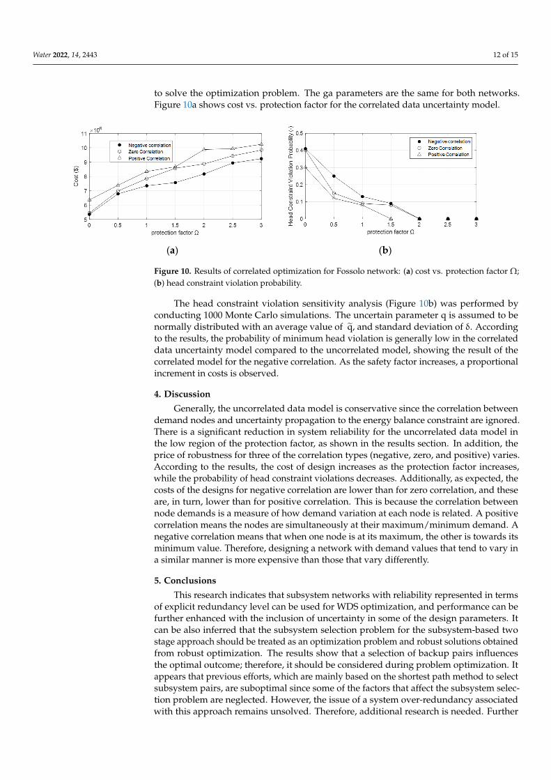
first issue with uncorrelated data models was that the effect of uncertainty in demand on the minimum head constraint was not taken into consideration. Second, there was no con-sideration given to the correlation between demand nodes. Even though the backups are tree networks, the problem is no longer linear due to the nonlinearity of the new constraint derived from the robust counterpart. Due to this reason, a genetic algorithm was em-ployed to solve the optimization problem. The ga parameters are the same for both net-works. Figure 10a shows cost vs. protection factor for the correlated data uncertainty model.

(a) (b)

Figure 10. Results of correlated optimization for Fossolo network: (a) cost vs. protection factor Ω; (b) head constraint violation probability.

The head constraint violation sensitivity analysis (Figure 10b) was performed by con-ducting 1000 Monte Carlo simulations. The uncertain parameter q is assumed to be nor-mally distributed with an average value of q, and standard deviation of δ. According to the results, the probability of minimum head violation is generally low in the correlated data uncertainty model compared to the uncorrelated model, showing the result of the correlated model for the negative correlation. As the safety factor increases, a proportional increment in costs is observed.

4. Discussion Generally, the uncorrelated data model is conservative since the correlation between

demand nodes and uncertainty propagation to the energy balance constraint are ignored. There is a significant reduction in system reliability for the uncorrelated data model in the low region of the protection factor, as shown in the results section. In addition, the price

Figure 9. Results of uncorrelated optimization for Fossolo network: (a) cost vs. protection factor Ω;(b) head constraint violation probability.

3.2.2. Correlated Data Uncertainty

This uncertainty data model resolves two of the shortcomings of the first model. Thefirst issue with uncorrelated data models was that the effect of uncertainty in demandon the minimum head constraint was not taken into consideration. Second, there was noconsideration given to the correlation between demand nodes. Even though the backups aretree networks, the problem is no longer linear due to the nonlinearity of the new constraintderived from the robust counterpart. Due to this reason, a genetic algorithm was employed

Water 2022, 14, 2443 12 of 15

to solve the optimization problem. The ga parameters are the same for both networks.Figure 10a shows cost vs. protection factor for the correlated data uncertainty model.

Water 2022, 14, 2443 12 of 15

(a) (b)

Figure 9. Results of uncorrelated optimization for Fossolo network: (a) cost vs. protection factor Ω; (b) head constraint violation probability.

3.2.2. Correlated Data Uncertainty This uncertainty data model resolves two of the shortcomings of the first model. The

first issue with uncorrelated data models was that the effect of uncertainty in demand on the minimum head constraint was not taken into consideration. Second, there was no con-sideration given to the correlation between demand nodes. Even though the backups are tree networks, the problem is no longer linear due to the nonlinearity of the new constraint derived from the robust counterpart. Due to this reason, a genetic algorithm was em-ployed to solve the optimization problem. The ga parameters are the same for both net-works. Figure 10a shows cost vs. protection factor for the correlated data uncertainty model.

(a) (b)

Figure 10. Results of correlated optimization for Fossolo network: (a) cost vs. protection factor Ω; (b) head constraint violation probability.

The head constraint violation sensitivity analysis (Figure 10b) was performed by con-ducting 1000 Monte Carlo simulations. The uncertain parameter q is assumed to be nor-mally distributed with an average value of q, and standard deviation of δ. According to the results, the probability of minimum head violation is generally low in the correlated data uncertainty model compared to the uncorrelated model, showing the result of the correlated model for the negative correlation. As the safety factor increases, a proportional increment in costs is observed.

4. Discussion Generally, the uncorrelated data model is conservative since the correlation between

demand nodes and uncertainty propagation to the energy balance constraint are ignored. There is a significant reduction in system reliability for the uncorrelated data model in the low region of the protection factor, as shown in the results section. In addition, the price

Figure 10. Results of correlated optimization for Fossolo network: (a) cost vs. protection factor Ω;(b) head constraint violation probability.

The head constraint violation sensitivity analysis (Figure 10b) was performed byconducting 1000 Monte Carlo simulations. The uncertain parameter q is assumed to benormally distributed with an average value of q, and standard deviation of δ. Accordingto the results, the probability of minimum head violation is generally low in the correlateddata uncertainty model compared to the uncorrelated model, showing the result of thecorrelated model for the negative correlation. As the safety factor increases, a proportionalincrement in costs is observed.

4. Discussion

Generally, the uncorrelated data model is conservative since the correlation betweendemand nodes and uncertainty propagation to the energy balance constraint are ignored.There is a significant reduction in system reliability for the uncorrelated data model inthe low region of the protection factor, as shown in the results section. In addition, theprice of robustness for three of the correlation types (negative, zero, and positive) varies.According to the results, the cost of design increases as the protection factor increases,while the probability of head constraint violations decreases. Additionally, as expected, thecosts of the designs for negative correlation are lower than for zero correlation, and theseare, in turn, lower than for positive correlation. This is because the correlation betweennode demands is a measure of how demand variation at each node is related. A positivecorrelation means the nodes are simultaneously at their maximum/minimum demand. Anegative correlation means that when one node is at its maximum, the other is towards itsminimum value. Therefore, designing a network with demand values that tend to vary ina similar manner is more expensive than those that vary differently.

5. Conclusions

This research indicates that subsystem networks with reliability represented in termsof explicit redundancy level can be used for WDS optimization, and performance can befurther enhanced with the inclusion of uncertainty in some of the design parameters. Itcan be also inferred that the subsystem selection problem for the subsystem-based twostage approach should be treated as an optimization problem and robust solutions obtainedfrom robust optimization. The results show that a selection of backup pairs influencesthe optimal outcome; therefore, it should be considered during problem optimization. Itappears that previous efforts, which are mainly based on the shortest path method to selectsubsystem pairs, are suboptimal since some of the factors that affect the subsystem selec-tion problem are neglected. However, the issue of a system over-redundancy associatedwith this approach remains unsolved. Therefore, additional research is needed. Further

Water 2022, 14, 2443 13 of 15

considerations are also required on the service constraint from subsystems and how it isrelated to the overall optimality.

Author Contributions: Conceptualization, A.H. and A.O.; Methodology, A.H. and A.O.; Writing—Original Draft Preparation, A.H.; Writing—Review and Editing, A.H. and A.O.; Supervision, A.O.;Project Administration, A.O.; Funding Acquisition, A.O. All authors have read and agreed to thepublished version of the manuscript.

Funding: This research received no external funding.

Institutional Review Board Statement: Not applicable.

Informed Consent Statement: Not applicable.

Data Availability Statement: The data presented in this study are available on request from thecorresponding author.

Conflicts of Interest: The authors declare no conflict of interest. The funders had no role in the designof the study; in the collection, analyses, or interpretation of data; in the writing of the manuscript, orin the decision to publish the results.

Appendix A. Solution to a Subproblem

Minimize cTxs.t a(ξ)T x ≤ b, ξ ∈ U

(A1)

Box model: U = ξ|‖ξ‖∞ ≤ r

maxξ∈U

(ξTdiag(a)x

)+ aT

0 x− b ≤ 0 (A2)

where diag(~

a)

refers to a diagonal matrix with its diagonal entry~a.

If there is more than one constraint in the original problem, it needs to be writtenexplicitly for each constraint and solve the problem of max

ξ∈U

(ξTdiag

(~a)

x)

. Since b and a0

are not dependent on ξ, they can be taken out of the optimization. It can be seen that theremaining problem is simply a dot product between vectors ξ and diag

(~a)

x.

The supremum value of ξTdiag(~

a)

x can be achieved using Holder’s inequality.Holder’s inequality relates the norm of two vectors f and g to their dot product valueas stated below ∣∣∣fTg

∣∣∣ ≤ ‖f‖p ‖g‖q1p + 1

q = 1(A3)

When p = q = 2, a very special case of Holder’s inequality which is called Cauchy–Schwarz inequality is achieved. Using the fact that a dot product of two vectors cannot begreater than its absolute value, choosing p = 1 and q = ∞, and combining it with Holder’sinequality, ξTdiag(~a )x can be bounded from above.

maxξ∈U

(ξTdiag(a)x

)≤ max

ξ∈U

∣∣∣ξTdiag(a)x∣∣∣ ≤ ‖diag(a)x‖1max

ξ∈U||ξ||∞ = ‖diag(a)x‖1 r (A4)

The last equality is obtained from the fact that maxξ∈U‖ξ‖∞ = r. The supremum value

is attained when ξi = r~a

ixi∣∣∣∣~aixi

∣∣∣∣ , which satisfies the constraint ξ ∈ U = ‖ξ‖∞ ≤ r. The worst

realization constraint now becomes:

r‖diag(a)x‖1 + a0x− b ≤ 0 (A5)

Water 2022, 14, 2443 14 of 15

An alternative way to solve the subproblem is by adding a Lagrangian multiplier andthus converting the problem from constrained to unconstrained optimization problem.

Finally, the deterministic equivalent for cube uncertainty space is

Minimize cTxs.t r‖diag(a)x‖+ a0x− b ≤ 0

(A6)

Although the problem is now no longer linear, it is a convex problem. Therefore, itcan be solved using methods available to solve convex optimization problems.Ellipsoidal set:

U =

a|(a− a)T Σ−1 (a− a) ≤ ω2

(A7)

By making a variable transformation of Σ = PPT and a =~a + Pξ, the uncertainty

space becomes

U = a|a = a + Pξ, ‖ξ‖ ≤ ω (A8)

Note that a very special case of an ellipsoidal uncertainty set is a spherical space. Inthe same way the box set is defined, the worst-case realization can be formulated, and thesubproblem can be thus optimized over the ellipsoidal space.

Minimize cTxs.t max

ξ∈U

((a + Pξ)Tx− b

)≤ 0 (A9)

By solving maxξ∈U

((a + Pξ)∧T x− b

), the worst scenario can be obtained. Again, it can

be shown that the maximum isω‖PTx‖ and it is attained when ξ = ω PTx‖PTx‖ , which also

satisfies the constraint ‖ξ‖ = ‖ω PTx‖PTx‖‖ =ω‖

PTx‖PTx‖‖ =ω ≤ω.

The robust deterministic equivalent for ellipsoidal uncertainty is:

Minimize cTxs.t aTx +ω‖PTx‖ − b ≤ 0

(A10)

Therefore, robust optimal solutions can be achieved by solving the robust deterministicequivalent written in Equation (A10).

References1. Ormsbee, L.; Kessler, A. Optimal upgrading of hydraulic-network reliability. J. Water Resour. Plan. Manag. 1991, 116, 784–802.

[CrossRef]2. Agrawal, M.L.; Gupta, R.; Bhave, P.R. Optimal Design of Level 1 Redundant Water Distribution Networks Considering Nodal

Storage. J. Environ. Eng. 2007, 133, 319–330. [CrossRef]3. Rathi, S.; Gupta, R. Genetic Algorithm for Minimization of Variance of Pipe Flow-Series for Looped Water Distribution Networks.

In Hydrological Modeling; Springer: Cham, Switzerland, 2022; pp. 205–219. [CrossRef]4. Yazdani, A.; Jeffrey, P. Applying Network Theory to Quantify the Redundancy and Structural Robustness of Water Distribution

Systems. J. Water Resour. Plan Manag. 2012, 138, 153–161. [CrossRef]5. Rathi, S.; Gupta, R.; Palod, N.; Ormsbee, L. Minimizing the variance of flow series using a genetic algorithm for reliability-based

design of looped water distribution networks. Eng. Optim. 2020, 52, 637–651. [CrossRef]6. Gupta, R.; Kakwani, N.; Ormsbee, L. Optimal Upgrading of Water Distribution Network Redundancy. J. Water Resour. Plan

Manag. 2015, 141, 04014043. [CrossRef]7. Jung, D.; Kim, J.H. Water distribution system design to minimize costs and maximize topological and hydraulic reliability. J. Water

Resour. Plan Manag. 2018, 144, 06018005. [CrossRef]8. Ostfeld, A.; Shamir, U. Design of optimal reliable multiquality water-supply systems. J. Water Resour. Plan. Manag. 1996,

122, 322–333. [CrossRef]9. Filion, Y.R.; Adams, B.J.; Karney, B.W. Stochastic design of water distribution systems with expected annual damages. J. Water

Resour. Plan Manag. 2007, 133, 244–252. [CrossRef]

Water 2022, 14, 2443 15 of 15

10. Kapelan, Z.; Babayan, A.V.; Savic, D.A.; Walters, G.A.; Khu, S.T. Two new approaches for the stochastic least cost design of waterdistribution systems. Water Sci. Technol. Water Supply 2004, 4, 355–363. [CrossRef]

11. Guistolisi, O.; Laucelli, D.; Colombo, A.F. Deterministic versus stochastic design of water distribution networks. J. Water Resour.Plan Manag. 2009, 135, 117–127. [CrossRef]

12. Ben-Tal, A.; El Ghaoui, L.; Nemirovski, A. Robust Optimization; Princeton University Press: Princeton, NJ, USA, 2009. [CrossRef]13. Perelman, L.; Housh, M.; Ostfeld, A. Robust optimization for water distribution systems least cost design. Water Resour. Res. 2013,

49, 6795–6809. [CrossRef]14. Perelman, L.; Housh, M.; Ostfeld, A. Explicit demand uncertainty formulation for robust design of water distribution systems. In

Proceedings of the World Environmental and Water Resources Congress 2013: Showcasing the Future, Cincinnati, OH, USA,19–23 May 2013; pp. 684–695. [CrossRef]

15. Itai, A.; Rodeh, M. Multi-Tree Approach To Reliability in Distributed Networks. Annu. Symp. Comput. Sci. 1984, 79, 43–59.16. Takeaki, U.N.O. An algorithm for enumerating all directed spanning trees in a directed graph. In International Symposium on

Algorithms and Computation; Lect Notes Comput Sci (Including Subser Lect Notes Artif Intell Lect Notes Bioinformatics); Springer:Berlin/Heidelberg, Germany, 1996; Volume 1178, pp. 167–173. [CrossRef]

17. Geen, Z.W. Multiobjective Optimization of Water Distribution Networks Using Fuzzy Theory and Harmony Search. Water 2015,7, 3613–3625. [CrossRef]