PREFACE

Rapid economic development and population growth exert

great pressure on water resource development requiring an active

control. The necessity of creating a strong data base for Water

Resource Planning especially for developing countries is well

known. Rainfall being primary input to water budgeting, a

systematic study of this data is essentially required. Although

systematic measurement of rainfall has a long history, the design

procedures involving areal variability are recent.

A point rainfall ts collected at a given station. Byt

water resource engineers are interested in the knowledge of total

rainfall over an area. For extracting the areal information, one

cannot increase the raingauge stations uncritically as they

involve considerable cost. An ideal design procedure could be

based an economic considerations: However there is no method now

available for such considerations. An engineering approach is

the only resort to the data collection problem now. In this

statistical structure of rainfall over the area under

consideration is studied from the existing data. Therefrom the

number or stations required to represent the rainfall over the

area for a prescribed accuracy is arrived at.

In this report, a network desig of raingauge stations

for the state of Nagaland has been, made. The Directorate of

Irrigation and Flood Control provided the data used in the study.

This report has been prepared by Dr.A.B.Palaniappan,

Head, Scientist 'E' and Sh.D.Mohana Rangaft, Technician of North

Eastern Regional Centre, Guwahati.

(S.M.

Director

TABLE OF CONTENT

Preface

Abstract 11

List of Tables

List of Figures iv

1.0 INTRODUCTION A.

2.0 REVIEW 3

2.1 ISI and WMO Specifications 3

2.2 Rainfall analysis for design 4

2.3 C, Method 5

2.4 Optimum Estimation Method 6

2.4.1 Polynomial Surface Fitting 7

2.4.2 Kirging Method 7

2.5 Halls Method

2.6 Optimum Interpolation Method 9

2.7 Spatial Correlation Method SO

2.7.1 Spatial Interpolation 13

. 2,'S Principal Component Analysis method (PCA)14

2.9 DYmond and Zawadzksi Methods 15

3.0 DESCRIPTION OF STUDY AREA 18

3.1 Geology 21

3.2 Drainage 22

3.3 Climate and Weather 23

3.4 Natural Vegetation 24 ,

3.5 Soils 24

3.6 Agriculture 25

3.7 Minerals 26

2.8 Existing Network 29

4.0 NETWORK DESIGN 30

4.1. ISI Code 30

4.2 Cy Method 32

4.3 Spatial Correlation Method 32

40

4.4 Dymond and Zawadzki Methods 41.

4.5 Recommendations

5.0 CONCLUSION 42

REFERENCES 43

APPENDIX I STATISTICS USED FOR NETWORK DESIGN 45

LIST OF TABLES

S.NO. TITLE PAGE NO

AREA OF EACH DISTRICT OF NAGALAND 19

AREA UNDER DIFFERENT LAND USE IN NAGALAND 25

ROTATION OF CROPSN I/N- NAGALAND 26

AVERAGE RAINFALL AT DIFFERENT STATIONS IN NAGALAND 29

5, DISTRICT WISE_RAINGAUGE DISTRIBUTION - ISI 30

ERROR VS RAINGAUGES - ISI 32

STATION DISTANCE - CORRELATION 32

ERROR VS RAINGAUGES - SPATIAL CORRELATION METHOD 35

DISTRICT WISE ERROR VS RAINGAUGES - SPATIAL 35

CORRELATION METHOD ERROR VS RAINGAUGES - DYMOND AND ZAWADZKI METHODS

41

DISTRIBUTION WISE DISTRIBUTION OF RAINGAUGES 41

LIST OF FIGURES

S.No. TITLE PAGE NO

1.. EFFECT OF INCREASE IN NUMBER OF GAUGES . 2 STUDY AREA AND EXISTING METEROLOGICAL STATIONS £7

ELEVATIONAL FEATURES OF, NAGALAND 20 4-A.VARIATION OF DAILY RAINFALL OBSERVED IN NAGALAND

2 7

4-0.VARIATION OF MONTHLY RAINFALL OBSERVED FOR THE 28 1085 IN NAGALAND

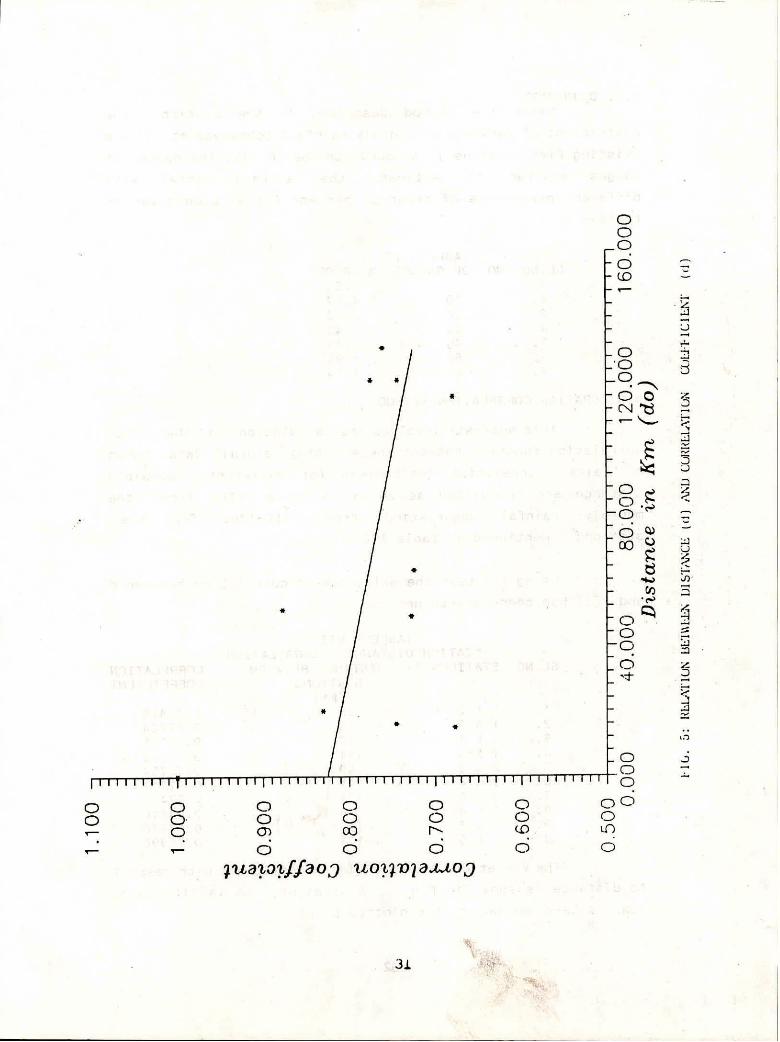
5. RELATION BETWEEN DISTANCE (d) AND CORRELATION 31 COEFFICIENT c(d)

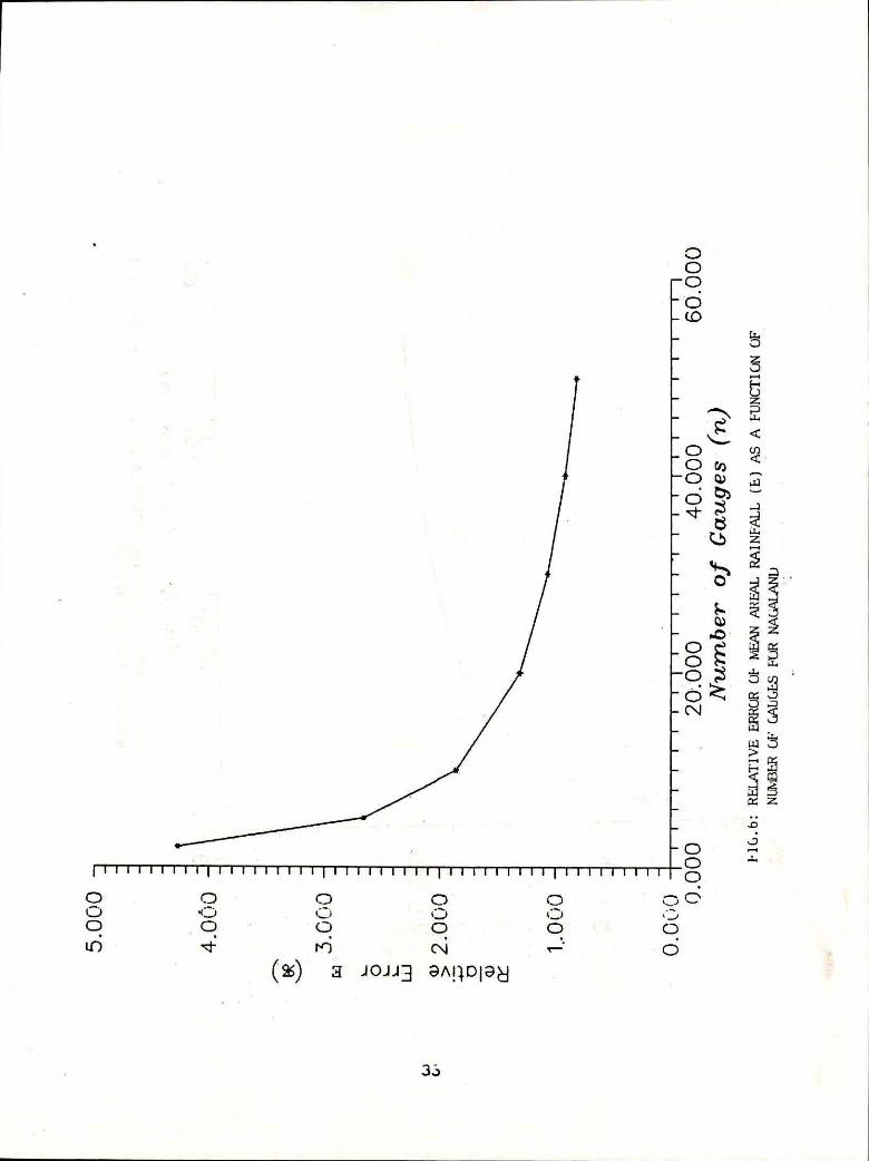
. RELATIVE ERROR OF MEAN AREAL RAINFALL (E) AS A 33

FUNCTION OF NUMBER OF GAUGES FOR NAGALAND

RELATIVE ERROR OF SPATIAL INTERPOLATION (E) AS A 34

FUNCTION OF NUMBER OF GAUGES FOR NAGALAND

S. DISTRICT WISE RELATIVE ERROR OF AEAN AREAL RAINFALL 37

(E) AND SPATIAL INTERPOLATION (E) AS A FUNCTION OF'

NUMBER OF GAUGES

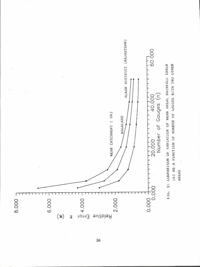
g. COMPARISON OF VARIATION OF MEAN AREAL RAINFALL ERROR 38

(E) AS A FUNCTION OF NUMBER OF GAUGES WITH TWO OTHER

AREAS

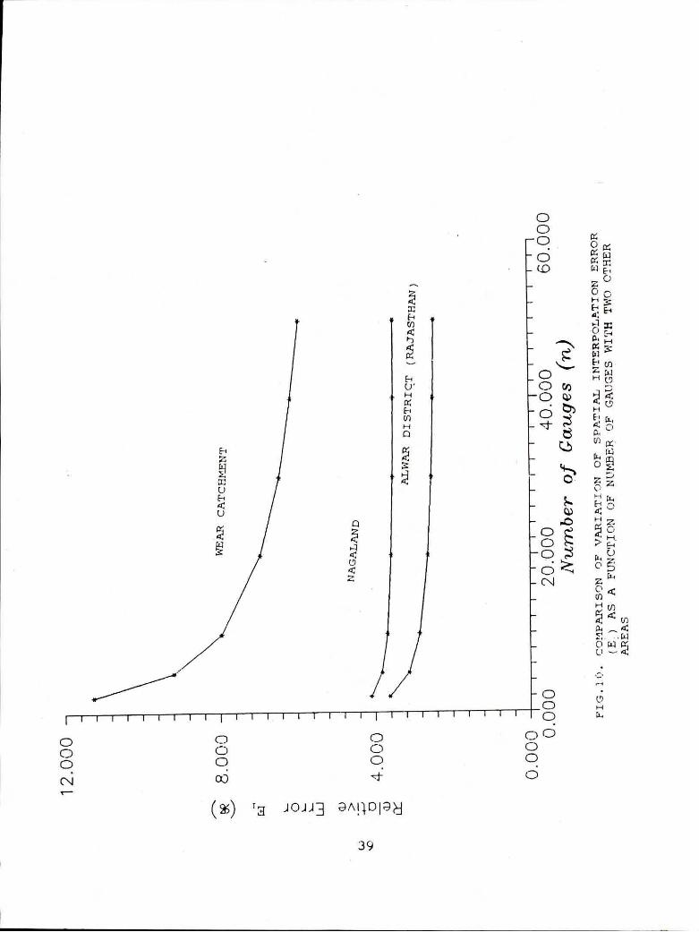
10. COMPARISON OF VARIATION OF SPATIAL INTERPOLATION ERROR 39

(E) AS A 'FUNCTION OF NUMBER OF GAUGES WITH TWO d-P4ER

AREAS

ABSTRACT

A sound hydrological data base is very essential

for Water Resources Planning. The main aim of hydrological

network is to provide a distribution of stations for an area so

as to measure adequately the required parameters. With the

increase in gauging stations, hydrological information available

also increases. But as one increases the number of gauging

stations the . cost associated with these measurements also

increases considerably. Infect, the network design is an economic

issue. Hence one should not attempt to increase the number of

gauging stations uncritically and increase the data. Certain

statistical techniques allow us to determine the number of

gauges required for certain' objectives. These techniques

require a prior knowledge of variation of the hydrological

parameter to be observed which is obtained from available data.

Brief discussion of different methods of Raingauge network

generally used for network design and the underlying principles

are given in this report. Applying four different methods the

raingauge network design for the state of Nagaland has been

made in the study, reported. The ISI Code, Cv method , Spatial

Correlation method, Dymond and Zawadzki methods have been

chooeen for the above design inview of the data availability.

The requirement of raingauge stations with the relative error

on mean areal rainfall and spatial interpolation error are

computed. It is found that the requirement of stations computed

using various methods are nearly the same for a desired accuracy

on mean areal precipitation. District wise requirement of

raingauge stations has been given in this report. It is

that sixty three raingauge stations including seven

recording stations would be sufficient at present for the state

of Nagaland. However on receipt of more rainfall observation the

design may be- revised.

found

self

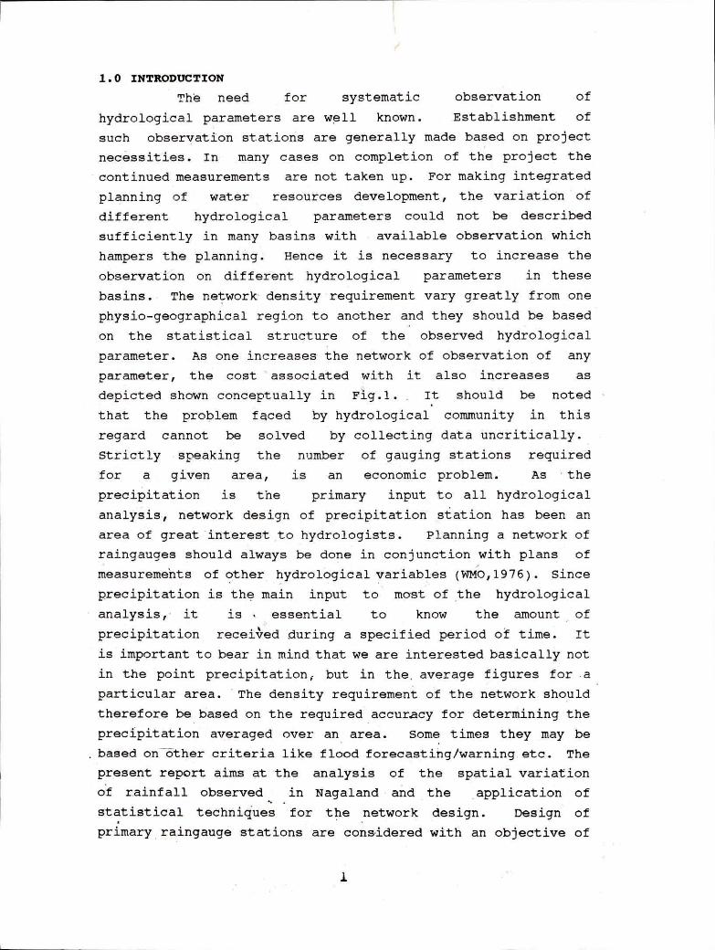
1.0 INTRODUCTION

The need for systematic observation of

hydrological parameters are well known. Establishment of

such observation stations are generally made based on project

necessities. In many cases on completion of the project the

continued measurements are not taken up. For making integrated

planning of water resources development, the variation of

different hydrological parameters could not be described

sufficiently in many basins with available observation which

hampers the planning. Hence it is necessary to increase the

observation on different hydrological parameters in these

basins. The network density requirement vary greatly from one

physio-geographical region to another and they should be based

on the statistical structure of the observed hydrological

parameter. As one increases the network of observation of any

parameter, the cost associated with it also increases as

depicted shown conceptually in Fig.].. It should be noted

that the problem faced by hydrological community in this

regard cannot be solved by collecting data uncritically.

Strictly speaking the number of gauging stations required

for a given area, is an economic problem. As the

precipitation is the primary input to all hydrological

analysis, network design of precipitation station has been

area of great interest to hydrologists. Planning a network

raingauges should always be done in conjunction with plans

measurements of other hydrological variables (WM0,1976). since

precipitation is the main input to most of the hydrological

analysis, it is • essential to know the amount of

precipitation recei4ed during a specified period of time. It

is important to bear in mind that we are interested basically not

in the point precipitation, but in the, average figures for •a

particular area. The density requirement of the network should

therefore be based on the required accuracy for determining the

precipitation averaged over an area. Some times they may be

based on—Other criteria like flood forecasting/warning etc. The

present report aims at the analysis of the spatial variation

of rainfall observed in Nagaland and the application of

statistical techniques for the network design. Design of

primary raingauge stations are considered with an objective of

an

of

of

Cost/Information

INF

OR

MA

TIO

N

.

A- C

OS

T

IIIIIIII]l1

11

11

11

11

11

11

11

11

No o

f gauges

FIG.1. EFFECT OF INCREASE IN NUMBER OF GAUGES

accessing the rainfall receipt in Nagaland.

A brief review of different methods viz, ISI Code, WHO

specification, C, method, Spatial Correlation method,

Optimisation methods, Principal Component Analysis, Dymond and

Zawadzki methods have been given in section 2.0. After breif

description of the study area application of four different

methods are provided in section 4.0 along with recommendation.

Appendix I provides basic statisticsused for the design.

2.0. REVIEW

2.1. ISI AND WHO SPECIFICATIONS

ISI codes & WHO specification provides certain

recommendations on the density of precipitation network. Further

IMD, WHO manuals also recommend certain statistical

procedure. The latter procedure requires prior knowledge of the

variation of the rainfall over the area under consideration,

but when the existing raingauges are large, a true variation

of the rainfall can be determined from which minimal/optimal

need can be easily found. However this variation is obtained

through the available rainfall data pertaining to that area.

Hence a note of caution is necessary when using data from

sparse observation for design.

The object of providing a network of raingauges is

to adequately sample the rainfall and explain its variability

within the area of concern . The rainfall variability

depends on topography, wind, direction of storm movement as well

as type of storm. The location and spacing of gauge depend not

only on the above factors but also upon the use of

precipitation data for that region for the people. Network

design covers following three main aspects(WMO, 1976):

i. number of data acquisition points required; location'of data acquisition points arid

iii. duration of data collection from a network.

Measurement station are divided into three main

categories by WHO, viz.

3

Primary stations:- These are long term reliable stations expected to give good and representative records. Secondary stations or Auxilary Stations :- These are placed to define the variability over an area. The readings observed at these stations are correlated with the primary stations, if and when 'consistent correlation are obtained, secondary station may be discontinued or removed. Special Stations:- These are established for particular studies and do not form part of a minimum network.

If economy permits it is desirable to establish primary

stations along with large number of secondary stations so that

useful statistical relationship can be developed between the

primary and secondary stations.

The WMO (1976) has recommended the following as minimum

network densities for general hydrometerological practices

1-For plain regions of temperate mediterranean and tropical zones one station for 600 - 900 Sq. Km.

2.For mountainous region of temperate, mediterranean and tropical zones one station for 100 - 250 sq. Km

3.For arid and polar region one station for 1,500 7 10,000 Sq. Km depending upon the feasibility.

The IsI 4987 - 1968 standard also lays down

recommendations for distribution denpity.

1.For Plain areas one raingauge up to 520 Sq. Km. shall be sufficient to plain areas. However if the catchment lies in the path of low pressure, system which cause precipitation in the area during its movement which can be seen from maps published by IMD, then the network should be denser particularly in the up stream.

2.In region of moderate elevation (up to 1 Km above mean sea level), the network density shall be one raingauge in 260 Sq. Km. to 390 Sq.Km.

3.In predominantly, hIlly areas and where heavy rainfall'is experienced the density reCommended was one raingauge in not more than 130 Sq. Km.

2.2 RAINFALL ANALYSIS FOR DESIGN

The quantitative study of statistical structure of meteorological network design was first attempted by Dr.

0.A.Drozdov in 1936. He has introduced the use of standard error

of linear 'interpolation at .the mid point between a pair of

statione for determining permissible distance. Pioneering

studies_by him and Dr.A.A. epelevskij in 1946 formed the basis

of many of the development that took place in network design.

The rainfall data recorded at individual sites

are combined in a suitable way to obtain a representative

estimate of the areal rainfall and this value may depart ,from

the true areal mean for the following reasons:

(a)inadequate coverage of the area by the gauges, (b)systematic errors of instrumental measurements ie,

poor siting of the raingauge, incorrect exposure of the instrument etc.

(c)random errors ie, observational error, errors due to the type of precipitation, micro climatic irregularities of the site etc.

Gandin suggests that a reliable data set of about sixty

stations with a minimum of sixty observations at different times

is required for deriving the statistical structure of the

observation. The frequency of the data set used should not be _1 too short for network design - in practice hydrologists have used

daily, ten daily monthly or annual intervals for design

purposes.

The common practice is to evaluate the error

associated with a particular sampling density. Quite often an

error criterion is applied. Some of the methods which are

being used are simple random sampling, correlation function,

regression techniques, structural functions, and the

spatial application of time series analysis. These methods

assume that the values recorded by each station is independent

of the values recorded by other gaugPq in the area considered.

2.3. C, METHOD

The ISI Code and IMD (1972) have recommended a simple

formula.

n = ( c,/e)2 (i)

where n is the number of raingauges C, is the coefficient of variation of the rainfall of the eXISting rainganges, given by ohrn cr is the overall monthly variance Pay is the arithmetic mean of monthly rainfall,

5

over the area. e is the error permissible or the desired error of accuracy

2.4 OPTIMUM ESTIMATION METHOD

The theory of optimum estimation by

imposing climatological constraints minimises the root mean

square error estimation Mooley et al. (1981).

The areal value P, =.(1/A)jf Pi dx dy (2)

This areal average can ' be estimated by a

linear combination of point observational values as

n.

PE = E WiPi

j=1

where n is the number of gauges.

PA is the rainfall at different stations (ie j = 1,2,...n)

The weight value W, can be found out by substituting R

obtained from eqn.(2).

The relative mean square error R is given by

xi 2

E = { Ewjpi-(1/A).is pidx dY } (4)

j=1 which should be minimum.

The optimum number of gauges re4uired over an area

for the estimation of areal rainfall can be directly

determined from the relationship for a given error tolerance.

The advantage of this method of optimum estimation

is that it takes into cCount the local Variation as well as

inter station relationship of rainfall, spatial di. tribution of

gauges over an area is also taken into acthount Mooley et al.

(1981).

6

2.4.1.FOLYNOMIAL SURFACE FITTING,—

A polynomial surface is fitted by the method of least

squares over the data. Given a set of observed point. (x,y) where

(x,y) are the geometric coordinates of the raingauge and P are

the observed rainfall values. The rainfall P, are calculated using

Pc = b1+ b2x + ba + b4x2 + bsity + b5y2 )

The second degree polynomial coefficients (b„....,b,) are

evaluated using least square techniques. This method of

describing the rainfall surface can be used to find the areal

rainfall. By varying the number of existing raingauges steadily

the method can be applied repeatedly to determine the optimum

raingauge network for the estimation of areal rainfall for a desired level of accuracy.

2.4.2. K/RGING METHOD

An optimum interpolation between gauge values can be implemented by Kirging. This is essentially a method

of estimation of areal rainfall. Kirging was originated by

Matneron (1971). .Hughes and Lettenmaier (1981) suggested the

potential use of Kirging in network design.

Consider an area A, over which a number of raingauge are sited with some additional observation points. The unknown

mean precipitation for the area is defined as

P = (1/A)f PR(x) dx ' (6) A

is the location of a point of observation. PA(x) is a funeuion describing depth of storm over

region A.

Taking account of the time interval, k used in the discretization of the observed rainfall an estimate of P(k) from a storm can be given for the set of rainfall observations in area A and expressed as

7

P(k) = 141 (k) q (K,xi )

1=1

where W, is the solution of the Kirging system by a set of weight i = 1 to n.

Ti is the number of gauges. k is a discreted time interval. q(k,x,) is the rainfall depth at location x, over

time duration k.

Spatial relationship between rainfall depths at

location x, and x3 is given by

p(d) =ad

(8)

where p(d) is the value at a separation distance, 'd', between location x, and xj

The other forms of Kitging methods are Linear,

non linear and disjunctive Kirging more details can be seen in xassim (1991).

2.5 HALLS METHOD

Hall (1972) suggested a method for determination of

key station network for flood forecasting purpose. First correlation coefficient between the average of the storm

rainfall and individual station rainfall are found. The

stations are arranged in descending order of correlation

coefficient and the station with highest correlation coefficient

are considered for inclusion in the network. The station with

highest correlation coefficient is called the key station. The

first key station data are removed, the second key station among

the remaining raingauge stations' is found similarly. As each

station gets added to the key station network, the total amount of variance which is accounted for by the network at that stage

is determined: From this the number of gauges required for

achieving an acceptable degree of error can be found.

8

(7 )

2.6 OPTIMUM POINT INTERPOLATION METHOD

The interpolation method can be separated into three

groups polynomial, weighted mean and optimum interpolation. In,

the interpolation method, weighing factors Wj can be calculated

depending on the distance between interpolation points (0)

and-adjacent point (i), and th9n be used in estimating the value

of the given variable at the point of interest.

In optimum interpolation problems can be formulated

in the form of linear weighing coefficients W., of the known

values of rainfall f: at n observation points u“ un for

determining the values f at point u .

Ii

f, = w] fj

j=1

and also

f'a = V Wj f'j

j=1

where f', f0 - To , - and W are weighing factors.

Mean Square Interpolation error is given by

2 E = (f', - I • W, Us) (10)

J=1 1=1

where in represents individual events More details of this method

can be seen in Unal etal (1983)

2.7. SPATIAL CORRELATION METHOD

Two statistical methods of areal rainfall

analysis applicable to rain gauge network design generally

used by hydrologists are

The Eagan methOd based_, on on:pas co-relation techniques. Trend surface representation of rainfall by least squares fitting of polynomials.

40

The spatial variability can be quantified through

a spatial correlation function and network of raingauges can

be designed to meet a specified error criterion. However in

applying such an approach, care must be taken to ensure that

conditions necessary for the existence of a spatial

correlation function, such as horizontal homogeneity and

isotropy, are fulfilled. Experience suggest that homogenity and

isotrophy can be assumed without causing significant error for

the covariance function and structure function (see Appendix I)

for flat areas with a relatively homogenous underlying surface.

In mountainous region these assumptions are not generally

fulfilled. The objective of these assumptions is to make sure

that the above functions depend mainly on the distance.

Validity of these assumptions over the available data

can be clearly seen by plotting correlation and covariance

function against distance. An erratic plot with no trend

invalidates the above assumption. It is also possible that the

correlation aspect shows a dependence where as the covariance

lacks homogenity. If data of any particular station is suspected

they may be excluded from the analysis as they may either be

inaccurate or unrepresentative. In this way the above

assumptions can be fulfilled with reasonable accuracy.

The basis of the method advocated by Kagan (1966)

is the correlation function p(d) where ,d, is the distance

between stations, and the form of which depends on

characteristics of the area under consideration and on the type

of precipitation. The function p(d) can be described by the

following exponential form.

,p(d) = p(0)e° "

where p(0) is the cortelation corresponding to zero distance.

d, is the correlation radius or distance at which the

correlation is p(0)e-1, (e = 2.71828)

Theoretically o(0) should be equal to unity as it is

the correlation corresponding to zero distance but it is rarely

found in practice as in the present case also, due to random

errors in precipitation measurement and micro , climatic

irregularities over an area which make o(0) less than unity.

The two parameters p(0) and d, are necessary for assessing

the accuracy of a given raingauge network.

The correlation function largely depends on the

interval of precipitation total. Analysis on different interval

like daily, ten daily, monthly, reveals that longer the interval

over which the precipitation is totaled, the slower the decrease

of the correlation function with the increasing distance. The

error in determining total precipitation also indreases as the

length of interval decreases. Therefore the.tetWork density

requirement are more rigid for short interval of time for which

it is necessary to know the total precipitation.

The relative root mean Square error E is defined by

Kagen (1966) as

E = (a(h)" /Pay) = Cv ((1-0(0)) + 0.23 ((A/a)"/(10))/s)

(12)

where c(h) is the variance of the error in average rainfall;

A is the area. He used an arithmetic (equal weight l/n) mean

while deriving the above equation and assumed maximum error to

occur at the centre of the triangular element considered.

From equation (12) the Value of 'n' required to meet

a specified err-or criteridn 'E. 'can be obthined if the values

of o(0) and d, are known.

A dense network of rainfall stations over a certain

area gives results of the neighbouring stations, that are highly

correlated and do not turniah,further information.

.12

The uniform spacing of stations (d) over the area

'A, can be given assuming triangular grid by:

d = 1.07 (A/fl)" (13)

2.7.1. spatial Interpolation

Most of the proposed spatial interpolation techniques

are of the type weighted average of surrounding nations using

the formula (Kruizinga et al. 1978)

P„ = E Wk hk

k=1

where P, is the estimated rainfali h, is the measured rainfall amount at the

surrounding stations. WK is the applied Weights. n is the surrounding stations.

11

In most cases one requires that E = k=1

The methods differ in the choice of weights only, in

some cases the weights are independent of the distance (Saltes

1972) in other cases the,weights are optimized on the basis

of correlation function.

The accuracy of spatial interpolation is to be

evaluated. Kagen (1966) tias given the relative errors

associated with linear interpolation between two points and

interpolation at the centre of a square and a triangle, where a

maximum error of interpolation occur. For a triangular grid

with spacing d, the relative error is given by

EI = C. (0.33(1- p(0)) + 0.52 p(0)(k/u)",/d0))" (15)

p(d)can be described y eq.(11)

The resulting error for different number of rain/auges can be

found from the above equation.

(14).

13

2.8. Principal Component Analysis Method (PCA)

In this method, the maximum number of climatologically

homogenous sub-divisions was delineated. The delineation also

involves the use of interlocation correlation analysis and

vector clusters of the locations onto pairs of the significant

PCA modes, together with several other statistical or

physical analysis in order to determine the physical reality of

the derived homogenous climatological subdivisions. In the development of the minimum raingauge network, the maximum number

of climatologically homogenous sub divisions are used. This

method ensures that each climatologically homogenous subdivisions

is represented by at least one rainfall station.

Recognising a general weakness of network design

methods on the basis of a specified error criteria in the areal

rainfall estimates that they provide large number of raingauges

even for dry area where rainfall dependent activities are the

least Basalirwa et al. (1993) have used PCA method for network

design of raingauge stations for Uganda. They expected that

large spatial rainfall variations can occur in dry area during

dry seasons causing a dense network. Considering the economic

they suggested minimum raingauge network where representation of

each of the homogenous rainfall subdivions can be made.

The basic PCA model has been expressed by Harman ( 976) among many others as

Z = r a

k=1

Fk(j =1,2,

n) (16)

where Z. is the standardized factor -k (principal compone regression co-efficient of number of common factor and

variable j; Fk is the hypothetical nt); at is the standardized multi variable j or factor k; m is the n is the number variables.

To ensure that the stations which represented

the individual homogenous subdivisions are realistic and

represent most of the required informations, the principle

of commonality ate used. The commonality of each variable Z; given by (h.) is obtained- by

JA

m

(hi)2 =E (a02(j = 1,2, n) (17)

k=1

The commonality of a station, represents the degree

of association that the station has with all other stations in

the data set. The best representative station will be the

station with highest commonality among the stations of a

homogenous group.

The ability of the generated minimum raingauge

network in representing the areal rainfall characteristics

within the individual homogenous regions can be examined by

computing the correlation coefficient between , the rainfall

totals at the representative station (j) over time (t) and

the areal rainfall estimates from the individual homogenous

groups.

To determine the representativeness of each chosen

station. An equation that expresses areal rainfall values as

a function of the representative station is given by

PR (t) = a + b P(t) (18)

where

P1/4(t) is the areal rainfall estimate for the homogenous group over time t;

P1(t) is the rainfall total at station j over time t; a and b are regression coefficients.

The variance accounted by the representative station

is based on this linear model. A case study using this method

upon Uganda can be seen in Basalirwa .(1993)

2.9. DYMOND AND ZAWADZK/ METHODS

It is usual to go in for large number of raingauge

stations to gain complete knowledge of precipitation phenomena

occuring in a project area. After an initial period of close

monitoring of rainfall in a given area it is desirable to reduce

the number of raingauge Stations in order to reduce the man

power and other efforts required for observations. While

15

reducing/minimising the number of raingauge stations the random error is kept in view. A systematic sampling of an areal

rainfall is the prime object. Statistical methods with special

application to rainfall data have been d6veloped with specific

reference to such situations. Hendrick and Comer(100) have

derived correlation function which has been used by many

approximating it by a linear variation.

Zawadzki (1973) considered a rectangular area of dimension 1,1 x 1,,over which N, number of raingauges (n x m) are

situated spaced at Ax and Ay. He derived an expression for the

mean square error 22 of areal rainfall (arithmetic average)

n-1 m-1 E2 = (1/(nm)2 ) S S (n-ii)(m-iji)A(inx,jny)

' 1i-n j=i-m

7, (Li- ,x ) (L,- l y )A(x,y)dxdy

—Li 42

n-1 m-1 -(2/nmLI Ld > I (n- i )(m- j )

i=l-n j=1-m

(14-flAx (jtflay x I 2 A(x,y)dxdy (19) x=0-flax Y=1j-flay

Here, the error E is the difference between the average rainfall

of N gauges and the average that would have been had N been

increased to sufficiently large that any further increase would

not change the average and A(x,y) is the expected value of the

product of rainfall observed in two gauge stations defined by x,y co-ordinates. The rainfall used in the above equation is for a prescribed period.

The coefficient of variation of rainfall is defined by

cv = u(p)2 ]3v_ Epav12}1/2 irp 3

where [Pay] is the expected rainfall over any point within the

given area which is assumed to be constant over that area.

(20)

16

/'

r

r-

I

MO

N

• N

.0

1,

Mon

I.'

I •

KM

S

r n."

.---

% 1

,- _

'1 1- ‘1

", t, '-

„, %

.-

/ ,

— - Y

i

BO

UN

DA

RIE

S

i

i 4

-C"-Y

I se !

WO

NG

I-• 0 a

n

0 /

1

—•—

In

tern

ati

on

ai

I

04-M

ekch

un

/ i

Z

— S

tate

I

1 I

- --

Dis

tric

1

...

l.".

.. "

(4.

Sta

te C

ap

ita

l 0

ci.,

Tuen

saib

rig

(..

Dis

tric

t H

ead

qu

art

ers

4\ .

.t.?

. meteorologicat 0 Wolote• 0 M

. k

Stations , 1.

-- • : w :

‘ m

i

au

rin

bo

to „

' kg

-f

t

i•

1 /

ti, -,7,

/

4.*

I •

‘( ;REDZIPHEMA

i N

t-

..,

, ..

_.1

)

- . i

4-0

•

\:,

PFUTSERO I

Ko

him

o

1 -

-

4 e

P

he

tt .

..1

/

I K

i , p C

O

.1 \

t ,H

EN

ING

KO

NG

LW

A

/ '

H

'j

' P

-

( /

r -1

---

-

.-

.-{'

- -

L -

‘

,

-• /

• 1 r

•

NA

GA

LA

ND

I0 5

0 1

0 2

0 3

0

1P

UR

•

•

FIG

.2. S

TU

DY

AR

EA

AN

D E

XIS

TIN

G M

ET

ER

OL

OG

ICA

L S

TA

TIO

NS

1

The correlation function is defined by

(x,y) = [A(x,Y)-EPav l2}/[[(P)2]av - [Pavl2} (21)

These expressions have been reduced by. Dymond(1982) to the

following for the case of a square area with uniform spacing of

gauging stations.

(E/Pu) = [[(1-p)Cv2 n-07/310 (22)

where 0, is the correlation between neighbouring gauges (average

of correlation coefficients) and N is the total number of gauges.

Zawadzki assumed an exponential decay of correlation function

which is given below 1

CE/Pay) = C 088( 1-pr k + 1)"/(2.23 N") (23)

The above equations can be used for finding out the

r.m.s. error of an areal rainfall which is observed by Many

gauges providing information of the spatial variation of the

rainfall. However one has to be cautious of the variation caused

by strong winds which might be occuring. The observational

deficiency caused by strong winds have been studied by

Aldridge(1976) and Neff(1977).

Dymond studied the monthly rainfall data from raingauge

network of Rangitawa basin in New Zealand and illustrated the use

of the above analysis.

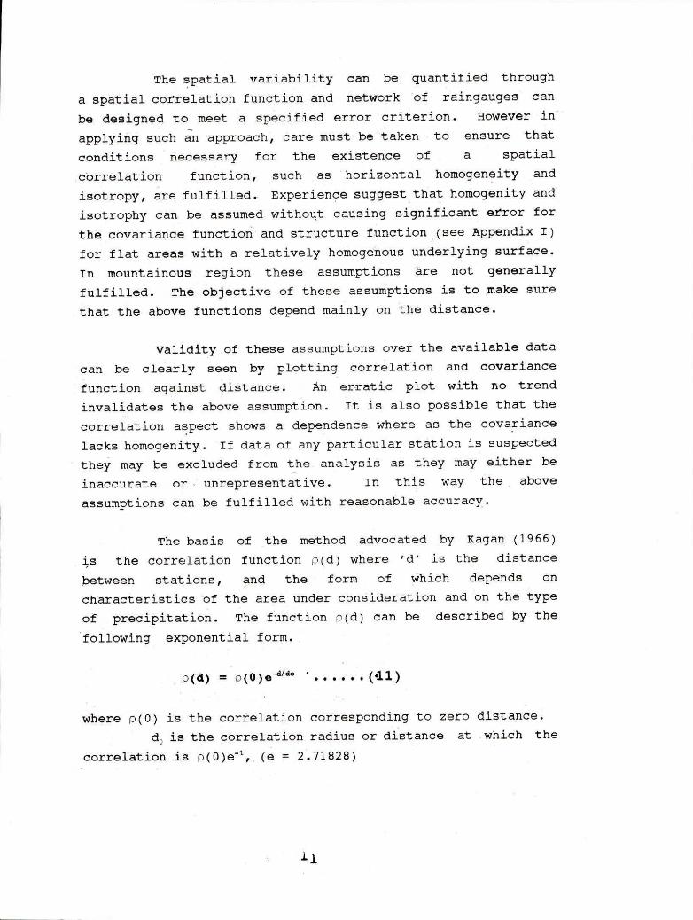
3.0. DESCRIPTION OF THE STUDY AREA

Nagaland is a mountainous state with highly

elevated ridges spurs and peaks. Baring a few hundred Sq.Km

of plains around Dimapur foot hills and along river beds, the

entire state ls hilly. Nagaland is the 3rd smallest state of the

country after Sikkim and Goa. Nagaland stretches between 26:

6'N and 29 4'N latitudes between 92 20'E to 95:E longitude

and is shCwn in Fig.2. The state is bounded by Assam in the

west, Arunachal Pradesh in the North, Burma is the east and

18

Manipur in the South.

It has an area of 16,579 Sq.Km. Nagaland as per

.the 1981 censes had a population of 1,74,930 with an average

density of 47 persons per sq.km. The state comprises

of seven administrative districts. The districts are Kohima,

Phek, Wokha, Zunheboto, Tuensang - and Mon, 17 -subdivisions,

21 development blocks, 963 inhabited villages and 7 towns. The

table I shows the area of each district.

TABLE I AREA OF EACH DISTRICT OF NAGALAND

S.No. District Area (Sq.Km)

1. Kohima 4,041

L. Phek 2,026 Wokha 1,628 Zunheboto 1,255

Mokokchang 1615

Tuensang 4,228 Mon 1,786

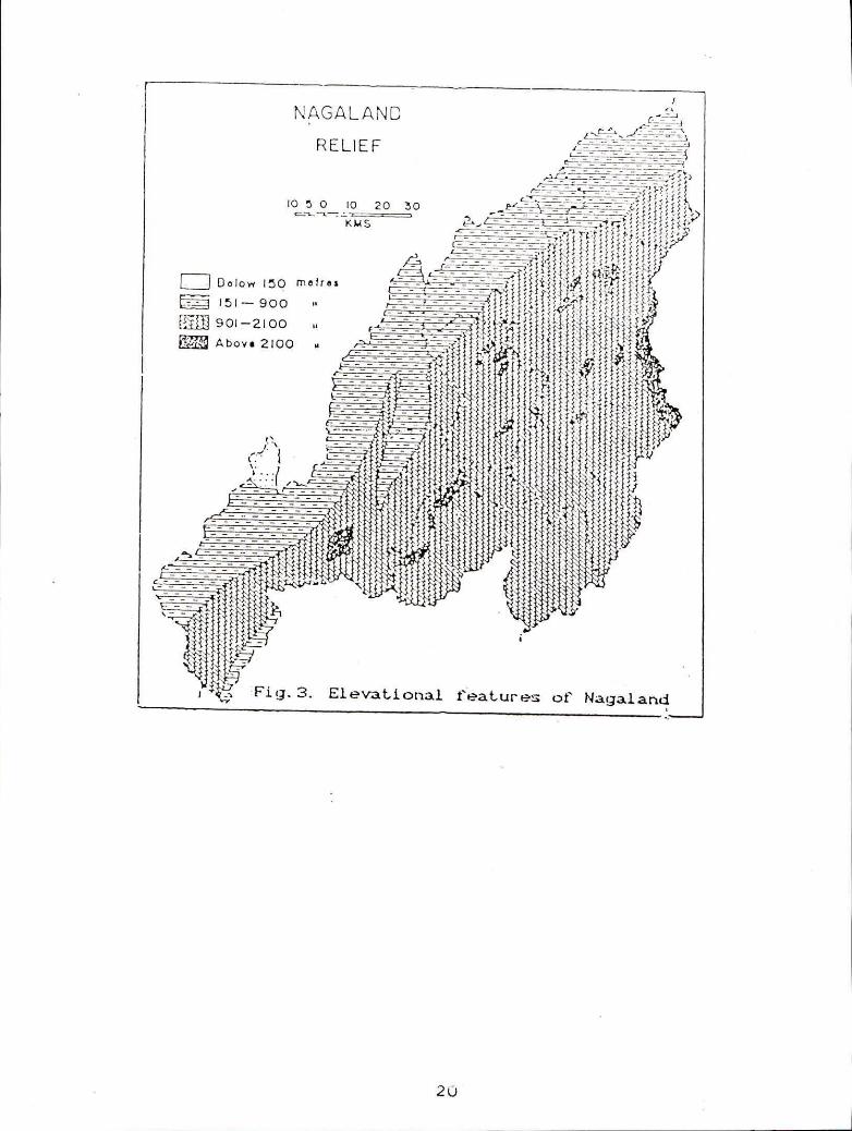
The elevation of Nagaland ranges from 914m to

3840m above msl. The Banal range locally known as Radhuma

enters the state from north Kachar and after passing through

Kohima runs in the direction of Wokha. Japava which lies to

the south of Kohima is the highest peak of Barail (Radhuma)

range and attains a height of 3804m above msl. At this place

the range is met by the meridinal axis of axis prolonged

from the Arakanyoma (the major mountain system of Burma) and

from this point the main range runs in a north and north

easterly direction. Owing to a sudden rise of the Barail

Range on its northern face, about 12Km rise miniature type

of valley is formed in between the Barail range and Samaguling

Hills. Kohima and Naga hills are located further east. The

Patkai range forms a watershed which donstitutes the

international boundary -between India and Burma. Saramati

situated in TUensang district is the highest peak. of Nagaland

which is 3877m above msl. The other peaks include Japfu

(3,014m), Ezupu (2,841m), Paona (2,486m), Angola (2:062m),

Laishing (2,059m). Parts of Japfu mountain summit owing to its

high altitude are snow bound during the cold weather (Dec and

Jan). The elevational features can be seen in Fig,3.

19

nz

krerefirN Jo se.inivai TruontneT3 •E: Td

A91-132:1

ONCIVOVN

C,

0013 IPAOCIV

00I3-106 ifin 006 —1Q1 t=]

senoui Ogr mo4°0

SrIN

0£ OZ 01 0 01 -

Recent Pleistocene UnconfirmitY

Pliocene Dihing Series Unconfirmity

Mio-Pliocene Namsang - beds Unconfirmity

Miocene

Tipam Stage

Surma Series

Oligocene Small

Eocence Disang Series

Tijsans Series

Tikat Parbat Carbonaceous stage Baragolai Satge Naogaon Sandstone stage.

Nagaland is predominantly a tribal state. The

entire tribal populatirn is divisible into twenty major tribal

groups. The dominant tribes which have their defined cultural '

jurisdiction are the Ws, Angamis, Changs, Chakhesang, Kabius,

,Khein - Mangas, Konyaks, Kukis, Lothas (Lhotas), Maos, Mikris

(Mikhirs), Phoms, Rengmas, Sangtams, Semas, Thankuls, Yimchungars

and Zelliang.

English is the official language of the state .

for administration and education. However, the common language

used by the tribal people is Nagamese and English. About 49%

of the total population is literate and only 15.5% live in urban

areas (Hussain, 1994).

3.;. GEOLOGY

The entire Nagaland has almost identical

geological formation, Naga Hills is a continuation of the

Himalayan folded mountains. The formations belong to the

Tertiary period. The tertiary succession of Nagaland is given

below (Hussain, 1994).

Alluvium and high level terraces. Loose sandstones, clay and pebbles beds. Soft coarse sandstorMs, clay and occasional coal conglo-mates. Girujan, Mottled clays and clay fine,grained stages sand stones. Coarse grained Sandstone ferrogenous micancom sand,storms and minor clay. Sandstones, shales and coal seams. Sandstone, shales

Grey SO4.intery shales and ealt haversed by their quartz veins and experi-enced intrusion.

21.

The southern Nagaland has the Serail and

Disang formations. The Disang confirming to the oldest rocks are

dominant towards the east between Japfu and Saramati at an

altitude of 914m to 1,220m, but the Barail series are more

conspicuous towards the west. Slate of superior quality is

found abundantly in Tizu valley which is used by the Nagas for

their building and for commercial *purpose. Disang beds are

generally deep at steep angles. The structure is soft, thin

splinting character has helped to cause frequent landslides

around .Kohima. Deposits of chrysotile asbestos are found

towards the south bordering Burma between Puchimi and kerrosin

in Tizu valley.

3.2. DRAINAGE

The state of Nagaland is drained by numerous streams

and rivers. Some of the important rivers are Dzulu, Dhansiri,

Milak, Zungki, Tizu. Most of these rivers originate

from the central mountain ranges. From the centre the rivers

move north and southwards. The Doyang river which

originates from the vicinity of Mao village of the Angami

territory of the Kohima District is the largest stream of the

Nagaland state. It flows northward and is navigable for a

short distance before it enter the valley of Brahmaputra.

All the rivers of Nagaland discharge little

quantities of water during winter seasons but in the rainy

season they suddenly assume threatening posture. The inundated

streams - and riVers cause heavy soil erosion and become

difficult to feed during the summer monsoon seasons. Most of

the rivers are not navigable owing to mountainous topography.

There is a famous Lacham, a natural lake . in

eastern Chakhesang, east of Masluri. There is also a another

small lake called Achie in Pfutsero. At Dimapur tanks

surviving as historical relics of the old Kachari kings are

still to be seen in Purnabazaar but many have become mere pits

and hallows ,as they are all dried up. The most important tanks

are Bongola, Padum, Jor, Ramon, Dipo,Thana, Podo, and Garani

Pukhari.

22

3.3. ,CLIMATE AND WEATHER

In general the climate of Nagaland is modified

tropical monsoon type and comes 'under 4 sub-divisions as

classified .by IMD for their studies of rainfall departure. In

this climate temperature at low altitudes remain high

throughout the year excepting the month of - December and

January. The summer monsoon is strong which generally lasts

from mid June to mid October in Nagaland. The monsoon climate

is characterized by different seasons which is caused by

the southwest and northeast monsoonS.

At the time of North East monsoon winds are

of continental origin and blows generally in the state from • west

to east and during south west monsoon they are oceanic in nature

and blow mostly in Nagaland from southwest'to northeast. Almost

all the rainfall recording stations of Nagaland record over

75% , of their total rainfall during the rainy season (mid June

to mid October).

January is the coldest month of the year, occurrence

of fog and mist are the common phenomenon in this month.

The relative humidity in December and January varies between

40 to 60%. Areas situated above 2000m record very low

temperature during winter. March to mid June is the period of

warm summer and at low altitudes the temperature varies between

15 C to 38 C. The relative humidity in summer varies between 60

to 78%.

The summer monsoon is strong which generally lasts

from mid June to mid October in Nagaland. The summer monsoon

usually begins in the state by the middle of June and most of the

rainfall recording stations receive over 75% of the total

rainfall during the rainy season. July is the wettest month and

December is the dry month of the year. On certain occasions

slight to light snowfall has been observed on Saramati (3877m)

and other loftier- peaks. Frost is the quite common feature in

winter which hampers the agricultural operation in Jhum land.

The premonsoon showers in Nagaland occur in the latter part of

23

April and continues with intermittent gaps, till the onset

of summer monsoon. These premonsoons are highly beneficial

for the Jhum operations. In the rainy season the rainfall

alternates with short spell of a day or two..

3.4. NATURAL VEGETATION

The state of Nagaland is well endowed with forests.

The natural vegetation of Nagaland has great diversity ranging

from the alpine and bamboo forests to scrub forests of the foot

hills to the deciduous forests at the lower altitudes and gentle

slopes. The natural vegetatiOn of Nagaland is mainly classified

into (i) Wet evergreen (ii) Sub tropical wet hill (iii) Wet

temperate and (iv) Pine forests.

The plain area around Dimapur and the tracts adjacent

to the Assam valley are bound with evergreen vegetation. .The

main species of this region comprises Nahor, Sam, Poma, Khokan,

Jhan, Makan, Gonseroi, Amain, Hingari, Hollong, Lail', Rata,

Titasopa and Nagaser.

The sub tropical wet hill vegetation thrives at

an altitude ranging from 300m to 1200m above msl. The maln

species are Chestnut, Michelia, Champaca, Schima Wallichii,

Gmelina Arborea, Albizzia and members of Meliaceae.

In between 1000m to 1300m is the home of pine trees,

cah is also found in this zone. Above 1300m to 2000m elevation

are the wet temperate forests. The main species are Setula,

Rhododen-dron, Magnolia, Juglansregia and Runus. According to

1986 census Nagaland has a forest cover for an area of about

2,87,556 hectares out of which 28,560 (9.33%) hectares are

clothed with reserved forests, 51,799 (18%) by protected

forests and 2,07,198 hectares (72%) by private forests.

3.5. SOILS

In general the soil cover in Nagaland excepting

the valleys and along the foothills is quite thin .on the

steeper slopes, torrential rains result in soil erosion.

24

The soil material washed is deposited in the valleys and

along the foothills. The levelled flood plains which covers

less •than 5% of the total area of the state are covered by

clayey barns. These soils are rich in lumus content and

therefore well known for their fertility'.

The hilly and mountainous slopes of Nagaland are

covered by laterates and ferroginous red soil. JhuMming is

normally practiced in the ferroginous red soils. In southern

parts of Nagaland, especially the territory occupied by Angamis,

Chakhesang and Zelliangs, the rock strata being weak, landslides

are frequent and occur almost annually during the monsoon and

post monsoon periods.

3.6 AGRICULTURE

Nagaland is essentially an agrarian state, about 80%

of its total population is directly dependent on agriculture.

jhumming (mbre about jhumming can be seen in Palaniappan ,1993)

also known as slash and burn is widely practiced in the hills

of Nagaland. It covers over 73% of the total area of the

state. Banana, pine-a:ple and ginger are planted on the

fertile soils,, pumpkin, beans and sweet potatoes in areas with

ash content potatoes in well drained fertile patches, yams

in moist depression, climbers along the fences and grains on the

drier areas of Jhum field.

TABLE - II Area under different land use in Nagaland (in hectares)

Year 1982-83 1983-84 1984-85 1985-86 1986-87

Forest 2,86,138 2,88,252 2,88,252 8,62,532 8,62,532 Area not available for Cultivation.

a)Land put to non- agricultural 28,089 use.

27,840 27,840 27,844 27,844

3.0ther unculti-vated land exclu—ding.

a)Land under Misc. tree crops 2,00,194 and grooves.

b)Cultivable 62,784 waste land.

4.Fallow land a)Current 95,145 fallow

b)Fallow land other than 2,61,839 current fallow

5.Net area 1,64,650 sown

6.Area sown more than once 13,390

7.Total cropped area: Gross 1,78,040

2,00,090 2,02,192 1,89,511 1,86,175

95,120 62,050 62,050 96,360

95,120 95,130 95,213 1,18,428

2,63,650 2-,63,740 2,57,203 2,35,707

1,85,002 1,82,800 1,66,730 1,70,990

9,788 8,480 19,340 19,960

1,94,790 1,91,280 1,85,970 1,90,955

TABLE - III ROTATION OF CROPS IN NAGALAND

First Year Second Year Kharif Rabi Kharif Rabi Summer Winter Summer Winter Season Season Season Season

Paddy, Kachu, Sesamum, vegetables, Ginger, Mejade, Jute hemp, tapioca. Maize mixed with Rap seeds Nagdal, Cotton. Paddy,lentil, Nagdal Jobster,maize,pulses Potatoes Sweet potatoes,tobacc vegetables,maize

Short duration paddy or maize or small millets.

Kin i (small millets)

Kin i mixed with Nagdal Potatoes, millets Potatoes Early paddy or millets or vegetables.

3.7. MINERALS

Nagaland is not rich in minerals. The Nagzira coal

field and its south westerly extension is the major' coal

providing centre of Nagaland. The coal of these mines

contains, moisture (4.35%), volatile matter (48%), fixed

carbon (47.7%) and ash (1.95%). Coal is also, found at Janji

and the Disai valley south west of Nagzira fields. In Disang

26

100.000 MEN:NGY.,_IV,LWA

50.000

.e2

0.000 0.000 20.000

Day

100.000 D/MAPOR

Rainf

all i

n rn

m

80.000

Y I 14EMY,N1

40.000 --- -6 -a CC I

0.000 0:000

11\ TITT4 FAT—r r

20.000 Day

200.000

0.000 0.000 0.000

0.000 . 20.000 Day

FIGA—A. VARIATION Or DAILY RAINFALL OBSERVED

1 100.000

a

MEDZIPHEMA

IN NAGALAND

27

Y I SEMYONG

500.000 a

10.000 Month

1000.000

500.000

0.000 0.000 10.000

Month

BENI NCAUNGLIAA

400.000 PATISERO 500.000 — DIMAPUR

200.000

0.000 0.000 10.000

Month

0.000 0.000 10.000

Month

Rai

nfall in m

m

VAR1A11UN OF NCIJTHLY RAINFALL OBSERVED FOR THE 1EAR 1985 IN .NArAll MD

800.000

IC 406.000

0.000 0.000 10.000

Month

1000.000

MEDZ I PHEMA

28

valldy coal seems are located around the settlements of Lismen,

Aonokpu, Merinokpu and Lakhuni coal seams have also been

located in Tiru valley area of Mon district. Oil seepage

are also found in Dikhu valley. The people of adjacent

settlements collect the Crude oil for local use. Marble

has been found near Burma border in Tuensang district.

Limestone deposits around Nimi (Tuensang Distrfct) and Wazeho

(Phek District) have, been located. Magnetite have been

reported in Teusang and Phek distriCt. Sandstone is found and

mined near Kohima, Mokokchung and WOkha. Good quality slate is

mined in Tensang district and is used for rooging purpose.

3.8. EXISTING NETWORK

Nagaland State Department of Agriculture established

five raingauge stations in different parts of the State and

observed rainfall since 1978. The existing network stations'

marked on the map is' shown in Fig.2. Centinous rainfall records

ara,available for 5 stations mentioned in Table - III as per the

publication, (Investigation Cell (M.I.), Department of

Agriculture ), Govt. of Nagaland (11). Rainfall varies greatly

both in time, and space. Considering the continuity of the

records the rainfall data pertaining to 1980 to 1985 have, been

included in this study. The variability can be visualized by

analysing rainfall records of different gauging stations.

Fig.4a-b shows the daily (Aug. 1985), monthly (1985) variation

of rainfall between different gauging stations in Nagaland

for the same period.

TABLE-IV

NAME OF THE AVERAGE ANNUAL AVERAGE NO. STATION RAINFALL (MM) OF RAINY DAYS

Dimapur 1407.07 112 Pfutsero 1720.66 125 Medziphema 2092.54 113 Heningkunglwa 1772.59 113 Mokokchung 2405.78 133

29

4.0. NETWORK DESIGN

The following methods have been used in the present

analysis which are described in the early sections:

181 Code;'

C, Method;

Spatial Correlation Method (Kagen,1966);

Dymond and Zawadzki Methods.

In view of the non-availability of rainfall data reOresenting

different homogenous regions, of the study area the Principal

Component Analysis proposed by Basalirwa (1993) has not been

carried out.

4.1. ISI CODE Although Nagaland is a hilly area the water resource

development being at its nascent stage the lower limit specified

for category 2 (elevation upto 1Km above sea level) by ISI code

4987 - 1968 is adopted which requires one station per (station

unit area) 260 Sq.Km.

Number of stations n = (Area / station unit area)

= (16,579/260)

= 63 stations.

Table below Shows the District wise distribution

of raingauge for:Nagaland: ,

DISTRICT WISE District

TABLE - RAINGAUGE

Area

V DISTRIBUTION -.IsI

No. of raingauge

Kphima 4041 15

Phek 2026 08

Wokha 1628 06

Zunheboto 1255 05

Mokokchung 1615 06

Teunsang 4228 16

Mon 1786 07

30

5:

Itig

ArI

UN

liiI

MU

IN;

- • •

* *

•

Correlation Coefficient 0 o o 0 — _, a) 1.4 CO 'co b o 0 0 o o o

cc 0 o 0 0 0 0 It11111111iiiiiiii t ttttiiiiil I i it

4.2 C METHOD Using the method described in the section the

coefficient of variance of monthly rainfall (observed at all the

existing five stations ) is found to be 0.135. The number of

gauges required to estimate the average ra'nfall with

different percentage of error as per eqn.(1). as b en given in

table - VI.

TABLE - VI SL.NO. NO OF GAUGES % ERROR

1 . 2 9.55 10 4.27 20 3.02 30 2.46 40 2.13 50 1.91 60 1.74

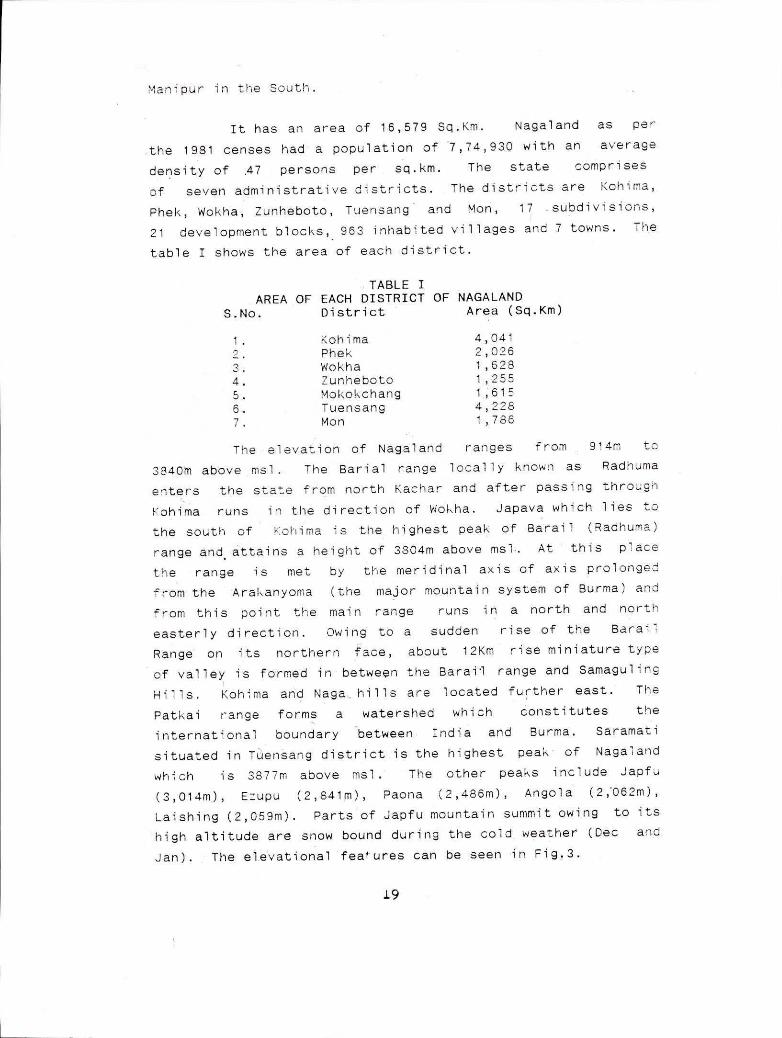
4.3. SPATIAL CORRELATION METHOD

This analysis involJes the calculation of the cross

correlation function between the existing rainfall data taken _r in pairs. Correlation coefficient for different possible

distance are calculated as shown in Table- VII from the

monthly rainfall observation from 1980-1985 for the

stations mentioned in Table-III.

Using 't' test the existence of correlation between d

and r(d) has been ascertained

SL. NO STATION

STATIONS

TABLE - VII DISTANCE - CORRELATION

DISTANCE BETWEEN STATIONS (Km)

CORRELATION COEFFICIENT

1. 1 & 0 63 0.72426 2. 1 & 3 15 0.67724 3. 1 & 4 20 0.83025 4. • 1 & 5 121 0.74280 5. 2 & 3 49 0.72754 6. 2 & 4 51 0.87717 7. 2 & 5 121 0,77429 8. 3 & 4 16 0.74518 9. 3 & 5 116 0.67870 10. 4 & 5 131 0.75996

The variation of correlation coefficient with respect

to distance is shown 'in Fig.5. A straight line is fit (using

least square method) to the plotted pOints.

32

cc

Relative Error E (96) N.)

C0 0

'4

.0

00

-1

1.1 4

.50

0 -

3.00

0 0.0

00

20

.00

0

40

.00

0

60.0

00

Num

ber

of

Gauges

(n)

FIG.7: RELATIVE ERROR OF SPATIAL INTERPOLATION (E ) AS A F

UN

CT

ION

OF

N

tiN

bER

OF

GAUhFC

FOR

NAGALAND

From this_figure it is seen that the straight line

intercepts the 'Y' axis at 0.825 which is the value of p(0)

and corresponding do la found to be 1302 km.

Substituting the above values in eqn.(12) .and in

eqn:(15) the value of E and E/ for the area 16579 Sq.Km.and for

the given n, E ,E1 is calculated to be as shown in Table - VIII;

It may be seen that with an increase of number of gauges

accuracy also increases. However, there is no appreciable

increase in accuracy results with increase in number of gauges

beyond 60.

TABLE - VIII ERROR FOR DIFFERENT NUMBER OF GAUGES

METHOD SL.NO. NO. OF GAUGES E(%)

- SPATIAL

E1(%)

CORRELATION

L(Km) 2 4.27 4.11 97 5 2.66 3.84 61 10 1.86 3.69 43 20 1.31 3.59 30 30 1.07 3.54 25 40 0.92 3.51 21 50 0.82 3.49 19 60 0,75 3.48 17

Hence the required number of gauges is 60.

Fig.6 & 7 shows the variation of the relative error in

the estimation of mean areal rainfall (E) and spatial

interpolation error (ET) as a function of number of gauges.

DiStrict wise relative error of mean areal rainfall (E)

and spatial interpolation (E0 are shown

TABLE - IX

District:- Kohima (Area =4041 Sq.Km) SL.NO. NO. OF GAUGES E(%)

in table

ET(%)

IX.

L(Km) 1. 2 4.03 g.60 48 2. 4 2.83 3.48 34 3. 6 2.30 3.43 27 4. 8 1.99 3.40 24 5. 10 1.78 3.38 21 6. 11 1.69 3.37 20 7. 12 1.62 3.37 19 8. 13 1.56 3.36 18 9. 14 1.50 3.35 18 10. 15 1.45 3.35 17 11. 16 1.40 3.34 17 12. 18 1.32 3.34 16

35

District Phek (Area = SL.NO. NO.

2,026 Sq.Km) OF GAUGES E(%) E1(%)

L(Km)

1 2 4.00 3.49 34

2 4 2.82 3.40 24

3. 6 2.29 3.37 19

4. 8 1.98 3.34 17

5. 9 1.87 3.34 16

6. 10 1.77 3.33 15

7. 12 1.62 3.32 13

8. 14 1.50 3.31 12

9. 16 1.40 3.30 12

10. 18 1.32 3.30 11

District Wokha (Area = 1,628 Sq.Km) SL.NO. NO. OF GAUGES E(%) E1(%) L(Km)

1. 2 3.99 3.46 30

2. 4 2.81 3.38 21

3. 6 2.29 3.35 17

4. 7 2.12 3.34 16

5. 8 1.98 3.33 15

6. 10 1.77 3.32 13

7. 12 1.62 3.31 12

8. 14 1.50 3.30 11

9. 16 1.40 3.29 10

10. 18 1.32 3.29 10

District Zunheboto (Area SL.NO. NO. OF

= 1,255 Sq.Km) GAUGES E(%) EI(%) L(Km)

2 3.99 3.43 26

4 2.81 3.36 18

.3. 5 2.51 3.34 16

4. 6 2.29 3.33 15

5. 7 2.12 3.32 14

6. 8 1.98 3.31 13

7. 9 1.87 3.31 12

8. 10 1.77 3.30 11

9. 12 1.62 3.29 10

10. 14 1.49 3.29 10

11. 16 1.40 3.28 9 12. 18 1.32 3.28 8

District Mokokchung (Areae=; 1,615 SL.NO. NO. OF GAUGES

Sq. Km) E(%) EI(%) L(Km)

1. 2 3..89 3.46 30

2. 4 2.81 3.38 21

3. 6 2.29 2'.35 17

4. 7 2.12 3.34 16

5. 8 1.98 3.33 15

6. 10 1.77 3.32 13

7. 12 1.62 3.31 12

8. 14 1.50 3.30 11

9. 16 1.40 3.29 10

10. 18 1.32 3.29 10

z tr

-c

cc

d-a

>I

c cr

z

re

?I A

=

Er

C

En c

r

— t

r.

z

C

is kill!

Z —

Rel

ativ

e

oo

.

Err

or

E

i ;it

0

0

Rela

tive E

rror

E

0

0

0

0 0

0

0

z 0

-

5 - -

0 a .0

-

a 1"

- p

0

Re

lative

Err

or

E (

e)

& E

. (S

t)

0

0

CC

a In

CD

Rel

ativ

e E

rror

P1

0

PC

o

z o

. -

a

_

ID

W

C) —

III III 11

*c-

o

N.) -

S

CD -

Re

lative

Err

or

E (

z)

&

(s)

0

0

0

0 0

0

I

0

z 0

3 10

Z—

c 3

-

Tr

III II tilil

Rela

tive E

rror

E

0

0

90

z0

-

C 3

-

o _ -

C - -

'3' 0

b—

(e)

& E

(se)

Cu

I I I I!III]

Rel

ativ

e E

rror

E

(s

e) &

E

(s

) C-

0

0

.0

0

- -

C-

00

0

WEAR CATCHMENT ( UK)

NAGALAND

8.0

00 -

6.0

00 -

biZ

CLI 24

.00

0 -

LI

j_

ALIPAR DISTRICT (RAJASTHAN)

cow

cr 2

.000 -

_

0.0

00

iii

0.0

0Q

1

11

11

11

11

11

11

20

.00

0

40

.00

0

Nu

mb

er

of

Ga

ug

es (

n)

FIG. 9: COMPARISON OF VARIATION OF MEAN AREAL RAINFALL ERROR

(E) AS A FUNCTION OF NUMBER OF GAUGES MTH TWO OTHER

AREAS

i 60.0

00

be

8.0

00

- _

ELT

uJ 4.)

> W

1;7,

4.0

00

- '1)

12.0

00 -

ALWAR DISTRICT (RAJASTHAN)

0.000

i

I I

I

I

I I

I

I I

I1

11

11

11

0.0

00

2

0:0

00

4

0.0

00

6

0.0

00

N

um

ber o

f G

auges (

n)

FIG.10. COMPARISON OF VARIATION OF SPATIAL INTERPOLATION ERROR

(E:) AS A FUNCTTON OF NUMBER OF GAUGES WITH TWO OTHER

AREAS

WEAR CATCHMENT

NAGALAND

District Tuensang (Area = 4,228 Sq.Km) 'SL.NO. NO. -OF GAUGES E(%) EI(%) L(Km)

I. 2 4.03 3.61 49 2. 4 2.83 3.49 34 3. 6 2.30 3.44 28 4. 8 1.99 3.41 24 5. 10 1.78 3.39 22 6. 11 1.70 3.38 20 7, 12 1.62 3.37 20 8. 13 1.56 3.36 19 9. 14 1.50 3.36 18 10. 15 1.45 3.35 17 11. 16 1.40 3.35 17 12. 17 1.36 3.34 16 13. 18 1.32 3.34 16

District Mon (Area = 1,786 Sq.Km) SL.NO. NO. OF GAUGES E(%) EI(%) L(Km) 1. 2 4.00 3.47 31 2. 4 2.81 3.39 22 3. 5 2.51 3.37 20 4. 6 2.29 3.36 18 5. 7 2.12 3.35 17 6. 8 1.98 3.34 15 7. 9 1.87 3.33 15 8. 10 1.77 3.32 14 9. 11 1.69 3.32 13 10. 12 1.62 3.31 13 11. 14 1.50 3.30 12 12. 16 1.40 3.30 11 13. 18 1.32 3.29 10

Fig.8 shows the district wise variation of relative of

error on mean areal rainfall (E J and spatial interpolation

error (E1) as a function of number of gauges.

Fig.9. & Fig.10. shows the relative error of mean

areal rainfall (E), spatial interpolation (E1) as a function of

number of raingauges. Similar .analysis done by Mr.E.M.Shaw and

Mr.P.E.O'Connel (4) for Wear catchment (U.K) and by Seth et al

(1986) for Alwar district in Rajasthan (India) are shown in

these figures for the sake of comparison. The general variation

appears to be the same.

4.4. DYMOND AND ZAWADZKI METHODS

Using the eqn (22) & (23) proposed by Dymond (1983) and

by Zawadzki (1973) respectively for finding out the Root Mean

Square Error of basin rainfall as described in section (2.9), the

following table of error vs gauges are computed.

40

TABLE - X STATION ERROR - DYMOND AND

Sl.No. No. of Dymond's stations rms

ZAWADZKI Zawadzki's

error

2 3.24 3.02 5 2.57 1.98 10 2.16 1.44 20 1.82 1.05 30 1.64 0.87 40 1.53 0.76 50 1.45 0(69 60 1.38 0.63

4.5. RECOMMENDATIONS The requirement of number of gauges is found to be 63,.

60 and 60 for ISI Code, C, Method and Spatial Correlation Methods

respectively. The largest requirement of stations amongst these

calculated number of gauges stations -is chosen.

The required number of stations for Nagaland is 63,

out of which 7 number are to be self recorling raingauges (SRRG).

The distribution of gauges both ordinary . cand

self recording for different districts in Nagaland is shown

below in Table XI.

TABLE - XI DISTRICT WISE DISTRIBUTION OF RAINGAUGES

,L.NO. DISTRICT NO. OF GAUGES SRRG 1. Kohima 15 01 2. Pheh OS 01. 3. Wokha 06 01 4. Zunheboto 05 01 5. Mokokchung 06 01 6. Tuensang 16 01 7. Mon 07 01

It should be remembered that the analysis was

carried using 5 stations, mostly covering the lower elevational

area as can be seen in fig.3. As more data are collected a

revision is necessary. While applying the statistical

formulations one should not be over confidence of the accuracy

provided, by them, but also minimum requirPment should be

considered.

-41

5.0. CONCLUSION

The rainfall data observed at five different station

since 1980 are analysed for network design using four different

methods. It is seen that the requirement by both ISI and spatial

methods at spatial interpolation error of 3.35% is the same. The

computations using methods by Dymond(1982) and Zawadzki (1973)

supports the above requirement. It should be remembered that the

statictical estimation made here in are based on comparatively

unreliable data with respect to their spatial variations

(Nagaland being predominantly hilly ). For this reason the above

study can be regarded merely as a first approximation and provide

Only an idea for planning a network. In such hilly terrain, one

would normally tend to recommend a large number of raingauge for

accurate representations of orographic variations, but it is

irrational to include such large number of stations without

definite studies on the rainfall variation structure and without

a definite program on water related activity. On the other hand

one would hesitate to increase the network from five gauges to

sixty three - a twelve fold increase. Having arrived at sixty

three stations from a systematic and scientifically based study,

a network of sixty three stations as per table is recommended.

The data from these sixty three stations could be further

utilised for revising the network.

42

REFERENCE

Aldridge, R.,_1976. The measurement of rainfall at ground level. J.Hydrol.(N.Z),15(1):35-50.

Basalirwa C.P.K, L.J.Ogallo and F.M.Mutua, The design of a regional minimum raingauge network. Water

resource Development, Volume 9, N0.4,1993, page 94. David Sharon, Modelling of correlation function for rainfall

studies. Dymond ,J.(1982) Raingauge network reduction, Journal 'of Hydrology,57,pp.81-91.

Encyclopaedia of India (Nagaland) by Majid Hussain, Rima Publishing House, New Delhi.

Edward, K.A., .1971, Distribution of precipitation in Mountainous areas,WMO tech. Pap 326, 565.

Eddy A. Objective analysis of convective scale rainfall using gauges and radar, Journal of Hydrology Vol.44, No.1/2, Nov 1979.

Felgate D.G. and D.G.Read, Correlation analysis of the cellular structure of storms observed by raingauges, Journal of Hydrology, Vol.24,No.1/2, Jan 1975.

Guide to Hydrological Practices, Vol-I, data acquistion and processing WMO No.168, 1981.,

10.Hydrological network design, needs, problems and approach, WMO, Report No.12, 1968.

11.Hall A.J. (1972) 'Method of selection of areal rainfall stations and the calculation of areal rainfall for flood fore casting purposes'. Aust. Bureau of Meteorology Working paper No.146.

12.Harman, H.H.,(1976), Modern factor analysis (Chicago, IL, Univ. of Chicago -Press.

13.Hendrick, R.L. and Corner, G.H., 1970, Space variations of precipitation and implicatons for raingauge network design. J. Hydrol., 0:151 - 163.

14.Hersfeld.D.M.,1965. On the spacing of raingauges.In:Symposium Design of Hydrological Networks. Int, Assoc. Sci Hydrol., Pub1.65; 72-79.

15.Hutchison, P., 1970. A contitution to the problem Of spacing ' raingauges in rugged terrain. J.Hyool., 12: 1-14.

16.Investigation Ce17 (M.I.), Deptt. of Agriculture, Nagaland, Partial record of Meteorological & Hydrologic& data, Nagaland 1980-1986.

17.Kruizinga and G.J.Yperlaan, Spatial Interpolation of daily totals of rainfall, Journal of Hydrology, Vol.36, No 1/2

18.Kagen, R.L. (1966). An evaluation of the representativeness of precipitation data. WorKs of the Main Geophysical Observatory, USSR, Vol.191.

19.Kassim. AHM and N.T.Kottegoda, Rainfall network design through comparative Kringing method, Hydrological Sciences Journal, Vol.36, No.3, June 1991.

20.Majid Hussain (1988), Nagaland Habitant Society and Shifting Cultivation, Pima Publishing House, New Delhi.

21.Mir. J. Effective rainfall estimation, Journal of Hydrology, Vol 45, No.3/4, Feb. 1980.

22.Mocley, D.A and P.M.Mohaned Ismail, Network density for the estimation of areal rainfall, Hydrological Sciences Journal. ,Vo1,26, No.4, Dec.1981.

43

23.Mohana Rangan.D. and A.B.Palaniappan, Network Design of Raingauge stations for Nagaland (1994), Proc. of the St'l National Symposium on Hydrology, Shillong.

24.Neff, E., 1973. How much rain does a raingauge gauge? J. Hydrol., 35:213-220.

25.Palaniappan, A.B.,(1993) 'Loktak Lake Studies. - Part-1, National Institute of Hydrology, Roorkee, TN-149.

26.Sharp, A.L., Owen, W.J. and Gibbs, A.E., 1961. A comparison of methods for estimating precipitation on watersheds. 42nd Ann. Meet. Am. Geophys. Uni on.

27.Seth,S.M., Ramashastri,K.S., and Vibha Jain (1985-86). Network design of raingauges in Rajasthan State. Report CS-12, National Institute of Hydrology, Roorkee, India.

28.Statistics of North East, North East Council, Shillong. 29.Stol PH. TH, The relative efficiency of the density of

raingauge network, Journal of Hydrology, Vol.XV, No.3, 1972. 30.Unal Sorman and Guven Balkan, An application of network

design procedures for redesigning Kizilirmak river basin rain gauge network Turkey Hydrological Sciences Journal, Vol.28, No.2, June 1983.

31.WM0,(1976) No.433, Report No.68, Hydrological network design and information transfer.

32.WMO, NO.168, 1981, Guide to hydrological Practices. 33.WM0,, Report No.12, 1969, Hydrological Network design, needs,

problems and approaches. 34.Zawadzki, II., 1972. Statistical Studies of Radar

precipitation Patterns. McGill University, Montreal. 99pp. 35.Zawadzki, I.I., 1973. Errors and fluctuations of raingauge

estimates of areal' rainfall. J. Hydrol., 18:243-255.

44

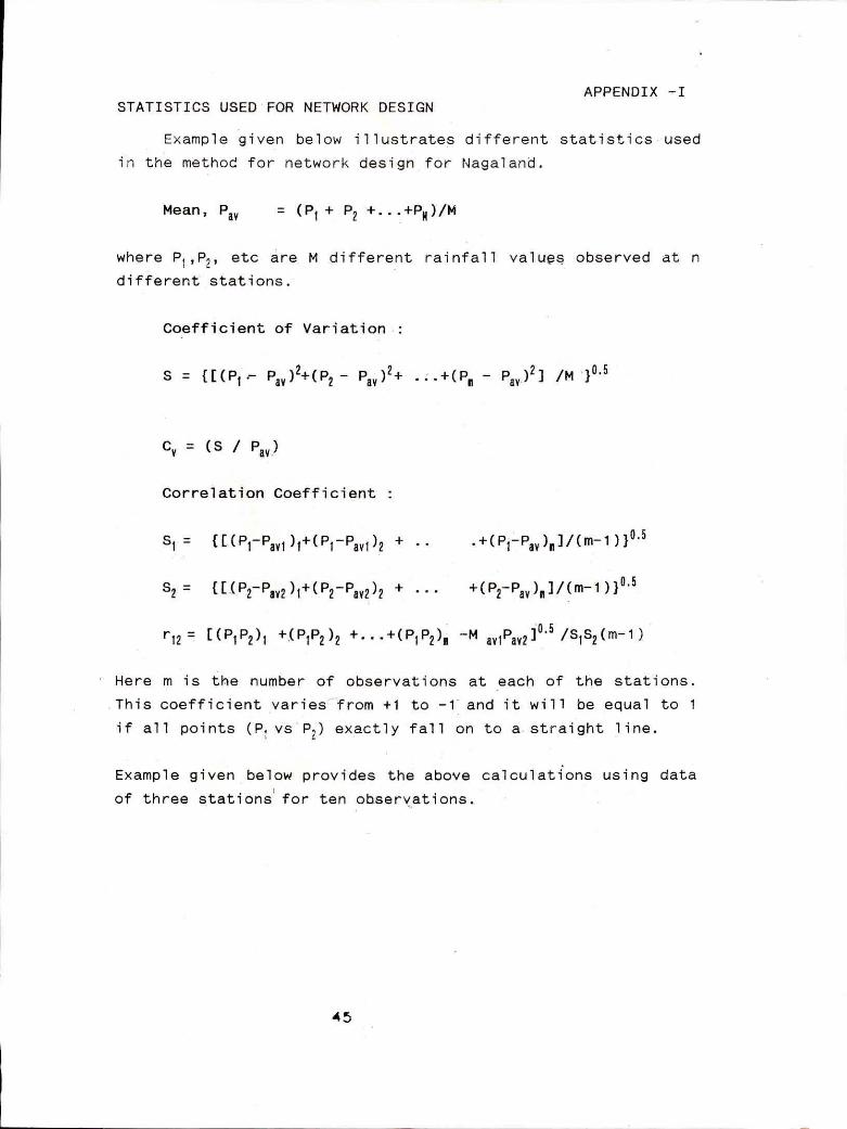
APPENDIX -I STATISTICS USED FOR NETWORK DESIGN

Example given below illustrates different statistics used

in the method for network design for Nagaland.

Mean, Po = (P1 + P2 +...+PN)/M

where PI,PP etc are M different rainfall values observed at n

different stations.

Coefficient of Variation :

S = {[(P/ c P")24-(P2 a - P v)2+ .:.+(PN - Pug] /M 10.5

Cv = (S / P ) aV

Correlation Coefficient :

S1 = [[(P1-Pav1 )1+(P1-Pav1)2 + .+031-130)10/(m-1)1M

s2 = E P2-Pav2 )1 +(P2 -Pav2 ) 2 + • • • +032-Paddgm-1)11"

r12 = E (P1 P2 )1 ÷(P1 P2 )2 +" •+(P1 P2 )m -M av1Pav2 3°3 /5152 (m-1)

Here m is the number of observations at each of the stations.

This coefficient varies from +1 to -1 and it will be equal to 1

if all points (Pi vs P2) exactly fall on to a straight line.

Example given below provides the above calculations using data

of three stations for ten observations.

45

Si .No (mm)

1 1.40 -235.20 55317.47 2 23.00 -213.60 45623.54 3 54.60 -.182.00 33122.79 4 80.20 -156.40 24459.92 5 184.40 -52.20 2724.49 6 491.80 255.20 65128.73 7 243.00 6.40 41.00 8 275.80- 39.20 1536.90 9 397.00 160.40 25729.23 10 178.80 -57.80 3340.45

1 7.80 -228.80 52347.91 2 36.40 -200.20. 40078.70 6 98.00 -138.60 19209.04 4 56.00 -180.60 32615.15 r ._, 205.20 -31.40 985.75 6 577.60 341.00 116283.30 7 247:60 11.00 121.87 8' 208.80 -27.80 772.65 9 189.20 -47.40 2246.44 10 336.20 99.60 9920.83

1 9.60 -227.00 51527.48 2 66.0C -170.60 29103.22 3 144.2C -92.40 8537.14 4 110.8C -125.80 15824.80 5 458.40 221.80 49196.72 6 574.20 337.60 113976.00 7 568.00 331.40 109828.20 8 490.70 254.10 64568.51 9 467.20 230.60 53177.90 10 316.00 79.40 6304.89

MEAN Pa = 236.60 mm = 162.62360 = 169.41940

Correlation coefficient taking stations (1) and (2) = 0.8337933

CHARACTERISTIC OF STATISTICAL STRUCTURE OF A HYDROLOGICAL

PARAMETER.

Extracting statistical characteristic of a random field is

to obtain the structure of covariance and correlation function.

The deviation of a hydrologicl P :

P1 (x,y) = P(x,y) - P (x,y)

.96

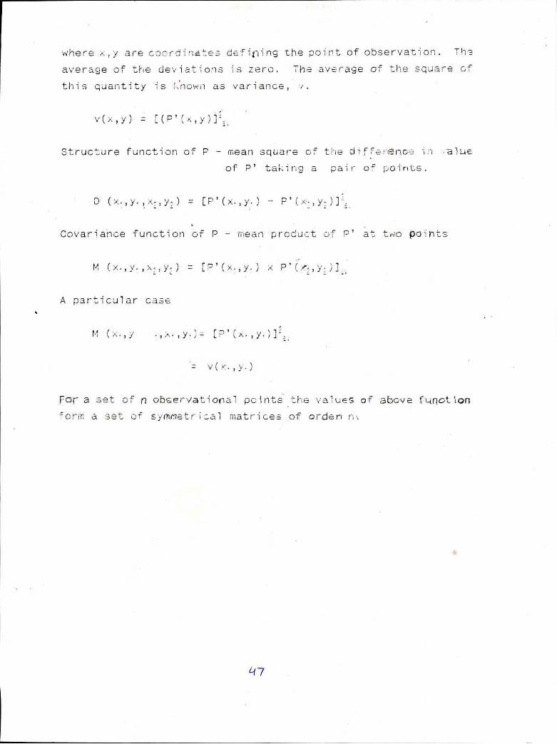
where x,y are coordinates defining the point of observation. Ths

average of the deviations is zero. The average of the square of

this quantity is !Ulown as variance, v.

v(x,y)

Structure function of P - mean square of the difference In alwe

of P' taking a pair of points.

D = [P'(x.,y.) -

Covariance function of P - mean product of P' at two points

M = t ) x

A particular case

M (x. ,y y.). EP'(

v(x.,y.)

For a set of n observational points the values of above function

form a set of symmetrical matrices of order r-K

117

DIRECTOR : S.M. SETH

STUDY GROUP

A.5.PALANIAPPAN SCIENTIST 'E' & HEAD

D.MOHANA RANGAN TECHNICIAN

NETWORK DESIGN OF RAINGAUGE STATIONS FOR ...

Documents

Transcript of NETWORK DESIGN OF RAINGAUGE STATIONS FOR ...