Natural-Scene Statistics Predict How the Figure-Ground Cue of Convexity Affects Human Depth...

Natural-Scene Statistics Predict How the Figure-Ground Cue ofConvexity Affects Human Depth Perception

Johannes Burge1, Charless C. Fowlkes3, and Martin S. Banks21School of Optometry, University of California at Berkeley, Berkeley, California 94720-20202Vision Science Graduate Program, University of California at Berkeley, Berkeley, California94720-20203University of California, Irvine, Irvine, California 92697

AbstractThe shape of the contour separating two regions strongly influences judgments of which region is“figure” and which is “ground.” Convexity and other figure– ground cues are generally assumedto indicate only which region is nearer, but nothing about how much the regions are separated indepth. To determine the depth information conveyed by convexity, we examined natural scenesand found that depth steps across surfaces with convex silhouettes are likely to be larger than stepsacross surfaces with concave silhouettes. In a psychophysical experiment, we found that humansexploit this correlation. For a given binocular disparity, observers perceived more depth when thenear surface’s silhouette was convex rather than concave. We estimated the depth distributionsobservers used in making those judgments: they were similar to the natural-scene distributions.Our findings show that convexity should be reclassified as a metric depth cue. They also suggestthat the dichotomy between metric and nonmetric depth cues is false and that the depthinformation provided many cues should be evaluated with respect to natural-scene statistics.Finally, the findings provide an explanation for why figure– ground cues modulate the responsesof disparity-sensitive cells in visual cortex.

IntroductionEstimating three-dimensional (3D) layout from the two-dimensional retinal images isgeometrically underdetermined, but biological visual systems solve the problem nonetheless.This “inverse optics problem” has generated interest for centuries (Berkeley, 1709; vonHelmholtz, 1867). The current view is that perceived depth is computed from features in theretinal images that provide information about depth in the scene. Theoretical and empiricalresearch of these so-called depth cues has yielded an extensive taxonomy based ongeometric analyses of the information they provide (Palmer, 1999; Bruce et al., 2003). Inthis taxonomy, some cues, like binocular disparity, are called metric depth cues because theyallow the absolute distance between two points in the scene to be recovered via simpletrigonometry. Other cues, such as those indicating occlusion, are called ordinal depth cuesbecause they do not directly indicate the distance between two objects; consequently, theyare said to provide only “information about ordering in depth, but no measure of relative …distance” (Bruce et al., 2003).

Copyright © 2010 the authorsCorrespondence should be addressed to Johannes Burge, 360 Minor Hall, School of Optometry, University of California at Berkeley,Berkeley, CA 94720-2020. [email protected]. .

NIH Public AccessAuthor ManuscriptJ Neurosci. Author manuscript; available in PMC 2011 May 26.

Published in final edited form as:J Neurosci. 2010 May 26; 30(21): 7269–7280. doi:10.1523/JNEUROSCI.5551-09.2010.

NIH

-PA Author Manuscript

NIH


NIH


To estimate depth as accurately and precisely as possible, all relevant information should beused. Experimental evidence suggests that the visual system combines information frommultiple metric depth cues in a statistically optimal manner (Knill and Saunders, 2003;Hillis et al., 2004). However, it is unclear how information from ordinal and metric cuesshould be combined (Landy et al., 1995). Ordinal information conveys only the sign ofdepth between pairs of surfaces, so either the ordinal cue is consistent with the metric cueand provides no additional numerical information, or the cues are inconsistent and it is notobvious how to resolve the conflict. And yet, the shape of an occluder’s silhouette affectsthe perceived depth separation between the occluder and the background even when a metricdepth cue, disparity, is available (Burge et al., 2005; Bertamini et al., 2008).

This counterintuitive result can be understood by considering the depth informationpotentially provided by both disparity and the shape of the occluding contour. Disparity cansignal depth directly although uncertainty arises from noise in disparity measurement(Cormack et al., 1997) and in other signals required to interpret measured disparities(Backus et al., 1999). There is no a priori geometric reason that contour shape shouldprovide metric depth information, but we propose that the convexity of an image region (i.e.,the convexity of a silhouette) is statistically correlated with depth in natural viewing—just asother cues are statistically related (Brunswik and Kamiya, 1953; Hoiem et al., 2005; Saxenaet al., 2005)— and therefore that convexity imparts information about metric depth. If such arelationship exists, any system (human, animal, or machine) could exploit it when estimatingdepth. We measured natural-scene statistics and indeed found a systematic relationshipbetween convexity and depth. In a parallel psychophysical study, we found that humans usethis relationship when estimating 3D layout. These results demonstrate a useful andpreviously unrecognized role for naturalscene statistics in depth perception.

Materials and MethodsMethods for natural-scene analysis

We investigated the hypothesis that figure–ground cues—specifically contour convexity—provide useful metric depth information by examining natural-scene statistics. Depth isdefined as the difference in viewing distance for two points along a line of sight. Weanalyzed the figure–ground cue of convexity because convexity can be readily measured inimages of natural scenes (Fowlkes et al.,2007) and because convexity is known to affectfigure–ground assignment in human perception (Metzger, 1953; Kanizsa and Gerbino,1976).

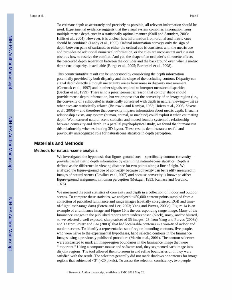
We measured the joint statistics of convexity and depth in a collection of indoor and outdoorscenes. To compute these statistics, we analyzed ~450,000 contour points sampled from acollection of published luminance and range images (spatially coregistered RGB and time-of-flight laser-range data) (Potetz and Lee, 2003; Yang and Purves, 2003a). Figure 1a is anexample of a luminance image and Figure 1b is the corresponding range image. Many of theluminance images in the published reports were underexposed (black), noisy, and/or blurred,so we selected a well exposed, sharp subset of 35 images [23 from Yang and Purves (2003a)and 12 from Potetz and Lee (2003)] that had localizable contours in a variety of indoor andoutdoor scenes. To identify a representative set of region-bounding contours, five people,who were naive to the experimental hypotheses, hand selected contours in the luminanceimages using a previously published procedure (Martin et al., 2001). The contour selectorswere instructed to mark all image-region boundaries in the luminance image that were“important.” Using a computer mouse and software tool, they segmented each image intodisjoint regions. The tool allowed them to zoom in and refine boundaries until they weresatisfied with the result. The selectors generally did not mark shadows or contours for imageregions that subtended <3° (~20 pixels). To assess the selection consistency, two people

Burge et al.

J Neurosci. Author manuscript; available in PMC 2011 May 26.

NIH


NIH


NIH


marked each image. The agreement in their selections was measured using local consistencyerror (LCE) (Martin et al., 2001). The median LCE was 0.13, which is slightly larger thanpreviously reported values of 0.08 (Martin et al., 2001). We did not use the range data tosegment the images because we were investigating the depth information provided by theshape of luminance contours. To use the range image for segmentation would, therefore,undermine the logic of our analysis.

For each point along a selected contour, we computed the distance and the convexity of thelocal image regions on either side of the contour. The local image region was defined by acircular analysis window of fixed radius (2.16°, 15 pixels) centered at each point along aselected contour. To compute depth, we determined the difference between the meandistances to each pixel in the two regions. To compute local convexity, we sampled pairs ofpixels inside both regions and recorded the fraction of pairs for which a line segmentconnecting them lay completely within the region. We defined convexity, c, as the log ratioof the two fractions (Fowlkes et al., 2007). Figure 1e shows convexity along each selectedcontour in the expanded region from Figure 1a. Finally, we determined the frequency ofdifferent depths as a function of region convexity. This analysis (see Fig. 3) is the simplestpossible in that it concerns the relationship between convexity and depth without regard toother image or scene properties. For example, we did not consider how the convexity–depthrelationship varies with scene properties such as the distance to a contour. Later, weconsider how some low-level image properties affect the relationship (see Fig. 10).

Methods for psychophysical experimentsWe conducted three psychophysical experiments. Two experienced observers participated inexperiment 1. Seven and ten observers participated in experiments 2 and 3, respectively. Allhad normal visual acuity and stereopsis. All but one observer in experiment 3 were naive tothe experimental hypotheses.

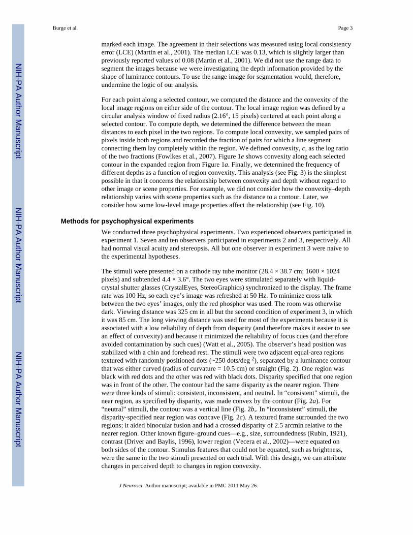
The stimuli were presented on a cathode ray tube monitor (28.4 × 38.7 cm; 1600 × 1024pixels) and subtended 4.4 × 3.6°. The two eyes were stimulated separately with liquid-crystal shutter glasses (CrystalEyes, StereoGraphics) synchronized to the display. The framerate was 100 Hz, so each eye’s image was refreshed at 50 Hz. To minimize cross talkbetween the two eyes’ images, only the red phosphor was used. The room was otherwisedark. Viewing distance was 325 cm in all but the second condition of experiment 3, in whichit was 85 cm. The long viewing distance was used for most of the experiments because it isassociated with a low reliability of depth from disparity (and therefore makes it easier to seean effect of convexity) and because it minimized the reliability of focus cues (and thereforeavoided contamination by such cues) (Watt et al., 2005). The observer’s head position wasstabilized with a chin and forehead rest. The stimuli were two adjacent equal-area regionstextured with randomly positioned dots (~250 dots/deg 2), separated by a luminance contourthat was either curved (radius of curvature = 10.5 cm) or straight (Fig. 2). One region wasblack with red dots and the other was red with black dots. Disparity specified that one regionwas in front of the other. The contour had the same disparity as the nearer region. Therewere three kinds of stimuli: consistent, inconsistent, and neutral. In “consistent” stimuli, thenear region, as specified by disparity, was made convex by the contour (Fig. 2a). For“neutral” stimuli, the contour was a vertical line (Fig. 2b,. In “inconsistent” stimuli, thedisparity-specified near region was concave (Fig. 2c). A textured frame surrounded the tworegions; it aided binocular fusion and had a crossed disparity of 2.5 arcmin relative to thenearer region. Other known figure–ground cues—e.g., size, surroundedness (Rubin, 1921),contrast (Driver and Baylis, 1996), lower region (Vecera et al., 2002)—were equated onboth sides of the contour. Stimulus features that could not be equated, such as brightness,were the same in the two stimuli presented on each trial. With this design, we can attributechanges in perceived depth to changes in region convexity.

Burge et al.


NIH


NIH


NIH


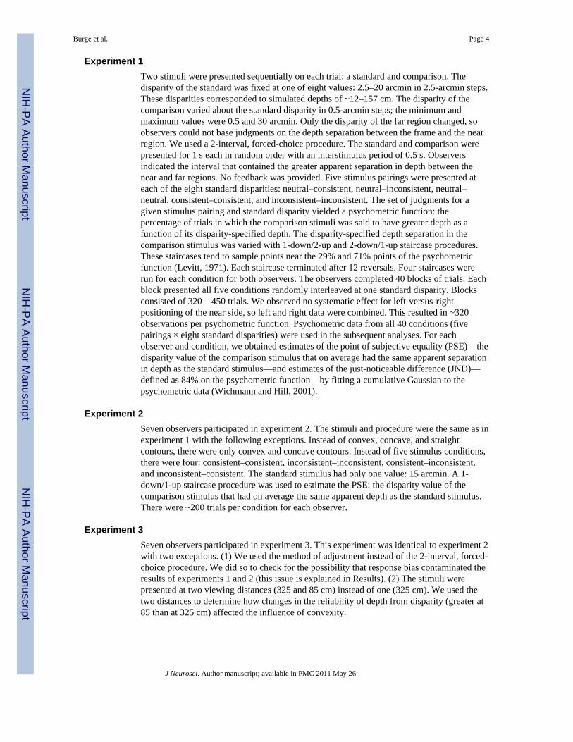
Experiment 1Two stimuli were presented sequentially on each trial: a standard and comparison. Thedisparity of the standard was fixed at one of eight values: 2.5–20 arcmin in 2.5-arcmin steps.These disparities corresponded to simulated depths of ~12–157 cm. The disparity of thecomparison varied about the standard disparity in 0.5-arcmin steps; the minimum andmaximum values were 0.5 and 30 arcmin. Only the disparity of the far region changed, soobservers could not base judgments on the depth separation between the frame and the nearregion. We used a 2-interval, forced-choice procedure. The standard and comparison werepresented for 1 s each in random order with an interstimulus period of 0.5 s. Observersindicated the interval that contained the greater apparent separation in depth between thenear and far regions. No feedback was provided. Five stimulus pairings were presented ateach of the eight standard disparities: neutral–consistent, neutral–inconsistent, neutral–neutral, consistent–consistent, and inconsistent–inconsistent. The set of judgments for agiven stimulus pairing and standard disparity yielded a psychometric function: thepercentage of trials in which the comparison stimuli was said to have greater depth as afunction of its disparity-specified depth. The disparity-specified depth separation in thecomparison stimulus was varied with 1-down/2-up and 2-down/1-up staircase procedures.These staircases tend to sample points near the 29% and 71% points of the psychometricfunction (Levitt, 1971). Each staircase terminated after 12 reversals. Four staircases wererun for each condition for both observers. The observers completed 40 blocks of trials. Eachblock presented all five conditions randomly interleaved at one standard disparity. Blocksconsisted of 320 – 450 trials. We observed no systematic effect for left-versus-rightpositioning of the near side, so left and right data were combined. This resulted in ~320observations per psychometric function. Psychometric data from all 40 conditions (fivepairings × eight standard disparities) were used in the subsequent analyses. For eachobserver and condition, we obtained estimates of the point of subjective equality (PSE)—thedisparity value of the comparison stimulus that on average had the same apparent separationin depth as the standard stimulus—and estimates of the just-noticeable difference (JND)—defined as 84% on the psychometric function—by fitting a cumulative Gaussian to thepsychometric data (Wichmann and Hill, 2001).

Experiment 2Seven observers participated in experiment 2. The stimuli and procedure were the same as inexperiment 1 with the following exceptions. Instead of convex, concave, and straightcontours, there were only convex and concave contours. Instead of five stimulus conditions,there were four: consistent–consistent, inconsistent–inconsistent, consistent–inconsistent,and inconsistent–consistent. The standard stimulus had only one value: 15 arcmin. A 1-down/1-up staircase procedure was used to estimate the PSE: the disparity value of thecomparison stimulus that had on average the same apparent depth as the standard stimulus.There were ~200 trials per condition for each observer.

Experiment 3Seven observers participated in experiment 3. This experiment was identical to experiment 2with two exceptions. (1) We used the method of adjustment instead of the 2-interval, forced-choice procedure. We did so to check for the possibility that response bias contaminated theresults of experiments 1 and 2 (this issue is explained in Results). (2) The stimuli werepresented at two viewing distances (325 and 85 cm) instead of one (325 cm). We used thetwo distances to determine how changes in the reliability of depth from disparity (greater at85 than at 325 cm) affected the influence of convexity.

Burge et al.


NIH


NIH


NIH


Methods for modeling of psychophysicsThe psychophysical results suggest that human observers have incorporated the natural-scene statistics associated with region convexity and depth. We next asked whether theobserved behavior is consistent with the behavior of an ideal observer that has incorporatedthe natural statistics associated with convexity and depth. To do so, we fit the observers’responses with a probabilistic model of depth estimation to determine the probabilitydistributions that provided the best quantitative account of their responses. We modeled theconstruction of the depth percept as a probabilistic process. Assuming conditionalindependence, Bayes’ rule states the following:

(1)

That is, the posterior probability of a particular depth, Δ, given a measurement of disparity,d, across an contour bounding an image region with convexity, c, is equal to the product ofthe likelihood of the disparity measurement for a particular depth, P(d|Δ), the likelihood ofthe convexity measurement for a particular depth, P(c|Δ), and the prior distribution ofdepths, P(Δ), for all such contours, divided by a normalizing constant, P(d,c). The productrule, P(c|Δ)P(Δ) = P(c,Δ), allows us to combine the latter two terms in the numerator intothe joint probability of c and Δ as follows:

(2)

We regroup using the product rule again as follows:

(3)

where 1/[P(d,c)/P(c)] is a normalizing constant, P(d|Δ) is the disparity likelihood, and P(Δ|c) is the convexity–depth distribution, which is the distribution we measured from theluminance range images (Fig. 1). Note that the depth prior, P(Δ), has been absorbed by P(Δ|c).

In this model, both the convexity of an image region and its disparity relative to theadjoining region affect the expected perceived depth. This is illustrated schematically below:Figure 4 shows probability distributions associated with convexity and disparity (left) andthe posterior distributions generated from the products of those distributions (right). Thedisparity signal indicates that the region on one side of the contour is nearer than the regionon the other side. If the region is bounded by a contour that makes it convex (upper left), theconvexity–depth distribution is skewed toward larger depths than when the region isconcave (lower left). As a consequence, the estimated depth will be greater in the convexcase (upper right) than in the concave case (lower right). Said another way, when regionconvexity and disparity are consistent with one another (i.e., both indicate that the sameregion is nearer than the other), perceived depth should be greater than when they areinconsistent.

The disparity likelihood, P(d|Δ), is plotted as a distribution over depth (see Fig. 4). We cando this because of the following relationship between depth and disparity:

Burge et al.


NIH


NIH


NIH


(4)

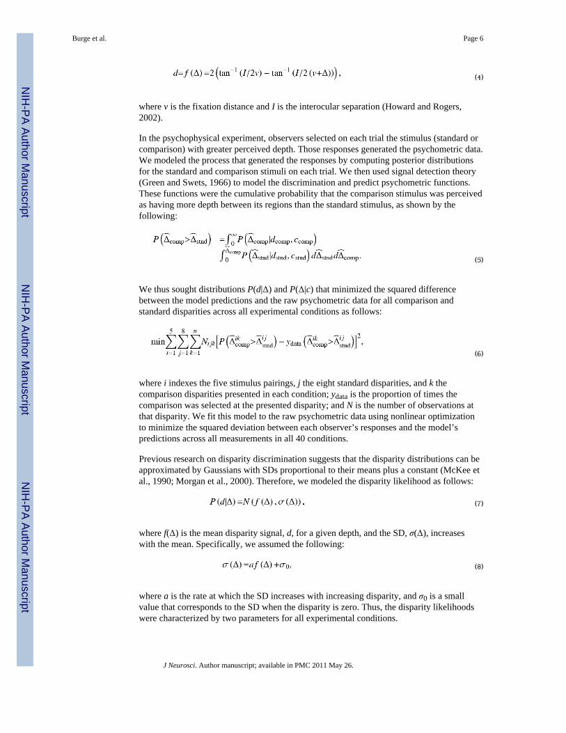
where v is the fixation distance and I is the interocular separation (Howard and Rogers,2002).

In the psychophysical experiment, observers selected on each trial the stimulus (standard orcomparison) with greater perceived depth. Those responses generated the psychometric data.We modeled the process that generated the responses by computing posterior distributionsfor the standard and comparison stimuli on each trial. We then used signal detection theory(Green and Swets, 1966) to model the discrimination and predict psychometric functions.These functions were the cumulative probability that the comparison stimulus was perceivedas having more depth between its regions than the standard stimulus, as shown by thefollowing:

(5)

We thus sought distributions P(d|Δ) and P(Δ|c) that minimized the squared differencebetween the model predictions and the raw psychometric data for all comparison andstandard disparities across all experimental conditions as follows:

(6)

where i indexes the five stimulus pairings, j the eight standard disparities, and k thecomparison disparities presented in each condition; ydata is the proportion of times thecomparison was selected at the presented disparity; and N is the number of observations atthat disparity. We fit this model to the raw psychometric data using nonlinear optimizationto minimize the squared deviation between each observer’s responses and the model’spredictions across all measurements in all 40 conditions.

Previous research on disparity discrimination suggests that the disparity distributions can beapproximated by Gaussians with SDs proportional to their means plus a constant (McKee etal., 1990; Morgan et al., 2000). Therefore, we modeled the disparity likelihood as follows:

(7)

where f(Δ) is the mean disparity signal, d, for a given depth, and the SD, σ(Δ), increaseswith the mean. Specifically, we assumed the following:

(8)

where a is the rate at which the SD increases with increasing disparity, and σ0 is a smallvalue that corresponds to the SD when the disparity is zero. Thus, the disparity likelihoodswere characterized by two parameters for all experimental conditions.

Burge et al.


NIH


NIH


NIH


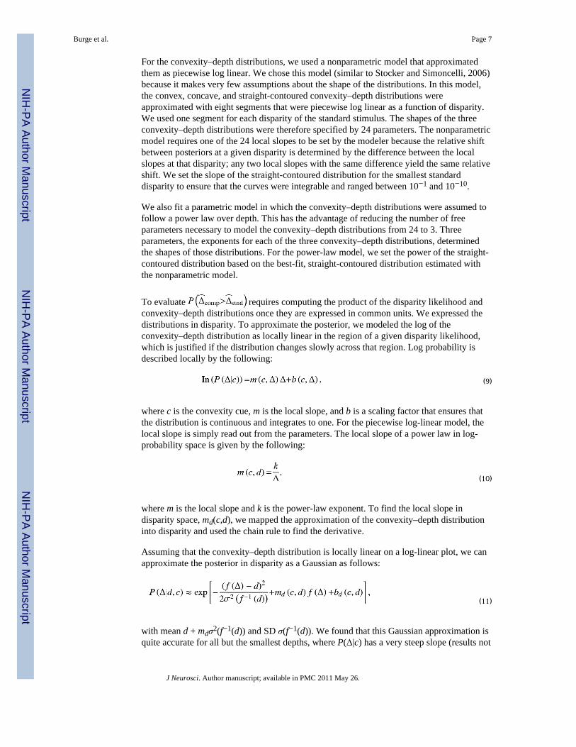
For the convexity–depth distributions, we used a nonparametric model that approximatedthem as piecewise log linear. We chose this model (similar to Stocker and Simoncelli, 2006)because it makes very few assumptions about the shape of the distributions. In this model,the convex, concave, and straight-contoured convexity–depth distributions wereapproximated with eight segments that were piecewise log linear as a function of disparity.We used one segment for each disparity of the standard stimulus. The shapes of the threeconvexity–depth distributions were therefore specified by 24 parameters. The nonparametricmodel requires one of the 24 local slopes to be set by the modeler because the relative shiftbetween posteriors at a given disparity is determined by the difference between the localslopes at that disparity; any two local slopes with the same difference yield the same relativeshift. We set the slope of the straight-contoured distribution for the smallest standarddisparity to ensure that the curves were integrable and ranged between 10−1 and 10−10.

We also fit a parametric model in which the convexity–depth distributions were assumed tofollow a power law over depth. This has the advantage of reducing the number of freeparameters necessary to model the convexity–depth distributions from 24 to 3. Threeparameters, the exponents for each of the three convexity–depth distributions, determinedthe shapes of those distributions. For the power-law model, we set the power of the straight-contoured distribution based on the best-fit, straight-contoured distribution estimated withthe nonparametric model.

To evaluate requires computing the product of the disparity likelihood andconvexity–depth distributions once they are expressed in common units. We expressed thedistributions in disparity. To approximate the posterior, we modeled the log of theconvexity–depth distribution as locally linear in the region of a given disparity likelihood,which is justified if the distribution changes slowly across that region. Log probability isdescribed locally by the following:

(9)

where c is the convexity cue, m is the local slope, and b is a scaling factor that ensures thatthe distribution is continuous and integrates to one. For the piecewise log-linear model, thelocal slope is simply read out from the parameters. The local slope of a power law in log-probability space is given by the following:

(10)

where m is the local slope and k is the power-law exponent. To find the local slope indisparity space, md(c,d), we mapped the approximation of the convexity–depth distributioninto disparity and used the chain rule to find the derivative.

Assuming that the convexity–depth distribution is locally linear on a log-linear plot, we canapproximate the posterior in disparity as a Gaussian as follows:

(11)

with mean d + mdσ2(f−1(d)) and SD σ(f−1(d)). We found that this Gaussian approximation isquite accurate for all but the smallest depths, where P(Δ|c) has a very steep slope (results not

Burge et al.


NIH


NIH


NIH


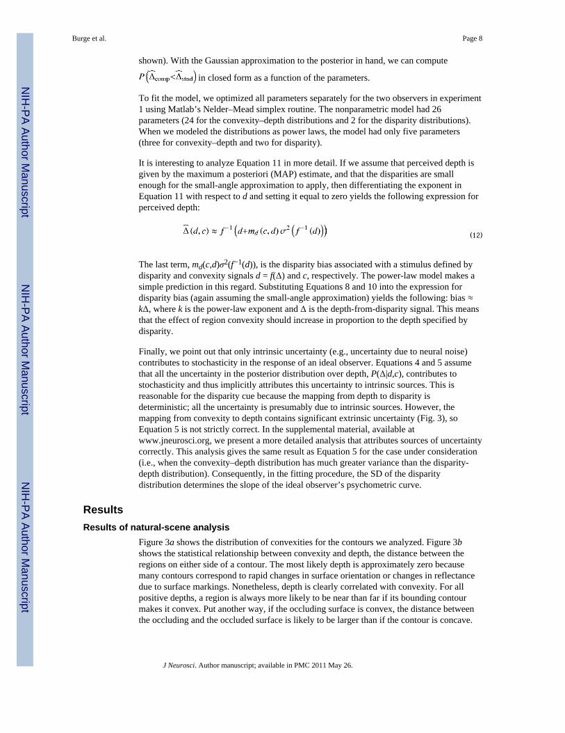
shown). With the Gaussian approximation to the posterior in hand, we can compute

in closed form as a function of the parameters.

To fit the model, we optimized all parameters separately for the two observers in experiment1 using Matlab’s Nelder–Mead simplex routine. The nonparametric model had 26parameters (24 for the convexity–depth distributions and 2 for the disparity distributions).When we modeled the distributions as power laws, the model had only five parameters(three for convexity–depth and two for disparity).

It is interesting to analyze Equation 11 in more detail. If we assume that perceived depth isgiven by the maximum a posteriori (MAP) estimate, and that the disparities are smallenough for the small-angle approximation to apply, then differentiating the exponent inEquation 11 with respect to d and setting it equal to zero yields the following expression forperceived depth:

(12)

The last term, md(c,d)σ2(f−1(d)), is the disparity bias associated with a stimulus defined bydisparity and convexity signals d = f(Δ) and c, respectively. The power-law model makes asimple prediction in this regard. Substituting Equations 8 and 10 into the expression fordisparity bias (again assuming the small-angle approximation) yields the following: bias ≈kΔ, where k is the power-law exponent and Δ is the depth-from-disparity signal. This meansthat the effect of region convexity should increase in proportion to the depth specified bydisparity.

Finally, we point out that only intrinsic uncertainty (e.g., uncertainty due to neural noise)contributes to stochasticity in the response of an ideal observer. Equations 4 and 5 assumethat all the uncertainty in the posterior distribution over depth, P(Δ|d,c), contributes tostochasticity and thus implicitly attributes this uncertainty to intrinsic sources. This isreasonable for the disparity cue because the mapping from depth to disparity isdeterministic; all the uncertainty is presumably due to intrinsic sources. However, themapping from convexity to depth contains significant extrinsic uncertainty (Fig. 3), soEquation 5 is not strictly correct. In the supplemental material, available atwww.jneurosci.org, we present a more detailed analysis that attributes sources of uncertaintycorrectly. This analysis gives the same result as Equation 5 for the case under consideration(i.e., when the convexity–depth distribution has much greater variance than the disparity-depth distribution). Consequently, in the fitting procedure, the SD of the disparitydistribution determines the slope of the ideal observer’s psychometric curve.

ResultsResults of natural-scene analysis

Figure 3a shows the distribution of convexities for the contours we analyzed. Figure 3bshows the statistical relationship between convexity and depth, the distance between theregions on either side of a contour. The most likely depth is approximately zero becausemany contours correspond to rapid changes in surface orientation or changes in reflectancedue to surface markings. Nonetheless, depth is clearly correlated with convexity. For allpositive depths, a region is always more likely to be near than far if its bounding contourmakes it convex. Put another way, if the occluding surface is convex, the distance betweenthe occluding and the occluded surface is likely to be larger than if the contour is concave.

Burge et al.


NIH


NIH


NIH


http://www.jneurosci.org

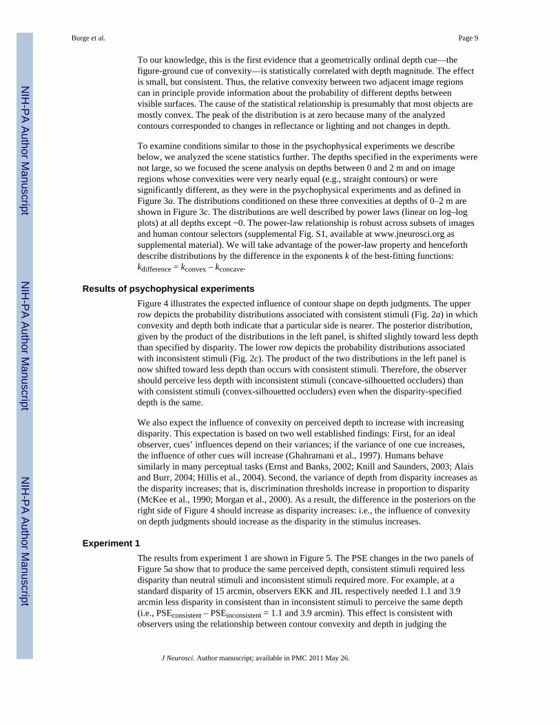
To our knowledge, this is the first evidence that a geometrically ordinal depth cue—thefigure-ground cue of convexity—is statistically correlated with depth magnitude. The effectis small, but consistent. Thus, the relative convexity between two adjacent image regionscan in principle provide information about the probability of different depths betweenvisible surfaces. The cause of the statistical relationship is presumably that most objects aremostly convex. The peak of the distribution is at zero because many of the analyzedcontours corresponded to changes in reflectance or lighting and not changes in depth.

To examine conditions similar to those in the psychophysical experiments we describebelow, we analyzed the scene statistics further. The depths specified in the experiments werenot large, so we focused the scene analysis on depths between 0 and 2 m and on imageregions whose convexities were very nearly equal (e.g., straight contours) or weresignificantly different, as they were in the psychophysical experiments and as defined inFigure 3a. The distributions conditioned on these three convexities at depths of 0–2 m areshown in Figure 3c. The distributions are well described by power laws (linear on log–logplots) at all depths except ~0. The power-law relationship is robust across subsets of imagesand human contour selectors (supplemental Fig. S1, available at www.jneurosci.org assupplemental material). We will take advantage of the power-law property and henceforthdescribe distributions by the difference in the exponents k of the best-fitting functions:kdifference = kconvex – kconcave.

Results of psychophysical experimentsFigure 4 illustrates the expected influence of contour shape on depth judgments. The upperrow depicts the probability distributions associated with consistent stimuli (Fig. 2a) in whichconvexity and depth both indicate that a particular side is nearer. The posterior distribution,given by the product of the distributions in the left panel, is shifted slightly toward less depththan specified by disparity. The lower row depicts the probability distributions associatedwith inconsistent stimuli (Fig. 2c). The product of the two distributions in the left panel isnow shifted toward less depth than occurs with consistent stimuli. Therefore, the observershould perceive less depth with inconsistent stimuli (concave-silhouetted occluders) thanwith consistent stimuli (convex-silhouetted occluders) even when the disparity-specifieddepth is the same.

We also expect the influence of convexity on perceived depth to increase with increasingdisparity. This expectation is based on two well established findings: First, for an idealobserver, cues’ influences depend on their variances; if the variance of one cue increases,the influence of other cues will increase (Ghahramani et al., 1997). Humans behavesimilarly in many perceptual tasks (Ernst and Banks, 2002; Knill and Saunders, 2003; Alaisand Burr, 2004; Hillis et al., 2004). Second, the variance of depth from disparity increases asthe disparity increases; that is, discrimination thresholds increase in proportion to disparity(McKee et al., 1990; Morgan et al., 2000). As a result, the difference in the posteriors on theright side of Figure 4 should increase as disparity increases: i.e., the influence of convexityon depth judgments should increase as the disparity in the stimulus increases.

Experiment 1The results from experiment 1 are shown in Figure 5. The PSE changes in the two panels ofFigure 5a show that to produce the same perceived depth, consistent stimuli required lessdisparity than neutral stimuli and inconsistent stimuli required more. For example, at astandard disparity of 15 arcmin, observers EKK and JIL respectively needed 1.1 and 3.9arcmin less disparity in consistent than in inconsistent stimuli to perceive the same depth(i.e., PSEconsistent – PSEinconsistent = 1.1 and 3.9 arcmin). This effect is consistent withobservers using the relationship between contour convexity and depth in judging the

Burge et al.


NIH


NIH


NIH


http://www.jneurosci.org

separation of the near and far regions in our stimuli. The effect of contour shape increasedsystematically with increasing disparity. This is also expected because the reliability ofdepth from disparity decreases with increasing disparity (McKee et al., 1990;Morgan et al.,2000) so the influence of contour shape should increase with increasing disparity. Theresults thus suggest that contour shape provides metric depth information to humanobservers.

Figure 5b shows that JNDs rose systematically with increasing disparity, as expected, butdid not vary significantly across consistent, inconsistent, and neutral conditions.Interestingly, convexity had a larger influence in observer JIL who had higherdiscrimination thresholds than EKK, the expected result if both observers had internalizedthe same natural-scene statistics for convexity and depth.

Experiment 2To make sure that the observations of experiment 1 would generalize, we performed ashorter version of the experiment with more observers. Figure 6a shows that the sevenobservers exhibited the same pattern of results as the observers in experiment 1. Figure 6bshows the results averaged across observers. On average, consistent stimuli requiredapproximately 2.1 arcmin less disparity than inconsistent stimuli to produce the sameapparent depth. We conducted a repeated-measures, two-factor ANOVA with the standardstimulus type (consistent or inconsistent) as one factor and the relationship between thestandard and comparison stimuli as the other factor (control: conditions in which thestandard and comparison were the same: consistent versus consistent and inconsistent versusinconsistent; or experimental: conditions in which the standard and comparison weredifferent: consistent versus inconsistent and inconsistent versus consistent). The interactionbetween the factors was highly significant (F(1,6) = 34.8; p < 0.0011). A multiple-comparisons test showed that the difference between consistent versus consistent andconsistent versus inconsistent conditions and between inconsistent versus inconsistent andinconsistent versus consistent conditions were both significant. The results from experiment2 show that the effect of contour convexity is generally observed.

Experiment 3Experiment 3 tested the possibility that a response bias, rather than a change in perceiveddepth, was responsible for the effects we observed in experiments 1 and 2 (Gillam et al.,2009). In a 2-interval, forced-choice procedure like ours, observers must choose a stimulusinterval even if they are uncertain about which interval contained more depth. Perhapsobservers in this uncertain state chose the stimulus in which the ordinal depth signaled byconvexity was compatible with the depth ordering specified by disparity. Such a strategycould yield shifts in the PSEs similar to those in Figures 5a and 6a,b. We circumvented thisproblem by using the method of adjustment (Gillam et al., 2009): observers adjusted thedisparity in the comparison stimulus until it appeared to have the same depth as the standardstimulus. By using this technique, we made sure that observers were really equating theperceived depth in the consistent and inconsistent stimuli. Figure 6c shows the results for the325 cm viewing distance. On average, consistent stimuli required approximately 2.4 arcminless disparity than inconsistent stimuli to yield the same perceived depth. A two-factor,repeated-measures ANOVA with the same factors as in experiment 2 revealed a significantinteraction (F(1,9) = 8.68; p < 0.0163). Eight of ten subjects required inconsistent stimuli tohave more disparity than consistent stimuli. Figure 6d shows the results for the 85 cmdistance. Consistent stimuli now required 1.6 arcmin less disparity than inconsistent stimuli.A three-factor, repeated-measures ANOVA revealed a marginally significant three-wayinteraction between standard stimulus type, standard/comparison relationship, and viewingdistance (F(1,9) = 4.50; p < 0.063). The trend toward a smaller effect at the near viewing

Burge et al.


NIH


NIH


NIH


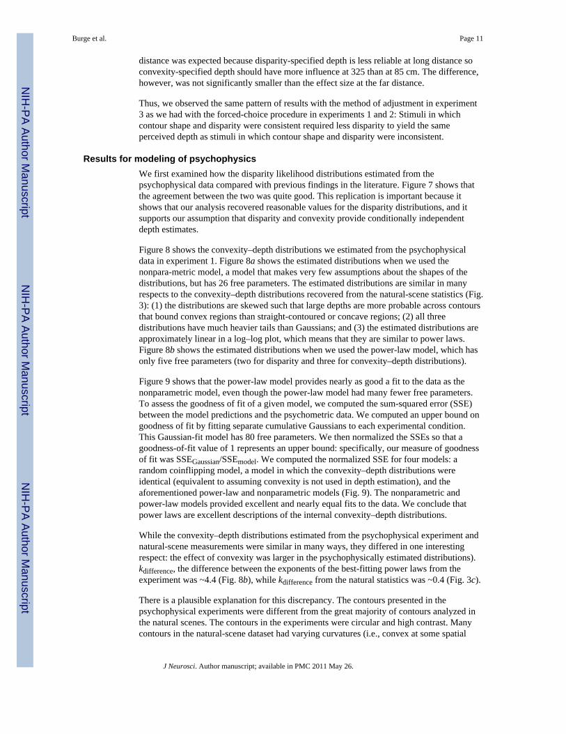
distance was expected because disparity-specified depth is less reliable at long distance soconvexity-specified depth should have more influence at 325 than at 85 cm. The difference,however, was not significantly smaller than the effect size at the far distance.

Thus, we observed the same pattern of results with the method of adjustment in experiment3 as we had with the forced-choice procedure in experiments 1 and 2: Stimuli in whichcontour shape and disparity were consistent required less disparity to yield the sameperceived depth as stimuli in which contour shape and disparity were inconsistent.

Results for modeling of psychophysicsWe first examined how the disparity likelihood distributions estimated from thepsychophysical data compared with previous findings in the literature. Figure 7 shows thatthe agreement between the two was quite good. This replication is important because itshows that our analysis recovered reasonable values for the disparity distributions, and itsupports our assumption that disparity and convexity provide conditionally independentdepth estimates.

Figure 8 shows the convexity–depth distributions we estimated from the psychophysicaldata in experiment 1. Figure 8a shows the estimated distributions when we used thenonpara-metric model, a model that makes very few assumptions about the shapes of thedistributions, but has 26 free parameters. The estimated distributions are similar in manyrespects to the convexity–depth distributions recovered from the natural-scene statistics (Fig.3): (1) the distributions are skewed such that large depths are more probable across contoursthat bound convex regions than straight-contoured or concave regions; (2) all threedistributions have much heavier tails than Gaussians; and (3) the estimated distributions areapproximately linear in a log–log plot, which means that they are similar to power laws.Figure 8b shows the estimated distributions when we used the power-law model, which hasonly five free parameters (two for disparity and three for convexity–depth distributions).

Figure 9 shows that the power-law model provides nearly as good a fit to the data as thenonparametric model, even though the power-law model had many fewer free parameters.To assess the goodness of fit of a given model, we computed the sum-squared error (SSE)between the model predictions and the psychometric data. We computed an upper bound ongoodness of fit by fitting separate cumulative Gaussians to each experimental condition.This Gaussian-fit model has 80 free parameters. We then normalized the SSEs so that agoodness-of-fit value of 1 represents an upper bound: specifically, our measure of goodnessof fit was SSEGaussian/SSEmodel. We computed the normalized SSE for four models: arandom coinflipping model, a model in which the convexity–depth distributions wereidentical (equivalent to assuming convexity is not used in depth estimation), and theaforementioned power-law and nonparametric models (Fig. 9). The nonparametric andpower-law models provided excellent and nearly equal fits to the data. We conclude thatpower laws are excellent descriptions of the internal convexity–depth distributions.

While the convexity–depth distributions estimated from the psychophysical experiment andnatural-scene measurements were similar in many ways, they differed in one interestingrespect: the effect of convexity was larger in the psychophysically estimated distributions).kdifference, the difference between the exponents of the best-fitting power laws from theexperiment was ~4.4 (Fig. 8b), while kdifference from the natural statistics was ~0.4 (Fig. 3c).

There is a plausible explanation for this discrepancy. The contours presented in thepsychophysical experiments were different from the great majority of contours analyzed inthe natural scenes. The contours in the experiments were circular and high contrast. Manycontours in the natural-scene dataset had varying curvatures (i.e., convex at some spatial

Burge et al.


NIH


NIH


NIH


scales and concave at others, like the silhouette of a tree) and low contrast. Perhaps thedifferences in contour properties were the cause of the discrepancy between kdifference for thenatural-scene and psychophysical data. To test this idea, we recomputed the natural-scenestatistics for contours with greater contrast, more consistent convexity, and greater averageconvexity. Figure 10a plots kdifference as a function of the lowest contrast among thecontours included in the analysis. As minimum contrast increases (i.e., as average contrastincreases), kdifference increases monotonically. Figure 10b plots kdifference as a function of theconsistency of convexity across spatial scale. As convexity becomes more consistent (e.g.,contours become more circular), kdifference increases monotonically. Figure 10c plotskdifference as a function of the convexity value. When convexity is near zero (e.g., straightcontours), there is little difference in the convexities of image regions on either side of thecontour and kdifference is low. As convexity increases, the analyzed contours become moresimilar to the contours presented in the psychophysical experiment, and kdifference increases.We would like to have been able to select contours on all three criteria combined, but doingso leads to too few samples to compute meaningful statistics.

The analysis in Figure 10 shows that restricting the contours in the natural-scene dataset tobe more similar to the contours in the psychophysical experiment makes the natural-sceneconvexity–depth distribution more similar to the psychophysically recovered distributions.Unfortunately, we cannot further restrict the contours selected from the scene database tomake them even more similar to the experimental stimuli because doing so yields too fewsamples to calculate meaningful statistics. As more natural-scene data become available, onecould pursue this further.

DiscussionThe depth information in figure–ground cues

Figure–ground cues are image features that bias observers to see one region as occludinganother (Palmer, 1999). Such cues—e.g., convexity, lower region, size, familiarity, contrast—help determine to which region a contour belongs; the figure region appears shaped by thecontour and closer to the viewer. The role of figure–ground cues in biological and machinevision has been investigated extensively (Rubin, 1921; Peterson et al., 1991; Driver andBaylis, 1996; Palmer, 1999; Sugita, 1999; Bakin et al., 2000; Vecera et al., 2002; Burge etal., 2005; Qiu and von der Heydt, 2005; Fowlkes et al., 2007; Bertamini et al., 2008), but nocomprehensive theory of how figure–ground cues affect contour assignment and depthperception has emerged. Our analysis of natural-scene statistics reveals why convexity is acue to occlusion and metric depth, the probabilistic model shows how convexity might beintegrated with well established metric depth cues, and the psychophysical results areconsistent with this form of integration.

Many other figure–ground cues could affect metric depth percepts in similar manner.Consider the cue of lower region (Vecera et al., 2002). Because objects typically rest on theground plane, positions low in the visual field are likely to be nearer to the viewer thanpositions high in the field (Huang et al., 2000; Potetz and Lee, 2003; Yang and Purves,2003b,. In our analysis of natural-scene statistics, we observed that the asymmetry in thedistribution of depth was affected more by elevation in the visual field than by contourconvexity. We therefore expect larger perceptual effects from lower region than fromconvexity. Psychophysical experiments confirm this expectation: Lower region andconvexity determine figural assignment ~70% and ~60% of the time, respectively (Vecera etal., 2002; Peterson and Skow, 2008). Lower region is also a better predictor than convexityof depth-ordering judgments in images of natural scenes (Fowlkes et al., 2007).

Burge et al.


NIH


NIH


NIH


Two other phenomena are consistent with our claim that figure–ground cues provide metricdepth information. First, a monocularly viewed sequence of stacking disks generates a vividsense of movement toward the viewer (Engel et al., 2006). By the traditional taxonomy, thedepth cues in this stimulus—T-junctions (Palmer, 1999), surroundedness, and size (Rubin,1921)—provide only ordinal information. Second, a monocularly viewed moving disk thatoccludes a background of vertical bars when translating leftward and is occluded by the barswhen moving rightward is perceived as moving elliptically in depth; it also elicits vergenceeye movements consistent with an elliptical path (Ringach, 1996). If cues to occlusionprovide only distance-ordering information, standard models cannot explain these motion-in–depth percepts, nor the vergence eye movements induced by the second stimulus.However, if occlusion cues provide metric information, as proposed here, the percepts andeye movements are readily understood.

Other depth cuesMany other depth cues such as aerial perspective (Troscianko et al., 1991), shading(Koenderink and van Doorn, 1992), and blur (Mather and Smith, 2000) are regarded asnonmetric because from the cue value alone, one cannot uniquely determine depth. Wepropose that this taxonomy is unnecessary and that the visual system uses the information inthose cues probabilistically to refine estimates of metric depth. By capitalizing on thestatistical relationship between images and the environment to which our visual systemshave been exposed, the probabilistic approach will yield a richer understanding of how weperceive 3D layout.

The usefulness of treating depth cues in a probabilistic framework is further evidenced byrecent results in computer vision (Hoiem et al., 2005; Saxena et al., 2005) in which machine-learning techniques were used to combine statistical information about depth and surfaceorientation provided by a diverse set of image features. From the information in thesefeatures, the algorithms could generate reasonably accurate estimates of 3D scene layout.These results confirm that useful metric information is available from image features thathave traditionally been considered nonmetric depth cues. The results also reveal that usefuldepth information is available from image features that have not yet been identified as depthcues.

Neurophysiology and figure–ground cuesFigure–ground cues affect the responses of many neurons in early visual areas. For example,the responses of V2 and V4 neurons to the figure–ground cues of surroundedness and sizehave been studied. A small square of one luminance—defined by surroundedness and size—was presented on a uniform background of another luminance (Zhou et al., 2000). Eventhough the information specifying “figure” was outside the classical receptive field, manyneurons responded more to the contour when the square was on the preferred side of thecontour. Other research has found that many V2 neurons selective for disparity-definedcontours specifying that one side of the contour is near, also respond to figure–ground-defined contours indicating that the same side is near. Importantly, these neurons respondmore vigorously when disparity and figure–ground cues are consistent than when they areinconsistent (Qiu and von der Heydt, 2005). It would be interesting to investigate whetherconvexity modulates responses in similar manner.

Sensitivity to the consistency of disparity and figure–ground cues has been demonstrated inother ways. Most V1 and V2 neurons respond vigorously to extended bars of the preferredorientation. When a small patch covers the classical receptive field but only partiallyobscures the stimulus bar, the response of some V1 and many V2 neurons depend stronglyon the patch’s disparity relative to the bar: They barely respond when disparity specifies that

Burge et al.


NIH


NIH


NIH


the patch is in the plane of the bar or behind it, but respond vigorously when disparityspecifies that the patch is in front (Sugita, 1999; Bakin et al., 2000).

These neurophysiological results are consistent with the view that a representation of cue-invariant object boundaries emerges in processing from V1 through V2 to V4 (Orban, 2008).The neurons involved in this representation may mediate the perceptual effects reportedhere. A given disparity stimulates numerous cortical neurons with different preferreddisparities (Poggio et al., 1988). Presumably, perceived depth is determined by a read-outfrom the noisy population response. When a figure–ground cue is added specifying askewed distribution of depths, the cue may increase the response of neurons with disparitypreferences consistent with the cue and/or decrease the responses of neurons withinconsistent disparity preferences. This could yield an increase in the perceived metricdepth.

Natural-scene statisticsThe importance of natural-scene statistics in perceptual tasks was first articulated byBrunswik (Brunswik and Kamiya, 1953) who argued that Gestalt cues could and should beecologically validated. The role of natural-scene statistics has since been investigated inrelation to several perceptual tasks: contour grouping (Geisler et al., 2001; Elder andGoldberg, 2002; Ren and Malik, 2002), figure–ground assignment (Fowlkes et al., 2007),and length estimation (Howe and Purves, 2002). It is useful to distinguish this work from amuch larger literature on the relationship between the statistics of natural images and theefficiency of neural coding in early visual pathways (Barlow, 1961; Simoncelli andOlshausen, 2001). To determine encoding efficiency, one must know the statistics of theimage properties to be encoded, so recent work has focused on measuring natural-imagestatistics and determining if cortical neurons exploit those statistics (Olshausen and Field,1996; Vinje and Gallant, 2000).

It is unclear, however, that efficient encoding is the primary task of early visual processing.To make strong claims about the role of natural statistics in perception, we believe it isimportant to study tasks that are known to be critical for the biological system under study.This makes it possible to distinguish suboptimal performance from a mistaken hypothesisabout what the system does. Surely, estimating the 3D layout of the environment is a crucialtask because such estimation is required for guidance of visuomotor behavior (Geisler,2008). It is plausible, therefore, that natural selection would work toward the incorporationof 3D information contained in natural-scene statistics.

Closing the loop in probabilistic models of perceptionA key idea in the probabilistic characterization of perception is that perceptual systems haveinternalized the statistical properties of their sensors and the natural environment, and thatthe systems use those properties efficiently to make optimal perceptual estimates. Manyobservations in the literature are compatible with this framework. These include the findingsthat the variances of multiple sources of sensory information are integrated optimally (Ernstand Banks, 2002; Knill and Saunders, 2003; Alais and Burr, 2004). There has also beenwork motivated by the idea that prior information affects perception optimally (Mamassianand Goutcher, 2001; Weiss et al., 2002). However, previous work has not demonstrated thatperceptual systems do in fact behave optimally.

For example, perceived speed decreases when the contrast of the moving stimulus is reduced(Weiss et al., 2002; Stocker and Simoncelli, 2006). This effect can be understood if weassume that the visual system has a prior for slow motion. With lower contrast, the varianceof sensory measurement increases so the prior is expected to have greater influence; it pulls

Burge et al.


NIH


NIH


NIH


perceived speed toward zero. By varying contrast, Stocker and Simoncelli (2006) estimatedthe speed prior from psychophysical data. Although the estimated prior is consistent withseveral phenomena in motion perception (Weiss et al., 2002), there is no evidence that theestimated prior actually matches the distributions of speeds encountered in natural viewing.Thus, it cannot be argued from psychophysical analysis alone that the visual system hasaccurately internalized statistical properties of the environment.

The work described here attempts to close this gap by measuring the statistics from naturalscenes and seeing whether observers have internalized those same statistics. We showed thatpeople behave as if they use an asymmetric convexity–depth distribution when makingdepth judgments in the presence of a region-bounding contour. The convexity–depthdistribution that best explains their behavior is qualitatively similar to the distribution fornatural scenes. Our experiment thus demonstrates the ecological validity of convexity as acue to metric depth and explains its usefulness to the visual system. But we too have not yetclosed the above-mentioned gap because the distributions estimated from thepsychophysical data were not quantitatively the same as the natural-scene distributions.Thus, with the possible exception of findings in categorical perception (Geisler et al., 2001;Elder and Goldberg, 2002; Ren and Malik, 2002, Fowlkes et al., 2007), the field still awaitsevidence that the internalized statistics really do match the statistics of natural scenes.

SummaryIn the analysis of natural-scene statistics, we found that the convexity of an image regionprovides information about the probability of different depths across the contour boundingthat region. We constructed a probabilistic model of how this information can be used tomaximize the accuracy of depth estimates. In psychophysical experiments, we showed thatconvexity affects depth estimation in a manner consistent with such a model. Our work thusestablishes the ecological validity of the figure–ground cue of convexity and its usefulnessto the human viewers. The increasing availability of natural-scene datasets of theenvironmental properties the visual system seeks to estimate—depth, velocity, surfaceorientation, object identity—should allow similar undertakings for many cues and tasks andguide the study of neural mechanisms that underlie the relationship between scene statisticsand perceptual estimates.

Supplementary MaterialRefer to Web version on PubMed Central for supplementary material.

AcknowledgmentsThis work was supported by the American Optometric Foundation’s William C. Ezell Fellowship to J.B. andResearch Grants R01-EY12851 (National Institutes of Health) and BCS-0617701 (National Science Foundation) toM.S.B. We thank Ahna Girshick, Mike Landy, Jitendra Malik, Steve Palmer, and Mary Peterson for helpfuldiscussion and Zhiyong Yang, Dale Purves, Brian Potetz, and Tai Sing Lee for making their natural-scene datasetsavailable.

ReferencesAlais D, Burr D. The ventriloquist effect results from near-optimal cross-modal integration. Curr Biol.

2004; 14:257–262. [PubMed: 14761661]Backus BT, Banks MS, van Ee R, Crowell JA. Horizontal and vertical disparity, eye position, and

stereoscopic slant perception. Vision Res. 1999; 39:1143–1170. [PubMed: 10343832]Bakin JS, Nakayama K, Gilbert CD. Visual responses in monkey areas V1 and V2 to three-

dimensional surface configurations. J Neurosci. 2000; 20:8188–8198. [PubMed: 11050142]

Burge et al.


NIH


NIH


NIH


Barlow, HB. Possible principles underlying the transformation of sensory messages. In: Rosenblith,WA., editor. Sensory communication. MIT; Cambridge, MA: 1961. p. 217-234.

Berkeley, G. An essay toward a new theory of vision. Pepyat; Dublin: 1709.Bertamini M, Martinovic J, Wuerger SM. Integration of ordinal and metric cues in depth processing. J

Vis. 2008; 8:1–12. [PubMed: 18318636]Bruce, V.; Green, PR.; Georgeson, MA. Visual perception: Physiology, psychology, and ecology.

Psychology; New York: 2003.Brunswik E, Kamiya J. Ecological cue validity of “Proximity” and of other gestalt factors. Am J

Psychol. 1953; 66:20–32. [PubMed: 13030843]Burge J, Peterson MA, Palmer SE. Ordinal configural cues combine with metric disparity in depth

perception. J Vis. 2005; 5:534–542. [PubMed: 16097866]Cormack LK, Landers DD, Ramakrishnan S. Element density and the efficiency of binocular

matching. J Opt Soc Am. 1997; 14:723–730.Driver J, Baylis GC. Edge-assignment and figure-ground organization in short term visual matching.

Cogn Psychol. 1996; 31:248–306. [PubMed: 8975684]Elder JH, Goldberg RM. Ecological statistics of Gestalt laws for the perceptual organization of

contours. J Vis. 2002; 2:324–353. [PubMed: 12678582]Engel SA, Remus DA, Sainath R. Motion from occlusion. J Vis. 2006; 6:649–652. [PubMed:

16881795]Ernst MO, Banks MS. Humans integrate visual and haptic information in a statistically optimal

fashion. Nature. 2002; 415:429–433. [PubMed: 11807554]Fowlkes CC, Martin D, Malik J. Local figure/ground cues are valid for natural images. J Vis. 2007;

7:1–9.Geisler WS. Visual perception and the statistical properties of natural scenes. Annu Rev Psychol.

2008; 59:10.1–10.26.Geisler WS, Perry JS, Super BJ, Gallogly DP. Edge co-occurrence in natural images predicts contour

grouping performance. Vision Res. 2001; 41:711–724. [PubMed: 11248261]Ghahramani, Z.; Wolpert, DM.; Jordan, MI. Computational models of sensorimotor integration. In:

Morasso, PG.; Sanguineti, V., editors. Self-organization, computational maps and motor control.Elsevier; Amsterdam: 1997. p. 117-147.

Gibson BS, Peterson MA. Does orientation-independent object recognition precede orientation-dependent recognition? Evidence form a cuing paradigm. J Exp Psychol. 1994; 28:299–316.

Gillam BJ, Anderson BL, Rizwi F. Failure of facial configural cues to alter metric stereoscopic depth.J Vis. 2009; 9:3, 1–5. [PubMed: 19271873]

Green, DM.; Swets, JA. Signal detection theory and psychophysics. Wiley; New York: 1966.Hillis JM, Watt SJ, Landy MS, Banks MS. Slant from texture and disparity cues: optimal cue

combination. J Vis. 2004; 4:967–992. [PubMed: 15669906]Hoiem, D.; Efros, AA.; Hebert, M. Geometric context from a single image; IEEE International

Conference on Computer Vision; Beijing. 2005; October.Howard, IP.; Rogers, BJ. Seeing in depth. Vol 2. Depth perception. Oxford UP; New York: 2002.Howe CQ, Purves D. Range image statistics can explain the anomalous perception of length. Proc Natl

Acad Sci U S A. 2002; 99:13184–13188. [PubMed: 12237401]Huang, J.; Lee, AB.; Mumford, D. Statistics of range images; Proceedings of the IEEE Conference on

Computational Vision and Pattern Recognition; IEEE: Hilton Head Island, SC. 2000; p. 324-331.Kanizsa, G.; Gerbino, W. Convexity and symmetry in figure-ground organization. In: Henle, M.,

editor. Vision and artifact. Springer; New York: 1976. p. 25-32.Knill DC, Saunders JA. Do humans optimally integrate stereo and texture information to slant? Vision

Res. 2003; 43:2539–2558. [PubMed: 13129541]Koenderink JJ, van Doorn AJ. Surface shape and curvatures scales. Image Vis Comput. 1992; 10:557–

565.Landy MS, Maloney LT, Johnston EB, Young M. Measurement and modeling of depth cue

combination: in defense of weak fusion. Vision Res. 1995; 35:389–412. [PubMed: 7892735]

Burge et al.


NIH


NIH


NIH


Levitt H. Transformed up-down methods in psychoacoustics. J Opt Soc Am. 1971; 49:467–477.Mamassian P, Goutcher R. Prior knowledge on the illumination position. Cognition. 2001; 81:B1–B9.

[PubMed: 11525484]Martin, D.; Fowlkes, CC.; Tal, D.; Malik, J. A database of human segmented natural images and its

application to evaluating segmentation algorithms and measuring ecological statistics. ICCV;Vancouver: 2001.

Mather G, Smith DR. Depth cue integration: stereopsis and image blur. Vision Res. 2000; 40:3501–3506. [PubMed: 11115677]

McKee SP, Levi DM, Bowne SF. The imprecision of stereopsis. Vision Res. 1990; 30:1763–1779.[PubMed: 2288089]

Metzger, F. Gesetze des Sehens. Waldemar Kramer; Frankfurt: 1953.Morgan MJ, Watamaniuk SN, McKee SP. The use of an implicit standard for measuring

discrimination thresholds. Vision Res. 2000; 40:2341–2349. [PubMed: 10927119]Olshausen BA, Field DJ. Emergence of simple-cell receptive field properties by learning a sparse code

for natural images. Nature. 1996; 381:607–609. [PubMed: 8637596]Orban GA. Higher order visual processing in macaque extrastriate cortex. Physiol Rev. 2008; 88:59–

89. [PubMed: 18195083]Palmer, SE. Vision science: photons to phenomenology. Bradford Books, MIT; Cambridge, MA:

1999.Peterson MA, Skow E. Inhibitory competition between shape properties in figure-ground perception. J

Exp Psychol. 2008; 32:251–267.Peterson MA, Harvey EM, Weidenbacher HJ. Shape recognition contributions to figure-ground

organization: which route counts? J Exp Psychol Hum Percept Perform. 1991; 17:1075–1089.[PubMed: 1837298]

Poggio GF, Gonzalez F, Krause F. Stereoscopic mechanisms in monkey visual cortex: binocularcorrelation and disparity selectivity. J Neurosci. 1988; 8:4531–4550. [PubMed: 3199191]

Potetz B, Lee TS. Statistical correlations between 2D images and 3D structures in natural scenes. J OptSoc Am. 2003; 20:1292–1303.

Qiu FT, von der Heydt R. Figure and ground in the visual cortex: V2 combines stereoscopic cues withGestalt rules. Neuron. 2005; 47:155–166. [PubMed: 15996555]

Ren, X.; Malik, J. A probabilistic multi-scale model for contour completion based on image statistics.Vol. 1. ECCV; Copenhagen: 2002. p. 312-327.

Ringach, DL. PhD dissertation. New York University; 1996. Binocular eye movements caused by theperception of three-dimensional structure from motion.

Rubin, E. Visuell wahrgenommene Figuren. Glydenalske Boghandel; Copenhagen: 1921.Saxena, A.; Chung, SH.; Ng, A. Learning depth from single monocular images. Neural information

processing systems; Proceedings of Conference on Neural Information Processing Systems(NIPS); Cambridge, MA: MIT. 2005; p. 1161-1168.

Simoncelli EP, Olshausen BA. Natural image statistics and neural representation. Annu Rev Neurosci.2001; 24:1193–1216. [PubMed: 11520932]

Stocker AA, Simoncelli EP. Noise characteristics and prior expectations in human visual speedperception. Nat Neurosci. 2006; 9:578–585. [PubMed: 16547513]

Sugita Y. Grouping of image fragments in primary visual cortex. Nature. 1999; 401:269–272.[PubMed: 10499583]

Troscianko T, Montagnon R, Le Clerc J, Malbert E, Chanteau PL. The role of color as a monoculardepth cue. Vision Res. 1991; 31:1923–1929. [PubMed: 1771776]

Vecera SP, Vogel EK, Woodman GF. Lower region: a new cue for figure-ground assignment. J ExpPsychol. 2002; 131:194–205.

Vinje WE, Gallant JL. Sparse coding and decorrelation in primary visual cortex during natural vision.Science. 2000; 287:1273–1276. [PubMed: 10678835]

von Helmholtz, H. Handbuch der physiologischen Optik. Leopold Voss; Leipzig: 1867.Watt SJ, Akeley K, Ernst MO, Banks MS. Focus cues affect perceived depth. J Vis. 2005; 5:834–862.

[PubMed: 16441189]

Burge et al.


NIH


NIH


NIH


Weiss Y, Simoncelli EP, Adelson EH. Motion illusions as optimal percepts. Nat Neurosci. 2002;5:598–604. [PubMed: 12021763]

Wichmann FA, Hill NJ. The psychometric function: I. Fitting, sampling and goodness-of-fit. PerceptPsychophys. 2001; 63:1293–1313. [PubMed: 11800458]

Yang Z, Purves D. Image/source statistics in natural scenes. Network: Computation in Neural Systems.2003a; 14:371–390.

Yang Z, Purves D. A statistical explanation of visual space. Nat Neurosci. 2003b; 6:632–640.[PubMed: 12754512]

Zhou H, Friedman HS, von der Heydt R. Coding of border ownership in monkey visual cortex. JNeurosci. 2000; 20:6594–6611. [PubMed: 10964965]

Burge et al.


NIH


NIH


NIH


Figure 1.Luminance and range images. a, An example luminance image. b, Corresponding rangeimage. Blue indicates nearer distances, yellow intermediate distances, and red fartherdistances. c, Close-up of the luminance image with a representative hand selection overlaid.d, Close-up of the associated range image with the same selection overlaid. e, The sameimage as d, but with convexity flags added. Flags point toward the image region that wasclassified as more convex. Longer flags correspond to larger convexity values.

Burge et al.


NIH


NIH


NIH


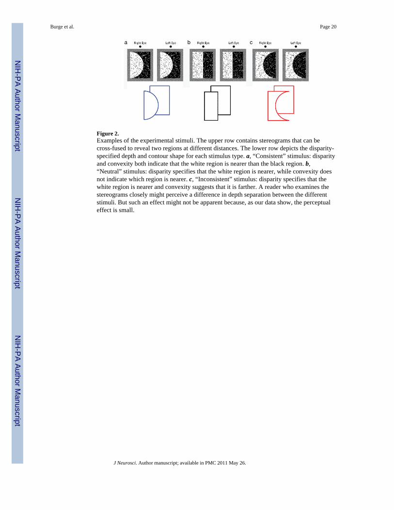
Figure 2.Examples of the experimental stimuli. The upper row contains stereograms that can becross-fused to reveal two regions at different distances. The lower row depicts the disparity-specified depth and contour shape for each stimulus type. a, “Consistent” stimulus: disparityand convexity both indicate that the white region is nearer than the black region. b,“Neutral” stimulus: disparity specifies that the white region is nearer, while convexity doesnot indicate which region is nearer. c, “Inconsistent” stimulus: disparity specifies that thewhite region is nearer and convexity suggests that it is farther. A reader who examines thestereograms closely might perceive a difference in depth separation between the differentstimuli. But such an effect might not be apparent because, as our data show, the perceptualeffect is small.

Burge et al.


NIH


NIH


NIH


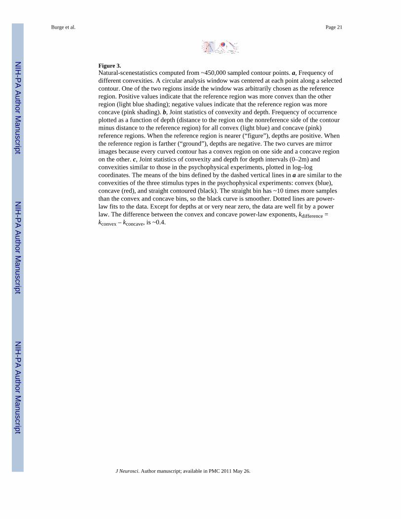
Figure 3.Natural-scenestatistics computed from ~450,000 sampled contour points. a, Frequency ofdifferent convexities. A circular analysis window was centered at each point along a selectedcontour. One of the two regions inside the window was arbitrarily chosen as the referenceregion. Positive values indicate that the reference region was more convex than the otherregion (light blue shading); negative values indicate that the reference region was moreconcave (pink shading). b, Joint statistics of convexity and depth. Frequency of occurrenceplotted as a function of depth (distance to the region on the nonreference side of the contourminus distance to the reference region) for all convex (light blue) and concave (pink)reference regions. When the reference region is nearer (“figure”), depths are positive. Whenthe reference region is farther (“ground”), depths are negative. The two curves are mirrorimages because every curved contour has a convex region on one side and a concave regionon the other. c, Joint statistics of convexity and depth for depth intervals (0–2m) andconvexities similar to those in the psychophysical experiments, plotted in log–logcoordinates. The means of the bins defined by the dashed vertical lines in a are similar to theconvexities of the three stimulus types in the psychophysical experiments: convex (blue),concave (red), and straight contoured (black). The straight bin has ~10 times more samplesthan the convex and concave bins, so the black curve is smoother. Dotted lines are power-law fits to the data. Except for depths at or very near zero, the data are well fit by a powerlaw. The difference between the convex and concave power-law exponents, kdifference =kconvex – kconcave, is ~0.4.

Burge et al.


NIH


NIH


NIH


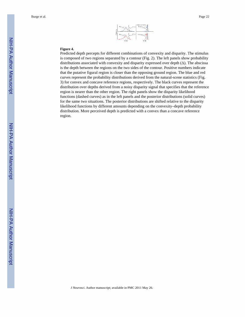
Figure 4.Predicted depth percepts for different combinations of convexity and disparity. The stimulusis composed of two regions separated by a contour (Fig. 2). The left panels show probabilitydistributions associated with convexity and disparity expressed over depth (Δ). The abscissais the depth between the regions on the two sides of the contour. Positive numbers indicatethat the putative figural region is closer than the opposing ground region. The blue and redcurves represent the probability distributions derived from the natural-scene statistics (Fig.3) for convex and concave reference regions, respectively. The black curves represent thedistribution over depths derived from a noisy disparity signal that specifies that the referenceregion is nearer than the other region. The right panels show the disparity likelihoodfunctions (dashed curves) as in the left panels and the posterior distributions (solid curves)for the same two situations. The posterior distributions are shifted relative to the disparitylikelihood functions by different amounts depending on the convexity–depth probabilitydistribution. More perceived depth is predicted with a convex than a concave referenceregion.

Burge et al.


NIH


NIH


NIH


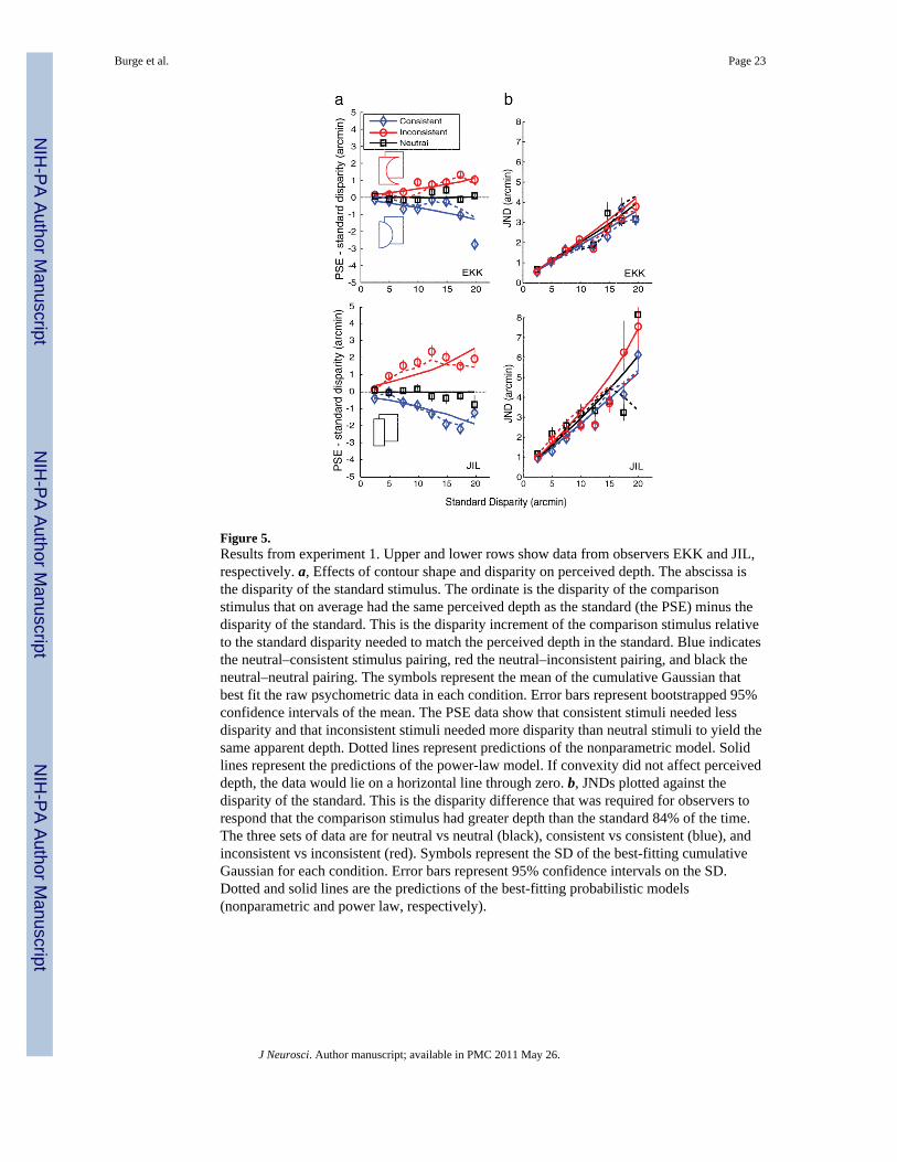
Figure 5.Results from experiment 1. Upper and lower rows show data from observers EKK and JIL,respectively. a, Effects of contour shape and disparity on perceived depth. The abscissa isthe disparity of the standard stimulus. The ordinate is the disparity of the comparisonstimulus that on average had the same perceived depth as the standard (the PSE) minus thedisparity of the standard. This is the disparity increment of the comparison stimulus relativeto the standard disparity needed to match the perceived depth in the standard. Blue indicatesthe neutral–consistent stimulus pairing, red the neutral–inconsistent pairing, and black theneutral–neutral pairing. The symbols represent the mean of the cumulative Gaussian thatbest fit the raw psychometric data in each condition. Error bars represent bootstrapped 95%confidence intervals of the mean. The PSE data show that consistent stimuli needed lessdisparity and that inconsistent stimuli needed more disparity than neutral stimuli to yield thesame apparent depth. Dotted lines represent predictions of the nonparametric model. Solidlines represent the predictions of the power-law model. If convexity did not affect perceiveddepth, the data would lie on a horizontal line through zero. b, JNDs plotted against thedisparity of the standard. This is the disparity difference that was required for observers torespond that the comparison stimulus had greater depth than the standard 84% of the time.The three sets of data are for neutral vs neutral (black), consistent vs consistent (blue), andinconsistent vs inconsistent (red). Symbols represent the SD of the best-fitting cumulativeGaussian for each condition. Error bars represent 95% confidence intervals on the SD.Dotted and solid lines are the predictions of the best-fitting probabilistic models(nonparametric and power law, respectively).

Burge et al.


NIH


NIH


NIH


Figure 6.Results from experiments 2 and 3. a, Effect of contour shape for the seven observers inexperiment 2. The abscissa represents the four stimulus pairings: consistent–consistent(CvC), consistent–inconsistent (CvI), inconsistent–inconsistent (IvI), and inconsistent–consistent (IvC). The first member of each pair is the standard stimulus; the second is thecomparison. The ordinate represents the disparity of the comparison stimulus that onaverage yielded the same perceived depth of the standard (the PSE) minus the disparity ofthe standard. Error bars represent 95% confidence intervals. The dashed horizontal linesthrough zero represent the expected data if region convexity did not affect perceived depth.b, Data from experiment 2 averaged across observers. The abscissa and ordinate are thesame as in a. To perceive depth separation as the same, observers needed more disparity ininconsistent comparison stimuli than in consistent standard stimuli. The reverse was true forconsistent comparisons and inconsistent standards. Error bars represent 1 SD of the groupmean. c, Results of experiment 3 with a viewing distance of 325 cm. The abscissa andordinate are the same as in b. Data are averaged across observers. d, Results of experiment 3with a viewing distance of 85 cm. Data are averaged across observers.

Burge et al.


NIH


NIH


NIH


Figure 7.Disparity increment thresholds from the literature and recovered from our modeling. Thecurves represent the SDs of the disparity likelihood distributions estimated from experiment1. They are plotted as a function of the disparity of the standard stimulus. Solid and dashedcurves represent the estimated values when the data were fit with the nonparametric andpower-law models, respectively. There are two pairs of curves for each observer. Symbolsrepresent disparity increment thresholds for different subjects and conditions in McKee et al.(1990). In that report, threshold was defined as the 75% point on the psychometric function,so we transformed the data to match our 84% criterion.

Burge et al.


NIH


NIH


NIH


Figure 8.Convexity–depth distributions estimated from experiment 1. Probability is plotted as afunction of the separation in depth between the adjacent regions. Blue represents thedistribution for convex reference regions, red the distribution for concave reference regions,and black the distribution for straight-contoured reference regions. a, Convexity–depthdistributions estimated with the nonparametric model. The distributions are approximatelylinear in these log–log plots, suggesting that they were well described by a power law. b,Convexity–depth distributions estimated with the power-law model. Note the similarity tothe nonparametric distributions in a. One free parameter had to be set to uniquely determinethese fits (see Materials and Methods), but the differences between the estimateddistributions were unaffected by the value of that parameter. The SEs for the best-fittingparameters were estimated by redoing the fitting procedure 30 times with bootstrapped setsof psychometric data. The SE intervals were about the same as the line widths in a and b, sothey are not plotted.

Burge et al.


NIH


NIH


NIH


Figure 9.Goodness of fit for four models. The SSE between model predictions and the psychometricdata was calculated. Goodness of fit was indexed by SSEGaussian/SSEmodel so that 1represents an upper bound. The inverse of those values was then computed and normalizedsuch that 1 represents the normalized inverse error obtained by fitting a cumulative Gaussianto each experimental condition independently (80 free parameters). Larger values representbetter fits (lower SSE). Normalized error is shown for four models fit to the data: (1) Coin-flipping model (0 free parameters); (2) a model that assumed that the convexity–depthdistributions were the same for convex, concave, and straight-contoured regions; this isequivalent to assuming that convexity was not used when observers estimated perceiveddepth (3 free parameters); (3) power-law model (5 free parameters); (4) nonparametricmodel (26 free parameters). We also measured the fits when the difference between theconvex and concave distributions was set equal to the difference recovered from the natural-scene statistics. The fits were nearly as poor as the model in which convexity is not used(relative fit error: EKK = 0.62; JIL = 0.67). Finally, we measured the fit errors withGaussians instead of power laws and found poor fits (relative fit error: EKK = 0.7; JIL =0.82); JIL’s Gaussian fit is comparable to the power-law fit, but that fit required extremelylow-variance disparity likelihoods, which were inconsistent with McKee et al. (1990) andMorgan et al. (2000). We conclude the power-law model is a good description of the internalconvexity–depth distributions.

Burge et al.


NIH


NIH


NIH


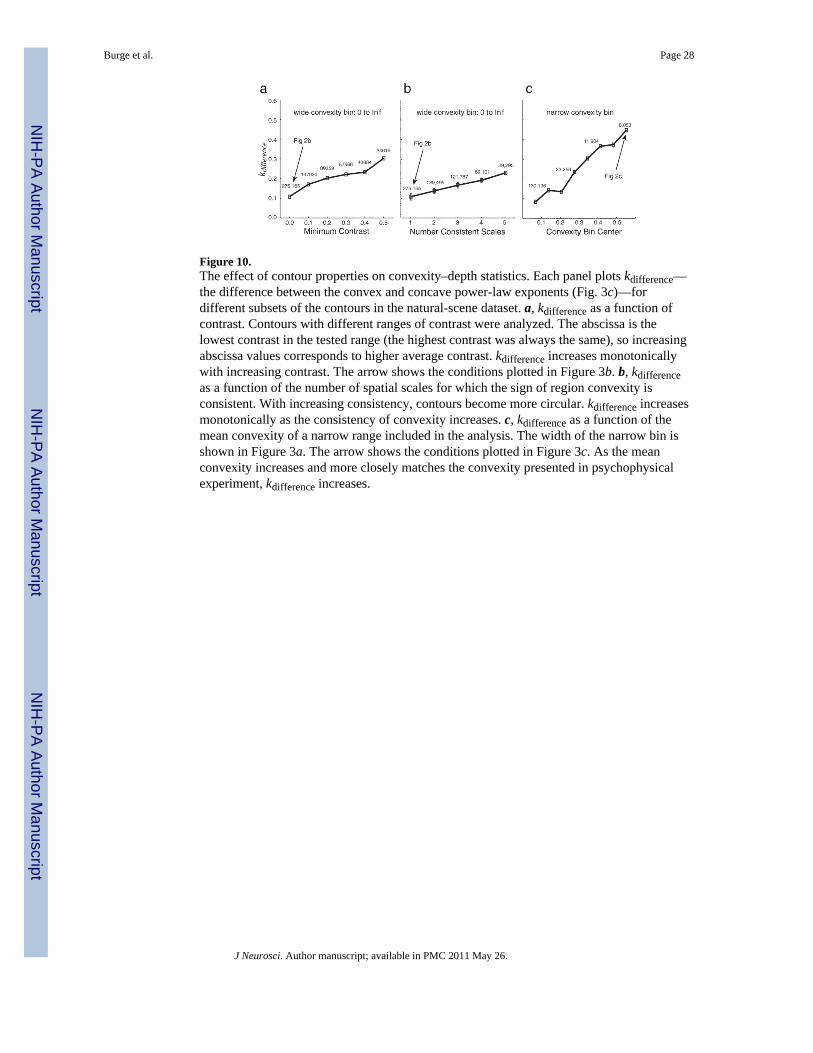
Figure 10.The effect of contour properties on convexity–depth statistics. Each panel plots kdifference—the difference between the convex and concave power-law exponents (Fig. 3c)—fordifferent subsets of the contours in the natural-scene dataset. a, kdifference as a function ofcontrast. Contours with different ranges of contrast were analyzed. The abscissa is thelowest contrast in the tested range (the highest contrast was always the same), so increasingabscissa values corresponds to higher average contrast. kdifference increases monotonicallywith increasing contrast. The arrow shows the conditions plotted in Figure 3b. b, kdifferenceas a function of the number of spatial scales for which the sign of region convexity isconsistent. With increasing consistency, contours become more circular. kdifference increasesmonotonically as the consistency of convexity increases. c, kdifference as a function of themean convexity of a narrow range included in the analysis. The width of the narrow bin isshown in Figure 3a. The arrow shows the conditions plotted in Figure 3c. As the meanconvexity increases and more closely matches the convexity presented in psychophysicalexperiment, kdifference increases.

Burge et al.


NIH


NIH


NIH


Natural-Scene Statistics Predict How the Figure-Ground Cue of Convexity Affects Human Depth...

Documents

Transcript of Natural-Scene Statistics Predict How the Figure-Ground Cue of Convexity Affects Human Depth...