Univers

ity of

Cap

e Tow

n

NATURAL LANGUAGE INTERFACE TO RELATIONAL

DATABASE:

A SIMPLIFIED CUSTOMIZATION APPROACH

TRESOR MVUMBI

SUPERVISED BY:

DR. MARIA KEET

CO-SUPERVISED BY:

PROF. ANTOINE BAGULA

DISSERTATION PRESENTED FOR THE DEGREE OF MASTER OF SCIENCE

IN THE DEPARTEMENT OF COMPUTER SCIENCE

UNIVERSITY OF CAPE TOWN

AUGUST 2016

The copyright of this thesis vests in the author. No quotation from it or information derived from it is to be published without full acknowledgement of the source. The thesis is to be used for private study or non-commercial research purposes only.

Published by the University of Cape Town (UCT) in terms of the non-exclusive license granted to UCT by the author.

Univers

ity of

Cap

e Tow

n

Plagiarism Declaration

I know the meaning of plagiarism and declare that all the work in the dissertation, save for that

which is properly acknowledged, is my own.

__________________________

Tresor Mvumbi

April 2016

Signature removed

Abstract

Natural language interfaces to databases (NLIDB) allow end-users with no knowledge of a formal

language like SQL to query databases. One of the main open problems currently investigated is the

development of NLIDB systems that are easily portable across several domains. The present study

focuses on the development and evaluation of methods allowing to simplify customization of NLIDB

targeting relational databases without sacrificing coverage and accuracy. This goal is approached by

the introduction of two authoring frameworks that aim to reduce the workload required to port a

NLIDB to a new domain. The first authoring approach is called top-down; it assumes the existence of

a corpus of unannotated natural language sample questions used to pre-harvest key lexical terms to

simplify customization. The top-down approach further reduces the configuration workload by auto-

including the semantics for negative form of verbs, comparative and superlative forms of adjectives

in the configuration model. The second authoring approach introduced is bottom-up; it explores the

possibility of building a configuration model with no manual customization using the information

from the database schema and an off-the-shelf dictionary. The evaluation of the prototype system

with geo-query, a benchmark query corpus, has shown that the top-down approach significantly

reduces the customization workload: 93% of the entries defining the meaning of verbs and

adjectives which represents the hard work has been automatically generated by the system; only 26

straightforward mappings and 3 manual definitions of meaning were required for customization. The

top-down approach answered correctly 74.5 % of the questions. The bottom-up approach, however,

has correctly answered only 1/3 of the questions due to insufficient lexicon and missing semantics.

The use of an external lexicon did not improve the system's accuracy. The bottom-up model has

nevertheless correctly answered 3/4 of the 105 simple retrieval questions in the query corpus not

requiring nesting. Therefore, the bottom-up approach can be useful to build an initial lightweight

configuration model that can be incrementally refined by using the failed queries to train a top-

down model for example. The experimental results for top-down suggest that it is indeed possible to

construct a portable NLIDB that reduces the configuration effort while maintaining a decent

coverage and accuracy.

Acknowledgements

I would like to acknowledge and thank Dr. Maria Keet for supervising this work. Each meeting with

you has been a great source of treasure. Thank you for being available, for your insightful guidance

and encouragements.

I would like to thank Prof. Antoine Bagula for co-supervising this work. Thank you for your countless

and valuable feedbacks. Special thank for always doing your best to make yourself available for

meetings, sometimes till late and/or over Skype.

I would like to thank all the friends from the ISAT lab. I loved and will miss the time spent together. I

am grateful for the relaxed and friendly environment where I have been given a chance to present

several times the work progress. The insights received from these lab meetings have greatly

contributed toward improving this dissertation.

Thank to my family and friends in both South Africa and back home (Democratic Republic of Congo)

for the love and support while studying. You are too many to mention; please find in these words

the expression of my profound gratitude. Special thanks to my parents Donatien Vangu Lukelo and

Concilie Cigoha Limba for the unconditional and carrying love.

i

Table of contents

Chapter 1 Introduction ........................................................................................................................ 1

1.1 Natural language interfaces to databases .............................................................................. 1

1.2 Problem statement and motivation........................................................................................ 2

1.3 Research questions ................................................................................................................. 2

1.4 Scope ....................................................................................................................................... 2

1.5 Methodology ........................................................................................................................... 3

1.6 Overview of the thesis ............................................................................................................ 3

Chapter 2 Background ......................................................................................................................... 5

2.1 Natural Language Interface to Databases ............................................................................... 5

2.1.1 Approaches to natural language processing ................................................................... 5

2.1.2 Phases of linguistic analysis ............................................................................................ 6

2.1.3 Design and architecture of NLIDB ................................................................................... 7

2.1.4 NLIDB portability ............................................................................................................. 9

2.1.5 NLIDB evaluation ........................................................................................................... 12

2.2 Approaches toward domain portable NLI to RDB ................................................................. 14

2.2.1 Early attempts to transportable NLIDB ......................................................................... 14

2.2.2 NLIDB using a semantic graph as domain knowledge model ....................................... 16

2.2.3 Portable NLIDB based on semantic parsers .................................................................. 18

2.2.4 Empirical approaches toward portable NLIDB .............................................................. 19

2.2.5 NLIDB based on dependency grammars ....................................................................... 20

2.3 Literature review synthesis ................................................................................................... 21

Chapter 3 Design of the authoring system ........................................................................................ 23

3.1 Design objectives and system architecture .......................................................................... 23

3.2 Design of data structures for configuration .......................................................................... 24

3.2.1 Data structure for the database schema ...................................................................... 24

3.2.2 Data structure for adjectives ........................................................................................ 24

3.2.3 Data structure of verbs ................................................................................................. 25

3.2.4 Representation of meaning in the configuration.......................................................... 25

3.3 Design of the top-down authoring approach ....................................................................... 26

3.3.1 Lexicon element harvesting .......................................................................................... 27

3.3.2 Steps in system configuration with top-down approach .............................................. 28

3.4 Design of the bottom-up authoring approach ...................................................................... 32

Chapter 4 Design of the query processing pipeline ........................................................................... 34

4.1 Design objective and system architecture ............................................................................ 34

ii

4.2 Lexical analysis ...................................................................................................................... 36

4.2.1 Part of speech tagging................................................................................................... 36

4.2.2 Lemmatization .............................................................................................................. 36

4.2.3 Named entity recognition ............................................................................................. 36

4.3 Syntactic analysis .................................................................................................................. 40

4.4 Semantic analysis .................................................................................................................. 40

4.4.1 Heuristic rules to build the select part of the intermediary query ............................... 41

4.4.2 Construction of the query part of the intermediary query ........................................... 43

4.5 SQL Translation ..................................................................................................................... 48

4.5.1 Construction of the intermediary SQL query ................................................................ 48

4.5.2 Construction of the final SQL query .............................................................................. 51

Chapter 5 Experiment design ............................................................................................................ 55

5.1 Material and experiment design ........................................................................................... 55

5.2 Experiment 1 – evaluation of the top-down approach ......................................................... 57

5.3 Experiment 2 – evaluation of the bottom-up approach ....................................................... 58

5.4 Experiment 3 – Evaluation of the processing pipeline.......................................................... 59

5.5 Experiment 4 – comparison of the result to other systems ................................................. 59

Chapter 6 Experiment results and discussion .................................................................................... 61

6.1 Experimental results ............................................................................................................. 61

6.1.1 Result evaluation of the top-down approach ............................................................... 61

6.1.2 Result evaluation of the bottom-up approach ............................................................. 62

6.1.3 Result evaluation of the processing pipeline ................................................................ 64

6.1.4 Result comparison with other systems ......................................................................... 65

6.2 Result discussion ................................................................................................................... 66

6.2.1 Top-down evaluation .................................................................................................... 66

6.2.2 Bottom-up evaluation ................................................................................................... 67

6.2.3 Processing pipeline evaluation ..................................................................................... 67

6.2.4 Comparison with other systems ................................................................................... 68

Chapter 7 Conclusion ......................................................................................................................... 70

7.1 Contributions ........................................................................................................................ 70

7.2 Future work ........................................................................................................................... 71

Appendix ............................................................................................................................................... 77

iii

List of tables

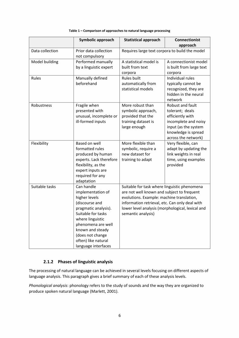
Table 1 – Comparison of approaches to natural language processing ................................................... 6

Table 2 – Confusion matrix defining the notions of true positives, false positives, false negatives and

true negatives (Manning et al., 2008) ................................................................................................... 12

Table 3 – List of NLIDB and their benchmark database, sample query corpus and evaluation metric

definition ............................................................................................................................................... 13

Table 4 – Comparison of TEAM with other early transportable systems (Grosz et al., 1987) .............. 16

Table 5 – Example of semantic frames for the relation “teach” and “register” (Gupta et al., 2012) ... 21

Table 6 – Example of query and their corresponding intermediary queries ........................................ 41

Table 7 – List of rules to retrieve the select part of the logical query .................................................. 41

Table 8 – Final list of triple groups corresponding to the query: “what states have cities named dallas

?’ ............................................................................................................................................................ 44

Table 9 – List of rules used to generate logical queries ........................................................................ 45

Table 10 – proportions of the training and testing set used for evaluation ......................................... 58

Table 11 – List of systems the top-down result is compared to ........................................................... 60

Table 12 – Average precision and recall for each experiment.............................................................. 61

Table 13 – Average number of manual and automatic configuration entries...................................... 61

Table 14 – List of terms produced by bottom-up model (the external terms from WordNet are

highlighted) ........................................................................................................................................... 63

Table 15 – List of column’s synonyms missing in the bottom-up model .............................................. 64

Table 16 – Sources of errors in the processing pipeline ....................................................................... 64

Table 17 – Result of NLIDB from Group A ............................................................................................. 65

Table 18 – Result of NLIDB from Group B ............................................................................................. 66

Table 19 – Experiment A results ........................................................................................................... 77

Table 20 – Experiment B results ........................................................................................................... 77

Table 21 – Experiment C results ........................................................................................................... 78

Table 22 – Experiment D results ........................................................................................................... 78

Table 23 – Experiment E results ............................................................................................................ 78

Table 24 – Experiment F results ............................................................................................................ 79

iv

List of figures

Fig 1 – Generic architecture of a syntactic parser .................................................................................. 8

Fig 2 – Generic architecture of NLIDB combining syntactic and semantic parsing (Androutsopoulos et

al, 1995) .................................................................................................................................................. 9

Fig 3 – Definitions of precision and recall ............................................................................................. 13

Fig 4 – Example of parse tree from TEAM (Grosz et al., 1987) ............................................................. 14

Fig 5 – Translation of logical query to SODA query in TEAM (Grosz et al., 1987) ................................. 15

Fig 6 – System customization screen in TEAM: acquisition of a new verb ........................................... 15

Fig 7 – Example of semantic graph structure (G. Zhang et al., 1999) ................................................... 17

Fig 8 – Semantic graph structure of (Meng & Chu, 1999) .................................................................... 18

Fig 9 – Example of subgraph corresponding to a query about runaways and aircrafts (Meng & Chu,

1999) ..................................................................................................................................................... 18

Fig 10 – Tailoring operation in (Minock et al., 2008) ............................................................................ 19

Fig 11 – Parse tree of a natural language query and its SQL query (Giordani & Moschitti, 2010) ....... 20

Fig 12 – Example of dependency tree from the Stanford dependency parser ..................................... 20

Fig 13 – Architecture of authoring system with top-down and bottom-up approach ......................... 24

Fig 14 – Structure of the database model in memory .......................................................................... 24

Fig 15 – Data structure of a verb........................................................................................................... 25

Fig 16 – Typed dependency graph for query “what is the longest river ?” .......................................... 28

Fig 17 – Typed dependency graph for query “which state has the longest river?” .............................. 28

Fig 18 – User interface mapping nouns to database columns .............................................................. 29

Fig 19 – User interface capturing adjective information ...................................................................... 29

Fig 20 – User interface capturing meaning for adjectives and verbs ................................................... 31

Fig 21 – Processing pipeline from natural language query to SQL ....................................................... 34

Fig 22 – System’s architecture .............................................................................................................. 35

Fig 23 – Processing pipeline user interface ........................................................................................... 35

Fig 24 – Structure of a token ................................................................................................................. 36

Fig 25 – Structure of named entities..................................................................................................... 37

Fig 26 – Visualization of the typed dependency query for “John loves Marie” .................................... 40

Fig 27 – Steps in join construction ........................................................................................................ 51

Fig 28 – Construction of a database graph from a database schema ................................................... 51

Fig 29 – Entity-relationship model of geo-query .................................................................................. 56

Fig 30 – Structure of a relational database version of geo-query ........................................................ 56

v

Code listings

Listing 1 – Context-Free Grammar defining the subset of SQL used to define semantics during system

configuration ......................................................................................................................................... 26

Listing 2 – Noun harvesting algorithm .................................................................................................. 27

Listing 3 – Adjective harvesting algorithm ............................................................................................ 27

Listing 4 – Verb harvesting algorithm ................................................................................................... 28

Listing 5 – Algorithm constructing the comparative form of adjective ................................................ 30

Listing 6 – Algorithm constructing the superlative form of adjective .................................................. 30

Listing 7 – Algorithm generating the SQL conditional expression for the negative form of a verb ..... 31

Listing 8 – Algorithm generating the SQL conditional expression for the superlative form of an

adjective ................................................................................................................................................ 32

Listing 9 – Algorithm generating the SQL conditional expression for the comparative form of an

adjective ................................................................................................................................................ 32

Listing 10 – Algorithm constructing the configuration automatically through bottom-up approach .. 33

Listing 11 – Named entity recognition algorithm ................................................................................. 37

Listing 12 – Algorithm grouping triples from the typed dependency query ........................................ 43

Listing 13 – Algorithm that constructs intermediary queries ............................................................... 45

Listing 14 – Algorithm merging intermediary queries element ............................................................ 46

Listing 15 – Merging rules for two intermediary queries ..................................................................... 47

Listing 16 – Algorithm translating the intermediary query to intermediary SQL ................................. 49

Listing 17 – Algorithm processing binary functions .............................................................................. 49

Listing 18 – Algorithm processing unary functions ............................................................................... 49

Listing 19 – Algorithm processing term ................................................................................................ 50

Listing 20 – Algorithm generating a graph from a database schema ................................................... 52

Listing 21 – Algorithm retrieving the list of tables to be joined ........................................................... 52

Listing 22 – Algorithm generating the joins from the paths between nodes representing table to join

.............................................................................................................................................................. 53

Listing 23 – Algorithm generating the FROM clause ............................................................................. 53

Listing 24 – Algorithm associating aliases to table’s names ................................................................. 54

1

Chapter 1 Introduction

Spoken natural languages are used by humans to verbally communicate with each other. Japanese,

English, French and Chinese are examples of natural languages. Natural languages contrast with

artificial languages which are constructed by humans; examples of artificial languages include

programming language and database query languages. The field of computer science interested in

analysing natural language is called Natural Language Processing (NLP).

Tamrakar & Dubey (2011) define Natural Language Processing as a “theoretically motivated range of

computational techniques for analysing and representing naturally occurring texts at one or more

levels of linguistic analysis for the purpose of achieving human-like language processing for a range

of tasks or applications”. NLPs’ objective is to perform language processing. The NLP field in the early

days targeted to achieve Natural Language Understanding (NLU), but this goal has not been achieved

yet (Kumar, 2011) and current works focus toward developing efficient theories and techniques for

natural language processing. NLP research focuses on particular applications with narrowed

purposes; this include among others:

- Information retrieval (IR) aims to mine for an interesting piece of information from large

corpus of text;

- Machine translation (MT) aims to achieve automatic language translation;

- Natural Language Interfaces (NLI) aim to develop human-computer interfaces enabling users

to interact with the computer through natural languages.

NLP borrows a lot from computational linguistics; as it studies languages from a computational

perspective (Kumar, 2011). Natural Language Interfaces constitute a subfield of NLP, aiming to

simplify human-computer interactions by enabling computers to process commands and produce

results in natural language. Natural Language Interfaces to databases (NLIDB) is the most popular

sub-domain of NLI.

Natural Language Generation (NLG) is also a sub-domain of NLI focusing on automatic generation of

natural language. A NLG module can be included in a NLI to allow the system to produce results in

natural language.

1.1 Natural language interfaces to databases

Information plays a crucial role more than ever in our nowadays organizations (Sujatha, 2012). The

Internet is growing at a fast rate, creating a society with a higher demand for information storage

and access (Range et al, 2002). Databases are the de facto tool to store, manage and retrieve large

amount of data. Unsurprisingly, they are used in various application areas in multiple organizations

(Nihalani et al, 2011). Databases use a formal query language to communicate; currently, Structured

Query Language (SQL) is the norm and standard way to interact with relational databases, but it is

difficult for non-domain experts to learn and master. Graphical interfaces and form-based interfaces

improve data analysis (Calvanese et al, 2010) and are easier than formal languages but still

constitute artificial languages that require some training to be properly used by casual users (Panja

& Reddy, 2007). One of the most convenient means for casual users to ask questions to databases is

to use natural language they are accustomed to (Freitas & Curry, 2014).

2

Research in Natural Language Interface to Databases aims to develop intelligent and easy to use

database interfaces by adopting the end user’s communication language (Sujatha, 2012). A NLIDB is

"a system that allows the user to access information stored in a database by typing requests

expressed in some natural language" (Androutsopoulos et al, 1995). NLIDB systems receive users'

inputs in natural language (text or speech) and translate them into commands in a formal language

(like SQL or MDX, for DataWarehouse) that can be processed by a computer. This approach greatly

simplifies the interaction between the system and user, since there is no need to learn and master a

formal query language (Sharma et al, 2011).

1.2 Problem statement and motivation

Full understanding of natural language is a complex problem in artificial intelligence that is not

completely solved yet. There are still a lot of challenges that need to be addressed before

developing a fully usable natural language interface that can accept arbitrary natural language

constructions. The main open problems include system portability, disambiguation, and

management of user expectation. This research addresses the first problem.

Natural language interfaces often require tedious configuration to be ported to new domains. The early works on NLIDB have been tailored to interface a particular knowledge domain or application; examples include LUNAR (Woods et al, 1972) and LADDER (Hendrix & Sacerdoti, 1978). The natural language processing literature contains several works aiming to build highly portable NLIDB with various levels of success. However, a review of the literature reveals a trade-off between portability and coverage. Highly portable systems tend to have a limited coverage while systems achieving high accuracy tend to be hard to customize and maintain. This research addresses the problem of bridging the gap between portability and coverage while avoiding the loss of accuracy.

1.3 Research questions

This research addresses the challenge of simplifying customization of NLIDB without negatively

impacting the linguistic coverage and accuracy of the system. The study hypothesizes the feasibility

of a portable NLIDB design targeting a relational database whose configuration requires only the

knowledge of database and the subject domain without sacrificing the system coverage and

accuracy. The following research questions are investigated:

- Is the exploitation of an unannotated corpus of sample questions combined with automatic

generation of configuration for negative form of verbs, comparative and superlative form of

adjective an effective approach to reduce the workload required to customize a NLIDB

targeting relational databases?

- Is it viable to use the database schema and an off-the-shelf dictionary as the only source of

configuration data for an authoring system requiring no manual customization?

1.4 Scope

The NLIDB design in this research work will use SQL as the formal language to query relational

databases. Additionally, the system will support only English natural language questions that are

assumed to be free of spelling or grammar errors. And finally, the parser engine is based on symbolic

approach as the parsing method of natural language questions. This research will explore two

authoring approaches aiming to reduce the workload needed to customize a NLIDB system. The first

approach is called top-down, it assumes the existence of a list of sample questions before

customization. The sample query corpus is used to harvest key lexical terms and construct a

3

customization framework based on mapping harvested elements to either database objects or their

corresponding semantics. The second customization method is called bottom-up, it explores the

feasibility of porting a NLIDB to a new database without any manual customization, using only the

database schema and WordNet (a public external dictionary) as source of configuration information.

1.5 Methodology

The present research project is based on the computer science experimental methodology which

consists of identifying “concepts that facilitate solutions to a problem and then evaluate the

solutions through construction of prototype systems”(Dodig-Crnkovic, 2002). In this research, we

propose a design and evaluation of an experimental prototype called NALI which aims to simplify

NLIDB customization. The experimental research has been completed in two main phases which are

the prototype design and its evaluation. The waterfall model has been used to implement the

prototype. The development cycle went through the following five phases: requirement gathering,

design, development, testing, and evaluation.

A system based evaluation method, i.e., an intrinsic evaluation, has been selected to evaluate the

experimental prototype. This choice is firstly motivated by the fact this research aims to contribute

mostly on improving the efficiency and performance of NLIDB customization. System based

evaluations allow assessing quantitatively the system’s performance in controlled environments

while user based or extrinsic evaluations are better suited to assessment of qualitative features like

user perception of the system (Woodley, 2008). A system evaluation will secondly allow easily

comparing the result with similar systems that are mostly evaluated through a system based

approach as well.

The prototype was evaluated with geo-query1, a corpus of sample questions, and its related

database (Tang & Mooney, 2001). We built a gold SQL result in order to automate the evaluation of

the correctness of the responses returned by the system. The metrics2 used to evaluate and

compare the system performance are precision and recall.

The tests were run in a computer with the configuration below:

- Hardware configuration: processor Intel(R) Core(TM) i7-2630QM CPU @ 2.00 GHz with 16

GB of RAM;

- Software configuration: Windows 7 Professional, PostgreSQL 9.4, Java version 1.7.

The experimental results are recorded in several html files that are kept in folders labelled with the

date and time of the experiment. The configuration data used for evaluation were recorded in a file

and can be used to re-run the experiments.

1.6 Overview of the thesis

The remainder of this thesis is structured as follows:

Chapter 2 gives some context and background on natural language processing and natural language

interface to databases. The related work section focuses on research aiming to simplify the task of

customization and the chapter concludes with a synthesis of the current state of the art and open

problems.

1 The motivations for choosing geo-query are presented in section 5.1. 2 The definitions for precision and recall are presented in section 5.1.

4

Chapter 3 presents the design of top-down and bottom-up approaches and describes the data

structures and algorithms used for both methods.

Chapter 4 presents the design of the processing pipeline for NALI and describes each of the main

phases of query processing, namely lexical analysis, syntactic analysis, semantic analysis and SQL

translation.

Chapter 5 describes the material and design of experiments used to evaluate the methods proposed

in Chapter 3 and Chapter 4.

Chapter 6 presents the experiment results followed by a discussion and interpretation of the

outcomes.

Chapter 7 concludes the thesis with a presentation of the main contributions and possible future

work.

5

Chapter 2 Background

This chapter presents a context to NLIDB with a focus on the approaches toward easily customizable

systems and the related work. The first section draws a bigger picture on approaches and techniques

used by NLIDBs to process natural language inputs and concludes with a discussion on the problem

of NLIDB portability. The second section looks closely at the approaches used in the literature to

simplify NLIDB customization and reviews in depth the research projects whose objectives and

approaches are similar to the present research. The chapter concludes with a summary of the

related literature.

2.1 Natural Language Interface to Databases

NLIDBs allow non-technical users to query databases using natural language sentences. To achieve

this, a NLIDB needs to process natural language input and produce a formal query like SQL to query a

database. The next sections present the approaches used to process natural language, the levels of

linguistic analysis, the main architectures of NLIDB and finally a discussion on portable NLIDBs.

2.1.1 Approaches to natural language processing

There are three main approaches to achieve natural language processing: symbolic, statistical and

connectionist approach (Pazos et al., 2013). Symbolic and statistical approaches have been used in

the early works in the NLP field, while connectionist approaches are relatively recent. Research

conducted between 1950 and 1980 focused on development of symbolic theories and

implementations. The symbolic approaches are based on in-depth analysis of linguistic properties

and sentence grammatical structures. This analysis uses a set of well-formed rules predefined by a

human expert. Statistical approaches are based on analysis of large text corpora to automatically

develop an approximated general model of linguistic phenomena. There is no need, therefore, to

manually create rules or world knowledge. Statistical approaches require large datasets of text

corpora as their primary source of evidence. Statistical methods regained popularity in the 1980’s,

thanks to the broader availability of computational resources. Like in the statistical approaches, the

connectionist approach develops generalized models from large text samples. Connectionism uses

an artificial neural network (ANN) to model language features. The ANN is constituted of

interconnected simple processing units called neurons. The knowledge is stored as weights

associated to connections between nodes. Like in the statistical approaches, the connectionist

approach develops generalized models from large text samples. We compiled in Table 1 a summary

of the similarities and differences between approaches.

The symbolic approaches have the advantage of being simple to implement; however, their

functionalities are limited by the quality and quantity of rules defined. Statistical and connectionist

methods are more flexible and can learn through training; but this learning depends on the

effectiveness of the training corpus (Pazos et al., 2013). Hybrid NLPs aim to complementarily use the

strengths of all approaches to effectively address NLP problems. An example of a hybrid system can

be found in (Mamede et al, 2012).

6

Table 1 – Comparison of approaches to natural language processing

Symbolic approach Statistical approach Connectionist approach

Data collection Prior data collection not compulsory

Requires large text corpora to build the model

Model building Performed manually by a linguistic expert

A statistical model is built from text corpora

A connectionist model is built from large text corpora

Rules Manually defined beforehand

Rules built automatically from statistical models

Individual rules typically cannot be recognized, they are hidden in the neural network

Robustness Fragile when presented with unusual, incomplete or ill-formed inputs

More robust than symbolic approach, provided that the training dataset is large enough

Robust and fault tolerant; deals efficiently with incomplete and noisy input (as the system knowledge is spread across the network)

Flexibility Based on well formatted rules produced by human experts. Lack therefore flexibility, as the expert inputs are required for any adaptation

More flexible than symbolic, require a new dataset for training to adapt

Very flexible, can adapt by updating the link weights in real time, using examples provided

Suitable tasks Can handle implementation of higher levels (discourse and pragmatic analysis). Suitable for tasks where linguistic phenomena are well known and steady (does not change often) like natural language interfaces

Suitable for task where linguistic phenomena are not well known and subject to frequent evolutions. Example: machine translation, information retrieval, etc. Can only deal with lower level analysis (morphological, lexical and semantic analysis)

2.1.2 Phases of linguistic analysis

The processing of natural language can be achieved in several levels focusing on different aspects of

language analysis. This paragraph gives a brief summary of each of these analysis levels.

Phonological analysis: phonology refers to the study of sounds and the way they are organized to

produce spoken natural language (Marlett, 2001).

7

Morphological analysis: this level deals with the componential nature and structure of words. Words

are composed of morphemes, which represent the smallest units of meaning. For instance, the word

“interaction” is composed of three different morphemes: “inter” (the prefix), “act” (the root) and

“ion” (the suffix). The meaning of morphemes is the same for all the words, making it possible to

understand any given word by breaking it into its constituents (Aronoff & Fudeman, 2011).

Lexical analysis: also referred to as tokenization, is the process of breaking a stream of characters

into meaningful unit elements (i.e. words) called tokens (Bird et al, 2009).

Syntax analysis: the syntax represents the structure of a language. For natural language, the syntax

defines the order, connections, and relationships between words. The ensemble of syntax rules

forms the language grammar (Nigel, 1987). Syntactic analysis, referred to sometimes as parsing is

the process of analyzing a text structure to determine if it respects a given formal grammar. Context

Free Grammars (CFG) is the most used grammar in syntactic analysis (Kumar, 2011).

Semantic analysis: this level deals with possible meanings of natural language inputs, by analyzing

interactions in the word-level meanings within a sentence (Kumar, 2011). This level includes also

disambiguation of words with several possible interpretations, in order to ideally keep only one final

meaning for the sentence. A computational representation or knowledge representation is needed

to model, store and process sentence meaning (Kumar, 2011). First Order Logic or another logic

language can be used as a formal representation model to represent sentence meaning.

Discourse analysis: James Paul Gee (2005) defines discourse analysis as “the study of language-in-

use”. At this level, the meaning of several sentences is analyzed to draw an overall sense, while

semantic analysis focuses on the meaning of a single sentence.

Pragmatic analysis: at this level, external contextual knowledge is introduced to refine the discourse

meaning (Kumar, 2011). For example, a mobile handset NLP being queried “What’s the weather like

today ?” can use pragmatic analysis to “understand” that the current geographical position is

needed to answer the query, and obtain it through GPS.

Currently, there are significantly more NLP systems implementing the four lower levels of analysis.

This can be explained by the fact not all NLP actually need to analyze text at higher levels. In

addition, lower levels have benefited from extensive research work. Lower level analysis is done by

applying rules on small units: morphemes, words, and sentences. Higher levels, especially pragmatic

analysis, often require extensive external world knowledge to perform efficiently.

2.1.3 Design and architecture of NLIDB

There are three approaches used to design NLIDB: pattern-matching, syntax-based systems, and

semantic grammar systems.

Pattern-matching: systems were used in some of the early NLIDB. The input is matched with a set of

predefined patterns. Only the questions defined in the patterns can be interpreted. Following is an

example of pattern definition borrowed from (Androutsopoulos et al, 1995):

Pattern: ... "capital" ... <country>.

Action: Report Capital of row where Country = <country>.

This rule searches for the word "capital", followed by <country> which represents a word appearing

in the list of countries in a database table. If this condition is matched, the system returns the

content of column "Capital" where "Country" = <country>. This technique has the advantage that it

8

is simple: the rules are simple to write, no elaborate parsing module is needed, and as a result the

system is easy to implement. One important disadvantage of a pattern-matching technique is that it

can lead to a wrong answer when a query matches the wrong rule (Androutsopoulos et al, 1995).

Syntax-based systems: have a grammar that describes all the possible syntactic structures of queries

(Androutsopoulos et al, 1995). The user’s query is analyzed (parsed) syntactically and the resulting

parsing tree is mapped to an intermediary language (see Fig 1), that will be translated into the

database query language. LUNAR (Woods et al., 1972) is an early example of NLIDB using this

approach. The parser can produce more than one parse tree for a given natural language; a syntax-

based system needs in this case to resolve the ambiguity.

Fig 1 – Generic architecture of a syntactic parser

Semantic grammar systems: are similar to syntax-based systems in the sense that the input is also

parsed to generate a parse tree. The difference lies in the fact that the leaf nodes represent

semantic concepts instead of syntactic concepts. Semantic knowledge refers to the target domain

and is hard-wired into the semantic grammar (Androutsopoulos et al, 1995). Semantic grammar is a

standard approach used in several NLIDB implementations (Knowles, 1999). The query in natural

language is parsed to generate a model or representation of the meaning of the sentence which will

be translated into SQL or any targeted database query language. A semantic parser can be

complementarily used with a syntactic parser to perform semantic analysis (see Fig 2). In the

architecture illustrated in Fig 2, the domain-dependent knowledge is contained in the lexicon, world

model, and mapping to DB modules. The domain-independent knowledge is contained in the syntax

rules (used by the lexical parser) and semantic rules (used by the semantic parser). The semantic

interpreter produces a logical query that is translated to the final database query by the query

generator module.

9

Fig 2 – Generic architecture of NLIDB combining syntactic and semantic parsing (Androutsopoulos et al, 1995)

The drawback of semantic grammar systems is the difficulty to port them to different application

domains (Pazos et al., 2013). Customization requires the development of a new grammar for each

new configuration. Other samples of semantic grammar based systems can be found in (Nguyen &

Le, 2008) and (Minock et al., 2008).

2.1.4 NLIDB portability

Early NLIDBs were designed to interface a specific database and for only one given knowledge

domain (lunar geology for LUNAR, for example). From the 1980’s, research focused more on

portability; the aim being to create NLIDBs that can easily adapt to a database with a different

universe of discourse or even new natural language. The following sections discuss challenges

related to NLIDB portability and methods developed to address the problem.

2.1.4.1 Domain portability

NLIDBS are often designed to answer questions within a particular domain (example: weather

forecast, train service, etc.). A domain portable NLIDB is designed in such a way that the system can

be configured easily for use in several subject domains (Androutsopoulos et al, 1995). The challenge

here is to construct an effective linguistic model that includes new words and concepts pertaining to

the new domain. The configuration task has to be performed by system developers, knowledge

engineers or users. The quality of the linguistic model used has a tight effect on the correctness of

the system. However, designing and building a model to be used by a NLI system often requires

certain knowledge of computational linguistics, an understanding of the database structure and

finally expertise in the formal language to query the target data source. Therefore, customizing NLI

10

has historically been the responsibility of a few experts. The previous situation resulted into costly

system customization which hindered development and wide adoption of NLI. In response to this

problem, recent research trends in NLI investigate how to reduce the effort and expertise required

for building linguistic models needed to customize systems to new domains. The following

paragraphs describe the various strategies developed that simplify customization to new domains.

Simple authoring systems

Simple authoring systems focus on minimizing the effort required to adapt the system to new

domains by building a user-friendly authoring (or customization) interface that does not require

expertise in computational linguistics. The project TEAM (Transportable English database Access

Medium) is among the first NLIDB applying this strategy (Grosz, Appelt, Martin, & Pereira, 1987).

Customizing TEAM requires some general knowledge of computer systems and the target database;

the user is not required to have a background in computational or formal linguistics. System

customization is performed by adding new verbs, adjectives and synonyms of existing words through

the customization module. ORAKEL (Cimiano, Haase, Heizmann, & Mantel, 2008) is a more recent

example of an easy to customize NLI. ORAKEL first auto-constructs the lexicon from the ontology

targeted; this helps to simplify the task of customization which consists of mapping lexicon terms to

relations specified in the ontology domain. Most of the NLIDB systems integrating a user-friendly

authoring module we reviewed interface with ontologies; the relatively few systems targeting

relational databases are presented in section 2.2. Further examples of NLIDB targeting ontologies

with a user-friendly authoring module can be found in (Lopez et al. , 2005) and (Bernstein et al.,

2005).

Interactive natural language interfaces

The interactive approach advocates building systems with a concise model and interactively

cooperating with the end-user to customize the system. Consequently, systems based on this

paradigm will often have a very small or no domain specific entries in the model. This design choice

results in a more generic linguistic model that is easily portable to new domains.

NALIR is an interactive NLIDB to relational databases that translates natural language questions to

SQL (F. Li & Jagadish, 2014). NALIR integrates a limited set of possible interactions with the user in

order to assist incrementally building complex natural language questions. The interface supports

advanced SQL features such as aggregations, sub-queries and queries joining multiple tables. The

system also provides a natural language feedback to the user, explaining how the query was

interpreted. Ambiguities in the questions are dealt with by letting the user select the correct

interpretation from a list of multiple possible answers.

FREyA (Damljanovic, Agatonovic, & Cunningham, 2012) is an interactive NLI to ontologies that relies

on clarification dialogs with the end user to parse queries. FREyA compared to NALIR has the

advantage of learning from previous user choices to self-train and improve its model, thereby

reducing the need for subsequent clarification dialogs. However, NALIR can support more complex

queries compared to FREyA. Both FREyA and NALIR do provide feedbacks to user about queries’

interpretations. Another example of an interactive natural language interface can be found in (Li et

al, 2007).

Automatic acquisition of the linguistic model

Automatic acquisition consists of automatically constructing the model required for query parsing.

One approach consists of auto-extracting the information required to build the model from the

11

meta-data describing a data source structure or directly from the actual data. A second approach

consists of training the NLI using a corpus of annotated or non-annotated data.

Kaufmann et. al (2007) presents NLP-Reduce, a natural language interface to the Semantic Web.

NLP-Reduce extracts properties from the Semantic Web to build the lexical dictionary automatically.

This initial dictionary is completed by retrieving word synonyms from WordNet (Miller, 1995), an

external lexical dictionary on the Web.

Freitas & Curry (2014) propose a NLI over heterogeneous linked data graphs. The system uses a large

text corpus to auto-build a semantic model for the graph based on statistical analysis of co-occurring

words. The lexical dictionary is extracted from an unannotated text corpus instead of an external

source like with NLP-Reduce. The semantic model built allows users to express questions to the

graph without prior knowledge of the underlying structure.

An example of a NLI trained with a labelled corpus is presented in (Zettlemoyer & Collins, 2012) and

a NLI project based on unsupervised learning can be found in (Goldwasser et al, 2011).

Controlled natural language interfaces

A controlled natural language is a sub-set of natural language that uses a limited set of grammar

rules that allows a subset of possible phrase constructions. One way of building an easily portable

NLI consists of restricting the system to a controlled natural language that can be fully supported.

NLyze (Gulwani & Marron, 2014) is an example of a NLI using a controlled natural language called

DSL (Domain-Specific Language) to interrogate a tabular spreadsheet. Queries written with DSL use a

restricted grammar (i.e. “sum the totalpay for the capitol hill baristas”) (Gulwani & Marron, 2014)

but the system can be ported to any spreadsheet without the need for customization. Ginseng

(Bernstein et al., 2005) uses a “quasi-natural language” to query semantic Web data sources. To

cope with the necessity to first teach the user the restricted language (as the case with NLyze),

Ginseng proposes a guided input interface which gives suggestions and auto-completion of the

query in real-time. A project similar to Ginseng based on ontologies can be found in (Franconi et. al,

2010).

2.1.4.2 DBMS portability

A DBMS-independent NLIDB should be easily customizable to work with various underlying database

management systems (Androutsopoulos et al, 1995). When SQL (the standard query language for

RDBMs) is supported, it is trivial to port the NLIDB to any SQL-based DBMS. In the case of a

completely new DBMS query language, only the module that translates logical intermediate queries

to database queries must be rewritten. If the NLIDB architecture does not include an intermediary

language, extensive modifications may be required to successfully support the new RDMS query

language. Examples of NLIDBs designed to support multiple database management systems can be

found in (Cimiano et al, 2008) (Hendrix et al., 1978), (Hinrichs, 1988) and (Thompson & Thompson,

1983). Most of the works on DBMS portable NLI are from the 70’s and 80’s. More recent works use

ontologies to aggregate data from different sources (RDBMS, XML or Web, for example). Therefore,

integrating different database models is done through an integration layer before involving the

natural language interface. In consequence, there is a greater focus on developing domain

independent NLIs instead of DBMS portable systems.

12

2.1.4.3 Natural language portability

The vast majority of research in NLP focuses on English. A natural language independent NLIDB

should be easily customized to work with a new natural language. This task is complex and difficult,

as it requires the modification in almost every level of the NLIDB architecture. A possible approach

to create multilingual NLP is to design syntactic and semantic parser modules loosely coupled to the

overall architecture. This approach allows plugging new language modules without changing the

entire system. Another approach consists of using machine translation (can be an external module)

to first translate the query to a target natural language. Examples of system designed to work with

various natural language can be found in (Zhang et al, 2002), (Jung & Lee, 2002) and (Wong, 2005).

2.1.5 NLIDB evaluation

There is currently no generally accepted evaluation framework or benchmark for NLIDB (Pazos et al.,

2013). NLIDB evaluation can focus on several facets, the most common found throughout the

literature are result’s accuracy, system’s performance, and usability. The assessment of usability

often involves user testing. The assessment of system’s accuracy is the most used approach in NLIDB

evaluation; it is typically performed by testing a system prototype with a set of queries from a

benchmark corpus.

The most commonly used benchmark databases are geo-base, rest-base and job-base; all developed

by L. Tang and R. Mooney (Tang & Mooney, 2001). The three databases are implemented in Prolog

and have a simple structure (maximum 8 entity classes). When used to evaluate a NLI targeting a

relational database, the databases need to be converted into a relational version. Mooney

additionally provides three benchmark query corpora, one for each database. The questions from

Mooney’s corpora present a high degree of logical complexity and contains arguably the most

challenging questions among publicly available corpora (Pazos et al., 2013). The second most used

database is ATIS; which is a relational database containing information on airline flights (Hemphill et

al., 1990). The ATIS database structure is more complex compared to Mooney’s; it has 27 tables and

123 columns. ATIS is provided along with the largest corpus but most of the questions are repetitive

using the same grammatical structures with different values (Pazos et al., 2013).

There are no benchmark metrics globally accepted throughout the field to assess NLIDBs. The two

most common metrics are precision and recall whose meaning reflects the definition in information

retrieval (Manning et al., 2008) (Table 2 helps clarify the definition of precision and recall in

information retrieval). And again, there is no consensus on the definition of recall; the two

definitions found in the literature (see Table 3) are presented in Fig 3.

Table 2 – Confusion matrix defining the notions of true positives, false positives, false negatives and true negatives (Manning et al., 2008)

Relevant Non relevant

Retrieved True positives False positives

Not retrieved False negatives True negatives

Table 3 gives a list of NLIDB along with the benchmark corpus, database and metric definition used

for their evaluation.

13

Definition 1 (the most prevalent definition in NLIDB field)

Recall=#(retrieved items)

#(relevant items)=

#true positive+#false positive

#true positive+#false negative

Definition 2 (the standard definition in information retrieval)

Recall=#(relevant items retrieved)

#(relevant items)=

#true positive

#true positive+#false negative

Definition of precision

Precision=#(relevant items retrieved)

#(retrieved items)=

#true positive

#true positive+#false positive

Fig 3 – Definitions of precision and recall

Table 3 – List of NLIDB and their benchmark database, sample query corpus and evaluation metric definition

NLIDB Benchmark database Benchmark query

corpus Metric

definition

COCKTAIL (Tang & Mooney, 2001)

Geo-query and Jobs-query

Geo-query and Jobs-query

2

PRECISE (Popescu et al., 2003)

Geo-query, Rest-query and Jobs-query (converted to a relational version)

Geo-query, Rest-query and Jobs-query

1

GINSENG (Bernstein et al., 2005)

Geo-query and Rest-query (converted to OWL)

Geo-query and Rest-query

1

KRISP (Kate & Mooney, 2006)

Clang and Geo-query Clang and Geo-query 2

PRECISE ATIS (Popescu et al., 2004)

ATIS ATIS 1

(Chandra, 2006) Geo-query Geo-query (175 queries) 2

PANTO (Wang et al., 2007)

Geo-query, Rest-query and Jobs-query (converted to ontology, OWL format)

Geo-query, Rest-query and Jobs-query

1

(Minock et al., 2008) Geo-query Geo-query (250 queries) 1

FREYA (Damljanovic et al., 2012)

Geo-query Geo-query (250 queries) 2

(Giordani & Moschitti, 2010)

Geo-query Geo-query (250 queries) 1

(Giordani & Moschitti, 2012)

Geo-query Geo-query (800 queries) 1

Ask Me (Llopis & Ferrández, 2013)

ATIS ATIS 1

14

2.2 Approaches toward domain portable NLI to RDB

This section reviews NLI to relational databases using approaches similar to the present research

work; the common problems and strategies used to solve them are presented as well; and finally the

strengths and weaknesses of diverse approaches similar to this research are discussed.

2.2.1 Early attempts to transportable NLIDB

TEAM (Grosz et al., 1987) is a foundational earlier work that addressed in the most exhaustive way

the challenges related to transportable NLIDBs. The TEAM project hypothesized that if a NLI is built

in a sufficiently well-principled way, the information required to customize it can be provided by a

user with general expertise about computer systems and the particular database, but without

special knowledge on computational linguistics. This hypothesis is still used in recent works on

portable NLIDB (Cimiano et al., 2008) (Minock et al., 2008). The TEAM’s architecture comprises two

major modules: DIALOGIC and Schema Translator. The DIALOGIC’s module leverages Paxton’s parser

(Paxton, 1974) and also performs a few basic programmatic functions and quantifier scope

resolution. Fig 4 shows a parse tree corresponding to the query “Show each continent's highest

peak”. The schema translator module first translates the parse tree to a first-order logic query, then

translates the logical query to SODA (the formal language to query the underlining database). Fig 5

shows an example of the translation process.

Fig 4 – Example of parse tree from TEAM (Grosz et al., 1987)

To verify its core hypothesis, TEAM developed a user-friendly authoring system that required from

the user only a general knowledge on computers and understanding of the targeted database. The

system pre-included a domain-independent knowledge base. Customization consisted of completing

domain related knowledge including synonyms for database objects, new verbs, and their meaning.

Fig 6 shows the screen for acquiring new verbs; which is performed in a question-response fashion

to guide the user through customization. As illustrated below, TEAM collects the base form of the

verb along with the conjugated forms.

15

Fig 5 – Translation of logical query to SODA query in TEAM (Grosz et al., 1987)

Fig 6 – System customization screen in TEAM: acquisition of a new verb

16

TEAM offered support for aggregation functions and methods to handle superlative and comparative

forms of adjectives, but did not support more advanced features like nesting and sorting. To simplify

handling superlative and comparative forms of adjectives, TEAM includes two additional parameters

into its lexicon: firstly a link to a predicate that quantifies the adjective (e.g. the field

‘montainLength’ for ‘big mountain’) and secondly a ‘scale direction’ for the predicate (e.g. positive

for tall and negative for short). TEAM did not undergo a systematic testing (Grosz et al., 1987); this

makes it hard to have a clear idea of the actual performances of the system. Table 4 presents a

comparison of TEAM with other early portable NLIDB.

Table 4 – Comparison of TEAM with other early transportable systems (Grosz et al., 1987)

TEAM Ginsparg IRUS CHAT-80 ASK LDC-1 EUFID Types of portability

Linguistic domain, db, DBMS

Linguistic domain, db, DBMS (Relational)

Linguistic domain, db, DBMS

Linguistic domain, db

Linguistic domain, db

Linguistic domain, db

Linguistic domain, db, DBMS

Expertise of transporter

Db expert System designer

System designer

System designer

User, super user, system designer

Super user System designer, domain expert

Information acquired

Lexical, conceptual, db schema

Lexical, semantic network, db schema

Lexical, domains semantics, db schema

Lexical, logical form to db predicate mapping

Lexical, conceptual, db schema

Lexical, conceptual, conceptual to db mapping

Lexical, semantic graph, database

Time to adapt

Minute-hours

Hours-days Weeks Days-weeks - Minutes-hours

months

In the above table:

a system designer: refers to a user with a general knowledge of computer systems who received a

training to customize the system;

a super user: refers to an advanced end user who is more knowledgeable in computer systems;

a domain expert: refers to a simple user or super user with expertise in the target domain

knowledge.

2.2.2 NLIDB using a semantic graph as domain knowledge model

Barthélemy et al (2005) defines a semantic graph as “a network of heterogeneous nodes and links”

containing semantic information. The semantic graph structure is used in the literature to model the

domain knowledge. The semantic graph is used for its intuitive structure that makes it easy to build

and extend even by a user with no background in computational linguistics. EUFID (Templeton &

Burger, 1983) is among the earliest NLIDB to use semantic graph to model the domain knowledge.

The semantic graph structure in (Zhang et al., 1999) (see Fig 7) has the particularity of including

weights to the links to express their strength or likelihood. During query analysis, the system first

searches for key terms in the user’s input (like concepts in the semantic graph, database attributes,

and values). The query is therefore viewed as a set of unconnected semantic graph nodes. The

system uses the information from the semantic graph to build several possible subgraphs by

including links between disconnected nodes. The weights of the links in the domain model are used

to compute a ranking for each subgraph. The highest ranked subgraph is selected and translated into

the final query. The system supports aggregation, but not nesting. The NLIDB has not been

17

thoroughly evaluated: the test consisted of running 30 queries from an unsaid number of candidates

which all have been correctly answered. It is, therefore, hard to clearly evaluate the real capability of

the system.

Fig 7 – Example of semantic graph structure (G. Zhang et al., 1999)

Meng & Chu (1999) also present a portable NLIDB targeting a SQL database which uses a semantic

graph to model the domain’s knowledge. The graph’s structure in (Meng & Chu, 1999) is composed

of nodes (representing database tables), database attributes, and links (see Fig 8). The squares

represent the tables and circles represent the database attributes. The system in (Meng & Chu,

1999) retrieves from the natural language input three components: the query topics, the select list

and the query constraints. A query topic corresponds to a subgraph of the semantic graph containing

the keywords found in the user’s query. This subgraph allows retrieving joins between tables

automatically (Fig 9 shows an example of subgraph). The query constraints are retrieved using values

from the database found in the query (translated to “sourceColumn = ‘valueFound’”). And finally,

any other column mentioned in the query but not part of constraints are assumed to be part of the

select clause. The information gathered in query topics, select list, and query constraints are used to

build the final SQL query.

18

Fig 8 – Semantic graph structure of (Meng & Chu, 1999)

Fig 9 – Example of subgraph corresponding to a query about runaways and aircrafts (Meng & Chu, 1999)

The approach used in (Meng & Chu, 1999) uses only the semantic graph as the source of information

describing the domain knowledge in order to translate natural language questions to SQL; no

additional grammar is required. However, the prototype built supports only simple SELECT FROM

WHERE queries and there is no evaluation of the system available to assess its performance.

2.2.3 Portable NLIDB based on semantic parsers

Semantic parsers include production rules that can translate a natural language query to a formal

query in a meaning representation language like first-order logic. NLIDBs based on this approach are

relatively straightforward to develop.

Minock et al. (2008) present a good example of a portable NLI to SQL using a semantic parser that is

defined with Lambda Synchronous Context-Free Grammar. The parser maps the user query to a

variant of Codd’s tuple calculus which includes higher order predicates like “LargestByArea”. The

system’s objective is to allow an everyday technical team member to build a robust NLI. A lot of

attention has been put on constructing a user-friendly authoring module based on light annotations.

The system customization is completed in three steps: naming, tailoring and defining. The naming

phase provides synonyms to database attributes, joins, and facts from the database. Tailoring

consists of mapping patterns from the natural language query to their corresponding concepts

expressed in tuple calculus (see illustration in Fig 10). Finally, the defining phase allows adding more

definitions to the system using natural language. An example of a possible definition borrowed from

(Minock et al., 2008) is “define a ‘major’ state as a state with more than 1 million people”.

19

Fig 10 – Tailoring operation in (Minock et al., 2008)

To evaluate the system, two subjects had been requested to customize the system by manually

tailoring 100 random queries from the geo-query corpus (Tang & Mooney, 2001). The subjects, who

were undergraduate students with a background in databases, have taken two hours to customize

the system. The accuracy yielded on various testing set varied between 80% and 90%. However, it

must be noted that the prototype included complex concepts in the parser in the form of higher

order predicates. For example, the semantics for all the superlative forms were pre-loaded, this

alone can explain the high accuracy observed.

Another example of portable NLI to SQL based on a semantic parser can be found in (Nguyen & Le,

2008) where the system uses a domain-independent semantic grammar and can be used with no

customization.

An important drawback with semantic parsers is that the use of rigid production rules makes the

system less robust against noise and unknown structures. The empirical methods presented in the

next section address this problem.

2.2.4 Empirical approaches toward portable NLIDB

An empirical approach allows training a model using a corpus and therefore the NLI is generic and

portable. Empirical approaches are gaining importance in NLP again with much recent research work

focusing on statistical approaches to process natural languages. This trend is explained by the high

complexity of language making it difficult to capture a full range of natural language contexts and

their corresponding semantic concepts when using a limited set of predefined rules (Kate & Mooney,

2006).

Giordani & Moschitti (2010) use machine learning algorithms to train a semantic parser that

translates natural language queries to SQL. The training is achieved using Support Vector Machines

(SVM), a supervised learning method (Smola & Vapnik, 1997). The training set used is composed of a

set of pairs 𝑃 = 𝑁 × 𝑆 where N represents the set of parse trees of natural language queries parsed

with Charniak’s syntactic parser (Charniak, 2000) and S represents the set of parse trees of the

corresponding SQL query. Fig 11 shows an example of a pair (𝑛𝑖, 𝑠𝑖). An experiment with a model

trained with 250 queries from geo-query (Tang & Mooney, 2001) achieved 76% accuracy.

20

Fig 11 – Parse tree of a natural language query and its SQL query (Giordani & Moschitti, 2010)

KRIPS is a more generic system based on machine learning that is trained with pairs composed of the

natural language queries and their corresponding formal queries in a given Meaning Representation

Language (MRL) (Kate & Mooney, 2006). The system accepts any MRL that can be defined with a

deterministic Context-Free Grammar (CFG) in order to ensure that each MRL query will have a

unique parse tree.

Statistical approaches offer the advantage of being more robust to noise (sentence with typos, for

example) and uncertainty (like unseen grammatical structures). The main drawback of this approach

is the need to build a large annotated corpus with questions related to the subject domain for

customization. This task is especially costly when correct formal queries (like SQL or first-order logic)

need to be manually produced.

2.2.5 NLIDB based on dependency grammars

Dependency grammars (DG) are the fruits of developments in syntactic theories. The work of

Tesnière (1959) greatly contributed to the development of DG. The focus in DG is on the analysis of

dependency relationships between words in the sentence with the verbs being the structure center

of the dependency trees. Fig 12 illustrates the dependency tree generated by the Stanford

dependency parser (De Marneffe et al., 2006) for the query “Which states border the state with the

most rivers?” from geo-query corpus (Tang & Mooney, 2001).

Fig 12 – Example of dependency tree from the Stanford dependency parser

Giordani & Moschitti (2012) presents a NLIDB to SQL based on dependency grammar that uses the

Stanford parser. The system uses the metadata in the RDMS describing the database as source of

synonyms to build its lexicon. The prototype supports complex queries, including nesting,

aggregation, and negation. For each query, up to 10 possible results ranked by their relevance are

produced. The experimental result with geo-query showed that 81% of the responses ranked as the

best answers are correct. The accuracy increases to 92% for the 3 first responses and 99% for the 10

best results. An intermediary MRL was not used; the system relies on a custom made algorithm (see

(Giordani & Moschitti, 2012) for details) which analyses the dependency parse tree and produces

the final SQL. The result obtained shows the potential power of dependency parsers. However, the

21

prototype does not feature an authoring module to customize the system. The only input used is the

metadata in the RDBM. Therefore, additional semantic rules to support special cases are directly

hard coded in the engine. This approach makes the system less portable. A similar work can be

found in (Gupta et al., 2012), where the authors present a NLIDB to SQL using a dependency

framework called "Computational Paninian Grammar” which used the Stanford Typed Dependency

(STD) parser (De Marneffe et al., 2006) in the background. The semantic analysis here consists of

mapping elements from the dependency tree to the domain’s conceptual model retrieved from the

database schema. The mapping rules are encoded in the semantic frames (see an example in Table

5). Each verb has a role “root” and is associated to his subject and object that have the roles K1 and

K2. The concepts are mapped to their query terms and possible values they can have.

Table 5 – Example of semantic frames for the relation “teach” and “register” (Gupta et al., 2012)

Role Concept Query Term Value

Root teach -

K1 faculty faculties -

K2 course - NLP

Root register took

K1 student students which

K2 course - NLP

The interest of the semantic frames approach is that it offers a simple and straightforward

framework that simplifies expressing semantic mapping rules.

2.3 Literature review synthesis

The overall area of NLP research remains very experimental. Even though there are several usable

commercial systems available, unrestricted use of natural language is still an open problem. Sujatha

(2012) points out the following general open problems that still require extensive research:

- NLIDB portability: involves development of NLIDB that can easily adapt to multiple domains,

underlying RDMS and natural languages;

- Error reporting and handling: give to the user a clear explanation when a query cannot be

handled to help him/her adapt his/her questions;

- Disambiguation when large domains are considered.

The last two decades have witnessed interest in developing easily portable NLI. However, most of

the works focus on NLI targeting ontologies, but there is relatively less work on portable NLI

targeting relational databases.

The review of portable NLI to relational databases shows a trade-off between portability and

coverage. Highly portable systems tend to achieve a relatively smaller coverage and accuracy. For

example, systems using a semantic graph like in (G. Zhang et al., 1999) and (Meng & Chu, 1999) use

a domain knowledge model that is intuitive and easy to build by a user with no expertise in

linguistics. As a consequence, the system built is easily portable. However, the model’s simplicity

prevents expressing advanced concepts which results in lower coverage. A similar difficulty is found

in (Gupta et al., 2012), where the use of semantic frames simplifies customization while also

hindering the system’s coverage.

22

Approaches ensuring coverage of complex queries require an important effort for customization.

The approaches reviewed yielding interesting coverage include NLIDB based on semantic grammars

and empirical approaches. As a general rule of thumb, semantic parser based systems are required

to include a very large set of rules to achieve a decent accuracy (Pazos et al., 2013). This translates

into increased customization work. The authoring module plays a key role for semantic parser based

systems; as a user-friendly customization module can positively impact the system’s portability. The

system in (Minock et al., 2008) uses Codd’s tuple calculus to define semantic production rules. In

consequence, a background in computational linguistics is required which limits the number of

potential users capable to set up the system. The systems based on empirical approaches such as in

(Giordani & Moschitti, 2010) and (Kate & Mooney, 2006) are promising and can support very

complex query constructions. However, they do require important upfront work to build the

training corpus. The accuracy achievable is directly dependent on the size and quality of the training

corpus.

The literature shows that nowadays parsing techniques (both syntactic and semantic) when supplied

with enough production rules can achieve a remarkable accuracy (recall above 90%) with English.

The problem resides in building an exhaustive model with little customization effort and expertise.

Finally, the literature review shows a lack of supporting experimental results for portable NLI

targeting relational databases; this was the case for most the systems reviewed. A recent review of

the state of the art in NLIDB (Pazos et al., 2013) emphasise the urgent need for more annotated

corpora of sample queries in diverse domains.

23

Chapter 3 Design of the authoring system

The review of the literature shows that it is presently possible to achieve good results when the

correct quantity and quality of production rules are provided. However, constructing an effective

linguistic model requires both time and expertise. This research contributes toward firstly the

reduction of the workload needed to customize NLIDB and secondly retaining a decent system

coverage. Chapter 3 presents an authoring system which addresses simplification of customization;

the coverage aspect is addressed in chapter 4. The authoring systems presented in this chapter

produce a configuration model that is used by the processing pipeline presented in chapter 4 (see

Fig 21). The first section presents the design objectives and system architecture. Following is the

presentation of data structures used in the design. The third and fourth sections present the top-

down and bottom-up authoring approaches.

3.1 Design objectives and system architecture

The authoring system design has the objective of reducing the workload involved when configuring a

NLIDB system to a new domain. Two authoring approaches are proposed to attempt achieving this

objective. The architecture of the configuration module proposed is illustrated in Fig 13.

The first authoring approach proposed is called top-down; it investigates the possibility to use a pre-

existing corpus of questions to simplify configuration. A corpus of questions contains actual terms

used by end-users to reference the concepts modelled in the database. The top-down authoring

approach explores the possibility of minimizing the customization workload by pre-harvesting key

terms (nouns, adjectives, and verbs) from a sample corpus so that the configuration work is reduced

to mapping the terms found to database concepts and their corresponding meaning. The use of

sample corpus to support customization is found in the literature mainly with empirical systems

(Giordani & Moschitti, 2010) (Kate & Mooney, 2006) (Chandra, 2006) (Tang & Mooney, 2001). Most

of the related work reviewed uses an annotated corpus in order to train a statistical model.

Manually annotating a corpus is a costly task; we propose with top-down design to use the sample

corpus as-is and avoid the annotation workload. The top-down approach does not use the corpus to

train automatically a new configuration model as with statistical approaches; but pre-harvests terms

in order to construct a lightweight configuration framework. The top-down attempts to further

reduce the work load by automatically including the configuration for negative form of verbs,

superlative and comparative form of adjectives.

The second authoring approach presented is called bottom-up; it explores the possibility of auto-

building completely a model with no manual customization. The bottom-up approach automatically

retrieves the configuration information from the database schema and from WordNet. The

exploitation of an external lexicon to automatically include new terms has been successfully used to

improve accuracy in several works mainly targeting ontologies (Wang et al., 2007) (Palaniammal &

Vijayalakshmi, 2013) (Ramachandran & Krishnamurthi, 2014) (Paredes-Valverde et al., 2015).

Bottom-up investigates the effectiveness of this approach with a relational database.

24

Fig 13 – Architecture of authoring system with top-down and bottom-up approach

3.2 Design of data structures for configuration

The authoring system for both top-down and bottom-up approaches generates configuration data

which includes a representation of the database schema, the list of adjectives and verbs along with

their respective meanings. The next sections present the data model for each component of the

configuration.

3.2.1 Data structure for the database schema

The data structure representing the database schema is illustrated in Fig 14. The database model is a

collection of tables which are themselves collections of columns.

Fig 14 – Structure of the database model in memory

3.2.2 Data structure for adjectives

The structure storing adjectives includes the following elements:

- adjective: the adjective’s base form;

- superlative form: the adjective’s superlative form;

- comparative form: the adjective’s comparative form;

- described column: the database column the adjective describes;

25

- a flag indicating if the adjective is scalar or not: a ‘scalar’ adjective in this context describes

an adjective implicitly referring a numerical value (i.e. “large city” refers to cityArea). The

notion of scalar adjective is similar to the one in TEAM (Grosz et al., 1987);

- scalar column: indicates which database column contains the numerical values described by

the adjective;

- scale direction: can either be ‘positive’ (or true) or ‘negative’ (or false); a positive scale

means that a superlative form of the adjective indicates a greater value of the scalar column;

Example: smart student Adjective details:

- adjective: smart;

- superlative: smartest;

- comparative: smarter;

- describedColumn: t_student.studentName;

- isScalar: true

- scalarColumn: t_student.averageMark;

- scalarDirection: true (because smartest indicates greater averageMark);

3.2.3 Data structure of verbs

The structure storing verbs is described in Fig 15, it includes the following elements:

- verb: the verb’s base form;

- verb’s subject: a noun acting as the verb’s subject;

- verb’s object: a noun acting as the verb’s object;

Fig 15 – Data structure of a verb

Example: student registers to faculty - verb: register;

- subject: student;

- object: faculty;

3.2.4 Representation of meaning in the configuration

Both adjectives and verbs can optionally be associated to a meaning which represents a conditional

expression. We propose the use of SQL to express meaning during configuration. This design choice

allows an administrator with knowledge in databases and SQL to customize the system without

needing additionally a background in computational linguistics. The meaning is expressed in a subset

of SQL whose formal definition is presented in the context-free grammar in Listing 1. The SQL subset

used does not include a FROM clause which is automatically generated during query parsing. The

meaning can be defined as a simple or complex SQL conditional expression. A simple conditional

expression has the form “DB_COLUMN COMPARISON_OPERATOR OPERAND” like in “studentMark >

26

10”. A complex conditional expression includes nesting and can have the form “EXISTS/NOT EXISTS

(NESTED_QUERY)” or “DB_COLUMN COMPARISON_OPERATOR (NESTED_QUERY)”. Example of SQL

expression for smartest student: “studentId IN (SELECT studentId ORDER BY studentMark DESC

LIMIT 1)”.

root : WHERE WHERE_CLAUSE ; WHERE : 'WHERE'; WHERE_CLAUSE :CONDITIONAL_EXPRESSION | WHERE_CLAUSE LOGICAL_OPERATOR WHERE_CLAUSE | PAR_L WHERE_CLAUSE PAR_R; CONDITIONAL_EXPRESSION : EXITS_OR_NOT PAR_L SQL_QUERY PAR_R | DB_COLUMN COMPARISON_OPERATOR OPERAND; LOGICAL_OPERATOR : 'AND' | 'OR'; PAR_L : '('; PAR_R : ')'; EXITS_OR_NOT : 'NOT EXISTS' | 'EXISTS' ; SQL_QUERY : SELECT SELECT_CLAUSE | SELECT SELECT_CLAUSE WHERE WHERE_CLAUSE | SELECT SELECT_CLAUSE ORDER_BY LIST_COLUMNS | SELECT SELECT_CLAUSE LIMIT LIMIT_CLAUSE | SELECT SELECT_CLAUSE WHERE WHERE_CLAUSE ORDER_BY LIST_COLUMNS | SELECT SELECT_CLAUSE WHERE WHERE_CLAUSE LIMIT LIMIT_CLAUSE | SELECT SELECT_CLAUSE ORDER_BY LIST_COLUMNS LIMIT LIMIT_CLAUSE | SELECT SELECT_CLAUSE WHERE WHERE_CLAUSE ORDER_BY LIST_COLUMNS LIMIT LIMIT_CLAUSE; DB_COLUMN : [a-z0-9_]+.[a-z0-9_]; COMPARISON_OPERATOR : 'NOT IN' | 'IN' | '>=' | '<=' | '<>' | '<' | '>' | '='; OPERAND : VALUE_OPERAND | COLUMN_OPERAND | SUB_QUERY_OPERAND; SELECT : 'SELECT'; SELECT_CLAUSE : SELECT_COLUMN | SELECT_CLAUSE COMMA SELECT_CLAUSE; ORDER_BY : 'ORDER BY'; LIST_COLUMNS : DB_COLUMN | LIST_COLUMNS COMMA LIST_COLUMNS; LIMIT : 'LIMIT'; LIMIT_CLAUSE : [0-9]+; VALUE_OPERAND : [.*\\\"(.*)\\\".*"]; COLUMN_OPERAND : DB_COLUMN; SUB_QUERY_OPERAND : PAR_L SQL_QUERY PAR_R; SELECT_COLUMN : AGR_FUNC PAR_L DB_COLUMN PAR_R | DB_COLUMN; COMMA : ','; AGR_FUNC : 'SUM' | 'AVG' | 'MAX' | 'MIN' | 'COUNT';

Listing 1 – Context-Free Grammar defining the subset of SQL used to define semantics during system configuration

3.3 Design of the top-down authoring approach

The top-down authoring approach assumes the existence of a corpus of sample queries available

during customization. The corpus is used to harvest nouns, adjectives and verbs from sample

questions. The harvesting of lexicon elements simplifies customization which thereby consists of

mapping nouns to the database objects and including meaning for certain adjectives and verbs.

27

3.3.1 Lexicon element harvesting

The harvesting and storage of nouns from sample queries is described in Listing 2. The part of speech

tagging is performed by the Stanford POS tagger3 which associates a tag representing the

grammatical category of each word using Penn Treebank tag set (Santorini, 1990). The nouns have a

tag starting with “NN”. Each unique noun is stored and represents a potential database column

synonym.

For Each sentence in corpus posSentence = partOfSpeechTagging(sentence) For Each token in posSentence If token.getTag().startsWith(“NN”) Then listOfNoun.addUniqueValue(token.getValue()) End if End For End For

Listing 2 – Noun harvesting algorithm

The adjective harvesting module leverages the Stanford dependency parser (De Marneffe et al.,

2006) to find the relationships between words in the sentence. Listing 3 presents the adjective

harvesting algorithm.

For Each sentence in corpus Call StanfordDependencyParser(sentence) For Each token in POS(sentence) If token.getTag().isAdjective() Adjective adj = new Adjective(token.getTag().getWord()) String describedWord = getDescribedNoun() adj.setDescribedWord(describedWord) listAdjectives.addUniqueValue(adjective) End If End For End For

Listing 3 – Adjective harvesting algorithm

The dependency parser firstly performs part of speech tagging to categorize each word in the

sentence. The adjectives have a tag starting with “JJ” (“JJ” = adjective base form, “JJR” = adjective in

comparative form and “JJS” = adjective in superlative form). The noun associated with the adjective

can be found by retrieving the adverbial modifier (encoded as “amod”) dependency relationship

ending in the adjective as illustrated4 in the example in Fig 16.

Example: what is the longest river ?

3 The Stanford POS tagger is distributed under a General Public Licence and can be freely downloaded from http://nlp.stanford.edu/software/tagger.shtml 4 The visualizations are produced with DependenSee, a java API developed by Awais Athar available here: http://chaoticity.com/dependensee-a-dependency-parse-visualisation-tool/

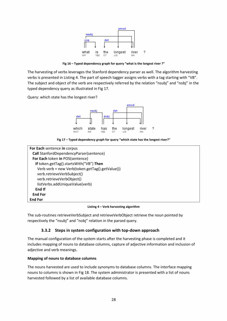
28

Fig 16 – Typed dependency graph for query “what is the longest river ?”

The harvesting of verbs leverages the Stanford dependency parser as well. The algorithm harvesting

verbs is presented in Listing 4. The part of speech tagger assigns verbs with a tag starting with “VB”.

The subject and object of the verb are respectively referred by the relation “nsubj” and “nobj” in the

typed dependency query as illustrated in Fig 17.

Query: which state has the longest river?

Fig 17 – Typed dependency graph for query “which state has the longest river?”

For Each sentence in corpus Call StanfordDependencyParser(sentence) For Each token in POS(sentence) If token.getTag().startsWith(“VB”) Then Verb verb = new Verb(token.getTag().getValue()) verb.retrieveVerbSubject() verb.retrieveVerbObject() listVerbs.addUniqueValue(verb) End If End For End For

Listing 4 – Verb harvesting algorithm

The sub-routines retrieveVerbSubject and retrieveVerbObject retrieve the noun pointed by

respectively the “nsubj” and “nobj” relation in the parsed query.

3.3.2 Steps in system configuration with top-down approach

The manual configuration of the system starts after the harvesting phase is completed and it

includes mapping of nouns to database columns, capture of adjective information and inclusion of

adjective and verb meanings.

Mapping of nouns to database columns

The nouns harvested are used to include synonyms to database columns. The interface mapping

nouns to columns is shown in Fig 18. The system administrator is presented with a list of nouns

harvested followed by a list of available database columns.

29

Fig 18 – User interface mapping nouns to database columns

Capture of additional adjective information

The phase of adjective information capture allows the administrator to set the scalarFlag and when

applicable, the scalar column and direction (see

Fig 19). When the adjective’s base form is harvested, the system automatically builds the

comparative and superlative form. The algorithm for building comparative and superlative are

presented respectively in Listing 5 and Listing 6.

Fig 19 – User interface capturing adjective information

30

Function constructSuperlative(adjective) If getSyllableNumber (adjective) > 2 Then return “more” + adjective Else If getSyllableNumber (adjective) = 2 And isConsonant(lastLetter(adjective)) Then return “more” + adjective End If If isConsonant(lastLetter (adjective)) Then If isConsonant(secondLastletter(adjective))Then return adjective + secondLasLetter(adjective)+”er” Else return adjective + “er” End If Else If endsWithY(adjective) Then return removeLastY(adjective) + “ier” Else If endsWithE(adjective) Then return adjective + “r” End If End Function

Listing 5 – Algorithm constructing the comparative form of adjective

Function construct_superlative(adjective) If getSyllableNumber(adjective) > 2 Then return “most” + adjective End If If isConsonant(lastLetter (adjective)) Then If isConsonant(secondLastletter(adjective)) Then return adjective + secondLasLetter(adjective)+”est” Else return adjective + “est” End If Else If endsWithY(adjective) Then return removeLastY(adjective) + “iest” Else If endsWithE(adjective) Then return adjective + “st” End If End function

Listing 6 – Algorithm constructing the superlative form of adjective

3.3.2.1 Inclusion meaning for adjectives and verbs

The administrator adds the meaning expressed as a SQL conditional expression to certain adjectives

and verbs harvested using the interface illustrated in Fig 20. Not all the adjectives and verbs need to

have a meaning explicitly included. In addition, the engine automatically builds the meaning for

negative form of verbs, superlative and comparative form of adjectives using the meaning provided

for the base forms. Automatically building the meaning reduces the workload for authoring the

system. Listing 7 presents the algorithm building the verb’s negative form from semantic provided

for the base form.

31

Fig 20 – User interface capturing meaning for adjectives and verbs

Function generateNegativeForm(semanticBaseForm) If typeOfSQL(semanticBaseForm).equals(“EXISTS”) Then newSemantic = reversePolarityOfExist(semanticBaseForm) Else newSemantic = reversePolarityOfMainOperator(semanticBaseForm) End If return newSemantic End Function

Listing 7 – Algorithm generating the SQL conditional expression for the negative form of a verb

The following operations are performed by the sub-routines reservePolarityOfExits and

reversePolarityOfMainOperator:

- reservePolarityOfExits: replaces “EXISTS” by “NOT EXISTS” and vise-versa in the SQL;

- reversePolarityOfMainOperator: negates the comparison operator of the conditional

expression in the SQL (i.e. “student.studenMark > 5” becomes “student.studentMark <= 5”).

The meaning is auto-generated for adjective superlative forms and included in the configuration. The

system selects the record corresponding to either the highest or smallest value (depending on the

scalar direction) of the scalar column. Listing 8 presents the algorithm generating the meaning

expressed in SQL for the superlative form of adjective.

For the comparative form, the system selects the record where the scale column is greater or lesser

(depending on the scale direction being respectively positive or negative) than the scale’s column of

the subject. For example, the query “Student smarter than John” would correspond to “Select

student whose mark is superior to John’s mark”. Listing 9 presents the algorithm building the

semantic for the comparative form of adjective.

32

Function generateSemanticSuperlativeForm(adjective) primaryKeyColumn = getPrimaryColumn(adjective.getDescribedColumn().getTable()) If adjective.scalarDirection = true Then semantic = primaryKeyColumn + “ IN (SELECT “ + primaryKeyColumn + “ ORDER BY “ +

adjective. scalarColumn + “ DESC LIMIT 1” Else semantic = primaryKeyColumn + “ IN (SELECT “ + primaryKeyColumn + “ ORDER BY “ +

adjective. scalarColumn + “ ASC LIMIT 1” End If return semantic End Function

Listing 8 – Algorithm generating the SQL conditional expression for the superlative form of an adjective

Function generateSemanticComparativeForm(adjective) If adjective.scalarDirection = true Then Semantic = adjective. scalarColumn + “ > (SELECT “ + adjective. scalarColumn + “ LIMIT 1)” Else Semantic = adjective. scalarColumn + “ < (SELECT “ + adjective. scalarColumn + “ LIMIT 1)” End If return semantic End Function

Listing 9 – Algorithm generating the SQL conditional expression for the comparative form of an adjective

Example: what is the largest city in Wisconsin? Adjective: large Superlative form: largest Comparative form: larger Scale column: city.city_area Scale direction: positive Semantic auto-generated for superlative form: "city.pkey_city IN (SELECT city.pkey_city ORDER BY

city.city_area DESC LIMIT 1)" Semantic auto-generated for comparative form: "city.city_area > (SELECT city.city_area LIMIT 1)" Final SQL query:

SELECT city1.city_name FROM city AS city1 WHERE city1.pkey_city IN ( SELECT city2.pkey_city FROM city AS city2, state AS state2 WHERE state2.state_name = 'wisconsin' AND city2.fkey_state = state2.pkey_state ORDER BY city2.city_area DESC LIMIT 1)

Note: the condition and clauses included in the final SQL originating from the semantic defined for the superlative form are underlined.

3.4 Design of the bottom-up authoring approach

The bottom-up approach aims to explore the possibility of building a configuration with no human

intervention, using the database schema and column synonyms harvested from WordNet as the only

sources for customization data.

33

The first phase of bottom-up extracts the database schema. The schema extraction module

leverages JDBC (Java Database Connectivity) which is Java API for database interfacing. The JDBC API

also provides a generic interface to read the database meta-data like table’s names, column’s

names, column’s types and table’s relationships.

The second phase of bottom-up retrieves synonyms for database columns. Each column from the

database that is not a primary or foreign key is used to auto-harvest possible synonyms from

WordNet. The algorithm describing the construction of bottom-up configuration end-to-end is

described in Listing 10.

For Each table in DBModel For Each column in table If NotAPrimaryKey(column) And NotAForeignKey(column) Then listSynonyms = getListSynonymsFromWordNet(columnName) column.synonyms = listSynonyms End If End For End For

Listing 10 – Algorithm constructing the configuration automatically through bottom-up approach

The bottom-up approach assumes that the database uses meaningful English nouns for column

names; otherwise, no new additional synonyms will be retrieved from WordNet. The WordNet

library JWI5 has been used to interface with WordNet dictionary.

5 http://projects.csail.mit.edu/jwi/

34

Chapter 4 Design of the query processing pipeline

The present chapter presents the design of a query interpreter which translates a natural language

input query into SQL query using the configuration generated during the system’s customization.

The first section presents the design objectives and system architecture; the rest of the chapter

describes with more details each of the main phases of query processing, namely lexical analysis,

syntactic analysis, semantic analysis and SQL Translation.

4.1 Design objective and system architecture

The design objective of the query interpreter is to yield the highest accuracy possible using the

configuration model produced during system customization. The configuration includes the

following elements:

- the list of nouns mapped to database columns;

- the list of adjectives including the nouns they describe and their corresponding meanings;

- the list of verbs including their arguments and the corresponding meanings.

During query processing, each word’s grammatical category needs to be extracted from the natural

language query. This task is achieved using a part of speech (POS) tagger and a syntactic parser. The

Stanford natural language processing group presents a parser that retrieves grammatical relations

between words in a sentence (De Marneffe et al., 2006). The Stanford dependency parser uses a

statistical model trained with a corpus of 254,840 English words manually annotated (Silveira et al.,

2014). The important effort put into manual annotation addresses the problem of scarcity of gold

standard dependency corpus and motivates the use of Stanford parser for this research. The

grammatical relations between words from the parse tree facilitate the retrieval of adjectives and

verbs along with their arguments. The system’s core architecture is, therefore, a syntax-based NLIDB

using the Stanford dependency parser.

The processing pipeline translates the natural language query to SQL in four main steps illustrated

Fig 21. The lexical analysis phase processes the sentence at word level, the process includes part of

speech tagging, lemmatization and named entity recognition. The syntactic analysis leverages the

Stanford parser to extract the relationship between words in the sentences. The semantic analysis

phase translates the query into an intermediary meaning representation language. In this research,

the intermediary query uses first order logic to represent query meaning. Finally, the SQL

translation phase converts the logical query into SQL query.

Fig 21 – Processing pipeline from natural language query to SQL

The system architecture is illustrated in Fig 22, it has three conceptual layers which are the client,

middleware and persistence layer. The client layer is a Web user interface (see Fig 23) that captures

the natural language query and presents the final result to the user. The prototype built is

experimental and therefore includes the intermediary results as well. The middleware layer

encapsulates the query processing logic which leverages the Stanford NLP API and Java WordNet

Interface (JWI). Both the system’s backend and external API are built on top of the Java Standard

Edition core library. The persistence layer is composed of a relational database management system

35

where the actual data are stored. The experimental prototype called NALI (NAtural Language

Interface) uses a PostgreSQL database but any relational database supporting SQL can be used.

Fig 22 – System’s architecture

Fig 23 – Processing pipeline user interface

36

4.2 Lexical analysis

The lexical analysis phase is concerned with processing the sentence at word level, the process

includes part of speech tagging, lemmatization and named entity recognition. The subsequent

sections present more details for each of the lexical analysis stages.

4.2.1 Part of speech tagging

The part of speech tagging stage associates each word in the text to its corresponding “part of

speech” (POS) or grammatical category like nouns, verbs, adjectives, etc. Each grammatical category

is represented by a discrete POS tag. POS in this research leverages the open source Stanford POS

tagger (Toutanova et al., 2003). The Stanford POS tagger uses the Pen Treebank tag set (Marcus et

al., 1993) to encode each grammatical category and is provided with a trained empirical model. The

internal model is based on a Conditional Markov Model (CMM) trained with Penn Treebank

annotated corpus and yields a 97,24% accuracy score (Toutanova et al., 2003). The tagger is

distributed as Java library6 including the trained model. The POS tagger produces a tokenized query

which is a collection of token objects (see Fig 24). Each token is composed of the original word and

the tag representing the grammar category.

Example of POS tagging: Query: what is the longest river in mississippi ? POS Tokenized Query: what/WP is/VBZ the/DT longest/JJS river/NN in/IN mississippi/NNS ?/.

Fig 24 – Structure of a token

4.2.2 Lemmatization

The phase of lemmatization aims to remove ineffectual endings and keep only the base or dictionary

form of each word called a “lemma”. For example, a plural noun will be transformed to its singular

form and a conjugated verb is transformed to the base form. The use of lemma allows more

flexibility during semantic analysis like identifying concepts appearing in plural form for example.

Example: which rivers run through states bordering new mexico ? Lemmatized Query: which river run through state border new mexico ?

The processing pipeline uses the Stanford lemmatizer; it is distributed along with the core API and

uses a pre-trained model to perform lemmatization.

4.2.3 Named entity recognition

The named entity recognition (NER) phase labels words from the text that belong to special

categories like person’s name, location or organization’s name. In this research, NER is performed to

6 The Stanford POS Tagger is distributed under GNU License and accessible on http://nlp.stanford.edu/software/tagger.shtml

37

mark database columns and facts appearing in the natural language query. The named entities are

formatted using IOB (Inside-Outside-Beginning) tags which are standards in NLP field (Ramshaw &

Marcus, 1995). The structure of each named entity is represented in Fig 25.

Fig 25 – Structure of named entities

The named entity (NE) type can be either “DB_COL” or “DB_FACT” depending on the NE

representing a database column or fact. Attribute1 and attribute2 store respectively the table’s

name and column’s name. The NER module adds a NE tag to each token of the tokenized query. The

field iobTag store the tag’s symbol which can have the following values:

- O: Outside, meaning the current token is not a named entity;

- B: Beginning, meaning the current token is part of a named entity and represents the first

word constituting the NE;

- I: Inside, meaning the current token is part of a named entity and represents a word within

the NE.

Example: which students enrolled in computer science ? NER result: which/O students/B enrolled/O in/O computer/B science/I ?/O

In the above query, “student” and “computer science” are named entities; “student” and

“computer” receives respectively the symbol “B” for being the first word of the NE; and “science”

receives the symbol “I” for being within a NE with more than one word. The rest of the words which

are not named entities receives a “O” symbol.

Listing 11 presents the algorithm marking database facts and column synonyms found in the text as

named entities. The database schema is automatically extracted and the database column’s

synonyms are populated during system’s customization. The interface “getAllDBColumns” retrieves a

list with all the columns. The system retrieves and stores database facts from all the columns

containing text values in a list accessed through the interface “getAllDBFacts”. More than one

named entity can be assigned to a token because both database facts and columns can contain

duplicated values. For example “area” can be a synonym to both cityArea and stateArea columns;

and “New York” is a fact existing in both cityName and stateName columns. A token with more than

one named entity requires disambiguation which is presented in the next section.

For Each fact in dbModel.getAllDBFacts() If (query.contains(fact.word)) markNE(fact.word,query,”DB_FACT”,fact.tableName,fact.columnName) End If End For For Each col in dbModel.getAllDBColumns() If (query.getLemmatizedQuery().contains(col.getSynonyms())) markNE(fact.word,query,”DB_COL”,col.tableName,col.columnName) End If End For

Listing 11 – Named entity recognition algorithm

38

4.2.3.1 Resolution of ambiguities in named entities

Let X be a word from the natural language query and NE(X) the set of possible named entities

associated to X. X is ambiguous when #NE(X) > 1. Three heuristic rules allow resolving lexical

ambiguities; one for database fact ambiguities and two for database column ambiguities. The

heuristic rules for named entities disambiguation (and for the other modules involving rules as well)

were derived from observing examples of both the input (ambiguous named entity, for example)

and output (correct named entity, for example). This observation allowed noticing the most

occurring common patterns which were codified as rules.

Rule 1 – database fact disambiguation

The first rule is applied when the ambiguous word is an adjective. Formally, rule 1 is applied when

there exists an ambiguous word X for which the following conditions are met:

- the attribute “type” for all NE(X) = “DB_FACT”;

- there exists in the typed dependency query a triple amod(JJ*,NN*) where X.tag = “JJ*” and

Y.tag = “NN*”.

Note:

- amod: is the adverbial modifier relationship which links an adjective (JJ*) to a noun it defines

(NN*);

- Y: is the noun defined by the adjective X;

- JJ*: is a part of speech tag starting with JJ which represents an adjective;

- NN*: is a part of speech tag starting with NN which represents a noun.

The engine resolves the ambiguity by selecting the table’s name mapped to the noun that the

ambiguous adjective describes. Formally, the engine keeps NE(X) where NE(X).attribute1 =

NE(Y).attribute1. Note: attribute1 represents the database table associated to the named entity.

Example: how long is the mississippi river ? Typed dependency query:

In the above example “mississippi" is ambiguous and associated to the two following named entities:

- NE1: type = “DB_FACT”, iobTag=”B”, attribute1 = “state”, attribute2 = “stateName”

- NE2: type = “DB_FACT”, iobTag=”B”, attribute1 = “river”, attribute2 = “riverName”

The matching triple is: amod(mississippi,river) where: - NE(river): type = “DB_COL”, iobTag = “B”, attribute1 = “river”, attribute2 = “riverName”

Therefore, the engine resolves the ambiguity by keeping only NE2 for NE(mississippi).

39

Rule 2 – database column disambiguation

The second rule uses the object of the proposition referring the ambiguous noun to disambiguate.

Formally, rule 2 is applied when there exists an ambiguous word X for which the following conditions

are met:

- the attribute “type” for all NE(X) = “DB_COL”;

- there exists in the typed dependency query a triple prep_*(NN*,NN*) where X.tag = “NN*”

(X can correspond to either the first or second argument) and Y.tag = “NN*”.

The engine resolves the ambiguity by selecting the table’s name mapped to the noun that is the

object of the preposition. Formally, the engine keeps NE(X) where NE(X).attribute1 =

NE(Y).attribute1.

Example: what is the area of the largest state ? Typed dependency query:

In the above example “area” is ambiguous and associated to the two following named entities:

- NE1: type = “DB_COL”, iobTag=”B”, attribute1 = “state”, attribute2 = “stateArea”

- NE2: type = “DB_COL”, iobTag=”B”, attribute1 = “city”, attribute2 = “cityArea”

The matching pattern is: prep_of(area,state) where: - NE(state): type = “DB_COL”, iobTag = “B”, attribute1 = “state”, attribute2 = “stateName”

Therefore, the engine resolves the ambiguity by keeping only NE1 for NE(area).

Rule 3 – database column disambiguation

The third rule is applied when the ambiguous word is a verb’s object; the corresponding subject is

used to disambiguate. Formally, rule 3 is applied when there exists an ambiguous word X for which

the following conditions are met:

- the attribute “type” for all NE(X) = “DB_COL”;

- there exists in the typed dependency query two triples t1 = nsubj(VB*,NN*) and t2 =

dobj(VB*,NN*) where X.tag = “NN*” from t2 and Y.tag = “NN*” from t1.

The engine resolves the ambiguity by selecting the table’s name mapped to the verb’s subject.

Formally, the engine keeps NE(X) where NE(X).attribute1 = NE(Y).attribute1.

40

Example: which state has the highest population density ? Typed dependency query:

In the above example “population" is ambiguous and associated to the two following named entities:

- NE1: type = “DB_COL”, iobTag=”B”, attribute1 = “state”, attribute2 = “statePopulation”

- NE2: type = “DB_COL”, iobTag=”B”, attribute1 = “city”, attribute2 = “cityPopulation”

The matching triples are t1 = nsubj (has,state) and t2 = dobj(has,density) where: - NE(state): type = “DB_COL”, iobTag = “B”, attribute1 = “state”, attribute2 = “stateName”

Therefore, the engine resolves the ambiguity by keeping only NE1 for NE(population).

4.3 Syntactic analysis

The syntactic phase analyses the grammar structure of the natural language sentence. It leverages

the Stanford probabilistic context-free grammar parser (Klein & Manning, 2003) which includes an

empirical model constructed from manually parsed sentences. The Stanford parser extracts the

grammatical relations which are represented as Stanford typed dependencies (SD), a format

designed to be “easily understood and effectively used by people who want to extract textual

relations” (De Marneffe & Manning, 2008). The SD format represents each grammatical relation as

triple composed of the relation’s name, a governor (or head) and a dependant. The head and

dependant are words from the sentence while the relation describes the grammatical link between

the governor and dependant. A more detailed description of the SD format and exhaustive list of

relationships supported can be found in (De Marneffe & Manning, 2008). The ensemble of

relationships forms a graph, starting from an abstract ROOT node which is a virtual node added by

the parser and representing the entry point to navigate the parsed query’s graph.

Example: John loves Marie The typed dependency query (illustrated in Fig 26) comprises the following triples:

root(ROOT,loves) nsubj(loves,John) dobj(loves,Marie)

Fig 26 – Visualization of the typed dependency query for “John loves Marie”

4.4 Semantic analysis

The phase of semantic analysis extracts and expresses the sentence meaning in an intermediary

Meaning Representation Language (MRL). The intermediary query is expressed as a first-order logic

(FOL) expression using only the function’s part of FOL. The intermediary query is composed of two

parts which are both expressed in FOL: the select and query part (see examples in Table 6). The

41

select part designates the information that needs to be retrieved and returned in the final result.

The query part expresses the restriction or conditions the final result needs to satisfy. The select part

must satisfy either one of the two following conditions:

- must be a function of valence 0: if X is this function, the column to be selected corresponds

to attribute2 of NE(X);

- must be a unary function: the function name can be either an aggregation term (“count”,

“sum”, “avg”, “max” and “min”) or an adjective. An adjective indicates the engine to return

the scalar column corresponding to the adjective.

Table 6 – Example of query and their corresponding intermediary queries

Natural Language Query Intermediary query

Select part Query part

what is the area of the largest state ? area() of(area,largest(state))

how many rivers are in colorado ? count(rivers) be in(rivers,colorado)

4.4.1 Heuristic rules to build the select part of the intermediary query

The semantic analyser is based on a set of generic heuristic rules that translates the typed

dependency query from the parser into an intermediary query for both the select and query parts.

The algorithm retrieving the select part uses five heuristic rules to construct the select clause from

the typed dependency query. Each rule is composed of a pattern and an associated template. The

pattern part is matched against triples from the typed dependency query and the template part

describes how the select part is constructed from the matching triples. The patterns and their

corresponding templates are presented in Table 7. Each rule is applied following the order in the

table below until a matching pattern is found.

Table 7 – List of rules to retrieve the select part of the logical query

Rule Pattern looked up Template Comment

1 *(NN*,”total”) or *(NN*,”average”) or *(NN*,”maximum”) or *(NN*,”minimum”)

sum(NN*) or avg(NN*) or max(NN*) or min(NN*)

Searches for a noun referencing respectively “total”, “average”, “maximum” and “minimum” to construct an aggregation function with the matched noun as argument

2 *(W*,NN*) or *(NN*, W*) NN*() Searches for a Wh- question (tag starting with “W”) that is related to a noun (tag starting with “NN”). The latter becomes the select part.

3 *(“many”,”how”) and *(NN*, “many”)

count(NN*) Searches for “how many” and selects the noun linked to “many” to build a select part with a count function.

4 *(*,“how”) [*]([first_noun]) When “how” is found, the word it points to becomes the function; and the function argument corresponds to the first noun found in the query

5 - NN*() When the first three patterns do not match, the engine selects the first noun found in the query as the select

42

Example 1: what is the total area of the usa ? Typed dependency query:

Rule 1 applied, matched pattern: amod(area,total). Result: sum(area)

Example 2: which rivers run through states bordering new mexico ?

Typed dependency query:

Rule 2 applied, matched pattern: det(rivers,which). Result: rivers()

Example 3: how many rivers are there in idaho ? Typed dependency query:

Rule 3 applied, matched patterns: advmod(many,how) and amod(rivers,many) Result: count(rivers)

Example 4: how long is the mississippi river ? Typed dependency query:

Rule 4 applied, matched pattern: advmod(long,how) and the first noun is “river” Result: long(river)

43

Example 5: name all the rivers in colorado ? Typed dependency query:

Rule 5 applied, no matching pattern and first noun is “rivers” Result: rivers()

4.4.2 Construction of the query part of the intermediary query

The construction of the query part is completed in three steps. The first step traverses the typed

dependency query from the root element and creates groups of triples read in the same round. The

second step constructs the intermediary query corresponding to each group from the first step. The

last step merges all intermediary queries and constructs the final intermediary query. The next

sections describe in detail the three steps.

4.4.2.1 Grouping of typed dependency triples

The grouping algorithm is presented in Listing 12. The algorithm starts the traversal of the typed

dependency query from the ROOT triple which forms the first group. The second round reads all the

triples starting from the dependent element of the ROOT triple to form the second group. The

process repeats for each new triple traversed until the entire query is navigated as illustrated in the

example. The algorithm produces a two-dimensional array where the first dimension contains the

groups and the second the triples within each group.

Function groupTripleDependencyQuery() DepTriple trip = parsedQuery.getRootTriple() Token firstToken = trip.getArgument1() browse(firstToken)

End Function Function browse(Token token) DepTriple [] trips = getTripleStartingFrom(token) finalListTriples.add(trips) For Each DepTriple trip in trips browse(trip.getArgument1()) End For End Function

Listing 12 – Algorithm grouping triples from the typed dependency query

44

Example: what states have cities named dallas? Typed dependency query:

List of triples:

det(states-2,what-1) dep(named-5,states-2) aux(named-5,have-3) nsubj(named-5,cities-4) root(ROOT-0,named-5) dobj(named-5,dallas-6)

Round 1: browse all the triples starting from ROOT-0

Group 1 created: root(ROOT-0,named-5) Round 2: browse all the triples starting from named-5

Group 2 created: dep(named-5,states-2) aux(named-5,have-3) nsubj(named-5,cities-4) dobj(named-5,dallas-6)

Round 3: browse all the triples starting from states-2

Group 3 created : det(states-2,what-1) Round 4: browse all the triples starting from what-1

Not triple found

Round 5: browse all the triples starting from have-3 Not triple found

Round 6: browse all the triples starting from cities-4 Not triple found

Round 7: browse all the triples starting from dallas-6 Not triple found

The final list of groups created for the above example is presented in Table 8.

Table 8 – Final list of triple groups corresponding to the query: “what states have cities named dallas ?’

Group 1 root(ROOT-0,named-5)

Group 2 dep(named-5,states-2) aux(named-5,have-3) nsubj(named-5,cities-4) dobj(named-5,dallas-6)

Group 3 det(states-2,what-1)

45

4.4.2.2 Construction of intermediary queries

The second step constructs an intermediary query for each group of triple from step 1. The

algorithm for step 2 is presented in Listing 13; it reads each group and calls the rule engine which

translates the triples from the group into an intermediary query. The rule engine maps triple

patterns to an intermediary query template. The list of rules is presented in Table 9.

For Each tripleGroup in listOfGroups IntermediaryQuery intQuery = rule(1, tripleGroup) // 1 represents the rule’s number For (i=2,i <= 6;i++) If (intQuery =null) intQuery = rule(i, tripleGroup) // i represents the rule’s number Else listOfIntQuery.add(intQuery) continue End If End For End For

Listing 13 – Algorithm that constructs intermediary queries

Table 9 – List of rules used to generate logical queries

Rule Pattern Intermediary query template

Type of query

1 nsubj(VB*,NN*) and dobj(VB*, NN*) VB* (NN*, NN*) Binary function

2 *( VB*,NN*) NN*() Term

3 *( NN*,JJ*) JJ* (NN*) Unary function

4 *( JJ*,RBS) RBS(JJ*) Unary function

5 prep_*( NN*, NN*) pre_*( NN*, NN*) Binary function

6 *(*, NN*) NN*() Term

Example: what states have cities named dallas ? Typed dependency query:

Groups created:

- Group 1: root(ROOT-0,named-5)

- Group 2: dep(named-5,states-2), aux(named-5,have-3), nsubj(named-5,cities-4) and

dobj(named-5,dallas-6)

- Group 3: det(states-2,what-1)

Round 1: group browsed: root(ROOT-0,named-5) Rule applied: no rule Action: no action

46

Example continued

Round 2 : group browsed: dep(named-5,states-2), aux(named-5,have-3),nsubj(named-5,cities-4), dobj(named-5,dallas-6)

Rule applied: Rule 1 Pattern “nsubj(VB*,NN*1)” matched to “subj(named-5,cities-4)” Pattern “dobj(VB*, NN*2)” matched to “dobj(named-5,dallas-6)”

Action: create intermediary query with pattern: VB* (NN*1, NN*2); Result: named(cities,dallas)

Round 3 : group browsed: det(states-2,what-1) Rule applied: none

The final list of intermediary queries has one element: named(cities,dallas)

4.4.2.3 Merging of intermediary queries parts into the final query

The merging algorithm is presented in Listing 14; it merges intermediary queries from the previous

step two by two starting from the two last queries in the list. The algorithm has six merging rules

containing the merge logic presented in Listing 15.

Function mergeIntermediarylQuery(IntermediaryQuery[] elements) If (elements.length == 1)

return elements[0] End If rootElement = elements[elements.length-1]

For(i=elements.length-2;i>=0;i--) rootElement = merge(elements[i],rootElement) End For End Function

Listing 14 – Algorithm merging intermediary queries element

Example: what is the capital of the state with the highest point ? Typed dependency query:

List of intermediary queries (from step 2): “capital”, “of(capital,state)”, “with(state,point)” and

“highest(point)” Merge round 1: merge “with(state,point)” and “highest(point)”

Merging rule 4 applied, result: “with(state,highest(point))” Merge round 2: merge “of(capital,state)” and “with(state,highest(point))”

Merging rule 6 applied, result: “of(capital, with (state,highest(point)))” Merge round 3: merge of “capital” and “of(capital, with (state,highest(point)))” Merging rule 1 applied, final result: “of(capital, with(state,highest(point)))”

47

Function merge(LogicalQueryElement query1, LogicalQueryElement query2) If (query1 is Term) // merging rule 1 If (query2.contains(query1)) return query2 End If End If If (query1 is unary function And query2 is term) // merging rule 2 query1.setArgument1(query2) End If If (query1 is unary function And query2 is binary function) // merging rule 3 If (query1.functionName() = query2.functionName()) return query2 Else If (query2.contains(query1)) return query2 Else If (query2.contains(query1.getArgument1()) query1.setArgument1(query2) return query1 End If End If If (query1 is binary function And query2 is unary function) // merging rule 4 If(query2.contains(query1.getArgument1()) Query1.setArgument1(query2) return query1 Else If (query2.getArgument1().contains(query1.getArgument2()) Query1.setArgument2(query2) return query1

End If End If If (query1 is unary function And query2 is unary function) // merging rule 5 If(query2. getArgument1().contains(query1.getArgument1()) Query1.setArgument1(query2) return query1

Else If (query2.contains(query1.getArgument1()) Query1.setArgument1(query2) return query1 Else If (query1.contains(query2.getArgument1()) Query2.setArgument1(query1) return query2 End If

If (query1 is binary function And query2 is binary function) // merging rule 6 If (query2.contains(query1.getArgument1())) Query1.setArgument1(query2) return query1 Else If (query2.contains(query1.getArgument2()) Query1.setArgument2(query2) return query1 End If

End If

Listing 15 – Merging rules for two intermediary queries

48

4.5 SQL Translation

The last phase translates the intermediary query into a SQL query. The translation process is

executed in two steps: the first step translates the intermediary query into an intermediary SQL

query which does not include the FROM clause and joins between tables. The second phase

completes the FROM clause, the joins and adds aliases for table in order to avoid naming conflicts.

4.5.1 Construction of the intermediary SQL query

The algorithm translating the Intermediary query to SQL is presented in Listing 16. The algorithm

generates an empty SQL before calling the routines processing the select and query part of the

intermediary query. The routine processSelectPart contains the logic that inserts the correct column

into the select clause of the current SQL from the select part of the intermediary query. The routine

browse navigates the query part of the intermediary query; for each function or term read, the

appropriate processing is called (processBinaryFunction, processUnaryFunction or processTerm). A

recursive call of browse routine for each function allows the process to repeat itself until the entire

intermediary query is navigated. The algorithms in Listing 17, Listing 18 and Listing 19 present the

processing of binary function, unary function, and term respectively.

Function translateIntermediaryQuery(IntermediaryQuery intQuery) SQLQuery query = new SQLQuery() query = processSelectPart(intQuery.getSelectPart()) query = browse(query, intQuery) End Function Function processSelectPart(SQLQuery query, IntermediaryQuery selectPart) If (selectPart is Term) DBColumn col = selectPart.retrieveColumn() query.addSelectClause(col) return query

Else If (selectPart is BinaryFunction) If (selectPart.getFunctionName() = “count”) DBColumn col = selectPart.retrieveColumn() col.setAggregation(COUNT)

query.addSelectClause(col) return query

Else Adjective adj = selectPart.retrieveAdjective() DBColumn col = adj.getScalarColumn()

query.addSelectClause(col) return query

End If End If

End Function

49

Listing 16 continued

Function browse(SQLQuery query, IntermediaryQuery intQuery) If (intQuery is BinaryFunction) newSQLQuery = processBinaryFunction(sqlQuery, intQuery) browse(newSQLQuery, intQuery.getArgument1()) browse(newSQLQuery, intQuery.getArgument2())

Else If (intQuery is UnaryFunction) newSQLQuery = processUnaryFunction(sqlQuery, intQuery) Else processTerm(sqlQuery, intQuery) End If

End Function

Listing 16 – Algorithm translating the intermediary query to intermediary SQL

Function processBinaryFunction(SQLQuery sqlQuery, IntermediaryQuery intQuery) DBColumn column1 = retrieveDBColumn(intQuery.getArgument1())

DBColumn column2 = retrieveDBColumn(intQuery.getArgument2()) Semantic semantic = KnowledgeModel.retrieveVerbSemantic(intQuery.getFunctionName,column1,column2) SQLQuery sqlSemantic = semantic.translateToSQL() For (whereClause wc in sqlSemantic.getWhereClauses()) sqlQuery.addWhereClause(wc) End For If(sqlSemantic.isSubQuery()) return sqlSemantic.getSubQuery() Else return sqlQuery End If

End Function

Listing 17 – Algorithm processing binary functions

Function processUnaryFunction(SQLQuery sqlQuery, IntermediaryQuery intQuery) DBColumn column = retrieveDBColumn(intQuery.getArgument1())

Semantic semantic = KnowledgeModel.retrieveAdjectiveSemantic(intQuery.getFunctionName,column) SQLQuery sqlSemantic = semantic.translateToSQL() For(whereClause wc in sqlSemantic.getWhereClauses()) sqlQuery. addWhereClause (wc) End For If(sqlSemantic.isSubQuery()) return sqlSemantic.getSubQuery() Else return sqlQuery End If

End Function

Listing 18 – Algorithm processing unary functions

50

Function processSimpleTerm(SQLQuery sqlQuery, IntermediaryQuery intQuery) Value = logQuery.getValue() DBColumn column = retrieveDBColumn(intQuery)

whereClauseExpression = column + ComparisonOp.EQUAL + value sqlQuery.whereClause().addWhereClause(whereClauseExpression)

End Function

Listing 19 – Algorithm processing term

Example: which state borders kentucky ? Intermediary query:

select part: state() query part: border(state,kentucky)

Processing select part of the logical query

The token “state” has a named entity of type database column that reads “state.state_name”; which is directly inserted into the main select clause of the intermediary query. Current intermediary query: SELECT state.state_name

Processing the query part of the logical query Round 1: browse border(state,kentucky)

Apply Binary Processing: corresponding semantic rule found: border(state.state_name,state.state_name) -> state.pkey_state IN (SELECT

border.fkey_bordering_state) The semantic part of the rule corresponds to the condition to include inside the current intermediary query. New intermediary query: SELECT state.state_name WHERE state.pkey_state IN (SELECT border.fkey_bordering_state). Note: the rule has included a new sub-query, meaning all sub-sequent browsing will include restriction at the level of the sub-query. Arguments for next browse: state, kentucky

Round 2: browse state

Apply Term Processing: capital is not a database fact (no db NE tag here); therefore, no further action taken.

Round 3: browse kentucky Apply Term Processing: kentucky is bound to database fact (there is named entity

associated to it). Action: include the restriction: state.state_name = 'kentucky' into the sub-query.

Final Intermediary SQL query: SELECT state.state_name WHERE state.pkey_state IN ( SELECT border.fkey_bordering_state WHERE state.state_name = 'kentucky')

51

4.5.2 Construction of the final SQL query

4.5.2.1 Join clause generation

Fig 27 describes the steps in the algorithm of join construction module. The schema of the database

and the intermediary SQL query constitute the inputs to build the joins.

Step 1 builds an undirected graph from the database schema where nodes represent tables and links

represent relationships between tables (see the algorithm in Listing 20). Fig 28 shows an example of

a database schema and its corresponding graph. All the tables in the database are included in the

graph. The approach used to produce joins from graphs is similar to (Meng & Chu, 1999).

Step 2 retrieves the list of tables to be joined from the intermediary SQL query. The corresponding

algorithm extracts all tables existing in the intermediary query; it is presented in Listing 21.

Step 3 evaluates the paths between all node pairs from the node set corresponding to the tables to be joined. The Dijkstra shortest path algorithm presented in (Dijkstra, 1959) is used to compute the paths. Step 4 generates the joins between tables from the paths between node pairs. The corresponding

algorithm is presented in Listing 22.

Fig 27 – Steps in join construction

Fig 28 – Construction of a database graph from a database schema

52

Function generateGraph(DBModel dbModel) Graph graph = new Graph() For Each Table table in dbModel Node node1 = new Node(table.getName()) graph.addNode(node1) For Each Column column in table.getColumns() If (column.isForeignKey()) Table foreignTable = column.getForeignTable() Node node2 = new Node(foreignTable.getName()) If (graph.notContain(node2) graph.addNode(node2) End If Edge edge = new Edge(node1,node2) graph.addEdge(edge) End If End For End For return graph

End Function

Listing 20 – Algorithm generating a graph from a database schema

Function retrieveListTablesFromIntermediaryQuery(SQLQuery intQuery) List listTable = new List() browseQuery(listTable, intQuery) End Function Function browseQuery(List listTable, SQLQuery intQuery) For Each Table table in intQuery.getSelectClause() listTable.addUniqueValue(table) End For

For Each WhereClause wc in intQuery.getWhereClause() If (wc.hasSubQuery()) browse(listTable, wc.getSubQuery()) Else Table table = wc.getOperand1().getTable() listTable.addUniqueValue(table) End If End For End Function

Listing 21 – Algorithm retrieving the list of tables to be joined

53

Function generateJoinFromPath(List listNodesInPath) List joins = new List() For (i = 0; i<listNodeInPath.size()-2;i++) Table table1 = dbModel.getTable(listNodesInPath.get(i).getName()) Table table2 = dbModel.getTable(listNodesInPath.get(i+1).getName()) If (table1.hasForeignKeyTo(table2)) Column localColumn = table1.retrieveLocalColumnTo(table2) Column foreignColumn = table2.retrieveLocalColumnTo(table1) Join join = new Join(localColumn,foreignColumn) listJoins.add(join) Else Column localColumn = table2.retrieveLocalColumnTo(table1) Column foreignColumn = table1.retrieveLocalColumnTo(table2) Join join = new Join(localColumn,foreignColumn) listJoins.add(join) End If End For return joins

End Function

Listing 22 – Algorithm generating the joins from the paths between nodes representing table to join

4.5.2.2 FROM clause generation

The FROM clause is a comma separated list of all the tables in the SQL query. The tables to include in

the FROM clause are extracted from all the other parts of SQL query, and included with no

redundancy in the FROM clause. The algorithm generating the FROM clause is presented Listing 23

(the browseQuery routine is defined in Listing 21).

Function generateFromClause(SQLQuery intQuery) List listTable = new List() browseQuery(listTable, intQuery) For Each table in listTable intQuery.addFrom(table) End For End Function

Listing 23 – Algorithm generating the FROM clause

4.5.2.3 Table aliases

The aliases are table synonyms that avoid naming conflicts between the main and sub-queries. Each

table is given an alias composed of the original table’s name and an index corresponding the level of

sub-query nesting (the main query has index 1). The algorithm associating aliases to tables is

presented in Listing 24.

The resulting query after the aliases are completed correspond to the final SQL that is sent to the

RDBMS to retrieve the result.

54

Function associateAliase(SQLQuery intQuery) associateAliase (1, intQuery) End Function Function associateAliase(int index, SQLQuery intQuery) For Each Table table in intQuery.getFromClause() table.addAliase(table.getName()+index) End For

For Each WhereClause wc in intQuery.getWhereClause() If (wc.hasSubQuery()) associateAliase (index+1, wc.getSubQuery()) End If End For End Function

Listing 24 – Algorithm associating aliases to table’s names

55

Chapter 5 Experiment design

A NLIDB prototype called NALI has been developed; it implements the design introduced in chapters

3 and 4. This chapter presents the design of the experiments listed below:

1) The first experiment evaluates the top-down approach; it assesses the top-down capability to

reduce the workload for customization and the system’s accuracy when provided a configuration for

only terms harvested from an unannotated training corpus.

2) The second experiment evaluates the bottom-up approach; it assesses the accuracy yielded from

a model with no manual customization and helps evaluate the usefulness of this approach.

3) The third experiment evaluates the processing pipeline and allows analysing the cases where the

system did not provide the correct answers and study the sources of errors.

4) Finally, we compare the performance obtained with NALI to other similar NLIDB

The remainder of the chapter describes the material and design of the above experiments.

5.1 Material and experiment design

The experiments are based on testing the system prototype NALI with a corpus of natural language

questions and a relational database. The geo-query database and query corpus have been selected

to evaluate the system (Tang & Mooney, 2001). The following reasons motivated the choice of geo-

query:

- the questions from geo-query corpus have rich grammatical structures with a high degree of

logical complexity (Pazos et al., 2013) and will allow assessing the system’s coverage;

- geo-query is the most used corpus in the NLIDB literature; this facilitates comparing the

result to other systems.

The concise version of the corpus (250 queries) has been selected because it contains very few

duplications of questions with the same grammar structure. The resources provided along with the

corpus include a list of questions7, the structure, and content of a Prolog database containing the

facts to answer the questions, and the logical queries written in Prolog that answer the questions.

We constructed a relational database version of geo-query and populated with data from the Prolog

database facts. The Entity-Relationship model of the geo-query database is shown in Fig 29 and the

database schema is shown in Fig 30.

7 The country’s name has been streamlined throughout the corpus to read “USA”

56

Fig 29 – Entity-relationship model of geo-query

Fig 30 – Structure of a relational database version of geo-query

The metrics used to assess the system’s performance are precision and recall defined as follow

(Manning et al., 2008):

57

Precision=#(relevant items retrieved)

#(retrieved items)=

#true positive

#true positive+#false positive

Recall=#(relevant items retrieved)

#(relevant items)=

#true positive

#true positive+#false negative

Most of NLIDB in the literature reviewed uses a different definition of recall (referred to as Recall”

here), which reads:

Recall"=#(retrieved items)

#(relevant items)=

true positive+false positive

true positive+false negative

In order the compare the result, the recall for systems using a different definition has been

recalculated and streamlined to the standard definition.

Recall=Recall"×Precision = #true positive+false positive

#true positive+false negative ×

#true positive

#true positive +#false positive

Recall=#true positive

#true positive+#false negative

A list of correct SQL (gold SQL result) has been manually created in order to automate the evaluation

of the metrics. The remainder describes the design of experiments, the questions they answer, the

test set up and the result format.

5.2 Experiment 1 – evaluation of the top-down approach

The first experiment addresses to the following question:

1) Does the exploitation of an unannotated corpus of sample questions combined with

automatic generation of configuration for negative form of verbs, comparative and

superlative form of adjective reduce the workload required to customize a NLIDB? If yes, to

what extent?

In order to evaluate the effectiveness of the top-down approach, the administrator customizing the

system is simulated using the following assumptions:

- the administrator has the knowledge of both the database structure and the domain;

- the administrator knows SQL and can therefore express meaning as a SQL conditional

expression;

- the administrator is capable of providing the correct mappings and meanings for the terms

harvested.

The above assumptions allow developing an automated test where the system’s administrator is

emulated. The virtual administrator includes the correct mapping and semantics only for the terms

harvested. The experiment will help find the accuracy yielded when using a configuration model with

only the terms harvested through top-down are mapped.

The top-down approach assumes the existence of a corpus of unannotated questions prior

configuration. This requirement is emulated by splitting the corpus into two disjoint parts: a training

set used for term harvesting and a testing set. The model resulting from the configuration is tested

against the questions in the testing set. Different proportions between the training and testing set

58

are used to evaluate top-down. Each proportion corresponds to a specific experiment, Table 10 lists

all the experiments along with their respective sizes of the training and testing set.

Table 10 – proportions of the training and testing set used for evaluation

Experiment Size of training set Size of testing set

Experiment A 100 150

Experiment B 125 125

Experiment C 150 100

Experiment D 175 75

Experiment E 200 50

Experiment F 225 25

Using several ratios for the training and testing set will allow determining if and how each

proportion affects the final accuracy. The content of both the training and testing set is selected

randomly from the main corpus while ensuring that no query appear simultaneously in both sets.

For each experiment, 10 different samples of both the training and testing set are randomly selected

to run each experiment. The following actions are performed for each experiment:

- 10 samples of both the training and testing set are randomly generated according to the

proportion set for the experiment;

- the top-down module is used to automatically harvest terms from the training sample;

- the emulated virtual administrator adds mapping and semantics for only the terms

harvested to produce a configuration model;

- the authoring system includes automatically semantics for negative form of verbs,

comparative and superlative form of adjectives;

- the configuration model produced is used by the processing pipeline to answer the

questions in the testing set;

- the gold SQL result table is used to automatically calculate the precision and recall;

- the evaluation module counts the number of manual8 and automatic entries in the

configuration model.

The result collected will help assess the accuracy of the configuration model produced through top-

down under multiple settings. The experiments will also show how many manual entries are

required for respectively noun mapping, adjective updates, and semantics mapping in order to

weight the workload required for customization. The number of automatic mapping entries can be

compared to manual ones in order to assess how the system does contribute toward reducing the

workload. Each result table is aggregated to produce the average metrics by experiment and the

global average for all the experiments will correspond to the final metrics for the top-down method.

5.3 Experiment 2 – evaluation of the bottom-up approach

The second experiment addresses the following questions:

2) How effective is the use of the database schema to build a configuration model with no

manual customization?

8 Manual in this context refers to the entries provided by the emulated administrator

59

3) To what extent do additional synonyms from WordNet contribute toward improving the

final accuracy of bottom-up?

In order to evaluate the bottom-up approach, a configuration model is automatically generated

using the database schema and WordNet as the only sources of data. The automated testing for

bottom-up includes the following steps:

- the bottom-up configuration model is generated from both the database schema and

WordNet;

- the configuration model is used in the processing pipeline to answer all the 250 questions in

the corpus;

- the gold SQL result table is used to automatically calculate the precision and recall.

The final result includes the configuration model and the metrics’ values. The experiment results will

provide insights on firstly the accuracy of the bottom-up approach and secondly on how the use of

an off-the-shelf lexicon does contribute toward improving accuracy.

5.4 Experiment 3 – Evaluation of the processing pipeline

The third experiment addresses the following questions:

4) How effective is the processing pipeline?

5) What are the limits of the processing pipeline components?

The experiment 3 reviews the effectiveness of the processing pipeline. To assess the processing

pipeline, a “perfect” top-down configuration model is trained using the entire corpus. This

configuration should ideally yield a 100% recall and is therefore used to get insights on the limits of

the processing pipeline. Each incorrect query is manually reviewed to examine at which phase of

processing the error originated from and what caused the fail. The experiment result will provide

insights on the performance at each stage in the processing pipeline.

5.5 Experiment 4 – comparison of the result to other systems

The forth experiment addresses the following question:

6) How does NALI perform compared to both NLIDB with similar design objectives and systems

with a different design?

The results from the top-down approach are compared to other NLIDB systems evaluated with geo-

query. The NLIDBs selected for comparisons are split into two groups. The first group called “Group

A” contains the systems whose design objectives are similar to the top-down approach and satisfy

the two following conditions. The first criterion is that the system should be customizable by an

administrator with only basic knowledge of database systems (including knowledge of SQL) and the

domain; no background in computational linguistics should be required. The second condition is that

no manual annotation of a query corpus should be required to customize the system as this implies

an important workload. The systems not satisfying one of the two conditions are included in the

second group called “Group B”. Table 11 gives the list of systems the top-down model is compared

to, their group and a short comment motivating their classification.

The literature review showed a trade-off between portability and accuracy; systems with a complex

configuration module achieve greater accuracy compared to more portable ones. The result will help

60

to get insights on how the top-down approach performs comparatively to firstly other portable

systems with similar design objectives from Group A and secondly less portable systems from Group

B. The metric used for comparison is recall because it gives the proportion of correct answers

respective to relevant items. The recall for systems using definition 1 is recalculated using the

standard definition.

Table 11 – List of systems the top-down result is compared to

NLIDB Group Type of data source

Comment

PANTO (Wang et al., 2007)

Group A Ontology Acquires the lexicon automatically from WordNet

FREYA (Damljanovic et al., 2010)

Group A Ontology Builds the configuration from an interactive dialog with the user in natural language

Prototype in (Goldwasser et al, 2011)

Group A Knowledge Base

Uses an unannotated corpus and unsupervised method to construct a model

Prototype in (Giordani & Moschitti, 2012)

Group A RDB Uses the database meta-data to build the configuration

Prototype in (Chandra, 2006)

Group B RDB Requires to first manually annotate a training corpus with their corresponding valid SQL

COCKTAIL prototype 1 (Tang & Mooney, 2001)

Group B Knowledge Base

Requires to first manually annotate a training corpus with their corresponding meaning expressed in first order logic

COCKTAIL Prototype 2 Group B Knowledge Base

COCKTAIL Prototype 3 Group B Knowledge Base

COCKTAIL Prototype 4 Group B Knowledge Base

COCKTAIL Prototype 5 Group B Knowledge Base

PRECISE (Popescu et al., 2003)

Group B RDB Prototype customized at design time; no authoring system provided

GINSENG (Bernstein et al., 2005)

Group B Knowledge Base

Required testers with a background in both databases and computational linguistics to customize the system

KRISP (Kate & Mooney, 2006)

Group B Knowledge Base

Requires to first manually annotate a training corpus with their corresponding meaning expressed in the system’s custom meaning representation language

Prototype in (Minock et al., 2008)

Group B RDB Background in computational linguistics required to customize the system

Prototype in (Giordani & Moschitti, 2010)

Group B RDB Requires to first manually annotate a training corpus with their corresponding syntactic parse tree

61

Chapter 6 Experiment results and discussion This chapter presents and discusses the experimental results.

6.1 Experimental results

6.1.1 Result evaluation of the top-down approach

Table 12 presents the average precision and recall for all the top-down experiments; Table 13 shows

the average number of emulated manual entries and automatic entries in the configuration model.

The detailed9 results for each experiment are presented in Appendix A. The experiments with a

greater training set yielded a relatively better precision and recall. This result shows that increasing

the size of the corpus of sample queries will have a positive impact on the final accuracy.

Table 12 – Average precision and recall for each experiment

Experiment Precision Recall

Experiment A 75.5 72.9

Experiment B 76.2 73.2

Experiment C 76.8 74.8

Experiment D 78.6 75.8

Experiment E 79.8 76.2

Experiment F 77.2 74.0

Average 77.4 74.5

Table 13 – Average number of manual and automatic configuration entries

Experiment #noun manually mapped

#adjective manually updated

#semantics manually mapped

#semantics auto mapped

Experiment A 16.0 7.4 2.6 31.0

Experiment B 16.5 7.9 2.8 34.1

Experiment C 17.5 7.8 2.9 38.2

Experiment D 18.1 8.0 3.4 40.3

Experiment E 19.6 8.0 3.5 42.5

Experiment F 19.5 8.0 3.7 45.2

Average 17.9 7.9 3.2 38.6

The configuration model produced through top-down contained in average 68 entries with the break

down below:

1) 18 manual mapping between noun and database columns;

2) 8 manual completion of adjective information;

3) 3 manual completion of semantics;

4) 39 automatic mapping of semantics.

9 The complete experiment details including the parsing result of each query, the configuration models and the training sets can be accessed from: http://people.cs.uct.ac.za/~tmvumbi/nali_experiments.html The queries incorrectly answered are highlighted with a red background.

62

The emulated administrator performed 29 manual entries in average out of which 18 mappings

between noun and database columns, 8 completion of adjective information and 3 inclusion of

semantics. The mapping of noun and completion of adjective information are straightforward tasks

and represented 90% of the manual entries. Providing semantics requires writing the restriction in

SQL and constitutes a relatively tougher task. In total 42 semantic entries are included in the model

out of which 39 are automatically provided by the engine. The automatic semantics corresponds to

negative form of verbs, comparative and superlative form of adjectives. The experiment shows that

the top-down approach has automated 93% of semantic generation which corresponds to the hard

work for customization.

The top-down model has been used by the processing pipeline to respond to questions from the

testing set. The average metrics obtained are respectively 77.4 % precision and 74.5 % recall. These

results are put in context and compared to other NLIDBs in 6.1.4.

6.1.2 Result evaluation of the bottom-up approach

The configuration model auto-constructed with the bottom-up approach only includes mapping

between columns and their synonyms. The column’s synonyms have been retrieved from either the

database schema or WordNet. The processing pipeline using the configuration model constructed

through the bottom-up approach has attempted to respond to 241 questions from the 250 in the

dataset and answered correctly 80 questions. The metrics obtained are respectively 33.2% precision

and 32.0% recall. Table 14 presents the mappings automatically built and the source of each

synonym10.

The first source of incorrect parsing is the insufficient number of mapping entries between nouns

and database columns. The bottom-up model contained 38 mappings between nouns and database

columns out of which 14 (37%) are synonyms retrieved from WordNet. None of the synonyms from

WordNet were found in the questions in geo-query and consequently their inclusion in the model

did not improve the final accuracy. Table 15 gives the list of missing synonyms and their

corresponding database columns.

The second source of incorrect parsing is the absence of manual update of adjective information

which allows indicating the scalar direction and column for each adjective. Because the scalar

column and direction are not present, the engine cannot automatically generate the semantics for

comparative and superlative form of adjective which affects negatively the final accuracy. The fact

there is no manual configuration of semantics for adjectives and verbs also reduces the accuracy.

Finally, the engine cannot automatically generate the semantics for the negative form of verbs since

the semantics for the base forms are not present; this reduces further the accuracy.

The questions that were correctly answered by the bottom-up model are basic retrieval queries not

involving nesting. The corpus contains 105 such basic questions out of which 80 are answered

correctly, which is 76%.

10 More details including the parsing result for each query is accessible at the following address: http://people.cs.uct.ac.za/~tmvumbi/nali_experiments.html. The queries incorrectly answered are highlighted with a red background.

63

Table 14 – List of terms produced by bottom-up model (the external terms from WordNet are highlighted)

Synonym DB Column Source

city city.city_name Schema

metropolis city.city_name WordNet

urban_center city.city_name WordNet

population city.city_population Schema

area city.city_area Schema

country city.city_area Schema

density city.city_density Schema

denseness city.city_density WordNet

state country.country_name Schema

nation country.country_name WordNet

country country.country_name Schema

land country.country_name WordNet

commonwealth country.country_name WordNet

res_publica country.country_name WordNet

body_politic country.country_name WordNet

lake lake.lake_name Schema

area lake.lake_area Schema

country lake.lake_area Schema

mountain mountain.mountain_name Schema

mount mountain.mountain_name WordNet

height mountain.mountain_height Schema

tallness mountain.mountain_height WordNet

river river.river_name Schema

length river.river_length Schema

road road.road_number Schema

route road.road_number WordNet

state state.state_name Schema

province state.state_name Schema

abbreviation state.state_abbreviation Schema

population state.state_population Schema

area state.state_area Schema

country state.state_area Schema

number state.state_number Schema

figure state.state_number WordNet

density state.state_density Schema

denseness state.state_density WordNet

capital state.capital Schema

working_capital state.capital WordNet

64

Table 15 – List of column’s synonyms missing in the bottom-up model

Noun DB Column

point mountain.mountain_name

people city.city_population

elevation mountain.mountain_height

citizen city.city_population

spot mountain.mountain_name

peak mountain.mountain_name

people state.state_population

citizen state.state_population

6.1.3 Result evaluation of the processing pipeline

The top-down model trained with the entire corpus yielded 85.5% precision and 82.4% recall. 44

queries were not answered correctly due to errors from the lexical parser (43 %), semantic analysis

(30 %) and SQL translator (27 %). The prototype attempted answering 241 questions out of which

206 are correct answers. Table 16 shows the number and proportion of errors originated from each

stage of the processing pipeline.

Table 16 – Sources of errors in the processing pipeline

Phase Module Number of errors Percentage

Lexical analysis Part of speech tagging 12 27 %

Named entity disambiguation

7 16 %

Semantic analysis Intermediary query construction

13 30 %

SQL Translation SQL Construction 12 27 %

Total 44

In the lexical analysis module, the incorrect queries have originated from either an incorrect part of

speech (POS) tagging or incorrect disambiguation of named entities. The POS tagger did not classify

correctly 12 requests representing 27 % of errors observed and 5% of the entire corpus. All the

errors observed in POS are due to firstly the noun "states" incorrectly classified as the verb “to state”

in the third person singular and secondly the verb “border” incorrectly classified as a noun. The

example bellow illustrates a typical case of POS incorrect classification.

Query: “What states border montana ?” Incorrect classification: “what/WP states/VBZ border/NN montana/NN ?/.” Correct classification: “what/WP states/NN border/VB montana/NN ?/.”

The incorrect POS errors originate from the Stanford POS tagger privileging a grammatically possible

but semantically improbable interpretation of the query that can be rewritten as “The border of

montana states what?”. The Stanford POS tagger selects the most probable classification using a

trained statistical model which achieves a high accuracy (95 % with geo-query) yet not perfect. The

error cases like the above are progressively reduced as the statistical model is improved.

65

The engine allows more than one named entity to be associated to a word. A simple rule based

disambiguation strategy has been used to resolve ambiguities. In total 98 ambiguous cases have

been found and the rule-based algorithm correctly disambiguated 91 cases representing 93 %. The 7

failed cases are due to the lack of suitable rule to disambiguate.

The semantic parser has been fed with the correct tokenized query from lexical analysis 219 cases

(88%) and produced the correct intermediary query in 206 cases achieving a precision of 94%. The

semantic analysis phase produced 13 incorrect results due to non-existing rules as well.

The SQL translator module received the correct intermediary query in 217 cases (87%) and produced

the correct SQL for 205 queries which corresponds to a precision of 94%. The SQL translator failed to

produce the correct SQL 12 times due to not supported English constructions. The unsupported

queries involved mainly the use of a custom GROUP BY clause like in “What is the largest state

capital in population” and query requiring a comparison with an aggregated value like in “Which

state borders most states”.

6.1.4 Result comparison with other systems

Table 17 and Table 18 presents the results from NLDB in Group A and Group B.

Table 17 – Result of NLIDB from Group A

NLIDB Type of data source

Corpus / Size Precision Recall

PANTO (Wang et al., 2007)

Ontology Geo-query/880 88.1 75.6

FREYA (Damljanovic et al., 2010)

Ontology Geo-query/250 81.2 65.9

Prototype in (Giordani & Moschitti, 2012)

RDBMS Geo-query/800 81.0 71.2

Prototype in (Goldwasser et al, 2011)

Knowledge Base

Geo-Query/250 - 65.6

NALI (top-down model) RDBMS Geo-query/250 77.4 74.5

Group A contains 4 portable NLIDBs with design objectives similar to the top-down approach, out of

which one system that targets a relational database is like in this research. The top-down recall (74.5

%) is higher than the system targeting RDB which is 71.2% (Giordani & Moschitti, 2012). PANTO

(Wang et al., 2007) achieves a slightly better recall (75.6%) and it targets ontology. The remaining

system in group A are FREYA which targets ontologies as well and achieves 65.9% recall and

(Goldwasser et al, 2011) which achieves 65.6% recall.

The second group includes systems with an authoring approach requiring either more expertise or

more workload to customize which translates to potentially better performances. The top-down

result outperforms 8 of the 11 systems from group B. The system scoring the highest performance is

GINSENG with a reported 91.3% recall over an ontology version of geo-query (Bernstein et al., 2005).

The work targeting RDB from group B that performed better than the top-down model are

respectively PRECISE (Popescu et al., 2003) with 77.5% recall and the prototype in (Minock et al.,

2008) with 75.7% recall.

66

Table 18 – Result of NLIDB from Group B

NLIDB Data source Corpus / size Precision Recall

Prototype in (Chandra, 2006)

RDBMS Geo-query/250 96.0 67.211

COCKTAIL prototype 1 (Tang & Mooney, 2001)

Knowledge base

Geo-query/1000 89.9 71.4

COCKTAIL Prototype 2 (Tang & Mooney, 2001)

Knowledge base

Geo-query/1000 89.0 66.8

COCKTAIL Prototype 3 (Tang & Mooney, 2001)

Knowledge base

Geo-query/1000 91.4 64.7

COCKTAIL Prototype 4 (Tang & Mooney, 2001)

Knowledge base

Geo-query/1000 90.8 64.5

COCKTAIL Prototype 5 (Tang & Mooney, 2001)

Knowledge base

Geo-query/1000 87.1 58.8

PRECISE (Popescu et al., 2003)

RDBMS Geo-query/880 100 77.5

GINSENG (Bernstein et al., 2005)

Knowledge base

Geo-query/880 92.8 91.3

KRISP (Kate & Mooney, 2006)

Knowledge base

Geo-query/250 90.5 67.4

Prototype in (Minock et al., 2008)

RDBMS Geo-query/250 86.0 75.7

Prototype in (Giordani & Moschitti, 2010)

RDBMS Geo-query/250 73.6 66.2

6.2 Result discussion

We hypothesized that it is feasible to build a portable NLIDB targeting a relational database whose configuration requires only the knowledge of databases and the subject domain without sacrificing the system coverage and accuracy. Four experiments have been conducted in order to respond the research questions. The following sections discuss the result obtained.

6.2.1 Top-down evaluation

The first experiment investigated the effectiveness of the top-down approach and aimed to answer

the following question:

1) Does the exploitation of an unannotated corpus of sample questions combined with

automatic generation of configuration for negative form of verbs, comparative and

superlative form of adjective reduce the workload required to customize a NLIDB? If yes, to

what extent?

The experimental result has shown that pre-harvesting the key lexical terms allowed reducing most

of the configuration work into a few straightforward mappings between database objects and

harvested terms. Only 26 such mappings on average have been required to customize NALI for geo-

11 The high recall (96%) reported in (Chandra, 2006) is due to the fact that only questions not involving nested queries (175 questions out of 250) have been used to evaluate the recall. The system responded correctly to 168 of the 250 questions in the dataset which corresponds to an actual recall of 67.2% that is used in Table 18 in order to compare fairly the result to other systems.

67

query. The result has additionally shown that automatic generation of configuration allowed further

reducing the workload for customization by auto-generating 93% of the configuration for verb and

adjective meaning for geo-query. The result obtained with top-down is put in context and compared

to the related work in section 6.2.4.

The top-down approach assumes the pre-existence of a corpus of sample questions which will not

always be available at design time. A possible way to address this problem is to construct a

minimalistic configuration model (using the bottom-up approach for example) and record the failing

questions to be used as sample corpus for top-down. The bottom-up and top-down approaches can,

therefore, be used complementarily.

6.2.2 Bottom-up evaluation

The second experiment investigated the effectiveness of the bottom-up model and aimed to answer

the following questions:

2) How effective is the use of the database schema to build a configuration model with no

manual customization?

3) To what extent do additional synonyms from WordNet contribute toward improving the

final accuracy of bottom-up?

The evaluation of bottom-up has shown that this approach yields a smaller recall; with only 32.0% of

the questions being answered correctly with geo-query. The low accuracy of bottom-up is due to the

relatively small lexicon and the lack of semantics for verbs and adjectives. However, the bottom-up

model has been shown to handle relatively well simple queries not involving nesting; 76% of simple

questions in geo-query have been correctly answered. Consequently, the bottom-up approach can

be used to construct an initial model that will be improved at a later stage.

Concerning question 3, WordNet did not improve the final accuracy of the bottom-up model while

testing with geo-query. None of the synonyms retrieved through WordNet (presented in Table 14)

were used in the questions. The database schema combined with an off-the-shelf lexicon did not

provide sufficient configuration data to yield an acceptable recall. This result suggests that it remains

necessary to gather at least some of the configuration entries from a domain’s expert to yield an

acceptable accuracy for a system targeting a relational database. The result observed with the

bottom-up approach is put in context and compared with the related work in section 6.2.4.

The bottom-up result can be improved by using additional information from a meta-database (the

database describing the schema) when this is available. This avenue was not exploited in the present

research due to time limitation and can be explored as a future work. A research project using the

meta-database but without WordNet can be found in (Giordani & Moschitti, 2012).

6.2.3 Processing pipeline evaluation

The third experiment investigated the effectiveness of the processing pipeline and aimed to answer

the following questions:

4) How effective is the processing pipeline?

5) What are the limits of the processing pipeline components?

The processing pipeline achieves an overall recall of 74.5% using the top-down configuration. The

use of a simplified meaning representation language (only function’s part of first order logic) allowed

building lightweight components for the processing pipeline based on small number of heuristic

68

rules. The rule-based modules developed yielded high precision; 93 % for the disambiguation

algorithm, 94 % for semantic analysis and 94 % for SQL translator.

Concerning question 5, the main causes of errors in the processing pipeline were the limitation of

the POS tagger used and the lack of suitable production rules for the rule based components of the

processing pipeline. The POS tagger used is continuously improved and such errors will be minimized

with future versions. The generic production rules created at design time were not modified during

evaluation in order to avoid a bias on the result by overfitting the prototype to geo-query.

6.2.4 Comparison with other systems

The forth experiment compared the result observed with the top-down and bottom-up approaches

to similar systems and aimed to answer the question:

6) How does NALI perform compared to both NLIDB with similar design objectives and systems

with a different design?

The top-down approach uses a sample query corpus in order to reduce the customization workload.

A similar method is found with empirical approaches where a corpus is used to train a statistical

model. Most of the NLIDB systems reviewed in this category use a supervised training approach with

an annotated corpus to construct automatically a configuration model. Examples include (Tang &

Mooney, 2001), (Kate & Mooney, 2006), (Chandra, 2006) and (Giordani & Moschitti, 2010) which

respectively achieve a recall of 71.4%, 67.4%, 67.2% and 66.2%. The use of an annotated corpus

allows constructing a relatively more precise configuration model; however, this is done at the

expense of portability as manually annotating a corpus is a costly task. The top-down approach uses

an unannotated corpus and thus avoids the extra workload due to manual customization. The recall

observed with top-down (74.5%) is higher than the empirical based NLIDBs reviewed using an

annotated corpus. This result is encouraging given the fact top-down is relatively more portable

since it avoids the annotation work. The reviewed NLIDB evaluated with geo-query that uses an

unannotated corpus like for the top-down is (Goldwasser et al, 2011). The prototype in (Goldwasser

et al, 2011) uses a non-supervised training approach and achieves 65.6% recall, which is

comparatively lower than the top-down result.

The top-down approach does not require the user to have a background in computational linguistics

and uses SQL to express the meaning during configuration. This choice allows an administrator with

knowledge of SQL with no background in computational linguistic to customize the system.

However, a system requiring a background in computational linguistics offers a more expressive

authoring approach which translates into a broader system coverage. This is shown with the

prototypes in (Bernstein et al., 2005), (Popescu et al., 2003) and (Minock et al., 2008) which

respectively achieve a recall of 91.3%, 77.5% and 75.7%. These results are higher than recall

achieved by both empirical systems and top-down approach.

The bottom-up approach is an attempt to construct a configuration model with no manual

configuration using only the database schema and WordNet. A work similar to the bottom-up model

is found in (Giordani & Moschitti, 2012) where the prototype additionally includes information

inserted by a domain expert in the meta-database but does not use WordNet. The prototype in

(Giordani & Moschitti, 2012) targets a relational database like in this research and achieves a recall

of 71%. This result shows that additional configuration information from a human expert yields a

better accuracy compared to automatically retrieving synonyms from only WordNet when a

relational database is targeted. The second related work reviewed similar to bottom-up is found in

69

(Wang et al., 2007) where the prototype constructs the configuration model from an ontology and

WordNet with no additional information from a domain expert; the recall achieved is 75.6%. The

result observed with ontology motivated the construction of a model attempting the same approach

with a relational database. However, the bottom-up evaluation has shown that this approach, when

not provided with additional information from a domain expert like in (Giordani & Moschitti, 2012),

does not provide sufficient configuration data to yield an acceptable recall when interfacing a

relational database.

70

Chapter 7 Conclusion This research set out to investigate how to simplify customization of NLIDB to relational databases. The review of literature (presented in chapter 2) shows a trade-off between portability and coverage with portable systems achieving a relatively smaller coverage and accuracy while approaches ensuring coverage of complex queries require an important effort for customization. The main contribution of the present research is the proposition of customization approaches that reduce the manual workload, therefore, making NLIDBs more portable and easier to adopt. The following sections review the main research contributions and present possible future work.

7.1 Contributions

The first contribution of this work is the top-down approach to customization. The top-down approach constitutes an attempt to address the current gap that exists between portability and coverage. The experimental result for top-down has shown that pre-harvesting key terms from a sample query corpus sensibly reduces the manual workload needed for customization. The reduction factor is further improved by generating automatically the configuration for negative form of verbs, comparative and superlative form of adjectives. The fact the top-down model uses an unannotated corpus of questions allows avoiding the cost due to manual annotation. It is therefore possible for example to use the logs from a NLIDB search history as-is in order to mine for new terms and improve a NLIDB system’s accuracy with a relatively little effort. However, closing the gap between portability and coverage is yet an open problem that has not been completely solved with the top-down approach. The top-down approach contributes in reducing this gap especially with relational databases. The result achieved with top-down put in context is higher than similar portable NLIDB reviewed using an annotated or unannotated sample query corpus.

The second contribution of this work is the assessment of a configuration approach (bottom-up) where the configuration model is generated completely automatically using inputs from solely the database schema and WordNet. The evaluation of a prototype implementing bottom-up with geo-query corpus has shown that this approach does not provide sufficient configuration data to yield an acceptable recall. This result suggests that it remains necessary to have at least some of the configuration manually provided to achieve an acceptable accuracy with relational databases. However, the experiment has also shown that the bottom-up model can handle relatively well simple queries not involving nesting. This result is encouraging given the fact no manual configuration has been provided up front and suggests that the bottom-up model can be used at least as a starting point that can be incrementally improved at a later stage.

The third contribution of the present work is the development of NALI, a NLIDB prototype system that translates a natural language query to SQL. The techniques used to implement the prototype are not new but their combination into one system is what makes the work unique. A relational database version of geo-query has been designed to evaluate the prototype system. This database can be reused by other future research projects targeting a relational database which need to be

tested with geo-query.

71

7.2 Future work

The present research focused more on the correctness of the final result and less on the

performance of methods developed. Further work can be done to improve the efficiency of methods

developed. For example, a further study can investigate the possibility to include a query

optimization module to the architecture that removes unnecessary sub-queries which have a

negative impact on performance. Including database facts in the dictionary can as well create a

performance problem when a large database is interfaced. Further work can be done to investigate

the possibility of using relationship between concepts in the intermediary query to decide during

runtime which columns to include in the dictionary and avoid importing the entire database.

The geo-query database has meaningful name for entities and their properties which have been

used by the bottom-up approach to construct the initial configuration. There is no guarantee

however that database objects will have a meaningful name and this will directly impact the

accuracy of the bottom-up model. A future research can investigate the possibility of accessing the

meta-database (database describing the data structures) when this is available and use it as an

additional source of configuration along with the database object names and WordNet.

72

References

Androutsopoulos, I., Ritchie, G., & Thanisch, P. (1995). Natural language interfaces to databases–an introduction. Natural Language Engineering, 1(01), 29–81.

Aronoff, M., & Fudeman, K. (2011). What is morphology? (Vol. 8). John Wiley & Sons.

Barthélemy, M., Chow, E., & Eliassi-Rad, T. (2005). Knowledge Representation Issues in Semantic Graphs for Relationship Detection. In AAAI Spring Symposium: AI Technologies for Homeland Security (pp. 91–98). Palo Alto, California: AAAI Press.

Bernstein, A., Kaufmann, E., Göhring, A., & Kiefer, C. (2005). Querying ontologies: A controlled english interface for end-users. In Y. Gil, E. Motta, V. R. Benjamins, & M. Musen (Eds.), The Semantic Web - International Semantic Web Conference 2005, vol. 3729 of Information Systems and Applications (pp. 112–126). Galway, Ireland: Springer.

Bernstein, A., Kaufmann, E., & Kaiser, C. (2005). Querying the semantic web with ginseng: A guided input natural language search engine. In 15th Workshop on Information Technologies and Systems (pp. 112–126). Las Vegas, NV: Pennsylvania State University.

Bird, S., Klein, E., & Loper, E. (2009). Natural language processing with Python. “ O’Reilly Media, Inc.”

Bumbulis, P., & Cowan, D. D. (1993). RE2C - A More Versatile Scanner Generator. ACM Letters on Programming Languages and Systems (LOPLAS), 2(1-4), 70–84.

Calvanese, D., Keet, C. M., Nutt, W., Rodríguez-Muro, M., & Stefanoni, G. (2010). Web-based graphical querying of databases through an ontology: the WONDER system. In Proceedings of the 2010 ACM Symposium on Applied Computing (pp. 1388–1395).

Chandra, Y. (2006). Natural Language Interfaces to Databases. University of North Texas.

Charniak, E. (2000). A maximum-entropy-inspired parser. In Proceedings of the 1st North American chapter of the Association for Computational Linguistics conference (pp. 132–139). Stroudsburg, PA, USA: Association for Computational Linguistics.

Cimiano, P., Haase, P., Heizmann, J., & Mantel, M. (2008). Orakel: A portable natural language interface to knowledge bases. Data & Knowledge Engineering, 65(2), 325–354.

Damljanovic, D., Agatonovic, M., & Cunningham, H. (2010). Natural language interfaces to ontologies: Combining syntactic analysis and ontology-based lookup through the user interaction. In L. Aroyo, P. Traverso, F. Ciravegna, P. Cimiano, T. Heath, E. Hyvönen, … E. Simperl (Eds.), The semantic web: Research and applications (Vol. 6088, pp. 106–120). Crete, Greece: Springer.

Damljanovic, D., Agatonovic, M., & Cunningham, H. (2012). FREyA: An interactive way of querying Linked Data using natural language. In G. Antoniou, M. Grobelnik, E. Simperl, B. Parsia, D. Plexousakis, P. de Leenheer, & J. Z. Pan (Eds.), The Semantic Web: European Semantic Web Conference 2011 Workshops (Vol. 7117, pp. 125–138). Crete, Greece.

De Marneffe, M.-C., MacCartney, B., Manning, C. D., & others. (2006). Generating typed dependency parses from phrase structure parses. Proceedings of Language Ressources and Evaluation Conference, 6(2006), 449–454.

De Marneffe, M.-C., & Manning, C. D. (2008a). Stanford typed dependencies manual. Retrieved August 1, 2015, from http://nlp.stanford.edu/software/dependencies_manual.pdf

De Marneffe, M.-C., & Manning, C. D. (2008b). The Stanford typed dependencies representation. In

73

Coling 2008: Proceedings of the workshop on Cross-Framework and Cross-Domain Parser Evaluation (pp. 1–8). Stroudsburg, PA, USA: Association for Computational Linguistics.

Dodig-Crnkovic, G. (2002). Scientific methods in computer science. In Proceedings of the Conference for the Promotion of Research in IT at New Universities and at University Colleges in Sweden, Sk{ö}vde, Suecia (pp. 126–130).

Franconi, E., Guagiliardo, P., & Trevisan, M. (2010). Quelo Natural Language Interface: Generating queries and answer descriptions. In N. E. Fuchs (Ed.), Second Workshop on Controlled Natural Languages, vol. 5972 of Lecture Notes in Computer Science (pp. 1–16). Bozen-Bolzano BZ, Italy: Springer-Verlag Berlin Heidelberg.

Freitas, A., & Curry, E. (2014). Natural language queries over heterogeneous linked data graphs: a distributional-compositional semantics approach. In Proceedings of the 19th international conference on Intelligent User Interfaces - IUI (pp. 279–288). Haifa, Israel: ACM.

Gee, J. P. (2005). An Introduction to Discourse Analysis: Theory and Method. Routledge.

Giordani, A., & Moschitti, A. (2010). Semantic mapping between natural language questions and SQL queries via syntactic pairing. In C. J. Hopfe, Y. Rezgui, E. Métais, A. Preece, & H. Li (Eds.), Natural Language Processing and Information Systems (1st ed., pp. 207–221). Cardiff, UK: Springer.

Giordani, A., & Moschitti, A. (2012). Generating SQL queries using natural language syntactic dependencies and metadata. In G. Bouma, A. Ittoo, E. Métais, & H. Wortmann (Eds.), Natural Language Processing and Information Systems (1st ed., pp. 164–170). Groningen, The Netherlands: Springer.

Goldwasser, D., Clarke, J., & Roth, D. (2011). Confidence Driven Unsupervised Semantic Parsing. In Proceedings of the 49th Annual Meeting of the Association for Computational Linguistics: Human Language Technologies (pp. 1486–1495). Portland, Oregon: Association for Computational Linguistics.

Grosz, B., Appelt, D., Martin, P., & Pereira, F. (1987). TEAM: an experiment in the design of transportable natural-language interfaces. Artificial Intelligence, 32(1), 173–243.

Gulwani, S., & Marron, M. (2014). NLyze : Interactive Programming by Natural Language for SpreadSheet Data Analysis and Manipulation Categories and Subject Descriptors. In Proceedings of the 2014 ACM SIGMOD International Conference on Management of Data (pp. 803–814). Utah, USA: ACM.

Gupta, A., Akula, A., Malladi, D., Kukkadapu, P., Ainavolu, V., & Sangal, R. (2012). A novel approach towards building a portable nlidb system using the computational paninian grammar framework. In Asian Language Processing (IALP), 2012 International Conference on (pp. 93–96). Hanoi, Vietnam: Conference Publishing Services - IEEE.

Hemphill, C. T., Godfrey, J. J., & Doddington, G. R. (1990). The ATIS spoken language systems pilot corpus. In Proceedings of the DARPA speech and natural language workshop (pp. 96–101). Montreal, Canada.

Hendrix, G. G., Sacerdoti, E. D., Sagalowicz, D., & Slocum, J. (1978). Developing a Natural Language Interface to Complex Data. ACM Transactions on Database Systems (TODS), 3(2), 105–147.

Hinrichs, E. W. (1988). Tense, Quantifiers, and Contexts. Computational Linguistics, 14(2), 3–14.

Jung, H., & Lee, G. G. (2002). Multilingual question answering with high portability on relational databases. In Proceedings of the 2002 conference on multilingual summarization and question

74

answering - COLING-02 (Vol. 19, pp. 1–8). Morristown, NJ, USA: Association for Computational Linguistics.

Kate, R. J., & Mooney, R. J. (2006). Using string-kernels for learning semantic parsers. In Proceedings of the 21st International Conference on Computational Linguistics and the 44th annual meeting of the Association for Computational Linguistics (pp. 913–920). Stroudsburg, PA, USA: Association for Computational Linguistics.

Kaufmann, E., Bernstein, A., & Fischer, L. (2007). NLP-Reduce : A “naıve” but Domain-independent Natural Language Interface for Querying Ontologies. In E. Franconi, M. Kifer, & W. May (Eds.), European Semantic Web Conference (pp. 1–3). Innsbruck, Austria.

Klein, D., & Manning, C. D. (2003). Accurate unlexicalized parsing. In Proceedings of the 41st Annual Meeting on Association for Computational Linguistics-Volume 1 (pp. 423–430). Stroudsburg, PA, USA: Association for Computational Linguistics.

Knowles, S. (1999). A natural language database interface for sql-tutor. University of Canterbury, Christchurch, New Zealand. Retrieved from http://www.cosc.canterbury.ac.nz/research/reports/HonsReps/1999/hons_9904.pdf

Kumar, E. (2011). Natural Language Processing. I.K. Internation Publishing House Pvt. Ltd.

Li, F., & Jagadish, H. (2014). NaLIR: an interactive natural language interface for querying relational databases. In SIGMOD ’14 Proceedings of the 2014 ACM SIGMOD international conference on Management of data (pp. 709–712). Snowbird, UT, USA: ACM.

Li, Y., Chaudhuri, I., Yang, H., Singh, S., & Jagadish, H. V. (2007). DaNaLIX: a domain-adaptive natural language interface for querying XML. In Proceedings of the 2007 ACM SIGMOD international conference on Management of data (pp. 1165–1168).

Llopis, M., & Ferrández, A. (2013). How to make a natural language interface to query databases accessible to everyone: An example. Computer Standards & Interfaces, 35(5), 470–481.

Lopez, V., Pasin, M., & Motta, E. (2005). Aqualog: An ontology-portable question answering system for the semantic web. In A. Gómez-Pérez & J. Euzenat (Eds.), The Semantic Web: Research and Applications, vol 3532 of Lecture QNotes in Computer Science (1st ed., pp. 546–562). Crete, Greece: Springer-Verlag Berlin Heidelberg.

Mamede, N., Baptista, J., Diniz, C., & Cabarrão, V. (2012). STRING: An Hybrid Statistical and Rule-Based Natural Language Processing Chain for Portuguese. In International Conference on Computational Processing of the Portuguese Language (pp. 2–4). Coimbra, Portugal: Springer.

Manning, C. D., Raghavan, P., Schütze, H., & others. (2008). Introduction to information retrieval (Vol. 1). New York, USA: Cambridge university press Cambridge.

Marcus, M. P., Marcinkiewicz, M. A., & Santorini, B. (1993). Building a large annotated corpus of English: The Penn Treebank. Computational Linguistics, 19(2), 313–330.

Marlett, S. (2001). An introduction to phonological analysis. North Dakota, USA.

Meng, F., & Chu, W. W. (1999). Database query formation from natural language using semantic modeling and statistical keyword meaning disambiguation. California, USA: Citeseer.

Miller, G. A. (1995). WordNet: A Lexical Database for English. Communications of the ACM, 38(11), 39–41.

Minock, M., Olofsson, P., & Näslund, A. (2008). Towards building robust natural language interfaces to databases. In E. Kapetanios, V. Sugumaran, & Myra (Eds.), Natural language and information

75

systems (pp. 187–198). London, UK: Springer.

Nguyen, A. K., & Le, H. T. (2008). Natural language interface construction using semantic grammars. In Ho, Tu-Bao, Zhou, & Zhi-Hua (Eds.), PRICAI 2008: Trends in Artificial Intelligence (pp. 728–739). Hanoi, Vietnam,: Springer.

Nigel P., C. (1987). LR Parsing Theory and Practice. (S. Omatu, Q. M. Malluhi, S. R. Gonzalez, G. Bocewicz, E. Bucciarelli, G. Giulioni, & F. Iqba, Eds.). New York: Press Syndicate of the University of Cambridge.

Nihalani, N., Motwani, M., & Silaka, S. (2011). Natural language interface to database using semantic matching. International Journal of Computer Applications, 31(11), 29–34.

Palaniammal, K., & Vijayalakshmi, S. (2013). Ontology Based Meaningful Search Using Semantic Web and Natural Language Processing Techniques. ICTACT Journal on Soft Computing, 4(01), 662–666.

Panja, A., & Reddy, R. (2007). A Natural Language Interface to a Database System. Journal of Intelligent Systems, 16(4), 359–3.

Paredes-Valverde, M. A., Noguera-Arnaldos, J. Á., Rodríguez-Enríquez, C. A., Valencia-García, R., & Alor-Hernández, G. (2015). A Natural Language Interface to Ontology-Based Knowledge Bases. In Distributed Computing and Artificial Intelligence, 12th International Conference (pp. 3–10).

Pazos, R., Rodolfo, A., Juan, J., Gonzalez, B., Marco, A., Aguirre, L., & Fraire, H. (2013). Natural language interfaces to databases: an analysis of the state of the art. Recent Advances on Hybrid Intelligent Systems, 451, 463–480.

Popescu, A.-M., Armanasu, A., Etzioni, O., Ko, D., & Yates, A. (2004). PRECISE on ATIS: semantic tractability and experimental results. In Association for the Advancement of Artificial Intelligence (pp. 1026–1027). San Jose, California, USA.

Popescu, A.-M., Etzioni, O., & Kautz, H. (2003). Towards a theory of natural language interfaces to databases. In Proceedings of the 8th international conference on Intelligent user interfaces - IUI ’03 (Vol. terfaces, pp. 149–157). New York, New York, USA: ACM Press.

Ramachandran, V. A., & Krishnamurthi, I. (2014). TANLION--TAmil Natural Language Interface for Querying ONtologies. In T. Supnithi, T. Yamaguchi, J. Z. Pan, V. Wuwongse, & M. Buranarach (Eds.), Semantic Technology (1st ed., pp. 89–100). Chiang Mai, Thailand: Springer.

Ramshaw, L. A., & Marcus, M. P. (1995). Text chunking using transformation-based learning. arXiv preprint cmp-lg/9505040. New York, USA.

Range, R., Gelbukh, A., & Barbosa, J. (2002). Spanish natural language interface for a relational database querying system. In Text, Speech and Dialogue (pp. 123–130). Berlin Heidelberg: Springer.

Santorini, B. (1990). Part-of-speech tagging guidelines for the Penn Treebank Project (3rd revision). Pennsylvania, USA.

Sharma, H., Kumar, N., Jha, G., & Sharma, K. (2011). A Natural Language Interface Based on Machine Learning Approach. In Trends in Network and Communications (pp. 549–557). Berlin Heidelberg: Springer.

Silveira, N., Dozat, T., de Marneffe, M.-C., Bowman, S. R., Connor, M., Bauer, J., & Manning, C. D. (2014). A gold standard dependency corpus for English. In N. Calzolari, K. Choukri, T. Declerck, H. Loftsson, B. Maegaard, J. Mariani, … S. Piperidis (Eds.), Proceedings of the Ninth International Conference on Language Resources and Evaluation (LREC-2014). Reykjavik, Iceland.

76

Smola, A., & Vapnik, V. (1997). Support vector regression machines. Advances in Neural Information Processing Systems, 9, 155–161.

Sujatha, B. (2012). A Survey of Natural Language Interface to Database Management System. International Journal of Science and Advance Technology, 2(6), 56–61.

Tamrakar, A., & Dubey, D. (2011). Query Optimization Using Natural Language Processing. International Journal of Technology, 1(2), 96–100.

Tang, L., & Mooney, R. (2001). Using multiple clause constructors in inductive logic programming for semantic parsing. In L. De Raedt & P. Flach (Eds.), Machine Learning: European Conference on Machine Learning and Principles and Practice of Knowledge Discovery in Databases 2001 (pp. 466–477). Freiburg, Germany: Springer.

Templeton, M., & Burger, J. (1983). Problems in natural-language interface to DBMS with examples from EUFID. In Proceedings of the first conference on Applied natural language processing (pp. 3–16).

Tesnière, L. (1959). Elements de syntaxe structurale. Librairie C. Klincksieck.

Thompson, B., & Thompson, F. (1983). Introducing ASK, A Simple Knowledgeable System. In Proceedings of the 1st Conference on Applied Natural Language Processing (pp. 17–24). Santa Monica, California, USA: Association for Computational Linguistics.

Toutanova, K., Klein, D., Manning, C. D., & Singer, Y. (2003). Feature-rich part-of-speech tagging with a cyclic dependency network. In Proceedings of the 2003 Conference of the North American Chapter of the Association for Computational Linguistics on Human Language Technology-Volume 1 (pp. 173–180). Edmonton, Canada.

Wang, C., Xiong, M., Zhou, Q., & Yu, Y. (2007). Panto: A portable natural language interface to ontologies. In The Semantic Web: Research and Applications (Vol. 4519, pp. 473–487). Berlin Heidelberg: Springer.

Wong, Y. W. (2005). Learning for Semantic Parsing Using Statistical Machine Translation Techniques. University of Texas, Austin.

Woodley, A. P. (2008). NLPX: a natural language query interface for facilitating user-oriented XML-IR.

Woods, W., Kaplan, R., & Nash-Webber, B. (1972). The LUNAR Sciences Natural Information System. Cambridge, Massachusetts.

Zettlemoyer, L., & Collins, M. (2012). Learning to map sentences to logical form: Structured classification with probabilistic categorial grammars. Computing Research Repository (Vol. 1207).

Zhang, D., Sheng, H., Li, F., & Yao, T. (2002). The model design of a case-based reasoning multilingual natural language interface for database. In Machine Learning and Cybernetics, 2002. Proceedings. 2002 International Conference (pp. 1474 – 1478). Beijing, China: IEEE.

Zhang, G., Chu, W. W., Meng, F., & Kong, G. (1999). Query formulation from high-level concepts for relational databases. In User Interfaces to Data Intensive Systems, 1999. Proceedings (pp. 64–74). California, USA: Institute of Electrical and Electronics Engineers.

77

Appendix

Appendix A – Result top-down evaluation

Table 19 – Experiment A results

Sample Precision Recall #Nouns manually mapped

#Adjective manually updated

#Semantics manually mapped

#Semantics auto

mapped

Experiment A - 1 74.0 70.0 16.0 7.0 3.0 32.0

Experiment A - 2 76.0 74.0 14.0 7.0 3.0 33.0

Experiment A - 3 78.0 75.0 18.0 7.0 1.0 35.0

Experiment A - 4 78.0 76.0 14.0 7.0 3.0 36.0

Experiment A - 5 72.0 70.0 14.0 8.0 2.0 30.0

Experiment A - 6 77.0 74.0 14.0 8.0 3.0 27.0

Experiment A - 7 76.0 72.0 16.0 7.0 3.0 29.0

Experiment A - 8 74.0 71.0 18.0 7.0 3.0 28.0

Experiment A - 9 74.0 72.0 20.0 8.0 3.0 30.0

Experiment A - 10 76.0 75.0 16.0 8.0 2.0 30.0 Average 75.5 72.9 16.0 7.4 2.6 31.0

Table 20 – Experiment B results

Sample Precision Recall #Nouns manually mapped

#Adjective manually updated

#Semantics manually mapped

#Semantics auto

mapped

Experiment B - 1 76.0 72.0 18.0 8.0 4.0 36.0

Experiment B - 2 76.0 72.0 16.0 8.0 3.0 34.0

Experiment B - 3 77.0 73.0 15.0 7.0 3.0 30.0

Experiment B - 4 75.0 72.0 14.0 8.0 3.0 34.0

Experiment B - 5 82.0 80.0 19.0 8.0 3.0 34.0

Experiment B - 6 78.0 75.0 15.0 8.0 1.0 36.0

Experiment B - 7 74.0 70.0 17.0 8.0 2.0 32.0

Experiment B - 8 78.0 76.0 18.0 8.0 3.0 35.0

Experiment B - 9 70.0 68.0 17.0 8.0 4.0 33.0

Experiment B - 10 76.0 74.0 16.0 8.0 2.0 37.0 Average 76.2 73.2 16.5 7.9 2.8 34.1

78

Table 21 – Experiment C results

Sample Precision Recall #Nouns manually mapped

#Adjective manually updated

#Semantics manually mapped

#Semantics auto

mapped

Experiment C - 1 77.0 75.0 17.0 8.0 3.0 39.0

Experiment C - 2 76.0 75.0 17.0 8.0 3.0 35.0

Experiment C - 3 78.0 75.0 20.0 7.0 2.0 36.0

Experiment C - 4 74.0 71.0 18.0 7.0 2.0 35.0

Experiment C - 5 76.0 75.0 16.0 8.0 3.0 40.0

Experiment C - 6 75.0 74.0 18.0 8.0 2.0 41.0

Experiment C - 7 82.0 80.0 19.0 8.0 3.0 40.0

Experiment C - 8 76.0 74.0 16.0 8.0 4.0 37.0

Experiment C - 9 81.0 77.0 15.0 8.0 3.0 38.0

Experiment C - 10 73.0 72.0 19.0 8.0 4.0 41.0 Average 76.8 74.8 17.5 7.8 2.9 38.2

Table 22 – Experiment D results

Sample Precision Recall #Nouns manually mapped

#Adjective manually updated

#Semantics manually mapped

#Semantics auto

mapped

Experiment D - 1 78.0 76.0 20.0 8.0 4.0 36.0

Experiment D - 2 81.0 78.0 19.0 8.0 3.0 40.0

Experiment D - 3 78.0 73.0 19.0 8.0 4.0 43.0

Experiment D - 4 71.0 68.0 17.0 8.0 3.0 38.0

Experiment D - 5 81.0 77.0 18.0 8.0 4.0 39.0

Experiment D - 6 78.0 76.0 17.0 8.0 3.0 42.0

Experiment D - 7 86.0 85.0 18.0 8.0 3.0 42.0

Experiment D - 8 83.0 80.0 17.0 8.0 3.0 40.0

Experiment D - 9 72.0 69.0 17.0 8.0 3.0 42.0

Experiment D - 10 78.0 76.0 19.0 8.0 4.0 41.0 Average 78.6 75.8 18.1 8.0 3.4 40.3

Table 23 – Experiment E results

Sample Precision Recall #Nouns manually mapped

#Adjective manually updated

#Semantics manually mapped

#Semantics auto

mapped

Experiment E - 1 91.0 88.0 20.0 8.0 4.0 44.0

Experiment E - 2 80.0 74.0 18.0 8.0 3.0 42.0

Experiment E - 3 91.0 90.0 20.0 8.0 4.0 43.0

Experiment E - 4 81.0 78.0 20.0 8.0 3.0 42.0

Experiment E - 5 71.0 66.0 19.0 8.0 4.0 41.0

Experiment E - 6 69.0 68.0 20.0 8.0 3.0 39.0

Experiment E - 7 78.0 72.0 19.0 8.0 4.0 44.0

Experiment E - 8 80.0 76.0 20.0 8.0 4.0 45.0

Experiment E - 9 78.0 74.0 20.0 8.0 2.0 43.0

Experiment E - 10 79.0 76.0 20.0 8.0 4.0 42.0 Average 79.8 76.2 19.6 8.0 3.5 42.5

79

Table 24 – Experiment F results

Sample Precision Recall #Nouns manually mapped

#Adjective manually updated

#Semantics manually mapped

#Semantics auto mapped

Experiment F - 1 75.0 72.0 18.0 8.0 4.0 44.0

Experiment F - 2 91.0 88.0 20.0 8.0 3.0 46.0

Experiment F - 3 86.0 76.0 20.0 8.0 4.0 46.0

Experiment F - 4 88.0 88.0 20.0 8.0 4.0 48.0

Experiment F - 5 62.0 60.0 19.0 8.0 3.0 47.0

Experiment F - 6 56.0 56.0 18.0 8.0 3.0 44.0

Experiment F - 7 70.0 68.0 20.0 8.0 4.0 44.0

Experiment F - 8 75.0 72.0 20.0 8.0 4.0 46.0

Experiment F - 9 82.0 76.0 20.0 8.0 4.0 45.0

Experiment F - 10 87.0 84.0 20.0 8.0 4.0 42.0 Average 77.2 74.0 19.5 8.0 3.7 45.2