Title

NATIONAL TECHNICAL UNIVERSITY OF ATHENS

SCHOOL OF MECHANICAL ENGINEERING LABORATORY OF AERODYNAMICS

A THESIS SUBMITTED FOR THE DEGREE OF DOCTOR OF PHILOSOPHY

Hydro-Aero-Elastic Analysis of Offshore Wind Turbines

Dimitris Manolas

October 2015

iii

Hydro-Aero-Elastic analysis of Offshore Wind Turbines

Ph.D. Thesis Dimitris Manolas

Examining committee:

1. G. Politis, Professor, NTUA, School of Naval Architecture and Marine Engineering

2. G. Tzabiras, Professor, NTUA, School of Naval Architecture and Marine Engineering

3. K. Belibassakis, Ass. Professor, NTUA, School of Naval Architecture and Marine Engineering

4. V. Riziotis, Lecturer, NTUA, School of Mechanical Engineering

5. A. Zervos *, Professor, NTUA, School of Mechanical Engineering

6. S. Mavrakos *, Professor, NTUA, School of Naval Architecture and Marine Engineering

7. S. Voutsinas (Supervisor) ∗, Professor, NTUA, School of Mechanical Engineering

*Member of the Advisory Committee

v

Abstract

The present Ph.D. thesis aims at developing simulation tools for the integrated analysis of offshore wind turbines detailed in two parts.

The first part concludes hGAST, a general fully coupled hydro-servo-aero-elastic simulation platform for offshore wind turbines. It is formulated within the framework of analytic dynamics for mechanical systems. Each of its building modules, namely the aerodynamic, hydrodynamic, structural, dynamics and control, is considered separately and nonlinear couplings are applied between the interfaces. The structural part is based on the multibody dynamic formulation. Each member, or part of it in the sub-body approach, is modeled as a Timoshenko beam and solved using the Finite Element Method (FEM). The aerodynamic loads are calculated based on the Blade Element Momentum Theory (BEMT) or the free wake vortex particle method GenUVP, while hydrodynamic loading is considered either using potential theory or Morison’s equation. A dynamic mooring line model is adopted in the case of floating Wind Turbines (WT) using co-rotating truss elements defined in the FEM context as well. Any variable speed / variable pitch controller can be considered either defined by external subroutines or Dynamic Link Library (DLL) files, in most cases corresponding to linear control elements (PID). hGAST performs nonlinear time domain simulations, as well as modal and stability analysis based on a consistent linearization process. By defining the environmental conditions (wind, wave and sea current states), fatigue and extreme loads are estimated within the framework of the IEC standard.

hGAST can consistently model all bottom based and floating offshore Wind Turbine (OWT) concepts for both horizontal and vertical axis rotors and is verified by code-to-code comparisons for a monopile, a jacket, a semi-submersible and a spar-buoy floater for the NREL 5MW Reference WT related to the OC3 and OC4 IEA Annexes.

In engineering science terms, the present thesis:

- Assesses the 3D aerodynamic effects on the behavior of offshore wind turbines by comparing the BEMT and the free wake method in the case of the spar-buoy. The main differences appear in asymmetric inflow conditions, while BEMT is on the safe side in damage equivalent loads (DELs) estimation for this concept.

- Assesses the geometric nonlinear effects due to large deflections by comparing the 1st order baseline beam model to the 2nd order beam model and the sub-bodies model both accounting for geometric nonlinearities. It is concluded that the bending-torsion coupling is identified as the main drive of the differences between linear and nonlinear modeling predictions. The linear (1st order) beam modeling is still acceptable except for the torsion of the blade.

The second part concerns the development of two hydrodynamic solvers. The first one, freFLOW is a hybrid integral equation method for the solution of the wave-body interaction hydrodynamic problem in the frequency domain. It is based on the Boundary Element Method (BEM), while the analytic solution is imposed at the matching boundary following a variational formulation. freFLOW

vi

can be used either as a preprocessor for hGAST providing the linear hydrodynamic operators (excitation force, added mass and damping coefficients) or as a floater design tool defining the natural frequencies and RAOs’ of the coupled floating system. The method is verified compared against numerical simulations.

The second hydrodynamic tool, hFLOW is a fully nonlinear, inviscid, two dimensional solver (numerical wave tank) that solves the complete wave-body-current interaction problem. It is based on BEM and the mixed Eulerian-Lagrangian method. The wave is generated either by simulating the wave generator’s physical motion or by matching along the inflow vertical boundary the steam function wave solution. In the latter case, the modified implementation of the matching procedure permits the generation and the propagation of strongly nonlinear periodic waves (~90% of maximum height) in shallow, intermediate and deep water depths for more than 100 wave periods, with or without the inclusion of a steady current. Wave absorption at the end of the tank is added using damping layers. Moreover, the simulation of free-floating bodies is performed using the iterative method which determines the body acceleration. The motions and the drift force of a free-floating barge subjected to wave excitation are well compared against other numerical results and experiments. Moreover the method simulates overturning waves up to the breaking point by adopting linear distributions and plane elements in BEM, without applying any smoothing scheme. The solver is verified compared against theoretical, numerical and experimental data.

vii

Περίληψη

Ο σκοπός της διδακτορικής διατριβής είναι η ανάπτυξη υπολογιστικών εργαλείων για την ολοκληρωμένη ανάλυση υπεράκτιων ανεμογεννητριών, αποτελούμενη από δύο μέρη.

Σο πρώτο μέρος. στο πλαίσιο της αναλυτικής μηχανικής εφαρμοζόμενης σε μηχανικά συστήματα αναπτύχθηκε το hGAST, ως γενική πλατφόρμα για την ύδρο-σέρβο-αέρο-ελαστική προσομοίωση των υπεράκτιων ανεμογεννητριών. Τα επιμέρους πρότυπα που την απαρτίζουν, δηλαδή το αεροδυναμικό, το υδροδυναμικό, το ελαστο-δυναμικό πρότυπο και το πρότυπο αυτόματου ελέγχου εξετάζονται χωριστά και στη συνέχεια συντίθενται επιβάλλοντας κατάλληλη μη-γραμμική σύζευξη στα σημεία αλληλεπίδρασης τους. Κάθε διακριτό ελαστικό τμήμα της κατασκευής ή μέρος αυτής μοντελοποιείται με βάση τη θεωρία δοκού Timoshenko και επιλύεται με τη μέθοδο των πεπερασμένων στοιχείων. Τα αεροδυναμικά φορτία υπολογίζονται είτε με τη μέθοδο του δίσκου ορμής είτε με τη λεπτομερέστερη μέθοδο των στοιχείων στροβιλότητας με ελεύθερο ομόρρου. Τα υδροδυναμικά φορτία υπολογίζονται μέσω επιλυτή των γραμμικών εξισώσεων της υδροδυναμικής βασισμένο στη μέθοδο των συνοριακών στοιχείων ή χρησιμοποιώντας τον ημιεμπειρικό τύπο του Morison. Το σύστημα αγκύρωσης στην περίπτωση πλωτής ανεμογεννήτριας διακριτοποιείται με μη-γραμμικά στοιχεία που υπόκεινται μόνο σε εφελκυστικά φορτία. Το σύστημα αυτομάτου ελέγχου μεταβλητών στροφών / μεταβλητού βήματος λαμβάνεται υπόψη συνήθως με κατάλληλη προσαρμογή εξωτερικών αρχείων σε μορφή βιβλιοθήκης (αρχεία DLL) και υλοποιεί ελεγκτές τύπου PI και κατάλληλα φίλτρα. Το λογισμικό hGAST πραγματοποιεί μη-γραμμικούς υπολογισμούς στο πεδίο του χρόνου, καθώς και ιδιοδιανυσματική ανάλυση και ανάλυση ευστάθειας στη βάση συνεπούς διαδικασίας γραμμικοποίησης. Καθορίζοντας την εξωτερική περιβαλλοντική διέγερση (συνθήκες αέρα, κύματος και θαλάσσιου ρεύματος) οι υπολογισμοί στο πεδίο του χρόνου επιτρέπουν την εκτίμηση των κοπωτικών και των ακραίων φορτίων της κατασκευής κατά το διεθνή κανονισμό (IEC standard).

Το hGAST μοντελοποιεί όλα τα υπάρχοντα είδη βάσεων στήριξης στο βυθό καθώς και πλωτήρες για οριζοντίου και κατακορύφου άξονα ανεμογεννήτριες, ενώ πιστοποιείται σε σύγκριση με άλλα υπολογιστικά εργαλεία στα πλαίσια των ερευνητικών δραστηριοτήτων της ΙΕΑ OC3 και ΟC4. Εξετάζονται περιπτώσεις στήριξης με μονοκόμματο πυλώνα (monopile), χωροδικτύωμα (jacket), πλωτή ημιβυθισμένη πλατφόρμα (semi-submersible) και πλωτήρα τύπου «spar-buoy» όπου επάνω τους εδράζεται η NREL 5MW ανεμογεννήτρια αναφοράς.

Από τεχνολογική άποψη, η παρούσα διατριβή:

- Αξιολογεί τη σημασία των τριδιάστατων αεροδυναμικών φαινομένων στη συμπεριφορά υπεράκτιων ανεμογεννητριών συγκρίνοντας τις μεθοδολογίες του δίσκου ορμής και των στοιχείων στροβιλότητας στην περίπτωση πλωτής ανεμογεννήτριας σε spar-buoy πλωτήρα. Οι κύριες διαφορές εμφανίζονται σε συνθήκες ασύμμετρης εισερχόμενης ροής. Επιπλέον διαπιστώνεται ότι η θεωρία δίσκου ορμής είναι στην ασφαλή πλευρά όσον αφορά τον υπολογισμό των κοπωτικών φορτίων.

viii

- Αξιολογεί τη σημασία των γεωμετρικών μη-γραμμικοτήτων εξαιτίας μεγάλων παραμορφώσεων του πτερυγίου, συγκρίνοντας ένα τυπικό, πρώτης τάξης μοντέλο δοκού με ένα δεύτερης τάξης μοντέλο δοκού και ένα βασισμένο στην υποδιαίρεση των πτερυγίων σε «υποσώματα» (sub-bodies), όπου τα δύο τελευταία διαχειρίζονται τις γεωμετρικές μη-γραμμικότητες. Συμπεραίνεται πως το γραμμικό μοντέλο δοκού παραμένει αξιόπιστο με μοναδική εξαίρεση την πρόβλεψη της στρέψης του πτερυγίου. Η κύρια αιτία διαφοροποίησης μεταξύ του γραμμικού (πρώτης τάξης) μοντέλου και των δύο ανώτερης τάξης είναι το μη-γραμμικό φαινόμενο σύζευξης μεταξύ κάμψης και στρέψης που δεν λαμβάνεται υπόψη στο πρώτης τάξης μοντέλο δοκού.

Το δεύτερο μέρος αφορά την ανάπτυξη δύο υδροδυναμικών επιλυτών. Ο πρώτος (freFLOW) επιλύει το τρισδιάστατο υδροδυναμικό πρόβλημα αλληλεπίδρασης σώματος-κύματος στο πεδίο συχνότητας με χρήση της μεθόδου συνοριακών στοιχείων και ικανοποίηση της αναλυτικής λύσης στο σύνορο συναρμογής μέσω μεταβολικής διατύπωσης. Η μέθοδος προσδιορίζει τα υδροδυναμικά χαρακτηριστικά των πλωτήρων τα οποία εισάγονται στον κώδικα hGAST για την ανάλυση των πλωτών ανεμογεννητριών. Επίσης προσδιορίζει τις ιδιοσυχνότητες και τις κινήσεις της πλωτής κατασκευής - βασικές παράμετροι σχεδιασμού πλωτών κατασκευών. Η πιστοποίηση της μεθόδου γίνεται σε σύγκριση με αντίστοιχους αριθμητικούς υπολογισμούς.

Ο δεύτερος επιλύτης (hFLOW) επιλύει το μη-γραμμικό, μη συνεκτικό, δισδιάστατο πρόβλημα αλληλεπίδρασης κύματος-σώματος-ρεύματος βασισμένος στη μέθοδο των συνοριακών στοιχείων και την μεικτή Eulerian-Lagrangian διατύπωση. Το κύμα δημιουργείται είτε προσομοιώνοντας τη φυσική κίνηση του κυματιστήρα είτε θέτοντας στο σύνορο εισόδου τη λύση από τη stream function θεωρία. Σχετικά με τη δεύτερη επιλογή η τροποποιημένη υλοποίηση της συναρμογής στο σύνορο εισόδου, επιτρέπει τη δημιουργία και διάδοση ισχυρά μη-γραμμικών περιοδικών κυμάτων (~90% του μέγιστου ύψους) με ή χωρίς σταθερό ρεύμα σε όλα τα βάθη νερού για μεγάλο αριθμό περιόδων. Ο χειρισμός των συνθηκών στο άπειρο πραγματοποιείται εισάγοντας όρους τεχνητής απόσβεσης. Για την προσομοίωση της κίνησης ελεύθερα πλωτών σωμάτων χρησιμοποιείται επαναληπτική διαδικασία προσδιορισμού της επιτάχυνσης του σώματος, που προσδιορίζει τις drift δυνάμεις με συνέπεια. Επιπλέον η μέθοδος προσομοιώνει αναδιπλούμενα κύματα μέχρι το όριο θραύσης όπου η κορυφή του κύματος ακουμπάει την ελεύθερη επιφάνεια. Η πιστοποίηση της μεθόδου γίνεται σε σύγκριση με θεωρητικά, αριθμητικά και πειραματικά δεδομένα.

ix

Contents Title ........................................................................................................................................................... i

Abstract .................................................................................................................................................... v

Περίληψη ............................................................................................................................................... vii

Contents .................................................................................................................................................. ix

List of Figures ......................................................................................................................................... xiii

List of Tables .......................................................................................................................................... xxi

List of Abbreviations ............................................................................................................................ xxiii

Acknowledgements .............................................................................................................................. xxv

Chapter 1 ................................................................................................................................................. 1

1.1 Motivation and Aims ............................................................................................................... 1

1.2 State of the art in offshore and wind energy .......................................................................... 5

1.2.1 Aerodynamics .................................................................................................................. 5

1.2.2 Hydrodynamics ................................................................................................................ 7

1.2.3 Structural dynamics ......................................................................................................... 9

1.2.4 Mooring lines ................................................................................................................. 10

1.2.5 Synthetic tools ............................................................................................................... 10

1.3 Contribution of the thesis ..................................................................................................... 12

1.4 Outline ................................................................................................................................... 14

Chapter 2 ............................................................................................................................................... 15

2.1 Introduction ........................................................................................................................... 15

2.2 The modeling framework ...................................................................................................... 16

2.3 Structural dynamics ............................................................................................................... 20

2.3.1 Modeling of the Wind Turbine components ................................................................. 21

2.3.2 Modeling of the mooring lines ...................................................................................... 35

2.3.3 Assembly of the coupled system ................................................................................... 41

2.3.4 Special Modeling aspects .............................................................................................. 45

2.4 Control ................................................................................................................................... 49

x

2.5 Aerodynamics ........................................................................................................................ 50

2.5.1 The Blade Element Momentum model ......................................................................... 50

2.5.2 The vortex flow model .................................................................................................. 55

2.6 Hydrodynamic modeling ....................................................................................................... 65

2.6.1 Linear potential flow modeling ..................................................................................... 65

2.6.2 Morison’s equation ....................................................................................................... 67

2.6.3 Buoyancy calculation ..................................................................................................... 68

2.7 Wind and wave excitation ..................................................................................................... 69

2.7.1 Wind conditions ............................................................................................................ 69

2.7.2 Wave and current conditions ........................................................................................ 71

Chapter 3 ............................................................................................................................................... 73

3.1 Introduction ........................................................................................................................... 73

3.2 Representative results from OC3 and OC4 activities ............................................................ 74

3.2.1 The jacket case (OC4 phase I) ........................................................................................ 77

3.2.2 The semi-submersible floating case (OC4 phase II)....................................................... 88

3.2.3 The monopile case (OC3 phase I, II) ............................................................................ 105

3.2.4 The spar-buoy floating case (OC3 phase IV) ................................................................ 113

3.2.5 Overall assessment ...................................................................................................... 121

3.3 Assessment of 3D aerodynamic effects on the behavior of floating WT ............................ 122

3.3.1 Rationale ...................................................................................................................... 122

3.3.2 Deterministic load cases without controller ............................................................... 123

3.3.3 Deterministic load cases with controller ..................................................................... 125

3.3.4 Stochastic simulations ................................................................................................. 128

3.3.5 Concluding remarks ..................................................................................................... 129

3.4 Assessing the Importance of Geometric Nonlinear Effects in the Prediction of Wind Turbine Blade Loads...................................................................................................................................... 131

3.4.1 Rationale ...................................................................................................................... 131

3.4.2 Structural characterization of the NREL 5MW reference wind turbine (RWT) ........... 132

3.4.3 Static loading results ................................................................................................... 134

3.4.4 Normal operation – uniform and turbulent inflow results ......................................... 139

3.4.5 Concluding remarks ..................................................................................................... 146

xi

Chapter 4 ............................................................................................................................................. 149

4.1 Introduction ......................................................................................................................... 149

4.2 Mathematical formulation .................................................................................................. 151

4.3 Numerical implementation ................................................................................................. 156

4.3.1 Integral form of the Laplace equation and its numerical solution .............................. 156

4.3.2 Symmetry consideration ............................................................................................. 156

4.4 Loads calculation ................................................................................................................. 158

4.5 Equation of motion.............................................................................................................. 159

4.6 Surface elevation ................................................................................................................. 161

4.7 Numerical Results – Validation ........................................................................................... 162

4.7.1 The OC3 spar buoy ...................................................................................................... 162

4.7.2 The OC4 semi-submersible case .................................................................................. 165

Chapter 5 ............................................................................................................................................. 175

5.1 Introduction ......................................................................................................................... 175

5.2 Mathematical formulation .................................................................................................. 179

5.3 Numerical implementation ................................................................................................. 183

5.3.1 Mixed Eulerian Lagrangian method for the nonlinear wave problem ........................ 183

5.3.2 Integral form of the Laplace equation and its numerical solution .............................. 183

5.3.3 Rigid Body Kinematics ................................................................................................. 185

5.3.4 Body force and solution of BIE for φt .......................................................................... 185

5.3.5 The free-floating case .................................................................................................. 187

5.3.6 Time integration .......................................................................................................... 188

5.3.7 Wave generation ......................................................................................................... 189

5.3.8 Accuracy check ............................................................................................................ 195

5.3.9 Linearized approaches; ‘body nonlinear’ and linear formulations ............................. 195

5.4 Description of the solver ..................................................................................................... 196

5.5 Numerical Results – Validation ........................................................................................... 197

5.5.1 Wave generation by matching a stream function wave including a steady uniform current and wave absorption using damping layers ................................................................... 198

5.5.2 Evolution of a high overturning solitary wave generated by a piston wave maker .... 206

5.5.3 Generation, shoaling and breaking of solitary waves over a gentle slope .................. 208

xii

5.5.4 Interaction of periodic waves with a trapezoid, submerged bar ................................ 211

5.5.5 Nonlinear radiation of a submerged cylinder undergoing large amplitude prescribed motion 213

5.5.6 Nonlinear diffraction and radiation of a moored submerged cylinder ....................... 216

5.5.7 Nonlinear diffraction of a surface piercing barge ....................................................... 219

5.5.8 Nonlinear diffraction and radiation of a moored surface piercing barge ................... 225

5.5.9 Nonlinear diffraction and radiation of a moored surface piercing barge in the presence of a steady current ...................................................................................................................... 231

Chapter 6 ............................................................................................................................................. 235

6.1 Overview.............................................................................................................................. 235

6.2 Outlook ................................................................................................................................ 238

Appendix A .......................................................................................................................................... 241

Appendix B .......................................................................................................................................... 243

References ........................................................................................................................................... 245

xiii

List of Figures Figure 1.1: Overview of the different bottom based support structures for offshore WTs ................... 2

Figure 1.2: Share of substructure types for online wind farms, end 2012 (UNITS) ................................ 2

Figure 1.3: Overview of the offshore WT concepts for increasing water depth .................................... 3

Figure 1.4: Overview of state-of-the-art codes participated in OC4 phase II [taken from [73]] .......... 12

Figure 2.1: Definition of a multibody configuration and the global and local coordinate systems ...... 22

Figure 2.2: Examples of effective couplings in multi-body configurations. Left: Tower fore-aft bending induces a flapwise deflection of the blades; Right: Pitch and teeter rotations add rigid body motions to the blades .......................................................................................................................................... 23

Figure 2.3: Realization of multibody kinematics at the level of the component .................................. 25

Figure 2.4: Coordinate systems definition of the beam ....................................................................... 26

Figure 2.5: Normal and shear stress definition ..................................................................................... 27

Figure 2.6: Loads equilibrium for a differential beam element ............................................................ 29

Figure 2.7: Definition of a 15x15 FEM with 3 internal nodes (dofs correspondence to nodes) ........... 33

Figure 2.8: Definitions of the geometry and the kinematics of a single truss element. ....................... 35

Figure 2.9: Form of the global matrices ................................................................................................ 43

Figure 2.10: Definition of the three foundation models the AP, CS and DS [figure taken from [94]] .. 47

Figure 2.11: (Left) Block diagram of the speed controller regulated by the generator torque Tgen, also includes a drive train damper (DTD). (Right) Block diagram of the pitch regulation targeting the rated generator torque, also includes a notch filter. In both cases the controller is a PI. ............................. 50

Figure 2.12: Definition of the effective inflow conditions .................................................................... 52

Figure 2.13: Definition of the effective inflow conditions in case of yawed inflow and aeroelastic coupling ................................................................................................................................................. 54

Figure 2.14: Basic notations, definition of surface panels of lifting bodies and near wake and the corresponding normal unit vectors ....................................................................................................... 55

Figure 2.15: Definitions for the surface dipole distribution.................................................................. 56

Figure 2.16: Notation of the wake of a lifting surface .......................................................................... 58

xiv

Figure 2.17: Notations of the grid on the bodies and their wake. ........................................................ 60

Figure 2.18: The hybrid scheme of the wave. ....................................................................................... 63

Figure 2.19: Pierson-Moskowitz and JONSWAP wave spectra comparison for significant wave height Hs=6m and peak period Tp=10s. ............................................................................................................ 72

Figure 3.1: Placement of sensors on jacket support structure (left) and wind turbine (right) [figure taken from [117]] .................................................................................................................................. 77

Figure 3.2: Comparison of global jacket loads calculated at (0, 0, -50). The loads are the sum of the reaction force of all legs (dlc3.2 [Table 3.1]: Nonlinear wave (stream function) H=8m, T=10s, uniform inflow at 8m/s) ...................................................................................................................................... 82

Figure 3.3: Comparison of Jacket axial force at K1L2, K1L4 (4.378m), at middle of braces 59 and 61 (-38.25m) and at mud brace level (-44.001m) (dlc3.2 [Table 3.1]: Nonlinear wave (stream function) H=8m, T=10s, uniform inflow at 8m/s) ................................................................................................. 83

Figure 3.4: Comparison of Jacket deflections in fore-aft and side-to-side directions at X2S2, X2S3 (-1.958m) and X4S2, X4S3(-33.373m) - (dlc3.2 [Table 3.1]: Nonlinear wave (stream function) H=8m, T=10s, uniform inflow at 8m/s). ............................................................................................................ 84

Figure 3.5: Comparison of tower top deflections and tower top loads (dlc3.2 [Table 3.1]: Nonlinear wave (stream function) H=8m, T=10s, uniform inflow at 8m/s). .......................................................... 85

Figure 3.6: Comparison of shaft loads (dlc3.2 [Table 3.1]: Nonlinear wave (stream function) H=8m, T=10s, uniform inflow at 8m/s) ............................................................................................................. 86

Figure 3.7: Comparison of electrical power and shaft rotation speed (dlc3.2 [Table 3.1]: Nonlinear wave (stream function) H=8m, T=10s, uniform inflow at 8m/s) ........................................................... 86

Figure 3.8: Comparison of blade root loads and blade tip deflections (dlc3.2 [Table 3.1]: Nonlinear wave (stream function) H=8m, T=10s, uniform inflow at 8m/s) ........................................................... 87

Figure 3.9: Description of the semi-submersible floater of the OC4 [figure taken from [125]] ........... 88

Figure 3.10: Comparison of platform motions (dlc3.1 [Table 3.1]: Airy Wave H=6m, T=10s, uniform inflow at 8m/s). ..................................................................................................................................... 93

Figure 3.11: Comparison of tension at fairleads 1 and 2 (dlc3.1 [Table 3.1]: Airy Wave H=6m, T=10s, uniform inflow at 8m/s). **hGAST blue solid line: potential theory, blue dotted line: Morison IP+MSL, blue dashed line: Morison IP+IWL. ........................................................................................................ 94

Figure 3.12: Comparison of tower top deflections and tower bottom loads (dlc3.1 [Table 3.1]: Airy Wave H=6m, T=10s, uniform inflow at 8m/s). ...................................................................................... 95

Figure 3.13: Comparison of shaft loads (dlc3.1 [Table 3.1]: Airy Wave H=6m, T=10s, uniform inflow at 8m/s). .................................................................................................................................................... 96

Figure 3.14: Comparison of electrical power and shaft rotation speed (dlc3.1 [Table 3.1]: Airy Wave H=6m, T=10s, uniform inflow at 8m/s). ................................................................................................ 96

xv

Figure 3.15: Comparison of blade root loads and blade tip deflections comparison (dlc3.1 [Table 3.1]: Airy Wave H=6m, T=10s, uniform inflow at 8m/s). ............................................................................... 97

Figure 3.16: PSDs comparison of platform motions (dlc4.2 [Table 3.1]: NTM at 11.4m/s, Jonswap spectrum Hs=6m, Tp=10s). **hGAST blue solid line: potential theory, blue dotted line: Morison IP+MSL, blue dashed line: Morison IP+IWL. ........................................................................................ 100

Figure 3.17: PSDs comparison of tension at fairlead 1 and 2 (dlc4.2 [Table 3.1]: NTM at 11.4m/s, Jonswap spectrum Hs=6m, Tp=10s). .................................................................................................... 101

Figure 3.18: PSDs comparison of Tower top deflections and of tower bottom loads (dlc4.2 [Table 3.1]: NTM at 11.4m/s, Jonswap spectrum Hs=6m, Tp=10s). ........................................................................ 102

Figure 3.19: PSDs comparison of shaft loads (OC4 phase II dlc3.2 – NTM at 11.4m/s, Jonswap spectrum Hs=6m, Tp=10s). ................................................................................................................... 103

Figure 3.20: PSDs comparison of pitch angle and of shaft rotation speed (dlc4.2 [Table 3.1]: NTM at 11.4m/s, Jonswap spectrum Hs=6m, Tp=10s). ..................................................................................... 103

Figure 3.21: PSDs comparison of blade root loads and of blade tip deflections (dlc4.2 [Table 3.1]: NTM at 11.4m/s, Jonswap spectrum Hs=6m, Tp=10s). ........................................................................ 104

Figure 3.22: Comparison of monopile with rigid foundation (dlc3.1 [Table 3.1]: Airy Wave H=6m, T=10s, uniform inflow at 8m/s) ........................................................................................................... 108

Figure 3.23: Comparison of monopile with flexible foundation fore-aft bending moment at seabed (left column) and fore-aft deflection at seabed (right column) for the 3 foundation models AF, CS and DS (dlc2.1 [Table 3.1]: Airy Wave H=6m, T=10s, no wind, stiff drive train and stiff blades) .............. 109

Figure 3.24: PSDs comparison of the fore-aft bending moment at seabed for the monopile with rigid foundation, and the AF, CS and DS models (dlc4.1 [Table 3.1]: turbulent wind at 11.4m/s, Pierson-Moskowitz spectrum Hs=6m, Tp=10s) ................................................................................................. 111

Figure 3.25: hGAST PSD comparison of the blade root and the monopile base moments for monopile with rigid foundation and the AF, CS and DS models (dlc4.1 [Table 3.1]: turbulent wind at 11.4m/s, Pierson-Moskowitz spectrum Hs=6m, Tp=10s) .................................................................................... 112

Figure 3.26: Illustration of the OC3 phase IV spar-buoy OWT [figure taken from [94]] ..................... 113

Figure 3.27: Platform motions comparison (dlc3.1 [Table 3.1]: Airy Wave H=6m, T=10s, uniform inflow at 8m/s) .................................................................................................................................... 116

Figure 3.28: Comparison of tension at fairleads 1 and 2 (dlc3.1 [Table 3.1]: Airy Wave H=6m, T=10s, uniform inflow at 8m/s) ...................................................................................................................... 117

Figure 3.29: Comparison of tower top deflections and tower bottom loads (dlc3.1 [Table 3.1]: Airy Wave H=6m, T=10s, uniform inflow at 8m/s) ..................................................................................... 118

Figure 3.30: Comparison of shaft loads (OC3 phase IV – dlc3.1: Airy Wave H=6m, T=10s, uniform inflow at 8m/s) .................................................................................................................................... 119

xvi

Figure 3.31: Comparison of electrical power and shaft rotation speed (dlc3.1 [Table 3.1]: Airy Wave H=6m, T=10s, uniform inflow at 8m/s) ............................................................................................... 119

Figure 3.32: Comparison of blade root loads and blade tip deflections (dlc3.1 [Table 3.1]: Airy Wave H=6m, T=10s, uniform inflow at 8m/s) ............................................................................................... 120

Figure 3.33: DELs comparison between BEMT and free wake (Vortex) for the OC3 spar-buoy floating WT at 11.4 and 18m/s ......................................................................................................................... 129

Figure 3.34: Mean blade tip deflections of the NREL 5MW RWT from cut in to cut out wind speeds. ............................................................................................................................................................. 133

Figure 3.35: Bending-torsion coupling effect due to high bending deformation. .............................. 136

Figure 3.36: Blade torsion angle, for uniformly distributed load of 10kN/m, acting in the flapwise direction and applied on the elastic axis. ............................................................................................ 137

Figure 3.37: Blade extension, for uniformly distributed load of 10kN/m, acting in the flapwise direction and applied on the elastic axis. ............................................................................................ 137

Figure 3.38: Blade flapwise deflection, for uniformly distributed load of 10kN/m, acting in the flapwise direction and applied on the elastic axis. ............................................................................. 137

Figure 3.39: Blade torsion angle vs. flapwise deflection, for uniformly distributed load acting in the flapwise direction, applied on the elastic axis and ranging from 1kN/m to 10kN/m. ........................ 137

Figure 3.40: Blade torsion angle, for uniformly distributed load of 10kN/m, acting in the flapwise direction and applied on the mass center........................................................................................... 137

Figure 3.41: Blade extension vs. flapwise deflection, for uniformly distributed load acting in the flapwise direction, applied on the mass center and ranging from 1kN/m to 10kN/m. ...................... 137

Figure 3.42: Blade torsion angle vs. flapwise deflection, for uniformly distributed load acting in the flapwise direction, applied on the mass center and ranging from 1kN/m to 10kN/m (each symbol on the lines corresponds to a step of 1kN/m). ......................................................................................... 138

Figure 3.43: Blade torsion angle, for uniformly distributed combined flapwise and edgewise load of 10kN/m (in each direction), applied on the elastic axis. ..................................................................... 138

Figure 3.44: Blade torsion angle vs. flapwise deflection, for uniformly distributed combined flapwise and edgewise load, applied on the elastic axis and ranging from 1kN/m to 10kN/m in each direction ............................................................................................................................................................. 138

Figure 3.45: Centrifugal force effect on blade pitch due to large bending. ........................................ 141

Figure 3.46: Time series of blade tip torsion angle, uniform inflow, wind speed 11.4m/s (rotational speed 12rpm and pitch at zero degrees). ........................................................................................... 141

Figure 3.47: Time series of blade tip flapwise deflection, uniform inflow, wind speed 11.4m/s (rotational speed 12rpm and pitch at zero degrees). ......................................................................... 141

xvii

Figure 3.48: Time series of blade root torsion moment, uniform inflow, wind speed 11.4m/s (rotational speed 12rpm and pitch at zero degrees). ......................................................................... 141

Figure 3.49: Time series of blade root flapwise bending moment, uniform inflow, wind speed 11.4m/s (rotational speed 12rpm and pitch at zero degrees). ......................................................................... 141

Figure 3.50: Time series of blade tip torsion angle, uniform inflow, wind speed 18m/s (rotational speed 12.1rpm and pitch at 15 degrees). ........................................................................................... 142

Figure 3.51: Time series of blade tip flapwise deflection, uniform inflow, wind speed 18m/s (rotational speed 12.1rpm and pitch at 15 degrees). ......................................................................... 142

Figure 3.52: Time series of blade root torsion moment, uniform inflow, wind speed 18m/s (rotational speed 12.1rpm and pitch at 15 degrees). ........................................................................................... 142

Figure 3.53: Time series of blade tip twist angle and root torsion moment, turbulent inflow, mean wind speed 11.4m/s, Ti=0.16. ............................................................................................................. 145

Figure 3.54: PSD of blade tip twist angle, turbulent inflow, mean wind speed 11.4m/s, Ti=0.16. .... 146

Figure 3.55: PSD of blade root torsion moment, turbulent inflow, mean wind speed 11.4m/s, Ti=0.16. ............................................................................................................................................................. 146

Figure 3.56: PSD of blade root edgewise bending, turbulent inflow, mean wind speed 11.4m/s, Ti=0.16. ................................................................................................................................................ 146

Figure 4.1: Definition of the inner domain D, the boundary surfaces, the outer domain D* and the coordinate systems ............................................................................................................................. 152

Figure 4.2: Description of the spar buoy floater of the OC3 ............................................................... 162

Figure 4.3: Magnitude and phase of the diffraction surge and heave forces and pitch moment for zero wave heading of the OC3 spar buoy floater ................................................................................ 163

Figure 4.4: Hydrodynamic added mass and added damping coefficients A11, A15, A33, B11, B15 and B33 of the OC3 spar buoy floater ................................................................................................................... 164

Figure 4.5: Hydrodynamic added mass and added damping coefficients A55 and B55 of the OC3 spar buoy floater ......................................................................................................................................... 165

Figure 4.6: Description of the semi-submersible floater of the OC4 [figure taken from [125]] ......... 165

Figure 4.7: Unstructured grid of the free surface of 11588 elements ................................................ 166

Figure 4.8: Structured grid of the surface boundary of the semi-submersible floater ....................... 166

Figure 4.9: Magnitude and phase of the diffraction surge and heave forces and pitch moment for zero degrees wave heading of the OC4 semi-submersible floater ..................................................... 169

Figure 4.10: Magnitude and phase of the diffraction surge, sway and heave forces for 30 degrees wave heading of the OC4 semi-submersible floater ........................................................................... 170

xviii

Figure 4.11: Magnitude and phase of the diffraction roll, pitch and yaw moments for 30 degrees wave heading of the OC4 semi-submersible floater ........................................................................... 171

Figure 4.12: Hydrodynamic added mass and added damping coefficients A11, A15, A33, B11, B15 and B33 of the OC4 semi-submersible floater .................................................................................................. 172

Figure 4.13: Hydrodynamic added mass and added damping coefficients A55, A66, B55 and B66 of the OC4 semi-submersible floater ............................................................................................................. 173

Figure 4.14: RAOS comparison between frequency and time domain predictions of the coupled OC4 semi-submersible floating wind turbine for 30deg wave heading at 0 m/s and rated (11.4m/s) wind speeds .................................................................................................................................................. 174

Figure 5.1: Layout of the numerical wave tank ................................................................................... 179

Figure 5.2: Description of the algorithm ............................................................................................. 197

Figure 5.3: Definition of the BEM computational domain in the case of generation and absorption of stream function waves. ....................................................................................................................... 198

Figure 5.4: Generation and absorption of a stream function wave with d/λ=0.968 and H/λ=0.126 corresponding to deep water depth and a high wave height 89% of the maximum. ........................ 201

Figure 5.5: Generation and absorption of a stream function wave with d/λ=0.309 and H/λ=0.121 corresponding to intermediate water depth and a high wave height 91% of the maximum. ........... 202

Figure 5.6: Generation and absorption of a stream function wave with d/λ=0.077 and H/λ=0.05 corresponding to shallow water depth and a high wave height 88% of the maximum. .................... 203

Figure 5.7: Snapshots of the free surface elevations for 3 stream function waves at a deep, an intermediate and a shallow water depth of wave heights 60% of the maximum. ............................. 204

Figure 5.8: Generation and absorption of stream function waves with d/λ=1.085 and H/λ=0.065 corresponding to wave height 46% of the maximum (in the absence of the current) interacting with a positive and a negative steady, uniform current of U0/c=0.2 (solid lines correspond to fully nonlinear solution and dashed lines to stream function solution). .................................................................... 205

Figure 5.9: Definition of the BEM computational domain in case of solitary wave generation, shoaling and breaking. ....................................................................................................................................... 206

Figure 5.10: Free surface wave profiles of a solitary wave with H’=2 generated by a piston wave maker. Time of profiles t’ is a: 2.152, b: 2.776, c: 3.556, d: 4.092, e: 4.724, f: 5.064, g: 5.392, h: 5.648, i: 5.904, j: 6.152. .................................................................................................................................. 207

Figure 5.11: Definition of the BEM computational domain in case of solitary wave generation, shoaling and breaking. ........................................................................................................................ 208

Figure 5.12: Local non-dimensional wave heights of solitary waves in the upper part of a slope 1:35. Initial wave heights H’ are a: 0.1, b: 0.15, c: 0.2, d: 0.25, e: 0.3, f: 0.4. .............................................. 209

xix

Figure 5.13: Time series of the surface elevation of a solitary wave of initial height H’=0.2, shoaling on a slope 1:35. The horizontal position of the gauges x’ is g0: -5, g1:20.96, g3: 22.55, g5: 23.68, g7: 24.68, g9:25.91 .................................................................................................................................... 210

Figure 5.14: Definition of the BEM computational domain in case of periodic waves interacting with a submerged bar .................................................................................................................................... 211

Figure 5.15: Free Surface profiles of a periodic wave with H=1.905cm and T=2.02s, interacting with a submerged bar. ................................................................................................................................... 212

Figure 5.16: Definition of the BEM computational domain in case of a heaving submerged cylinder. ............................................................................................................................................................. 213

Figure 5.17: Fourier components of the non-dimensional vertical force Fz/(ρAπR2ω2) of a heaving cylinder with kR = 1, for increasing motion amplitudes A/R. .............................................................. 215

Figure 5.18: Definition of the BEM computational domain in case of a moored, submerged cylinder. ............................................................................................................................................................. 216

Figure 5.19: The Bristol cylinder moored free floating case ............................................................... 218

Figure 5.20: Definition of the BEM computational domain in case of a fixed surface piercing barge. ............................................................................................................................................................. 219

Figure 5.21: Non-dimensional diffraction loads comparison of a fixed surface piercing barge for wave height H=0.07m. .................................................................................................................................. 222

Figure 5.22: 1st, 2nd and 3rd hydrodynamics loads harmonics comparison of a surface piercing barge for nonlinear calculations for wave height H=0.07m. ......................................................................... 223

Figure 5.23: Time series of the hydrodynamic loads of a fixed surface piercing barge for wave frequency ξ=1.5. .................................................................................................................................. 224

Figure 5.24: Definition of the BEM computational domain in case of a moored, surface piercing floating barge. ..................................................................................................................................... 225

Figure 5.25: 1st harmonic of the 3 rigid body motions (surge, heave, pitch) and the horizontal mean drift force of a floating surface piercing barge for wave height H=0.07m. ......................................... 227

Figure 5.26: 1st, 2nd and 3rd hydrodynamic loads harmonics comparison of a floating surface piercing barge - nonlinear calculations for wave height H=0.07m ................................................................... 228

Figure 5.27: Time series of the loads and the motions of a floating surface piercing barge for wave frequencies ξ=0.25, 0.75 and 1.75 and wave height H=0.07m. .......................................................... 229

Figure 5.28: Time series of the loads and the motions of a floating surface piercing barge near the resonance for wave frequencies ξ=0.5, 0.55 and 0.6 and wave height H=0.07m. ............................. 230

Figure 5.29: Definition of the BEM computational domain in case of a moored, surface piercing floating barge. ..................................................................................................................................... 231

xx

Figure 5.30: 1st harmonic of the 3 rigid body motions (surge, heave, pitch) and horizontal mean drift force of a floating surface piercing barge – nonlinear calculations for wave height H=0.07m including a steady current for non-dimensional frequencies ξ=0.25, 0.75 and 1.00. ........................................ 233

Figure 5.31: 1st, 2nd and 3rd hydrodynamic loads harmonics of a floating surface piercing barge - nonlinear calculations for wave height H=0.07m including a steady current for non-dimensional frequencies ξ=0.25, 0.75 and 1.00. ..................................................................................................... 234

Figure A.1: Local panel geometry for calculation of the influence coefficients. ................................ 242

xxi

List of Tables Table 3.1: Dlcs definition, taken from OC3 and OC4 ............................................................................ 76

Table 3.2: Natural frequencies [Hz] comparison of the jacket coupled OWT of OC4 phase I .............. 79

Table 3.3: Natural frequencies [Hz] comparison of the semi-submersible coupled OWT of OC4 phase II ............................................................................................................................................................. 90

Table 3.4: Natural frequencies [Hz] comparison of the monopile of OC3 with rigid foundation (phase I) and 3 foundation models namely the apparently fixed (AF), the concentrated spring (CS) and the distributed springs (DS) ....................................................................................................................... 106

Table 3.5: Natural frequencies [Hz] comparison of the spar-buoy coupled OWT of OC3 phase IV ... 114

Table 3.6: Deterministic cases ............................................................................................................ 123

Table 3.7: OC3 Phase IV load cases considered for the stochastic simulations.................................. 123

Table 3.8: Deterministic results for 0o wave angle – no controller .................................................... 124

Table 3.9: Deterministic results for 30o wave angle – no controller .................................................. 126

Table 3.10: Deterministic results for 0o wave angle – controller enabled .......................................... 127

Table 3.11: Equivalent loads and Statistics ......................................................................................... 128

Table 3.12: RWT free-fixed and free-free natural frequencies at standstill (pitch=0 deg). ................ 133

Table 3.13: DELs comparison for wind speeds: 8 m/s, 11.4 m/s and 18 m/s. sub-bodies model (sb), (1st) 1st order model (1st), 2nd order model (2nd) ............................................................................ 143

Table 4.1: Symmetry simplifications for the coefficients of the expansions of the outer solution .... 158

Table 4.2: Natural frequencies [Hz] of the semi-submersible coupled OWT of OC4 phase II for a flexible and a rigid WT ......................................................................................................................... 168

Table 5.1: Coefficients for the standard 4th order Runge-Kutta explicit integration method ............ 188

Table 5.2: Wave properties and numerical parameters for the generation and absorption of stream function waves .................................................................................................................................... 199

Table 5.3: Incident wave inputs for the barge simulations ................................................................. 220

Table 5.4: Modified wave heights for the considered current velocities for wave height Ho=0.07m 231

xxiii

List of Abbreviations AP: Apparently fixed

BEM: Boundary Element Method

BEMT: Blade Element Momentum Theory

BIE: Boundary Integral Equation

BVP: Boundary Value Problem

CFD: Computational Fluid Dynamics

CS: Concentrated Spring

DEL: Damage Equivalent Loads

DES: Detached Eddy Simulation

DLC: Design Load Case

DOF: Degree of Freedom

DS: Distributed Springs

FE: Finite Element

FEM: Finite Element Method

GenUVP: General Unsteady Vortex Particle

hGAST: General hydro-Aeroelastic Structural Tool

IEC: International Electrotechnical Commission

IWL: Instantaneous Water Level

IP: Instantaneous Position

LES: Large Eddy Simulation

MSL: Mean Sea Level

NTM: Normal Turbulence Model

NSS: Normal Sea State

NWT: Numerical Wave Tank

OC3: Offshore Code Comparison Collaboration

OC4: Offshore Code Comparison Collaboration Continuation

OWT: Offshore Wind Turbine

PSD: Power Spectral Density

RANS: Reynolds Averaged Navier Stokes

RAO: Response Amplitude Operator

ROM: Reduced Order Model

RWT: Reference Wind Turbine

xxiv

SPH: Smooth Particle Hydrodynamics

TLP: Tension Leg Platform

VAWT: Vertical Axis Wind Turbine

WT: Wind Turbine

xxv

Acknowledgements

I would like to thank the people that during the last 7 years contributed directly or indirectly to the successful completion of my Ph.D.

First and foremost I wish to thank my supervisor, Professor Spyros Voutsinas, my mentor and friend “Voutsi”. I would like to express my gratitude and respect not only for his invaluable contribution in the scientific part of the work, but also for the encouragement, support and freedom that he offered me during this endeavor. Since I was an undergraduate student of his, Voutsi has always been generously providing me his profound scientific knowledge and he has always been instilling to me his principles, values and behaviors. Meeting him has been a milestone in my life and I thank him for the lifelong and strong relationship we have built.

I would also like to thank Professors Spyros Mavrakos and Arthouros Zervos members of the advisory committee, as well as Professors Gerasimos Politis, Giorgos Tzabiras, Kostas Belibassakis and Vasilis Riziotis, members of the examining committee for their contribution to the present work. I feel indebted to Vasilis Riziotis for being a valuable collaborator and advisor and for guiding me through my Ph.D. I would also like to thank Professor Mavrakos and his team for the cooperation during the projects.

A great thank you to my good friend Giorgos Papadakis or Papis, for being my irreplaceable companion to this journey. We started sharing the ride to NTUA as first year undergraduate students and we ended up sharing the same office for the last 10 years. Everything would be different without him.

Many thanks to all the members of the Laboratory of Aerodynamics for the cooperation we had these years. To John Prospathopoulos and Petros Chasapogiannis, to my friends Marinos Manolessos, Panagiotis Schinas and Alkis Milidis and the newly added member of the Lab, Kostas Diakakis. Each of you and all of you together, you create the unique, friendly atmosphere in the Lab that has made the years we spent there unforgettable. Special thanks to Panagiotis for being the best kite surfing teacher and Marinos for our stimulating discussions and thoughts sharing.

George Katsaounis is acknowledged for his help regarding the mooring lines modeling and the linear hydrodynamics. I am also grateful to the Ph.D. students and friends Aris Kapellonis, Christos Papoutselis and Ivi Tsantili for the nice moments we have spent together and Vasilis Tsarsitalidis, Stelios Polizos and Baggelis Filippas for being wonderful neighbors in work. Christos is also acknowledged for our interesting conversations in regard to non-linear water waves.

A special thank you to the people we spend together our free time, taking all my concerns and anxieties away. Many thanks to my dearest friends Ago, Vaggo and Vitzi for everything we live together and for my memories. They are invaluable just for being in my life. I also thank Bajan and my teammates in “Kotopoulakia”, our football team, for all the pleasant moments we have enjoyed together.

xxvi

A wholehearted thank you to my mother, my father and my sister Sofia for their invaluable support and love and for everything they have done for me, providing me the opportunity to become who I am. I am also grateful to my beloved aunt Smaro, Giorgos and Katerina for their support.

Last but not least, I would like to thank Georgia-Virginia, or “Poulan” for all the moments we have lived together the last 14 years and for her unconditional love, support and patience throughout the challenging period of my Ph.D. I feel very lucky for meeting her in NTUA and since then she has been a part of myself.

Dimitris Manolas

Athens, October 2015

1

Chapter 1

Introduction In this introductory charter, the context of the present thesis is defined. Aiming at developing simulation tools capable of concurrently taking into account all the underlying physical mechanisms, first the motivation for undertaking this task is given in connection to the current technology knowhow and practice. In support to that an overview of the simulations tools available as background is given and an outline of the contributions of the present work are listed.

1.1 Motivation and Aims

Wind Energy moves offshore quite noticeably for the simple reason that in the sea there is high wind potential [1]. The successful path Wind Energy took onshore over the last 30 years was substantiated by a consistent development and validation of design tools alongside with the consolidation of standards for safety and reliability [2]. So, within the Wind Energy community it is clear that if the transition to offshore installations is to become successful, design tools are a definite prerequisite. To this end the logical step is to upgrade the existing tools so as to also take into account the extra features that are present in an offshore operation of wind turbines.

The first generation of offshore wind turbines consisted of bottom mounted installation which to a certain degree is a direct extension of onshore designs [Figure 1.1]. The tower gets longer, but not that much since friction over the surface of the sea is lower and the thickness of the atmospheric boundary layer smaller. Also turbulence intensity is expected to be lower which allows some savings on the fatigue loading and by that a less demanding design. Since part of the structure is submerged, the coupled system is subjected to hydrodynamic loading rising from water waves and currents. This is probably the most important additional contribution to the loads compared to onshore applications. There are several challenges associated with wave and current loading. Extra design load cases (dlcs) are added to assure safety with respect to extreme and fatigue loads, while the design of the foundation requires a more careful consideration given the different characteristics of the soil at the seabed.

2

Figure 1.1: Overview of the different bottom based support structures for offshore WTs

At present, bottom mounted offshore wind turbines cover the majority of the existing installations [Figure 1.2]. In shallow waters, monopile, gravity based or tripod substructures are used, but at increasing depths the dominating design is the jacket which resembles to a truss tower used in the early days of wind energy development. Of course the design of a jacket is different, first because it is subjected to extra loads and second because of the presence of a transition piece that connects the jacket with the tower of the wind turbine.

Figure 1.2: Share of substructure types for online wind farms, end 2012 (UNITS)

3

At sea depths above 50m bottom based support structures applicability is questionable due to the increased cost and because of that floating wind turbines have been proposed for the so called deep-sea applications [Figure 1.3]. In this respect, the support structure includes the floater and its moorings. Depending on how the roll and pitch restoring is achieved, the floater can be categorized into three types as: tension leg platforms (TLP), semi-submersible and spar-buoy floaters. In TLP floaters restoring comes from the pretensioned tendons, in semi-submersible floaters from the buoyancy force distributed over the free surface and in spar-buoy floaters from the gravity force on the ballast at low drafts. Clearly a successful design should minimize the excitation induced by the incoming waves and currents and in turn minimize the motions of the floater at the minimum cost. One of the main goals within the offshore wind energy field in next years is to come up with an optimized floating concept in terms of cost and performance.

Figure 1.3: Overview of the offshore WT concepts for increasing water depth

As already mentioned, in view of advancing wind energy exploitation into offshore, suitable design tools are necessary. Such tools should meet two targets:

- Include all of the underlying mechanisms that affect the operation of wind turbines and challenge their reliability and safety.

- Have a level of accuracy and consistency that allows verification of the different offshore design concepts within the framework of properly defined standards.

The mechanisms involved include: the aerodynamic and hydrodynamic flows, the structural dynamics of the system taking into account elastic deformations, the moorings together with their sea-bed support and the control system.

4

As discussed in the next section, each of these mechanisms can be modeled at various levels of sophistication. Although modeling sophistication is often linked to fidelity, consistency is often overlooked especially in complex system involving multi-physics simulations. So when adding sophistication in one of the sub-models it is important to check its contribution to the overall improvement of the accuracy of the complete model. For example upgrading the aerodynamic model from Blade Element Momentum theory to Reynolds Averaged Navier Stokes (RANS) solvers will not necessarily improve the aeroelastic analysis results obtained by using beam theory. Of equal importance is to also take into account the significance to the engineering aspect of the problem. Modeling sophistication will always increase the computational cost which in many cases can render an advanced model not affordable for design purposes.

In view of combining consistency, accuracy and engineering practice, the usual approach is to start with a baseline model that can include all the basic physics and then proceed to the improvement of the models. The context in which these improvements are considered is defined by the engineering requirements. In the present thesis, the modeling of offshore wind turbines in stand-alone operation conditions is considered.

Along these lines the present thesis aimed at formulating a fully coupled hydro-servo-aero-elastic tool capable of simulating the behavior of all existing bottom based and floating offshore support structures for both horizontal and vertical axis wind turbines. This has led to hGAST. The form concluded within the present thesis, incorporates the experience and expertise that has been accumulated over more than 20 years of wind energy research at NTUA. In this connection, the previous onshore version has been completed with all the necessary modeling associated to offshore operation of wind turbines, while at the same time existing parts have been advanced.

In order to combine concurrent engineering state-of-art with future modeling advancements, hGAST has modular structure. In most of its modules, there is a default option which corresponds to comprehensive engineering modeling which is supplemented with more advanced modeling. For example besides the Blade Element Momentum Theory (BEMT) aerodynamic modeling, a vortex based 3D flow solver has been implemented. Also for the structure, in addition to the usual 1st order beam model, a sub-body model has been added in view of taking into account large displacements and rotations. Similarly in the hydrodynamic part potential theory as well as Morison’s equation is implemented, while for the moorings linear and nonlinear dynamic modeling options have been added. Then in order to facilitate advanced modeling, parallel programming in OpenMP [3] and MPI [4] has been implemented.

Moreover a hybrid integral equation method for the solution of the wave-body interaction hydrodynamic problem in the frequency domain has been formulated. The method provides hGAST the linear hydrodynamic operators and in addition is a floater design tool defining the natural frequencies and the RAOs’ of the coupled floating system.

Finally, the present thesis also aimed at addressing the nonlinear hydrodynamic problem which is relevant to the response of offshore wind turbines (OWT) in extreme sea states. In this connection

5

the case of a 2D moored floating barge has been chosen as generic problem and a fully nonlinear hydrodynamic solver was developed that is extendable in 3D.

1.2 State of the art in offshore and wind energy

A complete simulation tool for offshore wind turbines should combine various physical models in strong coupling. The proper general framework is that of analytic dynamics in which aerodynamics, hydrodynamics, structural dynamics and control can be brought together. Modeling in each of these aspects can take several forms of varying complexity and fidelity. So in order to facilitate the present survey, the existing modeling options for each of the main physical mechanisms are first considered. Then the coupled tools are categorized based on the modeling method that is adopted for each building block.

1.2.1 Aerodynamics

The main challenges in aerodynamics include: the unsteady nature of the flow due to wind shear and yaw misalignment; the onset of stall, a crucial flow feature especially in stand still conditions; the effect of a 3D wake development; the loading augmentation due to rotation; and finally the nonlinear aeroelastic coupling. This is a quite demanding mix far more complicated than in other applications so that a newcomer would expect to find in use advanced aerodynamic models. However this is not the case. As explained next, the use of engineering aerodynamic models based on the Blade Element Momentum Theory (BEMT) is compulsory at least in wind turbine design. Other more sophisticated models do exist including vortex and CFD models. But their use is restricted to research, targeting a better understanding of the underlying physics and an assessment of BEMT based models. In general aerodynamic models can be classified according to their complexity which in several cases is connected to fidelity, a conjecture not always well supported. BEMT based models belong to the low-complexity class, vortex methods to the medium-complexity class and CFD to the high complexity one.

BEMT based modeling was the first considered already by Froude [5], Betz [6, 7] and Glauert [8] (see also [9-12]). Its main advantage is the very low cost compared to any other model ever developed or proposed. Even though computational speed has increased by several orders of magnitudes and the user time has equally decreased, BEMT remains the absolute winner. The main reason for that is that the design process of wind turbines requires a substantially more extensive list of load cases compared to any other aerodynamically dominated sector. The environment in which wind turbines operate is by far more complicated and more extreme which increases the number of load cases needed in order to reproduce the complete design load spectrum. A rough estimation of the computational time given in [13] indicates that 7 10^6 time steps or approximately 81 days of simulations are required if each step lasts 1 sec. Note that this corresponds to one of the several

6

design cycles that are carried out. Therefore, any aerodynamic model that requires more than 1 sec per time step is out of question.

Although BEMT appears to be a must, this does not imply that BEMT is either accurate or rigorous. There are several parts in the modeling that apply empirical corrections in combination with critical simplifying assumptions. BEMT models solve the axial and angular momentum equations in stream tubes that are assumed independent the one from the other. Making use of simple aerodynamic considerations, the flow characteristics through a stream tube are correlated to aerodynamic loads that are obtained from 2D look-up tables for the lift-drag and moment coefficients. The output of the model is the axial and circumferential induced velocities. Because there is no link amongst the stream tubes, there is no specific account on any 3D feature of the real flow. In particular at the root and at the tip the theory fails to give satisfactory results, which has led to the so called root and tip corrections. Furthermore in its original form only axial and steady inflow conditions are considered and so dynamic inflow effects as in the case of yaw need special treatment.

There exist various versions of BEMT based models that differ in their details some related to purely implementation aspects [11, 14]. Although there is no complete consensus, still there is good agreement on the quality of predictions obtained with BEMT models if properly calibrated. The latter is not necessarily negative. Semi-empirical models although not strictly predictive, they are tunable and can indeed become very good design tools. In fact since BEMT modeling is in use for long, research has judiciously improved and generalized the corrections that are applied [15]. Of course each time the design context changes, everything must be checked and eventually redone. For example by increasing the size of the rotor, there is a significant shift in the Reynolds number, the airfoils become thicker and various flow features such as transition and compressibility might become important. Recognizing the knowledge gap issues in these respects, the recently launched EU project AVATAR [16] addresses the validation, improvement and eventual recalibration of BEMT models. In this connection the shortcomings of BEMT are addressed through comparisons with more advanced aerodynamic theories such as vortex theory or CFD. In particular dynamic inflow, operation in heavy loading and operation in stand still conditions constitute some of the aspects that need reconsideration in BEMT theory [17].

The next alternative to BEMT concerns the so called vortex methods [18]. Vortex theory is quite old and is part of the classical aerodynamic theory. The most well-known examples are the lifting-line and lifting surface theories that were developed in the early 60’s for fixed wing aircrafts [19]. Vortex models are 3D by construction with strong coupling along the span which is completely absent in BEMT. In Vortex models tip and/or root corrections are no longer needed while the assumption of infinite number of blades is dropped. Also in the free wake formulation of these models the response to dynamic inflow is straightforward.

The most detailed version of vortex methods is the one that considers the exact 3D geometry and is linked to potential theory and panel methods. [20-24]. Although vortex methods address most of BEMT shortcomings, they still rely on 2D aerodynamics and look up tables for correcting the loads for viscous effects. One thing that vortex methods are expected to do well is the calculation of the so-

7

called induction from the wake [25]. Of course these improvements have certain side effects. In particular the cost of vortex models is substantially higher compared to BEMT especially when the wake is left free to evolve. Cost reduction techniques have been implemented which have rendered long simulations feasible. On one hand the Particle Mesh technique introduced in [26] and further extended in [27, 28], together with the so-called hybrid wake techniques [29-31] have substantially reduced the cost. Nevertheless switching to vortex methods in the design phase is still impractical. However taking into account that vortex methods are easily parallelized and the progress in multi-processor computing, it will not be long before vortex models become a true competitor of BEMT modeling.

Models based on CFD are regarded as the best choice in terms of completeness and accuracy. The most frequent option is to solve the Reynolds Averaged Navier Stokes (RANS) equations supplemented with appropriate turbulence closure and transition modeling. Out of the variety of turbulence closures, eddy viscosity models are most frequently used, such as the Spalart-Almaras [32] and the k-ω [33, 34]. As regards transition, there are models based on flat-plate boundary layer theory, on stability considerations as in the eN method [35], and on similarity theory as the Reθ-γ model [36, 37]. Compared to other models, RANS requires the least of external input or ad-hoc modeling. They can reproduce the complete 3D flow around a wind turbine including the estimation of loads. RANS simulations are regarded to be of high-fidelity. Recently Sorensen [38] published a very good survey on current status of CFD wind turbine aerodynamics pointing out the achievements and the open issues. Clearly the most important issue concerns the cost which is directly linked to the size of the grid and the stiffness of the problem. High Reynolds flows with the eventual onset of separation do not favor compromises in terms of cost, while in cases inherent unsteadiness of the flow becomes important RANS modeling is not enough and even more demanding formulations of the DES (Detached Eddy Simulation) or the LES (Large Eddy Simulation) are required. However despite of the existing open issues, it has been shown that RANS models clearly outperform all other less complex models [39]. Aiming at reducing the cost of CFD based models without compromising the accuracy, recently hybrid vortex-CFD models have been proposed with quite promising results [40].

1.2.2 Hydrodynamics

The majority of hydrodynamic models are based on potential theory. Linear as well as nonlinear models can be formulated depending on the characteristics of the sea state. Linear modeling is well established and numerous examples can be found with respect to offshore platform and ship applications (see Chapter 4). All formulations solve the Laplace equation subjected to solid and free surface boundary conditions and combined with far-field conditions. Within the context of potential theory, there are two alternative formulations: the first uses the full space Green function, while the other uses the so called free surface Green function which satisfies by construction the free surface and far field conditions. When the full space Green function is used matching with the far-field solution provided by Garret [41] is necessary. If modeling is restricted to only linear theory, these

8

two alternatives are more or less equivalent despite the significant implementation differences. In the free surface Green option, only the solid boundaries are discretized while in the full-space Green option discretization includes the free-surface together with the far-field matching boundary. However the cost of calculating the convolution integrals of the free-surface Green functions is substantially higher and the procedure by far more complicated. Furthermore if extension to nonlinear is also sought, then the full space Green function is the only choice.

An alternative to the above options consists of solving the Laplace equation in variational formulation using the finite element method. The method requires matching with a far-field solution as in the case of the full space Green method and is also extendable to nonlinear problems. Detailed references with respect to the solution of the nonlinear hydrodynamic problem are given in Chapter 5.

With respect to offshore wind energy applications, two methods are widely used for estimating the hydrodynamic loading. The first is based on linear potential theory and the second on Morison’s empirical equation.

Linear potential theory accounts for wave excitation, diffraction and radiation (added mass and added damping) terms. In order to account for the viscous damping, the quadratic damping term appearing in Morison’s equation is usually added on top. Linear potential theory has solid theoretical background within the range of its validity and requires no calibration, except for the damping coefficient from the Morison’s equation. The wave kinematics is based on the Airy linear theory and is applied up to the mean sea water level (MSL). Although linear potential solvers require some non-negligible computational effort, their overall cost remains low. This is because within the linear context, the hydrodynamic problem is solved in the frequency domain only once, providing the necessary operators (exciting loads, added mass and damping coefficients) that are input into the dynamic equations of the full model. Potential theory can be also extended to 2nd order considering the quadratic transfer functions, in order to include mean drift forces or 2nd order difference and/or sum frequency loads. These loads are proportional to the square of the wave amplitude A and could be of significant importance in case of increased wave steepness (H/λ) at low or high wave frequencies [42]. Often only the difference frequency loads are considered using Newman’s approximation [43] which only requires the mean drift forces from the solution of the 1st order hydrodynamic problem [44].

On the other hand, Morison’s semi-empirical equation [45, 46] applies to slender bodies and is valid in case the ratio λ/D>5, where D is the characteristic length of the body (i.e. the diameter) and λ the wave length. In order to estimate the wave loads two hydrodynamic coefficients (inertia and drag coefficients) should be defined. Morison’s equation accounts for wave excitation, diffraction, hydrodynamic added mass and viscous effects. The linear radiation hydrodynamic damping is not accounted for. Since Morison’s equation is subjected to calibration is approximate by definition and introduces a certain level of uncertainty. Regarding its accuracy, it depends a lot on the context of the calibration followed. At engineering level, if the empirical parameters are fitted based on measured data, then higher order wave theories such as the stream function [47, 48], can be used. In

9

this respect, loads from nonlinear wave theories at the instantaneous water level (IWL) and the instantaneous position (IP) of the body can be computed.

Currently for bottom mounted support structures the hydrodynamic modeling is exclusively performed by Morison’s equation, while in case of floating wind turbine both the potential theory and Morison’s equation are applied.

1.2.3 Structural dynamics

Structural modeling of wind turbines is almost exclusively based on beam theory [49]. Full 3D FEM structural modeling is only applied to certain areas such as the hub and the nacelle where beam theory fails to provide design information. All early developments considered linear classical beam modeling. Making ad hoc additions or corrections certain nonlinearities were included, as for example the centrifugal stiffening due to the rotation of the blades. But the basic modeling remained linear giving relatively stiff designs. In this context linear models provided sufficiently good predictions so there was no need to consider more advanced structural modeling. However, as the size of commercial turbines increased beyond the MW scale, and the pressure for cost reduction became critical, blades started to become more flexible and the validity of linear beam theory was put in doubt. Larger deflections were anticipated leading to significant nonlinear coupling effects and potentially unfavorable blade loading [50-52].

So, over the last few years, a number of advanced nonlinear beam models have been implemented in the new generation of aeroelastic design tools. Options in this respect, include nonlinear intrinsic formulations (generalized Timoshenko methods) [53], multi-body formulations [54, 55] and truncation methodologies [56, 57]. Methods in the first category apply an extended form of Hamilton’s variational principle. However, instead of expressing variations in terms of displacement and rotation variables, they adopt an intrinsic formulation of beam theory, see [58]. The formulation is intrinsic if not tied to a specific choice of displacement and rotation variables. Methods in the second category, divide each component into a number of interconnected elements that are either considered as (flexible) beams or as rigid bodies. In the case of rigid elements, concentrated springs can be added at the connection points in order to account for the flexibility of the component in different directions. For the flexible beams, all types of models have been used, ranging from simple linear to geometrically exact and nonlinear ones. Finally, the last category comprises methods in which the nonlinear dynamic equations of the deformed beam are derived by following a consistent ordering scheme where higher order terms beyond a certain degree of accuracy are truncated [59]. In deriving the dynamic equations, the assumption of homogenous isotropic material is usually made. In this way, the necessary input is limited to the standard set of structural properties (bending stiffness in flapwise and edgewise direction, torsional stiffness etc.). Recently a number of methods have been developed in which the full stiffness matrix of the composite lay-up is taken into account [60, 61]. Methods of this type need as input the detailed inner structure of the composite materials in order to derive appropriate equivalent beam structural properties. Such models become attractive as passive load alleviation based on the structural tailoring of the inner structure of the blades [60], is

10

gaining attention. Furthermore, in some of the newly developed tools the possibility to simulate nonlinear material behavior and the structural damping characteristics [53] is also offered.

Amongst the existing design tools, some directly apply the finite element method (FEM) to the full dynamic system of equations [62-64] while others adopt reduced order models based on various order reduction techniques, as the linear modal expansion [65, 66] or the Craig-Bampton method [67]. In the latter case the aim is to substantially reduce computational effort in view of the long list of simulations required by the IEC standard [68, 69]. Reduction of computational cost has also led most modal codes to suppress torsion [65] assuming that blades are rather stiff in torsion.

1.2.4 Mooring lines

Modeling of the mooring lines is performed by either applying quasi-static or dynamic mooring line modeling. The former solves in every time step the static catenary equations without considering inertial effects or hydrodynamic loading (see for example [46, 70]). The latter solves the dynamic equilibrium equations of the mooring lines, as performed for any flexible part of the WT. Inertia of the mooring line and gravity load, as well as hydrodynamic loads are considered usually using Morison’s equation. The interaction of the mooring line and the seabed should be taken into account. Methods that follow the FEM context (see section 2.3.2) or multibody models have been developed. Finally some codes model the mooring lines by using preprocessed data derived by a line analysis method. The simplest way is to model the mooring line as generalized springs (a 6x6 stiffness matrix) and a constant force corresponding to gravity or pretension directly applied at the degrees of freedom (dofs) of the floater. An improvement is to consider nonlinear springs through force-displacement relationship either referring to the degrees of freedom of the floater or at the fairlead of each line. The latter simplified case permits the estimation of the tension at each mooring line, while the former two options only estimate the total effect of the mooring line at the dofs of the floater. These thee simplified options were available in the Offshore Code Comparison Collaboration project [71].

1.2.5 Synthetic tools

Hydro-servo-aero-elastic tools can be classified depending on the methods adopted for the modeling of each building block (hydro, servo, aero, elastic) as presented in the previous sections. In this connection, the first classification concerns the structural modeling. Two main classes/groups of codes exist: the FEM based and the modal based. FEM codes usually consider a large number of degrees of freedom, while modal codes end up having a small number of degrees of freedom. FEM models are regarded superior mainly because they can be extended to nonlinear formulations. Otherwise, in case of small strains as is the usual one, reduced order models (ROM) based on modal representation by component can be accurate in an engineering context. Models that use global modes are by default linear and therefore they necessarily suppress nonlinear coupling that is still present in ROM based on a modal representation at the component level.

11

The second classification concerns the way hydrodynamic loads are calculated. Two different methods are widely used in case of floating wind turbines: the potential theory and Morison’s equation.

The third classification refers to the modeling of the mooring lines. As already discussed two modeling options are widely used, the quasi-static and the dynamic mooring lines modeling which is of higher fidelity.

Finally, the forth classification is related to the modeling of the aerodynamic loads. The default option is to use BEMT alongside with corrections and add-on’s. Figure 1.4 presents the list of the state-of-the-art tools that participated in OC4 phase II project. All participants in OC4 (and also in OC3) use BEMT aerodynamic modeling. Due to its semi-empirical character, the performance of BEMT models depends on the specific implementation and corrections followed which are not always clear.

Previous attempts to include more sophisticated aerodynamic models have not ended up to a complete aeroelastic simulation tool. The first successful model in this respect was made at NTUA by coupling GAST with GENUVP [56]. In particular the hybrid wake modeling together with the application of the particle mesh method allowed conducting complete 10min simulations with turbulent wind inflow in the context of the IEC standard. Clearly the cost is by far higher but feasible, especially on multi-processor computers using parallel computing.

Finally, in addition to the already presented building blocks, the complete hydro-servo-aero-elastic tools should be able to model the controlling system as well as the environmental excitation. Current wind turbines are speed and pitch controlled. Usually baseline controllers are incorporated into the codes, while advanced controllers can be loaded using external subroutines as DLL files. The environmental excitation refers to the wind, the wave and sea current, as well as the soil properties in case that modeling of the foundation is carried out (bottom based support structures or mooring lines). Various inflow conditions are defined in order to simulate the dlcs defined in the IEC regulation, for example steady or turbulent wind, vertical shear, extreme gust cases, direction change etc. Regular and irregular wave conditions are defined usually based on the Airy theory. If Morison’s equation is used then stream function theory is often applied in order to accurately consider nonlinear wave kinematics for extreme wave height cases, valid up to the instantaneous water level. Steady sea currents are widely used exponentially decaying with the water depth. Modeling of the foundation is performed by properly defining linear as well as nonlinear springs (see section 2.3.4.3 and [72]).

12

Figure 1.4: Overview of state-of-the-art codes participated in OC4 phase II [taken from [73]]

1.3 Contribution of the thesis

The thesis concerns the development and verification of design tools related to Offshore WT one of which is hGAST. The specific software is a descendent of GAST which was originally developed for onshore wind turbines at NTUA. The original version [63, 74, 75] used BEMT aerodynamic modeling, linear Euler-Bernoulli beam theory for the structure while from the beginning the dynamics was formulated in a multi-body context. Since then GAST went through several revisions and extensions. With respect to structural modeling, in [56] 2nd order beam theory was added as an alternative to classical Euler-Bernoulli beam modeling while in the course of the present thesis [51, 76] the Timoshenko beam was implemented together with sub body discretization. With respect to aerodynamic modeling GenUVP was first added in [56]. In [77, 78] linear and nonlinear aeroelastic stability analysis was formulated and validation was carried out for models of varying complexity. BEMT as well as vortex aerodynamic models were combined with 1st and 2nd order beam theory indicating the superiority of the more complex models. Finally in [79] controls were added leading to a complete servo-aero-elastic tool.

13

The onshore version of hGAST has been extensively validated against measured data in the past within the framework of several EU research projects such as MOUNTURB [80], COMTERID [81], VEWTDC [82], STABCON [83] and UPWIND [84] (see for example [56, 74]).

Within the present thesis in addition to the implementation of the Timoshenko beam model and the incorporation of the sub-body technique, the 3D vortex aerodynamic model GENUVP has been successfully coupled. By completely reprogramming GAST a parallel version has been concluded.

In this respect hGAST as finalized within the present thesis can perform:

• Eigenvalue analysis providing the natural frequencies and damping ratios of the fully coupled system.

• Linear aeroelastic stability analysis.

• Time domain calculations and provide extreme and fatigue loads.

All of the above can be carried out using: either BEMT aerodynamic modeling or free-wake vortex modeling; either plain 1st order beam theory model or 2nd order beam theory or sub-body modeling that takes into account large displacements and rotations. Furthermore the following new capabilities have been added: a consistent Reduced Order dynamic Model (ROM) [85], the complete modeling of Vertical Axis Wind Turbines (VAWT) [86] and the generalization of the control module to also accept controllers defined as DLL. In all of the developments regarding hGAST, special care was given so that the interfaces between the physical sub-models are conservative and of general applicability.

In parallel to these developments the present thesis has addressed the hydrodynamic effects and any additional couplings appearing in offshore designs. They include the jacket and floater modules as well as the mooring lines module in which the extra dynamics due to the interaction with waves and currents are included. The jacket module refers to the structural modeling of multi-member configurations while the floater module refers to the modeling of the dynamics connected to the 6 rigid body motions of the floater. Then as regards the hydrodynamic loading two options are offered: the application of Morison’s equation and the use of hydrodynamic operators (added mass, added damping, exciting loads and mean drift forces) that are pre-calculated based on linear potential theory. Also the mooring module offers two options: an engineering one which amounts to a generalized stiffness matrix and a dynamic mooring line model using co-rotating truss elements together with a seabed interaction model.

In addition to the work done in hGAST, a 3D frequency domain hydrodynamic solver has been developed and used as a pre-processor to hGAST providing the necessary hydrodynamic operators. Also it is a design tool for floaters during the preliminary stages [87].

Finally, in view of further advancing hydrodynamic modeling, the 2D nonlinear hydrodynamic problem has been addressed and a time domain solver has been finalized. This development constitutes the first step towards a fully nonlinear solver for offshore wind turbines with respect to wave and current loading. The developed solver has been validated against theoretical and measured

14

data and other numerical predictions in an extensive list of generic problems that end up with a floating moored 2D barge.

1.4 Outline

In Chapter 2 the theory of the developed hydro-servo-aero-elastic simulation platform hGAST is presented. It includes the framework taken from analytic dynamics and the modeling of the structural dynamics, the aerodynamics, the hydrodynamics and the mooring lines, as well as of the wind and the wave excitation.

In Chapter 3 the verification of the hGAST capabilities for various offshore wind turbine concepts is presented. This part is based on comparisons against other simulation results that were part of the IEA OC3 and OC4 international activity on code-to-code comparisons. Furthermore in the same chapter assessment of two important design aspects are considered. The first assesses the nonlinear coupling between the dynamic wake effects and the floater motions while the second concerns the geometrical nonlinearities that are expected to play an important role in future more flexible designs.

In Chapter 4 the 3D wave-body interaction hydrodynamic problem is solved in the frequency domain by means of a hybrid integral equation method. Verification of the method is carried out in comparison to numerical results for the OC3 spar-buoy and the OC4 semi-submersible floaters.

In Chapter 5 the modeling of the fully nonlinear wave-body-current interaction hydrodynamic problem is considered. A 2D solver is developed based on BEM and the mixed Eulerian-Lagrangian formulation which is validated against theoretical, numerical and experimental data.

In Chapter 6 the thesis is concluded summarizing the work and indicating topics for future research.

15

Chapter 2

Coupled hydro-servo-aero-elastic analysis: Theory The present chapter provides the theoretical background of hGAST. The coupled problem for the complete system is formulated in the context of analytic dynamics and derives from the identification of the different underlying physical mechanisms that define the building blocks of hGAST. This includes aerodynamics, hydrodynamics, structural dynamics, elasticity and control. First the overall modeling context is described and then each of the building blocks is considered separately. In its present form, hGAST can handle all the known offshore concepts (bottom mounted monopile, tripod and jacket support structures or spar buoy, semi-submersible and TLP floating ones) and offers options of varying complexity ranging from comprehensive up to advanced modeling procedures. hGAST surpasses the currently available state of art tools in terms of unsteady aerodynamic modeling and geometrical structural nonlinearities, while uses the potential theory or Morison’s equation for hydrodynamics and a dynamic mooring line method for modeling catenary or TLP mooring systems. hGAST has a flexible modular structure with generalized interfaces and therefore is regarded as a simulation platform rather than single software.

2.1 Introduction

hGAST is a fully coupled hydro-servo-aero-elastic simulation tool for Offshore Wind Turbines that has been built in modular form in order to accommodate models of varying complexity for its basic building blocks; namely the hydro- and aero-(dynamic) modules, as well as the elastic one which also includes the system dynamics and the control module. In this respect the modeling context is the most general possible and so are the interfaces that bring together in one single package the separate modules. In principle any kind of model for each of the separate modules can fit into the hGAST platform. For example in addition to the standard BEMT, a 3D free wake vortex particle method of higher fidelity has been also implemented. So in this respect hGAST acts not only as a specific simulation tool but also as a modeling platform that can accommodate other modeling options in future.

Outline of the chapter:

- In Section 2.2 the modeling framework is defined.

16

- In Section 2.3 the details on the structural modeling are given. This section explains the multi-body approach followed; the formulation of the Timoshenko beam model; the modeling of the mooring lines and the coupled solution procedure.

- In Section 2.4 a brief account is given on how the dynamic equations of the control system are introduced and coupled to the complete system.

- In Section 2.5 the two aerodynamic models that are available in hGAST are described, namely a Blade Element Momentum (BEMT) model and a 3D vortex particle free wake one.

- In Section 2.6 the modeling of hydrodynamic loads is presented. It contains a brief account on linear theory together with the formulation of Morison’s equation. Here the aim is to explain how the hydrodynamic loads enter into the dynamic equations. A detailed formulation of the linear theory and a description of the associated numerical tools that have been developed are given in Chapter 4.

- In Section 2.7 the modeling of the external conditions, namely the wind and sea state, are briefly presented.

Comparison to other existing simulation tools is carried out in Chapter 3 in connection to the verification of hGAST as a whole. At modular level, specific discussion on how hGAST’s basic modules compare to other existing ones is given in the subsections through references.

2.2 The modeling framework

hGAST is formulated within the framework of dynamic systems. The complete system is considered as a combination of interacting components seen in a generalized context. This combination includes:

1. the air flow which is developed by the wind inflow and interacts with the part of the structure above the sea

2. the water flow which is developed by the incoming waves and currents and interacts with the submerged fixed or floating structure of the system

3. the solid structure of the system which interacts on one hand with the air and water flows and on the other with the generator (and eventually the electrical grid) and the control system

4. the structure of the sea bed which interacts with the mooring lines of floating wind turbines or with the substructure of bottom mounted wind turbines

5. the control system which specifies the pitch for every blade and the generator torque based on response input and by that interacts with the structure

6. the electrical system which provides the generator’s operating conditions

17

The behavior of each component and of the system as a whole is defined by its state which includes all the necessary degrees of freedom. The governing equations of the system take the form of a set of 1st order evolution equations,

( ) ddt

+ =u A u u fA A A (2.1)

where uA denotes collectively all of the degrees of freedom, A(.) is a properly defined operator that includes all inter-component interactions and f contains all external excitation terms. The dependence on uA signifies the eventual nonlinearity of the problem.

Let subscripts { }, , , , , I a h s c e b= denote a set of indices that make reference to the various components: a=the air flow, h (hydro)=the water flow, s=the dynamics of the structure, c=the control system, e=the electrical grid and b=the sea-bed conditions respectively. Then,

ij{ }, =[ ] and ={ }, , i i i j I= ∈u u A A f fA A ,

( ) ( ) ij jij

A=∑A u u u uA A A A (2.2)

In the general case of a nonlinear problem, (2.1) is solved iteratively. For the sake of simplicity it will be assumed that time integration is carried out with a 1st order Euler scheme. Let ouA denotes the state at the previous time step and *uA a prediction of the current state. Then,

* δ= +u u uA A (2.3)

defines linearization with respect to the known current state *uA so that,

( ) ( )( )

* * *

* * * * *

( ) ( ) ( )

( ) ( ) ( )

δ δ

δ

≅ + ∂ ⋅ +

≅ + + ∂

A u u A u A u u u u

A u u A u A u u u

A A A A A A A

A A A A A A

(2.4)

By substituting into (2.1), the following incremental formulation is obtained,

( )*

* * * * *1( ) ( ) ( )

Δ Δ

o

δt t

−+ + ∂ = − −

u uA u A u u u f A u u

A A

A A A A A A (2.5)

Evaluation of *( )∂A uA is often difficult, so depending on the stiffness of the problem an approximate form is used. The usual approximation is to only keep the “diagonal” term. This means that for every component,

18

* * *( ) iiii

i

∂∂ ≅

∂A

A u u uu

A A A

A

(2.6)

Provided that convergence is achieved, i.e. 0δ →uA , such an approximation will not affect the solution.

Not all component equations are initially formulated as 1st order problems. Speaking of loads and dynamic equilibrium the usual formulation in structural dynamics leads to 2nd order equations of the form:

+ + =M u C u K u f (2.7)

where M, C, K denote mass, damping and stiffness, u denotes the displacements and f the external loading. By augmenting the set of degrees of freedom to also include velocities, { , }=u u uA a 1st order formulation is readily obtained which, besides leading to a uniform expression, is needed in aeroelastic stability analysis.

For a mechanical dynamic system, the interaction between components is defined in terms of kinematics and dynamics. Kinematics is related to displacements and rotations while dynamics is related to load transfer involving forces and moments. For a system in dynamic equilibrium, continuity constraints are set for both kinematics and dynamics. In mathematical terms, the two correspond to the essential and natural conditions of the associated problems. This means that if several components interact, then one component provides the kinematics while all other feed-back loads. In all of the interactions defined on a floating wind turbine this rule applies except for the control system for which this concept of interaction is interpreted in a generalized state space context.

Taking each component separately, the degrees of freedom and the interactions that are defined are as follows:

1. Air flow: The degrees of freedom are related to the associated aerodynamic loads. As explained in the sequel, the air flow interaction with the rotor that provides the aerodynamic loads is simulated either by the Blade Element Momentum Theory (BEMT) or by vortex theory. In BEMT, the degrees of freedom are the axial and circumferential induction factors which specify the flow kinematics. In vortex theory, the degrees of freedom are the bound dipole intensities on the blades which are also of kinematic nature. In both cases the governing equations are 1st order in time. In BEMT the equations correspond to the momentum and moment of momentum conservation in stream tubes, while in vortex theory the equations correspond to the Bernoulli equation that translates the dipole distributions into pressure and thereby into loads. In this case the no-penetration condition that defines the dipole distribution acts as kinematic constraint.

19

The “air flow” component interacts with the blades by providing the aerodynamic loads while receiving from the structural part the updated blade geometry as well as the associated body velocity distribution. Both of the latter are introduced in the kinematic conditions that define the aerodynamic loads.

Note: In both aerodynamic models, the estimation of the loads also includes the so called dynamic stall corrections. It consists of a separate model within the basic one which is formulated as a set of dynamic equations.

2. Water flow: The water flow is connected to water waves and eventually the sea current. The current together with the incoming surface waves constitute external excitations while the radiated waves generated by the response of the sub structure are internally generated excitations. In the present state of art, the water flow is considered within the context of linear hydrodynamic theory which largely simplifies the whole formulation. Linear theory( 1) allows solving the problem in the frequency domain and through that defining explicitly the necessary operators, namely the added mass, damping and stiffness operators plus the excitation forces, without any need of having specific degrees of freedom except for those defining the motion of the floating body, if applicable.

Extension to potential nonlinear theory would require solving the corresponding flow equations. As indicated in Chapter 5, in such a modeling context, the degrees of freedom needed are the boundary (surface) potential distributions which as in the case of air flow will appear in the Bernoulli equation that defines the pressure field and the free surface elevation. The application of the Bernoulli equation on the wetted surface of the structure will define the loading, while its application to the free surface will determine the elevation together with the kinematic condition.

The water flow interacts with the structure by providing the loading while receiving from the sub structure its updated geometry as well as the associated velocity distribution. Both are needed in order to fulfill the no penetration condition which as in the air flow case acts as constraint.

3. Solid structure: The solid structure includes as sub-components: the blades, the drivetrain, the tower, the substructure and the mooring lines, in the case of a floating wind turbine. All sub-components are modeled with 1D models based on either beam theory or truss elements. The degrees of freedom refer to displacements and rotations that include elastic as well as rigid body motions. The structure interacts with the air and water flows over the corresponding wetted surfaces. The structural degrees of freedom together with their time derivatives provide the current geometry of these surfaces and the associated velocities that are considered in the corresponding flow boundary conditions. Rigid body motions are introduced either through the control system or as constrained floater motions.

1 But also 2nd order theory

20

4. Control system: The control system in most cases has as degrees of freedom the pitch angle of the blades and the generator torque. Other possibilities include the flap deflection in case the blades are equipped with deformable trailing edges, the yaw angle if actively regulated in view of optimizing the performance of a wind turbine in a wind park etc. Input to the control system are specific sensor readings which by comparing them to targeted conditions, the output controller variables are updated and fed back into the system.

5. Structure of the sea bed: This part is related to the foundation of either the support structure itself or of the attachments of the mooring lines. Based on soil characterization, the stiffness and the damping of the foundation is provided which constraints the kinematics at the sea-bed connection points of the system.

6. Electrical system: At the end of the drive drain the torque of the generator is specified as provided by its electrical model. Because the electrical frequencies are by far larger than the mechanical ones, the modeling of the electrical system which includes the generator and the connection to the grid ends up giving a characteristic function for the generator torque. But in principle a fully coupled model is possible. In fact in [88] the full coupling was tested and results fully supported the validity of neglecting it.

2.3 Structural dynamics

Structural modeling in hGAST is formulated using the multi-component description of the complete system, as outlined in Section 2.2 and first implemented with respect to structural dynamics in [63, 74]. This includes the kinematics of the system and the associated equilibrium equations. First the solid structure of the wind turbine is divided into its components as listed below. In between, connection points are defined at which kinematic and dynamic coupling is carried out.

The solid structure of an offshore wind turbine includes:

- The components of the wind turbine: the blades, the drive train and the tower

- The support structure that can be one of the following: a monopile tower extension up to the seabed, a tripod, a jacket or a floater

- The mooring lines if present

Unless otherwise specified, all of the above components are considered flexible. Almost exclusively all flexible components are modeled as beam structures subjected to bending in two directions including shear, tension and torsion. This applies to slender components such as the blades, the tower, the brackets of the jacket etc. Certain parts clearly do not fit to the assumptions of beam theory. This is true for example for the hub, the gear box, the buoyant elements of the floater etc. In such cases, the common approach is to introduce concentrated structural properties, namely masses, dampers and springs. In general the above properties are defined as operators involving all 6 motions (3 displacements and 3 rotations). This option allows easy modeling of rigid bodies as in the case of

21

voluminous floaters in which only the mass matrix is needed. Finally, particularly for the mooring lines the usual modeling considers them as a collection of truss elements only transmitting axial loads. In order to allow large rotations, co-rotating nonlinear truss elements are used [89].

Currently, there exist two beam models in hGAST: a 2nd order Euler Bernoulli beam model [56] and a linear Timoshenko beam model [51]. In order to account for large displacements and rotations, a “sub-body” modeling approach has been introduced [76]. Beams are divided into a number of inter-connected “sub-bodies”, each having its own coordinate system and with respect to which elastic deformations are defined. Dynamic and kinematic conditions are imposed at the connecting points. In this way, nonlinear geometric effects due to large displacements are taken into account.

2.3.1 Modeling of the Wind Turbine components

2.3.1.1 Multibody and sub-body modeling

Following the multi-body formulation, the dynamic behavior of the wind turbine is analyzed by considering a number of interconnected sub-components/bodies. Each sub-component may represent a physical structure of the wind turbine (i.e. the tower, the shaft, a blade, the sub-structure and a mooring line) or a part of it (part of the jacket support structure or part of the blade). A local coordinate system [Oxyz] is assigned to the beginning of each sub-component, with respect to which the local elastic displacements are defined. This local frame is allowed to move subjected to rigid body motions, i.e., 3 rotations and 3 translations assigned to the beginning of each sub component. The rigid body motions can be zero (i.e. the cantilevered tower bottom at the ground), prescribed (i.e. the rotation of the shaft with constant rotational speed), controlled (i.e. the rotation of the shaft or the pitch of the blade based on the controller system demand) or dynamically constrained through the system solution (i.e. the motion of the tower root is defined by the dynamic equations of the floater in case of a floating wind turbine; the elastic motion of a sub component follows the elastic motion of the previous bodies). For example, the blades are subjected to pitch motion (a rigid body motion directly imposed to the blade by the control system), azimuthal rotation and yaw rotation (rigid body motions indirectly imposed to the blades through the drive train and the nacelle) and the elastic translational and rotational motions of the drive train and of the tower. Seen from a sub component stand point, these constitute extra motions that generate extra inertial terms, which must be added in the equilibrium equations.

Let Rk denote the position vector of the origin [Oxyz] of the “k” component and Tk the local to global rotation matrix (see Figure 2.1); then the position of a point on the k-th component with respect to the inertial (global) frame [OGxGyGzG], rG

k and its first and the second time derivatives are defined as,

22

2

k k k kG

k k k k k kG

k k k k k k k kG

= + ⋅

= + ⋅ + ⋅

= + ⋅ + ⋅ ⋅ + ⋅

r R T r

r R T r T r

r R T r T r T r

(2.8)

while the acceleration expressed in local coordinates is defined as,

( ) ( ) ( ) ( )2T T T Tk k k k k k k k k k k

G

accelerationof theorigin centrifugal acceleration Coriolis acceleration

⋅ = ⋅ + ⋅ ⋅ + ⋅ ⋅ ⋅ +T r T R T T r T T r r

(( (( ((((

(2.9)

Equation (2.9) contains the centrifugal and Coriolis acceleration terms that appear through the time derivatives of Tk.

OG ,O

xG, x

z

zG, y y

z

x

O

x

y

z

O

yG

kGr

kR

Figure 2.1: Definition of a multibody configuration and the global and local coordinate systems

Rk and Tk are defined as a sequence of displacements and rotations dj and tj that connect the local frame [Oxyz] of k-th component to the global frame [OGxGyGzG],

23

( ){ }[ ]{ }

2 2 1 1

( )

2 2 11

...

... ,

k kG m m

J kk k

m m jj=

= + ⋅ + ⋅ + ⋅ ⇒

= + ⋅ + ⋅ =∏

r d t d t d t

R d t d t d T t

r (2.10)

Each of dj and tj is connected to either a single displacement or a single rotation in a certain direction. By collecting all displacements and rotations that are involved in the definition of Rk and Tk, for all sub components, the vector of kinematic degrees of freedom (dof’s) q is introduced. Each element of q is associated to a certain direction of rotation or translation and so dj=dj(qn;dirn) corresponds to a qn displacement in the dirn direction and similarly for tj. In general the elements of q are time dependent and therefore Rk=Rk(k;t) and Tk=Tk(qk;t) where qk denotes the restriction of q for the k-th component. If qn refers to a controlled rigid body motion, then the corresponding dynamic equation is added to the system in the control system part. If qn is an already existing elastic dof then a simple assignment equation is added. For example, the blades follow the elastic motion of the tower [Figure 2.2, left] and so the tower top deflections are included in q. Furthermore the blades will follow the yawing of the nacelle, the rotation of the shaft and the pitch rotation, which are all included in q as dof’s of controlled motions. The motions of the supporting structure of a floating wind turbine and the teetering angle of two bladed rotors are also included as dof’s in q [Figure 2.2 right].

zG, y

OG ,O

xG, x

z

y

z

x

O

O

x

yz

u

q

flapwise bending

tower for aft bending rotation

OG ,O

xG, x

z

zG, y

x

O y

z

O

x

y

z

qteeter qpitchqyaw

qgenerator

qfoundation

yGyG

Figure 2.2: Examples of effective couplings in multi-body configurations. Left: Tower fore-aft bending induces a flapwise deflection of the blades; Right: Pitch and teeter rotations add rigid body motions to the blades

24

In addition to the kinematic conditions that are imposed at the connection points, loading conditions are also satisfied. In particular, at every connection point, one of the connected bodies contributes the displacements and rotations to all others, which in turn contribute their internal (reaction) loads. So, in the previous example the tower will receive the loads from the nacelle.

The advantage of the above formulation in comparison to other multibody formulations that apply Lagrange multipliers is that the resulting dynamic equations of motion can be easily linearized analytically and thereafter linear eigenvalue stability analysis can be performed with respect to a possibly highly deflected steady or periodic state. The nonlinear kinematics defined in (2.9), will render the dynamic equations of the system nonlinear irrespective of whether the beam model is linear or not. The nonlinearity is due to the dependency of Tk, Rk and of their time derivatives on q. By assuming small perturbations δq about the reference state q0, q and its time derivatives (velocity and acceleration), are approximated as,

0 0 0, , ≅ + δ ≅ + δ ≅ + δq q q q q q q q q (2.11)

and so Rk and similarly Tk can be linearized as follows (superscript “k” has been omitted for the sake of simplicity),

( ) ( ) ( δq

( ) ( ( δq (

( ) ( ( ( δq

( ( (

0 0j j

0 0 0 0 0j j jk j k j jj

0 0 0 0 0 0 0 0j j jk k j jkm m k j

0 0 0 0 0jk k j jk k j j j

)

) q ) q ) δq

) q ) q q ) q q

) q δq 2 ) q δq ) δq

≅ + ∂ ⋅

≅ ∂ ⋅ + ∂ ⋅ ⋅ + ∂ ⋅

≅ ∂ ⋅ + ∂ ⋅ ⋅ + ∂ ⋅ ⋅ ⋅ +

∂ ⋅ ⋅ + ∂ ⋅ ⋅ + ∂ ⋅

R q R q R q

R q R q R q R q

R q R q R q R q

R q R q R q

(2.12)

In (2.12) repeated indices mean summation while (.), (.), (.)j jk jkm∂ ∂ ∂ denote 1st, 2nd, 3rd derivative with respect to the corresponding q’s. Expressions for Tk are similar. By introducing the linearized expressions for Rk and Tk in (2.9) and retaining terms up to 1st order, (2.9) is linearized.

Another advantage is that linear constraints are avoided. Constraint equations increase the stiffness of the system matrix and slow down convergence. The same multibody formulation can be also extended to the component level. In this way, major flexible sub components undergoing large deflections, such as the blades, are divided into a number of interconnected sub-bodies, each considered as a separate beam element or as an assembly of beam elements. Every sub-body has its own coordinate system [Oxyz], which follows the deflection of the body. The first end (P1) of the sub-body is considered as the origin O while the second end (P2) is considered as a free end. As illustrated in Figure 2.3, the coordinate system [Oxyz] of the v-th sub-body of the k-th body is defined with respect to the coordinate system [Okxkykzk] of the component by the position vector of its origin

kνRA and a rotation matrix k

νTA . Large deflections and rotations are gradually built and nonlinear dynamics are introduced by imposing to each sub-body, the deflections and rotations of the preceding sub-bodies as rigid body motions. In particular, a vector k

νqA is defined for each v-th sub-

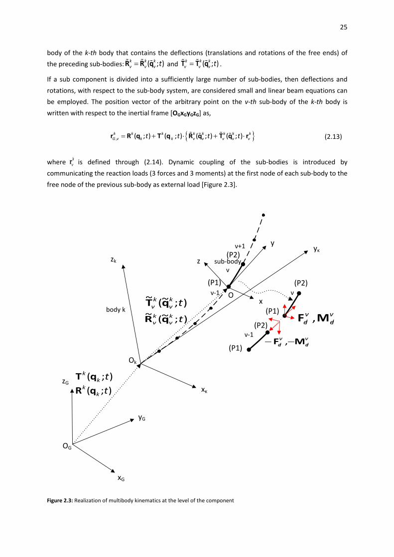
25

body of the k-th body that contains the deflections (translations and rotations of the free ends) of the preceding sub-bodies: ( ; )k k k

ν ν ν t=R R qA A

A and ( ; )k k kν ν ν t=T T qA A

A .

If a sub component is divided into a sufficiently large number of sub-bodies, then deflections and rotations, with respect to the sub-body system, are considered small and linear beam equations can be employed. The position vector of the arbitrary point on the v-th sub-body of the k-th body is written with respect to the inertial frame [OGxGyGzG] as,

{ }, ( ; ) ( ; ) ( ; ) ( ; )k k k k k k k kG ν k k ν ν ν ν νt t t t= + ⋅ + ⋅r R q T q R q T q rA A

A A (2.13)

where rkν is defined through (2.14). Dynamic coupling of the sub-bodies is introduced by

communicating the reaction loads (3 forces and 3 moments) at the first node of each sub-body to the free node of the previous sub-body as external load [Figure 2.3].

x

z

y

sub-body ν

xG

yG

zG

zk

xκ

yκ

body k

ν-1

ν+1

ν

ν-1

OG

Ok

(P1)

(P2)

(P1)

(P2)

(P1)

(P2)

O

);( tkk qT

);( tkk qR

);~(~ tkv

kv qT

);~(~ tkv

kv qR v

elvel MF ,

vel

vel MF −− ,

Figure 2.3: Realization of multibody kinematics at the level of the component

26

2.3.1.2 Timoshenko beam theory

For the derivation of the model equations, the loads equilibrium based on Newton’s 2nd law is used, although Hamilton’s principle leads to identical expressions. The procedure can be described by the following steps,

a) definition of the deformation kinematics and by that definition of the strains

b) introduction of the stress-strain relations and calculation of the internal loads

c) formulation of the dynamic equilibrium differential equations

x

zy

A

dAr

undeformed elastic axis

deformed elastic axis

r0dA

ζ0

η0

ξ0

ζ

ξ

η

Ο

1OO′

u

v

w

Figure 2.4: Coordinate systems definition of the beam

Let [Oxyz] denote the coordinate system with respect to which the beam axis in the un-deformed state coincides with the y-axis Figure 2.4. Axes x, z correspond to the two lateral bending directions. A beam structure subjected to combined bending in the two lateral directions x and z including shear and torsion and tension in y direction is considered. In the context of 1st order linear theory, the position r of any point P(x, y, z) in the deformed state is defined with respect to displacements and rotation angles as follows,

27

= + = + ⋅ = + ⋅

0 0 0 0 0 0 0

0

1 0 0 0 0( ; ) ( ; ) ( , ) ( ; ) 0 1 0 - 0

0 0 1 0 - 0

0

x

y

z

uv

zw

t t x z y t z xθ

xθθ

0 0 0r r r U r r S u r

(2.14)

r0 = (xo, yo, zo)T denotes the position of P in the undeformed state and u(yo,; t) = (u, v, w, θx, θy, θz)T contains the two bending displacements u, w, the axial displacement v, the torsion angle θy and the bending rotation angles θx, θz which include the shear deflections. The above expression defines the displacement field U = (U, V, W)T with respect to which strains are defined. Note that matrix S depends only on xo, zo while u on yo and time. By integrating over the beam cross section, the dependence of strains on xo, zo will subsequently define the sectional properties of the beam and so the derivation will only contain derivatives in the y direction which are denoted with a prime (.)’.

Using the definition of Green’s strains and Hooke’s law for the stress-strain relation of an isotropic material, the following equations for the stresses are derived:

' ' '0 0

0

' '0

0 0

' '0

0 0

yy yy x z

xy x xy x x x y x z

yz z yz z z z y z x

Vσ E ε E E v E z θ E x θ

y

U Vτ G γ G G u G z θ G θ

y x

V Wτ G γ G G w G x θ G θ

z y

∂= ⋅ = ⋅ = ⋅ − ⋅ ⋅ + ⋅ ⋅

∂

∂ ∂= ⋅ = ⋅ + = ⋅ + ⋅ ⋅ + ⋅ ∂ ∂

∂ ∂= ⋅ = ⋅ + = ⋅ − ⋅ ⋅ − ⋅ ∂ ∂

(2.15)

where εyy, yxy, γyz denote the Green’s strains and σyy, τxy and τyz the corresponding stresses [Figure 2.5], E is the Young’s modulus and Gx, Gz the shear modulus in x and z directions respectively.

Figure 2.5: Normal and shear stress definition

28

By integrating the stresses over any cross section of the beam structure, the internal forces and moments are obtained which will be later on introduced in the dynamic equilibrium equations,

( )

( )

( )

( )

( )

( )

= = + +

= = +

= =

= = +

= =

= + + + +

∫ ∫

∫ ∫

∫ ∫

∫ ∫

∫

' '0

' ' '0 0

' '0

' 2 ' '0 0 0 0 0

0 0

2 2 ' ' '0 0 0 0 0

-

- -

- -

-

-

x xy x x y x zA A

y yy x zA A

z yz z z y z xA A

x yy x zA A

y xy yzA

x z y x x z z z

F τ dA G u G z θ G θ dA

F σ dA Ev Ez θ Ex θ dA

F τ dA G w G x θ G θ dA

M σ z dA Ez v Ez θ Ex z θ dA

M τ z τ x dA

G z G x θ G z u G z θ G x w G x

( )

= = +

∫

∫ ∫

0

' ' 2 '0 0 0 0 0-

xA

z yy x zA A

θ dA

M σ x dA Ex v Ez x θ Ex θ dA

(2.16)

The sectional stiffness properties of the beam structure are defined as,

( )

= = =

= = =

= +

= =

= =

∫ ∫ ∫

∫ ∫ ∫

∫

∫ ∫

∫ ∫

0 0

2 20 0 0 0

2 20 0

0 0

, ,

, ,

, ,

, ,

A A A

A A A

x zA

x zA A

x zA A

EA EdA EAx Ez dA EAz Ex dA

EIxx Ez dA EIxz Ex z dA EIzz Ex dA

GJ G z G x dA

GxA G dA GzA G dA

GxAx G z dA GzAz G x dA

(2.17)

For a differential beam element dy of cross section A and end points (P1), (P2), the balance of forces and moments with respect to point (P1) in the [Oxyz] coordinate system takes the following differential form (see Figure 2.6),

: ,e e

A A

dy d dy ρ dA ρ dA L

i if F f f r f g= + = = +∫ ∫

(2.18)

( ) ( )

( )

+ d : ,

ee p

A

ep a

A

dy d d dy ρ dA

ρ dA

m

L

i iM + r F F m m r r

m r g r

= × + = ×

= × + ×

∫

∫

(2.19)

29

F+dF

M +dM

M

F

drera

L

(P1)(P2)

x

zy

A

dAr

rp

dyundeformed elastic axis

Figure 2.6: Loads equilibrium for a differential beam element

In equations (2.18) and (2.19) L=(Lx, Ly, Lz)T corresponds to the external force vector per unit length acting on the element (i.e. aerodynamic, hydrodynamic), F = (Fx, Fy, Fz)T and M = (Mx, My, Mz)T are the net elastic internal (reaction) forces and moments, g = (gx, gy, gz)T is the acceleration of gravity, F+dF is the vector of the resultant elastic force at the end point (P2), re is the position vector of a point on the deformed elastic axis,

0 uy v0 w

er = +

(2.20)

Let re(1,2) denote the position vectors of the two ends, dre=re

(2)-re(1), ra=(xa, 0, za)T denote the local

position of the external forces center with respect to the elastic axis of the beam and rp=r-re(1).

By introducing (2.16) and (2.17) in equations (2.18) and (2.19) and writing them in condensed matrix form, the final set of equations expressing Newton’s Law is obtained,

[ ] [ ] [ ] [ ] T1 2 3 4 a

A A

ρdA ρdA′ ′′ ′= + + + + +∫ ∫II S r K u K u K u K u II T g II L (2.21)

where the matrices in (2.21) are defined as,

30

1

0 0 0 00 0 - 00 0 0 - 00 - 0 0 -

0 - 0 00 0 - 0

x x

z z

x z

G A G AxEA EAx EAz

G A G AzEAx EIxx EIxz

G Ax G Az GJEAz EIxz EIzz

K

(2.22)

2

0 0 0 0 00 0 0 0 0 00 0 0 - 0 00 0 0 0 0 00 0 0 00 0 0 0 0 0

x

z

z x

G A

G A

G Az G Ax

K

(2.23)

3

0 0 0 0 0 00 0 0 0 0 00 0 0 0 0 00 0 - 0 - 00 0 0 0 0 0

- 0 0 0 - 0

z y z

y x x

G A F G Az

F G A G A

K

(2.24)

4

0 0 0 0 0 00 0 0 0 0 00 0 0 0 0 00 0 0 - 0 00 0 0 0 0 00 0 0 0 0 -

z

x

G A

G A

K

(2.25)

T0

T0 0

0

1 0 0 0 0 0 1 0 - 0

0 0 1 0 - 0

zz x

xII S

(2.26)

T1 0 0 0 00 1 0 0 0 00 0 1 0 - 0

a

a

a

z

x

II (2.27)

31

In the above equations, although a standard 1st order linear beam is employed, the nonlinear rotational stiffening terms Fy·w’ and Fy·u’ in the x and z moment equations, are retained due to their significant loading contribution.

Similarly to the stiffness sectional stiffness properties obtained in (2.17), integration over the beam cross section A will give the following inertial/mass properties,

( )

= = =

= = =

= +

∫ ∫ ∫

∫ ∫ ∫

∫

0 0

2 20 0 0 0

2 20 0

, ,

, ,A A A

A A A

A

m ρdA mx ρz dA mz ρx dA

mIxx ρz dA mIxz ρx z dA mIzz ρx dA

Ip ρ z x dA

(2.28)

Extension of the above formulation into the case of a moving beam is straightforward. It consists of introducing (2.9) into the left hand side of (2.21) expressing the balance of forces and moments. In doing so several nonlinear inertial terms will appear which in addition to the dof’s included in u will also contain the dof’s contained in q. As explained in Section 2.3.1.1 q provides the means to kinematically couple components and sub-bodies into a complete dynamic setup. Further details are given in this respect in section 2.3.3.

2.3.1.3 Finite Element Discrete formulation

The system of dynamic equations (2.21) after introducing the expression for the total acceleration (2.9) is reformulated in variational form by applying the principle of virtual work,

0

1 2 3 40 0 0 0

Ta 1 2

00 0

( ) d

( ) d ( ) d d d

d d ( ) [ ]

LT

GA

L L L LT T T T

L L LT T T

A

δ ρdA y

δ y δ y δ y δ y

δ ρdA y δ y δ

+

′ ′′ ′+ − − =

′ ′+ + +

∫ ∫

∫ ∫ ∫ ∫

∫ ∫ ∫

Tu II S T r

u K u u K u u K u u K u

u II T g u II L u K u K u

(2.29)

where δu denotes the virtual displacement and the last term on the right hand side corresponds to boundary terms that appear after integration by parts is performed.

(2.29) is discretized based on Finite Element (FE) approximations [90]. It consists of expressing the displacement field u and its kinematically admissible virtual displacement δu with respect to the same discrete function basis. At the element level (denoted by the subscript “e”),

32

ˆ ˆ( , ) ( ) ( ); ( , ) ( ) ( )e e e ey t y t δ y t y δ t= =u N u u N u (2.30)

where N(y) denotes the matrix of shape functions and ˆeu the vector of the discrete dof’s. By choosing a 15 dof finite element with 3 internal nodes [Figure 2.7], ˆeu and N(y) are defined,

= 1 1 1 1 1 1 3 5 4 2 2 2 2 2 2ˆ ( , , , , , , , , , , , , , , )Te x y z y x y zu v w θ θ θ v θ v u v w θ θ θu

(2.31)

=

1 1 2 20, 1, 0, 1,

1 3 4 2

1 1 2 20, 1, 0, 1,

1 1 2 20, 1, 0, 1,

1 5 2

1 1 2 20, 1, 0, 1,

Ν 0 0 0 0 0 0 0 Ν 0 0 0 0 Ν0 Ν 0 0 0 0 Ν 0 Ν 0 Ν 0 0 0 00 0 Ν Ν 0 0 0 0 0 0 0 Ν Ν 0 00 0 Ν Ν 0 0 0 0 0 0 0 Ν Ν 0 00 0 0 0 Ν 0 0 Ν 0 0 0 0 0 Ν 0

Ν 0 0 0 0 Ν 0 0 0 Ν 0 0 0 0 Ν

b x b x b x b x

v v v v

b z b z b z b z

b θx b θx b θx b θx

t t t

b θz b θz b θz b θz

N

N

(2.32)

In (2.32) 3rd order C0 approximation shape functions are considered for v (tension),

= − − + − +

= − −

= − − +

= − + − +

1 2

3

4

2 2

Ν ( ) 0.125(1 )[ 10 9((2 1) 1)]

Ν ( ) 4.5(1 ) ( 2 3 )

Ν ( ) 4.5(1 ) ( 1 3 )

Ν ( ) 0.125 [ 10 9((2 1) 1)]

v

v

v

v

ξ ξ ξ

ξ ξ ξ ξ

ξ ξ ξ ξ

ξ ξ ξ

(2.33)

2nd order C0 approximation shape functions for θy (torsion),

= − − −

= −

= −

1

5

2

Ν ( ) (1 )(2 1)

Ν ( ) 4(1 )

Ν ( ) (2 1)

t

t

t

ξ ξ ξ

ξ ξ ξ

ξ ξ ξ

(2.34)

and modified Hermitian shape functions for the two bending modes u, w defined as,

33

−

= − − +

= −

= − + + + −

= + − + −

= −

= −

= +

1 2 30, 1 2 2

2 10, 0,

1 2 2 31, 1 1 2 2

2 2 2 31, 1 1 2 2

1 10, 1

2 10, 0,

11,

Ν ( ) 1 Φ 3 Φ 2 Φ

Ν 1 Ν ( )

Ν ( ) ( 0.5 Φ 0.5 Φ 2 Φ Φ )

Ν ( ) ( 0.5 Φ 0.5 Φ Φ Φ )

Ν ( ) 6 Φ (1 )

Ν ( ) Ν ( )

Ν ( ) 1

b x x x x

b x b x

b x x x x x

b x x x x x

b θz x

b θz b θz

b θz

ξ ξ ξ ξ

ξ

ξ L ξ ξ ξ ξ ξ

ξ L ξ ξ ξ ξ

ξ ξL ξ

ξ ξ

ξ − + − +

= + − + − +

= = =+ +

1 1

21, 1 1

1 22

[ Φ Φ ( 4 3 )

Ν ( ) [ Φ Φ ( 2 3 )

12 1, Φ , Φ

1 1

x x

b θz x x

xx x x

x x

ξ ξ

ξ ξ ξ

EIzz φφ

φ φGxA L

(2.35)

Expressions in (2.35) correspond to the bending in the x direction. By switching x and z variables in (2.35), similar expressions for the other bending direction z are derived. The bars over , EIzz GxAdenote the average structural properties of the element, while the modification weighting functions Φ prevent shear locking.

Shape functions (2.33)-(2.35) are defined with respect to the non-dimensional length of the element ξ∈[0,1] and include in their definition the length of the element L.

Figure 2.7: Definition of a 15x15 FEM with 3 internal nodes (dofs correspondence to nodes)

After introducing (2.30) and (2.9) in (2.29), eliminating the virtual displacements ˆeδu and performing linearization, the nonlinear system of equations at element level is derived,

δ δ δ δ δ δq q q+ + + + + =M u C u K u M q C q K q Q (2.36)

where subscript e has been omitted from , , δ δ δu u u that denote the perturbation of the elastic dof’s of the element, defined by linearizing the element dof’s as in (2.11),

34

0 0 0, , ≅ + δ ≅ + δ ≅ + δu u u u u u u u u (2.37)

Projection of the global acceleration on the local coordinate system Oxyz of the element after introducing (2.14) in (2.9) yields,

T T T T T0 2 G = + + + +T r S u T T S u T T S u T R T T r

(2.38)

which is linearized based on (2.11), (2.12) and (2.37). The matrices in (2.36) are defined as,

1T

0

dA

L ρdA y= ∫ ∫M N II S N

1T T 0

0

2 ( ) dA

L ρdA y= ∫ ∫C N II T T S N

1 1T T 0

10 0

1 1 1

2 3 40 0 0

( ) d ( ) d

( ) d ( ) d d

T

A

T T T T

L ρdA y L y

L y L y L y

′ ′= +

′ ′+ − −

∫ ∫ ∫

∫ ∫ ∫

K N II T T S N N K N

N K N N K N N K N

1T T 0 T T

q i q i q i 010

( ) ( ) ( ) dnq

qi A

L ρdA y=

= ∂ + ∂ + ∂ ∑∫ ∫M N II T T S N u T R T T r

1T T 0 T 0 T T

q i q i q i q i 010

2 ( ) ( ) ( ) ( ) dnq

qi A

L ρdA y=

= ∂ + ∂ + ∂ + ∂ ∑∫ ∫C N II T T S N u T T S N u T R T T r

1T T 0 T 0 T T

q i q i q i q i 010

1T T

q i10

2 ( ) ( ) ( ) ( ) d

( ) d

nq

qi A

nq

i A

L ρdA y

L ρdA y

=

=

= ∂ + ∂ + ∂ + ∂

− ∂

∑∫ ∫

∑∫ ∫

K N II T T S N u T T S N u T R T T r

N II T g

1 1T T T

a0 0

1T 0 T 0 0 T 0 0 T 0 T 0

00

1 1 10 0 0

1 2 30 0 0

d d

2 ( ) ( ) ( ) ( ) d

( ) d ( ) d ( )

A

A

T T T T

L ρdA y L y

L ρdA y

L y L y L

= +

− + + + +

′ ′ ′′− + −

∫ ∫ ∫

∫ ∫

∫ ∫ ∫

Q N II T g N II L

N II S N u T T S N u T T S N u T R T T r

N K N u N K N u N K N u

10

40

d dTy L y− ∫N K N u

(2.39)

where nq denotes the total number of q dof’s.

The dimension of local element matrices M, C, K is 15x15, of Mq, Cq, Kq 15xnq and of Q 15x1. The boundary terms that would normally appear when integration by parts is applied, are eliminated due

35

to the admissibility conditions on ˆeδu . The integration over the element is carried out using a 6 point Gaussian quadrature which involves the shape functions, but also the material properties (equations (2.17) and (2.28)) that can linearly depend on ξ.

Note that extra mass, damping and stiffness terms can be introduced as the damping term that models structural damping (section 2.3.4.1), the added mass and damping terms in Morison’s equation (section 2.6.2) and the stiffness term originating from the linearization of the buoyancy force (section2.6.3).

2.3.2 Modeling of the mooring lines

A 3D dynamic mooring line model is presented, based on the finite element method. Truss elements that only transfer axial loading are used. Each element is subjected to inertial, gravitational and hydrodynamic loading, calculated by means of Morison’s equation. The seabed interaction is modeled with appropriately stiffness and damping terms. For the coupled analysis, the floater imposes the displacements at the connection points while the mooring lines feedback the corresponding loading. Both catenary mooring lines and tendons for tension leg platforms (TLP) can be modeled. The derivation is based on the nonlinear truss element presented by [89] and also used in [91], here based on the standard engineering strain.

2.3.2.1 Geometry and the strain-displacement relation of the truss element

Each mooring line is divided into truss elements exhibiting a geometric nonlinear behavior. Such elements transfer only the tensile forces while their compression stiffness is zero. In Figure 2.8 a truss element P0Q0 of initial undeformed length L0 is shown. As a result of rigid body motion and elastic deformation, the truss element will move to a new position PQ so the length becomes L. The non-dimensional coordinate ξ∈[0, 1] defines the position of any point R along the element. The position vector r of a point along the element is defined as,

ξ

ξ

initial positionfinal position0L

LQ

R

P r

0r

0R

0P

0Q

u

Figure 2.8: Definitions of the geometry and the kinematics of a single truss element.

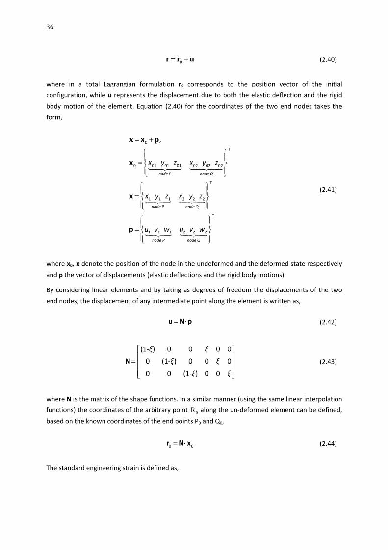
36

= +r r u0 (2.40)

where in a total Lagrangian formulation r0 corresponds to the position vector of the initial configuration, while u represents the displacement due to both the elastic deflection and the rigid body motion of the element. Equation (2.40) for the coordinates of the two end nodes takes the form,

0

T

0 01 01 01 02 02 02

T

1 1 1 2 2 2

T

1 1 1 2 2 2

,

node P node Q

node P node Q

node P node Q

x y z x y z

x y z x y z

u v w u v w

= +

=

=

=

x

x

x

p

(( ((

(( ((

(( ((

x p

(2.41)

where x0, x denote the position of the node in the undeformed and the deformed state respectively and p the vector of displacements (elastic deflections and the rigid body motions).

By considering linear elements and by taking as degrees of freedom the displacements of the two end nodes, the displacement of any intermediate point along the element is written as,

= ⋅u Ν p (2.42)

(1- ) 0 0 0 00 (1- ) 0 0 00 0 (1- ) 0 0

ξ ξξ ξ

ξ ξ

=

N (2.43)

where N is the matrix of the shape functions. In a similar manner (using the same linear interpolation functions) the coordinates of the arbitrary point 0R along the un-deformed element can be defined, based on the known coordinates of the end points P0 and Q0,

0 0= ⋅r Ν x (2.44)

The standard engineering strain is defined as,

37

−= = − = + + = ⋅2 2 20

2 1 2 1 2 10 0

1, ( - ) ( - ) ( - ) TL L Lε L x x y y z z D DL L

x x

(2.45)

while Dx0, Dx and Dp are expressed as,

T2 1 2 1 2 1

T0 02 01 02 01 02 01 0

T2 1 2 1 2 1

{ - , - , - }

{ - , - , - }

{ - , - , - }

D x x y y z z

D x x y y z z

D u u v v w w

= = ⋅

= = ⋅

= = ⋅

x A x

x A x

p A p (2.46)

and the matrix A is defined as,

=

-1 0 0 1 0 0 0 -1 0 0 1 0 0 0 -1 0 0 1

A

(2.47)

The variation in length δL is defined as,

= ⋅ = ⋅ ⋅ =T Tδ(D ) , D /δL δ Lt x t A p t x (2.48)

where t is the unit vector tangent to the element.

Using (2.48) the variation of the strain δε is determined as,

= = ⋅ ⋅-1 T0

0

δδLδε LL

t A p

(2.49)

while the variation of the tangent unit vector δt is,

= ⋅ ⋅ ⋅T1 { - } δδL

t I t t A p

(2.50)

and I is the unit 3x3 matrix.

2.3.2.2 Variational formulation and Finite Element analysis

Application of the virtual work principle [89] leads to the dynamic equations of a truss element in space. The principle requires that, for an arbitrary virtual displacement field δu,

38

( )− − =∫ ∫ u q q

0 0

Τ 0e i

V L

σ δε dV δ d

(2.51)

where: qi and qe are the inertial and external (hydrodynamic, gravitational and buoyancy) forces per unit length that act on the element; σ and δε are the axial stress and the variation of the axial strain caused by the relative motion of the element ends P and Q; and V0 and L0 are the volume and the length of the un-deformed element.

The stress field is defined by the stress-strain relations and so by assuming a linear elastic material, Hooke’s law specifies that,

=σ E ε (2.52)

where E denotes the Young’s modulus.

By introducing (2.49) and (2.52) into (2.51) and assuming that the cross section remains unchanged and equal to A0 so that dV = A0 dl, the following system of nonlinear dynamic equations is obtained,

( )1

T T0 0

0

e i L dξ EA ε− = ⋅ =∫N q q A t f (2.53)

Nonlinear equations (2.53) are next expressed in perturbed form (i.e. linearization about a reference deflected position 0p ) and then solved iteratively, until perturbations converge to zero. Taylor’s expansion of the nonlinear expression of the internal loads f about a reference deflected position p0 yields,

( ) ( )0 00 0 tδ δ

∂= + + ⋅ = + + ⋅

∂f

f f x p p f x p K pp

(2.54)

Thereby, making use of (2.49) and (2.50) the element tangent stiffness matrix Kt is obtained,

= ⋅ − ⋅ ⋅ + ⋅ ⋅ ⋅Τ T Τ T

0

{ } { }tEA EAεL L

K Α I t t A Α t t A

(2.55)

If the density of the material ρ is assumed constant along the element then the inertia terms become,

( ) ( )( )= = = ⋅∫ ∫ ∫

1 1 1T i T T

0 0 0 0 00 0 0

L dξ ρA L dξ ρA L dξN q N u N N p Μ p

(2.56)

39

where ρΑ0 is the linear mass distribution of the mooring line. Analytic integration of the mass matrix gives,

=

0 0 0 0

0 0 0 0 0 0

0 0

0 0 0 0

0 0 0 0

0 0 0 0

/ 3 0 0 / 6 0 00 / 3 0 0 / 6 / 60 0 / 3 0 0 0

/ 6 0 0 / 3 0 00 / 6 0 0 / 3 00 0 / 6 0 0 / 3

ρA L ρA LρA L ρA L ρA L

ρA LρA L ρA L

ρA L ρA LρA L ρA L

M

(2.57)

The external loads denoted by Q, comprise the hydrodynamic and hydrostatic (buoyancy) forces on the element, the gravity loads as well as the force from the seabed contact. They are expressed in the following form,

1 1 1 2T T T T *

0 00 0 0 1

le

zw H SB zw H SBl

L dξ L dξ Ldξ L dξ= = + + = + +∫ ∫ ∫ ∫Q N q Q Q Q N q N q N q (2.58)

It is convenient to define the weight of the mooring line in the water per unit length Fzw which actually takes into account the gravity and the buoyancy external loading. Then analytic integration of Qzw gives,

0

0

00

/ 200

/ 2

zwzw

zw

F L

F L

− = −

Q (2.59)

The hydrodynamic loads are calculated based on Morison’s equation (see section 2.6.2, eq. (2.134).) and after linearization about a reference state, additional mass and damping terms are defined. Note that the hydrodynamic loads are applied along the deformed length of the element as indicated in the second integral in (2.58) where the actual length L is used. Numerical integration is performed.

The effect of the seabed contact is modeled through distributed stiffness and damping terms which are activated when the element approaches the seabed. Their magnitude is linearly increasing inside a vertical buffer zone extending from the seabed to zbuff. The vertical force per unit length exerted on each element is defined as,

40

= + +=

20 0 z z sb sb sb sb sb

buff buff

z zF k z c k c z zz z

(2.60)

where,

k0sb and c0sb denote the seabed stiffness and the damping,

ksb and csb denote the modified seabed stiffness and the damping including the zbuff

zbuff denotes the vertical length of the buffer area in which the seabed contract is activated.

The variation of this force is defined as,

= + + 2 sb sb sb sbδF k z δz c z δz c z δz (2.61)

When present in the left hand side, contributes the corresponding stiffness and damping terms. The integration length of the associated virtual work is properly adjusted in order to handle the situation of having part of the element outside the buffer area, as indicated by the third integral in (2.58) where L*denotes the active length defined by the ends l1 and l2. The integration is carried out analytically using a symbolic software i.e. Mathematica [92].

In addition to the above-mentioned force terms, an additional force proportional to the time derivative of the strain in the direction tangent to the element is introduced, in order to model the structural damping of the truss element. It takes the form,

= ⋅ = ⋅ ⋅ ⋅

T T( ) ( )d c D cF t x t t t A p (2.62)

where c denotes the damping coefficient. The variation of the damping force is,

( )T T T T( ) dc

d D D δ c δL = ⋅ + ⋅ ⋅ − ⋅ ⋅ ⋅ + ⋅ ⋅ ⋅ F t x I t x I t t A p t t A p (2.63)

The final linearized form of the dynamic equation of a truss element is derived by introducing the linearized expressions for the internal, inertial and external loading, as well as the structural damping terms in (2.53),

0 0 0( + ) ( + + ) ( + + )H d H sb t sb d dδ δ δ⋅ + ⋅ + ⋅ = − ⋅ − −M M p C C C p K K K p Q M p f Q (2.64)

where

M denotes the mass matrix (eq. (2.57))

41

f, Kt, the internal force vector and the associated tangent stiffness matrix (eq. (2.53), (2.55))

MH and CH denote the mass and damping matrices due to the linearization of the hydrodynamic loading from Morison’s equation (eq.(2.134))

Cd, Kd, Qd denote the damping and stiffness matrices and the force vector from the structural damping (derived by integration of (2.62) and (2.63))

Csb, Ksb denote the damping and stiffness terms due to the seabed interaction modeling (derived by integration of (2.61))

Q denotes the total external force vector including gravity, buoyancy, hydrodynamics and reaction force due to the seabed contact (eq. (2.59), (2.132) and integration of (2.60))

For multi-element modeling of mooring lines, the local matrices of the various elements are assembled to global matrices for the full configuration in the standard FEM way. This assembling procedure does not require any coordinate transformation because the dynamic equations (2.64) of the single element have been expressed with respect to inertial frame.

2.3.3 Assembly of the coupled system

2.3.3.1 The coupled operators

The vector of the unknown dof’s X can be split in 3 parts: The 1st part contains the local deformations u that are associated to the components modeled as beam structures; the 2nd part contains the global deformations p associated to the mooring lines; and the 3rd part contains the q dof’s that realize the coupling amongst the components (or sub-bodies). Thus the total vector of the unknown variables is,

( )TT , ,δ δ δ δ=X u p q (2.65)

The first two parts have been extensively presented in sections 2.3.1.3 (eq. (2.36)) and 2.3.2.2 (eq. (2.64)). Next the equations for the q dof’s that were introduced in 2.3.1.1 are further detailed.

In q, the 6 rigid body motions of the floater, the azimuth angle of the shaft and the yaw angle of the nacelle are included as independent dof’s. Each of these dof’s is determined by solving a dynamic equation.

If the floater is assumed rigid, the 6 dynamic equations are defined as in (2.126). A similar approach is also followed when the floater is considered flexible. Then the motions of the floater are defined based on the reaction forces that are applied at the point of reference i.e. the reaction loads at the bottom of the tower and those at the upper part of the flexible floater.

The rotation of the shaft is defined by the dynamic equilibrium of moments at its starting node. The balance concerns on one hand the rotor torque acting at the end of the drive train and on the other

42

the generator torque while in between the flexibility and the inertias of the drive train are present. This dynamic equation provides the instant azimuth angle, the rotational speed and its acceleration.

The same approach is followed for the yaw mechanism which is modeled as a concentrated spring and a concentrated damper introduced in the yaw rotation equation (θz). The dynamic equilibrium is considered at the top of the tower (position of the main bearing). The reaction moment of the nacelle on one hand and the spring and the damper of the yaw mechanism on the other define the yaw angle along with its velocity and acceleration.

In addition to the above-mentioned q dof’s, at the 1st and the last node of every component (or sub-body), 6 q’s are defined that allow realizing the kinematic coupling conditions. At the 1st node Dirichlet conditions are set and therefore the local deformations and rotations are set equal to zero. The only exception to this rule is the blade root where the blade pitch angle must be explicitly set. At the last node the set of 6 q’s are set equal to the local deformation and rotation. As already mentioned in this way the components follow the deformed geometry and an inherent nonlinearity is introduced, expressed through the position vectors, the rotation matrices and their time derivatives (section 2.3.1.1) that depend on q’s.

2.3.3.2 Boundary conditions

Based on the multibody formulation, Dirichlet and Newman boundary conditions are imposed at the connection points. Kinematic couplings defined through q, are combined with zero boundary conditions for the 6 dof’s at the first element of every component. In multi-component structures without any q dof (see section 2.3.4.4), the kinematic boundary conditions are applied to the dof’s of the connection node. The same also holds for the end nodes of every mooring line. At the seabed, fixed conditions are imposed, while at fairlead point the floater imposes the kinematics.

In addition to the kinematic boundary conditions, dynamic conditions are also required at the connections points of a multibody configuration. This consists of adding the reaction forces obtained from the contributing components. As explained in 2.3.1.1 when more than one component is connected to a point, one body is selected to provide the kinematics while all others feedback the reaction loads. Based on (2.36) or (2.64), expressions for the reaction loads are derived for a beam or a truss element, by adding the virtual work of the reaction loads. For all the components except for the mooring lines, the reaction loads are given with respect to the local system of the contributing component or sub-body. Therefore in order to obtain the corresponding virtual work, the reaction loads must be projected on the local system of the receiving component. Along the mooring lines the reaction loads are given in the global coordinate system, so their virtual work is directly obtained. If there is an offset, the corresponding moments of the forces must be also added.

2.3.3.3 Assembling procedure

In order to assemble all the equations into the final system, the following procedure is followed:

43

1. First the element matrices are introduced according to a preset sequence. This sequence respects the loading flow, so for a wind turbine system, blades appear first, then the drive train, the tower, and if applicable the support structure followed by the mooring line equations. The terms related to the body dof’s will give a block diagonal structure to the assembled mass, damping and stiffness matrices. The additional terms that depend on the q dof’s defined in the kinematic couplings are kept separately and appear in the right most columns.

2. Next the dynamic conditions are introduced. They will give lower off-diagonal terms as indicated in Figure 2.9. For the specific configuration, loading couplings are introduced at the end of the drive train, at the end of the tower and at the 6 q’s of the floater. The system thus obtained is completed with the dynamic equations for the q dof’s that appear in the last block of rows. Depending of the nature of each q, the equation can take either the form of a simple assignment to an already existing dof as in the case of deflections at the top of the tower or the hub or the form of a complete dynamic equation as in the cases of the motions of a rigid floater, of the azimuth and of the yaw angles.

3. Dirichlet boundary conditions are imposed on the dof’s by properly modifying the lines that correspond to the virtual work associated to the selected dof’s.

Figure 2.9: Form of the global matrices

44

The system thus obtained will have the usual form:

δ δ δ+ + =M X C X K X Q (2.66)

where X denotes the complete vector of unknowns defined in (2.65). The mass, damping and stiffness matrices, M, C, K as well as the external forcing Q will depend on X and its time derivatives which will render the system nonlinearity.

2.3.3.4 Solution

Time integration

The final set of dynamic equations (2.66) is integrated in time using the Newmark second order implicit scheme [90]. and X X based on Taylor expansions over the previous time step values, denoted with subscript P yields,

( )( )

2 2 2P P P PRE

P P PRE

0.5

1

dt dt β βdt βdt

dt γ γdt γdt

= + + − + = +

= + − + = +

Χ Χ Χ Χ Χ Χ Χ

Χ Χ Χ Χ Χ Χ

(2.67)

where β, γ denote the Newmark constants. For 2nd order accuracy γ=0.5 and for numerical stability β≥γ/2. PRE PRE and X X contain the known contribution from the previous time step. If both expressions in (2.67) are linearized about a reference state based on (2.37), then the first expression solved for δX and the second for δX and introduced in (2.66) a linear system of equations is formed,

00 0 0PRE

PRE PRE2 2

1( )

γ γδ

βdt βdt βdt βdt − + + = − − − − + −

X XM C K X Q X M X X X X C (2.68)

and is solved with LU decomposition method. In every time step of the simulation, the equations are solved iteratively until δΧ goes to zero by applying a full Newton-Rapshon iterative scheme.

Static Solution

At the beginning of the simulation, a static solution of (2.66) is performed in order to estimate the initial deformations, instead of consider them zero and so transient is reduced.

Modal analysis

In order to solve the eigenvalue problem for the coupled structure and define its natural frequencies the corresponding modes and the damping ratios, the 2nd order in time differential system of equations (2.66) is transformed into a 1st order differential equations system with twice as many dofs,

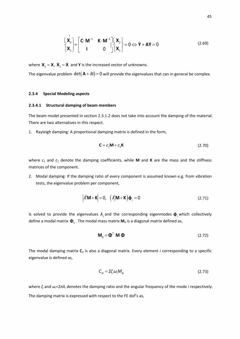
45

1 12 2

1 1

0 00

− − ⋅ ⋅ + = ⇔ + =

Χ ΧC M K MY AY

Χ ΧΙ

K

(2.69)

where 1 2, = =Χ Χ Χ Χ and Y is the increased vector of unknowns.

The eigenvalue problem ( )det 0λ+ =A I will provide the eigenvalues that can in general be complex.

2.3.4 Special Modeling aspects

2.3.4.1 Structural damping of beam members

The beam model presented in section 2.3.1.2 does not take into account the damping of the material. There are two alternatives in this respect.

1. Rayleigh damping: A proportional damping matrix is defined in the form,

1 2c c= +C M K (2.70)

where c1 and c2 denote the damping coefficients, while M and K are the mass and the stiffness matrices of the component.

2. Modal damping: If the damping ratio of every component is assumed known e.g. from vibration tests, the eigenvalue problem per component,

( )+ = + =2 20, 0j jλ λM Κ M Κ φ

(2.71)

Is solved to provide the eigenvalues jλ and the corresponding eigenmodes jφ which collectively define a modal matrix kΦ . The modal mass matrix Md is a diagonal matrix defined as,

Τd =M Φ M Φ (2.72)

The modal damping matrix Cd is also a diagonal matrix. Every element i corresponding to a specific eigenvalue is defined as,

d d2i i i iC ζ ω M= (2.73)

where ζi and ωi=2πλi denotes the damping ratio and the angular frequency of the mode i respectively.

The damping matrix is expressed with respect to the FE dof’s as,

46

Τ -1 -1d( ) =C Φ C Φ (2.74)

and is directly applied to the global matrix.

2.3.4.2 Concentrated inertia, damping and stiffness properties

In structural modeling, there is often a need to include concentrated mass, damping and stiffness properties. For example the hub, the nacelle, the generator’s inertia, the flange of the tower, the transition piece of the jacket etc. are modeled as concentrated masses and inertias. Modeling of the foundation is performed by concentrated stiffness, while the yaw mechanism is modeled as a concentrated spring and a damper. In general concentrated properties are introduced by means of Dirac functions that specify the placement of the properties at any point within a specific FE. Once this is done, the integration takes care that the correct virtual work is obtained. Concentrated mass, damping and stiffness properties are introduced by 6x6 matrices. For example for a concentrated mass placed at y0 of a specific FE, the following virtual work is added to (2.29),

00

( ) ( ) dL

Tc C C G

A

δ ρ dA δ y y y−∫ ∫ Tu II S T r (2.75)

In which a more general form of (2.26) is defined for IIC and SC,

T

0 0T

0 0

0 0

1 0 0 0 0 1 0 0

0 0 1 0

off off

C C off off

off off

z z y yz z x xy y x x

II S

(2.76)

that contains all the inertial properties of a concentrated mass (first – second moments). xoff, yoff and zoff denote the offset of the concentrated mass/inertia with respect to the elastic axis. Note that the inertial loading of a concentrated mass/inertia considers the total acceleration as defined in (2.9). Moreover a gravity force and the corresponding moments due to the offsets are applied as external concentrated loading at the position y0.

The 6x6 matrix for concentrated damping or stiffness properties applies to all motions. Directions in which no stiffness of damping contribution is considered are excluded by inserting zeros.

2.3.4.3 Foundation

The default option for bottom mounted support structures is to assume the end nodes clamped to the ground, so fixed boundary conditions are imposed. Alternatively, modeling of the foundation is performed leading to a slight reduction of the tower lateral frequencies, depending on the soil

47

properties. Three foundation models have been implemented and verified in hGAST, as proposed in the offshore code comparison (OC3) phase II [72, 93].

1. The apparently fixed (AF) model, in which the structure extends under the ground level. No springs are defined, while the structural properties of the extra part which is embedded to the ground are chosen to reproduce the effect of the foundation. At the bottom end fixed conditions are applied.

2. The concentrated spring (CS) model, in which the structure does not extend below the ground level but instead a 6x6 stiffness matrix is defined. In general, springs are defined in all 6 dofs. If the springs are only imposed in the lateral directions, then fixed conditions should be imposed in the vertical direction (z motion and yaw rotation).

3. The distributed spring (DS) model, in which the structure again extends below the ground level. The difference compared to the AF model is that the structural properties should be defined based on the actual foundation. Also springs are defined in the two lateral directions based on the soil properties. At the bottom end, fixed conditions are applied only for the vertical motion and the yaw rotation, while the lateral dof’s are free.

The DS model is by definition more detailed, but all three models provide very similar results if they are properly calibrated. Moreover, in the DS model it is straight forward to define springs of variable stiffness based on given p-y curves, since the solver is nonlinear.

Figure 2.10: Definition of the three foundation models the AP, CS and DS [figure taken from [94]]

2.3.4.4 Tripod or Jacket support structure

Modeling of a multimember support structure such as a tripod or a jacket is carried out in accordance to the basic principles already set. The members are modeled as beams undergoing combined bending including shear, torsion and tension and coupling conditions are added at the nodes. However due to the complexity of the jacket configuration, the equations for the jacket members are simplified by assuming that all deformations are small compared to the un-deformed (or static) state. This means that passage from one member to another involves rotation matrices that are fixed in time. As a consequence there is no need to add any q’s at the connections for the

48

kinematic coupling which becomes straightforward by assigning one set of degrees of freedom per node. The transfer of loads is also straightforward. As already mentioned, one member of the connection point provides the deflections, while all the others contribute the loading.

2.3.4.5 Partial Pitch, Tip Brake

By taking advantage of the sub-body formulation, modeling of the partial pitch of the blade or of the tip brake is straightforward. By dividing the blade in sub-bodies the pitch motion can be imposed at the beginning of any sub-body so the dynamics are consistently simulated.

2.3.4.6 Reduced Order Modeling

The dimension of the final system in the case of a complete offshore wind turbine can become large. For engineering purposes it is desirable to reduce the size of the system by formulating Reduced Order Models (ROM’s). Size reduction is equivalent to a projection operation from a high dimensional space, already used in the FEM, to one of significantly smaller dimension. In FEM the function basis is defined by the shape functions, but in principle any other complete discrete basis can be used. In structural mechanics an alternative basis is that of the eigenmodes. Depending on the system properties the set of eigenmodes can be truncated to a relatively small number and thus significant size reduction can be accomplished.

For a multi-component system, the eigenmode basis must be properly chosen so that nonlinear couplings are retained. To this end, instead of obtaining the eigenmodes of the complete system 2, the eigenmode set per component is chosen. The synthesis to the complete system will still follow the procedure with the q dof’s already presented, but with reference to the eigenmode function basis of the corresponding component.

More specifically,

- Consider one of the main components (for example one of the blades) and let Mk, Kk denote the component mass and stiffness matrices.

- The eigenvalue problem for this component,

( )+ = + =2 20, 0j jλ λM Κ M Κ φ

(2.77)

will provide the eigenvalues jλ and the corresponding eigenmodes jφ which collectively will define a modal matrix kΦ . Let u denote the vector of unknown displacements and rotations and c the vector of the modal coefficients that correspond to the specific analysis. Then,

2 Approximate eigenmodes of nonlinear systems can be obtained by means of Proper Orthogonal Decomposition [95].

49

∑m

j jj=1 nxmnx1 mx1

= c =κ κu φ Φ c

(2.78)

where m denotes the number of modes retained. By introducing this expression into the system,

ROM ROM ROMM K Q

κ κ κ κ κ κ κ κ κ κΤ Τ ΤΦ Μ Φ c + Φ K Φ c = Φ Q

(( ((

(2.79)

In most cases m can be significantly smaller than n. For example a typical blade FEM approximation leads to 150dof’s while m can be reduced to 4 - 9.

In the multi component case a compound modal Φ will be needed made of the modal matrices of every component kΦ along its diagonal. The procedure is simple, the complete mass, damping, stiffness and loading matrices are left multiplied by ΤΦ . Note that for the last block containing the equations for the q dof’s the corresponding modal matrix is the unit matrix. Also the mass, damping and stiffness matrices are right multiplied by Φ . This ROM procedure has been applied and verified to offshore wind turbines [85].

2.4 Control

Current wind turbines are speed and pitch regulated. The yaw angle of the nacelle is also controlled, but usually in aero-elastic simulations is assumed fixed within the time scale of the simulation. Recent proposed concepts also include actively moving trailing edge flaps. With respect to modeling, the control system is described by a set of differential equations expressed for the output control variables, such as the pitch angle (possibly different for every blade as in the individual pitch control case), the torque demand of the generator, the flap deflection angle and the yaw of nacelle (if it is controlled), as well as additional differential equations for the considered filters.

In order to include the control system in the coupled solution, i.e. for stability analysis in closed loop operation, the output control variables and those correspond to the associated filters must be included in q, as in [79]. If qc denotes the subset of dof’s that are associated to the control system, the modification to the system is straightforward. By introducing qc a set of dynamic equations is appended as part of the equations for the q dof. The form of these equations depends on the controller structure which contains filters, dampers, models of the actuators etc. In most cases they correspond to linear control elements (PID). Typical examples are given in Figure 2.11. Details can be found in [96, 97], including the logic that is used in order to switch between the modes of control. A common approach is to vary the rotor speed at conditions below rated and then switch to variable pitch part keeping the rotational speed at its nominal value. Usually around rated conditions a transient mode ensures smooth switching between the two main modes.

50

Another possibility is to call in every time step an external controller subroutine provided as DLL. Such a subroutine independently solves the control equations and provides the pitch and the generator demand values. The actual pitch angle (i.e. the angle provided by the actuator) is imposed at the corresponding q, while the actual generator torque (i.e. after the generator internal lag modeling is applied) is added to the dynamic equilibrium equation for the rotation of the drive train. This is the case for example of the NREL 5MW reference wind turbine [98] or the DTU 10MW reference wind turbine [99] which both are paper case machines that are used by the wind energy research community.

In open loop operation the solver ignores the control equations and fixed values are given for the pitch angles and the rotor speed. Finally in parked operation the rotor is idling with a pitch angle close to 90o. In this case, the drivetrain equation is still solved providing the instantaneous rotational speed, but the generator torque is zero.

Figure 2.11: (Left) Block diagram of the speed controller regulated by the generator torque Tgen, also includes a drive train damper (DTD). (Right) Block diagram of the pitch regulation targeting the rated generator torque, also includes a notch filter. In both cases the controller is a PI.

2.5 Aerodynamics

In the present section the aerodynamic methods in hGAST are briefly presented. The Blade Element momentum theory (BEMT) model was initially introduced in [100] while the 3D free wake vortex particle method GenUVP in [101] and [102], while in [74] the ONERA dynamic stall model [103] was introduced.

2.5.1 The Blade Element Momentum model

2.5.1.1 The baseline model

The most famous and widely used method for the calculation of the aerodynamic loading on the blades of a wind turbine is the so called blade element momentum theory (BEMT). BEMT is the

51

simplest aerodynamic theory that can describe the energy extraction process and is exclusively used by the industry for design and certification purposes. The actuator disk theory and the blade element theory are combined, leading to two nonlinear equations which are solved iteratively:

( )

( )

∞

∞

= + = −

′= − = −

cos sin a( a)

sin cos Ω a ( a)

2eff 2

L D

2eff 3

L D

ρUdT N C φ C φ cdr 4πρU 1 rdr

2ρU

dQ N C φ C φ crdr 4πρ U 1 r dr2

(2.80)

The first expression in both equations is derived from the blade element theory which is based on 2D polars provided either by experimental measurements or CFD calculations. The second expression is derived from the actuator disk theory which is based on the conservation of the linear and the angular momentum along the potential, steady, axisymmetric and 1 dimensional flow through a stream tube, expressed for the axial and the circumferential induction factors a and a’. The axial velocity on the rotor is equal to ( a)U 1∞ − while the circumferential is equal to Ω ( a )r 1 ′+ .

In (2.80) dT and dQ denote the thrust and the torque of an annular tube of width dr, N the number of the blades, ρ the air density, Ueff the magnitude of the effective velocity, U∞ the magnitude of the undisturbed wind velocity, CL and CD the lift and the drag coefficients provided from look up tables, φ the angle between the effective velocity and the rotor plane, r the radial position of each blade element with respect to the hub, c the local chord length and Ω the rotational speed.

The axial induction factor a expresses the reduction of the wind speed as it passes through the disk, while the circumferential induction factor a’ the rotation which is added to the flow by the rotor. The effective speed Ueff and the angle φ are defined as [Figure 2.12],

∞ ′= − + +( ( a)) (Ω ( a ))2 2effU U 1 r 1

(2.81)

( a) tan

( a ) Ω1 1 U

φ1 r

− ∞ −= ′+

(2.82)

while the angle of attack α which is needed in order to define the CL, CD data from the lookup tables is,

= − −t pα φ θ θ (2.83)

where θt and θp denote the local twist angle and the blade pitch angle respectively.

52

z

x

Cn

Ct

CL

CD

Ueff

Ωr (1+a')

φ

θt+θp

α

U∞(1-a)

Figure 2.12: Definition of the effective inflow conditions

2.5.1.2 Corrections and add-on’s

In practice the BEMT method is enhanced with empirical add-on’s and corrections in order to account for the following effects which originally are not supported by the theory, but are crucial for the accurate estimation of the aerodynamic loads:

• unsteadiness of the flow

• correction of the thrust coefficient CT for highly loaded rotors

• reduction of energy extraction due to tip loses

• skewedness of the flow in case of inclined flow (yaw, tilt)

• consideration of the deformation velocities in case of aeroelastic coupling

• dynamic stall modeling in order to capture the unsteady CL, CD, CM loops

To this end, when the aforementioned aspects are accounted for (2.80) is written as,

∞ ∞

∞

+ =

′ − =

coscos4 a

2

σa ( a)

8Ω cos

2 2n eff cc

a T 2

2t eff

c

σC U φR φ rf CU R U

C U1 F

rU φ

(2.84)

where in (2.84) R denotes the radius of the rotor, φc the cone angle of the blade, Cn, Ct the normal and the tangential to the rotor disk local force coefficients defined as,

= += −

cos sinsin cos

n L D

t L D

C C φ C φC C φ C φ

(2.85)

53

CT denotes the thrust coefficient including the correction for high induction factor a [104] and is defined as,

= − <= + >

4a(1 a) a 0.33(0.425 1.39a) a .

T

T

C FC F 0 33

(2.86)

fa term originates from the integration of the unsteady momentum equation and accounts for the inertia of the wake [105] and is defined as,

−

− = + −

∫az

/

cos

cos

1

2π az

a 3 220

az

r1 φ dφr Rf 2πR r r1 2 φ

R R

(2.87)

where φaz is the azimuth angle,

F denotes the tip loss coefficient factor originally developed by Prandtl [106] defined as,

− − −= =( ) cos ( ), ( )

sin1 f2 N R rF r e f r

π 2 r φ (2.88)

σ denotes the local solidity defined as,

=Ncσ2πr

(2.89)

In case there is yaw misalignment and/or blade coning as well as deformation velocities from the aeroelastic coupling, equations (2.81) and (2.82) become [Figure 2.13],

∞ ∞ ′= − − − + − + y y az(( cos )( a)cos ) (( sin sin )( a ))2 2eff i el c elU U φ u u 1 φ w U φ φ 1

(2.90)

∞

∞

− − ⋅= = ′+ ⋅ − −

-1

y

sin sin(1 a) costan ,

(1 a ) cosel y azc

LL i el

w U φ φφφ x

x U φ u u (2.91)

= − − +t p elα φ θ θ θ (2.92)

where φy denotes the yaw angle, , el elu w the deformation velocities in the out-of-plane and the in-plane directions and θel the torsion angle. The rotational term Ωr has been included in elw .The

54

velocity term ui denotes the axial induced velocity due to the skewedness of the wake because of the wind yaw angle and is defined as [100, 107, 108],

∞

∞

= − +

= + +

= −

u

y-1

y

( ( / )tan cos ... (2 ))

f ( / ) . .

sintan

cos

i i 0 u az az

3 5

i0

χu u 1 f r R φ O φ2

r r rr R 0 4 0 4R R R

U φχ

U φ u

(2.93)

where the coefficients have been calibrated based on experimental data and calculations using advanced aerodynamic methods.

z

x

Ueff

ẇel (1+a')

φ

θt+θp-θel

α

U∞cosφy(1-a)cosφC

ůel(1-a)cosφC

ui(1-a)cosφC

U∞sinφysinφaz(1+a’)

Figure 2.13: Definition of the effective inflow conditions in case of yawed inflow and aeroelastic coupling

Once the iterative process converges the normal and the tangential force and the pitching moment along the blade span-wise direction are calculated as,

= = +

= = −

=

r ( cos sin ) r

r ( sin cosφ) r

r

2 2n n eff L D eff

2 2t t eff L D eff

2 2M eff

ρ ρF C U cd C φ C φ U cd2 2ρ ρF C U cd C φ C U cd2 2ρM C U c d2

(2.94)

In is noted that in case a dynamic stall model is considered, the coefficients CL, CD and CM do not retain their steady values based on the angle of attack a, but are defined by solving the ONERA [103] or the Beddoes - Leishman [109] dynamic stall model equations. Details can be found in [74].

55

2.5.2 The vortex flow model

2.5.2.1 Formulation of the problem

The unsteady flow of an inviscid, incompressible fluid around a combination of NB three-dimensional bodies Bk (blades) with boundaries Sk, k = 1, NB that form the configuration of a wind turbine rotor is considered. Each component of the configuration is regarded as an infinitely thin lifting body. In order to describe the geometry of the flow, a fixed co-ordinate system is introduced. All the flow quantities are defined with respect to this system.

Let D denote the flow field, S its boundary and ν the outward unit normal vector to surface S [Figure 2.14]. The presence of the lifting bodies Bk generate wake. The surface of the wake is considered as an active boundary of the problem. So if SWk, k = 1, NB are the surfaces of the vortex sheets generated by the 𝑁𝑁𝐵𝐵 blades [Figure 2.14] and νWk the unit normal vectors to SWk, then the boundary surface is,

= =

∂ ≡ = +

B BN N

k wkk 1 k 1

D S S S

(2.95)

Figure 2.14: Basic notations, definition of surface panels of lifting bodies and near wake and the corresponding normal unit

vectors

According to Helmholtz decomposition theorem, the velocity field u(x; t) takes the form,

56

∞= +∇ + ∈ ≥( ; ) ( ; ) ( ;t) ( ; ), ,ωt t φ t D t 0u x u x x u x x (2.96)

where ∞ ( ; )tu x is the infinite velocity field, ( ;t)φ x is the disturbance velocity potential and ( ; )ω tu x is the velocity induced by the free vorticity of the wake.

Within the framework of the potential theory, the velocity potential can be represented by means of surface singularity distributions. For the case of thin blades, dipole distributions are defined over their solid surface and the corresponding wake. A dipole distribution ∈( ), μ Sx x defined on a surface S, introduces a discontinuity of the scalar potential [Figure 2.15]

= ∈( ) -[ ]( ),μ φ Sx x x . (2.97)

where [φ] denotes the potential jump over S.

Figure 2.15: Definitions for the surface dipole distribution

The potential itself at a point x0 of the domain D is given by,

⋅ ⋅ −= −

−∫ 00

( ;t) ( ) ( )( ; ) ( )3

S 0

μφ t dS

4πx v x x x

x xx x .

(2.98)

By differentiation of (2.98), the corresponding field uμ(·; t) is obtained. After application of Stokes theorem, uμ(·; t) takes the form,

∂

∇ × × − × −=∇ = +

− −∫ ∫0 0( ;t) ( ) ( ) d ( ) ( )( ; ) ( ; ) ( ) ( ;t)s

μ 0 0 3 3S S0 0

μt φ t dS μ

4π 4πx v x x x l x x x

u x x x xx x x x

(2.99)

where ∂S is the boundary of S and dI the infinitesimal vector tangent to ∂S [Figure 2.15]. ∇ ⋅( ) denotes differentiation with respect to x0 and ∇ ⋅( )S denotes surface differentiation.

57

As x0 approaches S the velocity becomes discontinuous. In particular if [uμ] denotes the velocity jump defined on S, then

⋅ = ∈× =∇ × = ∈0 0

[ ]( ; ) ( ) ,( ) [ ]( ; ) ( ;t) ( ) ( ;t),

μ 0 0 0

0 μ 0 S 0 0

t 0 St μ S

u x v x xv x u x x v x γ x x

(2.100)

where γ(·; t) denotes the intensity of the surface vorticity and ∇ ⋅ = ∇ ⋅ ⋅ ⋅( ) ( ( ) )S S Sτ τ the superficial differential operator only appeared in (2.99). τs is the unit vector tangent to S in the direction of the surface vorticity γ. Equations (2.99) and (2.100) state that a surface on which a dipole distribution is defined corresponds to a vortex sheet, i.e. a surface with tangential velocity discontinuity.

Following representation (2.98), the disturbance velocity potential φ(·; t) on D, including the solid bodies and the wake dipole distributions is written as,

= =

⋅ − ⋅ −= − −

− −∑ ∑∫ ∫0 w 0

k wk( ) ( ) ( ) ( )

( ; ) ( ;t) ( ) ( ;t) ( )B B

k wk

N N

0 w3 3k 1 k 1S S0 0

φ t μ dS μ dS4π 4π

ν x x x ν x x xx x x x x

x x x x (2.101)

where, μk(·; t) is the dipole distribution of the k-th thin lifting surface (1st term) and μWk(·; t) is the dipole distribution of the vortex sheet originating from the k-th lifting body (2nd term).

Due to the unsteadiness of the flow, the unknown distributions μk(·; t) and μWk(·; t) are time dependent. Besides that, as the vortex sheets SWk are freely moving material surfaces, the geometry of the problem is also time dependent. Consequently the problem to be solved is a free boundary evolution problem with unknowns the surface distributions μk(·; t) and μWk(·; t), as well as the geometry of the vortex sheets SWk. In order to determine the unknown fields two types of conditions are disposed.

(a) the kinematic conditions and more specifically the non-entry condition on all the solid surfaces and the conditions describing the material motion (evolution) of the vortex sheets.

(b) the dynamic conditions, i.e. the requirement for zero pressure jump throughout the vortex sheets.

Let uB(·; t) denote the body velocity distribution on the blades that includes both the rigid body velocity component and the elastic movement component. Then the non-entry conditions on the solid surfaces take the form,

( )∞

∂∇ ⋅ = = − − ⋅ ∈ =

∂0 0 k 0( ; ) ( ; ) ( ; ) ( ; ), , ,0 B ω 0 k Bφφ t t t t S k 1 Nν

x ν x x u u u ν x x

(2.102)

For the calculation of the perturbation velocity field, equation (2.99) is used, which takes a more flexible form if a piecewise constant approximation of the dipole distributions is chosen. In this case the first term in the right hand side of (2.99) is equal to zero. The remaining term is the contribution of a line vorticity distribution (usually termed as vortex lattice) defined on the boundary ∂S of S.

58

Let,

: ( , ; ), [ , ], ,w w w w 1 2 1 2S ξ ξ t ξ 0 1 ξ 0 t 0∈ = ∈ − ≥ ≥x x x (2.103)

denote a parametric representation of a vortex sheet SW shed from a lifting body along its trailing edge and possibly its tip edges (i.e. the vorticity emission line) [Figure 2.16]. SW can be regarded as a surface formed by the sequence of material lines leaving the emission line. In order to keep track with the history of the vortex shedding, a point xw(ξ1,ξ2; t) is identified as the position at time t of a material element that was shed at time ξ2 ≤ t from the emission point ξ1. Consequently, xw(ξ1,t; t), represents the current position of the emission line. Moreover, the lines ξ1= ct are formed by the material elements shed from the same point on the emission line.

The evolution of the wake SW(t) in time is determined through the following kinematic equation,

∞= = +∇ + =( ; )

( ; ) ( ; ) ( ; ) ( ; ), ( , )1 2wm w w w ω w

d t t t φ t t ξ ξdt

x ξu x u x x u x ξ

(2.104)

where um(xw;t) is the mean velocity on the wake sheet.

Figure 2.16: Notation of the wake of a lifting surface

By applying Bernoulli’s equation to the two faces of SWk and taking into account the dynamic condition that the pressure jump is zero over the wake, [p](xw;t) = 0,

∂+ ⋅ =

∂[ ] ( ; ) [ ]( ; )m w μ wφ t t 0t

u x u x

(2.105)

where [uμ](xw;t) is the velocity jump on the wake surface.

Using (2.97) and (2.100) it follows that,

59

= =∇μ Sw( ; ) -[ ]( ; ) , [ ]( ; ) ( ; )w wμ t φ t t μ tξ ξ u ξ ξ (2.106)

Thus if,

⋅ ∂ ⋅= + ⋅∇ ⋅∂

( ) ( ) ( )( )w

mm S

ddt t

u

(2.107)

is the superficial material time derivative, then (2.105) yields the following condition,

⋅=

( )m wd μ 0dt

(2.108)

From condition (2.108) it follows that the dipole distribution defining a vortex sheet is materially conserved and that this condition is equivalent to Kelvin’s theorem. As regards the case of a vortex sheet SW(t) shed from a lifting body, condition (2.108) can be used in two ways. At first, in accordance with the time history defined by (2.103),

=( ( , ; ); ) ( ( , ; ); )w w 1 2 w w 1 2 2 2μ ξ ξ t t μ ξ ξ ξ ξx x (2.109)

Equation (2.109) simply states that the intensity of the dipole distribution carried by the material element ξ is equal to the value this element had when it first shed from the emission line of the body.

At second, condition (2.109) can be used in order to determine the intensity of the vorticity shed from the emission line at any time. In the case of a piecewise constant approximation of the dipole distributions, condition (2.109) leads to equal values of μk(·; t) and μwk(·; t) for two points on the body and the wake respectively, adjacent to the emission line.

Theoretical results as well as experimental and numerical evidence suggest that in time, a free vortex sheet loses its smoothness because of the singular character of the integrals involved in the calculation of ∇ w( ; )φ tx . In order to overcome this difficulty a generalization of the vorticity is introduced. Based on (2.100) the generalized vorticity field associated with a vortex sheet can be defined as,

∂ ∂ ∂

= ∇× = − ⋅ ∇ ×

+ − ⋅ ⋅

((((((((((((

((((((((((((

Sw Sw

surface term

Sw

line term

( ; ) ( ; ) ( ) [ ( ; ) ( ; )]

( ) ( ; ) ( ; )

wS μ Sw Sw w

Sw Sw Sw w

t t δ μ t t

δ t μ t

ω x u x x x x v x

x x τ x x

(2.110)

where ⋅( )Swδ and ∂ ⋅( )Swδ denote the surface and line Dirac functions defined on the interior and the boundary of 𝑆𝑆𝑊𝑊(𝑡𝑡) respectively and τ(·; t) the unit tangential to 𝜕𝜕𝑆𝑆𝑊𝑊(𝑡𝑡) vector [Figure 2.17]. It is

60

noted that if a piecewise constant dipole distribution is assumed, the surface term of (2.110) is eliminated. The above generalized form allows the application of a vortex particle approximation for the wake.

Figure 2.17: Notations of the grid on the bodies and their wake.

2.5.2.2 The numerical model

On every body Sk and its wake SWk a grid is defined, dividing the body and the wake in a number of panel elements 𝑆𝑆𝑘𝑘𝑒𝑒 , 𝑒𝑒 = 1, 𝐸𝐸𝑘𝑘 and 𝑆𝑆𝑊𝑊𝑘𝑘

𝑒𝑒 , 𝑒𝑒 = 1, 𝐸𝐸𝑊𝑊𝑘𝑘 respectively (where Ek and EWk denote the number of elements considered on a body and its wake) with boundaries 𝜕𝜕𝑆𝑆𝑘𝑘𝑒𝑒 and 𝜕𝜕𝑆𝑆𝑊𝑊𝑘𝑘

𝑒𝑒 [Figure 2.17]. On every element of the body and the wake constant dipole distribution 𝜇𝜇𝑘𝑘𝑒𝑒(∙; 𝑡𝑡) and 𝜇𝜇𝑊𝑊𝑘𝑘

𝑒𝑒 (∙; 𝑡𝑡) is defined. Thus, the velocity induced by a lifting surface is obtained as a summation of the contributions of the vortex lattices corresponding to the elements of the grid used for Sk and SWk. According to the above remark the kinematic condition (2.102) takes the form,

= = = =∂ ∂

∞

× − × −⋅ = − ⋅ +

− −

+ ⋅ −

∑∑ ∑∑∫ ∫

B k B wkN E N Ee e

0 k 0 wkk 1 e 1 k 1 e 1

0 Bk

( ) ( ) ( ) ( )( ;t) μ ( ) ( ;t) μ ( )

( ;t) ( ; ) ( ;

e ek wk

0 03 3

S S0 0

0 0

d dt t

4π 4π

t

l x x x l x x xν x ν x

x x x x

ν x u x u x( )−) ( ; )ω 0t tu x

(2.111)

Condition (2.111) provides the discrete equations for the unknown intensities 𝜇𝜇𝑘𝑘𝑒𝑒(∙; 𝑡𝑡). This is done by applying (2.111) to the centers e

cx of the elements that form the solid boundaries Sk, i.e. for = e0 cx x .

The dipole intensities 𝜇𝜇𝑊𝑊𝑘𝑘𝑒𝑒 (∙; 𝑡𝑡) of the wake are calculated from the dynamic condition (2.109). Given

that a piecewise constant approximation is used, application of the condition (2.109) on the wake elements 𝑆𝑆𝑊𝑊𝑘𝑘

𝑒𝑒 results in the reduction of the unknown d.o.f to the dipole intensities carried by the elements that have been recently shed and they are distributed along the emission line. The value of the rest of the wake dof is considered known from previous times. Moreover, as already mentioned condition (2.108), demands equal dipole intensities 𝜇𝜇𝑘𝑘𝑒𝑒 and 𝜇𝜇𝑊𝑊𝑘𝑘

𝑒𝑒 for the body and the wake elements

61

adjacent to the emission line. The above remarks complete the system of equations for the unknown intensities 𝜇𝜇𝑘𝑘𝑒𝑒 and 𝜇𝜇𝑊𝑊𝑘𝑘

𝑒𝑒 .

Since the problem is formulated in time, a time marching scheme is defined. Let Δ𝑡𝑡 denote the time step of the scheme. According to the previous analysis, all information concerning the vortex sheets of the flow is known from the previous steps, except for the near part, i.e. the part generated during the current time step. Consequently different approximations can be used for the near (“new” part) and the far (“old” part) region of the free vortex sheets. More specifically the vortex sheet assumption is retained only for the near region of every wake. On the contrary the rest is transformed into free spatial vorticity in the sense that a vortex particle approximation is introduced.

In this connection, let 𝑆𝑆𝑊𝑊𝑊𝑊Δ and 𝑆𝑆𝑊𝑊𝑊𝑊

∗ be the near and far part respectively of the vortex sheet of the k-th lifting body. Accordingly the wake potential (2nd term in (2.101)) is decomposed into two parts: the potential 𝜑𝜑𝑊𝑊

Δ (∙, 𝑡𝑡) induced by the near parts and the potential 𝜑𝜑𝑊𝑊∗ (∙, 𝑡𝑡) induced by the far parts of all

the vortex sheets. Thus the total induced potential is written as,

= + +Δ *( ; ) ( ; ) ( ; ) ( ; )B W Wφ t φ t φ t φ tx x x x (2.112)

where,

=

=

=

=

=

=

∑

∑

∑

Δ Δ

* *

( ; ) ( ; )

( ; ) ( ; )

( ; ) ( ; )

B

B

B

N

B Bkk 1

N

W Wkk 1N

W Wkk 1

φ t φ t

φ t φ t

φ t φ t

x x

x x

x x

(2.113)

where 𝜑𝜑𝐵𝐵 (∙; 𝑡𝑡) is the potential induced by the bodies.

As regards the velocity calculation, it follows from (2.100) and (2.110) that ∇𝜑𝜑𝑊𝑊∗ (∙; 𝑡𝑡) can be identified to the rotational part of the flow uω(·; t),

× −=

−∫( ; )

( ; ) ( )( ; ) ( )

ω

w 0ω 0 3

D t 0

tt dD

4πx

ω x x xu x x

x x (2.114)

where 𝐷𝐷𝜔𝜔(𝑡𝑡) denotes the support of the free vorticity ωw(·; t), given by (see (2.110)),

∂= =

=∇× = − ⋅ ⋅∑∑BN

k 1

( ; ) ( ; ) ( ) ( ; ) ( )wk

ewk

Ee e

w ω wk wk w wkSe 1

t t δ t μ tω x u x x x τ x

(2.115)

Note that as already mentioned in (2.115) only the line vorticity terms are included due to the piecewise constant approximation of the dipole distributions 𝜇𝜇𝑊𝑊𝑘𝑘

𝑒𝑒 (∙; 𝑡𝑡). The above interpretation of

62

∇𝜑𝜑𝑊𝑊∗ (∙; 𝑡𝑡), leads to some modifications in (2.101) and (2.111). The contribution of the wake should be restricted only to the near parts 𝑆𝑆𝑊𝑊𝑘𝑘

Δ , while the 𝜑𝜑𝑊𝑊∗ (∙, 𝑡𝑡) and uω(·; t) components should be taken

into account. In (2.111) uω(·; t) corresponds to the contribution of the far wake and is included in the right hand side of the equation.

As regards the discrete approximation of ωW(·; t) by means of vortex particles, it is given as,

∈∈

= ⋅ −∑( )

( ; ) ( ) ( ( ))w j jj J t

t t ζ tω x Ω x Ζ

(2.116)

where Ωj(t) and Ζj(t) denote the intensity and the position of the vortex particles, J(t) the index set for the vortex particles and ζε(r) the cut-off function, defined as,

= − = −

( ) exp , ( )3

jε j j j3

r1ζ r tε ε

r x Ζ

(2.117)

Using (2.116), uω(·; t) takes the form,

∈

−× − = ⋅ − − − ∑ω

( )

( ) ( ( ))( ; ) exp

3

jj j3

j J t j

t tt 1

ε4π

x ΖΩ x Ζu x

x Ζ

(2.118)

Thus instead of calculating the geometry of the vortex sheets and the dipole distributions they carry, the evolution of the vortex particles is defined by the following dynamic equations,

= ∈( )

( ; ) , ( )jj

d tt j J t

dtΖ

u Z

(2.119)

( )= ⋅∇ ⋅ ∈( )

( ) ( ; ) , ( )jj j

d tt t j J t

DtΩ

Ω u Z

(2.120)

63

Figure 2.18: The hybrid scheme of the wave.

Equations (2.119) and (2.120) concern the evolution of the far parts of the wakes. As the near parts still retain their vortex sheet form, their determination is different. Let uem denotes the mean velocity at a point xem along the vorticity emission line of a lifting body. The geometry of the near part of the corresponding wake 𝑆𝑆𝑊𝑊

∆ is determined kinematically through,

= + ⋅ΔemΔtemX X u (2.121)

where XΔ - Χem is the width of 𝑆𝑆𝑊𝑊𝑘𝑘∆ in vectorial form [Figure 2.18]. Finally the intensity of the dipole

distribution of 𝑆𝑆𝑊𝑊𝑘𝑘∆ is determined by means of condition (2.108).

Due to the time dependent character of the problem the free vortex particles of the far wake are generated gradually at every time step, from the integration of the surface vorticity, carried by the near wake elements. In order to initially determine the intensity Ωj(t) and the position Ζj(t) of every new generated vortex particle, the following relations are used,

64

= × = ×∫ ∫Δe Δe

w w,wk wk

j w j j wS S

dS dSΩ ω Ω Z ω x

(2.122)

where 𝑆𝑆𝑊𝑊𝑘𝑘∆𝑒𝑒 , 𝑒𝑒 = 1,𝐸𝐸𝑊𝑊𝑘𝑘

∆ are the elements that constitute the near wake of the k-th body. In this way, the vorticity of each near wake element is integrated to produce one vortex particle [Figure 2.18].

2.5.2.3 Loads calculation

The aerodynamic loads on every lifting surface are calculated directly by application of Bernoulli’s equation for two adjacent points on the blade surface, the first located on the upper side and other on the lower side of the thin blade. Then the following expression of the pressure jump distribution [𝑝𝑝](. ; 𝑡𝑡) over the blade is derived,

∂+ ⋅ = −

∂[ ] [ ]( ; ) ( ; ) [ ]( ; )mφ pt t tt ρ

x u x u x

(2.123)

where μ = -[φ] is the dipole distribution on the blade, um and =∇ = −∇[ ] [ ]φ μu [u] are the mean velocity and the velocity jump of the two sides respectively. Since a piecewise constant dipole distribution is adopted, the ∇μ is calculated in terms of finite differences along the 2 surface directions.

In the discrete problem (2.123) is applied to the control points (i.e. the centers of the elements). Let [𝑝𝑝]𝑘𝑘𝑒𝑒 , 𝑒𝑒 = 1,𝐸𝐸𝑘𝑘 and 𝑊𝑊 = 1,𝑁𝑁𝐵𝐵 be the pressure discontinuity on the e-th element of the k-th body, the aerodynamic force on the element will be given by ( ) [ ]e e e e

k k k kt p S= ⋅ ⋅F ν . Integration of the elementary forces over the blade strip gives the distribution of loads along the blade span,

=∑strip ( ) [ ] e e ek k k k

e

t p SF ν

(2.124)

Accordingly the local 𝑐𝑐/4 pitching moment of a blade strip is given by,

( )= ×∑strip ( ) [ ] e e e ek o k k k

e

t p SM r ν

(2.125)

where eor is the distance vector of the position of the control point on the e-th element with respect

to the blade quarter chord where the moment is calculated.

Due to the inherently inviscid character of the method, the loads calculated through the application of Bernoulli’s equation do not include the viscous effects related to the skin friction and the flow separation. A way to take into account these effects is through the implementation of an a-posteriori

65

correction scheme to the loads, based on the steady CL, CD and CM or on the ONERA dynamic stall model [74], as in the BEMT case.

2.6 Hydrodynamic modeling

In the present section the hydrodynamic methods in hGAST based on potential theory or Morison’s equation are presented (see also section 1.2.2).

2.6.1 Linear potential flow modeling

For rigid floaters, the 6 equations of motion in time domain take the following form, based on the impulse response function method [110],

∞+ + + =∫

(1) (2)H G 3

0

( ) ( - ) ( )d ( + + ) + + + + + ( - )t

Moor exc exc Moor WT visc ιt τ τ τ δ B WM a q R q K K K q F F F F F

(2.126)

where

q denotes the vector containing the 3 displacements and the 3 rotations of the floater. Dots denote time derivatives.

M denotes the 6x6 generalized mass matrix of the floater, defined in (4.27)

∞a denotes the added mass matrix corresponding to infinite wave frequency, while the added mass matrix is defined in (4.25a).

R(t) denotes the retardation matrix appearing in the convolution which allows capturing the hydrodynamic damping due to memory effects. Its elements are defined as,

∞

= ∫0

2( ) ( )cos( )ij ijR t b ω ωt dωπ

(2.127)

where bij denote the elements of the added damping matrix b defined in (4.25a).

KH and KG denote the hydrostatic stiffness matrix and the restoring stiffness matrix due to gravity defined in (4.28) and (4.31) respectively.

KMoor denotes the linear stiffness matrix that accounts for the mooring lines (zero if the dynamic mooring line model is used).

(1)excF denotes the 1st order wave exciting force accounting for the wave force and diffraction effects,

66

=

=

= =

∑

(1)(1)

(1)(1)

i1

( )( ) cos( ( )- )

( )( ) cos( ( )- + ), 2 ( )

excexc

nexc i

exc i i i i i ii

ωt A φ ω ωt

A

ωt A φ ω ω t ε A S ω dω

A

FF

FF

(2.128)

In (2.128) the first expression is valid for a single Airy wave of height 2A, while the second expression is valid for an irregular wave described by a spectrum with spectral density S(ω). The term in square brackets and the angle φ(ω) correspond to the magnitude (per wave amplitude) and the phase of the exciting force calculated in the frequency domain and is defined in (4.24), while εi is the random phase angle of each wave component i uniformly distributed over [0, 2π].

(2)excF denotes the 2nd order wave induced force proportional to the square of the wave amplitude A

and derived by the interaction of a pair of regular waves with frequencies ωi and ωj. If the complete 2nd order hydrodynamic problem is solved, then low frequency loads of frequency |ωi - ωj| and high frequency loads of frequency ωi + ωj are generated. The low frequency loads are referred as difference frequency loads, while the high frequency as sum frequency. Currently in hGAST only the difference terms loads are considered using the Newman’s approximation formula [43],

=>

=

=

− − =

∑

∑

2

(2)2

1( ) 0

2

21

( )<0

( )( ) 2 cos(- + )

( ) 2 cos(- + ) , 2 ( )

drift i

drift i

ndrift i

exc i i ii

ω

ndrift i

i i i i ii

ω

ωt A ω t ε

A

ωA ω t ε A S ω dω

A

F

F

FF

F

(2.129)

where Fdrift is the mean drift force.

FMoor is the force exerted on the floater from the mooring system.

FWT is the force exerted on the floater from the wind turbine.

FVisc is the viscous quadratic force from the Morison’s equation (see section 2.6.2) which adds extra damping to the system defined as,

=( ) ( ) ( )2Visc d rn rnρt C S t tF u u

(2.130)

where Cd is the drag coefficient, S the surface normal to the flow and urn the relative velocity normal to the floater surface.

B and W are the buoyancy and the weight of the floater, only applied at the third equation which corresponds to the force equation in the vertical direction.

67

Note that the hydrodynamic properties added mass-damping matrices, wave exciting force and mean drift force vectors are calculated by solving the 1st order hydrodynamic problem in the frequency domain.

2.6.2 Morison’s equation

The hydrodynamic force per unit length for an inclined submerged moving member based on the relative form of Morison’s equation [45] takes the following form,

= + − + − −

(( (( (( ((((((((((

/ 0.5 | | ( )n a n a n d n n

Froude Krylov Diffraction Added mass Drag term

dF dL ρ dV a C ρ dV a C ρ dV q C ρ dS u q u q

(2.131)

where

a and u denote the total (wave and current) induced acceleration and velocity, based on the considered wave theory (i.e. Airy regular (see section 5.3.7.1) or irregular theory (see section 2.7.2), stream function (see section 5.3.7.2)). The subscript n denotes the normal to the surface component.

, q q denote the acceleration and the velocity of the member/body.

Ca and Cd are the added mass coefficient and the drag coefficient.

dV and dS denote the infinitesimal volume and normal to the flow surface (i.e. for a cylinder of radius R, dV=πR2dL and dS=2RdL).

ρ denotes the density of the water.

In (2.131) the total force is the sum of the Froude Krylov force, the diffraction force, the added mass force and the drag force. The force is valid if λ/D > 5. The wave kinematics is evaluated at the center of each component (i.e. at the center of the circle in case of a cylinder).

By defining the inertia coefficient Cm=1+Ca, then (2.131) becomes,

= − + − − / 0.5 | | ( )m n a n d n ndF dL C ρ dV a C ρ dV q C ρ dS u q u q (2.132)

The normal to the surface component of a vector X can be written as,

= − = − ⋅ = − ⋅T T ( ) ( ) n tX X X X t X t I t t X (2.133)

where t is the unit tangent vector and I the unit 3x3 matrix. Subscripts n and t denote the normal and the tangent components. Then, the perturbation of the force is,

= − − ⋅ − − − ⋅

T T ( ) 0.5 | | ( )a d nδ C ρ dV δ C ρ dS u q δF I t t q I t t q (2.134)

68

It is noted that the variation of the tangent unit vector t is not considered in (2.134). By moving (2.134) to the left hand side, additional mass and damping terms appear that reduce the stiffness of the problem (and so helps the convergence). The implementation in hGAST is based on (2.132), (2.133) and (2.134).

The Froude Krylov force as considered in Morison’s equation is valid only for fully submerged bodies, as reported for example in [46]. In case of a floating wind turbine and in order to correctly introduce the hydrodynamic loading in the heave direction, the Froude Krylov force is expressed in terms of the dynamic pressure pd. Equation (2.132) equation is still valid for the horizontal force components, but not for the vertical because of the surface piercing structure. To this end Morison’s equation in heave direction for a plate which represents the bottom part of the floater is written as,

= + − + − −

(( (( ((((((((

0.5 | | ( )n d a n a n d n n

Froude Krylov Diffraction Added mass Drag term

F S p C ρ V a C ρ V q C ρ S u q u q

(2.135)

where S denotes the area of the plate and V the volume of the structure that corresponds to each plate.

2.6.3 Buoyancy calculation

In case the floater is considered rigid, the total buoyancy (concentrated load) and the hydrostatic stiffness terms are directly considered in the equation of motion (see (2.126)). On the contrary if the substructure is considered flexible, the distributed buoyancy force is applied along the flexible members. When conical members are used, the pressure integration over the wet side surface leads to the following force and moment per unit length, expressed in local coordinates,

31 33

33 33

cos sin/ ( + )sin , d / 0

cos sin

c c

b g d c b

c c

ρgST θ ρgSRT θd dL P ρgz p θ dL dL dL

ρgST θ ρgSRT θ

= − = −

F M (2.136)

where S, P and R denote the area, the circumference and the radius of the member at the point where the buoyancy force is evaluated, zg the global vertical coordinate of the center of the section, pd the dynamic pressure, θc the cone angle of the member and Tij the elements of the local to global transformation matrix. Note that in the local coordinate system the y-axis corresponds to the beam axis.

In the local frame, the buoyancy at the end nodes, i.e. at the bottom of floater, is normal to the surface and defined as,

=bn gF ρgz S (2.137)

69

The dynamic pressure term in (2.137) is omitted, since is already considered in (2.135). The total hydrodynamic force at the end nodes is the sum of (2.135) and (2.137).

In the case of multimember structures with complex geometry, the buoyancy force sometimes is modeled as an opposite gravity force per unit length equal to,

= 3,1:3/bd dL ρgS dLF T (2.138)

If the buoyancy force is calculated based on (2.136) and (2.137), then is called “pressure integration method”, while if based on (2.138) “volume method”. Note that according to the volume method, no end nodes integration should be introduced. Both methods are implemented in hGAST.

The surface integration method is considered to be more accurate, because buoyancy is applied at the exact position where it acts. Multi-member jacket structures, with complicated geometry should be treated with care, in order to correctly consider the wet surfaces at the connecting points. On the contrary the volume method assumes that the buoyancy is a field force, although in reality it is a surface force. There is an inconsistency in this approach, since the force is assumed to act all over the wetted volume, and not over the wet surface. Due to its simplicity, the volume method is preferred for complex multimember geometries.

Note that by linearizing the above expression for the rotation matrix T and the global position zg the convergence is improved. In this way the hydrostatic stiffness is indirectly introduced in the floater equation of motion, i.e. in case Morison’s equation is applied along the flexible members of the floater.

2.7 Wind and wave excitation

Both wind and wave are considered stochastic. The principle in defining them is similar. By assuming a specific power spectral density function S(ω) for the defining parameter, statistically equivalent time series are generated using random phases uniformly distributed over [0,2π]. The details are given next for each of the two main environmental features in offshore wind energy field.

2.7.1 Wind conditions

The wind conditions are defined with respect to the wind velocity components (u, v, w) that correspond to space directions (x, y, z). The wind field is usually decomposed into its deterministic and stochastic parts. The deterministic part, here denoted with capital letters as (U, V, W) is usually referenced at hub height. If x, y and z denote the mean wind speed direction, the lateral and the

70

vertical directions respectively, and V=W=0, at y=03 while U follows a vertical shear profile given in exponential form then,

=

( )

a

WHub

zU z Uz

(2.139)

In certain cases horizontal shear and vertical veer are also added, so in general U, V, W may depend on y and z but not on x. With respect to time, two possibilities are considered: the presence of a deterministic gust in which case UW will vary in time; and a wind direction change in which case (U, V, W) are appropriately rotated. Details on the definition of (U, V, W) are given in the IEC standard [68].

Coming to the stochastic part of the wind field, fluctuations ′ ′ ′, , u v w in all three components are considered. They are defined in a y-z plane: ′ ′= ( , , )u u t y z . By applying Taylor’s hypothesis, dependence on time is transformed into x dependence: = Wx t U and the information on the turbulent fluctuations defines a so called turbulent box that is transported at constant velocity UW. In order to obtain such a box, a specific theoretical PSD is defined for each of the three components at one point (usually the hub center) alongside with a spatial correlation function Coh. A usual choice is the von Karman spectrum,

( )( )( )

( ) ( )( )( )( )

( ) ( )( )( )( )

=+

+=

+

+=

+

2 20

21

2 22

21

2 22

4 / ( )

1 /

4 / 1 / ( )

1 /

4 / 1 / ( )

1 /

u Wuua

uu W

v W v Wvvβ

vv W

w W w Wwwβ

ww W

f L Uf S fσ c f L U

f L U c f L Uf S fσ c f L U

f L U c f L Uf S fσ c f L U

(2.140)

where f is the frequency, *L denotes the length scales and 2*σ the variance of each component. The

constants 0 1 2, , , ,c c c α β in the above expressions are calibrated using measured data as proposed in [111]. The spectrums are combined with Davenport’s exponential coherence,

jk

Δ = exp -Coh jk

W

C r fU

(2.141)

3 In complex terrain a vertical inclination is added which is not included here, but is easy to introduce.

71

where C is the coefficient of the exponential decay and Δ jkr the distance between the two points considered. Also of exponential form is the correlation between the velocity components as proposed in [112, 113].

Based on the above spectral information, a turbulent box can be generated by first factorizing the complete spectral matrix S that includes the spectral information of all three components together with their spatial correlation and then adding random phases as proposed in [114] and assessed in [115].

2.7.2 Wave and current conditions

A similar approach is applied to the generation of the wave input. The spectrum concerns the height of the wave and is defined i.e. by the Pierson-Moskowitz or the JONSWAP 4 spectra SPM and SJS, given by the following equations,

( )

−

−

− −

= −

= −

2

4

exp 0.5

5 5( ) exp

16 4

( ) ( ) 1 0.287ln( ) p

p

2 4 5PM S p

p

ω ω

σω

JS PM

ωS ω H ω ω

ω

S ω S ω γ γ

(2.142)

where:

ω is the angular spectral frequency

HS is the significant wave height

ωp is the angular spectral peak frequency at which the wave energy spectrum is maximum

σ is the spectral width parameter defined as [69],

0.07 ( )=

0.09 p

p

for ω ωσ ω

for ω ω≤

> (2.143)

γ is the dimensionless peak shape parameter defined as [69],

4 Any other site specific spectrum can be used instead.

72

5 .

exp 5.75 1.15 .

1

P

S

P P

S S

P

S

Tfor 3 6

H

T Tγ for3 6 5

H H

Tfor 5

H

≤ = − < ≤ >

(2.144)

Tp is the peak period corresponding to ωp

The Pierson-Moskowitz spectrum is recommended for fully developed sea, while the JONSWAP for limited fetch [46]. In Figure 2.19 the above-mentioned spectra are compared for the case the significant wave height is Hs=6m and the peak period is Tp=10s.

Figure 2.19: Pierson-Moskowitz and JONSWAP wave spectra comparison for significant wave height Hs=6m and peak period Tp=10s.

If the wave field is defined based on Airy theory then the wave elevation of an irregular sea described by the spectrum S(ω) is,

G1

( ; ) cos( ), 2 ( )n

Wavei i i i i i

i

ζ x t A k x ω t ε A S ω dω=

= − + =∑

(2.145)

where similar to (2.128) εi denotes the random phase angle of each wave component i uniformly distributed over [0, 2π] and ki the wave number of each wave component i provided by solving the dispersion relation (see section 5.3.7.1 for details about the Airy theory).

73

Chapter 3

Coupled hydro-servo-aero-elastic analysis: Results In the present chapter, coupled hydro-servo-aero-elastic simulations using hGAST are performed considering the NREL 5MW reference WT. At first selected load cases are taken from the OC3 and OC4 IEA Annexes concerning a bottom based jacket support structure, a monopile with rigid or flexible foundation, a semi-submersible and a spar-buoy floating wind turbine. The comparison against other simulated results on one hand shows the completeness of the modeling followed in hGAST and on the other proves the capability of hGAST to consistently simulate all offshore concepts. Moreover, assessment of the 3D aerodynamic effects on the behavior of offshore wind turbines (OWT) is carried out by comparing the blade element momentum theory (BEMT) and the free wake vortex aerodynamic method GenUVP, in the case of the spar-buoy. It is concluded that the main differences appear in asymmetric inflow conditions and that the BEMT model predicts increased damage equivalent loads, so is on the safe side for this concept. Finally, assessment of the geometric nonlinear effects due to large deflections is performed by comparing the 1st order baseline beam model, the 2nd order beam model and the sub-bodies modeling presented in section 2.3. It is concluded that bending-torsion coupling is identified as the main drive of the differences between linear and nonlinear modeling predictions. The linear (1st order) beam modeling is still acceptable except with respect to blade torsion.

3.1 Introduction

The present chapter examines the performance of the hydro-servo-aero-elastic results produced by hGAST and addresses certain aspects in the modeling options the specific software offers. The chapter is divided into three sections.

In section 3.2 hGAST simulations are verified in comparison to other state of the art tools. This part is connected to NTUA’s participation in the IEA Annex 30 “offshore code comparison collaboration continuation” (OC4) [116] on code-to-code comparisons for offshore Wind Turbine (OWT) design verification codes. In OC4, a bottom mounted jacket support structure was examined in Phase I and a semi-submersible floating WT in Phase II. Two more concepts a monopile support structure and a spar-buoy floating WT are also considered. Both have been studied in the “Offshore Code Comparison Collaboration” (OC3) [94]. For the aforementioned simulations the BEMT version of

74

hGAST (see section 2.5.1) has been used. The choice of BEMT as aerodynamic model was made in order to comply with the rest of the software that were considered in OC4. Results and findings from the OC4 annex have been published in [73, 117].

In section 3.3, assessment of the 3D aerodynamic effects on the behavior of OWT is carried out through comparison between the BEMT and the Vortex aerodynamic methods (see section 2.5), in the case of the spar-buoy OWT [118].

Finally in section 3.4, assessment of the geometric nonlinear effects due to large deflections is performed, by comparing the 1st order baseline beam model, the 2nd order beam model and the sub-bodies modeling (see section 2.3) [51].

Moreover in [76, 119] the effect of the initial curvature of the blade in both directions (pre-bend: normal to rotor disk, pre-sweep: tangential to rotor disk) has been studied with respect to the reduction of the blade loading. Also hGAST has been used in [120] for the modeling of a TLP floater, while in [121] the coupled analysis of the TLP floating WT with an Oscillating Water Column (OWC) device for wave energy extraction has been performed. Finally in [44] the 2nd order hydrodynamic loads using Newman’s approximation have been introduced and their effect has been assessed compared to the first order wave exciting loads.

3.2 Representative results from OC3 and OC4 activities

In order wind energy to move offshore there is a clear need for developing and validating coupled simulation tools known as hydro-servo-aero-elastic codes. In the beginning, due to lack of experimental data, code-to-code comparison was the only option.

The Offshore Code Comparison Collaboration (OC3) project was the first to specifically address the development and verification of design tools for Offshore Wind turbines. OC3 started in 2006 and was operated under the International Energy Agency (IEA) Wind Task 23. Universities, research institutes and companies participated in a code-to-code benchmark study. The aim was to develop and verify advanced hydro-servo-aero-elastic tools, capable of modeling different offshore wind turbine concepts. Design load cases (dlcs) with increasing complexity were defined and predictions were compared. The 3 bladed 5MW reference wind turbine (RWT) [98] designed by NREL was mounted on 3 different support structures. In phase I the wind turbine was mounted on a monopile with rigid foundation at 20m depth. In phase II, 3 different foundation models were considered for the same monopile: an apparently fixed (AF) model, a concentrated spring (CS) model and a distributed spring (DS) model. In phase III a tripod at 45m depth was used. Finally in phase IV a spar-buoy floater with catenary mooring lines at 320m depth was examined.

The OC4 project was an extension of OC3 which started in 2010 under the IEA Wind Task 30, named Offshore Code Comparison Collaboration Continuation (OC4). In phase I the RWT was mounted on a bottom based jacket at 50m depth, while in phase II on a semi-submersible floater with catenary

75

mooring lines at 200m depth. NTUA participated in the OC4 project with hGAST in both phases, delivering results for the two offshore concepts [73, 117].

In the following sections, representative results from OC3 and OC4 are presented as part of the verification of hGAST in offshore applications. Comparisons between the results predicted with hGAST and those delivered by other organizations are performed, in terms of natural frequencies, time series and power spectral densities (PSD). In Table 3.1 the total design load cases (dlcs) matrix that will be considered in the next sections is defined, consisted of selected dlcs from the OC3 and the OC4 annexes.

As already discussed in Chapter 1 hydro-servo-aero-elastic tools can be classified depending on the methods adopted for the modeling of each building block (hydro, servo, aero, elastic). The first (and most important) classification concerns the structural modeling which can be either based on FEM or modal based codes. The second classification concerns the way hydrodynamic loading is estimated. Two options exist: the Morison’s equation or potential theory. For bottom mounted support structures (monopile, tripod and jacket) Morison’s equation is widely used. The third classification is specific to floating WT and concerns the modeling of the mooring lines which is either based on the quasi static or the dynamic mooring lines model. Finally, the forth classification is related to the modeling of the aerodynamic loads. The default option is to use BEMT theory alongside with corrections and add-on’s. Recently attention was given in also implementing free-wake 3D models that were developed for onshore WTs. In this respect the most advanced and in fact the only aerodynamic model in this class that has been fully coupled into a complete design software is GenUVP [56].

An overview of the state-of-the-art codes participated in OC4 phase II is given in Figure 1.4. All participants in OC3 and OC4 used BEMT aerodynamic modeling. Due to its semi-empirical character, the performance of BEMT models depends on the specific implementation and corrections followed which are not always clear. So in all previous assessments comparisons are made in reference to specific codes rather than specific modeling choices. Codes following the finite element method (FEM) for the structural modeling of the WT and adopting a dynamic mooring line modeling are preferred, in order to compare hGAST results against those formulated on similar basis.

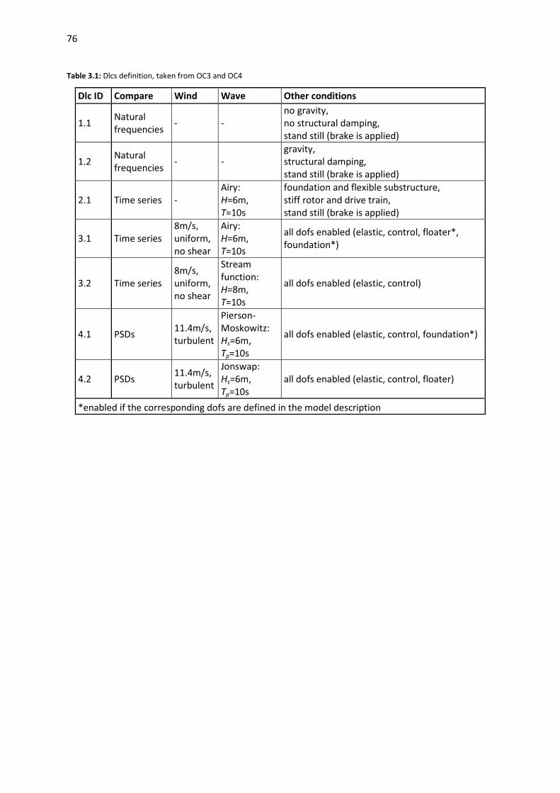
76

Table 3.1: Dlcs definition, taken from OC3 and OC4

Dlc ID Compare Wind Wave Other conditions

1.1 Natural frequencies - -

no gravity, no structural damping, stand still (brake is applied)

1.2 Natural frequencies - -

gravity, structural damping, stand still (brake is applied)

2.1 Time series - Airy: H=6m, T=10s

foundation and flexible substructure, stiff rotor and drive train, stand still (brake is applied)

3.1 Time series 8m/s, uniform, no shear

Airy: H=6m, T=10s

all dofs enabled (elastic, control, floater*, foundation*)

3.2 Time series 8m/s, uniform, no shear

Stream function: H=8m, T=10s

all dofs enabled (elastic, control)

4.1 PSDs 11.4m/s, turbulent

Pierson-Moskowitz: Hs=6m, Tp=10s

all dofs enabled (elastic, control, foundation*)

4.2 PSDs 11.4m/s, turbulent

Jonswap: Hs=6m, Tp=10s

all dofs enabled (elastic, control, floater)

*enabled if the corresponding dofs are defined in the model description

77

3.2.1 The jacket case (OC4 phase I)

3.2.1.1 Introduction

In OC4 phase I the NREL 5MW RWT [98] is mounted on a bottom based jacket support structure at 50m water depth. Detailed description of the jacket and of the tower is given in [122] while the list of the load cases and of the output recorded sensors can be found in [123]. The sensors on the jacket are shown in Figure 3.1.

Figure 3.1: Placement of sensors on jacket support structure (left) and wind turbine (right) [figure taken from [117]]

The jacket is formed by 4 vertical legs free flooded up to MSL which are constrained by one horizontal bracer and 4 “X-bracer” connections. From z=-49.5m to -45.5m the legs are connected to the piles and concrete is placed in between. Marine growth is applied from z=-40m to -2m to all jacket members leading to an increase of the mass and of the external diameter. The tower is connected to the jacket at z=20.15m through a concrete transition piece. As a simplification, in OC4, the nodes connecting crossed members are defined at the intersection of the two elastic axes. This leads to an artificial mass increase, although in hGAST and other codes a more accurate modeling is available.

The specific offshore WT concept requires the modeling of: the WT; the jackets; the marine growth; the transition peace; the leg – pile connections; the free-flooded members. In hGAST, the jacket is modeled using 117 different members. The marine growth and the leg-pile connection are modeled by properly modifying the structural properties of the corresponding members. Marine growth does not influence the stiffness, but reduces the eigenvalues due to the extra mass added and thereby influences the dynamics of the coupled structure. In addition, marine growth increases the

78

hydrodynamic loading, because of the increased outer diameter. The leg-pile members are modeled as beams with very high stiffness, considering the total distributed mass of the pile, the grout and the leg. The transition peace is modeled as a concentrated generalized mass. Moreover at 20.15m height, 4 stiff diagonal elements connect each leg with point (0, 0, 20.15) where the tower is mounted. The water inside the flooded members reduces the buoyancy and contributes extra inertial terms, of minor importance though because the deflections are small. The flooded water mass has not been modeled by modifying the structural properties, because the axial loads of the flooded legs that apply to the seabed level would increase by the weight of the flooded water. The WT blades are modeled using 9 sub-bodies and the tower using 1 sub-body and 20 elements.

Due to the complexity of the system and its modeling 4 or 5 revisions were needed in order to detect interpretation errors and modeling deficiencies. In the following comparisons out of the list of all OC4 phase I participating codes, tree codes have been selected and referred in the sequel as Code1, Code2 and Code3. All codes use BEMT aerodynamic modeling and Morison’s equation for hydrodynamic modeling. Code1 follows similar to hGAST FEM structural modeling while Code2 and Code3 adopt the modal approach. Wave kinematics in Morison’s equation is calculated up to the instantaneous water level using Wheeler stretching method [124] (see section 5.3.7.1).

3.2.1.2 Natural frequencies

In Table 3.2, the natural frequencies of the coupled structure from dlc1.1 [Table 3.1] are compared, which corresponds to dlc1.0b from OC4 phase I. The influence of gravity and of structural damping is not taken into account. The predictions are in very good agreement. This is an indication that the modeling of the structure is consistent and that the dynamics are well captured. The influence of gravity and structural damping is recorded by presenting hGAST predictions from dlc1.2 which corresponds to load case 1.0d from OC4 phase I and are denoted as hGAST* in Table 3.2. As also reported in [117], the influence of gravity and structural damping on the eigenvalues is in general very small; much less than 1.5% a fact that is confirmed. The highest relative reduction is visible in the global fore-aft and side-to-side modes.

79

Table 3.2: Natural frequencies [Hz] comparison of the jacket coupled OWT of OC4 phase I

Mode description hGAST Code1 Code2 Code3 hGAST*

1st global fore-aft 0.312 0.319 0.315 0.316 0.307

1st global side-to-side 0.309 0.317 0.312 0.314 0.304

1st drive train torsion 0.604 0.601 0.605 0.602 0.604

1st asymmetric flapwise pitch 0.671 0.659 0.664 0.700 0.669

1st asymmetric flapwise yaw 0.625 0.625 0.629 0.647 0.627

1st flapwise collective 0.711 0.697 0.699 0.737 0.710

1st asymmetric edgewise pitch 1.073 1.070 1.074 1.078 1.074

1st asymmetric edgewise yaw 1.083 1.080 1.084 1.066 1.081

2nd global fore-aft 1.177 1.193 1.217 1.215 1.172

2nd global side-to-side 1.194 1.214 1.205 1.237 1.189

2nd asymmetric flapwise yaw 1.620 1.640 1.653 1.646 1.622

2nd asymmetric flapwise pitch 1.910 1.882 1.906 1.987 1.908

2nd flapwise collective 2.002 1.969 1.972 2.061 2.001

1st global torsion 2.804 - 2.861 2.793 2.804

2nd edgewise collective 2.749 2.755 2.787 2.708 2.750

3.2.1.3 Time series

Time series of the recorded sensors are compared for the dlc3.2 [Table 3.1] which corresponds to the dlc5.6 from OC4 phase I. A constant uniform inflow of 8m/s and a 9th order stream function wave with period 10sec and height 8m at 50m depth are considered. All elastic degrees of freedom are enabled and the controller is switched on in the variable speed option. The blade pitch remains zero since the wind speed is well below the rated one of 11.4m/s.

In the present simulation the buoyancy force is calculated with the volume method in hGAST, due to the complex geometry of the jacket structure (see section 2.6.3). No dynamic pressure or drag terms are considered at the end nodes of the jacket members. Morison’s equation is applied up to the actual instantaneous wet position, since wave kinematics is defined based on the stream function theory.

In Figure 3.2 the global loads (3 forces and 3 moments) are compared, as obtained from a post processing procedure. The force on each leg is transferred to the center of the jacket as a combination of a force and a moment. In this way the global forcing acting on the structure is recorded. The fore-aft force and moment are in a very good agreement both in terms of mean value and amplitude. The wave period of 10sec is clearly depicted and the overturning moment due to the aerodynamic thrust compares well. The side-to-side signals are driven by the control system because

80

the wind and wave are aligned with the x-axis and so no significant loading is applied in the lateral y-axis direction, except of the rotor torque. The mean values are almost the same, while differences appear in the amplitudes due to the high sensitivity to the implementation of damping. The presence of high frequencies in one simulation that also appear in other signals is not straight forward to explain. They have no relation to either the wave or the rotor frequencies, but on the other hand they do not influence the results since the mean value, the amplitude and the main frequencies are correctly represented. The mean value of the global vertical force is defined by the difference of the weight minus the calculated buoyancy. Although the buoyancy is a constant force and in this respect does not contribute to the dynamic loading, still different implementations can lead to mean value differences in the jacket loads and deflections. This was a finding of the OC4 project where the two different methods were used; the volume method and the surface integration method (see section 2.6.3).

The mean value of the vertical force in Figure 3.2 is well predicted, while the different amplitude and phase are probably caused by the different modeling of the buoyancy force. It is not clear how each partner has calculated the buoyancy force. Differences could be also attributed to different modeling of the flooded legs. The yaw moment excitation is caused by the aerodynamics due to inflow asymmetries caused by the blade deflections, the cone and the tilt angles. No wave yaw excitation occurs because of the symmetry of the structure and of the loading. So the yaw moment at the tower top, is transferred through the tower and then through the jacket to the piles. It is known that modal based codes face difficulties in accurately predicting the yaw moment. Because of modal reduction structural couplings are not accounted for and in certain cases blade and tower torsion dofs are excluded. This was reported in the OC3 project as well [94].

In Figure 3.3, the local axial force on the 2nd and the 4th leg is compared at 3 different vertical heights; at 4.378m, at -38.25m and at -44.001m. Above MSL the tower frequency is excited, while below MSL the wave frequency is dominant. All the codes predict almost the same amplitude, but results are separated into two groups in terms of mean values. As already mentioned, this could be linked to the different calculation of the buoyancy or the different modeling of the flooded members. If the structural mass of the legs is increased in order to include the contained water mass, then higher negative axial forces will appear.

In Figure 3.4 the out of plane deflections in the fore-aft and in the side-to-side directions at the connection points X2S2, X2S3 at -1.958m depth and at the connection points X4S2, X4S3 at -33.373m depth are compared. Predictions agree well both in the mean value and the amplitude except for the side-to-side direction at X4S3 where the mean value is different most probably due to the already mentioned different buoyancy or flooded members modeling. As expected, fore-aft deflection is higher (both in mean value and amplitude) compared to side-to-side, due to the wave excitation. It is remarkable that deflections of 1mm are so consistently captured.

In Figure 3.5, the tower top moments and deflections are compared. Again the predictions are found in very good agreement. Comments related to the side-to-side and yaw directions from Figure 3.2 also apply to the tower top moments and deflections, because no other excitation in these directions

81

is present in between the tower top and the mudline. hGAST predicts slightly less fore-aft deflection compared to the other three codes. The yaw angle attains very small values, so the opposite sign obtained could be just an artifact.

In Figure 3.6, time series of the shaft torque and the bending moment at the main bearing position are well compared, as defined in the rotating frame. A phase shift in the hGAST bending moment results is due to different azimuthal synchronizing. The electrical power and the rotational speed are compared in Figure 3.7, where predictions are consistent. Differences are small given the scale of the vertical axis.

In Figure 3.8, the blade root moments and the main blade tip deflections are presented. As expected, the in-plane moment is identical and the FEM codes predict almost the same in-plane deflection because both signals are driven by gravity. A zero mean value in the in-plane deflection possibly justifies the absence of the mass offset in the beam equation. Differences in the out-of-plane moment are small given the scale. Out-of-plane deflections follow the trend of the mean value differences of the out-of-plane moment and of the rotational speed of the rotor. hGAST and Code3 predict almost the same pitching moment and torsion angle while the amplitude from Code1 is bigger. Code2 does not include the torsion degree of freedom.

82

(a) Global fore-aft force [kN]

(d) Global fore-aft moment [kNm]

(b) Global side force [kN]

(e) Global side moment [kNm]

(c) Global vertical force [kN]

(f) Global yaw moment [kNm]

Figure 3.2: Comparison of global jacket loads calculated at (0, 0, -50). The loads are the sum of the reaction force of all legs (dlc3.2 [Table 3.1]: Nonlinear wave (stream function) H=8m, T=10s, uniform inflow at 8m/s)

83

(a) Local axial force at K1L2 [kN]

(b) Local axial force at K1L4 [kN]

(c) Local axial force at middle of B59 [kN]

(d) Local axial force at middle of B61 [kN]

(e) Global axial force at mudL2 [kN]

(f) Global axial force at mudL4 [kN]

Figure 3.3: Comparison of Jacket axial force at K1L2, K1L4 (4.378m), at middle of braces 59 and 61 (-38.25m) and at mud brace level (-44.001m) (dlc3.2 [Table 3.1]: Nonlinear wave (stream function) H=8m, T=10s, uniform inflow at 8m/s)

84

(a) Deflection in fore-aft direction at X2S2 [m]

(b) Deflection in side-to-side direction at X2S3 [m]

(c) Deflection in fore-aft direction at X4S2 [m]

(d) Deflection in side-to-side direction at X4S3 [m]

Figure 3.4: Comparison of Jacket deflections in fore-aft and side-to-side directions at X2S2, X2S3 (-1.958m) and X4S2, X4S3(-

33.373m) - (dlc3.2 [Table 3.1]: Nonlinear wave (stream function) H=8m, T=10s, uniform inflow at 8m/s).

85

(a) Tower top side-to-side moment [kNm]

(d) Tower top side-to-side deflection [m]

(b) Tower top fore-aft moment [kNm]

(e) Tower top fore-aft deflection [m]

(c) Tower top yawing moment [kNm]

(f) Tower top yaw angle [deg]

Figure 3.5: Comparison of tower top deflections and tower top loads (dlc3.2 [Table 3.1]: Nonlinear wave (stream function) H=8m, T=10s, uniform inflow at 8m/s).

86

(a) Shaft’s torque [kNm]

(b) Bending moment at main bearing [kNm]

Figure 3.6: Comparison of shaft loads (dlc3.2 [Table 3.1]: Nonlinear wave (stream function) H=8m, T=10s, uniform inflow at 8m/s)

(a) Electrical Power [kW]

(b) Shaft rotation speed [rpm]

Figure 3.7: Comparison of electrical power and shaft rotation speed (dlc3.2 [Table 3.1]: Nonlinear wave (stream function) H=8m, T=10s, uniform inflow at 8m/s)

87

(a) Root in-plane bending moment [kNm]

(d) Tip in-plane deflection [m]

(b) Root out-of-plane bending moment [kNm]

(e) Tip out-of-plane deflection [m]

(c) Root pitching moment [kNm]

(f) Tip twist angle [deg]

Figure 3.8: Comparison of blade root loads and blade tip deflections (dlc3.2 [Table 3.1]: Nonlinear wave (stream function) H=8m, T=10s, uniform inflow at 8m/s)

88

3.2.2 The semi-submersible floating case (OC4 phase II)

3.2.2.1 Introduction

In the OC4 phase II, the RWT is mounted on the steel DeepCwind semi-submersible floater at 200m depth. The draft of the floater is 20m and the deck clearance is 12m. The main structure is formed by the main column and 3 offset columns [Figure 3.9]. The tower is mounted in the middle of the structure, on top of the main column of 6.5m diameter. The diameter of the lower part of the offset columns is 24m and of the upper part is 12m. Both parts are partially filled with water (the sloshing is neglected). The 4 columns are connected by “Y”, “delta” and “crossed” connections, using 15 pontoons in total. Catenary mooring lines are used. Detailed description of the semi-submersible floater, the mooring lines, the tower and the modifications in the controller is given in [125], the description of the NREL RWT and the baseline controlling system is given in [98], while the definition of the load cases in [116].

Figure 3.9: Description of the semi-submersible floater of the OC4 [figure taken from [125]]

In the following comparisons out of the list of all OC4 phase II participating codes, four codes have been selected and referred in the sequel as Code1, Code2, Code3 and Code4. All codes use BEMT aerodynamic modeling. hGAST, Code1 and Code4 are FEM based codes and also adopt dynamic mooring line modeling, while Code2 and Code3 are modal based codes with quasi static mooring line modeling. Code1 and Code2 use Morison’s equation for the hydrodynamic modeling, while Code3 and Code4 potential theory. Both hydrodynamic models are implemented in hGAST. Solid blue lines correspond to results using potential hydrodynamic theory, while blue dashed and dotted lines correspond to simulations using Morison’s equation. Wave kinematics in hGAST’s Morison module is always calculated in the instantaneous position (IP) of the body. Dotted lines correspond to Airy wave kinematics calculated up to mean sea level (MSL), while dashed lines correspond to Airy wave kinematics calculated up to the instantaneous water level (IWL) by applying Wheeler’s stretching method.

It is noted that the hydrodynamic coefficients in Morison’s equation have been calibrated on the basis of the linear theory. Because the Airy theory is applied at the MSL and at the mean body

89

position, application of Morison’s equation at the instantaneous body position and at the instantaneous water level is questionable. The best choice would be to estimate the hydrodynamic coefficients based on experimental data. The above-mentioned nonlinear options (calculation at the instantaneous position of the body and at the instantaneous water level) were found during the OC4 project to cause drift effects [73].

For the hGAST simulations performed with Morison’s equation the buoyancy force is calculated using the surface integration method (see section 2.6.3).

3.2.2.2 Natural frequencies

In Table 3.3, the Natural frequencies of the coupled semi-submersible OWT dlc1.2 [Table 3.1] which corresponds to dlc1.1 from OC4 phase II are presented. Gravity and structural damping contributions are considered. In general the agreement is good which indicates consistent modeling of the WT and of the semi-submersible floater. It also proves that the dynamics of the floating system are well captured. Rigid body modes of the floater are similar. The Morison’s equation version of hGAST and Code1 predict slightly reduced surge and sway frequencies 0.0088Hz compared to 0.0093Hz predicted by the other codes, including the potential version of hGAST. Both versions of hGAST predict slightly bigger frequencies for the roll and pitch rigid body motions of the floater in comparison to the others. Code4 predicts higher tower bending and drive train torsional frequencies. 1st blade modes are consistent, except that Code1 predicts lower blade asymmetric pitch and yaw frequencies in the edgewise direction.

Expected differences between modal (Code2 and Code3) and FEM codes (hGAST, Code1 and Code4) are found in the 2nd tower fore-aft and side-to-side bending modes and the 2nd blade asymmetric yaw mode in the flapwise direction [Table 3.3]. Modal codes overestimate the frequency of the aforementioned modes. For example Code3 over predicts the 2nd tower side-to-side bending mode at 5Hz, while the other codes predict it at ~3.5 Hz. Also both modal codes overestimate the 2nd blade asymmetric yaw mode in the flapwise direction giving ~1.9 Hz instead of 1.68 Hz predicted by hGAST and Code4 and 1.61 Hz predicted by Code1.

The effect of the different hydrodynamic modeling on the natural frequencies is identified by comparing the 2 different approaches of hGAST. Clearly the WT frequencies remain unchained, while small differences are found in the 6 floater rigid modes. In the present case, application of Morison’s equation gives slightly lower frequencies for the 6 floater motions which are in agreement with the Code1 results, but since the Morison’s equation is subjected to calibration a firm conclusion cannot be drawn.

90

Table 3.3: Natural frequencies [Hz] comparison of the semi-submersible coupled OWT of OC4 phase II

Mode description hGASTp hGASTm Code1 Code2 Code3 Code4

Platform surge 0.0093 0.0088 0.0086 0.0094 0.0093 0.0093

Platform sway 0.0093 0.0088 0.0088 0.0092 0.0093 0.0093

Platform heave 0.0583 0.0574 0.0573 0.0581 0.0581 0.0556

Platform roll 0.0413 0.0404 0.0384 0.0397 0.0392 0.0385

Platform pitch 0.0413 0.0404 0.0384 0.0397 0.0392 0.0385

Platform yaw 0.0131 0.0126 0.0132 0.0136 0.0132 0.0127

1st tower fore-aft 0.424 0.423 0.424 0.425 0.426 0.465

1st tower side-to-side 0.415 0.414 0.415 0.417 0.418 0.458

1st drivetrain torsion 0.622 0.622 0.608 0.623 0.628 0.672

1st blade collective flap 0.717 0.717 0.686 0.706 0.704 0.692

1st asymmetric flapwise pitch 0.677 0.677 0.618 0.641 0.670 0.664

1st asymmetric flapwise yaw 0.639 0.639 0.648 0.670 0.667 0.635

1st asymmetric edgewise pitch 1.079 1.079 1.002 1.080 1.079 1.095

1st asymmetric edgewise yaw 1.092 1.092 1.015 1.091 1.092 1.103

2nd tower fore-aft 3.417 3.415 3.314 3.864 3.898 3.405

2nd tower side-to-side 3.540 3.537 3.494 3.437 5.012 3.875

2nd collective flap 2.000 2.000 1.840 1.972 2.023 1.928

2nd asymmetric flapwise pitch 1.876 1.876 1.739 1.718 1.914 1.829

2nd asymmetric flapwise yaw 1.681 1.681 1.609 1.870 1.934 1.672

*hGASTp: potential theory is applied, hGASTm: Morison’s equation is applied

3.2.2.3 Time series

Similar to the jacket case, results from dlc3.1 [Table 3.1], which correspond to OC4 phase II dlc3.1, are presented considering all the flexibilities of the structure enabled. Wind speed is 8m/s and an Airy wave of 6m height and 10s period aligned to wind and x–axis is considered at 200m depth. The Airy wave is selected, instead of the stream function wave of the jacket case, so that the linear potential theory can be applied. The controller is operating in variable speed mode. The provided results are compared in terms of time series.

In Figure 3.10, the rigid body motions of the floater are presented and in general the agreement is good. Only the surge, heave and pitch motions are directly excited by the wave. In the corresponding signals the wave period of 10sec is well represented. In sway, roll and yaw motions the wave period is also depicted due to couplings, but the amplitudes are much smaller. As reported in [73] differences in the surge mean value are attributed to nonlinear hydrodynamic effects. In the

91

Morison’s equation approach, drift effects are caused by applying the hydrodynamic loads at the instantaneous position (IP) of the body or at the instantaneous water level (IWL) using Wheeler’s stretching or by combining the two. When the potential theory is applied, drift effects are revealed if 2nd order terms are included either directly through the solution of the 2nd order problem or through Newman’s approximation [43]. Different aerodynamic thrust could also affect the mean surge position, although the above conclusion was initially drawn from simplified load cases with no wind excitation. Code3 and the potential version of hGAST that both apply 1st order potential theory predict almost identical surge motion. It is noted that a difference in the surge mean value signal is not expected to influence the other signals. The pitch signals are very similar and the mean value determined by the aerodynamic thrust is consistent. The amplitude of the pitch motion predicted by Code2 is about 0.5o higher. Although sway, roll and yaw motions attain small values, the agreement is very good. These motions are less damped so in certain cases the provided results have not completely reached a periodic state. The positive roll angle is set by the torque of the rotor. It is not straightforward to explain the differences in the sway sign because of the very small values attained. Heave motion is well represented. Again some of the codes using Morison’s equation predict higher amplitudes. By comparing hGAST potential (solid blue line) and the two Morison based results (dotted blue line corresponding to IP+MSL and dashed blue line corresponding to IP+IWL) minor differences are found in the surge and the pitch motion. Both versions of Morison’s equation predict a negative drift effect in the surge motion. In the IP+IWL approach the mean surge is 0.3m lower and in the IP+MSL version is 0.4m lower as compared to the results based on potential theory that do not include drift effects. Both versions of Morison’s equation predict a minor increase in the pitch mean value by ~0.20.

In Figure 3.11, the tensions of the mooring lines at fairlead 1 and 2 are compared. The mean values are identical, while phase shift and higher frequencies appear in the codes that adopt the dynamic mooring lines modeling, compared to those that adopt the quasi static approach. These differences do not seem to influence the dynamics of the coupled floating WT system, but will possibly affect the DELs of the mooring lines, as also reported in [73]. They could be of crucial importance for the mooring lines and the foundation design.

In Figure 3.12, deflections at the tower top and moments at the tower bottom are compared. As expected, loads and deflections in the same directions depict similar behavior. Signals in the side-to-side direction are driven by the torque of the rotor and indirectly by the controller. The 1st tower mode is mainly excited (period about 2.5sec). The wave period is also depicted due to couplings with the sway and the roll motions. Mean values are very similar. Because of the absence of side excitation, the side signals are very sensitive to the modeling of damping which partially explain the differences. On the other hand, signals in the fore-aft direction are mainly affected by the wave excitation. Higher amplitude predictions in Morison based codes are explained from the higher amplitudes of the pitch motion. Although the already mentioned difference in the mean value of the tower yaw moment between FEM and modal based codes is still present (see section 3.2.1.3), it is masked by the increase in amplitude due to the rigid motions of the floater. The twist angle, which corresponds to the torsion degree of freedom of the tower, is only considered in hGAST, Code1 and

92

Code2. Although its value is very small about 0.01o, hGAST and Code1 predictions are very similar, while the increased mean value in Code2 is explained by the already mentioned mean value difference in the yaw moment.

In Figure 3.13, the torque of the shaft and the bending moment at the main bearing are compared. Differences in the torque signal are less that 5% but pronounced because of the scale in the figure. Higher frequencies appear in modal based codes predictions. This indicates a possible difference in the damping implementation but could be also associated to different modeling of the drive train or to the application of a drive train damper as a means to avoid instabilities induced by the controller that are not usually triggered in modal codes. FEM codes approximate the drive train as a beam structure while in modal codes it is introduced as a torsion spring. The bending moment at the position of the main bearing is well represented.

In Figure 3.14, the electrical power and the rotational speed are presented, both exhibiting similar form. The electrical power is directly affected by the rotational speed of the rotor which in turn is influenced by the pitch motion of the floater. Results again agree well, while differences seem amplified given the scale in the figures. The wave excited pitch motion of the floater is clearly depicted in the rotational speed as defined by the baseline controller defined in the OC4 project. This implies a need for more advanced controllers capable of reducing the floater motion. For example in [126] the OC4 controller was enhanced with an extra PI which added a feedback torque based on the filtered tower top acceleration

In Figure 3.15, moments at the root and deflections at the tip of the 1st blade are presented. Similar to the tower signals, loads and deflections in the same direction should be linked. Signals in the in-plane direction are almost identical, since they are driven by gravity. The rotor period of about 6sec is clearly depicted. Bending moment and deflection in the out-of-plane direction are consistent, although differences are bigger compared to the in-plane signals. As expected, the out-of-plane signals are mainly affected by the presence of the wave, leading to increased amplitudes as compared to the jacket case (see Figure 3.8). Both wave and rotor frequencies are depicted. Code2 increased amplitudes are linked to the increased amplitudes in the pitch motion. The torsion moment is similar, while hGAST underpredicts its amplitude. The bigger differences are seen in the torsion angle. hGAST and Code1 that both account for geometric nonlinear effects, predict similar results with the same phase, but with different mean value and amplitude [52]. In Code2 results, the difference in the torsion angle and the smaller amplitude is possibly explained by the use of a simplified beam model. This point is detailed in section 3.4 where geometrical nonlinear effects due to large deflections are addressed.

93

(a) Platform surge motion [m]

(d) Platform roll motion [deg]

(b) Platform sway motion [m]

(e) Platform pitch motion [deg]

(c) Platform heave motion [m]

(f) Platform yaw motion [deg]

Figure 3.10: Comparison of platform motions (dlc3.1 [Table 3.1]: Airy Wave H=6m, T=10s, uniform inflow at 8m/s).

**hGAST blue solid line: potential theory, blue dotted line: Morison IP+MSL, blue dashed line: Morison IP+IWL.

94

(a) Fairlead 1 tension [kN]

(b) Fairlead 2 tension [kN]

Figure 3.11: Comparison of tension at fairleads 1 and 2 (dlc3.1 [Table 3.1]: Airy Wave H=6m, T=10s, uniform inflow at 8m/s). **hGAST blue solid line: potential theory, blue dotted line: Morison IP+MSL, blue dashed line: Morison IP+IWL.

95

(a) Tower base side-to-side moment [kNm]

(d) Tower top side-to-side deflection [m]

(b) Tower base fore-aft moment [kNm]

(e) Tower top fore-aft deflection [m]

(c) Tower base yawing moment [kNm]

(f) Tower top yaw angle [deg]

Figure 3.12: Comparison of tower top deflections and tower bottom loads (dlc3.1 [Table 3.1]: Airy Wave H=6m, T=10s, uniform inflow at 8m/s).

**hGAST blue solid line: potential theory, blue dotted line: Morison IP+MSL, blue dashed line: Morison IP+IWL.

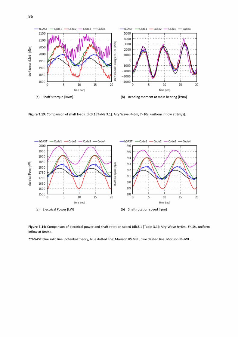
96

(a) Shaft’s torque [kNm]

(b) Bending moment at main bearing [kNm]

Figure 3.13: Comparison of shaft loads (dlc3.1 [Table 3.1]: Airy Wave H=6m, T=10s, uniform inflow at 8m/s).

(a) Electrical Power [kW]

(b) Shaft rotation speed [rpm]

Figure 3.14: Comparison of electrical power and shaft rotation speed (dlc3.1 [Table 3.1]: Airy Wave H=6m, T=10s, uniform inflow at 8m/s).

**hGAST blue solid line: potential theory, blue dotted line: Morison IP+MSL, blue dashed line: Morison IP+IWL.

97

(a) Root in-plane bending moment [kNm]

(d) Tip in-plane deflection [m]

(b) Root out-of-plane bending moment [kNm]

(e) Tip out-of-plane deflection [m]

(c) Root pitching moment [kNm]

(f) Tip twist angle [deg]

Figure 3.15: Comparison of blade root loads and blade tip deflections comparison (dlc3.1 [Table 3.1]: Airy Wave H=6m, T=10s, uniform inflow at 8m/s).

**hGAST blue solid line: potential theory, blue dotted line: Morison IP+MSL, blue dashed line: Morison IP+IWL.

98

3.2.2.4 Power spectral densities

Results from the dlc4.2 [Table 3.1], which correspond to dlc3.2 of the OC4 phase II are compared in terms of power spectral densities (PSDs), since stochastic wind and wave excitation is considered. Wind conditions correspond to a zero yaw angle turbulent inflow at rated wind speed of 11.4m/s with turbulence intensity Τi=0.147 and shear exponent α=0.14 corresponding to normal turbulence model (NTM) conditions. Wave conditions are defined based on an irregular Airy wave described following Jonswap’s spectrum with peak period Tp=10s (peak frequency 0.1Hz), significant wave height Hs=6m and dimensionless peak shape parameter γ=2.87 at a water depth of 200m with zero wave heading angle, corresponding to normal sea state conditions. All the elastic degrees of freedom are enabled and the controller is switched on, operating in both the variable speed and the variable pitch modes. One hour simulations are performed considering both hydrodynamic methods in hGAST (blue solid lines correspond to potential theory, blue dotted lines to Morison’s equation applied at IP and MSL, while blue dashed lines to Morison’s equation applied at IP and IWL).

In general the agreement for all the examined signals is very good. In Figure 3.16, the PSD of the rigid body motions of the floater are presented. Only the surge, heave and pitch motions are directly excited by the wave. In the corresponding signals the wave peak frequency of 0.1Hz (peak period of 10sec) is clearly depicted. In sway, roll and yaw motions the wave frequency is also excited due to couplings, but the energy is much smaller. At low frequencies in all the PSDs the corresponding rigid body natural frequencies (see Table 3.3) are clearly excited and the agreement is almost perfect. The surge-pitch and the sway-roll couplings are identified as double peaks in the corresponding figures. At the frequency range [0.2 – 06Hz] increased energy appears in hGAST predictions based on Morison’s equation compared to those based on potential theory. The former results agree with those by Code1 also using Morison’s eq., while the latter with Code3 and Code4 which are based on potential theory. It is noted that the energy in this frequency range is about 4 orders of magnitude lower with respect to the maximum, so differences could be of minor importance.

In Figure 3.17, the PSD of the mooring line tension at fairlead 1 and 2 are compared. As already mentioned in section 3.2.2.3 the implementation of a different mooring line model is clearly identified. Although the peak at the wave frequency of 0.1Hz is almost identical, codes that adopt the dynamic mooring line predict excitation in a wider frequency range from 0.1Hz to 0.7Hz that do not influence the dynamics of the coupled floating WT. This conclusion follows by comparing the PSD of the 6 rigid body modes [Figure 3.16]. The already discussed difference between predictions of codes based on Morison eq. and potential theory is visible at 0.4Hz.

In Figure 3.18, the PSDs of the deflections at the tower top and the moments at the tower bottom are compared. As expected, loads and deflections in the same directions exhibit similar behavior. In the side-to-side PSDs the tower frequency at 0.42Hz is more excited followed by the sway and roll rigid body modes and the 3P, 6P and 9P at 0.6Hz, 1.2Hz and 1.8Hz respectively. It is noted that hGAST predicts less energy at 1.8Hz due to the application of the drive train damper at 1.75Hz as clearly seen in the PSD of the torque of the shaft in Figure 3.19. In the fore-aft direction the wave frequency is more excited because it coincides with the wave propagation direction. The rotor frequencies 3P,

99

6P and 9P are pronounced in the fore-aft and the yaw directions. Agreement between the codes is fine. The difference between predictions of codes based on Morison eq. and potential theory is clearly visible at 0.4Hz in the fore-aft signals that are directly excited by the wave.

In Figure 3.19, the PSD of the torque of the shaft and of the bending moment at the main bearing (defined in the rotating frame) are compared. As already mentioned hGAST predicts lower peak in the PSD of the torque at the drive train free-free natural frequency (~ 1.75Hz) due to the drive train damper. Good agreement is found in the bending moment where the main excitation is at 1P frequency of 0.2Hz and 2P at 0.4Hz respectively.

In Figure 3.20 the PSD of the blade pitch and of the rotor speed are compared. The wave frequency is clearly excited, similar to section 3.2.2.3 in both control variables. The 3P frequency is also depicted as well as the 2nd flapwise and the drive train free-free (about 1.75Hz). Again the agreement is fine.

In Figure 3.21, the PSD of moments at the root and of deflections at the tip of the 1st blade are compared. Similar to the tower signals, loads and deflections in the same direction should be linked. The 1P rotor frequency of 0.2Hz is the most excited one for all blade signals. In the in-plane and the yaw directions the edgewise natural frequency at about 1.1Hz is clearly depicted, while in the out-of-plane direction the wave frequency is 0.1Hz. Code1 predicts increased wave excitation and a shift in the edgewise frequency also derived from Table 3.3, in comparison to the other codes.

100

(a) Platform surge motion [m2/Hz]

(d) Platform roll motion [deg2/Hz]

(b) Platform sway motion [m2/Hz]

(e) Platform pitch motion [deg2/Hz]

(c) Platform heave motion [m2/Hz]

(f) Platform yaw motion [deg2/Hz]

Figure 3.16: PSDs comparison of platform motions (dlc4.2 [Table 3.1]: NTM at 11.4m/s, Jonswap spectrum Hs=6m, Tp=10s). **hGAST blue solid line: potential theory, blue dotted line: Morison IP+MSL, blue dashed line: Morison IP+IWL.

101

(a) Fairlead 1 tension [kN2/Hz]

(b) Fairlead 2 tension [kN2/Hz]

Figure 3.17: PSDs comparison of tension at fairlead 1 and 2 (dlc4.2 [Table 3.1]: NTM at 11.4m/s, Jonswap spectrum Hs=6m, Tp=10s).

**hGAST blue solid line: potential theory, blue dotted line: Morison IP+MSL, blue dashed line: Morison IP+IWL.

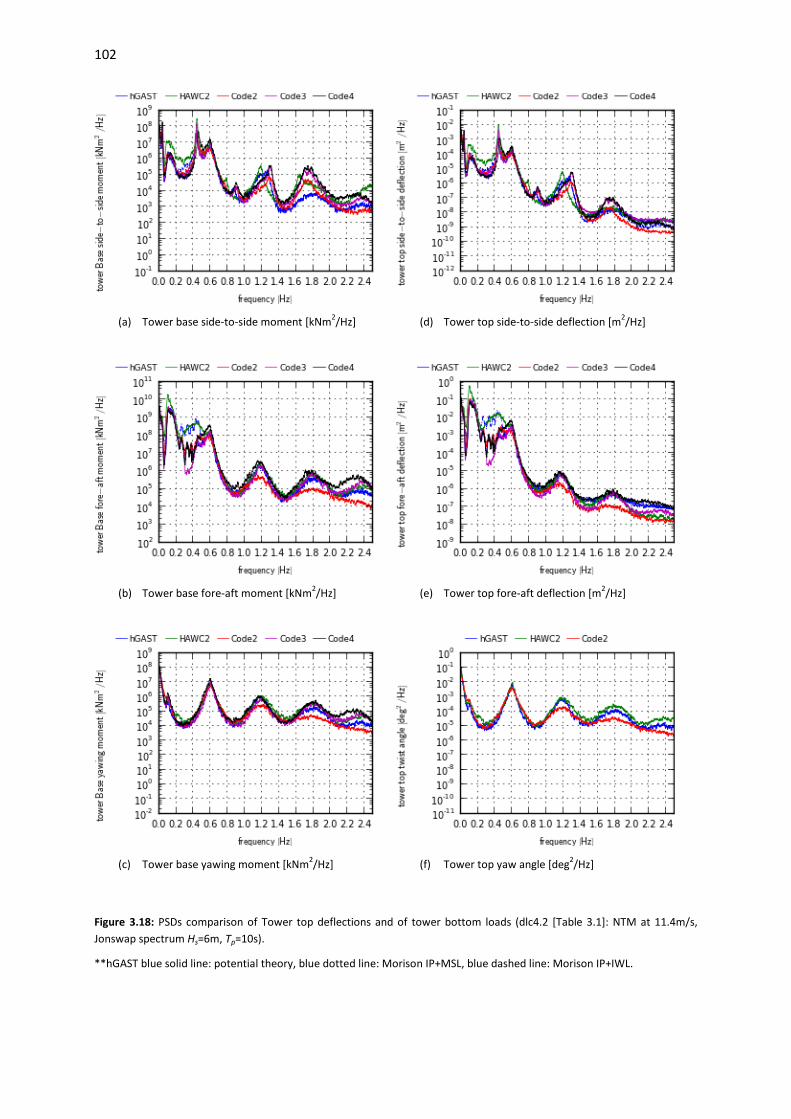
102

(a) Tower base side-to-side moment [kNm2/Hz]

(d) Tower top side-to-side deflection [m2/Hz]

(b) Tower base fore-aft moment [kNm2/Hz]

(e) Tower top fore-aft deflection [m2/Hz]

(c) Tower base yawing moment [kNm2/Hz]

(f) Tower top yaw angle [deg2/Hz]

Figure 3.18: PSDs comparison of Tower top deflections and of tower bottom loads (dlc4.2 [Table 3.1]: NTM at 11.4m/s, Jonswap spectrum Hs=6m, Tp=10s).

**hGAST blue solid line: potential theory, blue dotted line: Morison IP+MSL, blue dashed line: Morison IP+IWL.

103

(a) Shaft’s torque [kNm2/Hz]

(b) Bending moment at main bearing [kNm2/Hz]

Figure 3.19: PSDs comparison of shaft loads (OC4 phase II dlc3.2 – NTM at 11.4m/s, Jonswap spectrum Hs=6m, Tp=10s).

(a) Blade pitch angle [deg2/Hz

(b) Shaft rotation speed [rpm2/Hz]

Figure 3.20: PSDs comparison of pitch angle and of shaft rotation speed (dlc4.2 [Table 3.1]: NTM at 11.4m/s, Jonswap spectrum Hs=6m, Tp=10s).

**hGAST blue solid line: potential theory, blue dotted line: Morison IP+MSL, blue dashed line: Morison IP+IWL.

104

(a) Root in-plane bending moment [kNm2/Hz]

(d) Tip in-plane deflection [m2/Hz]

(b) Root out-of-plane bending moment [kNm2/Hz]

(e) Tip out-of-plane deflection [m2/Hz]

(c) Root pitching moment [kNm2/Hz]

(f) Tip twist angle [deg2/Hz]

Figure 3.21: PSDs comparison of blade root loads and of blade tip deflections (dlc4.2 [Table 3.1]: NTM at 11.4m/s, Jonswap spectrum Hs=6m, Tp=10s).

**hGAST blue solid line: potential theory, blue dotted line: Morison IP+MSL, blue dashed line: Morison IP+IWL.

105

3.2.3 The monopile case (OC3 phase I, II)

3.2.3.1 Introduction

In the OC3 phase I and II, the RWT is mounted on a steel bottom based monopile support structure at 20m depth. In phase I the monopile is assumed cantilevered to the sea bed where fixed conditions are applied, while in phase II 3 foundation models are examined: the apparently fixed (AF) model, the concentrated spring (CS) model and the distributed springs (DS) model (see Section 2.3.4.3). Detailed description of the monopile and of the load cases is given in [94], while of the foundation models in [93]. The description of the NREL RWT and the baseline controlling system is given in [98]].

In the following comparisons out of the list of all OC3 phase I and II participating codes, HAWC2 from DTU, ADAMS and FAST from NREL and BLADED from GH have been selected. All codes use BEMT aerodynamic modeling and Morison’s equation for the hydrodynamic modeling, while HAWC2 and ADAMS follow similar to hGAST FEM structural modeling and FAST and BLADED adopt the modal approach. The wave kinematics in Morison’s equation are calculated up to the instantaneous water level using Wheeler stretching method [124] (see section 5.3.7.1).

3.2.3.2 Natural frequencies

In Table 3.4, the natural frequencies of the coupled structure mounted on a bottom based monopile support structure from dlc1.2 [Table 3.1], which corresponds to OC3 phase I and phase II dlc1.2 are compared. The influence of the gravity and the structural damping has been taken into account. The predictions are in excellent agreement which indicates consistent modeling. Codes that adopt similar FEM structural modeling to hGAST (namely ADAMS and HAWC2) are selected in the comparison that follows.

The consideration of the foundation: reduces the 1st tower bending frequencies by 12% from 0.27Hz to 0.24Hz; reduces the 2nd tower fore-aft and side-to-side bending frequencies by 33% and 24% respectively from 2.35Hz to 1.59Hz and from 2.22Hz to 1.70Hz; and increases the 2nd asymmetric flapwise pitch frequency by 10% from 1.80Hz to 1.98Hz. All other modes are not affected and differences are less than 1%. The concentrated spring model in HAWC2 predicts increased 2nd tower and 2nd asymmetric flapwise pitch natural frequencies. Otherwise the frequencies determined with the 3 different foundation models are almost identical.

106

Table 3.4: Natural frequencies [Hz] comparison of the monopile of OC3 with rigid foundation (phase I) and 3 foundation

models namely the apparently fixed (AF), the concentrated spring (CS) and the distributed springs (DS)

Mode description hGAST ADAMS HAWC2

Rigid AF CS DS Rigid AF CS DS Rigid AF CS DS

1st tower fore-aft 0.27 0.24 0.24 0.24 0.27 0.24 0.24 0.24 0.27 0.24 0.24 0.24 1st tower side-to-side 0.27 0.24 0.24 0.24 0.27 0.24 0.24 0.24 0.28 0.24 0.24 0.24 1st drivetrain torsion 0.60 0.59 0.59 0.59 0.60 0.59 0.59 0.59 0.60 0.60 0.60 0.60 1st blade collective flap 0.71 0.71 0.71 0.71 0.70 0.70 0.70 0.70 0.70 0.69 0.70 0.69 1st asymmetric flapwise pitch 0.67 0.66 0.66 0.66 0.66 0.66 0.66 0.66 0.66 0.66 0.66 0.66 1st asymmetric flapwise yaw 0.63 0.62 0.63 0.62 0.62 0.62 0.62 0.62 0.62 0.62 0.63 0.62 1st asymmetric edgewise pitch 1.08 1.08 1.08 1.08 1.07 1.07 1.07 1.07 1.07 1.07 1.07 1.07 1st asymmetric edgewise yaw 1.09 1.09 1.09 1.09 1.08 1.08 1.08 1.08 1.09 1.08 1.09 1.08 2nd tower fore-aft 2.35 1.59 1.59 1.59 2.37 1.59 1.59 1.59 2.34 1.57 1.76 1.55 2nd tower side-to-side 2.22 1.70 1.70 1.69 2.25 1.71 1.71 1.71 2.30 1.70 2.15 1.67 2nd blade collective flap 2.00 2.02 2.02 2.02 1.96 1.95 1.95 1.95 1.94 2.00 1.96 2.00 2nd asymmetric flapwise pitch 1.80 1.98 1.98 1.98 1.79 2.01 2.01 2.01 1.78 1.94 2.24 1.94 2nd asymmetric flapwise yaw 1.64 1.63 1.64 1.62 1.61 1.60 1.61 1.59 1.65 1.63 1.64 1.61

3.2.3.3 Time series

Results from dlc3.1 [Table 3.1], which corresponds to OC3 phase I dlc5.1 are presented considering all the flexibilities of the structure enabled. Uniform wind speed is 8m/s and an Airy wave of 6m height and 10s period with zero wave heading are considered at 20m depth. The controller is operating in the variable speed mode. The provided results are compared in terms of time series.

Since a detailed comparison of all the considered sensors have been performed in previous sections for the jacket and the semi-submersible floater, only a few representative signals are presented for the monopile with the rigid foundation. In addition to the FEM codes hGAST, HAWC2 and ADAMS predictions by the modal based codes BLADED and FAST have been included.

In Figure 3.22a and b the tower top deflection and the monopile bending moment at the seabed level in the fore-aft direction compare well. The rotation frequency and the wave frequency are depicted in the tower top deflection, while the wave frequency is dominant in the bending moment at the seabed level. In Figure 3.22c and d, the blade tip deflection and the root bending moment in the out-of-plane directions are presented. A small mean value difference in the deflection is due to differences in the aerodynamic loading estimation and is consistent with the mean values of the root bending moments. In Figure 3.22e the rotor speed has reached an almost steady value. The controller operates in variable speed mode and small differences in the mean value can be again linked to aerodynamics. In Figure 3.22f the blade tip twist angle is compared. Only the FEM codes are compared since the modal based codes do not include the torsion degree of freedom in the structural modeling. hGAST and ADAMS predictions are in good agreement, while HAWC2 predicts almost 0.50 smaller mean values and slightly increased amplitudes.

107

In Figure 3.23 the monopile bending moment and deflection at the seabed level at -20m in the fore-aft direction are compared for the 3 foundation models, namely the apparently fixed, the concentrated spring and the distributed springs. The simulations correspond to dlc2.1 [Table 3.1], which are the OC3 phase II dlc4.1, in which the blades and the drive train are assumed stiff and an Airy wave of H=6m and T=10s is considered. In the absence of wind, the rotor is assumed fixed (i.e. the brake is applied).

Although the distributed spring model is of higher fidelity compared to the apparently fixed and the concentrated spring models, similar results are obtained for all 3 foundation models as it is also indicated through the eigenvalues comparison [Table 3.4]. All predictions agree well. ADAMS code predicts higher frequencies, not straight forward to explain, but this does not affect the mean value and the amplitude of the moment and of the deflection. The wave frequency is clearly depicted in all the figures.

108

(a) Tower top fore-aft deflection [m]

(b) Monopile at seabed fore-aft moment [kNm]

(c) Blade tip out-of-plane deflection [m]

(d) Blade root out-of-plane bending moment [kNm]

(e) Shaft rotation speed [rpm]

(f) Blade tip twist angle [deg]

Figure 3.22: Comparison of monopile with rigid foundation (dlc3.1 [Table 3.1]: Airy Wave H=6m, T=10s, uniform inflow at 8m/s)

109

(a) Apparently fixed model: fore-aft bending moment at seabed [kNm]

(b) Apparently fixed model: : fore-aft deflection at seabed [m]

(c) Concentrated spring model: fore-aft bending moment at seabed [kNm]

(d) Concentrated spring model: fore-aft deflection at seabed [m]

(e) Distributed spring model: fore-aft bending moment at seabed [kNm]

(f) : Distributed spring model: fore-aft deflection at seabed [m]

Figure 3.23: Comparison of monopile with flexible foundation fore-aft bending moment at seabed (left column) and fore-aft deflection at seabed (right column) for the 3 foundation models AF, CS and DS (dlc2.1 [Table 3.1]: Airy Wave H=6m, T=10s, no wind, stiff drive train and stiff blades)

110

3.2.3.4 Power spectral densities

Results from dlc4.1 [Table 3.1], which corresponds to dlc5.2 of the OC3 phase I and II are compared in terms of power spectral densities (PSDs), since stochastic wind and wave excitation is considered. Wind conditions correspond to a zero yaw angle turbulent inflow at rated wind speed of 11.4m/s with turbulence intensity Τi=0.174 and shear exponent=0.14. Irregular Airy wave conditions are considered based on the Pierson-Moskowitz spectrum with peak period Tp=10s (peak frequency 0.1Hz), significant wave height Hs=6m at the water depth of 20m and zero wave heading angle, corresponding to normal sea state conditions. All the elastic degrees of freedom are enabled and the controller is switched on, operating in both the variable speed and the variable pitch modes.

In Figure 3.24, the PSDs of the monopile fore-aft bending moment at the seabed is compared considering 4 foundation types; the rigid foundation, the apparently fixed, the concentrated spring and the distributed springs model. The agreement is fine for all foundation types.

In order to assess the influence of the foundation modeling on the WT loads, in Figure 3.25 the PSDs of the moments at the blade root and the monopile at the seabed level for the 4 foundation options are compared as predicted by hGAST. On the left side of the figure the PSDs of the blade moments remain unaffected, so does the PSD of the monopile yawing moment [Figure 3.25f]. In the PSDs of the fore-aft and the side-to-side bending moments there is a shift in the 2nd tower bending mode as also indicated in Table 3.4 from 2.2Hz to 1.6Hz. In the side-to-side signal shift of the 1st tower bending mode from 0.27Hz to 0.24Hz is also visible. It was found that only the tower moments and deflections are affected if the foundation modeling is considered, while all the other signals remain the same.

111

(a) Rigid foundation: PSD of the fore-aft bending moment at seabed [kNm2/Hz]

(b) Apparently fixed model: PSD of the fore-aft bending moment at seabed [kNm2/Hz]

(c) Concentrated springs fixed model: PSD of the fore-aft bending moment at seabed [kNm2/Hz]

(d) Distributed springs model: PSD of the fore-aft bending moment at seabed [kNm2/Hz]

Figure 3.24: PSDs comparison of the fore-aft bending moment at seabed for the monopile with rigid foundation, and the AF, CS and DS models (dlc4.1 [Table 3.1]: turbulent wind at 11.4m/s, Pierson-Moskowitz spectrum Hs=6m, Tp=10s)

112

(a) Blade root in-plane moment [kNm2/Hz]

(d) Monopile at seabed side-to-side moment [kNm2/Hz]

(b) Blade root out-of-plane moment [kNm2/Hz]

(e) Monopile at seabed fore-aft moment [kNm2/Hz]

(c) Blade root pitching moment [kNm2/Hz]

(f) Monopile at seabed yawing moment [kNm2/Hz]

Figure 3.25: hGAST PSD comparison of the blade root and the monopile base moments for monopile with rigid foundation and the AF, CS and DS models (dlc4.1 [Table 3.1]: turbulent wind at 11.4m/s, Pierson-Moskowitz spectrum Hs=6m, Tp=10s)

113

3.2.4 The spar-buoy floating case (OC3 phase IV)

3.2.4.1 Introduction

In the OC3 phase IV, the RWT is mounted on the steel spar-buoy floater [Figure 3.26] at 320m depth. The draft of the floater is 120m, while the tower is mounted at z=10m. Catenary mooring lines are used. Detailed description of the floater, the mooring lines, the tower and the modifications in the controller is given in [71], the description of the NREL RWT and the baseline controlling system is given in [98], while the definition of the load cases in [94].

Figure 3.26: Illustration of the OC3 phase IV spar-buoy OWT [figure taken from [94]]

In the following comparisons out of the list of all OC3 phase IV participating codes, ADAMS and FAST from NREL have been selected. All three codes use BEMT aerodynamic modeling and potential hydrodynamic theory. As already mentioned, hGAST and ADAMS are FEM based codes, while FAST is modal based. hGAST adopts dynamic mooring line modeling, while FAST and BLADED quasi static mooring line models.

3.2.4.2 Natural frequencies

In Table 3.5, the Natural frequencies of the coupled spar-buoy OWT from dlc1.2 [Table 3.1], which corresponds to OC3 phase IV dlc1.1 are presented, similar to Table 3.3 which presents the natural frequencies of the semi-submersible OWT. Gravity and structural damping contributions are considered.

The excellent agreement indicates consistent modeling of the coupled structure. hGAST and ADAMS (FEM codes) results differ by less than 2%, while expected differences between the modal based code FAST and the FEM codes hGAST and ADAMS are found in both 2nd tower fore-aft and side-to-side bending modes and the 2nd blade asymmetric yaw mode in the flapwise direction. FAST code overestimates the frequency of the aforementioned modes, as already discussed in previous sections (see section 3.2.2.2).

114

By comparing hGAST predictions for the spar-buoy floater [Table 3.5] to those for the semi-submersible [Table 3.3], the main differences appear in the 1st tower bending modes (~0.46Hz - 0.47Hz to 0.42Hz) and the 1st Blade Asymmetric Flapwise Yaw mode (0.67Hz to 0.64Hz). It is noted that both floater concepts have the same rotor nacelle assembly and tower, so the differences are exclusively related to the floater design and the associated mooring line system.

Table 3.5: Natural frequencies [Hz] comparison of the spar-buoy coupled OWT of OC3 phase IV

Mode description hGAST ADAMS FAST Platform surge 0.008 0.009 0.008 Platform sway 0.008 0.008 0.008 Platform heave 0.032 0.031 0.032 Platform roll 0.035 0.034 0.034 Platform pitch 0.035 0.034 0.034 Platform yaw 0.120 0.120 0.121 1st tower fore-aft 0.473 0.473 0.473 1st tower side-to-side 0.455 0.456 0.457 1st drivetrain torsion 0.643 0.642 0.650 1st blade collective flap 0.721 0.710 0.710 1st blade asymmetric flapwise pitch 0.683 0.677 0.678 1st blade asymmetric flapwise yaw 0.666 0.661 0.695 1st blade asymmetric edgewise pitch 1.081 1.078 1.081 1st blade asymmetric edgewise yaw 1.094 1.089 1.093 2nd tower fore-aft 3.465 3.522 3.751 2nd tower side-to-side 3.601 3.697 4.263 2nd blade collective flap 2.000 1.962 2.023 2nd blade asymmetric flapwise pitch 1.879 1.868 1.933 2nd blade asymmetric flapwise yaw 1.705 1.675 1.957

3.2.4.3 Time series

Results from dlc3.1 [Table 3.1], which corresponds to OC3 phase IV dlc5.1 are presented considering all the flexibilities of the structure enabled. Wind speed of 8m/s and an Airy wave of 6m height and 10s period are considered at 320m depth. Wind and wave are aligned to x-axis. The controller is operating in the variable speed mode. The provided results are compared in terms of time series. The environmental conditions are the same as in section 3.2.2.3 but at a different water depth.

In Figure 3.27, the rigid body motions of the floater are presented. In general the agreement is good. Surge, heave and pitch motions that are directly excited by the wave are consistent. hGAST predicts slightly lower mean surge and pitch mean value due to a lower aerodynamic thrust. The wave period of 10sec is well represented in all 6 rigid body motion signals. In sway, roll and yaw motions that are not directly excited by the wave, its period is also depicted is the signals due to couplings but the

115

amplitudes are much smaller. Although sway, roll and yaw motions attain small values, the agreement is very good. The small difference in the yaw motion originates from the different aerodynamic loading.

In Figure 3.28, the tension of the mooring lines at fairlead 1 and 2 are compared. The mean values are identical, while a phase shift between the quasi static and the dynamic mooring line model is found, as already discussed in section 3.2.2.3.

In Figure 3.29, deflections at the tower top and moments at the tower bottom are compared. As expected, loads and deflections in the same directions exhibit similar behavior. Signals in the side-to-side direction are driven by the torque of the rotor and indirectly by the controller. The 1st tower mode is mainly excited (period about 2.2sec). The wave period is also depicted, coming from the sway and the roll motions through coupling effects. Mean values are very similar. Because of the absence of side excitation, the side signals are very sensitive to the modeling of damping which explains the differences obtained. On the other hand, signals in the fore-aft direction are mainly affected by the wave and an almost perfect agreement is obtained. Although the same difference in the mean value of the tower yaw moment between FEM and modal based codes is still present, it is masked by the increase in the amplitudes due to the rigid motions of the floater. The twist angle, which corresponds to the torsion degree of freedom of the tower, is only considered in hGAST and ADAMS and attains very small values. The time series of the yaw deflection is consistent with the yaw moment.

In Figure 3.30, the torque of the shaft and the bending moment at the main bearing are compared. Differences in the torque signal are less that 5%. Absence of higher frequencies in hGAST’s signal indicates the application of a drive train damper in view of avoiding instabilities induced by the controller, as in the semi-submersible floater case. The bending moment is well represented.

In Figure 3.31, the electrical power is directly affected by the rotational speed of the rotor which in turn is influenced by the pitch motion of the floater. Results again agree well, while the wave frequency excites the baseline controller as already stated in section 3.2.2.3.

In Figure 3.32, the moments at the blade root and the deflections at the blade tip are presented. Signals in the in-plane direction are almost identical, since they are driven by gravity. The rotor period of about 6sec is clearly depicted. The Bending moment and the deflection in the out-of-plane direction are consistent, although differences are bigger compared to the in-plane signals. The torsion moment is similar, while hGAST underpredicts its amplitude as in semi-submersible case. Contrary to the semi-submersible case a very good agreement in the torsion angle of the blade is observed.

116

(a) Platform surge motion [m]

(d) Platform roll motion [deg]

(b) Platform sway motion [m]

(e) Platform pitch motion [deg]

(c) Platform heave motion [m]

(f) Platform yaw motion [deg]

Figure 3.27: Platform motions comparison (dlc3.1 [Table 3.1]: Airy Wave H=6m, T=10s, uniform inflow at 8m/s)

117

(a) Fairlead 1 tension [kN]

(b) Fairlead 2 tension [kN]

Figure 3.28: Comparison of tension at fairleads 1 and 2 (dlc3.1 [Table 3.1]: Airy Wave H=6m, T=10s, uniform inflow at 8m/s)

118

(a) Tower base side-to-side moment [kNm]

(d) Tower top side-to-side deflection [m]

(b) Tower base fore-aft moment [kNm]

(e) Tower top fore-aft deflection [m]

(c) Tower base yawing moment [kNm]

(f) Tower top yaw angle [deg]

Figure 3.29: Comparison of tower top deflections and tower bottom loads (dlc3.1 [Table 3.1]: Airy Wave H=6m, T=10s, uniform inflow at 8m/s)

119

(a) Shaft’s torque [kNm]

(b) Bending moment at main bearing [kNm]

Figure 3.30: Comparison of shaft loads (OC3 phase IV – dlc3.1: Airy Wave H=6m, T=10s, uniform inflow at 8m/s)

(a) Electrical Power [kW]

(b) Shaft rotation speed [rpm]

Figure 3.31: Comparison of electrical power and shaft rotation speed (dlc3.1 [Table 3.1]: Airy Wave H=6m, T=10s, uniform inflow at 8m/s)

120

(a) Root in-plane bending moment [kNm]

(d) Tip in-plane deflection [m]

(b) Root out-of-plane bending moment [kNm]

(e) Tip out-of-plane deflection [m]

(c) Root pitching moment [kNm]

(f) Tip twist angle [deg]

Figure 3.32: Comparison of blade root loads and blade tip deflections (dlc3.1 [Table 3.1]: Airy Wave H=6m, T=10s, uniform inflow at 8m/s)

121

3.2.5 Overall assessment

In the present simulations, the structural integrator follows the multibody formulation using the sub-bodies approach with 1st order Timoshenko beam models while the mooring lines are modeled using the dynamic mooring line method. The aerodynamic loads are introduced using the BEMT aerodynamic method with ONERA dynamic stall model and dynamic inflow. The hydrodynamic loads are estimated using Morison’s equation or linear potential theory. Regular and irregular Airy and stream function wave kinematics have been considered.

The comparisons presented prove that hGAST can accurately simulate offshore WTs either mounted on bottom based support structures (monopile or jacket) or on floating structures (semi-submersible or spar-buoy floater). The foundation is consistently modeled using the apparently fixed, the concentrated spring and the distributed spring models. The loads and the deflections at the monopile and the jacket members and the motions of the spar-buoy and of the semi-submersible as well as the tension of the mooring lines are well compared to other state-of-the-art tools. Consistent predictions are also produced for the other sensors of the coupled system placed at the tip and root of the blade, the shaft, the controller (generator and pitch mechanism) as well as at the tower top and bottom points, monitoring the corresponding loads, deflections, rotational speed and electrical power. The natural frequencies of the coupled offshore structures are also accurately determined.

Then in technical terms, the comparisons show that:

1. Modal based codes overpredict some 2nd natural frequencies which also have an impact on the tower yawing moment.

2. The torsion dof of the blade is the signal with the higher uncertainty. 3. The buoyancy force is found to provoke the main difference in the jacket case. 4. The 3 foundation models (AF, CS and DS) exhibit similar behavior, while their effect is only

visible in the tower signals. 5. Morison based codes can provide similar results to those obtained from potential theory (if

properly calibrated) as concluded by comparing hGAST simulations using both hydrodynamic methods.

6. The Froude Krylov term in Morison’s equation in the heave direction should be expressed in terms of the dynamic pressure when applied to floating WT, especially for floaters with low draft.

7. Drift effects are not only introduced by the consideration of the quadratic transfer function (potential theory), but also by applying Morison’s equation at the instantaneous position of the body and/or at the instantaneous water level.

8. Quasi static mooring line models predict different PSD plots for the tension compared to the more advanced dynamic mooring line models. However, the differences do not affect the dynamic behavior of the floating structure.

.

122

3.3 Assessment of 3D aerodynamic effects on the behavior of floating WT

3.3.1 Rationale

While current state-of-the-art models for offshore wind turbines differ in many aspects, they all use the BEMT aerodynamic modeling. BEMT is known to be in many aspects simplistic and empirical. So far, verification of BEMT aerodynamic modeling has been carried out almost exclusively for ground based wind turbines. Studies of this sort have concluded that BEMT has difficulty in simulating asymmetric and time varying inflow, unless appropriate calibration is introduced that depends on the specific operational characteristics. Floating wind turbines constitute a relatively new concept that has not been analyzed in depth partially due to lack of measurements. The new features of floating wind turbines refer mainly to the motions of the floater that eventually introduce additional dynamics to the relative inflow with respect to the rotor.

In the present section, simulations using BEMT modeling [section 2.5.1] are compared to those provided by the GENUVP vortex 3D model [section 2.5.2] in view of assessing the significance of adopting complex aerodynamic modeling for estimating the response of a floating WT. Both aerodynamic models are similarly coupled in hGAST and therefore the two sets of simulations share the same hydro, servo and structural modeling. All simulations concern the NREL 5MW mounted on the OC3 spar-buoy floater which was already presented in section 3.2.4 where the BEMT based predictions were verified against other current state-of art results.

A matrix of deterministic and stochastic load cases is defined and the signals obtained from BEMT and GENUVP based simulations are compared in terms of mean value and amplitude. Anticipating that significant differences could occur in cases with strong asymmetric inflow, yaw misalignment, strong shear and wave direction are selected as main parameters in this study.

The results are divided into three groups. The first set of results focuses on deterministic cases in which 3D aerodynamic effects such as wind shear and yaw misalignment are known to have an important role [Table 3.6]. In this set the controller has been switched off, in order to confine attention on the aerodynamic effects. Next, in the second set of results, the controller is enabled, and selected cases from the first set are recalculated. In the first 2 groups, the signals obtained from BEMT and GENUVP based simulations are compared in terms of mean value and amplitude. Finally in the third set, BEMT and GENUVP based stochastic simulations for the OC3 dlc5.2 and 5.3 cases are compared in terms of statistics and damage equivalent loads [Table 3.7].

123

Table 3.6: Deterministic cases

Uniform Wind shear exp 0.2 yaw +15 yaw -15

8m/s 0o/30o 0o/30o 0o/30o 0o/30o

wave direction wave direction wave direction wave direction

11.4m/s 0o/30o 0o/30o 0o/30o 0o/30o

wave direction wave direction wave direction wave direction

* the underlined cases have been considered in the 2nd set of results as well (controller ON)

+ Wave characteristics: Airy wave with T=10sec and height=8m.

Table 3.7: OC3 Phase IV load cases considered for the stochastic simulations

Dlc Wind Condition Wave Condition

5.2 NTM: Vhub = 11.4m/s, Iref = 0.14 (B),

turbulence model = Mann

NSS: Irregular Airy,

Hs = 6m, Tp = 10s

5.3 NTM: Vhub = 18m/s, Iref = 0.14 (B),

turbulence model = Mann

NSS: Irregular Airy,

Hs = 6m, Tp = 10s

3.3.2 Deterministic load cases without controller

Two different wind speeds are considered at 8m/s and 11.4m/s and constant rotational speeds of 9rpm and 12rpm respectively. The pitch angle is set to 0o. Results are presented in terms of mean value and amplitude in Table 3.8 and Table 3.9. “B” stands for BEMT and “G” for GENUVP, while “e” is the absolute relative difference with respect to GENUVP results.

In general, BEMT predicts higher aerodynamic thrust, which in turn increases the mean values of the floater’s surge and pitch motions. Increased surge motion (at positive x) reduces the length of the two moorings sitting on the sea bed, so the moorings actual weight is increased, leading to reduced mean value of the heave motion. The difference of the mean values of the floater motions is ~10%, while the amplitudes of the motions are almost the same for all the floater motions except yaw which in any case attains small absolute values. The specific wind shear and yaw misalignment have small effect on the floater motions.

124

Table 3.8: Deterministic results for 0o wave angle – no controller

Uniform

8m/s

Uniform

11.4m/s

Shear

8m/s

Shear

11.4m/s

Yaw+15o

8m/s

Yaw+15o

11.4m/s

Yaw-15o

8m/s

Yaw-15o

11.4m/s

mean amp mean amp mean amp mean amp mean amp mean amp mean amp mean Amp

Floater surge [m]

B 12.6 4.5 25.2 4.3 12.9 4.3 25.2 4.0 12.3 4.3 24.3 4.1 12.4 4.2 24.3 4.1

G 11.2 4.5 22.8 4.2 11.7 4.3 22.8 4.0 11.4 4.2 22.4 4.0 11.5 4.1 22.4 4.0

e 0.13 0.01 0.11 0.03 0.10 0.01 0.11 0.01 0.08 0.03 0.08 0.01 0.08 0.02 0.09 0.03

Floater heave [m]

B -0.198 0.759 -0.593 0.822 -0.201 0.723 -0.591 0.773 -0.176 0.700 -0.538 0.693 -0.198 0.704 -0.578 0.691

G -0.169 0.754 -0.497 0.838 -0.172 0.725 -0.521 0.799 -0.165 0.690 -0.468 0.707 -0.175 0.688 -0.496 0.693

e 0.17 0.01 0.19 0.02 0.17 0.00 0.14 0.03 0.07 0.01 0.15 0.02 0.14 0.02 0.17 0.00

Floater pitch [deg]

B 2.58 2.16 5.04 2.11 2.58 2.15 5.03 2.11 2.46 2.14 4.81 2.10 2.46 2.16 4.81 2.11

G 2.33 2.14 4.55 2.08 2.43 2.13 4.55 2.08 2.27 2.12 4.42 2.07 2.29 2.12 4.44 2.07

e 0.10 0.01 0.11 0.01 0.06 0.01 0.11 0.01 0.08 0.01 0.09 0.02 0.07 0.02 0.08 0.02

Floater yaw [deg]

B -0.069 0.837 -0.132 0.809 0.057 0.927 0.158 1.026 -0.462 0.554 -0.778 0.398 0.331 1.253 0.497 1.217

G -0.107 0.995 -0.242 0.868 0.014 1.245 -0.052 1.292 -0.229 1.167 -0.562 1.169 0.018 0.850 0.066 0.547

e 0.35 0.16 0.45 0.07 3.19 0.26 4.01 0.21 1.02 0.53 0.38 0.66 17.71 0.47 6.49 1.22

Flap-wise moment [kNm]

B 5738 4032 10440 4983 5662 3971 10286 4973 5470 3736 9931 4845 5489 4758 10015 6281

G 5474 4865 9873 5498 5410 4681 9754 5298 5353 4559 9631 5641 5355 5187 9634 6070

e 0.05 0.17 0.06 0.09 0.05 0.15 0.05 0.06 0.02 0.18 0.03 0.14 0.02 0.08 0.04 0.03 Side-to-side moment [kNm]

B 2836 3725 5701 4822 3398 3583 6823 4354 2496 3792 5258 4382 2698 3903 5145 4481

G 2695 3992 5276 4383 3246 3942 6162 4266 2775 3931 5628 3913 2436 3968 4210 4142

e 0.05 0.07 0.08 0.10 0.05 0.09 0.11 0.02 0.10 0.04 0.07 0.12 0.11 0.02 0.22 0.08

Fore-aft moment [kNm]

B 44869 123106 88921 116679 45187 123564 89294 116989 42565 123835 84693 118391 42633 123535 84608 114826

G 40435 124515 79808 119523 45500 125101 80580 120005 39070 124564 77188 120030 39716 124480 77915 118622

e 0.11 0.01 0.11 0.02 0.01 0.01 0.11 0.03 0.09 0.01 0.10 0.01 0.07 0.01 0.09 0.03

Yawing moment [kNm]

B -137 498 -456 658 104 656 281 678 -890 469 -1509 702 632 930 938 805

G -205 649 -640 731 -44 979 -120 1042 -441 855 -1093 720 29 569 112 512

e 0.34 0.23 0.29 0.10 3.37 0.33 3.34 0.35 1.02 0.45 0.38 0.03 20.46 0.64 7.41 0.57

Torque [kNm]

B 2032 2729 4185 3910 1983 2771 4074 3945 1852 2711 3850 3810 1852 2608 3834 3768

G 2015 3224 4100 4359 1913 3326 3999 4402 1910 3217 3880 4257 1919 3194 3880 4301

e 0.01 0.15 0.02 0.10 0.04 0.17 0.02 0.10 0.03 0.16 0.01 0.11 0.04 0.18 0.01 0.12

In terms of loads, BEMT predicts higher mean loads compared to GENUVP with differences that range from 1% to more than 100%. Differences higher than 10% concern the yawing moment. BEMT predicts 2%-5% higher mean values for the flap-wise bending moment on the blade, while GENUVP predicts about 10% higher amplitudes. Amplitude differences are higher at 8m/s, while shear and yaw reduce them in comparison to the uniform wind inflow case. For the tower bottom bending moments, a 10% difference in the mean value is observed, while the amplitudes are the same when

125

the motion is driven from the wave (i.e. the fore-aft direction and the side-to-side direction when the wave angle is 30o). About 10% difference is observed for the amplitude of the side-to-side bending moment for the zero wave angle cases. The two models give similar mean values of the shaft torque while GENUVP predicts 10%-18% higher amplitudes. The edge-wise bending moment and the pitching moment at the root of the blade, are almost the same, and are not showed in the tables. Taking into account the formulation of the two models, these differences are associated to the different wake modeling.

The 30o wave direction mainly alters the side loads and floater motions. Because the wave drives the fore-aft and the side-to-side motions of the floater, the effect of modeling differences is reduced. The differences in the yaw moment and motion are eliminated, because of the couplings between the motions. The yawing moment is still the load with the maximum divergence, especially for the shear and yaw cases in which the wake induced effects are not as pronounced in the BEMT results. For all cases except the yaw+15 at 8m/s, BEMT predicts slightly higher mean values for the side-to-side tower moment, while the amplitudes are identical. The wave misalignment reduces the differences in the floater yaw motion, but not in the surge, the heave and the pitch which remain the same.

3.3.3 Deterministic load cases with controller

The 2nd set of results corresponds to selected cases from Table 3.6 with the controller enabled. The results are given in Table 3.10, for 0 wave direction. At the below rated wind speed, the controller activates the rotational speed variation. GENUVP predicts higher amplitudes for the rotational speed, while the mean values are the same. The differences between BEMT and GENUVP results agree with the previous “no controller” cases.

At the rated wind speed of 11.4m/s, due to pitch control, the rotational speed reaches its nominal value. Now high differences are noted in blade pitch which masks the differences due to the different aerodynamic methods. The differences in the flap-wise bending moment and shaft torque are eliminated, while the differences in the tower yawing and side-to-side moments persist.

126

Table 3.9: Deterministic results for 30o wave angle – no controller

Uniform

8m/s

Uniform

11.4m/s

Shear

8m/s

Shear

11.4m/s

Yaw+15o

8m/s

Yaw+15o

11.4m/s

Yaw-15o

8m/s

Yaw-15o

11.4m/s

mean amp mean amp mean amp mean amp mean amp mean amp mean amp mean amp

Floater surge [m]

B 12.6 3.8 25.3 3.9 12.8 3.9 25.1 3.4 12.3 3.7 24.3 3.5 12.4 3.6 24.4 3.6

G 11.3 3.8 22.9 3.7 11.7 3.9 22.8 3.4 11.5 3.9 22.5 3.4 11.7 3.7 22.5 3.5

e 0.11 0.02 0.10 0.05 0.09 0.01 0.10 0.00 0.08 0.03 0.08 0.01 0.06 0.03 0.08 0.04

Floater heave [m]

B -0.204 0.723 -0.594 0.823 -0.201 0.697 -0.595 0.703 -0.178 0.695 -0.537 0.718 -0.202 0.697 -0.582 0.698

G -0.184 0.707 -0.498 0.821 -0.184 0.733 -0.530 0.697 -0.174 0.710 -0.474 0.714 -0.178 0.709 -0.503 0.694

e 0.11 0.02 0.19 0.00 0.09 0.05 0.12 0.01 0.02 0.02 0.13 0.01 0.14 0.02 0.16 0.01

Floater pitch [deg]

B 2.60 1.90 5.06 1.86 2.59 1.88 5.05 1.83 2.47 1.89 4.82 1.85 2.46 1.87 4.82 1.84

G 2.37 1.88 4.59 1.83 2.37 1.86 4.57 1.81 2.30 1.86 4.45 1.82 2.31 1.86 4.45 1.82

e 0.10 0.01 0.10 0.01 0.09 0.01 0.10 0.01 0.07 0.02 0.08 0.02 0.07 0.01 0.08 0.01

Floater yaw [deg]

B -0.046 2.380 -0.086 3.916 0.065 2.377 0.164 3.815 -0.452 1.734 -0.748 3.013 0.330 2.509 0.518 3.846

G -0.087 2.168 -0.200 3.117 -0.025 2.235 -0.050 3.096 -0.221 2.070 -0.546 2.909 0.013 1.835 0.070 2.618

e 0.48 0.10 0.57 0.26 3.62 0.06 4.32 0.23 1.05 0.16 0.37 0.04 25.21 0.37 6.43 0.47 Flap-wise moment [kNm]

B 5777 4063 10475 5474 5683 3979 10312 5345 5505 3424 9953 5063 5506 4757 10035 6497

G 5532 4670 9942 5543 5461 4492 9803 5439 5412 4388 9713 5241 5392 4950 9673 6015

e 0.04 0.13 0.05 0.01 0.04 0.11 0.05 0.02 0.02 0.22 0.02 0.03 0.02 0.04 0.04 0.08 Side-to-side moment [kNm]

B 2915 66011 6416 61920 3520 64399 6167 62732 2644 65112 6075 62899 2798 62998 5705 58740

G 2634 66587 5580 62459 3255 64736 5674 62194 2735 64198 5881 62319 2418 64363 4546 60793

e 0.11 0.01 0.15 0.01 0.08 0.01 0.09 0.01 0.03 0.01 0.03 0.01 0.16 0.02 0.25 0.03

Fore-aft moment [kNm]

B 45506 107182 89764 102633 45756 107381 89586 103033 43074 107208 84765 105078 43097 108017 85405 101808

G 41287 108071 80862 104934 41841 108559 81029 105207 40024 108216 77932 105225 40306 108005 78613 105314

e 0.10 0.01 0.11 0.02 0.09 0.01 0.11 0.02 0.08 0.01 0.09 0.00 0.07 0.00 0.09 0.03

Yawing moment [kNm]

B -129 612 -275 1921 121 607 105 4124 -874 717 -1633 3699 643 552 937 1586

G -197 681 -475 1931 -48 721 -278 3570 -425 533 -1230 3474 42 572 112 2018

e 0.35 0.10 0.42 0.01 3.55 0.16 1.38 0.16 1.06 0.35 0.33 0.06 14.16 0.03 7.38 0.21

Torque [kNm]

B 2020 2506 4175 3518 1966 2523 4084 3500 1838 2480 3836 3566 1831 2402 3830 3407

G 2005 2893 4107 3893 1966 2963 3985 3889 1906 2846 3885 3694 1895 2845 3874 3894

e 0.01 0.13 0.02 0.10 0.00 0.15 0.02 0.10 0.04 0.13 0.01 0.03 0.03 0.16 0.01 0.13

127

Table 3.10: Deterministic results for 0o wave angle – controller enabled

Uniform

8m/s

Uniform

11.4m/s

Shear

8m/s

Shear

11.4m/s

Yaw+15o

8m/s

Yaw+15o

11.4m/s

mean amp mean amp mean amp mean amp mean amp mean amp

Floater surge [m]

B 13.3 4.1 21.4 3.7 12.5 4.3 21.9 3.8 12.5 4.2 23.1 3.8

G 12.1 4.1 19.9 4.0 11.2 4.3 20.3 4.0 11.7 4.2 20.9 4.1

e 0.10 0.01 0.07 0.06 0.12 0.01 0.08 0.04 0.07 0.01 0.10 0.08

Floater heave [m]

B -0.193 0.784 -0.437 0.817 -0.177 0.707 -0.457 0.826 -0.163 0.900 -0.482 0.887

G -0.165 0.788 -0.393 0.813 -0.163 0.709 -0.432 0.812 -0.153 0.887 -0.406 0.871

e 0.17 0.00 0.11 0.01 0.09 0.00 0.06 0.02 0.06 0.01 0.19 0.02

Floater pitch [deg]

B 2.67 2.18 4.27 1.92 2.60 2.30 4.40 1.89 2.47 2.19 4.56 1.98

G 2.43 2.16 4.02 1.93 2.35 2.27 4.14 1.96 2.31 2.18 4.14 2.01

e 0.10 0.01 0.06 0.01 0.10 0.01 0.06 0.03 0.07 0.01 0.10 0.01

Floater yaw [deg]

B -0.073 0.417 -0.218 0.944 0.059 0.560 0.154 0.825 -0.478 0.136 -0.701 0.558

G -0.105 0.652 -0.253 1.061 -0.035 0.875 -0.018 0.846 -0.229 0.878 -0.525 1.092

e 0.31 0.36 0.14 0.11 2.66 0.36 9.40 0.03 1.09 0.85 0.33 0.49

Flap-wise moment [kNm]

B 5933 4049 8937 6301 5780 4372 9073 7113 5527 3925 9512 6172

G 5654 4886 8843 6526 5532 5114 8974 7080 5427 4827 9167 6315

e 0.05 0.17 0.01 0.03 0.04 0.15 0.01 0.00 0.02 0.19 0.04 0.02 Side-to-side moment [kNm]

B 2745 721 5163 5050 3167 1463 6436 8273 2416 2172 5269 7358

G 2647 753 4733 9823 3047 1844 5667 5761 2712 1533 5346 3467

e 0.04 0.04 0.09 0.49 0.04 0.21 0.14 0.44 0.11 0.42 0.01 1.12

Fore-aft moment [kNm]

B 46263 120818 74919 131268 46016 127020 78010 129486 42843 122446 80306 122084

G 41954 122123 70210 128276 41608 127472 73013 126208 39725 122805 72226 125615

e 0.10 0.01 0.07 0.02 0.11 0.00 0.07 0.03 0.08 0.00 0.11 0.03

Yawing moment [kNm]

B -143 232 -435 558 66 541 275 722 -919 401 -1367 656

G -206 397 -492 719 -115 889 -41 758 -437 644 -1024 734

e 0.31 0.41 0.12 0.22 1.57 0.39 7.78 0.05 1.10 0.38 0.33 0.11

Torque [kNm]

B 2016 450 3932 1537 1977 513 3886 1504 1862 541 3793 1514

G 2004 561 3813 1635 1961 634 3779 1617 1902 622 3733 1535

e 0.01 0.20 0.03 0.06 0.01 0.19 0.03 0.07 0.02 0.13 0.02 0.01

Shaft Omega [rpm]

B 9.31 0.99 12.10 1.72 9.25 1.04 12.10 1.64 9.05 0.93 12.10 1.36

G 9.31 1.16 12.10 1.75 9.24 1.22 12.10 1.68 9.13 1.13 12.06 1.59

e 0.00 0.15 0.00 0.02 0.00 0.15 0.00 0.03 0.01 0.18 0.00 0.14

Blade Pitch [deg]

B 0.00 0.00 2.28 3.59 0.00 0.00 1.92 3.49 0.00 0.00 0.89 2.33

G 0.00 0.00 1.56 3.30 0.00 0.00 1.25 2.95 0.00 0.00 0.83 2.35

e 0.00 0.00 0.46 0.09 0.00 0.00 0.53 0.18 0.00 0.00 0.07 0.01

128

3.3.4 Stochastic simulations

Results from the two stochastic load cases of the OC3 are compared in Table 3.11 in terms of 1Hz damage equivalent loads (DEL) and statistics. The DELs are calculated at the blade root (m=12), at the tower bottom (m=4) and at the main bearing (m=8) and also presented in Figure 3.33. Although in the previous test cases the action of the controller seemed to eliminate the differences between the two models, BEMT overestimates the flap-wise bending moment by 15% compared to the GENUVP results. The tower bottom fore-aft moment is overestimated for only 2%.The present indicative results suggest that BEMT predictions for the specific load cases lay on the safe side.

Table 3.11: Equivalent loads and Statistics

dlc Loads [kNm] DEL Mean Value Standard Deviation

BEMT GEN e BEMT GEN e BEMT GEN e

dlc5

.2

Edgewise moment 7063 6969 -0.01 918 1005 0.09 2528 2516 0.00

Flapwise moment 8473 7481 -0.13 8632 8725 0.01 1918 1739 -0.10

Pitching moment 131 134 0.02 -4 -5 0.19 35 36 0.03

Side-to-side moment 7794 8017 0.03 6318 6184 -0.02 3098 3235 0.04

Fore-aft moment 63765 62412 -0.02 74478 71323 -0.04 26602 25902 -0.03

Yawing moment 4124 4176 0.01 -322 -615 0.48 1707 1677 -0.02

Shaft Torque 1201 1172 -0.02 3686 3716 0.01 562 527 -0.07

dlc5

.3

Edgewise moment 7519 7337 -0.02 240 251 0.04 2485 2515 0.01

Flapwise moment 11646 9938 -0.17 4735 5211 0.09 2657 2336 -0.14

Pitching moment 148 147 -0.01 -32 -32 -0.02 34 33 -0.01

Side-to-side moment 14694 14015 -0.05 8917 8211 -0.09 5097 4642 -0.10

Fore-aft moment 74981 73436 -0.02 45977 43527 -0.06 28462 28143 -0.01

Yawing moment 6105 5641 -0.08 -461 -434 -0.06 2543 2176 -0.17

Shaft Torque 1096 1017 -0.08 4180 4180 0.00 242 228 -0.06

129

Figure 3.33: DELs comparison between BEMT and free wake (Vortex) for the OC3 spar-buoy floating WT at 11.4 and 18m/s

3.3.5 Concluding remarks

The BEMT and GENUVP (free-wake) aerodynamic models in hGAST are used in order to analyze the 3D aerodynamic effects on spar-buoy floating wind turbines performing various deterministic and stochastic loads. Out of these comparisons the following conclusions can be drawn:

1. Application of the BEMT aerodynamic modeling to a spar-buoy floating WT is found to provide higher loads and therefore is on the safe side. This is important especially since the difference in cost between BEMT and GENUVP is substantial. When turbulent wind inflow is considered, the difference in run time is in the order of 50.

2. The averaged difference between the two models is ~15% for the blade loading and ~5% for the tower loading. Disregarding the various uncertainties in modeling, such a difference may have an impact on the cost and therefore should be further checked.

3. As expected the highest differences appear in asymmetric inflow conditions. Assuming that free-wake modeling is of higher fidelity, then one possible use of more sophisticated models is to provide the basis for better calibrating the modeling of yaw and shear in BEMT. Note that a yaw misalignment of 15o corresponds to the limit beyond which yaw correction is activated. Higher yaw angles should be considered in view of assessing also extreme / fault load cases.

8%

8%

2%

5%

1%

17%

2%

2%

1%

2%

3%

2%

13%

1%

11.4 m/s18m/s

Edgewise moment

Flapwise moment

Pitching moment

Tower side moment

Tower fore-aft moment

Tower yawing moment

Shaft Torque

VORTEX BEMT

130

4. In the present study, BEMT and GENUVP aerodynamic models are compared considering normal sea state, within the context of linear hydrodynamic theory, applied to the spar-buoy floater case. Other floating concepts as well as different sea states should be checked in future studies.

5. Of particular importance is the role of the controller. Results indicate that the controller can reduce the differences, indicating that a better tuned controller or an adaptive controller can substantially reduce loading and limit the level of uncertainties.

Clearly the above conclusions are subjected to the limited number of load cases considered. A full load spectrum and an estimation of extreme loads is needed in order to firmly conclude that BEMT remains on the safe side and estimate the relevant safety margin in case of floating wind turbines. Then as regards the adaptation of more advanced modeling the results suggest that it may offer the context for reducing the cost of Offshore Wind Energy and therefore should be further pursued in future research.

131

3.4 Assessing the Importance of Geometric Nonlinear Effects in the Prediction of Wind Turbine Blade Loads

3.4.1 Rationale

As the size of commercial wind turbines increases, new blade designs become more flexible in order to comply with the requirement for reduced weights. In normal operation conditions, flexible blades undergo large bending deflections, which exceed 10% of their radius, while significant torsion angles towards the tip of the blade are obtained, which potentially affect performance and stability.

In the present section, the effects on the loads of a wind turbine from structural non linearities induced by large deflections of the blades are assessed, based on simulations carried out for the NREL 5 MW wind turbine. hGAST is used in its BEMT version in terms of aerodynamic modeling. As regards the structural part the two nonlinear beam models, a second order (2nd order) model [51, 56] and the sub-body model (see section 2.3.1.1) that both account for geometric nonlinear structural effects, are compared to a first order (1st order) beam model.

The 2nd order model is derived by applying a truncating (ordering) scheme to the beam equations and by retaining nonlinear terms up to 2nd order. The equilibrium equations are formulated with reference to the deflected beam axis and thereby geometric nonlinearities are inherently accounted for. A clear advantage of this formulation is that due to the analytic derivations, the nonlinear terms are clearly identified and the effect of each one of them is easily quantified.

The sub-body option, as indicated by its name, consists of dividing the component into sub-bodies, which are subsequently treated as (beam) components of the system subjected to global displacements and rotations. At the sub-body level, local deflections and rotations are assumed small, and thus the use of a linear beam model is justified. By imposing kinematic and dynamic continuity between consecutive sub-bodies at their connection points, large deflections and rotations are gradually built

Deflections and loads produced by FEM based aeroelastic simulations using these three models show that the bending-torsion coupling is the main nonlinear effect that drives differences on loads. The main effect on fatigue loads is the over 100% increase of the torsion moment, having obvious implications on the design of the pitch bearings. In addition, nonlinearity leads to a clear shift in the frequencies of the second edgewise modes.

A three steps analysis is performed. In the first, static loading of a single blade is considered. The deflection field of the blade is recorded and the nonlinear couplings are identified as the external loading of the blade is gradually increased. In the second step, dynamic loading of the isolated rotor in normal operation and uniform inflow conditions is examined. In the last step, the analysis of the full wind turbine in turbulent wind is performed and the fatigue damage loads are calculated. Geometric nonlinearities are assessed through the comparison of the results of the nonlinear against the linear structural modeling options. By assuming that the material is isotropic, nonlinear structural coupling effects associated with the direction dependent behavior of the material are not addressed.

132

Within the context of investigating nonlinear effects, the aim is to signify the importance of the geometric nonlinear coupling effects on the loading of wind turbine blades. The importance of geometric nonlinearities has been also analyzed by Kallesøe [50]. The emphasis in that work was mainly put on the aeroelastic stability of the blades and in particular the effect that large flapwise deflections have on the damping of the edgewise modes. The present investigation elaborates on the resulting blade deflection distributions in the presence of geometric structural couplings and assesses their effects on loads.

3.4.2 Structural characterization of the NREL 5MW reference wind turbine (RWT)

Regarding the suitability of the RWT mounted on the monopile support structure (see section 3.2.3) for analyzing nonlinearities and structural coupling effects triggered by large deflections, the following remarks can be made on the natural frequencies of the RWT at standstill (see Table 3.12) including the structural damping but with zero gravity. The first tower bending frequencies (fore-aft and side-to-side) are found in the vicinity of 1.5 P as in most commercial 3-bladed wind turbines (the nominal rotational frequency of the turbine is 0.2Hz). Also, the values of the first rotor flapwise and edgewise natural frequencies are according to common design practice i.e. 3-4 P for the asymmetric rotor flap frequencies, 3.5 P for the symmetric rotor flap frequency and near 5.5 P for the asymmetric rotor edgewise frequencies. So, in terms of natural frequencies, the RWT wind turbine is a rather standard 3-bladed design. However, since the weight of the blades is relatively low (17.740tn) in comparison to earlier designs in the MW-scale they are also expected to be very flexible. In Figure 3.34 the mean blade flap and lag deflections, as functions of the wind speed are shown. The maximum mean flapwise deflection (at rated conditions) is found to be almost 10% of the rotor radius. Also in full load conditions, torsion angles of about 2.50 are encountered. The above recorded values are relatively high as compared to earlier MW scale designs.

The above results clearly demonstrate that the RWT can establish a basis for analyzing nonlinear effects due to large deflections. Structural nonlinearities are expected to be predominant near rated wind conditions where maximum flapwise deflections are obtained and presumably at high wind speeds where blade torsion angles become large. In addition, the equivalent beam characteristics of the RWT blade have been defined on the basis of the assumption of the isotropic material and therefore are well suited to the considered models.

133

Table 3.12: RWT free-fixed and free-free natural frequencies at standstill (pitch=0 deg).

Mode Description

Free-fixed Free-free

Frequency

[Hz]

Structural

Damping [%]

Frequency

[Hz]

Structural

Damping [%]

1st tower fore-aft 0.276 0.32 0.278 0.34

1st tower side-to-side 0.278 0.34 0.282 0.33

1st drivetrain torsion 0.600 0.32 1.732 0.15

1st blade asymmetric flapwise yaw 0.617 0.43 0.614 0.46

1st blade asymmetric flapwise pitch 0.658 0.47 0.658 0.47

1st blade Collective Flap 0.700 0.45 0.694 0.47

1st blade asymmetric edgewise pitch 1.084 0.48 1.084 0.48

1st blade asymmetric edgewise yaw 1.099 0.47 1.099 0.47

2nd blade asymmetric flapwise yaw 1.626 0.40 1.626 0.40

2nd blade asymmetric flapwise pitch 1.790 0.49 1.790 0.49

2nd blade collective flap 1.971 0.47 1.971 0.47

2nd tower side-to-side 2.233 0.71 2.291 0.78

2nd tower fore-aft 2.352 0.69 2.352 0.69

Figure 3.34: Mean blade tip deflections of the NREL 5MW RWT from cut in to cut out wind speeds.

134

3.4.3 Static loading results

In the first step of the analysis the RWT blade is clamped at its root (cantilever beam case) and subjected to a uniformly distributed external, time invariant (static) load with increasing magnitude. First, the load is applied only in the flapwise direction (i.e. the (un-twisted) local z axis of the blade); the force is pointing towards the suction side and acts on the elastic axis of the beam. It is allowed to follow the deflected elastic axis of the blade, which means that it is re-directed as the blade deflects. Then, the complexity of the loading state is gradually increased by applying: (a) the load on the mass center (with an offset with respect to the elastic axis) and (b) a combined flapwise and edgewise load (45 degree angle). The distributed load varies from 1kN/m to 10kN/m, with a step-increase of 1kN/m. The self-weight of the beam is ignored. The blade is divided into 31 finite elements. In the sub-body analysis each of the 31 elements is considered as a sub-body consisting of one finite element. Grid independency analysis (not presented herein) indicated that this is a sufficient number of elements to obtain converged solution.

In Figure 3.36 to Figure 3.38 the torsion angle, the blade extension and the flapwise deflection along the blade span are plotted for the case of a 10kN/m flapwise load, acting on the elastic axis (highest loading). In Figure 3.36, the linear 1st order model predicts zero torsion angle, while the two nonlinear models predict a non-zero nose up angle that increases towards the tip. At the tip, the torsion angle reaches a value of 0.60-0.80. The agreement of the two nonlinear models is good up to the radius of 40-45m. Further outboard the 2nd order model predicts an almost constant torsion angle while in the sub-body model the torsion angle continues to increase (with a decreasing rate though). In this case of high flapwise loading, torsion deformation develops as a result of bending-torsion coupling driven by the high flapwise deformation (10m at the tip as shown in Figure 3.38). As the flapwise bending displacement of the blade increases, the local bending moment Mξ generates a torsion moment about the undeformed blade axis y, as illustrated in Figure 3.35. The magnitude of the twisting moment depends primarily on the spatial derivative w’, which is directly linked to the blade curvature. In the absence of external twisting moment, the 1st order model will necessarily predict zero torsion deformation.

Figure 3.39 presents the torsion angle at the tip of the blade as function of the tip flapwise deflection for increasing external loading ranging from 1-10kN/m (each point corresponds to a 1kN/m step). As expected, the 1st order model predicts zero torsion angle, regardless of the magnitude of the flapwise deflection. On the contrary, the two nonlinear models predict torsion angles that gradually increase with the flapwise deflection. The dependency of the torsion angle on flapwise deflection is nonlinear and the rate of increase is higher as flapwise deflections get higher. As already mentioned, the 2nd order model predicts slightly lower tip torsion angles compared to the sub-bodies model, as well as a lower torsion angle increase, especially for the higher flapwise deflections. However, the shape of the dependency predicted by the two nonlinear models is very similar. It is noted that in the 2nd order model, higher order terms are suppressed. This partially explains the increasing deviations for increasing flapwise deflections.

135

In Figure 3.37, the blade extension for the case of the 10kN/m flapwise loading is presented. Again the 1st order model predicts zero extension. The two higher order models predict an increasing extension deformation along the blade towards the value of 1.4m at the tip. Again the agreement of the two nonlinear models is perfect up to the radius of 40m while small deviations are seen further outboard. Large bending deflections give rise to virtual axial displacements of the blade; so, there is an effective reduction of the blade length driven by the high flapwise deflection.

Figure 3.38 presents the flapwise deflection along the blade span for the same case. A perfect agreement is noted between the 1st and the 2nd order model. This indicates that higher order terms in the equation of the flapwise direction have negligible contribution. On the other hand, the sub-body model predicts slightly lower flapwise deflection for the same load. The reason for this difference is that the sub-bodies follow the deflected axis of the blade and therefore the external loading is applied at a displaced position. Due to the effective shortening of the blade (induced by the increasing flapwise deformation), lower flapwise moments will develop along the blade. This effect is not taken into account in the 2nd order model although this is possible by displacing the nodes of the original finite element grid. As illustrated in Figure 3.39, for low values of the external load, the flapwise deflections predicted by the 2nd order model and the sub-body model are in good agreement. Deviations begin when the load exceeds 3kN/m leading to flapwise deflections of about 3m.

Next, the flapwise load is applied with an offset with respect to the elastic axis. The load is applied at the mass center of the various cross sections and by that an exaggerated effect from inertial and gravitational loads is simulated. Figure 3.40 gives the blade torsion angle along the blade span for the case of the 10kN/m flapwise loading. In this case where the load is applied with an offset with respect to the elastic axis, a twisting moment develops along the blade that gives rise to a nose down twisting of the blade cross sections. The twisting angle predicted by the 1st order model reaches 2.50 at the blade tip. The two nonlinear models predict a ~10 lower torsion angle as a result of the contribution of the bending-torsion coupling that tends to twist the blade in the opposite direction (nose up). As in the previous case, the agreement of the 2nd order model and the sub-body model is very good up to the radius of 40-45m, while the 2nd order model again predicts lower nose up torsion angles (driven by the bending torsion coupling) towards the tip.

Figure 3.41 and Figure 3.42 show the blade tip axial displacement and torsion angle versus blade tip flapwise deflection. As previously, the axial displacement of the tip goes up to 1.4m-1.5m for a flapwise deflection of about 10m. Good agreement is found between the 2nd order and the sub-body models when the load is low, while deviations start to develop as soon as the load exceeds 5kN/m. The 1st order model predicts a linear increase of the blade tip torsion angle with the flapwise deflection. This implies that in the linear model, both the flapwise deflection and the torsion deformation increase linearly with the external load. In the two nonlinear models, the dependency of the torsion deformation on the flapwise deflection is clearly nonlinear. As the flapwise deflection increases, the torsion angle also increases but at a lower rate, determined by the bending-torsion coupling. Although the 2nd order model predicts higher nose down torsion angles than the sub-body

136

model (it is closer to the linear case), the shape of the curves predicted by the two models are very similar.

Next, a combined flapwise and edgewise load is applied on the elastic axis of the blade. Figure 3.43 presents the torsion angle along the blade for the loading case of 10kN/m. The resulting torsion deformation attains higher values (goes up to 50 for the 2nd order model) because both bending moments contribute to the torsion moment.

In this case a notable difference of half a degree is obtained between the 2nd order and the sub-body model. However, the shape of the blade deformation is similar in both models. It follows that the torsion angle increases up to the radius of 53m and thereafter remains almost constant. As opposed to the previous case where the load only acted in the flapwise direction, now the 2nd order model predicts higher torsion deformations. In Figure 3.44 the dependency of the torsion angle to the total bending deflection is shown for the combined loading case. The agreement between the two nonlinear models is very good. The rate at which torsion angle increases with the bending deflection is very similar in both models (again reaches an almost constant value at high bending deflections). However it is also noted that for the same load, the 2nd order model predicts slightly higher blade tip bending deflections as well as blade tip torsion angles. Higher bending deflections were also noted earlier when the load was applied solely in the flapwise direction (explanation is already provided above).

Figure 3.35: Bending-torsion coupling effect due to high bending deformation.

z

yx

Mζ

w

Mz

My

ζ

η

ξ

137

Figure 3.36: Blade torsion angle, for uniformly distributed load of 10kN/m, acting in the flapwise direction and applied on the elastic axis.

Figure 3.37: Blade extension, for uniformly distributed load of 10kN/m, acting in the flapwise direction and applied on the elastic axis.

Figure 3.38: Blade flapwise deflection, for uniformly distributed load of 10kN/m, acting in the flapwise direction and applied on the elastic axis.

Figure 3.39: Blade torsion angle vs. flapwise deflection, for uniformly distributed load acting in the flapwise direction, applied on the elastic axis and ranging from 1kN/m to 10kN/m.

Figure 3.40: Blade torsion angle, for uniformly distributed load of 10kN/m, acting in the flapwise direction and applied on the mass center.

Figure 3.41: Blade extension vs. flapwise deflection, for uniformly distributed load acting in the flapwise direction, applied on the mass center and ranging from 1kN/m to 10kN/m.

138

Figure 3.42: Blade torsion angle vs. flapwise deflection, for uniformly distributed load acting in the flapwise direction, applied on the mass center and ranging from 1kN/m to 10kN/m (each symbol on the lines corresponds to a step of 1kN/m).

Figure 3.43: Blade torsion angle, for uniformly distributed combined flapwise and edgewise load of 10kN/m (in each direction), applied on the elastic axis.

Figure 3.44: Blade torsion angle vs. flapwise deflection, for uniformly distributed combined flapwise and edgewise load, applied on the elastic axis and ranging from 1kN/m to 10kN/m in each direction

139

3.4.4 Normal operation – uniform and turbulent inflow results

In the second step geometric nonlinearities are identified through aeroelastic simulations on the RWT, at normal operation conditions. First the problem of the isolated rotor is addressed. Given that the response to a spatially and time varying inflow may conceal the differences associated with higher order nonlinear effects, a simple uniform inflow with no wind shear, no yaw misalignment, no rotor tilt, no blade cone angle, no turbulence and no tower shadow effects is first considered. In this way, the energy of the 1 P response (response to the rotational frequency) becomes much smaller; it is only driven by gravitational and inertial loads.

The rotor is operated at fixed rotational speed and pitch angle (open loop operation, i.e. the controller is not active) corresponding to average operating conditions at a certain wind speed. Results are presented for two wind speeds: 11.4m/s (rated wind speed) and 18m/s (full load region) respectively. As indicated in section 3.4.2 the first test point is characterized by the large flapwise deflections due to high thrust force, while the second is selected because of the big torsion angles obtained at high wind speeds.

Comparisons at the level of the blade deflections and loads are provided for: (a) the baseline 1st order beam model, (b) the 2nd order beam model and (c) the sub-bodies model. Especially with regard to the 2nd order model, identification of nonlinearities can be easily performed by gradually switching off the various nonlinear terms towards the 1st order model. Three variants of the 2nd order beam model are examined: (a) the “2nd order beam-0” model in which dynamic equations are formulated with respect to the deformed blade state (as opposed to the 1st order model where equations are developed with respect to the un-deformed elastic axis) but only the structural coupling terms appearing in the baseline 1st order model are retained, (b) the “2nd order beam-1”, which in addition to the previous one, includes the tension-torsion coupling terms and (c) the “2nd order beam-2”, which is the full model (it also includes the bending-torsion coupling terms) (see [51] for details). As previously, a grid of 31 finite elements is used in all simulations. Results are presented, in the form of time-series for four rotor revolutions, after periodicity has been reached.

Figure 3.46, presents the blade tip torsion angle for the 11.4m/s case. The two nonlinear models (2nd order beam-2 and sub-bodies models) predict significantly higher amplitudes of the torsion angle variation as compared to the 1st order model. Although the increase in amplitude as predicted by the sub-bodies model is lower than that of the 2nd order beam model, the phase characteristics of the two signals are in perfect agreement. Also there is only a small shift in the mean value. The increase in the amplitude of the torsion angle also affects the flapwise deflection of the blade (through the corresponding change in the effective angle of attack) shown in Figure 3.47. The phase of the signal is shifted in such a way that almost coincides with the phase of the signal of the torsion angle. So the phase of the flapwise deflection signal is mainly affected by the large oscillations in the angle of attack and less by gravitational/inertial loads. The 2nd order beam-2 model also predicts a slight increase in amplitude not seen in the predictions of the sub-bodies model.

Coming now to the identification of the effect of the various terms in the 2nd order model, Figure 3.46 indicates that the variations in the torsion angle as predicted by the 1st order beam, the 2nd

140

order beam-0 and the 2nd order beam-1 model are similar in shape (a very small difference in the amplitude is noted) but different in level. The mean value of the torsion angle is 0.50 higher in the 2nd order beam-0 model as compared to the 1st order model. As specified in Figure 3.45, when the mass center of the section is offset with respect to the elastic axis, the increase in the flapwise bending deflection will give rise to a higher component of the centrifugal force, perpendicular to the deformed blade axis, which in turn will produce extra twisting moment. If the mass center is located aft (towards the trailing edge) of the elastic axis then this twisting moment will generate a nose up (as in the present case) rotation of the section. The opposite occurs when the mass center is fore (towards the leading edge) of the beam axis. A nose up rotation of the sections leads to higher effective angles of attack and consequently higher flapwise directions as shown in Figure 3.47. The above effect has been also identified by Lobitz and Veers in [127] as the “tennis racket” effect. The introduction of the tension–torsion coupling terms (model variant 2nd order beam-1) gives rise to a counter acting – nose down – pitching moment and therefore torsion angles decrease by about 0.20. A reduction is also noted in the mean flapwise deflection as a result of the lower effective angle of attack. The nonlinear coupling term with the highest significance is that of the bending–torsion coupling. By introducing the corresponding terms (2nd order beam-2), the amplitudes of the torsional deformations at 11.4m/s significantly increase while the mean value of the torsion angle further drops in comparison to the 2nd order beam-1 results. As already mentioned in section 3.4.3, the torsion moment produced by the internal bending loads of a highly deflected blade, depends on u’’ and w’’ (directly linked to blade curvature).

Regarding the loads, at the wind speed of 11.4m/s the nonlinear models predict considerably higher amplitude of the blade root torsion moment due to bending-torsion coupling, as seen in Figure 3.48. The 1st order model predicts an almost constant torsion moment independent of the azimuth position of the rotor. As opposed to flapwise deflections, the amplitude of the flapwise bending moment at the blade root is clearly affected by the increase in the amplitude of the torsion angle in Figure 3.49. This is depicted in the results of both nonlinear models. A good agreement between these two models is obtained in the phase of the signal (which again follows the phase of the torsion angle variation) while there is small difference in the amplitude, being consistent with the lower amplitude of the torsion angle variation predicted by the sub-bodies model.

At the wind speed of 18 m/s the differences between the 1st order and the higher order models are much smaller as shown in Figure 3.50 to Figure 3.52. At this wind speed, the flapwise deflections are expected to be lower since thrust is lower, while the mean torsion angle will be high as indicated in Figure 3.34. The differences in the deflections are marginal. The 2nd order beam-2 model predicts a 0.10 lower mean torsion angle as a result of the tension-torsion coupling effect. The same effect is not seen in the sub-bodies model, which predicts slightly higher mean torsion angle. Even smaller differences between the different models are found in the flapwise deflection. Also a slight increase in the amplitude of the torsion moment is obtained, which is similarly predicted by both higher order models. As a general remark it can be said that the differences between the models are mainly triggered by high flapwise deflections and that high torsion angles do not seem to provoke any significant nonlinear structural effect.

141

Figure 3.45: Centrifugal force effect on blade pitch due to large bending.

Figure 3.46: Time series of blade tip torsion angle, uniform inflow, wind speed 11.4m/s (rotational speed 12rpm and pitch at zero degrees).

Figure 3.47: Time series of blade tip flapwise deflection, uniform inflow, wind speed 11.4m/s (rotational speed 12rpm and pitch at zero degrees).

Figure 3.48: Time series of blade root torsion moment, uniform inflow, wind speed 11.4m/s (rotational speed 12rpm and pitch at zero degrees).

Figure 3.49: Time series of blade root flapwise bending moment, uniform inflow, wind speed 11.4m/s (rotational speed 12rpm and pitch at zero degrees).

x

yz

c.m.

Component perpendicular to deformed beam axis

Component tangent to deformed beam

axis

142

Figure 3.50: Time series of blade tip torsion angle, uniform inflow, wind speed 18m/s (rotational speed 12.1rpm and pitch at 15 degrees).

Figure 3.51: Time series of blade tip flapwise deflection, uniform inflow, wind speed 18m/s (rotational speed 12.1rpm and pitch at 15 degrees).

,

Figure 3.52: Time series of blade root torsion moment, uniform inflow, wind speed 18m/s (rotational speed 12.1rpm and pitch at 15 degrees).

Next the full wind turbine configuration is analyzed in turbulent inflow conditions. The aim of the analysis is to assess the effect nonlinearities have on the fatigue loads of the wind turbine. The modeling of the stochastic wind inflow is based on the specifications of the IEC standard [68] for normal turbulent conditions (NTM) and for wind turbine class IA. This exceeds the design limits of the NREL RWT, which has been designed for IB. The high turbulence level class has been chosen on purpose in order to assess the maximum range of the nonlinear effects in actual wind turbine designs. As opposed to the simulations presented earlier, the effects of wind shear, tower shadow and rotor tilt and cone are now taken into account. Also, the wind turbine is operated in closed loop. Ten-minute simulations are performed for wind speeds of 8, 11.4 and 18m/s.

The equivalent fatigue damage loads (DELs), of the various components, as predicted by the 1st order, the 2nd order and the sub-bodies model, are summarized in Table 3.13. The loads of the 2nd order and the sub-bodies model are presented as percentage variations with respect to the loads of

143

the 1st order model. Big differences are only noted in the blade root torsion moment. The 2nd order model predicts a 40%-185% increase while the predicted increase in the sub-bodies model results is considerably lower; about 25-120%. This is in agreement with the findings of the uniform inflow analyses in which it was concluded that at the wind speed of 11.4m/s the 2nd order model over-predicts the amplitude of the torsion moment as compared to the sub-bodies model. The highest increase is found at the wind speed of 11.4m/s where flapwise deflections are bigger and therefore bending-torsion coupling is excited. A 5%-7% reduction is seen in the two bending moments of the shaft.

Table 3.13: DELs comparison for wind speeds: 8 m/s, 11.4 m/s and 18 m/s. sub-bodies model (sb), (1st) 1st order model

(1st), 2nd order model (2nd)

8m/s 11.4m/s 18m/s

1st [kNm]

2nd [%]

sb [%]

1st [kNm]

2nd [%]

sb [%]

1st [kNm]

2nd [%]

sb [%]

Blade root edge-wise bending moment

7085 -2 -2 7571 -3 -3 7956 -1 -1

Blade root flap-wise bending moment

4981 0 1 7227 -1 0 10820 1 1

Blade root pitching moment

37 185 118 78 105 65 116 39 25

Tower base side-to-side bending moment

3992 0 -1 5615 -3 -2 15526 0 1

Tower base fore-aft bending moment

15235 0 0 21404 -1 0 36195 2 3

Tower base yawing moment [kNm]

2551 -1 -1 4145 -1 0 6749 0 1

Shaft torque (LSpd) 823 -1 0 761 0 0 57 1 2

Shaft bending moment 0 deg at main bearing

5409 -4 -2 6903 -6 -5 10440 1 1

Shaft bending moment 90 deg at main bearing

5398 -4 -3 7005 -7 -5 10496 1 2

In Figure 3.53, the time series of the blade tip torsion angle and the torsion moment at the root of the blade are shown for the wind speed of 11.4 m/s. For wind speeds below the rated speed of 11.4 m/s, the amplitude of the 1 P variation of the torsion angle (about 5s period) is much higher in

144

the results of the two nonlinear models. The same holds for the blade root torsion moment. Within the time interval of 400 s - 420 s, where the wind speed remains well above the rated value (pitch regulation region), the differences between the 1st order and the nonlinear models get smaller. This is clearly associated to the reduced flapwise deflections obtained when the blades start to pitch.

In Figure 3.54 and Figure 3.55, the PSD plots of the blade tip torsion angle and the blade root torsion moment are shown. In addition to the higher 1 P (0.2Hz) peak, already seen in the time series, some additional peaks are observed that are not excited in the 1st order simulation. For example in the torsion angle signal, a high peak is seen at the frequency of 3.4Hz and a second, lower one, at the frequency of 2.8Hz. The corresponding peaks are both predicted by the nonlinear models while they are not seen in the results of the 1st order model. They correspond to the 2nd edgewise symmetric and asymmetric modes of the rotor lying in the [3 - 4Hz] frequency range. Also, a close to 1Hz peak corresponding to the frequencies of the two asymmetric edgewise modes (see Table 3.12) is excited in the blade root torsion moment. Excitation of the edgewise modes in the signals of the torsion moment and torsion deformation comes in support to the argument that in the occurrence of excessive flapwise deflections, the edgewise bending moment of the highly deflected blade will produce a significant twisting moment component. The 3.4Hz and 2.8Hz peaks are also seen in the PSD plot of the blade root edgewise moment in Figure 3.56. They are found to be shifted with respect to the corresponding peaks as predicted by the 1st order model, indicating that nonlinear structural effects give rise to a shifting of the 2nd edgewise modes natural frequencies.

145

Figure 3.53: Time series of blade tip twist angle and root torsion moment, turbulent inflow, mean wind speed 11.4m/s,

Ti=0.16.

146

Figure 3.54: PSD of blade tip twist angle, turbulent inflow, mean wind speed 11.4m/s, Ti=0.16.

Figure 3.55: PSD of blade root torsion moment, turbulent inflow, mean wind speed 11.4m/s, Ti=0.16.

Figure 3.56: PSD of blade root edgewise bending, turbulent inflow, mean wind speed 11.4m/s, Ti=0.16.

3.4.5 Concluding remarks

A step by step assessment of the importance geometric nonlinear effects have on the aeroelastic response of WT has been carried out on the basis of static and time domain simulations for the NREL 5MW RWT. Three versions of the Euler Bernoulli beam model were compared: the standard linear 1st order model, a 2nd order beam model and a sub-body model.

The main indicator of nonlinear effects in the response is the increase of the flapwise blade deflection. It attains its highest value near rated operation conditions at which thrust is maximum. Bending-torsion coupling is identified as the main drive of the differences between linear and nonlinear modeling predictions. The specific coupling depends on bending curvature that explicitly appears in the nonlinear terms. The consequence of such a coupling is that the torsion moment at the pitch bearing is more than doubled. Moreover, under turbulent wind inflow, peaks of the 1st edgewise asymmetric, 2nd edgewise symmetric and asymmetric frequencies at 1Hz, 2.8Hz and 3.2Hz

147

respectively are only predicted by the nonlinear beam modes in the blade root torsion moment. The above mentioned differences could be important in the design of the pitch mechanism and the controlling system. The frequency of the corresponding modes is clearly shifted as a result of the geometric nonlinearity. However at the DEL level, for this particular machine, it was found that linear (1st order) beam modeling is still acceptable except for the torsion moment at blade root. The latter is also related to the differences in torsion angle along the blade. These differences are not expected to affect the overall performance of the rotor since they will be compensated by the controller.

Finally, regarding the future needs in structural modeling, the present work indicates that linear models are actually close to their limits. The 5MW RWT represents a rather intermediate design stage towards light weighted slender blades that will appear on future multi MW WTs, possibly exceeding the 10MW level soon. So adopting nonlinear structural models will become mandatory. In this respect it is noted that the required modifications for switching to a sub-bodies modeling of the blades are rather limited and the extra computational cost is manageable. The situation with higher order models is less straightforward but still manageable since at least in the context of FEM approximations the modifications are confined at the element level.

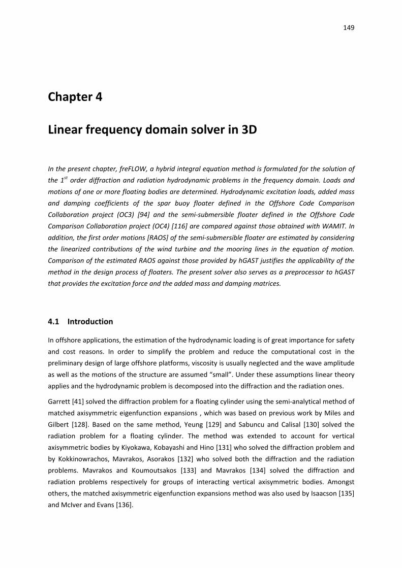
149

Chapter 4

Linear frequency domain solver in 3D In the present chapter, freFLOW, a hybrid integral equation method is formulated for the solution of the 1st order diffraction and radiation hydrodynamic problems in the frequency domain. Loads and motions of one or more floating bodies are determined. Hydrodynamic excitation loads, added mass and damping coefficients of the spar buoy floater defined in the Offshore Code Comparison Collaboration project (OC3) [94] and the semi-submersible floater defined in the Offshore Code Comparison Collaboration project (OC4) [116] are compared against those obtained with WAMIT. In addition, the first order motions [RAOS] of the semi-submersible floater are estimated by considering the linearized contributions of the wind turbine and the mooring lines in the equation of motion. Comparison of the estimated RAOS against those provided by hGAST justifies the applicability of the method in the design process of floaters. The present solver also serves as a preprocessor to hGAST that provides the excitation force and the added mass and damping matrices.

4.1 Introduction

In offshore applications, the estimation of the hydrodynamic loading is of great importance for safety and cost reasons. In order to simplify the problem and reduce the computational cost in the preliminary design of large offshore platforms, viscosity is usually neglected and the wave amplitude as well as the motions of the structure are assumed “small”. Under these assumptions linear theory applies and the hydrodynamic problem is decomposed into the diffraction and the radiation ones.

Garrett [41] solved the diffraction problem for a floating cylinder using the semi-analytical method of matched axisymmetric eigenfunction expansions , which was based on previous work by Miles and Gilbert [128]. Based on the same method, Yeung [129] and Sabuncu and Calisal [130] solved the radiation problem for a floating cylinder. The method was extended to account for vertical axisymmetric bodies by Kiyokawa, Kobayashi and Hino [131] who solved the diffraction problem and by Kokkinowrachos, Mavrakos, Asorakos [132] who solved both the diffraction and the radiation problems. Mavrakos and Koumoutsakos [133] and Mavrakos [134] solved the diffraction and radiation problems respectively for groups of interacting vertical axisymmetric bodies. Amongst others, the matched axisymmetric eigenfunction expansions method was also used by Isaacson [135] and McIver and Evans [136].

150

In the case of arbitrary shaped bodies, three methods are widely used as reported by Mei [137]: the free surface Green function method, the boundary element method and the finite element method. In the first class already used by Garrison [138], Hogben and Standing [139], Faltinsen and Michelsen [140] and Eatock-Taylor [141], the free-surface Green function satisfies the Laplace equation and all the boundary conditions (at the free surface, the sea bed and at infinity) except that on the wetted surface of the moving body. So the problem is solved by only satisfying the boundary condition on the body surface. The convenience in using this method is that only the body surface is required. On the other hand, the computational cost gained by reducing the number of equations is counteracted by the calculation of the influence matrices which are full and complex. The cost is further penalized because the influence matrices must be recalculated for every frequency value. Another clear disadvantage of this method is the presence of irregular frequencies, as reported in [142]. To circumvent these frequencies special treatment is required as implemented in the commercial code WAMIT [143].

The finite element method which is widely applied in structural mechanics can be applied in hydrodynamic problems as done by Chenault [144], Newton, Chenault and Smith [145] and Bai [146], [147]. The method is based on either a variational formulation or a weak formulation of Galerkin type. The whole domain of interest must be discretized and the matrices produced are in general symmetric and sparse. The method does not suffer from irregular frequencies, but the application of the radiation condition at infinity requires special treatment. An elegant way to overcome the issues concerning the radiation condition is to adopt a hybrid method in which the inner domain around the body is solved using the FEM method while the flow in the outer domain is described based on an analytical or semi-analytical solution. Across the outer boundary of the FEM domain, matching of the two solutions should be performed according to Berkhoff [148], Chen & Mei [149], Bai and Yeung [150], Chenot [151] and Yeu, Chen and Mei [152]. In the hybrid approach, the inner domain is reduced and the only requirement is to contain the considered bodies. A disadvantage of the FEM method, as compared to the boundary element method, is the need to discretize the full flow domain instead of only the boundaries.

The third class of numeral methods, similar to the first one, uses the free space Green function and solves the problem by means of the boundary element method. The difference compared to the first class, lies in the choice of the Green function. The boundary domain is defined by the body surface, the free surface, the sea bed and the far field, where the radiation condition is applied as described in Bai and Yeung [150], Ferdinande and Kritis [153] and Au and Brebbia [154]. The increased computational cost due to the extra boundary surfaces, as compared to the free-surface Green function method, is compensated by the simple calculations of real valued influence matrices. The influence matrices only depend on the geometry and therefore are only calculated once for all frequencies. In addition, no irregular frequencies appear. Similar to the FEM method, a hybrid scheme can be also adopted, in order to reduce the extension of the outer boundary. The hybrid integral equation method was originally proposed by Yeung [155] in 2D and extended in 3D by Matsui, Kato and Shirai [156] and Yuen and Chau [157] assuming a constant depth infinite domain. In the linear context, Zhang and Miao [158] studied the varying bathymetry using a hybrid integral

151

equation method in conjunction with the mild-slope equation, while Belibassakis [159] did that in conjunction with the coupled-mode theory by Athanasoulis and Belibassakis [160, 161].

The present method is similar to [156] where the depth of the infinite domain is assumed constant. The only difference lies in the implementation of the matching at the outer boundary with the semi-analytical solution. In the aforementioned methods [156, 157] the number of panels used at the matching boundary must be equal to the number of the unknown truncated coefficients of the semi analytical solution, while in the present method this is not mandatory thanks to a projection operation. Although this method cannot be considered novel, the coupling of the hydrodynamic problem with wind turbine dynamics still presents a challenge. The coupled dynamic behavior of floating wind turbines can be analyzed over the range of the wave frequencies by adding the contribution of the wind turbine and the mooring lines in the coupled dynamic equations of the floater motion, following a linearization process. More specifically, additional mass, damping and stiffness matrices contribute the aerodynamic, gravity and inertia-gyroscopic loads of the wind turbine and the mooring lines [44, 120, 121]. In this respect, the present method can be used for the design of a floating support structure carrying a wind turbine. Finally, the frequency domain method serves as a preprocessor for the time domain hydro-servo-aero-elastic code hGAST, by providing the hydrodynamic excitation force and the added mass and added damping coefficients.

4.2 Mathematical formulation

The potential, irrotational flow of an incompressible fluid, without surface tension is considered in the presence of one or multiple floating bodies. The outer domain D* extends to infinity, while the inner domain D is formed by the free surface boundary SFS, the body boundaries SBO, the seabed boundary SSB and the outer cylindrical boundary, called matching boundary SMB [Figure 4.1]. In D the geometry of the seabed can be arbitrary, but must reach a constant depth at the intersection with the matching boundary which should contain all the bodies. The distance between the body and the matching boundary can be arbitrary small since the matching also accounts for the evanescent modes. The Cartesian and the cylindrical global, fixed coordinate systems OGxyz and OGrθz are placed in the middle of the matching boundary at the mean water level with the z-axis pointing upwards. A second Cartesian coordinate system Oxyz is defined for each body, with respect to which the body motions are defined. It is assumed that the bodies are carrying out small amplitude periodic motions over their mean position in response to incident regular Airy waves with amplitude A and frequency ω.

Following standard linear hydrodynamic theory (see for example [46, 162, 163]), the vector of the generalized motion of each body and the velocity potential are written in the frequency domain as,

-( )=Re[ e ]iωttX x

(4.1)

152

-Φ( , , ; )=Re[ ( , , ) e ]iωtx y z t φ x y z (4.2)

where x , φ are the complex amplitudes of the generalized motion vector and the velocity potential respectively. Each component of x corresponds to one mode of motion; surge, sway, heave, roll, pitch and yaw. In the case of multiple bodies, vector x is extended to xA in order to contain collectively the 6 modes of motion of all the bodies, i.e. 6*nb in total, where nb denotes the number of bodies. In the sequel, the potential φ(x,y,z) will be simply written as φ.

Figure 4.1: Definition of the inner domain D, the boundary surfaces, the outer domain D* and the coordinate systems

By applying superposition and assuming that every motion is independent on the others, the velocity potential is decomposed into the following three components,

6nb 6nb

I 0 R I 0 j j D j jj 1 j 1

+ + = + - + φ φ φ φ φ φ iω x φ φ x φ= =

= =∑ ∑

A A

(4.3)

( cos + sin )I

cosh[ ( + )]-cosh[ ]

ik x β y βigA k z dφ eω kd

=

(4.4a)

153

= ( cos + sin )I - [deep water]kz ik x β y βigAφ e e

ω (4.4b)

where:

φI denotes the potential of the incident Airy wave without the presence of any body,

φ0 denotes the scattered potential which corresponds to the boundary value problem assuming fixed bodies subjected to incident waves,

φR denotes the total radiation potential,

φD denotes the diffraction potential and defined as the sum of the incident and the scattered potentials

φj, j= 1,2,..,6*nb denote the radiation potentials which correspond to the 6*nb boundary value problems assuming calm water and a unit oscillation in the j-th mode of motion.

In (4.4a) k denotes the wavenumber, d the water depth (absolute value), β the wave incidence angle relative to Ox-axis and g the acceleration due to gravity. Equation (4.4b) is valid for deep water.

The diffraction problem when solved for the scattered potential is mathematically and physically related to the radiation one [164]. They are both formulated as a radiation type problem. Within the linear context, the aforementioned boundary value problems take the general form (φk = 0 corresponds to diffraction problem, while φk= 1,2,…,6*nb to radiation problems),

Δφk = 0, in D (4.5)

∂=

∂

2k

k FS- 0, on Sφ ω φz g

(4.6)

∂=

∂k

k ΒΟ, on Sφ gn

(4.7)

∂=

∂k

k SΒ, on Sφ hn

(4.8)

∂+ =

∂k

k ΜΒ[ ] 0, on Sφ T φn

(4.9)

The governing Laplace equation (4.5) describes mass conservation in the flow domain D with boundaries collectively denoted as S. Equation (4.6) is the linearized free surface boundary condition of Robin type, in which the kinematic and the dynamic equations have been combined. Equation (4.7) provides the forcing to the system of equations (4.5) to (4.9) and both equations (4.7), (4.8), describe the no flow condition. gk and hk are defined as follows,

154

I0 0= =-

φg hn

∂∂

(4.10)

k k k= & =0 , for k=1,2,...,6*nbg n hA

(4.11)

(ib 1)+1 (ib 1)+2 (ib 1)+3 ib (ib 1)+4 (ib 1)+5 (ib 1)+6 ib ib( , , )= , ( , , )= x n n n n n n− − − − − −n r nA A A A A A (4.12)

where n or nib is the normal vector to the boundary with direction from the boundary to the inner domain D [Figure 4.1], and r or rib is the position vector with respect to the origin of each body at which the unit rotations are defined. In case of multiple bodies, equation (4.12) applies to all bodies (ib=1:nb) in order to define the total generalized normal vector nA that corresponds to xA . In addition

1 2 nb={ , ,.., }n n n n

A where ibn is the generalized unit vector of the body ib.

The potential in the outer domain D* is represented by its eigenfunction expansion in cylindrical coordinates (r, θ, z) and takes the following form,

[ ]ma 00 0

*( , , ) ( ) ( ) cos + sin , ma a mam a

φ r θ z R r Z z F mθ G mθ r r∞ ∞

= =

= ≥∑∑

(4.13)

0

0

( ) / ( ) , for 0( )

( ) / ( ) , for 1m α m α

mam α m α

H k r H k r αR r

K k r K k r α=

= ≥ (4.14)

cosh( ( + )) , for 01 sinh212 2

( ) cos( ( + )), for 1

sin21 12 2

maα

α

α

k z d αkd

kdZ z k z d

αk d

k d

= + = ≥

+

(4.15a)

= =( ) , for 0 [deep water]1

2

kz

maeZ z α

kd

(4.15b)

where:

Fma, Gma are unknown coefficients,

indices m and α correspond to the infinite series expansions in the azimuthal and the vertical directions respectively,

Hm is the Hankel function of the first kind of order m,

Km is the modified Bessel function of the second kind of order m,

155

r0 is the radius of the matching boundary,

The set of numbers (ik, k1,..,k∞) denotes the eigenvalues of the regular Sturm-Liouville problem in the vertical direction.

Zma denotes the corresponding normalized eigenvectors,

More specifically, k is the wavenumber - the index 0 is usually omitted - that corresponds to the propagating mode, while kα for α≥1 corresponds to the evanescent modes. The eigenvalues kα are given as roots of the dispersion relation,

2 tanα αω gk k d= − (4.16a)

Substitution of the 0th term which is equal to ik in (4.16a) gives,

2 tanhω gk kd= (4.16b)

Equation (4.15b) is valid for deep water and the wavenumber is given as k=ω2/g.

The operator T[φk] in equation (4.9) is an appropriate Dirichlet-to-Neumann map, ensuring the complete matching of the solution between the inner and the outer domain D and D* respectively. In this connection, the potential as well as its normal (radial in the present set up) derivative on the matching boundary SMB at r=r0 must be continuous. These two (matching) conditions depend on the same unknown coefficients Fma, Gma. So by adopting a variational formulation of one of them and making use of the orthogonality of the eigenvectors, expressions for the coefficients Fma, and Gma are derived. These expressions are next introduced in the other matching condition that leads to the definition of the matching operator T[φk],

2 0

k ma k 00 0 0

2 0

k 00

T[ ] (z) cos ( , , ) cos (ζ) d d

+sin ( , , ) sin (ζ) d d

{

}

π

a am a d

π

ad

φ L Z mθ φ r γ ζ mγ Z ζ γ

mθ φ r γ ζ mγ Z ζ γ

∞ ∞

= = −

−

= +∑ ∑ ∫ ∫

∫ ∫

(4.17)

00 1

( ) , =1, =2

2α ma m

mα m mk R r ε

L ε επd = ≥

′=

(4.18)

where γ and ζ are used instead of θ and z inside the integrals, while (‘) in (4.18) denotes the derivative with respect to r.

The same approach was also used by Garrett [41] in order to match the solution between the exterior domain (infinite) and the interior domain (under the cylinder). In his case, the solution in the azimuthal direction in both domains was expressed by Fourier series. In the exterior domain, the

156

solution in the vertical direction is expressed by an eigenfunction expansion, while in the interior by the Fourier series.

Finally, it is noted that the Somerfield radiation condition is satisfied in the outer domain D* - the potential is defined in (4.13) – and so the complete matching between the D and D* domains ensures that the radiation condition is satisfied in D as well.

4.3 Numerical implementation

4.3.1 Integral form of the Laplace equation and its numerical solution

The boundary integral equation for the Laplace equation takes the following form,

( ) ( ) ( ; ) ( )S

φ σ G dS= ∫0 0x x x x x

(4.19)

01( ; )=- , = -

4G r

πr0x x x x

(4.20)

where G(x, x0) is the Green function, x0 denotes any field point in domain D, x any point along S and r the distance between x, x0.

By applying the boundary conditions (4.6) to (4.9), the resulting boundary value problem is numerically solved using the boundary element method (BEM), for the unknown strength of the piecewise constant source distributions. The collocation points are placed at the centroids where the equations are evaluated. Assuming plane panels, the integrations in (4.19) are carried out analytically [165]. The discrete form of (4.19) forms a linear system of equations, which is solved by means of LU decomposition. The influence matrices are calculated once and used for every frequency. Application of equation (4.17) requires the truncation of the infinite expansions in z and θ directions. The integrations along the matching boundary surface in equation (4.17) - integrals in the z and θ directions - are carried out by introducing local piecewise constant or linear interpolating functions at the centers of the panels. The dispersion relation defined in equations (4.16a), (4.16b) is solved using the method of bisection.

In order to speed up calculations the OPENMP library is used. Parallelization in shared memory environment is applied during the solution of the linear system and for all panel-to-panel computations.

4.3.2 Symmetry consideration

When bodies are symmetric about one or two planes of symmetry (x=0 or y=0) the computational cost can be significantly reduced by solving for half or a quarter of the domain D. Two problems are

157

solved in case of one plane of symmetry and four in case of two planes of symmetry, for the complete solution of the hydrodynamic problem (diffraction problem for arbitrary incidence angle and all 6 radiation problems). If one plane of symmetry is considered, the symmetric and the anti-symmetric problems are solved. The mirror potentials in the symmetric case are equal, while in the anti-symmetric case are of opposite sign. In case of two planes of symmetry, all possible combinations are considered: the potential being symmetric about y=0 plane and anti-symmetric about x=0, symmetric about x=0 plane and anti-symmetric about y=0, symmetric about both planes x=0 and y=0 and anti-symmetric about both planes x=0 and y=0.

Surge and pitch motions are symmetric about y=0 and anti-symmetric about x=0, sway and roll motions are symmetric about x=0 and anti-symmetric about y=0, heave motion is symmetric about both x=0 and y=0, while yaw motion is anti-symmetric about both x=0 and y=0 planes. The scattered potential for an arbitrary incidence angle, although neither symmetric nor anti-symmetric, can be still decomposed into two or four components based on the aforementioned problems and solved in the same way, as in the radiation problems. If P(x,y,z), Px(x,y,z), Py(x,y,z) and Pxy(x,y,z) are image points with respect to x=0, y=0 or both then,

( ) ( ) ( ) ( ), , - , , ,- , - ,- ,x y xyx y z x y z x y z x y z= = =P P P P (4.21)

The scattered, the incident and the diffraction potentials can be decomposed into (here presented for the diffraction potential),

D D D D D( ) = 1/2[ ( )+ ( )] + 1/2[( ( )- ( )]x xφ φ φ φ φP P P P P (4.22a)

D D D D D( ) = 1/2[ ( )+ ( )] + 1/2[( ( )- ( )]y yφ φ φ φ φP P P P P (4.22b)

D D D D D

D D D D

D D D D

D D D D

( ) = 1/4[ ( ) ( ) ( ) ( )] +

1/4[ ( ) ( ) ( ) ( )] +

1/4[ ( ) ( ) ( ) ( )] +

1/4[ ( ) ( ) ( ) ( )]

x xy y

x xy y

x xy y

x xy y

φ φ φ φ φ

φ φ φ φ

φ φ φ φ

φ φ φ φ

− − +

+ − −

+ + +

− + −

P P P P P

P P P P

P P P P

P P P P

(4.22c)

Terms in square brackets [] correspond to the solved boundary value problems assuming symmetric or anti-symmetric potential with respect to the plane/s of symmetry. Equation (4.22a) applies when x=0 is a plane of symmetry, (4.22b) when y=0 is a plane of symmetry and (4.22c) if both x=0 and y=0 are planes of symmetry. The symmetry should be also considered in equation (4.13) by appropriate elimination of part of coefficients Fma, Gma as shown in Table 4.1.

158

Table 4.1: Symmetry simplifications for the coefficients of the expansions of the outer solution

valid for x=0 y=0 Fma Gma

S-R, H S 0, for odd m 0, for even m

S-P, Y A 0, for even m 0, for odd m

S-P, H S 0, for all m

S-R, Y A 0, for all m

S-P A S 0, for even m 0, for all m

S-R S A 0, for all m 0, for even m

H S S 0, for odd m 0, for all m

Y A A 0, for all m 0, for odd m

*S-R: sway –roll, S-P: surge-pitch, H: heave, Y: yaw, S: symmetry, A: anti-symmetry

4.4 Loads calculation

Once the diffraction and the radiation problems are solved, the unknown strengths of the sources along the boundary S are determined and the potential φ can be calculated from (4.19). Then the excitation and the reaction forces are calculated by integrating the surface pressure over the body solid surface. The pressure itself is calculated using the linearized Bernoulli equation,

=- = =- =-S S

φp ρ iωρφ F pndS iωρ φndSt

∂⇒

∂ ∫ ∫

(4.23)

kEXC Ι 0 k/ = ( + ) d ,k=1:6S

F A iωρ φ φ n S− ∫

(4.24)

k

2 2REACT R k j j k kj kj=- d =- d , k=1:6, j=1:6*nbj

S S

iF iωρ φ n S ω ρ x φ n S ω a b xω

= + ∫ ∫

(4.25a)

kj kj j k- d , k=1:6, j=1:6*nbS

ia b ρ φ n Sω

+ = ∫

(4.25b)

where p denotes the pressure along the body surface, ρ the density of the fluid, FEXC the generalized excitation force vector, FREACT the generalized reaction force and akj, bkj the elements of the added mass and added damping coefficient matrices. The excitation force is calculated for unit wave amplitude, while the added mass and damping coefficients for unit oscillations in each mode of motion. It is noted that in the above expressions the hydrostatic terms have been excluded.

159

4.5 Equation of motion

The 1st order motions per unit wave amplitude A, of a standalone floating body are estimated by solving the complex linear 6x6 system that is formed from the dynamic equation of motion expressed in the frequency domain,

[ ] -12EXC EXT EXT H G EXT(ω)/ = (ω)/Α -ω ( (ω) )-iω( (ω)+ )+( + + )A + + x F M a M b C K K K

(4.26)

where

(ω)/Ax is the Response Amplitude Operator (RAO) of the 6 motions of the body,

M denotes the structural mass matrix of the floater,

KH and KG denote the hydrostatic stiffness matrix and the restoring stiffness matrix due to gravity,

ω is the frequency of the wave and of the motions (in the linear context the motions have the same frequency with the wave),

[FEXC/A] is the 1st order wave induced force for unit wave amplitude defined in (4.24),

a and b are the added mass and damping coefficients defined in (4.25b) and

MEXT, CEXT and KEXT are external mass, damping and stiffness matrices independent of the frequency ω.

The linearized contribution of the wind turbine is considered through the external matrices. In KEXT the mooring lines contribution is also added. If the external matrices are zero, then the motions of the free floating floater are estimated.

The mass matrix M for a floater with mass m, center of gravity xG and inertias Iij is defined as,

− − −

= −

− −

0 0 00 0 00 0 00

00

G G

G G

G G

G G XX XY XZ

G G YX YY YZ

G G ZX ZY ZZ

m mz mym mz mx

m my mxmz my I I I

mz mx I I Imy mx I I I

M (4.27)

while the restoring matrix KG due to gravity is defined as,

160

= −

−

0 0 0 0 0 00 0 0 0 0 00 0 0 0 0 00 0 0 00 0 0 00 0 0 0 0 0

GG G

G G

mgz mgxmgz mgy

K (4.28)

The hydrostatic properties of the floater are calculated as surface integrals using Gauss’ divergence theorem. For example the volume V is defined as,

BO BO BO BO BO BO

x y z(x)dV (y)dV (z)dV xd yd zdV V V S S S

V n S n S n Sx z z∂ ∂ ∂

= = = = = =∂ ∂ ∂∫ ∫ ∫ ∫ ∫ ∫

(4.29)

Similarly the center of buoyancy xB is calculated as,

BO

2x

1= d ,2B

S

x n x SV ∫

BO

21= d ,2B y

S

y n y SV ∫

BO

2z

1= d2B

S

z n z SV ∫

(4.30)

while the nonzero elements of the hydrostatic stiffness matrix KH are defined as,

33

BO

H z=- d ,S

K ρg n S∫

34

BO

H z=- d ,S

K ρg n y S∫

35

BO

H z= dS

K ρg n x S∫

(4.31) 44

BO

2H z B=- d ,

S

K ρg n y S ρgVz+∫

45

BO

H z= d ,S

K ρg n xy S∫

46H B=-K ρgVx

55

BO

2H z B=- d ,

S

K ρg n x S ρgVz+∫

56H B=-K ρgVy

Elements KH43, KH53 and KH54 are equal to their symmetric KH34, KH35 and KH45 respectively.

In the case of multiple floating bodies, equation (4.26) is extended to include the dynamic equations of all bodies. Then the system of equations is 6nb x 6nb and the relevant matrices are accordingly augmented.

The added mass and damping matrices contribute to the coupling terms between the motions of different bodies.

161

4.6 Surface elevation

After solving the boundary value problems for diffraction and radiation and estimating the corresponding RAOs, the free surface elevation ζ is calculated for unit wave amplitude A. By introducing the expression for the total potential (4.3) in the linearized dynamic equation, ζ is obtained on the panels of the free surface,

2 6nb

D j j FSj 1

/ [ / Α] [ / ] [ / ] , on at =0iω iω ωζ A φ φ A x A φ S zg g g =

= = + ∑ A

(4.32)

162

4.7 Numerical Results – Validation

Validation of freFLOW in comparison to results obtained with WAMIT [143] is given. The results concern the spar buoy floater of the OC3 [71] and the semi-submersible floater of the OC4 [125].

4.7.1 The OC3 spar buoy

The linear diffraction and radiation hydrodynamic problems are solved considering the spar buoy floater defined in OC3 [94] [Figure 4.2]. The draft of the floater is 120m, while the diameter is 9.4m for -120m ≤ z ≤ -12m, 6.5m for z≥-4 and in between linearly reduces. Analysis is performed for water depth equal to 320m. The floater is symmetric about both axis x=0 and y=0 and so the unknowns of the problem can be reduced to one quarter. In addition, because of the cylindrical shape, only 2 of the 4 problems are solved [i.e. axis x=0 anti-symmetry – axis y=0 symmetry and both axis x=0 and y=0 symmetry]. Structured grids are used in the present analysis having a total number of degrees of freedom equal to 11025, while the infinite expansions in the outer domain in z and θ directions are truncated to 100 and 1 modes respectively. 1 mode is enough because of the cylindrical shape.

Figure 4.2: Description of the spar buoy floater of the OC3

In Figure 4.3 the magnitude and the phase of the non-zero generalized excitation force for 0o wave heading angles are compared, while in Figure 4.4 and Figure 4.5 non-zero added mass and damping coefficients are presented. As expected, the two sets are in very good agreement since both methods adopt the same theory (1st order linear hydrodynamics), despite the difference in the formulation – WAMIT uses the free-surface Green function method while freFLOW is a hybrid boundary integral method based on the free space Green function. Differences in the added mass coefficients are regarded small, although pronounced because of the figure scale.

163

(a) Magnitude of the surge diffraction force (normalized)

(b) Phase of the surge diffraction force

(c) Magnitude of the heave diffraction force (normalized)

(d) Phase of the heave diffraction force

(e) Magnitude of the pitch diffraction moment (normalized)

(f) Phase of the pitch diffraction moment

Figure 4.3: Magnitude and phase of the diffraction surge and heave forces and pitch moment for zero wave heading of the

OC3 spar buoy floater

164

(a) Hydrodynamic added mass A11

(b) Hydrodynamic added damping B11

(c) Hydrodynamic added mass A15

(d) Hydrodynamic added damping B15

(e) Hydrodynamic added mass A33

(f) Hydrodynamic added damping B33

Figure 4.4: Hydrodynamic added mass and added damping coefficients A11, A15, A33, B11, B15 and B33 of the OC3 spar buoy

floater

165

(a) Hydrodynamic added mass A55

(b) Hydrodynamic added damping B55

Figure 4.5: Hydrodynamic added mass and added damping coefficients A55 and B55 of the OC3 spar buoy floater

4.7.2 The OC4 semi-submersible case

Similarly to the spar buy case, the linear diffraction and radiation hydrodynamic problems are solved considering the semi-submersible floater defined in OC4 [Figure 4.6]. A brief description of the floater was given in section 3.2.2.1, while a detailed description can be found in [125]. The analysis in this case is performed for water depth equal to 200m. The floater is symmetric about the y=0 axis and so the unknowns of the problem are reduced to half. Both the symmetric and the anti-symmetric problems are solved. In order to handle the complex geometry, for the free surface an unstructured grid is used [Figure 4.7], created with ANSYS ICEM grid generator, while structured grids are used for the other boundaries including the floater [Figure 4.8]. The total number of degrees of freedom is equal to 27487, while the infinite expansions in the outer domain in z and θ directions are truncated to 50 and 20 modes respectively.

Figure 4.6: Description of the semi-submersible floater of the OC4 [figure taken from [125]]

166

Figure 4.7: Unstructured grid of the free surface of 11588 elements

Figure 4.8: Structured grid of the surface boundary of the semi-submersible floater

The non-zero generalized excitation forces for 0 and 30 degrees wave heading angles are compared in Figure 4.9, Figure 4.10 and Figure 4.11, while in Figure 4.12 and Figure 4.13 the non-zero added mass and damping coefficients are presented. Similarly to the spar buoy case, the two sets are in very good agreement.

In order to estimate the RAOS of the coupled semi-submersible floating wind turbine, using the frequency domain method, the contribution of the wind turbine and the mooring lines are introduced in the equation of motion (2.126), following a linearization process. Inertial/gyroscopic,

167

gravitational and aerodynamic loads of the wind turbine are considered through additional mass, damping and stiffness matrices. Details of the linearization can be found in [44, 120, 121]. A linear stiffness matrix is used for the mooring lines consideration. The viscous damping is not considered in the frequency domain case.

A validation of the 1st order RAOs estimated in frequency domain is performed, by comparing with the RAOs estimated by time domain simulations using hGAST. hGAST uses the same hydrodynamic loads, calculated in frequency domain and transformed into the time domain, while including extra viscous damping in Morison’s equation. In addition, nonlinear aerodynamic and dynamic terms, elasticity of the flexible members, nonlinear stiffness from the dynamic mooring lines and the variable speed variable pitch controller are considered.

Similar comparisons between RAOs predicted using frequency domain and time domain methods can be found in [166], for the OC3 spar buoy and in [44, 120, 121] for a TLP floater. In the latter case, the roll and the pitch modes of the floater are strongly coupled with the two bending modes of the tower in the fore-aft and the lateral direction. This coupling leads to a frequency reduction of the roll and the pitch frequency from 0.3Hz to 0.25Hz, which is clearly seen in the roll and pitch RAOs. Such an effect is not expected in the conventional semi-submersible floater because is constrained by catenary mooring lines.

The RAO’s can be estimated from time series data using the following equation, as in [120],

(ω)(ω)

(ω)xy

xx

PRAO

P=

(4.33)

where Pxx is the auto power spectral density and Pxy is the cross spectral density. Pxx, Pxy are calculated using Welch’s method [167] with a sufficient number of data split and 50% overlap between the split data parts. x refers to the input (wave elevation) and y to the output (one for every motion). The simulations corresponded to 3600sec - the first 600sec were excluded – assuming a uniform wind speed and white noise waves of 1m significant wave height.

In Figure 4.14 four sets of results are presented in logarithmic scale. Blue and red lines correspond to RAOs obtained with the frequency domain method (fd) at zero and at rated wind speed of 11.4m/s, while black and green lines correspond to RAOs obtained with time domain simulations (td) for the same wind conditions. In the zero wind speed case the rotor does not rotate (i.e. the brake is activated). The 30deg wave heading case is presented in which all the 6 motions are excited. The frequency axis is presented in Hz in order to better identify the eigen frequencies which are calculated with hGAST for a flexible and a stiff wind turbine [Table 4.2]. As expected the elastic degrees of freedom do not change the 6 natural frequencies of the floater.

In general both simulations give similar RAOs. In Figure 4.14a, b the frequency domain method predicts a 2nd peak at 0.041Hz in the surge and sway motions. The additional peak corresponds to the roll and pitch natural frequency. In the time domain results the surge-pitch and sway-roll

168

couplings are not so pronounced. In Figure 4.14c the heave RAO is in excellent agreement, at 0 frequency the RAO is equal to 1 as expected, while differences for frequencies higher than 0.3Hz (2rad/s) which are small in value they can be explained by the fact that the heave exciting force is zero [Figure 4.10e]. The influence of the aerodynamic damping is only depicted in the roll and the pitch RAOs [Figure 4.14d, e], where the peak amplitudes of the roll and pitch motions at 0.041Hz are reduced with the presence of the wind. Moreover, peak amplitudes predicted with the time domain method are 10 times less, which is due to viscous damping. The flexibility of the tower is only visible in the roll and the pitch RAOs at 0.43Hz, but does not influence the corresponding RAOs, since the 6 natural frequencies of the floater do not change. In the yaw RAO [Figure 4.14f] gyroscopic effects are clearly predicted by both methods. The peak amplitude of the yaw natural frequency at 0.013Hz is increased when the wind together with the rotation of the rotor are considered. Contrary to the roll and pitch amplitudes, time domain calculations predict higher amplitudes. At 0.15Hz and 0.3Hz local maxima are driven by the wave excitation yaw moment (see Figure 4.11e).

Table 4.2: Natural frequencies [Hz] of the semi-submersible coupled OWT of OC4 phase II for a flexible and a rigid WT

Mode description hGAST flex hGAST rigid

Platform Surge 0.0093 0.0093

Platform Sway 0.0093 0.0093

Platform Heave 0.0583 0.0583

Platform Roll 0.0413 0.0417

Platform Pitch 0.0413 0.0417

Platform Yaw 0.0131 0.0131

1st Tower Fore-Aft 0.424 -

1st Tower Side-Side 0.415 -

169

(a) Magnitude of the surge diffraction force (normalized)

(b) Phase of the surge diffraction force

(c) Magnitude of the heave diffraction force (normalized)

(d) Phase of the heave diffraction force

(e) Magnitude of the pitch diffraction moment (normalized)

(f) Phase of the pitch diffraction moment

Figure 4.9: Magnitude and phase of the diffraction surge and heave forces and pitch moment for zero degrees wave

heading of the OC4 semi-submersible floater

170

(a) Magnitude of the surge diffraction force (normalized)

(b) Phase of the surge diffraction force

(c) Magnitude of the sway diffraction force (normalized)

(d) Phase of the sway diffraction force

(e) Magnitude of the heave diffraction force (normalized)

(f) Phase of the heave diffraction force

Figure 4.10: Magnitude and phase of the diffraction surge, sway and heave forces for 30 degrees wave heading of the OC4

semi-submersible floater

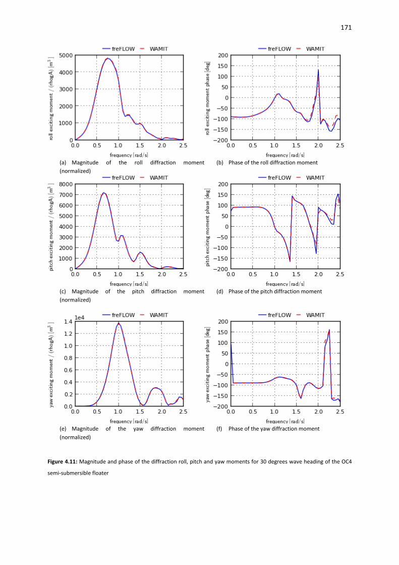
171

(a) Magnitude of the roll diffraction moment (normalized)

(b) Phase of the roll diffraction moment

(c) Magnitude of the pitch diffraction moment (normalized)

(d) Phase of the pitch diffraction moment

(e) Magnitude of the yaw diffraction moment (normalized)

(f) Phase of the yaw diffraction moment

Figure 4.11: Magnitude and phase of the diffraction roll, pitch and yaw moments for 30 degrees wave heading of the OC4

semi-submersible floater

172

(a) Hydrodynamic added mass A11

(b) Hydrodynamic added damping B11

(c) Hydrodynamic added mass A15

(d) Hydrodynamic added damping B15

(e) Hydrodynamic added mass A33

(f) Hydrodynamic added damping B33

Figure 4.12: Hydrodynamic added mass and added damping coefficients A11, A15, A33, B11, B15 and B33 of the OC4 semi-

submersible floater

173

(a) Hydrodynamic added mass A55

(b) Hydrodynamic added damping B55

(c) Hydrodynamic added mass A66

(d) Hydrodynamic added damping B66

Figure 4.13: Hydrodynamic added mass and added damping coefficients A55, A66, B55 and B66 of the OC4 semi-submersible

floater

174

(a) Surge RAO

(d) Roll RAO

(b) Sway RAO

(e) Pitch RAO

(c) Heave RAO

(f) Yaw RAO

Figure 4.14: RAOS comparison between frequency and time domain predictions of the coupled OC4 semi-submersible

floating wind turbine for 30deg wave heading at 0 m/s and rated (11.4m/s) wind speeds

175

Chapter 5

Fully nonlinear potential time domain solver in 2D In the present chapter, hFLOW, a fully nonlinear, inviscid two dimensional solver (numerical wave tank) is formulated for the solution of the wave-body-current interaction problem, based on BEM and mixed Eulerian-Lagrangian method. The wave is either generated by simulating the wave generator’s physical motion or by matching along the inflow vertical boundary the steam function wave solution with or without the inclusion of a steady current. Wave absorption at the end of the tank is added using damping layers. The simulation of free-floating bodies is performed using the iterative method which determines the body acceleration. Numerical results are presented and discussed addressing: the generation and absorption of nonlinear stream function period waves in shallow, intermediate and deep water depths with or without the presence of a steady current; the evolution of a highly overturning solitary wave generated by a piston wave maker; the generation, shoaling and breaking of a solitary wave; the calculation of the loading on a submerged cylinder undergoing a large amplitude motion; the calculation of the wave induced motion of a free-floating cylinder; and the calculation of the loads and the motion of a fixed and a free-floating surface piercing barge. Comparisons with linearized solutions assess the importance of the nonlinear terms.

5.1 Introduction

As already mentioned in Chapter 4, the design of offshore structures and ships is mainly based on the linear theory. The random wave is usually considered as a Gaussian process and the response of the structure linear. By using 2nd order theory the area of validity of the linearized approach is extended, but still safety factors are introduced in order to account for the higher order nonlinear wave effects. In order to reduce the uncertainty of the design and in turn reduce safety factors and cost, more advanced numerical models should be formulated. To this end, the so called numerical wave tanks in correspondence to the physical wave tanks have been defined. The aim is simple; reproduce the experimental results using numerical simulations. In this respect the methods should be capable of accurately simulating the wave generation and absorption as well as the dynamic behavior and the loading on fixed or free floating structures.

The associated fluid-structure interaction problem must be solved as in aeroelasticity. However the presence of the free surface further complicates the problem and is the main reason why

176

hydrodynamic solvers are less advanced compared to the aerodynamic ones. Since the geometry of the free surface in not known a priori, but is part of the solution, adds an implicit nonlinearity while wave breaking further complicates the problem. A detailed overview of recent advances in numerical simulation of nonlinear water waves can be found in [168], where models that also account for viscosity and/or wave breaking are presented (CFD, SPH). In the present literature review, only works relative to the fully nonlinear potential wave problem will be presented.

The first pioneer work was the development of the mixed Eulerian Lagrangian (MEL) method by Longuet-Higgins and Cokelet [169]. Based on this method, the evolution of the free surface was consistently reproduced in the Lagrangian frame by stepwise integrating the two nonlinear free surface boundary conditions. The unknown normal velocity on the Lagrangian markers of the free surface is calculated in the Eulerian frame (see section 5.3.1).

The second pioneer work was by Vinje and Brevig [170]. They were the first to introduce the acceleration field in order to accurately estimate the pressure distribution and in turn the hydrodynamic loading over the wet moving solid surfaces, which is necessary since the time derivative of the velocity potential φt appears in Bernoulli equation. Solving for φt requires an appropriate boundary condition that, in accordance to that for φ, requires the normal to the body acceleration which is however unknown. In order to solve this implicit loop, Vinje and Brevig developed the mode decomposition method. It was the first consistent method for the nonlinear simulation of free floating bodies. The mode decomposition method was also used by Cointe et al [171] and Koo and Kim [172]. There are three more methods that can treat the aforementioned implicit loop; the iterative method proposed by Sen [173] and Cao et al [174], the indirect method proposed by Wu and Eatock-Taylor [175] and the implicit method by van Daalen [176] and Tanizawa [177].

Another important aspect is the treatment of the far-field radiation condition. By truncating the domain at finite distance, at the corresponding open/free boundary any condition should be non-reflecting. At first Longuet-Higgins and Cokelet [169] used periodic conditions so no radiation condition was needed, while in the subsequent early developments the Sommerfeld/Orlanski boundary condition was employed [178]. Romate [179] reviewed the methods based on this approach. This kind of boundary condition seemed to face numerical instabilities especially in transient flows due to irregular waves or the presence of flow disturbances.

A different approach is to absorb the waves and avoid reflections following the experimental wave tank practice. Two possibilities are available in this respect: the modeling of a physical wave absorber or the introduction of artificial dissipative terms in the evolution equations. Along the first option, Bessho [180] and Naito [181] studied the plunger type physical wave absorber, while Clément [182] considered the piston type physical absorber suitable for long waves. Along the second option Baker et al [183] and Cointe et al [171] followed the idea of Israeli and Orszag [184] and Le Méhauté [185] and introduced dissipative terms in the dynamic and the kinematic free surface boundary conditions. Differences in the implementation exist with respect to the choice of damping function, the variable to which damping is applied (i.e. the potential or its normal derivative in the dynamic equation) and

177

the conditions at which dissipation is added (in both free surface equations or only in one). A combination of the two methods was proposed by Clément [182] and further extended by Grilli and Horrillo [186].

Many works have been published along the aforementioned guidelines i.e. by Dommermuth et al [187] who first compared the numerical results against experimental data and proven the ability of the fully nonlinear potential theory to accurately model the physics of wave breaking, and by Boo and Kim [188] who simulated the nonlinear diffraction force on a vertical cylinder. Detailed review of the work on the fully potential nonlinear solvers can be found in Kim, Clément and Tanizawa [189], Tanizawa [190], Tsai and Yue [191] and Grilli [192], most of which are connected to the boundary element method (BEM).

The nonlinear wave-current interaction has been studied by Ryu, Kim and Lynett [193] and the wave–current-body interaction by Ferrant [194] and Kim, Celebi and Kim [195] in 3D for a bottom mounted cylinder and by Koo and Kim [196] in 2D for a free floating barge. Wave kinematics based on the stream function theory by Dean [47] and Rienecker and Fenton [48] have been considered in the inflow boundary by Grilli and Horrillo [186] and by Ferrant [194].

The method developed in this work concerns the solution of the complete fully nonlinear problem in 2D. It has been validated by direct comparison against experimental data, analytical data or other published results in the following problems:

1. Generation, propagation and absorption of highly nonlinear stream function periodic waves in deep, intermediate and shallow water depths with or without a steady current,

2. Generation, propagation and breaking of solitary waves, 3. Shoaling of a periodic wave over a submerged bar, 4. Nonlinear diffraction and radiation of submerged or surface piercing bodies.

The method developed considers:

- The direct boundary integral formulations for φ and φt, which are approximated by means of plane linear boundary elements,

- The mixed Lagrangian-Eulerian formulation of the free-surface conditions which are solved with an explicit 4th order Runge-Kutta time integration scheme,

- Nonlinear incoming waves generated either by modeling the motion of the wave maker or by consistently matching the inlet conditions to a stream function based wave field,

- Submerged or surface piercing moored free floating bodies by solving their equations in fully coupled mode,

- Far field conditions by means of a damping layer (non-reflecting boundary condition).

Compared to previous works, the contribution of the present work can be summarized as follows:

178

1. Implementation of the matching with stream function waves including a steady uniform current. In this connection, accurate solutions have been obtained for very high wave steepness (up to ~90% of the maximum) that remains stable after many wave periods.

2. Accurate simulation of overturning/breaking waves by periodically re-gridding the free-surface.

3. Accurate formulation of the expression for ∂tnφ on free floating bodies in the presence of a steady current.

4. Accurate and consistent calculation of the drift force on a floating barge.

179

5.2 Mathematical formulation

The potential, irrotational flow of an incompressible fluid without surface tension is considered in the physical flow domain D(t), with boundaries collectively denoted as S(t) [Figure 5.1]. The 2D problem is considered in the vertical plane (x, z), with the global coordinate system OG located at the free surface mean water level. The z axis is pointing upwards and the x axis is pointing along the wave propagation to the right. SFS(t) denotes the free surface boundary, SSB(t) the seabed boundary, SWG(t) and SBE(t) the vertical boundaries on the wave generator side and the absorbing beach side respectively and SBO(t) denotes the boundary surface of any fully or partially submerged solid body. Bodies are allowed to either move in a prescribed way or freely floating under the action of the hydrodynamic loads. In the present derivation wave generation is defined on the left side of D(t), and wave absorption on the right. The total scalar potential Φ(x; t) is defined as,

= + 0( ) (; ) Φ ;t φ t U xx x (5.1)

where φ(x; t) is the unsteady wave potential and U0 the velocity of the steady uniform current.

Figure 5.1: Layout of the numerical wave tank

Mass conservation is expressed by the Laplace equation for the total potential Φ(x; t). The problem is formulated for the wave potential φ(x; t), while the contribution of the current field is directly applied to the entire field. The scalar wave potential φ(x; t) also satisfies the Laplace equation (5.2),

=Δ 0, ( )φ i D tn (5.2)

On the instantaneous free surface position at z = ζ(x; t), the Bernoulli equation (5.3), also known as the dynamic boundary condition, assures pressure continuity across the interface between fluids with different densities (i.e. water and air). Written for the wave potential φ(x, z=ζ; t) reads,

180

22 0

0 11

, ( ) ( )2

;2 F

aS

φ φ U pg ζ φ U damp t t

t x ρon S at z ζ x

∂ ∂= − − ∇ =− − − −

∂ ∂ (5.3)

In (5.3) g denotes the acceleration due to gravity, pa a known reference pressure (i.e. the atmospheric which can be set equal to zero) and ρ the fluid density in domain D(t). The time varying integration constant that originally appears in Bernoulli equation has been eliminated leading to a proper redefinition of φ(x; t). The kinetic energy current term 2

0 / 2U , although constant should be retained in order to accurately simulate surface piercing bodies.

The unknown free surface geometry is determined by a second nonlinear equation; the kinematic boundary condition (5.4),

∂ ∂ ∂= −∇ ⋅∇ − + −

∂ ∂ ∂=0 2 , ( ) ( ) ;FS

ζ ζ φφ ζ U damp ton S at z ζz

x tt x

(5.4)

which states that the fluid particles on the free surface will always move along the free surface.

The free surface dynamic and kinematic boundary conditions in equations (5.3) and (5.4) are expressed in Eulerian form, while dampi terms correspond to artificial dissipation terms (see equations (5.12), (5.13)).

The free surface conditions can be equivalently expressed in Lagrangian form,

22 0

11

, ( ) ( )2 2

;Fa

Sdφ U p

g ζ φ damp t tdt

on S a xρ

t z ζ= − + =∇ − − − (5.5)

=∇ + − =0 ix 2 iz δ δ , ( ) ( ) ;FSon Sd φ U da at z ζmp td

x ttx

(5.6)

or in ‘semi-Lagrangian’ form,

22 0

0 1 1

, ( ) ( )2

;2 FS

adφ φ U dζ φ pg ζ φ U dam on S at z ζp t t

dt x dt z ρx

∂ ∂= − − ∇ − − + ⋅ − −

∂ ∂= (5.7)

∂ ∂= −∇ ⋅∇ − + =−

∂ ∂0 2 , ( ) );(FSdζ ζ φφ ζ U dam on S at zp t tdt x

ζ xz

(5.8)

where δij denotes the delta of Kronecker and = ∂ ∂ + ⋅∇p(.)/ (.)/ (.)d dt t U the material derivative. For the derivation of the above-mentioned approaches, the velocity of the marker Up has been set equal to the total velocity Φ∇ (including the current effect) in the Lagrangian formulation and equal to (0, 0, dζ/dt) in the semi-Lagrangian formulation. It is noted that in the Lagrangian formulation the damping term of the kinematic boundary condition is only applied to the equation for the vertical

181

velocity component and the current term only appears in the evolution equation for the horizontal space variable x.

On the solid boundaries, namely the sea bed SSB(t) and any fully or partially submerged body SBO(t), the no-penetration condition is applied,

∂= ⋅ −∇ = −

∂G 0 0 x( ) , ( ( ) )Bn SB BO

φ U x V U n on S and on St tn

x n

(5.9)

where Gx denotes the velocity of points on the body surface as defined in section 5.3.3, n denotes the normal to the surface boundary unit vector always pointing towards the flow domain, nx is the horizontal component of n and VBn denotes the magnitude of the normal body velocity. It is noted that the seabed velocity is zero, unless the generation of long waves is examined by modeling a moving bottom (i.e. earthquake or land sliding).

Boundary conditions should be specified along the vertical boundaries as well, in order to get a well posed problem, which moreover should ensure accurate and valid wave generation and absorption. In the present method, the wave is introduced in 3 different ways: a) by modeling a physical wave maker as a moving boundary; b) by matching a valid wave solution along the inflow boundary (based for example on the stream function theory); c) by imposing the potential and the wave elevation along the free surface nodes which corresponds to an initial value problem. In either case the normal velocity along the vertical boundary at the wave generator side is assumed known and a Newmann boundary condition is imposed. Moreover both vertical boundaries should allow the current pass through.

∂ ∂= − = ⋅

∂ ∂G G( ; ) or ( ), Wa

Gx Wveφ on Sφu t t

n nx x n

(5.10)

The 1st expression in (5.10) applies when a known wave field is matched at the inflow boundary, while the 2nd expression applies when the motion of the physical wave maker is simulated. Details about wave generation are presented in section 5.3.7.

Wave absorption is achieved by means of dissipation. In this respect, the right vertical boundary SBE(t) is assumed fixed allowing only the current to cross out of the flow domain D(t),

∂=

∂0 (, )BEon Sφ t

n (5.11)

In addition, on the beach side a “sponge layer” is defined, usually extending to 1 to 2 wavelengths. Within this layer, gradually increasing damping terms are introduced in both free surface boundary conditions. In open sea conditions, a sponge layer is also applied to the wave maker side. This prevents back-reflection of waves. The dampi terms added in the free surface boundary conditions are defined as,

182

1 1 , for the dynam( )( ic boundary condition)Waven ndamp v x φ φ= ∂ −∂ (5.12)

2 2 , for the kinematic b( )( oundary condi) tionWavedamp v x ζ ζ= − (5.13)

where both Wavenφ∂ and Waveζ are defined based on the known incident wave field, i.e. the stream

function theory. They are introduced in order to dissipate only the reflected waves instead of the total wave at the wave generator side. As already mentioned in the introduction, the damping term in the dynamic equation can be either proportional to φ or to ∂nφ . Both alternatives have been implemented, but the ∂nφ choice performs better. At the beach side Wave

nφ∂ and Waveζ are zero in order to absorb the total wave, while v i(x) is a function of space of the form,

(x)ib

ei i

d

x xv α ω

L −

=

(5.14)

The absolute value is added in order to ensure positive vi(x) on both sides while exponents higher than 1 give an increasing damping effect as the outer boundaries are approached. ω is the wave frequency, Ld is the length of each damping layer, xe defines the position where the damping layer ends or starts, while αi and bi are tuning coefficients which usually take the values: α1=(1/2k0) for ∂nφ or α1=1 for φ, α2=1, b1= b2=2. k0 is the local wave number at the damping layer depth.

183

5.3 Numerical implementation

5.3.1 Mixed Eulerian Lagrangian method for the nonlinear wave problem

Based on the mixed Eulerian-Lagrangian formulation [169] the solution of the nonlinear wave problem is obtained by considering either the full-Lagrangian or the semi-Lagrangian form of the free surface boundary conditions defined in equations (5.5) and (5.6) or (5.7) and (5.8) respectively.

For given x or ζ (depending on the formulation) and φ over the free surface, explicit time integration of the two evolution equations defines the new position and potential of the free surface particles, forming the Lagrangian part of the formulation. In the purely Lagrangian description the markers on the free surface are tracked as material particles using their full velocity, while in the semi-Lagrangian description the markers are only allowed to move in the vertical direction. Initially, zero φ and a free surface at rest (equal to the mean water level) are set, unless an initial wave solution is available.

In either formulation the Laplace equation acts as a constraint, and is conveniently introduced in the form of an integral boundary equation, connecting the Neumann and Dirichlet data over the entire S(t), as detailed next in section 5.3.2. This is the Eulerian part of the MEL method.

It is noted that the Lagrangian and semi-Lagrangian formulations are equivalent, provided that the surface elevation is a single valued function. On the contrary, only the Lagrangian formulation can handle breaking waves and this until an overturning wave crest contacts the free surface.

5.3.2 Integral form of the Laplace equation and its numerical solution

The boundary integral equation (BIE) for the Laplace equation takes the following form,

;∂∂ ⋅ = ⋅ − ⋅ ∂ ∂ ∫ 00 0 0

x xxx x x x x x( )( )( ) ( ) ( ; ) ( ) ( )S

Gφa φ G φ dSn n

(5.15)

1( ; ) ln -2

Gπ

=0 0x x x x

(5.16)

where G(x, x0) is the Green function, x0 denotes any field point D(t), x any point in S(t) and α(x0) the solid angle associated to x0. For points in D(t), α(x0) =2π, while for points on S(t), α(x0) is directly calculated by defining the following simplified boundary value problem, assuming uniform boundary data 0nφ∂ = and φ=1. Then the solid angle is calculated as,

;∂⋅ = −

∂∫ 00

x xx x( )( ) ( )

S

Ga dS

nI

(5.17)

For the solution of (5.15) either φ (Dirichlet data) or nφ∂ (Neumann data) on every part of S(t) is prescribed. Along the free surface a Dirichlet condition is imposed while over all other boundaries a

184

Neumann one. The resulting mixed problem is numerically solved using the boundary element method with piecewise linear approximations for φ and nφ∂ . The collocation points are placed at the nodes of the surface grid. By assuming plane panels, the integrations in (5.15) are carried out analytically [Appendix A]. The discrete form of (5.15) is solved with the LU decomposition method. It is noted that in their discrete form (5.15) and (5.17) have the same influence matrices.

The tangent velocity sφ∂ on S(t) and the gradient of the surface elevation ∂ xζ that are needed in (5.8) and in the calculation of the loading on solid bodies, are obtained at the boundary surface grid nodes by means of 2nd order finite difference approximations.

Special treatment is required at the end nodes of the free surface where the boundary condition switches from Dirichlet to Neumann (i.e. at the intersection between the free surface and the vertical walls or between the free surface and surface piercing bodies). In order to uniquely define the velocity and prevent the onset of saw-tooth instabilities, these particular nodes are considered as “double nodes” [197], [190]. At the double node points, the velocity is expressed in terms of the two known normal components D

nφ∂ and Nn∂ ϕ defined at the end points of the Dirichlet and the

Newmann boundaries respectively. At the Dirichlet boundary Dnφ∂ (free surface) is obtained as part

of the solution of the BIE (5.15), while at the Newmann boundary Nn∂ ϕ (lateral boundary or surface

piercing body) is assumed known from the boundary data. Based on this information, the velocity at the double node u = (ux, uz) is obtained by solving the following 2x2 linear system instead of using the numerically obtained tangential velocity component.

Dx Dx z Dz D nu n u n⋅ + ⋅ = ⋅ = ∂u n ϕ

(5.18) N

x Nx z Nz N nu n u n⋅ + ⋅ = ⋅ = ∂u n ϕ

Another important point when solving BIE (5.15), concerns the need for regridding the free surface in the Lagrangian formulation context. Regridding is based on spline fitting and is decided by monitoring the ratio between the maximum and the minimum free surface panel lengths within certain pre-selected limits usually set in between 1.1 and 1.5. In this way the panels of the free surface retain an almost uniform spacing which is important in BEM calculation. Also for numerical consistency and accuracy, regridding of all Newmann boundaries is performed in order to ensure that S(t) remains a closed surface. The lateral boundaries and the boundaries of surface piercing bodies are also modified based on the instantaneous surface elevation. Finally when a physical moving piston wave maker is considered the sea bed boundary is changed according to the prescribed motion of the wave maker. In practice regridding of the Newmann boundaries is carried out at every time step.

185

5.3.3 Rigid Body Kinematics

The solid body undergoes a combined translation and rotation, defined with respect to a body-fitted system OB. Let xB(t) denote the position of the origin OB in time and θB(t) the rotation angle of OB with respect to the global reference OG coordinate system.

Every point on the body surface is defined by its local position rL and its global position, velocity and acceleration G G G, ,x x x that are expressed as,

G B B B G B G B( , ; ) (t)+ ( ( )) + +t θ t= ⋅ ⇒ = ⋅ ⇒ = ⋅L L L Lx ξ r x A r x x A r x x A r

(5.19)

The generalized position, velocity and acceleration vectors of each body incorporating the surge, heave and pitch motions in 2D are defined as,

B B B B B B B B B={ , }, ={ , }, ={ , }θ θ θξ x ξ x ξ x

(5.20)

B( )θA denotes the rotation matrix and the first and second time derivatives are defined as,

2B B B B B B B B

B

d( , ) = , ( , , )d Bθ θ θ θ θ θ θ θ θ

θ′ ′ ′′= = +

AA A A A A

(5.21)

In equations (5.19) to (5.21) dots denote time derivative.

5.3.4 Body force and solution of BIE for φt

The forces acting on the body are calculated by integrating the pressure given from Bernoulli’s equation,

22 0

01

( )2 2t

φ Up ρ φ φ U gz

x∂

= − + ∇ + + +∂

(5.22)

As reported in [190], [198], the calculation of the unsteady term φt by means of finite difference schemes becomes unstable, especially when the problem involves moving bodies. Instead as noted in [176], the Laplace equation for φt can be solved which takes full account of the kinematics of the flow and by that the correct dynamics are added on the body either standing or freely floating. The boundary value problem for φt is defined similarly to that for φ except that now time derivatives are used,

Δφt= 0, in D(t) (5.23)

186

22 0

0 1 , 1

( )2 2 FS

at

φ U pφ g ζ φ U dam n S top

x ρ∂

= − − ∇ − − − −∂

(5.24)

∂=

∂, 0 ( ) ( )BE

tSBon S t and on S

nt

φ

(5.25)

∂= ⋅ +

∂G G( , ) ( )t

BOon tq Sφn

x n x

(5.26)

∂ ∂= − = ⋅ +

∂ ∂G G G( ; ) or ( ), ( ) Wavet

WGt

xφ φ

ont qn

ta Sn

x x n x

(5.27)

The Dirichlet data on the free surface (5.24) and the Newmann data on the moving bodies (5.26) and (5.27) can be defined only after the boundary value problem for the velocity potential is solved, so that nφ∂ at the free surface and the potential φ at the body surface have been determined.

G G G, , x x x denote the position, velocity and acceleration of points on the body surface as defined in section 5.3.3 and q(xG) is the contribution of the velocity potential to the calculation of the normal body acceleration. In order to express q(xG), a body fitted curvilinear system (s, n) is introduced with s, n being the tangential and the normal to the surface unit vectors. Based on the derivation provided by van Daalen [176] and also used in [199] in 2D, the q(xG) term is further elaborated [Appendix B] in order to account for the steady current. The expression for q(xG) in this case is,

= ⋅ − ∂ − ∂

− ∂ + ∂ + ∂ + ∂ ⋅

− ∂ + ∂ − ∂ − ∂ ⋅

G G 0 B

0 0 G

0 0 G

( ) ( 2 )

( 2 )( )

, ( )( ) ( )

s s

n s n s ns sn

n n n n ss ss BO

q φ U x θ

k φ k U x φ U x

k φ k U x φ U x on S t

x x s

x s

x n

(5.28)

∂ ∂ − ∂ ∂=

∂ + ∂ 1.5

( )

s ss s ssn

s s

x z z xk

x z (5.29)

where B B B, , θ θ θ are the pitch angle, angular velocity and angular acceleration of the body. kn is the local curvature of the surface.

Local tangent derivatives , , , , , , s ss ns s ss s ssφ φ φ x x z z∂ ∂ ∂ ∂ ∂ ∂ ∂ are calculated numerically along the body surface using 2nd order finite differences valid for non-uniform grids. The corresponding boundary integral equation is defined similarly to (5.15) as,

;∂ ∂ ⋅ = ⋅ − ⋅ ∂ ∂ ∫ 00 0 0

x x xx x x x x x( ) ( )( ) ( ) ( ; ) ( ) ( )t

t tS

φ Ga φ G φ dS

n n (5.30)

The extra computational cost of solving (5.30) is considered small, since the same influence matrix with (5.15) is used and the LU decomposition direct method is selected. Only the right hand side of the corresponding system will be different.

187

In the definition of the boundary value problem for φt in equations (5.23) to (5.27) the seabed is assumed fixed. If instead the seabed is moving then it is modeled as a moving body subjected to a boundary condition similar to (5.26). The same is followed in the 2nd expression in (5.27) in case a physical wave maker is modeled.

5.3.5 The free-floating case

The motions of freely floating bodies are part of the solution and are obtained from the corresponding dynamic equilibrium equations. Gravity and hydrodynamic loading are acting as external forcing. In order to determine the hydrodynamic loading on the free floating bodies, a boundary value problem for φt is solved (see section 5.3.4). However neither φt nor n tφ∂ are known on the body surface. As already mentioned in section 5.1 there are four widely used methods for solving this implicit problem [190]: the iterative method, the modal decomposition method, the indirect method and the implicit boundary condition method. In the present work, the iterative method [173, 174] is adopted.

The iteration loop is initiated by assuming the body acceleration Bξ equal to that of the previous time step. n tφ∂ on the body is then defined from (5.26) and so the BIE for φt can be solved. Once φt is obtained and the hydrodynamic loading is determined, Bξ is updated from the equation of body motion,

{ }−= − ⋅ − ⋅

1B B Bξ M F C ξ K ξ (5.31)

In equation (5.31) M is the mass matrix of the body defined with respect to the center of gravity, C and K are external damping and stiffness terms (i.e. from mooring lines) and F corresponds to the hydrodynamic plus the gravity loading. Bξ and Bξ are also determined by integrating the following equations,

ddt

=BB

ξξ

(5.32)

ddt

=BB

ξξ

(5.33)

It is noted that the body acceleration Bξ only influences the calculation of φt by modifying the Newmann boundary conditions (5.26) and (5.27), while the boundary geometry and the velocity potential φ remain unchanged. So in the aforementioned iterative process, the solution of the BIE for φt (5.30) always involves the same decomposed influence matrix and updates only concern the right hand side.

188

5.3.6 Time integration

Let u(t) denote the vector of the unknowns (i.e. the potential φFS on the free surface, the geometry of the free surface xFS, and the generalized position and velocity of free floating bodies ξB and Bξ respectively),

( ) FS FS BB{ , , ,= }t φu ξ ξx

(5.34)

Then based on the explicit Runge-Kutta 4th order method, integration in time is carried out using the following scheme:

( )

( )

S

i ii=1

i i

1 1

i i,1:i-1 1

+d

:i-1 i

=

d

+

+ d

=d ; d

=d +{ }; , d 2d

t t t

t

t

b k

t t c t

k t tt

k t a k t i St

⋅

= ⋅

⋅

⋅ ≤ ≤

∑u u

u u

uuK

(5.35)

For S=4 (4th order), the coefficients ai,j, bi and ci are given in Table 5.1.

Table 5.1: Coefficients for the standard 4th order Runge-Kutta explicit integration method

0 0

c2 a21 1/2 1/2

c3 a31 a32 1/2 0 1/2

c4 a41 a42 a43 1 0 0 1

b1 b2 b3 b4 1/6 1/3 1/3 1/6

189

5.3.7 Wave generation

The physical wave generator is modeled either as a piston or as a flap moving wave maker. In the piston case, the horizontal component xB(t) of the generalized vector ξB(t) (5.20) is prescribed while in the flap moving case the rotation θB(t) defined around the seabed corner is defined.

In open sea conditions, the incoming wave is defined based on a valid wave theory. The complete field is assumed known at every time step on the left boundary SWG(t) of D(t). Based on that, n∂ ϕ is set along the left lateral boundary. In case the fully nonlinear equations are solved, wave kinematics are defined based on the nonlinear stream function theory [47, 48]. If the free surface is linearized (see section 5.3.9) the Airy theory is applied. Both theories can properly account for the interaction between the wave and the steady uniform current.

It is noted that the generation and the propagation of nonlinear waves that retain a constant form in the flow domain D(t), is only possible when an accurate nonlinear wave solution is imposed, such as that stream function theory provides. Airy or even Stokes theories are based on expansions that retain terms up to a certain order. So for a given depth if the wave steepness is higher than a certain level, either of the two is no longer valid and resonant nonlinear interactions create higher-order harmonic modulation of the wave shape. The same phenomenon is also observed in water tank tests since the motion of the wave generator is defined based on linear or 2nd order solutions [200-202].

5.3.7.1 Wave kinematics based on 1st order Airy theory

In the Airy wave theory, the expressions of the surface elevation ζ, the wave potential φ, the horizontal velocity Wave

xu and the horizontal acceleration Wavexα that also account for a uniform

current are[[203], p.66],

=G G( ; ) cos( - )2

Wave Hζ x t kx ωt (5.36)

GG G

0

cosh[ ( +d) ]( ; ) sin( - )

2 ( ) cosh( )Wave H g k z F

φ t kx ωtω kU kd

=−

x (5.37)

GG G

0

cosh[ ( +d) ]( ; ) cos( - )

2 ( ) cosh( )Wavex

H gk k z Fu t kx ωt

ω kU kd=

−x (5.38)

GG G

0

cosh[ ( +d) ]( ; ) sin( - )

2 ( ) cosh( )Wavex

H gkω k z Fα t kx ωt

ω kU kd=

−x (5.39)

where H denotes the current affected wave height, ω the wave frequency, g the acceleration due to gravity, d the water depth and k the wave number defined from the modified dispersion relation,

20(ω - ) tanh( )kU gk kd= (5.40)

190

The current affected wave height can be estimated based on the conservation of wave action [204] as,

−= g00

0g

cω kUH H

ω c (5.41)

where cg is the group velocity and H0 and cg0 denote the current-free wave height and group velocity. Expression (5.41) is a general one which is not only valid within the Airy theory, but also applies to the stream function theory.

F denotes the scale factor that is applied in the vertical direction in order to extend the area of validity of the linear theory. If F=1 the standard formulas based on the Airy theory are derived, valid for zG∈[-d, 0]. If F=d/(d+ζ) is defined based on Wheeler stretching [124] then the vertical field is scaled and is valid for zG∈[-d, ζ]. It is noted that any stretching method (i.e. vertical, linear or Wheeler) is an engineering approach, not derived by the conservation laws.

5.3.7.2 Wave kinematics based on the stream function theory

A short description of the stream function theory first introduced by Dean [47] and further extended by Rienecker and Fenton [48] is given. The present implementation follows Fenton’s [205] approach where details can be found.

The 2D, incompressible, irrotational flow is considered in a frame moving with the wave celerity c. The wave is assumed symmetric and periodic. A depth-uniform current U0 is also accounted for. A stream function ψ exists that satisfies the Laplace equation, the bottom kinematic boundary condition and the free surface dynamic and kinematic boundary conditions, all applied to the exact instantaneous free surface position. The core of the method is the expansion of ψ in Fourier series and the pointwise representation of the free surface. The only approximation of the method is the truncation of the infinite Fourier series up to N terms. The selected expression for ψ identically satisfies the bottom boundary condition and the Laplace equation, so ψ should satisfy the two nonlinear free surface equations evaluated at N+1 equispaced points and 8 additional simple geometric or kinematic equations (see [205]). The nonlinear system of equations is solved with Newton’s method. The estimated unknowns are the wave number k or the wave period T, the Bernoulli constant R, the volume flux Q, the free surface elevation at N+1 points and the N+1 Fourier coefficients. The velocity potential, the horizontal velocity and the horizontal acceleration expressed in the physical frame xG are,

=

= + − − −∑2

GG 0 G3

1

cosh ( +d)( ; ) sin ( ) ( )

cosh 2

NWave

jj

jk zg U gφ t U x B jk x ct R tk jkd k

x

(5.42)

191

=

= + −∑ GG 0 G

1

cosh ( +d)( ; ) cos ( )

cosh

NWavex j

j

jk zgu t U jB jk x ctk jkd

x (5.43)

=

= −∑ 2 GG G

1

cosh ( +d)( ; ) sin ( )

cosh

NWavex j

j

jk za t gc j B jk x ct

jkdx (5.44)

In the above equations Bj are the Fourier coefficients. The current term U0 appears as expressed from the stream function theory (terms in brackets), but it is not imposed along the inflow boundary. As already mentioned, only the wave potential φ is introduced not the total potential Φ. The current field is directly added into the flow domain (see section 5.2). The last term of (5.42) is the integration constant from the unsteady Bernoulli equation and U denotes the mean fluid speed in the frame of the wave defined as = − = −0 0U c U B . c denotes the wave celerity.

In nonlinear wave theory, the mean wave mass transport is not zero, as in Airy theory. Fluid mass is transported in the direction of propagation, called Stokes drift. In this case, extra mass flow will cross the inflow boundary SWG(t) over a wave period, that would gradually increase the fluid volume. Consequently inaccurate results will be obtained especially in long time simulations. A simple way to cancel the Stokes drift is to require zero net mass flux over the wave period as an extra constraint in the solution of the stream function method that defines an opposite to the direction of propagation uniform current. This can be achieved by setting equal to zero the vertically integrated mean transport velocity US, also called Stokes current, which is accounted for i.e. in Fenton’s implementation [205].

In Grilli and Horrillo [186] who have used stream function waves in their fully nonlinear BEM, the inflow boundary SWG(t) was not fixed but moved following the position of the 1st node of the free surface, based on its Lagrangian velocity. In order to achieve zero mean mass flow over the period and also account for the movement of the inflow boundary, Grilli and Horrillo calculated the opposite current based on the Lagrangian wave period iteratively. It is noted that the current field was not separated from the wave potential φ, so the problem was solved for the total potential Φ. Also in their approach the damping term was only applied to the dynamic boundary condition at the beach side, proportional to ∂nφ .

In the present implementation the horizontal position of the inflow boundary is held fixed. The 1st node of the free surface is allowed to move vertically as in the semi-Lagrangian formulation (5.8), even though the rest of the free surface particles follow the Lagrangian one. In order to overcome the mass increase from the inflow boundary due to the Stokes drift, the boundary condition on the beach side (5.11) is modified to allow the extra net mass to leave the domain D(t),

∂ ∂= − → = −

∂ ∂ 0Φ + , ( ) s s BE

φU U on SU tn n

(5.45)

192

where US is the vertically integrated mean transport velocity and the orientation of the normal unit vector to the beach side has been considered [Figure 5.1].

In this way any stream function wave can be imposed, not only those that account for zero mass transport that is a special case. Moreover by introducing the current terms in the free surface equations (see section 5.2) the wave-current interaction problem is accounted for. It is noted that if the physical wave maker is modeled and the current velocity U0=0 then no extra mass will enter the domain D(t) since the no penetration boundary condition is applied on the wave maker solid surface.

The Lagrangian approach (equations (5.5) and (5.6)) is found to be more robust compared to the semi Lagrangian (equations (5.7) and (5.8)) for high current velocity, most probably because of the terms ∂0 xU φ and ∂0 xU ζ which only appear in the semi Lagrangian approach and are both calculated numerically. In the Lagrangian approach, since the free surface nodes are tracked with the total velocity (current velocity U0 is included) the time step, the free surface grid spacing and the control of the regridding algorithm must be properly selected in order not to permit the 2nd free surface node to leave the domain from either vertical side (inflow boundary or beach side) that will cause numerical instability.

After many tests it was concluded that the damping terms should be applied at both free surface equations because the performance of the damping layer is much optimized. Also in the dynamic equation the damping should be applied to ∂nφ and not to φ because it performs better in the whole water depth range. A damping layer at the inflow side of 1 wavelength length ensures that the imposed wave field along the inflow is consistent to the free surface elevation and potential, important for highly nonlinear cases. The ramp function as already mentioned is applied at both the inflow wave field and the current.

It is noted that the damp2 damping term (5.13) in the kinematic boundary condition indirectly accounts for the mass increase due to the Stokes drift, because the fluid particles tend to concentrate on the beach side where the water level gradually increases. Since the damping term keeps the surface elevation to an almost zero level the extra mass is eliminated. For low wave steepness and insignificant Stokes drift effect, even if equation (5.11) is used instead of (5.45) long time simulations can be performed. For high wave steepness equation (5.11) will lead to inaccurate results, although the water level will be almost zero because of the inconsistent modeling of the physical problem.

The advantages by matching a stream function wave are that a numerically exact wave solution is imposed, valid in the whole water depth and wave height range, without the need to apply any stretching since the method is valid up to the instantaneous wave height. Since the stream function wave theory and the fully nonlinear BEM solver are based on the same assumption of potential flow, no other simplification is made except the truncation of the Fourier series and the discretization of the boundary surface. So a wave of constant form will be transmitted without modulation of its shape, given that grid independence has been performed. Also the steady uniform current is consistently accounted for.

193

Numerical results for wave generation and absorption of nonlinear waves based on the stream function theory are presented in Section 5.5.1.

5.3.7.3 Generation of 1st order sinusoidal waves with a physical wave maker

Based on 1st order wave making theory, sinusoidal waves of height H can be generated by subjecting the wave maker to a forced harmonic motion. In the case of a piston wave maker, the amplitude of the horizontal motion Ax is [[203], p.177],

2

sinh(2 )+22 4sinh ( )xH kd kdA

kd=

(5.46)

while in the case of a flap wave maker the amplitude of the rotation is [[203], p.177],

sinh(2 )+2atan2 ,2 4sinh( ) sinh( )-cosh( )+1θH kd kd kdA d

kd kd kd kd =

(5.47)

where k is the linear dispersion relation given in (5.40) and d the water depth. The frequency of the wave maker motion is equal to the wave frequency ω.

5.3.7.4 Generation of 1st order solitary waves with a piston wave maker

In order to generate a 1st order solitary waves of height H with a piston wave maker, the horizontal position, velocity and acceleration B B B, ,x x x are,

[ ]B B( ) tanh ( ) tanh , ( ) (c ( ) )cc

Hx t χ t kλ χ t k t x t λk′

′ ′ ′ ′ ′ ′ ′ ′ ′ ′= + = − −

(5.48)

B 2

1( ) 1cosh ( )

x t H Hχ t H

′ ′ ′ ′= +′ ′+

(5.49)

33/2

B 2 3

cosh ( )sinh ( )( ) 3 (1 )(cosh ( ) )

χ t χ tx t H Hχ t H′ ′

′ ′ ′ ′= +′ ′+

(5.50)

For the derivation of (5.48) the permanent wave solution of the Boussinesq equations is used [[203], p.315] with the surface elevation ζ defined as,

2G G(x , ) sech [ (x - c )], with 3 / 2, 1c cζ t H k t k H c H′ ′ ′ ′ ′ ′ ′ ′ ′ ′= = = + (5.51)

194

In equations (5.48) to (5.51) ()‘ denotes non-dimensional variables (space is non-dimensionalized by water depth d and acceleration by gravity acceleration g), c is the wave celerity, kc is a coefficient defined in (5.51) and 2λ is the wave length of the truncated solitary wave. Truncation is necessary because theoretically both sides of a solitary wave extend to infinity. Following Goring’s approach [206], also described in [192] λ is defined as,

-1/2

c

arcosh( )ελ

k′ = (5.52)

where ε is the truncation parameter such that ζ’=εΗ’ on both sides at x’=±λ’ and set equal to 0.002 as proposed in [192].

Equation (5.48) is derived from the mass conservation during the generation of long waves by a piston wave maker (see [206], [192]) and is iteratively solved in every time step with Newton‘s method. Solitary waves with wave height up to H’=0.2 can be generated that retain their form. For higher wave heights the potential and the free surface elevation must be initially imposed at the free surface, based on a nonlinear solution (i.e. Tanaka [207]).

5.3.7.5 Ramp function

Initially the free surface is at rest, unless an initial solution is applied. In order to avoid the so-called “cold start” and the huge accelerations that could trigger the corner weak singularity of the intersection between the free surface and the inflow boundary, a ramp or tapered weighting function Framp(t) is introduced. Framp(t) varies from 0 to 1 and usually spans over 2 to 3 wave periods. Framp(t) is applied to either the prescribed wave generator motion,

= ⇒ = + ⇒ = + +

B B B B B B B B B( ) ( ) ( ) ( ) 2 ( ) ( )ramp ramp ramp ramp ramp rampF t F t F t F t F t F tξ ξ ξ ξ ξ ξ ξ ξ ξ (5.53)

or the matched wave field at the inflow boundary,

∂ = − ⇒∂ = − −

G G G( ; ) ( ) ( ; ) ( ) ( ; ) ( )Wave Wave Waven x ramp n t x ramp x rampφ u t F t φ a t F t u t F tx x x (5.54)

The following “tanh” type function is used,

=

=

= − =

2

2 2

ramp

( ) tanh( )

( ) sech ( )

2.5( ) 2 sech ( )tanh( ), μ

ramp

ramp

ramp

F t μt

F t μ μt

F t μ μt μtT

(5.55)

where Tramp is equal to 2 to 3 wave periods.

195

The ramp function is also applied to the current velocity U0.

5.3.8 Accuracy check

At every time step, the volume and the energy errors are estimated in order to monitor the stability and accuracy of the solution procedure. The volume error checks mass conservation, while the energy error checks the momentum and energy conservation. The Volume V and the total energy E are calculated in BEM as,

ZΩ

= d = dS

V V z n S⋅∫ ∫

(5.56)

Ω

2Z n X Z

d

d

22 0

0

0 0S

2

E g z V

g

1 φ Uφ U

2 x 2

1 1 1φ Uz n φ φ n z n SU

2 2 2

= +

= + +

∂

∇ + +∂

∂ +

∫

∫ (5.57)

The corresponding relative volume and energy errors are defined with respect to the initial volume and the initial potential energy.

5.3.9 Linearized approaches; ‘body nonlinear’ and linear formulations

In the present method, two nonlinearities are mainly accounted for: the free surface nonlinearity and the moving body nonlinearity. The two free surface boundary conditions are applied at the exact free surface geometry (implicit nonlinearity), and their nonlinear form is retained (explicit nonlinearity). Also boundary conditions on moving bodies are applied at their exact position. Two simplifications can be made in the present method that speed up the calculations and provide a consistent way to identify the importance of the nonlinear terms.

The first simplification, also known as body nonlinear approach, only accounts for the body nonlinearity. Free surface boundary conditions are applied at the mean water level, and nonlinear terms are eliminated.

The second simplification, also known as the linear approach, is formed if in addition to the linearized free surface, moving bodies are considered at their mean position. The q(x) term in equation (5.26) is set equal to zero and the influence matrices are only calculated once, since the geometry in BEM remains unchanged. If free floating bodies are considered, the structural (gravity) and the hydrodynamic stiffness terms in heave and pitch motions should be added to the linear stiffness matrix.

196

When the free surface is linearized, the Eulerian form of the evolution equations is used as defined in equations (5.3) and (5.4) by dropping the nonlinear terms. Also, the matching field on the inflow boundary is based on the Airy theory in the case of artificial wave generation.

5.4 Description of the solver

The core of the solver contains four steps which define all the necessary tasks that are performed at every sub step ti (5.35) of the time integrator [Figure 5.2]:

1. Definition of the boundary S(t)

2. Solution of the BIE for φ(5.15) and calculation of dφFS/dt, dxFS/dt, φtFS and q(x) terms

3. Solution of the BIE for φt (5.30), calculation of body forces, and body acceleration Bξ [free floating case]

4. Time integration

In step 1 the free surface geometry and the moving bodies geometry are updated based on u(t) as defined by the time integrator or based on the prescribed motion. Also regridding of all the Newmann boundaries is performed and if needed of the free surface.

In step 2 the influence matrices and the Dirichlet or Newmann data for the BIE for φ are calculated. The linear system is formed and solved providing φn at the free surface nodes. The tangential derivatives of φ and z of the free surface are calculated by means of finite differences. Next, the total time derivatives of φ and x of the free surface are calculated, as well as, φt from equation (5.22) which is the Dirichlet boundary condition on the free surface for the BIE for φt. Finally the q(x) term in the n tφ∂ equation (5.26) is calculated from (5.28) for all the points of the moving boundaries. Tangent derivatives along body surfaces , , , , , , s ss ns s ss s ssφ φ φ x x z z∂ ∂ ∂ ∂ ∂ ∂ ∂ needed for the calculation of q(xG) are also calculated by means of finite differences.

In step 3 the Newmann data n tφ∂ along the moving bodies are calculated from (5.26). The BIE for φt is solved and the hydrodynamic force is calculated by integrating the pressure. Only in the case of free floating bodies, step 3 is repeated until the body acceleration Bξ from (5.31) converges.

In step 4 time integration of u(t) is performed based on the calculated total derivatives of u(t) in step 2 for the free surface and in step 3 for the body based on Runge-Kutta definition in (5.35). The updated solution vector is then used in the next Range-Kutta sub step.

197

FS FS B B FS FS B BB

time evolution ( d )

d d , { , , , } , : FS eq., , : Motion eq.d

tt dt t

t t t

tt

+

→ +

= + =uu u u x ξ ξ x ξ ξ ϕ ϕ

Ne

FS FS FS FS

BB B

at time (known)( ), & on S

FS: , d

Bo: , =d

n tn

s

tS t

z

t

→∂ →∇xξ

ξ ξ

ϕ ϕϕ ϕ

FS

FS FSFS FS B

B B B

BB

d dΒΕΜ : , , , ( )

d dguess ( ) (iterations)

dΒΕΜ : Body force Motion eq.: =

d

B

B

n t

tn

t t

qt t

q

t

∂ →∇ →

→ = ⋅ +

→ →

xx

ξ ξ n x

ξξ

ϕϕ ϕ ϕ ϕ

ϕ

ϕ ϕ

Figure 5.2: Description of the algorithm

5.5 Numerical Results – Validation

The main building blocks of the method presented in section 5.3, are validated by comparing the results against known analytical solutions, already published results and experimental data. The following cases are considered:

• Wave generation by matching a stream function wave including a steady uniform current and wave absorption using damping layers

• Evolution of a highly overturning solitary wave generated by a piston wave maker

• Generation, shoaling and breaking of solitary waves over a gentle slope

• Interaction of periodic waves with a trapezoid, submerged bar

• Nonlinear radiation of a submerged cylinder undergoing large amplitude prescribed motion

• Nonlinear diffraction and radiation of a moored, submerged cylinder

• Nonlinear diffraction of a surface piercing barge

• Nonlinear diffraction and radiation of a moored, surface piercing barge

• Nonlinear diffraction and radiation of a moored surface piercing barge in the presence of a steady current

198

5.5.1 Wave generation by matching a stream function wave including a steady uniform current and wave absorption using damping layers

Figure 5.3: Definition of the BEM computational domain in the case of generation and absorption of stream function waves.

The first test case concerns on one hand the verification of wave generation procedure described in section 5.3.7.2 by matching a stream function wave - also accounting for a steady current - and on the other hand the verification of the absorption of the wave in terms of dissipation. The square computational domain is shown in Figure 5.3. Results are presented in non-dimensional form; space is non-dimensionalized by the water depth d and acceleration by the gravity g, so that time is non-dimensionalized by /d g .

In order to demonstrate the accuracy and the robustness of the proposed method, waves with very high wave steepness (wave heights 90% of the maximum value) are generated in deep, intermediate and shallow water depths. The same simulations are also performed for wave heights 60% of the maximum and finally the wave-current interaction problem is examined by considering an opposing and a coplanar steady current.

In all simulations a small time step equal to dt=T/100 has been used. For the higher wave heights, the length of the domain is L=7λ and the damping layer at the beach side is defined for 3 wave lengths Ld2=3λ, while for the rest cases L=6λ and Ld2=2λ. The damping at the inflow side is Ld1=λ in all the cases. Initially the water is at rest, so zero surface elevation and potential initial conditions are imposed. In order to avoid the wave breaking due to initial transients of the high wave steepness, the ramp function is specified for 25 wave periods. The wave properties and the numerical parameters for the considered cases are presented in Table 5.2.

199

Table 5.2: Wave properties and numerical parameters for the generation and absorption of stream function waves

Height 90% of maximum Height 60% of maximum Current case

Deep Interme-

diate Shallow Deep Interme-diate Shallow U0/c=

-0.2 U0/c=

0.0 U0/c=

0.2

d/λ 0.968 0.309 0.077 1.063 0.325 0.081 1.809 1.085 0.798 H/λ 0.126 0.121 0.05 0.085 0.081 0.036 0.109 0.065 0.048 max 89% 91% 88% 60% 60% 60% 77% 46% 34%

Ld1/λ 1 1 1 1 1 1 1.8 1 0.8

Ld2/λ 3 3 3 2 2 2 7.3 4 3.2 L/λ 7 7 7 6 6 6 10.9 6 4.8 time/T 130 100 100 25 25 25 66 66 66 T/dt 100 100 100 100 100 100 100 100 100 NFS 800 800 1100 700 700 700 500 500 500 NSB 300 300 300 300 300 300 200 200 200 NSIDE 90 90 90 60 60 60 30 30 30 TRamp/T 25 25 10 5 2 2 5 5 5

In Figure 5.4a, Figure 5.5a, Figure 5.6a the time series of the free surface elevation as predicted by the nonlinear BEM method hFLOW, are compared against the stream function solution which is imposed on the inflow boundary for deep, intermediate and shallow water depths respectively. The numerical wave gauge is placed just before the damping layer on the beach side, about 4 wave lengths from the inflow boundary. The simulations are stable even after 100 wave periods. The effect of the ramp function is seen in the beginning of the simulation. The specified damping layer absorbs the waves very efficiently. In the shallow water case a denser grid is used on the free surface but still the wave height is slightly lower than that of the stream function solution.

In Figure 5.4b, Figure 5.5b, Figure 5.6b the time series of the relative error in volume [section 5.3.8] is presented. In all water depths, once the periodic state has been reached, the mean value of the error remains constant and close to zero which is an evidence of a stable and consistent simulation.

Figure 5.4c, Figure 5.5c, Figure 5.6c zoom into the last 3 wave periods. The agreement between the nonlinear BEM and the stream function solution is excellent for the deep water case and very good for the intermediate and the shallow water ones. The slight time shift in the last two cases is noted in the comparison of snapshots over the last section of the simulations, after 100 wave periods. The BEM method predicts slightly shorter waves compared to the stream function solution, but the differences are very small given the large wave length of these waves. Note the scale difference in the horizontal and the vertical direction.

Similar to these comparisons, in Figure 5.7 the snapshots of the free surface elevation are presented for the case the wave height is set equal to 60% of the maximum value for every depth after 26 wave periods. It is noted that this wave height still corresponds to high wave steepness. Contrary to the

200

previous case, the comparison for all 3 water depths is excellent. The damping layer defined for 2 wave lengths performs well.

Finally the wave-current interaction problem is examined. The zero current case corresponds to a deep water wave of height equal to 46% of the maximum [Table 5.2]. The non-dimensional current velocity is equal to U0/c=0.2. An opposing and a coplanar current are considered. The same computational domain and the same boundary discretization are used for both current directions and the zero current case so the results are presented together. In Figure 5.8a the snapshot of the free surface after 66 wave periods is presented for the 3 current velocities and compared against the imposed stream function solution. The results are in excellent agreement. In Figure 5.8b the time series of the surface elevation at x’=3.85 is also in excellent agreement between hFLOW and the stream function. As expected the opposing current leads to a steeper and a shorter wave, while the coplanar current has the opposite effect. It is noted that the current affected wave height is imposed and considered equal for the 3 cases.

The present test case proves the consistency of the generation of periodic stream function waves including a steady current in the whole water depth range. The solver provides accurate solution of the nonlinear water wave problem. The implementation of the damping layer is also very efficient, so it does not seem necessary to implement a piston absorber. On the implementation side, as the wave height increases the damping layer must be longer and also the cnoidal waves require a finer free surface discretization per wave length compared to the deep and the intermediate cases.

201

(a) Time series of the free surface elevation at x’=4 for 130 wave periods

(b) Time series of the volume relative error of the fully nonlinear BEM solution for 130 wave periods

(c) Time series of the free surface elevation at x’=4 for the last 3 wave periods

(d) Snapshot of the free surface elevation at t’=300 (the damping layer starts at the vertical line)

Figure 5.4: Generation and absorption of a stream function wave with d/λ=0.968 and H/λ=0.126 corresponding to deep water depth and a high wave height 89% of the maximum.

202

(a) Time series of the free surface elevation at x’=12 for 100 wave periods

(b) Time series of the volume relative error of the fully nonlinear BEM solution for 100 wave periods

(c) Time series of the free surface elevation at x’=12 for the last 3 wave periods

(d) Snapshot of the free surface elevation at t’=450 (the damping layer starts at the vertical line)

Figure 5.5: Generation and absorption of a stream function wave with d/λ=0.309 and H/λ=0.121 corresponding to intermediate water depth and a high wave height 91% of the maximum.

203

(a) Time series of the free surface elevation at x’=45m for 100 wave periods

(b) Time series of the volume relative error of the fully nonlinear BEM solution for 100 wave periods

(c) Time series of the free surface elevation at x’=45m for the last 3 wave periods

(d) Snapshot of the free surface elevation at t’=1180s (the damping layer starts at the vertical line)

Figure 5.6: Generation and absorption of a stream function wave with d/λ=0.077 and H/λ=0.05 corresponding to shallow water depth and a high wave height 88% of the maximum.

204

(a) Deep water depth: d/λ=1.063, H/λ=0.085

(b) Intermediate water depth: d/λ=0.325, H/λ=0.081

(c) Shallow water depth: d/λ=0.081, H/λ=0.036

Figure 5.7: Snapshots of the free surface elevations for 3 stream function waves at a deep, an intermediate and a shallow water depth of wave heights 60% of the maximum.

205

(a) Snapshot of the free surface elevation at t’=135 (the damping layer starts at the vertical line)

(b) Time series of the free surface elevation at x’=3.85

Figure 5.8: Generation and absorption of stream function waves with d/λ=1.085 and H/λ=0.065 corresponding to wave height 46% of the maximum (in the absence of the current) interacting with a positive and a negative steady, uniform current of U0/c=0.2 (solid lines correspond to fully nonlinear solution and dashed lines to stream function solution).

206

5.5.2 Evolution of a high overturning solitary wave generated by a piston wave maker

Figure 5.9: Definition of the BEM computational domain in case of solitary wave generation, shoaling and breaking.

The second test case concerns a very high solitary wave generated in a square domain by a piston wave maker, as described in section 5.3.7.4. The non-dimensional wave height H’=2 and the horizontal length of the domain L’=8, in order to include the breaking that occurs at x’=7.1. Grilli and Subramanya [208] have simulated the same case using a higher order nonlinear BEM. The length is non-dimensionalized by the depth d and the acceleration by g.

For the calculations 400 nodes along the free surface are used, 200 at the seabed and 60 at the vertical boundaries, while the time step dt’=0.004. Regridding of the free surface is performed if dsmax/dsmin>1.2. Zero initial conditions for both the free surface elevation and the free surface potential are considered. The parameter ε=0.0001 in (5.52) in order to avoid huge initial acceleration at the first time step and by that eventual numerical instability. In [208] ε=0.002 was set that reduced the simulation time, together with linearized initial conditions.

In Figure 5.10 snapshots of the surface profiles at several time instances are compared to those reported in [208]. The vertical lines correspond to the wave generator position, which is initially at x’=0. For the comparison all the results are synchronized with respect to the first wave profile.

The agreement between the a-d surface profiles is excellent, while for the e-h profiles although the wave jets are almost identical, differences appear near the wave maker. The reason is that in [208] the free surface grid resolution near the wave maker is not fine enough as the time passes, because the free surface nodes tend to drift away of the wave maker wall as they are moved with their Lagrangian velocity. In hFLOW this is treated by regridding every several time steps. Finally, in the last two profiles (i and j) minor differences appear, as a result of the different regridding strategy. hFLOW predicts the breaking of the wave slightly later.

The selection of the time and the space discretization is crucial for the calculation of the overturning wave up to the breaking point. In order to achieve grid independent solution, the overturning jet should be discretized by a dense boundary grid, which in turn requires a reduction of the time-step.

207

The regridding scheme is also important, because free surface particles tend to drift away of the wave maker. Furthermore the calculation of the self-induced potential and velocity, as well as that between elements on the overturning jet, which get too close, must be treated consistently in order to avoid numerical instabilities. We are not aware of any other nonlinear BEM employing linear distributions for the geometry and the field variables capable of providing accurate results up to the breaking point. It is also noted that no artificial smoothening is applied, as for example the widely used Chebychev 5 or 7 points smoothening scheme, first reported by Longuet-Higgins and Cokelet [169].

This case proves the capability of hFLOW to accurately generate waves by moving the inlet boundary and to study highly nonlinear overturning waves until the wave jet reaches the free surface, which is the theoretical limitation of the method.

Figure 5.10: Free surface wave profiles of a solitary wave with H’=2 generated by a piston wave maker. Time of profiles t’ is

a: 2.152, b: 2.776, c: 3.556, d: 4.092, e: 4.724, f: 5.064, g: 5.392, h: 5.648, i: 5.904, j: 6.152.

208

5.5.3 Generation, shoaling and breaking of solitary waves over a gentle slope

Figure 5.11: Definition of the BEM computational domain in case of solitary wave generation, shoaling and breaking.

The present test case examines solitary waves of non-dimensional height H’ equal to 0.1, 0.15, 0.2, 0.25, 0.3 and 0.4 which are generated by a piston wave maker, as in section 5.5.2. Furthermore, shoaling over a gentle slope s = 1:35 up to the breaking point is considered. The computational domain is shown in Figure 5.11. Results obtained by hFLOW are compared to experimental and simulation data from Grilli and Svendsen [209] who use a nonlinear higher order BEM.

As already concluded in 5.5.2 a fine discretization of the free surface and a small time step are necessary in order to accurately capture the overturning wave jet. For this reason 2600 nodes are placed at the free surface, 480 at the seabed and 20 at the wave generator surface. The non-dimensional time step dt’ is initially equal to 0.05, but when the wave starts to overturn, dt’ is reduced by a factor of 10. Regridding of the free surface is performed if the dsmax/dsmin>1.2. Zero initial conditions for both the free surface elevation and the free surface potential are imposed. The ε parameter in (5.52) is set equal to 0.002. It is noted that a much coarser grid could had been considered at the free surface, if an adaptive algorithm was implemented that increases the grid resolution near the overturning wave jet, in order to reduce the computational cost.

In Figure 5.12 the local non-dimensional wave height at the upper part of the slope is compared for different initial wave heights from 0.1 to 0.4 (curves a to f). It is defined as the maximum wave height at each horizontal position divided by the local depth. The sudden drop of the height corresponds to the breaking point. Good agreement is observed for all wave heights between the two BEM methods and the experiment. For the smaller ones (a and b curves) the present method predicts almost the same wave heights compared to the nonlinear BEM by Grilli et al [209]. For the wave height 0.2 (curve c) hFLOW predicts slightly higher heights, while for the higher wave amplitudes (d to f) the present method predicts smaller wave heights. An explanation of this mixed behavior could be the different wave generation method used in [209] for wave heights greater than 0.2 (d to f), where the nonlinear solution by Tanaka [207] is initially applied along the free surface nodes instead of the wave generated by the piston wave maker.

209

Both the calculated and the measured maximum wave heights, which vary from 1.36 to 1.57 for curves f to a, are dramatically above the highest stable wave heights, which according to [207] should be about 0.78 to 0.8. As also reported in [209], the reason is that the aforementioned limit is valid for symmetric solitary waves propagating over a constant depth. The asymmetry due to shoaling is the reason that the breaking limit is increased.

Figure 5.12: Local non-dimensional wave heights of solitary waves in the upper part of a slope 1:35. Initial wave heights H’

are a: 0.1, b: 0.15, c: 0.2, d: 0.25, e: 0.3, f: 0.4.

Next the calculated free surface elevation for the case the initial wave height H’=0.2 is compared to the experimental data from [209]. The gauge g0 is located at x’=-5, before the slope, in order to compare the generated wave, while the other gauges g1 to g9 are placed at the upper part of the slope, in order to capture the surface elevation before the breaking point. The results are synchronized with respect to the signal of gauge g0. In Figure 5.13a a stable and accurate solitary wave of height H’=0.2 is generated using the piston wave maker. A small increase in the water level for t’>25, about 0.008 corresponds to reflections from the slope, also predicted by Grilli et al and recorded in the measurements. In Figure 5.13b there is excellent agreement between the measured and the computed wave profiles up to the breaking point. As reported in [209] this proves the ability of the potential theory to accurately simulate the shoaling of solitary waves over gentle slopes.

210

(a) Gauge before the slope at x’=-5

(b) Gauges at the top of the slope, just before wave breaking takes place.

Figure 5.13: Time series of the surface elevation of a solitary wave of initial height H’=0.2, shoaling on a slope 1:35. The

horizontal position of the gauges x’ is g0: -5, g1:20.96, g3: 22.55, g5: 23.68, g7: 24.68, g9:25.91

211

5.5.4 Interaction of periodic waves with a trapezoid, submerged bar

Figure 5.14: Definition of the BEM computational domain in case of periodic waves interacting with a submerged bar

The present test case considers the interaction of periodic waves with a trapezoid, submerged bar. The setup of the tests conducted Beji and Battjes [210] is shown in Figure 5.14 (depth d=0.4m and length L=30m). A periodic wave of height H=1.905cm and period T=2.02s is considered. These are corrected values to the intended ones: H=2cm, T=2s, that were matched to the actual recordings at the 1st station located upstream of the bar at x=5.7m. Due to shoaling, energy is transferred at higher harmonics in the shoaling region which however remains bounded. These higher harmonics are released in the deepening part after the bar, creating an irregular pattern.

A grid independence study has led to: 1800 nodes along the free surface, 650 at the seabed and 30 at the side boundaries, and a time step dt=T/200=0.0101s. This dense discretization is used in order to capture the generated higher harmonics. A stream function wave has been matched along the inflow boundary and the length of the damping layer has been set to 4m at the wave generator side and 8m at the absorbing beach side. The ramp function has been defined for 2 periods.

In Figure 5.15 series of the free surface profiles are compared against the experimental data at specific stations (1 to 7). A linear solution is also plotted in order to demonstrate the importance of nonlinearities. In general the agreement is very good. The higher frequencies that appear initially at the first station are the main source of minor differences at the following ones. The linear theory clearly fails to reproduce the present phenomenon. The present test verifies the expected capabilities of the fully nonlinear potential solver to accurately simulate nonlinear and dispersive phenomena. From the agreement between the numerical and the experimental data it is derived that the viscous effects and the vorticity do not seem to affect the free surface elevation for the examined non-breaking wave height.

212

(a) Station 1 at x=5.7m

(b) Station 2 at x=10.5m

(c) Station 3 at x=12.5m

(d) Station 4 at x=13.5m

(e) Station 5 at x=14.5m

(f) Station 6 at x=15.7m

(g) Station 7 at x=17.3m

Figure 5.15: Free Surface profiles of a periodic wave with H=1.905cm and T=2.02s, interacting with a submerged bar.

213

5.5.5 Nonlinear radiation of a submerged cylinder undergoing large amplitude prescribed motion

Figure 5.16: Definition of the BEM computational domain in case of a heaving submerged cylinder.

In the present test case, the nonlinear radiation problem of a submerged cylinder is examined. The calculation of the hydrodynamic loading exerted on submerged bodies is performed which depends on the solution of a 2nd boundary value problem for φt [section5.3.4]. The correct implementation of the boundary condition for ∂tnφ on the moving body defined in (5.26) and (5.28) and the solution of the boundary value problem for φt are verified. This is the first step in order to simulate the motion of free floating bodies since the accurate estimation of the loading is needed.

In a square domain of depth d=6m (kd=60 corresponding to deep water) and length L=7m (L/λ=11), a cylinder of radius R=0.1m is initially submerged at z=-3R=-0.3 m [Figure 5.16]. The cylinder undergoes large amplitude heaving motion with non-dimensional amplitude A/R varying from 0 to 1.75 and period T=0.63s (or kR=1). Damping layers of length Ld=1.3m on both ends have been added. Discretization of the boundaries amounting 700 nodes (63 per wave length) at the free surface, 200 (18 per wave length) at the seabed, 20 at the vertical boundaries and 80 at the cylinder, and a time step dt=T/100 have been set. Two sets of results are simulated with hFLOW: the first adopts the body nonlinear approach [section 5.3.9] while the second the fully nonlinear Lagrangian approach. The body nonlinear case is compared against the analytical solution given by Wu [211] for infinite depth. In [211] the free surface equations had been linearized, the body boundary condition was applied at the exact position and the nonlinear Bernoulli equation was used for the calculation of the hydrodynamic loads. On the other hand, the fully nonlinear simulation is compared against the nonlinear higher order BEM of Guerber, Benoit, Grilli and Clément [199] and the results provided by Kent and Choi [212]. In [212] the free surface equations are valid to 3rd order, the body boundary condition is applied at the exact position and the nonlinear Bernoulli equation is used for the calculation of the hydrodynamic loads.

214

The vertical hydrodynamic force of the cylinder after 6 periods is expressed in Fourier series and non-dimensionalized with (ρAπR2ω2). The first 8 terms are compared for different non-dimensional amplitudes of the motion from 0 to 1.75 in Figure 5.17. The agreement between the semi analytic results by Wu with those of the present body nonlinear approach is perfect up to the 7th term. This verifies the implementation of the body boundary condition and the calculation of the hydrodynamic loads. Kent and Choi unfortunately simulated only the A/R=0.2 and A/R=0.8 amplitudes, while Guerber et al only presented the 3 first terms. In general the fully nonlinear results are in good agreement with those provided by Kent and Choi and Guerber et al. In most terms the nonlinearity of the free surface becomes important for A/R>0.6 which also leads to reduced amplitudes of the higher harmonics.

215

Figure 5.17: Fourier components of the non-dimensional vertical force Fz/(ρAπR2ω2) of a heaving cylinder with kR = 1, for

increasing motion amplitudes A/R.

-0.06

-0.05

-0.04

-0.03

-0.02

-0.01

0.00

0.00 0.50 1.00 1.50 2.00

Fz (0

)

A/R

hFLOW: body nonlinear hFLOW: fully nonlinear Wu 1993 Guerber et al 2012 Kent, Choi 2006 0.82

0.83

0.84

0.85

0.86

0.87

0.88

0.89

0.00 0.50 1.00 1.50 2.00

Fz (1

)

A/R

hFLOW: body nonlinear hFLOW: fully nonlinear Wu 1993 Guerber et al 2012 Kent, Choi 2006

0.00

0.02

0.04

0.06

0.08

0.10

0.12

0.14

0.00 0.50 1.00 1.50 2.00

Fz (2

)

A/R

hFLOW: body nonlinear hFLOW: fully nonlinear Wu 1993 Guerber et al 2012 Kent, Choi 2006

0.00

0.01

0.02

0.03

0.04

0.05

0.06

0.00 0.50 1.00 1.50 2.00

Fz (3

)

A/R

hFLOW: body nonlinear hFLOW: fully nonlinear Wu 1993 Kent, Choi 2006

0.00

0.01

0.01

0.02

0.02

0.03

0.00 0.50 1.00 1.50 2.00

Fz (4

)

A/R

hFLOW: body nonlinear hFLOW: fully nonlinear Wu 1993 Kent, Choi 2006

0.0000.0010.0020.0030.0040.0050.0060.0070.0080.009

0.00 0.50 1.00 1.50 2.00

Fz (5

)

A/R

hFLOW: body nonlinear hFLOW: fully nonlinear Wu 1993 Kent, Choi 2006

0.000

0.001

0.001

0.002

0.002

0.003

0.003

0.004

0.00 0.50 1.00 1.50 2.00

Fz (6

)

A/R

hFLOW: body nonlinear hFLOW: fully nonlinear Wu 1993 Kent, Choi 2006

0.0000

0.0002

0.0004

0.0006

0.0008

0.0010

0.0012

0.0014

0.00 0.50 1.00 1.50 2.00

Fz (7

)

A/R

hFLOW: body nonlinear hFLOW: fully nonlinear Wu 1993 Kent, Choi 2006

216

5.5.6 Nonlinear diffraction and radiation of a moored submerged cylinder

Figure 5.18: Definition of the BEM computational domain in case of a moored, submerged cylinder.

In the present test case a free floating submerged cylinder, constrained by 2 springs is examined. Since the calculation of the hydrodynamic loads on the submerged cylinder undergoing a prescribed motion has been verified in the previous section, the next step is to allow the submerged body to move under the action of the hydrodynamic loads and calculate the wave induced motion. The so called “Bristol cylinder” was studied in the context of the linear theory by Evans et al [213]. According to Evans et al, the trajectory of a moored cylinder will be circular if the stiffness k and the damping c of the mooring system in both heave and surge directions are defined as,

= + =20 0 0[Μ ( )], ( )ii iik ω a ω c b ω (5.58)

In the above, ω0 is a tuning angular frequency, αii(ω0) and bii(ω0) the linear added mass and damping coefficients at the tuning frequency ω0, while the mass M is defined such that the cylinder is neutrally buoyant. Then in infinite water depth and under the action of regular waves, the trajectory of the center of the cylinder is a circle of radius Rc defined as:

= − + +

2

2 2 2 2

2 (ω) /[ (Μ (ω))] + ( (ω))

c ii

ii ii

R ρg b ωA k ω a ω c b

(5.59)

where ω and A denote the wave frequency and amplitude and αii(ω) and bii(ω) the linear added mass and damping coefficients at the wave frequency ω.

A cylinder of radius R=0.05m and its center initially placed at zc=-0.0625m is considered, a case also studied by Guerber et al [199] using a high order nonlinear BEM. In order to compare the predictions against the analytic expression (5.59) which is valid in the linear regime, very low wave steepness H/λ=0.05% is considered. The tuning frequency is ω0=10rad/s (kR=0.51) and waves with non-dimensional wave frequency kR varying from 0.1 to 1.5 are considered.

217

The depth of the square domain is kd=25, adaptively set for each wave frequency in order to satisfy the infinite depth condition, the length of the domain is L=6λ and the length of the damping layer at the right side is Ld=1.5λ. Discretization of the boundaries amounting 100 nodes per wavelength at the free surface, 50 nodes per wavelength at the seabed, 150 at the vertical boundaries and 80 at the cylinder, and a time step dt=T/100 have been set. The ramp function has been defined for 2 periods.

At first the linear radiation problem in time domain is solved in order to estimate the linear added mass and added damping coefficients, appeared in (5.59) and also needed in order to estimate the damping and the stiffness of the mooring system based on (5.58). The computed added mass and damping coefficients using the linearized approach of hFLOW are well compared in Figure 5.19a against the results of Frank [214]. In Figure 5.19b, the computed mean normalized radius of the trajectory of the moored free floating cylinder is in perfect agreement with the linear analytic theory of Evans et al for all the examined wave frequencies.

As also reported in [199] the trajectory of the cylinder is not perfectly circular. The eccentricity e of the trajectory is defined as,

= −

2

min

max

1 C

C

Re

R

(5.60)

where Rcmin and Rcmax are the minimum and the maximum radius of the cylinder trajectory over the last wave period. Zero eccentricity corresponds to a circular trajectory. In Figure 5.19c the eccentricity as a function of kR is compared against the fully nonlinear computations by Guerber et al [199]. Similar values are obtained while the 14% maximum eccentricity corresponds to Rcmin/Rcmax≈0.99.

Finally in Figure 5.19d, the normalized position of the moored free floating cylinder is compared to Evans et al linear analytic solution, as a function of time. The case that the wave frequency is equal to the tuned frequency kR=0.51 is selected, at which the radius Rc attains its maximum value. Initially the cylinder is at rest xc=zc=0 with respect to a body fitted coordinate system, while the radius Rc of the trajectory gradually increases following the increase of the wave height which increases based on the ramp function. After about 3 wave periods the trajectory becomes almost circular, as expected.

218

(a) Added mass and damping coefficients in heave direction for the submerged horizontal 2D cylinder 2D, compared to Frank [214] frequency domain predictions.

(b) Mean normalized radius of the trajectory of the moored free floating cylinder, compared to Evans et al [213] analytic linear theory.

(c) Eccentricity of the cylinder trajectory, compared to fully nonlinear results by Guerber et al [199].

(d) Normalized position of the center of the moored free floating cylinder as a function of time, compared to Evans et al [213] analytic linear theory.

Figure 5.19: The Bristol cylinder moored free floating case

0.0

0.5

1.0

1.5

2.0

0 0.5 1 1.5

Non

dim

entio

nal A

33, B

33

kR

A33, hFlow linearB33, hFlow linearA33, Frank 1968B33, Frank 1968

0.0000.1000.2000.3000.4000.5000.6000.7000.8000.900

0 0.5 1 1.5

R/A

kR

hFLOW: fully nonlinearEvans et al 1979

0.000.020.040.060.080.100.120.140.16

0 0.5 1 1.5

ecce

ntric

ity

kR

hFLOW: fully nonlinearGuerber et al 2012

219

5.5.7 Nonlinear diffraction of a surface piercing barge

Figure 5.20: Definition of the BEM computational domain in case of a fixed surface piercing barge.

The present test case considers the diffraction problem of a surface piercing barge. This constitutes a necessary verification step before solving the freely floating surface piercing body case. Having the body fixed, it is possible to verify the calculation of the hydrodynamic loads. Regridding of the body surface and the double nodes representation at the intersections between the body and the free surface are crucial and are verified in the present test case.

A fixed surface piercing barge of draft dr=0.25m, base B=0.5m, radius of round corner r=0.064m and center of mass zcm=-0.115m is considered in the square domain of depth d and length L [Figure 5.20]. A stream function periodic wave is imposed along the inflow boundary, with A=H/2 denoting the wave amplitude. The non-dimensional wave frequency ξ=ω2B/2g varies from 0.2 to 1.75 [Table 5.3]. The depth and the length of the domain are adaptively set for each wave frequency so that d=λ and L=8λ, while the length of the damping layers at both sides is Ld=2λ. Regridding is applied if dsmax/dsmin>1.5.

For the simulations, the free surface is discretized by 400 nodes, the seabed by 200 nodes, the vertical boundaries by 30 nodes and the barge by 100 nodes, while the time step dt=T/100 and the initial ramp function is applied for 3 wave periods. In order to quantify the significance of the wave steepness (H/λ), linear simulations [section 5.3.9] are compared to fully nonlinear Lagrangian ones for wave heights 0.01 and 0.07 m. For the short wave of H=0.01m the linear results were almost identical to the nonlinear ones and because of that they are not presented. However this indicates that the nonlinear approach is consistent.

220

Table 5.3: Incident wave inputs for the barge simulations

n ξ=ω2Β/2g ω [rad/s] T [s] λ [m] H/λ, H=1cm

H/λ, H=7cm

1 0.20 2.8009 2.2432 7.8540 0.0013 0.0089

2 0.25 3.1316 2.0064 6.2832 0.0016 0.0111

3 0.35 3.7053 1.6957 4.4880 0.0022 0.0156

4 0.40 3.9611 1.5862 3.9270 0.0025 0.0178

5 0.50 4.4287 1.4187 3.1416 0.0032 0.0223

6 0.55 4.6448 1.3527 2.8560 0.0035 0.0245 7 0.60 4.8514 1.2951 2.6180 0.0038 0.0267

8 0.65 5.0495 1.2443 2.4166 0.0041 0.0290

9 0.70 5.2401 1.1991 2.2440 0.0045 0.0312

10 0.75 5.4240 1.1584 2.0944 0.0048 0.0334

11 0.82 5.6715 1.1079 1.9156 0.0052 0.0365

12 1.00 6.2631 1.0032 1.5708 0.0064 0.0446 13 1.25 7.0024 0.8973 1.2566 0.0080 0.0557

14 1.50 7.6707 0.8191 1.0472 0.0095 0.0668

15 1.75 8.2853 0.7584 0.8976 0.0111 0.0780

16 2.00 8.8574 0.7094 0.7854 0.0127 0.0891

In Figure 5.21 the 1st harmonic of the hydrodynamic loads and the horizontal mean drift force as predicted by hFLOW are compared against experimental measurements by Nojiri and Murayama [215], numerical simulations by Tanizawa and Minani [216] and Koo and Kim [198] who used fully nonlinear BEMs and 2nd order results of Maruo [217]. Tanizawa and Nimani use a linear panel BEM, while Koo and Kim use a constant panel BEM. The experimental and numerical results correspond to the 0.07m wave height case. The presented Fourier series are calculated over the last 5 wave periods (25 to 29) of the time series.

Forces: For wave frequencies up to approximately ξ=1 good agreement is found between the linear and the nonlinear results while in all simulations Fx is underpredicted in comparison to the measured data. At higher frequencies and wave steepness (see Table 5.3) linear predictions gradually deviate from the nonlinear ones. There is good agreement among the three nonlinear results. hFLOW slightly over estimates Fx in comparison to the other two codes which get closer to the measured data. In Fz good agreement between the present results and those by Koo and Kim is found which are slightly higher from the nonlinear results of Tanizawa. For frequencies ξ>1.5 the deviations between all predictions and measurements become significant. They are attributed to viscous effects and wave breaking that are not considered in any of the numerical methods considered.

Moment: Linear results for My start to deviate from the nonlinear ones already at ξ<0.5. There is good agreement amongst the three set of nonlinear results. However all three sets overestimate My

221

in comparison to the measured data. In fact they all predict higher My compared to that obtained with the linear method which is closer to the measured data.

Drift force: There is good agreement between simulations and measurements. Small deviations do exist without showing a clear trend. For the calculation of the drift force all BEM codes integrate the pressure distribution. Predictions by hFLOW are more close to the 2nd order results of Maruo for both wave heights 0.01m and 0.07m. Tanizawa reported [216] that by using the pressure integration method the drift force was not consistently calculated, contrary to the present experience. Instead he also estimated the drift force from the wave reflection coefficient. It is noted that the calculation of the drift force is very sensitive to the time step and the convergence of the time series to a steady periodic state.

In Figure 5.22 the 1st, 2nd and 3rd harmonics of the hydrodynamic loads are compared with those provided by Koo and Kim [198]. The agreement is very good. The only difference is that hFLOW predicts higher 2nd harmonics of the vertical force above ξ=1.5.

In the horizontal force and the moment the 1st harmonic is clearly higher than the 2nd and the 3rd. On the other hand, the 2nd harmonic of the vertical force is bigger than the 1st harmonic above ξ=1.25. This is a nonlinear effect caused by a slowly-decaying 2nd harmonic pressure field in case of standing waves on the upstream side of the barge in case of short waves. As also reported in [198], fully nonlinear BEM codes predict this nonlinear effect, originally studied in [218-220].

222

(a) First-harmonic of horizontal force

(b) First harmonic of vertical force

(c) First harmonic of pitching moment

(d) Horizontal mean drift force

Figure 5.21: Non-dimensional diffraction loads comparison of a fixed surface piercing barge for wave height H=0.07m.

0.5

0.7

0.9

1.1

1.3

1.5

1.7

1.9

0.0 0.5 1.0 1.5 2.0

Fx(1

) / (ρ

gΑdr

)

ξ=ω2Β/2g

hFLOW linear hFlow nonlinear H=7cm experiment Tanizawa 1998 Koo, Kim 2007

0.0

0.1

0.2

0.3

0.4

0.5

0.6

0.7

0.8

0.0 0.5 1.0 1.5 2.0

Fz(1

) / (ρ

gΑB)

ξ=ω2Β/2g

hFLOW linear hFlow nonlinear H=7cm experiment Tanizawa 1998 Koo, Kim 2007

0.0

0.1

0.1

0.2

0.2

0.0 0.5 1.0 1.5 2.0

My(

1) /

(ρgΑ

Bdr)

ξ=ω2Β/2g

linear hFlow nonlinear H=7cm experiment Tanizawa 1998 Koo, Kim 2007

0.0

0.2

0.4

0.6

0.8

1.0

1.2

0.00 0.50 1.00 1.50 2.00

Drift

For

ce /

(0.5ρg

Α2)

ξ=ω2Β/2g

hFLOW nonlinear H=1cm hFlow nonlinear H=7cm experiment Tanizawa 1998 Koo, Kim 2007 Maruo 1960

223

(a) Horizontal normalized force

(b) Vertical normalized force

(c) Normalized moment

Figure 5.22: 1st, 2nd and 3rd hydrodynamics loads harmonics comparison of a surface piercing barge for nonlinear

calculations for wave height H=0.07m.

In Figure 5.23 time series of the normalized hydrodynamic loads for the non-dimensional wave frequency ξ=1.5 are compared for the linear and the fully nonlinear simulations for wave heights 0.01m and 0.07m. The selected wave frequency corresponds to a high wave steepness (1/15) so higher order nonlinear terms are clearly excited. In the high wave height case of 0.07m, nonlinear terms are present in all load signals, but get more pronounced in the vertical force, as shown in Figure 5.22. These terms also lead to a phase shift. Nonlinear terms are also excited in the short nonlinear wave case of 0.01m height in comparison to the linear results. They are more pronounced in the vertical force, but are also present in the horizontal force signal where the mean drift force is non-zero due to the small asymmetry of the time series with respect to the horizontal axis (also shown in Figure 5.21d).

0.0

0.5

1.0

1.5

2.0

2.5

0.0 0.5 1.0 1.5 2.0

Fx /

(ρgΑ

dr)

ξ=ω2B/2g

hFLOW 1st hFLOW 2nd hFLOW 3rd Koo 2007 1st Koo 2007 2nd Koo 2007 3rd

0.0

0.1

0.2

0.3

0.4

0.5

0.6

0.7

0.8

0.0 0.5 1.0 1.5 2.0

Fz /

(ρgΑ

B)

ξ=ω2B/2g

hFLOW 1st hFLOW 2nd hFLOW 3rd Koo 2007 1st Koo 2007 2nd Koo 2007 3rd

0.00

0.05

0.10

0.15

0.20

0.25

0.30

0.0 0.5 1.0 1.5 2.0

My

/ (ρ

gΑBd

r)

ξ=ω2B/2g

hFLOW 1st hFLOW 2nd hFLOW 3rd Koo 2007 1st Koo 2007 2nd Koo 2007 3rd

224

(a) Horizontal normalized force

(b) Vertical normalized force

(c) Normalized moment

Figure 5.23: Time series of the hydrodynamic loads of a fixed surface piercing barge for wave frequency ξ=1.5.

225

5.5.8 Nonlinear diffraction and radiation of a moored surface piercing barge

Figure 5.24: Definition of the BEM computational domain in case of a moored, surface piercing floating barge.

The present test case concerns moored, surface piercing floating bodies. This case is similar to the previous one, except that the barge is free to move under the action of the wave excitation and constrained by the mooring in the horizontal direction. The mass of the barge is 125kg, the inertia with respect to the center of gravity is 4.05kgm2 and the stiffness and the damping of the mooring line in the horizontal direction are 197.58N/m and 19.8N/(ms) respectively. The other parameters remain unchanged and so do the space and time discretization. The duration of the simulations has been increased in order to damp the initial transients and arrive at a steady periodic state. Similarly to the fixed case, a stream function periodic wave of height H=0.01m or H=0.07m and of non-dimensional frequency ξ=ω2B/2g varying from 0.2 to 1.75 are considered as inflow conditions.

In Figure 5.25 hFLOW predictions of the 1st harmonic of the 3 rigid body motions (surge, heave, pitch) and the horizontal mean drift force are compared to the experimental data by Nojiri and Murayama [215] and to the simulations by Tanizawa and Minami [216] and Koo and Kim [172] for 0.07m wave height. Fourier series are calculated over the last 5 wave periods of the time series. In order to indicate the effect of wave steepness, results for H=0.01m are also included. In these conditions, the nonlinear solution is close to the linear one.

Away from resonance, the agreement between the BEM codes is perfect for all three motions [Figure 5.25a, b, c]. Close to resonance in the frequency range of 0.5<ξ<0.7, nonlinear terms become important as indicated by the difference between the results for H=0.01m and H=0.07m. In high wave steepness case (H=0.07m) surge, heave and pitch are reduced as also found in the experiments. Although in general the numerical results agree with the experimental data, viscous effects probably further reduce the pitch motion and in turn the surge through the surge-pitch coupling. This is case at frequencies ξ=0.35 and 0.5. Thorough comparison amongst the three BEM results was not possible since Tanizawa and Nimani do not provide results for this frequency range, while Koo and Kim only provide results at ξ=0.6. Otherwise, the present experience is that the devised method can robustly

226

perform simulations in the vicinity of the resonance at ξ=0.5 to 0.6 where the amplitude of the pitch motion exceeds 30o.

Concerning the drift force results [Figure 5.25d], Maruo’s 2nd order results have been added as a means to verify the present method. The results obtained by hFLOW for H=0.01m are identical to those of Maruo (simulations were performed with a 0.1 frequency step and therefore the apparent deviation in the 0.4<ξ<0.5 range is an artifact). In the H=0.07m case, the present results only deviate from Maruo’s in the resonance frequency range giving higher drift force values that remain however significantly lower as compared to those by Koo and Kim. Over this frequency range the measured drift force values are consistently lower compared to those of Maruo. This could be attributed to viscous effects since near resonance the pitch motion attains high values which are not captured by the potential methods. Outside the resonance area, the present results agree well with the experimental data up to ξ=1.25. At higher frequencies a gradual over-prediction builds up which however remains smaller than that found in the other two simulated results and again could be explained by viscous effects or wave breaking.

Similar to the fixed barge case (see Figure 5.22), in Figure 5.26 the 1st, 2nd and 3rd harmonics of the hydrodynamic loads are compared with those provided by Koo and Kim [172]. There is perfect agreement with respect to Fz and My. With respect to Fx while the agreement is good, hFLOW predicts, slightly lower 1st harmonic values at frequencies ξ>0.75 and lower 2nd and 3rd harmonic values close to the resonance. Both methods predict higher values of 2nd harmonic of Fx and Fz than those of the corresponding 1st harmonics. For Fx the switch appears at ξ=0.6 while for Fz at ξ>=1.5. This is the nonlinear effect already discussed in the previous section, which is however less pronounced in the floating case.

In Figure 5.27 time series of the loads and the motions of the floating barge are presented after the transients have been damped. The high wave height of 0.07m is selected for 3 wave frequencies ξ=0.25, 0.75 and 1.75. The lowest frequency ξ=0.25 is within the linear regime and as expected leads to almost harmonic signals. Mild nonlinear effects start to show at ξ=0.75 while at ξ=1.75 these effects become stronger and are clearly depicted in both heave force and motion signals, as expected from Figure 5.26b.

In Figure 5.28 time series of the loads and the motions are presented in the resonance frequency range for ξ=0.5, 0.55 and 0.6. Highly nonlinear effects appear in the surge force and motion, most pronounced at ξ = 0.6 where the surge motion takes a cnoidal form, as also expected from Figure 5.26a. The highly nonlinear surge motion is triggered by the very large pitch motion of ~30o, through the surge-pitch coupling.

Although viscous pitch damping correction could had been added, which is crucial in large amplitude motions near resonance, this was not considered in the present study, in order to better assess the capabilities of a potential solver.

227

(a) Horizontal normalized motion

(b) Vertical normalized motion

(c) Normalized rotation angle

(d) Normalized horizontal drift force

Figure 5.25: 1st harmonic of the 3 rigid body motions (surge, heave, pitch) and the horizontal mean drift force of a floating

surface piercing barge for wave height H=0.07m.

0.0

0.2

0.4

0.6

0.8

1.0

1.2

1.4

0.00 0.50 1.00 1.50 2.00

Surg

e /

A

ξ=ω2Β/2g

hFLOW H=1cmhFLOW H=7cmexperimentTanizawa 1998Koo, Kim 2004

0.0

0.5

1.0

1.5

2.0

2.5

0.00 0.50 1.00 1.50 2.00

Heav

e /

A

ξ=ω2Β/2g

hFLOW H=1cmhFLOW H=7cmexperimentTanizawa 1998Koo, Kim 2004

0.0

1.0

2.0

3.0

4.0

5.0

6.0

7.0

8.0

0.00 0.50 1.00 1.50 2.00

Pitc

h /

(Aω

2 /g)

ξ=ω2Β/2g

hFLOW H=1cmhFLOW H=7cmexperimentTanizawa 1998Koo, Kim 2004

0.0

0.5

1.0

1.5

2.0

0.00 0.50 1.00 1.50 2.00

Drift

For

ce /

(0.5ρg

A2 )

ξ=ω2Β/2g

hFLOW H=1cmhFLOW H=7cmexperimentTanizawa 1998Koo, Kim 2004Maruo 1960

228

(a) Horizontal normalized force

(b) Vertical normalized force

(c) Normalized moment

Figure 5.26: 1st, 2nd and 3rd hydrodynamic loads harmonics comparison of a floating surface piercing barge - nonlinear

calculations for wave height H=0.07m

0.0

0.2

0.4

0.6

0.8

1.0

0.25 0.50 0.75 1.00 1.25 1.50 1.75

Fx /

(ρgΑ

d r)

ξ=ω2B/2g

hFLOW 1st hFLOW 2nd hFLOW 3rd Koo 2004 1st Koo 2004 2nd Koo 2004 3rd

0.0

0.2

0.4

0.6

0.8

1.0

1.2

0.25 0.50 0.75 1.00 1.25 1.50 1.75

Fz /

(ρgΑ

B)

ξ=ω2B/2g

hFLOW 1st hFLOW 2nd hFLOW 3rd Koo 2004 1st Koo 2004 2nd Koo 2004 3rd

0.0

0.2

0.4

0.6

0.8

1.0

1.2

0.25 0.50 0.75 1.00 1.25 1.50 1.75

My

/ (ρ

gΑBd

r)

ξ=ω2B/2g

hFLOW 1st hFLOW 2nd hFLOW 3rd Koo 2004 1st Koo 2004 2nd Koo 2004 3rd

229

(a) Horizontal normalized force

(d) Horizontal normalized motion

(b) Vertical normalized force

(e) Vertical normalized motion

(c) Normalized moment

(f) Normalized rotation angle

Figure 5.27: Time series of the loads and the motions of a floating surface piercing barge for wave frequencies ξ=0.25, 0.75

and 1.75 and wave height H=0.07m.

230

(a) Horizontal normalized force

(d) Horizontal normalized motion

(b) Vertical normalized force

(e) Vertical normalized motion

(c) Normalized moment

(f) Normalized rotation angle

Figure 5.28: Time series of the loads and the motions of a floating surface piercing barge near the resonance for wave

frequencies ξ=0.5, 0.55 and 0.6 and wave height H=0.07m.

231

5.5.9 Nonlinear diffraction and radiation of a moored surface piercing barge in the presence of a steady current

Figure 5.29: Definition of the BEM computational domain in case of a moored, surface piercing floating barge.

In the final test case the nonlinear wave-body-current interaction problem is solved, considering the free floating surface piercing barge of the previous section, in which the current-free case was studied. All numerical parameters remain the same. Ten non-dimensional current velocities kUo/ω are considered varying from -0.15 to 0.15. The modified wave height H is set for the generation of stream function waves as defined by (5.41) and shown in Table 5.4. Three non-dimensional wave frequencies are considered: ξ=0.25, 0.75 and 1.00. The same case was studied in [196], but the current terms in (5.28) (see Appendix B) and the kinetic energy term Uo2/2 in Bernoulli equation (5.3) were not considered.

Table 5.4: Modified wave heights for the considered current velocities for wave height Ho=0.07m

kUo/ω Η -0.150 0.0858 -0.125 0.0820 -0.100 0.0789 -0.075 0.0762 -0.050 0.0739

0 0.0700 0.050 0.0668 0.075 0.0654 0.100 0.0641 0.125 0.0629 0.150 0.0618

232

In Figure 5.30 the 1st harmonic of the 3 rigid body motions (surge, heave, pitch) and the horizontal mean drift force are presented as a function of the current speed, for wave frequencies ξ=0.25, 0.75 and 1.00, while the same plots have been presented in Figure 5.25 as a function of the non-dimensional wave frequency ξ for the current-free case. In most of the cases, as the current velocity increases the variation of the motions follows the trend of reducing frequency ξ and vice versa (see Figure 5.25). An opposing current reduces the wave length while a coplanar current increases it. The clearest example is the pitch motion which reduces at ξ=0.25 as the current velocity is increasing while the opposite is found at ξ=1.00, being consistent with the slope of the pitch motion (see Figure 5.25c). In case the motion lies in the vicinity of mild slopes in Figure 5.25 the dependence of the motion on the current speed is almost negligible, as for example the surge motion at ξ=0.75, or may follow an opposing trend, as for example the surge motion at ξ=0.25. On the other hand the drift force consistently follows the trend of Figure 5.25d being almost zero at ξ=0.25, while increasing for increasing current velocities at ξ=0.75 and ξ=1.00.

Ιn Figure 5.31 the 1st, 2nd and 3rd harmonics of the hydrodynamic loads Fx and Fz are presented as a function of the current speed, for wave frequencies ξ=0.25, 0.75 and 1.00, while the plots that correspond to the current-free case have been presented in Figure 5.26 as a function of the non-dimensional wave frequency ξ. The loads clearly increase when approaching resonance at about ξ=0.6, which corresponds to opposing currents at ξ=0.25 (frequency below resonance) and for coplanar currents at ξ=0.75 and ξ=1.00 (frequencies above resonance). At ξ=0.25 nonlinear effects are almost negligible (see also Figure 5.27) since the 2nd and 3rd harmonics are almost zero for both Fx and Fz. At ξ=0.75 Fx1 decreases for increasing current velocity while on the other hand Fx2 and Fx3 increase, following consistently the predictions of Figure 5.26a. In the present case Fx2 is half Fx1 at ξ=0.75 and kUo/ω=0.1. At the same frequency, Fz1 and Fz2 consistently increase for increasing current velocity while Fz3 remains almost zero, as expected from Figure 5.26b. A similar trend is observed at ξ=1.00 for all harmonics except for Fx1 which slightly increases for increasing current velocity.

233

(a) 1st harmonic of surge, heave and pitch motions for ξ=0.25

(b) 1st harmonic of surge, heave and pitch motions for ξ=0.75

(c) 1st harmonic of surge, heave and pitch motions for ξ=1.00

(d) Horizontal mean drift force for ξ=0.25, 0.75, 1.00

Figure 5.30: 1st harmonic of the 3 rigid body motions (surge, heave, pitch) and horizontal mean drift force of a floating

surface piercing barge – nonlinear calculations for wave height H=0.07m including a steady current for non-dimensional

frequencies ξ=0.25, 0.75 and 1.00.

0.0

0.5

1.0

1.5

2.0

2.5

-0.15 -0.10 -0.05 0.00 0.05 0.10 0.15

x/Α o

, z/Α

o, θ/

(Αoω

2 /g

Uok/ω

ξ=0.25 surgeheavepitch

0.0

0.5

1.0

1.5

2.0

2.5

-0.15 -0.10 -0.05 0.00 0.05 0.10 0.15

x/Α o

, z/Α

o, θ/

(Αoω

2 /g)

Uok/ω

ξ=0.75 surgeheavepitch

0.0

0.1

0.2

0.3

0.4

0.5

0.6

0.7

-0.15 -0.10 -0.05 0.00 0.05 0.10 0.15

x/Α o

, z/Α

o, θ/

(Αoω

2 /g

Uok/ω

ξ=1.00

surgeheavepitch

0.0

0.2

0.4

0.6

0.8

1.0

1.2

1.4

-0.15 -0.10 -0.05 0.00 0.05 0.10 0.15

Drift

For

ce /

(0.5ρg

Α o2 )

Uok/ω

Drift force

ξ=0.25 ξ=0.75 ξ=1.00

234

(a) Horizontal normalized force, ξ=0.25

(b) Vertical normalized force, ξ=0.25

(c) Horizontal normalized force, ξ=0.75

(d) Vertical normalized force, ξ=0.75

(e) Horizontal normalized force, ξ=1.00

(f) Vertical normalized force, ξ=1.00

Figure 5.31: 1st, 2nd and 3rd hydrodynamic loads harmonics of a floating surface piercing barge - nonlinear calculations for

wave height H=0.07m including a steady current for non-dimensional frequencies ξ=0.25, 0.75 and 1.00.

0.0

0.1

0.2

0.3

0.4

0.5

0.6

-0.15 -0.10 -0.05 0.00 0.05 0.10 0.15

Fx /

(ρgΑ

od)

Uok/ω

ξ=0.25 Fx1Fx2Fx3

0.00

0.05

0.10

0.15

0.20

0.25

0.30

0.35

-0.15 -0.10 -0.05 0.00 0.05 0.10 0.15

Fz /

(ρgΑ

oB)

Uok/ω

ξ=0.25

Fz1Fz2Fz3

0.00.10.20.30.40.50.60.70.80.9

-0.15 -0.10 -0.05 0.00 0.05 0.10 0.15

Fx /

(ρgΑ

od)

Uok/ω

ξ=0.75 Fx1Fx2Fx3

0.0

0.2

0.4

0.6

0.8

1.0

1.2

1.4

-0.15 -0.10 -0.05 0.00 0.05 0.10 0.15

Fz /

(ρgΑ

oB)

Uok/ω

ξ=0.75

Fz1Fz2Fz3

0.0

0.2

0.4

0.6

0.8

1.0

-0.15 -0.10 -0.05 0.00 0.05 0.10 0.15

Fx /

(ρgΑ

od)

Uok/ω

ξ=1.00

Fx1Fx2Fx3

0.0

0.1

0.2

0.3

0.4

0.5

0.6

0.7

-0.15 -0.10 -0.05 0.00 0.05 0.10 0.15

Fz /

(ρgΑ

oB)

Uok/ω

ξ=1.00

Fz1Fz2Fz3

235

Chapter 6

Overview and Outlook In this final chapter, the present thesis is concluded summarizing the work and indicating topics for future research.

6.1 Overview

The present thesis had three main objectives:

1. To conclude a fully coupled hydro-servo-aero-elastic simulation tool for offshore wind turbines capable of conducting all the necessary design verification simulations for a variety of support structure concepts

2. To formulate a 3D frequency domain linear potential solver of the wave-body interaction problem

3. To formulate a 2D fully nonlinear solver of the wave-body-current interaction problem With respect to the 1st objective, hGAST as described and formulated in Chapter 2 has been concluded. The software produced,

- is based on multi-body dynamics and FEM approximations - uses the linear Timoshenko beam model [section 2.3.1.2] in its usual or sub-body form

[section2.3.1.1] which accounts for geometric nonlinearities due to large deflections and rotations

- is equipped with two aerodynamic modeling options: the BEMT aerodynamic modeling [section 2.5.1] and the free wake vortex particle 3D flow solver [section 2.5.2],

- is equipped with two hydrodynamic modeling options: one based on linear potential theory [section 2.6.1] and another applying Morison’s equation [section 2.6.2],

- uses nonlinear dynamic mooring line modeling [section 2.3.2], - can handle any king of controlling system either as a user defined subroutine on as a DLL file, - accommodates all the modeling requirements related to design verification procedures, - can model all offshore concepts: monopile [section 3.2.3] and jacket [section 3.2.1] bottom

based support structures as well as semi-submersible [section 3.2.2] and spar-buoy [section 3.2.4] floaters for both horizontal and vertical axis wind turbines,

236

- has been parallelized using OpenMP or MPI libraries, - has been thoroughly verified against other state of the art design tools [section 3.2], - offers consistent Reduced Order dynamic Modeling at varying levels, based on component

modes.

In engineering terms,

- in section 3.3 the two aerodynamic models in hGAST have been compared in connection to the OC3 spar-buoy floater. It was found that BEMT predicts higher damage equivalent loads and therefore is on the safe side and that the highest differences appear in asymmetric inflow conditions.

- in section 3.4 the baseline linear beam model has been compared to a 2nd order beam model and the sub-body model both accounting for geometric nonlinear effects. It was found that the bending-torsion coupling is the main drive of the differences between linear and nonlinear modeling predictions. The linear (1st order) beam modeling is still acceptable with the exception of torsion.

With respect to the 2nd objective, freFLOW as described and formulated in Chapter 4 has been concluded. The method produced,

- is a hybrid integral equation method based on BEM; the analytic solution is imposed at the matching boundary following a variational formulation; and in case of symmetric structures one or two planes of symmetry can be defined which reduces the computational cost.

- calculates the linear hydrodynamic operators (exciting force vector, added mass and damping coefficient matrices) and has been validated against WAMIT analyzing the OC3 spar-buoy floater [section 4.7.1] and the OC4 semi-submersible floater [section 4.7.2].

- estimates the 1st order response amplitude operators of coupled floating wind turbine systems in the frequency domain, by considering the contribution of the WT and the mooring lines using external linear mass, damping and stiffness matrices.

The method has been verified compared to the RAO’s provided by hGAST from time domain simulations for the OC4 semi-submersible floater [section 4.7.2].

With respect to the 3rd objective, hFLOW as described and formulated in Chapter 5 has been concluded. The method produced,

- is a fully nonlinear potential time domain solver in 2D, based on mixed Eulerian – Lagrangian method and BEM with linear distributions and plane elements,

- generates waves by either simulating the wave generator’s physical motion or by matching along the inflow vertical boundary the steam function wave solution including a steady current,

237

- simulates overturning waves up to the breaking point, - absorbs the waves at the end of the tank using damping layers, - estimates the hydrodynamic loading and the motion of submerged or surface piercing bodies, - has been validated against reference data originating from theory, other numerical results

and measurements in a series of generic cases all linked to the so called numerical wave tank problem. The list includes: the generation and absorption of nonlinear periodic waves with or without the presence of a steady current in shallow, intermediate and deep water depths [section 5.5.1] , the evolution of an overturning solitary wave generated by a piston wave maker [section 5.5.2], the generation, shoaling and breaking of solitary waves over a gentle slope [section 5.5.3], the interaction with a submerged obstacle [section 5.5.4], the nonlinear radiation problem of an oscillating cylinder [section 5.5.5], the complete nonlinear problem of a moored submerged cylinder [section 5.5.6], the nonlinear diffraction and/or radiation problem of a fixed or a moored free-floating surface piercing barge [sections 5.5.7, 5.5.8] and the nonlinear wave-body-current interaction problem of a free-floating barge [section 5.5.9].

Novelties

In engineering terms relevant to offshore WTs, hGAST besides being a complete design tool in which several implementation details have been revised and cross checked,

1. is the only tool that has efficiently implemented free-wake aerodynamic modeling which in the case of VAWTs is the only realistic and physically advanced tool,

2. is amongst the very few tools that consider all couplings as nonlinear, can take into account geometric nonlinear effects due to large deflections and rotations and is equipped with a nonlinear dynamic modeling of the mooring lines,

3. is amongst the very few tools that consistently apply linearization schemes that on one hand permit the effective nonlinear solution of the coupled dynamic system of equations and on the other hand permit eigenvalue and stability analysis with respect to a possibly highly deflected steady or periodic state to be performed.

4. is the only tool that offers consistent Reduced Order dynamic Modeling based on component modes and the number of modes (dofs) is not defined a priori, but can be chosen based on the application needs.

In technical/modeling terms, in the nonlinear hydrodynamic solver in 2D,

1. the modified implementation of the matching of stream function waves along the inflow boundary permits the consistent and stable generation and propagation of strongly nonlinear periodic waves (~90% of maximum height) with or without the inclusion of a steady current in shallow, intermediate and deep water depths for more than 100 wave periods.

2. overturning waves are consistently simulated up to the breaking point (until the jet reaches the free surface) using piecewise linear approximations and plane elements in BEM without need of smoothening

238

3. a valid expression of the φtn on moving solid boundaries has been considered, taking into account the steady current term as well, which defines the Newman boundary condition for solving Laplace equation for the time derivative of the velocity potential φt,.

4. the motion and the drift force of a floating barge are consistently estimated even in the frequency range where pitch resonance occurs and the rotation exceeds 30o,

6.2 Outlook

Having concluded a complete hydro-servo-aero-elastic design tool for offshore WTs, a natural follow up would include its use in engineering investigations related to design and verification specific issues. In this respect future research could include:

- Further support the findings and conclusions drawn in section 3.3 with respect to the conservativeness of BEMT simulations. By comparing BEMT against vortex aerodynamic modeling on a spar-buoy it was found that on average BEMT gives ~15% more loading. However the number of DLCs considered was limited and only in normal sea states. So a full load spectrum should be performed. Also other floater concepts besides the spar-buoy should be considered in the same context. Along this line simulations are currently under way within the AVRA [221] and POSEIDON [222] projects.

- Further support the findings and conclusions drawn in section 3.4 with respect to the nonlinear structural modeling. The indication was that 1st order beam theory is approaching its validity limits. As designs tend to give more flexible blades, extension of the investigation in this respect should be pursued. In this respect in the AVATAR EU project [16], research on structural tailoring in view of reducing loads is scheduled in 2016.

- Based on the findings of section 3.3, the vortex version of hGAST can be used as a basis for calibrating the empirical relations in BEMT modeling in asymmetric operating conditions.

- Along the same research line, there can be contribution to the assessment of modeling uncertainties when using BEMT modeling in certification procedures. This exercise could also help in defining best practices for design verifications.

- Also the vortex version of hGAST is suitable for investigating the operation of WTs in partial wake effect. Work in this respect is currently in progress within the AVATAR project.

- Due to its low cost, hGAST is suitable for design based on evolutionary algorithms. Such an activity could refer to one part of the design (i.e. the blade planform or the floater), but also the complete WT system. In this connection activity is under way in THALIS [223] and INNWIND EU [224] projects. In this direction of particular importance is the design optimization of advanced controllers in view of reducing the loads on floating WT as in [126, 225],

239

Future research can be also directed to specific modeling improvements. In this respect, the following topics are relevant,

- Implement the Generalized Timoshenko beam model and add structural anisotropy. Development along this line is currently under way within a collaborative research between the Schools of Civil and Mechanical Engineering at NTUA [223].

- Implement wake generation from floating support structures in view of including viscous damping at large scale. To this end the required fast vortex method has been developed by Papadakis [28].

- Upgrade the linear frequency domain hydrodynamic solver. In this respect, the current version can be extended to also include the calculation of the drift forces using either pressure integration or momentum conservation method, the effect of a steady current and the solution of the 2nd order hydrodynamic problem so that to obtain the full quadratic transfer functions.

- Extend the 2D nonlinear hydrodynamic solver into 3D, facing the challenge of high computational cost by using tree algorithms and adopting parallel computing.

- Include a third option in aerodynamic modeling by coupling the recently developed CFD codes MaPFlow (RANS CFD) and HoPFlow (Eulerian – Lagrangian hybrid method) [28] in order to investigate cases that lay outside the validity of less demanding models, as for example the behavior at parked / idling conditions.

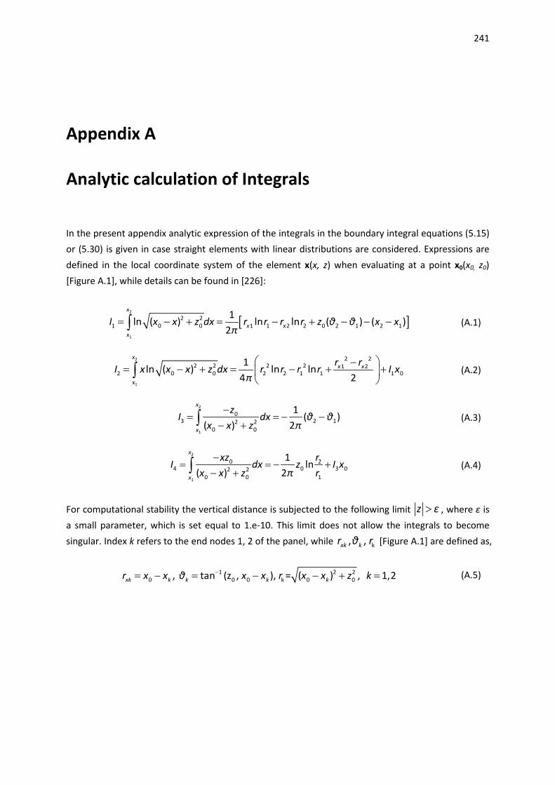
241

Appendix A

Analytic calculation of Integrals In the present appendix analytic expression of the integrals in the boundary integral equations (5.15) or (5.30) is given in case straight elements with linear distributions are considered. Expressions are defined in the local coordinate system of the element x(x, z) when evaluating at a point x0(x0, z0) [Figure A.1], while details can be found in [226]:

[ ]2

1

2 21 0 0 1 1 2 2 0 2 1 2 1

1ln ( ) ln ln ( ) ( )

2

x

x xx

I x x z dx r r r r z θ θ x xπ

= − + = − + − − −∫ (A.1)

2

1

2 22 2 2 2 1 2

2 0 0 2 2 1 1 1 01

ln ( ) ln ln4 2

xx x

x

r rI x x x z dx r r r r I x

π −

= − + = − + +

∫ (A.2)

2

1

03 2 12 2

0 0

1( )

( ) 2

x

x

zI dx θ θ

x x z π−

= = − −− +∫ (A.3)

2

1

0 24 0 3 02 2

0 0 1

1ln

( ) 2

x

x

xz rI dx z I x

x x z π r−

= = − +− +∫ (A.4)

For computational stability the vertical distance is subjected to the following limit z ε> , where ε is a small parameter, which is set equal to 1.e-10. This limit does not allow the integrals to become singular. Index k refers to the end nodes 1, 2 of the panel, while k, , xk kr θ r [Figure A.1] are defined as,

1 2 20 0 0 k 0 0, tan (z , ), = ( ) , 1,2xk k k k kr x x θ x x r x x z k−= − = − − + = (A.5)

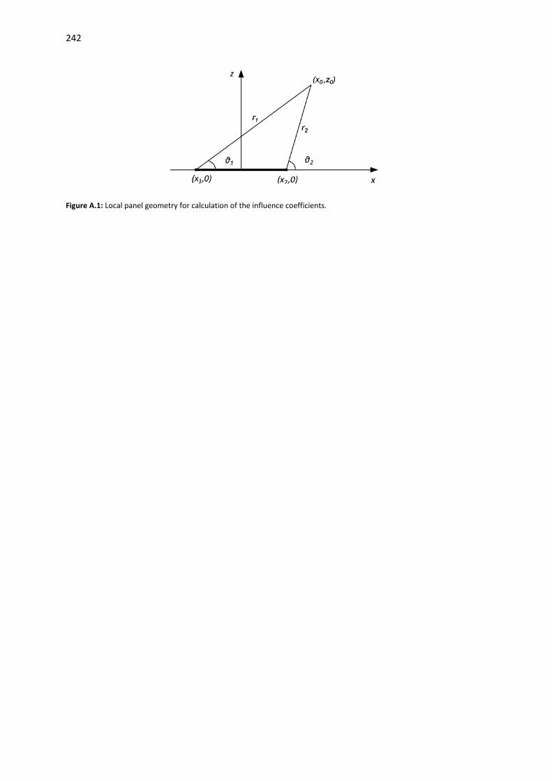
242

Figure A.1: Local panel geometry for calculation of the influence coefficients.

243

Appendix B

An expression for φtn on the body including the steady current In the present appendix the expression for φtn on the body including the steady current term Uo is derived. The derivation follows that by van Daalen [176] in terms of an orthogonal curvilinear coordinate system (s1, s2, n). The expression provided by van Daalen [equation A.28 in [176]] for ∂tnφ should hold for the total velocity potential Φ as well,

∂ = ⋅

+ ⋅ − ∂ ⋅ − ⋅ − ∂ ⋅

− ∂ + ∂ ⋅ − ∂ + ∂ ⋅

+ ∂ + ∂ − + ∂ ⋅

1 2

1 1 2 2

1 1 2 2

G

G 1 G 2 G 2 G 1

1 G 1 2 G 2

1 1 G

Φ

( Φ) ( ) ( Φ) ( )

( Φ Φ) ( ) ( Φ Φ) ( )

[ Φ Φ ( ) Φ] ( )

tn

s G s G

s ns s ns

s s s s n

k k

k k

x n

x s θ s x s θ s

x s x s

x n

(B.1)

In (B.1) k1 and k2 denote the curvature along s1 and s2 (see [176])

From the definition of the total velocity potential Φ (see (5.1))

∂ = ∂ − ∂ = ∂ − ∂ ∇ ⋅ = ∂ − ∂Φ ( ) Φ ( ) Φtn tn tn o tn o t tn o t xφ U x U x U nn (B.2)

The term ∂t xn is written as,

∂ = − ∇t x t x xn d n nx (B.3)

where dt denotes the material derivative of a scalar function. The first term of (B.3) is written as,

= × = × × = ⋅ − ⋅

G G 1 2 G 2 1 G 1 2( ) ( ) ( ) t G G G Gd n θ n θ s s θ s s θ s s (B.4)

while the second term of (B.3) by making use of equation A8, A13 and A14 from [176] yields,

∇ = − −1 1 1 2 2 2x x xn k s k ss s (B.5)

By introducing (B.4) and (B.5) into (B.3),

244

∂ = ⋅ − ⋅ + ⋅ + ⋅

G 2 1 G 1 2 1 1 1 2 2 2( ) ( ) ( ) ( )t x G x G x x G x Gn s s k s k sθ s θ s x s x s (B.6)

while by introducing (B.1) and (B.6) into (B.2) the final expression for ∂tnφ including the current term is derived,

∂ = ⋅

+ ⋅ − ∂ − ⋅ − ⋅ − ∂ − ⋅

− ∂ + ∂ + ⋅ − ∂ + ∂ + ⋅

+ ∂ + ∂ − + ∂ ⋅

1 2

1 1 2 2

1 1 2 2

G

G 1 1 G 2 G 2 2 G 1

1 1 1 G 1 2 2 2 G 2

1 1 G

( Φ ) ( ) ( Φ ) ( )

( Φ Φ ) ( ) ( Φ Φ ) ( )

[ Φ Φ ( ) Φ] ( )

tn

s o x G s o x G

s ns o x s ns o x

s s s s n

φ

U s U s

k U k s k U k s

k k

x n

x s θ s x s θ s

x s x s

x n

(B.7)

(B.7) is valid for 3D. By making use of (5.1) and also retaining only the terms which are valid for 2D, the final expression in 2D is derived,

G

G 0 B

0 0 G

0 0 G

( 2 )

( 2 )( )

( )( )

tn

s s

n s n s ns sn

n n n n ss ss

φ

φ U x θ

k φ k U x φ U x

k φ k U x φ U x

∂ = ⋅

+ ⋅ − ∂ − ∂

− ∂ + ∂ + ∂ + ∂ ⋅

− ∂ + ∂ −∂ − ∂ ⋅

x n

x s

x s

x n

(B.8)

245

References 1. Arapogianni, A., A. Genachte, R. Ochagavia, J. Vergara, D. Castell, A. Tsouroukdissian, J.

Korbijn, N. Bolleman, F. Huera-Huarte, F. Schuon, A. Ugarte, J. Sandberg, V. de Laleu, J. Maciel, A. Tunbjer, R. Roth, P. de la Gueriviere, P. Coulombeau, S. Jedrec, C. Philippe, S. Voutsinas, A. Weinstein, L. Vita, E. Byklum, L. Hurley, and H. Grubel, Deep water—the next step for offshore wind energy. European Wind Energy Association (EWEA), Brussels, Belgium, ISBN, 2013: p. 978-2.

2. Quarton, D., The evolution of wind turbine design analysisÐa twenty year progress review'. Wind Energy, 1998. 1: p. 5-24.

3. Chandra, R., Parallel programming in OpenMP. 2001: Morgan Kaufmann.

4. Gropp, W., E. Lusk, and R. Thakur, Using MPI-2: Advanced features of the message-passing interface. 1999: MIT press.

5. FROUDE, R., W. JOHN, C. WINGFIELD, J. THORNYCROFT, A. GREENHILL, C. STROMEYER, A. RIGG, E. REYNOLDS, E. COWPER, and S. BARNABY. DISCUSSION. THE SCREW-PROPELLER. in Minutes of the Proceedings. 1890. Thomas Telford.

6. Betz, A., Wind-energie und ihre ausnutzung durch windmühlen. 1926: Vandenhoeck.

7. Betz, A., Behavior of vortex systems. 1933.

8. Glauert, H., Aerodynamic theory. The General Momentum Theory, 1935. 4.

9. Vries, O.d., Fluid dynamic aspects of wind energy conversion. 1979, DTIC Document.

10. Vries, O., On the theory of the horizontal-axis wind turbine. Annual review of fluid mechanics, 1983. 15(1): p. 77-96.

11. Hansen, M.O., Aerodynamics of wind turbines. 2015: Routledge.

12. Burton, T., D. Sharpe, N. Jenkins, and E. Bossanyi, Wind energy handbook. 2001: John Wiley & Sons.

13. Schepers, J.G., Engineering models in wind energy aerodynamics: Development, implementation and analysis using dedicated aerodynamic measurements. 2012: TU Delft, Delft University of Technology.

14. Moriarty, P.J. and A.C. Hansen, AeroDyn theory manual. 2005: National Renewable Energy Laboratory Golden, Colorado, USA.

15. Shen, W.Z., R. Mikkelsen, J.N. Sørensen, and C. Bak, Tip loss corrections for wind turbine computations. Wind Energy, 2005. 8(4): p. 457-475.

16. EU project AVATAR: AdVanced Aerodynamic Tools for lArge Rotors, http://www.eera-avatar.eu.

17. Manolas, D., G. Pirrung, A. Croce, M. Roura, V. Riziotis, H. Madsen, C. Pizarro, and S. Voutsinas. Cross comparison of aeroelastic state-of-the-art design tools on a 10 MW scale wind turbine. in EWEA CONFERENCE. 2015. Paris, France.

18. Snel, H., Review of aerodynamics for wind turbines. Wind energy, 2003. 6(3): p. 203-211.

19. Prandtl, L. and O.G. Tietjens, Applied hydro-and aeromechanics: based on lectures of L. Prandtl. 1957: Dover Publ.

246

20. Bareiss, R. and S. Wagner. A hybrid wake model for hawt. in Proc. of the Sixth IEA Symposium on the Aerodynamics of Wind Turbines, McAnulty, KF, ed., ETSU, Harwell. 1993.

21. Simoes, F. and J. Graham. Prediction of loading on a horizontal axis wind turbine using a free vortex wake model. in Proc. 13th BWEA Wind Energy Conference, Quarton, DC and Fenton, VC, eds., Mechanical Engineering Publications Limited, London, UK. 1991.

22. Robison, D., F. Coton, R. Galbraith, and M. Vezza, Application of a prescribed wake aerodynamic prediction scheme to horizontal axis wind turbines in axial flow. Wind Engineering, 1995. 19(1): p. 41-51.

23. Zervos, A., S. Huberson, and A. Hemon, Three-dimensional free wake calculation of wind turbine wakes. Journal of Wind Engineering and Industrial Aerodynamics, 1988. 27(1): p. 65-76.

24. Voutsinas, S.G., Vortex methods in aeronautics: how to make things work. International Journal of Computational Fluid Dynamics, 2006. 20(1): p. 3-18.

25. Hauptmann, S., M. Bülk, L. Schön, S. Erbslöh, K. Boorsma, F. Grasso, M. Kühn, and P. Cheng, Impact of the lifting-line free vortex wake method on the simulated loads of multi-MW wind turbines. The Science of Making Torque from Wind, Oldenburg, 2012.

26. Huberson, S.G. and S.G. Voutsinas, Particles and grid. Computers & fluids, 2002. 31(4): p. 607-625.

27. Manolas, D., Particle mesh method: reduction of computational cost and application to large scale simulations. Diploma Thesis (in Greek), NTUA, Athens, 2007.

28. Papadakis, G., Development of a hybrid compressible vortex particle method and application to external problems including helicopter flows. PhD Thesis, NTUA, Athens, 2014.

29. Belessis, M., P. Chassapoyiannis, and S. Voutsinas. Free-wake modellng of rotor aerodynamics: recent developments and future perspectives. in EWEC CONFERENCE. 2001. Copenhagen, Denmark.

30. Bhagwat, M.J. and J. Leishman. Transient rotor inflow using a time-accurate free-vortex wake model. in AIAA, Aerospace Sciences Meeting and Exhibit, 39 th, Reno, NV. 2001.

31. Baldacchino, D., Horizontal AxisWind Turbine (HAWT) wake stability investigations: Insights Through a Vortex-Ring Modelling Approach. Master's thesis, TU Delft, Delft, October, 2012.

32. Spalart, P.R. and S.R. Allmaras, A one-equation turbulence model for aerodynamic flows. 1992.

33. Menter, F.R., Two-equation eddy-viscosity turbulence models for engineering applications. AIAA journal, 1994. 32(8): p. 1598-1605.

34. Wilcox, D.C., Turbulence modeling for CFD. Vol. 2. 1998: DCW industries La Canada, CA.

35. Drela, M., XFOIL: An analysis and design system for low Reynolds number airfoils, in Low Reynolds number aerodynamics. 1989, Springer. p. 1-12.

36. Menter, F.R., R. Langtry, S. Likki, Y. Suzen, P. Huang, and S. Völker, A correlation-based transition model using local variables—Part I: model formulation. Journal of turbomachinery, 2006. 128(3): p. 413-422.

37. Langtry, R.B. and F.R. Menter, Correlation-based transition modeling for unstructured parallelized computational fluid dynamics codes. AIAA journal, 2009. 47(12): p. 2894-2906.

38. Sørensen, J.N., Aerodynamic aspects of wind energy conversion. Annual Review of Fluid Mechanics, 2011. 43: p. 427-448.

39. Schepers, J., K. Boorsma, T. Cho, S. Gomez-Iradi, P. Schaffarczyk, A. Jeromin, W. Shen, T. Lutz, K. Meister, and B. Stoevesandt, Final report of IEA Task 29, Mexnext (Phase 1): Analysis of Mexico wind tunnel measurements. Wind Energy, 2015. 2014: p. 2013.

40. Papadakis, G. and S. Voutsinas. In view of accelerating CFD computations through coupling with vortex particle approximations. in TORQUE 2014, Journal of Physics: Conference Series. 2014.

247

41. Garrett, C., Wave forces on a circular dock. Journal of Fluid Mechanics, 1971. 46(01): p. 129-139.

42. Duarte, T., A. Sarmento, and J. Jonkman, Effects of Second-Order Hydrodynamic Forces on Floating Offshore Wind Turbines. 2014, NREL/CP-5000-60966. Golden, CO: National Renewable Energy Laboratory, 18 pp. Accessed November 3, 2014: http://www. nrel. gov/docs/fy14osti/60966. pdf.

43. Newman, J.N., Second-order, slowly-varying forces on vessels in irregular waves. 1974.

44. Mazarakos, T., D. Konispoliatis, D. Manolas, S. Voutsinas, and S. Mavrakos. Modelling of an Offshore Multi – Purpose Floating Structure Supporting a Wind Turbine Including Second – Order Wave Loads. in 11th European Wave and Tidal Energy Conference EWTEC2015. 2015. Nantes, France.

45. Morison, J., J. Johnson, and S. Schaaf, The force exerted by surface waves on piles. Journal of Petroleum Technology, 1950. 2(05): p. 149-154.

46. Faltinsen, O., Sea loads on ships and offshore structures. Vol. 1. 1993: Cambridge university press.

47. Dean, R., Stream function representation of nonlinear ocean waves. Journal of Geophysical Research, 1965. 70(18): p. 4561-4572.

48. Rienecker, M. and J. Fenton, A Fourier approximation method for steady water waves. Journal of Fluid Mechanics, 1981. 104: p. 119-137.

49. Hansen, M.O.L., J.N. Sørensen, S. Voutsinas, N. Sørensen, and H.A. Madsen, State of the art in wind turbine aerodynamics and aeroelasticity. Progress in aerospace sciences, 2006. 42(4): p. 285-330.

50. Kallesøe, B.S., Effect of steady deflections on the aeroelastic stability of a turbine blade. Wind Energy, 2011. 14(2): p. 209-224.

51. Manolas, D., V. Riziotis, and S. Voutsinas, Assessing the importance of geometric non-linear effects in the prediction of wind turbine blade loads. Journal of Computational and Nonlinear Dynamics, 2014.

52. Riziotis, V., S. Voutsinas, E. Politis, P. Chaviaropoulos, A.M. Hansen, H. Madsen Aagaard, and F. Rasmussen. Identification of structural non-linearities due to large deflections on a 5MW wind turbine blade. in EWEC CONFERENCE. 2008.

53. Chortis, D., N. Chrysochoidis, and D. Saravanos. Damped structural dynamics models of large wind-turbine blades including material and structural damping. in Journal of Physics: Conference Series. 2007. IOP Publishing.

54. Larsen, T.J., A.M. Hansen, and T. Buhl. Aeroelastic effects of large blade deflections for wind turbines. in Special topic conference: The science of making torque from wind. 2004.

55. Bottasso, C.L., A. Croce, B. Savini, W. Sirchi, and L. Trainelli, Aero-servo-elastic modeling and control of wind turbines using finite-element multibody procedures. Multibody System Dynamics, 2006. 16(3): p. 291-308.

56. Riziotis, V.A. and S.G. Voutsinas. Advanced aeroelastic modelling of complete wind turbine configurations in view of assessing stability characteristics. in EWEC CONFERENCE. 2006.

57. Kallesøe, B.S., Equations of motion for a rotor blade, including gravity, pitch action and rotor speed variations. Wind Energy, 2007. 10(3): p. 209-230.

58. Hodges, D.H., Nonlinear Composite Beam Theory (Progress in Astronautics and Aeronautics), American Institute of Aeronautics and Astronautics. Inc., Reston, VA, 2006. 213.

59. Hodges, D.H. and E. Dowell, Nonlinear equations of motion for the elastic bending and torsion of twisted nonuniform rotor blades. 1975.

60. Bottasso, C., F. Campagnolo, A. Croce, and C. Tibaldi. Integrating active and passive load control in wind turbines. in EWEA Annual Event. 2012. Copenhagen.

248

61. Chortis, D.I., D.S. Varelis, and D.A. Saravanos, Prediction of material coupling effect on structural damping of composite beams and blades. Composite Structures, 2012. 94(5): p. 1646-1655.

62. Chaviaropoulos, P.K., Development of a state-of-the art aeroelastic simulator for horizontal axis wind turbines. Part 1: Structural aspects. Wind Engineering, 1996. 20(6): p. 405-419.

63. Riziotis, V. and S. Voutsinas. GAST: A general aerodynamic and structural prediction tool for wind turbines. in EWEC CONFERENCE. 1997. Dublin Castle, Ireland.

64. Petersen, J.T., Kinematically nonlinear finite element model of a horizontal axis wind turbine. 1993: Riso National Laboratory.

65. Jonkman, J.M. and M.L. Buhl Jr, FAST user’s guide. National Renewable Energy Laboratory, Golden, CO, Technical Report No. NREL/EL-500-38230, 2005.

66. Bossanyi, E., GH Bladed Version 3.6 User Manual. Garrad Hassan and Partners Limited Document, 2003. 2.

67. Øye, S. FLEX4 simulation of wind turbine dynamics. in Proceedings of the 28th IEA Meeting of Experts Concerning State of the Art of Aeroelastic Codes for Wind Turbine Calculations (Available through International Energy Agency). 1996.

68. Commission, I.E., Wind Turbines-Part 1: Design Requirements, IEC 61400-1 Ed. 3. 2005.

69. Commission, I.E., Wind Turbines-Part 3: Design Requirements for Offshore Wind Turbines, IEC 61400-3. 2008.

70. Jonkman, J.M., Dynamics modeling and loads analysis of an offshore floating wind turbine. 2007: ProQuest.

71. Jonkman, J.M., Definition of the Floating System for Phase IV of OC3. 2010: National Renewable Energy Laboratory Golden, CO, USA.

72. Jonkman, J., S. Butterfield, P. Passon, T. Larsen, T. Camp, J. Nichols, J. Azcona, and A. Martinez. Offshore code comparison collaboration within IEA wind annex XXIII: phase II results regarding monopile foundation modeling. in 2007 European Offshore Wind Conference & Exhibition, 4–6 December 2007, Berlin, Germany. 2008.

73. Robertson, A., J. Jonkman, F. Vorpahl, W. Popko, J. Qvist, L. Frøyd, X. Chen, J. Azcona, E. Uzunoglu, C. Soares, C. Luan, H. Yutong, F. Pengcheng, A. Yde, T. Larsen, J. Nichols, R. Buils, L. Lei, T. Nygaard, D. Manolas, A. Heege, S. Vatne, H. Ormberg, T. Duarte, C. Godreau, H. Hansen, A. Nielsen, H. Riber, C. Le Cunff, F. Beyer, A. Yamaguchi, K. Jung, H. Shin, Marco Alves, W. Shi, H. Park, M. Alves, and M. Guérinel. Offshore code comparison collaboration continuation within IEA Wind Task 30: Phase II results regarding a floating semisubmersible wind system. in ASME 2014 33rd International Conference on Ocean, Offshore and Arctic Engineering. 2014. American Society of Mechanical Engineers.

74. Riziotis, V., Aerodynamic and aeroelastic analysis of dynamic stall on wind turbine rotors. PhD Thesis (in Greek), NTUA, Athens, 2003.

75. Riziotis, V., P. Chaviaropoulos, and S. Voutsinas, Develpoment of a state-of-the art aeroelastic simulator for horizontal axis wind turbines. Part 2: Aerodynamic aspects and application. 1996.

76. Riziotis, V., S. Voutsinas, D. Manolas, E. Politis, and P. Chaviaropoulos. Aeroelastic analysis of pre-curved rotor blades. in EWEC CONFERENCE. 2010. Warsaw, Poland.

77. Riziotis, V., S. Voutsinas, E. Politis, and P. Chaviaropoulos, Aeroelastic stability of wind turbines: the problem, the methods and the issues. Wind Energy, 2004. 7(4): p. 373-392.

78. Riziotis, V., S. Voutsinas, E. Politis, and P. Chaviaropoulos, Assessment of passive instability suppression means on pitch‐regulated wind turbines. Wind Energy, 2008. 11(2): p. 171-192.

79. Riziotis, V., E. Politis, S. Voutsinas, and P. Chaviaropoulos, Stability analysis of pitch‐regulated, variable‐speed wind turbines in closed loop operation using a linear eigenvalue approach. Wind Energy, 2008. 11(5): p. 517-535.

249

80. MOUNTURB:. Load and Power Measurement Programme on Wind Turbines operating in Complex Mountainous Regions (JOU2-CT93-0378) [A.N.Fragoulis, "MOUNTURB: results from the "Load and Power measurement program on wind turbines operating in complex mountainous regions project". Proc. EUWEC '96 pI7.17, 1050-1054, EUWEC '96 Goteborg, Sweden].

81. COMTERID:. Investigation of design aspects and design options for wind turbines operating in complex terrain environments (JOR3-CT95-0033) [Fragoulis, A.N., Voutsinas, S.G., Markkilde, P.S., Cuerva, A., Winkelaar, D., Ganander, H. (1999) “Final results from the “Investigation of design aspects and design options for wind turbines operating in complex terrain environments” EWEC’99, Nice, March’99, pp46-51].

82. VEWTDC:, Verification of European Wind Turbine Design Codes (JOR3-CT98-0267) [G. Schepers, J. Heijdra, K. Thomsen, T. Larsen, D. Foussekis, R. Rawlinson Smith, L Kraan, B. Visser, S. Oye,H. Ganander, L Carlen, S. Voutsinas, M. Belessis, L. Drost (2001) “Verification of european wind turbine design codes“, Proceedings of the EWEC’ 01, Copenhagen, Denmark, July 1-7, 2001].

83. STABCON:, Aeroelastic Stability and Control of Large Wind Turbines” (EU ENERGY programme, 2002-2006) [Hansen, MH and Buhl, T, 2006, Design Guidelines for Passive Instability Suppression - Task II Report, Techinical report of STABCON project (NNK5-CT 2002-00627 contract), Risoe-R-1575(EN), RISOE National Laboratory].

84. UPWIND:, Finding design solutions for very large wind turbines” (EU ENERGY programme, 2006-2011) [UpWind: Design and solutions for very large wind turbines, EWEA Report, 2011].

85. Jaeke, A. Manjock, D. Manolas, F. Sander, and S. Voutsinas, INNWIND D4.2.3: Integrated design methods and controls for floating offshore wind turbines, in Report for WP4, Task 4.2.3 , CEU Project. 2015.

86. Azcona, J., D. Bekiropoulos, H. Bredmose, A. Fischer, N.F. Heilskov, A. Krieger, T. Lutz, A. Manjock, D. Manolas, D. Matha, K. Meister, R. Pereira, J. Rønby, F. Sandner, and S. Voutsinas, INNWIND D4.21: State-of-the-art and implementation of design tools for floating structures, in Report for WP4, Task 4.2, CEU Project. 2015.

87. Sandner, F., Y. Wie, D. Matha, E. Grela, J. Azcona, X. Munduate, D. Manolas, S. Voutsinas, and A. Natarajan, INNWIND D4.3.3: Innovative Concepts for Floating Structures, in Report for WP4, Task 4.3, CEU Project. 2015.

88. Papathanassiou, S., Contribution to the analysis of variable speed wind turbines with induction generator. PhD Thesis (in Greek), NTUA, Athens, 1997.

89. De Borst, R., M.A. Crisfield, J.J. Remmers, and C.V. Verhoosel, Nonlinear finite element analysis of solids and structures. 2012: John Wiley & Sons.

90. Bathe, K.-J., Finite element procedures. 2006: Klaus-Jurgen Bathe.

91. Riziotis, V., G. Katsaounis, G. Papadakis, S. Voutsinas, G. Bergeles, and G. Tzabiras, Numerical and experimental analysis of the hydroelastic behavior of purse seine nets. Ocean Engineering, 2013. 58: p. 88-105.

92. Mathematica, Version 6.0, Wolfram Research. Inc., Champaign, IL, 2007.

93. Passon, P., Memorandum: derivation and description of the soil-pile-interaction models. IEA-Annex XXIIII Subtask, 2006. 2.

94. Jonkman, J. and W. Musial, Final Technical Report, IEA Wind Task 23, Subtask 2, Offshore Code Comparison Collaboration (OC3). 2010, International Energy Agency (IEA), IEA Wind Task.

95. Dowell, E.H. and D. Tang, Dynamics of very high dimensional systems. Vol. 1. 2003: World Scientific.

96. Bossanyi, E., The design of closed loop controllers for wind turbines. Wind energy, 2000. 3(3): p. 149-163.

250

97. Bossanyi, E., Wind turbine control for load reduction. Wind Energy, 2003. 6(3): p. 229-244.

98. Jonkman, J.M., S. Butterfield, W. Musial, and G. Scott, Definition of a 5-MW reference wind turbine for offshore system development. 2009: National Renewable Energy Laboratory Golden, CO.

99. Bak, C., F. Zahle, R. Bitsche, T. Kim, A. Yde, L. Henriksen, A. Natarajan, and M. Hansen, Description of the DTU 10 MW reference wind turbine. DTU Wind Energy Report-I-0092, 2013.

100. Katopis, K., Contribution to the development of a design tool for the load analysis and certification of horizontal axis wind turbines. Diploma Thesis (in Greek), NTUA, Athens, 1995.

101. Belessis, M., Unsteady flow analysis on rotors and propeller equipped aircrafts. PhD Thesis (in Greek), NTUA, Athens, 1999.

102. Chassapoyiannis, P., Rotor analysis in steady and unsteady operation conditions. PhD Thesis (in Greek), NTUA, Athens, 2005.

103. Petot, D., Differential equation modeling of dynamic stall. La Recherche Aerospatiale(English Edition), 1989(5): p. 59-72.

104. Van Grol, H., H. Snel, and J. Schepers, Wind turbine benchmark exercise on mechanical loads. Volume 1, part A & B. A state of the art report, in ECN report, ECN-C- -91-031. 1991.

105. Schepers, J. and H. Snel, Joint investigation of dynamic inflow effects and implementation of an engineering method for response analysis, in ECN Report ECN-C-94-107, The Netherlands. 1994.

106. Glauert, H., Airplane propellers, in Aerodynamic theory. 1935, Springer. p. 169-360.

107. Schepers, J. and H. Snel, Dynamic Inflow: Yawed conditions and partial span pitch control, in ECN Report ECN-C-95-056, The Netherlands, Final Report for JOU2-CT92-0186 CEU project. 1995.

108. Schepers, J., An engineering model for yawed conditions, developed on the basis of wind tunnel measurements. 1998: Netherlands Energy Research Foundation ECN.

109. Leishman, J. and T. Beddoes. A generalised model for airfoil unsteady aerodynamic behaviour and dynamic stall using the indicial method. in Proceedings of the 42nd Annual forum of the American Helicopter Society. 1986. Washington DC.

110. Cummins, W., The impulse response function and ship motions. 1962, DTIC Document.

111. Koulouvari, M., G. Glinou, and E. Morfiadakis, MOUNTURB: Load and Power Measurement Program on Wind Turbines Operating in Complex Mountainous Regions. Results of the Benchmark Exercise. Part.1 Wind Data Analysis, in CRES Report for JOU2-CT93-0378, CEU project. 1995.

112. Fragoulis, A., COMTERID: Investigation of Design Aspects and Design Options for Wind Turbines Operating in Complex Terrain Environments, in Final Report for JOR3-CT95-0033, CEU Project. 1998.

113. Breard, C., V. Riziotis, and S. Voutsinas. Fatigue loading on wind turbines operating at extreme sites. in EWEC CONFERENCE. 1997. Dublin Castle, Ireland.

114. Veers, P.S., Three-dimensional wind simulation, Sandia Report SAND88 0152. 1988, Sandia National Labs., Albuquerque, New Mexico (USA).

115. Mourikis, D.G., V.A. Riziotis, and S.G. Voutsinas. Length scale effects on fatigue loads calculation procedure. in EWEC CONFERENCE. 1999.

116. Robertson, A., J. Jonkman, and W. Musial, Final Technical Report, IEA Wind Task 30, Offshore Code Comparison Collaboration Continued (OC4). 2014, International Energy Agency (IEA), IEA Wind Task.

117. Popko, W., F. Vorpahl, A. Zuga, M. Kohlmeier, J. Jonkman, A. Robertson, T. Larsen, A. Yde, K. Sætertrø, K. Okstad, J. Nichols, T. Nygaard, Z. Gao, D. Manolas, K. Kim, Q. Yu, W. Shi, H. Park, A. Vásquez-Rojas, J. Dubois, D. Kaufer, P. Thomassen, M. de Ruiter, T. van der Zee, J. Peeringa,

251

H. Zhiwen, and H. von Waaden, Offshore Code Comparison Collaboration Continuation (OC4), Phase I—Results of Coupled Simulations of an Offshore Wind Turbine with Jacket Support Structure. Journal of Ocean and Wind Energy, 2014. 1(1): p. 1-11.

118. Manolas, D., V. Riziotis, and S. Voutsinas. Assessment of 3D aerodynamic effects on the behaviour of floating wind turbines. in TORQUE 2012, Journal of Physics: Conference Series. 2014. IOP Publishing.

119. Riziotis, V., D. Manolas, and S. Voutsinas. Free-wake Aeroelastic Modelling of Swept Rotor Blades. in EWEA CONFERENCE. 2011. Brussels, Belgium.

120. Mazarakos, T., D. Manolas, T. Grapsas, S. Mavrakos, V. Riziotis, and S. Voutsinas. Conceptual design and advanced hydro-aero-elastic modeling of a TLP concept for floating wind turbine applications. in 1st International Conference on Renewable Energies Offshore RENEW2014. 2014. Lisbon, Portugal.

121. Mazarakos, T., D. Konispoliatis, D. Manolas, S. Mavrakos, and S. Voutsinas. Coupled Hydro – Aero – Elastic Analysis of a Multi – Purpose Floating Structure for Offshore Wind and Wave Energy Sources Exploitation. in 12th International Conference on the Stability of Ships and Ocean Vehicles STAB2015. 2015. Glasgow, UK.

122. Vorpahl, F., D. Kaufer, and W. Popko, Description of a basic model of the" UpWind reference jacket" for code comparison in the OC4 project under IEA Wind Annex 30. 2011, Technical report, Fraunhofer Institute for Wind Energy and Energy System Technology IWES.

123. Vorpahl, F. and W. Popko, Description of the Load Cases and Output Sensors to be Simulated in the OC4 Project under IEA Wind Annex 30. Fraunhofer Institute for Wind Energy and Energy System Technology IWES, Bremerhaven, Germany, 2013.

124. Wheeler, J., Methods for calculating forces produced on piles in irregular waves. Journal of Petroleum Technology, 1970. 1: p. 1-2.

125. Robertson, A., J. Jonkman, M. Masciola, H. Song, A. Goupee, A. Coulling, and C. Luan, Definition of the Semisubmersible Floating System for Phase II of OC4. Offshore Code Comparison Collaboration Continuation (OC4) for IEA Task, 2012. 30.

126. Iliopoulos, A., Loading analysis-comparison for offshore WTs and control strategies for loads reduction. Diploma Thesis (in Greek), NTUA, Athens, 2012.

127. Lobitz, D.W. and P.S. Veers, Aeroelastic behavior of twist-coupled HAWT blades. AIAA Paper No. 98-0029, 1998.

128. Miles, J. and F. Gilbert, Scattering of gravity waves by a circular dock. Journal of Fluid Mechanics, 1968. 34(04): p. 783-793.

129. Yeung, R.W., Added mass and damping of a vertical cylinder in finite-depth waters. Applied Ocean Research, 1981. 3(3): p. 119-133.

130. Sabuncu, T. and S. Calisal, Hydrodynamic coefficients for vertical circular cylinders at finite depth. Ocean Engineering, 1981. 8(1): p. 25-63.

131. Kiyokawa, T., H. Kobayashi, and M. Hino, Scattering of water waves and induced forces on vertical axisymmetric bodies. Coastal Engineering of Japan, 1983. 26: p. 175-192.

132. Kokkinowrachos, K., S. Mavrakos, and S. Asorakos, Behaviour of vertical bodies of revolution in waves. Ocean Engineering, 1986. 13(6): p. 505-538.

133. Mavrakos, S. and P. Koumoutsakos, Hydrodynamic interaction among vertical axisymmetric bodies restrained in waves. Applied Ocean Research, 1987. 9(3): p. 128-140.

134. Mavrakos, S., Hydrodynamic coefficients for groups of interacting vertical axisymmetric bodies. Ocean engineering, 1991. 18(5): p. 485-515.

135. Isaacson, M., Wave forces on compound cylinders. Proc. Civil Engineering in the Oceans IV, ASCE, San Francisco, 1979: p. 518-530.

252

136. McIver, P. and D. Evans, The occurrence of negative added mass in free-surface problems involving submerged oscillating bodies. Journal of engineering mathematics, 1984. 18(1): p. 7-22.

137. Mei, C.C., Numerical methods in water-wave diffraction and radiation. Annual Review of Fluid Mechanics, 1978. 10(1): p. 393-416.

138. Garrison, C., Hydrodynamic loading of large offshore structures: three-dimensional source distribution methods. In: Numerical methods in offshore engineering., 1978.

139. Hogben, N. and R. Standing. Wave loads on large bodies. in Proceedings of the International Symposium on the Dynamics of Marine Vehicles and Structures in Waves. 1974.

140. Faltinsen, O.M. and F.C. Michelsen, MOTIONS OF LARGE STRUCTURES IN WAVES AT ZERO FROUDE NUMBER. Nor Veritas Publ, 1975(90): p. 3-18.

141. Eatock-Taylor, R., Generalised hydrodynamic forces on vibrating offshore structures by wave diffraction technique. Offshore structures engineering, 1977: p. 249-274.

142. Lee, C. and J. Newman, Computation of wave effects using the panel method. Numerical Models in Fluid Structure Interaction, 2005. 42: p. 211-251.

143. Lee, C., WAMIT–a radiation–diffraction panel program for wave-body interactions, user manual. Dept. of Ocean Engineering, Massachusetts Institute of Technology, USA, 1998.

144. Chenault, D.W., Motion of a Ship at the Free Surface. 1970, United States Naval Postgraduate School.

145. Newton, R., I. Chenault, and D. Smith. Finite element solution for added mass and damping. in Finite Elementary Methods in Flow Problems, Int Symp, Proceedings, University of Swansea, Wales, Jan 1974. 1974.

146. Bai, K.J., A variational method in potential flows with a free surface. 1972, DTIC Document.

147. Bai, K.J., Diffraction of oblique waves by an infinite cylinder. Journal of Fluid Mechanics, 1975. 68(03): p. 513-535.

148. Berkhoff, J. CW 1972 Computation of combined refraction-diffraction. in Proc. 13th Zntl Conf. Coastal Engng, ASCE, Vancouver.

149. Chen, H. and C. Mei. Oscillations and wave forces in a man-made harbor in the open sea. in Symposium on Naval Hydrodynamics, 10th, Proceedings, Pap and Discuss, Cambridge, Mass, June 24-28, 1974. 1974.

150. Bai, K.J. and R.W. Yeung. Numerical solutions to free-surface flow problems. in Proceedings of the tenth symposium on naval hydrodynamics. 1974.

151. Chenot, J.-L., Méthode numérique de calcul du mouvement d'un corps flottant soumis à l'influence d'une houle périodique en théorie linéaire. Oil & Gas Science and Technology, 1975. 30(5): p. 779-802.

152. Yue, D.K., H.S. Chen, and C.C. Mei, A hybrid element method for diffraction of water waves by three‐dimensional bodies. International Journal for Numerical Methods in Engineering, 1978. 12(2): p. 245-266.

153. Ferdinande, V. and B. Kritis, An economical method of determining added mass and damping coefficients of axisymmetric floating bodies in oscillatory heaving motion. International Shipbuilding Progress, 1980. 27(313): p. 231-240.

154. Au, M. and C. Brebbia, Water waves analysis, in Basic Principles and Applications. 1984, Springer. p. 97-122.

155. Yeung, R. A hybrid integral-equation method for time-harmonic free-surface flow. in Proc, 1st International Conference on Numerical Ship Hydrodyn, Gaithersburg, MD. 1975.

156. Matsui, T., K. Kato, and T. Shirai, A hybrid integral equation method for diffraction and radiation of water waves by three-dimensional bodies. Computational mechanics, 1987. 2(2): p. 119-135.

253

157. Yuen, M. and F. Chau, A hybrid integral equation method for wave forces on three-dimensional offshore structures. Journal of Offshore Mechanics and Arctic Engineering, 1987. 109(3): p. 229-236.

158. ZHANG, J. and G.-p. MIAO, A linear hybrid model of MSE and BEM for floating structures in coastal zones. Journal of Hydrodynamics, Ser. B, 2006. 18(6): p. 649-658.

159. Belibassakis, K., A boundary element method for the hydrodynamic analysis of floating bodies in variable bathymetry regions. Engineering analysis with boundary elements, 2008. 32(10): p. 796-810.

160. Athanassoulis, G. and K. Belibassakis, A consistent coupled-mode theory for the propagation of small-amplitude water waves over variable bathymetry regions. Journal of Fluid Mechanics, 1999. 389: p. 275-301.

161. Belibassakis, K., G. Athanassoulis, and T.P. Gerostathis, A coupled-mode model for the refraction–diffraction of linear waves over steep three-dimensional bathymetry. Applied ocean research, 2001. 23(6): p. 319-336.

162. Newman, J.N., Marine hydrodynamics. 1977: MIT press.

163. Falnes, J., Ocean waves and oscillating systems: linear interactions including wave-energy extraction. 2002: Cambridge university press.

164. Newman, J. The interaction of stationary vessels with regular waves. in Proceedings of the 11th symposium on naval hydrodynamics, London. 1976.

165. Hess, J.L. and A. Smith, Calculation of non-lifting potential flow about arbitrary three-dimensional bodies. 1962, DTIC Document.

166. Ramachandran, G., A. Robertson, J. Jonkman, and M. Masciola. Investigation of Response Amplitude Operators for Floating Offshore Wind Turbines. in The Twenty-third International Offshore and Polar Engineering Conference. 2013. International Society of Offshore and Polar Engineers.

167. Welch, P., The use of fast Fourier transform for the estimation of power spectra: a method based on time averaging over short, modified periodograms. IEEE Transactions on audio and electroacoustics, 1967: p. 70-73.

168. Ma, Q., Advances in numerical simulation of nonlinear water waves. 2010: World Scientific.

169. Longuet-Higgins, M.S. and E. Cokelet, The deformation of steep surface waves on water. I. A numerical method of computation. Proceedings of the Royal Society of London. A. Mathematical and Physical Sciences, 1976. 350(1660): p. 1-26.

170. Vinje, T. and P. Brevig, Numerical simulation of breaking waves. Advances in Water resources, 1981. 4(2): p. 77-82.

171. Cointe, R. and P. Geyer, Nonlinear and linear motions of a rectangular barge in a perfect fluid. 1991.

172. Koo, W. and M.-H. Kim, Freely floating-body simulation by a 2D fully nonlinear numerical wave tank. Ocean Engineering, 2004. 31(16): p. 2011-2046.

173. Sen, D., Numerical simulation of motions of two-dimensional floating bodies. 1993.

174. Cao, Y., R.F. Beck, and W.W. Schultz. Nonlinear computation of wave loads and motions of floating bodies in incident waves. in Proceedings of the 9th International Workshop on Water Waves and Floating Bodies (IWWWFB). 1994.

175. Wu, G. and R. Eatock Taylor. Transient motion of a floating body in steep water waves. in Proceedings of the 11th International Workshop on Water Waves and Floating Bodies (IWWWFB). 1996.

176. van Daalen, E.F.G., Numerical and theoretical studies of water waves and floating bodies. 1993.

254

177. Tanizawa, K., A nonlinear simulation method of 3-D body motions in waves (1st Report). 日本造船学会論文集, 1995. 1995(178): p. 179-191.

178. Orlanski, I., A simple boundary condition for unbounded hyperbolic flows. Journal of computational physics, 1976. 21(3): p. 251-269.

179. Romate, J., Absorbing boundary conditions for free surface waves. Journal of computational Physics, 1992. 99(1): p. 135-145.

180. Bessho, M., Feasibility study of a Floating-type Wave Absorber. 34th JTTC, 1973: p. 48-65359.

181. Naito, S. and S. Nakamura, Wave energy absorption in irregular waves by feedforward control system, in Hydrodynamics of ocean wave-energy utilization. 1986, Springer. p. 269-280.

182. Clément, A., Coupling of two absorbing boundary conditions for 2D time-domain simulations of free surface gravity waves. Journal of Computational Physics, 1996. 126(1): p. 139-151.

183. Baker, G.R., D.I. Meiron, and S.A. Orszag, Generalized vortex methods for free-surface flow problems. Journal of Fluid Mechanics, 1982. 123: p. 477-501.

184. Israeli, M. and S.A. Orszag, Approximation of radiation boundary conditions. Journal of Computational Physics, 1981. 41(1): p. 115-135.

185. Le Méhauté, B., Progressive wave absorber. Journal of Hydraulic Research, 1972. 10(2): p. 153-169.

186. Grilli, S.T. and J. Horrillo, Numerical generation and absorption of fully nonlinear periodic waves. Journal of Engineering Mechanics, 1997. 123(10): p. 1060-1069.

187. Dommermuth, D.G., D.K. Yue, W. Lin, R. Rapp, E. Chan, and W. Melville, Deep-water plunging breakers: a comparison between potential theory and experiments. Journal of Fluid Mechanics, 1988. 189: p. 423-442.

188. Boo, S. and C. Kim. Fully nonlinear diffraction due to a vertical circular cylinder in a 3-D HOBEM numerical wave tank. in The Sixth International Offshore and Polar Engineering Conference. 1996. International Society of Offshore and Polar Engineers.

189. Kim, C., A. Clement, and K. Tanizawa, Recent research and development of numerical wave tanks-a review. International Journal of Offshore and Polar Engineering, 1999. 9(4): p. 241-256.

190. Tanizawa, K. The state of the art on numerical wave tank. in Proc. 4th Osaka colloquium on seakeeping performance of ships. 2000.

191. Tsai, W.-T. and D.K. Yue, Computation of nonlinear free-surface flows. Annual review of fluid mechanics, 1996. 28(1): p. 249-278.

192. Grilli, S., Fully nonlinear potential flow models used for long wave runup prediction. 1997.

193. Ryu, S., M. Kim, and P.J. Lynett, Fully nonlinear wave-current interactions and kinematics by a BEM-based numerical wave tank. Computational mechanics, 2003. 32(4-6): p. 336-346.

194. Ferrant, P., Runup on a cylinder due to waves and current: potential flow solution with fully nonlinear boundary conditions. International Journal of Offshore and Polar Engineering, 2001. 11(1): p. 33-41.

195. Kim, M., M. Celebi, and D. Kim, Fully nonlinear interactions of waves with a three-dimensional body in uniform currents. Applied Ocean Research, 1998. 20(5): p. 309-321.

196. Koo, W. and M.-H. Kim, Current effects on nonlinear wave-body interactions by a 2D fully nonlinear numerical wave tank. Journal of waterway, port, coastal, and ocean engineering, 2007. 133(2): p. 136-146.

197. Grilli, S. and I. Svendsen, Corner problems and global accuracy in the boundary element solution of nonlinear wave flows. Engineering Analysis with Boundary Elements, 1990. 7(4): p. 178-195.

255

198. Koo, W. and M. Kim, Fully nonlinear wave-body interactions with surface-piercing bodies. Ocean Engineering, 2007. 34(7): p. 1000-1012.

199. Guerber, E., M. Benoit, S.T. Grilli, and C. Buvat, A fully nonlinear implicit model for wave interactions with submerged structures in forced or free motion. Engineering Analysis with Boundary Elements, 2012. 36(7): p. 1151-1163.

200. Mei, C.C., The applied dynamics of ocean surface waves. 1989.

201. Chapalain, G., R. Cointe, and A. Temperville, Observed and modeled resonantly interacting progressive water-waves. Coastal engineering, 1992. 16(3): p. 267-300.

202. Goda, Y. Perturbation analysis of nonlinear wave interactions in relatively shallow water. in Proc. 3rd Int. Conf. on Hydrodynamics, Seoul, Korea. 1998.

203. Dalrymple, R.A. and R.G. Dean, Water wave mechanics for engineers and scientists. 1991: Prentice-Hall.

204. Bretherton, F.P. and C.J. Garrett, Wavetrains in inhomogeneous moving media. Proceedings of the Royal Society of London. Series A. Mathematical and Physical Sciences, 1968. 302(1471): p. 529-554.

205. Fenton, J., The numerical solution of steady water wave problems. Computers & Geosciences, 1988. 14(3): p. 357-368.

206. Goring, D.G., Tsunamis--the propagation of long waves onto a shelf. 1978, California Institute of Technology.

207. Tanaka, M., The stability of solitary waves. Physics of Fluids (1958-1988), 1986. 29(3): p. 650-655.

208. Grilli, S.T. and R. Subramanya, Numerical modeling of wave breaking induced by fixed or moving boundaries. Computational Mechanics, 1996. 17(6): p. 374-391.

209. Grilli, S., R. Subramanya, I. Svendsen, and J. Veeramony, Shoaling of solitary waves on plane beaches. Journal of Waterway, Port, Coastal, and Ocean Engineering, 1994. 120(6): p. 609-628.

210. Beji, S. and J. Battjes, Experimental investigation of wave propagation over a bar. Coastal Engineering, 1993. 19(1): p. 151-162.

211. Wu, G., Hydrodynamic forces on a submerged circular cylinder undergoing large-amplitude motion. Journal of Fluid Mechanics, 1993. 254: p. 41-58.

212. Kent, C.P. and W. Choi, An explicit formulation for the evolution of nonlinear surface waves interacting with a submerged body. International Journal for Numerical Methods in Fluids, 2007. 55(11): p. 1019-1038.

213. Evans, D., D. Jeffrey, S. Salter, and J. Taylor, Submerged cylinder wave energy device: theory and experiment. Applied Ocean Research, 1979. 1(1): p. 3-12.

214. Frank, W., Oscillation of cylinders in or below the free surface of deep fluids. 1967, DTIC Document.

215. Nojiri, N. and K. Murayama, A study on the drift force on two-dimensional floating body in regular waves. Transactions of the West-Japan Society Naval Architect, 1975. 51: p. 131-152.

216. Tanizawa, K. and M. Minami. On the accuracy of NWT for radiation and diffraction problem. in Proceeding of 6th Symposium on Nonlinear and Free-surface Flow. 1998.

217. Maruo, H., On the increase of the resistance of a ship in rough seas. J. Zosen Kiokai, 1960. 108.

218. Kim, M.-H. and D.K. Yue, The complete second-order diffraction solution for an axisymmetric body Part 1. Monochromatic incident waves. Journal of Fluid Mechanics, 1989. 200: p. 235-264.

219. Newman, J., Second-harmonic wave diffraction at large depths. Journal of Fluid Mechanics, 1990. 213: p. 59-70.

256

220. Kim, M.H., Second-harmonic vertical wave loads on arrays of deep-draft circular cylinders in monochromatic uni-and multi-directional waves. Applied ocean research, 1993. 15(5): p. 245-262.

221. National project SYNERGASIA - AVRA: Program for offshore wind source exploitation in the Aegean Sea.

222. National project ARISTEIA - POSEIDON: Multi-purpose floating structures for offshore wind and wave energy sources exploitation.

223. National project THALIS.

224. EU project INNWIND: INNovative WIND conversion systems (10-20MW) for offshore applications, http://http://www.innwind.eu.

225. Tsiantas, T., Reduction of flapwise loading on WT blades using flaps. Diploma Thesis (in Greek), NTUA, Athens, 2015.

226. Katz, J. and A. Plotkin, Low-speed aerodynamics. Vol. 13. 2001: Cambridge University Press.

Τίτλος

ΕΘΝΙΚΟ ΜΕΤΣΟΒΙΟ ΠΟΛΥΤΕΧΝΕΙΟ

ΣΧΟΛΗ ΜΗΧΑΝΟΛΟΓΩΝ ΜΗΧΑΝΙΚΩΝ ΤΟΜΕΑ ΡΕΥΣΤΩΝ, ΕΡΓΑΣΤΗΡΙΟ ΑΕΡΟΔΥΝΑΜΙΚΗΣ

ΚΕΙΜΕΝΟ ΠΟΥ ΥΠΟΒΛΗΘΗΚΕ ΓΙΑ ΤΗΝ ΑΠΟΚΤΗΣΗ ΤΟΥ ΤΙΤΛΟΥ ΤΟΥ ΔΙΔΑΚΤΟΡΑ ΜΗΧΑΝΙΚΟΥ

Ύδρο-Αέρο-Ελαστική Ανάλυση Υπεράκτιων Ανεμογεννητριών

Περίληψη στα Ελληνικά

Δημήτρης Μανωλάς

Οκτώβριος 2015

iii

Ύδρο-Αέρο-Ελαστική Ανάλυση Υπεράκτιων Ανεμογεννητριών

Περίληψη στα Ελληνικά

Δημήτρης Μανωλάς

Εξεταστική επιτροπή:

1. Γ. Πολίτης, ,Καθηγητής, ΕΜΠ, Σχολή Ναυπηγών Μηχανικών

2. Γ. Τζαμπίρας, Καθηγητής, ΕΜΠ, Σχολή Ναυπηγών Μηχανικών

3. Κ. Μπελιμπασάκης, Αναπληρωτής Καθηγητής, ΕΜΠ, Σχολή Ναυπηγών Μηχανικών

4. Β. Ριζιώτης, Λέκτoρας, ΕΜΠ, Σχολή Μηχανολόγων Μηχανικών

5. Α. Ζερβός * , Καθηγητής, ΕΜΠ, Σχολή Μηχανολόγων Μηχανικών

6. Σ.. Μαυράκος * ,Καθηγητής, ΕΜΠ, Σχολή Ναυπηγών Μηχανικών

7. Σ. Βουτσινάς (Επιβλέπων) ∗ , Καθηγητής, ΕΜΠ, Σχολή Μηχανολόγων Μηχανικών

*Μέλος της τριμελούς επιτροπής

v

Περιεχόμενα Τίτλος ........................................................................................................................................................ i

Περιεχόμενα ............................................................................................................................................. v

Λίστα σχημάτων ..................................................................................................................................... vii

Λίστα πινάκων ......................................................................................................................................... ix

Λίστα συντομογραφιών .......................................................................................................................... xi

Κεφάλαιο 1. ............................................................................................................................................. 1

1.1 Κίνητρο και Στόχοι ................................................................................................................... 1

1.2 Αναφορά στις μεθόδους επίλυσης ......................................................................................... 4

1.3 Διάρθρωση της διατριβής ....................................................................................................... 5

Κεφάλαιο 2. ............................................................................................................................................. 7

Περιγραφή των βασικών συνιστωσών του λογισμικού hGAST .......................................................... 7

2.1 Το αεροδυναμικό πρότυπο ..................................................................................................... 7

2.2 Το ελαστικό πρότυπο ............................................................................................................ 11

2.3 Το δυναμικό πρότυπο ........................................................................................................... 16

2.4 Το υδροδυναμικό πρότυπο ................................................................................................... 20

2.4.1 Η εξίσωση κίνησης του πλωτήρα στο πεδίο του χρόνου .............................................. 20

2.5 Το πρότυπο των αγκυρώσεων .............................................................................................. 22

2.6 Η σύνθεση για το συζευγμένο σύστημα ............................................................................... 28

Κεφάλαιο 3. ........................................................................................................................................... 31

3.1 Ο ημι-βυθισμένος πλωτήρας από τη φάση II του OC4 ......................................................... 31

3.1.1 Εισαγωγή ....................................................................................................................... 31

3.1.2 Ιδιοσυχνότητες .............................................................................................................. 32

3.1.3 Χρονοσειρές .................................................................................................................. 33

Κεφάλαιο 4. ........................................................................................................................................... 41

4.1 Μαθηματική διατύπωση ....................................................................................................... 41

4.2 Αριθμητική υλοποίηση .......................................................................................................... 45

vi

4.3 Υπολογισμός δυνάμεων ........................................................................................................ 45

4.4 Εξισώσεις κίνησης ................................................................................................................. 46

4.5 Ανύψωση ελεύθερης επιφάνειας ......................................................................................... 46

4.6 Αριθμητικά αποτελέσματα - Πιστοποίηση ........................................................................... 47

Κεφάλαιο 5. ........................................................................................................................................... 55

5.1 Μαθηματική διατύπωση του προβλήματος ......................................................................... 55

5.2 Αριθμητική υλοποίηση .......................................................................................................... 59

5.2.1 Μεικτή Eulerian - Lagrangian μέθοδος ......................................................................... 59

5.2.2 Ολοκληρωτική μορφή της εξίσωσης Laplace και η αριθμητική επίλυσή της ............... 59

5.2.3 Κινηματική των σωμάτων ............................................................................................. 61

5.2.4 Δύναμη των σωμάτων και επίλυση της ολοκληρωτικής εξίσωσης για το φt ............... 61

5.2.5 Ελεύθερα πλωτά σώματα ............................................................................................. 63

5.2.6 Ολοκλήρωση στο χρόνο ................................................................................................ 64

5.2.7 Έλεγχος ακρίβειας ......................................................................................................... 65

5.2.8 Γραμμικοποιημένες διατυπώσεις ................................................................................. 65

5.3 Αριθμητικά αποτελέσματα: Μη-γραμμική αλληλεπίδραση κύματος-ελεύθερα πλωτού σώματος ............................................................................................................................................ 66

Κεφάλαιο 6. ........................................................................................................................................... 75

6.1 Αποτίμηση ............................................................................................................................. 75

6.2 Μελλοντική έρευνα ............................................................................................................... 77

Αναφορές .............................................................................................................................................. 79

vii

Λίστα σχημάτων Σχήμα 1.1: Τύποι στηρίξεων υπεράκτιων ανεμογεννητριών εδραζόμενων στο βυθό .......................... 2

Σχήμα 1.2: Κατανομή των εγκαταστημένων υπεράκτιων ανεμογεννητριών σε σχέση με το είδος στήριξής τους (2012) ............................................................................................................................... 2

Σχήμα 1.3: Τύποι βάσεων στήριξης υπεράκτιων ανεμογεννητριών συναρτήσει του βάθους .............. 3

Σχήμα 1.4: Περιγραφή των κωδίκων που συμμετείχαν στη 2η φάση του OC4 [πίνακας από [3]] ........ 5

Σχήμα 2.1: Τρίγωνο ταχυτήτων και συμβολισμοί .................................................................................. 8

Σχήμα 2.2: Ορισμός των συνθηκών ροής στη περίπτωση απόκλισης και αεροελαστικής σύζευξης .. 11

Σχήμα 2.3: Το σύστημα συντεταγμένων και ο καθορισμός της κινηματικής στη θεωρία δοκού ........ 12

Σχήμα 2.4: Ορθές και διατμητικές τάσεις ............................................................................................. 13

Σχήμα 2.5: Ισορροπία δυνάμεων και ροπών για διαφορικού μήκους τμήμα δοκού. ......................... 14

Σχήμα 2.6: Τα συστήματα συντεταγμένων στη θεώρηση πολλαπλών σωμάτων (multibody θεώρηση) ............................................................................................................................................................... 17

Σχήμα 2.7: Παραδείγματα συζεύξεων: (αριστερά) Σύζευξη της διαμήκους κάμψης του πύργου με την πτερύγιση των πτερυγίων, (δεξιά) Σύζευξη της γωνίας βήματος και της γωνίας παλινδρόμησης (teeter) των πτερυγίων δίπτερου δρομέα. ........................................................................................... 18

Σχήμα 2.8: Η διαχείριση μεγάλων μετακινήσεων και στροφών μέσω του διαχωρισμού μιας συνιστώσας του συστήματος σε τμήματα (sub bodies) ....................................................................... 20

Σχήμα 2.9: Κινηματική του στοιχείου (truss element) ......................................................................... 23

Σχήμα 2.10: Μορφολογία των μητρών του τελικού συστήματος ........................................................ 29

Σχήμα 3.1: Ο ημι-βυθισμένος πλωτήρας του OC4 [εικόνα από [16]] .................................................. 31

Σχήμα 3.2: Σύγκριση των κινήσεων του πλωτήρα: Airy κύμα H=6m, T=10s, ομοιόμορφος άνεμος 8m/s). .................................................................................................................................................... 36

Σχήμα 3.3: Σύγκριση της τάσης των κλάδων αγκύρωσης 1 και 2: Airy κύμα H=6m, T=10s, ομοιόμορφος άνεμος 8m/s). ................................................................................................................ 37

Σχήμα 3.4: Σύγκριση των ροπών στη βάση του πύργου και των παραμορφώσεων στην κορυφή του: Airy κύμα H=6m, T=10s, ομοιόμορφος άνεμος 8m/s). ......................................................................... 37

viii

Σχήμα 3.5: Σύγκριση της στρεπτικής και της καμπτικής ροπής του άξονα: Airy κύμα H=6m, T=10s, ομοιόμορφος άνεμος 8m/s). ................................................................................................................ 38

Σχήμα 3.6: Σύγκριση της ηλεκτρικής ισχύος και την γωνιακής ταχύτητας: Airy κύμα H=6m, T=10s, ομοιόμορφος άνεμος 8m/s). ................................................................................................................ 38

Σχήμα 3.7: Σύγκριση των ροπών στη ρίζα του πτερυγίου και των παραμορφώσεων στο άκρο του: Airy κύμα H=6m, T=10s, ομοιόμορφος άνεμος 8m/s). ......................................................................... 39

Σχήμα 4.1: Ορισμός του χωρίου επίλυσης και του συνόρου ............................................................... 42

Σχήμα 4.2: Περιγραφή του ημι-βυθισμένου πλωτήρα του OC4 [εικόνα από [16]] ............................. 47

Σχήμα 4.3: Μη-δομημένο πλέγμα της ελεύθερης επιφάνειας αποτελούμενο από 11588 στοιχεία .. 47

Σχήμα 4.4: Δομημένο πλέγμα του πλωτήρα ........................................................................................ 48

Σχήμα 4.5: Μέτρο και φάση των δυνάμεων διέγερσης στη διεύθυνση surge, heave και pitch για 0ο γωνία κύματος του ημι-βυθισμένου πλωτήρα του OC4. ..................................................................... 49

Σχήμα 4.6: Μέτρο και φάση των δυνάμεων διέγερσης στη διεύθυνση surge, sway και heave για 30ο γωνία κύματος του ημι-βυθισμένου πλωτήρα του OC4. ..................................................................... 50

Σχήμα 4.7: Μέτρο και φάση των δυνάμεων διέγερσης στη διεύθυνση roll, pitch και yaw για 30ο γωνία κύματος του ημι-βυθισμένου πλωτήρα του OC4. ..................................................................... 51

Σχήμα 4.8: Συντελεστές πρόσθετης μάζας και απόσβεσης A11, A15, A33, B11, B15 και B33 του ημι-βυθισμένου πλωτήρα του OC4. ............................................................................................................ 52

Σχήμα 4.9: Συντελεστές πρόσθετης μάζας και απόσβεσης A55, A66, B55, και B66 του ημι-βυθισμένου πλωτήρα του OC4. ................................................................................................................................. 53

Σχήμα 5.1: Ορισμός του χωρίου επίλυσης και του συνόρου ............................................................... 56

Σχήμα 5.2: Ορισμός του υπολογιστικού χωρίου στη μέθοδο συνοριακών στοιχείων για την περίπτωση του ελεύθερα πλωτού σώματος. ....................................................................................... 66

Σχήμα 5.3: 1η αρμονική των 3 κινήσεων (surge, heave, pitch) και οριζόντια drift δύναμη του ελεύθερα πλωτού σώματος για ύψος κύματος H=0.07m. ................................................................... 70

Σχήμα 5.4: 1η, 2η και 3η αρμονική των υδροδυναμικών φορτίων του πλωτού σώματος – μη-γραμμικοί υπολογισμοί για ύψος κύματος H=0.07m ........................................................................... 71

Σχήμα 5.5: Χρονοσειρές φορτίων και κινήσεων του πλωτού σώματος για συχνότητες κύματος ξ=0.25, 0.75 και 1.75 και ύψος H=0.07m. ............................................................................................. 72

Σχήμα 5.6: Χρονοσειρές φορτίων και κινήσεων του πλωτού σώματος για συχνότητες κύματος ξ=0.5, 0.55 και 0.6 και ύψος H=0.07m. ........................................................................................................... 73

ix

Λίστα πινάκων Πίνακας 3.1: Σύγκριση ιδιοσυχνοτήτων [Hz] για το συζευγμένο σύστημα του ημι-βυθισμένου πλωτήρα του OC4 .................................................................................................................................. 33

Πίνακας 5.1: Συντελεστές της μεθόδου ολοκλήρωσης Runge-Kutta 4ης τάξης .................................... 64

Πίνακας 5.2: Εισερχόμενα κύματα για την προσομοίωση του πλωτού σώματος ............................... 67

xi

Λίστα συντομογραφιών 2Δ: 2 διαστάσεις

3Δ: 3 διαστάσεις

CFD: Computational Fluid Dynamics

FEM: Finite Element Method

hGAST: General hydro-Aeroelastic Structural Tool

IEC: International Electrotechnical Commission

IWL: Instantaneous Water Level

IP: Instantaneous Position

MSL: Mean Sea Level

OC3: Offshore Code Comparison Collaboration

OC4: Offshore Code Comparison Collaboration Continuation

RANS: Reynolds Averaged Navier Stokes

1

Κεφάλαιο 1.

Εισαγωγή Στο παρόν εισαγωγικό κεφάλαιο παρουσιάζεται το πλαίσιο της διατριβής. Στοχεύοντας στην ανάπτυξη υπολογιστικών εργαλείων που ταυτόχρονα θα λαμβάνουν υπόψη όλους τους φυσικούς μηχανισμούς, αρχικά παρουσιάζεται το κίνητρο και οι στόχοι σε σύνδεση με την τρέχουσα τεχνολογική γνώση και πρακτική. Στη συνέχεια παρουσιάζονται τα διαθέσιμα υπολογιστικά εργαλεία καθώς και η διάρθρωση της διατριβής.

1.1 Κίνητρο και Στόχοι

Η αιολική ενέργεια σταδιακά εγκαθίσταται σε υπεράκτιες τοποθεσίες εξαιτίας του άφθονου αιολικού δυναμικού και της απέραντης ανεκμετάλλευτης έκτασης της θάλασσας [1]. Η επιτυχημένη πορεία που κατέγραψε η αιολική ενέργεια τα τελευταία 30 χρόνια στηρίχθηκε στην ανάπτυξη και την επιβεβαίωση των υπολογιστικών εργαλείων σχεδιασμού, παράλληλα με την θέσπιση προτύπων για την ασφάλεια και την αξιοπιστία [2]. Έτσι, στην κοινότητα της Αιολικής ενέργειας είναι σαφές πως για να καταστεί επιτυχής η μετάβαση στις υπεράκτιες εφαρμογές τα εργαλεία σχεδιασμού είναι απαραίτητη προϋπόθεση. Για το σκοπό αυτό το λογικό βήμα είναι η αναβάθμιση των υφιστάμενων υπολογιστικών εργαλείων, έτσι ώστε να ληφθούν υπόψη τα επιπλέον χαρακτηριστικά που υπεισέρχονται στο πρόβλημα εξαιτίας της εγκατάστασης των ανεμογεννητριών στη θάλασσα.

Η πρώτη γενιά των υπεράκτιων ανεμογεννητριών αποτελείται από κατασκευές με βάσεις στήριξης στο βυθό [Σχήμα 1.1], οι οποίες ουσιαστικά αποτελούν άμεση επέκταση της χερσαίας τεχνολογίας με αύξηση του ύψους του πύργου. Αν και στη θάλασσα η ένταση της τύρβης είναι μικρότερη, οπότε αναμένονται μικρότερα κοπωτικά φορτία προερχόμενα από τον άνεμο, εντούτοις το βρεχόμενο τμήμα της κατασκευής υπόκειται σε υδροδυναμική φόρτιση προερχόμενη από τα θαλάσσια κύματα και ρεύματα. Αυτή είναι η σημαντικότερη πρόσθετη συνιστώσα στα φορτία της κατασκευής σε σχέση με τις χερσαίες εγκαταστάσεις, γεγονός που προκαλεί επιπλέον προκλήσεις. Από τη μία στον ορισμό των συνθηκών που θα πρέπει να εξετάζονται ώστε να εξασφαλίζεται η ασφάλεια και η επιβίωση της κατασκευής σε ακραία φορτία και κόπωση, και από την άλλη στο σχεδιασμό της θεμελίωσης που εξαρτάται άμεσα από την περιοχή εγκατάστασης λόγω των διαφορετικών ειδών εδάφους του βυθού.

2

Σχήμα 1.1: Τύποι στηρίξεων υπεράκτιων ανεμογεννητριών εδραζόμενων στο βυθό

Σήμερα που ακόμα βρισκόμαστε σε πρώιμο στάδιο ανάπτυξης της υπεράκτιας αιολικής ενέργειας, η πλειοψηφία των εγκαταστάσεων αποτελείται από ανεμογεννήτριες με βάσεις στήριξης εδραζόμενες στο βυθό [Σχήμα 1.2]. Στα πιο ρηχά βάθη, χρησιμοποιούνται βάσεις στήριξης με ένα πυλώνα, βάσεις βαρύτητας ή τρίποδες, ενώ σε λίγο μεγαλύτερα βάθη τα χωροδικτυώματα αποτελούν το επικρατούν πρότυπο σχεδιασμού.

Σχήμα 1.2: Κατανομή των εγκαταστημένων υπεράκτιων ανεμογεννητριών σε σχέση με το είδος στήριξής τους (2012)

Για βάθη μεγαλύτερα των 50m η στήριξη στον πυθμένα είναι υπό διερεύνηση εξαιτίας του αυξημένου κόστους. Έτσι, για εφαρμογές σε μεγάλα βάθη έχει προταθεί η λύση των πλωτών

3

ανεμογεννητριών [Σχήμα 1.3]. Στην περίπτωση αυτή, η ανεμογεννήτρια στηρίζεται σε πλωτήρα με κατάλληλο σύστημα αγκύρωσης. Ο στόχος που έχει τεθεί από την κοινότητα της αιολικής ενέργειας για τα επόμενα χρόνια είναι ο σχεδιασμός βέλτιστων πλωτών ανεμογεννητριών συνδυάζοντας την καλύτερη δυνατή απόδοση στο ελάχιστο κόστος.

Σχήμα 1.3: Τύποι βάσεων στήριξης υπεράκτιων ανεμογεννητριών συναρτήσει του βάθους

Τα υπολογιστικά εργαλεία που αναλύουν τη συμπεριφορά των ανεμογεννητριών θα πρέπει να ικανοποιούν δύο βασικά κριτήρια:

- Να περιλαμβάνουν όλους τους μηχανισμούς που επηρεάζουν τη λειτουργία των ανεμογεννητριών και απειλούν την ασφάλεια και την επιβίωσή τους.

- Να έχουν ένα επίπεδο ακρίβειας και συνέπειας που να επιτρέπει την πιστοποίηση των διαφόρων υπεράκτιων σχεδιασμών στα πλαίσια ορθά καθορισμένων κανονισμών.

Οι εμπλεκόμενοι φυσικοί μηχανισμοί περιλαμβάνουν την αεροδυναμική και την υδροδυναμική ροή, τη δυναμική του συστήματος συμπεριλαμβανομένης και της ελαστικότητας, τους κλάδους αγκύρωσης με τη θεμελίωση τους στο βυθό και το σύστημα ελέγχου. Στο πλαίσιο ανάλυσης των υπεράκτιων ανεμογεννητριών οι παραπάνω μηχανισμοί πρέπει να αλληλεπιδρούν με ισχυρή σύζευξη.

Η παρούσα εργασία έχει τρεις στόχους. Πρωταρχικός στόχος είναι η ανάπτυξη ενός πλήρως συζευγμένου υδρο-σερβο-αερο-ελαστικού εργαλείου για την ανάλυση της συμπεριφοράς υπεράκτιων ανεμογεννητριών, ικανού να προσομοιώσει όλα τα είδη βάσεων στήριξης και πλωτήρων καθώς και όλους τους τύπους ανεμογεννητριών (οριζοντίου και κατακορύφου άξονα). Ως βάση χρησιμοποιήθηκε η πλέον των 20 ετών ερευνητική εμπειρία και τεχνογνωσία στο ΕΜΠ. Ο

4

κώδικας hGAST που αναπτύχθηκε στηρίχθηκε σε προγενέστερη υλοποίηση που προσομοίωνε χερσαίες ανεμογεννήτριες. Ενσωματώθηκαν όλα τα απαραίτητα μέρη για την ανάλυση των υπεράκτιων ανεμογεννητριών καθώς και εξελίχθησαν προϋπάρχοντα τμήματα ώστε να συμβαδίζουν με τις απαιτήσεις της συνεχούς αύξησης του μεγέθους των δρομέων.

Δεύτερος στόχος της εργασίας είναι η ανάπτυξη μεθόδου επίλυσης στο πεδίο της συχνότητας του τρισδιάστατου υδροδυναμικού προβλήματος αλληλεπίδρασης σώματος-κύματος. Η μεθοδολογία προσδιορίζει αφενός τα υδροδυναμικά χαρακτηριστικά πλωτήρων διαφόρων γεωμετριών τα οποία και εισάγονται στον κώδικα hGAST για την ανάλυση των πλωτών ανεμογεννητριών, και αφετέρου τις ιδιοσυχνότητες και τις κινήσεις πλωτών κατασκευών, που αποτελούν βασικές παράμετροι σχεδιασμού.

Τέλος, τρίτος στόχος της εργασίας είναι η επίλυση του δισδιάστατου μη-γραμμικού υδροδυναμικού προβλήματος με μέθοδο επεκτάσιμη στις 3 διαστάσεις. Στα πλαίσια της παρούσης εργασίας, η μεθοδολογία που αναπτύχθηκε χρησιμοποιήθηκε στη διερεύνηση της σημασίας των μη-γραμμικών φαινομένων που λαμβάνουν χώρα στην περίπτωση πλωτών κατασκευών (προβλήματα αλληλεπίδρασης σώματος-κύματος και σώματος-κύματος-ρεύματος).

1.2 Αναφορά στις μεθόδους επίλυσης

Ένα ολοκληρωμένο υπολογιστικό εργαλείο για την ανάλυση των υπεράκτιων ανεμογεννητριών θα πρέπει να ενσωματώνει τις επιμέρους συνιστώσες με ισχυρή σύζευξη στο πλαίσιο της αναλυτικής δυναμικής. Για καθένα από τα πρότυπα (εμπλεκόμενους φυσικούς μηχανισμούς) υπάρχουν περισσότερες επιλογές μοντελοποίησης. Στη συνέχεια επιγραμματικά δίνονται οι επικρατέστερες εκδοχές, ενώ εκτενής βιβλιογραφική ανασκόπηση δίνεται στο αγγλικό κείμενο της εργασίας ως προς την επίλυση του ύδρο-σέρβο-αέρο-ελαστικού προβλήματος (κεφάλαιο 1) και ως προς την επίλυση του γραμμικού (κεφάλαιο 4) και του μη-γραμμικού (κεφάλαιο 5) υδροδυναμικού προβλήματος αντίστοιχα.

Στα ύδρο-σέρβο-αέρο-ελαστικά εργαλεία συνήθως η αεροδυναμική μοντελοποιείται με τη μέθοδο του δίσκου ορμής συνδυασμένη με τη θεωρία αεροτομών ενώ σπανιότερα χρησιμοποιούνται στροβιλές μεθοδολογίες προδιαγεγραμμένου ή ελεύθερου ομόρρου. Τα υδροδυναμικά φορτία λαμβάνονται υπόψη με χρήση του ημιεμπειρικού τύπου του Morison ή μέσω της επίλυσης του υδροδυναμικού προβλήματος ιδανικού ρευστού στο πεδίο της συχνότητας. Η ελαστικότητα σχεδόν αποκλειστικά λαμβάνεται υπόψη με χρήση της θεωρίας δοκού, ενώ η διάκριση αφορά στην τάξη και το είδος του μοντέλου δοκού. Ανάλογα με το πλήθος των βαθμών ελευθερίας που θεωρούν, τα υπολογιστικά εργαλεία διακρίνονται σε αυτά που επιλύουν το πλήρες σύστημα άγνωστων (κώδικες FEM) και τα μοντέλα χαμηλής τάξης, όπου πραγματοποιείται μείωση του πλήθους τους (π.χ. με βάση τις ιδιομορφές της κατασκευής ή του κάθε σώματος ξεχωριστά) με σκοπό τη μείωση του υπολογιστικού χρόνου (κώδικες modal). Η μοντελοποίηση του συστήματος αγκύρωσης γίνεται με χρήση της quasi static μεθόδου ή με χρήση δυναμικών μοντέλων ανάλυσης βασιζομένων συνήθως στη μέθοδο των πεπερασμένων στοιχείων. Τέλος το σύστημα ελέγχου αφορά στη ρύθμιση της

5

γωνίας βήματος του πτερυγίου και των στροφών της γεννήτριας και συνήθως εισάγεται με προσαρμογή κατάλληλων εξωτερικών βιβλιοθηκών που συνοδεύουν την κάθε ανεμογεννήτρια και πρακτικά συνδυάζουν ελεγκτές τύπου PI και κατάλληλα φίλτρα.

Στο Σχήμα 1.4 παρουσιάζονται ενδεικτικά υπολογιστικά εργαλεία που συμμετείχαν στο Offshore Code Comparison Collaboration Continuation (OC4), ερευνητικό έργο όπου συμμετείχε και το ΕΜΠ με στόχο την βελτίωση και πιστοποίηση των υπολογιστικών εργαλείων.

Σχήμα 1.4: Περιγραφή των κωδίκων που συμμετείχαν στη 2η φάση του OC4 [πίνακας από [3]]

1.3 Διάρθρωση της διατριβής

Στο κεφάλαιο 2 παρουσιάζεται συνοπτικά η θεωρία της συζευγμένης ύδρο-σέρβο-αέρο-ελαστικής μεθόδου ενώ στο κεφάλαιο 3 η παραπάνω μέθοδος πιστοποιείται συγκρινόμενη με άλλα αντίστοιχα λογισμικά. Στο κεφάλαιο 4 παρουσιάζεται η μέθοδος επίλυσης του τρισδιάστατου υδροδυναμικού προβλήματος στο πεδίο της συχνότητας, ενώ στο κεφάλαιο 5 η αντίστοιχη μέθοδος επίλυσης του μη-γραμμικού, δισδιάστατου υδροδυναμικού προβλήματος. Τέλος στο κεφάλαιο 6 γίνεται η αποτίμηση της εργασίας και παρουσιάζονται προτάσεις για μελλοντική έρευνα.

7

Κεφάλαιο 2.

Συζευγμένη ύδρο-σέρβο-αέρο-ελαστική ανάλυση: Θεωρία Στο παρόν κεφάλαιο παρουσιάζεται το θεωρητικό υπόβαθρο του ύδρο-σέρβο-αέρο-ελαστικού λογισμικού hGAST. Διατυπώνεται το συζευγμένο πρόβλημα στο πλαίσιο της αναλυτικής μηχανικής και παρουσιάζονται τα πρότυπα που το απαρτίζουν, το αεροδυναμικό, το ελαστικό, το δυναμικό, το υδροδυναμικό και το πρότυπο των αγκυρώσεων.

Περιγραφή των βασικών συνιστωσών του λογισμικού hGAST

Το λογισμικό hGAST βασίζεται στη σύζευξη των παρακάτω επιμέρους προτύπων:

1. Του αεροδυναμικού προτύπου 2. Του ελαστικού προτύπου 3. Του δυναμικού προτύπου 4. Του υδροδυναμικού προτύπου 5. Του προτύπου αγκύρωσης

2.1 Το αεροδυναμικό πρότυπο

Το hGAST διαθέτει δύο μεθόδους υπολογισμού των αεροδυναμικών φορτίων: το πρότυπο δίσκου ορμής που συνδυάζεται με τη μεθοδολογία στοιχείων πτερύγωσης [4] και το σύνθετο τρισδιάστατο πρότυπο ελεύθερου ομόρρου [5, 6]. Το πρότυπο του ελευθέρου ομόρρου παρουσιάζεται στο αγγλικό κείμενο, ενώ στη συνέχεια περιγράφεται η μεθοδολογία του δίσκου ορμής.

Η θεωρία στην οποία βασίζεται, αποτελεί τη βασική επιλογή ανάλυσης και σχεδίασης που χρησιμοποιείται από τη βιομηχανία και τους οργανισμούς πιστοποίησης ανεμογεννητριών. Βασίζεται στη θεωρία δίσκου ορμής σύμφωνα με την οποία η ώση dT και ροπή dQ σε ένα δακτύλιο εύρους dr δίνεται από τις σχέσεις:

8

( )

( )

cos sin a( a)

sin cos Ω a ( a)

2eff 2

L D

2eff 3

L D

ρUdT N C φ C φ cdr 4πρU 1 rdr

2ρU

dQ N C φ C φ crdr 4πρ U 1 r dr2

∞

∞

= + = −

′= − = −

(2.1)

Όπου N ο αριθμός πτερυγίων, ρ η πυκνότητα του αέρα, Ueff το μέτρο της σχετικής ταχύτητας στο πτερύγιο, U∞ το μέτρο της ταχύτητας του ανέμου, CL και CD οι συντελεστές άνωσης και αντίστασης που δίνονται ως δισδιάστατα χαρακτηριστικά σε πίνακες ως προς τη γωνία πρόπτωσης, φ η γωνία μεταξύ της σχετικής ταχύτητας και του επιπέδου του δρομέα, r η ακτινική θέση, c το μήκος της τοπικής χορδής, Ω η ταχύτητα περιστροφής και a, a’ οι συντελεστές αξονικής και περιφερειακής επαγωγής που ορίζουν τις συνιστώσες της σχετικής ταχύτητας ( a)U 1∞ − και Ω ( a )r 1 ′+ στην αξονική και περιφερειακή κατεύθυνση αντίστοιχα. Τα Ueff και φ δίνονται από τις σχέσεις [Σχήμα 2.1],

∞ ′= − + +( ( a)) (Ω ( a ))2 2effU U 1 r 1

(2.2)

( a) tan

( a ) Ω1 1 U

φ1 r

− ∞ −= ′+

(2.3)

Η γωνία πρόσπτωση α που χρησιμοποιείται για τον προσδιορισμό των CL, CD από πίνακες δεδομένων για κάθε τύπο αεροτομής, ορίζεται από τη σχέση,

= − −t pα φ θ θ (2.4)

θt και θp είναι η τοπική γωνία συστροφής και βήματος αντίστοιχα.

z

x

Cn

Ct

CL

CD

Ueff

Ωr (1+a')

φ

θt+θp

α

U∞(1-a)

Σχήμα 2.1: Τρίγωνο ταχυτήτων και συμβολισμοί

9

Στην πράξη το μοντέλο επεκτείνεται ώστε να μπορούν να λαμβάνονται υπόψη,

• Η μη μονιμότητα της ροής ανέμου

• Η λειτουργία σε μεγάλη φόρτιση όπου διορθώνεται ο συντελεστής ώσης CT

• Οι απώλειες ακροπτερυγίου

• Η λειτουργία με απόκλιση της ροής του ανέμου (yaw, tilt)

• Η περίπτωση παραμόρφωσης των πτερυγίων οπότε προστίθεται η ταχύτητα παραμόρφωσης

• Η υστέρηση των συντελεστών CL, CD, CM στην περίπτωση μη-μόνιμης αεροδυναμικής

Στην κατεύθυνση αυτή η (2.1) παίρνει τη μορφή,

∞ ∞

∞

+ =

′ − =

coscos4 a

2

σa ( a)

8Ω cos

2 2n eff cc

a T 2

2t eff

c

σC U φR φ rf CU R U

C U1 F

rU φ

(2.5)

Όπου R είναι η ακτίνα του δρομέα, φc η γωνία κώνου, Cn, Ct ο κάθετος και εφαπτομενικός στο δίσκο του δρομέα συντελεστής φόρτισης που ορίζονται από τις σχέσεις,

= += −

cos sinsin cos

n L D

t L D

C C φ C φC C φ C φ

(2.6)

Ο συντελεστής ώσης CT διορθώνεται ανάλογα με την ένταση της φόρτισης ως εξής,

= − <= + >

4a(1 a) a 0.33(0.425 1.39a) a .

T

T

C FC F 0 33

(2.7)

Ο συντελεστής fRaR προκύπτει από ολοκλήρωση,

−

− = + −

∫az

/

cos

cos

1

2π az

a 3 220

az

r1 φ dφr Rf 2πR r r1 2 φ

R R

(2.8)

όπου φaz η γωνία αζιμουθίου,

10

F είναι ο συντελεστής των απωλειών ακροπτερυγίου,

− − −= =( ) cos ( ), ( )

sin1 f2 N R rF r e f r

π 2 r φ (2.9)

και σ είναι η τοπική στερεότητα,

=Ncσ2πr

(2.10)

Σε περίπτωση απόκλισης της ροής καθώς και θεώρησης των ελαστικών παραμορφώσεων, οι (2.2), (2.3) και (2.4) μετατρέπονται ως εξής [Σχήμα 2.2],

∞ ∞ ′= − − − + − + y y az(( cos )( a)cos ) (( sin sin )( a ))2 2eff i el c elU U φ u u 1 φ w U φ φ 1

(2.11)

∞

∞

− − ⋅= = ′+ ⋅ − −

-1

y

sin sin(1 a) costan ,

(1 a ) cosel y azc

LL i el

w U φ φφφ x

x U φ u u (2.12)

= − − +t p elα φ θ θ θ (2.13)

όπου φy η γωνία οριζόντιας απόκλισης, , el elu w οι ταχύτητες παραμόρφωσης στην κάθετη και εφαπτομενική ως προς το δίσκο του δρομέα κατεύθυνση και θel η γωνία στρέψης. Ο όρος ui αντιστοιχεί στην επαγόμενη αξονική ταχύτητα και δίνεται από τη σχέση,

∞

∞

= − +

= + +

= −

u

y-1

y

( ( / )tan cos ... (2 ))

f ( / ) . .

sintan

cos

i i 0 u az az

3 5

i 0

χu u 1 f r R φ O φ2

r r rr R 0 4 0 4R R R

U φχ

U φ u

(2.14)

Όπου οι συντελεστές έχουν βαθμονομηθεί με βάση πειραματικά δεδομένα και υπολογισμούς με εξελιγμένα μοντέλα.

11

z

x

Ueff

ẇel (1+a')

φ

θt+θp-θel

α

U∞cosφy(1-a)cosφC

ůel(1-a)cosφC

ui(1-a)cosφC

U∞sinφysinφaz(1+a’)

Σχήμα 2.2: Ορισμός των συνθηκών ροής στη περίπτωση απόκλισης και αεροελαστικής σύζευξης

Μετά τον υπολογισμό των συντελεστών επαγωγής, τα αεροδυναμικά φορτία, δηλαδή η κάθετη και η εφαπτομενική στο δίσκο δύναμη και η ροπή στην ακτινική κατεύθυνση υπολογίζονται από τις σχέσεις,

= = +

= = −

=

r ( cos sin ) r

r ( sin cosφ) r

r

2 2n n eff L D eff

2 2t t eff L D eff

2 2M eff

ρ ρF C U cd C φ C φ U cd2 2ρ ρF C U cd C φ C U cd2 2ρM C U c d2

(2.15)

Σημειώνεται ότι στην περίπτωση μη μόνιμης εισροής ανέμου, τα CL, CD και CM διορθώνονται με βάση το μοντέλο ONERA [7] ή Beddoes - Leishman [8] (για λεπτομέρειες βλ [9]).

2.2 Το ελαστικό πρότυπο

Το ελαστικό πρότυπο βασίζεται στη θεωρία δοκού του Timoshenko. Ας είναι [Oxyz] το σύστημα συντεταγμένων της δοκού ως προς το οποίο στην απαραμόρφωτη κατάσταση ο άξονας της δοκού συμπίπτει με τον άξονα y [Σχήμα 2.3]. Οι άξονες x, z αντιστοιχούν στις δύο κάμψεις ενώ στον άξονα y της δοκού ορίζεται o εφελκυσμός και η στρέψη. Στο πλαίσιο της γραμμικής θεωρίας αν r είναι η θέση ενός σημείου P(x, y, z) στην παραμορφωμένη κατάσταση,

12

= + = + ⋅ = + ⋅

0 0 0 0 0 0 0

0

1 0 0 0 0( ; ) ( ; ) ( , ) ( ; ) 0 1 0 - 0

0 0 1 0 - 0

0

x

y

z

uv

zw

t t x z y t z xθ

xθθ

0 0 0r r r U r r S u r

(2.16)

Όπου r0 = (xo, yo, zo)T η αρχική θέση του P και u(yo,; t) = (u, v, w, θx, θy, θz)T οι μετακινήσεις και στροφές με τις u, w να αντιστοιχούν στις δύο κάμψεις, την v να αντιστοιχεί στην αξονική μετακίνηση, την θy στη στρέψη και τις θx, θz στις καμπτικές στροφές επίσης περιλαμβάνοντας τη διάτμηση. Στην παραπάνω σχέση με U = (U, V, W)T συμβολίζεται το διάνυσμα της μετακίνησης με βάση το οποίο ορίζονται οι τροπές.

x

zy

A

dAr

undeformed elastic axis

deformed elastic axis

r0dA

ζ0

η0

ξ0

ζ

ξ

η

Ο

1OO′

u

v

w

Σχήμα 2.3: Το σύστημα συντεταγμένων και ο καθορισμός της κινηματικής στη θεωρία δοκού

Με βάση την τροπή κατά Green και το νόμο του Hooke, προκύπτουν οι σχέσεις για τις τάσεις:

' ' '0 0

0

' '0

0 0

' '0

0 0

yy yy x z

xy x xy x x x y x z

yz z yz z z z y z x

Vσ E ε E E v E z θ E x θ

y

U Vτ G γ G G u G z θ G θ

y x

V Wτ G γ G G w G x θ G θ

z y

∂= ⋅ = ⋅ = ⋅ − ⋅ ⋅ + ⋅ ⋅

∂

∂ ∂= ⋅ = ⋅ + = ⋅ + ⋅ ⋅ + ⋅ ∂ ∂

∂ ∂= ⋅ = ⋅ + = ⋅ − ⋅ ⋅ − ⋅ ∂ ∂

(2.17)

13

όπου εyy, yxy, γyz οι τροπές και σyy, τxy, τyz οι αντίστοιχες τάσεις στη διατομή [Σχήμα 2.4], E είναι το μέτρο του Υoung και Gx, Gz είναι οι συντελεστές διάτμησης στις x, z κατευθύνσεις αντίστοιχα.

Σχήμα 2.4: Ορθές και διατμητικές τάσεις

Με ολοκλήρωση των τάσεων στη διατομή προκύπτουν τα εσωτερικά φορτία,

( )

( )

( )

( )

( )

( )

= = + +

= = +

= =

= = +

= =

= + + + +

∫ ∫

∫ ∫

∫ ∫

∫ ∫

∫

' '0

' ' '0 0

' '0

' 2 ' '0 0 0 0 0

0 0

2 2 ' ' '0 0 0 0 0

-

- -

- -

-

-

x xy x x y x zA A

y yy x zA A

z yz z z y z xA A

x yy x zA A

y xy yzA

x z y x x z z z

F τ dA G u G z θ G θ dA

F σ dA Ev Ez θ Ex θ dA

F τ dA G w G x θ G θ dA

M σ z dA Ez v Ez θ Ex z θ dA

M τ z τ x dA

G z G x θ G z u G z θ G x w G x

( )

= = +

∫

∫ ∫

0

' ' 2 '0 0 0 0 0-

xA

z yy x zA A

θ dA

M σ x dA Ex v Ez x θ Ex θ dA

(2.18)

14

Ενώ οι ιδιότητες της διατομής δίνονται από τις σχέσεις,

( )

= = =

= = =

= +

= =

= =

∫ ∫ ∫

∫ ∫ ∫

∫

∫ ∫

∫ ∫

0 0

2 20 0 0 0

2 20 0

0 0

, ,

, ,

, ,

, ,

A A A

A A A

x zA

x zA A

x zA A

EA EdA EAx Ez dA EAz Ex dA

EIxx Ez dA EIxz Ex z dA EIzz Ex dA

GJ G z G x dA

GxA G dA GzA G dA

GxAx G z dA GzAz G x dA

(2.19)

Για ένα τμήμα dy της δοκού με διατομή A και άκρα (P1), (P2), η ισορροπία δυνάμεων και ροπών ως προς το σημείο (P1) στο [Oxyz] σύστημα δίνει [Σχήμα 2.5],

: ,e e

A A

dy d dy ρ dA ρ dA L

i if F f f r f g= + = = +∫ ∫

(2.20)

( ) ( )

( )

+ d : ,

ee p

A

ep a

A

dy d d dy ρ dA

ρ dA

m

L

i iM + r F F m m r r

m r g r

= × + = ×

= × + ×

∫

∫

(2.21)

F+dF

M +dM

M

F

drera

L

(P1)(P2)

x

zy

A

dAr

rp

dyundeformed elastic axis

Σχήμα 2.5: Ισορροπία δυνάμεων και ροπών για διαφορικού μήκους τμήμα δοκού.

Όπου L=(Lx, Ly, Lz)T η εξωτερική δύναμη ανά μονάδα μήκους (π.χ. αεροδυναμική ή υδροδυναμική), F = (Fx, Fy, Fz)T και M = (Mx, My, Mz)T οι εσωτερικές ελαστικές δυνάμεις και ροπές, g = (gx, gy, gz)T το διάνυσμα της επιτάχυνσης της βαρύτητας, F+dF η εσωτερική δύναμη στο σημείο (P2), re η θέση ενός σημείου του παραμορφωμένου ελαστικού άξονα,

15

0 uy v0 w

er = +

(2.22)

reP

(1,2)P είναι οι θέσεις των δύο άκρων του τμήματος, dre=re

(2)-re(1), ra=(xa, 0, za)T

P είναι η θέση του σημείου εφαρμογής των εξωτερικών φορτίων και rp=r-re

(1).

Συνδυάζοντας τα παραπάνω, οι δυναμικές εξισώσεις ισορροπίας παίρνουν τη μορφή,

[ ] [ ] [ ] [ ] T1 2 3 4 a

A A

ρdA ρdA′ ′′ ′= + + + + +∫ ∫II S r K u K u K u K u II T g II L (2.23)

Όπου,

(2.24)

(2.25)

(2.26)

16

(2.27)

(2.28)

(2.29)

Αντίστοιχα με το μητρώο δυσκαμψίας προκύπτει και το μητρώο μάζας, με βάση τις ακόλουθες αδρανειακές ιδιότητες της διατομής,

( )

= = =

= = =

= +

∫ ∫ ∫

∫ ∫ ∫

∫

0 0

2 20 0 0 0

2 20 0

, ,

, ,A A A

A A A

A

m ρdA mx ρz dA mz ρx dA

mIxx ρz dA mIxz ρx z dA mIzz ρx dA

Ip ρ z x dA

(2.30)

Η επέκταση της παραπάνω διατύπωσης των εξισώσεων στην περίπτωση κινούμενης δοκού είναι άμεση: αρκεί να προστεθούν οι επιπλέον αδρανειακοί όροι που προκύπτουν εξαιτίας της κίνησης. Σημειώνεται ότι στην περίπτωση συνδυασμού περισσοτέρων δοκών, προκύπτουν μη-γραμμικές συζεύξεις από τη σύνδεσή τους, όπως εξηγείται στη συνέχεια.

2.3 Το δυναμικό πρότυπο

Το δυναμικό πρότυπο βασίζεται στη θεώρηση πολλαπλών σωμάτων (multibody formulation). Στο πλαίσιο αυτό η συνολική κατασκευή διαχωρίζεται σε επιμέρους συνιστώσες. Κάθε συνιστώσα μπορεί να αντιστοιχεί σε ένα στοιχείο της κατασκευής (π.χ. το πτερύγιο, το αξονικό σύστημα κλπ) ή σε ένα τμήμα του. Η δεύτερη εκδοχή αντιστοιχεί στην περίπτωση που ένα εύκαμπτο στοιχείο όπως είναι τα πτερύγια, χωρίζεται σε περισσότερα τμήματα (sub-bodies) ώστε να λαμβάνονται υπόψη

17

γεωμετρικές μη-γραμμικότητες εξαιτίας μεγάλων μετακινήσεων και στροφών. Για κάθε συνιστώσα ορίζεται ένα τοπικό σύστημα συντεταγμένων ως προς το οποίο αναφέρονται οι ελαστικές μετακινήσεις. Σε κάθε συνιστώσα υπάρχει η δυνατότητα γενικής κίνησης της στο χώρο που περιλαμβάνει 3 μετακινήσεις και 3 στροφές.

Έστω Rk η θέση της αρχής του τοπικού συστήματος συντεταγμένων [Oxyz] της συνιστώσας “k” και Tk το μητρώο στροφής ως προς το γενικό (ακίνητο/αδρανειακό) σύστημα αναφοράς. [OGxGyGzG] [Σχήμα 2.6]. Η θέση rG

k ενός σημείου της συνιστώσας k ως προς το [OGxGyGzG] καθώς και οι αντίστοιχες ταχύτητες και επιταχύνσεις γράφονται ως:

2

k k k kG

k k k k k kG

k k k k k k k kG

= + ⋅

= + ⋅ + ⋅

= + ⋅ + ⋅ ⋅ + ⋅

r R T r

r R T r T r

r R T r T r T r

(2.31)

Ενώ η επιτάχυνση ως προς το τοπικό σύστημα παίρνει τη μορφή:

( ) ( ) ( ) ( )2T T T Tk k k k k k k k k k k

G

accelerationof theorigin centrifugal acceleration Coriolis acceleration

⋅ = ⋅ + ⋅ ⋅ + ⋅ ⋅ ⋅ +T r T R T T r T T r r

(( (( ((((

(2.32)

OG ,O

xG, x

z

zG, y y

z

x

O

x

y

z

O

yG

kGr

kR

Σχήμα 2.6: Τα συστήματα συντεταγμένων στη θεώρηση πολλαπλών σωμάτων (multibody θεώρηση)

Τα Rk και Tk ορίζονται ως ακολουθίες μετακινήσεων και στροφών dj και tj τα οποία συνδέουν το εκάστοτε τοπικό με το γενικό σύστημα και δίνονται ως εξής:

18

( ){ }[ ]{ }

2 2 1 1

( )

2 2 11

...

... ,

k kG m m

J kk k

m m jj=

= + ⋅ + ⋅ + ⋅ ⇒

= + ⋅ + ⋅ =∏

r d t d t d t

R d t d t d T t

r (2.33)

Κάθε dj και tj αφορά σε μετακίνηση και στροφή σε συγκεκριμένη κατεύθυνση. Συγκεντρώνοντας όλες τις μετακινήσεις και τις στροφές για όλες τις συνιστώσες του συστήματος ορίζεται ένα διάνυσμα βαθμών ελευθερίας q. Για κάθε qn η αντίστοιχη κατεύθυνση συμβολίζεται με dirn οπότε dj=dj(qn;dirn) και αντίστοιχα για τα tj. Στη γενική περίπτωση το q μεταβάλλεται στο χρόνο οπότε και τα Rk=Rk(k;t), Tk=Tk(qk;t). Σημειώνεται ότι στο διάνυσμα περιλαμβάνονται τόσο οι ελαστικές κινήσεις στα σημεία σύζευξης όσο και κινήσεις που συνδέονται με τη λειτουργία του συστήματος και αποτελούν μεταβλητές ελέγχου (π.χ. η γωνία βήματος των πτερυγίων). Δύο παραδείγματα δίνονται στο Σχήμα 2.7. Στην περίπτωση πλωτής μηχανής οι κινήσεις του πλωτήρα περιλαμβάνονται στο διάνυσμα q.

zG, y

OG ,O

xG, x

z

y

z

x

O

O

x

yz

u

q

flapwise bending

tower for aft bending rotation

OG ,O

xG, x

z

zG, y

x

O y

z

O

x

y

z

qteeter qpitchqyaw

qgenerator

qfoundation

yGyG

Σχήμα 2.7: Παραδείγματα συζεύξεων: (αριστερά) Σύζευξη της διαμήκους κάμψης του πύργου με την πτερύγιση των

πτερυγίων, (δεξιά) Σύζευξη της γωνίας βήματος και της γωνίας παλινδρόμησης (teeter) των πτερυγίων δίπτερου δρομέα.

19

Εκτός από τις κινηματικές συνθήκες σύζευξης που εισάγονται μέσω του διανύσματος q, στα σημεία σύζευξης επιβάλλονται και δυναμικές συνθήκες. Συγκεκριμένα σε κάθε σημείο σύζευξης, ένα από τα συνδεόμενα μέρη ορίζει τις κινήσεις του σημείου σύζευξης που αποτελούν συνοριακές συνθήκες για όλα τα άλλα τα οποία μεταφέρουν τις αντιδράσεις τους.

Συνέπεια της θεώρησης αυτής είναι η σημαντική απλοποίηση της γραμμικοποίησης των εξισώσεων που απαιτείται τόσο για την αριθμητική επίλυση των δυναμικών εξισώσεων, όσο και για την ανάλυση της αεροελαστικής ευστάθειας του συστήματος. Ειδικότερα, εισάγοντας μικρές διαταραχές δq γύρω από μια κατάσταση αναφοράς qP

0P,

0 0 0, , ≅ + δ ≅ + δ ≅ + δq q q q q q q q q (2.34)

Οπότε,

( ) ( ) ( δq

( ) ( ( δq (

( ) ( ( ( δq

( ( (

0 0j j

0 0 0 0 0j j jk j k j jj

0 0 0 0 0 0 0 0j j jk k j jkm m k j

0 0 0 0 0jk k j jk k j j j

)

) q ) q ) δq

) q ) q q ) q q

) q δq 2 ) q δq ) δq

≅ + ∂ ⋅

≅ ∂ ⋅ + ∂ ⋅ ⋅ + ∂ ⋅

≅ ∂ ⋅ + ∂ ⋅ ⋅ + ∂ ⋅ ⋅ ⋅ +

∂ ⋅ ⋅ + ∂ ⋅ ⋅ + ∂ ⋅

R q R q R q

R q R q R q R q

R q R q R q R q

R q R q R q

(2.35)

Στην παραπάνω σχέση οι τελεστές (.), (.), (.)j jk jkm∂ ∂ ∂ συμβολίζουν παραγώγιση ως προς τα q που αντιστοιχούν στους δείκτες. Παρόμοιες εκφράσεις προκύπτουν και για το Tk.

Ένα ακόμα πλεονέκτημα της συγκεκριμένης θεώρησης είναι η δυνατότητα διαχωρισμού μιας συνιστώσας του συστήματος σε τμήματα τα οποία στη διαδικασία επίλυσης εισάγονται ως ανεξάρτητα «υποσώματα» (sub-bodies). Καθώς οι σχέσεις σύνδεσης (κινηματικές και δυναμικές) είναι γενικές, λαμβάνουν υπ’ όψη μεγάλες μετακινήσεις και στροφές που προκύπτουν στην περίπτωση εύκαμπτων στοιχείων. Στο πλαίσιο αυτό κάθε τμήμα έχει το δικό του τοπικό σύστημα αναφοράς [Oxyz], το οποίο ακολουθεί την παραμόρφωσή του. Έτσι η αρχή (P1) του κάθε τμήματος ορίζει την αρχή O ενώ το τέλος του (P2) εισάγεται ως αρχή του επομένου συμπεριλαμβάνοντας τις παραμορφώσεις. Είναι ακριβώς η σωρευτική άθροιση της παραμόρφωσης που εισάγει τις μεγάλες μετακινήσεις και στροφές [Σχήμα 2.8].

20

x

z

y

sub-body ν

xG

yG

zG

zk

xκ

yκ

body k

ν-1

ν+1

ν

ν-1

OG

Ok

(P1)

(P2)

(P1)

(P2)

(P1)

(P2)

O

);( tkk qT

);( tkk qR

);~(~ tkv

kv qT

);~(~ tkv

kv qR v

elvel MF ,

vel

vel MF −− ,

Σχήμα 2.8: Η διαχείριση μεγάλων μετακινήσεων και στροφών μέσω του διαχωρισμού μιας συνιστώσας του συστήματος σε

τμήματα (sub bodies)

2.4 Το υδροδυναμικό πρότυπο

Στο hGAST οι υδροδυναμικές δυνάμεις λαμβάνονται υπόψη με χρήση είτε του τύπου του Morison είτε των υδροδυναμικών τελεστών στο πεδίο του χρόνου, που προκύπτουν από την επίλυση του υδροδυναμικού προβλήματος στο πεδίο της συχνότητας για ιδεατό ρευστό. Στη συνέχεια παρουσιάζεται η προσαρμογή των υδροδυναμικών τελεστών στις δυναμικές εξισώσεις κίνησης του πλωτήρα, ενώ η επίλυση του υδροδυναμικού προβλήματος στο πεδίο της συχνότητας παρουσιάζεται στο κεφάλαιο 4.και ο τύπος του Morison στην παράγραφο 2.5 (βλ. εξίσωση (2.61)).

2.4.1 Η εξίσωση κίνησης του πλωτήρα στο πεδίο του χρόνου

Η εξίσωση κίνησης ενός απαραμόρφωτου πλωτήρα στο πεδίο του χρόνου όπως προκύπτει από τη μέθοδο παλμικής κρουστικής απόκρισης του Cummins [10] είναι,

∞+ + + =∫

(1) (2)H G 3

0

( ) ( - ) ( )d ( + + ) + + + + + ( - )t

Moor exc exc Moor WT visc ιt τ τ τ δ B WM a q R q K K K q F F F F F

(2.36)

Όπου,

q είναι το διάνυσμα των βαθμών ελευθερίας του πλωτήρα (3 μετακινήσεις και 3 στροφές), ενώ οι τελείες δηλώνουν τις αντίστοιχες χρονικές παραγώγους

M είναι το 6x6 μητρώο γενικευμένης μάζας του πλωτήρα

21

∞a είναι το μητρώο πρόσθετης μάζας για άπειρη συχνότητα κύματος όπως ορίζεται στην (4.23b)

R(t) είναι το μητρώο της χρονικής ιστορίας που εμφανίζεται στον όρο της συνέλιξης και ορίζεται ως,

∞

= ∫0

2( ) ( )cos( )ij ijR t b ω ωt dωπ

(2.37)

όπου bij είναι τα στοιχεία του μητρώου πρόσθετης απόσβεσης b όπως ορίζεται στην (4.23b).

KH και KG είναι τα γραμμικά μητρώα δυσκαμψίας υδροστατικής και βαρυτικής προελεύσεως

KMoor είναι το μητρώο δυσκαμψίας λόγω των αγκυρώσεων

(1)excF είναι η πρωτοτάξια δύναμη διέγερσης που περιλαμβάνει τη συνεισφορά της δύναμης του

κύματος καθώς και την επίδραση λόγω της παρουσίας του σώματος (περίθλαση) και ορίζεται ως,

=

=

= =

∑

(1)(1)

(1)(1)

i1

( )( ) cos( ( )- )

( )( ) cos( ( )- + ), 2 ( )

excexc

nexc i

exc i i i i i ii

ωt A φ ω ωt

A

ωt A φ ω ω t ε A S ω dω

A

FF

FF

(2.38)

Ο πρώτος όρος εφαρμόζεται στην περίπτωση ενός μονοχρωματικού αρμονικού Airy κύματος ύψους 2A,ενώ ο δεύτερος στην περίπτωση κυμάτων συνεχούς φάσματος S(ω) (irregular waves). Ο όρος στην αγκύλη και η γωνία φ(ω) αφορούν στο μέτρο ανά εύρος κύματος της δύναμης και στη γωνία φάσης της δύναμης αντίστοιχα και υπολογίζονται στο πεδίο της συχνότητας όπως ορίζεται στην (4.22), ενώ εi είναι η τυχαία φάση της κάθε συνιστώσας i του κύματος θεωρούμενη ομοιόμορφα κατανεμημένη στο διάστημα [0, 2π].

(2)excF είναι η δευτεροτάξια δύναμη διέγερσης ανάλογη του τετραγώνου του εύρους του κύματος και

οφείλεται στην αλληλεπίδραση δύο αρμονικών κυμάτων με συχνότητες ωi και ωj. Με επίλυση του πλήρους δευτεροτάξιου υδροδυναμικού προβλήματος προκύπτουν χαμηλόσυχνοι και υψίσυχνοι όροι δυνάμεων που αντιστοιχούν στις συχνότητες |ωi - ωj| και ωi + ωj αντίστοιχα. Στον κώδικα hGAST λαμβάνονται υπόψη μόνο οι χαμηλόσυχνες δυνάμεις όπως προσεγγίζονται από τον τύπο του Newman [11],

=>

=

=

− − =

∑

∑

2

(2)2

1( ) 0

2

21

( )<0

( )( ) 2 cos(- + )

( ) 2 cos(- + ) , 2 ( )

drift i

drift i

ndrift i

exc i i ii

ω

ndrift i

i i i i ii

ω

ωt A ω t ε

A

ωA ω t ε A S ω dω

A

F

F

FF

F

(2.39)

όπου Fdrift είναι η μέση drift δύναμη

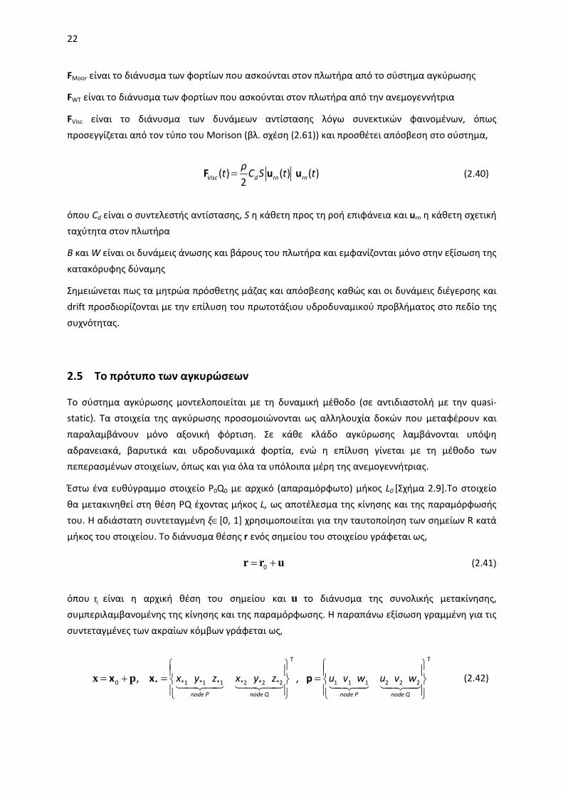
22

FMoor είναι το διάνυσμα των φορτίων που ασκούνται στον πλωτήρα από το σύστημα αγκύρωσης

FWT είναι το διάνυσμα των φορτίων που ασκούνται στον πλωτήρα από την ανεμογεννήτρια

FVisc είναι το διάνυσμα των δυνάμεων αντίστασης λόγω συνεκτικών φαινομένων, όπως προσεγγίζεται από τον τύπο του Morison (βλ. σχέση (2.61)) και προσθέτει απόσβεση στο σύστημα,

=( ) ( ) ( )2Visc d rn rnρt C S t tF u u

(2.40)

όπου Cd είναι ο συντελεστής αντίστασης, S η κάθετη προς τη ροή επιφάνεια και urn η κάθετη σχετική ταχύτητα στον πλωτήρα

B και W είναι οι δυνάμεις άνωσης και βάρους του πλωτήρα και εμφανίζονται μόνο στην εξίσωση της κατακόρυφης δύναμης

Σημειώνεται πως τα μητρώα πρόσθετης μάζας και απόσβεσης καθώς και οι δυνάμεις διέγερσης και drift προσδιορίζονται με την επίλυση του πρωτοτάξιου υδροδυναμικού προβλήματος στο πεδίο της συχνότητας.

2.5 Το πρότυπο των αγκυρώσεων

Το σύστημα αγκύρωσης μοντελοποιείται με τη δυναμική μέθοδο (σε αντιδιαστολή με την quasi-static). Τα στοιχεία της αγκύρωσης προσομοιώνονται ως αλληλουχία δοκών που μεταφέρουν και παραλαμβάνουν μόνο αξονική φόρτιση. Σε κάθε κλάδο αγκύρωσης λαμβάνονται υπόψη αδρανειακά, βαρυτικά και υδροδυναμικά φορτία, ενώ η επίλυση γίνεται με τη μέθοδο των πεπερασμένων στοιχείων, όπως και για όλα τα υπόλοιπα μέρη της ανεμογεννήτριας.

Έστω ένα ευθύγραμμο στοιχείο P0Q0 με αρχικό (απαραμόρφωτο) μήκος L0 [Σχήμα 2.9].Το στοιχείο θα μετακινηθεί στη θέση PQ έχοντας μήκος L, ως αποτέλεσμα της κίνησης και της παραμόρφωσής του. Η αδιάστατη συντεταγμένη ξ∈[0, 1] χρησιμοποιείται για την ταυτοποίηση των σημείων R κατά μήκος του στοιχείου. Το διάνυσμα θέσης r ενός σημείου του στοιχείου γράφεται ως,

= +r r u0 (2.41)

όπου 0r είναι η αρχική θέση του σημείου και u το διάνυσμα της συνολικής μετακίνησης, συμπεριλαμβανομένης της κίνησης και της παραμόρφωσης. Η παραπάνω εξίσωση γραμμένη για τις συντεταγμένες των ακραίων κόμβων γράφεται ως,

= + = =

x p(( (( (( ((

TT

0 * *1 *1 *1 *2 *2 *2 1 1 1 2 2 2, , node P node Q node P node Q

x y z x y z u v w u v wx x p

(2.42)

23

όπου x* είναι η θέση του κόμβου είτε στην αρχική θέση (*=0) είτε στην τρέχουσα παραμορφωμένη θέση (*=’ ‘) και p είναι το διάνυσμα των μετακινήσεων (κινήσεις και παραμορφώσεις).

Σχήμα 2.9: Κινηματική του στοιχείου (truss element)

Θωρώντας γραμμικά στοιχεία και ως βαθμούς ελευθερίας τις μετακινήσεις των 2 ακραίων κόμβων, η μετακίνηση ενός ενδιάμεσου σημείου κατά μήκος του στοιχείου γράφεται ως,

= ⋅u Ν p (2.43)

(1- ) 0 0 0 00 (1- ) 0 0 00 0 (1- ) 0 0

ξ ξξ ξ

ξ ξ

=

N (2.44)

όπου N είναι ο πίνακας με στοιχεία τις συναρτήσεις μορφής (shape functions). Αντίστοιχα οι συντεταγμένες ενός σημείου R0 στην αρχική γεωμετρία περιγράφονται με βάση τις γνωστές συντεταγμένες των κόμβων P0 και Q0,

0 0= ⋅r Ν x (2.45)

Η τροπή ορίζεται ως,

−= = − = + + = ⋅2 2 20

2 1 2 1 2 10 0

1, ( - ) ( - ) ( - ) TL L Lε L x x y y z z D DL L

x x

(2.46)

ενώ τα Dx* και Dp εκφράζονται ως,

0P

0R

ξ

0α

0α

0r

0dr

nP

nQ

nR

ξnα

nα

nr

ndr

u

initial positionfinal position

0Q

24

= = ⋅

= = ⋅

T* *2 *1 *2 *1 *2 *1 *

T2 1 2 1 2 1

{ - , - , - }

{ - , - , - }

D x x y y z z

D u u v v w w

x A x

p A p (2.47)

και ο πίνακας A ορίζεται ως,

=

-1 0 0 1 0 0 0 -1 0 0 1 0 0 0 -1 0 0 1

A

(2.48)

Η μεταβολή του μήκους δL ορίζεται ως,

= ⋅ = ⋅ ⋅ =T Tδ(D ) , D /δL δ Lt x t A p t x (2.49)

όπου t είναι το μοναδιαίο διάνυσμα παράλληλο προς το στοιχείο.

Χρησιμοποιώντας την παραπάνω σχέση η μεταβολή της τροπής δε ορίζεται ως,

= = ⋅ ⋅-1 T0

0

δδLδε LL

t A p

(2.50)

ενώ η μεταβολή του μοναδιαίου εφαπτομενικού διανύσματος δt είναι,

= ⋅ ⋅ ⋅T1 { - } δδL

t I t t A p

(2.51)

με I τον μοναδιαίο 3x3 πίνακα.

Οι δυναμικές εξισώσεις του στοιχείου παράγονται από την εφαρμογή της αρχής δυνατών έργων,

( )− − =∫ ∫ u q q

0 0

Τ 0e i

V L

σ δε dV δ d

(2.52)

Όπου δu η δυνατή μετακίνηση, iq και eq τα αδρανειακά και εξωτερικά φορτία (υδροδυναμικά, βαρυτικά και άνωση) ανά μονάδα μήκους, σ και δε η αξονική τάση και μεταβολή της τροπής που οφείλεται στην αλλαγή μήκους του στοιχείου και V0 και L0 ο όγκος και το μήκος του απαραμόρφωτου στοιχείου.

Με εφαρμογή του νόμου του Hooke καθορίζεται η τάση σ ως,

=σ E ε (2.53)

25

όπου E είναι το μέτρο ελαστικότητας του Young

Εισάγοντας τις σχέσεις για την τάση (2.53) και τη μεταβολή της τροπής (2.50) στην αρχή δυνατών έργων (2.52) και θεωρώντας τη διατομή σταθερή και ίση με A0 έτσι ώστε dV = A0 dl, προκύπτει το σύστημα των μη γραμμικών δυναμικών εξισώσεων,

( )1

T T0 0

0

e i L dξ EA ε− = ⋅ =∫N q q A t f (2.54)

Οι μη γραμμικές εξισώσεις (2.54) γραμμικοποιούνται γύρω από μια θέση αναφοράς 0p και στη συνέχεια λύνονται επαναληπτικά μέχρι τα σφάλματα να γίνουν αρκούντως μικρά, με βάση το κριτήριο σύγκλισης. Το ανάπτυγμα Taylor της έκφρασης των εσωτερικών φορτίων f γύρω από το

0p δίνει,

( ) ( )0 00 0 tδ δ

∂= + + ⋅ = + + ⋅

∂f

f f x p p f x p K pp

(2.55)

Με χρήση των (2.50) και (2.51) προκύπτει το μητρώο δυσκαμψίας Kt [12],

= ⋅ − ⋅ ⋅ + ⋅ ⋅ ⋅Τ T Τ T

0

{ } { }tEA EAεL L

K Α I t t A Α t t A

(2.56)

Αν η πυκνότητα του υλικού ρ θεωρηθεί σταθερή κατά μήκος του στοιχείου οι αδρανειακοί όροι ορίζονται ως,

( ) ( )( )= = = ⋅∫ ∫ ∫

1 1 1T i T T

0 0 0 0 00 0 0

L dξ ρA L dξ ρA L dξN q N u N N p Μ p

(2.57)

όπου η ποσότητα ρΑ0 εκφράζει την ανά μονάδα μήκους μάζα του στοιχείου. Με αναλυτική ολοκλήρωση προκύπτει το μητρώο μάζας ως,

=

0 0 0 0

0 0 0 0 0 0

0 0

0 0 0 0

0 0 0 0

0 0 0 0

/ 3 0 0 / 6 0 00 / 3 0 0 / 6 / 60 0 / 3 0 0 0

/ 6 0 0 / 3 0 00 / 6 0 0 / 3 00 0 / 6 0 0 / 3

ρA L ρA LρA L ρA L ρA L

ρA LρA L ρA L

ρA L ρA LρA L ρA L

M

(2.58)

Το διάνυσμα των εξωτερικών φορτίων που συμβολίζεται με Q, αποτελείται από τα υδροδυναμικά και τα υδροστατικά φορτία (άνωση) του στοιχείου, τη δύναμη εξαιτίας της βαρύτητας, καθώς και

26

την αντίδραση του εδάφους στην περίπτωση επαφής με το βυθό. Έτσι αναλύονται στις παρακάτω συνιστώσες,

1 1 1 2T T T T *

0 00 0 0 1

le

zw H SB zw H SBl

L dξ L dξ Ldξ L dξ= = + + = + +∫ ∫ ∫ ∫Q N q Q Q Q N q N q N q (2.59)

Θεωρώντας το βάρος ανά μονάδα μήκους της αγκύρωσης στο νερό Fzw λαμβάνονται ταυτόχρονα υπόψη οι επιδράσεις του βάρους και της άνωσης, ενώ αναλυτική ολοκλήρωση του Qzw δίνει,

0

0

00

/ 200

/ 2

zwzw

zw

F L

F L

− = −

Q (2.60)

Τα υδροδυναμικά φορτία ανά μονάδα μήκους του στοιχείου L υπολογίζονται με τον τύπο του Morison [13],

Mor

/ 0.5 | | ( )n a n a n d n n

Froude Krylov Diffraction Added mass Drag term

dF dL ρ dV a C ρ dV a C ρ dV q C ρ dS u q u q= + − + − −

(( (( (( ((((((((((

(2.61)

όπου:

a και u είναι η συνολική επαγόμενη επιτάχυνση και ταχύτητα όπως προκύπτουν πχ από κλειστές σχέσεις πχ από τη θεωρία των αρμονικών κυμάτων Airy ή από τη θεωρία των stream function κυμάτων. Το σύμβολο n δηλώνει την κάθετη συνιστώσα του αντίστοιχου διανύσματος στο στοιχείο.

, q q είναι η συνολική (κίνηση και παραμόρφωση) επιτάχυνση και ταχύτητα του στοιχείου

Ca και Cd είναι οι συντελεστές πρόσθετης μάζας και αντίστασης που υπόκεινται σε βαθμονόμηση

dV και dS είναι ο απειροστός όγκος και επιφάνεια κάθετη στη ροή (πχ για ένα κυλινδρικό στοιχείο ακτίνας R ισχύει dV=πRP

2PdL και dS=2RdL).

ρ είναι η πυκνότητα του ρευστού νερού

Όπως φαίνεται στην (2.61) η συνολική υδροδυναμική δύναμη είναι το άθροισμα της δύναμης του κύματος Froude Krylov, της δύναμης περίθλασης, της δύναμης λόγω πρόσθετης μάζας και της δύναμης αντίστασης. Ο τύπος του Morison παρέχει αξιόπιστα αποτελέσματα αν λ/D > 5, όπου λ το μήκος κύματος και D ένα χαρακτηριστικό μήκος π.χ. η διάμετρος του στοιχείου, ενώ η κινηματική του κύματος υπολογίζεται στο κέντρο του κάθε στοιχείου για κάθε διατομή.

27

Η κάθετη συνιστώσα ενός διανύσματος Χ γράφεται ως,

= − = − ⋅ = − ⋅T T ( ) ( ) n tX X X X t X t I t t X (2.62)

όπου t είναι το μοναδιαίο εφαπτομενικό διάνυσμα στο στοιχείο και I ο μοναδιαίος πίνακας 3x3. Τα σύμβολα n και t δηλώνουν την κάθετη και την εφαπτομενική διεύθυνση του διανύσματος. Η μεταβολή της υδροδυναμικής δύναμης γράφεται ως,

T TMor ( ) 0.5 | | ( )a d nδ C ρ dV δ C ρ dS u q δ= − − ⋅ − − − ⋅F I t t q I t t q (2.63)

Από τη σχέση (2.63) προκύπτουν πρόσθετα μητρώα μάζας και απόσβεσης όταν μεταφερθεί στο πρώτο μέρος των εξισώσεων που διευκολύνουν τη σύγκλιση του μη γραμμικού συστήματος κατά τη διάρκεια των επαναλήψεων. Σημειώνεται πως η μεταβολή του μοναδιαίου t δεν συμπεριλήφθηκε στην παραπάνω εξίσωση.

Η ολοκλήρωση των υδροδυναμικών φορτίων (2ος όρος στη (2.59)) γίνεται αριθμητικά στη στιγμιαία θέση και λαμβάνοντας υπόψη το τρέχον μήκος L του στοιχείου.

Ακολουθώντας παρόμοια λογική λαμβάνονται υπόψη η συνεισφορά της επαφής του κλάδου αγκύρωσης με το βυθό καθώς και επιπλέον όροι που μοντελοποιούν τη δομική απόσβεση του υλικού. Αυτό οδηγεί σε πρόσθετα μητρώα απόσβεσης και δυσκαμψίας στο πρώτο μέλος των δυναμικών εξισώσεων συνοδευόμενα με τους αντίστοιχους όρους δυνάμεων στο δεύτερο μέλος (για λεπτομέρειες βλ. το αγγλικό κείμενο).

Η πλήρης μορφή του γραμμικοποιημένου συστήματος των δυναμικών εξισώσεων για ένα στοιχείο είναι,

0 0 0( + ) ( + + ) ( + + )H d H sb t sb d dδ δ δ⋅ + ⋅ + ⋅ = − ⋅ − −M M p C C C p K K K p Q M p f Q (2.64)

όπου,

M είναι το μητρώο μάζας

f, Kt, είναι το διάνυσμα των εσωτερικών δυνάμεων και το αντίστοιχο μητρώο δυσκαμψίας

MH και CH είναι πρόσθετα μητρώα μάζας και απόσβεσης προερχόμενα από τη γραμμικοποίηση των υδροδυναμικών φορτίων από τον τύπο του Morison

Cd, Kd, Qd είναι μητρώα απόσβεσης και δυσκαμψίας και διάνυσμα φορτίου προερχόμενα από τον υπολογισμό της δομικής απόσβεσης του υλικού του κλάδου αγκύρωσης

Csb, Ksb είναι τα αντίστοιχα μητρώα απόσβεσης και δυσκαμψίας προερχόμενα από την μοντελοποίηση της επαφής του κλάδου αγκύρωσης με το βυθό

Q είναι το συνολικό διάνυσμα των εξωτερικών φορτίων που συμπεριλαμβάνει όρους βαρύτητας, άνωσης, υδροδυναμικών φορτίων και την αντίδραση του βυθού λόγω επαφής

28

Η παραπάνω εξίσωση αφορά στο κάθε στοιχείο, ενώ για την μοντελοποίηση του συνολικού κλάδου αγκύρωσης, τα τοπικά μητρώα που παράγονται τοποθετούνται κατάλληλα στα αντίστοιχα καθολικά όπως γίνεται παραδοσιακά στη μέθοδο των πεπερασμένων στοιχείων [14]. Η διαδικασία δεν απαιτεί μετατροπή συστημάτων συντεταγμένων, αφού στη συγκεκριμένη ανάλυση οι εξισώσεις του κάθε στοιχείου είναι εκφρασμένες στο καθολικό σύστημα.

2.6 Η σύνθεση για το συζευγμένο σύστημα

Η σύνθεση όλων των επιμέρους εξισώσεων προκύπτει ως εξής:

1. Αρχικά για κάθε συνιστώσα υπολογίζονται τα μητρώα μάζας, απόσβεσης και δυσκαμψίας καθώς και τα διανύσματα εξωτερικής φόρτισης. Τα στοιχεία αυτά εισάγονται στο τελικό σύστημα με βάση μια προκαθορισμένη ακολουθία διαδοχής που συμφωνεί με τη ροή φόρτισης (στην περίπτωση μιας ανεμογεννήτριας η ακολουθία αυτή ξεκινά από τα πτερύγια και συνεχίζει με το αξονικό σύστημα, τον πύργο, τη βάση στήριξης και τελειώνει με τις αγκυρώσεις). Στο τέλος του βήματος αυτού το σύστημα παρουσιάζεται κατά τμήματα διαγώνιο (block diagonal) [Σχήμα 2.10].

2. Στη συνέχεια εισάγονται οι κινηματικές συνθήκες που σχετίζονται με τους βαθμούς ελευθερίας q. Οι όροι αυτοί συμπληρώνουν το δεξί τμήμα των μητρών του συστήματος [Σχήμα 2.10].

3. Στο 3ο βήμα συμπληρώνονται οι δυναμικές συνθήκες που θα εμφανίζονται στο αριστερό κάτω μέρος του διαγωνίου τμήματος των μητρώων και σχετίζονται με τη μεταφορά των φορτίων μεταξύ των σωμάτων.

4. Τέλος το σύστημα συμπληρώνεται με τις εξισώσεις των βαθμών ελευθερίας q. Σ’ αυτές περιλαμβάνονται είτε απλές σχέσεις αντιστοίχισης (π.χ. ενός ελαστικού βαθμού ελευθερίας με τον αντίστοιχο κινηματικό) είτε δυναμικές εξισώσεις όπως στην περίπτωση των κινήσεων του πλωτήρα καθώς και των βαθμών ελευθερίας του συστήματος ελέγχου (γωνία αζιμουθίου του αξονικού συστήματος ή γωνία βήματος των πτερυγίων).

Το τελικό σύστημα έχει τη συνήθη μορφή για μηχανικά δυναμικά συστήματα,

+ + =MX CX KX Q (2.65)

όπου X είναι το διάνυσμα των αγνώστων. Τα μητρώα μάζας, απόσβεσης και δυσκαμψίας, M, C, K καθώς και η εξωτερική φόρτιση Q εξαρτώνται από το X και τις χρονικές παραγώγους του οπότε το τελικό σύστημα είναι μη-γραμμικό. Για την επίλυση του ακολουθείται η ίδια διαδικασία γραμμικοποίησης με αυτή που υιοθετήθηκε για τα q. Οπότε αν = +ο δX X X , για καθένα από τα M, C, K και Q, θα ισχύει,

29

= + ∂ ⋅ + ∂ ⋅ + ∂ ⋅Χ Χ Χ( , , ) ο ο ο οδ δ δM X X X M M X M X M X

(2.66)

Όπου ο δείκτης «ο» συμβολίζει υπολογισμούς με βάση το γνωστό οX και τις παραγώγους του. Εισάγοντας τις εκφράσεις γραμμικοποίησης, το σύστημα θα γράφεται παρόμοια αλλά με τα αντίστοιχα μητρώα M, C, K και Q που προκύπτουν από τη γραμμικοποίηση ως προς τις διορθώσεις δX ,

+ + =δ δ δM X C X K X Q

(2.67)

Το τελικό πλέον σύστημα ολοκληρώνεται στο χρόνο χρησιμοποιώντας ένα 2ης τάξης σχήμα Newmark. Καθώς η επίλυση γίνεται ως προς τις διορθώσεις δX απαιτούνται επαναλήψεις μέχρι η νόρμα του δX γίνει επαρκώς μικρή.

Σχήμα 2.10: Μορφολογία των μητρών του τελικού συστήματος

31

Κεφάλαιο 3.

Συζευγμένη ύδρο-σέρβο-αέρο-ελαστική ανάλυση: Αποτελέσματα Στο παρόν κεφάλαιο παρουσιάζονται αποτελέσματα της συζευγμένης ύδρο-σέρβο-αέρο-ελαστικής μεθόδου hGAST για την NREL 5MW ανεμογεννήτρια αναφοράς τοποθετημένη στον ημι-βυθισμένο πλωτήρα του OC4, συγκρίνοντας με προλέξεις αντίστοιχων υπολογιστικών εργαλείων.

3.1 Ο ημι-βυθισμένος πλωτήρας από τη φάση II του OC4

3.1.1 Εισαγωγή

Στη φάση ΙΙ του OC4 [15], η ανεμογεννήτρια αναφοράς τοποθετείται στον DeepCwind ημι-βυθισμένος πλωτήρα με συμβατικούς κλάδους αγκύρωσης στα 200m βάθος. Το βύθισμα του πλωτήρα είναι 20m, ενώ εκτείνεται 12m πάνω από τη μέση στάθμη της θάλασσας. Ο πλωτήρας αποτελείται από τον κεντρικό κύλινδρο διαμέτρου 6.5m όπου επάνω εδράζεται η μηχανή και 3 έκκεντρους κυλίνδρους με διάμετρο 24m στη βάση τους και 12m στο επάνω μέρος [Σχήμα 3.1]. Οι έκκεντροι κύλινδροι είναι μερικώς γεμισμένοι με νερό. Η κατασκευή συγκρατείται από 15 οριζόντιες και διαγώνιες ράβδους. Λεπτομερής περιγραφή της κατασκευής δίνεται στα [16], [17] και των υπό εξέταση περιπτώσεων στο [15].

Σχήμα 3.1: Ο ημι-βυθισμένος πλωτήρας του OC4 [εικόνα από [16]]

32

Στις επερχόμενες συγκρίσεις από όλους τους συμμετέχοντες παρουσιάζονται τα αποτελέσματα 3 κωδίκων που θα αναφέρονται ως Code1, Code2 και Code3.

Όλοι οι κώδικες χρησιμοποιούν τη μέθοδο του δίσκου ορμής για τον υπολογισμό των αεροδυναμικών φορτιών. Επιπλέον οι κώδικες hGAST, Code1 και Code4 είναι κώδικες FEM και επίσης χρησιμοποιούν δυναμική μέθοδο μοντελοποίησης των αγκυρώσεων, ενώ οι κώδικες Code2 και Code3 είναι modal κώδικες που βασίζονται στη μείωση των βαθμών ελευθερίας με βάση τις ιδιομορφές της κατασκευής και χρησιμοποιούν quasi-static μοντελοποίηση των αγκυρώσεων. Τέλος οι κώδικες Code1 και Code2 χρησιμοποιούν τον τύπο του Morison για τον υπολογισμό των υδροδυναμικών δυνάμεων, ενώ οι κώδικες Code3 και Code4 την επίλυση του υδροδυναμικού προβλήματος ιδανικού ρευστού στο πεδίο συχνότητας. Ο κώδικας hGAST χρησιμοποιεί και τις 2 μεθόδους και συγκεκριμένα οι συνεχείς μπλε καμπύλες αντιστοιχούν στη θεωρία ιδανικού ρευστού, ενώ οι 2 διακεκομμένες στον τύπο του Morison.

Στο hGAST τα κυματικά χαρακτηριστικά υπολογίζονται λαμβάνοντας υπόψη τη στιγμιαία θέση του πλωτήρα που εν συντομία αναφέρεται ως (IP). Η διαφοροποίηση μεταξύ των 2 διακεκομμένων καμπύλων αφορά στον καθ’ ύψος υπολογισμό των κυματικών χαρακτηριστικών. Οι καμπύλες με τις τελείες υπολογίζουν τα κυματικά χαρακτηριστικά στη μέση στάθμη της θάλασσας (MSL), ενώ οι καμπύλες με τις παύλες έως τη στιγμιαία ανύψωση της ελεύθερης επιφάνειας (IWL) με χρήση της μεθόδου Wheeler’s stretching.

3.1.2 Ιδιοσυχνότητες

Στον Πίνακα 3.3 παρουσιάζονται οι ιδιοσυχνότητες της συζευγμένης κατασκευής λαμβάνοντας υπόψη τη βαρύτητα και τη δομική απόσβεση των σωμάτων. Γενικώς παρατηρείται καλή συμφωνία που πιστοποιεί και τη συνεπή μοντελοποίηση της ανεμογεννήτριας και της δυναμικής του πλωτήρα. Οι ιδιοσυχνότητες των 6 κινήσεων του πλωτήρα είναι σε καλή συμφωνία. Συγκεκριμένα η έκδοση του hGAST με τον τύπο του Morison [hGASTm] και ο Code1 προβλέπουν ελάχιστα μικρότερες surge και sway ιδιοσυχνότητες στα 0.0088Hz, αντί 0.0093Hz που προβλέπουν οι υπόλοιποι κώδικες συμπεριλαμβανομένου και του hGAST με χρήση της θεωρίας ιδανικού ρευστού [hGASTp]. Επίσης οι δύο εκδόσεις του hGAST προβλέπουν λίγο μεγαλύτερες roll και pitch ιδιοσυχνότητες, ενώ ο Code4 προβλέπει αυξημένες ιδιοσυχνότητες πύργου και αξονικού συστήματος. Οι πρώτες ιδιοσυχνότητες των πτερυγίων είναι σε καλή συμφωνία με εξαίρεση τον Code1 που προβλέπει μικρότερες ασύμμετρες ιδιοσυχνότητες στην edgewise κατεύθυνση.

Οι modal κώδικες (Code2, Code3) υπερεκτιμούν τις 2ες καμπτικές ιδιοσυχνότητες του πύργου και τη 2η ασύμμετρη flapwise yaw ιδιοσυχνότητα των πτερυγίων [Πίνακας 3.3] σε σχέση με τους FEM κώδικες (hGAST, Code1, Code4). Παραδείγματος χάρη ο Code3 προβλέπει τη 2η πλευρική ιδιοσυχνότητα του πύργου στα 5Hz, ενώ οι υπόλοιποι κώδικες περίπου στα 3.5Hz. Επίσης οι κώδικες Code2 και Code3 υπερεκτιμούν την ασύμμετρη flapwise yaw ιδιοσυχνότητα στα ~1.9Hz αντί στα 1.68Hz που προβλέπεται από το hGAST και ο Code4 και τα 1.61Hz από τον Code1.

33

Η επίδραση που έχουν στις ιδιοσυχνότητες της συζευγμένης κατασκευής οι διαφορετικές μέθοδοι υπολογισμού των υδροδυναμικών φορτίων αποτιμάται από τη σύγκριση των 2 διαφορετικών εκδόσεων του hGAST. Οι ιδιοσυχνότητες της ανεμογεννήτριας παραμένουν αμετάβλητες, ενώ η έκδοση με χρήση του τύπου του Morison, που είναι σε συμφωνία με τον Code1, προβλέπει λίγο μικρότερες ιδιοσυχνότητες για τις 6 κινήσεις του πλωτήρα.

Πίνακας 3.1: Σύγκριση ιδιοσυχνοτήτων [Hz] για το συζευγμένο σύστημα του ημι-βυθισμένου πλωτήρα του OC4

Mode description hGASTp hGASTm Code1 Code2 Code3 Code4

Platform surge 0.0093 0.0088 0.0086 0.0094 0.0093 0.0093

Platform sway 0.0093 0.0088 0.0088 0.0092 0.0093 0.0093

Platform heave 0.0583 0.0574 0.0573 0.0581 0.0581 0.0556

Platform roll 0.0413 0.0404 0.0384 0.0397 0.0392 0.0385

Platform pitch 0.0413 0.0404 0.0384 0.0397 0.0392 0.0385

Platform yaw 0.0131 0.0126 0.0132 0.0136 0.0132 0.0127

1st P tower fore-aft 0.424 0.423 0.424 0.425 0.426 0.465

1st P tower side-to-side 0.415 0.414 0.415 0.417 0.418 0.458

1st P drivetrain torsion 0.622 0.622 0.608 0.623 0.628 0.672

1st P blade collective flap 0.717 0.717 0.686 0.706 0.704 0.692

1st P asymmetric flapwise pitch 0.677 0.677 0.618 0.641 0.670 0.664

1st P asymmetric flapwise yaw 0.639 0.639 0.648 0.670 0.667 0.635

1st P asymmetric edgewise pitch 1.079 1.079 1.002 1.080 1.079 1.095

1st P asymmetric edgewise yaw 1.092 1.092 1.015 1.091 1.092 1.103

2nd tower fore-aft 3.417 3.415 3.314 3.864 3.898 3.405

2nd tower side-to-side 3.540 3.537 3.494 3.437 5.012 3.875

2nd collective flap 2.000 2.000 1.840 1.972 2.023 1.928

2nd asymmetric flapwise pitch 1.876 1.876 1.739 1.718 1.914 1.829

2nd asymmetric flapwise yaw 1.681 1.681 1.609 1.870 1.934 1.672

3.1.3 Χρονοσειρές

Στη συγκεκριμένη παράγραφο παρουσιάζονται συγκρίσεις χρονοσειρών από την περίπτωση dlc3.1 της 2ης φάσης του OC4, που αντιστοιχεί σε συνθήκες ομοιόμορφου ανέμου 8m/s και Airy κύματος ύψους 6m και περιόδου 10s σε βάθος 200m. Η κατεύθυνση διάδοσης του κύματος και του ανέμου συμπίπτει με τον άξονα x. Όλοι οι βαθμοί ελευθερίας είναι ενεργοποιημένοι και το σύστημα ελέγχου λειτουργεί στην περιοχή των μεταβλητών στροφών.

34

Στο Σχήμα 3.2 οι 6 κινήσεις του πλωτήρα είναι γενικώς σε καλή συμφωνία. Οι κινήσεις surge, heave και pitch διεγείρονται άμεσα από το κύμα και είναι εμφανής η συχνότητά του των 10s, ενώ στις κινήσεις sway, roll και yaw εμφανίζεται μειωμένη κυματική διέγερση λόγω σύζευξης. Όπως αναφέρθηκε στο [3] διαφορές στη μέση τιμή της surge κίνησης προκαλείται από μη-γραμμικούς υδροδυναμικούς όρους (drift effects). Στην περίπτωση εφαρμογής του τύπου του Morison εμφανίζονται όταν τα φορτία υπολογίζονται στη στιγμιαία θέση του σώματος (IP: instantaneous position) ή/και όταν τα κυματικά χαρακτηριστικά υπολογίζονται στο στιγμιαίο βρεχόμενο ύψος (IWL: instantaneous water level). Στην περίπτωση χρήσης της θεωρίας ιδανικού ρευστού (potential theory) μη-γραμμικά φαινόμενα λαμβάνονται υπόψη όταν συμπεριλαμβάνονται όροι 2ης τάξης π.χ. μέσω του τύπου του Newman [11]. Ο κώδικας Code3 και η βασιζόμενη στη θεώρηση δυναμικού (potential) έκδοση του hGAST που εφαρμόζουν την γραμμική θεωρία (1ης τάξης) προβλέπουν όμοια surge κίνηση. Σημειώνεται πως η μέση τιμή της surge κίνησης δεν αναμένεται να επηρεάσει κάποιο άλλο σήμα. Η pitch κίνηση είναι σε καλή συμφωνία και η μέση τιμή της καθορίζεται με συνέπεια από την αεροδυναμική ώση. Ο κώδικας Code2 προλέγει περίπου 0.5ο μεγαλύτερο εύρος. Παρόλο που οι κινήσεις sway, roll και yaw λαμβάνουν πολύ μικρές απόλυτες τιμές η συμφωνία μεταξύ των κωδίκων είναι καλή. Οι κινήσεις αυτές είναι λιγότερο αποσβενύμενες οπότε σε ορισμένες περιπτώσεις δεν έχει επέλθει σύγκλιση σε περιοδική λύση, γεγονός που ενδεχομένως εξηγεί τις διαφορές στη sway κίνηση. Η θετική γωνία roll σωστά καθορίζεται από τη ροπή του δρομέα. Η κίνηση heave είναι επίσης σε πολύ καλή συμφωνία με τον Morison κώδικα Code2 να προβλέπει μεγαλύτερο εύρος. Συγκρίνοντας τις 3 εκδοχές του κώδικα hGAST μικρές διαφορές εμφανίζονται στην surge και την pitch κίνηση. Οι δύο εκδόσεις που χρησιμοποιούν τον τύπο του Morison προβλέπουν μικρότερη μέση τιμή κατά 0.3-0.4m στη surge κίνηση και περίπου 0.2ο μεγαλύτερη μέση τιμή στην pitch κίνηση σε σχέση με την potential έκδοση, ως αποτέλεσμα των προαναφερθέντων μη-γραμμικών φαινομένων.

Στο Σχήμα 3.3 συγκρίνεται η τάση των κλάδων αγκύρωσης 1 και 2 στο σημείο πρόσδεσής τους με τον πλωτήρα. Η μέση τιμή των σημάτων είναι σε πλήρη συμφωνία, ενώ είναι εμφανής η διαφορά φάσης και η εμφάνιση επιπλέον υψίσυχνων συχνοτήτων στους κώδικες που χρησιμοποιούν δυναμική μέθοδο προσομοίωσης του συστήματος αγκύρωσης. Οι διαφορές αυτές δεν επηρεάζουν τις κινήσεις του πλωτήρα όμως πιθανότατα θα οδηγήσουν σε διαφορετικά κοπωτικά φορτία στους κλάδους αγκύρωσης [3] και κατ’ επέκταση σε ενδεχόμενο διαφορετικού σχεδιασμού τους.

Στο Σχήμα 3.4, συγκρίνονται οι παραμορφώσεις στην κορυφή του πύργου και οι αντίστοιχες ροπές στη βάση του. Όπως αναμένεται, φορτία και παραμορφώσεις στην ίδια διεύθυνση έχουν παρόμοια συμπεριφορά. Τα σήματα στην εγκάρσια διεύθυνση καθορίζονται από τη ροπή του δρομέα και άρα εμμέσως από τον controller. Κυρίως διεγείρεται η 1η ιδιοσυχνότητα του πύργου (περίοδος περίπου 2.5sec) ενώ είναι επίσης εμφανής η συχνότητα του κύματος μέσω σύζευξης με τις sway και roll κινήσεις. Οι μέσες τιμές είναι σε καλή σύμπτωση, ενώ εξαιτίας της απουσίας διέγερσης στην εγκάρσια διεύθυνση το εύρος των σημάτων είναι πολύ ευαίσθητο στη μοντελοποίηση της απόσβεσης, γεγονός που πιθανώς εξηγεί τις διαφορές. Τα σήματα στη διαμήκη κατεύθυνση επηρεάζονται κυρίως από το κύμα. Η πρόβλεψη διεγέρσεων με μεγαλύτερα εύρη σε ορισμένους

35

κώδικες που κάνουν χρήση του τύπου του Morison εξηγείται από τα αντίστοιχα μεγαλύτερα εύρη της pitch κίνησης.

Στο Σχήμα 3.5, συγκρίνονται η ροπή στον άξονα και η καμπτική ροπή στο σημείο του κυρίως εδράνου. Οι διαφορές στη ροπή είναι μικρότερες από 5% αλλά μεγεθύνονται από την κλίμακα του διαγράμματος. Οι modal κώδικες προβλέπουν αυξημένες υψίσυχνες συχνότητες που φανερώνουν διαφορά στη μοντελοποίηση της απόσβεσης, του αξονικού συστήματος ή του φίλτρου του controller (drive train damper). Η καμπτική ροπή είναι σε πολύ καλή συμφωνία.

Στο Σχήμα 3.6, παρουσιάζεται η παραγόμενη ηλεκτρική ισχύς και η γωνιακή ταχύτητα περιστροφής του δρομέα που εμφανίζουν παρόμοια συμπεριφορά. Η ηλεκτρική ισχύς επηρεάζεται άμεσα από την ταχύτητα περιστροφής που με τη σειρά της επηρεάζεται από την pitch κίνηση του πλωτήρα. Οι συγκρίσεις είναι σε καλή συμφωνία, ενώ οι διαφορές ενισχύονται από την κλίμακα των διαγραμμάτων. Η περίοδος του κύματος φαίνεται στην ταχύτητα περιστροφής που αναδεικνύει την ανάγκη ανάπτυξης εξελιγμένων συστημάτων ελέγχου.

Στο Σχήμα 3.7, συγκρίνονται οι ροπές στη ρίζα του πτερυγίου και οι αντίστοιχες παραμορφώσεις στο άκρο του. Όπως και στα μεγέθη του πύργου, φορτία και παραμορφώσεις στην ίδια κατεύθυνση παρουσιάζουν παρόμοια συμπεριφορά. Τα μεγέθη στο επίπεδο του δρομέα (in-plane) καθορίζονται από το βάρος και είναι σχεδόν πανομοιότυπα, ενώ είναι εμφανής η περίοδος της περιστροφής του δρομέα περίπου στα 6sec. Οι προβλέψεις της καμπτικής ροπής και της αντίστοιχης παραμόρφωσης στην διαμήκη κατεύθυνση κάθετα στο επίπεδο το δρομέα (out-of-plane) είναι συνεπείς, αν και εμφανίζονται μικρές διαφορές. Επειδή η διαμήκης κατεύθυνση συμπίπτει με αυτή της διάδοσης του κύματος, παρατηρούνται αυξημένα εύρη εξαιτίας της pitch κίνησης. Επιπλέον είναι ταυτόχρονα εμφανείς και οι δύο συχνότητες περιστροφής και κύματος. Η ροπή στρέψης είναι παρόμοια, με το hGAST να προβλέπει το μικρότερο εύρος. Οι μεγαλύτερες διαφορές παρουσιάζονται στη γωνία στρέψης στο άκρο του πτερυγίου. Οι κώδικες hGAST και Code1 που λαμβάνουν υπόψη τους μη-γραμμικά γεωμετρικά φαινόμενα εξαιτίας μεγάλων παραμορφώσεων [18] προβλέπουν ίδια φάση, αλλά με διαφορετική μέση τιμή και εύρος.

36

(α) Surge κίνηση του πλωτήρα [m]

(δ) Roll κίνηση του πλωτήρα [deg]

(β) Sway κίνηση του πλωτήρα [m]

(ε) Pitch κίνηση του πλωτήρα [deg]

(γ) Heave κίνηση του πλωτήρα [m]

(στ) Yaw κίνηση του πλωτήρα [deg]

Σχήμα 3.2: Σύγκριση των κινήσεων του πλωτήρα: Airy κύμα H=6m, T=10s, ομοιόμορφος άνεμος 8m/s).

**hGAST μπλε συνεχής γραμμή: potential theory, μπλε διακεκομμένη γραμμή (τελείες): Morison IP+MSL, μπλε διακεκομμένη γραμμή (παύλες): Morison IP+IWL.

37

(α) Τάση του κλάδου αγκύρωσης 1 [kN]

(β) Τάση του κλάδου αγκύρωσης 2 [kN]

Σχήμα 3.3: Σύγκριση της τάσης των κλάδων αγκύρωσης 1 και 2: Airy κύμα H=6m, T=10s, ομοιόμορφος άνεμος 8m/s).

(α) Πλευρική ροπή στη βάση [kNm]

(γ) Πλευρική παραμόρφωση στην κορυφή [m]

(β) Διαμήκης ροπή στη βάση [kNm]

(δ) Διαμήκης παραμόρφωση στην κορυφή [m]

Σχήμα 3.4: Σύγκριση των ροπών στη βάση του πύργου και των παραμορφώσεων στην κορυφή του: Airy κύμα H=6m, T=10s, ομοιόμορφος άνεμος 8m/s).

**hGAST μπλε συνεχής γραμμή: potential theory, μπλε διακεκομμένη γραμμή (τελείες): Morison IP+MSL, μπλε διακεκομμένη γραμμή (παύλες): Morison IP+IWL.

38

(a) Στρεπτική ροπή άξονα [kNm]

(b) Καμπτική ροπή άξονα στο ρουλεμάν [kNm]

Σχήμα 3.5: Σύγκριση της στρεπτικής και της καμπτικής ροπής του άξονα: Airy κύμα H=6m, T=10s, ομοιόμορφος άνεμος 8m/s).

(a) Ηλεκτρική ισχύς [kW]

(b) Γωνιακή ταχύτητα άξονα [rpm]

Σχήμα 3.6: Σύγκριση της ηλεκτρικής ισχύος και την γωνιακής ταχύτητας: Airy κύμα H=6m, T=10s, ομοιόμορφος άνεμος 8m/s).

**hGAST μπλε συνεχής γραμμή: potential theory, μπλε διακεκομμένη γραμμή (τελείες): Morison IP+MSL, μπλε διακεκομμένη γραμμή (παύλες): Morison IP+IWL.

39

(a) Εγκάρσια καμπτική ροπή στη ρίζα [kNm]

(d) Εγκάρσια παραμόρφωση στο άκρο [m]

(b) Διαμήκης καμπτική ροπή στη ρίζα [kNm]

(e) Διαμήκης παραμόρφωση στο άκρο [m]

(c) Ροπή στρέψης στη ρίζα [kNm]

(f) Γωνία στρέψης στο άκρο [deg]

Σχήμα 3.7: Σύγκριση των ροπών στη ρίζα του πτερυγίου και των παραμορφώσεων στο άκρο του: Airy κύμα H=6m, T=10s, ομοιόμορφος άνεμος 8m/s).

**hGAST μπλε συνεχής γραμμή: potential theory, μπλε διακεκομμένη γραμμή (τελείες): Morison IP+MSL, μπλε διακεκομμένη γραμμή (παύλες): Morison IP+IWL.

41

Κεφάλαιο 4.

Γραμμικός υδροδυναμικός επιλύτης στις 3Δ Στο παρόν κεφάλαιο αναπτύσσεται η υβριδική μέθοδος ολοκληρωτικών εξισώσεων freFLOW για την επίλυση του πρωτοτάξιου τρισδιάστατου υδροδυναμικού προβλήματος (προβλήματα περίθλασης και ακτινοβολίας) στο πεδίο συχνότητας, χρησιμοποιώντας τη μέθοδο συνοριακών στοιχείων βασισμένη στην έμμεση διατύπωση με τμηματικά σταθερές πηγές και επίπεδα στοιχεία. Στο σύνορο συναρμογής επιβάλλεται η αναλυτική λύση μέσω μεταβολικής διατύπωσης. Η μέθοδος αναλύει την αλληλεπίδραση κύματος-σώματος και χρησιμοποιείται για τον υπολογισμό των φορτίων και των κινήσεων πλωτών σωμάτων. Η πιστοποίηση της μεθόδου γίνεται αναλύοντας τον ημι-βυθισμένο πλωτήρα του OC4 και συγκρίνοντας τους συντελεστές πρόσθετης μάζας και απόσβεσης και τις δυνάμεις διέγερσης με τις αντίστοιχες προλέξεις του WAMIT.

4.1 Μαθηματική διατύπωση

Η μέθοδος επιλύει την αστρόβιλη, ασυμπίεστη ροή γύρω από πλωτήρες γενικής γεωμετρίας. Όπως παρουσιάζεται στο Σχήμα 4.1, ο συνολικός χώρος αποτελείται από το εξωτερικό τμήμα D* που εκτείνεται στο άπειρο και το εσωτερικό τμήμα D που ορίζεται από την ελεύθερη επιφάνεια SFS, τις στερεές επιφάνειες των σωμάτων SBO, τον πυθμένα SSB και το εξωτερικό κυλινδρικό σύνορο SMB. Στο D ο πυθμένας μπορεί να είναι μεταβλητός ενώ στο D* πρέπει να είναι επίπεδος.

Υιοθετώντας τη συνήθη περιγραφή [19-21] για τις κινήσεις του πλωτήρα

( )tX και το δυναμικό της ροής Φ( , , ; )x y z t ([19-21]) στο πεδίο της συχνότητας ισχύει,

-( )=Re[ e ]iωttX x

(4.1)

-Φ( , , ; )=Re[ ( , , ) e ]iωtx y z t φ x y z (4.2)

όπου x , φ τα αντίστοιχα μιγαδικά εύρη.

42

Σχήμα 4.1: Ορισμός του χωρίου επίλυσης και του συνόρου

Καθώς το πρόβλημα είναι γραμμικό ισχύει η αρχή της επαλληλίας οπότε,

6 6

I 0 R I 0 j j D j jj 1 j 1

+ + = + - + φ φ φ φ φ φ iω x φ φ x φ= =

= =∑ ∑

(4.3)

( cos + sin )I

cosh[ ( + )]-cosh[ ]

ik x β y βigA k z dφ eω kd

=

(4.4a)

( cos + sin )I - [βαθύ νερό]kz ik x β y βigA

φ e eω

= (4.4b)

όπου:

φI το δυναμικό του προσπίπτοντος αρμονικού κύματος Airy εύρους A και συχνότητας ω,

φ0 το δυναμικό σκέδασης εξαιτίας της παρουσίας των σωμάτων θεωρούμενα ακίνητα,

φR το συνολικό δυναμικό ακτινοβολίας,

φD το δυναμικό περίθλασης που αντιστοιχεί στο άθροισμα του προσπίπτοντος και του σκεδαζόμενου δυναμικού

φj, j= 1,2,..,6 τα δυναμικά ακτινοβολίας που αντιστοιχούν στις 6 κινήσεις του πλωτήρα

Στις παραπάνω σχέσεις k είναι ο κυματαριθμός, d το βάθος, β η γωνία του προσπίπτοντος κύματος ως προς τη κατεύθυνση Ox-και g η επιτάχυνση της βαρύτητας.

Στα πλαίσια της γραμμικής θεωρίας τα προβλήματα για τους διάφορους όρους δυναμικού παίρνουν την ακόλουθη γενική μορφή:

43

Δφk = 0, in D (4.5)

∂=

∂

2k

k FS- 0, on Sφ ω φz g

(4.6)

∂=

∂k

k ΒΟ, on Sφ

gn

(4.7)

∂=

∂k

k SΒ, on Sφ hn

(4.8)

∂+ =

∂k

k ΜΒ[ ] 0, on Sφ T φn

(4.9)

Όπου φk k= 0 αντιστοιχεί στο πρόβλημα περίθλασης ενώ φk k 1,2,…,6 στα προβλήματα ακτινοβολίας,

I0 0= =-

φg hn

∂∂

(4.10)

k k k= & =0 , for k=1,2,...,6g n h (4.11)

1 2 3 4 5 6( , , )= , ( , , )= x n n n n n nn r n (4.12)

n ή nib είναι το κάθετο στο αντίστοιχο σύνορο διάνυσμα με κατεύθυνση προς το εσωτερικό του χωρίου D, και r είναι η θέση σημείου του σώματος ως προς το τοπικό σε αυτό σύστημα [Oxyz].

Το δυναμικό στο εξωτερικό χωρίο D* αναπαρίσταται σε κυλινδρικές συντεταγμένες (r, θ, z) στην ακόλουθη μορφή αναπτύγματος ως,

[ ]ma 00 0

*( , , ) ( ) ( ) cos + sin , ma a mam a

φ r θ z R r Z z F mθ G mθ r r∞ ∞

= =

= ≥∑∑

(4.13)

0

0

( ) / ( ) , for 0( )

( ) / ( ) , for 1m α m α

mam α m α

H k r H k r αR r

K k r K k r α=

= ≥ (4.14)

cosh( ( + )) , for 01 sinh212 2

( ) cos( ( + )), for 1

sin21 12 2

maα

α

α

k z d αkd

kdZ z k z d

αk d

k d

= + = ≥

+

(4.15a)

44

= =( ) , for 0 [deep water]1

2

kz

maeZ z α

kd

4.15b

όπου:

- Fma, Gma είναι οι άγνωστοι συντελεστές του αναπτύγματος, - Οι δείκτες m και α αντιστοιχούν στους όρους των αναπτυγμάτων σε σειρά στην αζιμουθιακή και

την κατακόρυφη κατεύθυνση αντίστοιχα, - Hm είναι η συνάρτηση Hankel 1ου είδους τάξης m, - Km είναι η τροποποιημένη συνάρτηση Bessel 2ου είδους, τάξης m, - r0 η ακτίνα της κυλινδρικής επιφάνειας συναρμογής, - Οι αριθμοί (ik, k1R,..,k∞) είναι οι ιδιοτιμές του προβλήματος Sturm-Liouville στην κατακόρυφη

κατεύθυνση. Από τις ιδιοτιμές αυτές η k0 = k είναι ο κυματαριθμός που αναφέρεται στη διάδοση των κυμάτων ενώ οι kRαR για α≥1 αντιστοιχούν στους κυματαριθμούς των αποσβενόμενων ιδιομορφών. Οι ιδιοτιμές kRαR αποτελούν τις ρίζες της εξίσωσης διασποράς,

2 tanα αω gk k d= − (4.16a)

Όπου για τον μηδενικό όρο ik προκύπτει η σχέση,

2 tanhω gk kd= (4.16b)

που για βαθύ νερό δίνει k=ω P

2P/g.

- Zma είναι τα κανονικοποιημένα ιδιοδιανύσματα, - Τέλος ο τελεστής T[φk] αντιστοιχεί στην κατάλληλη διατύπωση της συναρμογής με το εξωτερικό

πρόβλημα η οποία εξασφαλίζει πλήρη συνέχεια μεταξύ της λύσης στα χωρία D, D*. Η συγκεκριμένη απαίτηση ισοδυναμεί με τη συνέχεια τιμής και κάθετης παραγώγου στο SMB.

Καθώς τα *φ και ∂ *nφ ορίζονται από το ίδιο σύνολο συντελεστών Fma, Gma δίνεται η

δυνατότητα ασθενούς διατύπωσης της απαίτησης συνέχειας προβάλλοντας τη λύση του εσωτερικού προβλήματος στη βάση του εξωτερικού. Με το τρόπο αυτό προκύπτουν οι εξισώσεις για τα Fma και Gma. Ειδικότερα,

2 0

k ma k 00 0 0

2 0

k 00

T[ ] (z) cos ( , , ) cos (ζ) d d

+sin ( , , ) sin (ζ) d d

{

}

π

a am a d

π

ad

φ L Z mθ φ r γ ζ mγ Z ζ γ

mθ φ r γ ζ mγ Z ζ γ

∞ ∞

= = −

−

= +∑ ∑ ∫ ∫

∫ ∫

(4.17)

00 1

( ) , =1, =2

2α ma m

mα m mk R r ε

L ε επd = ≥

′=

(4.18)

45

Όπου γ και ζ χρησιμοποιούνται αντί των θ και z ώστε να αποσαφηνίζεται η διαδικασία ολοκλήρωσης και (‘) αντιστοιχεί σε παραγώγιση ως προς r.

Σημειώνεται ότι με την παραπάνω προσαρμογή, η συνθήκη ακτινοβολίας του Somerfield επαληθεύεται ταυτοτικά καθώς περιλαμβάνεται εκ κατασκευής στο ανάπτυγμα της λύσης στο D*.

4.2 Αριθμητική υλοποίηση

Για την αριθμητική επίλυση του προβλήματος χρησιμοποιείται η αναπαράσταση του δυναμικού από επιφανειακή κατανομή πηγών,

( ) ( ) ( ; ) ( )S

φ σ G dS= ∫0 0x x x x x

(4.19)

01( ; )=- , = -

4G r

πr0x x x x

(4.20)

όπου S συμβολίζει το σύνορο του D.

4.3 Υπολογισμός δυνάμεων

Μετά την επίλυση των προβλημάτων περίθλασης και ακτινοβολίας, μπορούν να υπολογιστούν οι δυνάμεις στα στερεά σύνορα με ολοκλήρωση των πιέσεων p. Χρησιμοποιώντας τη γραμμικοποιημένη εξίσωση Bernoulli, οι γενικευμένες δυνάμεις διέγερσης EXCF και απόκρισης REACTF καθώς και τα στοιχεία των μητρώων πρόσθετης μάζας και απόσβεσης akj, bkj προκύπτουν ως εξής:

=- = =- =-S S

φp ρ iωρφ F pndS iωρ φndSt

∂⇒

∂ ∫ ∫

(4.21)

kEXC Ι 0 k/ = ( + ) d ,k=1:6S

F A iωρ φ φ n S− ∫

(4.22)

k

2 2REACT R k j j k kj kj=- d =- d , k=1:6, j=1:6j

S S

iF iωρ φ n S ω ρ x φ n S ω a b x

ω = + ∫ ∫

(4.23a)

kj kj j k- d , k=1:6, j=1:6S

ia b ρ φ n S

ω + = ∫

(4.23b)

Οι δυνάμεις διέγερσης δίνονται για μοναδιαίο εύρος κύματος ενώ οι συντελεστές πρόσθετης μάζας και απόσβεσης για μοναδιαία ταλάντωση κίνησης. Σημειώνεται ότι στις παραπάνω σχέσεις οι υδροστατικοί όροι δεν περιλαμβάνονται.

46

4.4 Εξισώσεις κίνησης

Οι κινήσεις για μοναδιαίο εύρος κύματος Α ενός πλωτήρα δίνονται έπειτα από την επίλυση του μιγαδικού γραμμικού συστήματος των δυναμικών εξισώσεων κίνησης στο πεδίο της συχνότητας ως,

[ ] -12EXC EXT EXT H G EXT(ω)/ = (ω)/Α -ω ( (ω) )-iω( (ω)+ )+( + + )A + + x F M a M b C K K K

(4.24)

Όπου,

[FEXC/A] είναι η πρωτοτάξια δύναμη διέγερσης ανά εύρος κύματος Α

M είναι το 6x6 μητρώο γενικευμένης μάζας του πλωτήρα

a, b είναι τα μητρώα πρόσθετης μάζας και απόσβεσης

KH και KG είναι τα γραμμικά μητρώα δυσκαμψίας υδροστατικής και βαρυτικής προελεύσεως

MEXT, CEXT και KEXT είναι μητρώα μάζας, απόσβεσης και δυσκαμψίας ανεξάρτητα από τη συχνότητα του κύματος και χρησιμοποιούνται στην ενσωμάτωση επιπλέον συνεισφορών π.χ. από την ανεμογεννήτρια ή τους κλάδους αγκύρωσης

4.5 Ανύψωση ελεύθερης επιφάνειας

Τέλος η κατανομή της ανύψωσης της ελεύθερης επιφάνειας για μοναδιαίο εύρος κύματος υπολογίζεται αφού έχουν προσδιοριστεί οι κινήσεις από την (4.24) από την παρακάτω σχέση,

2 6nb

D j j FSj 1

/ [ / Α] [ / ] [ / ] , on at =0iω iω ωζ A φ φ A x A φ S zg g g =

= = + ∑

(4.25)

47

4.6 Αριθμητικά αποτελέσματα - Πιστοποίηση

Η πιστοποίηση της μεθόδου freFLOW επιτυγχάνεται συγκρίνοντας υπολογισμούς με αντίστοιχους του WAMIT [22] για τον ημι-βυθισμένο πλωτήρα του OC4 [16] [Σχήμα 4.2]. Συνοπτικά ο συγκεκριμένος πλωτήρας παρουσιάστηκε στην παράγραφο 3.1.1. Τα γραμμικά προβλήματα περίθλασης και ακτινοβολίας επιλύονται στα 200m βάθος. Λαμβάνοντας υπόψη τη συμμετρία του πλωτήρα γύρω από το y=0 ο αριθμός των αγνώστων μειώνεται στο μισό για εξοικονόμηση υπολογιστικού χρόνου. Στην ελεύθερη επιφάνεια χρησιμοποιήθηκε μη-δομημένο πλέγμα [Σχήμα 4.3], ενώ στο υπόλοιπα σύνορα συμπεριλαμβανομένου του πλωτήρα [Σχήμα 4.4] δομημένα. Ο συνολικός αριθμός βαθμών ελευθερίας είναι 27487, ενώ στα αναπτύγματα της εξωτερικής λύσης κρατήθηκαν 50 και 20 όροι κατά z και θ κατεύθυνση αντίστοιχα.

Σχήμα 4.2: Περιγραφή του ημι-βυθισμένου πλωτήρα του OC4 [εικόνα από [16]]

Σχήμα 4.3: Μη-δομημένο πλέγμα της ελεύθερης επιφάνειας αποτελούμενο από 11588 στοιχεία

48

Σχήμα 4.4: Δομημένο πλέγμα του πλωτήρα

Οι μη-μηδενικοί όροι των δυνάμεων διέγερσης για γωνίες κύματος 0ο και 30ο συγκρίνονται στα σχήματα 4.5-4.7, ενώ στα σχήματα 4.8 και 4.9 παρουσιάζονται τα μη-μηδενικά στοιχεία των μητρώων πρόσθετης μάζας και απόσβεσης. Όπως αναμενόταν οι συγκρίσεις είναι σε πολύ καλή συμφωνία εφόσον οι δύο κώδικες χρησιμοποιούν την ίδια θεωρία (1ης τάξης), παρόλο που υιοθετείται διαφορετική διατύπωση με το μεν WAMIT να χρησιμοποιεί τη μέθοδο της ελευθεροεπιφανειακής συνάρτησης Green, ενώ η παρούσα μέθοδος ανήκει στην κατηγορία των υβριδικών συνοριακών μεθόδων χρησιμοποιώντας την παραδοσιακή συνάρτηση Green στις 3 διαστάσεις. Διαφορές στους συντελεστές πρόσθετης μάζας κρίνονται μικρές παρόλο που ενισχύονται από την κλίμακα των διαγραμμάτων.

49

(a) Μέτρο της surge δύναμης

(b) Φάση της surge δύναμης

(c) Μέτρο της heave δύναμης

(d) Φάση της heave δύναμης

(e) Μέτρο της pitch ροπής

(f) Φάση της pitch ροπής

Σχήμα 4.5: Μέτρο και φάση των δυνάμεων διέγερσης στη διεύθυνση surge, heave και pitch για 0ο γωνία κύματος του ημι-

βυθισμένου πλωτήρα του OC4.

50

(a) Μέτρο της surge δύναμης

(b) Φάση της surge δύναμης

(c) Μέτρο της sway δύναμης

(d) Φάση της sway δύναμης

(e) Μέτρο της heave δύναμης

(f) Φάση της heave δύναμης

Σχήμα 4.6: Μέτρο και φάση των δυνάμεων διέγερσης στη διεύθυνση surge, sway και heave για 30ο γωνία κύματος του

ημι-βυθισμένου πλωτήρα του OC4.

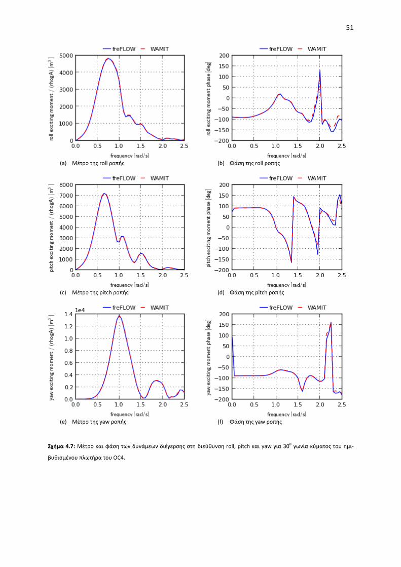
51

(a) Μέτρο της roll ροπής

(b) Φάση της roll ροπής

(c) Μέτρο της pitch ροπής

(d) Φάση της pitch ροπής

(e) Μέτρο της yaw ροπής

(f) Φάση της yaw ροπής

Σχήμα 4.7: Μέτρο και φάση των δυνάμεων διέγερσης στη διεύθυνση roll, pitch και yaw για 30ο γωνία κύματος του ημι-

βυθισμένου πλωτήρα του OC4.

52

(a) Πρόσθετη μάζα A11

(b) Πρόσθετη απόσβεση B11

(c) Πρόσθετη μάζα A15

(d) Πρόσθετη απόσβεση B15

(e) Πρόσθετη μάζα A33

(f) Πρόσθετη απόσβεση B33

Σχήμα 4.8: Συντελεστές πρόσθετης μάζας και απόσβεσης A11, A15, A33, B11, B15 και B33 του ημι-βυθισμένου πλωτήρα του

OC4.

53

(a) Πρόσθετη μάζα A55

(b) Πρόσθετη απόσβεση B55

(c) Πρόσθετη μάζα A66

(d) Πρόσθετη απόσβεση B66

Σχήμα 4.9: Συντελεστές πρόσθετης μάζας και απόσβεσης A55, A66, B55, και B66 του ημι-βυθισμένου πλωτήρα του OC4.

55

Κεφάλαιο 5.

Μη-γραμμικός υδροδυναμικός επιλύτης στις 2Δ Στο παρόν κεφάλαιο αναπτύσσεται η μέθοδος hFLOW που επιλύει το δισδιάστατο, μη-γραμμικό υδροδυναμικό πρόβλημα αλληλεπίδρασης σώματος-κύματος-ρεύματος για ιδανικό ρευστό. Το λογισμικό βασίζεται στη μέθοδο των συνοριακών στοιχείων και τη μεικτή Lagrangian-Eulerian διατύπωση. Τα κύματα δημιουργούνται είτε προσομοιώνοντας τη φυσική κίνηση του κυματιστήρα είτε θέτοντας στο σύνορο εισόδου τη λύση της stream function θεωρίας. Ο χειρισμός των συνθηκών στο άπειρο πραγματοποιείται εισάγοντας όρους τεχνητής απόσβεσης, ενώ για την προσομοίωση της κίνησης ελεύθερα πλωτών σωμάτων χρησιμοποιείται επαναληπτική διαδικασία προσδιορισμού της επιτάχυνσής τους. Τα αριθμητικά αποτελέσματα που παρουσιάζονται αφορούν πλωτό σώμα, ενώ η πιστοποίηση της μεθόδου γίνεται συγκρίνοντας πειραματικά και αριθμητικά αποτελέσματα, όπου επίσης αναδεικνύονται και αποτιμώνται τα μη-γραμμικά φαινόμενα.

5.1 Μαθηματική διατύπωση του προβλήματος

Η μέθοδος επιλύει την αστρόβιλη, ασυμπίεστη ροή χωρίς να λαμβάνεται υπόψη η επιφανειακή τάση, στο φυσικό χωρίο D(t) που ορίζεται από το σύνορο S(t) [Σχήμα 5.1]. Στη συγκεκριμένη υλοποίηση, επιλύεται το δισδιάστατο πρόβλημα στο κατακόρυφο επίπεδο (x, z) με το καθολικό σύστημα συντεταγμένων OG να τοποθετείται στη μέση στάθμη της ελεύθερης επιφάνειας. Ο άξονας z έχει κατεύθυνση προς τα επάνω και ο άξονας x προς τα δεξιά, κατά μήκος της κατεύθυνσης διάδοσης του κύματος. Ως SFS(t) ορίζεται το σύνορο της ελεύθερης επιφάνειας, ως SSB(t) του βυθού, ως SWG(t) και SBE(t) τα κατακόρυφα σύνορα στα αριστερά όπου δημιουργείται το κύμα και στα δεξιά του χωρίου όπου γίνεται απορρόφηση του κύματος αντίστοιχα, ενώ ως SBO(t) συμβολίζονται οι επιφάνειες πλωτών ή βυθισμένων σωμάτων. Τα σώματα κινούνται είτε με προδιαγεγραμμένη κίνηση είτε πλέουν ελεύθερα υπό την επίδραση των υδροδυναμικών φορτίων. Το ολικό βαθμωτό δυναμικό Φ(x; t) ορίζεται ως,

= + 0( ) (; ) Φ ;t φ t U xx x (5.1)

όπου φ(x; t) είναι το μη-μόνιμο κυματικό δυναμικό και U0 η ταχύτητα του μόνιμου, σταθερού καθ’ ύψος ρεύματος.

56

Σχήμα 5.1: Ορισμός του χωρίου επίλυσης και του συνόρου

Η διατήρηση της μάζας εκφράζεται από την εξίσωση Laplace για το ολικό δυναμικό Φ(x; t) - παρόλο που στη συνέχεια το πρόβλημα περιγράφεται για το κυματικό δυναμικό φ(x; t) - ενώ η συνεισφορά του κύματος προστίθεται απευθείας στο πεδίο. Το κυματικό δυναμικό φ(x; t) επίσης ικανοποιεί την εξίσωση Laplace (5.2),

Δ 0, στ ( )ο φ D t= (5.2)

Σε κάθε σημείο z = ζ(x; t) του συνόρου που απαρτίζει την ελεύθερη επιφάνεια η εξίσωση Bernoulli (5.3), γνωστή και ως δυναμική συνοριακή συνθήκη, εξασφαλίζει συνέχεια πιέσεων στη διεπιφάνεια μεταξύ δύο ρευστών διαφορετικής πυκνότητας (π.χ. μεταξύ νερού και αέρα). Γραμμένη για το κυματικό δυναμικό,

22 0

0 11

, στο ( ) όπο2 2

υ ;( )aFSS z ζ x

φ φ U pg ζ φ U damp t t

t x ρ∂ ∂

= − − ∇ − − − − =∂ ∂

(5.3)

όπου g είναι η επιτάχυνση της βαρύτητας, pa μία γνωστή πίεση αναφοράς (π.χ. η ατμοσφαιρική που μπορεί να τεθεί και ίση με μηδέν) και ρ η πυκνότητα του ρευστού στο πεδίο D(t). Η εξαρτώμενη από το χρόνο σταθερά ολοκλήρωσης που αρχικά εμφανίζεται στην εξίσωση Bernoulli απαλείφεται οδηγώντας σε κατάλληλο επανορισμό του φ(x; t).

Η άγνωστη γεωμετρία της ελεύθερης επιφάνειας προσδιορίζεται από τη μη-γραμμική κινηματική συνοριακή συνθήκη (5.4),

0 2 όπου ;, στο ( ) ( )FSζ ζ φ

φ ζ U damp tS z tt x

xz

ζ∂ ∂ ∂

= −∇ ⋅∇ =− + −∂ ∂ ∂

(5.4)

που εξασφαλίζει πως τα στοιχεία ρευστού στην ελεύθερη επιφάνεια θα κινούνται παραμένοντας συνεχώς σε αυτή.

57

Η δυναμική και η κινηματική συνοριακή συνθήκη στις εξισώσεις (5.3) και (5.4) είναι εκφρασμένες σε Eulerian μορφή, ενώ οι όροι dampi αφορούν όρους τεχνητής συνεκτικότητας και αναλύονται στη συνέχεια (βλ. εξισώσεις (5.12), (5.13)).

Οι εξισώσεις της ελεύθερης επιφάνειας γράφονται ισοδύναμα σε Lagrangian μορφή ως,

22 0

11

, στο ( ) ( )2 2

όπου ;aFS

dφ U pg ζ φ damp t t

dt ρS z ζ x= − =+ ∇ − − − (5.5)

0 ix 2 iz δ δ , όπου ;στο ( ) ( )FSd

φ U damp ζt tdt

S z x==∇ + −x

(5.6)

ή σε «ήμι-Lagrangian» (semi-Lagrangian) μορφή,

22 0

0 11

, στο ( ) ( )2 2

όπου ;aFS

dφ φ U dζ φ pg ζ φ U damp t t

dt x dt zS x

ρz ζ

∂=

∂= − − ∇ − − + ⋅ − −

∂ ∂ (5.7)

0 2 ό, στο ( ) ( )που ;FSdζ ζ φ

φ ζ U damp t tdt

S z ζ xx z∂ ∂

= −∇ ⋅∇ =− + −∂ ∂

(5.8)

όπου δij είναι το δέλτα του Kronecker και = ∂ ∂ + ⋅∇p(.)/ (.)/ (.)d dt t U ο τελεστής ολικής παραγώγισης.

Στα στερεά σύνορα του βυθού SSB(t) και των σωμάτων SBO(t), εφαρμόζεται η συνθήκη μη εισχώρησης,

G 0 0 x( ) , στ ( )ο και ( )SB BBn Oφ

U x V U n tn

S S t∂

= ⋅ −∇ = −∂

x n (5.9)

όπου Gx είναι η ταχύτητα σε κάθε σημείο της συνοριακής επιφάνειας όπως ορίζεται στην παράγραφο 5.2.3, n είναι το κάθετο μοναδιαίο διάνυσμα στην επιφάνεια του σώματος με κατεύθυνση προς το πεδίο ροής και VBn είναι το μέτρο της κάθετης ταχύτητας σε κάθε σημείο της επιφάνειας του σώματος.

Συνοριακές συνθήκες ορίζονται επίσης στα κατακόρυφα σύνορα για να είναι σωστά ορισμένο το πρόβλημα, οι οποίες πρέπει να εξασφαλίζουν συνεπή δημιουργία και απορρόφηση των κυμάτων. Στην παρούσα μέθοδο το κύμα δημιουργείται με 3 τρόπους: α) μοντελοποιώντας τον φυσικό κυματιστήρα ως ένα κινούμενο σώμα, β) θέτοντας κατά μήκος του συνόρου εισόδου τη λύση της stream function θεωρίας, γ) θέτοντας αρχικά το δυναμικό και την ανύψωση στους κόμβους της ελεύθερης επιφάνειας. Σε όλες τις περιπτώσεις η κάθετη ταχύτητα κατά μήκος του κατακόρυφου συνόρου στην είσοδο θεωρείται δεδομένη, καθορίζοντας μία Neumann συνοριακή συνθήκη. Επιπλέον και τα 2 κατακόρυφα σύνορα εισόδου-εξόδου θα πρέπει να επιτρέπουν στο ρεύμα να τα διαπερνά.

58

G

G

( )

( ; ) (

, στο

, στο )

WG

WGWavex

S

S

φt

nφ

u t tn

∂= ⋅

∂∂

= −∂

x n

x

(5.10)

Η 1η έκφραση στην (5.10) αντιστοιχεί στην περίπτωση α), ενώ η 2η στην περίπτωση β). Λεπτομέρειες ως προς τη δημιουργία των κυματισμών δίνονται στην παράγραφο 5.3.7 του αγγλικού κειμένου.

Η απορρόφηση των κυμάτων επιτυγχάνεται με χρήση όρων τεχνητής συνεκτικότητας. Έτσι στο δεξιά κατακόρυφο σύνορο εξόδου εφαρμόζεται η συνθήκη μη-εισχώρησης που επιτρέπει μόνο στο ρεύμα να διαπερνά το σύνορο,

, στο 0 ( )BESφ

tn

∂=

∂ (5.11)

Επιπλέον στο δεξιά τμήμα του πεδίου ορίζεται η ζώνη απόσβεσης, η περιοχή όπου γίνεται η απορρόφηση του κύματος συνήθως έκτασης 1-2 μήκη κύματος. Στη συγκεκριμένη περιοχή σταδιακά ενεργοποιούνται οι όροι απόσβεσης των 2 εξισώσεις της ελεύθερης επιφάνειας. Επίσης ζώνη απόσβεσης ορίζεται και στην αριστερή πλευρά του χωρίου, ώστε να αποτρέπονται ανακλάσεις από τον κυματιστήρα. Οι όροι απόσβεσης dampi στις εξισώσεις της ελεύθερης επιφάνειας ορίζονται ως,

1 1 , γι( )( ) α τη δυναμική συνθήκηWaven ndamp v x φ φ= ∂ −∂ (5.12)

2 2 , για την κ( ) ιν( ) ηματική συνθήκηWavedamp v x ζ ζ= − (5.13)

Όπου τα Wavenφ∂ και Waveζ θεωρούνται γνωστά και εισάγονται ώστε να απορροφούνται μόνο τα

ανακλώμενα κύματα στην περιοχή του κυματιστήρα, ενώ στην περιοχή εξόδου τίθενται 0. Ο συντελεστής vRiR(x) ορίζεται ως,

(x)ib

ei i

d

x xv α ω

L −

=

(5.14)

όπου ω είναι η συχνότητα του κύματος, Ld το μήκος της κάθε ζώνης απόσβεσης, xe η θέση που τελειώνει ή αρχίζει η ζώνη απόσβεσης, ενώ αi και bi είναι ρυθμιστικοί συντελεστές όπου συνήθως λαμβάνουν τις ακόλουθες τιμές: α1=(1/2k0), α2=1 και b1= b2=2. k0 είναι ο κυματαριθμός στο τοπικό βάθος της κάθε ζώνης απόσβεσης.

59

5.2 Αριθμητική υλοποίηση

5.2.1 Μεικτή Eulerian - Lagrangian μέθοδος

Με βάση τη μεικτή Eulerian-Lagrangian διατύπωση [23] επιτυγχάνεται η επίλυση του μη-γραμμικού υδροδυναμικού προβλήματος θεωρώντας είτε τις Lagrangian είτε τις ήμι- Lagrangian συνθήκες στην ελεύθερη επιφάνεια, όπως ορίστηκαν στις εξισώσεις (5.5), (5.6) ή (5.7), (5.8) αντίστοιχα.

Για δεδομένο x ή ζ (ανάλογα με τη διατύπωση) και δυναμικό φ κατά μήκος του συνόρου της ελεύθερης επιφάνειας, αριθμητική ολοκλήρωση στο χρόνο των δύο εξελικτικών εξισώσεων της ελεύθερης επιφάνειας προσδιορίζει τη νέα θέση και δυναμικό. Αυτό αποτελεί το Lagrangian μέρος της μεθόδου. Στην Lagrangian διατύπωση οι κόμβοι τις ελεύθερης επιφάνειας κινούνται με βάση τη συνολική ταχύτητά τους, ενώ στην ήμι-Lagrangian οι κόμβοι κινούνται μόνο κατακόρυφα. Κατά την εκκίνηση της επίλυσης τίθενται μηδενικές τιμές για τα ζ και φ, εκτός κι αν μία αρχική λύση είναι διαθέσιμη.

Και στις 2 διατυπώσεις η εξίσωση Laplace, που εισάγεται με τη μορφή ολοκληρωτικών εξισώσεων, λειτουργεί ως περιορισμός συνδέοντας τα Neumann δεδομένα με τα Dirichlet σε ολόκληρο το σύνορο S(t), όπως λεπτομερώς παρουσιάζεται στην παράγραφο 5.2.3. Αυτό αποτελεί το Eulerian μέρος της μεθόδου.

Σημειώνεται πως οι δύο διατυπώσεις (Lagrangian και ήμι-Lagrangian) είναι ισοδύναμες στην περίπτωση που η μορφή της ελεύθερης επιφάνειας περιγράφεται από κάποια συνάρτηση. Αντιθέτως, μόνο η πλήρως Lagrangian διατύπωση επιτρέπει την προσομοίωση αναδιπλούμενων κυμάτων μέχρι τη θραύση τους, τη στιγμή δηλαδή που η κορυφή του αναδιπλούμενου κύματος ακουμπάει στην ελεύθερη επιφάνεια. Αυτό είναι και το θεωρητικό όριο εφαρμογής της συγκεκριμένης μεθόδου.

5.2.2 Ολοκληρωτική μορφή της εξίσωσης Laplace και η αριθμητική επίλυσή της

Η ολοκληρωτική εξίσωση για την εξίσωση Laplace έχει την ακόλουθη μορφή,

;∂∂ ⋅ = ⋅ − ⋅ ∂ ∂ ∫ 00 0 0

x xxx x x x x x( )( )( ) ( ) ( ; ) ( ) ( )S

Gφa φ G φ dSn n

(5.15)

1( ; ) ln -2

Gπ

=0 0x x x x

(5.16)

όπου G(x, x0) είναι η συνάρτηση Green, x0 οποιοδήποτε σημείο του πεδίο D(t), x οποιοδήποτε σημείο του συνόρου S(t) και α(x0) η γωνία που σχετίζεται με το x0. Για σημεία στο D(t), α(x0) =2π, ενώ για σημεία του συνόρου S(t), η α(x0) υπολογίζεται απευθείας επιλύοντας ένα απλοποιημένο πρόβλημα συνοριακών τιμών, θεωρώντας ομοιόμορφες συνοριακές συνθήκες 0nφ∂ = και φ=1. Έτσι η γωνία α(x0) υπολογίζεται ως,

60

;( )( ) ( )

S

Ga dS

n∂

= −∂∫ 0

0x xx x (5.17)

Για την επίλυση της (5.15) το φ (Dirichlet δεδομένο) ή το nφ∂ (Neumann δεδομένο) θεωρείται γνωστό σε κάθε τμήμα του συνόρου S(t). Στο σύνορο της ελεύθερης επιφάνειας τίθεται Dirichlet συνοριακή συνθήκη, ενώ στα υπόλοιπα σύνορα Neumann. Το προκύπτον μεικτό πρόβλημα επιλύεται με τη μέθοδο των συνοριακών στοιχείων υιοθετώντας τμηματικά γραμμικές κατανομές φ και nφ∂ με επίπεδα στοιχεία. Τα σημεία όπου ικανοποιούνται οι ολοκληρωτικές εξισώσεις ορίζονται στους ακραίους κόμβους κάθε στοιχείου, ενώ οι απαραίτητες ολοκληρώσεις στην (5.15) γίνονται αναλυτικά. Η διακριτή μορφή της (5.15) επιλύεται με τη μέθοδο LU decomposition. Σημειώνεται πως στη διακριτή τους μορφή οι (5.15) και (5.17) χρησιμοποιούν τα ίδια μητρώα.

Επιπλέον η εφαπτομενική ταχύτητα sφ∂ στο σύνορο S(t) και οι χωρικές παράγωγοι της ανύψωσης της ελεύθερης επιφάνειας ∂ xζ που υπεισέρχονται στην (5.8), καθώς και στον υπολογισμό των δυνάμεων των σωμάτων λαμβάνονται στους κόμβους του συνόρου αριθμητικά με χρήση πεπερασμένων διαφορών 2ης τάξης.

Ειδική μεταχείριση απαιτείται στους ακραίους κόμβους της ελεύθερης επιφάνειας όπου η συνοριακή συνθήκη αλλάζει από Dirichlet σε Neumann. Για τον μονοσήμαντο και συνεπή ορισμό της ταχύτητας και την αποφυγή εμφάνισης της λεγόμενης “saw-tooth” αστάθειας οι κόμβοι αυτοί θεωρούνται διπλοί (“double nodes” [24], [25]). Έτσι η ταχύτητα u = (ux, uz) ορίζεται μέσω των 2 γνωστών κάθετων συνιστωσών D

nφ∂ και Nn∂ ϕ στους ακραίους κόμβους του Dirichlet και του

Neumann συνόρου αντίστοιχα και υπολογίζεται λύνοντας το παρακάτω 2x2 γραμμικό σύστημα,

Dx Dx z Dz D nu n u n⋅ + ⋅ = ⋅ = ∂u n ϕ

(5.18) N

x Nx z Nz N nu n u n⋅ + ⋅ = ⋅ = ∂u n ϕ

Επιπλέον για να προκύψουν συνεπή αποτελέσματα σε μεγάλης διάρκειας προσομοιώσεις είναι σημαντική η επαναπλεγματοποίηση του συνόρου S(t). Για το μεν σύνορο της ελεύθερης επιφάνειας χρησιμοποιείται παρεμβολή spline, ενώ για τα υπόλοιπα σύνορα γραμμική παρεμβολή εξασφαλίζοντας πως κάθε χρονική στιγμή το σύνορο S(t) παραμένει κλειστό.

61

5.2.3 Κινηματική των σωμάτων

Τα στερεά σώματα υπόκεινται σε συνδυασμένη μεταφορική και περιστροφική κίνηση, που ορίζεται ως προς το σωματόδετο σύστημα OB. Αν xB(t) είναι το διάνυσμα θέσης του OB, θRBR(t) η γωνία των αξόνων του OB ως προς το καθολικό σύστημα OG και κάθε σημείο στο σύνορο του σώματος ορίζεται από το τοπικό διάνυσμα θέσης rL, τότε τα διανύσματα θέσης, ταχύτητας και επιτάχυνσης στο καθολικό σύστημα G G G, ,x x x ορίζονται ως,

G B B B G B G B( , ; ) (t)+ ( ( )) + +t θ t= ⋅ ⇒ = ⋅ ⇒ = ⋅L L L Lx ξ r x A r x x A r x x A r

(5.19)

Ενώ τα γενικευμένα διανύσματα θέσης, ταχύτητας και επιτάχυνσης του κάθε σώματος, που στις 2 διαστάσεις αποτελούνται από τη surge, heave και pitch κατεύθυνση ορίζονται ως,

B B B B B B B B B={ , }, ={ , }, ={ , }θ θ θξ x ξ x ξ x

(5.20)

B( )θA είναι το μητρώο στροφής, ενώ η πρώτη και η δεύτερη παράγωγός του ορίζονται ως,

2B B B B B B B B

B

d( , ) = , ( , , )d Bθ θ θ θ θ θ θ θ θ

θ′ ′ ′′= = +

AA A A A A

(5.21)

Στις εξισώσεις (5.19) έως (5.21) οι τελείες δηλώνουν χρονική παράγωγο.

5.2.4 Δύναμη των σωμάτων και επίλυση της ολοκληρωτικής εξίσωσης για το φt

Οι δυνάμεις που ασκούνται στο σώμα υπολογίζονται με ολοκλήρωση των πιέσεων μέσω της μη-γραμμικής εξίσωσης Bernoulli γραμμένης ως προς την πίεση,

22 0

01

( )2 2t

φ Up ρ φ φ U gz

x∂

= − + ∇ + + +∂

(5.22)

Όπως αναφέρεται στα [25], [26], ο υπολογισμός του μη-μόνιμου όρου φt με σχήματα πεπερασμένων διαφορών στο χρόνο προκαλεί αριθμητικές αστάθειες, ιδιαίτερα στην περίπτωση κινούμενων σωμάτων. Εναλλακτικά όπως αναφέρεται στο [27], η εξίσωση Laplace για το φt μπορεί να επιλυθεί λαμβάνοντας υπόψη την κινηματική της ροής. Αυτό οδηγεί σε ακριβή προσομοίωση της δυναμικής των σωμάτων, κινούμενων ή μη. Το πρόβλημα συνοριακών τιμών για το φt ορίζεται όμοια με αυτό για το φ αν παραγωγιστούν οι αντίστοιχες συνθήκες ως προς το χρόνο,

62

Δφt= 0, στο D(t) (5.23)

22 0

0 11

( )2 2

, στο at FS

φ U pφ g ζ φ U damp t

x ρS

∂= − − ∇ − − − −

∂ (5.24)

, στα και 0 ( ) ( )BE St

BS t Sφn

t∂

=∂

(5.25)

G G , στ (ο ( ) )tBO

φq S t

n∂

= ⋅ +∂

x n x (5.26)

G G

G

( ) ( )

( ; ) ,στο ( )

, στο Wt

Wavetx

G

WG

S t

S t

φq

nφ

a tn

∂= ⋅ +

∂∂

= −∂

x n x

x

(5.27)

Το Dirichlet δεδομένο στην ελεύθερη επιφάνεια (5.24) και το Neumann δεδομένο στα κινούμενα σώματα (5.26) και (5.27), ορίζονται μετά την επίλυση του συνοριακού προβλήματος για το δυναμικό φ, ώστε να έχουν προσδιοριστεί το nφ∂ στην ελεύθερη επιφάνεια και το δυναμικό φ στο σύνορο των σωμάτων.

Επιπλέον G G G, , x x x είναι τα διανύσματα θέσης, ταχύτητας και επιτάχυνσης στο σύνορο των σωμάτων όπως ορίστηκαν στην παράγραφο 5.2.3 και q(xG) είναι το εξαρτώμενο από το δυναμικό φ μέρος της κάθετης στο σώμα επιτάχυνσης. Για να υπολογιστεί το q(xG), εισάγεται ένα σωματόδετο, καμπυλόγραμμο σύστημα συντεταγμένων (s, n) με s, n το εφαπτομενικό και κάθετο μοναδιαίο διάνυσμα στην επιφάνεια του σώματος. Με βάση την απόδειξη του van Daalen [27], που επίσης χρησιμοποιήθηκε στο [28] για τις 2 διαστάσεις, ο όρος q(xG) αναπτύχθηκε περαιτέρω ώστε να λαμβάνει υπόψη τους όρους του σταθερού ρεύματος [Appendix B του αγγλικού κειμένου]. Η τελική έκφραση στις 2 διαστάσεις για το q(xG) είναι,

G G 0 B

0 0 G

0 0 G

( ) ( 2 )

( 2 )( )

( )( ), στο ( )

s s

n s

B

n s ns

O

sn

n n n n ss ss

q φ U x θ

k φ k U x φ U x

k S tφ k U x φ U x

= ⋅ −∂ − ∂

− ∂ + ∂ + ∂ + ∂ ⋅

− ∂ + ∂ −∂ − ∂ ⋅

x x s

x s

x n

(5.28)

∂ ∂ − ∂ ∂=

∂ + ∂ 1.5

( )

s ss s ssn

s s

x z z xk

x z (5.29)

όπου B B B, , θ θ θ είναι η pitch γωνία, ταχύτητα και επιτάχυνση του σώματος και kn η τοπική καμπυλότητα της επιφάνειας του σώματος.

Οι εφαπτομενικές παράγωγοι , , , , , , s ss ns s ss s ssφ φ φ x x z z∂ ∂ ∂ ∂ ∂ ∂ ∂ υπολογίζονται αριθμητικά με χρήση πεπερασμένων διαφορών 2ης τάξης για ανομοιόμορφα πλέγματα. Η αντίστοιχη ολοκληρωτική εξίσωση ορίζεται όμοια με την (5.15) ως,

63

;∂ ∂ ⋅ = ⋅ − ⋅ ∂ ∂ ∫ 00 0 0

x x xx x x x x x( ) ( )( ) ( ) ( ; ) ( ) ( )t

t tS

φ Ga φ G φ dS

n n (5.30)

Το επιπλέον υπολογιστικό κόστος για την επίλυση της (5.30) κρίνεται μικρό, εφόσον χρησιμοποιούνται τα ίδια μητρώα με την (5.15) και χρησιμοποιείται η μέθοδος LU decomposition στην οποία μόνο το δεξί μέλος του γραμμικού συστήματος θα είναι διαφορετικό.

5.2.5 Ελεύθερα πλωτά σώματα

Οι κινήσεις ελεύθερα πλωτών σωμάτων είναι επιπλέον άγνωστοι βαθμοί ελευθερίας του προβλήματος. Ο προσδιορισμός τους βασίζεται στις δυναμικές εξισώσεις κίνησης και αποτελεί μέρος της επίλυσης. Υδροδυναμικές δυνάμεις και δυνάμεις βαρύτητας αποτελούν την εξωτερική διέγερση των σωμάτων. Όπως αναφέρθηκε στην παράγραφο 5.2.4, τα υδροδυναμικά φορτία υπολογίζονται επιλύοντας επιπλέον το πρόβλημα συνοριακών τιμών για τη χρονική παράγωγο του δυναμικού φt. Στην περίπτωση ελεύθερα πλωτών σωμάτων όμως, κανένα εκ των φt και n tφ∂ δεν είναι αρχικά γνωστό, οπότε δεν μπορεί να καθοριστεί η απαραίτητη συνοριακή συνθήκη για την επίλυση του προβλήματος συνοριακών τιμών για το φt. Για να ξεπεραστεί η παραπάνω δυσκολία εφαρμόζεται μία επαναληπτική διαδικασία [29, 30], όπου σε κάθε βήμα η επιτάχυνση του σώματος

Bξ τίθεται αρχικά ίση με αυτή του προηγούμενου χρονικού βήματος. Έτσι γίνεται εκτίμηση του

n tφ∂ μέσω της (5.26) και καθίσταται επιλύσιμο το πρόβλημα συνοριακών τιμών για το φt. Μόλις προσδιοριστεί το φt στο σύνορο των σωμάτων και υπολογιστούν τα υδροδυναμικά φορτία, η επιτάχυνση του σώματος ανανεώνεται από την εξίσωση κίνησης ως,

{ }−= − ⋅ − ⋅

1B B Bξ M F C ξ K ξ (5.31)

όπου στην (5.31) M είναι το γενικευμένο μητρώο μάζας του σώματος ορισμένο ως προς το κέντρο βάρους του, C και K είναι εξωτερικά μητρώα απόσβεσης και δυσκαμψίας (π.χ. από το σύστημα αγκύρωσης) και F είναι τα υδροδυναμικά και βαρυτικά φορτία. Οι επαναλήψεις συνεχίζονται μέχρι να ικανοποιηθεί το κριτήριο σύγκλισης για την επιτάχυνση του σώματος.

Τα διανύσματα θέσης και ταχύτητας των σωμάτων Bξ και Bξ προσδιορίζονται με ολοκλήρωση στο χρόνο των παρακάτω εξισώσεων,

ddt

=BB

ξξ

(5.32)

ddt

=BB

ξξ

(5.33)

64

Σημειώνεται πως η επιτάχυνση του σώματος επηρεάζει μόνο τον υπολογισμό του φt επανορίζοντας μόνο τις Neumann οριακές συνθήκες (5.26) και (5.27) για το 2ο πρόβλημα συνοριακών τιμών για το φt, ενώ η γεωμετρία του συνόρου καθώς και το δυναμικό φ παραμένουν αμετάβλητα. Έτσι η προαναφερθείσα επαναληπτική διαδικασία δεν αυξάνει το υπολογιστικό κόστος, αφού απαιτεί μόνο την επίλυση του προβλήματος συνοριακών τιμών για το φt (5.30) χρησιμοποιώντας τα ήδη αντεστραμμένα μητρώα, ανανεώνοντας μόνο το δεξί μέλος.

5.2.6 Ολοκλήρωση στο χρόνο

Αν με u(t) συμβολίσουμε το διάνυσμα των αγνώστων που περιλαμβάνει το δυναμικό στην ελεύθερη επιφάνεια φFS, τις θέσεις που ορίζουν τη γεωμετρία της ελεύθερης επιφάνειας xFS και τα γενικευμένα διανύσματα θέσης και ταχύτητας των ελεύθερα πλωτών σωμάτων ξB και Bξ αντίστοιχα,

( ) FS FS BB{ , , ,= }t φu ξ ξx

(5.34)

Τότε με βάση τη μέθοδο Runge-Kutta 4ης τάξης γίνεται ολοκλήρωση στο χρόνο ακλουθώντας τα ακόλουθα βήματα,

( )

( )

S

i ii=1

i i

1 1

i i,1:i-1 1

+d

:i-1 i

=

d

+

+ d

=d ; d

=d +{ }; , d 2d

t t t

t

t

b k

t t c t

k t tt

k t a k t i St

⋅

= ⋅

⋅

⋅ ≤ ≤

∑u u

u u

uu

(5.35)

Όπου για S=4 (4η τάξη), οι συντελεστές ai,j, bi και ci δίνονται στον Πίνακα 5.1.

Πίνακας 5.1: Συντελεστές της μεθόδου ολοκλήρωσης Runge-Kutta 4ης τάξης

0 0

cR2 aR21 1/2 1/2

cR3 aR31 aR32 1/2 0 1/2

cR4 aR41 aR42 aR43 1 0 0 1

bR1 bR2 bR3 bR4 1/6 1/3 1/3 1/6

65

5.2.7 Έλεγχος ακρίβειας

Σε κάθε χρονικό βήμα υπολογίζονται τα σφάλματα όγκου και ενέργειας, ως ενδείξεις σταθερής και ακριβούς αριθμητικής επίλυσης. Το σφάλμα όγκου ελέγχει την διατήρηση της μάζας, ενώ το σφάλμα της ενέργειας την διατήρηση της ορμής και της ενέργειας. Στη μέθοδο των συνοριακών στοιχείων ο όγκος V και η συνολική ενέργεια E υπολογίζονται ως,

ZΩ

= d = dS

V V z n S⋅∫ ∫

(5.36)

Ω

2Z n X Z

d

d

22 0

0

0 0S

2

E g z V

g

1 φ Uφ U

2 x 2

1 1 1φ Uz n φ φ n z n SU

2 2 2

= +

= + +

∂

∇ + +∂

∂ +

∫

∫ (5.37)

Τα αντίστοιχα σχετικά σφάλματα όγκου και ενέργειας ορίζονται ως προς τις αρχικές τιμές τους.

5.2.8 Γραμμικοποιημένες διατυπώσεις

Η παρούσα μέθοδος λαμβάνει υπόψη τις 2 μη-γραμμικότητες του προβλήματος: αυτή που σχετίζεται με την ελεύθερη επιφάνεια και αυτή που σχετίζεται με τα κινούμενα σώματα. Όπως έχει ήδη περιγραφεί στις προηγούμενες παραγράφους, οι συνθήκες στην ελεύθερη επιφάνεια εφαρμόζονται στην στιγμιαία θέση της (πεπλεγμένη μη-γραμμικότητα), διατηρώντας όλους τους μη-γραμμικούς όρους των εξισώσεων (ρητή μη-γραμμικότητα), και το ίδιο συμβαίνει με τις οριακές συνθήκες στα κινούμενα σώματα που εφαρμόζονται στην ακριβή θέση τους. Δύο απλοποιήσεις μπορούν να εισαχθούν που από τη μία επιταχύνουν τους υπολογισμούς και από την άλλη παρέχουν τη δυνατότητα αποτίμησης της σημασίας των μη-γραμμικοτήτων.

Η πρώτη απλοποίηση συχνά αναφέρεται ως ‘body nonlinear’ διατύπωση και λαμβάνει υπόψη μόνο τη μη-γραμμικότητα εξαιτίας των σωμάτων, ενώ οι 2 συνοριακές συνθήκες στην ελεύθερη επιφάνεια εφαρμόζονται στη μέση στάθμη, απαλείφοντας τους μη-γραμμικούς όρους. Η δεύτερη απλοποίηση εκτός από τη γραμμικοποιημένη ελεύθερη επιφάνεια, επιπλέον θεωρεί τα κινούμενα σώματα στη μέση θέση τους.

66

5.3 Αριθμητικά αποτελέσματα: Μη-γραμμική αλληλεπίδραση κύματος-ελεύθερα πλωτού σώματος

Σχήμα 5.2: Ορισμός του υπολογιστικού χωρίου στη μέθοδο συνοριακών στοιχείων για την περίπτωση του ελεύθερα

πλωτού σώματος.

Στην παρούσα παράγραφο εξετάζεται σε ορθογώνιο υπολογιστικό χωρίο βάθους d και μήκους L ένα ελεύθερα πλωτό σώμα που τέμνει την ελεύθερη επιφάνεια [Σχήμα 5.20]. Οι κινήσεις του σώματος καθορίζονται από την δράση των κυμάτων, ενώ αυτό συγκρατείται από ένα ελατήριο που ενεργεί στην οριζόντια κατεύθυνση x. Το βύθισμα του σώματος είναι dr=0.25m, η βάση του B=0.5m, η ακτίνα της κυκλικής γωνίας r=0.064m, η μάζα του m=125kg, η αδράνεια ως προς το κέντρο μάζας Ip=4.05kgmP

2P, το κέντρο μάζας zcm=-0.115m και η δυσκαμψία και απόσβεση του ελατηρίου

k=197.58N/m και c=19.8N/(ms) αντίστοιχα [Σχήμα 5.2].

Τα κύματα εύρους A=H/2 εισάγονται στο πεδίο από το αριστερό σύνορο, όπου γίνεται συναρμογή με τη stream function λύση, ενώ η αδιάστατη συχνότητα ξ=ωP

2PB/2g μεταβάλλεται από 0.2 έως 1.75

[Πίνακας 5.3]. Για κάθε συχνότητα ρυθμίζεται κατάλληλα το χωρίο ώστε d=λ και L=8λ, ενώ οι ζώνες απόσβεσης έχουν μήκος Ld=2λ και στα 2 άκρα.

Η διακριτοποίηση του συνόρου περιλαμβάνει 400 κόμβους στην ελεύθερη επιφάνεια, 200 στο βυθό, 30 στα κατακόρυφα σύνορα και 100 στο σώμα, ενώ το χρονικό βήμα ορίζεται για κάθε συχνότητα ίσο με dt=T/100.

67

Πίνακας 5.2: Εισερχόμενα κύματα για την προσομοίωση του πλωτού σώματος

N ξ=ω2Β/2g ω [rad/s] T [s] λ [m] H/λ, H=1cm

H/λ, H=7cm

1 0.20 2.8009 2.2432 7.8540 0.0013 0.0089

2 0.25 3.1316 2.0064 6.2832 0.0016 0.0111

3 0.35 3.7053 1.6957 4.4880 0.0022 0.0156

4 0.40 3.9611 1.5862 3.9270 0.0025 0.0178

5 0.50 4.4287 1.4187 3.1416 0.0032 0.0223

6 0.55 4.6448 1.3527 2.8560 0.0035 0.0245 7 0.60 4.8514 1.2951 2.6180 0.0038 0.0267

8 0.65 5.0495 1.2443 2.4166 0.0041 0.0290

9 0.70 5.2401 1.1991 2.2440 0.0045 0.0312

10 0.75 5.4240 1.1584 2.0944 0.0048 0.0334

11 0.82 5.6715 1.1079 1.9156 0.0052 0.0365

12 1.00 6.2631 1.0032 1.5708 0.0064 0.0446 13 1.25 7.0024 0.8973 1.2566 0.0080 0.0557

14 1.50 7.6707 0.8191 1.0472 0.0095 0.0668

15 1.75 8.2853 0.7584 0.8976 0.0111 0.0780

16 2.00 8.8574 0.7094 0.7854 0.0127 0.0891

Στο Σχήμα 5.3 συγκρίνονται μη-γραμμικές προλέξεις της μεθόδου hFLOW για την πρώτη αρμονική των 3 κινήσεων του σώματος (surge, heave, pitch) και για την οριζόντια drift δύναμη με μετρήσεις των Nojiri και Murayama [31], καθώς και υπολογισμούς από τους Tanizawa και Minami [32] και τους Koo και Kim [33] για ύψος κύματος H=0.07m, που επίσης χρησιμοποιούν μη-γραμμικούς επιλύτες με βάση τη μέθοδο συνοριακών στοιχείων. Για να γίνει διερεύνηση της σημασίας της παραμέτρου μη-γραμμικότητας (wave steepness Η/λ) έγιναν υπολογισμοί με το hFLOW και για H=0.01m, όπου η μη-γραμμική λύση δεν διαφέρει πολύ από τη γραμμική.

Μακριά από το σημείο συντονισμού η συμφωνία των 3 διαφορετικών κωδίκων είναι άριστη και για τις 3 κινήσεις [Σχήμα 5.3a, b, c]. Κοντά στο συντονισμό στο εύρος συχνοτήτων 0.5<ξ<0.7 οι μη-γραμμικοί όροι είναι σημαντικοί, όπως προκύπτει από τη διαφορά των αποτελεσμάτων μεταξύ H=0.01m και H=0.07m. Στην περίπτωση H=0.07m τα εύρη των κινήσεων surge, heave και pitch μειώνονται όπως στο πείραμα. Παρόλο που γενικώς οι υπολογισμοί συμφωνούν με τα πειραματικά αποτελέσματα, η συνεκτικότητα πιθανότατα μειώνει ακόμα περισσότερο την pitch στροφή και κατ’ επέκταση την surge κίνηση μέσω της surge-pitch σύζευξης στις συχνότητες ξ=0.35 και 0.5. Σύγκριση των υπολογιστικών εργαλείων στην περιοχή του συντονισμού δεν είναι δυνατή, καθώς οι Tanizawa και Nimani δεν δίνουν αποτελέσματα σε αυτό το εύρος συχνοτήτων, ενώ οι Koo και Kim δίνουν μόνο για ξ=0.6. Παρόλα αυτά το hFLOW δίνει συνεπή αποτελέσματα στο συντονισμό για ξ=0.5 έως 0.6, όπου το εύρος της pitch κίνησης ξεπερνά τις 30P

oP.

68

Στη σύγκριση των δυνάμεων drift [Σχήμα 5.3d], έχει προστεθεί και η πορτοκαλί καμπύλη που αντιστοιχεί στους 2ης τάξης υπολογισμούς κατά Maruo, ως μία επιπλέον πηγή πιστοποίησης. Τα αποτελέσματα τoυ hFLOW για H=0.01m είναι σε άριστη συμφωνία με αυτά του Maruo (οι υπολογισμοί έγιναν με βήμα αδιάστατης συχνότητας dξ=0.1 και άρα η διαφοροποίηση στο εύρος 0.4<ξ<0.5 οφείλεται σε αυτό). Στην περίπτωση όπου H=0.07m, τα αποτελέσματα του hFLOW διαφέρουν από αυτά του Maruo μόνο στην περιοχή του συντονισμού, προλέγοντας μεγαλύτερη δύναμη drift, όμως σημαντικά μικρότερη από αυτή των Koo και Kim. Στην περιοχή του συντονισμού η μετρημένη δύναμη drift είναι συστηματικά μικρότερη από αυτή του Maruo πιθανώς εξαιτίας της συνεκτικότητας που δεν μοντελοποιείται από τις παρούσες αριθμητικές μεθόδους. Στην περιοχή συχνοτήτων εκτός του συντονισμού και μέχρι ξ=1.25 τα αποτελέσματα της παρούσας μεθόδου συμφωνούν με το πείραμα. Για μεγαλύτερες συχνότητες σταδιακά η μέθοδος προβλέπει μεγαλύτερες δυνάμεις drift σε σχέση με τις μετρήσεις, που όμως είναι μικρότερες από τις προβλέψεις των δύο άλλων μεθόδων και σε πλήρη συμφωνία με τον υπολογισμό κατά Maruo. Αυτή η διαφοροποίηση με το πείραμα ενδεχομένως να οφείλεται στη συνεκτικότητα ή την πιθανή θραύση των κυμάτων.

Στο Σχήμα 5.4 συγκρίνονται οι 3 πρώτες αρμονικές των υδροδυναμικών φορτίων με τις αντίστοιχες προβλέψεις των Koo και Kim [33]. Η συμφωνία στην κατακόρυφη δύναμη Fz και τη ροπή My είναι άριστη, ενώ στην οριζόντια δύναμη Fx είναι καλή. Συγκεκριμένα το hFLOW προβλέπει λίγο μικρότερη 1η αρμονική για συχνότητες ξ>0.75 και μικρότερες 2η και 3η αρμονικές στην περιοχή του συντονισμού.

Παρόλα αυτά, και οι 2 μέθοδοι προβλέπουν μεγαλύτερες 2ες αρμονικές από 1ες στις περιπτώσεις της οριζόντιας και κατακόρυφης δύναμης Fx και Fz, που είναι ένδειξη ενεργοποίησης των μη-γραμμικοτήτων. Για την Fx αυτό συμβαίνει στο συντονισμό για ξ=0.6 όπου το σώμα οδηγείται σε μεγάλες στροφές, ενώ για την Fz για ξ>=1.5 και αφορά στάσιμα κύματα που αναπτύσσονται στην αριστερή πλευρά του σώματος από τους επερχόμενους κυματισμούς που δημιουργούν ένα αργά φθίνον καθ’ ύψος δευτεροτάξιο πεδίο πιέσεων, όπως αναφέρεται και στο [26] και έχει μελετηθεί στα [34-36].

Στο Σχήμα 5.5 παρουσιάζονται χρονοσειρές των φορτίων και των κινήσεων του σώματος μετά το πέρας των μεταβατικών φαινομένων με το hFLOW. Η περίπτωση όπου το ύψος του κύματος είναι Η=0.07m επιλέχθηκε για 3 συχνότητες ξ=0.25, 0.75 και 1.75 που καλύπτουν όλο το εύρος συχνοτήτων, εκτός του συντονισμού. Η χαμηλότερη συχνότητα ξ=0.25 βρίσκεται στο όριο ισχύος της γραμμικής θεωρίας και ως εκ τούτου δίνει σχεδόν αρμονικά σήματα. Στη συχνότητα ξ=0.75 σταδιακά ενεργοποιούνται οι μη-γραμμικοί όροι, ενώ για ξ=1.75 αποκτούν σημασία και είναι κυρίως εμφανείς στη δύναμη και την κίνηση στην κατακόρυφη διεύθυνση heave, όπως αναμενόταν και από το Σχήμα 5.4b.

Τέλος στο Σχήμα 5.6 παρουσιάζονται οι αντίστοιχες χρονοσειρές δυνάμεων και κινήσεων στην περιοχή του συντονισμού για συχνότητες ξ=0.5, 0.55 και 0.6. Ιδιαίτερα ισχυρά μη-γραμμικά φαινόμενα εμφανίζονται στην οριζόντια δύναμη και κίνηση και για τις 3 συχνότητες. Περισσότερο ισχυρές είναι οι μη-γραμμικότητας για ξ = 0.6 όπου η οριζόντια κίνηση surge αποτυπώνεται ως

69

‘cnoidal’ μορφή, όπως επίσης αναμενόταν από τις συγκρίσεις στο Σχήμα 5.4a. Σημειώνεται πως η ισχυρά μη-γραμμική οριζόντια κίνηση διεγείρεται από την πολύ μεγάλη γωνία pitch της τάξεως των 30P

oP, μέσω της σύζευξης των δύο κινήσεων.

Αν και θα μπορούσε να προστεθεί συνεκτική διόρθωση στην pitch κίνηση, που είναι σημαντική στην περίπτωση των μεγάλων στροφών στην περιοχή του συντονισμού, δεν έγινε στην παρούσα ανάλυση ώστε να γίνει αποτίμηση των δυνατοτήτων της μεθόδου για μη-συνεκτικό ρευστό.

70

(a) Οριζόντια κίνηση

(b) Κατακόρυφη κίνηση

(c) Στροφή pitch

(d) Οριζόντια δύναμη drift

Σχήμα 5.3: 1η αρμονική των 3 κινήσεων (surge, heave, pitch) και οριζόντια drift δύναμη του ελεύθερα πλωτού σώματος για

ύψος κύματος H=0.07m.

0.0

0.2

0.4

0.6

0.8

1.0

1.2

1.4

0.00 0.50 1.00 1.50 2.00

Surg

e /

A

ξ=ω2Β/2g

hFLOW H=1cmhFLOW H=7cmexperimentTanizawa 1998Koo, Kim 2004

0.0

0.5

1.0

1.5

2.0

2.5

0.00 0.50 1.00 1.50 2.00

Heav

e /

A

ξ=ω2Β/2g

hFLOW H=1cmhFLOW H=7cmexperimentTanizawa 1998Koo, Kim 2004

0.0

1.0

2.0

3.0

4.0

5.0

6.0

7.0

8.0

0.00 0.50 1.00 1.50 2.00

Pitc

h /

(Aω

2 /g)

ξ=ω2Β/2g

hFLOW H=1cmhFLOW H=7cmexperimentTanizawa 1998Koo, Kim 2004

0.0

0.5

1.0

1.5

2.0

0.00 0.50 1.00 1.50 2.00

Drift

For

ce /

(0.5ρg

A2 )

ξ=ω2Β/2g

hFLOW H=1cmhFLOW H=7cmexperimentTanizawa 1998Koo, Kim 2004Maruo 1960

71

(a) Οριζόντια δύναμη

(b) Κατακόρυφη δύναμη

(c) Ροπή

Σχήμα 5.4: 1η, 2η και 3η αρμονική των υδροδυναμικών φορτίων του πλωτού σώματος – μη-γραμμικοί υπολογισμοί για

ύψος κύματος H=0.07m

0.0

0.2

0.4

0.6

0.8

1.0

0.25 0.50 0.75 1.00 1.25 1.50 1.75

Fx /

(ρgΑ

d r)

ξ=ω2B/2g

hFLOW 1st hFLOW 2nd hFLOW 3rd Koo 2004 1st Koo 2004 2nd Koo 2004 3rd

0.0

0.2

0.4

0.6

0.8

1.0

1.2

0.25 0.50 0.75 1.00 1.25 1.50 1.75

Fz /

(ρgΑ

B)

ξ=ω2B/2g

hFLOW 1st hFLOW 2nd hFLOW 3rd Koo 2004 1st Koo 2004 2nd Koo 2004 3rd

0.0

0.2

0.4

0.6

0.8

1.0

1.2

0.25 0.50 0.75 1.00 1.25 1.50 1.75

My

/ (ρ

gΑBd

r)

ξ=ω2B/2g

hFLOW 1st hFLOW 2nd hFLOW 3rd Koo 2004 1st Koo 2004 2nd Koo 2004 3rd

72

(a) Οριζόντια δύναμη

(d) Οριζόντια κίνηση

(b) Κατακόρυφη δύναμη

(e) Κατακόρυφη κίνηση

(c) Ροπή

(f) Στροφή

Σχήμα 5.5: Χρονοσειρές φορτίων και κινήσεων του πλωτού σώματος για συχνότητες κύματος ξ=0.25, 0.75 και 1.75 και

ύψος H=0.07m.

73

(a) Οριζόντια δύναμη

(d) Οριζόντια κίνηση

(b) Κατακόρυφη δύναμη

(e) Κατακόρυφη κίνηση

(c) Ροπή

(f) Στροφή

Σχήμα 5.6: Χρονοσειρές φορτίων και κινήσεων του πλωτού σώματος για συχνότητες κύματος ξ=0.5, 0.55 και 0.6 και ύψος

H=0.07m.

75

Κεφάλαιο 6.

Αποτίμηση και μελλοντική έρευνα

6.1 Αποτίμηση

Η παρούσα εργασία είχε τρεις βασικούς στόχους:

1. τη σύνθεση ενός πλήρως συζευγμένου ύδρο-σέρβο-αέρο-ελαστικού εργαλείου για την ανάλυση των υπεράκτιων ανεμογεννητριών

2. την ανάπτυξη ενός τρισδιάστατου υδροδυναμικού επιλύτη στο πεδίο της συχνότητας για το πρόβλημα αλληλεπίδρασης σώματος-κύματος

3. την ανάπτυξη ενός δισδιάστατου μη-γραμμικού υδροδυναμικού επιλύτη για το πρόβλημα αλληλεπίδρασης κύματος-σώματος-ρεύματος

Σε σχέση με τον 1ο στόχο, το λογισμικό hGAST που αναπτύχθηκε:

- βασίζεται στη δυναμική πολλαπλών σωμάτων και τη μέθοδο των πεπερασμένων στοιχείων - χρησιμοποιεί το γραμμικό μοντέλο δοκού Timoshenko και με τη διατύπωση των υπο-

σωμάτων (sub-bodies) λαμβάνονται υπόψη γεωμετρικές μη-γραμμικότητες - διαθέτει 2 αεροδυναμικές μεθόδους: τη μέθοδο του δίσκου ορμής και τη στροβιλή μέθοδο

ελευθέρου ομόρρου - διαθέτει 2 υδροδυναμικές μεθόδους: η πρώτη βασίζεται στη γραμμική θεωρία ιδανικού

ρευστού και η δεύτερη εφαρμόζει τον τύπο του Morison - χρησιμοποιεί μη-γραμμικό δυναμικό μοντέλο επίλυσης των αγκυρώσεων - μπορεί να ενσωματωθεί οποιοδήποτε σύστημα ελέγχου - πραγματοποιεί όλους τους απαραίτητους για την πιστοποίηση υπολογισμούς - μοντελοποιεί όλα τα είδη βάσεων στήριξης σε οριζοντίου και κατακορύφου άξονα

ανεμογεννήτριες - πιστοποιήθηκε συγκρινόμενο με άλλα υπολογιστικά εργαλεία - παρέχει ένα συνεπές μοντέλο χαμηλής τάξης, με βάση τις ιδιομορφές του κάθε σώματος

76

Σε σχέση με το 2ο στόχο, η μέθοδος freFLOW που αναπτύχθηκε,

- επιλύει το γραμμικό υδροδυναμικό πρόβλημα αλληλεπίδρασης κύματος-σώματος στις 3Δ, ικανοποιώντας την οριακή συνθήκη στο σύνορο συναρμογής χρησιμοποιώντας μία μεταβολική διατύπωση

- πιστοποιήθηκε συγκρινόμενη με το λογισμικό WAMIT

Σε σχέση με τον 3ο στόχο, η μέθοδος hFLOW που αναπτύχθηκε:

- επιλύει το μη-γραμμικό υδροδυναμικό πρόβλημα κύματος-σώματος-ρεύματος στις 2Δ - πιστοποιήθηκε συγκρινόμενη με θεωρητικά, υπολογιστικά και πειραματικά δεδομένα

Πρωτότυπα σημεία

Σε σχέση με το ολοκληρωμένο εργαλείο σχεδιασμού hGAST που σχετίζεται με την επιστήμη του μηχανικού στον τομέα των υπεράκτιων ανεμογεννητριών,

1. είναι το μοναδικό εργαλείο στο οποίο έχει αποδοτικά υλοποιηθεί η αεροδυναμική μέθοδος του ελευθέρου ομόρρου, όπου στην περίπτωση των ανεμογεννητριών κατακορύφου άξονα είναι η μόνη αξιόπιστη μέθοδος υπολογισμού των αεροδυναμικών φορτίων

2. είναι από τα ελάχιστα υπολογιστικά εργαλεία που σε όλα τα σημεία σύζευξης λαμβάνει υπόψη του τις γεωμετρικές μη-γραμμικότητες εξαιτίας μεγάλων παραμορφώσεων και στροφών και έχει ενσωματωμένο ένα μη-γραμμικό δυναμικό πρότυπο ανάλυσης των αγκυρώσεων

3. δίνει τη δυνατότητα συνεπούς γραμμικοποίησης που εκτός από τη διευκόλυνση κατά τη μη-γραμμική επίλυση στο πεδίο του χρόνου, επιτρέπει και την ιδιοδιανυσματική ανάλυση και την ανάλυση ευστάθειας του πλήρους συστήματος

4. είναι το μόνο εργαλείο που έχει υλοποιημένο ένα μοντέλο χαμηλής τάξης στο επίπεδο του κάθε σώματος, με δυνατότητα επιλογής του αριθμού των βαθμών ελευθερίας ανά σώμα

Σε σχέση με τον 2Δ μη-γραμμικό υδροδυναμικό επιλύτη hFLOW,

1. η τροποποιημένη υλοποίηση της συναρμογής της stream function λύσης στο σύνορο του υπολογιστικού χωρίου επιτρέπει τη συνεπή και σταθερή δημιουργία και διάδοση περιοδικών μη-γραμμικών κυμάτων με ή χωρίς σταθερό ρεύμα σε όλα τα βάθη νερού

2. αναδιπλούμενα κύματα προσομοιώνονται μέχρι το όριο θραύσης τους με τμηματικά γραμμικές κατανομές ιδιομορφιών και επίπεδα στοιχεία στη μέθοδο των συνοριακών στοιχείων, χωρίς να απαιτείται η χρήση κάποιου φίλτρου

3. χρησιμοποιεί την ακριβή έκφραση για το φtn στην επιφάνεια κινούμενων σωμάτων λαμβάνοντας υπόψη και τους όρους του σταθερού ρεύματος που απαιτείται για τον προσδιορισμό της Neumann οριακής συνθήκης κατά την επίλυση της εξίσωσης Laplace για την παράγωγο του δυναμικού φt

4. υπολογίζονται με συνέπεια οι drift δυνάμεις, ακόμα και στην περίπτωση πλωτού σώματος στην περιοχή του συντονισμού, όπου η pitch κίνηση ξεπερνά τις 30ο

77

6.2 Μελλοντική έρευνα

Έχοντας ολοκληρώσει ένα πλήρες ύδρο-σέρβο-αέρο-ελαστικό υπολογιστικό εργαλείο η φυσική συνέχεια είναι η εφαρμογή του σε προβλήματα σχεδιασμού και πιστοποίησης ανεμογεννητριών. Έτσι μελλοντική έρευνα σε αυτή την κατεύθυνση αφορά:

- στην περαιτέρω διερεύνηση της αξιοπιστίας της μεθόδου του δίσκου ορμής καθώς και στην κατάλληλη βαθμονόμηση της με βάση τη λεπτομερέστερη μέθοδο ελευθέρου ομόρρου

- στην περαιτέρω διερεύνηση της σημασίας των δομικών γεωμετρικών μη-γραμμικών - στη διερεύνηση των αβεβαιοτήτων και τη διατύπωση πρότυπων μεθόδων σχεδιασμού - στη διερεύνηση της συμπεριφοράς του δρομέα κατά τη λειτουργία του υπό την επίδραση

του ομόρρου προηγούμενης ανεμογεννήτριας - στην εφαρμογή βέλτιστου σχεδιασμού τμημάτων της ανεμογεννήτριας (π.χ. της δομικής

σύστασης του πτερυγίου ή του πλωτήρα) ή της πλήρως συζευγμένης ανεμογεννήτριας

Μελλοντική έρευνα σε σχέση με τη βελτίωση/αναβάθμιση των υπολογιστικών εργαλείων αφορά:

- στην αναβάθμιση του μοντέλου δοκού (π.χ. Generalized Timoshenko) καθώς και στην μοντελοποίηση της ανισοτροπίας των υλικών

- στην αναβάθμιση του υδροδυναμικού μοντέλου ώστε να μοντελοποιείται ο ομόρρους του πλωτήρα και κατ’ επέκταση οι αντίστοιχοι όροι απόσβεσης

- στην αναβάθμιση του τρισδιάστατου υδροδυναμικού επιλύτη ώστε να υπολογίζονται οι δυνάμεις drift, η επίδραση του θαλάσσιου ρεύματος και να επιλύεται το δευτεροτάξιο πρόβλημα

- στην επέκταση του δισδιάστατου μη-γραμμικού επιλύτη στις 3 διαστάσεις, καθιστώντας ταυτόχρονα διαχειρίσιμο τον αυξημένο απαιτούμενο υπολογιστικό χρόνο

- στην ενσωμάτωση λεπτομερέστερων αεροδυναμικών μεθόδων της υπολογιστικής ρευστομηχανικής, χρησιμοποιώντας τους κώδικες MaPFlow (RANS CFD) και HoPFlow (Eulerian – Lagrangian υβριδική μέθοδος) [37]

79

Αναφορές 1. Arapogianni, A., A. Genachte, R. Ochagavia, J. Vergara, D. Castell, A. Tsouroukdissian, J.

Korbijn, N. Bolleman, F. Huera-Huarte, F. Schuon, A. Ugarte, J. Sandberg, V. de Laleu, J. Maciel, A. Tunbjer, R. Roth, P. de la Gueriviere, P. Coulombeau, S. Jedrec, C. Philippe, S. Voutsinas, A. Weinstein, L. Vita, E. Byklum, L. Hurley, and H. Grubel, Deep water—the next step for offshore wind energy. European Wind Energy Association (EWEA), Brussels, Belgium, ISBN, 2013: p. 978-2.

2. Quarton, D., The evolution of wind turbine design analysisÐa twenty year progress review'. Wind Energy, 1998. 1: p. 5-24.

3. Robertson, A., J. Jonkman, F. Vorpahl, W. Popko, J. Qvist, L. Frøyd, X. Chen, J. Azcona, E. Uzunoglu, C. Soares, C. Luan, H. Yutong, F. Pengcheng, A. Yde, T. Larsen, J. Nichols, R. Buils, L. Lei, T. Nygaard, D. Manolas, A. Heege, S. Vatne, H. Ormberg, T. Duarte, C. Godreau, H. Hansen, A. Nielsen, H. Riber, C. Le Cunff, F. Beyer, A. Yamaguchi, K. Jung, H. Shin, Marco Alves, W. Shi, H. Park, M. Alves, and M. Guérinel. Offshore code comparison collaboration continuation within IEA Wind Task 30: Phase II results regarding a floating semisubmersible wind system. in ASME 2014 33rd International Conference on Ocean, Offshore and Arctic Engineering. 2014. American Society of Mechanical Engineers.

4. Katopis, K., Contribution to the development of a design tool for the load analysis and certification of horizontal axis wind turbines. Diploma Thesis (in Greek), NTUA, Athens, 1995.

5. Belessis, M., Unsteady flow analysis on rotors and propeller equipped aircrafts. PhD Thesis (in Greek), NTUA, Athens, 1999.

6. Voutsinas, S.G., Vortex methods in aeronautics: how to make things work. International Journal of Computational Fluid Dynamics, 2006. 20(1): p. 3-18.

7. Petot, D., Differential equation modeling of dynamic stall. La Recherche Aerospatiale(English Edition), 1989(5): p. 59-72.

8. Leishman, J. and T. Beddoes. A generalised model for airfoil unsteady aerodynamic behaviour and dynamic stall using the indicial method. in Proceedings of the 42nd Annual forum of the American Helicopter Society. 1986. Washington DC.

9. Riziotis, V., Aerodynamic and aeroelastic analysis of dynamic stall on wind turbine rotors. PhD Thesis (in Greek), NTUA, Athens, 2003.

10. Cummins, W., The impulse response function and ship motions. 1962, DTIC Document.

11. Newman, J.N., Second-order, slowly-varying forces on vessels in irregular waves. 1974.

12. De Borst, R., M.A. Crisfield, J.J. Remmers, and C.V. Verhoosel, Nonlinear finite element analysis of solids and structures. 2012: John Wiley & Sons.

13. Morison, J., J. Johnson, and S. Schaaf, The force exerted by surface waves on piles. Journal of Petroleum Technology, 1950. 2(05): p. 149-154.

14. Bathe, K.-J., Finite element procedures. 2006: Klaus-Jurgen Bathe.

15. Robertson, A., J. Jonkman, and W. Musial, Final Technical Report, IEA Wind Task 30, Offshore Code Comparison Collaboration Continued (OC4). 2014, International Energy Agency (IEA), IEA Wind Task.

80

16. Robertson, A., J. Jonkman, M. Masciola, H. Song, A. Goupee, A. Coulling, and C. Luan, Definition of the Semisubmersible Floating System for Phase II of OC4. Offshore Code Comparison Collaboration Continuation (OC4) for IEA Task, 2012. 30.

17. Jonkman, J.M., S. Butterfield, W. Musial, and G. Scott, Definition of a 5-MW reference wind turbine for offshore system development. 2009: National Renewable Energy Laboratory Golden, CO.

18. Riziotis, V., S. Voutsinas, E. Politis, P. Chaviaropoulos, A.M. Hansen, H. Madsen Aagaard, and F. Rasmussen. Identification of structural non-linearities due to large deflections on a 5MW wind turbine blade. in EWEC CONFERENCE. 2008.

19. Newman, J.N., Marine hydrodynamics. 1977: MIT press.

20. Faltinsen, O., Sea loads on ships and offshore structures. Vol. 1. 1993: Cambridge university press.

21. Falnes, J., Ocean waves and oscillating systems: linear interactions including wave-energy extraction. 2002: Cambridge university press.

22. Lee, C., WAMIT–a radiation–diffraction panel program for wave-body interactions, user manual. Dept. of Ocean Engineering, Massachusetts Institute of Technology, USA, 1998.

23. Longuet-Higgins, M.S. and E. Cokelet, The deformation of steep surface waves on water. I. A numerical method of computation. Proceedings of the Royal Society of London. A. Mathematical and Physical Sciences, 1976. 350(1660): p. 1-26.

24. Grilli, S. and I. Svendsen, Corner problems and global accuracy in the boundary element solution of nonlinear wave flows. Engineering Analysis with Boundary Elements, 1990. 7(4): p. 178-195.

25. Tanizawa, K. The state of the art on numerical wave tank. in Proc. 4th Osaka colloquium on seakeeping performance of ships. 2000.

26. Koo, W. and M. Kim, Fully nonlinear wave-body interactions with surface-piercing bodies. Ocean Engineering, 2007. 34(7): p. 1000-1012.

27. van Daalen, E.F.G., Numerical and theoretical studies of water waves and floating bodies. 1993.

28. Guerber, E., M. Benoit, S.T. Grilli, and C. Buvat, A fully nonlinear implicit model for wave interactions with submerged structures in forced or free motion. Engineering Analysis with Boundary Elements, 2012. 36(7): p. 1151-1163.

29. Sen, D., Numerical simulation of motions of two-dimensional floating bodies. 1993.

30. Cao, Y., R.F. Beck, and W.W. Schultz. Nonlinear computation of wave loads and motions of floating bodies in incident waves. in Proceedings of the 9th International Workshop on Water Waves and Floating Bodies (IWWWFB). 1994.

31. Nojiri, N. and K. Murayama, A study on the drift force on two-dimensional floating body in regular waves. Transactions of the West-Japan Society Naval Architect, 1975. 51: p. 131-152.

32. Tanizawa, K. and M. Minami. On the accuracy of NWT for radiation and diffraction problem. in Proceeding of 6th Symposium on Nonlinear and Free-surface Flow. 1998.

33. Koo, W. and M.-H. Kim, Freely floating-body simulation by a 2D fully nonlinear numerical wave tank. Ocean Engineering, 2004. 31(16): p. 2011-2046.

34. Kim, M.-H. and D.K. Yue, The complete second-order diffraction solution for an axisymmetric body Part 1. Monochromatic incident waves. Journal of Fluid Mechanics, 1989. 200: p. 235-264.

35. Newman, J., Second-harmonic wave diffraction at large depths. Journal of Fluid Mechanics, 1990. 213: p. 59-70.

81

36. Kim, M.H., Second-harmonic vertical wave loads on arrays of deep-draft circular cylinders in monochromatic uni-and multi-directional waves. Applied ocean research, 1993. 15(5): p. 245-262.

37. Papadakis, G., Development of a hybrid compressible vortex particle method and application to external problems including helicopter flows. PhD Thesis, NTUA, Athens, 2014.