
National Educators' Workshop: Update 93 - NASA Technical ...
564
NASA Conference Publication 3259 National Standard Experiments Technology Educators' Workshop: Update 93 in Engineering Materials Science and Compiled by James E. Gardner and ]ames A. Jacobs (NASA-CP-3259) NATIONAL EDUCATORS' WORKSHOP: UPDATE 1993. STANDARD EXPeRIMENTS IN ENGINEERING MATERIALS _CIENCE AND TECHNOLOGY (NASA. Langley Research Center) 509 p HI/23 N94-36398 --THRU-- N94-36415 Unclas 0003937 c_ Proceedings of a workshop sponsored jointly by the National Aeronautics and Space Administration, Washington, D.C., the Norfolk State University, Norfolk, Virginia, the United States Department of Energy, Oak Ridge, Tennessee, and the National Institute of Standards and Technology, Washington, D.C., and held in Hampton, Virginia November 3-5, 1993 April 1994
-
Upload
khangminh22 -
Category
Documents
-
view
2 -
download
0
Transcript of National Educators' Workshop: Update 93 - NASA Technical ...

NASA Conference Publication 3259
National
Standard Experiments
Technology
Educators' Workshop: Update 93
in Engineering Materials Science and
Compiled by
James E. Gardner and ]ames A. Jacobs
(NASA-CP-3259) NATIONAL EDUCATORS'
WORKSHOP: UPDATE 1993. STANDARD
EXPeRIMENTS IN ENGINEERING
MATERIALS _CIENCE AND TECHNOLOGY
(NASA. Langley Research Center)
509 p
HI/23
N94-36398
--THRU--
N94-36415
Unclas
0003937
c_
Proceedings of a workshop sponsored jointly by
the National Aeronautics and SpaceAdministration, Washington, D.C., the Norfolk
State University, Norfolk, Virginia, the United
States Department of Energy, Oak Ridge,Tennessee, and the National Institute of
Standards and Technology, Washington, D.C.,and held in Hampton, Virginia
November 3-5, 1993
April 1994

rl
rJ_
_r
_l ¸ _

NASA Conference Publication 3259
National Educators' Workshop: Update 93
Standard Experiments in Engineering Materials Science andTechnology
Compiled by
James E. Gardner
Langley Research Center • Hampton, Virginia
James A. Jacobs
Norfolk State University • Norfolk, Virginia
National Aeronautics and Space AdministrationLangley Research Center • Hampton, Virginia 23681-0001
Proceedings of a workshop sponsored jointly by
the National Aeronautics and SpaceAdministration, Washington, D.C., the Norfolk
State University, Norfolk, Virginia, the United
States Department of Energy, Oak Ridge,Tennessee, and the National Institute of
Standards and Technology, Washington, D.C.,
and held in Hampton, VirginiaNovember 3-5, 1993
April 1994

The opinions expressed in this document are' not necessarily approved or endorsed by the
National Aeronautics and Space Administration.

TESTING RIGIDITY, YIELDPOINT, ANDHARDENABILITY BY TORQUE WRENCH
Edward L. Widener
MET Department
Purdue University
Knoy Hall - Room 119
West Lafayette, Indiana 47907
Telephone 317-494-7521
PRI_'_ P..I'_E BLMiK NOT FIL_ • - ; _ :.. • ,,_ _'_v_-
499


PREFACE
NEW:Update 93 was held November 3 - 5, 1993, at the National Aeronautics and SpaceAdministration, Langley Research Center, Hampton, Virginia. As with previous workshops, thetheme was strengthening materials education. Participants witnessed demonstrations of
experiments, discussed issues of materials science and engineering (MS&E) with people fromeducation, industry, government, and technical societies, heard about new MS&E developments,and attended mini workshops in state-of-the-art NASA LaRC materials laboratories. Concurrent
.......... ,ations of experiments. Faculty in!er colleges, and major universities._thers were from well established
>
t)
4.J0 *-J
0
0 _
0
-.1 -_< ,
oo
>-,
Z0
t./Ul
0__)
U.1
t_
t_
0,_U m
,.4 _"_
°.I 0.4 G _
Illu0
m
0-.i
I
_orkshop:Update. Onewho attended previouswere presented before the-.ngineering and technology
\ r composite".rials, new developments in
.,,4
m t_
\ who are interested inesearch aimed at better
_pedments were_s. There is a blend of
s in MS&E,e demonstrations_,ed.
)mission of abstracts,submission of
the cooperation of the_rior to NEW:Updateaeir experiments.
h authors used to make
er and Alfred E.
_¢orkshop to provide
t_t_
°,=t"tl.,.4
t_at2-n
taO
_1Awards to James E.
;to materials engineering
ice a long overdue

recognitionof theinvaluablecontributionto theNEW:Updateactivitiesby DianaLaClaire,AssistantDirector. Ms.LaClairehasprovidedinvaluablesupportto theproject.TheMaterialsEducationCouncilof theUnitedStateswasrepresentedagainandwill publishselectedexperimentsin the Journal of Materials Education.
NEW:Update 93, and the '86, '87, '88, '89, '90, '91 and '92 workshops are, to ourknowledge, the only national workshops or gatherings for materials educators that have a focus onthe full range of issues on strategies for better teaching about the full complement of materials.Recognizing the problem of motivating young people to pursue careers in MSE, we have includedexemplary pre-university activities such as Adventures in Science, ASM International EducationFoundation's Career Outreach Program, Engineers for Education, and several programs runthrough high schools.
Through the workshops we have learned about ORNL Out Reach Programs, an NSF fundedproject to develop modules for pre-college materials education, and the Materials Science
Technology (MST) Project at Richland High School (Richland, Washington) that has receivedsupport from Battelle PNL (Pacific Northwest Laboratory). An experiment was presented fromthe Richland High School's MST program. NEW:Update 93, with its diversity of faculty,industry, and government MSE participants, served as a forum for both formal and informal issues
facing MSE education that ranged from the challenges of keeping faculty and students abreast ofnew technology to ideas to insure that materials scientists, engineers, and technicians maintain theproper respect for the environment in the pursuit of their objectives.NEW:Update 93 resulted from considerable cooperative efforts by individuals in government,education, and industry. The workshop's goal is to maintain the network of participants and to
continue to collect these ideas and resources to bring them together in a comprehensive manual ofstandard experiments in materials science, engineering and technology.
We hope that the experiments presented in this publication will assist you in teaching aboutmaterials science, engineering and technology. We would like to have your comments on theirvalue and means of improving them. Please send comments to James A. Jacobs, School ofTechnology, Norfolk State University, Norfolk, Virginia 23504.
We express our appreciation to all those who helped to keep this series of workshops viable.
The use of trademarks or manufacturers' names in this publication does not constitute
endorsement, either expressed or implied, by the National Aeronautics and SpaceAdministration.
iv

Workshop Co-Directors
James E. GardnerNASA Langley Research Center
Liaisons
Claudia Ford, ASM IntemationalRobert Berrettini, Materials Education CouncilCurtis R. Nettles, Battelle-Pacific Northwest Laboratories
James A. JacobsProfessor of Engineering TechnologyNorfolk State University
Director's AssistantDiana P. LaClaireNorfolk State University
Committee Members
Edward Aebischer, Oak Ridge National LaboratoryL. Roy Bunnell, Battelle-Pacific Northwest LaboratoriesDouglas F. Craig, Oak Ridge National LaboratoryAnna Fraker, National Institute of Standards & Tech.Linda L. Horton, Oak Ridge National LaboratoryNorman J. Johnston, NASA LangleyThomas F. Kilduff, Thomas Nelson Community CollegeJames V. Masi, Westem New England CollegeJohn W. Patterson, Iowa State UniversityHeidi Ries, Norfolk State UniversityJames Thomas, American Society for Testing & MaterialsJennifer A.T. Taylor, NY State College of CeramicsF. Xavier Spiegel, Loyola College ,Willie E. Spencer, Femald Environmental Rest.Mgmt.Corp.Margaret Weeks, Coming Community CollegeDavid Werstler, American Society for Engineering EducationWilliam Winn, Department of Energy
Management Team
¥ BLACK
ORIGINAL PAGE'
AND WHITE PHOTOGRAPH

\
• %

CONTENTS
PREFACE .................................. iii )¢
/
PLANNING COMMITTEE MEMBERS v :• * . • • ° • • ° ° ° • • • • .... • • • °
STUDENT PRESENTERS .............................
REVIEWERS OF EXPERIMENTS .......................
NASA MINI WORKSHOPS ........................... xii
LISTING OF EXPERIMENTS FROM NEW:UPDATES .............. xvii
ORDERING INFORMATION FOR ADDITIONAL RESOURCES .......... xxi
X •
.ix1
: ' lJ,-jY
PARTICIPANTS ................................ xxv
SPONSORS ............................... xxxiv •/
ASTM TEST METHODS FOR COMPOSITE CHARACTERIZATION AND1--!
EVALUATION ................................
John Masters - Lockheed Engineering and Science
CONTINUOUS UNIDIRECTIONAL FIBER REINFORCED COMPOSITES:FABRICATION AND TESTING ......................... 43
M. D. Weber - Pennsylvania State University
F. X. Spiegel - Loyola CollegeHarvey A. West - North Carolina State University
DESIGN AND CONSTRUCTION OF A TENSILE TESTER FOR THE TESTING _,OF SIMPLE COMPOSITES ........................... 51 -
Mark A. Borst and F. Xavier Spiegel - Loyola College
APPLICATION OF MATERIALS DATABASE (MAT. DB.) TO MATERIALS101 ;
EDUCATION ...............................
Ping Liu and Tommy L. Waskom - Eastern Illinois University
LAMINATED THERMOPLASTIC COMPOSITE MATERIAL FROM RECYCLEDHIGH DENSITY POLYETHYLENE ..................... 111
Ping Liu and Tommy L. Waskom - Eastern Illinois University
INEXPENSIVE MATERIALS SCIENCE DEMONSTRATIONS ......... 119 _'
F. Xavier Spiegel - Loyola College
125"RECYCLING OF AUTOMOBILES: AN OVERVIEW ...............
S. S. Labana - Ford Motor Company
AN INTRODUCTION TO STRENGTH OF MATERIALS FOR MIDDLE SCHOOL145 _-,
AND BEYOND ................................
Nancy L. Denton and Vemon S. Hillsman - Purdue University
SIMULATION OF MATERIALS PROCESSING: FANTASY OR REALITY? ..... 153Thomas J. Jenkins and Victor M. Bright - Air Force Institute of Technology
PImGIE)4NG PAGE BLANK NOT FILMED
vii
USING EXPERIMENTAL DESIGN MODULES FOR PROCESSCHARACTERIZATIONIN MANUFACTURING/MATERIALS PROCESSES LABORATORIES ........ 169
Bruce Ankenman - Center for Quality and Productivity ImprovementDonald Ermer - University of Wisconsin - Madison
James A. Clum - State University of New York at Binghamton
PROCESS CAPABILITY DETERMINATION OF NEW AND EXISTING EQUIPMENTH. T. McClelland - University of Wisconsin - StoutPenwen Su - Arizona State University
185 r
INTRODUCTION TO USABLE STATISTICAL METHODS ............. 195 cF
H. T. McClelland - University of Wisconsin - Stout
MEASUREMENT OF SURFACE HEAT FLUX AND TEMPERATURE ........ 203 /R. M. Davis, G. J. Antoine, T. E. Diller and A. L. Wicks
Virginia Polytechnic Institute & State University
MICROSCALE SYNTHESIS AND CHARACTERIZATION OF POLYSTRYENE:
NSF-POLYED SCHOLARS PROJECT ...................... 219(_
Karen S. Quaal - Siena College and Chang-Ning WuUniversity of Massachusetts-Dartmouth
CRATER CRACKING IN ALUMINUM WELDS .................. 239 ;?_
R. Carlisle Smith - West Virginia University, Parkersburg Campus
BRIDGMAN SOLIDIFICATION EXPERIMENT TO ASSESS BOUNDARIES ANDINTERFACE SHAPE .............................. 245 ;'_
Jonathan H. Fisher and Glenn A. Shelby - Nichols Research CorporationLawrence R. Holland - Alabama A & M University
PREPARATION OF SIMPLE PLASTER MOLD FOR SLIP CASTING ........ 253T. G. Davidson and L. A. Ketron - Hocking Technical College
SLIP CASTING ................................ 259
T. G. Davidson and L. A. Kelron - Hocking Technical College
FROM SAND CASTING TO FINISHED PRODUCT (A BASIC UNIVERSITY-INDUSTRY PARTNERSHIP) .......................... 268
Donald H. Martin - Tri-State UniversityKeith Sinram - Dana/Spicer Clutch DivisionJeff Durbin - Auburn Foundry, Inc.
THE ANISOTROPY OF TOUGHNESS IN HOT-ROLLED MILD STEEL ....... 285Philip J. Guichelaar - Western Michigan University
DEVELOPMENTS IN CARBON MATERIALS .................. 291i_Timothy D. Burchell - Oak Ridge National Laboratory
LIQUIDS THAT TAKE ONLY MILLISECONDS TO TURN INTO SOLIDS
John A. Marshall - East Carolina University
..... 315,
MECHANICAL PROPERTIES OF CROSSLINKED POLYMER COATINGS ..... 323 [_
Jeffrey Csernica - Bucknell University
o,.Viii
EXPERIMENTS IN DIAMOND FILM FABRICATION IN TABLE-TOP PLASMAAPPARATUS ................
James V. Masi "- @estem'New l_ngland'College " "
PLASTIC PART DESIGN ANALYSIS USING POLARIZED FILTERS AND
BIREFRINGENCE .............................J. L. Wickman - Ball State University
MICROWAVE SINTERING OF MACHINING INSERTS ..............
David E. Werstler - Western Washington University
339 /U
353
361
367KNOTTY KNOTS ...............................
Alan K. Karplus - Western New England College
THREE-POINT BEND TESTING OF POLY (METHYL METHACRYLATE) AND373BALSA WOOD ................................
Wayne L. Elban - Loyola College
DIELECTRIC MEASUREMENTS OF SELECTED CERAMICS AT MICROWAVE391
FREQUENCIES ...........................J. N. Dahiya and C. "K. Templeton - Southeast ]Vlissouri State University "
UNIVERSITY OUTREACH FOCUSED DISCUSSION: WHAT DO EDUCATORSWANT FROM ASM INTERNATIONAL ..................... 401
Thomas Passek - ASM International
NEW DEVELOPMENTS IN ALUMINUM FOR AIRCRAFT AND AUTOMOBILES 419
Jocelyn I. Petit - Alcoa Technical Center
451SCLEROSCOPE HARDNESS TESTING .....................Patricia J. Olesak and Edward L. Widener - Purdue University
GRAPHING TECHNIQUES FOR MATERIALS LABORATORY USING EXCEL
Nikhil K. Kundu - Purdue University
469
481
489
AN AUTOMATED DIGITAL DATA COLLECTION AND ANALYSIS SYSTEM FORTHE CHARPY IMPACT TESTER ........................
Glenn S. Kohne and F. Xavier Spiegel - Loyola College
PEEL PROPERTIES OF A PRESSURE SENSITIVE ADHESIVEElizabeth C. Edblom - 3M Center
SYMMETRY AND STRUCTURE THROUGH OPTICAL DIFFRACTION
Jennifer Gray and Gretchen Kalonji - University of Washington
TESTING RIGIDITY, YIELDPOINT, AND HARDENABILITY BY TORQUEWRENCH ...................................
Edward L. Widener - Purdue University
499
ADHESIVES AND ADHESION - THE STATE OF THE INDUSTRY ......... 503Elizabeth C. Edblom - 3M Center
USE OF BELLS TO ILLUSTRATE CERAMIC FIRING EFFECTS ......... 515
Steven W. Piippo - Richland High School and L. Roy Bunnell - Battelle
ix

Student Presenters
iiii!i!iii
ORIGINAL PAGE
BLACK AND WHITE PHOTOGRAPH
X

REVIEWERS FOR NEW:Update 93
Ashok BelagunduAssociate Professor of Mechanical
EngineeringPennsylvania State University
Thomas Gorman
Assistant Professor
Forest Products
University of Idaho
Else Breval
Senior Research Associate
Materials Research Laboratory
Pennsylvania State University
Michael GrutzeckAssociate Professor
Materials Research Laboratory
Pennsylvania State University
Witold Brostow
Professor of Materials Science
Center for Materials Characterization
University of North Texas
Girish Harshe
Research Associate
Materials Research Laboratory
Pennsylvania State University
Paul W. Brown
Professor of Ceramic Science
Materials Research Laboratory
Pennsylvania State University
Susan HoyleResearch Associate
Materials Research Laboratory
Pennsylvania State University
Wenwu Coo
Senior Research Associate
Materials Research Laboratory
Pennsylvania State University
M. N. Kallas
Assistant Professor of Mechanical
EngineeringPennsylvania State University
James Clum
Mechanical & Industrial Engineering
T. J. Watson School of Engineering
State University of N.Y. at Binghamton
Bruce E. KnoxAssociate Professor of Materials Science
Materials Research Laboratory
Pennsylvania State University
Theodore Davidson
Professor
Polymer Processing InstituteStevens Institute of Technology
Anil K. KulkarniAssociate Professor of Mechanical
EngineeringPennsylvania State University
Richard Devon
Associate Professor
Engineering Graphics
Pennsylvania State University
Rustum Roy
Evan Pugh Professor of the Solid StateMaterials Research Laboratory
Pennsylvania State University
Renatta S. EngelAssistant Professor
Engineering Science and Mechanics
Pennsylvania State University
Robert C. VoigtA_ssociate Professor of Industrial Engineering
Pennsylvania State University
Technical notebooks, videotaping, and announcements of the workshop were provided by
NASA LANGLEY RESEARCH CENTER
xi

NASA Mini Workshops
Half-day workshops for small groups that provided participants in-depth view of materials science
and engineering research at NASA-LaRC. Provides excellent technology transfer of NASA'sresearch.
• High Performance Composites - Resin Synthesis, Fabrication, Evaluation - Building
1293A Norman J. Johnston, Manager, Composites Technology, Materials Division
Steven P. Wilkinson, Polymeric Materials Branch
Chemistry Lab, prepregging lab, composite fabrication, nondestructive evaluation, and compositeevaluation.
• Non Destructive Evaluation Applications to Integrity - Building 1230BJoseph S. Heyman, Head, Non Destructive Evaluation, Science Branch IRD
Thermal NDE of bonds and corrosion in aircraft, ultrasonic scanning of defects in composites,
micro-NDE of advanced composites, radiography-realtime and X-ray cat scans for integrity anddesign verification.
• Advanced Fabrication Technology. Building 1232A
John D. Buckley, Technical Assistant, Fabrication Division
Fabricating superconductors, resin transfer molding, no draft slip casting of high
temperature ceramic structures, fabricating active structures of intelligent materials, and quality
assurance techniques.
• Materials Characterization for Durability and Damage Tolerance - Building 1205
Charles E. Harris, Head - Mechanics of Materials Branch, Materials Division
Corrosion fatigue of aluminum and aluminum lithium, thermo mechanical fatigue of metal matrix
composite for NASA, impact damage in composites, durability of composites for an SST.
• Advanced Metals - Buildings 1148 and 1205
W. Barry Lisagor, Head - Metallic Materials Branch, Materials Division
Advanced light metals and metal matrix composites, light weight, high strength structural alloys
and composites to achieve thermal/mechanical performance, synthesis of new or improved ingot
and powder metallurgy alloys, joining and forming processes for light-alloy material systems,
near net shape processing, and advanced metallographic and test methods.
• Superconductors - Building 1222
Robert A. Hawsey and Richard Kerchner - Super Conducting
Technology Program, Oak Ridge National LaboratoryRobert W. Dull, Largo High School
Use new demonstration tools to show the Meissner effect, critical current and temperature,
resistivity, and an operating electric motor. Review new instructional material and resources forteachers.
xii

Moving to WorkshopsORIGINAL PAGE
BLACK AND WHITE PHOTOGRAPH
Mini Workshops
XIH

Mini Workshops
(continued)
OP,,IGINAL PAGE
BLACK AND WHITE PHOTOGRAPH
xiv

I_L..AC_ Al'iL; _,Vhi;_:_ F_iOTOGRAp._Mini Workshops
(continued)
ii_; !!!
X¥

Mini Workshops(concluded)
xvi

LISTING OF EXPERIMENTS FROM NEW:UPDATES
EXPERIMENTS & DEMONSTRATIONS IN TESTING AND EVALUATION
NEW:Update 88
Sastd, Sankar. "Fluorescent Penetrant Inspection"
Sastri, Sankar. "Magnetic Particle Inspection"
Sastri, Sankar. "Radiographic Inspection"
NASA Conference Publication 3060
NEW:Update 89 NASA Conference Publication 3074
Chowdhury, Mostafiz R. and Chowdhury, Farida. "Experimental Determination of Material Damping
Using Vibration Analyzer"
Chung, Wenchiang R. "The Assessment of Metal Fiber Reinforced Polymeric Composites"
Stibolt, Kenneth A. "Tensile and Shear Strength of Adhesives"
NEW:Update 90 NIST Special Publication 822
Azzara, Drew C. "ASTM: The Development and Application of Standards"
Bates, Seth P. "Charpy V-Notch Impact Testing of Hot Rolled 1020 Steel to Explore Temperature Impact
Strength Relationships"
Chowdhury, Mostafiz R. "A Nondestructive Testing Method to Detect Defects in Structural Members"
Cornwell, L. R., Griffin, R. B., and Massarweh, W. A. "Effect of Strain Rate on Tensile Properties ofPlastics"
Gray, Stephanie L., Kern, Kristen T., Harries, Wynford L., and Long, Sheila Ann T.
"Improved Technique for Measuring Coefficients of Thermal Extension for Polymer Films"
Halperin, Kopl. "Design Project for the Materials Courser To Pick the Best Material for a Cooking Pot"
Kundu, Nikhil. "Environmental Stress Cracking of Recycled Thermoplastics"
Panchula, Larry and Patterson, John W. "Demonstration of a Simple Screening Strategy for Multifactor
Experiments in Engineering"
Taylor, Jenifer A. T. "How Does Change in Temperature Affect Resistance.'?"
Wickman, Jerry L. and Corbin, Scott M. "Determining the Impact of Adjusting Temperature Profiles on
Photodegradability of LDPE/Starch Blown Film"
Widener, Edward L. "It's Hard to Test Hardness"
Widener, Edward L. "Unconventional Impact-Toughness Experiments"
NEW:Update 91 NASA Conference Publication 3151
Bunnell, L. Roy. "Tempered Glass and Thermal Shock of Ceramic Materials"
Lundeen, Calvin D. "Impact Testing of Welded Samples"
Gorman, Thomas M. "Designing, Engineering, and Testing Wood Structures"
Strehlow, Richard R. "ASTM - Terminology for Experiments and Testing"
Karplus, Alan K. "Determining Significant Material Properties, A Discovery Approach"
Spiegel, F. Xavier and Weigman, Bernard J. "An Automated System for Creep Testing"
Denton, Nancy L. and Hillsman, Vernon S. "Isotropic Thin-Walled Pressure Vessel Experiment"
Allen, David J. "Stress-Strain Characteristics of Rubber-Like Materials: Experiment and
Analysis"
Dahl, Charles C. "computer Integrated Lab Testing"
Cornwell, L. R. "Mechanical Properties of Brittle Material"
xvii

EXPERIMENTS& DEMONSTRATIONSIN CEILA, MICS
NEW:Update 88
Nelson, James A.Schull, Robert D.
NASA Conference Publication 3060
"Glasses and Ceramics: Making and Testing Superconductors"
"High Tc Superconductors: Are They Magnetic?"
NEW:Update 89 NASA Conference Publication 3074Beardmore, Peter. "Future Automotive Materials - Evolution or Revolution"
Bunnell, L. Roy. "Hands-On Thermal Conductivity and Work-Hardening and Annealing in Metals"
Link, Bruce. "Ceramic Fibers"
Nagy, James P. "Austempering"
Ries, Heidi R. "Dielectric Determination of the Glass Transition Temperature"
NEW:Update 90 NIST Special Publication 822
Dahiya, J.N. "Dielectric Behavior of Superconductors at Microwave Frequencies"
Jordan, Gail W. "Adapting Archimedes' Method for Determining Densities and Porosities of Small
Ceramic Samples"
Snail, Keith A., Hanssen, Leonard M., Oakes, David B., and Butler, James E. "Diamond Synthesis with
a Commercial Oxygen-Acetylene Torch"
NEW:Update 91 NASA Conference Publication 3151
Bunnell, L. Roy. "Tempered Glass and Thermal Shock of Ceramic Materials"
Craig, Douglas F. "Structural Ceramics"
Dahiya, J.N. "Dielectric Behavior of Semiconductors at Microwave Frequencies"Weiser, Martin W., Lauben, David N., and Madrid, Philip. "Ceramic Processing: Experimental
Design and Optimization"
NEW:Update 92 NASA Conference Publication 3201
Bunnell, L. Roy. "Temperature-Dependent Electrical Conductivity of Soda-Lime Glass"
Henshaw, John M. "Fracture of Glass"
Stephan, Patrick M. "High Thermal Conductivity of Diamond"
Vanasupa, Linda S. "A $.69 Look at Thermoplastic Softening"
EXPERIMENTS & DEMONSTRATIONS IN COMPOSITES
NEW:Update 88 NASA Conference Publication 3060
Nelson, James A. "composites: Fiberglass Hand Laminating Process"
NEW:Update 89 NASA Conference Publication 3074Beardmore, Peter. "Future Automotive Materials - Evolution or Revolution"
Chung, Wenchiang R. "The Assessment of Metal Fiber Reinforced Polymeric Composites"
Coleman, J. Mario. "Using Template/Hotwire Cutting to Demonstrate Moldless Composite Fabrication"
NEW:Update 90 NIST Special Publication 822
Bunnell, L. R. "Simple Stressed-Skin Composites Using Paper Reinforcement"
Schmenk, Myron J. "Fabrication and Evaluation of a Simple Composite Structural Beam"
West, Harvey A. and Sprecher, A. F. "Fiber Reinforced Composite Materials"
oo,
XVH!

NEW:Update 92 NASA Conference Publication 3201
Bunnell, L. Roy. "Temperature-Dependent Electrical Conductivity of Soda-Lime Glass and
Construction and Testing of Simple Airfoils to Demonstrate Structural Design, Materials
Choice, and Composite Concepts"
Marpet, Mark I. "Walkway Friction: Experiment and Analysis"
Martin, Donald H. "Application of Hardness Testing in Foundry Processing Operations: A University and
Industry Partnership"
Masi, James V. "Experiments in Corrosion for Younger Students By and For Older Students"
Needham, David. "Micropipet Manipulation of Lipid Membranes: Direct Measurement of the
Material Properties of a Cohesive Structure That is Only Two Molecules Thick"
Perkins, Steven W. "Direct Tension Experiments on Compacted Granular Materials"
Shih, Hui-Ru. "Development of an Experimental Method to Determine the Axial Rigidity of aStrut-Node Joint"
Spiegel, F. Xavier. "An Automated Data Collection System For a Charpy Impact Tester"
Tipton, Steven M. "A Miniature Fatigue Test Machine"
Widener, Edward L. "Tool Grinding and Spark Testing"
EXPERIMENTS & DEMONSTRATIONS IN MEq'ALS
NEW:Update 88 NASA Conference Publication 3060
Nagy, James P. "Sensitization of Stainless Steel"
Neville, J. P. "Crystal Growing"
Pond, Robert B. "A Demonstration of Chill Block Melt Spinning of Metal"
Shull, Robert D. "Low Carbon Steel: Metallurgical Structure vs. Mechanical Properties"
NEW:Update 89 NASA Conference Publication 3074
Baisamei, Richard. "The Magnetization Process - Hysteresis"
Beardmore, Peter. "Future Automotive Materials - Evolution or Revolution"
Bunnell, L. Roy. "Hands-On Thermal Conductivity and Work-Hardening and Annealing in Metals"
Kazem, Sayyed M. "Thermal Conductivity of Metals"
Nagy, James P. "Austempering"
NEW:Update 90 NIST Special Publication 822
Bates, Seth P. "Charpy V-Notch Impact Testing of Hot Rolled 1020 Steel to Explore Temperature Impact
Strength Relationships"
Chung, Wenchiang R. and Morse, Margery L. "Effect of Heat Treatment on a Metal Alloy"
Rastani, Mansur. "Post Heat Treatment in Liquid Phase Sintered Tungsten-Nickel-Iron Alloys"
Spiegel, F. Xavier. "Crystal Models for the Beginning Student"
Yang, Y. Y. and Stang, R. G. "Measurement of Strain Rate Sensitivity in Metals"
NEW:Update 91.
Cowan, Richard L.
Kazem, Sayyed M.
K.repski, Richard P.
Lundeen, Calvin D.
McCoy, Robert A.
Patterson, John W. "Demonstration of Magnetic
Assembled Videocam-Microscope System"
Widener, Edward L. "Heat-Treating of Materials"
NASA Conference Publication 3151
"Be-Cu Precipitation Hardening Experiment"
"Elementary Metallography"
"Experiments with the Low Melting Indium-Bismuth Alloy System"
"Impact Testing of Welded Samples"
"Cu-Zn Binary Phase Diagram and Diffusion Couples"
Domain Boundary Movement Using an Easily
xix

NEW:Update 91Greet, Richard J. "Composite Column of Common Materials"
NASA Conference Publication 3151
NEW:Update 92 NASA Conference Publication 3201
Thornton, H. Richard. "Mechanical Properties of Composite Materials"
EXPERIMENTS & DEMONSTRATIONS IN ELECTRONIC MATERIALS
NEW:Update 88
Sastri, Sankar. "Magnetic Particle Inspection"
NASA Conference Publication 3060
NEW:Update 89 NASA Conference Publication 3074
Kundu, Nikhil K. and Kundu, Malay. "Piezoelcclric and Pyroelectric Effects of a Crystalline Polymer"
Molton, Peter M. and Clarke, Clayton. "Anode Materials for Electrochemical Waste Destruction"
Ries, Heidi R. "Dielectric Determination of the Glass Transition Temperature"
NEW:Update 90 NIST Special Publication 822
Dahiya, J.N. "Dielectric Behavior of Superconductors at Microwave Frequencies"
NEW:Update 91 NASA Conference Publication 3151
Dahiya, J.N. "Dielectric Behavior of Semiconductors at Microwave Frequencies"
Patterson, John W. "Demonstration of Magnetic Domain Boundary Movement Using an Easily Assembled
Videocam-Microscope System"
NEW:Update 92 NASA Conference Publication 3201
Bunnell, L. Roy. "Temperature-Dependent Electrical Conductivity of Soda-Lime Glass
Dahiya, Jai N. "Phase Transition Studies in Barium and Strontium Titanates at Microwave
Frequencies"
xx

ORDERING INFORMATION FOR ADDITIONAL RESOURCES
Twenty copies of the NATIONAL EDUCATORS' WORKSHOP PUBLICATIONS(NASA-CPs from 1988 - 1993) are available on a first come, first served basis from
Dr. James A. Jacobs
Department of TechnologyNorfolk State University
2401 Corprew AvenueNorfolk, VA 23504
NASA publications may be ordered from
National Technical Information Center (NTIS)Attention: Document Sales
5285 Port Royal Road
Springfield, VA 22161
OI"
National Center for Aerospace Information (CASI)P.O. Box 8757
Baltimore, MD 21240-0757
BOB POND'S "FUN IN METALS" TAPE - AVAILABLE FROM
Johns Hopkins UniversityMaryland Hall 210
3400 N. Charles Street
Baltimore, MD 21218
Cost = $30.00
xxi

JOURNAL OF MATERIALS EDUCATION SUBSCRIPTIONS:
JME has two categories of subscription: Institutional and Secondary. The institutional
subscription -- for university departments, libraries, government laboratories, industrial, or other
multiple-reader agencies is $245.00 (US$) per year. Institutional two-year subscriptions are
$398.00 (US$). When the institution is already a subscriber, secondary subscriptions for
individuals and subdivisions are $40.00 (US$). (Secondary subscriptions may be advantageous
where it is the desire to preserve one copy for reference and cut up the second copy for ease of
duplication.) Two-year subscriptions for secondary for individual or subdivision are $70.00
(US$). Back issues of JME are $35 (US$).
Other Materials Education Council Publications available :
Classic Crystals: A Book of Models - Hands-on Morphology. Twenty-Four Common Crystal
models to assemble and study. Aids in learning symmetry and Miller indices. $17.00.
A Set of Four Hardbound Volumes of Wood Modules - The Clark C. Heritage Memorial
Series. Published by MEC in cooperation with the U.S.Forest Products Laboratory, Madison,
Wisconsin. A compilation of nine modules entitled Wood: Its Structure and Properties (I),
edited by Frederick F. Wangaard. A compilation of eight modules especially developed for
architects and civil engineers entitled Wood As A Structural Material (II). Also, Adhesive
Bonding of Wood and Other Structural Materials III and Wood: Engineering Design Concepts
Each of the first three wood volumes costs $27.00; the fourth volume costs $37.00. The
entire four-volume set is only $ 115.00 plus $3.50 shipping ($4.50 overseas).
The Crystallography Course - MEC's popular nine-unit course on crystallography. $37.00.
Instructional Modules in Cement Science - Five units prepared for civil engineering and
ceramic materials science students and professionals. $19.00.
Laboratory Experiments in Polymer Synthesis and Characterization - A collection of fifteen
peer-reviewed, student-tested, competency-based modules. $21.00. Topics include: bulk
polycondensation and end-group analysis, interfacial polycondensation, gel permeation
chromatography, x-ray diffraction and others.
Metallographic Atlas - Royal Swedish of Technology. $28.00. A brief introduction to the
microstructures of metallic materials - how they appear and how they can be modified.
Please add $2.00 per book shipping charge.
Checks payable to The Pennsylvania State University
Managing Editor, JME
110 Materials Research Laboratory
The Pennsylvania State University
University Park, PA 16802
xxii

Workshop Location
oBo
XXlll

ORIGINAE PAGE
_LACK AND WH;TE PHOTOGRAPN
Participants
National Educator's Workshop 1993 NEW Update '93
Back Row (L Io R): J. Clum, T. Ommund_n, B. Jones. W. Hunter, F. Shirvani, B. Ross, I. Gardner, P. Guichelaar, W. Saner, M. Ferguson, D. Hollenbach,B. Hawsey. R. Kerchner, D. Werstler; 41h Row: J. Ho, A. McKenney, C. Wie, J. Nagy, M. Galling, J. Moore, P. Wojcicchowski, R. Mantena, J. Roades,
E. Minlz, J. Cannaday, T. Jenkins, B. Dull, T. Kilduff; 3rd Row: R. Wilcox, K. Quaal, E. Edblom, C. Diez, E. lsaacson, P. Vaishnava, A. GriJfin, R. Douglas,L. Fine, E. Jones, I. Harruna, P. Liu, L. Moeli, T. Winters, M. Pclrou; Sealing: S. Brown. A. Karplus, S. Labana. F. Spiegel. D. LaClaire, J. Gray, M. Weber.L. Hollcman. C. Smilh, J. Jacobs, H. Ries. P. Shaw, L. Ketron, W. EIban, C. Miller: Kneeling: S. Piippo, R. Cowan, D. Martin, J. Mast. E. Widener,T. McClelland. H. West. J. C_mica, G. Maxwell, J. Springer, T. Waskom, M. Middlelon, J. Mclver.
xxiv

PARTICIPANTS
G. J. Antome
Virginia Polytechnic Institute & State University
Mechanical Engineering Department
Blacksburg, VA 24061-0238
Robert M. Baucom
Polymeric Materials Branch
NASA-Langley Research Center
6A W. Taylor Street, MS 226
Hampton, VA 23681804-864-4252
Robert Berrettini
Materials Education Council
106 Materials Research Laboratory
Pennsylvania State University
University Park, PA 16802814-865-1643
Mark A. Borst
Loyola College4501 North Charles Street
Baltimore, MD 21210-2699410-617-5123
Victor Bright
Air Force Institute of Technology
Dept. of Electrical and Computer Engineering
Building 640, Area B
Wright-Patterson Air Force Base,OH 45433-6583513-255-3576 ext. 4598
Scott Brown
Princess Anne High School
4400 Virginia Beach Blvd.
Virginia Beach, VA 23462
John D. BuckleyTechnical Assistant, Fabrication Division
NASA-Langley Research Center
6A Langley Blvd., MS 399
Hampton, VA 23681804-864-4557
Timothy Burchell
Oak Ridge National LaboratoryP. O. Box 2008
Bldg. 4508, MS 6088
Oak Ridge, TN 37831-6088615-576-8595
John E. Cannaday, Jr.
Roanoke Valley Governor's School2104 Grandin Road, S. W.
Roanoke, VA 24015703-981-2116
James A. Clum
Mechanical & Industrial Engineering
T. J. Watson School of Engineering
State University of New York at BinghamtonP. O. BOx 6000
Binghamton, New York 13902-6000607-777-4555
Clarence D. Coleman
Norfolk State University
2401 Corprew Avenue
Norfolk, VA 23504804-683 -8909
Edmond J. Conway
High Energy Science BranchSpace Systems Division
NASA-Langley Research Center
18 Langley Blvd., MS 493
Hampton, VA 23681804-864-1435
Richard L. Cowan
Ohio Northern University
Ada, OH 45810419-772-2383
Jeffrey CsernicaBucknell University
Department of Chemical EngineeringLewisburg, PA 17837717-524-1257
XXV

Jai N. Dahiya
Southeast Missouri State University
Mail Stop 6600, One University PlazaCape Girardeau, MO 63701314-651-2390
R. Michelle Davis
Virginia Tech
Mechanical Engineering Department
Blacksburg, VA 24061-0238
Nancy L. Denton
Purdue University1417 Knoy Hall, Room 137
W. Lafayette, IN 47907-1417317-494-7517
C. Ray Diez
University of North DakotaBox 7118
Department of Industrial TechnologyGrand Forks, ND 58202-7118701-777-2249 ext 2198
Thomas E. Diller
Virginia Polytechnic Institute & State UniversityDepartment of Mechanical Engineering
College of Engineering
Blacksburg, VA 24061-0238703-231-7198
Ransom DouglasNorfolk State University
2401 Corprew Avenue
Norfolk, VA 23504804-683 -8833
Robert W. Dull
Largo High School1351 Woodcrest Avenue
Clearwater, FL 34616815-585-5606
Elizabeth Edblom
Senior Research Chemist3M Center
Bldg. 251-3B-13
St. Paul, MN 55144-1000612-736-7372
Wayne L. Elban
Loyola College
Dept. of Electrical Engineering and
Engineering Science4501 N. Charles Street
Baltimore, MD 21210410-617-2853
Milton Ferguson
Norfolk State University
2401 Corprew AvenueNorfolk, VA 23504804-683-8360
Leonard W. Fine
Columbia University
116 St. Broadway/Havemeyer HallNew York, NY 10027212-854-2017
Jonathan Fisher
Nichols Research Corporation
4040 S. Memorial ParkwayP. O. Box 400002
Huntsville, AL 35815-1502205-883-1170 ext 1381
Anna Fraker
National Institute of Standards and TechnologyGaithersburg, MD 20899301-975-6009 FAX 301-926-7975
James E. Gardner
Technical Staff Assistant
NASA-Langley Research Center
11 Langley Blvd., MS 118Hampton, VA 23681-0001804-864-6003
Michael Gatling
Norfolk State University2401 Corprew Avenue
Norfolk, VA 23504804-683 -2265
George Grant
Norfolk State University
2401 Corprew AvenueNorfolk, VA 23504804-683 -9587
xxvi

JenniferGrayDept.of MaterialsScienceandEngineeringUniversityof Washington302RobertsHall FB-10Seattle,WA98195206-685-3851
BruceGregoryPrentice-Hall,Inc.4613KensingtonAvenueRichmond,VA 23226804-353-1368
E.Alair GriffinResearchPeakEngineering,Inc.1270W.2320South,SuiteFWestValleyCity, UT 84119801-975-7979
PhilipJ.GuichelaarAssociateProfessorWesternMichiganUniversityCollegeof EngineeringandApplied Sciences
Dept. of Mechanical and Aeronautical Engr.
Kalamazoo, MI 49008-5065616-387-3366
Andrew HargroveNorfolk State University
2401 Corprew AvenueNorfolk, VA 23504804-683-8771
Charles E. Harris
Head, Mechanics of Materials BranchMaterials Division
NASA-Langley Research Center2 W. Reid Street, MS 188E
Hampton, VA 23681804-864-3449
Issifu I. Harruna
Clark Atlanta University
223 James P. Brawley Drive, SW
Atlanta, GA 30314404-220-0175
Robert A. Hawsey
Oak Ridge National LaboratoryP. O. Box 2008, MS 6040
Oak Ridge, TN 37831-6040615-574-8057
Joseph S. Heyman, HeadNon Destructive Evaluation Science Branch
NASA-Langley Research Center
3B E. Taylor Street, MS 231
Hampton, VA 23681804-864-4970
James C. Ho
Wichita State University
Department of PhysicsWichita, KS 67260316-689-3992
Lois Holleman
Princess Anne High School
4400 Virginia Beach Blvd.
Virginia Beach, VA 23462
Edwin C. Hollenbach
Roanoke Valley Governor's School2102 Grandin Road, S. W.
Roanoke, VA 24015703-563-0281
Jeffrey J. Hoyt
Washington State UniversityDepartment of Mech. & Matls. Engineering
Pullman, WA 99164-2920509-335-8523
Charles R. Hunt
Norfolk State University
2401 Corprew AvenueNorfolk, VA 23504804-683-8037
Willie L. Hunter
Norfolk State University
2401 Corprew Avenue
Norfolk, VA 23504804-683-8089
xxvii

Emil H. Isaacson
University District of Columbia39 Great Pines Court
Rockville, MD 20850301-762-1277
Richard Kerchner
Oak Ridge National LaboratoryP. O. Box 2008
Oak Ridge, TN 37831615-574-6270
James A. Jacobs
Norfolk State University
2401 Corprew Avenue
Norfolk, VA 23504804-683-8109
Ka'is Kern
Norfolk State University
2401 Corprew AvenueNorfolk, VA 23504804-683-2447
Thomas J. Jenkins
U. S. Air Force
Air Force Institute of Technology
Dept. of Electrical and Computer EngineeringBuilding 640, Area B
Wright-Patterson Air Force BaseOH 45433-6583
513-255-3576, ext. 4818
Norman J. Johnston
Manager, Composites TechnologyMaterials Division
NASA-Langley Research Center
6A W. Taylor Street, MS 226
Hampton, VA 23681804-864-4260
Edward Otagus JonesOakwood College
6019 Rickwood Drive, N. W.
Huntsville, AL 35810205-726-7057
Robert E. Jones, Jr.
University of Texas at San Antonio
6900 N. Loop 1604 WestSan Antonio, TX 78249210-691-5522
Alan K. Karplus
Department of Mechanical Engineering
Western New England College1215 Wilbraham Road
Springfield, MA 01119-2684413-782-1220
Lisa Ketron
Ceramic Engineering Technology
Hocking Technical College3301 Hocking ParkwayNelsonville, OH 45764-9704614-753-3591 ext. 2653
Thomas F. Kilduff
Thomas Nelson Community College504 Brafferton Circle
Hampton, VA 23663-1921804-851-0272
Glenn S. Kohne
Department of Electrical Engineering and
Engineering Science
Loyola College in MarylandBaltimore, MD 21210410-617-2249
David Krall
Norfolk State University
2401 Corprew AvenueNorfolk, VA 23504804-683-9434
Nikhil K. Kundu
Purdue University
Statewide Technology2424 California Road
Elkhart, IN 46514219-264-3111
S. S. Labana
Ford Motor CompanyP. O. Box 2053
Dearborn, MI 48138313-594-7740
boo
xx'¢lll

DianaP.LaClaireNorfolkStateUniversity2401CorprewAvenueNorfolk,VA 23504804-683-9072
W.BarryLisagorHead,MetallicMaterialsBranch
NASA-Langley Research Center
8 W. Taylor Street, MS 188A
Hampton, VA 23681804-864-3140
Ping LiuEastern Illinois University
School of TechnologyCharleston, IL 61920
217-581-6267
Rich Lomenzo
Virginia Polytechnic Institute & State University
Mechanical Engineering DepartmentBlacksburg, VA 24061-0238
John Marshall
East Carolina University
School of Technology
Greenville, NC 27858919-758-6433
Raju Mantena
University of Mississippi
Mechanical Engineering Department201D Carrier Hall
University, MS 38677601-232-5990
Donald H. Martin
Associate Professor
Tri-State University
300 S. Darling Street
Angola, IN 46703219-665-4265
James V. Masi
Western New England College
Department of Electrical Engineering
Springfield, MA 01119413-782-1344
Samuel MassenbergDirector of Office Education
NASA-Langley Research Center
17 Langley Blvd., MS 400
Hampton, VA 23681804-864-2145
John Masters
Lockheed Engineering and Science144 Research Drive
Hampton, VA 23666804-766-9474
Larry MattixNorfolk State University
2401 Corprew Avenue
Norfolk, VA 23504804-683 -2298
George M. Maxwell
University of Wisconsin-Madison
College of Engineering
General Engineering Bldg.
1527 University AvenueMadison, WI 53705608-262-4811
H. T. McClelland
Technology DepartmentUniversity of Wisconsin-Stout
Menomonie, WI 54751715-232-2152
Jon McIver
Oakwood College6019 Rickwood Drive, N. W.
Huntsville, AL 35810205-726-705"7
Alfred E. McKenney
516 Fairfax WayWilliamsburg, VA 23185804-221-0476
Maury MiddletonDenbigh High School
259 Denbigh Boulevard
Newport News, VA 23602804-886-7700
xxix

ClaytonMillerOakwoodCollege6019 Rickwood Drive, N. W.
Huntsville, AL 35810205-726-7057
George Miller
Norfolk State University2401 Corprew AvenueNorfolk, VA 23504804-683-2381
Eric A. Mintz
Clark Atlanta University
223 James P. Brawley Drive, S. W.Atlanta, GA 30314404-880-8589
Lebone T. Moeti
Clark Atlanta University
223 James P. Brawley Drive, S. W.Atlanta, GA 30314404-880-8907
Joseph E. Moore
Norfolk State University
2401 Corprew AvenueNorfolk, VA 23504804-683-8081
James P. Nagy
Erie Community College$4580 Lake Shore Road
Hamburg, NY 14075716-627-3930
Patricia J. Olesak
MET Department
Purdue University1417 Knoy Hall, Room 145
West Lafayette, IN 47907317-494-7532
Toby Ommundsen
Poquoson High School51 Odd Road
Poquoson, VA 23662804-868-7123
Thomas Passek
Assistant Director of Chapter RelationsASM International
Materials Park, OH 44073216-338-5151
Jocelyn I. Petit
Manager Alloy Technology DivisionAlcoa Technical Center
100 Technical Drive
Alcoa Center, PA 15069-0001412-337-5922
Michael F. Petrou
University of South Carolina
Dept. of Civil EngineeringColumbia, SC 29208803-777-7521
Steven Piippo
Material Science TechnologyRichland High School
930 Long AvenueRichland, WA 99352509-946-5121
Karen S. Quaai
Siena College515 Loudon Road
Loudonville, NY 12211518- 783 -2977
Heidi Ries
Norfolk State University
2401 Corprew AvenueNorfolk, VA 23504804-683-8020
Joseph E. Roades
Roanoke Valley Governor's School
2102 Grandin Road, S. W.Roanoke, VA 24015703-297-4131
Harry Rook
Deputy Director
National Institute of Standards & TechnologyRoom B310, Bldg. 223Gaithersburg, MD 20899301-975-5660
m

WilliamRossMuskegonCommunityCollege221S.QuarterlineMuskegon,MI 49442616--777-0367
BobbyRushing,Jr.NorfolkStateUniversity2401CorprewAvenueNorfolk,VA 23504804-623-8109
WolfgangSauerUniversityof SouthernColorado2200BonforteBlvd.Pueblo,CO81001-4901719-549-2884
FaramarzShirvaniNorfolkStateUniversity2401CorprewAvenueNorfolk,VA 23504804-683-8833
K. GeorgeSkenaNorstarNTVC/Norstar1330No.Military HighwayNorfolk,VA 23502804-441-5633
R. CarlisleSmithKanawhaManufacturingCompanyBOx17861520DixieStreetCharleston,WV 25311304-342-6127
F.XavierSpiegelEngineeringDepartmentLoyolaCollege4501N. CharlesStreetBaltimore,MD 21210-2699410-617-2515
JohnM. SpringerDepartmentof PhysicsFiskUniversityBox 15Nashville,TN 37208615-329-8780
Munir SulaimanNorfolkStateUniversity2401CorprewAvenueNorfolk,VA 23504804-683-8089
Prem Vaishnava
GMI Engineering & Management Institute1700 W. Third Avenue
Flint, MI 48504-4898313-762-7933
Tommy L. WaskomEastern Illinois University
School of Technology
Charleston, IL 61920217-581-6267
Marie D. Wampler-Weber
Pennsylvania State University9 Simmons Hall
University Park, PA 16802814-862-4314
David E. Werstler
Western Washington University
Engineering Technology Department
Bellingham, WA 98225-9086206-650-3447
Harvey West
North Carolina State UniversityBox 7907
Riddick Hall Room 229
Raleigh, NC 27695-7907919-515-3568
xxxi

Jerry L. WickmanDirector Plastics Research and Education Center
Ball State University
College of Applied Sciences and Technology
Department of Industry and TechnologyMuncie, IN 47306-0255317-285-5648
A. L. Wicks
Virginia Polytechnic Institute & State University
Department of Mechanical EngineeringCollege of Engineering
Blacksburg, VA 24061-0238703-231-4323
Edward L. Widener
MET Department
Purdue University
Knoy Hall - Room 119West Lafayette, IN 47907317-494-7521
Chu Ryang Wie
State University of New York at Buffalo
201 Bonner Hall, Dept. of ECEBuffalo, NY 14260716-645-3119
Roy C. Wilcox
Auburn University201 Ross Hall
Auburn, AL 36849205-844-3323
Steven Wilkinson
Polymeric Materials BranchNASA-Langley Research Center
MS 226, Bldg. 1293A
Hampton, VA 23681804-864-4268
Todd A. Winters
Norfolk State University
2401 Corprew AvenueNorfolk, VA 23504804-683-8109
Jack P. Witty
Norfolk State University
2401 Corprew AvenueNorfolk, VA 23504804-683-8076
Paul H. Wojciechowski
Rochester Institute of TechnologyCollege of EngineeringOne Lomb Memorial DriveP. O. Box 9887
Rochester, NY 14623-0887716-475-7142
Robert L. YangUniversity Affairs Officer
NASA-Langley Research Center
Mail Stop 105A
Hampton, VA 23665
Corey Zimmerman
District ManagerInstron Corporation
11876 Sunrise Valley Drive
Reston, VA 22091703-860-2272
xxxU

Participants8LAO_,K AND WHITE PI'IOTOGRAPh
ooe
XXXlII

NATIONAL EDUCATORS' WORKSHOP
Update 93: Standard Experimentsin Engineering Materials Scienceand Technology
November 3 - 5, 1993 - NASA LaRC, Hampton, Virginia
Sponsored by
National Am_nmutics & Space AdminimmtionLangley Rm_u-ch Center
Norfolk Slate Univ_sitySchool of Technology
United Stat_
Department c_"_nerl_FMF_ and ORNL
National Institum of Standards
& Technology, Materials Science& Engineering Laboratories
with the support of American Society for Engineering Education
ASM International
Battelle, PaciSc Northwest Laboratory
Fernald Environmental Restoration Management Corp.
Martin Marietta Energy Systems, Inc.
Materials Education Council
xx]dv

DLACK Ai;D ,':;,_', L f',_L;TOGRAP3-1Welcome
XXXV

Recognizing Contributions
xxxvi

Recognizing Contributions(concluded)
[
Registration
xxxvii


N94- 36399 --"'- _ '_"
i
ASTM TEST METHODS FOR COMPOSITECHARACTERIZATION AND EVALUATION
John E. Masters
Lockheed Engineering and Science
144 Research Drive
Hampton, Virginia 23666
Telephone 804-766-9474


Outline of Presentation:
• Introduction
Objectives
Discussion of ASTM
General Discussion
Subcommittee D-30
Composite Materials Characterization andEvaluation
General Industry Practice
Test Methods for Textile Composites
PAGE BLANK f'_OT FH..MLmD3

Objectives ."
• Introduce ASTM Organization and Activities
• Offer ASTM as a Resource
• Recruit New, Active Members
4

American Society for Testing and Materials
Definition:
A not-for-profit, voluntary, full-consensusStandards Development Organization.
ASTM publishes standards for Materials, Products,
Systems and Services
Activities encompass Metals, Composites,
Adhesives, Plastics, Textiles, paints, petroleum,construction, energy, the environment, consumer
products, medical services and devices, computersystems, electronics, and many others.

American Society for Testing and Materials
Purpose:
"the Development of Standards... and the Promotionof Related Knowledge."
Promotion of Related Knowledge Accomplished through:
• Symposia and Workshops
• Technical Publications
6

American Society for Testing and Materials
ASTM produces six principal types of Standards. They are:
Standard Test Methods - a definitive procedure for theidentification, measurement, and evaluation of one or morequalities, characteristics, or properties of a material,product, system, or service that produces a test result.
Standard Specification - a precise statement of a set ofrequirements to be satisfied by a material, product, system,or service that also indicates the procedures fordetermining whether each of the requirements is satisfied.
Standard Practice - a definitive procedure for performingone or more specific operations or functions that does notproduce a test result.
Standard Terminology - a document comprised of terms,definitions, descriptions of terms, explanations of symbols,abbreviations, or acronyms.
Standard Guide - a series of options or instructions thatdo not recommend a specific course of action.
Standard Classification - a systematic arrangement ordivision of materials, products, systems, or services intogroups based on similar characteristics such as origin,composition, properties, or use.
7

American Society for Testing and Materials
Technical Publications :
ASTM publishes a variety of technical documents otherthan standards, They include:
Special Technical Publications (STPs) - collections ofpeer-reviewed technical papers. Most STPs are based onsymposia sponsored by ASTM Technical Committees.
Manuals, Monographs, and Data Series-
Technical Journal_.
• Journal of Composites Technology and Research
• Journal of Testing and Evaluation
• Cement, Concrete, and Aggregates
• Geotechnical Testing Journal
• Journal of Forensic Sciences
Note: Papers presented in all publications arereviewed.
12¢_eg
8

American Society for Testing and Materials
Facts and Figures :
• Organized In 1898.
• Membership Totals 34,000 Worldwide.
• 132 Standards-Writing Committees.
Publishes 9000 ASTM Standards In The69 Volume Annual Book Of ASTM Standards.
• Conducts Approximately 40 Symposia Annually.
Publishes 40 To 50 Standard Technical Publications
(STPs) Annually.

Amertcan Society for Testing and Materials
Information •
American Society for Testing and Materials1916 Race Street
Philadelphia, Pa19103-1187
Telephone: (215) 299-5400FAX: (215) 977-9679
I0

ASTM Committee D-30,
on High Modulus Fibers and Their Composites
Roster of Officers and Subcommittee Chairmen :
Chairman:
Dale W. WilsonASHRAE1791 Tullie CircleAtlanta, Ga 30329Tel. (404) 636-8400
Vice Chairman:
John E. Masters
Lockheed Eng. and Science144 Research Drive
Hampton, Va 23666Tel. (804) 766-9474
Subcommittees and their Chairmen"
Subcommittee D30.01 - Editorial
Elizabeth C. GoekeU. S. Army Materials Technology Lab.Attn. SLCMT-MRMWatertown, Massachusetts 02172-0001Tel. (617) 923-5466
Subcommittee D30.02- Research and Mechanics
Roderick H. Martin
Analytical Services and Materials, Inc.107 Research DriveHampton, Va 23666Tel. (804) 865-7093
Subcommittee D30.03 - Constituent Properties
Christopher J. SpraggAmoco Performance Products
4500 McGinnis Ferry RoadAlpharetta, Georgia 30202-3944Tel. (404) 772-8349
Subcommittee D30.04 - Lamina/Laminate Properties
Richard E. FieldsMartin MariettaP. O. Box 628007Mail Point 1404Orlando, Florida 32862-8007
Tel. (407) 356-5842
1!

ASTM Committee D-30,on High Modulus Fibers and Their Composites
Roster of Officers and Subcommittee Chairmen (Cont.) :
Subcommittee D30.05 - Structural Properties
Ronald F. Zabora
Boeing Commercial AirplanesP. O. Box 3707
Mail Stop 48-02Seattle, Washington 98124-2207Tel. (206) 662-2655
Subcommittee D30.06 - Interlaminar Properties
T. Kevin O'Brien
U. S. Army Aeronautical DirectorateNASA Langley Research CenterMail Stop 188EHampton, Virginia 23665-5225Tel. (804) 864-3465
Subcommittee D30.07 - Metal Matrix Composites
W. Steven JohnsonNASA Langley Research CenterMail Stop 188EHampton, Virginia 23665-5225Tel. (804) 864-3463
Subcommittee D30.08- Thermomechanical Properties
Thomas S. Gates
NASA Langley Research CenterMail Stop 188EHampton, Virginia 23665-5225Tel. (804) 864-3400
ASTM Staff Manager
Kathie SchaafASTM1916 Race Street
Philadelphia, Pennsylvania19103Tel. (215) 299-5529
12

ASTM Committee D-30,on High Modulus Fibers and Their Composites
Test Methods, Practices, Guides, and Terminology Documents:
High Modulus Fibers and Their Composite Materials
Test Methods:
D2344 - 84 (1989)
D2290 - 87
D3410- 87
D3171 - 76 (1990)
D3553 - 76 (1989)
D3532 - 76 (1989)
D2586 - 68 (1990)
D2585 - 68 (1990)
C613 - 67 (1990)
D3531 - 76 (1989)
D3529/3529M - 90
D3552 - 77 (1989)
D3039 - 76 (1989)
D3479 - 76 (1990)
D4108 - 87
D3530/D3530M-90
Apparent Interlaminar Shear Strength of Parallel Fiber Compositesby Short-Beam Method
Apparent Tensile Strength of Ring or Tubular Plastics andReinforced Plastics by Split Disk Method
Compressive Properties of Unidirectional or Crossply Fiber-ResinComposites
Fiber Content of Resin-Matrix Composites by Matrix Digestion
Fiber Content by Digestion of Reinforced Metal MatrixComposites
Gel Time of Carbon Fiber-Epoxy Prepreg
Hydrostatic Compressive Strength of Glass-Reinforced PlasticCylinders
Preparation and Tension Testing of Filament-Wound PressureVessels
Resin Content of Carbon and Graphite Prepregs by SolventExtraction
Resin Flow of Carbon Fiber-Epoxy Prepreg
Resin Solids Content of Carbon Fiber-Epoxy Prepreg
Tensile Properties of Fiber Reinforced Metal Matrix Composites
Tensile Properties of Fiber-Resin Composites
Tension-Tension Fatigue of Oriented Fiber Resin MatrixComposites
Thermal Protective-Performance of Materials for Clothing byOpen-Flame Method
Volatiles Content of Epoxy-Matrix Prepreg by Matrix Dissolution
13
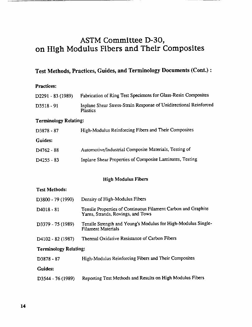
ASTM Committee D-30,
on High Modulus Fibers and Their Composites
Test Methods, Practices, Guides, and Terminology Documents (Cont.) :
Practices:
D2291 - 83 (1989)
D3518 - 91
Fabrication of Ring Test Specimens for Glass-Resin Composites
Inplane Shear Stress-Strain Response of Unidirectional ReinforcedPlastics
Terminology Relating:
D3878 - 87
Guides:
D4762 - 88
D4255 - 83
High-Modulus Reinforcing Fibers and Their Composites
Automotive/Industrial Composite Materials, Testing of
Inplane Shear Properties of Composite Laminates, Testing
Test Methods:
D3800 - 79 (1990)
D4018 - 81
D3379 - 75 (1989)
D4102 - 82 (1987)
High Modulus Fibers
Density of High-Modulus Fibers
Tensile Properties of Continuous Filament Carbon and GraphiteYarns, Strands, Rovings, and Tows
Tensile Strength and Young's Modulus for High-Modulus Single-Filament Materials
Thermal Oxidative Resistance of Carbon Fibers
Terminology Relating:
D3878 - 87
Guides:
D3544 - 76 (1989)
High-Modulus Reinforcing Fibers and Their Composites
Reporting Test Methods and Results on High Modulus Fibers
14

ASTM Committee D-30,
on High Modulus Fibers and Their Composites
Recent Special Technical Publications:
STP 1059 : Composite Materials: Test and Design (Ninth Volume)
S. P. Garbo, Ed. - 1990
STP 1080 : Thermal and Mechanical Behavior of Metal Matrix and Ceramic
Matrix Composite Materials
J. M. Kennedy, H. H. Mocller, and W. S. Johnson, Eds. - 1990
STP 1110 : Composite Materials: Fatigue and Fracture (Third Volume)
T. K. O'Brien, Ed. - 1991
STP 1120 : Composite Materials: Testing and Design (Tenth Volume)
G. C. Grimes, Ed. - 1992
STP 1128 : Damage Detection in Composite Materials
J. E. Masters, Ed. - 1992
STP 1156 : Composite Materials: Fatigue and Fracture (Fourth Volume)
W. W. Stinchcomb and N. E. Ashbaugh, Eds. - 1993
STP 1174 : High Temperature and Environmental Effects on Polymeric Composites
C. E. Harris and T. S. Gates, Eds. - 1993
STP 1203 : Fractography of Modern Engineering Materials: Metals andComposites, Second Volume
J. E. Masters and L. N. Gilbertson, Eds. - 1993
STP 1206 : Composite Materials: Testing and Design (Eleventh Volume)E. T. Camponeschi, Ed. - 1993
15

Composite Material :Characterization and Evaluation
A Survey Of Major Aircraft Manufacturers Indicates that:
Procedures Are Designed to Minimize the Risk of
Spending A Large Amount Of Funds On'Materials
Which Do Not Meet Structural or Processing
Requirements.
Materials Evaluation Conducted in Three Stages:
Material Screening, Material Characterization,
and Development of Design Allowables.
Although The Tests Employed Were Not Identical, The
Properties Measured At Each Level Of Investigation
Were Similar From Company To Company.
Majority Of Tests Focus On Obtaining The Mechanical
Properties Which Are Most Useful To The Designer
And The Structural Analyst But Which May Not Be
Of Great Interest To The Material Scientist.
Three Major Design Factors that Control the Weight of
an Aircraft: Stiffness, Damage Tolerance, and
Stress Concentrations at Cut-Outs and Loaded
Bolt Holes.
16

Composite Material :Characterization and Evaluation
Screening Evaluation :
First Step In the Material Characterization andEvaluation Process.
Objective: Determine Material Acceptability for
Aircraft Structural Applications.
Compared Candidate Material To A Baseline Material To
Determine if a More Extensive Evaluation Program is
Warranted.
• 50 to 60 Tests Typically Performed.
17

Composite Material :Characterization and Evaluation
Screening Evaluation Tests :
A list of test methods commonly employed in screening evaluations is contained
in the following table.
Test Type
0 ° Tension
0 ° Compression
+/- 45 ° Tension
Interlaminar Shear
Laminate
Compression
Open Hole Tension
Open HoleCompression
Compression afterImpact
Bolt BearingTension
PropertiesMeasured
EnvironmentalCondition
Strength, Modulus RTA
Strength, Modulus RTA, ETW
Strength, Modulus CTA, RTA, ETW
Strength RTA
Strength RTA
Strength
Strength
CTA, RTA, ETW
CTA, RTA, ETW
Strength RTA
Strength RTA
Note: CTA indicates -65 ° F/Ambient Moisture Conditions
RTA indicates Room Temperature/Ambient Moisture ConditionsETW indicates Elevated Temperature/Saturated Moisture Conditions
18

Composite Material :Characterization and Evaluation
Material Characterization :
Objective: Establish Preliminary Design Properties
for Design and Analysis of Test Components for DesignTrade Studies.
Measure Lamina Properties Required to Support
Laminated Plate Theory and Failure Criteria.
Measure Laminate Properties to Support Analysis and
Design.
• 200 to 250 Tests Typically Performed.
19

Composite Material :Characterization and Evaluation
20
Materials Characterization Tests :
A list of test methods commonly employed in materials characterization tests iscontained in the following table.
Test Type
0° Tension
90" Tension
0° Compression
90 ° Compression
+/- 45 ° Tension
In-Plane Shear
Interlaminar Shear
Interlaminar Tension
Laminate Compression
Open Hole Tension
Open Hole Tension (Fatigue)
Filled Hole Tension
Open Hole Compression
Filled Hole Compression
Compression after Impact
Bolt Bearing Tension
Mode I Delamination Resistance
Mode II Delamination Resistance
Note:
Properties Measured
EnvironmentalCondition
Strength, Modulus, Poisson'sRatio
CTA, RTA, ETW
Strength, Modulus, Poisson's CTA, RTA, ETWRatio
Strength, Modulus CTA, RTA, ETW
Strength, Modulus CTA, RTA, ETW
Modulus CTA, RTA, ETW
Strength RTA
Strength RTA
Strength RTA
Strength, Modulus CTA, RTA, ETW
Strength CTA, RTA, ETW
S - N Data RTA
Strength RTA
Strength CTA, RTA, ETW
Strength RTA
Strength RTA
Strength RTA
GIC RTA
GIIC RTA
Bold Type indicates tests performed in Screening EvaluationCTA indicates -65 o F/Ambient Moisture Conditions
RTA indicates Room Temperature/Ambient Moisture ConditionsETW indicates Elevated Temperature/Saturated Moisture Conditions

Composite Material :Characterization and Evaluation
Development Of Design Allowables :
Objective: Develop Complete Database for Final
Design and Certification.
Same Types of Tests Used in Materials Screening andCharacterization Evaluations.
Test Matrix Expanded to Include Additional Laminate
Configurations, Alternate Specimen Geometries (e.g.
Width/Diam. Ratios), Additional Environmental
Conditions, More Replicate Tests on Samples taken from
Several Batches of Material.
Could Total Thousands of Tests Depending on
Certification Requirements.
21

Composite Material :Characterization and Evaluation
Tests Applied to Laminated Tape Composites :
TEST TYPE
• TENSION:
Unnotched
Notched
• COMPRESSION:
Unnotched
Notched
• COMPRESSION
AFTER IMPACT
• BOLT BEARING
• INTERLAMINAR TENSION
• INTERLAMINAR SHEAR
• MODE I DELAMINATION
• MODE II DELAMINATION
TE_;T METHOD
ASTM D3039, D3518MISC. COMPANY METHODS
SACMA SRM 5
NASA 1142- B9
ASTM 3410
SACMA SRM1
NASA SHORT BLOCK
MISC. COMPANY METHODS
SACMA SRM 3
NASA 1092 ST-4
MISC. COMPANY METHODS
SACMA SRM 2
NASA 1142 Bll
MISC. COMPANY METHODS
FLATWlSE TENSION
CURVED BEAM
ASTM D2344
DOUBLE CANTILEVER BEAM
END NOTCHED FLEXURE
Note: SACMA Indicates Test Methods Developed by the Suppliers of Advanced CompositeMaterials Association
22

Composite Material :Characterization and Evaluation
Physical Properties Measured :
Prepreg Tape:
Resin Content
Fiber Content
Volatile Content
Cured Laminates:
Resin Content
Fiber Content
Void Content
Density/Specific Gravity
Glass Transition Temperature (Dry and Wet)
Equilibrium Moisture Content
Thermal Conductivity
Heat Capacity
Coefs. of Thermal Expansion
Thermal Oxidative Stability
23

Development of Test Methods forTextile Composites
Program Objective:
As indicated below, the objective of this on-going effort, simply stated, is to
develop a set of test methods and guidelines to be used to measure the mechanical and
physical properties of composite materials reinforced with fibrous textile preforms.
Investigations conducted to date have indicated that existing methods, which were
developed largely to evaluate laminated tape type composites, may not adequately
address the subtleties of these new material forms.
Develop And Verify Recommended Mechanical
Test Procedures And Instrumentation
Techniques For Textile Composites
24

Development of Test Methods forTextile Composites
Statement of Problem :
The problem to be addressed is summarized in the two bullet statements given
below. Simply stated, the test methods listed in the previous figures were developed to
evaluate composite materials formed by laminating layers of pre-impregnated fiber-
reinforced tape. The microstructure of these laminated composite materials differs
significantly from the braided, woven, and stitched materials to be evaluated in this
program. The fiber architecture will play a prime roll in determining the mechanical
response of these textile composite materials. Will existing methods and practices
accurately reflect the material response of these materials?
TEST METHODS DEVELOPED FOR
LAMINATED TAPE COMPOSITES
),. TEXTILE ARCHITECTURE CONTROLS
MATERIAL R ESPONSE
25

Development of Test Methods forTextile Composites
Textile Composites Testing Issues :
It is not difficult to identify a number of specific testing issues relative to textile
composites. Several of these concerns, which are applicable to virtually all of the testmethods listed on the previous page, are listed below.
The f'trst two reflect the unique size effects these materials may present. A unit
cell is defined as the smallest unit of repeated fiber architecture. It may be considered thebuilding block of the material. The size of the unit cell is dependent on a number offactors including the size of the yarns, the angle at which they are intertwined orinterwoven, and the intricacy of the braid or weave pattern. A representative volume ofmaterial must be tested and monitored to accurately reflect true material response.
Specimen geometry and strain gage sizes must be reexamined in terms of unit cell size.The effect of the sizes of the yarn bundles must also be considered since they may alsoaffect the performance and the measurements. This is expressed in the third statement.
The final three items on the list reflect concerns over specimen geometry. Test
specimen dimensions established for tape type composites may not be applicable totextile composites. The degree of heterogeneity present in the latter materials is quitedifferent than that encountered in the former. The potential effects of these differences
must be also quantified.
A limited amount of relevant data has been developed for 2-D triaxially braided
textile composites. These results will be reviewed in the following section. They includeMoire interferometry and strength and modulus measurements.
EFFECT OF UNIT CELL SIZE ON
MECHANICAL PERFORMANCE
EFFECT OF UNIT CELL SIZE ON STRAIN
GAGE AND DISPLACEMENT MEASUREMENTS
EFFECT OF TOW SIZE AND FIBER ARCHITECTURE
ON MECHANICAL PERFORMANCE
EFFECT OF FINITE WIDTH ON UNNOTCHED AND
OPEN-HOLE SPECIMENS
EFFECT OF EDGE CONDITIONS ON MECHANICAL
PERFORMANCE
EFFECT OF TEXTILE THICKNESS ON MECHANICAL
PERFORMANCE
26

Development of Test Methods for
Textile Composites
Program Approach :
A straightforward approach has been adopted to meet the objective outlined in the
previous figure. An extensive test program will be conducted to gather data addressing
the concerns listed earlier. The program, which will include a wide variety of woven,
braided, and stitched preform architectures, will consider several loading conditions.
The general approach is outlined below. Details of material tested and test
methods are supplied in the following pages.
• IDENTIFY AND/OR DESIGN AND DEVELOP SPECIMEN
CONFIGURATIONS AND TEXT FIXTURES
CONDUCT MECHANICAL TEST PROGRAM
• Variety of Test Methods
• Variety of Instrumentation Techniques
• Full Field Strain Measurements
• Analytical Support
• IDENTIFY SMALLEST LEVEL OF HOMOGENEITY
• IDENTIFY APPROPRIATE TEST METHODS AND
INSTRUMENTATION GUIDELINES
27

Development of Test Methods forTextile Composites
Description of Material Tested :Preforms and Textile Parameters Studied
Fifteen woven, braided, and stitched preforms will be evaluated in the program.
The preform types are listed below in the table; the number of each type to be tested is
indicated in parentheses. The table also lists the braid parameter that will be varied for
each preform type. The list of materials reflects the material forms that are being
evaluated by the aircraft manufacturers in the ACT program.
TEXTILE PREFORM TYPES "
2-D TRIAXIAL BRAIDS - (4)
• Tow Size
• % Longitudinal Tows
• Braid Angle
3-D INTERLOCK WEAVE - (6)
• Weave Type - (3)
• Warp, Weft, and Weaver Tow Size
STITCHED UNIWEAVE - (5)
• Stitch Material
• Stitch Spacing
• Stitch Yarn Size
MATERIALS :
FIBER: HERCULES AS4
RESIN: SHELL 1895
28

Development of Test Methods forTextile Composites
Description of Material Tested :Triaxial Braid Pattern
The specimens studied in this investigation featured 2-D triaxially braided AS4graphite fiber preforms impregnated with Shell 1895 epoxy resin. In a triaxially braidedpreform three yarns are intertwined to form a single layer of 0"/+ O" material. In thiscase, the braided yams are intertwined in a 2 x 2 pattem. Each + O yam crosses
alternatively over and under two - O yams and vice versa. The 0" yams were insertedbetween the braided yams. This yields a two dimensional material. The figure belowschematically illustrates the fiber architecture and establishes the nomenclature used in
the paper.
The yarns were braided over a cylindrical mandrel to a nominal thickness of 0.125in. The desired preform thickness was achieved by overbraiding layers; there are nothrough-the-thickness fibers. After braiding, the preforms were removed from themandrel, slit along the 0 ° fiber direction, flattened, and border stitched to minimize fibershifting. The resin was introduced via a resin transfer molding process.
Axialloading
direction
A BraidTransverse angle
Axial -_--loadingyarns direction
29
Development of Test Methods for
Textile Composites
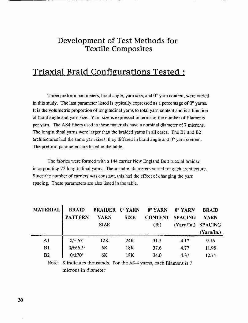
Triaxial Braid Configurations Tested :
Three preform parameters, braid angle, yarn size, and 0 ° yarn content, were varied
in this study. The last parameter listed is typically expressed as a percentage of 0 ° yarns.
It is the volumetric proportion of longitudinal yarns to total yarn content and is a function
of braid angle and yarn size. Yarn size is expressed in terms of the number of filaments
per yam. The AS4 fibers used in these materials have a nominal diameter of 7 microns.
The longitudinal yarns were larger than the braided yarns in all cases. The B1 and B2
architectures had the same yarn sizes; they differed in braid angle and 0 ° yarn content.
The preform parameters are listed in the table.
The fabrics were formed with a 144 carrier New England Butt triaxial braider,
incorporating 72 longitudinal yarns. The mandrel diameters varied for each architecture.
Since the number of carriers was constant, this had the effect of changing the yarn
spacing. These parameters are also listed in the table.
MATERIAL
A1
B1
B2
Note:
BRAID BRAIDER 0 ° YARN 0 ° YARN 0 ° YARN
PATTERN YARN SIZE CONTENT SPACING
SIZE (%) (Yarn/In.)
0/+ 63 ° 12K 24K 31.5 4.17
0__66.5 ° 6K 18K 37.6 4.77
0/+70 ° 6K 18K 34.0 4.37
K indicates thousands. For the AS-4 yarns, each filament is 7
microns in diameter
BRAID
YARN
SPACING
(Yarn/In.)
9.16
11.98
12.74
3O
Development of Test Methods forTextile Composites
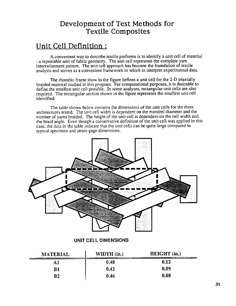
Unit Cell Definition :
A convenient way to describe textile preforms is to identify a unit cell of material- a repeatable unit of fabric geometry. The unit cell represents the complete yarnintertwinement pattern. The unit cell approach has become the foundation of textileanalysis and serves as a convenient framework in which to interpret experimental data.
The rhombic frame show in the figure defines a unit cell for the 2-D triaxiallybraided material studied in this program. For computational purposes, it is desirable todefine the smallest unit cell possible. In some analyses, rectangular unit ceils are also
required. The rectangular section shown in the figure represents the smallest unit cellidentified.
The table shown below contains the dimensions of the unit cells for the three
architectures tested. The unit cell width is dependent on the mandrel diameter and thenumber of yarns braided. The height of the unit cell is dependent on the cell width andthe braid angle. Even though a conservative definition of the unit cell was applied in thiscase, the data in the table indicate that the unit cells can be quite large compared to
typical specimen and strain gage dimensions.
lllm
UNIT CELL DIMENSIONS
MATERIAL
A1
B1
B2
WIDTH (in.)
0.48
0.42
0.46
HEIGHT (in.)
0.12
0.09
0.08
31

MOIRI_ INTERFEROMETRYAxial Load - Vertical DisplacementField
As indicatedearlier,Moir_ interferometrywasusedto definethefull field straindistributionin thesebraidedspecimens.Thetechniquedefinesdeformationpatterns inboth the vertical and horizontal directions. The technique was applied to specimenssubjected to longitudinal and transverse loading. These results are shown in this and the'
following figures.
The figure below illustrates the specimen geometry and highlights the sectionstudied. The vertical displacement field that resulted when a specimen was loaded to1200 micro-su'ain along the 0" fiber direction is also shown in the figure.
The vertical displacement fields (V fields) consist of basically horizontal fringes;this indicates specimen extension where points along one fringe have been displacedvertically with respect to points along a neighboring fringe. For a uniform extension thefringes should be evenly spaced and straight. The fringes for the specimens tested,however, are wavy and the spacing between them varies. The variation is cyclic andcoincides with the repeated unit of the textile architecture.
,,,,9__ 1.50 in.
©
iiiiiiiiili ii i iiii i i ii!i!li:_:!:!:i:?i:i:':!:!:_:i:i::.:i:i:!'i:i:_:i:i:i:ii!:_:-:i:i:i:i:!:i:_:_:i:!:_:i:i:i:i:i$_:i:_:_:'_.::i:_:i:_$_
N
O FiberDirection
-_1.50 in.
Vertical Displacement Field
©
32

MOIRI_ INTERFEROMETRY
Axial Load - Horizontal Displacement Field
The horizontal displacement patterns (U fields) consist of zigzag vertical
fringes that display the Poisson's effect. For uniform contraction the fringes should bestraight and the spacing constant. The fringes however display a variation which iscyclic, and matches that Of the braid geometry. The sharp kinks in the U field fringesreveal the presence of shear strains between the fiber bundles.
-.-,_-_ 1.50 in.
0
Horizontal Displacement Field
t O° FiberDirection
0
33

ENLARGED VIEW OF TWO UNIT CELLS OF SPECIMEN
(Axial Loading)
The figure shows the V and U fields of a highly magnified region of specimen
that consists of two unit cells. The boundaries between adjacent fiber bundles and the
outline of the cells are marked. It was revealed that the shear deformation at interfaces
between the fiber bundles occurred over a finite width. This width is illustrated in the
patterns as the distance between the closely spaced lines. This is consistent with the
presence of the resin rich areas between the fiber bundles, which was on the order of one
Fifth of the width of the fiber bundle itself. The U field shows that the shear strain 7xy in
the resin rich zones was on the order of 0.5 times that of the average applied normal strain
ey. Additionally, the U field shows that the Poisson effect was nearly" constant across the
unit cell. The V displacement pattern clearly shows that the strain Ey varies significantly
within each unit cell as can be seen by the nonuniform fringe spacing. The ratio of
maximum strain ey to minimum strain was about 2 to 1. The normal strain varies on top
of the fiber bundles and is nearIy constant throughout all of the resin rich zones.
Vertical Displacement Field
Horizontal Displacement Field

SPECIMEN SECTION COINCIDING WITHMOIRE FRINGE PATI'ERNS
(TransverseLoading)
Interferomet:-ywasalsoperformedonspecimensloadedin theu-ansvers¢
direction(i.e. at 90" to the axial direction). This fi_ure shows the re#on investigated in
these specimens. The pattern of the surface braided yarns is shown schematically in the
figure. The deformation fields that developed in these coupons are shown in the next two
figures.
0 ° FiberDirection
©
©
35

.MOIRI_ INTERFEROMETRY
Transverse Load - Vertical Displacement Field
In general, the inte,_erometry results indicate that greater variations in normal andshear strains existed in specimens loaded in the transverse direction than in the axialdirection.
This figure displays the vertical displacement field for a coupon loaded in thetransverse direction. The location of the yarns is evident in the vertical displacementfringe patterns, where sudden jogs in the fringes represent strong shear strains in the resinrich regions between the yarns. From the V displacement pattern, the spacing of thefringes in the vertical direction displays a cyclic variation. The strains are highest overthe region where there are 90 ° fibers under the braider yarns. They are lowest over theregions where the braider yarns cross. The difference between the average strains inthese areas is on the order of 3 times.
Unlike the axial loading case, the cyclic variation is not confined to the
dimensions of the unit ceil. The variation breaches the unk cell to form a global materialresponse that covers the entire specimen. This is illustrated by the horizontal bands seenin the figure. They span several unit cells and extend across the specimen width.
0° FiberDirection
Vertical Displacement Field
36

Development of Test Methods forTextile Composites
Effect of Strain Gage Size on Modulus :
The inhomogeneity in the strain fields demonstrated in the Moire interferometricresults discussed in the previous slides has significant implications with regard to
specimen instrumentation. The large strain gradients seen within the unit cell graphicallyillustrate the need to measure strain over a truly representative volume of material to getan accurate determination of the global material response. Local strain readings can be
misleading and confusing.
The data shown in the figure below demonstrate these points. The figure plots themeasured transverse modulus of several B 1 laminates vs. the size of the gages used to
measure the strain. The gages ranged in length from 0.062 in. to 1.0 in.; the preform'sunit cell measures 0.42 in. in this direction. The average modulus and the standarddeviation of the data are shown in the figure. As the figure indicates, significant scatterwas evident in the results obtained using the small gages. These effects are reduced as
the length of the gage increased. The results also indicate that average value alsodecreased as strain gage size increased.
The results illustrate the need to consider the textile architecture when choosing
instrumentation for a specimen.
10.00
8.00
036.00
03
-- 4.00
O2.00
0.00
Transverse Modulus vs Strain Gage Size
a ! I l I . . . . | s • . . | . . . • I . . . .
• ' ' ' I ' ' ' ' I " ' ' ' I ' ' ' ' I '
0.00 0.25 0.50 0.75 1.00 1.25
STRAIN GAGE SIZE (in.)
37
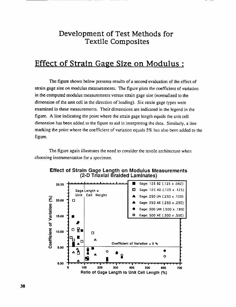
Development of Test Methods forTextile Composites
Effect of Strain Gage Size on Modulus :
The figure shown below presents results of a second evaluation of the effect of
strain gage size on modulus measurements. The figure plots the coefficient of variation
in the computed modulus measurements versus strain gage size (normalized to the
dimension of the unit cell in the direction of loading). Six strain gage types were
examined in these measurements. Their dimensions are indicated in the legend in the
figure. A line indicating the point where the strain gage length equals the unit cell
dimension has been added to the figure to aid in interpreting the data. Similarly, a line
marking the point where the coefficient of variation equals 5% has also been added to the
figure.
The figure again illustrates the need to consider the textile architecture when
choosing instrumentation for a specimen.
Effect of Strain Gage Length on Modulus Measurements(2-D Triaxial Braided Laminates)
25.00
A
20.oov
=_ca 15.00
>
O
e- 10.00_Q_owe_oo
0 5.00
i • • = . d t • • • I • •
Gage Length -
Unit Cell Height
[3
0.00
• • I • • , • Gage: 12S BZ (.125 x.062)
[] Gage: 125 AD (.125 x .125)
• Gage: 250 UN (.250 x .1?-0)
• Gage: 250 AE (.250 x .2S0)
• Gage: S00 UW (.500 x .180)
O Gage: 500 AE (.S00 x .S00)
Coefficient of Variation = 5 %
0
100 200 300 400 500 600
Ratio of Gage Length to Unit Cell Length (%)
70o
38
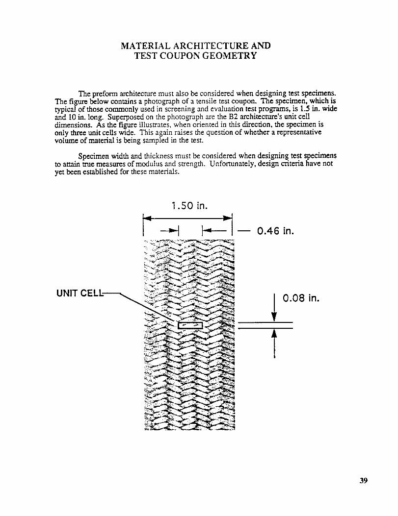
MATERIAL ARCHITECTURE AND
TEST COUPON GEOMETRY
The preform architecture must also be considered when designing test specimens.The figure below contains a photograph of a tensile test coupon. The specimen, which istypical of those commonly used in screening and evaluation test programs, is 1.5 in. wideand 10 in. long. Superposed on the photograph are the B2 architecmrc's unit celldimensions. As the figure illustrates, when oriented in this direction, the specimen isonly three unit cells wide. This again raises the question of whether a representativevolume of material is being sampled in the test.
Specimen width and thickness must be considered when designing, test specimensto attain true measures of modulus and strength. Unfortunately, design criteria have not
yet been established for these materials.
UNIT CEI.
1.50 in.
-- 0.46 in.
0.08 in.
39
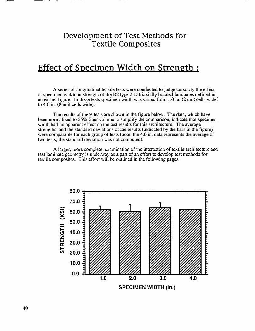
Development of Test Methods forTextile Composites
Effect of Specimen Width on Strength :
A series of longitudinal tensile tests were conducted to judge cursorily the effectof specimen width on strength of the B2 type 2-D triaxially braided laminates defined inan earlier figure. In these tests specimen width was varied from 1.0 in. (2 unit cells wide)to 4.0 in. (8 unit cells wide).
The results of these tests are shown in the figure below. The data, which havebeen normalized to 55% fiber volume to simplify the comparison, indicate that specimenwidth had no apparent effect on the test results for this architecture. The averagestrengths and the standard deviations of the results (indicated by the bars in the figure)were comparable for each group of tests (note: the 4.0 in. data represents the average oftwo tests; the standard deviation was not computed).
A larger, more complete, examination of the interaction of textile architecture andtest laminate geometry is underway as a part of an effort to develop test methods fortextile composites. This effort will be outlined in the following pages.
ZI--
Ziii
I-¢/1
80.0 -
70.0
60.0
50.0
40.0
30.0
20.0
10.0
0.01.0 2.0 3.0 4.0
SPECIMEN WIDTH (in.)
4O

Development of Test Methods for
Textile Composites
Summary Investigation of 2-D Braids:
A brief summary of the technical results reviewed in the presentation is given
below. The experimental investigation conducted on 2-D braided materials indicated that
significant strain gradients existed within the materials unit cell as a result of the braid
architecture. This inhomogeneity in the strain field is an important factor that must be
considered when choosing instrumentation for a test specimen. Although the 2-D braided
laminates tested did not demonstrate a width effect, the size of the unit cell must also be
considered when designing a test specimen.
Finally, the concerns discussed above and others listed in an earlier figure will be
addressed in an on-going test method development effort.
MOIRI_ INTERFEROMETRY IDENTIFIED LARGE STRAIN
GRADIENTS WITHIN THE UNIT CELL
INHOMOGENEITY IN STRAIN FIELD EFFECTS
INSTRUMENTATION
UNIT CELL SIZE MAY AFFECT TEST RESULTS
ON-GOING INVESTIGATION TO DEFINE TEXTILE TEST METHODSUNDERWAY
41


N94- 36400
/"
"_ r'//- f
CONTINUOUS UNIDIRECTIONAL FIBER REINFORCED
COMPOSITES: FABRICATION AND TESTING
M. D. Weber
Pennsylvania State University9 Simmons Hall
University Park, Pennsylvania 16802
Telephone 814-862-4314
and
F. X. Spiegel
Loyola College
Baltimore, Maryland
and
Harvey A. West
North Carolina State Unive/'sityBox 7907
Riddick Hall Room 229
Raleigh, North Carolina 27695-7907
Telephone 919-515-3568
43

CONTINUOUS UNIDIRECTIONAL FIBER REINFORCED COMPOSITES:
FABRICATION AND TESTING *
M.D. Weber, F.X. Spiegel, H.A. West **
Loyola College, Baltimore, Maryland
**North Carolina State University, Raleigh, NC
*Hauber Fellowship Funded
ABSTRACT: The study of the anisotropic mechanical
properties of an inexpensively fabricated composite with
continuous unidirectional fibers and a clear matrix was
investigated. A method has been developed to fabricate these
composites with aluminum fibers and a polymer matrix. These
composites clearly demonstrate the properties of unidirectional
composites and cost less than five dollars each to fabricate.
KEY WORDS: anisotropy, composite, fibers, matrix,
reinforcement, strain, stress.
INTRODUCTION: A process was developed to make fiber
composites with continuous fibers spanning the composite and
aligned in one direction (Fig. i). H.A. West and A.F. Sprecher
have been studying the mechanical properties of this type of
composite with samples of rubber reinforced with nylon cord. I
These samples, however, are not readily available and require a
hot press for consolidation and curing. It would be desirable to
develop a system which sufficiently demonstrates the effect of
fiber orientation, yet is easily fabricated from available
materials. In addition to studying the parameters of this type
of composite, a clear matrix was desired in order to view the
fibers.
While developing this process to demonstrate anisotropic
mechanical properties, it was very important to limit costs and
to develop educational opportunities for composites in the
laboratory and classroom. Composites are widely used in our
society today; fiberglass, plywood, and concrete are just a few
examples. 2
PREREQUISITE KNOWLEDGE: The previous .or concurrent study of
composites, specifically continuous unidirectional composites,
and their mechanical properties would be beneficial. The effect
of fiber orientation on elastic modulus, Poisson's ratio, and
state of strain can be investigated.
OBJECTIVE: An inexpensive fabrication process was developed
for continuous unidirectional fiber reinforced composites with
clear matrices in order to study material properties such as
elastic anisotropy.
EQUIPMENT AND SUPPLIES: (I) Six 3" x 5 1/8" pieces of
aluminum screening; (2) Utility knife; (3) Cutting board;
(4) transparent or masking tape; (5) Manicure scissors or small
wire cutters; (6) Three 200 mL plastic containers; (7) Plastic
container i" x 3" x 5" ; (8) Ferris see thru; (9) Por-a-mold;
P-AGE BLAJ',IK NOT FILIMED
45

(i0) Release agent (Synair 1711); (ii) Vacuum pump; (12) Oven
(350 F); (13) Ferris jig (see Fig.3); (14) Two 4" x 6" x 1/8"
glass plates; (15) Two clamps; (16) Isopropyl rubbing alcohol to
clean containers.
PROCEDURE: Composite fabrication began with the preparation
of either plain or anodized aluminum screening, the fibers, which
were then set up for the matrix addition of either Por-a-mold or
Ferris see thru. After the composite cured completely, its
mechanical properties were tested.
Fibers
After cutting the screening with the fibers at the desired
angle and affixing a 1/2" border of tape to all sides (to hold
the screen together), a utility knife and a pair of manicuring
scissors were used to cut out the unwanted fibers. By cutting
the columns between every two desired fibers, the unwanted fibers
slip away and leave the desired fibers intact (Fig. 2).
While preparing several layers, usually three or five, it
was beneficial to leave three of the unwanted fibers intact near
the center (support wires) and place the layer under a book while
working on the others. Finally, the tape and support wires were
removed; the preparation time ranged from 20-60 minutes per
layer.
Matrix: Por-A-Mold
In the plastic container sprayed with the release agent,
three layers of identical fibers were stacked flat. Then, the
por-a-mold matrix was prepared by:
(I) stirring the curative thoroughly and measuring 75 mL in
a plastic container
(2) stirring the prepolymer thoroughly and measuring 75 mL
in a plastic container
(3) noting the time when adding the curative to the
prepolymer (9-12 minutes working time)
(4) mixing it to a clear consistency (< 2 minutes)
(5) vacuuming it for 4 minutes
(6) pouring it evenly over the fibers
(7) spraying the release agent on the surface to removeadditional air bubbles.
Finally, after allowing the matrix to cure at room
temperature for 16 to 24 hours, 3 the composite was removed from
the container and trimmed for testing.
Ferris See Thru
When a matrix of Ferris see thru was desired, three or five
identical layers of fibers were fit into the grooves of the
ferris jig before clamping a glass plate to each side (Fig. 3).
Then, a small amount of the white ferris see thru liquid was
46

dripped along the edges between the glass and jig to be heatcured at 350 degrees Fahrenheit until it turned clear (5-10minutes). After a good seal was made, 175 mL of the ferris seethru was poured into the jig and vacuumed for five minutes. TheFerris see thru was then heat cured at 350 degrees Fahrenheit.After 50-60 minutes, the matrix became a clear solid with aslight medium yellow tint. The new composite was removed fromthe jig after it cooled.
Testing
Several composites were made using the two matrices, two
types of fiber, and angles of 0, 15, 30, 45, 60, 75, and 90
degrees. Also, a few support wires were left in many of the
first composites. Before testing, the supporting border of
fibers was trimmed off to yield the continuous unidirectional
fiber reinforced composite.
One purpose of combining two (or more) distinct materials to
create a composite was clearly demonstrated by the first two
samples tested under tension. A sample of solid por-a-mold
elongated 7.5 inches with only 0.19 inches of plastic deformation
and broke under merely 9.5 pounds. However, the por-a-mold and
anodized A1 fiber composite maintained its length up to 50 pounds
and did not break under ii0 pounds.
The most interesting tests depict elastic anisotropy. After
a 90 degree angle is marked in the center of the sample, it is
placed under tension while recording any angle change and the
tension (Fig.4). The original 90 degree angle may or may not
change, depending on the fiber orientation.
SAMPLE DATA: For a composite of pot-a-mold and three layers
of anodized AI:
30 degree fibers @ 40 ibs. 90 degrees became 97
45 degree fibers 40 ibs. 90 degrees stayed 90
INSTRUCTOR'S NOTES: These composites can be used to
demonstrate and study the Rule of Mixtures and Poisson's ratio 4
in addition to calculating percent fiber content by volume and
observing deviations due to slight alterations. For example, if
a 90 degree fiber composite is trimmed to leave only a few
unwanted (0 degree) fibers along the length of one edge, it will
torque under tension. However, once the 0 degree fibers are
removed, it does not torque. At high forces, slippage and fiber
pullout may occur. Also, the kinks in the fibers from being
woven might want to be considered.
REFERENCES:
(I) West, H.A.; and Sprecher, A.F.: "Fiber Reinforced
Composite Materials," National Educators Workshop:
Update '90, NIST Special Publication 822, 1991.
(2) Askeland, Donald R.: The Science and Enqineerinq of
Materials, PWS-Kent,Boston, 1970.
47

(3) Product Bulletin Number CC-91-02, "Basic Techniques For
Using Por-A-Mold, Clear-Cut," Synair Corporation.
(4) Agarwal, Bhagwan D.; and Broutman, Lawrence J.: Analysis
and Performance of Fiber Composites, Second ed.,
John Wiley & Sons, Inc., New York, 1990.
SOURCES of SUPPLY: While the aluminum screening can be
easily purchased at a hardware store (less than $0.15 sq. ft.),
the Ferris see thru can be obtained through a jewelry dealer
(approximately $55 per gallon). Unfortunately, por-a-mold is no
longer on the market.
ACKNOWLEDGEMENTS: We would like to thank Mr. Howard Moore,
Technical Assistant, Physics department, Loyola C611ege, for
machining the ferris jig and allowing us the use of his tools.
Also, we appreciate the interest and input of Jon Thompson,
Technical Assistant, Engineering department, Loyola College, and
many others at Loyola College and North Carolina State Univesity.
48

fiber
matrix
-0------ 30 °
Figure I. Continuous unidirectional fiber-reinforced composite
{ tape : :
i ¸i i !_._,._
---7/
m _
u F)_brt _ _r_s
m
Figure 2. Fiber preparation of AI screening
49

.8
groo_on p_
II fl
H t_
IJ 11
II LI
@//
Figure 3. The Ferris Jig
-J.1" /1[//.i.1/../" A
• /_IA
A
J'l
_-/lJ-I
Draw a 90" angle.
t/1..."1..,-1A...-'1A
..-'1
Jq
/I
/I
A
A
A
4
The angle may change.
Figure 4. Composite under uniaxial tension
5O

N94- 36401"7 (
DESIGN AND CONSTRUCTION OF ATENSILE TESTER FOR THE TESTING OF
SIMPLE COMPOSITES
Mark A. Borst
and
F. Xavier Spiegel
Loyola College
4501 N. Charles Street
Baltimore, Maryland 21210-2699
Telephone 410-617-5123 or 410-617-2515
51


Foreword
Materials testing has been an important part of engineering in America for over one
hundred years. In 1832, the Franklin Institute began a systematic investigation into the cause of
steam boiler explosions. This study was broken down into two parts. The first part was
concerned with the operation of the boilers. The second part of the study, however, was
concerned with the material used to construct the boilers. At the time, manufacturers of iron
knew that their product was strong, but had no idea of how strong it was. The manufacture of
iron was guided by rule of thumb and virtually nothing was measured. This ignorance
concerning the production of iron did not have tremendous consequences until the arrival of the
steam engine. Boilers proved the inadequacy of some irons by exploding violently. As a result,
a method for testing materials was developed and initially executed by Walter R. Johnson,
Professor of Mechanics and Natural Philosophy at The Franklin Institute in Philadelphia. This
marked the first time that quantitative data on "proving tenacity" was gathered in America. ]
Materials testing has grown considerably since Johnson's work and is now a major part of
engineering. The material strength requirements for a steam engine pale in comparison to the
requirements tbr the machines of today. From high speed electronic switches to space flight, the
"boiler explosions" of today are much more costly, both in money and potential loss of life, than
they were in Johnson's day. The explosion of the space shuttle Challenger is an example of the
potential hazards waiting to happen. A single O-ring, cooled below an acceptable temperature,
caused the loss of seven lives and billions of dollars. As a result, the strength and characteristics
of a material must be fully understood before that material may be used in the manufacture of a
product.
PAGE BLANK NOT FIL_:I_D
53

The following is a design for a tensile tester which will be used to test the tensile strength
and anisotropic properties of simple composites. These simple composites are suspected to be
anisotropic primarily in a single plane. When the composites undergo a tensile force, they wil'l
undergo deformation, causing movement either to the left or right. The composites are suspect
due to their method of construction.
fibers embedded in a rubbery resin.
Each sample has a single layer of unidirectional continuous
It has been well established that a serious limitation of
unidirectional fiber composites is the very large in-plane anisotropy. 2
The design presented here incorporates a single degree of freedom such that distortion (to
the left or right) due to anisotropic tendencies may be measured. The device will spend the vast
majority of its time in an undergraduate materials lab. As a result, ease of use and durability are
valued more highly than research grade accuracy. Additional concerns focus on the fact that this
machine will be built as a student project.
Issues which are dealt with during this design include:
.
2.
3.
4.
5.
6.
7.
8.
Specimen configuration or shape.
Method of applying consistent, linear tension force.
Method of gripping specimen without affecting its overall properties.
Method of collecting data.
Repeatability of data.Ease of use.
Ease of construction.
Cost.
After the device has been constructed, it will be used to test the simple composites which
were fabricated in house. A comparison will be made between composites manufactured using
aluminum screening as the strengthening fibers and those manufactured using fiberglass
screening.
54

Design
Application of Force
The first matter which will be taken up is the application of force. A device is needed
which can provide a consistent, linearly applied force, but still allow for lateral movement of the
sample so that anisotropic properties as well as the modulus of elasticity and yield strength may
be observed and measured. In addition, the machine must provide for an easy method by which
several characteristics can be measured. These characteristics include:
1. Elongation
2. Lateral displacement as a result of anisotropic behavior.
3. Force applied.
A hand operated screw mechanism was chosen for the application of force. This
provides a simple means of applying tbrce in a single direction. In addition, the amount of force
applied may be increased in a linear fashion with infinitesimal changes. The screw chosen was
an Acme® threaded screw, one inch in diameter with a pitch often threads per inch. The
Acme® thread is a square cut thread and is designed to support large amounts of force. This
thread is commonly used in such high pressure applications as vices and large clamps. For each
rotation of the screw, the sample will be elongated by one tenth of an inch. This provides a
convenient point at which to take a reading of the force. As a result, measurements of force are
taken every one tenth of an inch and the number of readings taken prove an accurate guide for
the total elongation.
The screw is operated by means of a large hand wheel. The large wheel will provide
leverage so that an adequate amount of torque may be easily applied to the screw which in turn
will impart a large tensile force to the specimen which may be easily controlled by the operator.
55

In addition to being able to impart a tensile force to the sample, the screw must be able to
support itself. This was accomplished by using a twenty inch long section of screw and turning
down a one inch section on each end to 0.627" so that it would fit into two, flanged bushings.
Figure 1 shows the hand wheel. Tensile force will be applied when the knob is turned
clockwise. Most people associate a clockwise rotation of threaded objects with an application of
force and hence operation of the wheel will be of second nature. The Acme® threaded rod
appears in figure 2. Figure 3 shows the assembled screw mechanism. The screw and hand
wheel are attached by means of a roll pin. A hole was drilled through the hand wheel and rod
and the pin was then inserted.
Support and Load l'rans[er
Next to be considered is the frame of the machine. This is an important part since the
frame not only supports the machine but facilitates the transfer of the load from the screw
mechanism to the sample. In addition, it allows for lateral movement of the sample during
testing. The frame is also the heart of the information gathering process. A load cell is mounted
on the frame to allow for the measurement of the force being applied to the sample. The output
from the load cell is read from a Fluke digital multimeter in milli-volts. Through information
provided by the manufacturer as well as use of a standard, the relationship between the load
cell's output in milli-volts to the actual pounds of force delivered was determined.
The support part of the frame was constructed from 1"x3" sections of maple (Note:
These are mill dimensions ). Maple was chosen because of its high strength and its beauty. The
drive beam was constructed from oak. Maple would have been preferred, but a large enough
piece was not available. The properties of these two woods appear in table 1 (all figures
56

referto forcesappliedparallelto thegrain). Poplaris includedin thetablesinceit is of
sufficientstrengthto use in the construction of the frame and drive beam. In addition, relatively
large poplar beams (4"x4") are readily available and poplar is less expensive than maple or oak.
Unfortunately, poplar has a yellowish green tint that renders it much less pleasing to the eye than
either oak or maple. One should never neglect the aesthetics of a design.
Wood Specific Modulus of Modulus of Compressive
Gravity Elasticity Rupture Strength
[Ib/in 2 x 10 3] [Ib/in 2] [lb/in2l
Maple, sugar 0.676 1,830 15,500 7,800
Oak, white 0.710 1,770 15,100 7,440
Poplar, yellow 0.427 1,500 9,200 5,540
Table 1: Properties of selected hard woods. 3
The frame was constructed by using carpenter's glue to laminate five pieces of maple
together to form four beams. The sections were offset such that finger joints were formed at the
comers. These beams were clamped tightly and the glue was allowed to dry. After the glue had
dried, holes were drilled as required using a drill press and the appropriate bits. Figure 4 shows
the construction of the support beams. The drive beam appears in figure 5. All parts must be
assembled within the frame before any final gluing can take place. This includes two steel rods,
as well as the drive beam itself and the Acme® rod with hand wheel in place. Once assembled,
the frame was measured to check for squareness. It was racked into shape by use of large wood
working clamps which mount on standard one inch diameter black pipe. Once the frame was
squared, four 1/2" holes were drilled at each corner and four 1/2" hardwood dowels which had
57

beencoatedwith glueweredrivenin placeusingahammer.Theresultantappearsin figure 6
alongwith thetwo driverods,rail assemblyandmountedloadcell.
Theforcefrom thedrivebeamisdeliveredto thesampleby meansof two, 36" longsteel
rods,1"diameter. These drive rods support a rail and shuttle system which actually allows for the
single degree of freedom. The rods have holes drilled in them such that the rail and shuttle
system may be placed at different heights, thereby allowing for different length samples or grips
(Figure 7).
A section of rail that was used appears in figure 8. The guide rail was commercially
available in 6'-6" lengths. The rails were cut into four, 1'-3" sections and doubled as
reinforcement to prevent any deformation during loading. The rails must remain straight if any
anisotropic behavior is to be observed. If the rails bow, the shuttle system will remain in the
trough of the bow. Figures 9 and 10 show how the rail assembly is constructed.
(]rips and Shuttle system.
The grips were machined from aluminum and are straightforward in design. Each grip
basically consists of a center, mounting plate and two gripping plates. The two gripping plates
are fastened to either side of this center plate by means of four, knurled nuts. These nuts have
four small holes on the knurled surface that allow for the insertion of a taper pin. This provides
additional leverage in tightening the grips. The gripping plates were designed to be the exact
same dimension as the sample to be tested. As a result, the plates alone are unable to grip the
sample. This was done in order to minimize sample deformation from metal to composite
clamping as this might affect the test. A thin sheet of rubber (obtained from the plumbing
58

sectionof a hardware store) was attached to the face of the gripping plates using Duro® contact
cement. This allowed the clamping surface to conform somewhat to the sample as opposed to
pinching it. To provide additional gripping ability, pieces of 3M's Press'n Sand® "Sticky back"
sanding sheets were cut to size and affixed to the rubber faces. The gripping plates are the same
for the top and bottom (Figure 11). The bottom grip (Figure 12) screws into the load cell
(Figure 13).
The top grip consists of two gripping plates identical to those on the lower grip. These
plates mount on a shuttle system. The shuttle system consists of a center plate and four guide
wheels. The guide wheels were obtained from the same company which supplied the guide rail.
The unassembled shuttle system appears in figure 14.
Some comments concerning the machine's operation might prove helpful in improving on
the design. The grips were insufficient in holding the samples without the sandpaper faces, and
even then loads peaked at a maximum of just over 100 pounds before the samples began to pull
free from the grips. Also, the sandpaper faces slipped during tests and had to be replaced
periodically. A better idea might be to alter the design to accept commercial grips. This may
not alleviate all the problems. It was noticed that when a series of samples 1" wide were tested
(to match the 1" wide samples being run on the Chatillon LDX tensile tester since its grips could
accommodate nothing larger) anisotropic tendencies did not appear consistently. The 2.5" wide
samples, however, displayed excellent anisotropic tendencies. Still, the commercial grips might
be capable of delivering enough of a load to a 1" sample such that its anisotropic characteristics
are revealed.
59

('alibration and Verification of Devices Functioning
The load cell was connected to a Fluke digital multimeter as per manufacturer's
instructions. Using the load celrs specifications sheet, a relationship was determined between
the load cell's output in milli-volts and the corresponding force in pounds. The relationship
between the load cell's output in milli-volts and the tensile force applied was calculated to be:
Lbf= 998.84_ × v Equation 1
Lbf = pounds forcev = volts
The first problem was that of collecting the data. After each full turn of the hand wheel
(equivalent to an elongation of one tenth of an inch) the reading was taken from the multimeter
and written down. In the time taken to write down the data, however, the sample had relaxed
substantially. To prevent this, a small tape recorder was used to record data while the hand
wheel was turned in a slow, constant fashion. This eliminated the problem of relaxation during
data collection. Two people working together, as in an undergraduate lab, could also overcome
the problem with one student turning the hand wheel and calling out the readings while the other
student jots down the data.
The next problem encountered was the inaccuracy of the machine's output. Like samples
of Ferris See-thru® (Neat, 0.3"xl "x5-3/4") were tested on the hand operated device and on a
Chatillon LDX 500 pound capacity tensile tester. The data was offby an amount considered
unacceptable (Figure 15). Two things are readily apparent in viewing figure 15. The first is that
the hand operated device is reading ten pounds high (assuming the just purchased Chatillon was
6O

correct). Thesecondis that the slopes, or moduli of elasticity, are similar. It was suspected that
since the samples were being subjected to less than I00 pounds force, that the 5000 pound
capacity load cell simply was not in its most effective range. A small, 50 pound capacity hand
held spring scale (similar to a "fish scale") was used to check this. First, the scale was checked
for accuracy using the Chatillon. While the scale's readings fluctuated high and low with respect
to the Chatillon's output, a series often trials running from zero to forty-four pounds yielded an
average that was reasonably accurate (Figure 16). The scale was then attached to the hand
operated device. Ten sets of readings were taken ranging from zero to forty-four pounds. The
data was averaged, zeroed and plotted (Figure 17). The relationship between the load cell's
output in milli-volts and pounds force was determined to be:
Lbf = ml-ml'o Equation 20.963
Figure 1 8 shows the comparison of the data from figure 15 using Equation 2. The fit is
still not perfect, but it is closer. In addition, the two plots in figure 18 are closer to being parallel
at values above' 3/4 pounds. The modulus of elasticity was determined by determining the slope
of a hand fitted line. The results are as follows:
Chatillon: (2462-0)Lbf_ 12.3 1 /.by(2-0)inche,_ inch
Hand Operated:
Difference:
(29.69-1f).46)Lbf 8 Lbf(2-os),,,,he._ - 12. 2 5
(1282-1231)
12.31x 100=4.14%
61

It is suspectedthatthis smallamount of error could be eradicated ifa 500 pound load cell were
used in the construction of the hand operated tensile tester. Unfortunately, none were available
during the course of this project.
Samples
Many samples were tried during the course of working with this device. One inch wide
samples were attractive at first because six were obtained from a single mold. Also, the
Chatillon LDX's grips accepted nothing larger than a 1" sample. Unfortunately, 1" samples were
very difficult to hold, slipping from the grips with as little as 40 pounds force. Also, the narrow
span of fibers made the viewing ofanisotropic properties difficult. Lateral displacement in
samples which were obviously anisotropic was hit and miss. Data obtained from 1" samples
will be ignored for the most part since like samples failed to respond in a consistent fashion.
Finally, 2.5" wide samples were used. The grips had originally been designed to hold
samples of this size. The additional gripping surface proved invaluable, though slippage
remained a problem throughout the tests.
pronounced with the larger span of fibers.
In addition, anisotropic properties were much more
The bulk of data obtained from the 2.5" samples
appears in the following brief discussion of tests.
Tes_
The following is a series of eleven tests which were run on the completed and calibrated
device. The composites which were tested were developed by M. D. Wampler and F. X. Spiegel
of Loyola College, Maryland. 4 The original concept was modified by constructing a divider
62
whichallowedfor two, 0.Y'x2.5"x5.75"samplesto beconstructedat a time. Aluminumand
fiberglassscreeningwereusedfor the strengtheningfibers. Strandsof screenwereselectively
removedto producecompositeswith continuousunidirectionalfibersat differentanglesto the
horizontal(0°_30°, 45°, 60° and90°). Thebitsof screenwereremovedusingeithera fine pair
of scissorsor a modelingknife. A singlelayerof fiberswasusedfor eachsample.
Sampletestnumbersconsistof thedateandtheorderin whichthetestswereperformed
on thatdate. Thesamplesusedwere0.Y'x2.5"x5.75". Two plotsaccompanyeachtest. The first
plot isof poundsforceversuselongation.Themodulusof elasticitywascalculatedfrom these.
Thesecondplot isof lateraldisplacementversuselongation. Ifa sampleisanisotropic,ashear
strainwill beproducedwhenatensilestressisapplied5 Theshuttlesystemusedin supporting
thetopgrip allowsthis shearstressto beexpressedin movementeitherto the left or right.
Test#0716931Test#0716932
Test#0716933Test#0716934Test#0716935Test#0716936
Test#0716937
TestTestTestTest
#0716938
21&22)- Ferns See-thru® with
- Ferris See-thru® with
- Ferris See-thru® with
- Fen'is See-thru® with
30).- Ferris See-thru® with
32).- Fen'is See-thru® with
Ferris See-thru(R) Neat (Figures 19 & 20).
Ferris See-thru® with aluminum fibers at
aluminum fibers at
aluminum fibers at
aluminum fibers at
aluminum fibers at
fiberglass fibers at
fiberglass fibers at
0 ° (horizontal) (Figures
30 ° (Figures 23 & 24).
45 ° (Figures 25 & 26).
60 ° (Figures 27 & 28).
90 ° (vertical) (Figures 29 &
0 ° (horizontal) (Figures 31 &
30 ° (Figures 33 & 34).
#0716939 - Ferris See-thru® with fiberglass fibers at 45 ° (Figures 35 & 36).
#07169310 - Ferris See-thru® with fiberglass fibers at 60 ° (Figures 37 & 38).
#07169311 - Ferris See-thru® with fiberglass fibers at 90 ° (vertical) (Figures 39 &
40)
None of the samples tested were brought to failure. In the force versus elongation plots,
the drop off is due to the sample slipping from the grips. While the force existing as the sample
63

slips from the grips is not important, what is important is the lateral displacement. Figures 26,
28, 30, 34, 36 and 38 clearly show the samples being laterally displaced as tension is applied. As
the samples slipped from the grip, the lateral displacement reversed itself, with the samples
moving back towards their original position. This data was retained since it further
demonstrated the anisotropic properties of these composites.
Results
0716931 - Neat.
Modulus of Elasticity - _4822-2ov_hf(l.6-0.6)inch -- 28.22_
The neat sample showed no surprises. It did not experience any permanent deformation,
returning to its original dimensions after having slipped from the grips. The results appear in
figures 19 and 20.
Alummum
0716932 - AI fibers at 0 ° (Horizontal):
Modulus of Elasticity= _s857-0)Lbf t,_f_16-0)mc_ - 36.60_
The sample experienced some permanent deformation. Its final dimensions were
0.30"x2.42"x5.8". The aluminum wires were protruding from the sides of the sample as a result
of the samples necking while under tension. It is believed that an uneven slippage rate of the
aluminum wires caused the minimal amount of lateral displacement that was witnessed. The
results appear in figures 21 and 22.
64

0716933- AI fibersat 30°:
Modulusof Elasticity= (.6257-(_)Lbf _ 31 29_(2-())tt_,_'h
The sample experienced some permanent deformation. Its final dimensions were
0.30"x2.48"x5.73". The aluminum wires were protruding from the sides of the sample as a result
of the necking that occurred. In addition, the sample retained the shape of a parallelogram with
an offset angle of 1o. The sample was originally 90 ° at the comer but has deviated to 89 °. The
results appear in figures 23 and 24.
0716934 - AI fibers at 45:
(5943-OILhf 37.14_Modulus of Elasticity - _l_-,_,,ch -
The sample experienced permanent deformation. Its final dimensions were
0.30"x2.42"x5.80". The aluminum wires were protruding from the sides of the sample due to the
necking which occurred while the sample was under tension. In addition, the sample
overcompensated, returning slightly past its zero lateral displacement and retaining the shape of
a parallelogram with an offset angle of 2.5 ° (87.5 ° at the comer). The results appear in figures
25 and 26.
0716935 - AI fibers at 60°:
Modulus of Elasticity - (4286-0)Lhf _ 57.15 t.bf((!. 7 5-())mch mch
The sample experienced severe permanent deformation. Its final dimensions were
0.30"x2.40"x60". The aluminum wires were not protruding from the sides of the sample but
there was a substantial amount of pull-out visible through the clear resin. In addition, the sample
severely over compensated. As it slipped from the grips, it moved towards zero lateral
65

displacement. It overshot, however, and came to rest -0.200" away from zero deviation.
offset angle was 11 ° (79 ° at corner). The results appear in figures 27 and 28.
Its
0716936 - AI fibers at 90 ° (Vertical):
Modulus of Elasticity - (94.55--O)Lbf Lbf(02-O)mch -- 472.73
The sample experienced severe permanent deformation. Its final dimensions were
0.30"x2.40"x6.00". The aluminum wires had suffered pull-out and were protruding from the
broad flats of the sample. The lateral movement was caused by slack in the wires. This slack
arose during fiber orientation during flow. 2 When the liquid Ferris See-thru® was poured over
the fibers, they shifted position and took on a bowed shape. As the curve was pulled out of the
bow, the sample shifted laterally. The results appear in figures 29 and 30.
Analysis
In measuring the modulus of elasticity, a line was hand fitted to each plot. An attempt
was made to include only points which were measured before any slippage occurred. The
modulus of elasticity is directly related to the stiffness of a material. 6 A high modulus of
elasticity indicates that a large amount of force is required to elongate a specimen. The results
obtained here showed that the sample with vertical fibers (90 ° ) had the highest modulus of
elasticity. This was expected since the aluminum fibers receive the entire load. It would have
been expected that the composite with horizontal fibers (0 °) would have had the lowest modulus
of elasticity. This was not the case, according to the results. The sample with fibers at 30 ° had
the lowest at 31.29 Lbflinch as compared to 36.60 Lbfmch The validity of this result is in
66

question,but thepercenterrorwhichwascalculatedduringcalibrationdoesnotaccountfor it.
Thetendencyof thesamplesto slip, however,wouldaccountfor it.
The neat sample had the lowest modulus of elasticity of all. This was expected, since the
chore of fibers within a composite is to provide strength while the resin's job is to support and
protect the fibers.
It is suspected that the overcompensation displayed by the 45 ° and 60 ° aluminum was
due to pull-out. Pull-out occurs when the fibers pull loose from the matrix. 2 Since the
aluminum fibers are held in place by mechanical adhesion (mechanical interlocking of two
surfaces) the bond between fiber and matrix is a weak one. 2 The hole left due to the pull-out of a
fiber would neck down under tension, thus increasing the mechanical adhesion of the fiber. As
the tension is released, the fiber does not slide entirely back into the hole from which it came. If
this were the case, the array of aluminum fibers would now push the matrix in the opposite
direction. This would explain the over compensation and the deformation which was so
prominent in the 60 ° sample. Figure 41 shows a schematic of the distortion which took place in
the aluminum fiber samples.
I `'iherglass
0716937 - Fiberglass fibers at 0 ° (Horizontal):
Modulus of Elasticity - (53,43-s86)L_f _ 3 1.84 Z( 1 6-0.2)inch
The sample experienced no permanent deformation. The fiberglass appears to have
formed a more secure bond with the Ferris See-thru®. This was demonstrated by a lack of
protrusion of fibers which was prevalent in the 0 ° with aluminum. The results appear in figures
31 and 32.
67

0716938-Fiberglassfibersat 30°:
Modulusof Elasticity- (5543-10.86)Lbf(1.2-2)inch-- 44.5 7 _t'bf
The sample experienced some permanent deformation. Its dimensions remained the
same, but it was offset by I° (89 ° at the comer). Again, the fiberglass appears to have a more'
secure bond with the Ferris See-thru®. There was virtually no protrusion of fibers from the
resin. The results appear in figures 33 and 34.
0716939 - Fiberglass fibers at 45 °
Modulus of Elasticity - (49.86-28.12)Lhf_ 54.35_(O g_L 4)inch
The sample experienced some permanent deformation. Its dimensions remained the
same, but it was offset by 3 ° (87 ° at comer) due to over compensation. Again, the fiberglass
appears to have a more secure bond with the Ferris See-thru®. This is demonstrated by a lack of
protrusion of fibers which was more pronounced in the 45 ° with aluminum. The results appear
in figures 35 and 36.
07169310 - Fiberglass fibers at 60 °
Modulus of Elasticity - (60- t3._4)Lb.[_ 78.10 t,bf(0.8_). 2)inch - - inch
The sample experienced some permanent deformation. Its dimensions changed to
0.30"x2.42"x5.78". There was not as much offset due to over compensation as might be
expected, only 2 ° (88 ° at comer). This is probably due to the comparably tenacious bond that
the fiberglass fibers seem to have with the resin. The results appear in figures 37 and 38.
68

07169311- Fiberglassfibersat90°
Modulusof Elasticity - (84 35-O)Lbf 421.74_(0.2-O)inch
The sample experienced no permanent deformation, despite having experienced stresses
in excess of one hundred pounds (by far the heaviest). The sample's dimensions remained the
same and the fiberglass fibers showed no signs of pull-out. As with the aluminum at 90 °, the
lateral movement here is a result of fiber orientation during flow. The results appear in figures
39 and 40.
Analysis
The modulus of elasticity for the fiberglass composites behaved as expected with the 0 °
having the lowest modulus and the 90 ° having the highest. The composites whose fibers had
higher angles of orientation had correspondingly higher moduli. This is as expected.
The fiberglass fibers form a bond with the resin that is far superior to the bond formed
between the resin and aluminum fibers. The bond is still due to mechanical adhesion, but the
fiberglass fibers have more surface rigosity. In addition, t-here are small "tabs" that remain on
either side of the unidirectional fibers after the superfluous middle fibers are snipped free. This
superior bond results in less sample deformation. Pull-out was virtually eliminated.
Overall, the fiberglass fibers proved superior to the aluminum fibers. Both pull-out and
sample deformation were minimized with the use of fiberglass fibers. The aluminum was the
stronger fiber, as evidenced by the modulus of elasticity for aluminum fibers arranged vertically.
At 472.73 Lb./ inch, it was 12% higher than the modulus of elasticity for the corresponding
fiberglass sample. The aluminum sample, however, emerged from the test severely deformed
while the fiberglass sample appeared unscathed.
69

(;losing Comments
While the device designed and constructed during this course is useful, many
improvements could be made to increase its usefulness as an educational instrument. Below are
several suggestions.
1 ) The addition of two LVDT's, one to measure lateral displacement and one to
measure necking.
2) The addition of a device which could collect data from the load cell, convert it
to pounds force and store it.
3) A redesigned grip, based on the commercial grips used by Chatillon, but
capable of holding 2.5" wide samples.
4) Replace the 5000 pound capacity load cell with a 500 pound capacity loadcell.
These are only suggested modifications. In its current state, the device is simple to learn and
provides reasonable results. The best results are obtained when people work in teams of two or
three. This is especially the case when lateral displacement readings are being made. One
person operates the hand wheel, reading offthe voltages to a note taker. As each reading is
taken, a third student can make measurements of the lateral displacement by means of a small
ruler clipped on the rail assembly.
Acknowledgments
Finally, in closing, we would like to thank all those who contributed time and advice
during the design, construction, and testing of this device: special thanks to Walter Krug and Mike
Francoviac, who were so helpful with advice concerning the machining of the grips; Bob Borst,
whose woodworking tools and skill were invaluable; John Ward, who aided in the actual
operation of the completed device. We could not have accomplished so much in so little time
without their help.
70

.
2.
.
.
List of materials used in the construction of this device.
Machinist's Labor (approximately 40 hours) $1000
Guide Rail A7C15-3065, one 6.5' section at $55.60
from Stock Drive Products
Guide Wheel A7QI6-2, four at $25.51
from Stock Drive Products
Flanged Bushing - 0.627" inner diameter, O.D. 0.878", Length 1 ",two at $2.04 from Stock Drive Products, A 7B 4-SF202808
.
.
.
.
10.
11.
12.
Alloy Steel Fully threaded rods, 1/2" -13, one at $4.78
McMaster-Carr, 98957A636
Alloy Steel Fully threaded rods, 1/2"-20, one at $8.75
McMaster-Carr, 92580A 111
Round Drill Rod, 1/4", 3' long, one at $2.29
McMaster-Carr, 8893K36.
Steel Rod, 3/8" dia., 12" length, one at $5.95
McMaster-Carr, 6061 K32
Guide Rod - 1" diameter, 20" length, two at $8.00
from McMaster-Carr
Load Rod - I" diameter, 36" length, two at $12.00
from McMaster-Carr
Acme® threaded rod - 1" - 10 threads, 6' length, one at $55.00
from McMaster-Carr, 98935A219
71

13. Acme® Carbon Steel Flange - 1" -flange dia. 2.760", mounting hole dia.
0.266", from McMaster-Carr, 95082A644, $28.00
14. Acme® Bronze round nut, 1" - 10 threads, outer dia. 1.5", length 1.5"
McMaster-Carr, 95072A116, $28.00
15. Knurled nut, !/2"-13, four at $3.58
McMaster-Carr, 94775A033
16. Cast Iron Hand Wheel - 10" outer dia., 2-1/4" tall, 2-1/4" dia. cntr.
1" dia. grip, McMaster-Carr, 6025K14, $29.38
17. Lumber and other materials obtained from hardware stores, $100.00
Total cost of construction = $1478.19
Suppliers:
McMaster-Carr Supply Company
Dayton, New Jersey
TEL. (908) 329-6666
FAX. (908) 329-3772
Stock Drive Products
Box 5416
New Hyde Park NY
(516) 328-3300
11042-5416
72

//
f
,\\\
\ \
\,\
\\\
\\
\
\
JA T
1 0"
I I
J_J
J
j/ _/
_2 1/4":'-
1//4"
A2
x-V
v".-t
CU
Y
Figure 1. Hand wheel with through holes for Acme rod and roll pin.
73

Drive Pod (1"-10) wlth ends turned
clown to 5/8",
Attach to hand
wheel wi±h Pot[ pin£our inches _pom bottom,
_x
_/
0 5/8"
tI
0 5/8"
Figure 2. Acme threaded rod with ends turned down.
74

_1"- IP_ 0 S/{7"
S/,,
_A
_ i',l
I I A
Y _
t
i
T_--._ I i,,t
1/4"
I
0 S/8"
Figure 3. Acme threaded rod with hand wheel.
I
75

Laminated maple beam,Construct two horizontal
beams with dimensions
at right. Construct two
vertical beams with thedimensions below.
2 I/_,
7;-- _'-a,/_ I O
,iH .f, it I,
I 1'-$ 1/2"
L -,,,I I/4"B. - 1 I/4"
Top side of lower horizontal beam All three
holes are only I" deep The outer holes
accept the I" dia guide rods while the
center hole accepts the bushing which theAeme screw will ride in
Under _!de o.f upper horizonta! besm The twoouter holes, in addition to the center hole, are
the same as on the lower, horizontal beam The
two I 1/4" dia holes that are 6" off center
go all the way through the beam, allowing for
passage of the two drive rods
Figure 4. Construction of laminated maple beams.
76

I I '.I _ . ___ _
i'-9 1/4"
6 _ 6"
9" 9"
T
l%
t_
1/4"
!
l "P'l
1Top of drive beam. The lwo, I" dia.holes B" off center are 1 1/2" deepThe center and two outer holes are
through holes.
0" 9"
| Bottom of drive beam. _.
| All holes are through co
|"
Figure 5. Construction of laminated oak drive beam.
77

78
m
Figure 6.
I l2__0-
2'-Z l/_--
Maple frame with oak drive beam and Acme threaded rod.Two r' diameter drive rods go up to the rail. The uppergrip hangs from the rail while the lower grip screws intothe load cell which is attached to the top of the frame by
means of lag bolts.

_3
O
t
[ •
!
• -t •
•"_I A
_! .... _1_
;d-- --e
_ui v
# -*• !
Zt ,s
Upper food rods (2).
Figure 7. Drive rod (2) with drilled holes to accommodate 1/4" support pin.
79

%
L.....
Sm_. r. _-r m4orc_._l Psl.o
Figure 8. Single rail. Four are required.
• • • • • • •
• • • • • • •
1'-3"
,_upl,orl Iostened
Io rnils by two rows
Of _evcrl. evel21y
F.d_e view of rail assembly
I
_t_ta
qqWe_|n Iq4. I
--;-_---
i/4"
_'"_'_t/4" bole drilled throulh
lower rail (I I/2" from either
et_d) to allow for locklnlJ
pin which paeaea Lhroulbrod
Figure 9. Rail assembly.
80

f.t"c_il, _qepor'o-t:or" det:olt,
- ] _'YP_A ..... r_Y_ "_,_A- ,.:--:-%L.4 Y_.,dY,I
Foce, _hown is l" hole to occept rod (muq't be olrilledafter block ig secured be±ween to; Is_
I _I,-'//, / " _ .4
t_
....
L__t_/_'J--1 L 0,_,,6.
,..p
,\
.+
(--,
l_-_t-_
Edge of" sepo,_o±or plo±e
CO
Flott:om oF seporotor plate,
0
Top of" _epot otor plate
Figure 10. Detail of rail separator.
81

-- 0 5/8"
2 1/2"
i
_J
09
0")
f_J
gO
b_
Od
/////
X////
L// // //
5164"
ru
t
I
--I1/2" -- 112"
Figure 11. Gripping plate. Four are required.
o
° lI
T!
o
I t/2"--_
!/2" /
,, _ _"
N
i/g',_ uNr
-- o i/2"
- o 3/4"
////_
t/_'. _o UNr
Figure 12. Bottom grip center plate. Two 1/2" dia. holes drilled throughto allow passage of threaded rods. Gripping plates attach by nuts.
82

J':t
..... 7,t__ _-
:. [ ..... KI
0.82
6 cleor_nce holes equoHy sp_ced on
E'.625" d;ometer B.C,, 0,34" d;or_eteF
II_t'U,
Manufacturer's Specifications_
Sensotec Model 41 Load Cell
Serial No. 296393
__t, Part No. 572-05Capacity: 0-5000 6bs
- Excitation Voltage 10.0
T'4 T.C. Range' 60-160 degrees F.Shunt Resistor Value 59 kohms
Matching cable and connector (AAll3)
With Amplifier: %Capacity Output0 0 volls
50 2.5004 volts100 4.9996 volts
50 2.50270 0 volts
Figure 13. Sensotec load cell with manufacturer's specifications.
Axles For guide wheets
_ ,. -!E-i 77_-J/1
Groovem at end or mlll_ mllew
._ for _trclipm to be uses inm. rs_tenln&_ wheelt to either aide
of the* mxlrs
d w_g _I_ $o o+toch ¢j* mo,c'_J plo't,o¢
Figure 14. Shuttle assembly for upper grip.
83

50 I I I I
4OForce
30
Po-nds i
Lbs i
-- 20
10
Figure 15.
j-J
jj /
I I0.5 1 1.5 2 2.5
Inches i
Elongation
Neat samples of Ferris See-thru tested on Chatillon (Pounds}and hand operated device {Ibs} using load cell manufacturer'sspecifications.
5O
AverageForce as
40--measured
by Handscale
AVglb s
2O
10
0
I I I I I I I I
J
J
_1 i__11 j I I I
5 10 15 20 25 30
Force applied by Chatillon Tensile Tester
Figure 16.
I I35 40 45
Average reading of hand scale (Chatillon Model IN-50)for ten trials, 0 - 44 pounds on Chatillon Tensile Tester.
84

5O I I I I I I I I
Force (pounds)
obtainedfrom 4oLoad cell
usingcalibration
equation.30
mVib s 9.373
0.963
20
I0
///J
,/lj I
5
/-
/
jz /.jl
//
///"
I I l I I I I ,I0 15 20 25 30 35 40 45
lbs
Force measured by Hand scale (pounds)
Figure 17. Calibration of load cell using Chatillon Model IN-50 Hand Scale.
The load cell's average output in millivolts for ten trials is plotted
against the hand scale's reading in pounds. The relationshipbetween the load cell's output in millivolts to the force applied was
determined to be...
mV- mVoLbf
0.963
mV = reading in milli-volts
mVo = initial reading [millivolts]
Lbf = Pounds force
85

40 I I I I
Force
3o
Poundsi
.......20
Lbfi
I0
0
I I0.5 I
hw.h_ i
Elongation
I I1.5 2 2.5
Figure 18. Neat samples of Ferris See-thru tested on Chatillon {pounds} andhand operated device (Lbf) using calibration data.
86

6,") I I i I I i I I i
Force
50
4o
Lbfi 30
2O
IO _ J/
/Ji i i J
0.2 0.4 0.6 0.8
l i I I II 1,2 1.4 1.6 1.8
Inchesi
Elongation
Figure 19. Force vs. elongation for Ferris See-thru Neat (0716931).
Lateral
Displace-
ment
(inches)
_li o
o
Figure 20.
I I I I I I I I I
I I I I I I I I I0.2 0.4 0.6 0.8 I 1.2 1.4 1.6 1.8
Inchesi
Elongation
Lateral displacement vs. elongation for Ferris See-thruNeat (0716931).
87

gO I I I I I I I I i
Force6O
Lb_40
2O
/I I I I
0.4 0.6 0.$ l
Ind_ i
Elongation
I I I I I1.2 1.4 1.6 1.8 2
Figure 21. Force vs. elongation for Ferris See-thru Ai 0 ° (0716932).
006
Lateral
Displace-ment
(inches) o.o4-
Lateral i
0.02 -
00
Figure 22.
I I I I I I I I
I I I I I I I I0.2 0.4 0.6 0.8 ) 1.2 ) .4 1.6 l .g
Inches i
Elongation
Lateral displacement vs. elongation for Ferris See-thruA! 0° (0716932).
88

80 I I I I I I I I I
Force
6O
Lb_40
20
0
Figure 23.
j/
0 0.2 0,4 0,6 0.8
I I I I I1 1,2 1,4 1.6 1.8 2
Inches i
Elongation
Force vs. elongation for Ferris See-thru A! 30 ° (0716933).
0.15
Lateral
Displace-ment o.1 -
(inches)
Lateral i
0.05 --
00
Figure 24.
I I I I I I I I I
/
I I I I 1 I I I0.2 0.4 0.6 0.8 1 1.2 1.4 1.6 1.8
Inches i
Elongation
//
Lateral displacement vs. elongation for Ferris See-thru
A! 30 ° (0716933).
89

go
60-
Force
Lbfi40 -
20-
0_"0
Figure 25.
! ! I ! I I I I 1
I I I I I I I I I0.2 0.4 0.6 0.8 I 1.2 1A 1.6 1.8
Inchesi
Elongation
Force vs. elongation for Ferris See-thru A! 45 ° (0716934).
04
Lateral
Displace- 0.3ment
(inches)
Lateral i 0.2
0.I
I I I I I I I I I
J
_ S
//
/ I0.2
I I I I I I 1 I0.4 0.6 0.8 1 !.2 1.4 1.6 1.8
Inchesi
Elongation
Figure 26. Lateral displacement vs. elongation for Ferris See-thru
A! 45 ° (0716934).
90

80 I I I I
Force
6o
Lbfi 40
2O - ///
/
,/
//
/o'
o
Figure 27.
I I I I0.5 l 1.5 2 2,5
Inchesi
Elongation
Force vs. elongation for Ferris See-thru AI 60 ° (0716935).
0.6
Lateral 0.4Displace-ment
(inches)
Lal_mli0.2
I I I I
fii
f-
_).2' I I I I0 0,5 ) 1.5 2
Inchesi
Elongation
\
\
Figure 28. Lateral displacement vs. elongation for Ferris See-thru
A! 60 ° (0716935).
2.5
91

1GO I I 1 I I I I I I
8O
Force
60
40
2O
00
Figure 29.
m
I I I I I I I I I
0.2 0.4 0.6 0,8 ! 1.2 1.4 1.6 I ,$
Inches i
Elongation
Force vs. elongation for Ferris See-thru A! 90 ° (0716936).
0.1
LateralDisplace- ).osment(inches)
0
Lateral i
-0.0_
-0,]
_),1. _
Figure 30.
I I I I I I I
m
\
I I I I I I I I I I
0.2 0.4 0.6 0.8 1 1,2 1.4 1.6 I .g
Inches i
Elongation
Lateral displacement vs. elongation for Ferris See-thru A! 90 °(0716936).
92

80 I I I I 1 I I I I
Force
Lbfi40
2O
Figure 31.
1//
/
/" I I I I I I I I I I0 0.2 0.4 0.6 0.8 I 1.2 1.4 1.6 1.8
Inchesi
Elongation
Force vs. elongation for Ferris See-thru Fiberglass 0 ° (0716937).
Lateral
Displace-ment
(inches)
Figure 32.
I I I I I I I I I
I I I I I I I I I0 0.2 0.4 0.6 0.8 l 1.2 1.4 1.6 1.8 2
Inchesi
Elongation
Lateral displacement vs. elongation for Ferris See-thru Fiberglass 0 °(0716937).
93

80 I I I I I I I I I
Force6o
20
0 ,- I I I I I I I I I0 0.2 0.4 0,6 0.8 l 1.2 1.4 1.6 1.8
Inches i
Elongation
Figure 33. Force vs. elongation for Ferris See-thru Fiberglass 30 ° (0716938).
[ \f
Lateral _ //Displace- 0.3 /ment __(inches) _,
Laterali 0.2 --
I I0.2 0.4
0.1
I I I I I I I0.6 0.8 i 1.2 1.4 1,6 1,8 2
Inches i
Elongation
Figure 34. Lateral displacement vs. elongation for Ferris See-thru Fiberglass
30 ° (0716938).
94
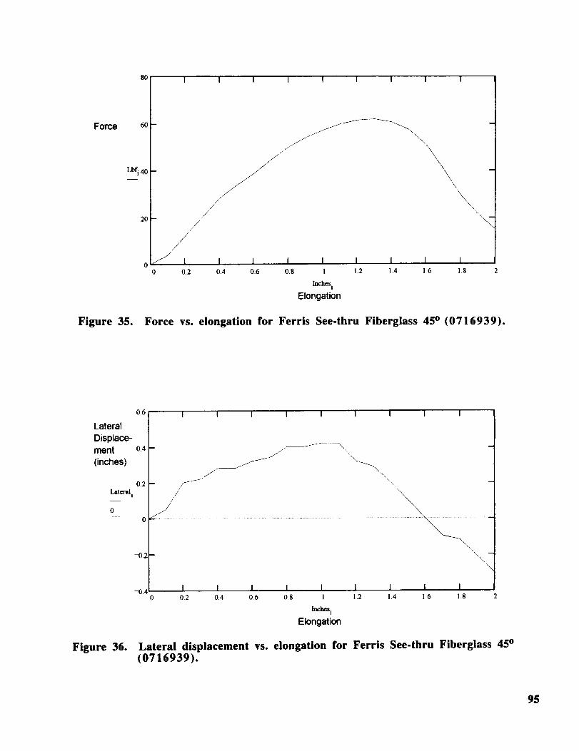
80 I I I I 1 I I I I
Force 6o
Lbf i 40
2O
Figure 35.
/
/
//
/_///I I I I
0 0.2 0.4 0.6 0.8
\
\\,
I1
Inchesi
Elongation
I I I I
\\
1.2 1.4 1.6 18 2
Force vs. elongation for Ferris See-thru Fiberglass 45 ° (0716939).
Lateral
Displace-ment
(inches)
Laterali
0
Figure 36.
0,6
0.4
0.2
_).2
-0,4
I I I I I I I I I
I I I I I I I I I0 0.2 0.4 0.6 0.8 I 1.2 1.4 1.6 1.8
Inches i
Elongation
Lateral displacement vs. elongation for Ferris See-thru Fiberglass 45 °
(0716939).
95

80 I I I I I I I I I
6O
Force
Lbfi40
2O
Figure 37.
I I I I I0 0.2 0.4 0.6 0.8 1 1.2 1.4 1.6. 1.8 2
Inches i
Elongation
Force vs. elongation for Ferris See-thru Fiberglass 60 ° (07169310).
Lateral
Displace-ment
(inches)
-0.2
-0.4I I I I I I I
0 0.2 0.4 0.6 0.8 1 1.2 1.4
Inches i
Elongation
1.6 1,8
Figure 38. Lateral displacement vs. elongation for Ferris See-thru Fiberglass 60 °(07169310).
96

120 1 1 I I | I I I 1
I00
Force
80
Lbfi 60
4O
2O
Figure 39.
\
I I I I I0 0.2 0.4 0.6 08 I
Inches i
Elongation
I I I_T _
1.2 1.4 1.6 18
Force vs. elongation for Ferris See-thru Fiberglass 90 ° (07169311).
0.15
Lateral
Displace-
ment
(inches) o.1
Lateral.I
0.05
I I I I
I I/ I I I I I0 0.2 0.4 0.6 0.8 1 1.2 1.4 1.6 1.8
hw.l_ i
Elongation
I I I I I
Figure 40. Lateral displacement vs. elongation for Ferris See-thru Fiberglass 90 °(07169311).
97

It
Tension isapplied
!
1Specimen Sampleundergoes ret urnsshear stress to initialdue to shapetension
Final, over compensatedsample
Figure 41. Schematic of sample deformation.
98

°
.
3.
.
.
.
.
.
.
10.
11.
References
Penniman, Charles F.: The First Materials Testing in America. ASTM Standardization
News. January, 1991
Hull, Derek An Introduction to Composite Materials Cambridge University Press (1981)
Fellers, William O. Materials Science, Testing, and Properties for Technicians Prentice
Hall, copyright 1990
Wampler, M. D, Spiegel, F. X. and West, H A. Continuous Unidirectional Fiber
Reinforced Composites: Fabrication and Testing Journal of Materials Education, Vol.
14, pp. 293-301, 1992.
West, Harvey A., Sprecher, A. F. Fiber Reinforced Composite Materials National
Educators' Workshop: Update '90, NIST Special Publication 882 (1991).
Askeland, Donald R., The Science of Engineering Materials, Second Edition PWS-Kent
Publishing Company ( ! 984).
Agarwal, Bhagwan D., Broutman, Lawrence J. Analysis and Performance of Fiber
Composites, Second Edition John Wiley & Sons, 1990
Larsen, Carl G.: Design Considerations for Materials Testing Tension/Compression
MTS Systems Corporation Minneapolis, Minnesota
Georgeson, Gary & Milstein, Frederick: Load and Fixture for Uniform Plastic
Deformation Single Crystals. Rev. Sci. Instrum 54 (8), August, 1983
Perlov, Anatoly & Martin, James: Calibration and Verification of Materials Testing
Machines and Systems. ASTM Standardization News. January, 1991
Sterling Instrument Handbook of Design Components. Sterling Instrument, 2101
Jericho Turnpike, New Hyde Park, N.Y. 11042-5416
99


N94- 36402
APPLICATION OF MATERIALS DATABASE (MAT. DB.)
TO MATERIALS EDUCATION
Ping Liu
and
Tommy L. Waskom
School of TechnologyEastem Illinois UniversityCharleston, Illinois 61920
Telephone 217-581-6267
_G PAGE BLANKNOT FILMffD P;_-_ __
101


Application of Materials Database (MAT. DB.) to Materials Education
Ping Liu and Tommy L. Waskom
School of Technology
Eastern Illinois University
Charleston, IL 61920
KEY WORDS: material properties, strength, ductility, material data base,
environment and working conditions.
PREREQUISITE KNOWLEDGE: The student should understand the
fundamentals of materials behavior such as tensile strength, percent elongation, area
reduction, manufacturability and formability. Some understanding of change in material
behavior with different environments and loading conditions is expected. Knowledge
of the basic application of a microcomputer and DOS commands are essential.
OBJECTIVES: To use the materials database MAT. DB. to search for useful
data on materials behavior related to specific applications. With the materials database,
design analysis, materials selection and manufacturing of products can be more efficient.
EQUIPMENT AND SUPPLIES:
1. IBM compatible 286 or higher microcomputer.a. 640 K RAM
b. At least 15 M free hard disk
c. Graphics card of CGA, Hercules, EGA, and VGA
d. 4.25" or 3.5" floppy disk drive
d. DOS 3.0 or higher.2. MAT. DB and database files from ASM International.
3. Printer is optional for output.
INTRODUCTION:
Findirrg the right material for the job is an important aspect of engineering.
Sometimes the choice is as fundamental as selecting between steel and aluminum.
Other times, the choice may be between different compositions in an alloy. Discovering
and compiling materials data is a demanding task, but it leads to accurate models for
analysis and successful materials application.
Mat. DB is a database management system designed for maintaining information
on the properties and processing of engineered materials, including metals, plastics,
composites and ceramics. It was developed by the Center for Materials Data of
American Society for Metals (ASM) International. The ASM Center for Materials Data
collects and reviews material property data for publication in books, reports, and
electronic database. Mat. DB was developed to aid the data management and material
applications.
Mat. DB can provide the following functions to manage database for materials:
1. View information on specific material:
The material data are organized in material records, which include material
103

designations, specifications, composition, product forms, classes, ranking, properties,
graphs and notes. Once entering the database, the user can navigate among the nine
categories of information for a specific material.
2. Searching:
One of the most powerful features of Mat. DB is its ability to search through
megabytes of information to locate needed material data. The user begins a search
session by creating a "folder", which contains all related results. The searched folder canbe viewed in the same manner as above.
3. Editing:
Users can build their own database with the tools provided by Mat. DB.
Sophisticated databases can be established to suit various applications for users.
4. Reports:
Mat. DB is capable of viewing and printing the results of a search in formats that
help analyze search results.
PROCEDURE:
1. Start the Mat. DB and load the desired database file for the material of
interest. A main manual will be prompted for each database file.
2. View data for a specific material:
After choosing "VIEW FOLDER" from the main manual, a material record
manual will be shown on the screen. Mat. DB's basic building block is the Material
Record, the file in which information on materials is organized. A separate record is
devoted to each materials designation, e.g. AISI 1020, Ti-6A1-4V, etc. These records are
then stored in Mat. DB databases. Each record can contain the following information
for a given material:
Designation: The designations screen contains necessary information to identify
the material and source of the data. It includes Accession Number (an identifying
number unique to a material record), UNS Number (a cross-referencing number
standardized by American Society for Testing and Materials (ASTM) and Society of
Automotive Engineers (SAE)), Material Group, Designation, Common Name,
Manufacturer, Country and User.
Specifications: Each material can be cross-referenced to a maximum of 50
alternate specifications. Each specification can be annotated with a short note.
Composition: Minimum and maximum percentages can be maintained for up to
20 elements. Additional comments on compositions can also be stored for display along
with the element percentages.
Product Forms: The user may index the material by up to 50 different productforms.
104

Classes: The user may index each material condition by up to 50 application
classes such as heat resistant, high strength, etc.
Ranking. Each material condition can be ranked for processing characteristics
such as formability, weldability, machinability, hardenability, processing cost, and
availability. The user can define up to 6 ranking categories.
Properties: Properties can be reported for up to 20 different conditions per
material. For each condition up to 100 properties can be reported at as many as 20
temperatures. The properties are displayed on a screen that looks like a spreadsheet.
Graphs: Up to 20 graphs can be maintained and displayed for each material.
Graphs can also be saved to a DOS file or printed directly to a laser or dot matrix
printer.
Notes: Mat. DB can maintain up to 200 lines of comments for each material.
The Notes section offers many standard word-processing features, making it extremely
easy to add new comments to a record or edit existing comments.
3. Search information with "SIFT FOLDER" feature of Mat. DB.
Material information can be searched according to various combinations of
material data on designation, specifications, composition, forms, classes, rankings,
properties and so on. For example, in the folder of STARTER.DB (database supplied
with Mat. DB), "sift folder" with the following conditionsCLASSES = CORROSION RESISTANT and
FORMS = BARS
results in the following three materials316 STAINLESS STEEL
410 STAINLESS STEEL and
A3003 WROUGHT ALUMINUM.
All the material data on these three corrosion resistant bars can be found using the
"VIEW FOLDER".
4. Build your own database with "editing" feature of Mat. DB.
If the database was opened in the read-write mode, a new material record can be
created by moving the highlight to "new" at the bottom of the List Screen and pressing
enter. This will open an empty material record.
The new material record will begin with "DESIGNATION" and data will be
entered in the edit boxes. When finished, press the F10 function key and the editing will
be saved.
5. Output the results:
The results can be printed with a dot matrix printer.
105

SAMPLE DATA SHEETS:
The following are two examples for the property data of AISI 4140 steel and high
density polyethylene, respectively.
A. AISI 4140 Steel
Database: STARTER.DB
Folders: Metal Alloys (11)
View Folder: 4140 G41400 Alloy Steel
1. DesignationAccession Number
UNS Number
Material Group
DesignationCommon Name
Manufacturer
Country USAUser ASM
281189015
G41400
Alloy SteelAISI 4140
4140
2. Specifications
OrganizationAMS
AMS
AMS
AMS
ASTM
ASTM
ASTM
ASTM
ASTM
ASTM
MIL
SAE
SAE
SAE
DIN
Specification
6381 (*Aerospace
Specification)6382
6390
6395
A322
A331
A505
A519
A547
A646
S-16974
J404
J412
J770
1.7225
Material
3. CompositionElement
C
Cr
Mn
Mo
P
S
Si
Min.%
.38
.8
.75
.15
.15
Max. %
.43
1.1
1.
.25
.035
.04
.3
106

4. NotesHigh-hardenability, medium-carbon steels;popular gradesDESCRIPTION: Grades4140,4140H, 4142and 4142H arecombined fordiscussion purpose because they are so similar in compositions andcharacteristics. Actually, they are so close that the composition could be
either 4140 or 4142.
5. Properties4140 Typical Properties
E1Resis n{o}*m
ThCoefExp {u}m/m'K
ThConduct W/m*K
ThSpcHeat J/kg=K
100 °C 200 °C 400 °C
262. 326. 475.
12.2 12.6 13.7
42.6 42.2 37.7
473. 519.
6. Graphs: One example is shown below.
14
1414
100
10
o.oolRISI 4140: C]lST]I, Creep s't.x'_noth
0.01 O. 1 1 lO...... I ....... I ....... 1 ...... I
_,, 5z,
........ I I I I I I l Ill ........ I I , , , , , ,,I .......
e.6Ol e.el e. 1 1 le lOO
Time, h
Sheet, e._r_ in., annealed at 1550 ¥, and tested at tee0 F.
Struct. Rllogs Handbook, D.J.l_g]mth, Ed., Vol I _ 2,n 11_. ll_ffi, l lP, lClA1
tO
107

B. High Density_ Polyethylene (HDPE)
Database: THERPLAS.DB
Folders: Polyethylene (A-M) (63)View Folder: Marlex HXM 50100
1. DesignationAccession Number
Code Number
Material Group
Designation
Common Name
Manufacturer
CountryUser
81789333
190100
Polyolefin
PolyethyleneMarlex HXM 50100
Philips Chemical Co.USA
Engineering Thermoplastic
2. Notes
High-density polyethylene, use with food and drugs.
Uses: Large formed parts, cattle feeders, pallets, boats
FOOTNOTES
A Condition 190/2.16
B Type IV specimen, 2 per min.
3. Process: Thermoforming
4. Properties
Typical Properties
Density, kg/m 3
FlexModul, GPA
StrElgYld, %
TenYldSt, MPa
23 °C
950
2.08
600
26
5. Features:
Impact resistance
Food/drug use
6. RankingsChemical Resist.
Creep Resist.
Fatigue Resist.Heat Resist.
ProcessabilityCost
108

INSTRUCTOR NOTES:1. It is always a good idea for students to start with "Read-Only" mode for
materials database folder. In the "Read-Only" mode, no change in any material record
will be saved. This will prevent any useful information from being lost.
2. When searching materials with "SIFT FOLDER", students need to make sure
to use "NEW" in the folder list. Otherwise, the existing folders will be replaced by the
new folder. Some information could be lost.
3. Basic knowledge of DOS for microcomputer will be essential to the operation.
REFERENCES:
1. Puttre, Michael: Materials Data Bases are Key to Design Analysis, Mechanical
Engineering, vol. 115 (5), 1993, pp 69-71.
2. ASM International, Materials Properties Database System: Mat. DB,
ASM/Center for Materials Data, Materials Park, OH 44073, 1992.
SOURCES OF SUPPLIES: This is basically a computer software project.
Microcomputers are readily available. However, the software is relatively expensive.
The Mat. DB costs approximately $556-695, and material database files cost from
$295.20 to 526 for each major category of materials. But, the software and database files
can be purchased separately, which makes the cost planning a little easier.
ACKNOWLEDGMENT: Financial support for this project from the Council for
Faculty Research (CFR) at Eastern Illinois University is greatly appreciated.
109


N94- 36403
LAMINATED THERMOPLASTIC COMPOSITEMATERIAL FROM RECYCLED HIGH DENSITY
POLYETHYLENE
Ping Liu
and
Tommy L. Waskom
School of TechnologyEastern Illinois UniversityCharleston, Illinois 61920
Telephone 217-581-6267
F_ PAGE _LAt_K NOT FILMED111


Laminated Thermoplastic Composite Material from
Recycled High Density Polyethylene
Ping Liu and Tommy L. Waskom
School of Technology
Eastern Illinois University
Charleston, IL 61920
KEYWORDS: thermoplastic composite, high density polyethylene, laminate, glass
fiber fabric, ASTM standards, tensile test, ultimate tensile strength.
PREREQUISITE KNOWLEDGE: The student should understand the
fundamentals of polymer processing and mechanical property testing of materials. The
ability to use ASTM standards is also necessary for designing material test specimens
and testing procedures.
OBJECTIVES: To understand the concept of laminated composite materials,
processing, testing and quality assurance of thermoplastic composites; to observe an
application example of recycled plastics.
EQUIPMENT AND SUPPLIES:
1. Recycled one-gallon milk containers
2. One glass fiber fabric of 127 x 127 mm
3. Steel rules and compass (or a specimen template)
4. Scissors
5. Thermoforming or compression machine for plastics
5. Tensile test machine.
PROCEDURE:
1. Collect and clean recycled milk containers.
2. Cut four (4) fiat sheets of high density polyethylene from the milk containers.
The sheet size is approximately 130 x 130 mm.
3. Cut a piece of glass fiber fabric of 127 x 127 mm.4. Place two sheets of high density polyethylene on both sides of the glass fiber
fabric, as shown in Figure 1.
5. Compress the above combination of sheets under a normal load of 2/9 tons
and a temperature of 135 °C for 5 minutes.6. Turn off the heater of the mold, turn on the circulation pump and maintairl the
same normal load until room temperature.
7. Remove the laminated composite from the mold.
8. Cut the tensile test specimen from the laminate according to dimensions
specified by ASTM standards [1], as shown in Figure 2.
9. Test the tensile strength of the laminated composite.
113

High Density
Pol yethyl ene (4)
Glass Fiber
Fabric
Load = 2/9 ton
Figure 1. Configuration of laminated composites: two layers of HDPE on both
sides of glass fiber.
114
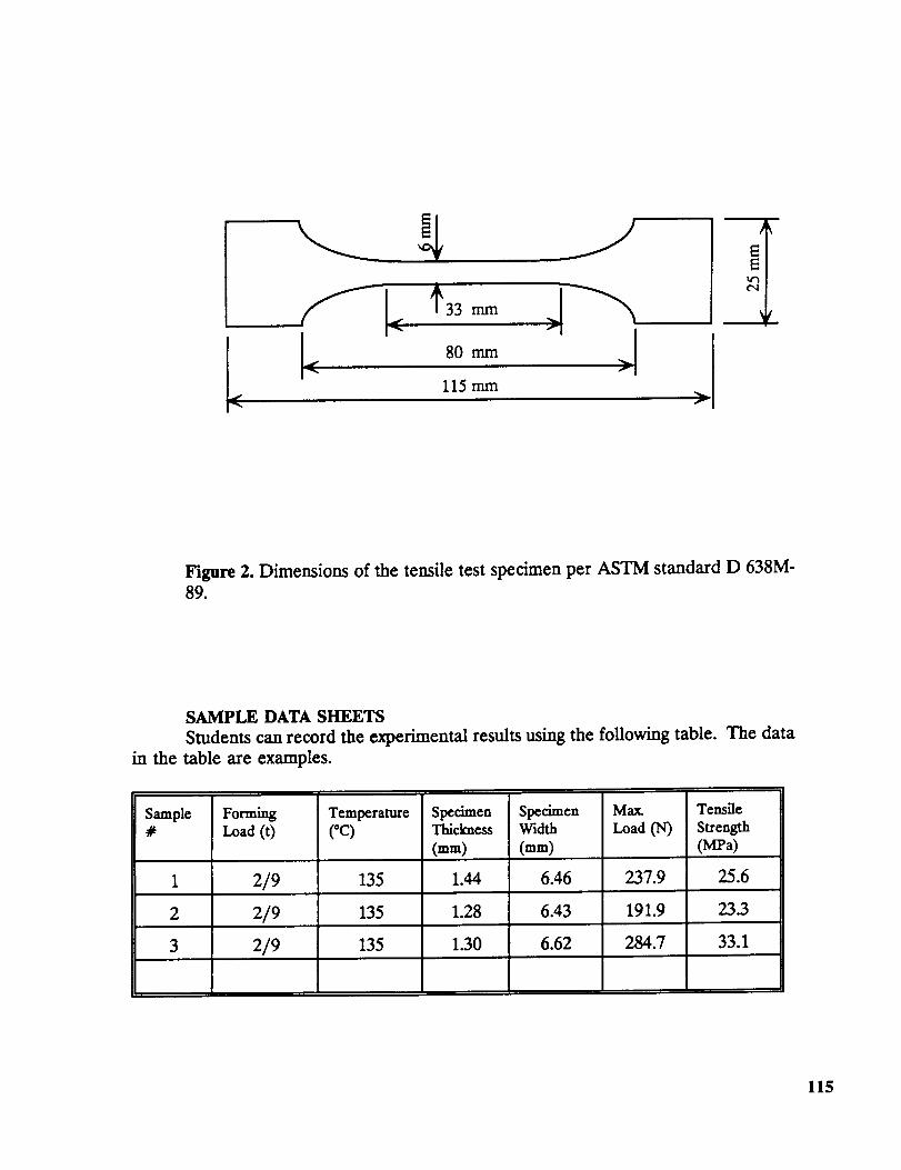
Lfl ¢33mm
I_" f| ] I
80< >
115 mJ'n
Figure 2. Dimensions of the tensile test specimen per ASTM standard D 638M-89.
SAMPLE DATA SHEETS
Students can record the experimental results using the following table. The data
in the table are examples.
Sample#
Forming
Load (t)
Temperature(*c)
1 2/9 135
2 1352/9
2/9 135
SpecimenThickness
(mm)
SpecimenWidth
(ram)
Max.
Load (N)
Tensile
Strength(r_'a)
1.44 6.46 237.9 25.6
1.28 6.43 191.9 23.3
1.30 284.76.62 33.1
115

INSTRUCTOR NOTES:
Students can perform investigative studies on the effects of forming temperature
on the strength of the laminated composite [2,3]. Figure 3 shows a typical relationship
between the compression temperature and ultimate tensile strength. As the temperature
increases, the strength of laminated composite increases. This increase may be due to
several reasons. One of the reasons is that as the temperature increases, better bondingmay take place between the glass fibers and the plastic sheets. Another possible r_asonis that as the temperature increases, the thickness of the laminate decreases, whichactually increases the percentage of glass fiber relative to the polymer. Glass fiber is
stronger than high density polyethylene matrix. Therefore, material strength increaseswith increasing temperature.
The reinforcing effect of glass fiber is seen in Figure 3. The strength of recycledhigh density polyethylene is improved by laminating it with glass fiber. With the
improved mechanical properties, the application of recycled plastics could be expanded,and therefore the mount of solid waste going to landfills can be reduced.
..-..3O
1tl2.5
nora m m
l l I l I
Temperatm'e (C)
One Lair of F_enalau
No Lair8 of Frbergla88
Figure 3. The relationship between the compression temperature and the tensilestrength of recycled high density polyethylene laminated with glass fiber and
recycled high density polyethylene without reinforcement.
116
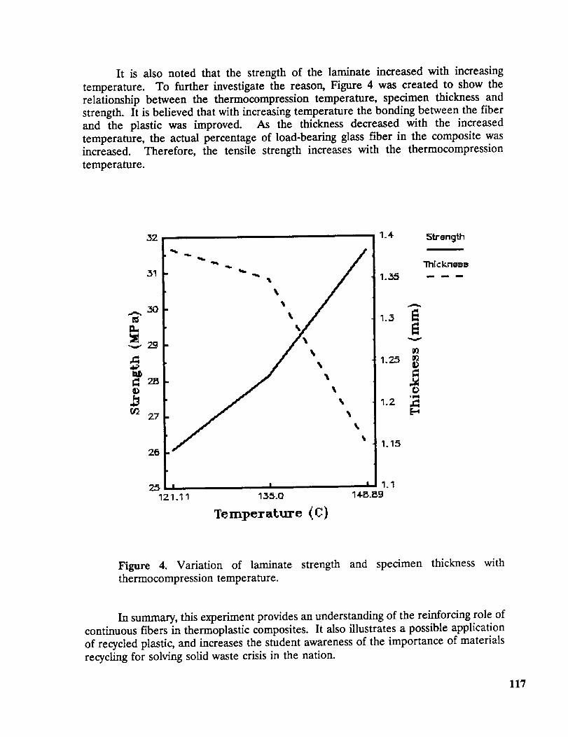
It is also noted that the strength of the laminate increased with increasing
temperature. To further investigate the reason, Figure 4 was created to show the
relationship between the thermocompression temperature, specimen thickness and
strength. It is believed that with increasing temperature the bonding between the fiber
and the plastic was improved. As the thickness decreased with the increased
temperature, the actual percentage of load-bearing glass fiber in the composite was
increased. Therefore, the tensile strength increases with the thermocompression
temperature.
32
31
2O
I121.11
1_2.B
27
"hill
I13;5.0
Tornporatu_o (C)
Figure 4. Variation of laminate strength and specimen thickness with
thermocompression temperature.
In summary, this experiment provides an understanding of the reinforcing role of
continuous fibers in thermoplastic composites. It also illustrates a possible application
of recycled plastic, and increases the student awareness of the importance of materials
recycling for solving solid waste crisis in the nation.
117

REFERENCES:
1. ASTM: 1989 Annual Book of ASTM Standards, Vol. 8.01
American Society for Testing and Materials, Philadelphia, 1989.
Plastics (I),
2. Carlsson, Leif A.: Thermoplastic Composite Materials, Elsevier Science
Publishers, 1991.
3. Agarwal, B.D.; and Broutman, L.J.: Analysis and Performance of Fiber
Composites (2nd edition), John Wiley & Sons, Inc., 1990.
SOURCES OF SUPPLIES:
The high density polyethylene is obtained from milk containers which can be
recycled by faculty and students without any cost. The cost of _lass fiber fabric is the
lowest among all engineering fibers, which is $2.65 - $6.25/m 2 (Fibre Glast, 1-800-821-
3283).
ACKNOWLEDGMENT:
Part of the financial support for this project is from the Illinois Department of
Energy and Natural Resources through the Office of Solid Waste Research at the
University of Illinois at Urbana-Champaign. Another part of the material is based uponwork supported by the National Science Foundation under Grant No. DUE-9350629.
118

INEXPENSIVE MATERIALS SCIENCEDEMONSTRATIONS
F. Xavier Spiegel
Department of Electrical Engineering and Engineering Science
Loyola College
4501 North Charles Street
Baltimore, Maryland 21210-2699
Telephone 410-617-2515
119

Xavier SpiegelLoyola College
ORIGINA[ PAGE"
Bt.AC_ AND WHITE PHOTOGRAPH
120

INEXPENSIVE MATERIALS SCIENCE DEMONSTRATIONS
F. Xavier Spiegel
Department of Electrical Engineering and Engineering Science
Loyola College, Baltimore, Maryland
ABSTRACT: Readily available materials can be used to
demonstrate such properties as anisotropy, stress concentration
effects and composite behavior.
REQUISITE KNOWLEDGE: Curiosity.
KEY WORDS:
Anisotropy.
Composite, Bi-metallic, Filament Tape,
OBJECTIVES: The purpose of these demonstrations is to
illustrate some interesting properties of composites. The
following demonstrations have been performed by the author many
times and have been received enthusiastically by audiences of all
ages.l,2,3, 4
EQUIPMENT AND SUPPLIES:
i) Filament Tape
2) Sheet of Paper
3) Index Card
4) Bi-metallic Disk *
FILAMENT TAPE: Filament tape is an excellent example of the
anisotropy of a composite material. Filament tape consists of
aligned parallel threads embedded in a polymer film. One side of
this composite is coated with an adhesive. If you try to tear the
composite in the direction of the threads the tape will separate
very easily; however, if you try to tear the tape in any other
direction you will find that it is almost impossible. This is an
example of anisotropy or the directional dependence of a property
of a material. In other words in this instance the mechanical
property of tearing is different according to which direction you
try to tear the tape. If you cut several pieces of the tape about
5cm long and stack them together so that different layers have
their threads running in different directions, you will find that
the anisotropic properties change. This technique is often used
in industry to provide a more isotropic material. One major
weakness of this type of composite is de-layering or de-
lamination of the stacked layers. 1,2
* Available from: Edmund Scientific Company
i01 E. Gloucester Pike
Barrington, N.J. 08007-1380
121

SHEET OF PAPER: A sheet of paper can be used to demonstrate
the action of an airfoil and also the effect of folding paper.
If the sheet of paper is held in front of the mouth and you blow
across the top of the paper the paper will rise demonstrating the
way that faster moving air on the top of a wing surface than on
the bottom of the wing surface causes the wing to experiencelift.
Another interesting demonstration with a piece of paper (any
size!) is that if you try to continually fold a piece of paper in
half, eventually you will not be able to fold it again. You just
are not strong enough. Ten folds cannot be done! This
demonstrates how mechanical strength can be affected by composite
folds.
INDEX CARD: A 3"x5" index card can be used to demonstrate
crack deflection in a material. Crack deflection can be
engineered into most materials and is not peculiar to composites.
If two one inch slits are cut parallel to the 3 inch sides about
one inch from either end and then a hole is punched at the bottom
of one of the slits, the index card can then be pulled at the 3
inch sides and the index card will invariably fail not where the
hole was punched but where the slit alone was made. This is an
example of crack deflection. The energy supplied to fracture the
card was deflected around the hole and was diminished whereas the
same enerqy supplied to the slit alone was unimpeded and caused afracture. 1,2
BI-METALLIC DISK: Some composites are formed by joining two
materials either mechanically or by some other means. The bi-
metallic disk is a composite formed by joining stainless steel
and Invar. THe composite behavior of this combination arises from
the fact that stainless steel and Invar have different
coefficients of expansion. When the disk is received it is
concave on one side and convex on the other. If the convex side
is rubbed with the thumb and then pressed, the convex side will
become concave and vice-versa. If the disk is then placed concave
side down on a surface after a short time it will jump off of the
surface as it returns to its original state. Some thermostats
take advantage of this property to accurately determine small
temperature changes. Of course, nothing in a thermostat jumps
since the metals joined are strips, are not discs, and one end isfixed.
CONCLUSIONS: The author has had enthusiastic response from
audiences of all ages, with each of these demonstrations.
Quantitative results can be measured and each demonstration can
be expanded and/or altered. You are only limited by your
imagination and curiosity.
122

REFERENCES:
i. Jacobs, James A. and Kilduff, Thomas F.: Engineering
Materials Technology, Prentice-Hall 1985.
2. Fellers, William O.: Materials Science, Testing and
Properties for Technicians, Prentice-Hall 1990.
3. Spiegel, F. Xavier: Five experiments in Materials Science
for less than $i0.00, NASA Conference Publication 3151November 1991 263-265.
4. Spiegel, F. Xavier: Experiments in Materials Science
From Household Items, NASA Conference Publication 3201November 1992 373-375.
ACKNOWLEDGEMENT: The author wishes to thank Mary L.
Spiegel for typing this manuscript.
123

RECYCLING OF AUTOMOBILES
AN OVERVIEW
S. S. Labana
Ford Motor CompanyMD 3198 SRL
P. O. Box 2053
Dearborn, Michigan 48121-2053
Telephone 313-594-7740
125


RECYCLING OF AUTOMOBILESAN OVERVIEW
S. S. LABANAFORD MOTOR COMPANY
DEARBORN, MICHIGAN
SCOPE
TOTAL SOLID WASTE: 326 Billion Pounds In 1988
PLASTICS: 7% By Weight30% By Volume
Plastics Projected To Increase 10-11% By Weight By TheYear 2000.
80-85% Of Solid Waste Is Landfill.
Household Plastic Waste Is Six Times The Automotive
Plastics Waste.
PLASTICS WASTEUSA 1990
TOTAL PLASTICS WASTE
WEIGHT % OF TOTAL
VOLUME % OF TOTAL
POLYMER PRODUCTION
YEAR 2000 PROJECTION
PLASTICS WEIGHT
PRICJIO'if_ P,AGE BLAt_K NOT FILMED
12.0 MILLION TONS
7.5
19.0
30.0 MILLION TONS
11%
127

LAND FILLS IN USA
YEAR NUMBER
1979 18000
1989 6300
1995 3800
LANDFILL TIPPINGS/TON BY REGION
REGION
NORTHEAST
MID-ATLANTIC
SOUTH
MIDWEST
WEST CENTRAL
SOUTH CENTRAL
WEST
NATIONAL
AVERAGE
64.76
40.75
16.92
23.15
11.06
12.50
25.63
26.56
SOURCE: NSWMA
FEES
MAXIMUM
120.00
89.00
40.00
50.00
13.50
26.25
55.0O
120.00
128

DISPOSAL COSTS
_CYCUI_
RECYC ING RATESUSA 1992
MATERIAL
ALUMINUM
IRON & STEEL
PAPER
GLASS
PLASTICS
RECYCLED %
33
39
22
8
1
129

MAGNITUDAUTOMOTIVE RECYCLING
NO. of Cars Shredded
Ferrous Metals
Non Ferrous Metals
Shredder Residue
Landfill Cost
Heating Value
10 Million
11.2 Million Tons
0.8 Million Tons
3.8 Million Tons6.7 Million Cu, Yds.
$20 - 100 Per Ton
5000 - 7000 btu/Ib
COMPOSITION OF USIbs/car
1990
BUILT CAR
1980
Steel
Conventional 1246 1697
High Strength 233 169
Stainless 32 28
Other 53 54
Iron 398 480
Aluminum 158 123
Copper 46 37
Zinc Die Cast 19 21
Powder Metal 23 17
Rubber 128 130
Plastics/Composites 222 196
Fluids 167 181
Other Materials 88 90
Source: Wards Reports
130
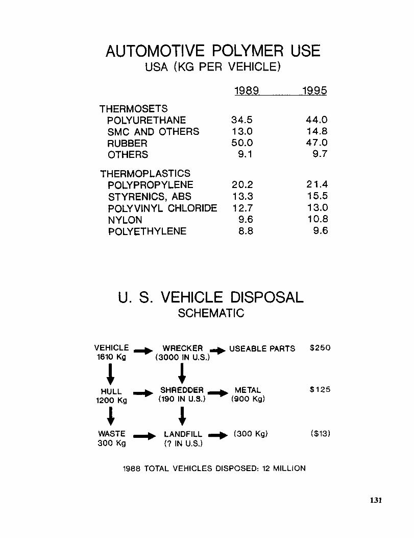
AUTOMOTIVE POLYMER USEUSA (KG PER VEHICLE)
1989 1995
THERMOSETSPOLYURETHANE
SMC AND OTHERSRUBBEROTHERS
34.5 44.013.0 14.850.0 47.0
9.1 9.7
THERMOPLASTICSPOLYPROPYLENE 20.2
STYRENICS, ABS 13.3POLYVlNYL CHLORIDE 12.7NYLON 9.6POLYETHYLENE 8.8
21.415.5
13.010.8
9.6
U • S. VEHICLE DISPOSALSCHEMATIC
VEHICLE m=_.1610 Kg
WRECKER(3000 IN U.S.)
USEABLE PARTS
HULL ===_ SHREDDER _ METAL1200 Kg (190 IN U.8.) (900 Kg)
WASTE LANDFILL =m_. (300 Kg)300 Kg (? IN U.S.)
$250
$125
($13)
1988 TOTAL VEHICLES DISPOSED: 12 MILLION
131

DISMANTLING TIMES
COMPONENT WT. kg TIME, SEC.
SIDE MOLDING 0.5 18
DOOR INNER 0.6 32
BUMPER 12.2 9O
SEAT 19.5 100
INSTRUMENT PANEL 48OO
VEHICLE DISPOSALPARTS TAKEN OFF BY DISMANTLERS
Radiator
BatteryGas Tank
Tires
Catalytic ConverterUsable Parts
132

FLUID DRAINAGE
ENGINE OIL
BRAKE FLUID
RADIATOR COOLANT
WASHER
FUEL
VEHICLE DISPOSALSHREDDER FRACTIONS
Ferrous MetalsNon-Ferrous MetalsFluffDirt
133

VALUE OF CAR HULK
Material Wt. Ibs Value
Steel
Nonferrous MetalsFluff
FreightProcessing
225O15075O
135.0018.00
(47.00)
(lo.oo)(47.00)
Net Value 3 150 49.00
$
Source Waxman Metals Group
SHREDDER RESIDUE
P_=CSRUmSRUm__GLAS_OTHEm
t 7P/_,
t6j%

TIRE RECYCLING
R ETR EAD
LANDFILL
MISC.
RECLAIM
JAPAN
EXPORT
USA
Tire Recycling
NO. of Scrap Tires per yr.
Scrap Tires in Environment
Fraction RecycledRetreadReclaimCrumb RubberMisc. Products
Asphalt Paving
Tire Recycle Incentive Act
234 Million
3 Billion
20 Percent
S.2462 / HR 4147
135

COST BALANCE
RAW MAT'L
VIRGIN MAT'L
FABRICATION
US
_'_ DISPOSAL
,I,
COLLECTION
SEPARATION
PROCESSING
FABRICATION
US
136

Support new recycling efforts .._..__
Dumpers bury citym-out rubber - g_a_gche
__ ;3 MAILBAG
Incineration no solution
Plastics recyclio_ _,_ o/_/_"__ 8h_3/Tt Lag in Plastics Rkcycling4
__ Sparks Heated DebateOh _ _,t,_/, Co]_ _-_.G.)v_,/. .nLAS'rlCS recycling is going
"* -g_/D/. Z'_ _ _i-Pstrong, according to the Part-:/"/"OL,_ - _°e _ _'_ _ nership [or Plastics Progress,
- ¢"0'/_/), _-"tgS_._'/" _ a trade group.
o ¢"[q_e/,: _vz'ltCS,_ " _ Hogwash, counter environmental
-_,.,t/CI_ -o t2 p,. _ _oups. "The plastics industry ;.¢
e_cl_'h6_Process
137

DAN1ELMEARS/TheDetroit News
Charles Grimmer, 70, his house visible in the background, walks by the ever-growingmountain of tires dumped in his east side neighborhood near Van Dyke and Mr. Olivet.
138

I
/
/
/
139

is pyrolysisbreaking down coalition?
Trash Tllat Recycling Plan
Here's the inside story on
recycling our automobilesAt Ford, paper and o_her materials
ALB TIMES-UNION 8/6/92. plants andoffices acrossl_veryone s heai'd o| recvchnn .... ,,, many
140

Automakerswant torecycle allof the carEnvironmental pressuresdictate recycling moreauto materials, but costsmake total disassembly
unlikely anytime soon.
By BRYAN BERRYAutomotive Editor
AUTOMOTIVE PLASTICS
Auto-part recycling is atop industry priority
_/-
__? '_°_°'tes
t3n'lo_ C.arbide Niari_s llecyCling Nlilestotae
AUTOMOTIVEPLASTICS:TAKINGAPARTTHEPUZZLETheautomotivea)gplasticsin&stries,jointlya)zdflzdivi&ally,seekgreaterrecyclabilityofplasticautomotivecompoT_ents.Thechallenge:gettflzgthematerialo_toftheca)'andintotherecyclingloop.
Recyclers Add Capacity _ .- ,_00 "_0 t_l_'_'_'B,o_,.........,,.............Throughout the Cog.try : i _J_g I_. __._,,........"I_TEW corporate facilitio_ =_r,llG_U ._. .............. "_"" ......
.A. _] cyclil G_ I UO'"'_.o_,_ ..... """°"Chemical o.,. .... _ _.,,_,ames ac-
count for sev_l'_ major efforts. New
recycling plants owned by Union
Carbide, Quantum Chemical and
Phillips Petroleum add significant
141
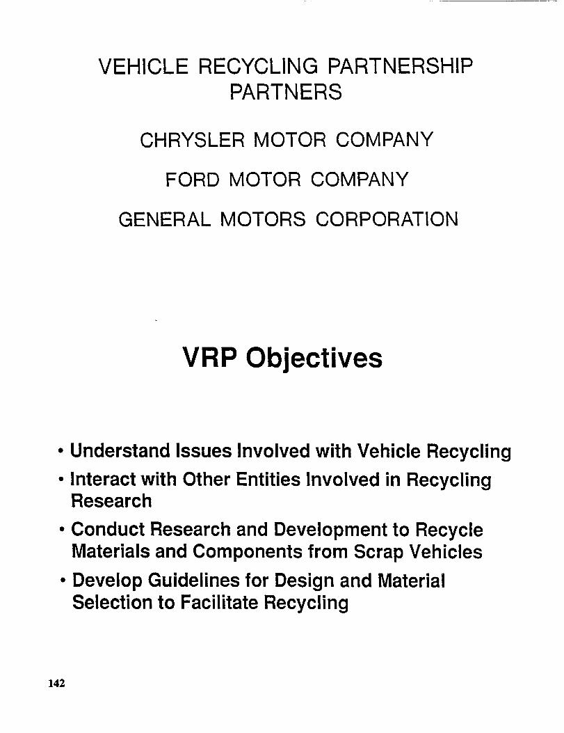
VEHICLE RECYCLING PARTNERSHIPPARTNERS
CHRYSLER MOTOR COMPANY
FORD MOTOR COMPANY
GENERAL MOTORS CORPORATION
VRP Objectives
• Understand Issues Involved with Vehicle Recycling
• Interact with Other Entities Involved in RecyclingResearch
• Conduct Research and Development to RecycleMaterials and Components from Scrap Vehicles
• Develop Guidelines for Design and MaterialSelection to Facilitate Recycling
142

NEEDED• RECYCLABLE
FOR RECYCLINGMATERIALS
• RECYCLING TECHNOLOGY
• DISMANTLING OR SEPARATION
• DESIGN FOR DISASSEMBLY
• MATERIALS IDENTIFICATION CODES
• DEVELOPMENT OF RECYCLING BUSINESS
RECYCLINGTHERMOPLASTICS
• Reuse
• Compatiblize
• Reactive Processing
• Incinerate
• Pyrolyse
• Depolymerize
143

RECYCLING THERMOSETS
• INCINERATION
• PYROLYSIS
• GRIND, USE AS FILLER
• CHEMICAL CONVERSION
144

AN INTRODUCTION TO STRENGTH OF MATERIALS
FOR MIDDLE SCHOOL AND BEYOND
Nancy L. Denton
and
Vernon S. Hillsman
Mechanical Engineering Technology Department
Purdue University
1417 Knoy Hall, Room 137
West Lafayette, Indiana 47907-1417
Telephone 317-494-7517 or 8486
145


An Introduction to Strength of Materials For Middle School and Beyond
Nancy L. Denton and Vernon S. HillsmanMechanical Engineering Technology Department
Purdue University, West Lafayette, Indiana 47907-1417
KEY WORDS: stress, strain, stability, bend, crush, shear, buckle, axial force, shearingforce, bending moment, torque.
PREREQUISITE KNOWLEDGE: The students should be able to follow directionsregarding safety of themselves and of those around them. No technical knowledge is required.
OBJECTIVES: To _.ain familiarity with the basic concepts of strength of materials;strength, stiffness and stabdity. To observe how materials respond to various types of loading.To promote a better understanding of technical professions.
EQUIPMENT AND SUPPLIES:
For specimens and demonstrations:
/i / Craft Cpopsicle")sticks- 50 or more per studentCircular cross-section plastic straws - up to 50Fishing line - approximately 0.5 m per student of two or more strengths. All should beof a single material.
/i / Wood model glue-at least one tube per student teamSmall hex head bolts - preferably of several materialsFoam bar with "stress element" - rectangular cross-section length of foam at least 50mmx 60mm x 250mm
(7) Tongue depressors - at least 4; with pairs glued lengthwise to form double-thickness"beams"
/i ! FlatUtilityplasticknife-f°rscalethe instructor's use only!) Safety glasses - one pair per person
For testing:
/21/ SmallDigitaltorque wrench with maximum value storagevise
Ii the materials/mechanical testing laboratory)
3 Universal test machine fixtured with flat plates (about 250 mm x 500 mm)Metal rods - 3 of same diameter and material, about 175 mm longInstrumentation to measure test machine loading (such as load cell and strain indicator)
i i any other location)
Lightweight bucket with round metal handleMetal rods - 2 of diameter similar to the bucket handle
Loading material such as sand or water
/76/ WeightSmallamount of clay, putty, beeswax, or similar materialscale
INTRODUCTION: Strength of materials is a subject that affects all walks of life, andeven children have some inherent qualitative understanding of strength, stiffness, and stability.
In a faculty-led workshop, precollegiate students consider how common items withstand loadsdue to axial forces, shear forces, bending moments, and torques. The effects of geometry and
material properties are investigated while students crush, shear, buckle, bend, stretch and twist
__ PAGE BLANK NOT FILMED
147

various items. For students who have studied basic algebra, the simplest equations governingthe resulting stresses and deflections (or strai.ns), can be presented. For all students, thegeneral concepts of strength, stiffness, and stability are demonstrated and engineering concernsrelated to design, testing, and manufacturing are discussed throughout. Experiential learningis emphasized inall actlMties of the workshop. 1
PROCEDURE: Note that the foam bar is used to illustrate each of the followingconcepts as it is presented, and thus, should be near the instructor at all times.
Axial Force and Deflection: Pull on the foam bar to show how tensile axial loads causeit to deflect. For older students, show the following equations:
Axial Stress = P/AAxial Deflection = PL/AE
where P is axial force, L is specimen length, A is cross-sectional area, and E is Young'smodulus.
Next, show the students the lengths of fishing line and point out that the only differenceis in cross-sectional area. Have the students slowly pull each line until it snaps. Discuss howthe line lengthens before breaking. Have them compare the force needed to break each line.This test demonstrates both strength and stiffness (deflection) for axial loading. (Ideally, therewill be a sufficient number of lengths of fishing] line for each student to break a pair of lines).
Ask the students for examples of matenals that stretch only a little or a lot. Discusshow some of them are used, and explain that designers usually consider both elasticity andstrength when selecting a material for a product.
Stability/Buckling: Apply a longitudinal compressive axial load to the foam bar andshow that it bows out (buckles) in the center of its length. Apply a similar load to the center ofa transverse side to show that the bar crushes when the length and cross section proportionsare reversed. Note that the bucklingoccurs at a much lower load than would be required tocrush the material in compression. Provide and discuss Euler's equation for buckling ofpinned-end columns:
Critical Buckling Load = _r2 EI/(Le)2
where E is Young's modulus (material stiffness), I is the area moment of inertia of the cross-section (shape stiffness); and Le is the effective length of the column.
To illustrate the concept of area moment ofinertia (I), apply a similar compressive loadto a scale (ruler) of rectangular cross-section, and note that it buckles in the directmn withmaterial occurnng closer to its center, its weak direction. Show the equation:
Rectangle's area moment of inertia: I = bh3/12
where b is the base of the rectangular cross-section and h is the height. Based on the Eulerequation, the scale will buckle in the direction of the lowest area moment of inertia, which iscalculated using] the smallest side dimension of the rectangular cross-section as the height, h.
Take a single full-length straw; install it between the flat plates on the pre-instrumenteduniversal test machine; and have a pair (or team) of students measure the straw's bucklingload. Next, cut a straw in two. Have the students guess if the buckling load should be higheror lower. Have another pair of students measure the load to determine who is correct.Finally, bundle two or more straws together; ask the students how much load should be neededfor buckling; and have a third pair measure the buckling load.
The straws typically vary noticeably in geometry and stability. This provides anopportunity to discuss manufacturing issues such as quality control and reasonable tolerances
148

for an item based on its expected use. For example, for some straws, the side may collapsebefore the length buckles due to variations in material thickness.
Torsion: Start by slowly and carefully twisting the foam bar about its longitudinal axis.Show that the center of the bar does not move, while the comers rotate through a significant
angle. While holding one end in place, again twist the bar to demonstrate that the comers atthe f'uted end of the bar do not move, but the comers at the bar's free end can experience agreat deal of deflection. Explain that in addition to motion, the bar is experienong torsionalshear stress, or stress due to slipping between "slices" of bar. At the center of the bar, becauseno motion occurs, there is no slipping, and therefore, no shear stress. At the comers, the
opposite is true, so there can be a large amount of torsional shear stress. The relatedequations (for a circular cross section rod) are:
Torsional Shear Stress = TR/J
Torsional Deflection = TL/JG
where T is torque, R is the radial distance from center, J is the area polar moment of inertia(shape stiffness), L is the length being twisted, and G is the shear modulus of the material
(material stiffness which resists twisting).Next, move to the vise and tighten about the threads of one bolt. Have a pair of
students use the torque wrench to SLOWLY twist the bolthead off while measuring the torc.lue
applied. (Note that the torque required will generally be low, so that torque measurement Isd_fficult without the peak hold option on the torque wrench). Use other students to removethe bolt and install one made of another material. Have another pair of students twist the
second bolthead. Repeat additional times with bolts of different materials. Compare thetorques required for failure, and discuss the benefits and limitations for use of each (i.e., nylonversus steel).
Bending: Begl'n by showing how. the shape of the stress element on the. foam barchanges when subjected to three point bending. Bend the foam beam so that its shape appearsconcave up, and have the students note the changes to the lengths of the lines at the top,bottom and center of the stress element. The top line will appear shorter, so the top otthe
beam is in compression. The bottom line will appear longer, which is evidence of tension onthe bottom of the beam. The line in the center of the stress element will remain unchanged,which relates to zero stress.
The equations used to quantify three point bending are as follows:
Flexural Stress at center = PLy/4I
Deflection at center = PL3/48EI
where P is the load applied at the center of the beam, L is the beam length, y is the distancefrom the neutral axis to the top or bottom surface of the beam, E is the modulus of elasticityand I is the area moment of inertia of the beam cross-section.
For workshops conducted in the mechanical/materials testing laboratory, explain thatthe students will be building a structure of their choosing during the next fifteen minutes, tlaenbending it until it breaks. The size of the structure is limited by the size of the flat plates usedfor loading. The load required to break each structure will be recorded, with recognition given
to the student(s) who build the strongest structure. Then distribute about 50 craft sticks (and
$1ue) to each student, or team, and let them build their structures. Assist them as needed withideas, cutting the sticks, etc. While the structures dry (about 5 minutes), proceed with other
bending tests.
149

Two rectangular cross-section beams, each made of a pair of glued tongue depressors,are tested in three point bending to show the effect ot the orientation ot the cross-section onbeam deflection and load carrying capability. Bend each to failure using three point bendingon the universal test machine, fixtured to obtain a concave up shape as shown with the foambeam. Measure the load required to bend about the weak axis and about the strong, axis.Discuss the concept of area moment of inertia (shape stiffness) again and point out howstructures are designed to take advantage of this property. , .
When the glue on the students' craftstick structures is dry and cured, have each fnstalltheir structure in the universal testing machine for three point bending (or crushing, if moreappropriate for the structure). Assist them in slowly loading the structt_res until failure occurs.Record the peak load each structure withstands, and recognize the stu0ent(s) who designedand built the strongest structure. Discuss how construction techniques affected the structures'ability to withstandload, just as they can affect the many structures used in daily life.
For workshops held outside of the mechanical/materials testing laboratory, it may notbe possible to test student-built structures. As an alternate method of illustrating three-point
bending, tongue depressor "beams" can _ mounted across two metal rods, with an emptybucket across the center of each "beam. Load can be applied by slowly adding water or sandto the bucket until the "beam" fails. The bucket can then be weighed to determine the loadrequired to break beams of various cross-sections. Preparation for this variation includessetting up a test frame and gluing tongue depressor "beams" of several thicknesses. The testframe can be set up many ways. A simple method is to move tables close to_ether, lay onemetal rod on each, and apply a small amount of clay or putty to prevent rolling. Sufficientbeams should be prepared to facilitate a discussion of shape stiffness, demonstrate how shapestiffness affects the amount of load required for failure, and to permit small teams of studentsto each test at least one "beam."
Conclusion: Summarize the basic concepts of strength of materials: strength, stiffness,and stability. Review the types of loading applied, and how items responded to each.Encourage the students to provide examples of each, and to think about how the work ofengineers and technologists affects them every day. Experiences like these illustrate thepractical applications of mathematics and the physical sciences while helping studentsunderstandwhy "to engineer is human. "2
INSTRUCTOR NOTES: Students are more interested, and retain more of what they
are taught when they are actively participating in the learnin_ process. 3 If possible, students.should do the setup and testing themselves. In order to facihtate that type ot participation, thegroup size needs to be limited to about 8 students per instructor. If two instructors lead theworkshop, a maximum of 15 students is recommended.
Safety must always be a top priority, and students should be warned about:(1) Continued inhalation of fumes from the glue can cause a variety of physical problems
including dizziness and difficulty breathing.(2) The typical universal testing machine is capable of applying great force onto fingers or
(3)
(4)
whatever gets in its path.When twisting the bolts, it is possible that the bolthead and/or torque wrench could flyloose.Safety glasses should be worn during all tests.
REFERENCES:1. National Council of Teachers of Mathematics. (1989). Curriculum and
Evaluation Standards For School Mathematics. The National Council ofTeachers of Mathematics, Incorporated, Reston, VA.
2. Petroski, H. To Engineer is Human: The Role of Failure in Successful Design.St. Martin's Press.
150

1 Resnick, L. B. (1987). Education and Learning to Think.National Academy Press, 1987.
Washington, D.C.,
SOURCES OF SUPPLY: The local hardware store or craft store will stock most
items required for the workshop. It may be necessary to obtain tongue depressors from a
pharmacy, and straws from a supermarket.
ACKNOWLEDGEMENT: The thoughtful and timely assistance of James D. Osborne,
department mechanician, in the development of this workshop is gratefully acknowledged.
151

N94- 36404
i .
!
/Y
SIMULATION OF MATERIALS PROCESSING:FANTASY OR REALITY?
Thomas J. Jenkins
and
Victor M. Bright
Department of Electrical and Computer Engineering
Air Force Institute of Technology
Wright-Patterson Air Force BaseOhio 45433-6583
Telephone 513-255-1200, ext. 4818, or 513-255-3576 ext. 4598
153


Simulation of Materials Processing:
Fantasy or Reality?
Thomas J. Jenkins, Capt, USAF
Victor M. Bright, PhD
Department of Electrical and Computer Engineering
Air Force Institute of Technology
Wright-Patterson Air Force Base, OH 45433-7765
KEY WORDS: computer-aided design (CAD), microelectrc,_.cs, oxidation,
computer simulation.
PREREQUISITE KNOWLEDGE: The students should understand the concepts
associated with the oxidation of silicon as applied to integrated circuit fabrication. In addition,
the students should be familiar with the operating system of the computer, which will be
executing the software.
OBJECTIVES: The objectives of this experiment are the following:
1. Introduce the general topic of simulation of materials processing as it
relates to the fabrication of microelectronic circuits,
, Familiarize the students with the use of the specific process simulation
tool, which they will be required to use during subsequent
semiconductor experiments, and
3. Introduce three independent measurement teclaniques which are used to
characterize oxide thickness and to verify computer simulations.
EQUIPMENT AND SUPPLIES: The equipment required to implement this
experiment is listed in Table I. The oxidation furnace is used to oxidize the silicon wafers.
The reflectance spectrophotometer, ellipsometer and profilometer are required to measure the
thickness of the resulting oxides.
The TSUPREM-4 (Technology Modeling Associates, Inc., Palo Alto, CA) simulation
software 1 is required. The students will use this software to simulate the various oxidation
furnace conditions utilized during the oxidation process.
155

Therequiredprocessingsuppliesarethosecommonlyfoundin asilicon-based
semiconductorresearchlaboratory.ThesesuppliesarelistedinTableII. All of thechemical
suppliesshouldbestandardelectronicsgrade.Thespecificsiliconwafersutilizedin this
experimentareprimegrade,(100)-oriented,p-type(borondoped)with anominalresistivityof6- 18f_.cm.
PROCEDURE: Thegeneralprocedureof thisexperimentconsistsof four steps:
1)simulationof theoxidationprocess,2) thermaloxidationof siliconwafers,3)measurement
of theresultingoxidethickness,and4) comparisonof thesimulationto theactualresultsof theoxidation.
1. Simulation of Oxidation Process.
To accomplish the computer simulations, the students are provided a user's guide 2 and
an introduction to the use of the TSUPREM-4 software. The user's guide briefly describes the
fundamental processes which can be simulated with the software. Practical information
concerning the trade-offs between accuracy and simulation time, as well as the basic structure
of the simulation input files, is presented. The introduction is accomplished by executing a
simple example with the students observing the flow of the simulation process. A commentary
is provided during the simulation process.
After familiarizing themselves with the software, the students simulate the thermal
oxidation of silicon for various process conditions. The various oxidation conditions are listed
in Table III. The wet oxygen ambient consists of atmospheric-pressure oxygen bubbled
through water containing 2% (by volume) HC1. In addition, the furnace pressure is maintained
at one atmosphere during all oxidation conditions. A sample simulation file is presented in
Figure 1, and portions of the generated output are depicted in Figures 2 and 3.
2. Thermal Oxidation of Silicon Wafers.
The students implement the thermal oxidation which they previously simulated. To
accomplish this process, the students must clean the wafers and expose them to the appropriate
oxidation conditions.
(A) Cleaning:
Since undetectable traces of contaminants can be catastrophic to both the wafer and the
oxidation furnace, proper cleaning is essential before exposing the wafers to the elevated
temperatures in the oxidation furnace.
156

(1) Thewafersshouldbeimmersedin amodifiedpiranhasolution
(H2SO4 : H202,3:2). Thewafersshouldbecleanedfor 20minutesandrinsedthoroughlywith deionized(DI) waterto atleasta 10Mf_-cmstandard.
(2) Then,afterblowingthewafersdry with N2, theyshouldbe transportedtotheoxidationfurnacein acoveredcontainer.
(B) Oxidation:
Two typesof oxygenambients(dryandwet)will beusedby thestudents.Thewet
ambientshouldberealizedby flowing thedryoxygenthrougha2%(by volume)solutionofHCI andDI water,which is heatedto 95°C.
(1) Thewafersshouldbeloadedintoaquartzoxidationboat.(2) A furnacesettingof 900°Candanoxygenflow of oneliter perminute
(lpm) shouldbeverified.
(3) Thewaferboatshouldthenbeslowlypushed(1 inch perminute)into thefurnace'scenterhot-zone.If awet oxidationis to bedone,thewafersshouldbeexposedto
thedry oxygenfor 5 minutesprior to flowing thewetoxygenthroughthefurnace.This brief
dry oxidationwill produceaninitial thinoxide. Thisinitial oxidewill preventtheintroduction
of defectsin thesiliconwaferwhichmaybecausedby theexposureto HCI.
(4) Uponcompletionof theoxidation,thewaferboatshouldbewithdrawn
from thefurnaceat therateof 1 inchperminute.Thewafersshouldberemovedfrom theboat
andplacedin acoveredcontainer.
(5) Theoxidationprocessisrepeatedfor eachof theprocessconditions.
3. Measurement of Oxide Thickness.
After completing the oxidation, the students measure the oxide thickness which was
produced during the various processing conditions. The thickness of the oxides is determined
by using a reflectance spectrophotometer, an ellipsometer and a profilometer. The reflectance
spectrophotometer and ellipsometer introduce the students to two types of non-contact,
nondestructive measurement techniques, whereas the profilometer introduces the students to
a destructive measurement technique.
While reflectance spectrophotometric and ellipsometric measurements do not require
specific post-processing of the oxidized wafers, profilometry requires the fabrication of mesas
within the oxide layer to be measured. This requirement makes profilometry destructive: To
fabricate the mesas, a simple multistep process is used. Portions of the oxide are selectively
etched. The remaining oxide forms mesas of silicon dioxide upon the silicon wafer's surface.
157

Thesemesasaresubsequentlymeasuredwith theprofilometerto determinetheoxidethickness.
Themesafabricationconsistsof thefollowingsteps:
(A) Masking:(1) WaycoatHR200negativephotoresistis dabbedontotheoxidizedwafer's
surface.A sterilecottonQ-tipis usedto applythephotoresist.Thediameterof thedotsor
specklesof photoresistshouldbe lessthan5 mm.(2) Thepatternedwafersareplacedin anovenat 135°Cfor 20minutesto
evaporatethesolventsfrom thephotoresistandhardenit. If anovenis notavailable,ahot
platecanbesubstituted.
(B) Etching:
(1) After allowingthewafersto cool,thewafersareetchedusingabufferedHF (NH4F :HF,4:1) solution. Freshetchantshouldbemixedsufficientlyearlyto let it
stabilize(2 hours)beforeit is used.Nevertheless,it mustbeusedwithin 6 hoursaftermixing.
Thewafersareetcheduntil theexposedportionsof thewaferbecomehydrophobicandall
unmaskedportionsof theoxidearecompletelyetchedaway.Studentscananticipateanetchrateof 110-150nm/min.
(2) Theetchedwafersarerinsedin DI waterfor 2 minutesafteretching.
(C) Stripping:
After etching,theremainingphotoresistmustbestrippedfrom thewafers'surface.(1) Thewafersareimmersedin amodifiedpiranhasolution(H2SO4 :H202,
3:2). Thewafersshouldbecleanedfor 20minutesandrinsedthoroughlywith DI water.(2) Then,afterblowingthewafersdrywith N2,theresultingmesasof silicon
dioxidecanbecharacterizedby profilometry.
Theresultsof reflectancespectrophotometer,ellipsometer,andprofilometer
measurementsof atypicalexperimentaltrial aredepictedinTableIV. Thereflectance
spectrophotometerresultsaretheaverageof tenmeasurementsof twosimilarly oxidized
wafers. Likewise,theellipsometerresultsaretheaveragevaluesof two similarlyoxidized
wafers. Theprofilometerresultsaretheaverageof multiplemesasononeof thetwo wafers,
whichwerepreviouslycharacterizedduringellipsometry.
158

4. Analysis of the Results.
The students compare the measured oxide thickness to the simuiations of the actual
fabrication process. In their analysis, the students use estimated oxide thicknesses from the
TSUPREM-4 results and oxidation charts from textbooks. As part of their analysis, the
students need to consider ease of use, accuracy, and precision of the computer simulations.
The students should "discover" the utility of CAD tools designed to model
technological processes. For example, the wet oxidation is not readily determined from simple
oxidation charts. Table V depicts the information which can be found in most oxidation charts.
While the use of HCI in the steam yields oxides with superior electrical properties, the HC1
modifies the oxidation rate of silicon. Also, the initial dry oxidation for 5 minutes (before
introducing the steam) produces an initial thin oxide which is not accounted for in most charts.
Hence, multi-step processes are more easily handled with CAD tools. Without CAD,
the students must compute the expected oxide thickness by consulting numerous tables of
parameters, such as linear and parabolic rate constants. This process can be tedious, repetitive,
and prone to errors; thus, the students realize the value of CAD.
In addition, the use of charts and other graphics requires interpolation of parameters to
account for the actual process conditions. Small deviations can affect the accuracy of the
process. For example, a deviation of 5 minutes and 10°C may yield an error of more than
10 nm. This error can be significant when working with typical microelectronic devices which
have critical oxide thicknesses of about 20 nm. These small deviations are easily entered into
CAD tools, whereas the interpolation errors in simple charts can be as large as the process
deviations. These errors can affect accuracy and precision.
The accuracy and precision of a calibrated simulation are readily obvious to the students
after they compile figures or tables comparing simulations to measurements. Examples of
typical results are depicted in Figures 4-7 and Table VI. The dry oxidation results are depicted
in Figures 4 and 5. Additionally, the wet oxidation results are illustrated in Figures 6 and 7.
Within each figure, the simulation results are compared to the measured reflectance
spectrophotometric results. The mean measured value is depicted with a bar, while the
maximum and minimum measured values are depicted with unconnected cross symbols. The
corresponding simulated values are depicted with a connected line.
The typical magnitudes of the deviation among the simulations and measured results are
depicted in Table VI. As depicted in Table VI, the deviations among the simulations and the
nondestructive techniques of measurement are consistently less than four percent. From simple
analyses, such as these, it should be readily apparent to the students that a great deal of
variability exists. However, it should also be evident to the students that CAD produces a
result comparable to the measured values with relative ease of use.
159

SAMPLE DATA SHEETS: Self-Evident.
INSTRUCTOR NOTES: This experiment introduces students to the application of
computer-aided design (CAD) and analysis of materials processing in the context of integrated
circuit (IC) fabrication. The fabrication of modern ICs is a complex process which consists, of
several sequential steps. These steps involve the precise control of processing variables such
as temperature, humidity, and ambient gas composition. In essence, the particular process
employed during the fabrication becomes a "recipe." Due to economic and other
considerations, CAD is becoming an indispensable part of the development of new recipes for
IC fabrication.
In particular, this experiment permits the students to explore the CAD of the thermal
oxidation of silicon. After the students simulate dry and wet oxidation processes, they
implement the simulated processes and measure the thickness of the oxide actually realized with
their recipes. The students conclude the experiment by reconciling the differences between the
simulated and real oxide.
The students should be divided into at least four groups. The groups are represented in
Table III. By assigning each group a particular oxidation condition, the individual groups of
students can complete the time consuming oxidations relatively quickly (during a single
laboratory period of three to four hours). Another laboratory period is required to complete the
measurements of the oxidation thickness. Upon completing the oxidations in the laboratory,
the four groups can share their measured results. Another laboratory period is required to
complete the simulations. The entire experiment can be easily incorporated within a lecture
course on integrated circuit technology. The integration of the experiment within a technology
course can provide a hands-on realistic appraisal of the utility of CAD tools in materials
processing.
The students should be cautioned about the hazards. When working with the acids, the
students should wear eye protection and gloves. Particular care should be exercised while
working with HF. When working with the ellipsometer, the students should be wamed not to
stare into the laser.
Upon completion of the experiment, the students gain an insight into the role of CAD in
material processing. Hence, they can begin to discem when CAD may be intelligently applied
to processing so as not to obfuscate, but to enlighten. That is, the student will be able to
distinguish between the fantasies and the realities associated with semiconductor-material
process simulation. In addition, the student will be prepared to apply the specific process
simulator in other academic studies.
160

REFERENCES:
° User's Manual: TMA TSUPREM-4 Two-Dimensional Process Analysis Program,
Version 9035. Technology Modeling Associates, Inc., 300 Hamilton Avenue, Third
Floor, Palo Alto, California 94301, September 1990.
, Thomas Jenkins: AFIT User's Guide to TSUPREM4, Student Handout, Department
of Electrical and Computer Engineering, Air Force Institute of Technology, Wright-
Patterson Air Force Base, Ohio 45433, December 1991.
3. Roy Colclaser: Microelectronics Processing and Device Design, John Wiley & Sons,
New York, 1980, pp. 92-93.
SOURCES OF SUPPLY: Other than the photoresist, all laboratory
chemicals required for this experiment are available from Mallinckrodt, Inc., Science Products
Division, Paris, Kentucky. The photoresist is available from Olin Hu:_! Specialty Products,
Inc., 5 Garret Mountain Plaza, West Paterson, New Jersey. The silicon wafers can be
obtained from Ziti, Inc., 14755 Preston Road, Suite 421, Dallas, Texas.
161

Table I. Laboratory Equipment
Diffusion/Oxidation Furnace
Model 4100, Thermco Products Corp., Orange, CA
EllipsometerModel L117, Gaertner Scientific Corp., Chicago, IL
Oven
Model Imperial IV 3450M, Lab-Line Instruments, Melrose park, IL
Prof'dometer
Model Dektak IIA, Sloan Technology Corp., Santa Barbara, CA
Reflectance SpectrophotometerModel LTS-M/SP, Leica Inc., Deerfield, IL
Table II. Laboratory Supplies
Ammonium Fluoride NH4F 40%
Hydrochloric Acid HCI 37%Hydrofluoric Acid HF 49.2%
Hydrogen Peroxide H20 2 30%
Sulfuric Acid H2SO 4 96%
Wa_ccoat HR200 NeGative Photoresist
(mixed with H20 )(mixed with H20)
(mixed with H20)
(mixed with H20)
(mixed with H20)
Table III. Conditions of Thermal Oxidation
Time (min) Temperature (°C) Oxygen Ambient
Group A45 900 dry60 900 dry120 900 dry
Group B45 1100 dry60 1100 dry120 1100 dry
Group C45 900 wet60 900 wet120 900 wet
Group D45 1100 wet60 1100 wet120 1100 wet
162

Dry Oxidation:900°C
1100°C
WetOxidation:900°C
ll00°C
TableIV. TypicalMeasuremen_
Time (min) Thickness (nm)Reflectance Ellipsometer Profilometer
45 23 23 3060 29 29 26120 43 42 64
45 103 103 14760 137 141 186123 212 214 253
45 104 102 13960 135 134 177120 235 235 298
46 485 490 57863 591 594 733124 839 846 990
Time
Table V. Oxide Thickness Estimated From Oxidation Charts 3
900°C Dry 900°C Wet 1100°C Dry 1100°C Wet
45 min 29 nm 150 nm 110 nm 550nm60 31 200 130 650120 50 300 190 900
Table VI. Deviations Among Simulated and Measured Results
Dry Oxidation:
900°C
ll00°C
Wet Oxidation:
900°C
ll00°C
Time (min) Deviation (%)
Reflectance Ellipsometer Profilometer Chart
45 2.1 2.1 28 2360 1.0 1.0 9.4 8.0120 1.2 3.4 47 15
45 0.0 0.0 43 6.860 0.29 2.6 35 5.4123 1.9 2.9 22 8.6
45 0.19 1.7 34 4560 1.7 0.98 33 51120 0.56 0.56 28 28
46 0.16 0.86 19 1363 2.2 2.7 27 12124 0.12 0.71 18 7.1
163
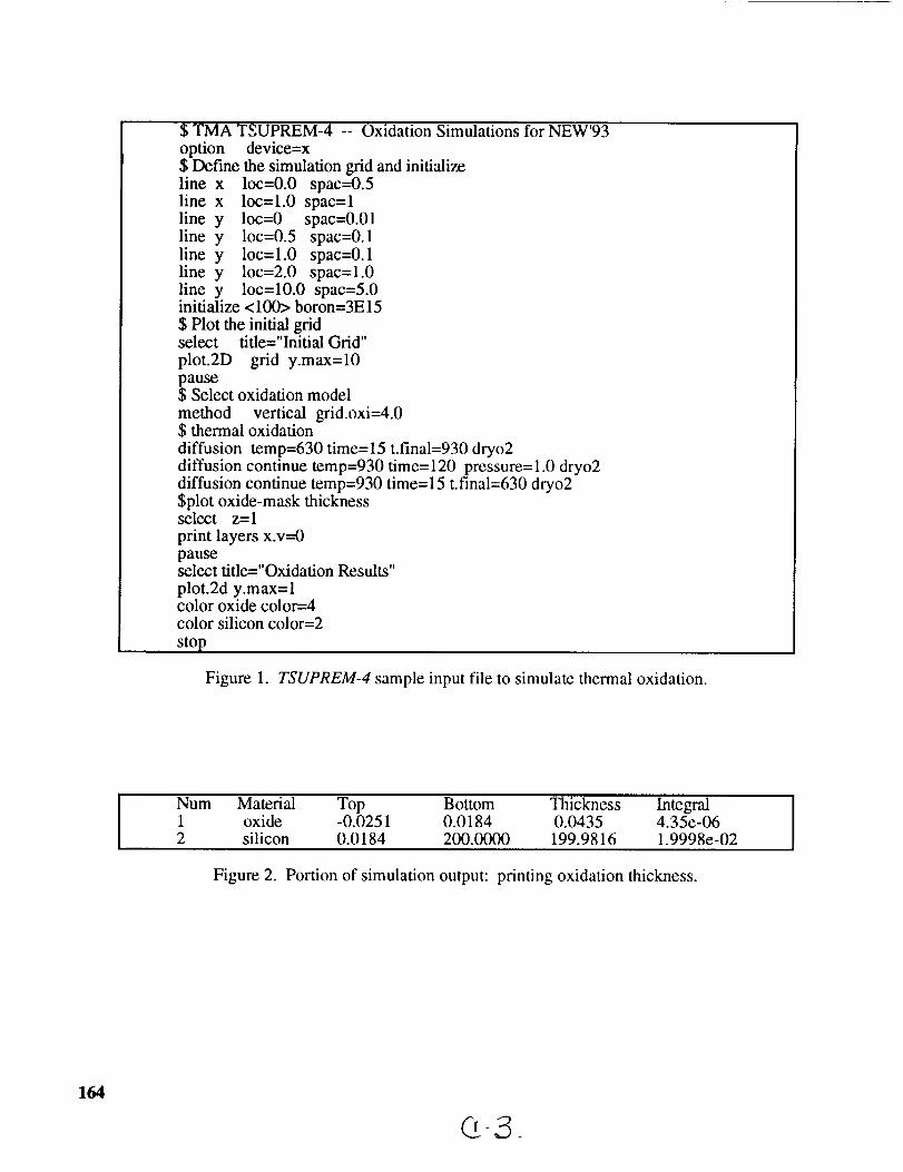
$ TMA TSUPREM-4 -- Oxidation Simulations for NEW'93
option device=x$ Define the simulation grid and initialize
line x loc=0.0 spac=0.5line x loc=l.0 spac=lline y loc=0 spac=0.01line y loc=0.5 spac=0.1line y loc=l.0 spac=0.1line y loc=2.0 spac=l.0line y loc=10.0 spac=5.0initialize <100> boron=3E15
$ Plot the initial gridselect title="Initial Grid"
plot.2D grid y.max=10pause$ Select oxidation model
method vertical grid.oxi=4.0$ thermal oxidation
diffusion temp=630 time=15 t.final=930 dryo2diffusion continue temp=930 time= 120 pressure= 1.0 dryo2diffusion continue temp=930 time=15 t.final=630 dryo2$plot oxide-mask thicknessselect z=l
print layers x.v=0
pauseselect title="Oxidation Results"
plot.2d y.max=lcolor oxide color=4color silicon color=2
stop
Figure 1. TSUPREM-4 sample input file to simulate thermal oxidation.
Num Material Top Bottom Thickness Integral1 oxide -0.0251 0.0184 0.0435 4.35e-062 silicon 0.0184 200.0000 199.9816 1.9998e-02
Figure 2. Portion of simulation output: printing oxidation thickness.
164

OxidationResultsI • " " • | | | • a . . | | • | . | • l • • • | • • . • | I i i a t . • . • i I • • . • • . • . •
0._ 0._ 0._ 0._ 0.80 1._
Distance (micrometers)
Figure 3. Portion of simulation output: two-dimensional view of oxidized wafer.
5O
40
30
o_,,_
_ 20
o_,_
©10
0
Mean-0--- Simulation
+ Minimum+ Maximum +
45 60 120
Oxidation Time imin)
Figure 4. Dry thermal oxidation of silicon at 900°C.
165

,xZ
_D
©
250
200
+
+150
1O0
5O
0
Mean
"O---Simulation
Minimum
Maximum
45 60
Oxidation Time (min)Figure 5. Dry thermal oxidation of silicon at 1100°C.
+
123
r.,/3
r./3
_D
,..c:Z
° I.,=_
©
300
250
200
Mean-O--- Simulation
+ Minimum
+ Maximum
150
100
5O
0
45
Figure 6.
60 120
Oxidation Time (min)Wet thermal oxidation of silicon at 900°C.
166

°_,,_
_D
°_,,_
©
9OO
800
700
60O
5OO
400
Mean
-0--- Simulation+ Minimum+ Maximum
46 63Oxidation Time _'min)
Figure 7. Wet thermal oxidation of silicon at 1100°C.
124
167


N94- 36405
USING EXPERIMENTAL DESIGN MODULES FORPROCESS CHARACTERIZATION IN
MANUFACTURING/MATERIALS PROCESSESLABORATORIES
Bruce Ankenman
Center for Quality and Productivity Improvement
and
Donald Ermer
Department of Industrial and Mechanical Engineering
University of Wisconsin - Madison
and
James A. Clum
Associate Dean
State University of New York at Binghamton
Watson School of Engineering
P. O. Box 6000
Binghamton, New York 13902-6000
Telephone 607-777-4555
ptlttl;lit'_ I'I-A_E tl_.llXi_ NOT Fii..lil_DPAGE_ INT-!'T',tT;,;ALLYBLANK 169


Using Experimental Design Modules forProcess Characterization in Manufacturing/Materials Processes Laboratories
Bruce Ankenman*, Donald Ermer** and James Clum***
*Center for Quality and Productivity Improvement**Department of Industrial and Mechanical Engineering
University of Wisconsin - Madison***Mechanical & Industrial Engineering Department
State University of New York at Binghamton..........................................................................................................
Abstract: Modules dealing with statistical experimental design(SED), processmodelling and improvement, and response surface methods have been developed and testedin two laboratory courses. One course was a manufacturing processes course in
Mechanical Engineering and the other course was a materials processing course in MaterialsScience and Engineering. Each module is used as an 'experiment' in the course with the
intent that subsequent course experiments will use SED methods for analysis andinterpretation of data. Evaluation of the modules' effectiveness has been done by bothsurvey questionnaires and inclusion of the module methodology in course examinationquestions. Results of the evaluation have been very positive. Those evaluation results anddetails of the modules' content and implementation are presented. The modules representan important component for updating laboratory instruction and to provide training inquality for improved engineering practice.
Introduction (history): What follows is a brief discussion of the history of thedevelopment of the SED and related topics modules in ME310 and MS&E370. The actual
ME310 module on SED is then presented in its format as one lab experiment followed byan example of the SED applications from one of five subsequent experiments which rely onthe module for data analysis. A discussion of the comparison of the ME310 andMS&E370 modules is given next. Finally, the results of the evaluation of the effectivenessof the ME310 and MS&E370 modules are presented which are based on measurements ofstudent skills (ME310) and student opinion surveys (ME310 and MS&E370).
ME310 Lab; The ME310 course (Manufacturing Processes I) has been a
requirement in the ME curriculum for decades. Industrial Engineering students also maytake the course as an option and many usually do so. It is a three credit per semester coursewith the course grading scheme effectively making for a division of student effort into two-thirds lecture and one-third lab. The labs in the current version of the course are verypractice oriented with emphasis placed on principles and practices of machining operationsand deformation processing, e.g., extrusion and sheetmetal forming. The SED moduleoccupies one lab period near the beginning of the course.
ME310 Lc_r¢; Although the focus of the module development andapplications has been the ME310 laboratory the lecture portion has also been a source ofinformation on SED methods and related quality improvement tools. During 1991-92, forexample, Visiting Professor John Corbett used the lecture to introduce quality functiondeployment (QFD) as a component of the broader topic, "design for competitivemanufacturing". In 1992-93, one of the authors (JAC) added presentations on fractionalfactorial designs, Taguchi methods, and exploratory data analysis tools (check sheets,cause-and-effect diagrams, flow charts, etc.) to the lectures.
MS&E370 Lectur¢; The module for this course was developed in 1992-93 withthe intent of being more comprehensive than the ME310 SED module. The reason for thechange of focus and format was two-fold: (1) MS&E370 was undergoing revision and the
applications of SED in the course's laboratories would be undertaken as a second stage ofthe course revision; (2) unlike students in ME310 those in MS&E370 would not likelyhave completed an introductory statistics or quality engineering course prior to the 370course.
_D,_ F;_GF. _tL_iK NOT FILMED171

Historically,thecourseMS&E370(MaterialsProcessing-UnitOperations)hasbeenafour creditpersemestercoursewith divisionof effortmakingthelab counteffectivelyasonecredit. In the 1992-93academicyearthecoursewasbeingrevisedto makeit fit, asanapprovedoption,into theMechanicalEngineeringcurriculum. Thus,therewasanincreasedinterestto incorporatetopicssuchasSEDandprocesscharacterizationandimprovementtoolsin therevisionof MS&E370aroseto makeit similarto ME310.
Lab Module(s): TheactualME310LabmoduleonStatisticalExperimentalDesignisgivenin AppendixI. Also in thatAppendixis anSEDProjectexercisewhich is thebasisof thestudentreportsfor theSEDlabsession.Subsequentto theSEDlab sessiontherearefive (5) SED-basedlab sessions:_, andForces and Power in Metal Cutting I andII (drilling; grinding; milling; turning). The five applications of SED along with the SEDmodule itself comprise approximately 40%, or 110 points out of 250, of the value allocatedto ME310 Lab reports. A copy of the ME310 Lab data sheet used in the SED applicationfor the Extrusion experiment is included in Appendix I. That data sheet is typical of theforms used in the five SED applications labs.
The module on Process Characterization Tools prepared for MS&E370 is excerpted
in Appendix II. Shown there are: (i) the cover page for the module which outlines themodule's intent, and (ii) a summary figure from the module, "PROCESSIMPROVEMENT TOOL BOX". As the cover page "Abstract" indicates the MS&E370module covers a wider range of topics than the ME310 SED module. Its future applicationin the revised MS&E370 was the basis for such a range of topics being introduced. An
exercise was included in the MS&E370 module which is similar to the 23 design analysis
of the ME310 SED module. However, in the first semester of its use none of the other lab
experiments in MS&E370, e.g., casting, heat treating and joining, were modified to takeadvantage of the new process characterization/improvement module.
Evaluation of Effectiveness: Two methods of evaluation were used to determinethe effectiveness of the ME310 module on SED. These methods were: (1) evaluation of
each student's skill level in designing, analyzing and interpreting a standard 23 factorial
experiment during an exam; (2) surveying each student to gain information about theirattitudes towards the perceived general usefulness and possible future career applications ofSED methods. Only the survey method was used with the students in MS&E370 sincethey did not have the opportunities for practice of the skills afforded in ME310.
Skill Level - ME310: As a part of one of the ME310 lecture examinations a
problem was given which asked the students to compare their actual lab experiment onsheetmetal forming (done in sequence prior to their SED lab, and also done without regardto balancing the pattern of investigation of the three test factors of: alloy type, sheet
thickness and lubrication) to data from a standard 23 factorial design of the same
experiment. Of the sixty-five (65) students taking the exam 62 got the problem completelycorrect, except for some math errors in calculating the predictive model residuals. Thethree remaining students' error was in writing the standard design in reverse order, afterwhich the rest of their calculations were correct except for the wrong signs in the
calculations of the predictive models. The exam was closed book and closed notes. They,as a group, had clearly developed the skill of being able to design and analyze simplefactorial designs. Of equal importance, they were able to recognize the "bad" design of theoriginal sheetmetal forming experiment.
Attitudes Survey - ME310 and MS&E370: At the end of Spring Semester 1993the 65 students in ME310 and 6 in MS&E370 were surveyed to determine how effective
they felt SED was as an experimental tool. The summary results from three questions
relating to usefulness of SED are presented below. The percentages are based on the totalnumber of responses who either agree, or strongly agree with the statement.
172

StatementI would recommend that SED methods be
incorporated in all lab courses.
ME310 MS&E370
82.5% 66.7%
I think SED is a tool that I will find useful in
future applications. 95.2% 100%
I would like to gain more experience in SEDmethods 88.9% 83.3%
The survey results provide a strong signal for those of us developing laboratorycourses and experiments. It is worth adding at this point that several students in bothcourses were co-op students. Their comments on the surveys were that they had alreadybeen introduced to these experimental planning and analysis tools during their co-op.Unfortunately, except for these instances (ME310 and MS&E370) they were not beinggiven regular access to such modem laboratory analysis methods in their engineeringeducation. (We should note here that the University of Wisconsin - Madison's PlasmaProcessing Laboratory offers SED instruction as part of the plasma lab course at thegraduate level. An SED module was written by Prof. Soren Bisgaard for that course.)
Summary: We have outlined an example of an instructional plan for incorporatingstatistical experimental design methods into existing laboratory courses. The incorporationof these techniques has been shown to be effectively accomplished in terms of both studentskill development and attitudes regarding experimentation. Furthermore, this procedure ofmaking the SED topic an integral part of the overall lab operation strengthens the entirecourse with minimal effect on the curricular focus of the lab course.
Instructor Notes: The major impediment to using SED methods in existing laboratorycourses is lack of instructor familiarity with the concepts. We offer two recommendationsfor overcoming that barrier. The first suggestion is to enlist the aid of a colleague at yourinstitution who has a background in statistical methods to help you write your ownmodule(s) using this module as a guide. In this approach you will find a willing supportperson with statistics as a background and you will 'learn by doing' as you develop themodule to fit your specific circumstances. A second way to modify your course(s) toinclude the SEE) techniques is to attend formal workshops or short courses offered by avariety of organizations. We will not list any of those offerings here, but can provide youwith suggestions if you contact us.
Acknowledgements: There have been many individuals responsible for thesuccessful development of the ME310 SED modules. Particular mention should be madeof the Teaching Assistants who have taught the lab course and specifically contributed tothe lab's success. They are, in alphabetical order: John Bashel, Dan Bee, Dave De Haan,Bill Durkin; Pat Galecki, Bob Gustafson, Jim Rink, Russ Tilsner, Dave Van Zuest, and Jim
Witte. The encouragement of several faculty also was essential to implementing thesechanges. The faculty to be acknowledged include, in alphabetical order: Prof. SorenBisgaard (IE and Associate Director of the Center for Quality and ProductivityImprovement), Prof. Marvin DeVries (Chairman of ME and a long time proponent of useof SED in manufacturing processes), and Prof. Slawomir Spiewak (ME and faculty in chargeof ME310 during these changes). Two of the authors (BA and JC) also wish to recognizethe support to CQPI by a grant from the Alfred P. Sloan Foundation during 1992-93 whenthis report was prepared.
173
(Appendix I)
ME310 LabSTATISTICAL EXPERIMENTAL DESIGN
Key Words: Statistical Experimental Design; Factorial designs;Randomization; Interaction Effects; Predictive models; Process characterization;Continuous Improvement; Response surfaces; Exploratory data analysis.
Prerequisite Knowledge: You are expected to have taken anintroductory materials science/engineering course and math through differential equations.No prior course work in statistics is required.
Purpose and Learning Objectives: The ['i4_ose of this instructionalmodule is to introduce you to an effective method of planning, conducting, analyzing and
interpreting experiments. This module will be followed by a series of laboratory moduleswhere practice of the methods will help to develop skills The methodology of statisticalexperimental design (SED) is especially useful for the initial characterization andcontinuous improvement of processes, particularly industrial processes.
Learning Objectives After completion of this module you should haveaccomplished the following knowledge, skill and attitude objectives:Knowledge Ob_iectives Know about the use of: Factorial SED techniques and theircapability to determine the effects of major process control parameters and interactionsbetween parameters; randomization,replication, blocking, and confounding in conductingand analyzing experiments; Exploratory data analysis tools;
$kill Objectives Be able to: Plan, and properly conduct a full 2n factorial design;Calculate contrasts and effects from standard results; Determine significant effects;Construct empirical predictive model of behavior based on significant effects; Constructcontour diagram (preliminary response surface)from predictive behavior model; To aid inproblem solving: Construct check sheets, Pareto diagrams, histograms, flow charts,cause-and-effect diagrams, scatter diagrams for a given data set;Attitude Obiectives Actively promote the application of." Designed experiments in thedetermination of major process effects for quality improvement and optimization; Simple
graphical methods of data analysis;
Equipment and Supplies: The SED modules require only data from realexperiments or industrial operations. Access to a computer software package withcapability to do graphics manipulations such as cube plots, normal probability plots, flowchart construction, etc. is desirable. Such software is best presented as a demonstration
(needing appropriate hardware for overhead projection from computer screen) initially withsubsequent student access to the software for report calculations.
174

Introduction to Statistical Experimental DesignStatistical Experimental Design is a method of experimentation which provides the
experimenter with tools to accurately and efficiently collect and analyze data. A factorialexperiment usually involves several factors which are varied by the experimenter and oneor more responses which are to be optimized. In the past, engineers and scientists haverelied on one-factor-at-a-time experiments. These are experiments in which each factor inthe experiment is varied independently while the other factors are kept constant. However,this type of experimentation has been found to be inadequate to produce the speed andaccuracy needed to develop new products and processes. The most notable short comingof the one-factor-at-a-time approach is that the interaction that factors often have with eachother cannot be estimated. For example, in a sheetmetal forming operation, it may be foundthat at one thickness of material, lubrication has a large effect on the formability of thematerial, but at another thickness level the lubrication has almost no effect. A one-factor-at-
a-time experiment will not provide any information about this interaction. However, afactorial experiment based on modern, statistical principles of experimental design will beable to detect such interaction effects.
Two-Level Factorials
Although there are many types of statistically designed experiments, some of themost useful are called two level factorials. For a two level factorial design each factor is setat a high and low level (usually a small amount above and below what is currentlyconsidered the best setting of that factor). Each possible combination of settings of thefactors is then run. Due to the properties of the experiment, the experimenter can determinewhich factors have the most effect on the response, which factors interact, and build anapproximate model relating the factors to the response. This information can then be used
to optimize the response. Unreplicated two-level, three factor experiments, called 2 3
factorials, are especially useful for efficiently investigating a process about which very little
is known. These experiments only require 2 3 or 8 experimental trial runs and the resultscan be used to get ideas about the underlying relationships of the factors with the responseduring the exploratory phase of an investigation. To confirm these results for publicationor other such purposes, replications would be needed.
Asan example, a 23 factorial mill experiment will be designed and analyzed. The
three factors will be the Speed of the cutter (RPM), the Feed rate (in./min.), and the DepthOf Cut or D.O.C. (in.).
Coding of the Factor LevelsFor ease of analysis, it is convenient to code the factors into high and low levels as
follows:
Factor
Speed (S)Feed (F)
D.O.C. (D)
Low Level
(-1)
502.5
.i
High Level(+1)
75
3.5
.2
Units
RPM
in./minin.
175

Usingthecodes"-1" and"+1" all thepossiblecombinationsof levelsmustnow belisted. For simplicity wewill use"-" to showthe"-1" level and"+" to showthe"+1"level. Theorderlistedbelowiscalledthestandardorderandyoucanquickly seethatthepatternof thestandardordermakesit easyto detectwhetherall 23possiblecombinationsoflow andhighfactorlevelsarepresent.
Standard Orderi2345678
SB
+
m
4-
+
+
F
+
+
+
4-
D
m
+
4- •
+
4-
RandomizationIt is unwise to run the actual experiment in the standard order. For example, if the
experiment were run in standard order and the calibration or any other uncontrolled factorchanged halfway through the experiment, it would be impossible to tell the differencebetween the effect of the uncontrolled change and the effect of depth of cut (D) since thisfactor changes only once at the midpoint of the experiment. This leads to the idea ofRandomization. Randomization is a principle which states that if the experimental trials arerun in random order, it is very unlikely that any uncontrolled factor change will exactly
correspond to any of the controlled factor changes and therefore the effect of theuncontrolled factors should not significantly bias the experimental results. For this reason,
the trials in this experiment will be run in a random order. To determine the random order,the numbers 1 through 8 should be written on small pieces of paper and drawn from a hator a bowl.
Cube Plots
A cube plot is a method of plotting the data from a 23 factorial. The plot consistsof a cube with a response value located at each comer. Each dimension of the cube
represents the coded scale of one of the factors from the low level (-) to the high level (+).An example is given below using metal removal rate (Q) of the mill as the response plottedversus the factors; Speed (S), Feed (F), and D.O.C.(D).
This plot is useful because one can easily compare the four responses with low Fon the left side of the cube (.031, .031, .063, .063) with those with high F in the
corresponding location on the right side of the cube (.044, .044, .088, .088) to see theeffect of F on metal removal rate,(Q).
In the figure below you will notice that there are four separate comparisons whichcan be made and in each comparison the only factor changed is F. These separate
comparisons are called hidden replications and are the reason that, even when unreplicated,
23 factorials can be relied upon to convey a great deal of information. Similarly one can
compare the front and back of the cube to see the effect of D on Q or the top and bottom ofthe cube to see the effect of S on Q. In the cube shown, one can see that the responses on
the top of the cube are identical to those in the corresponding position on the bottom of thecube, which shows that Speed has no effect on Q. This confirms the already known
relationship, Q = (D.O.C.)*(Feed)*(Width of Cut), in which Speed is not a factor.
176

Metal Removal Rate of the Mill
$
Calculation and Meaning of the Effects
To this point, the effect of each factor has been spoken of in a qualitative way.However, the specific quantitative definition of the main effect of a given factor on a givenresponse can now be defined as the average difference between the responses at the highlevel of the factor and the responses at the low level of that factor. Thus, the effect of Feedon Q is the average of the differences (.044 -.031), (.044 -.031), (.088 -.063), and(.088 - .063). Therefore, for the ranges used in this experiment the effect of Feed (F) onQ is .019, the effect of D.O.C. (D) on Q is .038, and the effect of Speed (S) on Q is zero.
The interaction effect between two factors is the average amount that the effect of afactor changes when another factor is varied. For example, the effect of F on Q at the lowlevel of D is the average of (.044 - .031) and (.044 -.031) or .013, but at the high level ofD the effect of F on Q is .025. The interaction effect then is (.025 - .013)/2 or .006.These interaction effects are most easily calculated using the table shown below, where theinteraction effect between Feed (F) and D.O.C.(D) is called FD and the other interaction
effects are similarly called SF and SD. SFD is the three way interaction effect. Thecontrast for each column is the sum of the data when the data is given the signs of thatcolumn as shown in the example column for FD. All effects, including the main effects,are calculated as shown by dividing the contrast for each column by 4*. In this case theonly interaction effect is the interaction between the Feed and the D.O.C. (FD); all otherinteractions show values of zero.
177

Trial #
1
2
3
4
5
6
7
8
Contrast
Effects
Main Effects
S F D
-- m --
+ n --
-- +
+ + --
-- -- +
+ -- +
-- + +
+ + +
0 .076 .152
0 .019 .038
Interaction Effects
SF SD FD (example FD)
+ + + (+.031)
- - + (+.031)
- + - (-.044)
+ - - (-.044)
+ - - (-.063)
- + - (-.063)
- - + (+.088)
+ + + (+.088)
0 0 .024 (.024)
0 0 .006 (.024/4=.006)
SFD 9
- .031
+ .031
+ .044
- .0q4
+ .063
- .063
- .088
+ .088
0
0
*4 equals the number of differences being averaged, and can be easily determinedby the number of + and - pairs in the column.
Model BuildingOnce the important effects have been identified, a model can be created which will
estimate the response, in this case Metal Removal Rate, at locations in or on the cube whichwere not specifically run in the experiment. The model uses the coded scale -1 to +1 foreach of the factors and includes only the strong effects. The coefficients for the polynomialmodel are exactly one half of the effects previously calculated, so the model we will use is:
Q = (.0095)F + (.019)D + .0565 (Model 1)
where .0565 is the average value of the Metal Removal Rate data. If we consider the FDinteraction to be important, the model would then be:
Q = (.0095)F + (.019)D + (.003)FD + .0565 (Model 2)
Based on Model 1, we would predict a Q of .07075 for F=.5 and D=.5.Model 2 would predict a Q of .070825, which shows that the interaction term is indeedquite a small effect. Using the cube plot and the model we can see that if Q is to beincreased, Feed and D.O.C. must be increased and Speed has no influence on Q.
References
Box, G.E.P., W.G.Hunter, and J.S. Hunter (1978). Statistics for Experimenters.New York: John Wiley & Sons.
Box, G.E.P., and Soren Bisgaard (1987), "The Scientific Context of QualityImprovement." Quality Progress, June 1987 and Report #25, Center for Quality andProductivity Improvement, Rm. 575 WARF Building, University of Wisconsin-Madison.
Box, G.E.P. (1989), "Do Interactions Matter?" Report #46, Center for Quality andProductivity Improvement, Rm. 575 WARF Building, University of Wisconsin- Madison.
Box, G.E.P. (1989), "Must We Randomize Our Experiment?" Report #47, Centerfor Quality and Productivity Improvement, Rm. 575 WARF Building, University ofWisconsin- Madison.
Box, G.E.P. and Soren Bisgaard (1988), "Statistical Tools for ImprovingDesigns", Mechanical Engineering, Jan. 1988, pp.32-40.CQPI Reports available from: Center for Quality and Productivity Improvement
University of Wisconsin - Madison610 Walnut Street, WARF Bldg., Rm. 575Madison, WI 53705
178

ME 310 Project II
Given the data in the standard order table below, perform the following
analysis: (Note: This experiment was performed in random order.)
1. Calculate the contrasts and main effects of speed (S), feed (F), and depth ofcut (D). Note: Show all calculations, no spread sheet analysis is allowed.
2. Calculate the contrasts and interaction effects of all control factors. Note:Show all calculations, no spread sheet analysis is allowed.
Main Effects Interaction Effects
Trial # S F D S F SD FD SFD Hpu
_ + + + - 29.51
2 + _ _ _ + + 40.7
3 + _ _ + _ + 28.6- 40.2
4 + + - + - -
5 _ + + _ _ + 21.3- 34.1
6 + - + - + -
7 + + _ _ + - 21.6
8 + + + + + + + 34.0
Contrast
Effects
.
4.5.
Draw the cube plot with the appropriate response at the comers of the cube.On your cube plot, circle the four (4) hidden replications of feed (F).Rank effects in ascending order, or lowest to highest, and calculate the
cumulative probabilities for each effect given by the equation:
P(i) = 100 ( i- .5 ) / n
.
7.
.
9.
where:i = ascending order number associated with each piece of data.n = size of the sample or number of effects.
Plot the cumulative probabilities on the normal probability plot provided.Determine which main effects and/or interaction effects are significant from
the above analysis.Develop the coded model for Hpu using the significant effects.From the coded equation, determine the actual value for speed if it is desiredto maximize depth of cut and have a Hpu value of 30.2. You will need to usethe table for coded factors on page 2 of the SED Lab Notes.
NOTE: For further examples of the graphical methods of using cube plots toanalyse factorial designed experiments please refer to the followingReferences. To see how an additional problem is analyzed see the Boxand Bisgaard 1988 article in Mechanical Engineering. For a morecomplete, but very readable description of cube plots refer to the textbookby Box, Hunter and Hunter (1978).
Copies of the ME310 Lab Manual may be requested from Prof. Donald Ermer at theMechanical Engineering Department, Univ. of Wisconsin-Madison, 1513 University Ave,Madison, WI 53706. New copies will, however, not be printed after Fall Semester 1993
179

Extrusion Summary Sheet
Random
Order
Direction
Die
Geometr 7
Lubricatior.
IS.O. i*
Forward
Square
No
S.O. 2
Reverse
Square
No
S.O. 3
Forward
Round
N0
S.O. 4
Reverse
Round
NO
S.O. 5
Forward
Square
Yes
S.O. 6
Reverse
Square
Yes
S.O. 7
Forward
Round
Yes
S.O. 8
Reverse
Round
Yes
Break
ThroughForce (ibs)
SQR= - FWD- - N/L= -RND-- + REV-- + LUB= +
* S.O. represents "standard order"
. Main EffectsS.O. # D G L DG DL GL
1 - - - + + +
'2 4- .... 4-
3 -- + -- -- + _
4 + + - + _ _
5 - - + + _ _
6 + - + - + _
7 - + + - _ +
8 . + + + + + +
Contrast
Effects
Interaction Effects
DGL B.T. Force
+
+
+
4-
180

(Name)
Sheet Metal Forming Exinerimental Design
Std. order
1
2
3
4
5
6
7
8
Contrast
Effects
Main Effects Interaction Effects
Axt AxL txL AxtxL Bulge
+ + + - 34.0
- - + + 21.3
- + - + 34.3
+ - - - 28.6
+ - - + 40.2
- + - - 21.6
- - + - 40.7
+ + + + 29.5
p. 6/6
Coding of the Factor LevelsFor ease of analysis, it is convenient to code the factors into high and low levels as
follows:
Factor
Alloy (A)thickness(t)
Lube (L)
Low Level
(-1)2024-0
0.05
No lube
High 'Level
(+1)
2024-T3
0.125
Lube
Units
treatmentin.
lubricant
NOTE: This page is from ME310 Exam #2. It is the data sheet for a questionabout how to reevaluate the Sheet Metal Formability Lab if a statistically designed
experiment had been conducted. In addition to completing the data table a cube plotand process model equation was required as part of the exam question.
181

(Appendix H)
MS & E 370Process Design and Control Toolbox: I
Exploratory Data Analysis Tools and Statistically Designed Experiments
Key Words: Statistical Experimental Design; Factorial designs;Randomization; Interaction Effects; Predictive models; Process characterization;
Continuous Improvement; Response surfaces; Exploratory data analysis.Prerequisite Knowledge: You are expected to have taken an
introductory materials science/engineering course and math through differential equations.No prior course work in statistics is required.
Purpose and Learning Objectives: The Purpose of this instructionalmodule is to introduce you to an effective method of planning, conductihg, analyzing andinterpreting experiments. This module will be followed by a series of laboratory moduleswhere practice of the methods will help to develop skills. The methodology of statisticalexperimental design (SED) is especially useful for the initial characterization andcontinuous improvement of processes, particularly industrial processes.
Learning Objectives: After completion of this module you should haveaccomplished the following knowledge, skill and attitude objectives.
Knowledge Obiectives Know about the use of:Factorially Designed experiments; Blocking, confounding and randomization in conductingand analyzing experiments; Exploratory data analysis tools;
Skill Objectives Be able to: Plan, and properly
conduct a full 2 n factorial design; Calculate contrasts and effects from standard results;Determine significant effects; Construct empirical predictive model of behavior based onsignificant effects; Construct contour diagram (preliminary response surface) frompredictive behavior model; Construct check sheets, Pareto diagrams, histograms, flowcharts, cause-and-effect diagrams, scatter diagrams for a given data set;
Attitude Ob_iectives Promote the application of: Simplegraphical methods of data analysis; Using designed experiments in the determination ofmajor process effects for improvement and optimization.
Equipment and Supplies: The SED modules require only data from real
experiments or industrial operations. Access to a computer software package withcapability to do graphics manipulations such as cube plots, normal probability plots, flowchart construction, etc. is desirable.............................................................................................................
Abstract: Traditional methods of designing and improving processes have been basedon one-factor-at-a-time (1-faat) procedures for obtaining information about the processes.Such methods are known to be inefficient and often misleading with regard to the wayprocess variables are determined to affect the output. In this module we will describe andillustrate the use of a variety of tools, or techniques, which are especially easy to use forexploring existing data, and for obtaining and interpreting new data. The tools which will
be introduced are: flow diagrams; check sheets; Pareto charts; histograms, control charts,cause-and-effect diagrams; designed experiments; response surfaces. These tools place
strong emphasis on visualization of data rather than on numerical descriptions of a system.They can, consequently, be effectively used by a wide range of personnel involved withdesign and monitoring of processes. Special emphasis will be given to factorial methods ofexperimental design since those methods provide one of the best techniques for acquiringdata and converting it into useful information.
182

FLOW DIAGRAM
so[]:°lPARETO ANALYSIS
A1 A2BI B2 B3 B4
I 3 406CI n_ 5 -1
3 -4 4!-1C2 5 0 3 2
DESIGNED EXPERIMENT
L = (y- T)_
TAGUCHI
SCATTER DIAGRAM
0-5 III
6-10 I_HIII II
11-15 ,IN ft4'd II II
16-20 Jgl4] J_41'
21-25 JUl.tf I I
26-30 Ill!
TALLY SHEET
TOOL BO
";-:,'-:;-_:-- --:- -ZI.__'______b_____1
"="- -;" - _'-,T _:.- :- -1
VARIABLE CONTROL CHART
1i _A A
ATTRIBUTE CONTROL CHART
CAUSE & EFFECT DIAGRAM HISTOGRAM
183


N94- 36406 - ;=_-_._
PROCESS CAPABILITY DETERMINATION OF NEW
AND EXISTING EQUIPMENT
H. T. McClelland
Technology Department
University of Wisconsin-Stout
Menomonie, Wisconsin 54751
Telephone 715-232-2152
and
Penwen Su
Manufacturing and Industrial Technology
Arizona State University
Tempe, AZ 85287-6806
PAGE BLANK NOT FILMED
_:"ca.,.................a_
185


PROCESS CAPABILITY DETERMINATION OF NEW AND EXISTING EQUIPMENT
H.T. McClelland
Technology Department
University of Wisconsin-Stout
Menomonie, WI 54751
Penwen Su
Manufacturing and Industrial Technology
Arizona State University
Tempe, AZ 85287-6806
KEY WORDS: Process capability, statistical process control,
statistics, equipment characterization.
PREREQUISITE KNOWLEDGE: Introductory statistics, some knowledge
of manufacturing processes and equipment. This will generally bean experiment for an advanced class.
OBJECTIVES: To illustrate a technique for determining the
process capability of new equipment, existing equipment, or
testing laboratories. To illustrate a method of objectively
determining wear and other changes in equipment used for small
quantity production over a period of time. To present an example
of the application of the technique.
INTRODUCTION
The objective of this paper is to illustrate a method of
determining the process capability of new or existing equipment.
The method may also be modified to apply to testing laboratories.
Long term changes in the system may be determined by periodically
making new test parts or submitting samples from the original setto the testing laboratory.
The technique described has been developed through a series
of projects in special topics manufacturing courses and graduate
student projects. It will be implemented as a standard
experiment in an advanced manufacturing course in a new
Manufacturing Engineering program at the University of Wisconsin-Stout campus.
Before starting a project of this nature, it is important to
decide on the exact question to be answered. In this case, it is
desired to know what variation can be reasonably expected in the
next part, feature, or test result produced. Generally, this
question is answered by providing the process capability or the
average value of a measured characteristic of the part or process
± three standard deviations. There are two general cases to be
considered: (I) the part or test is made in large quantities
with little change or (2) the process is flexible and makes a
large variety of parts. Both cases can be accommodated; however,the emphasis in this report is on short run situations.
187

GENERAL PROCEDURE
The first step in any investigation is to clearly define
what is desired. Specifically, what measurements will give the
most information about the process, can be measured with relative
ease, will continue to be made for the foreseeable future, and
relate directly to the quality of the part. Quite often, this
step is done too quickly and the results do not give the desiredinformation. It is suggested that extra time be taken to clearly
define the specific problem.
Selecting the proper sample is the next step. For large
runs of production parts or routine tests, the normally measured
features of the part or the standard test samples can be used. A
special part may have to be developed for short run, flexible
machinery. This part should include a variety of features which
incorporate as many of the functions of the machine as possible.
One such part is illustrated later. For short run situations, a
method can be used which focuses on the process, not the
product. I One technique is to use the deviation from the nominaldimension as the measured characteristic rather than the actual
dimension. _ This allows measurements of various depth holes or
different diameter rounds, etc. to be used to generate sufficient
numbers for reasonable process capability estimates. These
comparison procedures (comparing deviations from nominal
dimensions for similar features) can be used to give a running
process capability. Periodically, an original test sample can be
produced to evaluate any undetected changes with time in the
machine performance.When testing laboratories are to be evaluated, a large
number of identical samples are obtained from well characterized
material. If more than one type of material is tested routinely,
then representative samples of each should be included. About
one-fourth of these are used initially and the rest are submitted
over a period of time.
Each part produced may be measured but often a sample of the
production lot is measured. In the latter case, it is important
to randomize the part selection so the Laws of Chance will apply
and the results will be valid. All of the testing laboratory
specimens should be numbered sequentially (include all different
materials) and a random sample selected comprising the initial
one-fourth or so of the specimens. These should be submitted to
the laboratory with instructions to run the specimens in the
order listed. If the materials are sufficiently different, such
as those requiring different load cells on a tensile machine, a
stratified random sample may be required. The data from the
initial measurements or test results can be used to determine the
current, initial process capability. The process capability can
be updated as new measurements are obtained.
For testing laboratories, a small number of original
"standard" specimens can be blended into the normal productiontests and the variation of test lab results with time evaluated.
These results can be combined with the results for the normal
production specimens to give a continuously updated process
capability. It is suggested that test laboratory evaluations be
188
discussed with the lab manager after the initial results are
obtained before being generally distributed. Quite often there
are explanations for unexpected results of which the investigator
may be unaware. This also helps keep political peace within thecompany.
APPLICATION TO A MACHINE TOOLObjective:
The Manufacturing and Industrial Technology Department of
Arizona State University recently obtained a Fadal VMC-20
vertical machining center. Mr. Su was assigned to determine
baseline measurements of the dimensional reproducibility of this
machine as part of his Master of Technology project. Sample
materials were two alloys commonly used in the department: 1018
cold rolled steel and 6061-T6 aluminum. The objective was to
determine the initial dimensional reproducibility of the new
machine, to determine if a difference exists between the two
materials, and to quantify such a difference if one exists.
Procedure:
The machining center was obtained as a flexible component of
a manufacturing cell and is not part of a line producing many of
the same component. For this reason, a special part was designed
to give a measure of the various machine capabilities and this
part is shown in Figure i. The overall nominal dimensions are
102 mm x 102 mm x 44.5 mm (4 inches x 4 inches x 1.75 inches).
Each feature is dimensioned with respect to the center line or
top surface but the numbers are not shown because of the clutter.
The parts were machined to the same programmed nominal dimensions
and these dimensions were then measured on a coordinate measuringmachine. The deviations from the nominal dimensions were the
characteristics of interest. In this way, the various linear
dimensions could be combined with each other and likewise with
the various circular dimensions. Each part is therefore capable
of giving numerous samples for the calculation of the processcapabilities.
Six machining processes were evaluated using the designedpart:
i. End milling of the steps to preset depths.
2. End milling of steps to preset peripheraldimensions.
3. End milling circular interpolation clockwise in to
preset outside diameters of cylinders and round corners.
4. End milling circular interpolation clockwise out
for circular pockets and round corners.
5. Reaming the holes to preset diameters after center
hole and pilot hole drilling.
6. The relative positions of the holes from the center
lines of the part after reaming.
Two materials were used: 1018 cold rolled steel and 6061-T6
aluminum. The same basic program was used for each with
variations based on published optimum machining conditions for
189

each material. 3 These conditions were modified somewhat for the
steel as a result of chatter problems with the initial part. The
Fadal machining center was capable of holding the complete tool
sets needed for both parts and, thus, loading tooling into the
machine was not a factor in the results.
The initial experiment was designed to determine if there
was a difference in dimensional reproducibility between the
aluminum and steel at the 95% confidence level. A difference of
0.0076mm (0.0003 inches) was considered to be of practical
significance and an initial standard deviation of 0.0051 mm
(0.0002 inches) was used for the initial calculations. Thesevalues were estimated from experience and guessing. The standard
deviations were checked after the first parts were machined and
found to be higher for these parts, to vary with the process in
question, and with the material. The number of test parts
required was then recalculated. The calculations considered the
number of features to be combined on each part and showed that
six parts of each material were required to determine if adifference exists between the steel and aluminum. The machining
order for two materials was determined by randomization. Each
part blank was placed into the machine by hand.
Results:The results of the machining tests are summarized in Table
I.TABLE I
Summary of Machining ResultsValues are Variations from Nominal Dimensions mm (inches)
Aluminum--6061-T6:
Process Average Std Dev Initial PC #meas
(o) (± 3o)
1 -0.0061 0.0053 ± 0.015 36
(-0.00024) (0.00021) (± 0.0006)
2 0.0322 0.0990 _ 0.0305 36
(0.00125) (0.00039) (_ 0.0012)
3 0.0236 0.0104 ± 0.0305 36
(0.00093) (0.00041) (! 0.0012)
4 0.0142 0.0127 ± 0.0381 36
(0.00056) (0.00050) (± 0.0015)
5 -0.0338 0.0142 ± 0.0457 24
(-0.00133) (0.00056) (t 0.0018)5* 0.0310 0.0051 ± 0.0152 23
(0.00122) (0.00020) (± 0.0006)
6 -0.0079 0.0135 ± 0.0419 48
(-0.00031) (0.00053) (_ 0.0017)
*One hole in one part had a very high variation in process 5 and
no assignable cause was found for this variation. The data for 5
were calculated using all results and 5* dropped the questionable
reading. All of the readings were used in the comparisons.
190

Steel--1018 cold rolled
Process Average Std Dev Initial PC
(0) (_ 30)
#meas
1 0.0117 0.0117 ± 0.0356 36
(0.00046) (0.00046) (! 0.0014)
2 -0.1540 0.0991 + 0.2970 36
(-0.00607) (0.00390) (± 0.0117)
3 -0.0478 0.0937 + 0.282 36
(-0.00188) (0.00369) (! 0.0111)
4 0.1460 0.1430 ± 0.4270 36
(0.00573) (0.00562) (± 0.0168)
5 -0.0277 0.0610 _ 0.0152 24
(-0.00109) (0.00024) (! 0.0006)
6 -0.0157 0.0236 ! 0.0419 48
(-0.00062) (0.00093) (± 0.0017)
Each average is calculated from 24, 36, or 48 individual
readings depending on the type of measurement. For example,
there are six steps (one inside and five outside on each of the
six parts) which were measured for Process 1 so 36 measurements
were averaged. There are four holes in each part so Process 5 is
the average of 24 readings. Two measurements were made for the
position of each hole (x and y) with respect to the center of the
part so 48 measurements were averaged for process 6.
The data were compared using the "z Test for Measurements"
and the "Student's t Test" 4 and it was found that a significantdifference existed between the aluminum and steel at the 95%
confidence level for all processes measured except for processes
5 and 6. It should be noted that process 5 was the process with
the one unexplained high reading and the comparison statistic was
very close to the decision point. This would normally indicate
that another one or two parts should be run but, at the time of
writing this experiment, no free machine time was available to
run these parts.
Thus, except for processes 5 and 6, the two populations
cannot be combined and the process capability must be determined
for each material. These data are listed in Table I.
Discussion:
It should be emphasized that the process capability of the
machine in making a specific part will be greatly influenced bythe cutting conditions used. This machine will be used for a
variety of parts under a variety of cutting conditions as a class
room teaching tool and it is difficult to derive process
capability values for each situation. The cutting conditions
used in this study were arbitrarily chosen using handbook data
and may not represent the best conditions for precision cuttingof a particular part for a specific application. These data do
give a baseline to use for determining changes in the machine due
to wear or other factors as the machine is used. The programs
generated in this study can be used with the same, readily
available materials at various future times and the process
191

capabilities compared to the initial data presented above. Anywear should manifest itself as increases in the ± 3a values.
Because no assignable cause could be found for the high
reading in process 5 for the aluminum, the data point was
included in the comparison between the steel and aluminum for
this process.Many authors consider a minimum of 50 readings to be
necessary for an accurate process capability determin ation-5 _or
the situation in this study, 24 to 48 readings were considered
sufficient for initial process capability values. Additional
readings will be obtained from the parts made in the classes
which can be measured using the same techniques described here
and the data combined with the appropriate process category.
This will give a running process capability with the test parts
being machined at regular intervals of machining'time to spot
check for wear or other changes in the equipment.
CONCLUSIONS
A method has been presented by which the process capability
of machine tools, manufacturing processes, or testing
laboratories can be evaluated. The method allows the continuous
monitoring of the process capability over an extended time period
by running similar standard parts periodically mixed in with
normal production.An example was presented for a Fadal VMC-20 vertical
machining center. Initial process capabilities for six
individual machining processes were determined using 6061-T6
aluminum and 1018 cold rolled steel and a specially designed
part. It was also determined that 1018 cold rolled steel test
parts had a statistically higher variation in machined dimensionsthan 6061-T6 aluminum at the 95% confidence level when each were
machined using handbook values to establish the cutting
conditions. The data generated can be used as a baseline to
check for later wear or other machine changes by periodically
machining similar parts from similar materials using the same NC
program. Short run statistical techniques were used because this
machine was purchased as a flexible tool for making a variety of
parts in a classroom situation.The process capabilities determined apply only to the test
parts manufactured but additional data can be obtained from class
projects and combined to give running process capabilitymeasurements for each individual function of the machine.
192

SAMPLE DATA SHEETS: Data should be gathered in a manner
compatible to analysis using a computer spread sheet or database
program. One suggestion is as follows:
Material Process Nominal Actual Difference
meas meas
,!'1 If
SAFETY CONSIDERATIONS: There are no special safety
considerations for this experiment but all safety practices
common to the equipment or processes studied should be followed.
REFERENCES:
I. Keats, J.B. & Montgomery, D.C.; Statistical Process Control
in Manufacturing; Marcel Dekker, New York, 1991.
2. Pyzdek, T; "Process Control for Short and Small Runs";Quality Progress; April, 1993, P 51.
3. Machinability Data Center; Machinery Data Handbook; 3rd Ed.,Vol i; Ohio, 1980, P 2-161.
4. Miller, I. and Freund, J.E.; Probability and Statistics for
Enqineering, 3rd Ed.;Prentice-Hall, 1985.
5. Besterfield, D.; Quality Control 2nd Ed.; Prentice-Hall1986. ' '
ri i
r
Figure I: Top and side views of the specially designed part forthe machining study.
193


2 /
INTRODUCTION TO USABLE STATISTICAL METHODS
H.T. McCielland
Technology DepartmentUniversity of Wisconsin-StoutMenomonie, Wisconsin 54751
Telephone 715-232-2152
_'N'GVAGE BLANK NOT FtLM_'D/
I"ri.:: ...... _ .. _ C_i 5_J'a"
195


INTRODUCTION TO USABLE STATISTICAL METHODS
H. T. McClelland
Technology Department
University of Wisconsin--Stout Campus
Menomonie, WI
KEY WORDS: Statistics, Process analysis, Statistics courses.
PREREQUISITE KNOWLEDGE: College algebra, Introductory
manufacturing course helpful but not mandatory.
OBJECTIVES: Provide an introduction to statistics, experimental
design, and data analysis for engineering and engineeringtechnology students who do not have a full statistics course in
their curriculum or who are not exposed to experimental design.
INTRODUCTION
The purpose of this paper is to present a description of a
short course on usable statistical methods for students who are
not exposed to a full statistical course. The course is designed
to take approximately one fourth to one third of a semester (i0 -
16 class hours) as part of a more general technical course such
as a selected topics course in manufacturing. The need for a
course of this nature is apparent when it is realized that manyengineering programs do not require a statistics course and those
courses which are required often do not include experimental
design. Often, both students and faculty are not aware of basicstatistical principles.
There are many introductory statistics courses offered by
various departments with some campuses having four to seven
seemingly similar courses, t._ A nonscientific, personal poll of
students at two universities taking a variety of the introductorystatistics courses of which I was aware all described the same
course syllabi. A considerable amount of time is spent on basic
number theory (mostly manipulating numbers which is not the same as
understanding what the numbers mean) and more time on
permutations and combinations. These are all good subjects but
no time remained for discussing the basics of experimental
design, random sampling, or the statistical evaluation of
experimental data.
Personal experience in industry has shown that most
manufacturing applications of statistics involve determining
baseline process information (process capabilities) or comparing
baseline information with the process performance after a
controlled change. Generally, the results of the desired changes
must be fairly large to be justified economically, particularly
where new equipment must be purchased. Thus, techniques aimed at
finding subtle differences among the data are usually notrequired.
197

The course described in this paper covers only the basics of
probability and emphasizes experimental design and analysis.GENERAL COURSE DESCRIPTION
Practical Statistics, Simply Explained by Langley 3 is the
recommended text. This is a basic text which covers the
fundamentals very well while the examples are easily updated,
where necessary, by incorporating items from current news
sources. Following the text, the course covers how to understand
and interpret numerical data, basic probability theory, sampling,
averages and scatter, experimental design, and significance
tests.This is a course in which items from current events add a
generality to the topics which helps the students understand that
the basic concepts of interpreting numbers are widely applicable.
Occasionally some major events such as the oil crises of the
seventies and eighties lead to many years of examples of media
misuse of numbers on an almost daily basis. Currently, the
debates over mandatory AIDS testing, gun control, and the
President's budget offer regularly occurring topics. Sometimes
it requires a bit more searching for appropriate examples. If
you are teaching this course on a regular basis, you may pull
examples from the news media as they appear over the year and
save them for the class.
The concepts discussed in the early portion of the course
are those which, in my experience, students have not understood
during their earlier education. Students often become quite
adept at manipulating numbers and equations without gaining any
insight into what the numbers mean. The basic approach of the
Langley text is how to avoid being misled by numbers.Students often find the other side of this topic to also be of
interest, i.e. how to mislead others by the misuse of numbers.
Either approach can be used to get the concepts across.
SPECIFIC TOPICS
Each of these topics can be covered in one or two 1 hour
lectures.
Numbers:
The first chapter deals with being misled by arithmetical
errors, false percentages, fictitious precision, misleading
presentations, incomplete data, and faulty comparisons. Each of
these topics can be related to other courses which the students
are taking, particularly those with laboratory components such as
physics or chemistry. For example, excessive significant digits
resulting from students copying the answer directly from their
calculators can be used as a prime example of fictitious
precision. Generalizing mundane laboratory data to earth
shaking, socially significant conclusions can be used to explain
incomplete data or misleading presentations. Misleading
presentations can also be illustrated by reference to the "low
fat" competition going on in the grocery stores.
198

Langley states that these are all important causes of being
misled by numbers but that the usual causes are biased samples
and not considering the effect of chance on the numbers.
Probability:
Probability is introduced by a discussion of the Laws of
Chance. This leads into the Binomial and Poisson's probability
formula for describing the proportions of occurrence of two
classes of events, i.e. on/off, go/no-go, yes/no, happens/doesn't
happen. The normal probability formula is introduced to deal
with continuous data. A brief discussion at this point covers
the mean of the probability distributions and the scatter or
variation about the mean. The main objectives for this topic are
to introduce the probability distributions and the reasoning
behind them rather than memorizing a formula.
Experimental Planning and Sampling:
I spend a considerable amount of time discussing the
statement of the problem, planning the experiment, and devising
an appropriate sampling plan. The problem statement is extremely
important and is often made with little thought. A proper
problem statement prevents wasted time and effort finding an
possibly elegant solution to a non-problem or solving only a part
of the problem. It also allows the proper generalization of the
results. The importance of phrasing the problem in terms such as
"...to determine the effect of.." rather than "...to prove the
effect of..." is emphasized. This allows negative results (i.e.
no difference with the treatments) to still be valid. Another
important point is to state the problem so a path to the solution
is apparent. If no path to the solution is apparent, restating
the problem in different forms until a solution path is obviousis discussed. This also allows a better definition of what is
sought.
The next step is to select the method of data analysis
before the data are taken. In this manner, the data can be
obtained in a form which fits the analysis method. An example of
a lack of agreement would be to assume that the analysis will
involve the binomial distribution but the experiment measures a
continuously changing series of events which requires a normal
distribution based analysis. The result of this would be an
extra amount of data manipulation and less than satisfactoryconclusions.
Sampling is a big area of misunderstanding. I have often
seen situations where the student is simply told to go and take
an appropriate sample with no further instructions. The major
objective in this section is to emphasize the importance of a
properly designed sampling procedure.
If the whole population is measured, there is little need
for a formal sampling procedure. In many cases, however, the
population is very large and conclusions regarding this
population are desired using a minimum of measurements (and time
and cost). Considerable time is spent discussing the need for a
random sample if the Laws of Chance are to be satisfied and the
reliance of the various statistical analysis procedures on the
199

Laws of Chance is emphasized. The definition of a random sample
is that each possible outcome of an event has an equal chance of
being measured. This can only be achieved by using a random
number generator of some sort which covers the entire population.
One further point discussed on the Experimental Planning
topic is the personal recommendation of keeping the studies
simple. Many small studies concerning two or three factors are
easier for the student to comprehend than trying to measure
everything in one big study. Computer programs exist which can
analyze large amounts of experimental data but the human mind is
much more limited in trying to fully understand and document the
results of these studies.
The importance of documenting and communicating the results
is discussed in terms of what the student will be expected to do
upon graduation. Someone can be hired at minimum wage who cannot
tell the manager what the results mean in a clear manner; why pay
someone engineering wages for the same lack of information. This
leads naturally into a plug for the writing and speaking courses
which most students dislike.
I generally spend about half the course on the topics of
this section.
Analysis of the Results:Once the data are obtained, the previously determined
procedure is used for analysis. I generally spend time
discussing the general features of the various common procedures
with a brief worked example of one or two. Computer usage is
encouraged in the planning and analysis stages if the programs
are available, with an understanding of the procedure determined
through a separate in-class test.
The Langley text is very good in this regard. The last half
of the text contains a brief description of many common analysis
procedures with the required tables and worked examples. This
text was pre-computer so the mathematical manipulation is
simplified. These descriptions ca_ be used to guide the student
in a project.
Project:
The experimental project is key to illustrating the
important points of the course. The general ground rules are
that the student states a problem which involves a one-on-one
comparison, designs an appropriate experiment, and analyzes the
results using a standard, preselected technique. A simple one-
on-one comparison allows the student to complete the project in a
reasonably short time of two to three weeks.
Topics for the comparison are selected by the student with
the problem statement reviewed by the instructor prior to any
data collection. The review is to insure that the problem
statement is to the point and does not involve too much work.
Most students greatly underestimate the amount of time involved
in properly gathering data and trying to solve a problem of thisnature. A discussion of the amount of generalization which can
derive from the completed project based on the problem statement
is included in the review. Allowing the students to choose their
2_

topics leads to many similar topics such as how many red versus
green M&M's are there in a package but also leads to useful
information such as which brand of popcorn gives the most old
maids or which bartender at the local hangout fills the glasses
the fullest. One or two times through the course will give you
great insights on which local store has the best price on beer or
which hunting ammunition gives the most accurate and precisepatterns.
The project is documented in a formal engineering technical
report and I normally grade on content, spelling, and Englishusage.
SUMMARY
An outline for an introductory statistics course has been
presented which is designed for students who do not take a full
semester statistics course. The course is designed to be taught
in i0 - 16 class hours and covers topics of most use to working
engineers and engineering technologists. The understanding of
numerical information is presented followed by an introduction to
probability and probability distributions. Considerable time is
spent on the statement of the problem and designing a proper data
collection method. Statistical analysis techniques are discussed
and a final project using student selected topics reinforces themain points of the course.
REFERENCES:
i. 1987-88 Catalog, Montana State University, Bozeman, MT
2. 1990-91 Catalog, Arizona State University, Tempe, AZ
3. Langley, R, Practical Statistics, Simply Explained, Dover,1971.
The above represents views based on my experience. I
am very interested to hear from others as to their experiences
and welcome suggestions on course improvements. Please contactme at:
Tom McClelland
Associate Professor
Technology Department
University of Wisconsin--Stout
Menomonie, WI 54751
201


N94- 36407
MEASUREMENT OF SURFACE HEAT FLUX ANDTEMPERATURE
R. M. Davis
G. J. Antoine
T. E. Diller
and
A. L. Wicks
Department of Mechanical Engineering
Virginia Polytechnic Institute & State University
Blacksburg, Virginia 24061-0238
Telephone 703-231-7198
203


Measurement of Surface Heat Flux and Temperature
R. M. Davis, G. J. Antoine, T. E. Diller, and A. L. Wicks
Department of Mechanical EngineeringVirginia Tech
Blacksburg, VA 24060-0238
KEY WORDS: heat flux, temperature, computer data acquisition, experimental statistics,microsensor, combustion flame
PREREQUISITE KNOWLEDGE
Students should have an undergraduate course in heat transfer to understand the
fundamentals of conduction, convection, and radiation heat transfer. An understanding of transient
conduction is important and a background including semi-infinite conduction solutions is helpful.An introduction to elementary experimental statistics is necessary.
OBJECTIVES
The experiment demonstrates a new sensor technology. The students use the sensor to
observe details of a combustion flame and allows them to experience the application of modem
research. The data processing clearly demonstrates the different effects of integrating versusdifferentiating data.
EQUIPMENT AND SUPPLIES
1. Heat Flux Microsensor and associated amplifier2. Self-igniting propane torch
3. TEGAM thermocouple read out
4. DC power supply
5. Elenco Precision Bread board
6. Texas Instruments 741 OP-AMP7. Voltmeter
8. Macintosh Quadra 700 computer9. LabVIEW software
10. Leather gloves
INTRODUCTION
The Heat Flux Microsensor is a new sensor which was recently patented [1] by Virginia
Tech and is just starting to be marketed by Vatell Corp. The sensor is made using thin-film
microfabrication techniques directly on the material that is to be measured. It consists of several
205
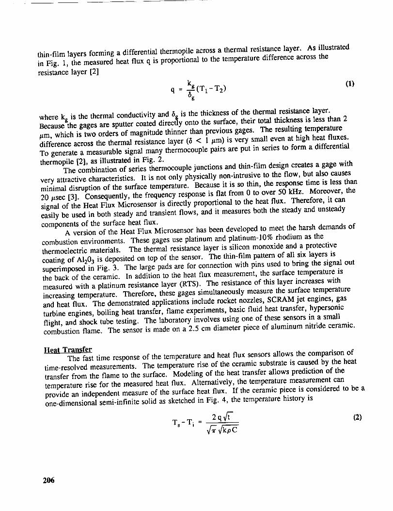
thin-film layers forming a differential thermopile across a thermal resistance layer. As illustrated
in Fig. 1, the measured heat flux q is proportional to the temperature difference across the
resistance layer [2]
kg (1)
q = _g(T1-T2)
where kg is the thermal conductivity and 6_ is the thickness of the thermal resistance layer.Because the gages are sputter coated direci_y onto the surface, their total thickness is less than 2
_m, which is two orders of magnitude thinner than previous gages. The resulting temperaturedifference across the thermal resistance layer (5 < 1 #m) is very small even at high heat fluxes.
To generate a measurable signal many thermocouple pairs are put in series to form a differential
thermopile [2], as illustrated in Fig. 2.The combination of series thermocouple junctions and thin-film design creates a gage with
very attractive characteristics. It is not only physically non-intrusive to the flow, but also causesminimal disruption of the surface temperature. Because it is so thin, the response time is less than
20 t_sec [3]. Consequently, the frequency response is flat from 0 to over 50 kHz. Moreover, the
signal of the Heat Flux Microsensor is directly proportional to the heat flux. Therefore, it can
easily be used in both steady and transient flows, and it measures both the steady and unsteady
components of the surface heat flux.A version of the Heat Flux Microsensor has been developed to meet the harsh demands of
combustion environments. These gages use platinum and platinum-10% rhodium as the
thermoelectric materials. The thermal resistance layer is silicon monoxide and a protective
coating of AI203 is deposited on top of the sensor. The thin-film pattern of all six layers is
superimposed in Fig. 3. The large pads are for connection with pins used to bring the signal outthe back of the ceramic. In addition to the heat flux measurement, the surface temperature is
measured with a platinum resistance layer (RTS). The resistance of this layer increases with
increasing temperature. Therefore, these gages simultaneously measure the surface temperature
and heat flux. The demonstrated applications include rocket nozzles, SCRAM jet engines, gas
turbine engines, boiling heat transfer, flame experiments, basic fluid heat transfer, hypersonic
flight, and shock tube testing. The laboratory involves using one of these sensors in a smallcombustion flame. The sensor is made on a 2.5 cm diameter piece of aluminum nitride ceramic.
Heat TransferThe fast time response of the temperature and heat flux sensors allows the comparison of
time-resolved measurements. The temperature rise of the ceramic substrate is caused by the heat
transfer from the flame to the surface. Modeling of the heat transfer allows prediction of the
temperature rise for the measured heat flux. Alternatively, the temperature measurement can
provide an independent measure of the surface heat flux. If the ceramic piece is considered to be aone-dimensional semi-infinite solid as sketched in Fig. 4, the temperature history is
Ts-T i -2q_- (2)
2O6

for a constant surface heat flux starting at time t=0. The values of the thermal conductivity (k),the density (p), and the specific heat (C) of the ceramic substrate are listed below.
k = 165 W/m.K
p = 3290 kg/m 3
C = 713 J/kg-Ko_ = 7.03 x 10 -5 m2/s
The surface temperature predicted by the semi-infinite solution is correct to within 1.0% for timesless than [4]
L 2t = 0.3 k (3)
ot
where ot is the thermal diffusivity and L the thickness of the substrate, which is 6.35 mm for the
given substrate. For times longer than given by eq. (3) the analytical solution loses accuracy.
Experimentally the temperature will rise faster than the semi-infinite solution predicts. For the
present case the effect should be small for times less than 1 second. A good additional assumption
is that the presence of the gage itself does not affect the substrate response of eq. (2).
The sensitivity of the Heat Flux Microsensor, S, is used to convert the voltage signal, E, toheat flux.
Eq = -- (4)
S
Calibrations give a gage sensitivity of S =23.2 mV/(W/cm 2) for the signal from the amplifier box
(at 1000X amplification). The equation to convert the RTS signal (at the 500X setting of theamplifier box) to temperature is
°C
T s = (132.33-.-Q-) E - 286.06°C(5)
Data Processin_
Equation (2) relates the temperature change of the surface of a material to a single step
change of the surface heat flux. Manipulation of this type of equation gives the temperature
response to a varying heat flux signal as a series solution [5]. This can be in the form of a series
of impulse functions as shown in Fig. 5. The solution for the temperature response to a varyingheat flux input is
Ts(tn)-Ti = 2 _lqj[_n-tj- V/tn-tj÷l lj--o
(o3
Note that this is similar to integrating the heat flux measurements.
207

In similar fashion the solution for determining the heat flux from a given set of surface
temperatures is [4]
q(tn)- _-_ "j=a ÷Jtn-q_,(7)
Note that this is similar to differentiating the surface temperature measurements.
Both of these expressions are in the form needed for digital signal processing. They have
been programmed on a computer disc for subsequent processing of the data. A listing of the
FORTRAN code is attached. By calculating the corresponding surface temperature response to the
measured heat flux and comparing with the experimental temperatures, additional confidence in the
measurements can be established. The data processing task is to do this and to quantify the
results.As an additional check of the program for data processing, a manual comparison can be
performed using eq. (2). Simply input an average heat flux over the time of the heated portion of
the test and compare the surface temperature rise with that calculated with the program. It should
be reasonably close.
Data AeauisitionThe LabVIEW software (a product of National Instruments) allows the student to formulate
an instrument in software. This instrument, referred to as a virtual instrument, incorporates the
data acquisition with drivers to support high speed AID boards, preprocessing algorithms, such as
digital filters, and post processing capability. The post processing for this experiment may include
the differentiation, or integration of the digital data. This software also provides data formats for
storage. Although the LabVIEW software is not required to perform this experiment, the iconified
format and the flexibility permit numerous variations in the experiment without extensive software
revision. This software is used extensively throughout the laboratory experience to promote the
concept of integrated data acquisition, signal conditioning, post-processing and graphical displays.
PROCEDURE
The flame is provided by a propane torch which is aimed directly at the heat flux gage, as
illustrated in Fig. 6. The torch has a self igniter which is activated by a button on the front. To
ignite the torch the gas is turned fully on by the knob on the back and then the button is pressed. "
After the flame is adjusted to the desired level the test is started by opening the shutter to allow the
flame to impinge on the heat flux gage. A chromel/alumel thermocouple is provided to measure
the flame temperature. An amplifier box is provided with the gage to boost the heat flux signal
and convert the resistance of the surface RTS to a voltage.
Safety ConsiderationsBecause the students are dealing with a high temperature flame test (1200°C), they need to
be reminded of a few safety factors.
208

.
.
.
Do not touch the upper part of the apparatus. When opening and closing the gate, leathergloves may be worn as added protection.
Do not leave the flame on for longer than necessary. Always turn it off between tests.
Because it does not have active cooling, the entire apparatus will become excessively hotwith only a few minutes continuous operation.
Do not run the flame on the gage for over a few seconds at a time. Leave the shutter
closed at all times except when actually taking data. This should keep the temperatureswell below 100°C.
Zeroing the Amplifier
After the amplifier is turned on and allowed to stabilize, both channels need to be zeroed.
Set the switch on the amplifier to the zero position. Connect the output from heat flux channel to
a voltmeter. Adjust the appropriate pot so that the output reads 0.0 V. Connect the output from
the RTS channel (surface temperature) to the voltmeter. Adjust the appropriate pot so that the
output reads 0.0 V. When the switch is flipped from zero to test, the output of the heat flux
channel should be 0.0 V, but there will be a DC offset of 2 or more volts on the temperature
channel. This reflects the resistance of the RTS at room temperature. Because the change in
resistance is only millivolts, this offset must be removed from the RTS output before being
processed by the computer to maximize the resolution of the A/D conversion. Therefore, a
differential amplifier should be used to remove 2 volts from the signal.
Building a Differential Amplifier
Construct the amplifier on the breadboard as illustrated in Fig. 7. An accurate reading of
Vin 1 (-2 V) should be taken by the voltmeter and recorded to be re-inserted into the computer.
Experimental Tests
Connect the heat flux and differential amplifier outputs directly into the interface box (A/D
board). Start the VI on the computer. Adjust the gain and offset for each channel (Hint:
Remember the 2 V that was measured and subtracted previously). Adjust Time Base, Interval and
Samples/channel accordingly. Record the values for Interval and Samples/channel for each test foruse in the FORTRAN code for data processing.
When ready to acquire data, light the propane torch. Immediately after pressing theAcquire Data button open the gate. Each test should last no more than 2 seconds. Save the data
and repeat the test until you have acquired at least five sets of data. Try to use varying flame
heights and conditions for each test. Observe the flame and make notes to explain the observedheat flux response.
209

Statistical Treatment of Data
For each test use the FORTRAN code to calculate the surface temperature and heat flux
values to compare with the corresponding measured values. Compute the residuals of themeasured and calculated data for both the heat flux and temperature responses. Plot the residuals
and perform a visual analysis. Discuss whether the data looks random or if there appears to be
some bias error present.Compute the mean and the standard deviation of the residuals. Perform a 95 % confidence
interval for the mean. Discuss results. Are the values different when computed for the first 1
second of the flame test than for the entire sampling period?
Given that the estimated uncertainty for heat flux is 0.05 W/era 2 and for temperature is
0.2°C, are the methods presented in this lab acceptable? Use the uncertainty to discuss your error,
and discuss which assumptions made in the calculations most likely lead to this error. Provide a
plot of the residuals and a tabulated summary of the statistical data.From the calculated values of the heat flux and surface temperature determine which is a
better approximation of the measured data. Discuss the advantages and disadvantages of each
method.
Sample Results
Each student should plot comparisons of their measured and calculated data versus time for
both temperature and heat flux and the resulting residuals from these comparisons. Sample results
are illustrated in Figures 8-11. Students are expected to complete a statistical analysis of their data
and present it in tabulated form as shown in Table 1 for the results in the figures.
Table 1 Statistical Results of Temperature and Heat Flux Residuals
Total Test Total Test
T s (°C) q (W/cm 2)
Mean 1.41 -2.69
Standard Deviation 1.80
-t-0.2595 % Confidence Interval
4.15
-t-0.59
First Second
of Flame
First Second
of Flame
T s (°C) q (W/cm 2)
0.25 -1.86
0.57 3.62
-t-0.16 +1.0
INSTRUCTOR NOTES
1. Care should be exercised once the test has been run several times because the Heat Flux
Microsensor housing becomes hot. Leather gloves can be worn as a precaution when opening and
closing the gate.2. Due to 60 Hz noise from surrounding equipment, a high sampling frequency should be
used on the LabVIEW software or an anti-aliasing filter should be used.
210

3. Results of the sample test are typical. The means of the residuals are close to zero
(based on the 95 % confidence intervals) only for the first second of the flame. The semi-infinite
assumption of the model breaks down for the four seconds of the test time. This is also evident in
the large increase of standard deviation of the temperature residuals going from the one second to
the four second time interval. Because of the small change in standard deviation of the heat flux
residuals, it can be concluded that the data set is ergodic and the residuals are obtained from the
sample population throughout the test period. This is not true for the temperature residuals.
4. The students should be able to identify that the calculation from the measured heat flux
to the surface temperature (an integration type process) is preferable to the temperature to heat flux
calculation (a differentiation type process).
REFERENCES
1. Diller, T. E., and Onishi, S.,"Heat Flux Gage," U.S. Patent No. 4,779,994, Issued 25 October1988.
2. Hager, J. M., Onishi, S., Langley, L. W., and Diller, T. E., "High Temperature Heat Flux
Measurements," AIAA Journal of Thermophysies and Heat Transfer, Vol. 7, 1993, pp. 531-534.
3. Hager, J. M., Simmons, S., Smith, D., Onishi, S., Langley, L. W., and Diller, T. E.,
"Experimental Performance of a Heat Flux Microsensor," ASME Journal of Turbomachinery,
Vol. 113, 1991, pp. 246-250.
4. Diller, T. E., "Advances in Heat Flux Measurement," Advances in Heat Transfer, Vol. 23,
1993, pp. 279-368.
5. Baker, K. I. and Diller, T. E., "Unsteady Surface Heat Flux and Temperature Measurements,"
ASME Paper No. 93-HT-33, 1993.
SOURCES OF SUPPLIES
1. Heat Flux Microsensor - $1500, Vatell Corp., Blacksburg, VA 24060, (703) 961-3576
2. Heat Flux Amplifier Box - $1500, Vatell Corp., Blacksburg, VA 24060
3. Thermocouple read out - $100, TEGAM, Madison, OH 44057, (216) 428-7505
4. BernzOmatic 2-piece Propane Torch Kit, Model TS 2000K - $18, WalMart
5. LabVIEW - $500 (Educational discount), National Instruments
6. Elenco bread board - $35, Radio Shack
7. Macintosh Quadra 700 computer - $4,000, Apple Computer
8. Texas Instruments 741 OP-AMP - $1, Radio Shack
211

qm Temperature
Sensors
TI - t' _ ____ThermalfB / _ Resistance
"1"2///////////////---SLtbst ra t e
Fig. 1 Measurement Concept of Heat Flux Microsensor
Lower UpperThermocouple Thermocouple
Thermalesistance
Series:tion
Lead
Connection
Fig. 2 Differential Thermopile
212

l i,em0e,.,u,o__. h.at,,ux
sensor _ _]_1 _ sensor
N/W _
1 mm
Fig. 3 Overlay Pattern of Heat Flux Microsensor
Thin Film [qTemperatureSensor_
f
_/ (semi Surfoce-infinite)
Fig. 4 Semi-Infinite Conduction Geometry
213

Alumi_m block
It
Heat Flux
q
t
Fig. 5 Impulse Representation of Heat Flux
$tlinlm
.E-
l
Fig. 6 Experimental Flame Apparatus
R1 R3100K 100K V = +/- 5V TO +/- 15V
v,o,o-/",/'__
100K
Vin 20__,,_ j I_ _p,46 ;,, _ Vout
100KVout=Vin2-Vinl
Fig. 7 Differential Amplifier
214

T_ (°C)
68
66
64
62
60
58
56
54
52
50
480
Measured
I I I I I I I
0.5 "1 1.5 2 2.5 3 3.5 4
Time (s)
Fig. 8 Measured and Calculated Temperature
T s (°C)
2
1
0
-1 i
0 0.5 1 1.5I I I I
2 2.5 3 3.5 4
Time (s)
Fig. 9 Temperature Residuals (Meas.-Calc.)
215

q (W/cm2)
3O
25
2O
15
10
5
0
-5
-!(]0
, _ii__.... !i,t i J ,, ,i d ,,j ii
_ ......_,,
, I
, q o,, ,, -- Measured'llt_t ,
_l I i, ,
'I": ' ' Calculated
i
,:_ it
,,,:J,ii _'' . ,',:',,:.1I'0- L * ' t_, t
.... 215 ' '0.5 1 1.5 2 3 3.5
Time (s)
Fig. 10 Measured and Calculated Heat Flux
10
q (W/cmb-5
I I I I I I I
"150 0.5 ! 1.5 2 2.5 3 3.5
Time (s)
Fig. 11 Heat Flux Residuals (Meas.-Calc.)
216

*****_*_***************************************************************
* This program converts the voltages obtained from the heat flux *
* sensor to their corresponding heat flux and temperature ** responses. It also utilizes the Cook and Felderman method to *
* differentiate temperature with respect to time to obtain the *
* corresponding heat flux and Green's function to integrate the *
* heat flux with respect to time to yield temperature. Variables ** used ,are: •
* K...thermal conductivity of resistance layer (W/cmK) *
* RHO...density of resistance layer (kg/cm^3) *
* CP...specific heat of resistance layer (J/kgK) *
* S...sensitivity of sensor (mV/W/cm^2) •
* ALPHA...thermalproperty of resistance layer ** TIME0...time interval *
* QVOLT0...voltage corresponding to measured heat flux *
* TVOLT0...voitage corresponding to measured temperature *
* QEXP0...heat flux calculated from experimental voltage *
* TEXP0...temperature calculated from experimental voltage *
* QCALC0...heat flux calculated from temperature ** TCALC()...temperature calculated from heal flux *
* TIMEF...number of data points taken **** • • _***** :,1¢_*****::# _***:,1.¢************ _**** _., ****** _*** _¢ _ _ _ _ _ _ _ _ _ _,.:1¢**** ,
REAL K, RHO, CP, S, ALPHA, TIME (201), QVOLT(201), TVOLT(201),+QEXP(201 ), TEXP(201), QCALC(201 ), TCALC(201)INTEGER TIMEF
PARAMETER (PI=3.141592654)
OPEN (9, FILE = 'RUN3.DAT')
OPEN (6, FILE = 'RUN3.OUT')
K=1.65
RHO=3.29E-3
CP=713S=23.1765
ALPHA=K/RHO/CP
TIMEF = 200
DO 1 I = I,TIMEF
READ (9, *) TIME(I), QVOLT(1), TVOLT(I)QEXP(I) = QVOLT(I)* 1000/S
217

TEXP(I)= 132.33*TVOLT(I)-286.06
1 CONTINUE
***********************************************************************
* Do loop to perform numerical expression dcvcloped by Cook and ** Felderman _ calculate heat flux _om sur_cctemperature *
DO 2 M = 1, TIMEF
QCALC(M) = 0DO3L=2, M
QCALC(M) = QCALC(M) + (TEXP(L) - TEXP(L-1))/(SQRT((M -L)*.02)
+ +SQRT((M-L+I)*.02))CONTINUE
QCALC(M) = 2.*SQRT(K*RHO*CP)/SQRT(PI)*QCALC(M)CONTINUE
* Do loop to perform method of Green's function to calculate *
* temperature from heat flux and write all previously calculated ** values to the output file created above *
520
DO 4 N = 1, TIMEF
TCALC(N) = TEXP(I)
DO5 J=N, l,-I
IF (J.EQ.I)THEN
TCALC(N) = TCALC(N) -2.*SQRT(ALPHA)/K/SQRT(PI)*QEXP(J)
+ *(SQRT(((N-.5)-(J-.5))*.02)-SQRT((N-.5)*.02))
ELSE
TCALC(N) = TCALC(N) -2.*SQRT(ALPHA)/K/SQRT(PI)*QEXP(J)
+ *(SQRT(((N-.5)-(J-.5))*.02)-SQRT(((N-.5)-(J- 1.5))*.02))ENDIF
CONTINUE
FORMAT (IX, F16.5, 2X, F16.5, 2X, F16.5, 2X, F12.8)
WRITE (6, 20) QEXP(N), TEXP(N), QCALC(N), TCALC(N)
CONTINUE
STOP
END
218

N94- 36408
MICROSCALE SYNTHESIS AND CHARACTERIZATIONOF POLYSTYRENE: NSF-POLYED
SCHOLARS PROJECT
Karen S. Quaal
Department of Chemistry
Siena College
Loudonville, New York 12211
Telephone 518-783-2977
and
Chang-Ning Wu
Department of Chemistry
University of Massachusetts-Dartmouth
North Dartmouth, Massachusetts 02747
219


Microscale Synthesis and Characterization of Polystyrene:NSF-POLYED SCHOLARS PROJECT
Karen S. QuaalDepartment of Chemistry
Siena CollegeLoudonville, NY 12211
Chang-Ning Wu
Department of ChemistryUniversity of Massachusetts-Dartmouth
North Dartmouth, MA 02747
KEY WORDS: Polystyrene, polymers, film-casting, molecular weightdetermination, film thickness determination.
PREREQUISITE KNOWLEDGE: The student should be familiar with the care
and handling of small amounts of hazardous materials and with simple laboratory techniquesnormally obtained in a first year chemistry course.
OBJECTIVES: To synthesize a polymer (polystyrene) using laboratory techniquestypically introduced in the first year chemistry course. In addition, the concepts of numberaverage molecular weight and weight average molecular weight in polymeric materials,polydispersity, methods of film casting, and film thickness determination are introduced.
EQUIPMENT AND SUPPLIES:
Polystyrene Synthesis:100 mL corn oil#
1 mL styrene
1-4 mg azobis(isobutyronitrile) commonly called AIBN
2 g Alumina Adsorption 80-200 mesh (Fisher Cat no. A540-500)50 mL methanolthermometer#250 mL beaker#50 mL beaker
2 small Teflon coated magnetic stir-barshot plate equipped with stirring rotor#small vacuum flask
small vacuum filter funnel10 X 75 mm test tubeslotted cork
3 Pasteur pipettes
Determination of Molecular Weight by Selective Precipitation (TLC):
Reverse phase thin layer chromatographic plate treated with indicator (Whatman 4803-425)Polystyrene standards (2K-100K)#polystyrene sample(s)5 capillary tubes1000 mL beaker
plastic rulerUV lamp#
50 mL graduated cylinder
PR6-_G P.AGE _LAJ',I_r_OT F'ILME_PA_E C7"-C7"U r_-E,- ,_, 221

100 mL stopper glass bottleBunsen burner
Film Casting:
0.5g Styrofoam2 mL chloroform or toluene1 mL of working solution composed of 40% dichloromethane and 60% diethyl ether
glass rodwatch glassNaC1 or KBr infrared plateMicrospatula or scalpelglass plate approximately 8 X 8 cm.
Film Thickness Determination:
polymer films of uniform thicknessInfrared Spectrophotometer or Spectrometer#
Quantities are estimated on a per student basis unless otherwise indicated# More than one student may share this equipment
INTRODUCTION: Polystyrene is a familiar polymer with many commercial uses.
Its applications range from the clear, high index of refraction, brittle plastic used to form audiocassette and CD cases to the foamed material used in insulated drink cups and packaging
material. Polystyrene constitutes 11% of the plastics used in packaging with only HighDensity Polyethylene (HDPE) and Low Density Polyethylene (LDPE) contributing a largershare (1). So much polystyrene is used today, it is one of six common plastics thatmanufacturers have assigned an identification code. The code helps recycling efforts.
Polystyrene's code is (PS code 6).
During the summer and fall of 1992 several new polymeric experiments were developed by theNSF POLYED Scholars for introduction into the chemistry core curriculum. In this
presentation one such project will be discussed.
This laboratory project is recommended for a first or second year laboratory course allowingthe introduction of polymeric science to undergraduates at the earliest opportunity. Thereliability of the experiments which make up this project and the recognition factor of
polystyrene, a material we come in contact with everyday, makes the synthesis andcharacterization of polystyrene a good choice for the introduction of polymerization toundergraduates. This laboratory project appeals to the varied interests of students enrolled inthe typical first year chemistry course and becomes an ideal way to introduce polymers to a
wide variety of science and engineering students.
In this sequence of experiments, students will:
a. Purify commercially available styrene by removing its inhibitor by small column
chromatography.b. Prepare polystyrene by using different amounts of inhibitors at constant temperature and
time.c. Determine the molecular weights of the synthesized polystyrene by Selective Precipitation
(TLC) using a calibration curve obtained from polystyrenes of known molecular weights.d. Prepare and evaluate polystyrene films formed by casting methods described below.
222

Procedures for the synthesis have appeared in the literature and several undergraduatelaboratory textbooks and manuals (2-5). However, the authors have found several problemswith these procedures. This modified procedure is introduced to improve the experiment andmake it more applicable to the lower level undergraduate laboratory curriculum.
First, the scale of many referenced procedures is such that students work with larger amountsof the hazardous material styrene than either of the authors felt was necessary. This is
consistent with current trends to adapt experiments to microscale in the interest of safety andcost reduction (4,6,7).
Second, the use of the reagent benzoyl peroxide as an initiator is considered too hazardous forlower level undergraduate laboratories. A suitable substitute is needed to lessen the risk.
Third, in order to accommodate the larger scale of the experiment reported in the literature, theinhibitors present in commercially available styrene are usually removed by distillation orextracted with sodium hydroxide prior to the formal laboratory time. Students lose thepedagogical opportunity to remove the inhibitors from their own sample and thus lose the
opportunity to understand its presence in the commercially available sample. The inhibitor,typically 10 to 15 parts per million of 4-tert-butylcatechol, is present to prevent the styrenefrom polymerizing in the bottle. The hazards of working with styrene are also minimized bythe microscale of this experiment. In addition, some procedures recommended using an excessof benzoyl peroxide to overwhelm the inhibitors present in the polystyrene. Given ourreluctance to use benzoyl peroxide, we were even more reluctant to use an excess. The authors
feel that the column method suggested by Williamson (4) has the advantages of being smallscale, rapid, and introduces chromatography as a method of purification.
Lastly, the time and temperature required for some of the procedures yield product in the formof a solidified glass plug of polystyrene. The formation of the plug shows the consequence ofextensive polymerization, but the solidified product is more difficult to characterize by theequipment available in the lower level undergraduate laboratory. The plug often needs to beremoved from the reaction test tube by wrapping the test tube in a cloth and shattering both thetest tube and the polystyrene plug with a hammer. In addition, the time needed for thepolystyrene plug to form uses too much valuable student and instructor time. Conditions are
needed that stop the synthesis short of solidification to allow characterization and make more
effective use of laboratory time. By purposely stopping the experiment before a solid plug ofpolystyrene is formed, the reaction yields a solution that is more easily manipulated than thesolid plug often seen in bulk polymerization of styrene. The viscous liquid that forms caneasily be transferred and precipitated. Precipitation of the polymer in methanol (a non-solvent)illustrates a common method of isolation and purification of a polymer. If a solid plug forms,the student should grind it with a mortar and pestle to obtain a dry powder.
Experience has shown us that the most successful laboratory synthesis experiments are thosecoupled with an additional goal besides the formation of the product itself. In this synthesis,an additional aspect of polymerization can be illustrated and the pedagogical function of the
experiment and the utility of the students' time are enhanced. For example, by using differentamounts of initiator in the synthesis, the effect of initiator on the yield can be investigated.Characterization of the polystyrene is accomplished by film casting and identification byinfrared spectroscopy.
In this experiment styrene is polymerized in the absence of solvent. Such a reaction is called a
bulk polymerization. The polymerization proceeds as a free radical polymerization of styreneinitiated by 2,2'-azobis-(2-methylpropionitrile), more commonly known asazobis(isobutyronitrile), AIBN.
223

n HC_CH2
AIBN
The value n is a function of the experimental conditions and will determine the molecular
weight of the resulting polymer. The molecular weight and polydispersity of a polymer greatlyaffect its physical properties and commercial applications. The molecular weight of smallmolecules is easily defined. The definition of molecular weight for pol_,mers is not as easilydefined because each polymeric chain constitutes a molecule and each chain can be of different
length. Definitions and methods of molecular weight determination used for small molecules
are not directly applicable to polymers.
Molecular Weights for polymers typically range from 5,000 to greater than 1,000,000.Students need to know how molecular weight differs for small and large molecules (polymers)to understand the effect that molecular weight has on the properties of all molecules. The
ability of polymer chains to exist in varying lengths gives rise to a distribution of molecularweights within a polymeric sample. Several types of molecular weights have been defined.Two of the more frequently encountered are the number-average molecular weight (Mn)
and the weight-average molecular weight (Mw). The number-average molecular
weight is defined as the total mass of polymer molecules divided by the total number of moles
of molecules present.
Mn= _niMi / ,_,ni (1)i i
Molecular weights of this type are typically obtained by methods involving effects on
colligative properties, GPC (gel permeation chromatography), and end group analysis.
Another definition of molecular weight is weight-average molecular weight which is
defined as:
Mw= _niMi 2 / ,_,niMi (2)i i
This value can be obtained by light scattering techniques. Due to the square of the Mi term,
this value is biased towards the contribution of the higher molecular weight chains.
The ratio of the number-average molecular weight and the weight-average molecular weight is
representative of the molecular weight distribution and is referred to as a sample's molecular
weight polydispersity.
Polydispersity = Mw/Mn (3)
This value is related to how broadly the chain lengths are distributed in the polymeric sample.
When Mw approaches Mn, their ratio approaches 1, and the sample approaches
monodispersity. Synthetic polymers exhibit varying degrees of polydispersity, with
22,4

vinyl polymerstypicallyhavingratiosfrom2-10. Manybiologicalmacromolecules(polymers)exhibitmonodispersity.Determinationof thepolydispersityof apolymericsampleis importantbecauseevensmallchangesinpolydispersitycanaffectthepropertiesof apolymericsample.
Molecularweightis oneof themostimportantcharacteristicsof apolymerandaspreviouslymentioned,is typicallydeterminedbyGPCor light scatteringtechniques.Eachof thesemethodsgivesmeaningfulmolecularweightsbut thesemethodsarenotaccessibleto mostlowerlevelundergraduatestudents.An alternativemethodfor determiningmolecularweightofpolystyrenehasbeenreportedusingSelectivePrecipitationbythin layerchromatography(TLC)(2,5,8,9). In theTLC procedures,polystyrenesamplesandstandards,overawide rangeofmolecularweights,arespottedonareversephaseTLC plateandelutedusingadichloromethane/methanolsolution.TheRf isrelatedto themolecularweightof thesample.Usingacalibrationcurveobtainedfromthepolystyrenestandards,themolecularweightof theunknownsampleis determined.
Thecouplingof apolystyrenesynthesiswithaTLC determinationwasreportedby Armstrong(2). Experiencehasuncoveredseveralproblemswith theseprocedures.First,variousproceduresreportthatthereproducibilityof thesemethodsis verysensitiveto theconditions.Yet eachprocedurerequiresslightlydifferentconditions.Second,thereversephaseTLCplatesareexpensiveandthecostperstudenttoohighfor somedepartments.Third,molecularweightsabove100,000give significantlypoorerresultsthanpolystyrenesamplesbetween2,000and 100,000.Manycommercialsamplesof polystyrenehavemolecularweightsabove100,000.Lastly,manypolystyrenesamplesarepolydispersedresulting,unfortunately,in adiffusespoton theTLC plate.Theindistinctnatureof thespotmakesit difficult to assignthe"center"anddeterminethemolecularweight.
Ourgoalsfor improvingthisprocedureincludedoptimizingconditions,developingamethodtorecycleanyreusableplates,anddetermininghowcloselytheresultsobtainedby TLCcorrespondwith themolecularweightdeterminedby GPCfor thesamepolystyrenesamples.In addition,amethodfor castingfilm fromthemicroscalesynthesisandassessingitsqualitywasdesired.
Theexperimentdiscussedin thispaperusesthin layerchromatographyto determinethemolecularweightof polystyrenesamplesobtainedfrom themicroscalebulk polymerizationsynthesis.Theseparationof polystyreneby molecularweightisdueto selectiveprecipitationof thepolymerfrom themobilephase.Themobilephasefor thiselutionconsistsofdichloromethaneandmethanol.Polystyreneis solublein dichloromethaneandinsolubleinmethanol.As thechromatogramdevelops,asolventgradientis establishedalongthelengthoftheplate. Thebottomof theplateisrich in thepolymersolublesolventdichloromethane.Asthechromatogramdevelops,theconcentrationof dichloromethanedecreasesandtherelativeconcentrationof thenon-solventmethanolincreases.Thelesssoluble,highpolymerweightfractionsprecipitatefirst, andasthesolventconcentrationchanges,thelowermolecularweightsprecipitateoutat variousRf's.
The developing chamber should be open to the air, away from drafts and without a wick toinsure non-equilibrium conditions while the TLC plate is developing. Considerable care mustbe used in preparing the eluting solvent because even small deviations from the suggested
concentrations alter the results. A fresh portion of eluting solvent must be used for each platebecause the relative concentration of the two solvents in the reservoir at the bottom of the
developing chamber changes during the developing process. A starting concentration of 71%dichloromethane/29% methanol (V/V) as reported by Armstrong (2) gives the best results.This concentration must be maintained to insure reproducibility. A more extensive applicationof this technique was applied to 47 different samples of polystyrene having molecular weights
225

between 2,000-100,000. Gel Permeation Chromatographic analysis of the same samplesshowed a correlation (96%) between the bottom of the TLC spot and the weight average
molecular weight determined by GPC. Additional correlation (85%) was observed for themidpoint of the TLC spot and the number average molecular weight. The poorer Mncorrelation is attributed to the difficulty determining the midpoint of a spot whose top may be
somewhat vague. A similar difficulty is not encountered when determining the bottom of the
TLC spot.
A polydispersity index for the polystyrene sample can be calculated based on the ratio ofMw/Mn determined by this method.
There has been much concern in the past over the reproducibility and the cost of this
experiment. The key to reproducibility is to keep the conditions as nearly identical as possiblefrom plate to plate. If care is taken, this experiment gives reliable results. One method tominimize variation is to divide a 10 cm X 10 cm reverse phase TLC plate into ten lanes of 1 cm
each. Assign the first five lanes to standards and the remaining five lanes to students (SeeFig. 1). This allows five students to have identical conditions and results in considerable cost
savings.
The ability to form films in high molecular weight compounds is one of the characteristicdifferences between high and low molecular weight compounds. Under similar conditions,
high molecular weight compounds form films where low molecular weight compounds formcrystalline deposits or oils. The quality of the films formed from polymeric material isproportional to the molecular weight. The formation of a high molecular weight polymer in areaction is often confirmed by the formation of a cohesive film. Films may be made by either
melt techniques or solution casting techniques (10,11). This procedure discusses two methodsof solution casting that are applicable to a wide variety of polymers, and is easily adaptable to
the undergraduate laboratory. Finding a suitable solvent is the most difficult part of thetechnique. A suitable solvent is volatile enough to evaporate in a reasonable amount of time butnot too volatile so that the film forms holes, bubbles or precipitates before the film formation is
complete.
Polystyrene is a glass at room temperature. A piece of clear brittle polystyrene produces sharpedges when broken. If the film is thick enough, it will appear brittle. When warmed in boilingwater, the glass transition temperature of 100°C is approached. At the glass transition
temperature, polystyrene undergoes a characteristic change from a glass to a flexiblethermoplastic. Above the glass transition temperature, T g, polymer chains have enough energy
to undergo conformational changes, resulting in a more tlexible polymer. Flexibility on themacroscopic scale is related to torsional mobility on the molecular level (10).
There are several options available in this experiment. The effect of initiator concentration on
yield and molecular weight distribution can be determined by running identical reactions usingthree different initiator concentrations. Each student can be assigned all three concentrations or
only one of the three variations. The class results are then pooled to determine the effects ofinitiator concentration on yield and molecular weight distribution.
226

PROCEDURE: Microscale Bulk Polymerization of Styrene
Safety Statements:
Styrene is a hazardous chemical with an unpleasant odor. Work in the hood at all times andavoid skin contact with this chemical. The flammability of this chemical should also berespected. There should be no open flames in the vicinity.
Waste Disposal:
All the alumina used to remove the inhibitors from the styrene should be placed in ajar labeled
styrene contaminated alumina. All organic solvents should be disposed of in properly labeledwaste containers.
Equilibration of Constant Temperature Bath:
1. Fill a 250 mL beaker 1/3 full with oil and place a magnetic stirring bar in the beaker.2. Heat the oil bath to 80°C on a hot plate equipped with a stirring rotor. In the interest oftime, the oil bath may be turned on and equilibrated prior to the beginning of the laboratoryperiod.
Preparation of Styrene: Removal of Inhibitors in Styrene
1. Prepare the mini-column by placing a small glass wool plug in the bottom of a Pasteurpipette and fill it one half full with alumina.
2. Place the mini-column in a hood and add styrene drop wise to the top of pipette. It takesabout 4 minutes to elute 2 mL of styrene. If it takes much longer than 4 minutes, the styrenemay be contaminated with some polymeric material and very little monomeric styrene will becollected in a reasonable amount of time. A new bottle of styrene should be substituted.
Preparation of Polystyrene:
3. Weigh 0.250 g of freshly eluted styrene and 1, 2 or 4 mg of the initiator, AIBN, in a 10 X75 mm test tube.
4. Cover the test tube(s) with a slotted cork.
5. Place the test tube(s) in the oil bath at the same time and record time and temperature.6. Remove the test tubes from the oil bath after 45 minutes.
7. Pour the reaction mixture, immediately after removal from the oil bath, into a beakercontaining 20 mL stirred methanol. A white precipitate should settle out.
7a. If the product is difficult to pour, add a small amount of toluene (-0.5 mL) to dissolve itand then pour as described in 7 into 40 mL of methanol.8. Continue to stir in methanol for another 10-20 minutes.
9. Vacuum filter the solid polymer and wash with methanol several times.10. Air dry the polymer or dry the polymer in a vacuum oven at room temperature untilconstant weight.
11. Weigh and save the polymer in a vial. Yields may be calculated on dried samples.
Plot % yield of polymer vs. mg of AIBN and note the effect of initiator concentration on theyield of polystyrene.
The polystyrene may be characterized by infrared spectroscopic identification of a film cast onglass, water, or a NaC1 or KBr plate and the molecular weight distribution may be determinedby selective precipitation (TLC) or GPC techniques.
227

PROCEDURE: Determination of Molecular Weight by SelectivePrecipitation
Safety Statements:Dichloromethaneand methanol are hazardous solvents. Avoid skin contact and breathing of
the vapor. Do not look directly at the UV lamp.
Waste Disposal:Dispose of all organic solvents in a properly labeled container. Dispose of all glass waste in a
properly labeled container.
1. Prepare 100 mL of 71:29 stock solution of dichloromethane/methanol by pipetting 71 mLof dichloromethane in a clean, dried stoppered bottle and adding 29 mL of methanol. Mix the
solution thoroughly and keep stoppered when not in use. This stock sQlution is enough for 2
separate slide developments, as 50 mL is needed for each.2. Using a pencil, very gently, without disturbing the adsorbent, draw a baseline across thewidth of the TLC plate, 1 cm from the bottom of the plate.3. Prepare a capillary spotter for each standard or sample that will be examined. Usingcapillary tubing, draw out the tubing into a fine narrow spotter using a Bunsen burner.4. Place the plate on a piece of wide ruled paper. This allows for easy visualization of laneson the TLC plate. If care is taken during the spotting procedure, 10 lanes can easily be run on
a 10 cm plate without risk of overlap. This allows for several permutations of standards andsamples on the same plate. Typically, 5-7 standards are needed for the calibration curve,leaving 3-5 lanes for samples to be analyzed. The standards and samples should havemolecular weights between 2,000 and 100,000 and be prepared by dissolving 5 mg of
polystyrene in approximately 1 mL of dichloromethane.5. Place a standard or sample spot 1 cm from the bottom of the plate in the center of a lane.Care should be taken to avoid overloading the plate at any one site. Check the standards and
sample spots with the UV lamp. Care should be taken not to overload the spot but make surethe spots can be clearly visualized under the UV lamp. As the spot develops, the material
spreads out and leaves a very diffuse spot after development.6. Place 50 mL of the stock solution in a clean and dry 1,000 mL beaker. This amount ofsolvent should be sufficient to cover the bottom of the 10 cm X 10 cm reverse phase TLC plate
without being above the spots. Place this beaker or an equivalent developing chamber in alocation free of drafts. Do not allow the solvent to sit too long in the developing chamber.
7. Place the TLC plate in the developing chamber gently. Lean the plate against the side ofthe beaker so that the plate only touches the beaker at the top and the bottom. Do not cover.8. Do not disturb the plate while it is developing. Remove the plate when the solvent comeswithin 5 mm of the top of the plate and gently mark the solvent front.9. Place the TLC plate under a UV lamp. Circle each spot with pencil and record the distancefrom the baseline to the bottom, the midpoint, and the top of each spot. (See Fig. 1).10. Determine the Rf of each of the recorded points for each spot by dividing the distance from
the baseline by the distance from the baseline that the solvent traveled.11. Plot log MW of each standard versus Rf for the bottom and the midpoint of each
corresponding spot. Obtain 2 calibration curves (See tables 1 and 2). The results of eachshould correlate best with a second power polynomial fit. If access to a curve fitting programis limited, a reasonable linear fit may be obtained using graphs of Log MW versus Rf bottom
and Rf midpoint.12. Using the calibration curves produced in step 11, determine the molecular weights of thebottom and midpoint for each of the unknown polystyrene samples.13. Under the conditions discussed above, the molecular weight derived from the bottom of a
spot correlates with the weight average molecular weight (Mw) for the sample. The molecular
228

weight derived from the midpoint of the spot correlates with the number average molecularweight (Mn) for the sample.
14. Calculate the polydispersity index for each sample by dividing Mw by Mn.
229

PROCEDURES: Film Casting
Safety Statements:The solvent used to cast the film is hazardous and the procedure should be carried out in the
hood.
Waste Disposal:Dispose of all organic waste in a properly labeled container.
Method 1. Traditional Film Casting on Glass
This method requires significantly more samples than methods 2 and 3 and may not be suitablefor small samples. The following procedure is adapted for a polystyrene sample.
1. Place approximately 0.5 g of pieces of polystyrene in a test tube and add 2 mL ofchloroform or toluene. Stir until completely dissolved.2. Pour the viscous solution near the edge of a glass plate. Spread the solution out by rolling
a glass rod or Pasteur pipette, whose edges have been wrapped in a layer of tape to allow for aspace between the rod and the glass plate, once across the surface of the solution in an effort toform a film of uniform thickness. Allow the solvent to slowly evaporate in the hood.
Complete drying may take overnight.3. Remove the film by lifting the edge of the film from the glass using a sharp instrument (a
knife, microspatula, or scalpel). If the film does not lift off the glass surface, the glass platemay be partially submerged in a pan of water and the film should float off the glass plate.Allow the film to air dry after excess water has been removed by gently patting with a paper
tissue.4. Examine the film and assess its quality. Does it appear uniform? Are there any
weaknesses or holes in the film? Is it flexible?5. The film may be mounted on a cardboard holder and its infrared spectrum obtained. If thefilm is uniform in thickness, then interference fringes will be evident and the film thickness
may be calibrated.
Method 2. Film Casting on Water
This method is applicable to small samples and limited to polymers which dissolve in solventsor mixtures of solvents that are immiscible and less dense than water. The following procedure
is adapted for a polystyrene sample.
1. Prepare a working solution by dissolving approximately 10 mg of the polystyrene samplein 1 mL of a 40% dichloromethane/60% diethyl ether (V/V) solution. Allow the polystyrene
sample to completely dissolve.2. Add a small amount of water to a clean watch glass to make a puddle approximately 5 cm
in diameter. As an alternative, half fill a small recrystallizing dish with water.3. Add the entire polystyrene solution dropwise to form a layer on top of the water.4. Observe the surface of the water closely. Almost immediately a film will begin to form.After several minutes the film should have set enough to allow for a qualitative evaluation of
the film. If it proves cohesive enough, gently remove the film from the surface of the waterand place on a paper towel to dry for 10 minutes. Using the alternative procedure, a glassmicroscope slide may be dipped under the fragile film in the recrystallizing dish, and raised at
an angle to aid in removal of the film from the surface of the water.5. Examine the film and assess its quality. Does it appear uniform? Are there any
weaknesses or holes in the film? Is it flexible?6. The film may be mounted on a cardboard holder and an infrared spectrum obtained.
230

Method 3. Film Cast Directly on Warm NaC1 or KBr Platen
This method is applicable to solutions of polymeric materials with low molecular weight whichdo not form quality films and for microscale samples.
This method usually yields the poorest quality films because the polymeric material often
precipitates on the plate prior to film formation. If this occurs, substitute a room temperature
salt plate to see if this improves the film quality. Fortunately, even if the film quality is poor,an infrared spectrum may be recorded and the material characterized by this method.
1. Dissolve the sample in an appropriate solvent.
2. Add the solution to the center of a NaC1 or KBr plate that has been warmed in a 60°C
oven. The solvent will flash evaporate leaving behind a film residue of the polymeric material.3. After the plate is dried, record the infrared spectrum.
PROCEDURE: Determination of the Thickness of a Polymer Film by theInterference Fringe Technique (12)
1. Place the polymer film in the sam]31e beam of an infrared instrument and record itsspectrum from 4000 cm-1 to 400 cm -1 .
2. Determine if any wavy interference pattern emerges in the spectrum. Such a patternemerges ONLY if the film is of uniform thickness.
3. Using the interference pattern, the thickness of the film can be calculated using thefollowing equation:
where:
d = Am/2n(v 1-v2) (4)
Am
Vl
v2
n
d = thickness of film in cm
- a whole number of complete fringe maxima(or minima) in the interval from u 1 to u2.
= frequency at which first maximum (or
minimum) occurs, in cm-1.
= frequency at which last maximum (or
minimum) occurs, in cm-1.= the index of refraction for the film.
INSTRUCTOR'S NOTES:
This sequence of experiments can be done in teams of two students.
Microscale Bulk Polymerization of Styrene
The mechanism of the free radical polymerization of styrene can be found in the section on
polymers and/or vinyl polymerization in any undergraduate organic chemistry text.
The AIBN and Styrene should be keep in the refrigerator when not in use.
The styrene contaminated alumina and pipettes should be placed in a beaker labeled styrenecontaminated alumina and pipettes and left in the hood until it can be disposed ofproperly as hazardous waste.
The synthetic experiment should be performed in the hood. Each student is only manipulatingone test tube and/or pipette column so that all students should be accommodated in the various
231

hoods. Styreneisextremelyflammableandtoxicsoencouragetheuseof gloveswhenhandlingthemonomer.Thepolymerdoesnotexhibitthesehealthhazards.Thedifferenceintoxicity betweenthemonomerandpolymerillustratejust oneof themanydifferencesbetweenthesetwo compounds.
Benzoylperoxideis traditionallyusedto initiatefreeradicalpolymerizationof styrene,but theexplosivehazardof thischemicalisconsideredtooriskyfor afirst yearexperiment.Thesubstitutionof AIBN provedacceptableandsignificantlylesshazardousfor undergraduates.
All reactionswererunwith andwithoutanitrogenpurge.Theyieldswithoutthenitrogenpurgewerehigherandwerebelievedto bedueto thelossof monomerduringthepurgingprocess.Thepresenceof oxygendoesnotseemto adverselyaffecttheoutcomeof thefreeradicalreactiononamicroscale,althougha smallinductionperiodis neededbeforeanypolymericmaterialcanbe isolated.
It is essentialtheoil bath(cornoil, cookingoil) beequilibratedbeforethebeginningof thelab.I providesettingsonvarioushotplatesthatshouldequilibratecloseto 80°C. If thetemperaturegoesmuchhigherthan80°C,thepolymerizationwill yieldasolidplugof polymer. Thismaterial,althoughpolystyrene,isnoteasilymanipulatedby equipmentavailableto first andsecondyearstudents.Theprecipitationof thepolymerin methanolisaclassicmethodforhandlingpolymericmaterial.Polystyreneis solublein tolueneanddichloromethanebutnot inmethanolor diethylether. If astudentdoesform apolystyreneplug(temperaturetoohigh orheatedtoolong)andit doesnoteasilyslideoutof thetesttube,try addingasmallamountoftolueneto dissolvethepolymer. If thatdoesnotwork, thentheonly methodopenedto themisto wrapthetesttubein atowelandcrack it openwith ahammer.Unfortunatelyit isoftendifficult to differentiatebetweenthesilicaglassof thetesttubeandtheorganicglassofpolystyrenewhenit is all commingledinpiecesonthepapertowel.
Onceprecipitated,thepolystyreneis filteredusingavacuumfiltrationsetup.Thewhitepowder (it doesnotprecipitateasatransparent,amorphousglass)ispolystyrene.Theyieldsareobtainedby weighingtheproduct.By combiningstudents'data,theclasscandetermineifthereis anycorrelationbetweentheamountof initiatorusedandtheyieldsobtained.If vacuumfiltration is notpossible,thengravityfiltration canbesubstituted.Thisreactionis achain-growthpolymerizationandassuchwill alwayshavemonomerpresentuntil polymerizationiscomplete.Thereforetheprecipitation,and,if possible,thefiltration (vacuumor gravity) shouldbedonein thehoodto minimizetheamountof styreneintroducedinto thelaboratory.
Further Extensions: Variation of yields and molecular weight distribution with temperature
may be investigated. The authors investigated 60 °, 70 ° and 80°C and found that 80°C gave the
highest yields.
Molecular Weight Determination by Selective Precipitation
The characterization by TLC is straightforward. The TLC is best run in the hood in a 1 Lbeaker that is clean. Soap residue interferes with the separation and gives uninterpretableresults. Once the students have obtained the Rfs of both the midpoints and the bottoms of all
spots they should plot the results using a plot program, if they have access to one, or usinggraph paper. A correlation coefficient of 1.0 was obtained for a second order polynomial fit,whereas correlation coefficients of .96-.99 were obtained for a linear fit of the same data (SeeTables 1 and 2). This method of determination of molecular weight of polystyrene is
applicable to all polystyrene samples whose molecular weight falls between 2,000-100,000.Samples whose molecular weight falls outside this window give significantly poorercorrelations with their corresponding GPC data.
232

From their results, students should be able to determine the Mn, Mw and the polydispersity of
their polystyrene sample. By combining students' data, the class can determine if there is anycorrelation between the amount of initiator used and the molecular weight obtained. As theconcentration of initiator increases, the yield of polystyrene should increase. More initiator
means more chains started. There should be a corresponding decrease in the molecular weightobtained. There is an inverse square root relationship between the molecular weight and theinitiator concentration. It is the authors' observations that students do not get precise enoughresults to support this mathematical relationship, but correlating trends are observed. Thephysical justification for this relationship lies in the frequency of termination steps. With moreinitiator present, more chains start, resulting in more chains termination steps, which causes theaverage molecular weight to stop increasing.
Recycling of the reverse phase TLC plates results in a significant cost reduction. Recycling canbe easily accomplished with only minor modifications in the procedure. These modifications
are time costly, as the student is required to spend more time using the UV lamp. Thelaboratory directors will determine which procedure best serves their needs. Reverse phaseTLC plates can be recycled by a method discussed in a separate procedure (13).
Film Casting
Another aspect of this experiment is to examine the relationship between molecular weight andfilm quality. Film formation is dependent on molecular weight. To form a film, polymerchains must be of sufficient length to have a large amount of chain entanglements. The longerthe chains (the higher the molecular weight) and more extensive the entanglements, the strongerthe film. For these samples, the students will see film formation on the surface of the water.
When they try to remove their samples they will find that the film is extremely fragile and maynot maintain its integrity. For comparison, samples of polystyrene made from packingpeanuts can be made in a similar manner. These films are normally stronger than the studentsamples because they are made from polystyrene of higher molecular weight. If a film can belifted from the surface of the water and placed on a paper towel to dry it can be suspended inthe infrared beam and a spectrum obtained. This spectrum should be identical to the
polystyrene film in the calibration strip including the distinctive 1601 cm -1 peak.
REFERENCES:
1. Modern Plastics, 1989, 66, 116.
2. Armstrong, D.W., Mark, J.N., Kyle, D., Alak, A., J. Chem. Educ. 1985, 62, p.705.3. Eaton, David C., Laboratory Investigations in Organic Chemistry, McGraw-Hill, NewYork, 1989.
4. Williamson, Kenneth L., Macroscale and Microscale Organic Experiments, D.C. Heath,Lexington, 1989, p. 635.
5. Laboratory Manual for Chemistry/Materials, Department of Chemistry, RensselaerPolytechnic Institute, Troy, NY 12180 Spring 1992.
6. Szafran, Z.; Pike, R.M.; Singh, M.M.; Microinorganic Chemistry, John Wiley And SonsInc., New York, 1991.
7. Mills,J.L.; Hampton, M.D.; Microscale and Macroscale Experiments for GeneralChemistry, McGraw-Hill Inc., New York, 1991.
8. Armstrong, D.W.; Bui, K.H.; Analytical Chemistry, 1982, 54, p.706.9. Droske, John P., "Determination of the Molecular Weight of Polystyrene by Fractionationon a Reversed-Phase TLC Plate", Procedure for Polymer Class 475, University of Wisconsin-Stevens Point, Department of Chemistry, Stevens Point, WI 54481.
10. Allcock, Harry R.; Lampe, Frederick W.;Contemporary Polymer Chemistry, EnglewoodCliffs, Prentice-Hall 1981.
233

11. Droske, John P., Polymer Chemistry Demonstration and Experiments Workshop,POLYED National Information Center for Polymer Education. Department of Chemistry,
University of Wisconsin-Stevens Point, 54481.12. Hannah, R.W., and Swinehart, J.S., Experiments in Techniques of Infrared
Spectroscopy, Norwalk, Perkin-Elmer Corporation, 1974.13. Determination of Molecular Weight by Thin Layer Chromatography (Selective
Precipitation). Modified for recycling of TLC Plates. Integrating Polymers into CoreChemistry Courses: A Sourcebook, POLYED National Information Center for PolymerEducation. Department of Chemistry, University of Wisconsin-Stevens Point, 54481.
234

I
Ruler ------._-
_0
, 2131415167 8 9110Figure I. Reverse Phase TLC plate on top of wide ruled paper. The paperserves as a guide for sample lanes. Rf is calculated by dividing the distancetravelled by the spot by the distance travelled by the solvent front.
distance from baseline
to solvent front.
top
midpoint
bottom
t
I
ent front
I
B
f
P
baselineI
distance from baselineto midpoint.
I
235
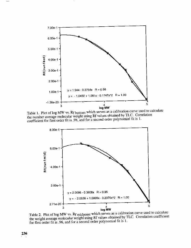
7.00e-1
6.00e-1
5.00e-1
o 4.00e-1rn
& 3.00a-1
2.00e-1
1.00e-1
y = - 1.0432 + 1.081x - 0.1747x^2 R = 1.00
-1.36e-20 t4 5
3 log MW
Table 1. Plot of log MW vs. Rf bottom which serves as a calibration curve used to calculate
the number average molecular weight using Rf values obtained by TLC. Correlation
coefficient for first order fit is .98, and for a second order polynomial fit is 1.
A
.m
E
IK
8.00e-1
6.00e-1
4.00e-1 _
2.00e-1
2.71e-20
y = - 2.0538 + 1.5999x - 0.2376x^2 R = 1.00
I
4 53 log MW
Table 2. Plot of log MW vs. Rf midpoint which serves as a calibration curve used to calculate
the weight average molecular weight using Rf values obtained by TLC. Correlation coefficientfor first order fit is .96, and for a second order polynomial fit is 1.
236
ACKNOWLEDGMENTS:
These experiments were prepared as part of the NSF-POLYED Scholars Program. Thiscollaborative effort involves the following individuals working at three regional sites:
University of Wisconsin-Stevens Poin!
John P. Droske, UWSP, Project Director
Jerry P. Jasinski a, Keene State College, NH
Joe Young b, Chicago State University
Rensselaer Polytechnic InstituteGary Wnek, RPI Site Director
Karen S. Quaa| a,b, Siena College
Chang-Ning Wu a,b, UMass-Dartmouth
University of Southern MississippiLon Mathias, USM Site Director
T. Carter Gilmer a, Univ. of Michigan-DearbornGuy Mattson b, Univ. of Central Florida
E. Ann Nalley a,b, Cameron University, OK
a: NSF-POLYED Scholar 1993, b: NSF-POLYED Scholar 1992
The helpfulness of the following individuals is gratefully acknowledged:
Jean Strong at UWSP, Beth McGraw at RPI and Janet Lewis at USM for secretarial support.S. Czysz, Jason Waldkrich, S. Baird, T. Maeder, J. Opsteen, Russ Cartwright, StephanieFrederick, Chris Peterson, C. Roberts, G. Tullos-student assistants at the three sites;
and S. Krause (RPI) and Paul Hladky (UWSP) and the members of the advisory panel fortheir helpfulness.
The project was supported by the National Science Foundation Division of UndergraduateEducation Grant DUE#91-50497 and 92-54351 and by POLYED, the joint polymer educationcommittee of the ACS Polymer Divisions.
237


CRATER CRACKING IN ALUMINUM WELDS
R. Carlisle Smith
Department of Welding Technology
West Virginia University, Parkersburg Campus
Parkersburg, West Virginia 26101
Telephone 304-342-6127
PAGE _[,.Atil< NOT FILMED239
Carlisle Smith
West Virginia UniversityParkersburg Campus
ORIGINAL PAGE
BLACK AND WHITE PHOTOGRAPH
240

CRATER CRACKING IN ALUMINUM WELDS
R. Carlisle (Carl) Smith
Department of Welding Technology
West Virginia University, Parkersburg Campus
Parkersburg, West Virginia 26101SPONSOR
Kanawha Manufacturing Company
Charleston, West Virginia 25311
KEY WORDS: Crater, crater crack, spider cracks, hot crack
propagation, capillary action, strain hardening, hot short, %6 Temper, dyepenetrant, non-aqueous, heattreatable, dwell time.
PREREQUISITE KNOWLEDGE: The students should have a
definitive knowledge of capillary action. The understanding of the non-
ferrous characteristics of aluminum will be helpful.
OBJECTIVES: To observe the importance of non-destructive testingeven after visual examination. To determine the extent of damage which canbe caused by crater cracking.
EQUIPMENT AND SUPPLIES:
(1) Safety glasses, gloves and a vapor mask should be worn.(2) Fractured aluminum material.
(3) Solvent cleaner. (Aerosol or liquid).
(4) Fluorescent Penetrant. (Aerosol or liquid).
(5) Developer (non-aqueous or powder).
(6) Lint free cloths or paper towels.
(7) Black light.
(8) Three acid swabs. (Brush type is preferred).NOTE: A tee joint with fillet welds on both sides is the most desirable
configuration.
241

INTRODUCTION: The non-heattreatable alloys, which are cold
work tempered, are much less difficult to weld than the heattreatable alloys.
Alcoa classifies weldability beginning with "A" as the easiest to "D" the r_ost
difficult. The 6061-T6 alloys rate a "D".
PREPARATION FOR WELDING: All aluminum alloys require
removal of oxidation. A mix of hydrofluoric or hydrochloric acid with nitric
acid and water works very satisfactorily. This should be applied at 70 ° to
80 ° F and followed by a thorough rinse. A 5% sodium hydroxide solution
may also be used and followed by a thorough coldwater rinse. A simplevolt OHM meter may be used to determine whether the part is cleaned
sufficiently. A high resistance reading will indicate a need for more
cleaning.
PERFORMING THE FIRST SIDE WELD: A wire such as
ER 5356 may be used to weld the first side which should be a good weld for
proving our point. The proper amps and volts should be used. The travel
speed should be sufficient to fill the joint on the first side to obtain a. 1875"throat depth. A pause at the terminal point of the weld will fill the crater and
assure a gas shield. Preheat to 350 ° F and slow cool.
PERFORMING THE SECOND SIDE WELD: Since we want the
second side weld to fail, the procedure will be changed to cause the failure.
The precleaning is still a must since an arc cannot be established through a
heavy aluminum oxide film. The elimination of preheat will cause thematerial to receive a thermal shock. The second error to be made is to
increase the amperage and voltage to about 30% above the recommended
parameters. The travel speed will be varied to cause uneven heatdistribution in the base material. The sure fire killer will be provided by a
sudden stop and immediate withdrawal of the welding gun from the weld.
This assures that a crater will form and no gas shield will be in place to
protect the molten, cratered weld pool. The crack may or may not be visible
to the eye, but a quick penetrant examination will reveal the spider like
fracture.
242

EXPERIMENT:
PERFORMANCE OF THE DYE PENETRANTEXAMINATION:
STEP 1:
STEP 2:
STEP 3:
Preclean the complete specimen using solvent type, rapid
evaporating solvent. Aerosol is faster than plain liquid.
Using the acid swab brush, apply a heavy coat of fluorescent
penetrant covering the welds on both sides.
Allow a 7 to 10 minute dwell time.
STEP 4:
STEP 5:
Spray the solvent cleaner on a lint free cloth or paper towel and
remove all the excess penetrant. Do not spray directly on the
part to be examined. This will wash out the penetrant.
Apply the developer.
STEP 6: Allow a 7 to 10 minute dwell time.
STEP 7: Turn on the black light and observe the results.
SUMMARY: The black light should show that even though the first
side was welded correctly, the propagation has carried the crack from the
correctly welded side through to the side that contained the crater.
The student should be made aware that although a failure was depicted in
the base material and the weld, aluminum is still a very good weldable
material. Any material that is fabricated improperly may fail. Proper
procedures are necessary even for the most simplistic forms of metalprocessing.
SAFETY PRECAUTIONS: Nearly all good penetrant products are
flammable. They should not be used on materials hotter than 120 ° F. No
fires or flames should be allowed in the area of use. The vapors are not
extremely toxic but prolonged exposure to the products can be harmful.
Contact with eyes and skin should be minimized, if not avoidable. Flushing
243

with water and soap will remove the product from skin. A thorough waterflush should be used for eye washing. If swallowed, do not induce vomiting.
See a physician as soon as possible. Keep all penetrant products in cool
storage (around 70 ° F) and away from possible fires. Secure the cabinet to
prohibit "sniffing" by those persons who indulge in such practices.
244
BRIDGMAN SOLIDIFICATION EXPERIMENTTO ASSESS BOUNDARIES AND INTERFACE SHAPE
Jonathan H. Fisher
and
Glenn A. Shelby
Science and Engineering Group
Nichols Research Corporation
4040 South Memorial ParkwayP. O. Box 400002
Huntsville, Alabama 35815-1502
Telephone 205-883-1170 extension 1381
and
Lawrence R. Holland
Department of Physics
Alabama A&M University
Normal, Alabama 35762
Telephone 205-851-5313
245

Jonathan FisherNichols Research Corporation
I
ORVQINAL PAGE
BLACK AND WHITE PHOTOGRAP[",
2,46

Bridgman Solidification Experiment to Assess Boundaries and Interface Shape
Jonathan H. Fisher
Glenn A. ShelbyScience and Engineering GroupNichols Research Corporation
Huntsville, Alabama 35815-1502
Lawrence R. Holland
Department of PhysicsAlabama A&M UniversityNormal, Alabama 35762
KEYWORDS: Bridgman solidification, solid-liquid interface shape, directional
solidification, thermal conductivity, crucible, II-VI semiconductors, III-V semiconductors, IV
semiconductors, and melt growth.
PREREQUISITE KNOWLEDGE: The student should understand the
fundamentals of thermal transport phenomena and the fundamentals of solidification processes,
specifically directional and Bridgman solidification. This material would typically be covered
during a materials science course, an introduction to solidification processes course,
introduction to metallurgy, or crystal growth techniques course. The growth interface shape
and its relationship to thermophysical properties is the key part of the experiment. [Ref. 1]
OBJECTIVES: To understand the basics of Bridgman-Stockberger solidification
using an experimental model that is directly related to II-VI, III-V, and IV semiconductors melt
growth like Mercury Cadmium Telluride, Silicon or other similar materials. To observe and
understand the interface shape and its relationship to thermal transport and thermophysical
properties of the solid, liquid, and crucible materials. NOTE: This lab can be taught at various
levels of understanding. The following will simply discuss interface shape models,
specifically the Holland effect. The Holland effect relates the solid-liquid (or melt) interface to
the thermal conductivity of the solid and liquid (see equation 2). Other topics such as solid
interface growth rate and temperature profile within solid - liquid during solidification will be
addressed.
EQUIPMENT AND SUPPLIES: [Ref. 2]
(1) P'lexiglas crucible (25 mm inner diamter (ID) approximately 600 mm in length)
(2) Aluminum or alloy cold finger (25 mm ID that fits into the Plexiglas crucible)
(3) Liquid Nitrogen dewar (20 liter) or other cryogenic source
247

(4) Styrofoamdewar-coldfingeradapter27/16"outerdiameter(O).Anythingthatwouldsecurethecoldfingerin thedewarwouldbeacceptable
(5) De-ionizedwater(6) Aluminumweldingrod-optional(3.175mmor 1/8")
(7) A meterstickor othermeasuringdevice
(8) Stopwatch
INTRODUCTION: Thethermalconditionsin Bridgman-Stockberger(denoted
Bridgmanfor theremainderof thepaper)growthsolidificationconfigurationscanbeusedto
understandtheinterfaceshapebetweenthesolid,liquid, andcruciblewall. Thetheory
proposedbyHollandcanbeusedto definethesolid-liquidinterfaceshape.[Ref.1] The
Bridgmangrowthcanbemodeledusingthesolidificationof water. For goodcrystallinity,a
convexcrystalfaceis requiredasshowbythesolidificationof lead. Holland'stheorymaybeusedto understandtheproblemsof II-VI, Ill-V, andIV semiconductorcrystalgrowthwhose
interfacepropagateswith aconcaveshape.
Bridgman Solidification System Boundary Conditions: A typical Bridgman
solidification system is illustrated in Figure 1. Bridgman solidification is directional crystal
growth where the loaded crucible moves in the direction from the hot zone into the cold zone
where the melt or liquid solidifies. The hot and cold zones are quasi-static for slow
solidification. The crucible moves through the stationary furnace at a predefined velocity that
defines the growth or solidification rate. A thermal resistance is encountered as the heat flux
propagates into the cold zone due to the change in thermal conductivity as illustrated in Figure 1.
Tile corresponding heat flow diverges outward through tile walls of the crucible. When the
heat flux diverges, the surfaces of constant temperature isotherms must curve up at the edges.
The growth face occurs at the freezing temperature isotherm. It should be noted that crystal
growth propagates perpendicular to the isotherm representing the solidification
temperature[Ref. 3]. The crucible walls form a thermal "short circuit" in the system.
The thermal flux and thermal gradient can be used to explain this phenomenon in a
more quantitative way. The thermal flux and thermal gradient boundary conditions at
boundaries 1, 2, and 3 (from Figure 1) can be used to define the ruling relationship. Within
the crucible wall, sufficiently close to the melt solid interface, the thermal gradients obey (the
subscripts m and s refer to the melt and solid phase of the load):
(_-_-Tz)m = (_-_Tz) s (1)
248

Thez-componentof thethermalflux, thethermalconductivity(k) timesthethermalgradient,atthesolid-meltinterfaceobeys:
/ = k(C3T]km7) m s \O-z-/s (2)
Both equations ] and 2 are valid only if either km=ks or _T/Oz = 0 in both media. We know
that km is not equal to ks. So, if kin is greater than ks, then at the fine of contact of the melt-
solid interface with the crucible the heat flux is strictly horizontal, into the crucible wall (0=0%
Similarly, if km is less than ks, as the case with a metal, then the interface turns down at the
edge, and 0=I 80 °.
Bridgman Model
Z
Hot Zone
Solid
Crucible Wall
Melt
Solid
I
i:_iiii!iiiiiiii_._:_:_:,iii!iii_ Crucible
Cold Zone
Figure l. Steady State Bridgman Model Schematic
249

PROCEDURE:
Safety considerations:
1. Explain the precautions of the use of nitrogen to the student.
have proper ventilation.
The laboratory should
Sample Preparation: This can be a class demonstration or done by each laboratory
team (i.e., you are probably equipment limited).
1. Insert the cold finger into the dewar adapter. [Note: Fabrication drawings for the
aluminum cold finger, dewar adapter, and crucible assembly can be obtained from author.]
2. Slip the transparent crucible over the cold finger until it fits over the o-ring. Note:
the meter stick does not need to be affixed to the crucible.
3. Fill the crucible with de-ionized water.
4. Insert the cold finger, crucible, and adapter assembly into the LN2 dewar or other
available cryogenic source. Note the starting time in the sample data sheets.
5. Upon solidification of the water note the morphology of the ice. Take
measurements of the ice growth length each minute after the ice has fully solidified past the
cold finger. Notice the interface shape at the wall of the crucible. Does the ice grow with a
concave or convex interface? Predict whether liquid water has a larger thermal conductivity
than solid water. Does the solid or liquid have a greater density? Does a relationship exist
between the density and the thermal conductivity of the solid and melt material? Consider the
packing fractions for the different states of matter.
6. [Optional] Insert an aluminum or other metallic rod into the crucible after the ice has
solidified past the cold finger. Let the rod rest on the ice. What happens at the point of contact
between the metallic rod and ice? Again, notice the interface shape as the water solidifies up
the metallic rod. Again, predict whether liquid water has a larger thermal conductivity than
solid water. Does this result agree with the conclusion from step 5.
7. The experiment or demonstration should last at least 30 minutes. Stop the
experiment. Remove the cold finger, crucible, and adapter assembly from the LN2 dewar.
Cap the LN2 dewar.
8. Complete the data sheet. Was the growth rate constant, increasing or decreasing?
SAMPLE DATA SHEETS: Each student should answer all questions given in the
sample preparation steps and complete the following data sheet. The growth rate as a function
of time should be plotted.
250

Start time:
Elapsed Time for first solidification:
Elapsed Time Solid Zone Length Growth Rate
(seconds) (cm) (cm/sec)
60
120
180
240
Observations
300
360
420
480
540
600
660
720
780
840
900
960
1020
1080
1140
1200
1260
1320
1380
1440
1500
1560
1620
1680
1740
1800
Does the ice grow with a concave or convex interface?
The thermal conductivity of the liquid water is less than or greater than the thermal
conductivity of the solid water. Explain your answer.
Predict the growth interface shape assuming the thermal conductivity of the liquid opposite to
the observed shape.
251

How does the thermal conductivity of the crucible wall matter to this solidification process?
Was the growth rate constant, increasing or decreasing?
INSTRUCTOR NOTES:
1. The laboratory instructor should review reference 1. The derivations for equations 1
and 2 are described in this article.
2. The most important lesson from this laboratory is the relationship between interface
shape and the thermophysical properties of the solidifying material. Advanced undergraduates
or graduate students should relate the growth kinetics to theoretical predictions. Much of the
background material for this can be found in references 1 and 3.
3. Other experiments such as that first performed by Azouni [Ref. 2] can be done to
understand the phenomena of convection in solidification systems. The Azouni experiment
requires a multi-channel (16) temperature measurement capability.
REFERENCES:1. Holland, L.R., Crucible Surface, Thermal Refraction, Boundaries, and Interface
Shape in Melt Growth, Journal of Crystal Growth 96 (1989) 577-583.
2. Azouni, M.A., Helical Impurity Distribution Produced By a Hydrodynamic
Instability, Journal of Crystal Growth 42 (1977) 405-410.
3. Kurz, W. and Fisher, D. J., Fundamentals of Solidification, 3rd. ed., Trans Tech
Publications, 1989.
SOURCES OF SUPPLY: The plexiglass crucible will have to be purchased from
your local plastics retailer. The plexiglass tube should cost less than $10.00 or you may obtain
for free as remnant stock. The 1 inch cylindrical Aluminum stock can be obtained and
fabricated by your department machine shop. A nitrogen dewar can be found in most Physics
departments. The styrofoam adapter can be cut into form using a lathe and knife (or simply cut
it into shape) from commonly available packing block material. The de-ionized water may be
obtained from the Chemistry department.
252

PREPARATION OF SIMPLE PLASTER MOLDFOR SLIP CASTING
T.G. Davidson
and
L.A. Ketron
Ceramic Engineering TechnologyHocking Technical College
3301 Hocking ParkwayNelsonville, Ohio 45764-9704
Telephone 614-753-3591 ext. 2653
253


HockingCollege
PREPARATION OF
SIMPLE PLASTER MOLD
FOR SLIP CASTING
T.G. Davidson and L. A. Ketron
Ceramic Engineering Technology
Hocking Technical CollegeNelsonville, OH 45764
KEY WORDS: model
plaster mold
parting agent
simple moldcottle
slake
working mold
gypsum
ABSTRACT:
The manufacture of permeable gypsum molds is an importantphase of the slip casting process, a process which can
economically produce complex shapes. Controlling the watercontent during the preparation of the mold can affect its
porosity, which in turn affects the strength and wearresistance of the mold, casting rate, and ability to transfer
detail. This demonstration of making a simple plaster mold
involves setting the cottle and model, mixing the plaster, andpouring the plaster.
PREREQUISITES: Ability to weigh out raw material.
Ability to operate a power mixer.Ability to slake.
OBJECTIVES:
1. Define keywords2. Build a cottle.
3. Produce a simple plaster mold.
MATERIALS: U.S. #i pottery plaster
20oz. styrofoam cup
parting agent (mold soap)
water clay
EQUIPMENT:
safety glasses carpenter's squarepower mixer . two 5-gal. buckets
dowel rod modeling claycottle boards with angle irons
wedges
paint brush
rasp
255

INTRODUCTION:
Many sophisticated methods of manufacturing have beenintroduced into the ceramics industry, yet complex shapes of
products can still be done economically only by slip casting.
Slip casting requires a mold which is highly permeable to drawexcess water from a liquid clay slurry and leave behind a
rigid clay piece which is subsequently fired. This water
permeability is a function of the number, size and shape of
the pores in the mold material. A second requisite is that themold material be easily worked, or tooled, into the desired
shape.
Gypsum plaster best fulfills these requirements. Naturally
occurring raw material gypsum (CaSO 2" H20) can _e heated to a
high temperature to yield a materia_ containing less water of
hydration. This dehydrated material is called plaster of
Paris (CaSO 4 72 H20) and is the starting ingredient formaking molds_ It is mixed with water forming a creamy slurry
which can be easily shaped by casting. The plaster of Paris
dissolves in the water and gypsum nucleates and grows from
solution. Only 18.6 pounds of water are required for chemical
hydration of 100 pounds of plaster, but excess water is
required to allow one to work the mixture. Upon drying, theexcess water above that required for crystallization is
evaporated away leaving behind interconnected pores. Theseinterconnected pores, some of which are open at the surfacesof the mold, create the necessary sponge-like microstructure
needed for slip casting.
The manufacture of gypsum molds is an important phase of
production, and preparing complicated molds is a highly
skilled process. Preparation of a complicated mold involves
preparing four types of molds: 1) model; 2) block; 3) case
mold; and 4) working mold. The model usually has largerdimensions than the final product to allow for shrinkage which
occurs during drying and firing. The block mold is a negative
of the model. The case mold is composed of several
interlocking pieces formed by casting plaster around the block
mold. The working mold is actually used for slip casting the
product. The block and case molds are made from harder and
stronger gypsum materials to minimize wear and cracking.
Gypsum plaster molds are not strong and have a limited life;
therefore, a plaster shop maintains a steady production of
molds.
This lab will involve producing a simple working mold
directly from the model. A simple mold consists of only one
part. A complex mold has two or more parts.
256

PROCEDURE:
A. Calculation of Material Amounts
i. Volume of cottle (V=):
V= = length x width x height
2. Volume of styrofoam cup (Vm):
V = (h_7/3) (R12 + RIR 2 + R22)
3. Volume of plaster mold (Vp) required:
•
Vp = V c - Vm
Amount of plaster (P) required is calculated by
multiplying the plaster mold volume (Vp) by the
density of the plaster (D). The density of the U.S.
#i pottery plaster is 20 g/in 3.
P = V x DP
5. Amount of water (w):
The water to plaster ratio is commonly between
i: 1 3/e and I: 1 i/2 .
w 1 w 1
--- = or --- =
P 1 3/s P I I/2
B• Making simple mold
i. Set up cottle by positioning boards using wedges to
secure the proper dimensions.
2. Use clay to seal (caulk) the cottle sides and bottom•
3. Fill model with clay to maintain shape and keep fromfloating.
4. Coat cottle and model with parting agent•
5. Position model in cottle with widest end on table top.
6. Weigh out plaster amount (P).
7. Weigh out water amount (w) separately.
8. Slake the plaster into the water by forming a cone
which allows the air to escape. This process ought totake about two minutes.
NOTE: Plaster set-up time is about six minutes total.
•
I0.
ii.
Mix with a power mixer for 1.5 to 2 minutes. WASH the
mixer blade immediately.
Insert hand into mixture to check for lumps andrelease air bubbles.
Watch for waves to form as you hand mix. This wave
formation indicates plaster is setting up.
257

NOTE: If you pour too soon, plaster will settle out of
the water and the mold will be more dense at the top.
12. Pour plaster into the cottle along its side. Pour
enough to cover model. Use dowel rod to keep model in
place.13. Gently shake cottle to release air (rock table). Air
bubbles are the enemy of the mold maker.
14. Set for forty (40) minutes.
15. Remove model and wash mold.
16. Use rasp to plane bottom of plaster mold if it is
uneven.
INSTRUCTOR COMMENTS:* Boards nailed together could be used as a cottle.
* New plaster sets up faster, therefore one may need todecrease the time of mixing with the power mixer and
by hand.* To allow for set-up time (in a limited laboratory
period) may start students making for which the
amounts are previously calculated and given to the
students. While the mold sets then show the students
how to calculate the amount of gypsum and water
needed.
* May divide class into two groups:
a) prepare cottle
b) weigh materials
* Density varies with ratio of water and the type of
plaster.* Use a three (3) inch blade on the power mixer.
REFERENCES:
i. "The Gypsum Mold", Ceramics and Glasses, Engineered
Materials Handbook, Vol.4, S.J. Schneider, Jr., ed.;
ASM: 1991; pp. 157-158.2. F.H. Norton, Elements of Ceramics, 2nd ed.,
Addison-Wesley Pub. Co., 1970, pp.99-100.
3. W. Ryan, Properties of Ceramic Raw Materials, Peramon
Press, 1978, pp.99-100.
258

SLIP CASTING
T.G. Davidson
and
L.A. Ketron
Ceramic Engineering TechnologyHocking Technical College
3301 Hocking ParkwayNelsonville, Ohio 45764-9704
Telephone 614-753-3591 ext. 2653
259

Lisa Ketron
Hocking Technical College
260

HockingCollege
SLIP CASTING
T.G. Davidson and L. A. Ketron
Ceramic Engineering Technology
Hocking Technical CollegeNelsonville, OH 45764
KEY WORDS: drain casting
solid castingreservoir
slip castingdeflocculants
working moldsimple mold
complex mold
electrolytes
ABSTRACT:
The production of highly complex shapes can be
accomplished by slip casting. A slip is a suspension of
colloidal powders in an immiscible liquid (usually water).Slip casting entails pumping or pouring the slip into a
permeable mold (usually gypsum). The capillary suction of the
mold causes the liquid to be filtered from the suspended
medium and a densely packed layer of particles to be depositedagainst the mold wall. This demonstration includes the
preparation of a sllp, evaluating its specific gravity and
viscosity, casting slmple hollow ware shapes, and solidcasting.
PREREQUISITES: Ability to weigh raw material.
Ability to operate a power mixer.
Ability to slake clays.
OBJECTIVES:
1. Define keywords2. Drain cast.
3. Solid cast.
4. Evaluate viscosity with Zahn cup.
5. Determine specific gravity with pycnometer bottle.
MATERIALS: ball clay kaolinsodium silicate flint
feldsparwater
261
EQUIPMENT:safety glasses
power mixertwo l-gal, jars
stop watchsimple plaster mold
_1Zahn cup
five 2-3gal. bucketsfive 100ml beakers
pycnometer bottle
complex bar molds
dinner plates
weighing scales
scoop
scrapers
popsicle stickcalipers
INTRODUCTION:The term "slip" in the ceramics field refers to a fluid
suspension or slurry (a pourable suspension of a high contentof insoluble particulate solids in a liquid medium, most often
water). All slips require three basic ingredients: a
suspension medium or vehicle, fine powdered solid material,
and electrolytes or deflocculants.
The suspension medium is usually water and suspendedsolids are the ceramic raw materials. For ease of casting,
the slip must be fluid enough to pour easily but yet be ofsufficient viscosity to prevent rapid settling of the
suspended solids. This balance is usually attained by theaddition of small quantities of selected electrolytes such assodium silicate, sodium polyphosphate, or many others to the
slip.
The electrolytes are charged particles which assist in
suspending the solid material in the vehicle. The
electrolytes are also called deflocculants. For high clay
slips, sodium silicate works quite well.
The ceramics industry uses the terms density and specific
gravity interchangeably when discussing slip. The specific
gravity (S.G.) of a liquid is the ratio of the liquid densityto the density of pure water at 20°C (lg/cc).
One standard test used to evaluate slip is the apparent
viscosity which can be performed with a Zahn cup. The Zahn
cup method evaluates the number of seconds it takes a liquid
to empty from the cup through an orifice of definite diameter.
Slip casting may be used to form hollow ware by drainingthe excess slip out of the mold when the desired wall
thickness is obtained. Solid casting is similar to metal
casting in a sand mold. As the water is drawn out of the slip
by the plaster mold, the volume of the slip inside the moldwill shrink, requiring an ample supply of slip during the time
of casting or the piece will be hollow.
262

PROCEDURE:
A. Slip Batch Preparation
i. Calculate the amount of each of the following raw
materials required to yield a dry batch weighing 3000grams.
Material %
ball clay 30
kaolin 18
feldspar 32flint 20
Chemical composition
A1203"0. IK20"4SiO2-2H20
AI203" 2 SiO 2"2 H20
A1203"0.5K20- 0.5Na20"SiO 2
SiO 2
Amount
• Calculate the amount of the liquids required based onthe dry batch weight•
Material %
water 45-50
sodium silicate 0.4-0.7
Chemical composition
H20
Na20"xSiO 2 (x = 3 to 5)
Amount
B•
3. Weigh the water into a suitable container.
4. Weigh the sodium silicate which is a liquid• Dip the
entire beaker containing the sodium silicate into the
water making sure all of it dissolves•
5. Mix the solution with a power mixer•
6. Weigh the ball clay.
7. Slake the ball clay into the liquid mixture and then
mix it with a power mixer.
8. Weigh the kaolin.
9. Slake the kaolin into the mixture and then mix it with
a power mixer•
i0. Weigh the feldspar.
ii. Add the feldspar to the mixture and mix it with a
power mixer.
12. Weigh the flint.
13. Add the flint to the mixture and mix it with a powermixer.
NOTE: MIX UNTIL SMOOTH OR UNTIL NO'LUMPS PERSIST.
Slip casting
i. Simple plaster crucible mold
a) Pour the slip into simple plaster mold.
b) Allow the mold to soak while maintaining a "cap"
(an excess of material at the top of the mold).
c) Pour off the slip and invert the mold on a
dinner plate for two (2) minutes•
d) Position mold upright for one minute•
e) Re-invert for two (2) minutes.
f) Remove crucible from plaster mold after
approximately 45 minutes.
g) Measure wall thickness with calipers.h) Weigh crucible.
263
2. Solid casting with a complex bar mold
a) pour slip into a complex bar mold.
b) Continue adding slip to the reservoir (fill
chamber) until the mold becomes solid.
c) Allow molds to set (approximately two hours).
d) After about an hour poke with stick to determine
if bars are setting up.
e) Separate molds to release bars after slip has
hardened (cured).
C. Density and Specific qravity
I. Weigh pycnometer bottle empty.
2. Weigh pycnometer bottle full of water, being sure thatthe water comes out of the hole in the top of the cap
as the cap is positioned. Dry off the bottle.
3. Weigh the pycnometer bottle with slip again being sure
that the slip has come out the hole in the top of the
cap as the cap is positioned. Clean and dry the
outside of the container.
4. Calculate the specific gravity using the following
formula:
Specific gravity = (bottle plus slip weiqht) - !bottle weiqht)
(bottle plus water weight) - (bottle weight)
m. Viscosity Measurement with Zahn Cup
i. Submerge the Zahn cup into the slip.
2. Fill the cup.
3. Raise the cup out of the slip hanging vertically from
finger and start timing with a stop watch. Hold the
draining cup about six inches above the liquid level
in the container.
4. Allow the slip to flow out of the cup until you can
see break in the flux stream.
5. Record the Zahn cup number and time it takes to empty
the cup.
INSTRUCTOR COMMENTS:
* Suggested batches to assign to each student:% water % sodium silicate
1 45 0.7
2 50 0.7
3 45 0.6
4 50 0.6
5 45 0.5
6 50 0.5
7 45 0.4
8 50 0.4
Slip casts better after it has aged about a week.
Suggested slip casting soak times: five or ten minutes
264

Use simple plaster molds of different densities and
compare the hollow ware wall thickness and the
weights of the castings made in each mold.
REFERENCES:
i. "Slip Control", Ceramics and Glasses, Engineered
Materials Handbook, Vol.4, S.J. Schneider, Jr., ed.;ASM: 1991; pp. 156-157.
2. F.H. Norton, Elements of Ceramics, 2nd ed.,
Addison-Wesley Pub. Co., 1970, pp. 95-96.
3. W. Ryan, Properties of Ceramic Raw Materials, Peramon
Press, 1978, pp. 7-8, 12.
4. W.W. Perkins, Ceramic Glossary 1984, Am. Cer. Soc.,1984, p. 81.
5. D.W. Richerson, Modern Ceramic Engineering:
Properties, Processing, and Use in Design, M. ekker,Inc., 1982, pp. 187-197.
265


FROM SAND CASTING TO FINISHED PRODUCT
(A BASIC UNIVERSITY-INDUSTRY PARTNERSHIP)
Donald H. Martin
School of Manufacturing Technology
Tri-State University
Angola, Indiana 46703
Telephone 219-665-4265
and
Keith Sinram
Team Coordinator/Heavy Duty Systems
Dana/Spicer Clutch Division
Auburn, Indiana 46706
and
Jeff Durbin
Project Engineer
Auburn Foundry, Inc.
Auburn, Indiana 46706
267


FROM SAND CASTING TO FINISHED PRODUCT
(A BASIC UNIVERSITY - INDUSTRY PARTNERSHIP)
Donald H. Martin
Associate Professor
School of Manufacturing TechnologyTri-State University, Angola, IN 46703
and
Keith Sinram
Team Coordinator/Heavy Duty SystemsDana/Spicer Clutch Division, Auburn, IN 46706
and
Jeff Durbin
Project Engineer
Auburn Foundry, Inc., Auburn, IN 46706
KEY WORDS: High density green sand molding, green sand,
castings, match plates, cores, patterns, foundry sands, fillets,radii, parting line, shrink rules, draft, runners, gates, core
prints, core boxes, loose pieces, shell molds, the mold cavity,
cope, drag, sprue, riser, permeability, green strength, durome-ter, the muller, binders, chaplets, the follow board, the bottom
board, chills, the pouring basin, vents, qualifying surfaces, andmachine locators.
PREREQUISITE KNOWLEDGE: The student should have a basic
understanding of metals and basic machining concepts. No indepth knowledge is required.
OBJECTIVES:
i. To understand green sand mold casting with sand cores.
•To understand permanent mold castings with collapsible metalcores.
•
To demonstrate current technology of high density green sandmolding and the foundry's application of just-in-time manu-
facturing concepts in foundry operations by a plant tour oflocal foundry.
•
To demonstrate machining operations of castings utilizing
current workcell and just-in-time manufacturing concepts bya plant tour of local manufacturing facility.
EQUIPMENT AND SUPPLIES: Castings, match plates, cores,
shell cores, patterns, core box, die casting, foundry sands,flask, and tools used in hand casting process. This is a class-
room demonstration only showing finished casting and machine partoperations (use video to show pouring molten metal).
269

PROCEDURE:
PHASE I - The professor will demonstrate the making of a
mold by hand-ramming of sand and pour an aluminum casting to show
the procedures necessary to go from an ingot to a finished cast-
ing for shipment (including removal of gate and runner systems).
Safety precautions must be taken when operating the furnace to
melt the aluminum. When taking the crucible from the furnace,care must be taken not to spill the molten aluminum. A sand pit
should be used for the pouring area. Protective clothing must beworn when handling the molten metal. The metal will remain 'hot"
upon solidification - DO NOT PICK-UP WITH BARE HANDS, USE TONGS.Wait until the casting has cooled to remove the gate and runner
systems.
DISCUSSION: Sand castings are produced in large numbers_
the molds are made on molding machines. However, in order to
design castings, patterns, and all the component jigs, fixtures,and core boxes, one must understand the fundamentals of molding.
Making a sand mold involves the proper ramming of molding sand
around a pattern. After the pattern is removed from the sand and
the gating arrangement is completed, the mold cavity is filledwith molten metal to form a casting. The sand used is a mixture
of sand grains, clay, water, and other materials added for spe-
cific purposes or properties.
Green-sand molding begins with inverting a loose pattern on a
mold board and placing a suitable-sized flask on the board.
Loose patterns are used when relatively few castings are needed.
A large production rate would call for match-plate or cope-and-
drag-plate patterns.
270

Steps in the construction of a mold made by hand-ramming of sand.(FIGURE i)
, :,. ,]_' ........_ ,,, :::::::::::::::::::::::::
U'' UDr_g comp]eled Ready forroll-over
F_ti i:i:_:i:i:i:i:i:i:'::i:i¢i:i:::i:i:i:_::':i:i::''i:i:i::::::::::::::::it
::::::::::::::::::::::-::-:-""X." ".,..v.v'.-..:.:-:.'.-:.:..:.:-.v.-.._.-.,,:v.v....._..:....... _..:.>..:.:.:.:._:.:.-_....:.:
':':':':':"•':':" '" "'.:'N.:.:!_:::._:::_'::'¢_.:"i:_::_:_:"''".... ":.'.::_::::::.':::::::Fiask ==============================
:::::-_.:::::.:.:.:.: .::::::::.'.':_:::::.:".:.:-.>_.4.:¢.:..". ...:....::.-:-::..:'::::.::::::" .:._...y.,.::..- .-.v.:.:,:.:.:.:.:.:.:-."_..'....:..:.. :..:.:.:.:.:.:.:.:.:.:. .:.•.......... .. ..:....:...........v.._-v _.-....-....•••v.-.,...-.v.. _.-...-.-:.:+:..:..._.'._._......:..:..:.:.._:.:.:.:.:.:.:..:.:.:.:.:.:.:....:.:.:.:.:..,..:..-+:....:.:.:.:.:.. .:.._,... ...:....%.._:.._:....,..v.-.-..-._....-.-.v.-.:.:.:.:.:.:.:.;.;.;.,.?:.:.;.:.:.:.:.:.:.:.:. _ P:.:_:_._X._:_:_:_:.:.:.:_:.:.:+:_..:.:.:.:.::.:.:.:...:....:.:.:.:.:._._._:.:.:_j
I I_-J L__ L_J
Afterroll-over Mold weight Cope rammed
Spru¢ and basin
Core __:::::
Mold cavity ."[ _ ' ' L..J _ Bottom board
Mold read), for pourini_
FIGURE 1
The making of the mold requires the ramming of sand around the
pattern within the confines of the flask (coDe and drag
assembly). As the sand is rammed, hardness and strength are
developed making the sand firm and rigid. This makes it possible
for the walls of the mold to retain their shape and not collapse
or erode when molten metal is poured into the mold cavity.
271

Steps in mold making using a Match Plate Pattern briefly are:
A° Place flask (drag or cope) on match plate, place sprue and
riser, (if cope), riddle sand over pattern, rap lightly over
pattern and firmly at flask. Strike off, place follow board
and roll-over.
B, Remove match plate, inspect or repair and assemble with
other mold half.
NOTE: Runners and gates are part of match plate.
Multiple cavities are possible. (FIGURE 2)
Match plate pattern.
CP. .,
ii. ........ ,
FIGURE 2
C.R
C.P. = Core Print
C.P.
C ° No parting compound is required with the match plate which
is an advantage as it tends to POISON the sand by reducing
its bond strength due to its contamination.
272

Steps in Sand Core Making briefly are:
i. Apply small amount of parting compound to inside of corebox.
B. Fill with sand and ram with fingers or hand bench ram to
ensure sharp and accurate detail.
Core box
Dowel
Core ptlnls_ Cement together II • \ I [ f.':.'...';.?,l II U II/ / Y/ _ o,,h;sioi_, If A \1.-_-_.;"..._:.':] II "Jr //
-+ _, 'lyplca± core poxesCore (Two h01_S)
FIGURE 3
C . Invert onto follow b_Qg_r_d and rap carefully but firmly onback of core box.
D. Lift core box to expose sand-core.
m . Two sand cores generally are made per casting, are baked and
glued together prior to their use in a green sand mold or a
permanent mold, just before the mold is assembled for pour-
ing. The core may be "washed" or "dipped" to provide im-
proved casting finish. (FIGURE 3)
(a) (b)
_)(d) _)
FIGURE 4
Making a core. (a) Ramming core sand, (b) drawing the core
box, (c) baking the core half (in a dielectric oven), (d)
pasting the core halves, (e) "washing" the core with refrac-
tory slurry to improve finish of casting surface. (FIGURE 4)
273

Importance of Gating Systems:
To increase production and improve the quality of castings pro-
duced with the use of molding machines, gating systems are pre-
fabricated and used directly with the patterns. Or a gating
system may be an integral part of a match plate, thus eliminatingvariations in the system. This method is far more reliable than
that of hand-cutting the gating system. Once the desired runner
system is determined, the designer can create a uniform systemfor all castings to be produced. Such a system must be carefully
engineered to develop the desired characteristics. Various
systems of gating are constantly being applied in the production
of quality castings of all sizes.
Pouring
basin
Sprue
Casting
Well
RunnerGates
FIGURE 5
A simple parting-line gating system with three gates. (FIGURE 5)
274

Improved flow conditions obtained by changing sprue-to-runner-to-gate cross sectional area ratio
i° |
/
I
Cross sectionarea of each gate, ½sq. in.
Cross section area of each runner, 1½sq. in.
Cross section ar_ at base of $prue. _r$q. in.
FIGURE 6
Gating system designed to give equal flow from all the gates.
Gating ratio is 1:4:4 or 1:6:6 to reduce runner velocities. Cope
gates make it possible for the runner to be completely filled
before the metal begins to flow through the gates. (FIGURE 6)
275

This take home exercise is used to reinforce the students' use of
library resources and prepare for tour of foundry by learning
common terms.
F._ the _H__ and the _ of each of the following terms in
ZD__ work. Do NOT use the same word to define the term!
In Design, what is the use or importance of:
Fillets
radii
The Parting line
In Pattern Making, what is the use or importance of:
Shrink rules
draft
runners
gates
core prints
core boxes
match plates
loose pieces
shell molds
the mold cavity
patterns
In The Casting Process, what is the use or importance of:
The Cope
The Drag
The Sprue
risers
276

permeability
green strength
durometer
The Muller
binders
green sand cores
baked sand cores
chaplets
The follow board
The bottom board
chills
The pouring basin
parting compound
vents
277
PHASE II - Class tour of local foundry (Auburn Foundry Inc.,
Auburn, IN) to observe current technology application of high
density green sand molding and the foundry's application of just-
in-time manufacturing concepts in foundry operation.
Gray iron foundry technology had its beginning in antiquity.
Records indicate the Chinese were making crude iron castings as
early as the sixth century before Christ. The combination of
properties which make gray iron unique and one of the most useful
basic construction materials are its strength, high modulus of
elasticity (stiffness), resistance to corrosion and heat, easy
castibility into intricate shapes, good machinahility, and rela-
tive cost economy. Gray iron is the material used for countless
familiar items such as automotive cylinder blocks, cylinder
heads, piston rings, manifolds, brake drums, kitchen and bathroom
sinks, bath tubs, machine tools, refrigeration and air compres-
sors, soil pipe, water mains, pipe fittings, electric motor end
bells, gear housings for trucks, tractors and farm machinery,
etc.
The nature of the foundry process is such that environmental
control both inside and outside the plant is a major management
concern. In order to attract and retain good employees the
foundry must constantly seek to reduce noise, heat, dust, and
improve ventilation inside the plant. In order to be considered
good community neighbors in this modern day it must find ways to
eliminate any air or water pollution. Auburn Foundry has in the
past and intends in the future to place as much emphasis onsolutions to these problems as to those of customer service.
The tour sequence follows the making and shipping of part
number 197C296C flywheel ring for Dana-Spicer Clutch Division.
i. Core Room - Overview of core making operations.
o Cupola Melt - Includes the charge yard and material
composition for specification control. Explanation of
cupola furnace controls and use of SPC charts.
. Molding Area - High density green sand molding (flask-
less molding) will see the total line operation includ-
ing pattern, sandmold, core setting, and pouring of
mold.
, Quality Lab - Will tour Q.C. Lab and observe sand
testing procedures and iron testing procedures. Will
review inspector's instruction sheet, process file,
microstructure analysis of cast part, and sand data
report.
278

SINCE 1911
aub_,nl fi_ ,_'ry, inc.635-639 WEST ELEVENTH STREET • AUBURN, INDIANA 46706 • TELEPHONE (219) 925-0900
FAX DAYS--925-5737 EXT 259
FAX NIGHTS--925-5137
TELEX 11--910 2405 797
[] ............. __
c
D 1
i
279

o
o
7.
.
,
i0.
Shake-Out - In this area all molding sand and gating
systems are removed.
Cleaning - All castings are shot blasted.
Grind - Hand grind operation to remove all the excess
flashing and gates and runners.
Prepare to Ship - In this area the casting is weighed
and the quality control tags are completed and attached
to the loads. (A load is a skid or woodflat of casting
ready for shipment.)
Warehouse - All loads must pass through the warehouse
for accounting and control.
Ship - Final processing of shipping documents and load
onto carrier for shipment.
PHASE III- Class tour of a local manufacturing facility to
observe machining operations of castings utilizing current tech-
nology workcells and just-in-time manufacturing concepts.
Dana - Spicer Clutch Division has set up their plant to
operate utilizing workcells. This is the tour sequence to follow
the part machining and assembly of part number 197C295 flywheel
ring (made from 197C296 flywheel ring casting from Auburn Found-
ry). The 45 lb. casting is received into Dana operations and 3
lbs of material is removed in metal chips and recycled back to
the foundry to become part of their charge yard scrap material.
Seauence of Tour Events
Introduction - i0 minute video presentation on Dana-Spicer
Clutch Division
Tour of Manufacturing Area
Most equipment is of the "dedicated" type as opposed to "flexi-
ble"
Heavy Duty Assembly is fed (components) like a fishbone (refers
to plant flow layout).
i. Receiving
2. "Cell 930"
i. Lathe OP.5 Face, Turn, Bore, Chamfer
(Run W/OP.7)
Threader Op.7 Thread ii 1/2 - 12 R.H.
(Run W/OP.5)
280

<__ SPICER CLUTCH DIVISION
SPICER CLUTCH DIVISION, DANA CORPORATION
201 BRANDON ST., AUBURN, IN 46706, TEL: (219) 925-3800. FAX (219) 925-2474
281

°
4.
5.
6.
So
C ,
n ,
Mill OP.10 Mill (4) Slots
(Run W/OP.15)
Drill OP.15 Hollow Mill (6) Embosses
(Run W/OP.10)
Mill OP.20
Drill OP.25
Mill (4) Slots
(Run W/OP.25)
Drill (4) 0/32" Holds
(Run W/OP.20)
Drill OP.30
Drill 0P.35
Drill (14) Holes
(Run W/OP.35)
Spotface (8) & (2) Holes
(Run W/OP.30)
m oDrill OP.40 Tap (2) Holes
(Run W/OP.45)
Balancer OP.45 Balance Flywheel Ring
(Run W/OP.40)
F. Inspection OP.50 Inspection Sell Out Stations
Flywheel Cover Assembly
Flywheel Cover Testing
Final Inspection
Packaging and Shipping
282

i ,
°
o
o
REFERENCES:
Doyle, Lawrence E., Manufacturing Processes and Materials
for Engineers, 3rd Ed., Prentice-Hall, Inc., 1985.
Hamilton, Ed, Patternmaking Guide, 2nd Ed., American Found-rymen's Society, Inc., 1990.
Sand Technology Manual, Collection of papers from: Interna-
tional Minerals & Chemical Corporation Industrial Group,Industrial Minerals Division, Mundelein, IL 60060.(312)566-2600.
Dansk Industri Syndikat, DISA Foundry Technology, Printed inDenmark, 1989.
283


THE ANISOTROPY OF TOUGHNESS
IN HOT-ROLLED MILD STEEL
Philip J. Guichelaar
Department of Mechanical and Aeronautical Engineering
College of Engineering and Applied Sciences
Western Michigan University
Kalamazoo, Michigan 49008-5065
Telephone 616-387-3366
_ ._,_
1 285


THE ANISOTROPY OF TOUGHNESS
IN HOT-ROLLED MILD STEEL
Philip J. Guichelaar
Department of Mechanical and Aeronautical EngineeringWestern Michigan University, Kalamazoo, MI 49008
KEY WORDS: hot-rolled mild steel, toughness, brittle fracture,
anisotropy
PREREQUISITE KNOWLEDGE: Students should be familiar with the basic theory of
metallic chip formation and its application in the milling process. They should also have
been exposed to steelmaking and they should know that rolling direction strength
properties differ from transverse direction strength properties and that inclusion shape
has a major effect on experimental toughness measurements. Finally, they should
understand why mechanical reliability is improved when processes such as forging areused to manage anisotropy through manipulation of grain flow.
OBJECTIVES: Observe the difference in the toughness of mild steel between the rolling
direction and the transverse direction after making test bars on a simple milling machine.
EQUIPMENT AND SUPPLIES:
1. 4" x 1/2" x 18" hot rolled AISI 1018 bar stock
2. Horizontal bandsaw, or equivalent.
3. Metal identification stamps or permanent marking pens.
4. Bridgeport milling machine, or equivalent.
5. Charpy impact test machine, or equivalent.
6. Dial Calipers, 0 to 50 nun span.
INTRODI_CTION: A milling machine exercise is described which reinforces important
mechanical engineering concepts such as anisotropy, the effect of steelmaking processes
on mechanical properties and design against brittle failure.
As preparation for this exercise, classroom lectures should have covered the basic
theory of metallic chip formation, the effect of varying feeds and speeds on tool wear,
metal removal rates and surface finish and the difference between up-milling and climb-
milling. Several textbooks provide an adequate base in this regard. Students should also
have been exposed to steelmaking, either in a manufacturing process course or in a
materials course. They should know that rolling direction strength properties differ from
transverse direction strength properties and that inclusion shape has a major effect on
PRKCliOiNG PAGE BLANK NOT FILMED287

experimental toughness measurements. Finally, they should understand why mechanicalreliability is improved when processes such as forging are used to manage anisotropy
through manipulation of grain flow.
PROCEDURE: The laboratory tasks are uncomplicated. Finished Charpy
V-notch impact test specimens have outer dimensions of 10ram x 10ram x 50ram. Sincewe wish to machine specimens that are either parallel or transverse to the rolling
direction and are from the same piece of steel, it is convenient to purchase 4" x 1/2" hot
rolled AISI 1018 bar stock in a convenient length. The instructor must first teach the
safe operation of the machine tools to be used in the exercise. Then the next taskrequires cutting the bar stock into 1/2" x 4" strips, some perpendicular and some parallelto the rolling direction of the steel. This is easily done in a horizontal bandsaw but anymetal cutting saw can be used since dimensional control is not critical. Stamp the
samples on their ends according to their orientation in the original bar stock. This canalternatively be done with permanent ink, using a different color for each orientation.In the third task, one of the two saw-cut sides of the strip is milled flat. Any available
milling machine will be satisfactory. We have used horizontal spindle Kearney &Treckers and vertical spindle Bridgeports with excellent results. After the first surface
is flat, remove the specimen, turn it over and clamp it in the vise again after clearingaway loose chips. Then mill the sample to a thickness of 5 ram. Repeat these steps forthe other two sides, finish one surface to flatness and then finish the opposite side toflatness and the specified 5 mm width. The 1.5 mm deep V-notch is made in the final
operation, using a milling cutter which has a 60' included angle on its periphery. Ahorizontal spindle milling machine is best suited for this operation. If your laboratoryis only equipped with the ubiquitous Bridgeport, you can make a non-standard impactbar by tipping the head at a 45' angle and then milling a 90" included angle notch witha conventional cutter. Use a new cutter to insure a sharp radius at the bottom of thenotch. In either situation, cut the notch 25 mm from the end of the impact bar that hasthe identification stamp and cut the notch to the same depth for all bars. After thenotch has been cut, it may be necessary to saw away any excess length from the otherend. Machine at least three bars for each orientation, ideally six.
Test the bars in a swinging pendulum or drop-weight impact test machine. For best
dramatic effect, pick the bars in random order and read the identifying mark after the
sample has been broken. Students will quickly learn to correlate lower values of impact
strength with samples cut parallel to the transverse direction of the bar stock and highervalues with samples cut parallel to the longitudinal direction.
288
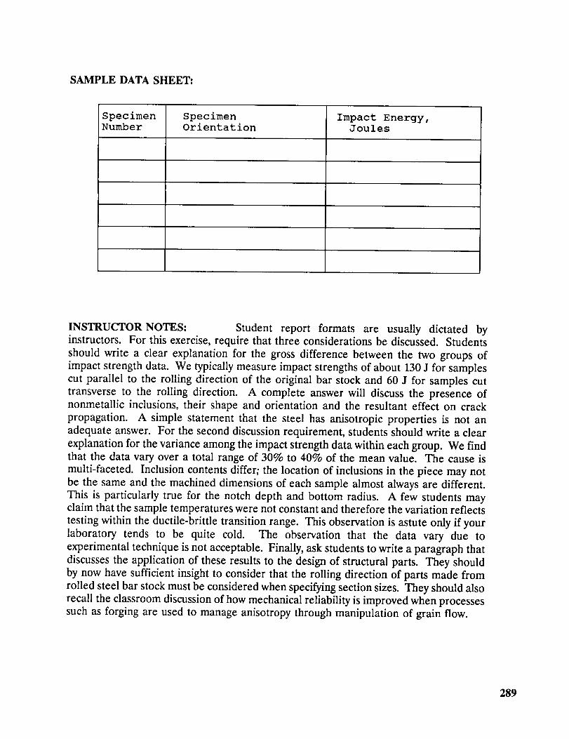
SAMPLE DATA SHEET:
Specimen Specimen Impact Energy,Number Orientation Joules
INSTRUCTOR NOTES: Student report formats are usually dictated byinstructors. For this exercise, require that three considerations be discussed. Students
should write a clear explanation for the gross difference between the two groups of
impact strength data. We typically measure impact strengths of about 130 J for samples
cut parallel to the rolling direction of the original bar stock and 60 J for samples cut
transverse to the rolling direction. A complete answer will discuss the presence ofnonmetallic inclusions, their shape and orientation and the resultant effect on crack
propagation. A simple statement that the steel has anisotropic properties is not an
adequate answer. For the second discussion requirement, students should write a clear
explanation for the variance among the impact strength data within each group. We find
that the data vary over a total range of 30% to 40% of the mean value. The cause is
multi-faceted. Inclusion contents differ; the location of inclusions in the piece may not
be the same and the machined dimensions of each sample almost always are different.
This is particularly true for the notch depth and bottom radius. A few students mayclaim that the sample temperatures were not constant and therefore the variation reflects
testing within the ductile-brittle transition range. This observation is astute only if your
laboratory tends to be quite cold. The observation that the data vary due to
experimental technique is not acceptable. Finally, ask students to write a paragraph that
discusses the application of these results to the design of structural parts. They should
by now have sufficient insight to consider that the roiling direction of parts made from
rolled steel bar stock must be considered when specifying section sizes. They should also
recall the classroom discussion of how mechanical reliability is improved when processes
such as forging are used to manage anisotropy through manipulation of grain flow.
289

REFERENCES:
1. Guichelaar, P. and M. Kenig, "Nurturing The Mechanical Skills Of Pre-
Engineering Students," Pro. 1989 ASEE Annual Conference, pp. 163-166.
2. Kalpakjian, S., Manufacturing Engineering and technology, Addison-Wesley, 1989.
3. Schey, J., Introduction to Manufacturing Processes, McGraw-Hill, 2nd Edition,1987.
SOURCES OF SUPPLY: Hot-rolled steel is available from mgst industrial supply
houses or steel supply centers.
290

N94- 36409
DEVELOPMENTS IN CARBON MATERIALS
Timothy D. Burchell
Leader, Carbon Materials Technology Group
Oak Ridge National Laboratory
Building 4508, MS 6088
P. O. Box 2008
Oak Ridge, Tennessee 37831-6088
Telephone 615-576-8595
291


DEVELOPMENTS IN CARBON MATERIALS
Timothy D. BurchellLeader, Carbon Materials Technology Group
Oak Ridge National Laboratory
DEVELOPMENTS IN CARBON MATERIALS
Overview of Presentation
The following carbon-based materials will be reviewed andtheir applications discussed:
• The Fullerenes
• Graphite (synthetic or manufactured)
• Activated carbon fibers
• Carbon-carbon composites
Carbon R&D activities at ORNL will be emphasized.
DEFINITION OF TERMS
SYNTHEllC; GRAPHITF
A MATERIAL CONSISTING OF GRAPHITIC CARBON WHICH HAS BEENOBTAINED BY GRAPHITIZ1NG NON-GRAPHITIC CARBON.
CARBON-CARBON COMPOSITES
A CARBON FIBER REINFORCED CARBON MATRIX MATERIAL IN WHICH THEFIBER AND/OR MATRIX MAY BE GRAPHITIC (GRAPHITE-GRAPHITE
COMPOSITE)
293_llt_N/_ PAGE Bt.._.r_KNOT FILMED PA_ _-_ I;'_iE,'_F:,L31',.,_,LLYE)LANK_

FULLERENES
CN'IIv
| I,,.I c." .
._ I , co,, .
_'-;"-,, "-'E "-_"=-,,_--_'" -_---
•pyricSne B
G{,i'
C:,I"
sOO IO0 _0 M ino _no tm _ 1_
i.i
|
, , , , ,
t,2,3,5.tetramethylbenzene G
FiS 4 Laser clcsorption TOF mm spcclra ol'soot cxt_cu
rcsuhinlt from s_qucntial extractions with {A) benzene. {BI
pyridinc, and (C) 1.2.3.3.tctramethylbenzene. The spectra
are plotted on the same mass scale for companson_
THE FULLERENES
Cg
l294

THE FULLERENES
Lov, esx eneru Kekul_ smx'tu_ o( saecet b,_ C_
R_)rmlecl by permlssaon for Hat_ vol. 329, pp. 529-331;
,co_! @ 1987 MacMiUam Mal_l=m L.imiled.
$truclute of the AI¢_,o SUl_"ondu_ol3. The open
and hatchc_l s_ms _:_'scnt the alkali atom at tettaheclral
and octahe_i s.es. r_spectlvely. Nole Ihe two possible on-
cntallons of the _ molecules and the three inequivalent
carbon sites _marked by arrow'son Ifle motecuie m the Iowel'
left comerl as desc'nhed in the text. After P, Stcphens
a/.[ZZ]
Potential Applications of the Fullerenes
• Pharmaceutical
• Tribological (lubricant)
• Super conductor
• Thermal insulator
295

SYNTHETIC GF APHITE
What is Graphite?
• An allotropic form of carbon
• Hexagonal 2D crystal structure
• Layered crystal planes
• Highly anisotropic
• Conductor in plane, insulator across planes
• A fun material to work with!
A
B
A
,____ 6._o_
2.46_
296

THE MAJOR PROCESSING STAGES IN THE MANUFACTUREOF CONVENTIONAL ARTIFICIAL GRAPHITES
RAW PETROLEUM
OR PITCH COKE
ICALCINED AT 1300°CI
CALCINED COKE
I_ CRUSHED, GROUNED
AND BLENDED
I BLENDED PARTICLES I IBINDER PITCH I
L I_"MIXED
_ COOLEDI
i EXTRUDED, MOLDED ORISOSTATICALLY PRESSED
GREEN ARTIFACT I
BAKED AT 1000 °C
BAKED ARTIFACT
IMPREGNATED TO DENSIFY
GRAPHITIZED 2500 - 2800 °C
GRAPHITE
297

Graphite Possesses Unique Properties
• High temperature stability
• High electrical and thermal conductivity
• Chemically inert
• Strength increases with temperature
• Processible and machinable to all forms and sizes
ADDlications of Graphite
• Arc furnace electrodes
• Resistance heating elements
• Crucibles and boats (semiconductor industry)
• Rocket motor throats, missile nose tips
• EDM electrodes
• Seals and bearings
• Electric motor brushes
• Metal refining and casting
• Nuclear moderator
298

The CMT Group Is Developing A DesignData Base For the Graphite Core
Of The MHTGR
Modular High-TemperatureGas-Cooled Reactor With
Steam Cycle Power Conversion
Graphite Data Base Development
• Effects of reactor environmenton graphite properties- Neutron irradiation
- He coolant chemistry and oxidation
- Temperature and pressure
• Strength, strain to failure- Elastic constants
- Fatigue behavior- Fracture mechanics data
- Thermal physical properties- Oxidation behavior and mechanisms
• C/C composite control rod development
299

ACTIVATED CARBONFIBERS
Activated Carbons are a Broad Familyof Carbon Materials
• Coal-derived carbons
° Almond shells
° Olive pits, peach pits
• Charcoal
° AC from waste paper
• Activated carbon fibers
Aoolications of Activated Carbons
300
• Gas separation
• Air filtration
• Water filtration
• Solvent recovery
• Military suiting
• Molecular sieves

A iv r n Fi r A
ACF can be derived from pitch (coal tar or petroleum),polyacrylonitrile (PAN), or rayon precursors
Fibers are loosely consolidated into a felt, mat or wovencloth, or rigid porous monolith
Product is thermally activated at temperatures in the range700-1000°C in steam
TYPICAL CARBON FIBER STRUCTURES
r _GRAPHITE rGRAPHIT E
/ P'ANES
TYPICAL FIBER DIAMETER ~ 40/./.m /_°""_"_"_ _"--GRAPHITE
PLANES
RADIAL HOURGLASS
G.M. Pennock etol.CARBON, Vol.31,p.596,597 _993
301

Carbon Fiber Composite Molecular Sieve
At ORNL we have developed a rigid, monolithic-activated
carbon material named a carbon fiber composite molecular
sieve. The material retains the advantages of ACF and,
additionally, overcomes problems associated with granular
activated carbons.
Hydrogen Separation Is Widely Achieved UsingPressure Swing Adsorption Systems
UOP Polybed PSA Unit
treats gas streams from
reformer hydrogen plant
to produce 66 millionSCFD of hydrogen.
302

"Although there is some room for improvements in
the pressure swing adsorption process, the potential
gains in process economics in the future are fikely
to come from the development of new and improvedadsorbents."
- R. V. Jasra, N. V. Choudary, and S. G. T. Bhat
Research Center, Indian Petrochemicals Corp.In their review "Separation of Gases by PressureSwing Adsorption", Separation Science and
Technology,Vol. 26, pp. 885-930, 1991.
CMT Group Has Developed A Novel Adsorbent/MolecularSieve Based On Carbon Fibers
Carbon Fiber CompositeMolecular Sieve
• High adsorption/desorptionrates
• High active surface area
• Microporous [5-10 A] fibers
Applications: Gas separation,gas storage, air filtration,pressure swing adsorptionsystems
303

• CCI4 adsorption rate is twice that of granular carbon
• >10 times higher adsorption/desorption rates reportedfor tolulene and methane
Carbon Tetrachloride Adsorption Rates
N2 BET Surface Areas Of Materials ThatHave Well-known Molecular Sieve Properties
• Active surface areasup to 1670 m 2/g havebeen achieved withORNL CFCs
MolecularSieve N2(m2/g)
Linde 5 A zeolite 316
Linde 4 A zeolite 35
Linde 3 A zeolite 11.6
Carbosieve 1040
Saranchar 900
Pitch fiber CFCMS >1,650
(non-optimal condition)
Carbon fiber activesurface areas > 2000m2/g and 10 A porewidth have beenreported (OSAKA Gas)
3o4

ORNL. UK2 CFCMS Material
Narrow pore sizedistribution
Pore size centered
at -- 6 A pore width
High active surfacearea (904 m 2/g)
Active surface areas>2000 m 2/g possible
o
>.,
m=1
I=1
10 -_
10-"
10 -8
i0 -°
I 0 -I°
-I110
SEPARATION OF CO 2 & CH 4 By CFCMS (STP)
(Initial composition 50v01% CO 2 and CH4)
: H4 INTFNStTY I
"_ J -- --CO,_ INTENSITV
I I I I I I 1
2 ,4 6 8 10 12 1,4
Time (min_
Carbon: CFCMS-48' BFT:8??m2Q - i I =0 ?4 nm
305

Summary And Conclusions
• ORNL/UKCAER have developed a monolithicadsorbent carbon based on carbon fibers
• Gross macroporosity and microporosity canbe controlled through processing variables
Activated carbon fibers have adsorptionrates greater than twice that of conventionalactivated carbons
Very high active surface areas can be developed incarbon fibers (OSAKA gas report >2000 m2/g (N2)ASA, 10 A pore width)
Narrow micropore size distributions can beachieved in the range 5-10 A
A monolithic activated carbon material has significantadvantages over granular activated materials for usein pressure swing adsorption equipment, such as theelimination of channelling, by-pass flows and pressure
drops
306

CARBON-CARBONCOMPOSITES
FLOW DIAGRAM FOR A TYPICAL CARBON/CARBONCOMPOSITE PRODUCTION PROCESS
PITCH (petroleum or coal
derived ), RESIN CARBON FIBER BUNDLES I(Pitch, PAN or Rayon)
,_ CLOTH LAY-UP, WEAVING
PIERCING, NEEDLING, etc.
DRY PREFORM
_ATION
15o 4so°c
r,/- I VACUUM TO 10MPa
I } CARBONIZATION
PTTON T 600- 800 °CU 05
AUDP , 5AL 60_U_._O TO 10 MPa
CYCLES _ GRAPHITIZATION
_ >2400 °C
I INAL COMPOSITE IDENSITY ,_- 1.9 g/cm 3
307

THE STRUCTURE OF AN ORTHOGONAL CARBON- CARBONCOMPOSITE SHOWING THE THREE MUTUALLY PERPENDICULAR
FIBER REINFORCEMENT DIRECTIONS (x, y, and z)
Z
Applications of Carbon-Carbon Composites
• Reentry vehicle nose tips
• Rocket motor throats and nozzles
• Exit cones
• Aircraft brakes
• Thermal protection
• Thermal management systems
• Fusion reactor first wall armor
308

Carbon-Carbon Composites for FusionEnergy Devices
ORNL has an active program to develop high-
thermal conductivity, carbon-carbon composites
for plasma facing components in tokamak fusion
reactors. Moreover, we are investigating the
effects of neutron damage on the structure and
properties of carbon-carbon composites.
CMT Group Is Leading The DevelopmentOf NeutronIrradiation TolerantC/C Composite Materials
For Fusion Energy First Wall ApplicationsJoint European Torus
First Wall C/C Composites
= Neutron damage
-- Dimensional stability-- Effects on thermal
conductivity
• Development of highthermal conductivityuni-directional C/Ccomposite
309

THE MAJOR PLASMA FACING COMPONENTSOF A TOKOMAK FUSION DEVICE
VESSEL
LIMITER
VERTOR
PUMPING PORT
Carbon Materials Are Widely UsedFor Tokomak First Wall Armor
JT-60U
(Japan) JET
(England)
TFTR
(USA)
310

PLASMA FACING COMPONENTS
MATERIALS REQUIREMENTS
, LOW ATOMIC NUMBER
• HIGH THERMAL CONDUCTIVITY
• GOOD THERMAL SHOCK RESISTANCE
• EROSION RESISTANT (PLASMA SPUTTERING)
• ADEQUATE STRENGTH AND STIFFNESS TO WITHSTANDELECTROMAGNETIC FORCES DURING DISRUPTIONS
• RESISTANT TO IRRADIATION DAMAGE
RADIATION DAMAGE IN GRAPHITE
COLLAPSING
(c) VACANCY
INTERSTITIA___VACANCY
EXPANSION
311

TYPICAL CARBON FIBER STRUCTURES
\o_,. _GRAPHITE GRAPHITEF PLANES
-_ _'/_\/;j[ PLANES
,,-_I V.//ttlttl\\\\\ _iF
TYPICAL FIBER DIAMETER - 40/J.m /_c'J_"_-_ _ GRAPHITE
PLANES
RADIAL HOURGLASS
G.M. Pennock et ol.CARBON, Vol.3t,p.596,597 4993
MICROSTRUCTURAL INTERPRETATIONS OF IRRADIATION
INDUCED DIMENSIONAL CHANGES IN 1D C/C COMPOSITES
CARBON FIBER
(o) CONTRACTION 4D C/C COMPOSITE
(c) EXPANSION INITIALLYACCOMMODATED BY POROSITY
(18
Ld "%_
-(18<_-r
-t.6..J
Zo -2.4
_ -5.2
-4.0
2 3 4 5
FLUENCE (dpo)
\
\\
\
\
312

MICROSTRUCTURAL INTERPRETATIONS OF IRRADIATIONINDUCED DIMENSIONAL CHANGES IN 2D C/C COMPOSITES
(a) CONTRACTION _ i'-_..w"l"(C) EXPANSION INITIALLY B _
ACCOMMODATED BY f '--ACCOMMODATING
POROSITY _ __ POROSITY
'
: j
0.4
0.0
W
_ -0.4
1-
_ -0.8<[zo
-t.2zb,.I=EQ
- t.6
-2.0
I I =FLU ENCE (,dl_): : ._..._
ozo#_
Developments in Carbon Material-_Recommended Texts for Carbon Materials
Introduction to Carbon Science
Harry Marsh
Published Butterworth & Co., Ltd., 1989ISBN 0-408-03837-3
Carbon Fibers
J. B. Donnett and R. P. Bansal2nd Edition, Published Marcel DekkerNew York, 1992
The Industrial Graphite Engineering Handbook
UCAR Carbon Company, 1991(39 Old Ridgebury Road, Danbury, CT 06817-0001)
313

More Advanced Text:
Physics of Graphite
B. T. KellyPublished Applied Science, 1981ISBN 0-85334-960-6
Adsorption, Surface Area, and Porosity
S. J. Gregg and K. S. W. Sing2nd Edition, Published Academic Press, 1982
314

LIQUIDS THAT TAKE ONLY MILLISECONDSTO TURN INTO SOLIDS
John A. Marshall
School of Industry and Technology
East Carolina University
Greenville, North Carolina 27858
Telephone 919-757-6705
315


Liquids That Take Only Milliseconds to Turn into Solids
John A. Marshall, PhDSchool of Industry and Technology
East Carolina UniversityGreenville, North Carolina 27858
KEY WORDS:
Electrorheology, electrorheological fluid, fluid power transmission,hydraulics.
PREREQUISITE KNOWLEDGE:
The student should understand the elementary concepts of
magnetism. A basic understanding of fluid flow would be helpful.
OBJECTIVE:
To observe the unusual characteristics of electrorheologicalfluids. To understand how these fluids change from a liquid to a solid. To
understand the potential power transmission advantages of these fluids.
EQUIPMENT AND SUPPLIES:
1) Plastic bottle containing electrorheological fluid.2) Energizing probe
3) Personal safety equipment4) Paper towels
5) Pen
INTRODUCTION:
Electrorheological fluids change their flow characteristics when
subject to an electrical field. Response, which takes only milliseconds, is
in the form of a progressive gelling that is proportional to field strength.With no field present, the fluid flows as freely as hydraulic oil (Korane,1991).
_lit."_N_ F_AGE 8LANK NOT FILMED 317

Electrorheological fluids represent a maturing technology that has
the potential to widen the performance range of automatedelectromechanical and electrohydraulic equipment. Research and
ongoing developments are refining this technology and experts predict an
important future for these fluids.
Importance of Electrorheological Fluids:
Current automation capabilities are not advanced enough to build
a robot that could play tennis. Even though cameras and computers
could direct the robot towards a ball, robots move in an awkward,
lumbering fashion because conventional hydraulic valves cannot keep
pace with the commands of the computerized controllers.
With electrorheological fluid technology, this type of response time
is possible. This technology will allow devices that can operate instantlyand without mechanical valves. Increased productivity and better product
quality through more dependable and responsive automated equipment is
just a small part of what this maturing technology can deliver.
How Electrorheological Fluid Functions:
Electrorheological fluids are composed of two primary components.
They are the carrier fluid and the suspended particles. The carrier fluid
needs to be a good insulator, compatible with the materials they contact.
Typical particle materials include polymersl minerals, and ceramics
(Scott, 1984).
When an electrical field is applied across the fluid, positive and
negative charges on the particles respond by separating, so each particlethen has a positive end and a negative end. Particles of the
electrorheological fluid then link together in the same manner that the
north pole of one magnet is attracted to the south pole of another magnet
(Duclos, 1988).
When the electrical field is removed, the particle attraction is no
longer present. The fluid then begins flowing freely. Please see Figures1 and 2.
318

Figure 1 - No electrical field present, charges are random,no particle attraction.
Figure 2 - Probe energizing the fluid, particles linked together.
319

Potential Applications:
Electrorheological fluids can change from solids to liquids so fast
they will work well with fast-acting computers. These characteristicssuggest a number of unusual engineering applications such as fluidclutches and vibration isolators (Duclos, 1988).
According to Hans Conrad, professor of materials,science and
engineering at North Carolina State University, electrorheological fluidswill lead to a whole new generation of brakes, automatic transmissions,
actuator devices, hydraulic valves, pump parts, and motors (Conrad,
1992).
PROCEDURE:
Safety Considerations:
1. Be very careful to avoid being shocked by the energizing probe.
2. Protective eye wear is mandatory for all those in the lab area.
3. Do not allow the electrorheological fluid to touch anyone's skin
or clothing.
4. Obtain a "Material Data Safety Sheet" on the fluid from thesupplier. Read the sheet completely and ask questions relating
to any information you do not understand.
Electrorheological Fluid Preparation:
1. Check the cap on the plastic bottle containing the fluid and
make sure it is securely tightened.
2. Shake the bottle to distribute the stratified particles evenly
within the fluid.
3. Set the bottle down on the lab bench and carefully remove the
top.
320

Observing Electrorheological Fluid as a Liquid:
1. Slowly insert the probe into the container of fluid until the metal
rods are submerged approximately two inches below thesurface of the fluid.
2. Slowly withdraw the probe from the fluid and hold it slightlyabove the bottle. Observe what happens to theelectrorheological fluid on the metal rods of the probe.
3. Set the probe on a paper towel and record you observations.
Observing Electrorheological Fluid as a Gelled Solid:
° Slowly insert the probe into the container of fluid until the metal
rods are submerged approximately two inches below thesurface of the fluid.
2. Press and hold down the button on the top of the probe.
, Slowly withdraw the probe from the fluid and hold it slightlyabove the bottle. Observe the status of the electrorheologicalfluid on the metal rods of the probe.
4. With the probe slightly above the fluid level in the bottle,
release the button (de-energizing the probe) and observe whathappens to the electrorheological fluid on the metal rods of theprobe.
5. Set the probe down on a paper towel and record yourobservations.
321

SAMPLE DATE SHEET:
Record below the characteristics of the fluid when the probe was not
energized:
Record below the characteristics of the fluid when the probe was
energized:
INSTRUCTOR NOTES:
o When the probe was removed from the fluid without being energized,students should have observed the fluid flowing off the metal rods and
back into bottle. The fluid will flow as easily as oil.
2. When the probe was removed from the fluid while being energized,students should have observed a gelling of the fluid around the rods
of the probe.
3. De-energizing the probe will cause the gelled electrorheological fluid
to liquify and drip into the bottle.
REFERENCES:
Korane, K.: Putting ER Fluids To Work. Machine Design, May 9,1991,
pp. 52-57.
Scott, D.: Amazing Hardening Fluids Open a New World of Hydraulic
Drives. Popular Science, April 1984, pp. 42-46.
Duclos, T.G.: Electrorheological Fluids and Devices. Automotive
Engineering, December 1988, pp.45-48.
Conrad, H.: The Impact of ER Fluids. Compressed Air Magazine, March
1992, pp. 14-17.
322

N94- 36410
MECHANICAL PROPERTIES OF CROSSLINKEDPOLYMER COATINGS
Jeffrey Csernica
Department of Chemical Engineering
Bucknell University
Lewisburg, Pennsylvania 17837
Telephone 717-524-1257
323


MECHANICAL PROPERTIES OF CROSSLINKED POLYMER COATINGS
Jeffrey Csemica
Department of Chemical Engineering
Bucknell University, Lewisburg, PA 17837
Keywords: polymer, crosslinking, hardness, impact resistance
Prerequisite knowledge: Some familiarity with polymers and polymer structures would
be beneficial, although not required. Also, students familiar with basic mechanical properties
and their measurement for metals, especially hardness and fracture toughness, will be able to
apply that knowledge to the material presented here.
Objectives
• Fabricate and test thin films to explore relations between a polymer's structure and its
mechanical properties.
• Expose students to testing methods for hardness and impact energy that are simple to
perform and which have results that are easy to comprehend.
• Show importance of polymer properties in materials that students frequently encounter.
• Illustrate a system which displays a tradeoff between strength and impact resistance, the
combination of which would need to be optimized for a particular application.
° Expose students to coatings technology and testing.
Equipment and Supplies
• 2-mm diameter pencil leads and lead holders, to cover a range of hardnesses. The available
pencil hardness range is 6B (softest) to 9H. To test the materials described here, pencils
from 2B to 5H (2B, B, HB, F, H, 2H, 3H, 4H, 5H) should be sufficient.
• Steel test panels--7.5 x 15 cm, 0.8 mm thick, with dull matte finish (from Q-Panel Co.,
Cleveland Ohio).
• Drawdown bar (film applicator)--see Appendix.
° Micrometer.
• Drop weight impact tester--see Appendix.
• Oven(s), capable of temperature control in the range 70-190 oc.
• Large glass plate, or other hard flat surface.
• Raw materials: see Procedure for specific examples and suppliers.
• Tukon ® or other microhardness tester (optional).
325

INTRODUCTION
Organic coatings, the paints and finishes we use for protection and decoration, are
polymeric materials--they consist of high molecular weight chain-like molecules, which
contain many atoms linked together by covalent bonds. Although the characteristics of a
particular paint or finish can be modified somewhat by additives, the basic chemical and
molecular structure of the polymer (or polymers) from which a coating is made is primarily
responsible for many of its important properties, such as hardness, durability, and chemical
resistance.
Many common coatings are composed of polymers with a crosslinked molecular
structure. After application as a liquid, these finishes do not merely 'dry' in the conventional
sense. They form hard solid films by undergoing a chemical reaction, called crosslinking (or
"curing"), after they have been applied to a surface.
Crosslinking is a process by which linear polymer chains ("primary chains") are joined
together at common junction points. These junction points can be provided by low molecular
weight compounds, which can chemically attach themselves to the ends of at least three
different primary chains (see Figure 1). Such compounds are referred to as "crosslinking
agents" because they provide the means of converting a collection of linear molecules into a
crosslinked polymer. The structure of a crosslinked polymer can be depicted a net (Figure 1),
and these materials are often referred to as network polymers.
/
.. ),---
linear polymer crosslinking crosslinkedchains agent polymer
Figure I. Formation of a Crosslinked Polymer
326

The properties of a network polymer depend strongly on its degree of crosslinking. To
use the net analogy, a network with extensive crosslinking (many junction points, or many
chains emanating from each one) would be classified as a "tight" network, while one with more
limited crosslinking would be called a "loose" network. A higher degree of crosslinking in a
polymer coating (tighter network) usually leads to increased hardness and solvent resistance,
but may also result in increased brittleness. Other mechanical and chemical properties can be
affected as well, and usually an optimum degree of crosslinking is sought which gives an
attractive combination of properties for a particular application.
In this laboratory, you will prepare a series of crosslinked coatings, and will determine
how the degree of crosslinking in these materials affects their hardness and impact resistance.
Like the schematic of Figure 1, you will fabricate crosslinked polymer networks by
combining a primary resin with a crosslinking agent. (The word "resin" is used to describe a
polymeric, or high molecular weight, compound). The primary resin consists of linear
polymer chains which contain hydroxyl groups (-OH) at the chain ends (see Figure 2). Acrylic
and polyester resins of this type are commonly used for automobile finishes and industrial
coatings. The hydroxyl groups are the reactive sites at which these primary chains will attach
to the crosslinking agent.
-- OH
OH
CH3OCH2
CH3OCH 2
/CH2OCH 3
IN% / N%c/N NC CH2OCH3
II IN\c N
IN
/ NCH3OCH 2 CH2OCH 3
primary resin chain crosslinking agent(hexamethoxymethyl melamine)
Figure 2. Components for Polymer Network
327

Several different types of compounds can serve as crosslinking agents for the primary
chains. The one you will use is a substance called hexamethoxymethyl melamine (HMMM).
Its chemical structure is shown in Figure 2.
The HMMM chemical structure may appear complex, but the important thing to note is
that it contains six (CH3OCH2-) groups. These are the chemical groups that can react with the
(-OH) groups of the primary resin chains. Such a reaction will result in a connection between
the HMMM and the primary chain. Because it contains six (CH3OCH2-) groups, the HMMM
can attach itself to as many as six different primary chains, and can therefore serve as junction
points for the network (see Figure 1). It should be noted that, despite the relative sizes of the
molecular drawings in Figure 2, the primary resin chains will typically be much larger than the
crosslinking agent molecules.
Chemically, the crosslinking occurs by a condensation reaction which produces
methanol (CH3OH) as a by-product:
b.. /-- OCH 2__OH + CH3OCH2_ w,-
+ CH3OH
This curing reaction requires the presence of a small amount of acid catalyst. You will
use para-toluene sulfonic acid (p-TSA).
Also, elevated temperatures are needed for the reaction to take place. After the
components (primary resin, crosslinking agent, catalyst, and some solvent) are applied to a
surface as a liquid film, the coated part will be heated in an oven for a specified time. The
crosslinking can therefore be controlled and delayed until an appropriate time after application.
You may have heard of automobile finishes being "baked" in this fashion.
The degree of crosslinking, and therefore the final properties, of the cured films can be
controlled by a number of factors. Two that you will explore are the curing temperature, and
the ratio of crosslinking agent to primary.resin in the liquid mixture. The degree of
crosslinking will generally increase as the cure temperature is increased, because this speeds up
the reaction. Also, adding more crosslinking agent to the mixture will, to a point, result in
more extensive crosslinking.
Two important coating properties you will measure for these cured films are hardness
and impact resistance.
Although there are a number of methods available to measure the hardness of polymeric
materials, one of the most fundamental involves attempting to scratch the material with objects
of differing hardnesses. This is in fact what you will do in this laboratory, using a series of
328

pencilleadsto evaluatethehardnessof your coating. This type of hardness measurement is
particularly appropriate for these materials, because coatings in service may have to resist
scratching or gouging by hard objects.
You will expose the cured materials to impact by dropping a weight onto coated steel
panels. Although other impact tests (Charpy, etc.) are available which can provide controlled
rapid deformation of bulk specimens, subjecting the polymers to impact as thin films on
substrates better simulates service conditions for these materials, and does not require
machining of special sample geometries.
329

PROCEDURE
Note to Instructor: Many commercially available products can serve as components for the
coating mixtures. The procedure as described here, as well as the results shown in the next
section, are for a specific experiment which uses the following raw materials (different
materials may require slight modifications, as specified by the supplier):
• primary resin--hydroxyl-functional polyester, #57-5803, Cargill, Inc., Minneapolis, MN.
• crosslinking agent (HMMM)--Resimene ® 747, Monsanto Co., St. Louis, MO.
• acid catalyst ( p-TSA)--K-Cure ® 1040, King Industries, Norwalk, CT.
1. **CAUTION** This step should be conducted in the fume hood!!
Prepare three different coatings formulations in small jars. The ratio (by weight) of
primary resin to crosslinking agent should be varied as follows:
Formulation A- 85:15
Formulation B- 70:30
Formulation C- 55:45
These ratios should be based on the "solids" portion of the components. That is, if the
components as supplied contain an added solvent, the solvent fraction is not included in
the ratios.
Add solvent (xylene, methyl isoamyl ketone, or other as recommended by resin supplier)
to the formulations such that each contains 30% solvent overall. Remember to include in
this 30% any solvent that may have been originally contained with the components. At
1% by weight, add to each mixture the K-Cure ® acid catalyst product. Mix each
formulation thoroughly with a mixing stick or spatula.
Note to Instructor: In the interest of time, formulations can be completely or partially
mixed for the students in advance, although determining appropriate amounts for each
component can provide a good exercise, especially if the compounds originally contain a
solvent fraction. When mixed in advance, the formulations may have a limited shelf-life
33O

(severalweeks).Also to savetime,a shorterexperimentcanbeconductedwhichexaminesonly oneformulationinsteadof three.
2. **CAUTION** Thisstepshouldbeconductedin thefumehood!!
Preparesamplesby applyingthinfilms of thecoatingmixturesto steelpanels.Because
themeasuredmechanicalpropertiesof afilm canbeaffectedby its thickness,it is
importantthatuniform,constantthicknessfilms bepreparedfor all samples.For eachsamplepreparation:
Placeapanelon the glass plate (it can be secured with a small piece of masking tape).
Deposit an amount (approximately 1 teaspoon) of the coating mixture near the far end of
the panel, in the center of its width. Place the drawdown bar with the 0.15 mm clearance
(see Appendix) at the far end of the plate and, in a continuous motion, pull it toward you
across the liquid so that it leaves behind a film. It may take a trial or two for practice, but
you should soon be able to quickly prepare film samples that appear smooth and uniform.
The bar should be cleaned with a quickly evaporating solvent such as acetone between
each sample preparation. Make three replicate samples for each combination of
formulation type (A, B, or C) and curing temperature you intend to test (remember to label
the panels with a marker!). Let each panel sit horizontally for at least ten minutes before
curing (step 3) to allow for solvent evaporation.
.
For each test temperature, cure the samples by placing them (3 for each formulation) into
the appropriate preheated oven. Panels can be placed horizontally or hung vertically in the
oven. Curing temperatures in the range 70 - 190 oc should be investigated--see
instructor for specific temperatures and ovens to be used. For each cure temperature, use
a baking time of 30 minutes.
Note to Instructor: If time and the number of available ovens make it difficult to examine
several different cure temperatures, try instead using a single temperature and varying the
amount of time samples remain in the oven. This will also produce films with varying
degrees of crosslinking.
.
After the panels are removed from the oven and have cooled, lightly touch the films with
your finger. Have they become hard and rigid, or are they still sticky and tacky? Using
the micrometer, measure the thickness of the cured films. You can do this by obtaining
331

.
the difference in thickness between coated and uncoated portions of the panel. Check for
uniformity between samples and within the same sample. Is the final film thickness the
same as the clearance of the drawdown bar?
Note to Instructor: The thickness of the cured films will be considerably less than the
drawdown bar clearance. The bar will leave behind a wet film that is typically about half
as thick as the bar's clearance. This film will then contract upon solvent evaporation and
curing. Using a bar with a 0.15 mm clearance depth, we obtained cured films that had
thicknesses in the range 0.04 - 0.05 mm.
Measure the hardness of the cured films by comparing their hardnesses to those of the
pencils. Pencil leads are ranked in order of increasing hardness as follows:
6B, 5B, 4B, 3B, 2B, B, HB, F, H, 2H, 3H, 4H, 5H, 6H, 7H, 8H, 9H
In a controlled fashion (see below), you will try to cut into each coating with these pencils.
Leads harder than the coating will be able to gouge the film, while those softer than the
coating will crumble and will leave the film uncut. For each trial:
Adjust the lead so that approximately 3 mm extends from the lead holder. With the lead
holder perpendicular to a piece of abrasive paper, prepare the lead by grinding it against
the paper so that a flat surface, normal to the lead's length axis, is obtained. Place the test
panel horizontally on a flat surface. With the pencil pointing away from you, place the
lead against the film at a 45 ° angle, and push the lead down and away from you in an
attempt to cut the film. An alternative method is to grip the pencil in your fist, and hold the
lead against the surface such that it is pointing toward you (45 ° to the surface), and then
pull rather than push the lead. In either case, you must exert enough downward pressure
so that either the paint film is gouged (preferably down to the steel panel surface), or the
lead crumbles. Make at least three trials with each lead tested, and note whether that lead
cuts the film or not. The hardness of the film is reported as that of the hardest lead which
doesno_ t gouge the film.
Note to Instructor: This procedure can be supplemented by having students read ASTM
D3363-74: Film Hardness by Pencil Test.
332

6. **CAUTION** Becertainto wearsafetyglasseswhileusingthisapparatus!!
Usingthedropweighttester,investigatethefilms' resistanceto impact. This will provide
ameasureof theirbrittleness--alowerimpactresistanceindicatesa morebrittle (lesstough)material.Foreachtest:
Placethecoatedpanelhorizontallyonthesupportring with thefilm facingupward.Raise
theweightedindenterto a specifiedheightinsidethedroptube,andallow it to fall ontothe
panel. Theenergyof theblowisgivenby theload(indenterweight)multipliedby the
heightfrom which it wasdropped.Joulesor inch-poundsareappropriateunits for impactenergy.Removethepanel,andexaminethefilm in theimpactarea.A failureis indicated
by crackscausedby theblow. A magnifyingglassmaybeuseful,althoughfailuresare
usuallydetectedeasilybyeye. Notetheenergyof eachimpact,andwhethera failureoccurred.
Youaretrying to determinethehighestimpactenergyeachfilm cansustainwithout
failure. Performtestsfrom differentheightsandtry to determinetheimpactenergyat
which thefilm exhibitsatransitionfrom passingto failing (i.e.,if it passesthefirst test,
youwould increasethedropheight). Youcanperformseveraltestson thesamepanelas
longasafiat, coatedareacanbeplacedovertheentiresupportring. Beginningwith large
variations,youshouldbeableto locatethetransitionpointto within adropheightof 25
cm. If possible,try to narrowit downto within a 10cm height,andperformmultipletestsfrom severalheightsin thisregion. Reportthe"impactenergy"of thesampleasthehighestenergyatwhichthesampleconsistentlydoes not fail.
NOTE: For all samples, use the 0.9 kg indenter initially. If no failure is achieved even
from the greatest possible height, switch to the 1.8 kg indenter.
. (optional) Measure the hardness of the test films using a Knoop indenter on the Tukon ®
Microhardness Tester. Use an applied load of 50 g. Report hardnesses as Knoop
Hardness Numbers (KHN).
333

EXPERIMENTAL RESULTS
All samples baked at 90 °C and above became hard to the touch after removal from the
oven. Samples exposed to a lower curing temperature (70 °C) remained sticky and fluidlike.
It can be concluded that little crosslinking occurred at this low temperature, and these films
were not subject to the hardness and impact tests.
Figure 3 shows the pencil hardness for all films cured at 90 °C and above. The 55:45
and 70:30 mixtures produced films whose hardness increased from HB to 3H as the curing
temperature was raised from 90 to 130 °C. The increase in crosslink density caused by curing
at higher temperatures resulted in greater film hardnesses. For these two formulations, the
pencil test did not detect any further changes in hardness at cure temperatures above 130 °C.
t..,
oN
4H-
3H-
2H-
H-
F-
HB-
B
2B
• • • •
! ! m ! m !
90 110 130 150 170 190
Cure temperature (degrees C)
• 70:30 and 55:45
• 85:15
Figure 3. Pencil Hardness Values for Cured Films
334

Althoughthepencilhardnessresultsfor the55:45and70:30formulationswere
indistinguishable,films madefromthe85:15mixture(theonecontainingtheleastamountof
crosslinkingagent)exhibitedsignificantlylowerhardnessesatall curingtemperatures.Whilealsoshowingsomeincreasein hardnesswith temperature,this formulationachieveda
maximumhardnessof only F. Thebehaviorof the85:15samplesdemonstratesthatreducing
theamountof crosslinkingagentin themixturecanresultin significantlysofterfilms.
It is interestingto comparepencilhardnessresultswith KnoopHardnessNumbers
(KHN) for thesefilms. KHN valuesfor theseriesof films fromthe70:30mixtureappearin
Figure4. Indentationsweremeasuredat leastthirty secondsaftertheKnoopindenterwas
removed;nochangesin themeasuredindentationwerenotedat increasedtimes(upto 10
minutes).Thegeneraltrendof hardnessincreasingwith curetemperature,seenin thepencil
hardnessresultsof Figure3, is confirmed.BecausetheKHN analysisprovidesalessdiscretizedmeasureof hardness,thecurvein Figure4 showsa somewhatsmootherincrease
andlevelingof hardnesscomparedto thepenciltest. AlsonotethattheKnooptestidentifiessignificantchangesin hardnessabovethe130oc curetemperaturethatwerenotdetectedin thepenciltest. (Noteto Instructor." Have students comment on the relative merits and drawbacks
of the two types of hardness tests.)
Z
35
30
25
20
15
10
5
0
7O
Figure 4.from
I I I I I I I
90 110 130 150 170 190 210
Cure temperature (degrees C)
Knoop Hardness Numbers for Cured Filmsthe 70:30 Formulation
335
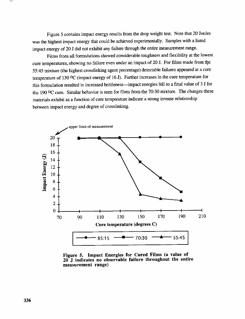
Figure 5 contains impact energy results from the drop weight test. Note that 20 Joules
was the highest impact energy that could be achieved experimentally. Samples with a listed
impact energy of 20 J did not exhibit any failure through the entire measurement range.
Films from all formulations showed considerable toughness and flexibility at the lowest
cure temperatures, showing no failure even under an impact of 20 J. For films made from the
55:45 mixture (the highest crosslinking agent percentage) detectable failures appeared at a cure
temperature of 130 °C (impact energy of 16 J). Further increases in the cure temperature for
this formulation resulted in increased brittleness--impact energies fell to a final value of 3 J for
the 190 °C cure. Similar behavior is seen for films from the 70:30 mixture. The changes these
materials exhibit as a function of cure temperature indicate a strong invex'se relationship
between impact energy and degree of crosslinking.
_40t_,
20
18
16
14
12
10
8
6
4
2
0
t upper limit of measurement
I I I I I I I
110 130 150 170 190 210
Cure temperature (degrees C)
70 90
e 85:15 "- 70:30 Jk 55:45 I
Figure 5. Impact Energies for Cured Films (a value of20 J indicates no observable failure throughout the entire
measurement range)
336
For cure temperatures where some samples exhibited detectable impact failures, the
effect of crosslinking agent ratio on film toughness is apparent. The formulation with the
largest percentage of crosslinking agent, 55:45, produced the most brittle films. The 70:30
samples had somewhat higher impact energies, and the 85:15 mixture produced the least brittle
films, which did not show impact failures even when cured at 190 oc. This supports the
earlier conclusion that more extensive crosslinking in these materials leads to a reduction in
impact resistance. Even though samples from the 85:15 mixture are relatively tough, recall that
they also exhibited considerably lower hardnesses than those from the other two formulations.
In summary, the hardness and impact energy of these organic coatings are directly
related to their internal network polymer structure, in particular, the degree of crosslinking,
which can be adjusted by changing the crosslinking agent percentage in the formulation, as
well as the film's cure temperature. These materials display a tradeoff between hardness and
toughness, with harder films generally exhibiting a lower resistance to impact. For a given
application, changes in the formulation and cure temperature can be used to prepare coatings
with an optimum combination of these mechanical properties.
REFERENCES
1. Turner, G.P.A., Introduction to Paint Chemistry and Principles of Paint Technology, ch.
7 & 9, Chapman and Hall, London, 1980.
2. Hill, L.W., Mechanical Properties of Coatings, Federation of Societies for Coatings
Technologies, Philadelphia, 1987.
3. Brown, R.P., ed., Handbook of Plastics Test Methods, George Godwin Ltd. and The
Plastics and Rubber Institute, London, 1981.
Appendix--Equipment Notes to Instructors
The drawdown bar is a steel bar, 3 to 4 inches in length, with a flat side that rests
squarely on the test panel. Along this side, a 2-inch long section has been machined away such
that it provides a clearance, which will leave behind a film when the bar is drawn along the
surface of a panel and over the deposited liquid mixture, as described in the Procedure. We
337
used a bar with a clearance depth of 0.15 mm (6 mil). Draw down bars are available
commercially from Paul N. Gardner Co., Inc., Pompano Beach, FL.
In the drop weight impact test, the test panel sits horizontally on a circular steel support
ring. A 4-foot long vertical tube, with a slot cut along its length, is positioned directly above
the center of the support ring. A cylindrical steel weight, tapered at the impact end to a
hemispherical tip, fits inside the tube. A bolt protruding from the side of the indenter weight
fits through the slot in the tube, and is used to lift the weight to the desired drop height. A unit
conforming to ASTM guidelines can be made by referring to ASTM D-2794-90: Resistance of
Organic Coatings to the Effects of Rapid Deformation, although alternate designs would be
suitable for the purposes of this experiment. A commercial device of this type is available from
Paul N. Gardner Co., Inc. (see above).
338

N94- 36411
._ ?. i
EXPERIMENTS IN DIAMOND FILM FABRICATION INTABLE-TOP PLASMA APPARATUS
James V. Masi
Department of Electrical Engineering
Western New England College
Springfield, Massachusetts 01119
Telephone 413-782-1344
339


EXPERIMENTS IN DIAMOND FILM FABRICATION IN
TABLE-TOP PLASMA APPARATUS
James V. Masi, PhD
Western New England College
Dept. of Electrical Engineering
Springfield, MA 01119
(413) 782-1344, FAX (413) 782-1746
KEY WORDS: Diamonds, plasma, heterojunctions, photoconductors.
PREREQUISITE KNOWLEDGE: The student should be familiar with the basics of materials
science and chemistry. Levels at which these experiments are performed are second semester junior and
either semester senior year. The students are first given lectures on band structure in solids, film formation
via chemical vapor deposition, semiconductor junction formation, and photoconductivity. Though a
scanning electron microscope would be helpful, film morphology can be seen with reasonable optical
microscopy. A video filmed by the instructor showing the plasma deposition onto silicon and sapphiregives the student an idea of what is expected.
OBJECTIVES: To illustrate the process of plasma assisted chemical vapor deposition and to
show devices which can be made simply in the laboratory. These devices illustrate clearly the concepts of
bandgap, junctions, and photoelectronic processes. Films and devices are measured electrically, optically,and thermally.
EQUIPMENT AND SUPPLIES:
(1)(2)(3)(4)(5)(6)(7)(8)(9)(10)
Silicon wafers, sapphire wafers, and microscope slides ( one per student)U.S.P. ethyl alcohol
Stoppered flask with tubing fittingsControlled air leak
High voltage (>2000 volts) d.c. supply
Microwave oven (500 watts), small (optional)
Polycarbonate belljar (25 cm. diameter)
Silver paint (DuPont 4817)Diode curve tracer
Microscope (optical, 400x) or electron microscope
INTRODUCTION: Using simple chemicals and materials, such as ethyl alcohol, sapphire, and
silicon wafers, students can heteroepitaxially deposit diamond films onto silicon and sapphire wafers in a
direct current plasma and/or microwave assisted plasma. By placing 1 part in 106 of either boron
trichloride or phosphorus trichloride into the ethyl alcohol, the diamond films can be doped p- or n-type
respectively. Undoped films serve as good photoconductor films. Small polycarbonate belljars purchased
from Cole-Parmer along with mini vacuum pumps serve as the reaction chamber, minimizing danger of
accident. The systems may be placed into a small microwave oven (500 watts, 2.45 GHz). The reaction
with partial pressures of oxygen combined with the ethyl alcohol yields diamond films whose properties are
dependent on deposition variables heretofore unknown to the student (and sometimes to the professor).
The three laboratory sessions spent provide the student with experience in:
i:'__G _AC_: BLAr_K NOT FILMED
341
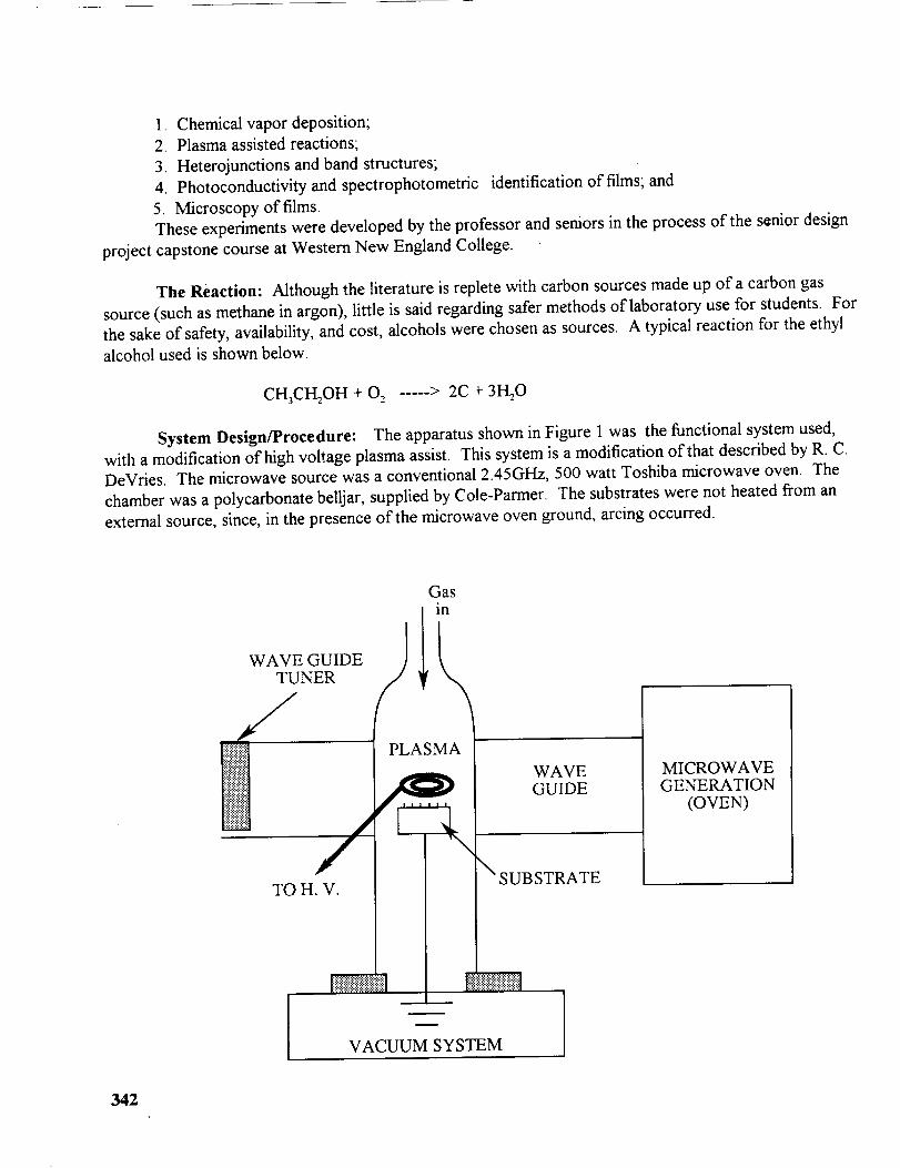
1. Chemical vapor deposition;
2. Plasma assisted reactions;
3. Heterojunctions and band structures;
4. Photoconductivity and spectrophotometric identification of films; and
5. Microscopy offilms.
These experiments were developed by the professor and seniors in the process of the senior design
capstone course at Western New England College. -project
The Reaction: Although the literature is replete with carbon sources made up of a carbon gas
source (such as methane in argon), little is said regarding safer methods of laboratory use for students. For
the sake of safety, availability, and cost, alcohols were chosen as sources. A typical reaction for the ethyl
alcohol used is shown below.
CH3CH2OH + 0 2 ..... > 2C + 3H20
System Design/Procedure: The apparatus shown in Figure 1 was the functional system used,
with a modification of high voltage plasma assist. This system is a modification of that described by R. C.
DeVries. The microwave source was a conventional 2.45GHz, 500 watt Toshiba microwave oven. The
chamber was a polycarbonate belljar, supplied by Cole-Parmer. The substrates were not heated from an
external source, since, in the presence of the microwave oven ground, arcing occurred.
WAVE GUIDETUNER
ilNiiiiil
Gas
I in
PLASMA
TOH. V.
WAVEGUIDE
\SUBSTRATE
VACUUM SYSTEM
MICROWAVEGENERATION
(OVEN)
342

The vacuum pump is run until the system reaches 80 microns or lower pressure. The pump is
allowed to run while a mixture of 1 part air and 1 part argon is bubbled through the ethyl alcohol and
"leaked" into the vacuum system until the pressure rises to 3-30 Tort-. The microwave power and/or the
high voltage was turned on and the plasma (blue-red column) decomposition/oxidation of the ethyl alcohol
proceeded. It should be noted that the morphology of the films obtained was quite different, dependent
• on the plasma source used. Though the process works better with the semiconductive substrates, with
microwave assist the sapphire and glass substrates also provide suitable substrates. All films are
polycrystalline with reasonable densities; best results and densities were obtained on single crystal silicon
substrates. Typical yellowing or browning of the film indicates the presence of carbon (or graphite)
included in the film. Each system appears to have somewhat different characteristics and the experimenter
should note these. Typical growth rates of these films are of the order of 0.01 to 0.1 micrometer per
minute. An x-ray diffraction scan of a film on (100) Silicon is shown in Figure 2. This film was grown atapproximately 0.06 micrometers per minute.
Typical dopants for the diamond film are introduced via dissolution of boron trichloride (acceptor)and ammonium chloride (donor) into the ethyl alcohol in the 1-1 O0 ppm ratio to carbon in the alcohol.
Care should be taken to clean the system well between each type change. The number of ionized acceptors
and donors is only expected to be from 1-10% in the diamond film at room temperature. Though time
usually doesn't permit, all four varieties of n/p, p/n, n/n, and p/p heterojunctions prove to be interesting indemonstrating isotype and heterotype heterojunctions and their characteristics.
Safety Note: Although the alcohol is safer than methane in the laboratory, a safety mesh or
Plexiglas sheet should be placed between the student and the apparatus. Good practice indicates thewearing of safety masks during the deposition.
Device Preparation: Devices of the heterojunction type are post-deposition prepared by roughing
the back side of the silicon wafer with 00 grit silicon carbide paper. Silver paint (DuPont #4817) is applied
to the back of the silicon wafer and is allowed 15 minutes to dry. Dots of silver paint may be applied to
the front of the wafer over the diamond. Fine aluminum wires may be attached for testing of the devices.
Sufficient light enters the device to cause both photovoltaic and photoconductive (reversed biased)
responses in the junctions. Devices of the non-junction photoconductive types on either sapphire or glasswork well with silver paint electrodes applied juxtaposed in parallel bar formation.Both devices are shown
in Figure 3. Carbon or gol d semi-transparent electrodes function better for photo devices and can be easily
deposited as replacements for the silver on diamond top electrodes. Attachment to these electrodes by
means of fine aluminum wires serves to ease testing of the devices iia the absence of probes.
343

r-
>.,L..
°--
.13t_
V
>.,°_
r-"
r"
D[AHOND OH JIO0] S[ WAFER
nltlll
s[ 11ooi
O-SPACEHG IIKL COUNTSO.A2 331 20
0.89 400 tO
1.06 311 43
t.26 220 t53
2.0G tit G7t
122o1
J ol]tllL _
'i',_-,'l-';_;,"'"_i_;"G-' _"']_n"-i'"'l .... ' .... !
40 50 GO 70 BO 90
DI4o01 I] I]]t
tOO ttO t20 t30 t40
2,0 (Degrees)
Figure 2
X-ray Diffraction of Diamond Film oil Silicon (100)
344

SFigure 3
Heterojunction Devices
Ag Paint
Diamon
photoconductive (Resistive)
Ag bars Devices
Diamond _/////
>Substrate
Typical Measurements: Measurements made on devices will vary according to doping levels, type mixes,
resistivities of the silicon, and conditions of deposition. Typical diode characteristics in the dark and light
are shown in Figures 4 and 5. Typical photoconductor characteristics are shown for light and dark
conditions in Figures 6 and 7. All characteristics are taken on a Tektronix curve tracer. The light sourcesused were tungsten-halogen "white" and 253.7 nm ultraviolet.
A typical spectrophotometric transmission curve vs wavelength for diamond is shown in Figure 8.
The cutoff (bandgap) wavelength as well as impurity and other absorption energy levels are easilycalculated (as shown in the appendix) from
E = hc/_,.
Spectral response characteristics can optionally be made with an added expenditure of time and effort.
REFERENCES:
1. Boenig, H. V., Plasma Science and Technology, Cornell University Press, Ithaca, NY. 1982.
2. Solymar, E. and Walsh, D., Lectures on the Electrical Properties of Materials, OxfordUniversity Press, Oxford, England. 1988.
3. Milnes, A. G. and Feucht, D. L., Heterojunctions and Metal-Semiconductor Junctions,Academic Press, New York. 1972.
4. Deutchman, A. and Partyka, R., Diamond Film Deposition - A Gem of a Process, AdvancedMaterials & Processes, ASM International, June, 1989.
5. DeVries, R. C., Synthesis of Diamond Under Metastable Conditions, MRS 1991 FallSymposium, MRS, Pittsburgh, PA. 1991.
SOURCES OF SUPPLY: The microwave oven was an $88 one obtained from a local appliance
store. The laboratory supplies and chemicals were obtained from Cole-Parmer and Fisher Scientific. The
high voltage supply is a $35 surplus TV. 4000 volt d.c. supply. The silicon wafers and sapphire disks were
obtained through Ms. Shannon John, Wafernet, San Jose, CA. The silver paint was obtained from Bert
Bricker, Wilmington, DE. All other supplies are easily obtained from local university supply houses.
345

....i....i....i....i....i....i__ .....
: " ...: ......... : .... : .... ; .... : ....
B
ZV/divO
_ Figure 4
Forward Biased p/n Diamoml/Si lletrroil"lcli'" Diode
...._....i....!....i!i !i i i!uN/dlv : : : : : :
.... i i :: i i !._:._.r i i :.... -.... .... .... .... .... ....
8 2 Vldiv _ :
Figure 6
l,ow Sensitivity Diamond Photoconductor on Glass
2
_g, cliv
2iiik IIii̧i "i .... i .... I ....i_,v!........ I .i.. i .
B Z V/div
Figure 5
rcvcm'se Iliased pl,i Diamoml/Si llelerojunclion l)iode
_,dlv
.2_dlv
....:....:.._U...:_'_.....:....!....:....",.-'_-.:.:"_'_
: : ,7,?,7 : : i .!_/i: i :
"! ....i,/::i ....i....i_.:,'_ " i....
B _ _V/div
Figure 7
lligh Sensitivity Diamond Photoconductor on Sapphire
346

I i ' t i! I : _:_' Figure8 I -[' :: i :i -i I ..... :-:o/-: .... :-, :--i -. Spectrophotomelric Curve of Diamond Film i , '
" [ ! [ _ -
i : I ..... I ....
__.' ...... ': J_¢_¢_¢': "_'v'_iT---i ,_ i J [. IW4_
! : )W__--I - !-=i-..... _ - ] I ' .....
_'.... _ _1.:..:-i ....i---_'-- !---_i_ _ I_--
- --..t -. I= !::1----!:"-
I -'--i _: '. ...... .L__ .:, f L:.;._- =: ---
/-__' _ '_ ..... ,_ ._'...... ._.._ _- _..... ' t I-:' __; " ' ' t I _+ -- --- '. 772 L-.. _
It _-:4 '. _ ; i- .t::
j'/__- : _ ;---i-_---.....J : ! ' + -t : ! , i I---
' I ' I -- I T ...... )P " I .....
] , ' ' I ' :, I :l : " : I
I_ " I _-2- ---, : -;- --
t _ t
........ x_0 0 : -
: . , , i- '-i- -:--" .... i: I I ! . ' : ', ,-! i I
; I ' 7; -=/i 1 _ - i; " I !7_"]2-- .... _ " ___r _Z _--]_-,, i _ . i I _" i i "" . ' ' -' ' i .- fr_
: " t := _: L : i , , I: -
7--% } " - ,_._=l_7_i...i_l._.. 111_1 _.. I- -!--I_ _-
2-_L :712 ;:" i _ _.; -' ;.7 I " ,_ :
, . i !..... i ................. Z _ L._
: -i ;- :__..... L _._ _ _--
Some original figures were unavailable at time of publication.
347

APPENDIX
Diamond Film #3
Diamond Film at t60x and 320x Magnification and 30 ° Angle
348

APPENDIX:
Heteroj unction Theory: Heterojunctions are semiconductor junctions which are composed of
two or more materials of differing band gaps in metallurgical contact with one another. The Anderson
Model (in the reference by Milnes and Feucht) was the model chosen for diamond on silicon, n/n, p/p, p/n,
and n/p structures. The energy band diagram for isolated and in-contact n/p (Si/diamond) is shown inFigures A1 and A2.
_m
E%ECTRCN
ENERGY
E:I
EF; .....
Evl
VACUUM _', IL_ _E_
....AE,,I L----F----E_2
Evz
Figure AI
Energy Band Diagram for Two Isolated Semiconductors
VACUUM _ 1L./E_
V V I/,° 04[,, x:,
II I .
' L t _! I i --JL-E_Eel---- T .... J, _._ _..
E t I ' , EvZ
E,-- f vo,T %_ A,,J_v'-"__L_I_I I II I II I I
Xl XO xZ
E¢2
Figure A2
Energy Band Diagram for n-p Heterojunction (V = 0)
349

The energy barrier ofajuncdon for non degenerate materials, materials
whose electron a/_dty and bandgap are not affected by doping, can be calculated
using the equation:
= E,,+_Y._'-&-&-qK'-V. Eq. I-I
lcVhere:
EGI
_=
8p ----
q =
V a =
= Bandgap ofMaterialOne
D[ffe1.enceIn the Energy of theValance Bands
DifferenceBetween theFenui Level and the Conduction
Band
DifferenceBetween theFermi Level and the Valence Band
Charge on an Electron (1.5x 10-LgC)
Applied Voltage
The expression for I<L is for low forward bias conditions and neglects the effects of
injection carriers:
/,C:=/_I + _Vo,_:l,Vo,a)Eq. I=2
W'_el'e"
N m = Number of Donor Atoms in Material Two
N m -- Number of Donor Atoms in Material One
¢I = PermeafiviVy of Material One
Ch = Permeafivity ofMater_ Two
The built-in voltage of the junction, v D, is the sum of the partial built-in
voltages, V m + V m, where V m and V m are the electrost_c potentials of'the
semiconductors I and 2 at equilA'bdum. The equation for the length of the
transition or depletion region of an n-p junction can be found using the derivation:
r2. NA,,,,,(Vo_--Vo)7" Eq. 1-3
(Xo- x,) =LqNo,(e,.ff,,,_e,,v,,---;)]
[_ n'o,e,_,(7,,"o-v,)"r(x_- xo)= ,v,,,(e,.,v,,,'-----We,.,v.,---;)j
The total width of'the depletion region is therefore equal to:
Eq. 1-4
350

W=(X:-Xo)+(Xo. XO=F2_'_:(Vo-V_)(N._+ N.,):f _=
Where:
Eq. I-5
N,u = Number of Acceptor Atoms in Material Two
Vr_ = Bu/k-h Voltage
m
Energ_ Diagram of a p-n Junction for (a)Forward Bias (b)Reverse Bias
The above diagrams demonstrate the principle ofrectificadort, which states that the
tota/current flowing for a voltage V a is not the same for a voltage of-V a. The
total current flowing Iet_ to right through thejtmction using the equation:
I = z0[exp(qV,/ kr)-
Where:
Eq. I-6
Io = Reverse Saturation Current
TI= QuaMty Factor
k = Boltzman's Constant (1.38 x 10 "z3I/I_
T = Temperature (K)
Dividing by the area of the jtmetion the current density can be calculated.
J = Jo[exp(qVa / rikT)- l] Eq. 1-7
351

APPENDIX
Si Ga.%s B-SiC Dia==.-.d
Ba_-.dNa? i.12 i.4Z Z.35 S. A8(eV) (ir./irec--) (_i_-ec=) (ir._i_-mc=) (L"-g'Lr=-c--)
Mmb £!i=I_"(==2 v-z s-l)
UeBn
E!ac==cn Sa_
D=ifu Ve!'
Vsa = (_- s-!
1.0 x iO 7
85OO400
Z x 107
900S0
Z.5 x 10 7 2.7 x: !0 7
Breakdm_= _ield
EB (v ==-z)
Die!ec=ric
Ehe:-...,_co=auc--i__r7 (Y..J
(w ==-Z i-.l.)
job_--.s_:r._ig. o_Meri= 1
(v",-13z
P_a=ion Ra!a=ive
=m S i!ic_a
_eys F_g. of
_k=K(_) i/Z
(W=-zlz s-!Iz
z-l)
Ra=£o Ra!a=ive
=o Si!£c=n
3 x 10⁵
1!.9
1.5
Z.3 x 10 Z2
Z3.8 x 10 z
L x 105
12.9
0.5
1_.2 x !0Z'_
4 x i05
9.7
Z.533 x 1023
1 x !G 7
5.5
ZQ
18_5_ x 1O 23
7.0
_.Z x 102
1101
80.3 x i0Z
0.45 J 5.8
80Z8
43_.Z :=10 Z
_118
352
PLASTIC PART DESIGN ANALYSIS USING POLARIZEDFILTERS AND BIREFRINGENCE
J. L. Wickman
Plastics Research and Education Center
Department of Industry and Technology
Ball State University
Muncie, Indiana 47306
Telephone 317-285-5648
353

Plastic Part Design Analysis Using Polarized
Filters and Birefringence
J.L. Wickman
Plastics Research and Education Center
Ball State University, Muncie, Indiana 47306
KEY WORDS: birefringence, stress/strain, transparent/translucent plastic materials,
index of refraction, optically heterogeneous, photoelastic fringe patterns, polarizing filters,ASTM D-4093.
PREREQUISITE KNOWLEDGE: The student should understand the fundamentals of
plastics processing, materials characterization, and plastic part design.
OBJECTIVES: To understand the application of ASTM D-4093, "Standard Method for
Photoelastic Measurements of Birefringence and Residual Strains in Transparent or Translucent
Plastic Materials" to plastics part design and processing. To be able to observe and understand
the impact of using a polariscope in plastics manufacturing in an effort to improve product
quality. To understand how critical part design is to possible future failure analysis.
EQUIPMENT AND SUPPLIES:
(1)Glare-stop polarizing filters (12" X 12")
(2)Plate glass (4 pieces - 0.125" X 12" X 12") to protect filters
(3)Light source (overhead projector)
(4)Part Loading Fixture (optional)
(5)Transparent or translucent plastic parts
(6)Polarizing unit
INTRODUCTION: As the demand for engineered plastic products increases, greater
emphasis must be placed on material, processing and part analysis. ASTM D-4093, "Standard
"Method for Photoelastic Measurements of Birefringence and Residual Strains in Transparent
or Translucent Plastic Materials" has some very real, cost effective applications for plastics
product design, materials selection and testing, processing and failure analysis.
Internal stress in a molded plastic product can cause the part to warp, twist or bend,
craze/fracture and/or eventually fail. The cause of this stress is residual physical pulling that is
present when the plastic is pliable, but becomes captured upon solidification of the plastic. These
stresses cannot be seen by the naked eye, but with the use of a polarized filter and a light sourcethrough a transparent or translucent part, these residual internal stresses are identifiable.
This laboratory will investigate the possible causes of internal residual stresses in a plastic
part as a result of poor part design. Processing parameters and material selection can also have
an impact on internal stresses but that is beyond the scope of this experiment.
355

Light waves travel through a vacuum in a straight line from its source, vibrating in a
direction perpendicular to its axis of transmission (the direction in which it is traveling). When
the light wave strikes a heterogenous material, the vibration that was perpendicular to its axisof transmission becomes distorted. In fact, the vibration splits into two separate waves vibrating
in separate planes. The two waves have different indexes of refraction, and the differencebetween these is called the birefringence. When these two light waves emerge from,the
heterogeneous medium, they are out of phase, and appear to the human eye as different color
bands when passed through an optical filter. These color bands in conjunction with injection
molding design will be the focus of this experiment. Large concentrations of different color
bands indicate a high level of internal, residual stress. See ASTM D-4093.
When a two dimensional model is subjected to loads, the resulting stresses exist generally
over the entire surface of the model. The stresses in the model produce proportional optical
effects which appear as isochromatic fringes. Starting with the unloaded model, and applying
the load in increments, fringes will appear first at the most highly stressed points. As the load
is increased and new fringes appear, the earlier fringes are pushed towards the areas of lower
stress. Under white light, the photoelastic fringe pattern appears as a series of successive and
contiguous different colored bands in which each band represents a different degree of
birefringence corresponding to the underlying stress in the part. The color of each band identifies
the birefringence, or fringe order (and stress level), everywhere along the band. White light is
composed of all wavelengths in the visible spectrum. Table 1 will give the complete color
sequence, the fringe order and the corresponding stress level possibly found in a part.
Color Relative Fringe StressRetardation Order psi MN/m 2
Black
GrayWhite
Pale-Yellow
OrangeDull Red
Purple (Tint of Passage)
Deep BlueBlue-Green
Green-Yellow
OrangeRose-Red
Purple (Tint of Passage)
Green
0 0 0 0
160 0.28 90 0.62
260 0.45 144 0.99
345 0.60 192 1.32
460 0.80 256 1.76
520 0.90 288 1.99
575 1.00 320 2.21
620 1.08 346 2.38
700 1.22 390 2.69
800 1.39 445 3.07
935 1.63 522 3.60
1050 1.82 582 4.02
1150 2.00 640 4.41
1350 2.35 752 5.19
356

Green-Yellow 1440 2.50 800 5.52
Red 1520 2.65 848 5.85
Red Green Transition 1730 3.00 960 6.62
Green 1800 3.10 992 6.84
Pink 2100 3.65 1168 8.05
Pink Green Transition 2300 4.00 1280 8.86
Green 2400 4.15 1328 9.16
Table 1. Isochromatic Fringe Characteristics using photoelastic plastic. Experimental StressAnalysis by Dally and Riley.
The basic polariscope utilizing the two polarizing filters will show full field interpretation of
fringe patterns in an effort to obtain an overall assessment of nominal stress magnitudes and
gradients. A more sophisticated polarizer and analyzer with two insertable quarter-wave
retardation plates that are mechanically coupled for synchronous rotation will provide additionalanalysis. The more sophisticated unit provides quantitative measurements for:
* determination of principal stresses
* magnitude and sign of the tangential stress along free boundaries and in regions wherethe state of stress is uniaxial
* magnitude of the difference in principal stresses in a bi-axial stress state.
The importance of proper plastics part design can be shown using ASTM D-4093. Part
failure can be minimized through attention to inside sharp corners, varying wall thickness, sink
marks, molded in metal parts, bosses, ribs, weld lines, gate size and location, blind holes, and
functional surface characteristics. The specific specifications for each part is a function of the
particular material selected. Even though there are approximately 15,000 different plastics
available, specific design guidelines have been developed for generic plastic classifications. Thegeneric guidelines are available from the material manufacturer.
Molded in stresses will be concentrated around gates, openings, inside sharp corners,sharp transitions in cross section, and weld lines. The stressed areas can detract from various
strength properties by as much as 20 percent. Loads, heat, pressure, light, and chemicals shouldbe used with caution in the affected stressed areas.
PROCEDURE:
1. Obtain a transparent/translucent injection molded plastic part with engineering
applications. The part should fit between the two polarizing filters and should be easily rotatedabout the X, Y, and Z axis. Use the polarizing filters to identify any and all residual stresses.
If there are no noticeable fringe patterns, find another plastic part. Be sure to rotate your partthoroughly in an effort to seek out all fringe patterns.
Each of the filters is unidirectional. Set up the polarizing unit on the overhead so that
the axesare crossed and the polariscope is in the dark-field. If the transmission axes coincide the
polariscope is in the light-field. Dark-field means that with no stress in the model, all light is
extinguished and the model appears uniformly black. As the load is applied, the most highly
357

stressed regions begin to take on color, first grey, then white, violet and so on. The purple
fringe is referred to as the tint of passage and is very sensitive to a small change in stress level.
The purple tint of passage is selected to mark the increment in relative retardation equal to a
fringe order of unity (N = 1). The tint of passage is a sharp dividing zone occurring betweenred and blue in the first order fringe, red and green in the second order fringe, and pink and
green in the third, fourth, and fifth order fringes. Beyond five fringes, white light analysis is not
adequate. See Table 1.
The part can be loaded either in tension or compression using the part loading fixture.
This analysis will begin to show how the part reacts under various forces and can also be used
in failure analysis. Fringe patterns will change in proportion to the force applied.
2. Locate where all gate(s), ejection pins, core pins, parting lines, etc. may have been
in the molding tool. Generate an isometric drawing of the part, include all bosses, ribs, bolt
holes, inserts, tapers, sink marks, blind holes, and functional surface characteristics. Assume
your part represents the typical/average part produced.
3. Determine the specific design criteria for the material that may have been used in your
particular part. Using available calipers, micrometers, and other measurement tools as necessarydetermine if your part falls within the design criteria as specified by the manufacturer. Cite all
deviations from the manufacturers specifications. Several assumptions need to be made 1) you
know what specific material is used to process the part and 2) the part specifications available
to you are identical to those used by the original designer.
4. Identify at least 10 critical engineering properties (as best as possible) that you would
design into the part. Consider the following and all assumed subheadings as a minimum:
Mechanical
Chemical
PhysicalDimensional
5. Map (using CAD) the fringe patterns of each critical area of the part that you have
selected. Record as accurately as possible the fringe patterns, include shape, width, height, and
the colors associated with each pattern. Associate color, fringe order, and stress present in
various areas of your part.
6. Associate the fringe patterns with your part as designed: i.e., identify what design
characteristics may have caused the fringe patterns. Recall material selection and processing may
impact the development of the fringe patterns. For the sake of this experiment, assume that the
impact of processing and material selection is negligible.
7. Identify where failure may occur in the part in normal use. Identify the conditions and
environment under the heading normal use.
8. Identify what design changes need to be implemented to avoid future part failure.
358

INSTRUCTOR NOTES:
1. Due to the variety of transparent/translucent plastic parts available it is important that
the students be encouraged to critique each part and material as a team. The use of the overhead
will bring the image to the screen for enhanced group participation.
2.Photographing with the more spectacular fringe patterns can be beneficial. 400 color
print film works well with an 80A (blue) filter to compensate for the projector halogen bulb.
A close up lens with the room lights out produces the best quality prints.
3.Processing parameters, material changes and chemical resistance tests can be used in
conjunction with the polarizing filters to further expand on the study of materials.
4.It is wise to keep a variety of parts and test samples at the polarizer to demonstrate theeffectiveness of the apparatus.
5.Pressure transducers can be used in conjunction with the part loading fixture to developa numerical index of forces.
loaded6.Depending on equipment availability slow speed video photography of the part beingcan contribute to design/failure analysis.
REFERENCES:
1. Dally, J.W., and Riley W.F., Experimental Stress Analysis, McGraw Hill BookCompany, New York, 1978.
2. Durelli, A.J., Applied Stress Analysis, Prentice Hall, Englewood Cliffs, New Jersey,1967.
3. Durelli, A.J., Introduction to Photomechanics, Prentice Hall, Englewood Cliffs, NewJersey, 1965.
4. Frocht; M.M., Photoelasticity, John Wiley and Sons, New York, 1941.
5. Heywood, R.B., Photoelasticity for Designers, Pergamon Press, New York, 1969.
6. Jessop, HIT. and Harris, F.C., Photoelasticity, Dover Publications, New York, 1960.
7. Kuske, A. and Robertson, G., Photoelastic Stress Analysis, John Wiley and Sons,New York, 1974.
8. Redner, S., Photoelasticity, Encyclopedia of Polymer Science and Technology, Vol9, John Wiley and Sons, New York, 1968.
9. Redner, S., Prediction of Failures in Service by Photoelastic Methods in Advanced
Testing Techniques, ASTM STP-476, American Society for Testing and Materials,Philadelphia, Pennsylvania, 1970.
359

10. Rosato, D.V. and Rosato, D.V., eds.: Injection Molding Handbook, Van Nostrand
Reinhold, New York, 1986.
11. Zandman, F.S., Redner, S. and Dally, J.W., Photoelastic Coatings, Iowa State
University Press, Ames, Iowa, 1977.
12. 1992 Annual Book of ASTM Standards, Volume 08.03. American Society for
Testing and Materials, Philadelphia, 1992, Pennsylvania.
SOURCES OF SUPPLY: The polarizing filters can be obtained at a local camera store.
The overhead projector should be readily available. All other parts for the polarizing unit and
part loading fixture can be obtained from a well stocked hardware store. Commercial polarizingunits available from Measurements Group - Photoelastic Division, P.O. Box 2777 Raleigh,
North Carolina. A basic polariscope can be produced for less than $60.00.
360

/ d r/
MICROWAVE SINTERING OF MACHINING INSERTS
David E. Werstler
Manufacturing Engineering Technology
Western Washington University
Bellingham, Washington 98225-9086
Telephone 206-650-3447
361


MICROWAVE SINTERING OF MACHINING INSERTS
David E. Werstler
Manufacturing Engineering TechnologyWestern Washington University
KEYWORDS: microwave, dielectric loss factor, sintering, structural ceramics,machining insert, design of experiments, bulk density.
PREREQUISITE KNOWLEDGE: The student should be aware of the normal
procedure for producing high quality ceramic parts from both dry powders and wetplastic forming, and an introduction to the dielectric properties of materials is also
necessary. Both of these can be found in most texts for introductory materials courses.
Some knowledge of metalcutting tools for a lathe is beneficial, and this may require ademonstration or observation in the university shop. A thorough concern for safety withmicrowave equipment is necessary.
OBJECTIVES: To use a designed experiment to determine the process control
parameters for microwave sintering in the production of ceramic cutting tool inserts.Parameters may include compaction load, heating rate, sintering temperature and time,and use of a preliminary degassing step.
EQUIPMENT AND SUPPLIES:
1. Prepared ceramic powder blend
2. Die set for triangular machining inserts with either 0 or 11 deg rake3. Universal testing machine set up for compression4. Scale which reads to hundreths of a gram
5. Microwave oven equipped with optical pyrometer or thermocouple6. Mechanical vacuum pump
7. Dewaxing cover with thermocouple8. Vacuum chamber with insulated sample holder9. Jolly balance
INTRODUCTION: Microwave heating is also known as UHF dielectric heating. Adielectric material (an insulator) becomes polarized when placed in an electric field, andan alternating current thereby causes cyclic distortion (dipolar rotation) of molecules andheating (1,2). Higher frequencies of the field cause a more intense internal frictioneffect, but penetration of the field into the interior of a workpiece is less. Radio
frequencies (10 to 300 MHz) can be used, but a household microwave oven operates at
2,450 MHz (2.45 GHz) and an industrial oven at 28 GHz has been developed (1).The dielectric loss tangent and the relative dielectric constant are material properties
that determine heating efficiency and penetration. When these are low, the material
tends to be opaque to microwaves, so higher values are necessary for adequate energy
L. , . 363

absorption. Some plastics such as PVC have high values in the radio range and can be"ultrasonically welded." Some ceramics such as alumina are opaque at room temper-ature but become absorbers exponentially as temperature increases, so preheating
them can trigger a response. Metals are not dielectric materials and reflect microwaves,which allows them to be used to contain the radiation in the oven.
Ceramic and cemented carbide cutting tools are made from a wide variety of combi-
nations of tungsten carbide, titanium carbide, alumina, silicon nitride, boron nitride, andother ceramics using powder pressing and sintering technology (3). Many of thesematerials have properties that allow them to be sintered with microwaves to greatly
decrease production times and costs. With the advent of surface coatings of TiCN, lowcost and high strength of the substrate are more important than wear resistance.
PROCEDURE:
1. The instructor will give the sintering cycle in a standard oven for your ceramic mix.
(For a cemented tungsten carbide insert, this would include dewaxing at 433 C for onehour, degassing at 1175 C for 45 minutes, and final sintering at 1475 C for two hours.)Determine which variables you want to study and design a two factor, three level experi-ment with bulk density as the response (4). Discuss your plan with the instructor first.
2. Determine the weight of powder necessary to fill the die cavity, allowing for 30%
porosity after pressing. Weigh out that amount and assemble the die set for pressing.Load the first sample, called a "compact," to 3200 kg. Unload the die, and measure thethickness of the compact and observe the condition of the edges. If the thickness is not
between 3.75 to 3.83 mm, adjust the weight of the powder for the next compacts.
3. To start the sintering process, load up to three compacts in the sample holder in the
oven. If your powder was coated with a wax plasticizer, that must be vaporized off first,so cover the samples with the dewaxing hood and connect it to the vacuum pump. Besure that the thermocouple in the hood is touching one of the compacts. Turn on theoven with medium power and bring the temperature up to about 400 C. Switch to low
power and try to keep the sample at that temperature for ten minutes or until no more
wax vapors are present.Turn off the oven, open the door and replace the dewaxing hood with the vacuum
hood. SAFETY PRECAUTION: the samples are hot enough to cause severe burns, and
other parts of the system may be hot. Wear safety glasses while working in the oven.Pump out the chamber, backfill with nitrogen, and evacuate again. Start the oven at
high power and monitor the temperature with the optical pyrometer. When itapproaches your planned cycle limit, reduce power and try to keep temperature withinten degrees of optimum. At the end of your cycle, turn off the oven and wait for theinserts to cool before turning off the vacuum.
4. Use the Jolly balance to measure bulk density. Plot results and make recommenda-
tions for optimum processing. Densities approaching 99% need to be achieved formaximum tool life.
364

INSTRUCTOR NOTES: This project demonstrates an emerging energy conservingtechnology, results in producing a usable product, relates a familiar device to the studyof materials, requires knowledge of electrical properties, and allows many avenues for adesigned experiment with minimal time consumption. It also demonstrates that real life
is not as simple as it first appears, because there is a high probability of nonuniform
fields, arcing, hotspots, and broken or porous parts. In fact, working on troubleshootingskills may be one of the main hidden objectives of this experiment.
An interesting addendum is to use the inserts on a lathe and measure wear rate
while cutting a material such as cast iron or 390 aluminum. This requires knowledge ofoptimum feeds and speeds for the material to avoid biasing and may take far too much
time for a materials class. But it can provide continuity to a later course on processes.In our manufacturing processes course, the students also make the tool holder for the
insert, so they have firsthand knowledge of the complete system.
Finding a source of small amounts of raw materials is one problem with this experi-ment. We were lucky to find a manufacturer that would sell us a small container of sizedand blended powder at cost. Another problem is avoiding reactions between the insert
and the atmosphere or the container, which is well documented and easily avoided.Unfortunately this is compounded by the need to use an insulating container with a lowdielectric loss. Some graphite boats used in traditional sintering proved to be betterabsorbers than our samples and therefore useless. A boat made from board insulation
also heated faster than the sample, so we started using a wool insulation. Castingplaster also seems to work well for the outer structure.
The cost of an optical pyrometer for high temperatures, with a small focal pointand appropriate focal length, is about $2,000. A platinum thermocouple with molyb-denum sheath is about $350, but it will read about 100 C too cold because of heat
transfer down the sheath. A ceramic sheath will tend to heat from microwave absorp-tion and is even more unreliable. A controller specifically for microwave ovens can be
purchased for about $10,000, but trial and error for finding appropriate power settingsfor each stage is acceptable. I am working on utilizing a standard furnace controller with
a platinum thermocouple and may find that to be the best way to provide acceptablecontrol of temperature.
REFERENCES:
1. Sutton, Willard H.: Microwave Processing of Ceramic Materials. Ceramic Bul.,vol. 68, no. 2, 1989, pp. 376-386.
2. Orfeuil, Maurice: Electric Process Heating, Battelle Press, 1987, pp 519-584.
3. Richardson, David W., ed.: Ceramics Applications in Manufacturing, Society ofManufacturing Engineers, 1988.
4. Snyder, W.B. Jr., Sutton, W.H., Iskander, M.F., and Johnson, D.L.: Microwave
Processing of Materials II, Materials Research Society Symposium Proceedings,1991.
5. Beatty, R.L., Sutton, W.H., and Iskander, M.F., eds.: Microwave Processing ofMaterials III, Materials Research Society Symposium Proc. Vol. 269, 1992.
365


KNOTTY KNOTS
Alan K. Karplus
Department of Mechanical Engineering
Western New England College
Springfield, Massachusetts 01119-2684
Telephone 413-782-1220


KNOTTY KNOTS
Alan K. Karplus
Department of Mechanical Engineering
Western New England College
Springfield, MA 01119-2684
KEYWORDS: String, Knots, Load reduction factor, Stress concentration
PREREQUISITE KNOWLEDGE: The student should be familiar with different types of ropes,
strings, and threads and may be aware that these materials can be weakened by tying a knot in the line.
At the high school and college levels this concept may be found in physics programs, but is familiar to
the student studying mechanics of materials in terms of the stress concentration factor. A backgroundin the tying of different styles of knots may be helpful.
OBJECTIVES: Tension tests are performed to determine the effect of different discontinuities on the
behavior of a material. String is first tension tested and then different t}pes of knots are tied in the string
to determine the impact of the type of knot on the load capacity of the string.
EQUIPMENT AND SUPPLIES:
1. String samples of different types: Fish line, thread, suture thread, string to tie cake boxes. An effort
should be made to secure string that will carry a maximum of 9 Kg (20 pounds) so the loads will notexceed this amount.
2. Model IN-50 Chatillon tubular scale to 25 Kg (50 lbs.) with two's' hooks and a 'homemade T' handle
attached to one of the 'S' hooks and the scale, and a slider on the barrel of the scale for maximum loadvalue indication.
3. Two load block holders for string ends (see Appendix Figures AI and A2 for details). Needed are
two standard size wooden spools 20 mm dia. by 30 mm long (3/4 in. dia. by 1 1/8 in. long), two
carriage bolts m5xl by 50 mm (1/4 20-UNC-2 by 2 in.) long each with one washer and one nut, two
150 mm (six inch) long pieces of 35 mm x 60 mm (1/2 in. by 2 1/4 in.) flex angle or equivalent with an'S' hook attached to the moveable holder.
4. Meter (Yard)stick
5. Scissors for cutting string
6. Vise attached to workbench to hold one holder
7. Data Sheet (see below for the format)
8. Heavy gloves (the kind a welder uses)
9. Safety glasses (always use eye protection)
PROCEDURE: Tension tests are to be performed to determine the effect of different discontinuities
on the behavior of a material. The initial step is to select a type of string to be tested. First is the tension
test for a single strand of string. This is the baseline for all comparisons. In each condition four trials
are run: samples are to be made, loaded to failure and the failure loads for each trial recorded and theaverage failure load tallied.
The subsequent conditions are to select a knot style to tie in the center of the string sample to be load
tested. Again, four samples with failure loads and an average failure are evaluated. The ratio of the
369

averageloadcarriedwith aknottedstringto theaverageloadcarriedby anunknottedstring iscalculated. Reductionin knottedstring loadcapacitychangesasa functionof knot type. Thetestprocedureshouldbeappliedto four differenttype knots to showtherangeof impactthetype ofknot presentsandthevariationsbetweenthe knot types.Thetestprocedureis presentedin detailbelow.
Theitfitial stepis theselectionof avarietyof string to test. Twenty samples,eachthreefeet,long,arerequired.The first conditionis atensileevaluationfor a singlestrandof string. This is thebaselineforall comparisons.Four samplesareto bemade,loaded to failureandthe failure loadfor eachsamplerecorded in thetableshownbelow in thesecondcolurrm,andthenthe averagefailure loadcomputedandtallied for future use.
To testthe singlestrandsecurea 0.8 meter(30 inch) lengthof string, tie a loop oneachend, fastenoneloop to eachthreadedextensionof thebindingpostof the load applicationapparatus(seeFigureA1),andwind the stringoneandone-halftimesaroundthespool. The spoolwinds areneededto reducethestressconcentrationin thestringmountingarea.The stringundertest is loadedbypulling on the springscalethat you readasthe loadis applied. If a maximumloadindicator slideris available,it will helprecordingthe maximumload. The experimentershouldweara pair of heavygloves,and in onehandsupportthe loadapplicationdeviceandwith the otherhand,apply load. Oneloadapplicatoris to befirmly held in thevise.Thehand-heldloadapplicationdeviceis to beheldlevelwith thevisemountedload application device to assure valid results. BE SURE YOU or your partner CAN READ THE
SCALE just before the line breaks. (The load may be close to 9 Kilograms (20 pounds) - Please
be very careful, wear safety glasses and avoid injury to yourself or the scale.)
Table of String Failure Loads in Kilograms (Pounds)
Unknotted String
Trial
1
2
3
4
Total
Averase [
Load ratio:
Unknotted
Knot 1 2 3 4
Load Load Load Load Load
Knot style to
Just below this table is a good place to describe the knot type used for each number (a sketch can be
made to show how to make the knot, too). For example, single loop, figure of eight, figure of eight
plus an half-loop, stevedore's.
The second condition is to select a knot style such as suggested in the notes below the table shown
above, and tie the knot in the center of the string to be load tested. Again, four samples with failure
loads and an average failure load are to be evaluated. Please add the data to the table, and compute the
average load carried by the knotted samples and the ratio of the average load carried by a knotted
370

string to the average load carried by unknotted string. One hundred times this ratio represents thepercentage of load carded by the knotted string.
The third, fourth, and fifth conditions are the second condition repeated for three more knot types.
Ashley (1), Boy Scouts of America (2), and The Encyclopedia of Sailing (3) provide good sourcesfor different knots which serve the same purpose.
COMMENTS :
There are some interesting things to consider after performing the first experiment.
1. Some knots tend to cut into and destroy string, and this varies between string types.
2. A test with Number 6, Black non-capillary braided suture silk found an average load of 4.367
Kilograms (9.625 lbs.) in an unknotted string with reduction factors of 54.0%, 51.3%, 65.1%, and
65.1% for a single loop knot, figure-of-eight knot, figure-of-eight plus an extra half loop knot, andstevedore's knot, respectively.
3. A different string will react differently, and a yellow covered plastic line 025-6-7013-66 available in
the Mechanical Laboratory took an average load of 7.656 Kilograms (]6.875 lbs.) in an unknotted
string with reduction factors of 54.1%, 62.2%, 49.0%, and 40.4% for a single loop knot, figure-of-eight
knot, figure-of-eight plus an extra halfloop knot, and stevedore's knot, respectively.
4. Instead of tying a knot in the center of a string, cut the string and tie selected knot to hold the endstogether.
5. Some lines when cut and the cut ends are tied as suggested in 4 above have new conditions to
consider. The surface finish on the string may be such that the tied knot slips and pulls out in contrast
to holding. A second single loop knot on each free cut end may provide enough resistance to minimizeknot(s) slipping/pulling out.
6. In the case of college students the connection between the load reduction factor and a stress
concentration factor (4) can be made. As an example consider that a given string carries 5 Kilograms
via a test and a knot is placed in the string which limits the load to 3 Kilograms. The load reduction
factor is 0.60 or 60% while the reciprocal of 0.60 is 1.67 and, this is often referred to as a stress
concentration factor. The meaning of the stress concentration factor is that when an engineer makes a
design calculation which involves a stress concentration factor, the actual material selected for a
member in a design must have the computed load increased by the factor. In this example, when a
calculated load of 10 Kilograms is made for the material, the selected material for the member must be
modified by 1.67 so 1.67 times 10 Kilograms or 16.7 Kilograms is the load the tensile member mustwithstand (without the stress concentrator present).
7. Strings can be conditioned by changing humidity, temperature, soaking in water, alcohol, oil, etc.,and cooking in a microwave to simulate artificial aging.
REFERENCES:
I. Ashley, C. W., The Ashley Book of Knots, Doubleday & Company, Garden City, NY, 1944
2. Boy Scouts of America, Knots and How To Tie Them, Boy Scouts Of America, Irving, TX, 19893. Encyclopedia of Sailing, Harper & Row, Publishers, New York, NY, 1971
4. Hibbler, R.C., Mechanics of Materials, MacMillan Publishing Co., New York, NY, 1991 pp. 151-155
371

APPENDIX 1 - LOAD APPLICATION APPARATUS
_ T-handle attached
to scale via s-hook
Scale wit
maximum load \slider indicator ---'
Carriagebolt,
to hold
spool
String
String looped over endof bolt + 1 1/2 turns on spool
Flex angle j
Figure A1 - Load block (2 needed).
a s Iedi
Chatillonscale
Hand heldload holder
1 1/2 tums on spoolfor string + loop
on bolt end
Vise heldload holder
Figure A2 - Load application set-up.
372

THREE-POINT BEND TESTING OF POLY
(METHYL METHACRYLATE) AND BALSA WOOD
Wayne L. Elban
Department of Electrical Engineering and Engineering Science
Loyola College
4501 North Charles Street
Baltimore, Maryland 21210
Telephone 410-617-2853
373


THREE-POINT BEND TESTING OF POLY(METHYL METHACRYLATE)
AND BALSA WOOD
Wayne L. Elban
Dept. of Electrical Engineering and Engineering Science
Loyola College, Baltimore, Maryland 21210
ABSTRACT: A procedure for determining the Young's modulus for poly(methyl
methacrylate) and balsa wood in three-point bending is described. A linear variable
differential transformer (LVDT) is used to measure displacement as a function of a series
of discretely applied loads. Emphasis is given to experimental methodology that includes
a verification of the operation/calibration of the LVDT using gage blocks. In addition,
the displacement of the test apparatus itself is measured and removed from the total
displacement data, allowing just the response of the materials to be obtained. The
problem statement for balsa wood is posed to require that an experimental procedure be
devised both to determine the Young's modulus and to address a specific design
requirement for maximum center deflection of road bed planking in a laboratory bridgetruss.
KEY WORDS: three-point bend testing, LVDT, Young's modulus, poly(methyl
methacrylate), balsa wood.
PREREQUISITE KNOWLEDGE: first-semester sophomore laboratory experiment
requiring training in the use of a digital multimeter and the assessment of measurement
uncertainty; flexural testing concepts, including the obtainment of Young's modulus, as
described in an introductory materials science or mechanics of materials course.
OBJECTIVES:
(a) Experimental Goals:
.
*
to measure the deflection of a flat plate of poly(methyl methacrylate), or
PMMA, in three-point bending in order to determine its Young's modulusand
to design and implement an experimental procedure to determine the
Young's modulus for a balsa wood beam in three-point bending and to
assess the maximum center deflection allowance specified for the
construction of a laboratory bridge.
C-S.375

(b) Learning Goals:
.
.
*
.
to become familiar with the use of a linear variable differential transformer
(LVDT), a widely used transducer for making linear displacement
measurements;
to become familiar with performing a laboratory calibration procedure
using National Institute of Standards and Technology (or equivalent)
traceable standards in characterizing the operation and accuracy of a
transducer provided with a factory calibration;
to become familiar with an experimental procedure for determining the
Young's modulus of a material tested in three-point bending by accounting
for any displacement in the test apparatus itself; and
to become familiar with designing and then implementing a measurement
procedure to obtain desired experimentally-determined material parameters.
EQUIPMENT AND SUPPLIES: (1) LVDT (direct current (DC)-operated and spring-
loaded) -- Lucas Schaevitz GCD-121-125 with mounting fixture; (2) Lab jack with
stabilizing weights; (3) Gage blocks: Jansson 0.020" and Mitutoya 0.050", 0.1001", and
0.200"; (4) Protoboard (Global Specialties Model 203A), supplying +15 V DC or
alternative power supply with the same DC voltage capability; (5) Digital multimeter
(Fluke model 45); (6) Three-point bend test apparatus (American Instrument Co. cat. no.
4-3900); (7) Set of 8 brass masses (Central Scientific Co. cat no. 09600); (8) Steel beam
(16 mm wide X 10 mm thick X 115 mm long); (9) PMMA plate (36.9 mm wide X 2.17
mm thick X 94.9 mm long); (10) Balsa wood beam (19.0 mm wide X 6.27 mm thick X
254 mm long); (11) Metric micrometer; and (12) Metric vernier caliper.
PROCEDURE:
Introduction
The modulus of elasticity, or Young's modulus, is a fundamental material
parameter defined using Hooke's law. For pure elastic deformation, stress, a, is related
to strain, e, by a = Ee, where E is Young's modulus. This modulus provides a measure
of material stiffness and is widely used in machine and structure design analyses. For
example, often structures have a requirement of undergoing no more than a specified
deflection for a given applied load. Computations yielding the necessary size of
structural members to achieve the specification can be performed knowing Young's
modulus for the material employed.
376

An LVDT [1,2] is a widely used electromechanical transducer that converts linear
displacement, sensed by the movement of the device's core (Figure 4-54, Holman [3]),
into a DC signal that can be detected, for example, by a digital multimeter (DMM) set tomeasure DC voltages.
This work consists of performing two displacement experiments involving the use
of an LVDT. The first experiment investigates the response of a flat plate of PMMA to
loading in a three-point bend test apparatus allowing determination of Young's modulus.
The second experiment involves designing a measurement procedure in order to
characterize the load-deformation behavior of a balsa wood beam proposed to be used in
a laboratory bridge design.
Prior to performing the first displacement experiment, the LVDT that is employed
must he calibrated using a series of gage blocks [4] to determine if the device is operating
as expected. HOWEVER, THE PERFORMANCE DATA PROVIDED BY THE
MANUFACTURER WAS OBTAINED UNDER MORE CONTROLLED
LABORATORY CONDITIONS AND SHOULD BE USED IN THE ANALYSIS OF
DATA MEASURED FOR THE TWO DISPLACEMENT EXPERIMENTS.
A schematic of the three-point bend test apparatus is given in Figure 1.
Originally, the test apparatus incorporated a dial indicator to measure sample deflection.
This is now accomplished using an LVDT. However, the dial indicator still is an
integral part of the apparatus, providing vertical positioning and alignment of the loading
nose (Figure 1, Reference [5]). Once a sample has been positioned in the apparatus,
various applied masses are placed on a circular load platform so as to leave enough room
for the LVDT to contact the platform near its circumference.
A. DEFLECTION OF A FLAT PLATE OF PMMA (Instructor Note 1)
,
Using the 0.020, 0.050, 0.1001, and 0.200" gage blocks, perform a calibration of
the LVDT to be used with the three-point bend test apparatus (Instructor Note 2).
To gain an additional gage block length, combine the 0.020 and 0.050" gage
blocks by rubbing them together until they stick. Likewise, combine the 0.020
and 0.1001" gage blocks; then the 0.050 and 0.1001" gage blocks; and finally the
0.020, 0.050, and 0.1001" gage blocks. Before beginning the calibration
procedure, adjust the height of the LVDT against a smooth rigid surface (e.g.,
steel beam placed on laboratory bench top) until the DMM reads 0.0 __+ 0.2 VDC.
377

To DigitalMultimeter
(DC Volts)
{ _} T°+-15V DC__ _ Power Supply
LVDT
Load J
Platform Screw
Dial
Indicator
Sample
Base Platform /
Figure 1. Schematic of Three - Point Bend Test Apparatus Instrumented with LVDT
378

.
Determine the displacement of the apparatus by testing the steel beam, having a
3 in. span support [5] length (Instructor Note 3). With the LVDT contacting the
load platform of the three-point bend test apparatus, adjust the initial height of the
LVDT until the DMM reads between +8 and +9 V DC. Load the beam with
masses of 50, 100, 150, 250, 350, and 550 g. Record the output voltage for each
loading.
.
Determine the deflection of the PMMA plate for a span support length of 3 in.
Adjust the LVDT to yield a DMM reading between +8 and +9 V DC. Load
with the same masses used previously, except for 550 g (Instructor Note 4).
Record the output voltage for each loading. Repeat the process.
o
Measure [4] the thickness of the PMMA plate with a micrometer and its width
with a vernier caliper. The span support length can be read directly off of the
three-point bend test apparatus.
Data Analysis
°
Adjust the gage block data so that zero displacement equals zero volts. Plot
LVDT output voltage, V, versus gage block thickness, in, for all of the gage
blocks used. Perform a computer least-squares fit analysis on the data that is
appropriate (Instructor Note 5) to determine the slope.
o
Adjust the steel loading data so that zero displacement equals zero volts. The
value generated for each mass should be tabulated for possible use in correcting
(Instructor Note 6) the deflection data of the materials (PMMA and balsa wood
(Part B)) being tested.
.
Ignore the first set of PMMA loading data because of complications caused by a
sample seating problem. Adjust the second set of PMMA loading data so that
zero displacement equals zero volts. This data possibly has two components. The
major portion is the actual PMMA deflection. There may be a minor contribution
to the measured deflection data coming from the displacement of the apparatus
itself. This can be evaluated quantitatively from the steel loading data since the
steel bar that was used is a rigid body (i.e., undergoes no deflection) to a very
good approximation for the masses used to load it. The apparatus displacement
needs to be removed from the total deflection data for each mass to yield only the
material response. This is accomplished using the relation
379

Vs ___Vm _ Va , (1)
.
where V s is sample deflection voltage;
V m is measured deflection voltage; and
V a is apparatus displacement voltage.
Plot applied force, N, versus deflection, mm, of the PMMA during
loading. Although this graph will probably exhibit some scatter, perform a
computer least-squares fit analysis on the plotted values to determine the
slope.
Compute E, GPa, for PMMA using the relation [6]:
E = L3m, (2)
4bd 3
where L is span support length;
m is slope of the force-deflection plot;
b is beam width; and
d is beam thickness.
Uncertainty Analysis
Compare the current experimental calibration data generated for the LVDT using
gage blocks with that supplied by the manufacturer.
B. DEFLECTION OF A BALSA WOOD BEAM
As part of an engineering assignment, it is of interest to design a bridge truss with
road bed planking of balsa wood beams. First, it is necessary to determine
experimentally the Young's modulus for balsa wood so that subsequent design analysis
can be undertaken. Second, one of the design specifications requires that a center
deflection of no more than 0.38 mm occurs when the bed planking experiences a load of
5.4 N applied at the center. The plank span support length is specified to be 8 in.
After examining a sample of the balsa wood planking, follow the guidelines that
are detailed in Table 2-7 of Holman [7] and implement a test procedure that will obtain
the requested material parameters. INCLUDE IN THE LAB WRITE-UP AN
380

EVALUATION AS TO WHETHER THE BALSA BEAM PLANKING THAT WAS
TESTED WILL MEET THE DEFLECTION SPECIFICATION.
As part of the uncertainty analysis, determine the uncertainty in an LVDT
displacement measurement on the balsa wood beam resulting when loaded with 5.4 N
(Instructor Note 7). BE SURE TO FACTOR THIS CALCULATION INTO THE
EVALUATION OF THE BEAM'S ABILITY TO SATISFY THE DESIGNSPECIFICATION.
SAMPLE DATA SHEETS AND PLOTS: All of the experimental steps were performed
several times to verify that the results were reasonably reproducible. The data sets
appearing in this section are considered to be representative.
LVDT Operation/Calibration Verification" The measured voltages obtained from the
DMM as the LVDT was exercised using gage blocks with thicknesses ranging from 0.020
to 0.200 in.appear in Table I. The zero-adjusted output voltages are also listed and
appear in a plot (Figure 2) versus gage block thickness. The least-squares fit analysis
yielded a slope of 83.8 + 0.2 V/in, comparing favorably with the scale factor = 83.513
V/in provided by the manufacturer.
Test Apparatus Displacement: Appearing in Table II are the measured and zero-adjusted
output voltages obtained as the LVDT monitored the displacement of the three-point bend
test apparatus as it was used to load a rigid steel beam for applied masses ranging from 0to 550 g (Instructor Note 8).
PMMA Plate Deflection: The measured and zero-adjusted LVDT output voltages
corresponding to the combined PMMA plate and test apparatus displacements are given in
Table III. The zero-adjusted voltages are corrected (Table IV) to account for the
apparatus displacement yielding voltages corresponding to" the deflection of the PMMA
sample alone. The applied masses are then converted to applied forces, N, using g =
9.81 m/s 2, while the corrected sample deflection voltages are converted (dropping the
minus signs) to deflections, mm, using the manufacturer's scale factor = 83.513 V/in.
The variation of applied force versus deflection is given in Figure 3. A least-squares fit
analysis yielded a slope of 13.0 __+0.6 N/mm (E = 3.81 + 0.18 GPa), which compares
favorably with a value of 12 N/mm corresponding to E = 3.4 GPa listed by Ashby andJones [8].
381

Table I. Measured and Zero-Adjusted LVDT Output Voltages for Various Gage Block
Thicknesses
Gage Block
Thickness, in
Measured
Voltage, V
Zero-Adjusted
Voltage, V
0.000 (No Block) -0.02 0.00
0.020 + 1.67 1.69
0.050 +4.24 4.26
0.070 +5.90 5.92
0.1001 +8.42 8.44
0.1201 + 10.08 10.10
0.1501 + 12.55/6 12.57/8
0.1701 + 13.73 13.75
0.200 + 13.73 13.75
Table II. Measured and Zero-Adjusted LVDT Output Voltages Assessing
Three-Point Bend Test Apparatus Displacement
Applied Measured Zero-Adjusted
Mass, g Voltage, V Voltage, V
0 +8.58 0.00
50 +8.59 +0.01
100 +8.60 +0.02
150 +8.62 +0.04
250 +8.62/3 +0.04/5
350 +8.68 +0.10
550 +8.72 +0.14
0 (Unloading) + 8.58/9 +0.00/1
382

15
O
>o_
o>,¢,,,a
©
z
<6
t'q
10
Slope = 83.8 V/in
0
o.00 0.05 0.10 0.15 0.20 0.25
Gage Block Thickness, in
Figure 2. Zero-adjusted output voltage versus gage block thicknessproviding verification on LVDT operation/calibration.
383

Table III. Measured and Zero-Adjusted LVDT Output Voltages Assessing Total
Displacement for PMMA Plate Loaded in Three-Point Bend Test Apparatus
Applied Measured Zero-Adj usted
Mass, g Voltage, V Voltage, V
0 +8.54 0.00
50 +8.45 -0.09
100 + 8.36/7 -0.18/7
150 +8.19 -0,35
250 +8.03/1 -0.51/3
350 +7.78 -0.76
0 (Unloading) + 8.53/4 -0.01/0.00
Table IV. Zero-Adjusted LVDT Output Voltages Assessing Total Displacement in
Three-Point Bend Testing of PMMA Corrected to Account for Apparatus Displacement
Applied Zero-Adjusted
Mass, g Voltage, V
Apparatus
Displacement Voltage, V
Corrected Sample
Deflection Voltage*, V
0 0.00 0.00 0.00
50 -0.09 +0.01 -0.10
100 -0.18/7 +0.02 -0.20/19
150 -0.35 +0.04 -0.39
250 -0.53/1 +0.04/5 -0.58/5
350 -0.76 +0.10 -0.86
*Corrected Sample Deflection Voltage = Zero-Adjusted Voltage - Apparatus
Displacement Voltage
384

Z
oo
°_,,_
<
4
3
Slope = 13.0 N/mm
0o.0 0.1 0.2 0.3
Deflection, mm
0.4 0.5
Figure 3. Elastic response of PMMA plate in three-point bend tester.
385

Balsa Wood Beam Deflection: Tables V and VI contain the various voltages for balsa
wood beam testing that are analogous to those appearing in Tables III and IV,
respectively, for PMMA plate testing. Figure 4 shows the variation of applied force
versus deflection of the balsa wood beam. A slope of 12.9 +__0.4 N/mm (E = 5.78 +__
0.18 GPa) was obtained by least-squares fit analysis to be compared with a value of 8.9J
+__ 1.8 N/mm corresponding to E = 4.0 GPa +__20% (parallel to wood grain) given by
Ashby and Jones [9]. While the agreement is not as good as that obtained for PMMA,
the current balsa wood determination is still reasonable given the large variability [9] in
the properties of wood. The measured center deflection is 0.405 mm, slightly exceeding
the stated design specification requirement even when measurement uncertainty is
considered (Instructor Note 7).
INSTRUCTOR NOTES:
1. This particular PMMA sample was chosen because it was readily available without
incurring additional machining cost. True beam dimensions are preferable rather than the
plate-like geometry used. American Society for Testing and Materials (ASTM) [5]
specifies a 10 mm (versus 19.0 mm in this work) wide sample when the thickness is less
than 3 ram. Additionally, the sample overhang must be greater than or equal to 10% of
the span length for each end.
2. The LVDT calibration provided by the manufacturer involves displacements reported
in inches. To connect with this calibration, the first part of the experiment uses gage
blocks with thicknesses given in inches. Posing the experiment with mixed units is
beneficial, however, because it allows students to gain facility with units conversion.
3. A 3 in. span support length for the steel beam was chosen to relate to the subsequent
PMMA plate testing. However, this length is also valid for the balsa wood beam testing
because the steel beam is rigid.
4. On unloading the PMMA sample that had been loaded to 550 g, the LVDT output
voltage did not return essentially to the initial value. This suggests that the elastic limit
of the PMMA plate may have been exceeded, necessitating that deflection data be
obtained with the smaller applied masses. It is also possible that loading the sample to
550 g caused the sample to shift on unloading, making the LVDT reading unreliable.
5. The last two gage block thicknesses cause the linear range of the LVDT to be
exceeded. This is readily seen in Figure 2 which the student must obtain before properly
386

Table V. Measured and Zero-Adjusted LVDT Output Voltages Assessing Total
Displacement of Balsa Wood Beam Loaded in Three-Point Bend Test Apparatus
Applied Measured Zero-Adj usted
Mass, g Voltage, V Voltage, V
0 +8.70 0.00
50 +8.60 -0.10
100 + 8.55/6 -0.15/4
150 +8.41/2 -0.29/8
250 +8.13/4 -0.57/6
350 +7.94 -0.76
550 +7.51 -1.19
0 (Unloading) + 8.73/4 +0.03/4
Table VI. Zero-Adjusted LVDT Output Voltages Assessing Total Displacement in
Three-Point Bend Testing of Balsa Wood Corrected to Account for Apparatus
Displacement
Applied Zero-Adjusted
Mass, g Voltage, V
Apparatus
Displacement Voltage, V
Corrected Sample
Deflection Voltage*, V
0 0.00 0.00 0.00
50 -0.10 +0.01 -0.11
100 -0.15/4 +0.02 -0.17/6
150 -0.29/8 +0.04 -0.33/2
250 -0.57/6 + 0.04/5 -0.62/0
350 -0.76 +0.10 -0.86
550 -1.19 +0.14 -1.33
*Corrected Sample Deflection Voltage = Zero-Adjusted Voltage - Apparatus
Displacement Voltage
387

Zo"
O
op,,_
<
6
4
3
Slope = 12.9 N/mm
Deflection, mm
Figure 4. Elastic response of balsa wood beam in three-point bend tester.
388

performing the least-squares fit analysis, having discarded those data which are outsidethe linear range.
6. Tegart [10] provides an excellent treatment of the characteristics of materials testing
machines. A sample pulled in tension is considered assuming linear elastic behavior for
both sample and machine. The basic principles developed have application for materials
tested in other stress states, such as compressive or flexural.
7. The calculation of the uncertainty in an LVDT displacement measurement depends on
the uncertainty specified by the DMM manufacturer for the DC voltage scale used. The
Fluke model 45 has a stated uncertainty of __+(0. 025 % (reading) + 2 least count digits).
From the least-squares fit analysis, a force of 5.4 N causes a deflection of 0.409 mm,
corresponding to a reading of 1.35 V with an uncertainty of +0.02 V. This translatesinto a displacement uncertainty of +0.006 ram.
8. Referring to Table II, the zero-adjusted voltages are positive indicating that the LVDT
core is experiencing an upward displacement. This initially surprising result occurs
because the load platform (Figure 1) is mounted to the vertical post by a butt joint with a
top fastening screw. When the screw is slightly loose, the load platform pivots on the
vertical post causing the LVDT to sense a small upward displacement as the masses are
applied. At the same time, the side of the platform supporting the masses is undergoing
a downward displacement. As an aside, an assignment could be given to redesign the
load platform, seeking to correct the off-axis positioning of the applied masses andimprove on the butt-joint mount.
REFERENCES:
[1]"Linear and Angular Displacement Transducers," Catalog #101, Lucas Schaevitz,7905 N. Route 130, Pennsauken, NJ 08110.
[2]Herceg, E.E.: Handbook of Measurement and Control, Revised Edition,
Handbook HB-84. Schaevitz Engineering (now Lucas Schaevitz), 7905 N. Route
130, Pennsauken, NJ 08110, 1976.
[31Holman, J.p.. Experimental Methods for Engineers, Fifth Edition. McGraw-Hill
Book Company, 1989, p. 159.
389

[4]
[51
[61
[7]
[8]
"The Tools and Rules for Precision Measuring," Bulletin No. 1211, Issue 5, The
L.S. Starrett Co., 121 Crescent Street, Athol, MA 01331, 1989.
"Standard Test Methods for Flexural Properties of Unreinforced and Reinforced
Plastics and Electrical Insulating Materials (Metric)," Designation D 790M-86,,
1989 Annual Book of ASTM Standards., Volume 08.01 Plastics (I). ASTM, pp.
290-298.
Turner, S..MechanicalTesting of Plastics, Second Edition. Longmanlnc., 1983,
pp. 32-34.
Holman, J.P.: _, P. 31.
Ashby, M.F.;and Jones, D.R.H.: Engineering Materials 1. Pergamon Press,
1980, p. 31.
[9] Ashby, M.F.; and Jones, D.R.H.: Engineering Materials 2. Pergamon Press,
1986, p. 255.
[10] Tegart, W.J.M." Elements of Mechanical Metallurgy. The Macmillan Co., 1966,
pp. 25-29.
SOURCES OF SUPPLIES: The LVDT is available from Lucas Schaevitz, 7905 N.
Route 130, Pennsauken, NJ 08110 for $545.00 (1993 price). The three-point bend test
apparatus was originally manufactured by the American Instrument Co. which is no
longer in business. It is not known whether this particular apparatus is still being made
by another company. However, an apparatus could be machined and use a dial indicator
(model 262J) purchased for $99.50 (1993 price) from B.C. Ames Co., 131 Lexington
Street, P.O. Box 70, Waltham, MA 02254. The type of back on the indicator must be
specified depending on the apparatus design. Alternatively, the dial indicator could be
replaced with a newly-designed and machined fixture for the load platform/loading nose
assembly.
ACKNOWLEDGEMENT: The help of D.S. Richards, Dept. of Electrical Engineering
and Engineering Science, Loyola College, in using computer graphics to obtain Figures 1
to 4 is gratefully recognized.
390
N94-36412
DIELECTRIC MEASUREMENTS OF SELECTED
CERAMICS AT MICROWAVE FREQUENCIES
J. N. Dahiya
and
C. K. Templeton
Physics Department
Southeast Missouri State University
One University Plaza
Mail Stop 6600
Cape Girardeau, Missouri 63701
Telephone 314-651-2390
391


Dielectric Measurements of Selected Ceramics
at Microwave Frequencies
J. N. Dahiya and C. K. Templeton
Physics Department
Southeast Missouri State University
KEY WORDS
Dielectric relaxation, ceramics, phase change, perturbation, frequency shift, Q-
change.
OBJECTIVES
1. To understand the basic concepts of dielectric relaxation.
2. To study the process of dielectric measurement of strontium titanate and lead
titanate zirconate ceramics at microwave frequencies.
SUMMARY
Dielectric measurements of strontium titanate and lead titanate zirconate
ceramics are conducted at microwave frequencies using a cylindrical resonant cavity
in the TE0u mode. The perturbations of the electric field are recorded in terms of
the frequency shift and Q-changes of the cavity signal. Slater's perturbation
equations are used to calculate e' and e" of the dielectric constant as a function of
temperature and frequency.
INTRODUCTION
A microwave resonant cavity has become a standard technique to study
dielectric relaxation in a compound of interest. It is a definite improvement over the
waveguide techniques in which the sample under investigation was placed in a hole
in the waveguide itself to study dielectric behavior. In a resonant cavity the
perturbations of the electric and magnetic fields are well defined depending on the
structure of the cavity.
For this experiment a cylindrical resonant cavity in the TE0u mode was
designed to study the dielectric behavior of strontium titanate ceramic at microwave
frequency of 9.7 GHz at different temperatures. The dielectric behavior of lead
PR_.,_4_ P-A:3E _Ar_K t'_.)T FtLME'D 393
titanate zirconate wasstudied asa function of frequency from 8.8to 9.7 GHz. The
strongperturbations of the electric field were recorded in terms of the frequency
shifts and Q-changesat different temperatures. Using Slater'sperturbation equations
(Ref. 4), the real and imaginary parts of the complexpermittivity were calculated at
different temperatures. The relaxation times for thesecompoundswere calculated
usingDebye's theory for polar molecules. Dielectric behavior of a mixture of barium
and strontium titanates and lead titanate zirconate hasbeen studied at different
frequencies (Ref. 1-3). The resonantcavity technique hasbeen very successfully
used to study dielectric relaxation in a number of compoundsof interest (Ref. 4-7).
EXPERIMENTAL PROCEDURE, THEORY AND RESULTS
The details of the microwave spectrometerused in this investigation operating
in the x-band of frequencieswere given in a number of papers(Ref. 4 and 7). The
block diagram of sucha spectrometer is shownin Figure 1. The signalwasproduced
by a tunable klystron and transmitted through the waveguidesto the resonantcavity
where the material under investigationwasplaced into the cavity. The modulated
signalas displayed on the oscilloscopewasof the form of a butterfly. A part of the
signal from the directional coupler was mixed with a standard frequencytaken from
an oscillator. A radio receiver was used to detect the change in the frequency of
these signals in the form of two markers also displayed on the oscilloscope. These
markers were used to find the positions of frequency shifts and Q-changes as the
sample under investigation goes through a dielectric change. A true copy of the
signal as taken from the oscilloscope is shown in Figure 2.
When a dipole is placed in an electric field E, it experiences a torque given by
=pxE (z)
where p is the dipole moment vector. The dipole rotates in the electric field and
stores potential energy given by
o = -p. E (2)
394
At lower frequencies, the dipole can follow the orientations of the applied field
without any phase difference. At higher frequencies, there is a phase lag between
the orientation of the field and the dipole and the dielectric constant becomes a
function of frequency. As a matter of fact, the dielectric constant becomes a
complex quantity
e* = e: _ je. (3)
With e' and e" being the real and imaginary parts of the dielectric constant and e"
being necessarily the loss term for the dielectric constant. The value of the dielectric
constant basically depends upon the number of dipoles that can follow the
orientations of the applied field. At higher frequencies the number of dipoles
following the orientations of the field goes down and hence a lower value for the
dielectric constant. The ratio of e' and e" is expressed as a loss tangent as given by
tan 8 - e//_: (4)
e' and e" are further related to the frequency shifts and Q-changes as expressed in
the Slater's perturbation equations (Ref. 4).
at_ f E, . t dv
2 f E.E, dv(5)
and
f E-E',,dV (')
where E is the field of the unperturbed cavity, E, is the microwave field as applied to
the cavity and Es is the field of the sample itself, v and V are the volumes of the
sample and cavity respectively.
The perturbations of the sample under investigation were studied by
experimentally recording the frequency shifts and the width changes of the
395

microwave resonant signal by placing a fixed length of the sample into the resonant
cavity. The width change of the signal is directly related to the Q-change of the
cavity. These changes in width and frequency of the signal were recorded at
different temperatures as the substance under investigation goes through a phase
change. The frequency of the signal was kept constant for one set of data taken
from one temperature to the other for strontium titanate. Dielectric relaxation in
lead titanate zirconate was studied as a function of frequency. Dry nitrogen gas at
the liquid nitrogen temperature from a heat exchanger was allowed to circulate
around the cavity containing the sample under investigation. A thermal equilibrium
was maintained by controlling the amount of cold air circulating around the resonant
cavity and this method is very useful in maintaining a certain temperature while the
material under investigation goes through a phase change.
Figures 3 and 4 show the dielectric behavior of strontium titanate as a
function of temperature at a microwave frequency of 9.7 GHz. Figure 3 shows the
behavior of Q-change as a function of temperature. From Slater's equations, Q-
change corresponds to the dissipation term (e") in the dielectric constant. This curve
shows a peak around 20°C and after that there is a sharp drop in the dissipation
factor. The frequency shift vs temperature behavior as displayed in Figure 4 shows a
dramatic change in the real part of the dielectric constant around -57°C. The
strontium titanate ceramic undergoes a phase change at this temperature and
polarization of the material follows the orientation of the field. The relaxation times
using Debye's theory are of the order of 10 12- 10 14 sec.
The dielectric behavior of lead titanate zirconate as a function of frequency is
displayed in Figures 5 and 6 with Figure 5 showing the Q-change vs applied
frequency and Figure 6 shows the behavior of Af/fo at different frequencies. The
dissipation factor (e") as displayed in Figure 5 shows an increase as the frequency
increases up to around 9.6 GHz and after that has a decreasing trend. The real
part of the dielectric constant decreases as the frequency increases and then levels
off around 9.6 GHz. This behavior is shown in Figure 6. The dielectric behavior of
strontium titanate and lead titanate zirconate ceramics has been studied very
396

successfully by using the microwave resonant cavity as a probe. This method will
also be applied to study the mass dependence of these materials at different
microwave frequencies and the free energy of activation calculated at these
frequencies.
REFERENCES
.
.
.
.
.
.
.
Iwayanagi, Hideo: Measurement of Permittivity of Mixed Barium and Strontium
Titanate in 3,000 Mc/s Region. J. Phys. Soc. of Japan, 8__(_, 1953, p. 525.
Davis, Luther JR., and Rubin Lawrence G.: Some Dielectric Properties of
Barium-Strontium Titanate Ceramics at 3000 Megacycle. J. Appl. Phys., 24___4(_,1953, p. 1194.2.
Gerson, Robert: Dielectric Properties of Lead Titanate Zirconate Ceramics at
Very Low Frequencies. J. Appl. Phys., 31_L(.9.),1960, p. 1615.
Dahiya, J. N., Jani, S. K. and Roberts, J.A.: Phase Transition Studies in Polar
and Non-Polar Liquids at Microwave Frequencies. J. Chem. Phys. 74__4(.fi),1981p. 3609.
Dahiya, J. N., and Freeman, R. W.: Computer Interfacing of a Microwave
Resonant Cavity for Temperature Measurements During Dielectric Relaxation.
Computers in Physics, Jul/Aug. 1989, p. 49.
Dahiya, J. N.: Dielectric Behavior of Superconductors at Microwave
Frequencies. NIST Special Publication 82__.._22,1990, p. 145.
Dahiya, J. N.: Dielectric Properties of Germanium and Silicon as Determined
in the Microwave Field. J. Mater Educ., 13, 1991, p. 367.
397

I POWER 1SUPPLY
'H H "-"' DIRECTIONAL NAVEMETER RESONANT F1 COMPUTERKLYSTRON AI"rENTUATO COUPLER CAVITY
I INTERFACEI iI OSCILLATOR _---
I EXTERNALMODULATION
L l
H FREQUENCY ICRYSTALMIXER COUNTER ]
IFM I
MODULATEDSIGNAL
:GENERATOR l
J J OSCILLOSCOPE
1DETECTOR
I
PRE- }AMPURER
1. Block diagram of the microwave spectrometer used in this investigation.
PRINTER
FREQUENCY
MARKERS
Dual trace oscilloscope display for frequency markers and cavity derivative
profile for a typical scan. (The marker interval is always twice the radio receiverreading and in this scan the spacing is 8 MHz, with center frequency at 9.7
GHz.)
398

- 16I12
°_
0_ 4< 2-
0
-160
• •
i i i
I I I I
-110 -60 -10 40
Temperature(°C)
3. Microwave loss A(1/Q) as a function of temperature for a sample of strontiumtitanate.
I
90
:5 12
= 8_ 6° 4
< 20-160
• mmm mm m
mmm nnmnmm•
I l
-110 -60I I !
-10 40 90
Temperature(oC)
4. Frequency. shift &fifo as a function of temperature for a sample of strontiumtitanate.
399

08.6 8.8 9 9.2 9,4
Frequency(GHz)
m mrmm
5. Microwave loss A(I/Q) as a function of frequency, for a sample of lead titanate
zirconate.
12-
10-t-"
_-. 8"
*- 6
_ 4
m
08.6
• •• •
I I I I I
8.8 9 9.2 9.4 9.6
Frequency(GHz)
• • mmm
I
9.8
6. Frequency shift tLf/fo as a function of frequency for a sample of lead titanatezirconate.
4OO

UNIVERSITY OUTREACH FOCUSED DISCUSSION:WHAT DO EDUCATORS WANT FROM
ASM INTERNATIONAL
Thomas Passek
Assistant Director Chapter Relations
ASM International
Materials Park, Ohio 44073
Telephone 216-338-5151

Brainstorming
|
ORIGINAL p,e,_l_
f.I'_CK AND WHITE PHOTOGRAFh/
402

17 November 1993
Dear National Educators Workshop '93 Attendees:
Subject: Summary of information gathered during our Focused Discussion on"How ASM could better serve educators?"
At the end of the day on Thursday I conducted a focused discussion on "How ASM International
could better serve the Educational Community." I was asked at the end of this session if I would
share with the participants the results of this discussion, and so I am.
With only 30 minutes to discuss several issues the group provided me with 10 flip-chart pages of
ideas and comments which can be seen on the attachment. No editing was done to the comments
so the power of the scribe prevails. If there is anything on here that your group provided that you
feel needs further clarification, please call me at 1-800-336-5152. This information is being
entered into our "Voice of Member Database" which will be used by ASM to be more responsive
to our member's needs. If you have any additional suggestions, comments or complaints pleaseuse the enclosed form to let us know how we could improve our service to you.
ASM has a wealth of information to share with you and your students. Please let us know how
we could make it more useful, convenient and customized for your needs.
Sincerely,
ASM International ®
Thomas S. Passek
Assistant Director,
Chapter Relations & Development
xe: Edward L. Langer, Managing Director
Melinda Carter, Student Chapter Relations
Enclosure
4O3

NATIONAL EDUCATORS WORKSHOP FOCUS GROUP
Background information:* 4 November 1993, Norfolk ,VA.
* Group size (40-50)* Make-up ( primarily educators from universities/colleges and
technical schools)* Meeting format (30 minutes in duration)
( broke them up into 4 groups)( each group had their own scribe)
- NO editing of comments
* Conducted by Thorn Passok
Question" What does ASM provide that is of value to educators and how could it be improved?
* Mat. DB - make it less expensiveMac version
* Education Yearbook - good* Metals Handbook- is a classic
* Coupons/discounts are good- overall pricing for education could be improved and better publicized
* Joint TMS/ASM membership - good
* Home study courses - good
Question" What should ASM be providing for educators that it is not?
* Demonstration materials - at no charge
* Videotapes - reasonable cost to college/Univ./CC/TIlower price on tapes
* More information on "Careers in field of materials"*ANSI-ISO-ASTM : Cross reference; cost too high
*Materials Dictionary*Student access to DB - via videotapes at the chapter level.
* resource sharing among technical societies* Recognition of students accomplishments in publications. - TEAM AWARDS* Local combined meetings between societies (joint, local, regional)
* Regional student conferences* Charge less money for student stuff* An inexpensive journal for ONLY student papers* Description of Mat'ls experiments* Database of Materials prices* Provide some FREE workshops
* Get programs sponsored by companies (or agencies)* Answer to "How to GET information on the kits for K- 12 & up -
called and NO follow-up
4O4

Question : I have heard a lot of interest in ASM providing video for use by educators. What type of
videos would you like to see - what processes, how long, what type of pricing, support materials?In what form should they be offered ?
* Tutorial videos
* Video plant tours (40-50 minutes)
* Processing with close-ups ( 20-25 minutes)
* Basic principles
*Testing ( with -in industrial setting, and/or not )
* Maximum price - $ 35
* Instructor guides to accompany
* Length 5-10 minute segments with stopping points for discussion. ACTION ORIENTED (fromindustry)* 3 dimensional models
frenel lenses type pictures
??? Notebook of crystals 2D to 3D ??? ( I'm not sure this was video related vs. a visual
tool)
* Demonstrations - experiments
* Library - nominal fees* Provide text
Question : What 3 changes would you like to see made at ASM ?
* More responsive to requests* More affordable
* Articulate mission - (Re-examine)- relation to other societies
* More hands-on demo kits at ALL levels
* Reduce mailings, i.e., redundancy, junk mailing
* Outreach to elementary
- Interactive video programs- Public Relations
* Clean, low cost videotapes for recruitment to materials sciences
- non-imposing
- show relationships to industry
4O5

Ab'N
The Mal_rtaisInforl_tJon $ocieW
ASM STUDENT OUTREACH PROGRAM (SOP)
SOP FACTS:
$inco 1952, ASM Foundation for Education and Research and ASM Chapters have initiated and maintained
outreach activities. ASM's Student Outreach Program mission is to encourage the development of capable
weU-educamd materials specialists. Today, the program plans to addrms the d_rmL_g interts_ and literacy
among pre-college stmients in science and mathematics. The aim is also to improve stmiemacademic
prepL, mion. Programming has been developed to meet tho e._h_e_ges in th.r_ levels : k-12th grade,
undergraduam and graduate. Curnmfly, tim Smde_ Outreach Program provides care_ awarenessproducts/services, resources, scho_p, awards competitions, school partnership assistance and classroom
vimtation support.
ASM SOP serves as a resourt¢ to groups and individuals interestedin
I. Supporting and improving science and math _iucation
2. Increasing career awanmess opportumties (engineering and materials science)
3. Improving academic preparations for smd_ts to enter the work world (from K-12th grade through college
levels)
CURRENT FOCUS
To addmds decreasing imeres_ and literacy
;cience and mat& among pre_oUege xtudentx
WHAT ASM OFFERS MEMBERS AND EDUCATION ADVOCATES...
Pilrmershio Suaaort
*Strucnu'e
°Training.Tools
oFacilimfion
Prommm Devdoom_mt Suovort
*Scholarships
• Student and young member nights• plant tours
• Carter talks
• Technical programs (clinics/science workshops)
oInmrnafionalStudent Exchange
NOTE: Local chapters have initiated and
maintained these and other programs and will
share their information
• LEADS list (List of Educat/onaI Aids and Direct
Sources)
• Career brochun_, kits,videos and _xpedmeats
• Partnership Guide
• Partnership training materials
Communication Networks
•ASM News (article space)
• Chapter Network News (announcemenm)
•Mailiag Lists (p_p coordinating
organizations,peer societies, schools)
oContacts for national education movemeam,
curriculum development, forming patmerships
•ReferralMcontacts for targeted programs (merit
badge clinics, scienc.z faixjudging, technical
fairs)
Nat/onal Committee Involvement
• Scholarship award administration
•Student Chapter award admires" tration
•New program research and development tobetter serve students
STUDENT OI71"REACH PROGRAM WILL
BENEFIT YOU BY...
1. Increasing your access to resources2. Broadening your outlook and expose you to
opportunities3. Providing contacts for new program ideas and
implementation
406

"Fortht first trazt, wt arc being treated as
prof_ionais. It's great/°
Brentwood Elementary School TeacherlLos Angeles, California
ThiJ is nat to htlp mr, it is to http socitty, today and
tomorrow. If wt don't do it now, w¢ may nt_tr hart _ht
opportune..Mat W',_broc.k. Chapter Vohmtt_r
Student Outreach Program will serve as an Information Exchange Network
AgIt4 I-,'Ihala FdU_
W _?zvlnE£
Txl'b'oDrr o_
NtOatA_
C.F_mED F&A_
To learn more about chapter activities nearest you, contact
ASM INTERNATIONAl,
$TUDENT OUTREACH PROGRAM
MATERIALS PARK, OHIO 44073-0002(216) 338..5151
Mr. Farrell.
Thank you for coming and
showing us your hydrmdic
dtmonstrattan. Whttt l g_t
oM_ ! want to be an enginetror an archia_ l think I'll
probably be an ¢nginttr afltr Isaw how much fun it ir.
Yourfritnd, /
-- Rabbit
2rid Period
ITumk you for all tl_ hard work
yot_'vt don# to help ms (and my
colltaguss) ri_e to ths challtngesof publ_ _ucat_ Knowing
that otl_ prof_ionj art willlng.
and eagw tohelp us r_a th_
needz of our _ rcntws my,enthusiasm for ttaching/
$inctrdy,
Martha Rogt_r andJohn
.r
Mr. FarreII,
Ihan_ for coming and.
sptaking to our class. It was
vtry _g and a great
txpw'_nct to lift _"eepounds/ I rtally tnjoy#d your
hydruul_ dsmonmu_n.
17tanks again for showing us
s_ _ that can a_ea ourewr,je_ Z¢*e...
Slnctrd,A
A_Oy tltnryd_t Period
407
ASM Books for Class Instruction
ASM provides a 50% discount to University/Conege Professors/Instructors and toUniversity/College Bookstores for books adopted as reference or course texts. The following
purchase options are available:
* Professors/Instructors may order directly from ASM at the 50% discount rate and pass
on this savings directly to their students.
* Students may purchase directly from ASM; their order must provide verification of the
university course, instructor's name, date of course.
* University/College Bookstores will be allowed a discount of 50% off list price on ASM
publications. These books are for resale to University/College students. (In order toensure that the student discount is applied to the bookstore orders, it would be helpful if
the Professor/Instructor includes the student discount at the time of order)
If you have any questions please contact Joan Bellian at ASM International - 216-338-5151 (460).
A partial listing of universities and colleges that have adopted ASM books for class instruction :
Institution Boo._k
Univ. of California -Davis
Wright State Univ. (OH)U.S. Naval Academy
Lafayette CollegeDuke Univ.
Oakland Univ.
Montclam Community CollegeW. Carolina Univ.
Univ. of Wisconsin
San Jose State
Wayne State Univ.Univ. of New Haven
Colorado School of Mines
Columbia Univ.
Washington State Univ.California State Univ. - Long Beach
Lehigh Univ.
Univ. of Michigan
Univ. of Michigan - Dearborn
Vol. 11, F/A Vol. 12, Fractography
Vol. 11, F/Atg _!
Ill It
|1 11
Vol. 18, Friction, Lubrication ...
Plastic Part TechnologyII II
Vol. 4, Heat Tr .eating
Voi. I, Packaging and Vol. 17, NDESteels
SteelsN l'e
N H
Engrg.Plastics,Vol.2
Practical Heat TreatingMetals Handbook; Desk Edition
Metals Engineering: A Teeh. GuideI! It
Univ. of Alabama - Huntsville
Univ. of Nebraska - Lincoln
DeAnza College
Truckee Metal Community College
Vol. 17, NDE
Materials Science & Engineering
Ceramics & Glasses, Vol. 4N N
Inspection of Metals
408

The Orqanization
MATERIALS INFORMATION (MI) is a service operated jointly by the Institute of Materials (incorporatingthe Institute of Materials, The Institute of Ceramics and The Plastics and Rubber Institute) and by ASM
International ® (formerly the American Society for Metals). The core of Ml's work is the monitoring,collecting and indexing of the world's materials literature to produce abstracts journals and bibliographicdatabases. MI also offers a document deliver service, a translations service and a range of otherpublications surveying and analyzing the international literature in engineering materials.
Much of Mrs activity centers around the world's technical journals: more than 2,500 journal titles areacquired by purchase, donation or exchange. Coverage of conferences, patents, books, reports andother types of documents is also part of the service. MI casts its net worldwide, sourcing materials inmore than thirty languages.
Abstracts Journals
Metals Abstracts (together with Metals Abstracts Index and Alloys Index) is still Ml's largestpublication, covering all aspects of metals science and technology through from ore preparation,extraction and smelting to the finished products, their properties and applications. Steelmaking andnonferrous alloy production are major areas of coverage and the abstracts journal also includes allaspects of foundry technology and heat treatment, working, machining, joining and finishing. Powdertechnology and metal matrix composites are also covered and the scope extends to related areas ofphysics and chemistry. Each monthly issue contains some 4,500 items, giving full bibliographic details(titles, dates, authors, journal references, conference information, publishers, etc.) in addition to theabstract itself which summarizes the contents of the paper.
Engineered Materials Abstracts, Metals Abstracts' sister publication, covers the technical literature onpolymers, ceramics and composites in engineering applications. Most areas of light and heavyengineering are covered, including such applications as sports equipment and domestic appliances.Coverage focuses on structural materials (in the very broadest sense of the word), but important non-structural engineered materials are also included - for example optical fibers, nuclear fuel rods,piezoelectric materials and superconducting ceramics.
Biblioqraphic Databases
Fast access to all of the above information can be obtained through Ml's bibliographic databases. Theseare, in effect, vast .electronic libraries and they now contain information on well over a million documents.METADEX is the database equivalent of Metals Abstracts and while EMA is the equivalent ofEngineered Materials Abstracts. A bibliographically-based numeric properties databank Metals Datafile- is also available. The databases can be accessed in several different ways:
° Ml's Search Service carries out custom searches on demand and also provides a regular updatingservice. For ASM student members, we charge only _;20 for this service - as opposed to $130 forregular members.
. The databases can be interrogated online from almost any home or office computer; all that isrequired is a modem and software to make the connection via the phone lines to a remote hostcomputer. Powerful retrieval capabilities mean that it only takes a few seconds to search throughnearly thirty years of intemational literature for appropriate subject keywords or other data such asauthors' names and journal or conference references.
409

, All of the published material collected and indexed by MI since 1985 (with the exception of thenumeric infonmation in Metals Datafile) is now also searchable on compact disc. This is theDIALOG OnDisc METADF..X/Materiais Collection, produced in collaboration with DIALOGInformation Se_ices, Inc. The discs are updated quarterly and the easy-to-use search softwareoffers even more power and flexibility than online searching. The CD-ROM has been very popularwith the academic commmunity, particularly in Europe. Universities subscribing in the UnitedStates include: Lehigh University, Massachusetts Institute of Technology, Carnegie MellonUniversity, the University of Cincinnati, and others. Materials Information encourages students atthese institutions to make use of this resource through on-site training seminars.
The education of tomorrow's materials scientists and metallurgists in the area of information resources isa key component of Materials Information's vision for the future. We welcome any comments orsuggestions you may have in this area.
410

InstructionalVideos for
Educational Institutionsand Students
Prices subsized
exclusively for the
educational community!
Videos can:
• show students materials processes
occurring within industry.
• can be a flexible way to teach;
customize your own course based
on individual tapes.
• maximize effectiveness of educational
programming with video support.
All Video Tapes $39.95 each.
Corresponding Lesson Material (where available) $3.00 each.
411

Practical Heat Treating• Oestgned for furnace operators as well as heat 1ranters and supervisors.
• Extensive on-location Iootage oi actual heat treating operations.• The most comprehensive video training series available today aimed at all
heat treating operations personnel.• Troubleshooting information describes typical problems, their causes and
ways to avoid costly errors and rework.
• Addresses major quality control and testing issues as they affect daily healtreating operations.
• Provides extensive coverage of all maior metals categories, and heattreating equipment conszderationc.
Topics covered inctude:Tape 1 -- Heat Treatment ol Carbon Steels: Iron-cementztediagrams _- introcluctzonto structure el metals, £ amount of carbon present in steel L_ austenzte formabon
Tape 2 -- Heat Treatment el Alloy SteMs: Amount and effects of alloying elementspresent .- effect ot alloymg on time at hardening temperatures _- effect of alloymgon quenching timeTape 3 -- Heat Treatment el Tool Steels: Definition C. carPon contents and materailoymg eiements- AISI classification C water-, air-. od-hareemnq types, as well assnock-res_stmg and high-speed steels austemt_zing temperaturesTape 4 -- Heat Treatment of Cast Irons: Definition ,C malor classes ,E.graphite andcarbon comparisons -- cast =rob treatments
Tape 5 -- Heat Treatment ol Stainless Steels: Deflation C. annealing and hardeningprotection during heatmg LC.quenching, lempering and stress relief
Tape 6 -- Heat Treatment el Aluminum: Alloy designations mclude:wrought and castalloys and tempers C strengthening mecnamsms C_heat treating processes include- annealing, stress relief, solution 1renting, quenching, straightenmg, agmg and testmg
Tape 7 -- Heat Treatment of Other Nontarrous Alloys: Titanium alloys mcludes- com-merical alloys; haraenmg mechamsms; neat treating times and temperatures relatedtostress reliM, annealing, solutlon treahng and aging; cleanmg and atmosoneres:potenbal
problemsTape 8 -- Typesof Furnaces and Associated Equipment -- Classification of furnacesincludes - energy source, temperature ranges, operation methods and application ofneat _ types of ovens and furnaces includes - box, pit, car bottom, elevator, integralquench, bell. gantry, rotary, roller hearth, shaker, salt bath, gels conveyor, vacuum,fiuidized bed, pusher, plasma and continuous
Tape 9 -- Furnace Atmospheres: Definition L_ use of furnace atmospheres includes- protection from detrimental elements, heat transfer and supply of alloy elements
Tape 10 -- Instrumentation and Controls: Temperature sensmg variablesinclude -mechanical, visual, tt_ermocouples,opticalcomparatorsand radiation_ atmospheresensing variables include - visual, chemical, physical and electrical
Tape 11 -- EquipmentOperationand Maintenance:Equipment design _ manual opera-t_oncategoriesinclude - specifications, start-up instruc_ns, use. shul-down and emergen-cy proceduresTape 12 -- Sudace Troatmeols: Reasons for surface treatments C work hardeningincludes - ShOtpeenmg, coining and burnishing C. metal/alloy Pudd-up on the surfaceincludes - graze or weld budd-up and plating
Tape 13 -- Testing and Quality Controlof Metals and Alloys: Properties affected byheattreatingincludes- physical and mechanicalproperties, mlcrostructure andchemistrycnanges, and hardness testing, tensile testing and other mecnancal tests
Tape 14 -- Problems Associated with Heat Treated Parts: Major causesof propertiesnot being achievedincludes - design, matenal selection, improper manufacturing stepsand imbroper heat treating processTape 15 -- Vacuum Heat Treating Processes: Vacuum heat treating processesvacuum fundamentals E partiat pressure_ pumping systems
Narrator Presentation. 2D & 3D Animated Graphics. Photos, Parts Demonstrations,Video Clips, Graphs & Word Charts, VISUALS: 85-90%
Induction Heating• Specific applications where induction melting offers unique advantages
• How induction simplifies or improves dozens of processes -- from hightech semiconductor processmg to sealing toothpaste tubes
• How the over-ait cost el using induction equipment can be lower than withcompetitive methods
Basic principlesof induction heating are presented, along w_thmethods of selectinglrequency,equipmentand _ower. Typical applicationsare also descnbed,including heattreating, preheating, melting and metal iolning. Topics covered include:
Tape 1 -- Introduction: Induction healingbasics- eddy currents,relerence depth, powerneeds, circuets and load matching
Tape 2 -- Power SuppliesJEguipmentSelection: Different types ot fixed andvanar.frequency 0ower sources that =ncluOeline IreQuency, frequency multipliers, motor-generator sets. solid-state, and radiO frequencyTape 3 -- CoilOuign and Selection -- Part I: Equationslor calculatingvoltage,_ower.and other =moortam parameters
Tape 4 -- Coil Design and Selection -- Part Ih High.frequency cod design coversco, materials and geometries _. load matching L_ important parameters
Tape 5 -- Preheating Prior to Hot Working: Static. multistage, and in.line heatmgStodgy-state and transientheat transfer E_calculations for 0tiles heat, powerdensi-
ty, heat and cycle times, power loss from radiation, and coil line
Tape 6 -- Induction Heat Treatment: Usinginduction 1o harden, temper, normalize,anneal, and stress relieve _ seiectwe heat treating applications
Tape 7 -- Induction Brazing and Soldering: How cod parameters_nfluence I_eatingpar'tern " tubular and sod copper mductors -- coils for conveyonzeooperabons
Tape 8 -- Induction and High Frequency Welding: S_eed is a malor advantageskin. proximity, andcontact effectsinhigh frequencywelding_Ehigh frequencytnduc-hen versus high frequency resistance welding
Tape 9 -- Induction Melting: Historyand advantages_ differencesbetween and ad-vantages of coreless and channel furnaces ;- relractory wear (erosion) and buildup
Tape 10 -- Part Handling Equipment: Factorsaffechngthe deslqnof induction beatingsystems _ handling systems for slab. Oar. t)tllet, and bar end heating
Tape 11 -- System Control and Factory Automation: Programmable logic controller_ sol_d-state power supplies _ energy monitors for critical applications
Tape 12 -- Special Applications: Magnetic particle weldingC food and drug packag-ing _ semiconductor processmg ano assemblyTape 13 -- Safetyand Economics:Advantagesover competitive equipmentS and tecnni-ques _ energy costs _. efficiency -- trequency C. power - cooling water
Lecture, RP Kodalilh Full Screen Words, RP Graphs and Line Orawings, SeveralPhotos, VISUALS: 90e/e
Heat Treatment:Metallurgy & Applications• How tO efficiently heat treat steels -- carbon, alloy, stainless and tool
• Properties of carbon and alloy stems produced by solid state changes
• How to accurately predict the effects o! femperoturo, time and compot.tionon structure and properties when heat treating
AcomprenensNe,authoritativecoursethat em_as_s the fundamentalsof heattreatingcast irons, andcarbon, alloy, stainless and tool steels, tt examinesdifficult proceduressuch as carbunzing, carbonitndingand nltnding. Top_cs covered include:
Tape 1 -- Physical Metallurgy: Structure and Properties: Physical makeup anddisslmdarities Petweenmetals and nonmetals_ Versatilityof metals instrength,hard-ness, ductility, toughness and malleaPility, plus magnetic and electrical properties
Tape 2 -- Mlcrostructurosof Steels: Fertile, Pearlita and 6oinite: Structure-propertyrelationship in steel E Carbon and alloymgelementsin heattreatment_ Developmentof iron-iron carbide diagram
Tape 3 -- Isothermal and ContinuoosCoolingTronMormationDiagrams:Useof isother-mal and continuouscoolingtransformahondiagrams to set up heat treatingprocedures
Formatmnof martenslte - plate and lath
Tape 4 -- Annealing and NormMizing of Steel: Uses of heat treatment mconlroilingsize, shapeanddistribution of carbidephase in fernteto producepeanite or spnero_dite
Tape 5 -- Hardening and Hardeeability: Development of the Jommy End QuenchHarpenabdityTestand its use m predicting neat treating harOenmgresponseof vanoussection sizes _ Study of variousquenching media
Tape 5 -- Tempering of SiaM: Methodsof obtainingacomPinationof strength. _ard-ness, ductility and toughnessinsleet to ensureproduct reliabili_ _. Effectsof controll-
ing time and temperature on various alloysTape 7 -- Sudace Hardening: Surtace heatingwithout changesin surface chemistry
Induction healing C Flame harpening transformation to austemteand quencningto martenslte
Tape 8 -- Heat Treatment of Cast Iron: Similarities and differencesbetweensteel andcast iron _ Cast iron classifications - gray, white, maUeaPleand ductde
Tape 9 -- Heat Traame_ ofTeal SlaMs: AISIcLsssdica_nsof too(steel- water ha-rag, coldwork, silock resisting, a_rhardening, notwork, nigh speeda_ specialpu,
Tape 10 -- Constitutionand HeM Treatment of Stainless Steels: Effect of chron_,.-z_.,on stainless behavior _ Differences between martensztic, fernbc and austenztic
Tape 11 -- Limitations of Heat Treatment: Designs to mmim_zecracking and distor-tion _- Types of cracking durmg heat treatment, including causes and prevention
Lecture, Una Drawings and Olagromsfrom Text, Several Photos, Mlcrostrocturosfrom Text, VISUALS: 80e/e
412

Metallurgy for thepion-Metailurgist 115TAPE SERIES
• What metals are and how they are put into usable form
• Which factors influence the materials selection process
• How tensile, hardness, impact, and other tests are performed and whattheir results can tell us
To answer the Question, "What is a metal?" there are sections devoted to the crystalstructure it metals and why most metals are "hardenable" to material ProPertiesandtheir relationship to m=crostructure: and to the reasons for alloying of metals to achrevespecific dropertJes. Topics covered include:
Tape I -- Metals: A History. Defines metals and alloys - discusses metallic proper-E_es,metal crystals. _sotrooy, ores - early use and discover it metals
Tape 2 -- Matermls Charactenzatfonand the Selection Process. Factors that _ntluencematerials selectton,including - structure, mecnamcal properties, e_asbcity, gram s_ze,and the effectsof temperature LCeconomic, functmnal and production requirements
Tape 3 -- Mechanical Properties and Their Measurement. The stress-strata curve- tensile _ests, hardness tests, impact tests -_ understanding test results
Tape 4 -- Solidllication of Metals. Cooling curves and onase edudibrium d_agramsC dendritic segregation, solidification and purification methods, eutect_ccomposttions,the Lever Rule, advances =nsolidification
Tape 5 -- Steels and Cast Irons: Applications and Metallurgy, History of steelmakingC the role of cation and oxygen C furnaces, melting, a_loymg,and casting tecnmques
Tape 6 -- Heat Trontmentof Steel. Transforma_ns m responseto changingtemperatureC guenchmg and tembenng LE the TTT diagram rc Jimmy hardenaDitity
Tape 7 -- Case Hardening of Steel. Mechanical, thermal. ,and chemcal treatmentsused to increasehardness C, the effects of time, temperature,structures, gram s_ze,and quenching LE depth of penetratmn
Tape 8 -- Nonferrous Metals: Industrial Applications and Properties. How nonfer-rous metals such as aluminum, beryllium, magnesium, titanium, Copper.lead, tin, zincare extractedand made into a usable formC. material prooerties C. refiningtechnzques
Tape 9 -- Extractive Metallurgy. Techmques used to win metals from ores _ flota-tion, drying, roasting, matte smelting, converting, fireand electrolyticrefining _ high-_"lting-temperature metals, like tungsten and molybdenum
Tape, 10 -- Getting Metals into Usable Form: Hot Working, Amorphouscasting LC_,=tinuous casting - casting _nto ingot molds [_ sand casting _. lost wax method
Tape 11 -- Getting Metals into Usable Form: Cold Workiog. How cold working in-creases a materat's strength _, role and behavior of grams (crystals)in cold working
cotd rolling, cold forming, extrusion, drawing, swaging, and machining
Tape 12 -- StrongffieningMsshanisms: Nonferrous Metals. Techniquesused to hardennonferrous metals, mcluOngagehardening and strain harOenmgiC diffusion mechanismtheories
Tape 13 -- Join rig. Soldering, brazing and fusion wetding techniques, and equipmentwhat makes a good weld _ effects of heating and cooling
Tape 14 -- Corrosion and Corrosion Provenlion. Non-corroding materials LZ corro-sion mecnamsms and requirements __ types of corrosion - wet. dry. and galvamcTape 15 -- Qualify Control and Failure Analysis. Statistical samplingand evaluationdye penetration [C radiography LZ magnate-particle inspection_ accoustlc emission
Lecture, Full Screen Words with Pointer, Une Drawings on Poster, VISUALS: Lessthan 5%
Superailoys J 4 TAPE SERIES
• Unperstaod why nicker, iron-nickel, and cobalt-basu superalloys have highstreogth at high temperatures
• Understand specifio goals of heat treating applicable to superalloys andhow the goals are achieved
• Be familiar with modern processing techniques that impart desirable pro-potties to superalloys
Theadventof the a_rcraflturbineenginegave great impetusto high-temperature matenais.Theconceptof the let engine dictated the need for new engineered matenals that Wouldcombine high-temperature andstrength with resistance to elevated temperature corro-:,",n The use of superalloys has spread beyond aircraft engines as other industries
recogmzed their high-temperature advantages. The turOine engine remains the:ratine of superalloy use.
Tape 1A -- Physical Metallurgy, Heat Treatment and Processing. (Part 1) Focusingon Physical metallurgyof n;ckel,iron-rocket,and cobalt-basesuperalloys. Gamma pnmeand gamma double pnme precipitates, coherence, ancl latticemismatch are examinedas they relate to superalloy mechamcal properties.
Tape 1B -- Physical Metallurgy, Heal Treatment and Processing. (PaN 2) Coversgoalsof heat treating and how they areachievedwrthsu_eralloys, direc_nal SOl_iificatmn,s;ngle-crystalsolidification, powder metallurgy, and redundant working of ingots.
Tape 2 -- Deformation and Creel=. Discusses re(at_onsnrosoetweensuoeratlov struc-Tures. strength and creeD: m_smatcn. :auntenergy, 3recto=tale size ,'olume tractionTtowstress annohaseOouno_nqenergy, :oop=ng,sneanng. Iemoerature _ffus=on ruOture.orientation and moronology
Tape 3 -- Fatigue. O_scusses low cycle fatigue and fatigue crack propagation theeconomic ImOllCahons ol fatigue and fracture: re_atlonsn_o[:etween cyclic tile and plasticstrain range: roles Of Silo 13ands:_;rams_ze.and temoerature the _nterat=vefatigue _aw:and parameters affecnng rate it fatigue crack prooaganon
Lecture. Full Screen Wo_s CG. Photosfrom Texts.Kodalilh _ne Drawings{ovemeadl,Microstructures (overhead), Chalkboard. VISUALS: 50-60q/o. This series does nothave corresponding lesson material available.
Principles of 114TAPE SERIES J
Metallography• How to evaluate microstructures through demonstrations using graphics and
over 200 actual micrographs
• Basic principles of metallography; history, delinitions, preparaltoo steps andequipment
• Helpful techniques for preparing specific metals and alloys formetallographic inspection supported by excellent step-by-slapdemonstrations
Learn "how to" prepare speomens for viewing w,th a metallograDh, and makingpnotom_crographs for permanent records. Incorporated in the fades are step-by-stepdemonstralmns m the processing of a specimen. Starting wtth selection and cuttingit the specimen and continuingw_th mounting, gnndmg, polishing andetching. Topicscovered include;
Tape 1 -- Metallography: Its Hixtory and Aims. Oeftnes basic terminology used mmetallography: reviews Henry Cliflon Sorhys' pioneering work _n metallography: ex-amines meaningful features of meteorite and Samurai sword m=crostructures
Tape 2 -- The Slates of Matfor. Attractive forces Oetween atoms, types of bonding,properties it meta c bonding, umt cetls, lattices, valence numPers, grams, and graindoundar_es
Tape 3 -- Introduction Io Phase Diagrams. Oefines terminology:_scusses importantdetails it phased_agrams, the lever rule and inverse leverrule; retatesnumerous s_ec_ficphase diagrams with specific mJcrostructures
Tape 4 -- Mlcrmltrocture and Cla_fications of Steels, Details s_nglephase consti-tuents and their microstructures: two-phase constituentsand their mlcrostructures;isothermal transformationdiagrams: and continuouscooling transformation
Tape 5a -- MMallo_hlc SpecimenPreperolionI. Coverscutoffand sectioning tecnnFdues and equipment: mounting tecnn_(lues and eclu_pment: and the effect of particles_ze(grit) and pressure on metal removal rate
Tape 5b -- Metallographic Specimen Preparation II. Grinding steps, cooling fluids,and patterns: rough and fine polishing; polishingcloths,abrasives,and fluids: chamondand other polishing compounds: electropolishing and electroetcning:chemicaletchingTape 6 -- Fundamentals of Motallographs and PhntomicroQraphy.Components oflight microscopes:image contrast, resolution, and depthof fietd: numerical aperture:wavelength of light source: exammanon modes; image recording; and requirementsof successful Photomicrography
Tape 7a -- Quantiletive Melallograplty I. Metrology and stereology: wnat to considerbefore starting tests: guidelines for measuring structural gradients: the _mportance itrandomness: how other tests can complement vlsuat tests; statistical analysis: anddefinibon of standard symbols and calculations
Tape 7b -- Quanlitatlve Metallography I1. (]uantitatwe techmoues ot analyzingmicro-structures: gram size measurement parameters; methods of measunng grain size:andmeasuring particle spacing and sha_e
Tape 8a -- Auxiliar/and Special Metallographic Techniques I. Brined. Vickers andRocknNellhardess testing; Knoop and Vickers m_cronardness testing: relahonsh_p be-tween error and indentation SiZe; aDp,cations: hot stage m_croscoDy
Tape 8b -- Auxiliaryand Special Mstallo_raphic TechniquesII. Generalcharac(ensncsit electronm_croscopy equipment:specificcharacteristics, features, and capabdltiesof scanning, transmission, and scanning transmission electronm_croscopes and elec-tron microprobe analysis; energy d_spersive spectroscopy; wavelength dispersivesoectroscopy
Tape 9a -- Plastic Deformation and Annealing of Metals I. Effects of plastic defor-mation on m_crostructure: alignment of grains and inclusions:annealing; recrystalJiza-lion; defimtion of cold working and hot working
Tape 9b -- Plastic Deformation and Annealing of Metals II. How dislocations el/octmechancal prope_es: wew_nqdislocations through the transmls,_onelectronm_croscoDe:strengthening through cold work; recystallizatlon and alloying
Tape 10 -- Metallogrophic Interdrolntion. Individual preparation tecnmduesfor castirons, steels, alum=hum,cobad,cooper. =ead,nlcket, trtanlum, refractory metals, preciousmetals, and others. Effects of heattng, cooling,alloy=no,etching, different lighbng tecnm-dues. and phase transformation on mcrostructure
I..estare,RP M_crographs,VideoClips Equipment,RP Phelps, Micrograp_ h'om Text,Oemo Samples, VISUALS: 45-55%
413

Corrosion [_15TAPESERIES
• How to solve corrosion problems and prevent them
• The important characteristics of metals and solutions that influencecorrosion
• How a corrosion reaction takes place and some of the variables that affectcorrosion
Topees covered include:
Tape 1 -- introduction to CorrOsion.Definitions: tour ways of classifyingcorrosion:costs assoceatedweth corrosion:ways to solve corrosion proOlems: ways to prevent
corros,onTape 2 -- Bss¢ Conceptsin Corrosmn.Ac,ve. immune,and gassrve corrosionbehawor:how corrosmn is affected by a metal's metallurgy, inherent reactivety, and tendencyto form insoluble corrosionproducts: how a solut=on's cnaractenstcs affect corrosionTape 3 -- Thermodynamics: Potential pH Diagram=. Changes ina metal's equdibnumw,th etaenvironment; the Nernst eduation: the electromotive force senes: potential-oH(Pourba_x)diagrams,how they're usedandwhat theycantell us;three statesofpassNity:
several real.world applications of mixed potentialtheoryTape 4 -- Kineticsof Corrosion:Polarization. Kineticsof the corrosionreact=on:elec-trochemical reactmns:important anodicand cathodicreactions:mixed potential theory:
some applicationsof mixed potential theoryTape 5 -- Eight Forms of Corrosaon:Uniform, Pitting Concentration Cell. Introduc-lion to the eightforms of corrosmn- uniform, p_ng. concentrat)onceil. galvan¢, stresscorrosioncracl_ng,er_o_-corro_n, intergranular, dealtoymg;detail._1diSCUSS_on coverscauses ot. ways of identifyingand methods to prevent the nrst mree _/pesTape 6 -- Eight Forms of Corrosion: Galvanic and Straes Corro=on Creaking. Twoof the e_ghtforms of corrosJon- galvanic antistresscorrosmncrac_ng; hydroqendamage,a form oi stress corrosioncracking; formationmechanisms, real-world examplesand
methods for controlTape 7 -- Eight Forms of CorrOsion:ErosionCorrosion, Intororanular and O.oalloy-ing. Erosion. mtergranularand dealloying corrosion are stuoieO;now to ioentm/eacntype: causes; successful methods to control or prevent: examplesTape 6 -- Corrosion Testing and Monitoring. Classdicatlon,purposes, and steps mconducting corros on tests; surlace preparation:standards;practices;plannedintervaltests; accelerated testing; monnonng; direct and ndirect measurements: numerousreal-world examplesTape 9 -- Electrechamioal Toot Methods. General classes of electrochemicalmeasurements: potential current, reststr_ity,polarization curves, linearpolanzatlon, fre-quency response; methods and equipment for these measurements: galvan¢ senna;pitting potential: protectionpotential; corrosion inhibitorsTape 10 -- GeneralMaterial Considersttoosand Appilcatioosto FerrousAlloys.Multipterequirements of materials for englneermgapplications; relative costs and propertiesof metals and nonmetals: generalcorroseonbehavior, typical applications, and com-mon corrosmn modes of ferrous alloysTape 11 -- Nonferrousand Nonmetallic Motenals. Properties, corrosionberiawor andpreventionandappdcations of nonferrousmetals and alloysand nonmetallicmatenals;nickel, copper, aluminum, titamum, zinC. lead. cobalt and their alloys, refractory, no-bte metals, ceramics, polymersTape 12 -- CormmvoEnvironments.important characteristicsof corrosrveenwronments:0H, oxldizing/reducmgpotentmL temperature,degreeof ionization,detnmetnal/benetictaispecies; how theserelate to the different forms of corroseveenvironments:how to pro-tect metal from a corrosive environmentTape 13 -- Economics and Failure Analysis. Corrosioncosts; corrosionprotectionan() its economicimportance: opportunities and motivatmns to reduce corrosioncosts;corrosmneconomics:definition,purposes, and steps of failure analysis:causesof cor-rosion tadures: failure analysestechmdues, egu_pment,and applicationsTape 14 -- Methods of Control-Design, Material Selestion, Environment Modifica-tion. Design methods and materials seleotton to control corrosion;changing enwron-lent to control corrosion: definition, bonding, types and applicationof inhibitorsTape 15 -- Methods of Control-Coatings and Potential Modification. Anodic andcathodic protection systems; impressed-current protecton; measuringand verifyingprotection:barner, inhibitive, and sacrificialcoatings: organic, inorganic,and metalliccoatings: desereai01ecoanngfeatures:elementsof Me coatingprocess, cunngmechanisms
Lecture, Full Screen Words CG, Line Drawings on CG, RP Photos, Parts Demonstra-tions, VISUALS: 55-65a/_
Understanding ISO 9000 TAPE SERIES I
• Gain an understanding of whet ISO 9000 is and what it does
• Learn about the internal anb exlerflal implicalions of ISO 9000 for yourorganization
• Unberstand the process for achloving ISO 9000 registration and/or
compliance
As tSO 9000 contmuesto grow in popularity, more and more people are looking foranswers to questionsthey have about the benefits and implicationsof the process
The purpose of this vtdeocourse ts to prowcle clarificationto this bmportant puality anclcertification_ssue.Tape 1 -- What is ISO9000? Understand wny QUALITYhas become the code wordto success =ntodays industrial and techmcatworld, UnderstanOthe philosophy Oehindthe ISO9000 senes of standards, and what this means in the context of your t;usmess
The20 basLce_emenrsot the tSO9000 ouality system are explained in detail: mana_lent responsibility - guality systems L_ contract rev=ewC design control - dolent control i _)urchasmg _ purchase supplied product, etc.
Tape 2 -- How Ooes My CompanyAchieve ISO 9000 Certification? The process foracn_evmgtSO9000 registration_sexplained...wnatyou are committing to and how toprepare lor the assessment. Oetermme if and when you needthe help ot a consultant.How to plan a certdicapon strategy. How detailed does this plan have to _e? What_tthere are deficiencies? How do you fix the deficiencies?What if there is nothing wrong?Knowwhat guidelines to followexplicitly,whatyou 'absolutely have to do". Nnat you'may have to do". and what you "don't haveto do" The enternal auOd.,wnat is it?Who performs the external audit?.What does an auditor look for?
Tape 3 -- What Can I Expect During ISO 9000 Assessment?What Will I Gain FromCertification?Thistape answersthese questions and morewnhoutcomplicatedjargonWhat zsthe approximate costof being audited?What are the internaland external im-plications of the audit? Who withinthe companywill be lnterv_ewed?What documents-_ionw_tlbe needed?How registrationexpenditurescan be mmimzzedthrough proper
planning.
Questionand AnswerOlscuwon, Key Point WordCG overVideo. VISUALS:Key Words75_. This series does not have corresponding lesson material available.
CompositesI1: Material I TAPESERIES i
Selection and Applications• The key role el fibers, their placement and matrices in influencing physw
properties of compmdtes• How properties el the composite are affected by fiber and matrix variables
• Become familiar with the strm-strain behavior el composites. Understandsome of the failure modes of composites
Topics covered include:
Tape 1 -- Introduction: Discusses wtiat composites are: their advantages, physicalproperties, and history; effects of fiber matenal, orientation, density, and d_stnbutionon physical properties: s_zeeffectTape 2 -- Strength and Stiffness of Fiber-Reinforced Composites: Factorsaffecting0roberties of umdireetionatcomposdes:fibers and matrixmaterials, stdfness, fiberlengthand onentateon,temperature,and humidity.Several widetyused fiber/matrix combma-lions are studied to dlustratepnnczples discussed in the lesson
Tape 3 -- Fatigue, Them_l, and EmnranmentolProl_es ofFiber Composdes:Coversfatigue and how _t is influenced, thermal stresses, impact damage and how _t =s,n-fluenced, damage fromenvironmentaleffects, and electricalproperties of composites
Tape 4 -- Failure Modes and Lamnato Analysis: Discusses axial tensdeand com-pressive strengttis, fiber and matrix failures, transverseand through-thcknessproper-ties, amsotropic nature of composites, elastic constants, and lammate analysescom-
puter orogramsTape 5 -- Design Approaches: ThecomOosdestructure developmentprocess. Manufac-turing, guali_ assurance, nondestructive evaluation, malntainabili_ andrepairconsidera-tions. How compositesdesign differs frommetals design. Cost considerations,materialselection process, laminatedesign, pans consolidation, failure cntena and sanOwcnconstruction Discussestr_e importance el through-thickness stresses
Tape 6 -- Joints and Finishing Techniguec: The importance of good ioint des_c_n.Mechan,ca,y lasteneo )dintsand adhes,vely Ponded idiOtS.Joints combining mechanicalfasteners and adhesive bonding. Machining considerations and techniques
Tape 7 -- Destructive Testing of Composites: Introducesdestructive test methodsmost commonly_rformed oncomposites,inctuOingtensde,compressionmplanesnear.three-pelt toadmg11exure.and interlammarshear. Advantages.procedures, proolemsand tim_rationsof each. and how to mterpret results
Tape B-- MotoristsTesting for Qua ty Control: Incomingmaterials ouaiity assurance:fibers, reams and preoregs. Processcontrol. Types of defects. Nondestructive evaua-ttonmethods. Visual. sonic, ultrasomc,acoustic emission,radiography, thermograr'"r
holography, and computer-assistedtelegraphyTape 9 -- CommercialApplications of Composites:Land transportation.Manne _,,lamers. Electncaland electromc. Recreational. Miscellaneous
Tape 10 -- Composites in Aerospace and the Future: Fighteraircraft, commercialaircraft vertical takeoffrotorcrall, general aviation, gas turbineI}etl engines,spacecraft.space shuttle DrOller,missiles, speceala_rcra11.Metal matrix composde applications.
Lecture, RP KodalithsWord Charts, Line Drawings and Graphs, Full Screen WordsCG, VISUALS: 30e/e
414

Welding Inspectionand Quality Control [ 19TAPESERIES_]• Learn about welding metallurgy so you'll understand which areas of dif-
ferent metals are critical and why -- and know what potential problems tolook for when using different metals
• Learn correct joint preparation procedures; the importance el temperaturecontrol -- and the mechanics of it
• Learn the more common -- and the more specialized -- welding and cut-ling processes
Preparespersonnel to become Certified Welding Inspectors. _sof practical use as afundamentalcoursefor new personnel and asa state-of-the-art refresherfor expenenced
personnel. Helps management understandthe responslbditiesof peopletMey super-vise. Topicscovered include:
Tape I -- Welding Inspector: Who is the welding respecterLCgualifldatmns LCcodeof ettfics E commumcat]ons C resoonsibilities
Tapes2 and3 -- Meb'tcSystems,Weidlng Terms and Symbols:SI Intema_nat system
of unds _ basic metric units _ welding terms and dentations ,C welding positionsC elements of and construction of welding symbols
Tapes4 and 5 -- Welding Metallurgy: Ironcarbon system C iron.iron carbide diagramZ diffusion _C effect of cooling rates and alloy addition on transformation
Tape 6 -- Weld Joint Preparation and Temperature Control: Checks prior to weld
joint preoaratmn LC joint preparation check E preheating and interpass heating
Tape 7 -- Welding and Cutting Processes I: Choosing the welding process ,C im-perfections and discontinuities _ oxyacetylene welding_. bring
Tapes 8 and 9 -- Welding and Cutting Pmcecses I1: Electrogaswelding _ plasmaarc welding C resistance welding
Tape 10 -- Welding Procedure and Welding Operator Qualifications: Weldingpro-cedure specifications _ ioint designs Z. welding positions _ heat input
Tape 11 -- CodesGoverning Welding Inspection: Structural welding code r_ ASME_,,_derand pressure vesset code C soot examination of welded iomts
Tape 12 -- Weldment Imperfectionsand Discontinuities:Ct_n of discont}nu_fies,_asemetat discontinuities _ methods of testing
Tapes 13 and 14 -- Chemical, Metallurgical and MechanicalTesting of Welds: Com-pansonof destructive andnondestructive tests C, chemicaltestsC forms el corrosion
testing for corrosion resistance C metallograpt_ic tests
Tape 15 -- Visual and Uquid Penetrant Inspection: Selection of NDT method C rela-tionship of weldingprocesses,discont]nu_tldsand inspectionmethods __-visua}inspectionprior to, during, and aMer welding
Tapes 16 and 17 -- Magnelic Particle and RadlogrephicInspection: Magnetic parti-cle _nsoect_on ___type of magnetizing current E demagnetization
Tape 18 -- Ultrasonic Inspeclion: Advantages LClimitations LEcntenea for successfulpnsoection -- test equipment .E techmgues
Tape 19 -- Eddy CurrentInspection. AcousticEmissions,ProofTestsand leak Tests:EddyCurrent inspection LC,fundamentals IC insoectmg weldedpipe and tui_ing LCap-plications _ acoustic emissions
Lecture, Line Drawings and Pages from Text, VISUALS: lOq_
Fundamentals of [ 10 TAPE SERIES ]
Nondestructive Testing• The technology of NOT anP the basic groups of tests based on their
responses to various mechanical, electrical or metallurgical changes
• The sleps necessary to establish proper inspection approaches dependingupon the nature, shape and size of test objects, plus techniques to optimizethe discontinuity image
• Guidelines of inspection approaches for basic products, including theparameters necessary for conducting routine ultrasonic examinations
s covered include:
Tape 1 -- Introduction to Nondestructive Testing: Introductionto the basic concepts
of NOT• _History and development C. Conditions necessaryto perform meaningful NOT
Tape 2 -- interpretation and Classification ol Discontinuities: Definihon of terms -
rndicatlon, discontinuity, defect _COverview of steelma_(mg_ Metals orocesslng - qn-got processing, primary process (roiling, extruding, drawing, forging, castingL secon-clap/processes (mactlmmg, heat treating, gnn(_lng,plating), in-serwce effectsandwelding_rocesses
Tape 3 -- Liquid Penetrant Testing: History and developmentof penetrants_ Basic
prlncioJes L_-Characzenst_csand nature of oenetrant matenal __ Methodsof processing
Tape 4 -- Magnetic Particle Testing: History anOdevetooment of magnetic _ar(_cletesting _ Pnnclole of magnetism and basic defin_llon L_-Magnehc !_art_cleequipmentand matenals
Tape 5 -- Ultrasonic Testing Fundamentals: HIstory and development C Pnnc=olesofwave propagation _ETransmission and retlectlon of ultrasound _ Charactenstlcsof ultrasound as they aoply to _nspect_onot materials
Tape 6 -- UllraJmnicTesting Applications: Calibration standards _ Factors to con-sider when select=rig tMecorrect method C Basic test approaches - compressmnal forcliscontinu=ties and thickness measurement, angle beam and immersion
Tape 7 -- Fundamentals of Radio_roplw I: History and development C Generation
of x-rays _ Technique variables using x-rays C Gamma-radiography
Tape 8 -- Fundamentals el Radiography II -- with Applications: Radiographic filmcharactenstics LC.Steps involved in the processing of radiographic film L_ Oual_tylevels
Tape 9 -- Eddy CurrentTesting: History and development C Basiceddy current pnn-ciples C Equipment and the various probes and cuds C Test vanables
Tape 10 -- Specialized Nondestructive Testing Methods: Overview mctudingpnn-doles, equipment, procedures, vanables, interpretation ot test results, advantages andlim=tat}ons for the following methods - visual, _hermal, acoustical imaging, acousticem=ssmnand others
Lecture, Title Cards (Cartoon), Pages from Text, Photosfrom Text, RP Photos, FullScreen Word Poster, VISUALS: 35-404_
Solving Quality Problemswith Statistical ProcessControl [ 3 TAPESERIES]
• How to recognize when a process is being overcontrelled
• How to tell whether a process needs to be adjusted or should be left alone
• How to interpret data points that fail outside of the control limits
Statistical 9rocess control is a valuable, analytical tool in process and product quali_/improvement programs. Overviews of basic statisticalconcepts, detaded instruction_nconstructing and interoretmgcontrol charls, analyzing data for vanance, statishcaJsigmficance, cause and effect relationships, and designing programs to locate and cur-rect non-conforming product and process charactenstlcs are presented. Topics covered_nclude:
Tape I -- Introduction to SPC. 8enehtsof SPC; m-processsampling and controlsystems:p_tfattsof overcontrol: chance vanabilities: the process average, 7: standard dewatlon,o.; 3_ control limits; comparing discrete, batch, and continuous processes; _ and R
charts: calculating upper and lower control limits for discrete processes: proper samplingmtervals
Tape 2 -- Control Charts for Measurement. Control cMad decision rules; how to lell
wt_enprocessc_anges are needed: 3o.lim_tsCurindividualdata points,process ca_ahd__ndex. Co: calculating control limits for batch and continuous grocesses via the stan-
clard dewatldn ot averages and average moving range techmgues
Tape 3 -- ControlCharts lot Altributes. Process vanaPles and process artnbules: ',Mep-chart, c-chart, and other orocess attribute ct_arts:wnen Io use a process a_tnbute
chart: _rooer sample size lor a_tribute charting; guidelines for setting up an in-olantSPC system: role of management in SPC: employee training regulrements
Lecture. RP Kodalitfl Words. Graphs and Charts, VISUALS: 2l)e_. This series doesnot have corresponding lesson material available.
415

Principles of 115TAPESERIESFailure Analysis• Extensive coverage of all major types of failures encountered throughout
the metalworking industry
• The causes of failures from material and manufacturing considerations toin.service conditions and environ-
mints
• Major categories of part and part configuration failures
• A thorough treatment of proper procedures used in failure analysis
• Extensive use of on-locution footage, photos, graphs, films, demonstrationsand animation to "tiring the technical material to fife"
Providesextensive coverageof general failure analysis, procedures, typesof failuresand stress,ductdeand bnttlefractures, fatiguefailures,wear failures,corrosionfailures
and elevated temperature failures. Also covered are failures of cast and wrought fer-rous metals, joining failures, failures of toolsand dies. failures ot shaftsand bearings.
gear failures, failures of mechanical fasteners, boder and heat exchanger failures, andfailuresof pressure vessels.
Tape 1 -- General Procedures for Failure Analysis. Collection of data and samples- preliminary examinationL_ non-destructive inspectionC. mechan*cal testing_ selec-t_onand preservation of fracture surfaces LZmacroscopic and microscopic examination
Tape 2 -- Types of Failure and Stress. Major failure types _. comioinatJonsand in-teractionsof failure types _ failure dehnitions C distortion C appliedstresses _ typesof loading_. stress systems L_ visualmngresidualstress _. directzonsof residualstresses
Tape 3 -- OuctUeand Brittle Fracture=. DefinitmnsandcompansonsC ductde-fracturemodes and causesC. ductde-to-bnttle transition_ causesof brittle fracture _ cleavage
_ mtergranular fracture L_ thermally induced brittle-behavior problems
Tape 4 -- Fatigue Failures. Factors affecting fatigue life Z laboratory tests _ S-Ncurves and prediction of fatigue life E stagesof crack initiation, propagation andfatigue
fracture_ fatsguecracking LCeffectsof variables L_overstress ._ freduency of loading
Tape 5 -- Wear Failures. Abraswe wear C. adhesivewear _- contact-stressfatigueZ corrosivewear I_ lubncatenmodes L_ lu_caUon surfaceeffects_- typesof lubncants_- lubricant failures L_ non-lubricated wear _ procedures for wear failure analysis
Tape 5 -- Corrosion Failures. Electro-chemical reactions C uniformcorrosion_- p_t-ring _ selective leaching _ intergranufarcorrosionL_ selectiveattack on inclusions- concentra_n ceil corrosionLZgaJvanlccorrosmnC. velocrty-affectedcorTosmnin water
Tape 7 -- Elesated-Temperature Failures. Types of elevated-temperaturefailuresmetallurgIal instabilities_ environmental affects LZ fadures in industrialapplications|o mctudesteam-tu_ine components,gas-turoinecomponents,contact w_thliquidmetals.
furnace parts and fixtures, cement mills and incinerators, engine exhaust valves.petroleum refinery components, and components of steam reformers
Tape 8 -- Failures of Cast and WrougM FerrousMetals. Castingdefectsandclassifica-tions, failures of Class 8, Cand G cast metal E effect of composition onmicrostructure
Tape 9 -- Failures of Welded, Brazed and Soldered Joints. Welded joint surfaceandsuPsurface failuresC, failuresdue to design, tit-up and workmanshipLZ preweld and
Oostweld heating problems LC,discontinuities in arc welds
Tape 10 -- Failures of Tools and Dies. Characteristics and analys_sof fool and diefailures _ influenceof design on failure C failures of coldworking toolsanddies/frac-
ture vs. wear _ failures caused by heat treatment
Tape 11 -- Failures of Shafts and Bearings. Fracture origins_nshafts _ fatigueandwear failures of shafts _ ductile and brittle failures in shafts Z. shalt stress-raisersC failure mechanisms of slide bearings
Tape 12 -- Failures of Gears. Gear-tooth contact as it relates to wear pattern andtooth ratio _ operatingloads (Z.causesof gear failure _ classification of gear failures
Tape 13 -- Failure=of Mechoniai Fanteoors.Threadedfasteners:failureorigins,causesof failures, fretting failures, corrosion, hydrogen damage, damage due to elevatedtemperatures ;- rivets _ blind fasteners: types and causes of failures
Tape 14 -- Failures of Boilers and Heat Exchangers. Failureof boders and relatedequipment: rupture from overheating,rupture from emhnttlemem, cortes)onand scal-ing, fatigue and erosmn, stress corrosioncracking, multiple mode failuresC failureof heat exchangers:operatingconditioners, sources of failures, corrosion, stress cor-rosion cracking,corrosion fatigue, weld joints, effect of elevatedtemperatures, failure
analysis procedures
Tape 15 -- Failures of PrecsureVmmls. Causesof failures andprocedures for analysismetallurgical discontinuities[] fabncat_onpractices _. pressure vesselsconstructed
of composite materials C service-related failures L_ brittle and ductile fractures
Narrator Presentation, 2D and30 AnimatedGraphics. Photos. Parts Demonstrations.
Video Clips. Graphs and Word Charts. VISUALS: 85-90o/o
] Mechanical Testingi
of Metals L 12 TAPE SERIES
• How strain gages, load ceils, and extensometars are used to acquiremechanical test data
• How to interpret engineering stress-strain curves
• Which tensile properties are structure sensitive and which are structureinsensitive
A comprehensiveoverwew of mechanical testing methods currently used in industry,w_th strong emphasIs on applications and lechmoues. Includes testing of the maloranalytical procedureslie.. hardness, tension, compressmn, faugue, creep, ductdity),and s_aec=allzedareas:streetmetal gnd analySLSand computeraol_,apons. Top¢,scoveredinclude:
Tape 1 -- Introduction to Mectlanical Testing. Definitions of basicterms: benefitsand applicationsof testing; calculatingstandard dewatton, probable error, precision,and maximum error: writing test reports and setting up table and graphs: featuresof
the certified testing lal)oratory
Tape 2 -- instrumentation& Calibrationof MechanicalTestingEquipment.Calibratinguniversal testingmachines, hardness testers,and impactandtorsiontestingmachines:applicable ASTM standards;principles of straingages and stratagage load cells: usingextensometers to measure strata: test specimen preparahon
Tape 3,1-- Hantem_ Testing. PaN I. RockwellandRockwellsuoerfioaltesting;Rockwelltesting machines: Brinell hardnesstesting;Brinell testers: scale selectionin Rockwelltesting; loadselec_on _nRockwell testing;load selection inBnnelltes_ng; surface prepara-tion: specmltesting machines; applications.Includes ecluroment demonstra_ns
Tape 3b -- HardnessTesting, Part II. Microharanessteshngw_thKnoopand Vickersindenters; surface preparation: applications of indentation m_crohardness testers;ultrasomcmcrohardness testing; Scleroscopes.durometers,Mobs' hardness, and file
hardness. IncludeS erlurpmenrdemonstrations
Tape 4 -- Fundamentals of Tension and CompressionTesting. The tensdetest andthe stress-strata curve; structure-insensitive properties such as Youflg's moau:;structure-sensitive propertiessuch as yield strength and tensdestrength:appllcat.t
of compress=reproperties: testing machines, specimen gnps. extensometers, ahuinstrumentation
Tops 5 -- Special Applications of Tension and CompressionTesting -- An in-depthlook at the stress-strain curve; precision elastic and mlcroelastic limits: effects of
_emperature.strain rate, and grain size:the truestress-true stratacurve: stratahameningexponenet, n: r-value and plastic anisotropyin sheetDroducts;notchsensitivity:com-
paring tensdetesters
Tape 5 -- Shear, Torsion, Creep and Creep-Rupture Testing. Single and douPle-sheartests: torsion testing;the shear modulus, G: shear andtorsiontestingmachines; creepcurves and the three stages of creep; creep testers; the Lateen-Miller and other
parameters: creep equations: isocnronousstress-strata curves
Tape 7a -- Ductilityand FormaPllltyTesting. Using tensiletestdata to evaluatespend-back tendency, stretch formabillty,and other forming charactenstIs: determlmngr-value, strain rate sensitivity, and the work hardening exponent:hydraulic bulge, hole
expansion,and stretch bend tests: the Enchsen.Olsen. and limitingdome height tests:the Swift. Englehardt, and Fukui tests
Tape 7b -- Circle Grid Analysis. The forming limit diagram: snape analysis via thestretch-drawchart:distinguishingbetween tootinganddes_Jnproblems:malgng amatenal
edge condilionanalysis; selectingthe optimum lubricant by usingcoefficientof fnchontest data: the formability data sheet: applications of circle grid analys_s
Tape 8 -- Fracture Testing. Charpy impact test: three ways to indicate resistancetoimpact:effects of spec=menorientation:instrumenting the Chamy test: derrvinqdynam¢fracture toughness from Charpy data: fracture toughness testing; using test data tofind KIc. Includes eQurpmentdemonstrations
Tape 10 -- AppUoatlonol Computers Io Mecltantcal Testing. Benefits of computeriz-ed data acquisition and control: levels ot computerization:analog-to-digital (A/D) con-veners and their selection: I/0 (input-output) dewces and ther selection: designing a
computerized mechamcal testing system: software develooment
Lecture, RP KoPallth Line Drawings and Word Charts, Word Posters (Paste-up},Chalkboard, VISUALS: 40-50_
416

Thermal SprayTechnology I 8 TAPE SERIES
• Understand thermal spray processing science as well as applications andpractice
• Learn how thermal spray processing interacts with the materials it isdesigned to protest
• Consider testing, characterization and standards used to evaluate coatings
This course provides an understanding of thermal spray processingscience as well
as applicationsand Practice. Youwill learnhow thermal sprayprocessing _nteractswith_he matenals _t is designedto protect.
Tape 1 -- Surface Science. Wear, corrosion,hardening, car'ounzmg, natnding, elec-troolating, electr01essplating, pnosphating, vapor deposrtion, _ardfacang.
Tape 2 -- Equipment & The=ry: Combustion and Electric Wira-Ars. Thermal sprayhistory, basic theory of coatingprocesses, porosity,bonding,application, combustionspray processing and equipment, wire-arc spray processingand edu_pment, matenalfeed, deposit characteristics, HVOF.
Tape 3 -- Equipment and Theory: Plasma Spray. Theory of 4th state of matter, APS
AirDlasmaspray, powder feed. particle distnhutuon tra/ectory, LPPSplasma spray vena-tions, matenat feed systems, controls, consoles and power supplies,ancillary equup-menl, safety and hygiene.
Tape 4 -- Pmc_mj and Delign. Bonding,cleaning, processang,masking, temperature
control, spray pattern, process variation, automation, fusing, denslficat_on, finishnng,stnop_ng.
Tape 5 -- Materials. Matenaloroduchon mett_ods,particle classificauonmethods, qualitycontrol, material st×'._:fficahon, standards.
Tape 6 -- Application,=.Aerospace, automobve,biomedical ceramic and glass, manne,_'_-skid, electronics,printing, processing industries, textdes.
Tape 7 -- Testing and Characterization: Methods and Mounting. Vanations in test_,4uipment. metallurgy and materials, grain size, bonding, coating I_uddup. response
generators and variations, metallographic procedures, sect_onnng,vacuum impregna-tion. mounting matenals and technldues.
Tape 8 -- Testing and Characterization: Preparation and Procedures. Specimenpreparation, grinding, equipment, abrasive types, material reaction, deformation andsmeanng, polishing concepts and procedures, etching, lubricants,hardness and ten-sfle testing.
Narrator Presentation, 2D Animated Graphics, Photos, Vide= Clips, VISUALS: 90%
Principles of Machining112TA ESERIES 1
• Rigidity and heat -- why these characteristics influence most machine tooland cutting tool decisions
• How 500 temperature reduction can give 5 limes more tool life
• How the carbon contents affect the heat treatment and machinaPility ofstool
Thiswdeocourse presents the pnnclolesand practicesof machining, tool matenat seiec-
then.cutting speeds, luPncants, and retated too_cs.Primarily concerned wnthmechanicalchip making machining processes, rtexamnnes everything from basnc machining pro-cesses Io macrostructural aspects of metals and hardness of mfcroconstntuems andtrle effects on machinaiodity Topics covered include:
Tape 1. The Machine Tool-- Pttnciploo and Operations._s_c comoonents_na machin-
ing process C machine tool structure C. cutting tools _2workp_eceC heat and rigidityturmng and bonng C drilling _ plamng 2 shapmcj - chip formatnon * BUE
Tape 2. Cuttlm]Tool=-- OesKjnand Effect=.Chioremoval C work harclennncjLCcoolantsfree macnmnng additives .C cratering - flank wear L2 rake angles and inclination
Tape 3. Tool Lile -- Measurement and Conlrol. Power measurements _. fool tile __
wear patterns C tool life curve C thermal overloading LCmachinaPility LEcutting speed=- gnndaPdity
Tape 4. MachinatHlity.Machinabilityvs. mJcrostructure,_ I)aasediagrams C mcrostnJC-
turesof ironand steel __ economics _ tool changingcost_. optimum machining con-dit_onsC. reducing machining costs L_cutting fluids _ gases, oilsand water-basenullsC cutting fluid applicationC surface quality C causesof poor finisr_ _. residual stress
Tapes 5 and 6. Turning I and I1. Charactenstics of turning C_engmge, turret, benchlathes __ speed _ feed _ depth of cut _ tracer attachments _ taper attachments
single point tools [C classes of tools _ counter balanced fixtures
Tape= 7 and B. Milling I and II. Milling characteristicsC. knee and column millingmachines [__special mdling machines __ millingcutters
Tapes 9 and 10. Drilling I and I1. Malor drill _mts LC.Web thinning of twist dnlls C
characteristics of dolling C use of bushings LCpnnciples of holemaking C angles andpoint tolerances
Tapes 11 and 12. Grinding I and II. Characteristics of gnnding C 0olishingC huffinghoning ,.C-lapping C precision gnndlng machinesC grinding wheels _CAbrasives
Lecture, Line Drawings and Graphs from Test, RP Kodalith Charts, VISUALS: 5_
Although the format of these videos is setup to instruct workers in the industry, they can easilybe cued to the process portion of the video to be used to augment your lessons. NOTE:Estimated percentage of lecture vs visuals. RP refers to Rear Projection whereby 35mm slides,overheads, etc. are projected on a screen from behind so that a pointer can be used to iden-
tify specific words or areas. Kodalith is an acetate or overhead in clear words or drawingson black background.
417

Mail this form to:ASM InternationalEducation DepartmentMaterials Park, Ohio 44073
Date of Order
Daytime Phone Number
QUANTITYTARE LESSON
ORDER FORMTo order by credit card call: 1-800-336-5152 ext. 246 or 601
Fax: 216-338-4634
TITLE
ASM Membership Number
PRICE SHIPfqN6 TOTAL
Videotape Format Desired:_z" VHS O_" PAL (Additional $10.00)
Please indicate method of payment:
[] Check or Money Order enclomKl:
S[] VISA [] MaaterCard [] Amedcan Express
[] Diners' Club [] Oiscover
;i Iti _ _ _ Exp. DateCard Number
SubTotalShipplng/Handling
$6.00 U.S,ICanada • $9.00 International
0ptlonM:ExprwsShipping(CallUs ForCharge)
Optional:$10.00"24-Hr. RUSH"Pmcldng FRTcdal
Cardholder's Signature
SHiP TO:
Name:
(Required if using Credit Card)
Title:
School:
Address:(Wo mull have I strut iddram; to guarantee delivery)
City/State/Zip
Phone:4*
Metallurgy / Materials Education Yearbook, 32nd Edition, July 1993-94
A 215-page reference book listing colleges and universities which offer four year and advanced degree programs in metallurgy/materials,ceramics and polymers (U.S, and International Schools). Includes Department Chairmen, addresses, phone numbers, faculty and theirspecialties. The yearbook is produced and distributed through the support of Dr. Kali Mukherjee, Sr. Editor and The ASM Foundationfor Education and Research.
Members $15.00 per copyNon-Members $35.00 per copy
Shipping/Handling: $6.00 U.S./Canada (add $1.00 for each additional item)$9.00 International (each item)(Not included in price per copy)
10 # QUANTITY AMOUNT $
Please add to order form above.
418

N94- 36413 - _
NEW DEVELOPMENTS IN ALUMINUM FORAIRCRAFT AND AUTOMOBILES
Jocelyn I. Petit
Alcoa Technical Center
Alloy Technology Division
100 Technical Drive
Alcoa Center, Pennsylvania 15069
Telephone 412-337-5922
419


Common bond for aircraft and
automobiles is need for cost-efficient,lightweight structure.
Aluminum base materials
New Developments in Aluminumfor Aircraft and Automobiles
• Automotive- Needs
- Developments- Directions
• Aircraft- Needs
- Developments- Directions
I,'_TE_d!Oi,:Ai.LY BLANK
421

Forces Shaping FutureAutomotive Materials Needs
• Need for fuel efficiency
• Changing consumer preferences
• Growing environmental awareness
• Giobalization of market
422

BACKGROUND, AUTOMOTIVE
1975 TO 1991 - SOURCES OF REDUCTION INFUEL CONSUMPTION
TIRES 22.4
WEIGHT 32.2
AERODRAG 34.7
POWER TRAIN 10.7
100%
423
LBS
4500
4300
4100
3gO0
3700
3500
3300
3100
2900
2700
250075 eo
U. S. Car WelghtJFuel Economy Relatlonshlp
• Weight ,t 22%
• CAFE =. 75% but down In list two years
02 e4 06 oo e9
o
oo
MPO
33
31
29
27
25
23
21
19
17
16
13
Source: U. S. Envkonmentll ProlecllOct A_onoy 1046JsblO624
424

Automotive
Why use aluminum?
• Weight reduction
- Increased fuel economy- Decreased emissions
- Increased performance- Increased cargo capacity
• Longer vehicle life
° Recycling capacity
425

Energy Cycle
LOWER WEIGHT = HIGHER MPG
32
30
o 28
L-
26
N 24
22
2O
3000 2750 2500 2250 2000
Weight in Ibs., with engine downsized proportionately
CAR WEIGHT/EMISSIONS
LESS WEIGHT = LOWER EMISSIONS
70O
_D
>o
v
oo ,.--'.-o
X o
t-ou_u_
EUJ
O_D
65
60
55
5O
45
40
35
30OO 2750 2500 2250
Weight in Ibs., with engine downsized proportionately
2000
426

Aluminum Strength/Weakness versusCompetitive Materials
AI Strength vs Steel AI Strength vs Plastic
• Lightweight effectiveness • Lightweight effectiveness• Corrosion Resistance • Stiffness
• Recyclable
• Ease of repair
AI Weakness vs Steel AI Weakness vs Plastic
• Stiffness • Design options• Ease of manufacturing • Corrosion resistance• Cost • Dent resistance
427

Automotive
O
Hang-on components• Outer panels
Class A surfaceCorrosion resistantY.S.U.S. and Europe: > 207 MPa
Japan: 138 MPa < Y.S. < 172 MPaFormable
Stretchable
DrawableHemmable
Alloys2XXX
6XXX
428

429

@5182-0
@
2036-T4
430

iii_!_!i!il
431

5030-T4
[]
2008-T4
@
432

@
6016-T4
A
_iiiiiiii
6111 -T4
Automotive
Emerging materials for hang-on componentsNear term
2XXX and 6XXX low bake temperature5XXX Luder-free
433

Automotive
Emerging materials for hang-on components
Long termLow costFormability, strength, weldability, and finishof best DQ steelCorrosion resistance of best AI sheet
434

This rendering of w generic spacaframe Illustralea the use of leas than 100 aluminum extrusions and Interconnecting aluminum die cast nodeswhich am robotlcwlly welded to form the car body. A limited number of aluminum sheet components (i.e. Inner fendere, floor pan) are then attachedto complete the body.
Automotive
o Space Frame componentsStrong
ToughCorrosion resistantSCC resistant
435

Automotive
,_ Space Frame components
Extrusions
Close tolerance 6XXX
Press quenched-Fo_med in T4
Aged to ~ 230 MPa YSCrushable
436

437

Evolution of Aluminum Aerospace AlloysNew aluminum base alloys continue to be introduced
• 1920's - 2017, 2014
• 1930's- 2024
• 1940's- 7075
• 1950's - 7178, 7079, X2020
• 1960's - 7175, 7475, 2124
• 1970's - 7050, 7150, 2324
• 1980's- 2034, 2090, 8090, 2091
• 1990's - 7055, C188, ???
• 2000's- ???
438

Forces Shaping Future Aircraft Materials NeedsMany factors are driving change in 1990's:
• Aging commercial fleetfatigue, corrosion
Attention to cost effectiveness
_> procurement, inventory, manufacturing,operating
Fuel prices ???
incremental weight savingsradical desigrl/material changes
• Future supersonic commercial aircraft
radical design change, high temperature
• New competition
439

Property Requirements for Jetliner and Military Transport Applications
Material properties:Corrosion FCG= FatigueCrack GrowlhCYS= CompressiveYield Slrength FT = FractureToughness
E= Modulus SS = ShearStrengthFAT= Faligue TS = TensileStrength( ) = Important,but notcritical, designrequirement
Fuselageskin: Corrosion,CYS,FAT,FCG, FT, SS, TS, (E)
440

441

Toughness vs. Yield Strength:
Strength�toughness relationship for C188-T3 and 2024-T3 a/clad sheet,O. 100 in. thick, T-L orientation. Toughness measured using 16 in.wide M(T) specimens.
r.
t)
d
OJo-
r"
"I
0
170
160
150
140
130
120
! i
• C188-T3, Lot 440-681
• C188-T3, Lot 440-691
• 2024-T3 Hlslorlcal Data
i
o
• • • @
• @o
110 i t J i ,
40 42 44 46 48 50
Long Transverse Yield Strength (ksi)
Constant AK Test:
Fatigue crack growth rate vs. crack length for C188-T3 and2024-T3 alclad sheet tested at constant AK=25 ksi_/in., R=O. 1,
T-L, high humidity (R.H.>90%) air.
0
¢-.u
z"0
"10
10-3
10-4
10-5
0.5
' 25" 'AK = ksi_/In.
• C188-T3
• 2024-T3
•A A
AAA A • • AAA k • A A• A A •
I !
0.6 0.7 0.8
Crack Length (in.)
442

Fiber/Metal Structural Laminates
(Typical 312 Lay-Up Shown)
Fiber/epoxy0.009 in.
(0.23 mm)
\
Aluminum sheet
0.012 in. (0.30 ram)
0.054 in.
(1.4 mm)
Aluminum sheet alloy
Fiber
Prepreg _t 2024 and 7475 YlAramid and glass
Unidirectional and cross-pl
443

Structural Lamlnltes Company
Fiber-Metal Laminates
I i/
I !/I I
........... I I
Benefit: Weight Reduction
Application: Fuselage Skin
Target: 20 o 25%
Weight Reduction Because of:
• Density Reduction (10 - 15%)
• Downgaging Sheet Thickness (10%)
• Part Elimination (Doublers, Tear Straps)
Downgaging Possible Because oE
• Superior Fatigue Properties
• Excellent Damage Tolerance
(Residual Strength, Fracture Toughness)
444

Property Requirements for Jetliner and Military Transport Applications
Material properlies:
Corrosion FCG= Fatigue Crack GrowthCYS = Compressive Yield Slrength FT = Fraclure Toughness
E = Modulus SS = Shear StrengthFAT= Faligue TS = Tensile Strength( ) = Importanl, but not crillcal, design requirement
Upperwing (Compression):Skins: CYS, E, FAT, FT,
(Corrosion, FCG)
445

446

mJ¢v
r-
1D(9
om
>-
100
90 -
80 -
70 -
60 -
50 -
40 -
30 -
20 -
10 -
01910
! I
DC-302024-T3
oJunkers F-13
2017-T4
I
B2907075-T651
1
7077178-T651
o7470
7075-T651o
L10117075-T7651
I I I
77707055-T7751
757-7670 O OC-17
7150-T651 A310 7150-T7751
MD-11
7150-T6151
Commercial and military alrcrafl
I I 1 I t I I I
1920 1930 1940 1950 1960 1970 1980 1990
Yearfirstusedin airplane
2000
Upper Wing Skin Plate Alloy/Temper Chronology
p.°m
u_a3.=¢J¢..
,.c
¢/)
>-
New 7055
7150
Alcoa proprietary
processed
Corrosion resistance increasing
Schematic Illustration of Strength/CorrosionResistance Improvements of the New Alcoa
Aluminum Alloy 7055 Comparedto Aluminum Alloys 7150 and 7050
447

448

449

Property Requirements for Jetliner and Military Transport Applications
Material properties:Corrosion FCG= Fatigue Crack Growth
CYS = Compressive Yield Strength FT = Fracture ToughnessE = Modulus SS = Shear Slrenglh
FAT= Fatigue TS = Tensile Strength( ) = Imporlant, but not critical, design requirement
tLower wing (Tension):
Slringers: FAT, FT, TS, (Corrosion, FCG)
450

/
SCLEROSCOPE HARDNESS TESTING
Patricia J. Olesak
MET Department
Purdue University
1417 Knoy Hall - Room 145
West Lafayette, Indiana 47907-1417
Telephone 317-494-7532
and
Edward L. Widener
MET Department
Purdue University
Knoy Hall - Room 119
West Lafayette, Indiana 47907
Telephone 317-494-7521
451


Scleroscope Hardness Testing
Patficia J. Olesak, Edward L. Widener
Mechanical Engineering TechnologyPurdue University, West Lafayette, IN 47907-1417
KEY WORDS: brinell, durometer, elastic/plastic, equotip, hardness, rockwell,scleroscope
PREREQUISITE KNOWLEDGE: Elastic and plastic responses of materials; basicdefinitions of mechanical properties, such as ultimate strength, yield point, stiffness, resilience,toughness and restitution.
OBJECTIVES: To observe and understand the principles of elastic and plastichardness, via scleroscope tests.
EQUIPMENT AND SUPPLIES:
.
2.3.4.5.6.
7.
Tube (15 mm OD x 30 cm tall; transparent and rind )Ball bearing (10 mm diameter; steel)Solid bench or block (anvil)Metric ruler
Metal samples (minimum 5 mm thick)Brinell scope (20x magnification)
Equotip portable hardness tester (scteroscope)
INTRODUCTION: Hardness is commonly defined as "resistance of metals to plasticpenetration". Labs routinely report plastic penetration by Mobs (scratch), Brinell (dent), andRockwell (depth) tests of metals. However, non-metal products (paper rolls, plastic foams) aretested quickly and cheaply for elastic penetration by durometers.Depth is indicated on a springloaded dial-gage.12
Shore Scleroscopes (rebound) should not be confused with Shore Durometers, norneglected in the Materials Lab. A scleroscope measures the rebound height for a diamondtipped tup, or drop weight.3, 4 Remember how "bouncing a quarter" off a taut army cot or"kicking the tires" on a used car views rebound as a measure of hardness.
BASIC PROCEDURE: A simple scleroscope can readily demonstrate both "elastic"
and "plastic" hardness. Place a clear tube of glass or plastic (15 mm dia. x 30 cm tall) verticallyon a sample. The sample should be thick enough (minimum 5 mm) to avoid anvil effects, from asolid backup-block or workbench. A steel ball bearing or BrineU ball (10 mm diameter) is
dropped down the 30 cm tube. A metric ruler is held alongside the clear tube for measuring therebound height. 5
Students enjoy participating in this crude test. Accuracy is a challenge. We learn to
discard initial readings (unfocused eye); to question low rebounds (tube friction) and highrebounds (work hardening); to avoid parallax (scale to ball); to read the scale quickly andconsistently (bottom of ball bearing). Such tedious data gathering prepares students toappreciate a commercial scleroscope.
One measure cf 7!astic hardness is the average diameter of dents produced by the fallingball-beaci=g. A standard Brinell scope (20x) works well for tiny dents, typically (0.1-0.3 ram).Students soon see that data matches intuition; harder material gives higher rebounds and smaller
dents. Several common materials with various hardness values are tested, such as stee_, copper.brass and aluminum. Students are challenged to compare test data with published stress/straincurves for typical metals. Bored veterans are challenged to develoo a "hardness index",
453

combining both elastic and plastic components, e.g., the coefficient of restitution and the impactenergy/area. 6
COMMERCIAL TEST: Purdue's ,MET department recently acclu_..ed an "Equotip"hardness tester, with electronic readout. The operation of the Equotip is s_rnilar to our labsimulation of a scleroscope. A spherical tungsten-carbide tip impacts the sample being tested.Impact and rebound velocities are magnetically sensed for an Equotip hardness indication.Again, harder materials have faster rebound velocities and higher Equotip hardness values. 'Ball-bearing measurements for aluminum are compared with Equotip hardness values, in Table 1 andFigure 1. Before testing, all samples were sanded with an 80 grit, to remove surface oxides andraised areas. As expected, Equotip hardness values correlate somewhat with rebound heights.
A significant advantage of the Equotip tester is its portability. When field testing isrequired, this Equotip unit can test a wide range of thickness (.,minimu m 3ram), unlike mostoortable testers. This discussion leads to a demonstrauon ot Diner portalgle.testers, such as._/ebster pliers and Ames units. Thus, students understand the need for various testers, then"advantages and limitations. The scteroscope provides an opportunity to observe eIastic resilienceand plastic toughness of many materials.
Aluminum
SampleI2345678910
Table 1
Rebound ht., cm Dent dia., mm Equotip HardnessAverage" Range Average" Range Average" Range
4.8 2.0 1.18 0.5 231.8 503.8 0.7 1.08 0.2 342.6 484.3 1.1 1.1(] 0.2 316.0 134.4 0.5 1.18 0.3 321.8 673.4 0.4 1.08 0.3 326.6 373.7 0.6 1.12 0.2 297.2 413.5 0.5 1.(36 0.1 303.4 434.1 0.6 1.08 0.4 322.2 253.7 0.7 1.16 0.1 314.4 673.7 0.9 1.16 0.1 316.2 66
"5 observations per sample
454

ALUMINUM
Equotipbareness
360
2_G
32O
300
i
I
rJ
+ •I
260 LI
240 i27.0 .
3.4. 3,6 3.8 4 4.2 4.4
Rei2ounctheight, cm
4,6 4.8
Egum 1
L
2.
3.
o
_Q
.
REFERENCES:
Boyer, H., Hardness Tesri_?_ Mate.-Saks Park, OH: ASM Publication, 1987
Landau, D, Hardness, New York: The Nitratloy Co_omdon, 1943
GEbert, B. Snore Sciemscone Hardness Tests Made on Mobs' Scale Mine..xIs from Talc
AS'IR_ E a_g..q2, "Standard Pmcdc= for Sc!emsc'oge Hardness Testing of Me'.zllicMatenais", p 560-563
Widener, E., "It's Hard to Test Hardness", !9o! ASE'E Av_nual Conference Proceeding, p577-580
Bam_e_zer, T., et al. Mark's Standard HandDogk fQr Mechanic--j En_nee_, McGraw-H_Book Com_. a._!, 1978
455


N94- 36414 ,.. ..... ,
}
/-- /0
GRAPHING TECHNIQUES FOR MATERIALSLABORATORY USING EXCEL
Nikhil K. Kundu
Purdue University
Statewide Technology
2424 California Road
Elkhart, Indiana 46514
Telephone 219-264-3111
PR_-C_ PAGE BLP.,f'tKNOT FV_M!r:u..,, ..
457


Graphing Techniques for Materials LaboratoryUsing Excel
Nikhil K. Kundu
Purdue University
Elkhart, Indiana
KEY WORDS: Spring rate, stress concentration, endurance limit, column buckling, linear regression,slope-intercept, logarithmic graphing.
PREREQUISITE KNOWLEDGE: Students should have a course in computer literacy and some
knowledge in strength of materials including stress-strain, cyclic loading, and column buckling.
OBJECTIVES: To introduce the use of Microsoft Excel spreadsheet for data reduction and evaluation of
experimental results. This paper is intended to serve as a tutorial with a number of sample experiments ona strength of materials course.
INTRODUCTION
Engineering technology curricula stress hands on training and laboratory practices in most of the technical
courses. Laboratory reports should include analytical as well as graphical evaluation of experimental data.
Experience shows that many students neither have the mathematical background nor the expertise forgraphing.
This paper briefly describes the procedure and data obtained from a number of experiments such as spring
rate, stress concentration, endurance limit, and column buckling for a variety of materials. Then with a
brief introduction to Microsoft Excel the author explains the techniques used for linear regression andlogarithmic graphing.
GENERAL GRAPHING PROCEDURE
The concepts one needs to know on Microsoft Excel worksheet are shown in figure 1. Arrange the data
such that all the X values are in the first column of the data area to be selected for graphing. The first row
of data is usually column headings and is displayed in the legend. The second column is the Y values for
the first curve and the third column is the Y values for the second curve and so on.
Highlight the data to be graphed and select the type of graph by clicking on FILE NEW CHART
OK. A bar graph is displayed as default. Now GALLERY shows up in the menubar. Select GALLERY
_ X (select an appropriate number for the desired type of graph for X)
To add legend highlight the data table including the legend and click on the CHART menu when a dialogbox is displayed. Click on ADD LEGEND.
To add text for title and axes click on
CHART _ ATTACH TEXT _ CHART TITLE _ OK. A set of squares appear on the graph. Type the title,
r, .... _5_ 459PRt_t[¢_ laA,.qE BLAtlK blOT FILMED '-_" .....-" - .... _'_"_"_!'..':'i'J.t;" " ;_,j,,._:,

ENTER, and then click the mouse with the arrow on the graph. Go back to chart menu and click on
ATTACH TEXT and repeat the same procedure for CATEGORY AXIS and VALUE AXIS
Entering data, graphing techniques and printing of your work are explained step by step with the help of
experimental data in the following. Experiments are selected to give readers a general overview of mostly
used graphing assignments.
EXPERIMENTS
Spring Rate:
Spring rate is the amount of load that is required to compress the spring per unit of deflection. The data
table shows the force(lb) used to compress a spring causing a reduction in length(in) recorded as
deflection.
This is an example of a set of curves including legend, title, and axes. This graph also demonstrates the
linear regression technique using the LINEST function.
Worksheet 1. Spring Rate:Click the mouse on FILE NEW - WORKSHEET _ OK
Enter title at the top, pick cell C3 and highlight C3:D3 with the mouse, change the font style, font type,
and size as follows:
FORMAT FONT BOLD SIZE 10 OK
Create column headings
Select cell and type text using appropriate font settings.
Enter data:
For the graph start column with zeros.Type the load data in A6 to A 11 and spring A deflection data in B6
to Bll.
To change the precision of the displayed value highlight the column, click FORMAT _ NUMBER,
position the cursor at the CODE bar and type in 0.000 _ OK.
Slope-Intercept Formula / Linear Regression:
Assign names to columns
Select the cell and highlight the selected column (do not include zeros), click
Click on FORMULA DEFINE NAME _ type in name (example: A for column A) _ OK
Create title for slope-intercept in the cells as shown:
To enter the slope-intercept function LINEST for spring A highlight the two adjacent cells below the slope
intercept titles, type the formula for spring A exactly as
=LINEST(B,A) where B is the name of the second column and A is the name of the first column as
460

defined earlier. Press and hold CONTROL + SHIFT and press ENTER. The slope and intercept valuesare now displayed in the selected cells.
Linear Regression:
The linear regression (L.R.) column for spring A is created by entering the slope - intercept formula incell C6 as =$A$14*A6+$B$14 _ ENTER, once entered click EDIT COPY
highlight cells C7:Cll _ ENTER. (C7:C11 means cell C7 through ce"il C11)
Repeat for spring B using column E for load, column F for deflection, and column G for slope-interceptformula.
Graphing Spring Rate (figure 2):
Highlight A5: C 11, press and hold CONTROL and highlight F5:G 11
Select FILE _ NEW _ CHART _ OK, bar graph is displayed, click on GALLERY, pick #5 OK.
at CHART menu click on ADD LEGEND
at CHART menu click on ATTACH TEXT CHART TITLE OKm
type title SPRING RATE _ ENTER, click mouse
click on CHART ATTACH TEXT CATEGORY AXIS OK
type LOAD(Ib), c]'ick mouse -
click on CHART _ ATTACH TEXT VALUE AXIS OKm
type DEFLECTION(in) _ ENTER, click mouse
click on CHART _ ADD ARROWS, position mouse at the arrow ends, press and hold and move to thedesired location
type SPRING A for the first spring
repeat for spring B
Stress Concentration
The presence of shoulders, grooves, keyways, threads, or any type of discontinuities in machine elements
results in modification of simple stress distribution.
In this experiment force is applied at the end of a cantilever beam with a hole creating stress proportional
to the deflection. Purpose of this experiment is to measure stress level at various distances from the hole.
Strain gages are installed at the desired locations on the beam for stress readings. The experimental data isdisplayed in the given table.
Worksheet 2. Stress Concentration:
Type STRESS CONCENTRATION in B2 ENTER
type Gage #1, Gage #2, Gage #3, and Gage #4 in B4, C4, D4, and E4type data table as given in A5:E9
461

Graphing Stress Concentration (figure 3):
highlight A4:E9click on FILE NEW CHART OK
click on GALLERY _ LINE 5 OK
click on CHART ADD LEGEND _ OK
click on CHART A'VI'ACH TEXT CHART TITLE _ OK, click
type STRESS CONCENTRATION _ ENTER, click
click on CHART _ ATTACH TEXT _ CATEGORY AXIS _ OK
type DEFLECTION(in) _ ENTER, click
click on CHART _ ATTACH TEXT _ VALUE AXIS _ OK
type STRESS(psi) _ ENTER, click
Printing •
click on FILE PRINTER SET UP
click on SET UP LANDSCAPE _ NLQ _ OK
click on FILE PRINT PREVIEW OK
click on ZOOM for close observation
click on PRINT
OK
Endurance Limit:
Endurance limit is a material property expressed in terms of stress(psi) that can be endured during cyclic
loading regardless of the number of applied cycles. This stress value is also called the fatigue limit.
In this experiment a 1/4" diameter grooved shaft is rotated under load till failure. The data table shows the
groove distances from the loading point X, Groove diameter d, Load plus the weight of the fixture P,
Accumulated number of cycles N, and the stress S.
Worksheet 3. Endurance Limit:
Type in the worksheet as shown, calculate the stress values using P, d, X, and Kt (= 1).
Select cell E24
type formula for stress S = 32*P'X/(3.14*d*d*d) in the worksheet as
=32"C24"A24/(3.14*B24*B24*B24) and click on E24,
stress value is displayed in E24
select E24 _ COPY, highlight E25:E29 _ ENTER, stress values are displayed in column E.
Graphing Endurance Limit (figure 4):
highlight D23 :E28
FILE NEW CHART OK
GALLERY SCA'ITER 5 OK
Enter necessary texts for the graph and print.
462

Column Buckling
Long columns and the more slender short columns usually fail by hucklin_ when critical load is reached.
In this experiment tahe critical load for I/4" diameter and 12", 16", 20", and 24" long rods isdetermined.
Worksheet 4. Column Buckling:
Type the title COLUMN BUCKLING DATA SHEET in B1
click on FORMAT _ FONT _ ttELV BOLD OK
type EXPERIMENTAL in B2
type the data table exactly as shown.
If you highlight B3:E6 column B is considered as the category axis and if you highlight A3:E6 column Aserves as legend with row 3 as category axis.
highlight A3 :E3
click on FORMAT _ BORDER _ SHADE _ OUTLINE _ OK, click
Graphing Column Buckling (figure 5):
highlight A3:E6
click on FILE _ NEW _ CHART _ OKclick on GALLERY LINE 6 OK
m
click on CHART ADD LEGEND OK
click on CHART ATTACH TEXT- CHART TITLE OK
type COLUMN BUCKLING _ EN'rER, click
click on CHART _ ATTACH TEXT _ CATEGORY AXIS OK
type LENGTH(in) _ ENTER, click
click on CHART _ ATTACH TEXT VALUE AXIS OK
type LOAD(lb) _ ENTER, click
FoLlow the previous instruction for printing.
REFERENCES:
1. Eliason, A. L., M_crosofl Excel Student Edition, _ Hall, 1993.
2. Denton, I-_11.,.'n.n Roach, and Thalen, Strength of Materials-Laboratory Manual, Pmdue Univet,aiiy,
Mechanical _ Technology, 1993.
463

Reference area
Concepts You Need to KnowFormula bar Menu bar Toolbar
File Edi_Fo_rmulaFormat O_ptJonsMac WindowHelp
Column heading
:t_._
_ri_'"=._"" [_:::$::.::: ;::?,::2:7::::::i:.1.:"::._.:.:.:.:;:: :;[$_i:.: ._-..,----.>:....> .,_:-x,_._-' ':s-zs::.::,, .>_:_::" .-._:::_:: :::-::'_:: i#_:_:'_?/:::_:_":::_:v_:_::z: _-'.v_:_,_"::_::" :a"::_:_F::'g_:<}_:_ zzz_:'-")'"ig.'_:. '.' • " ,.-a:_. _:::::>_:.-._: ._:::g_.*.: _::_::::: . .:.:..:.-2 ._,_::_:: ::::_¥5 :_::5:_:::> ,..):_.$:::_ :;_::_:::: ===================================;:::$
--_ --:..........................................._...................................................................................._i
N i °
_tive._zell.i(.l) 8-)..........................................................................i..........................................
":' "_':il_N..........................................!............................................................................................................:...........................................i............................................
?
_R....................:77..................:............... ................._ .........._C.........2277 .......................................................................,...............;7;7;;;i;;;;N_ ..........:..........................................................................................;71;11
_i_'_i?ii!ii:ii:_i£i
Status bar
Row heading
Figure I
Scroll bars
464

I I A f 8
J i I_/°rkaneeE 1 SprIng Rate:i
s I' o5 j 0eflectlon finl0.000
7 I TOO 0.085v
I 8 i 200 0.165
191 300 0,22510 400 _ 0.320
5OO I 0.380
1 c [ o I e _ I G
,SPRING RATEI
L.R. A OeflectTon linl L.R. 9
i o.ooo o oooo oooo' 3,088 _00 0.135 0.138
0.181 _ 200 0,235 0,2360.235 i 300 0.335 0.333
4OO0.3100.384 i
121 I ' i
14 0,0OO745_ O.0115 I
0.440 0.431500 0.520 0.528
I S_ ! Icn'm_em0.0OO975 I 0,04.05
0,600
0.500
0.400
Deflection (inl 0,300
0.200
0.100
0,000
O
Figure 2.. Sl_ing Rate
1O0 200 300 400 500
Load (Ibl
• DeflectJon (in)
[]L.R. A
• Oeflect_on (in|
_L.R. B
Sue_ (psi)
t E
' wo.,._,.,2.I B ] c1 S_ee$ Cancentl"atlon
2 ! I !i
3 ' ! Suee= Concentration I
4 Gage #I JGage #2 iGage #3 Gage #4
s i oi ol o! o6 0.1! 37301 2900 t 26601 2870
7 0.2J 75201 59301 53801 5900
S 0.31 11320 i 90301 80701 8920
9 0,41 151201 120101 108401 11900
F_gure 3. Stre_ Concerm'aldon
16OOO
,,ooo ; /"12000 f _-_
/ • i i0.1 0.2 0.3
Deflect'ion (inl
0.4
• Gagl #1
F-JGage #2
• Gage #3
_>Gage #4
465

A ! 8 l c I1 Worksl'teet 3. Endurance Limit: !
2 1 I I
3 J ALUMpINUMI4 X I d
5 I i6 20.68751 0.2941 6.80916i
o I E
]" i s
34 6 56491,08
7 18.1975t 0,3! 6.60916!s 15.6675t 0.274! 6.60918!9 13.18751 0,2741 6.809161
1110 10.6875
13! X
15 20.6875 t
16 18.1875
17 15.6875
18 13.18751
19 10.687512O
22 X
24 19.25
25 16.75
28 14.18
27 11.75
28 9.28
74061 4674.3.718175l 52919.52
0.2741 6.80916!
294041 44486.13
BRASS
d P
0.298 5.3021
0.3 5.30211
0.298 5.30211
0.301 5.3021
0.299 5.3021
N S
3748 42240.35
13947 36398
36871 32031.2
179778 26129.51
STEEL
d P N 6
0.279 13.2614 1725 11979_
0.2791 13.2614 3878 104234.E
0.2791 13.26141 7481 88241.5_
0.279 13.2614 16259 73119.7_0.279 13.2614 53230 ! 57749.0E
100000
R_t.u'e 4.. Endurance Unit: for Aluminum
$ _-esz (==i)
10000
100
100000
I I I I _lql+ I _ I tl)tl
I I !1 i!tll I II Ittll1000 10000
Cycles
Endurance L.imi'¢ for Brass
t ' ' ' _ P 'l!*I I -_ t i _lTi + + Itll
I I I I lilll I I t l tilll
,0000 t I 1111 t It tli1000 10000 100_300
Cy_de,,
1000000
100000
L I /
, , d , : ,,,i
t I ] I II,!l
1000000
Endurar,=m _ f_r $tmqd
S¢=_== (lUi) 100000
10000
1000
466

A I B I C O E
Worksheet 4. Column Buckling
t I........_........................./? _.:__:_ :_i:i::_:_i_i................;_i__:_"_i:__......?_:_!::_........Steel 425 220 138 115
Aluminum 1301 62 50 35
Brass 95 70 45 30
load (Ib)
1000
_oo!
10
12
Figure 5. Column Buckling
L
16 20 24
Length (in)
• Steel
[] Aluminum
_k Brass
467


N94- 36415/
/, I/
AN AUTOMATED DIGITAL DATA COLLECTION AND
ANALYSIS SYSTEM FOR THECHARPY IMPACT TESTER
Glenn S. Kohne
and
F. Xavier Spiegel
Department of Electrical Engineering and Engineering Science
Loyola College in Maryland
4501 North Charles Street
Baltimore, Maryland 21210
Telephone 410-617-2249
469

An Automated Digital Data Collection and Analysis System
for the Charpy Impact Tester
Glenn S. Kohne, Associate Professor
F. Xavier Spiegel, Associate Professor
Department of Electrical Engineering and Engineering Science
Loyola College in Maryland
Baltimore, Maryland 21210
Abstract: The standard Charpy Impact Tester has been modified by the addition of a
system of hardware and software to improve the accuracy and consistency of
measurements made during specimen fracturing experiments. An optical disc, light
source and detector generate signals that indicate the pendulum position as a function
of time. These signals are used by a computer to calculate the velocity and kinetic
energy of the pendulum as a function of its position.
Key Words: Charpy, fracture energy, impact testing, automated data collection,
experimental errors.
Prerequisite knowledge required:
To meet the first objective, the student should be familiar with fracture testing and
very basic use of computers. To meet the second and third objectives, the student
should be familiar with basic analog and digital electronics, computer interfacing,
experimental error analysis and simple BASIC programming.
Objectives:
This work was undertaken to explore three areas of materials experimentation. The
most obvious first objective was to add instrumentation to significantly improve the
accuracy of fracture measurements made with a Charpy impact tester. Measurements
471

madewith theuninstrumentedCharpyareperformedbyvisuallyobservingthe
maximumheightachievedin theupswingof thependulumafterthefractureis
completed.Dependingon theenergyrequiredfor fracture,thefinal positionof the
pendulummaybeanywhereon the26 inchlongscaleinscribedon themachine'scircumference.Sincetheapproximatefinal pointwherethevisualobservationis to be
madeisunknown,it is difficult to makeanaccuratedeterminationof its finalposition.
Theuncertaintyof carefullymadevisualmeasurementsisapproximately1to 2 in-lb1
(. 113-.226J).
Thesecondobjectivewasto provide a platform for students to discover and study
problems inherent in all instrumentation and automated data collection systems. This
system has three modular sections: the sensor and its analog conditioning electronics;
the digital circuitry and digital input-output interface to the computer; and the
computer program (algorithmic technique) which accumulates, evaluates and displays
the experimental data. Each of these modular areas (and problems which must be
addressed within them) can be studied in isolation.
The third objective was to provide a mechanism to allow students to redesign part of
the instrumentation to study different aspects of the fracturing experiment and to
minimize certain errors in making and evaluating measurements. The initial
configuration provides a measurement of the pendulum's kinetic energy prior to and
subsequent to the fracture of the sample. The three modules were designed to
optimize these two measurements. If one wanted to study the process of the fracture
as it occurred, changes to each of the three modules would be necessary. This system
was designed to make it easy for students to experiment with various alternatives to
each of the three modules.
Equipment and supplies:
Needed supplies include: a Charpy impact tester, an Intel based personal computer, a
digital input-output interface card; and various discreet physical and electronic
components (described in detail below).
IThe units ofin-lb are used because the Charpy is labeled in in-lb. SI units are included parenthetically.
472

Procedure:
Modification of the Charpy - An optical position detection system was constructed
and attached to the Charpy. This system consists of three sections: the optical
position disk, the light sensor, and the signal conditioning circuitry. The optical
position disk is an aluminum disk mounted on the pendulum axis and rigidly attached
to the pendulum arm. Physical details of this disk are given in Appendix 1. The light
sensor section consists of a light emitting diode and photosensitive transistor situated
such that the optical position disk can allow or interfere with the light link between
them. The signal conditioning circuitry serves to drive the light sensor section and to
generate a digital TTL signal suitable for input to the computer input-output interface
card. Physical and electrical details of the light sensor and signal conditioning
circuitry are given in Appendix 2.
The signal generated by the experimental apparatus is coupled to an Intel based
personal computer through a generic interface card. The computer program which
controls the experiment directs the operator in the setup of the Charpy, acquires the
experimental data, measures the times between signal pulses, computes and displays
physical parameters including velocity and kinetic energy of the pendulum just before
the fracturing impact and just after the fracture.
With an unmodified Charpy, an experiment is conducted by raising the pendulum to a
standard position to the right of center and then releasing it. The pendulum swings
down,.breaks the sample and continues up to the left of center. The observer watches
and notes the value on the inscribed scale at the position where the maximum height is
reached by the pendulum to the left of center.
With the modified Charpy, the energy used to break the sample is determined by
measuring the velocity of the pendulum's mass immediately prior to and subsequent to
the fracturing of the sample and then computing the loss in total energy.
Theory - The work done in fracturing the sample can be found by measuring the total
energy lost by the mass affecting the fracture. The total energy in the pendulum's
mass is:
1�2my 2 + mgy (1)
473

where m is the pendulum's mass, v is its velocity, and y is its height above its minimum
altitude. The measurement of initial velocity and final velocity were made very near
the pendulum's minimum altitude and equally displaced from that position, yfand Yi are
very small and are equal. Therefore, the total energy used to break the sample is:
2m(v -
The signal generated by the optical circuit is of the form below:
III I It t t t
1 2 3 4 5
Figure 1
The computer looks for falling edges in the incoming signal. The first edge at t 1 starts
the computer's timing function. The computer measures the time between t 2 and t3
which are generated by two slits just prior to the pendulum contacting the sample.
The breakage occurs during the interval between t 3 and t4. The computer measures
the time between t 4 and t 5 which is generated by two slits just subsequent to the
break. Since the position of the pendulum's mass is accurately known when each of
the slits generates its signal, the velocities of the mass can be accurately computed.
Analysis of data collection errors - The principal source of measurement error in
this experiment is the quantitizing error in measuring time. The computer must count
time in discreet steps. If an event occurs between count 5 and 6, it is not possible to
know whether the event occurred just after the counter became 5 or just before the
counter became 6. The impact of this quantitizing error depends on the size of the
time steps being counted. If the counter increments every 0. lms, the error would be
an order of magnitude greater than if the counter increments every 0.01 ms.
474

In our case, the counter is incremented every 0.021 ms. Physical dimensions of the
modified Charpy are such that 676 counts occur in the time between t2 and t 3. Since
the actual time oft 2 could be almost 1 count from the time it is detected and the
actual time oft 3 could be almost 1 count from the time it is detected, the interval t2-t 3
as measured by the computer could differ from reality by as much as 2 counts or
0.3%.
Several interesting student projects could be designed around the determination of the
effect of other errors introduced by physical aspects of the machine such as: accuracy
of the position of the mass at t2, t3, t4 and t5; accuracy of measurement of the
pendulum's mass.
Modifications for equipment improvement - The next logical step for this
experiment is to add more optical slits and to make them thinner and closer together.
A velocity measurement could be made as each slit passes thereby giving a graph of
velocity (energy) as a function of position as the pendulum mass breaks the sample.
Conduct of fracture experiments - Experiments which have been successfully
completed include measurement of the fracture energy of wood samples both with
and against the grain; the fracture energy of wood samples as a function of water
content; and the fracture energy of wooden samples which have been fractured and
then glued together with various types of glue. Wood samples were used because they are
readily available, easily worked and inexpensive. Polymers, ceramics and composites
could also be tested by this method.
475

Sample data sheet:
Calibration Check: (Run with no sample in place)
Initial speed:
Initial kinetic energy:
Final speed:
Change in KE
3.534 m/s
5.666 J
3.534 m/s
-1.02 (10 -3) J
Sample Type:
Orientation:
Dimensions:
Pine (white)
with the grain
1.35 x 1.25 x 5.5 cm
Sample # Fracture Energy fJ)
1 2.00
2 2.57
3 2.28
4 1.54
5 2.00
6 3.43
7 2.28
8 1.99
9 2.25
10 1.99
476
Instructor notes:
Conducting experiments on the unmodified Charpy was frustrating to most students.
Two students were required, one to accurately position the sample and to release the
pendulum. The second student would observe the highest position of the pendulum
alter it fractured the sample. Typically, several trial fractures were necessary to
determine the approximate location of the maximum position of the pendulum alter
the fracture.
With the addition of the automated data collection system to the Charpy, experiments
can be conducted by a single student in less than half of the time previously required.
The accuracy of the measurements achievable has been improved ten-fold
References:
Weigman, Bernard J. and Spiegel, F. Xavier: "An Automated Data Collection System
for a Charpy Impact Tester ", NASA CP-3201, 1992.
Eggebrecht, L.C.: Interfacing to the IBM Personal Computer, Howard W. Sams &
Co.
Thompson and Kuckes: IBM-PC in the Laboratory, Cambridge University Press.
Krutz, Ronald L." Interfacing Techniques in Digital Design, Wiley.
Stone, Harold S.: Microcomputer Interfacing, Addison Wesley.
Cripps, Martin: Computer Interfacing - Connection to the Real World, Edward
Arnold Publisher (Hodder & Stoughton).
Spiegel, F. Xavier and Weigman, Bernard J. "An Automated System for Creep
Testing", NASA CP-3151, 1991.
Fellers, William O." Materials Science, Testing and Properties for Technicians,
Prentice Hall, 1990.
477

Sources of Supplies: The resistors and integrated circuits used here should be common
stock to any electrical engineering/computer science department. The IR
emitter/receiver pair is available through Radio Shack. The mounting saddle for the
light link is tooled from scrap wood. The optical disk is made from ordinary 0.125"
sheet aluminum.
478

Appendix 1
The optical system consists of the white metal disk centered on the pendulum's axle and
rigidly attached to the pendulum, the light source/sensor which straddles the disk (B), and
the interchangeable slit plate (A).When the pendulum is near the bottom of'its swing, the slit
plate will be passing through the light source/sensor. The pulse train issued by the light
sensor is routed to conditioning circuitry (Appendix 2) and then to the digital input board in
the PC.
479

Appendix 2 - Light Sensor and Signal Conditioning Circuitry
+5 R_,_ R4
R1
D1to computer
÷5
R1 = 270
R2 = 2000
R3 = 3000 £_
R4 = 30000
R5 = 3000
R6 = 3000
U1 = LM324 Quad OpAmp
U2 = SN7404 Hex Inverter
D1/Q 1 = Generic IR source/receiver pair (Radio Shack)
480
J
PEEL PROPERTIESOF A PRESSURE SENSITIVE ADHESIVE
Elizabeth C. Edblom
Senior Research Chemist
3M Center
Building 251-3B-13
St. Paul, Minnesota 55144-1000
Telephone 612-736-7372
481

Elizabeth Edblom3M Center
482

Peel Properties of a Pressure Sensitive Adhesive
Elizabeth C. Edblom
Research Specialist3M
Abrasive Systems Division
St. Paul, Minnesota
Key Words: Pressure Sensitive Adhesive (PSA), peel
Prerequisite Knowledge: Knowledge of basic adhesive terminology is helpful but not
necessary.
Objective: To observe some of the factors affecting peel force on adhesive samples
prepared by the student such as adhesive composition, adhesive coating weight, peel rate, and
dwell time. To measure the peel rate/peel force response for a standard adhesive tape.
Equipment:
1. solution of synthetic rubber
2. solution of tackifier resin
3. coating rods
4. drying oven approved for organic solvents
5. 1 or 2 mil polyester film - #PE-1 or PE-2
6. one inch tape specimen cutter - #SC-100
7. 4.5 lb rubber roller - #HR-101
8. 2 x 6" stainless steel test panels - #TP-26
9. analytical balance
10. paper binder clip
11. plastic beaker
12. string13. steel BB balls
14. stop watch15. ruler
16. Magic tape
17. organic solvents; toluene, heptane, isopropyl alcohol, acetone, and ethyl acetate
18. computer and computer graphing program or graphing paper
Introduction:
Peel resistance is a function of many factors, including adhesive composition, strength of the
interfacial bond, adhesive thickness, backing stiffness, peel angle, peel rate, wet out or dwell
time, temperature, and application pressure.
483

Resistance to peel is defined as the force required to peel a strip of adhesive tape from a rigid
surface. Peel force, however is not equivalent to the forces of adhesion at the interface, rather
it is a combination of adhesion forces and the work done on the adhesive. It is not possible to
separate these two forces. None-the-less, of the frequently used pressure sensitive adhesive
tests, resistance to peel produces more information about expected performance than do tests
such as tack and creep.
Observe a piece of masking tape on a steel panel as it is slowly peeled from the panel. The
adhesive releases by forming individual strands. These strands are stretched and drawn until
sufficient elastic energy is stored and the adhesive separates from the interface. Adhesion
forces typically are weak Van der Waals attractions. Essentially all the work done in peeling
the tape goes into stretching the adhesive.
Behavior of an adhesive can be separated into elastic and viscous behavior, represented in
Figure 1 by a spring and a dash pot filled with a viscous material, respectively.
Figure 1. Spring and Dash Pot Model.
Viscoelastic properties are dependent upon the speed at which the adhesive is deformed. Since
this experiment focuses on the effect of peel rate on peel force let's consider what happens to
the model as it is pulled (peeled) at different rates. When pulled slowly the adhesive exhibits
liquid-like behavior; the dash pot moves but the spring does not deform. Since no energy is
stored in the spring, the adhesive splits when exposed to these slow peel forces. If the system
is pulled rapidly, the spring stretches. When the movement is very fast, the viscous materialdoes not have time to deform. This solid-like behavior results in a tape pop off. At
intermediate peel rates both components play a role. It is at these rates that the highest peel
forces are attained. In this experiment the students will control peel force and measure the
resulting peel speed.
484

oU.,
Peel Rate
Figure 2. Generalized Peel Force vs. Peel Rate for a PSA.
There are numerous American Society of Testing and Materials (ASTM) for peel adhesion.
This experiment will focus on the 180 ° peel as it is easy to maintain a 180 ° peel angle without
a special fixture.
Procedure:
Compounding and Coating:
Simple rubber/resin pressure sensitive adhesives can be compounded by blending a rubber
solution with a tackifier resin solution. Use the solutions of Kraton ®- 1107 elastomer and
Wingtack Plus resin prepared by your instructor to compound your adhesives. Note the
percentage solids of each solution (weight in grams of material/100 grams solvent).
Compound 100 gm of the following three adhesives: 40/60, 50/50, and 60/40 parts
rubber/resin based on percentage solids.
To coat the adhesive pour a small amount of solution onto the film and at a slow and even rate
spread the adhesive by rolling the coating rod the length of the film pushing the adhesive into a
thin fiat layer. The coating step is critical as ridges and variations in adhesive thickness will
affect peel results. After coating the handspread the rod should be cleaned with heptane. At
this stage the adhesive contains solvent. To dry the adhesive, place the coated polyester sheets
in an oven approved for organic solvents at 150°F for 20 minutes. Taping the handspreads to
a stiff board will prevent them from wrinkling during the drying step. After removing samples
from the oven let the tape cool to room temperature.
485

Now you are ready to measure your adhesive coating weight. Cut a piece of backing film and
tape of equal size, approximately 0.10 m2. The difference in weight of these two samples is
your coating weight in gm/m 2. A coating weight of about 25 gm/m 2 is a good place to begin.
Peeling the Tape Sample:
Peel properties of PSA tapes are influenced by how the tape sample is cut and applied to the
substrate. To minimize cut variability on a cardboard surface, use a one inch tape specimen
cutter to cut strips of tape about 6" in length. Use extreme caution when cutting tape samples
with the one inch cutter. Lay the tape adhesive side down on a clean steel panel. Try to place
the tape strip straight on the panel as angling of the sample will affect your results. Acetone
or isopropyl alcohol can be used to remove residue from the metal surface. Use the 4.5 lb
roller with a minimum of pressure to evenly smooth the tape to the panel. Allow the tape to
wet out on the panel for 30 seconds.
Fasten a paper binder clip to one end of the tape sample and hook the string suspending the
plastic beaker loaded with BB's to the clip. A 200 gm load of BB's is a good place to start.
At the start of the test the beaker should hang below the panel, see Figure 3. Peel the tape at a
180 ° angle off of the steel panel and note the time it takes for the tape to peel a convenient
distance. Marking a distance on the steel panel before beginning the peeling experiment will
help improve the accuracy of the peel speed determination. Record force in grams ( weight of
BB's + beaker) and peel speed (peel distance/time).
Figure 3. Arrangement for Peel Test.
Choose a different coating rod and prepare a second handspread of your adhesive with a higher
coating weight and repeat the peel resistance test. What happens to the peel force? Try a
lower coating weight. Next try coating the other adhesive formulations. What happens to the
peel force as the percentage of tackifier in the formulation increases? Finally, increase and
decrease the dwell time between tape application and peeling. Is the effect the same for all
486

coating weights of adhesive and all formulations? Enter your data into a table similar to the
one shown below. Include a section to describe any observations you made during the peeling
of each tape sample.
Adhesive
Composition
40/60 K-
1107/W +
Coating
Weight
g/m 2
Roll Down
Pressure
lb
4.5
Dwell Time
see
30
50/50 K- 4.5 301107/W +
60/40 K- 4.5 30
1107/W+
Peel Force
g
Peel Rate
cm/sec
Effect of Peel Rate on Peel Force:
Preparing reproducible handspreads is difficult. For this reason commercial rolls of Magic
Tape will be used in the determination of the effect of peel rate on peel force. Coating weight
must be determined for the tape. Cut a sample of tape and record its weight. To remove the
adhesive layer, place the tape in a jar of ethyl acetate for 20-30 minutes. Remove the film
from the solvent and scrape any remaining adhesive off the backing using a razor blade. Dry
the film in the drying oven for 10 minutes. Weigh the film and calculate the coating weight.
Make at least ten different peel rate measurements by varying the load of BB's in the
plastic beaker. Measure each force point three times. Use the data table to record your
results. Calculate both average and standard deviation peel rate and use those values in a plot
peel force vs. speed. Does it look like the plot shown in Figure 2?
Comment on any differences in the manner in which the tape samples peeled as peel rate
increased. Were the peels smooth at all speeds? Were any adhesive residues left on the
panels? What would you expect to happen if the tape were allowed to peel at an infinitelyslow rate?
Notes to the Instructor:
o Kraton ® polymers from Shell Chemical Company are especially suitable for solvent based
compositions. With gentle agitation it may take several hours for a Kraton ® rubber to
completely go into solution. Solutions should be made up ahead of time at 40-50% solids
using toluene or a 40/60 blend of toluene/heptane. Kraton®-1107 has been chosen as the
487

.
.
°
elastomeric material for this experiment. Information for more elaborate-adhesive
formulation can be found in Shell's adhesive bulletins SC68: Selector Guide and SC198:
Adhesive Formulating Guide. To request samples of literature from Shell call 800-323-
3405. Tackify the Kraton®-1107 with the Wingtack Plus resin from Goodyear
Chemicals. The resin solution should also be prepared ahead of time at a concentration of
40-50% solids in either solvent listed above. Contact Mike Martin at Goodyear at 216-
796-7482 for a resin sample.
RDS coating rods, equipment item 3, are available from R.D. Specialties ( 560 Salt Road
P.O. Box 206, Webster, NY 14580, 716-265-0220) in a variety of rod and wire sizes. A
starter set of six 1/4" diameter rods is available for $65.00. This set would give students
the capability of coating a broad range of thicknesses.
Equipment items 5-8 can be ordered from Chemsultants International Network, 9349
Hamilton Drive, P.O. Box 1118, Mentor, Ohio 44061-1108, 216-352-0218.
Use extreme caution with the one inch cutters. Sharp razor blades produce a cleaner
sample edge, but may also be responsible for deep cuts in the students fingers.
5. Organic solvents must be used in a hood or well vented area.
References:
Satas, Donatas., ed.: Handbook of Pressure Sensitive Adhesive Technology, Second ed., Van
Nostrand Reinhold Company, 1989, pp. 61-95.
488

SYMMETRY AND STRUCTURE THROUGHOPTICAL DIFFRACTION
Jennifer Gray
and
Gretchen Kalonji
Department of Materials Science and Engineering
University of Washington
302 Roberts Hall FB-10
Seattle, Washington 98195
Telephone 206-685-3851
489

Jennifer GrayUniversity of Washington
490
Symmetry and Structure Through Optical Diffraction
JenniferGrayandGretchenKalonji
Department of Materials Science and EngineeringUniversity of Washington
Seattle, Washington 98195
KEY WORDS: diffraction, symmetry, laser, optics
PREREQUISITE KNOWLEDGE: Basic diffraction from introductory physics andexposure to symmetry concepts.
OBJECTIVES: To understand diffraction and how it relates to symmetry and structurethrough direct observation. To provide an exploratory environment in which students
can readily pose and answer "what-if?" type questions concerning diffraction. Toprovide an introduction to some useful computational tools. Other offshoots for furtherinvestigation would include optics and principles of laser operation.
EQUIPMENT AND SUPPLIES:
(1) computer and laser printer with
(2) drawing software such as CrystalPaint or Claris Cad for creating patterns(3) optical bench including:
He-Ne laser
beam expanderslide holdertwo lenses
image screen
(4) instant slide film (such as Polaroid PolaBlue 35mm)(5) instant slide processor (Polaroid 35mm AutoProcessor)(6) 35mm camera and tripod
INTRODUCTION:
In this paper, we describe an activity which was created as part of a new introductory materialsscience course at the University of Washington. This course differs significantly fromtraditional versions in both content and pedagogy. Our new course was developed within the
framework of the ECSEL program at the University of Washington. ECSEL, the EngineeringCoalition of Schools for Excellence and Leadership, is a coalition of seven universities that hasbeen funded by the National Science Foundation to undertake a twofold mission:
(1) to dramatically improve the quality of the engineering undergraduate experience
(2) to significantly enhance the participation of women and under-represented minorities.
The other schools in the ECSEL coalition are Howard University, Morgan State University,City College of New York, Massachusetts Institute of Technology, Pennsylvania StateUniversity, and the University of Maryland.
In our introductory materials science subject, the changes have been major 1. The format of thecourse moved from the traditional engineering emphasis on lectures, problem sets and exams, to
a very heavy emphasis on student-initiated projects and research, undertaken both individually
491

andin largeandsmallgroups.Thecoursealsoplacesaheavyemphasison developingexperiencein oralandwrittenpresentationskills. In orderto allowsuchan innovativeexploratoryclassroomenvironmentto flourish,we foundit necessaryto dramaticallychangeourgradingstrategiesaswell. Wedevelopedajournal-basedassessmenttechnique,whichsimultaneouslyoffersmanyeducationalandsocialadvantages2. The traditional curriculum has
been replaced by a series of nine modules. These modules, though largely independent, share anumber of oowerful unifying conceptual themes, in particular the closely related ones of
symmetry and thermodynamic driving forces. The modules are entitled "Symmetry andStrength", "Ferroelectrics", "Solidification", "Diffraction and the Determination of Structure","Mechanical Properties of Materials", "Glass", Biological Materials", "Semiconductivity and
Superconductivity" and "What's in it and Why?".
Essential to the philosophy of our course is that the ratio of structured activity to free-formstudent-initiated project-based activity is tailorable to an individual student's needs andaesthetics. There is a common structure to each of the modules listed above, however. The
common components of each module include an "idea sheet", which can act as a launching padfor students who have a hard time getting started on projects on their own, a reference sheet,some curricular offshoots which we call "illuminating sidetracks" and an optional problem set,for those who find that medium useful. For each module, we have also prepared a structured
laboratory activity. This flexible structure allows those students who feel more comfortablewith the traditional format of homework, quizzes and exams to rely heavily on those activities,
while those who prefer to explore their own ideas in depth can do so. The activity described in
this paper is the structured lab activity portion of the module on "Diffraction and theDetermination of Structure".
This activity focuses on the understanding of diffraction and its relationship to symmetry andatomic structure. During the lab, students design and create two-dimensional patternsexhibiting various symmetries using a variety of computational tools. These patterns are thenmade into slides and analyzed using optical diffraction. Patterns representing some twodimensional slices of common crystallographic structures are also analyzed in the lab. This lab
activity allows students to use their creativity in the design of the patterns, as well as toexperiment with different computer drawing/painting software. A major benefit to this lab is thestudent-directed activity it encourages, in contrast to a traditional lab, in which students followan directive set by the instructor. Once the optical bench is set up, it is relatively easy for thestudents to use it on their own, exploring a wide variety of relatively sophisticated questions.
Another advantage to the optical diffraction activity is that, unlike in the case of X-raydiffraction, students can actually see the pattern from which they are diffracting, and observedirectly how changes in their patterns affect diffracted intensity. We believe that a more concreteunderstanding of diffraction, a topic difficult to visualize and to explain in lecture, is achieved
with this approach.
Diffraction in its various manifestations is clearly one of the most important tools in materials
science. In our optical diffraction activity, the patterns generated by the students can bearbitrarily complex, due to the variety of computational tools available, and are often very
pleasing aesthetically. While most students choose relatively simple patterns, ambitious onescan experiment with multi-component structures, with variations in density, and with crystallinedefects, opening up a far wider realm of materials science phenomena to their exploration. It isthe relatively quick and painless turn-around time between making changes in structure andobserving changes in diffracted intensity that makes this a valuable activity educationally.
The basic process occurring in optical diffraction by a laser source can be described in terms ofFraunhofer diffraction and interference.3, 4 The light emitted from a laser is assumed to be a
beam of parallel, monochromatic light that is coherent. When this light interacts with an object,
492

the diffraction pattern produced is the Fourier transform of the object. The diagram below
illustrates different diffraction patterns produced with variation in distance between scatteringcenters, as well as with variation of the scattering efficiency of the objects. Students find the
mathematical concepts associated with diffraction difficult to visualize. Furthermore, as patternsbecome more and more complex, the mathematics becomes more and more unwieldy. Yet withour optical set-up, a qualitative appreciation for aspects of diffraction can be attained, an
appreciation that can serve as a motivation as well as a sound basis for more advanced study.
ILaser beam
Figure 1. (a) and (b) Comparison of diffraction pattern formation with different distances
between scattering centers. As the distance becomes larger, the diffraction patternbecomes smaller. (c) and (d) Different scattering efficiencies of objects. The
relative intensities within each pattern do not change, but absolute intensity does.
493

PROCEDURE:
Safety considerations: It's rather hard to injure oneself in this lab, but students shouldnot look directly into the laser.
(1) Setting up optical bench ;Refer to Figure 2 below or any introductory physics textbook for positioning the lenses.Once lens (fl) is fixed, move lens (f2) back and forth to focus on either the back focal
plane, for the diffraction pattern, or the image plane, for the image. Use a slide with asample pattern, such as a grid, to focus the images onto a screen or the wall. Mark thepositions of lens (f2) corresponding to each plane.
back focal plane image plane
slide _'_ II II /'_
I obj_ctiflllns I I dif actio lens
_ fl I fl_t A
] a [ b I
Figure 2. Diagram for optical bench set up, where fl and f2 are the focal lengths of the lenses.
The position of the image plane can be determined by the equation, 5
1 1 1(1)
a b fl
(2) Generating the patterns:There are a wide variety of software packages that can be used to generate two-dimensional periodic patterns. Perhaps the most fun is CrystalPaint, which is also themost educational in terms of playing around with symmetry groups. The softwareallows the Macintosh user to choose one of the 17 planar crystallographic groups and todecorate it with a motif generated through a MacPaint-like palette. As an alternative,
students can experiment with various draw, paint, or CAD programs to create theirpatterns. Periodic greyscale changes can mimic the creation of ordered, multicomponentsolids. When designing these patterns, keep in mind that the features should be as small
in size as possible, so that when reduced into a slide they will be effective in diffractingradiation on the order of the wavelength of light. Sample patterns from various software
are shown below in Figure 3.
494

Figure 3. (a) BCC (111) plane made in Claris CAD. (b) MacPaint pattern. (c) CrystalPaintpattern with P31M symmetry. (d) CrystalPaint pattern with P6 symmetry.
(3) Making the slides:
Using the camera and tripod, take pictures of the patterns with the PolaBlue film,keeping in mind the correct feature size needed to interact with the laser light. Thismight take some experimenting. Take pictures at a few different camera distancesmaking the pattern effectively larger/smaller. This will show the effect of changingdistance between scattering objects on the diffraction pattern as shown in Figure 1.Rewind the film and follow the instructions on the AutoProcessor. (The processing ofthe slides only takes about five minutes, so students can quickly see the diffractionresults from their patterns.)
(4) Getting diffraction patterns and images:
Once the slides are made, insert one in the slide holder in front of the laser. Knowingthe correct positions for the intermediate lens, look at both the diffraction pattern andimage. Try to find relationships between the two and record observations. Look at the
diffraction pattern from another slide. Have other students try to guess what the imageof the pattern might look like, then show the image. Pictures of the diffraction patternsmay be taken and included in a report along with the original pattern. Figure 4 showspictures of diffraction patterns and images obtained by using optical diffraction in thelab.
495

(5) Optional Group Activity:Students can break into groups to create "mystery patterns". The challenge from one
group to another is then to determine as much information as possible concerning thereal space pattern another group has generated, given only its diffracted image.
Figure 4. (a) Image of square grid pattern and (b) corresponding diffractionpattern produced in lab experiment. (c) Image of rectangular grid patternand (d) corresponding diffraction pattern.
INSTRUCTOR NOTES:
Be sure to provide as much time and independent access to the equipment as possible, so thestudents have the opportunity to develop their insight and understanding.
SUMMARY:
We have described one of the structured lab activities that is a component of a new introductory
materials science course developed within the ECSEL program at the University of Washington.
The activity has the qualitative feature that it provides students with a relatively simplemechanism for exploring concepts that are relatively complex, and at the heart of modem
experimental materials science. It is an activity which is quite inexpensive in terms of equipmentrequirements but quite rich in its potential applicability. It could well be used as a supplement toa wide variety of other classroom or laboratory activities having to do with diffraction.
496

ACKNOWLEDGMENTS:
Theauthorswould like to thankDr. G. H. Kim for his help in this experiment.
REFERENCES:
. Kalonji, Gretchen: A Novel Introductory Materials Science Course and the Challenges itPoses for Long-term Institutionalization. in Towards 2000." Facing the Future inEngineering Education, ed. L.P. Grayson, p. 719. Proceedings of "Frontiers inEducation" conference, Nashville, TN, November, 1992.
. Kalonji, Gretchen: Alternative Assessment in Engineering Education: The Use ofJournals in a Core Materials Science Subject. in Engineering Education: CurriculumIntegration and Innovation, p. 215. Proceedings of the Engineering FoundationConference, Santa Barbara, CA, January 1992.
3. Taylor, Charles: Diffraction. IOP Publishing Limited, Bristol, 1987.
. Lipson, S. G. and Lipson, H.: Optical Physics. Cambridge University Press,Cambridge, 1981.
. Halliday, D. and Resnick, R.: Physics, Part H. John Wiley & Sons, Inc., New York,1978.
SOURCES OF SUPPLIES:
The optical bench including laser and lenses can be obtained from many companies selling generalscientific lab equipment. Camera and slide film supplies are available at stores sellingphotography equipment. CrystalPaint software is no longer available.
497


TESTING RIGIDITY, YIELDPOINT, AND HARDENABILIITYBY TORQUE WRENCH
Edward L. Widener- MET Dept.Purdue University, W. Lafayette, IN
KEY WORDS: force, elastic-plastic, resilience, rigidity, stiffness, stress-strain, torsion, toughness.
PREREQUISITES: Brittle and ductile materials; elastic or plastic deformation of metals; work-hardening of ductile or malleable metals.
OBJECTIVES: To demonstrate the phenomenon of work-hardening in ductile metals; toestimate a yield point and measure the shear strength; to use a torque-wrench and raise thematerial-stiffness.
EQUIPMENT/SUPPLIES:Assorted metal bars, 3-mm sq x 5-cm.Small bench-vise, or C-clamp.End-wrench, or crescent-wrench, for 3-mm bar-stock.
Torque-wrench, "Craftsman" or equivalent, 45-cm (18" lg), 150 ft-lb capacity (+ or -).
INTRODUCTION: Tensile tests and stress-strain curves provide mechanical properties, such as
Young's elastic-modulus (E). Literally, based on Hooke's Law, this familiar design-parameterrepresents material stiffness of a homogeneous metal sample, loaded axially and umformly to itselastic limit; however, such stiffness typically is the slope of a straight line, from origin toproportional limit, on a stress-strain curve. Often, such limits are almost identical to the material's
yield point; then the triangular area under this line (stress times strain over two) defines elasticenergy in the sample (resilience modulus). Consider the axial Moment-of-Inema (I) to be shape-stiffness of a cross-section, so your overall stiffness of design is E times I (Ref. J.P.Den Hartog,"Strength of Materials" ", Dover Inc, 1961). .
Rigidity (G) is a similar modulus, representing a direct linear relationship between shear-stress/strain-angle, but for torsional loads and maximum strains at the outside surface of a twisted
sample. Theoretically, to resist torque, the optimal design is a right-circular prism, shaped as athin-wall tube not a solid rod. The ultimate distribution of material, limited by zero thickness andinfinite radius, would be a mono-molecular layer at maximum distance from the neutral axis.Hence, our overall torsion-design stiffness is G (rigidity) times J (polar moment-of-inertia).
PROCEDURE:
A. For a start, 1) clamp the large-loop of a paper-clip in a small vise; 2) hook a fish-scale (spring-loaded) over the small inside-loop; 3) pull until that small loop bends about 90-degrees; 4)reverse the pull to restore the loop and straighten the clip; 5) have a student read both pulls(forces); 6) the restoring force should exceed the original one, if the leverage is constant. (Note:Weights could be hung on a horizontal clip to bend and harden the wire. However, avoid bendingat new places on the wire, as work-hardening occurs in the old.)
B. For practical tests of ductile metals: 1) clamp a 5cm length of 3mm square rod (say 3/4" by3/4" by 2") in a vise; 2) fit an end-wrench onto the rod; 3) twist 90-degrees, then 180; 4)reverse
twist to 90-degrees, then back to zero; 5) feel increasing twist-resistance from work-hardening,until fatigue and fracture occur. (Ref: M.A. Sarapin, "United Association Apprentice TrainingProgram", Metals Course #38, 1979-89).
C. For quantitative tests, use a torque-wrench: 1) braze a square socket-fitting to the wrench end;2) mount a new rod in the vise; 3) twist the rod slightly, then release and observe its elastic return
_ffr.),tf_ PAGE BLAr_K NOT FILII_ID

tO zero-degrees; 4) record the twist-angle at yield-point, via protractor, just after Qe rod has a _-,permanent set; 5) twist an extra 45, 90, 135, 180 degrees, recording the corresponolng torques; o)reverse the twist, then record torques which restore the rod to 135, 90, 45, and zero degrees; 7)test small rods (3-mm square) of steel, cast-iron, aluminum, copper, brass; 8) plot torques vs.angles for all samples; 9) compare results with published moduli of E and G (Ref: ASM MetalsHandbook, ed.9, v 1 & 2).
has taught Mechanical Engineering Technologyat Purdue University since 1978, concentrating on statics,fluid mechanics, materials, and technical writing. Memberof ASME, ASEE, ASM, TAPPI. Registered PE in New York andIndiana. ABET visitor from 1983-1990. BS(Physics) and BS(ME)
from Purdue University;, MS(EM) from University of Kansas...
Taught nights at IUPU-Indianapolis and Danville-JC,IL.Mechanical Development Engineer for "Coria"collagenmeat-casing with Teepak Co., Continental Group, IL (1976-78).Process Group Leader for mechanical contractor, Baker-McHenry-Welch, lndianapolis (1974-76). Project Leader for creped-waddingand secondary-fiber with Kimberly-Clark Co., Memphis, TN (1968-74).Process Engineer for "Nomex" nylon with E.I.duPont Co. Richmond,VA (1963-68). Associate Engineer for electric-furnace alloyswith Union Carbide Co., Niagara Falls, NY (1952-60). Fuel
Engineer for open-hearths and rail-mills with U.S.Steel Co., Gary,
In (1951-52).
502

ADHESIVES AND ADHESIONTHE STATE OF THE INDUSTRY
Elizabeth C. Edblom
Senior Research Chemist
3M Center
Building 251-3B- 13
St. Paul, Minnesota 55144-1000
Telephone 612-736-7372
503


ASTM Definition
An adhesive is a substance
capable of holding materialtogether by surfaceattachment.
Practical Adhesion
The ability to form a bondthat can carry a load.
......_o_505

Practical Adhesion
Classifications
Autohesion: When adherend andadhesive have similar chemical
compositions and rheological states
Heterohesion: When adherend and
adhesive are different in compositionand mechanical state
Why Use An Adhesive?
1. Uniformly distribute stress over the entirebonded areas.
2. Effectively bond dissimilar materials.
3. Maintain integrity of the bonded material.
4. Provide maximum fatigue resistance.
5. Provide continuous contact between mating
surfaces to effectively bond and seal against theenvironment.
6. Cut costs; increase and simplify production.
506

Adhesive Classifications
1. Structural Adhesives
2. Hot Melt Coatable Adhesives
3. Pressure Sensitive Adhesives
4. Reactive Adhesives
5. Solvent Activated Adhesives
Testing Adhesive BondStrength
Adhesives are tested to fracture but
used in a region of small deformation.
Fracture
Stress
Strain
507

Theories of Adhesion
• Diffusion Theory
•Electrostatic Theory
[ Material A J I ++++++++++I
I I I IMaterial B
Theories of Adhesion
• Mechanical Interlocking Theory
• Surface Energetics and Wettability
Theory
508

Physical Forces ofAdhesion
• Dipole-Dipole
• Dipole-Induced
• Electrostatic
• Dispersion
What Makes an Adhesive
Tacky?
Wetting
and
Resistance to Debonding
509

Bond Making
Linear PropertiesLonger Times
• Surface Properties
-Conditions for Wetting and Spreading
• Bulk Properties
-Time to Achieve Contact
Bond Making
For Wetting
• Substrate must not have a weak boundarylayer, 1.e. od, water, dust, rust, processingaids.
• Adhesive's critical surface tension for
wetting, _'¢must be lower than the surface
energy of the substrate.
510

Bond MakingIFor Contact
• Adhesive's shear modulus at time and
temperature of contact must be below
lxl06 dynes/cm 2 (14.5 psi).
• Elasticity (spring-back) must be less than 40%of the first 10 sec. deformation.
• Viscosity (non-recoverable flow) must be atleast 30% of deformation.
Bond BreakingNon-Linear
Fracture Properties
• Surface Properties
-20-10%
• Bulk Properties
-Adhesive strength
-80-90%
Shorter Times
511

Bond Breaking
For Strength
• Adhesive must store elastic energy to
exhibit strength.
• Relates to adhesive's energy to
fracture.
• Relates to adhesive's stress relaxation
rate versus the testing rate.
Acknowledgements
• Dr. Gregg Dahlke
• Linda Gapp
• Dr. Ramsis Gobran
• Dr. Albert Martin
• Dr. Spencer Silver
• Dr. David Yarusso
512

References
Dahlquist, Carl A.: Adhesion An Interdisciplinary Science. Interdiscip. Sci.
Rev., vol. 2, 1977, pp. 140-150.
Dahlquist, Carl A.: An Overview of Adhesive Technology. In Hi.ithig, Alfred,.
ed:Kautschup + Gummi Kunststoffe, vol. 38, no. 7, 1985, pp. 617-620.
Houwink, R.; and Salomon, G., eds.: Adhesion and Adhesives, Second ed., vol.
1. Elsevier Publishing Company., 1965.
Houwink, R.; and Salomon, G., eds.: Adhesion and Adhesives, Second ed., vol.
2. Elsevier Publishing Company., 1967.
Kaelble, D. H.: The Theory and Analysis of Peel Adhesion: Mechanisms and
Mechanics. Trans. Soc. Rheol., vol. 3, 1959, pp. 161-180.
Kaelble, D. H.: The Theory and Analysis of Peel Adhesion. In Weiss, P., ed.:
Adhesion and Cohesion. Elsevier, 1962, pp. 74-88.
Mizumachi, Hiroshi: Theory of Tack of Pressure Sensitive Adhesive. I. J.
Applied Poly. Sci., vol. 30, 1985, pp.2675-2686.
Patrick, Robert L., ed.: Adhesion and Adhesives vol. 1-4. Marcel Dekker, Inc.,1969.
Satas, Donatas, ed.: Handbook of Pressure Sensitive Adhesive Technology,
Second ed., Van Nostrand Reinhold Company., 1989.
Skeist, Irving., ed.: Handbook of Adhesives, Second ed., Van Nostrand Reinhold
Company., 1977.
513


USE OF BELLS TO ILLUSTRATECERAMIC FIRING EFFECTS
Steven W. Piippo
Material Science Technology
Richland High School
930 Long Avenue
Richland, Washington 99352
Telephone 509-946-5121
and
L. Roy Bunnell
Senior Research Engineer, Materials Science Department
Battelle, Pacific Northwest Laboratories
P. O. Box 999 MSIN P8-44
Richland, Washington 99352
Telephone 509-376-2799
P_._r3=E_ANR NOT FIL_,Eg_
515

Steven PiippoRichland High School
ORIGINAL PAGE
E_L.t_CK AND WHITE PHOTOGRAPH
516
USE OF BELLS TO ILLUSTRATE CERAMIC FIRING EFFECTS
Steven W. Piippo
Richland High School
Richland, WA 99352
KEY WORDS:
CastingPorcelain Ceramics, Firing, Densification, Slip
PREREQUISITE KNOWLEDGE: This demonstration is designed for
high school students in Materials Science, and demonstrates
the effects of densification and glassy bond formation in a
porcelain composition on the ringing quality and tone of a
simple bell. Understanding is largely intuitive, so there is
no special prerequisite knowledge necessary.
OBJECTIVE: Students will develop an understanding of the
effect of glass formation on properties of a ceramic object,
and will observe the glass content to increase with firingtemperature.
EQUIPMENT AND SUPPLIES:
i. At least six simple slip-cast I bells, purchased from a
local hobby ceramics supplier and with an original weight
constant to within 5%; the bells should be made from a low-
firing clay to permit densification within laboratory furnace
capabilities.
2. Laboratory furnace capable of 1200 C and preferably
programmable for unattended operation.
3. Common steel drill, 1/16-1/8 in., to make holes for
hanging, plus suitable string to suspend bells.
4. (Optional) Special high-temperature marking crayon, for
noting firing temperature on sides of bells. An alternative
would be to scratch the information with a sharp tool.
PROCEDURE: Using a wet sponge, remove all flash (excess clay
at the joint between the mold halves) from the bells. Using
an electric drill, make the hole for hanging the bells.
Number all the bells, using a special crayon capable of
leaving a mark that will withstand firing, or scratch
reference numbers in the bells. Weigh all of the bells after
cleaning and drying at i00 C, to be certain that all are
within 5% of the same weight, and record the weight of each
bell. Using the inside-marking blades of a dial-gauge
caliper, make two scratches on each bell, i" apart at the openlip at the bottom. These will be used later to calculate
relative density.
ISlip casting is a technique for making hollow ceramics, in
which a suspension of clay (the slip) is poured into a mold made
from plaster of Paris. The porous mold absorbs water from the slip
next to it, creating a hollow clay shell when the remaining slip ispoured out.
517

Consult your local ceramic supplier to find the proper
temperature for bisque firing 2 and for firing to full
maturity. If these temperatures are given as pyrometric cone
numbers, the ceramic shop will have a conversion table that
can be used to obtain corresponding temperatures. For
instance, say that bisque firing temperature is 700C and full
firing is carried out a_ ii00 C. One of the bells should be
left unfired, one should be fully fired, and three bells
should be fired to temperatures evenly spaced between the
highest firing temperature and the bisque firing temperature.
For our example, one bell would be fired at 700, one at 800,
one at 900, one at I000, and one at ii00 C. Mark the firing
temperatures on the bells before firing them. Bells should be
fired one at a time, each time starting with the furnace at
room temperature and firing to the set temperature, holding
one hour, and cooling in the furnace with door closed. A
programmable controller would be preferable, and should be set
to heat at about i00 C/h to the set temperature, hold one
hour, and turn off to allow the bells to furnace cool. Weigh
the bells after firing, recording data in the journal. After
firing, measure the distance between scratch marks, using the
same dial-gauge caliper used to make the marks. Weigh the
bells, recording the weights and reference distances in the
journal. Calculate relative density by the formula
Relative Density = Weiqht Before Firinq/Weiqht After Firinq
(Reference Distance)3
This relative density is relative to the starting density of
the bells before firing. While not an actual density, the
relative density is easy to determine on the irregular bell
geometry and gives an indication of temperatures at which
bells are densifying.
If desired, evaluate the fired bells to determine how
much open porosity remains, using the methods outlined in any
standard ceramics text; see, for example, ref. i. For a more
rough-and-ready approach, try an old ceramist's trick; apply
your tongue to the fired pieces, and see whether the moisture
is removed by capillary action of fine surface-connected
pores. If this happens, the tongue will stick to the bell.
As the glassy bond develops and the pores are eliminated, the
sticking tendency will lessen noticeably and may disappear
altogether.
Finally, attach string to the bells, using the holes
drilled previously. Lift each bell in order of firing
temperature and strike it very gently, using an available
2Bisque firing is a term used by ceramic artists, meaning a
firing temperature sufficient to drive hydration water from the
clay, but not high enough to develop significant glassy phase. At
the bisque stage, the ceramic is quite durable and may be handled
more readily than in the slip-cast condition.
518

metal piece such as a machine screw 1/4 in diameter and 4"
long. The nonfired bell will emit only a very dull thud and
will be quite fragile, as it is only bonded together by the
clay structure. The bisque-fired bell will be thoroughly
dehydrated but should not contain any bonding glass. It may
ring, but the frequency will probably be quite low and the
ring duration will be shorter than higher-fired bells. The
four remaining bells will ring for a longer time and at a
frequency that increases with firing temperature, because the
high frequencies resulting from the striking process will
propagate better in the denser, better-bonded ceramic
material. The highest-fired bell will ring best of all. The
amount of glassy material in each bell can be visualized by
holding them close to a light bulb. The glassy phase in the
high-fired bell transmits light better than the porous
material fired at the lower temperature. Firing at
excessively high temperature, or holding for a long time at
peak temperature, can result in slumping, caused by the
combination of excessive glass and low glass viscosity at low
temperature. An example of such an overfired condition could
also be made, to illustrate this effect.
SAMPLE DATA SHEETS: Not applicable, except if optional
porosity measurements are made as part of the experiment.
INSTRUCTOR'S NOTES: The explanation above should be
sufficient to make a set of bells. Once made, the bells
should last for years, given reasonable care and if they are
not struck too hard. (It might be prudent to buy extra bells
left unfired, as this condition will be the most fragile).
This demonstration would make a good lead-in to a more in-
depth study of the effects of firing temperature on the
structure of a porcelain composition. The composition could
be located approximately on a ternary phase diagram and its
structure inferred. As a follow-on, the time dependence of
glass formation could be easily studied by firing bells at a
temperature one increment less than the highest temperature--
Ii00 C in our example--for several different times, say 1 h,
2h, 4h, and 8h, and the effect on ringing determined. A
microphone and oscilloscope might even be used to analyze the
frequency response of the bells. The slip casting process
itself could be included in this experiment, by simply buying
a plaster of Paris bell mold from the ceramic supply house,
along with a supply of suitable slip. Slip is a water
suspension of fine clay, with an agent added to neutralize the
surface charge causing clay particles to clump together. The
solids content of such a material can be quite high, as may be
demonstrated by measuring the density of the liquid. The
plaster mold draws water away from the slip next to it,
causing a hard casting to build up. If you elect to cast your
own bells, there should be a consistent overnight drying
period between castings, to allow the water to leave the mold.
519

The reason for the original tolerance on bell weight is to
minimize effects of thickness on the ringing qualities of the
bells.
REFERENCES
I. Van Vlack, i,_ H,, Physical Ceramics for Enqineers,
Addison--Wesley, 19_4.
520


Form Approved
REPORT DOCUMENTATION PAGE OMBNo. 0704-0188
Public reporting burden for this collection of information is estimated to average 1 hour per response, including the time for reviewing instructions, searching e_isting data sources.gathering and maintaining the data needed, and completing and reviewing the collection of informatloa Send comments regarding this burden estimate or any other aspect of thiscollection of information, including suggestions for reducing this burden, toWashington Headquarters Services, Directorate for Information Operations and Reports, 1215 JeffersonDavis Highway. Suite 1204, Arlington. VA 22202-4302, and to the Office of Management and Budget, Paperwork Reduction Project (0704-0188). Washington. DC 20503.
1. AGENCY USE ONLY(Leave b/ank) 2. REPORT DATE
April 1994
4. TITLE AND SUBTITLE
National Educators' Workshop: Update 93
Standard Experiments in Engineering Materials, Science
and Technolo_6. AUTHOR(S)
Compilers: James E. Gardner, NASA Langley Research Center,
Hampton, VA, and James A. Jacobs, Norfolk State University,
Norfolk 1 VA7. PERFORMING ORGANIZATION NAME(S) AND ADDRESS(ES)
NASA Langley Research CenterHampton, VA 23681-0001
3. REPORT TYPE AND DATES COVERED
Conference Publication
S. FUNDING NUMBERS
505-63-50-01
8. PERFORMING ORGANIZATION
REPORT NUMBER
L-17396
9. SPONSORING/MONITORING AGENCY NAME(S) AND ADDRESS(ES) 10. SPONSORING/MONITORING
National Aeronautics and Space Administration, Washington, AGENCY REPORT NUMBER
D.C. 20546=0001; Norfolk State University, Norfolk, VA 23504; NASA CP-3259
National Institute of Standards and Technology, Gaithersburg, MD20899; United States Department of Energy, Oak Ridge, TN37831-6132
11. SUPPLEMENTARY NOTES
American Society for Engineering Education; ASM Foundation; Battelle, Pacific Northwest Laboratories;Fernald Environmental Restoration Management Corp.; Martin Marietta Energy Systems, Inc.; Materials
Education Council
12a. DISTRIBUTION/AVAILABILITY STATEMENT 12b. DISTRIBUTION CODE
Unclassified-Unlimited
Subject Category 23
13. ABSTRACT (Maximum 200 words)
This document contains a collection of experiments presented and demonstrated at the National Educators'
Workshop: Update 93 held at the NASA Langley Research Center in Hampton, Virginia, on November 3-5,
1993. The experiments related to the nature and properties of engineering materials and provided information
to assist in teaching about materials in the education community.
14. SUBJECT TERMS
Materials; Experiments; Education
17. SECURITY CLASSIFICATION 18. SECURITY CLASSIFICATIOI_
OF REPORT OF THIS PAGE
Unclassified Unclassified
_NSN 7540-01-280-5500
19. SECURITY CLASSIFICATION
OF ABSTRACT
Unclassified
i lS. NUMBER OF PAGES
559
16. PRICE CODE
A2420. LIMITATION
OF ABSTRACT
;tandard Form 298(Rev. 2-8g)Prescribed by ANSI Std. Z39-18298-102


National Aeronautics an4_
Space Administration
Langley Research CenterMail Code 180Hampton, VA 23681-00001
Official B ustness
Penalty for Private Use, $300
National Aeronautics andSpace AdministrationLangley Research CenterMail Code 180Hampton VA 23681-00001Official Business
Penalty for Private Use, $300
',._; :3'0 i C..!:'" ...,:,..":''::.,"';.
!',!A ,!;A
_":-]L,L,{::.E ,'>_ _ !-"3._'.:.;-
:.]0 0 E L i<R I _"" r-.........(} (.'t C. I- I':i i"i ]:) .}. i"t k'_
SPECIAL FOURTH'CLA6$. ,
'?.-"(:'_":("::'':::<:':_)">_............()% (_"/_:4
J:i',iI':(::i:::i"i,':'::7 ]:(:)i-i
-.:"ic',,"','".""''_......? ,:.:..:.y:3.':;.
/
,/