National Educators' Workshop: Update 91 - M-STEM

NASA Conference Publication 3151

National Educators' Workshop: Update 91

Standard Experiments in Engineering Materials Science and Technology

Compiled by James E. Gardner

NASA Langley Research Center Hampton, Virginia

James A. Jacobs Norfolk State University

Norfolk, Virginia

James O. Stiegler Oak Ridge National Laboratory

Martin Marietta Energy Systems, Inc. Oak Ridge, Tennessee

Proceedings of a workshop sponsored jointly by the United States Department of Energy, the Norfolk State

University, the National Institute of Standards & Technology, and the National Aeronautics and

Space Administration, and held in Oak Ridge, Tennessee

November 12-14, 1991

NJ\SJ\ National Aeronautics and

Space Administration

Office of Management

Scientific and Technical Information Program

1992

PREFACE

NEW:Update 91 was held November 12-14, 1991, at Oak Ridge National Laboratory (ORNL) in Oak Ridge, Tennessee. As with previous workshops, the theme was strengthening materials education. Participants witnessed demonstrations of experiments, discussed issues of materials science and engineering (MS&E) with people from education, industry, government, and technical societies, heard about new MS&E developments, and toured state-of-the-art ORNL laboratories. For the first time, concurrent sessions were held in order to accommodate all of the demonstrations of experiments. Faculty in attendance represented community colleges, smaller colleges, and major universities. Somc were the only materials cducators on their campus, while others were from well establishcd MS&E programs.

NEW:Update 91 marked the sixth annual National Educators' Workshop:Update. Eighty participants, including first time attendees and those who attended previous New: Updates, aided in evaluating nearly thirty-three experiments that were presented before the group. Additional updating information relating to materials science, engineering and technology was also presented. Mini plenary sessions involved structural ceramics, ASTM standard terminology for experiments and testing, and methods of assessing national laboratories, as well as materials and the environment. Special interest sessions with panel discussions focused on pre-college materials education and attracting minorities and females into technical fields.

The experiments in this publication can serve as a valuable guide to faculty who are interested in useful activities for their students. The material was the result of years of research aimed at better methods of teaching materials science, engineering and technology. The experiments were developed by faculty, scientists, and engineers throughout the United States. There is a blend of experiments on new materials and traditional materials. Uses of computers in MS&E, experimental design, and a variety of low cost experiments were among the demonstrations presented. Transparency masters of technical presentations are also included.

An extensive peer review process of experiments was followed. After submission of abstracts, selected authors were notified of their acceptance and given the format for submission of experiments. Experiments were reviewed by a panel of specialists through the cooperation of the Materials Education Council. Authors received comments from the panel prior to NEW:Update 91, allowing them to make necessary adjustments prior to demonstrating their experiments.

Comments from workshop participants provided additional feedback which authors used to make final revisions for this publication.

Videotapes were made of the workshop by Westinghouse Environmental Management Company of Ohio. As with previous NEW:Updates, critiques were made of the workshop to provide continuing improvement of this activity.

The Materials Education Council of the United States was represented again and will publish selected experiments in the Journal of Materials Education.

NEW:Update 91, and the '86, '87, '88, '89 and '90 workshops are, to our knowledge, the only national workshops or gatherings for materials educators that have a focus on the full range of issues on strategies for better teaching about the full complement of materials. Recognizing the problem of motivating young people to pursue careers in MSE, we have included exemplary pre-university activities such as Adventures in Science, ASM International Education Foundation's Career Outreach Program, Engineers for Education, and several programs run through high schools.

III

Through the workshops we have learned about ORNL Out Reach Programs, an NSF funded project to develop modules for pre-college materials education, and the Materials Science Technology Project at Richland High School (Richland, Washington) that has received support from Battelle PNL (Pacific Northwest Laboratory). An experiment was presented from the National Science Foundation and AT&T supported program at Science School in Newark, New Jersey.

NEW:Update 91, with its diversity of faculty, industry, and government MSE participants, served as a forum for both formal and informal issues facing MSE education that ranged from the challenges of keeping faculty and students abreast of new technology to ideas to insure that materials scientisl~,

engineers and technicians maintain the proper respect for the environment in the pursuit of their Objectives.

NEW:Update 91 resulted from considerable cooperative efforts by individuals in government, education, and industry. The workshop's goal is to maintain the network of participants and to continue to collect these ideas and resources to bring them together in a comprehensive manual of standard experiments in materials science, engineering and technology.

We hope that the experiments presented in this publication will assist you in teaching about materials science, engineering and technology. We would like to have your comments on their value and means of improving them. Please send comments to James A. Jacobs, School of TeChnology, Norfolk State University, Norfolk, Virginia 23504.

We express our appreciation to all those who helped to keep this series of workshops viable.

The use of trademarks or manufacturers' names in this publication does not constitute endorsement, either expressed or implied, by the National Aeronautics and Space Administration.

Workshop Co-Directors

James O. Stiegler Metals and Ceramics Division Oak Ridge National Laboratory

James A. Jacobs Professor of Engineering Technology Norfolk State University

Liaisons

James E. Gardner, NASA-LARC Margaret Gilson, ASM International Robert Berrettini, Materials Education Council Irene Hays, Battelle-Pacific Northwest Laboratories

Director's Assistant Diana P. LaClaire Norfolk State University

Committee Members

Seth Bates, San Jose State Univ.

William Callister, Materials Div., ASEE Milton Ferguson, Norfolk State University

James Gardner, NASA-LARC

Jonice Harris, NIST William Winn, Department of Energy

Carl Metzloff, Erie Community College

John W. Patterson, Iowa State Univ. Heidi Ries, Norfolk State University David Rupert, Martin Marietta Energy Systems,Inc.

F. Xavier Spiegel, Loyola College

iv

CONTENTS

PAGE

PREF ACE ...................................................................................................................................... iii

PLANNING COMMITTEE MEMBERS AND REVIEWERS ................................................ viii

PARTICIPANTS......................................................................................................................... IX

STRUCTURAL CERAMICS..................................................................................................... 1 Douglas F. Craig -- Oak Ridge National Laboratory,

Martin Marietta Energy Systems, Inc.

TEMPERED GLASS AND THERMAL SHOCK OF CERAMIC MATERIALS.................. 45 L. Roy Bunnell -- Battelle-Pacific Northwest Laboratories

ELEMENTARY METALLOGRAPHy..................................................................................... 55 Sayyed M. Kazem -- Purdue University

CERAMIC PROCESSING: EXPERIMENTAL DESIGN AND OPTIMIZATION................ 65 Martin W. Weiser, David N. Lauben, and Philip Madrid --

University of New Mexico

IMPACT TESTING OF WELDED SAMPLES........................................................................ 97 Calvin D. Lundeen -- University of the Pacific

COMPOSITE COLUMN OF COMMON MATERIALS ......................................................... 103 Richard 1. Greet -- University of Southern Colorado

Cu-Zn BINARY PHASE DIAGRAM AND DIFFUSION COUPLES .................................... 109 Robert A. McCoy -- Youngstown State University

DESIGNING, ENGINEERING, AND TESTING WOOD STRUCTURES ............................ 119 Thomas M. Gorman -- University of Idaho

COMPUTER VISION IN MICROSTRUCTURAL ANAL YSIS ............................................. 129 M. N. Srinivasan, W. Massarweh, and C. L. Hough -- Texas A&M University

EXPERIMENTS WITH THE LOW MELTING INDIUM-BISMUTH ALLOY SYSTEM .. 141 Richard P. Krepski -- Intermet Technology

A SENIOR MANUFACTURING LABORATORY FOR DETERMINING INJECTION MOLDING PROCESS CAPABILITy ..................................................................................... 149

Jerry L. Wickman and David Plocinski -- Ball State University

v

LABORATORY EXPERIMENTS FROM THE TOY STORE ............................................... 159 H. T. McClelland -- Arizona State University

DIELECTRIC BEHAVIOR OF SEMICONDUCTORS AT MICROWAVE FREQUENCIES .............................................................................................. 169

1. N. Dahiya .. - Southeast Missouri State University

Be-Cu PRECIPITATION HARDENING EXPERIMENT.. ...................................................... 187 Richard L. Cowan -- Ohio Northern University

ASTM - TERMINOLOGY FOR EXPERIMENTS AND TESTING ....................................... 195 Richard R. Strehlow -- Oak Ridge National Laboratory, Martin Marietta

Energy Systems, Inc.

PRE-COLLEGE MATERIALS EDUCATION ......................................................................... 211 Kenneth H. Eckelmeyer - Sandia National Laboratories L. Roy Bunnell - Battelle-Pacific Northwest Laboratories Linda L. Horton - ORNL, Martin Marietta Energy Systems, Inc. Richard P. Krepski -- Intermet Technology Robert Berrettini -- Materials Education Council Arlys Whitaker -- ASM International

SOURCES OF SUPPORT FOR ENGINEERING EDUCATION ............................................ 217 William Gamble -- American Society for Engineering Education

DETERMINING SIGNIFICANT MATERIAL PROPERTIES, A DISCOVERY APPROACH .................................................................................................. 221

Alan K. Karplus -- Western New England College

MECHANISM OF SLIP & TWINNING .................................................................................. 233 Mansur Rastani -- North Carolina A&T State University

THE MICROSCOPIC WORLD: A DEMONSTRATION OF ELECTRON MICROSCOPY FOR YOUNGER STUDENTS ...................................................................... 245

Linda L. Horton -- Oak Ridge National Laboratory, Martin Marietta Energy Systems, Inc.

AN AUTOMATED SYSTEM FOR CREEP TESTING and FIVE EXPERIMENTS IN MATERIALS SCIENCE FOR LESS THAN $10.00 ....................................................... 251

F. Xavier Spiegel and Bernard 1. Weigman - Loyola College

VI

ATIRACfING AND RETAINING MINORITIES AND WOMEN IN TECHNICAL STUDIES ..................................................................................................... 267

Heidi R. Ries -- Norfolk State University Jonice Harris -- National Institute of Standards and Technology Jenifer A. T. Taylor -- NYS College of Ceramics at Alfred University Albert L. McHenry -- Arizona State University Larry Mattix -- Norfolk State University

MATERIALS AND THE ENVIRONMENT ............................................................................ 275 Linda S. Farmer -- Westinghouse Environmental Management Company of Ohio

ISOTROPIC THIN-WALLED PRESSURE VESSEL EXPERIMENT ................................... 289 Nancy L. Denton and Vernon S. Hillsman -- Purdue University

STRESS-STRAIN CHARACfERISTICS OF RUBBER-LIKE MATERIALS: EXPERIMENT AND ANAL YSIS ........................................................................................... 299

David 1. Allen -- Northeastern University

DEMONSTRATION OF MAGNETIC DOMAIN BOUNDARY MOVEMENT USING AN EASILY ASSEMBLED VIDEO CAM-MICROSCOPE SySTEM ......................................... 307

John W. Patterson -- Iowa State University

AN EXPERIMENT ON THE USE OF DISPOSABLE PLASTICS AS A REINFORCEMENT IN CONCRETE BEAMS ....................................................................... 313

Mostafiz R. Chowdhury -- East Carolina University

STRUCfURE, PROCESSING AND PROPERTIES OF POTATOES .................................... 329 Isabel K. Lloyd, Kimberly R. Kolos, Edmond C. Menegaux, Huy Luo, Richard H. McCuen, and Thomas M. Regan -- University of Maryland

COMPUTER INTEGRATED LAB TESTING ......................................................................... 361 Charles C. Dahl -- Ventura College

MECHANICAL PROPERTIES OF BRITTLE MATERIAL ................................................... 367 L. R. Cornwell -- Texas A&M University

INTRODUCfORY HEAT-TRANSFER and HEAT-TREATING OF MATERIALS ............ 375 Edward L. Widener -- Purdue University

MEASURING THE SURFACE TENSION OF SOAP BUBBLES and MEASURING THE WEIBULL MODULUS OF MICROSCOPE SLIDES .......................... 389

Carl D. Sorensen -- Brigham Young University

vii

REVIEWERS FOR NEW:Update 91

Else Breval Senior Research Associate Materials Research Laboratory The Pennsylvania State University

Witold Brostow Professor of Materials Science University of North Texas

Wenwu eao Research Associate Materials Research Laboratory The Pennsylvania State University

E. K. Graham Professor of Geophysics Materials Research Laboratory The Pennsylvania State University

Girish Harshe Postdoctoral Fellow Materials Research Laboratory The Pennsylvania State University

Bruce E. Knox Associate Professor of Materials Science Materials Research Laboratory The Pennsylvania State University

R. I. A. Malek Research Associate Materials Research Laboratory The Pennsylvania State University

Gary Messing Professor of Materials Science The Pennsylvania State University

Rustum Roy Evan Pugh Professor of the Solid State Materials Research Laboratory The Pennsylvania State University

Clayton O. Ruud Professor of Industrial Engineering The Pennsylvania State University

Earle Ryba Associate Professor of Metallurgy The Pennsylvania State University

Skikanth Varanasi Research Associate Materials Research Laboratory The Pennsylvania State University

Technical notebooks were prepared by NASA LANGLEY RESEARCH CENTER

Video taping is being provided by WESTINGHOUSE ENVIRONMENTAL MANAGEMENT COMPANY OF OHIO

Announcements of the workshop were printed by ASM INTERNATIONAL

VIII

===================================================================

NATIONAL EDUCATORS' WORKSHOP:Update 91 Oak Ridge National Laboratory

Martin Marietta Energy Systems, Inc. Oak Ridge, Tennessee

November 12 - 14, 1991 Final Participants List

===================================================================== Edward Aebischer Martin Marietta Energy System, Inc. Oak Ridge National Laboratory P. O. Box 2008 Oak Ridge, TN 37831 615-574-0762

Nicholas O. Akinkuoye Iowa State University 217 I. Edt Building No.2 Ames, IA 50011 515-294-9805

David 1. Allen Northeastern University 120 Snell Engineering Center Boston, MA 02115 617-437-2500

Stanton Apple Corley Room 247 Arkansas Tech. University Russellville, AK 72801 501-968-0629

Seth P. Bates San Jose State University One Washington Square San Jose, CA 95192-0061 408-924-3227

Chris Berndt Materials Science & Engineering State University of New York Stony Brook, NY 11794-2275 516-632-8507

ix

Robert Berrettini Pennsylvania State University 110 Materials Research Laboratory University Park, PA 16802 814-865-1643

Douglas Bowling University of Cincinnati 498 Rhodes Hall Cincinnati, OH 45221 513-556-7759

L. Roy Bunnell Battelle-Pacific Northwest Laboratories Battelle Blvd., P. O. Box 999 Richland, W A 99352 509-376-2799

Susan Cable New Hampshire Technical College 194 Wight Street Berlin, NH 03570 603-752-1113

Mostafiz R. Chowdhury East Carolina University 325 Rawl Greenville, NC 27858-4353 919-757-6707

Lorenzo Copeland Westinghouse Environmental Management Company

P.O. Box 398704 Cincinnati, OH 45239

Richard L. Cowan Ohio Northern University Ada, OH 45810 419-634-7520

Douglas F. Craig Oak Ridge National Laboratory Martin Marietta Energy Systems, Inc. P. O. Box 2008 Oak Ridge, TN 37831 615-574-9181

Jeffrey Csernica Bucknell University Department of Chemical Engineering Lewisburg, PA 17837 717-524-1257

Jai N. Dahiya Physics Department Southeast Missouri State University One University Plaza Cape Girardeau, MO 63701 314-651-2390

Charles C. Dahl Ventura College 4667 Telegraph Road Ventura, CA 93003 805-654-6400

Kenneth H. Eckelmeyer Sandia National Laboratories Albuquerque, NM 87185-5800 505 -845 -8680

Linda Farmer Westinghouse Environmental Management Company of Ohio P. O. Box 398704 Cincinnati, OH 4:5239-8704 513-738-67 4 7

x

Carlos M. Ferregut The University of Texas at El Paso Department of Civil Engineering El Paso, TX 79968 915-747-5464

William Gamble American Society for Engineering Education

Suite 200 Eleven Dupont Circle Washington, DC 20036 202-293-7080

James E. Gardner National Aeronautics and Space Administration

LARC 11 Ames Road MS 118 Hampton, VA 23665 804-864-6005

Thomas Gorman University of Idaho Department of Forest Products Moscow, ID 83843 208-885-7402

Richard Greet University of Southern Colorado 2200 Bonforte Boulevard Pueblo, CO 81001 719-549-2884

Jonice Harris Materials Bldg. 223, Room B226 National Institute of Standards & Technology

Gaithersburg, MD 20899 301-975-6007

Antonio Harrison Norfolk State University 2401 Corprew Avenue Norfolk, VA 23504 804-683-8109

John C. Hibberd Millersville University Millersville, PA 17551 717-872-3326

Vernon S. Hillsman School of Technology Purdue University 145 Knoy Hall West Lafayette, IN 47907 317-494-7517

Linda L. Horton Oak Ridge National Laboratory Martin Marietta Energy Systems, Inc. P. O. Box 2008 Oak Ridge, TN 37831 615-574-5081

Emil H. Isaacson University District of Columbia 39 Great Pines Court Rockville, MD 20850 202-282-7426

James A Jacobs Norfolk State University 2401 Corprew Avenue Norfolk, VA 23504 804-683-8109

Jeffrey E. Jones Cuesta College 230 Wagon Wheel Way Arroyo Grande, CA 93420 805-546-3274

Alan K Karplus Western New England College 1215 Wilbraham Road Springfield, MA 01119 413-782-1220

xi

Sayyed M. Kazem Purdue University Knoy Hall West Lafayette, IN 47907 317-494-7528

Thomas F. Kilduff Thomas Nelson Community College 504 Brafferton Circle Hampton, VA 23663 804-851-0272

Richard P. Krepski Intermet Technology 116 Long Road Georgetown, PA 15043 412-573-7754

David N. Lauben University of New Mexico Mech. Engr. Dept. Albuquerque, NM 87131 505-277-2831

Leonard Leath Laney College 900 Fallon Street Oakland, CA 94607 510-464-3453

Joy S. Lee Oak Ridge National L1boratory Martin Marietta Energy Systems, Inc. P. O. Box 2008 Oak Ridge, TN 37831-6263 615-574-9918

Ping Liu School of Technology Eastern Iilinois University Charleston, IL 61920 217-581-6267

Isabel Lloyd University of Maryland College Park, MD 20742-2115 301-405-5221

Calvin Lundeen University of the Pacific 1502 Valencia Avenue Stockton, CA 95211 209-946-2151

Alan Lynam Delaware Technology & Community College

124 Osage Lane Newark, DE 19711 302-453-3772

Phillip Madrid University of New Mexico Albuquerque, NM 87131 505-277 -2831

Kenneth L. Matthews, Jr. San Joaquin Delta College 5151 Pacific Avenue Stockton, CA 95207 209-474-5298

Larry Mattix Norfolk State University 2401 Corprew Avenue Norfolk, VA 235104 804-683-2511

Jack Mauer MechanicallManufacturing Engineering Technology

Pellissippi State Technical Community College

10915 Hardin Valley Road P.O. Box 22990 Knoxville, TN 37933-0990

xii

H. T. McClelland Arizona State University Tempe, AZ 85287-6706 602-965-6584

Robert A. McCoy Youngstown State University Youngstown, OH 44555 216-742-1736

Albert L. McHenry Arizona State University Tempe, AZ 85207-6706

David Morrison Clarkson University Potsdam, NY 13699 315-268-6585

Herbert Newman Mohawk Valley Community College 1101 Sherman Drive Utica, NY 13501

Patrick Pandolfi Pasadena City College Pasadena, CA 91109 818-585-7123

John W. Patterson Iowa State University 110 Engineering Annex Ames, IA 50011 515-294-7562

Mansur Rastani North Carolina A&T State University 111 Price Hall Greensboro, NC 27411 919-334-7585

Bonnie S. Reesor Oak Ridge National Laboratory Martin Marietta Energy Systems, Inc. P. O. Box 2008 Oak Ridge, TN 37831-6263 615-574-5984

Heidi R. Ries Norfolk State University 2401 Corprew Avenue Norfolk, VA 23504 804-683-8020

Thomas Roberts Milwaukee Area Technical College 700 W. State Street Milwaukee, WI 53233 414-278-6891

William Ross Muskegon Community College 221 S. Quarterline Muskegon, MI 49442 616-777 -0367

Robert Scott Mechanical/Manufacturing Engineering Technology



Howard L. Schmidt Rock Valley College 3301 N. Mulford Rockford, IL 61111 815-654-5510

Carl Sorensen Brigham Young University 435 CTB Mfg. Engr. & Engr. Technology Dept. Provo, UT 84602 801-378-6397

XJll

Xavier Spiegel Loyola College 4501 N. Charles Street Baltimore, MD 21210 410-617-2515

Malur N. Srinivasan Texas A&M University College Station, TX 77843-3123 409-845-1417

James O. Stiegler Oak Ridge National Laboratory Martin Marietta Energy Systems, Inc. P. O. Box 2008 Oak Ridge, TN 37831-6132 615-574-4065

Richard R. Strehlow Martin Marietta Energy Systems Oak Ridge National Laboratory P. O. Box 2008 Oak Ridge, TN 37831-6088 615-574-4956

Jenifer A. T. Taylor New York State College of Ceramics at Alfred University

Alfred, NY 14802 607-871-2190

Monroe Thompson Westinghouse Environmental Management Company of Ohio

P. O. Box 398704 Cincinnati, OH 45239-8704 513-738-6051

Dev Venugopalan University of Wisconsin-Milwaukee 3200 N. Cramer Street, P.O.Box 784 Milwaukee, WI 53201 414-229-5691

Jeff Wagner Westinghouse Environmental Management Company of Ohio


Tom Wagner Westinghouse Environmental Management Company of Ohio


Margaret Weeks Corning Community College MIPf[ Division Corning, NY 14830 607-962-9243

Martin W. Weiser University of New Mexico Albuquerque, NM 87131 505-277-2831

Arlys Whitaker ASM International State Route 81 Materials Park, OH 44073 800-336-5152

Jerry L. Wickman Ball State University College of Applied Sciences and Technology

Muncie, IN 47306-0255 317-285-5641

Edward L. Widener Purdue University Knoy Hall- Room 119 West Lafayette, IN 47907 317-494-7521

xiv

William I. Winn U. S. Department of Energy Site Office P. O. Box 398705 Cincinnati, OH 45239 513-738-6155

Charles W. Wright MechanicallManufacturing Engineering Technology



David Yang University of Tennessee at Martin 108 Ramer Street Martin, TN 38237 901-587 -7389

Amer Zaza Alabama A&M University Department of Industrial Technology Normal, AL 35816 205-851-5589

STRUCTURAL CERAMICS

Douglas F. Craig

Oak Ridge National Laboratory Martin Marietta Energy Systems, Inc.

P. O. Box 2008 Oak Ridge, Tennessee 37831

Telephone 615-574-9181

1

NATIONAL EDUCATORS' WORKSHOP NEW: Update 91

®YI}{HUJ(g'lfllJJ IR1&\IL ©1~I~l&\ll~JU©®

Douglas F. Craig Oak Ridge National laboratory

November 12-14,1991

3

PERSPECTIVES ON WHERE MATERIALS ARE GOING

MATERIALS SCIENCE AND ENGINEERING FOR THE 19905, MAINTAINING COMPETITIVENESS IN THE AGE OF MATERIALS, National Research Council, National Academy Press, Washington D.C. 1989

M. F. Ashby, "TECHNOLOGY OF THE 19905: ADVANCED MATERIALS AND PREDICTIVE DESIGN", Phil. Trans. R. Soc. Lond. A 322, 393-407 (1987 )

E. L. Langer, "EVOLUTION OF ADVANCED MATERIALS IN A CHANGING WORLD", International Conference on Evolution of Advanced Materials, AI MIASM , Milano Italy, May 31-June 2, 1989

4

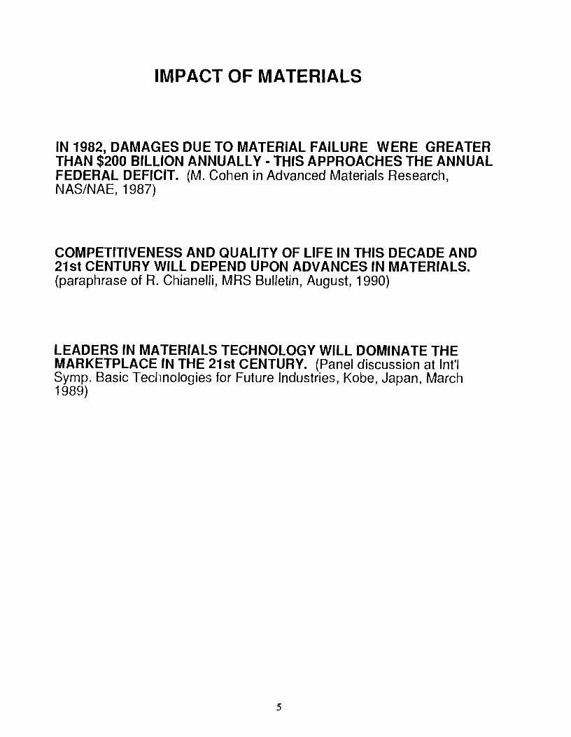
IMPACT OF MATERIALS

IN 1982, DAMAGES DUE TO MATERIAL FAILURE WERE GREATER THAN $200 BILLION ANNUALLY - THIS APPROACHES THE ANNUAL FEDERAL DEFICIT. (M. Cohen in Advanced Materials Research, NAS/NAE, 1987)

COMPETITIVENESS AND QUALITY OF LIFE IN THIS DECADE AND 21st CENTURY WILL DEPEND UPON ADVANCES IN MATERIALS. (paraphrase of R. Chianelli, MRS Bulletin, August, 1990)

LEADERS IN MATERIALS TECHNOLOGY WILL DOMINATE THE MARKETPLACE IN THE 21 st CENTURY. (Panel discussion at Int'I Symp. Basic Technologies for Future Industries, Kobe, Japan, March 1989)

5

EVOLUTION OF MATERIALS SCIENCE AND ENGINEERING

10,000 BC 5000 BC

w <..> z e:( I-0: o a. :E

w > le:( -I W 0:

o 1000 1500 1800 1900 1940 1960 1980 1990 2000

DATE

2010 2020

COMMODITY METALS AND PLASTICS HAVE PASSED DEMAND PEAK AND USAGE IS DECLINING

COMMODITY PLASTICS

SUPERALLOVS

SPECIAL TV METALS

ENG. PLASTICS

ADVANCED PMCs

STRUCTURAL CERAMICS

HEAVY R&D

RAPID GROWTH

GROWTH maturing=GDP

7

ALUMINUM

COPPER

CARBON STEEL

GROWTH < GOP

THERE IS A CHANGE IN BASIC MATERIAL USE

• SUBSTITUTION OF ONE MATERIAL FOR ANOTHER HAS SLOWED THE GROWTH OF DEMAND FOR PARTICULAR MATERIALS

• DESIGN CHANGES HAVE INCREASED THE EFFICIENCY OF MATERIALS USE

• SATURATION OF MARKETS WHICH WERE PREVIOUSLY EXPANDING HAS OCCURRED

• LOW MATERIALS CONTENT IN PRODUCTS FOR NEW MARKETS, PARTLY BECAUSE OF THE COST OF HIGHER PERFORMANCE MATERIALS

8

MARKET DEMAND IS NOW LIGHTER, STRONGER, MORE DURABLE MATERIALS

Desired Characteristic Aero. Auto Bio Chern. Elec. Energy Metal Tele.

Light / strong v v v High temp resist. v v v v v Corrosion resist. v v v v v v v

Efficient processing v v V' v v v v v Near-net-shape v v V' v v v v v Prediction of life v v V' v v v v v Prediction of properties v v v v v v v v Materials data bases v v V' v v v v v

(Materials Science and Engineering for the 1990s)

9

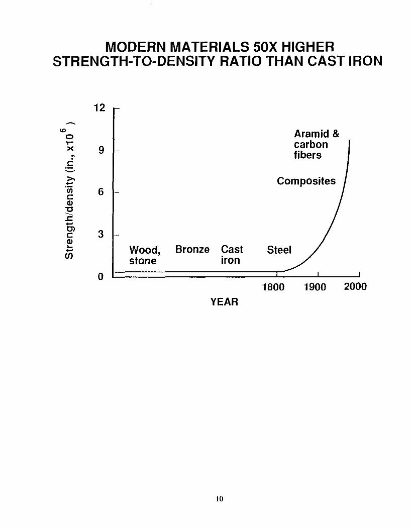
MODERN MATERIALS 50X HIGHER STRENGTH-TO-DENSITY RATIO THAN CAST IRON

12 ..-

to Aramid & 0 ,.. carbon >< 9 fibers ~ . c -->- Composites -en 6 -c cu

"C --J: -C) 3 c

cu :1.0 Wood, Bronze Cast Steel -en stone iron

0 1800 1900 2000

YEAR

10

--0 --Q) ... :::J -ro ... Q) a. E Q) J-Ol r:: :;:; ro ... Q) a. 0 Q) r:: Ol r:: w

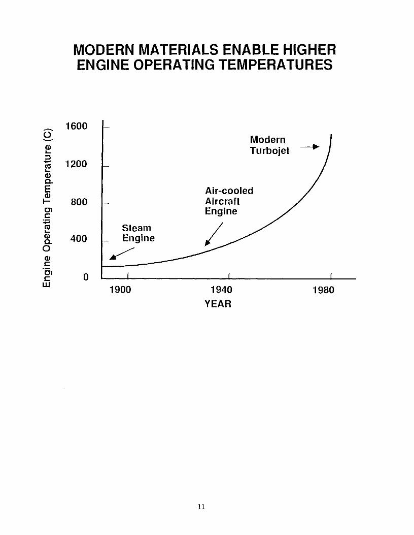
MODERN MATERIALS ENABLE HIGHER ENGINE OPERATING TEMPERATURES

1600 Modern Turbojet -.-

1200

Air-cooled 800 Aircraft

Engine

Steam 400 - Engine

/ 0

1900 1940 1980 YEAR

11

MATERIALS ENABLED EXPONENTIAL INCREASE IN CUTTING TOOL SPEED

1000-

-I:

E ---I: '-'

'C 100 OJ OJ a. en Ol I: ..... ..... Tool :J () steel

10 1800

12

BN, Diamond

Ceramic

High-speed steel

1900 YEAR

2000

c

THE PORTFOLIO OF ADVANCED MATERIALS

CERAMICS

13

STRUCTURAL CERAMICS ARE LEADING CANDIDATES FOR MANY APPLICATIONS

TRADITIONAL

Based primarily . Clay products CERAMICS on natural raw . Glass materials of clay

Inorganic, nonm,etallic and silicates Cement

materials processed

or consolidated at ADVANCED*

high temperaturE~s Include artificial

raw materials, ~ Structural

exhibit specialized Electronic properties, require

more sophisticated Optical

processing

* Fine ceramics, En9ineered ceramics, New ceramics, Value-added ceramics

14

THE APPEAL OF STRUCTURAL CERAMICS IS EASY TO UNDERSTAND

Desired Characteristic

Light / strong ~

High temp resist.

Corrosion resist. -Efficient processing

Near-net-shape

Prediction of life

Prediction of properties

Materials data bases

Light with compressive strength> or = metals

Withstand extreme temperatures

Chemically inert, hard, abrasion resistant

BUT REALIZING THESE PROPERTIES REQUIRES A LEVEL OF MICROSTRUCTURAL AND CHEMICAL PERFECTION FAR BEYOND THAT OF TRADITIONAL CERAMICS

15

STRUCTURAL CERAMICS ARE A RESULT OF A FEW KEY DEVELOPMENTS

TRADITIONAL + DEVELOPMENT = ADVANCED

MATERIALS NATURAL SYNTHETIC SYNTHETIC MATERIALS (CONTRIVED)

PREPARATION

ANALYSIS OPTICAL, XRD, MICRO-MACRO ELECTRON ANALYSIS

MICROSCOPY

PROCESSING HISTORIC, RELATIONS OF UNIFORM CHEMISTRY & TOLERANT PROCESSING STRUCTURE & PROPERTIES

16

SOPHISTICATED MICROSCOPY ALLOWS DETERMINATION OF MICROSTRUCTURE

17

MECHANICAL PROPERTIES CAN BE DETERMINED AT THE MICROSTRUCTURAL LEVEL

18

TENSILE TESTER-SPECIALIZED EQUIPMENT FOR DETERMINING CERAMIC MECHANICAL PROPERTIES

19

TENSILE TESTER-FULL VIEW

20

ADVANCES IN CERAMICS WILL BE BASED ON ATOMISTIC MODELING, TAILORED MICROSTRUCTURE AND

SOPHISTICATED PROCESSING

LU U Z

~ CC o c.. :: LU > i= « ....J LU CC

1O,000BC

I EMPIRICISM

o 1500

dill. calculus

thermo

ATOMISTIC MODELING & PROCESSING

e-micro

micro models

MATHEMATICS & CONTINUUM

MODELING

1800 1900 1940 1960 1980 2000

21

t LU en ~

t-Z LU cc cc ~ u

t 2020

TOUGHENING IS REQUIRED TO MAKE CERAMICS VIABLE FOR STRUCTURAL APPLICATIONS

2

103

FLEXURE STRENGTH

(MPo) 5

2

ORNL-DWG 89-18176

MAXIMUM FLAW SIZE (X1(}3 in.)

102L-~~L-~~UL~~~-L~LU~~ 10' 102 2

MAXIMUM FLAW SIZE (X 10-6 m)

TOUGHNESS (MPIJm)

ORNL· DWG 89-1 .... 19

25 r-----------------------------------~

15

10

0L....-__ L-__ 1...-__ 1...-__ 1...-_----J

o 200 400 600 800 1000

TEMPERATURE (OC)

MICROSTRUCTURE TAILORING & NOVEL COMPOSITE DESIGN ADDRESS INHERENT BRITTLENESS

OF CERAMICS

20

0 W

en en 15 W z :I: CJ :J 0 I-

10 W a: :J I-U <t a: LL 5

a: U z wa: QCJ mO -LL

en I-z LL Z <t- iii w :i z 0 0 a: w a: S< a:w o:I: 0 wU LLCJ

en • ~a: en:J w z eno zO 0 0 -LL <tI-S< Z :I: z a:

en 0 3:- I-

0 W

W a: en

D en <t ...J CJ

II o

COMPARED TO METALS WITH TYPICAL FRACTURE TOUGHNESS OF 15-200

23

FRACTURE RESISTANCE is INCREASED BY REINFORCING CERAMICS WITH STRONG MICROSCOPIC WHISKERS

Ceramic Whiskers and Human Hair

Ceramic Composite Fracture Surface

Toughness Model

• ,

.,~c, LlJ-l · · rr[~GJ

APPUED WHISKERS BRIDGING STRESS 'NHISKERS

'.\

.. :)i i -,¥'. I::

.N = Fracture strength Nhisker V = Vol. fracture whiskers r = Whisker radius E = Young's modulus G = Fracture Energy

~

R&D ADDRESSING EFFECTS OF WHISKER

COATINGS ON COMPOSITE PROPERTIES

Alumina-SiC whisker interface Carbon coated whisker-alumina interface

SILICON CARBIDE WHISKER-TOUGHENED ALUMINA CERAMICS

ORNL-PHOTO 71 04-88R

FIBER-REINFORCED CERAMIC COMPOSITES HAVE BEEN FABRICATED USING A FORCED CHEMICAL VAPOR INFILTRATION PROCESS

HfATING ELEMENT

GRAPHITE HOLDER

HOT ZONE

EXHAUST GAS

REACTANT GASES

WATER COOLED SURFACE

FIBROUS PREFORM

27

EXPERIMENTAL RESULTS SHOW MODIFICATION OF MATRIX! WHISKER INTERFACE IMPROVES COMPOSITE TOUGHNESS

SiC MATRIX

-{;ARIIoiON PRECOAT

28

t STRESS

EQUAL DEBONDING

STRAIN-

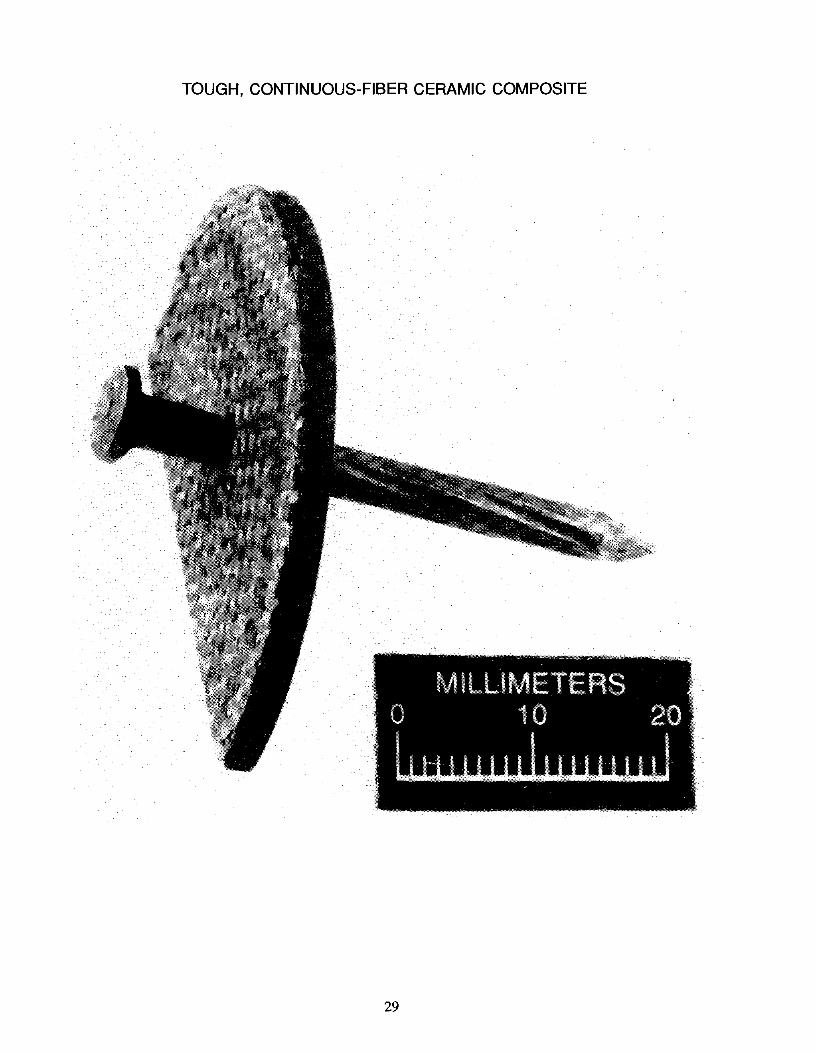
TOUGH, CONTINUOUS-FIBER CERAMIC COMPOSITE

29

w o

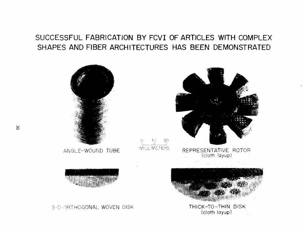
SUCCESSFUL FABRICATION BY FCVI OF ARTICLES WITH COMPLEX SHAPES AND FIBER ARCHITECTURES HAS BEEN DEMONSTRATED

, , , , •. ,,~,~,,~ __ '-__ _ ~.d.~~_.~

ND TUBE

HOGONAL WOVEN

REPRESENTATIVE (cloth layup)

THICK-TO-THIN DISK (cloth layup)

R

CERAMICS TESTED IN AEROSPACE APPLICATIONS

w N

Large Scale Manufacturing of Monocoque Cor Chassis at the Fibrous Materials Research Laboratory

w w

ADDITION OF Zr02 TO BRIDLE CERAMICS INCREASES RESISTANCE TO CRACK PROPAGATION

ORNl:- DWG 89 -18172

TRANSFORMATION ZONE

• Toughening is derived from stressinduced martensitic transformation in Zr02 particles

Transformation consumes energy needed for further propagation

Increased volume of new phase contributes compressive forces resisting further propagation

MICROWAVE SINTERING HAS SIGNIFICANT IMPLICATIONS FOR NEW MATERIALS APPLICATIONS

>l-V)

Z W

ORNL-DWG 89-18171

ALUMINUM OXIDE

MICROWAVE f. 28GHz P

/ , P ,

o 60 ;::1" o-.... STANDARD

50 L---L-.-L---J----L--L--.J

800 t 000 t 200 t 400 TEMPERATURE ("C)

Zr92:8mo1 "'0 Y2Q3 1 00 r-r;;r:;~tr::::I:M<Jo-1

~ 90 ,," ~28GHz

>-I- 80 V)

z w 70 o

, I

/~TANDARO d

2.45GHz 60 L--......... ..J_-L-.....L-.....L-...J

1100 1200 1300 1400 TEMPERATURE COC)

• Accelerated Kinetics: - Sintering occurs at lower

temperatures

• Significant Potential Benefits Lower temperature processing Finer microstructures Better mechanical properties

• Advanced Materials Applications:

34

- Composites from incompatible materials Self-lubricating high-temperature bearings Electrical materials Engine components

C/) o ::: « a:: w o CJ z it C/) z w Cl a:: f2 ~ :J o ~ w >

~ a:: o :::

35

Microstructure of Si3N4-6% Y203-2% AI203 After Annealing at 1200°C

for 20 hours

Conventional Heating Microwave Heating

MICROSTRUCTURE MODIFICATION SIGNIFICANTLY IMPROVES CREEP RESISTANCE

300

250

--.. co 200

0... 2

r ------- ~h 1 SN-6Y2A ANNEALING CONDITIONS: 1200°C/20 h ..

TEST TEMPERATURE: 1260°C ---_. ---------- ----. .-----

----_.-.../ I

",.

2400

2000

1600

--..

~ 150 1--_-__ --.1

W

CA ",. ., 1200 §.

a: I-Cf) 100

50

o o 20

-... ~.-."'.-._._I_._._._._I~."I_."'·-·- MA _.-.-.._-_.----_.-._.-.

800

400

_J 1 __ --L_...L....-.l.-~_~_-.l________1__ __ L-l 1 __ 1_ 1 __ 1 L -----1.. __ ---1-------1__ 0 40 60 80 100 120 140

TIME (h)

37

-

Tensile creep of NTX-1S4 and NT-164 at 1370°C

NTX-154 had a glass layer at most Si3NiSi3N4 grain boundaries after

creep (100 MPa, 1200 h).

No glass layer was found at NT-164 Si3NiSi3N4 grain boundaries after

creep (150 MPa, 959 h).

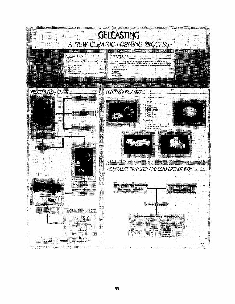
aaCASTlNG A NEW CERAMIC FORMING PROCESS

TECHNOLOGY TRANSFER AND COMMERClAUZATlON __

39

EXTENDED VEHICLE TESTING OF VALVE TRAIN COMPONENTS

J-)t I I f)M(J I 1 VI

f j I! ~ I r '" t- J I I;:: I ! ) I

41

SUMMARY

• SPECIALIZED, TECHNOLOGY-INTENSIVE, HIGH-VALUE-ADDED ADVANCED CERAMICS ARE MOVING TOWARD COMMERCIALIZATION TO Fill THE DEMAND FOR LIGHTER, STRONGER, MORE CORROSION RESISTANT MATERIALS

• ADVANCEMENTS Will RELY MORE AND MORE ON PROCESSING AND MODELING FROM THE ATOMIC SCALE UP WHICH IS MADE POSSIBLE BY ADVANCED ANALYTIC, COMPUTER, AND PROCESSING TECHNIQUES

• SPECIALIZED PROPERTIES AND HIGHER COST Will PROVIDE BOTH NEW OPPORTUNITIES AND CHAllENGES TO DESIGNERS AND END-USERS

• MORE RIGOROUS DEFINITION OF COMPONENT REQUIREMENTS

• COMPONENT REDESIGN TO ACCOMMODATE BRITTLE BEHAVIOR

• SYSTEM REDESIGN TO MAKE FUll USE OF NEW MATERIALS

• CLOSER COUPLING BETWEEN DESIGNERS AND MATERIALS DEVELOPERS

43

TEMPERED GLASS AND

THERMAL SHOCK OF CERAMIC MATERIALS

L. Roy Bunnell

Battelle-Pacific Northwest Laboratories Battelle Boulevard

P. O. Box 999 Richland, Washington 99352


45

TEMPERED GLASS

L. Roy Bunnell Pacific Northwest Laboratory', Richland, WA

KEY WORDS: glass, tempering, annealing

PREREQUISITE KNOWLEDGE: This material could be taught as a demonstration to a typical student of materials science, at the high school level or above. More depth can be provided by having students actually temper and anneal the glass, but this requires more equipment and time. This writeup contains a simplified method for making tempered glass which uses minimal equipment.

EQUIPMENT AND SUPPLIES: (Demonstration version) Automobile side windows, obtained from an auto wrecking yard; spring-loaded center punch; polyethylene bag large enough to hold a window; two polarizing filters; overhead projector. For the laboratory version, use all of the above plus the following: Pyrex" brand borosilicate glass rod, about 6 mm diameter; torch burning oxygen-acetylene or oxygen-natural gas or propane; water-filled bucket of 20-1 capacity; side-cutter pliers.

PROCEDURE: First, introduce the concept that glass is a very strong material, state that tensile strengths greater than 6.9 GPa have been measured on fresh surfaces free from all damage. Surface damage, including that resulting from the corrosive action of water, creates tiny defects that reduce the useful strength to a tiny fraction (0.2%) of this value. By using a special property of glass--the dependence of its density on its cooling rate--glass can be toughened to make it more durable and its fracture may be controlled so that dangerous shards are not produced. This process is called tempering.

Glass, like all other ceramic materials, is brittle, meaning that it will fracture at a very low strain, usually 0.01 to 0.1 percent. Like all other ceramics, failure usually starts at the surface, and this surface is very easy to damage by contact with other hard materials or even by atmospheric attack. Since the surface is easy to damage and failure begins at the surface, a process is required which makes the surface less sensitive to incidental damage. This is done by placing that surface in compression. A thermal process for accomplishing this is the subject of this experiment.

As shown in Figure 1, the density of a typical glass is dependent on its cooling rate. At high cooling rates, the glass structure becomes rigid at a density corresponding to that usually seen at high temperature. At lower cooling rates, there is more time for the glass structure to adjust so that the final density is higher. If a piece of glass is heated to a temperature above

Pacific Northwest Laboratory is operated by Battelle Memorial Institute for the U. S. Department of Energy under Contract DE-AC06-76RLO 1830.

•• Made by Corning Glass Works.

47

point A on the curve shown and suddenly quenched, the surfaces will cool first and become rigid at the low density corresponding to that temperature. The inner glass will cool more slowly and will reach a greater density, which means that it will pull inward on the outer glass, placing it in compression. The inner glass is placed in tension to balance the compression, but it is shielded from incidental damage by the outer glass. Since the surface glass is in compression, it will withstand quite a lot of bending strain before it is placed in tension, as is required to break it. The incidental impacts in everyday use are resisted far better by such glass, which is called tempered glass. The mechanism for tempering glass is much different than that used for tempering steel, and it may be productive to discuss the difference to avoid confusion.

In the manufacture of tempered glass for the side and rear windows of automobiles and for sliding glass doors, the glass is heated above point A, then cooled rapidly by an array of air jets blowing on both of its faces. Demonstrate this using a piece of car side window glass obtained from a wrecking yard for about $10. With a strong light behind the piece of tempered glass, place a polarizing filter on both sides of the glass. By rotating one of the filters, the pattern left by the air jets can be seen. Some students may recall seeing similar patterns through polarizing sun glasses in light reflected from back windows of cars. Polarized light is rotated differently passing through stressed glass than it is through unstressed glass. Demonstrate the toughness of the glass by supporting it between two short pieces of wood, then standing on it. It will support your weight easily, though you may want to resist the temptation to jump on it to make a point. Note: Just in case the &lass should break. place it inside the plastic bag so that the many fra&ments will be captured. This is important both to promote safety and to avoid cleanup problems.

Ask the students why, if tempered glass is so strong, it is not used in windshields. The answer is that when it breaks, it fractures into very small, roughly equiaxed pieces. A rock flipped up by the car ahead could leave you trying to drive using an opaque windshield! This fracture characteristic is an important safety feature, in that tempered glass is relatively safe when broken. It does not fracture into long, knifelike shards such as seen in ordinary glass.

Someone may ask how tempered glass may be broken, say in an escape situation if needed. Emergency personnel--policemen, ambulance drivers, etc.--routinely carry spring-loaded center punches for just such emergencies. This kind of punch generates large shock forces, enough to make indentations in steel, with enough force to overcome the compressive stress in our tempered glass window. Once the outer glass is damaged by a large enough force, the force equilibrium is disruptedl and the entire piece of glass destroys itself. Demonstrate this by first placing the car window in a plastic bag, then using the center punch to damage the glass through a small hole in the bag. The window will fail with a loud noise, and the pieces can be seen to be small and not very dangerous.

In a class permiltting more depth in this subject, students may temper glass for themselves. By heating a Pyrex rod in a suitably hot gas flame, droplets can be formed and allowed to fall into a bucket of water to quench them. Such a quenching method is poorly controlled, so the size of the droplets is critical; small droplets will experience less tempering than desired and large droplets may fracture when quenched. Use caution during this operation. both with molten glass and with less obviously hot glass that has been set aside. Tempering can be demonstrated by first grasping the droplet in the palm of the hand, then cutting the protruding "tail" off, using a pair of

48

side-cutting pliers. Use safety idasses or close eyes during this operation. The droplet will detonate, and will be easily felt by the student. Upon opening the hand, the glass will be found as tiny grains.

These droplets may be annealed by heating them in a furnace to 500 C, then letting them furnace cool. If the tail is now cut off the droplet, there will be no dramatic fracture as before; the stresses have been relieved by the annealing process.

SAMPLE DATA SHEETS: Not Applicable.

INSTRUCTOR NOTES:_Students should be closely supervised during the tempering and testing of the glass droplets.

REFERENCE: Kingery, W. D., H. K. Bowen, D. R. Uhlmann, Introduction to Ceramics, 2nd Edition, John Wiley & Sons, 1976, Ch. 16.

SOURCES OF SUPPLIES: Pyrex rod and polarized plastic sheets can be obtained from any scientific supply house, and a suitable torch from any supplier of welding supplies. Alternately, school shop facilities could be borrowed.

49

Q)

E ::J '0 >

Temperature

Figure 1. Relationship between temperature and volume for a typical glass. Rapid cooling results in a higher volume (lower density) than obtained with slower cooling, because more time is available for structural rearrangement in the glass.

50

THERMAL SHOCK OF CERAMIC MATERIALS

L. Roy Bunnell

* Pacific Northwest Laboratory, Richland, WA

KEY WORDS: thermal shock, Young's modulus, thermal expansion coefficient

PREREQUISITE KNOWLEDGE: This demonstration is suitable for students in materials science at the high school or college levels. The students should understand elementary mechanics concepts, such as Young's Modulus of Elasticity.

OBJECTIVES: To demonstrate the concept of thermal shock in cerami c materials, and to illustrate the pertinent factors of materials selection.

EQUIPMENT AND SUPPLIES: Furnace capable of controlled temperatures up to 500°C; aluminum oxide rod or 2-hole thermocouple insulator, approx. 3 mm diameter x 10 cm long; water; tongs; black or blue ink.

PROCEDURE: Thermal shock is a mechanism often leading to the failure of ceramic materials. Many uses for ceramics involve high temperatures, and if the temperature of a ceramic is rapidly changed failure may occur. Thermal shock failures may occur during rapid cooling or during rapid heating. As an example, consider rapid cooling, which is easier to visualize. If a ceramic material is cooled suddenly, the surface material will approach the temperature of the cooler environment. In doing so, it will experience thermal contraction. Since the underlying material is still hot, the skin material is stretched and so experiences tensile stress. If the resulting strain is high enough (0.01% to 0.1% for most ceramics), the ceramic will fail from the surface and cracks will propagate inward. Even if these cracks do not cause i mmedi ate failure, the ceramic will be severely weakened and may fail from mechanical overload of forces it would normally withstand.

After d i stri but i ng a 1 umi num oxi de rods to the students urge them to manipulate and bend the rods with their hands. Soon, popping sounds will be heard in the classroom. These sounds demonsrate how a brittle material fails without warning, with no permanent strain, and at a low-strain val ue. Next, place about ten of the rods into a stainless steel beaker or a small metal pan and heat to 500°C in a suitable furnace. Remove the container from the furnace and quickly quench the rods in a bucket of water, then dry them overnight at about 100°C. The following day, dip the rods in ink, which acts as a crude dye penetrant to make any cracking visible. Wipe excess ink from the rods, handling carefully to avoid breaking. Again, urge the students to bend the rods and note that the rods are much weaker than before. A 1 so, note from the parti a 1 penetration of the ink that the cracks do not extend into the centers of the rods. This is because the cracks start at the surface in a tensile stress area, but propagate into regions of lower stress until they stop. When a quench is performed at lower temperatures (down to about 300°C) crack density is lower and crack length is shorter. A quench temperature that is lower still will not

* Pacific Northwest Laboratory is operated by Battelle Memorial Institute for the U. S. Department of Energy under Contract DE-AC06-76RLO 1830.

51

result in any detectable damage. This temperature is not a constant, but is a function of both configuration and material.

When comparing different ceramics for thermal shock applications, it is common to use a figure of merit or index of thermal shock performance. This is a number (ratio) that is useful for both choosing materials and for visualizing the thermal shock process. Since the index should be high for a thermal shock resistant ceramic, its numerator should contain properties that are numerically large when good thermal shock performance is exhibited by a material. Tensile strength (S) and thermal conductivity (K) are therefore placed in the numerator, the former for obvious reasons and the latter because a high value of thermal conductivity tends to decrease thermal gradients, other factors being equal. The denomi nator of thE! thermal shock index is composed of the thermal expans ion coefficient (A) and the Young's modulus of elasticity (E). The thermal expansion is responsible for the failure-causing strain, so it should be as small as possible. The elastic modulus is a measure of the stress resulting from a given strain, so it should be a low value for good thermal shock performance. Combining these factors,

Thermal Shock Index (TSI) = SK AE

where the units of measurement should be consistent within a given comparison. In the case of common glasses, all of the properties except thermal expansion fall into a relatively narrow- range. By choosing a glass with low thermal expansion, thermal shock failure can be avoided in most cases. See, for example, the index values for soda-lime glass, borosilicate glass, and fused silica in Table I. Note the large difference between the thermal shock indices of aluminum oxide and graphite. This difference is backed by experience; it is extremely difficult to cause graphite to fail by thermal shock, principally because its Young's modulus is so low and its thermal conductivity is high.

SAMPLE DATA SHEETS: If students quench specimens from a series of temperatures, data sheets might be constructed to record crack frequency as a function of quench temperature. Alternately, ceramic rods might be broken in 3-poi nt bendi ng on a testing machi ne, and the bendi ng strength plotted as a function of quench temperature.

INSTRUCTOR NOTES: Provi ded above in Procedure. precautions to avoid burns.

Follow usual safety

REFERENCES: Kingery, W. D., H. K. Bowen, D. R. Uhlmann, Introduction to Ceramics, Second Edition, John Wiley & Sons, New York, 1979, Ch. 16.

SOURCES OF SUPPLIES: purity greater than 95%.

The alumina should be >95% dense, but can be of any One supplier is Coors Ceramics, Golden, CO.

52

Table I. Thermal Shock Index for Some Common Ceramic Materials

K,(1) A, oe l,

Materi a 1 WLcm-oC S, MPa x 10-6 E, GPa -.lSL

Soda-l ime-sil ica 2E-2 68(2) 9.2 69 2.1 glass

Borosilicate glass 2E-2 68 3.3 63 6.5

Fused Si02 6E-2 68 0.6 72 94

Aluminum Oxide 3E-l 204 5.4 344 33

Graphite(3) 1.4 8.7 3.8 7.7 416

(1) Thermal conductivity and expansion coefficients from Thermophysical Properties of Matter, Y. S. Touloukian, ed., Plenum Press, New York, 1970.

(2) Because glass tensile strength is so dependent on surface condition, a single "reasonable" value was chosen for all glass strengths.

(3) Values are typical of nuclear-grade graphite, from Industrial Graphite Engineering, Union Carbide Corp., 1959.

53

ELEMENTARY METALLOGRAPHY

Sayyed M. Kazem

MET Department Purdue University

Knoy Hall - Room 119 West Lafayette, Indiana 47907


55

ELEMENTARY METALLOGRAPHY

Sayyed M. Kazem MET Department, Purdue University

West Lafayette, Indiana 47907

INTRODUCTION

Materials and Processes I (MET 141) with two one-hour lectures and one two-hour laboratory is offered to freshmen by the Mechanical En~ineering Department at Purdue University. This elementary course, required for METjCIMT majors, is an elective for other majors (IT and AT) and is also a prerequisite for other process courses (casting, welding and metallurgy). The goal of MET 141 is to broaden the technical background of students who have not yet had any college science courses. Hence, applied physics, chemistry and mathematics are included, and quantitative problem-solving is involved. The course outline consists of (1) General Inspection; (2) Properties - Physical, Chemical and Mechanical; (3) Processes and Selection - Metallic, CeraIll1cs and Plastics. The goal of the laboratory is to reinforce and supplement the lecture material. There are eight experiments: (1) General Materials Inspection; (2) Hardness; (3) Toughness; (4) Polymers; (5) Steel Heat Treatments; (6) Aluminum Alloy Heat Treatments; (7) Metallography; (8) Recycling. Each lab section has up to 24 students. Depending on the type of the expenment and the available equipment, some experiments may split the students into subgroups (A and B). In the metallography experiment, there should be a maximum of 12 students in each group for alternate weeks.!

In an elementary metallography experiment, the objectives are: (1) Introduce the vocabulary and establish outlook; (2) Make qualitative observations and quantitative measurements; (3) Demonstrate the proper use of equipment; (4) Review basic mathematics and science.

BACKGROUND

Metallography, a branch of physical metallurgy, is the study of the constitution and structure of metals and alloys. When a molten metal starts to solidify, small nuclei or seeds at various locations and orientations are formed. On each seed the neighborin~ atoms attach themselves in an orderly manner and ~row continuously at different orientatIOns, until confronted by neighbors. Each dendntic growth is roughly spherical, separated from its neighbors by definite boundaries, and is called a "grain" or "crystal." The average diameter, called "grain size," is a function of nucleation rate, growth, later heat-treatment, etc. The grains of a pure metal have the same lattice but different orientation of their crystal axes. When two grains of two different orientations come in contact, the "grain boundary" is really a zone of mismatch2. Since these border atoms (along grain boundary) are packed less densely (have fewer neighbors) they possess more energy than those others within the grain. Also, other atoms diffuse more easily along the boundaries than in the grain proper. This indicates that atoms along the boundaries are less tightly held, more reactive and energetic3. Exposed to corrosives or etchants, the grain boundary dissolves more than does the grain proper. The etched boundary then appears as a groove (in an otherwise flat surface) and the microstructure reveals black lines.4

57

It has been shown that most of the complex "polycrystallines" have intersections of any three grain boundaries at angles of 1200 (see FIg. 1). Ideally, the grain structure of pure metals approximates the tri-corners (shown in Fig. 2.)4. Grains can be described as macroscopic or microscopic.

Grain 1 / Grain 3

Grain 2 \

Figure 1 Three grains at angles of 1200 to each other.

Figure 2 Micrograph of vacuum-deposited aluminum film, 0.5 Jl.m at 26,000 x.

MACROSCOPIC AND MICROSCOPIC SAMPLES

A. Qualitative Examinationl,5,6

Macrophotography is appropriate when the grains of a specimen are visible to the naked eye or with a diametral ma~nification up to SOX. Examples of macroexamination include: (1) surface grains (motthng) on a cast-brass doorknob polished by normal use; (2) lar~e size crystals (spangles) on galvanized steel-sheets; (3) aluminum grains on light-poles viSIble from the road; (4) columnar crystals at broken edges of cast-iron; (5) ice crystals at fractured ends of Popslcleslll

•

Preparation of samples for macro examination is usually simple, involving less polishing and larger areas, for gross problems. Specimens may be burned off by acetylene torch, trimmed by hacksaw, then sectioned by cutter (water-cooled). After burrs are removed, the sample surface is planed by belt-sanders and smoothed by table grinders (water-cooled). Polishing is done by coarse 40-150 grits of emery paper. Frictional heating and structural distortions should be avoided.

After surface cleaning by water, the sample is etched. Use a 10% solution of nitric acid (HN03) for steel structure; a 50% water solution of hydrochloric acid (HCl) or 25% solution of nitric acid may reve:al the flow-lines in forged steel and quench-cracks from heat treating. After deep etching is complete, the sample is rinsed in hot water, dipl?ed in benzene or acetone, and dried in warm air-blast. When a dry surface is coated With printer's ink, an impression may be transferred to art paper. Simple macrographs may even be produced by pencil rubbings or photographs.

Unprocessed specimens may be examined. For example, a tensile or bending specimen may show ductile necking and cup-cone fracture, whereas a brittle piece may have glassysmooth fracture without necking.

58

B. Quantitative Examination

Specimens are examined and evaluated by metallurgical microscopes and reflected light (50-200Ox). Specimen preparation is critical, since small areas are inspected and measured, with statistical inte!1'retation of data. Samples are cut and smoothed as before; however, flame cutting and fnctional heating are risky. A thin section is cut off (water-cooled) and mounted in "buttons" of thermoset plastic (phenolic Bakelite'", or acrylic Lucite '") about oneinch diameter and half-inch thickness. The sample surface is carefully flattened by a wet-belt sander, which leaves parallel scratches. The sample is always washed (in soapy water) and then rotated (9Qo) before each subsequent grind or polish. Exactly 2.54 cm equals an inch.

Polished samples are examined by microscopes for defects which require repolishing. Ideally, a mirror-surface (scratch-free at lOOOx) is achieved before etching. The polishers are usually fine emery (or diamond paste). The etchant is a weaker acid or base solution; conservative practice is to under-etch, then to re-etch as desired. This flushes away the last layer of "distorted atoms".

C. Grain Size, Grain Size Number and Grain Boundary Area? 8

Since grain size and grain bound~ area of a metal are important, the American Society for Testing and Materials (ASTM) has established reference nets with grain size numbers for comparison. When observed at lOOx, the ASTM grain size number (n) can be determined from the ASTM grain size equation N = 2n-l , where N is the number of grains per in2. If N' is the number of grains per in2 for other than lOOx, say (SOX), then multiply N' by (100/50)2 to obtain N; then use the ASTM grain size equation.

There are three methods to estimate grain size and determine the ASTM grain size number: (1) Planimeter (Jeffries) method; (2) Intercept Methods; (3) Comparison Method.

(1) Planimeter Method: A circle or rectangle of known area (usually 5000 mm2) is inscribed on a micrograph, or ground-glass screen of the metallograph, of known magnification. The magnification should be such to ~ive at least 50 grains in the inscribed area. The number of grains counted within the area IS added to one-half of those grains intersected by the boundary. The number of grains per mm2 (N) for the given ma~nification is calculated readily. For a reasonable average a minimum of three representative fIelds should be tried. From known magnification, the ASTM grain size number (n) can be determined.

This method works well with equiaxed grains; otherwise, count should be made on three mutually perpendicular planes determined by the longitudinal, transverse and nonnal conditions.

(2) Intercept Methods: The intercepts, more convenient than the planimeter method, are recommended for structures which depart from uniform equiaxed structures. The procedure may be done by hand or by machines. There are two common methods: a) Lineal and b) Circular.

a) Lineal Intercept (Heyn) Method: The ~rain size can be estimated by counting on a photomicrograph (or ground-glass screen or speCImen itself) the number of grains intercepted by one or more straight lines. Grains intersected by the end of the line count as half grains. For a reasonable average, counts must be made on at least three different lines. The length of the line, divided by the average number of grains intersected by it, gives the average intercept length (or grain diameter).

59

b) Circular Intercept Methods: These are favored7, because circular arrays automatically compensate for non-equiaxed shapes of grains. This procedure avoids overweighting local portions of the sample's field and eliminates ambiguous intersections at straight-line ends. The manual routine is effective for grain estimation in quality control. A circular method is slightly biased, overvaluing the mean-intercept distance for samples with few intersections, but bias fades fast as intersections increase. There are two common procedures: i) Monocircle, and ii) Tri-circle.

The single-circle procedure is recommended when grain-size variation is large, and high precision is not required. Draw a circle of known circumference (100, 200, or 25Onm) and count the intersected grain-boundaries. Different circles can be drawn at different locations. Select the magnification to yield no less than 35 counts per circle.

The three-circle procedure draws concentric and equally spaced circles, whose total circumference is 500 mm. Subsequent steps are the same as above.

The grain boundary area4,5: In the circular intercept method, after the circle is drawn on a photo-micrograph, the number of points of intersections per unit length of test line PL can be determined. If Sy is the boundary area per unit volume (say in2/in3), and LA is the sum of lengths of linear features per unit test area (say in/in2) then Sv = 2PL and LA = f PL.

(3) Comparison Method: After the sample is prepared, the image of the microstructure projected at 100x (or its photograph at 1OOx) 1S compared with a series of graded standards (grain size charts) indexed in four categories. Plates I, II, III, IV are available from ASTM Headquarters, 1916 Race Street, Philadelphia, P A 19103. By direct comparison of the specimen's microstructure with the appropriate photomicrograph of a standard grain size, one can select the standard photomicrograph (or interpolate between two) which most nearly matches the specimen. If a specimen has two different grain-sizes, it is reported in terms of two numbers, designating the approximate percent of each size.

EQUIPMENT AND SUPPLIES

A. Units in the Materials Laboratory of the MET Dept. 1. Equipment: Cut-off wheel, deburring wheel, mounting press, belt sanders, grinding wheels, polishing wheels, metallographic microscopes, ventilation hood, desiccator, planimeter ruler, compass. 2. Supplies: Metal samples (raw, polished), polishing powders (aluminum 0.3 and 0.05 micron), ethanol, acetone, coatmg oil, distilled water, water glass, swab (Q-tiplM); etch ants.

B. Notes 1) The equipment and supplies are well maintained. 2) Students operate equipment and handle supplies properly and cautiously

(under instructor's supervision). 3) The space for the above equipment and supplies is about 300-400 ft.2 (30-

40m2) •

C. Alternatives:

1) Using smaller portable equipment may occupy one-quarter of normal space.

60

A.

B.

2)

3)

Visiting the metallography laboratory of a metallurgy or materials department may involve a brief walk-through or an extensive show-andtell. The last resort is obtaining a film on metallography, to elucidate proper techniques.

PROCEDURE

Observation l. The instructor gives an overview of metallography terms, realms, and

uses. Then, students get a show-and-tell session, which may be followed by practice from sample-cutting to etching. Different students perform the tasks, while others watch. Under the supervision of the instructor, a student may be asked to cut the sample, another to debur, and a third to mount it; other students observe, while the instructor comments on their

2.

3.

4.

safety and technique. All students take notes. Students observe commercial samples having microscopic ~rain, such as brass door-knobs and galvanized steel-plates. Full-size (Ix) photographs, impressions, or prints of these metals are also exhibited. Students estimate grain SIze and grains/area using standard charts (Hexagonal or McQuaid-Ehn). Microphotographs of some alloys, with large or small magnifications, are exhibited. Students then calculate actual grain-size number from counts of grains (number per square inch). Micrographs of non-metallic ceramics and polymers are also exhibited. Some 2-D (Optical) and 3-D (Scanning Electron Microscope) views are compared and contrasted. Metal powders (P /M) are identified by size and shape, with 3-D photos.

Measurements 1. During observation and experimentation, each student makes free-hand

sketches of equipment. Then, students sketch samples they polished, as observed under the microscope. They are asked to record magnification, identify different regions, and label phases.

2.

3.

Photographs of different samples and various magnifications are handed to the students to determine grain concentration (grains/in2) or ASTM grain-size number by: a) line intercepts, and b) planimeter. Commercial sam,eles (brass doorknob and galvanized plate) are given to students to identlfy grain/in2 and to practice solving the formula for

C. Report grain-size number (at Ix).

Each student prepares a report which consists of 1. A brief theory of metallography. 2. Basic procedures of sample preparation and sketch of a sample observed

3. 4. 5.

under microscope. Sample calculations for grain size and ASTM grain size number. Answers to questions. Conclusions.

61

Sample Calculations

Consider the photo (lOOx). 1. Using a) lineal and b) circular intercept methods, determine i) number of

grains/area at 100x (~rains/in2, grains/cm2); ii) ASTM grain size number; (iii) grain size (average dlameter);and c) Check the above values, by planimeter method.

2. Assuming d) magnification of SOx, and e) magnification of 20Ox, calculate "ASTM" grain size number in each case (at lOOx).

3. Using the circular method determine f) PL , g) Sv, and h) LA for the photo shown.

Solution:

1. a. Draw lines LI to Lt at random. Measure

lengths, and count

the boundary

intercepts, bi to b4.

i) Grains

N at lOOx in2 .

LI = L2 = L3 =: L4 = 3.13 in = 7.95 em

bi = 7, ~ = 8, b4 = 7 boundaries

N =~ L(b -IJI2

=4.01 Gra~ns =0.621 Grains 4 L in em2

ii) From N = 2 n-I, where n = ASTM Grain size number

inN in4.01 n=-+I=--+l= 3.0 at lOOx

in2 in2

62

,

Ar 1 ·2 2 iii) ~=-=0.23~=1.49cm atloox

Grain N grain grain '

Actual area

grain .!..(_1_)2 = 2.3 x 10-5 in

2 = 1.48 x 10--4 cm

2

N 100 grain grain

Average size = 0.54 x 1O-2in = 1.37 x 10-2 cm

b. Circular Intercept Method: Detennine the circumference C and the boundary

intercepts b.

C = 9.84 in; b =21 at 100x

N = ( b - 1)2 = (21 - 1)2 Grains 4. 48 Grains = O. 694 grains c 9.84 in2 in2 cm2

Similarly, n = 3.15; and d = 5.33 x lO-\n = 1.35 x 1O-2cm

c. Planimeter Method:

A = Area = 7.694 in2; Grains = 27

i) N = Grains = 27 Grains 3. 51 Grains = 0.544 grains Area 7.694 in2 in2 cm2

ii) n=2.81; (iii) d=5.34x10-\n=1.35xlO-2cm

2. n' = n-2 = 3.11-2 = 1.11 at 50x n" = n+2 = 3.11 + 2 = 5.11 at 200x

3. f. 1\. = Intercepts x 100 C

21 x 100 =213/in=84/cm 9.843 in

63

1.

2.

3.

4.

5.

6. 7.

8.

REFERENCES

Widener, E.L., "Materials Laboratory," MET Department Manual, Purdue University, Kinko's Copies, West Lafayette, IN, 1991. Jacobs, J.A., and Kilduff, T.F., "Engineering Materials Technology," Prentice Hall, Englewood Cliffs, NJ, 1985. VanVlack, L.B., "A Textbook of Materials Technology," Addison-Wesley, Reading, MA, 1973. Brick, R.M., let ai, "Structure and Properties of Engineering Materials," McGraw-Hill, New York, 1977. "Metals Handbook," 9th ed., Vol. 9, "Metallography and Microstructures," American Society for Metals, Metals Park, OH, 1985. Reed-Hill, R.E., "Physical Metallurgy Principles," Van Nostrand, Princeton, NJ, 1964. Annual Book of ASTM Standards (1985) Section 3, Volume 03.03, "Metallography; Nondestructive Testing," ASTM, Race Street, Philadelphia, PA, 1985. Avner, S.H., "Introduction to Physical Metallurgy," 2nd ed., McGraw-Hill, New York, 1974.

64

CERAMIC PROCESSING: EXPERIMENTAL DESIGN AND OPTIMIZATION

Martin W. Weiser David N. Lauben

Philip Madrid

Mechanical Engineering Department University of New Mexico

P. O. Box 999 Albuquerque, New Mexico 87131


65

Ceramic Processing: Experimental Design and Optimization

Keywords

Martin W. Weiser, David N. Lauben, and Philip Madrid Mechanical Engineering Department

University of New Mexico Albuquerque, NM 87131

Ceramics, experimental design, Taguchi, optimization, slip casting, clay, four-point bend testing

Objectives

1. To gain some insight into the processing of ceramics and how green processing can affect the properties of ceramics.

2. To investigate the technique of slip casting as one of the methods used to fabricate ceramics. 3. To learn how heat treatment time and temperature contribute to the properties of ceramics:

• Density, • Strength, • Effect of under and over firing.

4. To experience some of the problems inherent in mechanically testing brittle materials and to learn about the statistical nature of the strength of ceramics and other brittle materials.

5. To investigate orthogonal arrays as tools to examine the effect of many experimental parameters using a minimum number of experiments.

6. To recognize appropriate uses for clay based ceramics developed by the slip casting process. 7. To measure several different properties important to ceramic use and optimize them for a given

application.

Equipment and Supplies

1. Three acrylic molds for slip casting bars as shown in Figure 1. 2. Six plaster bats for slip casting the bars as described in appendix B. 3. A programmable furnace capable of 1200°C with a minimum hearth size of one square foot and

height of three inches. It is possible to use a furnace with a smaller hearth size or that is not programmable but this will require more firing(s) and/or more supervision.

4. Approximately two kilograms each of an earthenware clay such as red art' and a moderate stoneware clay such as goldart·. Other materials may be substituted for the earthenware and stoneware clays to change the experimental results for variety and/or a different firing temperature. Suggested replacements are ball clay or kaolin for the stoneware clay and fluxes such as feldspar or talc for the

This work was supported in part by a grant from the University of New Mexico Teaching Allocation Subcommittee. Cedar Heights Clay but available from most local ceramic suppliers.

67

earthenware clay. Replacing one or more of the clays will require the relative amounts of the components to be adjusted.

5. A minimum of three 500 ml wide mouth bottles for mixing the slips. 6. A 50 to 200 ml buret for adding the dispersant solution. 7. 50 ml of a polymeric: dispersant such as the Daxad series of sodium salts of poly acrylic acid (P AA)

or polymethylacrylic acid (PMAA)t or ammonium salts of PAA or PMAA.* 8. Approximately one kilogram of coarse grog if this parameter is to be varied.

General Background

This laboratory experiment is designed to familiarize students with some of the processing techniques and properties of ceramics. This is necessary since advanced ceramics have been proposed for a wide variety of applications, many of which were unheard of just twenty years ago. This results from factors that include: realization of how diverse ceramic properties are, the desire to operate equipment in more extreme conditions, and improved reliability stemming from better processing and materials design. This experiment will describe some of the properties of ceramics and investigate the processing and properties of a relatively simple ceramic, structural clay.

Ceramics are a broad class of materials that exhibit diverse properties. They are most commonly divided into several chemical groups that include the oxides (AI20 3, Si02, MgO, etc.), nitrides (AIN, Si3N4 , BN, etc.), carbides (SiC, B4C, TiC, etc.), halid~s (NaCI, KCI, LiF, etc.) and many other inorganic compounds. Some common applications are window and container glass which are amorphous solid solutions of Sial> CaO, Na20 and olher oxides, sharpening stones composed of alumina (AI20 3) or silicon carbide (SiC) and transducers that are used in nearly alI forms of electro-acoustic (speakers) equipment based upon BaTi03 and related materials. Of great economic importance are ceramics used as refractories to contain molten metals or glasses (silica-Si02, muIlite-3AI20 3-2Si02, and zirconia-Zr02)' and as sensors (c-Zr02). More recent applications are in thermal engines (AI20 3, SiC, Si3N4 , and MoSi2), fiber optics (Si02 and phosphide glasses), and superconductors (YBa2Cu307)' The previous discussion shows that ceramics are very important products in both everyday life and for the production of other materials.

There are four primary properties that come to mind when ceramics are discussed; resistance to high temperature, corrosion resistance, high hardness, and brittleness. The first three of these properties are normalIy assets, while the llast is generally considered detrimental for most applications (grinding and polishing media are an exception). It is the first three properties that are currently driving the investigation of the use of ceramics for applications such as thermal engines while the fourth presents many of the major obstacles to more widespread use.

Many of the problems with brittleness in ceramics can be overcome by the use of ceramic matrix composites and/or use of improved processing techniques. Ceramic composites attack the brittleness problem directly by making the material more difficult to fracture (toughening) while improved processing techniques attempt to eliminate the pre-existing flaws that are normalIy the initiation site for fracture. Toughening methods currently in use include: fiber or whisker reinforcement to bridge cracks, particle reinforcement to deflect cracks, and transformation toughening to push cracks closed. Each of these

Daxad 37LN and 30, W.R. Grace & Co. Darvan C and 821·A, R.T. Vanderbilt Company, Inc.

68

techniques has both advantages and disadvantages, but the use of any of them makes the ceramic more difficult to fabricate.

A significant amount of research has been done recently that has focussed on improved ceramic processing techniques after it was recognized that removing the strength limiting flaws during the later stages of fabrication was a difficult process. Several approaches have been investigated including both colloidal routes to improve consolidation of powders such as pressure filtration and chemical routes to form the ceramic in situ such as chemical vapor infiltration. There have been notable successes in both areas with selected materials but no single technique has emerged as the ultimate method for ceramic fabrication.

Experimental Background

This experiment uses an inexpensive, easily processed ceramic to illustrate some of the principles of ceramic fabrication and mechanical properties. Unfortunately, this material has a complex chemical and phase structure. Detailed analysis of the processing kinetics and resultant microstructure would be difficult for the ceramic examined in this laboratory, especially for a course of this depth. However, certain trends or correlations can still be observed and explained based on general principles of ceramic science. Several simpler systems could have been used for this experiment, but they were either too expensive, toxic, difficult to process, required too high a heat treatment temperature, or a combination of these factors.

The processing of ceramics can be broken down into two major steps: the formation of the green body and the heat treatment to form the final product. The term green body comes from the early pottery industry and denotes the ceramic in a consolidated, friable state prior to heat treatment. The green body is normally formed by one of four methods. These are packing individual ceramic powder particles together by dry pressing, extrusion of a plastic body, injection molding, and slip casting. Heat treatment of ceramics is also known as firing which is also a vestige from pottery. It is carried out at high temperatures (800 to 2500°C) in a furnace that is often designed to allow a controlled atmosphere surrounding the sample.

The specimens for this experiment are to be processed by slip casting. Slip casting involves the production of a liquid slurry or slip from the dry components and pouring the slip into molds where it solidifies. The slip is made by adding the ceramic powder to a liquid solvent which lubricates and disperses the powder particles. The most common solvent is water, but a number of alcohols and organic solvents have been used in specialized cases. The dispersion of the powder particles in the solvent depends strongly on the nature of the particle/solvent interface and the electrostatic forces between the particles. The interface and electrostatic forces can be modified by changing the pH (acidity/alkalinity) of the solvent and/or the addition of dispersants and binders that bond to the particles. These dispersants are normally organic molecules that are related to the surfactants found in detergents. One of the principle reasons for controlling the interfacial behavior of the particles is to allow the slip to be highly concentrated while having a reasonable viscosity. This is often referred to as a high solids loading of the slip. The high solids loading makes it easier to form a homogeneous green body with fewer voids.

A typical slip casting mold is designed to draw the water out of the slip through one or more mold surfaces. Porous plaster bats are often used to draw the water out of the slip by capillary action. Since plaster is easily fabricated and quite effective at holding water, it is one of the most commonly used

69

materials for this process. However, technologies based upon a permeable membrane are also used that permit the water to be either pressed or sucked out of the slip.

This experiment uses an acrylic mold to contain the slip in the vertical plane. The mold is placed on top of a plaster bat to support the slip and remove water as shown in Figure 1. This geometry results in unidirectional water flow in the forming green body through the bottom of the sample. This yields more uniform samples than slip casting in a mold cavity in which the water is drawn off in more than one direction. After the green body is solid enough to hold its shape, the acrylic mold is removed and the sample is dried further in air. Nearly all the remaining water which is not chemically bonded to the ceramic powder can be removed by oven drying the sample at about SO°c. At this point the green body is quite porous and still contains a considerable amount of chemical water and the dispersants. The samples are weak and must be handled with care prior to firing.

r = 1.5 mm

.--" 1 em~ 10 em 12 em

r-.-------- 15 em ~I

T Ac ylic Mo d 2.5 em

t 4 em

1. Figure 1 The mold and plaster bat used to slip cast the ceramic samples.

During the firing operation several different phenomena occur. The first of these is that the chemically bonded water is driven off in the 100-400°C range. This water is part of the crystal structure of the ceramic powders such as kaolinite (AI2(Si20 5)(OH)4)' Kaolinite typically decomposes into alumina (AI20 3)

and silica (Si02) when the water is driven off. This reaction is irreversible except under extreme conditions. The next step in the process is for the particles to begin sintering together, allowing the system to reduce its internal surface energy. Sintering is a diffusion controlled process where the rate exponentially increases with temperature. In some ceramics, materials are included that form low melting

70

liquids that can greatly enhance the diffusion and sintering rates. These materials are normally referred to as fluxes. These liquids may be absorbed by the bulk of the material which is known as transient liquid phase sintering or they may remain in the ceramic component as glasses or second phases upon cooling.

The firing temperatures of the clays are frequently cited in terms of a pyrometric cone rather than a specific temperature. Pyrometric cones are used because they integrate the effect of temperature over time on a standard ceramic composition. The pyrometric cone gives a better representation of the complex reactions occurring during ceramic firing than would a simple measure of the temperature. Pyrometric cones are narrow triangular pyramids of a tightly controlled ceramic composition. They are normally 1.5 to 3 inches tall and are fired in the same furnace as the product being processed. The cones are placed with their long axis at an go angle from vertical and allowed to deform under the influence of gravity during the firing as the material softens under the combined effects of temperature and time at temperature.

The pyrometric cone gives a visual measure of the firing process since the tip of the cone will fall over as it deforms. A firing is said to have achieved a certain pyrometric cone if the cone with that number bends so the that tip of the cone is at one-half of the original cone height. Normally a series of three or more cones are used to allow the progress of the firing to be followed. The cones are numbered from 040 at the lowest firing temperatures to 50 with the highest firing temperatures. A leading zero, i.e. 06 or 010, is the equivalent of a negative sign before the other digits. Typical terra cotta is fired at cone 010 to 04, stoneware at cone 6 to 10, artistic porcelain at cone 10 to 15, and industrial porcelain such as sparkplugs at approximately cone 20. Pyrometric cones have been fired using various carefully controlled timetemperature profiles (heating rates of 1 or 5°C/min followed by a moderate quench) to determine the temperature equivalent.

Experimental Materials

Two different types of pottery clay are used in this experiment because they are readily available, inexpensive, non-toxic, and can be fired at temperatures of less than 1200°C. This is a significantly lower temperature than required for most of the advanced ceramics and is within the capabilities of many furnaces that are available in materials processing laboratories. The redart clay contains a relatively large fraction of fluxes and can be fired at temperatures below 1200°C. The goldart clay contains less flux and as a result is more refractory. The compositions and properties of the clays that are to be used in this experiment are summarized in Table I.

The compositions are supplied in terms of their oxide equivalents even though the elements are not necessarily distributed in this fashion. Most of the material will be present as various types of silicates such as kaolinite, illite, silica, and ferrous oxides. Kaolinite is a sheet silicate with a chemical composition of AI2(Si20 5)(OH)4 which can be contaminated with most of the other elements. It forms the basis of most clays and is present in the form of small platelike particles that contribute significantly to the plasticity of the clay. Illite is one of the principal fluxes in this system and is normally amorphous with a composition of AI2-xMgxKl.x.r<Si1.5_~lo5+P5)(OH2). The variables x and y in this formula indicate that the composition is variable and depends upon the relative abundance of the three cations, K+ 1, Mg+2, and Al+3

• The chemical formula of silica is Si02 which is normally present as a-quartz. The ferrous oxides are FeO, Fe20 3 , and Fe30 4 which either form small particles or are included as part of the structure of one of the other components.

71

Table I Nominal Composition and Properties of the Clays Used in this Experiment

Red art Gold art Composition (wt %)

Silica (Si02) 64.27 56.72 Alumina (AI20 3) 16.41 27.30 Iron Oxide (Fe20 3) 7.04 1.42 Titania (Ti02) 1.06 1.75 Magnesia (MgO) 1.55 0.42 Calcia (CaO) 0.23 0.22 Soda (Na2O) 0.40 0.16 Potassia (K2O) 4.07 1.87 Sulfur (S) 0.12

Loss on Ignition 4.92 10.03 Standard Firing Cone 04 6 Std. Cone Temp @ 1°C/min 1060°C 1230°C

Fired Shrinkage (-~l/lo) Cone 05 9.36 9.33 Cone 1 13.79 11.33 Cone 3 14.67 Cone 10 13.80

Absorption (wt% H2O) Cone 05 17.24 21.90 Cone 1 3.94 15.42 Cone 3 4.17 Con~ 10 0.91

From Data Sheets supplied by Cedar Heights Clay

Examination of the composition data shows that redart contains significantly more of the fluxes (F~03' MgO, Na20, and K20) and less Al20 3 than the goldart. This difference in composition reduces the firing temperature redart clay. The ferrous oxides result in the reddish color of both the green and fired clay body. The clays exhibit similar firing shrinkages and amounts of porosity (percent water absorption) at the lowest firing temperatures listed (~05). However, the goldart remains significantly more porous at intermediate temperatures (~1) and only achieves nearly completely closed porosity at much higher temperatures (~1O). It should also be noted that the goldart clay contains more organic matter as indicated by the higher loss on ignition.

Processing Parameters

There are a multitude of different parameters that affect the properties of a ceramic. Some of these are of an intrinsic nature and depend upon the type of ceramic material used. However, the vast majority of the parameters are process related and may be controlled by the experimentalist. The properties of ceramics

72

are probably more dependent on the processing than most other classes of materials. The following list summarizes many of the different parameters and how they affect the processing and properties.

Composition - Clay based ceramics are composed of three primary types of oxides: refractories, glass formers, and fluxes along with reinforcements. • Refractory components such as Alz0 3 and Crp3 have high melting temperatures and increase the

firing temperature of the clay body. • Glass Formers such as SiOz and Bz~ form a vitreous (glassy) matrix which holds the more

refractory particles together. • Fluxes such as LiP, NazO, KzO, MgO, CaO, and FeOx enter the glass network and assist in

dissolving the refractory elements into the glassy matrix. As a result the fluxes lower the melting temperature of the glass and the firing temperature of the body.

• Reinforcements can be added to the material in order to modify the properties. In clay based ceramics the most common are granules of previously fired clay ranging from 20 JLm to 2 mm in diameter known as grog. Grog is added to control drying shrinkage and improve the drying rate. Different types of particles, fibers, and flakes are added to other ceramics in order to modify the properties by forming a composite. The most common purpose is to improve the mechanical properties, particularly the fracture toughness.

In this experiment the composition of the body is controlled by altering the proportions of the different clays. The use of a higher fraction of the refractory clay should increase the necessary firing temperature but the effect is rarely linear. In addition, this should increase the strength of the product if the samples are fired to the same fraction of theoretical density since the crystalline phases that incorporate the refractory oxides are stronger than the vitreous phases based upon silica.

Green Processing - The green processing technique employed will have a dramatic effect on the properties since many of the strength limiting flaws are introduced during this step. • Dry Pressing is very fast and efficient but there is a tendency for the particles to bridge voids and

leave large pores behind. In addition the shapes that can be dry pressed are limited due to the need to uniformly distribute the pressing stresses.

•

•

•

Extrusion of a plastic (moist and easily deformed) ceramic material is a good method to produce pieces of uniform cross section. However, the process is limited to producing parts with a uniform cross section and only certain ceramic materials can be formed into a plastic suspension. Injection Molding incorporates the ceramic powder into a polymeric base that is molded under pressure to the desired shape. This is an expensive process and there is normally a large amount of polymer that must be removed during the later stages of processing by either burning it out or converting it into a desirable ceramic phase. Slip Casting is very useful for producing high quality parts with complex shapes. Proper dispersion of the ceramic powder virtually insures that no large voids will be formed and complex shapes can be made with properly designed molds.

Slip Casting - The properties of the slip cast part are strongly dependent upon the nature of the slip that is used to cast the parts. A well dispersed slip with a high solids loading normally results in a high density, homogeneous green body. • Solvent choice influences the viscosity of the slip, the ability to disperse the ceramic particles, and

the ability to dry the green body. Water is the most frequently used solvent because it disperses oxides fairly well, has a low viscosity, and is easy to remove from the green body.

73

• Slip pH has a strong effect on the dispersion of the powder particles. The primary force that prevents the particles from flocculating (clumping together) is electrostatic repulsion between particle surfaces. The pH of the slip influences the surface charge of the particles with flocculation occurring when the surface charge approaches zero (the isoelectric point). However, extreme pH's (high or low) can increase flocculation due to the high ionic strength of the slip.

• Dispersants are frequently added to the slip to modify the electrostatic repulsion between particles and allow either the solids loading of the slip to be increased or the viscosity to be decreased. They work by binding to the particle surfaces and preventing the particles from approaching each other too closely. Too much dispersant will increase the viscosity of the slip since most dispersants are moderately high molecular weight linear polymers. This experiment utilizes one of the salts of either polyacrylic or polymethylacrylic acid as a dispersant.

• Binders and plasticizers are sometimes added to the slip to increase the strength of the green body. These are normally low molecular weight polymers that can be induced to cross-link after the green body is dried.

Firing - The firing process removes the organics and chemically bonded water from the ceramic compact and fuses the particles together into a solid mass. In addition, it may result in densification and the elimination of pores. • Temperature of firing normally refers to the maximum temperature during the firing process. The

firing temperature must be high enough to cause the particles to fuse together and densify if desired. But it must be low enough to prevent sagging due to high temperature creep and grain growth, particularly abnormal grain growth where a few grains become much larger than the rest. Optimal firing of many ceramics is accomplished by a complex combination of ramps and holds at various temperatures in order to promote different reactions or diffusion mechanisms at different points in the firing process.

• Time normally refers to the hold time at the maximum firing temperature. It must be long enough for the particles to fuse together and densify but short enough to prevent creep and grain growth.

• Ramp Rate is the rate at which the furnace is heated and cooled from one temperature to another. Too high a ramp rate can cause a variety of problems such as uneven heating causing thermal stresses, trapping of gases that evolve as the organics break down, and thermal shock as phase transitions occur. Too slow a ramp rate wastes energy and may favor diffusion processes during sintering that lead to undesirable results. A number of different ramp rates are frequently employed over different temperature ranges to optimize the process in these temperature ranges. Clay based ceramics are susceptible to cracking due to the ex to B quartz transition at 573°C and the evolution of chemical water at 100 to 250°C. Consequently, low ramp rates are typical in these temperature ranges, particularly for large sections.

Experimental Design and Response

This laboratory experiment is intended to simulate the development process for ceramic materials that might be employed in commercial or industrial use. Specimen testing is intended to demonstrate that by altering the parameters associated with ceramic processing, the properties are directly affected. Four dissimilar parameters, each having a significant effect on the property characteristics, are studied in the laboratory. These parameters should be preselected from those listed in Table II. Also in this table is listed the range for each parameter. These ranges are judged suitable for this experiment based on their feasibility and whether they would prove to have a significant bearing toward the results.

74

Table II Possible Settings of the Experimental Parameters

Parameters Composition (wt % refractory clay) Inclusions (wt % of total clay) Dispersant type Dispersant concentration by volume Peak firing temperature (aT from mean) Peak firing time Ramp rate

Range or Type of Setting o to 100% o to 20%

Na-PAA, Na-PMAA, NH3-PAA o to 2%

-100 to l00°C o to 8 hrs

1 to lOoC/min

Each parameter selected for study will be allowed to take on three specific values from within these ranges. These settings are referred to as levels for the designed experiment. The precise levels for each parameter will be selected so that they will have the potential for influencing the system response. The specific parameter as well as the values for the parameter levels should be selected by the course . instructor(s) prior to the beginning of the experiment. The nomenclature used to describe each of the parameters and levels will be selected by the class during the first laboratory lecture. The effect of each of the chosen parameters on the quality of the product will be examined through the use of the additivity theory and Taguchi's signal-to-noise method. These techniques allow the relative effects of each of the parameters to be evaluated and the combination of the parameters that will result in an optimal product to be predicted.

The measured result of the experiment is referred to as the response. The objective of this experimental process is to determine how the optimal response may be obtained. If multiple responses are examined, as is the case with this experiment, the overall optimal response of the system may not be the optimal situation for any of the individual responses. This is where engineering judgement is needed. This experiment is designed to allow evaluation of the individual responses listed in Table III.

Table III Plausible Individual Measured Responses

Strength as measured by maximum bending stress Final mass density Fractional porosity Deformation during firing (sagging) Firing shrinkage

Optimizing the overall performance of the product may involve maximizing one response such as strength while minimizing another. The student will be called upon to decide what the optimal performance of the product is based upon those responses that are measured and to determine how the overall performance can be optimized.

In this experiment we intend to investigate the effect of four of the eight different parameters listed in Table II at three levels each. If all of the possible combinations of four parameters at three levels each were investigated employing the traditional scientific method, a total of 81 different experiments (34) or test conditions would have to be conducted. In addition, testing only a single specimen from each experiment would not yield information on the repeatability of the experiment or the effect of noises associated with the different parameters. Conducting several replications (several tests of the same

75

experiment) would soon make the total number of tests to be conducted prohibitive. This problem is circumvented by using the method of orthogonal arrays to allow the effects of each of the parameters to be ascertained with a minimum number of experiments. In this laboratory experiment an L9 orthogonal array will be used which allows four parameters to be tested at three levels each, using only 9 test conditions. A number of specimens can then be fabricated under each test condition to gain statistical information about the product without requiring an inordinate amount of work.

Table IV shows the L9 orthogonal array that will be used in this laboratory experiment. Once the four parameters and each of their three levels to be investigated are selected they will be randomly assigned as parameters A, B, C, and D. The random assignment of the actual parameters to the column of the orthogonal arrays helps insure that the investigator does not unduly influence the outcome of the experiment. It also dramatically lowers the probability that exactly the same set of experiments will be conducted in the lab in the near future. A number of samples will be tested for some of the responses and as such the indicated response in the table will be the average of all of the individual responses. The strength and density responses are such responses while the sagging response will only be measured once since measurement of it is mutually exclusive of measurement of most of the other responses.

Table IV The L9 Orthogonal Array and Sample Responses

Levels for each Parameter Responses Exp A I! C D Strength Density Deformation

1 1 1 1 1 a l PI XI 2 1 2 2 2 a2 P2 X2 3 1 3 3 3 a3 P3 X3 4 2 1 2 3 a4 P4 X4 5 2 2 3 1 as Ps Xs

6 2 3 1 2 a6 P6 X6 7 3 1 3 2 a7 P7 X7 8 3 2 1 3 as Ps Xs

9 3 3 2 1 a9 P9 X9

Mean a P x

Through the data reduction process associated with the Taguchi method the effect of each parameter on each of the measured responses is found along with an optimal combination of parameter levels for each response. Two examples of this method of data reduction are provided in Appendix A. If the condition for a particular response is not one of the original nine experimental conditions, a confirming experiment must be conducted. The confirming experiment will be based upon the combination of parameters that predict the optimal response.

76

Procedure

1. Determine which parameters are to be explored in this experiment and the three values of each parameter to be investigated. Assign a level (l, 2, or 3) to each of the different values in either ascending or descending order if possible.

2. Randomly assign each of the different parameters to one of the columns in the orthogonal array (A, B, C, or D).

3. Translate the combinations of parameters and levels in the L9 orthogonal array into the actual experiments to be conducted. Assign the experiments to the different laboratory groups in as random a fashion as possible to minimize bias introduced by different investigators without causing excessive duplication of effort.

4. Slip cast the samples using the following procedure. a. Fill a buret with dispersant solution of the appropriate pH and dispersant concentration as

determined by the experimental condition. b. Weigh out a 300 gram batch of the clay(s). Make sure that the proper amount of each

of the different clays is used. Mix the dry ingredients until they appear homogeneous to the naked eye.

c. Measure 50 ml of the dispersant solution into a 500 ml wide mouth bottle. d. Slowly add the clay mixture to the dispersant solution while stirring. The goal is a slip with a

viscosity of = 100 to 1000 cp (consistency between glycerol and honey) so it will probably be necessary to add more dispersant solution.

e. Once all of the clay has been added shake the bottle vigorously for a couple of minutes to break up any agglomerates and thoroughly mix the materials. It will probably be necessary to add more dispersant during this process as the liquid completely wets the powder.

f. Record the total amount of dispersant fluid used in order to calculate the solids loading of the slip.

g. Prepare a plexiglass mold by coating the interior surfaces with a thin layer of petroleum jelly. h. Clean a plaster bat thoroughly and scrap the surface flat using the aluminum straight edge. i. Slip cast seven samples for each experimental condition in the plexiglass molds on the clean

plaster bat. Fill each of the slots to the top edge and keep filling them for about 10 minutes by continually adding more slip. Allowing the slip level to drop too low will create voids in the center of the sample.

j. Dry the specimens on the plaster bat for about 24 hrs. k. Oven dry the specimens at = 80°C for an additional 24 hrs. This ensures that all of the

physical water has been removed from the powder compact. \. Trim and grind the specimens using 150 to 240 grit sandpaper to obtain a rectangular shape. m. Carefully engrave the end of the bars with a sharp object such as a pin or X-acto knife so that

they can be identified after firing. Store the specimens in a labeled jar taking care not to break them. They are very fragile at this time.

5. Fire the specimens using the peak time, peak temperature, and ramp rates defined by the parameter levels of the orthogonal array. Dust the bottom shelf of the furnace with refractory clay to prevent the bars from sticking to it and place all but one specimen on edge in a neat row. Set the remaining bar across the two point support (three inches apart with a minimum of one inch clearance to the shelf) for measurement of deformation during firing.

6. Test the strength of the relatively straight bars using the four point bend fixture in the load frame. Record the maximum strength data of all bars from a single test condition on a single sheet of plotting paper.

7. Measure the density of the specimens using Archimedes' method.

77

8. Conduct the confirming experiment(s) if required.

Results

We have conducted this experiment during the Spring and Fall 1991 semesters in a class of approximately 30 Mechanical Engineering seniors. The experiment requires approximately three three-hour laboratory periods to conduct. The laboratory periods are spread over three weeks to allow time for processing steps such as drying and firing of the samples. During the Spring semester the clay body composition, pH of the slip, the firing temperature, and the firing duration were varied. During the Fall semester the firing duration was replaced by the inclusion of different fractions of grog (prefired clay granules) and the ranges of the other variables were modified based upon our experience during the Spring semester. We will present the results from the Fall 1991 semester here.

The parameters and their levels for the experiment that was conducted are presented in Table V. The slips were dispersed with Daxad 30§ and ammonium hydroxide to achieve the desired pH. The furnace was heated and cooled at SOC/min and held at temperature for 1 hr. The top and bottom surfaces of the sample bars were ground flat and approximately parallel on a 180 grit belt grinder lubricated with flowing water prior to mechanical testing and the broken bars were then used to measure the density of the sample via Archimedes 'method. However, the results of the density measurements are not presented here due to space limitations.

Table V Parameters and Levels for the Fall 1991 Ceramics Experiment

Levels Parameter Variable 1 2 ~

A Fraction Redart Clay 0.60 0.80 1.00 B Fraction Grog 0.00 0.10 0.20 C pH of Dispersant 7 10 12 D Firing Temperature (0C) 1050 1100 1150

The flexural strength as measured in four point bending is presented in Table VI for each of the different experiments. The Taguchi signal-to-noise ratio, 17, was calculated using the more is better criterion as presented in appendix A. The particular combination of parameter levels used for each experiment can be found by inserting the values given in Table V into the definition of the L9 orthogonal array given in Table IV.

Based upon these results the effect of each of the different parameters at each of the different levels was calculated for both the flexural strength and 17. The results of these calculations are shown in Table VII and plotted later in Figure 2.

The optimum condition was assumed to be the maximum strength and it is always desired to achieve the maximum value of the Taguchi signal-to-noise ratio, 17. The maximum flexural strength was predicted to

§ W.R. Grace & Co.

78

Table VI Flexural Strength (MPa) of the Ceramic Bars

Experiment

1 2 3 4 5 6 7 8 9

Replication 1 2 3 4 5 6 7

2.83 1.98 2.41 3.02 3.35 2.59 3.56 3.11 2.98 3.24 3.34 3.87 2.97 3.43 3.01 3.53 3.37 3.93 8.74 8.11 8.18 8.23 8.67 7.13 6.92 2.55 2.37 2.06 2.19 2.06 2.53 2.19 3.54 3.61 3.40 3.80 4.54 6.71 3.77 5.39 7.03 7.55 5.27 5.44 6.59 5.47 6.94 6.50 6.48 6.69 6.42 3.52 3.21 3.12 3.25 3.24 3.24 2.82

Overall Mean

Mean

2.70 3.30 3.45 8.00 2.80 3.78 5.88 6.44 3.20

4.34

Table VII Parameter Effects for the Flexural Strength and 7J

Parameter Flexural Strength (MPa) Taguchi T/ (dB)

1 ~ J. 1 2 A -1.19 0.35 0.84 -2.11 0.31 B 1.19 -0.33 -0.86 1.81 -0.69 C -0.30 0.50 -0.47 0.09 0.92 D -1.61 -0.20 1.63 -3.38 0.30

8.24 10.26 10.67 17.96 7.06

11.42 14.75 16.11 10.05

11.84

J. 1.80

-1.12 -1.01 3.08

be 8.50 MPa for experimental condition A3B1C2D3 and the maximum T/ was predicted to be 19.45 dB for the same experimental condition. This confirming experiment was performed along with A3B1C1D3 which was predicted to have both the second best flexural strength and T/. The results of these confirming experiments are presented in Table VIII.

Discussion

Table VIII Flexural Strength (MPa) for the Confirming Experiments

Condition

A3B1C2D3

A3B1C1D3

Replication 1234567

9.78 8.68 8.48 6.87 8.5811.14 4.51 8.31 8.83 9.18 9.27 9.71 7.94 9.90

Mean

8.30 9.02

SIN

17.32 19.03

The experiment was performed rather smoothly and there were a couple of mild surprises that helped make this a real experiment rather than a cut and dried exercise.Examination of the data in Table VI shows that there was some variability in the flexural strength of the samples as is expected in brittle materials where the strength is often controlled by flaws. However, the variability was not so great as to render the data useless for explaining how changing the parameters can affect the strength.

79

The effects of the parameters are shown in Table VII and Figure 2 where it is seen that the firing temperature had the greatest effect upon the strength followed by the two different material composition factors. This is more or lless as expected since sintering is a diffusional process and the rate of diffusion increases exponentially with increasing temperature. The fIrst surprise to the students is that the strength is nearly a linear function of the firing temperature which does not agree with the diffusional nature of the sintering process. This can be explained based upon the competition between densification and grain growth that occurs during sintering. Brittle materials with larger grains typically exhibit lower strengths than similar materials with smaller grains since the size of the largest flaw in the material normally scales with the grain size. Howt!ver, no microscopy was performed to check this theory.

---oj

~

::E '-'

..c: ... 00 c: Q) ... .... til

c: 0 .... (.) Q)

...... ...... ~

1.8

1.2

0.6

0.0

-0.6

-1.2

-1.8

4

--- 3 a:l

2 "0 '-'

t=' 1 c:: 0 0 .... -1 (.) Q)

...... -2 ...... ~ -3

-4

0.60 0.80 1.00 Fraction Redart

0.60 0.80 1.00 Fraction Redart

-------~------

0.00 0.10 0.20 Fraction Grog

7 10 12 1050 1100 1150 Dispersant pH Firing Temperature

------~-----------

0.00 0.10 0.20 Fraction Grog

7 10 12 1050 1100 1150 Dispersant pH Firing Temperature

Figure 2 The parameter effects for the flexural strength and the Taguchi signal-to-noise ratio, '1/.

The other surprise was that the confirming experiment that was predicted to have the largest flexural strength and optimum Taguchi signal-to-noise ratio did not have the best values. However, it did have a higher strength and a good value of '1/ compared to the nine original experiments. The second confirming experiment, which was predicted to have the second best strength and '1/, resulted in the best values obtained during the course of this investigation. This indicates that there were interactions between the parameters that are not accounted for in the Taguchi Experimental Method. It might also be possible to explain this result based upon the inconsistent processing since the flexural strength for the first

80

confirming experiment had the greatest variability of all of the experiments performed even though the Taguchi signal-to-noise ratio predicted that it would have relatively small variability. It would probably be a wise idea to rerun the experiment to check this hypothesis.

The values obtained for both the flexural strength and 71 for the second confirming experiment agreed reasonably well with the predicted values for the first confirming experiment. In addition, the conditions for the two experiments only varied in the least significant experimental parameter. This finding is in good agreement with the fact that the effects from the least significant parameters should not really be used to make predictions since they often fall below the level of the noise in the system. This can be tested by performing analysis of variance (ANOVA), however, this was not done in this case. It also points out the fact that it is normalIy a good idea to perform the experiment that is predicted to have the second and possibly the third best response in order to find the true optimum response of the system.

Conclusions

This experiment is a very good hands on introduction to ceramic processing and properties along with the Taguchi Method of Experimental Design. The results agree fairly well with theory so they can be explained to all but the most introductory Materials Science classes. However, the system is not so welI behaved that there are no surprises. This property is very useful as a tool to acquaint the student with the fact that real experiments rarely go exactly as planned. In addition, there are a wide variety of parameters that can be easily varied so that exactly the same experiment is never performed twice. This prevents the students from using a file to write up the results and keeps the instructor interested since there will always be something that is a little bit different from the last time the experiment was performed.

References

1 M.S. Phadke, Quality Engineering Using Robust Design, Prentice Hall, NJ 1989 ..

2 W.D. Kingery, H.K. Bowen, and D.R. Uhlmann, Introduction to Ceramics, 3rd Edition, John Wiley & Sons, New York 1976.

3 P. Boch, "Ceramic Processes: Powders in Suspensions - Slip Casting", 1. Mater. Educ., 6 [3] 365-97 (1984).

4 G. Taguchi, likken Keikakuho, Vol. 1 and 2, 3rd Edition (in Japanese), Maruzen, Tokyo Japan, 1977 and 1978 English Translation: G. Taguchi, System of Experimental Design, Vol. 1 and 2, ed.by D. Clausing, UNIPUB/Kraus International Publications, New York, 1987.

5 P.J. Ross, Taguchi Techniques for Ouality Engineering, McGraw HilI, 1988.

6 L. Panchula and 1. W. Patterson, "Demonstration of a Simple Screening Strategy for Multifactor Experiments in Engineering", in National Educators Workshop: Standard Experiments in Materials. Science, & Technology, ed. by J.A. Jacobs and J. Harris, National Institute for Science and Technology, Gaithersberg, MD 1990.

81

Appendix A Taguchi Method Design of Experiments

Introduction

The traditional method of investigating the effect of multi-factor or multi-parameter system response is to systematically vary each parameter while simultaneously holding all others constant. This method is very useful for exploring how a. single parameter influences the response. However, it becomes time intensive and costly when many parameters and/or many different parameter settings are investigated. For example, analysis of a four parameter system with three levels for each parameter requires 81 different experiments (34

). Conducting every possible combination for a given set of parameters and levels is referred to as a full factorial experiment. If one considers that each experiment should be performed a number of times to verify that the results are reproducible it is seen that hundreds of experiments may be needed to fully investigate this relatively simple system.

Thankfully there are alternative strategies available that dramatically decrease the required number of experiments. The most familiar of these, and the method associated with certain laboratory experiments of this course, is the orthogonal array. With orthogonal arrays, as well as other alternative test strategies, it is common for the volume of information concerning a particular physical relationship to be reduced somewhat. However, provided certain stipulations are met, the data can still be highly informative. The orthogonal array is an ordered test sequence that permits statistical comparisons of test results on a partial factorial basis. Its chief advantage is that it allows the experimenter to rapidly determine what factors are critical and to what degree.

Orthogonal Arrays

Orthogonal arrays were first conceived by Jacques Hadamard, a French mathematician, in 1897. His purpose was to develop an optimal mathematical system that would allow accurate evaluation of that system's results without a fuIl factorial arrangement. However, it was Genichi Taguchi, a Japanese expert in quality control and assurance, who incorporated these arrays into the manufacturing and design engineering realm. Taguchi also developed a method (to be discussed later in this appendix) that accurately accounts for the statistical variability of the experimental results.

The use of orthogonal arrays decreases the number of required experiments to the minimum dictated by the degrees of freedom present in the system. To demonstrate how degrees of freedom are evaluated, it is helpful to make a comparative analogy with an important concept of materials science: the Gibbs Phase Rule for phase equilibria. The Gibbs Phase Rule is expressed as P + F = C + 2, where P is the number of phases, F is the number of degrees of freedom, C is the number of components, and "2" is the number of default degrees of freedom corresponding to pressure and temperature. The number of degrees of freedom in designed experiments is generated in a similar manner. In orthogonal arrays it is a function of the number of different parameters and the number of different levels that each parameter is allowed. The number of degrees of freedom for a system that obeys this criteria is given by

DF = F ( V-I) + II A.l

where DF is the number of degrees of freedom, F is the number of different factors, V is the number of different values that each factor can have, and the "1" accounts for the mean of all of the responses.

82

Application of equation A.I to our system of four different parameters with three levels for each yields nine degrees of freedom, nearly an order of magnitude fewer experiments than the traditional approach. In fact, the number of degrees of freedom of a Taguchi experimental system is closely related to the number of equations required to solve a set of linear equations containing N unknowns.

Taguchi differentiates experimental factors into two categories: those that the experimenter can control and those that are beyond control. The first of these are known as parameters while the latter are known as noises. As discussed below, the parameters can be assigned several levels. The noises normally assume a random value governed by an appropriate distribution function. However, for experimental purposes they are sometimes intentionally introduced to the system in a controlled manner as parameters. Using Taguchi's nomenclature, equation A.I can be rewritten as

DF = P(L-l)+l A.2

where P and L are the number of parameters and levels, respectively.

The similarity of the orthogonal array to a set of linear equations brings forth the first criteria for applicability which is: the effect on the response from each system parameter must be additive. Strictly speaking, this means that orthogonal arrays cannot be expected to produce perfect results when the parameters interact with one another. The problem with parameter interaction is that it produces a response that is not equivalent to the sum of the individual parameter influences. Typically, parameters have small interactions which allow a nearly linear relationship between the responses of an individual parameter and the overall system.

The non-additive interactions between parameters are classified as synergistic when the parameters compliment each other to improve the response, and anti-synergistic when the parameters conflict with each other and diminish the response. It turns out that synergistic interactions present fewer problems than anti-synergistic interactions in the analysis. Unfortunately, the parameters in most systems interact to some extent and designed experiments will not yield perfectly conclusive results. However, for a vast majority of systems the interactions are not overwhelming. In these situations these arrays can be used to optimize the system, especially when measures are taken to minimize interactions between parameters.

Orthogonal arrays are based upon the assignment of each of the parameters to one axis in an orthogonal ndimensional coordinate system. Everyone is familiar with orthogonal coordinate systems of 2 or 3 dimensions, normally referred to as cartesian coordinate systems. Features of these lower dimensional systems can be generalized into higher order, n-dimensional versions. In these multidimensional coordinate systems, the system response to a given set of values of the parameters can be plotted as a point in the n-dimensional space. It follows that each point in space corresponds to a given set of conditions of the n parameters and is in fact given by a unique combination of the parameters.

A slight complication of designed experiments is that orthogonal arrays only exist for a select number of test conditions. This does tend to limit the usefulness of this method to particular parameter and level combinations. It is possible to use dummy arguments to supplement the parameters and/or levels present, thereby allowing arbitrary quantities of either to be examined. However, there are two disadvantages involved with the use of dummy arguments. The first is that more experiments must be performed than dictated by the degrees of freedom of the system. The extra experiments allow the array to remain orthogonal with balanced interactions among the parameters. The second is that the set of experiments may be more sensitive to the effects of some parameters than to others due to the arrangement of the

83

dummy arguments. The number of parameters and levels included in some of the more common orthogonal arrays are given in the table below.

Table A.I Nomenclature of Orthogonal Arrays

Combinations Required Name Parameters Levels Possible Experiments

L4 3 2 8 4 L8 7 2 128 8 L9 4 3 81 9 L12 11 2 2048 12 L16 15 2 32768 16 L'16 5 4 1024 16

From M.S. Phadke[l]

The simplest orthogonal array that results in fewer experiments than the full factorial approach is the L4 which uses three parameters at two levels each. The L4 array is shown in Table A.II where each of the three parameters are labeled A, B, and C. ,It is also noted that in this table each parameter is set at two levels labeled 1 or 2. This array will be used as an example to illustrate the various principles and calculations that are performed with designed experiments.

Table A.II The L4 Orthogonal Array

Parameters Exp A ~ C Response 1 1 1 1 YI 2 1 2 2 Y2 3 2 1 2 Y3 4 2 2 1 Y4

The L4 array employs four experiments to determine the levels of four unknowns. These unknowns are the overall mean level of the response and the effect of each of the three parameters on the response. The overall mean level of the response is simply the mean of the four different responses.

_ 1 n

Y = - LY; n ;=1

A.3

Finding the effect of each parameter on the response is slightly more difficult. The effect of setting parameter A to level 1 is found by finding the mean of the response for all experiments where parameter A was set to levelland subtracting the overall mean of the responses. In the L4 array parameter A is set to level 1 in experiments 1 and 2 so this effect is given by

84

A4

where a l is used to denote the effect of parameter A at level 1 on the response. The effect of parameter A at level 2 is found in a similar manner such that

A5

Using the same reasoning, the effects of the other parameters are found in a similar fashion. For example, the effect for bl would require the responses generated by the first and third experiments. This process can be extended to larger arrays. Equation A.6 shows this relationship in its general form. The effect of any particular parameter level is found by subtracting the overall mean from the mean of the responses where the parameter of interest has that desired level. In this equation the effect of parameter Q at level m is desired, and there are n experiments where parameter Q was set to level m.

1 n

q,. = - L Yj - Y n j=1

A6

Examination of equations A4 and A.5 reveals that a l = - a2 • In fact one of the results of the orthogonality of the arrays is that the sum of the effects of different levels for each parameter must equal zero regardless of the number of levels involved such that

A7

As part of this type of experimentation it is frequently necessary or desirable to conduct more than one test per condition. Conducting multiple tests, known as experimental replications, insures that the statistical variability of the testing process is reduced. It also insures that the result of the experiment is repeatable. If the response for a given condition has a high degree of variability this usually means that the response is susceptible to outside factors. These factors are referred to as noises in the system. Reducing the level of noise is almost always beneficial for the process. In manufacturing situations, it may be more desirable to reduce the noise in the system than to achieve the absolute optimal response.

An additional concern is that systematic errors may occur that can distort the results. The most common type of systematic error is for one of the measuring systems, such as a thermocouple, to drift resulting in recording different values for the same phenomena. The normal solution to this problem is randomization of the experimental process so that the drift does not affect one parameter more than another. Another common solution is to periodically run a calibration experiment to check for drift. Phadke[ll states that systematic errors are normally not as large a problem as simple set up errors, particularly with the small number of experiments required in a Taguchi style experiment. As such he recommends that the experiments be run in order and that the most difficult parameters to change be placed on the left hand side of the array (parameter A & B). This is because the left hand parameters in most orthogonal arrays will have to be changed less frequently during the course of experimentation than the others. If this technique is employed, it is a good idea to run calibration experiments to check for systematic errors,

85

particularly if the experimental process is long and drawn out. A common technique is to rerun the first experiment after the end of the main experimental process.

Signal-to Noise Ratios

The signal-to-noise ratio, SIN, is frequently used to combine optimization of the response with reduction of the variability due to noise. The term SIN originated in the area of electronic circuit design where it was desirable to maximize the output of an amplifier for a given power input while minimizing the amount of noise introduced into the signal. It is obvious that the optimal result is an infinite SIN due to a combination of the output going towards infinity and the noises going to zero. A further result of the electronic origin of the SIN is that the values are normally converted to decibels, dB

SIN ~ 1010g (Sig1Ul:/-to-noise function) A.8

where the exact form of th<: signal-to-noise junction depends upon both the nature of the response to be optimized and the nature of the noises. An additional advantage of this formulation is that values for the extreme cases are converted to more manageable numbers. Signal-to-noise ratios approaching infinity (a good system) yield much smaller, more tightly grouped numbers using this transformation while in very noisy systems (SIN ~ 0), the transformation results in more widely spread numbers.

The signal-to-noise junction for any given set of replicated measurements can be evaluated in the general sense as a combination of two factors: mean value of a desired response and variability about that mean. These factors are accounted for in the relationship

SIN ~ 10 log ( ~) A.9

where p. is the mean value of the response and a is the standard deviation of the response for the population. It is readily seen that larger values of the mean or smaller values of the standard deviation will result in a larger SIN. This is a typical case of more-is-better where the desire is to maximize the response of the system while minimizing the noise.

The signal-to-noise evaluation is designed so that it is always desirable to get the most positive value. This makes practical sense if the response is viewed from the standpoint of a ratio of desired output to undesirable signal randomness. For this reason it is sometimes necessary to modify the formulation of the signal-to-noise junction or the logarithmic transformation from the most obvious form.

Taguchi introduced the concept of a parabolic loss function which is closely related to the signal-to-noise ratio in that it states that a part or process that is not right on target leads to an additional, avoidable cost. This Taguchi loss function, L(y), for a given part or process step is

L(y) ~ k(y_T)2 A. 10

where y is the measured response, T is the target value, k is the cost of deviation from the target.

86

Modification of the Taguchi loss function to account for an entire experimental run or a production run yields

All

where 1/ is the loss function for a series of identical experiments, a/ is the population variance, and /ly is the population mean for the responses. The population mean and variance, /lyand a/, are normally approximated by the mean and variance for a sample of the population, y and s/. The loss due to either producing parts that are off target (T -/ly) or with variability a/ is easily seen and quantified using this equation. In addition, the Taguchi loss function is normally easier to compute and assigns a cost to having a process off target that is easier for management to understand than the signal-to-noise ratio.

Optimization Formulas

The most commonly desired form of optimization is when a particular target value of the response is desired which is known as nominal-is-better (NB). An example of this would be the thickness of a coating. There is normally some parameter, such as coating time, that can be adjusted to force the mean to the target value while only scaling the variance by a similar amount. If the mean must be scaled by a factor a, ie. T = ally, manipulation of equation A.l1 allows the following simplifications when the second and larger order terms are eliminated

Al2

where y is the mean response of the experimental runs and s/ is the sample variance of the series.

In other processes the smallest response is desired, known as less-is-better (LB). An example of a less-isbetter process is the number of defects in a coating operation such as painting. In this case, the Taguchi loss function or practical signal-to-noise function in dB is

1') ~ -10 loglo (1. t y/) n i=1

A.13

where the sample size is n and the negative sign is used so that a larger value of 1/ is always better.

In producing a wire it may be desirable to maximize the tensile strength so more-is-better (MB) is the desired response. This yields

(1" 1) 1') ~ -1010glo - L-n ·-1 y2 1- i

A.14

where the reciprocal of the response is used to avoid maximizing the variance as well as the mean.

Responses from the signal-to-noise method are evaluated in the same manner as that of the simple mean. Equations A3 through A 7 are just as valid for the signal-to-noise principle as they are for responses

87

developed using a statistical average. The y values are now assumed to be generated by the appropriate equations for '1/ listed above and are assumed to be in decibels rather than having the same dimensions or units of the physical properties they evaluate. Taguchi's signal-to-noise ratio has the added feature of evaluating consistency among a series of replications as well as how close the system output is to the desired output. Simply put, the signal-to-noise method requires both optimum magnitude (high, low, or nominal) and consistent results to yield the best response. As a result it is strongly recommended that one of the variants of Taguchi'.s signal-to-noise ratio be used to optimize the system rather than only the response. The disadvantage of having to perform each experiment more than once is more than compensated for by the knowledge gained about the quality of the response.

Computational Procedure-

Once the overall mean for all the responses and the effects of each parameter have been calculated the system can be optimized to predict which level of each parameter will give the best result. The general equation for the model used to evaluate a predicted response has the form

Ypred = Y + L para. eff. + L interation eff. + error Al5

The terms on the right side of this equation. are, from left to right, the overall mean, the summation of all of the parameter effects, the summation of any interaction effects between the parameters, and any statistical error attributed to differences in the measured response between the statistical sample and its population.

Parameter interactions are present when two or more parameters interact to cause a different net effect than if both parameter effects were evaluated as separate entities and then summed together. Much of the time interactions are regarded as an undesirable part of experimental testing, especially in partial factorial experimentation. This is because it is difficult for them to be properly identified without conducting an additional series of designed experiments or several different confirming experiments. A common example of a parameter interaction is when two reactive chemicals are introduced as parameters in a production process. If the chemicals were to be evaluated onan individual basis, one chemical without the other, the response could be radically different than if both were evaluated together.

Error invades experimentation from numerous sources that are either in or out of the experimenter's control. One source of error stems from inaccuracies in the measurement of some physical quantity. Error like this might be based on inconsistency of testing done by the experimenter(s) or using poorly calibrated measuring equipment. With careful control of the process and the related measurement methods, this type of error may be significantly reduced, if not eliminated. A source of error less easily controlled may result from the random behavior of a tested material based on its flaws or microstructural differences.

Because the method used in this experiment is not designed to account for such things as interactive parameters or statistical error, those respective terms in equation Al5 are not taken into account. This results in a equation for the predicted response being

Ypred = Y + L para. eff. Al6

88

For a three parameter system the predicted response can be expressed as

Y d = y- + el'l'(a.) + eff(b.) + eff(c.).

pre » J J J A.17

where the last three terms in this equation represent the desired effects of these parameters. For instance, if the largest possible mean response is desired, the predicted response is found by taking the most positive level for each parameter and adding this to the mean. If the smallest possible mean response is desired, the predicted response is found by taking the most negative level of each parameter and adding it to the mean. For the Taguchi signal-to-noise response the most positive parameter effects are always desired to optimize conditions. If the experiment defined by the predicted parameter levels has not already been conducted, it is then necessary to conduct this experiment to confirm that this is indeed the largest response. If the prediction and the confirming experiment do not agree, there is a strong indication that the parameters interact and that Taguchi's method may not give accurate results. Another complication that can arise is that several conditions may generate similar predictions, which is more common in higher order arrays. In both cases it will be necessary to conduct more than one confirming experiment utilizing the best few sets of levels to determine which results in the one optimal response.

Often times it is convenient to show the relative effect for each parameter by means of a line chart. These charts graphically represent the relationship each parameter level has on the response. Typically two things are inferred by these types of graphs: the relative magnitude of effects between parameters and the trend of effects for the various levels within any given parameter. Both pieces of information can be extremely useful for optimization purposes.

Another way of demonstrating the relative effect each parameter setting has on the response is the use of a Pareto diagram. This diagram is a simple bar graph that arranges categories of influence in descending order. The specific categories considered in this chart depend on the situation analyzed. The intent of these charts is to graphically demonstrate how some parameters have significant influences on the results, while others are relatively insignificant. In a majority of designed experiments the number of parameters having a major role in the outcome is considerably smaller than the others. This is referred to in quality engineering circles as separating the vital few from the trivial many. For experiments conducted in the laboratory the objective of using Pareto diagrams is to compare and contrast the optimum of parameter levels affecting the response(s).

Two examples follow showing how this data reduction process is carried out. The first example is a system that includes three parameters at two levels each to demonstrate the fundamental principles of this experimental process. A designed experiment of this size is listed in Table A.I as the U orthogonal array. The second example involves an L9 orthogonal array with four parameters at three levels each, to show how the technique can be extended to a more complicated system.

Example 1

The orthogonal array and the fictitious experimental results for this example are shown in Table A.III. Each experiment has been carried out repeatedly to improve the quality of the responses. These results are shown as the five test replications to the right of the test matrix. The mean response, 7J, and the variance (square of the standard deviation) for each experimental condition are then tabulated to the right of the raw data. This example assumes that the test objective is to minimize the response (LB). For example, the measured response might be the density of a manufactured part or experimental specimen.

89

Table A.III Results from an L4 Designed Experiment

Orthogonal Matrix Experimental Replications

Exp A .!! c 1 2 l 1 ~ Mean Var !l. 1 1 1 1 13.9 12.8 14.5 15.1 13.4 13.94 0.81 -22.90 2 1 2 2 14.4 11.8 13.2 13.4 12.9 13.14 0.88 -22.39 3 2 1 2 19.4 18.5 14.9 15.3 17.6 17.14 3.89 -24.73 4 2 2 1 9.3 10.4 12.6 12.4 11.4 11.22 1.92 -21.05

Overall Means 13.86 1.88 -22.77

The Taguchi signal-to-noise ratio was calculated via equation A.13. In this case all of the signal-to-noise values are negative so the largest and most desirable 1/ is that which is least negative. The variance is provided as an indication of the combined noises within the system. A couple points of interest should be observed. First, based on the mean and the signal-to-noise responses, the fourth experimental condition is the best of the four test conditions. This suggests that the random noises of this experimental condition are low enough to give the lowest overall response even though they are not the lowest observed. Also, the sequence of experimental conditions, from best to worse, is the same for both methods. This is one indication that the experiment is probably "on track". If the two methods produced sequences that were drastically different there would be some reason for concern.

The next step in this process is to find the effect each parameter has on the response. To do this the mean for all the individual responses corresponding to each particular parameter level must be calculated. The overall mean is then subtracted from each of these values as shown in equation A.6. For instance the first two experimental conditions both have parameter A set to level 1. By first finding the mean of these two responses and subtracting the overall response mean, the effect a1 is found to be

13.94 + 13.14 _ 13.86 = -0.32 2

A18

The value of a2 is found by a corresponding computation where the levels of the A parameter are set to level 2.

17.14+11.22 - 13.86 = 0.32 A19 2

It should be noted that for a two level system the effect on the parameter of the first level is always the negative of the second. The effects of each level on each of the parameters for all three responses (mean, 1/, and variance) are calculated in a similar manner and are tabulated in Table AIV.

The system is optimized by selecting the parameter combination yielding a response that is closest to the desired. In this example the mean is to be minimized so the level of each parameter with the most negative effect is used to determine the optimal predicted mean. The best combination is when level 1 is used for parameters A and C and level 2 is used for parameter B. This combination is denoted as A1B2C1

and yields a predicted response of 10.58 which is calculated as shown in equation A17. Since this combination was not used as one of the original four experiments it is necessary to conduct a confirming

90

Table A.IV Example L4 Array Parameter Effects on System Responses

Parameter A Parameter B Parameter C

Mean a, = -0.32 b, = 1.68 c, = -1.28 {1z= 0.32 b2 = -1.68 C2 = 1.28

1/ a, = 0.123 b, = -1.047 c, = 0.793 a2 = -0.123 b2 = 1.047 c2 = -0.793

Variance a, = -1.04 b, = 0.47 c, = 0.85 a2 = 1.04 b2 = -0.47 c2 = -0.85

experiment. An additional point is that parameter B had the greatest effect on the mean followed by C and A.

A similar analysis can be conducted for the other two responses. The variance of the system will be minimized (less noisy) under condition A,B2Cz with an expected value of -0.48. This experiment was conducted with a result of 0.88 indicating that there are either strong interactions between the parameters that affect the level of noise or large random noises entered the experiments. In addition, it is impossible for the variance to be less than zero. The signal to noise ratio is maximized for condition A,B2C, with a predicted value of -20.81. This is the same combination that was predicted to minimize the mean, which is comforting.

The relative effect of the different parameters on the responses can be shown by generating a Pareto diagram based on the reduced data. The relative effects are found by taking the difference between the maximum and minimum effect of each individual parameter. Table A. V gives the difference between the maximum and minimum level for each parameter and the percentage that each parameter contributes toward the total effect.

Table A. V Relative Parameter Effects for Example 1

Mean Response {1z - a, = 0.64 (9.8%) b, - b2 = 3.36 (51.2%) C2 - c, = 2.56 (39.0%)

Signal-to-Noise {1z - a, = 0.246 (6.3%) b, - b2 = 2.094 (53.3%) C2 - c, = 1.586 (40.4%)

Noise {1z - a, = 2.04 (43.6%) b, - c2 = 0.94 (20.1 %) C'-C2 = 1.70(36.3%)

The percents are plotted as a bar chart to create the Pareto diagram for the system. The Pareto diagram for this system is shown in Figure A.l. It is seen that significance of each parameter depends upon response considered. As stated above parameter B is the most important in determining the mean and signal-to-noise ratio while A is the most important in determining the noise.

Example 2

This example uses an L9 orthogonal array to explore the effect of four parameters at three levels on the measured response. Multiple test runs were conducted in this example but only the final response for each experimental condition is shown in Table A. VI. This example assumes that the response is something which is to be maximized, such as strength.

91

70

""" ~ "'"

11.1 60 rn C 0

r; 50 11.1 ~

1j 40 +'

C 0

30 +' Q

~ ~ 20

~ ..... ~ 10 ......

11.1 ~

0

Exp

1 2 3 4 5 6 7 8 9

Mean Noise Measured Response

A

SIN

Figure A.I Pareto diagram of the responses of example 1.

Table A. VI Results from an L9 Designed Experiment

Parameter level combinations Mean A H .c D Response

1 1 1 1 500 1 2 2 2 480 1 3 3 3 721 2 1 2 3 624 2 2 3 1 582 2 3 1 2 390 3 1 3 2 659 3 2 1 3 702 3 3 2 1 517

Overall Mean 575

As in the previous example, the first step in this process is to find the effect that each parameter level has on the response. The first three experimental conditions were all conducted with parameter A set to level 1. The effect of level 1 on parameter A is found in the same way as in the previous example

A. 20

Corresponding computations are made for parameter A at levels 2 and 3 which are shown below.

92

The effect of each of the different levels on each of the parameters is calculated in a similar manner and is tabulated in Table A. VII.

Table A. VII Example L9 Array Parameter Effects on System Response

Parameter A

al = -8.00 a2 = -43.00 a3 = 51.00

Parameter B

bl = 19.33 b2 = 13.00 b3 = -32.33

Parameter C Parameter D

C I = -44.33 dl = -42.00 C2 = -34.67 d2 = -65.33 C3 = 79.00 d3 = 107.33

The maximum predicted strength is found by using the maximum value of the effect for each of the four parameters. The combination of parameter levels that maximizes the response is A3BIC3D3 with a predicted value of 831. 67. This condition is not one of the original nine combinations that were tested so a confirming experiment is required. The parameter that had the greatest bearing on the response was parameter D, followed by C, A, and B in descending order of importance. The effect that each parameter had upon the strength is shown in Figure A.2 as a line plot.

110

90

0 70 v.J s:: 0

50 0. v.J 0 ~ 30 0 .r:: ..... s:: 10 0 ..... u

-10 0 '+-< '+-< ~

-30

-50

-70 1 2 3 2 1 2 3 1 2 3 Parameter A Parameter B Parameter C Parameter D

Figure A.2 The parameter effects from example 2.

93

An additional observation is that some parameters have levels that are much more beneficial to the desired system response than others. The effects of parameters C and D show this behavior such that one of the levels is large and positive while the other two are moderate and negative. This type of behavior indicates that the proper range of levels for these parameters was not chosen for the experiment to truly optimize the performance of the system since all of the beneficial effects occurred for one of the levels. It is then necessary to conduct either the entire experiment or an experiment based upon another orthogonal array using new levels for these parameters. The next experiment should use a range of levels for the parameters that had very skewed effects that explores the values of the levels around the optimum from the first experiment in more detail.

Summary

The use of orthogonal arrays of designed experiments is a powerful tool for efficiently investigating the effect of a number of parameters on the response of a system. The method dramatically decreases the number of experiments that must be performed in comparison with the classical scientific experimental approach. However, there are a number of difficulties that can arise which limit the usefulness of the method. The biggest of these is that systems of orthogonal arrays rely on the response of the system being determined by addition of the individual effects of each parameter. Interaction of the parameters invalidates this assumption and means that the predicted response will not be accurate. If the interactions are weak (a common occurrence) this simply lowers the precision of the prediction. However, if the interactions are strong the entire system will be invalidated. As with all powerful analysis tools the engineer or scientist must apply a good deal of knowledge and common sense to design a set of experiments that attempts to minimize parameter interactions and use good judgement in interpreting the results.

94

Appendix B Plaster Bats

Plaster bats are frequently used to cast ceramic slurries because they are inexpensive, easily shaped, and reasonably efficient. Plaster is composed of fine needles of hydrated calcium sulfate (gypsum) containing a continuous network of sub micrometer pores. It is these pores that wick the water or other solvent out of the ceramic slurry during slip casting. Unfortunately, these pores become clogged with fine ceramic particles, salts, and organics from the slurry which necessitates periodic replacement of the bat.

Plaster bats can be cast into nearly any shape in order to make a mold for slip casting a ceramic slurry. We use flat bats with an impervious mold placed on its top surface to contain the slurry. The geometry is simpler to work with, and results in unidirectional casting and fewer voids and less residual stress in the green body.

Procedure

1. Coat the inside surfaces of the bat mold with a thin layer of petroleum jelly to prevent the plaster from sticking to the mold. We use a sheet of glass for the bottom of the mold and a 15 by 20 cm wood rectangle 4 cm tall held together by nails for the sides of the mold.

2. Separately measure 1 g of dry plaster-of-paris' and 0.61 ml of water (use a graduated cylinder and not a beaker) for each one cm3 of plaster to be cast. This allows for some waste and the water may need to be adjusted based upon the relative humidity (less in more humid climates than Albuquerque) .

3. Add the plaster to the water in a flexible bucket while stirring and breaking up the lumps. The best tool for stirring is your hand. The only drawback to this method is that the plaster can tend to dry the skin so application of hand lotion after washing is suggested.

4. Pour the plaster slurry into the mold and vibrate to fill the corners of the mold and to bring the air bubbles to the surface. Wipe the excess plaster out of the bucket and alIow the rest to harden. It can be broken away from the bucket folIowed by washing. Putting unhardened plaster down the drain is not recommended since it tends to set in the pipes.

5. Level the top surface of plaster bat with a straightedge. We use a piece of aluminum sheet 5 by 25 by 0.2 cm.

6. When the bat has hardened enough to keep its shape (approximately 30 to 90 minutes) remove it from the mold. Then scrape the top and bottom surfaces smooth and flat using the straightedge and gently bevel all of the corners to keep them from breaking off.

7. AlIow the bat to air dry for two to four days to remove most of the excess water. The rest of the water can be removed by drying in a low temperature oven «90 e C). Do not heat the plaster bat above 100ec since this may result in partial dehydration of the plaster accompanied by cracking and sometimes explosive fracture. Plaster particles should be kept out of the ceramic body to avoid fracture of the ceramic body during firing.

After use the plaster bat can be renewed by scrubbing the surface and redrying. If the surface becomes pitted, it is most easily flattened by soaking in water for a few minutes to soften it and scrapping with the straightedge. The bats will probably have to be retired after five to ten uses depending upon the hardness of the water and the dispersants used.

, #1 Pottery Plaster available from most ceramics supply companies.

95

IMPACT TESTING OF WELDED SAMPLES

Calvin D. Lundeen

University of the Pacific 1502 Valencia Avenue

Stockton, California 95211


97

SAMPLE DATA SHEETS:

Sample # B A C E D

Weld Quality Fair Poor Fair

Moderate Poor

Solid Bar

Groove Type Square

Single Bevel Single Bevel Double Bevel Double Bevel

Impact Energy 30 J (22 ft Ib) 20 J (15 ft Ib) 45 J (33 ft Ib) 83 J (61 ft Ib) 26 J (19 ft Ib)

332 J (245 ft Ib)

INSTRUCTOR NOTES: When the data from several groups is combined, the benefits of bevelling, particularly double bevelling, become apparent. The differences in weld quality account for the differences in impact energies. The experiment can be repeated with heat treatment after welding to illustrate effects of heat treatment. This is best done after the students can weld at the moderate or good level as defined in the lab. The experiment has been designed so the materials are widely available. The experiment could be repeated using other material/electrode combinations. This laboratory has been focused toward the engineer with limited welding experience. As a result, we have not found it necessary to clean and grind the samples just prior to testi ng.

REFERENCES: American Society of Metals, Metals Handbook. Volume 6 Welding Brazing. and Soldering, Ninth Edition, 1978, p. 57, 60, 69, 76, 85, 95.

SOURCE OF SUPPLIES: The 1020 steel is available from any steel supplier. The aluminum for the plate fixture can be obtained from most metals suppliers or as scrap. E6010 electrodes for arc welding are available at any welding suppl ier.

102

COMPOSITE COLUMN OF COMMON MATERIALS

Richard J. Greet

University of Southern Colorado 2200 Bonforte Boulevard Pueblo, Colorado 81001


103

COMPOSITE COLUMN OF COMMON MATERIALS

Richard Greet University of Southern Colorado

Pueblo, Colorado 81001

KEY WORDS: composite, shear failure, buckling, hoop stress, exothermic reaction.

PREREOUISITE KNOWLEDGE: This experiment can be used as a demonstration to students at the high school level or above. A knowledge of strength of materials principles is necessary to analyze the modes of failure observed.

OBJECTIVES: To demonstrate that a composite column of familiar materials, namely aluminum soda-pop cans and Plaster of Paris, exhibits behavior different than the constituent parts tested separately. To observe failure in shear of a weak material loaded in compression, failure by buckling of a thin walled container, and failure by hoop stress rupture of the composite of both materials.

EOUIPMENT AND SUPPLIES: 1) Aluminum soda-pop cans and Plaster of Parisi 2) Compression test machine, preferably with an X-Y plotter for recording force and deflection.

SAMPLE PREPARATIONS: The tops of soda-pop cans are scored with a razor knife. After a few scorings, the circular top plate can be cleanly removed, leaving a wide-mouth container.

Plaster of Paris is prepared by measuring two cups of powder into one cup of water for each can to be filled. This amount will more than fill a 12-oz soda-pop can. When the powder is first added to the liquid, the consistency of the mixture is thin. For reproducible results, it is recommended that more powder not be added, but rather that the mixture be stirred for 3-5 minutes until it thickens to the consistency of heavy cream. This mixture is then poured into a soda-pop can with the top removed.

If students are preparing their own samples, they will note that after five to ten minutes, the filled cans are very warm to touch. This is a demonstration that Plaster of Paris, like concrete, does not set up by drying, but rather by an exothermic hydration reaction between the powder and the water. A total cure time of two or more days is recommended.

After the Plaster of Paris has set, the top and bottom layers of the can are removed by cutting with a fine tooth blade on a radial arm or other shop saw that can produce cylinders approximately 90 mm (3-4 inches) in height, with flat, squareq off ends. The soft aluminum and Plaster of Paris can easily be cut with a wood working blade. It is especially necessary to remove the dished bottom of the can. Otherwise, the bottom region of the

105

Cu-Zn BINARY PHASE DIAGRAM AND DIFFUSION COUPLES

Robert A. McCoy

Materials Engineering Department Youngstown State U niversi ty

Youngstown, Ohio 44555


109

Cu-Zn BINARY PHASE DIAGRAM AND DIFFUSION COUPLES

Robert A. McCoy, Professor Materials Engineering

Youngstown State University Youngstown, Ohio 44555

KEY WORDS: Phase diagram, diffusion, diffusion couple, diffusion rate.

PREREQUISITE KNOWLEDGE: This experiment could be performed by students taking an introductory-level materials science course.

OBJECTIVES: 1. To learn what information a binary phase diagram can yield. 2. To learn how to construct and heat treat a simple diffusion

couple. 3. To learn how to prepare a metallographic sample. 4. To learn how to operate a metallograph. 5. To learn how to correlate phases found in the diffusion couple

with phases predicted by the phase diagram. 6. To learn how diffusion couples held at various temperatures could

be used to construct a phase diagram. 7. To learn the relation between the thickness of an intermetallic

phase layer and the diffusion time. 8. To learn the effect of one species of atoms diffusing faster than

another species in a diffusion couple.

EQUIPMENT AND SUPPLIES: 1. Three copper rods (99.9+% purity), about 1.27 cm (0.5 inch) in

diameter and 4 to 5 cm in length. 2. About 400g of mossy zinc (99+% purity). 3. Three Pyrex test tubes, about 2.5 cm in diameter and 20 cm in

length. 4. One stainless steel test tube holder. 5. One ceramic crucible, at least 200 ml capacity. 6. Appropriate safety equipment such as a face shield, heat-resistant

gloves, and tongs to handle the crucible and test tubes containing 600°C molten zinc.

7. One furnace capable of maintaining 600°C and with a chamber at least 21 cm tall.

8. Standard metallographic sample preparation equipment. 9. Etchant consisting of 20 ml NH40H, 40 ml water, and 5 ml H202

(3%). 10. Light metallograph with a Polaroid camera attached.

111

PROCEDURE: 1. Weigh out 400g of mossy zinc and place it in the ceramic crucible~ 2. Place the crucible in a 600u C furnance and hold for about a half-

hour until all the zinc is molten. 3. Clean the surfaces of the three copper rods using 120 grit paper. 4. Center one copper rod in the bottom of each test tube. 5. Place the test tube holder containing the three test tubes with

the copper rods in the same furnace as the crucible for about 5 minutes to preheat the copper and to ensure the dryness of the copper and the glass.

6. Carefully remove both the crucible and the test tube rack from the furnace using the appropriate gloves, face shield, and tongs. Reset the furnace to 400°C.

7. Quickly skim aside the oxide residue floating on the molten zinc and pour the zinc in equal proportions into each test tube to about 6 cm of height, completely covering the copper rods with molten Zn.

8. Immediately return the test tube rack containing the samples to the furnace (now set at 400 U C).

9. After holding at 400°C for 1 day, 4 days, and 9 days respectively, remove each sample from the furnace and quench in water. Be careful as the glass tube will crack as it is quenching.

10. Engrave identifying codes on the top and bottom parts of each diffusion couple.

11. Using a cutoff wheel or saw, cut transversely each diffusion couple in half.

12. Prepare metallographically the cut surface of one of the two halves of each diffusion couple, starting with 120-grit paper and working progressively through a l-wm abrasive polish.

13. Etch the polished surfaces using the etchant described in the previous section. When mixing and applying the etchant, use gloves and eye protection. It will take only a few seconds of swabbing this etch ant on the sample to etch it, as seen by the zinc portion of the diffusion couple turning a gray color.

14. View each sample under the light metallograph at magnifications varying from 50x to 500x. Find regions where there are no gaps between the Zn jacket and the Cu core. Identify the S, y, and E phase layers in each of the three diffusion couples and take Polaroid photos at 50x similar to those shown in Figure 1.

15. In order to more easily measure the width of the relatively narrow S-layer, additional photos at 500x should be taken of each of the diffusion couples (see Figure 2).

16. From the photos, measure the average width of Sand y layers for each diffusion couple as shown in Table 1. Find a simple mathematical relationship between the layer width versus the diffusion time for both the Sand y layers.

17. Observe the location of the phase layers relative to the original Cu-Zn interface.

18. Observe the location of holes or voids in the microstructure of the diffusion couples.

* Add flux if desired.

112

SAMPLE DATA SHEETS:

TABLE 1. INTERMETALLIC PHASE LAYER WIDTHS

Time s-layer width (mm) Ratio of S-layer Y-1ayer width (mm) Ratio of Y-1ayer (days) (from photos at width to width (from photos at width to width

500x) at 1 day 50x) at 1 day

1 2.7 1 25 1 4 4.9 1.8 52 2. 1 9 7.6 2.8 70 2.8

INSTRUCTOR NOTES: The instructor should provide each student with a copy of the Cu-Zn phase diagram. Across the phase diagram at 400°C, the student should draw a horizontal line (as shown in Figure 3) to determine the chemical composition (wt. % Zn) of each phase at the various phase interfaces. These chemical compositions indicate the solubility limits of Zn in each phase. Emphasize that the layers of intermeta11ic phases seen in the diffusion couples should have composition ranges predicted by the phase diagram at 400°C and not at room temperature since the water quench locks in the 400°C microstructure. Figure 3 is also useful to explain how diffusion couple experiments could be used to construct a phase diagram. Several diffusion couples of the same two metals could be held at different temperatures for a period of time, quenched, and then analyzed as to the chemical composition of the phases at the layer interfaces. After collecting the solubility limits of the phases at the different temperatures, the phase diagram could be constructed.

An approximate composition profile of the diffusion couple, as shown in Figure 4, is easy to construct from the information obtained from Figure 3 if one assumes that the chemical composition varies linearly as one moves across each single phase region. Together, Figures 3 and 4 are helpful in explaining why the chemical composition changes abruptly across each phase interface as well as why there are no regions consisting of a mixture of two phases in the diffusion couple even though such regions appear to exist in the phase diagram.

Depending upon the student level, the instructor could explain how Fick's Second Law of Diffusion predicts that the width of each phase layer varies with the square root of the diffusion time when the diffusion temperature is held constant. This relationship is easy for the student to deduce when using the diffusion times of 1 day, 4 days, and 9 days since the relative thickness of a particular layer is found to be approximately in a simple 1:2:3 ratio as shown in Table 1.

113

The student should be informed that the Zn atom diffuses much faster than the Cu atom. This fact can be used to explain why the intermetallic phases all form on the Cu side of the original Cu-Zn interface. It also can explain the formation of voids in the Y and E phases since the Zn atoms are moving in toward the center of the couple faster than Cu atoms are moving out toward the Zn jacket. This phenomenon is called the Kirkendall effect.

One of many applications of the principles learned from this experiment involves the manufacturing process to form wire of the superconductor Nb3Sn (see page 604 of reference 1). In this process, a composite consisting of niobium wire imbedded in a copper matrix is plated with tin. When heated, the tin diffuses through the copper and reacts with the niobium to produce the Nb3Sn superconductor in the form of wire.

Another application of diffusion principles involves the carburizing of steel to form a hard, high-carbon case around a softer, low-carbon core (see pages 386-387 of reference 2). If the amount of carbon present at the surface of the steel and the carburizing temperature are both held constant, then the depth of the resulting hardened case is found to vary as the square root of the carburizing time.

Still another application is the explanation of a premature failure of integrated circuits called the "purple plague" (see page 133 of reference 2). It is called the "purple plague" because of the surface discoloration that accompanies the failure. This failure occurs at the interface where gold wire leads are welded to aluminum terminals of the integrated circuit. During the operation of the integrated circuit, the Al atoms diffuse faster across the interface than the Au atoms. The resulting formation of voids at this interface due to the Kirkendall effect can eventually cause the electrical connection to fail.

REFERENCES: 1. D.R. Askeland, The Science and Engineering of Materials, 2nd

Edition, PWS-Kent Publishing Co., 1989, pp. 131-133, 385-387, 604.

2. F.N. Rhines, Phase Diagrams in Metallurgy, McGraw-Hill Book Co., 1956, pp. 107-109.

SOURCE OF SUPPLIES: The mossy zinc can be readily obtained from most any chemical supply

company for less than $25 for a l-kg jar. To buy the copper rod, contact your local metal supply house. A standard mill-size rod 12 feet long and 1/2-inch diameter of 99.9+% copper should cost about $50.

114

a

b

c

Figure 1. Single-phase layers in the Cu-Zn diffusion couples held at 4000 C for (a) 1 day, (b) 4 days, (c) 9 days. Mag. SOx.

115

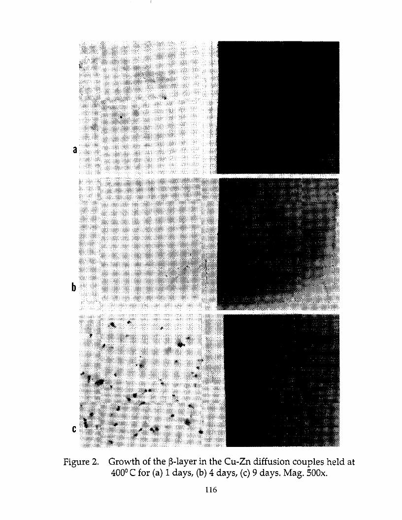
a

b

c

Figure 2. Growth of the ~-layer in the Cu-Zn diffusion couples held at 400°C for (a) 1 days, (b) 4 days, (c) 9 days. Mag. 500x.

116

°C~ ______________________________________________ -.

1000 L

800

600 Y

400 --l-----------+

200

a

a a+f3 f3 f3+Y Y y+E

100

50

Wt. % Zn

Figure 3. Correlation between the Cu-Zn phase diagram showing equilibrium phases at 4000 C and the single-phase layers formed in the Cu-Zn diffusion held at 4000 C for 9 days. Adapted from page 108 of reference 1.

117

100,-----------------------------------------------~

80

~ 60 N

40

20

I I

01 II II II

Ullf- A II IJ y E O~~------·----------------------------_+----------L-~

II Distance across diffusion couple

Figure 4,. Composition profile of the Cu-Zn diffusion o

couple held at 400 C for 9 days.

118

DESIGNING, ENGINEERING, AND TESTING WOOD STRUCTURES

Thomas M. Gorman

Department of Forest Products University of Idaho

Moscow, Idaho 83843


119

DESIGNING, ENGINEERING, AND TESTING WOOD STRUCTURES

Thomas M. Gorman, Ph.D. University of Idaho, Moscow, ID

KEY WORDS: wood, design, factor of safety, engineering economy, duration of load, stress, tension, compression, bending, deflection

PREREOUISITE KNOWLEDGE: This material could be taught to a typical student of materials science, at the high school level or above.

OBJECTIVES: To introduce basic structural engineering concepts in a clear, simple manner while actively involving students. This project emphasizes the fact that a good design uses materials efficiently.

* The test structure (Figure 1) can be easily assembled, has various design options, and can be reused year after year. Even when the structure is loaded until it collapses, only one or two pieces usually break, leaving the remaining pieces intact and reusable.

Groups of students are asked to use their intuition to choose different pieces with various cross-sectional areas for the structure, which will span a distance of 0.9 m (3 ft). Their goal is to support at least 23 kg (50 Ib) at a minimum cost.

EOUIPMENT AND SUPPLIES: This list includes materials for three demonstration models plus enough material for three student groups to complete any design that they choose.

Superstructure About 5.5 m (18 ft) of Southern Pine or Douglas-fir nominal 2 x 4 (38 x 89 mm). If another type of wood is used, you may have to adjust the target load value. The ideal structure should comfortably support the target load. Cut wood to sizes and drill the holes as indicated in Figure 2. Make pieces as clear (free of knots) and straight grained (grain parallel to length of piece) as possible.

• 32 red pieces • 32 blue pieces • 32 green pieces • 60 yellow pieces

Frame, supports and platform • Nine 19 mm x 51 mm x 305 mm (3/4 in x 2 in x 12 in) pieces of wood with slots as shown in

Figure 5a • Six 6.4 mm x 25.4 mm x 254 mm (1/4 in x 1 in x 10 in) pieces of wood • Two 216 mm (8-112 in) pieces of nominal 2 x 4s (38 mm x 89 mm) with a 3.2 mm (1/8 in)

lengthwise groove. • One 457 mm x 305 mm x 19 mm (18 in x 12 in x 3/4 in) piece of plywood with holes drilled in

each corner

* Figures 1--8 are grouped according to experimental sequence.

121

Hardware • 3.2 mm (1/8 in) diameter threaded rod--total of 9 m (30 ft) cut to 305 mm (12 in) lengths • 60 wing nuts • 120 hex nuts • 120 washers • Three nails, approximately 4 mm in diameter (lO-penny) • Approximately 6 m (20 ft) of 1.0 mm diameter (l8-gauge) copper or bronze wire

Other • Spray paint or marking pens (four colors for marking wood) • Nylon cord (4.6 m to :5.5 m (l5-18 ft) length, 3.1 mm (1/8 in) diameter) • Carpet or pad to protect floor • Weights (bricks or suitable dense objects of equal, known weight) • Safety glasses for each student

PROCEDURE: The structures to be built have interchangeable pieces of varying size and cost. There are four types of pieces of equal length with varying cross-sectional dimensions, referred to in units. Each unit equals 1.6 mm (1/16 in). Thus, a 1/4 in x 1 in piece is 4 x 16 units. Fictitious dollar values are assigned to each piece based on the amount of wood used and are color coded for easy identification (Figure 3).

Before the actual classroom activity, prepare three models for demonstration, using the model in Figure 4. Make sure to place a washer between each wooden piece and the hex and wing nuts on the rods. Once the structure is assembled, attach wire supports diagonally to the wing nuts at each end of the rods as shown in Figure 4. These supports prevent the structure from collapsing sideways.

The loading frame is necessary to prevent lateral buckling, or twisting, of the top pieces. The frame is designed to rest on the top pieces of wood that have been spaced 229 mm (9 in) apart by the hex nuts on the threaded rods. Make sure that this measurement is accurate. Three frames are needed with slots of different widths to match the three possible widths of the top cross pieces (see Figures 5a and 5b). The loading heads are made from nine 19 mm x 51 mm x 305 mm (3/4 in x 2 in x 12 in) wood pieces with 1 inch slots cut as shown in Figure 5a. The braces are made from six 6.4 mm x 25.4 x 254 mm (114 in x 1 in x 10 in) wood pieces. Three nails--approximately 4 mm in diameter (lO-penny)--serve as loading frame pins.

The "super economy" model is made with all yellow pieces (the weakest ones, 2 x 6 units) for a total cost of $14. The second model is made with all red pieces (the strongest ones, 4 x 16 units); it looks very sturdy, but its cost is a formidable $116. The third model (combination of blue, green, and yellow) costs $32 and is the most efficient design. This "ideal" model is kept out of view until all the students' structures are tested. It would be a good idea to pretest your ideal model to make sure that it supports the 23 kg (50 lb) load. If it doesn't, you could adjust the targetload value.

Explain the challenge--to design and build an efficient structure capable of supporting 23 kg (50 lb) at a minimum cost. As an example, bring out the red structure (the strongest) and load it to

122

46 kg (100 lb). No visible signs of stress on the structure will be evident. The students are told that the structures could be built without red pieces and still support 23 kg (50 lb), but they can use the red pieces if they'd like. You might want to put an upper limit on the total dollar cost for each structure to prevent students from being overly conservative in their design.

The class is divided into groups, and each group receives a supply of lumber and materials. Students are encouraged to use their intuition and discuss their design within their group before proceeding to build it. They should take about 15 minutes to complete their design. After everyone has assembled their structures, begin testing (Figure 6). By adding loads in small, 4.5 kg (10 lb) increments, students can see problems developing before catastrophic failure.

Add weights one at a time; be prepared for a sudden collapse of the structure. Green pieces (5 x 6 units), when used as top members, will break well below the target load. Blue pieces (2 x 16 units), as side compression members, should break or show considerable buckling at the target load. Wear safety glasses. Make sure that the students also wear safety glasses and stay several feet away from the structure. Continue adding weight until the structure collapses or the optimal weight is reached. It will become obvious to the students that the way a piece performs depends on where the piece is placed in the structure. Students will mentally revise their designs as they watch their structures contort and buckle under the heavy load.

In some cases, the bowed structures actually hold the 23 kg (50 lb) load, but students will realize that they wouldn't want to be driving across a structure of that design! This illustrates the concept that maximum allowable deflection is sometimes the limiting factor in engineering design.

Sometimes the structure will hold the load initially, but suddenly will come crashing down before the next weight is added. This unexpected phenomenon shows that the length of time a structure is loaded affects how it behaves. This illustrates the concept of duration of load.

After each group's structure is tested, load the "super economy" yellow structure (2 x 6 unit pieces) which, when tested, doesn't support even a 4.5 kg (10 lb) load. Next, unveil the so-called "ideal" design and show that it will indeed support the 23 kg (50 lb) load, without showing too many signs of impending failure. As a grand finale, load the red structure (the strongest). You can keep adding weight until the structure shows signs of stress, or for a dramatic effect, continue adding weight until it crashes to the floor as the load exceeds 69 kg (150 lb).

On the blackboard, record the cost of each structure and the load it held before it collapsed. These test results give you the opportunity to compare the safety, cost, and design efficiency of each structure. The structures that support a higher load are the safest, while the ones that support at least 23 kg (50 lb) for the lowest cost are the most efficient. Occasionally, variability in wood performance shows up when similar designs perform differently.

Another concept that may be discussed during this demonstration is the factor of safety. You may explain that the factor of safety chosen for a given situation depends on many variables, including the duration and frequency of the applied load, the variability in performance of the structure, and the consequences of a failure (would it be life threatening?).

123

Both the size (cross-sectional area) and shape of a piece of wood affects its performance when it is subjected to stress. By designing wisely, you can use less wood and still have a strong, reliable structure.

SAMPLE DATA SHEET:

.... .............. I STRVCTURE COST . UL TIMATELOAD

NO. .

... ... . .... . .. ..

1 $14 < 4.5 kg

2 $32 23 kg

3 $116 69 kg

4 $40 12 kg

5 $32 < 4.5 kg

6 $40 23 kg

INSTRUCTOR NOTES: As a way to begin analyzing what happens to the structures, have the students pick up individual pieces and try to bend, compress, and pull them in tension with their hands. Because of their different dimensions, each piece responds differently to the forces. By comparing what happens to the individual pieces with the performance of the structures, the students can begin to identify forces causing the structures to deform. All pieces for this experiment are made from clear wood (free of knots or other defects) and are very strong in tension. A small cross-sectional area can withstand very high loads. Try to pull apart a yellow piece (2 x 6 units) by pulling the ends away from one another. Next, try pushing in on the ends of the same yellow piece. When a piece is loaded in compression, it tends to buckle. The load at which it begins to buckle is controlled by the narrowest cross-sectional dimension. Compare the effects of compression on the blue (2 x 16 units) and green (5 x 6 units) pieces, which have nearly identical cross-sectional areas. The blue piece buckles more easily than the green piece because it has the narrowest critical dimension. In compression, then, a square cross-sectional area makes the most efficient use of material.

Now compare bending the blue piece (2 x 16 units) in the two ways shown in Figure 7. The most important dimension of bending is depth. The deeper the piece, the stiffer it is and harder it is to bend. This is because stiffness is directly proportional to the cube of the depth and only linearly proportional to the width ..

When a student-built structure is supporting a load, the forces distributed to each piece depend on its location within the structure (Figure 8). As discussed at the beginning of the demonstration, red pieces are more than adequate (but not necessary) to support the maximum predetermined load. A discussion of engineering principles applied to wood design provides the clues students need to choose pieces adequate for building a structure that meets its design criteria with a minimum amount of wood (or cost).

124

FOR FURTHER READING: Hoadley, R. B. 1980. Understanding Wood. The Taunton Press, Newtown, CT.

McCarthy, M., and T. Gorman. 1990. Building excitement in the classroom. The Science Teacher 57(5):43-49.

USDA Forest Service. 1987. Wood Handbook. USDA Agri. Handbk. 72 (rev.) Madison, WI.

SOURCES OF SUPPLIES: All materials for this demonstration are commonly available in home centers, hardware stores, and/or building supply outlets.

Figure 1. Assembled structure, resting on support blocks, with loading frame and wire cross bracing in place. (Photo courtesy of USDA Forest Products Laboratory)

125

,. 10 !RED) (BLUE)

t ~.4mm 0t-(I") I i ..

·0 [J 25_~rnm

II")

+ I 250~J r (I") l

L250mm I r (I") ,

10 (GREEN)

0t-

I '"

<I

" (YELLOW)

t t.. 25.~mm

I WI .. i.

<IT

508mm (20")

254mm (I")

+ ~9.1-~

(3/8")

6 ~mm(l/4") Thiel!

3 2mm (118<') 79mm(5/16"j 3_2mm tI/S") Thick Thick Thick

Figure 2. The dimensions of the red, blue, green, and yellow sections of wood. (Drawing courtesy of USDA Forest Products Laboratory)

I ~ RED BLUE GREEN YELLOW

price/ 158 piece 154 14 61

UNITS 4xl6 2xl6 5x6 2x6

mm 64 x 254 3.2x25.4 7.9x9.6 3.2 x 9.6

in 1/4 x I 1/8 x I 5116 x 318 118 x 3/8

UNIT = 1.6mm ( 1/16 in)

Figure 3. Cross-sectional view of the four types of pieces to be used in the structure. All are 508 mm (20 in) long. (Drawing courtesy of USDA Forest Products Laboratory)

wooden croSS pIece

upper rtghl-hond ........

threaded rod

Figure 4. A schematic of the completed structure. The upper and lower corners have been enlarged to show their construction. (Drawing counesy of The Science Teacher/May 1990)

126

3 each ~ t-305mm (12")-1

50.8mm (2 ") [J1 rtJ T 1--229mm--j

(9" )

6.4mm (114")wide 11011

3 each I-- 305mm ( 12")--i

LI1 rJ 1--229mm--j

(9" )

7.9mm (5/16") wide 11011

3each

1--305mm (12")--1.1

Ln n::J ~.4 mm(J") DEEP

I-- 229 m~' SLOT ( 9")

3.2 mm (118") wide slols

~IOd (4mm)~

r

I , , 1. __ SIfIo Ii NOli '

0, • 1

9'0<11 -1.

Figures 5a and 5b. The dimension of the loading heads for the loading frame are shown on the top. The assembly of the loading frame is shown below. (Drawing courtesy of USDA Forest Products Laboratory)

Figure 6. Testing the structure. In the first photo, one group's structure is loaded as the rest of the class looks on. (Note that everyone is wearing safety glasses) Next, side sections begin to buckle just before structural collapse. The structure supported 32 kg (70 lb) before it gave way. (Photos courtesy of USDA Forest Products Laboratory)

127

Figure 7. Bending a member in two different ways. The orientation with narrower depth is easier to bend. (Drawing counesy of USDA Forest Products Laboratory)

BENDING

TENSION TENSION

Figure 8. An exaggerated illustration of the structure shows how different members are subjected to different types of forces. The compression sections become shorter, the tension sections become longer, and the zero force sections remain essentially the same. (Drawing counesy of USDA Forest Products Laboratory)

128

COMPUTER VISION IN MICROSTRUCTURAL ANALYSIS

M. N. Srinivasan w. Massarweh

C. L. Hough

Department of Mechanical Engineering Texas A&M University

College Station, Texas 77843-3123


129

COMPUTER VISION IN MICROSTRUCTURAL ANALYSIS

M.N. Srinivasan, W. Massarweh, C.L.Hough Department of Mechanical Engineering

Texas A&M University, College station, TX

KEY WORDS: computer, microstructure, solidification, casting, aluminum, cooling rate.

PREREQUISITE KNOWLEDGE: This material could be demonstrated to a high school level materials science student, but would be more useful to a student at the college freshman level or above. This experiment is intended to convey to the student that properties are a consequence of the microstructure and, therefore, characterization of microstructure is very important.

OBJECTIVES: To demonstrate that the microstructure of engineered materials is affected by the processing conditions in manufacture, and that it is possible to characterize the microstructure using image analysis with a computer.

EQUIPMENT AND SUPPLIES: 1) Laboratory heating or melting furnace, 2) molding sand and mold boxes, 3) aluminum-7% silicon alloy ingot, 4) stepped bar pattern, 5) chromel-alumel thermocouple and indicator, 6) metallographic sample preparation facility, 7) personal computer with accessories as detailed in the paper.

PROCEDURE: The principle of computer vision will first be introduced followed by the description of the system developed at Texas A&M University. This in turn will be followed by the description of the experiment to obtain differences in microstructure and the characterization of the microstructure using computer vision.

The phenomenal advances in the computer and microelectronics industry have made computer vision within the affordable range of budget strapped users. A decent system could be assembled for under $10,000 and the prices are still falling. In this paper, we will introduce one such system and its application in microstructural analysis.

The application of computer vision in microstructural analysis varies in degree of sophistication from simple determination of phase ratio, up to sophisticated grain size and morphology analysis. For the sake of simplicity, we will suffice with the intrOduction of phase ratio determination as a simple but effective method for introducing imaging analysis methods in material science laboratory education.

131

system Description:

The microcomputer image acquisition and analysis system used in this experiment consists of two main modules: the optical module, and the image and analysis module.

The optical module consists of a Nikon MeasureScope 20 microscope equipped with the proper optical elements and lighting fixture. The microscope was also fitted with a lightweight black and white CCD (coupled charged device) camera. Depending on the specimen to be studied, the proper magnification and lighting method could be determined by trial and error.

The image acquisition and analysis module is based around a 10 MHz AT-compatible 286 microcomputer, 1 Mbyte random access memory, and 40 Mbyte hard disk. A color monitor is optional. The computer is equipped with a (PCVISION) frame grabber and image analysis board. This board is capable of storing 2 images with a 512x512 resolution, in addition to the capability of on-board image manipulation. The captured and processed images are displayed on a B&W TV monitor connected to the image board.

The control and analysis software runs under DOS (disk operating system) and is composed of two different components. First, a menu driven software component is used to grab, filter, and perform some basic measurements on the images, and finally store them in the image data base. with the system also comes a subroutine library containing functions that ease the manipulation of images. Using those subroutines, the user can construct functions tailored specifically for a particular application.

A typical digital image is composed of a collection of image elements, each known as a pixel, which represents the average light intensity over a discrete portion of the total image. Both spatial resolution and light intensity resolution of the image depend on the hardware used, but a 512x512 pixel image with 256 gray level represents an average reasonably priced system.

Phase Determinat:ion Procedure:

As a first step, a digitized image of the specimen in question needs to be acquired by the computer. This could be obtained directly through the camera mounted on the microscope from a metallographically prepared specimen. If a direct image is not feasible, a digitized image could be obtained from a still photograph scanned through a digitizer. It is very important in both options to preserve the contrast between the different phases in question. WI:!ak contrast between the different phases will increases the difficulty of subsequent phase discrimination steps.

To obtain phase discrimination in the image, it is crucial to map each phase in a different gray level intensity .zone. Under ideal conditions, and if the contrast in the original image is good, a simple -transformation of the image to a binary black and

132

white by simple thresholding will suffice, see Figure 1. Thresholding is a simple operation whereby pixels with a value above a preset threshold are assigned a binary value of 1 (or white). If a pixel's intensity value is below the threshold it is assigned a value of 0 (or black), as shown in Figure 2.

In many cases, the image quality is not superior, or contrast between the phases in weak. In such cases, a number of alternatives can be used to improve the quality of the picture. In conditions where the images are noisy, a number of filtering methods could be used to obtain a better separation between the phases in the image. Such filters include convolution operators like smoothing, sharpening, or averaging filters. Other filters include morphological filters like dilation and erosion operators. The majority of those filters are included as part of basic image processing package.

Even in cases where phase discrimination exists but with minimal difference in the intensity, area measurements become sensitive to the choice of a cutoff threshold value. In such situations a method called histogram stretching is used to enhance the contrast as shown in Figure 1.

In the case of a binary phase material where a thresholded binary image is obtained, phase fraction determination can be obtained by calculating the fractions of black and white areas. A simple program that tests the image pixel by pixel keeping account of pixel count, then calculating the fraction will perform this task.

Experiment Example:

An experiment to determine the effect of section thickness (cooling or solidification rate) on microstructure of Al-7%Si was performed by senior level undergraduate students at Texas A&M University.

A stepped bar pattern was used to make a composite casting of different thicknesses. The cooling curve in each section of the stepped bar, as the casting solidified, was recorded using a chromel-alumel thermocouple connected to a digital temperature readout. In Figure 3 the cooling curves thus obtained are shown-. Each section of the casting was then metallographically polished and etched to reveal the microstructure. The percentage of alpha phase in each section was then determined using the image analysis procedure described earlier and was plotted against the casting thickness, as shown in Figure 4. It is seen that the percentage alpha decreases with increase in section thickness (or decrease in cooling rate). This implies that the amount of eutectic (in the interdendritic regions of alpha) follows the reverse trend. Since the eutectic contains brittle beta phase, it follows that the strength of the aluminum-7% silicon casting decreases with increase in section thickness. In Figure 5 is shown a typical

133

photomicrograph with alpha (white) and alpha plus beta (dark) phases. The percentage alpha measured by the lineal analysis method for this case was about 65%, which compares favorably with the value of 67.5 % shown in Figure 4.

REFERENCE: Flemings, M.C., Solidification Processing, McGrawHill, 1974, pp 134-172.

SOURCES OF SUPPLIES: The casting materials, equipment and supplies can be obtained from companies listed in the Thomas Register. The personal computer (PC-AT) can be purchased from any reliable source. For details of the image analysis system, please contact the authors.

CONCLUDING REMARKS: The casting experiment has been chosen merely to demonstrate the need and capability to characterize the microstructure. Image analysis can be useful for any engineered product, manufactured by processes like forging, rolling, welding, etc.

ACKNOWLEDGEMENT:

The experiments were performed by Brian Branum, Brian Bidigare, Rafael Alvarez and Paul Bowers under the direction of the authors. The authors would like to thank these four former students for their dedicated work.

134

F'IXEl. COUNT

TlR:SHCU> UVEl

Figure 1 Image histogram stretching

135

PIXEL

COltfT

PIXEl.

COltfT

o

ORIGINAl HSTOGRAIA

STRETCHED HISTOGRAIA

Figure 2 Threshold selection in image histogram.

136

.... u

I v

o~ ____ ~ ____ ~ __________________ ~ ____ ~ ____ ~

12 168 903 1263 1623 2163 2875

TltoE (sec) o J/~ + 1 5/8 o 1 J/' 4 2 1/ ~ x 2 1/2

Figure 3 Cast.ing cooling curves

137

AI-51 7!Ii 68

66

6. -

62

60 -

58 - 0

• 515 -:t Q.

5. -' 0 <

• 52 .

50 i •

• 8 .

• 6 •

.. -

.2 0

.0

o 750 1 625 , 750 2 250 2 500

THICKNE5S (Inc .... )

Figure 4 Percentage alpha versus section thickness

138

Fiqure 5 Typical microstructure of Al-7% si casting

139

EXPERIMENTS WITH THE LOW MELTING INDIUM-BISMUTH ALLOY SYSTEM

Richard P. Krepski

Intermet Technology 116 Long Road

Georgetown, Pennsylvania 15043


141

* EXPERIMENTS WITH THE LOW MELTING INDIUM-BISMUTH ALLOY SYSTEM

Richard P. Krepski Intermet Technology, Georgetown, PA

-and-Geneva College, Beaver Falls, PA

G)1991 Intermet Technology

KEY WORDS: indium-bismuth alloy, phase diagram, intermetallic compounds, oxidation, solidification, casting, heavy metal toxicity, wetting behavior

PREREQUISITE KNOWLEDGE: The primary audience for this material is the junior high school or middle school science student having no previous familiarity with the material, other than some knowledge of temperature and the concepts of atom, element, compounds, and chemical reactions, The unit can be adapted to use at a more advanced level, as a means of exploring the meaning Cif the equilibrium phase diagram.

OBJECTIVES: The alloy system indium-bismuth has several features that make it useful for participatory demonstrations at the pre-college level. Near the eutectic composition, the liquidus is well below the boiling point of water, allowing simple, minimal hazard casting experiments. Such phenomena as metal oxidation, formation of intermetallic compound crystals, and an unusual volume increase during solidification could all be directly observed. A key concept for students to absorb is that properties of an alloy (melting point, mechanical behavior) may not correlate with simple interpolation of properties of the pure components. Discussion of other low melting metals and alloys leads to consideration of environmental and toxicity issues, as well as providing some historical context. Wetting behavior can also be explored.

EQUIPMENT AND SUPPLIES: 1) Small pellets of pure indium and bismuth, along with 100 gram samples of pre-alloy with 34 and 60 wt.% Bi; 2) A hot plate or other modest heat source; 36 Temperature measurement capability in the range 50 - 160 C, preferably a thermocouple with digital readout; 4) Stainless steel cups; 5) Plastic spatula; 6) Glass Slide; 7) Plastic funnel; 8) Various clay media for mold making; 9) Eye protection for all students, and gloves for students involved with melting; 10) Mineral sample showing crystal facets.

PROCEDURE:

1. Have a volunteer inspect the sample of pure indium (very soft and ductile - can be dented by a fingernail). We will then

* Development of this experiment was supported by a grant provided by the National Science Foundation Small Business Innovation Research Program.

143

explore mechanical behavior of pure bismuth and the two alloys by knocking samples inside plastic bags on a table top. (First explain what is meant by weight percent and "alloy".) The 60 wt.% bismuth alloy h; very brittle and shatters like glass; the 34 wt.% bismuth alloy i:s very tough and is unaffected. The pure bismuth is hard and brittle, but not to the extent of the bismuth-rich alloy.

Caution: Pass these samples around inside plastic bags; small chips of fractured metal could otherwise get on students' fingers and get rubbed into eyes.

Lead the students in a guided discussion of the possible reasons for these differences in mechanical behavior. Point out that the 60 wt. % bismuth alloy shows very flat surfaces where it breaks. This is a reflection of the crystal structure of the material - the lQay the atoms line up in orderly patterns when the metal solidifies. This alloy is mostly an extremely brittle InBi compound, and its fracture surface displays the planes of these crystals. Compare this to a highly "faceted" crystalline mineral like amethyst of fluorite. The other alloy is tough (difficult to crack) because :It is a fine combination of two kinds of crystals -indium (with dissolved bismuth) and the fairly tough In

2Bi cmpound.

Which alloy would the students choose to make a part from?

2. Introduce the periodic table and look up the crystal structures of indium and bismuth - no need to get into detail unless the kids ask. Also look up melting points. Bismuth melts at 271 0 C, Indium at 1570 C ... what temperature do they think the alloys will melt at? A logical guess would be to plot melting temperature ver!;us composition and just draw a straight line between the two endpoints.

Melt the 60 wt. % bismuth alloy chunk in a stainless cup on a hotplate and measure temperature with thermocouple. It should go liquid at about 1050 C. Why is melting point lower than for either pure material? Basically, the two different atoms have a hard time fitting together into a solid crystal structure.

Caution: Do not let the metal temperature get too much above 1200 C, as this increases the burn hazard. All students should have protective eyewear. Students handling temperature measurement should wear gloves.

While wai t:ing for alloy to melt: We have been using the word "metal". What are some metals in the room, and what makes a metal a metal? Students might say strength, or ability to bend like a wire, or shininess. Point out an electric wire and ask if there is metal in it and what it does. As another clue, discuss how a thermocouple measures temperature. When two different metal wires are joined together to make a circuit and the two junctions are at different temperatures, electrons will flow from one metal to the other - ~ie can measure this effect, the magnitude of which depends on the temperature difference between the two junctions. This reinforces the notion of electrons freely flowing in a metal,

144

because of the way the atoms are bonded together. This is really what makes a metal a metal.

Students should be able to make five key observations as we melt and re-solidify the metal in the stainless steel cup:

A. Cool the cup by immersing it in water ... we should be able to see the expansion in the solid as it forms on the outside of the cup. This is very unusual, and is due to the very open crystal structure. What other common material becomes less dense (expands) when it solidifies?? Have a glass of icewater available, to show solid ice floating in liquid water. What would happen if ice was more dense than water? Ice in lakes and oceans would sink to the bottom and take a much longer time to melt in the spring - something to think about!

B. On cooling, we will be able to see the higher melting crystals (InBi) forming first in the middle of the sample. When the alloy is partially solid, tip the cup to shift the liquid and expose the solid crystals.

C. We should also note that the alloy is slushy over a range of temperatures - it doesn't just freeze at a single temperature like water or pu~e indium or bismuth. This is typical of many alloys.

D. When the alloy is molten we should be able to see an oxide skin forming on the melt surface as it reacts with the air . .. discuss how nature would like to convert this metal into an oxide, and how melting allows this to happen faster. Note also that a protective chromium o}cide steel on the stainless steel cup is actually what makes it "stainless". The oxide film is so thin that we can't see it. !f the steel surface is scratched, chromium from the steel quickly reacts with the air to "heal" the protective film.

E. Using the glass slide, we can demonstrate that the liquid metal wets glass. This is unusual and relates to one practIcal use for indium-containing alloys - soldering of nonmetals.

3. Second melting experiment with 34 wt. % bismuth: Repeat the procedure above. In this case, the alloy melts and resolidifies at a temperature of about 72 0 C. This is the lowest melting composition. Note also that there is little or no range of slUShiness - the alloy changes from solid to liquid and back again at constant temperature. Go back to our map of melting point versus composition and plot the data we have generated for the two alloys. Is this what we expected?

4. The fact that the 34 wt. % bismuth alloy melts below the boiling poInt of water enables us to perform some simple casting experiments - we don't have to worry about boiling water when we cast into a wet medium like clay, and the low melting point in

145

A SENIOR MANUFACTURING LABORATORY FOR DETERMINING INJECTION MOLDING

PROCESS CAPABILITY

Jerry L. Wickman David Plocinski

College of Applied Sciences and Technology Department of Industry and Technology

Ball State University Muncie, Indiana 47306-0255


149

A Senior Manufacturing Laboratory For Determining Injection Molding

Process Capability

Jerry L. Wickman Ph.D. David Plocinski

Department of Industry and Technology Ball State University

KEY WORDS: process capability, quality control, statistical process control, parametric study, control charts.

PREREOUISITE KNOWLEDGE: This subject material is directed at an upper level undergraduate/graduate student in an Engineering or Engineering Technology program. It is assumed that the student has a thorough understanding of the process and quality control. The format of this laboratory does not follow that recommended because of the nature of process capability and that of the Sandretto injection molding equipment and tooling. This laboratory is instead developed to be used as a point of departure for determining process capability for any process in either a quality control laboratory or a manufacturing environment where control charts, process capability, and experimental or product design are considered important topics.

OBJECTIVES: To demonstrate the typical procedure by which one can determine process capability. To demonstrate the development of control charts. To statistically show the areas through which processing variation can enter into the manufacturing process.

EOUIPMENT AND SUPPLIES: A laboratory size injection molder (Sandretto, Spectrum 60) with an ASTM test bar fixture in place with associated machine

151

instrumentation. DataMyte Model 862 with an associated statistics package for generating pareto analysis, control charts, process capability indices, and measuring equipment interfaced with an appropriate software package, Monsanto ABS materials and a hopper dryer for materials control.

Introduction Spiring (1991) has indicated that

interest in process capability is growing, due partly to the changing philosophy in quality control. Motivational tools such as slogans about doing things right the first time and building a better quality product are lost if there is little or no analytical study of the process and the product. World wide competition is forcing everyone (not just the U.S.) to look at how variation in the process and product can be reduced, and how all personnel from design through manufacturing can be involved in the overall effort of reducing variatio~.

Process capability has been defined as the range over which the output of a process varies or the actual process spread (6 0). Process capability ties both the product and process together. Process capability and the associated indices have the potential to positively impact product design, setting of tolerances or specifications, vendor quality surveys, communication with suppliers, machine allocation and others. Process capability makes it possible to quantify what the process is

capable of doing, which determines if the product can be made to current or revised, possibly tighter specifications.

The following paper is divided into three subsections which lead to determining the process capability of the injection machine. It should be noted that although injection molding is a generic process, determining process capability from one machine to the next may vary considerabl y.

Sandretto Injection Press/Materials The machine utilized in the

capability study was a Sandretto model Spectrum 60 screw injection molder capable of a 3.17 ounce shot weight and 66 ton clamp capacity. The Sandretto was a new purchase and is considered to be a state of the art machine. Principal operation is at a control panel where virtually all processing characteristics are accessed and manipulated via a microprocessor. Processing characteristics can be seen in either tabular or graphical formats.

Injection molding is a process of molding solid plastic objects. It involves forcing molten plastic into a closed cooled mold where the plasti(; solidifies to a usable product upon closing.

Parameters were set according to manufacturers' data sheets of the material (Monsanto Cycolac ABS grade z80) being used. These parameters included; drying time, drying temperature, barrel temperature, nozzle temperature, injection speed, and screw plasticizing speed (RPM's).

Control Charts To determine process capability it

is assumed that a robust quality control program has been in place and is working. Control charts are being used and have been successful at removing most if not all assignable error. Juran (1980) states that a

152

control chart is a graphic comparison of process performance data to computed "control limits" drawn as limit lines on the chart. The process performance data usually consist of rational subgroups sampled and plotted sequentially. Process variations are traceable to two kinds of causes: (l) random, i.e., due solely to chance; and (2) assignable, i.e., due to specific "findable" causes (Juran 1980). Only random causes of variation should exist because this represents the minimum amount of variation present (X ± 3 a) in the process. The process is then said to be in a state of statistical process control. The actual process spread is 6 a which represents the width of the interval that contains 99.73% of the population.

Different types of control charts exist for both attribute and variable process data. Bothe (1991) states that current accepted practices for determining process capability are defined for only variable data. This capability study used X and R charts before determining process capability.

Process Capability Many different indices exist for

measuring process capability (Cp, Cr, Cpk). Bothe (1991) contends that this knowledge is extremely useful for shop personnel in determining what machines should be scheduled to run what parts and for monitoring process improvements by seeing these capability indices increase over time. Worthy (1991) indicates that the Japanese use process capability as a design tool to make sure that the intended design can be made to specifications. He also contends that in the U.S. we design the product without regard to whether or not manufacturing is capable of producing the part.

Control charts use rational subgroups with upper and lower control limits

calculated from the subgroups. Tolerances should not be used with control charts; tolerances are for individual items and are typically set independent of the process and may not relate well to process control chart averages. Process capability and the associated indices work with individual items and thus work well with tolerances. One of three situations exists relative to process capability and tolerances where 6 a equals the process capability and U - L equals the difference between upper and lower tolerances. 1. 6 a < U - L (Figure 1) This represents the most desired relationship. The process is in control and the tolerance is greater than the process capability. Even if there is a shift in the process average, no nonconforming products are likely to be produced since the parts may be considered out of control but conform to specified tolerances. 2. 6 a = U - L (Figure 2) Process capability is equal to the tolerance. As long as this situation holds, no nonconforming product will be produced. As soon as the process shifts up or down, nonconforming product will be produced. Either processing variation must be reduced or tolerances must be increased. 3. 6 a > U - L (Figure 3) This is the most undesirable of the three scenarios. Nonconforming product from both extremes of the normal distribution may occur. If a process shift occurs large quantities of nonconforming product may result (Besterfield 1990).

Various capability indices exist, thereby inviting comparisons among processes with different quality variables and promoting similar inferences regardless of the product or quality characteristic measured (Spiring 1991).

153

Cp - Capability index. A minimum value of 1.33 is recognized as a defacto standard.

Where: Cp = U - Ll6 a If Cp = 1.00 then scenario #2 from above. If Cp > 1. 00 then scenario # 1 from above. If Cp < 1. 00 then scenario #3 from above.

Cr - Capability ratio. The defacto standard for a Cr is 0.75.

Where: Cr = 6 a/U - L

Cpk - This is used to determine if the process is centered on the target or nominal value. A minimum value of 1.00 is recommended.

Where: Cpk = Z (Min)/3 Z (U) = U - Xla Z (L) = X - Lla

Process Capability Procedure The Sandretto was programmed to

print out thirty different process parameters following each shot (Table 1). Each data sheet and corresponding part were labeled to maintain traceability characteristics. Subsequent development of X and R control charts followed using select processing variables.

The design of the process capability experiment included but was not limited to: 1. Selection of a suitable molding

tool. Will the product have subsequent use, i.e., materials characterization, etc .. ? Would the tool be suitable for control charts and process capability studies? (Figure 4) (ASTM D647-90).

2. Design fixture for impact disc. Measuring tools available

3. 4.

5. 6.

7.

Data collection (DataMyte) Statistics and software used (SPCII) Traceability features Environmental soaking of fixture and related tooling Develop and build fixture. Develop Iskikawa diagrams of process. (Figures 5 & 6) A. Processing parameters. B. Machine components. C. Material handling. Selection of material. Determine Sandretto settings based on material selection and study. A. Barrel heats. B. Mold closing. C. Mold opening. D. Hydraulic ejection. E. Injection. F. Plasticizing. Determine if process is in control through the use of X and R charts. (Figure 7) A control chart distinguishes between random and assignable causes of variation through its choice of control limits. These are calculated from the laws of probability in such a way that highly improbable random variations are presumed to be due not to random causes, but to assignable causes (Juran 1980). If points on the graph exceed the established control limits, chances are that assignable causes entered the process and the process should be investigated. Injection molding Hydraulic Pressure points one and five are "out of control". These two points should be investigated. However the remaining points are within our control limits signifying that only random causes are present and the process should be left alone. Each point on a control chart

154

represents a test of hypothesis, but the chart simplifies the calculations and presents a graphic method for doing hypothesis testing continuously (Juran 1980).

8. Determine process capability for select processing characteristics.

Conclusions This study was initially conceived

in and intended to be used in an applied quality control class with an associated laboratory. Various aspects of this study have already been incorporated into the applied quality course and other "non quality control" classes. Determining process capability is an excellent tool for integrating undergraduate/graduate students from electronics to manufacturing, inclusive of the design and mechanical options. The applied study reinforces those manufacturing concepts of the quality philosophy, metrology and statistics as discussed in the classroom. The impact of slight or even dramatic changes in personnel, machines, materials and methods can be graphically determined by using control chart theory and applications. The students need to be aware of this cause and effect taking place in virtually any manufacturing environment. Process capability encourages the synthesis of design of experiments, metrology, statistics, fixture design and use, materials characterization, bench marking, defect concentration analysis, sampling, and process variation to name a few. This study represents a benchmark for future studies scheduled at regular intervals to determine changes in processing parameters and subsequent changes to process capability.

Recommendations Even though we have only begun

this series of studies it is clear that process

capability can be done on virtually any piece of industrial equipment available. The benefits far outweigh the time invested from both the students and faculty members standpoint. As with any scientific study my recommendations are:

* Have a good understanding of

*

*

*

*

*

*

statistical process control for all students and faculty involved. Provide adequate time for development of study. Select equipment with process capability in mind. Consider larger picture of process control with process capability being a smaller entity, i.e., spinoffs to other courses. Additional work with identifying and reducing sources of variation.

Personnel Machine Materials Methods

Incorporation of various types of measuring instruments. Industry cooperation.

References ASTM - D647, Design of Molds for Test

Specimens of Plastic Molding Materials, 1990 Annual Book of ASTM Standards, Philadelphia, P A.

Besterfield, Dale H. Quality Control, Prentice Hall, Englewood Cliffs, NJ, 1990.

Bothe, Davis R. A Capability Study for an Entire Product. ASQC Annual Quality Proceedings. Milwaukee, WI. May 1991.

Juran and Gryna, Quality Planning and Analysis, McGraw-Hill, Inc., NY, 1980.

Spiring, Fred A. The Cpm Index, Quality Progress, February 1991.

Worthy, Ford S. Japan's Smart Secret Weapon, Fortune, August 12, 1991.

155

Pla.ticisingActual Time In.jection 1st Stage Actual Time (Previous) OVerall Cycle Time Mold Closing Stages Actual Time Cooling Actual· Time Mold Opening Stages Actual Time 1.4 s ActualTime of Consents Awaiting Stages by RobntO.O s C$rriage. Approach ActualTime 0.0 s Ejector Sequence Actual Time 0.0 • fIy~raulic Ejection Sequence Actual Time 1.0. Aciual Dwell Time Break 0.1. Injection Hold on Stage Actual Time 4.4, Actual Hydr. Barrel Pressure at 2nd lnjeo. Stage ChangeQV IJl7. psi Screw Actual Position at the Change OVer Point 4.9% Cushion Final Position 2.8· % Actual Viscosity index 554 psi Actual Nozzle Temperature 444 "F Zone' A' Actual Temperature 427 "F Zone'B' Actual Temperature 401 "F' Zone 'c' Actual Temperature 348 'P Zone· I Actual Conditioning Temperature 863 OF Zone 2 Actual Conditioning TemperatUre 855 "F Real Melt Temperature at Holdirig Star! 446 OF Average MoidTemperatureatHoldingStar! 859 "F Obtainable Linear. Shrinlq.ge MaximulllLitnit 0.00 % Obtainable Line~r Shril)kage Minhnum timit 0.00 % Holding Pressure Optimized Duration •••.•• s Cooling Optimized Duration •••.•• s Maxilll1.lm.pressure in Hydraulic Cylinder Prom lnjectionStar 0 psi

TABLE 1. ProcessParamelers Available Prom Each Cycle ofSandretto Injection Molding Machine

-.------------------~-------u

I I

U - L 60

~I-

Out of Control

~-----------------------Undesirable

but No Wast,

FIGURE I. 6 a < U - L

r

~

~

"-"-

1

~

p

J

1"1"

F 15

,Ii I ~

~ . ~

~

'" " V

c:: t""' i[

'n B ~ [

9P[NLS:J..Q_~ II~f

!!j!~.f.!l.Qf~ ~~TU)

_ f!f~_!!~)~j

~ "1"1

__ flOW. GPM

_~_l[MPERA'U8i

FIGURE 5. Iskikawa Diagram of Various Injection Moldini Inpuls

I~ ~ ~I roo.

15 I ~ 3

!,-j ~ ".

'" ~ " ~ II c:: t""' .1:'

&a 'n II • !

j ---] flllllL

PRODUf:l

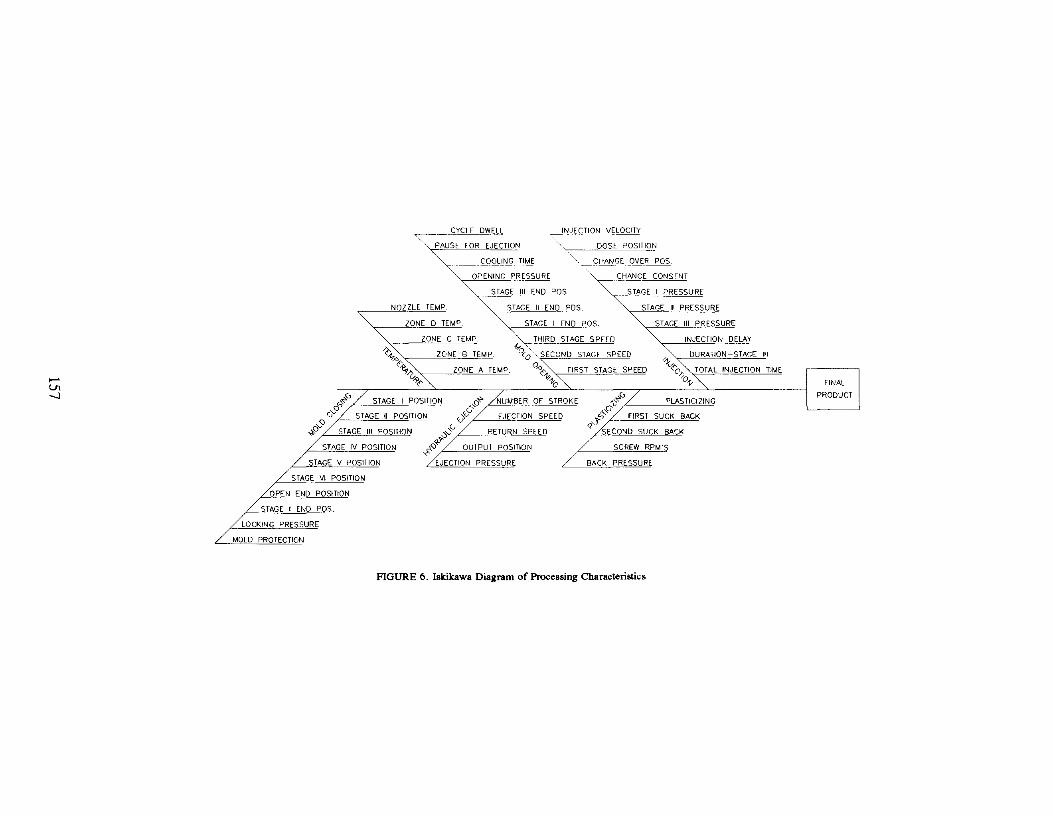
CYCLE DWELL ~-~~---~-~-~

" PAUSE FOR EJECTION

~N_JEC;TI9!'LY~LOCITY

"', DOSE POSiTiON

~ ___ ~Q1.!ti§~~ -'. __ ~1::!.6ti9~ . .2Yf:R pas

OPENING PRESSURE CHANGE CONSENT

~ STAGE III END pas ~ STAGE I PRESSURE

NOZZLE TEMP ~ STAGE II END PDS ~ STAGE II PRESSURE

"" ZONE 0 TEMP. ~ STAGE I END POS. ~ STAGE III PRESSURE

~ ZONE C TEMP ~ THIRD STAGE SPEED ~ INJECTION DELAY

~~ ZONE B TEMP f,..O(~SECOND STAGE SPEED

<t-e,~ ZONE A TEMP. o~~ FIRST STAGE SPEED

</1'(' "" 1f~Q ""

~ DURATION-STAGE III "', v('o/, " TOTAL INJECTION TIME

/o~ "" ~~0J / STAGE I POSITION

0,,-,°/ STAGE II POSITiON

o~ /NUMBER OF STROKE

" / <v0V / EJECTiON SPEED

PLAST1C1ZING 1:"''''/ 0/

.;y-C;'" / FIRST SUCK BACK ~/

~O / STAGE III POSITION q/sECOND SUCK BACK

/ STAGE IV POSITION

/ $1 AGE V POSITION

/ STAGE VI POSITION

bPEN END POSITION

0~v ~ RETURN SPEED

-f"J4-'?"L OUTPUT POSITION

'/EJECT10N PRESSURE

/ SCREW RPM'S

~ BACK PRESSURE

/ STAGE I END POS.

/LOCKING PRESSURE

/ MOLD PROTECTION

FIGURE 6. Iskikawa Diagram of Processing Characteristics

FINAL

PRODUCT

",""",p

'"" , ""1 '''''1 · 1 " , SIl, , , , , , 1mld utI 1111106 II!J1GS 1IIJ,I~ I:~t~ 1113.105 1113.

1101.4!'6 1101.455 1101.455 IIOI4~ 1I01.4M !IOU!!! 1101.4!'6 "OI.~ 110l«li 111UXI 1110.400 1108.100 1105.000 1011.100 110151JXl 1104.200 "~: 1101.100 III"

10000 15 12.000 YB O.COO 10Il00 ."'" '''''' 11.000 I.'"

'" '" 'IS NO lIS '" ![S lIS '" I I IIVIO/'I

--------------------------.-------. uct

L11'

IIl9Il.trol'------------------------------------------'

------------------ OCL

"trol------------------------------------------'LI1

FIGURE 7. X and R Chart of Sample Hydraulic Pressure Data

158

LABORATORY EXPERIMENTS FROM THE TOY STORE

H. T. McClelland

Department of Manufacturing and Industrial Technology Arizona State University

Tempe, Arizona 85287-6706


159

LABORATORY EXPERIMENTS FROM THE TOY STORE by

H.T. McClelland Department of Manufacturing and Industrial Technology

Arizona State University Tempe, AZ 85287-6706

KEY WORDS: Elasticity, plasticity, strain rate dependence, extrusion.

PREREQUISITE KNOWLEDGE: This material could be taught to a typical student of materials science or manufacturing at the high school level or above.

OBJECTIVES: To qualitatively demonstrate the concepts of elasticity, plasticity, and the strain rate and temperature dependence of the mechanical properties of engineering materials.

To qualitatively demonstrate the basics of extrusion including material flow, strain rate dependence of defects, lubrication effects, and the making of hollow shapes by extrusion. The two parts may be two separate experiments done at different times when the respective subjects are covered.

To demonstrate the importance of qualitative observations and the amount of information which can be gathered without quantitative measurements.

EQUIPMENT AND SUPPLIES: 1) One or more containers (eggs) of formable putty (Silly PuttyTM, Nutty PuttyTM, etc.); 2) one or more clay extrusion presses (made by PlayDoh™, Fun Dough™, etc.); 3) ice and a bowl; and 4) a low power heat source (depending on the ambient temperature, this may not be required).

PROCEDURE: Part 1 of this experiment involves allowing the students to manipulate the formable putty to illustrate the definitions and concepts of the mechanical properties of materials. Figure 1 contains a picture of the putty and normal packaging container.

While the students are unwrapping the putty, the definitions of elasticity (recoverable deformation) and plasticity (non-recoverable deformation) can be reviewed.

1) The students may form the putty into a smooth ball and bounce the ball on a rigid surface from a height of about 10 cm and note the general height of the rebound and the lack of permanent deformation. The amount of deformation can be quantified by using a measuring stick.

161

The ball may then be placed in the bowl of ice and cooled. It will be noticed that the ball flattens on the bottom illustrating creep.

After the putty is cold, it can be reformed into a ball and bounced again from the same 10 cm height and the amount of rebound noted. The rebound height will be higher than when warm indicating an increase in hardness with decreasing temperature.

2. The putty can then be formed into a cylinder. The students pull the putty slowly lengthwise and note the extensive plastic deformation (Figure 2). This is a graphic demonstration of the concept of ductility. A note should be made of the relative amount of force needed to pull the cylinder.

Reforming the cylinder and quickly pulling it may result in some plastic deformation and a sharp break if the room temperature is below about 24 C (Figure 3). If it is summer without good air conditioning, the faster pulling will still give extensive plastic deformation.

Forming a cylinder and cooling it in the ice will give a better visualization. Slow pulling will give extensive plastic deformation (ductile) and fast pulling will result in a sharp break (brittle). The amount of force necessary to pull the cylinder should be greater than that needed for the warmer conditions.

The audience at the initial presentation of this paper suggested two other experiments along these lines. The first involved cooling the putty in liquid nitrogen and hitting it with a hammer when it was cold. The ball will shatter further illustrating the temperature dependence of deformation. The second suggestion was to also use torsion for the ductile-brittle versus rate of deformation experiment. This illustrates that the method of deformation does not change the material's reactions in these matters.

3. A relatively short cylinder can be formed (height about twice the diameter). Placing the cylinder upright on a flat surface and gently deforming it in the length direction with the flat of the hand will illustrate the concept of barreling common in upset forging. The material next to the hand and next to the table will expand less than the center material due to the friction between the putty and hand and the putty and the table.

4. The students should be given time to try other experiments with the putty. It has been observed that most students will play with the putty for quite aWhile on their own.

Part 2 of this experiment involves the use of a clay extrusion press such as the Play-Doh™ Fun Factory or the Fun Dough™ Super Play Shop. As seen in Figure 4, the press comes with a variety of die shapes all of which have

162

approximately the same cross-sectional area and thus the same extrusion ratio. The presses come with two containers of different color clay.

1. The students may take one color of clay and extrude it through different die shapes noting the relative amount of force needed. In general, more force is required for those dies with the larger amounts of surface area (many small holes versus a few large holes). This indicates the effect of friction.

2. The students should extrude clay using the tube die (bridge or spider die) and make hollow tubes (Figure 5). This is a concept which is difficult for students to understand in lecture. The addition of a little water to the die prevents rewelding of the two halves demonstrating the effect of surface contamination. (It has been noticed that the Play-Doh™ spider die works better than the other brands) .

3. Using one of the dies, the students should slowly extrude a shape. A second shape should be extruded using much greater speed. The first shape should have a smooth surface and the second should be irregular due to "speed cracking", a common extrusion problem. This can also be done on the same extrusion as illustrated in Figure 6. A careful application of a small amount of water to the inside die face and the front (die side) of the clay can be used to increase the extrusion speed without the speed cracking showing the effects of lubrication. (Note: This may be a little tricky since the water will dissolve the clay if too much is used. oil may be used but may also react adversely and may be more difficult to separate afterwards).

4. Two experiments may be performed to demonstrate the material movement. In the first, two colors of clay are placed side-by-side with the intersection parallel to the extrusion axis. Extruding through a single hole die shows that the two colors maintain their respective positions. Placing the two colors so that the intersection is perpendicular to the extrusion axis and extruding demonstrates that the back color moves faster and moves inside the front color. The extruded shape can then be cut to show the extent of the movement. The amount of each color in a cross-section varies along the length of the extrusion as shown in Figure 7. Similar movement can also be demonstrated using the multi-small hole "spaghetti" die.

5. The students should then be allowed to experiment with the equipment.

163

SAMPLE DATA SHEETS: Putty: 1. Rebound height warm

Rebound height cold Observations:

2. Relative amount of force cold Relative amount of force warm Observations (include description of

fracture surface)

3. Sketch cylinder before and after deforming

4. Descriptions and observations

Extrusion: 1. Die Shape Relative amount of force

2. Observations

3. Observations and sketches

4. Sketch before and after for both cases

5. Descriptions and observations

INSTRUCT'OR NOTES: The relative measurements should be made into a numerical form such as 1 (low), 2(moderate), and 3 (high). The students will generally tend to play with the equipment for a fair amount of time after the designated experiments are over. Some of their documented observations may be included in future experiments.

SOURCES OF SUPPLIES: The putty and the extrusion press can be obtained in most large toy stores (before Christmas is a good time to find them though both of these are usually available all year). It generally requires two putty eggs per student t.o give enough material to work with. These cost about $3-$4 per egg. The extrusion presses are less than $10. These are all 1990-1991 prices in the Phoenix, AZ area. All of these should last a number of years except that new clay may be required every year. The clay costs about $4 per 4 pack. (The clay becomes mixed and thus a generic off color. The mixing experiments require separate colors) .

The measuring stick, if used, may be any available ruler or may be made by the students out a piece of paper with regularly spaced lines drawn on it.

164

Figure 1: Formable putty and packaging. The amount shown is from two eggs.

Figure 2: Deformed putty which underwent a large amount of ductile plastic deformation.

165

OU::1I1 J ii .... i .l34ki#M··.·.Ie·.Jv ..

Figure 3: The fracture surface of the putty after brittle, high-rate deformation.

Figure 4: Extrusion press showing die sE!lection and packaging.

166

Figure 5: Hollow tube extruded from the Fun Factory.

Figure 6: Rectangular shape extruded at slow then fast rates showing the transition to speed cracking.

167

Figure 7: Shape extruded from two color dough arranged front-to-back in the press demonstrating the movement of the rear (lighter) color into the center of the front (darker) color.

168

DIELECTRIC BEHAVIOR OF SEMICONDUCTORS AT MICROWAVE FREQUENCIES

J. N. Dahiya

Physics Department Southeast Missouri State University

One University Plaza Cape Girardeau, Missouri 63701


169

DIELECTRIC BEHAVIOR OF SEMICONDUCTORS AT MICROWAVE FREQUENCIES

J. N. Dahiya Physics Department

Southeast Missouri State University

KEY WORDS

Semiconductors; frequency shift; Q-change; dielectric relaxation, microwave resonant signal.

OBJECTIVES

1. To learn about the components of a microwave spectrometer.

2. To learn to operate the spectrometer.

3. To understand the shape of the signal and record data in terms of frequency shifts and Q-changes.

4. To understand the dielectric properties of semiconductors: germanium and silicon.

SUMMARY

A cylindrical microwave resonant cavity in TE011 mode is used to study the dielectric relaxation in germanium and silicon. The samples of these semiconductors are used to perturb the electric field in the cavity and Slater's perturbation equations are used to calculate the real and imaginary parts of the dielectric constant. The dielectric loss of germanium and silicon is studied at different temperatures and Debye's equations are used to calculate the relaxation time at these temperatures.

INTRODUCTION

A number of experiments have been performed to investigate the dielectric properties of solids, liquids and gases at various frequencies (ref. 1-6). The present experiment is to study the dielectric relaxation mechanism in germanium and silicon.

171

The microwave resonant technique has been used by several investigators in the past and it has become a standard technique to study the dielectric behavior in various compounds of interest. Hong and Roberts (ref. 7) used a cylindrical cavity in TM010 mode to study the dielectric properties of solids and liquids. Dahiya et al. (ref. 8-10) used a microwave resonant cavity to study dielectric relaxation mechanism in various polar and non polar compounds.

It has proven to be a very interesting experiment to find the dielectric response of a material near a phase transition region, i.e., going from an ordered to a disordered phase. From measurements of the static dielectric constant of compounds as a function of the temperature, important conclusions concerning molecular freedom may be drawn. The dielectric response of a polar liquid shows a large change at the freezing pOint. A typical example is that of water as studied by Dahiya et al. (ref. 8). The drop in the dielectric constant of water at the freezing point is caused by the partial or complete loss of rotational polarization (freedom to reorient), while the electronic and vibrational polarizations remain relatively unchanged.

In the present investigation, dielectric behavior of semiconductors, germanium and silicon were studied at different temperatures. The sample under investigation was placed along the vertical axis of the cavity. The sample was taken in a capillary tube and the thermocouple leads were inserted into the capillary tube to make a fine contact with the sample. The sample was then cooled by flushing cold nitrogen gas around the cavity and desired temperature was obtained. The temperature was then allowed to vary in small steps and frequency shifts and Qchanges were recorded.

EQUIPMENT CONFIGURATION AND THEORY

The block diagram of the microwave spectrometer used in this investigation is shown in Figure 1 that shows all the components needed to study the dielectric relaxation mechanism. The source of the microwaves was a 2K25 tunable klystron made by Western Electric. The frequency produced by the klystron varies between 8.8 to 11.0 GHz. The klystron was powered by a Hewlett Packard 715A power supply. The microwaves produced by the klystron were guided by waveguides in the x-band of frequency. The signal reaching the directional coupler was divided into two parts. A part of this signal reaches the microwave resonant cavity via an

172

attenuator and a wavemeter. The attenuator was used to adjust the right amount of microwave power for the sample being studied. The function of the wavemeter is to determine the exact frequency of the klystron by tuning it to the resonant frequency of the klystron.

The next important device in this operation is a crystal detector which is used for the radio frequency wave. Crystal detectors have wide use in the microwave field because of their sensitivity and simplicity. They are used as "video detectors" to provide either a dc output when unmodulated microwave energy is applied, or a low frequency ac output when the microwave signal is modulated. The essential parts of a crystal detector are a semiconducting wafer and a metal "whisker" which contacts the wafer. In the present experiment two such crystal detectors were used, one of which was installed in the reflectometer to provide dc output when the klystron modulated signal is reflected from the resonant cavity. Another crystal detector was mounted in a directional coupler to mix the modulated klystron signal with the nth harmonic waves from the standard frequency multiplier.

The purpose of modulating the microwave signal was as follows. The unmodulated signal from the klystron gives a very narrow frequency interval as shown in the microwave power vs frequency curve in Figure 2a. With a signal like that it is very difficult to measure the shifts in frequencies and the Q-changes of the signal. An oscilloscope horizontal sawtooth sweep voltage was applied to the repeller of the klystron. This voltage was derived from the time base of a Tektronix model 533A dual channel oscilloscope that sweeps the klystron over the range of frequencies desired while simultaneously a chopper signal of 31 kHz was impressed upon the klystron repeller electrode to produce an ac signal of that frequency at the detector. The modulated signal is shown in Figure 2b and Figure 2c shows the reflected power absorption by the resonant cavity. As shown in Figures 3a and 3b, the power absorption by the cavity was modulated to give a differential display of the resonance profile in the form of a butterfly. Figures 3c and 3d show the modulated signal before the sample under investigation was introduced into the cavity and after the sample had been introduced respectively. The resonance frequency shifted and the width of the signal changed as seen in Figure 3d. The modulated signal was amplified by a pre-amplifier and displayed on the oscilloscope.

Through the Webster G40P5158 directional coupler, a part of the microwave signal was mixed with a standard frequency obtained

173

from a Hewlett Packard 612A UHF signal generator. A Kenwood R-1000 radio receiver was used to detect the frequency difference between the klystron resonant frequency and the standard frequency source. The resulting frequency difference yielded two markers which were displayed on the oscilloscope. These markers were used to record the frequency shifts and the Q-changes of the resonant signal as the cavity was loaded with the sample under investigation.

A cylindrical cavity in the TE011 mode was designed. A long copper coil was wrapped around the cavity and the cavity placed in a thermal bath. As the sample under investigation is introduced into the cavity it perturbs the electric field of the cavity and as a result of that the resonant frequency shifts and the Q of the cavity changes. The frequency shifts and Q-changes of the signal are related to the real and imaginary parts of the dielectric constant through the Slater's perturbation equations as follows. (ref. 8)

= e'-l f Es . E dv

2 f E' Ea dV (1)

(2)

... where E is the field of the unperturbed cavity, Ea is the microwave field as applied to the cavity and Es is the field of the sample itself, and v and V are the volumes of the sample and cavity respectively.

The signal Q-change is further related to the width of the signal by

where fo is the resonant frequency of the system and W is the frequency separation in Hertz of the resonance half-power points.

174

(3)

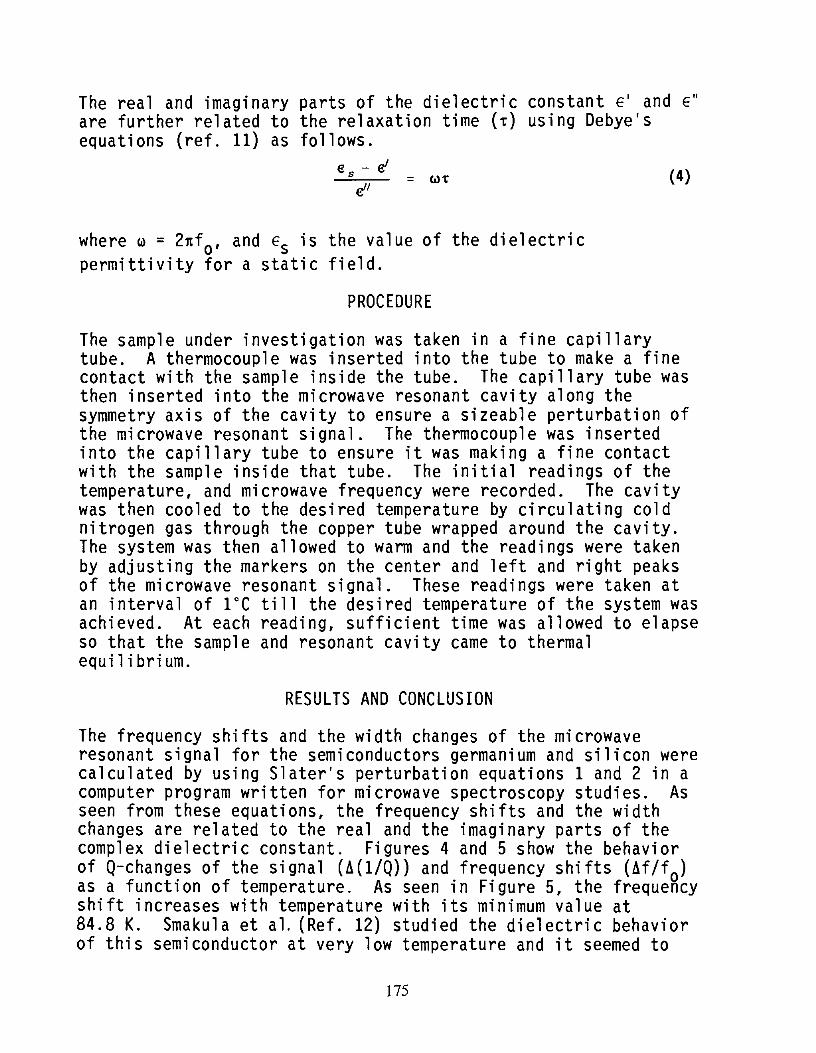
The real and imaginary parts of the dielectric constant E' and E" are further related to the relaxation time (.) using Debye's equations (ref. 11) as follows.

e - ~ s

e"

where ~ = 2nfo' and ES is the value of the dielectric permittivity for a static field.

PROCEDURE

(4)

The sample under investigation was taken in a fine capillary tube. A thermocouple was inserted into the tube to make a fine contact with the sample inside the tube. The capillary tube was then inserted into the microwave resonant cavity along the symmetry axis of the cavity to ensure a sizeable perturbation of the microwave resonant signal. The thermocouple was inserted into the capillary tube to ensure it was making a fine contact with the sample inside that tube. The initial readings of the temperature, and microwave frequency were recorded. The cavity was then cooled to the desired temperature by circulating cold nitrogen gas through the copper tube wrapped around the cavity. The system was then allowed to warm and the readings were taken by adjusting the markers on the center and left and right peaks of the microwave resonant signal. These readings were taken at an interval of 1°C till the desired temperature of the system was achieved. At each reading, sufficient time was allowed to elapse so that the sample and resonant cavity came to thermal equilibrium.

RESULTS AND CONCLUSION

The frequency shifts and the width changes of the microwave resonant signal for the semiconductors germanium and silicon were calculated by using Slater's perturbation equations 1 and 2 in a computer program written for microwave spectroscopy studies. As seen from these equations, the frequency shifts and the width changes are related to the real and the imaginary parts of the complex dielectric constant. Figures 4 and 5 show the behavior of Q-changes of the signal (4(1/Q)) and frequency shifts (4f/fo) as a function of temperature. As seen in Figure 5, the frequency shift increases with temperature with its minimum value at 84.8 K. Smakula et al. (Ref. 12) studied the dielectric behavior of this semiconductor at very low temperature and it seemed to

175

have another minimum around 4 K. Figure 4 shows a similar behavior of the Q-change with a minimum value around 84.8 K and a maximum value around 196 K and it decreases as the temperature increases up to 300 K. The low temperature studies of this material indicate another maximum around 10 K as shown by Smakula et al. (Ref. 12). Figures 6 and 7 show behavior of Q-change and the frequency shift for silicon between 70 K and 300 K. The relaxation times for these semiconductors were calculated using equation 4 and were of the order of 10-11 _10- 14 sec.

The bound electrons and the free carriers in a semiconductor material account for the dielectric permittivity and the conductivity of the material. The bound electrons in the semiconductor can be categorized as the core electrons of the materials, the valence electrons, and the electrons from the impurity atoms.. The valence electrons and the core electrons have excitations in the infrared frequency regions. The permittivity of these electrons may not have any imaginary term and these electrons do not show any temperature dependence at very low temperature. However, the impurity electrons vary with temperature and thus affect the complex permittivity or the dielectric constant of the material.

In this investigation, a microwave spectrometer was assembled to study the dielectric relaxation in various compounds of interest. The spectrometer was designed to study these behaviors at very low temperatures. The technique was very successful in monitoring the dielectric behavior of germanium and silicon. The main emphasis of this research was to create an advanced physics laboratory expE!riment in which undergraduate students were involved to design the spectrometer piece by piece. The spectrometer was then used as a tool to study the dielectric behavior of various polar and nonpolar compounds. Semiconductors germanium and silicon were chosen for their dielectric behavior at low temperatures. The cooling system used in the microwave spectrometer was also designed by undergraduate students and was very efficient.

The main purpose of this experiment was to understand the function of each component of the microwave spectrometer and to use it as a technique to monitor the dielectric behavior in semiconductors germanium and silicon at low temperatures. The detailed results of the dielectric relaxation in these semiconductors will be presented elsewhere as a continuation of this experiment.

176

REFERENCES

1. Baynham, A. C., Gibson, A. F., and Granville, J. W.: On the Dielectric Constant of Germanium at Microwave Frequencies. Proc. Phys. Soc., 75, 1960, p. 306.

2. Lurio, A., and Stern, E.: Measurements of the Dielectric Con~tant of BaTi03 Single Crystals in the Paraelectric Reglon at X-band. J. Appl. Phys., 11, 1960, p. 1805.

3. Nishioka, A., and Takeuchi, M.: Dielectric Property of Triglycine Sulphate Single Crystal in the 9,000 Mc/s Region. J. Phys. Soc. Japan, 14, 1959, p. 971.

4. Surber, W. H., and Crouch, G. E.: Dielectric Measurement Methods for Solids at Microwave Frequencies. J. Appl. Phys., ~, 1948, p. 430.

5. Grant, E. H., Buchanan, T. J., and Cook, H. F.: Dielectric Behavior of Water at Microwave Frequencies. J. Chern. Phys., 26, 1957, p. 156.

6. Birnbaum, G., Kryder, S. J., and Lyons, J.: Microwave Measurements of the Dielectric Properties of Gases. J. Appl. Phys:, 22, 1951, p. 95.

7. Hong, K. H., and Roberts, J.A.: Microwave Properties of Liquids and Solids Using a Resonant Microwave Cavity as a Probe. J. Appl. Phys., 45(6), 1974, p. 2452.

8. Dahiya, J. N., Jani, S. K. and Roberts, J. A.: Phase Transition Studies in Polar and Non-Polar Liquids at Microwave Frequencies. J. Chern. Phys. 74(6), 1981, p. 3609.

9. Jani, S. K., Dahiya, J. N. and Roberts, J. A.: Changes in Hyaluronate Solutions at Microwave as a Function of Concentration, System pH and Bioplymers, ~, 1980, p. 931.

Dielectric Frequencies Temperature.

10. Dahiya, J. N., and Freeman, R. W.: Computer Interfacing of a Microwave Resonant Cavity for Temperature Measurements During Dielectric Relaxation. Computers in Physics, Jul/Aug. 1989, p. 49.

177

p

(a) f

p

f (b)

p

-- --... - -.....

f (c)

2. (a) Klystron mode shape (unmodulated width).

(b) Klystron mode shape (modulated width).

(c) Reflected power absorption by cavity.

180

p

dP dt

3. (a)

(b)

(c)

(d)

to t

(a)

to t

(c)

QE dt

dP dt

to

(b)

to

(d)

Enlarged drawing for power absorption by the

First derivative of resonance absorption.

Resonance absorption signal (unperturbed).

Resonant frequency shift and width change due insertion of the sample into the cavity.

181

t

t

cavity.

to

--I -0

" -

L1 ( b ) ARBITRARY UNITS

o ~ en ~ t---r---~~---r--~--~-+--~--+--4--~

.... .... o

.... en 0

'" .... 0

w .... o

, + +

+ +

+

+

+ +

+ •

•

+++ .+

+

• +

• •

4. Microwave loss ~(l/Q) as a function of temperature for a sample of semiconductor germanium.

182

~ -0

=" -

( ~:) ARBITRARY UNITS

«:) .:::a. en ~+---~~---+--~--~-+--~--~-+--+-~

..... ..... «:)

..... en «:)

N ..... «:)

(N ..... «:)

+. + • + • + • • • + • •• • • •• • •

+ • • • •

5. Frequency shift df/fo as a function of temperature for a sample of semiconductor germanium.

183

-.. en 0

-I -0 :::-:: -

N -.. 0

• • •

~ ( 6 ) ARBITRARY UNITS

••

• • • • • • • • •• • • • ;

6. Microwave loss ~(l/Q) as a function of temperature for a sample of semiconductor silicon.

184

-I -0

:=-:: -

( ~!) ARBITRARY UNITS

...A. ...A. ...A. ...A. ...A. N N N Q N ~ en ~ Q N ~ en ~ Q N ~

~ +---~~---+--~--~-+--~--~-+--~--~~

...A.

en Q

N ...A.

Q

• • • • • • • • • • • • • •• • • • • ••••

7. Frequency shift ~f/fo as a function of temperature for a sample of semiconductor silicon.

185

Be-Cn PRECIPITATION HARDENING EXPERIMENT

Richard L. Cowan

Department of Mechanical Engineering Ohio Northern University

Ada, Ohio 45810


187

Be-Cu PRECIPITATION HARDENING EXPERIMENT

Richard L. Cowan Ohio Northern University

Ada, Ohio

KEY WORDS: precipitation, aging, hardening, solution annealing, super saturation, beryllium-copper alloys

PREREQUISITE KNOWLEDGE: The student performing this experiment should have a knowledge of binary phase diagrams.

OBJECTIVES: The objectives of this experiment are: to give the student a hands-on approach to changing materials properties through heat treatment of a specimen; to quantify the amount of strengthening obtained in the specimen; to encourage the student to speculate about the structural changes that have occurred in the material to cause the changes in strength.

EQUIPMENT AND SUPPLIES: 1) small furnace with capability of maintaining a temperature of 500 C +/- 5'C. (If solution anneal is to be done in the same furnace, temperature capability should be 800 C); 2) hardness tester with a range of 60 - 350 Brinell hardness; 3) small (1 gallon) water quench tank; 4) tongs to handle hot specimens; 5) insulated glove; 6) conversion chart for RB and Rc to Brinell hardness (not needed if you have Brinell tester) 7) a Cu-Be phase diagram for the 0 - 10% Be region (see Fig. 1) 8) several (9) 2.5 cm diameter x 1 cm thick specimens of Cu - 1.8 Be or Cu - 2.0 Be.

PROCEDURE: Precipitation hardening depends upon the controlled precipitation of a constituent from a supersaturated solid solution. The precipitation rate depends upon the treatment temperature. As the temperature approaches the solvus line for the alloy of interest the faster the reaction will be.[ll

The stUdents are provided with approximately ten solutionannealed disks of Cu - 1.8 Be and they develop a hardness vs. aging time graph at a specific temperature (i.e., 400 C).

Instructions to the students are as follows:

1. Equip the hardness tester to take readings on the Rockwell B scale (100 kg load - 1/16" ball penetrator). Check the reading of the tester with the standard block.

189

2. Take three hardness readings on each disk. Average the readings on each disk and record them.

3. Check the furnace temperature. It should be at the temperature specified for your group.

4. Place the disks in the furnace near the center. orient them so there will be easy access to remove them individually.

5. At the following times specified, remove the disks and quench them immediately: 2, 4, 6, 8, 10, 20, 30, 45, 1 hr., overnight.

6. Measure the hardness of the aged specimens and record the values.

7. Plot the Brinell hardness vs. log of time in seconds for the specimens. (If the hardness readings for the solutionized disks vary more than ± 3 points Rockwell B, plot hardness increase vs. aging time.)

The students follow the above procedure to obtain their data. They are then required to do the following in the discussion of the experimental results.

1. Relate the micro-structural changes that are occurring in the specimen as it is solution annealed and quenched, reheated and quenched repeatedly to the Be-Cu phase diagram.

2. Explain why the hardness of the specimen is increasing. Relate this change in hardness to the micro-structure.

3. What 'would you expect the aging curve to look like if the aging temperature was 50° lower?

4. 50° higher?

5. Explain answers to 3. and 4. based upon the phase diagram.

6. Did overaging occur for any of the specimens? If it did, explain what happened.

7. Sketch how you would expect the micro-structure to appear for a hardened material prior to over-aging.

8. Same as 7 except after over-aging.

9. Sketch the micro-structure if the material had cooled under equilibrium conditions from the solutionizing temperature.

190

10. For 9, would the material be harder or softer than if it was quenched?

11. Comment on 7, 8, 9, and 10.

12. At what temperature do you think the material was solutionized?

SAMPLE DATE SHEETS: Self-Evident

INSTRUCTOR NOTES: Specimens can be cut from round, square, or other available bar stock. They should be solution annealed at approximately 750 C. They may begin to melt if you heat them to 850 C. At 700 C the disks will not solutionize in a reasonable amount of time.

Samples that have been cut approximately one centimeter thick will solutionize in 20-30 minutes at 750 C. They should be removed from the furnace and immediately quenched and agitated in water. Specimens solutionized in this manner will have an approximate hardness of 40 Rockwell B.

Take hardness readings after solutionizing, and then group disks by hardness range so that you minimize initial hardness spread for the students. One group of 6 or 7 samples may be in the range of Rockwell B 40-45; another group in the range of Rockwell B 35-40.

Aging times are cumulative so that the students do not need a separate disk for each aging time. Students should be told to take hardness readings on one side only. After a few cycles through solution annealing and aging, the disks can be faced in a lathe and the sequence can start again. This can be continued until there is no longer enough material to grasp in the lathe collets or chuck.

Whenever the material is machined the machine operator must take precautions to avoid breathing any dust generated. The material should be machined wet, or in a hood, or the operator should wear a mask.

No harmful oxides are generated at the aging temperatures. The oxides that form on the surface are copper oxides.

Different groups of students can age their specimens at different temperatures. Then when they compare results they can see the shift in the aging curve.

Best control of properties is obtained when the specimens are aged at 350 C. But, it takes over two hours to obtain maximum strength and most lab schedules are not long enough to

191

permit using t:his temperature. Temperatures used to aging are 400 C, 450 C, 500 C, and 550 C.

Metallography is not an appropriate addition to this experiment because the precipitates that increase the hardness cannot be seen in an optical microscope.

REFERENCES: A.skeland, D. R. The Science and Engineering of Materials, Alt.ernate Edition, PWS Engineering, 1985, pp 215; pp 251.

Metals Handbook, Volume 8, American Society for Metals, 8th Edition, Sept. 1973.

SOURCES OF SUPPLIES: CU-1.8 Be bar stock from Brush-Wellman, Inc., 17876 st. Clair Ave., Cleveland, OH 44110. The material, solution annealed or as drawn, costs $10.50 to $15.00 per pound.

192

l'ltomlC Percentage Beryllium

5 10 15 20 25 30 35 40 °C 1100

1900F ~' I

\ ~I L I 1000

1700F

900 1600F

800 1400F

700 1200F

600

IOOOF

500

SOOF

400 700F

300 500F

200 Cu

'. +-

\\, ~ ',.... I'--........

, .... 866' .......... ~ 4.3 ---== l:::::::::: r- ------ ---- V--/2.7 4.1~ I

~ It 853', 5.0%

(Cu) V 1\1 YI V Y.+Y2 /: \ V 60S'

7 6.0

/ I (Cu)+ Yz

/ I ,

I ,L ,\

2 3 4 5 6 7 8 9 10 Weight Percentage Beryllium

Figure 1. Cu-Be Phase Diagram [2] .

193

ASTM - TERMINOLOGY FOR EXPERIMENTS AND TESTING

Richard R. Strehlow

ASTM Committee on Terminology Oak Ridge National Laboratory

Martin Marietta Energy Systems, Inc. P. O. Box 2008

Oak Ridge, Tennessee 37831-6263


195

Standard Terminology in the Laboratory and Classroom

Richard A. Strehlow Oak Ridge National Laboratory *

Chainnan, ASTM Committee on Tenninology

The materials produced by modern technologists are stunning and exciting. Every one of them is, however, associated with a family of immaterials-all the concepts of substance, process, and purpose. It is concepts that are essential to transfer knowledge. It is concepts that are the stuff of terminology.

Terminology is standardized today by companies, standards organizations, governments, and other groups. Simply described, it is the pre-negotiation of the meanings of tenns. Terminology has become a key issue in businesses, and terminology knowledge is essential in understanding the modem world.

The fundamental objective in terminology standardization is to decrease ambiguity in interpreting, understanding, and using language and to explain meanings of technical terms to those who are not conversant with them. It is a key element in infonnation retrieval and database design.

This 90 minute introductory workshop introduces the concepts of terminology and methods of its standardization. Exercises are used along with the presentation to rapidly survey and experience several aspects of contemporary terminology. Some of the questions to be addressed include, as examples:

• What is a tenn and what constitutes a satisfactory definition statement? • How does tenninology relate to definition of data elements in databases? • How does ASTM manage tenninology in a 35,000 member organization? • What is the role of standard terminologies in the process of explanation? • How can terminologies be exchanged between different countries with different languages?

The objectives of the workshop are to enhance terminological awareness and to demonstrate the usefulness of ASTM source materials for both laboratory and classroom teaching.

* Operated by Martin Marietta Energy Systems, Inc., under U. S. Department of Energy contract DE-AC05-840R21400

197

Standard Terminology in the Laboratory and Classroom

R A. Strehlow

OAK RIDGE NATIONAL LABORATORY*

Representing the

ASTM Committee on Terminology (COT)

National Educators' Workshop

Oak Ridge, TN

November 12-14, 1991

• Operated by Martin Marietta Energy Systems, Inc., under U. S. Department of Energy contract DE-AC05-840R21400

NEW:11/91, No.3

The Value of Standardized Terminology in Education

• To know a subject is to know its concepts and its terminology.

• To teach a subject is to organize and present its concepts and its terminology

• To find information efficiently requires specialized terminology

• To comprehend written materials requires knowledge of their terminologies.

NEW:11/91, No.9

N o o

Specific Skills for Terminology StandardizationWork

Identifying terms

Developing a concept system

Identifying concept characteristics

Writing definitions and term entries

Composing and designing terminology products

NEW:11/91, No. 12

t..l o .......

Terminology defined

1. The set of practices and methods used for the collection, description, and presentation of terms.

2. A theory explaining the relationships between concepts and terms.

3. A vocabulary of a special subject field.

NEW:11/91, No. 14

Terminology involves several disciplines.

Semantics

Lexicology Linguistics Discourse Orismology

13. Phonology

Grammar (Morphology and Syntax)

Knowledge Representatio Perception Abstraction Classificatio

General Semantics

Communication modelling

Dialog analysis

General Systems methodology

Metaphor analysis

NEW:11/91, No. 15

N o w

What is a term?-

a word belonging to specialized areas of usage in one or more languages

An exercise:

Identifying terms

NEW:11/91, No. 16

N o ....

Terminology provides the access to concepts that permit us to talk

about the world.

(Q)[]l)D®©~~,

1Rl®~@~O©[1j]~, @[1j]@] ©~[)jJ®1f

NEW:11/91, No. 18

tv o u.

Types of Terminology Exercises

• Identify terms representing concepts from a corpus

• Select those terms appropriate for standardization

• Define the term

• Organize concepts for clarity and completeness

• Present terminology products in a useful way

• Practice in the use of terminologies

NEW:11/91, No. 26

Canonical Form Definitions-

Genus + Differentiating characteristics

• Genus is the type of entity or relation.

• The differentiating characteristics are those properties that distinguish the particular item for others of the same type.

An exercise-definition

NEW:11/91, No. 30

N o -.J

Fundamental Concept Analysis

• A concept is described by a set of characteristics, properties, and other relations.

• For a definition we select those characteristics that carry meaning for the particular concept-those that are both semantic all relevan central to the concept.

NEW:11/91, No. 31

N o 00

Information on definitions?

Part E, Form and Style for ASTM Standards, 8th ed.

Peter Achenstein, Concepts of Science, Johns Hopkins Press, Baltimore, Md, 1968.

Standardization of Technical Terminology; Principles and Practice, ASTM STP 806, C.G.Interrante and F. J. Heymann, Eds., 1983.

Standardization of Technical Terminology; Principles and Practice. Second Volume, ASTM STP 991, R. A. Strehlow, ed., 1988.

NEW:11/91, No. 43

Representation of Terminologic Data may be done in many ways:

• Conventional definitions

• Thesauri and word lists

• Tree structures

• Semantic space maps and nets

• Frames and schemata

• Predicate calculus

• Tables and lists

• Data based structures (SGML)

NEW:11/91, No. 45

N ...... o

Exercises with Terminology Standards

E-44-84 Heat Treatment of Metals

Compare case hardening, induction hardening, and surface hardening. Suggest a way to harden an iron foil.

E-673-90 Surface Analysis

How is a Koster-Kronig (K-K) transition distinguished from a super K-K transition? Hint: (See Auger transition)

NEW:11/91, No. 55

PRE-COLLEGE MATERIALS EDUCATION

Kenneth H. Eckelmeyer, Sandia National Laboratories L. Roy Bunnell, Battelle-Pacific Northwest Laboratories

Linda L. Horton, ORNL, Martin Marietta Energy Systems, Inc. Richard P. Krepski, Intermet Technology

Robert Berrettini, Materials Education Council Arlys Whitaker, ASM International

211

~The submitted ~t hils been authored by a contractor of the U.S. Government under contract No. DE· AC05-84OR21400. Acconlngly, 'he U.S. Government retains a nonelCclusfve, royalty·free license to pubiah or reproduce the published form of this contribution, or allow others to do 10. for U.S. Government purposes

•

"Science in Action": An Interdisciplinary Science Education Program

L. L. Horton Metals and Ceramics Division, Oak: Ridge National Laboratory*

Oak Ridge, IN 37831-6118

Science in Action is an education outreach program for pre-collegiate students. It is based on the concept that, in order to interest students in science, they must see science and scientists at work. The program encompasses the fun range of scientific disciplines - the core sciences, engineering and mathematics. A unique aspect of the program is the involvement and support of scientists and engineers representing local professional societies, industries, businesses, and academic institutions.

The first "Science in Action" program took place during National Engineers' Week in 1990; the second expanded program at the same time in 1991. "Science in Action" is part of the annual WATIeC conference in Knoxville, IN. The WATIeC conference is a week-long technical conference sponsored by a consortium of local professional/technical societies. The theme for the past several years has focussed on "competitiveness." Since the education of our young people is an essential part of "being competitive," the educational program was a natural outgrowth of the conference.

For the 1990 program, "Science in Action" was a two-day program specifically targeted to middle school students and was held in a multi-story building, the Candy Factory, at the World's Fair Site in downtown Knoxville. We wanted to reach students before they made the fatal decision to drop out of the advanced mathematics curriculum in high schooL On each day of the program, 6 middle schools were invited to bring 40 students and teachers. Although only 5 of the schools were able to attend on the scheduled days, because of the enthusiasm for the program, the attendance on the first day neared 300 and on the second about 250. The middle school teachers and administrators were thrilled that someone was finally having a special program for them .... they were really appreciative.

In 1991, "Science in Action" expanded to four days and moved to the Tennessee Valley Authority (TVA) Towers, also located in downtown Knoxville. The move permitted consolidation of the program on a single floor of the building. However, because of the size of the auditorium in the TVA Towers, attendance was limited to about 200 students each day. The first day was devoted to elementary school students. Small groups (5 students and a teacher - a "car load") were invited from the elementary schools in the surrounding cities and counties. Over 30 schools were able to participate. The second and third days followed the 1990 middle school format (although we reduced the number of students invited from each school to 30); nine middle schools participated. The final day involved small groups of 8 to 10 students from the 15 high schools. For this program, we did not design the program for the top few students in the school; these students have many opportunities to visit Oak Ridge National Laboratories and other local technical businesses. Instead, we specifically targeted students who are interested in science but are not currently considering it as a career. The program emphasized the broad range of potential careers in science and engineering-related fields.

"Science in Action" Presentations

The goal of the presentations is to be highly interactive. We want the students to have some "hands on" experiences and to leave with a good feeling about science and engineering. To present a broad spectrum of role models, scientists and engineers were involved as presenters, guides, and exhibitors. Presentations for "Science in Action" followed the format: Keynote Presentation followed by Small Group Presentations

213

and visits to the Exhibit area. In 1990, the exhibits were available for the students to visit before the program and during lunch. In 1991, the program was modified so that a visit to the exhibits was considered one of the small group presentations. The keynote was the only presentation given to the group as a whole. After the keynote, the group split into the individual school groups for the remainder of the program. The groups cycled through the balance of the presentations; each presentation was given to each school group. In order to allow maximum participation and have appropriate presentations for the age of the students, there was a different set of presentations on each day.

Keynote Presentations: The keynote presentation in 1990 was "Creatures of the Night" by a local veterinarian. The presentation focussed on animal science and environmental science (the habitats of all animals). Live owls and opossums were an integral part of this program; the students were able to actually touch the animals.

For 1991, the keynote varied with the age group of the students. "Raptor Tales" was presented by the Clinch River Raptor Center to the elementary and one group of middle school students. This program informed the students of th,;! value of raptors and their place in our environment. Live rap tors were a major part of the program; the birds were handled by middle school age children who work at the RaptOf Center. The second middle school keynote was "Fun with Chemistry," an introduction to chemistry given by a professor from Tennessee Technological University, Cookeville. "Fun with Materials," an introduction to materials science and engineering, was the keynote presentation for the high school students. (Detailed description can be found under the small group presentations.)

1990 Small Group Presentations: The small-group presentations covered a wide range of topics. Two of the most popular were "Fun with Materials" and the "Magic of Chemistry in Today's World." The "Magic of Chemistry in Today's World" was an interactive demonstration of chemical reactions -- all performed with chemicals that could b(! obtained in supermarkets. The "Fun with Materials" presentation is an adaptation of the original presentation by Bob Pond, an emeritus Johns Hopkins professor who is known throughout the United States for his "Fun with Metals" presentations. The students learned about the properties of materials and how materials scientists modify the properties for specific applications. All participants left with an aluminum "coin" that showed the crystal structure of the metal. A lucky few were able to catch some melt-spun tin as it left a round cake pan spun by a drill. The tin was melted inside of a foot-long glass dropper by a standard home workshop propane torch; students operated the drill.

In "The Microscopic World," the students were able to operate a real scanning electron microscope (SEM) (courtesy of the Metals and Ceramics Division, Oak Ridge National Laboratory). In the SEM, they were able to view insects, fractured surfaces of metals, diamond films, a human hair, and an integrated circuit. They also saw the "creature:, they swam with in the pond last summer" in a life-sciences optical microscope demonstration. Two top-of.·the-line metallographic microscopes were also part of this popular presentation. The presentations focussed on what we learn from microscopy and how this information is used in scientific and engineering investigations.

The noisiest presentation was "Neat Stuff with Humans." Presented by the Institute of Industrial Engineers, the presentation included a robot, a demonstration of how to design an effective assembly line (the students assembled balll point pens with a variety of approaches), and the impact of excessive noise on the quality of production (students attempted to communicate data while the group provided background noise).

In "Radiation, It's Only Natural," students learned about the occurrence of radiation in our natural environment, how radiation is detected, and how it is used. "Fun with Figures" focussed on mathematics

214

and how it can be fun, with various mathematical tricks and short cuts. "A Hitch-Hikers Tour of the Solar System" consisted of a slide show from various space explorations.

1991 Small Group Presentations: In 1991, we repeated several of the 1990 presentations. For the elementary students, "Fun with Materials" and "Fun with Rocks and Minerals" were presented. "Fun with Rocks and Minerals" explored the history of the earth through rocks and fossils. The students hammered on rocks to learn about the difference in hardness and left the demonstration with their own personal fossil.

The middle school presentations included "Fun with Materials," "Statistics," "Electricity and Magnetism," and "Ceramics Processing." The statistics presentation introduced basic mathematical concepts related to statistics. The electricity and magnetism presentation included hands on demonstrations. Ceramics Processing focussed on modern methods of processing ceramics. It involved a microwave oven for heating ceramics and a demonstration of how chemistry is used to process ceramic powders. A magnet was floated over a high temperature ceramic superconductor and a number of high tech ceramic car parts and a space shuttle tile were on display.

For the high school students, the small group presentations were "Electricity and Magnetism" and "Radiation: It's Only Natural" (presented in 1990). Both of these presentations were elevated to the high school level and stressed possible careers in these important fields.

Exhibits: In addition to the presentations, there were exhibits from a number of technical societies and local facilities. In 1990, the students visited these exhibits prior to the beginning of the program and during lunch. In 1991, due to the interest in the exhibits and the positive interactions between the students and the people manning the exhibits, a visit to the exhibit area was made an official "small group presentation." Each of the student groups was assigned a period of time for visiting the exhibits.

A variety of exhibits was on display each year. The University of Tennessee (UT) student chapter of ASM International had a display that included shape-memory alloys. In 1990, the biomedical engineers exhibited medical equipment such as a blood pump (demonstrated with a full-scale model of the circulatory system) and a number of other biomedical devices. This was a very popular exhibit; we were dismayed when this group could not schedule an exhibit for 1991.

In 1990, there were wooden models of various types of structures in the display sponsored by the civil engineering group. This exhibit was considerably expanded for 1991 to include numerous examples of civil engineering including road and bridge materials. The American Nuclear Society had an exhibit of how radioactive materials are used in our lives every day.

In 1990, the High Temperature Materials Laboratory from ORNL had a light-box display that highlighted various materials developments for high temperature environments. For 1991, the number of light boxes was reduced and the exhibit expanded to include a superconductor demonstration and a display of car parts fabricated from ceramics.

The National Organization for the Professional Advancement of Black Chemists and Chemical Engineers (NOBCChE) sponsored a computer game that tested knowledge of the contributions by black scientists and engineers. In 1990, they also had a number of drawings by local school children that focussed on the theme of environmental protection. In 1991, there was a working model of a refrigeration cycle.

215

One of the highlights of thf: 1991 exhibits was an infrared camera provided by ALCOA Infrared photos were taken of each of the students. The application of this technology in manufacturing was discussed during the exhibit. ALCOA also provided an exhibit on aluminum recycling.

In 1991, the microscopy small group presentation became part of the exhibit area. Due to logistic difficulties and expense, the scanning electron microscope was not part of the exhibit. The pond water microscopy and optic metallographic instruments were retained and were a great success. For the upper level students in 1991, the Information Sciences group had an exhibit that described how information science is used in engineering and technology. Oak Ridge Associated Universities (ORAU) also sponsored an exhibit on its programs for high school and college students.

Organizers and Sponsoring Organizations

The co-organizers of "Science in Action" are Linda Horton, ASM International, and Julie Watts, Association for Women in Science. Both Horton and Watts are also staff members at Oak Ridge National Laboratory (ORNL), a facility operated for the Department of Energy by Martin Marietta Energy Systems (MMES). In 1990, the program was held at the East Tennessee Discovery Center (ETDC), located at the World's Fair site in downtown Knoxville. A pizza lunch was provided for all participants, presenters, guides, and exhibitors. For 1991, the program was moved to the TVA Tower office buildings, a more convenient location. Also, while the students enjoyed the pizza, serving it presented logistic nightmares. In 1991, bag lunches were provided.

The success of this program is the result of the cooperation and integration of the local technical and professional societies. Obviously, those involved also have the full support of their employers. In addition to support from ORNL, MMES, TVA, ALCOA, and the ETDC, many other groups contribute to the program. A partial list of these includes ORAU, Carl Zeiss, Inc., International Scientific Instruments, Inc., UT, Science Applications International Corporation, Grumman Aerospace, Pizza Hut, Dillard Paper Company, Pellissippi State Community College, and California State Polytechnic University. Professional society involvement also included the Institute of Industrial Engineers, the Health Physics Society, NOBCChE, the Project Management Institute, the American Nuclear Society, the Tennessee Society of Professional Engineers, and the American Society of Civil Engineers.

The support of employers is surprisingly easy to obtain. Representatives of local businesses serve on the Board of Directors of WATfeC. In addition, education activities have the unqualified support of both Alvin Trivelpiece, the Director of ORNL; Clyde Hopkins, the President of MMES; Richard Ray, the Manager of ALCOA; and Jon Veigel, the President of ORAU. Most importantly, however, everyone involved is interested in promoting science education in our schools. All are volunteers who use a tremendous number of hours of their personal time on behalf of "Science in Action."

Acknowledgement: Research sponsored by the Division of Materials Sciences, U.S. Department of Energy, under contract DE-AC05-840R21400 with Martin Marietta Energy Systems, Inc.

216

SOURCES OF SUPPORT FOR ENGINEERING EDUCATION

William Gamble

American Society for Engineering Education Suite 200

Eleven Dupont Circle Washington, DC 20036


217

ASEE FELLOWSHIP PROGRAMS

Bill Gamble

ABSTRACT

* Helen Carr Fellowship Program-As a way of addressing the lack of engineering faculty role models at the HBECs, the Historically Black Engineering College Committee(HBECC) instituted the awarding of yearly fellowships to African-American faculty members or students in pursuit of the doctoral degree. Upon completion of the doctoral degree requirements, a fellow is committed to return to one of the HBEC institutions.

* ONT Postdoctoral Fellowship program-The Office of Naval Technology (ONT) sponsors a Postdoctoral Fellowship Program at a number of Naval R&D centers and laboratories. The program is designed to significantly increase the involvement of creative and highly trained scientists and engineers from academia and industry in scientific and technical areas of interest and relevance to the Navy.

* U.S. Navy-ASEE Summer Faculty Research Program-The U.S. NavyASEE Summer Faculty Research Program provides science and engineering faculty members from colleges and universities the opportunity to participate in research at Navy laboratories for a ten week period during the summer break. Participants work with professional peers in the Navy laboratories on research task of mutual interest.

* U.S. Navy Graduate Fellowship Program-As a means of increasing the supply of U.S. citizens trained in disciplines of science and engineering critical to the U.S. Navy, the Office of Naval Research (ONR) plans to award as many as 50 new three-year fellowships to recent outstanding graduates to support study and research leading to doctoral degrees in specified disciplines.

* WISE Program-Fifteen students will be selected in nationwide competition to spend 10 weeks in the summer of 19992 in Washington, DC learning how engineers contribute to public policy decisions on complex technological matters.

* NASA Summer Faculty Fellowship Program-In a series of collaborations between NASA research and development centers and nearby universities, engineering and science faculty members spend ten of eleven weeks working with professional peers on research.

219

PROGRAM ELIGIBLE

Halen Carr Fellowship African-American Ph.D Program candidates

ONT Postdoctoral U.S. Citizen. EUglbie for F eltowshlp PrDgram 000 SeOJrlty Oearance

(500'81). Ph.D. or SC.O.

US Navy·ASEE U.S. dille" wldl Summer Faculty leadllng or research Researdl Program appointment al a

college or university

U.S. Navy Gradua1e U.S. dillen, No prior Fellowship Program graduate school

experience .Ince completing Baccalaureale

WISE Program 3rd year Englneer1ng SlUdents

NA SA Su mrTlOf F aCtJlty U.S. dtlzen wldl a Fellowship Program leadllng or rasearch

appolntmenlln a university, ptelerable wldl a minimum of two year s teaching axperlence

ASEE FELLOWSHIP PROGRAMS

DURATION STIPEND APPLICATION DEADLINE

Compladon 01 Degree 10,000 per year May 15, 1991-SPflng

One year. renewable a Vary with appointment SelecUon occurs lour second year $36,000 10 $<2,000 dmes a year

January 1 AprIl I .My I Oclober 1

10 weeks Vary wllh appointment January 15,1992 ($9,500, $12,500 & S15,500)

36 mandls, over 5 $15,000-'"'12 mot. January 15, 1992 consecutive calendar $16,000-,"""", 12 moo, years $ 17,OOo-IIoai 120101.

10 weeks $240 per week pluS December 10, 1991 travel allowance

10 weeks $900 per week piUS January 15, 1992 travel and relocation allowances

OFFER OF SPONSOR NUMBER OF OTHER DETAilS APPOINTMENT APPOINTMENTS

June 1992 t IislOrlcally Black 5 appolnlment Appointed by Dean 01 Seplemoor 1992 Eng!o£-edng Co!!egG~ per yaar JIBE CC Colllllliiiee

Comminee

OrtIce 01 Naval 40-nawappolnlm8nt No obllgallon 10 [he Technalogy per year governmenl

January 20 April 20 Jtiy 20 October 20

March 1992 U.S. Navy and ASEE 200 summer Securlry Clearance appolnlm8nts requlred-secral

March 1992 U.S. Navy and ASEE 50 ·three year Continue slUdls!! and appolnlmenl researdl et a Navy

laboralory (opllonal)

February 15, 1992 ASEE & various 16, 3rd year Complele a paper rhal prole!!slonal Engineering slUdenls analyze!! Engineering organizations Public Policy

Mardl1.1992 NASA 300 !!ummer Recommendation from appolnlments your Dean

For more Information contact: AEE-Projects Office

Eleven Dupont Circle, Suite 200 Washington, DC 20036

DETERMINING SIGNIFICANT MATERIAL PROPERTIES, A DISCOVERY APPROACH

Alan K. Karplus

Western New England College 1215 Wilbraham Road

Springfield, Massachusetts 01119


221

Determining Significant Material Properties, A Discovery Approach

Alan K. Karplus Western New England College, springfield, MA

KEY WORDS: plastics, recycling, mechanical properties, tensile test, statistical design of experiments

PREREQUISITE KNOWLEDGE: The experiment itself can be informative for persons of any age past elementary school, and even for some in elementary school. The preparation of the plastic samples is readily accomplished by persons with reasonable dexterity in the cutting of paper designs. The completion of the statistical Design of Experiments which uses Yates' Method requires basic math (addition and subtraction). Interpretive work requires plotting of data and making observations. Knowledge of statistical methods would be helpful.

OBJECTIVES: The purpose of this experiment is to acquaint students with the seven classes of recyclable plastics, and provide hands-on learning about the response of these plastics to mechanical tensile loading.

EQUIPMENT AND SUPPLIES: 1) recyclable class 1 - PETE plastic container such as a Sprite, Coca-Cola, or Pepsi 2 liter bottle large enough to make 8 samples (other recyclable plastic containers with recycle codes are listed in Appendix A and for more discussion on plastics and their properties see Smith, Askeland and Callister [1,2,3] ); 2) sample templates* which follow the American Society for Testing and Materials [4] specification Part 35 D638-80 type IV style (or equivalent); 3) a utility knife for scribing out the samples; 4) a 'magic' marker to label the samples; 5) a data sheet as laid out in Appendix C for a) sample preparation, b) data tally, and c) descriptive comments; 6) a tensile testing machine with a) grips suitable to hold the thin 0.5mm +/- 20% (0.020 in. +/- 20%) samples, b) position control to specify stretch or deformation rates of 500 mm/min. (20 in/min.) and 50 mm/min. (2 in./min.), and c) a method of recording the maximum first load held by the sample (see data sheet) which could be taken from a load versus deformation graph prepared while each specimen is tested; and 7) Normal Probability paper available from a stationary store.

PROCEDURE: The procedure requires making samples from recyclable plastic containers, pulling the samples apart, and evaluating the test results to determine if the variables of specimen orientation, specimen cross-section via throat width, and rate of stretch or 'pulling-apart' are singly or jointly important. This involves a visual/descriptive review of the samples as well as the data collected.

Step I: Procure a recyclable 2 liter. green Sprite PETE bottle and label the x-axis that is parallel to the base of the

* See Appendix B. 223

bottle and follows around the 'roundness', and the y-axis which is perpendicular to the base and which is coincident with the long axis of the bottle as shown in Appendix B - Figure B1.

step II: Devise a way to obtain four 6.25 rom (1/4 in.) wide throat and four 12.5 mm (1/2 in.) wide throat samples so that half the 6.25 mm(1/4 in.) wide throat samples have their long axis parallel to the x-axis and half parallel to the y-axis as shown in Appendix B; Figure B1 - Bottle, Figure B2 -Bottle Sheet for 'layout' and the specimen geometry in Figure B3 - Specimen. The ends of the bottle can be removed with a pair of scissors by first carefully piercing the bottle just below the expanded neck, cutting around the bottle, cutting along the long seam parallel to the long axis of the bottle, and cutting off the base just 6 mm. (1/4 inch) above the base. Check the data sheet in Appendix C which designates the 6.25 rom (1/4 in.) wide throat samples with a "-", and the 12.5 rom (1/2 in.) wide throat samples with a "+"; and the long sample axis parallel to x-axis as "-", and parallel to y-axis as "+".

Once the layout is complete and the specimens have been located, (see Figure B2), use the correct template set and clamp the plastic bet:ween the template plates. Secure the template set with C-clamps. Next, with the utility knife gently scribe several times around the specimen until the template set with the plastic inside can be released from the bottle sheet. A template set can be made by contouring two 6.25 mm. (1/4 in.) thick steel plates to a 'dog-bone' shape following the American Society for Testing and Mat:erials [4] specification Part 35 D638-80 type IV style. The type IV style will need to have a modified width for the 12.5 mm (1/2 in.) wide throat specimens. (Careful cutting could eliminate the use of the steel template set. However, extreme care must be exercised to avoid stray cuts into the throat area which can weaken the specimen.)

Step III: Label specimens as shown in Figure B3 to correspond with. the run numbers in the Appendix C data table. Measure the thickness of each specimen in the vicinity of the middle of the throat area. Record the findings on the data sheet in the proper space. Check the variation in the thickness of the specimens. The thickness should be uniform across all specimens so that throat width is representative of specimen cross-section area.

Step IV: Evaluation of the specimens under load can now begin. Be sure you are working with someone who is familiar with the operation of a tensile test machine in position control so that a stretch rate of 50 rom/min. (2 inches/min.) can be set. Now run the first four specimens (numbers 1 -4) where the third factor, factor (c), of stretch (deformation) rate has been assigned a '-' in the data table. As these tests are run it is important to record on the data sheet in the proper column the first maximum load reached by each specimen. The first maximum

224

load reached is the highest load reading obtained usually within the first 12.5mm (half-inch) of deformation. Be sure to place the specimens in the tensile testing machine so that the numbers on the specimen ends are positioned the same way for each run so that after fracture the ends can be lined-up for comparison.

After the first four specimens have been tested, change the deformation rate to 500 mm/min. (20 inches/ min.) needed for the ,+, value for the third factor. Be sure to record the first maximum load reached by each of these last four specimens. (An enhancement of the experiment is to obtain a recording of load against deformation for each tested specimen. If a scaled and labeled graph of load against deformation has been made during the test for each sample the first maximum load can be read from the graph.)

step V-A: After the tensile tests are complete take a close look at the failed specimens. Align the specimens using the numbers on the bulb ends of each specimen (see Figure B3) and have all the top bulbs at the same level. The changes in elongation of each sample can be seen. Notice how the plastic 'curled up'! The wide throat specimens curled more than the narrow throat specimens. What can be said about the rate of stretch? How does the idea of the faster the stretching, the more brittle type failure and the lower the elongation express your observations? Express what you have discovered via a sketch and words.

step V-B: Turn to the first maximum load held by each specimen recorded on the data sheet. A three factor, two level factorial Design Of Experiments procedure [5,6] is an efficient way to identify significant effects of the three factors of (a) specimen orientation, (b) cross-section area via throat width, and (c) stretch rate, and evaluate their interactions. The single, two, and three factor effect interactions can be assessed with the eight tests just completed.

To illustrate the Yates' Method a catapult intuitive outcome experiment influenced by three factors is shown in Appendix D. The three factors are: (a) thickness of elastic, (b) type of binding post cross-section, and (c) load on the elastic. Elastic stretch is measured to determine the impact of the three factor effects. Elastic thickness (a) and applied load (c) are found to be the major factors effects. There are no significant second and third order effects, and the cross-section of the binding post is unimportant. The same methodology is applied to the test results of the 2 liter, green PETE bottle with the three factor effects of: a) specimen orientation, b) cross-sectional area as given by the throat width and, c) rate of stretch, with your measurements of the first maximum load.

COMMENTS ON FINDINGS:

I. In the case of the green PETE bottle evaluated with the

225

first maximum load; factor effects of specimen orientation and throat width were found to be significant based on a Yates' Method analysis and a normal probability paper plot. significant failure features seen from the specimens are: 1) all speclmens curled about the load application axis, 2) the wide throat specimens curled less at the low stretch rate and wound up tight at the high stretch rate, 3) total specimen elongation in the xdirection was minimal in contrast to the elongation of 25 mm (one inch) or more in the y-direction, and 4) all of the fracture surfaces appeared to be 'brittle' with glass-like conchoidal features.

II. For a series of specimens cut from a white, opaque, HOPE, 32 oz. Ricotta cheese container evaluated with the first maximum load, the effects of specimen width and loading rate were found to be significant in contrast to the other effects. However when evaluated with specimen elongation at fracture, all first, second and third order factor effects based on specimen orientation, throat width, and stretch rate appeared not to be significant based on a Yates' Method analysis and a normal probability paper plot. The specimens exhibited failure features as follows: 1) the specimens aligned with the x-axis tend to a) show necking and stringy fingers at the failure surface at the low stretch rat:e, and b) minimal necking with cleaner cleavage at the high stretch rate; 2) the samples oriented with the length of the container (y-axis) broke cleanly if the specimen elongated, and if the specimen did not elongate appreciably the fracture surface was fibrous.

III. You now have the opportunity to collect different recyclable cont:ainers, make test specimens, run tests and compare findings. Al tE~rnati ve methods to the Yates' algorithm which address the Design of Experiments are found in Lochner (7) and Roy (8), and may be of interest. Enjoy!

REFERENCES:

1. Smith, William F., Principles of Materials Science and Engineering, 2nd edition, McGraw-Hill Publishing Company, N.Y., N.Y., 1990.

2. Askeland, Donald R., The Science and Engineering of Materials, 2nd edition, PWS-KENT Publishing Company, Boston, MA, 1989.

3. Callister, William D., Materials Science and Engineering, An Introduction, 2nd edition, John Wiley and Sons, Inc., N.Y., N.Y., 1991.

4. American So'ciety for Testing and Materials, Part 35, Plastics - Gene:ral Test Methods; Nomenclature, 0638-80 Standard Test Method for Tensile properties of Plastics, American Society for Testing and Materials, Philadelphia, PA. 1981.

226

5. Hogg, Robert V. and Ledolter, Johannes, Engineering statistics, Macmillan Publishing Company, NY, NY, 1987.

6. Miller, Irwin, and Freund, John E., Probability and statistics for Engineers, 3rd edition, Prentice-Hall Inc. Englewood Cliffs, NJ, 1977.

7. Lochner, Robert H., and Matar, Joseph H., Designing For Quality, American society for Quality Control, ASQC Press, Milwaukee, WI, 1990.

8. Roy, Rantit, A Primer on the Taguchi Methods, Competitive Manufacturing series, Vannostrand Reinhold, NY, NY, 1990.

APPENDIX A: Plastics Recycling Codes, symbols, and Samples

Code Symbol and material/ sample containers

1 PETE

2 HOPE

3 V or PVC

4 LOPE

5 PP

6 PS

7 OTHER

polyethylene terephthalate carbonated beverages, cooking oil, peanut butter, boil in bag foods high-density polyethylene milk, juice and water jugs; trash cans, laundry detergents, auto oil, dishwasher soaps polyvinyl chloride transparent bottles, cooking oil, mouthwash, household cleaners low-density polyethylene plastic bags, garbage bags, sandwich bags, shrink wrap films, yogurt containers polypropylene food containers and lids, screw caps, tubs polystyrene brittle yogurt containers, sour cream, cottage cheese, table ware, plates, 'styrofoam' items multiresin and others not listed above: microwave packages, multilayer bottles

227

2-liter PETE bottle

APPENDIX B: SPECIMEN PREPARATION

Cut off top Cut along seam

IYl

1 4"

1 2"

~ ~ ~

Specimen number on bulb ends

'l---W--4 -...--

Specimen width for guidance Figure 82

Figure 83

228

W - width 25 mm (1 in.) Specimen OL - overall length 125 mm (5 in.) GL - gage length 25 mm (1 in.) T - throat: thin 6.25 mm (1/4 in.)

wide 12.5 mm (1/2 in.) t - thickness 0.5 mm (0.02 in.)

N N '0

APPENDIX C: Specimen Data Sheet

Specimen Type Team of Testers

Source of specimens ______________ _

Place of Testing ________________ ___ Date of Test, ______________ __

Temperature of Test Facility __ __

Factors1 effects

Thick-ness

Run a b c in.

1

2 +

3 +

4 + +

5 +

6 + +

7 + +

8 + + +

Humidity in Test Facility

Yates' Method2 First

Max. load lbs.

columns (1) (2) (3) rank

Factor PP effect

mean

a

b

ab

c

ac

bc

abc

Comments

1Factor effects: 2See Appendix D for explanation (a) sample orientation: ,-, means along x-axis

means along y-axis

(b) throat width:

(c) stretch rate:

'+'

6.25 mm (1/4 in) is 12.50 rom (1/2 in) is

,-, ,+,

,-, is for 50 mm/sec ( 2 in/min) ,+, is for 500 mm/sec (20 in/min)

APPENDIX D: Catapult Exercise

Three factors impacting the operation of a catapult product delivery device are considered for a three factor, two level, factorial Design of Experiments exercise using Yates' Method. The three factors, each with two levels '-' and '+', are: factor (a): same length elastic band widths (thin and wide), factor (b): major support post cross-section (round and square), and factor (c): applied load (12 oz. and 24 oz.). A sketch of the catapult is shown in Figure D1.

Eight runs are made as delineated in data Table D1, below. The elongation of the rubber band under load is measured. The factors are listed in Table D1 and the application of the Yates' Method is explained below Table D1. The column labeled rank is the sequence of column (3) ranked in order from high to low value while PP refers to plot position for the Normal Probability paper plot and is given by 100 times the ratio of rank minus one-half, divided by seven. The last column in the table relates the factor effect to the value in column (3). On Normal Probability paper you can see graphically that the first and second ranked items are outstanding in contrast to the others which plot about zero. This observation provides for the result that the effect of the elastic band width (a) and the load applied (c) are the significant factors in the experiment, while the other effects are not considered as significant .

. Elastic

k-------Measured Length--------'~

Figure D1 Catapult

230

Table D1 Data and Yates' Method for catapult

Factors' Yates' Algorithm

Measured Length c01umns2 Factor

a b c in. (1) (2) (3) rank pp3 effect

1 5.375 17.375 36.375 100.00

2 + 12.000 19.000 63.625 29.00 7 92.9

3 + 5.750 31. 375 14.125 2.50 5 64.3

4 + + 13.250 32.250 14.875 1. 50 4 50.0

5 + 12.125 6.625 1. 625 27.25 6 78.6

6 + + 19.250 7.500 0.875 0.75 3 35.5

7 + + 12.250 7.125 0.875 -0.75 1 7.1

8 + + + 20.000 7.750 0.625 -0.25 2 21.4

'Factor effects:

(a) elastic band width: '-' means thin No. 19 elastic '+' means wide No. 33 elastic

(b) post cross-section: round post is '-' square post is '+'

(c) load: '-' means 12 oz. load applied '+' means 24 oz. load applied

2From the measured length column: add 5.375 to 12.000 to get 17.375, the 1st entry add 5.750 to 13.250 to get 19.000, the 2nd entry add 12.125 to 19.250 to get 31.375, the 3rd entry add 12.250 to 20.000 to get 32.250, the 4th entry

mean

a

b

ab

c

ac

bc

abc

subtract from 12.000, 5.375 to find 6.625, the 5th entry subtract from 13.250, 5.750 to find 7.500, the 6th entry subtract from 19.250, 12.125 to find 7.125, the 7th entry and subtract from 20.000, 12.250 to find 7.750, the 8th entry to complete column (1). Next, use column (1) as data and compute column (2). Repeat the process for column (3) with data in column (2). The column (3) values are used to assess the factor effects for this two level, three factor, factorial design.

3pp or Plot position for row 4 with the rank of 4 is 100 times rank minus one-half (4 - 0.5 = 3.5) divided by 7 to get 50.0 percent.

231

MECHANISM OF SLIP & TWINNING

Mansur Rastani

Department of Manufacturing Systems North Carolina A&T State University

111 Price Hall Greensboro, North Carolina 27411


233

Mechanism of Slip and Twinning

Mansur Rastani, Ph.d., P.E., C.Mfg.E. Dept of Manufacturing Systems

NC A&T State University

Keywords: deformation behavior of materials, mechanism of plastic deformation, slip bands, twin bands, ductile failure, intergranular fracture, shear failure, slip planes, crystal deformation, dislocations in ceramics.

Prerequisite Knowledge: elementary knowledge of: metal structure, specimen preparation, measurement of mechanical properties of materials, examination of microstructure of a polished surface with a metallurgical microscope.

Objectives: To demonstrate the mechanisms of deformation in bcc, fcc, and hcp-structure metals and alloys and in some ceramics as well. To examine the deformed microstructures (slip lines and twin boundaries) in different grains of metallic and ceramic specimens. To study visually the deformed macrostructure (slip and twin bands) of metals and alloys.

Background: Two of the most important mechanisms of plastic deformation are slip and twinning. Slip, which is the principal one, can be considered as a result of a distorted boundary, a line imperfection called dislocation, between two perfect regions of a space lattice, figure 1. Two types of dislocation segments are identified: edge dislocation, which causes axial strains in the space lattice, figure 2 ; and screw dislocation which causes the lattice to experience shear strains and to distort through a helical path, figure 3. The passage of a dislocation through a crystal results in the relative motion of one part of the crystal past the other part; this process is called slip. Figure 4-a shows a slip resulting from the movement (right to left) of a pure edge dislocation, and figure 4-b shows a slip resulting from the movement (front to back) of a pure screw dislocation through a simple cubic lattice. Slip occurs on the planes of the densest pack of atoms and in the direction of least distance between atoms. For example, in a face-centered-cubic (fcc) lattice, slip occurs on the four planes of ABC type, {Ill} planes, and in the direction of the diagonals of cube faces or the three sides of triangle ABC, <1 io> directions, figure 5. Slip planes and directions for some type of structures are shown in table 1. In a monocrystalline specimen under axial loading, figure 6-a, if the slip plane is oriented parallel with or at a right angle to the axis of loading, figures 6-b and 6-c, the crystal will fail with no plastic deformation at all. When the orientation lies between the above two extreme cases, figure 6-d, the fracture is preceded by an appreciable plastic deformation. The closer in

value the angle of slope of the slip plane is to 450 , the less load P is required to start the slip and the greater the plastic deformation is before the

235

failure. In a polycrystalline specimen under axial loading, slip occurs first in

grains whose slip planes are oriented at an angle of 450 with respect to the direction of applied force, while adjacent grains are affected by elastic deformation only. Surface examination of a deformed material under the optical microscope reveals a series of lines arising from steps on the surface called slip lines; this is shown in experiments number 1 and 2 for metallic and ceramic specimens. Also, these slip planes open up on the surface of the specimen as slip bands; this is shown in experiment number 3. The other mechanism of deformation is twinning. Twinning is the result of identical motions of atoms of a plurality of rows parallel to a twinning plane in the original lattice. The twin plane is a boundary which separates two orientations that are mirror images of one another. In other words, twinning is formed by a uniform shearing of atoms parallel to the twin boundary, figure 7. The strained part of the crystal becomes a mirror image of the zone free from twin crystals with respect to the twinning plane. When the polished surface of such a material is subjected to etching, usually the regions on both sides of the twin boundary will be attacked differently because of a difference in the atomic configurations. Hence, viewed under a reflected-light microscope the surface will show dark and bright parallel regions (twin boundaries) within each grain. Similar to slip bands, twin bands could be viewed on the surface of the specimen. Examples of twin boundaries and bands are shown in experiments number 4 and 5. Twinning occurs along with the slippage. The fraction of deformation by twinning is greater in hexagonal-lattice metals and in deformation occurring at great speed, as explosion stamping or extrusion.

Exp. # 1: Slip Lines in Metals Equipment: UTM, Metallurgical Microscope, Specimen Preparation Station, 4 copper (fcc), one iron (bcc) PROCEDURE: 1) One side of the specimens of copper and iron is ground and polished. 2) Measure the hardness of one of the copper specimens. 3) Examine the microstructures of the polished surfaces with a metallurgical microscope. 4) Keep one of the specimens of copper in the UTM in such a way that the polished surface is not in contact with the grips and deform the specimen approximately 10 percent in compression. 5) One specimen of copper is lightly etched and operation 4 is repeated to observe the change in deformed structures from grain to grain, figure 8. 6) Repeat operations 4 and 5 on iron specimen, figure 9.7) The remaining two specimens of copper are deformed 5 percent and 20 percent, respectively. 8) Examine the microstructures of the polished surfaces of the deformed specimens. 9) Measure hardness of copper specimens. Plot hardness vs percent deformation for copper specimens, figure 10, and conclude why does hardness change as a function of percent deformation'?

236

Exp. # 2: Dislocation in Ceramic by Etch Pit Pattern Equipment: Reflected light microscope, Sodium Chloride crystal, anhydrous methyl alcohol, ether, blade PROCEDURE: 1) Cleave the sodium chloride crystal with a single-edge razor blade. A slight press given to the blade placed on the crystal surlace will bring about cleavage if the blade is properly oriented with respect to the cleavage planes. In sodium chloride these are {100}. 2) Dip the crystal in anhydrous methyl alcohol and keep it there for a few seconds. 3) Take out the crystal, wash it in ether, and quickly dry it on a filter paper. 4) Put the specimen on a glass slide, mount the latter on the stage of the microscope and observe the etch pit patterns, figure 11.

Exp. # 3: Slip Bands Equipment: Tensile specimen of mild steel, furnace, UTM PROCEDURE:l) Select a tensile specimen of mild steel. 2) Fully anneal the specimen and then polish the surlace. 3) Load it in tension at a rate of 0.05 in/min. 4) Study the surlace pattern just as the yield load is reached (Slip

plane opens up on the surlace as a band with an angle of 450 with respect to the load axis), figure 12.

Exp. # 4: Twin Boundaries Equipment: Alpha-brass specimen, reflected-light microscope, etching solution, specimen preparation station PROCEDURE: 1) The specimen is ground and polished to a mirror like surlace. 2) Wash the specimen thoroughly with water and dry it with alcohol. 3) Immerse the specimen with polished surlace upward in the etching solution for about 2 seconds. 4) Locate the specimen on the glass slide and mount the slide on the microscope stage and view it in the reflected light, figure 13.

Exp. # 5: Twin Bands Equipment: A CPH-structure specimen such as zinc, specimen preparation station, UTM, reflected-light microscope. PROCEDURE: 1) Select a CPH-structure metal such as magnesium, titanium, or zinc. 2) Cut the specimen about 8-in long and obtain a metallographic polish on the surlace. 3) Place the specimen in a tensile stress and slowly load it while viewing the surlace reaction (Twin planes appear as broad lines).

Table 1: Slip planes and slip directions for some type of structures

structure slip plane slip direclion fcc )11 i( <I fo> bee !101L!112! <TII>,<IIi> hep JOOOII.)IOIO! <1120>

237

References: 1. T. L. Anderson, Fracture Mechanics, CRC Press, 1991. 2. D. A. Brandt, Metallurgy Fundamentals, Goodheart Willcox, 1985. 3. M. Meyers, and K. Chawla, Mechanical Metallurgy, Prentice Hall, 1984. 4. V. Masterov, Theory of Plastic Deformation, Mir Publishers, 1975. 5. W. G. Moffatt, and G. W. Pearsall, The Structure and Properties of Materials, V.1:. J. Wiley, 1964. 6. A. Nadai, Theory of Flow and Fracture of Solids, McGraw Hill, 1950.

(a)

Figure 1. The lattice distortion at the boundary between two perfect regions in a slip.

t Compression

Tension

Figure 2. The regions oftension (light) and compression (dark) around an edge dislocation in a simple cubic lattice.

238

Figure 3. (a) A simple cubic lattice before slip, (b) the lattice traces a helical path in a screw-dislocation slip.

: ~

(a) (b)

Figure 4. (a) Slip resulting from a pure edge dislocation, (b) Slip resulting from a pure screw dislocation.

239

fr-----'" /}

c Figure 5. Slip planes and their directions in an fcc crystal lattice.

ra) (b)

I I

(c)

I I

(d)

Figure E •. Effect of orientation of slip plane upon character of deformation of monocrystals.

Matrix

I

----1-

Figure 7. The formation of a twin in a tetragonal lattice.

240

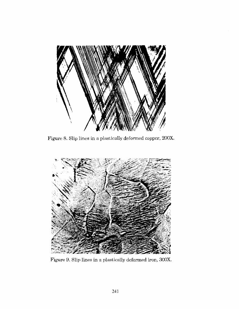
Figure 8. Slip lines in a plastically deformed copper, 200X.

Figure 9. Slip lines in a plastically deformed iron, 300X.

24]

'/ :~ I.:···~ ".$

I······· ... ···~ . .. ,":::',

.. ,.~

'.'··ZO ... · ....•.. ·.' ••.. j' "

79 82

Figure 10. Variation of hardness vs deformation.

Figure 11. Etch pit pattern (slip bands) in sodium chloride, 375 X.

242

Figure 12. Slip band of a deformed mild steel that makes a 450

angle with the tensile load axis.

Figure 13. Twin boundaries as dark and bright regions within each grain in an a-brass specimen, 400X.

243

THE MICROSCOPIC WORLD: A DEMONSTRATION OF ELECTRON MICROSCOPY FOR YOUNGER STUDENTS

Linda L. Horton

Metals and Ceramics Division Oak Ridge National Laboratory

Martin Marietta Energy Systems, Inc. P. O. Box 2008

Oak Ridge, Tennessee 37831


245

"The submitted manuscript has been authored by 8 contractor of the U.S. Government under contract No. OE~

AC05-~21400. Accor<fingly. the U.S. Government felains 8 nonexclusive, royalty·free ticense 10 pubtish or reproduce the published form of lhis contribution. or allow others to do so, for U.S. Government purposes

THE MICROSCOPIC WORLD: A DEMONSTRATION OF ELECIRON MICROSCOPY FOR YOUNGER STUDENTS

L. L. Horton Metals and Ceramics Division, Oak Ridge National Laboratory

Oak Ridge, 1N 37831-6118

KEY WORDS: Microscope, Scanning Electron Microscope, high magnification, scientific method

PREREQUISITE KNOWLEDGE: This demonstration is specifically designed for elementary school students. The level can be easily adjusted for more advanced students with the same basic presentation.

OBJECTIVES: The purpose of this demonstration is to excite the students about the importance of scientific investigation and why they should look at the things in greater detail, extending beyond superficial examinations.

EQUIPMENT AND SUPPLIES: The demonstration requires 35 mm slides of photographs (micrographs) of various objects taken with a wide range of magnifications. In addition, a simple object, such as a baseball, needs to be prepared as an initial focus of what can be learned from looking at an object compared to what we can learn by taking it apart and looking at it at high magnifications.

PROCEDURE: The focus of much of the demonstration is a slide show of electron micrographs of various things from the world around the students. In order to demonstrate the investigative nature of science, a baseball is used as an example. First, the baseball is described by the students as they see it and use it (color, texture, "bouncing", etc.) Then, the students are asked to examine a baseball that has been cut in half. Now, the students can see that the ball is composed of several different materials.

After the above introduction, a slide presentation begins with high magnification micrographs of the various components of the baseball. Following the baseball micrographs, slides of other common items are shown and discussed relative to the function of the item. These range from butterflies and sequins to rocks and broken pencils. Figures 1 and 2 show examples of micrographs of a butterfly wing and a broken pencil. For older students, these simple concepts can be extended to a discussion of advanced ceramics, the materials used, for example, as space shuttle tiles and high temperature superconductors. The toughening of advanced ceramics is largely accomplished by the introduction of microscopic fit5ers and secondary phases. Micrographs show the scale of these reinforcing materials (compared to a human hair, for example, as shown in Figure 3). In addition, the importance of the atomic scale in the processing of modern materials is emphasized.

The most important aspect of this demonstration is the narrative that accompanies the slides. Magnifications must be discussed in terms that the students can understand. For example, stating that the picture is a 400X magnification is not sufficient; the students can much better relate to "this is a picture of what a butterfly wing would look like if a 2 inch butterfly were enlarged to over 60 feet across!" It is equally important that items be photographed that are of interest to the students. The demonstration to be presented during the workshop is made-up of items gathered by a first grade class.

247

Figure 1: 700 X scanning electron micrograph of a butterfly wing. At this enlargement, a 2 inch butterfly would be over 60 feet across.

Figure 2: 20X scanning electron micrograph of a broken pencil. At this enlargement, a standard pencil would be over 5 inches wide.

248

Figure 3: 2,OOOX scanning electron micrograph of a human hair with silicon carbide fibers deposited on it (small fibers are silicon carbide, large scale object is the hair). Silicon carbide fibers are used as reinforcements to make ceramics stronger.

INSTRUCTOR NOTES: This demonstration is probably one that will need to be solicited from a facility with trained microscopists and access to scanning electron microscopes. The classroom teacher and the scientist can "team" to ensure the appropriate level discussion of the material and relevance of the objects presented relative to current classroom science curriculum. This approach provides the additional benefit of the involvement of a practicing scientist in the classroom.

SOURCES OF SUPPLIES: For information about the availability of an ORNL speaker or about possible microscopists in your area, please contact Dr. Linda L. Horton, Building 4500S, MS 6118, Oak Ridge National Laboratory, P. O. Box 2008, Oak Ridge, TN 37831-6118, Telephone: (615) 574-5081.

Acknowledgement: Research sponsored by the Division of Materials Sciences, U.S. Department of Energy, under contract DE-AC05-840R21400 with Martin Marietta Energy Systems, Inc.

249

AN AUTOMATED SYSTEM FOR CREEP TESTING and FIVE EXPERIMENTS IN MATERIALS SCIENCE FOR

LESS THAN $10.00

F. Xavier Spiegel Bernard J. Weigman

Department of Electrical Engineering and Engineering Science Loyola College

4501 North Charles Street Baltimore, Maryland 21210


251

An Automated system for Creep Testing

F. Xavier Spiegel and Bernard J. weigman

Loyola College, Baltimore, Maryland

KEY WORDS

Creep, strain, Plastic Deformation, Potentiometer, A-D Converter, Automated Data Collection, Multiplex.

ABSTRACT

A completely automated data collection system has been devised to measure, analyze and graph creep versus time using a PC, a 16 channel multiplexed A-D converter and low friction potentiometers to measure length. The sampling rate for each experiment can be adjusted in the software to meet the needs of the material tested. Data is collected and stored on a diskette for permanent record and also for later data analysis on a different machine.

INTRODUCTION

Creep is the time dependent plastic deformation of a material under constant load or stress at elevated temperatures. For a given material, elevated temperature means at or above one half the absolute melting temperature. structural materials typically creep at relatively high temperatures, rather large loads and typically over long periods of time. 1

In this experiment 60/40 solder (Tin/Lead) is used because the solder will creep at room temperature, with small loads, and will break within a week. In fact in some specimens the solder will break within a day. This experiment requires that extension or strain be measured at regular time intervals until fracture, and lends itself to automated data collection. The following is a description of such a system. All the experiments were conducted on 60/40 solder, .079 and .158 cm diameter wire, at room temperature. Initial length of the solder ranged from 10 cm to 100 cm. Loads ranged from .250 to 2.00 kgm.2


1. A ten turn precision potentiometer.

2. Any PC/XT/AT IBM compatible computer with at least a 20 Mbyte hard disk.

253

Cost

$ 20.00

600.00

3. A Data Translation DT2811 low cost Analog and Digital I/O board for IBM PC, PC XT and PC AT compatible computer systems (or the equivalent. The equivalent should have a 16 channel multiplexer leading to a 12 bit A to D converter. The convert time is not critical.) Source: Data Translation Inc., 100 Locke Dr. Marlboro, MA 01752-1192 tel. (508) 481-3700.

4. A 50 pin termination header Source: Industrial Computer Source, P.O. Box 23058, San Diego, CA 92193 tel. (619) 279-0084 part number 2M50FC.

AUTOMATED DATA COLLECTION SYSTEM

795.00

59.00

An automated data collection system was constructed using ten turn precision linear potentiometers as sensors (FIG.1) , Data Translation D'1'2811 A to D converter board and a PC with 640K of memory and a 20 Mbyte hard disk (FIG. 2) . Str ing was wrapped around the shaft of the ten turn precision linear potentiometer and connected to the weights at the end of the solder wire. Five volts were placed across the potentiometer. As the solder stretched, the potentiometer shaft rotated and the voltage at the wiper arm of the ten turn precision linear potentiometer changed. The change in the vol tage for one centimeter stretch was measured in order to calibrate the ten turn precision linear potentiometer. This voltage was 1:hen measured with a 12 bit resolution A to D converter. The smallest voltage change that the ADC could measure was 2.44 millivolts corresponding to a smallest distance which could be measured of 0.037 cm. Any stretch of the wire greater than .037 cm can be detected with the system. The stretch is related to thE! voltage measured by the ADC (1 volt = 15.27 cm). Thus, by measuring the voltage periodically with the ADC we kept a time history of the change in length of the solder wire.

The DT2811 has 16 channels which are multiplexed to one 12 bit A to D convertE:lr. One channel from 0 to 15 is selected by software and A to D conversion is started again by software. A READY bit is checked in software and when the conversion is complete, the voltage at the wiper arm of the potentiometer is read as a 12 bit digital number. This number is recorded in a disk file along with the time that the reading was made. The program then selects the next channel and repeats the process until all channels are read for that time.. This is repeated periodically until all of the solder wires break. The program is then terminated and the data in the disk file is analyzed. The time between readings varied, depending on how long it would take for the wire to break. For the thinner solder, readings were taken every 10 minutes. 3 , 4, 5, 6, 7

254

The data was analyzed using LOTUS 123. The raw data was imported into a LOTUS worksheet, scaled properly, converted to length and plotted all within LOTUS. No data was ever entered by hand, thus speeding up the operation and also avoiding transcribing errors. Data could also be conveniently archived on floppy disks in an easily accessed format.

The € = v/eo

conversion from volts to strain from a given sample is: . 15.27 cm/volt, where € = strain

v = voltage reading in volts eo original length, and

15.27 cm/volt conversion factor.

The strain rate can be determined by calculating the slope of the strain vs. time graph.

€ = €2 - €i / t2 - t i , where € = €i = €2 =

strain strain strain

rate at time at time

Note that strain is dimensionless (sometimes reported as IN/IN or cm/cm) and strain rate is in the dimensions of reciprocal time.

RESULTS

Typical creep data is shown in graphs 1-4. Graph 1 is a plot of voltage vs. time and Graphs 2, 3, and 4 are plots of strain vs. time. strain rates taken from the slopes of Graphs 2, 3, and 4 are 0.003, 0.0047, and 0.0025 cm/cm·min. The data is reproducible and has alleviated the problem of continual observation while the experiment is in progress. The data is consistent with other observations of the same wire which were monitored every hour, but this automated system of monitoring has the added advantage of catching very closely the time of fracture, and the onset of creep. Since solder is wrapped in a spool the kinks are not easily removed and the onset of deformation is delayed while the wire is straightened. The wire could be pre-straightened, but the duplication of the straightening technique is questionable. Future experiments will include several techniques for straightening the wire before testing to determine their effect.

ACKNOWLEDGEMENTS

The authors would like to thank Mr. Howard Moore, Technical Assistant of the Physics Department at Loyola College, for his assistance in assembling the apparatus' and Miss Margaret Davis, student of the Engineering Department'at Loyola College, for her assistance in conducting the experiments. We also wish to thank Mary spiegel for typing this manuscript.

255

REFERENCES

1. Materials Science, Testing, and properties for Technicians, William o. Fellers, Prentice-Hall.

2. Fundamentals of Creep and Creep-Rupture in Metals, Frank Garofalo, Macmillan series in Materials.

3. Interfacing, A Laboratory Approach Using the Microcomputer for Instrumen1:ation, Data Analysis, and Control, Stephen E. Derenzo, Prentice-Hall 1990.

4. The Indus1:rial Computer Industrial Computer Source.

5. Interfacing to the IBM Personal Computer, Lewis C. Eggebrecht, Howard W. Sams Inc.

6. User's Manual for DT2811. Low Cost Analog and Digital I/O Board, Dat:a Translation, Inc., 100 Locke Drive, Marlboro, MA 01752-1192:.

7. Computer Interfacing - Rev. 5, 1989, B.J. Weigman. College, Baltimore, Maryland.

256

Loyola

2,43cM, diD-Meter PULLEY

PLATFORM __ _

+5V

'WIRE UNDER TEST

GND TO ADC

10 TURN POTENTIOMETER o - lOOK OhMS

_ STRING

'WEIGHT

FIGURE 1

APPARATUS FOR MEASURING CREEP

N Vi 00

JAMECO

COMPUTER

PC-SOSB BASED DATA TRANSLATION

DT 2Bll

ADClDAC

640 K RAM

INTERFACE BOARD

20 Mbyte ('''n r" 0('"" (' ,,< n (,," (''''' ('h7

Hard Disk

10 TURN

~tt~-~~~ 5.25 Inch POTENTIOMETERS

Floppy

FIGURE 2

AUTOMATED DATA COLLECTION SYSTEM

r:h9

~

+S\/

~- ~'"" ~ ~

GRAPH 1 OIAMETER=O.079 ct~n WEIGHT =250gm LENGTH=25cm

vA

0.35 ~--

V 0.3 /

// /

N 0.25

Vl 1.0 V

\JI 0 0.2 ~ 0 >

Q, 1~,

j/

/

l/ l-/

01

v/ /

no,~;

//

(} - - / I' " " """" 1""" I' " .. "''''

v 10 20 30 40 50 60 70 80 90 100 110 120

lime (minutes)

GRAPH 2 DIAMETER=O.079 em WEIGHT =2509 m LENGTH=25cm

022 , , , , , , , , , , , , ,

0.2 / 018

0.16

I

I tv 014 0\ 0

/ /

c 012 6 '-..... VJ o 1

/

,/ /

0.08 / /

006

0.04

0.02

/ ,/

1/

0 - / '" "

o 10 20 30 40 50 60 70 80 90 1 00 110 120

Time (minutes)

c i5 L ~

(f)

0.7

06

0.5

0.4

0.3

0.2

0.1

o .--_.-

-.. --""

o

GRAPH .3 DIAMETER=O.079cm IhlEIGHT= 250 grn L&·JGTli= 50 ern

r //

/ /

//

/ e-/

/

v/ /--

/ //

-,.-/ -------

"'"'''' "" 30 60 90 120 150 180

11 rne (rn inutes)

GRAPH 4 DIAMETER =O.158cm LEi'lGTH=50 em WEIGHT=750 gm

1 I n 09 I

/ 08

07

06

/ /

c N 0 05 0\ ...

~

N (f)

/ V

04 /"

03

0.2

01

//

/ r" V

------~ ----.--------0

o 60 120 180 240 300 360 420 480

lime (minutes)

FIVE EXPERIMENTS IN MATERIALS SCIENCE FOR LESS THAN $10.00

F. Xavier spiegel

Loyola College, Baltimore, Maryland

KEY WORDS

Diffusion, Twinning, Fatigue, Acoustic Emission, Ageing.

ABSTRACT

Diffusion, Twinning, Fatigue, Acoustic Emission and Ageing can be studied using readily available materials and the household oven. Each experiment can be expanded to a more extensive investigation of the properties of the material investigated, as well as other materials, and offers an opportunity for the student to learn about the relationship between engineering, science, society and politics.

INTRODUCTION

simple experiments with everyday items can be used to familiarize students with the importance of materials and some of the properties which they possess. The following experiments have been performed by the author for over eight years with enthusiastic response by audiences of all ages.


1) Aluminum nails, 2) United states Pennies, 3) Metal Paper Clips.

THE ALUMINUM NAIL

Aluminum nails are age hardened to disperse the silicon and harden the aluminum. If an aluminum nail is re-heated to 600 F for one hour it will soften and can be bent by hand. This brief experiment demonstrates the movement of atoms in a material. This migration of atoms in a material is diffusion. In the age-hardened state the silicon atoms are finely dispersed, whereas in the reheated or over-aged material the silicon atoms coalesce into larger particles and no longer strengthen the aluminum to a useful hardened state. 1

THE UNITED STATES PENNY

The u.s. penny has an interesting history; the pennies minted since 1982 are electroplated zinc. The present composition is 97.6%

263

zinc and 2.4% copper. The copper can easily be scratched from the surface of the coin to reveal the zinc. Before 1982 the penny was 95% copper and 5% zinc or 95% copper, 2.5% zinc and 2.5% tin, except for 1943 when the penny was zinc coated on stee1. 2 , 3, 4, 5

An interesting experiment can be performed on all of the pennies except the 1943 version by placing them in an oven at 350-400 F for about an hour or so. The surface of the penny will acquire a heat tint that makes the coin appear golden. This heat tint can easily be removed by normal wear or by polishing.

The pennies minted since 1982 exhibit another interesting property when heat treated. If this penny is heated at 700 F for one hour the zinc grains will become large and can easily be twinned by bit.ing on the penny or by bending it. An acoustic emission will be heard when the penny is deformed. This experiment clearly demonstrates diffusion and grain growth, as the "as found" penny will not twin because the grains are so small. Diffusion is causing the grain growth of the zinc and the deformation is causing the twinning. The twinning is causing the crackling noise heard when the penny is deformed. This crackling is called acoustic emission and is being extensively researched for NDE purposes. 1,3,4,5

THE PAPER CLIP

An ordinary metal paper clip can readily be used to demonstrate fatigue. A fatigue failure arises from the cyclic loading of a material at relatively small loads. 1 If a paper clip is opened so that it appears as an elongated "s" and is repeatedly bent back and forth it will break, clearly demonstrating the phenomenon of fatigue. If the broken paper clip is quickly moved to the lower portion of the upper lip the paper clip appears warm, a result of internal friction. If the color of the region around the fracture is examined a discoloration will be observed, and if the texture is observed the area around the fracture will be noticeably roughened.

CONCLUSIONS

As previously mentioned, these demonstrations have met with much success and the author's experience has been that many in the audiences have demonstrated them to others and frequently called the author for more information or other experiments. Each of these experiments can be expanded to be quantitative, and include other materials, variation of heat treatments, different loading techniques and perhaps observations of different properties. It is the author's opinion that the equipment need not be complex and in fact should not be complex to interest students in the study of materials.

264

ACKNOWLEDGMENTS

The author wishes to thank Miss Margaret Davis, engineering student at Loyola College, for duplicating these experiments and commenting on their worth. I also wish to thank Mr. John Ross, friend and colleague, for his continued interest, advice and moral support in my endeavor to understand metals. I also thank my wife Mary for typing this manuscript.

265

REFERENCES

1. William o. Fellers, Materials Science, Testing, and Properties for Technicians, Prentice Hall 1990.

2. Wagner, H. J"., Hall, A. M., The New Coinage, Journal of Metals, March 1966, pp. 301-307.

3. French, Charles F., 1991 American Guide to U.S. Coins, Simon & Schuster Inc., 1990.

4. Junge, Company

Ewald, World Inc., 1984.

Coin Encyclopedia, William Morrow &

5. Yeoman, R. S., Current Coins of the World, 8th Edition, Western Publishing, Co. Inc., 1988.

266

ATTRACTING AND RETAINING MINORITIES AND WOMEN IN TECHNICAL STUDIES

Moderator - Heidi R. Ries, Norfolk State University Jonice Harris, National Institute of Standards

and Technology Jenifer A. T. Taylor, NYS College of Ceramics at

Alfred University Albert L. McHenry, Arizona State University

Larry Mattix, Norfolk State University

267

ATTRACTING AND RETAINING MINORITIES AND WOMEN IN TECHNICAL STUDIES:

A Panel Discussion

The underrepresentation of minorities and women in the fields of science and engineering is well-known. This fact, combined with current demographic trends toward increased minority percentages in the national population, indicates an impending shortage of technically-educated persons in the United states. Such a shortage would have a severe impact on our national ability to conduct research and development in technical fields. Therefore, in order to remain internationally competitive in science and engineering, it is imperative that increased numbers of minorities and women be attracted to, and retained in, technical studies.

The purpose of this panel discussion is to explore possible solutions to the enrollment shortages of minorities and women in technical fields, while addressing the underlying barriers discouraging the recruitment and retention of these students. currently functioning programs, such as the Dozoretz National Institute for Minorities in Applied Sciences at Norfolk State University and the educational development programs in the Southern Rocky Mountain region of the United states, will be highlighted.

269

ATTRACTING AND RETAINING MINORITIES AND WOMEN IN TECHNICAL STUDIES:

The Panelists

Dr. Larry Mattix is Associate Professor of Physics and Director of the Dozoretz National Institute for Minorities in Applied Sciences at Norfolk state University in Norfolk, Virginia. He holds a BS in physics from Clark-Atlanta University, anMS in physics from the University of Illinois in Urbana, and a Ph.D. in Physics from the College of William and Mary, Williamsburg, VA. From 1981 through 1983, he was a National Research Council Post-Doctoral Fellow at the Naval Research Laboratory in Washington, DC. His current research interests include Sol-Gel preparations of ceramic materials including high temperature superconductors. He has directed the Dozoretz Institute, an honors program for science and engineering students, since its inception in 1986.

Dr. Albert L. MCHenry is professor and Chair of the Department of Electronics and Computer Technology at Arizona State University, Tempe, Arizona. He holds a BS Industrial Technology from Southern university of Baton Rouge, Louisiana, an MS Technology and Ph.D. Technical Education from Arizona state. Dr. McHenry's area of technical specialization is digital electronics. He has industrial experience with the Boeing Co., 3M Co., and Motorola. His current research interests include CAD for digital systems, implementation of CAl in technical subjects areas and Technology Education. Dr. McHenry has been actively involved in four-year technology programs for over 28 years and is a contributing member of ASEE, ETD, ETLI, and NAITTE.

Dr. Jenifer Taylor graduated with a BS Degree in Ceramic Engineering in 1961 from the University of Washington in Seattle. She subsequently spent 20 years working with children; her own and other peoples', including teaching on several levels in public school both before and after earning an MS Degree in Education in 1974 from Alfred University. She returned to engineering, completing a Ph.D. in Ceramic Engineering in 1986 at Alfred University, where she has been employed since as faculty in the College of Ceramics.

During that time her involvement with undergraduates has included serving as advisor for the student chapter of the Society of Women Engineers and teaching many classes. Observation of these students combined with her experience as an engineering student and as a mother of girls has led Dr. Taylor to a rather unique perspective on the problem of retaining women in technical studies.

270

The Dozoretz National Institute for Minorities in Applied Sciences: Direct Intervention in Minority Retention.

Larry Mattix, Norfolk state University

After two decades of affirmative action, minorities have made little progress in gaining proportional representation in technical professions. In 1986 the Dozoretz National Institute for Minorities in Applied Sciences was established at Norfolk State University to address this problem.

We believe that the sword which bars minorities from scientific and engineering careers is double-edged. First minority students do not get the information about the resources and opportunities available to them and simply do not believe that careers in science and engineering are attainable. Second, an exceedingly high attrition for minority students in science and engineers further reduces an already diminished pool of minority science students and leads to the increasing disparity in graduate and professional schools. Only 30% of minority students who start out in science and engineering graduate in those areas. This is less than half of the national rate for science and engineering students (70%). The Dozoretz Institute attacks these problems with emphasis on noncurricular issues like self-awareness, faculty-student interactions, mentoring, counseling, and summer experiences in science and engineering.

The results after five years and two graduating classes are promising. A retention rate of 68% (students who graduate in science and engineering) has been achieved. Ninety-three percent of the graduates have gone on to postgraduate studies in science, medicine, or engineering.

271

RECRUITMENT AND RETENTION OF MINORITY STUDENTS

TO PROGRAMS IN ENGINEERING TECHNOLOGY:

WITH SPECIAL EMPHASIS OF HISPANICS AND AMERICAN INDIANS

by

Albert L. McHenry

ABSTRACT

The initiation of special efforts to recruit and maintain minority students in the southern Rocky Mountain region is little more than a decade old. The region includes several major cities that represen1: minority population centers and other large minority populations associated with the American Indian reservations, mining towns, and rural farm communities. The minority students in thl:!se areas have been targeted for special academic development.

The early development of minority recruitment programs was begun by motivated minority faculty members of universities and colleges. Their commitment led to the development of local chapters of minority professional organizations such as SHPE, AISES, and NSBE among others. These organizations provide a self-help academic support system for minority engineering, engineering technology and science students.

The philosophy and approach that has evolved is programmatic and development.al in nature. Engineering and engineering technology programs are academic areas that are at the focal point of the primary minority student developmental efforts. Programs such as PRIME, MEP, MESA, PROJECT 1000 and CIMO have become the established approach.

272

Improving Retention of Women in Technical Studies

Jenifer Taylor, College of Ceramics at Alfred University

American culture is experienced differently by men and women. As a matter of fact, the male American culture is different in a number of ways from the female American culture. Many of these differences impact on how women feel about being in a technical curriculum. Educators in these fields, male and female, can help women feel more at ease if they are aware of these differences and can help all the students be more accepting. For example, when a woman cries when she gets a D on a test, it doesn't mean she isn't tough enough to be an engineer. It merely shows that our culture trains women to cry rather than swear, which is a typical male response to the same situation. Since men far outnumber women in the technical fields, the dominant culture is male. Making allowance for typical female behavior when it differs from male will increase retention of women. Simple strategies will be suggested.

273

MATERIALS AND THE ENVIRONMENT

Linda S. Farmer

Manager Environmental Monitoring Westinghouse Environmental Management Company of Ohio

P. O. Box 398704 Cincinnati, Ohio 45239-8704


275

THE ENVIRONMENT AND HOW YOU CAN MAKE A DIFFERENCE

Linda S. Farmer

Manager Environmental Monitoring

Westinghouse Environmental Management

Company of Ohio

277

ENVIRONMENTAL CLEAN UP TAKES ....

GOVERNMENT INDUSTRY

COMMUNITY MONEY

278

EDUCATION

AND ALL OF US

WORKING TOGETHER

J{ q n JI, \{ ~~1 ( t, yf U ( L

GOVERNMENT

STATE AND FEDERAL

* ENVIRONMENTAL LAWS AND REGULATIONS

* ENVIRONMENTAL PROGRAM AND PROJECTS

* ENVIRONMENTAL FUNDING

* ENVIRONMENTAL EDUCATION

279

Environmental Concerns

/

// / /.//

./ //.////

/ ////// /'

// / '/ ,,//

DRIVERS USEPA OHIOEPA DOE

CWA SDWA ARARs

CAA TIGER TEAM

280

INDUSTRY

* ASSIST IN THE DEVELOPMENT OF STANDARDS

* COMPLY WITH ESTABLISHED LAWS AND REGULATIONS

* TAKE THE ENVIRONMENT INTO CONSIDERATION WHEN DEVELOPING NEW PRODUCTS

* PROMOTE CLEAN ENVIRONMENT TO EMPLOYEES AND IN PRODUCT ADVERTISEMENTS

281

COMPLIANCE ...

OR OR

FINES JAIL

282

WHAT CAN THE EDUCATIONAL COMMUNITY

DO ....

ENVIRONMENTAL MATERIALS SCIENCE COURSES OF STUDY GEARED TOWARDS DEVELOPING

ENVIRONMENTALLY MINDED MATERIALS EXPERTS

283

COMMUNITY

THINK GLOBALLY

ACT LOCALLY

284

WHERE DOES THE MONEY COME FROM ...

* UNIVERSITY GRANTS AND FUNDS

* CORPORATION GRANTS AND FUNDS

* GOVERNMENT GRANTS AND FUNDS

* HISTORICALLY BLACK COLLEGES

* WOMEN IN SCIENCE AND INDUSTRY

* PRE-COLLEGE FUNDING

* SCHOLARSHIPS

285

WHAT YOU

DO TODAY

AFFECTS

TOMORROW

286

* RE-DUCE WASTE * RE-CYCLE MATERIALS

* RE-USABLE PRODUCTS * RE-MEDIATE PROBLEM AREAS

TO HELP THE ENVIRONMENT

287

ISOTROPIC THIN-WALLED PRESSURE VESSEL EXPERIMENT

Nancy L. Denton Vernon S. Hillsman

Purdue University School of Technology

145 Knoy Hall West Lafayette, Indiana 47907


289

ISOTROPIC THIN-WALLED PRESSURE VESSEL EXPERIMENT

Nancy L. Denton Vernon S. Hillsman

Purdue University, West Lafayette, IN

KEYWORDS: (thin-walled) pressure vessel, cylinder, principal stress, brass, Poisson's Ratio, Poisson effect, axial stress, combined loading, superposition, strain rosette, elastic material.

PREREOUISITE KNOWLEDGE: This material could be taught as presented to a materials science or mechanics student at the college level. The student should be familiar with the concepts of principal stress/strain and the Poisson effect, which is an indication of the material strain transverse to applied load. Use of the linear regression function on a scientific calculator is expected. Previous exposure to thin walled pressure vessel theory is helpful, but not required.

OBJECTIVES: To investigate the stress and strain distributions on the surface of a thin walled cylinder subject to internal pressure and/or axial load. To relate stress and strain distributions to material properties and cylinder geometry.

EOUIPMENT AND SUPPLIES: 1) Brass tube of known Young's modulus and internal length, with pressure port and end treatment to facilitate internal pressure and axial loading, with strain rosette installed, as shown in Figure 1; 2) electromechanical test machine (ETM); 3) two digital strain indicators and switching unit; 4) load cell with greater than 9 kN capacity (minimum of 20 kN capacity recommended); 5) hydraulic pump with connections to tube and re~ating valve, as shown in Figure 2; 6) hydraulic fluid; 7) pressure gage, preferably dIgital; 8) dial calipers; 9) scrap piece of same brass tubing, approximately 50 mm long; 10) calculator with linear regression capability.

PROCEDURE: Preparation: Set up hydraulic system and suspend brass tube with strain rosette in advance, leaving enough time to work air out of the hydraulic fluid (two days minimum), as shown in Figure 2. Present or review thin walled pressure vessel (PV) theory, including calculation and direction of hoop (circumferential) stress and longitudinal stress, and discuss assumptions needed for a PV to be considered thin walled. (If necessary, review axial stress). Review equations for calculation of principal strain from strain gage rosette data and conversion of principal strain to principal stress. Tell students the Young's modulus and internal length of the tube and the bulk modulus of elasticity of the hydraulic fluid.

Experiment: Students begin by calibrating the load cell and one strain indicator to read load in kiloNewtons. Next, they will complete and calibrate the strain gage rosette circuitry as shown in Figure 2 to permit reading of each of the three strains in units of micros train for each loading. A quarter Wheatstone bridge will be used. To start the test, students should verify that the brass PV is affixed at top and bottom to the ETM, then apply a tensile axial load in increments of 4 kN up to a maximum of 16 kN. At each increment, the load and three strains will be recorded. Following the 16 kN measurements, all axial load must be removed. The students will next apply internal pressure in increments of 0.7 MPa up to a maximum pressure of 2.8 MPa, and obtain pressure and strain readings at each increment. Again, the loading should be removed. For the final loading variation, the students will apply an internal pressure of 2.8 MPa, then apply tensile axial load in increments of 4 kN up to 12 kN. At each increment, the axial load, strains, AND pressure readings are recorded. As axial loading increases, the instructor should

291

point out two significant phenomena. The more obvious of these is that the principal direction changes from hoop (horizontal) to longitudinal (vertical). A second, subtle observation is that the elongation of the tube from the axial loading actually reduces the internal pressure of the tube by increasing the tube's volume. The students next remove all loading and disconnect all wiring. The scrap of tube is then measured to obtain internal diameter, external diameter, and wall thickness. (All should be measured at several locations to establish the range of actual values).

Data Reduction: Theoretical values required include Poisson's Ratio for the brass, and principal stresses and/or strains for each loading condition. (Principal directions will be assumed to be vertical and horizontal). The brass material properties and bulk modulus of elasticity of the hydraulic fluid should be provided by the instructor or obtained from standard material references. The principal stresses should be calculated from equations for axial stress, hoop and lon~itudinal stress, and their combination. (Equations and symbols are listed in AppendIX A).

Extensive calculations are needed from the measured strains. For all loadings, principal strains must be calculated from the measured strain values. This requires initial calculation of shear strains. Principal strains can then be determined directly, using a reference axis through gage one of the rosette, or the measured strains can fIrst be transformed to vertical and horizontal positions, then principal strains found. (Hopefully the transformed strains and principal strains will agree!) At least one principal direction per loading type should be determined to confirm that vertical and horizontal are indeed the principal directions.

Using principal strains from the tensile axial load only, an empirical Poisson's Ratio may be obtained by performing a linear regression of the minimum and maximum principal strains. The resulting slope is the empirical ratio desired. This should be compared to the theoretical Poisson's RatIO for verification. The empirical value should be used for all remaining calculations.

Next, all principal strains must be converted to principal stresses, using the theoretical Young's modulus and the empirical Poisson's Ratio. At least one pair of principal stresses per loading should be compared to theoretical values for verification. A linear regression of maximum principal stress and pressure from the pressure only loading can be performed to determine an equation relating hoop stress and mternal pressure. When the theoretical hoop stress is substituted into this equation, an empirical value for wall thickness is obtained, which can be compared to the measured thickness.

For the combined pressure and axial loading, calculate the change in pressure due to the change in volume caused by the axial load. Compare calculated pressure change to measured pressure change. Note that the theoretical calculations for principal stresses for the combined load case assumed zero pressure drop; superposition assumes that the strains or stresses from the acting loads are additive, so thIS should allow discussion of the accuracy of the assumption used for the theoretical calculations. A second theoretical calculation of the principal stresses for the combined loading case could be completed based on the anticipated pressure drop due to the increase in volume.

SAMPLE DATA SHEETS: Self-evident.

INSTRUCTOR NOTES: This experiment was designed for students enrolled in an advanced strength of materials course. For additional study, a filament-wound composite cylinder could be included to investigate the effect of wind angle on stress/strain. Modeling of the vessels prior to testing could also be incorporated.

Conversely, the experiment could be modified to be conducted as a demonstration for beginning materials or strength of materials students. Additional study could include common polyvinylchoride piping. To simplify the experiment and its data reduction, a two gage rectangular strain rosette should be mounted along principal directions (vertical and horizontal), thus eliminating all principal strain and direction calculations.

292

Since published values for the bulk modulus of elasticity are difficult to find in standard reference material, and will vary widely if air is trapped in the fluid, it is advisable that the lab instructor should experimentally determine the bulk modulus prior to the lab experiment.

WARNING: Before conducting the experiment, test the PV at maximum loadings to confirm that the joints are sufficiently strong. Use of plastic sheeting or other means to catch any potentlalleaking hydraulic fluid is advisable.

REFERENCES: Beer, F. P., & Johnston, E. R. Jr. (1981). Mechanics of Materials. New York: McGraw-Hill Book Company, (pp. 62-70, 293-926, 325-342). Beckwith, T. G., Buck, N. L., & Marangoni, R. D. (1987). Mechanical Measurements (3rd ed.). Reading, MA: Addison-Wesley Publishing Company, (pp. 353-373). Fox & McDonald (1978) Introduction to Fluid Mechanics (2nd ed) New York, NY: Wiley & Sons, Inc. (pp. 610) Murdock, James W. PE (1976) Fluid Mechanics and its Applications USA: Houghton Mifflin Company (pp. 29-31)

SOURCES OF SUPPLIES: Brass tubing and caps - any metal distributor. Strain gages and rosettes can be obtained at substantially reduced cost for educational purposes from Measurements Group, P.O. Box 27777, Raleigh, NC, 27611, (919) 365-3800. New pumps can cost several hundred dollars, so investigate local industry and/or scrap dealers as potential sources (our pump was part of scrapped airplane landing gear). Hydraulic system (tubing, pressure ports, pressure valve) can be purchased from any local plumbing supply store.

ACKNOWLEDGEMENT: The thin walled pressure vessel experiment would not exist without the initial development work of George Stinchcombe, former Visiting Professor and current engineer with British Aerospace Corporation, and Jim Osborne, laboratory technician. Their efforts are greatly appreciated.

293

APPENDIX A: SYMBOL LIST (in order of appearance on Equation List)

t = wall thickness of tube

d = internal diameter

p = internal pressure

aH = hoop (circumferential) stress

aL = longitudinal stress

aR = radial stress

aA = axial stress

F = axial load

A = cross-sectional area (of tube)

2: 1, 2:2, 2:3 = strain gage rosette data

2: x,2: y = normal strains along X&Y reference axes (X-axis through gage 1; Y-axis through gage 3)

-yxy = shear strain with respect to X & Y reference axes

2: max and 2: min = priincipal strains

-y max = max shearing strain

ep = principal direction(s)

p = Poisson's Ratio

E = Young's Modulus

V = internal volume of the tube

L = internal length of the tube

B = bulk modulus of elasticity (for hydraulic fluid)

2:H = hoop strain

2:L = longitudinal strain

294

1.

2.

3.

EQUATION LIST (in order of appearance in the text)

ThinPV: If

Pressure-Induced

Stresses:

Axial Stress

d t :S :m

UR = 0 (zero)

F = A

(la)

(lb)

(Ic)

Principal Strains from Rectangular Strain Gage Rosette Data

LX = Ll (3a)

Ly = L3 (3b)

"(xy 1 (Ll + L3) ""2 = L2 - - (3c)

2

"(max = J (LX - Ly)2 + "(xi (3d)

LX + Ly "(max (3e) Lmax = +

2 -2-

LX + Ly "(max Lmin = (3f)

2 2

4. Principal Directions with respect to reference axes on rosette

"(xy tansp = -L--L

x- Y

295

(4)

EQUATION LIST (in order of appearance in the text) CONTINUED

5. Poisson Ratio (for Uniaxial Stress only)

~min Jl. = (5)

~max

6. Principal Stress from Principal Strain

a max = ~ "m~ :"mm ) (~~ ) + C:u 1 C:.) (6a)

a min = ("m": "mi. l (~-. ) -C:u l C:.) (6b)

7. Pressure Change Due to Volume Change

(7a)

Vinitial (7b)

V fina1 (7c)

B (7d)

296

holding fixture

~

E

hydraulic return

welded end caps

"-

holding fixture ----

:

0

~ Thin-walled brass cylinder

,

I

.-- --- ~r- - ---r-- -~ - -- -

'-

Figure 1.Ca) Thin-walled brass pressure vessel

------------~~---------------x

Gl

G2 G3

y

Figure 1.Cb) Orientation of 45 degree strain gage rosette

297

I

universal test machine

strain indicator

~ wrr===============~ ~

~==:::;-:, i , hydraulic reservoir

I

1

double-acting hydraulic pump

~ switching unit

? strain

indicator

Figure 2. Schematic of test equipment

298

STRESS-STRAIN CHARACTERISTICS OF RUBBER-LIKE MATERIALS: EXPERIMENT AND ANALYSIS

David J. Allen

School of Engineering Technology Northeastern University

120 Snell Engineering Center Boston, Massachusetts 02115


299

STRESS-STRAIN CHARACTERISTICS OF RUBBER-LIKE MATERIALS: EXPERIMENT AND ANALYSIS

David J. Allen School of Engineering Technology

Northeastern University, Boston, Massachusetts

KEY WORDS: rubber, neoprene, stress, strain, elasticity, tensile test, power equation.

PREREQUISITE KNOWLEDGE: The student should understand the concepts of stress and strain either previously or concurrently presented with experiment.

OBJECTIVES: To demonstrated tensile testing of materials and the application of the concepts of stress and strain. To introduce a method of analysis of curvilinear data which will yield a mathematical relationship between stress and strain for many artificial rubbers and plastics.

EQUIPMENT AND SUPPLIES: (1) No. 32 or No. 64 rubber (neoprene) bands; (2) Two S hooks approximately 5 cm long; (3) One screw eye; (4) Lumber as required; (5) rom scale; (6) micrometer; (7) Calibrated weights; (8) Log-log paper; (9) calculator.

PROCEDURE: The students may either design their own testing apparatus or make one similar to the one shown in figure 1. If they design their own, design factors such as the amount of space required should be discussed.

Students make a pair of gage marks near the middles of each side of a rubber band and measure the length between each pair of marks. These measurements are the initial unstrained length, Lo. The thickness and width at each gage section is also made which will yield the initial cross sectional area, A. Two sets of data are made from each test.

o The test is conducted by placing the specimen in the testing apparatus and adding incrementally calibrated weights. The length between the gage marks are measured for each load. Optionally, the thickness and the width of the rubber band may be measured at each loading. The test is conducted to failure.

Once the data is collected the students begin their analysis. The engineering stress may be computed from

( 1)

where a is the engineering stress and P is the load on the section. It is important not to forget that P is one half of the applied load since there are two sides of the rubber band. If the actual thickness, tACTUAL' and width, WACTUAL' are measured for each loading, the true stress can be determined from

301

p (J TRUE = --::--=--

AACTUAL

where the actual cross sectional area is

strain is computed from

€ = !::.L Lo

(2)

(3 )

(4)

where ~L is the change in length from the original undeformed length to the one being computed.

r------------' !

Jh !

LLUMBERAS i i REQUIRED-:

~~ : (2X4) : !

SCREW EYE

RUBBER BAND : :

PLYWOOD : :

PAN; i :

GAGE LENGTH

« l d

SHOOK

I BASE I

~ I

TABLE/

: :

~

WEIGHTS

Figure 1

The stress and strain values are plotted on an arithmetic graph and a smoothed best fit curve is drawn. Typical results are shown in figure 2. Note that the curve is nonlinear.

It would be useful to obtain a mathematical relationship between stress and strain but one is not readily apparent from figure 2. However, if the data are plotted on a log-log plot as shown in figure 3, the best-fit curve is obviously a straight line.

302

0 .... <»

CX)

r--.-.. 10 a.. U)

~ C/) on f:3 1=

...,. C/)

(I')

N

.... 0

0

Figure 2

o ....

0.01

Figure 3

STRESS vs STRAIN of NEOPRENE

1 234 5 6

STRAIN (mm/rrm)

STRESS vs STRAIN of NEOPRENE

0.1 1

STRAIN (mm/mm)

303

10

The equation of a straight line takes the form of

y=m'x+b (5)

but since the graph is log-log the equation needs to be modified to

Iny=m'lnx+lnb

or in terms of the stress-strain relationship

In a = m'ln e + In b

(6)

(7)

which only leaves the determination of parameters m and b once the best-fit line is drawn.

The SlOPE~, m, of the curve can be determined by choosing two arbitrary coordinates on the best-fit curve, say (E"O,) and (E 2 , O2), ~rhe slope can now be defined as

In( O2

) In0 2 -1no1 _ 0 1 m = -:----'''---::------=-

Ine2 -1ne1 (e ) In e: (8)

Once the parameter m has been computed from equation 8 the parameter b can be determined. Reorganizing equation 7 results in

In b = In a - m'ln e (9)

Substituting t:he arbitrary coordinates, (E"O,) and (E 2 , O2 ) , into equation 9 allows b to be computed from

(10)

The value of Inb can be evaluated two different ways in equation 10. 'I'his gives a check of the computations. utilizing the laws of logarithms equation 7 can be written as

Ino =lnEf'+lnb (11)

or

(12)

or

(13 )

This is the form called the power equation. Data whose plots

304

show a straight line best-fit relationship on log-log graphs can be represented mathematically by equation 13. Using the above method on the data shown in figure 3 yields

a = 3. 404·eO.6105. (14)

Many materials and systems will follow a power equation and it is worthwhile to make a log-log plot of data points following a curvilinear trend on an arithmetic plot. Allen and Phalen2

extend this approach to the artificial rubbers used in singleply roof systems.

For a more thorough treatment true stress utilizing equation 2 versus strain may be analyzed. Arithmetic and loglog plots and the corresponding best-fit curves and equations for true stress vs. strain are compared with the engineering stress analysis given above.

SAMPLE DATA SHEETS: Self-Evident.

INSTRUCTOR NOTES: Having the students design and build their own testing apparatus is a good project. The student's interest and creativity is harnessed which results in a better appreciation of experimentation. A thorough discussion of factors involved in experimental design should be made without dampening the student's creativity. One student used rolls of pennies as weights and obtained good results. Ideas should be encouraged even though they may lead to unsatisfactory results. This provides a fertile ground for discussion.

Some computer graphing and statistical programs provide linear regression analysis. They may use the term "geometric" equation rather than "power" equation. Even if computer programs are available it is recommended that the student do the graphing and analysis by hand computations to reinforce the concepts introduced. The computer can be used as a check.

This experiment also gives the students a better understanding and a physical "feel" of the concepts of stress and strain than that obtained by using a steel specimen in a testing machine. The large strains and applied loads are readily apparent.

REFERENCES: (1) Giesecke, F.E., et.al., Engineering Graphics, Third

ed., 1981, New York (2) Allen, D.J., and T.E. Phalen Jr.,"stress-strain

Characteristics for EPDM, CSPE, and PVC for the Development of Stresses in Membranes utilized as single-Ply Roof systems", proceeding of the 1991 International symposium on Roofing Technology, 1991

SOURCES OF SUPPLY: A well stocked hardware store or home center can supply the materials needed for the testing apparatus.

305

DEMONSTRATION OF MAGNETIC DOMAIN BOUNDARY MOVEMENT USING AN EASILY

ASSEMBLED VIDEOCAM-MICROSCOPE SYSTEM

John W. Patterson

Materials Science and Engineering Department Iowa State University

110 Engineering Annex Ames, Iowa 50011


307

DEMONSTRATION OF MAGNETIC DOMAIN BOUNDARY MOVEMENT USING AN EASILY ASSEMBLED VIDEOCAM-MICROSCOPE SYSTEM

John W. Patterson Department of Materials Science and Engineering

Iowa State University Ames, IA 50011

KEY WORDS: magnetic domains, domain boundary migration, videocam microscope.

PREREQUISITE KNOWLEDGE: Familiarity with the proper care and use of ordinary video equipment and such optical lenses as are found on video cameras and standard optical microscopes. The main concern here is to prevent damage to the microcsope objective lens, the videocam, and to the connectors for the video camera, the tv monitor or the vcr equipment used in this demonstration.

OBJECTIVES To build and demonstrate a low cost and highly flexible tv microscope facility and then use it to view the motion of magnetic domain boundaries as the local magnetic field is varied. The expense of an optical microscope and the videocam adapters sold for them is largely avoided by using the facility described below.


1. An inexpensive home video camera with a manually operated zoom capability. The type used by most athletic departments for making game and scrimmage tapes should do fine. In many high schools, colleges and universities, videocams are available on a Checkout basis from a media resources department.

2. A 10-power, 0.25 numerical aperture objective lens such as can be found on the optical microscopes in biology or metallographic preparation labs. However, new ones can be purchased from optical dealers such as Bausch and Lomb, Edmund'S Scientific and others for about $35 to $50.

3. A 1 mm x 1 mm x 0.1 mm sample of magnetic bubble material (ferrimagnetic garnet "FMG" crystal) such as can be found in the 1991 Cenco or TEL-Atomic science supplies catalog for around $145.00. The specimen comes already mounted at the center of a brass disk for ease of handling. It is also convenient for attaching it to the end of a mailing-tube holder as described below.

4. A small, adjustable beam flashlight (commonly called a mag-lite) for illuminating the sample from behind. This item can be purchased for a few dollars in most hardware and discount stores.

5. A mailing-tube such as the plastic ones used to package the disposable 40cc syringes used by livestock veterinarians. Vets view these as throwaway packaging materials, which makes it easy to a obtain free supply.

309

PROCEDURE: The procedure for setting up this simple but effective tv microscope facility has been demonstrated nicely in an informal videotape produced by Dr. Dale Stille, at the University of Iowa, who originated the idea. The procedure outlined here was taken from Stille's videotape. He uses an optical bench to reduce vibration and ease positioning, but it is not essential. Kindly refer to Figure 1.

1. Mount the video camera on a suitable tripod, turn it on, advance the zoom setting to its maximum, and place it on the lab or lecture bench with the line of sight horizontal and about chest high.

2. Affix the brass specimen holder to the end of the throwaway plastic tube and position this so that the specimen is about a foot or so from the videocam and directly in the line of sight. Of course the axis of the tube should be colinear with the line of sight of the videocam.

3. Now mount the microscope objective lens on an appropriate interpose it between the videocam lens and the specimen. axis is colinear with the other two and that the threaded

stand and Make sure its end of the

objective is just brushing the lens of the videocam. Don't worry about the light that may enter the videocam lens without going through the objective. Attempts to block it, as with a bellows or similar arrangement, will likely do more harm than good. The image quality without bellows is very good.

4. Switch on the mag--lite and lay it inside the specimen-holder tube so that it shines on the back of the brass specimen-holder and through the tiny FMG crystal.

5. Now, gently move 1:he specimen-holder tube toward the video camera until the specimen virtually touches the lens of the microscope objective. Be careful here; the objective is grazing the videocam lens to the rear while its own lens is within 1. 0 mm or so of the FMG crystal specimen, so there is danger of damaginq a lens.

6. Everything is now ready. Peer through the viewfinder of the videocam and back off on the zoom to bring the specimen into sharp focus-- manual focus of the videocam may also help. The tiny specimen should be well illuminated and should fill the entire field of view (and tv screen).

7. To induce domain boundary migration, bring the north or south pole of a permanent magnet close to the specimen and watch what happens. You will soon discover how to achieve the best effects for your purposes.

8. At this point you can tape a lecture demonstration for a later showing, or you can connect the videocam directly to a tv monitor and show the effects in real time as you describe what's going on.

NOTES TO THE INSTRUCTOR

A wide variety of quantitative experiments and demonstrations can be performed using the apparatus described above. The emphasis here, however, is more on the facility itself than on the experiments made possible once it is assembled.

310

It should be noted, however, that the TEL-Atomics FMG crystals come with a coil located in the brass mount. When connected to a dry-cell or a 0-6v dc power supply, one can vary the coil current and hence the magnetizing field strength, H, in a controlled fashion. The number of non-oriented domains decreases with H, as can be observed on the tv screen, and at saturation only a single domain will be seen and it will be oriented with H. To plot magnetization M vs H curves, hysteresis loops and the like, a way must be found to monitor and plot M. The references by Tanner1 , 2 and Nielson3 should prove helpful in this regard.

Specimens demonstrating other physical phenomena can be used in place of the FMG crystal. Brownian motion cells and liquid crystal specimens are two that come to mind but I am certain many readers will think up several of their own. A most intriguing-- but not yet tested-- possibilty is to use observations on liquid crystal specimens to simulate "phase and even in the early stages of cosmology. colmology angle, see the reference by Ivars

transitions" For a recent Peterson4 .

in polymeric materials article on the

One final note. Some instructors prepare several holder-tubes, each with its own specimen and microscope objective already fixed in the proper positions inside. Each can be mounted as a self-contained unit, which saves alignment and adjustment time before each demonstration, but this means objective lenses remain tied up.

ACKNOWLEDGMENTS

It is a pleasure to acknowledge Dale Stille (rhymes with Billy), who is the Lecture Demonstration Coordinator for the Physics Department of the University of Iowa in Iowa City, Iowa 52242. Dale originated the procedures described above and kindly provided many helpful comments during preparation of this manuscript. Mr. Erv Poduska of Kirkwood Community College presented Stille's videotaped demonstration at the Spring 1991 meeting of the Iowa Academy of Science, which is what piqued my interest.

REFERENCES

1. B. K. Tanner et ai, Physics Education 11, 356 (1976)

2. B. K. Tanner, American Journal of Physics 48, 59 (1980)

3. J. W. Nielson, IEEE Trans. on Magnetics MAG-12 ~, 327 (1976)

4. 1. Peterson, "Cracks in the Cosmos," Science News 139, 344 [June 1] (1991)

311

toVeR or TV -----I

monitor

video cam zoom lens x I 0 power

.--------, \ microscope objective lens

Figure 1

312

mounted sample .of magnetIc domains

housing: throwaway mailing tube

\ light source: mag light

AN EXPERIMENT ON THE USE OF DISPOSABLE PLASTICS AS A REINFORCEMENT IN

CONCRETE BEAMS

Mostafiz R. Chowdhury

Construction Management Department East Carolina University

325 Rawl Greenville, North Carolina 27858


313

AN EXPERIMENT ON THE USE OF DISPOSABLE PLASTICS AS A REINFORCEMENT IN CONCRETE BEAMS

Mostafiz R. Chowdhury, Ph.D., PE Assistant Professor, Construction Management Department

East Carolina University, Greenville, North Carolina

Key Words: Disposable Plastics, Prestressed Concrete Beam, Class Project, Computer Simulation

SUMMARY

This paper will illustrate the concept of reinforced concrete structures by the use of computer simulation and an inexpensive hands-on design experiment. The students in our Construction Management program use disposable plastics as a reinforcement to demonstrate their understanding of reinforced concrete and prestressed concrete beams. The plastics used for such an experiment vary from plastic bottles to steel reinforced auto tires. This experiment will show the extent to which plastic reinforcement increases the strength of a concrete beam. The procedure of using such throw-away plastics in an experiment to explain the interaction between the reinforcement material and concrete, and a comparison of the test results for using different types of waste plastics will also be presented in this paper.

A computer analysis to simulate the structural response is used to compare the test results and to understand the analytical background of reinforced concrete design. This interaction of using computers to analyze structures and to relate the output results with real experimentation is found to be a very useful method for teaching a math-based analytical subject to our non-engineering students.

OBJECTIVES

This project was assigned to the students to achieve the following objectives:

i) To develop a basic concept in designing, preparing, and testing concrete structures

ii) to understand the role of reinforcement in reinforced concrete structures

iii) to relate computer simulation with the actual structural response to applied loads

iv) to experience prestress concrete technology

315

v) to familiarize students with a systematic step by step procedure for executing and completing research

vi) to involve students with a h'Towing national concern for disposing plastic wastes by the use of an innovative recycling method.

INTRODUCTION

The Building System Design class is a three semester hour comprehensive structural design and analysis course. This course is designed to illustrate the concepts of structures and their fundamentals by using computer analyses and physical demonstrations of model structures. The students in this class apply their understanding of structural analysis in designing, building, and testing model structures in practical experiments. In this class practical design problems are included to develop a general concept for different structural systems. The first two-thirds of the semester is devoted to explaining the force-response relationships of structures. A broad spectrum of structures and their interactions with loads are explained. A structural analysis computer program is used to analyze structural systems. At the end of this period the students are required to fonn groups to study a particular type of structure. Each of the groups works under the supervision of the instructor and presents its findings in an open forum. This study discusses a concrete project and presents its findings.

Com.Tete is a very widely used construction material. As a material, concrete is stronger in compression and much weaker in tension. A material course in this respect can teach students about the general behavior of concrete and the practical aspects of its applications. A reinforced concrete design and analysis class could generally teach the importance of the reinforcement in a concrete structure and how many rebars are required to provide the additional tensile strength in the concrete. Apart from these courses a concrete laboratory session would substantially enhance the basic understanding of concrete and its characteristics. For construction majors, however, a laboratory session is more important. In our Building System Design class we have introduced a concrete project to understand concrete as a material and the practical aspects of its placement, testing, and preparation.

This paper will demonstrate the extent to which disposable plastic reinforcement interacts with concrete and increases the tensile strength of concrete beams. Computer analysis is perfonned to analyze the structure and relate the results with actual structural response to applied loads. The use of such an inexpensive and abundant resource also acquaints students with a national growing concern for managing plastic wastes.

The project was also designed to outline a systematic methodology to conduct and involve students in a research program. The final student project reports describing the limitations and recommendations for future study are also discussed.

PROCEDURE

The Building System Design class was divided into groups, consisting of two to four students each, to work on different projects. Each group was responsible for planning, managing, and executing the project in a systematic manner in order to complete the project on time and achieve its objective. As a guideline to help plan their project they were asked to follow the six step schedule. These activities included:

316

i) selection of group members

ii) consulting previous projects and literature survey to find any related works

iii) submission of a proposal - basic preparation to complete the project -

determining the objectives, highlighting the actions to be performed

iv) execution of the project - determining number, size and shape of beams and

cylinders to be prepared, preparing forms, concrete casting and slump testing

v) testing and analysis of concrete specimens

vi) summarizing the work done

The students were also given the following information.

A review of concrete structures and how they behave under the application of loads was provided by solving simple example problems. At this point the student had a basic understanding of flexural stress which results due to a bending moment induced by an applied load. The role of reinforcement was described by studying the computer analysis of an example problem. In this problem the flexural stresses due to an applied load on a simply supported non-reinforced concrete beam were computed for a symmetric crosssectional beam. The computed stresses due to an increment of load at regular intervals were monitored and compared with the flexural tensile strength of concrete. An attainment of the load carrying capacity of the beam was determined when the computed stress was found equal to the tensile flexural strength of concrete. Although the beam at this stage had reached its full tensile strength the compressive portion of the beam did not. For an effective use of material the additional compressive strength must be counterbalanced by tensile reinforcement. The amount of tensile reinforcement required to resist the balance of the tensile load was also computed. This provided the students with a background on the necessity ofreinforcement in concrete beams.

The students were informed to keep track of the schedule and to update it regularly. The project schedule for each group, reflecting their progress, was evaluated by the instructor and timely adjustment was made.

Students were also informed about the ASTM (American Society of Testing Materials) testing specifications for concrete and the importance of following a specified standard in order to achieve a valid test result which can be verified if required. The importance of water in concrete and how it affects the strength of concrete was also pointed out. The absorption and surface moisture of aggregates were not determined but the importance of their consideration in the design of concrete was mentioned. An additional amount of water on the surface of aggregates will increase the net water content of the concrete and eventually decrease the strength of concrete. In this regard the importance of calculating the surface water in aggregates was described in order to determine the correct batch weights.

Finally, they were provided with information about preparing a report. They were asked to arrange the report in five subheadings, namely;

i) Objectives - why they were doing the project

ii) Introduction - any prerequisites, basic information

iii) Methodology - how they would achieve the objective (s)

317

iv) Results and Finding - what they have found from the test results, interpretation

of the resul ts

v) Conclusions and Recommendations - outcome, any suggestions for future

improvement of the study

Basic preparation

According to the proposed preliminary objectives of the study the students obtained the necessary materials and prepared the testing devices as required. This took a bit of planning and designing on their part. A few of these project plans to achieve certain objectives are presented below.

a) To illustrate the concept of using tensile reinforcements in concrete beams, disposable plastic molds used for casting test cylinders were shredded and the strips were used in concrete beams as a possible reinforcement. The students had to cut strips of plastic of different sizes and shapes. Different sizes, types (such as perforated ones with different size holes, or with jagged edges) and shapes (with broadened ends) of strips were used in the beams to illusrrate the concept of bonding interaction between the concrete and the plastic strips.

Depending upon the objective(s) the students compared the results between the plastic reinforced concrete versus non-reinforced concrete, and also compared concrete with different size plastic reinforcements. The students also used plastic strips with jagged ends which interlock better with the concrete than plain plastic strips.

b) to understand the performance of different types of plastics they used plastic soda bottles and auto tire strips as reinforcing materials. To increase the bonding resistance of the plastic, the soda bottle strips were punctured. Fiberglass mesh was also used to see its impact in increasing the strength of concrete and in minimizing the weight of the composite beam. Layers of punctured polyfibers mat were also used to differentiate the effect of the location of reinforcement in a reinforced concrete beam.

c) to determine the effect of the distribution of reinforcement, plastic strips were also placed randomly in some structures and uniformly in others. Here the unifoml distribution was attained by maintaining equal number of strips at any (TOSS section of the beam. The proportions of plastics in the concrete molds were monitored by counting the number of strips in each specimen. To optimize the use of plastic strips in a simply supported beam, plastic strips were distributed non-uniformly along the length of the beam. In this case the optimization referred to the maximization of load capacity for the same amount of reinforcement. A higher percentage of plastic reinforcement was used at the mid-span than at the rest of the body to strengthen the weaker part of the beam.

d) to experience the prestressing concept and its behavior in concrete beams, an auto tire strip was used as a prestressing tendon. A custom built three-sided wooden box with two holes on the shorter side walls was used to mold the prestressed beam. The tire strip was slipped through the holes of the box. One end of the strip was fastened to the supporting board by drilled bolts. The other end of the strip was connected to a fixed block (support) by a hook. The adjustable hook was fastened to the block by a nut and washer on one side and the tire strip connection on the other side. The tire was then stressed by tightening the hook with a wrench. The prestressed tire strip inside the beam was cut jagged approximately three and half inches on both ends. Figure I shows the prestressing

318

mechanism used for this case. An identical regular (non-prestressed) tire reinforced beam was also prepared to compare the results between prestressed vs. non-prestressed cases.

In all cases non-reinforced identical concrete beams were prepared to compare the reinforcing property of the plastic-concrete structures as opposed to the homogeneous concrete beams. The students had to figure out how many beams were to be prepared to carry out the experiment. For each of the comparisons a minimum of two specimens was used. Three test cylinders were prepared for each batch of concrete.

The students first had to prepare the forms into which they would pour the concrete mixture. Mostly they made rectangular beams varying in dimensions from group to group. One group made 9 beams of dimension 3.5"x3.5"x 12", while another group made beams of 3.5"x6"x22". A 2.5"x5"xI6" beam was used for the prestressed concrete beam project. The students learned to put motor oil in the flat areas and Vaseline in the joints to prevent the concTete from adhering.

Once the number of beams and test cylinders was known they computed the required volume of the concrete to be prepared. A known proportion by weight for the ingredients, such as 1 :2:4 (I part of cement, 2 parts of sand and 4 parts of gravel) was used to compute the required amount of cement, water, sand and gravel. A known water cement ratio, e.g., 0.45, was also prescribed to determine the amount of water.

The computation of the amount of ingredients, however, required a knowledge of the material's volumetric properties such as unit weight, percent of voids, and percent of water absorption. In absence of actual material properties students had to perform the volumetric testing for sand, cement and gravel. A rough estimation of unit weight was determined by measuring the weight of the material in a cylinder divided by its volume. An example of such testing is presented below:

Weight of sand in a (4"x8") cylinder excluding the c~linder's weight = 5.419 Ibs Volume of the cylinder = (area x length) =0.05818 ft Unit weight of cement = 5.419/0.5818 = 93.15 Ibs/ft3

Plastic strips and Ouality tests

The plastic strips used in the bottom part of the beam were tested for determining their tensile strength. Three specimens of each of the different types of plastic strips were tested in a tensile testing machine. The average tensile strength for the plastic mold strips (polyethylene) was found to be 1,894 psi. For the plastic bottle strips the average tensile strength was limited to the percent of elongation of the plastic. In this case the plastic had elongated about two times its length before it broke and the average tensile strength was about 2,500 psi. The percent elongation is important since inside a concrete structure, plastic can not attain its full strength or rather can not elongate to its full extent due to limitation in the elongation of the composite structure (plastic inside the concrete). The contributing strength of plastic in a concrete element is controlled therefore by the concTete's elongation capacity. The plastic strength is limited to an equivalent strain equal to the cracking strain of concrete (about 0.003 for regular concrete).

The tensile strength for the auto tire strand was 52,112 psi. This strength was determined for the composite steel-mesh reinforced plastic (auto tire) using the tensile

319

strength testing machine. The load at which the steel wire tended to slip out of the plastic was considered as the capacity of the tire strip. During prestressing the tire strand was stressed below such a limit to avoid any form of slippage.

Concrete Casting and Curing

Using the concrete mixing machine the concrete was prepared and the mixture poured into the molds. All beams and test cylinders were poured using standard concrete practices and procedures. For each batch a concrete slump test was performed to measure the consistency of the concrete. Slump tests were performed according to the standard ASTM C143 practice. The students were able to see how the curing proceeded.

The beams and cylinders were allowed to cure (in air during the entire time) prior to testing. The students knew that allowing the concrete to cure for too long would increase its strength to the point where the strength of the plastic used would become lower relative to that of the concrete. This would mean that the plastic would be useless in reinforcing the structure, as only a material with a strength greater than the tensile strength of concrete can add any significant reinforcement. The students allowed a week's time for the curing to be complete. The students had to make thei r own assessments as to the readiness of the concrete structures.

Concrete Testing and Analysis

Concrete cylinders were tested in the compression testing machine to measure their compressive strength. The concrete beams, with and without plastic strips of different sizes and shapes, were tested for their flexural tension strengths. In order to test the beams using the compression testing machine, students had to build a specifically designed beam breaking platform. One such platform, as shown in Figure 2, allowed for a concentric load from the hydraulic machine to be applied at the mid span of a simply supported beam. The breaking loads for the beams were determined for each of the test objects. This load was used to compute the flexural strength in tension by using equation (1).

320

where,

PI M =- lbs-in

4

...... (1)

,and bd 2

S =-x 6

In equation (I), M is the moment in lbs-in due to a mid span load, P, applied to a beam of span, 1 . Sx is the section modulus for a rectangular beam (bxd). Fbt is the tensile-flex ural stress in the extreme bottom fiber of the beam.

FRAMEMAC, a structural analysis program was also used to analyze the beam. The necessity of using a computer program was more obvious when analyzing a complicated structure such as multi-story building frame, and non-traditional loads. A two story frame structure due to applied loads, for example, can be analyzed by using the computer program with a lesser amount of effort than by using the conventional procedure. The applied stresses for each member in such a structure can be computed. A successful application of such computer analysis in teaching the fundamental concepts of structural systems was demonstrated by the author in a previous paper (Ref #1). The author has furthered his efforts by using an advanced computer analysis in analyzing the plastic reinforced beams.

It was clear to the students that the plastic reinforced beam was not a solid homogeneous material like a solid steel beam. In making the beams for the project, the plastic was randomly distributed at the bottom - more concentration at the mid-span than the two ends of the beam. This was done to strengthen the most critical part of the beam i.e., the mid-span, which attains maximum flexural stress. This means the beam will have more strength ( to an extent more stiffness) at the mid span than at the ends. Also for concrete beams, material properties at the top of the neutral axis differ from the bottom half. By realizing the non-homogeneous distribution of materials and plastic reinforcement, it was understood that the simple FRAMEMAC analysis, which considers a single property for each beam element, cannot accurately analyze such a beam. At this point the Finite Element (FE) analysis was introduced with very little mentioning of its analytical background. An FE is important for this analysis since by dividing the beam into a number of blocks with different material properties in each block the actual material nonhomogeneity can be accounted for. A group of students was assigned to perform the finite element analysis for the plastic reinforced beams. The results and the procedure for this project will be discussed in a different paper.

An analysis of the prestressed concrete beam was also performed to determine the additional strength provided by the prestressed tendon. The mid-span load which caused the beams to fail was used to compute the flexural stresses for both cases. The flexural stress due to the applied load for both reinforced and prestressed beams was compared to determine such a difference. The difference in the flexural stresses between these cases is the additional strength which is developed due to the prestressed mechanism.

RESULTS

The flexural strength comparison results for four groups are presented in Tables 1 to 4. I "x6" size plastic soda bottle strips were used by group one as a reinforcement material.

321

Shredded plastic strips (of concrete test-cylinder molds) of different sizes were used by groups two and three. The length for the beams, L, and their cross-sectional dimensions, b for width and d for depth, are also presented in these tables. These tables also present the slump value and compressive strength for each batch of concrete.

The test results show that although the strength differences are marginal, the plastic appears to aid in increasing the tensile strength upon reinforcement. The test shows that the beams that did not contain plastic were brittle and fractured completely at breaking load. However, those containing plastic strips maintained their original cast state at breaking load without a complete collapse. Figures 3 and 4 show such a nature of failure in the test beams. In table one it is shown that the uniform placement of plastic with holes of about 1.8" diameter does not increase the beam's strength over the results of a non perforated plastic reinforced beam. This is because the holes in this case were not effective in interlocking with the concrete particles to enhance the bonding with the aggregates.

Table two shows that uniformly reinforced beams withstand an average of 8.1 % greater tensile stress than the beams with no reinforcing. The cylinders, on the other hand, with uniform reinforcing broke with approximately 11.7% less stress than the cylinders with no reinforcing. In this case, it was also found that the plastic strips left a clean smooth impression on the surface of the broken cylinders when removed, showing that the strips did not have proper bonding with the concrete.

Table three shows that most significant increase in the strength occurred in using the plastics with jagged edges, about 2.5 times more than the plain beam. It was found that the jagged edged plastic broke while the plain edged plastic slipped out from the concrete when the broken beams were bent to remove the plastic from the concrete beam. This test showed that the rough edges of plastic provided extra h'Tipping to aid in bonding with the concrete. Also, the smaller size plastic (1/8") provided greater strength than the larger size plastic reinforcing (1/4").

Table four shows a substantial increase in the strength of prestressed beam over regular reinforced concrete beam. The prestressing of the beam increased the beam's strength by six times. The load shown in this table is the mid-span load which caused the beams to fail.

Table I:

Group #

1

Test result for concrete beams, with and without (shredded soda bottles) reinfon;ement

Average Average 8 days Slump, in Compressive Flexural Tensile Strength, f t, psi

Strength, f'c, psi (b= 3.5", d=6", L= 22")

Plain Uniform Uniform no plastic) Holes* no Holes

*0/8" Dia.)

2.5 3,103 583 594 594

322

Table 2:

Group #

2

Table 3:

Group #

3

Table 4:

Group #

4

Test result for concrete beams with and without (shredded plastic cylinder mold) reinforcement

Average Average 8 days Slump, in Compressive Flexural Tensile

Strength, r'c, psi Strength, r't, psi (b= 3.5", d=3.5", L=12")

(plastic size, 8" long, 3/32"x1/4" cross section)

Plain with Plain Uniform Plastic plastic

4.5 2,150 1,899 635 687

Test result for concrete beams with and without (shredded plastic cylinder mold) reinforcement

Average 8 days Average 8 days Slump, in Compressive Flexural Tensile Strength, [t, psi

Strength, f'c, psi (b= 2", d=4", L=24") plain 1/8" 1/8" 1/4"

1/8" 1/4" Plastic plastic, plastic stri ps strips jagged

edges

4.5 1,460 2,070 103 271 361 258

Test result for prestressed vs. regular reinforced concrete beams (Both beams were reinforced with a 0.4 square inch auto-tire strip)

Average 14 day Average mid-span load Slump, in Compressive capacity, P, in pounds

Strength, [c, psi (b= 2.5", d=5", L= 16")

Plain Reinforced Prestressed no plastic) Beam Beam

1.5 2,467 250 1,030 6,150

323

CONCLUSIONS

The oral presentations and written reports from the students showed their enthusiastic involvement in the cost effective hands-on design experiment. The project was very helpful for the students in understanding the practical aspects of reinforced concrete beams. It required each student to participate in designing concrete, testing beams, and summarizing the test results in a systematic way.

The project clearly showed the importance of reinforcement in a concrete beam to increase its flexural tensile strength. The test results also differentiated between the brittle and ductile nature of structural failure. Beams with no plastic failed abruptly and severed completely while the beams with plastic did not. The test results of concrete beams reinforced with plastic strips, with and without jagged edges, showed the importance of the bond-length of rebars in achieving the strength of concrete beams. This conclusion is made by an observation of the greater bonding strength of jagged edged plastic reinforced beams than the plain surface plastic reinforced beams. The "honeycomb" structure found in some of the concrete beams showed the necessity of vibrating the concrete while pouring into a mold. A substantial increase in strength due to prestressing shows the importance of prestressed beams over regular reinforced concrete beams.

The recommendation part of the student's reports shows their interest in the project. A few of the recommendations include a) using much greater grade of plastic - like disposed auto tire to achieve the desired results, b) perforating the plastic with bigger holes (depending upon the maximum aggregate size) for increasing the bonding between concrete and the reinforcement, and c) using long strips extending the whole length of the beam.

REFERENCES

[11 "A Case Study of Incorporating Computer Analysis of Structural Systems for the Students of a Construction Management Program," M. R. Chowdhury, ASEE Southeastern section Annual Meeting, Charlotte, NC, April 9-10, 1990.

324

Figure 1: A Prestressing Mechanism.

POLmed SuppOrt

ConcreLe Heam

2 X 4 -in Wood Beam

PisLon of the Compression Tcsting Machine

A cross section

Figure 2: A customized Beam Breaking PlatfOIl11

325

Figure 3: A Brittle type Failure in a Non-Reinforced Concrete Beam.

320

Figure 4: An Auto-Tire Reinforced Concrete Beam Failure.

327

STRUCTURE, PROCESSING AND PROPERTIES OF POTATOES

Isabel K. Lloyd Kimberly R. Kolos

Edmond C. Menegaux Huy Luo

Richard H. McCuen Thomas M. Regan

Materials and Nuclear Engineering Unit University of Maryland

College Park, Maryland 20742-2115


329

Structure, Processing and Properties of Potatoes'

Isabel K. Lloyd, Kimberly R. Kolos, Edmond C. Menegaux, Huy Luo, Richard H. McCuen and Thomas M. Regan

University of Maryland, College Park, MD

KEYWORDS: thermodynamics, structure, properties, processing, phase change

PREREQUISITE KNOWLEDGE: This material is intended for high school students in an engineering or materials science course or college freshman

OBJECTIVES: General: To demonstrate the relation between processing, structure, and

thermodynamic and physical properties.

Specific: 1. To show the effect of structure and structural changes on thermodynamic

properties (specific heat) and physical properties (compressive strength). 2. To illustrate the first law of thermodynamics. 3. To compare boiling a potato in water with cooking it in a microwave in

terms of the rate of structural change and the energy consumed to "process" the potato.

4. To demonstrate compression testing.

EQUIPMENT AND SUPPLIES: 19 Idaho potatoes (large) 1

voltage meter (to measure at least 120 V) clamp on ammeter (0-15 amps) three wire extension cord standard home microwave oven 1.27 cm (1.2 in.) diameter wooden dowel 4 styrofoam cups (8 or 12 oz) digital scale (at least 1 kg capacity) 2 5.08 cm (2 in.) C clamps a bucket or very large beaker

potato peeler butcher knife oven mitts

paring knife tongs 1000 ml beaker

calipers 3 500 ml beakers 300 ml ice 1 150 ml beaker metal grinder 30.48 cm ruler three wire extension cord thermometer (-10°C-150°C) laboratory weig hts (~50 kg total)

• Support for the development of this experiment was provided by the National Science Foundation via the ECSEL Coalition.

1 3 potatoes for each boiling or microwave test time and 1 for the specific heat tests.

331

type T (copper-constantan) thermocouple and a digital readout or low mass thermometer (0-150°C)

hot plate (variac type power supply, so that power is continuously supplied) stainless steel pipe: ID=3.175 cm (l 1/4 in.), OD=4.123 cm (1 5/8 in.), length= 25.4

cm (10 in.) miter box, fit to cut a 3.05 cm (1.2 in.) diameter potato specimen Lugol's Iodine: 0.2 % iodine and 0.4 % potassium iodide in water compression tester (See appendix A for instructions for the compression tester. The general form, not the exact size, of the tester is important.)

INTRODUCTION:

In this experiment, potatoes will be "processed" by cooking cylindrical specimens in both boiling water and the microwave. During the cooking processes, potatoes undergo structural changes that affect their properties. The specific heat of a potato is similar in both the raw and fully cooked state. However, it increases dramatically as the potato undergoes the phase change which occurs to yield the state we regard as cooked. The compressive strength of the potato changes significantly as the potato is cooked; the change in the strength of a potato due to processing will be monitored by performing a compression test on samples cooked for different lengths of time. The changes in the cells and cell walls will be observed by staining the potato specimens with a solution of potassium iodide, and the change in the composition of the potatoes will be observed by noting the difference in the mass of the specimens before and after cooking.

What is the chemical composition of a potato? Raw potatoes consist largely of starch (-17 weight %) and water (-80 weight

%). Starch is a natural high polymer of glucose. The main starches in potatoes are amylose (which has an average molecular weight of -100,000) and amylopectin (which has an average molecular weight of -1,000,000). The chemical composition of potatoes varies depending upon the variety and age, as well as how a potato is grown, stored, and processed (Tal burt and Smith, 1959, as indicated by Mohsenin, 1986, p.445). Because of this variance, the tests conducted herein will be made with the same type of potato, preferably bought at the store at the same time. The potatoes will be peeled, cut into specimens, and soaked in water. To avoid bias during the testing, samples for each test should be taken from several different potatoes.

What happens to a potato when it is cooked? The important change that takes place when a potato is cooked is the change

of starch granules from a group of hard, compacted starch molecules to a tender, swollen mass. When they begin to take in water, the granules swell and "gelatinize". Gelatinization is a complex process. It involves the melting of the starch molecules within the cells as well as their hydration and dissolution

332

(Lelieve). A chemically bonded structure similar to that of gelatin (JELLOTM) or cement is formed during the process. Since the starch molecules have a variety of molecular weights and since processes other than melting are occurring, gelatinization in a potato occurs over a range of temperatures ( roughly 58°C to 66°C or 137°F to 150°F (McGee, p. 175» rather than at a single temperature like the melting of water. During this phase change the specific heat increases dramatically. When the cell walls rupture during cooking, the gelatinized starch is released, which is evident from the stickiness of a cooked potato. The starch gelatinization and the rupture of the potato-cell walls decreases the compressive strength of potatoes.

How does a microwave work? The microwaves produced in a microwave oven create an electromagnetic

field. Polar molecules in this field tend to align their dipole moment with the direction of the field. The frequencies used in microwaves provide a field that changes at about the same rate as it takes a water molecule to align in the field (Walker, p. 134). Since the field is continuously reversing with a frequency in the range of lx109 to 5x1012 Hz (Walker, p. 134), the water molecules are constantly rotating, bumping into each other, and generating heat due to friction. Since potatoes consist of approximately 80% water, they cook well in the microwave.

What is the First Law of Thermodynamics? Materials Scientists state the First Law of Thermodynamics as: Whenever a system undergoes a change in state, the change in the internal energy of the system is equal to the heat input to the system minus the work output by the system (dU=oq-ow). Other engineers tend to state it as: During a cycle that a system undergoes, the cyclic integral of the heat is proportional to the cyclic integral of the work. In simpler terms, the First Law states that energy is conserved.

What is specific heat? The specific heat or heat capacity of a system is the ratio of the heat added

or withdrawn from the system to the resultant change in temperature of the system. At constant pressure, Cp=( oq/oT)p. We can also relate the specific heat to the internal energy and enthalpy of the system, Cp=(oU/oT)p=(dH/dT)p. The specific heat of water is 4.190 kJ/kg. The average specific heat of potatoes IS

3.39 kJ/kg (Hayes, p. 65). How will the compressive strength be characterized? A compression tester will be used to develop a stress-strain curve for

potatoes. The tester consists of a piston that moves through a rigid support. The specimen is placed beneath the piston, and weights are applied to the top of the piston. The change in the height of the specimen will be an indication of the strain induced by the force of the weight. The equations that will be used are:

compressive stress=F/Ao (1) strain = (Ii -10 )/10 (2)

where F is the force applied by the weight, Ao is the original area of the specimen, 10 is the original length of the specimen and Ii is the length of the specimen after applying force F. The average strain will be found by testing three specimens at each cooking time. The test will be performed by applying stress to a specimen until it fails or until the required weight exceeds the available weight.

PROCEDURE:

Preparation: Potato corer Sharpen one end of the stainless steel pipe by grinding the edge to a thickness of about 1 mm. Be careful to keep the circular shape of the pipe.

Preparation: Potato specimens 1. Peel and then rinse one potato. Using the butcher knife dice it into cubes

which are roughly 2 mm on a side. This should yield enough potato to do the specific heat measurements.

2. Peel three Idaho potatoes (three potatoes should yield enough specimens to perform three compression tests, compute the mass difference after cooking, and observe structural changes by staining). Soak the peeled potatoes in a bucket of water while peeling the others to prevent discoloration due to contact with the air.

3. Cut into a potato using the potato corer to get a cylindrical piece of potato in the pipe at least 2.5 cm (0.984 in.) long (see Fig 1).

4. Using the wooden dowel, push the specimea back out the pipe until a straight-cut can be made on the bottom of the potato cylinder; cut the bottom with the edge of the knife blade against the pipe. Use the wooden dowel to push the remainder of the specimen out of the pipe.

5. Repeat steps 3 and 4 to obtain three additional 2-cm specimens. 6. Using the miter box to keep the ends straight, cut four specimens, each

with a length of 2 cm (0.787 in.); they will be tested in the compression tes ter.

7. Cut a 2-mm thick half-circle off of the top of the fourth 2-cm specimen (see Fig. 2); this specimen will be used to observe mass and temperature changes.

8. Cut another cylinder to a length of 4 cm (1.575 in.); this specimen will be used to show the extent of cooking through staining.

9. Place the five specimens in a 500-ml beaker. Fill the beaker with water so the potatoes are covered.

Preparation: Iniitial compression tester measurements 1. Weigh the piston and top plate; record the total mass on the worksheet.

(Remember to add this mass to the masses placed on top of the piston.)

334

2. Determine the datum points on both the left-hand and right-hand rulers (see Fig. 3).

Testi ng: Specific heat measurements

Safety note: Use an oven mitt to handle the beaker of hot water.

Note: If a low mass thermometer is used to measure temperatures instead of a thermocouple, take care not to puncture the styrofoam cups.

1. Record the weight of 2 nested styrofoam cups (these act as your calorimeter) on the worksheet.

2. Add approximately 30 g of the finely diced raw potatoes to the cups and record the total weight on the worksheet.

3. Measure the temperature of the potatoes and record it on the worksheet. 4. In a 150 ml beaker heat about 100 ml of water in the microwave for 20 sec.

at full power. 5. Measure the temperature of the heated water and then immediately pour

the water into the styrofoam cup calorimeter with the potatoes. Stir the water and potatoes with the thermocouple or the low mass thermometer. As soon as the temperature stabilizes, record it on the worksheet.

6. Weigh the calorimeter, potatoes and water; record the value. 7. Carefully pour the water down the drain and throw the potatoes away. Dry

the styrofoam cups. 8. Repeat the above using 100 ml of water heated in the microwave for 30

sec., 1 min. and 1 min. 30 sec. Fresh minced potato should be used for each tes 1.

9. Record the weight of the other 2 nested styrofoam cups on the worksheet. 10. Add approximately 30 g of the finely diced potatoes to the cups and record

the total weight. 11. Microwave the "calorimeter" with the raw minced potatoes for 2 min. 15

sec. Then remove it from the microwave using the oven mitt. 12. In a 150 ml beaker heat about 100 ml of water in the microwave for 1 min.

45 sec. at full power. 13. Measure and record the temperature of the cooked potatoes. 14. Repeat steps 5-7. (Be sure to stir the potatoes to break them apart.) 15. Repeat steps 10-14 using water heated in the microwave for 2 min.

Use fresh minced potatoes for the new test.

Testing: Boiling potatoes 1. Fill a 1000-ml beaker with 400 ml of water, measure and record its

temperature and place it on the hot plate. Record the time at which you place the beaker on the hot plate.

335

2. Measure and record the input voltage from the outlet where the hot plate is plugged in. Measure and record the amount of current flowing to the hot plate. An old extension cord with the outer insulation cut away at one section may be used to measure the input current with the clamp on ammeter since the clamp on meter should only be placed around one wire.

Safety note; extension cord

Only the outer insulation should be cut away on the - no bare wires should be exposed. Check with an

electrician or the electrical shop teacher.

3. From the 500-ml beaker remove the specimen with the half circle cut from the top (this will be referred to as the notched sample), shake off the excess water, and record the mass of the specimen. Then shake off the excess water from the other four specimens and record the total mass of the specimens ..

4. Record the temperature of the water in the beaker where the potatoes are stored.

5. When the water on the hot plate reaches 100°C, record the time. Then, put the five potato specimens in the water (including both the notched specimen and the longer specimen for staining) and record the starting time.

6. Cook the potatoes for a specified time. It is recommended that the experiment be performed for at least three time intervals: 2 1/2 minutes, 6 minutes, and 12 minutes are suggested. For each time interval, five new potato specimens must be used.

7. At the end of the cooking time-interval, immediately remove the potatoes with the tongs; immediately immerse the long specimen in a 500-ml beaker of ice water.

8. Shake the excess water from the notched specimen and quickly record the mass of the marked specimen by recording the first stable mass reading; it is recommended that a balance with a digital scale be used because the mass of the specimen will continue to change. Once the mass is recorded, measure the surface temperature of the potato; use the highest temperature the thermometer reaches while it is resting on the top of the potato against the uncut semicircle (see Fig. 2).

9. Measure the volume of water remaining in the 1000 ml beaker after the potatoes have been boiled. Record it on the worksheet.

10. Let the potatoes (except the long specimen in ice water), cool in air for 10 minutes and again record the mass and temperature of the notched specimen.

11. Perform the staining and compressive strength tests on the appropriate specimens.

336

Testing: Microwave cooking 1. Determine the amount of time required to cook the potatoes.

a. Fill a 500-ml beaker with 300 ml of water and place it in the microwave. b. Measure the voltage at the outlet with the volt meter. Then use the extension cord to plug in the microwave and use the clamp on ammeter to measure the current. Turn the microwave on for 1 minute and record the input current and voltage. c. Calculate the power input to the microwave by multiplying the input current by the input voltage. d. Calculate the energy input from the hot-plate by multiplying the cooking time by the power input. Divide the calculated hot plate energy input by the power input to the microwave to determine the cooking time period required for comparable input energy.

Example: microwave: current = 9.5 A; voltage = 117.3 V

power input = 9.5*117.3 = 1114 W hot plate: current = 1.8 A; voltage = 118.6 V

power input = 1.8* 118.6 = 213.5 W energy input = 213.5 W * 720 s = 153.7 kJ

microwave cooking time = 153.7 kJ/1.1l4 KW = 138 s

e. Choose three microwave cooking times. Use one time period for which the boiling time and the microwaving time are approximately equal. (For a microwave rated 700 W or higher energy microwave, appropriate times are roughly 0.5, 1 and 2.5 min.)

2. On a sheet of paper, draw five lines 7 cm (2.75 in.) long, at 72° angles (See Fig. 4). At the end of each line, draw a circle approximately the same size as the potato specimens. Label the circles according to Fig 4, where mass is the spot for the half- circle notched specimen, stain is for the long specimen, and the numbers are for the specimens to be tested in the compression tester.

3. Remove the notched specimen from the 500-ml beaker, shake off the excess water, and record the mass of the specimen on a fresh copy of pages 2 and 3 of the worksheet. Then shake off the excess water from the other four specimens and record the total mass of the specimens.

4. Record the temperature of the water in the beaker where the potatoes are stored.

5. Place the potato samples in the microwave on the sheet of paper with the specimens standing up.

6. Cook a set of potatoes for each of the chosen time periods; be sure to measure and record the input voltage from the outlet where the microwave

337

is plugged in and measure the amount of current flowing to the microwave for each cooking time.

7. Remove the potatoes with the tongs and immediately immerse the long specimen in a 500-ml beaker of ice water.

8. Quickly record the mass of the notched specimen by recording the first stable mass reading; it is recommended that a balance with a digital scale be used because the mass of the specimen will continue to change. Once the mass is recorded, measure the surface temperature of the potato; use the highest temperature the thermometer reaches while it is resting on the top of the potato against the uncut semicircle (see Fig. 2).

9. Let the potatoes (except the long specimen in ice water), cool in air for 10 minutes and again record the mass and temperature of the marked specimen.

10. Perform the staining and compressive strength tests on the appropriate specimens.

Testing: Staining 1 . Remove the cooked potato from the ice water. 2. Cut through the center of the specimen, leaving two small cylinders. 3. Rinse the freshly cut ends of the cylinders in the water to remove any

starch molecules that were knocked loose by the knife. 4. Cover the cut ends with the potassium iodide solution and note the shape

and color of the staining.

Te s ti n g: Compressive strength (Requires a group of at least two)

Clamp the compression tester to a table using the two C clamps.

Responsibilities: Student A:

Measure initial diameter of each specimen Determine base-level elevations on both left-hand ruler and right

hand ruler (see Fig. 3) Measure top-plate elevations (see Fig. 3)

Student B: Add masses to weight stand Ensure masses are centered and stable Record all data on worksheet

Both A & B: Initially align (center) piston and top plate over specimen.

1. Student A should measure and record the initial diameter of the specimen.

338

2. Set the potato specimen under the hole in the compression tester and center the small plate on top of the potato specimen. Insert the piston and center it over the specimen; let it rest on the small plate. Record the lefthand and right-hand top-plate elevations of the potato specimen as read directly from the rulers; these values will be used to calculate the initial length of the specimen.

3. Student B should successively place masses on the piston and record the masses. Student A should immediately state the resulting top-plate elevations with Student B recording the elevations on the worksheet. Use the following chart as a guide to the amount of mass to use for various cooking times:

Cooking Method

Microwave

Boiled

Cooking Time (Min)

less than 1 1 or more

less than 6 6 or more

Mass Increment (kg)

4 1

4 1

Maximum Load (kg)

36 16

36 1 6

4. Student B should continue to add weight to the piston until the specimen fails or until the maximum load of allowable mass has been reached. For safety reasons, Student B should make sure that the masses are centered and the pile of masses is stable.

Post-lab questions: 1. Complete all computations on the worksheet. 2. Plot the specific heat of the potatoes against the final temperature. 3. Calculate the average value of the specific heat for tests where the potato

was above and below the gelatinization range. How does this value compare with the specific heat of water? Do you think that this is a meaningful comparison? Why?

4. Why is there such a large increase in specific heat during gelatinization? 5. Why did the mass of the cooked potatoes decrease after the potatoes

cooled? 6. How is heat imparted to the potatoes when they are boiled in water? 7. Combine the stress-strain data for the three specimens cooked at the same

temperature, and use a curve-fitting program to fit the data to a power model (Y = aXb where Y is the stress and X is the strain). Plot the data and the corresponding function.

339

8. Graphically compare the following: a. Stress-strain curves for the potatoes cooked in the microwave at

different times. b. Stress-strai n cu rves for the potatoes cooked in boiling water at

different times. c. Stress-strain curves for the microwaved and boiled potatoes cooked

with the same input energy. d. Stress-strain curves for the microwaved and boiled potatoes cooked

for the same time. 9. Discuss the energy efficiency you obtained for microwave cooking. How

would you account for the remaining energy? 10. Discuss the energy efficiency you obtained for boiling the potatoes In

water. How would you account for the remaining energy? What role does time play when you are considering a cooking method?

11. Which is more energy efficient, microwaving or boiling? If you didn't consider the time it took to boil the water, how would the efficiencies compare? Would your answer change if you added in the energy efficiency in the process required to produce the input energy? Would your answer change if you considered the time that consumers typically used to cook potatoes?

12. What type of values for the voltage and current did your meters measure, rms (root mean square), average, peak or peak to peak? What is the most appropriate value to measure? How would the measurement errors In your energy measurements affect the energy efficiency calculations?

340

Potato VVorksheet

A. Specific Heat Tests

Raw Raw Raw Raw Cooked Cooked Potato; Potato; Potato; Potato; Potato; Potato; 20 sec. 30 sec. 1 min. 1 min 30 1 min. 45 2 min. water water water sec. water sec. water water

mass cups

(g)

mass cups and potatoes

(g)

mass potatoes

(g) mass cups, pot. and water

(g) mass hot water

(g)

T potatoes -(DC)

Thot water (0C)

Tfinal (0C)

specific heat pot.

(J/kg).

The specific heat of the potatoes is calculated using the formula:

-mhot water*cwater*(Tfinal- Thot wated Cpotatoes = m potato*(T final- T potato)

(The specific heat of water is 4190 J/kgOC.)

341

B Boiling and Microwaving Tests

Cooking process:

Time for water to boil: _________ _

Total mass of 5 samples:

Mass of notched sample before cooking:

Mass of notched sample after cooking (hot):

Mass of notched sample after cooking (cool):

Volume of water which evaporated during boiling:

Mass of piston and top plate: ____ _

TRIAL 1 TRIAL 2 diameter diameter -----

cm

MASS Height Height Height (kg) Left Right Left

(cm) (cm) (cm)

342

Time cooked:

Input voltage:

Input current:

Surface temperature before cooking:

Surface temperature (hot) after cooking: ________ _

Surface temperature (cool) after cooking: ______ _

Right datum point:

Left datum point:

TRIAL 3 diameter ----- ----

cm cm Height Height Height Right Left Right (cm) (cm) (cm)

Mass differences for the notched sample:

Mass loss (hot) = Mass before cooking - Mass after cooking =

% Mass loss (hot) = (Mass loss / Mass before cooking) X 100% =

Mass loss (cool) = Mass before cooking - Mass after cooking =

% Mass loss (cool) = (Mass loss / Mass before cooking) X 100% =

Staining observations:

Record any observations made during the staining process. If a regular geometric shape was observed, record the dimensions.

Stress-strain calculations:

Make a chart with the following columns:

Mass, Applied force, STRESS, true height (left), true height (right), average height, STRAIN.

Use the following equations to calculate the stress applied to the potato and corresponding strain:

STRESS: Original area of the specimen (m2) = Ao = 1t d2 /4 Applied force (kN) = Mass (kg) X 9.81 m/sec2 X 1000 STRESS (kPa) = Applied force / Original area

STRAIN: True height (left) = Measured height (left) - Left datum point True height (right) = Measured height (right) - Right datum point Average height = [True height (left) + True height (right)] / 2 STRAIN = (average height - original height) / original height

Energy calculations:

Input power = Input current * Input voltage = Input energy = (Input power * Cooking time in seconds) / 1000 =

343

___ w ___ kJ

The First Law of Thermodynamics states that energy is conserved. Therefore, all of the energy we put into the system can be accounted for directly or as waste heat. The ratio of the energy we need with the energy we use is the efficiency.

1. Microwave cooking:

Theoretically, microwave cooking should be very efficient since mIcrowaves are designed to heat up the food rather than the cooking medium. Therefore, the mimmum energy required to cook a potato is the energy required to heat the potato to the final temperature, E 1, and the energy required for gelatinization, E2.

a. Look at your compression test data and determine the minimum cooking time required to fully cook the potatoes in the microwave. Use the data from that test to estimate the minimum cooking energy and the energy efficiency.

b. Calculate the minimum energy, E, required to cook the potatoes:

E=El+E2=

Tr(°C)

E 1 = mass potatoes cooked * J CpotatodT = i=Tj(°C)

P; = Enthalpy or heat of gelatinization. Since the enthalpy of gelatinization is not available, we will roughly estimate it by the latent heat of potatoes which is 258 kJ/kg.

E2 = mass of potatoes cooked * 258 kJ/kg =

c. Calculate the efficiency of the microwave cooking process for your samples.

efficiency = e = minimum energy required I energy input=

2. Boiling in water:

a. Look at your compression test data and determine the mmimum cooking time required to fully cook the potatoes by boiling. Use the data from that test to estimate the minimum cooking energy and the energy efficiency. (Note: you must include the time it took to boil the water for a fair comparison with microwave cooking):

344

b. Calculate the mlmmum energy, E, required to cook the potatoes by boiling. Since you must boil the water as well as cook the potatoes, you will need to add two more terms, E3 and E4, to E. E3 is the energy to raise the temperature of the water from the initial temperature to 100°C. E4 is the heat of vaporization used by the water which evaporates during the boiling process.

Tf(°C)

E 1 = mass potatoes cooked * J CpotatodT = i=Tj(°C)

E2 = mass of potatoes cooked * 258 kJ/kg =

Tf(°C)

E3 = mass water boiled * J cwaterdT = i=Tj(°C)

(The heat capacity of water is 4190 J/kg.)

E4 = heat of vaporization of water = mass water evaporated * 2254 J/kg =

c. Calculate the efficiency of the boiling of your samples.

efficiency = e = minimum energy required / energy input =

345

INSTRUCTOR NOTES: Appendix B contains curves with sample data for all of the experiments.

Fresh copies of pages 2 and 3 of the worksheet are required for each boiling and microwaving test.

REFERENCES:

Haytowitz, D. B. and Matthew, R. H., Compositions of Foods: Vegetables and Vegetable Products, Agriculture Handbook 8-11, 294-297, USDA, Washington D.C., 1984.

Hayes, G. D., Food Engineering Data Handbook, John Wiley and Sons, New York, 1987.

Hunt, R. G., "The Physics of Popping Popcorn," The Physics Teacher, 29, 230-235 (1991).

Lelieve, J., "Gelatinization of Crosslinked Potato Starch," Starch/Starke 37, 267-269 (1985).

McGee, H., On Food and Cooking, Macmillan Publ. Co., New York, 1984.

Mohsenin, N.N., Electromagnetic Radiation Properties of Foods and Agricultural Products, Gordon and Breach Science Publishers, New York,1984.

Mohsenin, N. N., Physical Properties of Plant and Animal Materials, Gordon and Breach Science Publishers, New York, 1986.

Pomeranz, Y., Food Analysis: Theory and Practice, Van Nostrand Reinhold Co., New York, 1987.

Talburt, W.F. and Smith 0., Potato Processing, AVI Publishing Co., Westport, Conn, 1959.

Walker, J., "The Amateur Scientist", Sci. Amer., 256, 134-138 (1987).

SOURCE OF SUPPLIES: Most of the supplies. are readily available in the typical high school chemistry or physics laboratory or the grocery store. The clamp on ammeter and voltmeter (a multimeter is fine) are available from an electrical supply house, including the Radio Shack catalog, the clamp on meter is ~$50. The dowel, pipe, screws, etc. should be available from a home building supply store or the school shop. The metal necessary for the compression tester may be available in the school shop.

APPENDIX A THE COMPRESSION TESTER

SUPPLIES: 1 piece of metal (steel or aluminum) 91.44 cm x 5.08 cm x 0.635 cm (36 in. x 2 in.

x 1/4 in.) to be cut into 3 equal pieces 2 - 1.588 cm (5/8 in.) bolts, 15.24 cm (6 in.) long 4 - 1.588 cm (5/8 in.) hex nuts 4 - 1.588 cm (5/8 in.) flat washers 1 - solid aluminum shaft, 2.54 cm (1 in.) diameter, 12.7 cm (5 in.) long with the

ends squared 1 - aluminum plate, 10.16 cm x 6.35 cm x 1.27 cm (4 in. x 2 1/2 in. x 1/2 in.) 1 - 0.635 cm (1/4 in.) flat head screw, 2.54 cm (1 in.) long 2 - 15.24 cm (6 in.) rulers 1 - small circular plate, 5.08 cm (2 in.) diameter, 0.9525 cm (3/8 in.) thick (this is referred to as the top plate) 2 - 5.08 cm (2 in.) C clamps drill press with 5/8 in. drill bit, 1 in. drill bit, 1/4 in. drill and No. 7 drill

1/4-20 tap hacksaw

center punch f i I e

Construction of the compression tester:

counter sink

Warning: The compression tester should be built by a person with machine shop experience. throughout the process.

Safety glasses should be worn

1. Cut the 91.44 cm (36 in.) piece of metal into three equal parts with the hacksaw.

2. File the sharp edges using a metal file. 3. Stack the three pieces of metal on top of one another and clamp the ends

with the two C clamps. 4. Draw a line lengthwise through the center of the 30.48 cm (12 in.) piece.

Draw three perpendicular lines at 5.08 cm (2 in.), 15.24 cm (6 in.) and 25.4 cm (10 in.) from one end of the piece.

5. Center punch a dimple at each of the three line intersections. 6. Drill a 1.588 cm (5/8 in.) hole through the clamped pieces at the 5.08 cm (2

in.) and 25.4 cm (10 in.) intersections. 7. Unclamp the three pieces and reclamp two of the pieces using the 1.588 cm

(5/8 in.) bolts as locating pins through the two drilled 1.588 cm (5/8 in.) holes, keeping the marked piece on top.

347

8. Drill a 1.588 cm (5/8 in.) pilot hole through the clamped pieces at the 15.24 cm (6 in.) mark. Redrill the hole with the 2.54 cm (1 in.) drill bit. Unclamp the pieces.

9. Locate the center of the 2.54 cm (1 in.) solid shaft and dimple it with a center punch. Using a No.7 drill, drill a 1.588 cm (5/8 in.) deep hole. Thread the hole using the 1/4-20 tap.

10. Locate the center of the 10.16 cm by 6.385 cm (4 in. by 2 in.) aluminum plate and dimple it with the center punch. Drill a 0.635 cm (1/4 in.) hole through the plate and counter-sink it deep enough to make the head of the 0.635 cm (1/4 in.) flat-head screw flush with the top of the plate.

11. Place the plate on top of the shaft, insert the 0.635 cm (1/4-in.) flat-head screw through the plate into the shaft, and tighten the screw.

12. Assemble the framework using Fig. 3 as a guide. Put the two 1.588 cm (5/8 in.) bolts through the 30.48 cm (12 in.) piece with only two holes and install one: 1.588 cm (5/8 in.) nut on each bolt, leaving 9.525 cm (3 3/4 in.) between the nut and the head of the bolt. Install one of the remaining 30.48 cm (12 in.) pieces through the outside holes over the bolts and place two washers on each bolt. Place the remaining 30.48 cm (12 in.) piece on the bolts, lock the assembly together with one nut on each bolt, and tighten all four nuts. Insert the shaft with the attached plate through the 2.54 cm (1 in.) hole in the center of the framework.

13. Set the small circular plate underneath the shaft. Tape two 15.24 cm (6 in.) rulers to the framework in such a way that the centimeter markings on each ruler are at the outer edges of the circular top plate.

348

6"\7£

'ad!d pauad~DLjS D Bu!sn

suaw!=:Jads 0+ D+od BU!~Dda~d

1aMO P 1 < V

---7j W~ [ ([)

uaW!~ad5 0+ D+od

(n \ , /

lOp /iew

Side vie'./;

Front view

FigUr'e 2,

\

)

I~-

Views of the hQlf cir'cle cut on the potQto speciMe n to be weighed Qnd pr'oper' plQCeMent for' the ther'MoMeter' dUr'ing teMper'Qtur'e MeQSur'eMents

350

MUSSes ____ ~~=================r

(':=============0 ei g h t s t Q n d

L=WF , '--------;--,--~~ o· ~------~r. ~~~~--~I

~ // i

leFt SMull rUler

Figure 3.

1::- i

i_ ,i

I !=-I ~ i I_ I i

~Fiston I

I 1::- circulur! top

lQ te

tuble toe

buse-level elevu tions

I

right sMull ruler

COMpreSSion tester used to test the

cOMpressive strength

of potu toes.

351

I F ACE FRONT I

Figure 4, DiugrcHy) for Muking the sheet required for the proper pluceMent of potu to speciMens in the MicrowQve,

352

APPENDIX B SAMPLE OAT A

7000~~--~,--~--.-,~---r-,~--"--~--~,~---r-,~--,,r-~--.

6000 f- 0 . 0)

.:s:. --J -+-' 5000 . <tt Q) 0 I

C,) 0 - 4000 - -·0 0 Q)

a. e en

3000 I- 0 0 -

2000L-~--~1--~--~1~--_L-1~--~1--~--~1~--_L-1~--~1--~~

30 40 50 60 70 80 90 100

T (final) °C

Figure B 1: Specific heat versus the final temperature.

353

7001~------------------------------------~

C? c.. ~400

~ ~ 300 t;

200

.'

.. /'

.' .'

..-"" ,,-

./~ Boiled. 2;,5 min ". .;' .' .;' ,., .;'

,/ .;'.;' Boiled. 6 min ,I' ,.-

" , ,. .;' .' .;' .' .;' ", ,,/ ,. ..."' .......... ,,,

0.15 0.20 0.25 STRAIN (cm/cm)

Figure B2: Stress-strain curves for boiled potatoes.

354

700·~---------------------------------------'

MICROWAVED, 0.5 MIN -------...

0.10 0.15 0.20 0.25 0.30 0.35 STRAIN (crn/cm)

Figure B3: Stress-strain curves for microwaved potatoes.

355

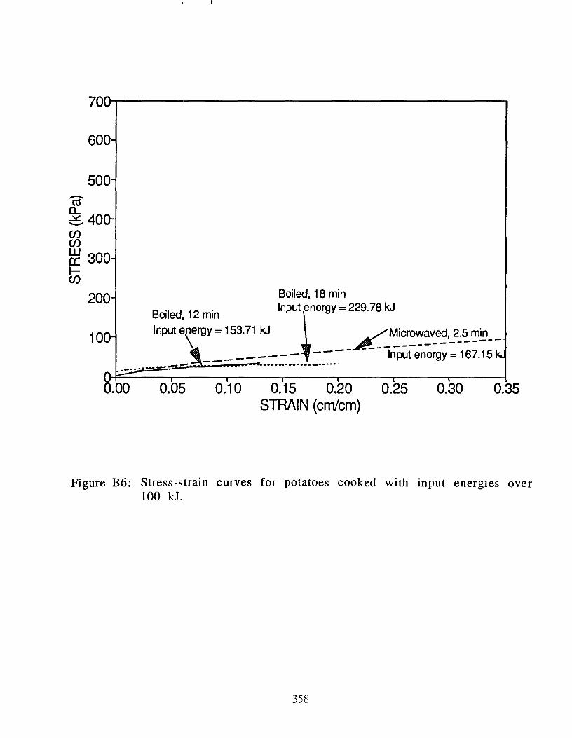
700~----------------------------------------,

600-

500-C? a.. ~ 400-CJ) CJ)

~ 300-t)

200-

100

Boiled, 18 min

B 'Ied 12 . Input~energy = 229.78 kJ 01 , min

Input~ e\rgy= 153.71 kJ LMi:~~:V_~,_2.:~~~--

__ ------- ---- Input energy = 167.15 k... - ............. - ----._- .----, .---- -..-

.00 0.05 0.10 0.15 0.20 0.25 STRAIN (em/em)

0.30 0.35

Figure B6: Stress-strain curves for potatoes cooked with input energies over 100 kJ.

358

ro ~400 ~ ~ 300 til

Boiled, 2.5 min

Inut energy = 30.60 kJ

~

_ L ~:r~~~v_~,_2.:~ ~!!1--_--------- Input energy = 167.15

0.10 0.15 0.20 0.25 0.30 0.35 STRAIN (cm/cm)

Figure B7; Stress-strain curves for potatoes cooked for 2.5 minutes by different methods.

359

COMPUTER INTEGRATED LAB TESTING

Charles C. Dahl

Engineering Department Ventura College

4667 Telegraph Road Ventura, California 93003

Telephone 805-654-6400 Extension 1367

361

COMPUTER INTEGRATED LABORATORY TESTING Charles C. Dahl

Engineering Department, Ventura College, Ventura, Ca.

KEY WORDS: Engineering Materials, Test Equipment, PIC, computer, retrofit, laboratory, transducer, thermocouple, LVDT, Young's Modulus, temperature, pressure, Datalogger.

PREREQUISITE KNOWLEDGE: This material is intended for the Engineering Materials laboratory. The course is for .second or third year engineering students with college chemistry and calculus based physics prerequisites. This computerized instrumentation would also be profitable for college Vocational/Technical or H.S. courses with such laboratories.

OBJECTIVES: Integration of computers into the Engineering Materials Science Laboratory course, where existing test equipment is not computerized, is the objective of this work. This includes temperature vs. time for phase change experiments: pressure vs. elongation for stress vs. strain; beam bending; creep; or a wide variety of experiments where change can be measured by transducers, strain/resistance (s/r) gages or bridges, thermocouples or similar devices that produce a resistance or voltage change. Input from such sensors is fed through a Datalogger to a PIC or 386. Data is imported to a spread sheet program for tables, graphs and charts.

EOUIPMENT AND SUPPLIES: Equipment and supplies include the following: 1) Sensors for specific test, i, temperature thermocouple, or pressure transducer, or Linear Variable Differential Transformer, or SIR strain gages, etc.; 2) Datalogger and related program for PIC, or storage: 3) PIC; 4) Spread sheet program for the computer; 5) Any additional standard test equipment used without computer instrumentation for the specific test, such asauniversal testing machine. 6) Normal specimens for the test, such as a wood tensile or compression sample, material to undergo phase change, beam to be bent, etc.

PROCEDURE: Lab 1) To demonstrate and produce a material phase change curve we shall do the following: 1) Measure temperature vs. time during cooling from a liquid to a solid with thermocouples connected to the data logger and the PIC. 2) Import the data into a spread sheet and produce a data table and graphs/curves of time vs. temperature for the cooling curves and related phase change point. 3) Discussion should interpret the curves which display the delay in cooling when phase change is taking place. 4) This combined with a phase diagram of the materials used allows the determination of the composition of the material.

A common materials experiment is to use a lead+antimony alloy to demonstrate the phase change, with delayed cooling recorded at the phase change point of the specific composition. Here the material is heated to 330 0 C, and the thermocouple is inserted in the liquid which is then allowed to cool. Assuming the same approximate temperature differential and conductivity of the container, the liquid will cool

363

at a constant rate to the point of phase change; it will hold that temperature until the heat of phase change has been transferred and the cooling rate for the solid pha~e will be displayed. The fact that this data is not normally taken or reduced by computer points out the difference of a computer integrated experiment from a conventional one. The student must analyze the data to be sure that it is meaningful. Materials such as antifreeze and water, with different phase change points may be substituted.

Lab 2) A demonstration of the modulus of elasticity and related stress strain curve, plastic performance, maximum and failure strength is done with force measurements taken by pressure transducer on the ram and change in gage length measured by an LVDT attached to the test sample. The pressure transducer and the LVDT signals are fed, with the given time interval, to the data logger and then to the PIC for recording. Parallel readings can be taken with an SIR strain gage and the LVDT mounted to the same sample, both measuring displacement. Our experience is that the SIR gage glue bond to the sample is broken prior to the material failure in the plastic range.

This process of recording data by sensors that are connected to a data logger which adds a time base, and the data logger in turn to a computer, places the materials labs into a computer integrated mode with minimum expense, maximum flexibility and in a commercial model and level. The sensor signals are input into a spread sheet for tabular records, curve generation and graph printing. The laborious process of hand recordings, related errors, data entering time and errors ~ eliminated and the tabular and graph quality is enhanced. Much of the equipment can be shared with the physics lab for other experiments.

CREDITS: Noise level and temperature environment research by the author was facilitated by Gerald Duffy of the Instrumentation Division of the NCEL at Port Hueneme, California. Mr Duffy introduced and set up the Campbell Scientific Micrologger, thermocouples and microphones for the study. Mr Duffy has continued to give counsel for this ventura College project.

REFERENCES: Elements of Material Science k Engineering, van Vlack; Introduction to Materials science for Engineers, Shackelford; Engineering Materials and Their Applications, Flinn; 21X Operators Manual, Campbell Scientific Inc. Synergistic effects of heat k high level noise on runway joint sealants; Alumbaugh, Dahl, Hoffard

SOURCE OF SUPPLIES AND EQUIPMENT WITH COST ESTIMATE: Campbell Scientific: 21X - 21X MICROLOGGER W/40K RAM 1845. ALK21X - ALKALINE BATTERY BASE FOR 21X INC. SC32A - OPTICALLY ISOLATED RS232 INTERFACE 130. SC25PS - RS232 RIBBON CBL WIPINS TO PINSISK 25. PC208 - SUPPORT SOFTWARE 200. AM416 - 16CHNL 4 WIRE INPUT MULTIPLEXER 435.

VIATRAN: PRESSURE TRANSDUCER MODEL 241 0-1000 PSIG 315.

364

SCHLUMBERGER: LVDT ARC 15 TRANSDUCER CONDITIONER 003

265. 295.

SIR STRAIN GAGES: THERMOCOUPLE WIRE: 386 OR PIC COMPUTER. 10/17/91 rev. 1/3/92

T HERMOCOUPLES

PR TR

JL'vDT

ESSURE ANSDUCER

Q:

OD3

PO'w'ER SUPPLY

/I

'-.J

/1

'-J

~ I

P SC32AI RS232

D ~ W LJ LJ

5 0 .-J COMPUTER <[ I-<[ 1=1

x .--<

0J

PRINT IPLOT ~

COMPUTER INTEGRATED LABORATORY DIAGRAM

365

MECHANICAL PROPERTIES OF BRITTLE MATERIAL

L. R. Cornwell

Department of Mechanical Engineering Texas A&M University

College Station, Texas 77843-3123


367

Mechanical Properties of Brittle Materials

L.R. Cornwell and H.R. Thornton Department of Mechanical Engineering

Texas A&M University College Station, Texas 77843-3123

KEY WORDS: Brittle materials, bending modulus, wood, glass, surface cracks, fracture toughness

PREREQUISITE KNOWLEDGE: This experiment is suitable for students who have been introduced to the concepts of ductility and brittleness. They should also understand the meaning of modulus of elasticity.

EQUIPMENT AND SUPPLIES: Universal testing machine such as Instron and MTS, bending fixture, rectangular wood specimens 1 cm by 1 cm 15 cm, glass slides.

INTRODUCTION

Brittle materials are difficult to tensile test because of gripping problems; they either crack in conventional grips or are crushed. Furthermore they may be difficult to make into tensile specimens for example threaded ends or of dogbone shape. To overcome the problem simple rectangular shapes can be used in bending (i.e., a simple beam) in order to obtain the modulus of rupture and the elastic modulus. The equipment necessary consists of a fixture for supporting the specimens horizontally at two points, these contact points being rollers which are free to rotate. The force necessary to bend the specimen is produced by tup attached to the cross head of an Instron machine.

PROCEDURE

The specimens are rectangular in shape and are measured for width and thickness; the length is the distance between the two supports. The wood specimens we used were ash, oak and cherry and were cut along the grain and normal to it. Most kinds of wood are suitable for this experiment and will show anisotropy. Three glass slides are used with a single scratch in each made with a suitable instrument such as a glass cutter. Effort should be made to keep the depths of scratches the same. The three scratches will be in different directions: one transverse, one longitudinal and the third at an angle of 45°, and with lengths equal to the transverse dimensions.

369

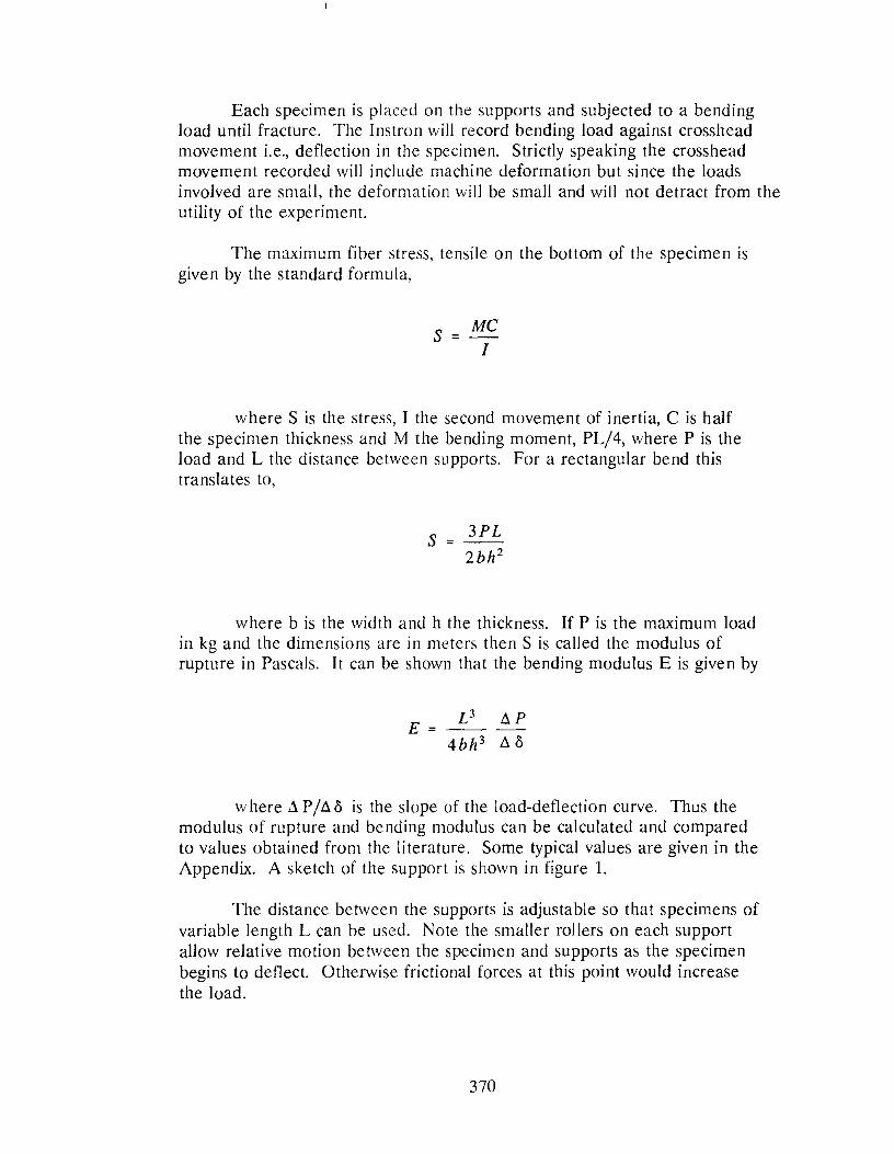
Each specimen is placed on the supports and subjected to a bending load until fracture. The Instron will record bending load against crosshead movement i.e., deflection in the specimen. Strictly speaking the crosshead movement recorded will include machine deformation but since the loads involved are small, the deformation will be small and will not detract from the utility of the experiment.

The maximum fiber stress, tensile on the bottom of the specimen is given by the standard formula,

s Me I

where S is the stress, I the second movement of inertia, C is half the specimen thickness and M the bending moment, PL/4, where P is the load and L the distance between supports. For a rectangular bend this translates to,

s = 3PL

2bh 2

where b is the width and h the thickness. If P is the maximum load in kg and the dimensions are in meters then S is called the modulus of rupture in Pascals. It can be shown that the bending modulus E is given by

E= ilP

where il P / il 0 is the slope of the load-deflection curve. Thus the modulus of rupture and bending modulus can be calculated and compared to values obtained from the literature. Some typical values are given in the Appendix. A sketch of the support is shown in figure 1.

The distance between the supports is adjustable so that specimens of variable length L can be used. Note the smaller rollers on each support allow relative motion between the specimen and supports as the specimen begins to deflect. Otherwise frictional forces at this point would increase the load.

370

Note that if a fairly ductile material is tested resulting in significant deflection the specimen may slip off the supports.

The purpose of the scratches on the glass is to show the influence of scratch orientation on strength. For the glass specimens one specimen is fractured without any surface stratches. For the other specimens scratches are placed on the tensile surface preferably with a diamond cutter with the same pressure. Sharp notches stay sharp in a perfectly brittle material since there is no mechanism for plastic flow. To demonstrate the influence of orientation on fracture behavior scratches are placed transverse to, 45° and along the length of the glass slides. The equation governing the stress intensity is

where I3 is the angle of the crack to the transverse direction and a is the crack depth. This relationship predicts that KJ is largest when I3 = 0, i.e. for the tranverse crack. Thus the fracture strength will be lowest for this orientation. When I3 = 45°, the stress intensity falls to half the transverse value. Strictly speaking this is only approximate since mode II on Kn is ignored so this would be a lower limit. When I3 = 90, i.e. for a longitudinal crack KJ becomes zero and this scratch should have no effect. Another way to think of this is the stress concentration at the side of a hole

o = 0 (1 + 2a) c n b

where 0 c is the stress concentration factor for a nominal stress 0 n applied at an ellipse with major axis 2a and minor axis 2b. In this case b ~ a so that 0 c = 0 n or a stress concentration of one.

The experimental values for an unscratched glass side approximate those of published values, see Table II. The largest drop in fracture strength is shown by the specimen with a transverse scratch, no effect with the longitudinal stratch, and the 45° scratched specimen in between.

In conclusion we would like to add that we tried the experiment described last year by Roy Bunnell on stress skin composites using paper reinforcement since our apparatus was ideally suited to the experiment. Essentially it shows that a very weak material like styrofoam can be strengthened considerably against bending by placing a piece of cardboard on the tensile side of the specimen. The demonstration was very conv1ncmg.

371

REFERENCES

ASM Metals Handbook, Vol. 8, Ninth Edition, p. 115, 1985.

Table I Typical Values For Different Woods

Type Young's Modulus Gpa Rupture Modulus Mpa

Along Perpendicula Along Grain Grain r

to Grain

Douglas Fir 16.4 1.1 70

Birch 16.3 0.9 ---

Ash 15.8 1.1 116

Oak 16.6 1.0 97

Suggested values of allowable stress in construction along grain 3.45 - 6.9 MPa

Table II Properties of Soda Lime Glass

Density Young's Modulus Modulus of Rupture

Mgm-3 GPa MPa

2.48 74 50

372

I

Or- L ~O z.

'- -

n 3 n I

Fig. 1 Sketch of three point bending fixture

Note: 1) 2)

3) 4)

Hardened steel pin .1 cm diameter Steel rollers, held in place by rubber bands attached to hooks in side of support Vertical supports slide in groove in base Scale approximate half size

373

INTRODUCTORY HEAT-TRANSFER AND

HEAT-TREATING OF MATERIALS

Edward L. Widener

Mechanical Engineering Technology Department Purdue University

Knoy Hall - Room 119 West Lafayette, Indiana 47907


375

INTRODUCTORY HEAT-TRANSFER E.L.Widener - MET. DeDt.

Purdue Univ. - W. Lafayette. IN.

PREREQUISITE KNOWLEDGE: TYPIcal high-school students of physics or chemIstry should understand basic concepts of mechanics (force. work. momentum. energy. velocity. acceleration) in fundamental units (U.S. and 5.1.) of basic dimensions (Length. Mass. Time).

OBJECTIVES: To introduce that notorious necessity. known as "thermo-dynamics", in exis"Cing heat-treating experiments using available items. To defIne thermal properties of materials: visualize expansivity. conductivity. heat-capacity. and melting-poInt of common metals; remember basic values: compare commercial materials. and consider electrical/mechanical analogs.

EQUIPMENT & SUPPLIES: Beakers (500 to 1000 ml) or buckets (2-5 gallon) for water-oil-sand quenches. Furnace. torch. or burner (electric or gas) for red-hot specimens: to re-heat speCImens (tempering or aging). Grating (expanded-metal. wire-mesh) and firebrick (supports) for a cooling table. Piece of pipe (steel. plastic) about 10" long (25 cm) and 4"-Schedule 40 size (10 cm round); with circumferential holes (6-8) for 1/8" rods (wires) about 6" long (say 3 mm X 15 cm). Coffee-pot or hot-plate. to boil water. Stop-watch (or timer) and thermometers (dial or glass). Tongs, gloves. and safety glasses.

BACKGROUND: In ancient Greece and Persia. heat was considered a universal

element (earth. air. water. fire); but not until 1698 (Savery steam-pump) and 1712 (Newcomen steam-engine) was heat reified to mechanical work. [1] The materials lab is a good place to demonstrate the dynamiC process of "heat transfer". to elUCidate the elusive concept of "heat". and to inter-relate "heat/work/energy".

Rooted in Old English words (hot. hetup). heat is a fundamental and fascinating subject. variollsly defined: energy added to substances to raise temperature. change state. or accelerate reactions; energy associated with random motion of atoms/ions/molecules; energy flow from high temperature to low. Although heat is not temperature nor a property of materials. it is prominent in properties an~ processes which are temperature-related: expans i vi ty (a). dens i ty (r) . conducti vi ty (0', It) . heat ca.pac i ty (Cp) viscosity (1-')' melting pOint (t); and annealing, normalizing, quenching, tempering. stress-relieving. aging. warping. corroding, hystereSiS, friction.

DEFINITIONS; Heat (Q) is thermal-energy in transit (area under a T-S curve. a

plot of temperature vs. entropy) because of a temperature difference. Similarly, Work is mechanical-energy in transit (area under a P-V diagram. a plot of pressure vs. volume) because of a force difference. Also, Amperage is electrical-energy in transit, because of a voltage (potential difference).

377

Heat has a work-equIvalent (about 778 ft-lb/Btu) but neither of these "path functions: 1 ,3.re identical to Enerqv. c5. Ipoin'C func1:ion. I Think of 03. truckload of goods. partway between a warehouse and ,a shop: heat is like the shipment. but energy is like an inventory (at warehouse or shop) [2J. Silmlat'ly, an accountant takes the difference between "balance sheets" (Iield strengths) as "proflt-or-loss" (heat transfer. work done) .

Heat is generally measured in units of joule. calorie. or Btu. Worl< or energy is expressed in foot x pounds (ft-Ib) or joules (newton-metre). The U.S.A. still prefers to use the "British Thermal UnIt" (Btu). defined as the energy to raise a pound (Avoirdupois) of water (atmospherIc pressure) by a Fahrenheit degree (FO). or absolute Rankine degree (R"). Think of this as the chemIcal energy (potential) in a regular, wooden. kitchen-match (about 3" long). It is almost a J<ilo-joule.

The ,)id metric calorie was defined as the energy to raise a gr,am (mIl of water (atmospheric pressure) by a CentIgrade degree (CO, now called Celsius) or absolute Kelvin degree (K). Note this standard for S.I. (Systeme Internationale) disallows a degree mark (KO). which precludes the convention of Jakob/Hawkins [3] : Water freezes at 32°F, but boils 180 FO higher, a useful distinctlon bet',.;een "point" and "line" functions. Also note the dieticians' usage of "Calorie". which is a "kilo-calorie" of food (l.OOO-cal = Cal).

The S.I. unit of work. heat, and energy is the joule: i.e., force (newton) times distance (metre). Of course. the newton is the mass (kilogram) times acceleration (metre per second-squared). Note "force" is better defined as "time rate-of-change of momentum": so. F-dCmvl/dT. Since 2.2 lb (mass) is about I-Kilogram, and 2.54 cm is exactly I-inch. the kilo-joule is about a Btu. A newton is about a quarter-pounder.

More precisely. a Btu = 1.055 kJ = 778.16 ft-lb - 251.98 small cal. A calorie = 4.1868 J. A kilogram = 2.205 Ib (Av). A Ib 4.448 N. And a Watt = J/s = 3;413 Btu/hr. [4]

Generally, hydraulic analogs are more graphic than thermal systems. Mechanical to thermal conversion is more efficient (up to 100%, including friction) than thermal to mechanical. An electrical system is more easily and accurately measured then its thermal analog.

Thus. electrical capacity (e1 ) is charge (coulombs) per voltage difference (C'=Q"/AE); and thermal capacity (C) is heat imput -i

temperature difference (C = Q/AT). Sometimes this is mis-named "heat-content." Specific heat-capacity is then standardized at constant pressure (Cp = Q/m XAT) per unit m,ass. So, Cp =Ah/A T) in terms of Entha 1 Py (A h - Q/m) .

Hydraulic flow rate (Q) is cross-sectional area (pipe) times average-velocity (fluid), so Q = AV. Then .. "pipe conductivity" could be expressed as C = QL/L2 X AT X At. the analog of thermal conductivity.

Electrical conductivity (O'igma). is the inverse of resistivity. Use Ohm's Law (E = IR = Ampere X Ohm) and define an Ampere (Coulomb/second): then 0' = l/RL.

Thermal conductlvity (ltappa) is heat input X length -i- (a.rea X time interval X temperature difference). Thus. It = QL/L2 X AT X At.

The classic Dulong-Petit Rule (1819) says: Specific-heat (Cp) times Atomic-weight (amu) is approximately constant (6.4) for solid

378

elements (above 40 wt.). The claSSIC Wiedemann-Franz Ratio says: Thermal-conductivity (x;) over Electrical-conductivIty (0") is approximately constant 17.5 X 106, J x Q 1 s x KJ for metals at constant temperature. This constant is also the "Lorenz" constant (L) times absolute "Kelvin" degrees (tl for variable-temperature tests.

EXPERIMENTS: Now the fun begins! 1. Relative Quench Factor (RQFl

A steel disk (AISI 1040. 2" dia. X ~" thick) is heated red-hot (1650" F. 900"C) and quenched quick!y In a pail of water (70" F. 21"C). The sizzling will stop in about 30 seconds. so the disk is not too hot to touch. A second disk (AISI 1080) quenched in water will take about 30 seconds. but has twice the carbon (0.80 W/O) and twice the BeT martensite grains (Body Centered Tetragon) so the disk cracks badly. A third disk (AISI 1080) quenched in oil will take about 90 seconds. make less martensite (shown by Rockwell C hardness). but has no cracks. Thus. the oil is a slower. safer quenCh; higher boiling point and greater viscosity are the reasons. Show students how a sore thumb. soaked in hot-water. becomes comfortable unless "stirring" ensues; thus. heat-transfer is enhanced by "turbulence". to redlice the laminar boundary-layer in water.

An aluminum disk (AA 6061. 1l!." dia. X 1" thick) is heated red-hot (1650" F); it melts to a "pancake" in the furnace. exhibiting a black alumina coating typical of "emery paper" (used for metallography grinding). A second Al disk is "solutionized" (990" F. 532"Cl and quenched quickly in the pail of water (70"F). We can predict how long it takes to stop sizzling. so the disk is not too hot to hold (threshold of pain is 140"F. 60"C). Use RQF = Q of Al + Q of steel. where Q = Cp xi'f X t; i.e .. (Btu/lb/F")times(lb/ft3) (ft3) (F")=Btu.

Thus. RQF = (0.215) (170 X 1.77) (990 - 70) = ~ X 1 X 1 X ~ = 1. (0.110) (480 1.57) (1650 -70) 1 3 1 3 9

Assume a constant 70" F in a 5-gal water pail. Note how volumes of disks (\f) in cubic inches will cancel, so conversion to cu ft is not needed. It will take the Al disk about ~ X 30 sec 113 sec to cool.

~ Furnace Calibration Test (FCTl Assume the heat-treating shop wants to check the furnace controls

(temperature control. thermocouple. and readout) every shift. The "suggestion - box" brings a test proposal for $100 award: Drop 10-disks of red-hot steel in 1-gallon water bucket and measure the temperature-rise. with stainless-dial thermometer. The foreman fears a steam explosion. Do we O.K. the test? Assume a heat-balance and neglect losses.

Say Q out of steel = Q into water; where Q = Cp X-y.tXLlt : the Q is "absolute value" of heat; and t is final temperature of ten-cold disks or a warm gallon (8.33 Ib). Therefore, 0.11 (10 X 480 X 1.57/l.728) (1.650 - t) = 1.0 (8.33) (t - 70)

So. 0.4797 (1650 - t) = 8.33 (t - 70) So,

791.5 - 0.48 t 8.33 t - 583.1

7.85 t = 1374.6. and l~t ____ 1_7_5_'_F~1 We conclude the water won't boil. the test is simple and safe. and

379

~he $100 award 1S well deserved. Of course. ~he men have already run the test. a disk at a time. and know It IS O.K. An eleGant . thermodynamIcs eq1lation says Q In - - Q out, with temoerature differences expressed ,~s "final-ori(]inal. ,. Ours 'rv"lere ~'hot-cold'l.

3. 50ecIflc Heat Cdoacity iwatel") Worldly WIsdom says, "3. pInt's a. pound the world around", If It's

water. ~ilk is mostly water. So. take a pint of milk and heat Its bottom WIth a kItchen match (one-Btu). With no heat losses, the milk only heats one F", a vIsual proof for Cp of H2D (one Btu per pound per F"l. No wonder water is used to quench red-hot steel and to douse tIres.

Next. visualize a Btu as 778 ft-Ib. An 80-lb bag of "softener salt", carried up 10-steps (1 foot risers) to the mezzanIne, ca.n injure a worker on the ground floor (800 ft-lb is bad). An 80-lb cannon-ball. dropped nn your foot (10 ft below) is worse. Holding your hand over a wooden mae:ch (one-Btu) gives "roase: hand", but not "roast milk". This is real energy:

4. Specific Heat CapaCIty (metals) Get samples of 5-common alloys (copper, aluminum, yellow-brass,

plain-steel, and stainless-steel). All samples must have the same weight (say 5 ounces); it's good to have the same surface area (a challenge) but not essential. Take 5-beakers: add ice-water enough to cover any sample (alumInum has most volume); but each beaker must have the same volume of water.

Meanwhile, the metal samples are immersed in a pan of water and brought to a boi.l. Put a thermometer in each beaker; st ir ,Oind measure the "ice-\.;ater" temperature; a rugged dial-thermometer is good. Then, add a hot sample to each beaker, stIr to avoid stratification, and read the maximum temperature rise (~t). Compare with va 1 ues of Cp and 'Y from a handbook, which should vary directly with ~t. - values, but inversely with density. Aluminm is lightest. so Cp is largest (about 0.215 Btu/lb/F"). Steel and Copper have less Cp (about 0.11).

5. Thermal Conductivity (metals) Get wire samoies (say 1/8" dia. X 6" long) of common metal alloys

(copper, aluminum, brass. steeL staInless) and insert them in your "pipe holder" (4" - Sched. 40 X 10" long). having radial holes and air-passages (see Sketch):.. Flame Each wire. with a ball-of-wax on the outer end. looks like a "Q-ti p". Inner ends of wires meet at the pipe-center, lIke spokes in a wheel. A burnerflame heats the WIres simultaneously (at the hub).

The wax falls off the copper. Burn ... e::.r.-.....::.....~~Hf~~_ then aluminum - brass - and steel; -the stainless steel stays cold. Measure the drop-off tImes by stop-watch; compared with handbook values for Kappa (thermal conductivityl) these metals should differ by halves: copper 1. aluminum 1/2. brass 1/4, steel 1/8. stainless 1/16. No wonder

380 PIPE - HOLDER

aluminum and stainless-steel are hard to weld. Compared to plain-steel. aluminum conducts too fast. holds heat too lonq. and tends to melt too much; stainless is slow to preheat. hard to preheat evenly. and tends to warp.

Notice the "oxide" colors (ranging from yellow to blue) which correspond to temperature (430 - 640° F). Do not confuse with "hot-metal" colors; hot-rolling is "red-hot" at 1650' F: cold-rolling is "black-hot" below 1333' F (allotropic transformation. from FCC austenite to BCC ferrite).

Throw in a "ringer" (copper-coated stainless welding-rod) and mystify the class. as the waxy tip stays cold indefinitely.

6. Melting Points (Solder) Molded balls of solder (60-40 eutectic mix) and component metals

(lead. tin) are made as "fish-line" weights (with a slot). An aluminum plate (say 4" dial is dent.ed with a ball-hammer (3-dents. in .'3. triangular pattern). Placed on a ring-stand and heated by gas-burner. the balls will melt. but the aluminum plate should not. First. the solder ball collapses to a pancake; next. the tin ball; finally. the lead ball. Shut off the flame. tap the plate. and watch the shimmering "puddles" as they re-freeze. First is the lead: next the tin: finally the solder.

Discuss the "eutectic-solder" (for electrical joints) which freezes at a definite .. lowest temperature); compare with "wipIng solder" (for plumbing joints) which freezes over a range of temperatures (like slush). This illustrates the 2-phase mixture of liquid and solid solutions. seen on a "binary phase-chart" of Pb and Sn.

7. Expansivity (linear) A stainless coffee-pot. fitted with a plastic-lid. may have easy

clearance (cold) but becomes difficult to remove (boiling hot). Compare values of linear expansivity (at) for steel ( O.ooooo6/FO) and plastics (0.00006). Visualize expansion of a steel pipe as 6"

per million" (16 miles). Samples of Al rod (at = 0.000009) easily show expansion and

contraction. if heated in boiling water (about 140 FO above 70° room temperature) and cooled on dry-ice (about 140° F below 70° F). Measuring can be done by a "vernier caliper" (to 0.001". called 1-mil) or a "micrometer" (to 0.0001"). Be careful of ice-crystals on a cold rod. interfering with measurements. Use a machinist's calioer (with center-screw adjustment) like an ice-man's tongs (a "go/no go" gage) .

Note area expansivity (aA) is about 2 Xat (210%); volume expansivity (a.,A is about 3 Xal (331%). When units are cancelled in a handbook (in 2. / in2·,or in 3jin3) we generally assume published values are linear. Wnen in doubt, find outf Remember, expansivity is generally measured close to room temperature. For red-hot steel, 6 "per million" is too little.

CONCLUSION: The materials lab experiments and demonstrations can introduce

students to thermal properties. as well as mechanical. The shock of "thermodynamics" is alleviated. and electrical correlations with thermal properties are enhanced.

381

KEY WORDS: heat.. work. energ'y. enthalpy: expansion. contraction: conduction. resistance: heat-capacity. heat.-transfer.

REFERENCES:

1. Garrison. E. G .. "A History of Engineering and Technology: Artful Methods". eRC Pt'ess, Inc .. 1991. p. 143.

2. Kazem, S. M., and Emshousen, F. W., "Introduction to Heat Power: MET 220 Laboratory". Learmng Systems. Inc, W. Lafayette, IN, 1989.

3. ,JaKob. M .. cl!1d Hawklns. l3. A., "Elements of Heat Transfer", 3rd ed .. WIley. N. Y .. 1957.

4. Faires. V. M., and Simmang, C. Moo "Thermodynamics". 6th ed .. MacMillan. N.Y .. 1978,

BIOGRAPHY:

EDWARD L. WIDENER

Teaches mechanical engineering technology at Purdue University (since 1978), concentrating on statics, fluid mechanics, materials, labs and technical writing ... Member ASME, ASEE, ASM, TAPP1. Registered P.E. in New York and Indiana ... ABET visitor in 1983-88 ... B.S. M.E. from Purdue University and M.S. E.M. from the University of Kansas ... Taught evenings at IUPU-Indianapolis and at Danville, IL. Worked as Mechanical Development ErYJineer for "Coria" collagen casing with Teepak Co., Continental Group (1976-78). Process Group Leader for mechanical contractor, Baker-McHenry-Welch, Indianapolis, IN (1974-76). Project Leader for creped-wadding and secondary-fibers with Kimberly Clark Co .• Memphis. TN (196&-74). Process ErYJineer for "Nomex" nylon with E.1. J)JPont Co., Richmond, VA (1963-68). Associate ErYJineer for electro-furnace alloys with Union Carbide Co., Niagara Falls. NY (1952-60). FUel ErYJineer with U.S. Steel Co., Gary, IN (1951-52) .

382

HEAT-TREATING OF MATERIALS Edward L. Widener - MET Dept.

Purdue Unversity, W. Lafayette, IN

PREREOUISITE KNOWLEDGE: Typical high-school students of math and science should understand basic concepts of crystals (solids) and glasses (super-cooled liquids) for elements (atoms) and compounds (molecules).

OBJECTIVES: To introduce those solid-state transformations of material structures, known as "heat-treatments".l To emphasize commercial importance of common processes for metals as well as non-metals.

'1. EQUIPMENT & SUPPLIES: Furnace, torch, or burner (electric or gas) for red-hot and re-heated specimens. Buckets (2-5 gallon capacity, say 9-22 litres) for water-oil-sand quenches. Grating (expanded-metal, wire-mesh) and firebricks (supports) for cooling-table. Stop-watch (or timer) and thermometer (dial or glass). Tongs, gloves, and safety glasses. Hammer, wrench, hack-saw, vise. Specimens of metals (ferrous and non-ferrous alloys) or non-metals (ceramics .and polymers) from ware-house or scrap-pile.

PAUSE & PONDER: What is the best way to learn a new topic? Start with simple, familiar examples? Survey a broad field? Why not do both?3 First, remember the blacksmith's dipping red-hot steel in cold-water, because "quenching" is a quick way to allotropically harden carbon-steel. 4 More broadly, define conventional heat-treating as: "controlled heating and cooling of metal alloys, to alter properties, in the solid state". Why order "special heats" from melting furnaces, needing long-term scheduling of large-tonnage orders in high-energy processes at high prices? Solid-state treatments are sooner performed on standard stock in small amounts, at market prices with fuel savings, available from local suppliers.

More specifically, define "heat treating" as the controlled heating and cooling of metal alloys in the solid-state. Start by "solutionizing", heating above a critical temperature and soaking I-hour per inch, to get a single-phase solidsolution. Then, cool at various rates to anneal (slow), normalize (medium), or quench (fast). "Tempering" is merely re-heating, so as to draw brittleness from allotropically-quenched martensite, to graphitize malleable-iron from white castiron, or to age a T-6 aluminum or P/H stainless-steel fron quenched supersaturated solutions. "Hardening", the usual objective, may involve workingalloying-carburizing-coating-quenching-or tempering operations. s

STEEL EXPERIMENTS: There are dozens of separate and distinct heat-treating operations that may be performed on steel. In this laboratory exercise, only four of the commonly used heat-treating operations will be performed, with explanations of their purpose and effects upon steel properties. 6

(a) Anneal - A part is heated to the proper temperature, where the structure becomes a single solid-solution of "austenite". After a suitable holding time at temperature, the part is slowly cooled, in hot-sand or furnace. This puts the steel in a condition having its lowest strength and softest properties. It is usually the best condition for machining - or for cold forming the material into parts. In slow cooling from red-hot state, austenite transforms into a predominately large-grain, lamellar-pearlite, micro-structure.

383

(b) Normalize - Has the same austenitic-temperature as for annealing; but, after a suitable holding time at temperature, the part is removed from the furnace and allowed to cool in still-air. This operation is less costly than anneal, produces slightly higher strength and hardness, but often is adequate for machining and cold-forming.

This heat-treatment may provide a uniform metallurgical structure, throughout the entire part. The slightly faster cooling of austenite from the normalizing temperature still produces a predominately pearlitic micro-structure; but, it is somewhat finer lamellar-structure, which contributes to slightly higher hardness and strength.

(c) QUench or Harden - A part is also heated to the proper temperature, where the structure becomes a single solid-solution of austenite. It is also held at temperature for a suitable time, to provide a homogenous solid-solution. For hardening, the cooling rate is all-important. The heated part must be cooled so rapidly that austenite does not expel carbon, nor become pearlite, but transforms into a wholly new constituent called "martensite". To do this, the rate of cooling must exceed a critical cooling rate (CCR) at critical cooling velocity (CCV) .

Martensite is an interstitial, super-saturated, solid-solution of carbon in tetragonal body-centered iron. The "diffusionless" transformation from austenite-to-martensite results in a volume expansion of 7 to 9%. It is the hardest and strongest condition for a given grade of steel, say 60-63 RockwellC(Rc). However, in this condition it lacks toughness and is seldom used in the as-quenched condition. Additionally, in this hard expanded-volume condition, there frequently are high internal-stresses, which may result in cracking or shattering, depending upon the shape of the part. The next heat-treatment puts martensite into a suitable condition, for engineering applications.

d) Temper or Draw - This relatively low-temperature operation reduces the hardness and strength of martensite, but improves toughness, for a specified application. Temperature is between l350-4000F (730-205OC), below the eutectoid temperature of the "Iron-Carbon" equilibrium diagram. For each part and application, the exact temperature for tempering is variable to provide a finished part with proper combinations of hardness, strength and toughness. 7

Since these changes in micro-structure are extremely difficult to evaluate, by viewing the changed structure, specify that structure as tempered-martensite of a certain Rockwell hardness.

Laboratory Exercise: Heat treat 5-samples, all of the same grade of steel (say AISI #1040). (a) Annealing - Heat sample to l6500F, hold for l-hour per inch at

temperature, shut off furnace, and allow sample to cool in furnace. Check and record hardness, using Rc-scale.

(b) Normalizing - Heat sample to 1650° F, hold for l-hour at temperature, remove sample from furnace, and cool in still-air on a metal-grating. Check and record Rc.

(c) Hardening - Heat sample to l6500F, hold for l-hour at temperature. Remove sample quickly from furnace, plunge in cold water and agitate during the cooling, to get an effective quench without insulating steam bubbles. Check and record Rc.

384

(d) Tempering - After recording the hardness of quenched sample (c) above, place in furnace and temper at 9000 F. Hold for I-hour at temperature. Remove from furnace and air-cool. Check and record Re.

(e) Drawing - Heat sample to l650oF, hold I-hour, then quench 1" of the end. File off black mill-scale, watch for blue-oxide color being "drawn" to silvery tip, and then quench to stop re-heat. Check and record Re.

ALUMINUM EXPERIMENTS:

Several metal alloys (mainly non-ferrous) can be hardened and strengthened by a 2-step process: a) Solution Heat-Treating involves heating-soaking-quenching. b) Precipitation Hardening includes natural aging (air) or artificiallyaccelerated aging (oven).

Wrought Al. Alloys - The "Aluminum Association" has a 4-digit system to designate various structural materials, from #1000-7000, plus tempers (F, 0, H, W, T) followed by 1 or more digits. HArdening mainly involves the 2000, 6000, and 7000 series. Cast AI. Alloys are similar, but designated with 3-digits, a decimal point, and 4th digit.

Commonly alloyed with Aluminum are Cu, Mg and Si, whose "solid-solubilities" are greater at hi-temp (vs. room). Thus, an alloy is heated to maximum-solubility, then quenched (rapidly cooled) to become temporarily a super-saturated solidsolution at room temperature; i.e., the solution has dissolved more alloy-element than normal for equilibrium conditions. Such state can be maintained (or prolonged) by refrigerated storage. However, if allowed to "age" naturally (at room temp.) or "artificially" (at oven temp.), the alloy can precipitate small crystals of "inter-metallic compound". Visible only by electron-microscope (S.E.M.), these particles act as "keys" at inter-granular boundaries and slipplanes. The product is harder and stronger.

Select AA alloy #606l-T6 (formerly #6lS), composed of Al-Mg-Si, commercially heat-treated and formed into bar-stock, l. 5" dia (say 4 cm). Cut samples approx. 1" long (2.5 cm). Demonstrate basic processes, such as: a) Full Anneal - To insure all samples/start with uniform softness, preheat

the furnace to 5320C for l-hr; then heat samples for I-hour, shut furnace off, and let samples slowly cool to room temp. (about l2-hrs inside furnace). Measure hardness.

b) Normalize - Remove solutionized sample from 5320C furnace; let coolon grating in still-air to room temp. (about 230C). Measure hardness.

c) Solution Heat-Treating - Samples heated to 53tOC and soaked I-hr.; then fast-quenched in water to room temp., and immediately tested for hardness.

d) Natural Aging - Store quenched samples at room temp., and regularly monitor the increasing hardness. Check with references for AA#606l-alloy to estimate the optimal-aging period (6-12 months) at room temp.

e) Artificial Aging - Three quenched samples of known hardness (from Test "c") are reheated (tempered) to 2000C for 20-40- 60 minutes; then "quench" in water to room temp. and measure hardness. Check ASM Metals Handbook (Ref. 5, Vol. II) for optimal time, hardness and strength. Rockwell may exceed 50 Re.

TIPS:Ferrous alloys (Fe over 50 w/o) are typically used for "allotropic quenching"; however, consider an "alpha-beta" titanium alloy (Ti 6 Al - 4 V) for

385

precipitation-hardening (solutionize at 9s0~, quench in water, age at s40qe). Common allotropic-metals include: Co, Cr, Mn, Ni, Sb, Sn, Ti, W, Zr.

Always define "percentages"; e.g., w/o by weight, v/o by volume. Always check hardness (or strength) of fresh (as-is) specimens, to establish a "benchmark" (control standard) before heat-treatment.

Samples are usually steel (AISI #1010 - 1080; 4340) or aluminum (AA #6061; 2024) sliced from 1-1/2 to 2" dia. bars (say 3-5 cm). However, scrap-metals are cheap and disposable: springs, paper-clips, hacksaw blades, razor blades, streetsweeper tines, pallet-straps. For typical "soaking" (l-hr per in, 2.54 cm) a thin specimen (1/16", 1.5 mm) needs only 4-5 minutes (depending on reflectivity) to "solutionize" in the solid-state .. Surface sanding is avoided, unless microhardness (Vickers, Knoop) is tested.

To show property differences (from various treatments), the usual tests are tensile-pulls or macro-dents, which require descaled ends (coupons) or surfaces (disks, blocks). However, consider "Mohs" scratching (sawing or filing) or a drop-weight (Brinell-ball through glass-tube) with Brinell-scope (20x).

Magnetic tests are appropriate. Use a magnetized screwdriver, file-cabinet clip, or recipe-holder to show "ferro-magnetism" of steel, nickel, or c.obalt specimens. Austenitic stainless-steel is usually not magnetized (contaminated welds may become ferro-magnetic). Black mill-scale (Fe3 04) is strongly "ferromagnetic"; so, cleanup around hot-rolling mill, heat-treating furnace, or blacksmith-shop is easy. Of course, red-hot "austenite" (gamma iron) is not ferro-magnetic.

With small metal-barstock, twisting tests are fast and effective. Mount a heat-treated bar (square or hexagonal section) in a vise, and twist 90 0 by wrench (torque-wrench is better). Note differences in "stiffness" between the annealed, normalized, quenched, tempered specimens. Note the 900 return-twist is stiffer (annealed, normalized bars) or makes cracks (quenched, tempered bars) and gives higher torque-readings (work-hardening). Such testing also averts descaling or smoothing steps.

Tines, lying in the street (after curb-sweeping) are hi-grade spring steel. Fresh samples are available from maintenance shops (after brush-change). After heat-treating, each tine can be vise-gripped and sharply-flexed (90 0 to and fro) from vertical. A slight pull is needed, to concentrate bending at one spot (as metal work-hardens). Annealed tines may take 20-flexes, tempered "as-is" tines take 3, and quenched tines only 1/2 flex. More tests are done, in less time.

Furnaces are often too costly, bulky, hot, slow, and unreliable. Our labs, for 10-20 yrs., have successfully used dual-box units (440V oven, 110v control) with inter-changeable base (temp. range) and bench size (2'x 2' x 3' clearance)~ However, with thin samples, a gas-welding torch or bunsen-burner is adequate for demonstrations. Cooling in a furnace (slowest), then in air (slow), one might assume "sand-burial" to be moderate (slower than air). Students are surprised to find cold-sand (room temp.) gives a mild "quench" and more hardness than airnormalizing. So, heated sand (100-200"C!) is needed, to better approach a "fullanneal"

386

Moreover, students are surprised, when "tool-steel" is hardened by an "airquench", because hi-alloy content slows the transformation-cooling rate and avoids "normalizing."

Plastic sheets, such as poly-carbonate (G.E. Lexan) or Acrylic PMM (DuPont Lucite, or Rohm & Haas Plexiglas) can be "stress-relieved" at lowtemperatures (say 100-400oC, plus 4-day slow-cQgldown). Examine a tensile-coupon by polariscope to check results (no colored fringes, in unstressed photoelasticity specimens). Melt-and-burn tests are also worth exploring, with common "ethenic" plastics.S

CONCLUSION:

With multiple lab-sections and repetitious testing, the materials lab has the opportunity of accumulating data (for several semesters) to run linear regressions, get dimensionless plots, or make a statistical analysis-ofvariances. Studying trend-lines and correlation-coefficients will enhance comparisons: a) Hardening vs. softening processes. b) Cooling efficiency of quenchants (water, oil, sand). c) Carbon content of steels. d) Ferrous vs. nonferrous alloys. e) Metals vs. non-metals. f) Cooling efficiency of water-oil-sand quenchants.

Virtually all materials (metals, ceramics, polymers) are being commercially heat-treated. Materials lab experiments can expand beyond metallurgy into ceramic-glass tempering, refractory curing, thermoplastics manufacturing, thermosetting, composites fabricating, repairing and maintaining.

REFERENCES:

l. __ Widener, E. L., "Materials Labs: MET 141 Packet #X7", Kinko' s Copies, 720 Northwestern Avenue, W. Lafayette, IN, 1991, pp.47-55.

2. __ Lindberg Furnaces (Div.of Gen.Signal - was Sola Basic), types 51442/59344, l2000e max., 304 Hart Street, Watertown, WI (53094).

3. __ Jacobs, J .A., and Kilduff, T. F., "Engineering Materials Technology", Prentice-Hall, Englewood Cliffs, N J , p. 155.

4. _ _ Fellers, William 0., "Materials Science, Testing, and Properties for Technicians", Prentice-Hall, Englewood Cliffs, NJ, p. 154

5. __ American Society for Metals, "Metals Handbook: Ninth Edition", Publ. by b Society for Materials (ASM) International, Materials Park, OH (44073): Vol. I - "Properties & Selection: Irons & Steels", 1978. Vol. II - "Properties & Selection: Nonferrous Alloys", 1979. Vol. III - "Properties & Selection: Stainless, Tools & Specials", 1980. Vol. IV - "Heat Treating", Alban-Easterday-Zamborsky (Ed.), 1981.

6. __ U.S. Steel, "The Making, Shaping and Treating of Steel", 9th ed., H.E. McGannon (Ed.), Herbick & Held, Pittsburgh, PA, 1971, Index pp.1360-l36l.

7. __ Bain, E.C., and Grossmann, M.A., "Principles of Heat Treatment", 5th ed., A.S.M., Materials Park, OH., 1964, p.129.

8. __ Widener, E. L., 1/ Burning Plas tics: For Fuels or Fools", Proceedings, ASME Hydrocarbon-Processing Symposium (ETCE), PD-Vol 28, 1990, p.13.

387

MEASURING THE SURFACE TENSION OF SOAP BUBBLES

AND MEASURING THE WEIBULL MODULUS

OF MICROSCOPE SLIDES

Carl D. Sorensen

Department of Manufacturing Engineering and Engineering Technology 435 CTB

Brigham Young University Provo, Utah 84602


389

Measuring the Surface Tension of Soap Bubbles

Carl D. Sorensen Brigham Young University, Provo, UT 84602

Key Words

Surface tension; surface energy; bubbles; soap films.

Prerequisite Knowledge Required

Students should probably have completed high school, although this is feasible for advanced high school students. The concepts of surface energy and surface tension should have been explained.

Students should be taught how to do a force balance on a hemispherical bubble, with the pressure inside the bubble balanced by the surface tension force at the equator of the bubble.

Objectives

• Students will gain an understanding of surface tension.

• Students will see that the pressure inside a small bubble is larger than that inside a large bubble.

• These concepts can be used to explain behavior of liquid foams as well as precipitate coarsening and grain growth.


• Commercial soap bubble solution

• Water colored with food coloring

• A basketball inflation needle or hypodermic needle with the end ground off

• Approximately two feet of clear vinyl tubing with an inside diameter of at least 1/4 in. (1/4 inch tubing works very well for use with a ball inflation needle

• Masonite or pegboard, made into a stand as shown below

• Two six-inch machinists' rules or fine graph paper

• A small watercolor paint brush

• Syringe or eyedropper to add fluid to the manometer

• Toolmaker's microscope or fine wire or drills to measure the inside diameter of the needle

391

Procedure

Set up the U-tube manometer with the needle pointing down. Pour a quantity of colored water into the manometer. Adjust the rules so the liquid level in the tubes is at the same place on both rules.

Dip the paintbrush into the bubble solution. Wipe the brush across the end of the needle to put a soap film in place. Periodically rub the brush against the side of the needle so fresh bubble solution can continue to drip down the needle.

With an eyedropper, slowly place colored water into the manometer. Because of the surface tension of the soap film, you will notice a higher pressure on the needle end of the manometer. Continue to add water, noting the height of the fluid on each scale.

Eventually, a bubble will form at the end of the needle, and the pressure measured by the manometer will suddenly decrease. Record the maximum pressure indicated. Also, estimate the size of the bubble and record the pressure.

Continue to add fluid to the manometer. The bubble will continue to grow. Record the bubble diameter and pressure at two or three different bubble sizes.

When the bubble pops, repeat the procedure two to three times. Record all data on the data sheet.

Empty the fluid out of the manometer. Using a drill or a toolmaker's microscope, measure the hole diameter of the needle and record it on the data sheet.

Since the soap bubble has two sides, the pressure difference between the inside and outside of the bubble is given by the formula

~P = 4y/r

where y is the surface tension of the soap film and r is the radius of the bubble. The pressure outside the bubble is atmospheric; the pressure inside the bubble is atmospheric plus the additional pressure of the water in the manometer tube. The additional pressure due to the water is given by

(1)

(2)

where p is the density of the fluid, g is the acceleration of gravity, and ~h is the height difference between the two sides of the manometer. If we consider that atmospheric

pressure is acting on both the inside and the outside of the bubble, it is clear that LlP is just Pwater. We can calculate Pwater either from equation (2) or by using conversion factors:

1 atm = 406.8 in H20 = 14.7 psi = 101.4 kPa (3)

The bubble forms on the end of the needle when the bubble has the same radius as the inside of the needle. The surface tension, then is calculated from

y = LlPmax r/4 (4)

392

where Mmax is the maximum pressure difference recorded.

A second way to measure y is to make a plot of ~p vs. 4/r. The slope of the line is y.

Measure the outside diameter of the drill. Based on your calculation of y, can you predict the heaviest bubble that will hang on to the end of the needle? Can you think of a way to measure the weight of a bubble?

Sample Data Sheets

Inside diameter of needle: 0.052 in (1.32 mm)

Outside diameter of needle· 0 080 in (203 mm)

Maximum Bubble 1 Difference

Run Left Right Diff. Left Right Diff. No.

1 2.15 2.90 0.75 2.90 3.16 .26

2 3.05 3.75 0.70 4.60 4.84 0.24

Dia.

.25

.32

Surface tension from maximum pressure difference:

y = ~Pmax r/4 = y = Mmax dl8

Left

75· H 0 14.7 Ibf/in2 0.052 in

Yl =. In 2 406.8 in H20 8 176xlO-6 lbf/in

Y2 = 164xlO-6 lbf/in (28.7xlO-6 N/mm)

Instructor Notes

Bubble 2

Right Diff Dia.

(30.8xlO-6 N/mm)

The V-tube manometer is made from masonite and vinyl tubing. A rectangular piece of masonite is cut; a second piece is hinged to the back to provide a stand. The tubing is wired in place with twist ties, other soft tie wire, or small nylon cable ties (available at Radio Shack or other electronics suppliers). Machinists scales or strips of fine graph paper are used to provide a reading for the manometer. See Figure 1 for details.

Alternatively, a commercial manometer may be used. However, most manometers do not have scales as fine as a machinist's rule.

393

A fluid with a lower density than water could be used to give larger readings. However, my experience is that low density fluids are either toxic or oily, so the problems they cause are not worth the benefits they bring.

The relationship between the radius of the bubble and the surface tension is found by considering equilibrium of a half bubble (Figure 2). The upward force is provided by the

pressure and has a magnitude of m2LiP. The downward force is provided by the inner and

outer surfaces of the bubble; it has a magnitude of 2(2my). Equating the two forces and

solving for LiP gives equation (1).

Figure 1: A sketch of the U-tube manometer. Details of the tube are omitted from the top and side views. The stand that holds the manometer vertical is hinged for storage. The vinyl tube is attached to the masonite background with soft wire. The needle must be placed far enough away

from the back late that the bubble will not touch the late.

394

Figure 2: The forces acting on a hemispherical soap bubble in e uilibrium.

References

Boys, C.V., Soap Bubbles, Their Colors and the Forces Which Mold Them, New York: Dover Press, 1959.

Cassidy, John, with David Stein, The Unbelievable Bubble Book, Palo Alto California: Klutz Press, 1987.

Source of Supplies

Supplies are readily available at hardware or discount stores.

395

Key Words

Measuring the Weibull Modulus of Microscope Slides

Carl D. Sorensen Brigham Young University, Provo, UT 84602

Ceramics, fracture test, Weibull statistics, modulus of rupture, glass, bend test.

Prerequisite Knowledge Required

Students should have completed a strength of materials course, or be familiar with the concepts of stress, strain, bending moments, shear force, and free body diagrams. In addition, students should appreciate that ceramics are brittle materials that are fundamentally different than metals.

Objectives

Students will come to understand why a three-point bending test is used for ceramic specimens. They will learn how Weibull statistics are used to measure the strength of brittle materials. They will appreciate the amount of variation in the strength of brittle materials with a low Weibull modulus. They will understand how the modulus of rupture is used to represent the strength of specimens in a three-point bend test. In addition, students will learn that a logarithmic transformation can be used to convert an exponent into the slope of a straight line.


• Glass microscope slides, 25 mm by 75 mm by I mm (thicker slides will also work, thinner slides are unreliable)

• Three-point bending mechanism, which is described in the Instructors Notes

• Materials testing machine with a compression load cell or other method of applying a measured force

• Micrometer or vernier caliper for measuring the microscope slides

• Calculator with natural logarithm function or preferably a computer spreadsheet for reducing the data.

Procedure

Each group of students is given 25 microscope slides. A representative slide is selected and measured to determine the width and thickness; the three-point bending fixture is measured to determine the separation of the outside rollers.

397

Be sure you are wearing your safety glasses. Place a slide in the test fixture. Place a shield of flexible material around the fixture to catch any flying glass. Gradually increase the load on the slide until the slide breaks. Record the fracture load. Repeat this procedure with the rest of your slides. If you get extremely low or extremely high fracture loads, don't assume them to be in error. This is a common feature of ceramics' fracture strengths.

The raw data has now been collected; the remainder of the lab consists of analyzing the data. Students have found it very helpful to use spreadsheets to complete this analysis, as nearly all the calculations are repeated for each of the slides.

Sort the fracture forces in increasing order. Assign a survival probability to each force. Since all but one of the slides survived the minimum breaking force, the probability of surviving that force is 24/25 or 0.96. Similarly, the probability of surviving the next lowest force is 0.92, and so forth. Since no slides survived the highest breaking force, the experimental probability is 0, but to avoid dividing by zero in future steps, you should use a value of Ix 10-6 instead.

For each fracture load, calculate the maximum tensile stress in the slide according to equation (1)

3Pd amax = 2wh2 (1)

where P is the applied load, d the separation between the supports, w the width of the slide, and h the thickness of the slide.

The nwdulus of rupture is defined as the maximum tensile stress in the slide for a survival probability of 50%. The modulus of rupture can now be estimated from the data. Record this answer in your lab book.

The Wei bull modulus shows up as the exponent m in equation (2)

m

InCl/Ps) = (amax) ~ 1 ao Vo2(m+1)2

(2)

where amax is the maximum tensile stress in the bend specimen, V is the volume of the

bend specimen, and ao and Vo are constants of integration. To determine the Wei bull modulus, we must take a natural logarithm of both sides of equation (2). As we can see in equation (3), if we make a plot with In( a) on the horizontal axis and In(ln(1/ps)) on the vertical axis, the data should fallon a straight line with a slope of m. The intercept of the straight line is the term in brackets; this term is not physically useful to us.

(3)

Transform the stress and survival probability calculated above as suggested by equation (3). To obtain the Weibull modulus, there are a number of ways to proceed. You could plot the transformed data and fit the best straight line through by eye, then measure the slope of

398

that line. You could enter the data into a calculator that performs linear regressions and let it calculate the slope for you For those who are familiar with spreadsheets, most spreadsheets have functions that will automatically perform the regression for you. However you do it, you should generate a plot and measure a slope.

If your data is ideal, the plot will be linear. However, the very weak and very strong slides usually have incorrect survival probabilities, so the tails of your graph will be nonlinear. It is usually best to calculate the slope based on the middle portion of your data.

Sample Data Sheets Slide Fracture Sorted Maximum Probability In O"max

In(In(l!Ps» No. Load Loads Stress of Survival

(Ibf) O"max

Ps (psi)

1 4.6 4.3 10178 0.96 9.23 -3.20

2 4.8 4.6 10888 0.92 9.30 -2.48

3 5.9 4.8 11361 0.88 9.34 -2.06

4 7.8 5.1 12071 0.84 9.40 -1.75

5 6.2 5.1 12071 0.8 9.40 -1.50

6 4.3 5.4 12781 0.76 9.46 -1.29

7 7 5.4 12781 0.72 9.46 -1.11

8 7 5.6 13254 0.68 9.49 -0.95

9 7.9 5.9 13964 0.64 9.54 -0.81

10 5.1 6.2 14675 0.6 9.59 -0.67

11 9.1 6.2 14675 0.56 9.59 -0.55

12 7.8 6.5 15385 0.52 9.64 -0.42

13 7 7 16568 0.48 9.72 -0.31

14 6.5 7 16568 0.44 9.72 -0.20

15 8.6 7 16568 0.4 9.72 -0.09

16 5.4 7.3 17278 0.36 9.76 0.02

17 5.4 7.3 17278 0.32 9.76 0.13

18 7.3 7.8 18462 0.28 9.82 0.24

19 6.2 7.8 18462 0.24 9.82 0.36

20 7.3 7.9 18698 0.2 9.84 0.48

21 5.1 8.3 19645 0.16 9.89 0.61

22 9.1 8.6 20355 0.12 9.92 0.75

23 10.5 9.1 21538 0.08 9.978 0.93

24 5.6 9.1 21538 0.04 9.98 1.17

25 8.3 10.5 24852 lE-06 10.12 2.63

399

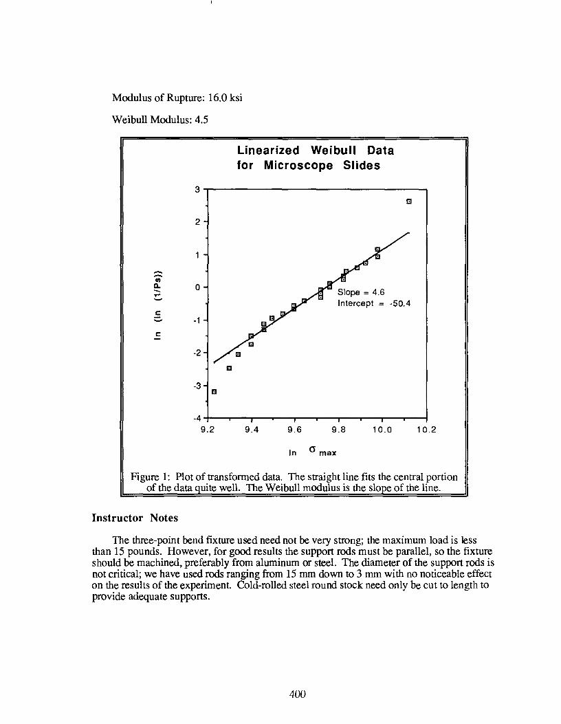
Modulus of Rupture: 16.0 ksi

Weibull Modulus: 4.5

Linearized Weibull Data for Microscope Slides

3,-------------------------------~

2

--<I)

11. 0 -... -c - -1

c

-2

-3 I!I

-4 9.2 9.4

Slope = 4.6 Intercept = -50.4

9.6 9.S 10.0

In 0' max

10.2

Figure 1: Plot of transfonned data. The straight line fits the central portion of the data uite well. The Weibull modulus is the slo e of the line.

Instructor Notes

The three-point bend fixture used need not be very strong; the maximum load is less than 15 pounds. However, for good results the support rods must be parallel, so the fixture should be machined, preferably from aluminum or steel. The diameter of the support rods is not critical; we have used rods ranging from 15 mm down to 3 mm with no noticeable effect on the results of the experiment. Cold-rolled steel round stock need only be cut to length to provide adequate supports.

400

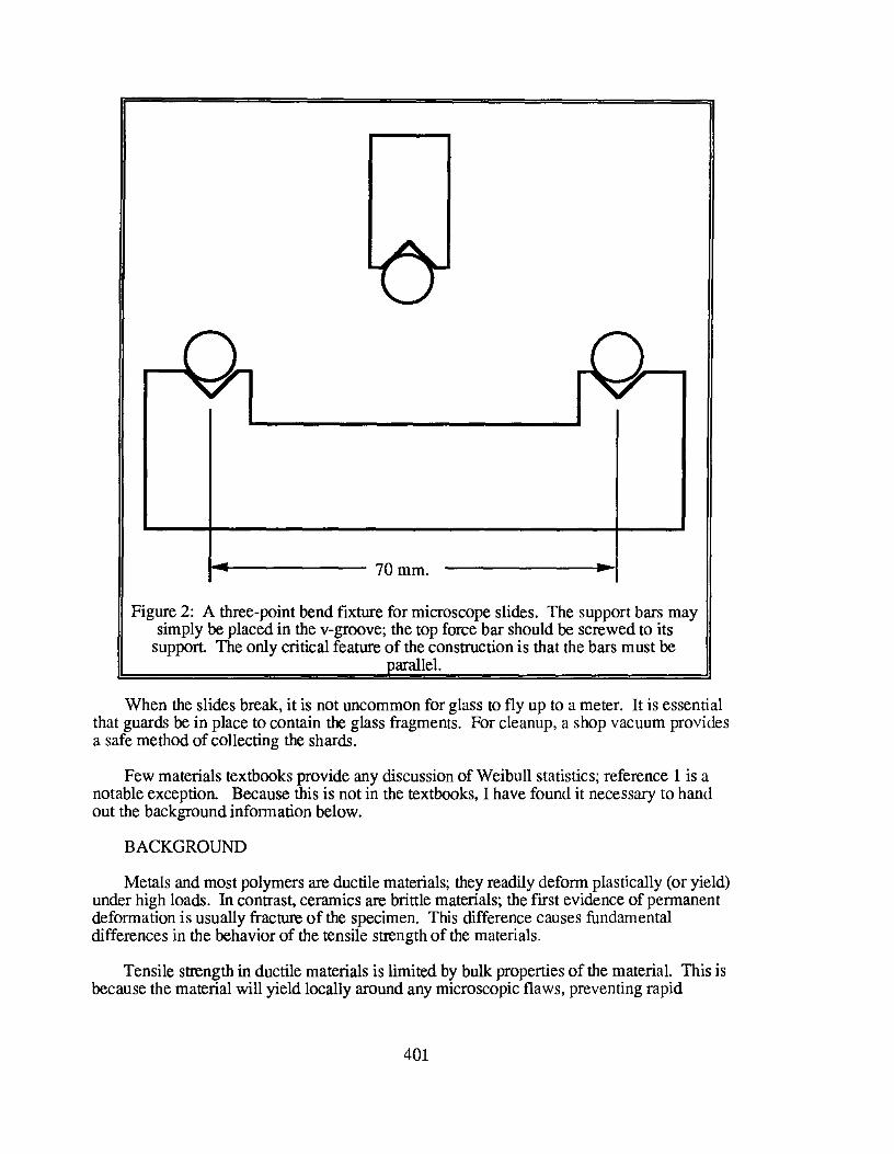
.. ------- 70 mm.

Figure 2: A three-point bend fixture for microscope slides. The support bars may simply be placed in the v-groove; the top force bar should be screwed to its

support. The only critical feature of the construction is that the bars must be arallel.

When the slides break, it is not uncommon for glass to fly up to a meter. It is essential that guards be in place to contain the glass fragments. For cleanup, a shop vacuum provides a safe method of collecting the shards.

Few materials textbooks provide any discussion of Weibull statistics; reference I is a notable exception. Because this is not in the textbooks, I have found it necessary to hand out the background information below.

BACKGROUND

Metals and most polymers are ductile materials; they readily deform plastically (or yield) under high loads. In contrast, ceramics are brittle materials; the first evidence of permanent deformation is usually fracture of the specimen. This difference causes fundamental differences in the behavior of the tensile strength of the materials.

Tensile strength in ductile materials is limited by bulk properties of the material. This is because the material will yield locally around any microscopic flaws, preventing rapid

401

fracture. In contrast, strength in ceramics is detennined by the microscopic flaws found in the specimen, as cracks will run rapidly through the bulk of the material since no local yielding occurs.

When the strength of a material is limited by flaws, standard methods of reporting the strength are inadequate. To obtain accurate predictions of the strength of brittle materials, special statistics known as Weibull statistics are used. These statistics recognize that flaws are likely to be evenly distributed through the specimen and that the probability of having a large flaw depends on the volume of the specimen. Thus, a large specimen is weaker per unit volume than a small specimen.

Ps

Stress

Figure 3: How probability of survival changes with Weibull modulus. Note that for higher values of Wei bull modulus, there is less variation in fracture

strength from specimen to specimen.

Weibull Statistics

Since each ceramic specimen will have a unique distribution of flaws, each specimen will have a unique strength. Thus, statistics are necessary to describe the strength of an untested specimen; we can only state the probability that a specimen will survive.

The fundamental equation for the probability of survival of a specimen is given by

In(l/Ps) = JIO(X,y'Z)]m ~V 00 0

(4)

where Ps is the probability of survival of the specimen, 0 0 and Vo are constants,

o(x,y,z) is the stress at a point (x,y,z) in the specimen, m is a constant known as the Wei bull modulus, and the integral is evaluated over the whole specimen. V 0 is the volume of a test

specimen that is placed under tensile load; 0 0 will be evaluated later.

402

The Weibull modulus of a material is the exponent m in equation 4. Figure 3 shows the effect of m on the survival probability of a specimen. Note that as the Weibull modulus increases, there is less scatter in the breaking strength; we have more confidence that the specimens will survive at loads near the breaking strength.

Uniaxial Tension

Consider a specimen that is loaded uniformly in tension. In this case, the stress is uniform in the specimen, and equation (4) evaluates to

(5)

When we are testing a specimen, V is equal to Yo; for other parts, V will be larger or smaller than Yo. When V=Vo, the probability of survival can be determined:

(6)

We can determine the probability of a specimen surviving a stress of 0"0 by substituting

()o for (). FOR THE CASE OF UNIAXIAL TENSION,

Note that equation (6) describes a distribution with two parameters, ()o and m. m is known as the Weibull modulus, and describes the scatter inherent in the strength of the

(7)

material. 0"0 determines the position of the distribution, and is related to the strength of the

material. We normally do not consider 0"0 to be the strength of the material, however. This designation is reserved for the stress that has a survival probability of 50%.

Three-Point Bending

We don't normally test brittle materials in tension. The stress concentration near the jaws of the testing machine causes failure at the jaws, rather than in the gage section. Instead, we load specimens in bending. There are a number of different bending tests; we will use the three-point bend test.

In the three-point bend test, a rectangular coupon is placed on two rollers spaced a known distance d apart. A third roll applies a load midway between the two support rolls; this places the specimen in bending (see Figure 4). In bending, the material above the neutral axis is loaded in compression, while the material below the neutral axis is in tension.

Another commonly used bend test is the four-point bend test, where two rollers separated by a bit less than d are used to apply the load. The four-point bend test creates a more uniform stress distribution in the specimen, and thus is less sensitive to the location of flaws within a single specimen. Therefore, fewer specimens need be tested to obtain the

403

properties of the material. However, the same information is available from the three-point bend test. We will use the three-point test because of its simplicity.

Brittle materials generally have much higher compressive strengths than tensile strengths (because the cracks tend to close in uniaxial compression). Thus, we will consider only the portion of the specimen in tension to be under load in the bend test. (Note that the material outside the bottom rollers is unstressed.) Unlike the tensile specimens, the stress varies with position in the bending specimen. Thus, before we can evaluate the integral in equation (4), we must determine the stress as a function of position.

Consider a free-body diagram of half the specimen, as shown in Figure 5. The external loads and moments are not shown in the figure; this is left as an exercise for the reader.

By cutting a specimen at a distance x from the right-hand roll, we can determine the bending moment M at any position along the length of the specimen.

M=xP/2 (8)

S tress in the specimen is independent of the width direction but varies in the thickness and length direction according to the equation of stress in pure bending (neglecting the shear force).

Mz cr= -I- (9)

where M is the bending moment as given by eqml.tion (8), z is the distance from the neutral axis, and I is the moment of inertia of the cross section of the specimen (bh3/12 for a rectangular cross section). If we substitute d/2 for x and h/2 for z in equations (8) and (9), we can obtain an expression for the maximum stress in the specimen.

Pdh 3Pd crmax = 81 = 2wh2 (10)

404

p

I .. d ..I

L T

Figure 4: A rectangular specimen under a load P in a three-point bend test. The portion of the specimen under a tensile load has a length d, a thickness

h/2, and a width w.

I'" d/2

Figure 5: A free-body diagram of the portion of the specimen between the middle roller and the right hand roller in figure 1. The external forces and

moments are not shown; this is left as an exercise for the reader.

We can substitute equations (8) and (9) into equation (4) to detennine the probability of survival for an applied load P. Solving equation (10) for P and substituting the result into the solved integral gives us the final expression for the probability of survival

(11)

The stress O"max that will cause the probability of survival in equation (11) to be 50% is known as the modulus of rupture; this is the strength index detennined by the three-point bend test.

405

In uniaxial tension, we found that 37% of the specimens would survive a load of ao. If

we set amax to ao in equation (8) and assume m=lO, we can detennine the probability that a

specimen will survive a bending load of ao.

Ps( a=ao) = 0.9959 (12)

Detennining the Weibull Modulus

Consider the case of uniaxial loading as given by equation (5). We want to detennine m, which appears as an exponent. To eliminate exponents, we commonly take the logarithm of both sides

In(ln(lIPs» = m In(~) + In( ~ ) ao 0

(13)

or

V In(ln( lIPs)) = m In( a) + In( V

o) - m In( ao) (14)

If we make a plot with In(a) on the horizontal axis and In(ln(l/Ps)) on the vertical axis, the data should fallon a straight line with a slope of m. This allows us to readily detennine the Weibull modulus. The same transfonnation can be applied to the bending specimen; the slope will remain m but the intercept will change (try it yourself to see).

References

1. Ashby, M.P. and D.R.H. Jones, Engineering Materials 2: An Introduction to Microstructures, Processing, and Design, Pergamon, 1986, pp.169-177.

Source of Supplies

Microscope slides can be obtained from any scientific equipment supplier. Micrometers or vernier calipers are available at machinist or industrial supply houses. Three-point bend fixtures are available from the manufacturers of material testing machines.

406

REPORT DOCUMENTATION PAGE Form Approved

OMB No. 0704-0188

Public reporting burden for this collection of information is estimat@d to average 1 hour per response, including the time for reviewing instructions. searching ~isting data sources, gathering and maintaining the data needed, and completing and reviewing the coliKtion of information. Send comments regarding this burden estimate or any other aspKt of this collection of information, including sugtestions for reducin~ this burden, to Washington Headquarters Services. Directorate for Information Operations and Reports. 1215 Jefferson Davis Highway, Suite 1204, Arlington. A 22202·4302, an to the Office of Management and Budget, Paperwork Reduction Project. (0704-0188). Washington, DC 20503.

1. AGENCY USE ONLY(L.ave blank) 2_ REPORT DATE 3. REPORT TYPE AND DATES COVERED June 1992 Conference Publication

4. TITLE AND SUBTITLE 5. FUNDING NUMBERS

National Educators' Workshop: Update 91 Standard Experiments in Engineering Materials 505-63-50-01 Science and Technology

6. AUTHOR(S)

Compilers: James E. Gardner-NASA Langley Research Center, Hampton, VA; James A. Jacobs-Norfolk State University, Norfolk, VA; James O. Stiegler-Oak Ridge National Laboratory, Oak Ridge TN

7. PERFORMING ORGANIZATION NAME(S) AND ADDRESS(ES) B. PERFORMING ORGANIZATION

NASA Langley Research Center REPORT NUMBER

Hampton, VA 23665-5225 1-17099

9. SPONSORING/MONITORING AGENCY NAME(S) AND ADDRESS(ES) 10. SPONSORING/MONITORING

National Aeronautics and Space Administration Washington, DC AGENCY REPORT NUMBER

20546-0001; Norfolk State University, Norfolk, VA 23504; NASA CP-3151 National Institute of Standards and Technology, Gaithersburg, MD 20899; United States Department of Energy, Oak Ridge, TN 37831-6132

11. SUPPLEMENTARY NOTES

Supporting Organizations: ASM International; Battelle Pacific Northwest Laboratory; Materials Education Council

12a. DISTRIBUTION/AVAILABILITY STATEMENT 12b. DISTRIBUTION CODE

Unclassified - Unlimited

Subject Category 23

13. ABSTRACT (Maximum 200 words) This document contains a collection of experiments presented and demonstrated at the National Educators' Workshop: Update 91 held at the Oak Ridge National Laboratory on November 12-14, 1991, in Oak Ridge, Tennessee. The experiments related to the nature and properties of engineering materials and provided information to assist in teaching about materials in the education community.

14. SUBJECT TERMS Materials; Experiments; Education

17. SECURITY CLASSIFICATION lB. SECURITY CLASSIFICATION 19. SECURITY CLASSIFICATION OF REPORT OF THIS PAGE OF ABSTRACT Unclassified Unclassified Unclassified

NSN 7540-01-2BO-5500

15. NUMBER OF PAGES

421 16. PRICE CODE

A18 20. LIMITATION

OF ABSTRACT

Standard Form 29B.(Rev. 2-B9) Prescnbed by ANSI Std. Z39-18 298-102

NASA-langley, 1992

National Educators' Workshop: Update 91 - M-STEM

Documents

Transcript of National Educators' Workshop: Update 91 - M-STEM