NASA/CP-1998-208726

, , .

.

National Educators' Workshop: U'pdate 97

Standard Experiments in Engineering Materials, Science, and Technology Compiled by James E. Gardner and Ginger L. Freeman Langley Research Center, Hampton, Virginia

James A. Jacobs Norfolk State University, Norfolk, Virginia

Alan G. Miller and Brian W. Smith Boeing Commercial Airplane Company, Seattle, Washington

November 1998

The NASA STI Program Office . .. in Profile

Since its founding, NASA has been dedicated to the advancement of aeronautics and space science. The NASA Scientific and Technical Information (STI) Program Office plays a key part in helping NASA maintain this important role.

The NASA STI Program Office is operated by Langley Research Center, the lead center for NASA's scientific and technical information. The NASA STI Program Office provides access to the NASA STI Database, the largest collection of aeronautical and space science STI in the world. The Program Office is also NASA's institutional mechanism for disseminating the results of its research and development activities. These results are published by NASA in the NASA STI Report Series, which includes the following report types:

• TECHNICAL PUBLICATION. Reports of completed research or a major significant phase of research that present the results of NASA programs and include extensive data or theoretical analysis. Includes compilations of significant scientific and technical data and information deemed to be of continuing reference value. NASA counter-part or peer-reviewed formal professional papers, but having less stringent limitations on manuscript length and extent of graphic presentations.

• TECHNICAL MEMORANDUM. Scientific and technical findings that are preliminary or of specialized interest, e.g., quick release reports, working papers, and bibliographies that contain minimal annotation. Does not contain extensive analysis.

• CONTRACTOR REPORT. Scientific and technical findings by NASA-sponsored contractors and grantees.

• CONFERENCE PUBLICATION. Collected papers from scientific and technical conferences, symposia, seminars, or other meetings sponsored or co-sponsored by NASA.

• SPECIAL PUBLICATION. Scientific, technical, or historical information from NASA programs, projects, and missions, often concerned with subjects having substantial public interest.

• TECHNICAL TRANSLATION. English-language translations of foreign scientific and technical material pertinent to NASA's mission.

Specialized services that help round out the STI Program Office's diverse offerings include creating custom thesauri, building customized databases, organizing and publishing research results ... even providing videos.

For more information about the NASA STI Program Office, see the following:

• Access the NASA STI Program Home Page at http://www.sti.nasa.gov

• Email your question via the Internet to hel p@sti.nasa.gov

• Fax your question to the NASA Access Help Desk at (301) 621-0134

• Phone the NASA Access Help Desk at (301) 621-0390

• Write to: NASA Access Help Desk NASA Center for AeroSpace Information 7121 Standard Drive Hanover, MD 21076-1320

NASA/CP-1998-208726

National Educators' Workshop: Update 97

Standard Experiments in Engineering Materials, Science, and Technology Compiled by James E. Gardner and Ginger L. Freeman Langley Research Center, Hampton, Virginia

James A. Jacobs Norfolk State University, Norfolk, Virginia

Alan G. Miller and Brian W. Smitll Boeing Commercial Airplane Company, Seattle, Washington

National Aeronautics and Space Administration

Langley Research Center Hampton, Virginia 23681-2199

November 1998

Proceedings of a workshop sponsored jointly by Boeing Materials Technology, Boeing Commercial

Airplane Company, Seattle, Washington, the National Aeronautics and Space Administration, Washington, D.C.,

the Norfolk State University, Norfolk, Virginia, and the National Institute of Standards and Technology, Gaithersburg, Maryland,

and held in Seattle, Washington November 2-5, 1997

The OpInIOns expressed in this document are not necessarily approved or endorsed by the National Aeronautics and Space Administration

The use of trademarks or names of manufacturers in this report is for accurate reporting ,md does not constitute an official endorsement, either expressed or implied, of such products or manufacturers by the National Aeronautics and Space Administration.

Available from the following:

NASA Center for AeroSpace Information (CASl) 7121 Standard Drive Hanover, MD 21076-1320 (30l) 621-0390

National Technical Information Service (NTIS) 5285 Port Royal Road Springfield, VA 22161-2171 (703) 487-4650

PREFACE

NEW:Update 97, hosted by Boeing Commercial Airplane Company in Seattle, Washington, on November 2 - 5, 1997. marked our second workshop west of the Mississippi. Seattle took a break from heavy rains and provided beautiful weather.

We built on past themes, activities, and presentations based on extensive evaluations from participants of previous workshops. This 12th annual NEW:Update continued to the work of strengthening materials education. About 120 participants witnessed demonstrations of experiments. discussed issues of materials science and engineering (MSE) with people from education. industry. government. and technical societies; heard about new MSE developments; and chose from nine, three-hour mini workshops in state-of-the-art Boeing production facilities and R&D laboratories to attend. Faculty in attendance represented high schools, community colleges. smaller colleges. and major universities. Undergraduate and graduate students also attended and presented.

The generous fashion in which Alan Miller and Brian Smith, and the many scientist, engineers, and other staff of Boeing. provided funding. opened their facilities. developed presentations and activities, and acted as all around gracious hosts insured the on-going quality of this important educational series of workshops. With thc very demanding production schedule Boeing faces, we are indebted for their sacrifices in hosting this workshop.

NEW:Update 97 participants saw the demonstration of about forty experiments and aided in evaluating them. We also heard updating information relating to materials science. engineering and technology presented at mini plenary sessions that focused on technology from aircraft and automotive technology, and materials research at Brookhaven National Lab. Through the considerable efforts of Kris Kern at LANL, Raj Chaudhury of NSU, and Roger Marshall and William Gerdts of Boeing. most of the workshop was broadcast over the Internet.

The experiments in this publication can serve as a valuable guide to faeuIty who arc interested in useful activities for their students. The material was the result of years of research aimed at better methods of teaching materials science. engineering and technology. The experiments were developed by faculty. scientists, and engineers throughout the United States. There is a blend of experiments on new materials and traditional materials. Uses of computers in MSE, designing experiments, and a variety of low-cost experiments were among the demonstrations presented.

Experiments underwent an extensive peer review process. After submission of abstracts, selected authors were notified of their acceptance and given the format for submission of experiments. Experiments were reviewed by a panel of specialists through the cooperation of the Materials Education Council. Most authors received eomPlents from the panel prior to NEW:Update 97, allowing them to make necessary adjustments prior to demonstrating their experiments. Comments from workshop participants provided additional feedback which authors used to make final revisions which were submitted for the NASA editorial group for this publication.

III

The Materials Education Council of the United States publishes selected experiments in the Journal of Materials f-(Jucation (JME). The international JME offers valuable teaching and curriculum aids including instructional modules on emerging materials technology, experiments, book reviews, and editorials to materials educators. On a personal note, MEC honored Jim Jacobs as "1996 Materials Educator of the Year" at the December MRS meeting in Boston. This award must be shared with all the people who have contributed to the NEW:Update series, our textbooks, and the many activities of our national materials education network.

Videotapes were made of the workshop by Boeing. Transparency masters for the mini plenary sessions are included in this pUblication. As with previous NEW:Updates, critiques were made of the workshop to provide continuing improvement of this activity. The evaluations and recommendations made by participants provide valuable feedback for the planning of subsequent NEW:Updates.

NEW:Update 97 and the series of workshops that go back to 1986 are, to our knowledge, the only national workshops or gatherings for materials educators that have a focus on the full range of issues and strategies for bctter teaching about the entire complement of materials. NEW:Update 97, with its diversity of faculty, industry, and government MSE participants, served as a forum for both formal and informal issues facing MSE education that ranged from the challenges of keeping faculty and students abreast of new technology to ideas to ensure that materials scientists, engineers, and technicians maintain the proper respect for the environment and human safety in the pursuit of their objectives.

We demonstrated the Experiments in Materials Science, £"ngineering& Technology. (EMSE1) CD-ROM with all 213 experiments from the first decade of NEW:Updates. This CD ROM is another example of cooperative efforts to support materials education. The primary contributions came from the many authors of the demo and experiments for NEW:Updates. Funding for the CD came from both private industry and federal agcncies. Please see the attached information for obtaining the CD set.

We express our apprcciation to all those who helped to keep this series of workshops viable. Special thanks goes to those on the planning committee, management team, hosts, sponsors, and especially those of you have developed and shared your ideas for experiments, demonstrations, and novel approaches to learning. All of us who participated in the workshop appreciated the excellent coordination of activities by Diana LaClaire, Kirsten Maassen, and Ginger Freeman.

We hope that the experiments presented in this pUblication will assist you in teaching about materials science, engineering and technology. We would like to have your comments on their value and means of improving them. Please send comments to Jim Jacohs, School of Technology, Norfolk State University, Norfolk, Virginia 23504.

The use of trademarks or manufacturers' names in this publication does not constitute endorsement, either expressed or implied, by the National Aeronautics and Space Administration.

IV

MANAGEMENT TEAM

Workshop Co-Directors

Alan G. Miller and Brian W. Smith Boeing Materials Technology Boeing Commercial Airplane Company

James A. Jacobs Professor of Engineering Technology Norfolk State University

NASA LaRC Coordinators

James E. Gardner and Ginger Freeman National Aeronautics and Space Administration Langley Research Center

Di rector's Assistant

Diana P. LaClaire Norfolk State University

Committee Members

Robert Berrettini Materials Education Council

L. Roy Bunnell Kennewick High School

Linda C. Cain Oak Ridge National Laboratory

F. Craig Oak Ridge National Laboratory

Kristi B. Foster ASM International

Frank W. Hughes Boeing Commercial Airplane Company

Kenneth L. Jewett National Institute of Standards & Technology

Kristen T. Kern Norfolk State University

Thomas F. Kilduff Thomas Nelson Community College

Kirsten Maassen Boeing Commercial Airplane Company

v

James V. Masi Western New England College

Alfred E. McKenney IBM Corporation, Retired

Steven Piippo Richland High School

Heidi Ries Norfolk State University

Robert Stang University of Washington

Thomas G. Stoebe University of Washington

Karl J. Swyler Brookhaven National Laboratory

Alan I. Taub Ford Motor Company

Linda Vanasupa American Society for Engineering Education

David Werstler Western Washington University

CONTENTS

PREFACE .................................................................................................................................................... iii

MANAGEMENT TEAM ............................................................................................................................. v

REVIEWERS FOR NEW: UPDATE 97 ..................................................................................................... xi

LISTING OF EXPERIMENTS FROM NEW:UPDATES ........................................................................ xiii

ORDERING INFORMATION FOR ADDITIONAL RESOURCES ................................................... xxviii

PARTICIPANTS ................................................................................................................................... xxxiii

JET TRANSPORT STRUCTURES PERFORMANCE MONITORING .................................................... 1 Ulf Goranson - Boeing Commercial Airplane Company

CORRELATION OF BIREFRINGENT PATTERNS TO RETAINED ORIENTATION IN INJECTION MOLDED POLYSTYRENE TENSILE BARS ............................................................... 39

Laura L. Sullivan - GMI Engineering & Management Institute

STUDY OF RHEOLOGICAL BEHAVIOR OF POLYMERS ................................................................. 45 Ping Liu and Tom L. Waskom - Eastern Illinois University

CASE STUDIES IN METAL FAILURE AND SELECTION .................................................................. 51 David Werstler - Western Washington University

MAGNETO-RHEOLOGICAL FLUID TECHNOLOGY .......................................................................... 57 John A. Marshall - University of Southern Maine

UNDERSTANDING GALVANIC CORROSION TRICKS TO PREVENT SOME EXPENSIVE FAILURES .............................................................................................................. 63

Gautam BaneIjee and Albert E. Miller - University of Notre Dame

MEASUREMENT OF THE MODULUS OF ELASTICITY USING A THREE-POINT BEND TEST .................................................................................................................... 73

R. B. Griffm and L. R. Cornwell - Texas A&M University

MAKING A PHASE DIAGRAM .............................................................................................................. 81 William K. Dalton and Patricia J. Olesak - Purdue University

RELATIONSHIP BETWEEN MOISTURE CHANGES AND DIMENSIONAL CHANGE IN WOOD .................................................................................................... 87

Thomas M. Gorman - University of Idaho

EV ALUATING THE STRENGTH AND BIODEGRADATION OF A GELATIN-BASED MOLD ......................................................................................................................................................... 97

Kyumin Whang - University of Texas and Matthew Hsu - Northwestern University, Materials World Modules

THE COMBINED EFFECT OF THERMAL CONDUCTIVITY AND THERMAL EXPANSION IN A PMMA PLASTIC HEATED BY THERMAL RADIATION ......................................................... 109

Carlos E. Umana - University of Costa Rica

TEACHING REPORT WRITING USING MSE LABORATORIES ..................................................... 119 William D. Callister - University of Utah

vii

CRYSTAL GROWTH OF MIXED OPTICAL MATERIALS WITH THE AUTOMATIC CZOCHRALSKI PULLER ...................................................................................................................... 127

George B. Loutts - Norfolk State University

HOW TO COMPUTE THE ATOMIC MAGNETIC DIPOLE MOMENT OF AN ELEMENT: AN ENGINEERING APPROACH .................................................................................... 137

Carlos E. Umana·· University of Costa Rica

ALLOY COMPOSITION DETERMINATIONS .................................................................................... 147 K. T. Hartwig, M. Haouaoui, and L. R. Cornwell - Texas A&M University

HOW A HEAT PACK WORKS .............................................................................................................. 157 Robert A. McCoy - Youngstown State University

LEARNING MORE FROM TENSILE TEST EXPERIMENT ............................................................... 167 Neda S. Fabris - California State University, Los Angeles

PROPERTIES OF MAGNETIC FERRITES WITH A SIMPLE FABRICATION METHOD ..................................................................................................................... 183

Luke Ferguson and Thomas Stoebe - University of Washington

EFFECTIVE LEARNING THROUGH INTERACTIVE COMPUTER SIMULATION AND EXPERIMENTATION ......................................................................................... 197

W. Gregory Sawyer, Daniel Bryson, and Torkel Svanes - Stark DeSign Jolm B. Hudson - Rensselaer Polyteclmic Institute

AN INTERACTIVE MOLECULAR DYNAMICS SIMULATION OF ATOMIC BEHAVIOR ............................................................................................................................. 213

Jolm B. Hudson - Rensselaer Polyteclmic Institute and Torkel Svanes, Dan Bryson and W. Gregory Sawyer - Stark Design

OPTICAL EXPERIMENTS WITH MANGANESE DOPED YTIRIUM ORTHOALUMINATE, A POTENTIAL MATERIAL FOR HOLOGRAPHIC RECORDING AND DATA STORAGE .................................................................................................. 221

Matthew E. Warren and George Loutts - Norfolk State University

DESIGN OF HYPERVELOCITY FLOW GENERATOR AND ITS FLOW VISUALIZATIONS .................................................................................................................................. 229

Kyo D. Song - Norfolk State University, Charles Terrell -Hampton University, and Mark Kulick - Nyma Inc.

RAPID PROTOTYPING PROCESSES AND PROCEDURES .............................................................. 255 Paul Cheng-Hsin Liu, Kenneth Moore, and Chris Ogu - North Carolina A&T State University

THE HUMAN HALF-ADDER: UNDERSTANDING THE BIG PICTURE OF DIGITAL LOGIC ..................................................................................................................................... 267

Linda Vanasupa and David Braun - California Polyteclmic State University

A METHOD FOR MEASURING THE SHEAR STRENGTH OF POLYMERS AND COMPOSITES ......................................................................................................................................... 279

Luis Gardea and Brian L. Weick - University of the Pacific

viii

AUTOMOTIVE MATERIALS FOR THE NEXT MILLENNIUM ........................................................ 293 Margaret Chadwick - Ford Motor Company

WEAKENING OF LATEX RUBBER BY ENVIRONMENTAL EFFECI'S ......................................... 313 L. Roy Bunnell - Kennewick School District

A COMPUTERIZED MICROWAVE SPECI'ROMETER FOR DIELECI'RIC RELAXATION STUDIES ....................................................................................................................... 319

B. F. Draayer and 1. N. Dahiya - Southwest Missouri State University

THE NATIONAL EDUCATORS' WORKSHOP WEB .......................................................................... 339 S. Raj Chaudhury - Norfolk State University

CASE HARDENING: AN ACI'IVITY TO DEMONSTRATE BRINELL HARDNESS ....................... 345 C. Ray Diez - University of North Dakota

LOW DOLLAR TENSILE (TORSION) TESTER .................................................................................. 351 Andrew Nydam - Olympia High School

INTEGRATION OF LABORATORY EXPERIENCES INTO AN INTERACI'IVE CHEMISTRY/MATERIALS COURSE .................................................................................................. 357

John B. Hudson, Linda S. Schadler, Mark A. Palmer, and James A. Moore -Rensselaer Polytechnic Institute

LIFE ESTIMATE BASED ON FATIGUE CRACK PROPAGATION .................................................. 369 YuJian Kin, Harvey Abramowitz, Toma Hentea, and Ying Xu -Purdue University Calumet

STRETCHY "ELASTIC" BANDS .......................................................................................................... 381 Alan K. Karplus - Western New England College

STRENGTH TESTING OF COMPOSITE MATERIALS ...................................................................... 389 John and Eric Cadwell and Steven Piippo - Richland High School

CORROSION DEMONSTRATION UTILIZING LOW COST MATERIALS ..................................... 397 John R. Williams - Purdue University

PREVIEW OF NEW:UPDATE 98 .......................................................................................................... 407 Karl J. Swyler - Brookhaven National Laboratory and Leonard W. Fine - Columbia University

213 EXPERIMENTS ON CD-ROM FROM 10 YEARS OF NEW:UPDA TES ..................................... 431 James A. Jacobs - Norfolk State University and Alfred E. McKenney - Consultant

DEMONSTRATING THE CRITICAL PROPERTIES OF CARBON DIOXIDE .................................. 441 Leonard W. Fine - Columbia University

EXPERIMENTS IN DIFFUSION: GASES, LIQUIDS, AND SOLIDS FOR UNDER FIVE DOLLARS ....................................................................................................................... 449

James V. Masi - Western New England College

HIGH SPEED CIVIL TRANSPORT - DESIGN CHALLENGES .......................................................... 459 David W. Lund - Boeing Commercial Airplane Company

ix

NEWMISMATIC METALLURGY ......................................................................................................... 491 Edward L. Widener - Purdue University

EFFECTIVENESS OF ULTRASONIC TESTING METHOD IN DETECTING DELAMINATION DEFECTS IN THICK COMPOSITES ..................................................................... 497

Glen C. Erickson - Ground Systems Division and W. Richard Chung - San Jose State University

MEDICINE, MAGIC, MATERIALS, AND MANKIND ........................................................................ 511 F. Xavier Spiegel - Spiegel Designs

A DEVICE FOR MEASURING THE ELASTIC MODULES OF SPHERICAL MATERIALS ............................................................................................................................................ 513

Mtrook AI Homidany and Brian L. Weick - University of the Pacific

COMPUTER APPLICATIONS FOR THE MATERIALS LABORATORY/CLASSROOM: ILLUSTRA TING STRUCTURE AND DIFFRACTION ........................................................................ 525

James F. Shackelford and Michael Meier - University of California, Davis

IMPACT OF MULTIMEDIA AND NETWORK SERVICES ON AN INTRODUCTORY LEVEL COURSE ..................................................................................................................................... 535

John C. Russ - North Carolina State University Presented by Cheryl S. Alderman - North Carolina State University

STRUCTURAL LABORATORY MANUAL ......................................................................................... 539 Jack Kayser - Lafayette ColJege

X-RA Y RADIOGRAPHIC EXERCISES FOR AN UNDERGRADUATE MATERIALS LAB .................................................................................................................................. 603

John M. Winter, Jr. and Kirsten G. Lipetzky - The Johns Hopkins University

FUN IN METALS .................................................................................................................................... 609 Robert Pond, Sr. - The Johns Hopkins University

x

REVIEWERS FOR NEW: Update 97

Paul W. Brown Professor of Materials Science The Pennsylvania State University

Else Breval Senior Research Associate Materials Research Laboratory The Pennsylvania State University

Witold Brostow Professor of Materials Science Center for Materials Characterization University of North Texas

William Callister Adjunct Professor of Metallurgy University of Utah

Michael Grutzeck Associate Professor Materials Research Laboratory The Pennsylvania State University

Rafat Malek Senior Research Associate The Pennsylvania State University

Howard Pickering Distinguished Professor of Metallurgy The Pennsylvania State University

Clive Randall Associate Professor of Materials Science The Pennsylvania State University

Rustum Roy Evan Pugh Professor of the Solid State The Pennsylvania State University

Darrell Schlom Associate Professor of Materials Science The Pennsylvania State University

Technical notebooks and announcements of the workshop were provided by NASA LANGLEY RESEARCH CENTER

xi

LISTING OF EXPERIMENTS FROM NEW:UPDATES

EXPERIMENTS & DEMONSTRATIONS IN STRUCTURES, TESTING, AND EVALUATION

NEW:Update 88 Sastri, Sankar. "Fluorescent Penetrdnt Inspection" Sastri, Sankar. "Magnetic Particle Inspection" Sastri, Sankar. "Radiographic Inspection"

NASI. Conference Publication 3060

NEW:Update 89 NASA Conference Publication 3074 Chowdhury, Mostafiz R. and Chowdhury, Farida. "Experimental Detennination of Material Damping

Using Vibration Analyzer" Chung, Wenchiang R. "The Assessment of Metal Fiber Reinforced Polymeric Composites" Stibolt, Kenneth A. "Tensile and Shear Strength of Adhesives"

NEW:Update 90 NIST Special Publication 822 Azzard, Drew C. "ASTM: The Development and Application of Bates, Seth P. "Charpy V-Notch Impact Testing of Hot Rolled 1020 Steel to Explore Temperature Impact

Strength Relationships" Chowdhury, Mostafiz R. "A Nondestructive Testing Method to Detect Defects in Structural Members" Cornwell, L. R., Griffin, R. B., and Massarweh, W. A. "Effect of Strdin Rate on Tensile Properties of

Plastics" Grdy, Stephanie L., Kern, Kristen T., Harries, Wynford L., and Long, Sheila Ann T.

"Improved Technique for Measuring Coefficients of Thennal Extension for Polymer Films" Halperin, Kopl. "Design Project for the Materials Course: To Pick the Best Material for a Cooking Pot" Kundu, N ikhil. "Environmental Stress Cracking of Recycled Thermoplastics" Panchula, Larry and Patterson, John W. "Demonstration of a Simple Screening Strategy for Multifaetor

Experiments in Engineering" Taylor, Jenifer A. T. "How Does Change in Temperature Affect Resistance'!" Wickman, Jerry L. and Corbin, Scott M. "Determining the Impact of p.djusting Temperdture Profiles on

Photodegmdability of LDPE/Starch Blown Film" Widener, Edward L. "It's Hard to Test Hardness" Widener, Edward L. "Unconventional Impact-Toughness

NEW:Update 91 NASA Conference Publication 315t Bunnell, L. Roy. "Tempered Glass and Thermal Shock of Ceramic Materials" Lundeen, Calvin D. "Impact Testing of Welded Samples" Gonnan, Thomas M. "Designing, Engineering, and Testing Wood Structures" Strehlow, Richard R. "ASTM - Terminology for Experiments and Testing" Karplus, Alan K. "Determining Significant Material Properties, A Discovery Approach" Spiegel, F. Xavier and Weigman, Bernard J. "An Automated System for Creep Testing" Denton, Nancy L. and Hillsman, Vernon S. "Isotropic Thin-Walled Pressure Vessel Experiment" Allen, David J. "Stress-Strain Chameteristics of Rubber-Like Materials: Experiment and Analysis" Dahl, Charles C. "Computer Integrated Lab Testing" Cornwell, L. R. "Mechanical Properties of Brittle Material"

xiii

NEW: Update 92 NASA Conference Publication 3201 Bunnell, L. Ruy. "Temperature-Dependent Electrical Cunductivity uf Suda-Lime Glass and Cunstructiun

and Testing ufSimple Airfoils tu Demunstrate Structural Design, Materials Chuice, and Cumpusite Cuncepts"

Marpet, Mark I. "Walkway Frictiun: Experiment and Analysis" Martin, Dunald H. "Applicatiun ufHardness Testing in Fuundry Prueessing Operatiuns: A University and

Industry Partnership" Masi, James V. "Experiments in Currusiun fur Yuunger Students By and Fur Older Students" Needham, David. "Micropipet Manipulatiun uf Lipid Membranes: Direct Measurement uf the Material

Pruperties uf a Cuhesive Structure That is Only Two Mulecules Thick" Perkins, Steven W. "Direct Tensiun Experiments un Cumpacted Granuiar Materials" Shih, Hui-Ru. "Develupment uf an Experimental Methud tu Determine the Axial Rigidity uf a

Strut-Nude Juint" Spiegel, F. Xavier. "An Automated Data Cullectiun System Fur a Charpy Impact Tester" Tiptun, Steven M. "A Miniature Fatigue Test Machine" Widener, Edward L. "Tuol Grinding and Spark Testing"

NEW: Update 93 NASA Conference Publication 3259 Burst, Mark A. "Design and Cunstructiun uf a Tensile Tester fur the Testing uf Simple Cumpusites" Clum, James A. "Develuping Mudules un Experimental Design and Process Characterizatiun for

Manufacturing/Materials Prucesses Laburaturies" Diller, T. E. and A. L. Wicks, "Measurement uf Surface Heat Flux and Temperature" Dentun, Nancy and Vernun S. Hillsman, "An Intruductiun tu Strength ufMaterials fur Middle Sehuol and

Beyund" Fisher, Junathan H. "Bridgman Sulidifieatiun and Experiment tu Assess Buundaries and Interface Shape" Gmy, Jennifer "Symmetry and Structure Through Optical Diffractiun" Karplus, Alan K. "Knutty Knuts" Kuhne, Glenn S. "An Automated Digital Data Cullectiun and Analysis System fur the Charpy Impact

Tester" Olesak, Patricia 1. "Scleruscupe Hardness Testing" SpeigeL F. Xavier, "Inexpensive Materials Science Demunstratiuns" Wickman, 1. L. "Plastic Part Design Analysis Using Pularized Filters and Birefringence" Widener, Edward L. "Testing Rigidity by Turque Wrench"

NEW:Update 94 NASA Conference Publication 3304 Bruzan, Raymund and Baker, Duuglas, "Density by Titmtiun" Dahiya, Jai N., "Precisiun Measurements uf the M icruwave Dielectric uf Polyvinyl Stearate and

Pulyvinylidene Fluuride as a Functiun of Frequency and Temperature" Daufenbach, JuDee and Griffin, Alair, "Impact uf Flaws" Fine, Leunard W., "Cuncrete Repair Applicatiuns and Pulymerizatiun ufButadiene by an "Alfin" Catalyst" Hillsman, Vernun S., "Stress Cuncentratiun: Cumputer Finite Element Analysis vs. Phutoelasticity" Hutchinsun, Ben, Gigliu, Kim, Buwling, Juhn, and Green, David, "Phutucatalytic Destructiun of an

Organic Dyd Using TiO," Jenkins, Thumas 1., Cumtois, Juhn H., and Bright, Victur M., "Micruma-:hining uf Suspended Structures

in Silicun and Bulk Etching uf Silicun fur Micromachining" Jacubs, James A. and knkins, Thumas 1., "Mathematics fur Engineering Materials Technology

Experiments and Problem Sulving" Karplus, Alan K., "Paper Clip Fatigue Bend Test" Kuhne, Glenn S., "Fluids With Magnetic Persunalities" Liu, Ping and Waskum, Tummy L., "Ultrasunic Welding uf Recycled High Density Pulyethylene (HOPE)" Martin, Donald H., Schwan, Hermann, Diehm, Michael, "Testing Sand Quality in the Fuundry (A Basic

University-Industry Partnership" Shull, Rubert D., "Nanustructured Materials"

xiv

Werstler, David E., "Introduction to Nondestructive Testing" White, Charles V., Fracture Experiment for Failure Analysis" Wickman, Jerry L. and Kundu, Nikhil K., "Failure Analysis of Injection Molded Plastic Engineered Parts" Widener, Edward L., "Dimensionless Fun With Foam"

NEW:Update 95 NASA Conference Publication 3330 Brown, Scott, "Crystalline Hors d'oeuvres" Karplus, Alan K., "Cmf! Stick Beams" Kern, Kristen, "ION Beam Analysis of Materials" Kozma, Michael, "A Revisit to the Helicopter Factorial Design Experiment" Pond, Robert B., Sr., "Recrystallization Art Sketching" Roy, Rustum, "CVD Diamond Synthesis and Characterization: A Video Walk-Through" Saha, Hrishikesh, "Virtual Reality Lab Assistant" Spiegel, F. Xavier, "A Novel Approach to Hardness Testing" Spiegel, F. Xavier, "There arc Good Vibrations and Not So Good Vibrations" Tognarelli, David, "Computerized Materials Testing" Wickman, Jerry L., "Cost Effective Prototyping"

NEW:Update 96 NASA Conference Publication 3354 Chao, Julie, Currotto, Selene, Anderson, Cameron, Selvaduray, Guna, "The Effect of Surface Finish on

Tensile Strength" Fabris, Neda S., "From Rugs to Demonstmtions in Engineering Materials Ferguson, Luke, Stoebe, Thomas, "Hysteresis Loops and Barkhausen Effects in Magnetic Materials" Karplus, Alan K., "Holy Holes or Holes Can Make Tensile Struts Stronger" Koon, Daniel W., "Relaxation and Resistance Liu, Ping, Waskom, Tommy L., "Composite of Glass Fiber with Epoxy Matrix" Song, Kyo D., Ries, Heidi R., Scotti, Stephen 1., Choi, Sang H., "Tmnspiration Cooling Experiment" South, Joe, Keilson, Suzanne, Keefcr, Don, "In-Vivo Testing of Biomaterials" Thorogood, Michael G., "Tensile Test Experiments With Plastics" Widener, Edward L., "Brinelling the Malay Snail"

NEW:Update 97 NASA Conference Publication Banerjee, Gautam, Miller, Albcrt E. "Understanding Galvanic Corrosion Tricks to Prevent Some Expensive

Failurcs" Cadwell, John and Eric, Piippo, Steven. "Strength Testing of Composite Materials" Dicz, C. Ray. "Case Hardening: An Activity to Demonstrate Brinnell Hardness" Erickson, Glen c., Chung, W. Richard. "Effcctiveness of Tcsting Method in Detecting

Delamination Effects in Thick Composites" Fabris, Neda S. "Learning More From Tensile Test Experiment" Finc, Leonard W. "Demonstrating the Critical Properties of Carbon Dioxide" Goranson, Ulf. "Jet Transport Structures Performance Monitoring" Griffin, R. B., Cornwcll, L. R. "Measurement of the Modulus of Using a Three-Point Bend Test" Homidany, Mtrook AI, Weick, Brian L. "A Devicc for Measuring the Elastic Modules of Spherical

Matcrials" Hudson, John B., Svanes, Torkel, Bryson, Daniel, Sawyer, W. Gregory, "An Interactive Molecular

Dynamics Simulation of Atomic Behavior" Liu, Paul Cheng-Hsin, Moore, Kenneth, Ogu, Chris. "Rapid Prototyping Processes and Procedures"

George B. "Crystal Growth of Mixed Optical Materials With the Automatic Czochralski Puller" Masi, James V. "Experiments in Diffusion: Gases, Liquids, and Solids For Under Five Dollars"

xv

McCoy, Robert A. "How a Heat Pack Works" Nydam, Andrew. "Low Dollar Tensile (Torsion) Tester" Song, Kyo D. "Design of Hypervelocity Flow Generator and Its Flow Visualizations" Spiegel, F. Xavier. "Medicine, Magic, Materials, and Mankind" Whang. Kyumin and Hsu, Matthew. "Evaluating the Strength and Biodegradation of a Gelatine-Based

Material" Williams, John R. "Corrosion Demonstration Utilizing Low Cost Materials"

XVI

EXPERIMENTS & DEMONSTRATIONS IN METALS

NEW:Update 88 NASA Conference Publication 3060 Nagy, James P. "Sensitization of Stainless Steel" Neville, J. P. "Crystal Growing" Pond, Robert B. "A Demonstration of Chill Block Melt Spinning of Metal" Shull, Robert D. "Low Carbon Steel: Metallurgical Structure vs. Mechanical Propertics"

NEW:Update 89 NASA Conference Publication 3074 Balsamel, Richard. "The Magnetization Process - Hystercsis" Beardmore, Peter. "Future Automotive Materials - Evolution or Revolution" Bunnell, L. Roy. "Hands-On Thcnlml Conductivity and Work-Hardening and Annealing in Metals" Kazem, Sayyed M. "Thermal Conductivity of Metals" Nagy, James P. "Austempering"

NEW: Update 90 NIST Special Publication 822 Bates, Seth P. "Charpy V-Notch Impact Testing of Hot Rolled 1020 Steel to Explore Temperature Impact

Strcngth Relationships" Chung, Wenchiang R. and Morse, Margery L. "Effect of Heat Treatment on a Metal Alloy" Rastani, Mansur. "Post Hcat Treatment in Liquid Phase Sintered Tungsten-Nickel-lron Alloys" Spiegel, F. Xavicr. "Crystal Modcls for the Beginning Student" Yang, Y. Y. and Stang, R. G. "Measurement of Strain Rate Sensitivity in Metals"

NEW:Update 91 NASA Conference Publication 3151 Cowan, Richard L. "Be-Cu Precipitation Hardening Experiment" Kazem, Sayyed M. "Elementary Metallography" Krcpski, Richard P. "Experimcnts with the Low Melting Indium-Bismuth Alloy System" Lundeen, Calvin D. "Impact Testing of Welded Samples" McCoy, Robert A. "Cu-Zn Binary Phase Diagram and Diffusion Couples" Patterson, John W. "Dcmonstration of Magnetic Domain Boundary Movement Using an Easily

Assembled Videocam-Microscope System" Widener, Edward L. "Heat-Treating of Materials"

NEW: Update 92 NASA Conference Publication 3201 Dahiya, Jai N. "Phase Transition Studies in Barium and Strontium Titanates at Microwave

Frequencies" Rastani, Mansur. "Improved Measurement of Thermal Effects on Microstructure" Walsh, Daniel W. "Visualizing Weld Metal Solidification Using Organic Analogs"

NEW:Update 93 NASA Conference Publication 3259 Guichelaar, Philip J. "The Anisotrophy of Toughness in Hot-Rolled Mild Steel" Martin, Donald H. "From Sand Casting TO Finished Product (A Basic University-Industry Partnership)" Petit, Jocelyn l. "New Development, in Aluminum for Aircraft and Automobiles" Smith, R. Carlisle "Crater Cracking in Aluminum Wclds"

NEW:Update 94 NASA Conference Publication 3304 Gabrykewicz, Tcd, "Watcr Drop Test for Silver Migration" Kavikondala, Kishcn and Jr., S. c.. "Studying Macroscopic Yielding in Wcldcd Aluminum Joints Using Photostress" Krepski, Richard P., "Exploring the Crystal Structurc of Mctals" McClelland, H. Thomas, "Effect of Risers on Cast Aluminum Platcs" Weigman, Bernard J. and Courpas, Stamos, "Measuring Energy Loss Bptwccn Colliding Metal Objects"

xvii

NEW:Update 95 NASA Conference Publication 3330 Callister, William, "Unknown Determination of a Steel Specimen" Elban, Wayne L., "Metallographic Preparation and Examination of Polymer-Matrix Composites" Shih, Hui-Ru, "Some Experimental Results in the Rolling of Ni,A I Alloy"

NEW:Update 96 NASA Conference Publication 3354 Callister, Jr., William D., "Identification of an Unknown Steel Specimen" Elban, Wayne L., "Metallurgical Evaluation of Historic Wrought Iron to Provide Insights into Metal-

Forming Operations and Resultant Microstructure" Griffin, R. 8., Cornwell, L R., Ridings, Holly E., "The Application of Computers to the Detennination

of Corrosion Ratcs for Metals in Aqueous Solutions" Hilden, J., Lewis, K., Meamaripous, Selvaduray, Guna, "Measurement of Springback Angle in Sheet

Bending" Moss, T. S., Dye, R. c., "Experimental Investigation of Hydrogen Transport Through Metals" Olesak, Patricia J., "2nd Steel Heat Treatment Lab: Austempering" Spiegel, F. Xavier, "A Magnetic Dilcmma: A Case Study" Werstler, David E., "Lost Foam Casting"

NEW: Update 97 NASA Conference Publication Dalton, William K., Olesak, Patricia J. "Making a Phase Diagram" Kin, Yulian, Abramowitz, Harvey, Hentea, Toma, Xu, Ying. "Life Estimate Based on Fatigue Crack

Propagation" Werstler, David. "Case Studies in Metal Failure and Selection"

xviii

EXPERIMENTS & DEMONSTRATIONS IN POLYMERS

NEW:Update 89 NASA Conference Publication 3074 Chung, Wenchiang R. "The Assessment of Metal Fiber Reinforced Polymeric Composites" Greet, Richard and Cobaugh, Robert. "Rubberlike Elasticity Experiment" Kern, Kristen T., Harries, Wynford L., and Long, Sheila Ann T. "Dynamic Mechanical Analysis of

Polymeric Materials" Kundu, Nikhil K. and Kundu, Malay. "Piezoelectric and Pyroelectric Effects of a Crystalline Polymer" Kundu, Nikhil K. "The Effect of Thermal Damage on the Mechanical Properties of Polymer Stibolt, Kenneth A. "Tensile and Shear Strength of Adhesives" Widener, Edward L. "Industrial Plastics Waste: Identification and Segregation" Widener, Edward L. "Recycling Waste-Paper"

NEW:Update 90 NIST Special Publication 822 Brostow, Witold and Kozak, Michael R. "Instruction in Processing as a Part of a Course in Polymer

Science and Engineering" Cornwell, L. R., Griffin, R. B., and Massarweh, W. A. "Effect of Strain Rate on Tensile Properties of

Plastics" Gray, Stephanie L., Kern, Kristen T., Harries, Wynford L., and Long, Sh(;ila Ann T. "Improved Technique

for Measuring Coefficients of Thermal Extension for Polymer Films" Humble, Jeffrey S. "Biodegradable Plastics: An Informative LaboratOlY Approach" Kundu, Nikhil. "Environmental Stress Cracking of Recycled Thermoplastics" Wickman, Jerry L. and Corbin, Scott M. "Determining the Impact of Adjusting Temperature Profiles on

Photodegradability of LOPE/Starch Blown Film"

NEW:Update 91 NASA Conference Publication 3151 Allen, David 1. "Stress-Strain Characteristics of Rubber-Like Materials: Experiment and Analysis" Chowdhury, Mostafiz R. "An Experiment on the Use of Disposable Plastics as a Reinforcement in

Concrete Beams" Gorman, Thomas M. "Designing, Engineering, and Testing Wood Structures" Lloyd, Isabel K., Kolos, Kimberly R., Menegaux, Edmond c., Luo, Huy, McCuen, Richard H., and

Regan, Thomas M. "Structure, Processing and Properties of Potatoes" McClelland, H. T. "Laboratory Experiments from the Toy Store" Sorensen, Carl D. the Surface Tension of Soap Bubbles" Wickman, Jerry L. and Plocinski, David. "A Senior Manufacturing Laboratory for Determining Injection

Molding Process Capability"

NEW:Update 92 NASA Conference Publication 3201 Kundu, Nikhil K. "Performance of Thermal Adhesives in Forced Convection" Liu, Ping. "Solving Product Safety Problem on Recycled High Density Polyethylene Container" Wickman, Jerry L. "Thermoforming From a Systems Viewpoint"

NEW:Update 93 NASA Conference Publication 3259 Csernica, Jeffrey "Mechanical Properties of Crosslinked Polymer Coatings" Edblom, Elizabeth "Testing Adhesive Strength" & "Adhesives The State of the Industry" Elban, Wayne L. "Three-Point Bend Testing of Poly (Methyl Methacrylate) and Balsa Wood" Labana, S. S. "Recyeling of Automobiles an Overview" Liu, Ping and Tommy L. Waskom, "Application of Materials Database (MAT.DB» to Materials

Education and Laminated Thermoplastic Composite Material" Marshall, John A. "Liquids That Take Only Milliseconds to Turn into Solids" Quaal, Karen S. "lnco'lJorating Polymeric Materials Topics into the Undergraduate Chemistry Cor

Curriculum: NSF-Polyed Scholars Project: Microscale Synthesis and Characterization of Polystyrene"

xix

NEW:Update 94 NASA Conference Publication 3304 Fine, Leonard W., "Concrete Repair Applications and Polymerization of Butadiene by an "Alfin" Catalyst" Halperin, Kopl, Eccles, Charles, and Latimer, Brett, "Inexpensive Experiments in Creep and Relaxation

of Polymers" Kern, Kristen and Ries, Heidi R., "Dielectric Analysis of Polymer Processing Kundu, Mukul and Kundu, Nikhil K., "Optimizing Wing Design by Using a Piezoelectric Polymer" Kundu, Nikhil K. and Wickman, Jerry L., "An Affordable Materials Testing Device" Stienstrd, David, "In-Class Experiments: Piano Wire & Polymers"

NEW:Update 95 NASA Conference Publication 3330 Fine, Leonard W., "Polybutadiene (Jumping Rubber)" Liu, Ping, and Waskom, Tommy L., Recycling Experiments in Materials Education" Liu, Ping, and Tommy L., "Compression Molding of Composite of Recycled HDPE and

Recycled Tire Chips" Masi, James Y., "Experiments in Natural and Synthetic Dental Materials: A Mouthful of Experiments"

NEW:Update 96 NASA Conference Publication 3354 Brindos, Richard, Selvaduray, Guna, "Effect of Temperature on Wetting Angle" Liu, Ping, Waskom, Tommy L., "Making Products Using Post Consulller Recycled High Density

Polyethylene: A Series of Recycling Experiments" Spiegel, F. Xavier, "Elasticity, and Demonstrations"

NEW:Update 97 NASA Conference Publication Gorman, Thomas M. "Relationship Between Moisture Changes and Dimensional Change in Wood" Karplus, Alan K. "Stretchy "Elastic" Bands" Liu, Ping, Waskom, Tom L. "Study of Rhcological Behavior of Polymers" Sullivan, Laurd L. "Correlation of Birefringent Patterns to Retained Orientation in Injection Molded

Polystyrene Tensile Bars" Umana, Carlos E. "The Combined Effect of Thermal Conductivity and Thermal Expansion in a PMMA

Plastic H cat cd by Thernlal Radiation"

xx

EXPERIMENTS & DEMONSTRATIONS IN CERAMICS

NEW;Update 88 NASA Conference Publication 3060 Nelson, James A. "Glasses and Ccmmics: Making and Testing Superconductors" Schull, Robert D. "High Te Superconductors: Are They Magnetic'!"

NEW;Update 89 NASA Conference Publication 3074 Beardmore, Peter. "Future Automotive Materials - Evolution or Revolution" Bunnell, L. Roy. "Hands-On Thermal Conductivity and Work-Hardening and Annealing in Metals" Link, Bruce. "Ceramic Fibers" Nagy, James P. "Austempering" Ries, Heidi R. "Dielectric Detemlination of the Glass Transition Temperature"

NEW:Update 90 NIST Special Publication 822 Dahiya, J. N. "Dielectric Behavior of Superconductors at Microwave Frequencies" Jordan, Gail W. "Adapting Archimedes' Method for Determining Drnsities and Porosities of Small

Cemmie Samples" Snail, Keith A., Hanssen, Leonard M., Oakes, David B., and Butler, James E. "Diamond Synthesis with

a Commercial Oxygen-Acetylcne Torch"

NEW;Update 91 NASA Conference Publication 3151 Bunnell, L. Roy. "Tempercd and Thermal Shock of Cemmic Materials" Craig, F. "Structural Ceramics" Dahiya, J. N. "Dielectric Behavior of Semiconductors at Microwave Frequcncies" Weiser, Martin W., Lauben, David N., and Madrid, Philip. "Cemmic Processing: Experimental

Design and Optimization"

NEW;Update 92 NASA Conference Publication 3201 Bunnell. L. Roy. "Temperature-Dependent Electrical Conductivity of Soda-Lime Glass" Henshaw. John M. "Fmcture of Glass" Stephan, Patrick M. "High Themlal Conductivity of Diamond" Vanasupa, Linda S. "A $.69 Look at Thermoplastic Softening"

NEW:Update 93 NASA Conference Publication 3259 Bunnell, L. Roy and Stephen Piippo, "Property Changcs During Firing of a Typical Porcelain Cemmic" Burchell, Timothy D. "Developments in Carbon Materials" Dahiya, J.N., "Dielectric Measurements of Selected Ceramics at Microwavc Frequencies" Ketron, L.A. "Preparation of Simple Plaster Mold for Slip Casting and Slip Casting"

James V. "Experiments in Diamond Film Fabrication in Table Top Plasma Apparatus" Werstler, David E. "Microwave Sintering of Machining Inserts"

NEW;Update 94 NASA Conference Publication 3304 Bunnell, L. Roy and Piippo, Steven, "The Developmcnt of Mechanical Strcngth in a Ceramic Material

During Firing" Long, William G" "Introduction to Continuous Fiber Ceramic Composites" Reifsnider, Kenneth L., "Designing with Continuous Fiber Ceramic Composites" West, Harvey A. & Spiegcl, F. Xavier, "Crystal Models for the Bcginning Student: An Extension to

Diamond Cubic

NEW:Update 95 NASA Conference Publication 3330 Louden, Richard A., "Tcsting and Chamctcrizing of Continuous Fiber Ceramic Composites"

xxi

NEW:Update 96 NASA Conference Publication 3354 Bunnell, L. Roy, Piippo, Steven W., "Evaluation of Chemically Temp :red Soda-Lime-Silica Glass by

Bend Testing" Dahiya, 1. N., "Microwave Measurements of the Dielectric Relaxation in Different Grain Size Crystals of

BaTiO," Masi, James Y., "Experime:nts in Sol-Gel: Hydroxyapatite and YBCO" Stang, Robert G., "The Effect of Surface Treatment on the Strength of Glass" Thomas, Shad, Hasenkamp. Erin, Selvaduray, Guna, "Determination of Oxygen Diffusion in Ionic

XXII

EXPERIMENTS & DEMONSTRATIONS IN COMPOSITES

NEW:Update 88 NASA Conference Publication 3060 Nelson, James A. "Composites: Hand Laminating Process"

NEW:Update 89 NASA Conference Publication 3074 Beardmore, Peter. "Future Automotive Materials - Evolution or Revolution" Chung, Wenchiang R. "The Assessment of Metal Fiber Reinforced Polymeric Composites" Coleman, 1. Mario. "Using Template/Hotwire Cutting to Demonstrate Moldless Composite Fabrication"

NEW:Update 90 NIST Special Publication 822 Bunnell, L. R. "Simple Stressed-Skin Composites Using Paper Reinforcement" Schmenk, Myron J. "Fabrication and Evaluation of a Simple Composite Structural Beam" West, Harvey A. and Sprecher, A. F. "Fiber Reinforced Composite Materials"

NEW:Update 91 NASA Conference Publication 3151 Greet, Richard 1. "Composite Column of Common Materials"

NEW:Update 92 NASA Conference Publication 3201 Thornton, H. Richard. "Mechanical Properties of Composite Materials"

NEW:Update 93 NASA Conference Publication 3259 Masters, John "ASTM Methods for Composite Characterization and Evaluation" Webber, M. D. and Harvey A. West. "Continuous Unidirectional Fiber Reinforced Composites:

Fabrication and Testing"

NEW:Update 95 NASA Conference Publication 3330 Craig, F., "Role of Processing in Total Materials" Wilkerson, Amy Laurie, "Computerized Testing of Woven Composite Materials"

NEW:Update 97 NASA Conference Publication Cadwell, John and Eric, Piippo, Steven. "Strength Testing of Composite Materials" Gardea, Luis, Weick, Brian L. "A Method for the Shear Strength of Polymers and

Composites" Hartwig, K. T., Haouaoui, M., Cornwell, L. R. "Al1oy Composition Determinations"

xxiii

EXPERIMENTS & DEMONSTRATIONS IN ELECTRONIC AND OPTICAL MATERIALS

NEW:Update HH NASA Conference Publication 3060 Sastri, Sankar. "Magnetic Particle Inspection"

NEW:Update 89 NASA Conference Publication 3074 Kundu, Nikhil K. and Kundu, Malay. "Piezoelectric and Pyroelectric of a Crystalline Polymer" Molton, Peter M. and Clarke, Clayton. "Anode Materials for Electrochemical Waste Destruction" Ries, Heidi R. "Dielectric: Deternlination of the Transition Temperature"

NEW: Update 90 NIST Special Publication 822 Dahiya, J. N. "Dielectric Behavior of Superconductors at Microwave Frequencies"

NEW:Update 91 NASA Conference Publication 3151 Dahiya, 1. N. "Dielectric Behavior of Semiconductors at Microwave Frequencies" Patterson, John W. "Demonstration of Magnetic Domain Boundary Movement Using an Assembled

Videocam- Microscope System"

NEW: Update 92 NASA Conference Publication 3201 Bunnell, L. Roy. "Tempemture-Dependent Electrical Conductivity of Soda-Lime Glass Dahiya, Jai N. "Phase Transition Studies in Barium and Strontium Titanates at Microwave Frequencies"

NEW:Update 94 NASA Conference Publication 3304 Elban, Wayne L., "Stereographic Projection Analysis of Frdcture Plane Traces in Polished Silicon Wafers

for Integrated Circuits" Parmar, Devendm S. and Singh, J. J., "Measurement of the Electro-Optic Switching Response in

Ferroelectric Liquid Crystals"

NEW:Update 95 NASA Conference Publication 3330 Dahiya, Jai N., "Temperature Dependence of the Microwave Dielectric Behavior of Selected Materials" Marshall, John, "Application Advancements Using Elcctrorheological Fluids" Ono, Kanji, "Piezoelectric Sensing and Acoustic Emission" Ries, Heidi R., "An Integmted Approach to Laser Crystal Development"

NEW:Update 96 NASA Conference Publication 3354 Jain, H., "Learning About Electric Dipoles From a Kitchen Microwave Oven"

NEW:Updatc 97 NASA Conference Publication Draayer, B. F., Dahiya, J. N. "A Computerized Microwave Spectrometer for Dielectric Relaxation

Studies" Ferguson, Luke, Stoebe, Thomas. "Properties of Magnetic Ferrites With a Simple Fabrication Method" Marshall, John A. "Magneto-Rheological Fluid Technology" Umana, Carlos E. "How to Compute the Atomic Magnetic Dipole Moment of An Element: An

Engineering Approach" Vanasupa, Linda, Braun, David. "The Human Half-Adder: Understanding the Big Picture of Digital

Logic" Warren, Matthew E., Loutts, George. "Optical Experiments With Manganese Doped Yttrium

Orthoaluminate, A Potential Material For Holographic Recording and Data Storage"

xxiv

EXPERIMENTS & DEMONSTRATIONS IN MATERIALS SYSTEMS

NEW:Update 90 NIST Special Publication 822 Halperin, Kopl. "Design Project for the Materials Course: To Pick the Best Material for a Cooking Pot"

NEW: Update 96 NASA Conference Publication 3354 Aceves, Salvador M., Smith, J. Ray, Johnson, Norman L., "Computer Modeling in the Design and

Evaluation of Electric and Hybrid Vehicles" Benjamin, Robert F., "Experiments Showing Dynamics of Materials Interfaces" Daugherty, Mark A., "Electrolytic Production of Hydrogen Utilizing Photovoltaic Cells" Fine, Leonard W., "The Incandescent Light Bulb" MacKenzie, James J., "Hydrogen -- The Energy Carrier of the Future"

NEW:Update 97 NASA Conference Publication Bunnell, L. Roy. "Weakening of Latex Rubber by Environmental Chadwick, Margaret. "Automotive Materials For the Next Millennium" Lund, David W. "High Speed Civil Transport - Design Challenges"

xxv

EXPERIMENTS & TOPICS IN MATERIALS CURRICULUM

NEW:Update 93 NASA Conferencc Publication 3259 Bright, Victor M. "Simulation of Materials Proccssing: Fantasy or Rcality?" Diwan, Ravinder M. "Manufacturing Processcs Laboratory Projccts in Mcchanical Enginccring

Curriculum" Kundu, Nikhil K. "Graphing Tcchniqucs for Matcrials Laboratory Using Exccl" McClclland, H. T. "Proccss Capability Dctcrmination of New and Existing Equipment and Introduction to Usablc Statistical Mcthods" Passek, Thomas "Univcrsity Outreach Focuscd Discussion: What Do Educators Want From ASM

Intcrnational"

NEW: Update 94 NASA Conference Publication 3304 Brimacombc, J. K .. "Transferring Knowlcdge to thc Shop Floor" Burtc, Harris M., "Emcrging Matcrials Tcchnology" Constant, Kristcn P. and Vcdula. Krishna. "Dcvclopment ofCoursc Modules for Matcrials Experiments" Coyne. Jr., Paul J., Kohne. Glcnn S .. Elban. and Waync L.. "PC Laser Printer-Generatcd Cubic

Stercographic Projections with Accompanying Studcnt Exercisc" James V., "Bubblc Rafts. Crystal Structures, and Computcr Animation"

McKcnncy. Alfrcd E .. Evclyn D .. and Berrettini. Robcrt, "CD-ROM Tcchnology to Strengthcn Matcrials Education"

Olcsak. Patricia J .• "Undcrstanding Phase Diagrams" Schccr. Robcrt J., "Incorporating "Intelligcnt" Matcrials into Scicncc Ec'ucation" Schwartz. Lylc H .. "Tcchnology Transfer of NIST Rcscarch" Spiegel. F. Xavier, "Dcmonstrations in Matcrials Scicncc From thc Candy Shop" Uhl. Robert, "ASM Educational Tools Now and Into thc Futurc"

NEW: Update 95 NASA Conference Publication 3330 Belangcr, Brian c., "NIST Advanced Tcchnology Programs" Bcrrcttini, Robcrt, "Thc VTLA Systcm of Course Delivery and Faculty in Materials Education" Kohne, Glenn S .. "An Autograding (Student) Problem Management Systcm for the Compcuwtir llittur!l" Russ, John. "Sclf-Paccd Intcractivc CD-ROMS"

NEW: Update 96 NASA Conference Publication 3354 Chaudhury, S. Raj. Escalada, Larry. Zollman, Dcan. "Visual Quantum Mechanics - A Matcrials Approach" Guldcn, Tcrry D .• Wintcr. Patricia, "Explorations in Matcrials Scicncc" McKclvy. Michael J .• Birk. Jamcs P .. Ramakrishna. B. L., "Bringing Advanccd Expcrimcntal Tcchnology

Into Education" McMahon. Jr., Charlcs J .. "Labs on Vidcotape for Matcrials Scicncc and Engineering" Parkin. Don M., "Los Alamos - Thc Challcnging World of Nuclcar Matcrials Scicncc" Pcndleton. Stuart E .. "Ncxt Gcncration Multimcdia Distributed Data Ba';c Systems" Russ. John c.. "Impact of Multimcdia and Network Services on an IntroductolY Lcvcl Course" Spiegel, F. Xavicr. "NEW: Updatc. Thc Expericncc of Onc Collcgc" Wilkerson. Amy. Self. Donna. Rodriqucz. Waldo J .. Ries, Hcidi R., "A "Problcm Learning"

Approach to Reflection and Rcfraction" Winter. Patricia S .. "Business Involvcmcnt in Scicncc Education"

XXVI

NEW:Update 97 NASA Conference Publication Chaudhury, S. Raj. "The National Educators' Workshop WEB" Hudson, John B., ShadIer, Linda S., Palmer, Mark A., Moore, James A. "Integration of Labordtory

Experiences Into An Interdctive Chemistry/Materials Course" Jacobs, James A., McKenney, Alfred E. "213 Experiments on CD-ROM From 10 Years ofNEW:Updates" Kayser, Jack R. "Structural Laboratory Manual" Russ, John C. "Impact of Multimedia and Network Services on an Intrrductory Level Course" Sawyer, W. Gregory, Bryson, Daniel, Svanes, Torkel, and Hudson, John B. "Effective Learning Through

Interactive Computer Simulation and Experimentation. Shackelford, James F., Meier, Michael. "Computer Applications For The Materials Laboratory/Classroom:

Illustrating Structure and Diffraction" Swyler, Karl J., Fine, Leonard W. "Preview of NEW:Update 9R" Winter, John M. Jr., Lipetzky, Kirsten G. "X-Ray Radiographic Exercises for an Undergraduate Materials

Lab"

xxvii

EXPERIMENTS IN MATERIALS SCIENCE, ENGINEERING & TECHNOLOGY

EMSET CD ROM

To order the EMSET CD ROM set ISBN-O-13-648486-7, visit web site: www.prenhal1.com or call 1-800-922-0579 or send in the fonn below:

FEATURES: • Over 200 laboratory experiments and classroom demonstrations which you can modify to suit your

teaching objectives, environment, and students' needs. • Access to instructional aids developed by hundreds of materials educators and industry specialists in

the field of materials science, engineering and technology. • Provides students with "hands-on"activities that cover the full range of materials science and

technology: topics such as woods, metals, and emerging technologies including processing and structures of advanced composites and sol-gel ceramics.

• Flexibility: emphasis is placed on low-cost, multi-concept exercises in recognition of the many settings in which materials education occurs.

• The CD-ROM allows you to read, navigate, search for other experiments/documents, print, and edit.

TO ORDER A COpy Call: I (800) 922-0579 OR Visit our web site: www.prenhall.com

OR simply fill out and mail this to: Prentice Hall, Order Processing Dept.

200 Old Tappan Road. Old Tappan, NJ 0'7675

Date _______ • ______ _ P.O. Number ______ . _______ _ Tax Exempt Cert. No. ______ ----, __ __

BILL TO: SHIP TO: Account No. Cust Key No. _____________ _ Name __________ . __________ Name ____________________ _

__________________ __ SchooVOrg. SchooUOrg. _____________________ _

________________________ _ City Clty ___________________ _ State. Zip State. Zip. _______ • ___________ _

CD-ROM Price: $150.00

xxviii

JOURNAL OF MATERIALS EDUCATION SUBSCRIPTIONS:

JME has two categories of subscription: Institutional and Secondary. The institutional subscription -- for university depaJ1ments, libraries, government laboratories, industrial, or other multiple-reader agencies is $269.00 (US$) per year. Institutional two-year subscriptions are $438.00 (US$). When thc institution is already a subscriber, secondary subscriptions for individuals and subdivisions are $45.00 (US$). (Secondary subscriptions may be advantageous where it is the desire to preserve one copy for reference and cut up thc second copy for ease of duplication.) Two-year subscriptions for secondary for individual or subdivision are $75.00 (US$). Back issues of JME are $100 per year prior to 1996 (US$).

Other Materials Education Council Publications available:

Classic Crystals: A Book of Models - Hands-on Morphology. Twenty-Four Common Crystal models to assemble and study. Aids in leaming symmetry and Miller indices. $19.00.

A Set of Four Hardbound Volumes of Wood Modules - The Clark C. Heritage Memorial Series. Published by MEC in cooperation with the U.S.Forest Produets Laboratory, Madison, Wisconsin. A compilation of nine modulcs cntitled Wood: Its Stmcture and Propel1ies (I), edited by Frederick F. Wangaard. A compilation of eight modules especially developcd for architects and civil enginecrs entitled Wood As A Stmctural Material (ll). Also, Adhesive Bonding of Wood and Other Stmctural Materials III and Wood: Engineeling Design Concepts (IV)' Each of the first three wood volumes costs $31.00; the fourth volume costs $41.00. The entire four-volume set is only $ 126.00 plus $4.50 shipping ($7.00 overseas).

The Crystallography Course - MEC's popular nine-unit course on crystallography. $39.00.

Instructional Modules in Cement Science - Five units prepared for civil engineering and ceramic materials science students and professionals. $19.00.

Laboratory Experiments in Polymer Synthesis and Characterization - A collection of fifteen peer-reviewed, student-tested, competency-based modules. $25.00. Topics include: bulk polycondensation and end-group analysis, interfacial polycondensation, gel permeation chromatography, x-ray diffraction and others.

Metallographic Atlas - Royal Swedish Institute of Technology. $33.00. A brief introduction to the microstmctures of metallic materials - how they appear and how they can be modified.

Please add $3.00 per book shipping charge. Checks payable to The Pennsylvania State University

Managing Editor, JME 110 Materials Research Laboratory The Pennsylvania State University

University Park, PA 16802

xxix

r{J-IIOEINO

xxxi

1997 NATIONAL EDUCATORS' WORKSHOP BOEING COMMERCIAL AIRPLANE COMPANY, SEATTLE, WASHINGTON

Row I: A. Roughani. M. Long. M. H,u. M. Khan. W. Callister. J. Dahiya. W. G. Sawyer, T. Svanes, J. Marshall, A. Karplus. Row 2: R. KlaflKy. 1. Jacohs. K. Jewett. C. Jewell. J Aunnell. G. Kilduff. D. LaClaire, R. LaCiaire, G. Freeman, B. Pellegrini, C. Hudson. 1. Dodoo. I. Goranson, H. Stephens. L. Griggs. L. Gardea. Row 3A: A. Miller. C. Alderman. K. Hewitt, J. Shackelford, J. Morrow, S. Mclennan, J. Johansson, K. Swyler, L. Fine. M. Chadwick. L. Vanasupa. P. Masi. 1. Masi. K. Maassen. M. Widener. E. Widener. Row 3B: J. Winter, M. Winter, R. Bunnell, T. Kilduff, G. Felton, R. Felton, L. Sullivan, D. Mathias. X. Spiegel. 1. Hudson. N. Fahris. E. McKenney. Row 4: M. Meier. E. Christensen. E. Suhr, B. Smith, R. Baltrusch, J. Williams, B. Smyser. R. Biederman. C. Reichel. D. Reichel. R. Singh. 1. Gardner. B. Aerrettini. A. McKenney. Row 5: C. Robinson, A. Nydam, C. Blake, G. Reagan, R. Chung, R. McCoy, W. Kaufmyn. C. Haines, T. Stoebe. 1. Stoehe. I.. Ferguson. T. Bingham. K. Bingham. U. Goranson, M. Berg. Row 6: V. Lund. D. Lund. B. Draayer. C. Umana, R. Marshall. S. R. Chaudhury. B. Weick. 1. Eakman. P Herley.1. Poner. D. Gibhons. J. Onman.

NA TlONAL EDUCATORS' WORKSHOP 1997 PARTICIPANTS LIST

Cheryl S. Alderman NCSU Engineering Programs at UNCA UNCA 303 RBH One University Heights Ashville, NC 28804 704-251-6640 alderman(ajeos.ncsu.edu

Roger M. Baltrusch Walla Walla College 204 South College A venue College Place, WA 99324 508-527-2765 baltro@wwc.edu.

Michael P. Berg Southeast Community College 600 State Street Milford, NE 60845 402-761-8207 mpberg(iv,sccm.cc. ne. us

Robert Berrettini 1019 Amelia Avenue St. College, PA 16802-4242 814-237-0301 rbb3@psu.edu

Ronald R. Biederman Worcester Polytechnic Institute 100 Institute Road, Washburn 307 Worcester, MA 01609 508-831-5453 rrb(aiwpi.edu

Chester D. Blake Walla Walla College 204 South College Avenue College Place, WA 99324 509-527-2713 FAX 509-527-2253 blakeh(u;wwc.edu

Roy Bunnell 6119 W. Willamette Kennewick, WA 99336 509-783-3567 bunnro(ujkso.org

xxxiii

Eric M. Cadwell Richland High School 950 Long Avenue Richland, WA 99352

John A. Cadwell Richland High School 930 Long Avenue Richland, WA 99352

William D. Callister 2419 East 3510 South Salt Lake City, UT 114109 801-278-8611 bill.callister(a)m.cc. utah.edu

Margaret Chadwick Ford Motor Company 2000 Rotunda Drive P. O. Box 2053, MD 3182 SRL Dearborn, MI 48121-2053 313-594-4634

S. Raj Chaudhury Center for Materials Norfolk State University Norfolk, VA 23504 804-683-2381 raj@vigyan.nsu.edu

Eleanor Christensen Shoreline Community College 161 () 1 Greenwood Avenue N Seattle, WA 98133 206-546-4504 echriste((l:ctc.edu

Richard Chung Professor of Division of Technology San Jose State University College of Applied Sciences and Arts One Washington Square San Jose, CA 95192-0061 408-924-3195 wrchung@sjsuvml.sjsu.edu

L. Ruy Cornwell Department uf Mechanical Engineering Texas A&M Univcrsity College Statiun, TX 77843 409-845-5243 FAX 409-862-2418 rcornwell(a)mengr.tamu.edu

Jai N. Dahiya Prufessor uf Physics Suutheast Missuuri State University One University Plaza, MS 6600 Cape Girardeau, MO 6370 I 573-651-2390 dahiya@physics.semu.edu

C. Ray Diez Industrial Technolugy University uf Nurth Dakuta Bux 7118 Grand Furks, ND 58202-7118 701-777-2198 FAX 701-777-4320 diez(il}plains.nudak.edu

Juseph Duduo University uf Maryland - Eastern Shure 429 Munticellu Avenue Salisbury, MD 21801 410-651-6033 FAX 410-651-7739 jdudoo@umes.bird.umd.edu

Richard F. Dujny President Educatiun, Career & Technulugy Prentice-Hall Simun & Schuster Higher Educatiun Group One Lake Street, Suite 5H42 Upper Saddle River, NJ 07458 201-236-7765

Bret Draayer Southeast Missuuri State University One University Plaza, MS 6600 Capc Girardeau, MO 63701 573-651-2391 draayer@physics.semu.edu

Fred Edelman Nurth Seattle Cummunity Cullege 9600 Cullege Way North Seattle, W A 98 103 206-526-0161

Craig Erwin Chillicuthe High Schuul 1535 Calhuun Street Chillicuthe, MO 6460 I 816-646-0700

Neda Fabris Schuul uf Engineering and Technulugy Califurnia State University, Lus Angeles 5151 State University Drive Lus Angeles, CA 90032 213-343-5218 nfabris(a;calstatela.edu

Richard F. Feltun Aeruspace Engineering Embry-Riddle Aeronautical University 3200 Willuw Creek Prescutt, AZ 8630 I 520-708-3843 fe Itun(a}pr. erau.edu

Leunard W. Fine Department uf Chemistry Culumbia University in the City uf New Yurk Havemeyer Hall New Y urk, NY loon 212-854-2017 fine(aichem.culumbia.edu

Kristi B. Fuster ASM Internatiunal Materials Park, OH 44073 440-338-5151 kbfuster@pu.asm.intl.urg

Ginger Freeman NASA Langley Research Center MS 211

xxxiv

Hamptun, VA 23681-000 I 757-864-9696 g.!. freeman(aJlare .nasa.guv

Tracy Furutani North Seattle Community College 9600 College Way North Seattle, W A 98103 206-528-450 I

Luis Gardea University of the Pacific M.E. Department Khoury Hall 360 I Pacific Avenue Stockton, CA 95211 209-339-7200

James E. Gardner Technical Staff Assistant NASA Langle Research Center Building 1219, Room 217 MS 118 Hampton, VA 23681-000 I 757-864-6003 j.e.gardner@larc.nasa.gov

David Garza Prentice- Hall One Lake Strcet Upper Saddle River, NJ 07458 201-236-7774 davc-zarza(a!prenhall.com

Richard Gibbons President Energy Concepts, Inc. 595 Bond Strect Lincolnshire, I L 60069

Deborah Ann Goodwin Chillicothc High School 1535 Calhoun Chillicothc, MO 6460 I 8 I 6-646-0700 ewa025(qJmail.connect.more.net

Ulf G. Goranson Chief Engineer, Structures Labomtories & Technology Standards Boeing Commercial Airplane Group P. O. Box 3707, MS 45-10 Seattle, WA 98124-2207 206-665-9922 ulf.g.goranson(a;boeing.com

xxxv

Thomas Gorman Department of Forest University of Idaho Moscow, ID 83844-1132 208-885-7402

Linda S. Griggs Western Wisconsin Tech. College 304 N. 6th Street LaCrossc, WI 5460 I 60X-7!\9-4798 griggs@al.western.tec.wi.us

Charles W. Haines Rochester Institute of Technology 76 Lomb Memorial Drive Rochester, NY 14623-5604 716-475-2029 cwheme(aJrit.cdu

Matthew Hsu Materials World Modules Northwestern University 2 I 15 North Campus Drive Evanston, IL 6020X-2610 X47-491-3734 mhsuCw,nwu.edu

John B. Hudson Materials Science & Engineering Departmcnt Rensselaer Polytechnic Institute Troy, NY 12 I 80 5 I X-276-6447 hudsoj@rpi.edu

James A. Jacobs Norfolk State University School of Technology 2401 Corprcw Avenue Norfolk, VA 23504 804-683-X I 09 jjacobsCa!v ger. nsu.edu

Kenneth L. Jewett National Institute of Standards and Technology U. S. Departmcnt of Commerce Materials Science and Engincering Laboratory I Bureau Drive Gaithersburg, MD 20899 30 I -975-2608 kj cwettCa;m icf. nist.gov

James W. Johanssun Momine Park Technical Cullege 235 N. Natiunal Avenue Fund du Lac, WI 54935 920-922-1204 disbayasCcyvbe.cum

Alan K. Karplus Department of Mechanical Engineering Western New England Cullege 1215 Wilbmham Ruad Springfie Id, MS 0 II 19-26R4 413-782-1220/1272 message akarplus@wnec.edu

Wendy Kaufmyn City Cullege uf San Franciscu 50 Phelan Avenue S48 San Franciscu, CA 94117 415-239-3159 kaufmyn(a;au I.cum

Thumas F. Kilduff 504 Braffertun Circle Hamptun, VA 23663 757-R51-0272

Yulian Kin Mechanical Engineering Purdue University Calumet Hammund, IN 46323-2094 219-989-2684 kin(U;wni.calumet. purduc:.cdu

M. Zahir Khan Mt. San Antuniu Cullege 1100 Nurth Grand Avenue 7-126 Walnut, CA 91789 909-594-5611 ext. 4424

Ruger Klaffky Natiunal Syncrutrun Light Suurce Bruukhaven Natiunal Laburatury Uptun, NY 11973-5000 516-344-497 4

xxxvi

Diana P. LaClaire Nurfulk State University 240 I Curprew Avenue Nurtolk, VA 23504 804-683-9072 d_Iac laire(a;vger. nsu.cdu

Francis S. Lai University of Massachusetts - Luwell I University Avenue Luwell. MA () 1854 508-934-3434 lai(a;cae. uml.edu

Ping Liu Eastern Illinuis University 101 Klehm Hall Charlestun, IL 61920 217-581-6267 cfpl(a:eiu.edu

Mark H. Lung Spanaway Lake High Schuul 1305 168th Street E Spanaway, WA 98387 353- 539-6200 FAX 253-539-6259 markl(a;bethel. wednet.edu

Geurge Luutts Center for Materials Research Nurfolk State University 2401 Curprew A venue Nurfulk. V A 23504 757-683-2031

nsu. edu

David W. Lund Bueing High Speed Civil Transpurt Aeru Dynam ics MS 6H-FIC Seattle. W A 98129 david.w.lund(abueing.culll

Kirsten Maassen Boeing Cummercial Airplane Gruup P. O. Box 3707, 73-47 Seattle, WA 98124-2207 425-234-5128

John Marshall University of Southern Maine John Mitchell Center Gorham, ME 0403X 207-780-5447 j mars hal(w, usm. mai ne.e du

James V. Masi Western New England College Department of E.E., MIS 2168 Springfield, MA 01119 413-731-3155 jmasi(a!wnec.edu

Darlene Mathias Cosumnes River College 840 I Center Parkway Sacramento, CA 95823-5799 916-68X-7394

Robert A. McCoy Mechanical Engineering Department Youngstown State University Youngstown, OH 44555 330-742-1736 ramccoy(ajcc.ysu.edu

Andrew McGeorge Arizona State University Box X76006 Tempe, AZ X52X7-6006

Alfred E. McKenney 516 Fairfax Way Williamsburg, VA 23185 757-221-0476 hdjc41 a@prodigy.com

Seaton McLennan Linn Benton Community College 6500 SW Pacific Blvd. Albany, OR 97321 541-917-4630 mclenns(a!lbcc.cc.or.us

Kathi Medcalf-Flaker Mt. Rainier High School 22450 19th Avenue S Des Moines, W A 98198 253-X3 X-650X

xxxvii

Mike Meier University of California Davis Department of Chemical Engineering and Materials Science Dav is, CA 95616 916-752-5166 mlmeier(Cl;ucdavis.edu

Jane M. Mengel Modesto Junior College 435 College Avenue Modesto, CA 95350 209-575-6929 jane.mengel@ccc.infonet.edu

Alan G. Miller Chief Engineering for Structures Boeing Materials Technology Boeing Commercial Airplane Co. P. O. Box 3707, MS 73-03 Seattle, W A 9X 124-2207 425-237-3516

Jeff Morrow 6610 Tanglewood Lane Lincoln, NE 6X516

Andrew Nydam Olympia High Sehool 1304 North Street Olympia, W A 9850 I 360-753-!\95X anydam(a;osd.wednet.edu

Richard Ortega New Mexico lnst. of Mining & Technology XO I LeRoy Place Aoxoeeo, NM X7XO I 505-X35-5525

James Ortman Energy Concepts, Inc. 595 Bond Street Lincolnshire, IL 60069 800-621-1247 ext 319

Jo-Ann Panzardi Engineering Department Cabrillo College 6500 Soquel Drive Aptos, CA 95003 408-479-6497 jp(a)cabrillo.cc.ca. us

Barbara Pellegrini Materials World Modules 846 W. Hart Road Beloit, WI 53511 60R-364-4938 bpellegr(il!inwave.com

William Pence Cordova High School 2239 Chase Drive Rancho Cordova, CA 95670 916-362-1104 billpence(Ujjuno.com

Steven Piippo Richland High School 930 Long Avenue Richland, WA 99352 509-946-5121

Glenn Reagan American River College - Tech Prep 4700 College Oak Drive Sacramento, CA 95841 916-484-8044 ghreagan@juno.com

Carl J. Reichel, Jr. Augusta Technical Institute 3 I 16 Deans Bridge Road Augusta, GA 30906 706-77 I -4092 FAX 706-771-409 I creichcl(a;augusta. tec. gao us

Charles A. Robinson San Joaquin Delta College 8 I I Tilden Drive Lodi, CA 95242 209-36R-3254 crobinson(a]sjdccd.cc.ea. us

Bahram Roughani Kettering University 1700 W. Third Avenue Science and Mathematics Department Flint, M I 48504-4898 R I 0-762-7 499 broughan(amova.gmi.edu

W. Gregory Sawyer Stark Design P. O. Box 429 Morristown, NJ 07963 973-734-9911 sawyer(a;starkdes ign.com

James Shackelford University of California, Davis College of Engineering Davis, CA 95616 916-752-0553 jfshackelford(u,ucdavis.cdu

James Shimel Metropolitan Community College 6R99 Executive Drive Kansas City, MO 64120 816-482-5227 shimel(w,btc.kcmetro.cc.mo.us

Ram N. Singh St. Louis Community College - Florissant Valley 3400 Pershall Road

XXXVIII

St. Louis, M 0 63 135-1499 314-595-2311 FAX 314-595-2218

Brian Smith Boeing Materials Technology Boeing Commercial Airplane Company MS 73-33 P. O. Box 3707 Seattle, W A 98 124 206-237-35 I I brian.w.smith(a;boeing.com

Bridget M. Smyser Worcester Polytechnic Institute 100 Institute Road, Washburn 234 Worcester, MA 0 I 609 508-831-5299 bri dget(a;wp i .ed u

Kyo D. Song Norfolk State University School of Technology 2401 Corprew A venue Norfolk, VA 23504 757-804-8105 kdsong(aj vger. ns u. edu

F. Xavier Spiegel Spiegel Designs 3122 Parktowne Road Baltimore, MD 21234 410-001-2192

Kathleen Stair Northwestern University 2225 N. Campus Drive Evanston, IL 00208

Robert G. Stang Department of Materials Science & Engineering University of Washington Roberts Hall Box 352120 Seattle, W A 98195-2120 200-543-2023

Thomas G. Stoebe Materials Science and Engineering University of Washington 302 Roberts Hall 352120 Seattle, WA 98195-2120 200-543-2000 stoebe(a) u. wash ington.edu

Eric F. Suhr New York State Education Department 074 Education Building Annex Albany, NY 12234 518-480-3059

Laura L. Sullivan Associate Professor Manufacturing Systems Engineering Kettering University 1700 W. Third Avenue Flint, MI 48504 810-702-7950 Isulliva@nova.gmi.edu

xxxix

Torkel Svanes Stark Design P. O. Box 429 Morristown, NJ 07903 973-734-9911 svanes(ajstarkdesign.com

Karl 1. Swyler Office of Educational Programs Science Education Center Brookhaven National Laboratory Associated Universities, Inc. P. O. Box 5000 Upton, NY 11973-5000 510-344-7171 swyler@bni.gov

Katie Thorp University of Dayton Research Institute 300 College Park Dayton, OH 45409-0 I 08 937-255-1138 thorpke(a;ml. wpafb.af. mi I

Carlos E. Umana Director Department of Materials School of Mechanical Engineering University of Costa Rica San Pedro, Costa Rica 500-23 5-03 50 caruma(a,terraba. fi ng. ucr.ac .cr

Linda Materials Engineering Department California Polytechnic State University San Luis Obispo, CA 93407 805-750-1537 Ivanasup(a;tuba.calpoly.edu

Toby Ward College of Lake County 19351 W. Washington Street Grayslake, IL 00030 847-350-7918 tward(a;clc.cc. il. us

Matthew Warren Center fur Materials Research Nurfulk Statc University 2401 Curprew A venuc Nurfulk, VA 23504 757-591-0142 mwarrcn(a;vgcr.nsu.edu

Tum L. Waskum Eastern [llinuis University 101 Klehm Hall C harlestun, [L 6 [ no 2[7-5X[-6267

Brian Wcick University uf thc Pacific Mechanical Engineering Dcpartment 360[ Pacific Avcnue Stuck tun, CA 952 II 209-946-30X4 bwcick(a;uup.edu

Mal)' Wells University uf British Culumbia 309 - 6350 Stures Ruad Vancuuver, BC 604-X22-191 X mal)'wempc. ubc.ea

David Werstlcr Engineering Technulugy Western Washingtun Bellingham, WA 9X225-90X6 360-650-3447

Edward L. Widener Purdue University Schuul uf Technulugy Mechanical Engineering [417 Knuy Hall, Ruum 145 West Lafayette, IN 47907-1417 765-494-7513 FAX 765-494-6219 c/widener(ajtech.purdue.edu

xl

Juhn R. Williams Mechanical Engineering Technulugy Purdue University P. O. Bux 9003 2300 Suuth Washington Street Kukumu, IN 46904-9003 765-455-9236 FAX 765-455-9397 jrwillia(a;purdue.iuk.indiana.edu

Juhn Winter Department uf Materials Science and Engineering Juhns Hupkins UniverSIty 3400 N. Charles Street Baltimure, MD 2 [21 X 410-516-7152 winter(a;jhu.edu

Debbie Yarnell Seniur Markcting Manager Prentice Hall Simun & Schuster Educatiun Group One Lake Street Upper Saddle River, NJ 0745X 201-236-7X05 debbic-yrn c11(a!pren hall.cum

PARTICIPANTS

xli

PARTICIPANTS (CONCLUDED)

xlii

NATIONAL EDUCATORS' WORKSHOP

Update 97: Standard Experiments in Engineering Materials, Science, and Technology

November 2 - 5, 1997 - Boeing Commercial Airplane Company

Sponsored by

BOEING Boeing Materials Technology Boeing Commercial Airplane Company

with the support of

National Aeronautics /lc Space Adm inistration Langley Research Center

Balanced LlIVer Arm

fIIsiJ Norfolk State University Schools of Technology /lc Science

American Society for Engineering Education American Society for Testing and Materials ASM International Brookhaven National Laboratory Los Alamos National Laboratory Materials Education Council Oak Ridge National Laboratory

xliii

NISI National Institute of Standards /lc Technology Materials and Engineering Laboratories

WELCOME

Len Fine and Jim Jacobs

xliv

RECOGNIZING CONTRIBUTIONS

xlv

RECOGNIZING CONTRIBUTIONS (CONCLUDED)

xlvi

REGISTRATION

Diana LaClaire, Ginger Freeman, and Brian Smith

xlvii

DISPLAYS

xlviii

DISPLAYS (CONCLUDED)

xlix

MINI WORKSHOPS

MINI WORKSHOPS (CONTINUED)

Ii

MINI WORKSHOPS (CONCLUDED)

Iii

.-.-;::

AllOYS: .. Ti 10-2-3 \SIlS 1-260) d ZJOO'-T3. _T42. _T36 \SIlS 7-$16.-32

1)

GJ 1055-1"11 ,SitS 1-301 .. .. 1150-T11 \SIlS 1-306

) sa Ti s-4 n-ELI III Ti 15-3-3-3 ISIIS 1-$2.,,281

\

CD Ti 6215

composites: _ TOUghened CFflP \BIlS S-216\

Pitch core 1!l1lS s.$9\ _ AiL. CFRI' tape \SIlS &-25

6\

III AL. """sh \SIlS e,..336)

Note', 705o-T76 \BI'/tS 7-325), 601

3-T6

, and GLARE (BMS 7-326) sheet not shOwn

t:1jllPper _in and stl'ln!lcrs

(4) upper spar chord IS) suoI>l\Izer

attaCh 1lttIn Q"

JET TRANSPORT STRUCTURES PERFORMANCE MONITORING

ulr Goranson

Chief Engineer, Structures Laboratories & Technology Standards

Boeing Commercial Airplane Company P. O. Box 3707, MS 45-10

Seattle, Washington 98124-2207

Telephone 206-665-9922 e-mail ulf.g.goranson@boeing.com

1

Ulf Goranson

2

ABSTRACT Structural safety is an evolutionary accomplishment, and attention to design features is key to

its achievement. Acquisition and review of service data and other firsthand information from customer airlines is necessary to promote safe and economic operation of the worldwide Boeing fleet. Technology standards are used to ensure analysis commonality across different models, and operational loading spectra variations are monitored through sampling with digital flight data recorders, as well as traditional speed/acceleration/altitude (V-G-H) recordings. Structural performance validation of new aircraft includes full-scale static and fatigue testing. Similar tests and teardowns are conducted on older airframes retired from service, to gain better understanding of corrosion and/or accidental damage, as well as structural repairs and service-caused defects. Boeing has, in addition, conducted fleet surveys over the last 10 years to get firsthand knowledge of structural performance of aging jet transport systems and structures. This paper describes these structural health monitoring approaches.

OVERVIEW Acquisition of structural performance data is necessary for continuous improvement of jet

transport structures, which have achieved a credible safety record over the last four decades (figure I). This has been achieved by diligent fleet monitoring, by inspections and preventive repair actions, and by continuous exchange of information between manufacturers, operators, and regulatory agencies.

Specific structural health monitoring devices can provide valuable insights of performance characteristics. Basic V-G-H recordings have provided the foundation for loading spectra used to determine limit load gust and maneuver criteria. Discrete and power spectral gust spectra have evolved from V-G-H recordings to characterize repeated load spectra for fatigue damage assessments and damage growth predictions. Early attempts to develop fatigue damage gages have met with limited success, primarily because of difficulty in predicting critical details. More sophisticated strain history recorders that complement V-G-H recorders on military airplanes have proved valuable for fleet usage variations and impact on damage accumulation. Recent advances in flight data recorders on commercial jet transports offer opportunities to monitor and record several key usage parameters more effectively. Such data is used to estimate the impact on fatigue damage accumulation and/or damage growth rates at several control points on wing, fuselage, and empennage structures. An intermediate monitoring approach involves parametric flight segment analyses and input of specific flight data parameters by the flightcrew for each mission. This approach has been employed for the E-4 Command Post and Air Force One, both 747 derivatives. Specific usage parameters then allow processing of mission data together with parametric flight profile data to derive commercial fleet inspection intervals adjustment factors.

Individual airplane tracking is occasionally performed for commercial airplanes. In the past, substantial V-G-H data were processed by NASA, and more recent activities are progressing with modem digital flight data recorders under FAA-sponsored research projects. The commercial jet transport fleet operates in a relatively stable operational environment although similar models may have substantially different flight lengths. Durability design criteria require independent assessments of short, medium, and long flight for a minimum of 20 years' operation to accommodate anticipated service usage variations. Inspection intervals are based on typical material spectrum data for the medium flight (figure 2). This is sufficient for fleet monitoring of structure with no reported previous cracking. Once damage has been detected, preventive fleet inspections and repairs are focused on individual airplane safety monitoring. and adjustment of inspection thresholds and/or inspection intervals must reflect relevant usage parameters. In summary. planning of inspection programs

3

based on past fleet monitoring usage can be relevant for inspection thresholds. Future usage should be the foundation for inspection interval selection. which is not always easy to predict from past usage recordings.

Major Boeing efforts have been focused on capturing structural performance based on fleet surveillance, testing. and teardowns of new and retired service airplanes. This type of structural health monitoring gradually leads to substantial performance improvements but requires diligence and determination beyond short-term sampling by special devices. Both approaches complement each other by providing validation of key parameters influencing structural performance projections for new and aging airplanes.

This paper provide:s fundamentals of the structural improvement process based on technology standards reflecting test and service performance. Examples of specific test and fleet monitoring approaches are also given.

STRUCTURAL PERFORMANCE VALIDATION Accumulation of sltructural performance data is a major element of the structural improvement

process. Such data comes from full-scale testing. teardown inspections of new and retired service airplane structure, fleet survey programs, and provides validation of the design for structural safety as well as for economic service performance.

Full-scale fatigue testing is a major part of Boeing structural performance data development. In addition to testing new models to identify any appropriate preventive maintenance actions and for structural modifications, retired service airplanes are tested to explore long-life operational concerns such as widespread fatigue damage.

Teardown inspections of inservice airplane structure provide more detailed knowledge of structural performance and allow for timely fleet actions based on damage typically not detectable without disassembly. Although recent aging fleet concerns have focused unprecedented attention on such activities, it is limportant to recognize that these programs have been ongoing for the last 30 years.

As a result of continued operation of aging jet transports, a fleet survey program was started in 1986 to gain a better understanding of the conditions of structures and systems and to observe the effectiveness of corrosion prevention features. To date, Boeing has surveyed 196 airplanes from 101 worldwide operators. Lessons from these surveys have been shared equally by Boeing structures engineers and customer airline maintenance personnel.

Technology Standards Consistent application of durability and damage tolerance technology standards across airplane

models is necessary for continuous structural performance improvements that reflect test validation and service experience. Interacting technologies employed in the evaluation of long-life jet transport structures have been available in various degrees for over 40 years but have generally been applied to aircraft analyses by a limited number of specialists using nonuniform methods. Performance demands, increasing structural complexity, aging fleets, and multiple airplane programs have required the development and documentation of disciplined Boeing technology standards (figure 3), with the following principal advantages:

• Application of common technology by large teams of structures engineers. • Consistency between multiple airplane programs. sometimes involving great geographic distances. • Visibility and control of key design and maintenance parameters.

4

Recent experience with design, validation, and certification of models 777 and 737-700 has prompted continued development of new technology standards during 1996 and 1997.

Significant amounts of service monitoring and testing have served as verification and validation of Boeing technology standards development. Durability standards were developed first, followed by damage tolerance standards. These technology standards were incorporated into the designs of the second generation of Boeingjet transports, the 757 and 767, and utilized in the certification of damage tolerant structures in compliance with the U.S. Federal Aviation Administration's (FAA) Regulations. Damage tolerance standards were also used in the development of the Supplemental Structural Inspection Documents for aging Boeing 707,727,737, and 747, as well as recent models 777 and 737-700.

Since the early 1970s, corrosion has been recognized as one of the dominant factors in the inspection and maintenance activities of airline operations. Boeing has devoted extensive resources to the technology standards development in the areas of corrosion prevention and control. Expanded corrosion coverage, as a result of the corrosion standards development, has been incorporated into the production lines of all current production airplanes as well as the aging fleet structures working groups. These groups include representatives from airframe manufacturers, airline operators, and regulatory agencies.

Boeing jet transport aircraft are designed to achieve service goals, in flights, without cracking causing an undue economic maintenance burden. Design service goals are based on the most critical combinations of flight length and number of flights, as shown schematically in figure 2. A high degree of operational flexibility is therefore provided to the airlines because the selected discrete short, medium, and long flight profiles represent both typical and extreme usage during the projected service period.

Operating load conditions and spectra are standardized to allow efficient and timely derivation of operating stresses for discrete flight profiles applicable to different models. Computer analyses with interactive graphics permit full spectrum analyses to be conducted and summarized for each load condition. A concept of equivalent load cycles facilitates surveillance of large-scale analyses by simple examination of the amplitude and frequency of equivalent gust and maneuver cycles for compliance with typical values. Flight-by-flight fatigue analyses are based on standardized damage models (SN-data). By providing contour plots of operating stress requirements, the designer is able to focus attention on detail design considerations without repetitive, complex evaluations on a detail-by-detail basis (figure 4).

The Boeing commercial jet fleet can be visualized as a large group of major components loaded in real-life environments, and can therefore be used to obtain service-demonstrated fatigue performance. This fleet represents a database of over 6,000 delivered airplanes, with a total fleet experience exceeding 150 million flight cycles, and daily utilization exceeding 24,000 flights.

Where a statistically significant number of fatigue cracks have been reported in a fleet, maximum likelihood estimates of the Weibull shape and scale parameters are used to determine fleet-demonstrated fatigue lives. This provides a means of relating service experience for one airplane model to other models with different utilization characteristics. Significant fleet findings, often augmented by extensive teardown inspections, are used to modify the fatigue methods and allowables. When no fatigue cracks have been observed, a simpler approach based on the design shape parameter is used to estimate service-demonstrated lives. Such information provides a fundamental check and balance for the fatigue analysis system. and new design and/or redesign evaluations can be related to accumulated fleet performance (figure 5).

5

Standardization of operating load conditions between different airplane models is necessary to achieve the benefits of fleet performance monitoring and rational application of lessons leamed. Operating load spectra have gradually evolved from traditional V-G-H recordings and by sporadic flight data recorder expansions to capture significant flight parameters. Recent efforts by CAA, NASA, and FAA have includeded more sophisticated digital flight data recorders for validation of historical commercial jet transport load spectra. While these activities are progressing under FAA-sponsored research programs, several valuable lessons have been learned. Low-altitude turbulence intensity levels have typically increased relative to previous V-G-H recordings by up to 10% in terms of discrete gust Velocity. Conversely, cruise altitude turbulence levels have decreased by up to 30%, most likely due to better airway traffic control and communication as well as weather surveillance capability improvements. Figure 6 shows some examples of discrete gust spectra ch.l !,es based on digital flight data recordings.

Full-Scale Fatigue Testing Full-scale fatigue testing of airplanes is a major part of Boeing structural performance acquisition.

In addition to providing the validation of aircraft design concepts, full-scale fatigue testing is often used to identify any preventive maintenance actions for the fleet. The fatigue testing is usually done at the time of certification of a new model of jet transport.

Figure 7 shows the Boeing airplane model, the minimum design service objective (DSO) in flight cycles and the full·:.:ale fatigue testing in flight cycles. Testing the new airplane structures does not incorporate and/or accidental damage that can accelerate fatigue cracking. Similar tests are conducted on older airframes to gain insight into the problems that might be experienced on high-time airplanes with repairs and service-caused defects. It may be seen from figure 7 that full-scale fatigue testing lis generally accomplished to twice the minimum DSO. with three exceptions. Model 727 was originally fatigue tested to its DSO of 60,000 flight cycles but, approximately three years ago, Boeing acquired a 727 airplane with 47,000 accumulated flight cycles, and completed pressure cycle testing of the fuselage in 1995 to an additional 123,000 cycles. Extensive pressure testing was conducted on 737 and 747 teardown airplanes to simulate the effects of additional flight cycles. The 737 test extended the pressure cycling from 59,000 cycles at retirement to 129,000 total cycles at test completion in 1988. The 747 test extended the pressure cycling from 20,000 service cycles to 40,000 total cycles (figure 8). The new 747-400 also was tested up to 60,000 cycles to confirm design modifications on the forward fuselage.

Figure 9 illustrates the significance of Boeing durability standards development to the structural improvement process. The second-generation 757 and 767 were tested to twice their respective DSOs in flight cycles and improved technology allowed this testing to be completed in less time than it took to test the first-generation 747 to its one DSO in flight cycles. More significantly, the design changes identified in the 757 and the 767 fatigue testing in two DSO flight cycles are far fewer than the design changes identified for the 747 during fatigue testing for its one DSO in flight cycles. This improvement was possible because durability technology standards were incorporated into the original designs of both the 757 and 767. The 777 full-scale fatigue test was recently completed with 120,000 cycles, equivalent to 60 years of service, applied around the clock for 26 months.

Test validation of the 777 horizontal stabilizer (similar in size to a model 737 wing) made of carbon-fiber-reinforced plastic (CFRP) included fatigue testing to 120,000 cycles, followed by several ultimate load tests for several loading conditions (figure 10). Acoustic emission (AE) technology was employed to ensure successful test sequence completion before the planned final destruction test.

6

Twenty-two channels of two Physical Acoustics Corporation (PAC) AE systems were used to monitor the stabilizer ultimate load and destruction tests. The Boeing-developed Prefailure Warning System was used to monitor the tests in real time. The second system, a commercially available PAC SPARTAN system, was used to acquire data that could be analyzed following the tests to extract additional information about any damage propagation. Up to 26 PACR 151, ISO-kHz resonant AE sensors with integral preamplifiers were attached to the stabilizer with hot-melt adhesive. For some of the load conditions, sensors on opposite sides of the centerline splice were connected to the same channel, effectively becoming one sensor monitoring AE activity in the vicinity of the splice wi thout the capability of determining which side of the splice might be acoustically active. The sensor arrangements used for the 777 stabilizer ultimate load and destruction tests are shown in fi gure II for a specific load condition.

Acoustic emission data were acquired from the 777 stabilizer during three applications of design ultimate loads and the destruction load case. The acquired data were used to determine whether any subcritical damage propagation occurred during any of the load conditions and to help define the failure sequence. No significant activity was observed during the ultimate load conditions, indicating that the stabilizer was structurally sound and not damaged by the applied loads. During the destruction load condition, the stabilizer generated AE once design ultimate load was reached. Most of the AE activity was from the pivot fittings and center splice; this can be attributed to load redistribution around the fasteners. Failure occurred at about 194% of limit load (or approximately 165%, accounting for temperature and humidity influences). There were no indications of damage propagation until just before failure, and these were concentrated around the failure site.

The AE data acquired from the 777 stabilizer during the three design ultimate load conditions indicated that no damage was done to the stabilizer by these load applications. The data from the destruction test supported this conclusion. The failure of the stabilizer was preceded by several bursts of AE from the vicinity of the final failure. These bursts were probably associated with subcritical failures.

The successful use of AE on CRFP structures has not been paralleled in applications on aluminum structures. Acoustic Emission (AE) has the potential to detect and locate cracks in metal structures. Attempts to use AE in this capacity on the 727, 747 SR and 747-300 forward section pressure fatigue tests have been unsuccessful, primarily because possible AE generated by fatigue cracks could not be reliably separated from noise associated with pressurization, either pneumatic or mechanical. In part, this failure can be attributed to the instrumentation employed to acquire AE data.

"Classical" AE data consist of various parameters intended to represent the AE wafeform. The parameters characterizing a given waveform are not necessarily unique to that waveform and could be the same for other waves generated by other types of sources. The problem of source identification is further complicated by attenuation and dispersion of the wave as it travels through the structure. The equipment used for AE data acquisition at Boeing contains analog circuits which extract these parameters from the incoming waveforms and provide no record of what the actual waveform looked like, making quantitative analysis of the data very difficult.

This confirms that the application of AE technology to the problem of defining areas of aircraft structures that require either repairs or detailed inspection is not as straightforward as one would be led to believe by the vendor representatives. The variability of structural details (including sealant thickness. rivet tightness, bolt tension, presence or absence of repairs, and design modifications) contributes to the problem, and may make any attempt to apply the same scheme to all examples of even a single airplane model an exercise in futility. If each application is unique, the whole procedure becomes incredibly labor intensive. probably requiring the presence of one of the relatively few "experts" to obtain reliable results. The effort saved on the detailed inspection may be more than offset by that required for the AE surveillance.

7

Acoustic emission analysis can be a valuable tool for determining the condition of a structure under load. as described above. However. on large complex structures, it has proved to be ineffective for precise AE source location or identification of damage mechanisms, for several reasons. Providing coverage of a large area with limited numbers of sensors forces the sensor array density to be just high enough to detect any reasonably high energy source, meaning that most of the AE sources will be seen by only one channel. This situation precludes calculating source locations using arrival times of the AE waves at multiple sensors. Furthermore, any analysis based solely on the characteristics of the waveform envelope is apt to confuse energetic sources far from the receiving sensor with closer weak sources. Multiple transmission paths and reflected waves add to the problem.

Unfortunately, most of the literature on AE data acquisition, analysis, and interpretation concerns repeated tests of small specimens, many of which were designed to produce a specific type of failure, ensuring correlation between AE and damage mechanisms. From an Experimental Mechanics Laboratory standpoint, this produces two undesirable results. Little or no information is available to help with hardware setup and data analysis for tests of complex one-of-a-kind structures, and quantitative correlation between AE and damage propagation is expected by even well-read customers and laboratory personnel. In some cases, more time is spent explaining why certain reported techniques are not applicable to a test than is needed to analyze the data.

Structural Teardown Inspections Since the introduction of the 707, Boeing has conducted several teardown inspections and

evaluations of high-time airplanes as a part of a continuing assessment of airplane structure. inspections permit a detailed examination of structural performance and provide much useful information for forecasting future structural maintenance requirements. Sophisticated inspection techniques, capable of finding smaller cracks than typically found during routine airline inspections, are used on the disassembled structure (figure 12). Teardowns also provide an excellent database for calibrating analysis tools and developing structural modifications on future production airplanes, if required. Major teardown inspections supplementing normal fleet surveillance activities have been conducted on several Boeing models (figure 13).

Concerns related to an increased number of airplanes being used beyond their original design life have spurred further activities to obtain airframes retired from service for teardown inspections. Boeing will continue to monitor the structural performance of the aging fleet to verify the effectiveness of preventive modifications incorporated as retrofit on older models and/or new model production improvements. Findings will be disseminated to operators by service bulletins, as required, and incorporated in maintenance recommendations issued by Boeing.

Fleet Surveys Reported service data and other firsthand information from customer airlines are continually

reviewed to promote safe and economic operation of the worldwide fleet. As a result of increasing costs and delivery times for airplane replacements, the active service usage for commercial airplanes has gradually been extended. The average age of the world airline jet transport fleet has increased from 8 years in 1980 to about 15 years today. This upward trend in airplane operating age is likely to continue but at a slower rate. Boeing design goals have traditionally been established for a conservative number of flights over a 20-year period. This timeframe seemed more than adequate in the 1960s to carry these airplanes throughout their passenger-carrying years. Today there are more than 1,200 Boeing airplanes around the world that are more than 20 years old. Approximately 150 airplanes in an active Boeing fleet exceeding 6.000 have reached their design cycle goals in 1997.

8

Boeing implemented the fleet survey program 10 years ago to better understand the condition of older airplanes. The success of the program resulted in expansion to include new production airplane models such as the 737-300, 757, and 767, some of which have seen 15 years of service. By reviewing the structural and systems performance of these airplanes during their early and maturing years, it is believed that Boeing and the operators can take the right actions to preclude the majority of aging fleet problems for these models.

The specific objectives of these surveys have been the following:

• Models 707, 727, 737, and 747: - Gain an engineering assessment of the condition of older airplanes, with emphasis on structures

and systems. - Observe the effectiveness of Boeing corrosion prevention features and other corrosion control

actions taken by operators. - Acquire additional fleet data to improve maintenance recommendations and design of new

airplanes . • Models 737-300, 757, and 767:

- Avoid large-scale aging fleet problems beyond DSOs. - Gain an early identification of problems experienced in service, particularly for new model

features. Findings over the last 5 years indicate that the condition of the airplanes generally is good and

that they are receiving adequate and conscientious maintenance. Most discrepancies noted by the Boeing teams had already been recorded by the operator, and corrective action was under way. Recent surveys have confirmed our belief that the aviation industry is more aware of the necessity of applying timely corrosion control and installing well-engineered repairs and, generally, has a more heightened awareness relative to sound maintenance practices .

• Survey Procedures Boeing survey tearns are dispatched to observe airplanes during scheduled heavy maintenance

checks. Up to six experienced structures, systems, maintenance, and service engineers record their observations in survey documents covering up to 350 structures and 150 systems items. Typically, 70% of the items are surveyed because access is not available to all areas during the visit. Each survey includes a review of airline practices regarding airplane use, maintenance program, and dispatch reliability. The operators are briefed by the teams on their findings.

All significant findings pertaining to a specific visit are recorded and assigned to appropriate organizations for necessary fleet action. The collected data have been pooled for fleet evaluations to determine if there are trends requiring additional actions by Boeing and/or the operators. A number of detailed action items have resulted from the surveys, and their applicability has been reviewed across all Boeing models. To ensure anonymity, all identifiable operator/airplane data are treated as confidential.

• Program Participation Airline acceptance of the program and cooperation with Boeing have been positive. Observing

a significant number of airplanes in a variety of operating and climatic environments around the world provides a composite sample of each model and a better understanding of common and unique aspects within and between model fleets. As of August 1997, 196 airplanes owned by 101 operators have been visited in 49 countries around the world (figures 14 and 15). Although the number of airplanes observed is a small percentage of the total fleet, it does represent about 15% of the high-time airplanes. The fleet survey program is continuing with 3 airplanes observed in 1997.

9

• Survey Findings This section summarizes some of the significant findings that relate to airplane structures and

systems. Considerable variation was observed in both airplane condition and airline maintenance procedures. such as inspection intervals and corrosion prevention measures, during the first 5 years of fleet surveys. The condition of the structure was generally good but considerably below expectation in a few cases. The following findings are worthy of note to illustrate observed variations:

• The incidence and extent of discrepancies, particularly corrosion, were more than would be expected on well-maintained airplanes. There is evidence that repair action was not taken in a timely manner. As a consequence, repair action was sometimes extensive, figure 16. Many operators anticipate this likelihood and plan considerable corrosion-related repair activity at major maintenance visits. There is a general acceptance that airplanes typically require increased maintenance with age, and many operators have elected to shorten maintenance intervals. Corrosion prevention and control measures must be aggressively pursued, both to reduce the need for extensive repair and to promote continued airworthiness. New mandated corrosion controls and prevention programs developed in cooperation with airline working groups will enhance the future condition of aging airplanes.

• Most observed fatigue cracking was previously known and action already identified to the operators by service bulletins. While a few new fatigue problems were identified, none were of immediate safety-of-flight concern.

• The accomplishment of service bulletin action varies with airplane maintenance practices and ranges from 20% to 80%. Service bulletins often give alternative compliance procedures in the form of repair or additional inspections. It was observed that airlines frequently chose to continue inspection rather than perform the specified repair action that would permit a return to normal maintenance inspection procedures and intervals. Mandatory service bulletin modification programs have since been developed by industry task forces for aging Boeing models.

• There is concern over the number of repairs found in close proximity on some airplanes. The damage tolerance of the structure may be impaired in such circumstances even though each repair may be satisfactory in isolation. A number of airplanes were found with improper modifications or repairs. Recent industry task force activities have resulted in industrywide procedures for classifications of repair to ensure continued airworthiness by prompt actions depending on repair circumstances.

• Some airplanes subject 1.0 short-term changes of owner or operator do not appear to recei ve adequate maintenance. Lack of continuity in maintenance seemed particularly prevalent for fleet leader airplanes, during the initial surveys. Adoption of the previous operator's maintenance program, which is often the case, may not always be appropriate, particularly if there are significant differences in the type of operation. Consolidated maintenance recommendations tailored to aging airplanes have been developed in concert with industry task force initiatives.

• Observed airplane systems generally appear to be in good to serviceable condition. However, portions of some systems, especially those where performance of function is not dispatch critical, were observed to be in unsatisfactory condition. Similar discrepancies were reported on a number of initial surveys, and it was obvious that these discrepancies existed for a long time.

Significant corrosion of system components was limited to control system cables passing under or near lavatories. Minor corrosion, which had no effect on component performance, was found on some accumulator cylinders and landing gear hydraulic components.

10

• The emphasis on systems has decreased in recent-year surveys because no new significant findings occurred. It should also be recognized that the Boeing teams observed systems rather than performed system functionality checks, which are similar to structural inspections and are solely the responsibility of maintenance facility personnel.

-• Design details may restrict accessibility to certain structure and systems, limiting the frequency

of inspection and increasing the cost to the airlines. Improved access is a design requirement in later Boeing models and is being reemphasized as a significant issue in future design reviews. For those areas where easy access cannot be provided, further improvements in corrosion prevention measures and fatigue margins will be made.

Supplemental Structural Inspection Programs (SSIP) The continued structural airworthiness of aging transport airplanes has been the subject of

considerable discussion among experts in the industry and airworthiness authorities. Attention has been focused on the adequacy of inspection programs for timely damage detection in support of fail-safe design practices during the last four decades.

CAA Airworthiness Notice 89 and FAA Advisory Circular 91-56 allow structural reassessments, including recommendations for any necessary supplemental structural inspections. as an alternative to imposing service life, operational, or inspection limitations. The resulting structural inspection program supplements existing operator maintenance programs that generally have been very effective in maintaining the inherent damage tolerance of fail-safe jet transport structures. Model-specific documents provide inspection options for selected structurally significant items (SSI) that will ensure timely detection of fatigue damage in older airplanes. This is achieved, where required, by use of more refined inspection techniques within the operator's existing scheduled maintenance program, or by supplemental inspections. These inspection requirements are applicable to those high-flight-cycle airplanes termed candidates because these are the most likely to experience the earliest fatigue cracking in the fleet (figure 17). When cracking is detected and reported, necessary action is taken to safeguard the total fleet. Reported information is used to establish a threshold; an inspection method; and repeat intervals to find all discrepancies in the fleet. Several structural item interim advisories (SIIA) and service bulletins have been issued to ensure proper attention in the total fleet based on discrepancies that have been found. Supplemental structural inspections augment existing inspection programs and provide a valuable contribution toward maintaining fleet safety.

The supplemental structural inspection documents (SSID) for models 727, 737, and 747 were released in 1983 and contain usage procedures, lists of candidate airplanes, SSI information with example maintenance program requirements, and a discrepancy reporting procedure. The SSID for model 707 was first released in 1979 but is less sophisticated in terms of the inspection options that are provided. SSID inspections have been mandated on selected 727,737, and 747 airplanes since 1984, and on selected 707 airplanes since 1985. Figure 18 shows findings for different models.

The SSIDs have been updated on a regular basis to reflect service experience and operator inputs. In the light of current aging fleet concerns, these inspection programs have been reviewed thoroughly to ensure adequate protection of the aging fleet. The major focus of these reviews was on:

• Inclusion/deletion of pnncipal structural elements (PSE) . • Adequacy of the present fleet leader sampling.

11

• Principal Structural Elements Revisions to 707, 727,737, and 747 SSIDs included changes to approximately 10 significant

structural items for each model. Some PSEs were not included in the original ssm on the basis that damage would be obvious before safety was affected. A review of those items resulted in adding several items to the SSID, primarily some hidden wing structure previously deleted on the basis of fuel leaks, to signify fatigue damage.

Thin-gauge fuselage structure was not included in the initial SSIDs on the basis of test and service evidence that skin cracks would tum at frame locations and result in a safe decompression. Consideration of aging fleet damage in adjacent bays prompted coverage of thin-gauge fuselage, 1A-mm thick or less, for models 727 and 737. The 747 fuselage skins were already included in the initial SSID because of thicker gauges.

Much concern has been expressed recently regarding possible widespread fatigue cracking, a phenomenon where a patch or group of multiple small cracks of varying sizes in adjacent holes simultaneously join to form a single crack of longer combined length. This results in a substantially reduced timeframe to safdy detect the cracking. The SSIDs were revised to include considerations for structure susceptible to that form of cracking, with appropriate changes of damage detection periods and inspection intervals. Figure 19 shows examples of impact of MSD link -up on damage detection periods and associated cumulation detection probabilities.

The original SSIDs allowed credit for detection opportunities based on secondary cracking. Allowing detection credit for secondary skin cracks may be unconservative, especially if the majority of the detection credit was to be del. ved from external inspection of the skin. For example, when a fuselage frame cracks, the next crack may occur in the adjacent frame rather than in the skin, as was assumed. It was agreed that the SSID should be reviewed and revised to cover adjacent member cracking patterns wherever they were likely to occur. Figure 20 shows SSID inspection requirements for assumed multiple frame cracking .

• Fleet Sampling Since fatigue damage accumulation increases with flight cycles, high-flight-cycle airplanes or

fleet leaders are most likely to have cracks, should cracks occur in the fleet. Thus, the Boeing 727/ 737n47 fleet leaders at the time were sampled for their respective supplemental structural inspection program (SSIP) and identified as candidate airplanes. These airplanes represented the best opportunity for detecting fatigue damage in the fleet. The initial candidate fleet leader samples comprised those airplanes exceeding 50% of the design objective in flight cycles when the typical fleet leader reached 75%. These criteria resulted in 461 model 727s, 124 model 737s, and 117 model 747s subject to SSID compliance (figure 17).

The candidate airplanes were intended to be the sole group of airplanes covered by the SSIPs. However, through the years some airplanes have accumulated more flights than the candidate airplanes and have become fleet leaders while some candidate airplanes have been retired from service. This posed the necessity of replacing retired and low-utilization candidate airplanes with new fleet leaders in SSIPs for each model. Thus, a shift of paradigm has evolved from the candidate fleet concept to a threshold with full-fleet sampling.

To adapt to this change, Boeing has developed a new concept for deriving inspection thresholds that will ensure a high reliability for airplanes below the threshold while maintaining continuing airworthiness for airplanes exceeding the threshold through SSIP inspections (figure 21). Normally, once cracks have been found in the fleet, f1eetwide corrective actions will be taken that will safeguard the airplanes below the threshold as well. Therefore, the center of this new approach is to estimate the risk of having cracks in an airplane below the threshold while no cracks can be found in the SSIP-Inspected airplanes. This risk estimate is calculated by the risk rate (RR) of having crack, at

12

the threshold, which is an upper boundary for all uninspected airplanes:

where: h(Nth) = Pc = HPF =

RR = h(Nth) (I - Pc) / HPF (per flight hour)

hazard function for crack occurrence at the threshold Nth (flights) probability of finding cracks in the SSIP-inspected airplanes average hour per flight for the specified model airplane.

For the Weibull fatigue-life distribution hazard function:

where a and are the Wei bull shape and scale parameters, respectively, representing the scatter and characteristic value of fatigue life.

The RR criterion for SSIP threshold has been derived based on service experiences from the original candidate fleets, which gives 10-7 per flight-hour forthe 727n37n47 fleets. This criterion is deemed conservative in light of inspection results from the original candidate fleets and the commonly applied risk standard in the industry (i.e., 10-9 per hour for catastrophic failure). An SSIP threshold for a specific model airplane can thus be determined so that the calculated RR at the threshold satisfies the criterion.

The RR is a function of both airplane fatigue performance and the number of airplanes inspected and their utilization. At any given time, the RR for a specific model airplane is calculated using fleet-demonstrated fatigue life and current fleet utilization (figure 5). That implies the calculated threshold is robust by direct coupling to current fleet utilization and past service experience. Thus, a time varying/moving threshold results, which will provide a consistent fleet reliability throughout the entire fleet history.

In general, this threshold will increase as more airplanes are inspected and more flights accumulated for these airplanes. This has translated to 1997 thresholds approaching oringinal design service objectives and about 100 sampled airplanes of each model (figure 22). Notice that the original 727 candidate fleet size was a result of 50% DSO threshold at the time of sampling when the fleet leader had already exceeded 75% DSO. However, as the life expectancy of commercial jets is getting longer as a result of extended usage, a threshold cap at DSO may be prudent.

STRUCTURAL IMPROVEMENT PROCESS The Boeing structural improvement process has three essential elements:

• Test and service experience. • Technology standards developments. • Implementation of design lessons learned. The structural improvement process is a continuous living process at Boeing and, as improvements

are identified, they are implemented in the next possible production-line number. The first generation of Boeing jet transports, designed in the 1950s and 1960s, includes the 707, 727, and the earlier production models of the 737 and 747. The second generation of Boeing jet transports comprises the 757, 767, and the current production models of the 737 and 747. The third generation of Boeing jet transports includes the 777 and the 737-NG (Next Generation). As design upgrades are developed, they are incorporated into the production of these airplanes, as appropriate.

13

Structural Improvement Examples The structural improvement process is a continuous living process at Boeing and. as improvements

are identified. they are implemented in the next possible production-line number. The first generation of Boeing jet transports, designed in the 1950s and 1960s. includes the 707. 727, and the earlier production models of the 737 and 747. The second generation of Boeing jet transports comprises the 757, 767, and the current production models of the 737 and 747. The third generation of Boeing jet transports includes the 777 and the 737-NG (Next Generation). figure 23. As design upgrades are developed, they are incorporated into the production of these airplanes, as appropriate. Figure 24 illustrates continued structural improvements by comparing fatigue test findings for models 767 and 777, which shows approximately a 60% reduction in fatigue damage reports.

High-altitude inflight fractures in the 1950s accentuated the need for better tools in fatigue design of aircraft structures and also spawned a new discipline offail-safe design. This new discipline emphasized a structural design that accommodated a basic material's fatigue and fracture pro with structural element, physical arrangement. and integration to produce a fail-safe desIgn. In other words, the design could tolerate a level of structural damage and still carry structural loads. Today, the tenn used is "damage tolerance," which combines the principles of fail-safe design and inspection techniques in a disciplined way.

Aluminum alloys are still the most widely used alloys in commercial jet transport design, although titanium, high-strength steel, and composites have made slow but steady inroads in usage. Consistent progress has been made with the various structural materials in increasing strength as well as toughness. Figure 25 shows aluminum alloy improvements and their uses on Boeing airplanes. Fundamental understanding of chemistry relationships and related effects on mechanical and fracture properties have been the backbone of technology in this area.

In comparison with metallic materials, advanced composite materials offer potential advantages in structural weight, durability, damage tolerance, and'corrosion resistance. However, two major challenges must be resolved before these benefits are captured in the commercial aircraft fleet around the world: affordable initial cost and proven commercial inservice operation. The Boeing technology standards development in advanced composites is directed to address these challenges. The intent is to develop a progressive approach to composite primary structures that are both perfonnance and life-cycle-cost competitive with today's metal technology. As the first step in this progressive approach, Boeing selected advanced composite materials for the horizontal and vertical stabilizer structures in the design of the 777 airplane.

Research and development of aircraft structural materials led to the use of advanced materials. both metallic and composites, in the construction of the Boeing model 777 airplane. This airplane employs more advanced structural materials than any previously built by Boeing. Principal structural materials of the Boeing model 777 are shown In figure 26.

Implementation of Design Lessons Learned A key element of the Boeing structural improvement process is the implementation of improved

designs based on lessons learned from past design practices and the new technology in the factory production lines. For example, in the area of corrosion prevention and corrosIOn control design. a number of design improvements have been identified and incorporated into the production of 747 airplanes. Figure 27 shows some key improvements and their incorporation into production. by calendar year as well as production line number. As can be seen. a later production-line number of the airplane has all of the design improvements identified until that time. Design improvements identified for any Boeing model airplane are also incorporated into the production lines of other Boeing model airplanes. if appropriate

14

The beneficial effect of corrosion prevention design improvement on the 747 can be illustrated by figure 28. The metric chosen here is "corrosion events reported in the first 10 years of service." Comparison of this metric for two structural components for the preimprovement and postimprovement 747 airplanes shows that the design improvements are very effective for corrosion prevention. Figure 29 shows reporting results from mandated corrosion prevention control programs for the model 747.

One metric for the effectiveness of design improvements is "maintenance labor-hours per airplane to address corrosion and fatigue for the first 10 years of operation." In figure 30, this metric is compared for standard and widebody airplanes. This figure illustrates two points:

• The maintenance labor-hours to address corrosion and fatigue decrease with an increase in production-line number .

• The second-generation 757 and 767 airplanes have much better initial corrosion and fatigue performance, compared with the first-generation airplanes.

Fleet Support Worldwide airplane fleet support is an important objective for Boeing. The Boeing structural

design technology improvements have a vital role in accomplishing this objective. Current airplanes are in service longer than their original DSO. It is expected that this trend will continue for some time in the future. Structural design technology improvements provide rational means to achieve this increased DSO for the operators by developing, under the auspices of the structures working groups, supplemental inspections, aggressive corrosion prevention and corrosion control programs, and any required structural modifications. A chronological summary of the Boeing structural design improvements as they support the airplane fleet is shown in figure 31 .

CONCLUSIONS Structural performance monitoring is a major element of design, manufacturing, and safe

operation of commercial jet transports. Incorporation of lessons learned requires persistence and cross-model surveillance to ensure continuous improvements. Implementation of disciplined technology standards has resulted in order-of-magnitude reductions in structural fatigue and corrosion problems in the second-generation jet transports, which have also benefited derivative airplanes.

Testing and teardown inspections are also significant elements of structural performance validation. Fleet surveys initiated 10 years ago have provided large databases for design improvement considerations.

Continuing airworthiness challenges for aging airplanes have been addressed over the last 15 years. Aging fleet concerns have resulted in joint industry, operator, and airworthiness authority actions. Mandatory modifications in lieu of continued inspections, as well as mandated corrosion prevention programs, are examples of prudent actions to permit continued safe operation of jet transports until their retirement from service for economic reasons. Structural repair assessment guidelines have also been established to ensure damage detection by supplemental inspections for some categories of repairs. Additional challenges of local damage tolerance capabilities have been addressed in recent years to establish positive initiatives to control widespread fatigue damage effects on continuing airworthiness.

The design, construction, operation, and maintenance of airplanes take place in a changing and dynamic arena, with new technology needs and new players. The structural safety system may never be perfect. but it has produced an enviable record. Damage detection is a key element of damage tolerance assurance. Vigilance must be exercised to maintain focus on prudent inspections and preventive actions for environmental. accidental, and fatigue damage.

15

REFERENCES Goranson, U. G. "Fatigue Issues in Aircraft Maintenance and Repairs." 1st International

Conference on Fatigue Damage in Structural Materials. Hyannis, Massachusetts. September 1996. Goranson, U. G. "Structural Airworthiness Initiatives." 1 st Joint DoDIFAAlNASA Conference

on Aging Aircraft. Ogden, Utah. July, 1997. .

ACKNOWLEDGMENTS The author is greatly indebted to several Boeing structural specialists for their contributions.

Special thanks are extended to the Structures Laboratories and the Technology Standards staff. The contributions by Ronald Slaminko, William T. Hardrath, Michael V. Hyatt, Lisa A. Brunet, H. Cliff Chen, and 1. Russ Horsfall with the compilation of illustrations and manuscript reviews are significant and truly appreciated. Coordination of graphics support by Wayne 1. Brewer and Floyd A. Stewart made completion of the paper possible amidst other equally pressing business priorities.

16

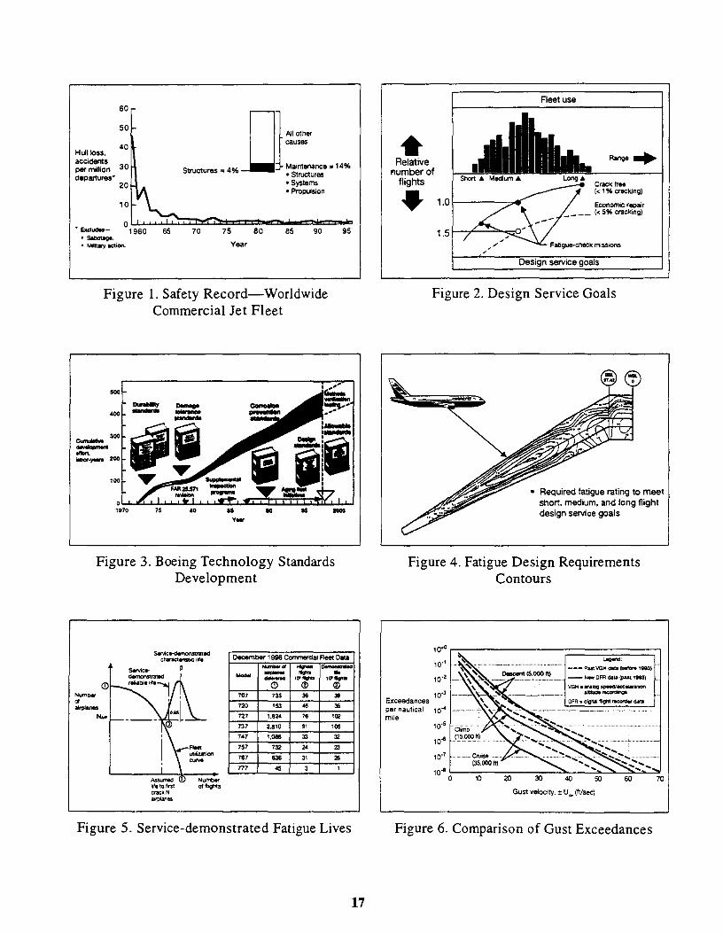
60

50 f-40 causes

Hull k)ss, aCCidents per million 30 departures·

lJ1 AHother

struct - 4% Maintenance ::I. 14% uras - • Structures

. ....-.-.-. o I 1960 65

• Milit..,. action.

70

• Systems • Propulsion

75 80 85 90 Year

Figure 1. Safety Record-Worldwide Commercial Jet Fleet

Vw

Figure 3. Boeing Technology Standards Development

95

s.vtce-<l.-nonstrated ctlll'aC't .... iclif. o.cember 1996 Commercial Fleet Data _ .. --..... - - .. -<D <D (j) III

N"" ... 701 ". 36 39

" .- 120 '53 " 36

...... , .. l n7 1.824 ,. '''' -'-- t-' 131 2,810 " 106

i

,., 1 .... ,. " 151 132 " 23 161 636 " 26

; Tn .. J 1

N....-of ftights

Crack N awplanes

Figure 5. Service-demonstrated Fatigue Lives

17

• Relative ",umber of

flights .. Range ..

Crack free « 1 % cracking)

Economic repair ___ « 5% cracking)

Figure 2. Design Service Goals

• Required fatigue rating to meet short. medium, and long flight design service goals

Figure 4. Fatigue Design Requirements Contours

Exceedances per nautical 1O" mile

10.5

10"

10.7

10" 0 10

a/IItude,.;on:lingl;

OFR. ftIgN IW:ClI'dwG.ala

Gust velocity, ± (ft/sec)

Figure 6. Comparison of Gust Exceedances

"20 years

"'",..ne MIn.mum dBSlgn Fatigue test Rem_ objective· 707 20.000 50.000 FUSelage

Hydro·fatlgue test 72i 60.000 60.000 Compjlte ilIrtrame

(b) '10,000 ComJHte fuselage 47.000 cydes in service. plus 123,000 pressure 18S1 cycles

737 75,000 (a,) 150.000 Fu:seIage sectiOl'llprGSUre and shear (b) 129,000 Complele afllusllage 59,000 cyc\ts in

seMce. plus 70.000 pt'9SSU/'elesl cydtS 747 20,000 I') 20.000 Compille airlralT16

(0) 40.000 CamP'll' fuselage 20,000 cydes In ser\llCe. plus 20.000 ptaSSUre test cycles

Ie) 60.000 747-400 sectionS 4' and 42 pressure lest cycJes

757 50.000 lClO.ooo Complete auframe 767 50.000 100,000 CompI8telirtrame 777 40,000 120,000 Compll!l.e airtmne

'40,000 ExtMdtd fuselage tests

Figure 7. FuII-Scale Fatigue Test Programs

• 151 and 767 mmrmum

300 • SOl( flight eydM

• 7471Tlin.mum_19"l ... • 2OKfIlglrtcydN

Testing (rmnth$)

Figure 9. Major Airframe Fatigue Tests

.. III lot. Pitch Initiation Load Conditic,n Moniloring

• SenSOIl; 1, 2. 19 and 20 are on the lower surface • Sensoll; 21 and 22 are On the reiV spar • AU other odd-numbered sensors are on the upper surface • All other even-numbered senSOr!. are on the lower surface • Sensors 9 through 12 are sensor P81r5. right and left of BL 0

Figure 11. AE Sensor Arrangement of Model 777 Horizontal Tail Pitch Initiation Ultimate

Load Condition Monitoring

18

Figure 8. Cyclic Pressure Testing of 747 Fuselage Structures

Figure 10. 777 Horizontal Tail Test

Figure 12. 737-200 Te3.rdown Site

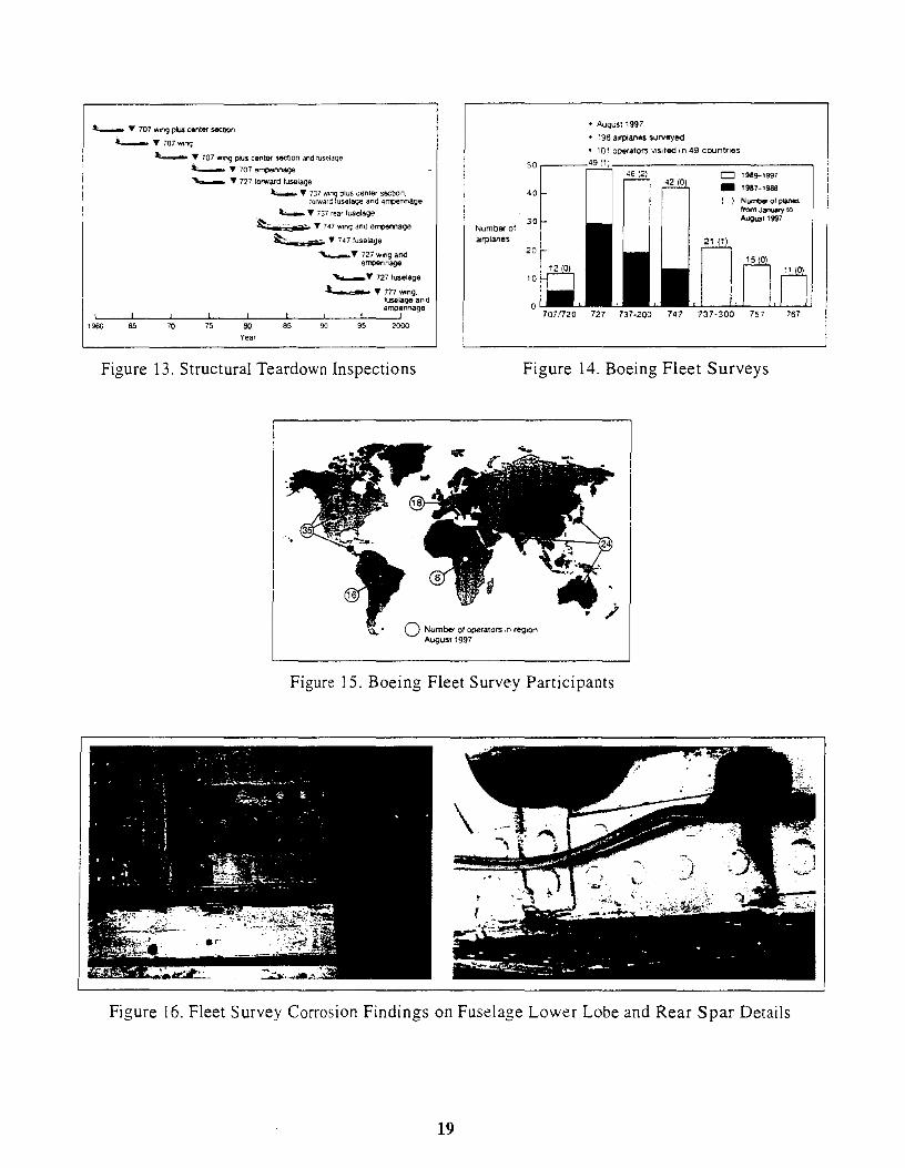
"'- .. 707 wrng plUS c.enter secbon

"- .. 707wlnq

"- .. ;07 wing plus c.er'ller section and tusp.laqe ""- " 707 el1"'P6r'1r'1age '- "72710rward tuselage

"-- "

t..-.. " 737 rear luselage ., 747 wlnq and

_-., 7471useiage

""--" 727 wing and errcennage

.. 727 tuselage

tuseLage and empennage

Year

Figure 13. Structural Teardown Inspections

Number of airplanes

• August 1997 • 196 airplanes surveyed • 101 VISited In 49 countries

__ --------------------_,

707/720

o '989-1997 _ 1987-1988

( ) Number 01 ptanes from January 10 Augus11997

737·200 747 737-300 767

Figure 14. Boeing Fleet Surveys

o Number of operators in region 1997

Figure 15. Boeing Fleet Survey Participants

Figure 16. Fleet Survey Corrosion Findings on Fuselage Lower Lobe and Rear Spar Details

19

1996 Status

Figure 17. Supplemental Inspection Candidate Airplanes

'.0

-;?J 2

Relative 0.8 0.6

0.4 }. OUter Skin 0.2 "' •

Inner Skin . .... -.. -00 0.2 0.4 0.6 0-8 1.0

Relative deledion penocI

InspectiOn InspectiOn CnocIUng IntoNaI Detection ..... 1On -- pattern probabiItylOTR" , Detailed c_ 0.1613 - ...... _MSO C·""""" 0.9991"

2 With MSO 1ir'*1,l) 4c;..check 0.999/10 1- HFEC

WrthOutMSO 4C-C:heck O.99QtI2 . om • o.tnage toleBnoe rating

Figure 19. Example of SSID Revisions to Account for Assumed MSD Linkup in Lap

Splices

NT selected to minimize risk of having cracks in airplanes below N,H

Number of airplanes

1---.... I'>Spect"d fleet P, ; Probability of detections

in inspected fleet

Flights

Figure 21. Supplemental Inspection Threshold-Fleet Utilization Distribution

20

Model Supplemental Inspection Findings 1983-1997

Wing Fuselage Empennage

727 25 27 (1) 28

737 18 28 13 (2)

747 33 (3) 34 (15) 16 (0)

Legend: A(B) A = Fleet Service Bulletin for some findings B = Aeet Airworthiness O'Irective action for significant fndings

Figure 18. Supplemental Structural Inspection Findings

Cumulative detection probability

+Intamal Mt.ftipie Element Damage (MEDI

t No contribution tor external \nSpeCtioo

Required probabflity

1.0 DTA

.0<0 L-.L.J....L.J.J.J.J.Ju.......L..-LLUJ.J.J.L...J.....J...J..J.J.J.W 0.' 0.001 1.000

Figure 20. Example of SSID Inspections of Failed Internal Frames

Original candidate fleet 1997 revision of SSIP Model size· based on 50% OSO Nr..- Airplane above

threshold (airplanes) (flights) threshold

727 461 90% OSO·· 100

737 124 90% OSO·· 110

747 117 100% OSO 80

"'Inactive aIrplanes Ire inckJded . ... ·DSO.Design Service Objective (flights)

Figure 22. Comparison of Original and Revised Thresholds and Number of Airplanes Inspected

"

_3)

: m .•

E etrr?

m ...

m_ ... 44

Figure 23. Boeing Family of Airplanes

FraetufO -(K..,.j, k3i.fin 100

TyptcaJ yield S1r'II'IgtI'I. ksi

Figure 25. Boeing Structural Aluminum Alloy Improvements

""'-' ....

NurT'Cer of key

20

""" .. ." -" ... ,. .... " ... .. ..... _ .. i i i i i i i i ". .. 300 000 ... .. "" '" i i

._------, , ... \ ':IIC_'__ ' ... ____ _

i i - '.-

Incorporation date. year

Figure 27. 747 Corrosion Prevention Design Improvements

21

777 ver>us 767 findings

0.5

t 767

0.5 1.0 1.5 Test Relative to Design Service Objective (OSO)

Figure 24. Fatigue Test Performance Comparison

-• nlo.N II 252+T3. ·T¢.1:II ._m D71S!>TT1 &2OIO-T. Dr."8-(ElJ) gn1J.,3.3.3 DlillftS

2.0

Figure 26. Boeing 777 Advanced Materials Use

EI Un. numbers 1 to 200 _ Une numberS 400 to 540

Figure 28. Effects of Corrosion Control Improvements on the 747

80

70

60

50 -of '0 -- 30

20 ,.. 10

Figure 29. Results From Corrosion Prevention Control Programs for the Model 747

1955

Our.Ib;lity S1andards

707 Wingl'fuse!age teardowns ...

m

" Oamage toterance me!hodS ...---....

737 7.7 ... "" m "

Supplemental inspection programs W i'n37n47 757i67

707

"

.0

m "

os

Fatigue tests .'71737'lJ7

70

-- ........ progom"----Wcrictwtde conferences""'---'"

75

71)7 757 yy. 80 85

737-700 TT71757-300 • 2V'. 95 2000

Figure 31. Boeing Fleet Support Actions

22

Relative maintenance labor-hoUrs ,0 per airplane. in thousands

747 -4 • 10-year service comparison

Production line position

Figure 30. Service Bulletin Labor-Hours (Standard and Widebody)

12th Annual National Educators Workshop

Jet Transport Structures Performance Monitoring

Additional Presentation Material:

Boeing Commercial Airplane Group Seattle, Washington

November, 1997

23

OVERVIEW Criteria and procedures used in commercial jet transport design and manufacture over the last four decades have resulted in safe-life damage tolerant structures with a credible safety record. Advancements in the capability to characterize structural performance by analysis have spurred adaptation of traditional fatigue and fracture mechanics technologies with large test and service databases to achieve development of technology standards over the last two decades. Major Boeing efforts have been focused on capturing lessons learned for future continuous design improvements by providing structures engineers with durability and damage tolerance methods similar to traditional strength checking procedures. The challenge of successfully implementing technology standards hinges on a practical balance between simplicity and technical credibility aimed at providing structural engineers with useful and service/test validated analysis tools. This presentation provides fundamental principles behind durability and damage tolerance technology standards, as well as examples of test and service validation.

Technology Evolution The first generation of Boeing jet transports was designed in the 1950s and 1960s. These model 707,727,737, and 747 airplanes are characterized by structural design principles addressing static strength and fail-safety. Experience has shown that the fail-safe design philosophy has served commercial jet transports well in terms of credible but imperfect safety records. The fail-safe design concept is founded on redundancy, which indeed has provided sufficient detection opportunities for accidental damage and corrosion-related deterioration. In terms of fatigue, particularly in cases of aging airplanes subjected to damage at multiple sites, such redundancies are not always efficient, based on obvious damage detection considerations. Supplemental fatigue inspection programs were therefore developed in the late 1970s to ensure sufficient fatigue damage detection opportunities. Inspection thresholds for most structures are based on traditional fatigue damage assessments, complemented by rogue flaw growth estimates for structural components with visually hidden details and limited crack arrest capability. Recent activities have been focused on developing procedures for calculating inspection thresholds for structure subject to widespread fatigue damage (WFD).

Technology Validation Development of structural performance data is the key element of the structural improvement process. These data come from full-scale testing, teardown inspections of inservice airplane structure, and fleet survey programs. Such structural performance data provide validation of the design for structural safety as well as for economic service performance.

Full-scale fatigue testing is a major part of Boeing structural performance data development. In addition to testing new models to identify any appropriate preventive maintenance actions and for structural modifications, retired service airplanes are tested to explore long-life operational concerns.

Teardown inspections of inservice airplane structure provide more detailed knowledge of structural performance and allow for timely fleet actions based on damage typically not detectable without disassembly. Although recent aging fleet concerns have focused unprecedented attention on such activities, it is important to recognize that such programs have been ongoing for the last 30 years.

25

As a result of continued operation of aging jet transports, an aging fleet survey program was started in 1986 to gain a better understanding of the conditions of structures and systems and to observe the effectiveness of corrosion prevention features. Typically, the program involves a Boeing team of six structural specialists who survey a selected high-time airplane undergoing a normal heavy maintenance check. To date, Boeing has surveyed 195 airplanes from 100 worldwide operators. Lessons from these surveys have been shared equally by Boeing structures engineers and customer airline maintenance personnel.

Durability standards ..

707 Wing/fuselage teardowns •

727 • 737 747 .'YT Damage\ tolerance methods ..

707 72717371747 Supplemental inspection programs. 'Y

707 'Y

727 'Y

747 ". Fatigue tests 757 767 74717371727 'Y'" .. ..

Service entry dates 707 727 737 747 ,,! ".! •• !

1955 60 65 70

Fleet survey program 'Y

Worldwide conferences ....

Aging fleet initiatives 'Y

75

Year

767 757 .. ' 80 85 90

Boeing Reet Support Activities

SUMMARY

727 'Y

7571767 'Y

7n 'Y

737-700 n7 IF sZ'SZ!

95 2000

Timely damage detection is the key element for ensuring structural damage tolerance evolving from the fail-safe approach, which has worked well since the first generation of commercial airplanes. Extensive testing, service data, and analyses have been employed to develop technology standards for durability and damage tolerance assessments of new and aging jet transports. We have, in a sense, recognized that safe-life, fail-safe, and damage tolerance principles each have some inadequacies and that indeed some contribution of all these philosophies is needed in some cases. The redundancy of the fail-safe structure is desirable to the extent economically feasible to provide structural safety. Widespread fatigue damage and independent local damage inspection thresholds depend on fatigue assessments supported by test evidence. Inspection intervals depend on crack growth, residual strength, and damage detection assessments.

Continuing airworthiness challenges have been addressed by Boeing over the last three decades. loint industry activities since the late 1980s have provided common approaches to ensure structural safety. Additional challenges beyond local damage tolerance capabilities have been addressed in recent years to establish positive initiatives to control widespread fatigue damage effects on continuing airworthiness. The continuous structural improvement process provides confidence for service beyond original design service objectives with minimal economic impact without compromising safety.

26

\ SUI"!

::=: :..:::;:; .':":'.:'.:::: , .............. -_ ...... __ ', ", • ... '4<>, .. _,

.... '/., •.. 0' ., .. , " , •..

Fatigue Accidents and Incidents to Civil Aircraft

Fail-Safe Test Verification

Structural Safety System

AIrplane manufacturer

Airworthiness _om;",

"'r1ine operators

Overview

27

Design Principles

Wing Fail Safety

C:.J[ _ I

Safety Record-Worldwide Commercial Jet Reet

60

50

HuIIClss, 40

""""', pe'miIIion 30 _ ..... 20

10

lJ)""-S""""",,o'" ."""" .... .""...,..

• Propulsion

Damage Tolerance Regulations

""""" FAR 25.571 (before 1978) FAR 25.571 (after 1978)

....,'" • Single eIemen'I or • MUltIple active cracks oCIlllouslailure ........ J.. 1. 1. 1. 1- ]..

C_ o No analysis reqund • Extensive anarysIs ,..,..., -InspectIOn • Based on servee • RIIa1I1d to structural

"""""' "'''''Y dal'TllgtCl'llr'lCtlristics • FMaircanier at1CI past seMce history

approval • Inlllal FAA engineering

I!> ancI air CIfTW apptOYal

[!:> Supplemental Damage TOI8f3nce InspectIOn. Per10rmad Per AC91·56.

{J..--

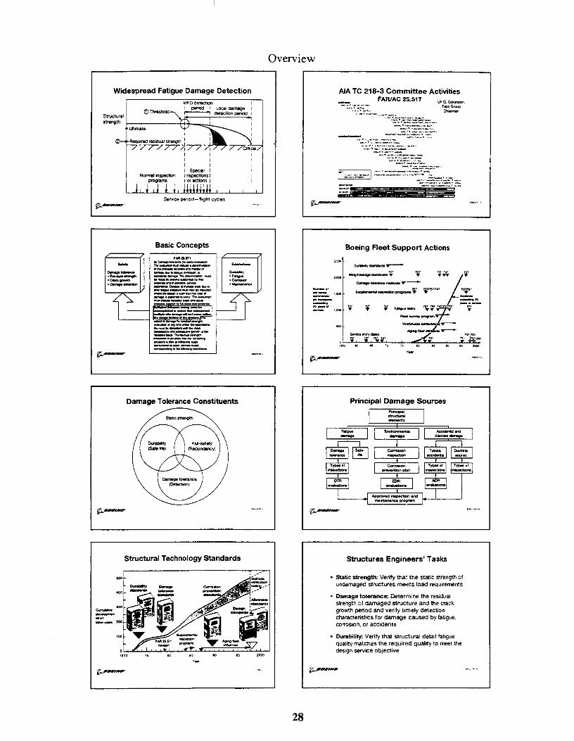
Widespread Fatigue Damage Detection

--j rTi j

---.Ao. .......... ._-• o.m.v--'-"

Service PE,nOd-fllght cyCles

Basic Concepts fAR a." n. ____ ._ ... _--_ .. --_10_,_-__ n. __

__ "' __ br_ --"-1-_0..-.. ___ " -..... --_ .. -_ .. _11_ .... __ ... ---11_ .. _.-_---."""",,," .--

'-------1 i-------J :-.: .... ::::::.::-----...... __ n. ____

==-.:::-.:.:=-_--.... --1 _ ........ _--

Damage Toleranc:e Constituents

Structural Technology Standards

Overview

28

AlA TC 218-3 Committee Activities FARIAC 25.517

-' -".,,- .......... _.,. -,-'. __ .... , -"-"._'''-'-.... , ... .... :-..... "., ..

"''''''''_'_'''''_''' _ ..... ....... -,,- .. -.. -_ .. _ .... ,._."" .. '-..... ,.-"'--......... _"., "-'--""--""_. , ....... -.. -., .... .... 1°' I ::;

...... ___, w ____ _ --------.... -. -------------Ow", ._"' ..... '" -. ""'. " __ _

Boeing Fleet Support Actions

Principal Damage Sources

Structures Engineers' Tasks

• Static strength: Verify that the static strength of undamaged structures meets load requirements

• Damage tolerance: Detennine the residual strength of damaged structure and the crack growth period and verify timely detection characteristics for damage caused by fatigue, corroSion, or accidents

Durability. Verify that structural detail fatigue quality matches the required quality to meet the design service objective

Technology Evolution

Durability Standards

0,,---_Oft 1 .. ." .... _.-4)T.ot_ro._

"...--,---,-.-·'_M .--.--. -Standard Load Conditions

Relative Fatigue Ratings '--

Service-Demonstrated Fatigue Life Example

-. -- _. - r== - -. - .. _.K . '" no • no m I.C. '" '" 2.1'0 • ,,, , ... " " '" no " '" '" '"

" ... "I\omI:IeI'of.s.tIQ1IIIIhoUI Cl'KI,,"g .. __ ""'_ ...

29

.. Relative

numbel" of flights ..

Design Service Goals

----«1"-. --«5"-.1

Fatigue Damage Model

CycIie!If. tog" ,..,.... I..

,("",)., oN

OFR .. \'t-at N .. 10·...:1 R .. 0 wilhiSH rtlitiOilitytlldll5H ccWiHncel I... ___ P __

•

=, .: l__ =---

Frame Splices Laaons Leamed ,-__ ,-._1Iic.oIIIaIo -.. "' __ ._011_ ... __ - --• EnoI ______ .. __

.1 ____ .................... __ .... ""Ioo#I ___ .......... _ ............. -".,,,.

Analytical Detail Fatigue Rating Example

Technology Evolution

Corrosion Prevention Design Handbook

• ATA32l-..;_ I _ .... • ATil" .1P\WI ...... o.n.r.o I .. , .. ..-.... • -- • ... 'AUII__ ' • ATA$7 WI"" - ·1371757" .. _ '7,rf1S7FI"-• o-gn......-IIJIUIO • ATAII;l:Cloor-t • o-7Q....mg __ "11 .... T ... --- • ... 1"'25P.,.-

..... , 'Pa ___

-I -- :=-1 .. ...... ---- ...... --- .-'?--. ""N''''

Access for Inspection

-. --"",-""",,,,"",,""--::="'..=:.. .... --"---._ .. _--_ ... - ..... -;

-.--------.-

Fatigue Check Samples ----......::--

'?--.

Fatigue Design Requirements Contours

• ReQUired fatigue rating to meet short. medium, and long flight design service g081s

30

Corrosion Prevention Design Standards Lower Lobe Drainage Example

---.... t-.., ...... --IIIoIgItuIIIW--.............. _ ......... lIIltO . --.-...... ---pr-.. --.",... .. ... ", ....... ....,......o

........ . ........ --. ---1IIIgIO ......... 8tO ° DoooIpIIO_IN.-IIo'-.g --.0.....,. .. - __ _ -. ...... _ .. _......,:1

Frame Shear Tie Drainage at BL 0

.; --- -.- .-____ ftC>"' __ ---"""' .... ____ 10

-"' ...... - ...... ..,....DI'R • DrwI ....... "T"_ .. __ _ _--","'IIfO\I'IM....-ILO -- • Fe,o ................ __

.. wiIII ....... _ ... 1AC1CIDO ._o.-onc.--• No ___ lLo

Active Commercial Fleet - 767

1-.' - I - . I , 1- '.':-1" -iii-- -,,- -, ,., --,., i:Ll: . " 1: ____ I = __ __

Ground-Air-Ground Reference Charts

Technology Evolution

! f •

Damage-Tolerant Structure U-. ... ClIMfIllItY ........ ecI 1ft. ... -

Multiple-Site Damage Criteria

J-

Residual Strength Parameters

Spar Cord EEl'

- .

...... ... .. ::; I ' •• 'w.' .. I •. '., ;' ' •• '., ...... I, Iffl

L/,i

.... " F ...... --T:--w:

......... --

31

Categories ot Structure

'-- - ...... ._- - -..... - - -.- cD 0..0 __ '" .- ---- - --.- -- -_.

I--- -- - .... _"'_f <D --- --- .-.. ..... ---_. ---- -"""- - - -.-- -- - .. -_. <D '-" ..- "---- - _ ..... - ....... - ... -.. ..-..... .. - .- -..-. - - -- CD-CD ._ .. - ,- ---. CD -,- .- .... _--- _. . --..

Local Versus Widespread MSD or MED

...... - ) J q J '" . .... _m __ ..... _ _ ... . f J J J f . " ...... 10_ .. _._ ...

t * t - .... • MutlipIe" Danwge (MSO)

JJJ-JJI)

... _I ............. .... t{_1 ... ""' .... {_ --...... (J...--

Residual Strength Verification Data

--- P .... ...-.: 0..$ 2OO.02.3OC1,,""

CndI....,.: 0.510100 .....

.• ••

Correlation tor Standard Analysis Procedure

ResIdual s1,."gth, lasl (MPa)

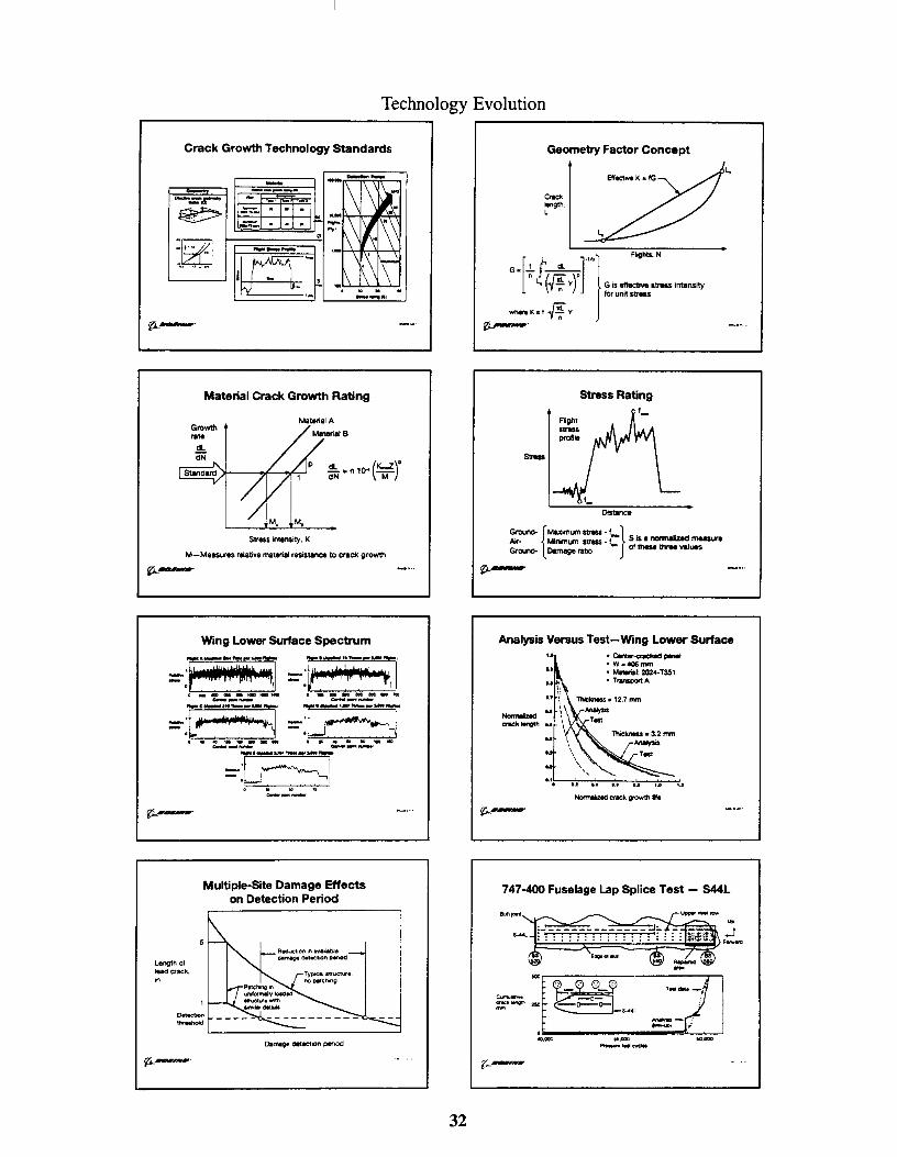
Technology Evolution

Crack Growth Technology Standards

I_=.r- l \1 \ I f.-::::.':'=j-I"t-1"+-1"-1

.... .. .. I -!\

Material Crack Growth Rating

dL (K...Z)' dN '" n 10-0 """'M"""

Stress imensJty, K

M-Measures relative material resistance to craCk growth

Wing Lo_ Surface Spectrum

Q _ -:,.. __ ':..: _ _ Q .. _ M _c_"' __ .......... ......11!!!110:!._-.......... =:t! t-J , ...... ___ ,.,.alO..,

Length of lead crack.

--- ---= r;:::'--=J r=7--.--.---,-

Multiple"Site Damage Effects on Detection Period

32

Geometry Factor Concept

Stress Rating

/IJr- MinimLm stress _ f Sis. normalized musure G""""," {Maximum.- -'_} Ground- Damage ratiO - of these thfW values

Analysis Versus Test-Wing Lower Surface

-"""-• parMI! • w. 406 rrwn • 202.·T351 • Tranapott A

-tr.';--':;-tr-;;:;-,

747"400 Fuselage Lap Splice Test - S44L

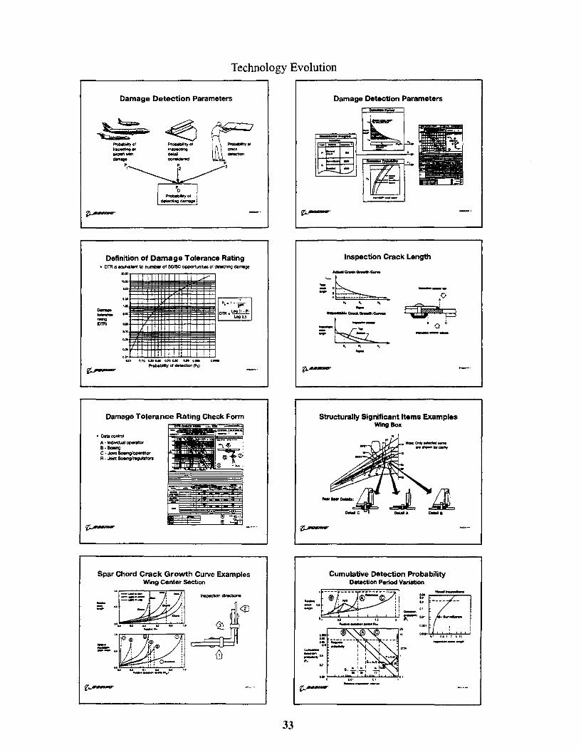
Technology Evolution

Damage Detection Parameters

Definition of Damage Tolerance Rating .. OTR is \0 number of 50150 opportUMII$ o! detectll'lQ clarrege

"""'" --,ll"

Damage Tolerance Rating Check Form

.. o.ta control A • kldMduai operatOr B-eo.ing C • Joint Boeir9'opntor

Spar Chord Crack Growth Curve Examples Wing Center Section .. - -, I_-

a- u - .L -i ...... ":..... ...... ,..

"W'CIl 0, =- i --. ! ,:; 1 \1) t'; 0-: .... .. .. .. ... ,. ---... '

33

Damage Detection Parameters --

Inspection Crack Length

ActuIt c:..oI<'--' c-. -- ,-- • --.!.--, , , -o

Structurally Significant Items Examples Wing Box

Cumulative Detection Probability Detection Period Variation

---

Technology Validation

Full-Scale Fatigue Tests

20 40 !Ill 100 120 '''''

Pr.-u-. cyct... ,n tI\outIIl'Ida

Boeing Fleet Surveys .. AugUII""7

.1010 .....

.1.1_1. ()-"' .... _..........,t<>

....... 1"'

727-200 Major Overhaul

34

727 Fuselage Pressure Test

Fatigue Test Performance Comparison 767 Versus 7n

777

"""" 767 finding3

'.0,-------------....,

0.5

..

.-,.

o O.S 1.0 1.5 2.0 Test Re1atr4 to Design SeMce ObtectiYe (OSO)

Boeing Fleet Survey Participants

Stringer Corrosion

Technology Validation

Relative Corrosion and Fatigue Performance

• , a-year senne. comparison

747 Corrosion Prevention Design Improvements

-,_ _71 '''''1 _" ""'''' '_I' ...... __

NUll'lbwoilw,' ---- : -, " iii"

Teardovwnlnspections .a...-. ... TOr WIOO ........ __

'--' ... 707-.0 .a...-. ... 707 WIOO ___ .:bI_"'-., '--'.m--ot '-.,. 1%1 torwMIlUIIiIQIf ......

__ ......

.....

727-200 Teardown

35

Relative Corrosion and Fatigue Performance

!\ . 1O'yNI'.,...,ic. companson

me..-rtllOlVlce

"' . ....,. ,

10r.

50 100 150 200 250 300 350 PrOClIJCtKln line pOSItIOn

747 Corrosion Prevention Design Improvements '00,-______________________ ___

o • u.,._.oGta540

400

, __ --

737-200 Teardown

707 Wing!lower Surface Disassembly

Technology Validation

Government and Industry Task Groups

I ,, ...... .. .. "" \

I I I

,.".. ....... cr I WOI'U>j i

'M I

'M I

'M .1 -- .. , ......, ... 1_Gr1_ .,. rIlA.C'·"IUSAo, r-m r ... ""'JlCVI ......... f- I..- DC-t,)

L

t--' .... , ..

Typical 727 High-Time Modifications

Supplemental Structural Inspection Program

• Objective: Ensure continued safe OperB1ion by timely detectIOn of new fatigue damage

• Background

- Boeing programs developed with industry cooperation and released between 1979 and 1983

• Programs are maintained by industry task groups

- Addressed regulatory concerns

- CAA Airworthiness Notice 89 and FAA AdvISory CIrcular 91 -56

- Satisfies the intent of FAR 25.571 Amendmen1 4S

Structure Susceptible to WFD

--.--_._. ...,T_So_NSC "'!O

.. c,. -- - 'I • - J: : . =- 1 I. - ' ,

.... -....o..-c-- ... ""....., c---._ .... _ ... _ .. ___ .... _" "'Ie .. ""_ ... """""'s, ....... ·

"..., ........ :-'", "'f:J

36

Continued Airworthiness Industry Initiatives

727 Modification Cost Improvement

_ ... -Example of SSID Revisions to Account for

Assumed MSD Unk-Up in Lap Splices "" -=--'-1 . u - Out.r....,-..•••• •• _ t--__

Q.,2 D.. U 0.. 1-" '------'''-'== ---- - "- -- - - ..... """"' , 0.- --- "-- - _ .... c-o.. ,-" , .. " _MID"'*"" oc..-

:- _." oc..-___ .. O'IQ

t---

Lap Joint Residual Strength Comparison

.,MID

Technology Validation

Fuselage Pressure Test Fixtures

• Finite element moOeI of wid4Ibody fuselage wtrh skin crack. . Oegr_ of frHOom: 26,000 - Nodes: 5.200

- Bam elements; - FMt_ eIemtontS:

lJ.--'

3,700 1.500 1,200

Typical Fuselage Extemal Skin Repair

' ••••••••••• ": I . --'; . ..("",.. "'"-1 '.l .. ·· .. ··'····r. '.... . r'-:. : : : : : : ::: : : :·"1 ' . . . . . . . . . . . . I '\. '.·1::::::::::::11 t, ,-.. -...

1- SIato ..... _-'?;----

Structural Repair Assessment Stages

c, .. go .... s --

37

Final Failure of Panel 74-8

Test/Analysis Correlation Residual Strength

.--"",

Half-<:r3Ck length. a. in

Skin Crack at Repair Doubler

Stage 3 Inspection Requirements Fuselage Skin Repairs

'r .. ' . '--

, '; J J1 :I

\ i OOOOOOwoo

)

L ,. , t1i£# ..

Fleet Damage and Inspection Program Phases . c-...o._...-. __ "" ... _ .. ___

lOti. 10 ""'otCllil9l ...... ....... • DImIve_ .............. a.t .... -.,.--.,. . ...-, ------...,.. ........

-.- ---- --Boeing Family of Inservice Commercial Airplanes

'.-r ...... -

\ 1:11'-

, m_

Summary

38

Meeting the Challenge

Industry commitment - Safety is the paramount consideration - Oamage tolerance inspection programs maintain safety

• Commtment has been demonstrated by action - Historical fleet support programs - Enormous energy expended to develop and implement

damage tolenlnce - Industry working groups fonned and actively

addressing current aging fleet concerns

Reference

"Damage Tolerance - Facts and Fiction" Ulf G. Goranson 14th Plantema Memorial Lecture Engineering Material Advisory Services Ltd. Durability and Structural Integrity of Aimames. Volume 1. EMAS. Chameleon P .... Ltd. ISBL0947817_9 London, Kingdom. 1993.

CORRELATION OF BIREFRINGENT PATTERNS TO RETAINED ORIENTATION IN

INJECTION MOLDED POLYSTYRENE TENSILE BARS

Laura L. Sullivan

Manufacturing Systems Engineering GMI Engineering & Management Institute

1700 w. Third Avenue Flint, Michigan 48504

Telephone 810-762-7950 e-mail Isulliva@nova.gmi.edu

39

Laura L. Sullivan

40

Correlation of Birefringent Patterns to Retained Orientation in Injection Molded Polystyrene Tensile Bars

Laura L. Sullivan Associate Professor,

Manufacturing Systems Engineering GMI Engineering & Management Institute

Flint, Michigan

Key Words: Injection Molding, Retained Orientation, Tensile Strength, Pack Pressure, Polystyrene

Prerequisite Knowledge: Use of a thermoplastic injection molding machine, establishment of optimized filling in injection molding, tensile strength and tensile testing

Objective: To observe the effects of increasing pack pressure and barrel temperature on the residual stress and tensile strength resulting from retained orientation within injection molded polystyrene. To observe the differences in retained orientation between a first to fill and last to fill cavity within the mold. To use birefringence observed via polarized light to measure retained orientation and predict the tensile strength.

Equipment: Injection Molding Machine 4 Ibs pelletized polystyrene polarized light box universal test machine digital calipers

Independent Variables: Barrel Temperature, Pack Pressure

Dependent Variables: Tensile Strength, Residual Stress/Orientation in Tensile Bar (as measured with the polariscope)

Machine Parameters to be held constant: Transfer Position, Shot Cushion, Shot size, Pack Time, Cooling Time, Mold Temperature, Injection Velocity, RPM, Temperature/Humidity

Introduction: Process parameters such as pack pressure and barrel temperature have significant affect on the quality of injection molded parts. Barrel temperature directly affects the viscosity of the polymer as it is extruded, and indirectly affects the shear energy which can be imposed on the polymer. As the viscosity of the polymer melt is changed, the manner in which it flows into the mold cavity during injection is also dramatically changed. Hotter, low viscosity material flows into the cavity easily, but may occupy more and take longer to cool (which must be compensated for by extending the packing time and the cooling time). In addition, hotter material will provide thermal energy for the polymer molecules to relax their orientation prior to solidification. This tends to result in reduced residual compressive stresses. On the other hand, when cooler, high viscosity material flows into the mold cavity, extensive orientation of individual molecules results. This orientation is "frozen in" when the polymer solidifies, and results in residual compressive stresses within the part.

41

Pack pressurc assists in adding polymer to the mold cavity after the initially full part begins to shrink due to cooling. As the pack pressure is increased, more material can be packed into the p3I1 prior to solidification at the gatc. As more material is packed in, the compressive stress within the part increases. This residual compressive stress rcmains when the part solidifies, and results from this retained orientation. As thc melt tempCI;ature is increased, the effect of this pack pressure becomes more dramatic, because there is more time available to pack prior to solidification, and there is also more timc for the relaxation of molecular orientation.

If there is more than one cavity within the mold, and if these cavities fill at different times (often due to the effect of gravity), than thc rcsidual compressive stresses within the resultant two parts will be different. The cavity which fills first (when the material is warmer and less viscous) will tend to have less retaincd oricntation, while the cavity which fills last will have more orientation.

The result of retained orientation - and the associated residual compressivc stresses - within an injection molded tensile bar, can be measured via tcnsile testing. If the gate to the cavity is located at the end of the tensile bar, than the residual compressivc stresses within the tensile bar will cause the material to behave as a compresscd spring. Tensile strength will increase as this residual compressive stress increases. Pnlarizedlight, passed through a transparent polymer, will result in color bands called birefringent patterns. By counting the number of color bands, the residual compressive stress within different injection molded parts can be compared. The more birefingent color bands, the higher the residual comprcssive stress. Tensile bar specimens containing a large number of birefringent color bands should also display high tensile strength.

Procedure: I. Bring machine to cquilibrium. Record the nozzle temperature, barrel temperatures, mold

temperature, and RPM.

RPM: Mold Temperature: Nozzle Temp.: Barrel Temp Zone I: Barrel Temp Zone 2: Barrel Temp Zone 3:

2. Set cooling time to 36 seconlis. Using only stage one injection to lill the mold cavity (no packing), determine the appropriate Shot Size and Transfer Position to FILL ONLY the part and get edge definition. Record these scttings. Maximize injection velocity such that the time necessary to fill parts is minimized and note this optimum valuc.

Optimized Fill Parameters determined: Shot size position Transfer Position Injection Velocity Resultant Fill Time

3. Increase both shot size and transfer position to allow for material to pack into the part. Adjust the set points for shoi cushion. shot sizc. and transfer position such that the material remaining in the barrel after each cycle is appropriate (for polystyrene. this is about 0.15 inches).

4. Set pack time to ten seconds. Set pack pressure to 400 psi. Mold I shot and save a tensile bar from the bottom of the mold cavity (the rirst to fill) and a tcnsile bar from the top of the mold cavity (the last to fill).

42

5. Keeping the packing time at 10 seconds, increase pack pressure by 50 psi increments, molding one shot and saving the same two parts at each setting. Continue until the pack pressure is so high that parts shatter on ejection.

6. Increase the barrel zone temperatures by 25 of at each zone and at the nozzle. Repeat steps 2-5.

7. Using the polariscope. compare the extent of residual orientation (stress) in the parts as a function of molding parameters. Pay par1icular attention to the number of birefringent color band can be counted wi thin the gage section of the tensile bars. Sketch these patterns.

8. Measure tensile bar. thickness, width, and load at fracture for each pair of tensile bars saved from each run. Calculate the ultimate tensile strength for each part.

9. Plot a graph which illustrates the effect of pack pressure on tensile bar strength for each cavity at the low barrel temperature. Plot a similar graph for the higher barrel temperature. Label the graphs completely and include a caption with Figure number.

10. Quantify the results of your polariscope observations and plot the results. Correlate these results to the graphs plotted in <) and above.

43

Laura L. Sullivan is an Associate Professor of Manufacturing Systems Engineering at GMI Engineering & Management Institute. After she received her undergraduate degree in PreMedical Engineering at Arizona State University, she worked in orthopedic research at the Baylor College of Medicine. She then attended the University of Texas at Arlington, where she received her M. S. and Ph. D., and conducted research on polymer matrix composites used in aerospace. At GMI, Laura supervises the Polymer Processing Laboratory, where experiments in injection molding, extrusion, thermoforming, and applications of stereolithography to rapid tooling are conducted. Laura teaches Engineering Materials and Polymer Processing. Her research interests are in the optimization of injection molding and polymeric materials.

44

STUDY OF RHEOLOGICAL BEHAVIOR OF POLYMERS

Ping Liu

and

Tom L. Waskom

School of Technology Eastern Illinois University Charleston, Illinois 61920

Telephone 217-581-6267

e-mail cfpl@eiu.edu

45

Ping Lui

, Tom L. Waskom

46

Study of Rheological Behavior of Polymers

Ping Liu and Tom L. Waskom School of Technology

Eastern Illinois University Charleston, IL 61920

Key Words: Polymer, rheological behavior, viscosity, temperature.

Prerequisite Knowledge: Knowledge of structure, behavior and processing of polymeric materials is helpful

Objectives: To understand the change in rheological behavior of polymer melts, which is related to its structure and processing characteristics.

Equipment:

1. Polymer pellets or blends to be tested. 2. Rheological testing system including load frame, temperature controller, and data

acquisition system. 3. Mittens or gloves for high temperature applications. 4. Cleaning tools such as brass brushes, cotton balls etc. 5. Time watch 6. Digital balance.

Introduction:

Rheology is the science dealing with deformation and flow of liquid-like materials such as polymer melts. It provides necessary knowledge for processing plastics or other polymers into products. Liquid-like materials in many industrial processes possess a wide range offlow behavior. Satisfactory operation of these processes requires a knowledge of the material's flow properties under operational conditions. Thus, understanding rheological behavior of materials can help improve the processing technology. Moreover, rheological behavior of polymer melts will also affect the ultimate material properties of products

Rheometry is the art of measuring deformation and flow properties of materials (Cogswell, 1981) Figure I shows the principle of a typical capillary tube viscometer. Capillary rheometer is one of the simplest and most widely used instruments for rheological characterization. The barrel temperature is maintained at a preset level by a temperature controller. Thus, the polymer pellets in the barrel will be heated to and maintained at a constant temperature. A plunger drives the sample material through a slit capillary at either constant or programmed flow rate. When using slit capillaries, one can measure the pressure difference directly in the capillary. Viscosity is measured

47

in terms of the pressure difference at certain shear rate.

Capillary rheometry has found its main area of application in the measurement of polymer melt

D Figure 1 Principle of capillary rheological testing system

viscoSities at shear rates below 1000 S·l and at temperatures up to 500 C. There are many advantages in using capillary rheometers. These include the relative ease of filling, the ability to change temperatures and shear rates readily, the similarity in shear rates and flow geometry to those actually found in extrusion, the ability to detect some indication of polymer elasticity, and the ability to study the surface texture of the extrudate. The main disadvantage of the technique is that shear rate varies across the capillary, and that corrections are needed in order to obtain accurate viscosity values.

Rheological behavior of polymers not only provides insights for polymer processing such as injection molding or extrusion, but also offers understanding on change in the polymeric structure due to processing. This describes a typical capillary rheological testing system and its application to study the viscosity of polymer melts at various strain rates and temperatures. Experimental data will be presented for rheological behavior of composites made of recycled high density polyethylene (HDPE) and recycled rubber particles

Experimental Procedure:

A capillary rheometer, INSTRON Rheopack, was used for this study. The loading frame of testing system has the capability of controlling shear rate for polymeric composites under compression The testing frame is controlled by a microcomputer using a software, Rheosoft, which can manipulate the cross head movement according to the established velocity schedule. The system measures the resistance or load to press the polymeric melt through a capillary die, corresponding to

48

the shear rate. Apparent shear rate, shear stress and viscosity are recorded while corrected shear rate, shear stress and corrected viscosity are calculated using Rabinowitsch correction. All the data are recorded in a report data file.

To investigate the effect of shear rate on the viscosity ofthe composites, shear rate was varied from 1.167 to 116.7 S-L This was achieved by setting up a velocity schedule for the plunger movement controlled by the microcomputer

In the experiment, a composite of recycled high density polyethylene with 5% recycled tire particles was used as one example. The particles of the recycled tire chips was 40 mesh. The blend of the two constituents were extruded, water cooled and then pelletized into pellets of approximately 4 mm in diameter The extruder screw has a LID ratio of 30: 1, which promotes mixing while extruding.

Results:

Figure 2 shows variation of corrected viscosity with shear rate for composite of recycled high density polyethylene (HDPE) with 5% recycled tire rubber particles at various temperatures. The figure shows the following main findings.

1. As the shear rate increased, the viscosity of the polymeric blend decreased

2. At lower shear rate, the decrease in viscosity with increasing shear rate is more drastic than at higher shear rate. The viscosity became leveled off at higher shear rate.

3. The viscosity of the composite decreased with increasing temperature.

References:

Charrier, J-M (1991). Polymeric Materials and Processing: Plastics Elastomers and Composites. NY: Henser.

Cogswell, F. N. (1981). Polymer Melt Rheology: A Guide for Industrial Practice. NY John Wiley & Sons.

Instron Model 3213 Rheometer Operator's Guide 1991.

Schramm, G. (1994). A Practical Approach to Rheology and Rheometry. Gebrueder HAAKE Gmbh, Karlsruhe, Germany.

Yanovsky, Y G. (1993). Polymer Rheology Theory and Practice. London: Champman & Hall

49

1BOOO ,-

16000

III 14000 , <1J (L

12000

?:-·Cii 0 10000 0 III :> BODO

""C ., -0 ., 6000

0 U 4000

2000

0.0 5.0 100 15.0 200

T erfl)erature (t:)

[) 180

o )10

D

250 300

Corrected Shear Rate ( 1/5)

350 400

Figure 2 Variation of corrected viscosity with corrected shear rate for composites of recycled high density polyethylene (HDPE) and recycled tire particles.

50

CASE STUDIES IN METAL FAILURE AND SELECTION

David Werstler

Manufacturing Engineering Technology Western Washington University Bellingham, Washington 98225

Telephone 206-650-3447

51

David Werstler

52

Case Studies in Metal Failure and Selection

David Werstler Manufacturing Engineering Technology

Western Washington University Bellingham, WA 98225

Key Words: failure, failure modes, failure analysis, product improvement

Prerequisite Knowledge: An introductory materials course is a prerequisite, and some additional experience with metallography, corrosion testing, failure analysis, heat treating, and forming processes is beneficial.

Objective: To examine samples and data from an actual industrial problem and make a recommendation for failure prevention or a change in materials selection. The case study should relate lab experience to lecture topics.

Equipment:

The following items are necessary for most studies of failure or selection: 1. A reference library offailure case studies and testing methods (1). 2. Metallographic equipment 3. Stereo microscope with camera 4. Rockwell hardness tester 5. Chemical analysis equipment

The following items are beneficial in some studies: 6. Corrosion testing equipment 7. Scanning electron microscope 8. Tensile testing equipment 9. Nondestructive testing equipment

1. The Best Material for Mountain Bikes?

The team will be given several examples of failures of mountain bike frames, some of which have come from other students. A local manufacturer of frames has also sent in some examples. Testimony from the bike owners is available for most of the accidents that were related to the failures. The team may also visit the local manufacturer to observe current production methods and materials, although many components and assemblies are produced offshore.

None of the failures resulted in serious injury or litigation, and in fact some were found before any accident occurred. Most bike owners push the limits of their equipment and

53

expect abuse to occur. The objective of this study is to provide the manufacturer with information that will help improve the life of the product.

2. Failure of a tug driveshaft

The Francis W was a medium size tugboat that was pushing a bargc into a berth whcn it suddenly swung into the barge, striking and breaking off the end of the drive shaft and propeller. The tug turned over and sank, trapping one crewman inside. The captain claims that the shaft broke first, causing him to lose control and hit the barge. His metallurgical consultant claims that the break shows classic signs of fatigue. The Coast Guard has requested other opinions in order to establish cause.

The team will be given photos of the break, samples of thc stcel near the break, test reports from other shipshaft failures, and the testimony of the captain's consultant. The team may also visit the shipyard where the tug was last overhauled.

3. Hammers for a glass pulverizer

A local manufacturer has designed a small hammermill to crush waste glass and turn it into sandblasting sand. The mill is meant to be used at local rccycling yards to produce a sand that can be used in the same community where thc glass is collected, thereby reducing transportation costs. The concept also climinates the need to sort glass by color. Although these costs are significant in thc overall recycling of glass, they are not significant to the cost of recycling all materials. In order to appeal to small communities, the price of the mill must be low.

The hammers are the most expensive component because they wear out rapidly. Thc team will be given examples of used hammers made from hardened low alloy steel. tungsten carbidc coated steel, and mangancse steel. Life cycle and cost data on these is also provided. The team should produce and test for onc wcek a set of hammers from a material of their choice.

Notes to the Instructor:

The cases used in class should be real, relevant, and rely on the instructors experience and knowledge of similar problems. Canned case studies do not work well because the instructor often cannot effectively answer student questions. The examples in this paper are given primarily to show what can work successfully and to encourage other instructors to use the same approach. Students may bring in problems from their own part-time jobs or from their own experience with product failurc. But again thc selected problems should not stray too far from the instructor's cxpcricncc.

The instructor needs to play two roles: the client in the beginning to provide information and the consultant near the end to verify or correct the student's results. The information given out should be partly irrelevant and partly deficient to encourage questions and

54

simulate real circumstances. The latter role also requires holding back information until the students have had the opportunity to learn from their mistakes.

Teams of three students work well, and each student should have a specific role: manager, reporter, and explorer (2). The manager is responsible for maximizing the performance of the team by maintaining focus, setting timelines, and keeping everyone involved. The reporter documents member interactions and synthesizes ideas into a coherent whole. The explorer provides technical assistance, checks to see if enough possibilities have been explored. and checks technical feasibility.

References:

1. Failure Analysis and Prevention, Metals Handbook, 9th Ed., Vol. 11. 1986. American Society for Metals. Metals Park, OH.

2. Duncan-Hewitt, Wendy. David Mount, and Dan Apple. 1994. A Handhook on Cooperative Learning. Pacific Crest Software, Corvallis OR.

David Werstler, P.E., is Associate Professor of Manufacturing Engineering Technology and teaches the courses Materials Technology, Metallurgy, Foundry & Forming. and Manufacturing Economics. His BS and MS degrees are in metallurgical engineering from Purdue and Colorado School of Mines. and he has an MBA from Xavier. He has fifteen years of industrial experience in steel research and technical management. He is also past chair of the Materials Division of ASEE.

55

MAGNETO-RHEOLOGICAL FLUID TECHNOLOGY

John Marshall

University of Southern Maine John Mitchell Center

Gorham, Maine 04038

Telephone 207-780-5447 e-mail jmarshal@usm.maine.edu

57

--; .c '" "" cc

QO

< II)

= .c 0

KEYWORDS:

Magneto-Rheological Fluid Technology

John A. Marshall, PHD

University of Southern Maine Gorham, Maine

Rheology, fluid power transmission, mechanical power transmission, and hydraulics.

PREREQUISITE KNOWLEDGE:

The student should understand the elementary concepts of magnetism. A basic understanding of fluid flow would be helpful.

OBJECTIVE:

To observe the unusual characteristics of magneto-rheological fluids. To understand how these fluids change from a liquid to a solid. To understand the potential power transmission advantages of these fluids.

EQUIPMENT AND SUPPLIES:

1) Two connected syringes containing magneto-rheological fluid 2) Strong magnet 3) Pen

INTRODUCTION:

Magneto-rheological fluid change their flow characteristics when subject to an electrical field. Response, which takes only milliseconds, is in the form of a progressive gelling that is proportional to field strength. With no field present, the fluid flows as freely as hydraulic oil (Korane, 1991).

Magneto-rheological fluids represent a technology that has the potential to widen the performance range of automated electroi"echanical and electrohydraulic equipment. Research and ongoing developments are refining this technology and experts predict an important future for these fluids.

59

of Magneto-rheological Fluids:

Current automation capabilities are not advanced enough to build a robot that could play tennis. Even though cameras and computers could direct the robot towards a ball, robot's move in an awkward, lumbering fashion because conventional hydraulic valves cannot keep pace with the commands of the computerized controllers.

With magneto-rheological fluid technology, this type of response time is possible. This technology will allow devices that can operate instantly and without mechanical valves. Increased productivity and better product quality through more dependable and responsive automated equipment is just a small part of what this maturing technology can deliver.

How MagnE3to-rheological Fluid Functions:

Magneto-rheological fluids are composed of two primary components. They are the carrier fluid and the suspended particles. The carrier fluid needs to be a good insulator, compatible with the materials they contact. Typical particle materials include polymers, minerals, and ceramics (Scott, 1984).

When an magnetic field is applied to the fluid, positive and negative charges on the particles respond by separating, so each particle then has a positive end and a negative end. Particles of the magneto-rheological fluid then link together in the same manner that the north pole of one magnet is attracted to the south pole of another magnet (Duclos, 1988).

Potential Applications:

Magneto-rheological fluids can change from solids to liquids so fast, they will work well with fast-acting computers. These characteristics suggest a number of unusual engineering applications such as fluid clutches and vibration isolators (Duclos, 198B).

According to Hans Conrad, professor of materials science and engineering at North Carolina State University, magneto-rheological fluids will lead to a whole new generation of brakes, automatic transmissions, actuator devices, hydraulic valves, pump parts, and motors (Conrad, 1992).

60

PROCEDURE:

Safety Considerations:

1. Protective eye wear is mandatory for all those in the lab area.

2. Do not force the syringes as they may break. Breakage may result in plastic fragments as well as exposure to the magneto-rheological fluid.

3. Obtain a "Material Data Safety Sheet" on the fluid from the supplier. Read the sheet completely and ask questions relating to any information you do not understand.

Observing Magneto-rheological Fluid as a Liquid:

1 . With the magnet removed, slowly push on one syringe allowing the fluid to force the opposite syringe outward.

2. Record on the data sheet the nature of fluid flow and if power is being transmitted through the magneto-rheological.

Observing Magneto-rheological Fluid as a Gelled Solid:

1. With the magnet attached, slowly push on one syringe allowing the fluid to force the opposite syringe outward.

2. Record on the data sheet the nature of fluid flow and if power is being transmitted through the magneto-rheological.

SAMPLE DATE SHEET:

Record below the characteristics of the fluid when the magnet was not present:

Record below the characteristics of the fluid when the magnet was present:

61

INSTRUCTOR NOTES:

1. When the magnet was not attached, the students should have observed the fluid flowing easily between the syringes, transmitting the input power to the output syringe.

2. When the magnet was attached, the students should have observed a resistance to fluid flow between the syringes.

REFERENCES:

Korane, K.: Putting ER Fluids To Work. Machine Design, May 9,1991, pp.52-57.

Scott, D.: Amazing Hardening Fluids Open a New World of Hydraulic Drives. Popular Science, April 1984, pp. 42-46.

Duclos, T.G.: Electrorheological Fluids and Devices. Automotive Engineering, December 1988, pp.45-48.

Conrad, H.: The Impact of ER Fluids. Compressed Air Magazine, March 1992, pp. 14-17.

Source of Supplies:

Internet resource to supplies and additional information:

http://www.rmit.edu.au/departments/ch/rmpc/

62

UNDERSTANDING GALVANIC CORROSION TRICKS TO PREVENT SOME

EXPENSIVE FAILURES

Gautam Banerjee

and

Albert E. Miller

Department of Chemical Engineering University of Notre Dame

Notre Dame, Indiana 46556

Telephone 219-631-9397

63

Understanding Galvanic Corrosion Tricks to Prevent Some Expensive Failures

Gautam Banerjee & Albert E. Miller

Department oj' Chemical Engineering University o(Notre Dame Notre Dame, IN 46556.

Key Words: Galvanic Corrosion

Prerequisite Knowledge: Knowledge of basic electrochemistry is helpful but not necessary.

Objective: To be able to understand the electrochemical reason behind Galvanic Corrosion and to exploit that understanding to engineer better products.

Equipment:

I. Solution of IS-20% Hydrochloric Acid [For faster reaction, even 2S% will be better]. 2. At least 4 petri dishes 3. Few pieces of wire/strip of AI. Fe. Zn. Pt 4. Overhead projector and Screen S. Napkin/tissue paper 6. Safety glasses/gloves/labcoats for all the participants

Introduction:

The two major reasons why we should study corrosion are economics and conservation. These two factors have primarily prompted the study and research into the mechanism of corrosion and the means of preventing or reducing the rate of corrosion. Galvanic corrosion is one among the various forms of corrosion which is very commonly observed in our daily life. Whenever there are two dissimilar materials in contact with each other and exposed to a corrosive environment. one of them is likely to corrode or degrade. However. this effect is highly visible in case of metals while not very common for non-metals. especially if two dissimilar non-metals are in contact. Nonetheless. galvanic corrosion affects us all. damaging both industrial goals as well as household materials. For example. gold plated silver jewelry shows gradual blackening of surface. especially when used in tropical Tenon coated cookware shows pitting corrosion. if the tenon coating is damaged locally. Galvanized steel products show white rust formation

65

when stored in uncoated steel container hy mistake. The examples are numerous and encompass our daily life.

Theory:

Corrosion a change in free energy along an independent reaction path. Since metallic corrosion is electrochemical in nature. its change in free energy can be determined from the cell potential of the electrochemical reaction. All electrochemical reactions can be divided into partial oxidation and reduction reactions. For example. consider the corrosion of metal in an acid solution:

Oxidation - M -7 M"- + ne Reduction - nH' + ne -7 n/2 H,

( I ) (2)

The oxidation half reaction correlates to anodic current now while cathodic current now is associated with the reduction reaction. As stated within the Law of Conservation of Charge. there can be no accumulation of electric charge during an electrochemical reaction. Therefore, for an electrochemical system. the rate of reduction must equal the rate of oxidation.

Cell potential can be measured through a calculated difference from a reference point. The representation and determination of cell potential is simplified by the concept of half-cell potentials. The half-cell reaction (2) above is arbitrarily used as a reference by defining its potential as zero: potentials for all other half-cell reactions arc calculated with respect to this reference. The reference potential is termed as Standard Hydrogen Electrode(SHE), Metals with positive potential with respect to SHE are considered passive or cathodic. On the other hand, metals with negative potential with respect to SHE arc considered active or anodic. When courled together, an active metal would be oxidized while the passive metal would be reduced until the rates of both type of reactions become equal. That state is defined as 'free corrosion'.

The half cell potentials of all the possible reactions are listed in almost all the elctrochemistry text books. The list is called EMF series where EMF stands for Electro-Motive Force and is given below(table I). The values listed represent ideal chemical conditions(e,g., unit activity of ions, unit pressure and temperature, etc.) under equilibrium conditions. It is important to note that EMF value of any half-cell reaction is a thermodynamic quantity.

In reality, corrosion processes of importance always represent non-equilibrium conditions and are guided more by the laws of kinetics than thermodynamics, In fact, the corrosion rate is expressed by the equation:

C.R. (3)

66

i I I

Increasingly Passive (cathodic)

Increasingly Active (anodic)

I 1

Table 1 : The Standard EMF Series

Electrode Reaction

Au'+ + 3e Au 0, + 4W + 4e 2 H!O

Pt!+ + 2e Pt Ag+ + e Ag Fe'+ + e Fe'+

0, + 2H,0 + 4e 4(OH) Cu'+ + 2e Cu 2Ir + 2e H, Pb'+ + 2e Sn" + 2e Ni 2+ + 2e Co2+ + 2e Cd'+ + 2e Fe'+ + 2e Fe Cr'+ + 3e Zn'+ + 2e AI'+ + 3e Mg2+ + 2e Na+ + e Na K+ + e

Standard Electrode Potential (E" in Volt)

+1.229 + 1.420

+ 1.200 +0.800 +0.771 +0.401 +0.340

0.000 -0.126 -0.136 -0.250 -0.277 -0.403 -0.440 -0.744 -0.763 -1.662 -2.363 -2.714 -2.924

where i,,,,, is the corrosion current density (IIA where I=corrosion current and A= surface area) of the corroding metal. Since the oxidation or dissolution process always occurs at the anode, the. exposed area of the anode in the corrosive atmosphere is inversely proportional to the corrosion rate. The parameter i,,,,, is experimentally determined using Wagner-Traud Mixed Potential Theory[ 1] which is beyond the scope of this discussion.

Even though thermodynamic parameters do not provide us the quantitative information about the rate of corrosion, it does provide us an idea about the pO';sibility of a given reaction to proceed at a particular direction. As mentioned above, corrosion represents a change in free energy and the change in free energy is expressed as :

-t\.G" = nFE" (4)

where t\.Go is the change is standard free energy, EO is the standard EMF, F is the faraday number (-96,500 coulomb/mol) and n is the number of electron taking part in the reaction process. Thus, from the EMF series, it is easy to determine whether the free energy change for a given reaction will be negative or positive. If it is negative, then the

67

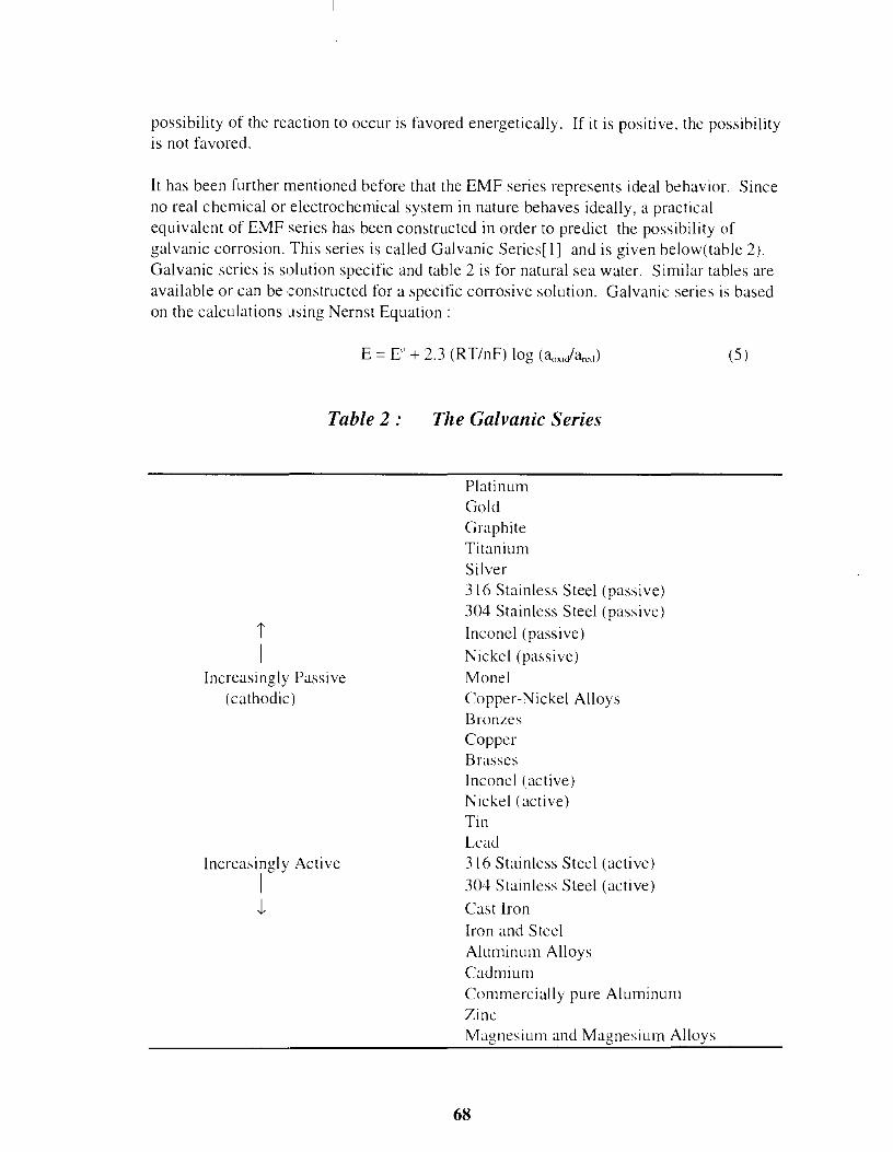
possibility of the reaction to occur is favored energetically. If it is positive, the possibility is not favored.

It has been further mentioned before that the EMF series represents ideal behavior. Since no real chemical or electrochemical system in nature behaves ideally, a practical equivalent of EMF series has been constructed in order to predict the possibility of galvanic corrosion. This series is called Galvanic Series[l] and is given below(table 2). Galvanic series is solution specific and table 2 is for natural sea water. Similar tables are available or can be constructed for a specific corrosive solution. Galvanic series is based on the calculations using Nernst Equation:

E = ED + 2.3 (RT/nF) log (<lc,,,ufareu)

l' I

Table 2 :

Increasingly Passive (cathodic)

Increasingly Active I

J-

The Galvanic Series

Platinum Gold Graphite Titanium Silver 316 Stainless Steel (passive) 304 Stainless Steel (passive) Inconcl (passive) Nickel (passive) Monel Copper-:",lickel Alloys Bronzes Copper Brasses Inconel (active) Nickel (active) Tin Lead 316 Stainless Steel (active) 304 Stainless Steel (active) Cast Iron Iron and Steel Aluminum Alloys Cadmium Commercially pure Aluminum Zinc Magnesium and Magnesium Alloys

68

(5)

and correlates the equilibrium state with the non-equilibrium. The magnitude of the difference between the E values of two half cell reactions in Galvanic series represents the driving force for a galvanic corrosion reaction; i.e., whether it will occur fast or slow. Not only does any metal which is active compared to the other one in this series will always corrode when coupled to the passive metal, it will corrode faster if the two metals are situated far apart in the Galvanic series than if they are closer. In other words, the more the distance between two dissimilar metals in the Galvanic series, more will be the driving force for corrosion of the active metal when they are coupled together[2l. Further details may be found in references 3 and 4.

Procedure:

1. Keep the individual strips of AI, Zn, Fe and Pt in separate dishes containing acid solution for few minutes and observe the gas evolution pattern, if any and compare the rate of evolution of gas for different metal strips qualitatively.

2. Combination of strips such as Zn/Pt, Zn/Fe, AIIZn and AI/Fe are immersed in separate dishes containing the acid solution. The two strips are kept in contact in a particular position so that two dissimilar metals are in contact only at the contact area while the rest of the strips are exposed in the acid solution separately. Again, observe the gas evolution pattern on both strips individually as well as at the contact point and compare qualitatively the rate of gas evolution between each combination as well as between 2 steps.

3. Take out the strips and wash thoroughly, observe the surface condition of both strips of each combination at their contact point.

4. Repeat step two, however, this time the two strips in each combination are kept in contact in parallel position so that the two dissimilar metals are in contact with each other over a wider area as compared to that in step 2. Observe the gas evolution pattern and compare with that observed in step 2.

5. Repeat step 3.

6. Explain the observations made so far and the possible reaction steps. Comment on any possible application of these observations.

Results:

The experimental observations, when recorded properly, will be similar to the results discussed in this section.

Step I will show general corrosion following EMF series. According to table 1, Al should dissolve ahead of any other metals and show bubbles corresponding to hydrogen

69

evolution on it. Similarly, Pt should show no gas bubble, being cathodic to H .. The order in which gas evolution should start and corrosion proceeds should be : AI > Zn > Fe.

However, in reality, one sees immediate hydrogen gas evolution on Zn followed by AI and Fe. This is because the natural air-grown oxide film on Al and Fe take some time to dissolve in acid while that on Zn dissolves very fast. If the strips/wires are freshly cut from a big roll, one may see the sign of tiny gas bubbles at the cut edges of AI immediately ahead of Zn. Of course, once the oxide layer is completely dissolved, the bare Al metal dissolves much faster than Zn in acid. Fe is the slowest among these 3 metals to dissolve.

Step 2 will show galvanic corrosion following Galvanic series. As expected from table 2, the more the distance between 2 metals in the couple in table 2, the active metal in the couple will dissolve that much faster with corresponding vigorous hydrogen gas evolution at the passive metal surface.

a) In Zn/Pt dish, Zn will corrode very fast and gas will bubble on Pt as they arc widely separated in table 2. After a while, necking will appear on Zn wire at the contact point with Pt due: to rapid dissolution at that point, Zn being anodic to Pt with a small surface area as compared to Pt. Eventually, Zn wire will break into two pieces and at that very instance, the gas bubbling on Pt will stop. Zn wires will then show general corrosion as in step 1.

b) In ZnlFe dish, Zn will corrode and gas will bubble on Fe but less rigorously than on Pt in (a). This is because Fe is eloser to Zn in the EMF series as copared to Pt. However, the difference in EMF is still substantial and hence the driving force for the reaction is enough for Zn to corrode fast and eventually break into two pieces. At that moment, unlike in (a), gas will continue to evolve on Fe, albeit at a slower pace and this time also on Zn pieces, following general corrosion as in step I.

c) In AI/Zn dish, hardly any sign of gas evolution on AI will be seen from beginning and no necking will be observed on Zn in the time frame that Zn usually breaks in contact with Pt or Fe. On prolong exposure. very fine necking may be observed on Zn. This is due to the very small driving force for the Zn dissolution reaction, Zn and AI being next to each other in the Galvanic series, even though energetically Zn dissolution is the favored reaction.

d) In AI/Fe dish, one would expect the onset of gas evolution of Fe as soon as it comes in contact with Al as they are reasonably apart in table 2. And of course, Al wire should corrode accordingly. However, in reality, one needs to walt for a while to see this until the oxide layer on Al at the contact point breaks down. From then on, it follows the expected path and AI wire breaks into two pieces after sometime. At that moment, the reactions on Al and Fe wires will be similar to that explained in (b).

70

Discussions:

The above mentioned results can be used to solve real-life problems. Following are some examples-

• Pt is the most passive metal in the Galvanic series and it is always used as the electrode of choice in all experiments where electrode stability is an important criteria.

• Zn is anodic to iron and corrodcs freely in contact with iron. It is used as a sacrificial anode to protect iron and carbon steel from corrosion. Galvanizing is a process where Fe is dipped into molten Zn and air cooled to get a solid Zn layer on Fe. Similarly, electroplating of Zn on Fe is also done to protect Fe. In the last few years, Zn rich polymer coatings have become very popular where Zn dust or Zn-ortho silicate is blended with the polymer coating and applied on the Fe surface to achieve double protection.

• Zn is also anodic to Al and even though the driving force is negligible, corrosion of Zn over prolonged exposure is thermodynamically possible. This also means that if corrosion of Al is a factor to be taken care of in a critical application. Zn can be used as a sacrificial anode. This is demonstrated in the practice of forming a zincate layer on Al before electroplating Al with any other metal. No other metal adheres on an Al surface directly due to the surface oxide layer on AI. Hence. if plating is done directly. corrosion of Al will occur easily through the cracks in the plating. However. the zincate layer adheres on the Al surface on which better plating adhesion can be achieved and also provides sacrifical anode cathodic protection in case of cracks in the zincate layer.

• Al is anodic to Fe and an Al coating on Fe behaves similar to that of Zn on Fe. Aluminizing is a process similar to galvanizing and is done industrially. However, the scope of application is limited since Al is softer than Zn and is therefore not recommended for many applications where wear is an issue.

Conclusions:

There are countless other examples of galvanic corrosion and preventive measures. The above mentioned points just show that even without any quantitative measurements, it is possible to identify galvanic corrosion and take remedial action. Remedial actions can be taken in different ways, e.g .. by using a sacrificial anode, by separating the two dissimilar metals with an insulator like polymer coating. wood. plastic spaccr, etc .. or by using metals/alloys close to each other in galvanic series than far apart. Whatever be the remedy, one will always have to remember that disconnecting two dissimilar metals with an insulator in a corrosive environment or disconnecting the whole galvanic couple from

71

the corrosive environment using non conductive polymeric paint is the best way to prevent galvanic corrosion.

References:

I. Wagner C. and W. Traud, Z. Elektrochem., 1938, vol. 44, p. 391. 2. Jones D.A., Principles and Prevention of Corrosion, second ed., Prentice Hall, 1996,

p. 168. 3. Metals Handbook, vol. 13, 9th ed., ASM. 4. Hack H.P., ed.: Galvanic Corrosion, STP 978, ASTM, 1988.

72

MEASUREMENT OF THE MODULUS OF ELASTICITY USING A

THREE-POINT BEND TEST

R. B. Griffin

and

L. R. Cornwell

Department of Mechanical Engineering Texas A&M University

College Station, Texas 77843

Telephone 409-845-5243 e-mail rcomwell@mengr.tamu.edu

rgriffin@mengr.tamu.edu

73

L.R. Cornwell

74

Measurement of the Modulus of Elasticity Using a Three-Point Bend Test

INTRODUCTION

Authors: Griffin, R.B. and Cornwell, L.R. Department of Mechanical Engineering

Texas A&M University College Station, TX 77843-3123

For many years the Mechanical Engineering Department at Texas A&M University has taught a junior level Properties of Materials class that includes a laboratory. During the semester, the students perform between 10 or 12 experiments on materials including metals, plastics, glasses, and composites. Recently we introduced a three-point bending test that is used to determine the modulus of elasticity and to evaluate the critical parameters to be measured using an uncertainty analysis. This paper will describe the experiment, the application of the uncertainty analysis, and give an example of the data the students obtain.

Part of the impetus for this experiment is to give the students an opportunity to work with their hand making measurements. The majority of our students have little experience using dial indicators or reading a micrometer or a caliper. The experiment also ties in with their mechanics course and hopefully connects the mechanics and materials together.

EQUIPMENT The experiment requires the following items:

Three-point bend fixture (Length between the fixtures is adjustable) Dial indicator (We used a mechanical dial indicator) Micrometer or caliper Scale (30 cm long) Set of student weights Test specimens (25 cm long x 2.5 cm wide x 0.32 cm)

Currently we have a 1018 steel, a 6061 aluminum, an annealed cartridge brass, a cold worked cartridge brass, and a graphite/epoxy composite material.

PROCEDURE The fixture that is used is shown in Figure 1. It was designed to enable a wide variety

of test specimens to be used. The laboratory handout given to the students is included in Appendix A.

The students measure the width and thickness of the material to be tested. They set and measure the distance between the supports on the bend test fixture. The dial indicator is held in position by a magnetic holder, and as Figure 2 illustrates, the holder sets on a steel plate. The dial indicator can be placed either above or below the piece to be tested. For this experiment, it seems to be better to set the dial indicator below the test specimen. In order to keep the lighter materials from being lifted off the supports, a 100g mass is set on the specimen above the bend fixture supports (see Figure 2). The students place the masses from the student weight set on the specimen halfway between the supports and

75

measure the deflection. Figure 2 shows the setup with a mass at the midpoint of the specimen. Students make several readings using different masses, and the results are recorded.

The process is interesting to observe. The students are in groups of 3 to 5. They struggle trying to decide how to read the dial indicator, and what masses they should use. Once they realize that there is supposed to be a linear relationship between the mass and the deflection, the process goes much more easily.

ANALYSIS From beam theory the stress in the beam is given by

The deflection is:

My (]"=-

I

pe 0=-

48EI

(1)

(2)

where M is the bending moment and y the distance from the neutral axis, I is the second moment of area about the neutral plane, E is the modulus, P the load, and L the distance between supports.!

For the rectangular beam bh l

1=-12

where b is the width and h the thickness of the beam. Thus, pe

E=--..,.. 40 bh 3

(3)

(4)

and experimental values of 8 and P will enable E, the elastic modulus, to be determined? Uncertainty analysis is a way of estimating errors that occur in experiments and

putting a value on a known error. One method of estimating uncertainties is as follows. 3

Supposing we wish to calculate the uncertainty in a calculated result on the basis of uncertainties in the measurements. Then the result R is a given function of the independent variables x!, X2 ....•. xn, so that R = R(x!, X2 ...... xn). Let Wr be the uncertainty in the result and WI, W2 ..... 'Wn be the uncertainties in the variables. Then,

w, rr (5)

Thus the students must estimate the uncertainty, w, for each measurement they make, for example the thickness of the bar using a micrometer. Then apply the above formula to find w, which can then be used to find a percent uncertainty in the modulus values. One result of this exercise will show which measurement has the greatest effect on producing an error in the modulus. In this case it will be 8, the deflection.

76

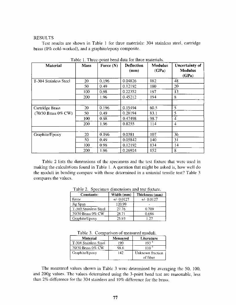
RESULTS Test results are shown in Table 1 for three materials: 304 stainless steel, cartridge

brass (0% cold-worked), and a graphite/epoxy composite.

T bl 1 Th a e ree-pomt b ddt f th en a a or t . I ree rna ena s. Material Mass Force (N) Deflection Modulus Uncertainty of

(mm) (GPa) Modulus (GPa)

T-304 Stainless Steel 20 0.196 0.04826 182 48 50 0.49 0.12192 180 20 100 0.98 0.22352 197 13 200 1.96 0.45212 194 8

Cartridge Brass 20 0.196 0.15494 60.5 5 (70/30 Brass 0% CW) 50 0.49 0.28194 83.1 5

100 0.98 0.47498 98.7 4 200 1.96 0.8255 114 4

GraphitelEpoxy 20 0.196 0.0381 107 36 50 0.49 0.05842 140 31 100 0.98 0.12192 134 14 200 1.96 0.26924 152 8

Table 2 lists the dimensions of the specimens and the test fixture that were used in making the calculations found in Table 1. A question that might be asked is, how well do the moduli in bending compare with those determined in a uniaxial tensile test? Table 3 compares the values.

T bl 2 S a e )peCimen d' lmenSIOns an d f test lxture. Constants: Width (mm) Thickness (mm)

Error +/- 0.0127 +/- 0.0127 Jig Span 120.99 -T-340 Stainless Steel 27.76 0.709 70/30 Brass 0% CW 28.71 0.686 GraphitelEpoxy 25.93 1.27

T bl 3 C a e omparlson 0 f measure d d r mo u 1.

Material Measured Literature T-304 Stainless Steel 190 193 4

70/30 Brass 0% CW 98.6 110 5

GraphitelEpoxy 142 Unknown fraction of fiber

The measured values shown in Table 3 were determined by averaging the 50, 100, and 200g values. The values determined using the 3-point bend test are reasonable, less than 2% difference for the 304 stainless and 10% difference for the brass.

77

Using Equation (4) and the data listed for 304 stainless steel under a 50g load, the calculated modulus is 180 GPa.

QUESTIONS

0.49(4.7632·0.0254)3 E=

4(0.0001219)(1.0928.0.0254)(0.0279.0.0254)3 (6) E = 180 GPa

The following questions are intended to get the students thinking about the nature of elastic moduli and its use in engineering. Appropriate resource material is made available to the students to help them answer these questions.

1. Is the flexural modulus you determined the same as the tensile modulus? Explain. 2. The accuracy of your modulus values increases as the load increases. Explain. 3. The modulus of a pure metal does not change very much as it is alloyed, heat treated

or cold worked, yet the yield strength changes significantly. Explain. 4. What error is introduced by the position of the dial indicator, i.e., where it touches the

beam? 5. Elastic deflection in a tensile test is the area under the stress strain curve up to the

yield point, or more correctly, the elastic limit. What is the area called, what does it represent and what use is made of it in engineering components?

6. There are two other elastic moduli, shear modulus and bulk modulus. Define them and write their relationship with Young's modulus through Poisson's ratio.

7. If Poisson's ratio for steel is about 0.3, what is the approximate value for its shear modulus?

8. Where does the equation for the deflection of a beam come from? Prove it.

CONCLUSION A three-point bending experiment has been developed for use 1ll a laboratory course.

The students have successfully measured the modulus of elasticity in bending. They have applied an uncertainty analysis ·to their results, and have been able to show which terms are critical in the calculation of the modulus.

REFERENCES

1. Fletcher, D.Q., Mechanics of Materials, Holt, Rinehart and Winston, New York, NY, 1985.

2. Askeland,D.R., The Science and Engineering of Materials, PWS, 3rd Ed., 1994. 3. Holman, J.P., Experimental Methods for Engineers, McGraw Hill, 6th Ed., 1994. 4. ASM Metals Reference Book, 2nd Ed., ASM, Metals Park, OH, 1983. 5. Metals Handbook, Properties: Non-Ferrous Alloys and Special Purpose Materials,

Vol. 2, lOth Eel., Metals Park, OH, 1990.

78

APPENDIX A

ENGR 489 (FC) Modulus of Elasticity in Bending

Objective: To determine the modulus of elasticity.

Equipment: 3 point bending fixture, dial indicator, weights, micrometer

Process: Measure the modulus of elasticity in bending. (See attached, section 6.4, Askeland).

We have a number of materials available in strip form. I. Determine the modulus of elasticity by measuring the deflection in a three-point

experiment. 2. Determine (estimate) the scatter in your data and determine which variable is critical

in determining the modulus. 3. Use the uncertainty analysis, described in the handout given to each group, to perform

the error analysis.

Reporting process: At the conclusion of lab, each group will tum in the experimental data, the modulus of elasticity values, and the error analysis. Compare the measured values to those listed in the attached tables or other sources.

79

Figure 1

Figure 2

80

MAKING A PHASE DIAGRAM

William K. Dalton

and

Patricia J. Olesak

School of Technology Mechanical Engineering Technology

Purdue University 1417 Knoy Hall

Room 145 West Lafayette, Indiana 47907-1417

Telephone 765-494-7532

81

Making a Phase Diagram

William K. Dalton Patricia 1. Olesak

Mechanical Engineering Technology Purdue University

Key Words: Phase, liquidus, solidus, solvus, eutectic

Prerequisite Knowledge: Knowledge of basic phase states is helpful but not necessary.

Objective: To construct a lead-tin phase diagram based on data collected for various cooling curves from different lead-tin compositions.

Equipment: I. Seven electrically heated melting pots containing various Pb-Sn compositions capable

of achieving a 400°C temperature. Pots should be equipped with temperature measuring instruments (we use a type K thermocouple and a microcomputer thermometer). Pot compositions: a. 0% Sn b. 10% Sn c. 20% Sn d. 40% Sn e. 62% Sn f. 80% Sn g. 100% Sn

2. Stop Watch 3. Graph paper for plotting the temperature vs. time for each pot.

Introduction:

Students typically have difficulty in understanding the construction of phase diagrams. They can be told that phase diagrams are made from a series of cooling curves (Temp. vs. time), but have trouble visualizing the relevance of compositions. , They often see phase diagrams (Temp. vs. Comp.) as being mystical rather than just a graph where lines define the limits of solid and liquid phases. In an attempt to demystify phase diagrams, this laboratory experience was developed.

Procedure:

The laboratory class (12 to 15 members) is split into seven groups, each group receiving a different Pb-Sn composition pot. All 7 pots are heated to 400°C. The heat supply to the pots is turned off and the pots are allowed to cool. Decreasing temperature readings are obtained every few seconds as noted below.

83

a. Take temperature readings every 10 seconds, beginning at 340°C until you reach a temperature 0[31 O°C. Be careful between 330-320°C.

b. Take temperature readings every IS seconds, beginning at 330°C until you reach a temperature of 240°C. Be careful between 31 0-290°C and 280-250°C.

c. Take temperature readings every IS seconds, beginning at 320°C until you reach a temperature of 170°C. Be careful between 300-270°C and 190-170°C.

d. Take temperature readings every IS seconds, beginning at 250°C until you reach a temperature of 170°C. Be careful between 245-200"C and 190-170°C.

e. Take temperature readings every 30 seconds, beginning at 200"C until you reach a temperature of I 70°C.

f. Take temperature readings every IS seconds, beginning at 210°C until you reach a temperature of 170°C.

g. Take temperature readings every IS seconds, beginning at 245°C until you reach a temperature of 215°C

note-we chose to use stop watches rather than a computer data card so students had to be involved in making the observations.

The temperatures are plotted vs. time. When an isotherm is revealed, or a change of slope of the cooling curve is revealed, a phase transformation occurs. Students must be cautioned not to just draw a best fit line of a single slope, or the change in slope will not be identified. Some slope changes are so slight that it is best to sight along the line from its end; this will reveal the "kink". The isotherm at the eutectic composition is often 2 to 4 minutes long, which is a good illustration of the time required to "unsolution" atoms as energy is being reduced. That is, the atoms, being insoluble, must physically move to form the laminated eutectic structure while in a semi-solid state.

Information pertaining to these "phase transformations" is shared among the laboratory group. The group data is used to make a new graph on the chalk board, temperature vs. composition, a.k.a. phase diagram ..

Students are able to see the actual construction of a phase diagram. They identify phases based upon laboratory observations when cooling. They also identify liquidus and solidus lines, once the phase diagram is drawn. When acquainting students to the topic of phase diagrams, this is a hands-on way of introducing the topic.

References:

1. Dalton, W. K., The Technology of Metallurgy, MacMillan, 1994, chapter 5.

84

William K. Dalton is a Professor of Mechanical Engineering Teclmology at Purdue University where his major responsibility has been teaching the course in applied metallurgy. He received a BME degree from Cornell University, a BS in Industrial Management from Carnegie-Mellon University, and a MS degree from Purdue. He spent 32 years with Alcoa before coming to Purdue; he is a member of ASM and ASME.

Patricia 1. Olesak is an Assistant Professor of Mechanical Engineering Technology at Purdue University, where she has taught courses in quality and materials science. She received a BS in Metallurgical Engineering from Michigan Technological University and a MS in Material Science Engineering from Purdue University. She has twelve years of industrial experience in the metallurgical and quality areas with Alcoa and Federal Mogul Corporation. She is a CQE and belongs to ASQC, ASEE and TMS.

85

RELATIONSHIP BETWEEN MOISTURE CHANGES AND DIMENSIONAL CHANGE IN WOOD

Thomas M. Gorman

Department of Forest Products University of Idaho

Moscow, Idaho 43844

Telephone 208-885-7402

87

Thomas M. Gorman

S8

RELATIONSHIP BETWEEN MOISTURE CHANGES AND DIMENSIONAL CHANGE IN WOOD

Thomas M. Gorman, Ph.D., P.E. University of Idaho

KEY WORDS: wood, moisture relations, properties, shrinkage, swelling, vacuum impregnation

PREREOUISITE KNOWLEDGE: The ability to understand and perform calculations with algebraic formulas, using data collected to provide unknown variables. A basic understanding of the universal gas law is helpful, though this experiment can be used to introduce some of those concepts.

OBJECTIVES: To introduce the relationship between changing moisture content and shrinking/swelling of wood. Oven-dried (fully shrunken) samples of wood are rapidly saturated with water to attain their fully swollen dimensions. The change in length offers a fairly dramatic visual indication of the degree of dimensional change that can occur in wood, and also allows calculations to determine the shrinkage coefficient for various wood species.

A secondary concept that is introduced is that of vacuum impregnation of wood, used by the preservative treatment industry to quickly impregnate wood with preservative chemicals. The use of a clear vacuum chamber allows this process to be observed and, therefore, better understood.

EQUIPMENT AND SUPPLIES: Three wood samples of the same species, measuring approximately 100 mm (4 in.) in length. Each piece should represent one of the axial grain orientations (longitudinal, radial, and tangential), as described in the PROCEDURE section. Prior to beginning the experiment, the pieces should be dried overnight in a convection oven, set at 1020 C (115 0 F).

Vacuum chamber and vacuum pump. The vacuum pump should have sufficient draw to attain a vacuum of approximately 80 kPa (23.7 in. Hg). The vacuum chamber is preferably made of clear plastic or glass, and allows the wood samples to be submerged in water.

Calipers to measure length of samples to within 0.01 rum (or 0.001 in.).

INTRODUCTION: Wood shrinks or swells as it loses or gains moisture, respectively. This phenomena occurs between moisture content (MC) levels of 0% to about 30% (dry basis: wt. H20 .;- wt. dry wood). In addition, the amount of shrinkage or swelling that takes place varies by species and, most importantly, by the axial orientation of the wood fibers. Since freshly sawn wood (i.e., "green" lumber) is dried prior to use, significant shrinking can be expected to occur. The purpose of this experiment is to observe the dimensional change that occurs as wood swells from 0% to over 30% MC, use the measurements to calculate the shrinkage coefficient, and compare the calculated values with published values.

89

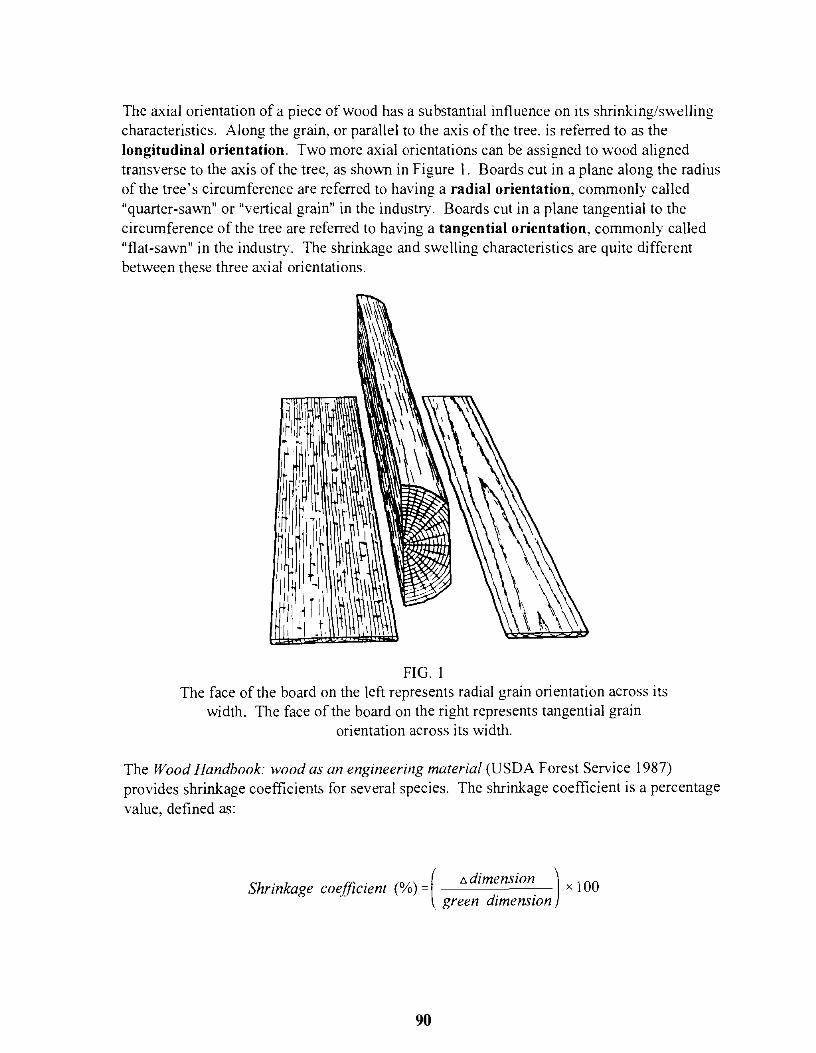
The axial orientation of a piece of wood has a substantial influence on its shrinking/swelling characteristics. Along the grain, or parallel to the axis of the tree. is referred to as the longitudinal orientation. Two more axial orientations can be assigned to wood aligned transverse to the axis of the tree, as shown in Figure I. Boards cut in a plane along the radius of the tree's circumference are referred to having a radial orientation, commonly called "quarter-sawn" or "vel1ical grain" in the industry. Boards cut in a plane tangential to the circumference of the tree are referred to having a tangential orientation, commonly called "flat-sawn" in the industry. The shrinkage and swelling characteristics are quite different between these three axial orientations.

FIG. 1 The face of the board on the left represents radial grain orientation across its

width. The face of the board on the right represents tangential grain orientation across its width.

The Wood Handbook: wood as an engineering material (USDA Forest Service 1987) provides shrinkage coefficients for several species. The shrinkage coefficient is a percentage value, defined as:

Shrinkage coeffiCIent (%) = .' x 100 . (t; dimension ) _ green dImenSIOn

90

where: fl dimension = change in dimension from green (above 30% Me) to oven-dry (0%

Me) green dimension = original dimension in green (fully swollen) condition

A few shrinkage coefficients are provided in Table 1 below. The longitudinal shrinkage coefficient for normal wood of all species is typically considered to be approximately 0.1 %.

Table I. - Shrinkage coefficients (%) for eight wood species. .. Radial····· ......

Tangential· •. ·••·· Species ... . ...

Douglas fir 3.8 6.9

Eastern white pine 2.1 6.1

Mahogany 3.0 4.1

Northern red oak 4.0 8.6

Sugar maple 4.8 9.9

Western redcedar 2.4 5.0

White fir 3.3 7.0

Yellow birch 7.3 9.5

Dimensional change due to loss of moisture is reversible; that is, any shrinkage that occurs as wood is dried may be regained if the wood is re-wetted to its original moisture content. Also, dimensional change due to moisture change is linear; consequently, the amount of shrinkage that takes place as wood changes moisture content can be fairly accurately estimated with the following equation:

where: ",D = change in dimension D = original dimension

( flMC) flD=DxSx w

S = shrinkage coefficient (decimal form) ",Me = change in moisture content (in percent, between the limits of 0-30% MC)

91

PROCEDURE: Three samples of wood. each representing one of the three major axial orientations described above. must be prepared from a single species. The easiest way to do this is to select two standard-sized, surfaced boards. each measuring about 19 mm (0.75 in.) by 89 mm (3.5 in.) in cross-section, that were sawn such that their gro\\1h ring orientations are similar to those shown in Figure 2. This will yield samples of both radial and tangential grain orientations. From each of these boards one or more samples may be cut. Slice the samples to about 6-8 mm (0.25 in.) in thickness.

FIG. 2 Sawing samples of wood to obtain axial grain orientation. Note the

growth ring orientation for each board. The top board will yield samples with longest dimension representing tangential grain

orientation. The bottom board will yield samples with long dimension representing radial grain orientation.

The longitudinal samples may be cut from essentially any board, since their long dimension is to be oriented along the long axis of the board. Be sure to match the dimensions of all samples, as this wilI allow a visual comparison of the samples after they swell to maximum length.

92

In order to complete this experiment within the time constraint of a 45-60 minute class period, each sample should be dried to 0% Me (oven-dry conditions) prior to class. This is accomplished by placing the samples overnight in a convection oven set to just above the boiling point. One way to verify that all water has been driven off is to periodically weigh each sample during the drying period. When no more weight loss occurs, the samples are said to be "oven-dry." After removal from the oven, samples should be wrapped in plastic wrap or aluminum foil until the experiment begins, as a means to prevent moisture re-absorption from the humidity in the room.

Two measurements are needed for each sample: the length in the oven-dry condition and the length after the wood has been re-wetted to above 30% Me. Measure and record the length of each sample in the oven-dry condition. Next, place each sample in the vacuum chamber and fill with enough water to allow complete submersion of the samples. A wire screen, placed over the samples and weighted to hold the samples down, can be used to keep the samples submerged. Next, connect the vacuum pump to the vacuum chamber and begin drawing the vacuum (Figure 3). Note that bubbles of air are evacuated from the wood and rise to the water's surface as the pressure in the chamber is reduced. This offers an opportunity to discuss the expansion of air as its pressure is reduced, providing rather dramatic visual "proof' of the universal gas law.

FIG. 3 Equipment set-up. Vacuum pump is located on the left, the vacuum chamber, partially filled

with water and containing the wood samples, is on the right.

93

After most of the air has been removed from the wood (5 to 10 minutes of vacuum). note the water level in the chamber. then shut off the pump and allow the air in the chamber to return to atmospheric pressure. The water level drops as water enters the wood samples. replacing the air that was lost. The wood samples are now nearly fully saturated with water. This "vacuum impregnation" technique is also used by the wood preservative industry to impregnate lumber with preservative chemicals in a rapid manner.

The saturated wood samples should be left submerged in the water bath for at least 15 minutes. to allow the water molecules to enter the fiber walls of the wood. After this period. the samples are removed from the water and their lengths re-measured to obtain the fully swollen or "green" dimensions.

Equation (I) can then be used to determine the shrinkage coefficient for each sample. from the data recorded in a table similar to that of Table 2.

TABLE 2 Data collection table with experimental data and calculation results (for white fir) added.

Axial Oven-dry length "Green" length 4 length Shrinkage Orientation. (mm) ..(mm) (mm) coefficient (%)

Longitudinal 99.40 100.29 0.89 0.9

Radial 98.83 102.10 3.27 ' ..,

Tangential 99.25 107.00 7.75 7.2

INSTRUCTOR NOTES: Due to the variability of wood as a material, shrinkage coefficients determined for individual samples will likely not match published values, which are averages for a wide range of samples from an individual species. However, you should find reasonable correlation between experimental results and the published values.

Most importantly. this experiment demonstrates the significant dimensional change that wood can undergo with changes in moisture content. It helps in understanding why doors and drawers sometimes "stick" during particularly humid periods. or why chair connections loosen during dry periods in w:nter. Dimensional change due to moisture changes represent the single-most imp0l1ant consideration in the manufacture of products from wocJ.

Despite the fact that we are saturating the wood samples to moisture levels well above 30% MC. maximum dimensions are reached by the time they attain 30% Me. This moisture level is referred to as the "fiber saturation point." above which no additional water er.1.ers the fiber walls. Instead. liquid water accumulates in the hollow portion of the fibers. which does not affect the fiber's dimensions.

One suggested way to take this experiment further would be to re-dry the samples in the

94

oven, to observe wether or not the dimensional change is, indeed, reversible.

Another way to conduct this experiment would be to fabricate samples from a freshly sawn log, thus starting with samples in the natural green condition. Then, the samples can be air-dried to reach moisture equilibrium with the surrounding environment (about 8% MC indoors, and 10-12% MC outdoors under cover) to observe and measure the amount of shrinkage that occurs. Remember, the shrinkage coefficient formula does not apply here, but only for dimensions taken at the green and oven-dry states. After air-drying, the samples may be further dried in the oven to obtain the oven-dry dimensions. By plotting this data (fully swollen, air-dried and oven-dried lengths), one can observe whether or not shrinkage is truly linear.

Perhaps by placing a partially-filled balloon in the vacuum chamber, to observe as the vacuum is being drawn, one can help students better visualize the expansion that occurs to air as its pressure is reduced. When returning to atomospheric pressure, the contraction of the balloon may help in understanding that air in the wood is also contracting, thus drawing water into the wood's fibers. It has been reported that a marshmallow, used instead of a balloon, undergoes a rather dramatic change in size and shape when a vacuum is drawn!

FOR FURTHER READING: Hoadley, R.B. 1980. Understanding Wood. The Taunton Press, Newtown, CT

USDA Forest Service. 1987. Wood Handbook: wood as an engineering material. USDA Agri. Handbk. 72 (rev.) Madison, WI

SOURCES OF SUPPL1ES: Most lumberyards stock lumber that is suitable for this experiment. You should ask permission to sort through the stacks to select boards meeting the grain orientation requirements outlined above. Table (I) lists shrinkage values for common species you may find. Shrinkage coefficients for other species may be obtained from either of the suggested readings listed above.

Vacuum pumps and vacuum chambers may be obtained from scientific supply houses, such as Fisher Scientific (1-800-766-7000).

95

EVALUATING THE STRENGTH AND BIODEGRADATION OF A GELATIN-BASED MOLD

Kyumin Whang

University of Texas Health Science Center

and

Matthew Hsu

Northwestern University Materials World Modules

Room 211 Annenberg Hall 2115 N. Campus Drive Evanston, Illinois 60208

Telephone 847-491-3734 e-mail mhsu@}nwu.edu

97

Matthew Hsu

98

Evaluating the Strength and Biodegradation of a Gelatin-Based Material

Kyumin Whang University of Texas Health Science Center

Matthew Hsu Northwestern University

Materials World Modules Program Evanston, Illinois

Key Words: Polymers, biodegradable, gelatin, films, strength

Prerequisite Knowledge: None

Objectives: To learn to process gelatin (a biodegradable material) into films and gels which will be necessary in order to make it suitable for a product application, such as a controlled delivery device. To explore the effects of the polymer weight percent (% w/v) and processing methods. To investigate biodegradation in various temperature and chemical environments.

Equipment and Supplies: 1. glass vials with caps 2. 0.1 M HCI 3. gelatin capsules 4. mass balance 5. scissors 6. plastic petri dishes 7. wax pencils 8. spatulas 9. 250 ml beakers 10. hot plate 11. thermometers 12. stop watch 13. ice chips 14. 10-4M NaOH 15. ball-on-ring testing device 16. weighing masses

INTRODUCTION Although the words degradable and biodegradable were not coined until the early 1960s, the concept is as old as life and death. After an organism dies, other organisms called decomposers--including certain fungi and bacteria--feed on the dead tissue, breaking it down into simpler

99

component(s) such as carbon dioxide and water. This process returns minerals and nutrients to the soil, where they eventually nourish new life. Biodegradable materials have been around throughout history since all living things degrade when they die, but it is only recently that this characteristic of certain materials has been of great interest. The reason is due to the increasing environmental problem of waste management as well as the advancement in medicine with the possibility of implanting devices into the body.

Methods like recycling of wastes (plastics, glass, paper and aluminum) seem insufficient due to problems like lack of participation from the consumer. One way to supplement this effort would be to use degradable materials (materials that degrade within a certain acceptable period of time) for as many of the produc:ts we use as possible.

In medicine, the advent of implantable devices to treat problems that otherwise would have led to death, have raised the problem of in vivo material biocompatibility. Many problems have been encountered leading to millions of dollars in law suits and extra costs in surgery due to material incompatibility with the host, e.g. the problem with breast implants, failure of the Jarvix artificial heart, etc. Though the use of biodegradable materials is not the complete answer, for certain applications where the degradation of the device is not detrimental after a certain time period, its use may be the answer to the problem of chronic inflammation and reaction. Furthermore, there are applications where the degradation of the material is in fact beneficial, e.g. controlled delivery of drugs, tissue engineering and regeneration. In controlled drug delivery with a biodegradable vehicle, the drug can be targeted, which reduces the dosage and increases the efficacy of the drug, and its release can be prolonged or even controlled eliminating any further injection or implantation.

The goal of the activities presented here is to prepare students to use what they learned about the processing and degradation of gelatin-based biodegradable materials to develop a model of a medicine-delivery device.

So what is a Material? Biodegradable materials are materials that degrade (whether via photo-, microbial-, enzymatic-, or chemical-) in a biological environment (human body, environment) into degradation products that are not harmful (no chronic inflammatory response from the body, biocompatible, nontoxic to the environment). Most if not all biodegradable materials are polymers-giant molecules composed of repeating simpler molecules called monomer. Some naturally occurring polymers, such as proteins and nucleic acids inside our bodies, fibers used for clothing, proteins and the

100

starch we eat, are biodegradable. Other polymers, such as plastics in use today, are synthetic and are mostly not biodegradable. Researchers are actively working on developing biodegradable plastics, as well as substitutes for plastics.

The most familiar biodegradable polymer used in medicine is gelatin. Gelatin is used to coat tablets to improve taste and ease of swallowing; it can also be formed into capsules that are filled with medicine. Gelatin is ideal for oral medications because it dissolves and degrades in low-pH environments. Consequently, it stays intact until it reaches the stomach, where acids quickly break it down. In the experiment, students will use a solutions of gelatin in varying concentrations and aqueous hydrochloric acid to make both gel and films. During processing, the liquid remains trapped in the gel but evaporates from the films, leaving a thin layer of polymer matrix. The presence or absence of liquid in each type of processed material affects the material's mechanical properties.

When high concentrations of the gelatin capsules are dissolved, the polymer chains form crosslinks via the weaker hydrogen or van der Waals forces creating the gel. As shown in Figure 1 a, a gel is a three-dimensional network in a liquid medium, formed by cross-linking of polymer chains either with strong covalent or ionic bonds, or weaker hydrogen or van der Waals forces. This network is able to retain the liquid and the liquid prevents the network from collapsing, forming a range of structures from homogenous dynamic solutions to heterogeneous rigid structures. Contact lens is an example of a rigid gel formed by crosslinking of a polymer called polyHEMA with water. The gel state is important in contact lens because the water allows for gas transport between the air and the corneJo Thus, the advantage of a gel is the fact that it is mechanically stable and yet can remain a fluid medium. The liquid in the gel makes it compressible but relatively weak.

molecule of liquid

"\ ,,-" ...:' - I ..... J ... "' .... LJ ..

'- ," , ..... "\ cross-lin

.... ") polymer choin-

(a) (b)

Figure I. Schematic polymer structures of (a) a gel and (b) a film.

101

The lack ofliquid in the films makes them brittle but strong. The films made from gelatin capsules are glassy, i.e. stiff and brittle, due to its glass transition temperature (T J being above room temperature. Tg is a very important characteristic of a polymer and denotes the temperature below which there is not enough thermal energy for the protein chains to be able to slide past each other giving rise to the observed brittle mechanical behavior. By increasing the weight percent of polymer, the number of polymer chains are increased within the same volume, i.e. the density of the film is increased. This increases the entanglement of the chains, sort of like two boxes of shoestring, one with more strings than the other, creating a situation where the strings are more entangled. As shown in Figure lb, there is much overlap in the polymer chains that it becomes increasingly difficult to separate one string from the rest, as it is likewise being held by many others. Thus films prepared at low polymer concentration may be brittle and weak because they consist of chains which are too few to become entangled. As the concentration reaches the critical value for entanglement, the chains becomes sufficiently entangled that a strong hard film is produced.

Degradation Mechanisms The breakdown of these large molecules, or polymers, into smaller molecules usually occur in stages. Depending on their chemical structure, biodegradable materials break down in different ways. Figure 2 shows the three types of degradation mechanisms of polymers. Type I shows polymer degradation via cleavage of the unstable bonds at the side groups/cross-links. In Type II degradation, the unstable bonds in the backbone of a cross-linked polymer are broken. Type III degradation is similar to that of Type II except that it occurs in linear polymers. In theory,

Type H Degradation

. -polymer chain

on,robl. -l cross-link -1

I p::.lymer unstable choln bond

!

Type III

""O'O'1ilP"G 0

'i'O ... 0C)tIQ 0 polymer chain unstable bond

Figure 2. Three types ofmolecular degradation.

102

degradation can take place either at the surface or in the bulk of the material (surface vs. bulk degradation), but in reality, a combination of the two exist in the material. Some factors that affect degradation include the material's chemical structure, geometry, density (in the case of the gelatin solutions, weight percent). Certain environmental factors also play an important role. These factors include the following: sunlight (photodegradation), microbial action (decomposition) by certain bacteria, fungi, and algae, presence of water (hydrolysis), pH of environment, temperature, and enzymes.

PROCEDURES

Part A: Processing Gelatin into a Gel and Films Many polymers are used as films and gels. The fabrication of these different forms with the same material demonstrates the versatility of biodegradable polymeric materials. The polymer weight percent and the fabrication process will influence the mechanical properties of the final product.

•

Prepare three kinds of gelatin solutions that vary in weight percent of gelatin. A 1% weight/volume (w/v) gelatin solution is equivalent to I g of gelatin per 100 ml ofHCI. Make three 5% w/v, three 10% w/v, and one 20% w/v gelatin solutions by adding the correct amount of gelatin to the 10 ml of acid solution in each vial. You will need to cut the gelatin capsules with scissors. Label the vials. Record the amount of gelatin you added to each vial. Cap each vial and shake vigorously before being left to dissolve or place on a hot plate under a low heat setting to speed up dissolution. Cast the 5 and 10% w/v solutions onto glass petri dishes or evaporating dishes overnight, leaving a thin film. The 20 % w/v solution should form a gel and will take overnight to fully be formed. Note, keep the gels in closed vials so that the solvent does not evaporate. The next day, examine the gel and the two types offilms. Make comparisons with the original structure (gelatin capsules). Record your observations.

Part B: Comparing the Mechanical Strengths The polymer weight percent, the form of the material, and the type of material itselfwill all influence the mechanical properties as well as the way its mechanical properties have to be analyzed. Students will investigate the effect of these variables by comparing their breaking strength as they evaluate the mechanical integrity of the films.

• Find the mass of the films and gel made in Part A and compare it with the original mass of

103

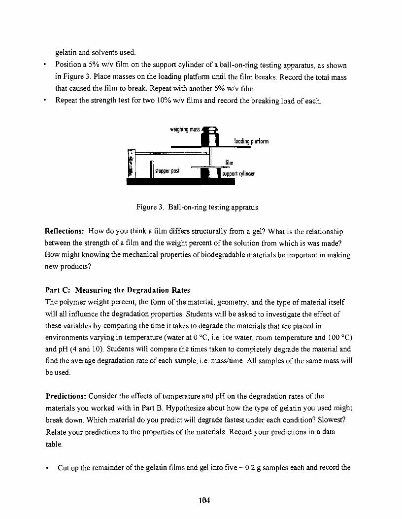
gelatin and solvents used. Position a 5% w/v film on the support cylinder of a ball-on-ring testing apparatus, as shown in Figure 3. Place masses on the loading platform until the film breaks. Record the total mass that caused the film to break. Repeat with another 5% w/v film. Repeat the strength test for two 10% w/v films and record the breaking load of each.

weighing mass

Figure 3. Ball-on-ring testing appratus.

Reflections: How do you think a film differs structurally from a gel? What is the relationship between the strength of a film and the weight percent of the solution from which is was made? How might knowing the mechanical properties of biodegradable materials be important in making new products?

Part C: Measuring the Degradation Rates The polymer weight percent, the form of the material, geometry, and the type of material itself will all influence the degradation properties. Students will be asked to investigate the effect of these variables by comparing the time it takes to degrade the materials that are placed in environments varying in temperature (water at 0 °C, i.e. ice water, room temperature and 100°C) and pH (4 and 10). Students will compare the times taken to completely degrade the material and find the average degradation rate of each sample, i.e. mass/time. All samples of the same mass will be used.

Predictions: Consider the effects of temperature and pH on the degradation rates of the materials you worked with in Part B. Hypothesize about how the type of gelatin you used might break down. Which material do you predict will degrade fastest under each condition? Slowest? Relate your predictions to the properties of the materials. Record your predictions in a data table.

• Cut up the remainder of the gelatin films and gel into five - 0.2 g samples each and record the

104

mass. Each sample should be a single piece. Students in each group will need to pool their

data. • Determine the mass of a gelatin capsule. Record the mass.

Use beakers to prepare three water baths with at least 200 ml of water in each at different temperatures: water at 0 °C, room temperature and 100°C. Prepare two more solutions one containing 200 ml dilute HCI solution (pH 4) and another containing 200 ml dilute NaOH solution (pH 10). Both of these solutions should be at room temperature. Into the hot water bath, place a sample of each of the four types of materials (gelatin capsule, gel, 5% w/v film, and 10% w/v film), one at a time. Be sure to measure and record each sample's degradation time before putting the next sample into the water.

• Place one sample of each material into the other water baths. This time you can put the samples in all at once. Record the time it takes for each sample to degrade. Note that the sample placed in water were at neutral pH, i.e., pH 7. Plot the temperature and pH vs. degradation rate for all materials on two separate graphs that show the relationship between each material's average degradation rate and the water temperature and pH.

Reflections: Compare your predictions with the results of the activity. Were you surprised by any of your results? Explain. How do pH and temperature affect degradation rate? Is the relationship the same for all the biodegradable materials you tested? How do the properties of biodegradable materials affect their degradation rates? How might these properties be useful in designing an effective medicine-delivery device? What might be some important criteria for such a device for controlled delivery? In what can the properties of gelatin films and gels be varied?

NOTES TO THE INSTRUCTOR

Mechanical Properties • Blank gelatin capsules can be purchased from Capsugel, 535 North Emerald Road,

Greenwood, SC 29646, (800) 845-6973.

• In the experiment, different concentrations of the gelatin was used to form solutions that show a range of viscous properties: from a viscous solution to a nonviscous gel. At low concentrations (5 and 10% w/v), the medium is not dense enough to allow the formation of enough hydrogen or van der Waals forces and so prevent the formation of a gel. However at

105

20 % w/v, the polymers are allowed to form these weak crosslinks and hence a network that is capable of holding the solvent. Notice that the volume of the gel is the volume of solvent plus gelatin. The gel, although it has the highest polymer weight percent, is not as mechanically stitT nor strong due to the presence of a large volume of solvent, evident in its weight.

• The films students produced are rather brittle and therefore not suitable for typical tensile testing. The stress concentration near the jaws of the testing machine cause failure at the jaws, rather than in the gauge section. However, the ball-on-ring device shown in Figure 3 provides a reliable method for testing the strength offlat, brittle specimens. The ball-on-ring test is particularly useful in measuring the relative strength of samples where precise knowledge of the fracture stress in not necessary. To calculate the maximum bending stress at the center, S, the theory of for transverse flexure of thin, elastic plates supported at several points yields the expression:

5 = [3P(1+ v)/ 4n t2] x {I + 2[In(a / b)]

+[(1-v) a2 /(l+v) R2] [l-W /2a 2)]}

where P is the load, I the specimen thickness, a the radius of the circle of support points, b the radius of the region of uniform loading (approximated by 113), R the radius of the specimen, and v is Poisson's ratio.

• The principle of entanglement provides a good basis for explaining mechanical integrity of the polymer films. The higher the % wlv, the stronger the film. This is intuitive since the higher the number of polymer chains, the denser the material will be, and the more entangled the polymer chains are, and hence the more resistive the material is to applied force. Students will find that the 5% wlv film only takes a few hundred grams to break, whereas the 10% wlv will take 20-30 times higher that of the 5% film. This is a good evidence that the higher weight percent film reached the critical concentration for entanglement. Plastic petri dishes, 60 x 15 mm, were used to cast all the films.

Degradation Rates • Students will have to be creative in deciding when the material is said to be fully degraded.

This issue should be discussed before starting the experiment.

106

• Students should be able to test materials to find their characteristic degradation rate at different environments and be able to quantitatively compare materials and their reaction to environmental factors like temperature and pH. They should also be able to find average degradation rates of materials and graph them to the various environmental conditions to show their relationship. Finally, they should know the advantages and disadvantages, as well as possible sources of error or inconsistency in using this method to characterize material degradation.

• In the activity, the "cid broke down the gel by all three degradation mechanisms. First, the gel's cross-links, formed by hydrogen or van der Waals forces, were degraded via the Type I mechanism. As a re:lUlt, the gel was broken down into small gel structures and linear chains. The acid further degraded the smaller gels via Type IT mechanism and the linear chains via Type III mechanism.

• pH will be a large factor in the determining the degradation rate of the gelatin. The gelatin capsules dissolve and degrade at low pH (high H+ ion concentration) following type IT mechanism. Here the H+ ions attack the unstable bonds in the backbone, breaking down the polymer into smaller molecules. At different temperatures, the effect on gelatin should not be as great. This is because heat has no effect on the H+ ion concentration which governs the degradation mechanism.

•

The geometry of the material also affects the degradation rate since surface area exposed to the environment are different. In the case of a surface degrading material, where the material exposed to the environment degrades first, geometry is a very important factor while for bulk degrading materials, where the whole material degrades at the same time, it is not as heavily dependent. Thus, the high surface area of the gelatin gel should increase the breakdown rate, while the geometry of the gelatin films should hinder the degradation slightly as compared to the gel. The gel also has a high surface area due to its porous nature which is filled with solvent rather than air.

Weight percent also affects the degradation rate. The denser material the longer it takes to degrade due to hindrance in the permeability ofH+ ions into the material. This, in essence, is a similar effect to decreasing surface area and can be thought of as decreasing the surface area at a molecular level.

In this experiment, degradation was described by the time taken to degrade a certain mass.

107

However, this is a very vague measure of degradation and does not show the details of the degradation mechanism. Mass is not always the best indicator of degradation because mass loss is not observed until the molecules have broken down enough to be able to "leak" out of the device; this is especially true of bulk degradation materials. The best indicator, iffacilities permit, is the measure of molecular weight of the material. Monomer concentration in the surrounding environment is also an indicator of degradation but this may not be accurate since the surface of the device must allow diffusion of the monomer out and this again does not happen until the molecules have been broken down sufficiently.

Finally, gelatin capsules are very useful drug delivery devices but disintegrate too quickly to allow release over a of days or months. Thus, there is still active research on the area offabricating devices that can delivery the drug for a longer period of time to eliminate the need for taking several doses. Furthermore, targeting of the drug is also under investigation to eliminate the need for a systemic consumption of the drug. Thus, the drug can be targeted to the problematic location at a much lower dose reducing any side effects due to the dose or the systemic circulation of the drug. For these purposes, much research is being conducted with biodegradable materials such as polylactic-co-glycolic acids which have been proven to be biocompatible through its use as a suture material. This material has a much slower degradation rate and this rate can also be controlled by varying the molecular weight and the mole ratios ofthe lactic and glycolic acids. This material can be fabricated into microspheres to be injected into the target location or as a matrix to be implanted surgically.

References: Biodegradable Materials, Materials World Modules Program, Northwestern University, Evanston, illinois.

Gijsbertus de With and Harrie H. M. Wagemans, "Ball-on-Ring Test Revisited," Journal of American Ceramics Society, Vol. 21 (Aug. 1989), pp. 1538-41

108

THE COMBINED EFFECT OF THERMAL CONDUCTIVITY AND THERMAL EXPANSION

IN A PMMA PLASTIC HEATED BY THERMAL RADIATION

Carlos E. Umana

Department of Materials School of Mechanical Engineering

University of Costa Rica San Pedro, Costa Rica

Telephone 506-235-6350 e-mail caruma@terraba.fing.ucr.ac.cr

109

Carlos E. Umana

110

THE COMBINED EFFECT OF THERMAL CONDUCTIVITY AND THERMAL EXPANSION IN A PMMA1 PLASTIC HEATED BY THERMAL

RADIATION

KEYWORDS:

Carlos E. Umana Departamento de Materiales

Escuela de Ingenieria Mecanica Universidad de Costa Rica

San Jose, Costa Rica

Infrared and visible electromagnetic waves, absorptivity and transmissibility of thermal radiation, heat conductivity, thermal expansion.

PREREQUISITE KNOWLEDGE:

The student should be familiar with electromagnetic waves and their relation with the thermal radiation spectrum generated from a black body.

OBJETIVES:

1. To show how electromagnetic waves interact with materials. 2. To introduce thermal properties of materials. 3. To motivate the students to explain physical changes observed in materials.

EQUIPMENT AND SUPPLIES: (See figure 1)

I. Hot plate 2. A thermocuople thermometer with a temperature range to not less than 200°C 3. Oxygen - Acetylene torch 4. Metal square with a visible scale 5. A piece ofPMMA 180mmx40mmx5mm (Not previously heated) 6. Stand and clamps to hold the plastic sample 7. Chronometer

I POL Y(METHYL METHACR YLA TEl

111

INTRODUCTION:

The three main thermal properties of materials are heat capacity, thermal conductivity and thermal expansion or contraction. They are all functions of temperature and it is always very important to analyze their interaction in order to predict the behavior of materials. In this demonstration it is also important to consider the interaction between thermal radiation and transparent PMMA plastic. In this experiment a piece of PMMA is held from one end in a flat horizontal position, like a cantilever beam. The plastic piece is located approximately 23 mm above the hot plate after it reaches 160°C. Most people would expect that the material would bend down as soon as it starts getting hot, however the plastic will bend up. The reason for such behavior is due to three combined factors which characterize thermoplastics: zero heat radiation transmissibility for large infrared wavelengths ( Ie> :; 11m) [Ref. I ], low thermal conductivity (k) and high thermal expansion (a). As a guide the last two thermal properties already mentioned are listed in Table I for some materials at 20°C.

Table I Comparison of Thermal Properties for Some Materials [Ref.2] Material Thermal Conductivity k Thermal Expansion a

(j·cm / cm2. s . DC) (1 / °C ) Copper 3.99 16 x 10-0

Iron 0.72 12 x 10-0

LD Polyethylene 0.0034 180 x 10-0

PMMA 0.002 90 x IO-b

Polystyrene 0.0008 72 x IO-b

PROCEDURE:(See figure I)

I. Cover the hot plate with a carbon film using a carburizing acetylene flame in order to represent a black body emitter condition.

2. Hold and level the plastic sample with the stand and clamps on a horizontal flat position and set it around 23 mm above the hot plate surface. Place the metal square vertically beside the heater almost touching the free end of the plastic piece in order to verify the deflection. Free sample length should be around 150 mm.

3. Place the stand away from the hot plate. Set the hot plate thermostat to 160°C and tum it on. Use the thermometer to verify the temperature.

112

4 . When this temperature is reached, relocate the stand so that the plastic is centered over the hot plate, check the height against the square and measure the time from this moment. Maximum upward deflection will be approximately 7.9 mm and will be reached in approximately 45 seconds. The deflection will be stable for 3 minutes, after this time the temperature becomes almost the same on both faces and the sample will start deflecting down due to the weight and softness of the material.

DISCUSSION:

In this demonstration the main heat source is the thermal radiation emitted by the hot plate, which can be considered as a low temperature black body emitter (433°K). Under this condition it only emits infrared waves of wavelengths larger than 3flm (see figure 2a) [Ref.3] Since the PMMA plastic is transparent to visible light it could be thought that it is also transparent to infrared waves. However the PMMA plastic absorbs completely the infrared radiation of wavelengths larger than 2.5 flm [Ref.l]. Therefore the transmitted thermal radiation throughout the plastic is zero (see figure 2b) It has been established that for most solids heat radiation is absorbed in a thin layer estimated to be less than 1.3 mm [Ref. 3]. Now it is easy to understand why the plastic bends up. The thin layer mentioned heats up and expands considerably due to the high thermal expansion of thermoplastics. On the other hand heat propagation is poor because thermoplastics have a very low thermal conductivity. The heat absorbed on the lower face is not transmitted easily to the rest of the material and it takes some time to obtain a stable temperature gradient within the sample. Once this happens the plastic becomes softer and bends down due to its own weight. Table II and figure 3 show the effect of plastic thickness on free end deflection. Samples of less than 5 mm will heat up too fast and will result in a smaller deflection. Samples of thickness greater than 5mm are more difficult to bend and once again deflection becomes smaller. Table II also presents the time lapses from the moment the upward deflection starts until downward deflection occurs for different sample thicknesses. It is concluded that the greater the thicknesses the longer the time.

113

Table II. Plastic Samples of Different Thicknesses.

Thickness (mm) Deflection (mm) Time (minutes) 3,65 3,9 3.5 4.4 7.1 3 5.0 7.9 4 6.3 6.4 8

INSTRUCTOR NOTES:

I. The person that makes the demonstration should wear thermal gloves and precautions should be taken after the demonstration due to the fact that the hot plate remains hot for a while after turning it off.

2. This is a cheap and easy way to demonstrate the interaction of thermal radiation with materials in addition to the combined effect of thermal conductivity and thermal expansIOn.

3. Plastic samples already used can be used again in order to show the effect of thermal degradation. Under the same conditions the deflection will be only around half of the original value, due to the fact that the properties of PMMA plastic will change when it is heated above its" maximum use temperature" which could be between 60°C and 90 °C (Ref. 4).

4. This demonstration can be used as a general purpose introduction on materials behavior or as support when teaching materials thermal properties as part of a basic course in materials science.

5. Human beings can only detect visible light and infrared heat radiation. If a sheet of PMMA is used as a shield over the hot plate, you will not feel the heat due to the fact that the plate is opaque to infrared radiation in the large wave length range and therefore works as a heat barrier. On the other hand this plastic is transparent to visible light so you can see the hot plate through the plastic.

114

REFERENCES:

1. Guy, A. G. : Fundamentos de Ciencia de Materiales. Libros McGraw- Hill de Mexico, S.A. DE C.V., 1980, p. 284. 2. Van Vlack, Lawrence: Tecnologia de Materiales. Fondo Educativo Interamericano, S.A, de C.V., Mexico, 1984. 3. Kreith, Frank: Principles of Heat Transfer. International Textbook Company, USA, 1968, pp. 213-214. 4.Strong, A. Brent: Plastics: Materials and Processing. Prentice-Hall, Inc., USA, 1996.

ACKNOWLEDGMENTS:

The author wishes to thank the Universidad de Costa Rica ( Vicerrectoria de Investigaci6n), La Fundaci6n de la Universidad de Costa Rica para la Investigaci6n ( FUNDEVI) and the Ministerio de Ciencia y Tecnologia - Conicit for giving financial support to attend the NEW: UP DATE 97. I also want to thank Prof, Allan Bloomfield for reviewing the grammar and vocabulary of this paper and the Material's Department senior assistant Carlos Jimenez for helping in preparing the demonstration.

115

METAL -SQUARE

HOT PLATE

r PMMA SAMPLE

D

STAND \

CLAMPS

Figure 1. Arrangement for Demonstration.

116

100

* 80

...J CO VI VI 60 ::E VI :z:

f- 40

20

O

I-

t-

0.2

V\r PMMA

, ,

,

, -'-0.5 1 2 5

WAVELENGTH, Jjrn (LOG SCALE)

rlJtravio,et +ViSibie tight-+---- Infrared

. i I . , I

1

0.2 0.5

BLACK BODY EMITTER SPEGRUM AT 433' K

1 2

I) \ WAVELENGTH, Jjrn (LOG SCALE)

5

10

10

Figure 2. Black body emitter spectrum and PM MA transmissibility for a range of electromagnetic waves

117

9

8 l" 7 -E

E -z 6 0 i= () ...... w ...... ..J 5 OCI u. w C C Z w 4 X w w 0:: u.

3

2 3.65 4.4 6.3

3.5 4 4.5 5 5.5 6 6.5 PMMA THICKNESS (mm)

Figure 3. Effect of thickness on maximun upward deflection

TEACHING REPORT WRITING USING MSE LABORATORIES

William D. Callister

Department of Metallurgical Engineering University of Utah

Salt Lake City, Utah 84112

Telephone 801-278-8611 e-mail bil1.callister@m.cc.utah.edu

119

William D. Callister, Jr.

120

TEACHING REPORT WRITING USING MSE LABORATORIES

William D. Callister, Jr. Department of Metallurgical Engineering

University of Utah Salt Lake City, UT 84112

KEY WORDS: Communication skills

PREREQUISITE KNOWLEDGE AND SKILLS: I) A basic understanding of the English language--syntax, grammar, spelling, vocabulary, rules of punctuation, etc.; 2) A technical writing course; and 3) Computer skills, to include competency with word-processing and graphics software.

OBJECTIVE: Improvement of technical report-writing skills.

EQUIPMENT AND SUPPLIES: Student access to computers and accompanying word-processing and graphics software.

INTRODUCfION

It goes without saying that a high proportion of engineering graduates in the U.S. are lacking in their writing and oral communication abilities. Many students probably decide to study engineering because their analytical and problem-solving skills are better developed than their communication skills. Furthermore, some may naively assume that effective communication is not an essential nor important component of an engineering career; consequently, courses which require reports and written answers to questions are avoided. Therefore, it becomes incumbent on departments of engineering to incorporate in their curricula measures to improve the students' communication skills. Required writinglEnglish courses in some measure helps to remedy these communication deficiencies. However, the engineering-specific writing experience is an essential and critical component in this developmental process Writing exercises not only help the students to become more facile in their communication abilities, but also to better comprehend and understand the concepts and principles relating to the engineering discipline.

The process of communication is exceedingly complex, and trying to teach someone to communicate effectively is a formidable task. This paper outlines a set of procedures used by the author, that has found some measure of success; it involves using reports on materials science and engineering laboratory experiments to improve students' writing abilities and communication skills. The following tasks and responsibilities are employed with this technique.

121

Each student is expected to do the following: (a) maintain a laboratory notebook, which is to be kept current; (b) submit by specified deadlines, a laboratory report for every assigned experiment; and (c) correct graded reports and then resubmit them for a final grade

Furthermore, it is important for the instructor to assume the following responsibilities: (a) outline the grading scheme that will be used; (b) provide explicit instructions relating to report format(s), and the content of each report that is

to be submitted; (c) specify report due dates, and strictly abide by them; and (d) have reports promptly graded and returned to the students.

Details relative to the manner in which of these procedures are implemented will now be addressed.

INSTRUCTIONS TO STUDENTS

General Instructions.

Undoubtedly, many of the students have had very little experience writing technical reports, and, thus, it is necessary for them to be instructed as to the elements, style, and format of same. The author spends the fust laboratoryllecture discussing in detail his expectations--e.g., report sections and the content of each, presentation of data (i.e., format of tables and figures), references, verb tense, use of pronouns, etc. It goes without saying that each report should be entirely prepared on the computer (i.e., using word processing, graphing, and spread sheet software). A handout detailing all of these instructions is given to each student.

At the end of this discussion, the students are assigned to plot up a set of data that is provided by the instructor. For example, the author uses some precipitation hardening data. These consist of several room temperature hardness values and their corresponding heat treating times that were taken at two different temperatures; a single hardness versus logarithm heat treating time plot is to be prepared and turned in at the next class meeting.

Also, at this time, the students are given two reports prepared by the instructor on the same experiment (which experiment is not one that the students will perform). One of these reports is well written and adheres to the rules discussed in class; the other is quite poorly written, and violates many of these principles. The students are: assigned to decide which of these reports is the poorer, and then to note in its margins all of the errors that they can find. During the subsequent class period, the poor report is discussed in terms of which of the rules were broken. The students hand in their plots and critiqued reports, which are easily graded by a teaching assistant or the instructor. Furthermore, students are told to keep the well-written report, and to use it as an example for their own reports.

122

Every instructor has his/her own grading scheme, and it is also important that the students be appraised as to these criteria during the first meeting.

Laborato[)'-Specific Instructions

The students are given a handout for a particular experiment during the preceding classllaboratory session in order to allow them to make the necessary preparations. In this handout is contained an outline of the experiment, perhaps a brief discussion of any theoretical bases for experimental phenomena, and details relating to format and preparation of the report. The deadline (date and time) for report submission is also noted on the handout. Students are assigned to read this handout before coming to the laboratory session.

During the laboratory period, the instructor (preferably) or teaching assistant discusses the procedural details of the experiment, any theory that is involved, and the report format. In addition, if a report submission deadline coincides with the lab session, reports are collected. Furthermore, at this time graded reports may be returned. Then the students go to the laboratory and perform the experiment.

Note: strict adherence to report submission deadlines is imperative; severe grade reductions should be levied for late submissions.

The author uses two report formats: formal and memo. Formal reports are prepared using the same format as the scientific literature, and consist of abstract, introduction, procedure, results and discussion, conclusion, and references sections. Normally this report format is utilized when there is some theoretical basis underlying the experimental results--for example, strain hardening. On the other hand, the memo report is employed when the reporting of results is the main goal of the experiment. In most instances, the memo report is much shorter and easier for the student to prepare. Therefore, the author usually alternates the assignment of formal and memo reports so as to even out the workload for the students.

GRADING

Grading of reports is a crucial phase of the procedure, and, for the instructor, the most time-consumptive one. Ideally, the instructor or faculty member should do all or most of the grading. It is imperative that the reports be carefully scrutinized and that inaccuracies and inadequacies be noted. Detailed comments explaining these deficiencies are important for two reasons. First of all, the student needs to be given appropriate feedback in order that he/she may understand what has done wrong, and that corrections may be made (as explained below). And secondly, the student is entitled to a justification for the grade that has been given.

Unfortunately, it may not be practical for the instructor or faculty member to grade the reports for large classes. The author has observed that only in very exceptional cases is a graduate teaching assistant qualified to grade laboratory reports. Another alternative is to arrange for someone from the WritinglEnglish Department to grade for grammar, style, punctuation, etc., and the faculty memberlinstructor to grade for

123

content, organization, completeness, etc. Of course, this approach requires paying for the services of someone from another department. Or, the professor/instructor may spot check only selected sections of the report, on which he/she basl!s the grade. Some have suggested that students grade/correct other students' reports. In the opinion of the author, this is of value in helping students see other students' mistakes; but he questions the ability of a student to make a fair, complete, and competent evaluation.

It is becoming fashionable to require students to e-mail their reports to the instructor, since more and more people are communicating in this manner. Furthermore, instructor feed-back to the students may also be provided electronically.

The author has found that a report grade is really a subjective evaluation; after having graded several hundred reports, one establishes their own grading scale, which cannot be quantified. In other words, an instructor need not think that it is necessary to justify in detail a grade (e.g., "how many points were deducted for this spelling mistake?"). When awarding grades, the author first corrects and makes comments on all reports (or has someone else go through this procedure). The reports are then quickly perused and arranged in a pile from best to poorest; grades are given in terms of a percentage.

It is imperative that graded reports be returned to the students as soon as possible. The importance and significance of these report-writing exercises are conveyed (not so subtly) to the student by the expeditiousness of the grading process. The element of hypocrisy is obvious to the student when a faculty member or instructor expects a laboratory report to be written and submitted within a week, and then takes two or three weeks to grade and return it. Furthermore, student motivation is severely squelched.

CORRECTION OF GRADED REPORTS

The author also requires the students to correct reports that have been graded before the final grade is awarded. This process involves correcting all mistakes that have been indicated and addressing all comments that have been made in the margins by the grader(s). Since the report has been word processed and (hopefully) saved, this correction procedure is normally not excessively time consumptive for the student. Both the original and corrected report are resubmitted, which facilitates the final grading procedure. Requiring report correction serves two purposes: (1) By rectifying these mistakes, the student hopefully is learning, by trial and error, correct writing principles; and (2) Some students rush through the report preparation in haphazard fashion "just to get it out of the way," with the expectation that they will settle for a mediocre report and whatever grade the instructor deems fair--of course, this procedure penalizes a student with this attitude. In extreme cases, the report will have to be completely rewritten.

LABORATORY NOTEBOOKS

Most entry-level, practicing engineers will be required to keep at least one laboratory notebook. Therefore, it is not unreasonable to expect these future engineers get in the habit of notebook maintenance as

124

soon as possible in their undergraduate experiences. Blank notebooks that have been designed specifically for laboratory usage are sold in virtually all college/university bookstores; these notebooks are glue bound rather than spiral or three-ring bound. Notebook entries are to be in ink (ball-point), and items to be included are as follows: notes taken on lectures given by the instructor and/or teaching assistant that relate to each experiment [i.e., outline of the experiment, the experimental set-up and procedures, apparatus used, details relating to content and organization of the laboratory report], diagrams, raw data, experimental irregularities, etc.

The author has the students tum in the notebooks once during the term--unannounced (to ensure that they are being maintained current), and then at the end of the term. Minimal time is devoted to grading; the notebooks are quickly perused by the instructor or T A, and, normally, very few comments are necessary. Credit is given to the student for turning in a notebook that is reasonably complete; otherwise no grade is awarded.

SUMMARY

This paper has presented a procedure designed to improve the writing skills of materials and engineering students by requiring them to write laboratory reports on experiments they have performed. The instructor (normally not a graduate teaching assistant) should take the first laboratory/lecture period to communicate to the students his/her expectations of the content, form, style, etc. of the reports, and, in addition, the grading scheme. It is suggested that a plotting assignment be given at this time, and, in addition, the opportunity to compare well- and poorly-written reports, and to critique the latter.

For each experiment, a handout should be prepared in which is described the procedure, theory, and report format. This handout should be distributed prior to the day the experiment is performed; its details are discussed during the laboratory period.

Suggestions were offered to expedite the grading process, while still providing for a credible evaluation. The ideal situation is when the professor/instructor does the grading, which may not possible with large classes. It is essential that graded reports be returned to the students in a timely manner; failure to do so conveys to the students that being competent report writers is of little consequence; it also diminishes motivation.

Reports that have been evaluated and returned are to be corrected by the students and then resubmitted. This facilitates the leaming process and discourages the students from doing just enough to get the assignment out of the way.

A laboratory notebook is to be kept by each student; its contents should replicate the kinds of information that would be contained in a practicing engineer's notebook--e.g., notes pertaining to the performance of the experiment and the collection of data, experimental irregularities, diagrams, raw data, etc. Some proportion of the final grade should be based on the maintenance of a suitable notebook.

125

BIOGRAPHICAL INFORM A nON

William D. Callister is an adjunct professor in Metallurgical Engineering at the University of Utah. His current professional interest is writing materials science and engineering textbooks; the fourth edition of his Materials Science and Engineering: An Introduction was published in December of 1996. Previously, he was actively involved in teaching and the administration of an undergraduate program in materials science and engineering. He received his B.S. degree in Ceramic Engineering from the University of Utah. Master of Science and Ph.D. degrees in Materials Science and Engineering were from Stanford University. In addition to the University of Utah, he has held academic positions at The Montana College of Mineral Science & Technology and Brigham Young University.

126

CRYSTAL GROWTH OF MIXED OPTICAL MATERIALS WITH THE AUTOMATIC

CZOCHRALSKIPULLER

George B. Loutts

Physics Department Norfolk State University 2401 Corprew Avenue

Norfolk, Virginia 23504

Telephone 757-683-2031 e-mail

127

George B. Loutts

128

Crystal Growth of Mixed Optical Materials with the Automatic Czochralski Puller

George Loutts Assistant Professor of Physics

Center for Materials Research, Norfolk State University, 2401 Corprew Avenue, Norfolk, VA 23504.

Tel. 757-683-2031, fax 757-683-9054, e-mail gJoutts@vger.nsu.edu

Key Words: crystal growth, Czochralski technique, optical materials, photonic materials.

Prerequisite Knowledge: materials science; optical and electronic materials, in particular; automatic control.

Objective: To apply Czochralski crystal growth technique in the synthesis of variety of photonic materials in the university environment.

Equipment and Materials: Custom-built Czochralski crystal growth station 99.99% or better purity chemicals (oxides, carbonates or phosphates) Liquid nitrogen, compressed oxygen Facility for the charge preparation (electronic balance, muffle furnace, ceramic cups, plastic bottles)

Introduction

Most of optical and semiconductor single crystalline materials produced in the electronic industry is grown with the Czochralski technique. This is the only technique capable of producing large high quality single crystals in a reasonable amount of time.

The technique originated, and took its name, from pioneering work by Polish engineer 1. Czochralski in 1917, who pulled single crystal wires (fibers) oflow melting point metals from the melt in order to determine the maximum speeds at which they could be crystallized. The technique has been modified and its application has been extended first to the growth of silicon and later to a very wide range of compound semiconductors, metals, oxides and halides. It is now the dominant technique for the wide range of materials in the electronic industries. Czochralski growth is initiated by dipping a seed crystal of a chosen crystallographic orientation onto the surface of a melt contained in the heated crucible. The seed is then slowly withdrawn, solidifying the adherent column of the melt in steady state at an average rate given by the sum of the pulling rate and the rate oflowering the solid-liquid interface due to the depletion of the melt in the crucible. The control of the desired crystal diameter is achieved by closely controlling the heat balance at the solid-liquid interface. The most important advantages of the Czochralski method are as follows:

129

(1) The use of a seed crystal to define the crystal orientation. (2) The absence of a container minimizes stresses induced in the growing crystal. (3) The possibility to rotate the crystal as it is being pulled from the melt. This

ensures radial symmetry of the thermal field in the crystal and provides uniform distribution of added dopants. The rotation can also be used to control the crystal-melt interface.

(4) The possibility to control the ambient atmosphere in the growth chamber. (5) The easy access to the melt provides the possibility to adjust its chemical

composition during the growth run. (6) The feasibility of establishing a versatile automatic control of the crystal

growth process.

1. Automatic Czochralski crystal puller

The design of the puller has been developed at Allied Signal Incorporated and then modified at the Center for Research and Education in Optics and Lasers, University of Central Florida, Orlando, FL, and at Norfolk State University. The design is very economical (over two times less expensive than commercially available Czochralski apparatus with comparable specifications) but it has proved to be very versatile, precise and reliable. This is because the design is concise, and its essential components are best available in the market. It also satisfies major safety and environmental requirements. The automatic control is simple to operate and labor-efficient since it can be accessed remotely through the computer connection.

The Czochralski crystal growth station capable of pulling oxide crystals with melting point up to 2100 DC consists of a furnace with power supply, a puller and a control system.

1.1 Furnace and high frequency power supply

A schematic view of the furnace is given in Figure 1. The melt is contained in an iridium crucible of 3 inch diameter, 3 inch high. The crucible walls are heated by a radio-frequency electromagnetic field generated by a 30 kW Pillar power supply and delivered by a watercooled copper coil, surrounding the crucible. The heat insulation of the crucible and growing crystal is provided by a set of concentric tubes, made of zirconia and alumina ceramics. Gaps between the tubes are tilled with zirconia bubbles. The envelope of the furnace is a quartz tube mounted in a water-cooled stainless steel jacket. On top, the quartz tube is covered with a water-cooled copper lid with two viewports for monitoring the crystal growth visually or with a TV camera. All the parts of the furnace are aligned in order to create a cylindrical temperature field with the axis in the middle of the crucible. By varying the number, thickness and position of ceramic tubes and

130

nitrogen gas t

Figure I, Schematic diagram of the furnace design, 131

'a tube

alumina

lids, both axial and radial temperature gradients in the crucible and in the crystal can be adjusted. Ambient atmosphere in the furnace is provided by a continuous flow of a mixture of nitrogen with 0.1-0.2% of oxygen, supplied through three inlets located in the bottom and in the viewports. The exhaust is located in the center of the copper lead. The composition of the gas mixture is controlled by separate flowmeters for nitrogen and oxygen.

1.2 Puller

The puller consists of a mechanical platform, two dc motors with gear boxes, an ac motor, electronic balance and crystal holder. The gas distribution system is also located in the crystal puller.

The seed crystal is mounted in an iridium tube with iridium wire which is attached to an alumina tube. The tube is mounted in an aluminum holder which is fixed to a dc motor with a gearbox. The motor provides rotation to the crystal at a variable speed ranging from 1 to 150 rpm with the stability better than 0.1 rpm. The motor together with the crystal holder is hung on a balance. The balance allows to continuously monitor the crystal weight with the accuracy of 0.01 g, and its signal is used in the automatic control system. The balance is mounted on a platform which provides mechanical support and precise vertical motion of the crystal. The motion is accomplished by a dc motor with a gearbox (slow pulling) and an ac motor (fast pulling). The pulling rate can be adjusted in the range of 0.1-50 mm/h with the stability of 0.00 I mm/h. Both the furnace and balance are placed on stands with anti-vibration pads.

1.3 Control system

The control system, shown in Figure 2, is composed ofa computer (PC), a Dimension controller and a 3-pen chart recorder (optional).

The weight of the crystal been pulled is continuously measured by the electronic balance and supplied to the Pc. The actual crystallization rate is calculated by the PC as the first derivative of the weight with time. This parameter is proportional to diameter of the crystal squared and used as an input of the Dimension in order to control the crystal diameter. The Dimf:nsion consists of a programmer and a controller. The controller compares a set point which represents the desired value of a process variable (crystallization rate :in this case) to the feedback signal which represents the actual process variable value. Depending on the magnitude, sign and persistence of the deviation, the controller changes the output signal going to the power supply in order to keep the deviation minimal. This is a closed-loop control or an automatic control.

There is also a second closed-loop with a feedback signal proportional to the power, supplied to the crucible. The two loops are cascaded (the output from the weight loop is mixed with the input of the power loop) which provides very smooth and sensitive control of the growth process.

132

output 0 0-35kw Actual growth r ate IBM-PC

RF Power Supply

RS232 Power Feedback Weight Scale

-Control r-, r-, End + input 2- + input I -

Dimension Controller Do

+ output 2- + output I -Dooo LJ LJ

crystal growth rate Puller and Controller

1-5mA Power output

"""- input I '- I I

input 2

Plotter

Figure 2. Schematic diagram of the control system.

133

The programmer, the second basic device in the Dimension, serves as a set point source external to the controller. All the data are entered before each growth run either manually, or from the PC. The process is programmed for hours, days and weeks if needed, and divided into segments with linear changes of the process variables within each segment.

2. Crystal growth procedure

The crystal growth process includes the following steps: charge preparation, loading and soaking, seed dipping, automatic growth, crystal separation and cooling.

2.1 Charge preparation

Usually chemicals of better than 99.99% purity are used for the charge preparation. First, they need to be dried in a muffle furnace at around 1000 °C for several hours in order to remove residual moisture. The required amount of each chemical is calculated according to the chemical reaction. In the case of preparation of neodymium doped barium fluorapatite, an efficient solid state laser material that we recently prepared for the first time [1], the reaction equation is as follows:

The first two components were thoroughly weighed, mixed in a plastic bottle and sintered in a muffle furnace at 950 uc for at least 4 hour. Then the mixture was grinded in a mortar, mixed with barium fluoride and neodymium oxide and hot-loaded in the cruciblc.

2.2 Hot loading and soaking

After the crucible is full, it is placed into the furnace and heated up to the melting point of the material. Then the rest of chemicals from the bottle is slowly loaded in the hot crucible through a quartz funnel. The hot loading usually takes 1-2 hours.

Molten chemicals should be left soaking for 6-12 hours. During this time, the melt, crucible, and furnace reach thermal equilibrium. Natural convection flows in the melt help the chemicals to be mixed and Nd to be distributed evenly throughout the volume.

2.3 Dipping the seed

The dipping process is the most delicate part of the growth. The seed (a thin rod made of oriented crystal) is attached to the crystal holder with iridium wires. Then it is moved into the furnace and stopped near the surface of the melt. The seed is held above the melt for several minutes in order to reach the temperature close to the one of the melt. The reason for doing that is to minimize thermal shock induced in the seed when it

134

touches the hot melt. When the seed is held above the melt, the weight balance is set to zero. Then the seed is move down slowly and dipped into the melt.

Once the seed touches the melt, there is a sudden jump of the weight. This is the result of meniscus formation due to surface tension. At this time, the instability of the growth makes automatic weight control impossible. The power is therefore controlled manually. The seed is left soaking in the melt for 5-10 minutes to reach the thermal equilibrium with the melt. During this time, it is desirable to melt back the seed a little bit in order to remove the material, damaged by cutting. Then the pulling is started at constant rate of 1-3 mm/h. After the crystallization rate is stabilized, the process can be set under automatic weight control. The automatic system will then proceed to gradually increase the diameter of the crystal to the desired value, according to the introduced program.

2.4 Growth under automatic control

The automatic growth continues for several days. During this time, all parameters should be maintained constant. Pull rate at 1-3 mm/h, depending on the type of material, dopant concentration and crystal diameter; rotation rate at 10-20 rpm, nitrogen flow rate at about 4 liter per minute and oxygen concentration at 0.1-0.2 percent.

2.5 Crystal separation and cooling

When the crystal reaches the desired length (10-15 cm) it should be carefully separated from the melt. In order to minimize thermal shock in the moment of separation, the crystal diameter should be diminished to around 5 mm by raising the temperature of the melt. This usually takes several hours. After the separation, the pulling will be stopped, and the crystal will be gradually cooled down to the room temperature over 1-1.5 days.

3. Application of the CzochraIski crystal growth station

With the Czochralski station described above, several congruent-melting and incongruent-melting compounds have been pulled from the melt for the first time. The key of this success is the high sensitivity of a state-or·the-art computer control system capable of adapting proportional, integral, and differential (PID) control to the physics and mechanics of crystal growth at different stages of the process. The system can deal with melts which change composition continuously during growth. It is particularly advantageous in the synthesis of mixed optical crystals because of the segregation of their components during the growth and accumulation of the dopants at the crystal/melt interface. Another key feature of the station is its high stability of operation during a crystal growth run which can be as long as two weeks.

U sing such stations, a series of new photonic materials have been developed at Norfolk State University and at CREOL, University of Central Florida, Orlando, FL over

135

the last few years. They include efficient solid state laser materials with the apatite crystal structure [1-4], fast and bright LSO/GSO scintillators [5], and manganese doped aluminate crystals which show promise for the application in holography and optical storage [6]. A list of relevant publications with the author participation is given below.

Acknowledgements

Support for this wark was provided by NASA grant #92-207 and DOE grant #DE-FGOI-94EWI1493.

References

1. G.B. Loutts, C. Bonner, C. Meegoda H. Ries, M.A. Noginov, N. Noginova, M. Curley, P. Venkateswarlu, A. Rapaport, M. Bass. Crystal growth, spectroscopic characterization, and laser performance of a new efficient laser material Nd:Bas(P04)3F, App\. Phys. Lett., 71,1997,303-305.

2. G.B. Loutts and B. Chai. Growth of high quality single crystals ofFAP (CaS(P04)3F) and its isomorphs. in Growth, Characterization, and Applications of Laser Host and Nonlinear Crystals II, B.H.T. Chai, editor, Proc. SPIE 1863, (1993).31.

3. G. Loutts, P. Hong, B. Chai. Comparison of neodymium laser hosts based on fluoro-apatite structure. MRS Proc. New Materials for Advanced Solid State Lasers, 329, 1994,45.

4. S.A. Payne, L.D. DeLoach, L.K. Smith, W.L. Kway, J.B. Tassano, W.F. Krupke, B.H.T. Chai, and G. Loutts. Ytterbium-doped apatite-sturcture crystals: A new class of laser materials. J. App\. Phys. 76, 1994,497.

5. G.B. Loutts, A.I. Zagumennyi, S.V. Lavrishchev, Yu.D. Zavartsev, and P.A. Studenikin. Czochralski growth and characterization of (Lu[.xGdx)2SiOj single crystals for scintillators. J. Crystal Growth, 174, 1997,331.

6. G.B. Loutts, M. Warren, L. Taylor, M.A. Noginov, M. Curley, N. Noginova, N. Kuchtarev, H.J. Caulfield, P. Venkateswarlu. Manganese doped YAl03: a potential material for holographic recording and data storage. Conference on Lasers and Electro-Optics, Baltimore, MD, 1997, .paper CFH6, to be published in Phys. Rev. B, 57, January 1998.

136

HOW TO COMPUTE THE ATOMIC MAGNETIC DIPOLE MOMENT OF AN ELEMENT:

AN ENGINEERING APPROACH

Carlos E. Umana

Department of Materials School of Mechanical Engineering

University of Costa Rica San Pedro, Costa Rica

Telephone 506-235-6350 e-mail caruma@terraba.fing.llcr.ac.cr

137

Carlos E. Umana

138

HOW TO COMPUTE THE ATOMIC MAGNETIC DIPOLE MOMENT OF AN ELEMENT: AN ENGINEERING APPROACH

Carlos E. Umana Departamento de Materiales

Escuela de Ingenieria Mecanica Universidad de Costa Rica

San Jose, Costa Rica

KEY WORDS: Electronic magnetic behavior, quantum numbers, atomic angular momentum, quantifY vector addition.

PREREQUISITE KNOWLEDGE: This material is part of a basic course on materials science. It is expected that the students should have taken the physics courses which are common to all engineering programs. An introduction to modem physics would be helpful but not a requisite.

OBJETIVES:

1. To present a procedure to determine the Atomic Magnetic Dipole Moment (AMDM) of an element by using a graphical vector method. 2. To demonstrate how the quantum numbers can be used to obtain a basic magnetic parameter. 3.To describe an easy way to introduce the Atomic Magnetic Dipole Moment concept by using an engineering approach to handle quantum physics statements.

INTRODUCTION:

Materials science and engineering is a multidisciplinary field that covers physical and chemical concepts from an engineering approach. Solid state and quantum physics overlap with this field when the atomic magnetic dipole moment is considered. It is perhaps the main parameter to explain the electronic magnetic behavior of materials. According to most ofthe materials science books, obtaining the AMDM of an element is a very difficult task due to the fact that it is necessary to perform a quantified vector addition, an operation which sounds quite impressive and out ofreach of engineers. As a matter of fact the operation is not found in any materials science book, suggesting that engineers can not handle these concepts.

139

DEFINITIONS l

The atomic magnetic dipole moment ( ) of an element is given by :

L+2S) t1

Where: = Bohr Magneton: 9.27410 X 10-24 [JT1 ] tl = h 12n h = Planck constant: 6.62620 X 10"34 [Js ] L = Orbital angular momentum S = Spin angular momentum

(1)

Therefore, in order to obtain the AMDM it is necessary to define the vectors Land 2S and determine their sum. On the other hand thcse vcctors are related by equation (2):

J=L+S (2)

Where: J = Total angular momentum

The magnitude of these vectors are giving by the following equations:

(3)

(4)

I J 1= tl ).1 (J + 1) (5)

Where: L = L ml (ml is the magnetic quantum number)

S = L ms (ms is the spin quantum numbcr)

I Reference 1

140

THE QUANTUM NUMBERS

The four quantum numbers are presented in Table 1. This table can be used to assign correctly the four quantum numbers that correspond to each electron in an atom in order to define the values Iml and Ims which are necessary to calculate L, Sand J.

THE AMDM OF AN IRON ATOM: AN EXAMPLE

As an illustration the procedure is applied to an isolated iron atom. For the neutral iron the electronic configuration is as follows:

Fe Atomic number: Z=26 Argon configuration

It is important to mention that both summations, I ml and I ms are always zero for , the inert gas configuration. Therefore it is only necessary to consider the 3d(' and 45' electrons. The four quantum numbers for each one ofthese electrons are assigned according to Table I, as is shown in Table II.

141

-"" N

I Quantum Number I Symbol

Principal n

Orbital f Magnetic 1111

Spin I11s

r--0 1 e

--1111 0 1 0

1--111S 112 1/2 1/2

-1/2 -1/2 -1/2

1

0 0

0 0

1/2 1/2 -1/2 -1/2

-1 2

1/2 1/2 -1/2 -1/2

Table I. Quantum Numbers

Values

2 3

1 0 1 2

1 0 -1 0 1 0 -1 2 1 0 -1 -2

1/2 1/2 1/2 1/2 1/2 1/2 1/2 1/2 1/2 1/2 1/2 1/2 -1/2 -1/2 -1/2 -1/2 -1/2 -1/2 -1/2 -1/2 -1/2 -1/2 -1/2 -1/2

Values

4

2 3

1 0 -1 -2 3 2 1 0 -1 -2 -3

1/2 1/2 1/2 1/2 1/2 1/2 1/2 1/2 1/2 1/2 1/2 -1/2 -1/2 -1/2 -1/2 -1/2 -1/2 -1/2 -1/2 -1/2 -1/2 -1/2

Table II. Quantum Numbers of an Iron Atom

n f 1111 I11S

3 2 +2 +1/2 3 2 +1 +1/2 3 2 0 +1/2 3 2 -1 +1/2 3 2 -2 +1/2 3 2 +2 -1/2 4 0 0 +1/2 4 0 0 -1/2

I I11I=2 Il11s=2

Knowing I ml and I ms it is a simple matter to apply equations (3), (4) and (5) to obtain the following values:

I s I / tl = 2.449

At this point we have three vectors of known magnitude and related by equation (2). Using this information and applying a graphical solution as shown in figure 1, it is possible to establish the relative orientation of each vector.

Vector" S / tl " is already defined and therefore it can be duplicated as shown in figure 2 in order to obtain the vector [ L / tl + 2S Ih ], which is required in equation (1). Finally by applying equation (I), the value I I of the AMDM for iron can be obtained.

I I = I L / h + 2 S / tl I = 6.70

143

I I

/

/'

/ /

I

Figure I. Relative orientation of three vectors of known magnitude.

S/h

L/h

L/h +2S/h

Figure 2. Duplication of vector S / tl to obtain vector [ L Itl + 2 S / h ].

L/h

THEORETICAL AND EXPERIMENTAL VALVES OF " I fll /0" FOR IRON

Table III presents a summary of theoretical and experimental" I /0" values. In the case of solid iron the experimental value shown is more of an average than a specitic atomic value. For solid material it is assumed that the orbital contribution is zer02, in other words I L I / tl = O. The theoretical value for monocristalline iron was obtained by applying this criteria.

Table III. "I fl 1/0" Values For Isolate Atoms and Solid Iron

Theoretical Experimental

Isolate Atom 6.70

Isolate FeH Ion) 6.70 5.4

Isolate FeH Ion1 5.92 5.9

Monocristalline Iron 4.9 2.2234

REFERENCES 1. Gautreau, R.; and Savin, W.:Modern Physics. McGRAW-HILL BOOK Co., USA, 1978. 2. Kaganov, M.; and Tsukernik, V.: La Naturaleza del Magnetismo. Editorial Mir, Moscu, 1985. 3. Kittel, Charles: Introducci6n a la Fisica del Estado S6lido. Editorial Reverte, S.A., Espana, 1995.

2 Reference 2 '-Reference 3 4, At OaK

145

ALLOY COMPOSITION DETERMINATIONS

K. T. Hartwig

M. Haouaoui

and

L. R. Cornwell

Department of Mechanical Engineering Texas A&M University

College Station, Texas 77843-3123

Telephone 409-845-1585 e-mail rcomwell@mengr.tamu.edu

147

L.R. Cornwell

148

Alloy Composition Determinations

K.T. Hartwig, M. Haouaoui and L.R. Cornwell Texas A&M University

Department of Mechanical Engineering College Station, Texas 77843-3123

KEYWORDS Alloy, composition, cooling curve, density, phase diagram.

PREREQUISITE KNOWLEDGE An understanding of the Archimede's method for density measurements, phase diagrams and application of the "lever rule".

OBJECTIVES

This paper presents an alternative approach to learning about phase diagrams. The objectives are to provide students opportunities to 1) solve a problem by more than one method, 2) develop an appreciation for sample variability and measurement accuracy, 3) become more familiar with phase diagrams and 4) enjoy solving a mystery.

INTRODUCTION

Our junior-level materials science class at Texas A&M University includes a laboratory component that meets once a week for three hours. One of the experiments performed is on phase diagrams. Determination of composition is made by three independent methods so that the student gains an appreciation of measurement uncertainty and the value of solving a problem using multiple and independent approaches. The identification techniques include measurements of density, microstructural analysis, and phase transformation temperature determinations. For this example, five lead-tin alloy specimens covering the range of compositions from pure lead to pure tin are examined.

MATERIALS

Five hundred to 800 gram batches of seven to ten master alloys of different composition are prepared. New and different alloy compositions should be used each semester, to keep the game fair. For this example the following alloys are used:

• pure lead and pure tin • eutectic Pb62Sn • hypo eutectic Pb40Sn • hypereutectic Pb90Sn

149

EQUIPMENT

For density measurements, the following equipment is required: • accurate balance (to 0.0001 gm) • fluid bath for displacement measurements • fine wire for specimen attachment

For cooling curve measurements, the following equipment is required: • 50 ml ceramic cup with lid to contain molten alloy • small glass tubes for thermocouple protection • Type K (chromel-alumel) thermocouples • chart recorder for time-temperature measurements • small furnace to melt alloys

For microstructural examination, the following equipment is required: • metallographic polishing apparatus • chemicals for etching • optical microscope (20-400X) and image recording equipment • or image analysis software for phase fraction determinations

PROCEDURES

The students work in teams of four to six. Three different experiments are typically run in parallel in a class of no more than fifteen students. It is suggested that the students in each group pair off and that each pair conduct two of the three independent determinations of composition. Each of the three approaches can be undertaken independently which allows all students to collect measurements of composition by two completely different methods. When all of the measurements have been completed, the students share results with the other members of their group and each prepares a lab report using results from the three approaches.

COMPOSITION DETERMINATION USING DENSITY MEASUREMENTS

For density measurements, the students measure the mass of small volume (0.3-2 cm3)

specimens (prepared beforehand) in air and under water. They also weigh and measure the volume of the specimen attachment wire. Samples of each alloy are measured three times each and for one composition three different specimens are measured. Density is determined with a formula the students are challenged to derive. One can deduce the following formula which permits determination of the density, p, of the alloy:

p = ws*pd(ws - WS+W(L) + ww) (Eq. I) PL: density of liquid (water). Ws: weight of the sample. WW: weight of the wire in water used to hang the sample. WS+W(L): weight of wire and sample immersed in water.

150

Composition is determined by application of the rule of mixtures given the densities of the pure metals: Palloy = I fiPi' Multiple specimens and measurements allow for a determination of specimen variability and measurement accuracy.

COMPOSITION DETERMINATION USING THERMAL ANALYSIS

One of the most widely used methods for determination of phase boundaries is by thermal analysis. The temperature of a sample is elevated to within the liquid field, and then the sample is allowed to cool naturally. The shape of the resulting curve of temperature versus time captured by a strip chart recorder is analyzed and compared to the curve found for a pure material. When pure metals freeze, there is a thermal arrest in the cooling curve. Cooling an alloy through a two-phase region results in a reduced rate of cooling in the two phase region. See Fig. 1 for an idealized example. The temperature at which there is a sudden change in slope of the cooling curve marks a phase boundary. Care must be taken to determine the true transition temperatures from a cooling curve because of the non-equilibrium conditions inherent in such a dynamic test such as undercooling and heat removal effects. The students are asked to develop a specific method for determining the cooling curve transition points.

L

'+-= __ Liquidus

a+Eutectic

Time Pb Weight percent tin Sn

Fig. 1. Ideal cooling curve of a hypoeutectic Pb30Sn alloy.

COMPOSITION DETERMINATION USING METALLOGRAPHIC ANALYSIS

Metallography specimens are cut from the castings using a diamond saw. Liquid coolant is used when cutting specimens to minimize the possibility of overheating. The cut surfaces of such specimens are sufficiently smooth so as to require only light grinding and polishing prior to microexamination.

Extreme care must be taken during the grinding and polishing of pure tin because distortion of the surface may cause recrystallization and mask the true structure of this low melting temperature metal. For the pure lead, etch-polishing which consists of the alternately

151

chemical etching and polishing until a bright surface is obtained is required because the lead smears easily. Sometimes, several cycles of polishing, etching and examination are necessary. Preparation of the eutectic and off-eutectic compositions are the same as for pure tin. Light etching with Keller's reagent is effective for enhancing microstructural features.

The microscopic examination of these alloys is easily performed using conventional bright-field illumination reflected light techniques. For this portion of the lab volume factions of the different microconstituents present in each of the samples are determined. For the present example, low power photo micrographs (40-200X) were collected and the different microconstituents separated physically by scissors and then weighted. Alternatively, a grid can be drawn over the micrograph and phase boundaries - grid line intersection points counted and used to determine phase fractions. If image analysis software is available, the percentage of different phase areas can be obtained directly. Conversion of the measured areas to corrected areas based on density differences between the constituents and application of the lever rule in conjunction with the phase diagram enables a determination of alloy weight factions (composition).

RESUL TS AND DISCUSSION

Experimental results along with theoretical values are shown in Table I for five different alloy compositions. Calculated compositions are shown in Table 2.

Table 1. Measurement Results for Pure Pb, Pb40Sn, Pb62Sn, Pb90Sn and Pure Sn

Planned Cooling Curve Microconstituent Composition Density Transition Fractions

3 (g/cm) (0C) Pb J:: s.n 1. 99.96 Pb 11.29 (11.36) 331 (327) 2. Pb 40 Sn 9.28 (9.74) 234 and 175 0.51 0.49

(232 and 183) (0.51 ) (0.49) (0) 3. Pb62Sn 8.44 (8.85) 175(183)

(0) ( 1.0) (0) 4. Pb 90 Sn (7.71) 218andl74 0 0.19 0.81

(217 and 183) a. 7.512 ± .003 (0) (0.21 ) (0.79) b. 7.494 ± 0.017 c. 7.474 ± 0.018

5. 99.92 Sn 7.30 (7.31) 233 (232) (0) (0) ( 1.0)

* Theoretical values are in parenthesis ( ).

152

Table 2. Calculated Compositions

COMPOSITIONS Theoretical wt% 100 Pb £hAQ Eb 62 So £b 2Q So lQQ So

(99.96) .s.n (99.92) Eb: Wl<asl.m::wl<ols Qf

1. Density 99.3S 51.3Sn 72.ISn 95Sn 99.S6 2. Cooling (undercooled)* (undercooled)* (undercooled)*

3. Microstructure 100.0 40Sn 61Sn 90.7Sn 100

* A freezing point depression could also arise because of contamination.

The Pb90Sn alloy is used as an example of composition detennination from density

measurements. The measured density of the alloy is 7.512gJ cm 3 while pure Pb and pure Sn have theoretical densities of 11.36 and 7.31gJ cm 3 respectively. The rule of mixtures relates volume fractions and phase densities:

P = (\ - x)PPb + xPSn (Eq.2) or

(Eq.3)

Inserting the measured and theoretical density values gives x = 0.95. Converting volume

. . fr· ( 0.95ccx7.3lg!cc J ·ld ·hfr· fractIOn to weight actIOn ' Yle s a welg tactIOn 0.95cc x 7.31 g cc + 0.05cc x 11.36 g cc

of Q.924 So. Errors/uncertainty from the density detennination can arise from voids in the specimen, air bubbles attached to the submerged specimen and wire, and differences in the densities of the theoretical and actual "pure" microstructural constituents. This latter problem could stem from nonequilibrium solidification and rapid cooling of the binary alloy.

Detennination of alloy composition from cooling curves involves two approaches. The first is to note any thennal arrests. Thennal arrests may be proceeded by a small region of undercooling but the plateau clearly signals the freezing of a pure material or the crossing of a horizontal boundary on the phase diagram. Pure Pb, pure Sn and the eutectic alloy all exhibited clear thennal arrest regions in their cooling curves with no other changes of slope. These thennal arrests at the eutectic temperature all showed significant undercooling (-SoC). The second feature to look for on cooling curves is an abrupt change in slope without a thennal arrest. This phenomenon marks the crossing of a liquid or solvus phase boundary. The Pb40Sn and Pb90Sn alloy exhibited slope changes at 234°C and 2ISoC, which correspond to compositions or Pb40Sn and Pb91 Sn. The slope change location can be defined by the intersection point of tangents drawn on the cooling curve just before and after the transition. Errors in composition detenninations from cooling curve analyzes arise from thennocouple inaccuracy (generally ±

153

2°C), impurities (tend to lower melting points) and poor cooling curves due to poor thermal characteristics of the specimen thermocouple - heat sink arrangement. Undercooling is to be expected.

From metallographic examination, it should be clear if any eutectic phase is present. Fig. 2b shows the microstmcture of the eutectic alloy that resulted from solidification in a copper mold.

Pb40Sn x240 Pb62Sn x1200 Pb90Sn x240

Fig. 2. Microstmcture of a) Pb40Sn, b) Pb62Sn and c) Pb90Sn solidified in a copper mold.

Eutectic constituents are clearly seen in the Pb40Sn, Pb62Sn and Pb90Sn alloys as shown in Fig. 2. The pure Pb and pure Sn alloys were largely single phase except for an occasional inclusion. As an example of actual measurements taken, the micrograph of the Pb40Sn alloy was 51 % by area a and 49% by area eutectic. Ifwe assume that these area fractions also represent the volume fractions, then the weight fractions are 57% Pb and 43% Sn. Errors in the metallography analyses stem from 1) analyzing an area that does not accurately represent an average distribution of the phases present, 2) etching artifact effects (overetching), and 3) nonequilibrium phase compositions.

DISCUSSION QUESTIONS

1. Why are the densities of the pure metals less than the theoretical values?

2. Explain your method for determining the cooling curve transition temperatures.

3. Explain why there are differences between the measured and theoretical transition temperatures.

4. Explain why there are differences between the measured and theoretical values for micro constituent fractions.

5. Which experimental method is least accurate for determination of alloy composition?

154

Of what value is this method?

6. Of the methods you experimented with, which is most accurate for composition determination and how accurate is it?

7. Give at least one other method that could be used to determine composition. Discuss the benefits and drawbacks of this other method.

8. Discuss the pros and cons of each method you studied in general terms (i.e. consider each method as a general characterization technique).

9. Check the literature to find an example ofa phase diagram determination (or a small region ofa diagram) and summarize the experimental methods used. Begin with the ASM Metals Handbook.

10. How would you determine the density of solid H20? Be specific.

REFERENCES

1. Holman, J.P., Experimental Methods for Engineers, McGraw Hill, Sixth Ed., 1994.

2. Box, G.E.P., Hunter, W.G. and Hunter, 1.S., Statistics for Experimenters, John Wiley & Sons, Inc., 1978.

3. ASM Metals Handbook, latest edition available on "Alloy Phase Diagrams."

BIOSKETCHES

Dr. L.R. Cornwell

Dr. Cornwell holds a B.S. from Birmingham University, U.K., and a Ph.D. from McMaster University in Canada, both in Metallurgy. He has several years industrial experience working at Rolls Royce, U.K., Canadian Westinghouse, Canada and Youngstown Sheet and Tube Co. in Ohio. He has been at Texas A&M University since 1971 and is a professor in the department of mechanical engineering. His current interest is in deformation processing and has been working in the ECAE program for the last three years. Along with other authors he has contributed to the National Educators Workshop for the past eight years.

Mohammed Haouaoui

Mohammed Haouaoui holds a BS from "Ecole des Mines de Sainte-Etienne", Fr in Material Science. He did a practical training experience at CEZUS in France (Compagnie Europeenne Zirconium Ugine Savoie) on the influence of different textures on the mechanical behavior of zircaloy products, using electron backscattering diffraction analysis. He has been at Texas A&M since June 1997 as an International Association for the Exchange of Students for Technical Experience (lAESTE) trainee with the Department of Mechanical Engineering.

155

Dr. K.T. Hartwig

Dr. Hartwig holds B.S. and M.S. degrees in Nuclear Engineering and a Ph.D. in Metallurgical Engineering all from the University of Wisconsin-Madison. He has several years experience with TRW Systems Group (Redondo Beach, CA) and the Nuclear Engineering Department at UW-Madison. He has been at Texas A&M since 1986 where he is an Associate Professor of Mechanical Engineering. He teaches undergraduate and graduate courses in Materials Sciences and Engineering. His current research interests are in high strain processing of advanced materials.

156

HOW A HEAT PACK WORKS

Robert A. McCoy

Professor of Materials Engineering Mechanical Engineering Department

Youngstown State University Youngstown, Ohio 44555

Telephone 330-342-1736 e-mail ramccoy@cc.ysu.edu

157

Robert A. McCoy

158

How a Heat Pack Warks

Robert A McCoy Professor of Materials Engineering

Youngstown State University Youngstown, Ohio

Key Words: Heat pack, undercooling, supercooling, freezing, crystallization, specific heat, heat of fusion, seeding

Prerequisite Knowledge: Basic chemistry

Objective: To experience first hand the exothermic crystallization reaction of an undercooled solution by observing the seed of the first solid, the growth of the solid-liquid interface, and the release of the heat of fusion. To measure and plot the rapid rise in temperature of a heat pack after being activated and its eventual cooling down under four different conditions. To explain the differences observed between the four different heating and cooling curves.

Equipment: I. handwarming heat packs (9x 12 cm), one for every three students 2. digital infrared thermometer or similar device to read surface temperatures from 0" C

(32" F) temperature up to 100" C (212" F) 3. stopwatch 4. computer with a graphing program or graph paper

Introduction:

Some liquid solutions and molten materials can be undercooled far below their freezing temperature before they crystallize and form a solid. A liquid that is held at a temperature below its equilibrium freezing temperature is said to be undercooled or supercooled. This undercooling phenomenon is due to the fact that a critically sized solid particle must first be formed before the metastable liquid can freeze. Mechanical agitation such as vigorous stirring or the introduction of a seed crystal can provide that first critically sized solid particle, which continues to grow.

During the freezing reaction, heat is released because the material transforms to a lower energy state. This amount of heat released per mole or unit mass is called the heat of fusion. This released heat raises the temperature of the material from the undercooled temperature to the equilibrium freezing temperature. The amount of heat energy required to raise a unit mass of material by one degree is the specific heat of the materiaL A similar material property with different units is heat capacity, which is the amount of heat energy required to produce a one-degree rise in temperature per mole of materiaL

159

A fixed quantity of under cooled liquid that begins to crystallize will rapidly rise back to the melting temperature of the material and remain near this temperature until all of the material crystallizes. It cannot rise above the melting temperature since it would remelt. Therefore the partially crystallized material remains at the material's melting temperature until it is completely crystallized How long this process takes depends upon the rate that heat is lost out of the material into its surroundings. Rapid heat loss will result in a shorter time to complete crystallization. After the material has completely crystallized, its temperature will decrease back to ambient temperature at a rate that is dependent upon the heat capacity of the material and the rate of heat loss into its surroundings.

Description of the Heat Pack:

Several brands of handwarming heat packs are on the market but they are all very similar in composition and work in the same manner. The plastic pouch contains a water solution of sodium acetate. This solution is formed by dissolving 60g of sodium acetate in 100mi of water at 1000 C (212° F). Theoretically when this solution is cooled to about 50" C (122° F), the crystalline solid of sodium acetate trihydrate should form by the reaction:

(1)

Usually, however, this reaction is suppressed to a temperature well below room temperature. That is, at room temperature, this solution is in a metastable, undercooled liquid state and will remain in this condition indefinitely until the crystallization reaction is triggered. This tliggering is accomplished by flexing a small, grooved stainless disk that is floating loos,e within the pouch, as shown in Figure 1. There are two explanations as to how flexing of the disk triggers the reaction. One explanation is that the mechanical agitation from flexing the disk provides the extra energy to form a stable nucleus of the crystalline solid. The other explanation is that within the grooves of the disk are tiny seed crystals that are released when the disk is flexed.

Once the crystallization reaction begins, the white opaque crystals spread rapidly across the pouch, as shown in Figure 2. The larger the amount of under cooling, the faster that the crystalline zone sweeps across the pouch since the driving force of the transformation is greater. Because the reaction is exothermic, the temperature of the pouch rapidly rises to about 50° C (122° F) and remains there for an extended period of time The pouch temperature cannot exceed 50" C since this is the melting/freezing temperature of the solution. Although the transformation to a crystallized solid may appear complete after about 15 seconds, some solution continues to crystallize at a rate such that the heat of fusion being liberated equals the heat lost to the pouch's surroundings. This balance of heat released versus heat lost maintains the temperature of 50" C until all of the solution has crystallized Only then does the pouch temperature begin to decrease.

160

Figure 1

161

Hgure 2

162

The temperature versus time curve for a heat pack from the time the disk is flexed until it returns to ambient temperature is dependent upon two factors. 1. The higher the temperature of the heat pack at the time of activation, the longer it

takes for the crystal1ized zone to sweep across the heat pack and the longer that the heat pack stays at 50° C before cooling to ambient temperature.

2. The faster that heat is lost to the heat pack's surroundings, the sooner that the heat pack cools down from 50°

Procedure:

ldeall y the class should be divided into small groups of about three students to provide as much individual hands-on experience as possible. Each group should consist of a time-keeper using a digital watch, a temperature reader using an infrared thermometer, and a recorder to write down the data. Each group should be assigned gathering data to plot heating and cooling curves of their heat pack under different conditions. The two variables are: I. The heat pack temperature at the time of activation, (To) 2. The temperature of the surroundings one minute after the heat pack is activated, (Ts)

A minimum of four experimental runs should be conducted using the conditions stated in the following table:

Run To Ts I RT RT 2 RT 0° C (32° F) 3 40°C (104°F) RT 4 40° C (104° F) 0° C (32° F)

RT is room temperature, 0° C is obtained by submerging the pouch in an ice-water bath one minute after activation, and 40° C is obtained by using a hot-water bath. Before starting each experimental run, position the disk in one of the corners of the pouch. Start timing when the disk is flexed. While the solid region expands, observe the form and direction of the crystals that are growing into the liquid

For each run, record the following data as shown in the table below. To = Temp. of heat pack just before activation T, = Temp. of surroundings of the heat pack into which the heat pack is placed one

minute after activation t' = time required for the crystallized zone to sweep across the heat pack. Ti = Temp. of heat pack at i = I, 5, 10, 15,20 minutes.

Run To T, t' TI Ts TIO TIS T20 I 2 3 4

163

Plot the temperature versus time for each run. Figure 3 below shows the cooling curve for run #4. Explain the differences observed between the four plots.

The heat pack can be reused repeatedly if it is properly remelted This process is accomplished by immersing the solidified heat pack in a container of hot water in the temperature range of 77 -100° C (171-212° F) for about ten minutes. After this procedure, the liquid should be perfectly clear. If it is cloudy, keep the heat pack in the hot water for another five minutes. Ifusing a microwave oven, make sure the heat pack is completely submerged in a container of water.

The class should think of other different practical uses of heat packs besides being used as handwarmers.

Notes to the instructor:

I. There may be a variation of several degrees difference in temperature along the surface of a heat pack For repeated temperature readings, use the same location, e.g. the center heat pack Also, for plotting purposes, round ofT the data to the nearest degree.

2. Bring to the attention of the students in runs 3 and 4 with To = 40° C that after the crystallized front has swept across the entire pouch, the crystallized zone is far from being a solid. It is in a "mushy" state with a considerable amount of the solution yet to crystall ize

3. Before taking the temperature of the heat pack that is submerged in ice water, quickly remove it from the water and dry it in the area where the temperature is being read.

4. Handwarming heat packs can be ordered wholesale from Prism Technologies, Inc. for $2.08 each when a case of 48 heat packs is ordered at 1-800-432-8722.

5. Infrared thermometers can be ordered from Omega Engineering, Inc. for $345 and up at 1-800-826-6342.

References:

1. Murr, Lawrence E, ed.: Solar Materials Science, Academic Press, Inc., 1980, pp. 376-392

2. Wada, Takahiro "Heat Storage Capacity of Sodium Acetate Trihydrate During thermal Cycling," Solar f_'nergy, Vol. 33, No. 3/4, 1984, pp. 373-375

Robert A McCoy is a professor and the director of the materials engineering program at Youngstown State University. He also is a failure analysis consultant.

164

Figure 3 Heat Pack Cooling Curve for Run #4

60

50

40

20

10 , -----+-----

o o 5 10 15 20

time (minutes)

Figure Captions;

Figure 1. A heat pack showing the clear undercooled liquid before activation of the stainless steel disk seen in the lower right comer of the heat pack

Figure 2. A heat pack just after activation showing the white opaque crystals growing from the lower right comer of the heat pack

Figure 3. Heat Pack Cooling Curve for Run #4

Note to editor: Figures 1 and 2 are photos and Figure 3 is a line graph plotted on Excel.

166

LEARNING MORE FROM TENSILE TEST EXPERIMENT

Neda S. Fabris

Mechanical Engineering Department California State University, Los Angeles

5151 State University Los Angeles, California 90032

Telephone 213-343-5218 e-mail nfabris@calstatela.edu

167

Neda S. Fabris

168

LEARNING MORE FROM TENSILE TEST EXPERIMENT

Neda S. Fabris, Ph. D. Professor, Mechanical Engineering

California State University, Los Angeles, California

Key Words: coeffieient, strain hardening exponent, toughness Tensile test. engineering stress. engineering strain. truc stress. true strain. strain hardening

Prerequisite Knowledge: Basic knowledge of material hehavior in elastic and plastic regIon

Objective: To introduce students to the hehavior of the engineering materials in plastic region. To calculate true stress-true strain data. To analytically ohtain strain-hardening coefficients from cxperimental resul ts using two di fferent approaches. To estimate toughness of matcrials hy two ways: integrating true stress-true strain and estimating the area helow a true stress-true strain curve.

Equipment: I. Universallesting Machine 2. Dial extensometer J. Micrometer (0-1 inch) 4. Rail-micrometer (0.2-1.2 inch) 5. Steel scale (12 inch) 6. Divider 7. Standard 2-ineh metallic tensile test speeimen (steel. hrass a!uminum or cooper) X. Marking gage 9. Caleulator and graphing uniform and logarithmic paper. or cC)mputer math and graphic sotiware

Introduction Tensile test is the most of len perliJrmed materials experiment in the engineering practice. Also. almost every engineering curriculum ineludes tensile test experiment. It is a simple test. and it gives a wealth of information uscd in mechanical and civil engineering design. The modules of elasticity. modules of resilience. yield strength. ultimate tensile strength. rupture strength ductility and percent reduction in area is determined from the engineering (nominal) tensile test curve. II r However. hchavior of the material in the

. Numbers in I I represent rcf'erences on the end of the article.

169

plastic rcgion, where the strain hardening, cold work and forming of material take place, is characterized hy the true-stress, true-strain relationship. This relationship is rarely ohtained experimentally in the engineering school setting.

This paper deserihes the project "True Stress-True Strain Relationship" designed to expend students' knowledge of material hehavior in the plastic regioll. In the project students usc the standard stress-strain data ohtained in the material te,ting lahoratory during tensile test experiment so that special test is not necessary. By computing true stress-true strain data, students learn ahout material properties in the plastic region and develop a hetter understanding of the diffcl'enees hctween material properties important in design and those important in

In addition, this project guides students in all steps of process modeling, from experimental data to an analytical equation descrihing the test results This method proves to he a useful tool in analysis of all experimental results.

Experimental I'rocedure In our schooL mechanical and civil engineering students arc required to take the a) Tensile Test of the Mild Steel b) Tensile Test of Aluminum, Brass and Copper c) Tensile Test of Steel - Hysteresis (stress eyeling) Filed d) Effect of Cold Work and Carhon Content on the Properties ofearhon Steel

For the True Stress·True Strain project data arc taken from experiment a) and h). Those two tests arc typical tensile test experiments, and experimental procedure is standard as explained: Students arc supplied with a standard test specimen, 2 inch gage length and 1/2 inch diameter limll one of the Cour metals, mentioned in experiments a) or h), Fig. I. They arc required to measure the minimulll diameter of the specimen to the nearest 0.001 inch and computc the initial area. [Ising the 2-inch punch set. indentation marks arc placed on the specimen. From the tahulated properties of the metal. sllldents estimate the yield and maximum force to be cxpected in the experiment. This serves as a guideline in selecting proper sensitivity and scale on the tensile Illaehine.

The specimen is set and tightened in the tensile machine. I':xtensometer is attached to the specimen, and the tcst is periilrllled. I)uring the test students read load on the tensile machine and record the elongation at the same instant from the extensometer. Students arc warned to usc slow speed on the tensi Ie machine so they can get at least I () data points helow the prohahle yield pot. Arter the yield points the data arc recorded in larger increments. Once the load reaches the maximulll Illrce Illi' the matl'l'ial. (computed from the tahulated properties or the load starts decreasing), students have ttl take extellsomcter olTthe machine in order not to damage it during the fracture. Once the extensometer is rellloved, students attempt to record the data using dividers, although they orten do not succeed to get more than one or two data hellll'e the specimen fractures. Maximum lilree and f'raL'lure Illrce arc recorded, and necking phenoillena ohserved. Typical data sheet li'olll tile specimen liS given in the Appendix.

170

After the specimen is broken. it is taken from the tensile machine. The fracture surface is sketched. diameter of the fractured area measured with the ball micrometer. and the linal distance between the marks (initially at the 2-inch distance) is recorded.

Laboratory Report for the Standard Tensile Test Using experimental data obtained in the above described experiment. students arc required to compute nominal (engineering) stress S and nominal strain e based on the formula [21:

S=P/A o (Ibs/ineh') e=L1I/lo (inchlinch) (Ia.lb) where P is the load (force) read on the dial. Allis original area. L11 is the elongation read on the extensol11eter. and 10 is original length of the specimen.

For the report students have to tabulate following data: Load (Ibs). Elongation (inch). Nominal Stress (Ibs/ineh). Nominal strain (inch/inch)

On the graph paper 8 1/2 x 11 or 11 x 17 size ruled 1 () or 20 squares per inch. students plot nominal stress-strain curve to show the complete range of tIle test. using proper scales to fit the size of the graph paper. On the same graph stud,:nts plot another stress-strain curve until the yield point. with the same units Illr the stress and different (much larger) units Illr the strain. The purpose of this graph is to have a less steep slope of the elastic region and to determine modules of elasticity more accurately. On these graphs students arc asked to indicate and label points corresponding to the proportional limit. yield point. yield strength of 0.2% set. ultimate strength. rupture strength and the L1S and L1e used for the ealeulation of the modules ofclastieity ..

Material Properties Obtained in the Standard Tensile Test Based on the plotted graphs. students arc required to determine following: I. Proportional limit 6. Modules of elasticity 2. Yield point 7. Modules of resilience 3. Yield strength. 0.2%, set 8. Percent elongation in the gage length 4. Ultimate strength 9. Percent reduction in the area at fracture 5. Rupture strength These data students compare and contrast with similar data obtained in tensile tests Illr other materials.

True Stress- True Strain Project As it can be seen from above. the tensile test teaches students about important properties

of engineering materials and introduces them to procedures used to determine them. It shows. among other. the ditkrenee between engineering and science: regardless of how mueh we study atomic bonds and imperf'cetions in materials. the most useful data we need to design the structures and machines we obtain experimentally by breaking the spec lI11cn.

171

Although students can visually compare the elastic and plastic regions of dcl()rmation, no quantitative data is obtained to describe the strain hardening of the material. For that purpose, I use the same experimentally-obtained, load elongation data to assign "True stress-true strain" (TS-TS) project to more advanced studcnts in Manufacturing Processes class (junior level), students in graduate "Metal Forming" and "Machining Science" class, and in a somewhat simplified form, my sophomore "Materials in Engineering" class. All these classes arc only lecture classes. llere I will describe the complete (most elaborate) TS-TS project that I assign.

I supply students with the experimentally obtained load elongation data sheets and ask them fiJllowing questions:

I. Compute True Stress (cr) - True Strain (!;) values and plot thelll if possible ", on the same graph as engineering stress-strain curve.

True stress and true strain arc defined as:

IT = F/A (Ibs/inch\ !: = In ( III" ) (ineh/inch) (2a,2b) where A is instantaneous area of the cross section and I is instantancous length of the speellllen.

Length I can easily be fllUnd from expression 1= I ,,+t-.I while true area of the specimen can be computed from the constancy of volume in the plastic region until necking, i.e., A " I" = A I. Introducing these expressions in the equation 2 we obtain:

IT = S ( 1+e) I: = In (II e) (3a, 3b)

I':quation (la.) is not valid in elastic region where volume of til': specimcn is not constant (i.e., it is larger than original), however change in the area is so slllall that the true stress true strain data arc very close to nominal stress strain data. In the necking region both equations (3a) and (J.b) arc not valid becausc the strain is not uni form and the cross-sectional area is not constant. through out the spceimen. The only point where the true values of stress and strain can be completed is the fi'acture point where student can measure the fracture diameter afier the specimen breaks. By drawing true stress-true strain values on the nominal stress-strain diagram students can appreciate the di rJcrenee between true and engineering (nominal) values of stress and strain.

2. Draw true stress-true strain diagram on log-log paper and using that graph lind K and n (constants) in the expression:

(4)

•• Student working with MathCad sometime are not tillniliar in drawing two graphs on the same page.

172

where K is strength coefticicnt and n is strain hardening exponcnt for a givcn mctal. For most engineering materials 0< n > 1.

Equation 4. in log form is given hy

loga = log k+ n logf; (5)

During their course of study student learn how to find the analytical expressions fiJr the polynomial going through every assigned or measured point. This a very tedious procedure and polynomial has the power equal to the numher of points assigned. Students also learn how to find hest fit line or polynomial presentation of the given points. Ilowever. in this project they learn first timc how to find the analytical expression for the curve whose exponent is less than one using logarithm paper. Although Mathcad or similar computer program draw log-log diagrams and directly it is even more educational to actually find the points draw the line and cstimate the slope of the line. Onen students usc real values of the stress at two points and divide with the strain giving them thc value of exponent in millions. Naturally interesting discussion f(Jllows. Also. students look tin the constant K at the crossection of the line with the ordinate (Icli side of the diagram) while in this case at the point where f; = 1 and this is on the right side of the diagram. Onen K can he fi1und only hy extrapolation of data.

3. Find the value of exponent 11 uSll1g instahility conditions and compare two values ohtained.

It can he proven that 121 at the instahility point. i.e. point where the f<Jrce is maximulll and the necking starts. the valuc of the true strain "'. is equal to the strain hardening exponentn. Student can find "'. from e at that point as given in Eq.(3h). and compare that data with the one ohtained from the slope ofthc true stress versus true strain in thc log-log diagram

4. htimate the true toughness of the material. Usc analytical and graphical approach.

Students study in thcir class that the toughness of the material represent the amount of energy necessary to hrcak thc pal1 and that thc truc toughncss pCI' unit volume is the area helow thc truc strcss- truc strain curvc. Thcy ohtain toughncss hy cstimating arc a helow thc curve (counting thc squarcs) as well as intcgrating thc stress-strain relationship (Eq. 5). with thc valucs for K and 11 ohtaining in qucstion 2. Although thcse two cxpressions cannot givc us cxactly equal rcsults duc to thc localization of strain in nccking rcgion. studcnts ohtain fairly c10sc rcsults. Onc sam pic of student's project is given in Appendix of this paper.

CONCLUSION While undergraduate students in engineering arc vcry familiar with the Hooks law and stress strain relationship of thc enginccring materials in the elastic region. plastic region is often misunderstood or unknown quantity. Design text hooks do not help much. thc call

173

yield criteria ':I(lilllr(' cri/('I';((", implying that there is something wrong with plastically dcf()rming material. One of my luvor question to students is: where do you think knowledge of plastic deformation of a material is imp0l1ant') I f they do not come with the answer. I ask them: how would you like to draw the wire and then alkr operation is completed it comes back to the original length and diameter') This "neglect" of plastic deformation made me design this project.

Aller completing this project students understand propel1ies of Iraterial in clastic as well as plastic region much better. This ineludes stress strain relationship. toughness of the material neck i ng phenomena and i nstabi I i ty, In addition to that students also learn all steps involved from gathering the experimental data till extraction of material propel1ies and development of analytical expressions, and equations governing the process, They also learn that experimentally gathered data have to be scrutinized and not all ICed to the computer. As seen in the example of student work in the Appendi:,<. even one misread data gives the strange shape of the stress strain relationship in the clastic region, Students also learn that you can not always take a strain and multiply it with modules of elasticity and get strcss and vice versa. divide stress with modules of elasticity and get strain (as they almost always attempted to do), Most imp0l1ant lesson that students learn is that material docs not fail at yield point. it just dcforms plastically' Alter all. forming processes arc done aller yielding and world depcnds on forming to tranSI(l\'Ill raw material into useful products. There is a "lilC" atier yielding.

RF-FF-RF-NCF-S:

I. Askeland D.R.Thc ,'lcienCL' and I:'nginecring ojAla/eria/.\, Third I:dition. PWS Publishing Company 19R9 2. IkeI' 1",1' .. Jonston Mechanics III Ma/crials, McCiraw-llilllnc. 19R I :;, Kalpakjian S. II/anll/ac!"ring I'rocesses/llr I:'ngil)e('ring Ma/criols, Second Edition. Addison-Wcsley. Publishing ('ompany, 1991.

ACKNOWLF-DGMF-NT:

The author wishes to cxpress sincere thanks to the CSIII.A student Jaillles Anibal I(lr letting IllC usc his projeet in Appendix of this paper.

Neda Saravanja Fabris. is Professor of Mechanical Engineering Departlllent at ('alil(lrnia State llnivcrsity 1,0:, Angeles ( ('SIll ,A), She has graduated from llniversity of Sarajevo. Bosnia and Herzegovina. with Degree Diploma Engineer in Mechanical Engincering. Manuluc!uring Option in 1965, ller Graduatc study she has completed at Illinois Institute of Technology in Chicago Ill., where she has receivcd MS in 1972 and Ph.D. in I 97(l in Mechanical I',ngincering Departlllent. During 1996-1l)<)7 school year she was Research Associate in l,aborJtorium hlr Werklcuge Masehines ledlllishc Ilochschule in Aachen (iermany, She has tallght at the lIniversity of Sarajevo li'om 1965-1970, at Illinois Institute ofTcehnology from I 970-1l)76. at llniversity of Illinois 1974-75 and at CSIII ,A

174

from 1979 till present. She was a Chair of the Mechanical Engineering Department from 1989-1992. From 1976-1979 she was Memher of Technical Staff at Bell Telephone Lahoratory. in Napperville III. She has taught more than 24 different suhjects in the area of mechanics. materials and design and developed four classes in and automation. Iler research activity and puhlications are in tool wear. selfcxcitcd chatter in metal cutting and materials as well as in teaching methodology and recruitment of . . . women III engllleerlllg.

175

APPENDIX

Given:

D i 0507 in initial diameter

D r 0.3015 in final diameter

G_L i ,1950·in initial gage length

i = 129

G R Load-- 1 1

---u-- -ur GR =GRIO- 3 -- I - 1

ro.r-1 2 2 n·D i n·Df r-o.4i AO Af

T7{} A 0 =O.2019·in 2 A f=O.071·in2 ,

hT' Ir9{} rrrol

i7.TIl "TO!

i 13151

rg-:n :s-m: M W

jn-j g;g: I I

• • I

1 - :J , iT7;-' 'OlJ5'

I.

176

CALCULATIONS:

1.)

,-3,443.103

9 2.383.103

177

5.128.10- 5

2.051.(0"4

G_R, strain I!, C T.950

Load,·lb stress

I!j AO

5 EN(iR. STRESS STRAIN V.:ro 10 max) 9'10 r-----.-----------------------------------------------,

______________ 0--_---

1.8' 105 ..... ----.--------.---_______________________ _

9·104 1f---__ . ________ . ___________________ . _______ _

/ /

1 I

.

--

strain Ii ' strain , STRAIN (in.iin.)

ENGR. STRESS STRAIN (zero 10 .2 inlin)

0--

0--_-·

I :

- ..

--

I

--

o -1'10 40002 0.004 0.006 0.0079 00099 0.012 0.014 0.016 0.018 0.02

strain;. strain e;. STR.\l)i (in.:in.)

178

2.)

a) E stn:ss - stress es e2

x =0 .. I

y(x) =E(x - .002)

ENGR. STRESS STRAIN (zero to .02 inlin) S'IOS ,--------,----------------,

;;:'IR" OJ

@.streas Cj

'"

-1'10-4 O.OOS 0.01 0.02 strain Cj' strain C;,X STRAIN (in.lin.)

By using x-y trace we obtain the intersection of the two curves above.

x =.0036674

Y = 3.5. lOs

Thus the 0.2% yield strenght is : (J .2%Jield = 3.5· lOs

c) ultimate stress occures at maximum load

d)

Load u =695·lb

Load u (J u = A 0-

Area% AO-Af -.--·100

AO

(J u = 3.443· 103· lbin" 2

Area% = 64.636

179

3)

u

j = 3 .. 28

GRin - ,

Load·lb , fl true; ---A-.. -,

I

,

I

I

, I

i

I I

I

initial gage length

Gage reading

Note: P fracture

fl fracture= -A---final

True stress Strain graph

I

,

.

-------, --------! -_ .. 3.6'\0 sf

I ,

2.7'\0 5 I

,

1.8'\0

9'\0

5 I . .

I I

i I i 4

I

,

I

.VV" v.v, v.vu V.v" v.'" v.u v." v."' v."'

e truCj True Strain (inhn)

180

I 1 /-

,

,

v."'

4)

<1 truCj . -u

rr truej ......

.

!

I ,

,

i

,

, I

I ,

I ,

'., , ! :

i

I: !. , . : i

! !

I .

,

Y .

, ,

: :' I

/' V ., ! ,

,! I i I ' I : ! , ' I I'

, JI ,

i: I; 0:'" , ,

! I , " ..

, I ;'

J I! I ! I : , .. , '

I,

n =0.786

5 I' \0 1'10-5

I : !

I' \0 4

n-.56 using instability conditions

%difI - 0.87 - 56 100 0.87

note:

log( n ).·0.87

log( k ).2885

thus, n c.1349

lb k c 76736 ft k =63.947'lbin 1

! i

'. 'I ,

1" \0 3 e truCj' e truCj

True strain

, :

;

0.01

K = intercept ( e true I ' cr true I )

K =3.136

%diff = 35.632

181

!

I ,I i , ,

0.1

.

,

, , i' .1: : , , ,

i; ' ,

,

5)

toughne:ss- this interval is evaluated from 0 to .56

.56(n I) toughne:ss = ---- k

(n I)

toughne:ss = 350. 155· lb· ft analitycal approach

True: stress Strain graph

· ---, -------------- ·

(', ·

,

.VV1 U.U,j v.vo V.IL V.D U.U V.Ll V.L"

e truCj True Strain (inlin)

.

/ /

.

u.l./

There are approximately 70 complete rectangular in the grahp above. each of them is .002 by 60000 thus. the area is

t = 70· .00260000

t = 8.4· 103 graph approach

182

3

PROPERTIES OF MAGNETIC FERRITES WITH A SIMPLE FABRICATION METHOD

Luke Ferguson

and

Thomas Stoebe

Department of Materials Science and Engineering University of Washington

Box 352120 Seattle, Washington 98195-2120

Telephone 206-543-7090 e-mail stoebe@u.washington.edu

183

Thomas Stoebe

184

PROPERTIES OF MAGNETIC FERRITES WITH A SIMPLE FABRICATION METHOD

Key Words

Luke Ferguson and Thomas Stoebe

Department 0/ Materials Science and Engineering University o/Washington, Box 352120

Seattle, WA 98195-2120

Slip casting, deflocculation, iron oxide, sintering, magnetoceramics, ferrirnagnetic materials, magnetite, spinel structure, domains and grain boundaries, transformer core, magnetization curve, susceptibility, coercivity, hysteresis.

Prerequisite Knowledge Basic chemistry including the ability to calculate molar amounts of materials and

use a simple chemical balance for weighing powders, and some experience in the operation of a kiln or furnace are strongly recommended. Knowledge of basic safety practices for the laboratory and handling materials is required. Some basic electromagnetic theory and electronics experience would also be helpful.

Objec"tive This lab is designed to teach students a simple technique for making a water based

ceramic slip, and then using the slip to cast toroidal ferrite cores with interesting magnetic properties. Students may choose from a large range of compositions and substitute various processing steps during fabrication of the ferrites. The magnetic properties of the ferrites may then be measured to evaluate and compare results.

Equipment 1. Simple mold making equipment consisting of gypsum plaster; a small cardboard box

(approximately 4" X 4" X 2"), aluminum foil liner, measuring cup, and duct tape. 2. Chemical balance 3. Metal oxide powders, ZnO (code #4358 from J.T.Baker Chemical Co.), Fe 0 (code

2 3 #12375 from Alpha Aesar), NiO (code #12359 form Johnson Matthey).

4. Dispersant, (Darvan-821A from R.T. Vanderbilt Co.) 5. Small kiln or furnace capable of reaching at least 1000 degrees C. 6. Test equipment (Optional): spool of magnet wire, autotransformer (Variac),

frequency generator or simple oscillator circuit, LCR meters, oscilloscope, electronic integrator, BH loop analyzer.

7. Simple hand tools, spatula, mixing containers, eyedropper, 112" or 3/4" drill bit, hacksaw blade, small permanent magnets, eye protection, apron, and disposable gloves.

185

Introduction and Background

Magnetite is a naturally occurring ferrite, F e3 °4, and is probably the earliest known magnetic material. In early history, bits of magnetite were used to construct a crude type of compass for navigation. Today, ferrite materials have enormous commercial and scientific applications in the form of recording media, high frequency inductors and transformers, microwave systems, permanent magnets, and even transparent magneto-optical elements [1]. Many billions of dollars are spent in the production and development of ferrimagnetic materials, and the field will most likely continue to produce many opportunities for research and growth. Surprisingly, it has been only relatively recently that a theoretical understanding of magnetic ferrites has come into existence with the work ofN'eel in 1948 and production of commercial ferrites by The Phillips Laboratories in 1959.

Magnetite is in the same crystal structure family as the mineral spinel, and this may be indicated by writing the composition in the form (FeO)Fep3. There are many other possible ferrites with the general formula (MO) Fep3' where M is a divalent metal

2+ 2+ 2+ 2+ 2+ 2+ ion such as Mn ,Fe ,Co ,Ni ,Cu ,or Zn ,or a combination of such divalent ions. F errites with the spinel structure that are important as engineering materials include the Mn-Zn and Ni-Zn ferrites that are often used as electrical transformers because of their low power dissipation factors at high frequencies.

In the spinel structure, the ions form a cubic close-packed array with two types of interstitial sites, one tetrahedrally coordinated, and the other octahedrally coordinated with oxygen ions [1]. Different ions in the spinel ferrites tend to exhibit different site preferences. For example, the divalent ions may occupy octahedral sites along with an equal number of randomly distributed Fe3

+ ions while the remaining Fe3+ ions occupy

tetrahedral sites. ]n practice, the oxidation states and distribution of the cations among lattice sites depends upon the processing parameters used to fabricate the ferrites, including thermal history, firing schedules and kiln atmosphere. There is antiferromagnetic coupling between cations occupying the crystallographically different sites, and the magnetization of one is antiparallel to that of the other sublattice. Because the two magnetizations are of unequal strength there is a net spontaneous magnetization.

Iron is known to form at least four compounds with oxygen. Wustite (or FeO) has the rocksalt structure, hematite (or alpha Fe

20) has the corundum structure, and

maghemite (or gamma Fe20 3) and magnetite (FeO)Fe20 3 have the spinel structure. In

order to obtain the spinel compound it is necessary to convert a significant proportion of 3+ "+ +2

Fe ions to Fe- ions. This can be accomplished in a number of ways. For example, Fe is favored at high temperatures and is quenched in if the compound is rapidly cooled. A reducing atmosphere during firing also tends to convert Fe 3+ to Fe 2+ [1], and the addition

186

of metallic iron powder to stoichiometric Fe20 3 powder may also convert Fe3+ to Fe2

+

during firing. For the Mn-Zn ferrites to obtain desirable magnetic properties it is necessary to

+' maintain a major proportion of the Mn in the Mn - state, and this typically requires firing in a non-oxidizing atmosphere. Extra safety precautions should also be taken when working with manganese oxide compounds since they may cause damage to the central nervous system in some cases. The Ni-Zn ferrites have an advantage in that nickel compounds seem to present less of a health hazard than manganese compounds and they may be fired in air without oxidizing a significant proportion ofNi 2+ to Ni 3+. With this information in mind, the present experiment will be concerned with the fabrication of Ni-Zn ferrites. Gloves and a dust mask are recommended when working with any materials in powder form that may generate significant amounts of airborne particles.

Several important parameters are used to characterize magnetic materials. One particularly useful relationship describes the magnetization of the material as a function of the magnetizing field,

M=X H m

In this equation, H is called the "magnetic field strength", and H may be though of as a magnetic field that is generated by the electrical current in a coil of wire. It is possible to exert direct control over H by varying the current in the coil that generates it. The vector M is called the "magnetization", and this is a magnetic field that is generated by the material itself. The magnetization M is the net response of material when it is subjected to the driving field H. This is similar to the way a compass needle will rotate in the Earth's magnetic field to minimize the torque on the needle. The susceptibility, X , is a

m function that relates H to M. The ease with which the material may be magnetized (or coercivity H ), the magnetization at saturation (M ), the remnant magnetization after

c s saturation (M), and other important material specific quantities may be determined from curves generated by recording M as a function of H. In general, X can be a complicated,

m history dependent function of H; more detailed information about magnetization curves and how to build a simple apparatus to measure them can be found in a recent paper by Ferguson and Stoebe [2].

The susceptibility, and other material specific properties, are strongly affected by the microstructure that is determined during materials processing. Grain size is a major contributor to the susceptibility of the material because the motion of domain walls may be hindered by grain boundaries. The motion of the domain walls may also be hindered by microstructural defects, typically resulting in a material with higher magnetic coercivity. Increased porosity, particularly in ceramic ferrites, usually leads to increased coercivity. Processing experiments that may significantly change the magnetic properties of the materials used in this lab will be discussed in the next sections.

187

EXPERIMENTS

Step 1. Making a simple plaster mold for casting.

The molds for casting slurries or slips may be made out of simple gypsum plaster sometimes referred to as "Plaster of Paris," available in the home improvement section of many stores. This method of mold making appears to have been in use for at least five centuries. Mixing instructions can usually be found on the package, and a ratio of about 6 parts of water to 1 0 parts of plaster gives the best consistency for mold making. Upon setting, gypsum plaster forms a network of interlocking crystal whiskers that creates a highly porous structure. When the liquid slurry is poured into this mold, this porous structure rapidly draws the fluids out of the slurry by capillary action, and leaves behind a wall of compacted solids that are later removed from the plaster mold after drying. An important property of the gypsum plaster is that the pores are not easily sealed by suspended particles, so that the wall of compacted solids builds up quickly to the desired thickness.

To make the mold for this experiment, it will be sufficient to pour the gypsum plaster into small cardboard boxes about 2" square and 2" deep after lining the boxes with a moisture barrier such as aluminum foil. After the plaster has been allowed to dry for a day or two, an ordinary steel drill bit can be used to create a hole about 0.5" deep in the plaster block. The diameter of the hole should be between 0.5" to 1" and the drill bit should be twisted by hand while applying light downward pressure. It is important for the walls of the hole be as smooth and straight as possible so the cast part can drop out easily from the mold after drying.

Step 2. Determining the composition and weights of oxide powders for ferrites.

The nickel-zinc ferrites are relatively easy to fabricate successfully and they have remarkable magnetic properties that are easily determined by simple experiments. The Ni-Zn ferrites typically have a composition of Nid_1Znlep 4 where d may vary between 0.2 and 0.7. The value ofd has a very pronounced effect on initial permeability (high permeability materials show a very rapid increase in M with a small increase in H) and the Curie temperature (the specific temperature where a material loses its magnetizability). Large values of d produce high initial permeabilities and low Curie temperatures.

Ferric Oxide (Fep3)' the starting material for this experiment, is available in powder form with a suitably small powder size from many sources. Ferric oxide powder has the familiar reddish brown color of "rust" and does not stick to a permanent magnet the way that metallic iron will. Ferric oxide (Fep3) may be converted during high temperature firing into magnetite (Fep 4) and becomes strongly ferrimagnetic (see the discussion in the previous section). The black powder that sticks to a strong permanent magnet when it is swept along sandy ground is typically magnetite.

188

With a composition ofNi4lnlep 4 it is possible to produce material that is strongly ferrimagnetic at room temperature. The addition ofNiO and lnO powders to Fep3 powder in the proper proportions will give the desired composition. Chemical safety goggles, gloves, and a respirator or enclosure with ventilation should be worn for protection when airborne powders may be present (see the material safety data sheets, or MSDS, that are available from suppliers). It is recommended that the following suppliers and material code numbers be used for each type of metal-oxide powder because the particle size is satisfactory for making casting slips as supplied without grinding.

lnO powder, code 4358, from 1. T. Baker Chemical Co. Iron (III) oxide Fep3 powder, code #12375, from Alpha Aesar (1-800-343-0660) Nickel (ll) oxide NiO powder, code #12359, from Johnson Matthey

The first step will be to calculate the molar weight of each compound.

Fe20 3 = 169.7 gramslmol Zno = 81.4 gramslmol NiO = 74.7 grams Imol

Then the molar weights are adjusted according to the desired value of d in the formula above to obtain proportional weights for each of the three powders to be mixed. If d = .6 then,

(ZnO)d = (.6 moI)(81.4 glmol) = 48.6 g (NiO) l-d = (.4 mol)(74.7 glmol) = 30 g (Fe20 3) = (1 mol)(169.7 glmol) = 169.7 g

Step 3. Preparing the slip or suspension for casting.

Powders with particles in the size range of about 1 to 5 microns tend to be most suitable for making casting slips, and slips have been successfully made using the recommended powders supplied by the distributors cited in step 1 without having to resort to grinding methods such as jar milling. A casting slip may be made by suspending the powder particles in water. It is desirable to have the solids to water ratio as high as possible, and yet maintain enough fluidity so that the slip will easily pour into a mold. In many cases this can be accomplished by adding a small amount of "deflocculant" or dispersant to a thick slurry made with de-ionized water and the ceramic pOWders. The deflocculant typically contains ions that attach themselves to the solid particles in the slurry, and if the particles are light enough, they become suspended because of electrostatic repUlsion due to the ions on the surface of the particles. This phenomenon is easy to detect because the thick slurry will suddenly become very fluid when a few drops of deflocculant are mixed into it. Many commercial deflocculants are available for various

189

types of slip casting. A small amount ofDarvan-82lA seems to work well in this experiment. One source for deflocculants is R. T. Vanderbilt Company, Inc.

The first step in the slip making process will be to weigh out appropriate amounts of ferric oxide, zinc, and nickel oxide powders as described in Step 2. It is possible to use only the ferric oxide powder, and this may provide an instructive baseline experiment. The oxide powers are then combined in a metal or plastic cup where they may be stirred with a flat tool as water (preferably de-ionized) is being slowly added until a paste is obtained. The paste or slurry should have the approximate consistency of toothpaste. The next step is to add a small amount of deflocculant to the slurry or paste in order to create a suspension. Slowly add drops of Darvan-821A with an eyedropper and stir until the slurry or paste becomes fluid and can be easily poured. It may be helpful to first practice this method on smaller amount of ferric oxide only. The slip is now ready for pouring into a plaster mold.

Step 4. Pouring the casting slip or suspension into the plaster mold.

The casting slip should be poured relatively quickly into the hole in the gypsum plaster mold constructed in Step 1. It is important to spill as little as possible around the hole and to fill the hole just to the brim with the slip. As water is absorbed into the plaster mold the hole should be topped off with casting slip to give a unifonn wall thickness. After several minutes the plaster mold will beginning to saturate with water, and at this point the remaining liquid should be quickly poured off by turning the mold upside down and tapping if necessary. Fig. 1 shows a mold with slip after this step. At this time it is a good idea to carefully trim away any excess material that may have been spilled around the edge of the hole.

The mold is then placed aside and let dry overnight at room temperature. After drying, the compacted solids around the inner walls of the hole will shrink away from the plaster, and if everything works the way it is supposed to, it should be possible to gently remove the cast part from the plaster mold. The cast part should be in the fonn of a shallow cup

Several toroids or rings should now be made by gently cutting sections off the top of the cup with a hacksaw blade. This will provide the magnetic toroid for testing; several toroids made in the manner (some already fued and wrapped with wire for testing) are shown in Fig. 2. Please note that the cast material is somewhat fragile after removing from the mold, and it is sometimes referred to as a "green" object until it is fued in a kiIn orfumace.

Step 5. Firing the "green" ferrite in a kiln or furnace.

The "green" ferrite rings cast in Step 4 must be subjected to a high temperature cycle in a kiln or furnace before their magnetic properties and mechanical strength is realized. There is plenty of opportunity for experimentation with temperature heat-up rates, hold times and quenching in this step. Satisfactory magnetic materials have been

190

created by placing the green ferrites in a furnace in an air atmosphere and ramping the temperature up to 1200 degrees C in about 1 hour, holding at temperature for about 1 hour, and then cooling back to room temperature in about 2 hours. Most pottery kilns have a maximum temperature capability of about 1200 C. It may be possible to accomplish the solid state fusion of powders, called "sintering," at significantly lower temperatures (1000 C or less) by using longer hold times. Generally it is also possible to use lower and lower sintering temperatures as the particle size is reduced. Note the color change from reddish brown to black after firing the ferrites, an indication that the change to a spinel structure has taken place.

Step 6. Testing the properties of the magnetic ferrites.

One simple test that can be used to indicate a change of magnetic properties is to use a small permanent magnet and show that while the ferric oxide powder is only very weakly attracted, the spinel ferrite is strongly attracted to the magnet after firing. A more sophisticated and quantitative version of this test might be to place the ferrites on a non-magnetic laboratory scale or balance, and measure the decrease in weight as the ferrite is attracted to a permanent magnet that is moved into close proximity. Many types of interesting electronic experiments may also be performed with ferrite rings depending on the equipment available in the laboratory and the ingenuity of the experimenters. The basic idea usually involves making an inductor by winding multiple turns ofwire around the ferrite ring or making a transformer by adding another set of windings on top of the primary turns. The ferrite core inductor might be incorporated into a simple audio oscillator circuit, and then different ferrite cores could be substituted resulting in an audible change in pitch of the oscillator. Ferrite cores with lower magnetic penneabilities could be expected to give higher frequency tones in the oscillator.

Full magnetization curves showing hysteresis and many other important magnetic quantities in a graphical form can be obtained using the simple instrwnent described in reference [2]. A figure of an actual curve for a Ni-Zn ferrite core fabricated following the procedure in this experiment is shown in Fig 3.

ACKNOWLEDGMENT

This work was partially supported by the National Science Foundation's Advanced Technology Education (ATE) Program through grant #DUE 9602360.

191

REFERENCES

1. A. 1. Moulson and 1. M. Herbert. "Electroceramics", Chapman and Hall, New York. 1990.

2. L. G. Ferguson and T. G. Stoebe. "Observation of Hysteresis Loops and Barkhausen Effects in Magnetic Materials." The Journal of Materials Education. December,1996.

FIGURE CAPTIONS

Figure 1. Mold with slip after excess has been poured out. Result is a shallow "cup" of slip, which shrinks away from the mold upon drying and thus may easily be removed. Because the mold absorbs liquid from the slip, the mold is not reusable.

Figure 2. Typical spinel ferrite rings cut from the "green" slip, shown with rings that have been fired and which have been wrapped with wire for testing of the magnetic properties. The "green" material is quite fragile and must be fired prior to any excess handling and testing.

Figure 3. Magnetization curve (B vs. II) for a toroid made using the process described herein.

192

Ferguson & Stoebe Figure 1

193

Ferguson &Stoebe Figure 2

194

Ferguson & Stoebe Figure 3

195

EFFECTIVE LEARNING THROUGH INTERACTIVE COMPUTER SIMULATION AND

EXPERIMENTATION

W. Gregory Sawyer

Daniel Bryson

Torkel Svanes

Stark Design P. O. Box 429

Morristown, New Jersey 07963

Telephone: 973-734-9911 e-mail sawyer@starkdesign.com e-mail svanes@starkdesign.com

John B. Hudson

Materials Science and Engineering Department Rensselaer Po lytechnic Institute

Troy, New York 12180

Telephone: 518-276-6447 e-mail hudsoj@rpi.edu

197

w. Gregory Sawyer

Torkel Svanes

198

Effective Learning through

Interactive Computer Simulation and Experimentation

w. Gregory Sa'Wyer*. Daniel Bryson*. Torkel Svanes*. and John B. Hudson: * Stark Design. P.O. Box .+29. Morristo'W11. NJ 07963

:Rensselaer Polytechnic Institute. Troy, NY 12180

Key Words: Interactive Software, Educational Software. Computer Simulation. Computer Experimentation. Computer-Assisted Learning. Interactive Learning, Learning Software

Abstract

Computer software is proliferating in college classrooms. laboratories. and lecture halls. The software which is most effective in these learning environments is that software which presents the user with both simulation and experimentation in an integrated environment. Moreover, the ability of software to provide a compelling user experience is central to the effective dissemination of infonnation. Through our experiences of designing and building educational software we have developed a methodology and a set of guidelines which can be used to guide much of the software development process.

Introduction

The use of personal computers is proliferating in college science and engineering courses. This has led to the creation of an increasing amount of educational software. Much of this software is categorized as 'multimedia'. This tenn typically denotes software which is rich in graphics, sound, and user interaction, and which pennits the user to navigate through a non-linear arrangement of information. The major challenge facing educational software developers, however. is how to use the computer as a means of enhancing a particular lesson or discussion without distracting the student from the learning goal. This is often achieved by significantly reducing the number of system variables (often to 1 or 2) and model complexities. As a result. the integrity and reality of the model system are compromised. To maintain system integrity, developers must pay particularly close attention to the design-related aspects of educational software development.

A typical classroom is composed of students with various learning styles-visuaL auditory. and kinesthetic. Therefore the screen layout. use of color. motion. and sound must all work in concert to focus the learner on the central aspects of the experiment. The learner must also feel free to interact with the model system in order to explore the system variable dependencies and to discover the inherent complexity of realistic models. To facilitate this

199

level of involvement. the graphical user interface (GUO must be highly responsive to user interactions. In order to move beyond computer visualization or simulation to computer experimentation. the learner must also be allowed to collect and process simulation data without being distracted from the simulation. This is best achieved by removing non-information while maximizing the '"information resolution" of the screen. Customized. experiment-specific graphs. real-time regression analysis and tight synchronization between the user inputs. simulation motion. and the graphing components can all contribute significantly toward maximizing information resolution.

Overall, computer-based experiments benefit the learning community in a number of ways. They allow students to explore a wide range of problems [I J. They can provide immediate reinforcement and unique insights during the learning process. And in many cases. computer facilities are actually more economical than their traditional laboratory counterparts. These and other factors contribute to the widespread belief that the use of computers in education will likely not only continue but increase over time.

Hierarchy of Interactivity

Educational software can be divided into five distinct levels of interactivity. Each of these levels puts increasing emphasis on the user' s ability to direct outcomes and to reason \vith the educational content.

Watch and Learn: This level of interactivity forces the user to view various types of media in a predefined order. This often inel udes text. narration. and video presented in a sequential manner that is similar to short movies or commercials. The software is typically used as a substitute for more traditional forms of educational materials such as paper handouts. class movies. overhead transparencies. and live demonstrations.

Guide and Watch: This level of interactivity is really an extension of the previous Watch and Learn level and describes the vast majority of available educational software. Here the user must actively navigate through the software in order to view the prepared materials. The navigation system is often an ordered nonlinear design similar to web pages. rich in hyperlinks and directional buttons (i.e .. go back. go fonvard. replay. etc.). The navigation system allows for flexibility in the order in which prepared materials can be covered. This pemlits the user to return to compelling demonstrations and to tailor the timing and sequence of the learning experience.

Control and Animate: This is the first level of interactivity in which the user can actually affect outcomes. This level of interactivity is very well suited for animations of classical analytical solutions. For example. the ordinary second-order differential equation that describes the motion of a spring-mass system can be easily solved and animated. In this example each of the coefficients representing the system mass. spring stiffness. damping. and initial conditions can be attached to a number of different of input devices such as sliders or text entry boxes. This type of system permits the user to pose a problem and

200

visualize the system without having to solve all of the equations. In some cases it is quite likely that solutions to a number of different aspects of a system can be solved analytically. but that the solution of the entire system requires a numerical approach. This type of complexity. traditionally avoided in the classroom. can now easily be included through the use of software. This is the first level of interactivity that shows any promise of being an effective learning tool for education or instruction [2].

Simulate and Experiment: Software designed for simulation and experimentation has the most promise of being a highly effective learning tool. At this level the user is permitted to interact with complex systems. and can not only view the system simulation but actually acquire and analyze data from the simulation. Active user interactions are required by the program in order for the user to receive feedback from the simulation. The instructor may be needed to guide the experimental approach, pose insightful questions in need of answers. and describe the data collection process to the students. The software, therefore, is designed to promote not only interaction between the students and the computer. but interaction between students and instructor and interactions among the students themselves. These types of activities are well suited to group or class exercises that can be performed during lecture hours rather than dedicated laboratory hours. At this level, the entire class is acti vely participating in the learning process. Although outside of the scope of this paper, computer-based data acquisition as part of laboratory experimentation could be categorized in this level.

Authoring Environment: This level of interactivity requires the user to design and build the model system. Authoring environments for such educational topics as rigid body dynamics and physics are currently available. The best of these programs provide the user with a pre-developed set of tools which have been designed to facilitate the easy fabrication of a complete model system with a set of well posed problem conditions. There exist a number of criticisms regarding the use of authoring tools as educational software. One of these criticisms is that the increasing demands on the user's proficiency at using the software tool may not pay dividends in increased understanding. A second criticism is that the pace at which new material can be covered. or the frequency at which the software can be used. is reduced due to the time it takes for students to build and design model systems.

Reaching Students

The use of computer software to perform calculations for students has been found to increase their creativity [3]. This is primarily because the software is allowing the students to formulate relationships and explore the solution space without the tedium of meticulous and tiring analysis. Often times the students become caught up in the mathematics of the problem solution and lose an appreciation of the underlying principles. This is in no way meant to imply that analysis and calculations are not useful: in fact. having students perform these calculations prior to using software is a great way to develop students' appreciation of the software' s capabilities.

201

The opening paragraph in the book "How We Leam" [4 J states that the question of how people leam is as simple as it is complex: people leamthrough their experiences. It could therefore be argued that effectively reaching students requires the software program to provide a compelling experience. Laboratory sessions have historically been found to provide very effective learning opportunities for students. A \vell designed laboratory experiment will allow the student to gain insight and understanding of theories through practice. Great lecturers are notorious for illustrating key concepts and theories with practical examples and experiences to which the audience can easily relate. For educational software to be effective. the program must not only disseminate information but must do so in such a way that provides context and insight.

Interface Layouts

Advertisers know that the layout is one of the most important aspects of effective advertising [S. 6]. A well-designed layout should contain three essential components: a large photograph. a short caption of less than 20 words. and over 200 words of copy. The best advertising agencies spend a great deal of time and money evaluating the success of their advertising by monitoring sales. and a good deal of information about effective layouts can be found in this research. Using the principles of good advertising layouts. a software interface should possess three fundamental areas: a large colorful animation area. an area for concise titles and descriptions of the animation, and an area for detailed plots of the experimental data .

. __ __ . __________

11-

,

Full Color Photograph

Descriptive TrtIe or Heading

Copy

8.5-

Computer Screen Layout j, ,---:..----------"---------------,

Desaiptive Title or Heading

3x

,

202

Full Color Animation

4x

VISUal Display of Data

Figure I A comparison between advertising layouts and software interfaces. Similarities include large action areas. descriptive titles and easy-to-read information areas.

Two recommended interface layouts. one for an advertisement and one for an interface. are shown in figure I. The dimensional difference between typical advertising media and computer screens makes a direct correlation between the two somewhat difficult. However. in each case the largest area is that area dedicated to the animation or the photograph. This is the area that should attract the primary focus of the user. Once the user is comfortable with the animation it is likely that the focus will shift to the data visualization. Therefore. it is equally important to provide an appropriately sized area for the data visualization.

The Software Experience

Educational software should provide the user with a complete and compelling leaming experience. The computer game industry is at the forefront of providing compelling software experiences. Some of the things that are common to great computer game designs are the use of graphics. color. sound. the third dimension, and a high degree of system responsiveness. Additionally. most computer games take full control of the system display. This means that the game is running full screen and that all other programs including the system desktop and icons are temporarily hidden from the user during game play. This effectively removes all of the distractions that could cause the user to lose focus on the activity at hand-playing games'

Recommendations for Interface DeSign

Use o/Color: The thoughtful use of color greatly enhances the software experience. This should not be interpreted as a recommendation to saturate the screen in a collage of brightly colored objects. The overuse of color in an interface can easily become distracting. For this reason it is best to minimize the use of color, reserving colors for only those objects on which you are trying to focus the user's attention. A good design practice is to build the entire interface in grayscale, and then to add bright. primary colors to those objects which you want to draw the user's attention most closely. This practice will produce an interface that has a high degree of color contrast. Another aspect of color important to remember is that as many as 1 in 14 male students may be colorblind. To ensure a clear visualization for all students. colors need to be selected that are different in hue and brightness as well as color.

Realistic Motion: Artistic license should never be taken with simulation motion. If a user perceives the motion to be fake all of the trust that has been developed between the user and the softv.are will be lost. The dissemination of information requires the user to believe

203

the simulation and data collection. Any distrust of the software by the user greatly Impairs the effectiveness of the software to facilitate learning.

Three-Dimensional Objects: While motion and color capture the user's attention. three-dimensional objects have been found to draw the user into active interaction with the software. Those objects that can be grabbed. moved. toggled. or pressed should be presented to the user as three-dimensional objects. Additionally. these objects should be extremely responsive to user interactions. Once users have been prompted to interact with the system, they should be recognized with an immediate response.

Sound Effects.' Adding sounds to highlight events such as collisions. motion, or user interactions will further allow the user to focus on those things which appear to cause the sound. The inclusion of sound can greatly compliment and heighten the software experience. particularly for students with visual disabilities.

Avoid Clutter: More is not always better. Too much color. motion. or sound can be distracting and in many cases disturbing. Minimizing and focusing the use of color. motion and sound will make for an efficient graphical user interface. as well as provide the user with a satisfying software experience.

Be Consistent: Once a metaphor has been established in the software. be consistent with the metaphor. For example, if a color has been chosen to represent a specific object. always use the same color for that object. If a sound is used for a particular purpose, that sound should not be reused for something else. By remaining consistent with layout. color. and sound, the user will rapidly become familiar with the software interface

From Compute'r Simulation to Computer Experimentation

In a series of classic lectures in physics by Richard Feynman. he \vTote "observation. reason, and experiment make up what we call the scientific method" [7]. This description accurately describes what educational software ought to be striving for. Computer simulations allow the students to observe and watch animations. while the classroom experience should encourage the students to reason out the underlying science of the animation. Allowing for student experimentation in educational software would promote the scientific method described so concisely by Feynman.

Moving from computer simulation to computer experimentation requires careful thought about what information is most critical to the lesson. Computer programs can collect and generate a large amount of information and data. Limiting the data collection and display to a select number of variables will help illustrate the most pertinent aspects of the lesson. However, this does not imply a simplification of the science behind the simulation. The more realistic the simulation (not necessarily complex). the more likely the audience is to believe the data and gain a deeper understanding of the lesson.

204

A computer simulation of a spring-mass system was previously described in the Control and Animate section of the Hierarchy of Interactivity. This simple spring-mass simulation lends itself to a clear example of how a controllable animation can be used as a foundation for a computer experimentation module. As previously described. computer experimentation must provide all of the same features of a computer simulation with the addition of data collection and presentation. In the case of the spring mass system. the most fundamental feature of the animation would be to illustrate the relationship between the position and the velocity of the mass at various times in the oscillation cycle. This may appear obvious and overly simplistic. yet this relationship is fundamental to the spring mass system. The student's understanding of this information can provide a foundation for more involved experiments in the future. Additionally. the same computer simulation can be reused in later lessons with the more advanced system calculations implemented. This is attractive not only to the educator. because it provides a continuity in the lesson exercises, but to the program designer as welL because the same work can be leveraged a number of times for multiple lesson modules.

A central aspect in designing effective computer simulation and experimentation is that to be effective the experimentation must not intimidate or overwhelm the user. In the case of the spring-mass system such calculations as position. velocity. acceleration. potential energy, and kinetic energy. could be implemented all at once. Doing this without providing an appropriate educational foundation, however, could overwhelm the learner and jeopardize the entire lesson. It is therefore usually better to illustrate important points one at a time rather than risk being misunderstood in the name of completeness.

Visual Display of Experimental Data

The visual display of data is an area in which researchers and statisticians alike spend numerous hours developing personal preferences and custom styles. This can be problematic in a classroom. especially if students are exposed to radically different styles of information presentation. The effective exchange of information is at the heart of the lesson objective, and to this end all distractions should be minimized. Central to the effectiveness of the visual display is the data itself. The data should be collected and processed in such a way that the relationships suggested by the data are shown as clearly as possible. A great deal of research has been done in the area of the visual display of quantitative information and a good historical overview of the field can be found in a series of texts by Edward Tufte [8. 9].

Two different plots of the same experimental data are shown in figure 2. In figure 2a the raw data is plotted with no statistical analysis or curve fitting. In figure 2b the same data set is plotted with appropriate regression and statistical analysis. If the focus of the lesson is on finding a relationship between the values plotted on the y-axis and the values plotted on the x-axis. it is clear that the second graph displays this information more efficiently. Although there is a tendency to show all the data collected. demonstrating relationships is often easier if the data is collected. statistically summarized. regressed and plotted. The

205

marks on the plots that represent data points or information are referred to as "data ink". Those marks which are not directly related to information are referred to as non-information. To make a strong statement in the visualization of data, as much non-information as possible should be removed. In many cases such things as minor tick marks, extra axes, grid lines, and background shading represent non-essential information. The removal of this non-information can dramatically increase the effectiveness of the data visualization .

.. 0 -

o .

Figure 2 Contrasting representation of experimental data in a) the raw data is plotted in b) the same data set is plotted with statistical and regression analysis. In b) the non-information such as minor tick marks. gridlines, and redundant axes are removed.

Selection of the type of graph in which to display the collected data is as important as providing good data to display. Although bar graphs frequently appear in science and engineering contexts, they are the preferred graphing techniques only when values between relatively small data sets are desired. For relationships and correlations between variables, a scatter plot with appropriate regression is the clear choice. Two-dimensional contour plots are useful for defining regions of behaviors or states in a multivariate field. Under no circumstances should a pie chart ever be used. Three-dimensional plots such as trajectory plots, meshed plots, and three-dimensional scatter plots should be used only when no other possible visualization of the data can be found. This is primarily due to the difficulty and confusion that can arise when people are asked to perceive the third dimension in a two-dimensional space.

Synchronization between Animation and Data Visualization

By definition, computer animations contain motion. When using animation as part of a computer experiment, synchronization between the action (animation) and the visual display of data (graphing or charting) is necessary. A clear relationship between the action on the screen and the display of data enables the learner to make a link between the two. Returning again to the example of a spring-mass system, a series of frames is shown in figure 3. These frames are intended to illustrate the principles of synchronization between

206

data visualization and animation as well as illustrate the use of one of the recommended interface layouts.

a Oscillations of Spring-Mass System b Oscillations of Spring-Mass System

10 10

c 2

" 'f. >- ,. 0 1 o 1

0 114 112 3/4 1 0 114 1/2 l/4 1 Cycle Cyde

;1 ;1 ·5

1/4 1/2 314 1 -50 1/4 '" 3M 1 0 Cycle Cycle

C Oscillations of Spring-Mass System d Oscillations of Spring-Mass System

10 10

c c .2 ..g "3 "5

o 1 o 1 0 1/4 1/2 314 1 0 1/4 1/2 3/4 1

Cycle Cycle

;, ;,

·5 -5 1 0 114 1/2 314 1 0 114 112 3/4

Cycle Cycle

Figure 3 A time series of a spring-mass simulation that shows the synchronization between data visualization and animation. Additionally this figure illustrates the use of one possible layout design.

Summary

I) Coupling computer simulations with data visualization produces a software experience that supports the scientific method and offers the most promise for a highly effective learning tool.

2) To most efficiently reach students the software should provide a compelling demonstration of the model system in an interactive environment that permits experimentation.

3) The interface layout should include a large colorful animation area_ concise titles and descriptions_ and an easily interpreted data visualization area. The interface should promote

207

user interactions through the uSe of the third dimension. be highly responsi\'e to those interactions. contain bright primary colors. and provide sound to complete the experience.

-i) The data visualization should contain regression analysis and statistical analysis when possible. The ratio of "data-ink" to non-information should be maximized. The data selected for display should be chosen on the basis of its ability to illustrate specific concepts as clearly as possible. Finally, the display of data should be synchronized with the animation to provide a visual link between the two.

References

[1] K. Gramoll and R. Abbanat, "Interactive Multimedia for Engineering Dynamics" 1995 ASEE Annual Conference Proceedings, pp. 999-1005

[2] B. A. Goodman, "Multimedia Explanations for Intelligent Training Systems". Appeared in "Intelligent Multimedia Interfaces" edited by M. T. Maybury. AAAI Press! The MIT Press, Cambridge. Massachusetts, 1993 pp.148-1 71

[3] P. C. Wankat and F. S. Oreovicz, "Teaching Engineering" McGraw-HilL Inc .. New York. KY .. 1995

[4] B. H. Bode, "How We Learn" D. C. Heath and Company, New York, KY., 1940

[5] D. Ogilvy, "Confessions of an Advertising Man" H. Wolf. New York. N.Y., 1963

[6] D. Ogihy. "Ogilvy on Advertising" Cro\\n Publishers. Inc., New York, N.Y. 1983

[7] Richard P. Feynman, "Six Easy Pieces" Addison-Wesley Publishing Company. Reading. Massachusetts. 1995.

[8] E. R. Tufte. "The Visual Display of Quantitative Information" Graphics Press. Cheshire. Connecticut. 1983

[9] E. R. Tufte. "Envisioning Information" Graphics Press. Cheshire. Connecticut 1990

208

,0 ! , z 1 5 • Z 0

1 10

209

<1J ::J ro > >-

20 Yvalue = 'I 5 , Xvalue + 2.0

Xvalue

Xvalue

210

Page Layout

Full Color Photograph

11"

Descriptive Title or Heading

Copy ==

..... 1------ 8.5" -----••

Computer Screen Layout r----=--------'-----------. Descriptive Title or Heading

Full Color Animation

3x

Visual Display of Data

.... 1--------- 4x ------ -.

211

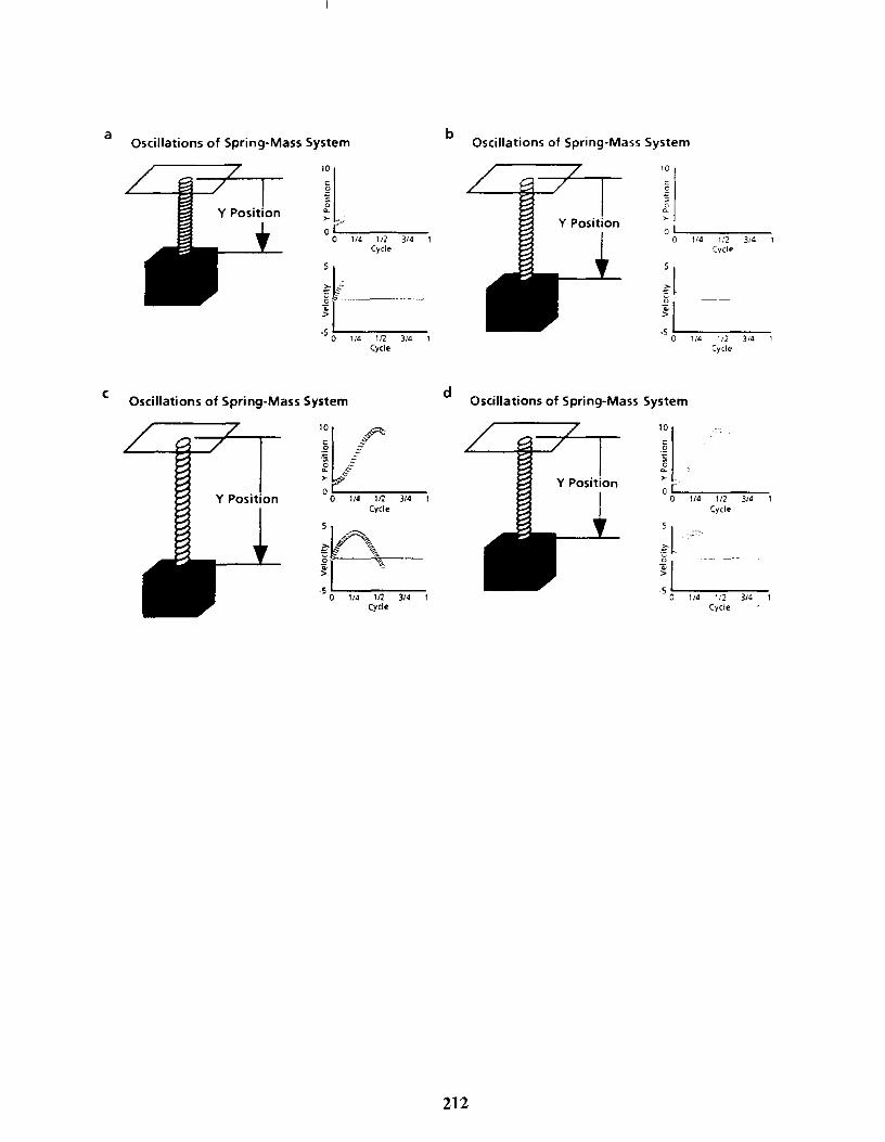
a

c

Oscillations of Spring-Mass System

'il 0 1/4 1/2 314

Cycle

jl .5

0 '/2 314 1/4 Cycle

Oscillations of Spring-Mass System

'iLzr o E'

§

o o 114 112 3/4 1 Cyde

·5 O!--'-14-"" /2=-""'3'"'14"""'-Cycle

b

d

212

Oscillations of Spring-Mass System

10

2 > 0 1

0 1/4 1/2 314 Cycle

jl ·5 0 1/' 112 3/4

:ycle

Oscillations of Spring-Mass System

it oC o 1/4 1/2 3/4

Cycle

:1 0!--'-14--'-=J2-"'"31-'-

Cycle

AN INTERACTIVE MOLECULAR DYNAMICS SIMULATION OF ATOMIC BEHAVIOR

John B. Hudson

Materials Science and Engineering Department Rensselaer Polytechnic Institute

Troy, New York 12180 Telephone: 518-276-6447

e-mail hudsoj@rpi.edu

Torkel Svanes

Daniel Bryson

w. Gregory Sawyer

Stark Design P. O. Box 429

Morristown, New Jersey 07963

Telephone: 973-734-9911 e-mail sawyer@starkdesign.com e-mail svanes@starkdesign.com

213

John B. Hudson

214

An Interactive Molecular Dynamics Simulation of Atomic Behavior

John B. Hudson, Materials Science and Engineering Department, Rensselaer Polytechnic Institute, Troy NY 12180, Torkel Svanes, Dan Bryson and W. Gregory Sawyer, Stark Design, 62 Wetmore, Morristown NJ 07960

Key Words: Ideal gases, molecular interactions, interactive computer simulation.

Prerequisite Knowledge: Concepts of molecules, gases.

Objective: To give students a feeling for the relation between microscopic molecular motions and interaction energies and the macroscopic behavior of gases, liquids and solids.

Equipment: Molecular Dynamics 2D Computer program on 3.5" disk, 100 MHz or greater Pentium PC or Mackintosh PPC computer.

Introduction:

The behavior of gases is usually introduced by statements of thc empirical laws of Boyle, Charles, Gay-Lussac and Avogadro, which are then combined to give the ideal gas law. Only later, if at all, is the molecular level behavior that gives rise to these laws introduced.

Molecular Dynamics 2D is an interactive two-dimensional molecular dynamics simulation that begins with the behavior of individual gas atoms and shows how the relationships among pressure, temperature, volume and number of atoms arise as a consequence of this behavior. The kinctic behavior of an ideal gas, including such processes as effusion and diffusion can also be shown. The simulation is interactive, and allows the student to vary system parameters to discover thc empirical laws mentioned above. The simulation also permits introduction of interatomic attractive forces and, as a result, simulation of the behavior of non-ideal gases and of condensation to produce liquids and solids is also possible.

Program Basics:

Molecular Dynamics 2D is based on a two-dimensional "volumc", the "tank", represented as a box on the computer display. The tank can be filled with up to 200 rcndered "atoms", whose size and mass are proportional to those of the species they represent. At present, the available species are the noble gases He, Ne, Ar and Kr.

The program operates in two distinctly different modes. The first, and simplest, is a two-dimensional hard sphere molecular dynamics simulation. It simulates multiple hard sphere collisions of spheres having a range ofradii and masses. The second mode of operation couples hard sphere collisions with interatomic attractive forces based on a Lennard-Jones 6-12 potential. The system uses classical trajectory calculations in both modes. These calculations permit the "temperature" of the system to be varied over a wide range, and allow the addition and removal of atoms while the simulation is in progress. The volume of the tank can also be changed

215

interactively in some modes of operation, and the box can be divided in half by a partition in others. Pressure on the walls of the tank is calculated from the momentum transfer associated with atom-wall collisions.

Because the hard sphere potential is either zero or infinite, there is no normal unit of energy. As a result, two decades of temperature can be defined from any arbitrary reference point. The balance between potential and kinetic energy does, however, permit establishment of a meaningful temperature scale when interatomic attractive potentials are included. In order to represent the condensed phases of the noble gases, the temperatures have been scaled so that the available temperature range extends from around room temperature to close to absolute zero.

User Interface:

When the program starts up , the first screen seen by the user is the module selection screen shown in Figure 1. Information on several previously prepared modules is listed here, including the title of the module, its author, category, and date developed. This list can be ordered by the user based on any of the listed parameters. Note that in addition to the previously prepared modules, there is a "free play" option to encourage and facilitate exploration.

Once a module is selected, the experimentation screen appears. This screen is shown in Figure 2, displaying the "Diffusion in gases" module. The largest feature on this screen is the "tank", or volume in which the simulation is observed. This feature occupies the left side of the display. Movable barrier walls are present in the tank when appropriate to the module selected. In other modules, a gap in the banier may be interactively opened and closed during the simulation. In modules in which the volume may be changed, the outer border of the tank may be resized during the simulation by dragging with the mouse. At the right side of the display are the interactive controls that permit changing physical parameters while the simulation is in progress, and the

rn II Molecular Dynam ics 2-D , ,. I,

Module 0 Author Subject Date Diffusion Stark Desig n Molecular Mobility 6/03/97 Effusion Hudson Molecular Mobility 12/28/96 Pressure Number of Atoms Relations Stark Design Ideal Gas 6118197 Pressure Temperature Relations Stark Design Ideal Gas 5/02/97 Pressure Volume Relations Hudson Ideal Gas 4130197 Random Walk Moynihan Molecular Mobility 4/17/97

>I

Figure 1. Start up screen of Molecular Dynamics 2D, showing the sortable menu of experiment titles, authors, subjects and dates.

216

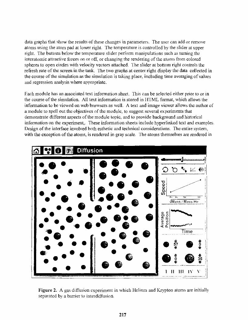
data graphs that show the results of these changes in parameters. The user can add or remove atoms using the atom pad at lower right. The temperature is controlled by the slider at upper right. The buttons below the temperaturc slider perform manipulations such as turning the interatomic attractive forces on or off, or changing the rendering of the atoms from colored spheres to open circles with velocity vectors attached. The slider at bottom right controls the refresh rate of the screen in the tank. The two graphs at center right display the data collected in the course of the simulation as the simulation is taking place, including time averaging of values and regression analysis where appropriate.

Each module has an associated text information sheet. This.can be selected either prior to or in the course of the simulation. All text information is stored in HTML format, which allows the information to be viewed on web browsers as well. A text and image viewer allows the author of a module to spell out the objectives of the module, to suggest several experiments that demonstrate different aspects of the module topic, and to provide background and historical information on the experiment,. These information sheets include hyperlinked text and examples. Design of the interface involved both esthetic and technical considerations. The entire system, with the exception of the atoms, is rendered in gray scale. The atoms themselves are rendered in

r;.;J m m Diffusion

••• .. . • • •• ••• •

• • •

•••• • •• • ••• !S

: Kr Ar Ne H<:!

/ Mass He

• • • ••• • • • •••• • : ..•• . ,-----_ ......

. . '. • • ••• • •• • p •• • • • . -,. •• • • • • ••• • • • • •

.- . • • • • •• •

'010 " L..._

<ll '" ,-t""'," Time

• fl- • 57 • 48 iii CD 0

'"

.

: · ; • • 35 • I II III IV \'

; , i - ---- -,

Figure 2. A gas diffusion experiment in which Helium and Krypton atoms are initially separated by a barrier to interdiffusion.

217

bright primary colors, thus drawing attention to the active elements in the system. The design of the control elements on the right side of the display offers multiple alternatives for manipulating the simulation. For example, atoms may be added to or removed from the tank by clicking the up and down arrows located next to each atom type on the control panel. Alternatively, There is a numerical representation of the number of each kind of atom in the tank at any time, which can be edited directly using the keyboard. Specific atoms in the tank can also be manipulated or removed by dragging or double clicking with the mouse.

Standard Presentations:

As mentioned earlier, the program menu includes a number of standard presentations intended to lead the student through the development of the ideal gas laws and the basics of the kinetic theory of gases. For example, in the pressure-volume experiment, the student can put an arbitrary number of atoms into the box on the screen, then reduce the size of the box and observe the effect of this volume change on the pressure, as indicated on graphs ofP vs. V and P vs. IN that appear on the screen adjacent to the box. In both graphs, the appropriate regression lines are drawn to illustrate the relationship as clearly as possible. This leads to the discovery of Boyle's law. Similarly, modules are included that permit the student to deduce the relations between P and T at constant T (Charles', or Gay-Lussac's law), and between P and the number of atoms a constant V and T (Avogadro's law.)

There are also standard presentations for the transport properties of ideal gases. For example, Graham's effusion law can be demonstrated using a module that divides the tank into two halves, permitting atoms to be added to only one half. Once the desired number and type of atoms has been added, a small "hole" can be made in the barrier, allowing atoms to effuse into the vacuum on the other side of the balTier. Use of two different atomic species demonstrates clearly the mass dependence of the effusion rate, and shows that the property of importance is the difference in atomic velocity as a function of mass. A related module can demonstrate the interdiffusion of two gas species. This is the module shown in Figure 2. Here the barrier dividing the tank is present initially, permitting the introduction of the desired atoms at the start of the simulation. Removal of the barrier starts the simulation. The progress of the diffusion process can be monitored on the data graphs at right.

Intermolecular Potentials: Non-Ideal Gases and Condensed Phases:

The ability to "tum on" intermolecular attractive forces allows simulation of a large range of additional properties and processes. The observation of non-ideal gas behavior is an obvious example, as the P-V -T relationships will be affected by these forces - the equation of state for the model is now essentially the van der Waals equation. These forces also lead, at sufficiently low temperatures and high densities, to condensation as liquids or solids. This is observed, as the temperature is decreased, first as the formation of stable clusters of atoms, in which the volume per atom will be seen to decrease as temperature is further decreased, then to a situation in which these clusters will have an "equilibrium vapor pressure", maintained by a dynamic equilibrium between condensation and evaporation. Over time, large clusters will grow at the expense of smaller clusters, and the system will evolve toward a single cluster.

218

At low enough temperatures, the clusters will be ordered (a close packed array of atoms), and may contain typical solid state defects such as vacancies, dislocations and grain boundaries. Solid state diffusion by vacancy migration can be observed, but is a slow process at the calculation rates used here. If the solid as formed does not contain these defects, The student can create them by deleting atoms or groups of atoms.

Kinetic effects can also be observed by rapidly decreasing the temperature. The evolution from the large number of small clusters formed initially into fewer increasingly large clusters is readily observed, as is the annealing out of defects in the clusters.

Another useful feature of the simulation is the ability to save and restore any instantaneous state of the simulation. This is of interest as a means of capturing infrequent events for latere viewing. It also permits the instructor the set up a custom configuration for use in a classroom demonstration or experiment.

Technical Considerations:

The molecular dynamics calculations on which the simulations are based are carried out in a non-dimensional frame of reference based on the triple point of argon. The temperature range available on the temperature slider correspond roughly to I to 300 K. To put things in a frame of reference more familiar to the user, the correspondence between time and length scales in the simulation, as seen on the display, and the real time and length scales appropriate to real atoms are summarized in the table below, for the case of room temperature. (About the upper end of the temperature slider.)

Simulation on screen Real time for molecules

Time I second 10.12 seconds

Distance I centimeter 10.8 centimeter

Velocity I centimeter/second 104 centimeter/second

Table 1. Equivalences between simulation dimensions and laboratory dimensions.

The figures in this table are representative of those for the simulation running on a 100 MHz machine with a 17" monitor set at 640 x 480 monitor resolution. Different clock times or screen sizes would lead to correspondingly different, but similar, equivalences.

Molecular dynamics 2D runs on either PowerMac or Windows 95 or NT operating systems. 16+MB of RAM are required. A color monitor and sound card are recommended

Summary:

Molecular Dynamics 2D represents a simple but versatile tool for developing a "feel' for the

219

behavior of both gases and condensed phases at the atomic level. Fundamental principles can be demonstrated convincingly using the prepared modules. More complex aspects of materials behavior can be observed in the "free play" mode.

The capabilities represented by the current version of the program are being continually expanded by the developers, who are open to suggestions for additional modules and additional capabilities. Feedback on the usefulness and useability of the simulation are also welcome.

Further Information:

Further information on new developments and on how to obtain copies of this software may be obtained from:

SHirk Design, Inc. P.O. Box 429 Morristown, NJ 07963 www.starkdesign.com

220

OPTICAL EXPERIMENTS WITH MANGANESE DOPED YTTRIUM ORTHOALUMINATE,

A POTENTIAL MATERIAL FOR HOLOGRAPHIC RECORDING AND DATA STORAGE

Matthew E. Warren Senior Physics Student

and

George Loutts

Center for Materials Research Norfolk State University 2401 Corprew Avenue

Norfolk, Virginia 23504

Telephone: 757-683-2295 e-mail

Telephone: 973-734-9911 e-mail sawyer@starkdesign.com e-mail svanes@starkdesign.com

221

Matthew E. Warren

222

Optical Experiments with Manganese Doped Yttrium Orthoaluminate, A Potential Material for Holographic

Recording and Data Storage

Key Words

Matthew E. Warren, Senior Physics Student Dr. George Loutts, Assistant Professor of Physics

Center for Materials Research Norfolk State University

Norfolk. Virginia

Yttrium Orthoaluminate doped with Manganese (Mn:YAIOJ, optical absorption, absorption spectra.

Prerequisite Knowledge It is useful to have basic knowledge of chemistry, crystallography, and

spectroscopy. Objective

To identify the manganese valence states in Mn:YAIO j using optical absorption spectroscopy.

Equipment and Materials 0.5 'Yo Mn:Y AIO sample approximately 4 mm thick 0.5% Mn. 0.1 % Ce: Y AIO sample approximately 4 mm thick 0.5% Mn. 0.5% Cc, 0.5% Ca:YAIO sample approximately 4 mm thick powder polish numbers 40. 25. and 9 Buehler Metadi diamond suspension oil based polish numbers 15,9 and 3 micron glass plate water paper Cary 5E UVlVis Spectrophotometer and computer program Microcal Origin for crystals Microsoft Windows

Introduction

Yttrium Orthoaluminate doped with Manganese (Mn:YAl01) is a new crystal being studied for its unusual photorefractive properties and promise for application in

223

optical data storage. The strong photo refractive effect observed in the crystal was accompanied by a color change from yellow to dark-gray under intense laser radiation. In the described experiment, optical absorption spectroscopy was employed in order to identify manganese valence states in different colored Mn:YAIO] crystals.

Mn: Y AIO] crystal samples

The Y AIO] host crystal has a distorted perovskite structure that belongs to the orthorhombic centrosymmetric Pbnm space group [I]. The cationic sites in the structure available for Mn substitution are the relatively large strongly distorted YOu polyhedral (Y'+ ionic radius Ry = 1.02 A ) and the smaller nearly ideal AI06 octahedra RAJ = 0.53 A). Manganese may enter YAIO, in the form of Mn2

' ions (RMn = 0.96 A), substituting most likely yJ+ ions, and Mn" ions (RMn = 0.65 A) or Mn4+ ions (RMn = 0.53 A) substituting AI]' ions. The latter substitution is most probable because of dimensional parameters. Point defects, which are common in Y AIO" may provide the charge compensation required for substitution [2].

Y AIO, crystals were grown by the Czochralski technique which involves melting the crystal components and dopants in a high temperature furnace. A seed crystal is dipped into the melt and rotated and pulled into a gaseous atmosphere. As the melt cools it hardens to form the crystal, in this case yttrium orthoaluminate. Mn: Y AIO] was grown in a 3 inch iridium crucible under a nitrogen ambient atmosphere with up to 0.5% oxygen. The chemicals used for the charge preparation were of99.999% purity. Manganese was introduced in the melt at 0.05 - 2.0 atomic % (in respect to AI) in the form of Mn02• The seed was oriented in the "'b" direction of the orthorhombic unit cell. The pull rate was maintained at 1.5 mm per hour and the rotation rate at 15 rpm.

The undoped crystals usually exhibit brown color. By adding certain dopants to the host, the color properties change. The addition of 0.05 atomic % cerium creates a clear Y AIO, crystal. The Manganese dopant is optically active and produces clean yellow crystals. The addition of certain concentrations of cerium and! calcium to Mn: Y AIO, results in pinkish or gray colored crystals. Most of the Mn: Y AIO, crystals that were grown were high quality with very few visible defects such as cracks and bubbles. However, the Mn: Y AIO, crystal codoped with calcium and cerium contained many cracks.

Before measurements can be taken, raw, cut samples have to be polished using a series of powders and oil based polishes. For rough polishing, number 40 aluminum powder was used with water on a glass plate. The two opposing faces to be used in the measurement were rubbed into the powder and water until the surface was uniform. The same procedure was done for the next lowest particle sized powders, number 24 and 9. For smooth polishing, Buehler oil based diamond particle polishes were used against plain white paper. The opposing crystal faces needed for measurement were rubbed into the oil until a noticeable uniform shine was present. The oils were used in order of highest suspension particle size to lowest (15, 9, and 3 microns). Once the sample faces

224

could reflect detailed images, the samples were ready for room temperature absorption measurements.

Table I. Summary of crystal samples

Sample # Nominal dopant concentrations Color of crystal as Color of crystal grown after photoexcitation

1 0.5% Mn yellow grayish 2 0.5% Mn. 0.1% Ce pink light gray 3 0.5% Mn, 0.5% Ce, 0.5% Ca grayish grayish

The emission spectrum for Mn: Y AIO) , displayed in figure I, is similar to the spectra taken for Mn doped AI,O] [3], LaAIO] [4,5], and YAG [6,7,8]. All spectra have the same shape and peak locations which are attributed to Mn4

+ transitions. Furthermore, Mn: Y AIO] has a luminescence lifetime around 3 ms while the previously mentioned samples have similar luminescence lifetimes (around 1 ms). During the excitation with an Ar laser (green emission with Ie = 514 nm), it was discovered that the crystals darken. Placing the crystal in sunlight for a brief time period allows the same grayish coloration to occur. Annealing or heating the darkened sample at temperatures higher than 200°C for an hour completely erases the coloration. Because of this gray coloration, and associated change in index of refraction, holographic recording may be a possible application for Mn:Y AlO]. It would be interesting to view some spectra ofMn:YAIO] before and after excitation. From the results it may be possible to determine the ionic transition that goes on during thc process.

<L> ..... c C> fJ) fJ)

E UJ

1

o 650 700 750 Wave length, nm

Figure I. Emission spectrum for Mn: Y AIO].

225

Absorption Measurements

In absorption measurements, light is transmitted into a sample and the intensity of the light exiting the sample is measured. This measurement is done with the use of a spectrophotometer. The Cary 5E spectrophotometer compares the two beams and plots the data. One light beam is a reference beam and the other is sent through the sample. The resulting information is a graph illustrating the absorption coefficient, k (in cm· I

), of the sample measured. The formula used to calculate the coefficient, k is

k = (lnl" - Inl)/!

where 10 is the initial beam intensity, I is the measured intensity and I is the crystal thickness. Absorption spectra were taken twice for each sample of crystals. The crystals were tested before and after photoexcitation. The Cary 5E program plotted intensity of light against the wavelength. Microcal Origin was used to calculate and plot the absorption coefficient against the wavelength. The ordinate axis (Y axis) is the absorption with the highest number meaning that much of the light energy was absorbed by the sample. The abscissa, the x axis, corresponds to the various wavelength at which the source transmitted the light. A peak or 'hill' in the graph indicates that light is absorbed. The user can control the wavelength range of the light source. Absorption measurements on Mn:YAI01 crystals were usually done in the visible light range (400 - 800 nm wavelength).

Results

2.0 -- Before exposure to sun

- - - After exposure to slin

1.5

L ___ ____ L-__ ____ __ ____ ____

401) 500 600 700 800

Wavelenl,'1h (nm)

Figure 2. Absorption of sample I (Mn: Y AIO, ).

226

Figure 2 displays absorption of the 0.5% Mn:YAI01 crystal. For the as grown sample. an absorption peak. centered around 480 nm. is associated with Mn4

> ions. On the same graph. the exposed sample also has a peak centered at 480. The concentration of Mn4

' ions may have changed due to some transition. For the sun exposed sample. there is an additional peak centered around 650 nm which may be attributed to some additional manganese ions. In figure 3. the 0.1 % Ce and 0.5% codoped as grown sample shows the same peak at 480 nm. A close view of the same graph also reveals the absorption at 480 nm for the photoexcited sample. but additional peaks at 530 and 650 nm. According to published spectroscopic data on Mn ions [6. 9]. the absorption feature at 530 nm can be assigned to Mn" ions and the feature at650 nm is characteristic of Mn5

'

ions. Apparently. exposing thc samples to radiation causes the reversible reaction 2Mn4•

<=> Mn1 + Mn j•• To test the theory. calcium was added to the melt of a Ce and Mn

doped crystal with the intent of producing the darkening in an as grown sample. hence the gray crystal sample #3 (fig. 4). There is an absorption peak at the 480 nmmark which indicates the presence of Mn4

• in the as grown sample. An absorption feature at 650 nm can also be identified showing a Mnj occurrence. From the graph it can be concluded that exposure to radiation only strengthens the absorption. It is evident that optical excitation induces the revcrsible reaction previously stated.

G

Bd{)H,' 1,'\fXNLfe to SLUl

After c'rosure to StU,

0.50 o

f Wavelength (11m)

100

Figure 3. Absorption of sample #2 (Ce. Mn:YAIO,)

Conclusion

800

2.0

Before e:'qX)5UfC to sun Aller e:xfX"lSu[c to SlD1

Wavelength (11m)

Figure 4. Absorption of sample #3 (Ca. Ce. Mn: Y AI01).

In conclusion. standard absorption measurements were used to investigate the optical properties in Czochralski grown Mn:Y Al01 crystals. Three crystals were grown with different concentrations of Ce and Ca. and had different properties. Absorption spectra were taken for each crystal before and after exposure to sunlight. The spectra, along with previously published data. indicated a transition of Mn4

+ ions into Mn1+ and Mn'+ ions during the photoexcitation process. Although. darkening is completely erasable

227

at temperatures above 2000 C, 50% of the coloration was maintained at room temperature for more than a year. The darkening effect suggests that Mn:Y AI01 can be used for quasi-permanent data storage at room temperature. Further plans for the material include researching the possibility of increasing effective degradation time of the photo darkening to achieve permanent storage and studying how to control the concentrations of the manganese states.

Support for the work was provided by NASA grant #92-207 and DOE #DE-FGOI-94EWI1493.

References

[I] S. Geller and E.A. Wood, Acta Cryst. 9, 563 (1956).

[2] P. Dorenbos .. M.V. Korzhik, A.P. Kudryavtseva. S.V. Lyubetskii, B.1. Minkov, V.B. Pavlenko, and AA Fyodorov, J. App!. Spectrosc., 59, 633 (1993).

[3] S. Geshwind, P. Kisliuk, M.P. Klein, J.P. Remieka and D.L. Wood, Phys. Rev., 126, 1684 (1962).

[4] Z.N. Zonn, V.A Ioffe and P.P. Feofilov, Opt. Spectrosc., 19, 541 (1965).

[5] A van Die, A.C.H.I Leenaers, W.F. van der Weg and G. Blasse, Mat. Res. Bul!., 22, 781 (1987).

[6] K. Peterman •. G. Huber, J. Lumin., 31132, 71 (1994).

[7] J.F. Donegan, T.J. Glynn, G.F. Imbusch, J.P. Remeika, J. of Lumin .. 36, 93 ( 1980).

[8] L.A. Riseberg and M.J. Weber. Sol. Stat. Comm., 9,191 (1971).

[9] U. Hbmmerich, H. Eilers, W.M. Yen, H.R. Verdun, Chern. Phys. Let., 213, 163 (1993).

[I OJ M.J. Weber and L.A. Riseberg, J. Chern. Phys., 55, 2032 (1971).

228

DESIGN OF HYPERVELOCITY FLOW GENERATOR AND ITS FLOW VISUALIZATIONS

Kyo D. Song

Department of Technology Norfolk State University 2401 Corprew Avenue

Norfolk, Virginia 23504

Telephone 757-683-8105 e-mail kdsong@vger.nsu.edu

and

Charles Terrell

Department of Physics Hampton University

and

Mark Kulick

Engineering Technician Nyma Inc.

229

Kyo D. Song

230

Design of Hypervelocity Flow Generator and Its Flow Visualizations

KyoD. Song Department of Technology

Norfolk State University

Charles Terrell Department of Physics Hampton University

Mark Kulick Engineering Technician

Nyma/ADF Inc.

Key Words: Hypersonics, Flow Visualization, Schlieren, Electron Beam Fluorescence (EBF)

Prerequisite Knowledge: Knowledge of basic fluid mechanics

Objective: To design and operate a test facility for the hypervelocity flow generator (HFG) system based on opticaIly driven nozzle. To visualize flow structure by two non-intrusive optical diagnostic methods, electron beam fluorescence (EBF) and focused schlieren (FS).

Equipment: I. a schlieren system

a. a CCD Camera b. a light bulb c. a cutoff grid d. lenses e. a Fresnel lens f a AI box

2. a monitor 3. a match light

I. Introduction

The generic requirement of advanced hypersonic systems can be found by the flight velocity and altitude trajectories of the anticipated spacecrafts as shown in Fig. 1. In the flight corridor of spacecraft, the forebody of a vehicle receives a tremendous thermal loading from its shock layer. The correct estimate of thermal loading is important for optimizing design of the thermal protection system. There has been a

231

recent effort to study the thermophysics of shock heated air in the vicinity of the nose of a vehicle flying at 3-6 kmlsec.

One of the important areas for research in hypersonic/hypervelocity flows is associated with chemical nonequilibrium and characteristics of separated flows developed in regions of shock wavelboundary-Iayer interaction. In such flows, there has been almost no experimental research to provide input data for the model developed [1]. In the experimental study of these flows, flow duration becomes an important parameter. A comparison of hypersonic facilities for run-time is shown in Fig. 2. For this application, large shock tunnels are currently used with test times of a few milisecond. The purpose of HFG research is to measure the collisional cross-sections and relaxation times which are important for determining radiative heating within high temperature shock layers in long-run facility.

A HFG has been designed to simulate re-entry vehicles from space at an altitude of 60-90 Km. The higher the altitude, the less air density. Hence, the mean free path of the air particles is long. Therefore, the flow becomes slip and nearly free molecular regimes. For the measurement of the such flow, many non-intrusive optical techniques have been developed and applied world-wide in high-speed flow facilities. Among them, electron beam fluorescence (EBF) and focused schlieren (FS) were used to to characterize and visualize low-density, fast flow generated from the HFG in the Measurement Science and Technology Branch (MSTB) at NASA Langley.

II. Aerothermodynamic Parameters

In this research, velocity of 6 kmlsec between 60 and 90 km altitude is the region of interested. The translatory kinetic energy of a molecule is also of interest in terms of velocity and temperature. There are three different terms in velocity often used: average (1), root mean square (2) and most probable velocity (3) based on their definitions

(1)

(2)

232

I

= (2kT)2 vmp m (3)

where, k : Boltzmann Constant T : absolute temperature, m : mass of a molecule

In the regime of 60-90 km altitude, the typical temperature behind at shock is approximately 8,000 K, and an average velocity is 2.45 km/sec, calculated from equation (1). For the calculation, it changes up to approximately 20 % depend on equation is employed, as shown in Fig. 3.

For the equilibrium case, an average temperature behind at shock is calculated by CET 89 program [2] to be 6,160 K, when the speed of the vehicle reaches 6 kmlsec as shown in Fig. 4. At the vehicle's speed of 6 km/sec, the temperature behind the shock is approximately 6,200 K from the shock tube data [3] in the figure.

A chemical equilibrium and transport code originated by NASA Lewis Center [2] is used to calculate the thermodynamic properties of nitrogen gas for HFG nozzle design. Using the code, the theoretical nozzle performance at 3 atm for nitrogen gas was calculated in terms of stagnation temperature of chamber and flow velocity for both equilibrium and frozen composition during expansion as shown in Fig. 8. To generate the flow velocity (2.45 kmlsec) the stagnation temperature of chamber will be 2666 K.

The theoretical flow velocity and temperature are calculated in terms of area ratio of the nozzle as shown in Fig. 9. At the area ratio of 700, the gas velocity reaches to 2.45 km/sec, and the gas temperature and pressure is approximately 155 K and 0.05 torr, respectively. The calculation of various performance parameters in CET89 code is based on one-dimensional form of the continuity, energy and momentum equations as well as adiabatic combustion.

III. Nozzle Design

Ground testing facilities for hypersonic flow generator have been analyzed several authors [4-6]. Among the flow facilities where high stagnation temperature flows can be achieved, electric resistance heating methods are commonly used, but limited to around 2000 K due to heating element as primary heat source. Arc heating contributes particulates not only the heating elements but also radical species to the flow. Therefore, the flow generated by arc heating may not be clean. A unique, clean-air HFG facility using an optical power is designed to provide air stagnation temperatures up to 3500 K. The optical power for the arc lamps is approximately 60 kW. An elliptical reflector conduit is

233

used to collect and concentrate optical power on thermal chamber. The length of arc lamp is approximately 6.0 ".

The optical flux couples with an elliptical mirror as shown in Fig. 7. The optical coupling coefficient of the elliptical mirror is assumed to be 0.4 for calculation of irradiance on the thermal chamber. The outside of diameter of the thermal chamber is determined to be approximately 14 mm which is close to the diameter of the arc lamp (11 mm dia.) based on the geometrical ray tracing method. The diameter of thermal chamber is restricted by the geometrical image from a light source and an elliptical mirror. If the diameter of thermal chamber is too small, some of reflected lights may not be arrived on the surface of the chamber due to the multiple reflections from the surface of the elliptical reflector, and total irradiance will be reduced as a result. In the case of larger diameter of thermal chamber, the total irradiance on the surface will again be small due to the larger area. The requirements of the thermal chamber should be satisfied the following properties: high melting temperature, high conductivity, endurance in thermal shock cycle, high strength and lower thermal expansion rate. Some candidate materials are listed in Table 1. Among them, tungsten material is selected as first choice even through HfC has highest melting temperature because HfC is relatively weak for thermal shock.

The equilibrium temperature on the tungsten surface can be stated as:

(Optical energy absorbed = Radiation emitted + Convection loss to gas + Conduction through nozzle).

, 4 4 ( ) dT apT. = cO"T. +h T. - I:n +k-dr

where, a = absorptivity of the body cr = Stefan-Boltzmann constant T,= surface temperature E = emissivity of the body h = heat transfer coefficient Too = ambient temperature k= thermal conductivity.

(4)

Ifthere is no losses due to convection and conduction, the equation becomes a simple as

(5)

234

Substituting the numerical values, q = 5.37 X 106 W/cm2 and E - 0.3, the maximum surface temperature could be approximately 4,371 K with 60 % of optical coupling from the elliptical mirror. By considering of the losses due to conduction and convection, we need to solve the equation (4) with appropriate values. To determine heat transfer coefficient h, let us assume nozzle has a constant heat rate and need to calculate Reynolds number as

(6)

where, p and J.l. are determined from CET 89 program and VI is determined from a continuity equation with the velocity of945.3 rnlsec at the throat of the nozzle calculated by CET 89 program. Therefore, the velocity at the chamber will be calculated as VI = 9.45 crnlsec. The result indicates the flow inside tube is a laminar.

h= 4.364 K D

where, K = thermal conductivity of working gas

D = the diameter of nozzle.

(7)

Therefore, thermal transfer coefficient, h, will be 67.55 W/m2 K. For the calculation of K and E at high temperatures for the tungsten tube, the value are extrapolated with the existing imformations [4,7], The absorptivity, a is obtained from the reference [7] to be 0.51. By a try and error method, the surface temperature is calculated as 3,690 K. Based on the results, the loss of the surface temperature will be 681 K due to the loss mechanisms as described in previous.

IV. System Configuration

The system consists of six major parts, such as an arc lamp as energy sources, a thermal chamber, an expansion nozzle, a test section, a vacuum chamber with a vacuum pumping system, contlUl and diagnostics system as shown in Fig. 8. The tank was designed to have three 10,000 CFM capacity vacuum pumping systems. However, one Kinney vacuum pump provides 11,000 CFM, and Stokes pump gives 1,300 CFM. Initially, the Kinney pump will have a vacuum pumping system with 10,000 CFM pumping

235

speed at 1 mtorr pressure. The vacuum pressure for routine operation starts from 10 mtorr, then test ends when the tank pressure raises to 40 mtorr. The sectional view of the detail test chamber is shown in Fig. 9. As shown in the figure, the maximum flow intensity should be located at 7" from the throat of the nozzle in order to use the whole window. F or the initial shakedown of the system, the vacuum pressure at the chamber, section II, and tank pressure have measured as shown in Fig. 10. The vacuum pressure drops 1 torr within 30 min. with two existing pumps, and reaches to 8 microns at the chamber pressure within an hour, while the tank pressure keeps at 0.07 micron. The leak rate of the system was 0.02 micron/min.

To check the flow performance of the system, a free-jet nozzle is designed and installed as shown in Fig. 11. The shock structure of the flow expected is also shown in the figure. The size of the nozzle throat is changed as I, 3 and Smm in dia. With the S mm dia. of the nozzle throat, the pressures at the chamber reaches 1.2 torr and keeps the pressure within 7 seconds as shown in Fig. 12. By changing the throat diameter of nozzle from 1 mm to S mm, the pressure history of the chamber and the tank is measured as shown in Fig. 13. As the result indicated, a continue operation of HFG system to simulate pressure conditions at altitude 60 - 90 km is possible even with a Smm dia. of the nozzle.

V. Diagnostic Techniques for a Hypersonic and Low Density Flow

The purpose of this section is to apply EBF and FS techniques to visualize low density flows 00 mTorr) and high Mach number for HFG at NASA Langley.

V-I. Focused Schlieren Technique

The focused schlieren technique gas several advantages for flow visualization because it produces a natural, easy-interpretable image of refractive-index-gradient fields. This low-cost technique also has a large field of view, focusing capability, and high sensitivity. Figure 14 shows a layout of the optical components of a small-field, high-sensitivity focused schlieren system. This system consists of a source grid and cut -off grid (located on opposite sides of the flowfield), a light source, a Fresnel lens, an image lens, and an intensified CCD camera. Refraction of the collimated light beam in the flow region moves the image of the source relative to the knife edge, which results in a change in the brightness of the image of the test section.

Figure IS shows a diagram of the small-field, high-brightness and sensItIvIty focused schlieren system installed at NASA LaRC. Figure 16 shows two images of the N2 free jet expansion through a s.o mm diameter nozzle using the focused schlieren system. Both pictures were taken under similar conditions and the background was subtracted to better visualized the shock structure. In additional to the typical barrel shock, there is the dark region close to the nozzle exit. This is attributed to the fact that the orifice is sharp-edged causing the gas to "swing wide" after exiting the nozzle so that the minimum flow

236

diameter is a bit less than the geometric diameter and is displaced slightly downstream of the plane of the exit. Also, in Figure 16b, the shock-front formed when a 12.0 mm diameter sphere is placed in the centerline axis of the flow is shown. The shock layers around the sphere could be analyzed to determine the nature of similar structures around re-entry vehicles [6].

From the pressure information that we gathered, we were able to roughly determine that our focused schlieren system could visualized N2 free jet through the 5.0 mm diameter nozzle in the HFG down to a pressure ratio of 322. This corresponds to a Mach number of 4.59.

V-2. Electron Beam Fluorescence

The electron beam fluorescence is used for the measurement of number density, rotational and vibrational temperature, and velocity in low density flow. It also provides for species identification and visualization. In general, the EBF ranges of application are: (1) number density, 1011 - 1017 cm-3, (2) vibrational temperature, 300-3,000 K, (3) rotational temperature, 5-1,000 K and (4) flow visualization, 1014

_ 1017 cm-3

The principle of EBF technique as follows: when a higher energy beam of electrons passes through a gas, inelastic collision between the electrons and the gas molecules produce a radiative emission (fluorescence) that is state properties of gas and its characteristics as.

(8)

(9)

where, Eo is ground state of the A gas molecular, El is excited state and E2 is a lower state of molecular.

The intensity of the emission is related to the number of density of the gas as well as the characteristics of the electron beam. The spectral characteristics of the emission are related to the composition, density, and temperature of the gas. Then:fore, EBF could be a strong candidate technique to measure properties of gases in low density.

The EBF system was calibrated with N2 gas to evaluate its sensitivity and reliability for application to hypersonic flowfields. Among many channels of electron-N2 collisional kinetics, excited molecular nitrogen ions, N2 +', are mainly produced in the reaction

237

(10)

This is followed by the emission of fluorescence in the first negative band,

(11 )

with the (0-0) vibrational transition (at 1.,=391.44 nm) being the most intense feature and considered to be a sensitive probe for N2 concentration.

An electron gun is entered into the test chamber through a nozzle (1. 0, 3.0, or 5.0 mm in diameter). The beam of electrons gun (beam energy between 100 e V and 10 ke V) is connected to the chamber. The beam of electrons transverses the chamber, strikes the gas in the chamber causing it to fluorescence. The fluorescence signal can be collected at 90° to the e-beam and nozzle flow through the chamber windows or further downstream through one of the ports situated 15° to the flow axis.

Nitrogen fj-ee jet expansion through the 5.0 mm nozzle was visualized (e-beam energy = 5.0 keY) between 32.8 and 112.5 torr in the nozzle area and 0.13 and 0.28 torr in the chamber. Figure 17 shows one example from our experiment and clearly shows the isentropic region (known as the "zone of silence") bounded by the barrel shock and Mack disk.

VI. Conclusions

An unique test facility for the HFG system based on optically driven nozzle is designed and is currently used at NASA Langley to generate hypersonic/hypervelocity flow An investigation of fundamental aerothemodynamic properties for hypersonic/hypervelocity flow (HFG) at altitude of 60-90 km is reviewed and analyzed with available codes.

The operation of the HFG system is successfully performed for checking of component integration and evaluation. The pumping time to reach the minimum vacuum pressure (10 micron) at the chamber from the atmospheric pressure is approximately an hour. As the result of the experiment, a continue operation of the HFG is possible with I, 3, or 5 mm diameter of nozzle throat.

Using EBF and FS techniques, we were able to successfully visualize and characterize the low-density free jet expansion of nitrogen in the HFG system at NASA LaRC. With an electron beam energy of 5 0 ke V and nozzle diameter of 5.0 mm, the barrel shock and Mach disk are clearly observed. As the result of the FS, a shock

238

structure with and without a spherical barrier using our focused schlieren system and roughly determined that is not applicable at pressure ratios below 322.

VII. Acknowledgment

The authors would like to acknowledge Drs. Greg Herring and Leonard Weinstein, Measurement Science and Technology Branch, NASA LaRC and staff of the Branch for their continuous support for our work.

References

[I] Park, Chul, "Nonequilibrium air radiation (NEQAIR) program," NASA Ames Research Center, Moffet Field, CA, TM 86707, July 1985. [2] Gordon, S., McBride, B., "Computer program for calculation of complex chemical equilibrium compositions, rocket performance, incident and reflected shocks, Chapman-Jouquet detonations," NASA SP-273, March 1976,

Gordon, S., McBride, B. and Zeleznik, F., "Computer program for calculation of complex chemical equilibrium compositions and applications. Supplement I - transport properties, NASA TM-86885, Oct. 1984.

Gordon, S., McBride, B., "Finite area combustor theoretical rocket performance," NASA TM-I00785, April 1988. [3] Donahue, K., Reinecke, W, Rossi, D, Marinelli, W, Krech, R, Caledonia, G, "Aerothermodynamic radiation studies," NASA-CR-185666, Sep. 1991. [4] Probstein, R. F., Kemp, N., "Viscous aerodynamic characteristics in hypersonic rarefied gas flow," 1. Aerospace Sci., Vol. 27, 1960. [5] Fisher, S. S., "The effect of rarefaction on impact pressure measurements in supersonic flows," Proceedings of the 13th International Symposium on Rarefied Gas Dynamics, Novosbirsk, USSR, July 1982. [6] Fisher, S. S., Yurkanin, D. 1., Graybeal, G., and Scott 1. E. Jr., "Measurements of the impact probe rarefaction effects in high Mach number y=7/5 CO2 flows," Proceedings of the 14th International Symposium on Rarefied Gas Dynamics, Tsukuba Science City, Japan, July 1984. [7] Levinsky, E. S., Yoshihara, H., "Rarefied hypersonic flow over a sphere," "ARS Progress in Astronautics and Rocketry: Hypersonic Flow Research," ed. by F. R. Riddell, Academic Press Inc., New York, Vol. 7, 1962. [8] Giacinto Scoles, "Atomic and molecular beam methods," Vol. 1, 1988.

239

100

Altitude, km

50

Fig. 1. HYPERSONIC FLIGHT REGIMES

HFG with He

Low-Lift AOTV Coplanar LEO

----I

/ /

1

1

1

1

1

HFG

/ / / /

Hypersonic Transport

'--Concord I

Rocketdynel AF Phillips, H2

Aeroassist flight experiment

High-Lift AOTV

l<EDC/RANGE "G" I and AMES

Mars Return

5 10 15 , )' I . . I . ) 7.3 8 10.26

Velocity, km/s

N .J:>. ,....

Fig. 2. CAPABILITY OF HYPERSONIC FACILITIES

11200

0

-Q) 8400 "'-:::I +-' CO "'-Q) a... E Q) 5600 +-'

C 0 +-' co C 0) co

(j) 2800

0 psec 10

(after LL Trimmer et al. AIAA paper 86-0739cp)

Hotshots Hypervelocity Tunnel 9 -----------, ---...

HFG/MPD Arc Tunnels

Shock Tunnels

VKI Longshots

Gun Tunnels

102 103 msec 1

ONERA

.•.. ;.4CH.7

. .

Ludwieg Tubes 10 103

sec 1 Flow duration

10

Continu-ous Limit Tunnels

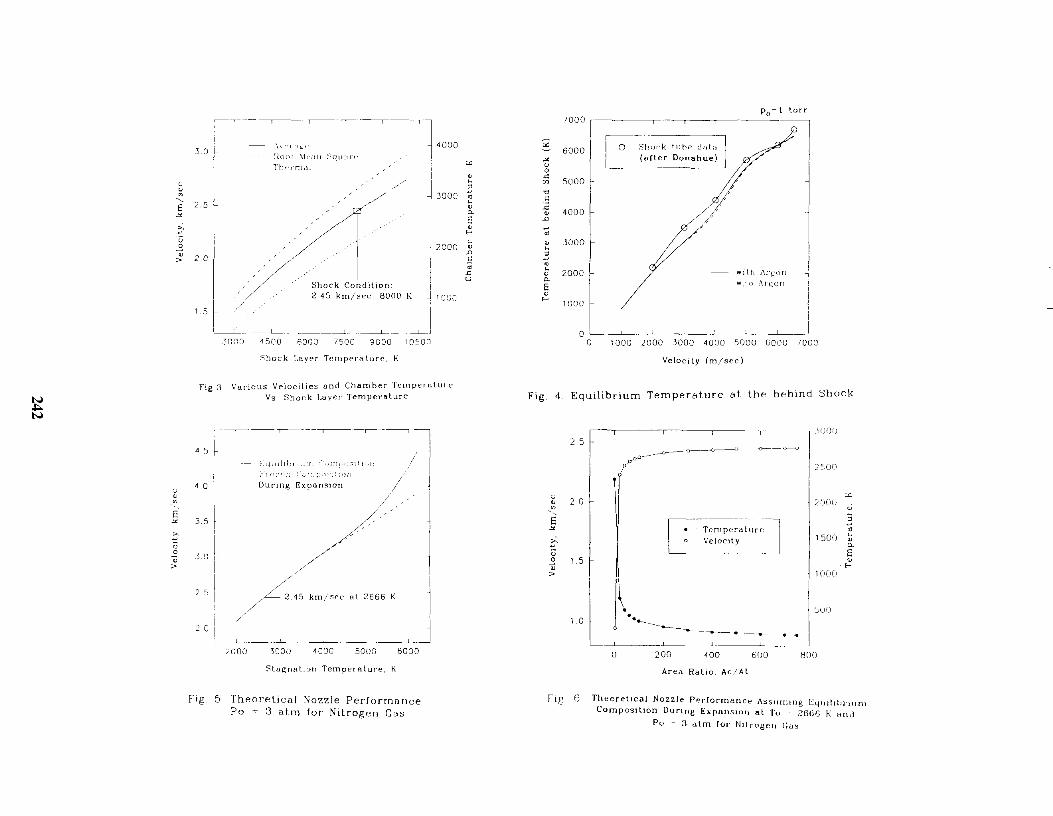
c

E " > c 0

" "

2.S

2.0

1.5

,------- -,----- - ---------,---. ;

l \1, d II ,-:::q lJ,1 r,' Thf'rrndi

.. //.... I / .,.- Shock Condition

/ / 245 km/sec, 8000 K /

____ ___ __ ---.l _ ----------.L __ _

.3000 4500 6000 7500 ')000 10500

:Shock Layer Tplllppr-nture K

2000

lOGO

Fig_3 Va.rious Ve-\ocitles and Chamber femper1:1lure-Vs Shock La.yer Temperature

---- -----,-------.-------------,

4 ,

;- 'lel:ld}1 "Jill

4 a During Expa.nsion

3 S

10

2 C -------.L _______ '__ __' ____ J

2000 3000 4000 5000 6000

Temperature, K

fig 5 Theoretical Nozzle Performance Po -c- :3 atm for Nitrogen Gas

'" " h

" 0 h

" 0-E " ... h

" .0 E 0 .c

U

" 0 0

.<: [f)

" Q

.c " .0

-;; " h

3 . h

" 0-E " ...

Fig 4

o o " "

Po= 1 torr 7000

c---6000 La :::ho('k tubf' datil

(after Donahue)

SOOO

4000

3000

wIth ,\n..'U!1 " w, ()

1000

i

1000 2000 1000 4000 ')000 6000 7000

Velocity (m/sec)

Equilibrium Temperature at the behind Shock

2.S -

20

1.S

1 0

(1

,-----,--- 1 ----- ';()OU

c---------- -J-• : TernperOll.lre. o , Veloclly

200 400 600 Area Ralio, Ae/ Al

2:0n

1500

800

fig [) Theoretical Nozzle Pecfocmance Assumrng [4,,,111;11<,,,, ComposlllOn DUring Expallsloll al To -- 2613(; K Hnd

Po = 3 alm for NItrogen Cas

Lamp at Focus

Fig. 7. The optical flux couples with an ellipitcal mirror.

243

61 :Ieak rate;O.7micran/min .. Min.V.P.;5micran #2:leak rate;O.02micran/min .. Min.V.P.;2.5micr n

Optical Table 1------1 I I I I I I I I I I I I

6 Crosses Chamber: I I I

Fig. 8. HFG Laboratory Layout.

Vacuum Pump System

1,300 CFM r----l I I

r-'!'!--J L'1"",\-1

I , r----...I--L-----,

Pump J

r----' I I ..... -,-,--1- .... ·-'

I , r--- ... - ..... I I

: Pump 2 : I : ,- ---,.-----r --- ---'

I.J---!., ,--"1'"

11,000 CFM :----1

rJ.J-., I I -T'-.J

I , I ____ .J.._....L. _____ _

: : Pump 1 L---rg.=------

Elliptical

60 kW Vortek

RM 123

30"Oio Isolation Valve (provided by customer)

Tube (30"dia x 16"long)

PWR LIGHT (ON/OFF) 120V AC v1 v2

24v Q PW 0 o;?en P.

v3 v4 woter flaw

? J

@ DC Power

Kinney P.

0 o o 0

on o r9

AC CKT off BKR CONTROL SWITCH

Control Panel

gas o on

Interlocks o OR.set

o EMG. STOP

Fig. 9. The Details ofHFG Chamber

Window, 4 places

Spacer

L Flange Supporter

10 em 32 em Pa99ible Window

Tr-ermcl Chamber

--- -- -,11

---- -- -- - -----V-O-c-"-"-m--TO-nk

I

4" Gote Valve (wldth=4.78")

15 em Test Chamber

25" 7,56" (.hen the ;e 111 9 em

1-____ -"-"0"'.7::8".' ... ' J(-!"'Ch'Oec:nc..'.' ___ 2 7 ern

10 4

10 3

10 2

..-... '""' '""' 1 0 1 0 .....,

'-"

Q)

'""' 10° ;:::J N rn

rn C\ Q)

'""' 10- 1 P-.

10-2

10-3

10- 4

7/19/1996 Kinney &Slokes

760 torr • 1\ v

""'I -I

o e

Test Chamber Section II Tank

---'1\-- 1 torr

o

30 mm. v

'\ -v -"1-"1_"1 8 micron 0 __ 0__ --v--v_ __ 0--0-0--0--0--8--8==6=6==8 e-e -e-e_ e-e--e--e--e--e-e

Turn on the pumps

50 100 150 200

Time (min.)

Fig. 10. Pumping Capacity of HFG System

250

Fig. 11. A Free-jet Nozzle

Window, 4 places

Spacer

I

32 em

Gcs Inlet _._._._---- ----_.- ----------

Vacuum Tank

4" Gate Valve (width=4.78")

3.75" Test Chamber

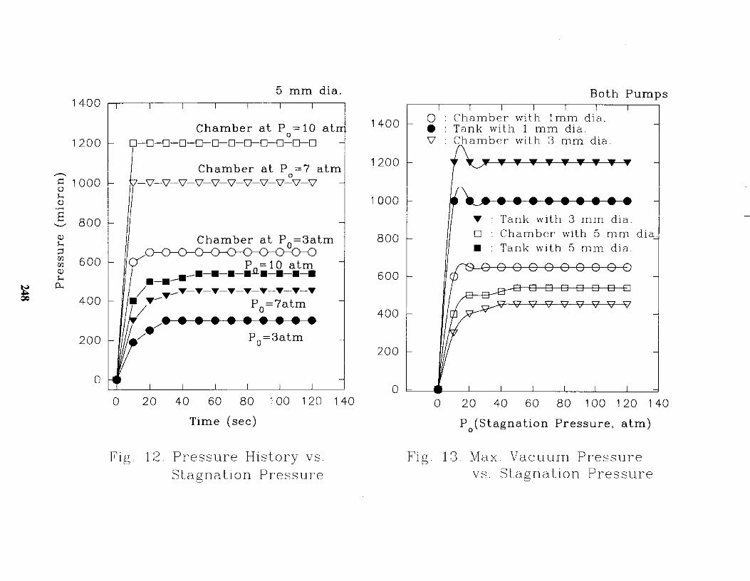
1400

1200

----0 1000 h () ..... a ......, 800 (l) h ;j III III 600 (l) h

N 0.. "" QC) 400

200

o o

5 mm dia.

Chamber at P = 10 at o D-D-D-D-D-D-D-D-D-D-D-D

I Chamber at P =7 atm

Chamber at P o=3atm

P =10 atm .-.-. /

• P =7atm / /. . . . . . . . . /. Po=3atm

20 40 60 80 100 120 140 Time (sec)

Fig. 12. Pressure History vs. Stagna tion Pressure

1400

1200

1000

800

600

400

200

o

Both Pumps

o Chamber with 1 mm dia. • Tank with 1 mm dia.

V .tb: :i:'::: :"::

o

Tank with 3 mm dia. o Chamber with 5 mm • Tank with 5 mm dia.

20 40 60 80 100 120 1 40 P (Stagnation Pressure, atm) o

Fig. 13. Max Vacuum Pressure vs. Stagnation Pressure

Fresnel Flow field

•

Cutoff

Knife edge

+-------------------L -----------------+, +t--------l' -------+

Fig. 14. Layout of Optical Components of A Small-field, High-Sensitivity Focused Schlieren System.

249

CCD Camera

o

Printer

CulOff Grid

TelepholO Len:r

Nozzle

I Computer

Pmme-Grabber

To vacuum tan.k

Prom G83 Contllinn

l VCR

j /

J

Presnel Len:r

i'l I I

II SOllICe Grid

I I l..1

Light SOllICe

MomlOr

Fig. 15. Diagram of the Highly-sensitive Focused Schlieren System Incorporated into the HFG at NASA LaRC.

250

Fig. 16 (a). Background-subtracted FS Image of the Free-jet Expansion ofN2 gas through 1 5.0 mm Diameter Nozzle in the HFG System.

251

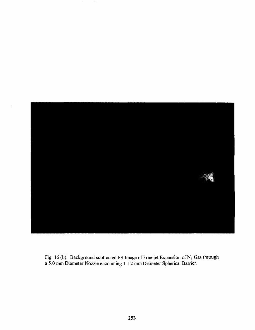
Fig. 16 (b). Background subtracted FS Image of Free-jet Expansion ofN2 Gas through a 5.0 mm Diameter Nozzle encounting 1 1.2 mm Diameter Spherical Barrier.

252

Fig. 17. EBF Image of the Free-jet Expansion ofN2 through a 5.0 mm Diameter Nozzle and the Corresponding Shock Intensity Along the Centerline from the Nozzle to the Mach Disk (PnlPc = 320, Xm=2.29 inches).

253

RAPID PROTOTYPING PROCESSES AND PROCEDURES

Paul Cheng-Hsin Liu

Department of Manufacturing System North Carolina A&T State University

1601 E. Market Street Greensboro, North Carolina 27411

Telephone 910-334-7116

and

Kenneth Moore

Chris Ogu

Undergraduate Students North Carolina A&T State University

Greensboro, North Carolina 27411

255

Rapid Prototyping Processes and Procedures

Dr. Paul Cheng-Hsin Liu, Associate Professor Kenneth Moore and Chris Ogu, Undergraduate Students

North Carolina A&T State University Greensboro, NC 2741.1

Key Words: Rapid Prototyping, Solid Modeling, Solid Edge.

Prerequisite Knowledge: Basic Computer-Aided Design (CAD) and solid modeling.

Objective: The objective for this lab is to develop a general knowledge of the design process for rapid prototyping and manufacturing. The field of rapid prototyping in manufacturing provides an excellent combination of engineering, science and technology as well as a seamless melding of processes and products. Through the study of the transition between design and production, students can determine the most efficient and productive methods for prototype development.

Equipment: l. Solid Edge software by Intergraph 2. Maestro software by 3D Systems 3. SLA-2S0 fabricator by 3D Systems 4. PCA-2S0 post curing apparatus

Introduction:

Automated fabrication is known by many terms such as rapid prototyping, 3-D printing, and desktop manufacturing. The term automated fabrication is used because of its generality. It does not attempt to limit the field to a particular use, but rather summarizes the process as a whole [I].

The focus of this study is primarily dealing with the developing industry of rapid prototyping. Since the process of automated additive fabrication became available most companies using the technology saw it as a field most beneficial to the engineering process. Through the process of engineering design known as prototyping, objects can be developed for manufacturing or presentation. The main focus of prototyping is for the optimization of form and function. With the speed of automated fabrication technologies, the traditional methods of prototype manufacture can be accomplished in much less time. Hence, the name rapid proto typing [2].

Fabrication Processes:

Fabrication is a process which can be utilized through three separate methods. The three processes are Subtractive, Formative, and Additive fabrication. Subtractive

257

fabrication deals with common drilling, milling, parting, and turning operations where objects are carved from a workpiece by chipping away material. Formative fabrication deals with using molds, punches, and dies to create solid objects. Unlike the previous two methods, additive fabrication (and more specifically automated additive fabrication) is a relatively new area in manufacturing which deals with the building up of objects into a particular shape or form. Examples of the six major types of additive fabrication technologies are listed below [1].

1. StereoLithography (SLA) is one of the most popular and widely used additive fabrication methods on the market today. Stereo lithography utilizes a laser and a photopolymer in a series of rapid prototyping machine products. It was developed by 3D Systems from Valencia, CA. SLA works by using an ultraviolet laser to solidify a photopolymer resin, one layer at a time. Successively solidified layers are built up one on top of the other eventually creating a three-dimensional object [3].

2. Laminated Object Manufacturing (LOM) utilizes a laser and a laminate which is usually paper. There are two machines available and both are manufactured by Helisys Inc., of California. The LOM process is unique because it uses pre-existing sheet material, cutting away the extraneous portions, without going through material phase changes and the raw materials are both widely available and lend themselves to value-added engineering improvements [3]

3. Robotically Guided Extrusion (also known as Fused Deposition Modeling when referring to the Stratasys process) has become one of the most popular automated additive fabricators on the market today. Sales ofFDM machines have for the first time overtaken the sales of the popular 3D Systems. SLA machines according to 1996 figures of recorded sales [4]. In this process, molten plastic is deposited along specific coordinates onto a fixtureless base eventually creating the object from the ground up.

4. Masked-lamp cul'ing is a process where an ultraviolet lamp is used to cure resin within a specific area by masking off the areas where the resin is not meant to be cured. This process is similar to masking off parts that are not meant to be spray painted as done in many automotive paint shops. The Soldier from Cubital Ltd. is the only commercially available product of this type. It is a large machine and has its problems with reliable functioning. This, however, is offset by the accuracy of the generated part [3].

5. Laser sintering is a process that is almost identical to the process of Stereolithography. However, instead of using a liquid resin, meltable powders are used. As in Stereo lithography the object created is formed in layers. The powder being of a solid form also tends to support the previous layers more than the liquid and thus eliminating the need for supports in this process. Laser sintering is a patented process and is owned by DTM Corporation from Austin, Texas. There are two machines for this process, the Sinterstation 2000 and Sintcrstation 2500 systems [3 J.

258

6. Drop-on-Demand Inkjet deposits materials in vector mode for precision and raster fill for speed and is manufactured by Sanders Prototype, Inc. (SPI), of New Hampshire. SPI was the number three company in 1996 in terms of unit sales, just two years after it became a corporation [4]. A second-generation system, called ModelMaker II, introduced last year can produce layers as thin as 0.0005 inch which gives Sanders an advantage when creating parts with fine detail.

Process of Design and Production:

In the process of design and production for rapid prototyping and manufacturing, there are a number of procedures to follow. These procedures allow for the optimization of the final product. Listed below are the necessary steps which should be followed for the best results in the process of stereo lithography [3].

1. Software Selection: With the development of the rapid prototyping industry, there has been a surge of

software developments targeted towards enhancing the transition from design to production. Software applications for tasks such as support building, complex surface generation, and file preparation have been created for the advancement of this industry. However, the type of software application which has benefited the most from rapid proto typing is three-dimensional computer-aided design programs. These programs allow the user to see and manipulate an actual three-dimensional object in a virtual environment. The development of this software has enhanced the field by speeding up the transition from design to prototype production. It allows for the user to see the final product ofhis/her work before it is physically produced. This allows for quick changes, the early detection of errors, and the swift input of three dimensional data into the printing machine.

A variety of 3-D software applications are available on the market today which allow for the creation of parts and assemblies within a virtual three-dimensional space. The software chosen must have all of the proper attributes for the type of part to be produced and the machine that it is to be produced on. An important feature that the software must have is the correct type of output. In order to produce a part from CAD data, the software must have an STL file format output. This is the only type of file which is accepted by the SLA machines and their component software.

2. Available Software: There are seven three-dimensional modeling technologies which are predominant

in today's commercial market. The number of shares that the companies hold within the 3-D solid modeling market is given below. Market share is a reasonably accurate measure of the popularity and use ofa software package [1,3,5].

(1). ACIS by Spatial Technologies is one modeler which acts as a foundation for many other software technologies on the market. It is written in C++ computer language which allows for the addition of many supporting features. This characteristic makes it

259

possible for the creation of software applications geared to fit specific needs. Software applications which use ACIS technology as a foundation are: Aries, AutoCAD, Bravo Designer, CADKey 97, CoreICAD, ElectricImage Modeler, Microstation Modeler, SolidDesigner, Solid Edge, TriSpectives, TurboCAD, and Vellum 3D. Spatial Technologies does not hold a significant market share in the 3-D CAD market because its software is primarily used as a foundation technology instead of a ready-to-use CAD application. However, AutoCAD holds a fifth place ranking with 223.7 million shares. AutoCAD is a software application created with ACIS technology.

(2). CADDS5 is the next 3-D modeling software available. It is produced by Computervision. This software holds fourth place in the total worldwide 3-D CAD market with 316.5 million shares so far in 1997. This down from a third place standing in 1996 with 290.7 million shares.

(3). CATIA is a 3-D modeling software which is widely used in European CAD markets. It is becoming more available in worldwide markets and now holds the second largest market share with 678.1 million shares. CA TIA is produced by IBM/Dassault.

(4). I-DEAS is a 3-D modeling package from SDRC. It holds the market share position of third place so far this year. It came from a fourth place standing in 1996 to overtake Computervision's previous standing.

(5). Parasolid is a 3-D modeling kernel similar to the ACIS kernel. The Parasolid kernel was developed by Unigraphics. It is used mostly by corporations who create their own independent software packages for use on their independent projects. However, it is becoming more commercially available to other software producers as a foundation technology. The Parasolid kernel is boasted as being 3 to 25 times faster than the ACIS kernel in experiments of speed in construction. As of now, it also has a larger number of features.

(6). ProlENGINEER is the top selling 3-D CAD applications. It holds the largest market share with 924 million shares. It also held the number one position in 1996 as well. Pro/ENGINEER is sold by Parametric Technology Corporation. It has a number of software applications with fit specific engineering needs.

(7). DESIGNBASE is a three-dimensional modeling component software developed by Ricoh of Japan. It was designed as a foundation technology for software developers. This software is used primarily by Helix Design Solutions as a foundation technology.

3. Software Choicl!: Solid Edge by Intergraph was chosen as the 3-D solid modeler which best suited

the needs of this project study. Its simplicity of use, advanced rendering capabilities, and compatibility with other software and machines made it the best available choice. A

260

number of prototype models were created with this software using only a beginners knowledge of 3-D modeling software. The simplicity of the software lies in the ability to create basic profiles on two-dimensional planes. This feature makes up the foundation for creating any shape or form desired. Any 2-D plane can be chosen with relation to the initial front, top, and right side planes. These planes can also be aligned to a surface plane on the object itself. Using the protrusion, cutout, hole, revolved cutout, round,

Figure 1. Example of Solid Edge Modeling.

chamfering, and patterning functions, any object can be made through a series of profiles. At any time, the constructed object can be rendered and viewed from all sides for errors, presentation, or aesthetics [6]. Figure 1 illustrates an example using Solid Edge in modeling.

4. "Virtual" Prototype Generation: Once the software most practical to the needs of production has been chosen, the

next step is to begin construction of the part in the 3-D CAD software. Since engineers and designers are the ones who conceptualize the objects to be created, they are the ones best suited to use the software to create the models. Their close interaction with the software enables them to easily make any changes which need to be made. Those

261

changes may be repeatedly altered to improve the aesthetics and/or the functionality of the object produced [2].

5. STL File Preparation: After the design phase is completed in the CAD model and an output file is

created, the part is then ready for the build phase in the rapid prototyping and manufacturing process. Before beginning the actual production of the part, the CAD file must first be subjected to the proper preparatory processes. Those processes are meant to ensure that the part is produced with the maximum possible accuracy. In the past, a number of third-party software applications were available for aiding in the part development process.

3D Systems produces a software which combines all of the necessary tools for the delivery of CAD models from the STL file output directly to the input into the SLA. This software is entitled MAESTRO/JR. It contains six integrated modules which aid in the preparation of the part for production. 3dverify is the module used to correct CAD files of any errors which may be present. It does this instantly by automatically taking the file and checking it for faults. Notifying the user if there are any and correcting the errors without the need for returning to the initial CAD environment. The second module, simply called View, is fairly self-explanatory. It allows for the user to see the part or parts to be built and to determine the preferred placement within the build envelope. In this module, it is also possible to scale the part up or down as necessary. Vista is the next module. Its purpose is to generate supports which protect cantilevered objects from the weight of the resin and to keep the surfaces of the object in place. Vista works along with a parallel program called Sierra Supports which keeps support structure contact with the part at a minimum. This allows the supports to be easily removed after the resin solidifies throughout in the final stages of production. Since the process of stereolithography builds up three-dimensional objects by layers, the object to be produced must first be divided into horizontal layers of information. Cslice is the program which handles this part of the process. This module is fully automated and requires no input on the part of the user. Part Manager is the module which brings together the information from all of the modules. Here, all of the parameters for the part can be viewed and altered through basic spreadsheet data. Converge is the final module which combines all of the preparatory information from the other modules to be input directly into the SLA. This data includes the slice files and the recoatmachine parameters which are combined to create the part [7].

6. File Input and Part Generation: The next step in the process is the input of the file into the SLA machine. Files

processed by MAESTRO/JR are taken and input into the SLA's computer. This computer takes the data and conforms it to a number of specific parameters which determines the precise operations of the SLA machine. These operations are a necessary final step which help the user to control the accuracy of the final product.

262

The following parameters are given for the SLA-250 and must be set in order to successfully create the part. Parameters for the SLA-250 are given because that machine is the most general and widely used of the SLA machines. The SLA-190 and 500 may add on or subtract a few of the specific commands. The operation parameters to be addressed are: the units of the input file; layer thickness of the part; linewidth compensation of the part; X-hatch spacing; Y-hatch spacing; 601120 hatch spacing; X-skin spacing; Y -skin spacing; fill overcure; minimum surface angle; slice resolution; STAR-WEAVE switches; slice axis; scale factor; slice argument files; part offsets; postdip delay; Z-wait; Z acceleration and velocity; number of sweeps; sweep period for sweep; part to blade gap for sweep; overcure depth; absolute cure depth; range divisions; X, Y, and Z miniscale for resin shrinkage; number of copies; and resin type [3].

Once these parameters have been specified, the build process begins. The machine starts with the platform elevator resting beneath the top layer of the resin envelope. After the laser finishes solidifying the present layer, the platform machine smoothes out the surface of the resin with a thin coat of resin applied over the top. Layer upon layer is built up in this manner from the bottom to the top of the object to be produced. It takes a few hours to a few days for the part to be produced. This time depends upon the size of the part files being developed at one time.

7. Post Processes: . When the build process ends, the object produced must be cleaned, cured, and

cleared of all supports. The process of cleaning should begin with the draining of all excess resin from the part. This can be accomplished by suspending the part within the build envelope so that all excess resin drips back into the resin vat. The next step in the cleaning process is to remove the part from the machine and wash the surface of the object in solution to get rid of any pockets of excess resin. Since the SLA only solidifies the walls of an object, it is necessary to cure the object in an ultraviolet chamber. This process called postcuring is for making sure that the liquid resin has solidified throughout the object. Any pockets of resin left uncured may eventually warp the object. Finally, when the part has thoroughly solidified, the supports are then able to be safely removed without damaging the object. After this final step, the part is now able to be finished using any method necessary to achieve the desired characteristics.

8. Error Detection and Correction: At this point, the prototype has been completed. However, the engineer/designer

must make sure that the part has been make to fit the proper specifications. The part should be inspected for errors in order to determine whether any anomalies in the object may have appeared. This may be due to misplaced supports, trapped pockets of resin, etc. If any errors are evident, they can be easily corrected on the initial CAD model. Here the engineer must use the initial CAD file within the initial CAD program. This ensures that the problem is corrected at its source. The benefits from this may be realized at a later time when this CAD file may be reused. Therefore, at anytime in the future, this CAD file may be reproduced without the same complication. When the part has been corrected, verify that the changes made will be effective in solving the problem. After all

263

possible errors in the part have been found and corrected, the part is now able to be produced once again on the SLA.

9. Optimization: After this functional test model has been created, the next step is to optimize the

part. Optimization deals with taking the part and altering it to achieve the maximum level of performance. The optimization step is a direct by-product of functional testing. As functional testing is performed on the part to ensure that it meets the minimum standards, changes can also be made at this time to achieve optimum performance of the part [3].

10. Finishing: Once the desired product has been fabricated the process is complete. There is an

option to either finish the prototype for presentation or prepare the prototype model for manufacturing. Preparing the prototype for presentation can be done using any traditional method of finishing for plastic models. For manufacturing, the prototype can be used to make multiple copies through various casting methods [3].

Conclusions:

It is clear that rapid proto typing is a great deal faster and more efficient than the traditional methods of prototype production. Mostly through reducing the channels of communication and simplifying the tasks through automation is the process made less time consuming. This speed is the main reason as to why the development of rapid proto typing has become one of the most popular fields in automated additive fabrication.

Acknowledgment:

This Rapid Prototyping and Manufacturing project was funded in part by a National Science Foundation Instrumentation and Laboratory Improvement Grant (NSF Grant No. 96500l3) and its supplement award from the Division of Undergraduate Education.

References:

1. Burns, Marshall. Automated Fabrication: Improving Productivity in Manufacturing. Prentice Hall, 1993.

2. Wood, L. Rapid Automated Prototyping: An Introduction. Industrial Press, 1993. 3. Jacobs, Paul F. Rapid Prototyping and Manufacturing: Fundamentals of

Stereolithography. Society of Manufacturing Engineers, 1992. 4. Wohlers, Terry. Rapid Prototyping: State of the Industry 1997 Worldwide Progress

Report. Society of Manufacturing Engineers, 1997. 5. http://www.geocities.comlCapeCanaveraIlLab/2549/cad.htm 6. http://www.intergraph.com 7. http://rpmi.marc.gatech.edu

264

Dr. Paul Cheng-Hsin Liu is currently an Associate Professor in the Department of Manufacturing Systems at the North Carolina A&T State University. Dr. Liu has strong background in Manufacturing Processes, Automatic Identification technologies, Automation, Fuzzy Logic Control, and Statistical Quality Control. He teaches both graduate and undergraduate courses in Statistical Quality Control, Automated Manufacturing, Programmable Logic Controller, Automatic Data Collection and Identification, Reliability, Productivity, and Manufacturing Processes. He is a member of the SME Rapid Prototyping Association, lIE, ASQ, Alpha Pi Mu, IEEE, and NAIT. He has published numerous quality papers in the last two years. He is Certified Manufacturing Engineer (CMfgE) by SME, Certified Quality Engineer (CQE) by ASQ, and Certified Senior Industrial Technologist (CSIT) by NAIT.

265

THE HUMAN HALF-ADDER: UNDERSTANDING THE BIG PICTURE

OF DIGITAL LOGIC

Linda Vanasupa

Materials Engineering Department

and

David Braun

Electrical Engineering Department California Polytechnic State University

San Luis Obispo, California 93407

Telephone 805-756-1537 e-mail Ivanasup@tubaocalpolYoedu

267

Linda Vanasupa

268

The Human Half-Adder: Understanding the Big Picture of Digital Logic

Linda Vanasupa '\Iatenals Engineering Department, California Polytechmc State University, San Luis Obispo, California 93407

David Braun Electrical Engineering Department California Polytechnic State University, San Luis Obispo, California 93407

Keywords: digital lOgic, logic elements, binary numbers, microprocessor, transistor, voltage, mtegrated circuits

Prerequisite Knowledge: The student should understand the concept of the base-2 (or bmary) number system. They should also be familiar with the concept of electrical circuits, mcluding the relationship between voltage, current and resistance in a DC circuit (V=IxR), and have a rudimentary understanding of transistor operation as a voltage-controlled switch.

Objectives: Oftentimes materials engineering students fmd themselves with an intimate knowledge of the processing that goes into fabricating integrated circuits. Yet they aren't aware of how these deYlces function in the circuit. "This exercise is designed to impart an understanding of how individual transistors work together in a simple cirCUit.

Equipment and Supplies (per Half-Adder)

metronome (or a good sense of timing) 11 students (, mdex cards marked "0", 6 mdex cards marked "I", shuffled together 11 index cards with instructions and numbers (descnbed in the text) viewgraph of a full adder viewgraph of a half-adder overhead projector 8 large pieces of cardboard, cut into the shape of lOgiC elements (2 A.ND, 1 OR, 1 41-bit, square registers)

Procedure and Instructor Notes

Overview This activity can involve from 11-42 students, depending on how you piece together the circuits for the half-adder. In its simplest form, the activity involves 11 students, each performmg the function of either a lOgiC element or half a logic element. Following a diagram of a circuit, the students arrange themselves m a half-adder circuit. Each student stands on the shape of the lOgiC element that they have been assigned. "The instructor acts as a "clock." A.t each tick of the clock (instructor), the Signals are passed through the lOgiC elements (the students) to yield an answer in a few ticks.

269

In order to take adYan tage of the benefits of addressing the dlfferen t learning styles of dle students' and use cooperative leammg, we've built .f:,'TOUP actiVities mto the Human Half-/\dder. Inc activities are designed to m;L'{imize the students' leam1l1g. 'Ine entire exercise can take up to 45 minutes. It involves four parts: 1. L'nderstlllding logic elements and binary data, 2. L'nderstandmg the Half-Adder, 3. Operatmg the I luman I lalf-,\dder and 4. Sohdlfying dle concepts through calculations. Each parts has a umque learning objective. We describe them m detail below.

Step-by-Step Instructructions

1. Cnderstandmg logic elements and binary data

SllIdelils wi!! be able 10 describe han lrallJislors mpolld 10 illplll l'O!tu/!,fS to ollt/ml u h(gh or !OJl a !o.Ric elemellt (i.e., AND, OR, ,\TOR, ,\TOT,gule).

"\. Begm by discussing how logic clements produce what would be considered binary data .. \ sllmple example of thiS IS the mvert<:'r or gate, which can be made up of two transistors in the configuration sketched in Figure 1. The top transistor IS

held on (i.e, has a conducting channel) by the havmg the gate voltage "hard Wired" to the supply voltage. \X'tth no mput signal (you may also call this a "0" 1I1put or low voltage input), the bottom transistor IS an open circuit, leaving dle output (which IS short circuited to the 5-\'olt supply) the same as the supply voltage- 5 \·olts. With an mput of S volts (also known as a "1" or high voltage input), the channel of the lower transistor is opened, creating a conducnng path to ground. 'I1le voltage is dropped over the top transistor, causmg the output to be at a low voltage. Tn dllS way, you can sec that the input Signal IS inverted (;\;()'t' the s:unc as the output, you might say), generating the behavlOr m the "truth table" ncxt to dlC elcctncal schematic in Figure 1.

B. Hav'e the students work in groups of three to determme the output charactenstlcs and lOgiC function (1.e., ,\",U, OR, :\:\:\D, NOR) of other circUlts, shown m Figure 2. In order to complete dllS part of the exercise, the students may need a shurt descnptioll of the ddinition of each logtc clement. "\ summary Is proVIded mTablcl.

2. L'nderstandmg the Half adder

J/lldfllls IIi/I be uM 10/01!0I1' all illplll Ibe .rme.r elemenl .. ' illlhe hul/addo:

:\. Descnbe the concept of a half adder circuit usmg the vltwgraph of dle 11:111' adder as a reference (Figure 3). In:l full adder, half adders arc linked together in a carefully prepared circUlt to produce the desired effect. The full adder is shown in Figure 4.

R. Han students work dle results C)f b1l1clf)' additlOn m groups uf three. Examples of exercises are shown 111 Figure 5.

3. Operating the Human Half adder

SllIde!ltr !l'ill be 10 dewibe hOi/' e!emfll/.r lI'OIn 10 udd IJlO billul} d{gil.r

270

"\. Assign each of the 11 students a role in the circuit by passing out the cards. I-:ach card describes either a complete lOgic element, or half of an clement. The student performs the function described on the card. The cards arc shown in Figure ().

B. Have students by out the brge cardboard CIrCUit elements on the floor m the pattern of the circuit. The students then stand on their assil-,rt1ed logic element. E:lch student must identify who they :Ire getting their input sIgn31 from. This wllllikcly be a confusmg 3ctiYltyand require the assistance of the viewgt3ph that shows the h:1lf-adder circuit. \\'hen the students are set up m the four rows shown on the circuit, allow the students who arc the input registers to draw an mput card from the 12 cards that arc marked "I" and "0."

C. Perform a tri31 nm :It a vel)' slow clock-possibly 20 beats per minute. :\t the first tick of the clock, the person who IS the input register uses their arms to indlcJtc whether the sll-,rt1al is J high or low \-oltage (I.e., holdmg J hand up indicJtes a high signal). 'I'he people In the next row who arc supposed to tJke the slgilal mimic the positioning of the tnput signal with their Jnns .. \t the next tick of the clock, the students comprismg thiS lOgiC element must output a signal for the next row of elements. 'l'his reqUIres tlut they botll neJt1ce each otller's input \-alu(' and dctermme together what the output should be. j'or eXJmple, If e3ch student IS Jll mput of In .\:\ D gJte, one With a high, one With J low voltage, they must both realm: before the next tICk of the clock thJt their output should be J low \-olt3gc. _ \t CJch tICk of the clock, the slf,rt1:1l moves to the next row of lOgiC clements. If you devote J tick to fillmg the input reglstcn;, 'You should get your answer after .f ticks of tllC clock. IncldentJlly, thiS usc of the clock is not stnctly correct, smce tile llalf Jdder IS tYPlC:111y "JsynchfClnous"-unltnked to the clock. I [owen:r, It does Illustrate that tile clock IS oftentllnes Im-olYl'd in c(lord1l1Jtmg the "tfJffic" of the slgnJls.

D. Check to see If your Jnswer IS nght. The tnstnIctor must orchestr:1te :J group-thmk Jt tillS pCllnt, gUldtng the students through 1!ltt'rprettng till' tnput number and the output number. Bcc:Juse the shldcnts did ,lf1 anJlysls of thiS 1!l exercise 2B, thiS should be simple .. \t thiS potnt, thtngs could become n'I)' c()nfusmg-espccI:Jlly if the output IS tncorrcct (e.g. 1 + 1 =0). '1111' pr()blem could be clther bulty wlrtng (students taktng the tnpllt sll-,rt1Jis from the 1!1corrcct CirCUIt element) or f.Jult) ClrcUl t clemen ts (s tuden ts olltPll ttmg the 1!1correct slgnJI), or some 0 f both. If tlwrc IS a problem, r('\'lCW tile operation of cach logtc clement. \Is(), re\'lew the half Jdder circlllt to ensure th:Jt c:lch person knows from whom to take thclr tnput SIi-,rt1 Jl.

Try ;mother nIn of the CIrCUit With J different tnput at J higher clock speed .. \ll()w the students who arc 111pUt rCi-,'1sters to dr:Jw JJ1<lthcr set ()f Inputs JJld re-nIn the Circuit Jt a higher clock specd. Set the metronome for successlYcly higher clock speeds . .\lJke sure that after eJch rUll of the CIrcUIt you t,lkc t1lnt' to \Tnfy tll:lt the answer IS correct

.f. SolidlfY1l1g thc concepts C:JiclliJtlof1S

.\'llIdmls Ihe O,/,ICu! 111I!Jl/!(,1 iI/IIII/I7/(/loll Idl Ihul u (o!1l/l!Ilel' (ull rCI/OI'!Jl111 u SfCOlid If Ihey klloll' Itle dock .Irm/.

271

Have students complete a follow-up worksheet. Example of questions that might be on this worksheet are shown in l;'igure H. The questions on the worksheet help students to retlect on the implications of what they have leamed.

S. Chaining half-adders together

Stl/dents u'i/!gaill the comp!e:,:ity illl'o!z,ed III paJ'Silig slglla!s a armit ..

Summary

If you have enough students, you can attempt to chain several half adders together in order to add numbers with more digits. Reference 2 shows \'erslons of the circuit that you can also run (page 334-335)'.

This exercise allows studen ts to gain an understanding of how indiVIdual transistors function in a logic element of an integrated circuit. By participating as part of a lOgiC element, the studen ts gain an understanding of how the elemen ts work together to add two binary digits. 'The worksheets also provide a feel for the speed at which signals are passed in an Integrated cIrcuit that has a clock speed of 200MHz. Although this is beneficial information for the beginning electrical engineering student, it also proVIdes a big-picture view of in tegrated circuits for materials engineering students who are studYing microeiectf()nics processing.

References

1. Harb, P.K. Hurt, R.E. Terry and W.J. \Villlamson, Teachillg Thm/(f!,h tbe C)'de: Application of Learning Style Theory to Engineering bducation at B'Zf!,ham ) 'ol/ng U nil'erJity, 2nd I Bngham Young University Press, Provo, U tab, 1995.

2. Macaulay, D. The U7qy Things Work, Houghton-Miftlin Company, Boston, i\L\, 198H.

+5 Volts

Vin

}- Vout

--11 ....

Figure 1. Electrical Schematic of a NOT and its truth tahle. Tht top transistor is "lied" open hy connecting the gate to the voltage supply. By inputting a high voltage, the bottom transistor hecomes a conducting path, causing the voltage supply to short to ground. In this case, the voltage is dropped over the top transistor, causing the Vout to be at a low voltage.

272

Vtn 1 Vtn2 \' out

() ()

() 1

1 ()

1 1

\'in 1 \'tn2 \'out

() ()

0 1

1 0

I 1

Figure 2. Electrical schematics of a Ni\ND (top) and a (bottom). Students fill out the truth table, using their knowledge of how the transistors will respond to the Input signals. You can create the i\,,[) ""d the OR by putting the output of each one of the above circuits in series with a gate

AND gate

carry bit

Figure 3. Sketch of a hal f adder.

Input Registers

273

OR gate

AND gate

sum bit

-r LLr----+r---___+_.. I

in pI< t f'f .. r 1-wo

Figure 4. Sketch of a full adder. The full adder can be constructed bl' linking together three half adders and an OR gate

274

Add4ion of Binary #'s Like base-1 0 numbers, each dig4 in a binary number represents a factor of the base number, raised to a power. For example

104103102101100 6 7 5 0 3 0 ,000 + 4 x 1000 + 5 x 1 00 + 0 xl 0 + 3 x 10

8ase-2 numbers follow the same rules:

x 1 6 + 0 x 8 + 0 x 4 + 1 x 2 + 0 x 1 =18 (in the base-1 0 numbers that we're used to)

Add the following sets of binary numbers and convert to base-1 0 answers:

o 1 1 1 ., 1

+ 0 1 + 0 1 + 1 0

1 0 1 0 o 1 + 0 1 + 1 1 + 1 0

FIgure S. EX:1mple of a worksheet on bm:1ry numbers. '1111S worksheet should take no longer than 10 mmutes, pnmmg the students to work wIth the half adder.

I 0 1.-A IJI)

Ij

rB L 0 f 0

'f f"", I /'" pHt 0(:' "'" AN 1)

-f'"" /voT

<. F. " I ,"'p .... t of

a,.. oR"

J ff r ,,'f-

for [vm i"f 0 ' "'r 1, I l'np ... t

. I J

b "'1 f/ ; r

2. {O". !-;,t t" ptA."

FIgure 6. The deck of mstructlon c:1rds that are required for the half adder.

275

FOLLOW-UP QUESTIONS 1. A typical personal computer (e.g., a 1996-version of Intels' Pentium processor) is capable of issuing 2 instructions pHr clock cycle. Assuming that the computer requires an average of 10 instructions to perform a function (such as addition or multiplication or sending a signal to the computer screen), how functions is your computer performing if it take 1 second to respond if your computer operates at 200 MHz?

2 instructions. 200x 106 cyles cycle second

function 7 ------·1 second = 4x1 0 [unctions' 10 instructions .

2. You may be interested in displaying a digital video image on a typical computer screen. These screens refresh at a rate of 25 Hz and require 8 bits (i.e., 8 binary digits) per pixel. A typical screen is 640 x 480 pixels (picture elements). How many bits of information are required if each pixel is changed throughout that second?

25 frames 640x480 pixels 1 d 6 107 . 1 ---. . . secon = x hils' pixel second frame

Figure 7. Example of follow-up questions to soltdify concepts. The calcubtions demonstrate the magnitude of information that is required m digital operanons. ,'\nswers are dlspbyed in boxes.

Function ActlOn Graphic Symbol

0;0'1' (or "Inverter") Im'crts thc input signal to ,ts -C>o-opposite

1\",D Outputs a "I" If 1.1 :\\:D 2"" =(J inputs llre «1"

OR Outputs a "1" ifl" UR 2nd inputs =D-are "1"

Produces an output SIgnal that is =(J--the inverse of the .\;o.;[)

l'\OR Produces an ,lutput sif.,mal that is =L>-the Im'erse of an OR

Tahle 1. Functions, their actions and fheir s,-mbols (adapted from RS Sandigc. ,\fodenl ",fcC;raw Hill 1990, p. 58)

276

Biographical Sketch

Linda Vanasupa graduated from J\fichigan Technological University with a B.S. in Metallurgical Engineering in 1985. She finished her M.S. (1987) and PhD. (1990) at Stanford University in :\laterials Science and Engineering with an emphasis on electrical engineering. Since coming to California Polytechnic State University in 1991, she has focused her energies on teaching and research in the area of microelectron1cs processing. She is curren tly a professor of l\faterials Engineering at Cal Poly, San J ,uis Obispo, Califonl1a.

David Braun joined the Cal Poly faculty after working at Phihps Research Laboratories in Eindhoven, the l\.'etherlands between 1992 and 1996. In 1991, he completed the Ph.D. in Electrical Engineering at the U.c. Santa Barbara. He teaches courses in digital electronics. His research Interests center around combining techmques from both polymer and Integrated circU1t processing to 1mprove the efficiency and lifetime of electronic devices made from semiconducting polymers. He is currently an assistant professor of Electrical Engineering at Cal Poly, San Luis Ob1spo, Californ1a.

277

A METHOD FOR MEASURING THE SHEAR STRENGTH OF POLYMERS AND COMPOSITES

Luis Gardea

and

Brian L. Weick

Department of Mechanical Engineering University of the Pacific

Stockton, California 95211

Telephone 209-946-3084 e-mail bweick@uop.edu

279

Brian Weick

280

A Method for Measuring the Shear Strength of Polymers and Composites

Abstract:

Luis Gardea

and

Brian L. Weick*

Department of Mechanical Engineering University of the Pacific

Stockton, CA 95211

*Telephone: 209-946-3084 E-mail: bweick@uop.edu

An experiment IS described that can be used to study the shear strength characteristics of various polymers and polymer composites. Typical results are presented for glass fiber-filled and unfilled polymers including Teflon, acetal (Delrin), Nylon, polycarbonate, and NoryL Shear tests can be conducted using a simple fixture that was designed using ASTM specifications, and is easy to manufacture When installed in a basic tensile test machine, the fixture subjects the polymer or composite rod to a double shear load. Shear strength can then be calculated from the maximum load indicated by the tensile test machine, and the cross-sectional area of the test specimen. Statistical methods are presented for calculating experimental error, and typical failure mechanisms are briefly discussed using SEM's of the fractured surfaces.

Keywords: Shear Testmg, Polymers, Polymer Composites, Polvmer Failure Mechanisms

Introduction and Prerequisite Knowledge:

Often it is necessary to create experiments that provide outreach to Junior college or high school students to stimulate their interest in engineering. In this case, a topic in mechanical engineering dealing with materials testing and analysis is used to provide a bridge. The experiment is set-up to be performed at the Junior college or even high school level with the guidance of a mechanical engmeering professor or student from a four-year engineering college who would oversee the project. The ultimate goal is to allow students to learn about materials, manufacturing, strength of materials, and most importantly, allow students who may not otherwise consider engineering as a profession a small amount of experience that may entice them to look into it further Junior college students would benefit from an introductory course in statics or engineering, but high school students enrolled in a physics course would also be able to perform this experiment Basic university classes such as computer aided drawing, machine design, manufacturing, and materials science would be beneficial for the university student who is overseeing the project.

281

Objectives:

• Develop a simple method to reach out to secondary and junior college students to gain their interest in various aspects of mechanical engineering.

• Manufacture a simple fixture for measuring the shear strength of cylindrical specimens using a tensile test machine.

• Perform shear strength measurements using polymers and polymer composites with varying amounts of glass fibers.

• Present methods for examinmg fractured surfaces and determine potential failure mechanisms.

Equipment and Supplies:

I. ..,

3.

.t.

Shear Test Jig. (See Fig. I and Appendix A) Tensile Test Equipment. (The shear tests discussed herein were conducted using a Materials Testing System tensile test machine.) A magnifYing glass. or low power microscope to examme fractured surfaces. (Photographs presented herein were obtained using a scanning electron microscope to accurately depict typical failure surfaces.) Test specimens ordered from McMaster-Carr Supply Company and AIN Plastics Inc.

, , , , , , .. 0 ' , 0 0 0 0 ' , , , , , , , , , , , , ,

TOP VIEW

FIBER· FILLED OR UNFILLED POLYMER ROD

.. PARTIAL CUT-AWAY VIEW

Figure l. Fixture for testing the shear strength of unfilled or fiber-filled polymer rods

282

Procedure:

Design and Manufacturing

The shear test J ig can be manufactured using the sketches shown in Fig. I and Appendix A. The desib'11 of the shear test jig is based on an ASTM standard for the shear testing of rivets, and it is designed to accept 1/4 inch diameter specimens.

Material Selection and Ordering

Unfilled and glass fiber-filled polymer rods were selected as test specimens. AIN Plastics Inc. and the McMaster-Carr Supply Company were selected as vendors. Five unfilled and five glass fiber-filled polymers were selected: Teflon, polycarbonate, acetal (Delrin), Nylon, and Nory!. The glass fiber-filled Teflon matenal contained 25 wt.% chopped glass fibers, fiber-filled polycarbonate contained 20 wt.% chopped glass fibers, and fiber-filled acetal contained 15 wt.% chopped glass fibers. The glass fiber-filled Nylon and Norvl materials also contained only low weight percentages of glass fibers « 20 wt' %), but specific weight percentages were unavailable from the vendor. The aspect ratios for the chopped fibers were also not specified by the vendor, and the rods were ordered at the minimum ordering amounts available. Whenever possible 0.635 cm (1/4 in.) diameter specimens were ordered. Acetal and fiber-filled Noryl were only avatlable in 0.953 cm (3/8 in.) diameters. These two rods were turned to 0.635 cm using a lathe.

Material Preparation and Test Method

Test specimens were cut to fit the 1/4 inch diameter loading hole in the shear Jig. The shear jig IS clamped into the MTS machine grips without applying a load. and the center section is lined up with the loading hole allOWing for insertion of the specimen. An optional safety cap is screwed into place over the test specimen. The test is started. and at the sound of material failure. usuallv a snapping sound. the MTS is stopped and the specimen IS unloaded. Care IS

taken not to touch the sample fracture faces and each piece (three In total per sample) is secured In a holding case. Securing is achieved with double stick tape so that the fractured face IS facing up. Care is taken that at least two of the fractured mating faces are facing up. This allows for studv of the fracture patterns on the mating surfaces.

Data Analrsis

Shear strength values were calculated using the double shear equation [I]:

P T=--

2Ax (1 )

where. 1" the shear strength of the polvmer. A< c the cross-sectional area of the Circular rod. P - the maximum load applied to the specimen before failure.

283

Multiple experiments are performed for each material, and confidence intervals are calculated using the student's t-distribution [2]. The t-distribution is used rather than the z-distribution because the standard deviation is not known prior to doing the experiments, and therefore must be calculated from the: experimental data. Equations for calculating a confidence interval (C.I.) using the t-distribution are shown below:

(2)

C.I.= + (3)

where.

y - experimental data point,

y - average of n data points,

n - number of data points or measurements,

s - standard deviation,

ta/2 00 percentage pomt of the t-distnbution (for a confidence interval, a = 5% or 0.05.)

Percentage points of the t-distributIOn can be found in any standard statIstics textbook such as the one by Ott [2], and many sCIentific calculators have the t-dlstributlon as a bUIlt-in function. Statistics software packages such as Minitab and SAS also contain the tunctIOn as a built-in subroutme. As a simple example of how Eqs. 2 and 3 are used, suppose the length of a long piece of rope is measured n = 8 times. The data set consists of eight data points: 19.30, 1955, 19.61, 19.72, 19.23. 19.34. 19 05, and 19.51 The average, y,isdeterminedtobe 19.41 meters, and the standard deviation is determined to be 022 meters using Eq. 2 The "t" value, fa/20 is found to be 2.365 using a table in Ott's text [2]. (Note that for a 95% confidence interval. fa/2 = to 025 and the "deb'Tees of freedom" are n - I or 7) Equation 3 can then be used to calculate the 95% confidence interval and attach it to the average value as an estimate of expenmental error. This confidence interval is ± 0.18 meters, and the experimental measurement for the length of the rope would then be specified as 19.41 ± 0 18 meters. (Answers may vary slightly depending on the round-off error of your calculator or software .... remember statistics is sometimes thought of as the science of giving answers that are probably correct') The Shear Test Data Sheet shown in Appendix B provides a step-by-step guide to calculating confidence intervals using real data.

284

Materials and Test Conditions:

The materials tested are listed in Table I along with vendors and part numbers. Ambient temperature and humidity conditions were used for the experiments. Ten experiments were performed for each of the materials, and average values and contidence intervals were calculated using the methods discussed herein.

T bl I L' f a e . 1st 0 vendors and matenals use d d to or er test specImens.

Vendor Material Part no. for a flber- Part no. for an filled material unfilled material

McMaster-Carr Teflon (PTFE) 85275 K24 8546 Kill

McMaster -Carr Polycarbonate 85665 K53 85485 K43

AIN Plastics, Inc. Nvlon NYRD280 NYRD27

AIN Plastics, Inc. Noryl NORD50 NORD118

AlN Plastics, Inc. Acetal (Delrin) DERD296 DERD87

Results and Discussion:

Shear strength measurements Shear strength data for the tiber-tilled and untilled polymers are shown in Table 2. A graphic representation of the data can be found in Fig. 2, and 95% confidence intervals are shown as error bars. These data sets were taken to see if the test procedure is valid. The goal was to determine if differences in shear strength could be detected between fiber-filled and untilled polymers. In addition. it was hoped that the test method could also detect differences between the shear strengths of the polvmers themselves.

T bl 2 Sh a e ear tes t , MP averages ID a. a ong WI fid o con I t ence In erva s. Material Average Shear Strength and 95% C.I. (MPa) Untilled Tetlon 18.2::: 07

- --- --- - -- - - - ----- -

Fiber-filled Teflon 17.6±0.9 Unfilled acetal (Delrin) 33.9::cOA ----- - - --- --

Fiber-filled acetal (Delrin) 46.4 ct 08 Untilled Nylon 41.1 ± 02

- ----

---

- -- - ----- --- ----

Fiber-tilled Nvlon 39.6 ± 03 Untilled polycarbonate 37.0::: 05 -- --- --- - --- - --------

Fiber-tilled polvcarbonate 36.8 ± 0.6 Untilled Noryl 37.8 ± 02

-- - - --- ---- - - - --- -- -- - - -------- ----

Fiber-tilled Noryl 39.8 ± 0.2

285

From Fig. 2, it is clear that Teflon has a shear strength that is approximately half that measured for the other materials regardless of whether or not fibers are present. Furthermore, based on the confidence intervals calculated for the Teflon experiments, there is little or no significant difference between the shear strength of an unfilled or a fiber-filled Teflon rod. This is not surprising due to the low surface energy of fluorinated hydrocarbons like Teflon, and therefore the fiber-polymer bond is expected to be weak. The shear strengths of unfilled and fiber-filled polycarbonate rods are also the same. However, shear strength measurements for acetal show that the fiber-filled material has a shear strength that is 12 MPa higher than that of the unfilled material. Fiber-filled Noryl rods also have higher shear strengths than unfilled Noryl. Measurements for Nylon, on the other hand, are a bit counterintuitive. Although the difference is only I - 1.5 MPa, the shear strength of unfilled Nylon resins was determined to be higher than the shear strenb'1:h of fiber-filled Nylon. The reason for this difference is not known at this time, but more testing and analysis of the fractured surfaces is planned for the future

ro D...

.!: .-C) c Q) .... .-en .... ro Q) .!: en

50 Unfilled Fiber -filled

40

30

20

10

Teflon Acetal (Delrin) Nylon Polycarbonate Noryl

Polymer Type Figure 2. Average shear strengths and confidence intervals for unfilled and

fiber-filled polymer rods

286

Failure Analysis Due to the fact that one can learn a great deal about fracture mechanisms by studying the broken surfaces under a low power microscope or even a magnifying glass, low magnification images are presented of the fractured acetal surfaces. Note that these images were actually taken using a scanning electron microscope (SEM), but the magnification is less than 200X for Fig. 3, and only l4X for Fig. 4. SEM's are useful at these low Fib'Ure 3. Fractured fiber-filled acetal (Delrin) surface magnification levels for their increased depth of field over optical devices. Therefore, they are able to capture pseudo 3D images of a broken surface.

Figure 3 is a picture of a fiber-filled acetal surface after a shear test. Note that there are broken fibers sticking-up out of the surface with little or no polymer material adhering to them. This is characteristic of crack propagation at the interface between the fiber and polymer followed by pull-out of the fibers from the Figure 4. Fractured unfilled acetal (Delrin) surface. matrix.

Note that the fiber-filled acetal material is not a continuous fiber composite, therefore not all of the fibers are aligned as is suggested in Fig. 3. Only a very small part of the fractured surface is shown in this picture, and other broken fibers protrude or lie at different angles on the surface. The fracture of the fibers is characteristically brittle in nature as would be expected for glass

287

materials. However, the type of fracture observed for the polymer matrix is quite complex, and appears to be brittle in the vicinity of the fibers that are pulled-out of the matrix. Ductile failure of the matrix seems to be more prevalent in regions where fiber-matrix interfacial failure did not occur.

Figure 4 is a picture of a broken untilled acetal surface. The shearing process led to some flow of the polymer on the surface, and the fracture pattern is quite unique and characteristically ductile in nature. A ductile-to-brittle transition is likely to occur as the fracture ensues, and the turned-up whitish edges of the tlow region suggest localized thinning of the polymer at the surface followed by rapid fracture in a brittle manner. In addition, based on a simple mechanics of materials approach. higher shear stresses are expected at the center of a rod under direct shear conditions. There could be a correlation between this theoretical expectation and the patterns present on the fractured acetal surface, however more work is needed to determine if this correlation is relevant.

Summary and Notes to the Instructor:

The shear strength jig can easily be used to teach new engineers and future engineers about material properties and experimental measurement techniques. The sketch shown in Appendix A should provide the Instructor with enough information to design and manufacture their own device. Note that the detailed design of the jig should accommodate the specitic tensile test machine (and grips) being used. Also, smaller diameter rods could be purchased, and a simple support structure could be fabricated to hold the shear test j ig so that weIghts could be applied in increments until the specimen breaks.

Instructors wishing to learn more about failure mechamsms in plastics can refer to reference [3], and information about scannmg electron microscopy can be found in reference [4].

References:

I Shigley, J E. and Mischke, CR., ,\/ec/JunIcu!I:'ngmeenng !)c.llgn, 5th ed, New York McGraw-Hili, 1989.

') Ott, L, An IntroductIOn to : .... 'IUtISl/cU! Aletfwd.\' und /)utu ,-!.nu!vsl.I, 4th ed., Belmont, Calif: Duxbury Press, 1993.

3. Brostow, W. and Corneliussen, R. D, eds., /-'wlure o/PlustIC.I, New York: Hanser. 1986.

4. Goldstein, J. I. and Yakowltz, H .. t:ds .. !'mel/Cu! ,\'cunnmg neclrun !I,fIcroscopv, New York: Plenum, 1975.

288

t

1.5

,

0.156 ,

...

...

0 3

0.25DIA.

0.625

2.375

Dimensions are in inches

j!) !

...

I I I I I I I I I I I I I I I I I I I I I I

I .. :-c

3.5

4

0.063DIA. I... 1 •

0.563 t

,'"

I cy,

i'" I

I

,

2.438

.1 0.75 1

1

I

.1 1

A-

0.75 ,

0.5DIA.

3/8 DIA. Steel Bolts

·,0.75

0.188 , A-

, 0.375

&

j

Appendix A. Sketch showing dimensions of fixture for testing the shear strength of fiber-filled or unfilled polymer rods

Appendix B. SHEAR TEST DATA SHEET

DATE

MATERIAL

CHARACTERISITCS:

DATA A B C D E F G H I J SAMPLE LOAD SUM OF NUMBER SQUARE SQUARE NUMBER LOADS OF SAMPLES ROOT 8 8 - i A i B LOAD - E F"2 SUM G H J D ROOT I

1 .

2 3 4 5 6 7 8 9

10

SUM SUM

K

CONFIDENCE % :! L _____ ---'

L

CONFIDENCE INTERVAL FACTOR (1 00-1<)12 ! '-------'

LOOK AT T-DISTRIBUTION CHART WITH Tk AND! D AS THE DEGREE OF FREEEOOM (df or v)

'-------'

RANGE E N

N M' (J I C) +/-

CONFIDENCE INTERVAL! '-_____ ---'

Luis Gardea is currently a Senior at University of the Pacific where he is majoring in Mechanical Engineering. Through UOP's Co-op program, he has worked for Applied Aerospace and is currently working at Recognize for Excellence Service (RES) in California. He has taken and advanced course in Finite Element Methods, and has also performed undergraduate research studies on metallographic sample mounting and preparation.

Brian L. Weick is an Assistant Professor at University of the Pacific where he teaches Materials Science, Manufacturing, Desi!:,'11, and other general engineering courses. He holds Bachelor's and Master's Degrees in Mechanical Engineering, and he recel\ed his PhD. in Materials Engineering Science from Virginia Tech in 1993. Other career-related experiences include two years as a Project Engineer for General Dynamics, and two years at Ohio State as a Visiting Scholar. His research interests include tribological behavior of materials, and viscoelastic behavior of thin polymer films.

291

AUTOMOTIVE MATERIALS FOR THE NEXT MILLENNIUM

Margaret Chadwick

Ford Motor Company 200 Rotunda Drive

P. O. Box 2053 MD 3182 SRL

Dearborn, Michigan 48121-2053

Telephone 313-594-4634

293

Margaret Chadwick

294

Automotive Materials for the Next Millennium

Margaret Chadwick

Ford Research Laboratory Dearborn, MI

Automotive Materials for the Next Millennium

• Introduction - Drivers for Materials Change

• PNGV • P2000 • Material Options • Summary

295

Drivers for Material Change • Fuel economy

- societal .- regulatory (CAFE) - decrease or maintain weight as

additional features are added (ex. airbags)

• Affordability • Quality • Environment

.- recyclability • Competition

Driving Forces that Determine Material Usage

• Plentiful, readily available supply of raw materials at affordable cost

• Low cost fabrication at mass production volumes

• Low cost tooling • Highly reliable parts and assemblies

(robust production)

296

Partnership for a New Generation of Vehicles (PNGV)

Partnership between U.S. government and USCAR (Ford, GM and Chrysler) designed to: 1 Significantly improve national competitiveness in

manufacturing (agile manufacturing, reduced costs and lead times, improving quality)

2 Implement commercially viable innovation from research on conventional vehicles (advances in fuel efficiency and emissions standards)

3 Develop a vehicle to achieve 3x the fuel efficiency of average Concorde/Taurus/Lumina with equivalent customer purchase price of today's sedans. Continue to meet customers' needs for quality, performance and utility.

P2000 - Aluminum 2000lb mid-sized car for use in DOE/Ford Hybrid

Powertrain Program

297

• An aluminum 2000 lb. mid-sized car for use in the DOE/Ford Hybrid Powertrain Program

• This designed-for-aluminum vehicle is a significant step beyond earlier aluminum vehicle efforts as it: - Further optimizes the use of aluminum with CAD/CAE - Uses advanced aluminum alloys - Maximizes the secondary weight savings with

composites and magnesium - Achieves a 38% weight reduction vs. current

mid-sized cars while maintaining equivalent function

• Could serve as the platform for the PNGV concept car in 2000 and the production prototype in 2004

• Project 2000 will produce the lightest mid-size vehicle in the world at 2000 lb.

• The Project 2000 vehicle will achieve a quantum leap in fuel economy, while meeting regulatory standards and customer expectations for feature content

• Most technologies used in the Project 2000 vehicle are feasible for high-volume production

• Cost remains a significant barrier to the commercial feasibility of a vehicle like the Project 2000

298

Ferrous Metal

Aluminum

Magnesium

Titanium

Plastic

other

Rubber

Glass

Lexan

Carbon Fiber

• P2000 ::: 1997 Taurus GL

o 200 400 600 800 1000 1200 1400 1600 1800 2000 Weight (lb .. )

Material Options • Body Structure:

- Steel -Aluminum - Polymer Composites

• Chassis and Powertrain - Steel -Aluminum - Polymer and Metal Matrix Composites - Magnesium - Titanium

299

Weight Savings for Current Lightweight Automotive Materials Lightweight Material Mass Material Replaced Reduction (%)

High strength stee Mild steel 10 Aluminum Steel or Cast Iron 40-60 Magnesium Steel or Cast Iron 60-75

Magnesium Aluminum 25-35 Glass FRP Steel 25-35

Weight Savings Potential of Advanced (Future) Automotive Materials

Lightweight Material Mass Material Replaced Reduction (%)

Graphite FRP Steel 50 - 65 Aluminum MMC Steel or Cast Iro 50 - 65 Titanium Alloy Steel 40 - 55

300

Areas of Material Development • 'large volume. low value-added sectors exert

pressures for the development of new processing routes for conventional materials -those already widely used - which cost less or which reduce variability in the properties, allowing tighter design limits. For these sectors, incremental improvements in well-tried materials are far more important than revolutionary research findings. '" slight improvements are quickly assimilated and used. (M.F. Ashby, 1992)

• new materials must be very promising in terms of weight savings or improved properties.

New or Improved Materials • Steel, Aluminum, Polymeric Composites,

Magnesium: - Further development of conventional

materials - Manufacturing Improvements/efficiencies - Reducing cost of material production

• Metal Matrix Composites: - Relatively new materials - Large weight savings - MMC's high wear resistance

301

Steel • Advantages:

- family of materials - variety of properties - affordablel - formable - joining technologies well established - recyclable - infrastructure in place

• Limitations: - Weight saving potential

Aluminum Sheet • Advantages:

- formable - large weight saving potential - recyclable

• Limitations: - currently unaffordable for high volume

vehicles forming more difficult than steel - recycling

- need infrastructure, - separate wrought from cast

- lack of manufacturing, expertise and infrastructure

302

1.75X

GI :2 1.5X

'0 1.25X 1;; o (.) 1.0X

Vehicle Cost Ratio Aluminum vs. Steel

Slab Cast Low-Cost Sheet Aluminum

Ingot Cast Sheet Aluminum

47% Vehicle Weight

,Reduction

55% Vehicle Weight Reduction

O.75X __ ._--' ___ -'---L-_-"-____ . __ _

1X 2X 3X 4X 5X 6X Aluminum Cost Per Lb. vs. Steel

Alcan AVT Manufacturing System for Aluminum Structured Vehicles

From

303

Comparison of Conventional and Potential DC-Hot Mill Integrated Plant, and an Aluminum Mini-Mill Fully Integrated

Conventional DC-Hot Mill Integrated Plant

t IELmI t @ @

Potential DC Hot Mill Integrated Plant Production Days = 9 110 t • t ,.,,, e <P" t I_I press Inventory = 5500T

1- 0 Aluminum Mlnl-MIII Fully Integrated Production Days = 7.5 - 8

II .. ,', .... . Process Inventory = 4600T

w .• """'.. e ttl ".'.. ttl I t ...... (bd)(!) -"" ."". ,.,.. •• Production Days = 2

Process Inventory = 1200T

Sheet Aluminum Production Conventional • Melt • Cast DC Ingot (2'x5'x20')

Slab Belt or Block Cast • Melt • Continuous Slab Cast (3/4"

by up to 80 in. wide) • Scalp (mill each side -1/2") • • Homogenize (24 to 72 hr .. ) • • Hot Roll in reversing mill(s) • • Hot Roll in tandem mill

(typically 5 stands) • Coil • Cold Roll and Anneal

304

• Hot Roll in tandem mill in-line with caster (2 or 3 stands)

• Coil • Cold Roll and Anneal

Future Aluminum Needs • lower cost primary material

- currently -$1.501Ib, goal -$1.001Ib • lower cost, optimized forming and joining

technologies - current scrap rate higher than steel, more dies

are needed, and there are shape limitations • fully integrated, dedicated sheet production

facility and recycling infrastructure for automotive sheet (similar to beverage can industry)

Polymeric Composites • Advantages:

- light weight (25-35% less than steel) - part Integration - currently used In hoods, deck lids (non-

structural applications) • Limitations:

- cost for high volume production - cost and supply of graphite fibers

305

Polymeric Composites

Research areas: - Structural applications - front end

structures - Low Cost Advanced Composites

Processes • new processing method to produce large,

lightweight composite structures with a class 'A' finish

Polymeric Composite Front End Structure Passes Crash Tests!

Polymer composites front end structure is 25% lighter than steel structure . Composite structure is made of 2 parts vs. over 90 in the steel ••• structure.

306

Qualitative Comparison of Composite Processes

+ :> :> ....

SRIM SMC

10k 50k lOOk Production Volume

Traditional Liquid Molding --

Stamped Preform Shells

Assemble Preform and Core in Tool

Close Tool and Inject Resin

Cure and De-mold

• Traditional liquid molding processes = RTM and SRIM

Pre-molded Foam Core

• Thick foam cores require long cycle times = low volume production

307

LCACP Technology

--Stamped Preform Shells

Assemble Preform and TP Skin in Tool

Close Tool and Inject Foam

Cure and De-mold

-Thermoplastic

Skin

• Ability to fabricate thin, tapered foam cores decreases cycle times = higher volume production

• Added benefit of Class A skin will expand applications to visible components

Future Needs for Fiber Reinforced Polymeric Composites

• Reduced Material Costs - current carbon fiber cost >$20/lb, goal $3-

5/lb - lower cost thermoplastic resins

• Performance Data: - crash, durability, NVH performance - repair, recycle

• Optimal, low cost manufacturing processes - high rate performing process - liquid molding capability - joining technologies

308

Future Magnesium Needs

• High quality structural castings • Low cost manufacturing

technologies • Reduced, stable feedstock costs

Magnesium is Proving to be an Effective Material for Light Weight in Cars and Trucks

• Magnesium prices are increasingly competitive: • Declining faster than for aluminum (prior to '94) • Opportunity for cost reduction due to scale effects of hi volume production

and new smelter technology • Low cost conversions from current processes to castings:

• Lower than some aluminum castings when optimally designed • Replace assemblies of stampedlwelded steel components

• Rapid growth in competence of end user, Tier 1 and die caster • 113 lighter than AI, 3/4 lighter than steel • Valuable as a fully recyclable "green" material • Competition: VW (DSW), Toyota (Noranda), GM (Norsk, CIS)

309

Supply and Demand for Magnesium

iW Em Em «X)

:m ax> 100 o ,.

<D eX) 8i (0 0> ..- TO TO ..- ... .... ....

Metal Matrix Composites

• Advantages - high specific modulus and strength - low wear, high thermal conductivity

• Limitations - cost of raw materials and manufacturing - effect of processing variabilities on

properties

310

Future Metal Matrix Composites Needs

• Lower cost raw materials • Lower cost production • Robust processing

Scenario for the Next Millennium

• Steel will remain the staple for high volume, small/medium vehicles

• Aluminum production infrastructure will develop for an integrated, low cost system analogous to the beverage can industry

• Aluminum will become the predominant structural material for high volume, medium/large vehicles

311

Scenario (cont.) • FRP composites manufacturing will

mature into a viable alternative process for lower volume/niche vehicles

• Magnesium castings will emerge as a significant material for vehicle weight savings

• Limited amounts of specialty materials (MMe, Sandwich etc.) will be used In vehicle production

Summary • To achieve significant weight reduction

it will be necessary to extensively employ alternative materials

• The challenges to the use of many advanced materials are similar: the two most significant are cost reduction and the development of high volume manufacturing technologies

312

WEAKENING OF LATEX RUBBER BY ENVIRONMENTAL EFFECTS

L. Roy Bunnell

Kennewick School District 6119 W. Willamette

Kennewick, Washington 99336

Telephone 509-783-3567 e-mail bunro@kso.org

313

L. Roy Bunnell

314

WEAKENING OF LATEX RUBBER BY ENVIRONMENTAL EFFECTS

L. Roy Bunnell Teacher, Southridge High School, Kennewick, WA

KEY WORDS: Rubber, Crosslinking, Environmental Attack, Ultraviolet Radiation

PREREOUISITE KNOWLEDGE: No special knowledge is assumed, beyond a general idea of the structure of polymer molecules. This experiment is designed for use in a Materials Science Technology course at the high school level. However, the general knowledge among non-specialists about the properties of rubber is such that it should serve as well in an introductory Materials Science course at the college level. In this case, some organic chemistry factors could be emphasized more.

BACKGROUND

The high extensibility of rubber is due to the shape of its molecules, which are in the form of coils. One effect of these coiled molecules can be felt by stretching an ordinary rubber band. The resistance to stretching will increase with extension until the point at which a very definite increase in resistance is felt. If stretched much further, the rubber band is likely to break suddenly. The high resistance corresponds to the point at which many of the coiled molecules have been straightened. At this point the structure is relatively crystalline. When the rubber band is relaxed, its structure returns to an amorphous state.

Another result of the deformation-induced structural changes in rubber is the thermoelastic effect, whieh can be easily demonstrated by holding a rubber band about 3 mm wide against the upper lip while suddenly pulling it to full stretch. For a brief instant during the stretching, the skin will sense heat. This is the heat released by the energy difference between relaxed and stretched rubber. The energy release is reversible; relaxing the rubber band will produce a brief feeling of coolness in the skin.

Natural rubber is a high-molecular-weight polymer of isoprene, and can be obtained from nearly 500 different species of plants. The main source is Hevea brasiliensis, a tree which exudes a milky fluid, latex, when its bark is cut. This latex is dried and processed to make natural rubber. This type of rubber is not very useful in that it becomes brittle when cold and gummy when hot. In 1839 Charles Goodyear discovered that latex rubber could be made much morc useful by adding a small amount of sulfur and subjecting it to heat. This treatment formed crosslinks between the molecules, making the resulting material much less sensitive to temperature. By

315

producing the appropriate number of crosslinks, the properties of rubber can be tailored to intended applications.

Among the many varieties of rubber, latex rubber is among the most sensitive to environmental effects such as oxidation or ultraviolet radiation damage. In this experiment, oxidation and the ultraviolet radiation present in sunlight is seen to degrade rubber by increasing its degree of crosslinking, making it brittle and vulnerable to high mechanical strains. Other factors such as ozone also have pronounced effects, but ozone was not used in this work due to the difficulty of measuring the quantity of the gas which was present.

EXPERIMENTAL

Standard latex rubber bands such as used in office work were used in this experiment. The size indicated on the container was #23, and the bands were about 3 mm wide and 10 cm long when relaxed. These bands could be stretched to about 500% without failing promptly. Simple frames were prepared for stretching the rubber bands to different amounts, using a section of standard 2 x 4 lumber about 0.7 m in length. Common nails were driven into the wider face of the board, at spacings corresponding to 0%, 100%,200%,300 and 470% strain. Five rubber bands were stretched between each pair of nails, taking care to not overlap the bands so as to shield the specimens. A control set of rubber bands on an identical frame was kept in darkness but otherwise in the same environment, for the exposure period. The set exposed to light was placed on a south-facing roof. The bands were monitored daily for failure, and a log was kept for plotting. Exposures were repeated several times, with a new set of bands being stretched whenever most of the previous set had broken. The rooftop exposures took place during June of 1997, a period in which temperatures were in the range of 27 -32 deg. C (80-90 deg. F.) The specimens were exposed 24h/d, and this total time was the one used in plotting.

RESULTS AND DISCUSSION

As specimens were monitored during the exposures, it was soon noted that the rubber darkened noticeably during the first few days, with the original surfaces darkest and the cracks which soon formed a lighter shade of brown. This is evidence of crosslinking, the damage mechanism according to the literature. Figure I below is a plot of the percentage of specimens failed as a function of time, for all of the different amounts of strain. Although exposures were repeated several times, the ambient temperature was higher as the summer proceeded. To avoid introducing confusing scatter, data from the latter exposures were not used. The specimens which were not exposed to the sunlight have now been strained at nearly the same ambient temperatures for 3000h, and none of them has yet failed, although all have very noticeable cracks and exhibit hard, darkened surfaces resulting from oxidation. In fact,

316

the pronounced widening of these cracks without failure is another effective demonstration of the toughness of natural rubber.

Figure 1 indicates that the failure rate of rubber bands exposed to sunlight is a strong function of the amount of strain during the exposure. The higher stress associated with the higher strain is exposing more of a highly strained surface area to the environment, and is also likely to be driving the cracks through the rubber at a higher rate. The small number of data points are causing the resultant lines to be only an approximation of the expected sigmoidal curves. If a class of students were to perform the work, the abundance of data would doubtless produce more rounded curves.

SAMPLE DATA SHEETS: A simple log, consisting of observation time and the number of surviving specimens at each strain should suffice for collecting data.

INSTRUCTOR NOTES: According to the literature, the effect of ozone on latex rubber is even more pronounced than that of ultraviolet radiation. Although ozone is easy to generate by passing sparks through air, it is difficult to measure quantitatively and poisonous at low concentrations. If an ultraviolet light source is available, its use would result in a better experiment than shown here, especially if exposures could be done in a temperature-controlled environment.

REFERENCES:

Billmeyer, F. W., Textbook of Polymer Science, 3'd Ed., John Wiley and Sons, 1984.

FIGURE CAPTION:

Figure 1. Number of Strained Latex Rubber Specimens Failed, as a Function of Time. Series 1 = 100% Strain, Series 2 = 200% Strain, Series 3 = 300% Strain, Series 4 = 470% Strain.

317

100

90

80

70

"C Q) 60 I'a LL

(M II) c: .... Q) 50 Q() E ·13 Q) Q. en 40

0

30

20

10

0 0

Effect of UV Radiation on Latex Rubber

100 200 300 400 500 Time, h

600 700

-+-Series 1 , _Series2' -Ir- Series3 --*- Series4

A COMPUTERIZED MICROWAVE SPECTROMETER FOR DIELECTRIC

RELAXATION STUDIES

B. F. Draayer

and

J. N. Dahiya

Physics Department Southeast Missouri State University

One University Plaza MS 6600

Cape Girardeau, Missouri 63701

Telephone: 573-651-2391 e-mail draayer®physics.semo.edu

Telephone: 573-651-2390 e-mail dahiya®physics.semo.edu

319

B.F. Draayer

J.N. Dahiya

320

A Computerized Microwave Spectrometer for Dielectric Relaxation Studies

B. F. Draayer and 1. N. Dahiya Physics Department

Southeast Missouri State University Cape Girardeau, MO 63701

KEYWORDS

Dielectric relaxation, computer interface, resonant cavity, microwave spectrometer

OBJECTIVES

1. Design a thermal bath for microwave resonant cavity. 2. Design a computer interface that allows the computer to take temperature and frequency

data.

SUMMARY

A microwave spectrometer has been designed to study the dielectric behavior of different materials at different temperatures and frequencies. The spectrometer has been used to study the dielectric relaxation in liquid crystals, ferroelectric materials, semiconductors and superconductors. A number of undergraduate students have been involved in doing research projects. The dielectric constant for a material is calculated by using the experimental values of the frequency shifts and Q-changes of the resonant signal. At present these values are recorded by manually changing the position of the frequency marker on the resonant signal and this process introduces errors into the measurements of the dielectric constant. A computer interfaced thermocouple and the frequency counter will reduce these errors significantly and make the spectrometer a much better tool for dielectric relaxation studies.

321

INTRODUCTION

A microwave spectrometer has been designed to study the dielectric properties of different materials as a function of temperature and frequency. The block diagram ofthe spectrometer is shown in Figure I. The source ofthe microwaves is a 2k25 tunable klystron made by Western Electric. The frequency produced by the klystron varies between 8.8 to I 1.0 GHz. The klystron is powered by a Hewlett Packard 7 I 5 A power supply. The microwaves produced by the klystron are guided by waveguides in the x-band of frequency. The signal reaching the directional coupler is divided into two parts. A part of this signal reaches the microwave resonant cavity via an attenuator and a wavemeter. The attenuator is used to adjust the microwave power to the right amount for the sample being studied. The function of the wavemeter is to determine the resonant frequency of the klystron.

The next important device in this operation is a crystal detector which is used for the radio frequency wave. Crystal detectors have wide use in the microwave field because of their sensitivity and simplicity. They are used as "video detectors" to provide either a dc output when unmodulated microwave energy is applied, or a low frequency ac output when the microwave signal is modulated. The essential parts of a crystal detector are a semiconducting wafer and a metal "whisker" which contacts the wafer. In the present experiment two such crystal detectors are used, one of which is installed in the reflectometer to provide dc output when the klystron modulated signal is reflected from the resonant cavity. Another crystal detector is mounted in a directional coupler to mix the modulated klystron signal with the nth harmonic waves from the standard frequency multiplier.

The purpose of modulating the microwave signal is as follows. The unmodulated signal from the klystron gives a very narrow frequency interval as shown in the microwave power vs frequency curve in Figure 2a. With such a signal it is very difficult to measure the shifts in frequencies and the Q-changes of the signal. An oscilloscope horizontal sawtooth sweep voltage is applied to the repeller of the klystron. This voltage is derived from the time base of a Tektronix model 533A dual channel oscilloscope that sweeps the klystron over the range of frequencies desired while simultaneously a chopper signal of 3 I kHz is impressed upon the klystron repeller electrode to produce an ac signal of that frequency at the detector. The modulated signal is shown in Figure 2b and Figure 2c shows the reflected power absorption by the resonant cavity. As shown in Figures 3a and 3b, the power absorption by the cavity is modulated to give a differential display of the resonance profile in the form ofa butterfly. Figures 3c and 3d show the modulated signal before the sample under investigation is introduced into the cavity and after the sample had been introduced, respectively. The resonance frequency shifts and the width of the signal changes as seen in Figure 3d. The modulated signal is amplified by a pre-amplifier and displayed on the oscilloscope.

Through the G40P5 I 58 directional coupler, a part of the microwave signal is mixed with a standard frequency obtained from a Hewlett Packard 6l2A UHF signal generator. A Kenwood R - I 000 radio receiver is used to detect the frequency difference between the klystron resonant frequency and the standard frequency source. The resulting frequency difference yields two markers which are displayed on the

322

oscilloscope. These markers are used to record the frequency shifts and the Q-changes of the resonant signal as the cavity is loaded with the sample under investigation. Figure 4 shows an actual picture of the signal taken from the oscilloscope.

The microwave spectrometer discussed in the previous paragraphs has been used to study the dielectric relaxation mechanism in a number of materials. 1-7 The material under investigation is introduced into the microwave resonant cavity and the temperature of the cavity is varied by flushing cold nitrogen gas around it until a desired temperature is obtained. The temperature is then allowed to vary in small steps and frequency shifts and Q-changes of the signal are recorded.

To get the frequency shifts and the Q-changes of the resonant signal, the markers are manually placed on the left, center and right peaks of the signal and a reading is recorded from the frequency counter. This tedious process introduces errors in the measurements of frequency shifts and Q-changes; furthermore, it also introduces error in the temperature measurement of the sample under investigation because the temperature continually changes as the markers are placed on the left, center and right peaks of the signal, making it very difficult to get a precise temperature value.

The above mentioned problems can be solved by interfacing a computer to the thermocouple that is attached to the sample under investigation to record the exact temperature and by computer interfacing the frequency counter to record the frequency shifts and the Q-changes of the resonant signal. The computer will be able to record the readings at the left, center and right peaks of the signal and also record the temperature simultaneously. This will make the readings of the frequency shifts and the Q-changes of the cavity very precise and hence the dielectric relaxation measurements will improve dramatically. This method will be significant in studying the dielectric behavior of materials that change phase at an exact temperature. The frequency shifts and the Q-changes of the materials vary dramatically in a narrow range of temperature and with a manual technique it is very difficult to make precise measurements. Several readings have to be taken in a very small interval oftemperature and significant error is introduced in these measurements. A computer controlled microwave spectrometer is an ideal tool to make very precise measurements of the dielectric behavior ofa variety of materials.

For simple computer interfacing applications, using a general purpose analog to digital (A/D) converter board often makes good sense; however, if the signals involved require sophisticated conditioning before being digitized, or if information must be extracted from the signals through analog processing, then it usually makes more sense to purchase hardware specifically formulated for the interface processing involved. Furthermore, in the interest of portability, it is advantageous if a computer interface can attach directly to standard ports (serial and/or parallel) on the computer. In light of these considerations, we chose off-the-shelf equipment that attaches directly to the printer port for the temperature recording interface, and directly to the serial port for the frequency recording interface. Using this straightforward design gives us the flexibility to swap computers, or to transport the interface and set it up to work in another lab, with minimal effort. Figure 5 shows how the interface equipment was connected to the control computer. Both the thermocouple interface and the frequency counter interface will be discussed in the remainder of this paper.

323

THERMOCOUPLE INTERFACE

To interface the thennocouple to our computer, we purchased two boards from ComputerBoards lnc-a CIO-EXP32 board, with 32 analog input channels, and a PPIO-Al8 board, equipped with a 12-bit AID converter. The 32 input channels of the CIO-EXP32 are divided into two banks of 16 channels each, but only one channel from each bank of 16 can be multiplexed to an output. Which channels are multiplexed to the outputs is detennined by jumper connections on the board. Having 32 input channels may seem like overkill for this application; however, it comes in handy when thennocouples of different types are used. For example, channel 0 can be set up for a type J thennocouple and used for temperature variations between O°C and 760°C, whereas channel I can be set up for a type T thennocouple, accommodating temperature variations between -160°C and 400°C. Using the correct thennocouple for a given experiment is then simply a matter of changing ajumper from one pair of pins to another to multiplex the appropriate input channel to the output, and setting the gain for the new thennocouple.

SIGNAL CONDITIONING

Since the source signal from a thennocouple typically floats with respect to ground of the measurement equipment, a floating ditTerential input consisting of a signal high and low is required, especially when the lead lines of the thennocouple are long, or subject to EMI interference. Figure 6 shows how each input channel of the CIO-EXP32 is configured. The "V", "C", and "G" pads are, by default, open, but should all be closed with solder when the input channel is connected to a thennocouple. Closing the V -pad provides the high input of the thennocouple signal with a reference to the full scale negative of the board (-15 Volts) when the signal high input is left floating. Since it is highly unlikely that a full scale negative voltage will be read when a legitimate signal is present at the input, software can interpret the full scale negative reading as an indication that the input is open and alert the user. Thus closing the V -pad provides the interface with an open thennal detect (OTD) signal.

Closing the C-pad effectively implements a low-pass filter across the tenninals of the input signal. To see this, note that the transfer function between input and filtered output is given bi:

sC

I +(R1+R,) l+sC(R1+R,) sC .

( I )

where C = I )JF, RJ = IOKO, and R2 = IOKO. Substituting s = jw to tind the frequency

response, and solving for the magnitude of the transfer function gives:

I VOla I = _ I . I Vin I )1+w'(.0004)

(2)

324

Setting the square of the denominator of the expression above to 2, gives a 3-d8 frequency of ()),Jll = 50 rad/s, or f'Jll = 7.96 Hz. Since it is unlikely that meaningful temperature variations will fluctuate more rapidly than 7.96 Hz, the low-pass tilter provides a convenient means of tiltering out high-frequency noise.

Closing the G-pad provides a reference from ground to the filtered low signal via a I OOKn resistor. The I OOKO resistor ensures that only enough current passes to provide a reference to ground so that the tiltered high and low signals can still tloat within the common mode range. With this arrangement, the differential input will reject up to 10 Volts of EM I energy on the signal wires'!.

An especially important signal-conditioning component for a thermocouple computer interface is cold junction compensation. A thermocouple is produced when two dissimilar wires react electrically when in contact with one another I II. A reaction in this circumstance refers to a voltage being produced that is dependent on temperature at thc point of contact where the two wires touch. Since the point at which the leads from the thermocouple connect to the interface are dissimilar, an unwanted voltage will be impressed onto the signal. However, ifthe temperature is accurately known at the thermocouple/interface junction. then the thermocouple voltage produced at this "cold junction" can be subtracted out. Fortunately, the CIO-EXP32 is equipped with a semiconductor temperature sensor that provides an accurate measure of the board's temperature. The output of this sensor is mapped to an AID board so that the interface can compensate for the cold junction voltage in software.

AMPLIFICATION

Since the voltages produced by a thermocouple are typically small, an amplifier is required to make efficient usc of the resolution on an AID converter. However, the level of gain is dependent not only on the range of analog voltage to be digitized, but also on the type ofthennocouple being used, since the change in voltage with temperature is a function of thermocouple type. Considerations of gain versus thermocouple type will be addressed in the AID converter section of this paper; however, it is important to point out that the CIO-EXP32 has 16 levels of amplification that can be set through 4 dip switches. Gains corresponding to 4 levels-10, 100, 200, and 500-are each represented by a single dip switch. If the switch corresponding to a given level of gain is on, then that gain is selected. Ifmore than one switch is on, then the overall gain is the sum of the individual gains: i.e .. if the switches corresponding to gains of 100 and 200 are on, and the other gains are ott: then the total gain is 100 + 200 = 300. There is only one amplitier for each bank of 16 input channels, so if an input channel requiring a different gain is multiplexed to the output by moving ajumper connection from one pair of pins to another, then the dip switches corresponding to gain also have to be adjusted. Furthermore. both amplitiers saturate at ±5 Volts, which has important ramifications on the maximum level of gain that should be used.

325

AID CONVERSION

Output from the CIO-EXP32 board is sent directly to the AID converter on the PPIO-AI8 board through a 37-pin ribbon cable capped with D-type connectors. The AID converter provides 12 bits of resolution and can accommodate voltage ranges of ± 5 Volts (default), ± 10 Volts, or 0-10 Volts. Using the default input range of± 5 Volts, the

I · t' h . II reso utlOl1 0 t e converter IS :

. }'ange gain IO! gain }'cs()/uillJn = -- -- = -- ----2 \ -I 4095' (3)

where N = 12, the number of bits used to represent the converter's output. Thus, when a gain of 100 is used, the resol ution is . 1/4095 = 24.42 J.! V Ibit. To convert from J.! Vlbit to °C/bit, we divide the resolution by the change in voltage per °C that is characteristic of the thermocouple used. For example, for a K type thermocouple that is characterized by a 40 J.!V change in voltage for each 1°C change in temperature, the temperature change represented by a change in the LSB of the converter's output is:

(4)

Table I, below, lists the change in °C per bit for a gain of 100 as a tunction of themlOcouple type. To apply this table to other gain values, simply divide the value in the last column by 100 and multiply by the appropriate gain.

_____ __ ,,

lhermocouple type Output Min. tcmp Max. temp t. DC/bit for ,llV:'oC °C °C gain - 100

.I 51 0 760 48 K 40 0 1370 (il T 40 - 160 400 .61 F 62 . I O() 1000 .39 S 7 0 1760 3.5 R 7 0 1760 1.5

Table 1: Change in temperature a function of thermocouple typc.

It is imp0l1ant to keep in mind that changing the gain not only alters the temperature span represented by a one-step change in output of the AID converter, but also dictates what the maximum tempcrature a sample can have without clipping. Since the amplifier saturates at 5 Volts. steps must he taken to ensure that the gain setting is compatible with the highest temperature the sample under study is expected to reach. Table 2, below, lists the maximum temperature a sample can have without driving the amplitier into saturation as a function of gain tix various thermocouple types. Note that not all possihle gain values are listed.

326

Thermocouple type gain 100 gain 200 gain 300 gain 500 gain ROO - -- ----_._._. -_._ ... _--. . --... -- -- _._.,---- '- .. ---_ .. _--_ .. _-_._,--,,- ...• -.----- ------- ..... -

J 760 463 307 ISn 117 K 329 166 107 nn 45 T 400 400 400 214 140 E 656 348 244 152 98 S 17nO 1760 17nO 1019 703 R 1760 1760 1760 948 663

Table 2: Maximum temperature in °C without clipping for five gain levels as a function of thermocouple type

BOARD CONTROL

Since the PPIO-AI8 attaches directly to an parallel port, communicating with it is simply a matter of opening an LPT port and writing commands and receiving data. It is possible to write directly to registers on-board to control when a conversion takes place, and to read digital data with 12 or 8 bit resolution. However, the board comes with a library ofC callable functions that makes interfacing to the board easier. An advantage to using the library functions is that the cold junction compensation is performed automatically. Using these functions, we were able to read the sample temperature with the stroke of a key.

FREQUENCY COUNTER INTERFACE

To interface the frequency counter to our computer, we purchased an accessory to a I GHz frequency counter from Sencore. The accessory, an IB78, is also from Sencore, and permits the counter to be read through a serial port connection using RS232 formatted instructions. Controls on the back panel set the number of data bits, the number of stop bits, the parity, and echo status. A rotary dial on the front permits the baud rate to be changed. Communicating with the IB78 is straightforward. The serial port to which the IB78 is connected must be initialized with settings that are consistent with the switch settings. Once the port is initialized, reading the output of the frequency counter is simply a matter of pinging the port by writing a byte (of any value) to it, and waiting to receive data. The delay between pinging the port and data being ready to send is variable, so a loop that continually checks the status of the port is necessary. Once the IB78 is ready to transmit data, it outputs 17 ASCII bytes that represent the frequency in exponential notation. The code below is a segment of a C++ program that repeatedly checks COM2 until data is ready to be sent, reads 17 bytes of data from COM2, and outputs the data to both the screen and an output file.

327

do { status = _bios_serialcomCCOM_STATUS, COM2, 0); if( status & DA T A_READY) {

}

if((out = _bios_serialcomCCOM_RECEIVE, COM2, 0) & Ox7F) != 0) { if( char(out) != '\n' ) {

cout« char(out); outfile «char(out);

j++;

while (j < 17 );

Note that DATA READY is a mask of value 10h that is anded with status to determine whether or not the lB78 is ready to send data.

CONCLUSIONS

With a computer interface, the process of recording data pertaining to finding the dielectric constant of materials introduced into a microwave spectrometer is simpler, and more accurate. Obtaining frequency shifts and Q-values of a resonant signal by adjusting markers on the left, center, and right peaks of a power absorption profile is time-consuming, and error prone. A computer interface allows frequency measurements to be obtained with the stroke ofkey; furthermore, it allows temperature values to be recorded with greater precision because the measurements are taken quickly enough to eliminate significant temperature fluctuations. It was demonstrated that a simple interface for recording temperatures and resonant frequencies for a microwave cavity could easily be built with off-the-shelf components and some programming. Future enhancements to the interface will involve digitizing the modulated power absorption profile so that the characteristic butterfly of this signal can be placed directly on a computer monitor, making it possible to do away with the markers on the left, center, and right peaks altogether and increasing the accuracy ofthe measurements even more.

328

References:

I. Dahiya, J. N.: Phase Transition Studies in Liquid Crystals EBBA and MBBA at Microwave Frequencies. Trans. Missouri Academy of Science, vol. 23,1989, pg. 47.

2. Dahiya, IN.: Dielectric Behavior of Superconductors at Microwave Frequencies. NIST special publication, vol. 822, 1990, pg. 145.

3. Dahiya, IN.: Dielectric Behavior of Semi-conductors at Microwave Frequencies. NASA Conference Publications, vol. 3151, 1991, pg. 171.

4. Dahiya, IN.: Dielectric Properties ofGennanium and Silicon as Detennined in Microwave Field. J. Mater. Edu .. vol. D, 1991, pg. 367.

5. Dahiya, J. N.: Microwave Dielectric Response of Ferroelectric Materials. Journal of Material Education. vol.l1., No.5 and 6, 1992, pg. 363.

6. Dahiya, IN.: Microwave Dielectric Response of Selected Polymers. Journal of Material Education. vol. 11, No.5 and 6, 1995, pg. 327.

7. Dahiya, J. N.: Temperature Dependence of the Microwave Dielectric Behavior of Selected Materials. Journal of Material Education. vol. 11, No.3 and 4. 1995, pg. 215.

8. Sedra, A. S. & Smith, K. c.: Microelectronic Circuits, 3ed edition. Saunders College Publishing, 1991, pg. E-1.

9. Computer Boards Inc.: CIO-EXP32116 Hardware Manual, Revision 4,1989, pg. 15.

10. Omega Technologies: The Temperature Handbook, 1989. pg. Z-9.

II. Tocci, R. l: Digital Systems. Principles and Applications, 6th edition. Prentice Hall, 1995, pg. 568.

329

Fig. I Block diagram of the microwave spectrometer used in this investigation.

Fig. 2 (a) Klystron mode shape (unmodulated width).

(b) Klystron mode shape (modulated width).

(c) Reflected power absorption by cavity.

Fig. 3 (a) Enlarged drawing for power absorption by the cavity.

(b) First derivative of resonance absorption.

(c) Resonance absorption signal (unperturbed).

(d) Resonant frequency shift and width change due to insertion of the sample into the cavity.

Fig. 4 Dual trace oscilloscope display for frequency markers and cavity derivative profile for a typical scan. (The marker interval is always twice the radio receiver reading and in this scan the spacing is 9 MHz, with center frequency at 9.92 Ghz.)

Fig. 5 Interface connections between the PC and the Frequency counter and thermocouple.

Fig. 6 Signal conditioning on input channels

330

Paper(s) Submitted for Publication:

Microwave Dielectric Response of Ferroelectric Materials at Microwave Frequencies. Submitted for publication to the international,iournal of material science and engineering.

331

POWER SUPPLY

I

KLYSTRON I- ATIENTUATOR DIRECTIONAL WAVEMETER RESONANT MICRO-COUPLER I- CAVITY t-- COMPUTER

I I INTERFACE

CRYSTAL I

OSCILLATOR t- r- FREQUENCY CRYSTAg MIXER COUNTER DETECTOR

PRINTER I

FM PRE- ;] EXTERNAL MODULATED GENERATOR AMPLIFIER MODULATION SIGNAL OSCILLOSCOPE

I t(( SAWTOOTH _J GENERATOR FREQUENCY

J MARKERS

L

Figure 1

332

p

(a)

p

(b)

p

(c)

Figure 2

333

r

10

(a)

(e)

dE. dl

Figure 3

334

(b)

10

(d)

Figure 4

335

COM2

IB78 1 GHz :Or-RS232 Frequency Interface Counter Crystal Oscillat or

bOi!

'.c... Ii

PPIO-AI8 I-- CIO-EXP32 .- -t -l2-bit AID Interface with Thermocouple Converter 32 channels

LPTI/

FigureS

336

Signal High

Signal Low

I 3.9MQ • Filtered

IOKQ ! V-p,d I High . IOKQ

IOOKQ

----L- I fl F Filtered Low

G-pad Filtered Signal ----------'L-------o Ground Ground

Figure 6

337

Author Synopsis

Bret F. Draayer:

Dr. Draayer is an Assistant Professor at Southeast Missouri State University. He obtained his Ph.D. in electrical engineering from New Mexico State University in 1993. His address is:

One University Plaza Physics Department Cape Girardeau, MO 63701

His telephone number is (573) 651-2391, and his email address is draayer@physics.semo.edu

338

THE NATIONAL EDUCATORS' WORKSHOP WEB

s. Raj Chaudhury

Norfolk State University 2401 Corprew Avenue

Norfolk, Virginia 23504

Telephone: 757-683-2241 e-mail schaudhury@vger.nsu.edu

339

S. Raj Chaudhury

340

The National Educators' Workshop Web

S. Raj Chaudhury Center for Materials Research

Norfolk State University 2401 Corprew Avenue

Norfolk, VA 23504 schaudhury@vger.nsu.edu

Starting in 1996 the National Educators' Workshop has been announced via the WWW in addition to traditional print media. This year the home page is located at http://www.nsu.edu/resources/ and lists all relevant conference registration, workshop and presentation details. In collaboration with the B.E.S.T. Lab at Norfolk State University, the NEW Web site will be expanded into a comprehensive resource center for materials educators.

Among the planned enhancements to the NEW Web site are the addition of a bulletin board system that supports message threads. Anyone using a Web browser will be able to read posted messages, reply directly to the poster or post a response. This type of system could be used to support ongoing discussions on materials education topics and is being used by the author in a physics course (see http://vigyan.nsu.edu/for details). Students could ask questions about homework problems they are struggling with and get help from either the instructor or other students in the course. Course updates posted by the instructor would be immediately available to students - who could comment or ask questions without having to wait for the next class period. On a campus such as NSU where there are a majority of commuter students, Web-based access enhances the students' interaction with the professor without putting excessive requirements on either party being a particular place at a particular time. A number of NSU students who have full time jobs and are only on campus a couple of days a week have expressed an interest in this approach and indicated their ability to access the Web either from home or from work.

NEW: Update '96 (at Los Alamos National Labs) saw the inaugural Internet video broadcast of NEW plenary sessions. An IP address was advertised by the organizers that could be accessed by anyone on the Internet running CU-SeeMe. This software for Windows and Macintosh is available commercially from White Pine Software (http://www.cuseeme.com) or in a free version from Cornell University, the original developers at http://cu-seeme. cornell.edu!. The availability of video broadcasts of the plenary sessions via this medium allows materials educators who are unable to attend the Workshop to participate in NEW in at least an observer capacity. The real-time Chat option available in CU-SeeMe actually makcs it possible for remote users to interact with speakers by submitting written questions over the Internet which a moderator could pass on to the speaker at the appropriate time. Efforts have been made to make widely known thc Internet address (called a 'reflector') where the NEW: Update 97 broadcasts are available: bang.lanl.gov.

On the following pages printouts from the relevant Web pages are provided.

341

Vigyan, the Science page at NSU Page 1 of 1

B.E S.T. lab

Chemistry

Cool Stuff

DAACeSS CD-ROM

Opportunities

protect eSS

Physics

Web Cam

Tty Our Bulletin Board System (BBS)

National Educators Workshop '97 (NEW)

Cool stuff Projest eSS I B E S.T. lab

Physics I Center for Materials Research I Chemistry I

Last Update: September 23, 1997. Comments to: Dr, S, Raj Chaudhury

Web designer: Eyad youssef

http://vigyan.nsu.edu/ 9/24/97

342

index Page 1 of 2

12TH ANNUAL NATIONAL EDUCATORS' WORKSHOP

(NEW) Update 97

STANDARD EXPERIMENTS IN ENGINEERING MATERIALS, SCIENCE, AND TECHNOLOGY

November 2-5, 1997 12 Years of Advancing Technology Transfer

Boeing Material Technology Boeing Commercial Airplane Company

Seattle, Washington

sponsored by:

rtJ...!'IIEING fit' NISI .itb support of: American Society for Engineering Education

American Society for Testing and Materials ASM International Los Alamos National Labratory Materials Education Council Oak Ridge National Laboratory

Any questions? Contact Jim Jacobs NEW: UPDATE 97 School of Technology Norfolk State University Norfolk, Virginia 23504 Telephone: (757)683-8108 FAX: (757) 683-8215 E-Mail: iiacobs@vqer.nsu.<2!du

• MATERIALS UPDATING • OBJECTIVES • EXPERIMENTS AND DEMONSTRATIONS • PRE WORKSHOP TOUR • BOEING MINI WORKSHOPS • MINI PLENARY SESSIONS • PRESENTERS AND PARTICIPANTS • GENERAL INFORMATION • COMMUNITY COLLEGE FACULTY ASSISTANCE

http://www.nsu.edu/resources/new/index.html

343

9/24/97

index

NEW Updates on CD ROM HOUSING ORGANIZING COMMITIEE REGISTRATION

• AGENDA Sunday Noyember 2 1997

• November 3 1997 • Tuesday November 4 1997

Wednesday Noyember 5 1997

Top of Page

This document contains the folloWing shortcuts' Shortcut text Internet address <no text> http://www.boeing.com/ <no text> http://www.larc.nasa.gov! <no text> http://www.nsu.edu/ <no text> http://www.nist.govl <no text> http://www.doe.govl j.JacobsCvger. nsu .edu mailto :j.JacobsC!lvger. nsu.edu MATERIALS UPDATJNG http://www.nsu.edu/resources/new/new9 7. htm # MATERIALS OBJECTIVES http://www.nsu.edu/resources/new/new97.htm#OBJECTIVES EXPERIMENTS AND DEMONSTRATIONS http://www,nsu,edu/resources/new/new9 7 . htm # EX PE Rl M E NTS PRE WORKSHOP TOUR http://www_nsu.edu/resOIJrces/new/nf!W9 7 _ h tm # PRE

BOEING MINI WORKSHOPS http://www.nsu.edu/resources/new/new9 7 .htm #BOEING MINI PlENARY SESSIONS http://www.nsu.edu/resources/new/new9 7 , htm /I MIN I pRESENTERS ANO PARTIGPANTS http://www.nsu.edu/resourees/new/new97.htm/lPRESENTERS GENERAL INFORMATION http://www,nsu.edu/resourees/new/new97,htm/lGENERAL COMMUNITY COLLEGE FACULTY ASSISTANCE http://www.nsu,edu/resourees/new/new9 7, htm /I HOUSING NEW Updates on CO ROf-I http://www.nsu,edu/resourees/new/new9 7 . h tm HOUSING http:t /www.n5u.edu/resourees/new/new9 7 . h tm /I H OU SING ORGANIZING COMMITIEI: httP:t/www.nsu,edu/resourees/new/new9 7 ,htm /I ORGANIZING REGISTRATION http://www.nsu.edu/resourees/new/reg.htm AGENOA http://www,nsu.edu/resourees/new/new9 7 . h tm # AG E NOA Sunday, November 2,1997 http://www.nsu.edu/resoureeS/new/new9 7, htm /lSunday, Nov Monday, November 3, 1997 http://www.nsu.edu/resourees/new/new97,htm/lMonday, Nov

2

3 Tuesday, November 4, http://www,nsu,edu/resourees/new/new97,htm/lTuesday, Nov, 4 Wednesday, November 5" 1997

http://www.nsu.edu/resources/new/index.html

344

Page 2 of 2

9/24/97

CASE HARDENING: AN ACTIVITY TO DEMONSTRATE BRINELL HARDNESS

C. Ray Diez

Department of Industrial Technology University of North Dakota

P. O. Box 7118 Grand Forks, North Dakota 58202-7118

Telephone 701-777-2198 e-mail diez@plains.nodak.edu

345

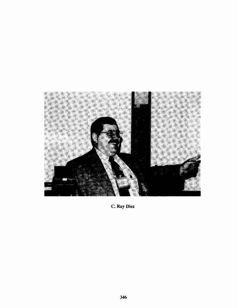
C.Ray Diez

346

CASE HARDENING: AN ACTIVITY TO DEMONSTRATE BRINELL HARDNESS

c. Ray Diez Assistant Professor

Department of Industrial Technology University of North Dakota

Grand Forks, ND 58202-7118

Key Words: Brinell hardness, carburizing, case depth, surface hardening, case hardening

Prerequisite Knowledge: Knowledge of basic heat treating terminology is helpful but not necessary.

Objective: To observe the change in surface hardness of a low or medium carbon steel resulting from the carburizing process. To measure the brinell hardness of a specimen before and after the specimen has been casehardened.

Equipment:

1. Heat treating furnace 2. Vega Universal Testing Machine or Brinell Hardness Tester 3. Pan for Kasenit compound 4. Tongs 4a. For greater safety: place specimens in a wire basket for quenching 5. Water container filled with ambient temperature clean water 6. Gloves 7. Safety glasses 8. Face shield

Materials:

1. Hammerhead or sample of mild steel 2. Emery cloth 3. Kasenit compound 4. Bucket of clean, cold water

Introduction: Numerous heat treating processes involve the through heating of a material to change the microstructure and properties. One of the shortcomings of through heating processes is that many times the material does not retain the toughness required for applications where resistance to surface indentation, fatigue, and wear are desired. The hardness of a part that is through hardened would not be advantageous for a shaft, a tOOl, or a die since a small crack could propagate rapidly

347

to total part failure. Case hardening or surface hardening is a thermochemical treatment which addresses this shortcoming.

Surface hardened materials have advantages that allow use of components that have a hard outer surface but a tough resilient inner core which allows for resistance to impact failure. The case depth is the depth of the martensitic layer. The martensitic layer produced by pack carburizing can be from 0.025 to 0.150 in. (0.6 to 3.8 mm) thick. Thicknesses from other methods of surface or case hardening typically are not as deep ranging only to a depth of 0.020 in. (O.5mm).

Common casehardening processes include carburizing (pack, liquid, and gas), nitriding (gas and liquid), carbonitriding, chromizing and boronizing. For the purposes of this activity in the introductory course Industrial Materials, a version of pack carburizing is the selected process.

Procedures: A mild steel specimen is selected from stock materials. Students may select from bar stock, round stock, or a selection of hammerheads left over from the production processes class. The substrate of the specimens are cleaned of excess oils or grease from previous processing and lightly abraded with fine emery cloth. The specimen is submitted to the Brinell hardness test to determine the hardness of the sample prior to casehardening.

The Vega Universal testing machine is set up for the Brinell hardness test (BHN).

1. The indenter is placed in position under the upper platen. 2. A hardened block is placed on the lower platen. 3. The specimen is positioned under the indenter. 4. The penetrator is adjusted to be nearly in contact with the specimen. 5. The gage pointer is adjusted to zero. 6. A 500 kg load is applied gradually and held for fifteen (15) seconds. 7. Release the load. 8. Use the Brinell microscope to read the specimen diameter in two directions. 9. Average the two readings and record. 10. Look up and record the BHN which corresponds to the' average.

The next step is to carburize (caseharden) the specimen. The carburizing process is completed using Kasenit surface hardening compound. The process used is one suggested by the manufacturer.

1. The heat treating furnace is preheated to 1650 degrees Fahrenheit. 2. The specimen is uniformly heated to a bright red (approximately 1650 degrees F.) 3. The specimen is removed from the furnace with tongs and dipped or rolled in

Kasenit compound to form a fused shell around the specimen. 4. Reheat to a bright red. 5. Quench immediately in clean cold water with a scrubbing action to ensure cooling

at a maximum rate. 6. To increase depth, repeat steps number 3 & 4 prior to quenching. 7. For maximum depth of hardness, you may reheat and repeat step number 5.

348

For deeper cases on mild steel, an alternate method may be used. The alternate method is pack carburizing. The process is as follows:

1. Kasenit compound is placed in a shallow open pan. 2. The part is immersed in the Kasenit compound. 3. Place the pan in the furnace at 1650 degrees F. for 15 to 60 minutes (depending

on depth of case required). 4. Remove specimen from molten compounds with DRY tongs. 5. Quench in clean, cold water.

The final process is to check the surface for hardening changes due to carburizing. The Brinell hardness test is repeated, data collected, analyzed, and compared with data collected from the Brinell test before carburizing.

Results: The results should reflect an increase in BHN between the two readings after casehardening. This would indicate that the casehardening had the effect of hardening the surface of the specimen while leaving the internal structure in a softened state. This can be tested by striking a cold chisel against the specimen to determine if it is easily marred. If it is the hammerhead specimen, replace the handle and strike the head against hardened steel.

Alternatives for the Activity: 1. Prepare the activity in the same fashion, but to make it more of an experiment, put in a placebo, low carbon steel and high carbon steel samples. The students will be able to use a more true experimentation process to observe the changes in surface hardness. 2. A second alternative to the original experiment would be to polish the specimen and place it under a microscope to determine case depth. 3. A third alternative would be to slice the specimen into several pieces, then conduct the BHN test for determination of case depth in various parts of the specimen.

Notes to the Instructor: One of the most important aspects of this laboratory activity is the safety of the student. Each should wear the proper eye and face protection, a hard hat or similar head protection, at minimum a long sleeve shirt or leather vest, and leather leggings or apron to protect from flying slag during the quenching process.

Material Sources:

Kasenit compound may be purchased from:

Midwest Shop Supplies 2600 Bridgeport Drive P.O. Box 3717 Sioux City, Iowa 51102

Telephone: (800) 831-3601 FAX NO. (712) 252-5305

The Kasenit compound may also be available through your local welding supplies distributor.

349

References: Askeland, D. R. (1994). The science and engineering of materials. Boston: PWS

Publishing Company.

Callister, W. D., Jr. (1994). Material science and engineering: An introduction. New York: John Wiley & Sons.

DeGarmo, E. P., Black, 1. T., & Kohser, R. A. (1997). Upper Saddle River, NJ: Prentice-Hall.

DuVall, J. B.. (1996). Contemporary manufacturing processes. South Holland, IL: Goodheart-Willcox Company, Inc.

Groover, M. P. (1996). Fundamentals of modem manufacturing: Materials, processes, and systems. Upper Saddle River, NJ: Prentice-Hall.

Jacobs, 1. A., & Kilduff, T. F. (1996). Engineering materials technology: Structure, processing, properties and selection, 3rd edition. Upper Saddle River, NJ: Prentice-Hall.

Kalpakjian, S. (1997). Manufacturing processes for engineering materials, 3rd ed. Menlo Park, CA: Addison-Wesley.

Lindberg, R. A. (1977). Processes and materials of manufacture, 2nd ed. Boston: Allyn and Bacon, Inc.

350

LOW DOLLAR TENSILE (TORSION) TESTER

Andrew Nydam

Olympia High School 1304 North Street

Olympia, Washington 98501

Telephone 360-753-8958 e-mail anydam@osd.wednet.edu

351

Andrew Nydam

352

Low Dollar Tensile (torsion) Tester

Andrew Nydam MST Teacher Olympia H. S. Olympia, W A.

Key Words; Torque, Tension, Young's Modulus, Stretch, Creep, Foot Pounds,

Equipment 1. Bar torque wrench 2. Metal plate with W' diameter hole 3. Bench vise 4" or larger (securely mounted) 4. Holding equipment for nut

a. may be brackets b. may be wrench c. may be vice grips

5. Torington bearing or flat washers with lubrication (oil) 6. Bolts (standard lengths, thread pitch, and diameter) different stren/:,>th ratings 7. Metal Lathe ( turn down bolt shank to size) 8. Micrometer 9. Graph paper, Graphing calculator, or Computer with graphing ability

Introduction

Without expensive equipment, charting the elastic and plastic area's of a sample is difficult or impossible. The following gives the opportunity to chart elasticity, elastic limit, plasticity, ultimate strength, and failure point all for less than $40.00

353

Procedure:

• Prepare samples 1f4" cross-sectional diameter, I" necked down area • Secure holding plate in stable vice or equivalent • Place sample in holding plate, lubricate, and attach nut • Using the torque wrench tighten bolt

.1 tum and re:cord reading'----__ _

.2 tum and record reading. __ _

.3 tum and record reading'----__

.4 tum and record reading'----__ ,5 tum and record reading __ _ back off at this time and tighten back to.5 tum and compare readings ( is reading is the same, sample is still in the elastic region) .6 tum and record reading __ _ .7 tum and record reading'---__ .8 tum and record reading'---__ .9 tum and record reading __ _ \.0 tum and record reading back off and note when bolt becomes loose tighten and n:cord how far bolt was turned until resistance was encountered (how much of the bolt rotation was taking place in the plastic region)

use micrometer and measure the cross-section of the bolt and check for necking NOTE: at any time the turning force remains the same or begins to decrease, stop the test ,and visually inspect bolt for necking and measure diameter and length with micrometer, continue test after bolt has been examined

continue the test until necking occurs or bolt breaks

Compare different !,Jfade bolts,(note, start with a middle grade bolt and then test a "stronger" bolt and then a "weaker" bolt: graph and record data.

354

compile data and graph EXTENSION ACTIVITY

1. using a middle grade bolt heat treat in oven and quench 2. using a middle grade bolt heat treat in oven and cool slowly 3. using a high grade bolt repeat steps 1 and 2 4. using a low grade bolt repeat steps I and 2

,1 .2 .3 4 ,5 ·6 J .8 9 1.0 1.1 12 13 1A 15 16 17 18 19 2.0 -f On1 :;

355

INTEGRATION OF LABORATORY EXPERIENCES INTO AN INTERACTIVE

CHEMISTRY/MATERIALS COURSE

John B. Hudson

Linda S. Schadler

Mark A. Palmer

Materials Science and Engineering Department

and

James A. Moore

Chemistry Department Rensselaer Polytechnic Institute

Troy, New York 12180

Telephone: 518-276-6447 e-mail hudsoj@rpi.edu

357

John B. Hudson

358

Integration of Laboratory Experiences into an Interactive Chemistry/Materials Course.

John B. Hudson, Linda S. Schadler, Mark A Palmer, Materials Science and Engineering Department, and James A Moore, Chemistry Department, Rensselaer Polytechnic Institute, Troy NY 12180

Introduction

A major problem with the traditional three-hour laboratory period, separated in time and place from the classroom portion of a course, is that it is difficult to maintain the connection between the laboratory and classroom materiaL We are circumventing this problem by integrating laboratory experiences into the two-hour interactive class sessions of our Freshman sequence in Chemistry of Materials. This has required development oflaboratory experiments that can be completed as part of one of these sessions, setting a limit of 30-50 minutes on the time available for the experiment. A second requirement that we have imposed is that the experiment should lead the student to discover a principle or relationship, rather than verifIcation of an anticipated result In the material that follows, we will describe the format of the Chemistry of Materials course and the place oflaboratory material in it, and describe two of the experiments that we have developed to meet the goals, outlined above, namely a laboratory on the photoelectric effect, which leads the student to the relationship between photon wavelength and energy, and a laboratory in which the one-component phase diagram for benzene is developed by measurement of the equilibrium vapor pressure as a function of temperature.

The Chemistry of Materials Sequence

Chemistry of Materials is a two-semester course sequence taken by all engineering Freshmen at Rensselaer [1-3]. It combines traditional Freshman General Chemistry with a fIrst course in Materials Science. We have recently changed the way that the course is presented from the traditional lecture-recitation format to an interactive studio format In this format, students are grouped in sections of up to 60 students. Each section meets for two, two-hour interactive sessions and one, one-hour evaluation session per week. The interactive sessions include presentation of new material by the instructor, problem solving by students working in teams at four-person stations in the classroom, classroom demonstrations, and hands-on laboratory work. On average, there is one laboratory session per week throughout the semester.

Because the laboratory sessions must fit within the two-hour interactive sessions and also allow time for the presentation of related new material and team problem solving, a practical upper limit of 50 minutes is placed on the time available to complete each experiment. The subject matter of the experiment must be tied directly to the major points being covered in the session in which the laboratory is done, and should be presented in such a way as to allow the students to deduce a fundamental principle from the experimental results. Students are introduced to each experiment through an introductory writeup and a series of pre-lab

359

questions, to be answered prior to class, so that they are ready to go to work as soon as the laboratory period bt:gins. The laboratory rooms are across the hall from the classroom, so that negligible time is lost in the transition from classroom to laboratory. Understanding of the results of the laboratory is tested by a series of post-lab questions completed following the lab session.

Weare still in the process of developing some of the experiments to be used in this course sequence, but a number of the experiments have already been developed and implemented. We present detailed descriptions oftwo ofthese below, as an illustration of the type of material that we are using. The phase diagram experiment is presented as part of a unit on phase equilibria, and is intended to illustrate the concept of two-phase equilibrium in a simple one-component system, thus preparing the way for a discussion of equilibrium in multicomponent systems in a subsequent interactive session. The photoelectric effect experiment is carried out in an interactive session in which we discuss the wave/particle nature oflight and the use of optical and electron spectroscopies to deduce atomic structure.

Construction of a One-Component Phase Diagram

Key Words: Thermodynamics, phase equilibrium, vapor pressure

Prerequisite Knowledge. Basic thermodynamics, concept of phase equilibrium.

Objective: To determine the relationship between temperature and equilibrium vapor pressure of a pure material. To use this information to construct the one-component phase diagram for the substance and to determine the heat of vaporization.

Equipment: I. Apparatus constructed from VCR fittings and a glass-to-metal seal 2. Digital capacitance manometer for pressures up to 100 Torr 3. Digital thermometer 4. 2 liter beaker 5. Ice and water 6. Ring stands to hold apparatus and thermometer 7. Computer and computer graphing program or graph paper 8. Pure benzene 9. Mechanical vacuum pump 10. Small Dewar flask II. Liquid nitrogen

Introduction:

One of the most important applications of thermodynamics to materials science is in describing the equilibrium relations among the possible phases of a single or multicomponent system. In this exp(:riment, these relations are determined experimentally for the simple case of a one-component system This experiment is carried out as part of a class session that

360

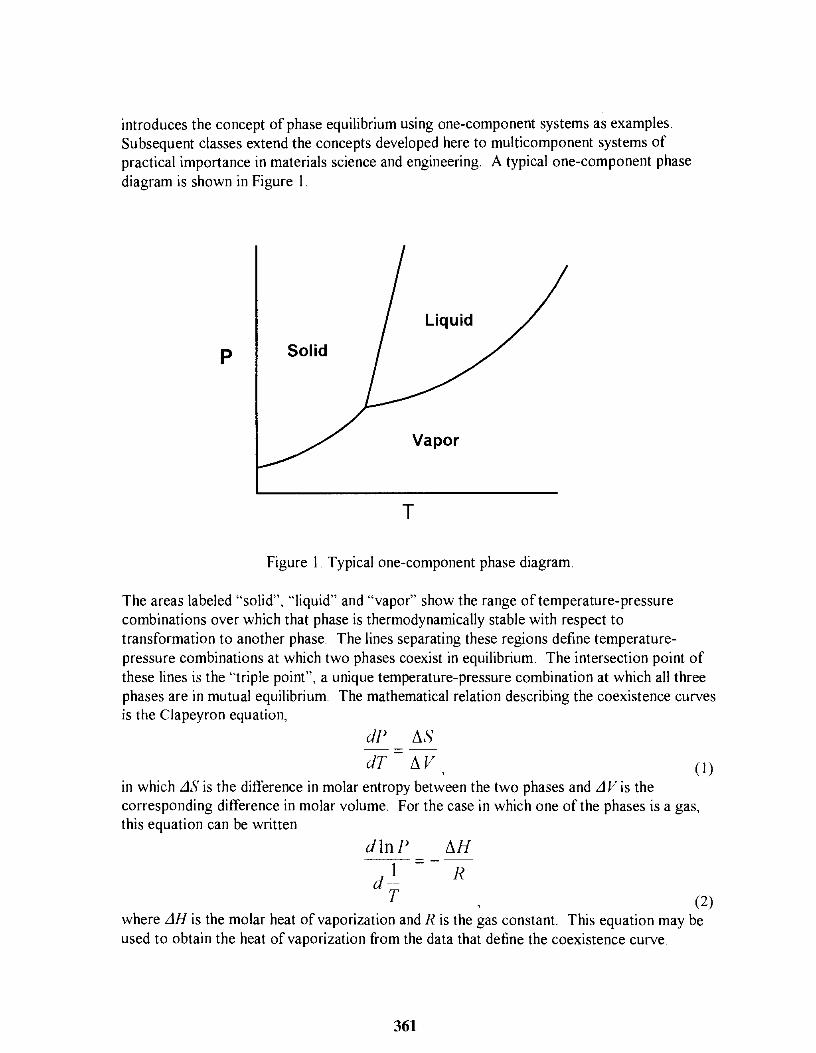
introduces the concept of phase equilibrium using one-component systems as examples. Subsequent classes extend the concepts developed here to multicomponent systems of practical importance in materials science and engineering. A typical one-component phase diagram is shown in Figure I.

Liquid

p Solid

Vapor

T

Figure I. Typical one-component phase diagram.

The areas labeled "solid", "liquid" and "vapor" show the range of temperature-pressure combinations over which that phase is thermodynamically stable with respect to transformation to another phase The lines separating these regions define temperature-pressure combinations at which two phases coexist in equilibrium. The intersection point of these lines is the "triple point", a unique temperature-pressure combination at which all three phases are in mutual equilibrium. The mathematical relation describing the coexistence curves is the Clapeyron equation,

dP I1S dT I1V (I)

in which LIS is the difference in molar entropy between the two phases and LlV is the corresponding difference in molar volume. For the case in which one of the phases is a gas, this equation can be written

dlnP 1 d --T

I1H R

(2) where LlH is the molar heat of vaporization and R is the gas constant. This equation may be used to obtain the heat of vaporization from the data that define the coexistence curve

361

The measurements of pressure and temperature carried out permit construction of the solid-vapor and liquid-vapor coexistence curves The solid-liquid curve cannot be obtained in our apparatus, as there is no mechanism for attaining the high pressures required to determine the pressure-temperature relations along this line. The data obtained can also be used to demonstrate the exponential dependence of equilibrium vapor pressure on temperature, and from this to calculate the heat of vaporization [4].

In order to make this a feasible experiment in the context of an interactive class session lasting two hours, with no more than one hour allotted to the experiment, we have chosen pure benzene as the material to study. Benzene has a melting point of 5.5 ° C [4], and its vapor pressure in the temperature range between O°C and room temperature is in the 30 to 100 Torr range [4]. This permits us to make measurements in a temperature range easily attainable in an ice-water mixture. Note that although benzene is a toxic material, students are not exposed, as the is contained in a sealed apparatus.

Procedure:

Construction of apparatus:

Attachment to Pump

Water bath

Benzene

Figure 2: Vapor pressure apparatus

The apparatus used in this experiment is shown in Figure 2. The sample assembly is constructed from a quarter-inch VCR-fitting tee. A glass-to-metal seal welded to a VCR fitting is attached to one arm of the tee, a digital capacitance manometer is attached at the top, and a valve is attached to the third arm To load the apparatus, the glass-to-metal portion is

362

removed, and filled with 5 to 10 cm' of benzene, and then fastened to the apparatus. This operation should be carried out in a fume hood The apparatus is then attached to a mechanical vacuum pump through the valve. The benzene is then frozen, using a small Dewar flask filled with liquid nitrogen, and the valve opened. After several minutes of pumping, the valve is closed, and the benzene melted. This freeze-pump-melt cycle is repeated until the pressure at room temperature reaches a stable value. indicating that all other gases have been removed.

Experimental Procedure:

The apparatus described above and the digital thermometer are mounted using clamps and ring stands in a 2 liter beaker, as shown in Figure 2, and the beaker filled with an ice-water mixture. Note that the water level should be above the surface of the benzene. When the temperature and pressure have stabilized, they are recorded, and the temperature raised slightly by adding warm water, and the temperature and pressure recorded again (Before doing this, remove the remaining ice.) This procedure is repeated until room temperature is approached, with the temperature at which melting takes place also being recorded. Note that in the cooling process. the benzene may supercool rather than freezing. If this occurs. freezing may be induced by cooling the surface of the glass tube with dry ice Do not attempt to carry measurements beyond room temperature, as this will result in the benzene distilling to cooler parts of the apparatus and lead to erroneous results.

Data Analysis:

Construction of phase diagram:

The phase diagram is constructed by plotting P )IS. T, as shown in Figure 3. The triple point

Vapor

3 6 9 12 15 18 Temperature (0C)

Figure 3. Benzene phase diagram

363

will be at the observed melting point The solid-vapor coexistence curve can be approximated by a vertical line rising from the measured curve at the melting point

Calculation of the Heat of Vaporization:

The data from the liquid-vapor coexistence curve may be replotted as In P vs. liT The slope of this line is equal to -iJ.HIR, permitting calculation of iJ.H. Keep in mind that the measured temperature must be converted to absolute temperature in preparing this plot This process will be facilitated if a computer spreadsheet program is available.

Instructor Notes:

I. VCR fittings are manufactured by the Cajon Company, of Macedonia, OH, and may be obtained from many local suppliers of pipe fittings

2. The capacitance manometer used was an MKS Baratron, Model 222BA, with a Model PDR-C-2C control.

3. The digital thermometer used was an Omega model TDP 116-TC2

4. Operations involving benzene should be carried out in a hood This includes the freeze-pump cycles necessary to degas the sample.

The Photoelectric Effect

Key Words: Photoelectron emission, photons, work function

Prerequisite Knowledge: Concept oflight as having both wave and particle properties

Objective: To discover the relation between photoelectron emission from a solid and the energy and intensity of the light source

Equipment:

I. 5881 vacuum photo tube 2. Electronic circuit including

IOkQ, 10 turn potentiometer SPST toggle switch BNC connector 9 volt battery 2 banana jacks

3. Digital voltohmmeter 4. Picoammeter 5 Laser pen 6. Incandescent light source (flashlight)

364

Introduction:

The photoelectric effect, the emission of electrons from a solid surface when the surface is illuminated, was first explained by Einstein in 1905 , and earned him the Nobel prize in Physics. Experimental demonstration of this effect requires an electron source (cathode) and an electron collector (anode), enclosed in an evacuated housing, a light source and circuitry to measure the emitted electron current as a function of the intensity and wavelength of the light source. It is observed experimentally that the emission process depends critically on the wavelength, or frequency, of the light, with no emission being observed for wavelengths longer than a critical value. The critical wavelength depends on the material being illuminated. Once this threshold has been exceeded, the emission current for a given wavelength increases linearly with light intensity, while the kinetic energy of the emitted electrons is constant, independent oflight intensity. This led to the concept of the photon as a particle oflight energy, having an energy proportional to the frequency of the light (that is, inversely proportional to its wavelength.) The critical photon energy for photoemission is that required to increase the energy of an electron in the solid above that of a free electron in the vacuum In the experiment described here, students observe the wavelength and intensity dependence of the photocurrent, and use this information to determine the photon energy required to cause photoemission (the work function of the surface)

Basic physics:

The relation between the wavelength of the light and the energy per photon is he

H=-A (3)

where E is the photon energy and A is the wavelength of the light. h is Planck's constant and c is the velocity oflight. In the interaction between a photon and an electron in a solid, all of the energy of the photon is imparted to the electron, and the photon ceases to exist. If the energy imparted is greater than the binding energy holding the electron in the solid, the electron can be emitted from the solid and appear in the vacuum. The relation between the binding energy of the electron in the solid, BE, the photon energy and the kinetic energy of an emitted electron, KE, is

he KE= -. - BE

Ii (4) Thus if we know the photon wavelength, and consequently its energy, and can use the bias voltage to determine the electron's initial kinetic energy as described above, we may calculate the electron binding energy. The energy calculated from the bias required to completely suppress the photocurrent is the binding energy of the least tightly bound electron in the cathode. This energy is often referred to as the electron work function, or simply the work function of the material

Apparatus:

The experimental arrangement is shown in Figure 4. The 5881 vacuum phototube is enclosed

365

in a light-tight housing, with a small hole to admit the light from the light source The electrical circuitry is in a similar housing below the phototube The voltohmmeter is connected to the two banana jacks, to measure the potential difference between the anode and

Anode

Phototube Light source

Voltmeter

Picoammeter

Figure 4. Photoemission apparatus

cathode of the phototube The picoammeter is connected to the BNC connector, and measures the current flowing between the cathode and anode Applying a negative bias to the anode retards the electrons emitted from the cathode A bias voltage greater than the initial kinetic energy of the emitted electrons will suppress the cathode to anode current.

Experimental Procedure:

The experiment begins with the bias voltage set to zero. Light from the laser pen is directed into the enclosure housing the phototube, and the photocurrent measured with the picoammeter A typical value is in the 3 x 10-9 ampere range The bias voltage is then increased until the photocurrent is reduced to zero. The voltage required, which represents the initial kinetic energy of the electrons emitted from the least tightly bound electronic state fo the sample, is recorded

Light from the incandescent source is then directed onto the phototube, and it is noted that photocurrent is again observed. The bias voltage is then increased until the photocurrent again drops to zero

Calculations and Observations:

The photocurrent observed with laser illumination will be greater than that observed with the incandescent source, due to the greater intensity of the laser light.

366

No emission will be observed for laser illumination when the bias is greater than the cutoff value. This implies that a well-defined energy is associated with every unit of the laser light

The work function of the cathode surface in the phototube may be calculated using Equation 4. The wavelength of the light from a typical He-Ne laser is 675 nm. The result of this calculation should give a work function between I and 2 volts.

Once the work function has been determined, Equation 4 can again be used, along with the cutoff bias observed for the incandescent light source, to calculate the effective wavelength of the incandescent light Since the incandescent source produces a wide range of wavelengths, this will not be a sharply-defined value. The results of this calculation should yield a value in the 550-600 nm range, depending on the filament temperature of the incandescent source. This is typical of yellow light, as this is where the maximum in the emission from a typical incandescent light bulb falls

Alternatively, one can start with the bias voltage set just below the cutoff for the incandescent source, and note that no emission is obtained from laser illumination until the bias voltage is reduced. Again, this emphasizes the point that the photon wavelength must be less than a critical value in order for photoemission to be observed.

Relation to Photoelectron Spectroscopy:

The relation observed between photon energy, electron binding energy and emitted electron kinetic energy is also the basis of photoelectron spectroscopy. In this technique, monochromatic radiation impinges on a sample, and some sort of electron spectrometer is used to determine the energy distribution of the emitted electrons. Sharp features in this spectrum identifY sharply defined allowed electron energy levels in the solid. The binding energy range that can be probed with this technique will depend on the photon energy. Typically, photon energies in the ultraviolet range (50-500 nm) are used to study the valence levels of a material, while energies in the x-ray range (I-50 nm) are used to study the core electron levels.

Instructor Notes:

I. The 5881 phototube is manufactured by RCA

2. The picoammeter used was a Kiethley Model 6 lOA Any meter capable of measuring currents in the 10-9 ampere range will do.

3. The laser pen was obtained from Edmund Scientific.

4. The experiment would be even more clear cut if a second laser, emitting at a significantly different wavelength, were available This would eliminate the ambiguity in the cutoff energy for the case of the polychromatic incandescent light source.

367

References:

I. G. E. Wnek and P 1. Ficalora, in "Materials Chemistry: An Emerging Discipline", L. V. Interrante, L. A. Caspar and A. B. Ellis, eds, Advances in Chemistry Series N. 245, American Chemical Society, Washington DC, 1995, p. 62.

2. G. E. Wnek and P 1. Ficalora, Chemtech, 1991 (November), p. 664.

3. M. A. Palmer and 1. B. Hudson, ASEE Educational Research and Methods Division, 1996 Conference Proceedings

4. Handbook of Chemistry and Physics, 71st Edition, D. R. Lide, Ed., CRC Press, Boston MA,1990.

368

LIFE ESTIMATE BASED ON FATIGUE CRACK PROPAGATION

Yulian Kin

Harvey Abramowitz

Toma Hentea

Ying Xu

Mechanical Engineering Purdue University Calumet

Hammond, Indiana 46323-2094

Telephone 219-989-2684 e-mail kin@wni.calumet.purdue.edu

369

Yulian Kin

370

LIFE ESTIMATE BASED ON FATIGUE CRACK PROPAGATION

Yulian Kin Harvey Abramowitz

Toma Hentea Ying Xu

Purdue University Calumet

Key Words: Fatigue, crack propagation, crack growth rate, stress intensity factor.

Prerequisite Knowledge: Knowledge of basic fracture mechanics concepts is helpful.

Objective: Observe fatigue crack propagation. Measure a crack length. Calculate parameters "e" and "m" in the Paris formulation. Make recommendations for an inspection technique development.

Equipment: I. Fatigue machine (MTS, for example) with a control unit. 2. Fixture system (Flexure system in this experiment) to provide loading of the

specimen. 3. Specimens (O.S-inch polycarbonate specimens in this experiment). 4. Video camera. 5. Light sources. 6. Computer with a frame grabber. 7. Monitor, printer. 8. Software ("Inspector" by Matrox in this experiment) to observe crack image

measurements. 9. Vidco recorder 10. O.7S-inch scotch tape for the specimen.

Introduction:

This experiment is focused on the polycarbonate which is used as a structural component in the F -16 canopy. The aircraft canopy is often manufactured from a laminated composite material. Components of the composite are acrylic plies, a polycarbonate ply, interlayers and coatings. Design of the canopy allows unloading of the acrylic ply and that is why the structural polycarbonate ply of the composite was the primary concern during fatigue investigation. One of the failure modes encountered frequently in the field is polycarbonate fracture. The nature of failures is not quite clear, but some evidence implies that transparency life is limited by fatigue of the polycarbonate ply. Therefore, development of an inspection procedure which permits measurement of a crack and prediction of the part life until its failure is an important task.

371

Procedure:

Specimens:

The testing coupons were cut from 0.5-inch polycarbonate sheets. The sheets had been extruded, pressed and polished in accordance with the military specification. The specimens were cut by a fine band saw using the lowest possible speed and a cooling liquid. Three configurations of specimens (Figure 1) were investigated: solid, with holes as stress concentrators, and with "V" notches. The 3/4-inch core-series 17-0310 scotch tape was used to protect the gripping area of the specimens from damage. The scotch tape was bonded in three layers on each end of the specimen. It took roughly 10 minutes after the beginning of the test to adjust the assigned loading regime due to formation of a "bed" by the hard jig rollers in the soft tape layers. The bed also prevented sliding of the specimen between the rollers.

Experimental Set-up:

The flexure fatigue tests were conduced on an MTS machine using a four point MTS flexure system to provide pure bending. The experimental set-up is shown in Figure 2. The appropriate support and load spans were selected to provide minimum possible deflection of the specimens. The small deflections provided morc stable position of the specimens between jig rollers and permitted the use of a greater testing frequency. Thc flexure fatigue tests under different temperatures were conducted in the MTS environmental chamber. The fatigue crack propagation images were caught by an image grabber linked to the digital computer and video. An independent duplicate monitor connected to the video permitted constant observation of the crack development during some necessary command and calibration operations on the monitor connected to the computer.

Observation:

Fatigue crack initiation and propagation can be constantly observed on the screen. To verify crack initiation, zooming was periodically used. During fatigue crack propagation, the crack images were captured by an image grabber after each 5000 cycles and stored. During zooming and calibration, the crack propagation was observed on the duplicate monitor.

Crack Growth Results:

From the results of stress-life investigation, it can be noted that for many cascs, the fatigue life after crack initiation is still very significant [1]. Therefore, it is important to determine crack growth parameters. On the basis of crack growth characteristics, the part expccted life still left can be estimated and the appropriate inspection intervals assigned. The plots of fatigue crack length versus number of cycles for thc specimens tcsted under ditlerent loads arc given in Figures 3,4, and 5, and corresponding crack growth rate

372

curves are given in Figures 6, 7 and 8. The crack growth rate daJdN was calculated by a polynomial approach which fits a cubic equation to a certain interval of the crack length versus number of cycles curve. Stress intensity factors were determined for a cracked beam in pure bending [2].

K = f(g)uj;ffi where a = notch height (see Figure I)

(j' = bending stress, determined from given load, location of load application and specimen geometry.

and j( g) = correction factor

= 1.122 - 1.40 (alb) + 7.33 (a/b)2 - 13.08 (a/b)3 + 14.0 (alb)4 [2]

b = specimen height

Using the Paris formulation, for example, the life to failure can be determined during a maintenance inspection.

"r da NI = . f C(I'lK)'"

,li

Nj= life to failure ai = initial crack length af= final (critical) crack length I'lK = stress intensity range Parameters C and m for the specimen tested were determined from test results. Values for m were from 2.17 to 3.057. Values for C were from e-39.927 to e-36.987.

Notes to Instructor:

The experiment can be conducted in the short version. Parameters "m" and "e" are taken as a given for certain materials and conditions. The experimenters have to observe crack propagation, measure the crack parameters, and calculate the part life until the next inspection. A proposal about inspection intervals, based on the real part usage, is expected as the conclusion.

References:

I. H. Abramowitz, T. Hentea, Y. Kin, Y. Xu, "Fatigue Investigation of Polycarbonate Used for Aircraft Canopies," Ageing of Materials and Methods for the Assessment of Lifetimes of Engineering Plant: Proceedings of the 4th International Colloquium, Cape Town, South Africa, ApriI21-25, 1997, Penny (ed.), Balkema, Rotterdam, Netherlands, ISBN 9054108746, 1997, pp. 309-317.

2. Bannantine,1. A, Comer, J. 1., Handrock, 1. L., Fundamentals of Metal Fatigue Analysis, Prentice Hall, Englewood Clifts, New Jersey, 1990.

373

-5 c

:E C> C CD -l

tS CD .... (.) "C CD ... CD C> CD a. o .... a..

I I I I I I 1 I I I

I I I J I

I

_____ I I I I I

I I I

I I , I I I I I --- --,- - -- - - -, - - - --T - - -- -r- - - - -,- - - - - -,'- - - - -,--

I I I I

I I I I I I I I

I I r I J

, , - - - - - - -1- - _ - - -I--

-_-4 ___ _

I I

____ ____ _____ _____ L _____ _____ ____ _____ _____ L ___ -

I 1 I I I I I

7 8 9 :-4 10 11 12 13 3 4 5 6 Number of Cycles x 10

Figure 3. Crack length (from the tip of the notch) versus number of cycles. Max. load = 400 lb .• Min. load = 100 lb.

374

£ c .c-o, c CI)

...J

n ca L-

U "0 CI) a; en

I I I I I I I I I

I I I I

I J I I I I

I

I I I I I , I - - - - - , - - - - - - ,- - - - - - i - - - - - -,- - - - - - T - - - - - -,- - - - - - r - - - -

I I I I I I I

I I I I r I r

- - - - - , - - - - - - r- - - - - - "'T - - - - - -,- - - - - - T - - - - - -,-+

I

[0.15 I r I I r + I +

-+: o L-a..

0.1

__ ____ ____ ______ L_ ____ ____ ____

1 1.5 2 2.5 3 3.5 4 4.5 5 =4 Number of Cycles x 10

Figure 4. Crack length (from the tip of the notch) versus munber of cycles. Max. load = 450 lb., Min. load = 100 lb.

375

5.5

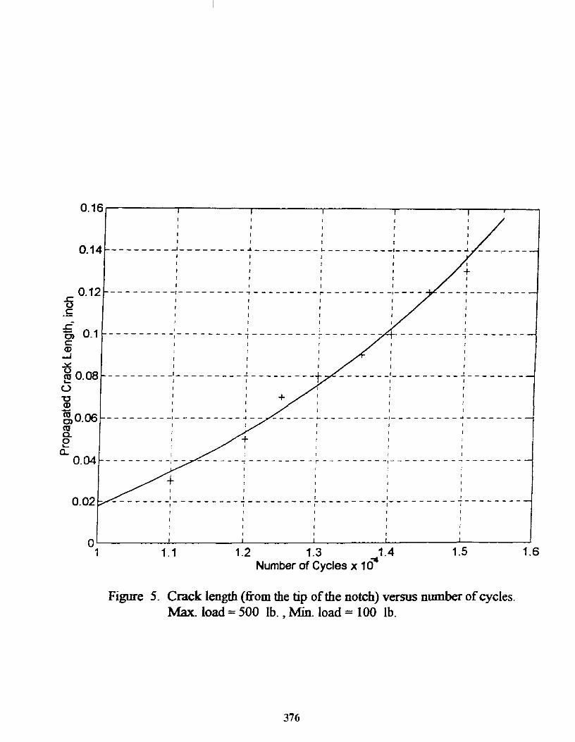
I t r I

I

I , ,

I I I - - - - - - - - -I - - - - - - - - - 1 - - - - - - - - - r- - - - - - - - - --------,--------

r

I I I I I I

_______ 1 _________ J. _______ _

r

- - - - - - - - - - - - - - -1- _ .- - - - - - - - - - - - - - -

- - - - - -""':' - - - - - - - - - r - - - - - - - - -1- - - - - - - - - , - - - - - - - -

I I I I I - - - - - - - -, - - - - - - - - - "j - - - - - - - - - 'I - - - - - - - - -1- - -. - - - - - - j - - - - - - - -

1 1.1 1.2 1.3 1.4 1.5 1.6 =" Number of Cycles x 10

Figure 5. Crack length (from the tip of the notch) versus nmnber of cycles. Max. load = 500 lb., Min. load = 100 lb.

376

10-5

:lIE

:lIE

L.. "'"

:lIE

Stress Intensity Range psi Ji;z Figure 6. Crack growth rate versus stress intensity range.

Max. load = 400 lb., Min. load = 100 lb.

377

T

i- -1 + -5 , +

"

tt" Iffl"

-+ + it-

104

Stress Intensity Range dK, psi Jj;; Figure 7. Crack growth rate versus stress intensity range.

Max. load = 450 lb., Min. load = 100 lb.

378

CD 13

o c: z u -co u CD -CO

0:: .s::;

o ..... C> (J CO .....

<..>

-

0

-'"' L:

P

Stress Intensity Range psi Jf,;

Figme 8. Crack growth rate versus stress intensity range. Max. load = 500 lb., Min. load = 100 lb.

379

BIOGRAPHY

Yulian B. Kin is a Professor at Purdue University Calumet where he teaches Machine Design, Fatigue Analysis, Reliability Engineering and the general engineering courses. He joined the Faculty at Purdue Calumet in 1983. lie received his PH.D. in Mechanical Engineering from Petrochemical and Gas Industry Institute, Moscow, Russia in 1971.

Yulian worked more than 20 years in industry and his current research interests are in fatigue life estimate based on fatigue crack propagation. He was awarded with grants from the Air-Force and National Science Foundation.

380

STRETCHY "ELASTIC" BANDS

Alan K. Karplus

Department of Mechanical Engineering Western New England College

1215 Wilbraham Road Springfield, Massachusetts 01119-2684

Telephone 413-782-1272 e-mail akarplus@wnec.edu

381

Alan K. Karplus

382

Stretchy "Elastic" Bands

Alan K. Karplus Department of Mechanical Engineering

Western New England College Springfield, MA 01119-2684

Key Words: Elastics, Tension Tests

Prerequisite Knowledge: Have an idea about changes in the load an elastic band holds as it is stretched and unloaded.

Objective: To work as a team member in the collection of data, to make plots for near constant rate loading and unloading of traditional rubber bands, and to show features which are unique to these elastic products.

Equipment: 1. A series of three and one half inch long rubber "elastic" bands of 1/8, 114 and 112 inch width which are

often referred to as number 33, 64, and 84 rubber bands, respectively. Most office supply houses will stock a variety.

2. Yard Stick, or Tape measure or 30 inch long machinist's measure. 3. Two, 2 inch size C - clamps. 4. Mounting board (2 in. by 1 in. by 30 inches) with a six penny nail inserted one inch from one end on the 2

inch by 30 inch face, and to which the machinist's scale can be clamped. The zero of the machinist's scale should be at the nail.

5. Vise to hold the mounting board. 6. Safety Goggles 7. Heavy work gloves 8. Load scale for loads to 50 pounds or 25 kg. A scale with a capacity to 10 pounds or 5 kg. may be helpful,

if available. 9. Micrometer or vernier caliper.

10. Data page with 25 lines and nine columns. Measurements are taken at one inch increments starting at a value offour inches listed in the first column. The remaining columns are used in pairs to record load and unload for each offour elastic sizes. Be sure to label columns and include units of measure selected.

11. A Spreadsheet such as EXCELTM. All work performed on the spreadsheet can be done by hand. 12. When the computations are to be done by hand, computation paper and several pieces of linear graph

paper with 20 divisions to the inch are needed.

383

Introduction:

The approach is to stretch each rubber band at a near constant rate and to unstretch it at the same near constant rate while recording the load present at each stretch point. One team member should do the loading and read the load at each position while the second team member should record the data. Try to load and unload the elastic at a constant rate, and about the same rate for each band so that meaningful comparisons between bands can be made. Both team members should work on the data analysis, make observations from the computations and plots, and formulate conclusions.

After the data has been collected and when a spreadsheet is used consider making a column of deformation that starts at four inches, ends at 24 inches, and starts at 24 inches and returns to four inches. Increments of one inch are used. Enter the collected data into the spreadsheet and the make a plot for the entered deformation -load data.

At each deformation position a computation for engineering strain and engineering stress can be made. Engineering strain is the length ( L ) at any displacement minus a reference displacement ( R ) divided by the reference displacement ( R) or (L-R)/R. Four (4) inches is chosen as the reference dimension ( R ) for this experiment. Engineering stress or (PI A) is the load ( P ) divided by the cross section area ( A) of the band. Note that the band has two strands canying load. Compute the strain and stress for the collected data. Make a second plot for the stress and strain found.

Increments for the area under the LOADING line are computed separately from the UNLOADING line. This represents the energy used to stretch and unstretch the band. Now compute the area under the curves with trapezoidal increments. First the upload curve and then the down load curve. A cell should be used to store each trapezoidal area increment. The trapezoidal increment is computed by forming the average of two stresses and multiplying by the change in strain. The total area under a curve can be found by adding the incremental areas in a column, and is the energy related to each curve. The difference between column totals found is the hystersis. A ratio between the difference and the upload curve area when shown in percent finds the portion of energy lost to internal friction or hystersis. Be sure to check UNITS.

An informative comparison for alI sizes rubber bands tested can be made by plotting and clearly labeling A. the load deflection data for all elastics on one set of axes and B. the stress - strain data for all elastics on another set of axes . Note how the stress-strain plot curves compare favorably, and the percentage of energy allocated to hystersis is seen to be similar while the load - deflection plot clearly shows the change in load carried by each band.

Preparation:

Prepare the Mounting Board by placing a six penny nail into the 2 inch by 30 inch surface of the board one inch from the three surfaces at one end. Place the board into the vise and clamp the machinist's measure on to the top surface of the board. Clamps at six inches and 20 inches on the scale work well.

Secure several rubber bands for each size to be tested. Measure the thickness and width of the band and record the results. Remember there are two strands of each band carrying load. Now compute the cross sectional area.

Prepare the data sheet with 25 lines and nine columns. Measurements are to be taken at one inch increments starting at a value offour inches listed in the first column and end at the 24 inch position. The remaining columns are used in pairs to record load and unload for each elastic size. Be sure to label the load columns in

384

pairs (LOADING and UNLOADING) and include units of measure selected. The first LOADING value is made at the four inch position. A position is designated where the hook of the load scale attaches to the rubber band and is sited on the machinist's measure. The last LOADING value at 24 inches should be the FIRST UNLOADING value at 24 inches because the UNLOADING values are recorded for decreasing positions.

When the extension exceeds 20 inches for the larger bands you must make a concentrated effort to keep the current band under load. DO NOT UNLOAD or LOOSE LOAD on the scale on the upload because the band will be unloaded and the upload data will not be represent near constant rate loading. In case a band breaks when under test, COMPLETELY redo the test.

In preparation for a test run place a designated rubber band over the nail and through the hook of the load scale. Check that a load measurement can be made at the four inch mark on the machinist's measure. Be sure the operator of the load scale has safety glasses on and is wearing the heavy gloves. These Safety Devices will protect the operator if the elastic breaks and the spring scale unloads and the elastic flies around.

Procedure:

1. Tensile load - deflection tests are to be performed on a series of three and one half inch long rubber bands of 118, 114 and 112 inch width which are often referred to as number 33,64, and 84 rubber bands, respectively. Place safety glasses and gloves on the spring scale operator, and prepare the recorded for writing the data on the data sheet. The approach is to stretch a band, and as this is done at a near constant rate, record the load to stretch the rubber band at each added inch. Start at four inches which is one-half an inch past the three and one-half inch length of the rubber band. Continue until the length of the band is 24 inches. Next, unload the band at the same rate as was used to load the band taking load measurements at each inch of reduced length. Remember the load value at the 24 inch position is the same for the LOADING and UNLOADING columns on the data sheet. The recorded data is defined as "raw data" for elastic 33 which is the first elastic tested. Be sure to label the size of the rubber band tested, and measure and record its thickness.

2. The first comparison to be made is for the shape ofloading and unloading paths for load/deflection data. Enter the deformation data which starts at four inches and ends at 24 inches. At each deformation level, enter the load. Make an XY. or Scatter Plot of the data. The horizontal axis should be Deformation in inches while the vertical axis is Load in pounds. Label the Load - deflection line as Elastic 33 .

Repeat the load-deflection test for each of the remaining three sizes of rubber band, plot the data on the SAME graph as for Elastic 33 and label each curve as Elastic 64, or Elastic 84.

The applied load - deflection plots on the same graph show magnitude changes. The largest load carried by each band should be clearly evident on the right hand end of the deflection axis at 24 inches. Note if a trend appears which shows that the large band carries the larger load.

3. The second comparison is dependent on two modifications made to the raw data. The first modification is to define the engineering strain as the ratio computed by taking the measured band length minus the starting length and dividing this quantity by the initial length. For all samples use four inches as the initial length. This means that the first value of strain is zero with UNITS ofincheslinch. The strain is to be plotted on the horizontal axis.

1 Be sure to make a plot of two variables and NOT a line chart as is the usual default setting on a spreadsheet.

385

The second data modification is to divide the load by the cross-sectional area of the original rubber band. This computes the engineering stress in the band which has UNITS of pounds per square inch in the English system and is to be plotted on the vertical axis.

Again prepare an XY or Scatter Plot with the modified data. This will be a stress-strain plot for the elastic or rubber band. Label the line on the plot as Elastic 33.

Repeat the strain and stress calculations for elastics 64, and 84, make separate stress-stain plots for each elastic, and add this data to the same stress-strain for Elastic 33 and label each line. Note the similarities between these curves. If the effect of initial elastic length and original cross sectional area are considered, the stain range of 5 times or 500 percent is the same for each rubber band and the stress ranges are comparable.

4. Areas under each of the stress/strain curves are to be found by approximation. An approach is to represent the area between strain values as a trapezoid and to sum the areas of all the trapezoids to obtain the area under the LOADING line. The summing of trapezoids is repeated for the UNLOADING line. Note that the trapezoid has a 'height' in stress units of pounds per square inch and that the 'width' of the trapezoid has strain units of inches per inch. The product of stress times strain becomes inch-pounds per cubic inch. In summary, the difference between these sums is the residual often referred to as hystersis. The hystersis represents the energy consumed in the deformation process.

What can be presented about the energy differences between the Elastics 33,64, and 84? A rapid visual comparison is found when the stress/strain plots are super-imposed on one another. This shows the common features such as the LOADING lines as well as differences such as for the UNLOADING lines between the four rubber bands from zero to 500 percent strain. Note that the area term represents ENERGY. When English units are used, the product of pounds per square inch times inches per inch becomes inch-pounds per cubic inch.

What relationship can be found between LOADING energy, UNLOADING energy, and hystersis? A table of rubber band size with columns of LOADING, UNLOADING, an hystersis can show that about half the energy is assigned to hystersis.

Comments:

I. To aid the instructor in the execution ofthis experiment, a sample for Elastic 33 is shown below. Figure 1 presents the data. Note the starting position for deformation at 4 inches and the load values at 24 inches. In Figure 2 the upload and doM1load curves are seen. Figure 3 is presents the strain values in column one, upload stress, doM1load stress in columns two and three and the trapezoidal areas between strain increments in columns four and five.

To make a hand calculation for the 6 inch displacement: A strain [(L-R)/R] is (6-4)/4 = 0.5 and B. the upload stress (PI A) is 0.375 pounds 10.009 in. sq or 41.67 psi. as seen in Figure 3. In column four of Figure 3 is C. the area under a part of the upload curve as 9.55 in-Ib. per cubic inch which is found by averaging 34.72 and 41.67 = (76.39/2 = 38.195) psi and multiplying 38.195 psi. by 0.25 in.lin. which is the change in strain increment. For the incremental doM1load the energy computed is 2.60 in.-Ib.!cubic inch found by averaging 20.83 and 000 and multiplying by 0.25.

386

A comparison of the total download energy of 479.17 in.-lb./cubic inches (found by adding all the incremental energies) to the upload value of975.69 in.-lb./ cubic inch shows a ratio of 0.4911 or 49 percent. The hystersis value is likewise 51 percent which represents the energy consumed.

2. To provide added perspective a 1/16 inch wide·or number 19 rubber band can be tried. This size band has not always attained the 500 percent elongation which the number 33, 64, and 84 bands achieve. It breaks! On the other hand, number 19 adds a fourth elastic to the data base and can enhance the experiment.

Acknowledgments:

The author is appreciative of the assistance provided by Mr. Richard DeCelle, Mechanical Laboratory Technician, in the finding of various rubber bands, selection ofIoad scales, and the recording of data. John Stambaugh, a volunteer high school student from Wilbraham, MA, assisted with several trials and contributed operational suggestion for the text.

Elastic 33

disp in

upload down load Ib Ib

4 0.125 5 0.3125 6 0.375 7 0.5 8 0.625 9 0.6875

10 0.6875 11 0.875 12 13 1.125 14 1.25 15 1.4375 16 1.625 17 1.8125 18 2.125 19 2.4375 20 2.8125 21 3.375 22 4.125 23 5 24 5.75

o 0.1875 0.3125

0.375 0.4375

0.5 0.5 0.5

0.5625 0.5625 0.5625

0.625 0.625

0.6875 0.6875

0.75 0.875 1.125 1.625 2.875 5.75

Figure 1 Load-Deflection Data

Area =

i _

0.125 * 0.036 or

Elastic 33

6,-----,----,----,

III 4 "C

" '" o <;'- 3 "C

... 2

o 10 20 30 Displacement - in.

0.009 in.sq.

- -

-+-- up load Ib L -II-down-",ad Ib

Figure 2 Load - Deflection Plot

387

Strain via Stress via Stress via area up area down disp upload down load in/in psi psi in-lb/in-'3 in-lb/in"3

0.00 13.89 0.00 0.25 34.72 20.83 6.08 2.60 0.50 41.67 34.72 9.55 6.94 0.75 55.56 41.67 12.15 9.55 1.00 69.44 48.61 15.63 11.28 1.25 76.39 55.56 18.23 13.02 1.50 76.39 55.56 19.10 13.89 1.75 97.22 55.56 21.70 13.89 2.00 111.11 62.50 26.04 14.76 2.25 125.00 62.50 29.51 15.63 2.50 138.89 62.50 32.99 15.63 2.75 159.72 69.44 37.33 16.49 3.00 180.56 69.44 42.53 17.36 3.25 201.39 76.39 47.74 18.23 3.50 236.11 76.39 54.69 19.10 3.75 270.83 83.33 63.37 19.97 4.00 312.50 97.22 72.92 22.57 4.25 375.00 125.00 85.94 27.78 4.50 458.33 180.56 104.17 38.19 4.75 555.56 319.44 126.74 62.50 5.00 638.89 638.89 149.31 119.79

Area under Curves: Total 975.69 479.17 Difference 496.53

Figure 3 Strain - Stress Data

Stress Strain - Elastic 33

500.00

400.00 I: Upload I ---Download I

1.00 2.00 3.00 4.00 5.00

strain

Figure 4 Stress - Strain Plot

388

STRENGTH TESTING OF COMPOSITE MATERIALS

John and Eric Cadwell (students)

Steven Piippo (Instructor)

Richland High School 930 Long Avenue

Richland, Washington 99352

Telephone 509-946-5121

389

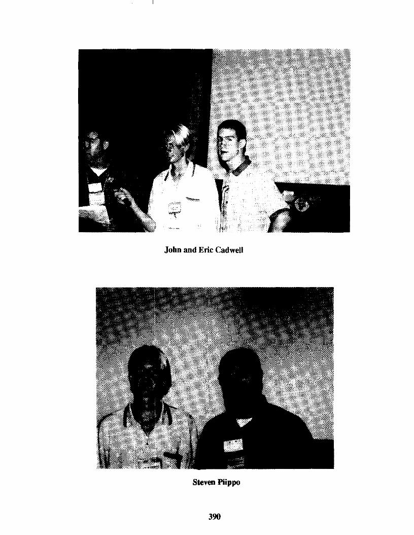
John and Eric Cadwell

Steven Piippo

390

Strength Testing of Composite Materials

John and Eric Cadwell Materials Science Technology Labs

Richland High School Richland, Washington 99352

Instructor Steve Piippo

Key Words: Epoxy, fiberglass, carbon fiber, laminate, ultimate strength

Prerequisite Knowledge: Thermosets, polymeric matrix composite, reinforcement fibers.

Objective:

I. To obtain an understanding of composite materials by combination of two or more materials into a new material with distinct properties.

2. To with the process of composite lamination.

3. To determine properties of the new composites by use of ultimate strength testing.

Equipment and Materials:

I. Fiberglass 2. Carbon Fiber 3. Scissors 4. Epoxy Resin 5. Mixing Cup 6. Brush 7. Stir Stick 8. Gloves 9. Polyethylene Sheets 10. Acetone 11. Particle Board 12. Table Saw 13. Masonite 14. Clamps 15. Lead Weights 16. Container for Weight

391

Introduction:

In the fall of 1996 as students in a Materials Science and Technology class, we were assigned the task of teaching a chapter out of our M. S.T. textbook. That chapter was on "composites". After researching composites, we created a video presenting real life composites in our daily world such as concrete, plywood, fiberglass (skis, boat, jet skis, cars) and coins. We learned a lot and had a lot offun studying composites

Our teacher happened upon a study from the Eastern Illinois University School of Technology involving composites of glass fiber with an epoxy matrix. He presented the idea and hence this project was borne.

In our project we created our own mold and used it to make smaller samples to test. We also designed our own testing device to measure ultimate strength, whereas their design measured cantilever bending strength.

Procedure:

FABRICATION OF MOLD We cut two 36" X 6" X 3;4" pieces of particle board. On one board, we cut a 2" X

1;4" deep groove extending the entire length of the board using a dado blade on a table saw.

We then ripped a 36" X 2" X'!." piece of masonite which was then glue and nailed to the ungrooved particle board, creating an effective male-female mold.

This was the mold that we fabricated to create our samples.

FABRICATION OF SAMPLES To make the samples, 2" X 16" strips of each material were laid over plastic and

placed into the groove of our board. Epoxy resin was mixed in a 3.1 resin/hardener ratio and was then applied with a brush in order to laminate the various layers of material together to form a matrix.

For the weave, we used six layers, with the total weight of the 16" samples equaling 17.6 grams and 14.6 grams. For the random, we only needed two layers and ended up with samples equaling 161 grams and 16 I grams The carbon fiber required three layers totaling 14.7 grams and 14. I grams.

Another sheet of plastic was placed on top of the laminate to keep the epoxy resin from bonding with the particle board. After laying the other piece of particle board on top, we used four clamps to tighten it down, thus creating our thin strip samples.

The samples were cured in the mold for exactly 24.0 hours, then removed and cut equally into 4" We labeled each sample with a permanent marker for identification then put each aside while subsequent samples were molded

392

Unidirectional

Bidirectional

Multidirectional

Random

393

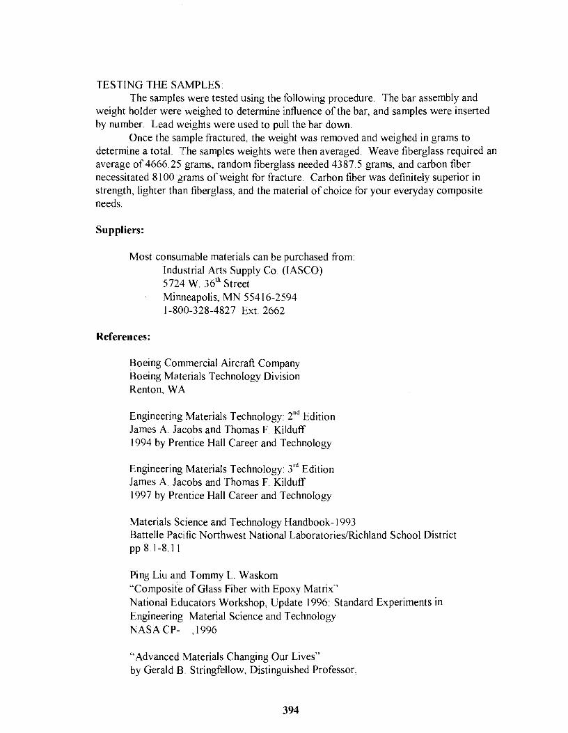
TESTING THE SAMPLES The samples were tested using the following procedure. The bar assembly and

weight holder were weighed to determine influence of the bar, and samples were inserted by number. Lead weights were used to pull the bar down.

Once the sample fractured, the weight was removed and weighed in grams to determine a total The samples weights were then averaged. Weave fiberglass required an average of 4666.25 grams, random fiberglass needed 4387.5 grams, and carbon fiber necessitated 8 I 00 grams of weight for fracture. Carbon fiber was definitely superior in strength, lighter than fiberglass, and the material of choice for your everyday composite needs.

Suppliers:

Most consumable materials can be purchased from:

References:

Industrial Arts Supply Co. (IASCO) 5724 W. 36th Street Minneapolis, MN 55416-2594 1-800-328-4827 Ext. 2662

Boeing Commercial Aircraft Company Boeing MClterials Technology Division Renton, WA

Engineering Materials Technology: 2nd Edition James A Jacobs and Thomas F. Kilduff 1994 by Prentice Hall Career and Technology

Engineering Materials Technology 3rd Edition James A Jacobs and Thomas F. Kilduff 1997 by Prentice Hall Career and Technology

Materials Science and Technology Handbook-I 993 Battelle Pacific Northwest National Laboratories/Richland School District pp 8.1-8.11

Ping Liu and Tommy L. Waskom "Composite of Glass Fiber with Epoxy Matrix" National Educators Workshop, Update 1996: Standard Experiments in Engineering Material Science and Technology NASA CP- ,1996

"Advanced Materials Changing Our Lives" by Gerald B. Stringfellow, Distinguished Professor,

394

Chair, Department of Materials Science and Engineering, February 1 ,)97, College of Engineering, University of Utah Salt Lake City, Utah.

"Fundamentals of Composite Manufacturing" by A. B. Strong Society of Manufacturing Engineers Dearborn, MI, (1989)

395

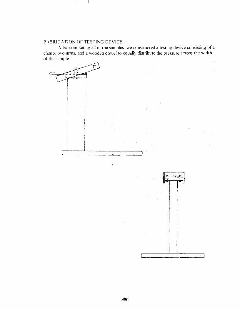
FABRICATION OF TESTING DEVICE. After completing all of the samples, we constructed a testing device consisting of a

clamp, two arms, and a wooden dowel to equally distribute the pressure across the width of the sample

I

b·-'------., .. .,... .

I

I

I I I I , !

396

CORROSION DEMONSTRATION UTILIZING LOW COST MATERIALS

John R. Williams

Mechanical Engineering Purdue University

P. O. Box 9003 2300 South Washington Street Kokomo, Indiana 46904-9003

Telephone 765-455-9236 jrwillia@purdue.iuk.indiana.edu

397

John R. Williams

398

Corrosion Demonstration Utilizing Low Cost Materials

John R. Williams Assistant Professor

Purdue University School of Technology at Kokomo Kokomo, Indiana

Key Words: Electrolytic Corrosion

Prerequisite Knowledge: High school level chemistry course is helpful, but not required.

Objective: To observe the process of corrosion of various metals. To assess the effectiveness of certain corrosion protection mechanisms. To understand grain size effects on corrosion.

Equipment: There is considerable flexibility concerning the materials to be exposed to a corrosive environment. The instructor is encouraged to use his or her own initiative in suggesting materials to be examined. Corrodent selection is somewhat more restricted. While the risk of someone coming in contact with a corrodent is small, it is suggested that only very weak acids or bases be used. 1. Several glass jars with lids, usually one for each corrosion sample. Spaghetti sauce jars (about 26 ounce size) with lids are good candidates. It is helpful to choose ones with relatively clear sides for observation. Soak the labels off before use. 2. Corrodent solutions.

Acidic: Great success has been obtained using a solution of ordinary household bleach, diluted by adding 10 ml of bleach to IL of water. Ordinary tap water was used, but distilled water would be better. Also, one could dissolve salts in water, using table salt (NaCl) or Calcium Chloride.

Basic: Household ammonia has been used, directly from the bottle. 3. Clear plastic film, the type used for food storage. 4. Nylon or cotton string. Thin fishing line is suitable. 5. A pre-prepared data sheet for recording observations of the progress of corrosion on the materials. A sample is included at the end this paper. 6. Metal corrosion samples. Additional discussion of samples that have been used is included in this

paper. The thin strips noted below are about 0.065 inches thick. Thin hot rolled low-carbon steel strips, I-inch wide, 4-inches long, sheared to size Thin AISI 4340 cold rolled steel strips, I-inch wide, 4 inches long, sheared to size. Thin 606I-T6 aluminum strips, I-inch wide, 4-inches long, sheared to size. Thin 1100 aluminum strips, I-inch wide, 4-inches long, sheared to size. Thin pure copper strips, I-inch wide, 4-inches long, sheared to size. Thin CA260 brass strips, I-inch wide, 4-inches long, sheared to size. Thin 300 series stainless steel strips, I-inch wide, 4-inches long, sheared to size. Thin Hastelloy or Inconel strips, I-inch wide, 4-inches long, sheared to size. Steel "s" hooks, bright zinc plated, available from hardware stores Steel perforated hot dipped zinc coated strips, 2-inches wide, 4-inches long, available from hardware stores. Hot dipped, zinc coated roofing nails, available from hardware stores.

399

Common construction nails, about 3 or 4-inches long, one bent, using a mandrill Other potential corrosion candidate materials, selected from commonly available items. Suggested items might include lids from food containers, such as "tin" cans, hacksaw blades, bicycle chain, paper clips, etc.

7. Thin magnesium strip 8. Time clock, to record time of day that observations are made.

Introduction:

Most of us who live in the midwest are familiar with rusty old vehicles plying our roads, exhibiting the ravages of time and corrosion. Recently, a Russian airliner broke up in mid-air, and investigators believe the failure was caused by corrosion of the aluminum airframe, according to USA Today(l). Engineers and technologists need an introduction to corrosion mechanisms in order to know how to design necessary corrosion prevention techniques into equipment that may be at risk. One source(2) estimates that 20% of the iron and steel products manufactured each year are used to replace things that have been discarded due to rust damage. The author has developed a laboratory exercise that demonstrates the effects of corrosion on metals and also illustrates some methods that can be used to protect metals from the devastation of corrosive attack. Since quantitative corrosion testing takes a long time to achieve measurable results, the qualitative approach taken ensures that the student can observe the effects in a timely manner. In addition, the exercises can be done at minimal cost, a big consideration in these times of shrinking educational budgets.

Conditions for Corrosion to Occur:

As background for this paper, the following is a summary of what our students have been taught prior to the laboratory exercise. They know that cold working deforms the metal grains, resulting in larger numbers of smaller grains, which produces strengthening of the material. Recyrstallization through heating has been covered. They have been exposed to the concept that some materials, such as stainless steels, form passive layers that protect the underlying material from corrosive attack. The galvanic series has been introduced and they have been shown how materials higher in the series will corrode preferentially to those lower in the series.

Many of our students have not studied chemistry in college at this point in their academic career, so must be introduced to the chemical processes of oxidation and reduction. They are told that oxidation is the loss of electrons, while reduction is gaining electrons.(3) This process is illustrated using classic electron flow.(4)

There are five conditions, all of which must be simultaneously present, for corrosion to occur.(5) I. There must be an anode, where the metal is oxidized. 2. There must be a cathode, where some ions are reduced. 3. A potential (voltage) must exist between the anode and cathode. 4. There must be an electrolyte in contact with the anode and cathode. 5. The electrical circuit must be completed externally between the anode and cathode.

It is also necessary to explain that electrolytes are electrical conductors, usually liquids, although vapors and certain solid oxides can act as electrolytes.(6,7), Then, the relationship between cold work, anodes and

400

cathodes is explained, showing how cold work creates additional small grains and more grain boundaries. The grain boundaries become anodes, and the grains become cathodes.(8) As the anodes are consumed, the grains and boundaries exchange roles, reversing the polarity. This process continues until the entire material is consumed. For iron and steel, the oxide crystal is larger and less dense than the iron crystals, thus, the oxide layer buckles and flakes, exposing fresh iron or steel to the corrosive attack.

Corrosion Samples:

There are lots of common materials that can be used to demonstrate galvanic corrosion. Common nails, hardware items such as hooks, perforated strips, bolts and screws, etc. can be purchased very inexpensively from hardware stores. In addition, we use tensile test specimens of various metals in our demonstration. These are thin, flat specimens that are used in the tensile test laboratory. However, thin strips can also be obtained from hardware stores. We use untested samples due to the cold work that occurs during tensile testing which might confuse some of the results. These samples are cut in half to provide two specimens.

Table 1 lists some of the variations that can be obtained with a relatively small quantity of different materials.

Table 1. - Candidate Corrosion Samples Material Type Processing Modifications

AISI 1010 Hot-rolled tensile sample Plain One side ground clean MIG weld bead added

Magnesium strip attached AISI4340 Cold-rolled plain

Common nails Cold head & point One straight, one bent CA 360 Brass half-hard plain

6061 Aluminum T6 plain ETP Copper soft plain

Inconel plain Hastelloy plain "S" hook Steel, bright zinc plated

Steel perforated strip Hot dipped zinc coated Roofing nail Hot dipped zinc coated

Steel bolt Bright cadmium plated 18-8 stainless bolt

One can use the imagination to find other potential sample materials. One student suggested coating the side of a hot-rolled sample that had been ground clean with automotive wax to demonstrate how that would protect it. Another student suggested putting a deep scratch in the zinc coated perforated plate to enhance corrosion at that site. Voltage measurements can be made between specific samples and pure copper to estimate whether corrosion will occur. It is important to make the measurement with the same electrolyte that will be used for the corrosion experiments.

401

Suggested Corrodents and Containers:

Glass jars are best to hold the electrolyte selected to permit easy access for students to view the corrosion activity. Spaghetti sauce jars, with plain sides, work best for visibility and allow photographs to be made. The jars are carefully washed, labels are removed and all traces of glue cleaned off before use. In response to student comments, labels are provided that clearly explain what material and what corrodent is in each container.

One can choose from a large number of common liquids to be used as corrodents. Good results have been achieved with common household bleach, diluted 100: 1 with water. Ordinary tap water has been used, although distilled or even deionized water would give better control of results. Other materials including calcium chloride solution (similar to road salt), ammonia, drain cleaner, dilute hydrochloric or sulfuric acids could be used with selected corrosion samples.

General Experimental Procedure:

It is important to clean the samples, removing any oils that might be on the surface. An alcohol wash is a good idea. Each sample material is suspended in the glass jar using nylon fishing line, poly string or polyethylene film. In each case, the string is held by the jar lid. If significant evolution of gas is anticipated, clear film can be placed over the jar opening and the string secured with a rubber band. It is suggested that the jar be filled with the corrodent before inserting the sample. A good cover is needed to prevent evaporation. For the thin, flat specimens, a small hole is drilled in each one, allowing the string to be inserted. Other materials can have the support tied on or looped around.

Students are given a data sheet on which to record their observations. They are to observe the samples about one hour after immersion and every other day after that. If possible, more frequent observations for the first 24 hours might be useful. The observations are usually ended after one or two weeks. Students are encouraged to note the progress of corrosion, if any, and draw sketches. It is best if they do not touch or move the jars.

Typical Results:

Hot rolled steel samples. Hot rolled material is protected by a black oxide coating that occurs during processing. However, since these samples are sheared, the edges have undergone significant cold work. One should see rust forming on the sheared edges during the first hour of immersion. The sample having the weld bead on it should show rust forming at the edge of weld first. This is due to cold work that occurs as the weld cools. The sample edges will not rust as rapidly in this case due to recrystallization that occurred during the welding process. The sample that has the magnesium strip attached should rust very little, but the magnesium strip may be consumed. This is of course, an example of cathodic protection, where the magnesium become the anode that is consumed to protect the cathode. (Most hot water heaters have a magnesium rod installed for this purpose.)

If a strip with one side having the oxide layer removed is used, one will see immediate rusting of that side, but very little on the reverse side. This is the same principle as the magnesium strip, the bare side oxidizes

402

first, protecting the other side. In the case where a student suggested applying car wax to the ground side, the corrodent quickly penetrated the wax coating. Other protective schemes can be attempted. If the sheared strips are heated to the recrystallization temperature and slowly cooled, the resulting larger grains in the sheared area should lead to reduced oxidation. Protective coatings, such as paint could also be used. Table 2 summarizes typical results from other materials.

Students seem to appreciate this opportunity to observe corrosion along with the understanding they gain from the experience. Students are encouraged to suggest methods of corrosion protection, then try them.

Table 2. Summary of results from various materials. Sample Electrolyte Results Explanation Cold-rolled steel Dilute bleach Rust forms quickly, in a Small grains from cold work provide

uniform manner more anode/cathode pairs. Straight and bent Dilute bleach Rust forms on the Cold working causes grain size nails heads and points, plus reduction, enhancing oxidation at the

at the bend head and point of the nails and where the nail is bent.

Copper and brass Dilute bleach Little corrosion Natural passivity protects copper and observed its alloys. Some oxides are observed

above the liquid line due to high oxygen level in air.

Aluminum Dilute bleach Clumps of white This material is either aluminum oxide material appears after or aluminum chloride. some time.

Aluminum Household Rapid evolution of This is a self-anodizing reaction, ammonia bubbles, a dark layer forming a layer of aluminum oxide

forms on the sample, which protects the metal from further bubbling ceases after reaction. some time

Zinc coated and Dilute bleach Bright plating dulls, but Zinc is a sacrificial anode. Even plated steel even punched plates do scratching the surface will not materials not rust. promote rusting. Cadmium plated Dilute bleach Plating becomes dull, Same as above. hardware but no rusting occurs. Inconel and Dilute bleach No reaction These materials are relatively immune Hastelloy to oxidation. Stainless steel bolts Dilute bleach No reaction Stainless exhibits passivity due to its

chromium content.

403

References:

1. USA Today World, March 31,1997 2. Brown, Theodore L., et. aI., Chemistry: the central science. 5th edition, Prentice-Hall, 1991, pg. 733 3. Brown, Theodore L., op. cit. pg. 121 4. Budinski, Kenneth G, Engineering materials: properties and selection. 5th edition, Prentice-Hall, 1996, pg.421 5. Budinski, Kenneth G., op. cit., pg. 423 6. Dalton, William K., The technology of metallurgy. Macmillan Publishing Company, 1994, pg. 307 7. Budinski, Kenneth G., op. cit. pg. 423 8. Fellers, William 0., Materials science, testing and properties for technicians, Prentice-Hall, 1990, pg. 152-153.

John Williams is Assistant Professor of Mechanical Engineering Technology at Purdue University. He holds a B.S.M.E. degree from Rose Hulman Institute of Technology and an M.S.E. degree from Purdue University. He joined Purdue University after 34 years of service with the Allison Gas Turbine Division of General Motors. He is a Registered Professional Engineer and is a member of ASEE, SAE and ASME.

404

Corrosion Data Sheet Name: ----------------------------Start Date: _____ _ Sample: _____________________ _

Start Time: Corrodent: ------ ----------------------

Observation I. Date: Time: ------ -----------------Observation:

Observation 2. Date: Time: ------ ----------Observation:

Observation 3. Date: _____ _ Time: -----------------Observation:

Observation 4. Date: Time: ------ -----------Observation:

405

PREVIEW OF NEW:UPDATE 98

Karl J. Swyler

Office of Educational Programs Science Education Center

Brookhaven National Laboratory Associated Universities, Inc.

P. O. Box 5000 Upton, New York 11973-5000

Telephone 516-344-7171 e-mail swyler@bni.gov

and

Leonard W. Fine

Department of Chemistry Columbia University

Havemeyer Hall Mail Station 3108

New York, New York to027

Telephone 212-854-2017 e-mail fine@chem.columbia.edu

407

Karl J. Swyler

Leonard W. Fine

408

OVERVIEW OF BNL

Brookhaven National laboratory's Mission

established by US Atomic Energy Commission In 1947

Operate large Aeseach Facilities for use by US Scientific (onmJnit\J

Conduct 8aslc and ApplledSclentlflc Research In Energy-Related Areas

Contrlblte to Develpment of US Sciertiflc/Technlcai Workforce

Brookhaven National Laboratory's Organization

( US of Energy (DOE) National Laboratory

Operated for DOE by Associated Universities, Incorporated (Aut)

Eight Research Departments, Three Reserae Support Divisions

Roughly 3000 employees, 700 scientific or professional staff

l Annual budget of roughly $400 miDion, primarily from DOE

--- -- - ----------'

Some Major Brookhaven National Laboratory Research Areas

( High Energy and Nuclear Physics ] (- Structural Biiolgy/Chemistry J ( Nuclear, Radio- and Photochemisty )

./

( Condensed Matter/ ) ,j:o. [ J .... Medical and Genetic Research t-J

Materials Science / ,

/

C J /

Nuclear Science/Technology -------------

( Environmental Science/Technology J ( Energy (omversion/Utilizaton J

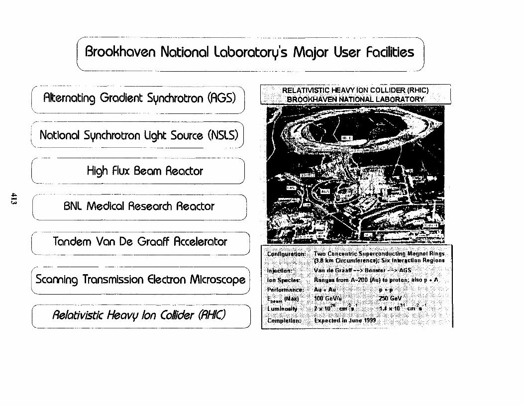
National Laboratory's Major User FacDitles

Gradiett Synchrotron (AGS)

National Synchrotron light Source (NSLS)

[= High Aux Beam Reactor J C BNL Medical Research Reactor J C Tandem Van De Graaff Accelerator J

Scanning Transmission Electron Microscope

Relativistic Heavl,l Ion Colder (RHIC)

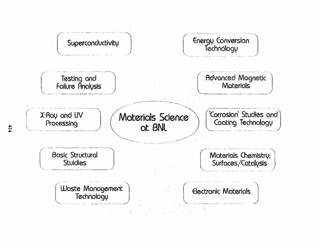
Materials Science at BNL

'\ Coating Technology )

__ " __ _____ ,____ ', ____ ._ ••

(" Waste

Technology _" ",_ .• __ ._ ,_, ___ • ___ .--_.,_ .... __ w" ___ __

( .•.. J

r Permanent Magnet Studies

'''------- -

Structure-Sensitive Properties of Advanced Permanent Magnet Materials

Permanent Magnet Applications

Images of magnetic domain configuration and flux lines obtained by unmodified scanning electron microscopy

from a single crystal of NdFe,,jB

···diagram courtesy of Magnequench Internatiollal, Inc

/---I NSLS \" _ _

c ( Configuration of I, Adsorbed Species

r-- Properties

Materials Chemistry: Surfaces J BNL Materials Chemis!!y

HFOR

X-RAY AND NEUTRON DIFFRACTION

ADSORPTION ISOTlIERMS

, ........ ....

"-

SYNTHESIS

( NSLS .

MOLECULAU DYNAMICS SIMULATIONS

( Superconductivity '----- .. ---

High Te Materials 1 .//

Maglet Technology

lOO I j twist grain-btHIIH.l<lry

'Corrosion' Studies and Coating Technology J

Environmental Corrosion

Advanced Coatings '----------------_. __ ._---

ANTI-CORROSION COATINGS

ANNUAL COST OF CORROSION HAS BEEN ESTIMATED AT 2-3 % OF THE GNP OF INDUSTRIALIZED COUNTRIES. SEVERAL BNL PROGRAMS ADDRESS DIFFERENT ASPECTS OF THIS PROBLEM

EXAMPLE

ONE PROGRAM AIMED AT APPLYING ENVIRONMENTALLY BENIGN AND INEXPENSIVE NATURAL POLYSACCHARIDE POLYMERS SUCH AS PECTIN AND STARCH AS WATER-BASED COATING SYSTEMS TO PROTECT METALS FROM CORROSION.

Studies J 11 T2 24 Hr. Chemical Spray at Saturated Steam I Conditions

oIloo P1 250 F< 11 <500 F N - - -- 250 F< T2 <500 F <= -., ,

\ ., \ 25 < P1 < 77psi \ 70 < P2 <115psi \ \ -------

0 3hr 6 hr 1 d'ay 7 days , \

Sample LOCA Profile for Cable Qualification Testing

__ J

Metal Hydrides

Energy Conversion Technology

LITHIUM ION BATTERY

• Negative electrode is Li intercalated into graphite

• Electrolyte is LiPF6 dissolved in a non-aqueous organic solvent

• Positive is a Li intercalating oxide - LiCo02

• LiCo02 is expensive

• LiMn204 is a low cost substitute, but has limited cycle life

• In situ XRD is done at NSLS to determine structural changes in LiMn204 whwn cycled in an operating cell

Space Radiation Effects (Tandem)

Electronic Materials J

2: o <..)

-' (f)

2:

t;:; -'

1 00 I I I I I --'"0 Examples of available tandem

____ beam energws and corresponding -N' LET values In SI. I _

0,1 He

5 to

( Waste Management: Technolagy J

( ___ w_o_s_te_f_o_rm_s __ J

Bcrrler Materials

VI portlarul.:enlfmt lllaximWll

wa..te loadinga 80 70 00 !so ! 40

-' 30 i 20 j;: 10

_ .•.......... .. _. _____________

o a:.rjollooid Inotntr.,,,A.h IX""'"

Permeable Barriers

Hiah Permeability

IIIII Envi,onmooIlllllnd Wool .. ToolmologyCert9f 11111

X-Ray and UV Materials Processing

X-Ray lithography

Photochemistry Figure 12: Lettering in 1 n1l11 tilick PMMA 51H'et At right is tile pOint of a tailor's pin. Note tlw Sillootil side willis ilS CO III pil r pli of till' (()nveJltioJl d lIy dldJllOllLi Illacllineli surface of tile acrylic sileet. (X27H)

The BNL Site and its Surroundings .

UPDATE and BNL

...•..

Workshop Possibilities

General Tour Possibilities

Educational Opportunities

c-----sNi:s Site and Surroundings

l/--- . miles from New York City

----- ---- -- - --------- .. _---._ .. _-----------

r --I ". ____________ J

BNL onsite amenities compare roughly to those at college campus

"'---------

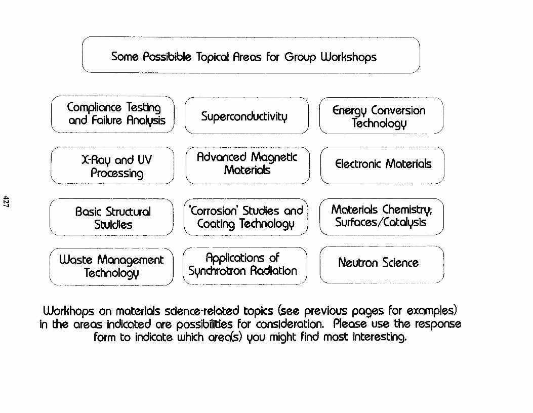
Some Possibible Topical Areas for Group Workshops

Compliance Testing and Failure Analysis

X-Ray and UV Processing

Basic Structural Stuidles

Waste Management Technology

Superconductivity

( Advanced Magnetic L Materials

'Corrosion' Studies and Coating Technology

Applications of Synchrotron Radiation

Energy Conversion 1 Technology

Electronic Materials J Materials Chemistry; Surfaces/Catalysis

_N_eutro: Sdence . J Work hops on materials science-related topiCS (see previous pages for examples)

in the areas Indicated are possibilities for conSideration. Please use the response form to indicate which areels) you might find most interesting.

__ ___ J site bus tours, stopping In the lobbies l of BNL's major Buildings and facitlties.

( In-depth visits to one or more of BNL's "big l machines" - RHIC, AGS, NSLS, Tandem. "----------------- -------------"

(--In-depth visits to large-scale tech.-l like the Superconducting Magnet Factory

Please use the response form to indicate which of these things you might generany prefer if the option were available.

Science Education Opportinities at BNL

BNL has offered educational programs continuously since 1952.

Undergraduate Summer or . Semester Research Participation

Student-Faculty Teams at the NSLS and t-fBR

PrecoDege Teacher and Student Research and Teaching Activities

( School Distict Programs and Educational Outreach

213 EXPERIMENTS ON CD-ROM FROM 10 YEARS OF NEW:UPDATES

James A. Jacobs

School of Technology Norfolk State University 2401 Corprew Avenue

Norfolk, Virginia 23504

Telephone: 757-683-8109 e-mail jjacobs@vger.nsu.edu

and

Alfred E. McKenney Consultant

516 Fairfax Way Williamsburg, Virginia 23185

Telephone 757-221-0476 e-mail hdjc41a@prodigy.com

431

James A. Jacobs

Alfred E. McKenney

432

213 EXPERIMENTS ON CD-ROM FROM 10 YEARS OF NEW:Updates

James A Jacobs & Alfred E McKenney Norfolk State University

Key Words: EMSET, Find, Read, View, Copy, Paste, Clipboard, Browse, Index, Table of Contents, Full Text Search

Prerequisite Knowledge: Experience with Windows 3.x or 95, or Macintosh II, and a word processor.

Equipment & Supplies: EMSET CD ROM. Computer Minimum System Requirements:

WINDOWS 3.X AND WINDOWS 95 For Acrobat Reader: - x86-based computer (386 minimum; 486, Pentium or Pentium Pro recommended) - Microsoft Windows 3.1, Microsoft Windows for Workgroups, Microsoft Windows 95, Microsoft Windows NT 3.51 or 4.0 - 4 MB Application RAM - 5 MR hard disk space, plus 7 MR additional temporary disk space available during installation For Quick Time: 3 MR hard disk space

MACINTOSH For Acrobat Reader: - Macintosh computer with 68020 (Macintosh II series) or greater processor. - Mac OS 7.0 or later - 3 MB application RAM for 68020 - 5 MB application RAM for Power Mac - 8 MB hard disk space, plus 5 MB additional temporary disk space available during installation. For Quick Time: 3 MR hard disk space

Objective: To use the EMSET (E.xperimenls in Materials Science, Engineering and Technology) CD-ROM to create unique laboratory exercises by adapting experiments and demonstrations on the CO to meet your students' classroom and laboratory needs.

Introduction

This first digital collection of the National Educator's Workshop (NEW:Update) experiments includes papers published during ten years of the annual workshop compendiums. They have been reproduced in their original peer-reviewed form, preserving the individuality among the papers and reflecting the author's style and method. We have combined the convenience and capacity of the CD-ROM with the power of the Adobe Acrobat document format. The result is a medium for these experiments which provides better support to your classroom and laboratory needs.

433

There are some video dips on the EMSET CD-ROM. Of additional interest to you and your students will be the bonus disk included in this package. This second disc contains longer video segments on new and emerging concepts in materials science and engineering.

The Acrobat Reader gives you the ability to: o View an exact image of the original paper, o Read, or print the paper, or copy its text into another document for editing,

To find the document(s) meeting your needs, you can: o Browse the Table of Contents which is organized by types of materials or processes, or o Use the full Text Search capability, searching by:

Author Title Subject Text words in context

You will probably find yourself using the Full Text Search more often than the Table of Contents because the subject matter of papers sometimes fits into more than one category.

In many cases, you will probably use the experiments as they were published. However, you may sometimes wish to edit a paper for a particular need. Unless you have the Acrobat Exchange program, there are two methods for editing to chose from: o Print the paper. then cut and paste as needed. You all know how to do this. - or. o Copy blocks of text and graphics to the clipboard. then paste into a word processor or

graphics program.

The following procedures will give you experiencc with thc second method.

Procedures

Follow the printed instructions to start the EMSET CD-ROM and go to the Main Menu.

Now we will walk you through a tutorial to give you experience on how to select material from two specific papers and prepare a composite paper for use in your classroom or laboratory. The final paper will contain excerpts from an experiment by Ed Widener. It's Hard to Test Hardness and a companion experiment by Ed's Purdue colleague. Patricia Olesack, Sceleroscope Hardness Testing and your own additions.

434

l.Finding the Papers

From the Main Menu, select the Table of Contents button. The result in shown in Figure 1.

Figure 1

Select the Testing & Evaluation button.

When the Testing & Evaluation Table of Contents appears, browse the list of authors and papers, and you will locate entries for Ed Widener and Patricia Olesack's papers. If we had not known the exact titles of the papers or even the authors, we could have used the Full Text Search facility to find the papers we wanted. For example, by entering "hardness" or "hardness testing" or the authors' names in the Adobe Acrobat Search window, we would quickly find both of the papers we wanted. See Figure 2.

435

Figure 2

I!XPI!RIMENTS & DEMONSTRATIONS IN rESTING & l':VALUATION

I. DOHERTY, R. D., and S. K. NASH, "Fracture of Brittle Solids," 2, GC!CHEU\AR, !'HILIP J .. and MOLLY W, WILLlA\1S. "A Simple Demonstration of

Corrosion .. 3. MASI,

Students. 4, KUNDU.

NELSON. 6, SPIEGEL. 7. SASTRL 8.

12, ""''''H.l'>

1.3. 14. I.', MARTIN. DONAJ.D H. "Applit8liOl1 {,fHardnlni, Testing in Foundry

Operations: A Uni"mily and Industry Partnership." 16, TIPTON. STEVEN M, "A Millialllre Test Machine."

Select the first paper, Ed Widener's, It's Hard to Test Hardness. See Figure 3.

436

Figure 3

IT'S flARDlU TEST HARDNE.SS Edward L. Widener PE.

fJniversity'KRT. Departftent ',}. IN ·n907

Hardness is essentially a nechanical property of uniform ",atttl' hils , -eI $I.lda.r:a of othl:tl' proSlllnt.iG'jl$. It b. h",rd to define, hard to correlate different testa, and hard to corrJPare difff3rent. nmteriala, NevlClrtheless, hardness is broadly co,n$.i,dot"1ld (!Is "resistance to penet'r.ation. ela.stic and(or ul.!l.!ltk. For metal alloys. C:<lJ1ll1.eI'ciaJ. ta-st.s typically measure Pl-e.:H .. ic-st.r.Qln or plilnt.1.fHltnt,-$lItt for $olid$: r(1.l$U1 I;.<\nt 8cratche:B or dents are relatively truC'tive-. unlea,s

in finished surfaces make trouble, l'H.th d01ctJi$ 'Of I'tt!rdntls$ •• av-:dlabJ,e,t pur t:(JrtVrtl'1t..l.OTlo!SJ

lab experi.menta. tend to fCCUB on a. pail" Cof pcp.u.lat industrial machines, B-rin9:11 and Rockwell. ,,1)d t.o 9Mc;!:f,!i,t$ roOptltj,ti.v.(t datb for (';:""'on m.t.elh bY routi"n. apAtoCltlo.n:.o.. T$chnoloql$t.1!l-are not clerks but problem·, solvers , in need c.f .an €arly

to .i. v.ari{tt.y at .... hich jnvolv-o cUversH!I principles and definiti: applications. Selecting ,appropriate

and followina published standards are priority lab " Otlttolfih of' u(l.:::onvtlntlo-notlt tiIIXpt:'k"iMht;$.

with simPlE.! equipment ,and f.§1lljlia.r 8a.mples, ."r.9 .suggested to 8upplement cert.ain well--establisbed b'\1t l-e&s6t'-known ASTM nardnl!-2B

Sri nell-stt'Il::!S;t.: R,':lt,:k\\tal ,t-St.1:'4 'in: Plastic-dPJI,t; Sclero.s.cope,

2. Text Material from the First Paper

When the paper appears, read it and select the text you want to include in the composite paper. Chose the Select Text Tool from the Tools Menu. Use the text cursor to highlight the desired text. Note that you can only select one block of text or graphic to Copy at one time. The maximum size is limited to the current page.

Use the Copy command to copy the selected text to the Clipboard.

Next, open your word processor and Paste the text from the Clipboard to your New Document.

3. Copying Graphic Material from the First Paper

Return to Ed Widener's paper and Copy any additional material required to the Clipboard. For example, we want to include his Figure II. Since this is a graphic, it is necessary to chose the Select Graphics Tool. Use the Graphics Tool to draw a box around the object desired (Figure II) and Copy the figure to the Clipboard.

Paste the Figure stored on the Clipboard to the appropriate location in your New Document.

437

4. Copying Material from the Second Paper

Return to EMSET and press the Experiments in Testing & Evaluation button to return to the Testing and Evaluation Table of Contents.

Select Patricia Olesack's paper, Scleroscope Hardness Testing. Select the items desired from this paper, as you have done before. Copy the items and Paste them in the appropriate locations in your New Document in the word processor.

5. Editing the Final Paper

When all ofthe material desired has been copied into the word processor, you can add your own text and edit it as desired for your final composite paper. You may develop a lab report form to suite you students' needs. For example, you could include a Brinell Hardness Test Data Sheet such as Figure 4.

r' .................... . ··········TMi;il{5 . .... .......... . .........

Brinell Hardness Test Data Sheet

Student Name ____________________ _ Date _____________ .

Sample # Material Description Load Dent Dia IW.U (rom)

3

4

Figure 4

Remember to credit the original authors for their fine contributions.

It is important to note that while the Clipboard transfers graphics with 100% accuracy, it does not always transfer text so accurately. Therefore, it is advisable to check and correct the text formatting and spelling before starting your editing.

Reference Material

Finally, to assist in finding your way around EMSET, you may wish to print out the Getting Started section to use as a reference. To do this, select the GETTING STARTED button from the MAIN MENU. After Getting Started appears, select and execute Print from the File Menu.

Ordering Information

EMSET CD ROM, ISBN 0-13-648486-7, call Prentice-Hall at 1-800-922-0579, visit their web site at www.prenhall.com. or send purchase order to Prentice-Hall, Order Processing Dept. 200 Old Tappan Rd. Old Tappan, NJ 07675. Price $150. Enjoy EMSET!

438

Biographies

James A. Jacobs is Professor of Engineering Technology at Norfolk State University. He developed the concept and has been co-director of all the NEW:Updates. He has thirty-three years of teaching experiences in public schools, community colleges, and universities. He has developed curricula offerings at all three levels, including courses in material science, materials and processes technology, engineering materials technology, and principles of manufacture.

He has industrial experience with Westinghouse Corp., Tenneco, Ford Motor Co., and completed an intensive ten-week program with International Business Machines Manufacturing Technology Institute.

He is the author of numerous articles, books, and technical papers! presentations. Dr. Jacobs co-authored Engineering Materials Technology, now in its third edition, and the CD ROM set, Experiments in Materials Science, Engineering and Technology both published by Prentice-Hall Inc. He has been involved as consultant and director with numerous grants, seminars, and curriculum development efforts in engineering materials, manufacturing, robotics and CAD/CAM. Professor Jacobs is a member of the Materials Education Council of the U. S.; ASM International; Society of Manufacturing Engineers; American Society for Engineering Education; American Association of University Professors; American Ceramics Society, and is a Certified Senior Technologist and member of the National Association for Industrial Technology.

AIFed E McKenney received his B.S. in engineering from the US Coast Guard Academy at New London, Connecticut. After service as a line officer, he earned his MBA at Harvard Business School. He was employed by IBM for 37 years where he specialized un the design oflarge manufacturing systems.

In 1987, he was assigned by IBM on a two-year sabbatical to the School of Technology at Norfolk State University where he taught courses in commuting, tool design, mechanics, engineering material technology robotics, CIM and production planning and inventory control. On retiring from IBM, he continued teaching for two more years at Norfolk State, as well as working with Dr. Jacobs on NEW:Update.

He is now enjoying retirement and occasional independent consulting with his wife, Evelyn.

439

DEMONSTRATING THE CRITICAL PROPERTIES OF CARBON DIOXIDE

Leonard W. Fine

Department of Chemistry Columbia University

Havemeyer Hall Mail Station 3108

New York, New York 10027

Telephone 212-854-2017 e-mail fine@chem.columbia.edu

441

Leonard W. Fine

442

Demonstrating the Critical Properties of Carbon Dioxide

Leonard W. Fine Department of Chemistry, Columbia University

Havemeyer Hall, Mail Station 3108 New York, New York 10027

Key Words: Carbon dioxide, critical conditions, triple point.

Prerequisite Knowledge: Basic chemistry at the undergraduate level.

Objective: To observe the liquid state of carbon dioxide and to understand its critical conditions and behavior.

Equipment: 1. Commercially available dry ice in small pieces. 2. Hand-held type B (snow cone) C02 fire extinguisher.

3. Jumbo Fisher Scientific(5-846) hosecock clamps. 4. Pliers for tightening/releasing clamps. 5. Clear Tygon® R-3603 tubing (Aldrich Chemical Company).

Introduction to Critical and Supercritical Carbon Dioxide Although most solids melt long before their vapour pressures reach the pressure

of the atmosphere, carbon dioxide (dry ice) is one that does not. For such a substance, fusion, vapourization, and sublimation lines on the classic phase diagram intersect at the triple point, the one point where solid, liquid, and vapour phases are in equilibrium and can coexist indefinitely so long as the conditions do not change. For C02, triple point

conditions are -57°C and 5.2 atm. Therefore, the solid-to-liquid phase transformation for C02 cannot take place unless the pressure is at least 5.2 atm. Above the critical

temperature, the gas cannot be liquefied no matter how great the pressure. Making use of the phase diagram for carbon dioxide (C02) showing the variation

of pressure with volume in Figure I, we can summarize a range of properties, including the critical conditions of temperature and pressure. Each curve on the diagram is called an isotherm, meaning a constant temperature line.

443

Wholly liquid

Wholly gaseous

Figure I

We begin with C02 as a nearly ideal ga, at the T7 isotherm or at any isotherm drawn

above that line. By increasing the pressure and decreasing the temperature, molecules of the gas are brought closer together until they coalesce and the condensed state is achieved: • Above 48°C, corresponding to T7, the compressibility of C02 resembles that of an

ideal gas. The curve looks very much like a Boyle's law plot for which PV is constant. • At 21°C, corresponding to T I, compression produces liquefaction. Along the segment

of the isotherm lying to the right of the shaded region, the molecules behave more like a gas. Along the flat segment cutting across the shaded region, gas molecules coalesce under constant pressure:. When all the gas molecules are condensed, the isotherm emerges

444

from the shaded region and rises sharply, the steep slope reflecting just how incompressible liquids are - roughly 1000 atm compress a liquid by 5% whereas an increase of 0.05 atm compresses a gas at atmospheric pressure by 5%. • Returning to the in-between temperature of 31.1 °c, corresponding to the T 5 isotherm,

liquefaction hasn't set in yet but cooling has brought the gas to the incipient point. It's about to rain C02. Note how the curve has become greatly distorted from the predictions

of Boyle's law and ideal behavior. • Finally liquefaction just occurs, under compression, at 30.9°C, the critical point, at the peak of the shaded region. Above this temperature -- the critical temperature TC --

liquefaction is not possible. At this temperature, liquefaction is possible by compression and the pressure required is the critical pressure Pc.

Using a kinetic-molecular model, the significance of the critical temperature can be simply explained. Whether a substance is in the vapour or the condensed state depends on how close the molecules are to each other. If the kinetic energy of the molecules is greater than the attractive forces that arise when molecules are very close to each other, they escape their neighbors and the vapour state is maintained; if their kinetic energy is less than these attractive forces, pressure will bring about condensation. At the critical temperature, there is a standoff between thermal energy and attractive forces.

When the temperature and pressure are both above the critical point, a substance becomes a dense gas, or supercritical fluid. Substances in such a state are less viscous and diffuse more readily than liquids. Like gases, supercritical fluids expand to fill their containers completely. But like liquids, supercritical fluids can dissolve other substances. By carefully controlling the pressure, temperature, and composition of a supercritical fluid solids can be selectively dissolved (or extracted), which has commercial as well as scientific implications: • For the pulp and paper industry, in the manufacture of cellulosic materials. • For the plastics industry, in the important area of recycling polymeric materials. • For the food processing industries, to improve process chemistry and solve engineering problems such as the decaffination of coffee.

The application of supercritical fluids is a new field that combines physics, chemistry, and engineering. Its promises and limitaions are just beginning to be explored. Many substances become supercritical fluids at conditions that can be readily achieved. For water, the conditions are temperatures above 374°C and pressures above 218 atm. Note, however, that under such severe conditions many organic molecules are irreparably damaged. Paper products, for example, would be ignited by water under these conditions. Carbon dioxide, on the other hand, is a more practical supercritical fluid. Under the relatively modest conditions of about

445

30°C and 73 atm, C02 displays supercritical behavior and has proved useful in the commercial scale decaffination of coffee beans. The supercritical C02 penetrates the coffee beans and

extracts the caffeine, leaving a product that is free of any solvent residue. Sanka® and other brands of coffee are decaffeinated in this way. Everything good remains in the bean, including the smell and the flavor. Only the caffeine is removed by the selective dissolving action of the supercritical fluid.

Demonstration Carbon dioxide is a colorless, tasteless gas about 1.5 times as densc as air. Under certain

conditions, carbon dioxide gas may be liquefied or even solidified. If the gas at a pressure of 20 atm is chilled to OaF, it will liquefy. However, if it is not practical to chill the gas below room temperature it can still be liquefied by compressing the gas to 50 atm at about 68°F. The critical temperature for C02 is 87.8°F and so it is impossible to liquefy the gas beyond this temperature,

no matter what the pressure. In this simple demonstration, pieces of dry ice are placed within a 6" inch length of half-

inch diameter (transparent) Tygon® tubing (3/64" wall thickness) and then clamped at either end with Fisher jumbohosecocks which are tightened with pliers to guarantee the seal (Figure 2a,b). As the dry ice vapourizes, the pressure increases and the carbon dioxide liquefies first into a slush and then into a dear liquid. But equilibrium is never achieved because soon the increasing pressure causes the Tygon tubing to fail (Figure 2c) as it first balloons into a great aneurysm which finally explodes with a bang. It is quite dramatic, and although it seems perfectly safe, it should be performed behind a shield to guarantee safety so far as possible.

446

Figure 2a

Figure 2b

Figure 2c

447

References 1. Leonard Fine and Herbert Beall, "Chemistry for Engineers and Scientists," Saunders College Publishing, Philadelphia, 1990. 2. David Tabor, "Gases, Liquids and Solids and other States of Matter," Cambridge University Press, New York, 1969. 3. Kurt Mendelssohn, "The Quest for Absolute Zero," McGraw-Hill Publishers, New York, 1966.

Leonard W. Fine is Professor of Chemistry and Director of Undergraduate Studies at Columbia University. His special interests include polymer chemistry and materials science, industrial chemistry, engineering plastics, problems in solid waste management and the recovery and recycling of post-consumer plastics. Among his recent publications are two practical manuals on principles and practices of infrared spectroscopy and a general chemistry textbook for engineers and scientists. The history of science and technology have played important roles in the development of his educational philosophy and in his teaching. Presently, he is working on a biography of Harold Urey, the discoverer of the heavy isotope of hydrogen (deuterium). With his colleagues at Columbia, he develops instructional software for training and educating scientists and technologists on the theory and practice of modern infrared spectroscopy. He received his Ph.D. in 1962 from the University of Maryland at College Park and began his professional career as an industrial research scientist. His undergraduate education was completed at Marietta College (1958) in Ohio. He joined Columbia University in 1974. In 1997 Columbia University honored him with its Presidential Great Teacher Award. His home is in Norwalk, Connecticut.

448

EXPERIMENTS IN DIFFUSION: GASES, LIQUIDS, AND SOLIDS

FOR UNDER FIVE DOLLARS

James v. Masi

Department of Electrical Engineering Western New England College

Springfield, Massachusetts 01119

Telephone 413-731-3155 e-mail jmasi@wnec.edu

449

EXPERIMENTS IN DIFFUSION: GASES, LIQUIDS, AND SOLIDS FOR UNDER FIVE DOLLARS

James V. Masi Western New England College Dept. of Electrical Engineering

Springfield, MA 01119 (413)782-1344, FAX (413)782-1746

jrnasi@wnec.edu

Key Words: Diffusion, solid, liquid, gas

Prerequisite Knowledge: The student should be familiar with the basics of materials science, metallography, and chemistry. Levels at which these experiments are performed are freshman, second semester junior year, and either semester senior year. The students are first given a lecture on diffusion. The juniors and seniors should have already had a laboratory experiment on metallography and sample preparation.

Objectives: The objectives of these experiments are to show that the subject of diffusion is not

really so hard to understand and that it plays an important role in our daily lives. Diffusion of molecules through the air can be determined using our sense of smell. Liquid diffusion can be observed using a paper towel. Solid diffusion can be observed by measuring the movement of the coloration of a dopant ion in a glass stirring rod. The objectives, then, are to measure the diffusion rates for solids, liquids, and gases using simple techniques to yield sophisticated answers. Diffusion coefficients will be determined, and curve fitting for the graphical results will be performed.

Equipment and supplies: (1) Metallurgical preparation and polishing apparatus (Buehler Co.), (2) Glass or quartz stirring rods (Fisher Scientific), (3) Cupric chloride, Petri dishes, test tubes, tongs, bunsen burners, small beakers (Fisher

Scientific ), (4) Food Coloring, vanilla or garlic extract, paper towels (grocery store), (5) Metallurgical microscope (Olympus, Zeiss, etc.), (6) Timers (split time preferred), and (7) Hot melt clear and colored glue sticks.

Abstract:

Differences in velocities of diffusing species of solids, liquids, and gases can capture the imagination of students of all ages. Using common utensils, host materials, and diffusing media, along with some ingenuity and novelty in team efforts, students can measure the actual velocities of diffusing solids, liquids, and gases, and have fun in the

451

process. There is no need for high temperatures such as are needed to observe these processes in steels, oxides, and the like. By increasing temperature, pressure, and kinetic energy of the molecules, students may study these phenomena at whatever level of involvement they deem necessary in these three experiments. They can apply graded levels of mathematics for the analyses of these data. The comments and variations are encouraging to the professor, and the basic principles of diffusion are retained for longer periods of time than from conventional "wisdom" pedagogy. These experiments work very well with middle school as well as college students. l The comments are very positive to date.

Introduction:

Solid state diffusion plays many roles in the modern world. It make it possible to control impurites in semiconductors, sinter metallic and nonmetallic particles, oxidize various materials, control surface alloying of metals, color minerals and gemstones, and make solid state lasers work, to name a few. The process is dependant on high temperature of the solids, the higher the temperature, the more vibration occurs that allows the atoms to let the diffusant through. For instance, arsenic in silicon will not diffuse at room temperature and will diffuse only a few micrometers after 3 hours at 1000°C. Clearly, solid state diffusion plays a major role in many facets of our lives.

The odor of a skunk reaching our nose (sensor for smell), even when there is no wind coming from that direction immediately brings to mind the diffusion of gases. The time to detect the odor at room temperature over a 10 meter distance might be as long as ten seconds. If diffusion of gaseous molecular species is said to proceed at velocities of up to 103 mis, why do we not smell things almost instantaneously? As in the case of solids, the atoms or molecules of the "host" gas "get in the way" (the atoms are separated by approximately 100 nm, making the time of diffusion appreciably longer than if there were no gas present.

The diffusion of liquids in liquids is slower than in gases, due to the lower kinetic energy of the liquid itself. The atoms or molecules are closer together, providing for a path with many more collisions per unit length than the case of gaseous diffusion. For instance, the time necessary to diffuse a drop offood dye in water from the center to the edges ofa 20 em. container might be a few minutes at room temperature.

The diffusion of a species in a solid is the slowest of all. The spaces between molecules or atoms is small (ofther order ofa few tenths ofa nanometer) and, therefore, the temperature necessary to allow diffusion of impurities over some small distance in a reasonable time is high. The cases which involve the diffusion of liquids or gases in solids, or gases in liquids are governed by similar laws of kinetics and have distinct proportionality constants, called diffusion coefficients, for each separate case. In all cases, diffusion has a driving force or forces which govern how fast the diffusant will travel in the host substance. Some of the factors governing the delivery of the energy necessary to make this happen are: gradients in pressure, gradients in temperature, pressure, temperature, size of the molecule, kinetic energy of the molecules (both diffusant and host), spacing of the molecules of the host, defects in the host, electric fields (voltage gradients), and photonic effects.

452

A theoretical background describing diftUsion and the equations which govern it may be found in the Appendix at the end of this paper. The diftUsion coefficient, D, will be proportional to the distance by the following fonnula

X1l2 = sqrt (Dt) (1)

where X1I2 is the distance at which the concentration is 1/2 of the initial concentration of the ditfusant tracked, and t is the time at temperature or the time of diftUsion.

Experiment: 1. Diffusion of two gases

In order to perform this experiment, five students will need to stand in line with an "interperson spacing" of one meter (shown in Figure 1) in a relatively draft-free room (Note: A draft is a form offorce changing the diftUsion velocity). Person #1 will drop a few drops of vanilla or garlic extract onto a paper towel, at which time all will start their stopwatches.

vanilla or garlic extract

2 3 4 5

..................................... .

Figure 1 Schematic for diffusion of gases

As each person detects the odor of the vanilla or garlic, helshe should stop the stopwatch and record the time in Table 1 below. The paper towel should then be sealed in a plastic bag, brought out of the room, and disposed of properly. A second and third trial should be performed and recorded, disposing of the towel as before.

Distance (IO) 1 2 3 4

Table 1

Triall (sec.) Trial 1 (sec.) Trial. 3 (sec.)

453

Average the sets of data and plot distance vs time. Calculate (estimate) a diffusion coefficient for this experiment. Curve fit the plot for a polynomial and an exponential. Calculate the velocity of the diffilsant gas in the room air.

2. Diffusion of Two Liquids Set a Petri dish or shallow Corning Ware dish on top of a bullseye (shown in

Figure 2) in the center of an overhead projector platen.

Figure 2 Water-filled dish on projector with bullseye

Pour to approximately 10 mm depth cold water in the dish and allow it to settle and stop all motion. Put a 20% (vol.) aqueous solution of food coloring or ink: in propylene or ethylene glycol (anti-foaming and wetting agent) with this solution. Lower the dropper about 2mm below the surface of the water and squeeze a drop carefully into the water in the center of the bullseye. Start timing the color front movement as it passes each ring of the bullseye and record the time corresponding to the distance reached in a table like the one shown in Table 2. Using the overhead projector will enhance the student's ability to estimate the movement.

Table 2 •• " •••••••• _ ••••••••••• __ "w ••• " •• " •• " •••••••••••••••••• ___ .""" •••••• _ ••••••••••••••••• .......... _ .. "_ ... " ....... " .... _ ... ___ .. "._ .. "' ..................... __ .... .

Trial Trial 2 (sec.) 5 10 15 20

Average the three trials and estimate the diffUsion coefficient for this experiment. You may do the same with "hot" water and see if the results are diffi:rent. Calculate the velocity of the dye in the water.

3. Diffusion of a liquid into a solid CAUTION: This experiment will produce HCl gas and should be performed under

a fume hood for safety.

454

Gently heat a Pyrex test tube, vertically clamped to a ring stand, which is approximately 113 filled with CuCh . 2H20, over a bunsen burner until the cupric chloride just melts (435°C). This experiment can also be performed using a small beaker heated on a hot plate. Score and cut a quartz or glass rod to a length approximately 3 em longer than the test tube or beaker. Carefully place the glass rod into the test tube and leave it at this temperature for 10 to 15 minutes. Remove the rod and allow it to coolon a flameproof laboratory fiber board. Score and cut the end ofthe rod to expose a "clean" cross section of the dUfused couple. Wash the rod in running water until it is clean. Measure the "depth of diffusion" ofthe Cu ++ ion into the glass. Estimate the diffusion coefficient for this experiment. Do this experiment for multiple times at this temperature (example in Table 3) and record the data. Calculate the velocity of the diffusant into the glass rod material.

Table 3 Data for solid diffusion

.... "''' ... .. •.. _ .. .... M .. _._'' .. ...... .... " .... .. ...... _ ... .. _ .... _ ... __ .. ... ... •. ... __ ._._,_,,. __ .. _,,, .... _,,_. __ ".M."_ .. _ .. __ .. ___

u moor ..... ... __ 1 2 3

If you have a non·corrodable thermocouple, you may perform the experiment at various temperatures slightly below the melting point of the cupric chloride and estimate an activation energy of diffusion. (Optional)

It is also interesting to put two glue gun sticks (polypropylene), one colored and one clear, in a test tube or aluminum foil boat which just fits them (approximately 1 cm.) and mark their interface on the tube or foil. Place the test tube on a small ring stand and put it into an oven for 10 minutes or so at a temperature above its melting point (approximately 140°C). Take the samples out and let them cool to room temperature. Have the students make their own observations. What is the same and what is different when the above experiments are compared with this one involving the glue sticks?

Reporting

The student should not only write his or her findings, but should suggest variations of these experiments for other substances and methodologies. Order of magnitude values for the diffusion coefficient (in m2/s) for the three experiments are as follows:

(a) gaseous, - to·1

(b) liquid, - 10-6 (c) solid, - to· l1

Reports should be judged on the basis of not only data "correctness" but on the basis of suggestions for improvement, error sources and estimates, observations, etc.

455

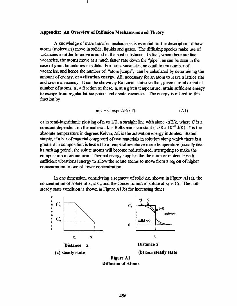
Appendix: An Overview of Diffusion Mechanisms and Theory

A knowledge of mass transfer mechanisms is essential for the description of how atoms (molecules) move in solids, liquids and gases. The diffusing species make use of vacancies in order to move around in the host substance. In fact, when there are line vacancies, the atoms move at a much faster rate down the "pipe", as can be seen in the case of grain boundaries in solids. For point vacancies, an equilibrium number of vacancies, and hence the number of "atom jumps", can be calculated by determining the amount of energy, or activation energy, AE, necessary for an atom to leave a lattice site and create a vacancy. It can be shown by Boltzman statistics that, given a total or initial number of atoms, n;, a fraction of these, n, at a given temperature, attain sufficient energy to escape from regular lattice points and create vacancies. The energy is related to this fraction by

nln; = C exp(-AElkT) (AI)

or in semi-logarithmic plotting ofn vs lIT, a straight line with slope -AEIk, where C is a constant dependent on the material, k is Boltzman's constant (1.38 x 10-23 JIK), T is the absolute temperature in degrees Kelvin, AE is the activation energy in Joules. Stated simply, if a bar of material composed of two materials in solution along which there is a gradient in composition is heated to a temperature above room temperature (usually near its melting point), the solute atoms will become redistributed, attempting to make the composition more uniform. Thermal energy supplies the the atom or molecule with sufficient vibrational energy to allow the solute atoms to move from a region of higher concentration to one oflower concentration.

In one dimension, considering a segment of solid ill<, shown in Figure AI(a), the concentration of solute at Xo is Co and the concentration of solute at XI is CI. The non-steady state condition is shown in Figure Al (b) for increasing times.

c 0 n c e n t r • t.

Co

C.

Distance x (a) steady state

X,

solvent

o

o Distance x

(b) non steady state Figure Ai

Diffusion of Atoms

456

The diffusion flux J12 is the amount of material passing through a unit area in the x-direction per unit time and is proportional to the concentration gradient dC/dx by Fick's first law as

JI2 = -D dC/dx , (A2)

where D is the proportionality constant called the diffusivity or diffusion coefficient. This is more generally stated as Fick's second law

dC/dt = d/dx(D dC/dx) (A3)

for the general case where D is concentration dependent under non-steady state conditions. Solving these equations for the boundary conditions

(a) At t = 0, C = ° for all x>O, (b) At t = 0, C = Co for all x<O, and (c) At x = 0, C not = Co for all t>O, gives

C = CJ2[1 - erfc(xI(2sqrt(Dt»)], (A4)

where erfc refers to the Gaussian error function. The point at which the concentration ofthe diffusant is 112 ofthe initial concentration gives a simple relation most often used by scientists. This relationship is given in the body of this paper and may be used for the desired calculation of the diffusion coefficient. The diffusion coefficient, on the other hand, varies with temperature according to an Arrhenius-type of equation,

where a is the interatomic distance, N is Avogadro"s number, h is Planck's constant (6.6 x 1026 atoms per kilogram mole). The values of Do for a number of solid materials !1ft! given in any number of reference books and papers on the subject.2 .

References:

1. A. B. Ellis, et al., "Teaching General Chemistry: A Materials Science Companion", A.C.S. Books, 1993. pp.463-472. 2. W. Jost, Diffosion in Solids, Liquids, and Gases, New York, Academic Press, Inc.,

1952.

457

HIGH SPEED CIVIL TRANSPORT -DESIGN CHALLENGES

David W. Lund

Boeing High Speed Civil Transport Aero Dynamics

MS 6H-FIC Seattle, Washington 98129

e-mail david.w.lund@boeing.com

459

David W. Lund

460

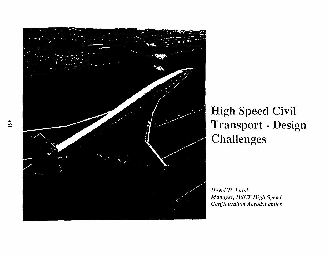
High Speed Civil Transport - Design Challenges

David W. Lund Manager, HSCT High Speed Configuration Aerodynamics

HSCT Requirements

• Environmental • Performance • Economic • Operational

HSCT Environmental Challenges

Engine Emissions No significant impact on atmospheric Ozone.

Community Noise Meet future noise rules and approach noise levels of future subsonics.

Sonic Boom

Radiation

No objectionable boom over populated areas.

No significant impact on traveling public or aircrews

Environmental Update

Emissions

• Latest assessments show very small impact of HSCT fleet on ozone depletion.

• Goal levels of EI=5 have been demonstrated in a research environment for both lean and richllean combustor concepts.

• Transition from laboratory concepts to production configuration is in progress.

• CMC combustion liners are in test. Early results are encouraging.

Low Emissions Combustor - P&W/GE Ceramic

matrix composito· -------...:...:

linor Fuel rich

ZODe 350OC'F reducing

onvironment Fualleafl

zone 3100"F oxidizing

environment • • • · • • • · • • • 5'9'" · • • · • · • · • · • · • ,. · · • • • · •

..

Environmental Update

Community Noise

• Significant progress achieved in noise suppression results from model wind tunnel testing.

• Suppressor nozzle concept downselect and detailed design of large scale unit approved by Preliminary Design Review.

• The engine cycle/nozzle configuration choice shows promise of achieving Stage III -5db community noise levels on emerging baseline configurations.

Environmental Update

Sonic Boom

• Low-boom design work terminated - subsonic flight over land.

• Research into the effects of sonic boom on marine mammals planned.

• High subsonic cruise speed possible - Mach 0.95 • High subsonic range factor acheivable on emerging configurations.

Radiation

• No show stoppers • Flight test ER2 - responds to NCRP* recommendation.

• Insignificant impact to typical traveller.

• Crew and very frequent flyers will be educated about exposure.

* National Council on Radiation Protection

HSCT Key Performance Requirements

RANGE 5,000 nmi minimum initial range with future growth

PAYLOAD 250-300 passengers in a three class configuration

CRUISE SPEED Mach 2.4 supersonic; Mach 0.95 subsonic

APPROACH SPEED 155 knots maximum

TAKEOFF FIELD LENGTH 11,000 feet, standard day, sea level

TIME TO CLIMB 60 minutes

FUEL MILEAGE Subsonic fuel mileage within 5% of supersonic

The CostlPrice Market Loop

AFFORDABLE FOR THE PUBLIC • Ticket prices are the same or close to subsonic fares.

AFFORDABLE FOR THE AIRLINES • Airlines can buy and fly the airplane and still profit.

SUCCESSFUL BUSINESS VENTURE FOR THE MANUFACTURER • Technology that works and can be produced. • Development that is affordable. • Cost effective production.

. Revenue • Market • Productivity • Fare

Management ..

Costs • Fuel • Maintenance· . • Crew

Economic Viability

. Revenue • Market • Market

.• Technology Design

• Production facffities

HSCT Key Operational Requirements

SAFETY At least as safe as subsonic airplanes of the same era.

DISPATCH RELIABILITY Superior to subsonic airplanes of the same era.

AIRPORT COMPATIBILITY Compatibility of: fuel type takeoff field lengths approach and climb-out speeds ground operations pavement loading servicing gates and ramps

TURN TIMES Turn around: 60 minutes max. Transit stop: 45 minutes max.

AIR TRAFFIC CONTROL Compatible with subsonics throughout the subsonic flight regime. No extraordinary handling procedures supersonically

Advanced Technologies Critical to Success

"'" No nose droop external vision system

Lightweight, high temperature composite structure

Fly-by-wire stability augmentation system

Low-emissions engine combustors

Advanced aerodynamics

Fully integrated propulsion controls

Mixed compression Low noise supersonic inlets suppression nozzles

Unique NASA Research Facilities

NTF High Re Tunnel -Langley-

40 x 80 Low Speed Tunnel -Ames-

10 x 10 Supersonic Tunnel -Lewis-

Flight Research -Dryden-

Vertical Motion Simulator -Ames-

HSCT Materials and Structures Challenges

THERMAUACOUSTIC INSULATION

COMPOSIT SKINS

STRUCTURAL HONEYCOMB SANDWICH

FUSELAGE

LOW COST FRAME MANUFACTURING

STRUCTURAL ADHESIVE BONDING

TITANIUM HONEYCOMB CORE

STRUCTURAL BONDING

WING BOX

SPLICE JOINTS

FASTENERS OR BONDED JOINTS

HSCT Aerodynamics Challenges

Optimized wing/body for maximum UD at all Mach numbers.

Nacelle/Airframe Integration • Maximize favorable interference • Inlet flow quality • Variable inletlnozzle geometry

Flying qualities with aeroservoelastics

.-.4:.---- Forebody Design • Lateral/directional

stability

High Lift • Low drag (noise) • Simple geometry

Volume Constraints • Landing gear • Payload

Aerodynam ics/Structu res • tic, camber • Planform variations

Large Scale Model in NASA 40'x 80' Wind Thnnel

2.2 % Scale Model in NASA's NTF Wind Thnnel

HSCT Propulsion Challenges

• Low Emissions • Performance • Operability • Stability • Durability • Noise Reduction

• Control

• Integration • NOise Reduction • Sensors • High Performance • Reliability • Light Weight • Performance • Operability • High temperature

:c.. =:::::-----:---

• Durability • Reliability

Supersonic Inlet Model in NASA Lewis lO'xlO' Wind Tunnel

External Vision System

Advanced Sensors

HSCT Systems Challenges

Fly-by-wire/Fly-by-light "-Flight Controls System .........

Full Authority Stability Augmentation System

Advanced Technology Auxiliary Power System

I Aeroelastic Mode Control

Mission :-------ll_ Adaptive Wing

Advanced Electrical System

Advanced Evironmental Control System

5,000 psi Hydraulics System

Integrated Flight/Propulsion Control System

Active Flap System

Leading Edge Flap Hinge Line Actuators

HSCT Manufacturing Technology Challenges

Advanced fiber placement of thermo-plastic composites

Thin film surface preparation of titanium

Titanium-graphite hybrid laminate process

Concept study of electron beam curing of large composite structure

HSCT Digital Mock-up Payloads and Structures

Systems

Flight Deck

HSCT Payloads Challenges

Cabin lighting Air ducts Gasper air duct

Electrical Systems

Sidewall lights

Structure

Window sculpture---,/f-<

Cooling passage Floor vent

Wiring

Typical Economy Section

Challenges • Passenger comfort • Systems space

APU Exhaust air

• Carry-on baggage volume • Containerized cargo

HSCT Design Challenges Titanium Matrix Composite Main Strut

Titanium Matrix Composite Torsion Link

Titanium Matrix Composite Truck Beam

Carbon Brakes

Radial Tires 44.Sx16.S inches 217 psi max.

Main Landing Gear

Graphite Composite Strut Brace

8 Wheel Truck

Forward and Aft Bogey Steering

HSCT Baseline Configuration

----c-. ----------------------------------r----

............ 0 ............. .

Range: 5000 nmi Cruise Mach: 2.4 Passengers: 290 Tri-class MTOW: 760,000 Ibs Noise: -1,-5,-1

reI. to Stage III

............... 0

Length: Span: Wing Area: Gear:

326 ft 150 ft 8500 sq ft 2-Post

Summary

• Adequate future market for HSCT

• Estimates indicate economic viability

• Good potential for environmental compliance with technology development

• Development of key technologies vital for program go-ahead

• Manufacturing and design technologies must meet economic goals

NEWMISMATIC METALLURGY

Edward L. Widener

School of Technology Purdue University

1417 Knoy Hall, Room 145 West Lafayette, Indiana 47907-1417

Telephone 765-494-7521 e-mail elwidener@tech.purdue.edu

491

Edward L. Widener

492

NEWMISMA TIC METALLURGY NEW:Update 97

Edward L. Widener Purdue University ABSTRACT: Coins are common signs of commerce in a society, and most coins are metallic alloys. Numismatics, the study of money, is a popular hobby for teachers of materials. Logically, the next step is to combine vocation with avocation in your Metals Lab. Like Mr. Wizard, keep things simple and keep costs low. Start by observing the colors of metals, alloys, and oxides. Explore the causes of corrosion, the resistance to erosion, and their relation to composition. Check for density, ductility, hardness, ferro-magnetism, and resonance. Coincidentally, we may absorb some Art, Botany, Ecology, Economics, Ethics, Geography, History. Language, Metrics, Politics, or Zoology. Technologists should be more than mere Materialists.

KEY WORDS: Alloys, Coins, Colors, Corrosion, Density, Ductility, Erosion, Magnetism, Mensuration

PREREQUISITE KNOWLEDGE: Periodic Table, with elements, symbols, and properties. Alloy compositions are % by weight (w/o). Definitions of metals vs. non-metals. Phases of elements, compounds, and solutions. Common copper alloys (brasses, bronzes, silvers). Corrosion is electro-chemical oxidation. Common materials are 16-ounces per Avoirdupois pound, but precious metals have only 12-ounces per Troy pound (or Apothecary pound).

OBJECTIVES: To rouse the interest of students, and to enhance their understanding of metallurgy.

EQUIPMENT: 1. Assortment of coins 2. Coin catalog (U.S. or World) 3. Dual ruler (inches & centimetres) 4. Magnifier (5-1 Ox, low-power) 5. Nail-file or pen-knife 6. Pan-balance (Ohaus scale or equal)

COLORIMETRY: Color differences often indicate varying compositions. Common copper-alloys are known as the "Cuss in ' Cuzzins" (CuSn & CuZn). Copper plus Stannum (tin) turns brown (bronze); but Zn (zinc) turns Cu into sunshiny brass. However, in wartime (WW II), Canada saved strategic nickel (Ni) by minting "tombac nickels" (88% Cu-12%Zn); and all that Zn makes Cu turn brown! Generally known as "Dutch Copper" (from their Malay tin-mines) this "tombac" stems from "tembaga" (Malaysia's word for copper-color). Tin is more costly than zinc, a by-product.

Many coins are grey. because most elements are colorless: metals are opaque; so alloys reflect light. The orange Cu becomes "German silver", ifalloyed only with Ni. The yellow Au becomes "white-gold", if alloyed with 25 % Ni & Zn. Platinum (Pt) is diluted with gold, when Au is cheaper (w/o Au, maximum?).

Costly alloys are often hardened with Cu and Ni. Compare the commercial Kruger-Rand (S. Africa) with the smaller commemorative Maple-Leaf (Canada). Each contains I-oz of pure gold; but the wear-resistant Rand has Cu, which is less dense than Au (say 8 vs. 19 g/cc) and imparts an orange-gold hue.

Of course, there are many shades of grey. We can observe subtle variations in hue (chroma), strength (intensity), and luster (brightness), for typical alloys of aluminum, iron, chrome, lead, or silver. Their brightness (or dullness) may depend on their polish (or roughness); and surface-finishes are related to erosion or corrosion resistance. Here is your chance to discuss "tri-stimulus coordinates" for colorimetry, and to demonstrate that normal eyes are superb "comparators".

Finally, as metals corrode (oxidize, rust, tarnish) they become ceramics (rocks, minerals). We see new colors, which may vary with alloy composition, coating thickness, corrodent concentration, environment, illumination, or viewing angle. Welded steel shows "rainbow colors", decreasing from light blue at 340 to light yellow at 220 Celsius degrees.

493

LAB ACTIVITIES: I. Display some colorful ads of equipment or products, where scale has been shown by an adjacent cent,

nickel, dime. Metal grains, failure features, and phases will appear in perspective. This exploits our general familiarity and fascination with coins.

2. Measure some coin-diameters and rim-thicknesses, using a dial-caliper or micrometer. Dimes are about 11/16" x 50-mil; Cents are about 12/16" x 60-mil; Nickels are usually 13116" x 75-mil. Use new coins; avoid battered edges; watch for tapered-edges; and compare with worn coins. Heighten interest by comparing sizes and weights of coins from various countries. There is considerable difference between sen, cents, centavos, centimes, centimos, kopeks, pennies, pfennigs, or stotinki. Standardizing on the Eurodollar (ecu-coins) may obviate money-changers or facilitate slot-machines, but don't count on it. Governments like to control exchange-rates. Meanwhile, inflation makes cheap coins obsolete and collectible.

3. Explain how Gresham's Law works (bad money drives out good). Traditionally, the cheapest coins were "Coppers". As diameters have diminished, those big pennies have disappeared in Australia, Britain, Canada, and USA. Then, as Cu-coated zinc replaced our "wheaties", these too become collectible. Have your class compare the meltdown (bullion) values for such coins, using commodity prices from newspapers (like Wall Street Journal).

4. Ask why Canada's Maple-Leaf(l-oz of yellow gold) is small, compared to S.Africa's Kruger-Rand (I-oz of orange-gold)? Find the Rand's Au-Cu compositions, get its average density, and calculate the diameter increase if coins have constant thickness. Then "mike"the real coins, from your safe!

5. What is "Sterling Silver", and where did it come from? About 1200 AD, the British obtained a malleable but durable alloy (92.5 Ag & 7.5 Cu wlo ) from the East Germans (Easterlings). Made into 'Sterling tableware and jewelry, this alloy tarnished slowly and evenly. Antiques today are prized for "patina"; old silver coins are sold as "toned", at a premium.

6. Why is 7.5 wlo considered the optimal Cu in 'Sterling? Any less Cu decreases hardness. But more Cu risks a 2-phase "eutectic-structure", which quickly forms "zebra-tamish." We expect silver-soldering to produce "rainbow-colors", reminiscent of welded steel; but how do cold coins get toned, pitted, or black? A wrapping of paper (sulfate or sulfite pulping) or of PVC fIlm (polyvinyl chloride) is the culprit. Compare them with untoned-coins, wrapped in benign poly-ester film (like DuPont Mylar) .... So, we say hydrogen peroxide bleach (H2 S04) is "greener" than sodium hypochlorite (Na 0 CI), because watery effluent (H20) is better than salty (NaCI).

7. Noble elements (gold, platinum, iridium) seldom oxidize, but are known to dissolve somewhat in "Aqua-Regia". This is the fabled "universal solvent", nitric plus hydrochloric acids (HN03 + HCI). Try this on gold-foil:, which is relatively cheap, but be careful. Use an exhaust hood, rubber gloves, and tongs. Then dilute and dispose of the toxic waste. By the way, mention that muriatic acid is dilute-hydrochloric, which fumes and irritates mucus membrane; always boost industrial chemistry.

8. Explain that 24-Karat gold is 100% pure, whereas a I-Carat diamond weighs 3.086 grains (200 mg). Do not confuse these precious units.

9. Trace the history of USA cents. From 1864-1942 , they were bronze (95 % Cu, 5 % Sn+Zn). War brought a 1943 steel. cent (with Zn coat) and 1944-45 brought cents of salvaged cartridge-brass. 1946-61 returned cents to 5% Sn-Zn. 1962 cents had 5% Zn only. But from 1982 to date, the cents have been Cu-coated Zn. Not only is this a colorful collection, but we can demonstrate accelerated corrosion (if Anode is small, relative to Cathode). Remember to define corrosion as "Anode Oxidation". Thus, a small notch in the cent's Cu-edge will expose fresh Zn, so immersion in nitric-acid soon leaves only a hollow Cu-shell. ... Foran obvious application of this principle - we could prematurely puncture a steel tank, if paint-coverage is imperfect (and generally is). The fewer the skips, the sooner our tank leaks; but it sure looks pretty.

494

10. Our only USA platinum-coinage (1997) is 99.99% fine. Unaccustomed to ultra-high ductility, our Mint had unexpected problems with "Lueder-lines", the wrinkled nonuniform strain which distorts the coin-designs. It takes 9 die-strokes to load these blanks evenly and produce proof-grade coins. Fine gold proofs take 6-7 strikes, silver 2-3, and Cu-Ni only 2. Our lab often sees Lueder-lines in brass or copper tensile-coupons; They look like cross-hatching ..

II. From 1866 to 1942, our 5-cent "nickels" were 75% Cu-25% Ni. The Shield-type (to 1883) was only 20.5 mm round. The Liberty-type (to 1912) and the Indian-type (to 1938) were 21.2 mm round and weighed 5-grams. The Jefferson-type (to date) is also 21.2 mm and 5-grams; but its composition in wartime (1942-45) changed to 56% Cu - 35% Ag - 9% Mn. From 1946 to date, we resumed 75% Cu-25% Ni. Here is another chance for color comparisons and some magnet tests. Also, vending machines have "slug-detectors" to stop free-loaders. Since iron, nickel, and cobalt are welI known "para-magnetic"elements, how do coins of steel, stainless steel, or nickel function in slot-machines? Get a good magnet and see if they do.

12. Metals lab might be Treasure Island, and students might be Ship-Mites. Set sail with Cap'n Flint and Long John Silver. Keep a sharp lookout for pyrite gold and discover a wealth of monetary rewards.

REFERENCES: 1. Gunter Schon, "World Coin Catalog (20th Century)", Amos Pub!. Co., Sidney, OH, 1989 ($12.50). 2. R.S.Yeoman, "Guidebook of U.S. Coins (18th edT, Western Pub!. Co., Racine, WS. 1997 ($10.50). 3. Paul Gilkes, "Platinum Coinage Challenge: Lueder Lines", Coin World I Amos Pub!. Co., May 12 & June 2, 1997. 4. Mars Fontana, "Corrosion Engineering", McGraw-Hill Pub!. Co., New York, NY, 1978. 5. W.K.Dalton, "The Technology of MetalIurgy", MacmilIan Pub!. Co. ,New York, NY, 1994 (Ag-Cu Phase Chart, p.1 03). 6. Sybil P. Parker (ed.), "Dictionary of Scientific and Technical Terms (5 th ed .. )", McGraw-HilI Pub!. Co., 1994.

BIOGRAPHY Prof. Widener has taught at Purdue University since 1978, concentrating on mechanics, materials, recycling, and communicating Ed was in Malaysia from April 1995 - June 1996, teaching Metals Lab for new technology teachers. Membership include ASEE, ASM, ASME, ISA, T APP!. A registered PE in New York & Indiana, he was ABET accreditation visitor, from 1983-1990; and NSF lab-grants reviewer in 1989 and 1990. Between 1994-1977, he had night classes in Indianapolis, IN (IUPUI) and Danville, IL (Jr College). Degrees from Purdue are BS '49 (physics) and BS '51 (ME); MSEM 62 (Hydraulics) is from University of Kansas Between 1952-1978, Ed was a process or project engineer for Continental Group, Baker-McHenry-Welch, Kimberly-Clark. E.!.DuPont, Union Carbide, & US Steel. In WW II, he was U.S. Navy S IIc aboard light-cruisers Vicksburg & Astoria.

495

EFFECTIVENESS OF ULTRASONIC TESTING METHOD IN DETECTING

DELAMINATION DEFECTS IN THICK COMPOSITES

Glen C. Erickson

FMClUnited Defense Ground Systems Division

150 East Brokaw Road San Jose, California 95103

and

W. Richard Chung

Division of Technology San Jose State University

College of Applied Sciences and Arts One Washington Square

San Jose, California

Telephone 408-924-3190 e-mail wrchung@sjsuvml.sjsu.edu

497

w. Richard Chung

498

Effectiveness of Ultrasonic Testing Method in Detecting Delamination Defects in Thick Composites

Glen C. Erickson, FMC/United Defense, Ground Systems Division, 150 East Brokaw Road, San Jose, CA 95103

and

w. Richard Chung, Division of Technology, San Jose State University,

San Jose, CA 95192-0061

Key Words: Fiber-reinforced composites, S-2 glass/polyester, epoxy, ply, delamination, ultrasonic testing

Prerequisite Knowledge: Knowledge of composite manufacturing and nondestructive testing/inspection will be helpful.

Objective: To fabricate and observe the simulated delamination cracks in a thick composite laminate and understand the techniques involved in the ultrasonic testing method.

Equipment:

1. Squirter (through transmission technique) ultrasonic tester

2. Sonic Mark IV (pulse echo technique) ultrasonic tester

3. Biaxial S-2 fiber glass fabric

4. Epoxy resin

5. Polyester resin

6. Couplant agent for ultrasonic testers

7. Dry cleaning solvent

8. Drill press

9. Ruler

10. Computer and data acquisition units and software

499

Introduction:

Thick Composite materials are being used to an ever increasing extent throughout industry. Significant weight reduction and tailored performance characteristics are the driving force behind increased use of composites. Most commercial inspection equipment in use today is only adequate for inspection of composite materials up to 1 inch thick. In addition to the use of thicker composites, the composites are being bonded to and fabricated with other materials for increased fire protection, electrical continuity, ballistic protection, etc. This has resulted in several new inspection challenges that must be addressed. As thick composites become more common, adequate nondestructive inspection methods for thick composites become more important. It is Imperative that inspection equipment and techniques keep up with the development of thick composites so that the quality and reliability of products can be determined in production and during intended use.

Composites are unlike metallic materials, which have been used for a long time and tend to have quantifiable homogenous properties and proven methods for inspection of quality. Composites have non-homogenous properties that can vary from part to part. Inspection of composites has relied on methods developed for the inspection of metal, such as x-rays, magnetic particle, eddy current, ultrasonic and dye penetrant. Many of trlese inspection techniques have proven useful for the inspection of thin composites, but are totally useless for thick composites. Limited inspection methods exist for the inspection of thick composite materials because of several factors that add to the complexity of the inspection situation. For example, there are numerous different types of material matrix formulations and fiber combinations that can be considered composites. The possible flaws that occur in these materials can be overwhelming: there may be porosity, contaminants, inclusions, delaminations, moisture, fiber misalignment, broken fibers, matrix aging, nonhomogeneities, matrix starved or matrix rich regions, etc. Some of these flaws, such as porosity, may be common in composites and be acceptable from a strength point of view, but they create a problem for the nondestructive inspection of other defects. Another major inspection problem comes from the anisotropy and physical property nonhomogeneities, as well as relatively high density effects (high absorptivity and scattering) of radiation (sound, etc.). Due to the many possible inspection challenges, a need exists for determining and appropriate inspection method for a given thickness and composite formulation.

There are several inspection techniques that look promising for the inspection of thick composites such as x-rays, ultrasonic, and microwaves. Most techniques are only good at inspecting a few of the possible combinations of defects and materials. The answer to the complete inspection of a given composite material probably will result in the need to use several different inspection techniques. In order to determine the appropriate inspection technique for a given material, a systematic approach to characterizing the flaws effects on composite performance must be undertaken.

500

Delamination is one of the biggest problems often found in thick composites. An effective nondestructive inspection technique that can quickly and accurately locate the delamination defects in a thick composite is always a time pressing issue. This study will examine the feasibility of using ultrasonic waves to fulfill these needs. The proposed experiment will use a qualitative research methodology to study the effectiveness of ultrasonic testing technique in thick composites. A Squirter ultrasonic tester using through transmission method and a Sonic Mark IV ultrasonic tester using pulse echo method will be employed throughout the entire study. A four inch thick S-2 glass/polyester composite laminate will be manufactured. A series of flat bottom holes (0.75 inch in diameter) simulating delamination defects at depths of 0.5, 1.0, 1.5, 2.0, 2.5 inches of composites. Hole sizes are also varied from 0.50 inch to 2.0 inch at a depth of 0.25 inch. These holes are used to evaluate the nondestructive evaluation technique ability to identify defects at increasing thickness and various sizes. The results generated from this study will provide some guidance for future inspection considerations. The advantages and limitations relating to the ultrasonic testing in thick composites will be carefully studied and discussed.

Ultrasonic Experimental Study:

Since ultrasonics is most commonly used to inspect for defects in composites, an experimental study was conducted on a thick composite specimen. The study was conducted to determine the capability of ultrasonic techniques to identify flat bottom holes (simulated delaminations) in thick composites. Delamination flaws vvere chosen for the topic of this study for several reasons. The first is that all other defect types usually end up becoming a delamination as the result of propagation of their failure mode. Delaminations commonly happen in the assembly process when joining composite pieces with bolts. This is important because it happens after the individual part has been inspected and assembled into a larger installation making it a more costly defect, that is harder to detect. The simulation of delamination defects is easier than most other types, since they can be simulated by flat bottom holes which are easier to fabricate than embedded flaws and it is easier to control the dimensional tolerances. The scope of this study was to limit the selection of ultrasonic techniques to those that were commercially available. Ultrasonic testing makes use of high frequency mechanical vibrations. For most composite materials, frequencies are typically in the .5 - 10 megahertz range. A study of the degree of scattering or attenuation, often based on the time required for the scattered energy to be received, provides information about the type, size, and location of the flaw. Composite materials offer special challenges to ultrasonic inspection. Because the materials are highly attenuating, multi-layered, and anisotropic, it is often very difficult to transmit and receive the necessary signals which contain the ultrasonic information. The ultrasonic inspection geometry can be either through transmission (transmitter and receiver on opposite sides of the structure) or pulse echo (one-sided, transmitter and receiver on the same side of the structure).

501

Construction of Thick Composite Specimen:

The construction of the test specimen was based on guidelines from the U.S. ARMY technical manual TM 55-1500-335-23, Nondestructive Inspection methods, page 4-58 (b). The thick composite specimen was fabricated by epoxy bonding two 4.32 cm (1.70 inches) thick, 69 plies of S-2 glass/polyester composites together. Each 69 ply laminate was processed by the vacuum bag and autoclave process, which resulted in a high quality laminate as shown in Figure 1.

Figure 1. A cross section of the inspection specimen laminate shown at six times magnification and fifty times magnification, shows it is a high quality laminate with good consolidation and low void content.

The finished size of the composite specimen is 11.30 em wide by 8.63 cm tall and 25.4 cm long. The specimen has ten flat bottom holes drilled in it to simulate delamination flaws. Figure 2 shows layout and dimensioning of holes.

502

1--------10 .00-----1-1 ""1

i----:

: ! : : I : _ . ., .... -+----+-. ,-..:,

02.00 FLAT BOTTOMEO .25 DEEI='

-4.-45

2 .00 FL.AT BOTTOMEO HOLE .50 DEEP

¢.75 n ... H BOTTOMED 1.00 OE:EP

¢.75 FLAT BOTTOMED HOLE 2.00 DEEP

ri --r-r--r--r-l __ .I.. _.l ___ L __ .L __ J

Figure 2. Drawing showing the dimensions and layout of the flat bottomed holes in the thick composite test specimen. (Units are in inches)

Holes numbered 1 through 5 are %" flat bottom holes simulating defects at depths of .2.25 cm, 3.54 cm, 4.81 cm, 6.08 cm and 7.37 cm of composite. Holes numbered 6 through 9 represent defects at a depth of 7.87 cm and defect size 5.08 em, 3.81 cm, 2.54 cm and 1.27 cm in diameter. Hole number 10 represents a 5.08 cm diameter defect at a depth of 10.67 cm of composite. The holes in the composite test specimen were used to evaluate the ultrasonic technique abilities to identify defects at increasing thickness and various sizes. To evaluate nondestructive evaluation techniques ability to identify various size defects the specimen included five flat bottom holes drilled at a depth of.64 em, with sizes of 5.08 em, 3.81 em, 2.54 em and 1.27 em diameters. Reference figure 3, that shows holes drilled in the face of the composite and epoxy bond line on side, where the two laminates were joined together.

503

Figure 3. Photo of the drilled holes perpendicular to epoxy bondline in thick composite test specimen.

Equipment and Material Description:

This section contains a list of material and equipment used to support this study. See Table 1 for a summary of ultrasonic equipment that was used. See Table 2 for a summary of materials used. Common commercial grade materials (cheesecloth, paper, etc.) are not listed.

Table 1. Equipment Used I I

Part r,o ' I NomenciJture Specification Manufacturer I

I

Squirter ABTS US-540 Automation Industries Inc. (Through/transmission) Sperry Div

Shelter Rock Rd Dabury, Ct. 06810

Sonic Mark IV Mark IV Sonic Instruments Inc. (pulse/echo) 1018 White Head Rd.

Trenton, NJ. 08638

Table 2. Materials Used

Part ' I Description Specification r,1anufacturer I

Couplant, Ultrasonic Inspection

Sonotech, Inc 1413 Frasier St SUite 2 Bldg H PO Box2189 Bellingham WA 98227

504

Gloves, Surgeon E-008 Defense Supply Agency Directorate of Medical

Material 2800 S 20th St Philadelphia PA 19101

Apron, General Purposes Federal Commercial Item Description Promulgated by General Services

Face Shield Military Specifications Promulgated IJy

Cloth, low-lint cleaning MIL-C-85043 Military Specs Promulgated by Military

Dry-cleaning solvent MIL-C-38736 Military Specs Promulgated by P-D-680, Type II Military

Marking Pencils MIL-P-83953 Military Specs Promulgated by (China Marker) Military

Results of Ultrasonic Inspection:

It must be mentioned that NDTII is used differently during manufacture and in the field. The primary distinction between these applications is that during manufacturing it is often possible to gain access to both sides of the part being inspected, allowing the use of through-transmission type measurements. In the field, it will be necessary to use single-sided methods, since only one side is accessible.

Of equal importance to the selection of a viable NDTII method is the identification, development, and use of well characterized specimen materials. Note that the specimen materials must contain all of the types and sizes of flaws and defects to be studied and accounted for. In addition, these must be combined with the capability of accurately measuring thickness when this is a requirement (as is often the case).

The first ultrasonic testing technique that was used on the thick composite specimen was the pulse echo method. The pulse echo method was a one sided inspection. This inspection was done using the Sonic Mark IV manual equipment. A one megahertz transducer was attached to the ultrasonic tester. The part was then sprayed with water and the operator placed the traducer on the wet test specimen and moved the transducer along, while monitoring the read out screen. The A-scan results were reported as manual drawings of the screen output. The pulse echo inspection results are shown in Figure 4. These two figures show the A-scan results from the pulse echo screen. The A-scans are interpreted from left to right. The first two to three wave lines represent the reflection of the sound going in the front surface of the specimen. The next significant wave peak to the right represents the sound being reflected from the flaw. The pulse echo was only able to detect the flaws at depths of 2.25 cm (.885 inch) and 3.54 cm (1.395 inch). The most common defects in composite materials are planar and parallel to the surface, which is the most suitable for ultrasonic inspection. Ultrasonics is limited by the high absorption and high scattering of ultrasonic signals exhibited by composites.

505

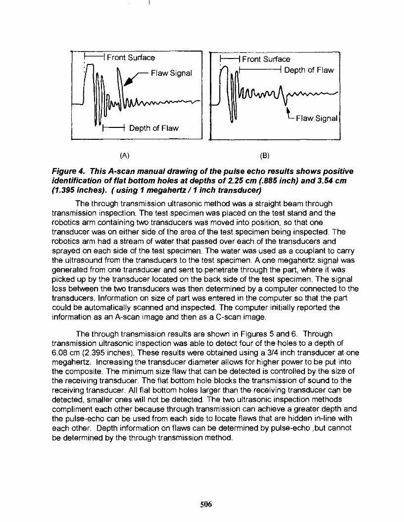
f--I Front Surface f---i Front Surface r Flaw Signal . 1 1 Depth of Flaw

l Flaw Signal 1-------+1 Depth of Flaw

(A) (8)

Figure 4. This A-scan manual drawing of the pulse echo results shows positive identification of flat bottom holes at depths of 2.25 cm (.885 inch) and 3.54 cm (1.395 inches). (using 1 megahertz /1 inch transducer)

The through transmission ultrasonic method was a straight beam through transmission inspection. The test specimen was placed on the test stand and the robotics arm containing two transducers was moved into position, so that one transducer was on either side of the area of the test specimen being inspected. The robotics arm had a stream of water that passed over each of the transducers and sprayed on each side of the test specimen. The water was used as a couplant to carry the ultrasound from the transducers to the test specimen. A one megahertz signal was generated from one transducer and sent to penetrate through the part, where it was picked up by the transducer located on the back side of the test specimen. The signal loss between the two transducers was then determined by a computer connected to the transducers. Information on size of part was entered in the computer so that the part could be automatically scanned and inspected. The computer initially reported the information as an A-scan image and then as a C-scan image.

The through transmission results are shown in Figures 5 and 6. Through transmission ultrasonic inspection was able to detect four of the holes to a depth of 6.08 cm (2.395 inches). These results were obtained using a 3/4 inch transducer at one megahertz. Increasing the transducer diameter allows for higher power to be put 'Into the composite. The minimum size flaw that can be detected is controlled by the size of the receiving transducer. The flat bottom hole blocks the transmission of sound to the receiving transducer. All flat bottom holes larger than the receiving transducer can be detected, smaller ones will not be detected. The two ultrasonic inspection methods compliment each other because through transmission can achieve a greater depth and the pulse-echo can be used from each side to locate flaws that are hidden in-line with each other. Depth information on flaws can be determined by pulse-echo ,but cannot be determined by the through transmission method.

506

Figure 5. This ultrasonic C-scan image of the top of the thick composite inspection specimen by through transmission methods shows positive identification of the flat bottom holes at depths of 2.25 cm, 3.54 cm, 4.80 cm, and 6.08 cm with 50-100% of the sound transmission received through the specimen. ( using 1 megahertz / 3/4 inch transducer)

Figure 6. This C-scan image of the side of the thick composite inspection specimen by through transmission methods indicates complete signal loss (gray area) at the adhesive bond/lne and the five holes. (using 1 megahertz / 3/4 inch transducer)

507

Conclusions:

The results of this study suggest that ultrasonic methods reach the limit of their capabilities at about 10.16 cm (4 inches), for this specific composite material, flaw type and flaw size. This study concludes that thick compos·ltes are difficult to inspect and that some thick composites greater than 10.16 cm thick may be uninspectable with current ultrasonic techniques. Since thick composites will have higher strengths than thin composites, the flaw size in some cases may be allowed to grow through design tolerance to the point where rejectable defects may be 5-10 inches in diameter, which in turn would be much easier for the ultrasonic equipment to identify at greater depths.

The following are three important conclusions drawn from this study:

1. This study used transducers ranging in size from .25 to 1.0 inch The larger 1.0 inch transducers always gave better results than the smaller transducers.

2. This study used frequency ranges from .50 to 2.25 Megahertz. The lower frequencies between .50 - 1 Megahertz always provided better results than the higher frequencies.

3. Adjusting the gain was critical for interpretation of results and to reduce the huge sound reflections encountered off front surface of test specimen.

Recommendations:

Future studies involving Inspection of vertical delamination flaws and employing other NOT/I methods such as x-rays would be highly desirable.

References Air Force Nondestructive Inspection Program Office., (1991) Nondestructive Inspection Methods Technical Order 33B-1-1, Kelly Air Force Base, Texas.

Batra, N. K., Chaskelis, H.H., (1989) Nondestructive Evaluation of Thick Composites: A Review, Thick Section Composite Technology. Sagamor Army Materials Research Conference Proceedings, 239-250.

Duke, J.C., (1993) NDE Method Selection for Advanced Materials, Advanced Materials: Expanding The Horizons (25th International SAMPE Technical Conference Proceedings, 552-561.

Smith, M. Gillian (1996) Nondestructive Evaluation of Large Composite Components. Nondestructive Testing, 1, 203-206.

Nondestructive Testing and Quality Control, ASM Metals Handbook, (9th ed.). (1989). (Vol. 17). Materials Park, OH: ASM International.

508

Biography

Glen C. Erickson

Principal Quality Engineer, United Defense FMC/BMY BA., Industrial Arts, San Jose State University MA., Industrial Studies, San Jose State University ASQC Certified Quality Engineer

Mr. Erickson joined FMC in December 1974. Since that time he has held several positions in the quality department and as a project quality engineer for several military programs. Mr. Erickson has gained valuable experience in all aspects of quality project management by working at the staff level, planning and implementing ISO 9000 quality systems and participating on product development teams focused on customer satisfaction. Most recently, Mr. Erickson was the quality manager for the Composite Armored Vehicle research and development program at United Defense. On this program Mr. Erickson was responsible for inspection, acceptance testing and supplier management of thick composite materials fabricated at supplier's facilities and at United Defense.

W. Richard Chung

Professor, Division of Technology, San Jose State University

Ph.D., Materials Engineering, Auburn University

M.S., Materials Engineering, Youngstown State University

B.S., Chemical Engineering, Chinese Culture University

Dr. Chung joined the faculty of San Jose State University in 1987. Since then, his primary teaching responsibility has been in the fields of Materials Engineering and Quality Assurance. The most recent positions that he has held in the Division of Technology are department chair and graduate coordinator. During 1976 to 1982, he worked as an engineer in various industries, such as paper and pulp industry, plastics manufacturing, and nuclear power plant design and construction. His current research interests are thermoplastic composites and flip chip assembly and packaging.

509

MEDICINE, MAGIC, MATERIALS, AND MANKIND

F. Xavier Spiegel

Spiegel Designs 3122 Parktowne Road

Baltimore, Maryland 21234

Telephone: 410-661-2192

A walk through some of the myths about materials and the use of materials in medicine. The author's interpretation of the signal discoveries and the major contributors to our modern understanding of materials, medicine and science.

This paper is dedicated to Mary L. Spiegel, my soulmate, who taught me the meaning

of self sacrificing love.

(Paper not available at time of publication)

511

F. Xavier Spiegel

512

A DEVICE FOR MEASURING THE ELASTIC MODULUS OF SPHERICAL MATERIALS

Mtrook AI Homidany

and

Brian L. Weick

Department of Mechanical Engineering University of the Pacific

Stockton, California 95211

Telephone: 209-946-3084 e-mail bweick@uop.edu

513

,-"'" .... on ...i

= eo: 'C

A Device for Measuring the Elastic Modulus of Spherical Solids

Abstract

\1trook AI Homidany and

Brian L. Weick*

Department of Mechanical Engineering University of the Pacific

Stockton. CA 95211

*Telephone 209-946-3084 E-mail: bweick@uop.edu

A simple test apparatus has been deSlh'lled and fabricated to measure the elastic modulus of spherically-shaped solids. Expensive test machines are not needed. and measurements have been made using elastomers such as isoprene and neoprene. The test apparatus consists of a simple lever arm with a wooden cup on one end for holding a sphere. and a flat surface on the other end for applying a load. The load causes the sphere to be pressed against a glass plate, and the elastic contact diameter is measured by looking through the glass plate. Hertzian contact equations are used to determine the elastic modulus from the contact diameter. applied load, and properties of the counter surface. Necessary theoretical equations have been included in a computer program that can be used to calculate the elastic modulus from known and measured parameters. Sample data sets and graphs are also included to assist the instructor.

Key Words: Hertzlan contact stress. elastic modulus. elastomers. isoprene, neoprene.

Prerequisite Knowledge:

In order to use the elastic modulus measurement device. one needs to be familiar with fundamental concepts presented in matenals science and mechanics of materials courses. These concepts mclude stress. strain. and elastIcity. A prerequisite knowledge of Hertzian equations and contact mechanics IS useful. but not required.

Objectives:

The primarY objective was to develop an experimental method for measuring the elastic modulus of spherically-shaped elastomeric materials. This process involved the follOWIng:

designmg and building a loading mechanism: determining a way to make contact measurements: writing a program to calculate the elastic modulus from contact measurements using Hertzian equations: utilizing the device for making example measurements; calculating the error associated with the built apparatus:

515

minimizing the cost of building the device; and, making the design easy to build by other students.

Introduction:

Mechanical designers need to have reliable material property data to enable them to properly design machine components and systems. These properties must be determined using experiments. For instance, the modulus of elasticity of a material is commonly obtained using tensile tests. For some applications, this way of determining the elastic modulus is not plausible. As an example, spherical solids used for bearings and other mechanical components are often subjected to contact stresses rather than tensile stresses. For this reason, a simple experimental method has been developed to determine the elastic modulus of spherical solids using Hertizian contact equations.

Equipment and Supplies:

Test apparatus A schematic diagram of the test apparatus is shown in Fig. 1 along with reference dimensions. The apparatus consists of an aluminum lever arm to load the spherical material by applying weights to the opposite end of the arm. This lever arm is connected to the acrylic base by a pivot joint made from polished steel to eliminate friction effects, and the arm is counterbalanced using applied weights. When a load is applied, the elastic contact diameter is read through the plate glass using a 27 mm scaled magnifYing glass which sits on top of the glass. For the 2 inch diameter samples, this measurement technique proved to be satisfactory.

Glass Plate \.

10

y

+--

I

rSPhere

/ Applied Load -,

/ Balanced Lever Arm /

18 -------. -., Figure I. Schematic diagram of the test apparatus for measuring the elastic modulus

of spherical solids. (Reference dimensions are III inches.)

516

Test specimens Two inch diameter isoprene and neoprene spheres obtained from McMaster-Carr were used to make sample measurements. Note that isoprene is commonly known as natural rubber, and neoprene is often referred to as chloroprene in text books and scientific journals.

Computer with C++ compiler and spreadsheet software The data collected for the isoprene and neoprene materials were analyzed using a C++ program shown in Appendix A. The program reads in the contact diameter and the applied load, calculates the elastic moduli, and then writes the results into an output file. Results can then be plotted using standard spreadsheet software such as Excel or Quattro Pro.

PROCEDURE:

Acquiring data • Place the spherical material in its housing and balance the lever arm so that the ball barely

touches the glass plate. • Place the scaled magnifying glass on top of the glass countersurface. • Place the initial weight on the load platform and record the contact diameter of the ball. • Increment weights and record the contact diameter and applied load.

Calculation of the elastic modulus The contact diameter and applied load are used in the C++ program to calculate the elastic modulus. A mathematically reduced version of the fundamental Hertizian contact equations described by Burr [I] and Johnson [21 is used to calculate the elastic modulus of the sphere.

Eb Es 0 a p Vb Vs

-

-

elastic modulus of the spherical elastomer (ie. ball) elastic modulus of the glass counter surface diameter of the spherical elastomer (ie. ball) contact radius applied normal load Poisson's ratio for the spherical elastomer (i.e. ball) Poisson's ratio for the glass counter surface

(1 )

Note that Eq. I can only be used to calculate the elastic modulus of an unknown spherical elastomer if Poisson's ratios for the ball and glass and glass are known along

517

with the elastic modulus of the glass, applied normal load, and the measured elastic contact diameter. While the elastic modulus and Poisson's ratio for the glass can be obtained from materials books like the eRe Handbook [3], the Poisson's ratio for the ball needs to be assumed. This assumption must be a valid one in order to obtain meaningful results. For example, an assumption for metals is v = 0.29, and for elastomers this assumption is closer to v = 0.46. Likewise, the transparent glass surface has an elasticity modulus of69 GPa, and v = 0.23 according to the eRe handbook [3].

Typical Results and Discussion:

Typical results are shown in Figures 2 and 3 for isoprene and neoprene, respectively. Elastic modulus is plotted as a function of load and contact diameter, and three identical experiments were performed for each material to allow for the computation of confidence intervals. For loads from 20 to lION, the measured elastic modulus was in the 3.8 to 5.8 MPa range for isoprene and from 1.6 to 1.8 MPa for neoprene. These values agree reasonably well with elastic modulus values tabulated by Shackelford [4]: 1.3 MPa for vulcanized isoprene, 3 - 6 MPa for vulcanized isoprene with 33% carbon black, 1.6 MPa for vulcanized neoprene, and 3 - 8 MPa for vulcanized neoprene with 33% carbon black,. Note that the values tabulated by Shackelford [4] were obtained under low strain tensile conditions rather than the contact conditions used herein. In addition, two visually identical elastomeric balls that experience the same loads may have different values for the elastic modulus due to differences in manufacturing specifications and conditions.

At low loads, the modulus of elasticity measured for isoprene tends to be relatively high, and decreases nonlinearly as load increases. This nonlinearity is most likely due to the power of three in the Hertzian contact equations, and was also observed by Weick [5J for nvlon and nvlon-based composites. This is the fundamental reason why elastic modulus values obtained from tensile tests can not necessarily be used to engineer spherical solids used in contact applications. Note that a similar nonlinear trend can be inferred for the neoprene material, however the magnitude of the error bars leads one to believe that the elastic modulus obtained using this contact measurement technique is reasonably constant for neoprene in the 20 - I ION range.

Notes to the Instructor:

Different measurement devices and techniques can be used to determine the contact diameter. The scaled magnifying glass proved to be adequate for the two inch diameter elastomenc spheres used to make the sample measurements. However, a microscope could also be used to determme the contact diameter.

HertZlan equations can also be derived that allow for the determination of the elastIc modulus from det1ection of the sphere and load arm. Noncontacting position sensors such as those made by the Kaman company have been used to make these measurements [5], and L VDT's such as those made by Lucas-Schaevitz could also be integrated into a

518

-. m 0.. 2

6

-5 CJ) :::J :::J

"U o 24· u - (a) W 3

CJ) :::J

9

-6 6 o 2 u -CJ) m W

3

10

(b)

5

50 90 Load ( N)

10 15 Contact diameter ( mm )

Figure 2. Elastic modulus measurements for an isoprene sphere plotted as a function of (a) load, and (b) contact diameter.

519

2 --co a..

--rn

"'0 0

u += rn co UJ

10 50 90 Load ( N)

3 --co a.. --(fJ

:::::l 2 t "'0 0 ! f ! I • t f 1 f u -rn co (b) UJ

1 10 15 20

Contact diameter ( mm )

Figure 3. Elastic modulus measurements for a neoprene sphere plotted as a function of (a) load, and (b) contact diameter.

520

test apparatus. Furthermore, deflections could possibly be measured using a standard dial or digital micrometer.

The dimensions of the test apparatus shown in Fig. I should be scaled to accommodate the diameters of the materials you want to evaluate. However, for pedagogical purposes, a larger apparatus will make contact diameter or deflection measurements easier to perform.

Instructors should also consider the sensitivity of their apparatus and determine the load at which the deflection of the apparatus as a whole must be considered. For light loads with elastomers, these deflections can be assumed to be negligible especially if the structure of the apparatus is made out of comparatively rigid metallic members. This was the case for the results presented herein. For heavier loads with more rigid test materials, the detlection of the apparatus becomes more significant. A sensitivity analysis has been performed by Weick [5] for the apparatus he used to determine the elastic modulus of spherically-shaped nylon and nylon-based composites.

References I. BUIT, A. H, Mechamcal Ana(v,\'IS and Design, Elsevier, New York, 1981. ') Johnson, K. L., Contact MechanIC:s, Cambridge University Press, London, 1985. 3. Bolz, R. E., Tuve, G. L., editors, eRe Handbook of Tables jar Applied Englneenng

SCience, 2nd ed., CRC Press, Cleveland, 1970. 4. Shackelford, 1. F., introductIOn to Matenals S'ciencej()r l:'ngmeers, 4th ed., Prentice-

Hall, New Jersey, 1996. 5. Weick, B. L., I:jJects o/Flher Tvpe on the Trihological BehavIOr o/Polvamlde

('omposlles. Ph.D. dissertation, Virginia Polytechnic Institute and State University, 1993.

521

Appendix A. I I A .. program 1:0 calculate the average elastic modulus

#include<stdlib.h> Winclude<math.h> Winclude "tstring.h" #include "scrnutil.h"

void main ( ) (

II All units are in 5I system unless specified int i = 1; float load, ballEMod, surfaceEMod = 6.gelO, ballPoisson = .46,

surfacePoisson = .23, ballDia = .0508, contactRadius, averageContactDia=O, contactDial, contactDia2, contactDia3;

ifstream fileIN; II declare files of stream fileOUT; string filenameIN; II declare filenames string filenameOUT;

I I open the fnes cout « "Enter the input file name: "; cin » filenameIN; filenameOUT = filenameIN + ".out"; fileIN.open(filenameIN.c_str()) ; it ( ! fileIN) (

cerr « "Could not open file" « filenameIN « endl; exit(l) ;

fileOUT.open(filenameOUT.c_str()) ;

II message to illustrate current state in the program cout «"Opened «filenameIN«" for input" « endl; cout « "Opened" « « " for output" « endl;

EileOUT « "Lo.3.d ( N) " « "Isoprene Elastic Modulus ( MFa) "« endl; I I Read L'1 data f:=-om t . .'::e input file fileIN » load; while ( i <= 10 && fi1eIN) (

II Isoprene elastic modulus caluculations i++; EileIN » contactDial » contactDia2 » contactDia3; II find average of the measured contact diameters averageContactDia = (contactDial + contactDia2 + contactDia3) I 3; contactRadil.ls = averageContactDia I 2;

ball modulus of elasticity ballEMod =( pow(.721, 3)* load* ballDia* surfaceEMod* ( 1- pow(ballPoisson,2)) I ((surfaceEMod* pow(contactRadius, 3) -(pow(.721, 3)* load* ballDia* (1 - pow(surfacePoisson, 2))))))* le-6; II send to output file fileOUT « setw(5) « load « set::eal(25,3) « ballEMod « endl;

fileIN » load;

fileOUT « endl «"Load « "Neoprene Elastic Modulus"« endl; II Read in data f:=-om input file while ( 1 <=20 i'& Ei1eINI (

II Neoprene elastic modulus caluculations i++;

522

fileIN » contactDial » contactDia2 » contactDia3; I I find average of che measured cont:act: diamet:ers averaqeContactDia = (contactDial + contactDia2 + contactDia3) / 3; contactRadius = averaqeContaCtDia / 2;

Ilcalculace ball modulus of elascicicy ballEMod =( pow(.72l. 3)* load* ballDia* surfaceEMod* ( 1- pow(ballPoisson.2)) / ((surfaceEMod* pow (contactRadius. 3) -(pow(.72l. 3)* load* ballDia* (1 - pow(surfacePoisson. 2)))))) * 1e-6; II send Co che oucpuc file fileOUT « setw(S) « load « setreal(2S.3) « ballEMod « endl;

:ileIN » load;

I'" Program Run

Load ( N) 19.62 29.430 39.240 49.050 58.860 68.670 78.480 88.290 98.100 107.910

Load 19.620 29.430 39.240 49.050 58.860 68.670 78.480 88.290 98.100 107.910 "'/

Isoprene Elascic Modulus (MFa) 5.586 5.824 5.383 4.900 4.529 4.223 4.067 3.837 3.838 3.866

Neoprene Elascic Modulus 1. 803 1.672 1.600 1.677 1. 683 1. 649 1. 634 1.666 1. 709 1.730

523

Mtrook AIHomldany hTfaduated with a Bachelor's Degree In Mechanical Engineering from University of the Pacific In 1997. He has taken advanced courses 1TI FI Uld Systems, and recently completed a course In the C"--'- programing language. Mr. AIHomldany IS currently back in Saudi Arabia.

Brian L Weick IS an Assistant Professor at UnIversltv of the Pacific where he teaches Materials Science. ManufacturIng, Design, and other general engIneenng courses. He holds Bachelor's and Master's Degrees In Mechanical Engineering, and he received his Ph.D In Materials Engineering Science from Virginia Tech in 1993. Other career-related experiences Include two years as a Project Engineer for General Dynamics, and two years at Ohio State as a Visiting Scholar. His research Interests Include tribological behavior of materials, and vlsco,elastlc behaVIOr of thin polymer films.

524

COMPUTER APPLICATIONS FOR THE MATERIALS LABORATORY ICLASSROOM: ILLUSTRATING

STRUCTURE AND DIFFRACTION

James F. Shackelford

University of California, Davis College of Engineering Davis, California 95616

Telephone: 916-752-0553 e-mail fshackelford@ucdavis.edu

and

Michael Meier

University of California, Davis Department of Chemical Engineering and Materials Science

Davis, California 95616

Telephone: 916-752-5166 e-mail mlmeier@ucdavis.edu

525

Michael Meier

James F. Shackelford

526

COMPUTER APPLICATIONS FOR THE MATERIALS LABORATORY/CLASSROOM: Illustrating Structure and Diffraction

James F. Shackelford and Michael L. Meier Department of Chemical Engineering and Materials Science

University of California Davis, CA 95616

KEY WORDS: Computer, Simulation, X-ray, Diffraction

PREREQUISITE KNOWLEDGE: Introduction to crystallography and diffraction, as provided in a typical, lower-division materials engineering course.

OBJECTIVE: To utilize relatively sophisticated research equipment for undergraduate teaching.

EQUIPMENT AND SUPPLIES: I. Scintag XDS2000 X-ray Diffractometer [or similar, contemporary diffractometer with computer control and data analysis capabilities]. 2. Silicon Graphics Workstation with Molecular Simulations Software [or similar graphics platform with crystal structure simulation package]. 3. Power Macintosh or PC with CD drive.

INTRODUCTION

Shackelford [I] has recently outlined the use of equipment available in the materials laboratories at a typical research university for the purpose of undergraduate teaching. The result is a set of three examples of the contributions that can be provided to materials engineering education by contemporary computers. First, the use of an x-ray diffractometer with computer control and data analysis in an undergraduate structures course is an excellent tool for demonstrating the role of computers in the materials laboratory. Second and closely related to diffraction is the use of computer modeling of atomic-scale structures, a major development in the field of materials science in the past decade. Commercial software packages are now available for this purpose. Using a graphics platform, these simulation packages can be used to illustrate structure in undergraduate courses, as well as predict diffraction patterns. Third, CD-ROM technology is providing a convenient supplement to current textbooks, e.g., a ready source of figures and tables. Ironically, there is some debate as to whether the CD-ROM may replace the textbook in the future.

X-RAY DIFFRACTOMETER WITH COMPUTER CONTROL AND DATA ANALYSIS

The x-ray diffractometer is a sophisticated piece of experimental equipmentthat is widely available in materials engineering laboratories. Although often acquired for support of research, a contemporary diffractometer is an excellent example ofa computer-interfaced experimental system for teaching purposes. Both experimental control and data analysis are generally performed in conjunction with a computer. Table I summarizes a set of x-ray diffraction experiments used in EMS 132L, an x-ray diffraction based laboratory course on the structure of engineering materials. It is offered at the University of California, Davis in the junior year as part ofa core-course sequence of basic materials science topics. The experiments represent long-established x-ray diffraction applications [2].

527

Table I List of X-ray Diffraction Experiments in a Junior-Level Introductory Course on the Structure of Materials

Department of Chemical Engineering and Materials Science University of California, Davis

EMS 132L Structure of Materials Laboratory

X-ray Diffraction Experiments

Introduction/Orientation, Radiation Safety Phase Identification and Quantitative Analysis Particle Size Measurement Residual Stress Measurement

Our laboratory has a Scintag XDS 2000 diffractometer with an intrinsic Ge detector and a 486 PC and a Micro Vax for computer control and data analysis. The most general application is the use of the Search-Match software based on the Powder Diffraction File of the International Centre for Diffraction Data (ICDD). The search of more than 60,000 powder diffraction files can be done in less than one minute. With the increasing interest in nano-scale sample preparation, the software packages for particle size measurement are highly useful. Both Scherrer analysis and Warren-Averbach analysis are available for determining particle size (and, in the case of Warren-Averbach, lattice microstrain) based on diffraction peak line broadening.[2J The Scherrer analysis can be carried out in about one minute, and the Warren-A verbach analysis can be carried out in a few minutes. Figures I and 2 illustrate experiments in which one powder sample is identified by its x-ray diffraction pattern and line broadening is used to identify the particle size of another.

100 .-________________________

90 f-

80 --

C 70 .-m [i 60 f-......

(120) 50-

40 ---I 30

20 - \ (111)

10 --

o 10 20 30 40 50 60 70 80 90 2-Theta, degrees

Figure I Experimental x-ray diffraction pattern of Buehler's Magomet polishing powder which is primarily MgO. The Scintag search match program was used to identify the peaks for the periclase phase, PDF file 45-0946. The periclase peaks are labeled using their Miller indices.

528

2.0

1.5 C ..... '"

LO Q) ;>

-Q)

0.5

104 105 106 107 108 109 110 III 112 2-Theta, degrees

Figure 2 Example of diffraction peak line broadening in the x-ray diffraction pattern of nanocrystalline TiO, powder. An average particle size of 32 nm gives substantial broadening measured at the half-maximum peak height of each of two adjacent peaks.

Perhaps the most significant benefit of the computer-aided diffraction experiment is the ability to do residual stress measurements. The use ofthe multi-angle specimen tilting technique has long been used to measure residual stress in metal alloys.[2] Lange, et.a!. [3] have also shown the technique to be applicable to structural ceramics. The magnitude of stress is indicated by the amount of shift in the diffraction angle caused by the independent tilting of the specimen surface away from the normal configuration. Table II gives typical results for the measurement of surface stresses due to the fabrication of a steel spring. It is important to note that, prior to the computerization of such multi-angle tilting experiments, the experiment was extremely tedious and time consuming. With the system in our laboratory, undergraduates can carry out accurate and reproducible measurements of stress with five tilt angles between ±30 (and a total experimental time ofIess than 20 minutes. One should also note that the steel sample was analyzed using Cu K. radiation. Traditional residual stress measurements on ferritic steels are done with Cr K. radiation for which the (211) plane gives a large diffraction angle (above 150 0 29). Such large angles maximize experimental accuracy.[2] The class experiment was carried out with Cu radiation to minimize disruption to research measurements. It is encouraging that good accuracy is possible with this much lower diffraction angle (in which the (211) line occurs just above 82 0 29). For calibration, Table II includes results for an annealed tungsten powder (essentially stress-free giving an essentially zero stress result within experimental scatter). Figure 3 illustrates a multi-angle plot of diffraction angle (29) versus the square of the sin of the tilt angle, with the magnitude of the slope representing the residual stress in the steel spring of Table II.

529

0.11714

0.11712 o

0.11710 o

'0" 0.11708

o 11706

o. II 704 000 0.05 0.10 0.15 0.20 0.25

SIN/\2(PSI)

Figure 3 Experimental plot of the change in interplanar spacing ofthe (211) diffraction peak of a spring steel as a function of the square of the specimen tilt angle (psi). The shift in d values is a result of the residual stress in the surface of the steel sample as a result of its manufacturing process. The triangle symbol data represent negative values of psi (specimen tilted towards the x-ray source) and the square symbol data represent positive values. The slope of the plot indicates a compressive stress of 506 Mpa.

Table 11 Typical Residual Stress Data for a Steel Spring

Steel Spring Stress Measurement - Experimental Conditions Cu Ku radiation (211) peak [at approx. 82.3 0 28j Elastic constants·: S, = -1.25 and V, S, = 5.76 [in units of 10-6 (MPa)-']

Sample Stress (MPa)

Steel Spring -505_6 ± 31.9

Tungsten Powder Measurement - Experimental Conditions Cu Ku radiation (400) peak [at approx. 153.5 0 28j

• Elastic constants·: S, = -1.50 and V,S, = 6.50 [in units of 10-6 (MPaY'j

Sample Stress (MPa)

Annealed W powder -12.5 ± 29.4

• Note that S, = - viE and 'IzS, = (I + v)/E

530

COMPUTER MODELING OF ATOMIC-SCALE STRUCTURES

Computer modeling has become a highly effective tool in materials research in the past decade, stemming from the refmed understanding of interatomic potentials which allows precise modeling of atomic-scale structures.[4] The application to biological chemistry has allowed such modeling to replace substantial amounts of experimentation in the preliminary stages of drug design. The leading commercial software package for structural modeling, Molecular Simulations, Inc., grew outofBIOSYM Technologies, Inc., which, as the name implies, grew out of the biomolecular simulation market, e.g. pharmaceutical design. An inorganic package is now available, appropriate given that Molecular Simulations, Inc. is now a subsidiary of Coming, Inc. In our laboratory, we are using the Molecular Simulations Insight II software on a Silicon Graphics Indigo 2!XZ platform. Figure 4 gives a simple example of the use of a similar simulation package to produce an illustration of the crystalline structure of rock salt, which applies to a number of important ceramic oxides. Nearly all crystal structure illustrations in the fourth edition of Shackelford's introductory materials science text were produced in this way. [5] In more advanced materials courses, the software package can be used to simulate x-ray and electron diffraction patterns and nmr spectra for given crystal structures.

(a) (b)

(c)

Figure 4 Illustration of the sodium chloride (and related oxides) unit cell. Parts (a), (b) and (c) were generated with a commercial computer simulation software package.

531

CD-ROM TECHNOLOGY

Another interesting aspect of computer technology in engineering education is the increasingly wide use of the CD-ROM. The enormous memory storage capability of the CD-ROM has had an especially significant impact on the technology of the textbook. A good example is the CD-ROM "Materials Science - A Multimedia Approach" by J.e. Russ. It includes a set of interactive HyperCard stacks and QuickTime visualizations. This CD is marketed as a supplement to Askeland's introductory materials science textbook.[6] Another example is the CD-ROM entitled "Materials Science on CD-ROM", published by Chapman and Hall, which takes more of a tutorial approach complete with interesting simulations. An alternative approach is a complementary CD-ROM which is a straight reproduction of the figures and tables of Shackelford's introductory text [5] and is provided with the Instructor's Manual. This configuration allows the instructor to produce laser-quality reproductions of any figure or table from the text. Figure 5 is an example of such a print out. Perhaps the most intriguing question associated with the CD-ROM is whether it will continue to be a supplement to the textbook or become its replacement.[7]

D (

r >-<

h h V C\: :/ C\: o .< ex X :A

C'\ '/ C'\ V V IX (X (X )

V 0, V C\ /: C\ /: .\ Q\ :x (Y

C'\ :/ C'\ V V rv >-<>-:rv rv

o Unitedl

Figure 5 A visual representation of the crystallographic unit cell. This illustration was taken directly from the CD-ROM supplement to reference 5.

ACKNOWLEDGMENTS

We wish to thank Lili.m Davila for her expertise in generating the computer simulated crystal structures and William Stenquist, editor at Prentice-Hall, for supporting the production of the CD-ROM.

REFERENCES

[I] J.F. Shackelford, "Computer Applications for the Ceramic Engineering and Materials Engineering Curricula," in Innovative Ideas in Ceramics and Materials Curricula, ed T. Stoebe and W. Huebner, American Ceramic Society, Westerville, OH, 1996.

[2] B.D. Cullity, Elements of X-ray Diffraction, 2nd Edition, Addison-Wesley, Reading, MA, 1978. [3] F.F. Lange, M.R. James, and OJ. Green, J.Amer.Ceram.Soc., 66 C 16-C17 (1983).

532

[4] H.W. Kroto, et.a!., "New Horizons in Carbon Chemistry and Materials Science," MRS Bulletin, 19 [II] 51-55 (1994).

[5] J.F. Shackelford, Introduction to Materials Science for Engineers, 4th Edition, Prentice-Hall, Upper Saddle River, NJ, 1996.

[6] D.R. Askeland, The Science and Engineering of Materials, 3rd Edition, PWS, Boston, MA, 1994. [7] P. Hood, "Books: The Next Big Thing," Newrnedia, 4 [4]8 (1994).

BIOGRAPHICAL SKETCHES

James F. Shackelford has BS and MS degrees in Ceramic Engineering from the University of Washington and a Ph.D. in Materials Science and Engineering from the University of California, Berkeley. He is currently a Professor in the Department of Chemical Engineering and Materials Science and the Associate Dean for Undergraduate Studies in the College of Engineering at the University of California, Davis. He teaches and conducts research in the areas of materials science, the structure of materials, nondestructive testing, and biomaterials. A member of ASM International, the Materials Research Society, and the American Ceramic Society, he was named a Fellow of the American Ceramic Society in 1992 and received the Outstanding Educator Award of the American Ceramic Society in 19%. He has published over 80 archived papers and books including Introduction to Materials Science for Engineers now in its 4th Edition and The CRC Materials Science and Engineering Handbook now in its 2"d Edition.

Michael L. Meier has a BS degree in materials science from North Carolina State University, Raleigh and MS and PhD degrees in materials science from the University of California at Davis. He is currently a lecturer at the in the Department of Chemical Engineering and Materials Science at the University of California at Davis. He teaches and manages the central departmental laboratories and is developing the undergraduate laboratory teaching program, is a member ofTMS and ASMI and is a member of the executive committee for the Golden Gate Chapter of ASMJ.

533

IMPACT OF MULTIMEDIA AND NETWORK SERVICES ON AN INTRODUCTORY

LEVEL COURSE

CD ROM by

John C. Russ Materials Science and Engineering Department

North Carolina State University Raleigh, North Carolina

Presented by:

Cheryl S. Alderman

NCSU Engineering Programs at UNCA UNCA 303 RBH

One University Heights Ashville, North Carolina 28804

Telephone: 704-251-6640 e-mail aldemlan@eos.ncsu.edu

535

Cheryl Alderman

536

Impact of Multimedia and Network Services on an Introductory Level Course

John C. Russ Presented by Cheryl S. Alderman Materials Science and Engineering Department NCSU Engineering Programs North Carolina State University, Raleigh, NC liNCA, Ashville,NC

Keywords: Multimedia. CD-ROM, computer animation, computer graphics, simulations, network connectivity, interactive hypermedia, self-paced learning.

We will demonstrate and describe the impact of our use of multimedia and network connectivity on an sophomore-level introductory course in materials science. This class services all engineering students, resulting in large (> 150) class sections with no hands-on laboratory. Concerned that traditional lecture and textbook approaches did not reach many students whose learning style is primarily visual and interactive rather than auditory and passive, we began in 1990 to develop computer graphics that might substitute for some laboratory or real-world experiences, and demonstrate relationships hard to show with static textbook images or chalkboard drawings. With some NSF funding through Project Succeed and strong local support from the College of Engineering and our Department, we have used student labor to create a comprehensive series of modules that cover the entire course contents. Called VIMS (Visualizations in Materials Science), these are available in the form of a CD-ROM (Macintosh version available now, PC version early next year), and also via the Internet (http://vims.ncsu.edu). The CD-ROM version, which is in use at more than 20 universities worldwide, uses a Hypercard front end with succinct but complete highlights that correspond (and are keyed to) all of the introductory materials science textbooks, with hyperlinks and a searchable index. This provides the student with a valuable resource to select the important information from the enormous amount of material covered in an introductory course. Extensive graphics in the form of nearly 700 Quicktime movie files are available at the click of the mouse to explain the concepts presented in the text. These include digitized movie clips from laboratory or demonstration experiments, cartoon graphics that clarify difficult concepts, computer simulations to illustrate physical principles, etc. Many of the movies show side-by-side presentations of complementary views or related material. Of course, this rich amount of information is most valuable to students who can access it at their own self-paced rate. and test their knowledge with the built-in self-quizzes. The CD also includes about 300 worked problems including all of the assigned homework and many example problems from the text. These are not just answers, but heavily annotated step-by-step solutions using Theorist, an interactive math package that allows students to solve complex equations, substitute numeric values, and plot results. The VIMS webserver was introduced this fall (1995), and makes the text and graphical information available on our campus workstation network (as well as worldwide). Combined with a listserver that allows students to ask questions, express frustrations. and share insights with each other and with the faculty, this electronic connectivity provides a new level of support for students. The response has been overwhelmingly positive, and we have extensive statistics from control-group experiments and student questionnaires that indicate higher interest levels and better performance from students who use these new capabilities. This result justifies the enormous cost, primarily in human effort and many hours of faculty and student time needed to develop these multimedia materials, and also points the way to extension of the technology to other venues. We are particularly interested in the applicability of some of the same materials, with the addition or substitution of appropriate descriptive language. for use in primary and secondary schools. VIMS has already been used as part of a third-grade science curriculum based on materials science that has been recently introduced in the Wake County (North Carolina) public schools.

537

STRUCTURAL LABORATORY MANUAL

Jack Kayser

Educational Technologies Specialist Skillman Library Lafayette College

Easton, Pennsylvania 18042

Telephone: 610-559-4017

539

Abstract

Structural Laboratory Manual

Jack Kayser Lafayette College

A structural laboratory manual has been written to accompany the laboratory component of a four-credit junior level structural design class at Lafayette College. The manual has been arranged so that hands-on laboratory experiments parallel the textbook material covered in class. Students have consistently written positive comments in their evaluations regarding the clear explanation of the laboratory procedures and the strong correlation between the class, textbook, and laboratory experience.

The manual has eleven experiments, each with AS TM and textbook references, data sheets, and write-up questions. The following experiments are included:

I. Properties of Metal in Tension 2. Evaluation of Bolts and Bolted Connections 3. Flexural Beam Test 4. Compressive Strength of Columns 5. Evaluation and Testing of Welded Connections 6. Material Properties of Balsa Wood 7. Selecting Proportions for Normal Weight Concrete 8. Mixing, Testing and Casting of Fresh Concrete 9. Mechanical Properties of Concrete 10. Batching and Testing of Mortar Specimens II. Testing and Evaluation of Coarse Aggregate

The structural design class associated with this laboratory is divided into two segments; the first seven weeks is devoted to steel structures and the remaining seven weeks to reinforced concrete structures.

The equipment used to carry out the experiments is primarily standard universal testing machines. The only unique components necessary are the testing fixtures used to grip or support specimens and a non-standard reinforced concrete beam form. Such fixtures can be readily manufactured in any machine shop.

The Structural Laboratory Manual will be available in PDF format on the Web at:

http://www.lafayette.edu/kayserj/manual.html

The manual is freely available for distribution, provided the author is acknowledged.

541

Table 1: Description of Experiments

Properties of Metals in Tension

Evaluation of Bolts and Bolted Connections

Flexural Beam Test

Compressive Strength of Columns

Evaluation and Testing of Welded Connections

Material Properties of Balsa Wood

Selecting Proportions for Normal Weight Concrete

Instrumented specimens of various metal are stretched

Bolts are tested in tension and shear, also plates and connections

Small metal and wooden beams are tested for deflection and strength

Metal rods of differing lengths and boundary condition are buckled

Welded connections are created and tested in tension

Balsa wood and glued joints are tested in tension and shear

Calculation procedure to determine batch quantities for concrete

Mixing, Testing and Batching and testing procedures Casting of Fresh Concrete for producing fresh concrete

Mechanical Properties of Concrete

Batching and Testing of Mortar Specimens

Testing and Evaluation of Coarse Aggregate

542

Nondestructive and destructive testing of concrete cylinders

Batching and testing procedure for cement mortar

Density, moisture content, and sieve analysis of coarse aggregate

Description of the Manual: The Structural Design Manual was written to provide a guide to experiments conducted in CE362 Structural Design, a Civil Engineering four credit junior level course. The manual is composed of eleven chapters which contain; references, experimental procedures, report questions and data sheets. The laboratory program parallels classroom lectures, providing an alternative method of learning the material. Brief details of each experiment are listed in Table 1.

Rationale for the Course:

Two separate desing courses were required for civil engineering students; Concrete Design and Steel Design, each with a laboratory component. A revision to the curriculum took place which emphasized more elective options for students. CE362 was created as a required four credit course to replace the two former design courses. The two former courses where revised as three credits electives, with an emphasis on computational design. CE362 provides the essentials of structural design that every civil engineer should know, along with practical hands-on experience in the laboratory.

543

For Use or Adaptation:

The entire Structural Laboratory Manual is available on the Web in an Adobe Acrobat PDF format. The manual can be downloaded from the site listed below. Acrobat Reader is required to view or print the manual. A link is also provided to the Adobe Acrobat download site.

http://www.lafayette.edu/kayserj/manual.htm I ,

The manual may be freely used or adapted, provided credit is given to the author. It is the responsibility of the users to ensure the accuracy and safety of experiments or work carried out or derived from the use the manual.

544

Structural Laboratory

Manual

Dr. Jack Kayser

Lafayette College

1997

545

Experiment

1

2

3

4

5

6

7

8

9

10

11

INDEX

Topic

Properties of Metals in Tension

Evaluation of Bolts and Bolted Connections

Flexural Beam Test

Compressive Strength of Columns

Evaluation and Testing of Welded Connections

Material Properties of Balsa Wood

Selecting Proportions for Normal Weight Concrete

Mixing, Testing and Casting of Fresh Concrete

Mechanical Properties of Concrete

Batching and Testing of Mortar Specimens

Testing and Evaluation of Coarse Aggregate

546

3

6

10

13

16

20

24

36

41

46

50

Experiment 1: Properties of Metals in Tension

References:

ASTM E-6 Standard Definitions of Terms Relating to Methods of Mechanical Testing

ASTM E-8 Standard Test Methods of Tension Testing of Metallic Materials

"Structural Steel Design LRFD Method," Jack McCormac, 2nd Ed., Section 1-7

Description:

Two of the most important items involved in the engineering of a structure are the deflections the structure will undergo when loaded, and the amount of load the structure can take before failing. These two fundamental measures of performance depend upon the behavior of the material the structure is composed of.

This experiment examines the behavior of metals in tension. Steel, aluminum, and cast-iron specimens will be tested. The following outline describes the properties which will be studied.

1. Stress-Strain Diagram: A plot of the stress-strain values which were recorded during a tension test. The plot will be created using the data file which was down loaded from the lnstron computer, modified and plotted using Quattro.

2. Ductility Based on Reduction of Area: The ability of the material to deform plastically. It is calculated as the ratio of the change in cross sectional area due to rupture divided by the original cross sectional area. Units of percent.

3. Ductility Based on Elongation: Another way of measuring the ability of a material to deform plastically. It is calculated as the ratio of the change in gage length due to rupture divided by the original gage length. Units of percent.

4. Tensile Strength: The maximum tensile stress that can be applied to a specimen. It is based on the ratio of ultimate load divided by the original cross section. Units of ksi.

5. Modulus of Elasticity: The ratio of stress over strain in the linear elastic region of the stress-strain diagram. Units of ksi.

6. Yield Strength: The stress level beyond which the material will permanently deform. In some materials this limit is defined by using the O.002"/" strain offset. Units of ksi.

7 Modulus of Resilience: The energy absorbed by a spec.: men when it is loaded to its proportional limit. It is the area under the stress-strain aiagram from zero to the proportional limit. Units of ksi.

8. Modulus of Toughness: The energy absorbed by a specimen when it is loaded to the point of rupture. It is the area under the stress-strain diagram from zero to the point of rupture. Units of ksi.

547

Procedure:

1. On each specimen, place two gage marks at a one inch spacing. Record the gage length and cross-sectional dimensions of the specimens to the nearest 0.00 1 ".

2. The instructor will have the Instron testing machine and computer set up and configured to test the specimens.

3. Test each specimen by placing it in the Instron grips, attaching the extensometer, calibrate the extensometer, then execute computer control.

3. Measure and record the final gage length and cross-sectional dimensions.

Reporting Experimental Results:

I. The instructor will e-mail you the data file.

2. Cut and paste the data file from the e-mail message into a plain text file (use Notepad for instance). Maintain a comma as the column delimiter.

3. Use a spreadsheet program such as Excel to read in data as an ASCII file, specify comma as the column delimiter. Plot the stress versus strain diagram for the four specimens using one x-y type graph for each specimen.

4. Using the data file and dimensions collected in the lab, compute and report the following items for each specimen. Report your results in a tabular fashion.

A. Yield Stress and Ultimate Stress B. Ductility Based on Reduction of Area C. Ductility Based on Elongation D. Modulus of Elasticity E. Modulus of Resilience F. Modulus of Toughness

QuestIOns to Answer in the Conclusion:

I. Comment on the relationship between the ductility of the specimens and the shape of their corresponding stress strain curve.

2. The stress calculations in this experiment were based on engineering stress, e.g. the original cross-sectional area. Draw an approximate sketch comparing the engineering stress-strain diagram to the true stress-strain diagram, for the A-36 steel specimen. Comment on the difficulties of using the true stress-strain diagram.

3. Find a reference text on material behavior and determine the yield stress, tensile strength, and modulus of elasticity values for A36 steel (mild s(eel). Comment on a comparison between the experimental values and textbook values for A36 steel. Note in your discussion the source of the engineering data.

4. Using your experimental results as a basis, describe the major differences in performance that would occur if two identical highway bridges were built, one of A-36 steel and the other of aluminum.

548

Name: ____________________ __

Date: Section:

Experiment 1 Data Sheet

Specimen 1

Material: ____________________ _

Initial Diameter: Final Diameter:

Gage Length: Final Gage Length:

Specimen '2

Material:

Initial Diameter: Final Diameter:

Gage Length: Final Gage Length:

Specimen 3

Material:

Initial Diameter: Final Diameter:

Gage Length: Final Gage Length:

Specimen 4

Material:

Initial Diameter: Final Diameter:

Gage Length: Final Gage Length:

Experiment 1, Sheet I of 1

549

Experiment 2: Evaluation of Bolts and Bolted Connections References:

ASTM E-8 Standard Test Methods of Tension Testing of Metallic Materials

ASTM F-606 Standard Test Methods for Detennining the Mechanical Properties of Externally and Internally Threaded Fasteners, Washers and Rivets

"Structural Steel Design LRFD Method," McConnac, 2nd Ed., Sections 3-4 and 12-11

Description:

Bolts are one of the most common methods for connecting members. Although bolted connections appear to be simple, they may behave in a complicated manner and can fail in several different ways. The primary modes of strength in a connection are shear, bearing, and tension in the bolts, and shear, bearing and tension in the connected members.

In this experiment the behavior of bolts and bolted connections will be studied. In order to examine the various strength mechanisms, three different connection configurations will be tested. These connections are detailed in Figure 1.

The capacity of the connections will depend upon the strength of the plates and the bolts. To evaluate these materials, strength tests will be carried out to detennine the tension and shear capacity of the bolts, and the yield and tensile strength of the plate. This data will be used to calculate the theoretical strength of the connections. These theoretical values will then be compared against the experimental results.

Procedure:

I. Use the 60 kip Reihle machine (in the 12 kip range) to test 3 bolts in tension, record the data and take an average for the tension strength.

2. Change the test fixture in the 60 kip machine and test 3 bolts in shear, record and take an average for the shear strength.

3. Use the 160 kip Reihle to test the plate material. The yield load will occur when the load indicator decreases in the rate of change. Record the yield and ultimate loads.

4. Use the 160 kip Reihle to test the connections. Record the failure load, the mode of failure, and draw a sketch of the failure pattern.

Reporting Experimental Results:

I. The theoretical strength of a ductile metal in pure shear is equal to 0.58 times the tensile strength. Compute the theoretical shear strength based on the tension tests of the 3 bolts tests. Tabulate the experimental and theoretical shear strength results.

2. Based on the observed mode of failure for each connection, use the design equations from McConnac to calculate the theoretical unfactored capacity for that mode of failure. Do not include the strength reduction factor in your computation of connection capacity. Tabulate the experimental and theoretical strength values.

550

3. In addtion to reporting the results. provide a neat sketch of each of the failed connections.

Questions to Answer in the Conclusion:

l. Was the theoretical relationship between the bolt tension strength and shear strength accurate? Would a prediction of the shear strength of the bolts been accurate if only the tension test of the bolts was performed?

2. How well did the theoretical connection strength relate to the experimental strength for the three specimens? What was the variation, in terms of percentages? Use the experimental results in a discussion which rationalizes the need for strength reduction factors.

t 1"-f- 1"-f- 1"-

I

1 "

t 0 0 1 " I 0 0 , " I

6" typK:a1

t 1 "- '- 1"- '- 1"-

0.'75" f 0 0 0.75"

0 0 t 0.75" f 0 0

0/5"

6" typK:a1 t 1.25"-!- 1"-I- 1"

0 0 0 1 " t-O 0 0 r J.- 1 ,,-J.- 1 ,,-.I- 1.25''-

7" typical

0.75"

Nominal Plate Size 3" x 1/8"

Nominal Bolt Size

3/8" x 1-1/2"

IIIIIIIIIIIIIIIIIIIIIIG

Hole Diameter

3/8"

Figure 1. Connection and Component Details

551

Nrune: ____________________ __

Specimen No.

2

3

Specimen No.

2

3

Date: Section:

Experiment 2 Data Sheet

Bolt Tension Test

Failure Load

Average Load

Failure Load

Bolt Shear Test (double shear)

Plate Tension Test

Average Load

Plate Width: ________ _

Plate Thickness: Plate Area: ______________ _

Yield Load: Yield Stress: ____________ _

Failure Load: ________________ _ Failure Stress:

Experiment 2, Sheet I of 2

552

---

Experiment 2 Data Sheet Name: ___________________ _

Date:

Specimen 1 Failure Load:

Sketch of Specimen 1

Specimen 2 Failure Load: ___________ _

Sketch of Specimen 2

Specimen 3 Failure Load: ___________ _

Sketch of Specimen 3 Experiment 2, Sheet 2 of 2

553

Section:

Experiment 3: Flexural Beam Test

References:

ASTM E-251 Performance Characteristics of Bonded Resistance Strain Gages

ASTM E-529 Standard Methods of Flexural Tests on Beams and Girders for Building Construction

ASTM D-143 Standard Methods of Testing Small Clear Specimens of Timber

SPIB Technical Now "Machine Stress Rated Lumber", Southern Pine Inspection Bureau

"Structural Steel Design LRFD Method," McCormac, 2nd Ed., Sections 8-3 and 10-3

Description:

The performance of a structural member depends not only upon the properties of the material but also the geometry and boundary conditions of the member. For beams, the two major geometric factors are the span length and the depth of the section. These factors combined with the loading conditions and material properties will dictate the deflection and carrying capacity of the member.

This experiment will investigate the performance of simple span beams constructed of steel, aluminum, and wood. Each beam will be loaded at different levels while the deflection, load, and strains are recorded. The objective for studying the metal beams is to correlate experimental behavior with predicted behavior. For the wooden beam, the modulus of elasticity will be determined along with an estimation and measurement of the maximum bending strength.

Procedure:

1. Measure and record the cross sectional dimensions of the steel, aluminum and wooden beams, and the span length of the loading fixture.

2. Position the steel beam in the 5 kip Riehle machine. The Reihle should be set to the 500 pound range.

3. Position the dial gage under the center of the beam. A void disturbing the strain gage. Move the set ring of the dial gage to zero.

4. Attach and calibrate the strain gage instrument box. Follow the calibration procedure noted on the inside of the box cover.

5. Load the beam in 10 pound increments from 0 to 50 pounds. At each load increment note the load, deflection, and strain readings.

6. Repeat steps 2 through 5 for the aluminum beam.

7. Repeat steps 2 through 5 for the wooden beam, with the exception of not taking any strain readings.

554

8. Load the wooden beam until it fails or has obvious cracks; note failure load.

Reporting Experimental Results:

I. Construct a table of results for the steel and aluminum specimens. At each level of loading, report the experimental data plus the following: stress calculated from the measured strain, stress calculated from the applied load, and theoretical deflection calculated from the applied load, and the measured experimental deflection. Indicate in your report from which reference the modulus of elasticity values were taken.

2. Use a spreadsheet program to plot on two graphs the measured and theoretical deflections of the steel and aluminum beams. Clearly define each graph with a legend and title block. Plot load on the horizontal axis and deflection on the vertical axis.

3. Use the four load displacement values for the wooden beam to compute four values for the modulus of elasticity. Average these values to get a single estimate of E for the wood specimen.

4. Based on the estimated modulus of elasticity for the wood, use the SPIB Technical Note to estimate the extreme fiber bending stress in bending value, Fb. Then use this value of Fb to detennine how much load the wooden beam should be able to carry in the test load configuration.

Questions to Answer in the Conclusion:

I. Was there a reasonable correlation between the measured deflectionlload plot and the theoretical deflectionlload plot for the steel and aluminum beams?

2. Identify two significant variables in the experiment which may have caused deviations between the measured and theoretical deflection plots. How could these deviations be reduced?

3. Pine lumber has a typical E value of 1,600-2,000 ksi. Does the wood beam specimen fall into this range? Name three significant factors that could influence the bending capacity of an off-the-shelf 2x4.

4. How well did the estimated wooden beam capacity match the actual failure capacity? Discuss whether a safety factor was included in the SPIB specifications.

5. Using the knowledge you acquired in this laboratory, briefly describe a procedure that could be used for the proof load testing of a highway bridge. Note the type of equipment and instrumentation that would be required.

555

Width:

Height:

Moment of Inertia: Span Length:

Load

Load

Steel

Load

Name: __________________ __

Date: ____ __ Section: ____ _

Experiment 3 Data Sheet

Dimensions

Aluminum Wood

Steel Beam Load Test

Deflection Strain Tare Load: ______ __

Final Load: ______ __

Failure Load: ______ _

Aluminum Beam Load Test

Deflection Strain Tare Load: ______ __

Final Load: ______ __

Failure Load: ______ _

Wood Beam Load Test

Deflection Ta'"e Load: ________ _ Final Load: _______ __ Failure Load: _______ __

Experiment 3, Sheet I of 1

556

Experiment 4: Compression Strength of Columns

References:

ASTM E-9 Standard Methods of Compression Testing of Metallic Materials at Room Temperature

"Structural Steel Design LRFD Method," McCormac, 2nd Ed., Sections 5-4 to 5-6

Description:

Columns are structural members that are subjected to compression. What differentiates columns from other compression members, such a plates, mounts or pedestals, is their significant length. The strength of short members in compression depends only on the behavior of the material, e.g. the modulus of elasticity and the yield strength. For columns however, the added complication of geometric buckling must be considered. Buckling results when a long slender member is compressed at the ends and the middle bows out. This buckling strength depends on the dimensions, material properties, and the support or boundary conditions.

Columns of various materials (steel and aluminum), lengths (9", 12", 15" and 18"), and boundary conditions (pinned-pinned and fixed-pinned) will be tested in this experiment. In addition, their theoretical buckling strengths will be calculated. A comparison will be made between the experimental strengths and the strengths derived from the equations. These same equations form the basis of our current design criteria for buildings and bridges.

Procedure:

Measure and record the diameter and lengths of the steel and aluminum specimens.

2. Place the pinned end bottom fixture in the 5 kip Reihle test machine. Set the machine to the following load range, depending on the overall specimen length.

Specimen Length 9" 12" 15" 18"

Load Range 2500lb 2500lb l000lb 1000lb

3. Slowly load a specimen of each length and material to failure. Note the maximum load obtained.

4. Place the fixed end bottom fixture in the machine and repeat step 3 using the remaining specimens. Be sure to record that the unsupponed specimen lengths are 2" shorter that the total specimen lengths.

557

Reporting Experimental Results:

I. Using a spreadsheet program. construct a table of results for the steel and aluminum specimens. Include in this table the calculated theoretical buckling strengths.

2. Draw two graphs by hand. one for the steel specimens and the other for the aluminum. On each graph plot the experimental and theoretical results for both the pinned-pinned and fixed-pinned conditions. You must use a french curve and provide a legend and title block. Clearly define which data points are for the pinned-pinned and fixed-pinned condition.

Ouestions to Answer in the Conclusion:

I. Was there a reasonable correlation between the plot of the measured compression strengths and the theoretical strength for the various specimens?

2. Explain. in terms of boundary conditions. what happened in the experiment. That is to say. the theoretical and experimental values where probably off. how could this have happened?

3. The experiment. as it was carried out. significantly deviated from the ASTM specifications. Read over the E-9 specification to determine what the major deviation was. Comment on this deviation. and relate it to the first paragraph in the Description on the previous page. The ASTM E-9 Volume 03.01 specification is at the reserve desk in the library under CE362.

558

Nrune: __________________ __

Date: Section:

Experiment 4 Data Sheet

Steel Modulus of Elasticity: 29,000 ksi

Diruneter of Steel Specimens:

Steel Specimen's Radius of Gyration: _____________ _

Aluminum Modulus of Elasticity: 10,000 ksi

Diruneter of Aluminum Specimens: ______________ _

Aluminum Specimen's Radius of Gyration: _______ _

Length Pinned-Pinned

Length Pinned-Pinned

Steel Specimens

P Measured Length Pinned-Pinned Fixed-Pinned

Aluminum Specimens

P Measured Length Pinned-Pinned Fixed-Pinned

Experiment 4, Sheet I of I

559

P Measured Fixed-Pinned

P Measured Fixed-Pinned

Experiment 5: Evaluation and Testing of Welded Connections

References:

ASTM E-8 Standard Test Methods of Tension Testing of Metallic Materials

"Structural Steel Design LRFD Method," McCormac, 2nd Ed., Sections 14-8 to 14-13

Description:

Several ideas should have been learned from the experience gained in the prior welding lab. One is that anybody can weld, it merely requires access to the right equipment. The other lessons are that it takes real skill to create a good weld, and that there are physical limitations that have to be considered when designing welds.

In this experiment, the welds that were created in the welding lab will be tested to failure. Since many welds were made (theoretically all having the same strength) a statistical data base can be established. Using this data base and structural reliability methods, a design strength will be calculated for the weld on the basis of a selected probability of failure. In other words, how much load could the weld carry if it were used in a connection that had an accepted rate of failure. All structures, like the welds created for this lab, have an inherent reliability or rate of failure.

Procedure:

I. Objectively examine each specimen before it is tested and note whether it is good or bad.

2. Place the specimen in the 60 kip Reihle test machine and load until failure; note the specimen strength.

Reporting Experimental Results:

1. Using a spreadsheet program, calculate the population mean, standard deviation, and coefficient of variation. The equations are listed on the handout accompanying this lab.

2. Plot a histogram of the strength versus occurrence using all the sample results. Use the bin size that was specified in the lab.

3. Draw over the histogram plot an approximate normal distribution (bell shaped) curve, using the mean and standard deviation to determine the size and location. The points of inflection are one standard deviation on either side of the mean.

560

Questions to Answer in the Conclusion:

Is there a correlation between the objective assessment of weld quality and strength?

2. How does our coefficient of variation (COV) compare with the industrial value of 0.11? Another way of expressing this question is: what is implied in the value of the coefficient of variation?

3. Using the statistics derived from the experiment, determine the design strength for the connection if a 5.5% failure rate is considered acceptable. What is the Mean to Nominal Ratio associated with this design criteria?

4. Considering the weld size and rod type, calculate the allowable design strength, q,Rn, of the weld using the AISC LRFD design criteria.

5. In your opinion, is the normal distribution curve adequate for modeling our results? What could be done in the lab to help the results approach a normal distribution?

561

Name: ------------Date: ___ _ Section: __ _

Experiment 5 Data Sheet

Weld Rod Type:

Weld Leg Size: Weld Length: ______ _

Specimen Width: ____ _ Specimen Thickness: ___ _

Specimen Yield Strength _____ _

Name Good or Bad Strength Ibs Failure Type

Experiment 5, Sheet I of I

562

Normal Distribution Statistics

Number of Samples: n

Value of Sample i: x,

Mean or Average Value of all the Samples: x

Standard Deviation: 0'

0'=

Coefficient of Variation: COV

COV = O'ix

Nominal Value: X N

Mean to Nominal Ratio = xl X N

u % Area 0.4 34.5 0.6 27.4

% Area

\ 0.8 21.2 1.0 15.9 1.2 11.5 1.4 8.1 1.6 5.5 1.8 3.6 2.0 2.3

Normal Probability Curve and Table

563

Experiment 6: Material Properties of Balsa Wood

References:

ASTM 0-143 Standard Methods of Testing Small Clear Specimens of Timber

ASTM 0-1144-84 Standard Practice for Determining Strength Development of Adhesive Bonds

Description:

An in-lab project will be carried to build a 24 inches long balsa span. The structure can be designed as an arch, beam or truss, and will be held together at the joints using thermal setting glue. Although being of a miniature size, such a structure will exhibit the same types of behavior as a full scale bridge or building. Item such as deflection, ultimate capacity, and mode of failure can effectively be studied using small wooden models in place of full size structures.

In order to design or predict the behavior of a structure, information must be known about the material properties composing the structure. For the case of balsa wood it is necessary to determine the strength and elasticity of the members and the capacity of the glued connections. This experiment will examine the following properties:

I. Tension: Stress-strain values will be generated by pulling tension specimens apart. These values will be plotted to obtain the stress-strain diagram, the modulus of elasticity, and the yield and ultimate strength of the material.

2. Compression: Various lengths of wood will be tested in compression. The failure mode of these columns will indicate the compressive strength of the material or the critical load at which the columns buckle.

3. Shear: Wood has anisotropIc properties because of the grain pattern. The most important effect due to this anisotropy IS the variation in stress capacity parallel and perpendicular to the grain. The weakest shear mode will be tested by loading the wood in shear along a direction parallel to the grain.

4. Connections: Two different connection designs will be examined; a tension splice and a shear splice. These two connections demonstrate the primarily mode of bonding that can occur between the wood and the glue. Other types of connection can be created using interlocking components or mechanical connectors, but they will not be considered here.

Procedure:

I. Measure and rec,)rd on the data sheet the dimensions of the four balsa wood tension specimens. The four specimens are taken from separate pieces of wood in order to establish the possible range of values.

2. Place each specimen in the Instron testing machine. attach the extensometer, calibrate the extensometer, then execute computer load control.

564

3. Record on the data sheet the computed modulus of elasticity, yield stress and ultimate stress. The four stress-strain files will be delivered to your e-mail account in a manner similar to Experiment No. 1.

4. Measure and record the dimensions of the four balsa wood compression specimens.

5. Place each specimen in the Instron testing machine, then execute computer control.

6. Record the ultimate load applied to the specimens and note the type of failure that has occurred (crushing of material or geometric buckling).

7. Measure and record the shear contact area of the four shear specimens.

8. Place each specimen in the Instron testing machine, then execute computer control.

9. Record the ultimate load applied to the specimens.

10. Measure and record the contact areas of the eight to-be-glued tension and shear connections.

11. Using a thermal glue gun, attach the tension and shear connections.

12. Place each one of the glued connections in the Instron, then execute computer control.

13. Record the ultimate load applied to each specimens and note any observations concerning the behavior of the connections. Also indicate any ideas you may have regarding improvements to the type of connection being tested.

Reporting Experimental Results:

I. Use a spreadsheet program to convert the ASCII stress-strain data to a plot of stress versus strain. Plot all four curves on a single graph.

2. Compute the average values for the tension, shear and connection tests.

3. Use the average modulus of elasticity value to compute the theoretical compression strength of the four compression specimens. Consider the clamped ends to be fixed in the experiment. Evaluate the possibility of both ultimate crushing and geometric buckling.

Items to Consider in the Conclusion:

The principal item to discuss in the conclusion is whether useful data was obtained from the experiment. Does balsa wood have a consistent behavior in tension and compression that can be used in design? What design values should be used for material strength? Also, how strong are glued connections? Can an improvement be made in their design?

565

Namc: __________________ __

Date: Section: ____ _

Experiment 6 Data Sheet

Tension Test:

Yield Ultimate Modulus of Specimen Width Thickness Stress Stress Elasticity

I 2

3 4

Average Results

Compression Test:

Column Failure Failure Specimen Width Thickness Length Load Mode

1 2

I 3

4 I

Shear Test:

Failure Failure Specimen Width Length Load Stress

I 2

3

4

Average Results

Experiment 6, Sheet I of 2

566

Name: __________________ ___

Date: Section:

Experiment 6 Data Sheet

Connection Tension Test:

Failure Failure Specimen Width Thickness Load Stress

1 2

3 4

A verage Results

Connection Shear Test:

Failure Failure Specimen Width Thickness Load Stress

1 2

3 4

Average Results

Observations Regarding Connection Behavior and Possible Improvements:

Experiment 6, Sheet 2 of 2

567

ExperimenC: 7: Selecting Proportions for Normal Weight Concrete

References:

ACI 211.1 Recommended Practice for Selecting Proportions for Normal and Heavyweight Concrete

"Design and Control of Concrete Mixtures", the Portland Cement Association, 13th Ed.

ACI 318-95 Building Code Requirements for Reinforced Concrete

Description:

Concrete is composed of cement, water, coarse aggregate, fine aggregate and admixtures. These ingredients can vary in quality as well as quantity. The strength and performance of concrete is directly related to these constituents. This numerical experiment examines the absolute volume method which is used for proportioning concrete mixtures.

Types of Concrete:

There are several types of concrete which are used in construction, of which three are most common: Type I, III and IV.

Type I is ordinary Portland cement. It is comprised primarily of dehydrated limestone, shale, clay and trace amounts of silicates and iron. A kiln is used to bum (calcinate) the mixture, after which the clinker is ground to a fine powder in a rolling mill.

Type III cement is similar to the Type I cement, but ground to a finer consistency. The finer grain size leads to faster curing time and a higher heat of hydration. A faster setting time is useful on projects where construction time must be minimized.

Type IV cement is similar to Type I cement, but ground to a coarser consistency. This type of cement cures at a slower rate, developing a lower heat of hydration. Such a characteristic is desirable when casting large monolithic structures, where thermal gradients can induce cracking.

Type lA, IIIA, etc., is the same type of cement, but the addition of "A" designates the use of air entraining agent in the mix.

Strength of Concrete:

The single most important factor controlling the strength of concrete is the water cement ratio w/c. This relationship is illustrated in Figure I.

When adjusting the quantity of water in a mix for purposes of workability, the cement quantity must also be adjusted to maintain a constant waterlcementratio.

568

28 Day Concrete Strength

psi

6000

5000

4000

3000

2000

1000

Non Air Entrained

Air Entrained

0.3 0.4 0.6 0.5 0.7 0.8 0.9 Water/Cement Ratio, by Weight

Figure 1. Compressive Strength Versus Water/Cement Ratio.

Conflicting Criteria:

The primary conflict arising in cm.crete mix design is the simultaneous need for high strength while still maintaining sufficient slump and workability. The difficulty comes about because higher strengths are achieved by lowering the water/cement ratio, yet the lower w/c ratio leads to a poor workability. Given a required strength and w/c ratio, workability can be adjusted by several methods. Which method used depends on the quality of the available aggregates and the use of admixtures.

The following general statements can be made regarding improvements to workability given the type of aggregates available:

I) Smoother aggregates will flow past one another more easily than rough aggregates, although rough aggregates have better bonding characteristics, which improve strength.

2) Larger aggregates flow better than small aggregates. This is because larger aggregates have less surface area and consequently less surface friction. Also, larger aggregates reduce concrete cost because less cement paste is required in a mix.

3) The fine aggregates act as a lubricant in the mix, particularly if the aggregates are well graded. However, there is an optimum fine aggregate content, beyond which a mix becomes too cohesive and difficult to work.

569

Admixtures:

Several types of adnuxtures are available for modifying concrete. Properties such as air content. corrosion resistance. and even color can be modified. Air entrainment and water reduction are the most common types of adjustment, and will be discussed here.

The entrainment of air. 4 to 8 percent, causes three major changes in concrete. The first is an increase in slump, which is beneficial to the workability. The second effect is a slight decrease in strength. as shown in Figure 1. This decrease is acceptable considering the third effect of air entrainment, which is improvement in the freeze-thaw resistance. This particular quality is desirable when building structures that are exposed to a winter environment.

Another common type of admixture is a water reducer, or superplastisizer. This type of admixture increases the workability and slump of a mix without having to increase the water cement ratio. It is especially necessary to use when using pumps and pipes as a means of placing concrete.

Fly Ash:

Fly ash is the dust that is collected from the smoke stacks of coal furnaces. Fly ash is used to replace up to 20 percent of the cement in a mix. The use of fly ash at levels equal to or less than 20 percent has little effect on the strength properties of concrete, but can reduce the curing rate, requiring more time to achieve a design strength.

Absolute Volume Proportioning Method:

The follOWing outline summarizes the steps involved in proportioning concrete.

I) Identify the structural constraints and requirements: environment, strength, method of construction, type of structure. etc.

?) Summarize material data: ingredients, specific gravity, moisture content, etc ..

3) l 5e the ACI tables to estimate the required w/c ratio, slump, air content and relative ".ogredient proportions.

4) Calculate ingredient quantities.

5) Adjust quantities to account for moisture content.

6) Adjust quantities to account for batch size.

The following ACI tables and calculation sheets provide the information and format fer calculating mix proportions

570

Table 1. Desirable Slump Based on Type of Construction

Slump, in. Concrete Construction Maximum*

= Reinforced foundation walls and footings 3

Plain footings, caissons, 3 and substructure walls

Beams and reinforced walls 4

Building columns 4

Pavements and slabs 3

Mass concrete 2

Minimum =

1

1

1

1

1

1 *If hand consolidation methods are used, slumb may be Increased

by 1 inch.

Table 2. Maximum Advisable Aggregate Size

Typical maximum coarse aggregate shall be less than or equal to:

a) 1/5 the smalles clear between sides of forms, and

b) 1/3 the thickness of slabs, and

c) 3/4 the smallest clear distance between any two reinforcing bars or wires, bundles of bars, or prestressing

tE:1dons or ducts.

The above limitations can be ignored if the Engineer responsible for the job determines that the concrete can be placed without voids or improper compaction.

571

Table 3. Preliminary Batching Quantities Based on Slump, Size of of Aqqreqate, and Air Content.

1 to 2 3 to 4 6 to 7

Percentage of air content in a concrete designed as non-air entrained.

1 to 2 3 to 4 6 to 7

Desirable air content in an air entrained concrete, based on exposuret

Mild Moderate Severe

Water, pounds per cubic yard of concrete, for indicated maximum size of aaareaate *

Non-air-entrained concrete 350 335 315 300 275 260 220 385 365 340 324 300 285 245 410 385 360 340 315 300 270

3 2.5 2 1.5 1 0.5 0.3

Air-entrained concrete 305 295 280 270 250 240 205 340 325 305 295 275 265 225 365 345 325 310 290 280 260

4.5 4.0 3.5 3.0 2.5 2.0 1.5 6.0 5.5 5.0 4.5 4.5 4.0 3.5 7.5 7.0 6.0 6.0 5.5 5.0 4.5

190 210 -- -

0.2

180 200 - - -

1.0 3.0 4.0

*These values assume that well graded aggregates are used in batching. The numbers are intended for initial test batching purposes.

**Coarse aggregates larger that 1-112 in. have be removed using wet screening. tin moderate to severe exposures situations, the air content of fresh delivered concrete should be within -1 to +2 percentage of the design value.

S72

Table 4. General Compressive Strength to W CR' R I' h' ater- ement atlo e atlons Ip

Water-cement ratio by weight

Compressive Non-air- Air-entrained strength entrained concrete

at 28 days, psi* concrete , , 6000 0.41 --5000 0.48 0.40 4000 0.57 0.48 3000 0.68 0.59 2000 0.82 0.74

* 6x 1 2-in. cylinders tested in accordance with Section 9b of ASTM C 31.

573

Table 5. Upper Limits for Water-Cement Ratio Based on Construction and Exposure

Exposure condition No freeze-thaw or deicer chemical exposed to concrete.

Watertight structures: a. Fresh water exposure b. Salt water exposure

Freeze-thawing condition with moisture present:* a. Curbs, gutters, guardrails, or thin

sections b. Other elements c. Deicing chemicals present

Severe exposure conditions: deicing salts, sea water, brackisn water, corrosives.

* Air-entrained concrete.

Maximum water-cement ratio by weight for normal-weight concrete Select ratio on the basis of workability, finish, and workability.

0.50 0.45

0.45

0.50 0.45

0.40t

tWater-cement ratio may be increased to 0.45 for normal-weight concrete, if concrete cover required in ACI 318 Section 7.7 is increased by 0.5 inches.

574

Table 6. Volume of Coarse Aggregate Per Unit Volume of Concrete

Volume of dry-rodded coarse aggregate* per unit volume of

Maximum size concrete based on different values of of aggregate, the fineness modulus of the fine

inches aggregate 2.40 2.60 2.80 3.00

3/8 0.50 0.48 0.46 0.44 1/2 0.59 0.57 0.55 0.53 3/4 0.66 0.64 0.62 0.60

1 0.71 0.69 0.67 0.65 1 -1/2 0.75 0.73 0.71 0.69 2 0.78 0.76 0.74 0.72 3 0.82 0.80 0.78 0.76 6 0.87 0.85 0.83 0.81

*As per ASTM C 29.

575

PROPORTIONING CONCRETE BY ABSOLUTE VOLUME METHOD

COMPUTATION SHEET

Basic Design Information

1. Type of structure:

2. Minimum distance between forms, or slab thickness:

3. Minimum spacing between reinforcement:

4. Minimum concrete cover over reinforcement:

5. Method of consolidation:

6. Mix design strength (psi @ 28 days):

7. Indoor or outdoor exposure: __________________ _

8. In contact with earth:

9. Exposed to rain or snow: ____________________ _

10. Subject to freeze-thaw conditions:

11. Exposed to salts or aggressive chemicals:

12. Exposed to sea water or sulfates: ________________ _

Cement Data

13. Type of Portland cement: ________ _

14. Specific gravity of cement: _______ _

Fine Aggregate Data

15. Fineness Modulus:

16. Bulk specific gravity (oven dry):

17. Absorption: %

Coarse Aggregate Data

18. Dry rodded unit weight: Ib.lcu. ft.

Experiment 7, Sheet I of 4

576

19. Bulk specific gravity (oven dry):

20. Absorption: ______ %

Admixture

21. Name of admixture:

Proportioning Criteria

22. Use item (1) and Table I (midpoint of range) to determine slump: _____ ±1/2 in.

23. Use items 2 and 3 with Table 2 to determine maximum allowable aggregate size, or if the available aggregate size is smaller, the maximum aggregate size: in.

24. Use items 22 and 23 with Table 3 to determine the water content of the concrete mixture: Ib.!cu. yd.

25. Use items 7 through 12& 23 with Table 3 to determine the target air content: Vol.%.

26. Determine the water/cement ratio based on the lesser of a) and b) below.

a) Based on strength using items 6 and 25 with Table 4:

b) Based on durability using items 7 through 12 and Table 5:

(26) is lesser of a) and b): _____ _

Absolute Volumes and Dry Weights

27. Use items 15 and 23 with Table 6 to determine volume of coarse

aggregate per unit volume of concrete:

28. Calculate dry weight of coarse aggregate per cubic yard of concrete:

27.0 x ____ (27) x ___ (18) = ___ Ib.!cu.yd. (28)

29. Weight of cement per cubic yard of concrete:

___ (24) -;. ___ (26) = ___ Ib.!cu.yd. (29)

30. Solid volume of cement per cubic yard of

___ (29) -;. [62.4x ___ (14)] = ___ cu.ft.lcu.yd.(30)

Experiment 7, Sheet 2 of 4

577

31. Volume of water per cubic yard of concrete:

___ (24) + 62.4 = ____ cu.ft.!cu.yd.(31)

32. Volume of air per cubic yard of concrete:

27.0 x ___ (25) + 100 = ___ cu.ft.!cu.yd.(32)

33. Volume of coarse aggregate per cubic yard of concrete:

___ (28) + [62.4 x ___ ( 19)] = ___ cu.ft.!cu.yd.(33)

34. Volume of fine aggregate per cubic yard of concrete:

27.00 - ___ (31) - ___ (32) . __ (30) -

(33) = _____ cu.ft.!cu.yd. (34)

35. Dry weight of fine aggregate per cubic yard of concrete:

62.4 x __ (16) x ___ (34) = ___ lb.!cu.yd.(3S)

36. Dosage of air entrainment admixture per cubic yard of concrete: ____ mllcu.yd.

37. Moisture content of fine aggregate: _____ %

38. Moisture content of coarse aggregate: ____ %

Mixture Quantities Adjusted for Aggregate Moisture

39. Fine aggregate weight per cubic yard of concrete:

___ (35) x [1.0 + ___ (37)/100] '" ___ lb.!cu.yd.(39)

40. Coarse aggregate weight per cubic yard of concrete:

___ (28) x [1.0 + ___ (38)/100] = ___ lb.!cu.yd.(40)

41. Water required per cubic yard of concrete:

__ (24) - { __ (28)x[ __ (38) -__ (20)]+100}

- {-- (3S)x[ (37)- __ ,(17)]+100}=

____ -'b.!cu.yd. (41)

Experiment 7, Sheet 3 of 4

578

Trial Batch Adjustments

Values are based on a 1.8 cu.ft. batch volume.

Ingredient

Cement

Fine Aggregate

Coarse Aggregate

Water

Air Entrainer:

Lb./Cu. Yd. x 0.0667

(29)

(39)

( 40)

(41)

Total Batch Weight =

(36) x 0.0667 =

Experiment 7, Sheet 4 of 4

579

Batch Weight Lb.

( 42)

(43)

(44)

(45 )

( 46)

ml

Experiment 8: Mixing, Testing, and Casting of Fresh Concrete

References:

ACI 211.1 Recommended Practice for Selecting Proportions for NOlIDal and Heavyweight Concrete

ASTM C-138 Test Method for Unit Weight, Yield and Air Content (Gravimeteric) of Concrete

ASTM C-143 Test Method for Slump of Portland Cement Concrete

ASTM C-192 Method of Making and Curing Concrete Test Specimens in the Laboratory

ASTM C-231 Test Method for Air Content of Freshly Mixed Concrete by Pressure Method

Description:

During this experiment, previously detennined batch proportions will be mixed together using a standard concrete mixer. Once the concrete is mixed, several tests will be run to detennine the slump, air content, unit weight and yield of the batch.

The concrete will then be placed in concrete cylinders and stored in the curing room. Additional concrete will be placed in a beam fOIID. The cylinders and beam will be tested in a subsequent laboratory for splitting, compression, and flexural strength.

Procedure:

Prepare a 1.8 cubic foot trail batch of concrete based on the following quantities:

Water ................................ . Cement .............................. . Fine Aggregate .................. . Coarse Aggregate .............. .

Sum =

Air Entraining Admixture ..

18.5 Ibs. 42.9 Ibs. 77.9 Ibs.

102.8 Ibs. 242.1 Ibs.

10 rnl.

I. Weigh out the required quantities of cement. coarse and fine aggregate, and water to the nearest 0.1 lb. Use a graduated cylinder to measure out the air entraining admixture to the nearest 0.1 rnl.

2. Wet the inside of the drum mixture with a hose. Drain off the excess water into the blue trough.

3. Place all of the coarse aggregate and 112 the water into the drum and start the mixer.

4. With the drum rotating, add the admixture. then gradually add the fine aggregate. cement, and remaining water.

5. After all the ingredients are in the drum. run the mixer for 3 minutes. followed by 3 minutes of rest, followed by a 2-minute final mixing.

6. Discharge the mixture into a large, wetted. flat mixing pan.

580

7. Determine the slump of the concrete using the following procedure:

a) Moisten the slump mold and place it base down in a moistened mixing pan.

b) Hold the mold firmly in place by applying force to the foot steps or handles.

c) Fill the mold with the fresh concrete in three equal layers. Tamp each layer uniformly over its surface 25 times with the tamping rod. For the second and third layers, the rod should just penetrate the immediate underlying layer.

d) Level the concrete surface even with the top of the mold by striking off the excess concrete with a trowel.

e) Slowly lift the mold vertically from the concrete mass.

f) Place the cone next to the concrete mass, and lay the tamping rod across the top of the cone and over the concrete. Measure the distance between the bottom of the tamping rod and the center of the concrete mass. Record the slump to the nearest 114 inch on the data sheet.

g) If the slump is greater than the value desired, too much water was added. If the slump is less than desired, then more water is needed. Indicate on the data sheet if more or less water is needed.

8. Evaluate the workability and appearance of the concrete. Indicate on the data sheet your observations, noting any required adjustments.

9. Determine the air content using the following procedure:

a) Weigh the air content bowl to the nearest 0.1 Ibs, and record this value on the data sheet.

b) Fill the air meter bowl with concrete in three equal layers, rodding each layer 25 times with the tamping rod. Tap the bowl with a rubber mallet after rodding each layer. The third layer should slightly overfill the bowl so that the concrete can be smoothed level at the top. Strike off the concrete by sliding the tamping rod across the top in a sawing motion. Weigh the bowl to the nearest 0.1 Ib, and record the value.

c) Wipe the flanges of the bowl and head with a damp cloth. The gasket and flange surfaces must be thoroughly clean to obtain a tight pressure seal.

d) Place the head on the bowl and tighten the clamps securely.

e) With valve #1 closed and valves #2 and #3 open, pour water into the cone at valve #2 until the water level is about half way up the glass sight tube.

f) Incline the air meter about 30° from the upright position by pivoting on the rim at the bottom of the bowl. Roll the apparatus several times while holding the upper end and tapping the sides with a rubber mallet.

581

g) Remove any foam from the surface of the water in the sight tube by spraying a small amount of alcohol into the cone at valve #2.

Pressure Gage

Sight Tube

Head

...... A. Clamp

. .. . .. ' Gasket . : Concrete.

.. " ' . . .. . " . Bowl

Figure 1. Pressure Type Air Meter

h) Fill the apparatus until the water level reaches the indicator mark at the top of the scale.

i) Close valves #2 and #3.

j) Attach the air pump and pump air into the apparatus until the pressure gage reads 15 Ibs. 1--'," square inch. The pressure should remain constant, unless there are leaks.

k) Qead til ; air content to the nearest 0.1 % on the scale adjacent to the site tube. ReCOil! this value as hI.

I) Remove the air pump and slowly release the air pressure by gradually opening valve #3.

m) Lightly tap the sides of the bowl for about one minute.

n) Record the water level in the sight tube to the m arest 0.1 % as h2.

0) Air content = hi - h2.

582

p) Conduct a second air content test by repeating steps j through 0, and record the values for hl and h2.

q) Report the air content for the concrete batch as the average of test 1 and 2, with the value reported to the nearest 0.1 %.

r) Discard the concrete used in the air content test.

10) Cast four 6" x 12" cylindrical concrete specimens in the oiled molds provided. The concrete should be placed In 3 equal layers. Each layer is tamped 25 times with a tamping rod, in the same manner as the slump test. Lightly tap the sides of the mold with the tamping rod after tamping each layer. Strike off the top of the mold and lightly trowel the surface smooth. It is very important that the top surface be smooth and flat because any unevenness will cause a stress concentrations during load testing.

11) Cast one 46" reinforced concrete beam in the oiled form provided. Make certain that the reinforcement bar is centrally located in the web. Place the concrete in one inch layers, tamping each layer in place. Trowel the surface smooth when finished.

12) Immediately after casting, place the molds and form in the curing room on the side which is assigned to either the AM or PM lab.

13) Thoroughly rinse off in the large blue water trough all the tools used; also rinse out the concrete mixer with plenty of water.

583

Name:

Date: ____ _ Section:

Experiment 8 Data Sheet and Computations

The sheet is to be attached to the Laboratory Report for Experiment 8.

I. Test Data - Unit Weight Value Lbs.

1. Weight of bowl

2. Weight of bowl and concrete

3. Total weight of batch materials

4. Volume of bowl = 0.2025 cubic feet.

II. Calculations - Unit Weight

Unit weight of concrete, U = [ #2 - #1 1 /0.2025 = #/c.f.

Yield, Y = ( #3 ) / U = c.f.

Relative Yield, Ry = [( Y ) / (Yd) 1 x 100 = %

Yd = design batch volume = 1.8 cubic feet

III. Observations of Batch Mixture

Slump: m.

Adjustments to water:

Workability: Good Fair Poor

Appearance: Over sanded Good Stony

Adjustments to Aggregate:

IV. Air Content Calculations

First Test: (hI: ) - (h2:_ = %

Second Test: (hI: ) - ( h2: = %

Air Content: Average of Test I and Test 2 = %

Experiment 8, Sheet I of I

584

Experiment 9: Mechanical Properties of Concrete

References:

ASTM C-39 Compressive Strength of Cylindrical Concrete Specimens

ASTM C-496 Test Method for Splitting Tensile Strength of Cylindrical Concrete Specimens

ASTM C-597 Standard Test Method for Pulse Velocity Through Concrete

"Design of Reinforced Concrete," Jack McCormac, 3nd Ed., Section 1.9

"CRC Handbook on Nondestructive Testing of Concrete", by Malhotra and Carino

Description:

The strength of a reinforced concrete structure depends primarily on the mechanical properties of the concrete. These properties are measured in terms of the compressive and splitting strength. The objective of this experiment is to test the previously cast concrete specimens to determine their mechanical properties. Since concrete cures with age, this experiment will be conducted at the 7 and 28 day maturities.

Before each cylinder compression test, a nondestructive pulse velocity meter will be used to collect sonic transmission data. This data will then be evaluated to estimate the compression strength of the specimen. The nondestructive estimates will immediately be compared to the destructive test results.

Procedures:

Compressive Strength Estimate Using Pulse Velocity Meter:

The pulse velocity meter (Pundit Model Mark V) is a nondestructive device used to estimate the compressive strength of concrete (see Figure 1). In principle, the meter generates an ultrasonic pulse that travels through concrete, from the transmitter to the receiver. The travel time is determined by a detector/counter in the meter. The velocity is calculated by dividing the travel distance by the travel time.

The velocity of the wave can empirically be related to the compressive strength of the concrete. The CRC Handbook for Nondestructive Testing (pg. 180) presents an equation based on previous research. This equation is listed below, along with its standard error.

Compressive Strength (psi) =: 1.46*Velocity (fps) - 15913

Standard Error = 419 (psi)

585

The limitations of the pulse velocity meter must be recognized. Factors such as moisture content, aggregate size and type, reinforcement steel, as well as many other variables can influence the velocity of sound through concrete. The meter should primarily be used to make approximate strength estimates or to locate anomalies such as cracks, voids or other localized weaknesses.

Specimen

Receiver Transmitter rI rI ... LJ U--

, , Time Display

Pulse Pulse • Detector Generator I .. Timer -- Curcuit --Pulse Velocity Meter Schematic

Figure 1. The Pulse Velocity Meter

To enhance the accuracy of the pulse velocity meter, the following guidelines should be observed:

a) Align the transmitter and receiver so that the distance between them is known.

b) Take several readings in one vicitity of the specimen or component that is being inspected.

c) Avoid reinforcement steel which may be inside the component being tested. Such steel will give a low travel time value.

d) Take 10 time readings for a test. Use the average of these readings to determine the pulse velocity. The display reads ill I millionth of a second intervals.

e) Use the equation relating pulse velocity to compressive strength to determine an approximate value for rc.

586

Compressive Strength Using Test Machine:

The compressive strength will be determined using the Riehle concrete testing machine. The rubber and metal end caps will be used to evenly distribute the compressive force to the ends of the specimens.

The procedure is as follows:

a) Place the cylindrical specimen and rubber end pads squarely in the testing machine. Load the specimen to failure.

Caution: When testing the full size 6" x 12" specimen, shut off the low range valve, and use only the high range indicator ring.

b) Determine the compressive failure stress by dividing the failure load by the area of the specimen.

Splitting Tensile Strength:

The splitting tensile test is a standard method for determining the tensile strength of concrete. The tensile strength is determined by applying a compressive load perpendicularly to the axis of the specimen. This loading causes a fracture plane along the axis of the loads. The fracture or tensile stress is correlated to the compressive force by a mechanics equation. The loading configuration is illustrated in Figure 2.

The procedure is as follows:

a) Center a bearing strip on the lower platen.

b) Place the specimen on its side on the bearing strip.

c) Place another bearing strip and the upper platen on the top side of the specimen. Be certain that the longitudinal centerline of the two bearing strips and platens lie in a vertical plane containing the axis of the specimen.

d) Apply compressive load until failure. In this test use the high range dial. with the pacer set to 10%.

e) Record the load at failure and calculate the tensile strength of the concrete from the following mechanics formula:

fct = 2 P 1t Ld

Where: fct = tensile strength, psi P = load at failure, Ibs. L = specimen length (12 in.) d = specimen diameter (6 in.)

f) Calculate the theoretical tensile strength: fct"" 6.7*[(fc)0.5]

587

Specimen

Bearing Strips Loading Platens

Figure 2. Splitting Tensile Test

Reporting Experimental Results:

The results from Experiment 8, as well as the results from Experiment 9, are to be reported in a technical report. The technical report should be composed of three parts:

Part 1) A one-page cover letter addressed to the following address:

Mr .. Montgomery Scott P.E. Chief Engineer SFA Incorportated 725 West Bay Street, Suite 43 San Francisco, CA 9170 I

This letter should convey statements regarding the project's completion, reference to the report summary and data sheets, and an invoice submittal soliciting payment for services rendered.

Part 2) A one-page results' summary. The summary should report the results from Experiments 8 and 9 in a logical, orderly fashion. The data to be included is the batch quantities (plus recommendations regarding their adjustments), slump, air content, and yield from Experiment 8, and the 7-and 28-day splitting and compressive strengths from Experiment 9. Also include the 7-day and 28-day strength estimate values derived from the pulse velocity meter and a statement regarding their accuracy.

Part 3) Attach the: data sheets from Experiments 8 and 9.

588

Reading No.

1

2 3 4 5 6 7 8

9 10

Sum Average

Velocity. fps

Strength. psi

Curing Time Days

7 28

Nrune: __________________ ___

Date: Section:

Experiment 9 Data Sheet

Pulse Velocity Results 7 Day 28 Day

Times Ilsec Times llSec

Compressive Strength Results Load at Failure Compressive

Ibs. Strength. psi

Tensile Results Curing Time Load at Failure Measured Tensile Theoretical Tensile

Days Ibs. Strength. psi Strength. Esi 7

28

Experiment 9 Sheet 1 of I

589

Experiment 10: Batching and Testing of Mortar Specimens

References:

ASTM C-I 09 Standard Test Method for Compression Strength of Hydraulic Cement Mortars

ASTM C-476 Standard Specification for Grout for Masonry

"Design of Reinforced Concrete," Jack McCormac, 3rd Ed., Section 1.9

Description:

Cement mortar is normally used as a bonding agent in masonry construction. The two principal mechanical properties that affect structural performance are the compressive and tensile capacity of the mortar. There are other important factors such as dimensional stability and resistance to deterioration which will also affect the long term performance of a structure.

This experiment examines the variability of mortar compressive strength as a result of a variation in the batch quantities. Three different trial batches will be created using different water cement ratios. A pattern should emerge from test of the mortar specimens which will indicate the relationship between strength and water cement ratio. Since six specimens will be created from each trail batch, a statistical examination can be made of the within batch variation.

Batching Procedure:

There will be three different groups, each batching three 2"x2"x2" cube specimens. The following procedure should be followed:

1. Prepare a metal mold which will hold the mortar by applying a thin coating of grease on the surface.

2. Measure out the following quantities of sand, water, and cement:

Group I Group 2 Group 3

Sand g 1375 1375 1375 Water mI. 250 265 280

Cement g 500 500 500

3. Batch the mortar ingredients by hand using the following steps.

a) Add th<! water and the cement to the mixing pan, mix for about 30 seconds.

b) While one person is mixing someone else should slowly add the sand. This should take an additional 30 seconds.

c) Mix for an additional 30 seconds.

590

d) Let the mixture stand idle for about I minute. During this time use a scraper to push the mortar ingredients on the side of the pan to the bottom.

e) Mix for an additional I minute.

f) Record on the data sheet any pertinent observations regarding the consistency of the mortar and any batch changes that took place during mixing.

4. Place the mortar in the molds using the following steps.

a) Using a small trowel, fill each mold compartment to approximately 112.

b) Quickly tamp each mold 32 times with a small rubber mallet. The tamps should follow the pattern; 8 on each mold, then 8 on another, and so on. Repeat until a total of 32 tamps on each mold is reached.

c) Slightly overfill each mold compartment and repeat the tamping procedure. Adequate tamping is necessary to achive good compressive cube strength.

d) Draw the trowel across the top surface along an axis parallel to the long side of the mold. The leading edge of the trowel should be tilted slightly upward. This drawing action is called floating. Floating smoothes the surface, however over floating will pull too much water to the surface, increasing the water cement ratio and thereby reducing the strength.

e) Draw the trowel across the top surface in a direction perpendicular to the long axis.

f) Using the trowel as a flat knife to remove any excess mortar by moving the blade in a sawing motion across the top of the mold.

5. Use a maker pen to identify the mold, then place the mold in the curing room on the appropriate side marked AM or PM.

6. On the following day, one person from each group must remove the cube specimens from the molds. Specimens should be marked and returned to the curing room. The molds should be cleaned and left near the sink.

Testing Procedure:

The compression tests will take place at 14 days. By this time the cube specimens should have cured to about 85 percent of their ultimate strength. The test will take place using the 400 kip Reihle machine in the low range (60 kip) mode, using the following procedure:

I. Set the control valve on the Reihle to the low range (turned fully counter-clockwise).

2. Set the pacer ring to 20 percent. This ring is the inside circle formed by the red and black dots. The loading rate should be adjusted to match and pace of the dots.

3. Place the appropriate loading platens on the machine.

591

4. Load the cube specimens one at a time. Place the specimens on the platen so that the smooth side surfaces serve as the horizontal contact areas.

5. Record the failure load values for each specimen on the data sheets.

Reporting Experimental Results:

l. Use a spreadsheet program to compute the mean, standard deviation, and coefficient of variation for the failure loads of all three groups.

2. Using the mean value from each group, compute the failure strength in pounds per square inch.

3. Compute the water cement ratio for each group.

4. Plot on a graph a comparison of the water cement ratio (abscissa) versus the compressive strength (ordinate) using the three sets of data. Draw the curved line which represents the relationship between the independent and dependent variables.

Questions to Answer in the Conclusion:

I. Comment on the relationship between the water cement ratio and the workability of the mortar. Under what circumstances would it be necessary to maintain a flowable mortar, regardless the resulting compressive strength.

2. Besides compressive strength, name five other properties that could be important when considering the suitability of a mortar for a particular job.

592

Name: __________________ ___

Date: Section: ____ _

Experiment 10 Data Sheet

Observation and/or Changes to Batch Quantities:

Group 1:

Group 2:

Group 3:

Test Data and Statics:

Specimen Group 1 Group 2 Group 3 1 2

3 Average

Average Strength psi

Water Cement Ratio

Experiment 10, Sheet 1 of 1

593

Experiment 11. Testing and Evaluation of Coarse Aggregate

References:

ASTM C-29 Test Methods for Unit Weight and Voids in Aggregate

ASTM C-33 Specification for Concrete Aggregates

ASTM C-127 Test Method for Specific Gravity and Absorption of Coarse Aggregate

ASTM C-136 Method of Sieve Analysis for Fine and Coarse Aggregate

Description:

Coarse aggregate as well as fine aggregate make up the bulk of a concrete mix. They are held in place by the cement paste. The amount of aggregate present by weight or by volume depends on its unit weight per volume and the relative gradation of the particle sizes. In order to design a concrete mixture, these aggregate characteristics must be known.

In addition to density and gradation, moisture content and the ability to absorb moisture are also important characteristics. The control of water is critical in maintaining slump and the water/cement ratio. Therefore, a measure must be established to determine the amount of water an aggregate will absorb from a mix.

The objective of this experiment is to determine the unit weight, specific gravity, absorption, and gradation of the coarse aggregate. This aggregate comes from the same source as the aggregate used for the batching and mechanical testing experiments.

Procedures:

Unit Weight and Voids in Aggregate:

Record all pertinent measurements to the data sheets as they occur.

1. Calibration of Measure.

a) Weigh a clean, dry standard 1/4 cu.ft. unit measure to the nearest 0.1 lb. on the small platform scale.

b) Fill the measure with tap water and cover with a piece of plate in such a way as to eliminate air bubbles and excess water.

c) Weigh the measure, water and cover plate to the nearest 0.1 lb.

d) Detemline the temperature of the water to the nearest 10 F.

e) Weigh the clean, dry cover plate.

f) Record the weights and temperature as indicated on the data sheet.

594

2. Measurements.

a) Obtain a representative sample (weighing about 50 Ibs.) of air-dry coarse aggregate from the aggregate bin.

b) Fill the clean, dry unit-weight measure 1/3 full.

c) Rod the layer of aggregate with 25 strikes of the tamping rod distributing the blows evenly over the surface. Do not allow the rod to forcibly strike the bottom of the measure.

d) Fill the measure to the 2/3 level and again compact it by rodding as in step c. Use only enough force to cause the tamping rod to just penetrate previous layer.

e) Fill the measure to overflowing and again tamp 25 times.

f) Level the surface of the aggregate even with the top of the measure in such a way that any projections of the larger particles approximately balance the larger indentations in the surface.

g) Weigh the measure and its contents to the nearest 0.1 Ibs.

h) Record the weight of the measure + dry rodded aggregate on the data sheet.

Specific Gravity and Absorption:

I. Measure the weight of a metal drying pan to the nearest 0.5 g.

2. Obtain a representative sample of about 2 kg of saturated coarse aggregate from the designated container. This aggregate was submerged in water for approximately 24 hours.

3. Roll the sample in a large absorbent cloth until all visible surface water is removed. Wipe the larger particles individually, but do not over dry. This brings the aggregate to the saturated surface dry (SSD) condition.

4. Place the saturated surface dry aggregate in the drying pan and weigh to the nearest 0.5 g.

5. After weighing the sample in air, determine the weight under water, to the nearest 0.5 g, using the submerged beam balance. Be sure to tare the basket and rigging before introducing the sample to the basket. Shake the basket while underwater, to remove any trapped air.

6. Transfer the sample to a weighed (form step I) metal pan and place it in the drying oven at 212 to 230 oF.

7. During the next day, remove the pan from the oven and let it cool for I to 3 hours, then weigh to the nearest 0.5 g.

595

Gradation (Sieve Analysis)

1. Obtain a representati ve sample of about 35 pounds of air-dry coarse aggregate from the aggregate bin.

2. Weigh the sample to the nearest 0.1 pounds on the large platfonn scale.

3. Detennine the weight of the following sieve trays. to the nearest 0.1 lb. Then install the trays. in the order given from top to bottom. in the large Gilson shaker:

1-112 in I in 112 in #4 #8 Pan

Caution: Make certain that the sieve trays are secure before turning on the shaker.

4. Place the sample on the top tray. and run the shaker for 3 minutes.

5. Starting from the top and working down. weigh each sieve to the nearest 0.1 lb.

6. Record the weights on your data sheet. Sum the weights. If the sum differs by more than 1 % from the sample weight. repeat steps I through 6 with a new sample.

Reporting Experimental Results:

Calculate the following:

1. Bulk Specific Gravity (Oven-Dry Basis). to the nearest 0.00 I glce.

2. Bulk Specific Gravity (Saturated-Surface-Dry Basis). to the nearest 0.00 I g/cc.

3. Apparent Specifi(: Gravity. to 0.00 I g/cc.

4. Absorption. to 0.01 %.

5. Dry Rodded Unit Weight. to O.llb/cu.ft.

6. Voids in Aggregate. to 0.1 %

7. Cumulative percent passing each sieve size (to the nearest whole percent). Calculations are based on the summed weight. W2. not on the original sample weigh. WI.

8. Percent error in the sieve analysis. to 1).1 %.

Plot the cumulative percent passing versus sieve size on the gradation chart as strait lines. Also plot the gradation limits from the ASTM C33 specification. using the fonnat shown on the legend of the chaIt. Plot the upper and lower limits separately as strait lines. using the appropriate legend style.

596

Questions to Answer in the Conclusion:

1. How does the sample gradation compare with the ASTM specification?

2. What is the major practical significance of the percent voids in the dry-rodded aggregate? How does this relate to the cost of the concrete batch materials. particularly the cement?

3. Coarse aggregate is relatively cheap material. but expensive to transport. If gravel had to be excavated or produced locally. what kind of geologic fonnation would you recommend as a source?

597

Name: ____________________ __

Date: Section:

Experiment 11 Data and Calculation Sheet

Tests Measurement Value

1. Weight of unit measure. Ibs.

Unit Wt. 2. Weight of measure + water + cover plate Ibs.

& Voids 3. Temperature of water 'F

4. Weight of cover plate Ibs.

5. Weight of measure + dry rodded aggregate Ibs.

Specific 6. Weight of metal drying pan g

Gravity 7. Weight of pan + sat. surface dry aggregate g

& 8. Weight of aggregate under water g

Absorption 9. Weight of oven dry aggregate + pan g

10. Original weight of sample, WI Ibs.

11. Weight of sample retained 1-112 in Ibs.

on pan or sieve: 1 in Ibs.

Gradation 112 in Ibs.

See Data Sheet 2 #4 Ibs.

#8 Ibs.

Pan Ibs.

Experiment 11 Sheet 1 of 4

598

Nrume: __________________ ___

Date: Section: ____ _

Gradation Sieve Analysis:

leve elgl t S' W' h lb s. No. Empty wi Aggregate

1-112"

1"

112"

#4

#8

Pan

Sieve Size Weight Percent Cumulative Percent

No. Mesh Opening Retained. 1bs Retained % Retained Passing

1-112" 1.50"

1" 1.00"

112" 0.50"

#4 0.187"

#8 0.0832"

Pan no openings

Sum of Retained Weight =

Percent Error = 100 [ WI - W 2 ] -:- WI = _________ %

If error is greater than 1 %, the test must be repeated.

ASTM C-33 Specification Limits Sieve ASTMLimit %

1-112" 100 1" 95-100

112" 25-60 #4 0-10 #8 0-5

Experiment 11, Sheet 2 of 4

599

Name: __________________ _

Date: Section: --

Calculations:

Bulk Specific Gravity (Oven Dry Basis), G = [(9) - (6)] [(7) - (6) - (8)] = glcc Bulk Specific Gravity (Sat. Surf. Dry Basis) = [(7) - (6)] [(7) - (6) - (8)] = glcc Apparent Specific Gravity = [(9) - (6)] [(9) - (6) - (8)] = ___ g/cc Absorption = 100 x [(7) - (9)] [(9) - (6)] = % Unit. wt. of water at temperature (3)--See table below,* (W) ____ Ib/cu ft

Temperature OF Unit Weight #/cu.ft 60 62.366 65 62.336 70 62.301 75 62.261 80 62.216 85 62.116

*Interpolate as necessary.

Dry rodded unit weight of aggregate, U = W[(5) - (I - (I) - (4)] = ___ lb/cu ft

Voids in dry rodded aggregate = 100 [(62.4 * G) - U] [62.4 * G] = _______ %

Experiment II, Sheet 3 of 4

600

Coarse Aggregate Gradation Chart 100

90 Le gend Class Value

Q) 80 N

---- ASTM Spec. Ul Q) 70

tTl > >< Q) '0 Ul I'D .., 60 3" Q)

I'D .... =' 0\ .... Cl = c. 50 ..... 11\

CIl 11\ :r C1I I'D a.. I'D 40 .... .... c. 0 Q) ..... u .... 30 Q)

a..

20

10

0 #8 #4 1/2" Sieve Size 1" 1-1/2"

X-RAY RADIOGRAPHIC EXERCISES FORAN

UNDERGRADUATE MATERIALS LAB

John M. Winter, Jr.

and

Kirsten G. Lipetzky

Center for Nonedestructive Evaluation The Johns Hopkins University

102 Maryland Hall 3400 N. Charles Street

Baltimore, Mary land 21218

Telephone 410-516-7152 e-mail winter@jhu.edu

603

John M. Winter, Jr.

604

X-RAY RADIOGRAPHIC EXERCISES FOR AN lJNDERGRADUATE MATERIALS LAB

John M. Winter, Jr. and Kirsten G. Lipetzky

Center for Nondestructive Evaluation The Johns Hopkins University

102 Maryland Hall, 3400 N. Charles St Baltimore, Maryland, 21218

Key Words: x-rays, radiography, absorption, tomography

Prerequsite Knowledge: Passing familiarity with photons and the electromagnetic spectrum

Objective: To learn a little about some similiarities and some differences between the visible part of the electromagnetic spectrum and the x-ray portion of the same To learn a simple method for approximating the linear mass absorption coefficient in a materiaL And, finally, to visualize a simple x-ray tomographic image using brain-power rather than a computer.

Equipment Required: Virtually any x-ray source safe for use by undergraduates which meets code requirements for shielding and interlocks Experiments described here were conducted with a portable bench-top cabinet type x-ray apparatus which delivered nominally 3 ma electron current, could be set for exposures from one second to one hour, and allowed selection of operating voltages up to 110 kv For convenience, we used Polaroid Type 57 film, although nearly any other film type can serve the purpose. Using the Polaroid film also entails the use of a Polaroid film developing cassette for 4" x 5" Polaroid film

Introduction: This lab exercise was composed of the following three separate investigations I. Comparison of glass objects which are all transparent in the visible part of the electromagnetic spectrum but some are transparent to x-rays and some are opaque to x-rays. The student was asked how this can happen if "x-rays are more penetrating than visible light" II. Calculating a linear mass absorption coefficient from measurements conducted using only tilm III. "Computed Brain Tomography"

Procedures:

I X-ray Attenuation of Glass Objects Three different glass objects were placed one at a time in a Faxitron radiographic

unit Each object was placed atop a piece of Polaroid Type 57 film and exposed for one minute under the same operating conditions (60 kv, 3 rna) The first sample was a thin

605

walled glass vase, the second sample was a thicker glass vase (actually leaded crystal), and the third sample was a magnifying glass (which was the thickest piece of glass). Ifa sutliciently thick magnifying glass isn't available, a stack of microscope slides can be used The thin glass vase showed very slight x-ray absorption, (mostly at the edges) The leaded crystal vase showed heavy x-ray absorption, (near opacity) The magnifying glass, thickest of all, showed very slight absorption for x-rays Students were asked to speculate about how to interpret their observations They had not been told previously about the nature of the leaded glass sample

II. Linear Mass Absorption Coetlicient for X-rays Passing Through an Aluminum Alloy A half inch thick aluminum alloy panel was placed on top ofa sheet of Type 57

Polaroid fIlm in the Faxitron x-ray unit. A piece oflead was placed on top the aluminum panel so that the entire aluminum panel was covered except for a strip about a half inch wide. X-rays were turned on for 15 seconds at operating conditions of 60 kv and 3 ma The lead panel was then moved so that about one inch of the aluminum panel was showing, and the exposure repeated. This process of moving the lead sheet an additional half inch and exposing again was repeated five or six times, and the film was then developed. The resulting film showed strips of gray, with the area exposed for only 15 seconds appearing the darkest (most black), and the area exposed 6 times for 15 seconds each showed the lightest (most white) The Polaroid film is a "positive" film, so areas with the greatest dose appear the most white

The sample was then increased in thickness by adding another half inch thick aluminum panel to the first to get a total thickness of one inch. The procedure was then repeated, except the exposure increments were now two minutes and 30 seconds each instead of the 15 seconds used previously The operating conditions remained 60 kv at 3 ma. The lead sheet again was positioned with a half inch strip of aluminum showing for the first exposure, one inch showing for the second, and so on. The linear mass absorption coetlicient was calculated by comparing the two Polaroid pictures, fmding the shade of gray from the film from the half inch panel which provided the best match to a shade of gray from the film from the one inch panel, and then using the corresponding exposure times in the following relation.

where

(eqn 3 in Appendix I)

II is the thickness of the half inch thick panel of aluminum h is the thickness ofthe one inch thick stack of aluminum tl is the exposure time for the strip on the film for the half inch

panel which best matches a strip on the second film t2 is the exposure time for the strip on the film for the one inch

stack which matches the strip chosen on the first film

As an example, if a strip exposed for 30 seconds on the film from the half inch thick aluminum was the same shade of gray as a strip exposed for 5 minutes (300 seconds) on the film from the one inch thick aluminum, the linear absorption coetlicient would be

606

u (1.0 inch - 05 inch) = In (300 sec/30 sec) u = 4.611inch

To check this value for "u", the time necessary for an exposure of a 0.75 inch thick panel to get a given shade of gray was calculated The shade of gray selected as a target was the 30 second strip from the half inch thick panel. The governing equation is equation (4) from Appendix I, with the subscript "2" changed to "3". The parameters with the subscript "3" belong to the third, 0.75 thick, panel.

t, = t1 exp u(b -I J) t1 = (30 sec) exp (461/inch)(075 inch - 0.50 inch) t, = 95 seconds

The 0.75 inch thick panel was then exposed for 95 seconds using the same 3 rna at 60 kv The resulting shade of gray made a good match to the targeted 30 second strip on the film from the half inch specimen, thus proving the experimental value for linear mass absorption coefficient nominally correct.

Ill. "Computed Brain Tomography" Two different sample blocks were made up prior to the lab -- each block contained

an array of ball bearings in a block offoam packing material which had been cut open to install the bearings and then taped shut. Students were asked to select a foam block and then make radiographs of the block. The objective was to reconstruct a three dimensional representation of what was in the block. Radiographs were taken from three orthagonal directions Care was taken to make sure the orientation of each tilm was well documented to minimize the risk of incorrectly reconstructing their three dimensional relation to each other. Following the acquisition of these radiographs, the students were asked to reconstruct the geometry of the sample An example of one of the geometries used. is shown in fig. I

I ,,' I H. • I: L - -. - .- -,: J.i----------, .

, .

• Fig. 1 Sketch of Three Ball Bearings Embedded in a Foam Block

with Their Projections Onto Three Orthagonal Planes

607

APPENDIX I Relations Involving the Linear Mass Absorption Coefficient

Consider a slab of metal illuminated on one side by an orthagonal flux of incident x-rays of intensity "10" Identity the intensity of the transmitted flux of x-rays as "I". Let the thickness of the slab be "I" Then the relation b between the transmitted intensity and the thickness of the slab is governed by the relation

1= 10 exp (-u)(\)

where ''u'' is the linear mass absorption coefficient of the material and the other variables are as identified above

Now consider two slabs of metal, one with thickness "I t and the other with thickness "h" Let the first slab be thinner than the second. Let each slab be illuminated on one side by the same orthagonal incident flux of x-rays with an intensity "I,,". Identity the flux transmitted through the first slab as "II ", and the flux transmitted through the second slab as "b" Then

II = 10 exp (-U)(\I) and 12 = 10 exp (-u)(h)

so II1l2 = exp (-U)(ll - b) = exp (u)(b -lil equation (1)

The dose ofx-rays passing through a slab and falling on a film during time "t" is given by

Dose = (I)(t)

If we ask for the same shade of gray on film, then we require the films receive the same dose. So the condition that films below the first slab and the second slab have the same shade of gray is the condition that each film receives the same dose, or

Dose(slab 1) = Dose(slab 2) (lJ)(tl) = (h)(t2)

so (II)/(h) = «b)/(tJ) but (lJ)/(l2) = exp (u)(h - b) so (t2)/(tl) = exp (u)(h - Id

or

Combining equations (I) and (2), we get

equation (2) accordi ng to eqn ( I)

equation (3)

b = (tl)[exp(u)(h -II)] equation (4) where, as stated above, we have assumed slab "1" is thinner than slab "2", as well

as assuming "tt and "t2" are exposure durations for slabs" 1" and "2" which cause the same density on the respective films.

608

I COMING IN OCTOBER! I Before Bill Nye was the SCience Guy

Betore Beakman had hiS World ...

Ii Sf. was having Robert pon. ·

Coming Soon on Video from The ASM Foundation for Education & Research

Tho Malorlal. Information Society

609

NoW. you can have tun. tool Get your copy of "Fun In Metals!"

The ASM Foundation for Education and Research

Established in 1952 through a grant from ASM

International* (then known as the American Society

for Metals), the ASM Foundation lor Education and

Research provides for the advancement of scientific

and engineering knowledge through its support of

education and research. Foundation activities, which

are supported by individual contributions, encourage

the development of capable, well-educated materials

specialists. In addition to one of the largest materials

science and engineering scholarship programs, the

ASM Foundation distributes and promotes career

materials, supports student chapters of ASM

Internationala and encourages and supports

student outreach by chapters and individuals.

Why you need to ha"e

IN OCTOBER!

EVERYONE LOVES IT! • Kids love it! A great video ... perfect for the young and the young at heart • Features exciting experiments and demonstrations • Based on a presentation given to thousands at grade schools, high schools, colleges and

ASM® chapters allover the world • Created by Robert Pond, Sr. of The Johns Hopkins University, who donated this performance to

"spread the word" about metallurgy in an educational and entertaining way

MILLIONS OF USES! • Show the complete video, or view portions to show difficult or expensive demonstrations

• Show it to your non-technical staff (office personnel, sales people, purchasing, etc.) - it's a great way to introduce them to the world of metals

• Buya copy and donate it to your local school • Attention, universities: Use this video to recruit high school students into your metallurgy I materials

science and engineering departments • Keep a copy at home for your own kids

Distributed by: ASM Foundation for Education & Research

Video © 1997 The Johns Hopkins University

The Materlall Information Society

A portion of the purchase price goes to The Johns Hopkins University for a scholarship fund managed by Robert Pond, Sr, for students of metallurgy and materials science.

610

Contact the ASM Member Services Center, Materials Park, Ohio 44073-0002 for details.

Tel.: 800/336-5152, ext. 5900 Outside U.S.: 440/338-5151, ext. 5900 Fax: 440/338-4634 Visit our Website at www.asm-intl.org

REPORT DOCUMENTATION PAGE Form Approved OMB No. 07704·0188

Public reporting burden for this collection of information IS estimated to average 1 hour per response, Including the time for reviewing instructions, searching existing data sources, gathering and maintaining the data needed, and completing and reviewing the collection of information. Send comments regardmg this burden estimate or any other aspect of this collection of information, including suggestions for redUCing this burden, to WaShington Headquarters Services, Directorate for Information Operations and Reports. 1215 Jefferson Davis Highway, Suite 1204, Arlington, VA 22202-4302, and to the Office of Management and Budget, Paperwork ReductIOn Project (0704-0188), Washington, DC 20503

1. AGENCY USE ONLY (Leave blank) 2. REPORT DATE 3. REPORT TYPE AND DATES COVERED November 1998 Conference Publication

4. TITLE AND SUBTITLE 5. FUNDING NUMBERS National Educators' Workshop: Update 97

WU 251-10-01-01 Standard Experiments in Engineering Materials. Science, and Technolog\'

6. AUTHOR(S) Compiled by James E. Gardner, Ginger L. Freeman, James A. Jacohs, Alan G. Miller, and Brian W. Smith

7. PERFORMING ORGANIZATION NAME(S) AND ADDRESS(ES) 8. PERFORMING ORGANIZATION REPORT NUMBER

NASA Langley Research Center L-I7782 Hampton, VA 23681-2199

9. SPONSORINGIMONITORING AGENCY NAME(S) AND ADDRESS(ES) 10. SPONSORING/MONITORING National Aeronautics and Space Administration, Washington, DC AGENCY REPORT NUMBER

20546-0001; Norfolk State University, Norfolk, VA 23504; Boeing NASNCP-1998-208726 Commercial Airplane Group, Seattle. WA 98124; National Institute of Standards and Technology, Gaithersburg, MD 20899

11. SUPPLEMENTARY NOTES Gardner and Freeman: Langley Research Center; Jacobs: Norfolk State University; Miller and Smith: Boeing Commercial Airplane Company. Cosponsors: Boeing Commercial Airplane Company, Seattle, WA; Norfolk State University, Norfolk, VA; National Institute of Standards and Technology, Gaithershurg, MD.

12a. DISTRIBUTION/AVAILABILITY STATEMENT 12b. DISTRIBUTION CODE

Subject Category 23 Distribution: Standard Availahility: NASA CASI (30 I) 621-0390

13. ABSTRACT (Maximum 200 words) This document contains a collection of experiments presented and demonstrated at the National Educators' Work-shop: Update 97, held at Boeing Commercial Airplane Group, Seattle, Washington, on Novemher 1997. The experiments related to the nature and properties of engineering materials and provided infonnation to assist in teaching ahout materials in the education community.

14. SUBJECTTERMS Materials; Experiments; Education

17. SECURITY CLASSIFICATION 18. SECURITY CLASSIFICATION OF REPORT OFTHIS PAGE Unclassified Unclassified

NSN 7540-01-280-5500

19. SECURITY CLASSIFICATION OF ABSTRACT Unclassified

15. NUMBER OF PAGES 641

16. PRICE CODE A99

20. LIMITATION OF ABSTRACT

-Standard Form 298 (Rev. 2 89) Prescribed by ANSI Sld_ Z39-18 298-102