MYcsvtu Notes

www.mycsvtunotes.in

Introduction

The boundary layer of a flowing fluid is the thin layer close to the wall

In a flow field, viscous stresses are very prominent within this layer.

Although the layer is thin, it is very important to know the details of flow within it.

The main-flow velocity within this layer tends to zero while approaching the wall (no-slip

condition).

Also the gradient of this velocity component in a direction normal to the surface is large as

compared to the gradient in the streamwise direction.

Boundary Layer Equations

In 1904, Ludwig Prandtl, the well known German scientist, introduced the concept of boundary

layer and derived the equations for boundary layer flow by correct reduction of Navier-Stokes

equations.

He hypothesized that for fluids having relatively small viscosity, the effect of internal friction in

the fluid is significant only in a narrow region surrounding solid boundaries or bodies over

which the fluid flows.

Thus, close to the body is the boundary layer where shear stresses exert an increasingly larger

effect on the fluid as one moves from free stream towards the solid boundary.

However, outside the boundary layer where the effect of the shear stresses on the flow is

small compared to values inside the boundary layer (since the velocity gradient is

negligible),---------

1. the fluid particles experience no vorticity and therefore,

2. the flow is similar to a potential flow.

Hence, the surface at the boundary layer interface is a rather fictitious one, that divides

rotational and irrotational flow. Fig 28.1 shows Prandtl's model regarding boundary layer flow.

Hence with the exception of the immediate vicinity of the surface, the flow is frictionless

(inviscid) and the velocity is U (the potential velocity).

In the region, very near to the surface (in the thin layer), there is friction in the flow which

signifies that the fluid is retarded until it adheres to the surface (no-slip condition).

The transition of the mainstream velocity from zero at the surface (with respect to the surface)

to full magnitude takes place across the boundary layer.

MYcsvtu Notes

www.mycsvtunotes.in

About the boundary layer

Boundary layer thickness is which is a function of the coordinate direction x .

The thickness is considered to be very small compared to the characteristic length L of the

domain.

In the normal direction, within this thin layer, the gradient is very large compared to

the gradient in the flow direction .

Now we take up the Navier-Stokes equations for : steady, two dimensional, laminar,

incompressible flows.

Considering the Navier-Stokes equations together with the equation of continuity, the following

dimensional form is obtained.

(28.1)

(28.2)

(28.3)

Fig 28.1 Boundary layer and Free Stream for Flow Over a flat plate

u - velocity component along x direction.

v - velocity component along y direction

p - static pressure

MYcsvtu Notes

www.mycsvtunotes.in

ρ - density.

μ - dynamic viscosity of the fluid

The equations are now non-dimensionalised.

The length and the velocity scales are chosen as L and respectively.

The non-dimensional variables are:

where is the dimensional free stream velocity and the pressure is non-dimensionalised by

twice the dynamic pressure .

Using these non-dimensional variables, the Eqs (28.1) to (28.3) become

click for details

(28.4)

(28.5)

(28.6)

MYcsvtu Notes

www.mycsvtunotes.in

where the Reynolds number,

Order of Magnitude Analysis

Let us examine what happens to the u velocity as we go across the boundary layer.

At the wall the u velocity is zero [ with respect to the wall and absolute zero for a stationary wall

(which is normally implied if not stated otherwise)].

The value of u on the inviscid side, that is on the free stream side beyond the boundary layer is

U.

For the case of external flow over a flat plate, this U is equal to .

Based on the above, we can identify the following scales for the boundary layer variables:

Variable Dimensional scale Non-dimensional scale

The symbol describes a value much smaller than 1.

Now we analyse equations 28.4 - 28.6, and look at the order of magnitude of each individual

term

Eq 28.6 - the continuity equation

One general rule of incompressible fluid mechanics is that we are not allowed to drop any term from

the continuity equation.

From the scales of boundary layer variables, the derivative is of the order 1.

The second term in the continuity equation should also be of the order 1.The reason

being has to be of the order because becomes at its maximum.

Eq 28.4 - x direction momentum equation

MYcsvtu Notes

www.mycsvtunotes.in

Inertia terms are of the order 1.

is of the order 1

is of the order .

However after multiplication with 1/Re, the sum of the two second order derivatives should produce at

least one term which is of the same order of magnitude as the inertia terms. This is possible only if

the Reynolds number (Re) is of the order of .

It follows from that will not exceed the order of 1 so as to be in balance with the

remaining term.

Finally, Eqs (28.4), (28.5) and (28.6) can be rewritten as

(28.4)

(28.5)

(28.6)

MYcsvtu Notes

www.mycsvtunotes.in

As a consequence of the order of magnitude analysis, can be dropped from the x direction

momentum equation, because on multiplication with it assumes the smallest order of magnitude.

Eq 28.5 - y direction momentum equation.

All the terms of this equation are of a smaller magnitude than those of Eq. (28.4).

This equation can only be balanced if is of the same order of magnitude as other

terms.

Thus they momentum equation reduces to

(28.7)

This means that the pressure across the boundary layer does not change. The pressure is

impressed on the boundary layer, and its value is determined by hydrodynamic considerations.

This also implies that the pressure p is only a function of x. The pressure forces on a body are

solely determined by the inviscid flow outside the boundary layer.

The application of Eq. (28.4) at the outer edge of boundary layer gives

(28.8a)

In dimensional form, this can be written as

(28.8b)

On integrating Eq ( 28.8b) the well known Bernoulli's equation is obtained

a constant (28.9)

Finally, it can be said that by the order of magnitude analysis, the Navier-Stokes equations are

simplified into equations given below.

MYcsvtu Notes

www.mycsvtunotes.in

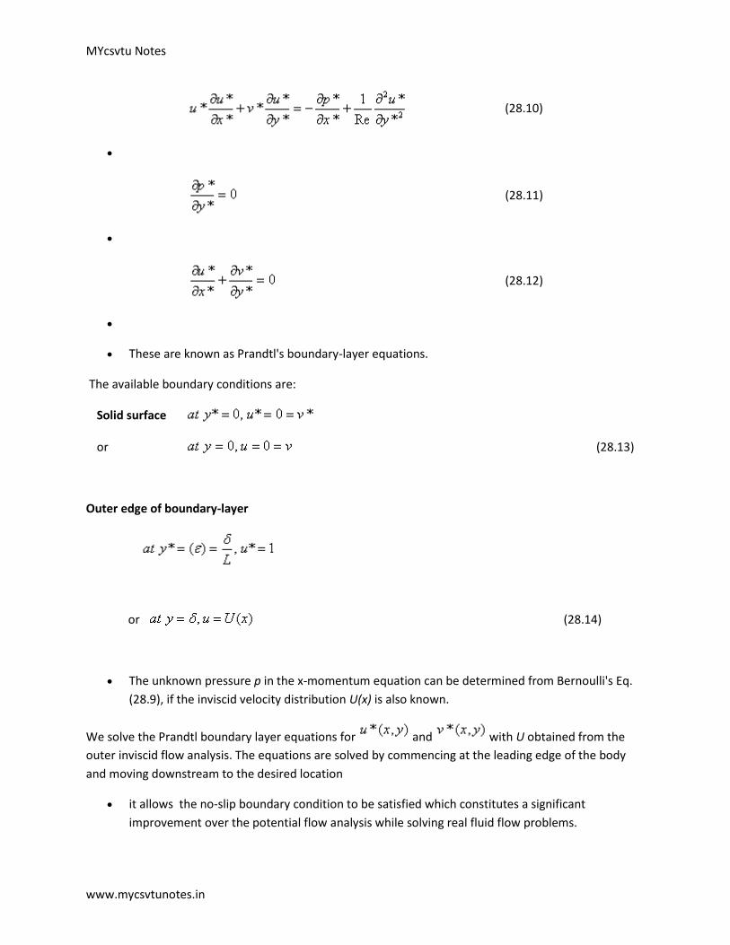
(28.10)

(28.11)

(28.12)

These are known as Prandtl's boundary-layer equations.

The available boundary conditions are:

Solid surface

or

(28.13)

Outer edge of boundary-layer

or

(28.14)

The unknown pressure p in the x-momentum equation can be determined from Bernoulli's Eq.

(28.9), if the inviscid velocity distribution U(x) is also known.

We solve the Prandtl boundary layer equations for and with U obtained from the

outer inviscid flow analysis. The equations are solved by commencing at the leading edge of the body

and moving downstream to the desired location

it allows the no-slip boundary condition to be satisfied which constitutes a significant

improvement over the potential flow analysis while solving real fluid flow problems.

MYcsvtu Notes

www.mycsvtunotes.in

The Prandtl boundary layer equations are thus a simplification of the Navier-Stokes equations.

Boundary Layer Coordinates

The boundary layer equations derived are in Cartesian coordinates.

The Velocity components u and v represent x and y direction velocities respectively.

For objects with small curvature, these equations can be used with -

x coordinate : streamwise direction

y coordinate : normal component

They are called Boundary Layer Coordinates.

Application of Boundary Layer Theory

The Boundary-Layer Theory is not valid beyond the point of separation.

At the point of separation, boundary layer thickness becomes quite large for the thin layer

approximation to be valid.

It is important to note that boundary layer theory can be used to locate the point of seperation

itself.

In applying the boundary layer theory although U is the free-stream velocity at the outer edge of

the boundary layer, it is interpreted as the fluid velocity at the wall calculated from inviscid flow

considerations ( known as Potential Wall Velocity)

Mathematically, application of the boundary - layer theory converts the character of governing

Navier-Stroke equations from elliptic to parabolic

This allows the marching in flow direction, as the solution at any location is independent of the

conditions farther downstream.

Blasius Flow Over A Flat Plate

The classical problem considered by H. Blasius was

1. Two-dimensional, steady, incompressible flow over a flat plate at zero angle of

incidence with respect to the uniform stream of velocity .

2. The fluid extends to infinity in all directions from the plate.

The physical problem is already illustrated in Fig. 28.1

MYcsvtu Notes

www.mycsvtunotes.in

Blasius wanted to determine

(a) the velocity field solely within the boundary layer,

(b) the boundary layer thickness ,

(c) the shear stress distribution on the plate, and

(d) the drag force on the plate.

The Prandtl boundary layer equations in the case under consideration are

(28.15)

The boundary conditions are

(28.16)

Note that the substitution of the term in the original boundary layer momentum

equation in terms of the free stream velocity produces which is equal to zero.

Hence the governing Eq. (28.15) does not contain any pressure-gradient term.

However, the characteristic parameters of this problem are that is,

This relation has five variables .

It involves two dimensions, length and time.

Thus it can be reduced to a dimensionless relation in terms of (5-2) =3 quantities ( Buckingham

Pi Theorem)

Thus a similarity variables can be used to find the solution

MYcsvtu Notes

www.mycsvtunotes.in

Such flow fields are called self-similar flow field .

Law of Similarity for Boundary Layer Flows

It states that the u component of velocity with two velocity profiles of u(x,y) at

different x locations differ only by scale factors in u and y .

Therefore, the velocity profiles u(x,y) at all values of x can be made congruent if they

are plotted in coordinates which have been made dimensionless with reference to

the scale factors.

The local free stream velocity U(x) at section x is an obvious scale factor for u,

because the dimensionless u(x) varies between zero and unity with y at all sections.

The scale factor for y , denoted by g(x) , is proportional to the local boundary layer

thickness so that y itself varies between zero and unity.

Velocity at two arbitrary x locations, namely x1 and x2 should satisfy the equation

(28.17)

Now, for Blasius flow, it is possible to identify g(x) with the boundary layers thickness

δ we know

Thus in terms of x we get

i.e.,

MYcsvtu Notes

www.mycsvtunotes.in

(28.18)

where

or more precisely,

(28.19)

The stream function can now be obtained in terms of the velocity components as

or

(28.20)

where D is a constant. Also and the constant of integration is zero if the

stream function at the solid surface is set equal to zero.

Now, the velocity components and their derivatives are:

(28.21a)

MYcsvtu Notes

www.mycsvtunotes.in

or

(28.21b)

(28.21c)

(28.21d)

(28.21e)

MYcsvtu Notes

www.mycsvtunotes.in

or,

where

(28.22)

and

This is known as Blasius Equation .

Contd. from Previous Slide

The boundary conditions as in Eg. (28.16), in combination with Eg. (28.21a) and

(28.21b) become

at , therefore

at therefore

(28.23)

Equation (28.22) is a third order nonlinear differential equation .

Blasius obtained the solution of this equation in the form of series expansion through

analytical techniques

We shall not discuss this technique. However, we shall discuss a numerical technique

to solve the aforesaid equation which can be understood rather easily.

Note that the equation for does not contain .

MYcsvtu Notes

www.mycsvtunotes.in

Boundary conditions at and merge into the condition

. This is the key feature of similarity solution.

We can rewrite Eq. (28.22) as three first order differential equations in the following

way

(28.24a)

(28.24b)

(28.24c)

Let us next consider the boundary conditions.

1. The condition remains valid.

2. The condition means that .

3. The condition gives us .

Note that the equations for f and G have initial values. However, the value for H(0) is not

known. Hence, we do not have a usual initial-value problem.

Shooting Technique

We handle this problem as an initial-value problem by choosing values of and solving

by numerical methods , and .

In general, the condition will not be satisfied for the function arising from the

numerical solution.

We then choose other initial values of so that eventually we find an which results in

.

This method is called the shooting technique .

In Eq. (28.24), the primes refer to differentiation wrt. the similarity variable . The

integration steps following Runge-Kutta method are given below.

(28.25a)

MYcsvtu Notes

www.mycsvtunotes.in

(28.25b)

(28.25c)

One moves from to . A fourth order accuracy is preserved if h is

constant along the integration path, that is, for all values of n . The

values of k, l and m are as follows.

For generality let the system of governing equations be

In a similar way K3, l3, m3 and k4, l4, m4 mare calculated following standard formulae for the

Runge-Kutta integration. For example, K3 is given by

The functions F1, F2and F3 are

G, H , - f H / 2 respectively. Then at a distance from the wall, we have

(28.26a)

MYcsvtu Notes

www.mycsvtunotes.in

(28.26b)

(28.26c)

(28.26d)

As it has been mentioned earlier is unknown. It must be

determined such that the condition is satisfied.

The condition at infinity is usually approximated at a finite value of (around ). The

process of obtaining accurately involves iteration and may be calculated using the

procedure described below.

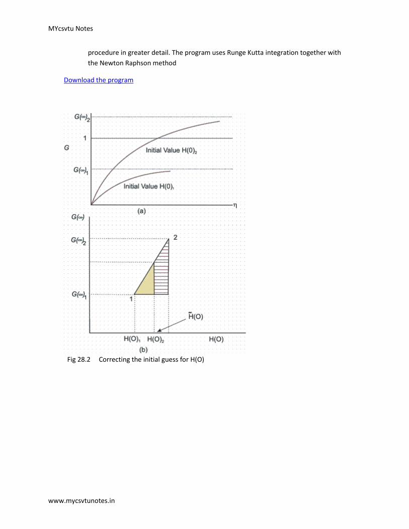
For this purpose, consider Fig. 28.2(a) where the solutions of versus for two

different values of are plotted.

The values of are estimated from the curves and are plotted in Fig. 28.2(b).

The value of now can be calculated by finding the value at which the line

1-2 crosses the line By using similar triangles, it can be said that

. By solving this, we get .

Next we repeat the same calculation as above by using and the better of the

two initial values of . Thus we get another improved value . This process

may continue, that is, we use and as a pair of values to find more

improved values for , and so forth. The better guess for H (0) can also be

obtained by using the Newton Raphson Method. It should be always kept in mind that

for each value of , the curve versus is to be examined to get the proper

value of .

The functions and are plotted in Fig. 28.3.The velocity

components, u and v inside the boundary layer can be computed from Eqs (28.21a)

and (28.21b) respectively.

A sample computer program in FORTRAN follows in order to explain the solution

MYcsvtu Notes

www.mycsvtunotes.in

procedure in greater detail. The program uses Runge Kutta integration together with

the Newton Raphson method

Download the program

Fig 28.2 Correcting the initial guess for H(O)

MYcsvtu Notes

www.mycsvtunotes.in

Fig 28.3 f, G and H distribution in the boundary layer

Measurements to test the accuracy of theoretical results were carried out by many

scientists. In his experiments, J. Nikuradse, found excellent agreement with the

theoretical results with respect to velocity distribution within the boundary

layer of a stream of air on a flat plate.

In the next slide we'll see some values of the velocity profile shape

and in tabular format.

Values of the velocity profile shape

Table 28.1 The Blasius Velocity Profile

0 0 0 0.33206

0.2 0.00664 0.006641 0.33199

MYcsvtu Notes

www.mycsvtunotes.in

0.4 0.02656 0.13277 0.33147

0.8 0.10611 0.26471 0.32739

1.2 0.23795 0.39378 0.31659

1.6 0.42032 0.51676 0.29667

2.0 0.65003 0.62977 0.26675

2.4 0.92230 0.72899 0.22809

2.8 1.23099 0.81152 0.18401

3.2 1.56911 0.87609 0.13913

3.6 1.92954 0.92333 0.09809

4.0 2.30576 0.95552 0.06424

4.4 2.69238 0.97587 0.03897

4.8 3.08534 0.98779 0.02187

5.0 3.28329 0.99155 0.01591

8.8 7.07923 1.00000 0.00000

Wall Shear Stress

With the profile known, wall shear can be evaluated as

MYcsvtu Notes

www.mycsvtunotes.in

Now,

or

or

from Table 28.1

(Wall Shear Stress)

(29.1a)

and the local skin friction coefficient is

Substituting from (29.1a) we get

(Skin Friction Coefficient)

(29.1b)

In 1951, Liepmann and Dhawan , measured the shearing stress on a flat plate directly.

Their results showed a striking confirmation of Eq. (29.1).

Total frictional force per unit width for the plate of length L is

MYcsvtu Notes

www.mycsvtunotes.in

or

or

(29.2)

and the average skin friction coefficient is

(29.3)

where, .

For a flat plate of length L in the streamwise direction and width w perpendicular to the flow,

the Drag D would be

(29.4)

Boundary Layer Thickness

Since , it is customary to select the boundary layer thickness as

that point where approaches 0.99.

From Table 28.1, reaches 0.99 at η= 5.0 and we can write

(29.5)

MYcsvtu Notes

www.mycsvtunotes.in

However, the aforesaid definition of boundary layer thickness is somewhat arbitrary, a

physically more meaningful measure of boundary layer estimation is expressed through

displacement thickness .

Fig. 29.1 (Displacement thickness) (b) Momentum thickness

Displacement thickness : It is defined as the distance by which the external potential flow

is displaced outwards due to the decrease in velocity in the boundary layer.

Therefore,

(29.6)

Substituting the values of and from Eqs (28.21a) and (28.19) into Eq.(29.6), we obtain

or,

(29.7)

MYcsvtu Notes

www.mycsvtunotes.in

Following the analogy of the displacement thickness, a momentum thickness may be defined.

Momentum thickness ( ): It is defined as the loss of momentum in the boundary layer as compared

with that of potential flow. Thus

(29.8)

With the substitution of and from Eg. (28.21a) and (28.19), we can evaluate numerically the

value of for a flat plate as

(29.9)

The relationships between have been shown in Fig. 29.1.

Momentum-Integral Equations For The Boundary Layer

To employ boundary layer concepts in real engineering designs, we need approximate methods

that would quickly lead to an answer even if the accuracy is somewhat less.

Karman and Pohlhausen devised a simplified method by satisfying only the boundary

conditions of the boundary layer flow rather than satisfying Prandtl's differential equations for

each and every particle within the boundary layer. We shall discuss this method herein.

Consider the case of steady, two-dimensional and incompressible flow, i.e. we shall refer to Eqs

(28.10) to (28.14). Upon integrating the dimensional form of Eq. (28.10) with respect to y = 0

(wall) to y = δ (where δ signifies the interface of the free stream and the boundary layer), we

obtain

MYcsvtu Notes

www.mycsvtunotes.in

or,

(29.10)

The second term of the left hand side can be expanded as

or, by continuity equation

or,

(29.11)

Substituting Eq. (29.11) in Eq. (29.10) we obtain

(29.12)

Substituting the relation between and the free stream velocity for the inviscid zone in

Eq. (29.12) we get

MYcsvtu Notes

www.mycsvtunotes.in

which is reduced to

Since the integrals vanish outside the boundary layer, we are allowed to increase the integration

limit to infinity (i.e . )

or,

(29.13)

Substituting Eq. (29.6) and (29.7) in Eq. (29.13) we obtain

(29.14)

where is the displacement thickness

is momentum thickness

Equation (29.14) is known as momentum integral equation for two dimensional incompressible

laminar boundary layer. The same remains valid for turbulent boundary layers as well.

Needless to say, the wall shear stress will be different for laminar and turbulent flows.

The term signifies space-wise acceleration of the free stream. Existence of this term

means that free stream pressure gradient is present in the flow direction.

MYcsvtu Notes

www.mycsvtunotes.in

For example, we get finite value of outside the boundary layer in the entrance region

of a pipe or a channel. For external flows, the existence of depends on the shape of

the body.

During the flow over a flat plate, and the momentum integral equation is reduced

to

(29.15)

Seperation of Boundary Layer

It has been observed that the flow is reversed at the vicinity of the wall under certain

conditions.

The phenomenon is termed as separation of boundary layer.

Separation takes place due to excessive momentum loss near the wall in a boundary layer

trying to move downstream against increasing pressure, i.e., , which is called adverse

pressure gradient.

Figure 29.2 shows the flow past a circular cylinder, in an infinite medium.

1. Up to , the flow area is like a constricted passage and the flow behaviour is like

that of a nozzle.

2. Beyond the flow area is diverged, therefore, the flow behaviour is much similar

to a diffuser

This dictates the inviscid pressure distribution on the cylinder which is shown by a firm line in Fig. 29.2.

Here

: pressure in the free stream

: velocity in the free stream and

: is the local pressure on the cylinder.

MYcsvtu Notes

www.mycsvtunotes.in

Fig. 29.2 Flow separation and formation of wake behind a circular cylinder

Consider the forces in the flow field.

In the inviscid region,

1. Until the pressure force and the force due to streamwise acceleration i.e.

inertia forces are acting in the same direction (pressure gradient being

negative/favourable)

2. Beyond , the pressure gradient is positive or adverse. Due to the adverse

pressure gradient the pressure force and the force due to acceleration will be opposing

each other in the in viscid zone of this part.

So long as no viscous effect is considered, the situation does not cause any sensation.

In the viscid region (near the solid boundary),

MYcsvtu Notes

www.mycsvtunotes.in

1. Up to , the viscous force opposes the combined pressure force and the force

due to acceleration. Fluid particles overcome this viscous resistance due to continuous

conversion of pressure force into kinetic energy.

2. Beyond , within the viscous zone, the flow structure becomes different. It is

seen that the force due to acceleration is opposed by both the viscous force and

pressure force.

Depending upon the magnitude of adverse pressure gradient, somewhere around , the

fluid particles, in the boundary layer are separated from the wall and driven in the upstream

direction. However, the far field external stream pushes back these separated layers together

with it and develops a broad pulsating wake behind the cylinder.

The mathematical explanation of flow-separation : The point of separation may be defined as

the limit between forward and reverse flow in the layer very close to the wall, i.e., at the point

of separation

(29.16)

This means that the shear stress at the wall, . But at this point, the adverse pressure continues to

exist and at the downstream of this point the flow acts in a reverse direction resulting in a back flow.

We can also explain flow separation using the argument about the second derivative of velocity

u at the wall. From the dimensional form of the momentum at the wall, where u = v = 0, we can

write

(29.17)

Consider the situation due to a favourable pressure gradient where we have,

1. . (From Eq. (29.17))

2. As we proceed towards the free stream, the velocity u approaches asymptotically,

so decreases at a continuously lesser rate in y direction.

MYcsvtu Notes

www.mycsvtunotes.in

3. This means that remains less than zero near the edge of the boundary layer.

4. The curvature of a velocity profile is always negative as shown in (Fig. 29.3a)

Consider the case of adverse pressure gradient,

1. At the boundary, the curvature of the profile must be positive (since ).

2. Near the interface of boundary layer and free stream the previous argument regarding

and still holds good and the curvature is negative.

3. Thus we observe that for an adverse pressure gradient, there must exist a point for

which . This point is known as point of inflection of the velocity profile in

the boundary layer as shown in Fig. 29.3b

4. However, point of separation means at the wall.

5. at the wall since separation can only occur due to adverse pressure

gradient. But we have already seen that at the edge of the boundary layer,

. It is therefore, clear that if there is a point of separation, there must

exist a point of inflection in the velocity profile.

MYcsvtu Notes

www.mycsvtunotes.in

Fig. 29.3 Velocity distribution within a boundary layer

(a) Favourable pressure gradient,

(b) adverse pressure gradient,

1. Let us reconsider the flow past a circular cylinder and continue our discussion on the wake

behind a cylinder. The pressure distribution which was shown by the firm line in Fig. 21.5 is

obtained from the potential flow theory. However. somewhere near (in experiments it

has been observed to be at ) . the boundary layer detaches itself from the wall.

2. Meanwhile, pressure in the wake remains close to separation-point-pressure since the eddies

(formed as a consequence of the retarded layers being carried together with the upper layer

through the action of shear) cannot convert rotational kinetic energy into pressure head. The

actual pressure distribution is shown by the dotted line in Fig. 29.3.

MYcsvtu Notes

www.mycsvtunotes.in

3. Since the wake zone pressure is less than that of the forward stagnation point (pressure at

point A in Fig. 29.3), the cylinder experiences a drag force which is basically attributed to the

pressure difference.

The drag force, brought about by the pressure difference is known as form drag whereas the shear

stress at the wall gives rise to skin friction drag. Generally, these two drag forces together are

responsible for resultant drag on a body

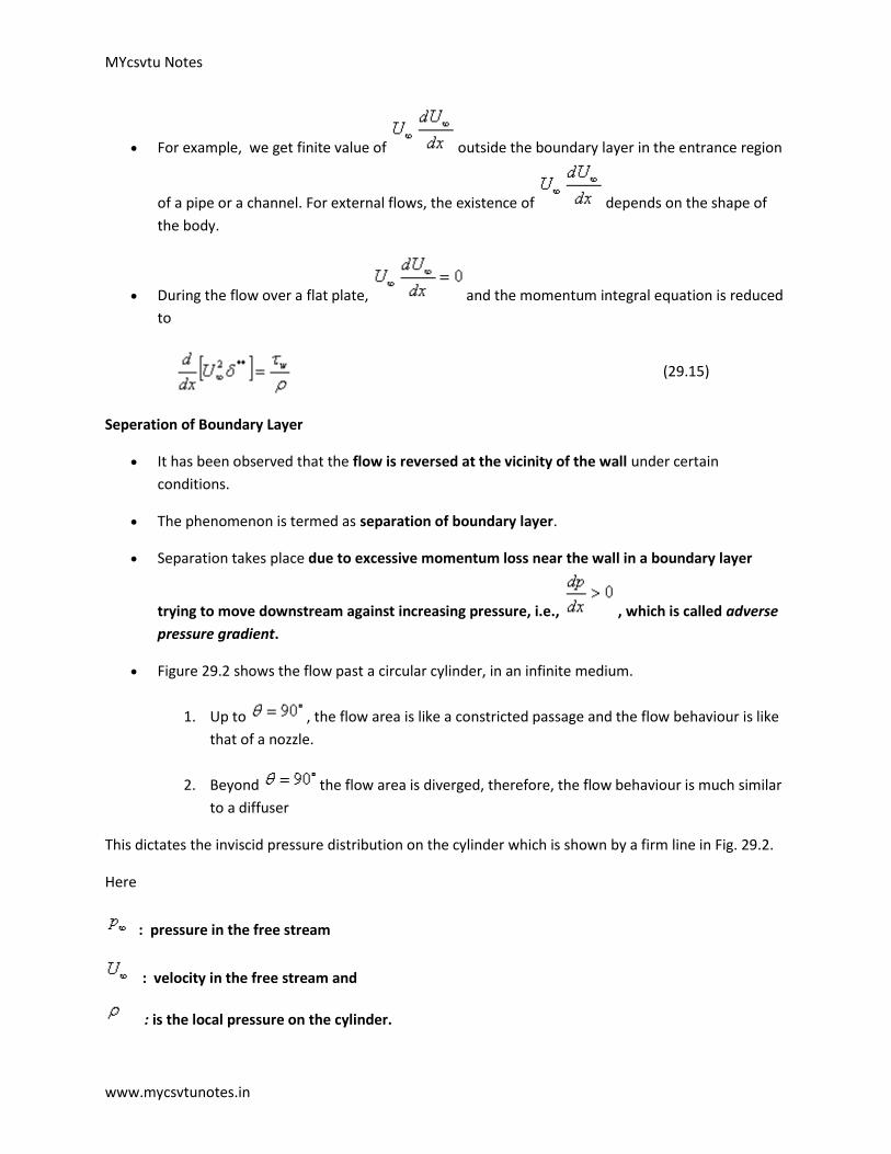
Seperation of Boundary Layer

It has been observed that the flow is reversed at the vicinity of the wall under certain

conditions.

The phenomenon is termed as separation of boundary layer.

Separation takes place due to excessive momentum loss near the wall in a boundary layer

trying to move downstream against increasing pressure, i.e., , which is called adverse

pressure gradient.

Figure 29.2 shows the flow past a circular cylinder, in an infinite medium.

1. Up to , the flow area is like a constricted passage and the flow behaviour is like

that of a nozzle.

2. Beyond the flow area is diverged, therefore, the flow behaviour is much similar

to a diffuser

This dictates the inviscid pressure distribution on the cylinder which is shown by a firm line in Fig. 29.2.

Here

: pressure in the free stream

: velocity in the free stream and

: is the local pressure on the cylinder.

MYcsvtu Notes

www.mycsvtunotes.in

Fig. 29.2 Flow separation and formation of wake behind a circular cylinder

Consider the forces in the flow field.

In the inviscid region,

1. Until the pressure force and the force due to streamwise acceleration i.e.

inertia forces are acting in the same direction (pressure gradient being

negative/favourable)

2. Beyond , the pressure gradient is positive or adverse. Due to the adverse

pressure gradient the pressure force and the force due to acceleration will be opposing

each other in the in viscid zone of this part.

So long as no viscous effect is considered, the situation does not cause any sensation.

In the viscid region (near the solid boundary),

MYcsvtu Notes

www.mycsvtunotes.in

1. Up to , the viscous force opposes the combined pressure force and the force

due to acceleration. Fluid particles overcome this viscous resistance due to continuous

conversion of pressure force into kinetic energy.

2. Beyond , within the viscous zone, the flow structure becomes different. It is

seen that the force due to acceleration is opposed by both the viscous force and

pressure force.

Depending upon the magnitude of adverse pressure gradient, somewhere around , the

fluid particles, in the boundary layer are separated from the wall and driven in the upstream

direction. However, the far field external stream pushes back these separated layers together

with it and develops a broad pulsating wake behind the cylinder.

The mathematical explanation of flow-separation : The point of separation may be defined as

the limit between forward and reverse flow in the layer very close to the wall, i.e., at the point

of separation

(29.16)

This means that the shear stress at the wall, . But at this point, the adverse pressure continues to

exist and at the downstream of this point the flow acts in a reverse direction resulting in a back flow.

We can also explain flow separation using the argument about the second derivative of velocity

u at the wall. From the dimensional form of the momentum at the wall, where u = v = 0, we can

write

(29.17)

Consider the situation due to a favourable pressure gradient where we have,

1. . (From Eq. (29.17))

2. As we proceed towards the free stream, the velocity u approaches asymptotically,

so decreases at a continuously lesser rate in y direction.

MYcsvtu Notes

www.mycsvtunotes.in

3. This means that remains less than zero near the edge of the boundary layer.

4. The curvature of a velocity profile is always negative as shown in (Fig. 29.3a)

Consider the case of adverse pressure gradient,

1. At the boundary, the curvature of the profile must be positive (since ).

2. Near the interface of boundary layer and free stream the previous argument regarding

and still holds good and the curvature is negative.

3. Thus we observe that for an adverse pressure gradient, there must exist a point for

which . This point is known as point of inflection of the velocity profile in

the boundary layer as shown in Fig. 29.3b

4. However, point of separation means at the wall.

5. at the wall since separation can only occur due to adverse pressure

gradient. But we have already seen that at the edge of the boundary layer,

. It is therefore, clear that if there is a point of separation, there must

exist a point of inflection in the velocity profile.

MYcsvtu Notes

www.mycsvtunotes.in

Fig. 29.3 Velocity distribution within a boundary layer

(a) Favourable pressure gradient,

(b) adverse pressure gradient,

1. Let us reconsider the flow past a circular cylinder and continue our discussion on the wake

behind a cylinder. The pressure distribution which was shown by the firm line in Fig. 21.5 is

obtained from the potential flow theory. However. somewhere near (in experiments it

has been observed to be at ) . the boundary layer detaches itself from the wall.

2. Meanwhile, pressure in the wake remains close to separation-point-pressure since the eddies

(formed as a consequence of the retarded layers being carried together with the upper layer

through the action of shear) cannot convert rotational kinetic energy into pressure head. The

actual pressure distribution is shown by the dotted line in Fig. 29.3.

MYcsvtu Notes

www.mycsvtunotes.in

3. Since the wake zone pressure is less than that of the forward stagnation point (pressure at

point A in Fig. 29.3), the cylinder experiences a drag force which is basically attributed to the

pressure difference.

The drag force, brought about by the pressure difference is known as form drag whereas the shear

stress at the wall gives rise to skin friction drag. Generally, these two drag forces together are

responsible for resultant drag on a body

Karman-Pohlhausen Approximate Method For Solution Of Momentum Integral Equation Over A Flat

Plate

The basic equation for this method is obtained by integrating the x direction momentum

equation (boundary layer momentum equation) with respect to y from the wall (at y = 0) to a

distance which is assumed to be outside the boundary layer. Using this notation, we can

rewrite the Karman momentum integral equation as

(30.1)

The effect of pressure gradient is described by the second term on the left hand side. For

pressure gradient surfaces in external flow or for the developing sections in internal flow, this

term contributes to the pressure gradient.

We assume a velocity profile which is a polynomial of . being a form of similarity

variable , implies that with the growth of boundary layer as distance x varies from the leading

edge, the velocity profile remains geometrically similar.

We choose a velocity profile in the form

(30.2)

In order to determine the constants we shall prescribe the following

boundary conditions

(30.3a)

(30.3b)

at

MYcsvtu Notes

www.mycsvtunotes.in

(30.3c)

at

(30.3d)

These requirements will yield respectively

Finally, we obtain the following values for the coefficients in Eq. (30.2),

and the velocity profile becomes

(30.4)

For flow over a flat plate, and the governing Eq. (30.1) reduces

to

(30.5)

Again from Eq. (29.8), the momentum thickness is

MYcsvtu Notes

www.mycsvtunotes.in

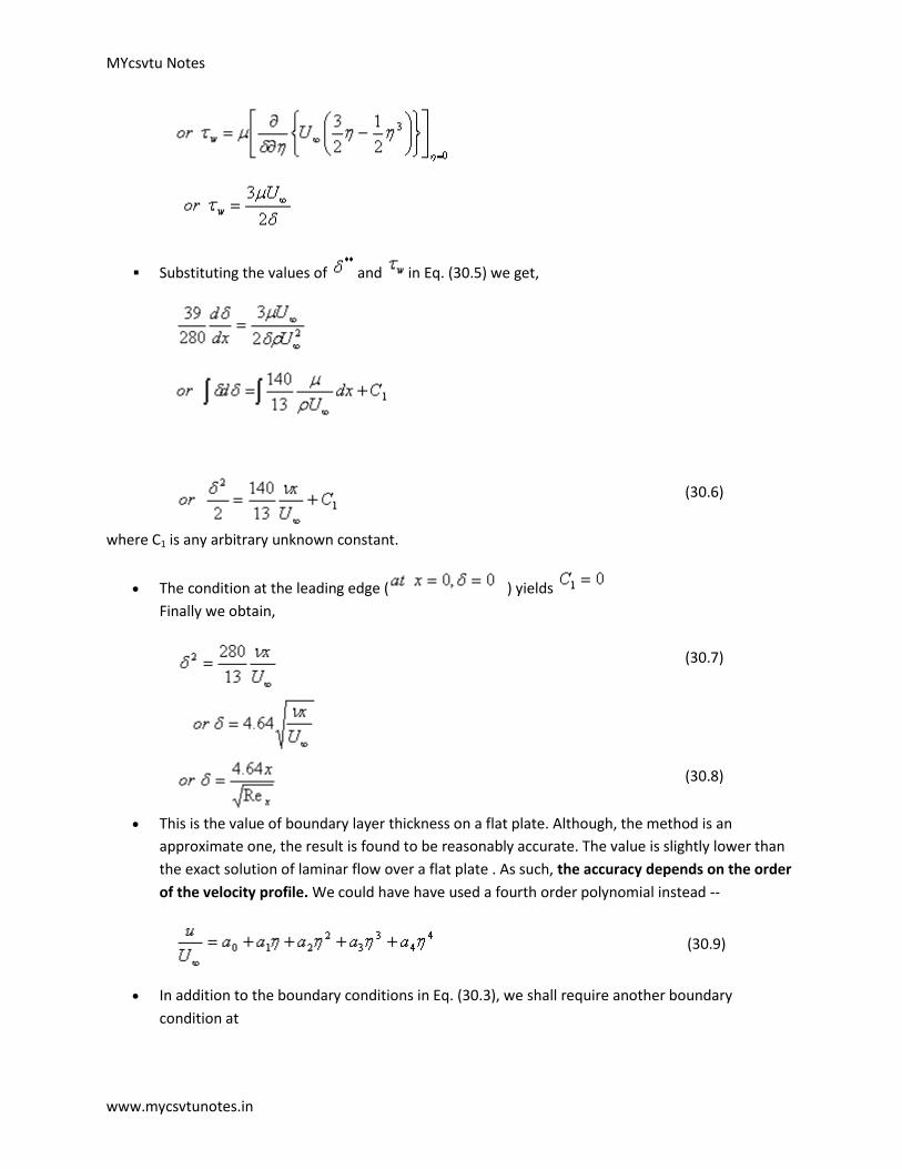
Substituting the values of and in Eq. (30.5) we get,

(30.6)

where C1 is any arbitrary unknown constant.

The condition at the leading edge ( ) yields

Finally we obtain,

(30.7)

(30.8)

This is the value of boundary layer thickness on a flat plate. Although, the method is an

approximate one, the result is found to be reasonably accurate. The value is slightly lower than

the exact solution of laminar flow over a flat plate . As such, the accuracy depends on the order

of the velocity profile. We could have have used a fourth order polynomial instead --

(30.9)

In addition to the boundary conditions in Eq. (30.3), we shall require another boundary

condition at

MYcsvtu Notes

www.mycsvtunotes.in

This yields the constants as . Finally the velocity profile will

be

Subsequently, for a fourth order profile the growth of boundary layer is given by

(30.10)

Integral Method For Non-Zero Pressure Gradient Flows

A wide variety of "integral methods" in this category have been discussed by Rosenhead . The

Thwaites method is found to be a very elegant method, which is an extension of the method

due to Holstein and Bohlen . We shall discuss the Holstein-Bohlen method in this section.

This is an approximate method for solving boundary layer equations for two-dimensional

generalized flow. The integrated Eq. (29.14) for laminar flow with pressure gradient can be

written as

or

(30.11)

The velocity profile at the boundary layer is considered to be a fourth-order polynomial in

terms of the dimensionless distance , and is expressed as

The boundary conditions are

MYcsvtu Notes

www.mycsvtunotes.in

A dimensionless quantity, known as shape factor is introduced as

(30.12)

The following relations are obtained

Now, the velocity profile can be expressed as

(30.13)

where

The shear stress is given by

(30.14)

We use the following dimensionless parameters,

(30.15)

(30.16)

(30.17)

The integrated momentum Eq. (30.10) reduces to

MYcsvtu Notes

www.mycsvtunotes.in

(30.18)

The parameter L is related to the skin friction

The parameter K is linked to the pressure gradient.

If we take K as the independent variable . L and H can be shown to be the functions of K since

(30.19)

(30.20)

(30.21)

Therefore,

The right-hand side of Eq. (30.18) is thus a function of K alone. Walz pointed out that this

function can be approximated with a good degree of accuracy by a linear function of K so that

[Walz's approximation]

Equation (30.18) can now be written as

Solution of this differential equation for the dependent variable subject to the boundary

condition U = 0 when x = 0 , gives

MYcsvtu Notes

www.mycsvtunotes.in

With a = 0.47 and b = 6. the approximation is particularly close between the stagnation point

and the point of maximum velocity.

Finally the value of the dependent variable is

(30.22)

By taking the limit of Eq. (30.22), according to L'Hopital's rule, it can be shown that

This corresponds to K = 0.0783.

Note that is not equal to zero at the stagnation point. If is determined from Eq.

(30.22), K(x) can be obtained from Eq. (30.16).

Table 30.1 gives the necessary parameters for obtaining results, such as velocity profile and

shear stress The approximate method can be applied successfully to a wide range of

problems.

Table 30.1 Auxiliary functions after Holstein and Bohlen

K

12 0.0948 2.250 0.356

10 0.0919 2.260 0.351

8 0.0831 2.289 0.340

7.6 0.0807 2.297 0.337

7.2 0.0781 2.305 0.333

7.0 0.0767 2.309 0.331

6.6 0.0737 2.318 0.328

MYcsvtu Notes

www.mycsvtunotes.in

6.2 0.0706 2.328 0.324

5.0 0.0599 2.361 0.310

3.0 0.0385 2.427 0.283

1.0 0.0135 2.508 0.252

0 0 2.554 0.235

-1 -0.0140 2.604 0.217

-3 -0.0429 2.716 0.179

-5 -0.0720 2.847 0.140

-7 -0.0999 2.999 0.100

-9 -0.1254 3.176 0.059

-11 -0.1474 3.383 0.019

-12 -0.1567 3.500 0

0 0 0 0

0.2 0.00664 0.006641 0.006641

0.4 0.02656 0.13277 0.13277

0.8 0.10611 0.26471 0.26471

1.2 0.23795 0.39378 0.39378

1.6 0.42032 0.51676 0.51676

MYcsvtu Notes

www.mycsvtunotes.in

2.0 0.65003 0.62977 0.62977

2.4 0.92230 0.72899 0.72899

2.8 1.23099 0.81152 0.81152

3.2 1.56911 0.87609 0.87609

3.6 1.92954 0.92333 0.92333

4.0 2.30576 0.95552 0.95552

4.4 2.69238 0.97587 0.97587

4.8 3.08534 0.98779 0.98779

5.0 3.28329 0.99155 0.99155

8.8 7.07923 1.00000 1.00000

As mentioned earlier, K and are related to the pressure gradient and the shape factor.

Introduction of K and in the integral analysis enables extension of Karman-Pohlhausen

method for solving flows over curved geometry. However, the analysis is not valid for the

geometries, where and

Point of Seperation

For point of seperation,

or,

or,

Entry Flow In A Duct -

MYcsvtu Notes

www.mycsvtunotes.in

Growth of boundary layer has a remarkable influence on flow through a constant area duct or

pipe.

Consider a flow entering a pipe with uniform velocity.

1. The boundary layer starts growing on the wall at the entrance of the pipe.

2. Gradually it becomes thicker in the downstream.

3. The flow becomes fully developed when the boundary layers from the wall meet at the

axis of the pipe.

The velocity profile is nearly rectangular at the entrance and it gradually changes to a parabolic

profile at the fully developed region.

Before the boundary layers from the periphery meet at the axis, there prevails a core region

which is uninfluenced by viscosity.

Since the volume-flow must be same for every section and the boundary-layer thickness

increases in the flow direction, the inviscid core accelerates, and there is a corresponding fall in

pressure.

Entrance length : It can be shown that for laminar incompressible flows, the velocity profile

approaches the parabolic profile through a distance Le from the entry of the pipe. This is known

as entrance length and is given by

For a Reynolds number of 2000, this distance, the entrance length is about 100 pipe-diameters. For

turbulent flows, the entrance region is shorter, since the turbulent boundary layer grows faster.

At the entrance region,

1. The velocity gradient is steeper at the wall, causing a higher value of shear stress as compared

to a developed flow.

2. Momentum flux across any section is higher than that typically at the inlet due to the change in

shape of the velocity profile.

3. Arising out of these, an additional pressure drop is brought about at the entrance region as

compared to the pressure drop in the fully developed region.

MYcsvtu Notes

www.mycsvtunotes.in

Fig. 31.1 Development of boundary layer in the entrance region of a duct

Control Of Boundary Layer Separation -

The total drag on a body is attributed to form drag and skin friction drag. In some flow

configurations, the contribution of form drag becomes significant.

In order to reduce the form drag, the boundary layer separation should be prevented or

delayed so that better pressure recovery takes place and the form drag is reduced

considerably. There are some popular methods for this purpose which are stated as follows.

i. By giving the profile of the body a streamlined shape( as shown in Fig. 31.2).

1. This has an elongated shape in the rear part to reduce the magnitude of the

pressure gradient.

2. The optimum contour for a streamlined body is the one for which the wake

zone is very narrow and the form drag is minimum.

Fig. 31.2 Reduction of drag coefficient (CD) by giving the profile a streamlined shape

ii. The injection of fluid through porous wall can also control the boundary layer

separation. This is generally accomplished by blowing high energy fluid particles

MYcsvtu Notes

www.mycsvtunotes.in

tangentially from the location where separation would have taken place otherwise. This

is shown in Fig. 31.3.

1. The injection of fluid promotes turbulence

2. This increases skin friction. But the form drag is reduced considerably due to

suppression of flow separation

3. The reduction in form drag is quite significant and increase in skin friction drag

can be ignored.

Fig. 31.3 Boundary layer control by blowing

Mechanisms of Boundary Layer Transition

One of the interesting problems in fluid mechanics is the physical mechanism of transition from

laminar to turbulent flow. The problem evolves about the generation of both steady and

unsteady vorticity near a body, its subsequent molecular diffusion, its kinematic and dynamic

convection and redistribution downstream, and the resulting feedback on the velocity and

pressure fields near the body. We can perhaps realise the complexity of the transition problem

by examining the behaviour of a real flow past a cylinder.

Figure 31.4 (a) shows the flow past a cylinder for a very low Reynolds number . The flow

smoothly divides and reunites around the cylinder.

At a Reynolds number of about 4, the flow (boundary layer) separates in the downstream and

the wake is formed by two symmetric eddies . The eddies remain steady and symmetrical but

grow in size up to a Reynolds number of about 40 as shown in Fig. 31.4(b).

At a Reynolds number above 40 , oscillation in the wake induces asymmetry and finally the

wake starts shedding vortices into the stream. This situation is termed as onset of periodicity as

shown in Fig. 31.4(c) and the wake keeps on undulating up to a Reynolds number of 90 .

MYcsvtu Notes

www.mycsvtunotes.in

At a Reynolds number above 90 , the eddies are shed alternately from a top and bottom of the

cylinder and the regular pattern of alternately shed clockwise and counterclockwise vortices

form Von Karman vortex street as in Fig. 31.4(d).

Periodicity is eventually induced in the flow field with the vortex-shedding phenomenon.

The periodicity is characterised by the frequency of vortex shedding

In non-dimensional form, the vortex shedding frequency is expressed as known as

the Strouhal number named after V. Strouhal, a German physicist who experimented with wires

singing in the wind. The Strouhal number shows a slight but continuous variation with Reynolds

number around a value of 0.21. The boundary layer on the cylinder surface remains laminar and

separation takes placeat about 810 from the forward stagnation point.

At about Re = 500 , multiple frequencies start showing up and the wake tends to become

Chaotic.

As the Reynolds number becomes higher, the boundary layer around the cylinder tends to

become turbulent. The wake, of course, shows fully turbulent characters (Fig31.4 (e)).

For larger Reynolds numbers, the boundary layer becomes turbulent. A turbulent boundary

layer offers greater resistance to seperation than a laminar boundary layer. As a consequence

the seperation point moves downstream and the seperation angle is delayed to 1100 from the

forward stagnation point (Fig 31.4 (f) ).

MYcsvtu Notes

www.mycsvtunotes.in

Fig. 31.4 Influence of Reynolds number on wake-zone aerodynamics

Experimental flow visualizations past a circular cylinder are shown in Figure 31.5 (a) and (b)

MYcsvtu Notes

www.mycsvtunotes.in

Fig 31.5 (a) Flow Past a Cylinder at Re=2000 [Photograph courtesy Werle and Gallon (ONERA)]

Fig 31.5 (b) Flow Past a Cylinder at Re=10000 [Photograph courtesy Thomas Corke and Hasan Najib

(Illinois Institute of Technology, Chicago)]

A very interesting sequence of events begins to develop when the Reynolds number is increased

beyond 40, at which point the wake behind the cylinder becomes unstable. Photographs show

that the wake develops a slow oscillation in which the velocity is periodic in time and

downstream distance. The amplitude of the oscillation increases downstream. The oscillating

wake rolls up into two staggered rows of vortices with opposite sense of rotation.

Karman investigated the phenomenon and concluded that a nonstaggered row of vortices is

unstable, and a staggered row is stable only if the ratio of lateral distance between the vortices

MYcsvtu Notes

www.mycsvtunotes.in

to their longitudinal distance is 0.28. Because of the similarity of the wake with footprints in a

street, the staggered row of vortices behind a blue body is called a Karman Vortex Street . The

vortices move downstream at a speed smaller than the upstream velocity U.

In the range 40 < Re < 80, the vortex street does not interact with the pair of attached vortices.

As Re is increased beyond 80 the vortex street forms closer to the cylinder, and the attached

eddies themselves begin to oscillate. Finally the attached eddies periodically break off

alternately from the two sides of the cylinder.

While an eddy on one side is shed, that on the other side forms, resulting in an unsteady flow

near the cylinder. As vortices of opposite circulations are shed off alternately from the two

sides, the circulation around the cylinder changes sign, resulting in an oscillating "lift" or lateral

force. If the frequency of vortex shedding is close to the natural frequency of some mode of

vibration of the cylinder body, then an appreciable lateral vibration culminates.

Numerical flow visualizations for the flow past a circular cylinder can be observed in Fig 31.6 and

31.7

Fig 31.6 Numerical flow visualization (LES results) for a low reynolds number flow past a Circular Cylinder

[Animation by Dr.-Ing M. Breuer, LSTM, Univ Erlangen-Nuremberg ]

MYcsvtu Notes

www.mycsvtunotes.in

Fig 31.7 Numerical flow visualization (LES results) for a moderately high reynolds number flow past a

Circular Cylinder

[Animation by Dr.-Ing M. Breuer, LSTM, Univ Erlangen-Nuremberg ]

An understanding of the transitional flow processes will help in practical problems either by

improving procedures for predicting positions or for determining methods of advancing or

retarding the transition position.

The critical value at which the transition occurs in pipe flow is . The actual value

depends upon the disturbance in flow. Some experiments have shown the critical Reynolds

number to reach as high as 10,000. The precise upper bound is not known, but the lower bound

appears to be . Below this value, the flow remains laminar even when subjected

to strong disturbances.

In the case of flow through a channel, , the flow alternates randomly

between laminar and partially turbulent. Near the centerline, the flow is more laminar than

turbulent, whereas near the wall, the flow is more turbulent than laminar. For flow over a flat

plate, turbulent regime is observed between Reynolds numbers of 3.5 × 105 and 106.

Several Events Of Transition -

Transitional flow consists of several events as shown in Fig. 31.8. Let us consider the events one after

another.

1. Region of instability of small wavy disturbances-

MYcsvtu Notes

www.mycsvtunotes.in

Consider a laminar flow over a flat plate aligned with the flow direction (Fig. 31.8).

In the presence of an adverse pressure gradient, at a high Reynolds number (water velocity

approximately 9-cm/sec), two-dimensional waves appear.

These waves are called Tollmien-Schlichting wave( In 1929, Tollmien and Schlichting predicted

that the waves would form and grow in the boundary layer).

These waves can be made visible by a method known as tellurium method.

2. Three-dimensional waves and vortex formation-

Disturbances in the free stream or oscillations in the upstream boundary layer can generate

wave growth, which has a variation in the span wise direction.

This leads an initially two-dimensional wave to a three-dimensional form.

In many such transitional flows, periodicity is observed in the span wise direction.

This is accompanied by the appearance of vortices whose axes lie in the direction of flow.

3. Peak-Valley development with streamwise vortices-

As the three-dimensional wave propagates downstream, the boundary layer flow develops into

a complex stream wise vortex system.

Within this vortex system, at some spanwise location, the velocities fluctuate violently .

These locations are called peaks and the neighbouring locations of the peaks are valleys (Fig.

31.9).

4. Vorticity concentration and shear layer development-

At the spanwise locations corresponding to the peak, the instantaneous streamwise velocity profiles

demonstrate the following

Often, an inflexion is observed on the velocity profile.

The inflectional profile appears and disappears once after each cycle of the basic wave.

5. Breakdown-

The instantaneous velocity profiles produce high shear in the outer region of the boundary layer.

The velocity fluctuations develop from the shear layer at a higher frequency than that of the

basic wave.

MYcsvtu Notes

www.mycsvtunotes.in

These velocity fluctuations have a strong ability to amplify any slight three-dimensionality,

which is already present in the flow field.

As a result, a staggered vortex pattern evolves with the streamwise wavelength twice the

wavelength of Tollmien-Schlichting wavelength .

The span wise wavelength of these structures is about one-half of the stream wise value.

The high frequency fluctuations are referred as hairpin eddies.

This is known as breakdown.

6. Turbulent-spot development-

The hairpin-eddies travel at a speed grater than that of the basic (primary) waves.

As they travel downstream, eddies spread in the spanwise direction and towards the wall.

The vortices begin a cascading breakdown into smaller vortices.

In such a fluctuating state, intense local changes occur at random locations in the shear layer

near the wall in the form of turbulent spots.

Each spot grows almost linearly with the downstream distance.

The creation of spots is considered as the main event of transition .

Fig. 31.8 Sequence of event involved in transition

Fig. 31.9 Cross-stream view of the streamwise vortex system

MYcsvtu Notes

www.mycsvtunotes.in

Exercise Problems - Chapter 9

1.Two students are asked to solve the Blasius flow over a flat plate to determine the variation of

boundary layer thickness as a function of the Reynolds number. One student solves the problem by

similarity method and arrives at the result . The other student chooses to solve the problem

by using the momentum-integer equation and Karman-Pohlhausen method and funds that .

Which of the two results is expected to be closer to the experimental results and why?

2. A scientist claims that a highly viscous flow around a body can generate the same flow patterns as the

flow of an inviscid and incompressible fluid around that body. According to our understanding, the

Reynolds number for the first flow is very small, while the Reynolds number for the second flow can be

taken to be (infinity). Do you think it is possible to get the same flow patterns for the two extreme

values of Reynolds number? Please use mathematical analysis to prove or disprove the scientist's claim.

3. In boundary layer theory, a boundary layer can be characterized by any of the following quantities (i)

Boundary layer thickness (ii) Displacement thickness (iii) Momentum thickness.

How do these quantities differ in their physical as well as mathematical definitions? For the flow over a

flat plate, which of these is expected to have the highest value at a given location on the wall, and which

the lowest?

4. What do you mean by the "point of separation" of a boundary layer? How will the velocity gradient

and the second gradient .Vary within the boundary layer at the point of separation? Please

show the variation graphically. Here u is the velocity along the wall and y is the co-ordinate

perpendicular to the wall.

5. Reduce the Prandtl's boundary layer equations to a simpler form than that given by equations (28.10)

- (28.12) for -

(a) Flow over a flat plate.

(b) The case (a constant)

(c) The case where velocity (v) is directly proportional to kinematic viscosity ( )

(d) Also solve the Prandtl's boundary layer equations for v = assuming pressure gradient =0.

6. Water of kinematic viscosity ( ) equal to 9.29x10 -7 m2 /s is flowing steadily over a smooth flat plate

at zero angle of incidence, with a velocity of 1.524 m/s. The length of the plate is 0.3048 m. Calculate-

(a) The thickness of the boundary layer at 0.1524 m from the leading edge.

MYcsvtu Notes

www.mycsvtunotes.in

(b) Boundary layer rate of growth at 0.1524 m from the leading edge.

(c) Total drag coefficient on the plate.

7. Use the Prandtl's boundary layer equations and show that the velocity profile for a laminar flow past

a flat plate has an infinite radius of curvature on the surface of the plate.

8. Air is flowing over a smooth flat plate at a velocity of 4.39 m/s. The density of air is 1.031 Kg/m3 and

the kinematic viscosity is 1.34x10-5 m2 /s. The length of the plate is 12.2 m in the direction of the flow.

Find-

(a) The boundary layer thickness at 15.24 cm from the leading edge.

(b) The drag coefficient (CDf ).

9. Show that the shape factor (H) has the value 2.6 for the boundary layer flow over a flat plate. Also

calculate the position where the flow is critical for flow velocity of 3.048 m/s and kinematic viscosity

9.29x10 -7 m2 /s.

Given that at the critical location Reynold's Number (based on distance from the leading edge surface) is

related to shape factor (H) by-

log(R critical ) =H.

10. Determine the distance downstream from the bow of a ship moving at 3.9 m/s relative to still water

at which the boundary layer will become turbulent. Also find the boundary layer thickness and total

friction drag coefficient for this portion of the surface of the ship. Given the kinematic viscosity =

1.124x10-6 m2 /s.

Turbulent Flow

Introduction

The turbulent motion is an irregular motion.

Turbulent fluid motion can be considered as an irregular condition of flow in which various

quantities (such as velocity components and pressure) show a random variation with time and

space in such a way that the statistical average of those quantities can be quantitatively

expressed.

It is postulated that the fluctuations inherently come from disturbances (such as roughness of a

solid surface) and they may be either dampened out due to viscous damping or may grow by

drawing energy from the free stream.

MYcsvtu Notes

www.mycsvtunotes.in

At a Reynolds number less than the critical, the kinetic energy of flow is not enough to sustain

the random fluctuations against the viscous damping and in such cases laminar flow continues

to exist.

At somewhat higher Reynolds number than the critical Reynolds number, the kinetic energy of

flow supports the growth of fluctuations and transition to turbulence takes place.

Characteristics Of Turbulent Flow

The most important characteristic of turbulent motion is the fact that velocity and pressure at a

point fluctuate with time in a random manner.

Fig. 32.1 Variation of horizontal components of velocity for laminar and turbulent flows at a point P

The mixing in turbulent flow is more due to these fluctuations. As a result we can see more

uniform velocity distributions in turbulent pipe flows as compared to the laminar flows .

Fig. 32.2 Comparison of velocity profiles in a pipe for (a) laminar and (b) turbulent flows

Turbulence can be generated by -

1. frictional forces at the confining solid walls

2. the flow of layers of fluids with different velocities over one another

The turbulence generated in these two ways are considered to be different.

MYcsvtu Notes

www.mycsvtunotes.in

Turbulence generated and continuously affected by fixed walls is designated as wall turbulence , and

turbulence generated by two adjacent layers of fluid in absence of walls is termed as free turbulence .

One of the effects of viscosity on turbulence is to make the flow more homogeneous and less

dependent on direction.

Turbulence can be categorised as below -

Homogeneous Turbulence: Turbulence has the same structure quantitatively in all parts of the

flow field.

Isotropic Turbulence: The statistical features have no directional preference and perfect

disorder persists.

Anisotropic Turbulence: The statistical features have directional preference and the mean

velocity has a gradient.

Homogeneous Turbulence : The term homogeneous turbulence implies that the velocity

fluctuations in the system are random but the average turbulent characteristics are independent

of the position in the fluid, i.e., invariant to axis translation.

Consider the root mean square velocity fluctuations

, ,

In homogeneous turbulence, the rms values of u', v' and w' can all be different, but each value must be

constant over the entire turbulent field. Note that even if the rms fluctuation of any component, say u' s

are constant over the entire field the instantaneous values of u necessarily differ from point to point at

any instant.

Isotropic Turbulence: The velocity fluctuations are independent of the axis of reference, i.e.

invariant to axis rotation and reflection. Isotropic turbulence is by its definition always

homogeneous . In such a situation, the gradient of the mean velocity does not exist, the mean

velocity is either zero or constant throughout.

In isotropic turbulence fluctuations are independent of the direction of reference and

= = or

It is re-emphasised that even if the rms fluctuations at any point are same, their instantaneous values

necessarily differ from each other at any instant.

Turbulent flow is diffusive and dissipative . In general, turbulence brings about better mixing of

a fluid and produces an additional diffusive effect. Such a diffusion is termed as "Eddy-diffusion

MYcsvtu Notes

www.mycsvtunotes.in

".( Note that this is different from molecular diffusion)

At a large Reynolds number there exists a continuous transport of energy from the free stream

to the large eddies. Then, from the large eddies smaller eddies are continuously formed. Near

the wall smallest eddies destroy themselves in dissipating energy, i.e., converting kinetic energy

of the eddies into intermolecular energy.

Laminar-Turbulent Transition

For a turbulent flow over a flat plate,

The turbulent boundary layer continues to grow in thickness, with a small region below it called

a viscous sublayer. In this sub layer, the flow is well behaved,just as the laminar boundary layer

(Fig. 32.3)

Fig. 32.3 Laminar - turbulent transition

MYcsvtu Notes

www.mycsvtunotes.in

Illustration

Observe that at a certain axial location, the laminar boundary layer tends to become unstable.

Physically this means that the disturbances in the flow grow in amplitude at this location.

Free stream turbulence, wall roughness and acoustic signals may be among the sources of such

disturbances. Transition to turbulent flow is thus initiated with the instability in laminar flow

The possibility of instability in boundary layer was felt by Prandtl as early as 1912.The

theoretical analysis of Tollmien and Schlichting showed that unstable waves could exist if the

Reynolds number was 575.

The Reynolds number was defined as

where is the free stream velocity , is the displacement thickness and is the kinematic viscosity .

Taylor developed an alternate theory, which assumed that the transition is caused by a

momentary separation at the boundary layer associated with the free stream turbulence.

In a pipe flow the initiation of turbulence is usually observed at Reynolds numbers ( )in

the range of 2000 to 2700.

MYcsvtu Notes

www.mycsvtunotes.in

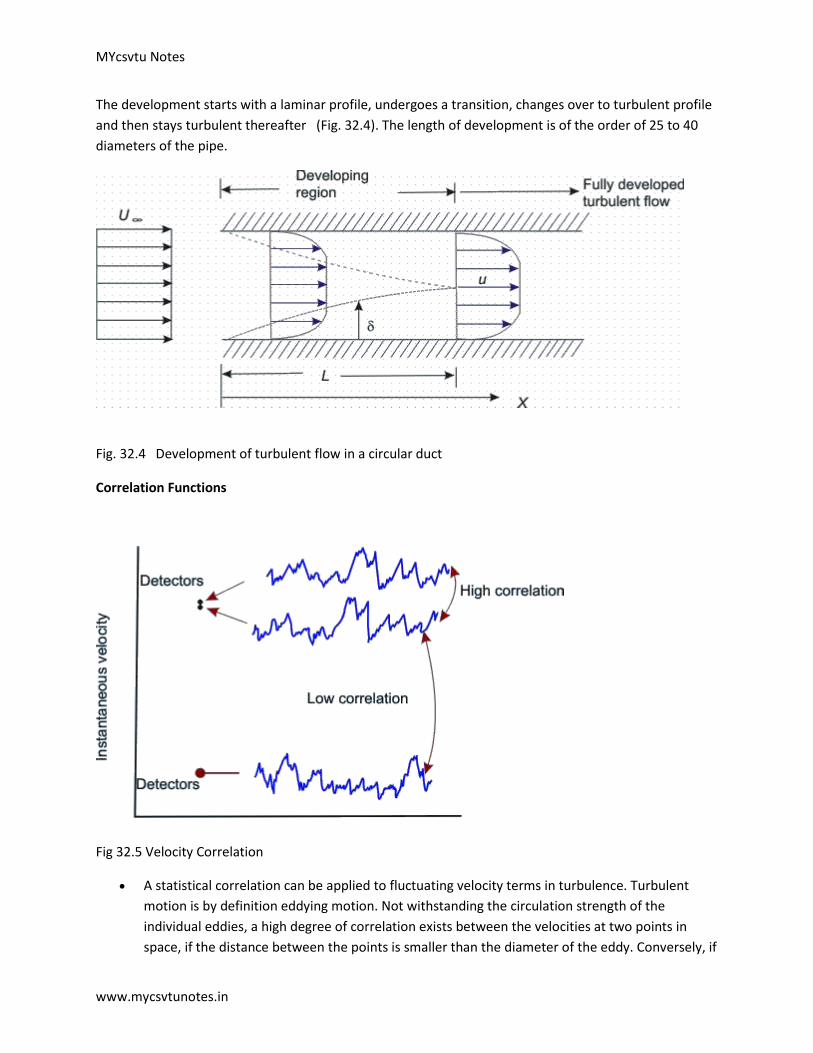
The development starts with a laminar profile, undergoes a transition, changes over to turbulent profile

and then stays turbulent thereafter (Fig. 32.4). The length of development is of the order of 25 to 40

diameters of the pipe.

Fig. 32.4 Development of turbulent flow in a circular duct

Correlation Functions

Fig 32.5 Velocity Correlation

A statistical correlation can be applied to fluctuating velocity terms in turbulence. Turbulent

motion is by definition eddying motion. Not withstanding the circulation strength of the

individual eddies, a high degree of correlation exists between the velocities at two points in

space, if the distance between the points is smaller than the diameter of the eddy. Conversely, if

MYcsvtu Notes

www.mycsvtunotes.in

the points are so far apart that the space, in between, corresponds to many eddy diameters

(Figure 32.5), little correlation can be expected.

Consider a statistical property of a random variable (velocity) at two points separated by a

distance r. An Eulerian correlation tensor (nine terms) at the two points can be defined by

In other words, the dependence between the two velocities at two points is measured by the

correlations, i.e. the time averages of the products of the quantities measured at two points. The

correlation of the components of the turbulent velocity of these two points is defined as

It is conventional to work with the non-dimensional form of the correlation, such as

A value of R(r) of unity signifies a perfect correlation of the two quantities involved and their motion is

in phase. Negative value of the correlation function implies that the time averages of the velocities in

the two correlated points have different signs. Figure 32.6 shows typical variations of the correlation R

with increasing separation r .

The positive correlation indicates that the fluid can be modelled as travelling in lumps. Since swirling

motion is an essential feature of turbulent motion, these lumps are viewed as eddies of various sizes.

The correlation R(r) is a measure of the strength of the eddies of size larger than r. Essentially the

velocities at two points are correlated if they are located on the same eddy

To describe the evolution of a fluctuating function u'(t), we need to know the manner in which

the value of u' at different times are related. For this purpose the correlation function

between the values of u' at different times is chosen and is called autocorrelation function.

The correlation studies reveal that the turbulent motion is composed of eddies which are

convected by the mean motion . The eddies have a wide range variation in their size. The size of

the large eddies is comparable with the dimensions of the neighbouring objects or the

dimensions of the flow passage.

MYcsvtu Notes

www.mycsvtunotes.in

The size of the smallest eddies can be of the order of 1 mm or less. However, the smallest eddies are

much larger than the molecular mean free paths and the turbulent motion does obey the principles of

continuum mechanics.

Fig 32.6 Variation of R with the distance of separation, r

Reynolds decomposition of turbulent flow :

The Experiment: In 1883, O. Reynolds conducted experiments with pipe flow by feeding into the

stream a thin thread of liquid dye. For low Reynolds numbers, the dye traced a straight line and

did not disperse. With increasing velocity, the dye thread got mixed in all directions and the

flowing fluid appeared to be uniformly colored in the downstream flow.

The Inference: It was conjectured that on the main motion in the direction of the pipe axis, there existed

a superimposed motion all along the main motion at right angles to it. The superimposed motion causes

exchange of momentum in transverse direction and the velocity distribution over the cross-section is

more uniform than in laminar flow. This description of turbulent flow which consists of superimposed

streaming and fluctuating (eddying) motion is well known as Reynolds decomposition of turbulent flow.

Here, we shall discuss different descriptions of mean motion. Generally, for Eulerian velocity u ,

the following two methods of averaging could be obtained.

(i) Time average for a stationary turbulence:

(ii) Space average for a homogeneous turbulence:

For a stationary and homogeneous turbulence, it is assumed that the two averages lead to the same

result: and the assumption is known as the ergodic hypothesis.

MYcsvtu Notes

www.mycsvtunotes.in

In our analysis, average of any quantity will be evaluated as a time average . Take a finite time

interval t1. This interval must be larger than the time scale of turbulence. Needless to say that it

must be small compared with the period t2 of any slow variation (such as periodicity of the mean

flow) in the flow field that we do not consider to be chaotic or turbulent .

Thus, for a parallel flow, it can be written that the axial velocity component is

(32.1)

As such, the time mean component determines whether the turbulent motion is steady or not. The

symbol signifies any of the space variables.

While the motion described by Fig.32.6(a) is for a turbulent flow with steady mean velocity the

Fig.32.6(b) shows an example of turbulent flow with unsteady mean velocity. The time period of

the high frequency fluctuating component is t1 whereas the time period for the unsteady mean

motion is t2 and for obvious reason t2>>t1. Even if the bulk motion is parallel, the fluctuation u '

being random varies in all directions.

The continuity equation, gives us

Invoking Eq.(32.1) in the above expression, we get

(32.2)

Fig 32.6 Steady and unsteady mean motions in a turbulent flow

MYcsvtu Notes

www.mycsvtunotes.in

Since , Eq.(32.2) depicts that y and z components of velocity exist even for the parallel flow if

the flow is turbulent. We have-

(32.3)

Contd. from Previous slide

However, the fluctuating components do not bring about the bulk displacement of a fluid

element. The instantaneous displacement is , and that is not responsible for the bulk

motion. We can conclude from the above

Due to the interaction of fluctuating components, macroscopic momentum transport takes place.

Therefore, interaction effect between two fluctuating components over a long period is non-zero and

this can be expressed as

Taking time average of these two integrals and write

(32.4a)

and

(32.4b)

Now, we can make a general statement with any two fluctuating parameters, say, with f ' and g'

as

(32.5a)

MYcsvtu Notes

www.mycsvtunotes.in

(32.5b)

The time averages of the spatial gradients of the fluctuating components also follow the same laws, and

they can be written as

(32.6)

The intensity of turbulence or degree of turbulence in a flow is described by the relative

magnitude of the root mean square value of the fluctuating components with respect to the

time averaged main velocity. The mathematical expression is given by

(32.7a)

The degree of turbulence in a wind tunnel can be brought down by introducing screens of fine mesh at

the bell mouth entry. In general, at a certain distance from the screens, the turbulence in a wind tunnel

becomes isotropic, i.e. the mean oscillation in the three components are equal,

In this case, it is sufficient to consider the oscillation u' in the direction of flow and to put

(32.7b)

This simpler definition of turbulence intensity is often used in practice even in cases when turbulence is

not isotropic.

Following Reynolds decomposition, it is suggested to separate the motion into a mean motion and a

fluctuating or eddying motion. Denoting the time average of the component of velocity by and

fluctuating component as , we can write down the following,

By definition, the time averages of all quantities describing fluctuations are equal to zero.

(32.8)

The fluctuations u', v' , and w' influence the mean motion , and in such a way that the mean

motion exhibits an apparent increase in the resistance to deformation. In other words, the effect of

fluctuations is an apparent increase in viscosity or macroscopic momentum diffusivity .

MYcsvtu Notes

www.mycsvtunotes.in

Rules of mean time - averages

If f and g are two dependent variables and if s denotes anyone of the independent variables x, y

Intermittency

Consider a turbulent flow confined to a limited region. To be specific we shall consider the

example of a wake (Figure 33.1a), but our discussion also applies to a jet (Figure 33.1b), a shear

layer (Figure 33.1c), or the outer part of a boundary layer on a wall.

The fluid outside the turbulent region is either in irrotational motion (as in the case of a wake or

a boundary layer), or nearly static (as in the case of a jet). Observations show that the

instantaneous interface between the turbulent and nonturbulent fluid is very sharp.

The thickness of the interface must equal the size of the smallest scales in the flow, namely the

Kolmogorov microscale.

MYcsvtu Notes

www.mycsvtunotes.in

Figure 33.1 Three types of free turbulent flows; (a) wake (b) jet and (c) shear layer [after P.K. Kundu

and I.M. Cohen, Fluid Mechanics, Academic Press, 2002]

Measurement at a point in the outer part of the turbulent region (say at point P in Figure 33.1a)

shows periods of high-frequency fluctuations as the point P moves into the turbulent flow and

low-frequency periods as the point moves out of the turbulent region. Intermittency I is defined

as the fraction of time the flow at a point is turbulent.

MYcsvtu Notes

www.mycsvtunotes.in

The variation of I across a wake is sketched in Figure 33.1a, showing that I =1 near the center

where the flow is always turbulent, and I = 0 at the outer edge of the flow domain.

Derivation of Governing Equations for Turbulent Flow

For incompressible flows, the Navier-Stokes equations can be rearranged in the form

(33.1a)

(33.1b)

(33.1c)

and

(33.2)

Express the velocity components and pressure in terms of time-mean values and

corresponding fluctuations. In continuity equation, this substitution and subsequent

time averaging will lead to

or,

Since,

We can write (33.3a)

From Eqs (33.3a) and (33.2), we obtain

MYcsvtu Notes

www.mycsvtunotes.in

(33.3b)

It is evident that the time-averaged velocity components and the fluctuating velocity

components, each satisfy the continuity equation for incompressible flow.

Imagine a two-dimensional flow in which the turbulent components are independent

of the z -direction. Eventually, Eq.(33.3b) tends to

(33.4)

On the basis of condition (33.4), it is postulated that if at an instant there is an increase in u' in

the x -direction, it will be followed by an increase in v' in the negative y -direction. In other

words, is non-zero and negative. (see Figure 33.2)

Fig 33.2 Each dot represents uν pair at an instant

Invoking the concepts of eqn. (32.8) into the equations of motion eqn (33.1 a, b, c),

we obtain expressions in terms of mean and fluctuating components. Now, forming

time averages and considering the rules of averaging we discern the following. The

terms which are linear, such as and vanish when they are averaged [from

(32.6)]. The same is true for the mixed terms like , or , but the quadratic

terms in the fluctuating components remain in the equations. After averaging, they

form , etc.

MYcsvtu Notes

www.mycsvtunotes.in

If we perform the aforesaid exercise on the x-momentum equation, we obtain

using rules of time averages,

We obtain

Introducing simplifications arising out of continuity Eq. (33.3a), we shall obtain.

Performing a similar treatment on y and z momentum equations, finally we obtain the

momentum equations in the form.

In x direction,

(33.5a)

In y direction,

MYcsvtu Notes

www.mycsvtunotes.in

(33.5b)

In z direction,

(33.5c)

Comments on the governing equation :

1. The left hand side of Eqs (33.5a)-(33.5c) are essentially similar to the steady-state

Navier-Stokes equations if the velocity components u, v and w are replaced by ,

and .

2. The same argument holds good for the first two terms on the right hand side of Eqs

(33.5a)-(33.5c).

3. However, the equations contain some additional terms which depend on turbulent

fluctuations of the stream. These additional terms can be interpreted as components

of a stress tensor.

Now, the resultant surface force per unit area due to these terms may be considered as

In x direction,

(33.6a)

In y direction,

(33.6b)

In z direction,

(33.6c)

Comparing Eqs (33.5) and (33.6), we can write

MYcsvtu Notes

www.mycsvtunotes.in

(33.7)

It can be said that the mean velocity components of turbulent flow satisfy the same Navier-

Stokes equations of laminar flow. However, for the turbulent flow, the laminar stresses must be

increased by additional stresses which are given by the stress tensor (33.7). These additional

stresses are known as apparent stresses of turbulent flow or Reynolds stresses . Since

turbulence is considered as eddying motion and the aforesaid additional stresses are added to

the viscous stresses due to mean motion in order to explain the complete stress field, it is often

said that the apparent stresses are caused by eddy viscosity . The total stresses are now

(33.8)

and so on. The apparent stresses are much larger than the viscous components, and the viscous stresses

can even be dropped in many actual calculations .

Turbulent Boundary Layer Equations

For a two-dimensional flow (w = 0)over a flat plate, the thickness of turbulent boundary layer is

assumed to be much smaller than the axial length and the order of magnitude analysis may be

applied. As a consequence, the following inferences are drawn:

MYcsvtu Notes

www.mycsvtunotes.in

The turbulent boundary layer equation together with the equation of continuity becomes

(33.9)

(33.10)

A comparison of Eq. (33.10) with laminar boundary layer Eq. (23.10) depicts that: u, v and p are

replaced by the time average values and ,and laminar viscous force per unit volume

is replaced by where is the laminar shear stress and

is the turbulent shear stress.

Boundary Conditions

All the components of apparent stresses vanish at the solid walls and only stresses which act

near the wall are the viscous stresses of laminar flow. The boundary conditions, to be satisfied

by the mean velocity components, are similar to laminar flow.

A very thin layer next to the wall behaves like a near wall region of the laminar flow. This layer is

known as laminar sublayer and its velocities are such that the viscous forces dominate over the

inertia forces. No turbulence exists in it (see Fig. 33.3).

For a developed turbulent flow over a flat plate, in the near wall region, inertial effects are

insignificant, and we can write from Eq.33.10,

MYcsvtu Notes

www.mycsvtunotes.in

Fig 33.3 Different zones of a turbulent flow past a wall

which can be integrated as , =constant

We know that the fluctuating components, do not exist near the wall, the shear stress on the

wall is purely viscous and it follows

However, the wall shear stress in the vicinity ofthe laminar sublayer is estimated as

(33.11a)

where Us is the fluid velocity at the edge of the sublayer. The flow in the sublayer is specified by a

velocity scale (characteristic of this region).

We define the friction velocity,

(33.11b)

as our velocity scale. Once is specified, the structure of the sub layer is specified. It has been

confirmed experimentally that the turbulent intensity distributions are scaled with . For example,

MYcsvtu Notes

www.mycsvtunotes.in

maximum value of the is always about . The relationship between and the can be

determined from Eqs (33.11a) and (33.11b) as

Let us assume . Now we can write

where is a proportionality constant (33.12a)

or

(33.12b)

Hence, a non-dimensional coordinate may be defined as, which will help us estimating

different zones in a turbulent flow. The thickness of laminar sublayer or viscous sublayer is considered

to be .

Turbulent effect starts in the zone of and in a zone of , laminar and turbulent motions

coexist. This domain is termed as buffer zone. Turbulent effects far outweight the laminar effect in the

zone beyond and this regime is termed as turbulent core .

For flow over a flat plate, the turbulent shear stress ( ) is constant throughout in the y

direction and this becomes equal to at the wall. In the event of flow through a channel, the

turbulent shear stress ( ) varies with y and it is possible to write

(33.12c)

where the channel is assumed to have a height 2h and is the distance measured from the centreline of

the channel . Figure 33.1 explains such variation of turbulent stress.

Shear Stress Models

MYcsvtu Notes

www.mycsvtunotes.in

In analogy with the coefficient of viscosity for laminar flow, J. Boussinesq introduced a mixing

coefficient for the Reynolds stress term, defined as

Using the shearing stresses can be written as

such that the equation

may be written as

(33.13)

The term νt is known as eddy viscosity and the model is known as eddy viscosity model .

Unfortunately the value of νt is not known. The term ν is a property of the fluid whereas νt is

attributed to random fluctuations and is not a property of the fluid. However, it is necessary to

find out empirical relations between νt, and the mean velocity. The following section discusses

relation between the aforesaid apparent or eddy viscosity and the mean velocity components

Prandtl's Mixing Length Hypothesis

Consider a fully developed turbulent boundary layer . The stream wise mean velocity varies only

from streamline to streamline. The main flow direction is assumed parallel to the x-axis (Fig.

33.4).

The time average components of velocity are given by . The fluctuating

component of transverse velocity transports mass and momentum across a plane at y1 from

the wall. The shear stress due to the fluctuation is given by

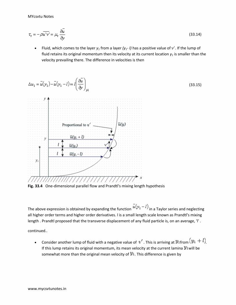
MYcsvtu Notes

www.mycsvtunotes.in

(33.14)

Fluid, which comes to the layer y1 from a layer (y1- l) has a positive value of . If the lump of

fluid retains its original momentum then its velocity at its current location y1 is smaller than the

velocity prevailing there. The difference in velocities is then

(33.15)

Fig. 33.4 One-dimensional parallel flow and Prandtl's mixing length hypothesis

The above expression is obtained by expanding the function in a Taylor series and neglecting

all higher order terms and higher order derivatives. l is a small length scale known as Prandtl's mixing

length . Prandtl proposed that the transverse displacement of any fluid particle is, on an average, 'l' .

continued..

Consider another lump of fluid with a negative value of . This is arriving at from .

If this lump retains its original momentum, its mean velocity at the current lamina will be

somewhat more than the original mean velocity of . This difference is given by

MYcsvtu Notes

www.mycsvtunotes.in

(33.16)

The velocity differences caused by the transverse motion can be regarded as the turbulent

velocity components at .

We calculate the time average of the absolute value of this fluctuation as

(33.17)

Suppose these two lumps of fluid meet at a layer The lumps will collide with a velocity

and diverge. This proposes the possible existence of transverse velocity component in both

directions with respect to the layer at . Now, suppose that the two lumps move away in a

reverse order from the layer with a velocity . The empty space will be filled from the

surrounding fluid creating transverse velocity components which will again collide at .

Keeping in mind this argument and the physical explanation accompanying Eqs (33.4), we may

state that

or,

along with the condition that the moment at which is positive, is more likely to be negative and

conversely when is negative. Possibly, we can write at this stage

(33.18)

where C1 and C2 are different proportionality constants. However, the constant C2 can now be included

in still unknown mixing length and Eg. (33.18) may be rewritten as

MYcsvtu Notes

www.mycsvtunotes.in

For the expression of turbulent shearing stress we may write

(33.19)

After comparing this expression with the eddy viscosity Eg. (33.14), we may arrive at a more

precise definition,

(33.20a)

where the apparent viscosity may be expressed as

(33.20b)

and the apparent kinematic viscosity is given by

(33.20c)

The decision of expressing one of the velocity gradients of Eq. (33.19) in terms of its modulus as

was made in order to assign a sign to according to the sign of .

Note that the apparent viscosity and consequently,the mixing length are not properties of fluid.

They are dependent on turbulent fluctuation.

But how to determine the value of the mixing length? Several correlations, using

experimental results for have been proposed to determine .

MYcsvtu Notes

www.mycsvtunotes.in

However, so far the most widely used value of mixing length in the regime of isotropic

turbulence is given by

(33.21)

where is the distance from the wall and is known as von Karman constant .

Universal Velocity Distribution Law And Friction Factor In Duct Flows For Very Large Reynolds

Numbers

For flows in a rectangular channel at very large Reynolds numbers the laminar

sublayer can practically be ignored. The channel may be assumed to have a width 2h

and the x axis will be placed along the bottom wall of the channel.

Consider a turbulent stream along a smooth flat wall in such a duct and denote the

distance from the bottom wall by y, while u(y) will signify the velocity. In the

neighbourhood of the wall, we shall apply

According to Prandtl's assumption, the turbulent shearing stress will be

(34.1)

At this point, Prandtl introduced an additional assumption which like a plane Couette flow

takes a constant shearing stress throughout, i.e

(34.2)

where denotes the shearing stress at the wall.

MYcsvtu Notes

www.mycsvtunotes.in

Invoking once more the friction velocity , we obtain

(34.3)

(34.4)

On integrating we find

(34.5)

Despite the fact that Eq. (34.5) is derived on the basis of the friction velocity in the

neighbourhood of the wall because of the assumption that = constant, we

shall use it for the entire region. At y = h (at the horizontal mid plane of the channel),

we have . The constant of integration is eliminated by considering

Substituting C in Eq. (34.5), we get

(34.6)

Equation (34.6) is known as universal velocity defect law of Prandtl and its distribution has

been shown in Fig. 34.1

MYcsvtu Notes

www.mycsvtunotes.in

.

Fig 34.1 Distibution of universal velocity defect law of Prandtl in a turbulent channel flow

Here, we have seen that the friction velocity is a reference parameter for velocity.Equation

(34.5) can be rewritten as

where

The no-slip condition at the wall cannot be satisfied with a finite constant of integration. This is

expected that the appropriate condition for the present problem should be that at a very

small distance from the wall. Hence, Eq. (34.5) becomes

MYcsvtu Notes

www.mycsvtunotes.in

(34.7)

The distance is of the order of magnitude of the thickness of the viscous layer. Now we can

write Eq. (34.7) as

(34.8)

where , the unknown is included in .

Equation (34.8) is generally known as the universal velocity profile because of the fact that it is

applicable from moderate to a very large Reynolds number.

However, the constants and have to be found out from experiments. The aforesaid profile is not

only valid for channel (rectangular) flows, it retains the same functional relationship for circular pipes as

well . It may be mentioned that even without the assumption of having a constant shear stress

throughout, the universal velocity profile can be derived.

Experiments, performed by J. Nikuradse, showed that Eq. (34.8) is in good agreement with

experimental results. Based on Nikuradse's and Reichardt's experimental data, the empirical

constants of Eq. (34.8) can be determined for a smooth pipe as

(34.9)

This velocity distribution has been shown through curve (b) in Fig. 34.2

.

MYcsvtu Notes

www.mycsvtunotes.in

Fig 34.2 The universal velocity distribution law for smooth pipes

However, the corresponding friction factor concerning Eq. (34.9) is

(34.10)

the universal velocity profile does not match very close to the wall where the viscous shear

predominates the flow.

Von Karman suggested a modification for the laminar sublayer and the buffer zone which are

(34.11)

MYcsvtu Notes

www.mycsvtunotes.in

(34.12)

Equation (34.11) has been shown through curve(a) in Fig. 34.2.

It may be worthwhile to mention here that a surface is said to be hydraulically smooth so long

(34.13)

where is the average height of the protrusions inside the pipe.

Physically, the above expression means that for smooth pipes protrusions will not be extended outside

the laminar sublayer. If protrusions exceed the thickness of laminar sublayer, it is conjectured (also

justified though experimental verification) that some additional frictional resistance will contribute to

pipe friction due to the form drag experienced by the protrusions in the boundary layer.

In rough pipes experiments indicate that the velocity profile may be expressed as:

(34.14)

At the centre-line, the maximum velocity is expressed as

(34.15)

Note that no longer appears with and . This means that for completely rough zone of turbulent

flow, the profile is independent of Reynolds number and a strong function of pipe roughness .

However, for pipe roughness of varying degrees, the recommendation due to Colebrook and

White works well. Their formula is

(34.16)

MYcsvtu Notes

www.mycsvtunotes.in

where is the pipe radius

For , this equation produces the result of the smooth pipes (Eq.(34.10)). For , it gives

the expression for friction factor for a completely rough pipe at a very high Reynolds number which is

given by

(34.17)

Turbulent flow through pipes has been investigated by many researchers because of its enormous

practical importance.

Fully Developed Turbulent Flow In A Pipe For Moderate Reynolds Numbers

The entry length of a turbulent flow is much shorter than that of a laminar flow, J. Nikuradse

determined that a fully developed profile for turbulent flow can be observed after an entry

length of 25 to 40 diameters. We shall focus to fully developed turbulent flow in this section.

Considering a fully developed turbulent pipe flow (Fig. 34.3) we can write

(34.18)

or

(34.19)

Fig. 34.3 Fully developed turbulent pipe flow

MYcsvtu Notes

www.mycsvtunotes.in

It can be said that in a fully developed flow, the pressure gradient balances the wall shear stress only

and has a constant value at any . However, the friction factor ( Darcy friction factor ) is defined in a

fully developed flow as

(34.20)

Comparing Eq.(34.19) with Eq.(34.20), we can write

(34.21)

H. Blasius conducted a critical survey of available experimental results and established the empirical

correlation for the above equation as

where (34.22)

It is found that the Blasius's formula is valid in the range of Reynolds number of Re ≤105. At the

time when Blasius compiled the experimental data, results for higher Reynolds numbers were

not available. However, later on, J. Nikuradse carried out experiments with the laws of friction in

a very wide range of Reynolds numbers, 4 x 103 ≤ Re ≤ 3.2 x 106. The velocity profile in this range

follows:

(34.23)

where is the time mean velocity at the pipe centre and is the distance from the wall . The exponent

n varies slightly with Reynolds number. In the range of Re ~ 105, n is 7.

Fully Developed Turbulent Flow In A Pipe For Moderate Reynolds Numbers

The ratio of and for the aforesaid profile is found out by considering the volume flow rate

Q as

MYcsvtu Notes

www.mycsvtunotes.in

From equation (34.23)

or

or

or

or

(34.24a)

Now, for different values of n (for different Reynolds numbers) we shall obtain different values

of from Eq.(34.24a). On substitution of Blasius resistance formula (34.22) in Eq.(34.21),

the following expression for the shear stress at the wall can be obtained.

putting

and where

MYcsvtu Notes

www.mycsvtunotes.in

or

or

For n=7, becomes equal to 0.8. substituting in the above equation, we get

Finally it produces

(34.24b)

or

where is friction velocity. However, may be spitted into and and we obtain

or

(34.25a)

Now we can assume that the above equation is not only valid at the pipe axis (y = R) but also

at any distance from the wall y and a general form is proposed as

MYcsvtu Notes

www.mycsvtunotes.in

(34.25b)

Concluding Remarks :

1. It can be said that (1/7)th power velocity distribution law (24.38b) can be derived from Blasius's

resistance formula (34.22) .

2. Equation (34.24b) gives the shear stress relationship in pipe flow at a moderate Reynolds

number, i.e . Unlike very high Reynolds number flow, here laminar effect cannot be

neglected and the laminar sub layer brings about remarkable influence on the outer zones.

3. The friction factor for pipe flows, , defined by Eq. (34.22) is valid for a specific range of

Reynolds number and for a particular surface condition.

Skin Friction Coefficient For Boundary Layers On A Flat Plate

Calculations of skin friction drag on lifting surface and on aerodynamic bodies are somewhat

similar to the analyses of skin friction on a flat plate. Because of zero pressure gradient, the flat

plate at zero incidence is easy to consider. In some of the applications cited above, the pressure

gradient will differ from zero but the skin friction will not be dramatically different so long there

is no separation.

We begin with the momentum integral equation for flat plate boundary layer which is valid for

both laminar and turbulent flow.

(34.26a)

Invoking the definition of , Eq.(34.26a) can be written as

(34.26b)

Due to the similarity in the laws of wall, correlations of previous section may be applied to the

flat plate by substituting for R and for the time mean velocity at the pipe centre.The

rationale for using the turbulent pipe flow results in the situation of a turbulent flow over a flat

plate is to consider that the time mean velocity, at the centre of the pipe is analogous to the

free stream velocity, both the velocities being defined at the edge of boundary layer thickness.

Finally, the velocity profile will be [following Eq. (34.24)]

MYcsvtu Notes

www.mycsvtunotes.in

for (34.27)

Evaluating momentum thickness with this profile, we shall obtain

(34.28)

Consequently, the law of shear stress (in range of ) for the flat plate is found out by making

use of the pipe flow expression of Eq. (34.24b) as

Substituting for and for R in the above expression, we get

(34.29)

Once again substituting Eqs (34.28) and (34.29) in Eq.(34.26), we obtain

.

(34.30)

MYcsvtu Notes

www.mycsvtunotes.in

For simplicity, if we assume that the turbulent boundary layer grows from the leading edge of

the plate we shall be able to apply the boundary conditions x = 0, δ = 0 which will yield C = 0,

and Eq. (34.30) will become From Eqs (34.26b), (34.28) and (34.31), it is possible to calculate the

average skin friction coefficient on a flat plate as

or,

or, (34.31)

Where

From Eqs (34.26b), (34.28) and (34.31), it is possible to calculate the average skin friction coefficient on

a flat plate as

(34.32)

It can be shown that Eq. (34.32) predicts the average skin friction coefficient correctly in the regime of

Reynolds number below .

This result is found to be in good agreement with the experimental results in the range of

Reynolds number between and which is given by

(34.33)

Equation (34.33) is a widely accepted correlation for the average value of turbulent skin friction

coefficient on a flat plate.

With the help of Nikuradse's experiments, Schlichting obtained the semi empirical equation for

the average skin friction coefficient as

(34.34)

Equation (34.34) was derived asssuming the flat plate to be completely turbulent over its entire length .

In reality, a portion of it is laminar from the leading edge to some downstream position. For this

purpose, it was suggested to use

MYcsvtu Notes

www.mycsvtunotes.in

(34.35a)

where A has various values depending on the value of Reynolds number at which the transition takes

place.

If the trasition is assumed to take place around a Reynolds number of , the average

skin friction correlation of Schlichling can be written as

(34.35b)

All that we have presented so far, are valid for a smooth plate.

Schlichting used a logarithmic expression for turbulent flow over a rough surface and derived

(34.36)

Exercise Problems - Chapter 10

1.Estimate the power required to move a flat plate, 15 m. long and 4 m. wide, in oil

at 4m/sec, under the following cases:

a) The boundary layer is assumed laminar over the entire surface of the plate. (Ans. 1665.5 N-m/sec)

b) Transition to turbulence occurs at and plate is smooth.(Ans. 9486 N-m/sec)

c) The boundary layer is turbulent over the entire plate which is smooth.(Ans. 10023.94 N-m/sec)

d) The boundary layer is turbulent over the entire rough plate with .(Ans. 17200 N-m/sec)

2. Water is transported through a horizontal pipeline, 800 m.

long, with a maximum velocity of 3m/sec. If the Reynolds number is , find the diameter of the pipe (with

and without the use of Moody Diagram ).

Also calculate the thickness of laminar sub-layer and the buffer layer, and find the power required to

maintain the flow. Calculate your results for a fully rough pipe with .

(Ans. Diameter of the pipe 0.8 m., laminar sub-layer thickness 0.1 mm, buffer layer thickness 1.3 mm,

power required 50250 W)

MYcsvtu Notes

www.mycsvtunotes.in

3. Find the frictional drag on the top and sides of a box-shaped moving van 2.4 m wide, 3.0 m high, and

10.5 m long traveling at 100km/h through air ( ). Assume that the vehicle has a rounded

nose so that the flow does not seperate from the top and side. also assume that a turbulent boundary

layer starts immediately at the leading edge.

Also, find the thickness of the boundary layer and the shear stress at the trailing edge.

(Ans. Drag = 105.9 N, B.L. = 0.136m, Shear stress = 0.904 Pa)

Applications of Viscous Flows Through Pipes

Introduction

A complete analytical solution for the equation of motion in the case of a laminar flow is

available, even the advanced theories in the analysis of turbulent flow depend at some point on

experimentally derived information. Flow through pipes is usually turbulent in practice.

One of the most important items of information that an hydraulic engineer needs is the power

required to force fluid at a certain steady rate through a pipe or pipe network system. This

information is furnished in practice through some routine solution of pipe flow problems with

the help of available empirical and theoretical information.

This lecture deals with the typical approaches to the solution of pipe flow problems in practice.

Concept of Friction Factor in a pipe flow:

The friction factor in the case of a pipe flow was already mentioned in lecture 26.

We will elaborate further on friction factor or friction coefficient in this section.

Skin friction coefficient for a fully developed flow through a closed duct is defined as

(35.1)

where, V is the average velocity of flow given by , Q and A are the volume flow rate through

the duct and the cross-sectional area of the duct respectively.

From a force balance of a typical fluid element (Fig. 35.1) in course of its flow through a duct of constant

cross-sectional area, we can write

MYcsvtu Notes

www.mycsvtunotes.in

(35.2)

FIG 35.1 Force Balance of a fluid element in the course of flow through a duct

where, is the shear stress at the wall and is the piezometric pressure drop over a length of L . A

and S are respectively the cross-sectional area and wetted perimeter of the duct.

Substituting the expression (35.2) in Eq. (35.1), we have,

(35.3)

where, and is known as the hydraulic diameter .

In case of a circular pipe, Dh=D, the diameter of the pipe. The coefficient Cf defined by Eqs (35.1) or

(35.3) is known as Fanning's friction factor .

To do away with the factor 1/4 in the Eq. (35.3), Darcy defined a friction factor f (Darcy's friction

factor) as

(35.4)

Comparison of Eqs (35.3) and (35.4) gives . Equation (35.4) can be written for a pipe

flow as

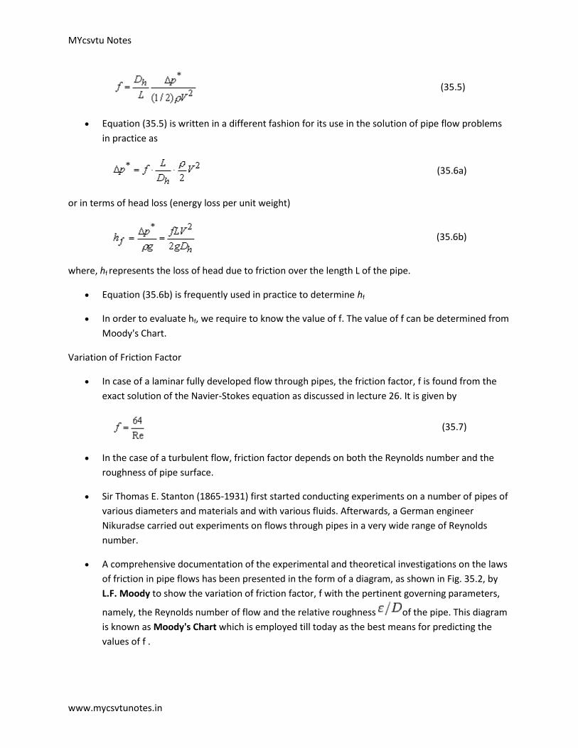
MYcsvtu Notes

www.mycsvtunotes.in

(35.5)

Equation (35.5) is written in a different fashion for its use in the solution of pipe flow problems

in practice as

(35.6a)

or in terms of head loss (energy loss per unit weight)

(35.6b)

where, hf represents the loss of head due to friction over the length L of the pipe.

Equation (35.6b) is frequently used in practice to determine hf

In order to evaluate hf, we require to know the value of f. The value of f can be determined from

Moody's Chart.

Variation of Friction Factor

In case of a laminar fully developed flow through pipes, the friction factor, f is found from the

exact solution of the Navier-Stokes equation as discussed in lecture 26. It is given by

(35.7)

In the case of a turbulent flow, friction factor depends on both the Reynolds number and the

roughness of pipe surface.

Sir Thomas E. Stanton (1865-1931) first started conducting experiments on a number of pipes of

various diameters and materials and with various fluids. Afterwards, a German engineer

Nikuradse carried out experiments on flows through pipes in a very wide range of Reynolds

number.

A comprehensive documentation of the experimental and theoretical investigations on the laws

of friction in pipe flows has been presented in the form of a diagram, as shown in Fig. 35.2, by

L.F. Moody to show the variation of friction factor, f with the pertinent governing parameters,

namely, the Reynolds number of flow and the relative roughness of the pipe. This diagram

is known as Moody's Chart which is employed till today as the best means for predicting the

values of f .

MYcsvtu Notes

www.mycsvtunotes.in

Fig. 35.2 Friction Factors for pipes (adapted from Trans. ASME, 66,672, 1944)

Figure 35.2 depicts that

The friction factor f at a given Reynolds number, in the turbulent region, depends on the relative

roughness, defined as the ratio of average roughness to the diameter of the pipe, rather than

the absolute roughness.

For moderate degree of roughness, a pipe acts as a smooth pipe up to a value of Re where the

curve of f vs Re for the pipe coincides with that of a smooth pipe. This zone is known as the

smooth zone of flow .

The region where f vs Re curves (Fig. 35.2) become horizontal showing that f is independent of

Re, is known as the rough zone and the intermediate region between the smooth and rough

zone is known as the transition zone.

The position and extent of all these zones depend on the relative roughness of the pipe. In the

smooth zone of flow, the laminar sublayer becomes thick, and hence, it covers appreciably the

irregular surface protrusions. Therefore all the curves for smooth flow coincide.

With increasing Reynolds number, the thickness of sublayer decreases and hence the surface

bumps protrude through it. The higher is the roughness of the pipe, the lower is the value of Re

at which the curve of f vs Re branches off from smooth pipe curve (Fig. 35.2).

MYcsvtu Notes

www.mycsvtunotes.in

In the rough zone of flow, the flow resistance is mainly due to the form drag of those

protrusions. The pressure drop in this region is approximately proportional to the square of the

average velocity of flow. Thus f becomes independent of Re in this region.

In practice, there are three distinct classes of problems relating to flow through a single pipe line as

follows:

1. The flow rate and pipe diameter are given. One has to determine the loss of head over a given

length of pipe and the corresponding power required to maintain the flow over that length.

2. The loss of head over a given length of a pipe of known diameter is given. One has to find out

the flow rate and the transmission of power accordingly.

3. The flow rate through a pipe and the corresponding loss of head over a part of its length are

given. One has to find out the diameter of the pipe.

In the first category of problems, the friction factor f is found out explicitly from the given values of flow

rate and pipe diameter. Therefore, the loss of head hf and the power required, P can be calculated by

the straightforward application of Eq.(35.6b).

(contd from previous...) Concept of Flow Potential and Flow Resistance

The velocity V in the above equation is usually substituted in terms of flow rate Q , since, under steady

state, the flow rate remains constant throughout the pipe even if its diameter changes. Therefore,

replacing V in Eq. (35.11) as we finally get

or, (35.12)

where

(35.13)

The term R is defined as the flow resistance .

In a situation where f becomes independent of Re, the flow resistance expressed by Eg. (35.13) becomes

simply a function of the pipe geometry. With the help of Eq. (35.10), Eq. (35.12) can be written as

(35.14)

in Eq. (35.14) is the head causing the flow and is defined as the difference in flow potentials

between A and B.

MYcsvtu Notes

www.mycsvtunotes.in

This equation is comparable to the voltage-current relationship in a purely resistive electrical

circuit. In a purely resistive electrical circuit, , where is the voltage or electrical

potential difference across a resistor whose resistance is R and the electrical current flowing

through it is I.

The difference however is that while the voltage drop in an electrical circuit is linearly

proportional to current, the difference in the flow potential in a fluid circuit is proportional to

the square of the flow rate.

Therefore, the fluid flow system as shown in Fig. 35.3 and described by Eq. (35.14) can be

expressed by an equivalent electrical network system as shown in Fig. 35.4.

Fig 35.4 Equivalent electrical network system for a simple pipe flow problem shown in Fig.35.3

Flow Through Branched Pipes

In several practical situations, flow takes place under a given head through different pipes jointed

together either in series or in parallel or in a combination of both of them.

Pipes in Series

If a pipeline is joined to one or more pipelines in continuation, these are said to constitute pipes

in series. A typical example of pipes in series is shown in Fig. 36.1. Here three pipes A, B and C

are joined in series.

Fig 36.1 Pipes in series

In this case, rate of flow Q remains same in each pipe. Hence,

MYcsvtu Notes

www.mycsvtunotes.in

If the total head available at Sec. 1 (at the inlet to pipe A) is which is greater than , the

total head at Sec. 2 (at the exit of pipe C), then the flow takes place from 1 to 2 through the

system of pipelines in series.

Application of Bernoulli's equation between Secs.1 and 2 gives

where, is the loss of head due to the flow from 1 to 2. Recognizing the minor and major losses

associated with the flow, can be written as

(36.1)

Friction loss

in pipe A

Loss due to

enlargement at

entry to pipe B

Friction loss

in pipe B

Loss due

to abrupt

contraction

at entry

to pipe C

Friction loss in

pipe C

The subscripts A, B and C refer to the quantities in pipe A, B and C respectively. Cc is the coefficient of

contraction.

The flow rate Q satisfies the equation

(36.2)

Velocities VA, VB and VC in Eq. (36.1) are substituted from Eq. (36.2), and we get

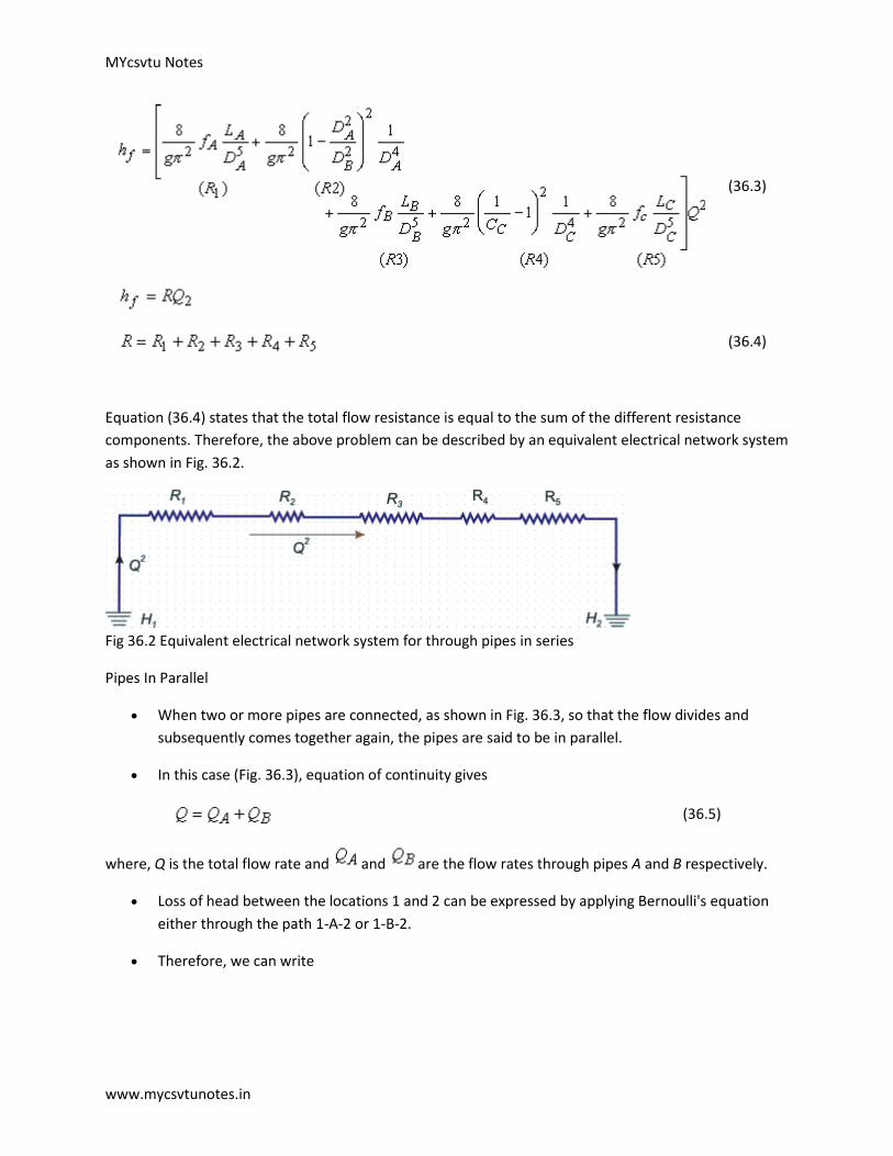
MYcsvtu Notes

www.mycsvtunotes.in

(36.3)

(36.4)

Equation (36.4) states that the total flow resistance is equal to the sum of the different resistance

components. Therefore, the above problem can be described by an equivalent electrical network system

as shown in Fig. 36.2.

Fig 36.2 Equivalent electrical network system for through pipes in series

Pipes In Parallel

When two or more pipes are connected, as shown in Fig. 36.3, so that the flow divides and

subsequently comes together again, the pipes are said to be in parallel.

In this case (Fig. 36.3), equation of continuity gives

(36.5)

where, Q is the total flow rate and and are the flow rates through pipes A and B respectively.

Loss of head between the locations 1 and 2 can be expressed by applying Bernoulli's equation

either through the path 1-A-2 or 1-B-2.

Therefore, we can write

MYcsvtu Notes

www.mycsvtunotes.in

Fig 36.3 Pipes in Parallel

and

Equating the above two expressions, we get -

(36.6)

where,

Equations (36.5) and (36.6) give -

(36.7)

MYcsvtu Notes

www.mycsvtunotes.in

where, (36.8)

The flow system can be described by an equivalent electrical circuit as shown in Fig. 36.4.

Fig 36.4 Equivalent electrical network system for flow through pipes in parallel

From the above discussion on flow through branched pipes (pipes in series or in parallel, or in

combination of both), the following principles can be summarized:

1. The friction equation must be satisfied for each pipe.

2. There can be only one value of head at any point.

3. Algebraic sum of the flow rates at any junction must be zero. i.e., the total mass flow rate

towards the junction must be equal to the total mass flow rate away from it.

4. Algebraic sum of the products of the flux (Q2) and the flow resistance (the sense being

determined by the direction of flow) must be zero in any closed hydraulic circuit.

The principles 3 and 4 can be written analytically as

at a node (Junction) (36.9)

in a loop (36.10)

While Eq. (36.9) implies the principle of continuity in a hydraulic circuit, Eq. (36.10) is referred to as

pressure equation of the circuit.

Pipe Network: Solution by Hardy Cross Method

The distribution of water supply in practice is often made through a pipe network comprising a

combination of pipes in series and parallel. The flow distribution in a pipe network is determined

from Eqs(36.9) and (36.10).

MYcsvtu Notes

www.mycsvtunotes.in

The solution of Eqs (36.9) and (36.10) for the purpose is based on an iterative technique with an

initial guess in Q

The method was proposed by Hardy-Cross and is described below:

The flow rates in each pipe are assumed so that the continuity (Eq. 36.9) at each node is

satisfied. Usually the flow rate is assumed more for smaller values of resistance R and

vice versa.

If the assumed values of flow rates are not correct, the pressure equation Eq. (36.10)

will not be satisfied. The flow rate is then altered based on the error in satisfying the Eq.

(36.10).

Let Q0 be the correct flow in a path whereas the assumed flow be Q. The error dQ in flow is then

defined as

(36.11)

Let (36.12a)

and (36.12b)

Then according to Eq. (36.10)

in a loop (36.13a)

and in a loop (36.13b)

Where 'e' is defined to be the error in pressure equation for a loop with the assumed values of flow rate

in each path.

From Eqs (36.13a) and (36.13b) we have

or, (36.14)

Where dh (= h - h' ) is the error in pressure equation for a path. Again from Eq. (36.12a), we can write

MYcsvtu Notes

www.mycsvtunotes.in

or, (36.15)

Substituting the value of dh from Eq. (36.15) in Eq. (36.14) we have

Considering the error dQ to be the same for all hydraulic paths in a loop, we can write

(36.16)

The Eq. (36.16) can be written with the help of Eqs (36.12a) and (36.12b) as

(36.17)

The error in flow rate dQ is determined from Eq. (36.17) and the flow rate in each path of a loop is then

altered according to Eq. (36.11).

The Hardy-Cross method can also be applied to a hydraulic circuit containing a pump or a turbine. The

pressure equation (Eq. (36.10)) is only modified in consideration of a head source (pump) or a head sink

(turbine) as

(36.18)

where is the head delivered by a source in the circuit. Therefore, the value of to be substituted

in Eq. (36.18) will be positive for a pump and negative for a turbine.

Flow Through Pipes With Side Tappings

In course of flow through a pipe, a fluid may be withdrawn from the side tappings along the

length of the pipe as shown in Fig. 37.1

If the side tappings are very closely spaced, the loss of head over a given length of pipe can be

obtained as follows:

MYcsvtu Notes

www.mycsvtunotes.in

Fig. 37.1 Flow through pipes with side tappings

The rate of flow through the pipe, under this situation, decreases in the direction of flow due to

side tappings. Therefore, the average flow velocity at any section of the pipe is not constant.

The frictional head loss over a small length dx of the pipe at any section can be written as

(37.1)

where, is the average flow velocity at that section.

If the side tappings are very close together, Eq. (37.1) can be integrated to determine the loss of

head due to friction over a given length L of the pipe, provided, can be replaced in terms of

the length of the pipe.

Let us consider, for this purpose, a Section 1-1 at the upstream just after which the side tappings

are provided. If the tappings are uniformly and closely spaced, so that the fluid is removed at a

uniform rate q per unit length of the pipe, then the volume flow rate Qx at a distance x from the

inlet Section 1-1 can be written as

where, is the volume flow rate at Sec.1-1.

Hence,

(37.2)

Substituting from Eq. (37.2) into Eq. (37.1), we have,

MYcsvtu Notes

www.mycsvtunotes.in

(37.3)

Therefore, the loss of head due to friction over a length L is given by

(37.4a)

Here, the friction factor f has been assumed to be constant over the length L of the pipe. If the

entire flow at Sec.1-1 is drained off over the length L , then,

Equation (37.4a), under this situation, becomes

(37.4b)

where, V0 is the average velocity of flow at the inlet Section 1-1.

Equation (37.4b) indicates that the loss of head due to friction over a length L of a pipe, where

the entire flow is drained off uniformly from the side tappings, becomes one third of that in a

pipe of same length and diameter, but without side tappings.

Losses In Pipe Bends

Bends are provided in pipes to change the direction of flow through it. An additional loss of

head, apart from that due to fluid friction, takes place in the course of flow through pipe

bend.

The fluid takes a curved path while flowing through a pipe bend as shown in Fig. 37.2.

MYcsvtu Notes

www.mycsvtunotes.in

Fig. 37.2 Flow through pipe bend

Whenever a fluid flows in a curved path, there must be a force acting radially inwards on the fluid to

provide the inward acceleration, known as centripetal acceleration .

This results in an increase in pressure near the outer wall of the bend, starting at some point A (Fig.

37.2) and rising to a maximum at some point B . There is also a reduction of pressure near the inner wall

giving a minimum pressure at C and a subsequent rise from C to D . Therefore between A and B and

between C and D the fluid experiences an adverse pressure gradient (the pressure increases in the

direction of flow).

Fluid particles in this region, because of their close proximity to the wall, have low velocities and cannot

overcome the adverse pressure gradient and this leads to a separation of flow from the boundary and

consequent losses of energy in generating local eddies. Losses also take place due to a secondary flow

in the radial plane of the pipe because of a change in pressure in the radial depth of the pipe.

This flow, in conjunction with the main flow, produces a typical spiral motion of the fluid which persists

even for a downstream distance of fifty times the pipe diameter from the central plane of the bend. This

spiral motion of the fluid increases the local flow velocity and the velocity gradient at the pipe wall, and

therefore results in a greater frictional loss of head than that which occurs for the same rate of flow in a

straight pipe of the same length and diameter.

The additional loss of head (apart from that due to usual friction) in flow through pipe bends is known as

bend loss and is usually expressed as a fraction of the velocity head as , where V is the

average velocity of flow through the pipe. The value of K depends on the total length of the bend and

the ratio of radius of curvature of the bend and pipe diameter R/D. The radius of curvature R is usually

MYcsvtu Notes

www.mycsvtunotes.in

taken as the radius of curvature of the centre line of the bend. The factor K varies slightly with Reynolds

number Re in the typical range of Re encountered in practice, but increases with surface roughness.

Losses In Pipe Fittings

An additional loss of head takes place in the course of flow through pipe fittings like valves,

couplings and so on. In-general, more restricted the passage is, greater is the loss of head.

For turbulent flow, the losses are proportional to the square of the average flow velocity and are

usually expressed by , where V is the average velocity of flow. The value of K depends

on the exact shape of the flow passages. Typical values of K are

Approximate Loss Coefficients, K for Commercial Pipe Fittings .

Type and position of fittings Values of K

Globe valve,wide open 10

Gate valve, wide open 0.2

Gate valve, three-quarters open 1.15

Gate valve, half open 5.6

Gate valve, quarter open 24

Pump foot valve 1.5

90°elbow(threaded) 0.9

45°elbow(threaded) 0.4

Side outlet of T junction 1.8

Since the eddies generated by fittings persist for some distance downstream, the total loss of

head caused by two fittings close together is not necessarily the same as the sum of the losses

which,each alone would cause.

These losses are sometimes expressed in terms of an equivalent length of an unobstructed

straight pipe in which an equal loss would occur for the same average flow velocity. That is

MYcsvtu Notes

www.mycsvtunotes.in

(37.5)

where, represents the equivalent length which is usually expressed in terms of the pipe diameter as

given by Eq. (37.5). Thus depends upon the friction factor f , and therefore on the Reynolds

number and roughness of the pipe.

Power Transmission By A Pipeline

In certain occasions, hydraulic power is transmitted by conveying fluid through a pipeline. For

example, water from a reservoir at a high altitude is often conveyed by a pipeline to an impulse

hydraulic turbine in an hydroelectric power station. The hydrostatic head of water is thus

transmitted by a pipeline. Let us analyse the efficiency of power transmission under this

situation.

Fig. 37.3 Transmission of hydraulic power by a pipeline to a turbine

The potential head of water in the reservoir = H ( the difference in the water level in the reservoir and

the turbine center)

The head available at the pipe exit (or at the turbine entry)

Where is the loss of head in the pipeline due to friction.

Assuming that the friction coefficient and other loss coefficients are constant, we can write

MYcsvtu Notes

www.mycsvtunotes.in

Where Q is the volume flow rate and R is the hydraulic resistance of the pipeline. Therefore, the power

available P at the exit of the pipeline becomes

For P to be maximum, for a given head H, dP/dQ should be zero. This gives

(37.6)

or,

is always negative which shows that P has only a maximum value (not a minimum) with Q.

From Eq. (37.6), we can say that maximum power is obtained when one third of the head

available at the source (reservoir) is lost due to friction in the flow.

The efficiency of power transmission is defined as

(37.7)

1. The efficiency equals to unity for the trivial case of Q = 0.

2. For flow to commence and hence is a monotonically decreasing function of Q from a

maximum value of unity to zero.

3. The zero value of corresponds to the situation given by

when the head H available at the reservoir is totally lost to overcome friction in the flow

through the pipe.

The efficiency of transmission at the condition of maximum power delivered is obtained by

substituting RQ2 from Eq. (37.6) in Eq. (37.7) as

MYcsvtu Notes

www.mycsvtunotes.in

Therefore the maximum power transmission efficiency through a pipeline is 67%.

Exercise Problems - Chapter 11

1. Calculate the force F required on the piston to discharge of water through a syringe (see

Fig. 37.4), taking into account the frictional loss in the syringe needle only. Assume fully developed

laminar flow in the syringe needle. Take the dynamic viscosity of water .

Figure 37.4

2. A hydrocarbon oil (viscosity 0.025 pa-s and density 900 kg/m3 ) is transported using a 0.6 m diameter,

10 km long pipe. The maximum allowable pressure drop across the pipe length is 1 MPa. Due to a

maintenance schedule on this pipeline, it is required to use a 0.4 m diameter, 10 km long pipe to pump

the oil at the same volumetric flow rate as in the earlier case. Estimate the pressure drop for the 0.4 m

diameter pipe. Assume both pipes to be hydrodynamically smooth and in the range of operating

conditions, the Fanning friction factor is given by:

3. Two reservoirs 1 and 2 are connected as shown in the Fig 37.5 through a turbine T. Given the friction

factor relation

for the connecting pipes, the turbine characteristics of water [ Q in m3/s] and an ideal

draft tube at the discharge end, find (a) the volume flow rate between the two reservoirs and (b) the

power developed by the turbine. Note:

MYcsvtu Notes

www.mycsvtunotes.in

Use an initial guess for power developed by the turbine as 1 MW. Show only two iterations . Also H is

head available at the turbine.

figure 37.5