Lecture Notes for ANTC: Introduction to Numerical Computation
111
Click here to load reader
-
Upload
khangminh22 -
Category
Documents
-
view
24 -
download
0
Transcript of Lecture Notes for ANTC: Introduction to Numerical Computation

Lecture Notes for ANTC:
Introduction to Numerical Computation
Amit Tiwari
Contents
1 Computer arithmetic 9
1.1 Introduction . . . . . . . . . . . . . . . . . . . . . . . . . . . . . . . . . . 9 1.2 Representation of numbers in different bases . . . . . . . . . . . . . . . . 10
1.3 Floating point representation . . . . . . . . . . . . . . . . . . . . . . . . 12
1.4 Loss of significance . . . . . . . . . . . . . . . . . . . . . . . . . . . . . . 13
1.5 Review of Taylor Series . . . . . . . . . . . . . . . . . . . . . . . . . . . 14
2 Polynomial interpolation 19
2.1 Introduction . . . . . . . . . . . . . . . . . . . . . . . . . . . . . . . . . . 19
2.2 Lagrange interpolation . . . . . . . . . . . . . . . . . . . . . . . . . . . . 21
2.3 Newton’s divided differences . . . . . . . . . . . . . . . . . . . . . . . . . 22
2.4 Errors in Polynomial Interpolation . . . . . . . . . . . . . . . . . . . . . 25 2.5 Numerical differentiations . . . . . . . . . . . . . . . . . . . . . . . . . . 29
3 Splines 31
3.1 Introduction . . . . . . . . . . . . . . . . . . . . . . . . . . . . . . . . . . 31
3.2 First degree and second degree splines . . . . . . . . . . . . . . . . . . . 32
3.3 Natural cubic splines . . . . . . . . . . . . . . . . . . . . . . . . . . . . . 33
4 Numerical integration 39
4.1 Introduction . . . . . . . . . . . . . . . . . . . . . . . . . . . . . . . . . . 39
4.2 Trapezoid rule . . . . . . . . . . . . . . . . . . . . . . . . . . . . . . . . 39
4.3 Simpson’s rule . . . . . . . . . . . . . . . . . . . . . . . . . . . . . . . . 42
4.4 Recursive trapezoid rule . . . . . . . . . . . . . . . . . . . . . . . . . . . 44
4.5 Romberg Algorithm . . . . . . . . . . . . . . . . . . . . . . . . . . . . . 45
4.6 Adaptive Simpson’s quadrature scheme . . . . . . . . . . . . . . . . . . 47
3

4 CONTENTS
4.7 Gaussian quadrature formulas . . . . . . . . . . . . . . . . . . . . . . . . 49
5 Numerical solution of nonlinear equations. 51
5.1 Introduction . . . . . . . . . . . . . . . . . . . . . . . . . . . . . . . . . . 51
5.2 Bisection method . . . . . . . . . . . . . . . . . . . . . . . . . . . . . . . 52
5.3 Fixed point iterations . . . . . . . . . . . . . . . . . . . . . . . . . . . . 52
5.4 Newton’s method . . . . . . . . . . . . . . . . . . . . . . . . . . . . . . . 56
5.5 Secant method . . . . . . . . . . . . . . . . . . . . . . . . . . . . . . . . 58
5.6 System of non-linear equations . . . . . . . . . . . . . . . . . . . . . . . 59
6 Direct methods for linear systems 61
6.1 Introduction . . . . . . . . . . . . . . . . . . . . . . . . . . . . . . . . . . 61
6.2 Gaussian elimination, simplest version . . . . . . . . . . . . . . . . . . . 62
6.3 Gaussian Elimination with scaled partial pivoting . . . . . . . . . . . . . 63
6.4 LU-Factorization . . . . . . . . . . . . . . . . . . . . . . . . . . . . . . . 66
6.5 Review of linear algebra . . . . . . . . . . . . . . . . . . . . . . . . . . . 67
6.6 Tridiagonal and banded systems . . . . . . . . . . . . . . . . . . . . . . 69
7 Iterative solvers for linear systems 73
7.1 General introduction . . . . . . . . . . . . . . . . . . . . . . . . . . . . . 73
7.2 Jacobi iterations . . . . . . . . . . . . . . . . . . . . . . . . . . . . . . . 74
7.3 Gauss-Seidal iterations . . . . . . . . . . . . . . . . . . . . . . . . . . . . 75
7.4 SOR . . . . . . . . . . . . . . . . . . . . . . . . . . . . . . . . . . . . . . 76
7.5 Writing all methods in matrix-vector form . . . . . . . . . . . . . . . . . 77
7.6 Analysis for errors and convergence . . . . . . . . . . . . . . . . . . . . . 79
8 Least Squares 81
8.1 Problem description . . . . . . . . . . . . . . . . . . . . . . . . . . . . . 81
8.2 Linear regression and basic derivation . . . . . . . . . . . . . . . . . . . 81
8.3 LSM with parabola . . . . . . . . . . . . . . . . . . . . . . . . . . . . . . 84
8.4 LSM with non-polynomial . . . . . . . . . . . . . . . . . . . . . . . . . . 84
8.5 General linear LSM . . . . . . . . . . . . . . . . . . . . . . . . . . . . . . 85
8.6 Non-linear LSM . . . . . . . . . . . . . . . . . . . . . . . . . . . . . . . . 87
9 ODEs 89
9.1 Introduction . . . . . . . . . . . . . . . . . . . . . . . . . . . . . . . . . . 89

CONTENTS 5
9.2 Taylor series methods for ODE . . . . . . . . . . . . . . . . . . . . . . . 90 9.3 Runge Kutta methods . . . . . . . . . . . . . . . . . . . . . . . . . . . . 93 9.4 An adaptive Runge-Kutta-Fehlberg method . . . . . . . . . . . . . . . . 94 9.5 Multi-step methods . . . . . . . . . . . . . . . . . . . . . . . . . . . . . . 96
9.6 Methods for first order systems of ODE . . . . . . . . . . . . . . . . . . 98
9.7 Higher order equations and systems . . . . . . . . . . . . . . . . . . . . 99
9.8 Stiff systems . . . . . . . . . . . . . . . . . . . . . . . . . . . . . . . . . . 100

List of Figures
1.1 The big picture . . . . . . . . . . . . . . . . . . . . . . . . . . . . . . . . 9
1.2 32-bit computer with single precision . . . . . . . . . . . . . . . . . . . . 12
1.3 Mean Value Theorem . . . . . . . . . . . . . . . . . . . . . . . . . . . . . 16
2.1 Finite differences to approximate derivatives . . . . . . . . . . . . . . . . 29
3.1 Linear splines . . . . . . . . . . . . . . . . . . . . . . . . . . . . . . . . . 33
4.1 Trapezoid rule: straight line approximation in each sub-interval. . . . . 40
4.2 Simpson’s rule: quadratic polynomial approximation (thick line) in each
sub-interval. . . . . . . . . . . . . . . . . . . . . . . . . . . . . . . . . . . 42
4.3 Simpson’s rule: adding the constants in each node. . . . . . . . . . . . . 43
4.4 Recursive division of intervals, first few levels . . . . . . . . . . . . . . . 45
4.5 Romberg triangle . . . . . . . . . . . . . . . . . . . . . . . . . . . . . . . 47
5.1 Newton’s method: linearize f (x) at xk. . . . . . . . . . . . . . . . . . . . 56
7.1 Splitting of A. . . . . . . . . . . . . . . . . . . . . . . . . . . . . . . . . . 78
8.1 Linear regression. . . . . . . . . . . . . . . . . . . . . . . . . . . . . . . . 82
7


Chapter 1
Computer arithmetic
1.1 Introduction
What are numeric methods? They are algorithms that compute approximations to solutions of equations or similar things. Such algorithms should be implemented (programmed) on a computer.
physical model
verification
❄
physical explanation of the results
mathematical model
presentation of results
❘
✯ visualization
solve the model with
numerical methods
✒ ■
mathematical theorems computer
numerical analysis programming
Figure 1.1: The big picture
Numerical methods are not about numbers. It is about mathematical insights. We will study some basic classical types of problems:
• development of algorithms;
• implementation;
9

10 CHAPTER 1. COMPUTER ARITHMETIC
• a little bit of analysis, including error-estimates, convergence, stability etc.
We will use Matlab throughout the course for programming purpose.
1.2 Representation of numbers in different bases
Some bases for numbers:
10: decimal, daily use;
2: binary, computer use;
8: octal;
18: hexadecimal, ancient China;
20: ancient France;
• etc...
In principle, one can use any number as the base.
integer part fractional part
_anan−1 · · · a1a0 . b1b2b3 · · ·
_
z
− z }| {
n }| n {1 + · · · + a1 + a0
= an + an−1 (integer part)
+b1−1
+ b2−2
+ b3−3
+ · · · (fractonal part)
Converting between different bases:
Example 1. octal → decimal
(45.12)8 = 4 × 82
+ 5 × 8 + 1 × 8−1
+ 2 × 8−2
= (37.15625)10 Example 2. octal → binary

1.2. REPRESENTATION OF NUMBERS IN DIFFERENT BASES 11
Observe
(1)8 = (1)2
(2)8 = (10)2
(3)8 = (11)2
(4)8 = (100)2
(5)8 = (101)2
(6)8 = (110)2
(7)8 = (111)2
(8)8 = (1000)2
Then,
(5034)8 = ( 101 000 011 100 )2
5 0 3 4
and |{z} |{z} |{z} |{z}
(110 010 111 001)2 = ( 6 2 7 1 )8
110 010 111 001
|{z} |{z} |{z} |{z}
Example 3. decimal → binary: write (12.45)10 in binary base.
Answer. integer part
2
0
12
2 6 0 ⇒ (12)10 = (1100)2
2 3 1
2 1 1
fractional part
0.45
× 2
0.9 × 2
1.8 × 2
1.6 × 2
1.2 × 2 ⇒ (0.45)10 = (0.01110011001100 · · · )2.
0.4 × 2
0.8 × 2
1.6 × 2
· · ·
Put together:
(10.45)10 = (1100.01110011001100 · · · )2

12 CHAPTER 1. COMPUTER ARITHMETIC
1.3 Floating point representation normalized scientific notation
decimal: x = ±r × 10n
, 10−1
≤ r < 1 . (ex: r = 0.d1d2d3 · · · , d1 6= 0)
binary: x = ±r × 10n
, 2−1
≤ r < 1
octal: x = ±r × 8n, 8
−1 ≤ r < 1 r:
normalized mantissa
n: exponent Computers represent numbers with finite length. These are called machine numbers. In a
32-bit computer, with single-precision:
1 byte 8 bytes radix point 23 bytes
❄ ❄ ❄ ❄
s c f
sign of ✻ ✻ ✻
mantissa biased exponent mantissa
Figure 1.2: 32-bit computer with single precision
The exponent: 2
8 = 256. It can represent numbers from −127 to 128.
The value of the number:
(−1)s × 2
c−127
This is called: single-precision IEEE standard
floating-point. smallest representable number: xMIN = 2−127
≈ 5.9
× 10−39
. largest representable number: xMAX = 2128
≈ 2.4 × 1038
. We say that x underflows if x < xMIN, and consider x = 0. We say
that x overflows if x > xMAX, and consider x = ∞. Computer errors in representing numbers:
• round off relative error: ≤ 0.5 × 2−23
≈ 0.6 × 10⁻⁷
• chopping relative error: ≤ 1−23
≈ 1.2 × 10⁻⁷
Floating point representation of a number x: call it fl(x) fl(x)
= x · (1 + )
relative error: = fl(x)
−
x = x
× (1.f )2

1.4. LOSS OF SIGNIFICANCE 13
absolute error: = fl(x) − x = · x | | ≤ , where is called machine epsilon, which represents the smallest positive number detectable by the computer, such
that fl(1 + ) > 1.
In a 32-bit computer: = 2−23
.
Error propagation (through arithmetic operation)
Example 1. Addition, z = x + y. Let
fl(x) = x(1 + x), fl(y) = y(1 + y ) Then
fl(z) = fl (fl(x) + fl(y))
= (x(1 + x) + y(1 + y )) (1 + z )
= (x + y) + x · ( x + z ) + y · ( y + z ) + (x x z + y y z ) ≈ (x
+ y) + x · ( x + z ) + y · ( y + z )
absolute error = fl(z) − (x + y) = x · ( x + z ) + y · ( y + z )
= x · x + y · y + (x + y) · z
abs. err. abs. err.
round off err
| {z }
|
{z
}
| {z }
for x for y
propagated error
| {z }
relative error = fl(z) − (x + y) = x x + y y + z
x + y
x + y
round off err propagated err
|{z}
| {z }
1.4 Loss of significance
This typically happens when one gets too few significant digits in subtraction. For
example, in a 8-digit number:
x = 0.d1d2d3 · · · d8 × 10−a
d1 is the most significant digit, and d8 is the least significant digit. Let y
= 0.b1b2b3 · · · b8 × 10−a
. We want to compute x − y.

14 CHAPTER 1. COMPUTER ARITHMETIC
If b1 = d1, b2 = d2, b3 = d3, then
x − y = 0.000c4 c5c6c7c8 × 10−a
We lose 3 significant digits.
Example 1. Find the roots of x2
− 40x + 2 = 0. Use 4 significant digits in the
computation.
Answer. The roots for the equation ax2 + bx + c = 0 are
1
r1,2
=
_
−b ±
p
b2 − 4ac_
2a
In our case, we have √
x1,2 = 20 ± 398 ≈ 20 ± 19.95
so
x1 ≈ 20 + 19.95 = 39.95, (OK)
x2 ≈ 20 − 19.95 = 0.05, not OK, lost 3 sig. digits
To avoid this: change the algorithm. Observe that x1x2 = c/a. Then
x2 = c
= 2
≈ 0.05006
ax 1 1 ·
39.95
We get back 4 significant digits in the result.
1.5 Review of Taylor Series Given f (x), smooth function. Expand it at point x = c:
f (x) = f (c) + f ′(c)(x − c) + 2!
1 f
′′(c)(x − c)
2 + 3!
1 f
′′′(c)(x − c)
3 + · · ·
or using the summation sign
∞
f (x) = X
k1
! f (k)
(c)(x − c)k .
k=0 This is called Taylor series of f at the point c. Special case, when c = 0, is called Maclaurin series:
∞
f (x) = f (0) + f ′(0)x + 2!
1 f
′′(0)x
2 + 3!
1 f
′′′(0)x
3 + · · · =
X k
1! f
(k)(0)x
k.
k=0

1.5. REVIEW OF TAYLOR SERIES 15
Some familiar examples
∞ xk x2 x3
ex = = 1 + x + + + · · · , |x| < ∞
k! 2! 3! k= 0
X
∞
k x2k+1
x3 x
5 x
7
sin x = (−1)
= x −
+ −
+ · · · ,|x| < ∞
(2k + 1)! 3! 5! 7! k= 0
X
∞
k x2k
cos x = (−1)
(2k)! k= 0
X
x2 x4 x6
= 1 −
+
−
+ · · · ,|x| < ∞
2! 4! 6!
1 ∞
= xk = 1 + x + x
2 + x
3 + x
4 + · · · ,|x| < 1
1 x
− k= 0
X
etc.
This is actually how computers calculate many functinos! For example:
N xk
X e
x ≈
k=0
k!
for some large integer N such that the error is sufficiently small.
Example 1. Compute e to 6 digit accuracy. Answer. We have
e = e1 = 1 + 1 + 2!
1 + 3!
1 + 4!
1 + 5!
1 + · · ·
And
1
= 0.5
2!
1
= 0.166667
3!
1 = 0.041667
4!
· · ·
1
= 0.0000027
(can stop here)
9!
so 1
1
1
1
1
e ≈ 1 + 1 + + +
+ + · · · = 2.71828
2! 3! 4! 5! 9!
Error and convergence: Assume f (k)
(x) (0 ≤ k ≤ n) are continuous functions. Call n
fn(x) = X
k1
! f (k)
(c)(x − c)k
k=0

16
the first n + 1 terms in Taylor series. Then, the error is
∞
En+1 = f (x) − fn(x) = X
k1! f
(k)
k=n+1
CHAPTER 1. COMPUTER ARITHMETIC
(c)(x − c)k =
1
(n + 1)! f (n+1)
(ξ)(x − c)n+1
where ξ is some point between x and c. Observation: A Taylor series convergence rapidly if x is near c, and slowly (or not at all) if x is far away from c.
Special case: n = 0, we have the “Mean-Value Theorem”: If f is
smooth on the interval (a, b), then
f (a) − f (b) = (b − a)f ′(ξ), for some ξ in (a, b).
See Figure 1.3.
f (x) ✻ ξ
✲ x
a b
Figure 1.3: Mean Value Theorem
This implies
f ′(ξ) = f (b) − f (a)
b − a
So, if a, b are close to each other, this can be used as an approximation for f ′. Given h > 0
very small, we have
f ′(x)
≈
f (x + h) − f (x)
h
f ′(x)
≈ f (x) − f (x − h)
h
f ′(x)
≈
f (x + h) − f (x − h)
2h

1.5. REVIEW OF TAYLOR SERIES
Another way of writing Taylor Series:
∞ 1 (k) k
f (x + h) =
f
(x)h =
k! k= 0
X
where
∞ 1
(k) k
En+1
=
f
(x)h =
k! k= n+1
X
17
n
X k
1! f
(k)(x)h
k + En+1
k=0
1 f (n+1)(ξ)hn+1
(n + 1)!
for some ξ that lies between x and x + h.

18 CHAPTER 1. COMPUTER ARITHMETIC
Chapter 2
Polynomial interpolation
2.1 Introduction Problem description:
Given (n + 1) points, (xi, yi), i = 0, 1, 2, · · · , n, with distinct xi such that
x0 < x1 < x2 < · · · < xn,
find a polynomial of degree n
Pn(x) = a0 + a1x + a2x2
+ · · · + anxn
such that it interpolates these points:
Pn(xi) = yi, i = 0, 1, 2, · · · , n Why should we do this?
• Find the values between the points;
• To approximate a (probably complicated) function by a polynomial
Example 1. Given table
xi 0 1 2/3 yi 1 0 0.5
Note that
yi = cos(π/2)xi Interpolate with a polynomial with degree 2. Answer. Let
P2(x) = a0 + a1x + a2x2
19

20 CHAPTER 2. POLYNOMIAL INTERPOLATION
Then
x = 0, y = 1 : P2(0) = a0 = 1
x = 1, y = 0 : P2(1) = a0 + a1 + a2 = 0
x = 2/3, y = 0.5 : P2(2/3) = a0 + (2/3)a1 + (4/9)a2 = 0.5
In matrix-vector form 1 0 0 a0
1
1 1 1
a1 = 0
2 4
1 3 9 a2 0.5
Easy to solve in Matlab (homework 1)
a0 = 1, a1 = −1/4, a2 = −3/4. Then
P2(x) = 1 − 1
4 x − 3
4 x2.
Back to general case with (n + 1) points:
Pn(xi) = yi, i = 0, 1, 2, · · · , n
We will have (n + 1) equations:
Pn(x0) = y0 :
Pn(x1) = y1 :
· · ·
Pn(xn) = yn : In matrix-vector form
1 x0 1 x1 . .
. . . . 1
xn or
a0 + x0a1 + x02a2 + · · · + x0
nan = y0
a0 + x1a1 + x12a2 + · · · + x1
nan = y1
a0 + xna1 + x2
na2 + · · · + xn
nan = yn
x02 · · · x0
n
a0
y0
x12 · · · x1
n a1 y1
. . . .
.
.
= .
.. .. .. ..
x2 x
n a n y n
n
· · ·
n
X~a = ~y where
x : (n + 1) × (n + 1) matrix, given, (van der Monde matrix) ~a : unknown vector, (n + 1) ~y : given vector, (n + 1)

2.2. LAGRANGE INTERPOLATION 21
Known: if xi’s are distinct, then X is invertible, therefore ~a has a unique solution. In
Matlab, the command vander([x1, x2, · · · , xn]) gives this matrix.
But: X has very large condition number, not effective to solve.
Other more efficient and elegant methods
• Lagrange polynmial
• Newton’s divided differences
2.2 Lagrange interpolation
Given points: x0, x1, · · · , xn
Define the cardinal functions: l0, l1, · · · , ln :∈ Pn
(polynomials of degree n)
li(xj ) = ij = _
1 , i = j
i = 0, 1, · · · , n
0 , i 6= j
The Lagrange form of the interpolation polynomial is
n
Pn(x) = li(x) · yi.
=0
Xi
We check the interpolating property:
n
Pn(xj ) = li(xj ) · yi = yj ,∀j.
=0
X
i
li(x) can be written as
n x x
j=0,j=6i _
li(x) = − j _
xi xj
Y −
= x − x0 x − x1 x −
xi−1 x − xi+1 x − xn
xi − x0 ·
xi − x1 · · ·
xi − xi−1 ·
xi − xi+1 · · ·
xi − xn
One can easily check that li(xi) = 1 and li(xj ) = 0 for i =6 j, i.e., li(xj ) = ij . Example 2. Consider again (same as in Example 1)
xi 0 1 2/3 yi 1 0 0.5
Write the Lagrange polynomial.

22
Answer. We have
l0(x)
l1(x)
l2(x)
so
CHAPTER 2. POLYNOMIAL INTERPOLATION
= x − 2/3 · x − 1 = 3 (x
− 2 )(x
− 1)
2 3
0 − 2/3 0 − 1
= x − 0 · x − 1 =
− 9 x(x
− 1)
2
2/3 − 0 2/3 −
1
= x − 0 ·
x − 2/3 = 3x(x 2 )
1 −
0 1 −
2/3 − 3
P2(x) = l0(x)y0 + l1(x)y1 + l2(x)y2
= 3
2 (x − 23 )(x − 1) −
92 x(x − 1)(0.5) + 0
= − 3
4 x2 −
14 x + 1
This is the same as in Example 1. Pros and cons of Lagrange polynomial:
• Elegant formula, (+)
• slow to compute, each li(x) is different, (-)
• Not flexible: if one changes a points xj , or add on an additional point xn+1, one must
re-compute all li’s. (-)
2.3 Newton’s divided differences Given a data set
xi
x0
x1 · · ·
xn
yi y0 y1 · · · yn
n = 0 : P0(x) = y0
n = 1 : P1(x) = P0(x) + a1(x − x0)
Determine a1: set in x = x1, then P1(x1) = P0(x1) + a1(x1 − x0)
so y = y + a (x 1
−
x ), we get a = y1 − y0
1 0 1 0 1 x1 − x0
n = 2 : P2(x) = P1(x) + a2(x − x0)(x − x1)
set in x = x2: then y2 = P1(x2) + a2(x2 − x0)(x2 − x1)
so a2 = y2 − P1(x2)
(x2 − x0)(x2 − x1)
General expression for an:

2.3. NEWTON’S DIVIDED DIFFERENCES 23
Assume that Pn−1(x) interpolates (xi, yi) for i = 0, 1, · · · , n − 1. We will find Pn(x) that
interpolates (xi, yi) for i = 0, 1, · · · , n, in the form
Pn(x) = Pn−1(x) + an(x − x0)(x − x1) · · · (x − xn−1) where
yn − Pn−1(xn) an
=
(xn − x0)(xn − x1) · · · (xn − xn−1)
Check by yourself that such polynomial does the interpolating job!
Newtons’ form:
pn(x) = a0 + a1(x − x0) + a2(x − x0)(x − x1) + · · ·
+an(x − x0)(x − x1) · · · (x − xn−1)
The constants ai’s are called divided difference, written as
a0 = f [x0], a1 = f [x0, x1] · · · ai = f [x0, x1, · · · , xi]
And we have (see textbook for proof)
f [x , x ,
· · ·
, x ] = f [x1, x1, · · · , xk] − f [x0, x1, · · · , xk−1]
0 1 k xk − x0
Compute f ’s through the table:
x0
f [x0] = y0
x
1 f [x1] = y1 f [x0, x1] = f [x1]−f [x0]
x1−x0
x2
f [x2] = y2
f [x1, x2] =
f [x2]−f [x1]
f [x0, x1, x2] = · · ·
x2−x1
. . . .
. . . .
. . . .
xn f [xn] = yn
f [xn−1, xn] =
f [xn]−f [xn−1 ] f
[xn−2
, xn−1 , xn] = · · ·
xn−xn−1
. . .
. . . f [x0, x1, · · · , xn]
Example : Use Newton’s divided difference to write the polynomial that interpolates the data
xi 0 1 2/3 1/3 yi 1 0 1/2 0.866
Answer. Set up the trianglar table for computation
0 1
1 0 -1
2/3 0.5 -1.5 -0.75
1/3 0.8660 -1.0981 -0.6029 0.4413

24 CHAPTER 2. POLYNOMIAL INTERPOLATION
So
P3(x) =
x(x − 1)(x − 2/3).
1 + -1 x + -0.75 x(x − 1) + 0.4413
Flexibility of Newton’s form: easy to add additional points to interpolate.
Nested form:
Pn(x) = a0 + a1(x − x0) + +a2(x − x0)(x − x1) + · · ·
+an(x − x0)(x − x1) · · · (x − xn−1)
= a0 + (x − x0) (a1 + (x − x1)(a2 + (x − x2)(a3 + · · · + an(x − xn−1)))) Effective to compute in a program:
• p = an
• for k = n − 1, n − 1, · · · , 0
– p = p(x − xk) + ak
• end Some theoretical parts: Existence and Uniqueness theorem for polynomial interpolation:
Given (xi, yi)n
i=0, with xi’s distinct. There exists one and only polynomial Pn(x) of degree ≤ n such that
Pn(xi) = yi, i = 0, 1, · · · , n
Proof. : Existence: OK from construction Uniqueness: Assume we have two polynomials, call them p(x) and q(x), of degree ≤ n, both interpolate the data, i.e.,
p(xi) = yi, q(xi) = yi, i = 0, 1, · · · , n
Now, let g(x) = p(x) − q(x), which will be a polynomial of degree ≤ n. Furthermore, we have
g(xi) = p(xi) − q(xi) = yi − yi = 0, i = 0, 1, · · · , n So g(x) has n + 1 zeros. We must have g(x) ≡ 0, therefore p(x) ≡ q(x).

2.4. ERRORS IN POLYNOMIAL INTERPOLATION 25
2.4 Errors in Polynomial Interpolation
Given a function f (x), and a ≤ x ≤ b, a set of distinct points xi, i = 0, 1, · · · , n, and xi ∈ [a,
b]. Let Pn(x) be a polynomial of degree ≤ n that interpolates f (x) at xi, i.e.,
Pn(xi) = f (xi), i = 0, 1, · · · , n Define the error
e(x) = f (x) − Pn(x) Theorem There exists a point ξ ∈ [a, b], such that
1
n
e(x) = f (n+1)(ξ) (x − xi), for all x ∈ [a, b].
(n + 1)!
=0
Yi
Proof. . If f ∈ Pn, then f (x) = Pn(x), trivial.
Now assume f ∈/ Pn. For x = xi, we have e(xi) = f (xi) − Pn(xi) = 0, OK. Now
fix an a such that a 6= xi for any i. We define n
W (x) = (x − xi) ∈ Pn+1
=0
Yi
and a constant
f (a) − Pn(a)
c = ,
W (a)
and another function
ϕ(x) = f (x) − Pn(x) − cW (x). Now we find all the zeros for this function ϕ:
ϕ(xi) = f (xi) − Pn(xi) − cW (xi) = 0, i = 0, 1, · · · , n and
ϕ(a) = f (a) − Pn(a) − cW (a) = 0 So, ϕ has at least (n + 2) zeros.
Here goes our deduction: ϕ(x) has at least n + 2 zeros.
ϕ′(x) has at least n + 1 zeros.
ϕ′′(x) has at least n zeros.
. .
.
ϕ(n+1)
(x) has at least 1 zero. Call it ξ.

26 CHAPTER 2. POLYNOMIAL INTERPOLATION
So we have
ϕ(n+1)
(ξ) = f (n+1)
(ξ) − 0 − cW (n+1)
(ξ) = 0.
Use
W (n+1)
= (n + 1)!
we get
f (n+1)
(ξ) = cW (n+1)
(ξ) = f (a) − Pn(a) (n + 1)!.
W (a)
Change a into x, we get
1
1 n
e(x) = f (x) − Pn(x) =
f (n+1)
(ξ)W (x) =
f (n+1)
(ξ) (x − xi).
(n + 1)! (n + 1)!
=0
Y
i
Example n = 1, x0 = a, x1 = b, b > a.
We have an upper bound for the error, for x ∈ [a, b],
e(x) = 1 f ′′(ξ) (x a)(x b) 1 f ′′ (b − a)
2 = 1 f ′′ (b a)
2.
2 _ − − 2 8 ∞ −
| | _ · | | ≤ ∞ 4
_ _
Observation: Different distribution of nodes xi would give different errors. Uniform nodes: equally distribute the space. Consider an interval [a, b], and we distribute n + 1 nodes uniformly as
x i
= a + ih, h = b − a , i = 0, 1, · · ·
, n.
n
One can show that
(Try to prove it!)
n
Y |x
i=0
− xi| ≤ 1
4 hn+1
· n!
This gives the error estimate
|e(x)| ≤
1
_
f (n+1)(x)_
hn+1 ≤ M
n+1 hn+1 _ _ _ _
4(n + 1) where
Mn+1
4(n + 1)
_ = max
__f
(n+1)(x)
__ .
x∈[a,b]
Example Consider interpolating f (x) = sin(πx) with polynomial on the interval [−1, 1] with
uniform nodes. Give an upper bound for error, and show how it is related with total number
of nodes with some numerical simulations.

2.4. ERRORS IN POLYNOMIAL INTERPOLATION
Answer. We have _
f (n+1) (x)_ ≤ πn+1
so the upper bound for error is
_ _
_ _
πn+1
27
_ 2
_n+1
|e(x)|
=
|f
(x)
−
Pn
(x)| ≤ 4(n + 1)
n .
Below is a table of errors from simulations with various n.
n error bound measured error
4 4.8 × 10⁻¹
1.8 × 10⁻¹
8 3.2 × 10⁻³
1.2 × 10⁻³
16 1.8 × 10⁻⁹
6.6 × 10⁻¹⁰
Problem with uniform nodes: peak of errors near the boundaries. See plots. Chebychev nodes: equally distributing the error.
Type I: including the end points.
For interval [−1, 1] : x¯ i = cos( i
π), i = 0, 1, · · · , n
n
For interval [a, b] : x¯ i = 21
(a + b) + 21
(b − a) cos( i π), i = 0, 1, · · · , n
n
With this choice of nodes, one can show that
n n
|x − x¯ k| = 2−n
≤ |x − xk|
k= 0 k= 0
Y Y
where xk is any other choice of nodes.
This gives the error bound:
1 _
f (n+1)(x)_ 2
−n.
| e(x)| ≤ (n + 1)!
_ _
_ _
Example Consider the same example with uniform nodes, f (x) = sin πx. With Cheby-shev nodes, we have
|e(x)| ≤
1
πn+12−n.
(n + 1)!
The corresponding table for errors:
n
error bound
measured error
4 1.6 × 10⁻¹
1.15 × 10⁻¹
8 3.2 × 10⁻⁴
2.6 × 10⁻⁴
16 1.2 × 10⁻¹¹
1.1 × 10⁻¹¹

28 CHAPTER 2. POLYNOMIAL INTERPOLATION
The errors are much smaller!
Type II: Chebyshev nodes can be chosen strictly inside the interval [a, b]:
x¯ i = 1
(a + b) +
1
(b − a) cos(
2i + 1
π), i = 0, 1, · · · , n
2 2 2n + 2
See slides for examples.
Theorem If Pn(x) interpolates f (x) at xi ∈ [a, b], i = 0, 1, · · · , n, then
n Y
f (x) − Pn(x) = f [x0, x1, · · · , xn, x] · (x − xi), ∀x =6 xi. i−0
Proof. Let a =6 xi, let q(x) be a polynomial that interpolates f (x) at x0, x1, · · · , xn, a. Newton’s form gives
n Y
q(x) = Pn(x) + f [x0, x1, · · · , xn, a] (x − xi). i=0
Since q(a) = f (a), we get
f (a) = q(a) = Pn(a) + f [x0, x1, · · ·
Switching a to x, we prove the Theorem.
As a consequence, we have:
f [x0, x1, · · · , xn] = n1
! f (n)
(ξ),
n
Y , xn, a] (a − xi).
i=0
ξ ∈ [a, b].
Proof. Let Pn−1(x) interpolate f (x) at x0, · · · , xn−1. The error formula gives
1
n
f (xn) − Pn−1(xn) = f (n)
(ξ) (xn − xi), ξ ∈ (a, b).
n!
=0
Yi
From above we know
n Y
f (xn) − Pn−1(xn) = f [x0, · · · , xn] (xn − xi) i=0

2.5. NUMERICAL DIFFERENTIATIONS 29
Comparing the rhs of these two equation, we get the result.
Observation: Newton’s divided differences are related to derivatives.
n = 1 : ′ ), ξ ∈
(x , x )
n = 2
f [x0, x1 ] = f (ξ ′′ 0 1
= x − h, x1 = x, x2 = x + h, then
: f [x0, x1 , x2] = f (ξ). Let x0
f [x0, x1, x2] =
1
[f (x + h) − 2f (x) + f (x + h)] =
1
f
′′
(ξ), ξ ∈ [x − h, x + h].
2h2 2
2.5 Numerical differentiations
Finite difference:
(1) f ′(x)
(2) f ′(x)
(3) f ′(x)
f ′′(x)
f (x)
✻
≈ h1
(f (x + h) − f (x)) 1
≈ h (f (x) − f (x − h))
≈
1 (f (x + h) − f (x − h))(central difference)
2h
≈
1
(f (x + h) − 2f (x) + f (x − h))
h2
(1) (3)
f ′(x)
(2)
✲ x x − h x x + h
Figure 2.1: Finite differences to approximate derivatives
Truncation erros in Taylor expansion

30 CHAPTER 2. POLYNOMIAL INTERPOLATION
′ 1 2 ′′ 1 3 ′′′ 4
f (x + h) = f (x) + hf (x) +
h f (x) +
h f
(x) + O(h )
2 6
′ 1 2 ′′ 1 3 ′′′ 4
f (x − h) = f (x) − hf (x) +
h f (x) −
h f
(x) + O(h )
2 6
Then,
f (x + h) − f (x) = f
′(x) +
1 hf
′′(x) + O (h
2) = f
′(x) + O (h), (1
storder)
h 2
similarly
f (x) − f (x − h) = f
′(x) −
1 hf
′′(x) + O (h
2) = f
′(x) +
O (h), (1st
order)
h 2
and
f (x + h) − f (x − h) = f
′(x) −
1 h
2f
′′′(x) + O (h
2) = f
′(x) + O (h
2), (2
ndorder)
2h 6
finally
f (x + h) − 2f (x) + f (x − h) = f ′′(x)+ 1 h
2f
(4)(x)+
O
(h4) = f
′′(x)+
O
(h2
), (2nd
order)
12
h2
Richardson Extrapolation : will be discussed later, in numerical integration, with Romberg’s algorithm

Chapter 3
Piece-wise polynomial interpolation. Splines
3.1 Introduction Usage:
• visualization of discrete data
• graphic design –VW car design
Requirement:
• interpolation
• certain degree of smoothness Disadvantages
of polynomial interpolation Pn(x)
• n-time differentiable. We do not need such high smoothness;
• big error in certain intervals (esp. near the ends);
• no convergence result;
• Heavy to compute for large n
Suggestion: use piecewise polynomial interpolation. Problem setting : Given a set of data
x t0
t1 · · ·
tn
y y0 y1 · · · yn 31

32 CHAPTER 3. SPLINES
Find a function S(x) which interpolates the points (ti, yi)ni=0.
The set t0, t1, · · · , tn are called knots. S(x) consists of piecewise polynomials
S0(x), t0 ≤ x ≤ t1
S1(x), t1 ≤ x ≤ t2
S (x)=˙ .
.
.
Sn− 1( x), tn−1 ≤ x ≤ tn
S (x) is called a spline of degree n, if
• Si(x) is a polynomial of degree n;
• S(x) is (n − 1) times continuous differentiable, i.e., for i = 1, 2, · · · , n − 1 we have
Si−1(ti) = Si(ti),
Si′−1(ti) = Si
′(ti),
.
.
.
Si(−
n−1
1)(ti) = Si
(n−1)(ti),
Commonly used ones:
• n = 1: linear splines (simplest)
• n = 1: quadratic splines
• n = 3: cubic splines (most used)
3.2 First degree and second degree splines
Linear splines: n = 1. Piecewise linear interpolation, i.e., straight line between 2 neighboring points. See Figure 3.1. So
Si(x) = ai + bix, i = 0, 1, ·, n − 1
Requirements:
S0(t0) = y0
Si−1(ti) = Si(ti) = yi, i = 1, 2, · · · , n − 1
Sn−1(tn) = yn.
Easy to find: write the equation for a line through two points: (ti, yi) and (ti+1, yi+1), S
i (x) = y + y
i+1
−
yi (x − t ), i = 0, 1, · · · , n − 1.

i ti+1
−
ti i

3.3. NATURAL CUBIC SPLINES 33
S(x) ✻
y1
×
y2 y3
y0
×
×
×
✲ x
t0 t1 t2 t3
Figure 3.1: Linear splines
Accuracy Theorem for linear splines: Assume t0 < t1 < t2 < · · · < tn, and let
h = max(ti+1 − ti) i
Let f (x) be a given function, and let S(x) be a linear spline that interpolates f (x) s.t.
S(ti) = f (ti), i = 0, 1, · · · , n
We have the following, for x ∈ [t0, tn],
(1) If f ′ exists and is continuous, then
| f (x) − S (x) 1 h max _f ′ (x)
_ .
2
| ≤ x
(2) If f ′′ exits and is continuous, then
_ _
1 2 ′′
max _f (x)
_ .
| f (x) − S( x)| ≤ 8 h x
_ _
Quadratics splines. read the textbook if you want.
3.3 Natural cubic splines
Given t0 < t1 < · · · < tn, we define the cubic spline S(x) = Si(x) for ti ≤ x ≤ ti+1. We require
that S, S′, S
′′ are all continuous. If in addition we require S0
′′(t0) = Sn
′′−1(tn) = 0,
then it is called natural cubic spline.

34 CHAPTER 3. SPLINES
Write
Si(x) = aix3 + bix
2 + cix + di,
i = 0, 1, · · · , n − 1
Total number of unknowns= 4 · n.
Equations we have
equation number
(1) S i (ti) = yi, i = 0, 1, · · · , n − 1 n
(2) i (t i+1 ) = y i+1 , i = 0, 1, , n 1 n
S
· · ·
−
(3) ′ (t ) = ′ (t ), i = 0, 1, , n 2 n 1 total = 4n.
i i+1
i+1
i
S
S
· · ·
−
−
′′ ′′
(4) S
i′′ (t
i+1
) =
Si+1
(ti
), i = 0, 1, · · · , n − 2 n − 1
(5) 0 (t0) = 0, 1
S
′′
(6) n−1 (tn) = 0, 1.
S
How to compute Si(x)? We know: S
i Si
′
Si′′
: polynomial of degree 3 : polynomial of degree 2 : polynomial of degree 1
procedure:
• Start with Si′′(x), they are all linear, one can use Lagrange form,
• Integrate Si′′(x) twice to get Si(x), you will get 2 integration constant
• Determine these constants by (2) and (1). Various tricks on the way...
Details: Define zi as
zi = S′′(ti), i = 1, 2, · · · , n − 1,z0 = zn = 0
NB! These zi’s are our unknowns.
Introduce the notation hi = ti+1 − ti.
Lagrange form zi+1
zi
′′
Si (x) =
(x − ti) −
(x − ti+1).
hi hi
Then
Si′(x) =
zi+1 (x − ti)
2 − zi (x − ti+1)
2 + Ci − Di
2hi 2hi
Si(x) =
z
i+1
(x − ti)3 −
z
i
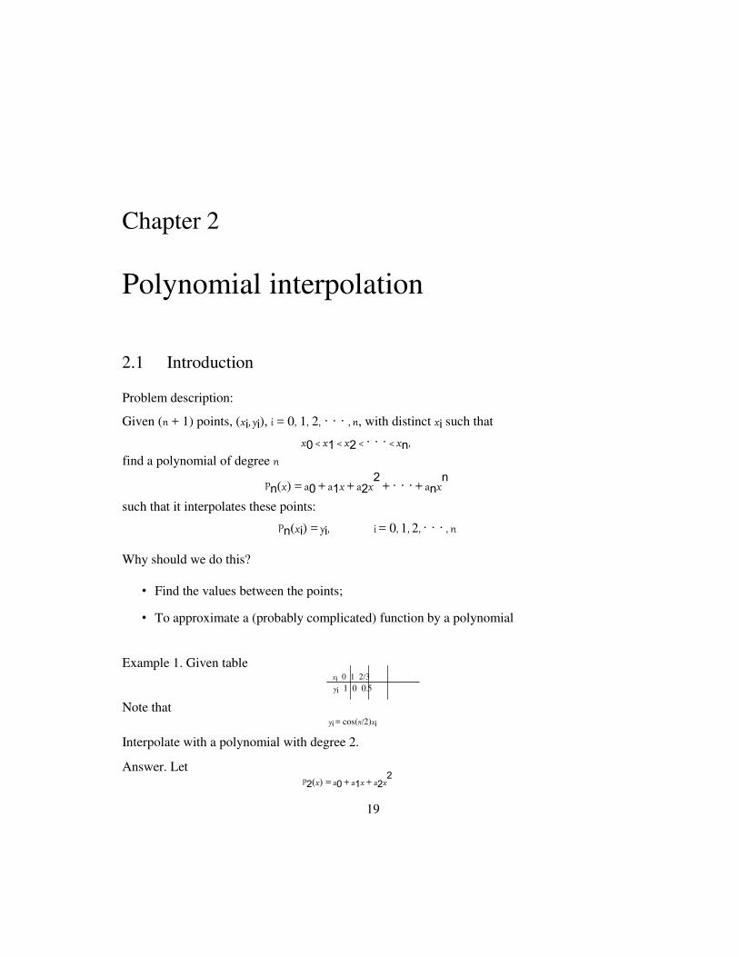
(x − ti+1)3 + Ci(x − ti) − Di(x − ti+1).
6hi 6hi
(You can check by yourself that these Si, Si′ are correct.)

3.3. NATURAL CUBIC SPLINES 35
Interpolating properties:
(1). Si(ti) = yi gives
z
i 1 y
i hi
yi = −
(−hi)3
− Di(−hi) =
zihi2 + Dihi ⇒ Di =
−
zi
6hi 6 hi 6
(2). Si(ti+1) = yi+1 gives
z
i+1 3 y
i+1 hi
yi+1
=
hi + Cihi, ⇒ Ci =
−
zi+1
.
6hi hi 6
We see that, once zi’s are known, then (Ci, Di)’s are known, and so Si, Si′ are known.
z
i+1 zi +
_
yi+1 hi
_ (x − ti)
Si(x) =
(x − ti)3 −
(x − ti+1)3
−
zi+1
6hi 6hi hi 6
− _
y
i h _ (x − ti+1).
−
i zi
hi 6 ′
(x) = z
i+1 (x
−
t )2
−
zi (x
−
t )2 y
i+1 −
y
i
−
zi+1
− z
i h .
hi
Si 2hi i 2hi i+1 6 i
How to compute zi’s? Last condition that’s not used yet: continuity of S′(x), i.e.,
Si′−1(ti) = Si
′(ti), i = 1, 2, · · · , n − 1
We have
′(t ) =
− zi ( h )
2 +
yi+1
−
yi
−
zi+1
−
zi h
Si i 2hi
− i hi 6 i
|
{z
}
bi
1 hi
zi+1 −
1
hizi +
= −
6 3
1 1
Si′−1(ti) =
zi−1
hi−1 +
zi
hi−1
6 3
Set them equal to each other, we get
_
hi−1zi−1 + 2(hi−1 + hi)zi + hizi+1 = 6(bi
−
z0 = zn = 0.
In matrix-vector form: ~
where H · ~z = b
2(h0 + h1)
h
b
i +
bi−1
bi−1), i = 1, 2, · · · , n − 1
h1 2(h1 + h2) h2
h.2 2(h2
+ h ) h
H = . . .
3 .3
. .
. .
h 2(h + h n−2 ) h

n−3
n−3
n−2
hn−2
2(hn−2 + hn−1)

36
and
z1
z2
~z = z.3 ,
..
z n−2
zn−1
6(b1 ~
b = 6(b2 6(b3
6(b n−2
6(bn−1
CHAPTER 3. SPLINES
− b0)
− b1)
.−
b2
) .
..
− bn−3) − bn−2)
Here, H is a tri-diagonal matrix, symmetric, and diagonal dominant
2 |hi−1 + hi| > |hi| + |hi−1| which implies unique solution for ~z. See slides for Matlab codes and solution graphs. Theorem on smoothness of cubic splines. If S is the natural cubic spline function that interpolates a twice-continuously differentiable function f at knots
a = t0 < t1 < · · · < tn = b
then b S
′′(x) 2 dx ≤
Za
b f
′′(x)
2 dx.
Za
_ _
_ _
R Note that (f
′′)2
is related to the curvature of f . Cubic spline gives the least curvature, ⇒ most smooth, so best choice.
Proof. Let
g(x) = f (x) − cS(x)
Then
g(ti) = 0, i = 0, 1, · · · , n
and f ′′ = S
′′ + g
′′, so ′′ 2 ′′ 2 ′′ 2 ′′
g
′′
(f ) = (S ) + (g ) + 2S
⇒ Z
ab(f ′′)2 dx =
Za
b(S′′)2 dx +
Za
b(g′′)2 dx +
Za
b 2S′′g′′ dx
Claim that
Za
b S′′g′′ dx = 0
then this would imply Z b Z b
(f ′′)2
dx ≥ (S′′)2 dx
a a

3.3. NATURAL CUBIC SPLINES 37
and we are done. Proof of the claim: Using integration-by-parts,
b b b
Za S′′g′′ dx = S′′g′ Za S′′′g
′ dx
_a −
_
_
Since g(a) = g(b) = 0, so the first term is 0. For the second term, since S′′′
is piecewise constant. Call
ci = S′′′
(x), for x ∈ [ti, ti+1].
Then n−1
n−1 Zab
S′ ′ ′g′ dx
=
i=0 ci Z
titi+1
g′(x) dx = i=0 ci [g(ti+1) − g(ti)] = 0,
X X
(b/c g(ti) = 0).

38 CHAPTER 3. SPLINES

Chapter 4
Numerical integration
4.1 Introduction
Problem: Given a function f (x) on interval [a, b], find an approximation to the inte-gral
Z b I(f ) = f (x) dx
a Main idea:
• Cut up [a, b] into smaller sub-intervals
• In each sub-interval, find a polynomial pi(x) ≈ f (x)
• Integrate pi(x) on each sub-interval, and sum up
4.2 Trapezoid rule
The grid: cut up [a, b] into n sub-intervals:
x0 = a, xi < xi+1, xn = b
On interval [xi, xi+1], approximate f (x) by a linear polynomial We use
xi+1
xi+1
1
Zxi f (x) dx ≈
Zxi p
i(x) dx = (f (xi+1) + f (xi)) (xi+1 − xi)
2
39

40 CHAPTER 4. NUMERICAL INTEGRATION
f (x) pi(x)
x0 = a xi x
i+1 xn = b
Figure 4.1: Trapezoid rule: straight line approximation in each sub-interval.
Summing up all the sub-intervals
Zab f (x) dx = n−1 x i+1 f (x) dx
i=0
Zxi
X
≈ n−1 x i+1 pi(x) dx
i=0 Z
xi
X
=
n−1 1 (f (xi+1) + f (xi)) (xi+1 − xi)
=0 2
Xi
Uniform grid: h = b−a
, xi+1 − xi = h,
n
b n−1 h
Za f (x) dx = i=0
(f (xi+1) + f (xi))
2
X
= h "
1 n−1
1 f (xn)
#
f (x0) +
f (xi) +
2 2
=1
Xi
| {z }
T (f ; h)
so we can write
Z b f (x) ≈ T (f ; h)
a
Error estimates.
n−1
X ET (f ; h) = I(f ) − T (f ; h) =
i=0
Z x i+1
_
f (x) − pi(x) dx
xi
_

4.2. TRAPEZOID RULE 41
Known from interpolation:
f (x) − pi(x) =
12 f
′′(ξi)(x − xi)(x − xi+1)
Basic error: error on each sub-interval:
1
xi+1
1
ET,i(f ; h) = f ′′(ξi)
Zxi (x − xi)(x − xi+1) dx = − h
3f ′′(ξi).
2 12
Total error: n−1 n−1
1 3
ET (f ; h) = ET,i(f ; h) =
− ′′
h f
(ξi) =
12
=0 i=0
X
i X
Total error is
b 12−a
Error bound
ET (f ; h) = h2
f ′′(ξ),
b − a
E (f ; h) ≤
h2
max
T 12 x∈(a,b)
1
n−1
# 1
b − a
h3 f
′′(ξ )
− 12 · n ·
" =0 i h
Xi = n
= f ′ ′
(ξ)
| {z } | {z }
ξ ∈ (a, b). _ ′ ′
(x)_ ._ f
Example Consider function f (x) = ex, and the integral
Z 2 I(f ) = e
x dx
0
Require error ≤ 0.5 × 10⁻⁴
. How many points should be used in the Trapezoid rule? Answer. We have
f ′(x) = e
x, f
′′(x) = e
x, a = 0, b = 2
so _
f ′′(x)_ = e
2.
max
_ _
x∈(a,b) By error bound, it is sufficient to require
|ET (f ; h)| ≤ 16 h
2e2 ≤ 0.5 × 10
−4 ⇒ h
2 ≤ 0.5 × 10
−4 × 6 × e
−2 ≈ 4.06 × 10
−5 ⇒ n
2 = h ≤
p4.06 × 10
−5 = 0.0064
2
⇒ n ≥ 0.0064 ≈ 313.8 We need at least 314 points.

42 CHAPTER 4. NUMERICAL INTEGRATION
4.3 Simpson’s rule Cut up [a, b] into 2n equal sub-intervals
b − a
x0
=
a, x2n
=
b, h
= 2n
, xi+1
−
xi
=
h
Consider the interval [x2i, x2i+2]. Find a 2nd order polynomial that interpolates f (x) at the
points
x2i
, x2i+1
, x2i+2
pi(x)
f (x) ✠
x2i
x2i+1
x2i+2
Figure 4.2: Simpson’s rule: quadratic polynomial approximation (thick line) in each sub-interval. Lagrange form gives
pi(x) = f (x2i) (x − x2i+1)(x − x2i+2) + f (x2i+1) (x − x2i)(x − x2i+2)
(x
2i −
x
2i+1)(x
2i −
x
2i+2)
(x2i+1
− x
2i)(x
2i+1 −
x
2i+2)
+f (x2i+2) (x − x2i)(x − x2i+1)
(x
2i+2 −
x
2i)(x
2i+2 −
x
2i+1)
1 1
=
f (x2i)(x − x2i+1)(x − x2i+2) −
f (x2i+1)(x − x2i)(x − x2i+2)
2h2 h
2
1 +
2h2
f
(x2i+2
)(x
−
x2i
)(x
−
x2i+1
)

4.3. SIMPSON’S RULE 43
Then
x x
Z
x2i2i+2 f (x) dx ≈
Zx2i
2i+2 pi(x) dx
1 x
2i+2
= f
(x2i
)f
(x2i
)
Zx2i (x − x2i+1)(x − x2i+2) dx
2h2
2 3
h
|
{z }
3
1 x
2i+2
−
f
(x2i+1
)
Zx2i (x − x2i)(x − x2i+2) dx
h2
4
|
{z −
h3 }
3
1 x
2i+2
+
f
(x2i+2
)
Zx2i (x − x2i)(x − x2i+1) dx
2h2
|
2
{z
}
h3
3
=
h [f (x2i) + 4f (x2i+1) + f (x2i+2)]
3
Putting together
Z
b f (x) dx ≈ S(f ; h)
a
= n−1 x
i=0 Zx2i
2i+ 2 p
i(x) dx
X
=
h n−1
[f (x2i) + 4f (x2i+1) + f (x2i+2)]
3 =0
X
i
1
= 2
4 1
1 4 1
x
2i−2 x
2i−1 x
2i x
2i+1 x
2i+2
Figure 4.3: Simpson’s rule: adding the constants in each node. See Figure 4.3 for the counting of coefficients on each node. Wee see that for x0, x2n we get
1, and for odd indices we have 4, and for all remaining even indices we get 2. The algorithm looks like:
h
n n−1
S(f ; h) = "
f (x0) + 4 f (x2i−1) + 2 f (x2i) + f (x2n)#
3
=1 i=1
Xi X

44 CHAPTER 4. NUMERICAL INTEGRATION
Error estimate. basic error is
1 5 (4)
−
h f
(ξi), ξi ∈
(x
2i, x
2i+2)
90
so
1
n−1 1
b − a
b − a
E (f ; h) = I(f ) S(f ; h) = h5 f (4)(ξ ) = h4f (4) (ξ), ξ(a, b)
− −
90 n ·
− 180
S =0 i 2h
Xi
Error bound
b − a
| E (f ; h) h4
max f (4)
(x) .
S
| ≤ 180 x∈(a,b)
_
_
_
_
_ _
Example With f (x) = ex in [0, 2], now use Simpson’s rule, to achieve an error ≤ 0.5 × 10
−4,
how many points must one take? Answer. We have
|ES (f ; h)| ≤ 1802
h4
e2 ≤ 0.5 × 10
−4
⇒ h4
≤ 0.5−4
× 180/e2
= 1.218 × 10⁻³
⇒ h ≤ 0.18682
⇒ n = b
−
a
= 5.3 ≈ 6 2h
We need at least 2n + 1 = 13 points. Note: This is much fewer points than using Trapezoid Rule.
4.4 Recursive trapezoid rule These are called composite schemes.
Divide [a, b] into 2n
equal sub-intervals.
So
T (f ; hn)
T (f ; hn+1)
hn =
b − a
,
hn+1
=
1
h
2n 2
1
1 2
n −1
f (a + ihn)#
= hn · "
f (a) +
f (b) +
2 2
=1
= hn+1 ·
Xi
f (a + ihn+1)
1 1 2n+1
−1
f (a) + f (b) +
2 2 =1
Xi

4.5. ROMBERG ALGORITHM 45
n = 1
n = 2
n = 3
n = 4
n = 5
n = 6
n = 7
Figure 4.4: Recursive division of intervals, first few levels
We can re-arrange the terms in T (f ; hn+1):
h
1 1 2n−1 2
n−1
f (a + (2j + 1)hn+1)
T (f ; hn+1) = n
f (a) +
f (b) +
f (a + ihn) +
2 2 2 =1
j=1
1 2n−1 Xi X
= T (f ; hn) + hn+1 f (a + (2j + 1)hn+1)
2
j=1
X
Advantage: One case keep the computation for a level n. If this turns out to be not accurate
enough, then add one more level to get better approximation. ⇒ flexibility.
4.5 Romberg Algorithm
If f (n)
exists and is bounded, then we have the Euler MacLaurin’s formula for error
E(f ; h) = I(f ) − T (f ; h) = a2h2 + a4h
4 + a6h
6 + · · · + anh
n
h h h 2 h 4 h 6 h n
E(f ;
) = I(f ) − T (f ;
) = a2 (
) + a4 (
) + a6 (
) + · · · + an(
)
2 2 2 2 2 2
Here an depends on the derivatives f (n)
. We have
(1) I(f ) = T (f ; h) + a2h2 + a4h
4 + a6h
6 + · · ·
(2) I(f ) = T (f ;
h h 2 h 4 h 6 h n
) + a2 (
)
+ a4(
)
+ a6(
)
+ · · · + an(
)
2 2 2 2 2
The goal is to use the 2 approximations T (f ; h) and T (f ; h2 ) to get one that’s more accurate,
i.e., we wish to cancel the leading error term, the one with h2.
Multiply (2) by 4 and subtract (1), gives
3 · I(f ) = 4 · T (f ; h/2) − T (f ; h) + a4′h
4 + a6
′h
6 + · · ·
⇒ I(f ) = 4
T (f ; h/2) − 1
T (f ; h) +˜a4h4
+ a˜6h6
+ · · ·
3 3
|
}
U (h){z
46 CHAPTER 4. NUMERICAL INTEGRATION
R(h) is of 4-th order accuracy! Better than T (f ; h). We now write:
U (h) = T (f ; h/2) + T (f ; h/2) − T (f ; h)
22 − 1
This idea is called the Richardson extrapolation.
Take one more step:
(3) I(f ) = U (h) + a˜4h4 + a˜6h
6 + · · ·
(4) I(f ) = U (h/2) + a˜4(h/2)4 + a˜6(h/2)
6 + · · ·
To cancel the term with h4
: (4) × 24
− (3)
(24
− 1)I(f ) = 24U (h/2) − U (h) + a˜
′6h
6 + · · ·
Let
24U (h/2) − U (h)
U (h/2) − U (h)
V (h) = = U (h/2) + .
24
− 1 24 − 1
Then
I(f ) = V (h) + a˜′6h
6 + · · ·
So V (h) is even better than U (h). One can keep doing this several layers, until desired accuracy is reached. This
gives the Romberg Algorithm: Set H = b − a, define:
R(0, 0) = T (f ; H) = H (f (a) + f (b))
2
R(1, 0) = T (f ; H/2)
R(2, 0) = T (f ; H/(22
))
.
.
.
R(n, 0) = T (f ; H/(2n
))
Here R(n, 0)’s are computed by the recursive trapezoid formula.
Romberg triangle: See Figure 4.5.
The entry R(n, m) is computed as
R(n, m) = R(n, m
−
1) + R(n, m − 1) − R(n − 1, m − 1)
22m−1
Accuracy: H
I(f ) = R(n, m) + O(h2(m+1)
),h =
.
2n
Algorithm can be done either column-by-column or row-by-row. Here we give some pseudo-code, using column-by-column.

4.6. ADAPTIVE SIMPSON’S QUADRATURE SCHEME 47
R(0, 0)
s
R(1, 0) ✲
R(1, 1)
s s
R(2, 0) ✲
R(2, 1) ✲
R(2, 2)
s s s
R(3, 0) ✲
R(3, 1) ✲
R(3, 2) ✲
R(n, 0) R(n, 1) R(n, 3) R(n, n)
Figure 4.5: Romberg triangle
R =romberg(f, a, b, n)
R = n × n matrix
h = b − a; R(1, 1) = [f (a) + f (b)] ∗ h/2;
for i = 1 to n − 1 do %1st column recursive trapezoid
R(i + 1, 1) = R(i, 1)/2; h = h/2;
for k = 1 to 2i−1
do
R(i + 1, 1) = R(i + 1, 1) + h ∗ f (a + (2k − 1)h) end
end
for j = 2 to n do %2 to $n$ column
for i = j to n do
R(i, j) = R(i, j − 1) + 4j
1−1 [R(i, j − 1) − R(i − 1, j − 1)]
end
end
4.6 Adaptive Simpson’s quadrature scheme Same idea can be adapted to Simpson’s rule instead of trapezoid rule. For interval [a, b], h = b−a ,
2
S [a, b] = b − a f (a) + 4f ( a + b ) + f (b)
6
1 _ 2 _
Error form: 1
5 (4)
E1[a, b] = −
h f
(ξ), ξ(a, b)
90
48 CHAPTER 4. NUMERICAL INTEGRATION
Then I(f ) = S1[a, b] + E1[a, b]
Divide [a, b] up in the middle, let c = a+
2b
.
I(f )[a, b] = I(f )[a, c] + I(f )[c, b] = S1[a, c] + E1[a, c] + S1[c, b] + E1[c, b] = S2[a, b] + E2[a, b]
where
S2[a, b] = S1[a, c] + S1[c, b]
E2[a, b] = E1[a, c] + E1[c, b] = −
1
(h/2)5 h
f (4)(ξ1) + f (4)(ξ2)i
90
Assume f (4)
does NOT change much, then E1[a, c] ≈ E1[c, b], and
E2[a, b] ≈ 2E1[a, c] = 2
1 E1 [a, b] =
1 E1 [a, b]
25 2
4
This gives
S2[a, b] − S1[a, b] = (I − E2[a, b]) − (I − E1[a, b]) = E1 − E2 = 24
E2 − E2 = 15E2
This means, we can compute the error E2:
1
E2
= 15
(S2
−
S1
)
If we wish to have |E2| ≤ , we only need to require S2
− S1 ≤
24 − 1
This gives the idea of an adaptive recursive formula:
(A) I = S1 + E1 1
(B) I
= S2
+ E2
= S2
+ 24
E1
(B) ∗ 24 − (A) gives
(24 − 1)I = 2
4S2 − S1
⇒
I = 24
S2 − S1 = S
2
+ S2 − S1
24 − 1
15
Note that this gives the best approximation when f (4)
≈ const. Pseudocode: f : function, [a, b] interval, : tolerance for error

4.7. GAUSSIAN QUADRATURE FORMULAS 49
answer=simpson(f, a, b, )
compute S1 and S2
If |S2 − S1| < 15
answer= S2 + (S2 − S1)/15; else
c = (a + b)/2; Lans=simpson(f,
a, c, /2); Rans=simpson(f, c, b,
/2); answer=Lans+Rans;
end In Matlab, one can use quad to compute numerical integration. Try help quad, it will give you info on it. One can call the program by using:
a=quad(’fun’,a,b,tol) It uses adaptive Simpson’s formula. See also quad8, higher order method.
4.7 Gaussian quadrature formulas We seek numerical integration formulas of the form
Z b f (x) dx ≈ A0f (x0) + A1f (x1) + · · · + Anf (xn),
a
with the weights Ai, (i = 0, 1, · · · , n) and the nodes
xi ∈ (a, b), i = 0, 1, · · · , n How to find nodes and weights?
Nodes xi: are roots of Legendre polynomials q Z
b xk
qn+1(x) dx = 0, a
n+1(x). These polynomials satisfies
(0 ≤ k ≤ n)
Examples for n ≤ 3, for interval [−1, 1]
q0(x) = 1
q1(x) = x
q2(x) = 3
x 2 −
1
2 2
q3(x) = 5
x 3 −
3 x
2 2
50 CHAPTER 4. NUMERICAL INTEGRATION
The roots are
q1 : 0 √
q2 : ±1/
3
± p
q3 : 0, 3/5
For general interval [a, b], use the transformation:
t = 2x − (a + b) , x = 1 (b −
a)t + 1 (a + b)
2 2
b −
a
so for −1 ≤ t ≤ 1 we have a ≤ x ≤ b.
Weights Ai: Recall li(x), the Cardinal form in Lagrange polynomial: n
x − xj
li(x) = =0,j=6i
j
xi
−
xj
Y
Then
Z−
ba li(x) dx.
Ai =
There are tables of such nodes and weights (Table 5.1 in textbook). We
skip the proof. See textbook if interested.
Advantage: Since all nodes are in the interior of the interval, these formulas can han-dle
integrals of function that tends to infinite value at one end of the interval (provided that the
integral is defined). Examples:
Z 1
x−1
dx, Z 1
(x2 − 1)
1/3psin(ex − 1) dx.
0 0

Chapter 5
Numerical solution of nonlinear equations.
5.1 Introduction
Problem: f (x) given function, real-valued, possibly non-linear. Find a root r of f (x) such that f (r) = 0.
Example 1. Quadratic polynomials: f (x) = x2 + 5x + 6.
f (x) = (x + 2)(x + 3) = 0, ⇒ r1 = −2, r2 = −3.
Roots are not unique.
Example 2. f (x) = x2 + 4x + 10 = (x + 2)
2 + 6. There are no real r that would satisfy
f (r) = 0.
Example 3. f (x) = x2 + cos x + e
x +
√
x + 1. Roots can be difficult/impossible to find
analytically.
Our task now: use a numerical method to find an approximation to a root. Overview
of the chapter:
• Bisection (briefly)
• Fixed point iteration (main focus): general iteration, and Newton’s method
• Secant method
Systems (*) optional...
51

52 CHAPTER 5. NUMERICAL SOLUTION OF NONLINEAR EQUATIONS.
5.2 Bisection method
Given f (x), continuous function.
• Initialization: Find a, b such that f (a) · f (b) < 0. This
means there is a root r ∈ (a, b) s.t. f (r) = 0.
• Let c = a+
2b
, mid-point.
• If f (c) = 0, done (lucky!)
• else: check if f (c) · f (a) < 0 or f (c) · f (b) < 0.
• Pick that interval [a, c] or [c, b], and repeat the procedure until stop criteria satis-fied.
Stop Criteria:
1) interval small enough
2) |f (cn)| almost 0
3) max number of iteration reached
4) any combination of the previous ones.
Convergence analysis: Consider [a0, b0], c0 = a0+b+0
, let r ∈ (a0, b0) be a root. The 2
error:
b0 − a0
e = r c
| ≤
0 | −
0 2
Denote the further intervals as [an, bn] for iteration no. n. Then
e = r c bn − an
≤
b0 − a0 = e0 .
n | − n| ≤ 2 2n+1 2n
If the error tolerance is , we require en ≤ , then
b0 − a0
≤
⇒
n log(b − a) − log(2 ) , (# of steps)
2n+1
≥ log 2
Remark: very slow convergence.
5.3 Fixed point iterations
Rewrite the equation f (x) = 0 into the form x = g(x). Remark: This can always be achieved, for example: x = f (x) + x. The catch is that, the choice of g
makes a difference in convergence. Iteration algorithm:

5.3. FIXED POINT ITERATIONS 53
• Choose a start point x0,
• Do the iteration xk+1 = xk, k = 0, 1, 2, · · · until meeting stop crietria.
Stop Criteria: Let be the tolerance
• |xk − xk−1| ≤ ,
• |xk − g(xk )| ≤ , • max # of iteration reached,
• any combination.
Example 1. f (x) = x − cosx. Choose g(x) = cos x, we have x = cos x.
Choose x0 = 1, and do the iteration xk+1 = cos(xk):
x1 = cos x0 = 0.5403
x2 = cos x1 = 0.8576 x3 = cos x2 = 0.6543
. .
.
x23 = cos x22 = 0.7390
x24 = cos x23 = 0.7391
x25 = cos x24 = 0.7391 stop here
Our approximation to the root is 0.7391.
Example 2. Consider f (x) = e−2x
(x − 1) = 0. We see that r = 1 is a root. Rewrite as
x = g(x) = e−2x
(x − 1) + x Choose an initial guess x0 = 0.99, very close to the real root. Iterations:
x1 = cos x0 = 0.9886
x2 = cos x1 = 0.9870
x3 = cos x2 = 0.9852
. .
.
x27 = cos x26 = 0.1655
x28 = cos x27 = −0.4338
x29 = cos x28 = −3.8477 Diverges. It does not work.
Convergence depends on x0 and g(x)!

54 CHAPTER 5. NUMERICAL SOLUTION OF NONLINEAR EQUATIONS.
Convergence analysis. Let r be the exact root, s.t., r = g(r).
Our iteration is xk+1 = g(xk ).
Define the error: ek = xk − r. Then,
ek+1 = xk+1 − r = g(xk ) − r = g(xk) − g(r)
= g′(ξ)(xk − r)(ξ ∈ (xk, r), since g is continuous)
= g′(ξ)e
k
g′(ξ)
_ |ek|
⇒ |ek+1| ≤ _
Observation: _ _
• If |g′(ξ)| < 1, error decreases, the iteration convergence. (linear convergence)
• If |g′(ξ)| ≥ 1, error increases, the iteration diverges.
Convergence condition:′ There exists an interval around r, say [r − a, r + a] for some
a > 0, such that |g (x)| < 1 for almost all x ∈ [r − a, r + a], and the initial guess x0 lies
in this interval.
In Example 1, g(x) = cos x, g′(x) = sin x, r = 0.7391,
_g′(r)
_ = |sin(0.7391)| < 1. OK, convergence.
_ _
In Example 2, we have
g(x) = e−2x
(x − 1) + x,
g′(x) = −2e
−2x(x − 1) + x
−2x + 1
With r = 1, we have _
g′(r_
= e−2
+ 1 > 1
Divergence. _ _
Pseudo code:
r=fixedpoint(’g’, x,tol,nmax} r=g(r); nit=1;
while (abs(r-g(r))>tol and nit < nmax) do r=g(r);
nit=nit+1;
end

5.4. NEWTON’S METHOD 55
How to compute the error?
Assume |g′(x)| ≤ m < 1 in [r − a, r + a].
We have |ek+1| ≤ m |ek|. This gives
|e1| ≤ m |e0| , |e2| ≤ m |e1| ≤ m2 |e0| , · · · |ek| ≤ m
k |e0|
We also have
|e0| = |r − x0| = |r − x1 + x1 − x0| ≤ |e1| + |x1 − x0| ≤ m |e0| + |x1 − x0| then
|e0| ≤ 1
|x1 − x0| ,(can be computed)
1 −
m
Put together m
k |e
k
| ≤ 1 − m
|x1
−
x0
|
.
If the error tolerance is , then
mk x
−
x
| ≤
,
⇒
mk
≤
(1 − m)
⇒
k
≥
ln( (1 − m)) − ln |x1 − x0|
1 − m | 1 0 |x1 − x0| ln m
which give the maximum number of iterations needed to achieve an error ≤ .
Example cos x − x = 0, so
x = g(x) = cos x, g′(x) = − sin x
Choose x0 = 1. We know r ≈ 0.74. We see that the iteration happens between x = 0 and x = 1.
For x ∈ [0, 1], we have _ _ _
g′(x)
_ ≤ sin 1 = 0.8415 = m
And x1 = cos x0 = cos 1 = 0.5403. Then, to achieve an error ≤ = 10−5
, the maximum # iterations needed is
k ≥ ln( (1
−
m))
− ln
|x1
−
x0
| ≈ 73. ln m
Of course that is the worst situation. Give it a try and you will find that k = 25 is enough.

56 CHAPTER 5. NUMERICAL SOLUTION OF NONLINEAR EQUATIONS.
f
(x) ✻ f ′(xk)
✲ x
xk+1
xk
Figure 5.1: Newton’s method: linearize f (x) at xk.
5.4 Newton’s method Goal: Given f (x), find a root r s.t. f (r) = 0.
Choose an initial guess x0. Once you have xk, the next approximation xk+1 is determined by treating f (x) as a linear
function at xk. See Figure 5.1. We have
f (xk) ′
= f (xk)
x
k
−
xk+1
which gives
xk+1 = xk −
f (xk) f (xk)
= xk − xk, xk =
.
f ′(xk) f
′(xk)
Connection with fixed point iterations:
f (x) = 0, ⇒ b(x)f (x) = 0, ⇒ x = x − b(x)f (x) = g(x) Here the function b(x) is chosen in such a way, to get fastest possible convergence. We have
g′(x) = 1 − b
′(x)f (x) − b(x)f
′(x)
Let r be the root, such that f (r) = 0, and r = g(r). We have
g′(r) = 1 − b(r)f
′(r), smallest possible:
_
g′(r)_ = 0.
Choose now 1 _ _
1 − b(x)f ′(x) = 0, ⇒ b(x) =
f ′(x)
we get a fixed point iteration for
f (x)
x
=
g(x) =
x
− f ′(x)
.

5.4. NEWTON’S METHOD 57
Convergence analysis. Let r be the root so f (r) = 0 and r = g(r). Define error:
ek+1 = |xk+1 − r| = |g(xk ) − g(r)|
Taylor expansion for g(xk) at r:
1
(xk − r)2
g′′(ξ), ξ ∈ (xk, r)
g(xk ) = g(r) + (xk − r)g′(r) +
2
Since g′(r) = 0, we have
g(xk) = g(r) + 1
(xk − r)2
g′′(ξ)
2
Back to the error, we now have
ek+1
= 1 (x r)
2
_
g′′(ξ) = 1 e
2
_
g′′(ξ)
Write again m = maxx g ′′ 2 k
− _ 2
k _
(ξ) , we have _ _ _ _
| |
ek+1 ≤ m e2
k This is called Quadratic convergence. Guaranteed convergence if e0 is small enough! (m can be big, it would
effect the convergence!) Proof for the convergence: (can drop this) We have
e1 ≤ m e0e0 If e0 is small enough, such that m e0 < 1, then e1 < e0.
Then, this means m e1 < me0 < 1, and so
e2 ≤ m e1e1 < e1, ⇒ m e2 < me1 < 1
Continue like this, we conclude that ek+1 < ek for all k, i.e., error is strictly decreasing after
each iteration. ⇒ convergence. Example Find an numerical method to compute
√a using only +, −, ∗, / arithmetic operations. Test it for
a = 3.
Answer. It’s easy to see that √
a is a root for f (x) = x2 − a.
Newton’s method gives
x = x f (xk) = x
k
−
xk2
− a = xk + a
k+1 k −
f ′(xk)
2xk
2xk 2
Test it on a = 3: Choose x0 = 1.7.
error
x0 = 1.7 7.2 × 10−2
x1 = 1.7324 3.0 × 10⁻⁴
−8
x2 = 1.7321 2.6 × 10−16
x3 = 1.7321 4.4 × 10
Note the extremely fast convergence. Usually, if the initial guess is good (i.e., close to r), usually a couple of iterations are enough to get an very accurate approximation.

58 CHAPTER 5. NUMERICAL SOLUTION OF NONLINEAR EQUATIONS.
Stop criteria: can be any combination of the following:
• |xk − xk−1| ≤
• |f (xk)| ≤ • max number of iterations reached.
Sample Code:
r=newton(’f’,’df’,x,nmax,tol) n=0; dx=f(x)/df(x);
while (dx > tol) and (f(x) > tol) and (n<nmax) do n=n+1;
x=x-dx;
dx=f(x)/df(x);
end
r=x-dx;
5.5 Secant method
If f (x) is complicated, f ′(x) might not be available.
Solution for this situation: using approximation for f ′, i.e.,
f ′(xk) ≈ f (x
k) −
f (x
k−1) x
k
−
xk−1
This is secant method:
xk −
x
k−1
xk+1
=
xk
− f (xk) − f (xk−1)
f
(xk
)
Advantages include
• No computation of f ′;
• One f (x) computation each step;
• Also rapid convergence.
A bit on convergence: One can show that
ek+1 ≤ Ce k, = 12 (1 +
√5) ≈ 1.62 This is
called super linear convergence. (1 < < 2)
5.6. SYSTEM OF NON-LINEAR EQUATIONS 59
It converges for all function f if x0 and x1 are close to the root r.
Example Use secant method for computing √
a. Answer. The iteration now becomes
x
= x
k
−
(xk2 − a)(xk − xk−1)
= x
xk2 − a
k+1 (xk2
− a) − (xk2
−1 − a) k −
xk + xk+1
Test with a = 3, with initial data x0 = 1.65, x1 = 1.7.
error
x1 = 1.7 7.2 × 10−2
x2 = 1.7328 7.9 × 10−4
x3 = 1.7320 7.3 × 10−6
x4 = 1.7321 1.7 × 10−9
x
5 = 1.7321 3.6 × 10⁻¹⁵
It is a little but slower than Newton’s method, but not much.
5.6 System of non-linear equations Consider the system
F(~x) = 0, F = (f1, f2, · · · , fn)t,
write it in detail:
f1(x1, x2, · · · , xn)
f2(x1, x2, · · · , xn)
fn(x1, x2, · · · , xn)
We use fixed point iteration. Same idea: choose ~x0
~x = G(~x)
The iteration is simply:
~xk+1 = G(~xk).
Newton’s mathod:
~xk+1 = ~xk − Df (~xk)−1
~x = (x1, x2, · · · , xn)t
= 0 = 0
.
.
. = 0
. Rewrite as
· F(~xk)

60 CHAPTER 5. NUMERICAL SOLUTION OF NONLINEAR EQUATIONS.
where Df (~xk) is a Jacobian matrix of f
∂f1 ∂f1
∂x1 ∂x2
∂f2 ∂f2
Df = ∂x1 ∂x2
..
.. .
.
∂fn ∂fn
∂x1 ∂x2
and Df (~xk)−1
is the inverse matrix of Df (~xk).
· · ·
· · ·
. . . · · ·
∂f1
∂xn ∂f2 ∂xn
. . .
∂fn
∂xn

Chapter 6
Direct methods for linear systems
6.1 Introduction The problem:
a11x1 + a12x2 + + a1nxn = b1 (1)
a21x1 + a22x2 + · · ·
+ a2nxn = b2 (2)
(A) : · · · ..
.
an1x1 + an2x2 + · · · + annxn = bn (n)
We have n equations, n unknowns, can be solved for xi if aij are “good”.
In compact form, for equation i:
n
aij xj = bi, i = 1, · · · , n.
j=1
X
Or in matrix-vector form: ~
A~x = b,
where A ∈ IR
n×n
,
n ~ n
~x ∈ IR , b ∈ IR
a11 a12 · · · a
1n
x1
b1
a21 a22 · · · a
2n x2 ~ b2
A = aij }
= .. .
,~x = . , b = . .
{ .... . . . .
. .. ..
a a n2 a x b
n1
· · ·
nn n n
Our goal: Solve for ~x. — We will spend 3 weeks on it. Methods and topics:
• Different types of matrix A:

61

62 CHAPTER 6. DIRECT METHODS FOR LINEAR SYSTEMS
1. Full matrix
2. Large sparse system
3. Tri-diagonal or banded systems
4. regularity and condition number
• Methods
A. Direct solvers (exact solutions): slow, for small systems ∗ Gaussian elimination, with or without pivoting ∗ LU factorization
B. Iterative solvers (approximate solutions, for large sparse systems) ∗ more interesting for this course ∗ details later...
6.2 Gaussian elimination, simplest version
Consider system (A). The basic Gaussian elimination takes two steps: Step
1: Make an upper triangular system – forward elimination.
for k = 1, 2, 3, · · · , n − 1
(j) ← (j) − (k) ×
ajk
, j = k + 1, k + 2, · · · , n
akk
You will make lots of zeros, and the system becomes:
a11x1 + a12x2 + + a1nxn = b1 (1)
a22x2 + · · ·
+
a
2nx
n = b2 (2)
(B) : · · · ..
.
ann
xn
=
bn (n)
Note, here the aij and bi are different from those in (A). Step 2: Backward substitution – you get the solutions.
xn =
bn
ann
1
bi −
n
aij xj ,i = n − 1, n − 2, · · · , 1.
xi =
aii =i+1
j
X
Potential problem: In step 1, if some akk is very close to or equal to 0, then you are in trouble.

6.3. GAUSSIAN ELIMINATION WITH SCALED PARTIAL PIVOTING 63
Example 1. Solve
x1 + x2 + x3 = 1 (1)
2x 1 + 4x 2 + 4x 3 = 2 (2)
3x1 + 11x2 + 14x3 = 6 (3)
Forward elimination:
(1) ∗ (−2) + (2) : ′
2x2 + 2x3 = 0 (2′)
(1) ( 3) + (3) : x = 3 (3 )
′ ∗ − ′ 8x
2 + 11
′′3
(2 ) ∗ (−4) + (3 ) : 3x3 = 3 (3 )
Your system becomes
x + x + x = 1
1 2x 2
2+ 2x
3 = 0
3
3x3 = 3
Backward substitution:
x3 = 1
x2 =
1
(0 − 2x3) = −1
2
x1 = 1 − x2 − x3 = 1 It works fine here, but not always.
6.3 Gaussian Elimination with scaled partial pivoting First, an example where things go wrong with Gaussian elimination.
Example 2. Solve the system with 3 significant digits.
_ 0.001x1 −x2 = −1 (1)
x1 2x2 = 3 (2) Answer. Write it with 3 significant digits
_ −1.00x2
−1.00
0.00100x1 = (1)
1.00x1 2.00x2 = 3.00 (2)
Now, (1) ∗ (−1000) + (2) gives
(1000 + 2)x2 = 1000 + 3 ⇒ 1.00 · 103x2 = 1.00 · 10
3
⇒ x2 = 1.00

64 CHAPTER 6. DIRECT METHODS FOR LINEAR SYSTEMS
Put this back into (1) and solve for x1:
1 1
x1 =
(−1.00 + 1.00x2) =
· 0 0
0.001 0.001
.
Note that x1 is wrong!! What is the problem? We see that 0.001 is a very small number! One
way around this difficulty: Change the order of two equations.
_
1.00x1 2.00x2 = 3.00 (1)
0.00100x1 −1.00x2 = −1.00 (2)
Now run the whole procedure again: (1) ∗ (−0.001) + (2) will give us x2 = 1.00.
Set it back in (1): x1 = 3.00 − 2.00x2 = 1.00
Solution now is correct for 3 digits. Conclusion: The order of equations can be important!
Consider
a11
x1
+ a12
x2 = b1
_ a21x1 + a22x2 =
b2
Assume that we have computed x˜2 = x2 + 2 where 2 is the error (machine error, round off error
etc).
We then compute x1 with this x˜2:
x˜1 =
1
(b1 − a12x˜2)
a11
=
1
(b1 − a12x2 − a12 2)
a11
1 a12
=
(b1 − a12x2) −
2
a11 a
11
=
|
x1 −}
1
Note that 1 = a12
2. Error in x2 {z | {z } a12
a11 propagates with a factor of a11 .
For best results, we wish to have |a11| as big as possible.
Scaled Partial Pivoting. Idea: use maxk≤i≤n |aik| for aii.
Procedure:
1. Compute a scaling vector
~s = [s1, s2, · · · , sn], where
max
si =
1≤j≤n |a
ij |
Keep this ~s for the rest of the computation.

6.3. GAUSSIAN ELIMINATION WITH SCALED PARTIAL PIVOTING 65
2. Find the index k s.t. _ a
k1 _
_ a
i1 _
≥ , i = 1, · · · , n
sk si
_ _ _ _ Exchange eq (k) and (1), and do 1 step of elimination. You get
_ _ _ _
_ _ _ _
ak1
x1
+ a
k2x
2 +
· · ·
+ a
knx
n = bk (1)
a22x2 + + a2nxn = b2 (2)
· · · ..
.
a 12 x 2 + + a 1n x n = b 1 (k)
· · · .
..
a n2 x
2 + + a nn x
n = b n (n)
· · ·
3. Repeat (2) for the remaining (n − 1) × (n − 1) system, and so on.
Example Solve the system using scaled partial pivoting.
+ 2x + x = 3 (1)
3xx1
+ 4x 2
2+ 0x
3 = 3 (2)
1
3
2x1 + 10x2 + 4x3 = 10 (3)
Answer. We follow the steps.
1. Get ~s.
~s = [2, 4, 10]
2. We have a11
1 a
21
3 a
31
2
=
,
=
,
=
, ⇒ k = 2
s
1 2 s
2 4 s
3 10
Exchange eq (1) and (2), and do one step of elimination
3x
1
+ 4x2 + 0x3 = 3 (2)
2 x 2 + x
3 = 2 (1
′) = (1) + (2)
∗ ( 1 )
3
3
22 = 8 ′ = (3) + (2) ∗ (− 2
3 x
2 + 4x
3 (3 ) 3 )
3. For the 2 × 2 system,
a¯ 12 2/3 1 a¯ 32 22/3 22
=
=
,
=
=
⇒ k = 3.
s1 2 3 s3 10 30
Exchange (3’) and (1’) and do one step of elimination
4x + 0x = 3 (2)

3x1
+22 x2 + 4x
3 = 8 (3
′)
3 2
3
7 = 14 ′′ ′ ′ 1
11 x
3 11 (1 ) = (1 ) + (3 ) ∗ (− 11 )

66 CHAPTER 6. DIRECT METHODS FOR LINEAR SYSTEMS
4. Backward substitution gives
x3 = 2,x2 = 0,x1 = 1. In MAtlab, to solve Ax = b, one can use:
> x= A\b;
6.4 LU-Factorization Without pivoting: One can write A = LU where
L: lower triangular matrix with unit diagnal
U : upper triangular matrix
1 0 0 · · · 0
u11 u12 · · ·
l21 1 0 · · · 0 0 u22 · · ·
l31
l32 1
·. · · 0
. .
L = , U = ..
. .
.. . 0
.. .
.
. . ..
0
l l l 1 0 0 · · ·
n1 n2 n3
· · ·
· · ·
u1,(n−1)
u2,(n−1)
.
.
. u
(n−1),(n−1) 0
u
1n u2n
.
.
. u(n−1),n u
nn
Theorem If Ax = b can be solved by Gaussian elimination without pivoting, then we can write A = LU uniquely. Use this to solve Ax = b: Let y = Ux, then we have
_ U x = y L y = b
Two triangular system. We first solve y (by forward substitution), then solve x (by backward substitution).
With pivoting:
LU = P A where P is the pivoting matrix. Used in Matlab:

6.5. REVIEW OF LINEAR ALGEBRA 67 > [L,U]=lu(A); > y = L \ b; > x = U \ y;
+ transparences. Work amount for direct solvers for A ∈ IR
n×n: operation count
flop: one float number operation (+, -, *, / )
Elimination: 13 (n
3 − n) flops Backward
substitution: 12 (n
2 − n) flops
Total work amount is about 13 n
3 for large n.
This is very slow for large n. We will need something more efficient.
6.5 Review of linear algebra
Consider a square matrix A = {aij }.
Diagonal dominant system. If
n
|aii| > |aij | , i = 1, 2, · · · , n
j
=1,j=6i
X
then A is called strictly diagonal dominant. And A has the following properties:
• A is regular, invertible, A−1
exists, and Ax = b has a unique solution.
• Ax = b can be solved by Gaussian Elimination without pivoting.
One such example: the system from natural cubic spline.
Vector and matrix norms: A norm: measures the “size” of the vector and matrix.
General norm properties: x ∈ IRn
or x ∈ IRn×n
. Then, kxk satisfies
1. kxk ≥ 0, equal if and only if x = 0;
2. kaxk = |a| · kxk, a: is a constant;
3. kx + yk ≤ kxk + kyk, triangle inequality.

68 CHAPTER 6. DIRECT METHODS FOR LINEAR SYSTEMS
Examples of vector norms: x ∈ IRn
n
1. kxk1 = |xi|, l1-norm
=1
Xi
n
!
1/2
2. kxk2 = xi2 , l2-norm
=1
Xi
3.
kxk∞ =
max x
i
|
, l -norm
1≤i≤n | ∞
Matrix norm related to the corresponding vector norm, A ∈ IRn×n
kAk = max kAxk
~x6=0 kxk Obviously we have
A kAxk Ax A x
k k ≥ kxk ⇒ k k ≤ k k · k k
In addition we have
kIk = 1,kABk ≤ kAk · kBk .
Examples of matrix norms:
n
l1 − norm : kAk1 = max a
ij
|
1≤j≤n |
=1
Xi
max ,
l2 − norm : kAk2 = i
| i
| i : eigenvalues of A
n
l∞ − norm : kAk∞ =
max a
|
1≤i≤n
| ij
X j=1
Eigenvalues i for A:
Av = v, : eigenvalue, v : eigenvector
(A − I)v = 0, ⇒ det(A − I) = 0 : polynomial of degree n
In general, one gets n eigenvalues counted multiplicity. Property: This implies
A−1
i(A−1
) =
1
i(A)
2 = max _ i(A −1 )_ = max 1 = 1
| i(A−1
)| mini | i(A−1
)| i
i
_ _

6.6. TRIDIAGONAL AND BANDED SYSTEMS 69
Condition number of a matrix A: Want to solve Ax = b. Put some perturbation:
Ax¯ = b + p
Relative error in perturbation:
eb =
kpk
Relative change in solution is
kbk
ex = kx¯ − xk
kxk
We wish to find a relation between ex and eb. We have
A(¯ x − x) = p, ⇒ x¯ − x = A−1
p
so A−1
p
A−1
· kpk
ex = kx¯ − xk = .
x
≤
x x
k k
By using the following k k kk
Ax = b
⇒ k
AX = b A x b
k ⇒
1
≤
kAk
kxk
we get k k k ⇒ k k k k ≥ k kbk
e A−1 p kAk = A A−1
e = (A)e ,
x ≤ · k k kbk k k b b
Here
max
(A) = kAk A−1 =
i | i|
mini | i|
is called the condition number
of A. Error in b propagates with a factor of (A) into the
solution. If (A) is very large, Ax = b is very sensitive to perturbation, therefore difficult to solve. We call this
ill-conditioned system.
In Matlab: cond(A) gives the condition number of A.
6.6 Tridiagonal and banded systems
Tridiagonal system is when A is a tridiagonal matrix:
d1 c1 0 · · ·
0 0 0
a1 d2 c2 0 0 0
0 a2 d3 ·.·.·. 0 0 0
A = . . . .
. . .
. . .
.
..
..
0 0
0
dn−2
cn−2 0
0 0 0 · · · a n−2 d c
· · · n−1 n−1
0 0 0 0 a n−1 d
· · · n


70 CHAPTER 6. DIRECT METHODS FOR LINEAR SYSTEMS
or we can write
A = tridiag(ai, di, ci). This can be solved very efficiently:
• Elimination (without pivoting)
for i = 2, 3, · · · , n
di ← di − ai−1
ci−1 d
i−1 bi ← bi −
ai−1 bi−1
di−1
end
Now the A matrix looks like
d c1
01
d2
0 0
A = .
..
0 0
0 0
0 0
• Backward substitution
xn ← bn/dn for i = n − 1, n − 2, · · · , 1
xi ← 1 (bi − cixi+1) di
c0
2 · · · 0 0 0
0 0 0 d
3 ·.·.·. 0 0 0
. . .
. . .
. . .
.
..
0
dn−2 cn−2 0
· · ·
0 0 d − c −
· · ·
n 1 n 1
0 0 0 d
· · ·
n
end Amount of work: O(Cn) where C is a fixed small constant.
Penta-diagonal system. We can write
A = pentadiag(ei, ai, di, ci, fi) which means
d1
c1
f1 0 0 · · ·
a1 d2 c2 f2 0 · · ·
e1 .a
2 .d
3 .c
3 .f3 ·. · ·
. .
. .
. .
. .
. .
A = . . . . . . . . . . . .
. . . . . . . . .
0 0
0
· · · 0 0 0 0
· · · 0 0 0 0 0
· · ·

0 0 0
0 0 0
0 0 0
. .
..
..
. . .
. . . . . .
dn−2 cn−2 fn−2
a − d − c −
n 2 n 1 n 1
e a n−1
d
n−2
n

6.6. TRIDIAGONAL AND BANDED SYSTEMS 71
Band matrix: This is a more general description:
.d
.1
. . . . . .
. . .
. . .
. . . 0
. . . .d
.2.
. . . . .
. . .
.
.
. d3. .
A = . . .
. . .
. . . . .
. . .
. . .
.
d4
. . . . . . . . . . . . . . . . . .
. . . . . . . . . . . . . . .
. . .
. . .
. . .
dn
0
| ← k → |
Here k ≥ 0 is the band width, meaning aij = 0 for all |i − j| > k. We have
• diagonal matrix: k = 0,
• tridiagonal matrix: k = 1,
• pentadiagonal matrix: k = 2.
Gaussian elimination is efficient if k << n.
Some Matlab commands:
[L,U] = lu(A); % LU-factorization norm(x); % vector norm eig(A); % eigenvalue/eigen vector of a matrix cond(A); % condition number of A

72 CHAPTER 6. DIRECT METHODS FOR LINEAR SYSTEMS

Chapter 7
Iterative solvers for linear systems
7.1 General introduction
Want to solve Ax = b, where A ∈ IRn×n
, n is very large, and A is sparse. Two classes of solvers:
• Direct solvers (Gaussian Eliminatio, LU factorizatio etc): very slow.
• Iterative methods: finding only approximation to solutions. Useful for large sparse
systems, usually coming from discretization of differential equations.
Properties of such systems
• Large, n is very big, for example n = O(106
).
• A is sparse, with a large percent of 0 entries.
• A is structured. (meaning: the product Ax can be computed efficiently)
Two classes of iterative methods
1. Fixed-point iterations
• Jacobi
• Gauss-Seidal
• SOR
2. Krylove technics (not covered in this course, though widely used)
73

74 CHAPTER 7. ITERATIVE SOLVERS FOR LINEAR SYSTEMS
7.2 Jacobi iterations
Want to solve Ax = b. Write it out
a11x1 + a12x2 + + a1nxn = b1
a21x1 + a22x2 + · · · + a2nxn = b2
· · · ..
.
an1x 1 + an2x 2 + · · · + a nnx n = bn
Rewrite it in another way:
x1 = 1 (b1 a11x1 + a12x2 + a1nxn)
11
−
· · ·
x 2
= a1 (b 2
a 21
x 1 + a
22 x
2 + a
2n x )
a22
−
· · ·
n
xn
or in a compact for:
. . .
= 1
(b2 − an1x1 + an2x2 + · · · annxn)
ann
1 bi −
n
aij xj ,i = 1, 2, · · · , n
xi =
aii =1,j=6i
j X
This gives the Jacobi iterations:
• Choose a start point, x0
= (x0
1, x0
2, · · · , x0
n)t. For example, one may choose x
0i = 1 for all i, or xi =
bi/aii.
• for k = 0, 1, 2, · · · until stop criteria
for i = 1, 2, · · · , n 1
bi −
n
aij xjk
xik+1
=
aii =1,j=6i
end j X
end
Stop Criteria could be any combinations of the following
• x k close
enough to xk−1
, for example xk −
xk−1 ≤
for certain vector norms.
k k r k .
Residual r
= Ax
b is small: for example
• − ≤

• or others...

7.3. GAUSS-SEIDAL ITERATIONS 75
About the algorithm:
• Must make 2 vectors for the computation, xk and x
k+1.
• Great for parallel computing.
Example 1. Solve the following system with Jacobi iterations.
2x1 − x2 = 0
−
x1 + 2x2 − x3 = 1
−x2 + 2x3 = 2
given the exact solution x =
(1, 2, 2)t.
Answer. Choose x0
by xi0
= bi/aii:
x0 = (1, 1/2, 1)
t
The iteration is
xk+1 = 1 xk
1 2 2
k+1 =
1 k k
x2
2 (1 + x1 + x3 )
x3k+1 = 21
(2 + x2k)
We run a couple of
iterations, and get
x1 = (0.25, 1, 1.25)
t
x2 = (0.5, 1.25, 1.5)
t
x3 = (0.625, 1.5, 1.625)
t
Observations:
• Looks like it is converging. Need to run more steps to be sure.
• Rather slow convergence rate.
7.3 Gauss-Seidal iterations An improved version: observe that in Jacobi iteration, we write
1
bi −
n
xik+1
=
aij xjk
aii =1,j=6i
j X
aij xjk
1
bi −
i−1 n
=
aij xjk −
aii
j=1 j=i+1
X X
In the first summation term, all xkj are already computed for step k + 1. We
will replace all these xkj with x
kj+1
. This gives:

76 CHAPTER 7. ITERATIVE SOLVERS FOR LINEAR SYSTEMS
Gauss-Seidal iterations: use the latest computed values of xi.
for k = 0, 1, 2, · · · , until stop criteria
for i = 1, 2, · · · , n
1
bi −
i−1 n
aij xjk
xik+1
aij xjk+1
−
=
aii
j=i+1
j=1
X X
end
end
About the algorithm:
• Need only one vector for both xk and x
k+1, saves memory space.
• Not good for parallel computing.
Example 2. Try it on the same Example 1, with x0 = (0, 0.5, 1)
t . The iteration now is:
xk+1 = 1 xk
1 2 2
k+1 =
1 k+1 k
x2
2 (1 + x1 + x3 )
k+1 = 1 k+1 )
x3 2 (2 + x2
We run a couple of iterations:
x1 = (0.25, 1.125, 1.5625)
t
x2 = (0.5625, 1.5625, 1.7813)
t
Observation: Converges a bit faster than Jacobi iterations.
7.4 SOR
SOR (Successive Over Relaxation) is a more general iterative method. It is based on Gauss-Seidal.
1
bi −
i−1 n
aij xjk
xjk+1
aij xjk+1
−
= (1 − w)xik + w ·
aii
j=i+1
j=1
X X
Note the second term is the Gauss-Seidal iteration multiplied with w. w:
relaxation parameter.

Usual value: 0 < w < 2 (for convergence reason)

7.5. WRITING ALL METHODS IN MATRIX-VECTOR FORM 77
• w = 1: Gauss-Seidal
• 0 < w < 1: under relaxation
• 1 < w < 2: over relaxation
Example Try this on the same example with w = 1.2. General iteration is now:
x1k+1
= −0.2x1k + 0.6x2
k
xk2+1
xk3+1
With x0
= (0, 0.5, 1)t, we get
x1
x2
= −0.2xk2 + 0.6 ∗ (1 + x
k1
+1 + x
k3)
= −0.2xk3 + 0.6 ∗ (2 + x
k2+1
)
= (0.3, 1.28, 1.708)t
= (0.708, 1.8290, 1.9442)t
Recall the exact solution x = (1, 2, 2)t .
Observation: faster convergence than both Jacobi and G-S.
7.5 Writing all methods in matrix-vector form Want to solve Ax = b. Splitting of the matrix A:
A = L + D + U where
• L is the lower triangular part of A:
L = {lij },
aij ,
lij = _ 0
• D is the diagonal part of A:
D = {dij }, dij =
_
aij
= a
ii
,
0
• U is the upper triangular part of A:
U = {uij }, uij = _
aij
,
0
i > j i
≤ j
i = j i =6 j
i < j i ≥ j

78 CHAPTER 7. ITERATIVE SOLVERS FOR LINEAR SYSTEMS
U
A = D
L
Figure 7.1: Splitting of A.
See the graph in Figure 7.1 for an illustration.
Now we have Ax = (L + D + U )x = Lx + Dx + Ux = b
Jacobi iterations:
Dxk+1
= b − Lxk − Ux
k
so
xk+1
= D−1
b − D−1
(L + U )xk = yJ + MJ x
k
where
yJ = D−1
b, MJ = −D−1
(L + U ). Gauss-Seidal:
Dxk+1
+ Lxk+1
= b − Uxk
so
xk+1
= (D + L)−1
b − (D + L)−1
Uxk = yGS + MGS x
k
where
yGS = (D + L)−1
b, MGS = −(D + L)−1
U. SOR:
xk+1
= (1 − w)xk + wD
−1(b − Lx
k+1 − Ux
k)
⇒ Dxk+1
= (1 − w)Dxk + wb − wLx
k+1 − wUx
k
⇒ (D + wL)xk+1
= wb + [(1 − w)D − wU ]xk
so
xk+1
= (D + wL)−1
b + (D + wL)−1
[(1 − w)D − wU ]xk = ySOR + MSORx
k
where
ySOR = (D + wL)−1
b, MSOR = (D + wL)−1
[(1 − w)D − wU ].
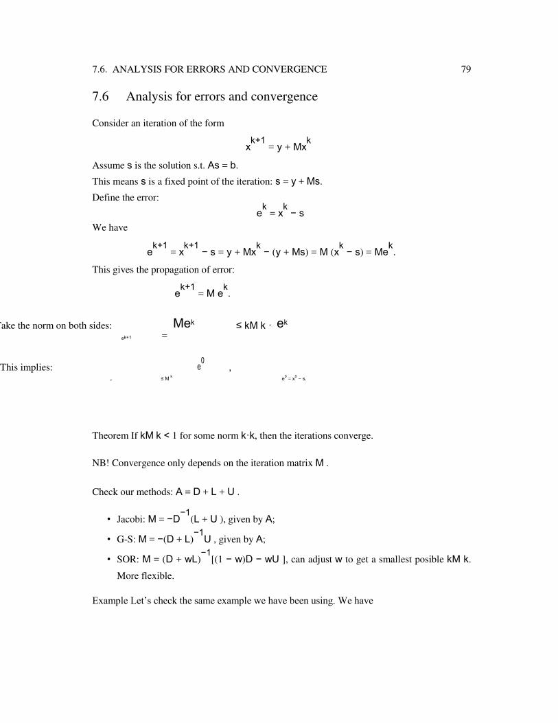
7.6. ANALYSIS FOR ERRORS AND CONVERGENCE 79
7.6 Analysis for errors and convergence
Consider an iteration of the form
xk+1
= y + Mxk
Assume s is the solution s.t. As = b.
This means s is a fixed point of the iteration: s = y + Ms.
Define the error:
ek = x
k − s
We have
ek+1
= xk+1
− s = y + Mxk − (y + Ms) = M (x
k − s) = Me
k.
This gives the propagation of error:
ek+1
= M ek.
Take the norm on both sides: Mek ≤ kM k · ek
ek+1 =
This implies:
e0 ,
ek ≤ M k e0 = x
0 − s.
Theorem If kM k < 1 for some norm k·k, then the iterations converge.
NB! Convergence only depends on the iteration matrix M .
Check our methods: A = D + L + U .
• Jacobi: M = −D−1
(L + U ), given by A;
• G-S: M = −(D + L)−1
U , given by A;
• SOR: M = (D + wL)−1
[(1 − w)D − wU ], can adjust w to get a smallest posible kM k.
More flexible.
Example Let’s check the same example we have been using. We have

2 −1 0 A = −1 2 −1 , 0 −1 2

80 CHAPTER 7. ITERATIVE SOLVERS FOR LINEAR SYSTEMS
so 0 0
0
2 0 0
0 −1 0
L = −1 0 0 , D = 0 2 0 , U = 0 0 −1 .
0 −1 0 0 0 2 0 0 0
The iteration matrix for each method:
0 0.5 0 0 0.5 0
−0.2 0.6 0
MJ = 0.5 0 0.5 , M
GS = 0 0.25 0.5 , M
SOR =
−0.12 0.16 0.6
0 0.5 0 0 0.125 0.25 −0.072 0.096 0.16
We list their various norms:
M l1 norm l2 norm l∞ norm
Jacobi 1 0.707 1
G-S 0.875 0.5 0.75
SOR 0.856 0.2 0.88
The l2 norm is the most significant one. We see now why SOR converges fastest.
Convergence Theorem. If A is diagonal dominant, i.e.,
n
|aii| > |aij | , ∀i = 1, 2, · · · , n.
j
=1,j=6i
X
Then, all three iteration methods converge for all initial choice of x0.
NB! If A is not diagonal dominant, it might still converge, but there is no guarantee.

Chapter 8
The Method of Least Squares
8.1 Problem description Given data set
x x
0 x
1 x
2 · · · x
m
y y
0 y
1 y
2 · · · y
M Data come from observation (measured) or experiments.
These yi’s can have error (called “noise”) in measuring or experimenting. y has
a relation with x from physical model: y = y(x). Then, our data is
yk = y(xk) + ek
where ek is error.
8.2 Linear regression and basic derivation
Example 1. If y = ax + b, this is called linear regression. Your lab data would not lie exact on
a straight line (or your lab instructor will be very suspicious!). Our job now is to find a
straight line that “best” fit our data. See Figure 8.1 for an illustration. A more specific way of saying the same thing: Find a, b, such that when we use y = ax+b, the “error” becomes smallest possible. How to measure error?
1. max |y(xk) − yk| — l∞ norm k
m X
2. |y(xk) − yk| — l1 norm k=0
81

82 CHAPTER 8. LEAST SQUARES
y ✻
✲ x
Figure 8.1: Linear regression.
m X
3. [y(xk) − yk]2
— l2 norm, used in Least Square Method. (LSM) k=0
Our problem can now be stated as a minimization problem:
Find a and b such that the error function ψ(a, b) defined as
m X
ψ(a, b) = (axk + b − yk)2
k=0
is minimized.
How to find a and b?
At the minimum of a function, we have
∂ψ = ∂ψ = 0
∂a
∂b
In detail:
∂ψ m
= 0 : 2(axk + b − yk)xk = 0, (I)
∂a k= 0
X
∂ψ m
= 0 : 2(axk + b − yk) = 0, (II)
∂b k= 0
X
Solve (I), (II) for (a, b). Rewrite it as a system
m ! · a +
m ! · b
xk2 x
k
k=0
k=0
X
X
m
xk
! · a + (m + 1) · b
k= 0
X
m X
= xk · yk k=0 m
X = yk
k=0

8.2. LINEAR REGRESSION AND BASIC DERIVATION 83
These are called the normal equations. Example 2. Consider the data set (from textbook, p.428)
Tk 0 10 20 30 40 80 90 95
Sk 68.0 67.1 66.4 65.6 64.6 61.8 61.0 60.0
where
S: surface tension in a liquid
T : temperature
From physics we know that they have a linear relation
S = aT + b
Use MLS to find the best fitting a, b.
Answer. We have m = 7, and
7 0 + 10
2 + 20
2 + · · · + 90
2 + 95
2 = 26525
Tk2 =
k= 0
X
7 T
k = · · · = 365
k= 0
X
7
TkSk = · · · = 22685
k= 0
X
7 S
k = · · · = 514.5
k= 0
X
The normal equations are
_
26525 a + 365 b = 22685
365 a + 8 b = 514.5
Solve it
a = −0.079930, b = 67.9593.
So
S(T ) = −0.079930 T + 67.9593.
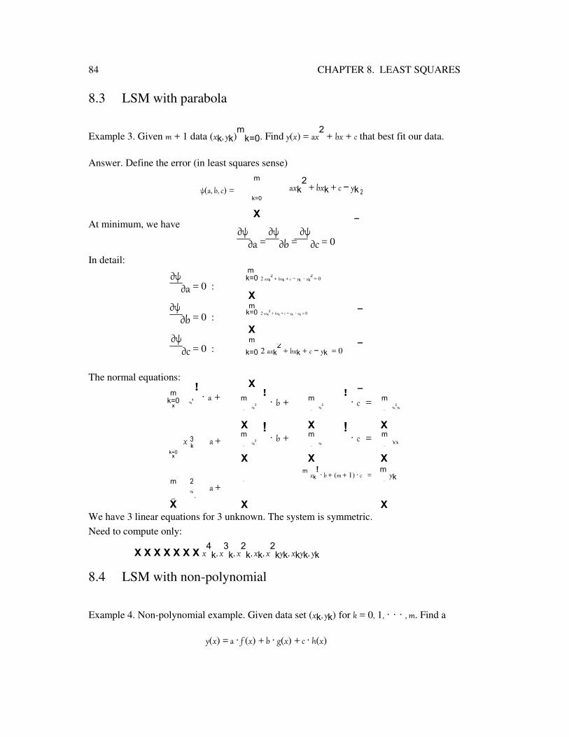
84 CHAPTER 8. LEAST SQUARES
8.3 LSM with parabola
Example 3. Given m + 1 data (xk, yk)m
k=0. Find y(x) = ax2 + bx + c that best fit our data.
Answer. Define the error (in least squares sense)
m axk
2 + bxk + c − yk
2
ψ(a, b, c) =
k=0
_
X
At minimum, we have
In detail:
∂ψ∂a = 0 :
∂ψ∂b = 0 :
∂ψ∂c = 0 :
The normal equations:
m !
· a +
k=0 xk4
X
m
x 3 a +
k
!
·
k=0
X
m 2 a +
xk
! ·
k=0
X
∂ψ∂a =
∂ψ∂b =
∂ψ∂c = 0
m k=0 2 axk
2 + bxk + c − yk · xk
2 = 0
X _
m
k=0 2 axk2 + bxk + c − yk · xk = 0
X _
m
k=0 2 axk2 + bxk + c − yk = 0
X _
m ! · b +
m ! · c =
m
xk3 xk
2 xk2
yk
k= 0 k= 0 k= 0
X ! · b +
X ! · c =
X
m m m
xk2 xk x
kyk
k= 0 k= 0 k= 0
X X X
m xk
! · b + (m + 1) · c =
m yk
k= 0 k= 0
X X
We have 3 linear equations for 3 unknown. The system is symmetric.
Need to compute only:
X X X X X X X x4k, x
3k, x
2k, xk, x
2kyk, xkyk, yk
8.4 LSM with non-polynomial
Example 4. Non-polynomial example. Given data set (xk, yk) for k = 0, 1, · · · , m. Find a
y(x) = a · f (x) + b · g(x) + c · h(x)

8.5. GENERAL LINEAR LSM 85
which best fit the data. This means we need to find (a, b, c).
Here f (x), g(x), h(x) are given functions, for example
f (x) = ex
, g(x) = ln(x), h(x) = cos x,
but not restricted to these.
Define the error function:
m m
ψ(a, b, c) = (y(xk ) − yk)2 =(a · f (xk) + b · g(xk ) + c · h(xk ) − yk)
2
k= 0 k= 0
X X
At minimum, we have
∂ψ m
= 0 : k=0 2h
a · f (xk) + b · g(xk) + c · h(xk) − yk
i · f (xk) = 0
∂a
X
∂ψ m
= 0 : k=0 2h
a · f (xk) + b · g(xk) + c · h(xk) − yk
i · g(xk ) = 0
∂b
X
∂ψ m
= 0 : k=0 2h
a · f (xk) + b · g(xk) + c · h(xk) − yk
i · h(xk ) = 0
∂c
X
The normal equations are
m
f (xk)2! a + m
k= 0 k= 0
X
X
m
f (xk)g(xk ) a +
!
k=0
X
m
f (x )h(x ) a +
k k
!
X
f (xk)g(xk)!
b + m f (xk)h(xk)!
c =
k= 0
m g(xk )2
! b +
X
m h(xk )g(xk)
! c =
k= 0 k= 0
X f (xk)h(xk )! X
m h(xk)2
! c =
m b +
X X
m
X f (xk)yk
k=0 m
X g(xk)yk
k=0 m
X h(xk)yk
k=0 k=0 k=0 k=0 We note that the system of normal equations is always symmetric. We only need to compute half of the entries.
8.5 General linear LSM
Let g0, g1, g2, · · · gn be n + 1 given functions (they don’t need to be linear). Given data set (xk, yk), k = 0, 1, · · · , m. (m and n are in general different). We
search for a function in the form n
X y(x) = cigi(x)
i=0 that best fit the data.

Here gi’s are called basis functions.

86 CHAPTER 8. LEAST SQUARES How to choose the basis functions? They are chosen such that the system of the normal equations is regular (invertible) and well-conditioned.
Requirements. gi’s must be a set of linearly independent functions. Meaning: one can not be written as linear combination of the others, or
n
cigi(x) = 0, if and only if c0 = c1 = c2 = · · · = cn = 0.
=0
Xi
Define error function
ψ(c0, c1, · · · , cn) = m y(xk) − yk 2
= m
" n cigi(x) − yk
#2
k=0
h
i
k=0 i=0
X X X
At minimum, we have
∂ψ
= 0, j = 0, 1, ·, n.
∂cj
This gives:
2
" n cigi(xk) − yk
# gj (xk) = 0
m
k= 0 i=0
X X
Re-arranging the ordering of summation signs:
n m gi(xk)gj (xk)!
ci = m gj (xk)yk,j = 0, 1, ·, n.
i=0 k= 0 k= 0
X X X This gives the system of normal equations:
~ A~c = b
where ~c = (c0, c1, · · · , cn)t and
A = {aij },
~ b = {bj },
m
X aij = gi(xk)gj (xk)
k=0 m
bj = gj (x k)yk. X
k=0
We note that this A is symmetric.

8.6. NON-LINEAR LSM 87
8.6 Non-linear LSM Next is an example of quasi-linear LSM.
Example 5. Consider fitting the data with the function
y(x) = a · bx
This means, we need to find (a, b) such that this y(x) best fit the data. Do a variable change:
ln y = ln a + x · ln b . Let
¯ S = ln y, a¯ = ln a, b = ln b.
Given data set (xk, yk). Compute Sk = ln yk for all k. ¯
We can now find (¯ a, b) such that Sk best fits (xk, Sk).
Then, transform back to the original variable
a = exp{a¯ },
¯
b = exp{b}.
Example 6. Non-linear LSM. For example,
y(x) = ax · sin(bx). We can not find a variable change that can change this problem into a linear one. So we will now deal with it as a non-linear problem. Define error m m
ψ(a, b) = k=0 h
y(x k) − y ki2
= k= 0 h
ax k · s in(bx k) − y ki2
.
X X
At minimum:
∂ψ m 2h
axk · sin(bxk) − yki · [xk · sin(bxk)] = 0
= 0 : k=0
∂a
X
∂ψ m 2h
axk · sin(bxk) − yki · [axk · cos(bxk)xk] = 0
= 0 : k=0
∂a
X
We now have a 2 × 2 system of non-linear equations to solve for (a, b)! May use Newton’s method to find a root. May have several solutions, including all the maximum, minimum and saddle points. (see slides)

88 CHAPTER 8. LEAST SQUARES

Chapter 9
Numerical solution of ordinary differential equations (ODE)
9.1 Introduction
Definition of ODE: an equation which contains one or more ordinary derivatives of an unknown function.
Example 1. Let x = x(t) be the unknown function of t, ODE examples can be
x′ = x
2, x
′′ + x · x
′ + 4 = 0, etc.
We consider the initial-value problem for first-order ODE
( ) x′ = f (t, x), − − differential equation
∗
_ x(t0) = x0 − − −initial condition, given
Some examples:
x′ = x + 1, x(0) = 0. solution: x(t) = e
t − 1
x′ = 2, x(0) = 0. solution: x(t) = 2t.
In many situations, exact solutions can be very difficult/impossible to obtain.
Numerical solutions: Given (*), find xn = x(tn), n = 1, 2, · · · , N , and t0 < t1 <
· · · < tN . Here tN is final computing time. Take uniform time step: Let h be the time step length
tn+1 − tn = h, tk = t0 + kh
Overview:
89

90 CHAPTER 9. ODES
• Taylor series method, and error estimates
• Runge-Kutta methods
• Multi-step methods
• System of ODE
• High order equations and systems
• Stiff systems
• Matlab solvers
9.2 Taylor series methods for ODE Given
x′(t) = f (t, x(t)), x(t0) = x0.
Let’s find x1 = x(t1) = x(t0 + h). Taylor expansion gives ∞
x(t0 + h) = x(t0) + hx′(t0) +
12 h
2x′′(t0) + · · · =
X m
1! h
mx(m)
(t0) m=0
Taylor series method of order m: take the first (m + 1) terms in Taylor expansion.
′ 1 2 ′′ 1 m (m)
x(t0 + h) = x(t0) + hx (t0) +
h x (t0) + · · · +
h x
(t0).
2 m!
Error in each step:
∞ 1
1
x(t0 + h) − x1 = k (k) m+1 (m+1)
h x
(t0) =
h
x
(ξ)
k! (m + 1)!
=m+1
k X
for some ξ ∈ (t0, t1).
For m = 1, we have Euler’s method:
x1 = x0 + hx′(t0) = x0 + h · f (t0, x0)
General formula for step number k:
xk+1 = xk + h · f (tk, xk), k = 0, 1, 2, · · ·
For m = 2, we have
′ 1 2 ′′
x1 = x0 + hx (t0) +
h x
(t0)
2

9.2. TAYLOR SERIES METHODS FOR ODE 91
Using
x′′(t0) = dt
d f (t0, x(t0)) = ft(t0, x0) + fx(t0, x0) · x
′(t0) = ft(t0, x0) + fx(t0, x0) · f (t0, x0)
we get
x1 = x0 + hf (t0, x0) + 12 h
2 [ft(t0, x0) + fx(t0, x0) · f (t0,
x0)] For general step k, we have
xk+1 = xk + hf (tk, xk) + 12 h
2 [ft(tk, xk) + fx(tk, xk) · f (tk, xk)]
Example 2. Set up Taylor series methods with m = 1, 2 for
x′ = −x + e
−t, x(0) = 0.
(Exact solution is x(t) = te−t
.)
Answer. The initial data gives x0 = 0. For m = 1, we have
xk+1 = xk + h(−xk + e−tk ) = (1 − h)xk + he
−tk For m = 2, we have
x′′ = (−x + e
−t)′ = −x
′ − e
−t = x − e
−t − e
−t = x − 2e
−t
so
′ 1 2 ′′
xk+1 = xk + hxk +
h xk
2
= xk + h (−xk + exp{−tk}) + 1
2 h2 [xk − 2 exp{−tk}]
= (1 − h + 12 h
2)xk + (h − h
2) exp{−tk}
Example 3. Set up Taylor series methods with m = 1, 2, 3, 4 for
x′ = x, x(0) = 1.
(Exact solution x(t) = et)
Answer. We set x0 = 1. Note that
x′′ = x
′ = x, x
′′′ = x
′′ = x, · · · x
(m) = x

92 CHAPTER 9. ODES
We have
m = 1 : xk+1 = xk + hxk = (1 + h)xk
m = 2 : xk+1 = xk + hxk + 1
2 h2
xk = (1 + h + 1
2 h2
)xk
m = 3 : xk+1 = xk + hxk + 12 h
2xk +
16 h
3xk = (1 + h +
12 h
2 +
16 h
3)xk
m = 4 : xk+1 = (1 + h + 12 h
2 +
16 h
3 + 24
1 h
4)xk
See slides.
Error analysis. Given ODE
x′ = f (t, x), x(t0) = x0.
Local truncation error (error in each time step) for Taylor series method of order m is
(k) = |xk+1 − x(tk + h)| = _ hm+1 = _ hm+1
dm
f (ξ) _ , ξ ∈ (tk, tk+1).
eL (m + 1)! x(m+ 1)
(ξ)_ (m + 1)! dtm
_ _ _ _
_ _ _ _
_ _ _ _
Here we use the fact that
Assume now that
We have
x(m+1) = d
mf
dtm
dm
f _ ≤ M.
_
dtm _ _
_ _
_ _
(k) M
eL ≤
hm+1
= O(hm+1
).
(m + 1)!
Total error: sum over all local errors.
Detail: We want to compute x(T ) for some time t = T . Choose an h. Then total number of steps is
N = fracT h, i.e., T = Nh.
Then
N _ N
M
E = k=1 (k) ≤ k=1
_
eL (m + 1)! hm+1
X _ _ X
_ M _ m+1 M m MT m m
= N
h
= (Nh)
h =
h
= O(h )
(m + 1)! (m + 1)! (m + 1)!
Therefore, the method is of order m.
In general: If the local truncation error is of order O(ha+1
), then the total error is of O(ha),
i.e., one order less.
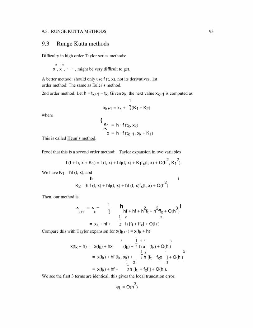
9.3. RUNGE KUTTA METHODS 93
9.3 Runge Kutta methods
Difficulty in high order Taylor series methods:
x′′, x
′′′, · · · , might be very difficult to get.
A better method: should only use f (t, x), not its derivatives. 1st
order method: The same as Euler’s method.
2nd order method: Let h = tk+1 − tk. Given xk, the next value xk+1 is computed as 1
xk+1 = xk +
(K1 + K2)
2
where
= h · f (tk, xk)
( K1
K2 = h · f (tk+1, xk + K1)
This is called Heun’s method.
Proof that this is a second order method: Taylor expansion in two variables
f (t + h, x + K1) = f (t, x) + hft(t, x) + K1fx(t, x) + O(h2, K1
2).
We have K1 = hf (t, x), abd h i
K2 = h f (t, x) + hft(t, x) + hf (t, x)fx(t, x) + O(h2)
Then, our method is:
1 hhf + hf + h
2ft + h
2ffx + O(h
3)i
xk+1
=
xk
+
2
1 2 3
= xk + hf +
h [ft + ffx] + O(h )
2
Compare this with Taylor expansion for x(tk+1) = x(tk + h)
′ 1 2 ′′ 3
x(tk + h) = x(tk) + hx (tk) +
h x (tk) + O(h )
2
= x(tk) + hf (tk, xk) +
1 2 ′ 3
h [ft + fxx ] + O(h )
2
1 2 3
= x(tk) + hf +
h [ft + fxf ] + O(h ).
2
We see the first 3 terms are identical, this gives the local truncation error:
eL = O(h3)

94 CHAPTER 9. ODES
meaning that this is a 2nd order method.
In general, Rung-Kutta methods of order m takes the form
= xk + w1K1 + w2K2 + · · · + wmKm where
= h · f (tk, xk)
= h · f (tk + a2h, x + b2K1)
= h · f (tk + a3h, x + b3K1 + c3K2)
. m−1
..
Km = h f (tk + amh, x + i=1 φiKi)
·
The parameters w , a , b , φ are carefully chosen to guarantee the order m.
i i i i
P
NB! The choice is NOT unique! The classical RK4 : a 4th order method takes the form 1
hK1 + 2K2 + 2K3 + K4
i
xk+1 = xk +
6
where
K1 = h · f (tk, xk)
K2 = h · f (tk +
1 h, xk +
1 K1)
2 2
K3 = h · f (tk +
1
h, xk +
1
K2)
2 2
K4 = h · f (tk + h, xk + K3) See slides for codes.
9.4 An adaptive Runge-Kutta-Fehlberg method In general, we have
1. smaller time step h gives smaller error;
2. The error varies at each step, depending on f .
Optimal situation: h varies each step to get uniform error at each step.
xk+1
K1
K2
K3
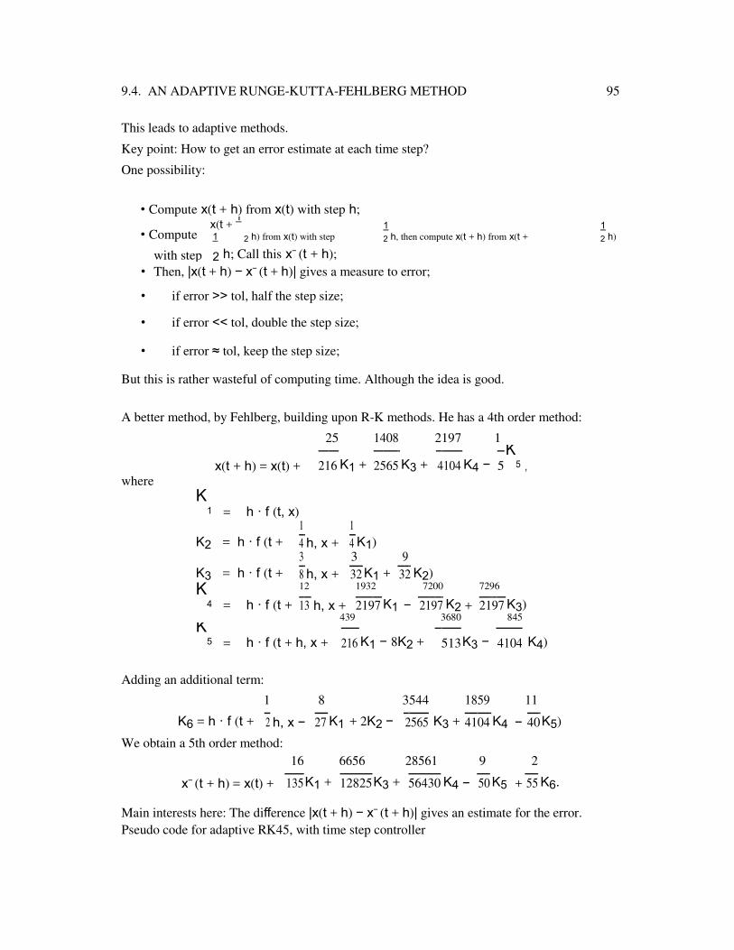
9.4. AN ADAPTIVE RUNGE-KUTTA-FEHLBERG METHOD 95
This leads to adaptive methods.
Key point: How to get an error estimate at each time step?
One possibility:
• Compute x(t + h) from x(t) with step h;
• Compute x(t +
1 1 1
1 2 h) from x(t) with step 2 h, then compute x(t + h) from x(t + 2 h)
with step 2 h; Call this x¯ (t + h);
• Then, |x(t + h) − x¯ (t + h)| gives a measure to error;
• if error >> tol, half the step size;
• if error << tol, double the step size;
• if error ≈ tol, keep the step size; But this is rather wasteful of computing time. Although the idea is good.
A better method, by Fehlberg, building upon R-K methods. He has a 4th order method: 25 1408 2197 1
x(t + h) = x(t) +
K1 +
K3 +
K4 −
K5 ,
216 2565 4104 5
where
K1 = h · f (t, x)
K2 = h · f (t +
1
h, x +
1
K1)
4 4
K3 = h · f (t +
3
h, x +
3
K1 +
9
K2)
8 32 32
K4 = h · f (t +
12 1932 7200 7296
h, x +
K1 −
K2 +
K3)
13 2197 2197 2197
439 3680 845
K5 = h · f (t + h, x +
K1 − 8K2 +
K3 −
K4)
216 513 4104
Adding an additional term:
1
h, x −
8
K1 + 2K2 −
3544
K3 +
1859
K4 −
11
K5)
K6 = h · f (t +
2 27 2565 4104 40
We obtain a 5th order method:
16 6656 28561 9 2
x¯ (t + h) = x(t) +
K1 +
K3 +
K4 −
K5 +
K6.
135 12825 56430 50 55
Main interests here: The difference |x(t + h) − x¯ (t + h)| gives an estimate for the error.
Pseudo code for adaptive RK45, with time step controller

96 CHAPTER 9. ODES
Given t0, x0, h0, nmax, emin, emax, hmin, hmax
set h = h0, x = x0, k = 0,
while k < nmax do
if h < hmin then h = hmin
else if h > hmax then h = hmax
end
Compute RK4, RK5, and e = |RK4 − RK5| if
e > emax, then h = h/2;
else
k=k+1; t=t+h; x=RK5;
If e < emin, the h = 2 ∗ h; end
end
end (while)
9.5 Multi-step methods Given
x′ = f (t, x), x(t0) = x0,
Let tn = t0 + nh. If x(tn) is given, the exact value for x(tn=1) would be
t +1
x(tn+1) = x(tn) + Z
tnn x
′(s) ds
Assume we know xn, xn−1, xn−2, · · · , xn−k one can approximate the integrand x′(s) by
using interpolating polynomial.
Example Consider k = 1. Given xn, xn−1, we can compute fn, fn−1 as
fn = f (tn, xn), fn−1
=
f
(tn−1
, xn−1
)
Use now linear approximation, i.e., straight line interpolation,
x′(s)
≈ P (s) = f +
fn
−
fn−1 (s
− t ).
1 n−1 h n−1
Then tn+1
h
xn+1
=
xn
+
Ztn P1(s) ds = xn +
(3fn − fn−1).
2

9.5. MULTI-STEP METHODS 97
Adams-Bashforth method: The explicit version. Given
x,xn−1, · · · , xn−k and
fn, fn−1, · · · , , fn−k
find interpolating polynomial Pk(t) that interpolates (ti, fi)ni=n−k. Compute
t +1
xn+1 = xn + Z
tnn Pk(s) ds
which will always be in the form
xn+1 = xn + h · (b0fn + b1fn−1 + b2fn−2 + · · · + bkfn−k).
Good sides: Simple, minimum number of f (·) evaluations. Fast.
Disadvantage: Here we use interpolating polynomial to approximate a function out-side the interval of interpolating points. This gives bigger error. Improved version. implicit method, Adams-Bashforth-Moulton (ABM) method. Find
interpolating polynomial Pk+1(t) that interpolates
(fn+1, tn+1), (fn, tn), · · · , (fn−k, tn−k), and use
t +1
xn+1 = xn + Z
tnn Pk+1(s) ds
which will always be in the form
xn+1 = xn + h · (b−1fn+1 + b0fn + b1fn−1 + b2fn−2 + · · · + bkfn−k)
where fn+1 = f (tn+1, xn+1) which is unknown. Therefore, we get a non-linear equation. Can
be solved by fixed-point iteration (Newton’s method). Use AB solution as the initial guess, it will converge in 2-3 iterations.
Example For a couple of k values, we have
k = −1 : x
n+1 = xn + h · fn+1, (implicit backward Euler’s method)
k = 0 : x
n+1 = xn +
h
(fn + fn+1), (trapezoid rule)
2
5 3 1
fn−1_
k = 1 : xn+1 = xn + h · _
fn+1 +
fn −
12 12 12
With fixed point iteration:

98 CHAPTER 9. ODES
Given xn, xn−1, fn, fn−1, compute AB solution with k = 1:
xn∗+1 = xn + h 3 fn 1
fn−1
(P ) 2 2
_ −
∗ ∗ _
fn=1 =
f t
n+ 1, x
n+ 1 .
_
Do one iteration of Newton’s method, to correct the error:
xn+1 = xn +
h fn∗+1 + fn
(C)
2
fn+1 = f (tn+1, xn+1) _
Here step (P ) is called the predictor, and step (C) is the corrector. This
is called predictor-corrector’s method.
9.6 Methods for first order systems of ODE We consider
~x ′ = F (t, ~x), ~x(t0) = ~x0
Here ~x = (x1, x2, · · · , xn)t is a vector, and F = (f1, f2, · · · , fn)
t is a vector-values
function. Write it out
x′
1
x′2
x′n
= f1(t, x1, x2, · · · , xn) = f2(t, x1, x2, · · · , xn)
· · ·
= fn(t, x1, x2, · · · , xn)
Remark: All methods for scalar equation can be used for systems!
Taylor series methods:
~x(t + h) = ~x + h~x ′ +
12 h
2~x
′′ + · · · + m
1! h
m~x
(m)
Example Consider
_
x1′ =
x1 −
x2 + 2t − t2 −
t3
′
=
x2 x1 + x2 − 4t2 + t
3
We will need the high order derivatives:
_
x1′′ = x1
′ −
x2′ + 2 −
2t − 3t
2
′′
= x
1
x2 + x2 − 8t + 3t
2
9.7. HIGHER ORDER EQUATIONS AND SYSTEMS 99
and x1
′′′ = x1
′′ −
x2′′ −
2 − 6t
′′′ ′′ ′′
and so on...
_ x2 = x1 + x2 − 8 + 6t
Runge-Kutta methods take the same form. For example, RK4:
~xk+1 = ~xk +
1 h
K~1 + 2K~
2 + 2K~
3 + K~
4
i
6
where ~ K
1 ~ K2
~ K3 ~ K4
= h · F (tk, ~xk)
1 1 ~
= h
·
F (t
k +
2
h, ~xk +
2
K1)
1 1 ~
= h
·
F (t
k +
2
h, ~xk +
2
K2)
~
= h · F (tk + h, ~xk + K3) Here everything is a vector instead of a scalar value.
9.7 Higher order equations and systems Treatment: Rewrite it into a system of first order equations. Example Higher order ODE
x(n)
= f (t, x, x′, x
′′, · · · , x
(n−1))
with
x(t0), x′(t0), x
′′(t0), · · · , x
(n−1)(t0)
given. Introduce a systematic change of variables
x1 = x, x2 = x′, x3 = x
′′, · · · xn = x
(n−1)
We then have
x1′
x2′
′
x3
xn′−′1
xn
= x′ = x2
= x′′ = x3
= x′′′ = x4
.
.
.
= x(n−1)
= xn
= x(n)
= f (t, x1, x2, · · · , xn)
This is a system of 1st order ODEs. Systems of high-order equations are treated in the same way.

100 CHAPTER 9. ODES
9.8 Stiff systems
A system is called stiff if the solution consists of components that vary with very different speed/frequency.
Example Consider
x′ = −ax,
x(0) = 1
the exact solution is
x(t) = e−t
We see that
x → 0 as t → +∞.
(P 1)
Solve it by Euler’s method:
xn+1 = xn − ahxn = (1 − ah)xn, ⇒ xn = (1 − ah)nx0 = (1 − ah)
h
In order to keep the property (P 1), in the approximate solution, i.e., xn →
0, as n → +∞, We must have
|1 − ah| < 1, ⇒ h < a2
which gives a restriction to the time step size: it has to be sufficiently small.
Example Now consider a system
x′ = −20x − 19y x(0) = 2
_ y′ = −19x − 20y
_ y(0) = 0
The exact solution is (
x(t) = e−39t
+ e−t
y(t) = e−39t
− e−t
Observations:
• The solution tends to 0, i.e., x → 0, y → 0 as t → +∞.
• Two components in the solution, e−39t
and e−t
;
• They decay at a very different rate. The term e−39t
tends to 0 much faster than the term
e−t
;
• For large values of t, the term e−t
dominate.
• Therefore, e−39t
is called the transient term.

9.8. STIFF SYSTEMS
Solve it with Euler’s method: (
xn+1 = xn + h · (−20xn − 19yn)
yn+1 = yn + h · (−19xn − 20yn)
101
_
x0 = 2 y0 = 0
One can show by induction that
xn = (1 39h)n + (1 h)
n
( yn = (1 − 39h)
n
−
(1 − h)n
− −
We must require that
xn → 0, yn → 0 as n → +∞.
This gives the conditions
|1 − 39h| < 1 and |1 − h| < 1
which implies 2
(1) : h <
and
(2) : h < 2
39
We see that condition (1) is much stronger than condition (2), therefore it must be satisfied.
Condition (1) corresponds to the term e−39t
, which is the transient term and it tends to 0 very
quickly as t grows. Unfortunately, time step size is restricted by this transient term.
A more stable method: Backward Euler, implicit method
xn+1 = xn + h ( 20xn+1 −
19yn+1)
( yn+1 = yn + h
· (
−19xn+1 20yn+1)
· − −
Let
−20 −19 , ~x = x
x
n .
A = , ~x =
_−19 −20
_ _y _ n
_yn _
We can write
~xn+1 = ~xn + A · ~xn+1,
⇒ (I − hA)~xn+1 = ~xn ⇒
~xn+1 = (I − hA)−1
~xn Take some vector norm on both sides
k~xn+1k = (I − hA)−1
~xn ≤ (I − hA)−1
k~xnk .

102 CHAPTER 9. ODES
We see that if (I − hA)−1
< 1, then ~xn → 0 as n → +∞.
Use the l2 norm:
(I
−
hA)−1
=
max (I
−
hA)−1
_
= max 1
| (1 − h · i(A))|
i
_ i i
We have _ _
1(A) = −1, 2(A) = −39
They are both negative, therefore 1 − h i > 1, implying
(I − hA)−1 < 1
independent of the value of h. Therefore, this method is called unconditionally stable.
Advantage: Can choose large h, always stable. Suitable for stiff systems. Disadvantage: Must solve a system of linear equations at each time step
(I − hA)~xn+1 = ~xn Longer computing time for each step. Not recommended if the system is not stiff.