14.581 International Trade — Lecture 2: Ricardian Theory (I)—
Upload
khangminh22Category
view
0download
0
1CSC 886 Lecture Slides (c) 2010, C. Boutilier and P. Poupart
CS886: Lecture 2January 12Probabilistic inferenceBayesian networksVariable elimination algorithm

2CSC 886 Lecture Slides (c) 2010, C. Boutilier and P. Poupart
Some Important Properties
Product Rule: Pr(ab) = Pr(a|b)Pr(b)
Summing Out Rule:
Chain Rule:Pr(abcd) = Pr(a|bcd)Pr(b|cd)Pr(c|d)Pr(d)
• holds for any number of variables
)Pr()|Pr()Pr()(
bbaaBDomb
∑∈
=

3CSC 886 Lecture Slides (c) 2010, C. Boutilier and P. Poupart
Bayes Rule
Bayes Rule:
Bayes rule follows by simple algebraic manipulation of the defn of condition probability
• why is it so important? why significant?• usually, one “direction” easier to assess than other
)Pr()Pr()|Pr()|Pr(
baabba =

4CSC 886 Lecture Slides (c) 2010, C. Boutilier and P. Poupart
Example of Use of Bayes RuleDisease ∊ {malaria, cold, flu}; Symptom = fever
• Must compute Pr(D | fever) to prescribe treatmentWhy not assess this quantity directly?
• Pr(mal | fever) is not natural to assess; Pr(fever | mal) reflects the underlying “causal” mechanism
• Pr(mal | fever) is not “stable”: a malaria epidemychanges this quantity (for example)
So we use Bayes rule:• Pr(mal | fever) = Pr(fever | mal) Pr(mal) / Pr(fever)• note that Pr(fev) = Pr(m&fev) + Pr(c&fev) + Pr(fl&fev)• so if we compute Pr of each disease given fever
using Bayes rule, normalizing constant is “free”

5CSC 886 Lecture Slides (c) 2010, C. Boutilier and P. Poupart
Probabilistic Inference
By probabilistic inference, we mean• given a prior distribution Pr over variables of interest,
representing degrees of belief• and given new evidence E=e for some var E• Revise your degrees of belief: posterior Pre
How do your degrees of belief change as a result of learning E=e (or more generally E=e, for set E)

6CSC 886 Lecture Slides (c) 2010, C. Boutilier and P. Poupart
Conditioning
We define Pre(α) = Pr(α | e)That is, we produce Pre by conditioning the prior distribution on the observed evidence eIntuitively,
• we set Pr(w) = 0 for any world falsifying e• we set Pr(w) = Pr(w) / Pr(e) for any world consistent
with e• last step known as normalization (ensures that the
new measure sums to 1)

7CSC 886 Lecture Slides (c) 2010, C. Boutilier and P. Poupart
Semantics of Conditioning
p1
p2
E=e
p1
p2
p3
p4
E=e E=e
Pr
αp1
αp2
E=e
Pre
α = 1/(p1+p2)normalizing constant

8CSC 886 Lecture Slides (c) 2010, C. Boutilier and P. Poupart
Inference: Computational Bottleneck
Semantically/conceptually, picture is clear; but several issues must be addressedIssue 1: How do we specify the full joint distribution over X1, X2,…, Xn ?
• exponential number of possible worlds• e.g., if the Xi are boolean, then 2n numbers (or 2n -1
parameters/degrees of freedom, since they sum to 1)• these numbers are not robust/stable• these numbers are not natural to assess (what is
probability that “Pascal wants coffee; it’s raining in Toronto; robot charge level is low; …”?)

9CSC 886 Lecture Slides (c) 2010, C. Boutilier and P. Poupart
Inference: Computational Bottleneck
Issue 2: Inference in this rep’n frightfully slow• Must sum over exponential number of worlds to
answer query Pr(α) or to condition on evidence e to determine Pre(α)
How do we avoid these two problems?• no solution in general• but in practice there is structure we can exploit
We’ll use conditional independence

10CSC 886 Lecture Slides (c) 2010, C. Boutilier and P. Poupart
IndependenceRecall that x and y are independent iff:
• Pr(x) = Pr(x|y) iff Pr(y) = Pr(y|x) iff Pr(xy) = Pr(x)Pr(y)• intuitively, learning y doesn’t influence beliefs about x
x and y are conditionally independent given z iff:• Pr(x|z) = Pr(x|yz) iff Pr(y|z) = Pr(y|xz) iff
Pr(xy|z) = Pr(x|z)Pr(y|z) iff …• intuitively, learning y doesn’t influence your beliefs
about x if you already know z• e.g., learning someone’s mark on 886 project can
influence the probability you assign to a specific GPA; but if you already knew 886 final grade, learning the project mark would not influence GPA assessment

11CSC 886 Lecture Slides (c) 2010, C. Boutilier and P. Poupart
What does independence buy us?
Suppose (say, boolean) variables X1, X2,…, Xnare mutually independent
• we can specify full joint distribution using only n parameters (linear) instead of 2n -1 (exponential)
How? • Simply specify Pr(x1), … Pr(xn)• from this I can recover probability of any world or any
(conjunctive) query easily• e.g. Pr(x1~x2x3x4) = Pr(x1) (1-Pr(x2)) Pr(x3) Pr(x4) • we can condition on observed value Xk = xk trivially by
changing Pr(xk) to 1, leaving Pr(xi) untouched for i≠k

12CSC 886 Lecture Slides (c) 2010, C. Boutilier and P. Poupart
The Value of Independence
Complete independence reduces both representation of joint and inference from O(2n) to O(n): pretty significant!Unfortunately, such complete mutual independence is very rare. Most realistic domains do not exhibit this property.Fortunately, most domains do exhibit a fair amount of conditional independence. And we can exploit conditional independence for representation and inference as well.Bayesian networks do just this

13CSC 886 Lecture Slides (c) 2010, C. Boutilier and P. Poupart
Bayesian Networks
A Bayesian Network is a graphical representation of the direct dependencies over a set of variables, together with a set of conditional probability tables (CPTs) quantifying the strength of those influences.Bayes nets exploit conditional independence in very interesting ways, leading to effective means of representation and inference under uncertainty.

14CSC 886 Lecture Slides (c) 2010, C. Boutilier and P. Poupart
Bayesian Networks
A BN over variables {X1, X2,…, Xn} consists of:• a DAG whose nodes are the variables• a set of CPTs Pr(Xi | Par(Xi) ) for each Xi
Key notions (see text for defn’s, all are intuitive):• parents of a node: Par(Xi) • children of node• descendents of a node• ancestors of a node• family: set of nodes consisting of Xi and its parents
CPTs are defined over families in the BN

15CSC 886 Lecture Slides (c) 2010, C. Boutilier and P. Poupart
An Example Bayes NetA couple CPTS are “shown”
Explicit joint requires 211 -1 =2047 parmtrs
BN requires only 27 parmtrs(the number of entries for each CPT is listed)

16CSC 886 Lecture Slides (c) 2010, C. Boutilier and P. Poupart
Alarm Network
Monitoring system for patients in intensive care

17CSC 886 Lecture Slides (c) 2010, C. Boutilier and P. Poupart
Pigs NetworkDetermines pedigree of breeding pigs
• used to diagnose PSE disease• half of the network shown here

18CSC 886 Lecture Slides (c) 2010, C. Boutilier and P. Poupart
Semantics of a Bayes Net
The structure of the BN means: every Xi is conditionally independent of all of its nondescendants given its parents:
Pr(Xi | S ∪ Par(Xi)) = Pr(Xi | Par(Xi))
for any subset S ⊆ NonDescendants(Xi)

19CSC 886 Lecture Slides (c) 2010, C. Boutilier and P. Poupart
Semantics of Bayes Nets (2)
If we ask for Pr(x1, x2,…, xn) we obtain• assuming an ordering consistent with network
By the chain rule, we have:
Pr(x1, x2,…, xn) = Pr(xn | xn-1,…,x1) Pr(xn-1 | xn-2,…,x1)… Pr(x1)= Pr(xn | Par(Xn)) Pr(xn-1 | Par(xn-1))… Pr(x1)
Thus, the joint is recoverable using the parameters (CPTs) specified in an arbitrary BN

20CSC 886 Lecture Slides (c) 2010, C. Boutilier and P. Poupart
Testing IndependenceGiven BN, how do we determine if two variables X, Y are independent (given evidence E)?
• we use a (simple) graphical propertyD-separation: A set of variables E d-separates X and Y if it blocks every undirected path in the BN between X and Y.X and Y are conditionally independent given
evidence E if E d-separates X and Y• thus BN gives us an easy way to tell if two variables are
independent (set E = ∅) or cond. independent

21CSC 886 Lecture Slides (c) 2010, C. Boutilier and P. Poupart
Blocking in D-SeparationLet P be an undirected path from X to Y in a BN. Let E be an evidence set. We say E blocks path P iffthere is some node Z on the path such that:
• Case 1: one arc on P goes into Z and one goes out of Z, and Z∊E; or
• Case 2: both arcs on P leave Z, and Z∊E; or
• Case 3: both arcs on P enter Z and neither Z, nor any of its descendents, are in E.

22CSC 886 Lecture Slides (c) 2010, C. Boutilier and P. Poupart
Blocking: Graphical View

23CSC 886 Lecture Slides (c) 2010, C. Boutilier and P. Poupart
D-Separation: Intuitions1. Subway and
Thermometer?
2.Aches and Fever?
3.Aches and Thermometer?
4.Flu and Malaria?
5.Subway and ExoticTrip?
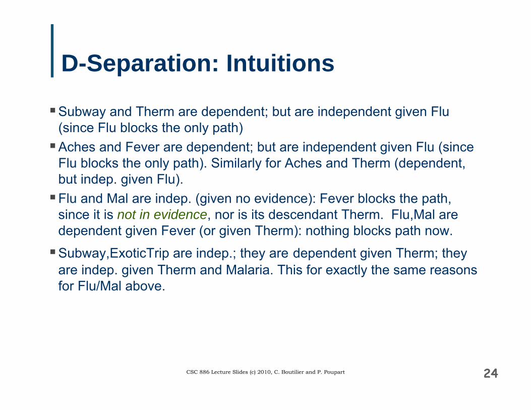
24CSC 886 Lecture Slides (c) 2010, C. Boutilier and P. Poupart
D-Separation: Intuitions
Subway and Therm are dependent; but are independent given Flu (since Flu blocks the only path)Aches and Fever are dependent; but are independent given Flu (since Flu blocks the only path). Similarly for Aches and Therm (dependent, but indep. given Flu).Flu and Mal are indep. (given no evidence): Fever blocks the path, since it is not in evidence, nor is its descendant Therm. Flu,Mal are dependent given Fever (or given Therm): nothing blocks path now.
Subway,ExoticTrip are indep.; they are dependent given Therm; they are indep. given Therm and Malaria. This for exactly the same reasons for Flu/Mal above.

25CSC 886 Lecture Slides (c) 2010, C. Boutilier and P. Poupart
Bayes net queries
Example Query: Pr(X|Y=y)?Intuitively, want to know value of X given some information about the value of Y Concrete examples:
• Doctor: Pr(Disease|Symptoms)?• Car: Pr(condition|mechanicsReport)?• Fault diag.: Pr(pieceMalfunctioning|systemStatistics)?
Use Bayes net structure to quickly compute Pr(X|Y=y)

26CSC 886 Lecture Slides (c) 2010, C. Boutilier and P. Poupart
Algorithms to answer Bayes net queries
There are many…• Variable elimination (aka sum-product)
very simple!• Clique tree propagation (aka junction tree)
quite popular!• Cut-set conditioning• Arc reversal node reduction• Symbolic probabilistic inference
They all exploit conditional independence to speed up computation

27CSC 886 Lecture Slides (c) 2010, C. Boutilier and P. Poupart
Potentials
A function f(X1, X2,…, Xk) is also called a potential. We can view this as table of numbers, one for each instantiation of the variables X1, X2,…, Xk.
A tabular rep’n of a potential is exponential in kEach CPT in a Bayes net is a potential:
• e.g., Pr(C|A,B) is a function of three variables, A, B, CNotation: f(X,Y) denotes a potential over the variables X ∪ Y. (Here X, Y are sets of variables.)
28CSC 886 Lecture Slides (c) 2010, C. Boutilier and P. Poupart
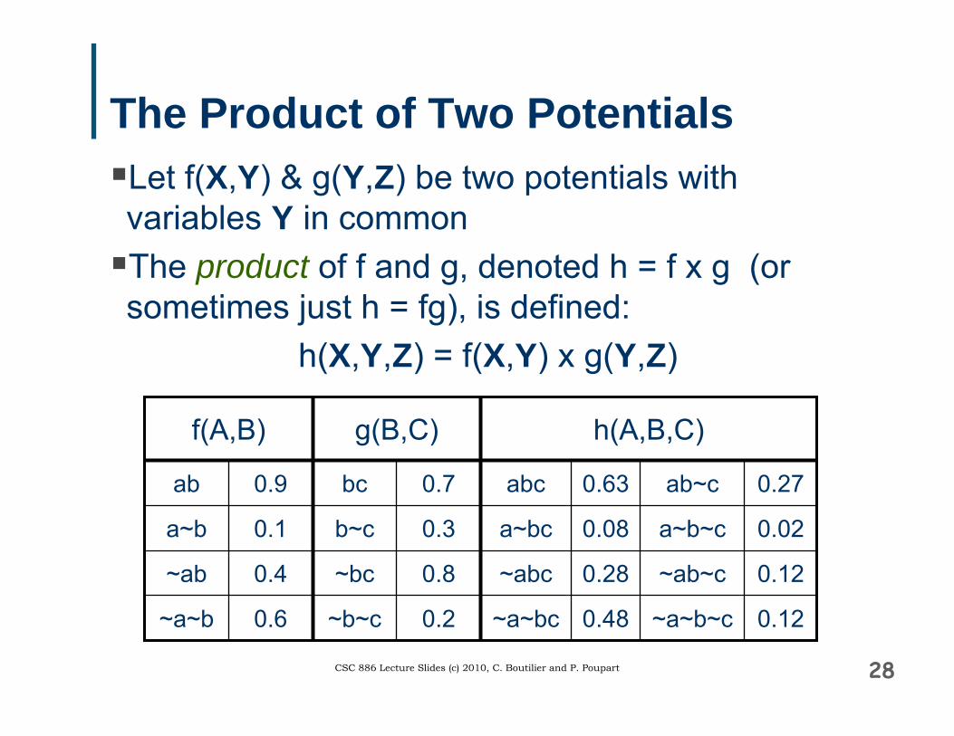
The Product of Two PotentialsLet f(X,Y) & g(Y,Z) be two potentials with variables Y in commonThe product of f and g, denoted h = f x g (or sometimes just h = fg), is defined:
h(X,Y,Z) = f(X,Y) x g(Y,Z)
0.12~a~b~c0.48~a~bc0.2~b~c0.6~a~b
0.12~ab~c0.28~abc0.8~bc0.4~ab
0.02a~b~c0.08a~bc0.3b~c0.1a~b
0.27ab~c0.63abc0.7bc0.9ab
h(A,B,C)g(B,C)f(A,B)

29CSC 886 Lecture Slides (c) 2010, C. Boutilier and P. Poupart
Summing a Variable Out of a PotentialLet f(X,Y) be a factor with variable X (Y is a set)We sum out variable X from f to produce a new potential h = ΣX f, which is defined:
h(Y) = Σx∊Dom(X) f(x,Y)
0.6~a~b
0.4~ab
0.7~b0.1a~b
1.3b0.9ab
h(B)f(A,B)

30CSC 886 Lecture Slides (c) 2010, C. Boutilier and P. Poupart
Restricting a PotentialLet f(X,Y) be a potential with var. X (Y is a set)We restrict potential f to X=x by setting X to the value x and “deleting”. Define h = fX=x as:
h(Y) = f(x,Y)
0.6~a~b
0.4~ab
0.1~b0.1a~b
0.9b0.9ab
h(B) = fA=af(A,B)

31CSC 886 Lecture Slides (c) 2010, C. Boutilier and P. Poupart
Variable Elimination: No EvidenceCompute prior probability of var C
P(C) = ΣA,B P(A,B,C)
= ΣA,B P(C|B) P(B|A) P(A)
= ΣB P(C|B) ΣA P(B|A) P(A)
= ΣB f3(B,C) ΣA f2(A,B) f1(A)
= ΣB f3(B,C) f4(B)= f5(C)
Define new potentials: f4(B)= ΣA f2(A,B) f1(A) and f5(C)= ΣB f3(B,C) f4(B)
B CAf1(A) f2(A,B) f3(B,C)

32CSC 886 Lecture Slides (c) 2010, C. Boutilier and P. Poupart
Variable Elimination: No EvidenceHere’s the example with some numbers
B CAf1(A) f2(A,B) f3(B,C)
~c
c
f5(C)
0.375
0.625
~b
b
f4(B)
0.15
0.85
0.1
0.9
~a
a
f1(A)
0.8~b~c0.6~a~b
0.2~bc0.4~ab
0.3b~c0.1a~b
0.7bc0.9ab
f3(B,C)f2(A,B)
33CSC 886 Lecture Slides (c) 2010, C. Boutilier and P. Poupart
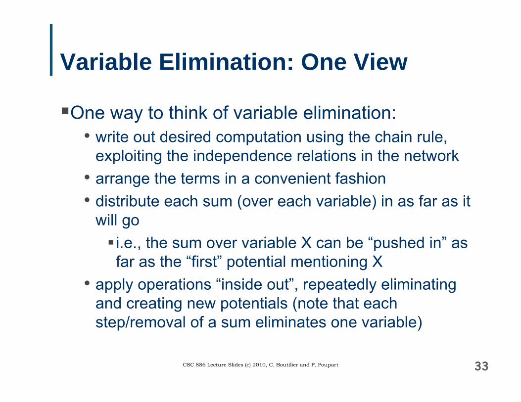
Variable Elimination: One View
One way to think of variable elimination:• write out desired computation using the chain rule,
exploiting the independence relations in the network• arrange the terms in a convenient fashion• distribute each sum (over each variable) in as far as it
will goi.e., the sum over variable X can be “pushed in” as far as the “first” potential mentioning X
• apply operations “inside out”, repeatedly eliminating and creating new potentials (note that each step/removal of a sum eliminates one variable)

34CSC 886 Lecture Slides (c) 2010, C. Boutilier and P. Poupart
Variable Elimination AlgorithmGiven query var Q, remaining vars Z. Let F be set of potentials corresponding to CPTs for {Q} ∪ Z.
1. Choose an elimination ordering Z1, …, Zn of variables in Z.2. For each Zj -- in the order given -- eliminate Zj ∊ Z
as follows:(a) Compute new potential gj = ΣZj f1 x f2 x … x fk,
where the fi are the potentials in F that include Zj(b) Remove the potentials fi (that mention Zj ) from F
and add new potential gj to F3. The remaining potentials refer only to the query variable Q.
Take their product and normalize to produce P(Q)

35CSC 886 Lecture Slides (c) 2010, C. Boutilier and P. Poupart
VE: Example 2
Step 1: Add f5(B,C) = ΣA f3(A,B,C) f1(A) Remove: f1(A), f3(A,B,C)
Step 2: Add f6(C)= ΣB f2(B) f5(B,C)Remove: f2(B) , f5(B,C)
Step 3: Add f7(D) = ΣC f4(C,D) f6(C) Remove: f4(C,D), f6(C)
Last factor f7(D) is (possibly unnormalized) probability P(D)
Factors: f1(A) f2(B) f3(A,B,C) f4(C,D)
Query: P(D)? Elim. Order: A, B, C
C DAf1(A)
f3(A,B,C) f4(C,D)Bf2(B)

36CSC 886 Lecture Slides (c) 2010, C. Boutilier and P. Poupart
Variable Elimination with EvidenceGiven query var Q, evidence vars E (observed to be
e), remaining vars Z. Let F be set of factors involving CPTs for {Q} ∪ Z.
1. Replace each potential f∊F that mentions variable(s) in Ewith its restriction fE=e (somewhat abusing notation)
2. Choose an elimination ordering Z1, …, Zn of variables in Z.3. Run variable elimination as above.4. The remaining potentials refer only to query variable Q.
Take their product and normalize to produce P(Q)

37CSC 886 Lecture Slides (c) 2010, C. Boutilier and P. Poupart
VE: Example 2 again with Evidence
Restriction: replace f4(C,D) with f5(C) = f4(C,d) Step 1: Add f6(A,B)= ΣC f5(C) f3(A,B,C)
Remove: f3(A,B,C), f5(C) Step 2: Add f7(A) = ΣB f6(A,B) f2(B)
Remove: f6(A,B), f2(B) Last potent.: f7(A), f1(A). The product f1(A) x f7(A) is (possibly
unnormalized) posterior. So… P(A|d) = α f1(A) x f7(A).
Factors: f1(A) f2(B) f3(A,B,C) f4(C,D)
Query: P(A)? Evidence: D = dElim. Order: C, B
C DAf1(A)
f3(A,B,C) f4(C,D)Bf2(B)
38CSC 886 Lecture Slides (c) 2010, C. Boutilier and P. Poupart
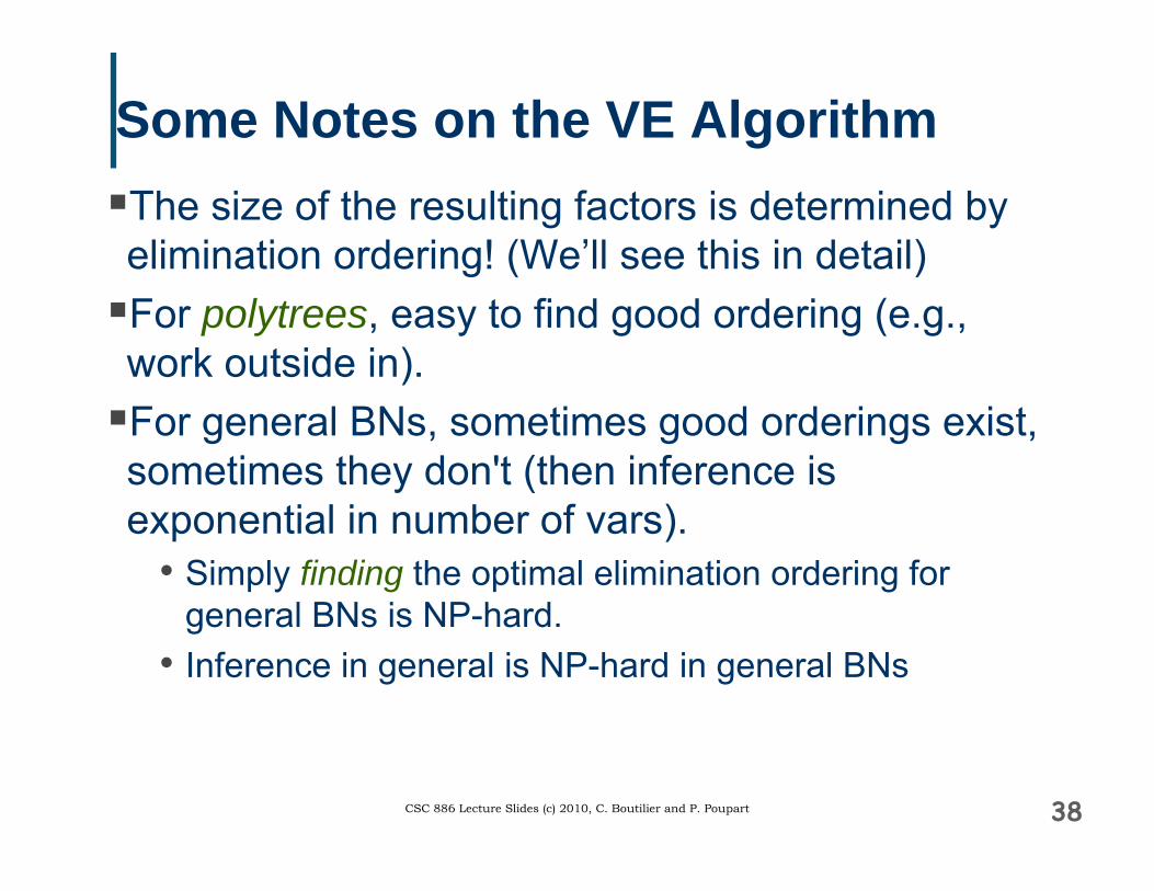
Some Notes on the VE AlgorithmThe size of the resulting factors is determined by elimination ordering! (We’ll see this in detail)For polytrees, easy to find good ordering (e.g., work outside in).For general BNs, sometimes good orderings exist, sometimes they don't (then inference is exponential in number of vars).
• Simply finding the optimal elimination ordering for general BNs is NP-hard.
• Inference in general is NP-hard in general BNs

39CSC 886 Lecture Slides (c) 2010, C. Boutilier and P. Poupart
Elimination Ordering: PolytreesInference is linear in size of network
• ordering: eliminate only “singly-connected” nodes
• e.g., in this network, eliminate D, A, C, X1,…; or eliminate X1,… Xk, D, A, C; or mix up…
• result: no factor ever larger than original CPTs
• eliminating B before these gives factors that include all of A,C, X1,… Xk !!!

40CSC 886 Lecture Slides (c) 2010, C. Boutilier and P. Poupart
Effect of Different OrderingsSuppose query variable is D. Consider different orderings for this network
• A,F,H,G,B,C,E:good: why?
• E,C,A,B,G,H,F:bad: why?
Which ordering creates smallest factors?
• either max size or totalwhich creates largest factors?

41CSC 886 Lecture Slides (c) 2010, C. Boutilier and P. Poupart
Relevance
Certain variables have no impact on the query. In ABC network, computing Pr(A) with no evidence requires elimination of B and C.
• But when you sum out these vars, you compute a trivial potential (all values are ones); for example:
• eliminating C: f4(B) = ΣC f3(B,C) = ΣC Pr(C|B)• 1 for any value of B (e.g., Pr(c|b) + Pr(~c|b) = 1)
No need to think about B or C for this query
B CA

42CSC 886 Lecture Slides (c) 2010, C. Boutilier and P. Poupart
Pruning irrelevant variables
Can restrict attention to relevant variables. Given query Q, evidence E:
• Q is relevant• if any node Z is relevant, its parents are relevant• if E∊E is a descendent of a relevant node, then E is
relevantWe can restrict our attention to the subnetworkcomprising only relevant variables when evaluating a query Q

43CSC 886 Lecture Slides (c) 2010, C. Boutilier and P. Poupart
Relevance: ExamplesQuery: P(F)
• relevant: F, C, B, AQuery: P(F|E)
• relevant: F, C, B, A• also: E, hence D, G• intuitively, we need to compute
P(C|E)=α P(C) P(E|C) to accuratelycompute P(F|E)
Query: P(F|E,C)• algorithm says all vars relevant; but really none
except C, F (since C cuts of all influence of others)• algorithm is overestimating relevant set
C
A B
D
E
F
G
Copyright © 2022 FDOKUMEN


![Course: Biostatistics Lecture No: [ 2 ] - Philadelphia University](https://static.fdokumen.com/doc/165x107/633a2618749bc7c55d0d5094/course-biostatistics-lecture-no-2-philadelphia-university.jpg)