Numerical Computation of Internal and External Flows

FM-H6594.tex 8/5/2007 12: 31 Page i

Numerical Computation of Internaland External Flows

Volume 1Fundamentals of Computational Fluid

Dynamics

This page intentionally left blank

FM-H6594.tex 8/5/2007 12: 31 Page iii

Numerical Computation ofInternal and External Flows

Volume 1Fundamentals of Computational

Fluid DynamicsSecond edition

Charles Hirsch

AMSTERDAM • BOSTON • HEIDELBERG • LONDON • NEW YORK • OXFORDPARIS • SAN DIEGO • SAN FRANCISCO • SINGAPORE • SYDNEY • TOKYO

Butterworth-Heinemann is an imprint of Elsevier

FM-H6594.tex 8/5/2007 12: 31 Page iv

Butterworth-Heinemann is an imprint of ElsevierLinacre House, Jordan Hill, Oxford OX2 8DP30 Corporate Drive, Suite 400, Burlington, MA 01803, USA

First published by John Wiley & Sons, LtdSecond edition 2007

Copyright © 2007. Charles Hirsch. All rights reserved

The right of Charles Hirsch to be identified as the authors of this work has been assertedin accordance with the Copyright, Designs and Patents Act 1988

No part of this publication may be reproduced, stored in a retrieval system or transmitted in anyform or by any means electronic, mechanical, photocopying, recording or otherwise withoutthe prior written permission of the publisher

Permissions may be sought directly from Elsevier’s Science & Technology Rights Department inOxford, UK: phone (+44) (0) 1865 843830; fax (+44) (0) 1865 853333;email: [email protected]. Alternatively you can submit your request online byvisiting the Elsevier web site at http://elsevier.com/locate/permissions, and selectingObtaining permission to use Elsevier material

NoticeNo responsibility is assumed by the publisher for any injury and/or damage to personsor property as a matter of products liability, negligence or otherwise, or from any useor operation of any methods, products, instructions or ideas contained in the material herein.Because of rapid advances in the medical sciences, in particular, independentverification of diagnoses and drug dosages should be made

British Library Cataloguing in Publication DataA catalogue record for this book is available from the British Library

Library of Congress Cataloguing in Publication DataA catalog record for this book is available from the Library of Congress

ISBN: 978-0-7506-6594-0

For information on all Butterworth-Heinemann publications visitour web site at http://books.elsevier.com

Typeset by Charon Tec Ltd (A Macmillan Company), Chennai, Indiawww.charontec.com

Printed and bound in Great Britain

07 08 09 10 10 9 8 7 6 5 4 3 2 1

FM-H6594.tex 8/5/2007 12: 31 Page v

To the Memory of

Leon Hirsch

and

Czypa Zugman

my parents,struck by destiny

FM-H6594.tex 8/5/2007 12: 31 Page vi

Contents

Preface to the second edition xv

Nomenclature xviii

Introduction: An Initial Guide to CFD and to this Volume 1I.1 The position of CFD in the world of virtual prototyping 1

I.1.1 The Definition Phase 2I.1.2 The Simulation and Analysis Phase 3I.1.3 The Manufacturing Cycle Phase 5

I.2 The components of a CFD simulation system 11I.2.1 Step 1: Defining the Mathematical Model 11I.2.2 Step 2: Defining the Discretization Process 13I.2.3 Step 3: Performing the Analysis Phase 15I.2.4 Step 4: Defining the Resolution Phase 16

I.3 The structure of this volume 18References 20

Part I The Mathematical Models for Fluid Flow Simulations atVarious Levels of Approximation 21

1 The Basic Equations of Fluid Dynamics 27Objectives and guidelines 271.1 General form of a conservation law 29

1.1.1 Scalar Conservation Law 301.1.2 Convection–Diffusion Form of a Conservation Law 331.1.3 Vector Conservation Law 38The Equations of Fluid Mechanics 39

1.2 The mass conservation equation 401.3 The momentum conservation law or equation of motion 431.4 The energy conservation equation 47

1.4.1 Conservative Formulation of the Energy Equation 491.4.2 The Equations for Internal Energy and Entropy 491.4.3 Perfect Gas Model 501.4.4 Incompressible Fluid Model 53

A1.5 Rotating frame of reference 54A1.5.1 Equation of Motion in the Relative System 54A1.5.2 Energy Equation in the Relative System 55A1.5.3 Crocco’s Form of the Equations of Motion 56

A1.6 Advanced applications of control volume formulations 57A1.6.1 Lift and Drag Estimations from CFD Results 57A1.6.2 Conservation Law for a Moving Control Volume 58

Summary of the basic flow equations 60

vi

FM-H6594.tex 8/5/2007 12: 31 Page vii

Contents vii

Conclusions and main topics to remember 63References 63Problems 63

2 The Dynamical Levels of Approximation 65Objectives and guidelines 652.1 The Navier–Stokes equations 70

2.1.1 Non-uniqueness in Viscous Flows 732.1.1.1 Marangoni thermo-capillary flow in a liquid bridge 732.1.1.2 Flow around a circular cylinder 77

2.1.2 Direct Numerical Simulation of Turbulent Flows (DNS) 832.2 Approximations of turbulent flows 86

2.2.1 Large Eddy Simulation (LES) of Turbulent Flows 872.2.2 Reynolds Averaged Navier–Stokes Equations (RANS) 89

2.3 Thin shear layer approximation (TSL) 942.4 Parabolized Navier–Stokes equations 942.5 Boundary layer approximation 952.6 The distributed loss model 962.7 Inviscid flow model: Euler equations 972.8 Potential flow model 982.9 Summary 101References 101Problems 103

3 The Mathematical Nature of the Flow Equations and TheirBoundary Conditions 105Objectives and guidelines 1053.1 Simplified models of a convection–diffusion equation 108

3.1.1 1D Convection–Diffusion Equation 1083.1.2 Pure Convection 1093.1.3 Pure Diffusion in Time 1103.1.4 Pure Diffusion in Space 111

3.2 Definition of the mathematical properties of a system of PDEs 1113.2.1 System of First Order PDEs 1123.2.2 Partial Differential Equation of Second Order 116

3.3 Hyperbolic and parabolic equations: characteristic surfaces anddomain of dependence 1173.3.1 Characteristic Surfaces 1183.3.2 Domain of Dependence: Zone of Influence 120

3.3.2.1 Parabolic problems 1203.3.2.2 Elliptic problems 122

3.4 Time-dependent and conservation form of the PDEs 1223.4.1 Plane Wave Solutions with Time Variable 1233.4.2 Characteristics in a One-Dimensional Space 1283.4.3 Nonlinear Definitions 129

3.5 Initial and boundary conditions 130A.3.6 Alternative definition: compatibility relations 132

A3.6.1 Compatibility Relations 133

FM-H6594.tex 8/5/2007 12: 31 Page viii

viii Contents


Part II Basic Discretization Techniques 141

4 The Finite Difference Method for Structured Grids 145Objectives and guidelines 1454.1 The basics of finite difference methods 147

4.1.1 Difference Formulas for First and Second Derivatives 1494.1.1.1 Difference formula for first derivatives 1504.1.1.2 FD formulas for second derivatives 153

4.1.2 Difference Schemes for One-Dimensional Model Equations 1544.1.2.1 Linear one-dimensional convection equation 1544.1.2.2 Linear diffusion equation 159

4.2 Multidimensional finite difference formulas 1604.2.1 Difference Schemes for the Laplace Operator 1624.2.2 Mixed Derivatives 166

4.3 Finite difference formulas on non-uniform grids 1694.3.1 Difference Formulas for First Derivatives 172

4.3.1.1 Conservative FD formulas 1734.3.2 A General Formulation 1744.3.3 Cell-Centered Grids 1774.3.4 Guidelines for Non-uniform Grids 179

A4.4 General method for finite difference formulas 180A4.4.1 Generation of Difference Formulas for First

Derivatives 181A4.4.1.1 Forward differences 182A4.4.1.2 Backward differences 183A4.4.1.3 Central differences 183

A4.4.2 Higher Order Derivatives 184A4.4.2.1 Second order derivative 186A4.4.2.2 Third order derivatives 187A4.4.2.3 Fourth order derivatives 189

A4.5 Implicit finite difference formulas 189A4.5.1 General Approach 189A4.5.2 General Derivation of Implicit Finite Difference

Formula’s for First and Second Derivatives 191Conclusions and main topics to remember 195References 196Problems 197

5 Finite Volume Method and Conservative Discretization with anIntroduction to Finite Element Method 203Objectives and guidelines 2035.1 The conservative discretization 204

5.1.1 Formal Expression of a Conservative Discretization 208

FM-H6594.tex 8/5/2007 12: 31 Page ix

Contents ix

5.2 The basis of the finite volume method 2095.2.1 Conditions on Finite Volume Selections 2105.2.2 Definition of the Finite Volume Discretization 2125.2.3 General Formulation of a Numerical Scheme 213

5.3 Practical implementation of finite volume method 2165.3.1 Two-Dimensional Finite Volume Method 2165.3.2 Finite Volume Estimation of Gradients 221

A.5.4 The finite element method 225A5.4.1 Finite Element Definition of Interpolation Functions 226

A5.4.1.1 One-dimensional linear elements 228A5.4.1.2 Two-dimensional linear elements 231

A5.4.2 Finite Element Definition of the EquationDiscretization: Integral Formulation 232

A5.4.3 The Method of Weighted Residuals or Weak Formulation 232A5.4.4 The Galerkin Method 234A5.4.5 Finite Element Galerkin Method for a

Conservation Law 237A5.4.6 Subdomain Collocation: Finite Volume Method 238


6 Structured and Unstructured Grid Properties 249Objectives and guidelines 2496.1 Structured Grids 250

6.1.1 Cartesian Grids 2526.1.2 Non-uniform Cartesian Grids 2526.1.3 Body-Fitted Structured Grids 2546.1.4 Multi-block Grids 256

6.2 Unstructured grids 2616.2.1 Triangle/Tetrahedra Cells 2626.2.2 Hybrid Grids 2646.2.3 Quadrilateral/Hexahedra Cells 2646.2.4 Arbitrary Shaped Elements 265

6.3 Surface and volume estimations 2676.3.1 Evaluation of Cell Face Areas 2696.3.2 Evaluation of Control Cell Volumes 270

6.4 Grid quality and best practice guidelines 2746.4.1 Error Analysis of 2D Finite Volume Schemes 2746.4.2 Recommendations and Best Practice Advice on Grid

Quality 276Conclusions and main topics to remember 276References 277

Part III The Analysis of Numerical Schemes 279

7 Consistency, Stability and Error Analysis of Numerical Schemes 283Objectives and guidelines 283

FM-H6594.tex 8/5/2007 12: 31 Page x

x Contents

7.1 Basic concepts and definitions 2857.1.1 Consistency Condition, Truncation Error and Equivalent

Differential Equation of a Numerical Scheme 2877.1.1.1 Methodology 287

7.2 The Von Neumann method for stability analysis 2927.2.1 Fourier Decomposition of the Solution 2937.2.2 Amplification factor 296

7.2.2.1 Methodology 2967.2.3 Comments on the CFL Condition 300

7.3 New schemes for the linear convection equation 3037.3.1 The Leapfrog Scheme for the Convection Equation 3047.3.2 Lax–Friedrichs Scheme for the Convection Equation 3057.3.3 The Lax–Wendroff Scheme for the Convection Equation 306

7.4 The spectral analysis of numerical errors 3137.4.1 Error Analysis for Hyperbolic Problems 316

7.4.1.1 Error analysis of the explicit First OrderUpwind scheme (FOU) 317

7.4.1.2 Error analysis of the Lax–Friedrichs schemefor the convection equation 320

7.4.1.3 Error analysis of the Lax–Wendroff schemefor the convection equation 320

7.4.1.4 Error analysis of the leapfrog scheme for theconvection equation 323

7.4.2 The Issue of Numerical Oscillations 3247.4.3 The Numerical Group Velocity 3267.4.4 Error Analysis for Parabolic Problems 3307.4.5 Lessons Learned and Recommendations 330


8 General Properties and High-Resolution Numerical Schemes 337Objectives and guidelines 3378.1 General formulation of numerical schemes 339

8.1.1 Two-Level Explicit Schemes 3408.1.2 Two-Level Schemes for the Linear Convection Equation 3438.1.3 Amplification Factor, Error Estimation and Equivalent 346

Differential Equation8.1.4 Accuracy Barrier for Stable Scalar Convection Schemes 349A8.1.5 An Addition to the Stability Analysis 351A8.1.6 An Advanced Addition to the Accuracy Barrier 352

8.2 The generation of new schemes with prescribed order ofaccuracy 3548.2.1 One-Parameter Family of Schemes on the Support

(i − 1, i, i + 1) 3558.2.2 The Convection–Diffusion Equation 3578.2.3 One-Parameter Family of Schemes on the Support

(i − 2, i − 1, i, i + 1) 361

FM-H6594.tex 8/5/2007 12: 31 Page xi

Contents xi

8.3 Monotonicity of numerical schemes 3658.3.1 Monotonicity Conditions 3668.3.2 Semi-Discretized Schemes or Method of Lines 3708.3.3 Godunov’s Theorem 3728.3.4 High-Resolution Schemes and the Concept of Limiters 373

8.4 Finite volume formulation of schemes and limiters 3898.4.1 Numerical flux 3908.4.2 The Normalized Variable Representation 397


Part IV The Resolution of Numerical Schemes 411

9 Time Integration Methods for Space-discretized Equations 413Objectives and guidelines 4139.1 Analysis of the space-discretized systems 414

9.1.1 The Matrix Representation of the Diffusion SpaceOperator 416

9.1.2 The Matrix Representation of the ConvectionSpace Operator 418

9.1.3 The Eigenvalue Spectrum of Space-discretized Systems 4219.1.4 Matrix Method and Fourier Modes 4259.1.5 Amplification Factor of the Semi-discretized System 4289.1.6 Spectrum of Second Order Upwind Discretizations of the

Convection Operator 4299.2 Analysis of time integration schemes 429

9.2.1 Stability Regions in the Complex � Plane andFourier Modes 431

9.2.2 Error Analysis of Space and Time Discretized Systems 4349.2.2.1 Diffusion and dispersion errors of the timeintegration 4349.2.2.2 Diffusion and dispersion errors of space andtime discretization 4359.2.2.3 Relation with the equivalent differential equation 436

9.2.3 Forward Euler Method 4369.2.4 Central Time Differencing or Leapfrog Method 4389.2.5 Backward Euler Method 439

9.3 A selection of time integration methods 4419.3.1 Nonlinear System of ODEs and their Linearization 4439.3.2 General Multistep Method 445

9.3.2.1 Beam and Warming schemes for the convectionequation 449

9.3.2.2 Nonlinear systems and approximate Jacobianlinearizations 450

9.3.3 Predictor–Corrector Methods 4539.3.4 The Runge–Kutta Methods 458

9.3.4.1 Stability analysis for the Runge–Kutta method 460

FM-H6594.tex 8/5/2007 12: 31 Page xii

xii Contents

9.3.5 Application of the Methodology and Implicit Methods 4659.3.6 The Importance of Artificial Dissipation with

Central Schemes 469A9.4 Implicit schemes for multidimensional problems:

approximate factorization methods 475A9.4.1 Two-Dimensional Diffusion Equation 478A9.4.2 ADI Method for the Convection Equation 480


10 Iterative Methods for the Resolution of Algebraic Systems 491Objectives and guidelines 49110.1 Basic iterative methods 493

10.1.1 Poisson’s Equation on a Cartesian,Two-Dimensional Mesh 493

10.1.2 Point Jacobi Method/Point Gauss–Seidel Method 49510.1.3 Convergence Analysis of Iterative Schemes 49810.1.4 Eigenvalue Analysis of an Iterative Method 50110.1.5 Fourier Analysis of an Iterative Method 504

10.2 Overrelaxation methods 50510.2.1 Jacobi Overrelaxation 50610.2.2 Gauss–Seidel Overrelaxation: Successive

Overrelaxation (SOR) 50710.2.3 Symmetric Successive Overrelaxation (SSOR) 50910.2.4 Successive Line Overrelaxation Methods (SLOR) 510

10.3 Preconditioning techniques 51210.3.1 Richardson Method 51310.3.2 Alternating Direction Implicit Method (ADI) 51510.3.3 Other Preconditioning and Relaxation Methods 516

10.4 Nonlinear problems 51810.5 The multigrid method 520

10.5.1 Smoothing Properties 52310.5.2 The Coarse Grid Correction Method (CGC) for

Linear Problems 52510.5.3 The Two-Grid Iteration Method for Linear Problems 52910.5.4 The Multigrid Method for Linear Problems 53010.5.5 The Multigrid Method for Nonlinear Problems 532

Conclusions and main topics to remember 533References 533Problems 535Appendix A: Thomas Algorithm for Tridiagonal Systems 536A.1. Scalar Tridiagonal Systems 536A.2. Periodic Tridiagonal Systems 538

Part V Applications to Inviscid and Viscous Flows 541

11 Numerical Simulation of Inviscid Flows 545Objectives and guidelines 545

FM-H6594.tex 8/5/2007 12: 31 Page xiii

Contents xiii

11.1 The inviscid Euler equations 54811.1.1 Steady Compressible Flows 54911.1.2 The Influence of Compressibility 54911.1.3 The Properties of Discontinuous Solutions 551

11.1.3.1 Contact Discontinuities 55311.1.3.2 Vortex sheets or slip lines 55311.1.3.3 Shock surfaces 553

11.1.4 Lift and Drag on Solid Bodies 55411.2 The potential flow model 556

11.2.1 The Limitations of the Potential Flow Model forTransonic Flows 557

11.2.2 Incompressible Potential Flows 55711.3 Numerical solutions for the potential equation 558

11.3.1 Incompressible Flow Around a Circular Cylinder 55811.3.1.1 Define the grid 56111.3.1.2 Define the numerical scheme 56611.3.1.3 Solve the algebraic system 56911.3.1.4 Analyze the results and evaluate the accuracy 570

11.3.2 Compressible Potential Flow Around the CircularCylinder 57111.3.2.1 Numerical estimation of the density and its

nonlinearity 57111.3.2.2 Transonic potential flow 572

11.3.3 Additional Optional Tasks 57411.4 Finite volume discretization of the Euler equations 574

11.4.1 Finite Volume Method for Euler Equations 57511.4.1.1 Space discretization 57611.4.1.2 Time integration 57811.4.1.3 Boundary conditions for the Euler equations 579

11.5 Numerical solutions for the Euler equations 58311.5.1 Application to the Flow Around a Cylinder 58311.5.2 Application to the Internal Flow in a Channel with a

Circular Bump 58711.5.3 Application to the Supersonic Flow on a

Wedge at M = 2.5 59111.5.4 Additional Hands-On Suggestions 595

Conclusions and main topics to remember 596References 597

12 Numerical Solutions of Viscous Laminar Flows 599Objectives and guidelines 59912.1 Navier–Stokes equations for laminar flows 601

12.1.1 Boundary Conditions for Viscous Flows 60312.1.2 Grids for Boundary Layer Flows 604

12.2 Density-based methods for viscous flows 60412.2.1 Discretization of Viscous and Thermal Fluxes 60512.2.2 Boundary Conditions 607

12.2.2.1 Physical boundary conditions 607

FM-H6594.tex 8/5/2007 12: 31 Page xiv

xiv Contents

12.2.2.2 Numerical boundary conditions 60912.2.2.3 Periodic boundary conditions 609

12.2.3 Estimation of Viscous Time Step and CFL Conditions 61012.3 Numerical solutions with the density-based method 610

12.3.1 Couette Thermal Flow 61112.3.1.1 Numerical simulation conditions 61312.3.1.2 Grid definition 61412.3.1.3 Results 61412.3.1.4 Other options for solving the Couette flow 616

12.3.2 Flat Plate 61812.3.2.1 Exact solution 61812.3.2.2 Grid definition 61912.3.2.3 Results 622

12.4 Pressure correction method 62512.4.1 Basic Approach of Pressure Correction Methods 62712.4.2 The Issue of Staggered Versus Collocated Grids 62912.4.3 Implementation of a Pressure Correction Method 632

12.4.3.1 Numerical discretization 63412.4.3.2 Algorithm for the pressure Poisson equation 636

12.5 Numerical solutions with the pressure correction method 63812.5.1 Lid Driven Cavity 63812.5.2 Additional Suggestions 639

12.6 Best practice advice 64012.6.1 List of Possible Error Sources 64212.6.2 Best Practice Recommendations 642

Conclusions and main topics to remember 644References 645

Index 647

FM-H6594.tex 8/5/2007 12: 31 Page xv

Preface to the second edition

This second, long (over)due, edition presents a major extension and restructur-ing of the initial two volumes edition, based on objective as well as subjectiveelements.

The first group of arguments is related to numerous requests we have received overthe years after the initial publication, for enhancing the didactic structure of the twovolumes in order to respond to the development of CFD courses, starting often nowat an advanced undergraduate level.

We decided therefore to adapt the first volume, which was oriented at the fundamen-tals of numerical discretizations, toward a more self-contained and student-orientedfirst course material for an introduction to CFD. This has led to the following changesin this second edition:

• We have focused on a presentation of the essential components of a simulationsystem, at an introductory level to CFD, having in mind students who come incontact with the world of CFD for the first time. The objective being to make thestudent aware of the main steps required by setting up a numerical simulation,and the various implications as well as the variety of options available. Thiswill cover Chapters 1–10, while Chapters 11 and 12 are dedicated to the firstapplications of the general methodology to inviscid simple flows in Chapter 11and to 2D incompressible, viscous flows in Chapter 12.

• Several chapters are subdivided into two parts: an introductory level written fora first introductory course to CFD and a second, more advanced part, which ismore suitable for a graduate and more advanced CFD course. We hope that byputting together the introductory presentation and the more advanced topics, thestudent will be stimulated by the first approach and his/her curiosity for the moreadvanced level, which is closer to the practical world of CFD, will be aroused.We also hope by this way to avoid frightening off the student who would betotally new to CFD, by a too ‘brutal’ contact with an approach that might appearas too abstract and mathematical.

• Each chapter is introduced by a section describing the ‘Objectives and guidelinesto this Chapter’, and terminates by a section on ‘Conclusions and main topicsto remember’, allowing the instructor or the student to establish his or her guidethrough the selected source material.

• The chapter on finite differences has been extended with additional considera-tions given to discretizations formulas on non-uniform grids.

• The chapters on finite element and finite volume methods have been merged,shifting the finite element description to the ‘advanced’ level, into Chapter 5 ofthis volume.

• A new Chapter 6 has been added devoted to an overview of various grids usedin practice, including some recommendations related to grid quality.

xv

FM-H6594.tex 8/5/2007 12: 31 Page xvi

xvi Preface

• Chapters 7 and 8 of the first edition, devoted to the analysis of numerical schemesfor consistency and stability have been merged and simplified, forming the newChapter 7.

• Chapter 9 of the first edition has been largely reorganized, simplified andextended with new material related to general scheme properties, in particu-lar the extremely important concept of monotonicity and the methodologiesrequired to suppress numerical oscillations with higher order schemes, with theintroduction of limiters. This is found in Chapter 8 of this volume.

• The former Chapters 10 and 11 have been merged in the new Chapter 9, devotedto the time integration schemes and to the general methodologies resulting fromthe combination of a selected space discretization with a separate time integrationmethod.

• Parts of the second volume have been transferred to the first volume; in partic-ular sections on potential flows (presented in Chapter 11) and two-dimensionalviscous flows in Chapter 12. This should allow the student already to come incontact, at this introductory CFD level, with initial applications of fluid flowsimulations.

• The number of problems has been increased and complete solution manuals willbe made available to the instructors. Also a computer program for the numericalsolutions of simple 1D convection and convection–diffusion equations, with alarge variety of schemes and test cases can be made available to the instructors,for use in classes and exercises sessions. The objective of this option is to providea tool allowing the students to develop their own ‘feeling’ and experience withvarious schemes, including assessment of the different types and level of errorsgenerated by the combination of schemes and test cases. Many of the figures inthe two volumes have been generated with these programs.

The second group of elements is connected to the considerable evolution and exten-sion of Computational Fluid Dynamics (CFD) since the first publication of thesebooks. CFD is now an integral part of any fluid-related research and industrial appli-cation, and is progressively reaching a mature stage. Its evolution, since the initialpublication of this book, has been marked by significant advancements, which wefeel have to be covered, at least partly, in order to provide the reader with a reliableand up-to-date introduction and account of modern CFD. This relates in particular to:

• Major developments of schemes and codes based on unstructured grids, whichare today the ‘standard’, particularly with most of the commercial CFD packages,as unstructured codes take advantage of the availability of nearly automatic gridgeneration tools for complex geometries.

• Advances in high-resolution algorithms, which have provided a deep insight inthe general properties of numerical schemes, leading to a unified and elegantapproach, where concepts of accuracy, stability, monotonicity can be definedand applied to any type of equation.

• Major developments in turbulence modeling, including Direct NumericalSimulations (DNS) and Large Eddy Simulations (LES).

• Applications of full 3D Navier–Stokes simulations to an extreme variety of com-plex industrial, environmental, bio-medical and other disciplines, where fluids

FM-H6594.tex 8/5/2007 12: 31 Page xvii

Preface xvii

play a role in their properties and evolution. This has led to a considerable overallexperience accumulated over the last decade, on schemes and models.

• The awareness of the importance of verification and validation of CFD codes andthe development of related methodologies. This has given rise to the definitionand evaluation of families of test cases including the related quality assessmentissues.

• The wide availability of commercial CFD codes, which are increasingly beingused as teaching tools, to support the understanding of fluid mechanics and/orto generate simple flow simulations. This puts a strong emphasis on the need foreducating students in the use of codes and providing them with an awarenessof possible inaccuracies, sources of errors, grid and modeling effects and, moregenerally, with some global Best Practice Guidelines.

Many of these topics will be found in the second edition of Volume II.I have benefited from the spontaneous input from many colleagues and students,

who have been kind enough to send me notices about misprints in text and in formulas,helping hereby in improving the quality of the books and correcting errors. I am verygrateful to all of them.

I also have to thank many of my students and researchers, who have contributedat various levels; in particular: Dr. Zhu Zong–Wen for the many problem solutions;Cristian Dinescu for various corrections. Benoit Tartinville and Dr. Sergey Smirnovhave contributed largely to the calculations and derivations in Chapters 11 and 12.

Brussels, December 2006

FM-H6594.tex 8/5/2007 12: 31 Page xviii

Nomenclature

a convection velocity or wave speedA Jacobian of flux functionc speed of soundcp specific heat at constant pressurecv specific heat at constant volumeD first derivative operatore internal energy per unit masse vector (column matrix) of solution errors�ex, �ey, �ez unit vectors along the x, y, z directionsE total energy per unit volumeE finite difference displacement (shift) operatorf flux function�fe external force vector�F ( f , g, h) flux vector with components f , g, hg gravity accelerationG amplification factor/matrixh enthalpy per unit massH total enthalpyI rothalpyJ Jacobiank coefficient of thermal conductivityk wave numberM Mach numbern normal distance�n normal vectorp pressureP convergence or conditioning operatorPr Prandtl numberq non homogeneous termqH heat sourceQ source term; matrix of non homogeneous termsr gas constant per unit massR residual of iterative schemeRe Reynolds numbers entropy per unit massS space discretization operator�S surface vectort timeT temperatureu dependent variableU vector (column matrix) of dependent variables

xviii

FM-H6594.tex 8/5/2007 12: 31 Page xix

Nomenclature xix

U vector of conservative variables; velocity�v (u, v, w) velocity vector with components u, v, wV eigenvectors of space discretization matrix�w relative velocityW weight functionx, y, z cartesian coordinatesz amplification factor of time integration scheme

α diffusivity coefficientβ dimensionless diffusion coefficient β = α�t/�x, also called Von

Neumann numberγ specific heat ratio� circulation; boundary of domain �

δ central-difference operatorδ+, δ− forward and backward difference operators� Laplace operator�t time step�U variation of solution U between levels n + 1 and n�x, �y spatial mesh size in x and y directionsε error of numerical solutionεv turbulence dissipation rateεD dissipation or diffusion errorεφ dispersion error�ζ vorticity vectorθ parameter controlling type of difference scheme�κ wave-number vector; wave propagation directionλ eigenvalue of amplification matrixμ coefficient of dynamic viscosityμ averaging difference operatorξ real part of amplification matrixη imaginary part of amplification matrixρ density; spectral radiusσ Courant numberσ shear stress tensorτ stress tensorν kinematic viscosityφ velocity potential; phase angle in Von Neumann analysis� phase angle of amplification factorω time frequency of plane wave; overrelaxation parameters� eigenvalue of space discretization matrix; volume

Subscripts

e external variablei, j mesh point locations in x, y directionsI, J nodal point indexJ eigenvalue number

FM-H6594.tex 8/5/2007 12: 31 Page xx

xx Nomenclature

min minimummax maximumn normal or normal componento stagnation valuesv viscous termx, y, z components in x, y, z directions; partial differentiation with respect

to x, y, z∞ freestream value

Superscripts

n iteration level; time level

Intro-H6594.tex 9/5/2007 11: 42 Page 1

Introduction: An Initial Guide to CFDand to this Volume

Computational Fluid Dynamics, known today as CFD, is defined as the set ofmethodologies that enable the computer to provide us with a numerical simulation offluid flows.

We use the word ‘simulation’ to indicate that we use the computer to solve numer-ically the laws that govern the movement of fluids, in or around a material system,where its geometry is also modeled on the computer. Hence, the whole system istransformed into a ‘virtual’ environment or virtual product. This can be opposed toan experimental investigation, characterized by a material model or prototype of thesystem, such as an aircraft or car model in a wind tunnel, or when measuring the flowproperties in a prototype of an engine.

This terminology is also referring to the fact that we can visualize the whole systemand its behavior, through computer visualization tools, with amazing levels of realism,as you certainly have experienced through the powerful computer games and/or movieanimations, that provide a fascinating level of high-fidelity rendering. Hence thecomplete system, such as a car, an airplane, a block of buildings, etc. can be ‘seen’on a computer, before any part is ever constructed.

I.1 THE POSITION OF CFD IN THE WORLD OF VIRTUAL PROTOTYPING

To situate the role and importance of CFD in our contemporary technological world, itmight be of interest to take you down the road to the global world of Computer-AssistedEngineering or CAE. CAE refers to the ensemble of simulation tools that supportthe work of the engineer between the initial design phase and the final definition ofthe manufacturing process. The industrial production process is indeed subjected toan accelerated evolution toward the computerization of the whole production cycle,using various software tools.

The most important of them are: Computer-Assisted Design (CAD), Computer-Assisted Engineering (CAE) and Computer-Assisted Manufacturing (CAM) soft-ware. The CAD/CAE/CAM software systems form the basis for the different phasesof the virtual prototyping environment as shown in Figure I.1.1.

This chart presents the different components of a computer-oriented environment,as used in industry to create, or modify toward better properties, a product. Thisproduct can be a single component such as a cooling jacket in a car engine, formedby a certain number of circular curved pipes, down to a complete car. In all cases thesuccession of steps and the related software tools are used in very much similar ways,the difference being the degree of complexity to which these tools are applied.

1

Intro-H6594.tex 9/5/2007 11: 42 Page 2

2 Introduction: An Initial Guide to CFD and to this Volume

ShapeDefinition

(CAD)

VirtualPrototypingSimulation

and Analysis(CAE)

ManufacturingCycle(CAM)

CAACEM

CSMCFD

Definitionphase

Simulation andanalysis phase

Manufacturingphase

ProductSpecification

Figure I.1.1 The structure of the virtual prototyping environment.

I.1.1 The Definition Phase

The first step in the creation of the product is the definition phase, which coversthe specification and geometrical definition. It is based on CAD software, whichallows creating and defining the geometry of the system, in all its details. Typically,large industries can employ up to thousands of designers, working full time on CADsoftware. Their day-to-day task is to build the geometrical model on the computerscreen, in interaction with the engineers of the simulation and analysis departments.

This CAD definition of the geometry is the required and unavoidable input to theCFD simulation task.

Figure I.1.2 shows several examples of CAD definitions of different models, forwhich we will see later results of CFD simulations. These examples cover a very widerange of applications, industrial, environmental and bio-medical.

Intro-H6594.tex 9/5/2007 11: 42 Page 3

Introduction: An Initial Guide to CFD and to this Volume 3

Figure I.1.2a, is connected to environmental studies of wind effects around a blockof buildings, with the main objective to improve the wind comfort of the peoplewalking close to the main buildings. To analyze the problem we will have to look atthe wind distribution at around 1.5 m above the ground and try to keep these windvelocities below a range of 0.5–1.0 m/s. Figure I.1.2b shows a CAD definition of anaircraft, in order to set up a CFD study of the flow around it.

Figure I.1.2c is a multistage axial compressor, one of the components of a gasturbine engine. The objective here is to calculate the 3D flow in all the blade rows,rotors and stators of this 3.5 stage compressor, simultaneously in order to predict theperformance, identify flow regions generating higher losses and subsequently modifythe blading in order to reduce or minimize these loss regions.

Figure I.1.2d, from Van Ertbruggen et al. (2005), is a section of several branches ofthe lung and the CFD analysis has as objective to determine the airflow configurationduring inspiration and to determine the path of inhaled aerosols, typical of medicalsprays, in function of the size of the particles. It is of considerable importance forthe medical and pharmaceutical sector to make sure that the inhaled medication willpenetrate deep enough in the lungs as to provide the maximal healing effect. Finally,Figure I.1.2e and f show, respectively, the complex liquid hydrogen pump of the VUL-CAIN engine of the European launcher ARIANE 5 and an industrial valve system,also used on the engines of the ARIANE 5 launcher. A CFD analysis is applied inboth cases to improve the operating characteristics of these components and defineappropriate geometrical changes.

I.1.2 The Simulation and Analysis Phase

The next phase is the simulation and analysis phase, which applies software toolsto calculate, on the computer, the physical behavior of the system. This is calledvirtual prototyping. This phase is based on CAE software (eventually supported byexperimental tests at a later stage), with several sub-branches related to the differentphysical effects that have to be modeled and simulated during the design process. Themost important of these are:

• Computational Solid Mechanics (CSM): The software tools able to evaluatethe mechanical stresses, deformations, vibrations of the solid parts of a system,including fatigue and eventually life estimations. Generally, CSM software willalso contain modules for the thermal analysis of materials, including heat con-duction, thermal stresses and thermal dilation effects. Advanced software toolsalso exist for simulation of complex phenomena, such as crash, largely used inthe automotive sector and allowing considerable savings, when compared withthe cost of real crash experiments of cars being driven into walls.

• Computational Fluid Dynamics (CFD): It forms the subject of this book, andas already mentioned designates the software tools that allow the analysis ofthe fluid flow, including the thermal heat transfer and heat conduction effectsin the fluid and through the solid boundaries of the flow domain. For instance,in the case of an aircraft engine, CFD software will be used to analyze the flowin the multistage combination of rotating and fixed blade rows of the compressorand turbine; predict their performance; analyze the combustor behavior, analyze

Intro-H6594.tex 9/5/2007 11: 42 Page 4


(a) Computer (CAD) model of an urbanenvironment.

(c) Computer model of a multistagecompressor.

(e) Computer model of the liquid hydrogenpump of the VULCAIN engine of theEuropean launcher ARIANE 5.

(b) Computer model (CAD) of an airplane.

(f) Computer model (CAD) of an industrialvalve system.

(d) Computer model of a section ofpulmonary branches in the lung. FromVan Ertbruggen et al. (2005).

RS1

RS2

RS3

RS6LS6

RS4 RS5RS7

RS10

LS10

LS4LS5

LS3

LS9

LS8

LS1_2

RS8

RS9

Figure I.1.2 Examples of computer (CAD) models to initiate the steps toward aCFD simulation (for color image refer Plate I.1.2).

Intro-H6594.tex 9/5/2007 11: 42 Page 5


Figure I.1.3 Simulation of the interaction between the cooling flow and the mainexternal gas flow around a cooled turbine blade (for color image refer Plate I.1.3).Courtesy NUMECA Int. and KHI.

the thermal parts to optimize the cooling passages, cavities, labyrinths, seals andsimilar sub-components. A growing number of sub-components are currentlybeing investigated with CFD tools; while the ultimate objective is to be able tosimulate the complete engine, from compressor entry to nozzle exit. An exampleof a complex simulation of a cooled gas turbine blade is shown in Figure I.1.3.In this simulation, the external flow around the cooled turbine interacts withthe cooling flow ejected from the internal cooling passages. You can observethe very complex three-dimensional flow, which is affected by the secondaryvortices, connected to the presence of the end-walls and by the tip clearanceflow at the upper blade end.

• Other simulation areas related to specialized physical phenomena are also cur-rently applied and/or in development, such as Computational Aero-Acoustics(CAA) and Computational electromagnetics (CEM). They play an importantrole when effects such as reduction of noise or electromagnetic interferencesand signatures are important design objectives.

I.1.3 The Manufacturing Cycle Phase

In the last stage of the process, once the analysis has been considered satisfactory andthe design objectives reached, the manufacturing cycle can start. This phase willattempt to simulate the fabrication process and verify if the shapes obtained from theprevious phases can be manufactured within acceptable tolerances. This is based onthe use of CAM software. This area is in strong development, as a growing numberof processes are being simulated on computer, such as Forging, Stamping, Molding,Welding, for which appropriate software tools can indeed be found.

With the exploding growth of the computer hardware performance, both in termsof memory and speed, industrial manufacturers expect to simulate, in the near future,a growing number of design and fabrication processes on computer, prior to any pro-totype construction. This concept of virtual product associated to virtual prototypingis a major component of the technological progress, and it has already a considerableimpact in all areas of industry. This impact is prone to grow further and to become akey-driving factor to all aspects of industrial analysis and design. In the automotiveindustry for instance, the time required for the design and production of a new carmodel has been reduced from 6 to 8 years in the 1970s to roughly 36 months in 2005,

Intro-H6594.tex 9/5/2007 11: 42 Page 6


1970 1975 1980 1985 1990 1995 2000

2 points

Effi

cien

cy (

at c

ruis

e)

Potential

Euler3D

Navier–Stokes2.5D

Navier–Stokes3D

Design year

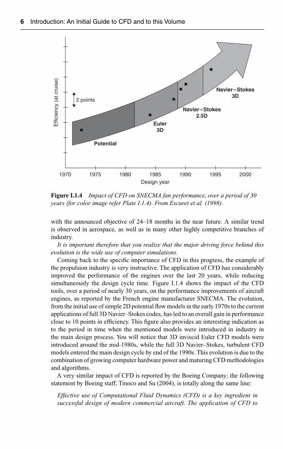
Figure I.1.4 Impact of CFD on SNECMA fan performance, over a period of 30years (for color image refer Plate I.1.4). From Escuret et al. (1998).

with the announced objective of 24–18 months in the near future. A similar trendis observed in aerospace, as well as in many other highly competitive branches ofindustry.

It is important therefore that you realize that the major driving force behind thisevolution is the wide use of computer simulations.

Coming back to the specific importance of CFD in this progress, the example ofthe propulsion industry is very instructive. The application of CFD has considerablyimproved the performance of the engines over the last 20 years, while reducingsimultaneously the design cycle time. Figure I.1.4 shows the impact of the CFDtools, over a period of nearly 30 years, on the performance improvements of aircraftengines, as reported by the French engine manufacturer SNECMA. The evolution,from the initial use of simple 2D potential flow models in the early 1970s to the currentapplications of full 3D Navier–Stokes codes, has led to an overall gain in performanceclose to 10 points in efficiency. This figure also provides an interesting indication asto the period in time when the mentioned models were introduced in industry inthe main design process. You will notice that 3D inviscid Euler CFD models wereintroduced around the mid-1980s, while the full 3D Navier–Stokes, turbulent CFDmodels entered the main design cycle by end of the 1990s. This evolution is due to thecombination of growing computer hardware power and maturing CFD methodologiesand algorithms.

A very similar impact of CFD is reported by the Boeing Company; the followingstatement by Boeing staff, Tinoco and Su (2004), is totally along the same line:

Effective use of Computational Fluid Dynamics (CFD) is a key ingredient insuccessful design of modern commercial aircraft. The application of CFD to

Intro-H6594.tex 9/5/2007 11: 42 Page 7


the design of commercial transport aircraft has revolutionized the process ofaerodynamic design.

Citing further from Boeing, you can find a very interesting account of 30 years ofhistory of CFD development at this Company in Johnson et al. (2003). We highlyrecommend you to read this paper, as a fascinating account of how CFD evolved froman initial tool to a strategic factor in the Company’s product development:

In 1973, an estimated 100 to 200 computer runs simulating flows about vehicleswere made at Boeing Commercial Airplanes, Seattle. In 2002, more than 20,000CFD cases were run to completion. Moreover, these cases involved physics andgeometries of far greater complexity. Many factors were responsible for such adramatic increase: (1) CFD is now acknowledged to provide substantial valueand has created a paradigm shift in the vehicle design, analysis and supportprocesses; … (5) computing power and affordability improved by three to fourorders of magnitude …

Effective use of CFD is a key ingredient in the successful design of moderncommercial aircraft. The combined pressures of market competitiveness, dedica-tion to the highest of safety standards and desire to remain a profitable businessenterprise all contribute to make intelligent, extensive and careful use of CFD amajor strategy for product development at Boeing. Experience to date at BoeingCommercial Airplanes has shown that CFD has had its greatest effect in theaerodynamic design of the high-speed cruise configuration of a transport air-craft. The advances in computing technology over the years have allowed CFDmethods to affect the solution of problems of greater and greater relevance toaircraft design, as illustrated in Figure 1.1Use of these methods allowed a morethorough aerodynamic design earlier in the development process, permittinggreater concentration on operational and safety-related features.

The 777, being a new design, allowed designers substantial freedom to exploitthe advances in CFD and aerodynamics. High-speed cruise wing design andpropulsion/airframe integration consumed the bulk of the CFD applications.Many other features of the aircraft design were influenced by CFD. For example,CFD was instrumental in design of the fuselage. Once the body diameter wassettled, CFD was used to design the cab. No further changes were necessary asa result of wind tunnel testing. In fact, the need for wind tunnel testing in futurecab design was eliminated … As a result of the use of CFD tools, the numberof wings designed and wind tunnel tested for high-speed cruise lines definitionduring an airplane development program has steadily decreased (Figure 3).2

These advances in developing and using CFD tools for commercial airplanedevelopment have saved Boeing tens of millions of dollars over the past 20 years.

1 See Figure I.1.5.2 See Figure I.1.6a. This figure shows information similar to Figure I.1.4. Figure I.1.6b shows theanalogous evolution, seen from the European AIRBUS industry. We will come back to the variousmodels mentioned in these figures in Chapter 2.

Intro-H6594.tex 9/5/2007 11: 42 Page 8


Engine/airframe integration Simultaneous design Three engine installations Including exhaust effects

Cab design

Wing designFlap track

fairings Tail and aftbody design

Wing-bodyfairing

Figure I.1.5 Role of CFD in the design of the Boeing 777. The arrows indicatethe parts that were designed by CFD. From Johnson et al. (2003). Reproduced bypermission of AIAA.

However, significant as these savings are, they are only a small fraction of thevalue CFD delivered to the company.

The following general considerations, from the same Boeing paper, confirm thestrategic impact of CFD:

A much greater value of CFD in the commercial arena is the added value ofthe product (the airplane) due to the use of CFD. Value is added to the airplaneproduct by achieving design solutions that are otherwise unreachable duringthe fast-paced development of a new airplane. Value is added by shorteningthe design development process. Time to market is critical and very importantin the commercial world is getting it right the first time. No prototypes arebuilt. From first flight to revenue service is frequently less than one year! Anydeficiencies discovered during flight test must be rectified sufficiently for govern-ment certification and acceptance by the airline customer based on a scheduleset years before. Any delays in meeting this schedule may result in substantialpenalties and jeopardize future market success. CFD is now becoming moreinterdisciplinary, helping provide closer ties between aerodynamics, structures,propulsion and flight controls. This will be the key to more concurrent engineer-ing, in which various disciplines will be able to work more in parallel ratherthan in the sequential manner, as is today’s practice. The savings due to reduceddevelopment flow time can be enormous!

To be able to use CFD in these multidisciplinary roles, considerable progressin algorithm and hardware technology is still necessary. Flight conditions ofinterest are frequently characterized by large regions of separated flows. Forexample, such flows are encountered on transports at low speed with deployedhigh-lift devices, at their structural design load conditions or when transportsare subjected to in-flight upsets that expose them to speed and/or angle of attack

Intro-H6594.tex 9/5/2007 11: 42 Page 9


Chronology and impact

38

1811

77

Num

ber

ofw

ings

test

ed

1980 1985 1990 1995 2000 2005

767 737-300 777 737NG757 787

NASATech

BoeingTools

PANAIR

A502 A488

FLO22A411

TRANAIR

CartesianGrid Tech.

TRANAIROptimization

HSR &IWD

TLNS3D-MB/ZEUS

TLNS3D-MBoverflowTLNS3D

BoeingProducts

1980 state of the art Modern close couplednacelle installation,0.02 Mach faster than737-200

21% thicker fasterwing than 757,767 technology

Highly constrainedwing designFaster wing than737-300

Successfulmultipointoptimizationdesign

CFD forloads and

stability, andcontrol

11

UnstructuredAdaptive Grid

3-D N-S

Faster andmore efficientthan previousaircraft

CFL3D/ZEUSoverflowCFD��

CFL3Doverflow

Figure I.1.6a Evolution of the CFD tools over the last 40 years at Boeing, with anindication of the influence of CFD on the reduction of the number of wing tests (forcolor image refer Plate I.1.6a). Courtesy Enabling Technology and ResearchOrganization, Boeing Commercial Airplanes.

Eulerequations

A310

Potentialequation

1975

Reducedconfigurationalcomplexity

Viscousflow

Turbulentflow


Simplevortex models

Subsonicflow

Flowproperties

Problem sizein service

Model

Inviscidflow

Complexconfigurations

Vortexflow


Wake vortex

Separation

Navier–Stokesequations

A321

A319A330/340

1965 1975 19951985

A340–500/600MEGAFLOW

102

104

106

108

2000

A318A320

A310A300

Configuration

Refinement of models Complexconfigurations

2002

A380

Figure I.1.6b Evolution of the CFD tools over the last 40 years at Airbus, with anindication of the evolution of the applied models (for color image refer Plate I.1.6b).From Becker (2003).

Intro-H6594.tex 9/5/2007 11: 42 Page 10


106

105

104

103

102

101

100

10�1

10�2

10�3

10�4

1955 1960 1965 1970 1975 1980

Year

1985 1990 1995 2000 2005

Com

putin

g sp

eed

(Gflo

p/s)

Massivelyparallelcomputers

IBM Blue Gene L LLNL (131072)

SGI Altix Nasa Ames (101601)

Earth simulator NEC SX (5120)

Intel Itanium2 Tiger4 1.4 GHz (4096)

ASCI White Pacific IBM SP Power 3 (7424)

ASCI Red Intel Pentium II (9632)Hitachi SR8000/112

NEC-SX5/32CRAY-T3E/512NEC-SX4/32

VPP 300/16VP 2600/20

VPP 400 EX

CRAY-YMP

CRAY-XMPCYBER-205

HP 9000 series 200

HP 9000 Apollo

HP 9000/735

HP C240

HP ZX6000 Itanium2 1 GHz

Workstations

PCs

CDC 7600

CDC 6600

IBM 7090

IBM 704

CRAY-1

Pentium IV 3 GHz

VPP 5000/100

IBM ASC purple (12208)

AMD K7 600 MHzPentium III 600 MHz

Pentium II 233 MHz

Pentium P6

i486

i386

ILLIAC-IVSTAR-100ASC

CRAY-2

Figure I.1.7 Evolution of Computer performance over the last 50 years, expressedin GfLOP/s, on a logarithmic scale. Courtesy Ch. Hinterberger and W. Rodi,University of Karlsruhe, Germany.

conditions outside the envelope of normal flight conditions. Such flows can onlybe simulated using the Navier–Stokes equations. Routine use of CFD basedon Navier–Stokes formulations will require further improvements in turbulencemodels, algorithm and hardware performance. Improvements in geometry andgrid generation to handle complexity such as high-lift slats and flaps, deployedspoilers, deflected control surfaces and so on, will also be necessary. How-ever, improvements in CFD alone will not be enough. The process of aircraftdevelopment, itself, will have to change to take advantage of the new CFDcapabilities.

Another interesting section in this paper deals with the very important interactionbetween CFD and wind tunnel tests of components. We recommend you to read thissection as a testimony of how CFD is contributing to raise the quality of experimentalinvestigations.

In the previous paragraphs, we referred several times to the extraordinary growthof computing power over the last 50 years. This is summarized in Figure I.1.7,where the various computer systems are positioned by their CPU performancein function of their year of appearance. The CPU performance is measured in

Intro-H6594.tex 9/5/2007 11: 42 Page 11


GigaFlops: i.e. Billions (109) of floating point operations per second (Flop/s); a quiteimpressive number, a Flop being typically an addition or subtraction on the computer.The first computers in 1955 had a processor speed of 10−5 Gflop/s, that is of the orderof 10,000 Flop/s; while the first PC with a 386 processor reached 100,000 Flop/s.Note that the level of 1000 Gflop/s, called TeraFlop/s, has been reached around theyear 2000. The fastest computers shown on this figure turn around 200TeraFlop/s,obtained through massively parallel computers over 100,000 processors. On the otherhand, current high-end PCs, which are scalar computers, have a remarkable speed ofthe order of 5 Gflop/s.

I.2 THE COMPONENTS OF A CFD SIMULATION SYSTEM

Having positioned CFD, and its importance, in the global technological world ofvirtual prototyping, we should now look at the main components of a CFD system.

We wish to answer the following question: What are the steps you have to define inorder to develop, or to apply, a CFD simulation? We make no difference at this stagebetween these two options, as it is similarly essential for the ‘user’ of a CFD code tounderstand clearly the different options available and to be able to exercise a criticaljudgment on all the steps involved.

Refer to Figure I.2.1 for a synthetic chart and guide to this section and the structureof this book. The CFD components are defined as follows:

• Step 1: It selects the mathematical model, defining the level of the approximationto reality that will be simulated (forms the content of Part I of this volume).

• Step 2: It covers the discretization phase, which has two main components,namely the space discretization, defined by the grid generation followed by thediscretization of the equations, defining the numerical scheme (forms the contentof Part II of this volume).

• Step 3: The numerical scheme must be analyzed and its properties of stabilityand accuracy have to be established (forms the content of Part III of this volume).

• Step 4: The solution of the numerical scheme has to be obtained, by selecting themost appropriate time integration methods, as well as the subsequent resolutionmethod of the algebraic systems, including convergence acceleration techniques(forms the content of Part IV of this volume).

• Step 5: Graphic post-processing of the numerical data to understand and interpretthe physical properties of the obtained simulation results. This is made possibleby the existence of powerful visualization software.

Let us look at this in more details step by step.

I.2.1 Step 1: Defining the Mathematical Model

The first step in setting up a simulation is to define the physics you intend to simulate.Although we know the full equations of fluid mechanics since the second half of the19th century, from the work of Navier and Stokes in particular, these equations are

Intro-H6594.tex 9/5/2007 11: 42 Page 12


Part I

RealWorld

Part I

Part II

Part III

Part IV

Levels of Approximationand MathematicalModel

Discretization of theMathematical Model

Discretization of theModel Equations

Select a discretizationmethod and definea numerical scheme

Analyze thenumerical scheme for:consistency, stabilityand accuracy

Solve the resultingalgebraic system andoptimize theconvergence rate

PostProcessingof the Results

Discretization of theSpace Domain

Grid Generation

Figure I.2.1 Structure of a CFD simulation system.

extremely complicated. They form a system of nonlinear partial differential equa-tions, with major consequences of this nonlinearity being the existence of turbulence,shock waves, spontaneous unsteadiness of flows, such as the vortex shedding behinda cylinder, possible multiple solutions and bifurcations. See Chapter 2 for some typicalexamples.

If we add to the basic flow more complex phenomena such as combustion, mul-tiphase and multi-species flows with eventual effects of condensation, evaporation,bursting or agglomeration of gas bubbles or liquid drops, chemical reactions as in fire

Intro-H6594.tex 9/5/2007 11: 42 Page 13


simulations, free surface flows, we need to model the physical laws describing thesephenomena and provide the best possible approximations.

The essential fact to remember at this stage is that within the world of continua,as currently applied to describe the macroscopic behavior of fluids, there is alwaysan unavoidable level of empiricism in the models. It is therefore important that youtake notice already that any modeling assumption will be associated with a generallyundefined level of error when compared to the real world.

Therefore, keep in mind that a good understanding of the physical properties andlimitations of the accepted models is very important, as it is not unusual to dis-cover that discrepancies between CFD predictions and experiments are not due toerrors in experimental or numerical data, but are due to the fact that the theoreticalmodel assumed in the computations might not be an adequate description of the realphysics.

Consequently, with the exception of Direct Numerical Simulation (DNS) of theNavier–Stokes equations, we need to define appropriate modeling assumptions andsimplifications. They will be translated into a mathematical model, formed generallyby a set of partial differential equations and additional laws defining the type of fluid,the eventual dependence of key parameters, such as viscosity and heat conductivityin function of other flow quantities, such as temperature and pressure; as well as vari-ous quantities associated to the description of additional physics and other reactions,when present.

The establishment of adequate mathematical models for the physics to be describedform the content of Part I of this volume. It is subdivided into three chaptersdealing with:

• the basic flow equations (Chapter 1);• an illustrated description of the different approximation levels that can be selected

to describe a fluid flow (Chapter 2);• the mathematical properties of the selected mathematical models (Chapter 3).

I.2.2 Step 2: Defining the Discretization Process

Once a mathematical model is selected, we can start with the major process of asimulation, namely the discretization process.

Since the computer recognizes only numbers, we have to translate our geometricaland mathematical models into numbers. This process is called discretization.

The first action is to discretize the space, including the geometries and solid bod-ies present in the flow field or enclosing the flow domain. The solid surfaces inthe domain are supposed to be available from a CAD system in a suitable digi-tal form, around which we can start the process of distributing points in the flowdomain and on the solid surfaces. This set of points, which replaces the continuityof the real space by a finite number of isolated points in space, is called a grid ora mesh.

The process of grid generation is in general extremely complex and requires ded-icated software tools to help in defining grids that follow the solid surfaces (this iscalled ‘body-fitted’ grids) and have a minimum level of regularity.

Intro-H6594.tex 9/5/2007 11: 42 Page 14


(a) Structured grid of a landing gear.From Lockard et al. (2004).Reproduced by permission from AIAA.

(b) Structured grid for part of the lung passagesshown in Plate I.1.2. From Van Ertbruggenet al. (2005).

(c) Grid for a 3D turbine blade passage. (d) Close-up view of the turbine grid.

Surface grid

Figure I.2.2 Examples of structured grids.

We will deal with the grid-related issues in Chapter 6, but we wish already here todraw your attention to the fact that, when dealing with complex geometries, the gridgeneration process can be very delicate and time consuming.

Grid generation is a major step in setting up a CFD analysis, since, as we willsee later on, in particular in Chapters 4, 5 and 6, the outcome of a CFD sim-ulation and its accuracy can be extremely dependent on the grid properties andquality.

Please notice here that the whole object of the simulation is for the computerto provide the numerical values of all the relevant flow variables, such as velocity,pressure, temperature, . . . , at the positions of the mesh points.

Hence, this first step of grid generation is essential and cannot be omitted. Withouta grid there is no possibility to start a CFD simulation.

Figure I.2.2 shows examples of 2D and 3D structured grids, while Figure I.2.3shows some examples of unstructured grids. These concepts will be detailed furtherin Chapter 6.

So, once a grid is available, we can initiate the second branch of the discretizationprocess, namely the discretization of the mathematical model equations, as shown inthe chart of Figure I.2.1.

Intro-H6594.tex 9/5/2007 11: 42 Page 15


From D´Alascio et al. (2004).A middle plane section of an helicopter fuselage with structured and unstructured grids.

Figure 3: ICEM-Hexa structuredmultiblock N.-S.mesh around the EC145

isolated fuselage: middle plane.

Figure 4: CENTAUR hybrid N.-S.mesharound the EC145 isolated fuselage:

middle plane.

Unstructured tetrahedral grid for an engine.From ICEM-CFD.

Unstructured hexahedral grid for an oil valve.HEXPRESS mesh. Courtesy NUMECA Int.

Figure I.2.3 Examples of unstructured grids (for color image refer Plate I.2.3).

As the mesh point values are the sole quantities available to the computer, allmathematical operators, such as partial derivatives of the various quantities, willhave to be transformed, by the discretization process, into arithmetic operations onthe mesh point values.

This forms the content of Part II, where the different methods available to performthis conversion from derivatives to arithmetic operations on the mesh point valueswill be introduced. In particular, we will cover the:

• finite difference method in Chapter 4,• finite volume and finite element methods in Chapter 5,• grid properties and guidelines in Chapter 6.

I.2.3 Step 3: Performing the Analysis Phase

After the discretization step, a set of algebraic relations between neighboring meshpoint values is obtained, one relation for each mesh point. These relations are calleda numerical scheme.

Intro-H6594.tex 9/5/2007 11: 42 Page 16


The numerical scheme must satisfy a certain number of rules and conditions tobe accepted and subsequently it must be analyzed to establish the associated level ofaccuracy, as any discretization will automatically generate errors, consequence of thereplacement of the continuum model by its discrete representation.

This analysis phase is critical; it should help you to select the most appropriatescheme for the envisaged application, while attempting at the same time to minimizethe numerical errors. This will be introduced and discussed in Part III.

Part III covers many subjects and should be studied with great attention. Thefollowing topics will be dealt with:

• The concepts of consistency, stability and convergence of a numerical schemeand a method for the analysis of stability in Chapter 7, including the quantitativeevaluation of the errors associated to a selected scheme.

• A general approach to properties of numerical schemes will be presented inChapter 8, together with a methodology to generate schemes with prescribedaccuracy. In addition this chapter will introduce the property of monotonicityleading to nonlinear high-resolution scheme.

I.2.4 Step 4: Defining the Resolution Phase

The last step in the CFD discretization process is solving the numerical schemeto obtain the mesh point values of the main flow variables. The solution algorithmsdepend on the type of problem we are simulating, i.e. time-dependent or steady flows.This will require techniques either to solve a set of ordinary differential equations intime, or to solve an algebraic system.

For time-dependent numerical formulations, a particular attention has to be givento the time integration, as we will see that for a given space discretization, not all thetime integration schemes are acceptable.

It is essential at this stage to realize that at the end of the discretization process, allnumerical schemes finally result in an algebraic system of equations, with as manyequations as unknowns. This number can be quite considerable, as the present capacityof computer memory storage allows large grids to be used to enhance the accuracyof the CFD predictions. The flow around an aircraft, such as shown in Figure I.1.2,might require a grid close to 50 million points for a minimal acceptable accuracy.This number is substantiated by the outcome of a recent ‘Drag Prediction’ workshop,run in 2003 by AIAA3 and NASA.4

The objective of the workshop was to assess the state-of-the-art of CFD for aircraftdrag and lift prediction (see the review by Hemsch and Morrison, 2004). The mainoutcome of this workshop was that a grid of the order of 10–15 million points wasrequired for acceptable accuracy of current CFD codes, on a wing–body–nacelle–pylon (WBNP) combination. The enhanced complexity of a full aircraft, compared

3 American Institute of Aeronautics and Astronautics (USA).4 National Aeronautics and Space Administration (USA).

Intro-H6594.tex 9/5/2007 11: 42 Page 17


with this simplified WBNP combination, leads to a minimal estimate of the order of50 million points for the full aircraft. With at least 5 unknowns per point (the threevelocity components, pressure, and temperature) we wind up with an algebraic systemof 250 million equations for 250 million unknowns; system that has to be solvedmany times during the iterative process toward convergence. You can understand onthis example why the availability of very fast methods for the solution of these hugealgebraic systems is crucial for an effective CFD simulation.

An introduction to the most important methods will be dealt with in Part IV, includ-ing also techniques for convergence acceleration, such as the important multigridmethods. Part IV is subdivided into:

• methods for ordinary differential equations, referring to the time integrationmethods, in Chapter 9;

• methods for the iterative solution of algebraic systems in Chapter 10.

Once the solution is obtained, we have to manipulate this considerable amount ofnumbers to analyze and understand the computed flow field. This can only be achievedthrough powerful visualization systems, which provide various software tools to study,qualitatively and quantitatively, the obtained results. Typical examples of outputs thatcan be generated are shown in Figure I.2.4:

• Cartesian plots for the distribution of a selected quantity in function of acoordinate direction or along a solid wall surface (Figure I.2.4a).

• Color plots of a given quantity on the solid surface or in the flow field (FigureI.2.4b and c).

• Visualization of streamlines, see Figure I.1.3 and of velocity vectors (FigureI.2.4d).

• Local values of a quantity in an arbitrary point, obtained by clicking the mouseon that point.

• Various types of animations.

Many other examples of visualizations will be shown in the following chapters.The last part of Volume I, Part V, is devoted to several basic applications of the

developed methodology, in order to guide you toward your first attempts in workingout a CFD simulation. We will consider one-dimensional models for scalar variables,up to the Euler equations for nozzle flows, as well as two-dimensional potential andlaminar flow models and present different numerical schemes in sufficient detail foryou to program and solve these applications:

• Chapter 11 will deal with 2D potential flows and 2D inviscid flows governed bythe system of Euler equations.

• Chapter 12 will deal with the 2D Navier–Stokes equations.

A particular section will be also devoted to some general Best Practice Guidelinesto follow when applying existing, commercial or other, CFD tools. This will be basedon the awareness of all possible sources of errors and uncertainties that can affect thequality and the validity of the obtained CFD results.

Intro-H6594.tex 9/5/2007 11: 42 Page 18


Time history

3.0E�031.5E�030.0E�00

�1.5E�03�3.0E�03

M�0.2

p'/(P�C2�)

(b) Perturbation pressure on solid surfaces

Magnitude V(m/s)4.5

4

3.5

3

2.5

2

1.5

1

0.5

0

�1.6

�0.8

0.0

Cp

Cp

0.0 0.2 0.4 0.6 0.8 1.0

�1.6

�0.8

0.8

0.8

0.00.0 0.2 0.4 0.6 0.8 1.00.0 0.2 0.4 0.6 0.8 1.0

0.0 0.2 0.4X/CX/C

X/CX/C

0.6 0.8 1.0

(a) Cartesian plot of pressure distribution atvarious positions along a wing–body–nacellemodel, compared to experimental data.From Tinoco and Su (2004),Reproduced by permission from AIAA.

(b) Instantaneous iso-surfaces of vorticitycolored by the span-wise component ofvorticity of a 70� delta wing.From: Morton (2004)

(d) Color plot and velocity vectors in onecross-section of the lung bifurcations shown inFigures I.1.2 and I.2.2. From VanErtbruggen et al. (2005).

(c) Perturbation pressure distribution for anaero-acoustic simulation of the noisegenerated by a landing gear.From Lockard et al. (2004).Reproduced by permission from AIAA.

Figure I.2.4 Examples of visual results from CFD simulations (for color imagerefer Plate I.2.4).

I.3 THE STRUCTURE OF THIS VOLUME

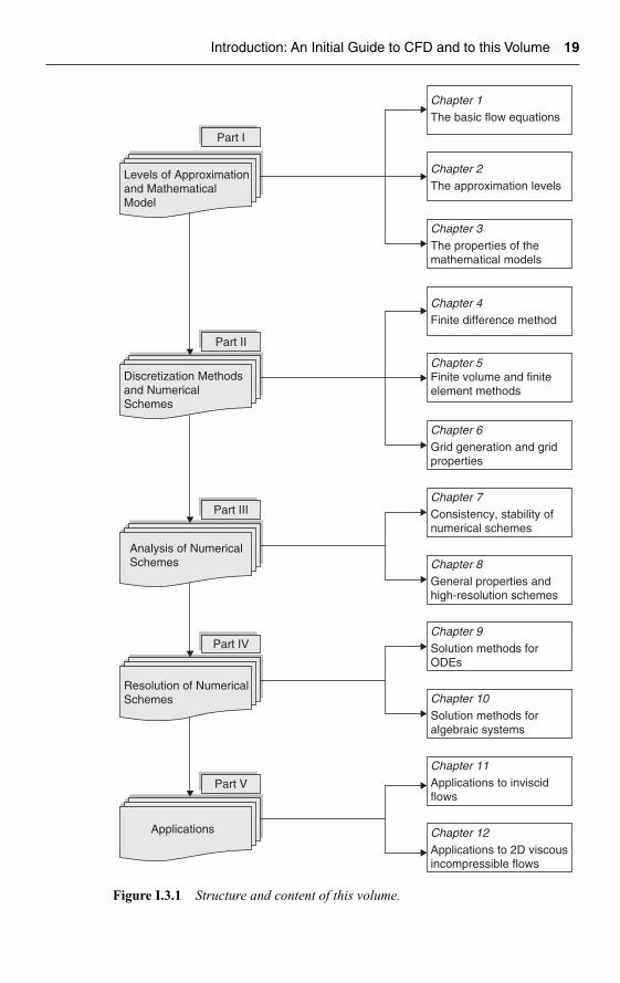
The guideline to the overall organization of this volume is summarized on the fol-lowing chart (Figure I.3.1), where each chapter is positioned. This will help you tosituate at any time the topics you are studying within the global context.

As mentioned earlier, the structure and the presentation of this second edition ofVolume I has been re-organized and focused in the first instance toward beginners andnewcomers to CFD.We have attempted to guide the student and reader to progressively

Intro-H6594.tex 9/5/2007 11: 42 Page 19


Part I

Levels of Approximationand MathematicalModel

Part II

Discretization Methodsand NumericalSchemes

Part III

Analysis of NumericalSchemes

Part IV

Resolution of NumericalSchemes

Part V

Applications

Chapter 1The basic flow equations

Chapter 2The approximation levels

Chapter 3The properties of themathematical models

Chapter 4Finite difference method

Chapter 5Finite volume and finiteelement methods

Chapter 6Grid generation and gridproperties

Chapter 7Consistency, stability ofnumerical schemes

Chapter 8General properties andhigh-resolution schemes

Chapter 9Solution methods forODEs

Chapter 10Solution methods foralgebraic systems

Chapter 11Applications to inviscidflows

Chapter 12Applications to 2D viscousincompressible flows

Figure I.3.1 Structure and content of this volume.

Intro-H6594.tex 9/5/2007 11: 42 Page 20


become familiar with the essential steps leading to a CFD application, either as astarting developer of CFD applications, or as a user of existing CFD tools, suchas commercial software packages. In both cases, it is essential to acquire a deepunderstanding of all the components entering a CFD simulation, and in particular todevelop a strong knowledge of the possible sources of errors and uncertainties.

On the other hand, we wish to give the opportunity to more advanced readersand students to also find material that would meet their objectives of accessing moreadvanced topics, while having at the same time a direct access to all the fundamentals.

Hence, we have identified in many chapters, topics and sections, indicated by A forAdvanced, that we consider outside the introductory level and that can form the basisfor a more advanced course. The relevant A-sections will be identified at the level ofeach chapter.

It goes without saying that any combination of ‘A’ sections with the other sectionscan be offered as course material at the discretion of the instructors.

On the other hand, we also hope that here and there, through the chapters, thenewcomer to CFD will have his/her intellectual curiosity aroused by the subject andtempted to make an incursion in some of these more advanced subsections.

REFERENCES

Becker, K. (2003). Perspectives for CFD. DGLR-2002-013, DGLR Jahrbuch 2002,Band III, Germany.

D’Alascio, A., Pahlke, K. and Le Chuiton, K. (2004). Application of a structured andan unstructured CFD method to the fuselage aerodynamics of the EC145 helicopter.Prediction of the time averaged influence of the main rotor. Proceedings ECCOMAS2004 Conference, P. Neittaanmäki, T. Rossi, S. Korotov, E. Oñate, J. Périaux andD. Knörzer (Eds.), Jyväskylä, Finland.

Escuret, J.F., Nicoud, D. and Veysseyre, Ph. (1998). Recent advances in compressoraerodynamic design and analysis. In Integrated Multidisciplinary Design of HighPressure Multistage Compressor Systems, RTO-LS-111, AC/323 (AVT) TP/l, ISBN92-837-1000-2, RTO/NATO Paris, France.

Hemsch, M.J. and Morrison, J.H. (2004). Statistical analysis of CFD solutions from 2nddrag prediction workshop, 42ndAIAAAerospace Sciences Meeting, Reno, AIAA Paper2004-556.

Johnson, F.T., Tinoco, E.N. andYu, N.J. (2003). Thirty years of development and applica-tion of CFD at Boeing commercial airplanes, Seattle, 16th AIAA Computational FluidDynamics Conference, Orlando, AIAA Paper 2003-3439.

Lockard, D.P., Khorrami, M.R. and Li, F. (2004). Aaeroacoustic analysis of a simplifiedlanding gear, AIAA Paper 2004-2887. 10th AIAA/CEHS Aeroacoustics Conference,Manchester, UK.

Morton, S.A. (2004). Detached-Eddy simulations of a 70 degree delta wing in the ONERAF2 wind tunnel. Proceedings ECCOMAS 2004 Conference, P. Neittaanmäki, T. Rossi,S. Korotov, E. Oñate, J. Périaux and D. Knörzer (Eds.), Jyväskylä, Finland.

Tinoco, E.N. and Su, B. (2004). Drag prediction with the Zeus/CFL3D system, 42ndAIAA Aerospace Sciences Meeting. AIAA Paper 2004-552.

Van Ertbruggen, C., Hirsch, Ch. and Paiva, M. (2005). Anatomically based three-dimensional model of airways to simulate flow and particle transport using Com-putational Fluid Dynamics. J. Appl. Physiol., 98, 970–980.

Ch01-H6594.tex 27/4/2007 15: 37 Page 21

Part I

The Mathematical Models for FluidFlow Simulations at VariousLevels of Approximation

INTRODUCTION

The invention of the digital computer and its introduction in the world of science andtechnology has led to the development, and increased awareness, of the concept ofapproximation. This concerns the theory of the numerical approximation of a set ofequations, taken as a mathematical model of a physical system. But it concerns alsothe notion of the approximation involved in the definition of this mathematical modelwith respect to the complexity of the physical world.

We are concerned here with physical systems for which it is assumed that thebasic equations describing their behavior are known theoretically, but for which noanalytical solutions exist, and consequently an approximate numerical solution willbe sought instead.

For various reasons, the first of these being the great complexity, it is often notpractically possible to describe completely the evolution of the system in its fullcomplexity. Of course, the definition of these limits is relative to a given time andenvironment and these are being extended with the evolution of the computer tech-nology. But taken at a given period, it is necessary to define mathematical models thatwill reduce the complexity of the original basic equations and make them tractablewithin fixed limits. Actually, the first level to be defined is the ‘scale of reality’ level.Physicists propose various levels of description of our physical world, ranging fromsubatomic, atomic or molecular, microscopic, macroscopic (defined roughly as thescale of classical mechanics) up to the astronomical scale. As is well known, in thestatistical description of a gas, the motion of the individual atoms or molecules aretaken into consideration and the behavior is ruled by the Boltzmann equation. Thisdescription leads for instance to the definition of temperature as a measure of the meankinetic energy of the gas molecules; to a definition of pressure as a result of the impulseof molecules on the walls of the body containing the gas; to a definition of viscosityconnected to the momentum exchange due to the thermal molecular motion, and so on.

At this molecular level of description the fundamental variables are molecule veloc-ities, number of particles per volume and other variables defining the motion of theindividual molecules, while pressure, temperature, viscosity e.g. are mean properties

21

Ch01-H6594.tex 27/4/2007 15: 37 Page 22

22 The Mathematical Models for Fluid Flow Simulations

which are deduced from other variables, more basic at this level of reality. Hence,we may consider that each level of reality can be associated with a set of fundamen-tal variables, from which other variables can be defined as measures of certain meanproperties. Continuing in the line of this example we have, beyond the molecular levelof statistical mechanics, the atomic level, the nuclear and the subnuclear level that wedo not plan to discuss here, since they are fully outside the domain of definition ofa fluid.

Actually, fluid dynamics starts to exist as soon as the interaction between a suf-ficiently high number of particles affects and dominates, at least partly, the motionof each individual particle. Hence, fluid dynamics is essentially the study of theinteractive motion and behavior of large number of individual elements.

The limit between individual motions of isolated particles or elements and theirinteractive motion is of significance in the study of rarefied gases. It is known thatthe interaction between the particles becomes negligible if the mean free path lengthattains a magnitude of the order of the length scale of the considered system. The ratioof the mean free path length to the reference length scale is called the Knudsen number.

For higher values of the mean free path length, or of the Knudsen number, theparticles behave essentially as individual elements. These limit situations will notbe considered here since they are outside the field of classical fluid dynamics. Notehowever that the intermediate range between the continuum and the rarefied gasapproximations is of practical significance for the prediction of the re-entry phase ofa Space Shuttle. When re-entering the earth atmosphere from space, the Space Shuttlecrosses the atmosphere from very high altitudes, where it cannot be considered asa continuum, through an intermediate range that evolutes with reducing altitude toa continuum fluid. We need therefore special models, intermediate between theNavier–Stokes and the Boltzmann equations to handle these situations, which areextremely critical for the safety of the return phase of the Shuttle.

We will focus, in the following, on the level of reality in which the density ofelements is high enough, so that we can make the approximation of considering thesystem of interacting elements as a continuum. This expresses that continuity or close-ness exists between the elements such that their mutual interaction dominates overthe individual motions, although these are not suppressed. What actually happens, isthat a collective motion is superimposed on the motion of the isolated elements as aconsequence of the large number of these elements coexisting within the same domain.

From this point of view, we understand easily why the concepts of fluid mechanicscan be applied to a variety of systems consisting of a large number of interactingindividual elements.

This is the case for the current fluids and gases where the individual ‘element’,or fluid particle is actually not a single molecule, but consists of a large numberof molecules occupying a small region with respect to the scale of the considereddomain, but still sufficiently large in order to be able to define a meaningful and non-ambiguous average of the velocities and others properties of the individual moleculesand atoms occupying this volume. It implies that this elementary volume contains asufficiently high number of molecules, with for instance a well defined mean velocity,mean kinetic energy, allowing to define velocity, temperature, pressure, entropy andso on, at each point. Hence, associated fields, which will become basic variables forthe description of the system, can be defined although the temperature, or pressure, orentropy of an individual atom or molecule is not defined and generally meaningless.

Ch01-H6594.tex 27/4/2007 15: 37 Page 23

The Mathematical Models for Fluid Flow Simulations 23

In the classical interpretation of turbulence, each fluid particle as defined aboveenters into a stochastic motion and in defining mean turbulent variables, such as amean turbulent velocity field, an average is performed, in this case an average in time,over the motion of the fluid particles themselves.

A still higher level of averaging occurs in the description of flows through porousmedia such as soils. In the description of groundwater flows an ‘element’ is the setof fluid particles, as defined above, contained in a volume large enough as to containa great number of soil particles and fluid particles such that a meaningful averagecan be performed, but still small with respect to the dimensions of the region to beanalyzed. Such a volume is considered as a ‘point’ at this level of description, and thefields are attached to these points, implying that groundwater flow theories do studythe behavior of collection of fluid particles.

Following this line, the movement or overall displacement of crowds at exit of rail-way stations during rush hours, or of a football stadium, can be analyzed with fluidmechanical concepts. In this case, an ‘element’ is the set of persons contained in aregion small with regard to the dimensions of the station for instance, but still contain-ing a sufficiently high number of individuals in order to define non-ambiguous averagevalues, such as velocity and other variables. In this description, the displacement ofan individual is not considered, but only the motion of groups of individuals.

A similar analysis can be defined for heavy traffic studies, where an ‘element’ isdefined as a set of cars (in the one-dimensional space formed by the road). Obviouslyin a light traffic, the isolated car behaves as a single particle but collective motioncomes in when a certain intensity of traffic has been reached such that the speed ofan individual car is influenced by the presence of the other cars. This is actually to beconsidered as the onset of a ‘fluid mechanical’ description.

Finally, at a still larger scale, astrophysical fluid dynamics can be defined for thestudy of the interstellar medium or for the study of the formation and evolution ofgalaxies. In this latter case for instance, an ‘element’consists of a set of stellar objects,including one or several solar systems and the dimensions of a ‘point’ can be of theorder of light years.

In conclusion of these considerations, we can say that fluid mechanics is essentiallythe study of the behavior of averaged quantities and properties of a large number ofinteracting elements. The same is true for another domain of scientific knowledge,namely thermodynamics, which is also the study of systems of large numbers of inter-acting elements. It is therefore no wonder that thermodynamics is, with the exceptionof incompressible isothermal media, tightly interconnected with fluid mechanics andplays an important role in the description of the evolution of ‘fluid mechanical’systemsas mentioned above.

An essential step in fluid dynamics is therefore the averaging process. We haveto decide, in front of a given system, which level of averaging will be performedin function of the quantities to be predicted, in function of the significant variableswhich can be defined in a meaningful way, in function of the precision and degree ofaccuracy to be achieved in the description of the system’s behavior. This is a basictask for the scientists in charge of the analysis that requires a great understanding ofthe physics of the system, a judgment and sense of compromise between requiredlevel of accuracy and degree of sophistication of the chosen mathematical model.

The next step in the definition of the levels of approximation is to define a timeor ‘steadiness level’. This implies an estimation of the various time constants of the

Ch01-H6594.tex 27/4/2007 15: 37 Page 24


considered flow situation and the choice of the lowest time constant to be taken intoconsideration in the modelization of this flow system. Then a time averaging will beperformed with regard to the time constants lower than the chosen minimal value. Thebest-known example of this procedure is the system of time averaged Navier–Stokesequations for the mean turbulent flow variables. An averaging is performed over theturbulent fluctuations, since we are concerned in that case with variations of the flowslower that the turbulent fluctuations and hence, with time constants much larger thanthe time constant of these fluctuations. Through this procedure, extra terms appear inthe equation, the Reynolds stresses, which are averaged products of fluctuations, andfor which external information will have to be provided.

Along similar lines, in Large Eddy Simulations, known as the LES approximation,the turbulent fluctuations are averaged only over part of their spectrum, namely thesmall scales are modeled while the larger turbulent motion, associated with the lowerfrequencies, is directly simulated.

The spatial level of approximation defines the number of space variables used in themodel. We have to decide in function of certain assumptions concerning the physicalbehavior of the system, if a one- or two-dimensional description will provide suffi-ciently accurate information about the behavior of the flow. It is of importance to notethat the basic flow equations being three-dimensional any description with less thanthree space variables will be obtained by disregarding the flow variations with respectto the corresponding space coordinate and this can be formulated mathematically byaveraging out the equations over that space variable.

Therefore, the averaging process, here over space, is again essential. In this spaceaveraging, we will obtain equations in a two- or one-dimensional region, whichcontain terms describing the averaged influence of the full three-dimensional motion.These terms, analogous to the Reynolds stresses, will generally be neglected due tothe lack of information to estimate them, although they can, or could, be estimatedin certain cases.

Since the averaging procedure implies a loss of information in the averaged spacevariables, this information will have, in many cases, to be provided from ‘outside’the model, for instance, through empirical data. It is also clear therefore, that simplemodels like one-dimensional flow descriptions, may require more empirical or exter-nal input than a viscous three-dimensional description, if some contributions fromthe three-dimensionality are to be taken into account.

The next level of approximation, the ‘dynamical level’, is tied to an estimation of therelative influence of the various forces and their components on the system’s behavior.The dynamical evolution of a flow system is determined by the equilibrium of thedifferent forces acting on it, but it seldom occurs that all the force components areequally important. Therefore, a very basic step in setting up a mathematical model forthe description of a system is an estimation of the dominant force components in orderto simplify the model as strongly a possible. For instance, although gravity forces arealways present on earth, in many cases these forces have only a negligible influence onthe flow behavior. The detailed study of the influence of viscosity by Prandtl, whichled to the boundary layer concept, is maybe the most fascinating example of theconsequences of a deep analysis of the relative influence of forces. As is well known,the considerable simplification of the Navier–Stokes equations introduced throughthis analysis, allowed the practical calculation of many flow situations, which werelargely intractable by the full Navier–Stokes equations.

Ch01-H6594.tex 27/4/2007 15: 37 Page 25

The Mathematical Models for Fluid Flow Simulations 25

This boundary layer concept led to the definition of the regions of validity ofinviscid flows, in which the viscosity forces could be neglected. Therefore, inviscidflow approximations play an important role in fluid mechanics although their rangeof validity in internal flows is more restricted than in external aerodynamics.

It is to be noted that the different levels of approximation considered here canstrongly interact with each other. For instance on a rotating blade of a turboma-chine, the centrifugal forces will create a radial migration of the boundary layer fluidalong the blade, leading to an increased spanwise mixing of the flow and hence willlimit the validity of a purely two-dimensional description of the blade-to-blade flow.But in all cases, the final word with regard to the validity of a given model is the com-parison to experimental data, or to computations at a higher level of approximation.

These remarks are presented here to introduce the methodology to be followed inthe next chapters. After having summarized the basic flow equations in Chapter 1,a systematic presentation of various mathematical models describing the most currentapproximations will be given in Chapter 2. Finally, Chapter 3 will introduce theanalysis of the properties of the system of equations describing the selected model;see the guideline chart (Figure I.3.1) for the global overview.

Ch01-H6594.tex 27/4/2007 15: 37 Page 27

Chapter 1

The Basic Equations of Fluid Dynamics

OBJECTIVES AND GUIDELINES

This first chapter will introduce the initial step in defining a CFD application, namelythe selection of the model to be discretized. In order to guide you through the com-plexities of fluid mechanics, which we alluded to in the introduction to this Volume,we need to establish the basic laws governing fluid flows.

You certainly have seen many flow situations and you have certainly recognizedthat they can be very complex, with phenomena such as turbulence, which is a globalinstability of a flow, as a dominant element of most of the flows encountered in natureand in technology.

In addition, applications to CFD have led to a new approach and a new way oflooking at the laws of fluid mechanics. Although they can be written in many differentmathematical forms, CFD has led us to put forward a specific form of these laws,through the concept of conservation and of conservation laws. This concept will becentral to most of this chapter.

In Section 1.1 we develop and present the most general form of a conservation law,without specifying the nature of the ‘conserved’ quantity. To achieve this, we haveto define first what conservation means and how we recognize an equation writtenin conservative form. We will see that this is a fundamental concept for CFD inmany chapters later on, but the main reason for the privileged conservative formis connected to the requirement that, after the equations are discretized, essentialquantities such as mass or energy will be conserved at the discrete level. This iscertainly essential, as you can imagine, since a numerical simulation wherein mass orenergy would be lost because of numerical artifacts, would be totally useless and notreliable.

A conservation law is strongly associated to the concept of fluxes and we willintroduce in Section 1.1.2 the extremely important distinction between convective anddiffusive fluxes. This distinction is central to the whole of fluid mechanics and of CFD.

With the basis obtained in Section 1.1, we are ready to apply the general conserva-tion laws to the three quantities that define uniquely the laws of fluid mechanics; mass,momentum and energy, described and developed in detail in Sections 1.2, 1.3 and 1.4.

The flow chart in Figure 1.0.1 illustrates the links and the structure of this chapter.We strongly suggest that you refer regularly, while progressing through the material,to this chart as a guide for the order and relative importance of the various topics.

In addition, the part in gray indicates the sections containing more advanced mate-rial that can form the basis of a more advanced CFD course. Of course, any instructorcan make his/her own ‘cocktail’ between the various topics, according to the level ofthe students.

These Advanced sections cover a few important topics, when dealing with CFDapplications to rotating systems or moving grids, which often occur in practice,

27

Ch01-H6594.tex 27/4/2007 15: 37 Page 28


Section A1 1.1 General formof a conservationlaw

A1.5 Rotatingframe of reference

1.3 The momentumconservationequation

1.2 The massconservationequation

1.4 The energyconservationequation

A1.6 Advancedproperties of controlvolume formulations

1.1.2 Convection-diffusion form of aconservation law

1.1.1 Scalarconservation law

1.1.3 Vectorconservation law

1.4.1 Conservativeformulation of theenergy equation

1.4.2 The equationsfor internal energyand entropy

A1.5.1 Momentumequation in therelative system

A1.5.2 Energyequation in therelative system

A1.5.3 Crocco'sform of theequations of motion

A1.6.1 Lift and dragestimations fromCFD results

A1.6.2 Conservationlaw for a movingcontrol volume

Figure 1.0.1 Guide to this chapter.

Ch01-H6594.tex 27/4/2007 15: 37 Page 29

The Basic Equations of Fluid Dynamics 29

in large areas of industry, such as rotating machines, flow around helicopters,or with moving grids as encountered in fluid–structure interactions with vibratingsurfaces.

We have also added a short section, which is a straightforward extension of thegeneral integral form of the momentum equation, in presence of solid bodies, pro-viding the formulation to post-process CFD data in order to extract the forces exertedon a body by the flow, such as lift and drag.

1.1 GENERAL FORM OF A CONSERVATION LAW

As mentioned in the introduction, the conservation law is the fundamental conceptbehind the laws of fluid mechanics.

But what is a conservation law?It is altogether very simple in its basic logic, but can become complicated by itsinternal content. Conservation means that the variation of a conserved (intensive)flow quantity within a given volume is due to the net effect of some internal sourcesand of the amount of that quantity which is crossing the boundary surface. This amountis called the flux and its expression results from the mechanical and thermodynamicproperties of the fluid. It will be defined more precisely in the next section. Similarly,the sources attached to a given flow quantity are also assumed to be known frombasic studies. The fluxes and the sources are in general dependent on the space–timecoordinates, as well as on the fluid motion. The associated fluxes are vectors for ascalar quantity and tensors for a vector quantity like momentum.

We can state the conservation law for a quantity U as the following logicalconsistency rule:

The variation of the total amount of a quantity U inside a given domain is equalto the balance between the amount of that quantity entering and leaving theconsidered domain, plus the contributions from eventual sources generatingthat quantity.

Hence, we are looking at the rate of change of the quantity U during the flow evolution,as a flow is a moving and continuously changing system.

Although we will write the conservation law for an undefined quantity U, it shouldbe mentioned at this stage that not all flow quantities obey a conservation law. Theidentification of the quantities that obey a conservation law is defined by the studyof the physical properties of a fluid flow system. It is known today that the lawsdescribing the evolution of fluid flows (this is what we call fluid dynamics) are totallydefined by the conservation of the following three quantities:

1. Mass2. Momentum3. Energy.

This represents in total five equations, as the momentum, defined as the product ofdensity and velocity, is a vector with three components in space.

Ch01-H6594.tex 27/4/2007 15: 37 Page 30


QV

QS

U dΩ

S

Ω(�F•dS )

dS

F

→→

→

→

Figure 1.1.1 General form of a conservation law for a scalar quantity.

On the other hand, it is essential to keep in mind that other quantities, such aspressure, temperature, entropy, for instance, do not satisfy a conservation law. Thisdoes not mean that we cannot write an equation for these quantities, it just means thatthis equation will not be in the form of a conservation law.

1.1.1 Scalar Conservation Law

Let us consider a scalar quantity per unit volume U , defined as a flow related property.We now consider an arbitrary volume �, fixed in space, bounded by a closed

surface S (see Figure 1.1.1) crossed by the fluid flow.The surface S is arbitrary and is called a control surface, while the volume � is

called a control volume.Our goal here is to write the fundamental law in its most general form, by expressing

the balance of the variation of U , for a totally arbitrary domain �. This control volumecan be anywhere in the flow domain and can be of arbitrary shape and size.

To apply the conservation law as defined above, we have to translate mathematicallythe quantities involved. The first one is the ‘total amount of a quantity U inside agiven domain’. If we consider the domain of volume �, the total amount of U in �

is given by

∫�

U d�

and the variation per unit time of the quantity U within the volume � is given by

∂

∂t

∫�

U d�

Ch01-H6594.tex 27/4/2007 15: 37 Page 31


Remark

I wish here to draw your attention to the interpretation of this mathematical expres-sion. The above relation would be read by a mathematician as ‘the partial derivativewith respect to time of the volume integral of U over �’. However, I would like you to‘translate’ this mathematical language in its physical meaning, by reading this rela-tion instead as: ‘the variation (∂) per unit of time (./∂t) of the total amount of U in �’.Try therefore, whenever appropriate, to always ‘read’ a mathematical expression byits translation of a physical property.

Coming back to the conservation law, we have now to translate mathematically‘the amount of that quantity U entering and leaving the considered domain’.

This is where the physics comes in: we know from the study of the laws of physicsthat the local intensity of U will vary through the effect of quantities called fluxes,which express the contribution from the surrounding points to the local value of U ,describing how the quantity U is transported by the flow.

The flux is a fundamental quantity associated to a conserved flow variable U ,and is defined as the amount of U crossing the unit of surface per unit of time.It is therefore a directional quantity, with a direction and an amplitude, so that itcan be represented as a vector. If this vector is locally parallel to the surface, thennothing will enter the domain. Consequently, only the component of the flux in thedirection of the normal to the surface will enter the domain and contribute to the rateof change of U . So, the amount of U crossing the surface element d �S per unit oftime is defined by the scalar product of the flux and the local surface element (seeFigure 1.1.1),

Fn dS = �F · d�S

with the surface element vector d�S pointing along the outward normal.The net total contribution from the incoming fluxes is the sum over all surface

elements d�S of the closed surface S, and is given by

−∮

S

�F · d�S

The minus sign is introduced because we consider the flux contribution as positivewhen it enters the domain. With the outward normal as positive, the scalar prod-uct will be negative for an entering flux, as seen from Figure 1.1.1. Hence theneed to add the minus sign. If we had defined the inward normal as positive, wewould not have added the minus sign. However, the generally accepted conventionis to define as positive the outward normal, so that the minus sign is of currentacceptance.

To finalize the balance accounts, we have to add contributions from the sources ofthe quantity U .

These sources can be divided into volume and surface sources, QV and �QS and thetotal contribution is

∫�

QV d� +∮

S

�QS · d�S

Ch01-H6594.tex 27/4/2007 15: 37 Page 32


Hence, the general form of the conservation law for the quantity U is

∂

∂t

∫�

U d� = −∮

S

�F · d�S +∫

�

QV d� +∮

S

�QS · d�S

which is generally written as

∂

∂t

∫�

U d� +∮

S

�F · d�S =∫

�

QV d� +∮

S

�QS · d�S (1.1.1)

This is called the integral conservation form and is the most general expression ofa conservation law.

This form has some remarkable properties:

• Equation (1.1.1) is valid for any fixed surface S and volume �.• The internal variation of U , in absence of volume sources, depends only on the

flux contributions through the surface S and not on the flux values inside thevolume �.

• The fluxes do not appear under a derivative or gradient operator and may thereforebe discontinuous, as will be the case in the presence of shock waves.

Why are these properties so important, in particular the second one? The importancearises from the fact that we will require this property to remain valid also afterdiscretization, to ensure hereby that we satisfy the conservation law at the discretelevel. When this is the case, we will speak of a ‘conservative numerical scheme’.

For instance, in an internal flow calculation it is essential to ensure mass conser-vation, that is constancy of the mass flow in all sections, for any grid resolution.Basically, we see from equation (1.1.1) that if the discretization leads to values offluxes inside the domain, they will not be distinguishable from the volume sourcesand will therefore act as such. These ‘numerical’ sources will then destroy the conser-vation property of the relevant quantity. For mass conservation, eventual numericalsources will create or destroy mass and hence the mass flow rate will not remainconstant. As we will see in Chapter 5, this property can easily be satisfied on arbitrarygrids, in particular through application of the finite volume method.

Differential form of a conservation lawAn alternative, local differential form of the conservation law can be derived byapplying Gauss’ theorem to the surface integral term of the fluxes and the surfacesources, assuming that these fluxes and surface sources are continuous.

Gauss’ theorem states that the surface integral of the flux is equal to the volumeintegral of the divergence of this flux:

∮S

�F · d�S =∫

�

�∇ · �F d�

for any volume�, enclosed by the surface S, where the gradient or divergence operator�∇ is introduced. The explicit expression of this gradient operator is defined later inCartesian coordinates, see equation (1.2.7).

Ch01-H6594.tex 27/4/2007 15: 37 Page 33


Introducing this relation in the integral conservation law (1.1.1), we obtain

∫�

∂U

∂td� +

∫�

�∇ · �F d� =∫

�

QV d� +∫

�

�∇ · �QS d� (1.1.2)

Since equation (1.1.2) is written for an arbitrary volume �, it must be validlocally in any point of the flow domain. This leads to the differential form of theconservation law,

∂U

∂t+ �∇ · �F = QV + �∇. �QS (1.1.3)

or

∂U

∂t+ �∇ · (�F − �QS ) = QV (1.1.4)

It is seen from these equations that surface sources have the same effect on thesystem as a flux term and therefore we might as well consider them from the start asan additional flux. However, we favor the present classification in fluxes and sources,since it allows a clear physical interpretation of all the contributions to the evolution ofthe quantity U . In any case, the term (�F − �QS ) can be considered as an effective flux.This will be considered for the momentum conservation law, Section 1.3, where thepressure and shear stresses are indeed acting as surface sources, but they are currentlyadded to the other flux terms to form one ‘effective’flux for momentum conservation.

Note that:

• The fluxes (and surface sources) appear exclusively under the gradient operator,which is the only space derivative term. This is the direct translation of the surfaceintegral of the fluxes in the integral form (1.1.1).

• This indicates the way to recognize a conservation law in differential form.Look at all the space derivative terms: if they can be grouped as a divergenceoperator, then the equation is in conservation form. If not, the equation issaid to be in ‘non-conservative’ form, or in ‘quasi-linear’ form.

• This differential form is more restrictive than the integral form, as it requiresthe fluxes to be differentiable, i.e. having at least C1 continuity, which is not thecase in presence of shock waves, for instance.

• For any quantity U , physical assumptions must provide definitions for the fluxesand the source terms, in function of other computed variables.

1.1.2 Convection–Diffusion Form of a Conservation Law

In Section 1.1.1, we have not provided any specific information concerning the fluxes,except for the fact that they do exist for any conserved quantity U . However, we cannow be more specific and look closer to the physics of transport of a quantity U in afluid flow.

The fluxes are generated from two contributions: a contribution due to the convec-tive transport of the fluid and a contribution due to the molecular agitation, which canbe present even when the fluid is at rest.

Ch01-H6594.tex 27/4/2007 15: 37 Page 34


The first component, which is always present, is the convective flux �FC , attachedto the quantity U in a flow of velocity �v. It represents the amount of U that is carriedaway or transported by the flow and is defined as

�FC = U �v (1.1.5)

The local contribution of the convective flux through a surface element d�S, (�FC .d�S)has an important physical significance.

For U = ρ the fluid density, the corresponding convective flux through the surfaced�S is equal to the local mass flow rate, where we designate the mass flow rate by m

ρ�v · d�S = dm (1.1.6)

This quantity represents the amount of mass flowing through the surface dS, per unitof time, and is expressed in kg/s.

For a different conserved quantity U = ρu, where u is the quantity per unit mass,the contribution of the convective flux is equal to

�FC · d�S = ρu�v · d�S = u dm (1.1.7)

clearly showing the physical meaning of the convective flux as defined by the quantityu entrained by the local mass flow rate.

The second component is a diffusive flux �FD, defined as the contribution presentin fluids at rest, due to the macroscopic effect of the molecular thermal agitation. Theeffect of the molecular motion translates in the tendency of a fluid toward equilibriumand uniformity, since differences in the intensity of the considered quantity createa transfer in space such as to reduce the non-homogeneity. This contribution to thetotal flux is proportional to the gradient of the corresponding quantity, since it has tovanish for a homogeneous distribution.

Diffusive fluxes do not always exist; for instance, from an analysis of the physicalproperties of fluid, it is known that in a single-phase fluid at rest, no diffusion of spe-cific mass is possible since any displacement of specific mass implies a macroscopicdisplacement of fluid particles. Therefore, there will be no diffusive flux contributionto the mass conservation equation.

The phenomenon of diffusion is indeed totally different from convection. Wecan best understand the physics of diffusion by the following experiment, whichestablishes the basics of diffusion.

Consider a reservoir of water, at rest, and inject a drop of a colored (black) dye,supposed having the same density as water.

Look at Figure 1.1.2. What is going to happen? Will the drop stay in its position?As you probably know from basics physics, we observe that after a certain time thewhole of the reservoir will become colored. What has happened?

At t � 0 After a finite time

Figure 1.1.2 A colored dye diffusing in a water reservoir.

Ch01-H6594.tex 27/4/2007 15: 37 Page 35


Due to the molecular agitation, the dye molecules are constantly in collision withthe water molecules and will be ‘hit’many times in all directions to wind up in arbitrarypositions. As a result, after a certain time, we will find dye molecules everywhere andthe whole reservoir will be colored. For us, as observer, we do not see the molecules,but we see the macroscopic results of these collisions and we notice the followingempirical facts:

• The process appears as a diffusion, since a local concentration peak diffusesfrom a high local value to a lower concentration, in all directions.

• The process stops when there is no dye concentration differences anymorebetween two points, that is when uniformity is reached, which corresponds toa statistically homogenous distribution of the dye molecules between the watermolecules.

• The diffusion process between two points is proportional to the concentrationdifference between these points and will tend to reduce these differences.

• An evolution whereby the concentration difference between two points increases(called anti-diffusion) has never been observed in this experiment.

The ‘transport’ of the dye molecules can therefore be described, from the point ofview of continuum mechanics (since we view the fluid as a continuous media, insteadof seen as constituted by molecules), by expressing the macroscopic observations bythe existence of a diffusive flux, with the following properties:

• The diffusive flux is proportional to the gradient of the concentration, the gradi-ent being the mathematical expression for the concentration difference betweenneighboring points, in their direction.

• It has to be opposite to the gradient, to express the tendency toward uniformity.• It will be proportional to a diffusivity factor, which expresses its ‘intensity’,

depending on the nature of the considered quantity and its environment.

This is summarized by the mathematical gradient law of Fick, where κ is thediffusivity coefficient:

�FD = −κρ �∇u (1.1.8)

Observe that the diffusivity constant κ has units of m2/s for any quantity U .Equation (1.1.3) then becomes

∂ρu

∂t+ �∇ · (ρ�vu) = �∇ · (κρ �∇u) + QV + �∇ · �QS (1.1.9)

This equation is the general conservative form of a transport equation for the quantityU = ρu and is also referred to as a convection–diffusion equation.

The structure of this equation is of utmost importance, both from physical aswell as mathematical point of view and you should study this very carefully, as itforms the backbone of all mathematical modeling of fluid flow phenomena.

The convection–diffusion equation takes its name from the physical propertiesof the two flux contributions and from their specific mathematical expressions,

Ch01-H6594.tex 27/4/2007 15: 37 Page 36


which reflect very different physical properties. Therefore, the following proper-ties will provide significant and fundamental guidelines when setting up a CFDdiscretization.

Convective and diffusive fluxes have indeed totally different physical properties:

• Convective fluxes describe the ‘passive’ transport of the conserved variable bythe flow, which you can visualize as a piece of wood carried away by a river flow.

• Consequently the convective flux describes a phenomenon that has directionalproperties, as it is proportional to the velocity. A convective flux cannot providea contribution in a direction transverse or opposite to the flow direction. It hastherefore properties very similar to wave propagation phenomena, which arealso essentially directional, for a selected propagation direction. We will see inChapter 3 that the relation between convective transport and wave propagationis indeed very close.

• Observe that the convective flux appears in the conservation law (1.1.9) as a firstorder partial derivative term, through the gradient term on the left-hand side.

• Another very important property of the convective flux, is that it is mostly non-linear as the velocity field will generally depend on the transported variable. Thisnonlinearity is an essential property of fluid dynamics, the most notorious beingturbulence, which is a direct consequence of the nonlinearity of the momentumconservation equation (see Section 1.3).

• The diffusion effects appear in the conservation law (1.1.9) as a second orderpartial derivative term. In particular, for constant values of the product (κρ), thediffusion term is the Laplace operator. This gives us the physical interpretationof the Laplace operator, as describing an isotropic diffusion, in all directionsx, y, z, of the three-dimensional space

�u�= ∂2u

∂x2+ ∂2u

∂y2+ ∂2u

∂z2

• Remember therefore, that each time you come across a Laplace equation ora Laplace operator, it describes a physical phenomenon corresponding to anisotropic diffusion.

We can summarize now the essential differences between convection and diffusionin Table 1.1.1.

These differences are crucial to the understanding of the physics of flows, but alsoto the rules for discretization and to essential properties of CFD numerical schemes.

We can already mention here a most fundamental rule of numerical discretizations,which will be elaborated further in the following chapters, namely:

The properties of a numerical discretization scheme may NEVER be incontradiction with the physics it aims to describe.

It is therefore of uttermost importance to clearly understand the physical properties ofthe equations to be discretized and the mathematical translation of these properties.This particular issue, namely the one-to-one relation between physical interpretationand mathematical properties of the equations will be treated in Chapter 3.

Ch01-H6594.tex 27/4/2007 15: 37 Page 37


Table 1.1.1 Differences between convection and diffusion.

Convection Diffusion

Expresses the transport of the Translates the effects of molecularconsidered quantity by the flow collisions

Does not exist in a fluid at rest Does exist in a fluid at restAll quantities are convected Not all quantities are subjected to diffusion

by the flowDirectional behavior Isotropic behaviorLeads to first order space derivatives Leads to second order space derivatives in

in the conservation law the conservation lawIs generally nonlinear, when the flow Is generally linear for constant fluid

velocity depends on the transported propertiesvariable

For instance, a numerical scheme tuned to handle a diffusion equation, such as aLaplace equation (�u = 0) or a Poisson equation (�u = q), will not work when appliedto a pure convection dominated equation. See Section 11.3.2.2 in Chapter 11 for anexample of great historical significance, related to the first attempts to treat transonicpotential flows numerically, during the 1960s, in the early years of CFD development.

The Peclet numberThe solution of convection–diffusion equations will strongly depend on the relativestrength of the two conflicting phenomena, which can range from pure convection topure diffusion.

It is therefore important in many applications to be able to judge this relativestrength by an appropriate indicator, which should be a non-dimensional number.If we compare the convective and diffusive fluxes, given respectively by equations(1.1.5) and (1.1.8), we can define a measure of their ratio, as follows:

| �FC|| �FD| ≈ ρuV

ρκu/L= VL

κ(1.1.10)

where V is a reference velocity and L a reference length, such that V /L is a measureof the gradient of u. The ratio in the right-hand side is the non-dimensional Pecletnumber, measuring the relative strength between convection and diffusion:

Pe ≡ VL

κ(1.1.11)

Hence, if this ratio is much larger than one, the evolution of the quantity U will bedominated by convection, while it will be dominated by diffusion when the Pecletnumber is lower than 1. For values in the intermediate range, the solution U will havea mixed behavior, influenced both by convection and diffusion.

We will come back to these important properties in several chapters of thisVolume.

Ch01-H6594.tex 27/4/2007 15: 37 Page 38


1.1.3 Vector Conservation Law

If the conserved property is described by a vector quantity �U , then the flux becomes

a tensor F , the volume source term a vector �QV and the conservation equation (1.1.1)becomes

∂

∂t

∫�

�U d� +∮

SF · d�S =

∫�

�QV d� +∮

SQS · d�S (1.1.12)

where the surface source term QS can be written also as a tensor.Applying Gauss’s theorem, if the fluxes and the surface sources are continuous, we

obtain

∂

∂t

∫�

�U d� +∫

�

�∇ · F d� =∫

�

�QV d� +∫

�

�∇.QS d� (1.1.13)

and the equivalent differential form:

∂ �U∂t

+ �∇ · (F − QS ) = �QV (1.1.14)

Here again, the surface sources have the same effect as the flux term. Note here that

the gradient of the flux tensor �∇ · F is a vector.The convective component of the flux tensor is given by

FC = �U ⊗ �v (1.1.15)

where ⊗ denotes the tensor product of the vectors �v and �U . In tensor notation, equation(1.1.15) becomes

(FC)ij = Uivj (1.1.16)

and the diffusive component of the flux tensor takes the following form, for an homo-geneous system

(FD)ij = −κρ∂ui

∂xj(1.1.17)

with

Ui = ρui (1.1.18)

The general form (1.1.12) is the integral formulation of a vector conservation lawand its most general expression, since it remains valid in presence of discontinuousvariations of the flow properties such as inviscid shock waves or contact discontinu-ities. Only if continuity of the flow properties can be assumed, will equation (1.1.13)and its fully equivalent differential form (1.1.14) be valid.

Ch01-H6594.tex 27/4/2007 15: 37 Page 39


Note that the differential form (1.1.14) is said to be in conservation form, recog-nizable, as for the scalar equation, by the fact that all spatial flux terms, with theexception of the volume sources, appear under the form of the divergence of a tensorquantity.

The Equations of Fluid Mechanics

As already mentioned above, the motion of a fluid is completely described by theconservation laws for the three basic properties: mass, momentum and energy.

The awareness of this fact has been one of the greatest achievements of modernscience, due to the high level of generality and degree of abstraction involved. Indeed,how complicated the detailed evolution of a system might be, not only are the basicproperties mass, momentum and energy conserved during the whole process at alltimes (in the sense to be defined later) but more than that, these three conditionscompletely determine the behavior of the system without any additional dynamicallaw. This is a very remarkable property, indeed. The only additional informationconcerns the specification of the nature of the fluid (e.g. incompressible fluid, perfectgas, condensable fluid, viscoelastic material, etc.).

Of course, an important level of knowledge implied in these statements has to bedefined before the mathematical expression of these laws can be written and used topredict and describe the behavior of the system.

A fluid flow is considered as known if, at any instant of time, the velocity fieldand a minimum number of static properties are known at every point. The number ofstatic properties to be known is dependent on the nature of the fluid. This number willbe equal to one for an isothermal incompressible fluid (e.g. the pressure), two (e.g.pressure and density) for a perfect gas or any real compressible fluid in thermodynamicequilibrium.

We will consider that a separate analysis has provided the necessary knowledgeenabling to define the nature of the fluid. This is obtained from the study of the behaviorof the various types of continua and the corresponding information is summarizedin the constitutive laws and in some other parameters such as viscosity and heatconduction coefficients. This study also provides the information on the nature andproperties of the internal forces acting on the fluid since, by definition, a deformablecontinuum such as a fluid, requires the existence of internal forces connected to thenature of the constitutive law.

Besides, separate studies are needed in order to distinguish the various externalforces that influence the motion of the system in addition to the internal ones. Theseexternal forces could be, e.g. gravity, buoyancy, Coriolis and centrifugal forces inrotating systems, electromagnetic forces in electrical conducting fluids.

Let us now move to the derivation of these basic fluid dynamic equations, byapplying the general expressions derived in this section, to the specific quantitiesmass, momentum and energy.

The equation for mass conservation is also called the continuity equation, while themomentum conservation law is the expression of the generalized Newton law, definingthe equation of motion of a fluid. The energy conservation law is also referred to asthe expression of the first principle of Thermodynamics.

Ch01-H6594.tex 27/4/2007 15: 37 Page 40


When applied to a viscous fluid, the set of these equations are known as the Navier–Stokes equations, while they are known as the Euler equations when applied to aprefect, inviscid fluid.1

1.2 THE MASS CONSERVATION EQUATION

The law of mass conservation is a general statement of kinematic nature, i.e. indepen-dent of the nature of the fluid or of the forces acting on it. It expresses the empiricalfact that in a fluid system, mass cannot disappear from the system, nor be created.The quantity U is, in this case, the specific mass, U = ρ in kg/m3.

As noted above, no diffusive flux exists for the mass transport, which means thatmass can only be transported through convection. With the convective flux definedby �FC = ρ�v and in absence of external mass sources, the general integral massconservation equation then becomes

∂

∂t

∫�

ρ d� +∮

Sρ�v · d�S = 0 (1.2.1)

and in differential form following (1.1.3):

∂ρ

∂t+ �∇ · (ρ�v) = 0 (1.2.2)

This equation is also called the continuity equation.An equivalent form to (1.2.2) is obtained by working out the divergence operator,

leading to

∂ρ

∂t+ (�v · �∇)ρ + ρ �∇ · �v = 0 (1.2.3)

and introducing the material or total derivative:

d

dt�= ∂

∂t+ �v · �∇ (1.2.4)

leads to the following form for the mass conservation law

dρ

dt+ ρ �∇ · �v = 0 (1.2.5)

Although both forms (1.2.2) and (1.2.5) are fully equivalent from mathematical pointof view, it will not necessarily remain so when a numerical discretization is performed.Equation (1.2.2) corresponds to the general form of a conservation law since it is

1 Do not confuse a perfect fluid with the notion of a perfect gas: a perfect fluid is a fluid withoutviscosity, while a perfect gas is defined by the gas law p = ρrT and can be considered as viscous ornot. On the other hand a perfect fluid can be a liquid or a gas.

Ch01-H6594.tex 27/4/2007 15: 37 Page 41


written in conservation form or in divergence form; while equation (1.2.3) is said tobe in quasi-linear or non-conservative form.

The conservative form in a numerical scheme is important, since if not properlytaken into account, a discretization of equation (1.2.5) will lead to a numerical schemein which all the mass fluxes through the mesh-cell boundaries will not cancel andhence the numerical scheme will not keep the total mass constant. The importanceof a conservative discretization of the flow equations has also been stressed by Lax(1954) who demonstrated that this condition is necessary in order to obtain correctjump relations through a discontinuity in the numerical scheme. We will come back tothis crucial point in Chapter 5 where the finite volume method is presented and in laterchapters when discussing the discretization of Euler and Navier–Stokes equations.

Physical interpretation of the material derivativeThe material derivative plays an important role in fluid mechanics and it is of interestto deeply catch its physical significance.

If you look at a log of wood entrained by a river flow, you can view the changein time of the log’s position due to the flow in two ways. If you keep looking at agiven fixed point, you will see the log pass in front of you and the change you willnotice after a short time step, is described by ∂/∂t; which by definition gives thevariation per unit of time at a fixed point, with all space coordinates being kept fixed(see Figure 1.2.1).

However, if you follow the log in its movement, you will see an additional variationdue to the motion of the fluid. Indeed, over a time interval �t, point P will move to

point Q, at a distance−→PQ = �vP�t and the value of an arbitrary quantity U has changed

by the difference (UQ − UP).From a Taylor series expansion, this difference is equal to

UQ − UP = (−→PQ · �∇)UP + · · · = �t(�vP · �∇)UP + · · · (1.2.6)

and the corresponding variation per unit of time is equal to (�v · �∇)U .

Qx

P

nP→

Figure 1.2.1 Contribution to the material derivative.

Ch01-H6594.tex 27/4/2007 15: 37 Page 42


The total variation that you now can observe, when you follow the log in its motionis obtained by adding this contribution to the local one ∂/∂t. This sum is called thematerial or total derivative and is defined by equation (1.2.4) .

As can be seen form equation (1.2.3) above, it is derived directly from the convectiveflux and hence, as you also can notice from the arguments leading to equation (1.2.6),the material derivative is another expression for the convection effects. We also usethe terminology convective derivative for the right-hand side of equation (1.2.6).

Some comment on the notationsFor reasons of clarity and compactness of the equations, we use a vector notation forthe space gradients, and we recommend you to become familiar with it, as it alsoallows a clear and direct physical interpretation. Indeed the operator (�v · �∇) is a scalarproduct between the velocity vector and the gradient operator, defined as

�∇ �= �ex∂

∂x+ �ey

∂

∂y+ �ez

∂

∂z(1.2.7)

where �ei is the unit vector in the i direction. The operator �v · �∇ is therefore equal tothe modulus of the velocity times the derivative in the direction of this velocity:

�v · �∇ = |�v| · ∂

∂l

where ∂l is the differential arc length along the velocity direction, that is along thestreamline.

Algebraically, this operator is defined in a Cartesian (x, y, z) coordinate system,with velocity components (u, v, w), as

�v · �∇ �= u∂

∂x+ v

∂

∂y+ w

∂

∂z(1.2.8)

On the other hand the divergence of the velocity, appearing in the third term ofequation (1.2.3), is directly obtained by the scalar product of the two vectors, in theright order, leading to

�∇ · �v �= ∂u

∂x+ ∂v

∂y+ ∂w

∂z(1.2.9)

Alternative form of a general conservation equationThe differential form of the general convection–diffusion conservation equa-tion (1.1.9) can be written in another way. If equation (1.2.2) multiplied by u issubtracted from the left-hand side of equation (1.1.9), we obtain

ρ∂u

∂t+ ρ�v · �∇u = �∇ · (κρ �∇u) + QV + �∇ · �QS (1.2.10)

or

ρdu

dt= −�∇ · �FD + QV + �∇ · �QS (1.2.11)

Ch01-H6594.tex 27/4/2007 15: 37 Page 43


where �FD is the diffusive component of the flux vector. Again, the difference betweenequations (1.2.10) or (1.2.11) and (1.1.9) lies in the conservative form of the equations.Clearly equation (1.2.10) is not in conservation form and a straightforward discretiza-tion of this equation will generally not conserve the property u in the numericalsimulation. Equation (1.2.10) is said to be in quasi-linear or non-conservative form.

It is also important to note that this conservation property is linked to the convectiveterm and that, in a fluid at rest, there is no difference between the conservative form(1.1.9) and the non-conservative form (1.2.10).

Incompressible fluidFor an incompressible fluid, the density is constant and the continuity equation (1.2.2)or (1.2.5) reduces to the divergence free condition for the velocity

�∇ · �v = 0 (1.2.12)

1.3 THE MOMENTUM CONSERVATION LAW OR EQUATION OF MOTION

Momentum is a vector quantity defined as the product of mass and velocity, whichbecomes when expressed per unit of volume, the product of density and velocity, i.e.

�U �= ρ�v (1.3.1)

and therefore the conservation law will have the general form given by equa-tions (1.1.12) and (1.1.14).

The convective flux tensor is defined by equation (1.1.15) applied to the momentumand becomes

FC = ρ�v ⊗ �v (1.3.2)

and the flux contribution through the surface dS, takes the form:

FC · d�S = ρ�v(�v · d�S) = �v dm (1.3.3)

where dm is the mass flow rate through dS, as defined by equation (1.1.6).As with the mass conservation equations, it is assumed that no diffusion of momen-

tum is possible in a fluid at rest, and hence there is no diffusive contribution to the

flux tensor F .In order to determine all the terms of the conservation equations, it is necessary to

define the sources influencing the variation of momentum. It is known, from Newton’slaw, that the sources for the variation of momentum in a physical system are the forcesacting on it. These forces consist of the external volume forces �fe and the internalforces �fi, defined per unit mass.

Hence, the source term �QV of the conservation equation (1.1.12) consists of thesum of the external volume forces per unit volume ρ�fe and the sum of all the internalforces ρ�fi.

Ch01-H6594.tex 27/4/2007 15: 37 Page 44


Ω

fe

f i

f idS

�f i

n→

→

→→ →

→

Figure 1.3.1 Internal and external forces in the flow domain �. The internalforces cancel at all internal points due to the action = reaction rule and only thesurface points remain for the internal forces contributions.

The latter are dependent on the nature of the fluid considered and result from theassumptions made about the properties of the internal deformations within the fluidand their relation to the internal stresses.

Note that internal forces are the expression of the deformability of a fluid medium,as opposed to a solid rigid body, in which the distance between two internal pointsremains fixed during the body motion. In a fluid, two points initially very close toeach other can be found some time later far apart due to the deformations of the fluidin its motion. This justifies the existence of internal forces, which are not present ina rigid body.

If you think about it, nobody has ever ‘seen’ a force, which is actually a veryabstract concept. What we only can see are the effects of forces, for instance thedisplacement of an object due to gravitational forces, or the displacement of a pointeron a measuring instrument under an electric potential difference indicating the pres-ence of an electrostatic or electromagnetic force. In fact one of the more fundamentalassumptions of modern physics is to consider that when we observe a certain effect,we assume the existence of a force behind it, as its cause.

This is exactly what is considered in fluid mechanics: since a fluid can sustaininternal deformations, a force, which is called the internal force of the fluid, mustcause these deformations (see Figure 1.3.1).

We refer you to your fluid mechanics courses for more details, and we will summa-rize here only the main properties. The most important is the definition of the internalforce, acting on a surface element dS. In the general case, the internal force actingon this surface element depends both on its position and on its orientation, definedby the normal. Therefore it should be described mathematically by a tensor σ, suchthat the local internal force vector is written as

�fi = σ · �n (1.3.4)

where �n denotes the unit normal vector to the surface element. The internal stresstensor σ is a local property of the fluid and the internal force is, in addition, dependenton the orientation through the definition (1.3.4).

Ch01-H6594.tex 27/4/2007 15: 37 Page 45


We will assume that the fluid is Newtonian and therefore, the total internal stresstensor σ is taken to be

σ = −pI + τ (1.3.5)

where I is the unit tensor. Here, the existence of the isotropic pressure component pIis introduced and τ is the viscous shear stress tensor, equal to

τij = μ

[(∂vj

∂xi+ ∂vi

∂xj

)− 2

3( �∇ · �v)δij

](1.3.6)

where μ is the dynamic viscosity of the fluid, see for instance Batchelor (1970). Akinematic viscosity coefficient ν is also defined by ν = μ/ρ.

This relation is valid for a Newtonian fluid in local thermodynamic equilibrium.Otherwise, the most general form for the viscous stress tensor is

τij =[μ

(∂vj

∂xi+ ∂vi

∂xj

)+ λ( �∇ · �v)δij

](1.3.7)

Up to now, with the exception of very high temperature or pressure ranges, there isno experimental evidence that the Stokes relation:

2μ + 3λ = 0 (1.3.8)

leading to equation (1.3.6), is not satisfied. Therefore we will not consider in thefollowing, the second viscosity coefficient λ as independent from μ.

It is very important that you remember here that the viscous shear stressesrepresent the internal friction force of fluid layers against each other.

By definition, internal forces cancel two per two in every point inside the volume.Therefore, after summation over all the volume points, the remaining internal forceswithin the volume � are those acting on the points of the boundary surface S, sincethey have no opposite counterpart within the considered volume.

Hence, the internal forces act as surface sources with the local intensity σ · d�S andthe momentum conservation equation becomes, after taking the sum over the wholesurface:

∂

∂t

∫�

ρ�v d� +∮

Sρ�v(�v · d�S) =

∫�

ρ�fe d� +∮

Sσ · d�S

=∫

�

ρ�fe d� −∮

Sp · d�S +

∮Sτ · d�S (1.3.9)

Note here that we could have considered from the start the internal forces as surfacesources, but we have chosen for this presentation to illustrate its physical background.

Applying Gauss’ theorem, we obtain

∂

∂t

∫�

ρ�v d� +∫

�

�∇ · (ρ�v ⊗ �v)d� =∫

�

ρ�fe d� +∮

Sσ · d�S (1.3.10)

Ch01-H6594.tex 27/4/2007 15: 37 Page 46


which leads to the differential form of the equation of motion:

∂ρ�v∂t

+ �∇ · (ρ�v ⊗ �v + pI − τ) = ρ�fe (1.3.11)

An equivalent non-conservative form is obtained after subtracting from the left-handside the continuity equation multiplied by �v:

ρd�vdt

≡ ρ∂�v∂t

+ ρ(�v · �∇)�v = −�∇p + �∇ · τ + ρ�fe (1.3.12)

where the material derivative d/dt has been introduced.When the form (1.3.6) of the shear stress tensor for a Newtonian viscous fluid is

introduced in equations (1.3.11) or (1.3.12), we obtain the Navier–Stokes equationsof motion. For constant viscosity coefficients, it reduces to

ρ∂�v∂t

+ ρ(�v · �∇)�v = −�∇p + μ

[��v + 1

3�∇( �∇ · �v)

]+ ρ�fe (1.3.13)

For an incompressible fluid, satisfying the divergence free velocity condition (1.2.12),the Navier–Stokes equation reduces to

ρ∂�v∂t

+ ρ(�v · �∇)�v = −�∇p + μ��v + ρ�fe (1.3.14)

For an ideal fluid without internal shear stresses (i.e. for a perfect or inviscid fluid),the momentum equation reduces to the Euler equation of motion:

ρd�vdt

≡ ρ∂�v∂t

+ ρ(�v · �∇)�v = −�∇p + ρ�fe (1.3.15)

Remark

Observe that the convection term, under either the form of the second term of equa-tions (1.3.11) or (1.3.13), is nonlinear even for incompressible flows. This is acrucially important property, as this term is in particular responsible for the appear-ance of turbulence. See Chapter 2 for an introductory presentation of turbulent flowproperties.

The vorticity equationThe equations of motion can be written in many equivalent forms, one of them beingobtained through the introduction of the vorticity vector �ζ

�ζ = �∇ × �v (1.3.16)

and the vector identity

(�v · �∇)�v = �∇( �v2

2

)− �v × ( �∇ × �v) (1.3.17)

Ch01-H6594.tex 27/4/2007 15: 37 Page 47


in the inertia term d�v/dt. Equation (1.3.12) becomes

∂�v∂t

− (�v × �ζ) = − 1

ρ�∇p − �∇

( �v2

2

)+ 1

ρ�∇ · τ + �fe (1.3.18)

This equation will be transformed further by introduction of thermodynamical rela-tions after having discussed the conservation law for energy.

An important equation for the vorticity �ζ can be obtained by taking the curl of themomentum equation (1.3.13). This leads to the Helmholtz equation:

∂�ζ∂t

+(�v · �∇)�ζ = (�ζ · �∇)�v−�ζ( �∇ ·�v)+ �∇p× �∇ 1

ρ+ �∇×

(1

ρ�∇ · τ

)+ �∇×�fe (1.3.19)

For a Newtonian fluid with constant kinematic viscosity coefficient ν, the shear stressterm reduces to the Laplacian of the vorticity

�∇ ×(

1

ρ�∇ · τ

)= ν��ζ (1.3.20)

The Reynolds number and viscosity as diffusionObserve that, although derived from the contribution of the internal forces, the viscousshear stress term �∇ · τ has all the features of a diffusion flux. Indeed, it satisfies all theproperties listed in Table 1.1.1 associated to diffusion, in particular the viscous termsappear as second order derivatives, reducing to a Laplacian for an incompressible fluid,as seen from equation (1.3.14). This confirms that the viscous stresses act as a diffu-sion, with the kinematic viscosity as the diffusion coefficient, with dimensions m2/s.

The ratio between momentum convection and diffusion is given by the Reynoldsnumber. It is defined as the particular form of the Peclet number (1.1.11), with thekinematic viscosity as diffusion coefficient:

Re = VL

ν(1.3.21)

The Reynolds number plays a most important role in fluid mechanics.

1.4 THE ENERGY CONSERVATION EQUATION

It is known, from the thermodynamic analysis of continua, that the energy content of asystem is measured by its internal energy per unit mass e. This internal energy is a statevariable of a system and hence its variation during a thermodynamic transformationdepends only on the final and initial states.

In a fluid, the conserved quantity is the total energy defined as the sum of itsinternal energy and its kinetic energy per unit mass �v2/2. We will indicate by E thistotal energy per unit mass and ρE the total energy per unit of volume, with

E = e + �v2

2(1.4.1)

Ch01-H6594.tex 27/4/2007 15: 37 Page 48


The first law of thermodynamic states that the sources for the variation of the totalenergy are the work of the forces acting on the system plus the heat transmitted tothis system.

Considering the general form of the conservation law for the quantity ρE, we havea convective flux of energy �FC

�FC = ρ�v(

e + �v2

2

)(1.4.2)

and a diffusive flux �FD, written as

�FD = −γρκ �∇e (1.4.3)

since, by definition, there is no diffusive flux associated with the motion. The coeffi-cient κ is the thermal diffusivity coefficient and has to be defined empirically, togetherwith the dynamic viscosity μ. The coefficient γ is the ratio of specific heat coefficientsunder constant pressure and constant volume γ = cp/cv.

Actually, this diffusive term (1.4.3) describes the diffusion of heat in a medium atrest due to molecular thermal conduction. It is generally written in a slightly differentform, namely under the form of Fourier’s law of heat conduction:

�FD = −k �∇T (1.4.4)

where T is the absolute temperature, and k is the thermal conductivity coefficient.We have the relation

k = ρcpκ = μcp/ Pr (1.4.5)

where Pr is the Prandtl number:

Pr = ν/κ = μcp/k (1.4.6)

With regard to the sources of energy variations in a fluid system, a distinction has tomade between the surface and the volume sources. The volume sources are the sumof the work of the volume forces �fe and of the heat sources other than conduction,such as radiation, heat released by chemical reactions, designated by qH.

Hence we have, per unit volume, QV = ρ�fe · �v + qH.The surface sources �QS are the result of the work done on the fluid by the internal

shear stresses acting on the surface of the volume considering that there are no externalsurface heat sources,

�QS = σ · �v = −p�v + τ · �v (1.4.7)

Ch01-H6594.tex 27/4/2007 15: 37 Page 49


1.4.1 Conservative Formulation of the Energy Equation

Grouping all the contributions, the energy conservation equation in integral form,becomes

∂

∂t

∫�

ρE d�+∮

SρE�v · d�S

=∮

Sk �∇T · d�S +

∫�

(ρ�fe · �v + qH )d� +∮

S(σ · �v) · d�S (1.4.8)

After transformation to volume integrals, the differential form of the conservationequation for energy becomes

∂ρE

∂t+ �∇ · (ρ�vE) = �∇ · (k �∇T ) + �∇ · (σ · �v) + Wf + qH (1.4.9)

where Wf is the work of the external volume forces

Wf = ρ�fe · �v (1.4.10)

Clarifying the term �∇ · (σ · �v), and introducing the enthalpy of the fluid h = (e + p/ρ),leads to the following alternative expression in differential form:

∂ρE

∂t+ �∇ · (ρ�vH − k �∇T − τ · �v) = Wf + qH (1.4.11)

where the stagnation, or total, enthalpy H is introduced

H = e + p

ρ+ �v2

2= h + �v2

2= E + p

ρ(1.4.12)

1.4.2 The Equations for Internal Energy and Entropy

An equation for the variation of the internal energy e, can be obtained after somemanipulations (see Problem 1.2) and the introduction of the viscous dissipationrate εV :

εV = (τ · �∇) · �v = 1

2μ(τ ⊗ τ

T)

= τij∂vi

∂xj(1.4.13)

This leads to

∂ρe

∂t+ �∇ · (ρ�vh) = (�v · �∇)p + �∇ · (k �∇T ) + εV + qH (1.4.14)

Ch01-H6594.tex 27/4/2007 15: 37 Page 50


Observe that the term Wf , representing the work of the external forces, does not con-tribute to the internal energy balance. Note also that this equation is not in conservationfrom, since the pressure term is not under the form of a divergence.

An alternative form is obtained after introduction of the continuity equation:

ρde

dt= −p( �∇ · �v) + �∇ · (k �∇T ) + εV + qH (1.4.15)

The first term is the reversible work of the pressure forces (and vanishes in an incom-pressible flow), while the other terms are being considered as heat additions, with thedissipation term εV acting as an irreversible heat source. This appears clearly by intro-ducing the entropy per unit mass s of the fluid, through the thermodynamic relation

T ds = de + pd

(1

ρ

)= dh − dp

ρ(1.4.16)

The separation between reversible and irreversible heat additions is defined by

T ds = dq + dq′ (1.4.17)

where dq is a reversible heat transfer to the fluid, while dq′ is an irreversible heataddition.As is known from the second principle of thermodynamics, dq′ is always non-negative and hence in an adiabatic flow (dq = 0), with irreversible transformations,the entropy will always increase.

Introducing the definition (1.4.16) in equation (1.4.15), we obtain

ρTds

dt= εV + �∇ · (k �∇T ) + qH (1.4.18)

where the last two terms can be considered as reversible head additions by conductionand by other sources. Therefore, in an adiabatic flow, qH = 0, without heat conduction(k = 0) the non-negative dissipation term εV behaves as a non-reversible heat source.Equation (1.4.18) is the entropy equation of the flow. Although this equation plays animportant role, it is not independent from the energy equation. Only one of these has tobe added to the conservation laws for mass and momentum. Note also that the entropyis not a ‘conserved’ quantity in the sense of the previously derived conservationequations.

1.4.3 Perfect Gas Model

The system of Navier–Stokes equations has still to be supplemented by the constitutivelaws and by the definition of the shear stress tensor in function of the other flowvariables. We will consider here only Newtonian fluids for which the shear stresstensor is defined by equation (1.3.6). The thermodynamic laws define the internalenergy e, or the enthalpy h as a function of only two other thermodynamic variableschosen between pressure p, specific mass ρ, temperature T , entropy s or any otherintensive variable. For instance,

e = e(p, T ) (1.4.19)

Ch01-H6594.tex 27/4/2007 15: 37 Page 51


or

h = h(p, T ) (1.4.20)

In addition, the laws of dependence of the two fluid properties, the dynamic viscositycoefficient μ and the coefficient of thermal conductivity k are to be given in functionof the fluid state, for instance in function of temperature and eventually pressure.In particular, the viscosity coefficient μ is strongly influenced by temperature. Forgases, a widely used relation is given by Sutherland’s formula, for instance for air, inthe standard international, metric system

μ = 1.45 T 3/2

T + 11010−6 (1.4.21)

where T is in degrees Kelvin. Note that for liquids, the dynamic viscosity decreasesstrongly with temperature, and that the pressure dependence of μ, for both gases andliquids is small. The temperature dependence of k is similar to that of μ for gaseswhile for liquids, k is nearly constant. In any case the temperature and pressuredependence of μ and k can only be obtained, within the framework of continuummechanics, by experimental observation.

In many instances a compressible fluid can be considered as a perfect gas, even ifviscous effects are taken into account, and the equation of state is written as

p = ρrT (1.4.22)

where r is the gas constant per unit of mass, and is equal to the universal gas constantdivided by the molecular mass of the fluid. The internal energy e and the enthalpy hare only function of temperature and we have the following relations, taking intoaccount that

cp = γ

γ − 1r (1.4.23)

where

γ = cp

cv(1.4.24)

is the ratio of specific heat coefficients under constant pressure and constant volume:

e = cvT = 1

γ − 1

p

ρ(1.4.25)

h = cpT = γ

γ − 1

p

ρ

The entropy variation from a reference state indicated by the subscript A, is obtainedfrom equation (1.4.16) as

s − sA = cp lnT

TA− r ln

p

pA(1.4.26)

Ch01-H6594.tex 27/4/2007 15: 37 Page 52


or

s − sA = −r lnp/pA

(T/TA)γ/(γ−1)(1.4.27)

Introducing the equation of state, we also obtain

s − sA = cv lnp/pA

(ρ/ρA)γ(1.4.28)

The stagnation variables can be derived from the total enthalpy H

H = E + p

ρ= h + �v2

2= cpT0 (1.4.29)

where the total or stagnation temperature T0 is defined by

T0 = T + �v2

2cp= T

(1 + γ − 1

2M 2)

(1.4.30)

The Mach number M has been introduced by

M = |�v|c

(1.4.31)

with

c2 =(

∂p

∂ρ

)s= γrT = γ

p

ρ(1.4.32)

being the square of the speed of sound. Similarly we have

E = cvT0 (1.4.33)

Considering that the transition of the fluid from static to stagnation state is isentropic,we have for the stagnation pressure p0

p0

p=(

T0

T

)γ/(γ−1)

=(

1 + γ − 1

2M 2)γ/(γ−1)

(1.4.34)

and hence the relations (1.4.27) and (1.4.28) remain unchanged if the static variablesare replaced by the stagnation variables. For instance, we have

s − sA = −r lnp0/p0A

(T0/T0A)γ/(γ−1)(1.4.35)

or


(H/HA)γ/(γ−1)(1.4.36)

Ch01-H6594.tex 27/4/2007 15: 37 Page 53


Various other forms of the relations between the thermodynamic variables p, ρ, T ,s, e, h can be obtained according to the choice of the independent variables. As afunction of h and s we have

p

pA=(

h

hA

)γ/(γ−1)

e−(s−sA)/r (1.4.37)

or from (1.4.27)

ρ

ρA=(

h

hA

)1/(γ−1)

e−(s−sA)/r (1.4.38)

Many other relations can be derived by selecting other combinations of variables.

1.4.4 Incompressible Fluid Model

The Navier–Stokes equations simplify considerably for incompressible fluids forwhich the specific mass may be considered as constant. This leads generally to adecoupling of the energy equation from the other conservation laws if the flow remainsisothermal. This is the case for many applications that do not involve heat transfer.

For flows involving temperature variations, the coupling between the temperaturefield and the fluid motion can occur through various effects, such as variations of vis-cosity or heat conductivity with temperature; influence of external forces function oftemperature, such as buoyancy forces in atmospheric flows; electrically, mechanicallyor chemically generated heat sources.

The mass conservation equation reduces in the case of incompressible flows to

�∇ · �v = 0 (1.4.39)

which appears as a kind of constraint to the general time-dependent equation ofmotion, written here in non-conservative form:

ρ∂�v∂t

+ ρ(�v · �∇)�v = −�∇p + μ��v + ρ�fe (1.4.40)

The system of equations for incompressible flow presents a particular situation inwhich one of the five unknowns, namely the pressure, does not appear under a timedependence form due to the non-evolutionary character of the continuity equation.This creates actually a difficult situation for the numerical schemes and special tech-niques have to be adapted in order to treat the continuity equation. This will beintroduced in Chapter 12.

An equation for the pressure can be obtained by taking the divergence of the momen-tum equation (1.4.40), and introducing the divergence free velocity condition (1.4.39),leading to

1

ρ�p = −�∇ · (�v · �∇)�v + �∇ · �fe (1.4.41)

Ch01-H6594.tex 27/4/2007 15: 37 Page 54


which can be considered as a Poisson equation for the pressure for a given velocityfield. Note that the right-hand side contains only products of first order velocityderivatives, because of the incompressibility condition (1.4.39). Indeed, in tensornotations, the velocity term in the right-hand side term is equal to (∂jvi).(∂ivj).

A1.5 ROTATING FRAME OF REFERENCE

In many applications such as geophysical flows, turbomachinery problems, flowsaround helicopter blades, propellers, windmills, we have to deal with rotating systemsand it is necessary to be able to describe the flow behavior relatively to a rotating frameof reference. We will assume that the moving system is rotating steadily with angularvelocity �ω around an axis along which a coordinate z is aligned.

A1.5.1 Equation of Motion in the Relative System

Defining �w as the velocity field relative to the rotating system and �u = �ω ×�r as theentrainment velocity, the composition law holds

�v = �w + �u = �w + �ω × �r (1.5.1)

Since the entrainment velocity does not contribute to the mass balance, the continuityequation remains invariant and can be written in the relative system:

∂ρ

∂t+ �∇.(ρ �w) = 0 (1.5.2)

With regard to the momentum conservation law, observers in the two systems ofreference will not see the same field of forces since the inertia term d�v/dt is notinvariant when passing from one system to the other. It is known that we haveto add in the rotating frame of reference two forces, the Coriolis force per unitmass �fC

�fC = −2(�ω × �w) (1.5.3)

and the centrifugal force per unit mass �fc�fc = −�ω × (�ω × �r) = ω2 �R (1.5.4)

where �R is the component of the position vector perpendicular to the axis of rotation.Hence, additional force terms appear in the right-hand side of the conservation law(1.3.9) if this equation is written directly in the rotating frame of reference. These twoforces, acting on a fluid particle in the rotating system, play a very important role inrotating flows, especially when the relative velocity vector �w has large componentsin the direction perpendicular to �ω.

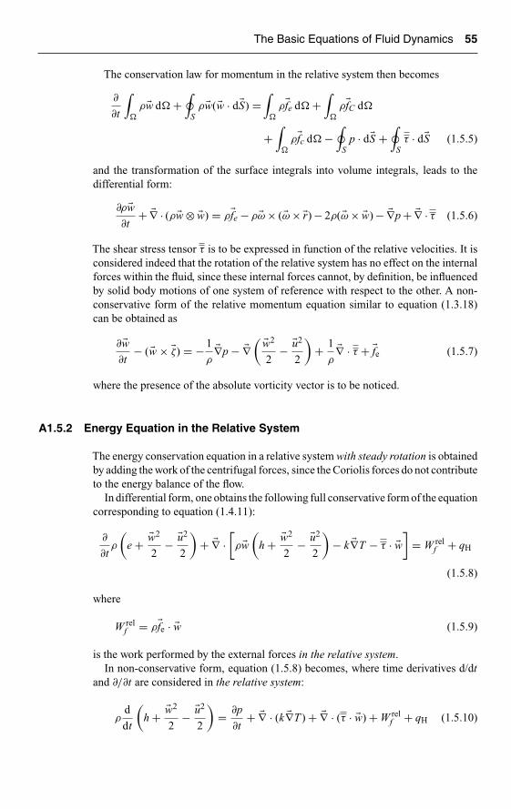
Ch01-H6594.tex 27/4/2007 15: 37 Page 55


The conservation law for momentum in the relative system then becomes

∂

∂t

∫�

ρ �w d� +∮

Sρ �w(�w · d�S) =

∫�

ρ�fe d� +∫

�

ρ�fC d�

+∫

�

ρ�fc d� −∮

Sp · d�S +

∮Sτ · d�S (1.5.5)

and the transformation of the surface integrals into volume integrals, leads to thedifferential form:

∂ρ �w∂t

+ �∇ · (ρ �w ⊗ �w) = ρ�fe − ρ�ω × (�ω ×�r) − 2ρ(�ω × �w) − �∇p + �∇ · τ (1.5.6)

The shear stress tensor τ is to be expressed in function of the relative velocities. It isconsidered indeed that the rotation of the relative system has no effect on the internalforces within the fluid, since these internal forces cannot, by definition, be influencedby solid body motions of one system of reference with respect to the other. A non-conservative form of the relative momentum equation similar to equation (1.3.18)can be obtained as

∂ �w∂t

− (�w × �ζ) = − 1

ρ�∇p − �∇

( �w2

2− �u2

2

)+ 1

ρ�∇ · τ + �fe (1.5.7)

where the presence of the absolute vorticity vector is to be noticed.

A1.5.2 Energy Equation in the Relative System

The energy conservation equation in a relative system with steady rotation is obtainedby adding the work of the centrifugal forces, since the Coriolis forces do not contributeto the energy balance of the flow.

In differential form, one obtains the following full conservative form of the equationcorresponding to equation (1.4.11):

∂

∂tρ

(e + �w2

2− �u2

2

)+ �∇ ·

[ρ �w(

h + �w2

2− �u2

2

)− k �∇T − τ · �w

]= W rel

f + qH

(1.5.8)

where

W relf = ρ�fe · �w (1.5.9)

is the work performed by the external forces in the relative system.In non-conservative form, equation (1.5.8) becomes, where time derivatives d/dt

and ∂/∂t are considered in the relative system:

ρd

dt

(h + �w2

2− �u2

2

)= ∂p

∂t+ �∇ · (k �∇T ) + �∇ · (τ · �w) + W rel

f + qH (1.5.10)

Ch01-H6594.tex 27/4/2007 15: 37 Page 56


The quantity

I = h + �w2

2− �u2

2= H − �u · �v (1.5.11)

appearing in the left-hand side of the above equations, plays an important role, sinceit appears as a stagnation enthalpy term for the rotating system. This term has beencalled the rothalpy and it measures the total energy content in a steadily rotatingframe of reference.

A1.5.3 Crocco’s Form of the Equations of Motion

The pressure gradient term in the equation of motion can be eliminated by makinguse of the entropy equation (1.4.16) written for arbitrary variations of the state ofthe fluid. In particular, if the flow is followed in its displacement along its (absolute)velocity line,

T �∇s = �∇h − �∇p

ρ(1.5.12)

and introducing this relation in equation (1.3.18), we obtain

∂�v∂t

− (�v × �ζ) = T �∇s − �∇H + 1

ρ�∇ · τ + �fe (1.5.13)

where the stagnation enthalpy H has been introduced. Similarly, in the relative system,we obtain from equation (1.5.7):

∂ �w∂t

− (�w × �ζ) = T �∇s − �∇I + 1

ρ�∇ · τ + �fe (1.5.14)

where the rothalpy I appears, as well as the absolute vorticity �ζ.The introduction of entropy and stagnation enthalpy gradients in the equation of

motions is due to Crocco (1937), and equations (1.5.13) and (1.5.14) reveal importantproperties. A first observation is that, even in steady flow conditions, the flow will berotational, except in very special circumstances, namely frictionless, isentropic andisoenergetic flow conditions, without external forces or with forces that can be derivedfrom a potential function where the corresponding potential energy is added to thetotal energy H . An analogous statement can be made for the equation in the relativesystem where the total energy is measured by I . However, since the absolute vorticityappears in the relative equation of motion, even under steady relative conditions,with constant energy I and inviscid flow conditions without body forces, the relativevorticity will not be zero, but equal to (−2�ω). The relative motion is therefore neverirrotational but will have at least a vorticity component equal to minus twice thesolid body angular velocity. This shows that under the above-mentioned conditionsof absolute vorticity equal to zero, the relative flow undergoes a solid body rotationequal to 2�ω in opposite direction to the rotation of the relative system.

Ch01-H6594.tex 27/4/2007 15: 37 Page 57


A1.6 ADVANCED APPLICATIONS OF CONTROL VOLUME FORMULATIONS

In this section we introduce some advanced applications of the control volumeconcept, which are of great importance in practical applications of CFD.

In external flows, CFD simulations are applied to predict the forces on the bodies,in particular lift and drag for aircrafts and cars, particularly for racing cars, wherethese quantities are crucial for the performance improvements. Reduction of dragby very small amounts in aircrafts and racing cars, can make the difference betweenacceptance or not, between winning and losing a race. Section 1.6.1 presents twocomplementary methods to evaluate these forces from the CFD results.

Another important application is connected to cases with moving grids or movingcontrol volumes. This is presented in Section 1.6.2.

A1.6.1 Lift and Drag Estimations from CFD Results

Solid bodies inside control volumeIf the volume � contains solid bodies, then an additional force (−�R) has to be addedto the right-hand side of equation (1.3.9), where �R is the total force exerted by thefluid on the body.

∂

∂t

∫�

ρ�v d�+∮

Sρ�v(�v·d�S) = −

∮S

p·d�S+∮

Sτ ·d�S+

∫�

ρ�fe d�+(−�R) (1.6.1)

This equation is currently applied for the determination of lift force �L and drag force�D on solid bodies, particularly for stationary flows.

For a surface S located in the steady far field, where the viscous shear stresses canbe considered as negligible, the sum of the stationary lift and drag forces are givenby the following relation, in absence of external forces:

∮Sρ�v(�v · d�S) +

∮S

p · d�S = (−�R) = −�L − �D (1.6.2)

The lift and drag forces are obtained from the calculated left-hand side vector afterprojection respectively along the direction perpendicular to the far-field incomingvelocity �U∞ and in its direction (Figure 1.6.1).

If the control surface S is taken along the solid body surface Sb, where the velocityfield is zero due to the non-slip condition of viscous flows, then the lift and drag forcesare also defined by

�R = �L + �D =∮

Sb

p · d�S +∮

Sb

τ · d�S (1.6.3)

These formulas are currently applied to determine these forces from computed flowfields, by either integrating pressure and shear stresses along the solid walls, followingequation (1.6.3) or alternatively by integrating momentum and pressure along thefar-field enclosing surface, following equation (1.6.2).

Ch01-H6594.tex 27/4/2007 15: 37 Page 58


Solid body

U∞

S

Sb

→

Figure 1.6.1 Far-field control surface for lift and drag determination on anenclosed solid body.

A1.6.2 Conservation Law for a Moving Control Volume

The general conservation law (1.1.1) was derived for a fixed control surface. However,many flow situations involve the simultaneous presence of moving and fixed parts,for which moving grids are required. In these cases, attaching a control volume to amoving grid or a moving body requires to take into account the displacement of thecontrol surfaces. Representative examples are:

• flow around a train entering a tunnel, or between two crossing trains in oppositedirections;

• flow around an oscillating wing, where the oscillations can be forced or flowinduced in an aero-elastic interaction;

• the flow between an aircraft and a separating store;• the flow of gases in internal combustion engines where the piston head has a

periodic motion with respect to the cylinder walls, modifying the available flowvolume accordingly;

• hydrodynamic of moving ships with free sea surface and wind induced waves.

In all these examples, two systems of reference are present simultaneously anddepending on the particular situation, fixed or deformable grids have to be attachedto the moving system and the conservation laws of mass, momentum and energy haveto take into account the effects of the relative motion between the two systems.

Scalar conservation lawReferring to Section 1.1.1, we consider now the volume � where each point of thebounding surface S has a velocity �vs in the inertial reference system (see Figure 1.6.2).

Over a time interval �t, the observer moving with the surface S will see a variationof the content of U inside the volume determined by the sum of the fluxes and thesource terms, plus an additional contribution from the volume deformation causedby the surface motion.

Ch01-H6594.tex 27/4/2007 15: 37 Page 59


S(t )

ΩS(t � �t )

Vs • dS �t dS

vS �t

→ →

→

Figure 1.6.2 Moving control volume with surface velocity.

Each surface element d�S gives rise to a volume variation during the time interval �tequal to �vs.d�S �t (see Figure 1.6.2) and therefore the content of U in � will increaseby an additional amount given by the surface integral

∮S U�vs.d�S �t. Summing up all

contributions, we have

∂

∂t

∫�

U d� =∫

�

∂U

∂td� +

∫�

U∂d�

∂t

=∫

�

∂U

∂td� +

∮S

U�vs · d�S

= −∮

S

�F · d�S +∫

�

QV d� +∮

S

�QS · d�S (1.6.4)

or, generalizing in this way equation (1.1.1) to a moving control volume:

∫�

∂U

∂td� +

∮S

(�F − U�vs − �QS ) · d�S =∫

�

QV d� (1.6.5)

The time derivative is to be considered here in the moving system, that is for fixedspace coordinates attached to the volume �.

The quantity �F rel �= (�F − U�vs) can be considered as a relative flux vector, since itcontributes to the convective flux in (1.6.5).

Indeed, introducing the relative velocity

�w = �v − �vs (1.6.6)

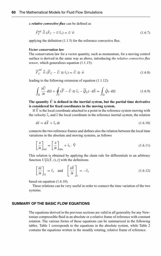
Ch01-H6594.tex 27/4/2007 15: 37 Page 60


a relative convective flux can be defined as

�F relC

�= (�FC − U�vs) = U �w (1.6.7)

applying the definition (1.1.5) for the reference convective flux.

Vector conservation lawThe conservation law for a vector quantity, such as momentum, for a moving controlsurface is derived in the same way as above, introducing the relative convective fluxtensor, which generalizes equation (1.1.15):

Frel

C�= (FC − �U ⊗ �vs) = �U ⊗ �w (1.6.8)

leading to the following extension of equation (1.1.12):

∫�

∂ �U∂t

d� +∮

S(F − �U ⊗ �vs − QS ) · d�S =

∫�

�QV d� (1.6.9)

The quantity �U is defined in the inertial system, but the partial time derivativeis considered for fixed coordinates in the moving system.

If �X is the local coordinate attached to a point in the reference system moving withthe velocity �vs and �x the local coordinate in the reference inertial system, the relation

d�x = d �X + �vs dt (1.6.10)

connects the two reference frames and defines also the relation between the local timevariations in the absolute and moving systems, as follows

[∂

∂t

]rel

=[

∂

∂t

]abs

+ �vs · �∇ (1.6.11)

This relation is obtained by applying the chain rule for differentials to an arbitraryfunction U [�x( �X , t), t] with the definitions

[∂�x∂t

]X

= �vs and

[∂ �X∂t

]

x

= −�vs (1.6.12)

based on equation (1.6.10).These relations can be very useful in order to connect the time variation of the two

systems.

SUMMARY OF THE BASIC FLOW EQUATIONS

The equations derived in the previous sections are valid in all generality for any New-tonian compressible fluid in an absolute or a relative frame of reference with constantrotation. The various forms of these equations can be summarized in the followingtables. Table 1 corresponds to the equations in the absolute system, while Table 2contains the equations written in the steadily rotating, relative frame of reference.

Ch01-H

6594.tex27/4/2007

15:37Page

61

Table 1 The system of flow equations in an absolute frame of reference.

DifferentialEquationform Integral Conservative form Non-conservative form

Conservationof mass

∂

∂t

∫�

ρ d� +∮

Sρ�v · d�S = 0

∂ρ

∂t+ �∇ · (ρ�v) = 0

dρ

dt+ ρ �∇ · �v = 0

Conservationof momentum

∂

∂t

∫�

ρ�v d� +∮

Sρ�v(�v · d�S)

∂ρ�v∂t

+ �∇ · (ρ�v ⊗ �v + pI − τ) = ρfe ρd�vdt

= −�∇p + �∇ · τ + ρ�fe

= −∮

Sp · d�S +

∮Sτ · d�S +

∫�

ρ�fe d�Crocco’s form

∂�v∂t

− (�v × �ζ) = T �∇s − �∇H + 1

ρ�∇ · τ + �fe

Conservationof energy

∂

∂t

∫�

ρE d� +∮

S(ρ�vH − k �∇T − τ · �v) · d�S ∂ρE

∂t+ �∇ · (ρ�vH − k �∇T − τ · �v) ρ

de

dt= −p( �∇ · �v) + �∇ · (k �∇T ) + (τ · �∇) · �v + qH

=∫

�

(ρ�fe · �v + qH )d� = Wf + qHAlternative form

Wf = ρ�fe · �v work of external forces H = h + �v2/2 stagnation enthalpy ρdH

dt= ∂p

∂t+ �∇ · (k �∇T + τ · �v) + Wf + qH

qH external heat sources E = e + �v2/2 total energy Entropy equation

ρTds

dt= εV + �∇ · (k �∇T ) + qH

Definitions τij = μ

[(∂ivj + ∂jvi) − 2

3( �∇ · �v)δij

]�∇ · τ = μ

[��v + 1

3�∇( �∇ · �v)

]for constant viscosity coefficients

Viscous dissipation rate: εV = (τ · �∇) · �v = 1

2μ(τ ⊗ τ

T) vorticity vector: �ζ = �∇ × �v

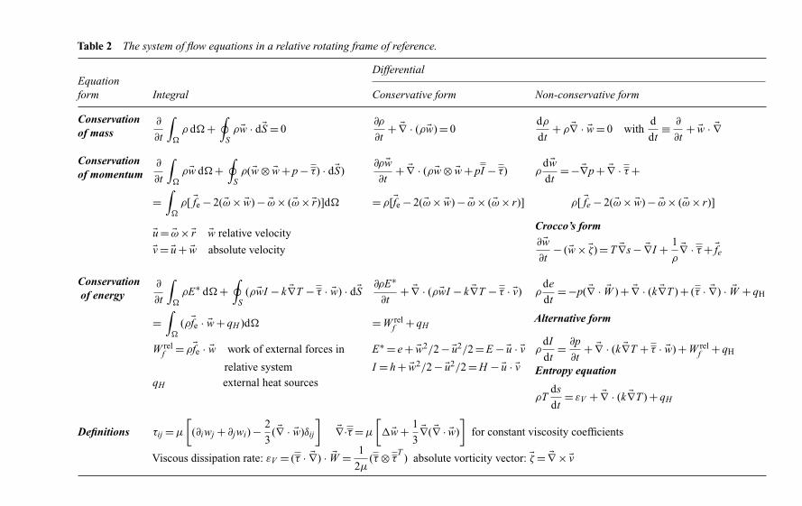
Ch01-H

6594.tex27/4/2007

15:37Page

62

Table 2 The system of flow equations in a relative rotating frame of reference.

DifferentialEquationform Integral Conservative form Non-conservative form

Conservationof mass

∂

∂t

∫�

ρ d� +∮

Sρ �w · d�S = 0

∂ρ

∂t+ �∇ · (ρ �w) = 0

dρ

dt+ ρ �∇ · �w = 0 with

d

dt≡ ∂

∂t+ �w · �∇

Conservationof momentum

∂

∂t

∫�

ρ �w d� +∮

Sρ(�w ⊗ �w + p − τ) · d�S)

∂ρ �w∂t

+ �∇ · (ρ �w ⊗ �w + pI − τ) ρd �wdt

= −�∇p + �∇ · τ +

=∫

�

ρ[ �fe − 2(�ω × �w) − �ω × (�ω ×�r)]d� = ρ[�fe − 2(�ω × �w) − �ω × (�ω × r)] ρ[ �fe − 2(�ω × �w) − �ω × (�ω × r)]

�u = �ω ×�r �w relative velocityCrocco’s form

�v = �u + �w absolute velocity∂ �w∂t

− (�w × �ζ) = T �∇s − �∇I + 1

ρ�∇ · τ + �fe

Conservationof energy

∂

∂t

∫�

ρE∗ d� +∮

S(ρ �wI − k �∇T − τ · �w) · d�S ∂ρE∗

∂t+ �∇ · (ρ �wI − k �∇T − τ · �v) ρ

de

dt= −p( �∇ · �W ) + �∇ · (k �∇T ) + (τ · �∇) · �W + qH

=∫

�

(ρ�fe · �w + qH )d� = W relf + qH

Alternative form

W relf = ρ�fe · �w work of external forces in E∗ = e + �w2/2 − �u2/2 = E − �u · �v ρ

dI

dt= ∂p

∂t+ �∇ · (k �∇T + τ · �w) + W rel

f + qH

relative system I = h + �w2/2 − �u2/2 = H − �u · �v Entropy equationqH external heat sources

ρTds

dt= εV + �∇ · (k �∇T ) + qH

Definitions τij = μ

[(∂iwj + ∂jwi) − 2

3( �∇ · �w)δij

]�∇·τ = μ

[��w + 1

3�∇( �∇ · �w)

]for constant viscosity coefficients

Viscous dissipation rate: εV = (τ · �∇) · �W = 1

2μ(τ ⊗ τ

T) absolute vorticity vector: �ζ = �∇ × �v

Ch01-H6594.tex 27/4/2007 15: 37 Page 63


CONCLUSIONS AND MAIN TOPICS TO REMEMBER

• The fundamental properties of fluid mechanics are contained in the conservationlaws, which can be written in the very general form given by equation (1.1.1)for a scalar quantity and by equation (1.1.12) for a vector quantity.

• To any conserved quantity, we can associate a flux (vector or tensor) describinghow that quantity is changed by the flow.

• You recognize an integral conservation law by the presence of the surfaceintegral of the fluxes, which is the only place where the fluxes appear. Thisfundamental property is the key to any integral conservation law: fluxes maynever appear inside the volume, as they will not be distinguishable from volumesources.

• For the differential form of the conservation law, equations (1.1.4) and (1.1.14),fluxes appear exclusively under a divergence operator. This is how a differentialconservation law is recognized.

• In general the flux associated to a conserved quantity will contain a convec-tive component, which is always present in a fluid in motion, and a diffusivecomponent, which is present in a fluid at rest, but may not always exist.

• The convective flux appears as a first order derivative in space, while the diffusionterms are always expressed by second order spatial derivative terms, reducing toa Laplacian for constant diffusivity properties.

• The distinction between convective and diffusive fluxes is of crucial importanceand translates the fundamental differences in their physical interpretation, asdescribed in Section 1.1.2. Please go back to this section if you feel that thesedifferences are not fully clear to you.

• The laws of fluid mechanics are governed by the conservation equations for thethree basic quantities: mass, momentum and energy. Make sure that you have agood insight into the form of these equations and of the significance of the variouscontributions to the conservation of momentum (the equation of motion) and ofenergy.

• Although equations can be written for other quantities, such as pressure, internalenergy, temperature, entropy, they nevertheless do not obey a conservation law,as they have no associated flux.

REFERENCES

Batchelor, G.K. (1970). An Introduction to Fluid Dynamics. Cambridge UniversityPress, UK.

Crocco, L. (1937). Eine neue stromfunktion fur die Erforschung der Bewegung der Gasemit Rotation. Z. Angew. Math. Mech., 17, 1–7.

Lax, P.D. (1954). Weak solutions of nonlinear hyperbolic equations and their numericalcomputation. Comm. Pure Appl. Math., 7, 159–193.

PROBLEMS

P.1.1 Develop the algebraic form for the gradient of the flux tensor appearing in thevector conservation law (1.1.14), in Cartesian coordinates.

Ch01-H6594.tex 27/4/2007 15: 37 Page 64


With the flux components denoted by Fij with i, j = x, y, z, show that

( �∇.F)x = ∂Fxx

∂x+ ∂Fyx

∂y+ ∂Fzx

∂z

Write out the two other components y and z.P.1.2 Write out the Navier–Stokes equation of motion (1.3.11) explicitly for the three

components u, v, w in Cartesian coordinates.Repeat it for the non-conservative form (1.3.12).

P.1.3 Obtain equation (1.3.13).P.1.4 Prove equation (1.3.20).P.1.5 Obtain the energy equations (1.4.14) and (1.4.15) for the internal energy e.

Hint: Introduce the momentum equation multiplied by the velocity vectorinto equation (1.4.9).

P.1.6 Show that in an incompressible fluid at rest the energy equation (1.4.14) reducesto the temperature conduction equation:

ρcV∂T

∂t= �∇.(k �∇T ) + qH

P.1.7 Show that the energy equation (1.4.11) reduces to a convection–diffusion bal-ance of the stagnation enthalpy H when the Prandtl number is equal to one andwhen only the contribution from the work of the shear stresses related to theviscous diffusion of the kinetic energy is taken into account.

Hint:Assume constant flow properties, setting k = μcp in absence of externalsources, and separate the contributions to the term �∇.(τ.�v) according to thefollowing relations, valid for incompressible flows:

�∇.(τ.�v) = ∂i[μ(∂ivj + ∂jvi)vj

] = �∇.[μ �∇(�v2/2)

]+ �∇.

[μ(�v. �∇).�v

]

Neglecting the second term, setting H = cpT + (�v2/2) leads to

∂ρE

∂t+ �∇.(ρ�vH ) = �∇.(μ �∇H )

P.1.8 Obtain the entropy equation (1.4.18).P.1.9 Derive equation (1.5.7).

P.1.10 Consider the integral mass conservation equation (1.2.1) for a permanent(steady) flow, defined as a time-independent flow for which all partial timederivatives vanish. Consider a channel of arbitrary varying section and twocross-sections at an arbitrary distance apart. Show that the application of thesteady form of the integral mass conservation law leads to the constancy of themass flow rate through each cross-section.

Hint: select a control surface formed by the two cross-sections and thechannel walls in-between and apply the steady integral mass conservation lawtogether with the definition (1.1.6) of the element of mass flow rate.

Ch02-H6594.tex 9/5/2007 8: 47 Page 65

Chapter 2

The Dynamical Levels of Approximation


The main objective of this chapter is to guide you through the different approxima-tions that can be defined to reduce the complexity of the system of flow equations.This process of simplification is based on physical considerations, connected to thedynamical properties of fluid flows, hence the denomination ‘dynamical’ in the titleof this chapter.

In Chapter 1, we derived and discussed the fundamental form of a conservation lawand applied it to obtain the basic equations of fluid mechanics, known as the systemof Navier–Stokes equations, expressing the conservation of the three fundamentalquantities, mass, momentum and energy.

These equations contain many levels of complexity; the most significant being thefollowing:

• They form a system of five (in three-dimensional space) fully coupled time-dependent partial differential equations for the five unknowns, velocity vector(three unknowns), and two thermodynamic quantities, such as for instance pres-sure and density, or pressure and temperature. The coupling occurs through thevelocity and density fields, possibly also through the temperature field, whenthermal effects are significant.

• Each of these equations is nonlinear. The nonlinearity of the flow equations isnot just a mathematical observation, as it has major consequences on the wholeof fluid mechanics:– The dominant nonlinearity is provided by the convection term ρ(�v. �∇)�v, see,

e.g., the momentum equation under the form (1.3.13). This term is responsiblefor the appearance of turbulence, which is a spontaneous instability of theflow, whereby all quantities take up a statistical (chaotic) behavior.

– For compressible flows, the products of density and velocity represent anothernonlinearity, leading to the existence of shock waves in supersonic flows.Through a shock, velocities, pressure, temperature, undergo a discontinuousjump and, as we will see later on, these discontinuities are indeed exactsolutions of the nonlinear inviscid Euler equations.

– With non-uniform temperature fields, flow-thermal nonlinearities appear,such as Bénard cells in shallow heated fluid layers, representative of com-plex thermal convection phenomena, which are crucial, among others, inweather forecasting.

– Other nonlinearities can appear in flows with free surfaces, such as thebreaking of waves that you can observe on the seashores, or during heavysloshing of a liquid in a tank. Also in two phase flows, the coalescence or

65

Ch02-H6594.tex 9/5/2007 8: 47 Page 66


breaking up of droplets or bubbles result from the nonlinear properties offlows and nonlinearities of thermodynamic origin lead to phase changes, suchas evaporation, condensation.

– Nonlinearities lead to non-unique solutions. This has also major conse-quences, under the form of the existence of multiple flow configurations forthe same initial and boundary conditions, resulting from bifurcations fromone flow state to another. Numerous examples of flow non-uniqueness andof bifurcations have been observed, experimentally and numerically, and wewill show some examples in this chapter.

These complexities in fluid dynamics pose considerable challenges for CFD, inparticular for turbulent flows.

The link with the available computing power at a given time is illustrated in Fig-ures I.1.4 and I.1.6, showing the evolution of the models used in industry, progressingtoward increased complexity, and hence reliability, due to the progress in availablecomputing power shown in Figure I.1.7.

We will present in this chapter an overview of the most significant and most widelyused approximation levels. All these models, ranging from Direct Numerical Simu-lation (DNS), Large Eddy Simulation (LES) and Reynolds Averaged Navier–Stokes(RANS), to various forms of simplified treatment of the viscous terms, includingboundary layer approximations, down to inviscid models of the Euler equations andthe most simplified forms of potential flow, have been used, and several of them arestill in use, in various sectors of industry.

The Issue of the Time and Length Scales

The issue of the time and length scales of the description of the physical flow featuresis critical to the world of simulation. The same flow will appear very different whenwe reduce the scale at which we look at it. This is illustrated by the following exampleof the experimental observation of a double annular jet, Figures 2.0.1 and 2.0.2. Whenmeasurements are taken with a standard Laser Doppler Velocimeter (LDV) instru-mentation, which averages the flow over a certain time scale, a steady averaged flow,with three backflow regions appear, as seen on Figure 2.0.1. On the other hand, thesame flow seen with a Particle Image Velocimetry (PIV) laser sheet technique, whichtakes an instantaneous snapshot of the flow in the plane of the laser sheet, shows ahighly unsteady flow with large-scale fluctuations, although the inlet conditions areconstant, Figure 2.0.2.

Look carefully at these figures, as they illustrate a fundamental issue in CFDsimulations. Before you consider a CFD application, you should evaluate and definethe time and length scales at which you want to model your flow system, in the sameway experimentalists choose their instrumentation in function of the level of detailsthey require.

This is the main objective of this chapter. It should help you develop a knowledgeand awareness of the best suited model for a given flow problem, by making aproper balance between the acceptable approximations with respect to the reality,and compatible with the computer capacity you have available.

We have chosen to illustrate the various approximations by typical results andexamples from CFD calculations performed at each level of approximation, as anillustration of the type of computations achievable with the model being considered.

Ch02-H6594.tex 9/5/2007 8: 47 Page 67

The Dynamical Levels of Approximation 67

50

0

0 50 100

X (mm)

Central toroidal vortex

150 200

Annular jets join

Annularcounter-rotatingvortices

Y (

mm

)

�50

e d c

b

a

U_mod

1

0.8

0.6

0.4

0.2

0

(a) (b)

(c) (d)

Single annular jet

Central jet

Single annular jet

Figure 2.0.1 Double annular burner: (a) Exit view of the burner. (b) Experimentalcolor plot of axial velocity in the symmetry plane, obtained from LDV. (c)Experimental streamlines of the flow with designation of specific position points,related to the vortex structure, obtained from LDV. (d) Experimental vector plot ofthe velocity field obtained from LDV data (for color image refer Plate 2.0.1). FromS. Geerts et al. (2005). Courtesy Vrije Universiteit Brussel (VUB).

(a) (b)

Figure 2.0.2 Double annular burner: two successive snapshots taken with a PIVlaser sheet technique. Courtesy Vrije Universiteit Brussel.

Ch02-H6594.tex 9/5/2007 8: 47 Page 68


Table 2.0.1 The simplification process leading to the scalar, linearized modelequations.

Degrees of Full system ofcomplexity flow equations Reduction of complexity

Three-dimensional Vector of minimum Reduce to one-dimensional space,space five unknowns with three unknowns

Coupled system System of minimum Decouple the equations and reducefive equations to a single scalar equation for one

unknown quantity

Nonlinearities Full nonlinear system Linearize the scalar equations

Simplified Model Equations

Most of the approximate models retain, at various degrees, the basic complexitiesof the Navier–Stokes equations, namely the three dimensions of space, the couplednature of the equations and the nonlinearities.

As you easily can imagine, it is hardly possible to develop and study the basics ofnumerical discretization methods on such complex models. Hence, we need a secondlevel of simplification, reducing these three degrees of complexity to their essentials,namely the fundamental effects of convection and diffusion, as seen in Section 1.1.2.This leads us to simplified model equations, obtained by the following simplificationprocess, summarized in Table 2.0.1, which can be followed by going down along thethird column:

• Three-dimensional space, to be simplified to one-dimensional space.• The coupled equations, to be decoupled to a single scalar equation.• The nonlinearities, to be removed by a linearization assumption.

These mathematically based simplifications lead to sufficiently simple modelequations to guide the development of the basic numerical schemes for CFD.

They will form the basis for all of Chapters 4–10, while Chapters 11 and 12, willfocus on applying the methods developed on the model equations to ‘real’approximateflow models formed by coupled and nonlinear equations.

Note that the numerical schemes developed and analyzed on these simplifiedmodel equations will ultimately be applied for the discretization of the full Navier–Stokes equations.

The simplified models will be introduced in Chapter 3.

Content of this chapter

It is considered that the system of Navier–Stokes equations, supplemented by empir-ical laws for the dependence of viscosity and thermal conductivity with other flowvariables and by a constitutive law defining the nature of the fluid, completely describesall flow phenomena (Section 2.1).

Ch02-H6594.tex 9/5/2007 8: 47 Page 69


For laminar flows, no additional information is required and one can consider thatany experiment in laminar flow regimes can be accurately duplicated by computations.However, and we could say unfortunately from the point of view of computationalfluid dynamics, most of the flow situations occurring in nature and in technologyenter into a particular form of instability called turbulence. Turbulence occurs in allflow situations when the velocity, or more precisely, the Reynolds number, defined asthe product of representative scales of velocity and length divided by the kinematicviscosity, exceeds a certain critical value. The particular form of instability generatedin the turbulent flow regime, is characterized by the presence of statistical fluctuationsof all the flow quantities. These fluctuations can be considered as superimposed onmean or averaged values and can attain, in many situations, the order of 10% of themean values, although certain flow regions, such as separated zones, can attain muchhigher levels of turbulent fluctuations.

Clearly, the numerical description of the turbulent fluctuations is a formidable task,which puts extremely high demands on computer resources. With increasing com-puter power, in both speed and memory, we are progressively able to simulate thelarge-scale turbulent fluctuations, or even the small-scale turbulent motion, directlyon the computer from the time-dependent Navier–Stokes equations. This forms thebasis of the growing development of Direct Numerical Simulation (DNS). An esti-mate of the computer requirements connected to this level of approximation can befound already in Chapman (1979) and in the recent books of Sagaut (2001) andGeurts (2004).

The computer requirements for DNS simulations of turbulent flows are out of reachin the foreseeable future for industrial applications and it is therefore essential to resortto approximations enabling the numerical description of turbulent flows in acceptablecomputer CPU times. The highest approximation, with good prospects for reachingthe industrial stage in the near future is the approximation known as Large EddySimulation (LES). This LES approach is similar to DNS, in its objective to simulatedirectly the turbulent fluctuations, but restricted to the larger scales with the smallerscales being modeled.

The next highest level of approximation is the Reynolds Averaged Navier–Stokes(RANS) model, which is restricted to the computation of the averaged turbulent flow.This requires the RANS equations to be supplemented by models for the Reynoldsstresses. These models can range from simple eddy viscosity or mixing length modelsto transport equations for the turbulent kinetic energy and dissipation rates, or theirmany two equation variants, or to still more complicated models solving directly thetransport equations for the Reynolds stresses. LES and RANS models are introducedin Section 2.2.

Considering the various stages within the dynamical level of approximation, a firstreduction in complexity can be introduced for flows with small amount of separationor back-flow and with a predominant mainstream direction at high Reynolds numbers.This allows neglecting viscous and turbulent diffusion in the mainstream directionand hence to reduce the number of shear stress terms to be computed, consideringthat they have a negligible action on the flow behavior. This is the ‘Thin Shear LayerApproximation’ discussed in Section 2.3.

Within the same level, we can situate the parabolic approximations for the steadystate Navier–Stokes equations. In these approximations, the elliptic character of theflow is put forward through the pressure field, while all other variables are consideredas transported or as having a parabolic behavior (Section 2.4).

Ch02-H6594.tex 9/5/2007 8: 47 Page 70


The next level to be considered is the Boundary Layer Approximation referred toin Section 2.5. As is well known, this analysis of the effects of viscosity by L. Prandtl,is a most spectacular example of the impact of a careful investigation of the mag-nitude of force components on the description of a flow system. For flows with noseparation and thin viscous layers, that is at high Reynolds numbers, a decouplingof the viscous and inviscid parts of the flow can be introduced. The pressure field ishereby decoupled from the viscous effects, showing that the influence of the viscousand turbulent shear stresses is confined to small regions close to the walls and thatoutside these layers the flow behaves as inviscid. This analysis, which was perhapsthe greatest breakthrough in fluid mechanics since the discovery of the Navier–Stokes equations, showed that many of the flow properties could be described bythe inviscid approximation, e.g. determination of the pressure distributions, and thata simplified boundary layer approximation allows for the determination of the viscouseffects.

When this influence or interaction is neglected, we enter the field of the inviscidapproximations, which allow generally a good approximation of the pressure field,and hence of lift coefficient for attached external flows.

An intermediate level between the partially or fully viscous flow descriptions andthe inviscid approximation is the distributed loss model, used in confined flow prob-lems, in particular in the simulation of multistage turbomachinery flows and shallowwater models in ocean dynamics. The overall effect of boundary layers and wakes isexpressed as a distributed friction force and the implications of this approximation arepresented in Section 2.6. At the same level, we can consider various viscid–inviscidinteraction models, which couple a boundary layer calculation, as a correction to aninviscid simulation, in order to obtain an approximation of viscous effects, includingfriction losses.Within the inviscid approximations, the model of the time-dependentEuler equation is summarized in Section 2.7.

The potential flow model, restricted to non-rotational flows, is at a lower level ofapproximation, due to the associated assumption of isentropic flow (Section 2.8).This leads to a description of shock discontinuities which deviate from the Rankine–Hugoniot relations and occasionally to problems of non-uniqueness. However, thepotential flow model is equivalent to the Euler equations for subsonic, non-rotationalflows.

The content of Chapter 2 is summarized in the chart of Figure 2.0.3.

2.1 THE NAVIER–STOKES EQUATIONS

The most general description of a fluid flow is obtained from the full system ofNavier–Stokes equations. Referring to Chapter 1, the conservation laws for the threebasic flow quantities (ρ, ρ�v, ρE) can be written in a compact form, expressing thecoupled nature of the equations:

∂

∂t

∣∣∣∣∣∣∣

ρ

ρ�vρE

∣∣∣∣∣∣∣+ �∇ ·

∣∣∣∣∣∣∣∣

ρ�vρ�v ⊗ �v + pI − τ

ρ�vH − τ · �v − k �∇T

∣∣∣∣∣∣∣∣=

∣∣∣∣∣∣∣

0

�feWf + qH

∣∣∣∣∣∣∣(2.1.1)

Ch02-H6594.tex 9/5/2007 8: 47 Page 71


Viscous-Inviscidinteractions

No

Yes

Boundary layerapproximation

Three-dimensionalNavier–Stokes equations

Large eddy simulation (LES-DES)Reynolds Averaged Navier–Stokes

equations (RANS)

Inputturbulence models

Large viscousregions?

Inputm (T,p)k (T,p)Fluid constitutiveequation

Distributed loss model

Parabolized N–Sequations

Thin shear layerapproximation

Time-dependent Eulerequations

Viscous–inviscidinteractions

Potential flow models

Inviscid models

Direct NumericalSimulation (DNS) of

turbulence

Figure 2.0.3 Hierarchy of the different dynamical levels of approximation.

The above equation defines a (5 × 1) column vector U of the conservative variables:

U =

∣∣∣∣∣∣∣

ρ

ρ�vρE

∣∣∣∣∣∣∣=

∣∣∣∣∣∣∣∣∣∣

ρ

ρuρvρwρE

∣∣∣∣∣∣∣∣∣∣(2.1.2)

Ch02-H6594.tex 9/5/2007 8: 47 Page 72


and a generalized (5 × 3) flux vector �F :

�F =

∣∣∣∣∣∣∣

ρ�vρ�v ⊗ �v + pI − τ

ρ�vH − τ · �v − k �∇T

∣∣∣∣∣∣∣(2.1.3)

with Cartesian coordinates f , g, h each of these components being a (5 × 1) columnvector. The right-hand side contains the source terms and these can be grouped intoa (5 × 1) column vector Q, defined by

Q =

∣∣∣∣∣∣∣

0

�feWf + qH

∣∣∣∣∣∣∣(2.1.4)

The source terms express the effects of the external forces �fe, of the heat sources qH

and of the work performed by the external forces Wf = ρ�fe · �v. The group of equations(2.1.1) takes then the following condensed form:

∂U

∂t+ �∇ · �F = Q (2.1.5)

Expressed in Cartesian coordinates, we obtain the more explicit algebraic form:

∂U

∂t+ ∂f

∂x+ ∂g

∂y+ ∂h

∂z= Q (2.1.6)

or in an alternative condensed notation:

∂tU + ∂x f + ∂yg + ∂zh = Q

where u, v, w are the x, y, z components of the velocity vector and the flux vector(2.1.3) is defined by its components f , g, h (subscripts indicate the correspondingCartesian components):

f =

∣∣∣∣∣∣∣∣∣∣∣

ρu

ρu2 + p − τxx

ρuv − τxy

ρuw − τxz

ρuH − (τ · �v)x − k∂xT

∣∣∣∣∣∣∣∣∣∣∣g =

∣∣∣∣∣∣∣∣∣∣∣

ρv

ρvu − τyx

ρv2 + p − τyy

ρvw − τyz

ρuH − (τ · �v)y − k∂yT

∣∣∣∣∣∣∣∣∣∣∣

h =

∣∣∣∣∣∣∣∣∣∣∣

ρw

ρwu − τzx

ρwv − τyz

ρw2 + p − τzz

ρwH − (τ · �v)z − k∂zT

∣∣∣∣∣∣∣∣∣∣∣(2.1.7)

Refer to Chapter 1 for a more detailed discussion, in particular for the association withthe Newtonian fluid model, the perfect gas model, or for the particular formulationrelated to incompressible fluids.

Ch02-H6594.tex 9/5/2007 8: 47 Page 73


This system of Navier–Stokes equations is valid for any laminar or turbulent flowof any fluid, defined by its constitutive equation relating the shear stresses to the otherflow variables.

2.1.1 Non-uniqueness in Viscous Flows

Non-unique solutions of the Navier–Stokes equations are known to exist for many flowsituations when some non-dimensional number, representing a measure of the balancebetween various forces reach a critical value. For instance, the Bénard problem of afluid heated from below or the Taylor problem of the flow between concentric cylin-ders, of which the inner one is rotating are known to generate more than one physicalstate for the same physical conditions. It is interesting to observe here that the non-uniqueness of the stationary Navier–Stokes equations has been proven theoreticallyfor these flow cases (see for instance Temam, 1977).

However, many other flow systems show this non-unique behavior, which is oftenassociated with additional complexities resulting from spontaneous unsteadiness,such as bifurcations, symmetry breaking and route to chaos. The latter step is oftenthe road to turbulence.

We will illustrate this with two examples. The first one is less familiar as it describesthe flow induced by the temperature gradient of surface tension on a cylinder of liquidbound by above and below by two surfaces at different temperatures. It is known asa liquid bridge and the flow phenomenon is known as the Marangoni effect.

The second example is the well-known flow over a cylinder with a uniform steadyincident velocity. The resulting flow is subject to the appearance of vortex shedding,known as the Von Karman street, but many levels of additional complexities appearwhen either compressibility and/or 3D effects are taken into consideration.

The non-uniqueness property of the viscous flows, connected to the spontaneouslygenerated unsteadiness, pose considerable problems to the numerical simulation andrepresent one of the main challenges in CFD. The flow can undergo sudden changes inits unsteady behavior, or be subjected to bifurcations, route to chaos and other effectstypical of nonlinear systems. Very high accuracy, at the level of the discretizationschemes, as well as in the treatment of the boundary conditions are required in orderto be able to recover numerically multiple solutions, when they exist; while avoidingspurious states of numerical origin.

2.1.1.1 Marangoni thermo-capillary flow in a liquid bridge

A liquid bridge is a small cylinder of liquid, of height h and diameter d, containedbetween two endplates at different temperatures, but with a free external surface,held together by surface tension. The Marangoni thermo-capillary effect designatesthe flow system that appears induced by a temperature gradient of the surface tensionand is of interest in float-zone crystal growth technology.

In the above equations, the external surface forces are defined by

�feS = σκ�n + �∇tσ (2.1.8)

Ch02-H6594.tex 9/5/2007 8: 47 Page 74


The first term on the right-hand side represents the normal component of the surfacetension σ, function of temperature, for a surface curvature κ, directed along the normaldirection n. The second term is the tangential component of the surface tensiongradient, which appears if the surface tension is not uniform, in particular due totemperature variations.

An associated heat source is generated by the work of these capillary forces,defined by

Wf S = ρ�feS · �vS (2.1.9)

where the subscript S indicates values defined on the peripheral surface.The surface tension forces hold the column of fluid together between two disks

maintained at different temperatures, and a convection pattern is generated by the sur-face tension gradients induced by the temperature gradient on the interfacial surface.

A non-dimensional Reynolds number is defined as

Re = |σT |h�T

ρv2(2.1.10)

h is the height of the liquid bridge, �T is the imposed temperature difference betweenthe endplates, σT = −dσ/dT is the negative rate of change of surface tension withtemperature.

The Marangoni number is defined by multiplication with the Prandtl numberPr = v/κ:

Ma = Re. Pr = |σT |h�T

ρv2· v

κ= |σT |h�T

ρvκ(2.1.11)

The flow structure depends on three non-dimensional parameters, Re, Pr and theaspect ratio of the liquid bridge, A = 2h/d.

For small temperature differences �T between the upper (hot) and lower (cold)endplate, that is for low values of the Marangoni number Ma, a steady axisymmetricflow is being generated by the temperature-dependent surface tension forces. Thissteady flow is characterized by two toroidal vortices and by a temperature field witha cold point at the lower corner. Figure 2.1.1 shows the liquid bridge configurationand the steady flow for half the cylinder, where the central limit of the velocity andtemperature plots is the vertical symmetry axis of the liquid bridge.

When the temperature difference, that is the Marangoni number increases, the flowstructure changes completely as the velocity and temperature fields become unsteady,with increasingly complex flow configurations.

The following flow structures are observed; Dinescu and Hirsch (2001), Hirschand Dinescu (2003):1

• A first spontaneous unsteadiness appears under the form of a standing pulsatingwave, with 2, 3 or more modes, depending on the Prandtl number and the aspect

1 The another would like to thank Cristian Dinescu for putting together these figures extracted fromthe CFD animation.

Ch02-H6594.tex 9/5/2007 8: 47 Page 75


Thot

d

h

Tcold0.1

0.3

0.5

0.7

0.9

Hot corner

Cold corner

(a) (b)

Figure 2.1.1 (a) Liquid bridge configuration and (b) Marangoni effect. Steadyaxisymmetric flow and temperature pattern shown on half of the cylinder, the axis ofsymmetry is the internal vertical line in each of these figures. From Dinescu andHirsch (2001).

ratio. Figure 2.1.2a shows four snapshots of the associated temperature andvelocity fields, for m = 2 mode.

• This pulsating mode is not permanent and after a certain time transforms itselfto a traveling mode, which remains unchanged over time (Figure 2.1.2b).

With further increasing Marangoni numbers, a succession of nonlineargenerated phenomena appear:– Symmetry breaking of the flow configuration first via a period doubling as

shown on (Figure 2.1.2c).– At different conditions, another route to chaos is identified, showing a quasi-

periodic state with frequency doubling. Inspecting Figure 2.1.2d, we can seethe pattern of the temperature disturbance field with the three cold (blue)spots placed near the free surface and the three hot spots located near thevertical axis of the liquid bridge. The loss of symmetry and the two fre-quencies of the traveling waves captured by the numerical simulation areconfirmed by the experiments of Schwabe (2001), identified as quasi-periodicstates.

– Route to chaos: with increasing Marangoni numbers an increasingly chaoticmotion starts to appear.

These results are confirmed by experimental observations and other simulations.The interested reader can consult the following additional references to learn moreabout these fascinating phenomena: Velten et al. (1991), Frank and Schwabe (1997),Shevtsova and Legros (1998), Kuhlmann (1999), Leypoldt et al. (2000), and Zenget al. (2004).

Ch02-H6594.tex 9/5/2007 8: 47 Page 76


Marangoniflow

Perturbation unsteadytemperature filed

Perturbation unsteady flow filed

(a)

Pul

satin

g w

ave

Ma�8773

Pr�8.9; A�1

m�2 mode

Red color:hot region

Blue color:cold region

(b)

Tra

velli

ng w

ave

Ma�35,092;Pr�8.9;A�1Symmetrybreakingwith perioddoubling ofmode m�2Red color:hot regionBlue color:cold region

(c)

Tra

velli

ng w

ave

Ma�28,255;Pr�7;A�0.73Symmetrybreakingwith quasi-periodicpattern ofmode m�3Red color:hot regionBlue color:cold region

(d)

Tra

velli

ng w

ave

Figure 2.1.2 Liquid bridge and Marangoni effect. Representation of variousunsteady and symmetry broken solutions for velocity and temperature Perturbationfields. Each group of four figures represents four snapshots of the correspondingunsteady peturbation field (for color image refer Plate 2.1.2). From Dinescu andHirsch (2001), Hirsch and Dinescu (2003).

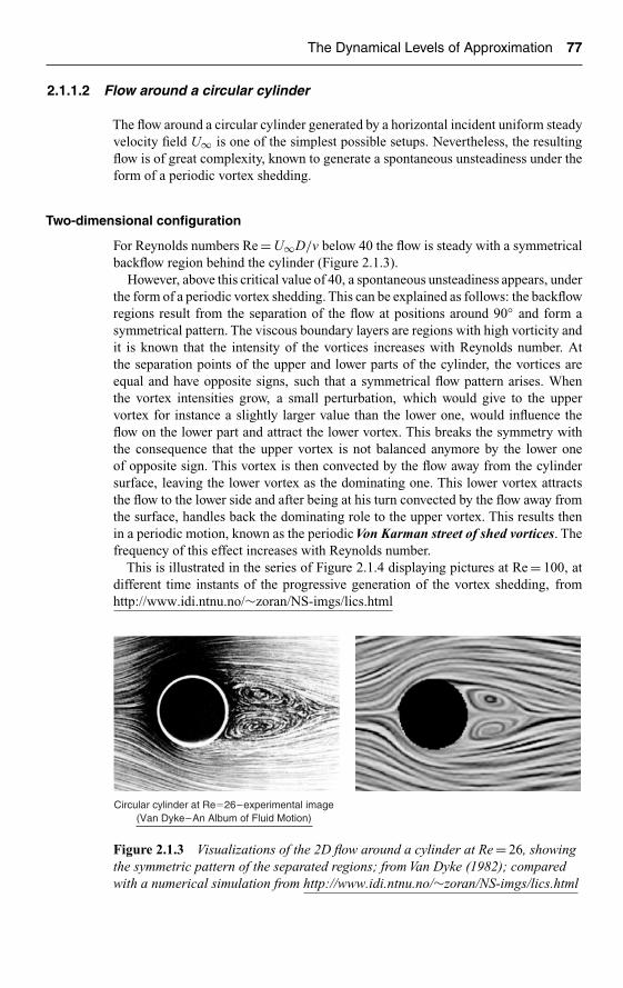
Ch02-H6594.tex 9/5/2007 8: 47 Page 77


2.1.1.2 Flow around a circular cylinder

The flow around a circular cylinder generated by a horizontal incident uniform steadyvelocity field U∞ is one of the simplest possible setups. Nevertheless, the resultingflow is of great complexity, known to generate a spontaneous unsteadiness under theform of a periodic vortex shedding.

Two-dimensional configuration

For Reynolds numbers Re = U∞D/v below 40 the flow is steady with a symmetricalbackflow region behind the cylinder (Figure 2.1.3).

However, above this critical value of 40, a spontaneous unsteadiness appears, underthe form of a periodic vortex shedding. This can be explained as follows: the backflowregions result from the separation of the flow at positions around 90◦ and form asymmetrical pattern. The viscous boundary layers are regions with high vorticity andit is known that the intensity of the vortices increases with Reynolds number. Atthe separation points of the upper and lower parts of the cylinder, the vortices areequal and have opposite signs, such that a symmetrical flow pattern arises. Whenthe vortex intensities grow, a small perturbation, which would give to the uppervortex for instance a slightly larger value than the lower one, would influence theflow on the lower part and attract the lower vortex. This breaks the symmetry withthe consequence that the upper vortex is not balanced anymore by the lower oneof opposite sign. This vortex is then convected by the flow away from the cylindersurface, leaving the lower vortex as the dominating one. This lower vortex attractsthe flow to the lower side and after being at his turn convected by the flow away fromthe surface, handles back the dominating role to the upper vortex. This results thenin a periodic motion, known as the periodic Von Karman street of shed vortices. Thefrequency of this effect increases with Reynolds number.

This is illustrated in the series of Figure 2.1.4 displaying pictures at Re = 100, atdifferent time instants of the progressive generation of the vortex shedding, fromhttp://www.idi.ntnu.no/∼zoran/NS-imgs/lics.html

Circular cylinder at Re�26–experimental image(Van Dyke–An Album of Fluid Motion)

Figure 2.1.3 Visualizations of the 2D flow around a cylinder at Re = 26, showingthe symmetric pattern of the separated regions; from Van Dyke (1982); comparedwith a numerical simulation from http://www.idi.ntnu.no/∼zoran/NS-imgs/lics.html

Ch02-H6594.tex 9/5/2007 8: 47 Page 78


t�4 t�8

t�12 t�24

t�27 t�32

t�35 t�40

t�360 t�400

Figure 2.1.4 Visualizations of the flow around a cylinder at Re = 100, showing theprogressive generation of the vortex shedding, at different time instants. Fromhttp://www.idi.ntnu.no/∼zoran/NS-imgs/lics.html

What this actually means is that above the critical value of the Reynolds number,there is no steady flow configuration anymore, although the cylinder and the incidentconditions remain fixed and constant.

If we consider in addition a high Mach number flow, an additional complexityappears, due to the interaction with compressibility effects.

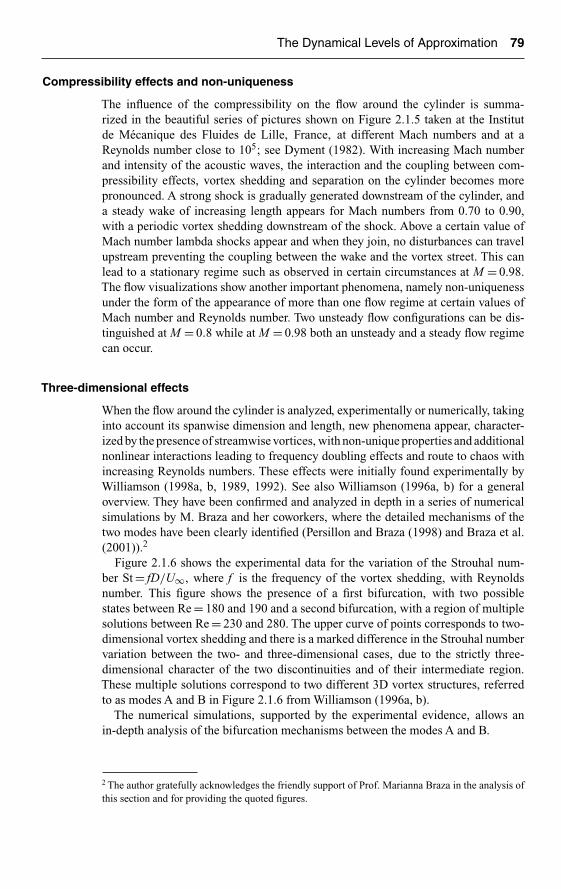
Ch02-H6594.tex 9/5/2007 8: 47 Page 79


Compressibility effects and non-uniqueness

The influence of the compressibility on the flow around the cylinder is summa-rized in the beautiful series of pictures shown on Figure 2.1.5 taken at the Institutde Mécanique des Fluides de Lille, France, at different Mach numbers and at aReynolds number close to 105; see Dyment (1982). With increasing Mach numberand intensity of the acoustic waves, the interaction and the coupling between com-pressibility effects, vortex shedding and separation on the cylinder becomes morepronounced. A strong shock is gradually generated downstream of the cylinder, anda steady wake of increasing length appears for Mach numbers from 0.70 to 0.90,with a periodic vortex shedding downstream of the shock. Above a certain value ofMach number lambda shocks appear and when they join, no disturbances can travelupstream preventing the coupling between the wake and the vortex street. This canlead to a stationary regime such as observed in certain circumstances at M = 0.98.The flow visualizations show another important phenomena, namely non-uniquenessunder the form of the appearance of more than one flow regime at certain values ofMach number and Reynolds number. Two unsteady flow configurations can be dis-tinguished at M = 0.8 while at M = 0.98 both an unsteady and a steady flow regimecan occur.

Three-dimensional effects

When the flow around the cylinder is analyzed, experimentally or numerically, takinginto account its spanwise dimension and length, new phenomena appear, character-ized by the presence of streamwise vortices, with non-unique properties and additionalnonlinear interactions leading to frequency doubling effects and route to chaos withincreasing Reynolds numbers. These effects were initially found experimentally byWilliamson (1998a, b, 1989, 1992). See also Williamson (1996a, b) for a generaloverview. They have been confirmed and analyzed in depth in a series of numericalsimulations by M. Braza and her coworkers, where the detailed mechanisms of thetwo modes have been clearly identified (Persillon and Braza (1998) and Braza et al.(2001)).2

Figure 2.1.6 shows the experimental data for the variation of the Strouhal num-ber St = fD/U∞, where f is the frequency of the vortex shedding, with Reynoldsnumber. This figure shows the presence of a first bifurcation, with two possiblestates between Re = 180 and 190 and a second bifurcation, with a region of multiplesolutions between Re = 230 and 280. The upper curve of points corresponds to two-dimensional vortex shedding and there is a marked difference in the Strouhal numbervariation between the two- and three-dimensional cases, due to the strictly three-dimensional character of the two discontinuities and of their intermediate region.These multiple solutions correspond to two different 3D vortex structures, referredto as modes A and B in Figure 2.1.6 from Williamson (1996a, b).

The numerical simulations, supported by the experimental evidence, allows anin-depth analysis of the bifurcation mechanisms between the modes A and B.

2 The author gratefully acknowledges the friendly support of Prof. Marianna Braza in the analysis ofthis section and for providing the quoted figures.

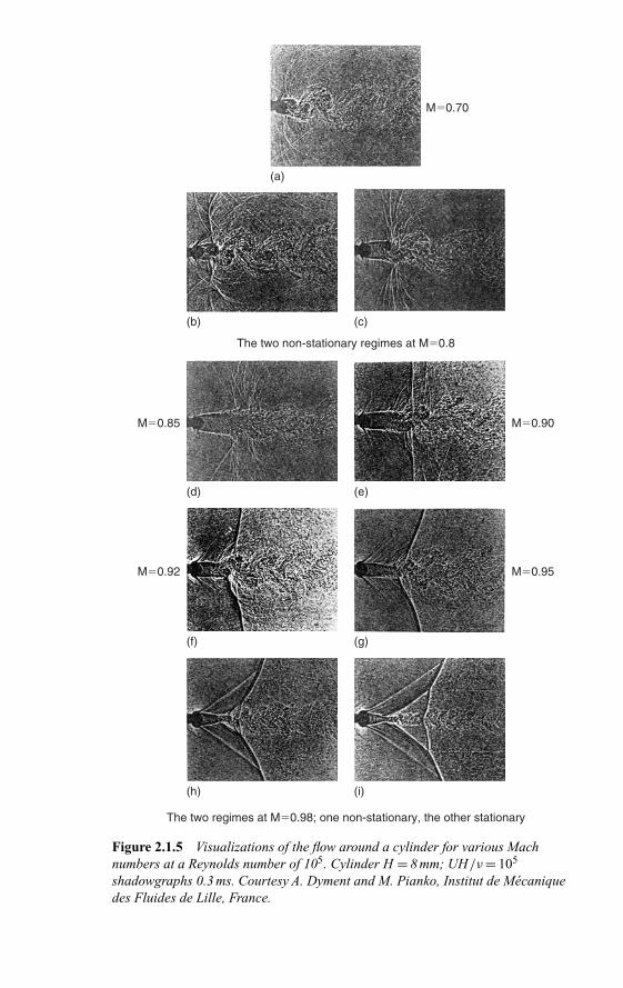
Ch02-H6594.tex 9/5/2007 8: 47 Page 80

(b) (c)

(a)

M�0.70

M�0.85 M�0.90

M�0.92 M�0.95

The two non-stationary regimes at M�0.8

The two regimes at M�0.98; one non-stationary, the other stationary

(f)

(d) (e)

(g)

(h) (i)

Figure 2.1.5 Visualizations of the flow around a cylinder for various Machnumbers at a Reynolds number of 105. Cylinder H = 8 mm; UH/ν = 105

shadowgraphs 0.3 ms. Courtesy A. Dyment and M. Pianko, Institut de Mécaniquedes Fluides de Lille, France.

Ch02-H6594.tex 9/5/2007 8: 47 Page 81


0.22

0.20

0.18

0.16

S

0.14

0.1240 100 160

Parallel laminarshedding

Mode A

Mode B

Williamson (1992)Miller and Williamson (1994)Prasad and Williamson (1995)Leweke and Provansal (1995)

Mode B(with dislocations)

220 280

Re

340 400 460

Figure 2.1.6 Strouhal number versus Reynolds number relation, showing thedifferent modes and a lower path with dislocations. Experiments reported byWilliamson (1996a, b) (detailed in the legend); * direct simulation by the presentstudy. From Braza et al. (2001).

(a) (b)D

Figure 2.1.7 Spanwise undulation of the main vortex rows and streamwisevortices, at Re = 220; shown by iso-contours of vorticity components. (b) Spanwiseexperimental flow visualization, provided by Williamson (1992). The frame showscorrespondence to the computational region explored (for color image refer Plate2.1.7). From Persillon and Braza (1998). Courtesy M. Braza. IMFT, Toulouse.

Figure 2.1.7, from Persillon and Braza (1998) shows the A configuration at aReynolds number of 220. The figure displays the three-dimensional vortex structurethrough the iso-contours of the transverse and streamwise vorticity components.A dis-tortion of the main vortex filaments is seen along the span, with the presence of

Ch02-H6594.tex 9/5/2007 8: 47 Page 82


D D(a) (b)

S

(c)

Figure 2.1.8 Modification of the spanwise vortex structures as Reynolds numberincreases; passage to mode B; (a) Re = 270; (b) Re = 300. (c) Spanwiseexperimental flow visualization, provided by Williamson (1992, 1996 a, b). Theframe shows correspondence to the computational region explored (for color imagerefer Plate 2.1.8). From Persillon and Braza (1998). Courtesy M. Braza. IMFT,Toulouse.

streamwise vortex structures. This pattern is compared with experimental visualiza-tions by Williamson (1992). At higher Reynolds numbers, we observe a modificationof the spanwise vortex structures and a transition to mode B, as seen from Figure2.1.8 where Figure 2.1.8a corresponds to Re = 270 and Figure 2.1.8b to Re = 300.Figure 2.1.8c shows the spanwise experimental flow visualization, from Williamson(1992, 1996a, b).

The mechanism behind the bifurcation between modes A and B is related to adislocation mechanism of the transverse vortices, as shown by the simulations per-formed by Braza et al. (2001). Details of this mechanism, involving a fundamentalfrequency reduction and route to chaos are summarized in Figure 2.1.9, showing thetransition steps from mode A to mode B. The figure displays the modification of thespanwise wavelengths, as well as the junction between two adjacent Von Karmanvortex rows, that illustrates the vortex dislocation pattern with an increase of thechaotic components.

Ch02-H6594.tex 9/5/2007 8: 47 Page 83


(a) (b)

(c) (d)

z�12D

z�0

(e) (f)

Figure 2.1.9 Spanwise and streamwise iso-vorticity contours showing mode Aformation and the transition to the vortex dislocations pattern at Re = 220 (forcolor image refer Plate 2.1.9). From Braza et al. (2001). Courtesy M. Braza. IMFT,Toulouse.

2.1.2 Direct Numerical Simulation of Turbulent Flows (DNS)

A fundamental property of fluid mechanics is the appearance of turbulence.Any flow system will remain laminar up to a certain critical value of the Reynolds

number V · L/v, where V and L are representative values of velocity and lengthscales for the considered flow system and v is the kinematical viscosity (expressed

Ch02-H6594.tex 9/5/2007 8: 47 Page 84


in m2/s). Above a critical value of the Reynolds number, all flows become tur-bulent. They are then characterized by the appearance of statistical fluctuations ofall the variables (velocity, pressure, density, temperature, etc.) around mean values.These fluctuations are a form of instability of the flow system, as a consequenceof the nonlinear convection terms. Hence, they cannot be described anymore in adeterministic way.

However, they could be computed numerically in direct simulations of turbulence,DNS or at a lower level of approximation by the ‘large eddy simulation’ (LES)approach whereby only the small-scale turbulent fluctuations are modeled and thelarger-scale fluctuations are computed directly.

The reader can find a review of the state of art of direct numerical simulationof turbulence in Jimenez (2003), B Geurts (2004) and in Rogallo and Moin (1984)for a historical perspective. Although this approach requires considerable computerresources, it has already led to very informative results on the fundamental physicsof turbulence.

Direct Numerical Simulation ofTurbulent Flows (DNS) has as objective to simulateon computer the whole range of the turbulent statistical fluctuations at all relevantphysical scales. This is a formidable challenge, which grows with increasing Reynoldsnumbers, since the size of the smallest turbulent eddies is inversely proportional toRe3/4, the well-known Kolmogorov scale related to the turbulent dissipation. If wewish a resolution of n points per unit length of the smallest eddy, the total numberof mesh points required, and the number of arithmetic operations, will scale withn3 · Re9/4. As the Navier–Stokes equations have to be integrated in time, with atime step determined by the smallest turbulent time scales, which are proportionalto Re3/4, the total computational effort for DNS simulations is proportional to Re3

for homogeneous turbulence! Wall flows and other inhomogeneous cases, are evenmore expensive, since the mesh should adapt to the resolution scales of the near-wallstructures.

This means that increasing the Reynolds number by a factor 10, requires an increasein the computational power of at least a factor 1000, and by a factor 109/4 = 178 forthe memory requirements.

Therefore, DNS simulations for realistic Reynolds numbers of the order of105−107, as found in many industrial external flows around aircrafts, cars, build-ings, or internal flows in engines, pumps, compressors, turbines, etc. are out of reachfor a long time, based on the current and projected computer capacities.

Nevertheless, DNS is widely applied as a basic research tool to better understandthe fundamental mechanisms of turbulence, with the objective to establish a databaseof information to be used to improve lower level approximations such as LES orturbulence models for RANS simulations (Section 2.2).

Some of the more advanced DNS simulations are being performed by J. Jimenezand his coworkers at the University of Madrid and University of Illinois (in par-ticular R.D. Moser). See for instance Jimenez (2004), Jimenez et al. (2004), DelAlamo et al. (2004, 2006), Hoyas and Jimenez (2006) and Flores and Jimenez(2006).

Their fundamental DNS simulations of the turbulent flow in a simple channelprovide a wealth of information on the basic turbulent properties at all scales. It is notthe place here to enter into a detailed discussion on these properties, but Figures 2.1.10and 2.1.11 provide representative examples of DNS simulations, under the form of

Ch02-H6594.tex 9/5/2007 8: 47 Page 85


Figure 2.1.10 Instantaneous view of the turbulent vortices colored with theirdistance to the wall (red is closest to the wall and yellow is at the center of thechannel. Only 1/4 of the channel is shown (full length, half-width and half-height),and the flow direction is from bottom-left to top-right (for color image referPlate 2.1.10). From del Alamo et al. (2004). Courtesy J. Jimenez and coworkers.

snapshots of the instantaneous turbulent fluctuation field and its underlying vortexstructure.3

The two figures correspond to simulations performed at two differentReynolds numbers. Figure 2.1.10 has been obtained at a Reynolds num-ber based on the channel width and the center line velocity of 47,500 fora friction Reynolds numbers Retau (based on the channel half-width and thefriction velocity) = 950. The simulations have been performed on a grid ofNX × NY × NZ = 1048 × 385 × 1556 = 1,226,874,880 mesh points. The case wasrun on several computers belonging to DoE in the US or at San Diego, mostly bythe group of Prof. R.D. Moser, then at University of Illinois in Urbana. It took about106 processors hours, usually on 384 SP2/SP3 processors. The insert in the figureallows observing the structure of single vortices, while the complexity of the flow ishighlighted in the main part of the figure.

Figure 2.1.11 shows a similar view of the instantaneous vorticity field at a Reynoldsnumber based on the channel width and the center line velocity of 100,000 (Retau basedon the channel half-width and the friction velocity = 2000). The simulations havebeen performed on a grid of NX × NY × NZ = 4096 × 633 × 3072 = 7, 964, 983, 296mesh points, with typical computation times of 6.106 CPU hours on the ‘Mare Nos-trum’ supercomputer in Barcelona on 2100 processors for about 6 months. Thisis the highest Reynolds number up to date applied for DNS simulations, and we

3 The author is grateful to Prof. Javier Jimenez, for the information on his work and on the shownfigures, as well as to J.C. Del Alamo and O. Flores, and for permission to publish them.

Ch02-H6594.tex 9/5/2007 8: 47 Page 86


0.8

0.6

0.4

0.2

00

0.5

1

1.5 0

0.5

1

1.5

2

2.5

3

Figure 2.1.11 Instaneous realization of a complex clustering of vortices in aturbulent channel flow at a Reynolds number of 100,000 (Retau = 2000). The flow isfrom left to right and the vortices are colored with their distance to the wall (blue isnear the wall while red is far from the wall) (for color image refer Plate 2.1.11).From Hoyas and Jimenez (2006). Courtesy J. Jimenez and coworkers.

recommend the cited papers to the interested reader for detailed analysis of theturbulence properties that emerge from these unique simulations.

Another important domain of application of DNS is the simulation of laminar–turbulent transition, of which many fundamental features are still unknown. DNSoffers a significant way of investigating the complexity of transition phenomena andFigure 2.1.12 shows a snapshot of a DNS simulation performed by J. Wissink andW. Rodi of the University of Karlsruhe, with a mesh of 56 million points, at a Reynoldsnumber of 60,000. The simulations investigate the effects of an external turbulence onthe transition, comparing a laminar incoming separation bubble with no turbulencewith an incoming 7% turbulence intensity.

2.2 APPROXIMATIONS OF TURBULENT FLOWS

The applications of CFD to real life flow systems, in nature or in technology, requirethe ability to handle turbulent flows, as these are the most widely encountered situa-tion. Hence we need to take into account the effects of turbulence on the mean flowand this requires approximate models, as DNS is not a short-term option.

Ch02-H6594.tex 9/5/2007 8: 47 Page 87


Time : 6,000

Tu�0% at inlet

Tu�7% at inlet

x/L�0.6x/L�0.7

x/L�0.6x/L�0.7

Vort.x

�150 �75 0 70 150

Figure 2.1.12 Snapshots of a DNS simulation at a Reynolds number of 60,000,showing the effects of an external turbulence on the transition, comparing thevorticity field of a laminar incoming separation bubble with no turbulence and with7% turbulence intensity (for color image refer Plate 2.1.12). Courtesy J. Wissinkand W. Rodi, University of Karlsruhe.

Two families of models are presently available: one family, called Large EddySimulation (LES) is of the same category as DNS, in that it computes directly theturbulent fluctuations in space and time, but only above a certain length scale. Belowthat scale, called the subgrid scale, the turbulence is modeled by semi-empirical laws.

The other family, called the Reynolds Averaged Navier–Stokes (RANS) model,ignores the turbulent fluctuations and aims at calculating only the turbulent-averaged flow. This is currently the most widely applied approximation in the CFDpractice.

The hierarchy between these three levels of turbulence modeling is summarized inFigure 2.2.1, which shows the turbulent energy spectrum in function of wave numberk , and the limits of the range of application of LES and RANS models. Rememberthat the wave number is defined as k = 2π/λ, where λ is the wavelength.

2.2.1 Large Eddy Simulation (LES) of Turbulent Flows

The equations describing LES models are obtained from the Navier–Stokes conser-vation laws by a filtering operation whereby the equations are averaged over the partof the spectrum that is not computed, that is over the smaller length scales (that is the

Ch02-H6594.tex 9/5/2007 8: 47 Page 88


Computedin RANS Modeled in RANS

Computed in LESModeled in

LES

10�2 10�1 10010�3

10�2

10�1

100

101

102

E

Largescales

Energycontaining

integralscales

Inertialsubrange

Viscoussubrange

k

k�5/3k�5/3

1/�� 1/� 1/�

Computed in DNS

Figure 2.2.1 Energy spectrum of turbulence in function of wave number k, withindication of the range of application of the DNS, LES and RANS models. Thelength scales lT and lI are associated with the LES and RANS approximations,respectively (for color image refer Plate 2.2.1). Courtesy C. Fureby (FOI, Sweden).

high wave number region). In practice, the lowest identified scales are related to themesh size and therefore the LES models are often referred to as subgrid scale models.

Since the remaining larger-scale turbulent fluctuations are directly simulated, thecomputational requirements on LES simulations are still very high. It can be shownthat for a resolution of n points per unit length of the simulated eddies, the numberof arithmetic operations will scale with n3 · Re3/2 and taking into account the timeintegration, the total computational effort for LES simulations is proportional toRe9/4. This is significantly lower than the DNS requirements, but still excessivelyhigh for large Reynolds number applications, particularly for wall-bounded flows.

A domain where LES is clearly coming close to practical industrial applications isthe modeling of combustion phenomena.

For many applications involving wall-bounded flows and attached boundary layers,various hybrid combinations of LES and RANS are being considered, whereby theRANS approximation is kept in the regions where the boundary layers are attachedto the solid walls. A recent account can be found in Haase et al. (2006).

Ch02-H6594.tex 9/5/2007 8: 47 Page 89


2.2.2 Reynolds Averaged Navier–Stokes Equations (RANS)

The most widely applied approximation for industrial applications of CFD is theapproximation whereby the turbulent equations are averaged out, in time, over thewhole spectrum of turbulent fluctuations. This leads to the so-called ‘ReynoldsAveraged Navier–Stokes equations’ which require, in addition, empirical or atleast semi-empirical information on the turbulence structure and its relation to theaveraged flow.

This approach goes back to O. Reynolds himself.

Biographical noteOsborne Reynolds (1842–1912) was born in Belfast and went to school at Dedham(Essex) where his father (a priest in the Anglican church, but having an academicdegree from Cambridge university) was headmaster. He studied mathematics atCambridge, graduating in 1867. In 1868, Osborne Reynolds became the first professorof engineering at Owens College in Manchester. That College is a predecessor ofthe Victoria University of Manchester, merged with UMIST in 2004 and now theUniversity of Manchester.

Before and after his university studies, O. Reynolds was shortly employed by engi-neering firms, which marked his interest for phenomena encountered in practice. Hewrote about himself: ‘From my earliest recollection I have had an irresistible likingfor mechanics and the physical laws on which mechanics as a science is based’, asreported in Lamb (1912–1913).

He initially worked on a wide range of phenomena: condensation and heat transferbetween solids and fluids, the effect of rain and oil in calming waves at sea, therefraction of sound by the atmosphere, as well as various engineering works: the firstmulti-stage turbine, a laboratory-scale model of the Mersey estuary that mimickedtidal effects.

By 1880 O. Reynolds became interested by the detailed mechanics of fluid motion,especially the sudden transition between direct and sinuous flow in circular pipeswhich he found occurred when UD/v ≈ 2000. He published his first experimentalobservations of turbulent flows and laminar–turbulent transition in 1883, obtainedby injecting an ink tracer into water flowing in a circular glass pipe, and varying thediameter and the velocity. His paper was called: ‘An experimental investigation of thecircumstances which determine whether the motion of water in parallel channelsshall be direct or sinuous and of the law of resistance in parallel channels’. What isknown today as the‘Reynolds number’, namely the combination UD/v, appears in thiswork. He further developed the theoretical basis of the RANS models and presented histheoretical ideas to the Royal Society in 1894, which included ‘Reynolds averaging’,Reynolds stresses and the first derivation of the turbulence energy equation.

O. Reynolds made also significant contributions to of the theory of lubrication, andhe is widely recognized as the founder of the science of tribology (friction, lubricationand wear).

H. Lamb, who new him well, wrote about the personality of Osborne Reynolds: ‘Thecharacter of Reynolds was like his writings, strongly individual. He was consciousof the value of his work, but was content to leave it to the mature judgment of thescientific world. For advertisement, he had no taste, and undue pretension on thepart of others only elicited a tolerant smile. To his pupils he was most generous in

Ch02-H6594.tex 9/5/2007 8: 47 Page 90


the opportunities for valuable work, which he put in their way, and in the share ofcooperation. Somewhat reserved in serious or personal matters and occasionallycombative and tenacious in debate, he was in the ordinary relations of life the mostkindly and genial of companions’.

A lively account of his particular teaching habits is cited by R.A. Smith (http://www.queens.cam.ac.uk/Queens/Record/1997/History/Reynolds.html): Reynolds hada characteristically uncompromising style of both written and oral communication,the latter well illustrated by this account of one of his lectures, given by his mostfamous pupil, Sir J.J. Thompson, later Nobel Laureate, President of the Royal Societyand Master of Trinity; ‘He was one of the most original and independent of men andnever did anything or expressed himself like anybody else. The result was that it wasvery difficult to take notes at his lectures so that we had to trust mainly to Rankine’stextbooks. Occasionally in the higher classes he would forget all about having tolecture and, after waiting for ten minutes or so, we sent the janitor to tell him that theclass was waiting. He would come rushing into the door, taking a volume of Rankinefrom the table, open it apparently at random, see some formula or other and say itwas wrong. He then went up to the blackboard to prove this. He wrote on the boardwith his back to us, talking to himself, and every now and then rubbed it all out andsaid it was wrong. He would then start afresh on a new line, and so on. Generally,towards the end of the lecture he would finish one which he did not rub out and saythat this proved Rankine was right after all’.

Reynolds became a Fellow of the Royal Society in 1877 and won the Royal Medalin 1888. By the beginning of the 1900s, Reynolds health began to decline and heretired in 1905. He died in 1912.

The original experimental equipment of Osborne Reynolds is still operational andcan be seen at the University of Manchester. A permanent exhibition of the life andachievements of O. Reynolds is visible in the Simon Engineering Laboratories of theUniversity of Manchester.

References for additional reading:

Lamb, H. (1912–1913). Osborne Reynolds. Proc. Roy. Soc., 88A.Rott, N. (1990). Note on the history of the Reynolds number. Annu. Rev. Fluid Mech.,

22 pp. 1–11.http://www-history.mcs.st-andrews.ac.uk/history/: The MacTutor History of Math-

ematics Archive is a website maintained by John J. O’Connor and Edmund F.Robertson and hosted by the University of St. Andrews in Scotland. It containsdetailed biographies of many notable mathematicians.

Ch02-H6594.tex 9/5/2007 8: 47 Page 91


The turbulent averaging process is introduced in order to obtain the laws of motion forthe ‘mean’, time-averaged, turbulent quantities. This time averaging is to be definedin such a way as to remove the influence of the turbulent fluctuations, while notdestroying the time dependence connected with other time-dependent phenomenawith time scales distinct from those of turbulence.

Turbulent averaged quantities

For any turbulent quantity A, the separation

A = A + A′ (2.2.1)

is introduced with

A(�x, t) = 1

T

∫ T/2

−T/2A(�x, t + τ)dτ (2.2.2)

A represents a time-averaged turbulent quantity, where T is to be chosen large enoughcompared to the time scale of the turbulence but still small compared to the timescales of all other unsteady phenomena. Obviously, this might not be always possible:if unsteady phenomena occur with time scales of the same order as those of theturbulent fluctuations, the Reynolds averaged equations will not allow to model thesephenomena. However, it can be considered that most of the unsteady phenomenain fluid dynamics have frequency ranges outside the frequency range of turbulence,Chapman (1979). The remaining term A′ represents the turbulent fluctuating part,which is of stochastic nature.

For compressible flows, the averaging process leads to products of fluctuationsbetween density and other variables such as velocity or internal energy. In order toavoid their explicit occurrence, a density-weighted average can be introduced, calledFavre-averaging, through

A = ρA

ρ(2.2.3)

with

A = A + A′′ (2.2.4)

and

ρA′′ = 0 (2.2.5)

This way of defining mean turbulent variables will remove all extra products of den-sity fluctuations with other fluctuating quantities. This is easily seen by performing

Ch02-H6594.tex 9/5/2007 8: 47 Page 92


the averaging process defined by equation (2.2.3) on the continuity equation,leading to

∂ρ

∂t+ �∇ · (ρ�v) = 0 (2.2.6)

Applied to the momentum equations, we obtain the following equation for theturbulent mean momentum, in absence of body forces:

∂ρ�v∂t

+ �∇ · (ρ�v ⊗ �v + pI − τv − τ

R) = ρfe (2.2.7)

where the Reynolds stresses τR

, defined by

τR = −ρ�v′′ ⊗ �v′′ (2.2.8)

are added to the averaged viscous shear stresses τv. In Cartesian coordinates we have

τRij = −ρv′′

i v′′j

The relations between the Reynolds stresses and the mean flow quantities areunknown. Therefore, the application of the Reynolds averaged equations to thecomputation of turbulent flows, requires the introduction of models for these unknownrelations, based on theoretical considerations coupled to unavoidable empirical infor-mation. A wide variety of models, from simple algebraic relations to transportequations for turbulent quantities, such as the turbulent kinetic energy, the turbu-lent dissipation or even transport equations for the Reynolds stress components havebeen developed and applied with varying degrees of success.

Reviews of turbulence models can be found in the books of Wilcox (1998), Pope(2000), Haase et al. (2006) and in the scientific literature; see for instance Leschzinerand Drikakis (2002) for an excellent review; and various conference proceedingsdevoted to turbulent flows.

It is to be mentioned that none of the available turbulence models offers today atotally accurate description of turbulent flows and although the RANS approxima-tions is the most widely used in practice, the turbulent model components are theirweakest link.

Practical example: The OBI diffuserAn asymmetric plane diffuser, known as the OBI diffuser, was computed on a gridmade of 39,000 cells with the models of Spalart–Allmaras (SA), Spalart–Allmaraswith curvature corrections (SARC), the k–ε model ofYang–Shih, Wilcox k–ω model,Menter’s SST variant and the v2-f model. The description of these various models aswell as details on this test case and an extended set of results can be found in Haaseet al. (2006).

Figure 2.2.2 shows the influence of the choice of the turbulence model on the lengthof the recirculation zone, as well as comparisons between calculated and measured

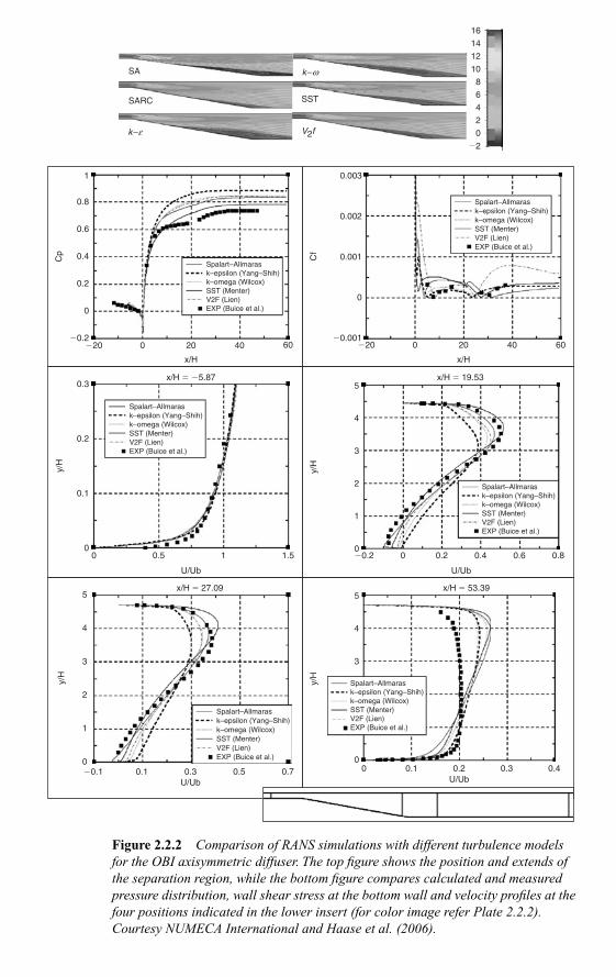
Ch02-H6594.tex 9/5/2007 8: 47 Page 93

x/H

1

0.8

0.6

0.4Cp

0.2

0

�0.2�20 0 20 40

Spalart–Allmarask–epsilon (Yang–Shih)k–omega (Wilcox)SST (Menter)V2F (Lien)EXP (Buice et al.)

60

x/H � 19.535

4

3

2

y/H

1

0


�0.2 0 0.2

U/Ub

0.4 0.80.6

0.003

0.002

0.001

0

�0.001

Cf


�20 0 20

x/H

40 60

x/H � 27.095

4

3

2

y/H

1

0


�0.1 0.1 0.3U/Ub

0.5 0.7

0.3x/H � �5.87

0.2

0.1

00 0.5 1 1.5

U/Ub

y/H


U/Ub


x/H � 53.395

4

3

y/H

00 0.1 0.2 0.3 0.4

SA

SARC

k–e

k–w

SST

V2f

16

14

12

10

8

6

4

2

0

�2

Figure 2.2.2 Comparison of RANS simulations with different turbulence modelsfor the OBI axisymmetric diffuser. The top figure shows the position and extends ofthe separation region, while the bottom figure compares calculated and measuredpressure distribution, wall shear stress at the bottom wall and velocity profiles at thefour positions indicated in the lower insert (for color image refer Plate 2.2.2).Courtesy NUMECA International and Haase et al. (2006).

Ch02-H6594.tex 9/5/2007 8: 47 Page 94


pressure distribution and wall shear stress at the bottom wall, velocity profiles at thepositions indicated in the lower insert. The last figure is noteworthy, as it demonstratesa clear weakness of all the tested turbulence models, in that the velocity profile in thedownstream duct of the diffuser is experimentally fully recovered, while the calculatedprofiles still show remaining effects of their earlier separation.

We can hope that the gained knowledge on turbulence from advanced DNS andLES simulations will contribute to the improvement of current turbulence models.

2.3 THIN SHEAR LAYER APPROXIMATION (TSL)

At high Reynolds numbers, wall shear layers, wakes or free shear layers will be oflimited size and if the extension of the viscous region remains limited during the flowevolution, then the dominating influence of the shear stresses will come essentiallyfrom the gradients transverse to the main flow direction.

If we consider an arbitrary curvilinear system of coordinates with ξ1 and ξ2 alongthe surface and ξ3 = n directed toward the normal, then the Thin Shear Layer (TSL)approximation of the Navier–Stokes equations consists in neglecting all ξ1 and ξ2

derivatives occurring in the turbulent and viscous shear stress terms, Steger (1978),Pulliam and Steger (1978, 1985). This approximation is also supported by the factthat generally, at high Reynolds numbers (typically Re > 104) the mesh is dense in thedirection normal to the shear layer and therefore the neglected terms are computedwith a lower accuracy than the normal derivatives.

This approximation is actually close to a boundary layer approximation, sinceviscous terms, which are neglected in the boundary layer approximation, are alsoneglected here. However, the momentum equation in the directions normal to theshear layer is retained, instead of the constant pressure rule over the boundary layerthickness along a normal to the wall. Therefore the transition from viscous dominatedregions to the inviscid region outside the wall layer is integrally part of the calcula-tion, and one has here a form of ‘higher order’ boundary layer approximation. Theclassical boundary layer approximation is obtained, when the momentum equation inthe direction normal to the wall is replaced by the condition:

∂p

∂n 0

The thin shear layer approximation amounts to neglect the viscous diffusion in thedirection parallel to the shear surface and keep only the contributions from thediffusion in the normal direction.

The main motivation for the TSL approximation is historical, as it allowed inthe 1980s some saving in computer times, compared to a full RANS approximation.

Today, this approximation is hardly justified, as it has to rely on the same turbulencemodels as current RANS simulations.

2.4 PARABOLIZED NAVIER–STOKES EQUATIONS

The Parabolized Navier–Stokes (PNS) approximation is based on considerationssimilar to the thin shear layer approximation, but applies only to the steady state

Ch02-H6594.tex 9/5/2007 8: 47 Page 95


formulation of the Navier–Stokes equations. This approximation is directed towardflow situations with a predominant main flow direction, as would be the case in achannel flow, whereby the cross-flow components are of a lower order of magnitude.In addition, along the solid boundaries, the viscous regions are assumed to be domi-nated by the normal gradients and hence, the streamwise diffusion of momentum andenergy can be neglected.

If x is the streamwise coordinate, the x-derivatives in the shear stress terms areall neglected compared to the derivatives in the two transverse directions y and z.A similar approximation is introduced in the energy diffusion terms. This approxi-mation is therefore valid as long as the mainstream flow of velocity u is dominant,that is as long as the positive x-direction corresponds to the forward flow direc-tion. This will not be the case anymore if there is a region of reverse flow of thestreamwise velocity component. In this case, the streamwise derivatives of u willbecome of the same order as the transverse derivatives and the whole approximationbreaks down.

Note that this approximation can also be applied to supersonic steady flows, wherethe streamwise direction appears as the ‘timelike’ direction; see Chapter 3 for adefinition of his concept.

2.5 BOUNDARY LAYER APPROXIMATION

It was the great achievement of L. Prandtl to recognize that at high Reynolds numbers,the viscous regions remain of limited extension δ (of the order of δ/L ≈ √

v/UL, for abody of length L) along the surfaces of the solid bodies immersed in, or limiting theflow. In practical terms, this means that for a Reynolds number of 106, on a body witha chord length of 1 m, the boundary layer will have a thickness of the order of a fewmm! If you consider an aircraft wing, flying at a speed of say 800 km/h, the velocityover the wing will change from zero on the wall to velocities in the range of 800 km/hover a distance of a few mm. Hence, the velocity gradients in the normal directionare much larger than the corresponding gradients in the streamwise direction.

In all cases where these viscous regions remain close to the body surfaces, that is inabsence of separation, the calculation of the pressure field may be decoupled from thecalculation of the viscous velocity field. A detailed discussion of the conditions forthe derivation of the boundary layer equations can be found in the books of Batchelor(1970), Schlichting (1971) and Cebeci and Bradshaw (1984).

With the assumption that the vertical velocity component in the boundary layeris very small compared to the mainstream velocity, the momentum equation in thenormal direction reduces to the condition of vanishing normal pressure gradient:

∂p

∂z≡ ∂p

∂n∼= 0 (2.5.1)

As a consequence, the pressure p (x, y, z) inside the viscous boundary layer maybe taken equal to the pressure outside of this layer and therefore equal to the valueof the pressure pe(x, y), obtained from an inviscid computation. The pressure pe(x, y)is the value taken by the inviscid pressure field at the edge of the boundary layer ofsurface point (x, y).

Ch02-H6594.tex 9/5/2007 8: 47 Page 96


Hence, the boundary layer equations are obtained from the streamwise and cross-flow momentum equations with the replacement of p (x, y, z) by pe(x, y):

∂

∂t(ρu) + ∂

∂x(ρu2) + ∂

∂y(ρuv) + ∂

∂z(ρuw) = −∂pe

∂x+ ∂

∂z

(μ

∂u

∂z

)(2.5.2)

∂

∂t(ρv) + ∂

∂x(ρuv) + ∂

∂y(ρv2) + ∂

∂z(ρvw) = −∂pe

∂y+ ∂

∂z

(μ

∂v

∂z

)(2.5.3)

The inviscid pressure gradient, which is obtained from an inviscid calculation priorto the resolution of the boundary layer equations, acts as an external force on theviscous region. The same inviscid computation also provides the velocities ue(x, y)and ve(x, y) at the edge of the boundary layer, connected to the pressure field pe bythe inviscid equation:

ρ∂�ve

∂t+ ρ(�ve · �∇)�ve = −�∇pe (2.5.4)

where �ve is the velocity vector parallel to the body surface with components ue(x, y)and ve(x, y). Equations (2.5.2) and (2.5.3) are to be solved with the additional boundaryconditions:

u = ue(x, y) and v = ve(x, y) at z = δ (2.5.5)

at the edge of the boundary layer.The system of equations obtained in this way has only the velocities as unknowns

and this represents a significant simplification of the Navier–Stokes equations. There-fore, the boundary layer equations are much easier to solve, being close to standardparabolic second order partial differential equation and many excellent numericalmethods have been developed (e.g. Kline, 1968; Cebeci and Bradshaw, 1977, 1984).

The inviscid region is limited by the edge of the boundary layer, which is initiallyunknown since the computational process has to start by the calculation of the pressurefield. In the classical boundary layer approximation, the limits of the inviscid regionare taken on the surface, which is justified for small boundary layer thicknesses. Thisleads to a complete separation between the pressure field and the velocity field sincethe pressure, in the remaining momentum equations (2.5.2) and (2.5.3), is equal tothe values of the inviscid pressure field at the wall and is known when these equationsare to be solved.

When the influence of the boundary layers on the inviscid flow field is consideredas non-negligible, this interaction can be taken into account in an iterative way, byrecalculating the inviscid pressure field with the limits of the inviscid region locatedat the edge of the boundary layer obtained at the previous iteration. This procedure isapplied for thick boundary layers up to small separated regions and is known as theviscid–inviscid interaction approximation; see Le Balleur (1983) for a recent reviewon the subject.

2.6 THE DISTRIBUTED LOSS MODEL

The distributed loss model is an approximation applied essentially in internal andchannel flows more particularly in the fields of turbomachinery, river hydraulics andoceanography.

Ch02-H6594.tex 9/5/2007 8: 47 Page 97


This model is defined by the assumption that the effect of the shear stresses on themotion is equivalent to a distributed friction force, defined by semi-empirical data.Obviously, a certain number of three-dimensional flow details will be lost in such anapproximation, in particular, all flow aspects that can be attributed to, or are stronglyinfluenced, by viscous effects.

Since the details of the loss mechanism, that is of the shear stresses, are not con-sidered, these equations are to be taken as describing an inviscid model, howeverwith an entropy producing term. The boundary conditions for the velocity field aretherefore the inviscid conditions of vanishing normal velocity components at thewalls, with a non-vanishing tangential velocity along these boundaries. The resultingapproximation is then of inviscid nature but not isentropic since the entropy variationalong the path of a fluid particle will be connected to the energy dissipation alongthis path. See for instance Hirsch and Deconinck (1985) for an application to internalturbomachinery flows.

A similar approximation is introduced in river hydraulics where the effects of thewall friction are represented by an empirical resistance force. The distributed lossmodel therefore consists in replacing the shear stress terms by an external frictionforce, function of velocity or other flow variables, but not directly expressed as secondorder derivatives of the velocity field.

2.7 INVISCID FLOW MODEL: EULER EQUATIONS

The most general flow configuration for a non-viscous, non-heat conducting fluid isdescribed by the set of Euler equations, obtained from the Navier–Stokes equations(2.1.1) by neglecting all shear stresses and heat conduction terms. As is known fromPrandtl’s boundary layer analysis, this is a valid approximation for flows at highReynolds numbers, outside viscous regions developing near solid surfaces.

This approximation introduces a drastic change in the mathematical formulationwith respect to all the previous models containing viscosity terms since the system ofpartial differential equations describing the inviscid flow model reduces from secondorder to first order. This is of paramount importance since it will determine thenumerical and physical approach to the computation of these flows. In addition, thenumber of allowable boundary conditions is modified by passing from the secondorder viscous equations to the first order inviscid system.

The time-dependent Euler equations, in conservation form and in an absolute frameof reference, for the conservative variables U defined by equation (2.1.2):

∂U

∂t+ �∇ · �F = Q (2.7.1)

form a system of first order partial differential equations hyperbolic in time (as will beshown later), where the flux vector F has the Cartesian components ( f , g, h) given by

f =

∣∣∣∣∣∣∣∣∣∣∣

ρu

ρu2 + p

ρuv

ρuw

ρuH

∣∣∣∣∣∣∣∣∣∣∣g =

∣∣∣∣∣∣∣∣∣∣∣

ρv

ρvu

ρv2 + p

ρvw

ρuH

∣∣∣∣∣∣∣∣∣∣∣h =

∣∣∣∣∣∣∣∣∣∣∣

ρw

ρwu

ρwv

ρw2 + pρwH

∣∣∣∣∣∣∣∣∣∣∣(2.7.2)

Ch02-H6594.tex 9/5/2007 8: 47 Page 98


and the source term Q is given by equation (2.1.4). Generally, heat sources willnot be considered since heat conduction effects are neglected in the system of Eulerequations.

It is important to notice the properties of the entropy variations in an inviscidflow. From equation (1.4.18) and in absence of heat sources, the entropy equation forcontinuous flow variations reduces to

T

(∂s

∂t+ �v · �∇s

)= 0 (2.7.3)

expressing that entropy is constant along a flow path. Hence, the Euler equationsdescribe isentropic flows, in absence of discontinuities.

As is known, the set of Euler equations allows also discontinuous solutions incertain cases, namely, vortex sheets, contact discontinuities or shock waves occurringin supersonic flows. The properties of these discontinuous solutions can only beobtained from the integral form of the conservation equations, since the gradients ofthe fluxes are not defined at discontinuity surfaces.

2.8 POTENTIAL FLOW MODEL

The most impressive simplification of the mathematical description of a flow systemis obtained with the approximation of a non-viscous, irrotational flow.

Setting the vorticity to zero, by

�ζ = �∇ × �v = 0 (2.8.1)

the three-dimensional velocity field can be described by a single scalar function φ,the potential function defined by

�v = �∇φ (2.8.2)

reducing the knowledge of the three velocity components to the determination of asingle potential function φ.

As seen from the preceding section, if the initial–conditions are compatible withuniform entropy, than for continuous flows, equation (2.8.1) implies that the entropyis constant over the whole flow field. Hence, for isentropic flows, the momentumequation under Crocco’s form (1.5.13) becomes

∂

∂t( �∇φ) + �∇H = 0 (2.8.3)

or

∂φ

∂t+ H = H0 (2.8.4)

the constant H0 having the same value along all the streamlines.This equation shows that the energy equation is not independent anymore from

the momentum equation, and therefore the flow will be completely determined by

Ch02-H6594.tex 9/5/2007 8: 47 Page 99


initial and boundary conditions on one hand and by the knowledge of the singlefunction φ on the other hand. This is a very considerable simplification indeed.

The equation for the potential function is obtained from the continuity equation,taking into account the isentropic conditions to express the density in function ofvelocity and hence in function of the gradient of the potential function. We obtain thebasic potential equation in conservation form:

∂ρ

∂t+ �∇ · (ρ �∇φ) = 0 (2.8.5)

and the relation between density and potential function obtained by introducing thedefinition of stagnation enthalpy in function of velocity and static enthalpy h, for aperfect gas:

ρ

ρA=(

h

hA

)1/(γ−1)

=[(

H0 − �v2

2− ∂φ

∂t

)/hA

]1/(γ−1)

(2.8.6)

The subscript A refers to an arbitrary reference state, for instance the stagnationconditions ρA = ρ0 and hA = H0.

Steady potential flows

A further simplification for steady potential flows is obtained since the potentialequation reduces to, with H = H0 = constant

�∇ · (ρ �∇φ) = 0 (2.8.7)

with the density given by equation (2.8.6) where hA can be chosen equal to H0. Hence,we have

ρ

ρ0=[

1 − ( �∇φ)2

2H0

]1/(γ−1)

(2.8.8)

where ρ0 is the stagnation density, constant throughout the whole flow field.Both for steady and unsteady flows, the boundary condition along a solid boundary

is the condition of vanishing relative velocity between flow and solid boundary in thedirection n normal to the solid wall

vn = ∂φ

∂n= �uw.�en (2.8.9)

where �uw is the velocity of the solid boundary with respect to the considered systemof reference.

Kutta Joukowski condition

Although the local vorticity in the flow is zero it may occur for a potential flow innon-simply connected domains that the circulation around a closed curve C becomesnon-zero. This is essentially the case for lifting airfoils. To achieve a non-zero lift

Ch02-H6594.tex 9/5/2007 8: 47 Page 100


on the body, a circulation � around the airfoil is imposed. This circulation is repre-sented by a free vortex singularity, although it originates from a vorticity productionphysically generated in the boundary layer. It follows that the value of � cannot bedetermined from irrotational theory and is an externally given value for a potentialflow. It is also to be remembered that, with the addition of the free vortex singularity�, an infinity of different potential flows can be obtained, for the same incident flowconditions, each one of these solutions having another value of �. However, for aero-dynamically shaped bodies such as airfoil profiles, a fairly good approximation of thecirculation and hence the lift, may be obtained by the Kutta–Joukowski condition,provided that no boundary layer separation occurs in the physical flow. The Kutta–Joukowski condition states that the value of the circulation, which approximates bestthe real (viscous) attached flow, is obtained if the stagnation point at the downstreamend of the body, is located at the trailing edge.

Supercritical airfoils

The development of supercritical airfoils, defined as having a shock-free transi-tion from supersonic to subsonic surface velocities, is one of the most spectacularoutcomes of the early developments of computational fluid dynamics. These airfoilsare now of general use on civil aircrafts, allowing important savings on fuel costs dueto the absence of the pressure drag produced by a shock.

Subsonic potential flows

In the subsonic range, the potential model has the same validity as the Euler model foruniform inflow conditions on a body, since the flow remains irrotational in this case.

The small disturbance approximation of the potential equation

In steady or unsteady transonic flow around wings and airfoils with thickness to chordratios of a few percent, we can generally consider that the flow is predominantlydirected along the chordwise direction, taken as the x-direction. In this case, thevelocities in the transverse direction can be neglected and the potential equationreduces to the so-called small disturbance potential equation:

(1 − M 2∞)∂2φ

∂x2+ ∂2φ

∂x ∂y+ ∂2φ

∂z2= 1

a2

(∂2φ

∂t2+ 2

∂φ

∂x

∂2φ

∂t ∂x

)(2.8.10)

Historically, the steady state, two-dimensional form of this equation was used byMurman and Cole (1961) to obtain the first numerical solution for a transonic flowaround an airfoil with shocks.

Linearized potential flows: singularity methods

If the flow can be considered as incompressible, the potential equation becomes alinear Laplace equation for which many standard solution techniques exist. One of

Ch02-H6594.tex 9/5/2007 8: 47 Page 101


these, based on the linearity of the equation is the singularity method whereby a linearsuperposition of known elementary flow fields such as vortex and source singularitiesare defined. The unknown coefficients of this linear superposition are obtained byimposing that the resultant velocity field satisfies the condition of vanishing normalvelocity along solid body surfaces (in absence of wall suction or blowing).

The three-dimensional extension of the singularity method, the Panel method,has been widely used in the aeronautical industry in order to compute the three-dimensional flow field around complex configurations. The method is still in use andalthough extensions to handle compressibility and transonic regimes can be devel-oped, these methods are best replaced, for high speed flows, by higher approximationssuch as the nonlinear potential model and the Euler equations for the inviscid flowdescription. We will therefore omit any detailed discussion of this approach and theinterested reader will find detailed information in the specialized literature.

2.9 SUMMARY

Different flow models, involving various degrees of approximation, have been definedand illustrated by a variety of examples. With the exception of laminar flows, whichcan be resolved by the Navier–Stokes model with the addition of empirical informa-tion on the dependence of viscosity and heat conductivity coefficients all other modelsare limited by either empirical knowledge about turbulence, as for the Reynoldsaveraged Navier–Stokes equations, or by some approximations.

Thin shear layer models are valid if no severe viscous separated regions existand similarly, the parabolized Navier–Stokes models for stationary formulations arelimited by the presence of streamwise separation.

Inviscid flow models provide a valid approximation far from solid walls or when theinfluence of boundary layers can be neglected and, although the isentropic potentialflow model is of questionable accuracy in transonic flows with shocks, it remains avalid and economical model for subsonic flows and for shock-free supercritical flows.

This should be kept in mind in the selection of a flow model, and the limits ofvalidity have to be established for each family of applications, by comparison withexperimental data or with computations from a higher level model.

REFERENCES

Batchelor, G.K. (1970). An Introduction to Fluid Dynamics. Cambridge UniversityPress, UK.

Braza, M., Faghani, D., Persillon, H. (2001). Successive stages and the role of naturalvortex dislocations in three-dimensional wake transition. J. Fluid Mech., 439, 1–41.

Cebeci, T. and Bradshaw, P. (1977). Momentum Transfer in Boundary Layers. Hemi-sphere, Washington, DC.

Cebeci, T. and Bradshaw, P. (1984). Physical and Computational Aspects of ConvectiveHeat Transfer. Springer Verlag, New York.

Chapman, D.R. (1979). Computational aerodynamics development and outlook. AIAA J.,17, 1293–1313.

del Alamo, J.C., Jimenez, J., Zandonade, P. and Moser, R.D. (2004). Scaling of the energyspectra of turbulent channels. J. Fluid Mech., 500, 135–144.

Ch02-H6594.tex 9/5/2007 8: 47 Page 102


del Alamo, J.C., Jimenez, J., Zandonade, P. and Moser, R.D. (2006). Self-similar vortexclusters in the logarithmic region. J. Fluid Mech., 561, 329–358.

Dinescu, C. and Hirsch, Ch. (2001). Numerically computed structure of the thermocap-illary flow in cylindrical liquid bridges. Proceedings of the ECCOMAS ComputationalFluid Dynamics Conference 2001, Swansea, Wales, UK.

Dyment, A. (1982). Vortices following two dimensional separation. In Vortex Motion,H.G. Hornung and E.A. Muller (Eds). Vieweg & Sohn, Braunschweig, pp. 18–30.

Flores, O. and Jimenez, J. (2006). Effect of wall-boundary disturbances on turbulentchannel flows. J. Fluid Mech., 566, 357–376.

Frank, S. and Schwabe, D. (1997). Temporal and spatial elements of thermocapillaryconvection in floating zones. Exp. Fluids, 23, 234–251.

Geerts, S., Hirsch, Ch., Broeckhoven, T. and Lacor, C. (2005). Validation of CFD andturbulence models for a confined double annular jet. AIAA 38th Fluid Dynamics,Plasmadynamics and Lasers Conference, AIAA Paper 2005-5894

Geurts, B.J. (2004). Elements of Direct and Large Eddy Simulation. R.T. Edwards,Philadelphia, PA.

Haase, W., Aupoix, B., Bunge, U. and Schwamborn, D. (Eds.) (2006). FLOMANIA –A European Initiative on Flow Physics Modelling. Notes on Numerical Fluid Mechanicsand Multidisciplinary Design (NNFM), Vol. 94, XI. Springer Verlag, Berlin.

Hirsch, Ch. and Deconinck, H. (1985). Through flow models in turbomachines:stream surface and passage averaged representations. In Thermodynamics and FluidMechanics of Turbomachinery, Vol. I, S.A. Ucer, P. Stow, and Ch. Hirsch, (Eds.)NATO ASI Series, Series E: Applied Sciences-No.97A, Martinus Nijhoff Publishers,Dordrechtt.

Hirsch, Ch. and Dinescu, C. (2003). A three dimensional finite volume approach ofthermocapillary flows in liquid bridges at medium Prandtl numbers. In InterfacialFluid Dynamics and Transport Processes. Lecture Notes in Physics, Vol. 628. SpringerVerlag, Berlin. pp. 369–385.

Hoyas, S. and Jimenez, J. (2006). Scaling of velocity fluctuations in turbulent channelsup to Retau = 2000. Phys. Fluids, 18, 117.

Jimenez, J. (2003). Computing high-Reynolds number flows: will simulations everreplace experiments. J. Turbul., 4, 22.

Jimenez, J. (2004). Turbulent flows over rough walls. Annu. Rev. Fluid Mech., 36,176–196.

Jimenez, J., del Alamo, J.C. and Flores, O. (2004). The large-scale dynamics of near-wallturbulence. J. Fluid Mech., 505, 179–199.

Kline, S.J. (1968). Proceedings of the 1968 AFOSR-HTTM-STANFORD Conference onComplex Turbulent Flows, Vol. I, II. University of Stanford, Thermosciences Division,Stanford, CA.

Kuhlmann, H.C. (1999). Thermocapillary Convection in Models of Crystal Growth.Springer Tracts in Modern Physics, Vol. 152. Springer Verlag, Berlin.

Le Balleur, J.C. (1983). Progres dans le calcul de l’interacton fluide parfait-fluide visqueux. AGARD Conference Proceedings CP-351 on Viscous Effects inTurbomachines. NATO-RTO Publications, Neuilly-sur-Seine, France.

Leschziner, M. and Drikakis, D. (2002). Turbulence modelling and turbulent-flowcomputation in aeronautics. The Aeronaut. J., 106, 349–384.

Leypoldt, J., Kulhmann, C.H. and Rath, J.H. (2000). Three-dimensional numerical sim-ulation of thermocapillary flows in cylindrical liquid bridges. J. Fluid Mech., 414,285–314.

Murman E.M. and Cole J.D. (1971). Calculation of Plane Steady Transonic Flows. AIAAJournal, 9, 114–121.

Ch02-H6594.tex 9/5/2007 8: 47 Page 103


Persillon, H. and Braza, M. (1998). Physical analysis of the transition to turbulence in thewake of a circular cylinder by three-dimensional Navier-Stokes simulation. J. FluidMech., 365, 23–88.

Pope, S. (2000). Turbulent Flows. Cambridge University Press, Cambridge, UK.Pulliam, T.H. and Steger, J.L. (1978). Implicit finite difference simulations of three-

dimensional flows. 16th Aerospace Sciences Meeting, AIAA Paper 78-10. see alsoAIAA J., 18, 1980, 159–167.

Pulliam, T.H. and Steger, J.L. (1985). Recent Improvements in Efficiency, Accuracy andConvergence for ImplicitApproximate FactorizationAlgorithms. AIAA 23rdAerospaceSciences Meeting. AIAA Paper 85-0360.

Rogallo, R.S. and Moin, P. (1984). Numerical simulation of turbulent flows. Ann. Rev.Fluid Mech., 16, 99–137.

Sagaut, P. (2001). Large Eddy Simulation for Incompressible Flows. Springer Verlag,Berlin.

Schlichting, H. (1971). Boundary Layer Theory. Mc Graw Hill, New York.Schwabe, D. (2001). Standing waves of oscillatory thermocapillary convection in float-

ing zones under microgravity observed in the experiment MAUS G141. 33rd COSPARConference, Warzaw, Paper GO.1-0030.

Shevtsova, V. and Legros, J.C. (1998). Oscillatory convective motion in deformed liquidbridges. Phys. Fluids, 7(5), 1631–1634.

Steger, J.L. (1978). Implicit finite difference simulation of flows about arbitrarygeometries. AIAA J., 16, 679–686.

Temam, R. (1977). Navier–Stokes Equations. North-Holland Co, Amsterdam.Van Dyke, M. (1982). An Album of Fluid Motion. The Parabolic Press, Stanford, USA.Velten, R., Schwabe, D. and Scharmann, A. (1991). The periodic instability of

thermocapillary convection in cylindrical liquid bridges. Phys. FluidsA, 3(2), 267–279.Wilcox, D.C. (1998). Turbulence Modeling for CFD, 2nd edn. DCW Industries,

California, USA. https://www.dcwindustries.com/Williamson, C.H.K. (1988a). Defining a universal and continuous Strouhal–Reynolds

number relationship for the laminar vortex shedding of a circular cylinder. Phys. Fluids,31, 2742.

Williamson, C.H.K. (1988b). The existence of two stages in the transition to three-dimensionality of a cylinder wake. Phys. Fluids, 31, 3165–3168.

Williamson, C.H.K. (1989). Oblique and parallel mode of vortex shedding in the wakeof a cylinder at low Reynolds numbers. J. Fluid Mech., 206, 579–627.

Williamson, C.H.K. (1992). The natural and forced formation of spot-like vortexdislocations in the transition of a wake. J. Fluid Mech., 243, 393–441.

Williamson, C.H.K. (1996a). Vortex dynamics in the cylinder wake. Ann. Rev. FluidMech., 28, 477–539.

Williamson, C.H.K. (1996b). Three-dimensional wake transition. J. Fluid Mech., 328,345–407.

Zeng, Z., Mizuseki, H., Chen, J., Ichinoseki, K. and Kawazoe, Y. (2004). Oscillatorythermocapillary convection in liquid bridge under microgravity. Mater. Trans., 45 (5),1522–1527.

PROBLEMS

P.2.1 By developing explicitly the shear stress gradient and the momentum terms,derive the equations (2.1.7).

P.2.2 By using the definition of the shear stress tensor, equation (1.3.6), work out thefull, explicit form of the Navier–Stokes equations, for non-constant viscosity

Ch02-H6594.tex 9/5/2007 8: 47 Page 104


coefficients, in function of velocity components, in Cartesian coordinates.Show also, that in the case of constant viscosity, the equations reduce to theprojections of equation (1.3.13).

Hint: Applying equation (1.3.6), we have

τxx = 4

3μ

∂u

∂x− 2

3μ

(∂v

∂y+ ∂w

∂z

)

τxy = μ

(∂v

∂x+ ∂u

∂y

)

τxz = μ

(∂w

∂x+ ∂u

∂z

)

and the x-projection of the momentum equation becomes

∂ρu

∂t+ ∂

∂x(ρu2 + p) + ∂

∂y(ρuv) + ∂

∂z(ρuw) = ∂τxx

∂x+ ∂τyx

∂y+ ∂τzx

∂z

P.2.3 Derive the energy conservation equation for a three-dimensional incompress-ible flow, in presence of gravity forces.

Hint: Apply equation (1.3.18) to the momentum equation (1.4.40) and mul-tiply scalarly by v. Introducing the total energy (H = p/ρ + v2/2 + gz) wherez is the vertical coordinate, proof the Bernoulli equation:

∂

∂t

( �v2

2

)+ (�v · �∇)H = ν�v · ��v

P.2.4 By working out explicitly the gradients of specific mass in function of thevelocities, show that the potential equation (2.8.5) can be written in the quasi-linear form, in function of the Mach numbers Mi = vi/c:

(δij − MiMj)∂2φ

∂xi∂xj= 1

c2

[∂2φ

∂t2+ ∂

∂t( �∇φ)2

]

with a summation on the Cartesian subscripts i, j = 1,2,3 or x,y,z. Show thatin two dimensions the steady state potential equation reduces to(

1 − u2

c2

)∂2φ

∂x2− 2

uv

c2

∂2φ

∂x∂y+(

1 − v2

c2

)∂2φ

∂y2= 0

Hint: Apply the isentropic laws and the energy equation (2.8.4) to derive therelations

dh = c2dρ/ρ

c2

ρ

∂ρ

∂t= −∂2φ

∂t2− ∂

∂t

( �∇φ)2

2

c2

ρ�∇ρ = −∂( �∇φ)

∂t− �∇ ( �∇φ)2

2

where c is the speed of sound, and substitute into equation (2.8.5).

Ch03-H6594.tex 8/5/2007 12: 0 Page 105

Chapter 3

The Mathematical Nature of the Flow Equationsand Their Boundary Conditions


We have learned in Chapter 1, how to derive the basic equations of fluid mechanicsand to recognize that any flow configuration is the outcome of a balance between theeffects of convective fluxes, diffusive fluxes and external or internal sources.1

From the mathematical point of view, diffusive fluxes appear through second orderderivative terms in space, as a consequence of the generalized Fick law, equation(1.1.8), which expresses the essence of the molecular diffusion phenomenon as atendency to smooth out gradients. The convective fluxes, on the other hand, appearas first order derivative terms in space and express the transport properties of a flowsystem.

Next, we have seen in Chapter 2 how various approximation levels give rise to dif-ferent mathematical models. The common property of all possible models describingflow behavior is that they constitute a system of partial differential equations (PDEs)in space or in space–time, which can take up various forms, but where the highestspace derivatives do not exceed second order.

Because of this variety of mathematical flow models, we need tools to analyzetheir properties, independently of their appearance and to tell us something about thebehavior of their solutions.

Let us illustrate this by the example of a stationary compressible potential flow. Wehave seen in Chapter 2 that we can describe this flow by two different models, namelythe set of time-independent Euler equations (2.7.1), or by the potential equation(2.8.5). If we restrict ourselves to two dimensions, the steady Euler model would bedescribed as

u∂ρ

∂x+ v

∂ρ

∂y+ ρ

∂u

∂x+ ρ

∂v

∂y= 0

u∂u

∂x+ v

∂u

∂y= − 1

ρ

∂p

∂x= −c2

ρ

∂ρ

∂x

1 If these properties are not very clear to you at this stage, we recommend you to go back toSection 1.1.2, and to study it again with great care. Give also a special attention to Table 1.1 and tothe associated discussion.

105

Ch03-H6594.tex 8/5/2007 12: 0 Page 106


u∂v

∂x+ v

∂v

∂y= − 1

ρ

∂p

∂y= −c2

ρ

∂ρ

∂y(I3.1)

with the isentropic relation between pressure and density defined by the speed ofsound

c2 =(

∂p

∂ρ

)s

(I3.2)

On the other hand, the steady compressible potential equation model can be writtenas (see Problem P. 2.4)

(1 − u2

c2

)∂2φ

∂x2− 2

uv

c2

∂2φ

∂x ∂y+(

1 − v2

c2

)∂2φ

∂y2= 0 (I3.3)

where φ is the potential function defined by u = ∂φ/∂x, v = ∂φ/∂y.For a uniform incoming flow, these two sets of PDEs describe exactly the same

physics of steady irrotational flows, but their formulation appears very different. Wehave therefore to develop methods that allow us to analyze the mathematical propertiesof PDEs, independently of the different forms they might take.

Hence, we wish to answer the following basic questions:

• How do we recognize if, or when, a mathematical model describes a convectionor diffusion phenomenon, taking into account that the models are generallyexpressed by a system of partial differential equations, where the presence ofconvection or diffusion terms might not be as obvious as in Section 1.1.2.

• What are the different types of physical situations, in addition to pure convectionor pure diffusion that can occur and how do we recognize them.

• What are the associated initial and/or boundary conditions.

In the process of numerical discretization, it is essential indeed to be able to identifythese differences, since it cannot be expected that a discretization compatible with thephysics of diffusion will be valid for the physics associated to convection, since thephysical properties of these two phenomena are fundamentally different, as discussedin Section 1.1.2.

In addition, there is another very important distinction we have to consider, namelythe option between steady and unsteady flow descriptions. In the former case, notime derivatives will appear in the mathematical model, which will contain onlyspace derivatives. In the latter case, time derivatives are present, next to the spacederivatives, these derivatives being also assumed not to exceed second order. As wewill see in the next sections, this is an important distinction since the mathematicalproperties of the considered equations can change significantly when introducing orremoving the time dependence.

Moreover, since the laws of fluid mechanics are nonlinear (with the sole excep-tion of incompressible potential flows), we have to consider the possibility for themathematical nature of the equations to be flow dependent, with different propertiesin different regions of the flow domain. This will be the case for instance for steadytransonic flows, as we will see in the following sections in more detail. But we can

Ch03-H6594.tex 8/5/2007 12: 0 Page 107

Mathematical Nature of Flow Equations and Their Boundary Conditions 107

already have a hint as to what we are referring to hereby looking at equation (I3.3) forthe simplified case of a unidirectional flow in the x-direction, with v = 0, reducing to(

1 − u2

c2

)∂2φ

∂x2 + ∂2φ

∂y2 = 0. Observe that for subsonic flows, i.e. u < c, the two second

derivative terms have the same positive sign, but they become of opposite sign forsupersonic flows, when u > c.

This chapter will introduce you, therefore, to the analysis of a chosen mathemat-ical model and to the derivation of the specific properties behind its set of partialdifferential equations. It is structured in the following way:

• We introduce first, in Section 3.1, the most simplified forms of the basicconvection–diffusion equation formulation of a conservation law (1.1.9), in orderto bring forward the essence of this type of equation, via reduction to two indepen-dent space–time variables. That is, to one space dimension for time-dependentproblems and to two space dimensions for time-independent problems. A fur-ther simplification is obtained after a linearization, whereby the nonlinearproperties are removed leading to linear convection or convection–diffusionequations.

• Section 3.2 is defining the basic methodology for the mathematical analysis of theproperties of PDEs. We will introduce the fundamental concepts and distinctionbetween hyperbolic, parabolic and elliptic PDEs. This will also lead us to adirect physical interpretation of these properties and to their fundamental linkwith the physical phenomena of convection and diffusion.

• An important extension of this analysis is developed in Section 3.3, where theconcepts of characteristic surfaces and the associated very fundamental proper-ties of domain of dependence and domain of influence are introduced. Theseare essential properties of hyperbolic and parabolic equations, and play a verycritical role in many areas of CFD.

• Section 3.4 redefines the mathematical properties for time-dependent modelsand introduces the notion of time-like variable. In addition, this will allow us toestablish the link with the conservation form of the PDEs.

• The distinction between hyperbolic, parabolic and elliptic equations is importantas it will form the basis of the analysis of the number and type of initial andboundary conditions associated to the various properties of a system of PDEs.This is described and analyzed in Section 3.5.

• An Advanced Section A3.6 will focus on the introduction of compatibilityrelations, associated to characteristic surfaces. These relations play a very impor-tant role in the numerical treatment of boundary conditions for the Euler andNavier–Stokes equations in many CFD codes.

Figure 3.0.1 provides you with the guide to this chapter, for further reference, whilegoing through the different sections.

Finally, in order to situate globally the important content of this chapter, we referyou to the general introduction and to the section entitled ‘The components of a CFDsimulation system’, Figure I.3.1 in particular. You will notice that this chapter isthe last step of Part I aimed at guiding you toward the definition of the approxima-tion levels and the associated mathematical model to be considered as candidate fordiscretization.

Ch03-H6594.tex 8/5/2007 12: 0 Page 108


Section A3

A3.6Compatibility

relations

3.1 Simplified models of aconvection –diffusionequation

3.2 Definition of themathematical propertiesof a system of PDEs

3.3 Characteristic surfaces,dependence and influencedomains

3.4 Time-dependent andconservation formof the PDEs

3.5 Initial and boundaryconditions

Basic 1D convectionand diffusion models

Hyperbolic,parabolic andelliptic equations

Basic properties ofhyperbolic equations

Basic properties fora time-dependentmodel

Figure 3.0.1 Structure and guide to this chapter.

3.1 SIMPLIFIED MODELS OF A CONVECTION–DIFFUSION EQUATION

We wish here to look at the simplest forms that can be taken by a convection–diffusionconservation equation, in order to focus on the basic mathematical properties, withoutbeing burdened by non-essential complexities, such as extra space dimensions, orspecific source terms.

Hence, we limit ourselves in this section to two independent space–time variables.Consequently, for time-dependent models, we will consider only one space dimension(1D formulation); while two space variables (x and y) will be considered for time-independent models.

3.1.1 1D Convection–Diffusion Equation

Focusing first on time-dependent models, we consider the quasi-linear equation(1.2.10), assuming constant density and constant diffusivity coefficients, absence

Ch03-H6594.tex 8/5/2007 12: 0 Page 109


of source terms and one space dimension x. The resulting simplified 1D convection–diffusion equation is written as follows:

∂u

∂t+ a(u)

∂u

∂x= α

∂2u

∂x2(3.1.1)

where we have written a(u) for the x-component of the convection velocity andα for the diffusivity coefficient. The convection velocity a(u) can be an arbitraryfunction of u.

We do not specify the significance of u at this stage, but when the simplificationsmentioned here are applied to the temperature equation, u will be replaced by the tem-perature T , while if one considers the x-projection of the momentum equation (1.3.14)in absence of pressure and external forces, u will represent the velocity and a(u) willbe equal to u, i.e. a(u) = u. In this case we obtain the well-known Burgers equation:

∂u

∂t+ u

∂u

∂x= α

∂2u

∂x2(3.1.2)

This equation plays an important role since it contains the full convective nonlinear-ity of the flow equations and a large number of analytical solutions of this equationare known (see Whitham, 1974). The general importance of analytical solutions tosimplified models cannot be enough underlined, as these solutions are essential to theverification and the validation process of numerical methods and solutions.

A further simplification is obtained by assuming a(u) to be constant, leading to theone-dimensional linear convection–diffusion equation:

∂u

∂t+ a

∂u

∂x= α

∂2u

∂x2(3.1.3)

Let us look now at specific particular cases.

3.1.2 Pure Convection

In absence of diffusion, α = 0, equation (3.1.1) reduces to the nonlinear convectionequation:

∂u

∂t+ a(u)

∂u

∂x= 0 (3.1.4)

A very important model is the ‘inviscid’ Burgers equation:

∂u

∂t+ u

∂u

∂x= 0 (3.1.5)

This equation generates discontinuous solutions from an initial continuous field, ina process very similar to the process of shock creation in supersonic flows, with theadvantage that this process can be fully analyzed from the corresponding analyticalsolution of the Burgers equation (3.1.5) (see Whitham, 1974).

Ch03-H6594.tex 8/5/2007 12: 0 Page 110


The ultimate simplification is obtained by assuming the convection velocity to bea constant, leading to the one-dimensional linear convection equation:

∂u

∂t+ a

∂u

∂x= 0 (3.1.6)

This equation describes the transport of the quantity u by the constant convectionvelocity a, whereby an arbitrary initial profile u(x, t = 0) = u0(x) is translated withoutchange with the velocity a. Stated otherwise, after a time t, the quantity u is the initialprofile displaced with distance x = at. Hence, the solution u(x, t) is given by

u(x, t) = u0(x − at) (3.1.7)

This equation can also be seen as a wave propagation equation, with the interpreta-tion of u as a wave amplitude having a phase propagation speed equal to a. Indeed,considering a plane wave of amplitude u, wavelength λ, pulsation ω = 2πf , where fdesignates the wave frequency, defined by

u = ueI(kx−ωt) (3.1.8)

with wave number k = 2π/λ and I = √−1, this propagating wave will be solution ofequation (3.1.6) if

ω = ak (3.1.9)

This relation states that the solution (3.1.8) is a plane wave satisfying the basic relationbetween wavelength and frequency f = a/λ.

This equivalence between pure convection and wave propagation is critical to theunderstanding of the physics of convection and is central to the approach taken inthis chapter.

Hence, we advise you to always remember that these two phenomena, convectionand wave propagation, are two facets of the same physical properties.

3.1.3 Pure Diffusion in Time

In the absence of convection, we have a time-dependent diffusion, described by

∂u

∂t= α

∂2u

∂x2(3.1.10)

Applied to the temperature, this equation is known as the heat diffusion equation ofFourier, describing heat conduction in solids or fluids at rest.

For constant values of the diffusion constant, exact solutions to this equation areknown. Looking for a solution of the type (3.1.8), we obtain after introduction in(3.1.10), the relation

Iω = αk2 (3.1.11)

Ch03-H6594.tex 8/5/2007 12: 0 Page 111


leading to the solution

u = ueIkxe−αk2t (3.1.12)

This represents the behavior of a wave in space, with wave number k , exponentiallydamped in time, due to the diffusion coefficient α. Observe that the diffusion coeffi-cient α has to be positive to describe a physical diffusion. A negative value of α, willrepresent an exponentially growing phenomenon, typical of an explosion.

We recommend you to closely remember this property of the diffusion equation intime: it represents an exponentially damped spatial wave, if the diffusion coefficientis positive.

3.1.4 Pure Diffusion in Space

In two dimensions, and for a time-independent model, the convection–diffusionequation (1.2.10) reduces to the Poisson equation:

∂2u

∂x2+ ∂2u

∂y2= q (3.1.13)

Hence, as already pointed out in Section (1.1.2), the Laplace operator describes apure spatial diffusion.

These various models form a basis for the development of numerical schemes andthe investigation of their properties. We will extensively come back to these modelsin Part II of this book, where they will be used to analyze and compare a large varietyof numerical schemes.

3.2 DEFINITION OF THE MATHEMATICAL PROPERTIES OFA SYSTEM OF PDES

Let us now move to the key part of this chapter, namely how do we define a generalmethod to identify the mathematical properties of a system of PDEs?

Although we have extensively stressed in Chapter 1, the importance of the conser-vation form of the equations, as compared to the quasi-linear and non-conservativeform, it is obvious that these two formulations will describe the same physics, andhence will share the same mathematical properties. Therefore, because of its explicitformulation, the quasi-linear form is more appropriate for the analysis of themathematical properties and will be used in this section and throughout thischapter.

Various approaches for the classification of PDEs can be found in the mathematicalliterature, connected to the possible existence of specific surfaces, called character-istic surfaces, which can be defined as families of surfaces, or hypersurfaces fora general three-dimensional unsteady flow, along which certain properties remainconstant or certain derivatives can become discontinuous. The discussion of theseproperties can be found in many textbooks, and we refer for instance to Courant andHilbert (1962), Ames (1965) and Hildebrandt (1976) for a mathematical presentation.

However, we will give here the preference to a more ‘physical’ presentation of thestructure of PDEs and of the associated concept of characteristic surfaces.

Ch03-H6594.tex 8/5/2007 12: 0 Page 112


We offer the following definition:A system of quasi-linear partial differential equations will be called of hyperbolic

type, if its homogeneous part admits wave-like solutions.This implies that a hyperbolic set of equations will be associated to propagating

waves and that the behavior and properties of the physical system described by theseequations will be dominated by wave-like phenomena.

In other words, a hyperbolic system describes convection phenomena andinversely, convection phenomena are described by hyperbolic equations.

On the other hand, if the equations admit solutions corresponding to dampedwaves the system will be called parabolic and if it does not admit wave-like solutionsthe equations are said to be elliptic. In this case, the behavior of the physical systemconsidered is dominated by diffusion phenomena.

3.2.1 System of First Order PDEs

The systems of partial differential equations (PDE) describing the various levelsof approximation discussed in the previous chapter are quasi-linear, and at most ofsecond order. It can be shown however that any second order equation, or system ofequations, can be transformed into a first order system. Although this transformationis not unique and could lead to an artificially degenerate system, it will be consideredthat an appropriate transformation has been defined such that the system of first orderrepresents correctly the second order equations.

Hence, the following steps define the procedure to identify the properties of amathematical model:

Step 1: Write the system of PDEs describing the mathematical model under theform of a system of first order PDEs

Suppose we have n unknown variables u j, in an (m + 1)-dimensional space xk, wecan group all the variables u j in an (n × 1) vector column U and write the system offirst order PDEs under the general form:

Ak ∂U

∂xk= Q k = 1, . . . , m + 1

U�=

∣∣∣∣∣∣∣∣

u1

··

un

∣∣∣∣∣∣∣∣

(3.2.1)

where Ak are (n × n) matrices and Q is a column vector of the non-homogeneoussource terms. The matrices Ak and Q can depend on xk and U, but not on the derivativesof U.

Note that we always assume that a summation is performed on repeated indices.This is called the Einstein summation convention.

Step 2: Consider a plane wave solution of amplitude U in the space of theindependent variables �x with components xk (k = 1, . . . , m + 1), defined by

U = UeI(�n·�x) = UeI(nk xk ) (3.2.2)

Ch03-H6594.tex 8/5/2007 12: 0 Page 113


where I = √−1 and �n is a vector in the m-dimensional space of the independentvariables xk .

Step 3: Introduce this solution in the homogenous part of the system (3.2.1) andfind the values of �n satisfying the resulting equation

The homogenous part of equation (3.2.1) is written as

Ak ∂U

∂xk= 0 k = 1, . . . , m + 1 (3.2.3)

and the function (3.2.2) is a solution of this system of equations if the homogenousalgebraic system of equations:

[Ak nk ]U = 0 (3.2.4)

has non-vanishing solutions for the amplitude U . This will be the case if and only ifthe determinant of the matrix Ak nk vanishes.

Step 4: Find the n solutions of the equation

det∣∣∣Ak nk

∣∣∣ = 0 (3.2.5)

Equation (3.2.5) defines a condition on the normals �n. This equation can have at mostn solutions, and for each of these normals �nα, the system (3.2.5) has a non-trivialsolution.

The system is said to be hyperbolic in the space xk if all the n characteristicnormals �nα are real and if the solutions of the n associated systems of equations(3.2.5) are linearly independent. If all the characteristics are complex, the systemis said to be elliptic in the space xk and if some are real and other complex thesystem is considered as hybrid .

If the matrix (Aknk) is not of rank n, i.e. there are less than n real characteristicnormals then the system is said to be parabolic in the space xk .

This will occur, for instance, when at least one of the variables, say u1 has derivativeswith respect to one coordinate, say x1, missing. This implies that the componentsA1

i1 = 0 for all equations i.

Example E.3.2.1: System of two first order equations in two dimensions

The above-mentioned properties can be illustrated in a two-dimensional space x, ywith the system:

a∂u

∂x+ c

∂v

∂y= f1

(E.3.2.1)b∂v

∂x+ c

∂u

∂y= f2

or in matrix form:∣∣∣∣ a 0

0 b

∣∣∣∣ ∂

∂x

∣∣∣∣ uv

∣∣∣∣+∣∣∣∣ 0 c

d 0

∣∣∣∣ ∂

∂y

∣∣∣∣ uv

∣∣∣∣ =∣∣∣∣ f1

f2

∣∣∣∣ (E.3.2.2)

Ch03-H6594.tex 8/5/2007 12: 0 Page 114


Hence, with x1 = x, x2 = y:

U =∣∣∣∣ u

v

∣∣∣∣ A1 =∣∣∣∣ a 0

0 b

∣∣∣∣ A2 =∣∣∣∣ 0 c

d 0

∣∣∣∣ Q =∣∣∣∣ f1

f2

∣∣∣∣ (E.3.2.3)

Equation (E.3.2.2) is written as

A1 ∂U

∂x+ A2 ∂U

∂y= Q (E.3.2.4)

The determinant equation (3.2.5) becomes, after division by ny supposed to bedifferent from zero

∣∣A1nx + A2ny∣∣ = ny

∣∣∣∣ anx/ny cd bnx/ny

∣∣∣∣ = 0 (E.3.2.5)

leading to the conditions for the characteristic normals

(nx

ny

)2

= cd

ab(E.3.2.6)

If cd/ab > 0, the solutions nx/ny are real and the system is hyperbolic in the space(x, y), for instance a = b = 1; c = d = 1 with vanishing right-hand side leading to thewell-known wave equations, obtained after elimination of the variable v:

∂2u

∂x2− ∂2u

∂y2= 0 (E.3.2.7)

If cd/ab < 0, equation (E.3.2.6) has no real solutions and the system is elliptic inthe space (x, y). For instance, a = b = 1; c = −d = −1 and vanishing right-hand sideleading to the Laplace equation which is the standard form of elliptic equations anddescribes diffusion phenomena.

Finally, if b = 0, there is only one characteristic normal ny = 0 and the system isparabolic. For instance, with a = 1, b = 0, c = −d = −1 and f1 = 0, f2 = v, we obtainthe standard form for a parabolic equation:

∂u

∂x= ∂2u

∂y2(E.3.2.8)

This is recognizable by the fact that the equation presents a combination of first andsecond order derivatives.

Example E.3.2.2: The stationary Euler equations in two dimensions

This system is defined by equations (I3.1), which can be written in the matrix form(3.2.3) as follows:

∣∣∣∣∣∣u ρ 0

c2/ρ u 00 0 u

∣∣∣∣∣∣∂

∂x

∣∣∣∣∣∣ρ

uv

∣∣∣∣∣∣+∣∣∣∣∣∣

v 0 ρ

0 v 0c2/ρ 0 v

∣∣∣∣∣∣∂

∂y

∣∣∣∣∣∣ρ

uv

∣∣∣∣∣∣ = 0 (E.3.2.9)

Ch03-H6594.tex 8/5/2007 12: 0 Page 115


Introducing the vector

U =∣∣∣∣∣∣ρ

uv

∣∣∣∣∣∣ (E.3.2.10)

the system is written in the condensed form:

A1 ∂U

∂x+ A2 ∂U

∂y= 0 (E.3.2.11)

The three characteristic normals �n, are obtained as the solutions of equation (3.2.5),with λ = nx/ny

∣∣∣∣∣∣∣uλ + v ρλ ρ

λc2/ρ uλ + v 0

c2/ρ 0 uλ + v

∣∣∣∣∣∣∣= 0 (E.3.2.12)

Working out the determinant (E.3.2.12) leads to the solution

λ(1) = − v

u(E.3.2.13)

and the two solutions of the quadratic equation

(u2 − c2)λ2 + 2λuv + (v2 − c2) = 0 (E.3.2.14)

λ(2),(3) = −uv ± c√

u2 + v2 − c2

u2 − c2(E.3.2.15)

The first solution is always real, and the two others are real if the flow is supersonic,since equation (E.3.2.15) can be written as follows, after introduction of the Machnumber:

M =√

u2 + v2

c(E.3.2.16)

λ(2),(3) = −uv ± c2√

M 2 − 1

u2 − c2(E.3.2.17)

Hence, the stationary Euler equations are hyperbolic in (x, y) for supersonic flows.For subsonic flows, the second and third solutions are complex conjugate, and hence

the system is a hybrid mix elliptic–hyperbolic, since one solution is always real.At the sonic velocity M = 1, the two solutions λ(2) = λ(3) and the system is

parabolic.

Ch03-H6594.tex 8/5/2007 12: 0 Page 116


3.2.2 Partial Differential Equation of Second Order

These different concepts can also be applied to the classical example of the quasi-linearpartial differential equation of second order:

a∂2φ

∂x2+ 2b

∂2φ

∂x ∂y+ c

∂2φ

∂y2= 0 (3.2.6)

where a, b and c can depend on the coordinates x, y, the function φ and its firstderivatives. This equation can be written as a system of first order equations, afterintroduction of the variables u and v defined by

u = ∂φ

∂xv = ∂φ

∂y(3.2.7)

Equation (3.2.6) is then equivalent to the following system:

a∂u

∂x+ 2b

∂u

∂y+ c

∂v

∂y= 0

(3.2.8)∂v

∂x− ∂u

∂y= 0

which can be written in matrix form:∣∣∣∣ a 0

0 1

∣∣∣∣ ∂

∂x

∣∣∣∣ uv

∣∣∣∣+∣∣∣∣ 2b c−1 0

∣∣∣∣ ∂

∂y

∣∣∣∣ uv

∣∣∣∣ = 0 (3.2.9)

Introducing the vector U and the matrices A1 and A2

U =∣∣∣∣ u

v

∣∣∣∣ A1 =∣∣∣∣ a 0

0 1

∣∣∣∣ A2 =∣∣∣∣ 2b c−1 0

∣∣∣∣ (3.2.10)

we obtain the form (3.2.3) and equation (3.2.5) leads to

∣∣∣∣ anx + 2bny cny

−ny nx

∣∣∣∣ = 0 (3.2.11)

Hence, from the roots of

a

(nx

ny

)2

+ 2b

(nx

ny

)+ c = 0 (3.2.12)

the well-known conditions defining the type of the second order quasi-linear partialdifferential equation (3.2.6) are obtained.

The solutions of equation (3.2.12) are given by

nx

ny= −b ± √

b2 − ac

a(3.2.13)

Ch03-H6594.tex 8/5/2007 12: 0 Page 117


The solution (3.2.2) will represent a true wave if ny is real for all real values of nx.Therefore, if (b2 − ac) is positive there are two wave-like solutions, and the equationis hyperbolic, while for (b2 − ac) < 0 the two solutions are complex conjugate and theequation is elliptic. When (b2 − ac) = 0 the two solutions are reduced to one singledirection nx/ny = −b/2 and the equation is parabolic.

Example E.3.2.3: Stationary potential equation

An interesting example is provided by the stationary potential flow equation in twodimensions x, y, defined by equation (I3.3) where c designates the speed of sound:

(1 − u2

c2

)∂2φ

∂x2− 2uv

c2

∂2φ

∂x ∂y+(

1 − v2

c2

)∂2φ

∂y2= 0 (E.3.2.18)

with

a =(

1 − u2

c2

)b = −uv

c2c =

(1 − v2

c2

)(E.3.2.19)

we can write the potential equation under the form (3.2.6). In this particular case thediscriminant (b2 − ac) becomes, introducing the Mach number M

b2 − ac = u2 + v2

c2− 1 = M 2 − 1 (E.3.2.20)

and hence the stationary potential equation is elliptic for subsonic flows and hyper-bolic for supersonic flows. Along the sonic line M = 1, the equation is parabolic.

The solution (3.2.13) takes the following form for the two-dimensional potentialequation:

nx

ny= uv ± c2

√M 2 − 1

c2 − u2(E.3.2.21)

This mixed nature of the potential equation has been a great challenge for the numer-ical computation of transonic flows since the transition line between the subsonic andthe supersonic regions is part of the solution. An additional complication arises fromthe presence of shock waves which are discontinuities of the potential derivatives andwhich can arise in the supersonic regions. The particular problems of transonic poten-tial flow with shocks and their numerical treatment will be discussed in Volume II.

3.3 HYPERBOLIC AND PARABOLIC EQUATIONS: CHARACTERISTICSURFACES AND DOMAIN OF DEPENDENCE

Parabolic and hyperbolic equations play an important role in CFD, due to their specificproperties associated to propagation, or convection, phenomena. They are recognizedby the existence of real characteristic normals, solutions of equation (3.2.5). Each of

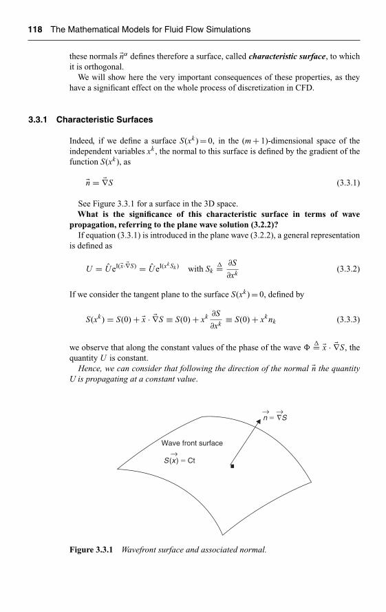
Ch03-H6594.tex 8/5/2007 12: 0 Page 118


these normals �nα defines therefore a surface, called characteristic surface, to whichit is orthogonal.

We will show here the very important consequences of these properties, as theyhave a significant effect on the whole process of discretization in CFD.

3.3.1 Characteristic Surfaces

Indeed, if we define a surface S(xk ) = 0, in the (m + 1)-dimensional space of theindependent variables xk , the normal to this surface is defined by the gradient of thefunction S(xk ), as

�n = �∇S (3.3.1)

See Figure 3.3.1 for a surface in the 3D space.What is the significance of this characteristic surface in terms of wave

propagation, referring to the plane wave solution (3.2.2)?If equation (3.3.1) is introduced in the plane wave (3.2.2), a general representation

is defined as

U = UeI(�x· �∇S) = UeI(xk Sk ) with Sk�= ∂S

∂xk(3.3.2)

If we consider the tangent plane to the surface S(xk ) = 0, defined by

S(xk ) = S(0) + �x · �∇S ≡ S(0) + xk ∂S

∂xk≡ S(0) + xk nk (3.3.3)

we observe that along the constant values of the phase of the wave ��= �x · �∇S, the

quantity U is constant.Hence, we can consider that following the direction of the normal �n the quantity

U is propagating at a constant value.

Wave front surface

S (x ) � Ct

n � �S

→

→ →

Figure 3.3.1 Wavefront surface and associated normal.

Ch03-H6594.tex 8/5/2007 12: 0 Page 119


The surface S is called a wavefront surface, defined as the surface separating thespace domain already influenced by the propagating quantity U from the points notyet reached by the wave.

Observe that in the general case of n unknown flow quantities u j , we have ncharacteristic surfaces, for a pure hyperbolic problem.

In a two-dimensional space the characteristic surface reduces to a characteristic line.The properties U are transported along the line S(x, y) = 0 and the vectors tangent tothe characteristic line are obtained by expressing that along the wavefront:

dS = �∇S · d�x = ∂S

∂xdx + ∂S

∂ydy = 0 (3.3.4)

Hence, the direction of the characteristic line in two dimensions is given by

dy

dx= −Sx

Sy= −nx

ny(3.3.5)

In two dimensions, there are two characteristic directions for a hyperbolic equa-tion, such as the two solutions (3.2.13). Hence out of each point in the (x, y)domain, two characteristics can be defined, along which two quantities propagate.As we have as many unknowns, at each point the solution can be obtained from thecharacteristic-related quantities that have propagated from the boundary to the pointP. See Figure 3.3.2 for an example.

A numerical method based on these properties has been applied in the past, partic-ularly for two-dimensional problems, and is known as the Method of Characteristics.

Example E.3.3.1:The small disturbance potential equation

Referring to Example E.3.2.3, the small disturbance potential equation is obtainedfor a horizontal incoming flow of Mach number M∞ in case the vertical velocity

Characteristic line

Characteristic line

y

x�

�

n

n

v

Figure E.3.3.1 Characteristics for two-dimensional potential equation.

Ch03-H6594.tex 8/5/2007 12: 0 Page 120


component can be considered as negligible, for instance for a flow along a thin body.The stationary potential equation reduces to the form, assuming that the horizontalvelocity component remains constant,

(1 − M 2∞)∂2φ

∂x2+ ∂2φ

∂y2= 0 (E.3.3.1)

where M∞ is the upstream Mach number.The solutions (E.3.2.21) reduce to the following, considering a supersonic flow, for

which the solutions are real

ny

nx= ∓

√M 2∞ − 1 (E.3.3.2)

hereby defining the normals to the two characteristics for supersonic flows. Theirdirections are obtained from equation (3.3.5) as

dy

dx= ±1/

√M 2∞ − 1 = ± tan μ (E.3.3.3)

Referring to Figure E.3.3.1, it can be seen that these characteristics are identical tothe Mach lines at an angle μ to the direction of the velocity, with

sin μ = 1/M∞ (E.3.3.4)

3.3.2 Domain of Dependence: Zone of Influence

The propagation property of hyperbolic problems has important consequences withregard to the way the information is transmitted through the flow region.

Considering Figure 3.3.2, where � is a boundary line distinct from a characteristic,the solution U along a segment AB of � will propagate in the flow domain along thecharacteristics issued from AB. For a two-dimensional problem in the variables x, y,there are two characteristics if the problem is hyperbolic.

Hence, the two characteristics out of A and B limit the region PAB, which deter-mines the solution at point P. The region PAB is called the region of dependence ofpoint P, since the characteristics out of any point C outside AB will never reach pointP. On the other hand, the region downstream of P, and located between the charac-teristics, defines the zone where the solution is influenced by the function value in P.This region is called the zone of influence of P.

3.3.2.1 Parabolic problems

For parabolic problems the two characteristics are identical, (Figure 3.3.3) and theregion of dependence of point P reduces to the segment BP. The zone of influence ofP, on the other hand, is the whole region right of the characteristic BP.

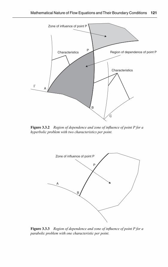
Ch03-H6594.tex 8/5/2007 12: 0 Page 121


Zone of influence of point P

Region of dependence of point PCharacteristics

Characteristics

P

A�

B

C

Figure 3.3.2 Region of dependence and zone of influence of point P for ahyperbolic problem with two characteristics per point.

Zone of influence of point P

A

B

P

Figure 3.3.3 Region of dependence and zone of influence of point P for aparabolic problem with one characteristic per point.

Ch03-H6594.tex 8/5/2007 12: 0 Page 122


P�

B

C

A

P depending on and influencingthe whole region

�

Figure 3.3.4 Region surrounding P in an elliptic problem.

3.3.2.2 Elliptic problems

In this case, there are no real characteristics and the solution in a point P depends on allthe surrounding points, since the physical problem is of the diffusive type. Inversely,the whole boundaryACB surrounding P, is influenced by point P (Figure 3.3.4). Hence,one can consider that the dependence region is identical to the zone of influence, bothof them being equal to the whole of the flow domain.

3.4 TIME-DEPENDENT AND CONSERVATION FORM OF THE PDES

Although we have not specified in the previous sections the exact definition of allthe xk coordinates, the examples in these sections all refer to pure space variables,implying a system of PDEs describing a steady flow model, that is not involving time.

However, many flow systems are time dependent, as we have seen from the deriva-tion of the conservation laws in the first chapter, and therefore we need to analyze theproperties of the PDEs, in presence of time derivatives.

In addition, an important alternative way to simulate steady flows is obtained by dis-cretizing the time-dependent equations in time and space and letting the time evolutiontake us to the steady state solution. This is called a ‘time-marching’ approach.

Although the time-marching approach will converge to the same solution asobtained from the stationary model, the properties of the time-dependent PDEs canbe significantly different from the properties of their associated spatial parts.

Let us illustrate this more precisely, by considering the system of n first order partialdifferential equations in time and space, written in conservation form, following thederivations seen in Chapter 1, which we rewrite here for convenience

∂U

∂t+ �∇ · �F = Q (3.4.1)

Ch03-H6594.tex 8/5/2007 12: 0 Page 123


where U is the column vector of the n unknown functions u j, in the m-dimensionalspace xk (k = 1, . . . , m). Here m is the space dimension, i.e. m = 1, 2 or 3 accordingto the number of space coordinates considered.

The equivalent algebraic form (with a summation convention on repeated super-scripts or subscripts), is written as the system of n equations, for line i:

∂ui

∂t+(

∂Fk

∂xk

)i

= Qi (i = 1, . . . , n) (3.4.2)

We consider here that this system is of first order in space; i.e., that the flux vector �Fdoes not contain space derivatives of U .

As stated in Section 3.2, the analysis of the properties of this system relies on thequasi-linear form, as opposed to the conservation form. This can be obtained afterintroduction of the Jacobian matrices Ak , where

Akij = ∂Fk

i

∂u j(3.4.3)

are the Jacobian matrix element of the flux Fki with respect to the variable uj .

In a compact notation, the Jacobian matrix is defined by

Ak ∧= ∂Fk

∂U(3.4.4)

With this definition, the time-dependent quasi-linear form of PDEs, derived from theconservation form, becomes

∂U

∂t+ Ak ∂U

∂xk= Q (3.4.5)

We see here that the stationary model, obtained when the time derivative is equal tozero for a time-independent vector U , reduces to equation (3.2.1), with k = 1, . . . , m.

3.4.1 Plane Wave Solutions with Time Variable

We have now to adapt the procedures defined in Section 3.2 to the time-dependentmodel (3.4.5).

To establish this link we observe that the general form (3.2.1) reduces to equation(3.4.6), if one variable, say xm+1, is singled out and the corresponding Jacobian matrixAm+1 is taken as the unit matrix. We call this variable time like and take xm+1 = t,with the conditions:

xm+1 ≡ t and Am+1 = I (unit matrix) (3.4.6)

With the introduction of the time variable, a plane wave solution can be written in amore conventional way:

U = U eI (�κ·�x−ωt) (3.4.7)

Ch03-H6594.tex 8/5/2007 12: 0 Page 124


The vector �κ is called the wave number vector and its magnitude is the number ofperiods or wavelengths over a distance 2π in the direction of the vector �κ and ω is thewave pulsation. This simple wave is a solution of the linear convection equation:

∂U

∂t+ (�a · �∇)U = 0 (3.4.8)

where

�a · �κ = ω (3.4.9)

If the direction of �κ is the propagation direction of the wave, then the phase velocityin the direction of propagation is given by:

a = ω

κ(3.4.10)

One has also the following relation between frequency ν, wavelength λ, and thevariables κ and ω

λ = 2π

κω = 2πν λν = a (3.4.11)

typical of plane waves.The general solution (3.3.2) becomes, with the explicit time variable xm+1 = t:

U = U eI(�κ· �∇S+tSt ) (3.4.12)

identifying the frequency ω of the wave as

ω = −∂S

∂t= −nt (3.4.13)

and the wave number vector �κ is defined by

�κ = �∇S = �n (3.4.14)

In this notation �∇S is the normal to the intersection of the characteristic or wavefrontsurface S(�x, t) with the hypersurfaces t = constant. Hence, the normals are definedhere in the m-dimensional space of the space variables, while the normals �n defined inSection 3.3.1 (equation (3.3.1)) are normals to the wavefront surfaces in the (m + 1)-dimensional space x1, . . . , xm+1. Observe also that the wave number �κ, in the space(x1, . . . , xm) is normal to the characteristic subsurfaces S(�x, t) at constant t.

In order for this wave to be a solution of the homogeneous system

∂U

∂t+ Ak ∂U

∂xk= 0 k = 1, . . . , m (3.4.15)

S has to satisfy the equation

det

∣∣∣∣∂S

∂t+ Ak ∂S

∂xk

∣∣∣∣ = 0 (3.4.16)

Ch03-H6594.tex 8/5/2007 12: 0 Page 125


or

det∣∣∣−ωδij + κk Ak

ij

∣∣∣ = 0 (3.4.17)

This important condition actually defines the wave pulsations ω, as the eigenvaluesof the matrix Kij = κk Ak

ij .

If we group the m matrices Ak in a vector �A of dimensions m, �A (A1, . . . , Am), wecan write the matrix K as a scalar product:

K = �A · �κ (3.4.18)

The system is said to be hyperbolic in space and time if all the n-eigenvalues ofthe matrix K are real and if the n associated solutions of equation (3.4.15) arelinearly independent.

If all the eigenvalues are complex, the system is said to be elliptic in space intime and if some are real and other complex the system is considered as hybrid .

If the eigenvalues are purely imaginary, then the system is said to be parabolicin space in time.

If some eigenvalues are real and other purely imaginary, the system is said tobe parabolic–hyperbolic in space in time.

Referring to equation (3.4.10), the propagation speed associated with a character-istic frequency ω is obtained as the eigenvalue of the matrix K :

K ≡ K

κ= �A · �κ

κ= �A · �eκ (3.4.19)

where �eκ is the unit vector in the direction �κ.Hence, for each wave number vector �κ, a perturbation in the surface normal to

�κ propagates in the direction of �κ with phase velocity �a and frequency ω equal tothe eigenvalue of the matrix K = Akκk . The associated characteristic speeds a(α) areobtained as solutions of the eigenvalue problem:

det∣∣∣−a(α)δij + Kij

∣∣∣ = 0 (3.4.20)

For an elliptic system, the eigenvalues are complex and the solution takes the form,for an eigenvalue ω1 = ξ + Iη:

U1 = U1 e−IξteI�κ·�x e+ηt (3.4.21)

Since the coefficients of the Jacobian matrices Ak are considered to be real, eacheigenvalue ω1 = ξ + Iη is associated to a complex conjugate eigenvalue ω2 = ξ − Iη,leading to a solution of the form:

U2 = U2 e−IξteI�κ·�x e−ηt (3.4.22)

Hence, according to the sign of the imaginary part of the eigenvalue, one of thetwo solutions U 1 or U 2 will be damped in time, while the other will amplified.

Ch03-H6594.tex 8/5/2007 12: 0 Page 126


Example E.3.4.1: Time-dependent shallow water equations in one dimension

The one-dimensional form of the time-dependent shallow water equations can bewritten as

∂h

∂t+ u

∂h

∂x+ h

∂u

∂x= 0

∂u

∂t+ u

∂u

∂x+ g

∂u

∂x= 0 (E.3.4.1)

where h represents the water height, g is the gravity acceleration and u the horizontalvelocity.

In matrix form, we have

∂

∂t

∣∣∣∣ hu

∣∣∣∣+∣∣∣∣ u h

g u

∣∣∣∣ ∂

∂x

∣∣∣∣ hu

∣∣∣∣ = 0 (E.3.4.2)

The two characteristic velocities a1,2 are obtained from equation (3.4.20) assolutions of

det

∣∣∣∣−a + u hg −a + u

∣∣∣∣ = 0 (E.3.4.3)

or

a1,2 = u ±√gh (E.3.4.4)

Since these eigenvalues are always real, the system is always hyperbolic in (x, t).

Example E.3.4.2: Time-dependent Euler equations in one dimension

Let us consider, as a second example, the one-dimensional form of the time-dependentEuler equations, for isentropic flows.

This is obtained by adding a time derivative of density and x-velocity componentto the first two equations of the system (I3.1), leading to

∂ρ

∂t+ u

∂ρ

∂x+ ρ

∂u

∂x= 0

(E.3.4.5)∂u

∂t+ u

∂u

∂x+ c2

ρ

∂ρ

∂x= 0

or in matrix form, defining the vector U and the matrix A:

U =∣∣∣∣ ρu∣∣∣∣ A =

∣∣∣∣ u ρ

c2/ρ u

∣∣∣∣ (E.3.4.6)

Ch03-H6594.tex 8/5/2007 12: 0 Page 127


as

∂U

∂t+ A

∂U

∂x= 0 (E.3.4.7)

Equation (3.4.7) becomes, in one space dimension x:

U = UeI(κx−ω t) (E.3.4.8)

and the condition (3.4.17) reduces to the eigenvalue equation:

det

∣∣∣∣ uκ − ω ρκ

κc2/ρ uκ − ω

∣∣∣∣ = 0 (E.3.4.9)

The two eigenvalues

a1 = ω1/κ = u + c and a2 = ω2/κ = u − c (E.3.4.10)

are real, for all values of the velocity u, and hence the system is always hyperbolic inspace and time.

This is an extremely important property comparing to the analysis of ExampleE.3.2.2 (confirmed by Example E.3.2.3) where it is shown that the steady isentropicEuler equations are elliptic in the space (x, y) for subsonic velocities and hyperbolicin the space (x, y) for supersonic velocities.

Here, in space and time, the inviscid isentropic equations are always hyperbolicindependently of the subsonic or supersonic state of the flow. As a consequence, thesame numerical algorithms can be applied for all flow velocities.

On the other hand, dealing with the steady state equations, the numerical algo-rithms will have to adapt to the flow regime, as the mathematical nature of thesystem of equations is changing when passing from subsonic to supersonic, orinversely.

This is the main reason for the very widespread choice of the time-dependentform of the conservation laws as basis for the numerical discretization, even for thesimulation of steady flows.

In this approach, we solve the flow equations in time until a numerical steady stateis reached, while the numerical transient is defined in such a way as to reach the steadystate as fast as possible, through different numerical acceleration techniques, such aslocal time steps, multigrid. These techniques will be introduced later on.

Take very carefully notice of the above fundamental property, as it conditions awide area of CFD applications.

It is indeed considered as a major advantage to be in a position to develop numer-ical algorithms, without having to bother about the subsonic or the supersonic stateof the flow.

The following example demonstrates that this property is not restricted to onespace dimension. It is indeed valid for all dimensions, and is shown here for twospace dimensions, considering the time-dependent form of the system (I3.1).

Ch03-H6594.tex 8/5/2007 12: 0 Page 128


Example E.3.4.3:Time-dependent Euler equations in two space dimensions

The time-dependent form of system (I3.1) for the two-dimensional isentropic Eulerequations is written as

∂ρ

∂t+ u

∂ρ

∂x+ v

∂ρ

∂y+ ρ

∂u

∂x+ ρ

∂v

∂y= 0

∂u

∂t+ u

∂u

∂x+ v

∂u

∂y+ c2

ρ

∂ρ

∂x= 0 (E.3.4.11)

∂v

∂t+ u

∂v

∂x+ v

∂v

∂y+ c2

ρ

∂ρ

∂y= 0

With the same definitions as in Example E.3.2.2, the system is written in the matrixform (3.4.15):

∂U

∂t+ A1 ∂U

∂x+ A2 ∂U

∂y= 0 (E.3.4.12)

and the eigenvalue equation (3.4.17) becomes

det

∣∣∣∣∣∣�u · �κ − ω ρκx ρκy

c2κx/ρ �u · �κ − ω 0c2κy/ρ 0 �u · �κ − ω

∣∣∣∣∣∣ = 0 (E.3.4.13)

The three solutions are given by the following three pulsations:

ω1 = �u · �κω2 = �u · �κ + cκ (E.3.4.14)

ω3 = �u · �κ − cκ

and as they are always real, the system (E.3.4.11) is always hyperbolic in spaceand time.

3.4.2 Characteristics in a One-Dimensional Space

The particular case of the one-dimensional space allows obtaining an important prop-erty of hyperbolic systems, typical for time-dependent first order equations, such asthe Euler equations.

For a general nonlinear equation of the form:

∂u

∂t+ a(u)

∂u

∂x= 0 (3.4.23)

the above formalism, see in particular equation (3.3.5), defines the characteristics inthe space–time domain (x − t), as

dt

dx= −Sx

St= −nx

nt= 1

a(u)(3.4.24)

Ch03-H6594.tex 8/5/2007 12: 0 Page 129


Hence, we can state that the general solution of the nonlinear convection equation(3.4.23) is given by the characteristic property:

u = Const alongdx

dt= a(u) (3.4.25)

3.4.3 Nonlinear Definitions

The n-eigenvalues of the matrix (3.4.18) define the n dispersion relations for thefrequencies ω(α):

ω(α) = λ(α)(�κ(�x, t)) (3.4.26)

Note that a nonlinear wave can be only written under the form (3.4.7) with:

�κ = �κ(�x, t)

ω = ω(�κ(�x, t)) (3.4.27)

and the same local definition of wave number and frequency, under certain conditions.Indeed, when introduced in equation (3.4.7), the above nonlinear solution gives the

following contributions:

∂U

∂t= IU

[−ω − t

∂ω

∂t+ �x · ∂�κ

∂t

]= IU

[−ω + (�x − t �∇κω) · ∂�κ

∂t

]

(3.4.28)∂U

∂xk= IU

[κk − t

∂ω

∂xk+ �x · ∂�κ

∂xk

]= IU

[κk + (�x − t �∇κω) · ∂�κ

∂xk

]

The derivative of the frequency with respect to the wave number component κj is thej-component of the group velocity of the wave

v(G)j = ∂ω

∂κj(3.4.29)

or, in condensed notation,

�v(G) = �∇κω (3.4.30)

The terms within the round brackets in equation (3.4.28) will vanish for an observermoving with the group velocity, i.e. for

�xt

= �∇κω (3.4.31)

Note that the group velocity is the velocity at which the wave energy propagates. Theinterested reader will find an extensive discussion of nonlinear waves in Whitham(1974).

Ch03-H6594.tex 8/5/2007 12: 0 Page 130


3.5 INITIAL AND BOUNDARY CONDITIONS

The information necessary for the initial and boundary conditions to be imposedwith a given system of differential equations in order to have a well-posed problemcan be gained from the preceding considerations. Well-posedness in the sense ofHadamard is established if the solution depends in continuous manner on the initialand boundary conditions. That is, a small perturbation of these conditions should giverise to a small variation of the solution at any point of the domain at a finite distancefrom the boundaries.

Two types of problems are considered with regard to the time variable t: an initialvalue problem or Cauchy problem where the solution is given in the subspace t = 0as U = U (�x, t = 0) and is to be determined at subsequent values of t. If the subspacet = 0 is bounded by some surface �(�x) then additional conditions have to be imposedalong that surface at all values of t and this defines an initial–boundary value problem.

A solution of the system of first order partial differential equations can be written asa superposition of wave-like solutions of the type corresponding to the n-eigenvaluesof the matrix K :

U =n∑

α=1

UαeI(�κ·�x−ω(α)t) (3.5.1)

where the summation extends over all the eigenvalues ω(α), U being the columncontaining the unknowns u j .

If Nr and Nc denote, respectively, the number of real and complex eigenvalues,considered to be of multiplicity one, with n = Nr + Nc, it is seen from equation(3.4.21) that the complex eigenvalues will generate amplified modes for η > 0. Ifsuch a mode is allowed the problem will not be well-posed according to Hadamard.Therefore, the number of initial and boundary conditions to be imposed have to beselected as to make sure that such modes are neither generated nor allowed. If theproblem is hyperbolic, Nc = 0 and Nr = n and since no amplified modes are generated,n initial conditions for the Cauchy problem have to be given in order to determinecompletely the solution.

That is, as many conditions as unknowns have be given at t = 0. On the other hand,if the problem is elliptic or hybrid, there will be Nc/2 amplified modes, and henceonly Nr + Nc/2 conditions are allowed. Since this number is lower than n, the pureinitial value or Cauchy problem is not well posed for non-hyperbolic problems andonly boundary value problems will be well-posed in this case. The inverse is also true,a pure boundary value problem is ill-posed for a hyperbolic problem.

For an elliptic system Nr = 0 and the number of boundary conditions to be imposedat every point of the boundary is equal to half the order of the system. For instance,for a second order hyperbolic equation two conditions will have to be fixed along theinitial Cauchy line, while for a second order elliptic equation one condition will haveto be given along the boundaries.

For hyperbolic problems, the n boundary conditions have to be distributed alongthe boundaries at all values of t, according to the direction of propagation of thecorresponding waves. If a wave number �κ is taken in the direction of the interiornormal vector �n, then the corresponding wave, whose phase velocity is obtainedas eigenvalue of the matrix (Ak nk ), will propagate information inside the domain

Ch03-H6594.tex 8/5/2007 12: 0 Page 131


if this velocity is positive. Hence, the number of conditions to be imposed for thehyperbolic initial–boundary value problem at a given point of the boundary is equal tothe number of positive eigenvalues of the matrix Ak nk at that point. Refer to Chapter11, section 11.4.1.3 for a detailed application to the 2D system of time-dependentEuler equations. The total number of conditions remains obviously equal to the totalnumber of eigenvalues that is to the order of the system.

For hybrid problems, the conclusions are the same for the real characteristics,but Nc/2 additional conditions have to be imposed everywhere along the boundary.Note also that, next to the number of boundary conditions to impose, the nature ofthese conditions can also be important in order to avoid ill-posed conditions alongthe boundaries.

Parabolic problems in t and �x define initial–boundary value problems. Hence, thesolution is to be defined at t = 0, that is for an order n, n conditions have to be given att = 0. Along the boundaries for all times, n/2 boundary conditions have to be imposed.This is the case for the standard form of parabolic equations ∂tu = L(u), where L(u)is a second order elliptic operator in space.

A more complex parabolic structure arises in boundary layer theory, where theequations are of the form uyy = L(u) where L(u) is a hyperbolic first order operator inthe space x, y, z, with y the coordinate normal to the wall. This leads to complex mixedparabolic–hyperbolic phenomena in space for three-dimensional boundary layer cal-culations. Some of these aspects are described in Krause (1973) and Dwyer (1981).The boundary conditions are of the initial value type for the hyperbolic componentsand of boundary value nature for the elliptic parts of the system.

The whole system of Navier–Stokes equations is essentially parabolic in time andspace or parabolic–hyperbolic while the steady state part is elliptic–hyperbolic due tothe hyperbolic character of the continuity equation considered for a known velocityfield. On the other hand, in absence of viscosity and heat conduction effects, thesystem of time-dependent Euler equations is purely hyperbolic in space and time.

The various approximations to the Navier–Stokes equations discussed in this chap-ter have evidently different mathematical properties. For instance, in the thin shearlayer approximation or the boundary layer approximations, the diffusive effect ofviscosity is neglected in all directions except in the directions normal to the wall.Therefore, the resulting equations remain parabolic in time and in the direction nor-mal to the surface, while the behavior of the system will be purely hyperbolic inthe other two directions and time. The global property remains, however, parabolicalthough the local behavior of the system is modified compared to the full Navier–Stokes model. This leads to important consequences for the numerical simulation ofthree-dimensional boundary layers, see Dwyer (1981) for a review of these issues.

From mathematical point of view, no general, global existence theorems for thenon-stationary compressible Navier–Stokes equation with a defined set of boundaryand initial conditions can be defined. Some partial, local existence theorems have beenobtained (see Temam, 1977; Solonnikov and Kazlikhov, 1981), for both the Cauchyproblems, i.e. given distributions of density, velocity and temperature at time t = 0,and for initial–boundary value problems where the flow parameters are given at t = 0and boundary conditions are imposed at all times for velocity and temperature on theboundary of the flow domain. These investigations do not lead presently to practicalrules for the establishment of boundary conditions and, therefore, case-by-case con-siderations have to be used in function of the type of the equations and of physical

Ch03-H6594.tex 8/5/2007 12: 0 Page 132


properties of the system. In general, the elliptic time-independent problems willimpose the values of the flow variables (Dirichlet conditions) or their derivatives (Neu-mann conditions) on the boundaries of the flow domain. From physical considerations,for fluid conditions far away from the molecular free motions (Knudsen numbersbelow 10−2) the velocity should be continuous at the material boundaries. This leadsto the well-known no-slip conditions for the velocity for the Navier–Stokes equations.

For the temperature one of the following three conditions can be used, Tw beingthe wall temperature:

T = Tw fixed wall temperature − Dirichlet condition

k∂T

∂n= q fixed heat flux − Neumann condition

k∂T

∂n= α(T − Tw) heat flux proportional to local heat transfer

(mixed condition)

For other elliptic equations such as the subsonic potential or stream function equa-tions the choice will be made on the basis of the physical interpretation of thesefunctions and this will be discussed in the appropriate chapters.

Inviscid flow equations, being first order, allow only one condition on the velocity,namely that the velocity component normal to the wall is fixed by the mass transferthrough that wall, while the tangential component will have to be determined fromthe computation and will generally be different from the non-slip value, since slipvelocities are allowed. For free surfaces, the physical conditions are chosen on thebasis of continuity of the normal and tangential stresses and of the statement that thefree boundary is a stream surface.

A.3.6 ALTERNATIVE DEFINITION: COMPATIBILITY RELATIONS

An alternative definition of characteristic surfaces and hyberbolicity can be obtainedbecause wavefront surfaces carry certain properties and that a complete description ofthe physical system is obtained when all these properties are known. This implies thatthe original system of equations, if hyperbolic, can be reformulated as differentialrelations written along the wavefront or the characteristic surfaces only. Hence, thefollowing definition can be given: A characteristic surface S(x1, . . ., xm) = 0 willexist, if the first order system of equation (3.2.1) can be transformed, through a linearcombination of the form, where the li are n arbitrary coefficients:

liAkij∂u j

∂xk= liQi i, j = 1, . . . , n k = 1, . . . , m (3.6.1)

into an equivalent system containing only derivatives along the surface S. Along thesurface S(x1, . . . , xm) = 0 one of the coordinates can be eliminated, for instance xm,by expressing

dS = ∂S

∂xkdxk = 0 (3.6.2)

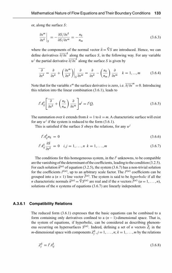
Ch03-H6594.tex 8/5/2007 12: 0 Page 133


or, along the surface S:

∂xm

∂xk

∣∣∣∣S

= − ∂S/∂xk

∂S/∂xm= − nk

nm(3.6.3)

where the components of the normal vector �n = �∇S are introduced. Hence, we can

define derivatives ∂/∂xk

along the surface S, in the following way. For any variable

u j the partial derivative ∂/∂xk

along the surface S is given by

∂

∂xk= ∂

∂xk+(

∂xm

∂xk

)∣∣∣∣S

∂

∂xm= ∂

∂xk−(

nk

nm

)∂

∂xmk = 1, ..., m (3.6.4)

Note that for the variable xm the surface derivative is zero, i.e. ∂/∂xm = 0. Introducing

this relation into the linear combination (3.6.1), leads to

liAkij

[∂

∂xk+(

nk

nm

)∂

∂xm

]uj = liQi (3.6.5)

The summation over k extends from k = 1 to k = m. A characteristic surface will existfor any u j if the system is reduced to the form (3.6.1).

This is satisfied if the surface S obeys the relations, for any u j

liAkijnk = 0 (3.6.6)

liAkij

∂S

∂xk= 0 i, j = 1, . . . , n k = 1, . . . , m (3.6.7)

The conditions for this homogeneous system, in the li unknowns, to be compatibleare the vanishing of the determinant of the coefficients, leading to the condition (3.2.5).For each solution �n(α) of equation (3.2.5), the system (3.6.7) has a non-trivial solutionfor the coefficients li(α), up to an arbitrary scale factor. The li(α) coefficients can begrouped into a (n × 1) line vector �l(α). The system is said to be hyperbolic if all then characteristic normals �n(α) = �∇S(α) are real and if the n vectors �l(α) (α = 1, . . . , n),solutions of the n systems of equations (3.6.7) are linearly independent.

A.3.6.1 Compatibility Relations

The reduced form (3.6.1) expresses that the basic equations can be combined to aform containing only derivatives confined to a (n − 1)-dimensional space. That is,the system of equations, if hyperbolic, can be considered as describing phenom-ena occurring on hypersurfaces S(α). Indeed, defining a set of n vectors �Zj in them-dimensional space with components Zk

j , j = 1, . . . , n; k = 1, . . . , m by the relations

Zkj = liAk

ij (3.6.8)

Ch03-H6594.tex 8/5/2007 12: 0 Page 134


equation (3.6.1) can be rewritten as

Zkj

∂uj

∂xk= liQi (3.6.9)

The vectors �Zj define n characteristic directions of which (n − 1) are independent. Theoperators (Zk

j ∂k ) are the derivatives in the direction of the vector �Zj . Hence defining

dj�= Zk

j∂

∂xk= �Zj. �∇ (3.6.10)

in the m-dimensional space, the transformed equation (3.6.1) can be written as aderivatives along the vectors �Zj:

djuj ≡ �Zj · �∇u j = liQi (3.6.11)

The above equation is known as the compatibility relation, and represent an alternativeformulation to the system (3.2.1). Condition (3.6.7) expresses that all the �Zj vectorslie in the characteristic surface whose normal is �n. Indeed, equation (3.6.7) becomes,with the introduction of �Zj

�Zj · �n = Zkj nk = 0 for all j = 1, . . . , n (3.6.12)

These phenomena correspond to propagating wavefronts, as seen earlier, and it canbe shown (see for instance Whitham, 1974) that the characteristic surfaces can alsocontain discontinuities of the normal derivatives ∂uj/∂n, satisfying

Akijnk

[∂uj

∂n

]= 0 (3.6.13)

where

[∂uj

∂n

]=(

∂uj

∂n

)+

−(

∂uj

∂n

)−

(3.6.14)

is the jump, over the surface S, of the normal derivatives of the solution uj . Thisrelation can also be written:

nk

[∂Fk

i

∂n

]= 0 (3.6.15)

where ∂/∂n is the normal derivative to the surface S. The corresponding vectors �l areobtained from equation (3.6.6), written as

li(δijnt + Akijnk ) = 0 k = 1, . . . , m − 1 (3.6.16)

Ch03-H6594.tex 8/5/2007 12: 0 Page 135


or

liKij = λ(α)liδij i, j = 1, . . . , n α = 1, . . . , n (3.6.17)

Hence, the vectors �l(α)of components li(α) are the left eigenvectors of the matrix Kcorresponding to the eigenvalues λ(α). If the n eigenvectors �l(α) are linearly indepen-

dent, the system will be hyperbolic. If the n eigenvectors �l(α)are grouped in a matrixL−1, where each row contains the components of an eigenvector �l(α), i.e.

(L−1)iα = li(α) (3.6.18)

we obtain from the eigenvector equation (3.4.13) that the matrix L diagonalizes thematrix K :

L−1 K L = � (3.6.19)

where � is the diagonal matrix containing the eigenvalues λ(α):

� =

∣∣∣∣∣∣∣∣∣∣

λ(1) 0λ(2)

.

.

0 λ(n)

∣∣∣∣∣∣∣∣∣∣(3.6.20)

It is also interesting to notice that, within the same assumptions, the intensities of thepropagating disturbances are the right eigenvectors r(α) of K , since equation (3.6.13)can be written as

Kij rj = λ(α)rjδij (3.6.21)

Example E.3.6.1: Small disturbance potential equation

The two vectors �l associated to the two characteristic normals (E.3.3.2) are obtainedfrom the system (3.6.6), which is written here as

(l1, l2)

∣∣∣∣ (1 − M 2∞)nx ny

−ny nx

∣∣∣∣ = 0 (E.3.6.1)

where the ratio λ = ny/nx is defined as the solutions (E.3.3.2). Choosing l1 = 1, thesystem (E.3.6.1) has the solution:

l1 = 1

l2 =√

(M 2∞ − 1) (E.3.6.2)

Ch03-H6594.tex 8/5/2007 12: 0 Page 136


The two characteristic directions �Zj defined by equation (3.6.8), become here

�Z1 = (1 − M 2∞, λ)

�Z2 = ( − λ, 1) (E.3.6.3)

Observe that these two directions are parallel to each other, since λ2 = (M 2∞ − 1) andthat their common direction is the characteristic line of Figure E.3.3.1, making theangle μ with the x-direction, since λ = cos μ/sin μ. This can also be seen from a directverification of equation (3.6.12), with the vector of the characteristic normal definedby the components �n ≡ (1, λ), which indicates that the Z-directions are orthogonal tothe normals n. The compatibility relation (3.6.9) or (3.6.11) becomes here

[(1 − M 2∞)

∂

∂x+ λ

∂

∂y

]u +

[−λ

∂

∂x+ ∂

∂y

]v = 0 (E.3.6.4)

or

cot μ

[cos μ

∂

∂x∓ sin μ

∂

∂y

]u ±

[cos μ

∂

∂x∓ sin μ

∂

∂y

]v = 0 (E.3.6.5)

For constant Mach angles μ, the compatibility relation expresses the property that thevelocity component along one characteristic (u cos μ ± v sin μ) is conserved alongthe other characteristic.


This chapter has introduced the general methodology for the determination of themathematical properties of a system of PDEs, defining a selected approximationmodel of the flow system.

It is of crucial importance to identify and distinguish when a system of PDEsdescribes convection, or diffusion, or mixed phenomena.

The main topics to remember are:

• A system of quasi-linear partial differential equations is hyperbolic if its homo-geneous part admits wave-like solutions. In other words, a hyperbolic systemdescribes convection phenomena and inversely, convection phenomena aredescribed by hyperbolic equations.

• If the equations admit damped wave solutions the system will be called parabolic.• If the equations do not admit wave-like solutions, they are elliptic, and

the behavior of the physical system considered is dominated by diffusionphenomena.

• Characteristic surfaces represent an important property of hyperbolic systems,as they are associated to the propagation phenomena.

• The notions of domain of dependence and zone of influence are very essentialproperties of PDEs and should be kept in mind in all cases.

Ch03-H6594.tex 8/5/2007 12: 0 Page 137


• Steady inviscid flows have the property of being elliptic in the subsonic rangeand hyperbolic in the supersonic regions.

• Time-marching methods for steady state problems offer the great advantage thattheir properties in space and time are independent of the Mach number. In theinviscid case, they are always hyperbolic in space and time, for all values of theMach number.

REFERENCES

Ames, W.F. (1965). Nonlinear Partial Differential Equations in Engineering. AcademicPress, New York.

Courant, R. and Hilbert, D. (1962). Methods of Mathematical Physics. Interscience,New York.

Dwyer, H.A. (1981). Some aspects of three dimensional laminar boundary layers. Annu.Rev. Fluid Mech., 13, 217–229.

Hildebrand, F.B. (1976). Advanced Calculus for Applications. Prentice Hall, EnglewoodCliffs, NJ.

Krause, E. (1973). Numerical treatment of boundary layer problems. In Advances inNumerical Fluid Dynamics, AGARD-LS-64.

Solonnikov, J.A. and Kazhikhov, A.V. (1981). Existence theorems for the equations ofmotion of a compressible viscous fluid. Annu. Rev. Fluid Mech., 13, 79–95.

Temam, R. (1977). Navier–Stokes Equations. North-Holland Publ. Co, Amsterdam.Whitham, G.B. (1974). Linear and Nonlinear Waves. J. Wiley & Sons, New York.

PROBLEMS

P.3.1 Show that the system of Cauchy–Riemann equations

∂u

∂x+ ∂v

∂y= 0

∂v

∂x− ∂u

∂y= 0

is of elliptic nature.P.3.2 Consider the two-dimensional stationary shallow water equations describing

the spatial distribution of the height h of the free water surface in a streamwith velocity components u and v. They can be written in the following form,where g is the earth’s gravity acceleration:

u∂h

∂x+ v

∂h

∂y+ h

∂u

∂x+ h

∂v

∂y= 0

u∂u

∂x+ v

∂u

∂y+ g

∂h

∂x= 0

u∂v

∂x+ v

∂v

∂y+ g

∂h

∂y= 0

Ch03-H6594.tex 8/5/2007 12: 0 Page 138


(a) Introduce the vector

U =∣∣∣∣∣∣

huv

∣∣∣∣∣∣and write the system (E.3.2.8) under the form (3.2.3).

(b) Obtain the three characteristic normals �n, as solutions of equation (3.2.5),by defining λ = nx/ny. Show that we obtain

λ(1) = − v

u

and the two solutions of the quadratic equation:

(u2 − gh)λ2 + 2λuv + (v2 − gh) = 0

λ(2),(3) = −uv ±√gh√

u2 + v2 − gh

u2 − gh

Observe that√

gh plays the role of a sonic, critical, velocity and thesystem is hyperbolic for supercritical velocities �v2 = u2 + v2 > gh.

P.3.3 Show that the one-dimensional Navier–Stokes equation without pressuregradient (known as the ‘viscous’ Burger’s equation)

∂u

∂t+ u

∂u

∂x= α

∂2u

∂x2

is parabolic in x, t.Hint: Write the equation as a system, introducing v = ∂u/∂x as second

variable and apply equation (3.2.5) to show that the matrix is not of rank 2.P.3.4 Consider the one-dimensional Euler equations:

∂ρ

∂t+ u

∂ρ

∂x+ ρ

∂u

∂x= 0

∂u

∂t+ u

∂u

∂x+ 1

ρ

∂p

∂x= 0

∂H

∂t+ u

∂H

∂x= 1

ρ

∂p

∂t

Introduce the isentropic assumption ∂p/∂ρ = c2, with c the speed of soundand replace the third equation by an equation on the pressure, by applying theperfect gas laws and the definition of H . Obtain the equation:

∂p

∂t+ u

∂p

∂x+ ρc2 ∂u

∂x= 0

Write the system in matrix form for the variable vector:∣∣∣∣∣∣

ρ

up

∣∣∣∣∣∣

Ch03-H6594.tex 8/5/2007 12: 0 Page 139


Show that the system is hyperbolic and has the eigenvalues u, u + c and u − c.Obtain the left and right eigenvectors.

P.3.5 Consider the system

∂u

∂t+ 1

2

∂u

∂x+ ∂v

∂x= 0

∂v

∂t+ ∂u

∂x+ 1

2

∂v

∂x= 0

(a) Write the system in matrix form (3.4.5) and obtain the matrix A:

∂U

∂t+ A

∂U

∂x= 0 with U =

∣∣∣∣ uv

∣∣∣∣(b) Find the eigenvalues of A and show that the system is hyperbolic.(c) Derive the left and right eigenvectors and obtain the matrix L which

diagonalizes A. Explain why the left and right eigenvectors are identical.(d) Obtain the characteristic variables and the compatibility relations.Hint: The eigenvalues of A are 3/2 and −1/2. The matrix L has the form:

L = 1√2

∣∣∣∣ 1 11 −1

∣∣∣∣The characteristic variables are

(u + v)√

2 and (u − v)√

2

The compatibility relations are

∂(u + v)

∂t+ 3

2

∂(u + v)

∂x= 0

∂(u − v)

∂t− 1

2

∂(u − v)

∂x= 0

P.3.6 Consider the steady potential equation (E.3.2.18) for supersonic flows, M > 1.From Example E.3.2.3, it is known that the equation is hyperbolic. Obtain thetwo vectors �l(α), α = 1, 2 associated to the two characteristic normal directions�n(α), solutions of equation (3.2.11). Show that the two characteristics form anangle ±μ with the velocity vector v, with sin μ = 1/M . The angle μ is calledthe Mach angle.

Hint: Defineβ as the angle of the velocity vector by cos β = u/|�v|, sin β = v/|�v|Setting nx = 1 shows that ny = −cotan(β ± μ). Selecting l1 = 1, obtainl2 = −cny from equation (3.2.2).

P.3.7 Show that for the transformation leading to equation (3.4.5) Amij = δij , the

characteristic directions (3.6.8) become

Zmj = liδij

Zkj = liAk

ij k = 1, . . . , m − 1

Ch03-H6594.tex 8/5/2007 12: 0 Page 140


Form the (n × m) matrix Z and note that the last line ( j being the columnindex) is formed by the vector �l.

Show that the orthogonality condition (3.6.12) is equivalent to equation(3.6.17) and that we have, for a wave number vector �κ:

Zkj κk = λliδij

P.3.8 Referring to the one-dimensional shallow water equations treated in ExampleE.3.4.1, find the eigenvectors �l(α), α = 1, 2 as well as the characteristic vectors�Z1 and �Z2. Derive also the compatibility relations (3.6.11).Hint: Show that the left eigenvectors are proportional to�l[1, ±√h/g] and thatthe characteristic vectors have the components:

�Z1 =∣∣∣∣ u ±√gh

1

∣∣∣∣ �Z2 = ±√

h

g

∣∣∣∣ u ±√gh1

∣∣∣∣Show that we obtain

∂h

∂t+ (u ±√gh)

∂h

∂x±

√h

g

{∂u

∂t+ (u ∓√gh)

∂u

∂x

}= 0

where the upper signs are to be taken together for the first and the lower signsfor the second compatibility relation.

P.3.9 Consider equation (3.2.6) and write also the compatibility relation (3.6.11) afterhaving defined the characteristic directions �Zj according to equation (3.6.8).

Hint: Obtain

�Z1 =∣∣∣∣ a−2b + cny

∣∣∣∣ �Z2 =∣∣∣∣−cny

c

∣∣∣∣

and verify equation (3.6.12). Note also that �Z1 and �Z2 are in the same direction,since they are both orthogonal to �n. Show by a direct calculation that thevector product of �Z1 and �Z2 is indeed zero. Referring to the general form ofequation (3.2.6), obtain the compatibility relation

a∂u

∂x+ (cny − 2b)

∂u

∂y− cny

∂v

∂x+ c

∂v

∂y= 0

Ch04-H6594.tex 27/4/2007 15: 31 Page 141

Part II

Basic Discretization Techniques

Having defined in Part I, the mathematical models for fluid dynamics and a method-ology for analyzing their fundamental properties in Chapter 3, we are now readyto move on to the next step toward setting up a CFD algorithm, namely thediscretization phase.

As outlined in Figures I.2.1 and I.3.1, to which we refer you again, this second step inthe definition of the computational approach deals with the choice of the discretizationmethod of the selected mathematical model and involves two components, the spacediscretization and the equation discretization.

The space discretization consists in setting up a mesh, or a grid, by which thecontinuum of space is replaced by a finite number of points where the numerical valuesof the variables will have to be determined. It is intuitively obvious that the accuracyof a numerical approximation will be directly dependent on the size of the mesh, thatis the closer the points, the better the discretized space approaches the continuum,the better the approximation of the numerical scheme. In other words, the error of anumerical simulation has to tend to zero when the mesh size tends to zero, and the paceof this variation will be characterized by the order of the numerical discretization.

For complex geometries the solution will also be dependent on the form of the mesh,since in these cases we will tend to develop meshes which are adapted to the geomet-rical complexities, as for flows along solid walls, and the mesh shape and size willvary through the flow field. Therefore, the generation of grids for complex geometriesis a crucial problem, whose importance increases with the space dimension, makingthis step the most significant in three-dimensional CFD simulations.

As described already in the general introduction, we distinguish between structuredand unstructured grids, the latter being of more general nature. Structured grids areformed by families of lines (one for each space dimension), each mesh point beingat the intersection of one line of each family and correspond to Cartesian grids in themathematical space of the curvilinear coordinates. In unstructured grids, the meshpoint distribution is arbitrary since they are not localized on identified lines and theycan be connected through various polynomials in 2D or polyhedrals in 3D.

Grid generation and grid quality are essential elements of the whole discretizationprocess. Not only is grid generation today a most critical element in the cost of runningCFD simulations, but more importantly, the accuracy of the obtained numericalresults is critically dependent on mesh quality.

In recent years methods have been, and still are developed in order to generateefficiently and as automatically as possible meshes adapted to arbitrary geometries.

141

Ch04-H6594.tex 27/4/2007 15: 31 Page 142

142 Basic Discretization Techniques

We will devote Chapter 6 of Part II to a presentation of different grid types and theirproperties, with some considerations and recommendations related to grid qualityand grid-related errors.

Once a mesh has been defined, the equations can be discretized leading to thetransformation of the differential or integral equations to discrete algebraic operationsinvolving the values of the unknowns related to the mesh points. The basis of allnumerical methods consists in this transformation of the mathematical model intoan algebraic, linear or nonlinear, system of equations for the mesh-related unknownquantities.

A very important aspect in the definition of an algorithm is the choice to be madebetween a time-dependent or steady state model for the flow equations, as mentionedalready in Chapter 3.

For physical time-dependent problems with a transient flow behavior or connectedto time varying boundary conditions, there is obviously no alternative to the use ofa time-dependent mathematical model as time accuracy of the numerical solution isrequired.

However, with stationary or steady state problems, an alternative exists and youcan decide to work either with a time-independent mathematical model of your flowproblem or to use an unsteady formulation and follow the numerical solution intime until the steady state is reached. This last family of methods is often called‘time marching’ or ‘pseudo unsteady’ since the time accuracy is not required andwe attempt to reach the steady state in the smallest possible number of time steps,without requiring the correct numerical simulation of the transient behavior. In thiscase, the numerical schemes will rely on the solution of systems of ODEs in time,while in the former case the numerical solution techniques will have to rely on themethods for solving algebraic systems of equations (in space).

This has been explained already in Chapter 3 and the advantages of the time-dependent formulation, whereby the properties of the equations do not change whenpassing from subsonic to supersonic flow conditions, have been stressed. Anothervery important advantage of the time dependent formulation is related to the fact thatmany flow configurations do not have a steady state behavior, even in presence ofstationary boundary conditions. A most popular example is the flow over a cylinder,characterized by the presence of a periodic vortex shedding, for Reynolds numbershigh enough (typically above ∼40), as shown in Section 2.1. This flow has no steadystate solution and hence attempting to solve the time-independent flow equations,will lead to non-physical solutions, or to no solution at all.

It is essential to be aware that, seen at small enough length scales all turbu-lent flow configurations are unsteady and that steady state flow conditions are theexception and not the rule. Although in practice, as we do not always look at thefine scales, many flows appear as steady.

For instance, the flow along an aircraft wing, under constant upstream conditions,considered at the level of the Reynolds averaged turbulent approximation (RANSmodel), may appear as steady, provided there is no large-scale separation. Sincenearly all separated flow regions tend to have an unsteady behavior when the grid isrefined, it is required to work with a mathematical model that is capable of detectinglarge-scale unsteadiness, as they appear.

Therefore, we recommend working with the time-dependent equations, unlessthere is an assurance that the flow will remain steady. However, even in this case thereis no significant advantage in working with the stationary flow models.

Ch04-H6594.tex 27/4/2007 15: 31 Page 143

Basic Discretization Techniques 143

For all those reasons, we are focusing on the discretization properties of time-dependent algorithms as the most general approach.

We will show, however, in the later Chapters 9 and 10, that bridges can be estab-lished between the two approaches, and they can be viewed as belonging to a commonfamily of schemes, when iterative methods are applied for the resolution of thealgebraic systems resulting from the space discretization.

With time-dependent numerical formulations, we will distinguish two families ofmethods, explicit or implicit. In explicit methods, the matrix of the unknown variablesat the new time is a diagonal matrix while the right-hand side of the system is beingdependent only on the flow variables at the previous times. This leads therefore to atrivial matrix inversion and hence to a solution with a minimal number of arithmeticoperations for each time step. However, this advantage is counter-balanced by the factthat stability and convergence conditions impose severe restrictions on the maximumadmissible time step. While this might not be a limitation for physical unsteadyproblems, it leads to the necessity of a large number of time steps in order to reachthe steady state solution corresponding to a physical time-independent problem.

In implicit methods, the matrix to be inverted is not diagonal since more thanone set of variables are unknown at the same time level. In many cases however,the structure of the matrix will be rather simple, such as block pentadiagonal, blocktridiagonal or block bidiagonal, allowing simple algorithms for the solution of thesystem at each time step, although the number of operations required will be higherwhen compared to the explicit methods. This is compensated by the fact that manyimplicit methods have, at least for linear problems, no limitation on the time step andhence a lesser number of iterations will be needed to reach the steady state.

In summary, the following steps have to be defined in the process of setting up anumerical scheme:

(i) Selection of a discretization method of the equations. This implies the selectionbetween finite difference, finite volume or finite element methods as wellas the selection of the order of accuracy of the spatial and eventually timediscretization.

(ii) Analysis of the selected numerical algorithm. This step concerns the analysisof the ‘qualities’of the scheme in terms of stability and convergence propertiesas well as the investigation of the generated errors.

(iii) Selection of a resolution method for the system of ordinary differential equa-tions in time, for the algebraic system of equations and for the iterativetreatment of eventual nonlinearities.

Step (i) will be discussed in Part II, Chapters 4–6; step (ii) will be addressed inPart III, Chapters 7 and 8 and step (iii) in Part IV, Chapters 9 and 10.

THE STRUCTURE OF PART II

In Part II, we will introduce you to the most important methods for the discretization ofthe space derivatives entering in the conservation laws. Three families of methods areavailable, with varying degrees of generality. The most traditional and oldest methodis the finite difference method (FDM ), which remains the reference for all studies ofnumerical discretization, although it is only applicable in practice to structured grids.

Ch04-H6594.tex 27/4/2007 15: 31 Page 144


Therefore, it is very important that you develop a strong understanding of the mainproperties of finite difference formulas.

By far the most widely applied method today in CFD is the finite volume method(FVM ), which discretizes directly the integral form of the conservation laws. Itspopularity is due to its generality, its conceptual simplicity and the relative ease ofapplication to both structured as well as to any kind of unstructured grids. A largebody of literature has been developed around the FVM and we will introduce itsmain properties. Although the FV discretization will lead to similar formulas as aFDM when applied to structured grids, it is equally important that you develop agood understanding of the main properties of FVMs. This will help you to follow thedevelopments behind current CFD tools and to better interpret the results obtainedby applying for instance commercial CFD codes to practical problems.

The third method is derived from the world of structural mechanics, where the finiteelement method (FEM ) is most widely, if not exclusively, applied. Its applicationto CFD is of interest, but is not dominant and we will restrict ourselves to a shortpresentation, at advanced level, mainly oriented at its basic properties and its relationwith the finite volume method.

Although the analysis of discretization methods is best performed on uniform grids,this is seldom the case in practice, where geometrical complexities can lead to highlyirregular and distorted grids. Due to the strong influence of the grid properties onthe quality of the CFD results and the associated loss of accuracy, it is important todevelop an understanding of these effects and to extract possible guidelines on gridquality in order to reduce the associated numerical errors. This will be introduced inChapter 4 on a one-dimensional basis, and further discussed in Chapter 6.

This second part is therefore organized in three chapters:

1. Chapter 4 deals with the basic method for the discretization of PDEs, namelythe finite difference method (FDM ), which can be applied to any structuredmesh configuration.

2. Chapter 5 will cover the fundamentals of what is today the most widely applieddiscretization method, valid for both structured and unstructured grids, the finitevolume method (FVM ). Some advanced sections will introduce the essentialsof the finite element method (FEM ), which is the reference method in structuralmechanics, but is also applicable to fluid mechanics.

3. Chapter 6 will introduce the important issue of mesh properties. As stated in theintroduction, two families of grids can be selected: structured or unstructured,the latter being the most general option. This chapter is not oriented at thetechniques for grid generation, which are quite specialized and outside the scopeof this book. Several excellent publications can be consulted on this subject andreferences will be given in Chapter 6. Instead, this new chapter will presentthe different grid types as encountered in CFD and will focus on issues of gridgenerated errors, grid quality and provide some best practice recommendationson grid properties in order to minimize the grid-related error sources.

Ch04-H6594.tex 27/4/2007 15: 31 Page 145

Chapter 4

The Finite Difference Method forStructured Grids


The Finite Difference Method (FDM) is based on the properties of Taylor expansionsand on the straightforward application of the definition of derivatives. It is probablythe simplest method to apply, particularly on uniform meshes, but it requires the meshto be set up in a structured way, whereby the mesh points, in an n-dimensional space,are located at the intersections of n families of lines and each point must lie on one,and only one, line of each family.

In Section 4.1, we explain the basic steps toward the establishment of finite dif-ference formulas and introduce the very important concept of order of accuracy, asapplied to first and second derivatives. It will be immediately clear from this sectionand further confirmed in the subsequent sections, that an unlimited number of FDformulas can be derived for any derivative. This implies that for any partial differentialequation (PDE) of a mathematical model, we will have an infinite number of possi-ble numerical schemes. This richness of numerical algorithms makes the selectionprocess and the associated criteria a challenging and altogether exciting issue and wehope to guide you in this wonderful world and to share with you the sense of beauty itcan provide. This will be directly illustrated on the simplest one-dimensional modelequations for linear convection and linear diffusion.

In Section 4.2, we introduce the extensions of FD formulas for partial derivativesin two dimensions, on uniform structured grids. This extension can be applied tosingle or mixed derivatives of any order. Although Section 4.2 is restricted to two-dimensional space, its extension to three dimensions is straightforward. A particularattention is given to finite difference formulas for the very important Laplace equation,which is the standard equation describing diffusion phenomena.

In Section 4.3, we introduce some issues related to FD formulas on non-uniformgrids, in one-dimensional space. This section is of great importance, since mostof the grids used in practical CFD simulations are non-uniform. We will show thatstandard FD formulas can easily loose at least one order of accuracy, when appliedto a non-uniform grid. In addition to the derivation of representative FD formulas,the presented analysis will provide some recommendations to be considered whendealing with non-uniform grids.

We consider Section 4.3 as one of the most important of this chapter, and recommendthat you give a particular attention to its content and its conclusions.

The two following sections are of a more advanced level and we suggest consideringthis section for a more advanced course. They will be marked as ‘Advanced’ in theroadmap of Figure 4.0.1.

145

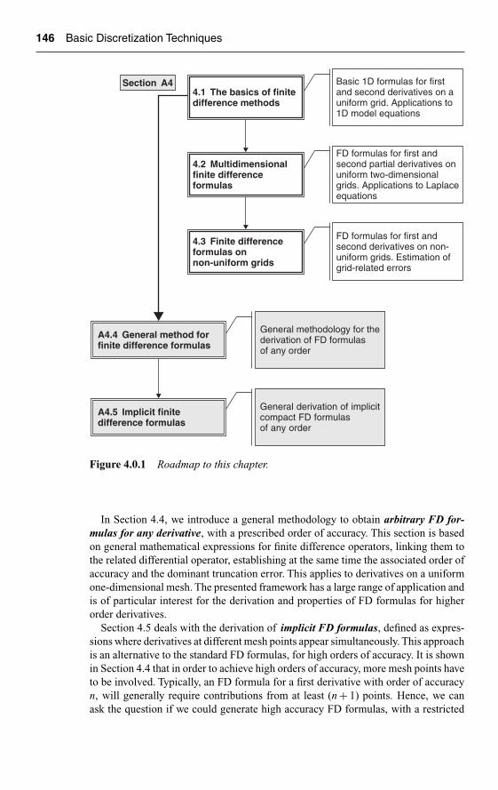
Ch04-H6594.tex 27/4/2007 15: 31 Page 146


Section A44.1 The basics of finitedifference methods

4.2 Multidimensionalfinite differenceformulas

4.3 Finite differenceformulas onnon-uniform grids

Basic 1D formulas for firstand second derivatives on auniform grid. Applications to1D model equations

FD formulas for first andsecond partial derivatives onuniform two-dimensionalgrids. Applications to Laplaceequations

FD formulas for first andsecond derivatives on non-uniform grids. Estimation ofgrid-related errors

General methodology for thederivation of FD formulasof any order

A4.5 Implicit finitedifference formulas

A4.4 General method forfinite difference formulas

General derivation of implicitcompact FD formulasof any order

Figure 4.0.1 Roadmap to this chapter.

In Section 4.4, we introduce a general methodology to obtain arbitrary FD for-mulas for any derivative, with a prescribed order of accuracy. This section is basedon general mathematical expressions for finite difference operators, linking them tothe related differential operator, establishing at the same time the associated order ofaccuracy and the dominant truncation error. This applies to derivatives on a uniformone-dimensional mesh. The presented framework has a large range of application andis of particular interest for the derivation and properties of FD formulas for higherorder derivatives.

Section 4.5 deals with the derivation of implicit FD formulas, defined as expres-sions where derivatives at different mesh points appear simultaneously. This approachis an alternative to the standard FD formulas, for high orders of accuracy. It is shownin Section 4.4 that in order to achieve high orders of accuracy, more mesh points haveto be involved. Typically, an FD formula for a first derivative with order of accuracyn, will generally require contributions from at least (n + 1) points. Hence, we canask the question if we could generate high accuracy FD formulas, with a restricted

Ch04-H6594.tex 27/4/2007 15: 31 Page 147

The Finite Difference Method for Structured Grids 147

number of points, defining hereby compact formulas. The answer to this questionis positive, leading to compact, implicit schemes, which can be of interest whenhigh order accuracy is required, for instance in simulations such as direct numericalsimulation (DNS), large eddy simulation (LES) for turbulent flows, computationalelectromagnetic (CEM) or computational aero acoustic (CAA).

The roadmap of this chapter is summarized in Figure 4.0.1.

4.1 THE BASICS OF FINITE DIFFERENCE METHODS

The finite difference approximation is the oldest of the methods applied to obtainnumerical solutions of differential equations, and the first application is attributed toLeonhard Euler (1707–1783) in 1768. The idea of finite difference methods is actuallyquite simple, since it corresponds to an estimation of a derivative by the ratio of twodifferences according to the theoretical definition of the derivative.

For a function u(x), the derivative at point x is defined by

ux = ∂u

∂x= lim

�x→0

u(x + �x) − u(x)

�x(4.1.1)

If we remove the limit in the above equation, we obtain a finite difference, whichexplains the name given to this method.

If �x is small but finite, the expression on the right-hand side is an approximationto the exact value of ux. The approximation will be improved by reducing �x, butfor any finite value of �x, an error is introduced, the truncation error, which goes tozero for �x tending to zero.

The power of�x with which this error tends to zero is called the order of accuracy ofthe difference approximation, and can be obtained from a Taylor series developmentof u(x + �x) around point x.

Actually, the whole concept of finite difference approximations is based on theproperties of Taylor expansions. Developing u(x + �x) around u(x) we have

u(x + �x) = u(x) + �x∂u

∂x+ �x2

2

∂2u

∂x2+ �x3

3!∂3u

∂x3+ · · · (4.1.2)

This relation can be written as follows:

u(x + �x) − u(x)

�x= ux(x) + �x

2uxx(x) + �x2

6uxxx(x) + · · ·

︸︷︷︸Truncation error

(4.1.3)

showing that

• The right-hand side (r.h.s) of equation (4.1.1) is indeed an approximation to thefirst derivative ux in point x.

• The remaining terms in the r.h.s represent the error associated to this formula.

Ch04-H6594.tex 27/4/2007 15: 31 Page 148


xi xi�1

xi�1 � xi � �x

Figure 4.1.1 Taylor expansion of the function u(x), around point x.

If we restrict the truncation error to its dominant term, that is to the lower powerin �x, we see that this approximation for u(x) goes to zero like the first power of �xand is said to be first order in �x and we write

u(x + �x) − u(x)

�x∼= ux(x) + �x

2uxx(x) = ux(x) + O(�x) (4.1.4)

indicating that the truncation error O(�x) goes to zero like the first power in �x.A very large number of finite difference approximations can be obtained for the

derivatives of functions as shown next and a general procedure will be described inSection 4.4, based on formal difference operators and their manipulation.

A remark about the significance of Taylor expansions

The Taylor expansion (4.1.2) actually tells us something quite remarkable about theproperties of continuous functions. The left-hand side (l.h.s) is the value of the func-tion u at an arbitrary distance �x from point x, with no restriction on this distance.In the right-hand side (r.h.s), all quantities are evaluated at point x. Hence, what theTaylor expansion tells us is that we can know the value of the function at an arbitrarydistance far away from point x (say 5000 km), if we know ‘everything’, that is all thederivatives, at this single point x (Figure 4.1.1). In practice, for any finite value of�x, the knowledge of a finite number of derivatives in point x, will suffice to evaluatethe value of u at point (x + �x) with a preset accuracy.

Example E.4.1.1

This is illustrated by the following plot of the Taylor expansion of (e√

x − 1) aroundx = 0, obtained by the Maple symbolic mathematical software (version Maple 10):

(e√

x − 1) = √x + 1

2x + 1

6x3/2 + 1

24x2 + 1

120x5/2 + 1

720x3 + 1

5040x7/2

+ 1

40,320x4 + 1

3,62,880x9/2 + O(x5) (E.4.1.1)

Figure E.4.1.1 illustrates that by increasing the number of terms of theTaylor expan-sion, we increase the distance over which the expansion provides a valid representationof the function. With four terms, that is the knowledge of up to four derivatives inpoint x = 0, the four term expansion covers nearly all the domain from 0 to 2.

Ch04-H6594.tex 27/4/2007 15: 31 Page 149


8.0

0.0

0.0 0.4 0.8 1.2 1.6 2.0 2.4x

2.8 3.2 3.6 4.0 4.4 4.8

0.8

1.6

2.4

3.2

4.0

4.8

5.6

6.4

7.2

Exact function

First term

Two terms

Three terms

Four terms

Figure E.4.1.1 Taylor expansion of (e√

x − 1) up to order 5.

�x�x

i � 1 i � 2i � 2

i � 1/2

i � 1 i

i � 3/2 i � 1/2 i � 3/2

Figure 4.1.2 One-dimensional uniform grid on the x-axis.

4.1.1 Difference Formulas for First and Second Derivatives

To apply this general definition, we consider a one-dimensional space, the x-axis,where a space discretization has been performed such that the continuum is replacedby N discrete mesh points xi, i = 1, . . . , N (Figure 4.1.2).

We will indicate by ui the value of the function u(x) at the points xi, i.e. ui = u(xi)and consider that the spacing between the discrete points is constant and equal to �x.Without loss of generality, we can consider that xi = i�x and this point will also bereferred to as ‘point xi’ or as ‘point i’.

Ch04-H6594.tex 27/4/2007 15: 31 Page 150


4.1.1.1 Difference formula for first derivatives

Applying the above relations (4.1.3) and (4.1.4) at point i, we obtain the followingfinite difference approximation for the first derivative (ux)i = (∂u/∂x)i:

(ux)i =(

∂u

∂x

)i= ui+1 − ui

�x−�x

2(uxx)i − �x2

6(uxxx)i + · · ·


(4.1.5)

= ui+1 − ui

�x+ O(�x)

As this formula involves the point (i + 1) to the right of point i, it is called the firstorder forward difference for the first derivative (ux)i = (∂u/∂x)i.

This is certainly not the only formula we can think of, as we can re-apply the rela-tions (4.1.1)–(4.1.4) by replacing everywhere �x by (−�x). This leads to the relation:

(ux)i =(

∂u

∂x

)i= ui − ui−1

�x+�x

2(uxx)i − �x2

6(uxxx)i + · · ·


(4.1.6)

= ui − ui−1

�x+ O(�x)

With respect to the point x = xi, this formula is the first order backward differ-ence for the derivative (ux)i. Both formulas (4.1.5) and (4.1.6) are called one-sideddifference formulas, since they involve points at one side of point i only.

Looking carefully at the two one-sided formulas, we observe that the dominant firstorder truncation errors are of opposite signs. Hence, if we add them up, we obtain asecond order approximation

(ux)i = ui+1 − ui−1

2�x− �x2

6(uxxx)i + · · · = ui+1 − ui−1

2�x+ O(�x2) (4.1.7)

This formula, which involves the points to the left and to the right of point i, iscalled therefore a central difference formula.

These three approximations are represented geometrically on Figure 4.1.3 while thederivative is represented by the tangent to the curve u(x), the forward, backward andcentral chords represent the approximations defined by the corresponding differenceformulas. It is clear that the central chord is always a much better approximation thanthe one-sided chords and this is reflected by its second order accuracy.

The formula (4.1.7) is indeed particularly interesting, as it provides, on the samesupport as the one-sided differences, namely points (i + 1), i, (i − 1), a second orderaccuracy, compared to first order. To better realize what this means, consider a domainbetween 0 and 1 on the x-axis, with 11 mesh points and �x = 0.1. A first order formulacan be interpreted as generating an error O(�x), that is of the order of 10%, whileapplying the second order central formula on the same 11-grid point mesh, will give anaccuracy O(�x2) of the order of 1%. If we want an accuracy of 1% with the one-sideddifference formulas, we will need to generate a mesh with 101 points and �x = 0.01,which represents a significantly higher cost, as we need to apply the formulas 100times instead of 10 times.

Ch04-H6594.tex 27/4/2007 15: 31 Page 151


Backwarddifference

Forwarddifference

Centraldifference

x

y

y � u(x )

ui�1

ui�1

i

�x �x

i�1 i�1

ui

Figure 4.1.3 Geometrical interpretation of difference formulas for first orderderivatives.

Important remarks and interpretations

• As the truncation error of a first order FD formula is proportional to the secondderivative, as seen from the above equations, we can state that a first order FDformula is exact for a linear function. Similarly, a second order formula has itstruncation error proportional to the third derivative; hence, this formula will beexact for a quadratic (parabolic) function.

• The first order forward difference formula for (ux)i can be considered as a centraldifference with respect to the mid-point

xi+1/2 = (xi + xi+1)

2(4.1.8)

leading to a second order approximation for the derivative (ux)i+1/2 in this point.This is an important property, which is often used in computations due to its com-pact character. The same formula (4.1.5) is either a first order forward differencefor (ux)i or a second order central approximation for (ux)i+1/2 but involving onlythe same two mesh points i and (i + 1). We therefore have

(ux)i+1/2 =(

∂u

∂x

)i+1/2

= ui+1 − ui

�x+ O(�x2) (4.1.9)

and similarly at (i − 1/2)

(ux)i−1/2 ≡(

∂u

∂x

)i−1/2

= ui − ui−1

�x+ O(�x2) (4.1.10)

Compared to the formulas (4.1.5) and (4.1.6) for (ux)i, we have gained an orderof accuracy by considering the same expressions as approximations for the mid-points (i + 1/2) or (i − 1/2), respectively.

Ch04-H6594.tex 27/4/2007 15: 31 Page 152


Actually, difference formulas for the first derivative (ux)i can be constructed involv-ing any number of adjacent points with the order of the approximation increasing withthe number of points. In any numerical scheme, a balance will have to be definedbetween the order of accuracy and the number of points simultaneously involvedin the computation. The bandwidth of the algebraic system that has finally to besolved in order to obtain the solutions ui is generally proportional to the number ofsimultaneous points involved.

Second order one-sided differences

For instance, a one-sided, second order difference formula for (ux)i, containing onlythe upstream points, i − 2, i − 1, i, can be obtained by an expression of the form

(ux)i = aui + bui−1 + cui−2

�x+ O(�x2) (4.1.11)

The coefficients (a, b, c) are found from a Taylor expansion of ui−2 and ui−1 aroundui. Writing

ui−2 = ui − 2�x(ux)i + (2�x)2

2(uxx)i − (2�x)3

6(uxxx)i + · · · (4.1.12)

ui−1 = ui − �x(ux)i + �x2

2(uxx)i − �x3

6(uxxx)i + · · · (4.1.13)

and multiplying the first equation by c, the second by b and adding to aui, leads to

aui + bui−1 + cui−2 = (a + b + c)ui − �x(b + 2c)(ux)i

+�x2

2(b + 4c)(uxx)i + O(�x3) (4.1.14)

Hence, identifying with equation (4.1.11), we obtain the three conditions

a + b + c = 0

(b + 2c) = −1 (4.1.15)

b + 4c = 0

and the second order accurate one-sided formula:

(ux)i = 3ui − 4ui−1 + ui−2

2�x+ O(�x2) (4.1.16)

This is a general procedure for obtaining finite difference formulas with an arbitrarynumber of points and an adapted order of accuracy. In general, a first order derivativeat mesh point i, can be made of order of accuracy p, by an explicit formula such as(4.1.11) involving (p + 1) points. For instance, a formula involving the forward pointsi + 2, i + 1, i, is

(ux)i = −3ui + 4ui+1 − ui+2

2�x+ O(�x2) (4.1.17)

Ch04-H6594.tex 27/4/2007 15: 31 Page 153


The first of the three equations (4.1.15) is of great importance, since it states thatthe sum of the coefficients of a finite difference formula, in this case (4.1.11), has tobe zero.

This is a general condition of consistency, ensuring that the numerical approxima-tion to the derivative of a constant will always vanish, as can be seen by replacing allthe ui by the constant value of one.

Therefore, any difference formula, for any order of the derivative and in any num-ber of dimensions, must always satisfy the condition that the sum of its coefficientsis equal to zero.

Higher orders of accuracy can also be obtained with a reduced number of meshpoints at the cost of introducing implicit formulas, as will be seen in Section A4.5.

4.1.1.2 FD formulas for second derivatives

Finite difference approximations of higher order derivatives can be obtained byrepeated applications of first order formula. For instance, a second order approxi-mation to the second derivative (uxx)i is obtained by

(uxx)i ≡(

∂2u

∂x2

)i= (ux)i+1 − (ux)i

�x(4.1.18)

= ui+1 − 2ui + ui−1

�x2+ O(�x2)

where backward approximations for (ux)i+1 and (ux)i are selected.This symmetrical, central difference formula is of second order accuracy as can be

seen from a Taylor expansion. We obtain indeed

ui+1 − 2ui + ui−1

�x2= (uxx)i + �x2

12

(∂4u

∂x4

)i+ · · · (4.1.19)

As with equation (4.1.11) we can define formulas with an arbitrary number ofpoints, around point i, by combination of Taylor series developments. For instance,an expression such as equation (4.1.11) for the second derivative (uxx)i will lead tothe conditions

a + b + c = 0

b + 2c = 0 (4.1.20)

b + 4c = 2

and to the one-sided, backward formula for the second derivative

(uxx)i = ui − 2ui−1 + ui−2

�x2+ �x(uxxx)i + · · · (4.1.21)

This one-sided formula is only first order accurate at point i. Note also that thissame formula is a second order accurate approximation to the second derivative atpoint (i − 1), as can be seen by a comparison with the central formula (4.1.18).

Ch04-H6594.tex 27/4/2007 15: 31 Page 154


The above procedure, with undetermined coefficients, can be put into a systematicframework in order to obtain finite difference approximations for any derivatives,with a pre-selected order of accuracy. In order to achieve this a formalization of therelations between differentials and difference approximations is to be defined, viathe introduction of appropriate difference operators. The methodology behind thisapproach is developed in Section A4.4.

4.1.2 Difference Schemes for One-Dimensional Model Equations

We are now ready to derive the first numerical finite difference schemes, by applyingdifferent FD formulas to some of the model equations introduced in Section 3.1.

4.1.2.1 Linear one-dimensional convection equation

Let us consider first the fundamental linear one-dimensional convective, hyperbolicequation (3.1.6), written here in the following notation:

∂u

∂t+ a

∂u

∂x= 0 (4.1.22)

where u(x, t) is the unknown function of (x, t) and a the convection speed, or the wavespeed according to the interpretation given to equation (3.1.6).

In the following, when no danger of ambiguity can arise, we will also use a short-hand notation, where the derivatives are indicated as subscripts. Hence, we will writeequation (4.1.22) as follows:

ut + aux = 0 (4.1.23)

Considering an initial, boundary value problem, this equation has to be substanti-ated by the following initial and boundary conditions, for a > 0:

At t = 0 u(x, 0) = u(0)(x) 0 ≤ x ≤ LAt x = 0 u(0, t) = g(t) t ≥ 0

(4.1.24)

In order to apply a finite difference method to this equation, we discretize the spaceand the time domains, with constant steps. That is, the x-axis is discretized with Nconstant mesh intervals �x, and the time axis is subdivided in constant time intervals�t, as in Figure 4.1.4, with

xi = i�x tn = n�tun

i = u(i�x, n�t)(4.1.25)

We indicate the time level n by a superscript and the space position is indicated bythe subscript i.

In order to obtain a numerical scheme, we have to discretize separately the space andthe time derivatives and let us concentrate first on the space discretization. We couldselect for instance, a central, second order difference formula for the discretization

Ch04-H6594.tex 27/4/2007 15: 31 Page 155


x

xi � i�x

t

tn � n�t

�x

�t

i � 1

n � 1

n � 1

ii � 1

n

Figure 4.1.4 Discretization of the time and the space axis.

of the space derivative at mesh point i. This leads to the semi-discrete scheme, alsocalled method of lines:

(ut)i = − a

2�x(ui+1 − ui−1) (4.1.26)

The left-hand side represents the time derivatives evaluated at point i, and the nextstep is to define a discretization in time. This implies the replacement of the timederivative by a discrete form but also a decision as to the time level at which theright-hand side will be evaluated.

In a convection (or propagation) problem, we know the solution at t = 0 and welook for the solution at later times. This is translated numerically, when we progress intime from time level n to time level (n + 1), by considering that we know the solutionat time level n and are looking for its evolution to time level (n + 1). It is thereforelogical to select a forward difference formula for (ut)i, leading to

un+1i − un

i

�t= − a

2�x(ui+1 − ui−1) (4.1.27)

The simplest scheme would be obtained with an evaluation of the right-hand side ofequation (4.1.27) at time step n, for which all quantities are considered as known. Thismethod is known as the Euler method for the time integration of ordinary differentialequations, leading to the explicit numerical scheme:

un+1i − un

i

�t+ a

2�x(un

i+1 − uni−1) = 0 (4.1.28)

Ch04-H6594.tex 27/4/2007 15: 31 Page 156


This is an explicit scheme, since the discretized equation contains only one unknownat level (n + 1). It will be programmed by isolating the unknown value, as

un+1i = un

i − a�t

2�x(un

i+1 − uni−1) (4.1.29)

This form shows that the unknown value at the time (n + 1) is obtained by a few arith-metic operations on known quantities. This is typical of explicit schemes, whichare very economical in terms of number of arithmetic operations necessary forprogressing in time.

As we will see in the following chapters (chapter 7) the price to pay is a severerestriction on the time step �t, as a consequence of stability conditions, which requiresmany short time steps to advance in time.

Evaluating the right-hand side at level (n + 1), leads to the implicit scheme:

un+1i − un

i

�t+ a

2�x(un+1

i+1 − un+1i−1 ) = 0 (4.1.30)

known as the backward or implicit Euler method, since three unknowns appearsimultaneously at time level (n + 1).

Equation (4.1.30) leads to a system of equations with a tridiagonal matrix and wewill present in an appendix to Chapter 10, algorithm leading to an efficient solutionof tridiagonal systems, known as the Thomas algorithm.

Note that this equation could also be obtained from equation (4.1.26) by applyinga backward difference in time for the discretization of ut .

From the definitions of the order of accuracy of the finite difference formulas, weexpect schemes (4.1.28) and (4.1.30) to be first order in time and second order inspace at points i and time level n.

First order in time, first order in space

Another alternative, with a first order approximation for the space derivative, wouldbe obtained with a backward difference in space, leading to the semi-discrete form:

(ut)i = − a

�x(ui − ui−1) (4.1.31)

With a forward difference in time, we obtain the following explicit scheme:

un+1i − un

i

�t+ a

�x(un

i − uni−1) = 0 (4.1.32)

The corresponding implicit version, evaluating the right-hand side at (n + 1), would be

un+1i − un

i

�t+ a

�x(un+1

i − un+1i−1 ) = 0 (4.1.33)

We could also choose to apply a forward difference in space instead, leading to

(ut)i = − a

�x(ui+1 − ui) (4.1.34)

Ch04-H6594.tex 27/4/2007 15: 31 Page 157


and with the same two choices for explicit and implicit schemes

un+1i − un

i

�t+ a

�x(un

i+1 − uni ) = 0 (4.1.35)

un+1i − un

i

�t+ a

�x(un+1

i+1 − un+1i ) = 0 (4.1.36)

These schemes are first order in space and in time and are known as the first orderupwind schemes for the convection equation.

The richness in the world of numerical schemes is unlimited, as we can selectany combination of discretization formulas for the space and the time differencesseparately. Hence, we can write an unlimited number of possible schemes, even for thesimplest model equation, such as the 1D linear convection equation. These schemeswill have different properties, in terms of accuracy, stability and error properties andthe analysis and prediction of these properties will form the subject of Part III.

To further illustrate this variety in possible schemes, let us look at some additionaloptions.

First order in time, second order backward difference in space

un+1i − un

i

�t+ a

3ui − 4ui−1 + ui−2

2�x= 0 (4.1.37)

with the explicit

un+1i − un

i

�t+ a

3uni − 4un

i−1 + uni−2

2�x= 0 (4.1.38)

or implicit options

un+1i − un

i

�t+ a

3un+1i − 4un+1

i−1 + un+1i−2

2�x= 0 (4.1.39)

Second order in time, second order central difference in space

un+1i − un−1

i

2�t+ a

uni+1 − un

i−1

2�x= 0 (4.1.40)

This explicit scheme is called the leapfrog scheme and is second order in space andtime. Its properties will also be discussed in Part III.

RECOMMENDATION FOR PRACTICAL TESTS

You can observe that the different schemes above differ by what we could consideras ‘small’ changes in the location of some points or in values of coefficients.However, their properties can differ significantly and we can already recommendthat you program some of these schemes, even before studying the next chapters,where methods for predicting their properties will be presented.

Ch04-H6594.tex 27/4/2007 15: 31 Page 158


We suggest that you program first the explicit central scheme (4.1.29), withthe non-dimensional parameter σ = a�t/�x equal to 0.8. Consider the initialsolution of triangular shape

u(0)(x) = 0 x ≤ 0.9= 10(x − 0.9) 0.9 ≤ x ≤ 1.0= 10(1.1 − x) 1.0 ≤ x ≤ 1.1= 0 x ≥ 1.1

and calculate five consecutive time steps. Compare with the exact solutionu(x, t) = u(0) (x − at), with a = 1, �x = 0.05 and 41 mesh points over the initialdomain between x = 0 and x = 2.

You will observe that the numerical solution grows erratically, showing that thisscheme is unstable, and therefore useless.

Write now a program for the same initial solution, but applying the first orderupwind scheme (4.1.32), with the parameter σ = a�t/�x equal to 0.8 and calcu-late 5, 10, 15 and 30 time steps. When you compare now the graphical results withthe exact solutions, you will observe that the numerical solution is acceptable, butthat it is significantly diffused with increasing number of time steps.

Repeat now the same calculation with the parameter σ = a�t/�x equal to 1.5and observe that the solution is again erratic. This is typical for what we will defineas conditional stability.

Here is what you should obtain, where the full line is the exact solution after,respectively 5 and 30 time steps (Figure 4.1.5).

(a)

Unstable explicit central schemeCFL � 0.8

�4

�3

�2

�1

0

1

2

3

4

5

1 6 11 16 21 26 31 36 41X

U (i

) af

ter

five

tim

e st

eps

U exact

U calculated 5

Figure 4.1.5a Explicit central scheme for triangular initial profile and σ = 0.8,after 5 time steps.

Ch04-H6594.tex 27/4/2007 15: 31 Page 159


(b)

Linear convection of a triangular profileFOU � CFL � 0.8

0

0.2

0.4

0.6

0.8

1

1.2

1 6 11 16 21 26 31 36 41 46 51

X

UU iterat 5

U iterat 10

U iterat 15

U exact 30

U iterat 30

Figure 4.1.5b First order upwind scheme for triangular initial profile andσ = 0.8, after 5, 10, 15 and 30 time steps.

4.1.2.2 Linear diffusion equation

We consider now the time-dependent diffusion equation (3.1.10), describing a dampeddiffusion in time

∂u

∂t= α

∂2u

∂x2(4.1.41)

which we write also in condensed notation as

ut = αuxx (4.1.42)

The physics of diffusion is of isotropic nature and therefore the FD formula whichcorrespond best to this property is a central difference, which does not distinguishbetween upstream and downstream directions. Hence, we select the second ordercentral difference (4.1.18) for the space derivative and a forward difference in time,leading to

un+1i = un

i + α�t

�x2(ui+1 − 2ui + ui−1) (4.1.43)

Here again we can choose an explicit scheme

un+1i = un

i + α�t

�x2(ui+1 − 2ui + ui−1)n (4.1.44)

Ch04-H6594.tex 27/4/2007 15: 31 Page 160


x

xi � i�x

y

yj � j�y

�x

�y

i � 1

j � 1

j � 1

ii � 1

j

(i � 1, j � 1)

(i, j)

Figure 4.2.1 Two-dimensional Cartesian mesh.

or an implicit scheme

un+1i = un

i + α�t

�x2(ui+1 − 2ui + ui−1)n+1 (4.1.45)

Both schemes are first order in time and second order in space.A well-known scheme for this parabolic time-dependent diffusion equation is

obtained by taking the average of the explicit and implicit schemes, leading to thescheme known as the Crank–Nicholson scheme

un+1i = un

i + 1

2

α�t

�x2(un+1

i+1 −2un+1i +un+1

i−1 )+ 1

2

α�t

�x2(un

i+1−2uni +un

i−1) (4.1.46)

This scheme is second order in time and in space.

4.2 MULTIDIMENSIONAL FINITE DIFFERENCE FORMULAS

It is easy to extend the one-dimensional FD formulas to the partial derivatives in two-or three-dimensional space, by applying the definition stating that a partial derivativewith respect to x is the variation in the x-direction at constant y.

In a two-dimensional space, a rectangular mesh can be defined by the points ofcoordinates xi = x0 + i�x and yj = y0 + j�y (Figure 4.2.1).

Defining uij = u(xi, yj), all the above formulas can be applied on either variablex, y, acting separately on the i and j subscripts, and all derivations are based on atwo-dimensional Taylor expansion of mesh point value around uij . For instance, for

Ch04-H6594.tex 27/4/2007 15: 31 Page 161


point (i + 1, j + 1)

u(xi + �x, yj + �y) ≡ ui+1, j+1 = uij +(

�x∂

∂x+ �y

∂

∂y

)u

∣∣∣∣ij

+ 1

2

(�x

∂

∂x+ �y

∂

∂y

)2

u

∣∣∣∣∣ij

+ 1

6

(�x

∂

∂x+ �y

∂

∂y

)3

u

∣∣∣∣∣ij

+ · · · (4.2.1)

For the first partial derivative in the x-direction a forward difference of first orderaccuracy is

(ux)ij =(

∂u

∂x

)ij

= ui+1, j − uij

�x+ O(�x) (4.2.2)

and similarly in the y-direction

(uy)ij =(

∂u

∂y

)ij

= ui, j+1 − uij

�y+ O(�y) (4.2.3)

Backward partial differences can be defined in a similar way, also with first orderaccuracy

(ux)ij =(

∂u

∂x

)ij

= uij − ui−1, j

�x+ O(�x) (4.2.4)

(uy)ij =(

∂u

∂y

)ij

= uij − ui, j−1

�y+ O(�y) (4.2.5)

For central difference formulas, we have

(ux)ij =(

∂u

∂x

)ij

= ui+1, j − ui−1, j

2�x+ O(�x2) (4.2.6)

(uy)ij =(

∂u

∂y

)ij

= ui, j+1 − ui, j−1

2�y+ O(�y2) (4.2.7)

Also, a second order, central difference formula for the second derivative will be,referring to formula (4.1.18):

(uxx)ij =(

∂2u

∂x2

)ij

= ui+1, j − 2uij + ui−1, j

�x2− �x2

12

(∂4u

∂x4

)ij

(4.2.8)

and similar expressions can be derived for the y-derivatives:

(uyy)ij =(

∂2u

∂y2

)ij

= ui, j+1 − 2uij + ui, j−1

�y2− �y2

12

(∂4u

∂y4

)ij

(4.2.9)

Ch04-H6594.tex 27/4/2007 15: 31 Page 162


Besides the straightforward application of the various formulas presented in the pre-vious section additional forms can be defined by introducing an interaction betweenthe two space directions for instance through a semi-implicit form on one of thetwo space coordinates. A representative example for a first x-derivative is a weightedaverage of the central difference formulas on the lines j − 1, j, j + 1, as

(∂u

∂x

)ij

= 1

6

[ui+1, j+1 − ui−1, j+1

�x+ 4

ui+1, j − ui−1, j

�x

+ui+1, j−1 − ui−1, j−1

�x

]+ O(�x2) (4.2.10)

which is also of second order accuracy.

4.2.1 Difference Schemes for the Laplace Operator

The Laplace equation plays an important role in CFD, as it appears in the Navier–Stokes equations, as well as in simple models such as heat conduction or potentialflows. Therefore, its discretization is of major importance for many aspects of CFD.

In order to illustrate this point, let us consider the Laplace operator �u = uxx + uyy

in two dimensions.As the Laplace equation is typical for diffusion phenomena, it has to be discretizedwith central differences, in order for the discretization to be consistent with thephysics it simulates.

This is a crucial element in the selection of an adequate numerical scheme,among all the possible options.

Application of second order central differencing in both directions leads to thewell-known five-point difference operator

�uij = ui+1, j − 2uij + ui−1, j

�x2+ui, j+1 − 2uij + ui, j−1

�y2+ O(�x2, �y2) (4.2.11)

or for a uniform mesh, �x = �y

ui+1, j + ui−1, j + ui, j+1 + ui, j −1 − 4uij

�x2= �uij+�x2

12

(∂4u

∂x4+ ∂4u

∂y4

)ij

(4.2.12)

referring to the truncation errors given by equation (4.1.19).This is the most widely applied difference scheme, of second order accuracy, for

the Laplace operator.This formula is illustrated by the computational molecule of Figure 4.2.2. The

concept of the computational molecule is based on representing, in an (i, j) plane,only the points which contribute to the difference formula, with their coefficients. Itprovides a visual, easy to remember, representation of a two-dimensional differenceformula.

Other combinations are possible whereby difference operators on the two spacecoordinates are mixed. For instance the following formula, for �x = �y, is also

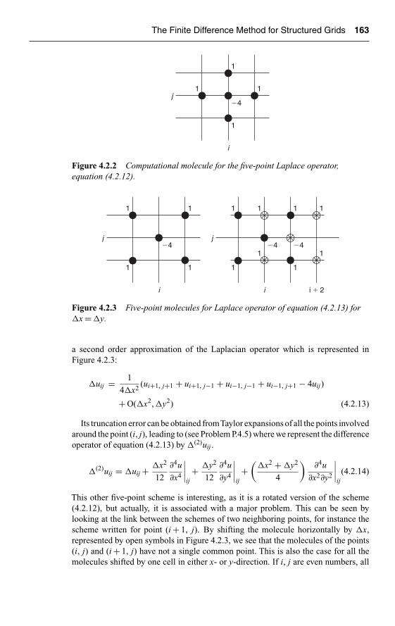
Ch04-H6594.tex 27/4/2007 15: 31 Page 163


j

i

1

1

11

�4

Figure 4.2.2 Computational molecule for the five-point Laplace operator,equation (4.2.12).

j

i

1

1

1

1

�4j

i i � 2

1 1

1

1

1 1

1

1�4 �4

Figure 4.2.3 Five-point molecules for Laplace operator of equation (4.2.13) for�x = �y.

a second order approximation of the Laplacian operator which is represented inFigure 4.2.3:

�uij = 1

4Δx2(ui+1, j+1 + ui+1, j−1 + ui−1, j−1 + ui−1, j+1 − 4uij)

+ O(�x2, �y2) (4.2.13)

Its truncation error can be obtained fromTaylor expansions of all the points involvedaround the point (i, j), leading to (see Problem P.4.5) where we represent the differenceoperator of equation (4.2.13) by �(2)uij .

�(2)uij = �uij + �x2

12

∂4u

∂x4

∣∣∣∣ij+ �y2

12

∂4u

∂y4

∣∣∣∣ij+(

�x2 + �y2

4

)∂4u

∂x2∂y2

∣∣∣∣ij

(4.2.14)

This other five-point scheme is interesting, as it is a rotated version of the scheme(4.2.12), but actually, it is associated with a major problem. This can be seen bylooking at the link between the schemes of two neighboring points, for instance thescheme written for point (i + 1, j). By shifting the molecule horizontally by �x,represented by open symbols in Figure 4.2.3, we see that the molecules of the points(i, j) and (i + 1, j) have not a single common point. This is also the case for all themolecules shifted by one cell in either x- or y-direction. If i, j are even numbers, all

Ch04-H6594.tex 27/4/2007 15: 31 Page 164


j

i

a

a b

bb

b

aa �4

Figure 4.2.4 Nine-point molecule for the Laplace operator (4.2.15) with a + b = 1.

these shifted points will have either i or j uneven. Hence, this total decoupling of thecomputational molecules is called an odd–even decoupling, leading to solutions oneven points which will have different error levels than the solutions on the unevenpoints.

Therefore, this scheme is not recommended.We can define a family of nine-point schemes for the Laplace operator on a uniform

cartesian mesh �x = �y, by the combination

�(3)uij = (a�(1) + b�(2))uij with a + b = 1 (4.2.15)

where we designate the standard five-point scheme of equation (4.2.12) by �(1)uij .Combining these two operators, we obtain (see also Problem P.4.6)

�(3)uij = �uij + �x2

12

[∂4u

∂x4+ ∂4u

∂y4+ 6b

∂4u

∂x2∂y2

]ij

(4.2.16)

The computational molecule associated to this scheme is shown in Figure 4.2.4The particular choice of a = b = 1/2 leads to the well-known scheme of Fig-

ure 4.2.5a, which is also obtained from a Galerkin finite element discretization ofthe Laplace operator on the same mesh, using bilinear quadrilateral elements, asshown in Chapter 5.

With b = 1/3, we obtain the computational molecule of Figure 4.2.5b, which isrecommended by Dahlquist and Bjorck (1974), because the truncation error is equal to

−�x2

12

(∂2

∂x2+ ∂2

∂y2

)2

u = −�x2

12�2u

Hence, the equation �u = λu can be discretized with this nine-point operator

�(3) = ( 23�(1) + 1

3�(2))

and will have a truncation error equal to − λ2�x2

12 uTherefore, the corrected difference scheme

�(3)uij =(

λ + λ2�x2

12

)u

will have a fourth order truncation error.

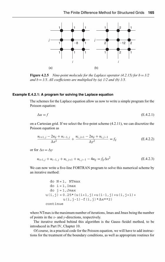
Ch04-H6594.tex 27/4/2007 15: 31 Page 165


j

i

1

1

(a)

1

11

1

11 �8

(b)

j

i

2

2 1

11

1

22 �12

Figure 4.2.5 Nine-point molecule for the Laplace operator (4.2.15) for b = 1/2and b = 1/3. All coefficients are multiplied by (a) 1/2 and (b) 1/3.

Example E.4.2.1: A program for solving the Laplace equation

The schemes for the Laplace equation allow us now to write a simple program for thePoisson equation:

�u = f (E.4.2.1)

on a Cartesian grid. If we select the five-point scheme (4.2.11), we can discretize thePoisson equation as

ui+1, j − 2uij + ui−1, j

�x2+ ui, j+1 − 2uij + ui, j−1

�y2= fij (E.4.2.2)

or for �x = �y

ui+1, j + ui−1, j + ui, j+1 + ui, j−1 − 4uij = fij�x2 (E.4.2.3)

We can now write a five-line FORTRAN program to solve this numerical scheme byan iterative method:

do N = 1, NTmaxdo i = 1,Imaxdo j = 1,Jmax

u(i,j) = 0.25*(u(i+1,j)+u(i-1,j)+u(i,j+1)+u(i,j-1)-f(i,j)*�x**2)

continue

where NTmax is the maximum number of iterations, Imax and Jmax being the numberof points in the x- and y-directions, respectively.

The iterative method behind this algorithm is the Gauss–Seidel method, to beintroduced in Part IV, Chapter 10.

Of course, in a practical code for the Poisson equation, we will have to add instruc-tions for the treatment of the boundary conditions, as well as appropriate routines for

Ch04-H6594.tex 27/4/2007 15: 31 Page 166


reading in the geometrical data and post-processing the results. These additions canrequire many thousands of lines, depending on the level of generality of the Poissonsolver.

But the point we want to make here is that, once the theoretical developments aredone, and this can take many pages of theory, ultimately the code implementing theselected numerical scheme can be very short and simple.

We expect that you will have the opportunity to verify this in the following whenprogramming some of the proposed schemes in the later chapters.

Nonlinear diffusion terms

In the Navier–Stokes equations, the diffusion terms have a more general form com-pared to the Laplace equation when the diffusion coefficients are not constant. Theyappear under the form of the operator �∇(κ �∇u) as shown in Chapter 1. A second orderdiscretization of this operator can be written as follows, introducing the values atmid-points (i ± 1/2, j) and (i, j ± 1/2):

�∇(κ �∇u)ij = 1

�x2(κi+1/2, j(ui+1, j − ui, j) − κi−1/2, j(ui, j − ui−1, j))

+ 1

�y2(κi, j+1/2(ui, j+1 − ui, j) − κi, j −1/2(ui, j − ui, j −1)) (4.2.17)

It is seen that for constant diffusion coefficient κ, we recover the five-point scheme(4.2.11) for Laplace equation.

4.2.2 Mixed Derivatives

Mixed derivatives of any order can be discretized in much the same way by using for∂/∂x and ∂/∂y the various formulas and their possible combinations described above.

The simplest, second order central formula for the mixed derivative is obtainedfrom applying central differences in both directions x and y:

(uxy)ij = ∂

∂x

(ui, j+1 − ui, j−1

2�y+ O(�y2)

)

= 1

4�x�y(ui+1, j+1 − ui−1, j+1 − ui+1, j−1 + ui−1, j−1) + O(�x2, �y2)

(4.2.18)

which is illustrated by the molecule of Figure 4.2.6.Other combinations are possible, for instance by combining a central difference in

the x-direction and a first order forward difference in the y-direction:

(uxy)ij = 1

2�x�y(ui+1, j+1 − ui−1, j+1 − ui+1, j + ui−1, j) + O(�x2, �y) (4.2.19)

which is first order in �y and second order in �x. This formula is represented inFigure 4.2.7.

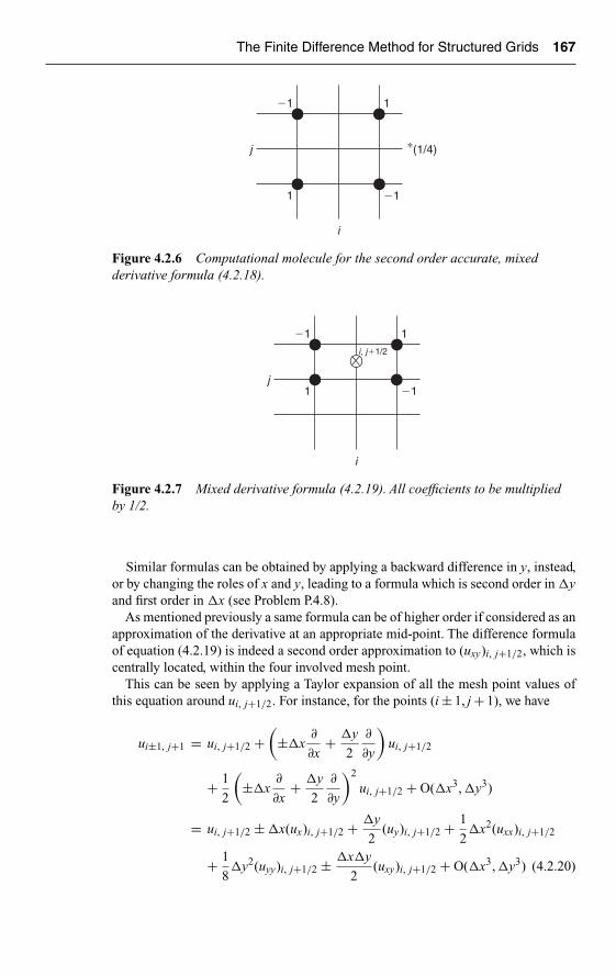
Ch04-H6594.tex 27/4/2007 15: 31 Page 167


j

i

�1

1

�(1/4)

�1

1

Figure 4.2.6 Computational molecule for the second order accurate, mixedderivative formula (4.2.18).

j

i

�1

1

1

�1

i, j�1/2

Figure 4.2.7 Mixed derivative formula (4.2.19). All coefficients to be multipliedby 1/2.

Similar formulas can be obtained by applying a backward difference in y, instead,or by changing the roles of x and y, leading to a formula which is second order in �yand first order in �x (see Problem P.4.8).

As mentioned previously a same formula can be of higher order if considered as anapproximation of the derivative at an appropriate mid-point. The difference formulaof equation (4.2.19) is indeed a second order approximation to (uxy)i, j+1/2, which iscentrally located, within the four involved mesh point.

This can be seen by applying a Taylor expansion of all the mesh point values ofthis equation around ui, j+1/2. For instance, for the points (i ± 1, j + 1), we have

ui±1, j+1 = ui, j+1/2 +(

±�x∂

∂x+ �y

2

∂

∂y

)ui, j+1/2

+ 1

2

(±�x

∂

∂x+ �y

2

∂

∂y

)2

ui, j+1/2 + O(�x3, �y3)

= ui, j+1/2 ± �x(ux)i, j+1/2 + �y

2(uy)i, j+1/2 + 1

2�x2(uxx)i, j+1/2

+ 1

8�y2(uyy)i, j+1/2 ± �x�y

2(uxy)i, j+1/2 + O(�x3, �y3) (4.2.20)

Ch04-H6594.tex 27/4/2007 15: 31 Page 168


j

i

1

1

�1

�1

i�1/2, j�1/2

Figure 4.2.8 Mixed derivative formulas (4.2.23) and (4.2.24).

Similarly for the points (i ± 1, j), we have

ui±1, j = ui, j+1/2 +(

±�x∂

∂x− �y

2

∂

∂y

)ui, j+1/2

+ 1

2

(±�x

∂

∂x− �y

2

∂

∂y

)2

ui, j+1/2 + O(�x3, �y3)

= ui, j+1/2 ± �x(ux)i, j+1/2 − �y

2(uy)i, j+1/2 + 1

2�x2(uxx)i, j+1/2

+ 1

8�y2(uyy)i, j+1/2 ∓ �x�y

2(uxy)i, j+1/2 + O(�x3, �y3) (4.2.21)

By forming the differences of equation (4.2.19), we obtain

(uxy)i, j+1/2 = 1

2�x�y(ui+1, j+1 − ui−1, j+1 − ui+1, j + ui−1, j) + O(�x2, �y2)

(4.2.22)

demonstrating the second order accuracy of this formula.A first order formula in both x and y is obtained from first order forward differences

in both directions, leading to

(uxy)ij = 1

�x�y(ui+1, j+1 − ui, j+1 − ui+1, j + ui, j) + O(�x, �y) (4.2.23)

Observe that the same formula (4.2.23) will give a second order accurate estimationof the mixed derivative taken at the point (i + 1/2, j + 1/2) (see Problem P.4.9) that is

(uxy)i+1/2, j+1/2 = 1

�x�y(ui+1, j+1 − ui, j+1 − ui+1, j + ui, j) + O(�x2, �y2)

(4.2.24)

These formulas are represented on Figure 4.2.8.Applying backward differences in both directions, leads to

(uxy)ij = 1

�x�y(ui−1, j−1 − ui, j−1 − ui−1, j + ui, j) + O(�x, �y) (4.2.25)

Ch04-H6594.tex 27/4/2007 15: 31 Page 169


j

i

�1

1

1

(a) (b)

�1�1 2

�1

j

i

1

1 �1

�1

11 �2

Figure 4.2.9 Second order mixed derivative approximations (a) equation (4.2.26)and (b) equation (4.2.27).

Since the truncation errors of equations (4.2.25) and (4.2.23) are equal but of oppositesigns (see Problem P.4.10) the sum of the two expressions will lead to a second orderaccurate formula for the mixed derivative:

(uxy)ij = 1

2�x�y(ui+1, j+1 − ui, j+1 − ui+1, j + ui−1, j−1 − ui, j−1 − ui−1, j

+ 2ui,j) + O(�x2, �y2) (4.2.26)

This formula is represented in Figure 4.2.9a and, compared to the central approxi-mation (4.2.18) shown in Figure 4.2.6, has a non-zero coefficient for uij . This mightbe advantageous in certain cases by enhancing the weight of the uij coefficients inthe matrix equations obtained after discretization, that is enhancing the diagonaldominance, see for instance O’Carroll (1976).

An alternative to the last formulation is obtained by a different combination offorward and backward differences, leading to the second order approximation for(uxy)ij , shown in Figure 4.2.9b:

(uxy)ij = 1

2�x�y(ui+1, j − ui+1, j−1 + ui, j+1 + ui, j−1 − ui−1, j+1 + ui−1, j

− 2ui, j) + O(�x2, �y2) (4.2.27)

It can also be seen, by adding up the two last expressions, that we recover the fullycentral second order approximation (4.2.18). Many other formulas can be found inthe literature, for instance in Mitchell and Griffiths (1980).

4.3 FINITE DIFFERENCE FORMULAS ON NON-UNIFORM GRIDS

Up to now, we have introduced finite difference formula on uniform grids wherethe distance between adjacent mesh points is constant over the whole grid. In prac-tice however, this will seldom be the case, as more often the grid has to adapt tothe geometrical boundaries or to the flow physics, making uniform grids unpractical.

Ch04-H6594.tex 27/4/2007 15: 31 Page 170


j

j � 1

xi xi � 1

�yj

j � 1

d

Figure 4.3.1 Representative grid in a boundary layer region above a solid wall.The velocity profile is superposed on the grid, which is selected to be uniform in thex-direction and non-uniform in the y-direction.

We refer you to the grid examples shown in the general introduction to this book,where you can observe a selected cross-section of realistic grids.

A very representative example is provided by the grids in boundary layer regionsaround solid surfaces (see Figure 4.3.1). In a laminar boundary layer, it is known fromPrandtl’s analysis that the boundary layer thickness δ over a flat plate scales with xlike the inverse of the square root of the Reynolds number. We refer you to your basiccourse of Fluid Mechanics for the background behind the boundary layer properties.

That is

δ ∼√

νx

U∞= x√

Rexwith Rex = U∞x

ν

where ν is the kinematic viscosity (in m2/s) and U∞ is the velocity outside the bound-ary layer. It is also known that the ratio of the velocity gradients in the normal andstreamwise directions is of the order of the square root of this same Reynolds number:

∂u

∂y

/∂u

∂x∼ √Rex

After having generated a grid, if we wish to ensure that the velocity variations inthe x- and y-directions are of the same order over the mesh distances �x and �y,respectively, we should generate a grid with an aspect ratio �x/�y of the order of

�y

�x∼ 1√

Rex

For a realistic Reynolds number of say, 1 million, this ratio is of the order of 1000!Hence, we would need to generate cells where �y is thousand times smaller than

�x. In practical terms, for a plate of unit length and 101 mesh points in the x-direction,that is �x = 0.01, �y should be of the order of 10−5!

This simple analysis shows that a uniform mesh would require unrealistic small cellsizes, to be equal to the smallest cell size of 10−5, leading to millions of mesh points.

Ch04-H6594.tex 27/4/2007 15: 31 Page 171


i � 2 i � 3i � 1

x

i i � 1

xi�1/2xi�1/2

�xi�1 �xi�2�xi

Figure 4.3.2 Arbitrary mesh point distribution in one-dimensional space x.

Another lesson of this analysis is that we should not generate uniform grids in they-direction, but have �y increase progressively when moving away from the wall asthe intensity of the gradients progressively reduces to values of the same order as inthe x-direction, as shown in Figure 4.3.1.

An approach often used in practice is to define a clustering factor r, such that

yj+1 = y1r j (4.3.1)

This creates mesh cells growing progressively in the y-direction as shown inFigure 4.3.1. Typical values of the clustering factor are r ∼ 1.1–1.5.

Due to the strong gradients in the normal directions, it is essential for reasons ofaccuracy to position at least 10–20 points in the boundary layer regions.

The derivation of accurate difference formulas for non-uniform grids is thereforevery important in CFD, since this is the situation most often found in practice. Hence,great care should be given to the choice of appropriate discretization formulas onthese grids.

It is very essential that you give a serious attention to the related problem of lossof accuracy on non-uniform grids, if either you write your own code, or if you useexisting, commercial or other, CFD codes to study practical fluid problems, whenyou evaluate the results of the simulations.

We will go along the following steps:

• Firstly, derive formulas valid on non-uniform grids.• Secondly, evaluate the loss of accuracy related to the FD formula on non-uniform

grids.• Thirdly, and more importantly, provide guidelines on the grid properties and on

grid quality in order to minimize the errors related to the non-uniform grids.

For one-dimensional non-uniform grids, we can define different types of configu-rations, depending on the way we position the mid-point values and the points wherethe function values are evaluated.

Figure 4.3.2 represents a mesh arrangement, where the points (i ± 1/2) are themid-points of the intervals (i, i ± 1) and is defined as a cell vertex configuration inthe finite volume context. If we consider the cell (i − 1/2, i + 1/2) mesh point i isnot at its center due to the grid non-uniformity. An alternative option, known as cellcentered , is shown in Figure 4.3.3.

In order to derive FD formula for non-uniform mesh sizes in a one-dimensionalspace defined by the grid of Figure 4.3.2, we refer again to theTaylor series expansions,

Ch04-H6594.tex 27/4/2007 15: 31 Page 172


written for the mesh points (i ± 1), (i ± 2):

ui−1 = ui − �xi(ux)i + �x2i

2(uxx)i − �x3

i

6(uxxx)i + · · ·

ui+1 = ui + �xi+1(ux)i + �x2i+1

2(uxx)i + �x3

i+1

6(uxxx)i + · · ·

ui−2 = ui − (�xi + �xi−1)(ux)i + (�xi + �xi−1)2

2(uxx)i

− (�xi + �xi−1)3

6(uxxx)i + · · ·

ui+2 = ui + (�xi+1 + �xi+2)(ux)i + (�xi+1 + �xi+2)2

2(uxx)i

+ (�xi+1 + �xi+2)3

6(uxxx)i + · · · (4.3.2)

where the notation

�xi = xi − xi−1 (4.3.3)

is introduced.In presence of a non-uniform grid, many options are open for difference formulas,

generalizing the formulas derived in Section 4.3.1 for uniform grids.The examples derived in the following sections are representative of the additional

variety that arises when the grid has non-constant cell sizes.

4.3.1 Difference Formulas for First Derivatives

A one-sided, first order, formulas for the first derivative can be defined as follows:

Forward difference

(ux)i = ui+1 − ui

�xi+1− �xi+1

2(uxx)i (4.3.4)

Backward difference

(ux)i = ui − ui−1

�xi+ �xi

2uxx (4.3.5)

Central differencesIf we take the simple average of the two formulas above, which is often done in finitedifference computer programs, as well as in finite volume or finite element methods,we obtain a form of central difference,

(ux)i = 1

2

[ui+1 − ui

�xi+1+ ui − ui−1

�xi

]− �xi+1 − �xi

4(uxx)i

− �x2i + �x2

i+1

12(uxxx)i (4.3.6)

Ch04-H6594.tex 27/4/2007 15: 31 Page 173


This formula reduces to equation (4.1.7) on a uniform grid, but the important obser-vation is the appearance of the third term, which is of first order if the difference inadjacent cell sizes (�xi+1 − �xi) remains finite. If the mesh size varies abruptly, forinstance if �xi+1 ∼ 2�xi the above formula will be only first order accurate.

This is a general property of finite difference approximations on non-uniformmeshes. If the mesh size does not vary smoothly, a loss of accuracy is unavoidable.

We will come back to this very important point at the end of this section.A more elaborate formula can be defined, by combining formulas (4.3.4) and (4.3.5)

in order to eliminate the first order truncation error, referring to the Taylor expansionsof equation (4.3.2). This leads to the following formula (see also Problems P.4.10 andP.4.13):

(ux)i = 1

�xi+1 + �xi

[�xi

�xi+1(ui+1 − ui) + �xi+1

�xi(ui − ui−1)

]

− �xi�xi+1

6(uxx)i (4.3.7)

which is second order for any grid size distribution. The price to pay for this propertyis a formula which is more complicated as it is formed by a weighted average of theone-sided formulas, based on the sizes of the adjacent cells.

It has to be mentioned here that these weighted averages are very difficult to gener-alize in two or three dimensions, while the simple average of formula (4.3.6) remainsstraightforward in multidimensional structured or unstructured grids. For practicalapplications, we have to restrict ourselves to simple expressions, easily extendable toarbitrary dimensions.

This explains why this simple average is most widely applied, with the risk ofreduction of the order of accuracy. Therefore, guidelines in order to minimize theunfavorable effect of this approach are required and will be given in the following.

4.3.1.1 Conservative FD formulas

Referring to the grid distribution of Figure 4.3.2, an alternative expression for thefirst derivative can be written under the following form, instead of (4.3.6), based onthe function values at the mid-points (i ± 1/2):

(ux)i = ui+1/2 − ui−1/2

xi+1/2 − xi−1/2

xi+1/2 − xi−1/2 = 1

2(�xi + �xi+1) = 1

2(xi+1 − xi−1) (4.3.8)

This formula is also said to be conservative.We have mentioned in Chapter 1, the importance of the conservative form of the

conservation laws of Fluid Mechanics. This important property has also to be satisfiedat the discrete level, that is after the discretization of the equations and the conservativediscretizations will be extensively discussed in general terms in the next Chapter 5,in relation with the finite volume method. However, we wish to provide you alreadyhere with a first glimpse at these essential properties.

Ch04-H6594.tex 27/4/2007 15: 31 Page 174


Stated here in relation with structured grids, a difference formula is said to bein conservative form, if it is written as the difference of two quantities defined onopposite cell-faces, where in addition the cell-face quantities are not dependent onthe cell in which the face is considered.

Observe that equation (4.3.7), although having second order accuracy does notsatisfy this condition of conservative discretization.

Formula (4.3.8) is at best of first order accuracy on a non-uniform grid, since pointi is not at the center of the interval (i − 1/2, i + 1/2) (see Problem P.4.11). This isreadily seen from the Taylor expansions (4.3.2), leading to the formula:

(ux)i = ui+1/2 − ui−1/2

xi+1/2 − xi−1/2− �xi+1 − �xi

4(uxx)i

− �x2i+1 − �xi+1�xi + �x2

i

24(uxxx)i (4.3.9)

Applying the approximation ui+1/2 = (ui + ui+1)/2 to equation (4.3.8), leads to thefollowing central difference formula:

(ux)i = ui+1 − ui−1

xi+1 − xi−1(4.3.10)

Performing a Taylor expansion, the truncation error becomes

(ux)i = ui+1 − ui−1

xi+1 − xi−1− �xi+1 − �xi

2(uxx)i

− �x2i+1 − �xi+1�xi + �x2

i

6(uxxx)i (4.3.11)

The same comments as stated in relation with formula (4.3.6) are valid here, namelythat this formula is only first order accurate on a general non-uniform grid, unless thevariation of the grid size is very smooth, namely (�xi+1 − �xi) ∼ O(�x2).

Observe also that the first term of the truncation error of formula (4.3.9) is lowerthan the corresponding term of formula (4.3.11) showing that on an irregular gridthis formula will be slightly more accurate.

4.3.2 A General Formulation

The general expression (4.3.8) can be applied to generate a whole family of FDformulas by defining a general interpolation rule for the cell-face values. The functionvalues at the cell ‘faces’ (i ± 1/2) are defined by a linear interpolation from the meshpoint values, following:

ui+1/2 = ui + αi(ui+1 − ui) + βi(ui − ui−1) (4.3.12)

General conditions can be written for this interpolation formula to be at least secondorder accurate (see Problem P.4.17). On a uniform mesh, the condition reduces toαi + βi = 1/2.

Ch04-H6594.tex 27/4/2007 15: 31 Page 175


On a uniform mesh, αi = 1/2, βi = 0, corresponding to the ‘central’ choiceui+1/2 = (ui + ui+1)/2, reproduces the second order central difference (4.1.7); thechoice αi = βi = 0 reproduces the first order backward difference (4.1.6), whileselecting αi = 0, βi = 1/2 leads to the second order backward difference (4.1.16).

On the non-uniform mesh, the backward difference obtained with αi = βi = 0 givesthe following expression, as an alternative to equation (4.3.5):

(ux)i = ui − ui−1

(xi+1 − xi−1)/2(4.3.13)

with the truncation error

ui − ui−1

(xi+1 − xi−1)/2= �xi+1 + �xi

2�xi(ux)i − �xi

2(uxx)i + �x2

i

6(uxxx)i + O(�x3)

(4.3.14)

The first term on the right-hand side has a coefficient different from one on a non-uniform grid, showing that this backward difference formula reduces to zero orderof accuracy on a general non-uniform grid and is therefore not acceptable.

Similarly, the option αi = 0, βi = 1/2, which gives the second order backwarddifference (4.1.16) on a uniform mesh, leads to the formula:

(ux)i = 3ui − 4ui−1 + ui−2

(xi+1 − xi−1)/2(4.3.15)


3ui − 4ui−1 + ui−2

(xi+1 − xi−1)/2= +3�xi − �xi−1

�xi + �xi+1(ux)i

− (�xi + �xi−1)2 − 4�x2i

2(�xi + �xi+1)(uxx)i + O(�x2) (4.3.16)

Hence, this formula is also of zero order of accuracy on an arbitrary grid, althoughit is second order on a uniform mesh. Again, this formula should not be used.

The main observation is that difference formulas generally can loose at least oneorder of accuracy, and sometimes two, on general non-uniform grids.

In order to achieve second order accuracy on arbitrary grids, one has to considerdifference formulas that are formally of higher order on uniform grids, involvingadditional mesh points.

Let us therefore consider a family of finite difference formulas for derivativesat point i on a four point support, whereby point (i − 2) is added to the basic set(i − 1, i, i + 1). Hence, we look for an expression of the form:

(ux)i = aui−2 + bui−1 + cui + dui+1

(�xi + �xi+1)/2(4.3.17)

Ch04-H6594.tex 27/4/2007 15: 31 Page 176


Applying the procedure of Section 4.1.2 based on the Taylor expansions (4.3.2), weobtain the following conditions for a second order accurate formula:

a + b + c + d = 0

d�xi+1 − b�xi − a(�xi + �xi−1) = 1

2(�xi+1 + �xi) (4.3.18)

d�x2i+1 + b�x2

i + a(�xi + �xi−1)2 = 0

or, defining the mesh ratio ri = �xi+1/�xi

a + b + c + d = 0

dri − b − a

(1 + 1

ri−1

)= 1

2(1 + ri) (4.3.19)

dr2i + b + a

(1 + 1

ri−1

)2

= 0

These relations define a one-parameter difference formula of second order accuracyfor the first derivative (see Problem P.4.13).

On a uniform mesh, the formulas are defined by the coefficients (a, b, c, d) =(a, −3a − 1/2, 3a, −a + 1/2) and the value a = 1/6 leads to the unique third orderformula on a uniform grid.

Observe that the three point formula with a = 0 leads to the unique second orderscheme (4.3.7), which is not conservative, since it cannot be written under theform (4.3.8).

The combination of second order and conservativity therefore requires an additionaldegree of freedom, provided by the coefficient a. Assuming the interpolation relation(4.3.12), formula (4.3.8) can be written under the form (4.3.17) and identifying thecoefficients leads to

a = βi−1

b = −(1 + βi − αi−1 + βi−1)(4.3.20)

c = 1 + βi − αi−1 − αi

d = αi

This has to be seen as a set of equations for the unknown functions α(r) and β(r), withαi = α(ri) and βi = β(ri), since these interpolation coefficients are non-dimensionalfunctions of �xi and �xi+1. Similarly, αi−1 = α(ri−1) and βi−1 = β(ri−1). Eliminat-ing b from the two last equations (4.3.19) leads to the following relation betweenαi = α(ri) and βi−1 = β(ri−1):

d = α(ri) = 1

2ri− β(ri−1)(1 + ri−1)

r2i−1

1

ri(1 + ri)(4.3.21)

The terms depending on ri−1 have to be equal to a constant K, since ri and ri−1 areindependent variables. Hence, we have

β(r) = Kr2

(1 + r)α(r) = 1 + r − 2K

2r(1 + r)(4.3.22)

Ch04-H6594.tex 27/4/2007 15: 31 Page 177


The constant K is easily determined, for instance by combining the second equation(4.3.19) with the second equation (4.3.20), leading to the unique value K = 1/2. Thischoice of interpolation coefficients, namely

βi ≡ β(ri) = r2i

2(1 + ri)αi ≡ α(ri) = 1

2(1 + ri)(4.3.23)

provides a second order, conservative formula for the first derivative on an arbitrarymesh (See Problem P.4.15).

It has been applied to the numerical simulation of two-dimensional nonlinear wavesolutions of the Euler and Navier–Stokes equations by Cain and Bush (1994), showingexcellent accuracy on stretched grids.

On a uniform mesh, this formula reduces to

(ux)i = ui+1 + 3ui − 5ui−1 + ui−2

4�x+ �x2

12(uxxx)i − �x3

8(uxxxx)i (4.3.24)

and is only second order accurate.Note that on this fourth-point mesh, a formula with third order accuracy can be

obtained by adding this condition to the system (4.3.19) (see Problem P.4.16). Thisformula is not conservative on a general grid and reduces to the following formulaon a uniform grid:

(ux)i = 2ui+1 + 3ui − 6ui−1 + ui−2

6�x− �x3

12(uxxxx)i (4.3.25)

Two-dimensional extensions on non-uniform Cartesian grids are straightforward,applying the ratios (4.3.23) in each direction separately.

Second derivatives

A three-point, central difference formula for the second derivative is obtained in thesimplest way by subtracting formulas (4.3.4) and (4.3.5), leading to

(uxx)i = 2

�xi+1 + �xi

[(ui+1 − ui)

�xi+1− (ui − ui−1)

�xi

]

+ �xi+1 − �xi

3(uxxx)i − �x3

i+1 + �x3i

12(�xi+1 + �xi)

(∂4u

∂x4

)i

(4.3.26)

On a uniform grid, this formula reduces to the second order accurate finite difference(4.1.18). However, as with equation (4.3.6), the presence of a truncation error pro-portional to the difference of two consecutive mesh lengths reduces the accuracy tofirst order, under similar conditions as mentioned above.

4.3.3 Cell-Centered Grids

Another popular choice for a finite volume discretization consists in selecting themesh points as the cell ‘faces’, which are then labeled at half-integer index values

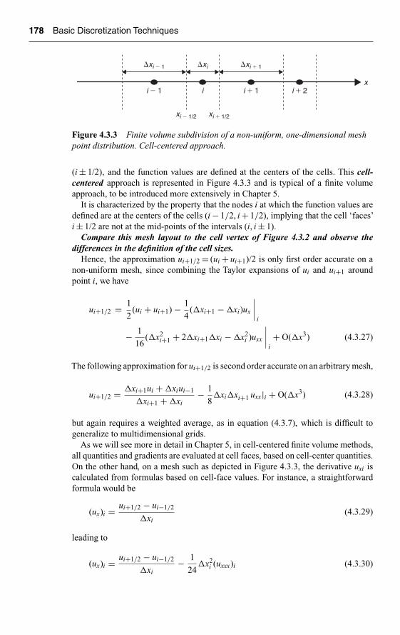
Ch04-H6594.tex 27/4/2007 15: 31 Page 178


i � 1 i � 2i � 1 i

�xi � 1 �xi � 1�xi

xi � 1/2 xi � 1/2

x

Figure 4.3.3 Finite volume subdivision of a non-uniform, one-dimensional meshpoint distribution. Cell-centered approach.

(i ± 1/2), and the function values are defined at the centers of the cells. This cell-centered approach is represented in Figure 4.3.3 and is typical of a finite volumeapproach, to be introduced more extensively in Chapter 5.

It is characterized by the property that the nodes i at which the function values aredefined are at the centers of the cells (i − 1/2, i + 1/2), implying that the cell ‘faces’i ± 1/2 are not at the mid-points of the intervals (i, i ± 1).

Compare this mesh layout to the cell vertex of Figure 4.3.2 and observe thedifferences in the definition of the cell sizes.

Hence, the approximation ui+1/2 = (ui + ui+1)/2 is only first order accurate on anon-uniform mesh, since combining the Taylor expansions of ui and ui+1 aroundpoint i, we have

ui+1/2 = 1

2(ui + ui+1) − 1

4(�xi+1 − �xi)ux

∣∣∣∣i

− 1

16(�x2

i+1 + 2�xi+1�xi − �x2i )uxx

∣∣∣∣i+ O(�x3) (4.3.27)

The following approximation for ui+1/2 is second order accurate on an arbitrary mesh,

ui+1/2 = �xi+1ui + �xiui−1

�xi+1 + �xi− 1

8�xi�xi+1 uxx|i + O(�x3) (4.3.28)

but again requires a weighted average, as in equation (4.3.7), which is difficult togeneralize to multidimensional grids.

As we will see more in detail in Chapter 5, in cell-centered finite volume methods,all quantities and gradients are evaluated at cell faces, based on cell-center quantities.On the other hand, on a mesh such as depicted in Figure 4.3.3, the derivative uxi iscalculated from formulas based on cell-face values. For instance, a straightforwardformula would be

(ux)i = ui+1/2 − ui−1/2

�xi(4.3.29)

leading to

(ux)i = ui+1/2 − ui−1/2

�xi− 1

24�x2

i (uxxx)i (4.3.30)

Ch04-H6594.tex 27/4/2007 15: 31 Page 179


based on the Taylor expansion of ui±1/2 around point i. However, in practice, theseare not the values at hand during a computation. If the values of formula (4.3.27) areused, a more straightforward formula would be

(ux)i = ui+1 − ui−1

�xi + (�xi+1 + �xi−1)/2(4.3.31)

leading to

(ux)i = ui+1 − ui−1

�xi + (�xi+1 + �xi−1)/2− 1

4(�xi+1 − �xi−1)(uxx)i

− 1

24(�x2

i+1 − �xi−1�xi+1 + �x2i + �xi−1�xi + �x2

i−1

+ �xi�xi+1)(uxxx)i (4.3.32)

which is first order on the non-uniform mesh.

4.3.4 Guidelines for Non-uniform Grids

The errors due to the grid non-uniformity will be minimized for smoothly varyinggrids, defined in such a way that the size variation between consecutive cells is ofsecond order in the grid size. That is, if

�xi+1 − �xi = O(�x2i ) (4.3.33)

then formulas such as (4.3.6), (4.3.11) will be of second order accuracy, as on auniform grid.

However, a grid variation, such as defined by equation (4.3.1), will not satisfy thiscondition, since this grid variation leads to, translated in the x-direction:

�xi+1 − �xi = �xi(r − 1) = O(�xi) (4.3.34)

Hence, this will reduce the formulas, such as (4.3.6), (4.3.11) to first order accuracy.However, as the coefficient is multiplied by (r − 1), which is generally a small number,the error could remain small and acceptable. In addition, keep in mind that these errorsare proportional to some derivative, second or higher, of the function u. Therefore,the impact of the errors due to the mesh non-uniformity will depend on the localflow properties. In regions where the flow variation is smooth, this impact will bereduced and could eventually be neglected. On the other hand, in regions with strongvariations, where the gradients are important these additional errors can becomecritical and have to be severely controlled.

Additional guidelines can be stated here:

• Avoid discontinuities in grid size of adjacent cells.• Always use laws for the grid size variation, defined by analytical, continuous

functions of the associated coordinate, to minimize the numerical error. For

Ch04-H6594.tex 27/4/2007 15: 31 Page 180


instance, clustering laws such as �xi+1 = r�xi where r is a constant factor,typically 1.1–2 are widely used.

• Pay a particular attention to the grid smoothness and grid density in regions ofstrong flow variations, for instance around a leading edge of an airfoil profile,or around stagnation points.

A4.4 GENERAL METHOD FOR FINITE DIFFERENCE FORMULAS

The following two sections are of interest for more advanced applications of finitedifference methods and cover a methodology for the generation of arbitrary FD for-mulas with prescribed order (Section A4.4) and the generation of high order compact,implicit finite difference formulas (Section A4.5).

They are marked by the letter A, for ‘Advanced’ and can be included or not in thebasic introductory course.

General procedures developed in order to generate finite difference formulas toany order of accuracy and a general theory can be found in Hildebrand (1956). Thisapproach is based on the definition of the following difference operators:

Displacement operator E

Eui = ui+1 (4.4.1a)

Forward difference operator δ+

δ+ui = ui+1 − ui (4.4.1b)

Backward difference operator δ−

δ−ui = ui − ui−1 (4.4.1c)

Central difference operator δ

δui = ui+1/2 − ui−1/2 (4.4.1d)

Central difference operator δ

δui = 1

2(ui+1 − ui−1) (4.4.1e)

Averaging operator μ

μui = 1

2(ui+1/2 + ui−1/2) (4.4.1f )

Ch04-H6594.tex 27/4/2007 15: 31 Page 181


Differential operator D

Du = ux ≡ ∂u

∂x(4.4.1g)

From these definitions some obvious relations can be defined between these operators,such as

δ+ = E − 1 (4.4.2)

δ− = 1 − E−1 (4.4.3)

where the inverse displacement operator E is introduced, defined by

E−1ui = ui−1 (4.4.4)

This leads to the following relations

δ− = E−1δ+ (4.4.5)

and

δ+δ− = δ−δ+ = δ+ − δ− = δ2 (4.4.6)

With the general definition, n being positive or negative:

Enui = ui+n (4.4.7)

we also have

δ = E1/2 − E−1/2 (4.4.8)

δ = 1

2(E − E−1) (4.4.9)

and

μ = 1

2(E1/2 + E−1/2) (4.4.10)

Any of the above difference operators taken to a given power n, is interpreted as nrepeated actions of this operator. For instance:

δ+2 = δ+δ+ = E2 − 2E + 1 (4.4.11)

δ+3 = (E − 1)3 = E3 − 3E2 + 3E − 1 (4.4.12)

A4.4.1 Generation of Difference Formulas for First Derivatives

The key to the operator technique for generating finite difference formulas lies in therelation between the derivative operator D and the finite displacement operator E.

Ch04-H6594.tex 27/4/2007 15: 31 Page 182


This relation is obtained from the Taylor expansion:

u(x + �x) = u(x) + �x ux(x) + �x2

2! uxx(x) + �x3

3! uxxx(x) + · · · (4.4.13)

or in operator form:

Eu(x) =(

1 + �xD + (�xD)2

2! + (�xD)3

3! + · · ·)

u(x) (4.4.14)

This last relation can be written formally as

Eu(x) = e�xDu(x) (4.4.15)

and therefore one has symbolically

E = e�xD (4.4.16)

This relation has to be interpreted as giving identical results when acting on theexponential function eax and on any polynomial of degree n. In this latter case, theexpansion on the right-hand side has only n terms and therefore all the expressionsto be defined in the following are exact up to n terms for polynomials of degree n.

The basic operation is then to use equation (4.4.16) in the inverse way, leading to

�xD = ln E (4.4.17)

A4.4.1.1 Forward differences

Formulas for forward differences are obtained by introducing the relation (4.4.3)between E and the forward operator δ+. We obtain after a formal development of theln function:

�xD = ln E = ln (1 + δ+)

= δ+ − δ+2

2+ δ+3

3− δ+4

4+ · · · (4.4.18)

The order of accuracy of the approximation increases with the number of terms kept inthe right-hand side. The first neglected term gives the truncation error. For instance,keeping the first term only, leads to the first order formula (4.1.5) and a truncationerror equal to (�x uxx/2). If the first two terms are considered, we obtain the secondorder formula (4.1.17) with the truncation error (�x2uxxx/3):

(ux)i = −3ui + 4ui+1 − ui+2

2�x+ �x2

3uxxx (4.4.19)

Hence, this relation leads to the definition of various forward finite difference formulasfor the first derivative with increasing order of accuracy. As the forward difference

Ch04-H6594.tex 27/4/2007 15: 31 Page 183


operator can be written as δ+ = �x ux + O(�x2), the first neglected operator δ+n isof order n showing that the associated truncation error is O(�xn−1).

A4.4.1.2 Backward differences

Similarly, backward difference formulas can be obtained with increasing order ofaccuracy, by application of the relation (4.4.3):

�xD = ln E = − ln (1 − δ−)

= δ− + δ−2

2+ δ−3

3+ δ−4

4+ · · · (4.4.20)

To second order accuracy we have

(ux)i = Dui = 3ui − 4ui−1 + ui−2

2�x+ �x2

3uxxx (4.4.21)

A4.4.1.3 Central differences

Central difference formulas are obtained from equation (4.4.8)

δui = ui+1/2 − ui−1/2 = (E1/2 − E−1/2)ui

and therefore

δ = e�xD/2 − e−�xD/2 = 2 sin h

(�xD

2

)(4.4.22)

which, through inversion, leads to

�xD = 2 sin h−1δ/2 = 2

[δ

2− 1

2 · 3

(δ

2

)3

+ 1 · 3

2 · 4 · 5

(δ

2

)5

− 1 · 3 · 5

2 · 4 · 6 · 7

(δ

2

)7

+ · · ·]

= δ − δ3

24+ 3δ5

640− 5δ7

7168+ · · · (4.4.23)

This formula generates a family of central difference approximations to the firstorder derivative (ux)i based on the values of the function u at half-integer mesh pointlocations. By keeping only the first term, we obtain, with second order accuracy

(ux)i = ui+1/2 − ui−1/2

�x− �x2

24uxxx (4.4.24)

Keeping the first two terms, we obtain a fourth order accurate approximation

(ux)i = −ui+3/2 + 27ui+1/2 − 27ui−1/2 + ui−3/2

24�x+ 3

640�x4 ∂5u

∂x5(4.4.25)

Ch04-H6594.tex 27/4/2007 15: 31 Page 184


To derive central differences involving only integer mesh points, we could apply theabove procedure to the operator δ. From equation (4.4.9) we have

δ = 1

2(E − E−1) = 1

2(e�xD − e−�xD) = sin h(�xD) (4.4.26)

and therefore, in function of δ,

�xD = sin h−1δ

= δ − δ3

6+ 3

2 · 4 · 5δ5 + · · · (4.4.27)

This formula can be used to replace equation (4.4.23) for the central difference at pointi. However, although the first term is the second order central difference approximation(4.1.7), the next term leads to a fourth order formula for (ux)i involving the four pointsi − 3, i − 1, i + 1, i + 3. This is of no interest for numerical computations since wewould expect a fourth order formula for (ux)i to involve the points i − 2, i − 1, i + 1,i + 2. This can be obtained from the identity:

μ2 = 1 + δ2

4(4.4.28)

After multiplication of equation (4.4.23) by

1 = μ

(1 + δ2

4

)−1/2

= μ

(1 − δ2

8+ 3δ4

128− 5δ6

1024+ · · ·

)(4.4.29)

we obtain the relation

�xD = μ

(δ − 1

3!δ3 + 1222

5! δ5 − · · ·)

= δ

(1 − δ2

3! + 22

5! δ4 − 22 · 32

7! δ6 + · · ·)

(4.4.30)

Hence, we obtain the following second and fourth order accurate central differenceapproximations to the derivative (ux)i, with integer mesh point values:

(ux)i = ui+1 − ui−1

2�x− �x2

6uxxx (4.4.31)

and

(ux)i = −ui+2 + 8ui+1 − 8ui−1 + ui−2

2�x+ �x4

30

∂5u

∂x5(4.4.32)

A4.4.2 Higher Order Derivatives

Applying the operator technique, an unlimited number of finite difference formu-las can be applied to obtain second and higher order derivatives. From equation

Ch04-H6594.tex 27/4/2007 15: 31 Page 185


(4.4.18) we have the one-sided, forward difference formula, see for instanceAmes (1977):

(∂nu

∂xn

)i

= Dnui = 1

�xn[ln(1 + δ+)]nui

= δ+n

�xn

[1 − n

2δ+ + n(3n + 5)

24δ+2 − n(n + 2)(n + 3)

48δ+3 + · · ·

]

(4.4.33)

In terms of the backward difference operator δ−, we have

(∂nu

∂xn

)i

= − 1

�xn[ln(1 − δ−)]nui

= 1

�xn

(δ− + δ−2

2+ δ−3

3+ δ−4

4+ · · ·

)n

ui

= δ−n

�xn

[1 + n

2δ− + n(3n + 5)

24δ−2 + n(n + 2)(n + 3)

48δ−3 + · · ·

]ui

(4.4.34)

Central difference formulas for higher order derivatives can also be obtained,through

Dnui =(

2

�xsin h−1δ/2

)n

ui

= 1

�xn

[δ − δ3

24+ 3

640δ5 − 5

7168δ7 + · · ·

]n

ui

= 1

�xnδn[1 − n

24δ2 + n

5760(22 + 5n)δ4

− n

45

(5

7+ n − 1

5+ (n − 1)(n − 2)

81

)δ6 + · · ·

]ui (4.4.35)

For n even, this equation generates difference formulas with the function values atthe integer mesh points. For n uneven, the difference formulas involve points at half-integer mesh points. To involve only points at integer values of i for n uneven wedefine, using equation (4.4.28):

Dnui = μ[1 + δ2/4

]1/2

(2

�xsin h−1δ/2

)n

ui

= μ

�xnδn[

1 − n + 3

24δ2 + (5n + 27)(n + 5)

5760δ4 + · · ·

]ui (4.4.36)

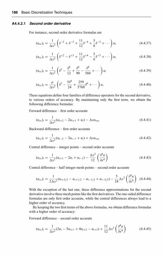
Ch04-H6594.tex 27/4/2007 15: 31 Page 186


A4.4.2.1 Second order derivative

For instance, second order derivative formulas are

(uxx)i = 1

�x2

(δ−2 + δ−3 + 11

12δ−4 + 5

6δ−5 + · · ·

)ui (4.4.37)

(uxx)i = 1

�x2

(δ+2 − δ+3 + 11

12δ+4 − 5

6δ+5 + · · ·

)ui (4.4.38)

(uxx)i = 1

�x2

(δ2 − δ4

12+ δ6

90− δ8

560+ · · ·

)ui (4.4.39)

(uxx)i = μ

�x2

(δ2 − 5δ4

24+ 259

5760δ6 + · · ·

)ui (4.4.40)

These equations define four families of difference operators for the second derivative,to various orders of accuracy. By maintaining only the first term, we obtain thefollowing difference formulas:

Forward difference – first order accurate

(uxx)i = 1

�x2(ui+2 − 2ui+1 + ui) − �xuxxx (4.4.41)

Backward difference – first order accurate

(uxx)i = 1

�x2(ui−2 − 2ui−1 + ui) + �xuxxx (4.4.42)

Central difference – integer points – second order accurate

(uxx)i = 1

�x2(ui+1 − 2ui + ui−1) − �x2

12

(∂4u

∂x4

)(4.4.43)

Central difference – half integer mesh points – second order accurate

(uxx)i = 1

2�x2(ui+3/2 − ui+1/2 − ui−1/2 + ui−3/2) − 5

24�x2

(∂4u

∂x4

)(4.4.44)

With the exception of the last one, these difference approximations for the secondderivative involve three mesh points like the first derivatives. The one-sided differenceformulas are only first order accurate, while the central differences always lead to ahigher order of accuracy.

By keeping the two first terms of the above formulas, we obtain difference formulaswith a higher order of accuracy:

Forward difference – second order accurate

(uxx)i = 1

�x2(2ui − 5ui+1 + 4ui+2 − ui+3) + 11

12�x2

(∂4u

∂x4

)(4.4.45)

Ch04-H6594.tex 27/4/2007 15: 31 Page 187


Backward difference – second order accurate

(uxx)i = 1

�x2(2ui − 5ui−1 + 4ui−2 − ui−3) − 11

12�x2

(∂4u

∂x4

)(4.4.46)

Central difference – integer points – fourth order accurate

(uxx)i = 1

12�x2(−ui+2 + 16ui+1 − 30ui + 16ui−1 − ui−2) + �x4

90

(∂6u

∂x6

)

(4.4.47)

Central difference – half-integer mesh points – fourth order accurate

(uxx)i = 1

48�x2(−5ui+5/2 + 39ui+3/2 − 34ui+1/2 − 34ui−1/2

+ 39ui−3/2 − 5ui−5/2) + 259

5760�x4

(∂6u

∂x6

)(4.4.48)

This last formula is of little practical use since it requires six mesh points to obtaina fourth order accurate approximation to the second derivative at point i, while theprevious formula (4.4.47) requires only four mesh points.

A more complex operator, often occurring in second order differential problems is∂x[k(x)∂xu]. A central difference formula of second order accuracy with three meshpoints is given by

∂

∂x

[k(x)

∂

∂x

]ui = 1

�x2δ+(k1−1/2δ

−)ui + O(�x2) (4.4.49)

which takes the explicit form

∂

∂x

[k(x)

∂

∂x

]ui = 1

�x2[ki+1/2(ui+1 − ui) − ki−1/2(ui − ui−1)] + O(�x2)

(4.4.50)An equivalent formula is obtained by inverting the forward and backward

∂

∂x

[k(x)

∂

∂x

]ui = 1

�x2δ−(k1+1/2δ

+)ui + O(�x2) (4.4.51)

leading to the same expression (4.4.50).

A4.4.2.2 Third order derivatives

Approximations for third derivatives are obtained from the above general expressions.To the lowest orders of accuracy one has the following difference formulas:

Forward difference(

∂3u

∂x3

)i

≡ (uxxx)i

= 1

�x3(ui+3 − 3ui+2 + 3ui+1 − ui) − �x

2

(∂4u

∂x4

)(4.4.52)

Ch04-H6594.tex 27/4/2007 15: 31 Page 188


or with the second order accuracy

(uxxx)i = 1

2�x3(−3ui+4 + 14ui+3 − 24ui+2 + 18ui+1 − 5ui) + 21

12�x2

(∂5u

∂x5

)

(4.4.53)

Backward difference

(uxxx)i = 1

�x3(ui − 3ui−1 + 3ui−2 − ui−3) + �x

2

(∂4u

∂x4

)(4.4.54)

or with second order accuracy

(uxxx)i = 1

2�x3(5ui − 18ui−1 + 24ui−2 − 14ui−3 + 3ui−4) − 21

12�x2

(∂5u

∂x5

)

(4.4.55)

Central difference – half-integer points

(uxxx)i = 1

�x3(ui+3/2 − 3ui+1/2 + 3ui−1/2 − ui−3/2) − �x2

8

(∂5u

∂x5

)(4.4.56)

This is a second order accurate approximation to the third derivative, and a fourthorder accuracy is obtained from the following formula:

(uxxx)i = 1

8�x3(−ui+5/2 + 13ui+3/2 − 34ui+1/2 + 34ui−1/2

− 13ui−3/2 + ui−5/2) + 37

1920�x4

(∂7u

∂x7

)(4.4.57)

Central difference – integer mesh point

(uxxx)i = 1

2�x3(ui+2 − 2ui+1 + 2ui−1 − ui−2) − �x2

4

(∂5u

∂x5

)(4.4.58)

or with fourth order accuracy

(uxxx)i = 1

8�x3(−ui+3 + 8ui+2 − 13ui+1 + 13ui−1 − 8ui−2 + ui−3)

+ 7

120�x4

(∂7u

∂x7

)(4.4.59)

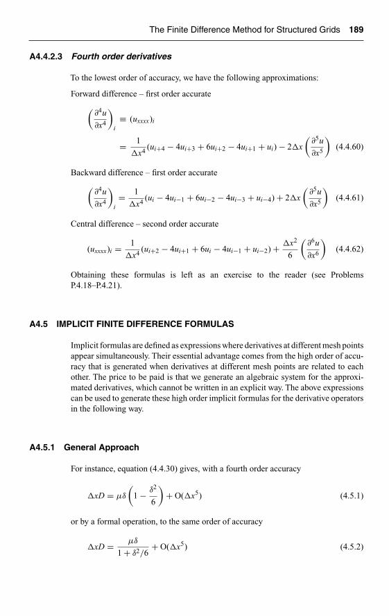
Ch04-H6594.tex 27/4/2007 15: 31 Page 189


A4.4.2.3 Fourth order derivatives

To the lowest order of accuracy, we have the following approximations:

Forward difference – first order accurate

(∂4u

∂x4

)i

≡ (uxxxx)i

= 1

�x4(ui+4 − 4ui+3 + 6ui+2 − 4ui+1 + ui) − 2�x

(∂5u

∂x5

)(4.4.60)

Backward difference – first order accurate

(∂4u

∂x4

)i= 1

�x4(ui − 4ui−1 + 6ui−2 − 4ui−3 + ui−4) + 2�x

(∂5u

∂x5

)(4.4.61)

Central difference – second order accurate

(uxxxx)i = 1

�x4(ui+2 − 4ui+1 + 6ui − 4ui−1 + ui−2) + �x2

6

(∂6u

∂x6

)(4.4.62)

Obtaining these formulas is left as an exercise to the reader (see ProblemsP.4.18–P.4.21).

A4.5 IMPLICIT FINITE DIFFERENCE FORMULAS

Implicit formulas are defined as expressions where derivatives at different mesh pointsappear simultaneously. Their essential advantage comes from the high order of accu-racy that is generated when derivatives at different mesh points are related to eachother. The price to be paid is that we generate an algebraic system for the approxi-mated derivatives, which cannot be written in an explicit way. The above expressionscan be used to generate these high order implicit formulas for the derivative operatorsin the following way.

A4.5.1 General Approach

For instance, equation (4.4.30) gives, with a fourth order accuracy

�xD = μδ

(1 − δ2

6

)+ O(�x5) (4.5.1)

or by a formal operation, to the same order of accuracy

�xD = μδ

1 + δ2/6+ O(�x5) (4.5.2)

Ch04-H6594.tex 27/4/2007 15: 31 Page 190


This formula is a rational fraction or PADE differencing approximation, Kopal (1961).The interpretation of these two last formulas are quite distinct from each other.

Equation (4.5.1), applied to ui leads to the fourth order formula (4.4.32), whileequation (4.5.2) is to be interpreted after multiplication of both sides by the operator(1 + δ2/6):

(1+δ2/6)Dui = 1

6[(ux)i+1+4(ux)i+(ux)i−1] = ui+1 − ui−1

2�x+ O(�x4) (4.5.3)

The left-hand side has an implicit structure and this formula has the important prop-erty of involving only three spatial points while being of the same fourth order asequation (4.4.32) which requires five mesh points. These schemes are called some-times Hermitian schemes and can also be obtained from a finite element formulation(see Chapter 5).

Similar procedures can be applied to generate other implicit formulas; for instanceequation (4.4.18) leads to

�xD = δ+ − 1

2δ+2 + O(�x3) = δ+

(1 − 1

2δ+)

+ O(�x3)

= δ+

1 + 1

2δ+

+ O(�x3) (4.5.4)

After multiplication by (1 + δ+)/2, we obtain the two point implicit relation, of secondorder accuracy

1

2[(ux)i + (ux)i+1] = ui+1 − ui

�x+ O(�x2) (4.5.5)

Formulas such as (4.5.3) or (4.5.5) do not allow the explicit determination of thenumerical approximations to the derivatives (ux)i. Instead these formulas have to bewritten for all the mesh points and solved simultaneously as an algebraic system ofequations for the unknowns (ux)i, i = 1, . . . , N .

For instance, the fourth order implicit approximation (4.5.3) for (ux)i will beobtained from the solution of the tridiagonal system:∣∣∣∣∣∣∣∣∣∣∣∣∣∣

.

.

1 4 11 4 1

1 4 1.

.

∣∣∣∣∣∣∣∣∣∣∣∣∣∣

·

∣∣∣∣∣∣∣∣∣∣∣∣∣∣

.

(ux)i−2

(ux)i−1

(ux)i

(ux)i+1

(ux)i+2

.

∣∣∣∣∣∣∣∣∣∣∣∣∣∣

= 3

�x

∣∣∣∣∣∣∣∣∣∣∣∣∣∣

.

.

ui − ui−2

ui+1 − ui−1

ui+2 − ui

.

.

∣∣∣∣∣∣∣∣∣∣∣∣∣∣

(4.5.6)

while equation (4.5.5) leads to a bidiagonal system:∣∣∣∣∣∣∣∣∣∣∣∣∣∣

.

.

1 11 1

1 1.

.

∣∣∣∣∣∣∣∣∣∣∣∣∣∣

·

∣∣∣∣∣∣∣∣∣∣∣∣∣∣

.

(ux)i−2

(ux)i−1

(ux)i

(ux)i+1

(ux)i+2

.

∣∣∣∣∣∣∣∣∣∣∣∣∣∣

= 2

�x

∣∣∣∣∣∣∣∣∣∣∣∣∣∣

.

.

ui − ui−1

ui+1 − ui

ui+2 − ui+1

.

.

∣∣∣∣∣∣∣∣∣∣∣∣∣∣

(4.5.7)

Ch04-H6594.tex 27/4/2007 15: 31 Page 191


As a consequence, the numerical value of (ux)i obtained as solution of the abovesystems, is influenced by all the mesh point values ui.

This explains why these formulas are of higher order of accuracy than the corre-sponding explicit formulas involving the same number of mesh points. When appliedto practical flow problems, the function values and the derivatives are considered asunknowns. They are obtained as solutions of an algebraic system formed by addingthe basic equations to be solved to the above implicit relations.

Along the same lines, we obtain implicit formulas for second order derivatives witha higher order of accuracy and a number of mesh point values limited to two or three.From equation (4.4.39), we have, to fourth order accuracy

(uxx)i = 1

�x2δ2(

1 − δ2

12

)ui + O(�x4)

= 1

�x2

δ2ui

(1 + δ2/12)+ O(�x4) (4.5.8)

Multiplying formally by (1 + δ2/12) we obtain the implicit, compact expression forthe second order derivative

(1 + δ2/12)(uxx)i = 1

�x2δ2ui + O(�x4) (4.5.9a)

or

1

12[(uxx)i+1 + 10(uxx)i + (uxx)i−1] = 1

�x2(ui+1 − 2ui + ui−1) + O(�x4)

(4.5.9b)

Here again a tridiagonal system is to be solved in order to calculate (ux)i from themesh point values ui.

There is no way of obtaining an implicit relation for the second derivatives withonly values at the two mesh points i and i + 1, without involving also first derivativevalues (Hirsh, 1975, 1983).

A4.5.2 General Derivation of Implicit Finite Difference Formula’s for First andSecond Derivatives

Implicit finite difference relations for first and second derivatives have been derivedby various methods and given a variety of names. Many formulas can be foundin Collatz (1966), under the name of Mehrstellen method or Hermitian methodby analogy with Hermitian finite elements. We have already mentioned the nameof Pade approximations and recently a large number of applications to the solu-tion of fluid-mechanical equations have been developed by Krause (1971), Hirsh(1975), Lele (1992) under the name of compact methods; Rubin and Graves (1975),Rubin and Khosla (1977) under the name of spline methods; Adam (1975, 1977),Ciment and Leventhal (1975), Leventhal (1980) as (operator) compact implicit (OCI)

Ch04-H6594.tex 27/4/2007 15: 31 Page 192


methods. However, following Peyret (1978) – see also Peyret and Taylor (1982) –all the implicit formulas can be derived in a systematic way from a Taylor seriesexpansion.

With a limitation to three-point expressions, the general form of an implicit finitedifference relation between a function and its first two derivatives would be

a+ui+1 + a0ui + a−ui−1 + b+(ux)i+1 + b0(ux)i + b−(ux)i−1

+ c+(uxx)i+1 + c0(uxx)i + c−(uxx)i−1 = 0(4.5.10)

Developing all the variables in a Taylor series about point i, we have the followingexpansion, for equal mesh spacing

ui±1 = ui ± �x(ux)i + �x2

2(uxx)i ± �x3

6(uxxx)i + �x4

24

(∂4u

∂x4

)i± �x5

5!(

∂5u

∂x5

)i

+ �x6

6!(

∂6u

∂x6

)i± �x7

7!(

∂7u

∂x7

)i+ �x8

8!(

∂8u

∂x8

)i+ · · · (4.5.11)

(ux)i±1 = (ux)i ± �x(uxx)i + �x2

2(uxxx)i ± �x3

6

(∂4u

∂x4

)i+ �x4

24

(∂5u

∂x5

)i

± �x5

5!(

∂6u

∂x6

)i+ �x6

6!(

∂7u

∂x7

)i± �x7

7!(

∂8u

∂x8

)+ · · · (4.5.12)

(uxx)i±1 = (uxx)i ± �x(uxxx)i + �x2

2

(∂4u

∂x4

)i± �x3

6

(∂5u

∂x5

)i+ �x4

24

(∂6u

∂x6

)i

± �x5

5!(

∂7u

∂x7

)i+ �x6

6!(

∂8u

∂x8

)i+ · · · (4.5.13)

When introduced in the implicit relation (4.5.10), one can request the coefficientsup to the third order derivative of the truncation error to vanish, in order toobtain at least second order accuracy, for the second derivatives. This leads to theconditions

a+ + a0 + a− = 0

�x(a+ − a−) + b+ + b0 + b− = 0

�x2

2(a+ + a−) + �x(b+ − b−) + c+ + c0 + c− = 0

�x3

6(a+ − a−) + �x2

2(b+ + b−) + �x(c+ − c−) = 0 (4.5.14)

Ch04-H6594.tex 27/4/2007 15: 31 Page 193


from which one can choose to eliminate a+, a0, a−, and b0, for instance, (otherchoices are obviously possible, see Problem P.4.22),

a+ = 1

2�x

[−5b+ − b− + 2

�x(2c− − 4c+ − c0)

]

a0 = 2

�x

[b+ − b− + 1

�x(c+ + c0 + c−)

]

(4.5.15)

a− = 1

2�x

[b+ + 5b− + 2

�x(2c+ − 4c− − c0)

]

b0 = 2(b+ + b−) + 6

�x(c+ − c−) = 0

and the truncation error R reduces to

R = �x3

4![

2(b+ − b−) + 10

�x(c+ + c−) − 2

�xc0

]∂4u

∂x4

+ �x4

5![

2(b+ + b−) + 14

�x(c+ − c−)

]∂5u

∂x5

+ �x5

6![

4(b+ − b−) + 28

�x(c+ + c−) − 2

�xc0

]∂6u

∂x6

+ �x6

7![

4(b+ + b−) + 36

�x(c+ − c−)

]∂7u

∂x7

+ �x7

8![

6(b+ − b−) + 54

�x(c+ + c−) − 2

�xc0

]∂8u

∂x8(4.5.16)

Hence, one has a four-parameter family of implicit relations (one parameter mayalways be set arbitrarily to one since equation (4.5.10) is homogeneous). These param-eters can be selected on the basis of various conditions, according to the number ofderivatives and mesh points one wishes to maintain in the implicit relation or by impos-ing a minimum order of accuracy. For instance, the second order relation (4.5.7) isobtained with b+ = b− = b0 = 0 and by selecting c+ = c− = 1, c0 = 10.

As can be seen from the expression of the truncation error, the highest order ofaccuracy that can be achieved is six. This is obtained by imposing the coefficients ofthe three first terms in R to vanish. This gives the relations:

b+ = − 1

�x(8c+ + c−)

b− = 1

�x(c+ + 8c−) (4.5.17)

c0 = −4(c+ + c−)

Ch04-H6594.tex 27/4/2007 15: 31 Page 194


Inserted into the above formulas, a one-parameter family of implicit relations isobtained between the function u and its first two derivatives, with α = c+/c−,

3

2�x2(13 + 3α)ui+1 − 24

�x2(1 + α)ui + 3

2�x2(3 + 13α)ui−1

− 1

�x(8 + α)(ux)i+1 − 1

�x(1 − α)(ux)i + 1

�x(1 + 8α)(ux)i−1

+ (uxx)i+1 − 4(1 + α)(uxx)i + α(uxx)i−1 = 0 (4.5.18)


R = 8�x5

7! (1 − α)∂7u

∂x7+ �x6

7! (1 + α)∂8u

∂x8(4.5.19)

The unique, implicit relation of order six, is obtained from α = 1

24

�x2(ui+1 − 2ui + ui−1) − 9

�x[(ux)i+1 − (ux)i−1]

+ (uxx)i+1 − 8(uxx)i + (uxx)i−1 = 0 (4.5.20)

with a truncation error

R = 2

8!�x6 ∂8u

∂x8(4.5.21)

Implicit relations with first derivatives only, are obtained from c+ = c0 = c− = 0, andcan therefore be at most fourth order accurate. From equations (4.5.15) and (4.5.16)we obtain the one parameter family, with β = b−/b+

1

2�x(−5 − β)ui+1 + 2

2�x(1 − β)ui + 1

2�x(1 + 5β)ui−1

+ (ux)i+1 + 2(1 − β)(ux)i + β(ux)i−1 = 0 (4.5.22)

with a truncation error

R = �x3

12(1 − β)

∂4u

∂x4+ �x4

60(1 + β)

∂5u

∂x5(4.5.23)

For β = 1, one obtains the unique fourth order relation (4.5.3). For other choices ofβ, the formula is only third order accurate.

Two-point implicit difference formulas

The most general two-point relation, with at least second order accuracy for the secondderivatives, is obtained from a− = b− = c− = 0. We obtain the one-parameter familyof relations, from (4.514) with γ = b+/(�xa+)

1

�x2(ui − ui+1) + 1 + γ

�x(ux)i − γ

�x(ux)i+1

+ 1

6[(1 + 3γ)(uxx)i+1 + (2 + 3γ)(uxx)i] = 0 (4.5.24)

Ch04-H6594.tex 27/4/2007 15: 31 Page 195



R = �x2

12

(γ + 1

2

)∂4u

∂x4+ �x4

24

(γ + 7

15

)∂5u

∂x5(4.5.25)

For γ = −1/2, we have the unique third order accurate relation,

1

�x2(ui+1 − ui) − 1

2�x[(ux)i+1 + (ux)i+1] + 1

12[(uxx)i+1 − (uxx)i] = 0

(4.5.26)


R = −�x3

720

∂5u

∂x5(4.5.27)

Many other formulas can be derived, according to the points or (and) the derivativeswe wish to isolate.


This chapter four has introduced you to the basis of numerical discretization, namelythe finite difference method. Although it is only applicable to structured grids, itremains the reference to all numerical analysis steps.

The main topics to remember are the following:

• The Taylor expansion for continuous functions is the key to the evaluation of theorder of accuracy of FD formulas.

• For any derivative, we always have an infinite number of possible FD formulas,depending on the number of mesh points we decide to involve in the formulaand on the expected order of accuracy, which can be arbitrarily high.

• Depending on the position of the points involved in the FD formula for point i,we distinguish between backward, forward, central or mixed FD formulas.

• Although the order of accuracy of an FD formula is uniquely defined by therelated Taylor expansion, it is very important to remember that the effectiveorder of the same formula can be different if interpreted as an approximationin the mesh point or at the mid-cell point. For instance, a first order backwardformula for a first derivative at point i, will provide a second order approximationof the same first derivative at the mid-point (i − 1/2).

• The extension to two-dimensional partial derivatives, as described in Section 4.2,should require your careful attention, as the number of possible discretizationsincreases with the number of space dimensions. An interesting example is givenby the FD formula for the Laplace equation, which appears currently in CFD.Observe the simplicity of these formulas.

• Section 4.3 on FD formulas for non-uniform grids is of utmost importance, asmost of the CFD applications are performed on non-uniform grids. You learn inthis section, how and why a non-negligible loss of accuracy of any FD formula

Ch04-H6594.tex 27/4/2007 15: 31 Page 196


can appear with ‘brutal’ changes of cell sizes. This loss of accuracy is oftenlimited to one order, but could also be more severe for strong discontinuous gridchanges or for inappropriate formulas.

• The important recommendation for avoiding a significant loss of accuracy onnon-uniform grids is to avoid discontinuous variations of cell size and to ensurethat the grid variations are defined by smooth analytical functions, such as apower law with a fixed cell size ratio.

• Take notice of the methodologies developed in Sections A4.4 and A4.5, as itprovides a general framework for the derivation of FD formulas of any order ofaccuracy, for any derivative of order n, on a uniform grid.

REFERENCES

Adam, Y. (1975). A Hermitian finite difference method for the solution of parabolicequations. Comp. Math. Appl., 1, 393–406.

Adam, Y. (1977). Highly accurate compact implicit methods and boundary conditions.J. Comp. Phy., 24, 10–22.

Ames, W.F. (1977). Numerical Methods for Partial Differential Equations, 2nd edn.Academic Press, New York.

Cain A.B. and Bush R.H. (1994). Numerical wave propagation analysis for stretchedgrids. 32nd AIAA Aerospace Sciences Meeting, Paper AIAA-94-0172.

Ciment, M. and Leventhal, S.H. (1975). Higher order compact implicit schemes for thewave equation. Math. Comp., 29, 885–944.

Collatz, L. (1966). The Numerical Treatment of Differential Equations, 3rd edn. SpringerVerlag, Berlin.

Dahlquist, G. and Bjorck, A. (1974). Numerical Methods. Prentice Hall, New Jersey.Hildebrand, F.B. (1956). Introduction to Numerical Analysis. Mc Graw Hill, New York.Hirsh, R.S. (1975). Higher order accurate difference solutions of fluid mechanics

problems by a compact differencing scheme. J. Comp. Phys., 19, 20–109.Hirsh, R.S. (1983). Higher order approximations in fluid mechanics-compact to spectral,

Von Karman Institute Lecture Series 1983-06, Brussels, Belgium.Kopal, Z. (1961). Numerical Analysis. J. Wiley & Sons, New York.Lele, S.K. (1992). Compact finite differences with spectral-like resolution. J. Comput.

Phys., 103(1), 16–42.Krause, E. (1971). Mehrstellen Verfahren zur Integration der Grenzschicht gleichungen.

DLR Mitteilungen, 71(13), 109–140.Leventhal, S.H. (1980). The operator compact implicit method for reservoir simulation.

J. Soc. Pet. Eng., 20, 120–128.O’Carroll, M.J. (1976). Diagonal dominance and SOR performance with skew nets. Int.

J. Numer. Meth. Eng., 10, 225–240.Peyret, R. (1978). A Hermitian finite difference method for the solution of the Navier–

Stokes equations. Proceedings First of the Conference on Numerical Methods inLaminar and Turbulent Flows, Pentech Press, Plymouth (UK) pp 43–54.

Peyret, R. and Taylor, T.D. (1982). Computational Methods for Fluid Flow. SpringerVerlag, New York.

Rubin, S.G. and Graves, R.A. (1975). Viscous flow solutions with a cubic splineapproximation. Comput. Fluid., 3, 1–36.

Rubin, S.G. and Khosla, P.K. (1977). Polynomial interpolation method for viscous flowcalculations. J. Comp. Phys., 24, 217–246.

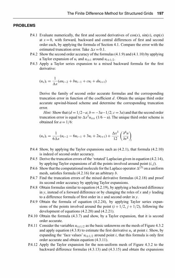
Ch04-H6594.tex 27/4/2007 15: 31 Page 197


PROBLEMS

P.4.1 Evaluate numerically, the first and second derivatives of cos(x), sin(x), exp(x)at x = 0, with forward, backward and central differences of first and secondorder each, by applying the formula of Section 4.1. Compare the error with theestimated truncation error. Take �x = 0.1.

P.4.2 Show the second order accuracy of the formulas (4.1.9) and (4.1.10) by applyinga Taylor expansion of ui and ui±1 around ui±1/2.

P.4.3 Apply a Taylor series expansion to a mixed backward formula for the firstderivative:

(ux)i = 1

�x(aui−2 + bui−1 + cui + dui+1)

Derive the family of second order accurate formulas and the correspondingtruncation error in function of the coefficient d. Obtain the unique third orderaccurate upwind-biased scheme and determine the corresponding truncationerror.

Hint: Show that (d = 1/2−a; b = −3a−1/2; c = 3a) and that the second ordertruncation error is equal to �x2uxxx (1/6 − a). The unique third order scheme isobtained for a = 1/6:

(ux)i = 1

6�x(ui−2 − 6ui−1 + 3ui + 2ui+1) + �x3

12

(∂4u

∂x4

)i

P.4.4 Show, by applying the Taylor expansions such as (4.2.1), that formula (4.2.10)is indeed of second order accuracy.

P.4.5 Derive the truncation errors of the ‘rotated’Laplacian given in equation (4.2.14),by applying Taylor expansions of all the points involved around point (i, j).

P.4.6 Show that the computational molecule for the Laplace operator �(3) on a uniformmesh, satisfies formula (4.2.16) for an arbitrary b.

P.4.7 Find the truncation errors of the mixed derivative formulas (4.2.18) and proofits second order accuracy by applying Taylor expansions.

P.4.8 Obtain formulas similar to equation (4.2.19), by applying a backward differencein y, instead of a forward difference or by changing the roles of x and y leadingto a difference formula of first order in x and second order in y.

P.4.9 Obtain the formula of equation (4.2.24), by applying Taylor series expan-sions of the points involved around the point (i + 1/2, j + 1/2), following thedevelopment of equations (4.2.20) and (4.2.21).

P.4.10 Obtain the formula (4.3.7) and show, by a Taylor expansion, that it is secondorder accurate.

P.4.11 Consider the variables ui±1/2 as the basic unknowns on the mesh of Figure 4.3.2and apply equation (4.3.8) to estimate the first derivative ux at point i. Show, byexpanding the ‘face values’ ui±1/2 around point i, that this formula is only firstorder accurate and obtain equation (4.3.11).

P.4.12 Apply the Taylor expansion for the non-uniform mesh of Figure 4.3.2 to thebackward difference formulas (4.3.13) and (4.3.15) and obtain the expansions

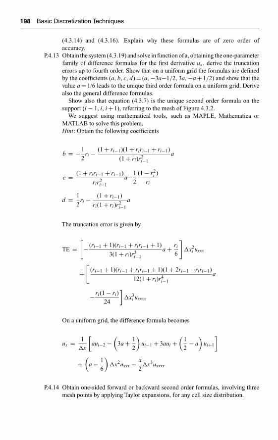
Ch04-H6594.tex 27/4/2007 15: 31 Page 198


(4.3.14) and (4.3.16). Explain why these formulas are of zero order ofaccuracy.

P.4.13 Obtain the system (4.3.19) and solve in function of a, obtaining the one-parameterfamily of difference formulas for the first derivative ux. derive the truncationerrors up to fourth order. Show that on a uniform grid the formulas are definedby the coefficients (a, b, c, d) = (a, −3a−1/2, 3a, −a + 1/2) and show that thevalue a = 1/6 leads to the unique third order formula on a uniform grid. Derivealso the general difference formulas.

Show also that equation (4.3.7) is the unique second order formula on thesupport (i − 1, i, i + 1), referring to the mesh of Figure 4.3.2.

We suggest using mathematical tools, such as MAPLE, Mathematica orMATLAB to solve this problem.Hint: Obtain the following coefficients

b = −1

2ri − (1 + ri−1)(1 + riri−1 + ri−1)

(1 + ri)r2i−1

a

c = (1 + riri−1 + ri−1)

rir2i−1

a−1

2

(1 − r2i )

ri

d = 1

2ri − (1 + ri−1)

ri(1 + ri)r2i−1

a

The truncation error is given by

TE =[− (ri−1 + 1)(ri−1 + riri−1 + 1)

3(1 + ri)r3i−1

a + ri

6

]�x2

i uxxx

+[

(ri−1 + 1)(ri−1 + riri−1 + 1)(1 + 2ri−1 −riri−1)

12(1 + ri)r4i−1

a

− ri(1 − ri)

24

]�x3

i uxxxx

On a uniform grid, the difference formula becomes

ux = 1

�x

[aui−2 −

(3a + 1

2

)ui−1 + 3aui +

(1

2− a

)ui+1

]

+(

a − 1

6

)�x2uxxx − a

2�x3uxxxx

P.4.14 Obtain one-sided forward or backward second order formulas, involving threemesh points by applying Taylor expansions, for any cell size distribution.

Ch04-H6594.tex 27/4/2007 15: 31 Page 199


For a forward formula, obtain

(ux)i =[�xi+1 + �xi+2

�xi+2�xi+1(ui+1 − ui) − �xi+1

�xi+2(�xi+1 + �xi+2)(ui+2 − ui)

]

+ �xi+1(�xi+1 + �xi+2)

6(uxxx)i + · · ·

Explain why this formula is not in conservative form.P.4.15 Apply the relations (4.3.23) combined to the relations (4.3.20) to obtain the

unique second order conservative difference formula for the first derivative on anon-uniform grid. Compare with the formula (4.3.7).

Hint: Show that the numerator of formula (4.3.17) can be written as

a(ui−2 − ui) + b(ui−1 − ui) + d(ui+1 − ui)

Apply the findings to the interpolation relation (4.3.12).P.4.16 Consider the general four-point formula (4.3.17) for the first derivative on a

non-uniform mesh and add the condition for third order accuracy to the system(4.3.18), by applying the consistency relations. Obtain the general formula infunction of the mesh ratios ri and ri−1, by solving the system for the four coef-ficients (a,b,c,d). Show that on a uniform grid, the formula reduces to equation(4.3.25).

We suggest using mathematical tools, such as MAPLE, Mathematica orMATLAB to solve this problem.

Hint: The condition for third order accuracy to be added to the system is

−a

(1 + 1

ri−1

)3

+ dr3i − b = 0

The solution is

a = ri(1 + ri)r3i−1

2(ri−1 + 1)(ri−1 + riri−1 + 1)b = −1

2(1 + ri−1)ri

c = 1

2

(1 + ri)(2riri−1 + ri − 1 − ri−1)

(1 + ri−1)rid = 1

2

(1 + ri−1)

ri(1 + ri−1 + riri−1)

P.4.17 Consider the general interpolation formula (4.3.12) and derive the relationbetween the coefficients α and β, for this formula to be at least second order accu-rate. Derive these conditions separately for the cell-vertex grid of Figure 4.3.2 andthe cell-centered grid of Figure 4.3.3. Derive also the conditions for the formula tobe third order accurate and show that on a uniform grid we have α = 1/8; β = 3/8.

Hint: Expand the left and right-hand side terms in a Taylor expansion aroundpoint i. Obtain the following conditions:

Cell-vertex case

αi�xi+1 + βi�xi = 1

2�xi+1 or αiri + βi = ri

2for second order accuracy

αi = (ri + 2)

4(ri + 1)βi = r2

i

4(ri + 1)for third order accuracy

Ch04-H6594.tex 27/4/2007 15: 31 Page 200


Cell-centered case

αi(�xi + �xi+1) + βi(�xi + �xi−1) = �xi or

αi(1 + ri) + βi(1 + ri−1) = 1 for second order accuracy

αi = (2ri−1 + 1)

(1 + ri)(1 + ri + 2ri−1ri)βi = r2

i−1ri

(1 + ri−1)(1 + ri + 2ri−1ri)

for third order accuracy.

P.4.18 Apply a Taylor series expansion to the general form:

(ux)i = aui+2 + bui+1 + cui + dui−1 + eui−2

and obtain the central fourth order accurate finite difference approximation tothe first derivative (ux)i , at mesh point i. Repeat the same procedure, to obtainan approximation to the second derivative for (uxx)i , with the same mesh points.Show that the formula is also fourth order accurate. Calculate the truncationerror for both cases.

Hint: Show that we have

(ux)i = 1

12�x(−ui+2 + 8ui+1 − 8ui−1 + ui−2) + �x4

30

(∂5u

∂x5

)

(uxx)i = 1

12�x2(−ui+2 + 16ui+1 − 30ui + 16ui−1 − ui−2) + �x4

90

(∂6u

∂x6

)

P.4.19 Repeat Problem P.4.18, for the third and fourth derivatives and obtain

(uxxx)i = 1

2�x3(ui+2 − 2ui+1 + 2ui−1 − ui−2) − �x2

4

(∂5u

∂x5

)

(uxxxx)i = 1

�x4(ui+2 − 4ui+1 + 6ui − 4ui−1 + ui−2) − �x2

6

(∂6u

∂x6

)

P.4.20 Obtain formulas (4.4.52) to (4.4.59).P.4.21 Obtain formulas (4.4.60) to (4.4.62).P.4.22 Derive a family of compact implicit finite difference formulas by eliminating the

coefficients a+, b+, c+ and a0 from the system (4.5.14). Derive the truncationerror and obtain the formulas with the highest order of accuracy.

P.4.23 Find the highest order implicit difference formula, involving second derivativesat only one point. Write this expression as an explicit relation for (uxx)i andderive the truncation error.

Hint: Select c+ = c− = 0, c0 = 1, obtain

(uxx)i = − 1

2�x[(ux)i+1 − (ux)i−1] + 2

�x2(ui+1 − 2ui + ui−1)

The truncation error is found to be

R = �x4

360

(∂6u

∂x6

)

and the formula is fourth order accurate.

Ch04-H6594.tex 27/4/2007 15: 31 Page 201


P.4.24 Derive a family of implicit difference formulas involving no second derivatives.Hint: Select c+ = c− = c0 = 0 and set α = b+/b−. Obtain the scheme

α(ux)i+1 + 2(1 + α)(ux)i + (ux)i−1

= 1

2�x[(1 + 5α)ui + 1 + 4(1 − α)ui −(5 + α)ui−1]


R = �x3

12(α − 1)

(∂4u

∂x4

)+ �x4

12(α − 1)

(∂4u

∂x4

)

Ch05-H6594.tex 26/4/2007 16: 50 Page 203

Chapter 5

Finite Volume Method and ConservativeDiscretization with an Introduction to FiniteElement Method


The Finite Volume Method (FVM) is the name given to the technique by which theintegral formulation of the conservation laws is discretized directly in the physicalspace.

It is the most widely applied method today in CFD, and this is likely to remain so inthe foreseeable future. The reason behind the appeal to the FVM lies in its generality,its conceptual simplicity and its ease of implementation for arbitrary grids, structuredas well as unstructured.

We consider it therefore as important, even for a first course in CFD, that youbecome knowledgeable with the basics of the FVM, as it has also many implicationsfor the understanding of the nature and properties of the results obtained from aCFD simulation. As we will see in the following, the FVM is based on cell-averagedvalues, which appear as a most fundamental quantity in CFD. This distinguishes theFVM from the finite difference and finite element methods, where the main numericalquantities are the local function values at the mesh points.

Once a grid has been generated, the FVM consists in associating a local finitevolume, also called control volume, to each mesh point and applying the integralconservation law to this local volume. This is a first major distinction from the finitedifference approach, where the discretized space is considered as a set of points, whilein the FVM the discretized space is formed by a set of small cells, one cell beingassociated to one mesh point.

An essential advantage of the FVM is connected to the very important concept ofconservative discretization. We have already introduced the notion of conservationform of the flow equations in Chapter 1, and we refer you to Section 1.1 for a quickreminder of these properties. It is of very great importance to maintain the globalconservation of the basic flow quantities, mass, momentum and energy, at the discretelevel and this puts conditions on the way the discretization process of the equations isperformed. The FVM has the great advantage that the conservative discretizationis automatically satisfied , through the direct discretization of the integral form of theconservation laws. This most fundamental property for numerical schemes, and itsprecise meaning will be discussed in Section 5.1.

The finite volume method takes its full advantage on an arbitrary mesh, where alarge number of options are open for the definition of the control volumes on whichthe conservation laws are expressed. Modifying the shape and location of the controlvolumes associated to a given mesh point, as well as varying the rules and accuracy

203

Ch05-H6594.tex 26/4/2007 16: 50 Page 204


for the evaluation of the fluxes through the control surfaces, gives a considerableflexibility to the finite volume method. This explains the generality of the FVM, andof course a certain number of rules have to be satisfied during these operations. Itwill be the objective of Section 5.2 to introduce you to these rules.

Here we draw your attention on Section 5.2.3, which is the most fundamentalcontribution of this chapter. By an exact and rigorous, although simple and straight-forward, derivation, the most general form of a numerical scheme is presented. Itprovides the significance of the input as well as the output of any numerical scheme.Section 5.2.3 is to be studied very carefully and to be remembered whenever youdeal with CFD, as a developer or as a user.

Section 5.3 introduces some practical aspects of the implementation of the FVM, inparticular the various choices available for the flux calculations at the cell interfaces,while numerical formulas that can be applied for the estimation of surfaces andvolumes on an arbitrary grid will be handled in Chapter 6.

As a more advanced topic, we introduce the Finite Element Method (FEM) andits application to fluid dynamic conservation laws in Section 5.4. The FEM is widelyused in structural mechanics and many books can be found providing an excellentintroduction to its basics. See for instance the books by Zienkiewicz andTaylor (2000),in three volumes, and you can also consult the web site http://ohio.ikp.liu.se/fe for anextensive database on the FEM past and most recent literature.

Hence, we restrict ourselves here to a short summary of the main properties. Forthose of you who would want to extend their knowledge of the FEM for fluid dynamicapplications, we recommend particularly Sections 5.4.3–5.4.5, where the weightedresidual method is introduced with its Galerkin method variant, as applied to thegeneral form of a conservation law. Finally, Section 5.4.6 indicates the link betweenthe weighted residual method and the finite volume method, seen as a particular caseof this more general method.

Figure 5.0.1 shows the suggested roadmap to this chapter. For an introductorycourse, the Sections 5.1–5.3 are very important and strongly recommended, while wewill leave Section 5.4 on the FEM as optional for a more advanced level. This sectionwill therefore be marked with A, based on our notation conventions.

5.1 THE CONSERVATIVE DISCRETIZATION

From the general presentation of Chapter 1, we know that the flow equations arethe expression of a conservation law. Their general form for a scalar quantity U ,with volume sources Q, is given by equation (1.1.1), incorporating eventual surfacesources into the flux term:

∂

∂t

∫�

U d� +∮

S

�F · d�S =∫

�

Q d� (5.1.1)

The essential property of this formulation is the presence of the surface integral andthe fact that the time variation of U inside the volume, only depends on the surfacevalues of the fluxes.

Hence for an arbitrary subdivision of the volume into say, three subvolumes, we canwrite the conservation law for each subvolume and recover the global conservation law

Ch05-H6594.tex 26/4/2007 16: 50 Page 205

Finite Volume Method and Conservative Discretization 205

Section A5

Introduction to thebasis and conditionsfor a validfinite volume method.General form of anumerical scheme

5.3 Practicalimplementation of afinite volumemethod

A5.4 The finiteelement method

5.2 The basis of thefinite volumemethod

5.1 The conservativediscretization

Definition of aconservativenumerical schemeand formal expression

Detailed formulationof a two-dimensionalFVM and generalformulas, includingsurfaces and volumes

Definitions, basicproperties. Themethod of weightedresiduals; Galerkinmethod andapplication to theconservation laws

Figure 5.0.1 Content and guide to this chapter.

by adding up the three subvolume conservation laws. Indeed, referring to Figure 5.1.1,the above equation written for the subvolumes �1, �2, �3 becomes

∂

∂t

∫�1

U d� +∮

ABCA

�F · d�S =∫

�1

Q d�

∂

∂t

∫�2

U d� +∮

DEBD

�F · d�S =∫

�2

Q d� (5.1.2)

∂

∂t

∫�3

U d� +∮

AEDA

�F · d�S =∫

�3

Q d�

When summing the surface integrals, the contributions of the internal lines ADBand DE always appear twice, but with opposite signs and will cancel in the additionof the three subvolume conservation laws. Indeed, for volume �2 for instance wehave a contribution of the fluxes:∫

DE

�F · d�S

while for �3 we have a similar term:∫ED

�F · d�S = −∫

DE

�F · d�S

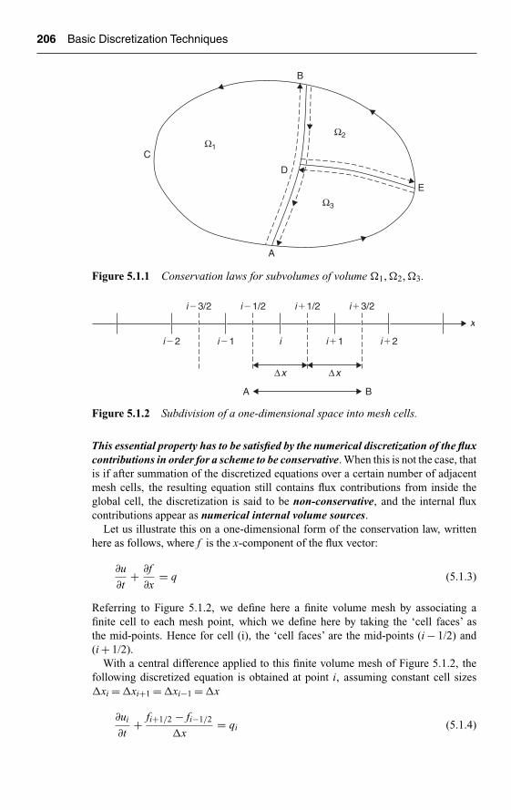
Ch05-H6594.tex 26/4/2007 16: 50 Page 206


E

C

B

A

D

Ω1

Ω2

Ω3

Figure 5.1.1 Conservation laws for subvolumes of volume �1, �2, �3.

A B

ΔxΔx

i�1/2i�3/2

i�2 i�1 i�1 i�2i

i�1/2 i�3/2

x

Figure 5.1.2 Subdivision of a one-dimensional space into mesh cells.

This essential property has to be satisfied by the numerical discretization of the fluxcontributions in order for a scheme to be conservative. When this is not the case, thatis if after summation of the discretized equations over a certain number of adjacentmesh cells, the resulting equation still contains flux contributions from inside theglobal cell, the discretization is said to be non-conservative, and the internal fluxcontributions appear as numerical internal volume sources.

Let us illustrate this on a one-dimensional form of the conservation law, writtenhere as follows, where f is the x-component of the flux vector:

∂u

∂t+ ∂f

∂x= q (5.1.3)

Referring to Figure 5.1.2, we define here a finite volume mesh by associating afinite cell to each mesh point, which we define here by taking the ‘cell faces’ asthe mid-points. Hence for cell (i), the ‘cell faces’ are the mid-points (i − 1/2) and(i + 1/2).

With a central difference applied to this finite volume mesh of Figure 5.1.2, thefollowing discretized equation is obtained at point i, assuming constant cell sizes�xi = �xi+1 = �xi−1 = �x

∂ui

∂t+ fi+1/2 − fi−1/2

�x= qi (5.1.4)

Ch05-H6594.tex 26/4/2007 16: 50 Page 207


The same discretization applied to the point (i + 1), will give

∂ui+1

∂t+ fi+3/2 − fi+1/2

�x= qi+1 (5.1.5)

and for (i − 1)

∂ui−1

∂t+ fi−1/2 − fi−3/2

�x= qi−1 (5.1.6)

The sum of these three equations is a consistent discretization of the conservation lawfor the cell AB (i − 3/2, i + 3/2):

∂

∂t

(ui + ui+1 + ui−1

3

)+ fi+3/2 − fi−3/2

3�x= qi + qi+1 + qi−1

3(5.1.7a)

since the flux contributions at internal points have canceled out. This is sometimescalled the ‘telescoping property’ for the flux terms (Roache, 1972).

As an exercise, let us write a possible scheme directly for the cellAB, if we considerthe cell AB associated to point i. This implies that we do not consider anymore onthis coarsest grid, the intermediate points i − 1 and i + 1. Hence we would write:

∂ui

∂t+ fi+3/2 − fi−3/2

3�x= qi (5.1.7b)

We see that the flux balance is identical to the result of equation (5.1.7a), obtained byadding up the contributions form the ‘internal’ of AB. This is exactly the conservativeproperty we wish to emphasize here.

If we consider now the non-conservative form of equation (5.1.3), by expressingthe flux derivative as

∂f

∂x=(

∂f

∂u

)∂u

∂x�= a(u)

∂u

∂x

defining hereby the Jacobian function a(u) as the derivative of the flux function withrespect to the variable u: a(u) = ∂f /∂u. For instance, if f = u2/2, as with the Burgersequation identified in Section 3.1, then a(u) = u.

The non-conservative form is then written as

∂u

∂t+ a(u)

∂u

∂x= q (5.1.8)

Both formulations (5.1.3) and (5.1.8) are mathematically equivalent for arbitrary,nonlinear fluxes, but their numerical implementation is not.

Applying, for instance a second order central difference at mesh point i, on thefinite volume mesh of Figure 5.1.2, we obtain

∂ui

∂t+ ai

ui+1/2 − ui−1/2

�x= qi (5.1.9a)

where ai is an estimate of the value of a(ui).

Ch05-H6594.tex 26/4/2007 16: 50 Page 208


If similar equations are written for (i + 1) and (i − 1)

∂ui+1

∂t+ ai+1

ui+3/2 − ui+1/2

�x= qi+1

(5.1.9b)∂ui−1

∂t+ ai−1

ui−1/2 − ui−3/2

�x= qi−1

and summed, a discretized equation for the cell AB of Figure 5.1.2 is obtained

∂

∂t

(ui + ui+1 + ui−1

3

)+ ai

ui+3/2 − ui−3/2

6�x− qi + qi+1 + qi−1

3

= −(ai+1 − ai)ui+3/2 − ui+1/2

6�x+ (ai − ai−1)

ui−1/2 − ui−3/2

6�x(5.1.10a)

A direct discretization of equation (5.1.8) on the cellAB would have given, referringto equation (5.1.7b):

∂ui

∂t+ ai

ui+3/2 − ui−3/2

6�x= qi (5.1.10b)

Hence, the right-hand side of equation (5.1.10a), which results from the fact thatthe flux contributions at the internal points of the cell AB do not cancel, appears asan additional source term, which somehow cannot be distinguished by the computerprogram from the physical sources qi.

We see that the discretization of the non-conservative form of the equation givesrise to internal sources. These terms can be considered (by performing a Taylorexpansion) as a discretization to second order of a term proportional to �x2(axux)x atmesh point i. For continuous flows, these numerical source terms are of the same orderas the truncation error and hence could be neglected. However, numerical experimentsand comparisons consistently show that non-conservative formulations are generallyless accurate than conservative ones, particularly in presence of strong gradients.For discontinuous flows, such as transonic flows with shock waves, these numericalsource terms can become important across the discontinuity and give rise to largeerrors. This is indeed the case and the discretization of the non-conservative formwill not lead to the correct shock intensities. Therefore, in order to obtain, in thenumerical computation, the correct discontinuities, such as the Rankine–Hugoniotrelations for the Euler equations, it has been shown by Lax (1954) that it is necessaryto discretize the conservative form of the flow equations.

5.1.1 Formal Expression of a Conservative Discretization

The conservativity requirement on equation (5.1.3) will be satisfied if the scheme canbe written under the form:

∂ui

∂t+ f ∗

i+1/2 − f ∗i−1/2

�x= qi (5.1.11)

Ch05-H6594.tex 26/4/2007 16: 50 Page 209


where f ∗ is called the numerical flux, and is a function of the values of u at (2k)neighboring points:

f ∗i+1/2 = f ∗(ui+k , . . . , ui−k+1) (5.1.12)

In addition, the consistency of equation (5.1.11) with the original equation, requiresthat, when all the ui+k are equal, we should have

f ∗(u, . . . , u) = f (u) (5.1.13)

The generalization to multidimensions is straightforward, the above conditions musthold separately for all the components of the flux vector. The importance of this for-malization of the conservativity condition is expressed by the following fundamentaltheorem of Lax and Wendroff (1960).

Theorem: If the solution ui of the discretized equation (5.1.11) converges boundedlyalmost everywhere to some function u(x, t) when �x, �t tend to zero, then u(x, t) isa weak solution of equation (5.1.3).

This theorem guarantees that when the numerical solution converges, it willconverge to a solution of the basic equations, with the correct satisfaction of theRankine–Hugoniot relations in presence of discontinuities. Indeed, by comparing thederivation of the Rankine–Hugoniot relations in Section 2.7.1 with the weak formu-lation of the basic flow equations, with W = 1 in equation (5.4.36), it is obviousthat these relations are satisfied by the weak solutions, since the starting point of thederivation is the integral form of the conservation law.

5.2 THE BASIS OF THE FINITE VOLUME METHOD

Historically, the finite volume method has apparently been introduced in the field ofnumerical fluid dynamics independently by Mc Donald (1971) and MacCormack andPaullay (1972) for the solution of two-dimensional, time-dependent Euler equationsand extended by Rizzi and Inouye (1973) to three-dimensional flows.

The strength of the FVM is its direct connection to the physical flow properties.Indeed, the basis of the method relies on the direct discretization of the integral formof the conservation law. This distinguishes the FVM significantly from the finitedifference method, described in the previous chapter, since the latter discretizes thedifferential form of the conservation laws. As indicated in Chapter 1, the integral formis the most general expression of a conservation law, as it does not require the fluxesto be continuous (property which is not satisfied for instance along shock waves oralong free surfaces). This is why we can state that the FVM is close to the physics ofthe flow system.

The FVM requires setting up the following steps:

• Subdivide the mesh, obtained from the space discretization, into finite (small)volumes, one control volume being associated to each mesh point.

• Apply the integral conservation law to each of these finite volumes.

Ch05-H6594.tex 26/4/2007 16: 50 Page 210


This approach is fully justified by the generality of the integral form, as seen inChapter 1, where we have pointed out that the integral form of the conservationlaw is valid for any volume �. It can therefore be applied to each individual finitevolume. However, we have to ensure that when adding the contributions of a certainnumber of neighboring finite volumes, we do not loose the consistency required for avalid discretization, as well as the conservativity property introduced in the previoussection. These conditions are now explained in what follows.

5.2.1 Conditions on Finite Volume Selections

Due to its generality the finite volume method can handle any type of mesh, structuredas well as unstructured. Moreover, an additional degree of freedom appears throughthe way we relate the control volumes to the grid. This has then an impact on theposition of the points at which the function values will be defined.

Considering Figure 5.2.1, we can define, for the same mesh, either

• A cell-centered approach, where the unknowns are at the centers of the meshcells and the grid lines define the finite volumes and surfaces. An obvious choice

39

B FC

2i, j�1

6i, j�1

4i�1, j

5 7A E

KHG

D

8i�1, j

1i , j

B

A

ΔyAB

ΔxAB

sAB

23

4

1

6

I

5

j

(a) Cell centered structuredfinite volume mesh

Cell vertex structuredfinite volume mesh

Cell centered unstructuredfinite volume mesh

Cell vertex unstructuredfinite volume mesh

i�1, j�1i�1, j�1

i�1, j�1 i�1, j�1

i�1, j

i, j�1

i , j i�1, j

i, j�1

C

D

G

B

A E

K

F

H

(b)

(c)

(d)

Ωj

2

3

4

1

6

5

j

Ωj

→

Figure 5.2.1 Cell-vertex (bottom) and cell-centered (top) finite volumeconfigurations for structured and unstructured grids.

Ch05-H6594.tex 26/4/2007 16: 50 Page 211


for the control volumes is indeed to make them coincide with the mesh cells.Here the variables are associated with a cell, as on Figure 5.2.1a and c. The flowvariables are averaged values over the cell and can be considered as representativeof some point inside the cell, for instance the central point of the cell.

• A cell-vertex approach, where the unknowns are defined at the corners of themesh. Here the variables are attached to the mesh points, i.e. to the cell vertices,as shown on Figure 5.2.1b and d. A larger flexibility exists for the definitionof the control volumes. Referring to Figure 5.2.1b, an obvious choice wouldbe to consider the four cells having mesh point (i, j) in common, as the controlvolume GHKEFBCDG, associated to point (i, j). Many other choices are howeverpossible and two of them are shown on Figure 5.2.2. Figure 5.2.2a, from McDonald (1971), selects an hexagonal control volume, while Denton (1975) useda trapezoidal control surface covering two half mesh cells (Figure 5.2.2b).

The following constraints on the choice of the �J volumes for a consistent finitevolume method have to be satisfied:

(i) Their sum should cover the entire domain �J .(ii) The subdomains �J are allowed to overlap with the conditions that each part

of the surface �J appears as part of an even number of different subdomainssuch that the overall integral conservation law holds for any combination ofadjacent subdomains.

(iii) Fluxes along a cell surface have to be computed by formulas independent ofthe cell in which they are considered.

Requirement (iii) ensures that the conservative property is satisfied, since theflux contributions of internal boundaries will cancel when the contributions of theassociated finite volumes are added.

Referring to Figure 5.2.3, the cells 1,2,3,4 have no common sides and their sum doesnot cover the whole volume. In addition, the sides are not common to two volumes. Thecells 5,6,7 overlap, but have no common surfaces. Hence the conservative propertywill not be satisfied.

(a)

j

i

AH

G

F E D

C

B

(b)

j

i

D

C B

A

Figure 5.2.2 Examples of two-dimensional control surfaces with cell-vertex finitevolume method: (a) Mc Donald (1971) (b) Denton (1975).

Ch05-H6594.tex 26/4/2007 16: 50 Page 212


1 2

43

5

6

7

8

Figure 5.2.3 Incorrect finite volume decomposition.

5.2.2 Definition of the Finite Volume Discretization

The integral conservation law (5.1.1) is applied to each control volume �J , associ-ated to mesh point J , defining hereby the discretized equation for the unknowns UJ

attached to that same vertex or cell:

∂

∂t

∫�J

U d� +∮

SJ

�F · d�S =∫

�J

Q d� (5.2.1)

The advantage of this method, especially in absence of sources terms, is that the fluxesare calculated only on two-dimensional surfaces instead of in the three-dimensionalspace.

Equation (5.2.1) is replaced by its discrete form, where the volume integrals areexpressed as the averaged values over the cell and where the surface integral is replacedby a sum over all the bounding faces of the considered volume �J :

∂

∂t(UJ �J ) +

∑faces

�F · ��S = QJ �J (5.2.2)

Referring to Figure 5.2.1a and to cell 1(i, j), we would identify UJ with Ui,j , �J withthe area of ABCD and the flux terms are summed over the four sides AB,BC,CD,DA.On the mesh of Figure 5.2.1d, �J is the doted area of the triangles having node J incommon and the flux summation extends over the six sides 12,23,34,45,56,61. Thisis the general formulation of the finite volume method and the user has to define, fora selected �J , how to estimate the volume and cell face areas of the control volume�J and how to approximate the fluxes at the faces. We will discuss some of the mostcurrent options, in two and three dimensions.

Equation (5.2.2) shows several interesting features which distinguish the interpreta-tion of finite volume methods from the finite difference and finite element approaches:

1. The coordinates of point J , that is the precise location of the variable UJ

inside the control volume �J , do not appear explicitly. Consequently, UJ is

Ch05-H6594.tex 26/4/2007 16: 50 Page 213


not necessarily attached to a fixed point inside the control volume and can beconsidered as an average value of the flow variable U over the control cell.This is the interpretation taken in Figure 5.2.1a. The first term of equation(5.2.2) represents therefore the time rate of change of the averaged flow vari-able over the selected finite volume. This will be further specified in the nextsection.

2. The mesh coordinates appear only in the determination of the cell volume andside areas. Hence, referring to Figure 5.2.1a, and considering for instance thecontrol cell ABCD around point 1, only the coordinates of A,B,C,D will beneeded.

3. In absence of source terms, the finite volume formulation expresses that thevariation of the average value U over a time interval �t is equal to the sumof the fluxes exchanged between neighboring cells. For stationary flows, thenumerical solution is obtained as a result of the balance of all the fluxes enteringor leaving the control volume. That is,

∑faces

(�F · ��S) = 0 (5.2.3)

When adjacent cells are considered, for instance cells ABCD and AEFB onFigure 5.2.1a, the flux through face AB contributes to the two cells but withopposite signs. It is therefore convenient to program the method by sweepingthrough the cell faces and, when calculating the flux through side AB, to add thiscontribution to the flux balance of cell 1 and subtract it from the flux balanceof cell 8. This guarantees automatically global conservation.

4. The finite volume method also allows a natural introduction of boundary condi-tions, for instance at solid walls where certain normal components are zero. Forinstance, for the mass conservation equation, �F = ρ�v and at a solid boundary�F · d�S = 0. Hence, the corresponding contribution to equation (5.2.2) or (5.2.3)would vanish.

5.2.3 General Formulation of a Numerical Scheme

A general and important interpretation of any numerical, conservative scheme, gener-alizing equation (5.1.11), is obtained directly from the integral conservation laws. Theformulation that follows is valid for all possible cases, with structured grids or unstruc-tured grids, either cell-centered or cell-vertex defined variables, as summarized inFigures 5.2.4.

If the integral form of the conservation law (5.2.1) is integrated from t = n�t to(n + 1)�t for a control volume �J associated to a node or cell J , we obtain

∫�J

U d�

∣∣∣∣n+1

=∫

�J

U d�

∣∣∣∣n

−∑faces

n+1∫

n

(�F · ��S)f dt +n+1∫

n

dt

∫�J

Q d�

(5.2.4)

Ch05-H6594.tex 26/4/2007 16: 50 Page 214


Node J

Node J

Node (J�1)

Node (J�1)

Structured meshes

Unstructured meshes

Cell J

Cell J

Cell (J�1)

Cell (J�1)

Cell vertexCell centered

Figure 5.2.4 Cell-centered and cell-vertex cells for structured and unstructuredgrids.

Introducing the cell-averaged conservative variable UnJ and source Q

nJ at time n�t,

the cell- and time-averaged sources Q∗J , together with the numerical flux �F∗ over

each side, defined by

UnJ

�= 1

�J

∫�J

U d�J

∣∣∣∣n

QJ�= 1

�J

∫�J

Q d�J (5.2.5a)

�F∗ · ��S �= 1

�t

∫ n+1

n

�F · ��S dt Q∗J

�= 1

�t

∫ n+1

nQJ dt (5.2.5b)

the conservative discretization takes the form:

[U J �J

]n+1 = [U J �J]n − �t

∑faces

�F∗ · ��S + �tQ∗J �J (5.2.6)

This is an exact relation for the time evolution of the space averaged conservativevariables U

nJ over cell J . It is also important to observe that there is no mesh point

associated to UnJ which is attached only to cell J . The numerical flux �F∗ identifies

completely a scheme by the way it approximates the time-averaged physical flux alongeach cell face.

Ch05-H6594.tex 26/4/2007 16: 50 Page 215


As already mentioned above, in order to fulfill conservation at the discretizedlevel, the estimation of the numerical flux at a given cell face must be independentof the cell to which it belongs.

The absence of a time index on the balance of fluxes and on the source term ismeant to indicate that one can choose between n for an explicit scheme and (n + 1)for an implicit scheme.

The above formulation of a numerical scheme can be generalized if one considersthat the space discretization is completely defined by its numerical flux, leaving openthe choice of the time integration. A general numerical scheme can then be definedas a system of ordinary differential equations in time by

d

dt

[U J �J

] = −∑faces

�F∗ · ��S + Q∗J �J ≡ −RJ (5.2.7)

The right-hand side defines the residual RJ as the balance of fluxes over a cell J plusthe source term contribution.

The scheme (5.2.6) is obtained by applying a forward difference in time to theleft-hand side of (5.2.7) and typical examples of other time integration schemes,such as Runge–Kutta methods or linear multistep methods will be discussed inChapter 9.

In practice, when the results of a CFD simulation has to be analyzed and post-processed, we need to assign the cell-averaged values to a mesh point, for instancethe center of the cell. This introduces an error, which is generally of second order,which becomes then part of the discretization error.

Alternative formulation of the conservative conditionExtending the subdivisions of equation (5.1.2) to an arbitrary number of cells, J =1–N , and summing over all the cells it is seen, after cancellation of the contributionsfrom all the internal cell faces, that the sum

N∑J=1

∫�J

∂U

∂td�J = −

∮S

�F · d�S +∫

�

Q d� (5.2.8)

will contain only contributions from the fluxes along the parts of the cells belongingto the boundaries of the domain and from the sources. Therefore, the conservativecondition can be expressed as a requirement on the transient time evolution of thescheme. Note that for stationary sources and boundary fluxes, the right-hand side ofthis equation vanishes at convergence.

Defining �U J/�t as the average value of ∂U/∂t over the cell �J , conservation ofthe scheme requires that, at each time step, the following condition is to be satisfied:

N∑J=1

�U J

�t�J = boundary and source terms (5.2.9)

Hence, the sum of �U J �J /�t over all the cells may not contain contributions frominside the domain, with the exception of the source terms (see also Problem P.5.13).

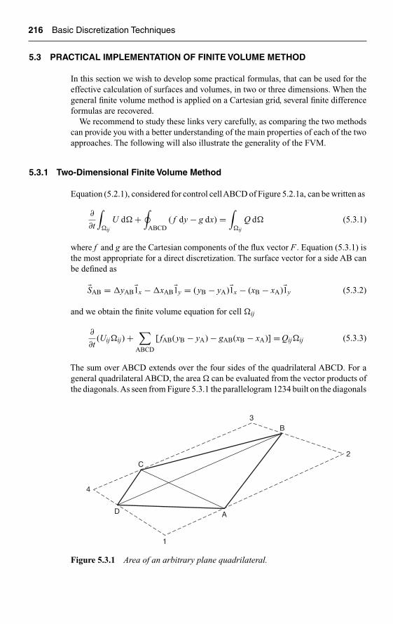
Ch05-H6594.tex 26/4/2007 16: 50 Page 216


5.3 PRACTICAL IMPLEMENTATION OF FINITE VOLUME METHOD

In this section we wish to develop some practical formulas, that can be used for theeffective calculation of surfaces and volumes, in two or three dimensions. When thegeneral finite volume method is applied on a Cartesian grid, several finite differenceformulas are recovered.

We recommend to study these links very carefully, as comparing the two methodscan provide you with a better understanding of the main properties of each of the twoapproaches. The following will also illustrate the generality of the FVM.

5.3.1 Two-Dimensional Finite Volume Method

Equation (5.2.1), considered for control cellABCD of Figure 5.2.1a, can be written as

∂

∂t

∫�ij

U d� +∮

ABCD( f dy − g dx) =

∫�ij

Q d� (5.3.1)

where f and g are the Cartesian components of the flux vector F . Equation (5.3.1) isthe most appropriate for a direct discretization. The surface vector for a side AB canbe defined as

�SAB = �yAB�1x − �xAB�1y = (yB − yA)�1x − (xB − xA)�1y (5.3.2)

and we obtain the finite volume equation for cell �ij

∂

∂t(Uij�ij) +

∑ABCD

[ fAB(yB − yA) − gAB(xB − xA)] = Qij�ij (5.3.3)

The sum over ABCD extends over the four sides of the quadrilateral ABCD. For ageneral quadrilateral ABCD, the area � can be evaluated from the vector products ofthe diagonals. As seen from Figure 5.3.1 the parallelogram 1234 built on the diagonals

4

3

2

1

D

C

B

A

Figure 5.3.1 Area of an arbitrary plane quadrilateral.

Ch05-H6594.tex 26/4/2007 16: 50 Page 217


is twice the area of the quadrilateral ABCD. Hence with �xAB = �xB − �xA where �xA isthe position vector of point A:

�ABCD = 1

2|�xAC × �xBD|

= 1

2[(xC − xA)(yD − yB) − (xD − xB)(yC − yA)] (5.3.4)

= 1

2(�xAC�yBD − �xBD�yAC)

The right-hand side of equation (5.3.4) should be positive for a cell ABCD whereA,B,C,D are located counterclockwise.

Evaluation of fluxes through cell facesThe evaluation of flux components along the sides, such as fAB, gAB, depends on theselected scheme, as well as on the location of the flow variables with respect tothe mesh.

As will be seen more in detail in the following chapters and in Volume II forthe systems of Euler and Navier–Stokes equations, one can distinguish essentiallybetween central and upwind discretization schemes. Central schemes are based onlocal flux estimations, while upwind schemes determine the cell face fluxes accordingto the propagation direction of the convection velocity:

(a) For central schemes and cell-centered finite volume methods, followingalternatives can be considered:1. Average of fluxes:

fAB = 1

2(fij + fi+1, j) (5.3.5)

fij = f (Uij) (5.3.6)

2. Since the flux components are generally nonlinear functions of U , thefollowing choice is not identical to equation (5.3.5):

fAB = f

(Uij + Ui+1, j

2

)(5.3.7)

3. Take fAB as the average of the fluxes in A and B,

fAB = 1

2( fA + fB) (5.3.8)

where either the variables are evaluated in A and B, for instance

UA = 1

4(Uij + Ui+1, j + Ui+1, j−1 + Ui, j−1) (5.3.9)

and

fA = f (UA) (5.3.10)

Ch05-H6594.tex 26/4/2007 16: 50 Page 218


or the fluxes are averaged, as

fA = 1

4( fij + fi+1, j + fi+1, j−1 + fi, j−1) (5.3.11)

Observe that formulas (5.3.7) and (5.3.10) will generally lead to schemesrequiring a lower number of flux evaluations compared to the applicationof formulas (5.3.5) and (5.3.11).

(b) For central schemes and cell-vertex finite volume methods, formulas (5.3.7)and (5.3.8) are straightforward approximations to the flux fAB. The choice(5.3.8) corresponds to the application of a trapezium formula for the integral:∫

AB

f dy = 1

2(fA + fB)(yB − yA)

By summing the contributions of these integrals over the four sides of cellABCD of Figure 5.2.1b, we obtain∮

ABCD

�F · d�S = 1

2[(fA − fC)�yDB + (fB − fD)�yAC

− (gA − gC)�xDB + (gB − gD)�xAC] (5.3.12)

Example E.5.3.1: Central scheme on Cartesian mesh

Over a Cartesian, uniform mesh the above finite volume formulation is identical to afinite difference formula. Indeed, with

�yAB = yi+1/2, j+1/2 − yi+1/2, j−1/2 = �y

�xAB = 0 �xBC = −�x (E5.3.1)

�ij = �x �y �yBC = 0

we obtain, writing fAB = fi+1/2, j and similarly for the other components:

∂

∂tUij�x �y + (fi+1/2, j − fi−1/2, j)�y + (gi, j+1/2 − gi, j−1/2)�x

= Qij�x �y (E5.3.2)

After division by �x �y this reduces to the central difference form:

∂Uij

∂t+ ( fi+1/2, j − fi−1/2, j)

�x+ (gi, j+1/2 − gi, j−1/2)

�y= Qij (E5.3.3)

We have still to define how to calculate the flux components at the side centersfi±1/2, j , gi, j±1/2. With the choice (5.3.5) applied to Figure 5.2.1a, equation (E.5.3.3)becomes

∂Uij

∂t+ ( fi+1, j − fi−1, j)

2�x+ (gi, j+1 − gi, j−1)

2�y= Qij (E5.3.4)

Ch05-H6594.tex 26/4/2007 16: 50 Page 219


while (5.3.8) with (5.3.11) leads to the formula:

∂Uij

∂t+ 1

4

[2

(fi+1, j − fi−1, j)

2�x+ (fi+1, j+1 − fi−1, j+1)

2�x+ (fi+1, j−1 − fi−1, j−1)

2�x

]

+ 1

4

[2

(gi, j+1 − gi, j−1)

2�y+ (gi+1, j+1 − gi+1, j−1)

2�y+ (gi−1, j+1 − fi−1, j+1)

2�y

]

= Qij (E5.3.5)

The central finite volume method therefore leads to second order accurate spacediscretizations on Cartesian meshes.

Observe that fij , gij do not appear in equation (E.5.3.4), and if (i + j) is even thisequation contains only nodes with (i + j) odd. Hence even and odd numbered nodesare decoupled, and this could lead to oscillations in the solution. This decoupling isnot present with formula (E.5.3.5). For applications to cell-vertex meshes, the readeris referred to Problems P.5.1–P.5.4.

(c) For upwind schemes and cell-centered finite volume methods, a convectiveflux is evaluated in function of the propagation direction of the associatedconvection speed. The latter is determined by the flux Jacobean

�A(U ) = ∂ �F∂U

= a(U )�1x + b(U )�1y (5.3.13)

with a(U ) = ∂f/∂U and b(U ) = ∂g/∂U .The simplest upwind scheme takes the cell side flux equal to the flux gen-

erated in the upstream cell. This expresses that the cell side flux is fullydetermined by contributions transported in the direction of the convectionvelocity.

Considering Figure 5.2.1a, we could define

(�F · �S)AB = (�F · �S)ij if (�A · �S)AB > 0

(�F · �S)AB = (�F · �S)i+1,j if (�A · �S)AB < 0 (5.3.14)

(d) For upwind schemes and cell-vertex finite volume methods, figure 5.2.1b, wecould define

(�F · �S)AB = (�F · �S)CD if (�A · �S)AB > 0

(�F · �S)AB = (�F · �S)EF if (�A · �S)AB < 0 (5.3.15)

When applied to the control volume GHKEFBCD of figure 5.2.1b, we obtaincontributions from points such as (i − 2, j) and (i, j − 2), for positive con-vection speeds. This leads to schemes with an unnecessary large supportfor the same accuracy. Therefore, this option is not applied in practice (seeProblem P.5.12).

Ch05-H6594.tex 26/4/2007 16: 50 Page 220


Example E.5.3.2: Upwind scheme on Cartesian mesh

We consider the discretization of the two-dimensional linear convection equation

∂U

∂t+ a

∂U

∂x+ b

∂U

∂y= 0 with a > 0 and b > 0 (E5.3.6)

by a finite volume formulation on the cell ABCD of figure 5.2.1a, defined as aCartesian cell following example E.5.3.1.

The fluxes are defined by f = aU and g = bU and with the choice of equation(5.3.14), we have for AB and CD taken as vertical sides:

(�F · �S)AB = fij�y = aUij�y

(�F · �S)CD = −fi−1, j�y = −aUi−1, j�y (E5.3.7)

and similarly for the two horizontal sides BC and DA.

(�F · �S)BC = gij�x = bUij�x

(�F · �S)DA = −gi, j−1�x = −bUi, j−1�x (E5.3.8)

The resulting scheme, obtained after division by the cell area �x�y, is onlyfirst order accurate and is a straightforward generalization of the first order upwindscheme:

∂Uij

∂t+ (fij − fi−1, j)

�x+ (gij − gi, j−1)

�y= 0 (E5.3.9)

or

∂Uij

∂t+ a

�x(Uij − Ui−1, j) + b

�y(Uij − Ui, j−1) = 0 (E5.3.10)

Non-uniform meshAlthough the finite volume formulation applies to arbitrary grids, the above formulasfor the determination of the fluxes nevertheless imply some regularity of the mesh.Referring for instance to formula (5.3.5) or (5.3.7) as applied to cell-centered finitevolume methods, and interpreting the cell averaged values Uij in Figure 5.2.1a asmid-cell values, it is seen that these formulas perform an arithmetic average of thefluxes (or the variables) on both sides of the cell face AB. This leads to a second orderapproximation on a Cartesian mesh (see Example E.5.3.1), if AB is at mid-distancefrom the cell centers 1 and 8.

However, this will seldom be the case on non-uniform meshes, as shown onFigure 5.3.2a and a loss of accuracy will result from the application of these for-mulas. Similar considerations apply to equations (5.3.9) and (5.3.11), based on theassumption that point A is in the center of the cell 1678.

An analysis of the truncation errors for certain finite volume discretizations onnon-uniform meshes can be found in Arts (1984) and more general analysis can befound in Turkel (1985), Turkel et al. (1985) and Roe (1987).

Ch05-H6594.tex 26/4/2007 16: 50 Page 221


i�1, j

i , j�1 i�1, j�1

(a) (b)

C B

8b

Ma

A

7E

KHG

D

6

i , j

i�1, j

i , j�1

i�1, j�1

1 F

�

�

�

�

C

D

G H

A E

K

B

ba1

6 7

8

� �

� �

F

Figure 5.3.2 Non-uniform finite volume meshes: (a) non-uniform finite volumemesh (b) orthogonal non-uniform finite volume mesh.

We will come back to this very important issue in the Chapter 6, when dealing withgrid properties.

5.3.2 Finite Volume Estimation of Gradients

It is often necessary, in finite volume discretizations, to define numerically cell aver-ages of derivatives of mesh variables. In particular with the Navier–Stokes equations,the viscous flux components are functions of the velocity gradients and we have toestimate appropriate values of these gradients on the cell faces.

A general procedure, valid for an arbitrary control volume in two and three dimen-sions, can be derived by application of the Gauss divergence theorem. This theoremcan be considered as defining the average of the gradient of a scalar U in function ofits values at the boundaries of the considered volume.

Since for an arbitrary volume �

∫�

( �∇U )d� =∮

SU d�S (5.3.16)

where S is the closed boundary surface, we can define the averaged gradients as

(∂U

∂x

)

�

≡ 1

�

∫

�

∂U

∂xd� = 1

�

∮

S

U �1x · d�S (5.3.17)

and(

∂U

∂y

)

�

≡ 1

�

∫

�

∂U

∂yd� = 1

�

∮

S

U �1y · d�S (5.3.18)

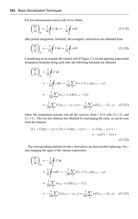
Ch05-H6594.tex 26/4/2007 16: 50 Page 222


For two-dimensional control cells � we obtain(∂U

∂x

)

�

= 1

�

∮

S

U dy = − 1

�

∮

S

y dU (5.3.19)

after partial integration. Similarly, the averaged y-derivatives are obtained from(

∂U

∂y

)

�

= − 1

�

∮

S

U dx = 1

�

∮

S

x dU (5.3.20)

Considering as an example the control cell of Figure 5.2.1d and applying trapezoidalintegration formulas along each side, the following formulas are obtained

(∂U

∂x

)

�

= 1

�

∮

S

U dy

= − 1

�

∮

S

y dU = 1

2�

∑I

(UI + UI+1)(yI+1 − yI )

= − 1

2�

∑I

(yI+1 + yI )(UI+1 − UI )

= 1

2�

∑I

UI (yI+1 − yI−1) = − 1

2�

∑I

yI (UI+1 − UI−1) (5.3.21)

where the summation extends over all the vertices, from 1 to 6 with U0 = U6 andU7 = U1. The two last relations are obtained by rearranging the sums, as can be seenfrom the relation:

(U1 + U2)(y2 − y1) + (U2 + U3)(y3 − y2) + · · · = U2(y3 − y1) + · · ·= −y2(U3 − U2) + · · ·

(5.3.22)

The corresponding relations for the y-derivatives are derived after replacing x by yand changing the signs of the various expressions:

(∂U

∂y

)

�

= − 1

�

∮

S

U dx

= 1

�

∮

S

x dU = − 1

2�

∑I

(UI + UI+1)(xI+1 − xI )

= 1

2�

∑I

(xI+1 + xI )(UI+1 − UI )

= − 1

2�

∑I

UI (xI+1 − xI−1) = 1

2�

∑I

xI (UI+1 − UI−1) (5.3.23)

Ch05-H6594.tex 26/4/2007 16: 50 Page 223


The area of the cells can be obtained by formulas similar to the above, by noting thatfor U = x the left-hand side of equation (5.3.21) is equal to 1. Hence, the followingexpressions can be used for the estimation of the area of an arbitrary cell:

� =∮

S

x dy = −∮

S

y dx = 1

2

∑I

(xI + xI+1)(yI+1 − yI )

= −1

2

∑I

(yI+1 + yI )(xI+1 − xI )

= 1

2

∑I

xI (yI+1 − yI−1)

= −1

2

∑I

yI (xI+1 − xI−1) (5.3.24)

For an arbitrary quadrilateral ABCD, as shown on Figure 5.3.2, an interestingformula is obtained by applying the third of the above relations, noticing that thedifferences �y can be grouped for opposite nodes, leading to

∮

ABCD

U dy = 1

2[(UA − UC)(yB − yA) − (UB − UD)(yA − yC)] (5.3.25)

and(

∂U

∂x

)

ABCD

= (UA − UC)(yB − yD) − (UB − UD)(yA − yC)

(xA − xC)(yB − yD) − (xB − xD)(yA − yC)(5.3.26)

with a similar relation for the y-derivative:

(∂U

∂y

)

ABCD

= (UB − UD)(xA − xC) − (UA − UC)(xB − xD)

(xA − xC)(yB − yD) − (xB − xD)(yA − yC)(5.3.27)

The vector version of the divergence relation, written for an arbitrary vector �a is alsoof interest

∫�

( �∇ · �a)d� =∮

S�a · d�S (5.3.28)

since it can be applied, in particular for the derivation of formulas for cell face areasand volumes. For a two-dimensional cell, taking �a = �x with �∇ · �x = 2 leads to theformula

2� =∮

S�x · d�S =

∮S

(x dy − y dx) (5.3.29)

which reproduces the above relations when a trapezium formula is applied. Applica-tions of this relation to three-dimensional volumes are discussed in Chapter 6.

Ch05-H6594.tex 26/4/2007 16: 50 Page 224


Example E.5.3.3: Two-dimensional diffusion equation

We consider the two-dimensional diffusion equation:

∂U

∂t+ ∂

∂x

(k∂U

∂x

)+ ∂

∂y

(k∂U

∂y

)= 0 (E5.3.11)

with diffusive flux components f = k ∂U/∂x and g = k∂U/∂y, where k is a constant.We would like to construct a finite volume discretization on the mesh of Figure

5.2.1a, considered as Cartesian, by expressing the balance of fluxes around the cellABCD with the choice

fAB = 1

2(fA + fB) (E5.3.12)

and an evaluation of the derivatives ∂U/∂x and g = ∂U/∂y in the cell corners A,B.Equation (5.3.3) for cell (i, j) is written here as

(∂U

∂t

)ij

�x �y + (fAB − fCD)�y + (gBC − gDA)�x = 0 (E5.3.13)

For point A, the derivatives of U are taken as the average value over the cell 1678 andwith equation (5.3.26):

fA = k

(∂U

∂x

)A

= k

2�x(Ui+1, j + Ui+1, j−1 − Uij − Ui, j−1) (E5.3.14)

A similar relation is obtained for point B

fB = k

(∂U

∂x

)B

= k

2�x(Ui+1, j + Ui+1, j+1 − Uij − Ui, j+1) (E5.3.15)

and the flux contribution through the side AB is given by the sum of the two equations(E5.3.13) and (E5.3.14) multiplied by �y.

The contributions of the other sides are obtained in a similar way, for instance theflux through BC is given by the sum:

gBC�x = 1

2(gB + gC)�x (E5.3.16)

with

gB = k

(∂U

∂y

)B

= k

2�y(Ui+1, j+1 + Ui, j+1 − Uij − Ui+1, j) (E5.3.17)

A similar relation is obtained for point C:

gc = k

(∂U

∂y

)C

= k

2�y(Ui, j+1 + Ui−1, j+1 − Uij − Ui−1, j) (E5.3.18)

Ch05-H6594.tex 26/4/2007 16: 50 Page 225


Finally, equation (E5.3.13) becomes with �x = �y

∂Uij

∂t+ k

Ui+1, j+1 + Ui+1, j−1 + Ui−1, j+1 + Ui−1, j−1 − 4Uij

4�x2= 0 (E5.3.19)

This scheme corresponds to the discretization of Figure 4.2.3 for the Laplace operator.Note that the alternative, simpler choice

fAB = k

(∂U

∂x

)AB

= k

�x(Ui+1, j − Uij) (E5.3.20)

leads to the standard finite difference discretization of the diffusion equation,corresponding to Figure 4.2.2:

∂Uij

∂t+ k

Ui+1, j + Ui, j−1 + Ui−1, j + Ui, j+1 − 4Uij

4�x2= 0 (E5.3.21)

Extensions to three-dimensional volumes, typical of current unstructured or struc-tured grids, such as tetrahedra, pyramids, prisms or hexahedra are shifted to Chapter 6.

A.5.4 THE FINITE ELEMENT METHOD

The finite element method originated from the field of structural analysis as an out-come of many years of research mainly between 1940 and 1960. The concept of‘elements’ can be traced back to the techniques used in stress calculations whereby astructure is subdivided in small substructures of various shapes and reassembled aftereach ‘element’ had been analyzed. The development of this technique and its formalelaboration led to the introduction of what is now called the finite element method byTurner et al. (1956) in a paper dealing with the properties of a triangular element inplane stress problems. The expression finite elements itself was introduced by Clough(1960).

After having been applied with great success to a variety of problems in linear andnonlinear structural mechanics, it appeared very soon that the method could be usedalso to solve continuous field problems (Zienkiewicz and Cheung, 1965). From thenon, the finite element method came out as a general approximation method for thenumerical solution of physical problems described by field equations in continuousmedia, containing actually many of the finite difference schemes as special cases.Today, after the initial developments in an engineering framework, mathematicianshave put the finite element method in a very elegant, rigorous, formal framework, withprecise mathematical conditions for existence and convergence criteria and exactlyderived error bounds. Due to the particular character of finite element discretizationsthe appropriate mathematical background is functional analysis and an excellent intro-duction to the mathematical formulation of the method can be found in Strang andFix (1973), Oden and Reddy (1976) and more advanced treatments in Oden (1972)and Ciarlet (1978).

Ch05-H6594.tex 26/4/2007 16: 50 Page 226


With regard to fluid flow problems a historical general introduction is to be foundin Chung (1978), Baker (1983) and more advanced developments are analyzed inTemam (1977), Girault and Raviart (1979) and Thomasset (1981). A recent additionto the literature on the applications of finite elements to fluid flow problems is to befound in the books by Zienkiewicz and Taylor (2000), in Volume 3.

You can also consult the web site http://ohio.ikp.liu.se/fe for an extensive databaseon the FEM past and most recent literature.

The finite element approximation has two major common points with the finitevolume method, namely that

• The space discretization is considered as a set of volumes or cells, called elementsin the finite element tradition, as opposed to a set of points as with finite differencemethods.

• It requires an integral formulation as a starting point which, as will be seen insection, can be considered as a generalization of the FVM.

The finite element method is based on the following steps:

1. Discretize the space in contiguous elements of arbitrary shapes, that is typicalof unstructured grids. These elements are actually the control cells defined inthe previous sections related to the FVM. Therefore, the FEM is ‘naturally’appropriate to unstructured grids, more particularly to cell-vertex grids, as seenin next section. We will often refer in this section to the elements of the mesh,instead of the cells, to follow the FEM terminology. However, keep in mind thatthese two names refer to the same basic components of a finite volume mesh.

2. Define in each element a parametric representation of the unknown variables,based on families of interpolating or shape functions, associated to eachelement or cell.

3. Define an integral formulation of the equations to be solved to each element(cell) of the discretized space.

We will now develop these three steps more explicitly.

A.5.4.1 Finite Element Definition of Interpolation Functions

The FEM is based on the definition of function values attached to the nodes of themesh, where the numerical value of the unknown functions, and eventually theirderivatives, will have to be determined.

Therefore, the FEM requires a cell-vertex definition. The total number of unknownsat the nodes, function values and eventually their derivatives are called the degrees offreedom of the numerical problem or nodal values. The field variables are approxi-mated by linear combinations of known basis functions also called shape functions,interpolations functions or trial functions.

If u is an approximate numerical solution of the unknown function u(�x) we defineits parametric representation as a linear superposition of basis functions NI :

u(�x) =∑

I

uI NI (�x) (5.4.1)

Ch05-H6594.tex 26/4/2007 16: 50 Page 227


where the summation extends over all the nodes I . To each node I , we associate onebasis function NI . The functions NI (�x) can be quite general with varying degrees ofcontinuity at the inter-element boundaries. Methods based on defining the interpola-tion functions on the whole domain, for instance as trigonometric functions leadingto Fourier series, are used in collocation methods and in spectral methods where theNI (�x) can be defined as orthogonal polynomials of Legendre, Chebyshev or similartypes. Other possible choices are spline functions, leading to spline interpolationmethods. In these cases, the coefficients uI are obtained from the expansions in seriesof the basis functions.

The properties of finite element methods are based on a very specific choice withthe following properties:

(i) The uI coefficients are the numerical values of the unknowns at node I , i.e.we require that:

u(�xI ) = uI (5.4.2)

Consequently, we have for any point �xJ :

NI (�xJ ) = δIJ (5.4.3)

implying also that the interpolation functions NI must be equal to one at thepoint I to which they are associated.

(ii) In standard finite element methods, the interpolation functions are chosen to belocally defined polynomials within each element, being zero outside the con-sidered element. As a consequence the local interpolation functions satisfy thefollowing additional conditions on each element (e), with I being a node of (e):

N (e)I (�x) = 0 if �x not in element (e) (5.4.4)

since uI are the values of the unknowns at node number I.(iii) An additional condition is provided by the requirement to represent exactly a

constant function u(x) = constant. Hence, this requires

∑I

N (e)I (�x) = 1 for all �x ∈ (e) (5.4.5)

(iv) The global function NI is obtained by assembling the contributions N (e)I of

all the elements to which node I belongs. This condition connects the variousbasis functions within an element and the allowed polynomials will be stronglydependent on the number of nodes within each element.

The above conditions (5.4.2)–(5.4.5) define the properties of the local polynomialinterpolation functions used in finite element approximations. Two families of ele-ments are generally considered according to their degree of inter-element continuityand to the associated nodal values.

If the nodal values are defined by the values of the unknown functions, then C◦continuity at the inter-element boundary is sufficient for systems described by partial

Ch05-H6594.tex 26/4/2007 16: 50 Page 228


differential equations not higher than two. These elements and their associated shapefunctions are then called Lagrangian elements.

If first order partial derivatives of the unknown functions are to be consideredas additional unknowns (or degrees of freedom), the inter-element continuity up tothe highest order of these derivatives will generally be imposed and the elementssatisfying these conditions are Hermitian elements. When the required continuityconditions are satisfied along every point of the inter-element boundary, the elementis called conforming. This condition is sometimes relaxed and elements whereby thiscontinuity condition is imposed only at a limited number of points of the boundaryare said to be non-conforming.

A.5.4.1.1 One-dimensional linear elements

The simplest element has a piecewise linear interpolation function and contains twonodes. Referring to Figure 5.4.1, the element between nodes i and i − 1 is denoted aselement 1 and the adjacent element between i and i + 1 as element 2. They have nodei in common and have respective lengths �xi and �xi+1.

Considering element 1, the relation (5.4.3) gives two conditions and we obtain forthe basis functions at the nodes i and i − 1 of element 1, the linear form:

N (1)i (x) = x − xi

�xiN (1)

i−1(x) = xi − x

�xi(5.4.6)

For element 2 we have the following linear shape functions:

N (2)i (x) = xi+1 − x

�xi+1N (1)

i−1(x) = x − xi

�xi+1(5.4.7)

i�1

1

Ni�1

(1)Ni�1

(2)Ni

(1)Ni

(2)

i i�1

x(1) (2)

x(1)Element 1

Node numbers

Element 2

Node numbers

21

21

10

10

x(2)

Figure 5.4.1 Linear one-dimensional element and shape functions.

Ch05-H6594.tex 26/4/2007 16: 50 Page 229


The global shape function Ni, associated with node i, is obtained by assembling N (1)i

and N (2)i , and is illustrated in Figure 5.4.1. It is zero for x ≥ xi+1 and x ≤ xi−1. If we

define a local coordinate ξ within each element through the mapping:

ξ = x − xi−1

�xi(5.4.8)

the interpolation functions take the universal form:

N1(ξ) = 1 − ξ N2(ξ) = ξ (5.4.9)

where node 1 corresponds to mesh point i − 1 with ξ = 0 and node 2 to mesh point iwith ξ = 1. Similarly for element 2, the mapping between the subspace (xi, xi+1) andthe subspace (0,1) of the ξ-space.

ξ = x − xi

�xi+1(5.4.10)

leads to

N (2)i (ξ) = 1 − ξ = N1(ξ) N (2)

i+1(ξ) = ξ = N2(ξ) (5.4.11)

Hence this mapping allows the base functions to be defined through the universalforms given by equation (5.4.9), independently of the physical coordinates. They aredetermined by the nature of the element and the number of nodal points. The explicitform of the shape function in physical space is reconstructed from the knowledgeof the mapping functions ξ(x) between the considered element and the normalizedreference element (0, 1):

N (1)i (x) = N (1)

i (ξ(x)) (5.4.12)

where the relation ξ(x) is defined by equation (5.4.8) or (5.4.10).The function u(x) is approximated on element 1 by the linear representation

u(x) = ui−1N (1)i−1(x) + uiN

(1)i (x) (5.4.13)

or

u(x) = ui−1 + x − xi−1

�xi(ui − ui−1) xi−1 ≤ x ≤ xi (5.4.14)

On element 2, u(x) is approximated by

u(x) = uiN(2)i (x) + ui+1N (2)

i+1(x)

= ui + x − xi

�xi+1(ui+1 − ui) xi ≤ x ≤ xi+1 (5.4.15)

Ch05-H6594.tex 26/4/2007 16: 50 Page 230


The derivative of u is approximated in this finite element representation by

∂u

∂x=∑

i

ui∂Ni

∂x(5.4.16)

and in particular at node i, we have within element 1:

(ux)i =(

∂u

∂x

)(1)

i= ui − ui−1

�xi(5.4.17)

which corresponds to the first order accurate, backward difference formula (4.1.6).Considered in element 2, we have the approximation

(ux)i =(

∂u

∂x

)(2)

i= ui+1 − ui

�xi+1(5.4.18)

which is identical to the forward difference formula (4.1.5). It should be observedthat the derivatives of u are not continuous at the boundary between two elements,since by definition, the interpolation functions have only C0-continuity, as can beseen from Figure 5.4.1.

It is therefore customary, in finite element approximations, to define a ‘local’approximation to the derivative (ux)i by an average of the two ‘element’ approxi-mations (5.4.17) and (5.4.18). If a simple arithmetic average is taken, the resultingformula is

(ux)i = 1

2

[(∂u

∂x

)(1)

i+(

∂u

∂x

)(2)

i

]= 1

2

[ui+1 − ui

�xi+1+ ui − ui−1

�xi

](5.4.19)

and has a dominant truncation error equal to

�xi − �xi+1

4(uxx)i

as seen from equation (4.3.6). This approximation is only strictly second orderaccurate on a uniform mesh.

However, if each ‘element’ approximation is weighted by the relative length of theother element, that is if we define

(ux)i = 1

�xi+1 + �xi

[�xi+1

(∂u

∂x

)(1)

i+ �xi

(∂u

∂x

)(2)

i

](5.4.20)

we obtain formula (4.3.7), which is second order accurate on an arbitrary mesh.Since any linear function can be represented exactly on the element, we can also

express the linear mapping ξ(x) or x(ξ) in function of the linear base functions (5.4.9).It is easily verified that equation (5.4.8) or (5.4.10) can be written as

x =∑

i

xiNi(ξ) (5.4.21)

where the sum extends over the two nodes of the element.

Ch05-H6594.tex 26/4/2007 16: 50 Page 231


This particular mapping is called an isoparametric mapping and illustrates a gen-eral procedure in finite element methods which applies also to two- and three-dimensional elements.

Polynomials of higher order, in particular quadratic, or cubic, are also currentlydefined, but they require of course more points, as more conditions (5.4.3) have to bespecified.

The most currently used elements are widely described in the finite element litera-ture and their derivation and properties can be found in most textbooks on the subject(see for instance Huebner, 1975; Zienkiewicz and Taylor, 2000).

A.5.4.1.2 Two-dimensional linear elements

The simplest element in a two-dimensional space is a triangle, to which we canassociate linear interpolation functions.

Having three points available, the nodes of the triangle, we have three conditionsto satisfy the equations (5.4.2) to (5.4.5). Referring to Figure 5.4.2 of an arbitrarytriangle 123, the linear shape function associated to, say node 1, is defined as

N1(x, y) = y2 − y3

2A(x − x2) + x3 − x2

2A(y − y2)

2A = (x1 − x2)(y2 − y3) + (y1 − y2)(x3 − x2) (5.4.22)

where A is the area of the triangle.We leave it as an exercise to verify that all the conditions (5.4.2)–(5.4.5) are indeed

satisfied (See Problem P.5.22).With these definitions, we have the following derivative values:

∂N1

∂x= (y2 − y3)/2A

∂N1

∂y= (x3 − x2)/2A (5.4.23)

Note that these derivatives are constants, as the functions are linear over each triangle.

x

y

1

3

2

Figure 5.4.2 Linear triangular element.

Ch05-H6594.tex 26/4/2007 16: 50 Page 232


A.5.4.2 Finite Element Definition of the Equation Discretization: IntegralFormulation

This is the most essential and specific step of the finite element approximation since itrequires the definition of an integral formulation of the physical problem equivalentto the field equations to be solved.

Two possibilities are open for that purpose, either a variational principle can befound expressing the physical problem as the extremum of a functional, either an inte-gral formulation is obtained from the differential system through a weak formulation,also called the method of weighted residuals. Although many physical models can beexpressed through a variational equation, for instance, the potential flow model, it iswell known that it is not always possible to find a straightforward variational principlefor all physical problems for instance for the Navier–Stokes equations. Therefore theweak formulation, or method of weighted residuals, is the most general techniquewhich allows to define in all cases an equivalent integral formulation. Actually, in sit-uations where discontinuous solutions are possible such as shock waves in transonicflows, the integral formulation is the only one which is physically meaningful sincethe derivatives of the discontinuous flow variables are not defined.

Since the weak formulations involve the definition of functionals, where restrictedcontinuity properties are allowed on the functions involved, it is important to definein a clear and precise way the functional spaces as well as their appropriate norms,in order to define the correct convergence properties and error bounds. It is not ourintention here to enter into these mathematical aspects and the interested reader willfind these detailed developments in the references mentioned.

A.5.4.3 The Method of Weighted Residuals or Weak Formulation

In order to illustrate the principles of this approach, we will consider first the classicalexample of the two-dimensional quasi-harmonic equation:

∂

∂x

(k∂u

∂x

)+ ∂

∂y

(k∂u

∂y

)= q (5.4.24)

written as L(u) = q, where L represents the differential operator.If u(x, y) is an approximation to the solution u, the quantity R, called the residual:

R(u)�= L(u) − q

= �∇ · (k �∇u) − q (5.4.25)

is different from zero, otherwise u(x, y) would be the analytical solution. Any resolu-tion algorithm will converge if it drives the residual R toward zero, although this valuewill never be reached in a finite number of operations. Hence, the residual appearsas a measure of the accuracy or of the error of the approximation u(x, y). Since thiserror cannot be made to vanish simultaneously in all the points of the discretizeddomain, a ‘best’ solution can be extracted by requiring that some weighted averageof the residuals over the domain should be identically zero.

Ch05-H6594.tex 26/4/2007 16: 50 Page 233


If W (x) is some weight function, with appropriate smoothness properties, themethod of weighted residuals or weak formulation, requires

∫

�

W · R(u) d� = 0 (5.4.26)

Applied to equation (5.4.25), this condition becomes

∫

�

W �∇ · (k �∇u)d� =∫

�

qW d� (5.4.27)

An essential step in this approach is the integration by part of the second orderderivative terms, according to Green’s theorem:

−∫

�

[k �∇u · �∇W ]d� +∮

�

k∂u

∂nW d� =

∫

�

qW d� (5.4.28)

where the normal derivative along the boundary � of the domain appears in theright-hand side. Equation (5.4.27) becomes

∫

�

W �∇ · (k �∇u)d� = −∫

�

[k �∇u · �∇W

]d� +

∮

�

k∂u

∂nW d� (5.4.29a)

or in condensed notation

−(k �∇u, �∇W ) +(

k∂u

∂n, W

)�

− (q, W ) = 0 (5.4.29b)

where the inner functional product ( f , g) is defined by

( f, g)�=∫

�

fg d� (5.4.30)

Equation (5.4.29) is the mathematical formulation of the weighted residual method,and is also called the weak formulation of the problem.

According to the choice of the weighting functions W , also called test functions,different methods are obtained. From numerical point of view, equation (5.4.29) isan algebraic equation and therefore, in any method, as many weighting functions asunknown variables (degrees of freedom) will have to be defined within the chosensubspace of test functions. That is, a unique correspondence will have to be establishedbetween each nodal value and a corresponding weighting function, in such a way thatone equation of the type (5.4.29) is defined for each nodal value. Note also that if�W is the subspace of the test functions, then the weighted residual equation (5.4.26)expresses the condition that the projection of the residual in the subspace of the testfunctions is zero, i.e. the residual is orthogonal to the subspace �W .

Ch05-H6594.tex 26/4/2007 16: 50 Page 234


A.5.4.4 The Galerkin Method

The most widely applied method is the Galerkin method in which the weightingfunctions are taken equal to the interpolation functions NI (x). This is also called theBubnow–Galerkin method, to be distinguished from the Petrov–Galerkin method inwhich the test functions are different from the interpolation functions NI .

For each of the M degrees of freedom, with the finite element representation

u(�x, t) =∑

I

uI (t)NI (�x) (I = 1, ..., M ) (5.4.31)

and the choice W = NJ (x) in order to obtain the discretized equation for node J , weobtain from equation (5.4.29)

−∑

I

uI

∫

�J

[k �∇NI · �∇NJ

]d� +

∮

�

k∂u

∂nNJ d� =

∫

�J

q NJ d� (5.4.32)

where �J is the subdomain of all elements containing node J and the summationover I covers all the nodes of �J , (see Figure 5.1.1). The matrix

KIJ =∫

�J

[k �∇NI · �∇NJ

]d�

�= (k �∇NI , �∇NJ ) (5.4.33)

is called the stiffness matrix. For linear problems whereby k is independent of u, itwill depend only on the geometry of the mesh and the chosen elements.

Equation (5.4.32) can also be obtained from the Rayleigh–Ritz method for homo-geneous boundary conditions. This is a general property, namely, the Rayleigh–Ritzmethod applied to a variational formulation leads to the same system of numericalequations as the Galerkin-weighted residual method.

Example E.5.4.1: One-dimensional equation

Consider the one-dimensional form of equation (5.4.24)

∂

∂x

(k∂u

∂x

)= q (E5.4.1)

and a Galerkin weak formulation with linear elements. Applying equation (5.4.32), wehave explicitly with the linear shape functions (5.4.9), and with �xi + 1 = �xi = �x:

−i+1∑

j=i−1

uj

i+1∫

i−1

k∂Nj

∂x

∂Ni

∂xdx −

i+1∫

i−1

q Nidx = 0 (E5.4.2)

Performing the integrations, with the shape function derivatives equal to ±1/�x, weobtain

ki+1/2ui+1 − ui

�x− ki−1/2

ui − ui−1

�x= 1

6(qi−1 + 4qi + qi+1) (E5.4.3)

Ch05-H6594.tex 26/4/2007 16: 50 Page 235


where

ki+1/2 =i+1∫

i

kdx (E5.4.4)

and a similar expression for ki − 1/2. If a linear variation within each element isassumed for k , than

ki+1/2 = 1

2(ki + ki+1) (E5.4.5)

It is interesting to note that the left hand side of equation (E.5.4.3) is identical to thecentral second order finite difference formula (4.2.17). In this latter case the right-hand side would be equal to qi while in the finite element Galerkin approach weobtain an average weighted over the three nodal points i − 1, i, i + 1. This is a typicalproperty of the weighted residual Galerkin method.

Observe also that linear elements lead to second order accurate discretizations. Itis a general rule, on uniform meshes, that elements of order p lead to discretizationsof order of accuracy p + 1.

Example E.5.4.2 : Laplace equation on a triangular uniform mesh

A triangulation of a uniform Cartesian mesh (�x = �y) can be defined as on Fig-ure 5.4.3 Node J is associated to the mesh coordinates (i, j) and the Laplace equationis considered with Dirichlet boundary conditions:

�u = q

u = u0 on � (E5.4.6)

The Galerkin equation (5.4.32) becomes

−∑

I

uI

∫

�J

[∂NI

∂x· ∂NJ

∂x+ ∂NI

∂y· ∂NJ

∂y

]dx dy =

∫

�J

q NJ dx dy (E5.4.7)

There is no boundary integral, since the weight functions are taken to vanish on theboundaries. The integration domain covers all the triangles containing node J (i, j),i.e. triangles 1–6. The summation extends over all the nodes of these triangles.

With the linear shape functions defined by (5.4.22) we have for J = (i, j) in triangle1 of Figure 5.4.3:

N 1ij ≡ N 1

J = 1 − x − xij

�x

N 1i+1, j = 1 + x − xi+1, j

�x− y − yi+1, j

�y

N 1i+1, j+1 = 1 + y − yi+1, j+1

�y(E5.4.8)

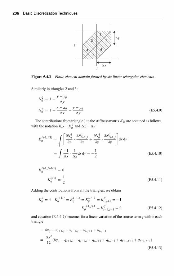
Ch05-H6594.tex 26/4/2007 16: 50 Page 236


�y

�x

j

i

1

2

3

45

6

Figure 5.4.3 Finite element domain formed by six linear triangular elements.

Similarly in triangles 2 and 3:

N 2ij = 1 − y − yij

�y

N 3ij = 1 + x − xij

�x− y − yij

�y(E5.4.9)

The contributions from triangle 1 to the stiffness matrix KIJ are obtained as follows,with the notation KIJ = Kij

ij and �x = �y:

Ki+1, j(1)ij =

∫

1

[∂N 1

ij

∂x· ∂N 1

i+1, j

∂x+ ∂N 1

ij

∂y· ∂N 1

i+1, j

∂y

]dx dy

=∫ −1

�x· 1

�xdx dy = −1

2(E5.4.10)

Ki+1, j+1(1)ij = 0

Kij(1)ij = 1

2(E5.4.11)

Adding the contributions from all the triangles, we obtain

Kijij = 4 Ki+1, j

ij = Ki−1, jij = Ki, j−1

ij = Kiji , j+1 = −1

Ki+1, j+1ij = Kij

i−1, j−1 = 0 (E5.4.12)

and equation (E.5.4.7) becomes for a linear variation of the source term q within eachtriangle

− 4uij + ui+1, j + ui−1, j + ui, j+1 + ui, j−1

= �x2

12(6qij + qi+1, j + qi−1, j + qi, j+1 + qi, j−1 + qi+1, j+1 + qi−1, j−1)

(E5.4.13)

Ch05-H6594.tex 26/4/2007 16: 50 Page 237


Compared to the finite difference discretization of the Laplace operator, it is seen thatthe left-hand side is identical to the five-point molecule of Figure 4.2.2. In a finitedifference method, the left-hand side would be equal to qij , while the finite elementmethod generates an average of the source term values at the points surrounding thenode (i, j).

A.5.4.5 Finite Element Galerkin Method for a Conservation Law

Consider the conservation law of the form:

∂U

∂t+ �∇ · �F = Q (5.4.34)

where F is the flux vector, containing only convective contributions with the followinginitial, boundary conditions on the domain � with boundary � = �0 ∪ �1

U (�x, 0) = U0(�x) for t = 0 x ∈ �

U (�x, t) = U1(�x) for t ≥ 0 x ∈ �0�F · �1n ≡ Fn = g for t ≥ 0 x ∈ �1

(5.4.35)

Defining a weak formulation, with W = 0 on �0,

∫

�

∂U

∂tW d� +

∫

�

( �∇ · �F)W d� =∫

�

Q W d� (5.4.36)

followed by an integration by parts on the flux term, leads to

∫

�

∂U

∂tW d� −

∫

�

(�F · �∇)W d� +∫

�

W �F · d�S =∫

�

Q W d� (5.4.37)

The finite element representation is defined by

U =∑

I

UI (t)NI (�x) (5.4.38)

and since the flux term F is generally a nonlinear function of U , it is preferable todefine also a separate representation for the fluxes F as

�F =∑

I

�FI NI (�x) (5.4.39)

The discretized equation for node J is obtained via the Galerkin method, W = NJ ,leading to

∑I

dUI

dt

∫

�J

NI NJ d� −∑

I

�FI

∫

�J

(NI · �∇)NJ d� +∫

�1

gNJ d� =∫

�J

Q NJ d�

(5.4.40)

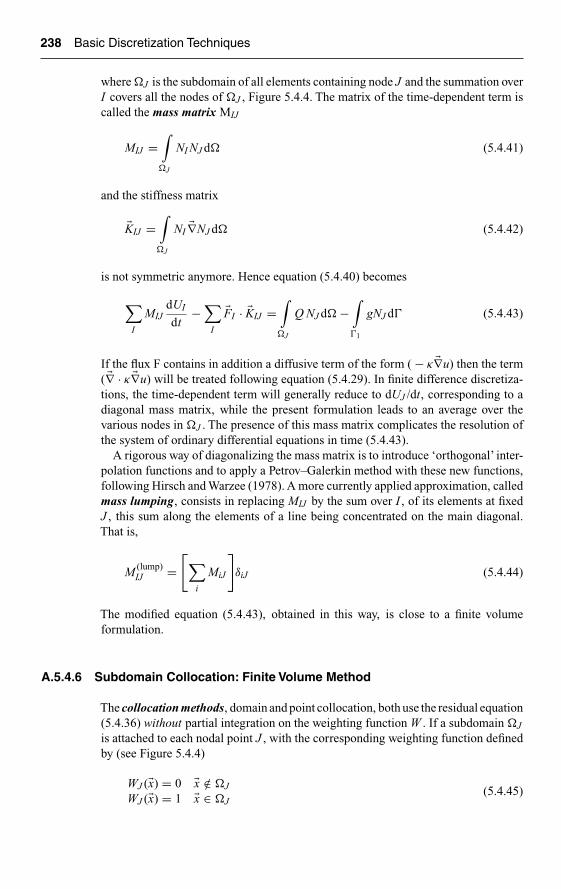
Ch05-H6594.tex 26/4/2007 16: 50 Page 238


where �J is the subdomain of all elements containing node J and the summation overI covers all the nodes of �J , Figure 5.4.4. The matrix of the time-dependent term iscalled the mass matrix MIJ

MIJ =∫

�J

NI NJ d� (5.4.41)

and the stiffness matrix

�KIJ =∫

�J

NI �∇NJ d� (5.4.42)

is not symmetric anymore. Hence equation (5.4.40) becomes

∑I

MIJdUI

dt−∑

I

�FI · �KIJ =∫

�J

Q NJ d� −∫

�1

gNJ d� (5.4.43)

If the flux F contains in addition a diffusive term of the form ( − κ �∇u) then the term( �∇ · κ �∇u) will be treated following equation (5.4.29). In finite difference discretiza-tions, the time-dependent term will generally reduce to dUJ /dt, corresponding to adiagonal mass matrix, while the present formulation leads to an average over thevarious nodes in �J . The presence of this mass matrix complicates the resolution ofthe system of ordinary differential equations in time (5.4.43).

A rigorous way of diagonalizing the mass matrix is to introduce ‘orthogonal’ inter-polation functions and to apply a Petrov–Galerkin method with these new functions,following Hirsch and Warzee (1978). A more currently applied approximation, calledmass lumping, consists in replacing MIJ by the sum over I , of its elements at fixedJ , this sum along the elements of a line being concentrated on the main diagonal.That is,

M (lump)IJ =

[∑i

MiJ

]δiJ (5.4.44)

The modified equation (5.4.43), obtained in this way, is close to a finite volumeformulation.

A.5.4.6 Subdomain Collocation: Finite Volume Method

The collocation methods, domain and point collocation, both use the residual equation(5.4.36) without partial integration on the weighting function W . If a subdomain �J

is attached to each nodal point J , with the corresponding weighting function definedby (see Figure 5.4.4)

WJ (�x) = 0 �x /∈ �J

WJ (�x) = 1 �x ∈ �J(5.4.45)

Ch05-H6594.tex 26/4/2007 16: 50 Page 239


2

3

4

1

6

5

j

Ω j

Figure 5.4.4 General triangular elements

then the residual equation (5.4.36) becomes∫

�J

∂U

∂td� +

∫�J

�∇ · �F d� =∫

�

Q d� (5.4.46)

A more interesting form of this equation is obtained after application of Gauss theoremon the flux term, leading to the conservation equation in integral form written for eachsubdomain �J limited by the closed surface �J .

∫�J

∂U

∂td� +

∮�J

�F · d�S =∫

�J

Q d� (5.4.47)

This equation, which can be obtained directly from equation (5.4.37), is the basicequation for the finite volume method as we have seen in the first part of this chapter.

Example E.5.4.3: Conservation law on linear triangles

We apply the Galerkin equation (5.4.40) with linear triangles for a node J not adjacentto the boundary �J of the domain and in absence of source terms. Referring toFigure 5.4.4, the domain �J contains six triangles and the nodes numbered 1–6around node J . We will also lump the mass matrix, leading to the approximation (seeProblem P.5.17):

MIJ = �J

3δIJ (E5.4.14)

The flux terms can be written as∫

�J

(�F · �∇)NJ d� =∑

I

�FI

∫

�J

NI · �∇NJ d�

=∑

I

fI

∫

�J

NI · ∂NJ

∂xd� +

∑I

gI

∫

�J

NI · ∂NJ

∂yd�

(E5.4.15)

where f and g are the Cartesian components of F .

Ch05-H6594.tex 26/4/2007 16: 50 Page 240


With the definitions (5.4.23) applied to the triangle J12 of figure 5.4.4, we have

∂NJ

∂x= (y1 − y2)/2A12

∂NJ

∂y= (x2 − x1)/2A12 (E5.4.16)

where A12 is the area of triangle J12. Since these derivatives are constants, the integralsin equation (E.5.4.16) reduce to the integrals over NI , which are equal to A12/3.

Hence, the contribution to the flux term of the Galerkin formulation from triangleJ12, becomes

∫

J12

�F · �∇NJ d� = y1 − y2

6(f1 + f2 + fJ ) − x1 − x2

6(g1 + g2 + gJ ) (E5.4.17)

Summing over all the triangles, we obtain

−∫

�J

�F · �∇NJ d� = 1

3

∑sides

( f12�y12−g12�x12) (E5.4.18)

with

f12 = 12 (f1 + f2) g12 = 1

2 (g1 + g2)�y12 = y2 − y1 �x12 = x2 − x1

(E5.4.19)

The contributions from fJ , gJ cancel out of the summation on all the triangles, since

∑sides

�y12 =∑sides

�x12 = 0 (E5.4.20)

because �J is a closed contour.Introducing this expression in the Galerkin equation (5.4.40) leads to the followingdiscretized scheme:

�JdUJ

dt+∑sides

( f12�y12−g12�x12) = 0 (E5.4.21)

which is nothing else than a finite volume discretization on the hexagonal contour �J

as seen in Section 5.3.

Alternative formulationsIf the flux terms of equation (E.5.4.21) are recombined, for instance by assemblingterms such as

(f1 + f2)(y2 − y1) + (f2 + f3)(y3 − y2) + · · · = f2(y3 − y1) + · · ·= −y2(f3 − f2) + · · ·

Ch05-H6594.tex 26/4/2007 16: 50 Page 241


we obtain the alternative formulation

�JdUJ

dt+ 1

2

∑l

[ fl(yl+1−yl−1) − gl(xl+1 − xl−1)] = 0 (E5.4.22)

where the summation extends over all the nodes, with y0 = y6 and y7 = y1 (andsimilarly for the x coordinates). We can also write equation (E.5.4.22) as

�JdUJ

dt+ 1

2

∑l

[(fl − fJ ) (yl+1−yl−1) − (gl − gJ ) (xl+1 − xl−1)] = 0

(E5.4.23)

since all the contributions to fJ and gJ vanish, because of

∑l

fJ (yl+1 − yl−1) = fJ∑

l

(yl+1 − yl−1) = 0 (E5.4.24)

The other formulation becomes

�JdUJ

dt− 1

2

∑l

[yl( fl+1 − fl−1) − xl (gl+1 − gl−1)] = 0 (E5.4.25)

or alternatively

�JdUJ

dt+ 1

2

∑l

[(yJ − yl)( fl+1 − fl−1) − (xJ − xl)(gl+1 − gl−1)] = 0

(E5.4.26)

with the conventions f0 = f6 and f7 = f1 (and similarly for g). The above relationscan also be derived from the results of Problem P.5.18. Note that these relations areindependent of the number of triangles inside �J and apply therefore to any polygonalcontour.


This chapter has been dealing with the most widely applied methodology in CFD,namely the finite volume method. For more advanced readers, we have also intro-duced the basics of the finite element method and in particular its application to theconservation laws.

The finite volume method (FVM) refers to the very important property of con-servation at the discrete level and leads also to a fundamental understanding of anynumerical scheme.


• The integral form of the conservation law is the basis of the FVM and satisfiesautomatically the discrete conservation property.

Ch05-H6594.tex 26/4/2007 16: 50 Page 242


• Look carefully at the finite volume treatment of the non-conservative form ofthe one-dimensional convection equation, as described in Section 5.1. It is ofgreat importance that you understand and recognize the numerical conservativityproperties, and its general form, as shown by equation (5.1.11).

• When defining an FVM, the space discretization divides the space in a number ofsmall volumes or cells, instead of arrays of points. A certain number of conditionshave to be satisfied by this finite volume space discretization. A key propertyfor an FVM to satisfy automatically conservativity is that the flux calculation oneach face has to be independent of the volumes shared by this face.

• Section 5.2.3 is of most essential significance and we recommend you to studyvery deeply all the consequences of this general formulation of a numericalscheme. Retain that any numerical scheme delivers as output cell-averagedapproximations and that assigning these values to a mesh point, as requiredfor post-processing, introduces a numerical error, generally of second order.

• The concept of numerical flux is also critical for finite volume methods. Allpossible schemes can always be written under the form of a numerical flux.

• Another key element in the FVM is the evaluation of the cell face flux approxima-tions, as defined by the numerical flux. A large number of choices are possible,some of them are listed in Section 5.3. Important to remember here is that thechoices presented are only the tip of the iceberg, and we will see in the followingchapters many more options.

• As the FVM is perfectly adapted to arbitrary grids, the formulas for the evalu-ation of surfaces and volumes establish a general framework for discretizationformulas applicable to non-uniform grids.

• On a more advanced level, pay attention to the links between the finite elementand finite volume methods.

REFERENCES

Arts, T. (1984). On the consistency of four different control surfaces used for finite areablade-to blade calculations. In. J. Numer. Meth. Fluids, 4, 1083–1096.

Baker, A.J. (1983). Finite Element Computational Fluid Mechanics. Hemisphere Publ.Co McGraw-Hill, New York.

Chung, T.J. (1978). Finite Element Analysis in Fluid Dynamics. McGraw-Hill, NewYork.Ciarlet, P.G. (1978). The Finite Element Method for Elliptic Problems. Studies in

Mathematics and Application, Vol.4. North-Holland Publ. Co., Amsterdam.Clough, R.W. (1960). The finite element method in plane stress analysis. Proceedings of

the 2nd ASCE Conference on Electronic Computation. J. Struct. Div. ASCE, 345–378.Denton, J. (1975). A Time Marching Method for Two and Three Dimensional Blade to

Blade flows. Aeronautical Research Council, R&M 3775.Girault, V. and Raviart, P.A. (1979). Finite Element Approximation of the Navier–Stokes

Equation. Lecture Notes in Mathematics, Vol. 749. Springer Verlag, New York.Glowinski, R. (1983). Numerical Methods for Non-LinearVariational Problems, 2nd edn.

Springer Verlag, New York.Hirsch, Ch. and Warzee, G. (1978). An orthogonal finite element method for transonic

flow calculations. Proceedings of the 6th International Conference on Numerical Meth-ods in Fluid Dynamics. Lecture Notes in Physics, Vol.90. Springer Verlag, New York.

Ch05-H6594.tex 26/4/2007 16: 50 Page 243


Huebner, K.H. (1975). The Finite Element Method for Engineers. J. Wiley & Sons,New York.

Lax, P.D. (1954). Weak solutions of non-linear hyperbolic equations and their numericalcomputation. Comm. Pure Appl. Math. 7, 159–193.

Lax, P.D. and Wendroff, B. (1960). Systems of conservation laws. Comm. Pure Appl.Math. 13, 217–237.

MacCormack, R.W. and Paullay, A.J. (1972). Computational efficiency achieved by timesplitting of finite difference operators. AIAA Paper 72–154.

McDonald, P.W. (1971). The computation of transonic flow through Two-dimensional gasturbine cascades. ASME Paper 71-GT-89.

Oden, J.T. (1972). Finite Elements of Non Linear Continua. McGraw-Hill, New York.Oden, J.T. and Reddy, J.N. (1976). An Introduction to the Mathematical Theory of Finite

Elements. J. Wiley & Sons, New York.Roache, P.J. (1972). Computational Fluid Dynamics. Hermosa Publ., Albuquerque, New

Mexico.Rizzi, A.W. and Inouye, M. (1973). Time split finite volume method for three-dimensional

blunt-body flows. AIAA J. 11, 1478–1485.Roe, P.L. (1987). Error estimates for cell-vertex solutions of the compressible Euler

equations. ICASE Report No. 87-6. NASA Langley Research Center.Strang, G. and Fix, G. (1973). An Analysis of the Finite Element Method. Prentice

Hall, New Jersey.Temam, R. (1977). Navier–Stokes Equations. North-Holland Publ. Co., Amsterdam.Thomasset, F. (1981). Implementation of Finite Element Methods for Navier–Stokes

Equations. Springer Series in Computational Physics, Springer Verlag, New York.Turkel, E. (1985). Accuracy of schemes with non-uniform meshes for compressible fluid

flows. ICASE Report N1/4 85-43. NASA Langley Research Center.Turkel, E., Yaniv, S. and Landau, U. (1985). Accuracy of schemes for the Euler equa-

tions with non-uniform meshes. ICASE Report N1/4 85-59. NASA Langley ResearchCenter; also in SIAM J. Sci. Statist. Computi.

Turner, M.J., Clough, R.W., Martin, H.C. and Topp, L.P. (1956). Stiffness and deflectionanalysis of complex structures. J. Aeron. Soc. 23, 805.

Zienkiewicz, O.C. and Cheung, Y.K. (1965). Finite elements in the solution of fieldproblems. Engineer, 507–10.

Zienkiewicz, O.C. and Taylor, R.L. (2000) Finite Element Method – Vol. 1: The Basis;Vol. 2: Solid Mechanics; Vol. 3: Fluid Dynamics. Elsevier, London.

PROBLEMS

P.5.1 Apply the finite volume formula (5.2.2) to the contourACDEGH of Figure 5.2.1aand derive the discretization for node (i, j). Compare with the formula (E.5.3.5)when the variables are defined at the nodes of the control volume, with the sidefluxes defined by the average of the corner points value, i.e.:

fAC = 1

2( fA + fC)

P.5.2 Apply the finite volume method to the contour of Figure 5.2.1b, and compare thedifferent assumptions for the evaluation of fluxes at the mid-side. Derive four

Ch05-H6594.tex 26/4/2007 16: 50 Page 244


schemes by combining the two options for the vertical sides with the two optionsfor the horizontal sides:

fAB = 1

2( fi+1, j + fij)

or

fAB = 1

6( fi+1, j + fi+1, j+1 + fi+1, j−1 + fij + fi, j+1 + fi, j−1)

with

fDA = fi, j−1

or

fDA = 1

4(2fi,j−1 + fi+1,j−1 + fi−1,j−1)

with similar expressions for g and for the two other sides.P.5.3 Determine the different formulas obtained in Problem P.5.2 when the mesh is

Cartesian and compare with the results of Problem P.5.1.P.5.4 Develop a finite volume discretization for mesh point A(i, j), with the control

volume BCDGHKEF of Figure 5.2.1b. Compare the results from the evaluationof the side fluxes by the following three options, written for instance for sideK(E)F:

fKF�yKF = 1

2( fi+1, j+1 + fi+1, j−1)(yi+1, j+1 − yi+1, j−1) (a)

or

fKF�yKF = fKE�yKE + fEF�yEF

= 1

2( fi+1, j + fi+1, j−1)(yi+1, j − yi+1, j−1)

+ 1

2( fi+1, j+1 + fi+1, j)(yi+1, j+1 − yi+1, j) (b)

or

fKF�yKF = fE�yKF = fi+1, j(yi+1, j+1 − yi+1, j−1) (c)

Compare the three results for a Cartesian mesh and refer also to Example E.5.3.1.P.5.5 Apply the results (5.3.21) in order to derive average values of the first deriva-

tives ∂f /∂x and ∂f /∂y over the triangle J12 of Figure 5.2.1d. Compare with theexpressions obtained in equations (E.5.4.21) , (E.5.4.22) and with the results ofProblem P.5.11. Note that the results are identical and comment on the reasonbehind the validity of the derivation by the finite element method with lineartriangles.

Ch05-H6594.tex 26/4/2007 16: 50 Page 245


P.5.6 Consider the two-dimensional diffusion equation treated in Example E.5.3.3 withdiffusive flux components f = k∂u/∂x and g = k∂u/∂y, where k is a function ofthe coordinates. Construct the discrete equation by the finite volume approachon the mesh of Figure 5.2.1a, considered as Cartesian, by generalizing the devel-opment of Example E.5.3.3. Consider the quadrilateral control surface ABCDfor the mesh point 1(i, j) and consider the values of k defined at the corners ofthe cell, that is in A,B,C,D. If necessary define

kAB = 1

2(kA + kB)

P.5.7 Consider the diffusion equation of the previous problem and apply it to the cellBCDGHKEF of Figure 5.2.1b, considered as Cartesian, with constant k . Definethe derivatives on the cell sides by one sided formulas, from inside the controlcell. Apply successively the three options of Problem P.5.4 and compare with theresults of Example E.5.3.3. Show in particular that the options a, b, c reproducethe schemes derived in this example.

Hint: For a point F, define the derivatives as

(∂u

∂x

)F

= ui+1, j+1 − ui, j+1

�x(∂u

∂y

)F

= ui+1, j+1 − ui+1, j

�x

and similar relations for the other points.P.5.8 Apply equation (5.3.29) to the quadrilateral ABCD of Figure 5.3.1 and take point

A as origin of the position vector �x. Show that the contour integral reduces tothe contributions along BC and CD with �x = �xAC and that

2� = �xAC ·∮

BCDd�S

By working out the integral, obtain the relation (5.3.4)

�ABCD = 1

2(�xAC�yBD − �xBD�yAC)

Hint: Observe that with A as origin the position vector is aligned with thesides AB and AD and hence normal to the vector dS. Therefore, there are nocontributions from these two sides.

P.5.9 Repeat Problem P.5.8 for triangleABC of Figure 5.3.1 and show that we can write

2�ABC = �xAB ·∮

BCd�S

obtaining

�ABC = 1

2(�xAB�yBC − �xBC�yAB)

Ch05-H6594.tex 26/4/2007 16: 50 Page 246


P.5.10 Consider the quadrilateral BDHE on Figure 5.3.2b and apply the relations(6.2.29) in order to define the average value of the x-derivative of a functionU . Consider yE = yD and obtain

(∂U

∂x

)

BDHE

= UE − UD

xE − xD

Comment on the accuracy of this formula when applied to point A.P.5.11 Repeat Problem P.5.10 for the contour BCDGHKEF of Figure 5.2.1b by applying

formulas (5.3.26) and (5.3.27). Obtain the following approximation:

(∂U

∂x

)= UE − UD

xE − xD+ �yBA

2�yBH

UF − UC

xF − xC+ �yAH

2�yBH

UK − UG

xK − xG

Derive also the corresponding expression for a Cartesian mesh.P.5.12. Apply the upwind flux evaluation (5.3.15) to derive a finite volume scheme for

the cell GHKEFBCD of Figure 5.2.1b, considered as Cartesian. Compare theobtained discretization with the results of Example E.5.3.2.

P.5.13 Show that the integral conservation law over the one-dimensional domaina ≤ x ≤ b, applied to the one-dimensional conservation law

∂u

∂t+ ∂f

∂x= 0

with the condition f (a) = f (b), reduces to the condition

∫ b

au dx = const.

with time.Apply this condition to the to a discretized x-space, with an arbitrary mesh

point distribution, as in Figure 4.3.2, and show that this condition reduces to

1

2

∑i

�ui(xi+1 − xi−1) = 0

where

�ui ≡ un+1i − un

i = ∂ui

∂t�t

Hint: apply a trapezoidal rule to evaluate the integral

∂

∂t

∫ b

au dx = 0

and rearrange the sum to isolate the ui-terms.

Ch05-H6594.tex 26/4/2007 16: 50 Page 247


P.5.14 Apply the Galerkin method, with linear elements to the first order equation

a∂u

∂x= q

Show that on a uniform mesh, �xi = �xi+1 = �x, we obtain the samediscretization as with central differences.

P.5.15 Work out all the calculations of Example E.5.4.2.P.5.16 Show by an explicit calculation, that the average value of a quantity U over an

element is approximated for linear triangles by

1

�

∫�

U d� = 1

3

3∑I=1

UI

P.5.17 Calculate the mass matrix elements attached to node J of Figure 5.4.4, withlinear triangles. Show that one obtains equation (E.5.4.14) for the lumped massapproximation.Hint: Obtain the following matrix, for a triangle of area A

MIJ = A

12

∣∣∣∣∣∣2 1 11 2 11 1 2

∣∣∣∣∣∣P.5.18 Referring to Figure 5.4.4, show that the average of ∂f /∂x and ∂g/∂y over the

domain �J covered by the six linear triangles, can be defined as

(∂f

∂x

)

�J

= 1

�J

∫�J

∂f

∂xd�

= 1

2�J

∑I

fI (yI+1 − yI−1)

where the summation extends over all the nodes of the contour �J , and

(∂g

∂y

)= 1

�J

∫�J

∂g

∂yd�

= − 1

2�J

∑I

gI (xI+1 − xI−1)

Hint: Calculate the average values for each triangle J12 by taking f = ∑ fI NI .Show that for each triangle we have∫

J12

∂f

∂xd� = 1

2[ f1(y2 − yJ ) + f2(yJ − y1) + fJ (y1 − y2)]

and sum these contributions over all the triangles.

Ch05-H6594.tex 26/4/2007 16: 50 Page 248


P.5.19 Apply the results of Example E.5.4.3 to a quadrilateral domain such as J 234 onFigure 5.4.1b, discarding node J , to obtain the following discretization of theflux integral on this quadrilateral.

∮J 234

�F .d�S = 1

2[(f2 − f4)(y3 − yJ ) + (f3 − fJ )(y4 − y2)

−(g2 − g4)(x3 − xJ ) − (g3 − gJ )(x4 − x2)]

P.5.20 Proof equation (5.4.21) for linear one-dimensional elements.P.5.21 Apply the Galerkin method with linear elements to the conservation equation

∂u

∂t+ ∂f

∂x= 0

following Section A54.4. Obtain the implicit formulation:

1

6

[dui−1

dt+ 4

dui

dt+ dui+1

dt

]+ 1

2�x(fi+1 − fi−1) = 0

P.5.22 Show that the shape functions (5.4.22) satisfy the conditions (5.4.2)–(5.4.5) fortwo-dimensional linear triangular elements.

Ch06-H6594.tex 26/4/2007 16: 56 Page 249

Chapter 6

Structured and Unstructured Grid Properties


Grid generation is a major component in setting up a CFD simulation and if youconsider Figure I.2.1 of the general introduction, you will find the explanation for itscrucial role in the overall CFD process. It is the first necessary step, as no simulationcan be started without having defined an appropriate mesh point distribution. Methodshave therefore been developed to help the CFD user in generating grids in the bestpossible way. The importance of grid properties cannot be emphasized enough. Wehave already stressed in Chapter 4 the effects of non-uniform grids and the potentialloss of accuracy of the most current finite difference formulas associated to grid non-uniformities. Although this analysis was restricted to one-dimensional grids, you caneasily imagine that these effects will be amplified on irregular 2D and 3D grids, ofthe type shown in the Introduction.

This emphasizes the essential role played by grid properties in the overall accuracyof a CFD simulation.

The software methods in support of the grid generation process are complicatedto develop, particularly for general geometries, as they require sophisticated pro-gramming and mathematical methodologies. The relevant software tools call uponalgebraic geometry theories, mathematical surface definitions, normals and curvatureestimations, coordinate transformations, topological properties, etc. The interestedreader will find detailed descriptions of grid generation methods in the followingreferences: Thompson (1984), Thompson et al. (1985), (1999), Dale and King (1993)for structured grids and George and Borouchaki (1998), Frey and George (1999) forunstructured grids.

We consider these topics as being outside the scope of this introduction to CFD,although you will need to generate grids for the applications to be covered in the lastpart of this text, in Chapters 11 and 12. We have therefore chosen not to take youthrough the different mathematical techniques applied to generate grids. Instead, ourobjective is to present you with an overview of the possible grid configurations asapplied in practice.

You can refer to the following web sites for a widely documented overview ofmost of the available grid generators: http://www-users.informatik.rwth-aachen.de/∼roberts/meshgeneration.html; http://www.andrew.cmu.edu/user/sowen/mesh.html.

Next to the commercial offers, a large variety of freely available grid generatorscan be found and downloaded for particular applications.1

1 We suggest exercising great care when downloading free software tools. Check carefully the lastupdate of the visited web site and verify that the software you are interested in is still being maintainedby the author(s). If not, we recommend avoiding its use, as you will face great risks of encounteringsoftware bugs and problems, for which no help would be available.

249

Ch06-H6594.tex 26/4/2007 16: 56 Page 250


Despite the numerous available software codes to support the task of grid gener-ation, it still can be a very time-consuming exercise, particularly when dealing withcomplex geometries. Consequently, automatic grid generation, with an adequatecontrol of grid quality, has become one of the major objectives of modern CFD, bothfor structured as well as unstructured grids.

As mentioned already in the Introduction and in Chapter 5, we distinguish betweenstructured and unstructured grids. The former is composed of families of intersectinglines, one for each space dimension (two families of lines in 2D and three in 3D),where each mesh point is located at the intersection of one line, and only one line, ofeach family.

Unstructured grids, on the contrary, refer to arbitrary distributions of mesh points,where the points are connected by triangles, quadrilaterals or polygons in 2D, orby various polyhedrals in 3D (tetrahedra, prisms, pyramids, hexahedra or arbitrarypolyhedrals).

The objective of this chapter is to introduce you to the various types of grids,both structured and unstructured, that you can select or encounter in practice. Fora given geometrical configuration, many different grid topologies can be definedand there are always several alternative possibilities for a given application and flowmodel. The choice of a mesh topology is often a matter of personal choice and it istherefore of importance to acquire knowledge of the various possibilities offered bygrid generation tools. The first choice is between a structured or an unstructured grid,based on the properties of the flow solver and on the level of geometrical complexity.The second choice is, within either of these two families, to select an adapted gridtopology or element type. We will cover these various options in this chapter, whichis subdivided as follows:

Section 6.1 describes and illustrates various options for structured grids, whileSection 6.2 focuses on unstructured grid configurations.

Once a grid is established, the flow solvers have to evaluate surfaces and volumes,based on the mesh point coordinates and element shapes, as required by the applicationof finite volume methods to cells of arbitrary shapes. Guidelines and a few easyto implement formulas for the numerical evaluation of surfaces and volumes areprovided in Section 6.3, as an extension to the formulas already given in Chapter 5.

As already mentioned, grid quality has a direct impact on the overall accuracyof the CFD results. An evaluation of grid related numerical errors for arbitrary 2Dgrids is presented to serve as a basis for the establishment of a few general guidelinestoward minimizing grid-related error sources. This forms the subject of Section 6.4,which offers recommendations concerning grid properties, to be followed as best aspossible in order to minimize grid-related losses of accuracy.

Figure 6.0.1 summarizes the roadmap to this chapter.

6.1 STRUCTURED GRIDS

Structured grids can be considered as most ‘natural’ for flow problems as the flow isgenerally aligned with the solid bodies and we can imagine the grid lines to follow insome sense the streamlines, at least conceptually, when not possible realistically.

It has to be emphasized that structured grids will, compared to unstructured grids,often be more efficient from CFD point of view, in terms of accuracy, CPU time and

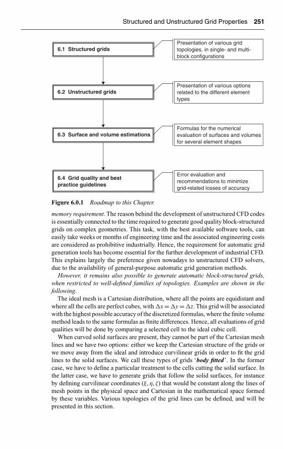
Ch06-H6594.tex 26/4/2007 16: 56 Page 251

Structured and Unstructured Grid Properties 251

6.1 Structured gridsPresentation of various gridtopologies, in single- and multi-block configurations

Presentation of various optionsrelated to the different elementtypes

6.2 Unstructured grids

Formulas for the numericalevaluation of surfaces and volumesfor several element shapes

6.3 Surface and volume estimations

Error evaluation andrecommendations to minimizegrid-related losses of accuracy

6.4 Grid quality and bestpractice guidelines

Figure 6.0.1 Roadmap to this Chapter.

memory requirement. The reason behind the development of unstructured CFD codesis essentially connected to the time required to generate good quality block-structuredgrids on complex geometries. This task, with the best available software tools, caneasily take weeks or months of engineering time and the associated engineering costsare considered as prohibitive industrially. Hence, the requirement for automatic gridgeneration tools has become essential for the further development of industrial CFD.This explains largely the preference given nowadays to unstructured CFD solvers,due to the availability of general-purpose automatic grid generation methods.

However, it remains also possible to generate automatic block-structured grids,when restricted to well-defined families of topologies. Examples are shown in thefollowing.

The ideal mesh is a Cartesian distribution, where all the points are equidistant andwhere all the cells are perfect cubes, with �x = �y = �z. This grid will be associatedwith the highest possible accuracy of the discretized formulas, where the finite volumemethod leads to the same formulas as finite differences. Hence, all evaluations of gridqualities will be done by comparing a selected cell to the ideal cubic cell.

When curved solid surfaces are present, they cannot be part of the Cartesian meshlines and we have two options: either we keep the Cartesian structure of the grids orwe move away from the ideal and introduce curvilinear grids in order to fit the gridlines to the solid surfaces. We call these types of grids ‘body fitted’. In the formercase, we have to define a particular treatment to the cells cutting the solid surface. Inthe latter case, we have to generate grids that follow the solid surfaces, for instanceby defining curvilinear coordinates (ξ, η, ζ) that would be constant along the lines ofmesh points in the physical space and Cartesian in the mathematical space formedby these variables. Various topologies of the grid lines can be defined, and will bepresented in this section.

Ch06-H6594.tex 26/4/2007 16: 56 Page 252


The drawback of structured grids is a form of stiffness connected to the fact thatadding a point locally implies adding lines of each family through that point, whichwill therefore affect the whole domain. In complex geometries, this can be verydetrimental and render the grid generation process quite cumbersome. One way toease these constraints is to define multi-block grids, each block covering a subset ofthe computational domain with its own structured grid. This can be further generalizedwhen the connectivity of the points at the block interfaces is relaxed by allowing ‘non-matching’ lines at the inter-block boundaries. This provides maximum flexibility toblock-structured grids.

Another way is to allow for overlapping grids, each grid being attached to a solidbody, when multiple moving bodies are present, or to separate blocks. Both ways implysophisticated treatment for the interpolation of the numerical flow variables betweentwo independent grids, with the requirement to satisfy constraints of conservationand accuracy.

6.1.1 Cartesian Grids

As mentioned above, uniform Cartesian grids are the ideal solution from the point ofview of accuracy and they should be applied whenever possible. It is a valid optionwhen the solid walls are parallel to the Cartesian axes, or in absence of solid walls infree space.

Cartesian grids are often applied in aero-acoustic computations, where high orderschemes are required for an accurate simulation of the propagation of acousticpressure waves (see for instance the review paper by Tam (2004)).

6.1.2 Non-uniform Cartesian Grids

Variable mesh sizesA first variant on the ideal Cartesian uniform grid is to allow for variable values ofthe mesh spacing, for instance in boundary layers where a strong clustering near solidwalls is required. Figure 6.1.1 shows an example of a Cartesian grid applied to theflow simulation over and in a rectangular cavity.

Quadtree-Octree gridA second variant consists of allowing for local refinements with ‘hanging nodes’,also called non-conformal grids, obtained by subdividing an initial Cartesian grid insub-cells, either uniformly or non-isotropically, as shown in Figure 6.1.2. This leadsto a quadtree structure in 2D and an octree structure in 3D.

In presence of curved boundaries, Cartesian grids still remain an option, withthe advantage that the grid generation process is trivial, while minimizing numer-ical errors. However, the treatment of the curved solid boundaries requires specialattention.

Several options can be considered:

• Method 1: The Cartesian type grid on both sides of the surface is maintained anda numerical procedure is defined in the flow solver to handle the physical bound-ary conditions (Figure 6.1.3). This is called the immersed boundary method(see for instance Mittal and Iaccarino (2005) for a review).

Ch06-H6594.tex 26/4/2007 16: 56 Page 253


Figure 6.1.1 Cartesian grid with non-uniform cell sizes for a cavity.

Figure 6.1.2 Quadtree grid, with hanging nodes, around an airfoil, with staircaseboundary approximation.

• Method 2: The Cartesian cells outside the computational domain are removed,replacing hereby the solid boundaries by a staircase shape; this is the case withFigure 6.1.2.

• Method 3: The intersection of the solid surface with the Cartesian cells is defined,leading to boundary cells of arbitrary shapes, called cut-cells; see Figure 6.1.4,from Aftosmis et al. (2000). This requires the application of a finite volumediscretization on the cut-cell faces.

Ch06-H6594.tex 26/4/2007 16: 56 Page 254


Figure 6.1.3 Cartesian mesh around a solid boundary with Immersed BoundaryMethod.

a

e

h

j k f

l

gmno

b c d

ip

q

Cartesian mesh with embedded geometry

Figure 6.1.4 Cut-cell configuration; from Aftosmis et al. (2000). AIAA copyright.

6.1.3 Body-Fitted Structured Grids

In this approach, the grid is made curvilinear to adapt as far as possible to the geome-tries. It calls upon more sophisticated methods to generate the grids in order to satisfyrequirements on smoothness and continuity of cell sizes. Depending on the orienta-tion of the grid lines, various configurations can be selected, indicated by the letterto which they resemble the most. We refer in this context to grids of H-type, C-type,O-type, I-type and their various combinations.

H-meshThe grid lines are curvilinear, approaching a set of horizontal and vertical lines in apseudo-orthogonal configuration, with a topology that can be associated to the letter H(see Figure 6.1.5 for a representative example).

Ch06-H6594.tex 26/4/2007 16: 56 Page 255


Figure 6.1.5 Structured curvilinear body-fitted grid of the H-type.

Figure 6.1.6 Structured curvilinear body-fitted grid of the C-type.

C-meshThe grid lines are curvilinear, surrounding the geometry, with a topology that can beassociated to the letter C, on one side (for instance around the leading edge of theairfoil), but remaining open at the other end of the computational domain. This can beadapted to concentrate grid lines in the wake region of an airfoil or wing (see Figure6.1.6 for a representative example).

O-meshThe grid lines are curvilinear, surrounding completely the geometry, with a topologythat can be associated to the letter O. This option allows an accurate mesh point distri-bution around both leading and trailing edges of external aerodynamic configurations,such as wings and airfoil sections (see Figure 6.1.7 for a representative example).

I-meshIn the particular case of highly staggered turbomachinery blade sections, thequality requirement of nearly orthogonal cells is better fulfilled with grid lines

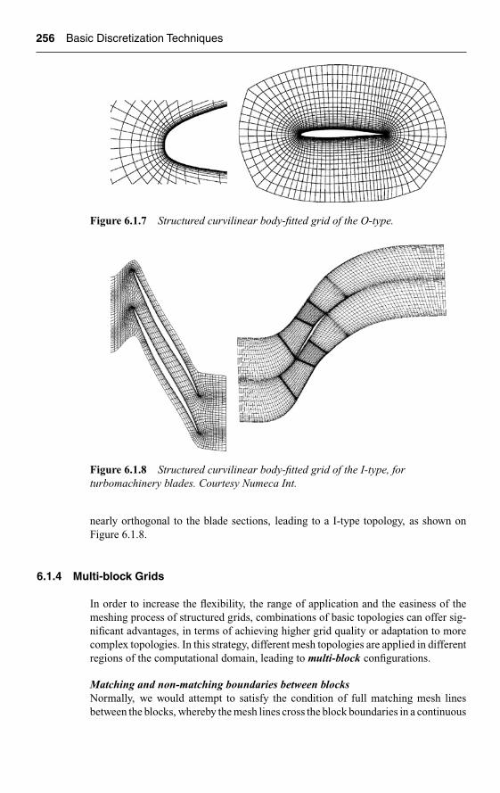
Ch06-H6594.tex 26/4/2007 16: 56 Page 256


Figure 6.1.7 Structured curvilinear body-fitted grid of the O-type.

Figure 6.1.8 Structured curvilinear body-fitted grid of the I-type, forturbomachinery blades. Courtesy Numeca Int.

nearly orthogonal to the blade sections, leading to a I-type topology, as shown onFigure 6.1.8.

6.1.4 Multi-block Grids

In order to increase the flexibility, the range of application and the easiness of themeshing process of structured grids, combinations of basic topologies can offer sig-nificant advantages, in terms of achieving higher grid quality or adaptation to morecomplex topologies. In this strategy, different mesh topologies are applied in differentregions of the computational domain, leading to multi-block configurations.

Matching and non-matching boundaries between blocksNormally, we would attempt to satisfy the condition of full matching mesh linesbetween the blocks, whereby the mesh lines cross the block boundaries in a continuous

Ch06-H6594.tex 26/4/2007 16: 56 Page 257


(a) (b)

Figure 6.1.9 Representation of (a) matching and (b) non-matching blockboundary interfaces of a multi-block-structured grid, with a channel connectingtwo circular ducts.

Figure 6.1.10 Full non-matching block boundary interfaces of amulti-block-structured grid. Courtesy Numeca Int.

way. However, in order to exploit maximally the potential of block-structured grids,the additional flexibility of allowing for non-matching block interfaces offers sig-nificant advantages. The price of this enhanced flexibility is the necessity for theflow solver to handle with sufficient accuracy the transfer of information through thenon-matching interface, requiring sophisticated interpolation routines between twototally independent surface grids.

This is illustrated in Figure 6.1.9, where the choice between the two options isstill available. This is not always the case and Figure 6.1.10 shows an example where

Ch06-H6594.tex 26/4/2007 16: 56 Page 258


Figure 6.1.11 Structured curvilinear body-fitted grid of the C–H type.

Figure 6.1.12 Structured multi-block body-fitted grid of the H–O–H type.

smaller exhaust pipes are connected on a larger duct. In this case, both componentscan be meshed optimally and freely connected in a non-matching mode.

C–H meshThis combines a C-mesh around the body and an H-mesh in the upstream region asshown in Figure 6.1.11.

H–O–H meshIn this configuration, an O-mesh is kept around the body, while H-topologies aredefined in the upstream and downstream regions (see Figure 6.1.12).

‘Butterfly’ grids for internal flowsHigh quality structured grids with internal flow configurations, such as complex ducts,are difficult to ensure and a high level of flexibility is required. One of the optionsis obtained by the so-called ‘butterfly’ topology shown in Figure 6.1.13, for a simpleduct section.

It can also be applied to bulbs of a rotating axis, in order to avoid a singularmesh line on the axis of rotation, at zero radius. Figure 6.1.14 shows combinationsof block-structured grids, obtained with the automatic grid generator Autogrid™from Numeca Int. (http://www.numeca.be), applied to the pump inducer of the liquidhydrogen pump of the VULCAIN engine of the EuropeanARIANE 5 rocket launcher.

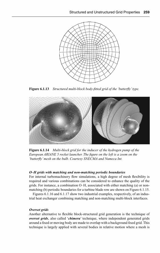
Ch06-H6594.tex 26/4/2007 16: 56 Page 259


Figure 6.1.13 Structured multi-block body-fitted grid of the ‘butterfly’ type.

Figure 6.1.14 Multi-block grid for the inducer of the hydrogen pump of theEuropean ARIANE 5 rocket launcher. The figure on the left is a zoom on the‘butterfly’ mesh on the bulb. Courtesy SNECMA and Numeca Int.

O–H grids with matching and non-matching periodic boundariesFor internal turbomachinery flow simulations, a high degree of mesh flexibility isrequired and various combinations can be considered to enhance the quality of thegrids. For instance, a combination O–H, associated with either matching (a) or non-matching (b) periodic boundaries for a turbine blade row are shown on Figure 6.1.15.

Figures 6.1.16 and 6.1.17 show two industrial examples, respectively, of an indus-trial heat exchanger combining matching and non-matching multi-block interfaces.

Overset gridsAnother alternative to flexible block-structured grid generation is the technique ofoverset grids, also called ‘chimera’ technique, where independent generated gridsaround a fixed or moving body are made to overlap with a background fixed grid. Thistechnique is largely applied with several bodies in relative motion where a mesh is

Ch06-H6594.tex 26/4/2007 16: 56 Page 260


Figure 6.1.15 Structured curvilinear body-fitted grid of the O–H type:(a) matching periodic boundaries and (b) non-matching periodic boundaries.Courtesy Numeca Int.

Figure 6.1.16 Structured multi-block grid of an industrial heat exchangercombining matching and non-matching multi-block interfaces. Courtesy AtlasCopco and Numeca Int.

attached to each body. The drawback is related to the necessity for an accurate inter-polation between three-dimensional overlapping grids. This is extremely challenging,particularly if conservative interpolations are required.

Note that the overset principle can equally be applied with unstructured grids,although it was developed initially for structured grids (Steger et al., 1983; Beneket al., 1985).

Figure 6.1.18 shows overlapping grids around moving parts of a flying structure,with a zoom on a section of the overlapping region.

Ch06-H6594.tex 26/4/2007 16: 56 Page 261


Figure 6.1.17 Structured multi-block grid of an industrial inlet ducting with guidevanes, combining matching and non-matching multi-block interfaces. CourtesyAtlas Copco and Numeca Int.

Figure 6.1.18 Overlapping grids around moving parts of a flying structure, with azoom on a section of the overlapping region.

6.2 UNSTRUCTURED GRIDS

Unstructured grids have progressively become the dominating approach to industrialCFD, due to the impossibility to generate automatically block-structured grids onarbitrary geometries. It is indeed nearly impossible, for topology-connected reasons,to envisage an automatic block-structured grid generator without an a priori knowl-edge of the involved topologies. However, this is possible with unstructured gridsand therefore unstructured flow solvers for the Navier–Stokes equations have gainedwide acceptance.

Although on a same regular distribution of points, an unstructured grid, formed forinstance by triangles in 2D, will tend to have a lower accuracy than the correspondingstructured grid, as will be shown in Section 6.4, this trend has arisen because of theindustrial requirements for automatic grid generation tools.

One of the advantages of unstructured grids is the possibility to perform localrefinements in a certain region, without affecting the grid point distribution outsidethat region. This opens the way for flexible grid adaptation by local refinement orlocal coarsening, based on some criteria associated either to some flow gradients or

Ch06-H6594.tex 26/4/2007 16: 56 Page 262


to some error estimation. Grid adaptation is based on the addition or removal of meshpoints in order to increase the accuracy in regions of strong flow variations and byremoving points in regions where the solutions has already reached an acceptableaccuracy. This process has as objective to optimize the number of grid points for acertain level of accuracy.

The space domain can be discretized by subdivision of the continuum into elementsof arbitrary shape and size. Since any polygonal structure with rectilinear or curvedsides can finally be reduced to triangular and quadrilateral elements, they form thebasis for the most current space subdivision in 2D space. Cells with an arbitrarynumber of faces can also be considered, resulting from a dual grid construction, orfrom an agglomeration process of groups of cells into coarser cells, as required bymultigrid methods. The only restriction is that the elements may not overlap and haveto cover the complete computational domain.

Most of the unstructured grid generators applied in practice are focused on thegeneration of basic cell shapes formed by:

• triangle/tetrahedra elements;• hybrid elements involving combinations of tetrahedra, pyramids and prisms, the

latter being concentrated near the solid surfaces;• quadrilaterals and hexahedra.

6.2.1 Triangle/Tetrahedra Cells

Various methods are available to generate triangular/tetrahedral grids around arbitrarybodies. Most of them require an initial surface triangulation, which has to be generatedfirst, before launching the generation of the volume mesh. See for instance the booksby George and Borouchaki (1998) and Frey and George (1999) for an overview.

The following examples are obtained with the system DELANDO developed byJens-Dominik Müller (see http://www.cerfacs.fr/∼muller/delaundo.html).

Figure 6.2.1 shows a two-dimensional unstructured grid with triangular cells,around an airfoil with flaps.

An example of a complex tetrahedral grid is shown on Figure 6.2.2, generated for thesimulation of the electrochemical plating of a system of decorative cronium wheels.

Figure 6.2.1 Example of an unstructured triangular grid.

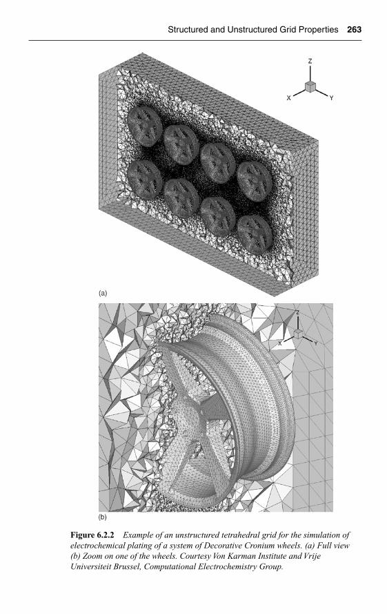
Ch06-H6594.tex 26/4/2007 16: 56 Page 263


Figure 6.2.2 Example of an unstructured tetrahedral grid for the simulation ofelectrochemical plating of a system of Decorative Cronium wheels. (a) Full view(b) Zoom on one of the wheels. Courtesy Von Karman Institute and VrijeUniversiteit Brussel, Computational Electrochemistry Group.

Ch06-H6594.tex 26/4/2007 16: 56 Page 264


6.2.2 Hybrid Grids

The main difficulty with triangular/tetrahedral grids is connected to the boundarylayer requirements of high Reynolds number flows, where the grid density in thenormal direction has to be adapted to the boundary layer velocity profiles. As seen inSection 4.3, the ratio of mesh sizes should optimally be of the other �x/�y ∼ √

(Re),where �x and �y are the representative mesh sizes in the streamwise and normaldirections, respectively. This implies mesh aspect ratios �x/�y of the order of 1000,for typical industrial flows, which would lead to very poorly configured triangles withheight to base ratios of that order and, consequently, a significant loss of accuracy.

To avoid this problem, hybrid grids have been developed, whereby layers of quadri-laterals or prisms are generated in the near-wall region, by a form of extrusion processout of the triangulated surface grid. This is shown on Figure 6.2.3, for a 2D case, fromthe same reference as the previous figure http://www.cerfacs.fr/∼muller/hip.html.

A three-dimensional example of a hybrid grid for a gas-turbine stator with rowsof film cooling holes in the leading edge region is shown on Figure 6.2.4. The gridsare obtained with the CENTAUR™ grid generator from Centaursoft (http://www.centaursoft.com), showing different views of the hybrid grid. The top figure showsthe 3D view and the other figures show a 2D section with a close-up view of theleading edge region.

6.2.3 Quadrilateral/Hexahedra Cells

It is known from numerous simulations (see also Section 6.4) that hexahedra offersignificant advantages compared to tetrahedral cells, in terms of memory requirementsand accuracy. For tetrahedral grids, the ratio of the number of cells to the number ofvertices is close to 6, not taking into account the boundaries. (for a two-dimensionaltriangulation this ratio is of the order of 3); while this ratio remains close to one forhexahedral cells.

Figure 6.2.3 Example of an unstructured hybrid grid showing the regularquadrilateral type structure near the solid walls.

Ch06-H6594.tex 26/4/2007 16: 56 Page 265


Automatic generation of unstructured hexahedra is quite challenging and someexamples from the HEXPRESS™ generator from Numeca Int. (http://www.numeca.be) are shown in the following figures. In this approach, the surface meshis obtained from the volume mesh, through a projection step of a Cartesian/octreevolume mesh, whereby the initial generation of a surface mesh is not required. Figure6.2.5 shows a 2D quadrilateral grid around an airfoil, while Figure 6.2.6 shows a 3Dunstructured hexahedral grid of a valve system, with cuts displaying the internal cells.

Similarly, Figure 6.2.7 shows the hexahedral mesh for a complex dusting system,with appropriate cuts to visualize the internal volume cells.

6.2.4 Arbitrary Shaped Elements

The most general unstructured grid configuration is obtained with cells having anarbitrary number of faces. They can be defined either by considering the dual meshof a base grid formed by simple shapes, or by an agglomeration process of cells.

Figure 6.2.4 Three-dimensional hybrid grid of a turbine blade with film coolingconfiguration, with a 2D section and a close-up view of the leading edge region.From http://www.centaursoft.com.

Ch06-H6594.tex 26/4/2007 16: 56 Page 266


Figure 6.2.5 Unstructured quadrilateral grid around an airfoil, obtained with theHEXPRESS™ generator from Numeca Int.

Figure 6.2.6 3D unstructured hexahedral grid of a valve system, with cutsdisplaying the internal cells, obtained with the HEXPRESS™ generator fromNumeca Int.

Two-dimensional dual grids are obtained by joining the midpoints of cell edges tothe center of the cells, as illustrated in Figure 6.2.8. Alternatively, they can be definedby joining the midpoint normals to the cell edges to form a polygonal cell.

The agglomeration process is generally applied for multigrid convergence acceler-ation methods (see Chapter 10) on unstructured grids, in grouping cells into coarsercells, typically with a ratio close to 8. This can be applied to tetrahedral or hexahedralgrids, as seen on the examples of Figures 6.2.9 and 6.2.10.

Ch06-H6594.tex 26/4/2007 16: 56 Page 267


Figure 6.2.7 Unstructured hexahedral mesh for a complex dusting system, withcuts to showing the internal volume cells, obtained with the HEXPRESS™generator from Numeca Int.

6.3 SURFACE AND VOLUME ESTIMATIONS

Non-Cartesian grids are predominantly applied with finite volume methods, and asseen in Chapter 5, this requires the numerical evaluation of cell volumes and faceareas, including the direction of the normals to the faces.

In this section, we intend to provide you with a few additional formulas for theevaluation of these geometrical quantities, up to second order accuracy.

In 2D cases, we will consider that we have either triangles or quadrilaterals andthe area of the cells is the only quantity we need, as the length of the edges is triviallydefined by the distance between its end-points. In case of cells of arbitrary shape, itwill be considered that they are subdivided in triangles and or quadrilaterals.

In three dimensions, we will assume that the geometrical space is subdivided intetrahedra, pyramids, prisms or hexahedra. When a face is formed by three nodes,i.e. by a triangle, as is the case with an arbitrary triangulation, then the calculationof the area is straightforward as three points lie always in the same plane. However,for a quadrilateral face, the four points forming the face are not necessarily coplanar,which can be a source of error, as there is more than one way to evaluate the cell facearea. Care has to be exercised in the evaluation of the cell volume and face areas,in order to ensure that the sum of the computed volumes of adjacent cells is indeedequal to the total volume of the combined cells.

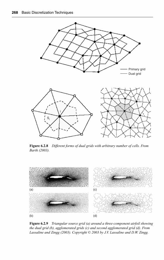
Ch06-H6594.tex 26/4/2007 16: 56 Page 268


Primary gridDual grid

i T0

Tk

Tk�1

Tk�1

Si

Figure 6.2.8 Different forms of dual grids with arbitrary number of cells. FromBarth (2003).

(a)

(b)

(c)

(d)

Figure 6.2.9 Triangular source grid (a) around a three-component airfoil showingthe dual grid (b), agglomerated grids (c) and second agglomerated grid (d). FromLassaline and Zingg (2003). Copyright © 2003 by J.V. Lassaline and D.W. Zingg.

Ch06-H6594.tex 26/4/2007 16: 56 Page 269


Figure 6.2.10 Two levels of agglomerated grids from an initial unstructuredhexahedral grid. Courtesy Numeca Int.

6.3.1 Evaluation of Cell Face Areas

Some formulas have already been derived in Sections 5.3 and A5.4 when we intro-duced the finite volume and finite element methods. Hence, the formulas presentedhere can be considered as a generalization, providing additional options.

An important property of the area vector S attached to a cell face is derived fromthe divergence theorem. Equation (5.3.16) with U = 1 becomes, where the integralloops over all the faces of the cell:

∮S

d�S = 0 or∑faces

�Sfaces = 0 (6.3.1)

This relation indicates that the sum over all the face surface normals of any closedcell must be zero. In addition, it shows that the outward surface vector of a given facebelonging to the closed surface S:

�Sface =∫

faced�S (6.3.2)

is only dependent on the boundaries of the face.Hence, for faceABCD of Figure 6.3.1, we could apply equation (5.3.4), reproduced

here:

�SABCD = 1

2(�xAC × �xBD) (6.3.3)

also when the pointsA, B, C, D are not coplanar, i.e. whenAC and BD do not intersect.Other alternative formulas are obtained by considering the area of the quadrilateralas the sum of the areas of the two triangles ABC and CDA. Since the surface of thetriangle CDA is defined by half of the area of the parallelogram constructed on twoof its sides, we have

�SCDA = 1

2(�xAC × �xCD)

= 1

2(�xCD × �xDA) (6.3.4)

= 1

2(�xDA × �xAC)

Ch06-H6594.tex 26/4/2007 16: 56 Page 270


4

1

C

3

B

AD

2

Figure 6.3.1 Arbitrary quadrilateral face.

and similarly for the other triangles, in an anti-clockwise rotation of the trianglepoints. Hence, the sum of the two triangles ABC and CDA is equal to

�SABCD = 1

2[(�xAB × �xBC) + (�xCD × �xDA)] (6.3.5)

This last formula expresses the surface vector �SABCD as the average of the surfacevectors of the two parallelograms constructed on the adjacent sides (AB, BC) and(CD, DA). In the general case, the two normals will not be in the same directionsince (ABC) and (CDA) are not in the same plane. Hence, equation (6.3.5) takesthe vector �SABCD as the average vector of these two surface vectors, while equation(6.3.3) expresses �SABCD as the vector product of the two diagonals.

Note that the two formulas lead to identical results, even for non-coplanar cellfaces, which can be seen by considering vector relations such as �xAC = �xAB + �xBC

and the properties of the vector products.Similar to equation (6.3.5), we have, considering the sum of the triangles BCD

and DAB:

�SABCD = 1

2[(�xBC × �xCD) + (�xDA × �xAB)] (6.3.6)

Another formula is obtained by averaging equations (6.3.5) and (6.3.6):

�SABCD = 1

4[(�xAB + �xCD) × (�xBC + �xAD)] (6.3.7)

All these formulas give identical results and are applied in practical computations.The first formula, equation (6.3.3) being the less expensive in number of arithmeticoperations.

6.3.2 Evaluation of Control Cell Volumes

We indicate here a few simple formulas for the volume estimation of basic cells,such as tetrahedra, pyramids or hexahedra. Referring to Figure 6.3.2a, we see that a

Ch06-H6594.tex 26/4/2007 16: 56 Page 271


A

B

C

D

G

H

E

F

A

B

C

D

G

H

E

F

(a) (b)

A

B

C

D

P

(c)

Figure 6.3.2 Subdivision of an hexahedral volume in tetrahedra or pyramids.

pyramid can be subdivided in two tetrahedra, while hexahedra can be subdivided inthree pyramids, or in tetrahedra.

As the tetrahedron forms the basic component, we first define its volume asfollows.

Volume of a tetrahedronThe volume of a tetrahedron �PABC is obtained by applying the Gauss formula forthe divergence of an arbitrary vector �a:

∫�

�∇ · �a d� =∮

S�a · d�S (6.3.8)

Taking the vector �a equal to the position vector �x, we obtain the following generalformula for cell volumes, since �∇ · �x = 3,

� = 1

3

∮S�x · d�S (6.3.9)

Ch06-H6594.tex 26/4/2007 16: 56 Page 272


Applying this formula to the tetrahedron PABC, leads to

�PABC = 1

3

∫PABC

�x · d�S = 1

3

∑faces

�x · �Sfaces (6.3.10)

In this formula, the vector �x has its end-point in the corresponding face, and canbe approximated by the center of gravity of the face. However, formula (6.3.10)simplifies considerably if we select the origin of the position vector as one of thevertices of the tetrahedron, for instance in point P. We can write then, where �x(P)

represents the vector originating in P:

�PABC = 1

3�x(P) · �SABC (6.3.11)

This relation results from the fact that �x(P) lies in the three faces containing P and istherefore orthogonal to the associated surface vector, which makes the scalar productvanish. The only remaining contribution comes from the face ABC, which is oppositeto P. Since any vector from P to an arbitrary end-point Q inABC can be decomposed inthe vector PA plus a vector AQ in ABC, this contribution will vanish as the vector AQis orthogonal to the surface vector of triangle ABC. Hence, with �x(P) = �xPA, we have

�PABC = 1

6�xPA · (�xAB × �xBC) = 1

6�xPA · (�xBC × �xCA) (6.3.12)

Equation (6.3.12) can also be expressed as a determinant:

�PABC = 1

6

∣∣∣∣∣∣∣∣

xP yP zP 1xA yA zA 1xB yB zB 1xC yC zC 1

∣∣∣∣∣∣∣∣(6.3.13)

Volume of a pyramidIn a similar way, for a pyramid, PABCD, we have

�PABCD = 1

3

∫PABCD

�x · d�S = 1

3�x(P) · �SABCD (6.3.14)

Since ABCD is not necessarily coplanar, �x(P) has to be estimated by an appropriateapproximation. For instance

�x(P) = 1

4(�xPA + �xPB + �xPC + �xPD) (6.3.15)

and with the expression (6.3.3) for �SABCD, we obtain

�PABCD = 1

24(�xPA + �xPB + �xPC + �xPD) · (�xAC × �xBD)

(6.3.16)

= 1

12(�xPA + �xPB) · (�xAC × �xBD)

Ch06-H6594.tex 26/4/2007 16: 56 Page 273


If the face ABCD is coplanar, then equation (6.2.44) reduces to

�PABCD = 1

6�xPA · (�xAC × �xBD) (6.3.17)

The volume formulas for the pyramids are actually expressed as the sum of the twotetrahedra.

Volume of a hexahedronDifferent formulas can be applied to obtain the volume of a hexahedral cell, the mostcurrent approach consisting in a subdivision in tetrahedra or in pyramids. Referringto Figure 6.3.2, the hexahedron can be divided into three pyramids, for instance withpoint D as summit,

�HEX = �DABFE + �DBCGF + �DEFGH (6.3.18)

Dividing each pyramid into two tetrahedra, leads to a decomposition of the hexahedroninto six tetrahedra, originating for instance in D, as

�HEX = �DABE + �DBFE + �DBCG + �DBGF + �DEFG + �DEGH (6.3.19)

Extreme care has to be exercised in the evaluation of the tetrahedra volumes sincethe sign of the volumes �PABC in equations (6.3.11) and (6.3.12) depends on theorientation of the triangular decomposition. In addition, when the cell surfaces arenot coplanar the same diagonal has to be used in the evaluations of the tetrahedra inthe two cells that share this surface. Otherwise gaps or overlaps would occur in thesummation of volumes. A useful guideline, in order to avoid sign errors, consists inapplying a right-hand rotation (screwdriver) rule from the base toward the summit ofeach tetrahedron.

Another alternative is to decompose the volume of the hexahedron into fivetetrahedra originating in D for instance, referring to Figure 6.3.2b, as

�HEX = �DABE + �DBCG + �DEGH + �DBGE + �FBEG (6.3.20)

In this decomposition four tetrahedra have D as summit and one tetrahedron originatesin point F, opposite to D. Considering the same two points D and F as references, thereis a unique, second decomposition into five tetrahedra shown on Figure 6.3.2c:

�HEX = �FACB + �FAEH + �FCHG + �FAHC + �DACH (6.3.21)

For a general hexahedral volume, where points of a same cell face are not coplanar,the two formulas (6.3.20) and (6.3.21) will not give identical volume values. It istherefore recommended to take an average of both.

In this context, it is interesting to observe that volumes of hexahedral cells can alsobe evaluated from a finite element isoparametric trilinear transformation, applying a2 × 2 × 2 Gauss point integration rule. Although very tedious to prove analytically,numerical experiments consistently show that this finite element procedure leads tovolume values equal to the average of the two formulas (6.3.20) and (6.3.21).

Ch06-H6594.tex 26/4/2007 16: 56 Page 274


An investigation of more elaborate decompositions of hexahedral volumes in pyra-mids can be found in Davies and Salmond (1985), while some of the above-mentioneddecompositions are also discussed in Rizzi and Ericksson (1981), Kordulla andVinokur (1983).

6.4 GRID QUALITY AND BEST PRACTICE GUIDELINES

The most critical issue of CFD simulations is the inevitable loss of accuracy due togrid non-uniformities, particularly with currently used schemes, which are generallyof second order accuracy on uniform grids.

This topic has already been introduced in Section 4.3, in the case of one-dimensionalgrids. We recommend you to turn back to this section, if needed, in order to refreshyour perception of the analysis and the impact of non-uniform grids on accuracy. Withtwo- or three-dimensional arbitrary grids, the situation is clearly more complicated.We can nevertheless draw some very useful guidelines from an elegant analysis of theerrors generated with second order finite volume methods on an arbitrary 2D grid,due to Roe (1987).

Cell J

Cell (J�1)

Node J

Node (J�1)

Figure 6.4.1 Cell-centered and cell-vertex configurations of a 2D grid.

6.4.1 Error Analysis of 2D Finite Volume Schemes

We consider an arbitrary 2D grid, either cell centered or cell vertex, as illustrated inFigure 6.4.1 and we look at the estimation of the flux through the face (J , J + 1).

We apply a finite volume method, following equation (5.2.7), which reduces toequation (5.3.3) in 2D. In absence of source terms, the residual reduces to the sumof the fluxes over all the sides (faces). For each side, the following quantity has to beestimated, as a contribution to the residual:

∫J, J+1

�F · d�S =∫

J, J+1f dy − g dx (6.4.1)

Ch06-H6594.tex 26/4/2007 16: 56 Page 275


Hence, the residual becomes, when applying a trapezium formula for the integration:

RJ =∑faces

1

2[( fJ + fJ+1)(yJ+1 − yJ ) − (gJ + gJ+1)(xJ+1 − xJ )] (6.4.2)

which is second order accurate on a uniform grid, as shown in Section 5.3.On a non-uniform grid, Roe’s analysis provides an expression for the truncation

error εJ , associated to the residual RJ , by applying Taylor expansions. The followingexpression is obtained

�J εJ = −E2 fxx + 2E3 fxy − E3 fyy − E1gxx + 2E2gxy − E3gyy (6.4.3)

where the subscripts on the flux components f and g, indicate second order derivativesand �J is the volume (area) of the cell J .

The E-coefficients are defined as follows:

E1 = 1

12

∑sides

(�x)3 E2 = 1

12

∑sides

(�x)2�y

E4 = 1

12

∑sides

(�y)3 E3 = 1

12

∑sides

(�y)2�x(6.4.4)

where �x and �y are the respective coordinate differences between the end-pointsof the cell side.

The following properties can be derived from these expressions, writing h for either�x or �y:

• The errors are of the order O(h3)/h2 on an arbitrary mesh. Hence, the schemereduces to first order.

• The general condition for maintaining second order accuracy on an arbitrarygrid, is expressed by the conditions:

∑opposite

faces

(�x) = O(h2)∑

oppositefaces

(�y) = O(h2) (6.4.5)

• On a parallelogram, i.e. for a quadrilateral cell with parallel sides, the E-coefficients vanish and the scheme remains second order. However, if the samepoints are connected by triangles, i.e. on a triangular grid, the coefficientscannot be made to vanish.

• The consequence of this important property is that quadrilateral/hexahedral gridswill tend to lead to a higher accuracy than triangular/tetrahedral grids, for thesame level of mesh non-uniformity.

• Conditions (6.4.5) are satisfied on grids with a high degree of continuity inthe cell size. This has been called ‘analytical grids’ by Turkel (1985). In non-mathematical terms, this very important condition requires that the cell size h isa continuous function with smooth variations.

Ch06-H6594.tex 26/4/2007 16: 56 Page 276


6.4.2 Recommendations and Best Practice Advice on Grid Quality

In addition to the grid size continuity, other typical multidimensional quantities influ-ence the global accuracy of the CFD simulation, related to the distortion of a cellfrom the ideal Cartesian shape. Typical quantities are aspect ratio �x/�y; skew-ness factor measured by the angle between adjacent sides/faces and their various 3Dgeneralizations.

Although it is not easy to quantify the effect of these cell shape quantities on thelocal accuracy, it is safe to keep in mind that highly distorted cells will always influencenegatively the accuracy of the solution, and consequently it will also deteriorate theconvergence rate of the numerical schemes.

Based on the above considerations, we can offer the following recommendationsregarding grid quality:

• Avoid absolutely discontinuities in grid cell size. Any sudden jump in grid sizecould reduce the local accuracy to order zero.

• Ensure that the grid sizes vary in a continuous way in all directions. This is notalways easy to achieve, as you can observe from the various examples shown inthe introduction to this book and in this chapter.

• Minimize grid distortion, avoiding concave cells or cells with angles betweenadjacent edges that are too far away from orthogonality. If these angles arereduced to a few degrees, poor accuracy is guaranteed.

• Avoid cells with one or more very short edges, except in boundary layers wherehigh aspect ratios are acceptable, provided the cells are sufficiently close toorthogonality to the solid surface.

The importance of these recommendations is particularly critical in flow regionswith high gradients, i.e. in regions where the flow variables undergo rapid variations.On the other hand, in regions where the flow is quasi-uniform, these recommendationscan be relaxed.


This chapter has focused on a qualitative presentation of the various grid types that canbe encountered or applied in practice, and to formulas for the estimation of surfacesand volumes.

If you develop a grid generator or apply an existing one, you have to decide betweenstructured and unstructured grids, with their respective advantages and drawbacks.

The main topics to remember are:

• Structured grids if easily obtained, will offer the highest guarantee for optimalaccuracy.

• Unstructured grids will give you higher flexibility for automatic generation ofgrids around complex geometries.

• Give the highest care to the quality of the grids, avoiding grid discontinuitiesand stretched distorted grids, particularly in regions where the flow is expectedto vary significantly.

Ch06-H6594.tex 26/4/2007 16: 56 Page 277


REFERENCES

Aftosmis, M.J., Berger, M.J. andAdomavicius, G. (2000).A parallel multilevel method foradaptively refined Cartesian grids with embedded boundaries. 38thAerospace SciencesMeeting, AIAA Paper 2000-0808.

Barth, T.J. (2003). Numerical Methods and Error Estimation for Conservation Laws onStructured and Unstructured Meshes. Lecture Series 2003-4, Von Karman Institute forFluid Dynamics, Brussels, Belgium.

Benek, J., Buning, P. and Steger, J. (1985). A 3-D chimera grid embedding technique,AIAA Paper 85-1523.

Davies, D.E., Salmond, D.J. (1985). “Calculation of the volume of a general hexahedronfor flow predictions’’. AIAA Journal, Vol. 23, pp. 954–956.

Frey, P.J. and George, P.L. (1999). Mesh Generation. Hermes Science Publishing, Oxford,UK.

George, P.-L. and Borouchaki, H. (1998). Delaunay Triangulation and Meshing. EditionsHermes Science Publishing, Oxford, UK.

Kordulla, W., Vinokur, M. (1983). “Efficient Computation of Volume in Flow Predic-tions’’. AIAA Journal, Vol. 21, pp. 917–918.

Lassaline, J. and Zingg, D. (2003). An investigation of directional-coarsening and lineimplicit smoothing applied to agglomeration multigrid. 16th AIAA ComputationalFluid Dynamics Conference, AIAA Paper 2003-3435.

Mittal, R. and Iaccarino, G. (2005). Immersed boundary methods. Annual Review FluidMechanics, Vol. 37, pp. 239–261.

Rassineux, A. (1998). Generation and optimization of unstructured tetrahedral meshesby advancing front technique. Int. J. Numer. Meth. Eng., 41, 651–674.

Rizzi, A.W., Eriksson, L.E. (1981). “Transfinite Mesh Generation and Damped EulerEquation Algorithm for Transonic Flow around Wing-Body Configurations’’. Proc.AIAA 5th Computational Fluid Dynamics Conference, AIAA Paper 81-0999, pp.43–68.

Roe, P.L. (1987). Error estimates for cell-vertex solutions of the compressible Eulerequations. ICASE Report No. 87-6, NASA Langley Research Center.

Steger, J.L., Dougherty, F.C. and Benek, J.A. (1983). A chimera grid scheme. Advancesin Grid Generation, K. Ghia and U. Ghia (Eds.). ASME-FED-Vol. 5, The AmericanSociety of Mechanical Engineers, pp. 59–69.

Tam, C. (2004). Computational aeroacoustics: an overview of computational challengesand applications. Int. J. Comput. Fluid Dynam., 18(6), 547–567.

Thompson, J.F. (1984). A survey of grid generation techniques computational fluiddynamics. AIAA J., 22, 1505–1523.

Thompson, J.F., Warzi, Z.U. and Mastin, C. (1985). Numerical, Grid Generation:Foundations and Applications. North-Holland.

Thompson, J.F., Soni, B. and Weatherill, N. (1999). Handbook of Grid Generation. CRCPress.

Turkel, E. (1985). Accuracy of schemes with non-uniform meshes for compressible fluidflows. ICASE Report N1/4 85-43, NASA Langley Research Center.

Ch06-H6594.tex 26/4/2007 16: 56 Page 278


Ch07-H6594.tex 8/5/2007 12: 8 Page 279

Part III

The Analysis of NumericalSchemes

Let us go back again to Figures I.2.1 and I.3.1 of the general introduction, whereyou can follow the succession of the steps and components required to set up a CFDmodel. We have now reached the third part, after following the steps of the previouschapters toward the development of a numerical simulation of our flow problem.Hence we are, at this stage, faced with a set of discretized equations. This set ofequations, defining the numerical scheme, has now to be analyzed for its properties,i.e. we have to investigate the validity of the selected discretization and its accuracyby attempting to quantify the associated numerical errors.

To achieve these objectives, we will define a certain number of concepts, suchas consistency, stability and convergence, which form the basis for the quantitativeassessment of validity and accuracy of a numerical scheme.

These fundamental concepts are all that is required and they have to provide uswith the assurance that the results of the computer simulation indeed represent a validapproximation of our ‘reality’.

What do we mean with this statement?Consider one of the examples from the general introduction or from Chapter 2. If

you want, for instance, to investigate by CFD the flow around a car, or an aircraft, or abuilding, with the full turbulent Navier–Stokes equations and tens of millions of meshpoints, you will wind up with a considerable amount of numbers as output. The mainquestion we have to ask ourselves is the following: how can we be assured that thehundreds of millions of numbers generated are a valid approximation of the ‘reality’we are trying to describe by our simulation, and not just an arbitrary set of numbers.

This is indeed a fundamental question, as we have to make sure that our numericalsimulation will approach the real flow, when we refine the mesh or increase the accu-racy of our simulation. This is very much the same as with experiments, where wehave also to make sure that our experimental equipment and our data processing tools,provide a valid representation of the flow configuration we are measuring, while thelevel of accuracy will depend on the quality and sensitivity of the measurement equip-ment. This fundamental question, remains unchanged for any mathematical modelwe decide to apply, simple potential flow, Euler equations for inviscid fluids, etc. Forany mathematical model, we must have the total assurance that the numerical datawe obtain indeed are a valid approximation of the ‘exact’solutions, which generallywe will not even know!

279

Ch07-H6594.tex 8/5/2007 12: 8 Page 280

280 The Analysis of Numerical Schemes

This requirement is called convergence. If not fulfilled, we could never claim anyconfidence in the obtained simulation results.

In addition to this fundamental requirement on the relation between the numericalresults and the ‘reality’ we are simulating represented by the exact solutions of ourmathematical model, a numerical scheme has to satisfy conditions of consistencybetween the mathematical model and its discretization. This means that we are notallowed to perform arbitrary discretization choices without verifying that when thespace and time steps ��x, �t tend to zero, we indeed recover the original mathematicalmodel equations. However, for finite values of the space and time steps, as is thecase for any simulation, the difference between the mathematical equations and thediscretized equations represents the truncation error of the scheme. The study ofthis truncation error is an important source of information on the expected accuracyof a scheme, and will be translated into the important concept of the equivalent (ormodified) differential equation of a numerical scheme.

The third condition, stability, has to ensure that the numerical scheme does notallow errors to grow indefinitely. We have to realize indeed that a computer is amachine with ‘finite arithmetic’, i.e. operates with a finite number of digits (e.g. 7digits on a 32-bit machine in single precision, or 14 in double precision). This meansvery practically that a simple fraction such as 1/3, will never be represented exactlybut will be affected by round-off errors, and these errors may not grow during theprogress of the computation. This condition is the stability condition of the scheme.As will be seen, the analysis of stability, will, as a by-product, lead to a methodologyto quantify the nature and the level of the discretization errors.

A most fundamental property, which makes our lives much easier with regardto the basic requirement of convergence, is provided by Peter Lax’s equivalencetheorem. This fundamental theorem states, in short, that a scheme that is provento be consistent and stable will automatically satisfy the convergence requirement.In other words, once we ensure consistency and stability of an algorithm, we havethe assurance we are looking for, namely we are certain that the numbers we obtainout of the computer are indeed a valid representation of the ‘reality’ described by theselected mathematical model.

In practical computations, additional conditions may have to be required on thebehavior of the numerical solution. For instance, many physical quantities, such asdensity, concentrations, turbulent kinetic energy, …, may never become physicallynegative, but there is nothing in the above-mentioned properties of consistency andstability, that ensures that the numerical values of these quantities will always sat-isfy the related physical requirements, and this even for a stable and convergentsolution! Therefore, additional conditions may have to be imposed on a numer-ical scheme, called monotonicity conditions, whose role is to ensure that theseproperties are also satisfied at the discrete level. This will require an in-depth anal-ysis, as it will be shown that linear schemes of order of accuracy higher thanone, that is second order or higher, always will generate numerical solutions thatdo not satisfy the conditions for a monotone behavior. This is known as the Godunovtheorem. The cure to this situation will require the introduction of new concepts,guided by nonlinear properties of limiters, to get around the ‘curse’ of this Godunovtheorem.

This part is a most fundamental step in the development and the understanding ofan algorithm, and its associated errors.

Ch07-H6594.tex 8/5/2007 12: 8 Page 281

The Analysis of Numerical Schemes 281

It forms a crucial step for the developer of a CFD method, but also for the userof a CFD code. When you apply an existing code, commercial or not, it is essentialthat you develop an understanding of the possible errors generated by the appliedalgorithm, in order to allow you to evaluate and to assess the accuracy of the obtainednumerical results.

This part is organized in two chapters:

1. Chapter 7 introduces the basic definitions and the most widely used methodsfor the analysis of consistency, stability and accuracy of a numerical scheme.Various methods for the analysis of stability are available, the most popular anduseful one being the Von Neumann method based on a Fourier analysis in spaceof the errors of the numerical solution. Next to the assessment of stability, thisapproach allows also a profound investigation of the accuracy and the errorstructure of a numerical scheme.

2. Chapter 8 will organize the various conditions to be imposed on a scheme.From the analysis of Chapter 7, we will derive conditions for the establishmentof families of schemes having a pre-determined support and order of accuracy.In addition, a particular attention will be given to the conditions and meth-ods that can be developed and applied to achieve the very important propertyof monotonic schemes. This will lead us to the definition of high-resolutionschemes, combining monotonicity and higher order of accuracy through theintroduction of the nonlinear limiters. The presented methodology will allowyou to either select a new scheme with pre-selected properties, or to evaluatean existing scheme.

Ch07-H6594.tex 8/5/2007 12: 8 Page 283

Chapter 7

Consistency, Stability and Error Analysis ofNumerical Schemes


If you go back to the first examples of numerical schemes in Section 4.1, whichwe hope you have programmed for the suggested test cases, you will have noticedthe complexity of the world of numerical discretization, as some schemes happen tobe completely unstable and hence useless, while others are acceptable under certainconditions. You have also noticed that the obtained numerical solutions can containlarge errors, which are not always acceptable neither. This diversity raises some basicquestions with regard to the properties of discretized equations:

1. What conditions do we have to impose on a numerical scheme to obtain anacceptable approximation to the differential problem?

2. Why do the various schemes have widely different behaviors and how can wepredict their stability limits?

3. For a stable calculation, such as shown on Figure 4.1.5, how can we obtainquantitative information on the accuracy of the numerical simulation?

To provide answers to these questions, it is necessary to define, more precisely, therequirements to be imposed on a numerical scheme.

These requirements are defined as consistency, stability and convergence.They cover different aspects of the relations between the analytical and the dis-

cretized equations, between the numerical solution and the exact, analytical solutionof the differential equations representing the mathematical model.

Since all fluid flow equations can be classified as elliptic, parabolic or hyperbolic,typical examples of each of them will cover the whole range of possible systems. Toanalyze the properties of numerical schemes and sustain the methodology to be devel-oped, we will rely on the simplified mathematical flow models, already introduced inSection 3.1.

Section 7.1 will introduce rigorous definitions of the key concepts of consistency,stability and convergence and focus more specifically on the analysis of the consis-tency conditions. Although the verification of this condition is very straightforward,it leads to the definition of two very essential concepts, namely the truncation errorof a scheme and the associated equivalent differential equation. The latter is of greatimportance as it contains all the information of the numerical errors generated bya given scheme, even if it is not always possible to explicitly derive them.

Section 7.2 is focusing on the most widely applied method for the analysis ofthe stability of a numerical scheme, namely the Von Neumann method, based on

283

Ch07-H6594.tex 8/5/2007 12: 8 Page 284


Definitions of consistency, stabilityand convergence. Introduction oftruncation error and equivalentdifferential equation of a numericalscheme

Introduction and application ofthe Von Neumann method.Distinction between unstable,conditionally stable orunconditionally stable schemes

Introduction and properties oftwo level schemes, such as theLax–Friedrichs, Lax–Wendroffschemes

Introduction of diffusion anddispersion errors. Comparisonof the error properties ofseveral schemes

7.2 The Von Neumannmethod for stability analysis

7.3 New schemes for thelinear convection equation

7.4 The spectral analysis ofnumerical errors

7.1 Basic concepts anddefinitions


a Fourier decomposition of the errors or of the numerical solution itself. It willprovide an easy way for distinguishing between unstable, conditionally stable orunconditionally stable schemes. TheVon Neumann method will be applied to variousschemes, including cases where three time levels appear simultaneously, on severalmodel equations from pure convection to diffusion.

The analysis of some of the most straightforward discretizations already introducedin Chapter 4, will lead us to generate new schemes, with advanced properties, inSection 7.3. It will provide us with an extended range of possibilities, with the veryimportant family of the Lax–Wendroff schemes, which opened the way to the modernapproach to CFD. The stability analysis methods introduced in Section 7.2 will beapplied to these new schemes.

Section 7.4 will introduce a most important component of numerical analysis,namely the quantitative evaluation and prediction of the numerical errors attached tothe computed solutions, through their decomposition into dispersion and diffusionerrors. This will permit an in-depth understanding and prediction of the behavior of thenumerical solutions for a variety of test cases, such as propagating discontinuities orpropagating waves. It will also lead to guidelines and recommendations for ensuringa given accuracy with a selected scheme.

Figure 7.0.1 summarizes the roadmap to this chapter.

Ch07-H6594.tex 8/5/2007 12: 8 Page 285

Consistency, Stability and Error Analysis of Numerical Schemes 285

7.1 BASIC CONCEPTS AND DEFINITIONS

As stated in the introduction, three main criteria have to be defined and satisfied, rep-resenting different aspects of the interrelations between the analytical mathematicalmodel, the numerical scheme and their solutions. These three criteria are consistency,stability and convergence:

1. Consistency is a condition on the numerical scheme, namely that the numericalscheme must tend to the differential equation, when time and space steps tendto zero.

2. Stability is a condition on the numerical solution, namely that all errors, suchas round-off errors (due to the finite arithmetic of the computer) must remainbounded when the iteration process advances. That is, for finite values of �tand �x, the error (defined as the difference between the numerical solution andthe exact solution of the numerical scheme) has to remain bounded, when thenumber of time steps n tends to infinity.

If we consider the error εni as the difference between the computed solution un

iand the exact solution of the discretized equation un

i :

εni = un

i − uni (7.1.1)

the stability condition can be formulated by the requirement that any error εni between

u and u should remain uniformly bounded for n → ∞ at fixed �t.Hence, the stability condition can be written as.

limn→∞

∣∣εni

∣∣ ≤ K at fixed �t (7.1.2)

with K independent of n.This stability condition is a requirement solely on the numerical scheme and does

not involve any condition on the differential equation.Actually, the stability condition (7.1.2) has to be valid for any kind of error.The rigorous definition of stability involves a number of subtleties and more

advanced mathematical concepts, which are out of the scope at this introductorystage. One point worth mentioning however, in relation with the above condition,is that it does not ensure that the error will not become unacceptably large at fixedintermediate times tn = n�t, while still remaining bounded in the general sense asnot tending to infinity. Practical examples showing that the condition (7.1.2) is notalways sufficient to control all error sources, will be discussed in Section 8.2.2, inrelation with the convection–diffusion equation.

A more general definition of stability, introduced by Lax and Richtmyer (1956)and developed in Richtmyer and Morton (1967), is based on the time behavior of thesolution itself instead of the error’s behavior. It will be applied in the next section, inrelation with the Von Neumann method for stability analysis, and also in Chapter 9,Section 9.2 when dealing with the general formulation of time integration methods.This stability criterion states that any component of the initial solution should notbe amplified without bound, at fixed values of tn = n�t, in particular for n → ∞,�t with n�t fixed.

Ch07-H6594.tex 8/5/2007 12: 8 Page 286


3. Convergence is a condition on the numerical solution: we have to be sure thatthe output of the simulation is a correct representation of the model we solve,i.e. the numerical solution must tend to the exact solution of the mathematicalmodel, when time and space steps tend to zero.

The mathematical formulation of the convergence condition states that the numericalsolution un

i should approach the exact solution u(x, t) of the differential equation, atany point xi = i · �x and time tn = n · �t when �x and �t tend to zero, i.e. whenthe mesh is refined, xi and tn being fixed. This condition implies that i and n tend toinfinity while �x and �t tend to zero, such that the products i�x and n�t remainconstant.

Here we define the error εni as the difference between the computed solution and

the exact solution of the analytical equation representing the selected mathematicalmodel:

εni = un

i − u(i�x, n�t) (7.1.3)

This error has to satisfy the following convergence condition

lim�x→0�t→0

∣∣εni

∣∣ = 0 at fixed values of xi = i�x and tn = n�t (7.1.4)

Note here that the stability and convergence conditions do not refer to the sameerrors.

Clearly the conditions of consistency, stability and convergence are related to eachother and the precise relation is contained in the fundamental Equivalence Theoremof Lax, a proof of which can be found in the now classical book of Richtmyer andMorton (1967).

Equivalence Theorem of Lax: For a well-posed initial value problem and a con-sistent discretization scheme, stability is the necessary and sufficient conditionfor convergence.

This fundamental theorem shows that in order to analyze a time dependent or initialvalue problem, two tasks have to be performed:

1. Analyze the consistency condition; this leads to the determination of the orderof accuracy of the scheme and its truncation error.

2. Analyze the stability properties.

From these two steps, convergence can be established without additional analysis.This is a crucial property, as it ensures that it suffices to test for the stability

of a consistent scheme, to ensure that the numerical solution will provide a validrepresentation of the ‘reality’ we wish to simulate numerically.

These interrelations are summarized in Figure 7.1.1 which expresses, in short, thatthe consistency condition defines a relation between the differential equation andits discrete formulation; that the stability condition establishes a relation betweenthe computed solution and the exact solution of the discretized equations; while theconvergence condition connects the computed solution to the exact solution of thedifferential equation.

Ch07-H6594.tex 8/5/2007 12: 8 Page 287


Convergence

Consistency Stability

Differentialequation

Discretizedequation

Exact solution ofdifferential equation

Numerical solution

Exact solution ofnumerical scheme

Numericalsolution

Figure 7.1.1 Relations between consistency, stability and convergence.

We will introduce and describe the associated methodology on the simplified timedependent one-dimensional models introduced in Chapter 3, taking as first referencesome of the schemes introduced in Section 4.1.

7.1.1 Consistency Condition,Truncation Error and Equivalent DifferentialEquation of a Numerical Scheme

Consistency expresses that the discretized equations should tend to the differentialequations to which they are related, when �t and �x tend to zero. This rather simplestatement will nevertheless lead us to the introduction of two essential properties ofnumerical discretizations, namely the truncation error of a numerical scheme andthe associated equivalent differential equation (EDE). They express a new vision ofthe relations between the numerical and the exact solutions, the numerical schemeand the differential equation, through the truncation error. The equivalent differentialequation will then appear as the strongest expression of these links.

One of the major conclusions of the analysis to follow is that the numerical solu-tion, because of the discretization errors, does not satisfy the mathematical modelequations, but is instead a solution of the equivalent differential equation. Hence, anyinformation on the properties of the solution of this EDE, will provide us with aninformation on the behavior and associated errors of the numerical solution.

In order to guide you through these steps, we apply the following methodology:

7.1.1.1 Methodology

In order to check for consistency, we consider the discretized equation for the unknownun

i . This equation contains values at other points (i + j) and other time levels (n + k):

• The function values un+ki+j in the numerical scheme are developed in aTaylor series

around the value uni and the high order terms are maintained in substituting these

developments back in the numerical equation.

Ch07-H6594.tex 8/5/2007 12: 8 Page 288


• An equation is hereby obtained expressing the numerical scheme as the mathe-matical model equation plus additional terms, resulting from the Taylor series.These additional terms are called the truncation error, and noted εT .

• The truncation error will have the form:

εT = O(�tq, �x p) (7.1.5)

where p and q are the lowest values occurring in the development of the truncationerror. This defines the order of accuracy of the scheme. Equation (7.1.5) tells usindeed that the considered scheme is of order q in time and p in space.

The condition for consistency can be stated as follows: A scheme is consistent ifthe truncation error tends to zero for �t, �x tending to zero. This can also be statedas the requirement that the orders of accuracy in time and in space, should be positivefor any combinations of �t and �x when they both tend to zero.

As will be seen next, we can select uni as representing either the exact solution of

the mathematical model, or as the exact solution of the numerical scheme. This willlead to different, but complementary interpretations.

To illustrate the methodology and the steps leading to the equivalent differ-ential equation of the numerical scheme, we consider first the linear convectionmodel

ut + aux = 0 (7.1.6)

and we select, as a first example, the second order central discretization in space anda first order explicit forward difference in time. This is the scheme (4.1.28), repeatedhere for convenience:

un+1i − un

i

�t+ a

2�x(un

i+1 − uni−1) = 0 (7.1.7)

Let us apply the above methodology to this first example.Step 1: We write the following Taylor expansions

un+1i = un

i + �t(ut)ni + �t2

2(utt)

ni + �t3

6(uttt)

ni + · · · (7.1.8)

uni+1 = un

i + �x(ux)ni + �x2

2(uxx)n

i + �x3

6(uxxx)n

i + · · · (7.1.9)

uni−1 = un

i − �x(ux)ni + �x2

2(uxx)n

i − �x3

6(uxxx)n

i + · · · (7.1.10)

where the x and t subscripts indicate partial derivatives.Step 2: We substitute these developments in equation (7.1.7), obtaining

un+1i − un

i

�t+ a

uni+1 − un

i−1

2�x− (ut + aux)n

i = �t

2(utt)

ni + �x2

6a(uxxx)n

i

+ O(�t2, �x4) (7.1.11)

Ch07-H6594.tex 8/5/2007 12: 8 Page 289


The right-hand side of this consistency relation represents the truncation error εT ,equal to

εT = �t

2(utt)

ni + a

�x2

6(uxxx)n

i + O(�t2, �x4) (7.1.12)

The truncation error (TE) is therefore defined as the difference between thenumerical scheme and the differential equation.

It is seen from the above equation that the right-hand side vanishes when �t and�x tend to zero and therefore scheme (7.1.7) is consistent. As expected, its accuracyis first order in time and second order in space since the right-hand side goes to zeroas the first power of �t and the second power of �x.

Note however that if a relation is established between �t and �x, when they bothtend to zero then the overall accuracy of the scheme might be different. If �t/�x iskept constant, then the scheme has a global first order accuracy, while it would besecond order, if �t/�x2 would be kept constant.

The consistency equation (7.1.11) can be interpreted in two equivalent ways.

First interpretation of the consistency condition

The Taylor expansion is performed around the exact solution of the differentialequation, i.e. around u(i�x, n�t) ≡ un

i , where u(x, t) is the analytical solution.Equation (7.1.11) then reduces to

un+1i − un

i

�t+ a

uni+1 − un

i−1

2�x= εT (7.1.13)

This relation shows that the exact solution uni does not satisfy the difference

equation exactly, but is solution of a modified scheme, with the truncation errorin the right-hand side.

We can also view equation (7.1.13) as a definition of the truncation error: thetruncation error is equal to the residual of the discretized equation for values of un

iequal to the exact, analytical solution.

Second interpretation of the consistency condition

The Taylor expansion is performed around the exact solution of the discretizedequation un

i . In this case equation (7.1.11) reduces to

(ut + aux)ni = −�t

2(utt)

ni − a

�x2

6(uxxx)n

i − O(�t2, �x4) ≡ −εT (7.1.14)

This relation shows that the exact solution of the discretized equation does notsatisfy exactly the differential equation at finite values of �t and �x (which isalways the case in practical computations).

However, the solution of the numerical scheme satisfies an equivalent differentialequation (EDE), also sometimes called modified differential equation, which differsfrom the original (differential) equation by a truncation error represented by the termson the right-hand side.

Ch07-H6594.tex 8/5/2007 12: 8 Page 290


Actually, the equivalent differential equation is not provided exactly by equa-tion (7.1.14), as the right-hand side contains higher order derivatives in time and inspace. In order to gain a better insight in this equation and learn something of itsproperties, the rule is to eliminate the lowest order time derivatives in the truncationerror, up to higher order correction terms, by applying the equivalent differentialequation itself to replace them by equivalent space derivatives.

Applying this rule to the above equation (7.1.14), we obtain

(ut)ni = −a(ux)n

i + O(�t, �x2) (7.1.15)

where all the remaining terms are proportional to �t and �x2, to the lowest order.By taking the time derivative of this relation, we have

(utt)ni = −a(uxt)

ni + O(�t, �x2) = −a((ut)x)n

i + O(�t, �x2) (7.1.16)

To eliminate the time derivative in the uxt term of the right-hand side, we applyonce more equation (7.1.15), leading to

(utt)ni = −a((ut)x)n

i + O(�t, �x2) = +a2(uxx)ni + O(�t, �x2) (7.1.17)

Hence, the truncation error can be written as

εT = a2 �t

2(uxx)n

i + a�x2

6(uxxx)n

i + O(�t2, �x4) (7.1.18)

Up to the lowest order, the equivalent differential equation (7.1.14) becomes

ut + aux = −�t

2a2uxx + O(�t2, �x2) (7.1.19)

What we see here is that the equation satisfied by the exact numerical solution u isnot the original convection equation, but is instead a convection–diffusion equation,with a numerical diffusion (also called numerical viscosity) coefficient equal hereto (−a2�t/2).

This shows why the corresponding scheme is unstable. Indeed, the right-hand siderepresents a diffusion term with a negative viscosity coefficient equal to (−a2�t/2).A positive viscosity is known to damp oscillations and strong gradients; a negativeviscosity on the other hand, will amplify exponentially any disturbance, describingexplosion phenomena. Since the exact numerical solution satisfies the above equation,it means that its behavior is unstable.

Hence, the determination of the equivalent differential equation and, in particularthe truncation error, provides essential information on the behavior of the numericalsolution.

General rules for obtaining the equivalent differential equation

We can now summarize the rules for the derivation of the equivalent differentialequation of a numerical scheme.

Ch07-H6594.tex 8/5/2007 12: 8 Page 291


Denoting by D(U ) = 0 the mathematical model we wish to solve numerically andby N (U n

i ) = 0 the numerical scheme, we proceed as follows:

• Perform the consistency analysis and obtain the truncation error εT , bygeneralizing equation (7.1.11) as

N (U ni ) − D(U n

i ) = εT (7.1.20)

• Consider the exact solution of the numerical scheme Uni defined by

N (Uni ) ≡ 0 (7.1.21)

leading to the differential equation satisfied by the numerical exact solution

D(Uni ) = −εT (7.1.22)

• Replace the lowest time derivatives in the truncation error by space derivatives,obtained by applying equation (7.1.22) to perform this replacement.

• The equivalent differential equation is defined as the equation obtained after thatreplacement step, restricted to the lowest order terms of the modified truncationerror, which contains now only space derivatives.

• If we could solve this equivalent differential equation, we would know thecomplete behavior and error properties of the numerical solution of our scheme.

Let us illustrate this with a second example, also treated in Section 4.1, namely the firstorder upwind scheme (FOU) for the linear convection equation, equation (4.1.32),repeated here for convenience:

un+1i − un

i

�t+ a

�x(un

i − uni−1) = 0 (7.1.23)

Introducing the Taylor expansions (7.1.8) and (7.1.10) in this scheme, we obtain,following the above steps (see Problem P.7.1), the equivalent differential equation:

∂u

∂x+ a

∂u

∂x= a�x

2

(1 − a�t

�x

)∂2u

∂x2≡ νnum

∂2u

∂x2(7.1.24)

Here again we observe that the numerical solution obeys a convection–diffusionequation, instead of the expected convection equation. The discretization has indeedintroduced a numerical diffusion or numerical viscosity equal to

νnum ≡ a�x

2

(1 − a�t

�x

)(7.1.25)

This numerical viscosity has to be positive for the solution of this equation to bedamped in time. Otherwise, as in the previous example, where the numerical viscosityis negative, the numerical solution will grow indefinitely with time and the schemewill be unstable. Hence for stability of the first order upwind scheme we should have

0 ≤ a�t

�x≤ 1 (7.1.26)

This stability condition requires a > 0 and the Courant or CFL (CourantFriedrichs–Lewy) number σ = a�t/�x to be lower (or equal) than one. This condition

Ch07-H6594.tex 8/5/2007 12: 8 Page 292


FOU � CFL � 0.8

0

0.2

0.4

0.6

0.8

1

1.2

1.6 1.85 2.1 2.35 2.6 2.85 3.1x

U a

fter

80 it

erat

ions

U exact U calculated 80

0

0.2

0.4

0.6

0.8

1

1.2

FOU � CFL � 0.8

5 5.25 5.5 5.75 6 6.25 6.5 6.75x

U a

fter

250

itera

tions

U exact U calculated 250

Figure 7.1.2 Numerical solution of a traveling block obtained with the FOUscheme after 80 and 250 time steps, with CFL = 0.8.

has a very deep physical significance, which we will analyze in the next section. Notethat the scheme is unstable for negative velocities a < 0.

It is seen that for constant Courant number, the first order upwind scheme (FOU)has a numerical viscosity of the order of O(�x), which is generally excessive, as itis only first order in time and space. Therefore the FOU scheme has a poor accuracy,being too diffusive. This can also be seen on the example of Figure 7.1.2 showing thenumerical solution of a traveling block after 80 and 250 time steps, for a CFL numberσ = 0.8. The progressive diffusion is clearly seen, because of the numerical viscosityof this scheme, and this diffusion will of course continue when the number of timestep iterations increases.

HANDS-ON TASK 1

We suggest that you work this example further out by applying the program youdeveloped in Section 4.1, running the FOU scheme for 500 and 1000 time steps.

More general developments and properties of the EDE are presented in Chapter 8,Section 8.1.

7.2 THE VON NEUMANN METHOD FOR STABILITY ANALYSIS

Once consistency has been verified, the next step is to establish the stability behaviorof the numerical scheme. With the Lax equivalence theorem, we will then have theassurance that the whole simulation will satisfy convergence, in the stability domainof the scheme.

Many methods have been developed for the analysis of stability, nearly all of themrestricted to linear problems. But even with this restriction, the investigation of sta-bility for initial, boundary value problems can be extremely complicated, particularlyin the presence of boundary conditions and their numerical representation.

To separate the influence of the boundary conditions from the main stability anal-ysis, we can consider a slightly different problem with periodic boundary conditions.

Ch07-H6594.tex 8/5/2007 12: 8 Page 293


This is the basis of the Von Neumann stability analysis that has emerged as the mostwidely applied and the most relevant of the stability methods. One could envis-age a second step consisting in analyzing the stability effects of the real boundaryconditions; although it can be sometimes be done, it turns out that it is generallynot necessary. Some guidelines towards the analysis of the influence of boundaryconditions on stability are given in Chapter 9, section 9.1.

The method developed by John Von Neumann has an interesting history. It startedin Los Alamos during World War II as he was part of the team of high-level scien-tists developing the first nuclear device. Consequently, the method was classified as‘secret’, until its brief description in Crank and Nicholson (1947) and in a publicationby Charney et al. (1950).

Biographical noteJohnVon Neumann was born in Hungary in 1903 and studied mathematics in Budapestand then at the ETH in Zurich (where Albert Einstein also had graduated in 1900). Hemoved to Germany where he became Professor at the University of Berlin, orientinghis work progressively toward applied mathematics. After the Nazi regime came topower in 1933, J. Von Neumann was forced to leave Germany, as many other Jewishscientists and joined Princeton University (where Albert Einstein had also found aproper scientific environment after his forced departure from Nazi Germany). Whencalled upon to join the Los Alamos team, he was charged with evaluation of theaerodynamic effects of an explosion and the estimation of the generated shock waves.He then developed what can be considered as the first modern approach to numericalsolutions of the Euler equations. In addition to the now famous stability analysismethod that bears his name, J. Von Neumann also introduced the concept of artificialviscosity to capture shock discontinuities.

In addition J. Von Neumann can also be considered as the inventor of the moderncomputer. During 1944–1945 he conceives the structure of an electronic comput-ing engine that would be ‘programmed’ to execute instructions and store them in anelectronic ‘memory’. The first computer, based on these principles, called EDSAC(Electronic Data Storage Automatic Calculator), was built at the University ofCambridge (UK) in 1949. J. Von Neumann died in 1957 in the USA.

Today, J. Von Neumann is rightfully considered as the ‘father’ of modern CFD.See the biography of S. Ulam (1958) and the book by W. Aspray (1990) for more

details.The key innovation of the Von Neumann stability analysis is the expansion of

the error, or the numerical solution, in a finite Fourier series in the spatial frequencydomain. To achieve this property, the computational domain on the x-axis of length L,is repeated periodically for instance by mapping it to the domain (−L,0) and thereforeall quantities, the solution, as well as the errors, can be developed in a finite Fourierseries over the domain (−L, +L).

As will be seen in Section 7.4, this Fourier expansion will lead furthermore to aquantitative estimation of the errors in function of the frequency content of the initialdata and of the solution.

7.2.1 Fourier Decomposition of the Solution

If uni is the exact solution of the difference equation and un

i the actual computedsolution, the difference might be due to round-off errors and to errors in the initial data.

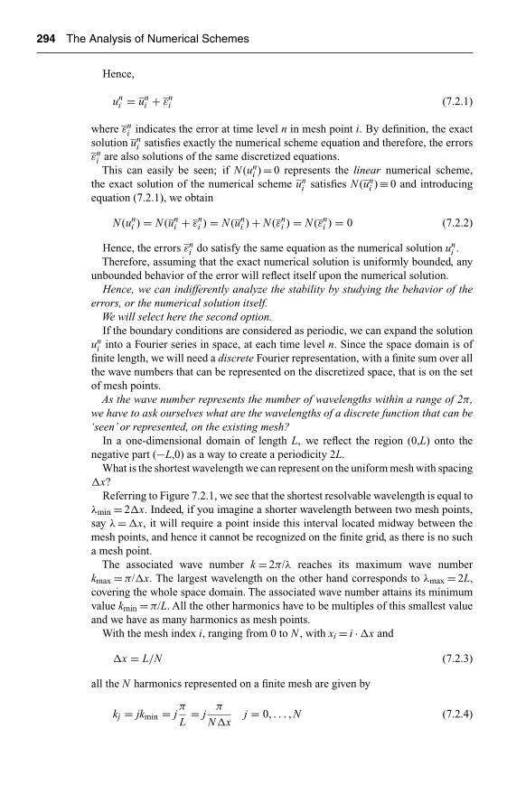
Ch07-H6594.tex 8/5/2007 12: 8 Page 294


Hence,

uni = un

i + εni (7.2.1)

where εni indicates the error at time level n in mesh point i. By definition, the exact

solution uni satisfies exactly the numerical scheme equation and therefore, the errors

εni are also solutions of the same discretized equations.This can easily be seen; if N (un

i ) = 0 represents the linear numerical scheme,the exact solution of the numerical scheme un

i satisfies N (uni ) ≡ 0 and introducing

equation (7.2.1), we obtain

N (uni ) = N (un

i + εni ) = N (un

i ) + N (εni ) = N (εn

i ) = 0 (7.2.2)

Hence, the errors εni do satisfy the same equation as the numerical solution un

i .Therefore, assuming that the exact numerical solution is uniformly bounded, any

unbounded behavior of the error will reflect itself upon the numerical solution.Hence, we can indifferently analyze the stability by studying the behavior of the

errors, or the numerical solution itself.We will select here the second option.If the boundary conditions are considered as periodic, we can expand the solution

uni into a Fourier series in space, at each time level n. Since the space domain is of

finite length, we will need a discrete Fourier representation, with a finite sum over allthe wave numbers that can be represented on the discretized space, that is on the setof mesh points.

As the wave number represents the number of wavelengths within a range of 2π,we have to ask ourselves what are the wavelengths of a discrete function that can be‘seen’ or represented, on the existing mesh?

In a one-dimensional domain of length L, we reflect the region (0,L) onto thenegative part (−L,0) as a way to create a periodicity 2L.

What is the shortest wavelength we can represent on the uniform mesh with spacing�x?

Referring to Figure 7.2.1, we see that the shortest resolvable wavelength is equal toλmin = 2�x. Indeed, if you imagine a shorter wavelength between two mesh points,say λ = �x, it will require a point inside this interval located midway between themesh points, and hence it cannot be recognized on the finite grid, as there is no sucha mesh point.

The associated wave number k = 2π/λ reaches its maximum wave numberkmax = π/�x. The largest wavelength on the other hand corresponds to λmax = 2L,covering the whole space domain. The associated wave number attains its minimumvalue kmin = π/L. All the other harmonics have to be multiples of this smallest valueand we have as many harmonics as mesh points.

With the mesh index i, ranging from 0 to N , with xi = i · �x and

�x = L/N (7.2.3)

all the N harmonics represented on a finite mesh are given by

kj = jkmin = jπ

L= j

π

N�xj = 0, . . . , N (7.2.4)

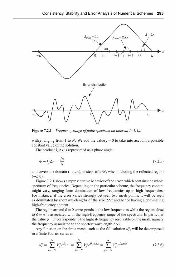
Ch07-H6594.tex 8/5/2007 12: 8 Page 295


Error distribution

0

0 1 i�1 i�1 L

L

x

x

i

�L

�L

l � �xlmax � 2L lmin � 2�x

�x

···

Figure 7.2.1 Frequency range of finite spectrum on interval (−L,L).

with j ranging from 1 to N . We add the value j = 0 to take into account a possibleconstant value of the solution.

The product kj�x is represented as a phase angle

φ ≡ kj�x = jπ

N(7.2.5)

and covers the domain (−π, π), in steps of π/N , when including the reflected region(−L,0).

Figure 7.2.1 shows a representative behavior of the error, which contains the wholespectrum of frequencies. Depending on the particular scheme, the frequency contentmight vary, ranging form domination of low frequencies up to high frequencies.For instance, if the error varies strongly between two mesh points, it will be seenas dominated by short wavelengths of the size 2�x and hence having a dominatinghigh-frequency content.

The region around φ = 0 corresponds to the low frequencies while the region closeto φ = π is associated with the high-frequency range of the spectrum. In particularthe value φ = π corresponds to the highest-frequency resolvable on the mesh, namelythe frequency associated to the shortest wavelength 2�x.

Any function on the finite mesh, such as the full solution uni , will be decomposed

in a finite Fourier series as

uni =

N∑j=−N

V nj eIkj ·xi =

N∑j=−N

V nj eIkj ·i�x =

N∑j=−N

V nj eIijπ/N (7.2.6)

Ch07-H6594.tex 8/5/2007 12: 8 Page 296


where I = √−1 and V nj is the amplitude of the jth harmonic. The harmonic associated

to j = 0, represents a constant function in space.Note that this decomposition separates the time and space dependence of the solu-

tion. The time behavior is represented by the amplitudes Vn, which contain the fulltime dependence, while the Fourier modes contain the full space dependence.

The Von Neumann method relies on the observation that for linear schemes, thediscretized equation (7.2.2), which is satisfied by the solution and by the error, mustalso be satisfied by each individual harmonic.

Hence, introducing an arbitrary harmonic in the numerical scheme, the stabil-ity condition of Von Neumann will be expressed by the following condition: theamplitude of any harmonic may not grow indefinitely in time, i.e. when n tends toinfinity.

7.2.2 Amplification Factor

As the Von Neumann stability condition requires that amplitudes V n do not growindefinitely, for any value j, we define an amplification factor

G�= V n+1

V n(7.2.7)

that has to satisfy the following Von Neumann stability condition:

|G| ≤ 1 for all values of φj = kj�x = jπ

Nj = −N , . . . , +N (7.2.8)

Note that this amplification factor is function of the scheme parameters and ofthe phase angle φ and is independent of n.

The methodology for the application of the Von Neumann stability condition canbe summarized as follows:

7.2.2.1 Methodology

• Replace in the numerical scheme all the terms of the form un+ki+m by

un+ki+m ⇒ V n+k eI (i+m)ϕ (7.2.9)

For a two time level scheme, involving the time steps n and (n + 1), k will belimited by k = 1. For a three time level scheme, k will take the values k = −1,k = 0 and k = 1.

• As all the terms contain the factor eIiϕ, the next step is to simplify all the termsby this factor.

• From the obtained relation, derive the explicit form of the amplification factor G.• The stability conditions, which are conditions on the scheme parameters, are to

be obtained from the condition (7.2.8). As we have removed the index j from thephase angle, it can be considered from now on as taking any value between

Ch07-H6594.tex 8/5/2007 12: 8 Page 297


(−π, +π). Hence we reformulate the Von Neumann stability condition asfollows:

|G| ≤ 1 for all values of φ in the range (−π, +π) (7.2.10)

Let us now apply this methodology to some of the schemes derived in Section 4.1for the linear convection equation ut + aux = 0.

First example: Second order central discretization in space with explicit firstorder difference in time

This scheme is given by equation (7.1.7), which we write here in an explicit form:

un+1i = un

i − σ

2(un

i+1 − uni−1) (7.2.11)

where the parameter σ is the unique parameter of the scheme, and has already beendefined as the Courant or CFL number:

σ = a�t

�x(7.2.12)

Observe here that the numerical solution will not depend on �x or on �t separately,but only on the non-dimensional CFL number. Therefore in practice, all computationswill be performed at constant values of σ, that is for �t values proportional to themesh spacing �x.

Let us now apply the general methodology step by step:The first step consists in applying the replacement (7.2.9), leading to

V n+1eIiφ = V neIiφ − σ

2[V neI (i+1)φ − V neI (i−1)φ] (7.2.13)

The second step is the simplification by eIiϕ, leading to

V n+1 = V n − V n σ

2[eIφ − e−Iφ] (7.2.14)

The third step, the derivation of the amplification factor, is here straightforward,

G ≡ V n+1

V n= 1 − σ

2· 2I sin φ = 1 − Iσ sin φ (7.2.15)

The stability condition (7.2.10) requires the modulus of G to be lower or equal toone. For the present example

|G|2 = G · G∗ = 1 + σ2 sin2 φ ≥ 1 (7.2.16)

which is always equal or larger than one and the stability condition is clearly never sat-isfied. Hence, the centered scheme (7.2.11) for the convection equation with forwarddifference in time is unconditionally unstable.

Ch07-H6594.tex 8/5/2007 12: 8 Page 298


Second example: Second order central discretization in space with implicit firstorder difference in time

This scheme is defined by the following equation:

un+1i = un

i − σ

2(un+1

i+1 − un+1i−1 ) (7.2.17)

Combining now the first and the second steps, we obtain

V n+1 = V n − V n+1 σ

2[eIφ − e−Iφ] (7.2.18)

The third step leads us to the following expression for the amplification factor:

G = 1 − σ

2G(eIφ − e−Iφ) or G = 1

1 + Iσ sin φ(7.2.19)

The modulus of G is always lower than one, for all values of σ, since

|G|2 = G · G∗ = 1

1 + σ2 sin2 φ≤ 1 for all φ (7.2.20)

and therefore the implicit scheme (7.2.17) is unconditionally stable.

Third example: FOU scheme – first order backward discretization in space withexplicit first order difference in time

This is the first order upwind scheme (FOU) already discussed in Section 7.1.1, givenby equation (7.1.23), which we rewrite here as

un+1i = un

i − σ(uni − un

i−1) (7.2.21)

Combining here the first, second and third steps, we obtain

G = 1 − σ(1 − e−Iφ) = 1 − σ + σ cos φ − Iσ sin φ

= 1 − 2σ sin2 φ/2 − Iσ sin φ (7.2.22)

In order to analyze the stability of the scheme (7.2.8), i.e. the regions where themodulus of the amplification factor G is lower than one, a representation of G in thecomplex plane is a convenient approach. Writing ξ and η, respectively for the realand imaginary parts of G, we have

ξ ≡ Re G = 1 − 2σ sin2 φ/2 = (1 − σ) + σ cos φ

η ≡ Im G = −σ sin φ (7.2.23)

which can be considered as parametric equations for G with φ as parameter. Werecognize the parametric equations of a circle centered on the real axis ξ at (1 − σ)with radius σ. In the complex plane of G, the stability condition (7.2.10) states

Ch07-H6594.tex 8/5/2007 12: 8 Page 299


Region ofinstability

ImG

ReG11�s

1

G

fΦs

Figure 7.2.2 Complex G-plane representation of upwind scheme (7.2.8), with unitcircle defining the stability region.

that the curve representing G for all values of φ = k�x, should remain within theunit circle (see Figure 7.2.2). It is clearly seen from this figure that the scheme isstable for

0 ≤ σ ≤ 1 (7.2.24)

Hence, the FOU scheme (7.2.21) is conditionally stable and we recover theCourant, Friedrichs, Lewy condition, or in short the ‘CFL-condition’already obtainedfrom the analysis of the equivalent differential equation.

This condition for stability was introduced for the first time in 1928 in a articleby Courant et al. (1928). This article can be considered as laying the foundationsof the concepts of convergence and stability for finite difference schemes, althoughthe authors were using finite difference concepts as a mathematical tool for provingexistence theorems of continuous problems.

Observe that the upwind scheme (7.2.21) is unstable for a < 0 (see also Prob-lem P.7.4).

Fourth example: Implicit FOU scheme – first order backward discretization inspace with implicit first order difference in time

This scheme is defined by the following equation:

un+1i = un

i − σ(un+1i − un+1

i−1 ) (7.2.25)

Ch07-H6594.tex 8/5/2007 12: 8 Page 300


Applying the now familiar steps, we obtain

G = 1

1 + σ(1 − e−Iφ)(7.2.26)

and the stability condition leads to

G · G∗ = 1

(1 − σ + σ cos φ)2 + σ2 sin2 φ≤ 1 for all values of φ (7.2.27)

Hence, this implicit FOU scheme is unconditionally stable.

7.2.3 Comments on the CFL Condition

This fundamental stability condition of most explicit schemes for wave and convectionequations expresses that the distance at covered during the time interval �t, by thedisturbances propagating with speed a, should be lower than the minimum distancebetween two mesh points. Referring to Figure 7.2.3 and to Chapter 3, we recognize theline PQ as the characteristic dx/dt = a of the hyperbolic linear convection equationthrough P. By adding the propagation case for negative values of a, we define thedomain of dependence of the differential equation in P, for convection velocities ofeither signs by the domain PQCQP. On the other hand, we can consider that thenumerical scheme also defines a numerical domain of dependence of P which is thedomain between PAC, since the solution at time level (n + 1) depends on the pointsi and (i − 1).

The CFL stability condition σ < 1 expresses that the mesh ratio �t/�x has tobe chosen in such a way that the domain of dependence of the differential equa-tion should be entirely contained in the numerical domain of dependence of thediscretized equations.

In other words, the numerical scheme defining the approximation un+1i in mesh

point i must be able to include all the physical information which influences thebehavior of the system in this point. If this is not the case, as seen on Figure 7.2.3bthen a change in physical conditions in the regions AQ and BQ would not be seenby the numerical scheme and therefore the difference between the exact solutionand the numerical solution could be made arbitrary large. Hence, the scheme willnot be able to converge. This interpretation is generally applied for two- and three-dimensional problems when it appears difficult to express analytically the stabilityconditions from the derived amplification factor or matrix. It will then lead at leastto a necessary condition.

We also understand hereby why the first order upwind scheme (FOU) (7.2.21) isunstable when a is negative. Indeed, in this case the variable u is convected from rightto left and the solution in point i can only depend on the upstream points such as(i + 1), and the physical domain of dependence is on the right side of point P. Hence,the scheme (7.2.21) which involves only the point (i − 1) is outside the domain ofdependence. In other words, this scheme is contrary to the physics it aims to describe,when a < 0.

In this case the space derivative has to be discretized with a forward difference.

Ch07-H6594.tex 8/5/2007 12: 8 Page 301


t

x

i � 1i � 1i

Pn � 1

nQ Q

Q

BC

Characteristicdx /dt � � a

Characteristicdx /dt � a

a Δt a Δt

Å

Δx

(a)

t

x

i � 1i � 1i

Pn � 1

n QQ BC

Characteristicdx /dt � a

Characteristicdx /dt � � a

a Δt a Δt

A

�x

(b)

Figure 7.2.3 Geometrical, characteristic interpretation of the CFL condition(a) σ < 1 (stable condition) and (b) σ > 1 (unstable condition).

Fifth example:Time-dependent diffusion equation with explicit first orderdifference in time and central discretization in space

Let us consider as next example the diffusion equation

∂u

∂t= α

∂2u

∂x2or ut = αuxx (7.2.28)

We select an explicit first order forward difference in time and a central, secondorder discretization of the second space derivative, leading to

un+1i = un

i + α�t

�x2(un

i+1 − 2uni + un

i−1) (7.2.29)

Ch07-H6594.tex 8/5/2007 12: 8 Page 302


The amplification factor is obtained, following the steps outlined in the methodol-ogy, as

G = 1 − 4β sin2 φ/2 (7.2.30)

with

β = α�t

�x2(7.2.31)

The stability condition is

|1 − 4β sin2 φ/2| ≤ 1

which is satisfied for

−1 ≤ 1 − 4β sin2 φ/2 ≤ 1

that is

0 ≤ β ≤ 1

2(7.2.32)

Hence, the above scheme is stable for

α ≥ 0 and β = α�t

�x2≤ 1

2(7.2.33)

The first condition expresses the stability of the physical problem, since for α < 0,i.e. for a negative diffusion coefficient, the analytical solution is exponentially increas-ing with time. The second condition provides the conditional stability of this explicitscheme.

Sixth example:Time-dependent diffusion equation with implicit first orderdifference in time and central discretization in space

If we select an implicit scheme, i.e., taking the space difference at time level (n + 1)instead of n, as in equation (7.2.29), we obtain the scheme

un+1i = un

i + α�t

�x2(un+1

i+1 − 2un+1i + un+1

i−1 ) (7.2.34)

leading to the amplification factor:

G = 1

1 + 4β sin2 φ/2(7.2.35)

Hence, this implicit scheme is unconditionally stable for α > 0.

General comments

In summary, it is seen that schemes can have conditional stability, unconditionalstability or unconditional instability.

Ch07-H6594.tex 8/5/2007 12: 8 Page 303


You will have noticed that explicit schemes lead at best to conditional stabilitywhile implicit schemes are generally unconditionally stable.

Conditional stability puts a limit on the time step, expressing that one can-not progress too rapidly in time in order to maintain stability. This is generally asevere requirement, in particular for convection dominated equations, as the con-vection speed a can be very large. For compressible flows it is of the order of thespeed of sound and the allowable time step becomes very small. For instance with101 mesh points, �x = 0.01 and for a = 350 m/s we obtain a time step limit of�t < 3 × 10−5 s.

Implicit methods have on the other hand no time step restrictions, and allow toprogress in time more rapidly, but the cost per iteration is much higher, as algebraicsystems have to be solved at each iteration.

The choice between explicit or implicit schemes is still a source of intense debatetoday and you will find in the literature, and in the practice of CFD codes, advocatesof both options. Actually, as implicit schemes have higher CPU costs per time stepand require also more memory, the balance will actually depend on the optimal valueof the product [(cost/iteration) times (number of iterations)], to be moderated by thememory requirements.

For stationary flow problems, we will see in Chapter 10 with the multigrid methodand in Volume II, that techniques are available to accelerate the numerical transientswhile iterating toward the steady state solution, which make explicit schemes morecompetitive.

For diffusion equations, the explicit time step restriction �t < �x2/2α is generallynot so severe, depending of course on the values of the diffusion coefficient. For avalue of α = 10−3 m2/s, �x = 0.01, we would have �t < 5 × 10−2 s.

The Von Neumann method offers an easy and simple way of assessing the stabilityproperties of linear schemes with constant coefficients, when the boundary conditionsare assumed periodic.

The problem of stability for a linear problem with constant coefficients is now wellunderstood when the influence of boundaries can be neglected or removed. This isthe case either for an infinite domain or for periodic conditions.

However, as soon as we have to deal with non-constant coefficients and (or) non-linear terms in the basic equations, the information on stability becomes limited.Hence, we have to resort to a local stability analysis, with frozen values of the nonlin-ear and non-constant coefficients, such as to make the formulation linear. In any case,linear stability is a necessary condition for nonlinear problems, but is certainly notsufficient.

7.3 NEW SCHEMES FOR THE LINEAR CONVECTION EQUATION

The explicit schemes considered up to this point for the linear convection equation,do not appear to be very satisfactory. Indeed the central scheme with forward timedifference, equation (7.2.11), is useless as it is an unstable scheme and the condi-tionally stable first order upwind scheme (FOU), equations (7.1.23) or (7.2.21), is ofpoor accuracy, as seen from Figure 7.1.2, since it has too much numerical dissipationresulting from its limited accuracy of first order.

Ch07-H6594.tex 8/5/2007 12: 8 Page 304


Hence, we still have to look for better schemes to be able to handle convectionphenomena with higher accuracy. Since the first order scheme is not adequate, wehave to look for second order accuracy, both in space and time.

7.3.1 The Leapfrog Scheme for the Convection Equation

A first option has already been briefly mentioned in Section 4.1, equation (4.1.40),where both time and space derivatives are discretized by second order centraldifference formulas. This leads to the so-called leapfrog scheme, defined by

un+1i − un−1

i

2�t+ a

2�x(un

i+1 − uni−1) = 0 (7.3.1)

or

un+1i = un−1

i + σ(uni+1 − un

i−1) (7.3.2)

This scheme is of second order accuracy, with a truncation error O(�t2, �x2) (seeProblem P.7.2).

This scheme is called leapfrog, because of the particular structure of its computa-tional molecule (Figure 7.3.1) where the new solution un+1

i is obtained by starting fromthe value at point i and time level (n − 1), then taking into account the values at timelevel n to the right and to the left, with un

i not contributing to the computation un+1i .

This scheme has the drawback of having to treat three time levels simultaneouslyand in order to start the calculation, two time levels n = 0 and n = 1 have to be known.This requires using another two level scheme to start the calculations.

Applying the methodology described in the previous section for the Von Neumannstability analysis, we obtain

V n+1 = V n−1 + σV n(eIφ − e−Iφ) (7.3.3)

n�1

n

n�1

i�1 i�1i

x

t

Figure 7.3.1 Computational molecule for the leapfrog scheme.

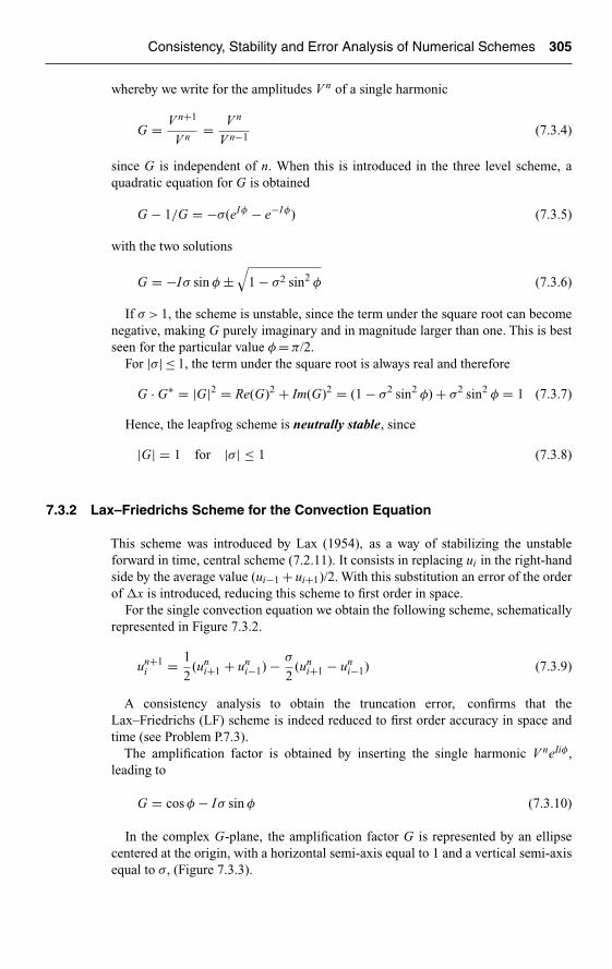
Ch07-H6594.tex 8/5/2007 12: 8 Page 305


whereby we write for the amplitudes V n of a single harmonic

G = V n+1

V n= V n

V n−1(7.3.4)

since G is independent of n. When this is introduced in the three level scheme, aquadratic equation for G is obtained

G − 1/G = −σ(eIφ − e−Iφ) (7.3.5)

with the two solutions

G = −Iσ sin φ ±√

1 − σ2 sin2 φ (7.3.6)

If σ > 1, the scheme is unstable, since the term under the square root can becomenegative, making G purely imaginary and in magnitude larger than one. This is bestseen for the particular value φ = π/2.

For |σ| ≤ 1, the term under the square root is always real and therefore

G · G∗ = |G|2 = Re(G)2 + Im(G)2 = (1 − σ2 sin2 φ) + σ2 sin2 φ = 1 (7.3.7)

Hence, the leapfrog scheme is neutrally stable, since

|G| = 1 for |σ| ≤ 1 (7.3.8)

7.3.2 Lax–Friedrichs Scheme for the Convection Equation

This scheme was introduced by Lax (1954), as a way of stabilizing the unstableforward in time, central scheme (7.2.11). It consists in replacing ui in the right-handside by the average value (ui−1 + ui+1)/2. With this substitution an error of the orderof �x is introduced, reducing this scheme to first order in space.

For the single convection equation we obtain the following scheme, schematicallyrepresented in Figure 7.3.2.

un+1i = 1

2(un

i+1 + uni−1) − σ

2(un

i+1 − uni−1) (7.3.9)

A consistency analysis to obtain the truncation error, confirms that theLax–Friedrichs (LF) scheme is indeed reduced to first order accuracy in space andtime (see Problem P.7.3).

The amplification factor is obtained by inserting the single harmonic V neIiφ,leading to

G = cos φ − Iσ sin φ (7.3.10)

In the complex G-plane, the amplification factor G is represented by an ellipsecentered at the origin, with a horizontal semi-axis equal to 1 and a vertical semi-axisequal to σ, (Figure 7.3.3).

Ch07-H6594.tex 8/5/2007 12: 8 Page 306


n�1

n

n�1

i�1 i�1i

x

t

Figure 7.3.2 Lax–Friedrichs scheme for convection equations.


Im G

Re G1

1

Gf

s

Figure 7.3.3 Stability region for the Lax–Friedrichs scheme.

This leads again to the CFL stability condition |σ| ≤ 1, as the G-ellipse will remaininside the stability circle of radius 1, as long as |σ| ≤ 1.

7.3.3 The Lax–Wendroff Scheme for the Convection Equation

The scheme of the previous example is of first order accuracy, which is insufficientfor practical purposes.

Ch07-H6594.tex 8/5/2007 12: 8 Page 307


The first scheme to be introduced historically with second order accuracy in spaceand time, with two time levels, is due to Lax and Wendroff (1960).

The introduction of this scheme (LW) was a landmark in the history of CFD, asit can be considered as the advent of many modern concepts of CFD. It has beenthe most widely applied scheme for aeronautical applications, up to the end of the1980s under various forms, some of them being presented in more details in VolumeII. Actually the first introduction of the Finite Volume method in CFD, was done onthe basis of a two-step variant of the LW schemes, introduced by W. MacCormack in1969; see the introduction of Section 5.2 for the relevant references.

The original derivation of Lax and Wendroff was based on a Taylor expansion intime up to the second order, such as to achieve second order accuracy in time.

un+1i = un

i + �t(ut)i + �t2

2(utt)i + O(�t3) (7.3.11)

The basis of the LW method is to keep the second time derivative in the dis-cretization, and replacing all time derivatives by equivalent spatial derivatives. Thisis straightforward for the first time derivative, while the second derivative is obtainedby taking the time derivative of the convection equation ut + aux = 0, resulting in

utt = −a(ux)t = −a(ut)x = +a2uxx (7.3.12)

Introduced in equation (7.3.11), we obtain

un+1i = un

i − a�t(ux)i + a2�t2

2(uxx)i + O(�t3) (7.3.13)

If we discretize all the space derivative with second order central formulas in meshpoint i, we obtain

un+1i = un

i − σ

2(un

i+1 − uni−1) + σ2

2(un

i+1 − 2uni + un

i−1) (7.3.14)

Observe that the third term, which stabilizes the instability generated by the first twoterms, is the discretization of an additional dissipative term of the form (a2�t/2)uxx.If you look back at the equivalent differential equation of this unstable scheme, equa-tion (7.1.19), we can interpret the Lax–Wendroff scheme as the discretization of amodified convection equation obtained by adding the lowest order truncation errorterm (which is responsible for the instability) to the left-hand side. In other terms, theLax–Wendroff scheme is obtained by discretizing the following corrected differentialmodel:

ut + aux + �t

2a2uxx = 0 (7.3.15)

Taking into account the truncation error (7.1.18), we also see that the dominatingterm of the truncation error of the Lax–Wendroff scheme is proportional to the thirdspace derivative, leading to the equivalent differential equation of the Lax–Wendroffscheme

ut + aux + �t

2a2uxx = a

�x2

6(uxxx) + O(�t2, �x4) (7.3.16)

Ch07-H6594.tex 8/5/2007 12: 8 Page 308


11�s 2

1

GFs


Im G Im G

Re G

(a)


Re G

(b)

11�s 2

1G F

s

Figure 7.3.4 Polar representation of the amplification factor for Lax–Wendroffscheme: (a): σ < 1 and σ2 < 1/2 and (b): σ < 1 and σ2 > 1/2.

The amplification matrix from theVon Neumann method is now readily obtained, as

G = 1 − σ

2(eIφ − e−Iφ) + σ2

2(eIφ − 2 + e−Iφ)

= 1 − Iσ sin φ − σ2(1 − cos φ) (7.3.17)

Writing ξ and η, respectively, for the real and imaginary parts of G, we have

ξ ≡ Re G = (1 − σ2) + σ2 cos φ

η ≡ Im G = −σ sin φ (7.3.18)

In the complex G-plane, this represents an ellipse centered on the real axis at theabscissa (1 − σ2) and having semi-axis length of σ2 along the real axis and σ alongthe vertical imaginary axis. Hence, this ellipse will always be contained in the unitcircle if the CFL condition is satisfied (Figure 7.3.4). For σ = 1, the ellipse becomesidentical to the unit circle.

The stability condition is therefore

|σ| ≤ 1 (7.3.19)

What have we achieved at this point?

We have now three new explicit schemes for the linear convection equation, in additionto the conditionally stable FOU scheme (7.2.21), namely the first order Lax–Friedrichs(LF) scheme and the two second order schemes, leapfrog and Lax–Wendroff (LW).All three of them are also conditionally stable under the CFL condition (7.3.19).

Ch07-H6594.tex 8/5/2007 12: 8 Page 309


Let us now compare the results obtained with these four schemes on somerepresentative, but also challenging test cases.

With any flow model, one of the most critical situations occurs in regions with verystrong local variations. For instance, the inviscid flow around a wing section undergoesa strong local velocity gradient in the leading edge region, where over a very shortdistance of a few percent of the chord downstream of the stagnation point, the velocityincreases from zero to values larger than the incoming velocity (see Figure 7.3.51).

20

15

10

Mag

nitu

de o

f V

5

0

0 0.2 0.4 0.6

Arc length

0.8 1

Figure 7.3.5 Inviscid flow around the leading edge of a NACA0012 airfoil section,at 8 degree incidence.

1 The author thanks Benoit Leonard, from NUMECA Int, for providing this figure.

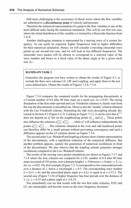
Ch07-H6594.tex 8/5/2007 12: 8 Page 310


Still more challenging is the occurrence of shock waves where the flow variablesare submitted to a discontinuous jump of velocity and pressure.

Therefore the numerical representation of a jump in the flow variables is one of themost difficult tasks facing the numerical simulation. This will be our first test case,where the initial distribution of the variable u is formed by a Heaviside function from1 to 0.

Another challenging situation is represented by a moving wave of a certain fre-quency. As can easily be expected, higher frequencies lead to higher difficultiesfor their numerical simulation. Hence, we will consider a traveling sinusoidal wavepacket as our second test case, and we will look at two different frequencies. Thesinusoidal wave packet will be chosen to correspond to a selected value of thewave number and hence to a fixed value of the phase angle φ for a given meshsize �x.

HANDS-ON TASK 2

Generalize the program you have written to obtain the results of Figure 4.1, toinclude the three new schemes LF, LW and Leapfrog, and apply them to the testcases defined here. Obtain the results of Figures 7.3.6–7.3.8.

Figure 7.3.6 compares the computed results for the propagating discontinuity ata Courant number of 0.8 after 80 time steps on a mesh size �x = 0.05. The strongdissipation of the first order upwind and Lax–Friedrichs schemes is clearly seen fromthe way the discontinuity is smoothed out. Observe also the ‘double’solution obtainedwith the Lax–Friedrichs scheme, illustrating the odd–even decoupling already dis-cussed in Section 4.2 (Figure 4.2.3). Looking at Figure 7.3.2, it can be seen that un+1

idoes not depend on un

i but on the neighbouring points uni+1 and un

i−1. These points

also influence the solutions un+1i+2 , un+1

i+4 , . . ., while uni will influence independently the

points un+1i+1 , un+1

i+3 , . . . The solutions obtained at the even and odd numbered pointscan therefore differ by a small amount without preventing convergence and such adifference appears on the LF solution shown on Figure 7.3.6.

The second order Lax–Wendroff and leapfrog schemes show a better representationof the discontinuity, with a significant reduction of the numerical diffusion. Butanother problem appears, namely the generation of numerical oscillations in frontof the discontinuity. We also observe that the leapfrog scheme generates strongeroscillations compared to the Lax–Wendroff scheme.

The results of the moving wave packet simulations are shown in Figures 7.3.7 and7.3.8 where the four schemes are compared for a CFL number of 0.8 after 80 timesteps on a mesh of 101 points, over a domain length L = 2 between x = 0 and x = 2; i.e.for �x = 0.02. The first example (Figure 7.3.7) corresponds to two sinusoidal periodsover a distance of 1, hence a wavelength λ = 0.5. The corresponding wave numberk = 2π/λ = 4π and the associated phase angle φ = k�x is equal to φ = π/12.5. Thesecond case (Figure 7.3.8) of higher frequency has four periods over the distance of1, i.e. λ = 0.25 and a phase angle φ = π/6.25.

You immediately can see that results with the two first order schemes, FOU andLF, are catastrophic and become worse as the wave frequency increases!

Ch07-H6594.tex 8/5/2007 12: 8 Page 311


0

1

FOU–CFL�0.8 80 time steps

0.2

0.4

0.6

0.8

1.2

0 1 20.5 1.5

U initialU calculated

LAX–F scheme CFL�0.8 80 time steps

0

1

0.2

0.4

0.6

0.8

1.2

0 1 20.5 1.5


0

1

0 1 2

0.2

0.4

0.6

0.8

1.2

0.5 1.5

Leapfrog CFL�0.8 80 time steps1.4


LW Scheme CFL�0.8 80 time steps

0

1

0 1 2

0.2

0.4

0.6

0.8

1.2

0.5 1.5


Figure 7.3.6 Comparison of four schemes on the linear convection equation for apropagating discontinuity.

The lesson to be learned form these results is that due to the excessive numericaldissipation of first order schemes, they become totally useless for time-dependentpropagation problems of this kind and should be avoided .

The second order schemes, leapfrog and LW, look much better, particularly atthe lowest frequency, where the numerical solutions are excellent. A small problemhowever is the appearance of oscillations in the numerical solution at the front of thepropagating wave. This is due to the discontinuity in the slope of the initial solution atthe points x = 0.25 and x = 1.5. This behavior is similar to the case of the propagatingdiscontinuity of Figure 7.3.6.

The same computations performed at a higher frequency, corresponding to a phaseangle of φ = π/6.25, shown in Figure 7.3.8 indicate larger deviations compared to theexact solution. The Lax–Wendroff scheme has an error in the amplitude as well as aphase shift of the numerical solution. The leapfrog scheme has a better behavior withregard to the amplitude of the wave, which is correctly reproduced by the scheme, buthere also we observe an increased level of numerical oscillations generated at the ini-tial slope discontinuity. A phase error is also to be observed with the leapfrog scheme.

Ch07-H6594.tex 8/5/2007 12: 8 Page 312


First order upwind scheme

00

0.2

�0.2

0.4

�0.4

0.6

�0.6

0.8

�0.8

1

�1

0.5 1 1.5 2


00

0.2

�0.2

0.4

�0.4

0.6

�0.6

0.8

�0.8

1

�1

0.5 1 1.5 2

Lax–Friedrich scheme


00

0.2

�0.2

0.4

�0.4

0.6

�0.6

0.8

�0.8

1

�1

0.5 1 1.5 2

Leapfrog scheme


00.2

�0.2

0.4

�0.4

0.6

�0.6

0.8

�0.8

1

�1

Lax–Wendroff scheme


0 0.5 1 1.5 2

Figure 7.3.7 Comparison of four schemes on the linear convection equation for apropagating wave packet for φ = π/12.5.

So, summarizing our observations, we note that:

• The first order schemes are of very poor accuracy.• The second order schemes provide a significant better accuracy, particularly at

the lower frequencies.• The second order schemes generate numerical oscillations as soon as function or

slope discontinuities in the solution are present. These oscillations being strongerwith the leapfrog scheme, compared to LW.

• The generated numerical errors are very sensitive to the frequency, i.e. to thephase angle.

• These results, although obtained on a simple one-dimensional linear convectionequation, are very representative of real flow simulations. You will encounterthese same effects also with the full 3D Navier–Stokes simulations.

The main questions arising from these representative examples are:

• How can we explain and predict the differences between these four schemes andtheir dependence with frequency?

• Why do numerical oscillations appear with the second order schemes and notwith the first order schemes?

Ch07-H6594.tex 8/5/2007 12: 8 Page 313


First order upwind scheme

0 0.2 0.4 0.6 0.8 1 1.2 1.4 1.6 1.8 20

0.2

�0.2

0.4

�0.4

0.6

�0.6

0.8

�0.8

1

�1


Lax–Friedrichs scheme

0 0.2 0.4 0.6 0.8 1 1.2 1.4 1.6 1.8 20

0.2

�0.2

0.4

�0.4

0.6

�0.6

0.8

�0.8

1

�1


Lax–Wendroff scheme

0 0.2 0.4 0.6 0.8 1 1.2 1.4 1.6 1.8 20

0.2

�0.2

0.4

�0.4

0.6

�0.6

0.8

�0.8

1

�1


Leap–frog scheme

0 0.2 0.4 0.6 0.8 1 1.2 1.4 1.6 1.8 20

0.2

�0.2

0.4

�0.4

0.6

�0.6

0.8

�0.8

1

�1


Figure 7.3.8 Comparison of four schemes on the linear convection equation for apropagating wave packet for φ = π/6.25.

• Although discontinuities in the solution and slopes are present at both ends ofthe solution, why do we see numerical oscillations only on the upstream side?

The response to these questions is of fundamental importance, not only for theunderstanding of numerical schemes, but even more importantly, for our capacityto analyze a numerical solution, to evaluate its accuracy and hence, its degree ofreliability. It will also determine the level of confidence we can attach to a numericalsimulation on a given mesh.

In order to provide an answer to these questions, we have to develop a methodologyfor error analysis of a numerical solution. This is the content of the next section.

7.4 THE SPECTRAL ANALYSIS OF NUMERICAL ERRORS

When we perform a Von Neumann stability analysis, we obtain a specific expressionof the amplification factor G as a function of the phase angle φ and of the parametersof the scheme. Hence we can consider that G(φ, scheme parameters) is a uniquelydefined ‘blueprint’ of a numerical scheme and should contain the complete infor-mation concerning its behavior, and in particular the information on the generatednumerical errors.

What errors are we referring to in this context?

Ch07-H6594.tex 8/5/2007 12: 8 Page 314


We have seen that the truncation error defines the global discretization error ofthe scheme, but it does not provide a direct evaluation of the errors on the solutions.Indeed, the comparisons shown in the previous section refer to the difference betweenthe numerical solution and the exact solution of the mathematical model. That is, welooked at the differences

ε�= un

i − uni (7.4.1)

where uni = u(xi, tn) is the exact analytical solution at point xi and time tn.

The numerical representation of the time evolution of the solution is fully con-tained in the amplitudes V n for each harmonic corresponding to the wave numberk . However, up to now we had no need to be more specific, as the definition of theamplification factor (7.2.7), did not require it.

Since we wish now to go a step further and gain additional information on theerrors, we have to be more specific about the time dependence of V n both for thenumerical and the analytical solutions.

Considering first the analytical solution, we always can represent it by a Fourierdecomposition in space, similar to the approach followed for the Von Neumannanalysis. It is known form the physics of plane waves that to each harmonic k of aspatial Fourier decomposition, a pulsation function ω = ω(k) can be attached, calledthe dispersion relation; the explicit dependence ω = ω(k) depending on the equationsto be solved. We refer you to Section 3.4 for the introduction and discussion of thisrepresentation.

For instance, for the linear convection equation ut + aux = 0, ω = ω(k) = ak , anda representative solution is the plane wave:

uni = V eIkxi e−I ωtn

(7.4.2)

For a more general solution, the harmonic k , has the same form, at time leveltn = n�t, as

(uni )k = V (k)e−I ωn�teIk(i�x) (7.4.3)

where we designate from now on the exact dispersion relation as ω = ω(k), obtainedfrom the differential system as solution of the eigenvalue equation (3.4.17).

The function V (k) is obtained from the Fourier decomposition of the initial solutionat t = 0. If we define u(x, 0) = f (x) at t = 0 we have

V (k) = 1

2L

∫ L

−Lf (x)e−Ikxdx (7.4.4)

This form of the exact solution is very similar to the representation of the numericalsolution applied for the Von Neumann analysis, equation (7.2.6), where a singleharmonic is described as

(uni )k = V neIk(i�x) (7.4.5)

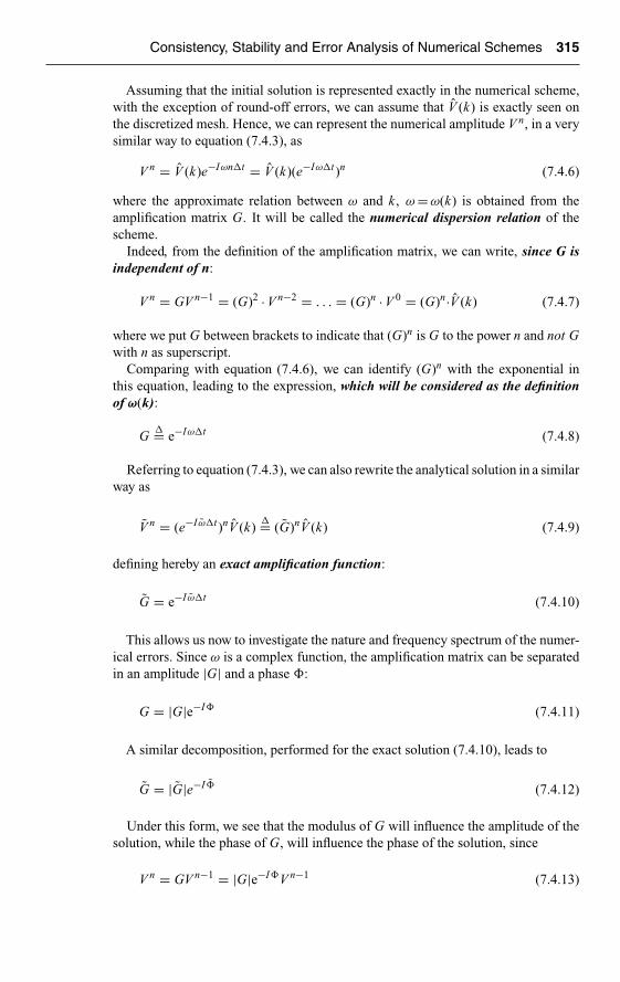
Ch07-H6594.tex 8/5/2007 12: 8 Page 315


Assuming that the initial solution is represented exactly in the numerical scheme,with the exception of round-off errors, we can assume that V (k) is exactly seen onthe discretized mesh. Hence, we can represent the numerical amplitude V n, in a verysimilar way to equation (7.4.3), as

V n = V (k)e−Iωn�t = V (k)(e−Iω�t)n (7.4.6)

where the approximate relation between ω and k , ω = ω(k) is obtained from theamplification matrix G. It will be called the numerical dispersion relation of thescheme.

Indeed, from the definition of the amplification matrix, we can write, since G isindependent of n:

V n = GV n−1 = (G)2 · V n−2 = . . . = (G)n · V 0 = (G)n·V (k) (7.4.7)

where we put G between brackets to indicate that (G)n is G to the power n and not Gwith n as superscript.

Comparing with equation (7.4.6), we can identify (G)n with the exponential inthis equation, leading to the expression, which will be considered as the definitionof ω(k):

G�= e−Iω�t (7.4.8)

Referring to equation (7.4.3), we can also rewrite the analytical solution in a similarway as

V n = (e−I ω�t)nV (k)�= (G)nV (k) (7.4.9)

defining hereby an exact amplification function:

G = e−I ω�t (7.4.10)

This allows us now to investigate the nature and frequency spectrum of the numer-ical errors. Since ω is a complex function, the amplification matrix can be separatedin an amplitude |G| and a phase �:

G = |G|e−I� (7.4.11)

A similar decomposition, performed for the exact solution (7.4.10), leads to

G = |G|e−I� (7.4.12)

Under this form, we see that the modulus of G will influence the amplitude of thesolution, while the phase of G, will influence the phase of the solution, since

V n = GV n−1 = |G|e−I�V n−1 (7.4.13)

Ch07-H6594.tex 8/5/2007 12: 8 Page 316


The error in amplitude, called the diffusion or dissipation error, is defined by theratio of the computed amplitude to the exact amplitude.

εD = |G||G| (7.4.14)

The error on the phase of the solution, the dispersion error, can be defined as thedifference

εφ = � − � (7.4.15)

suitable for pure parabolic problems, where � = 0, in absence of convective terms.For convection dominated problems, the definition

εφ = �/� (7.4.16)

is better adapted.In particular for hyperbolic problems, such as the scalar convection equation, the

exact solution is a single wave propagating with the velocity a. Hence

� = ka�t (7.4.17)

7.4.1 Error Analysis for Hyperbolic Problems

A hyperbolic problem such as the convection equation ut + aux = 0 represents a wavetraveling at constant speed a without damping, i.e. with constant amplitude. The exactsolution for a wave of the form (7.4.3) is given by

ω = ak (7.4.18)

and

u = V eIkxe−Iakt (7.4.19)

The exact amplification factor reduces here to

|G| = 1 and � = ak�t = a�t

�xk�x = σφ (7.4.20)

and

G = e−Iσφ (7.4.21)

This confirms that the exact solution of the linear convection equation is an initialshape propagating at the constant velocity a, without reduction of the amplitude.

Since in the numerical solution an initial wave amplitude is damped by a factor|G| per time step, as can be seen from equation (7.4.7), the error in amplitude, thediffusion error, will be given by the modulus of the amplification factor

εD = |G| (7.4.22)

Ch07-H6594.tex 8/5/2007 12: 8 Page 317


The phase of the numerical solution is determined by �, which can be consideredas defining a numerical convection speed anum = �/k�t, by direct comparison withthe relations (7.4.20)

anum = �

k�t= a�

σφ(7.4.23)

Therefore the error in phase, i.e. the dispersion error:

εφ = �

ak�t= �

σφ≡ anum

a(7.4.24)

can be interpreted as defining the ratio between the numerical and physical convectionspeeds, indicating that the physical convection (or propagation) speed will be modifiedby the dispersion error εφ.

When the dispersion error is larger than one, εφ > 1, the phase error is a leadingerror and the numerical convection velocity, anum, is larger than the exact one. Thismeans that the computed solution appears to move faster than the physical one. Onthe other hand, when εφ < 1, the phase error is said to be a lagging error and thecomputed solution travels at a lower velocity than the physical one.

Let us now analyze the error properties of the four schemes we have been comparingin the previous section, in order to explain their observed behavior. The procedure isas follows:

• Obtain the expression of the amplification factor G. For stability we decomposeG in its real and imaginary parts.

• For the error analysis, we have to write G in ‘polar’ form, i.e. defining its moduleand phase. The relation between the two representations is straightforward:

G = (Re G) + I (Im G) = |G|e−I�

|G| =√

(Re G)2 + (Im G)2 tan � = −Im G/Re G (7.4.25)

• Define the diffusion and dispersion errors by their definitions (7.4.22), (7.4.24)and analyze their behavior in function of frequency or phase angle φ.

A general comment can be made here, concerning the conflicting requirementsbetween stability and accuracy. Accuracy requires the modulus of G to be as closeto one as possible, but stability requires |G| to be lower than one, i.e. have a largerdiffusion error.

7.4.1.1 Error analysis of the explicit First Order Upwind scheme (FOU)

The amplification factor for this scheme is defined by equation (7.2.22). Its modulusis given by

|G| = [(1−σ+σ cos φ)2 +σ2 sin2 φ]1/2 = [1−4σ(1−σ) sin2 φ/2]1/2 (7.4.26)

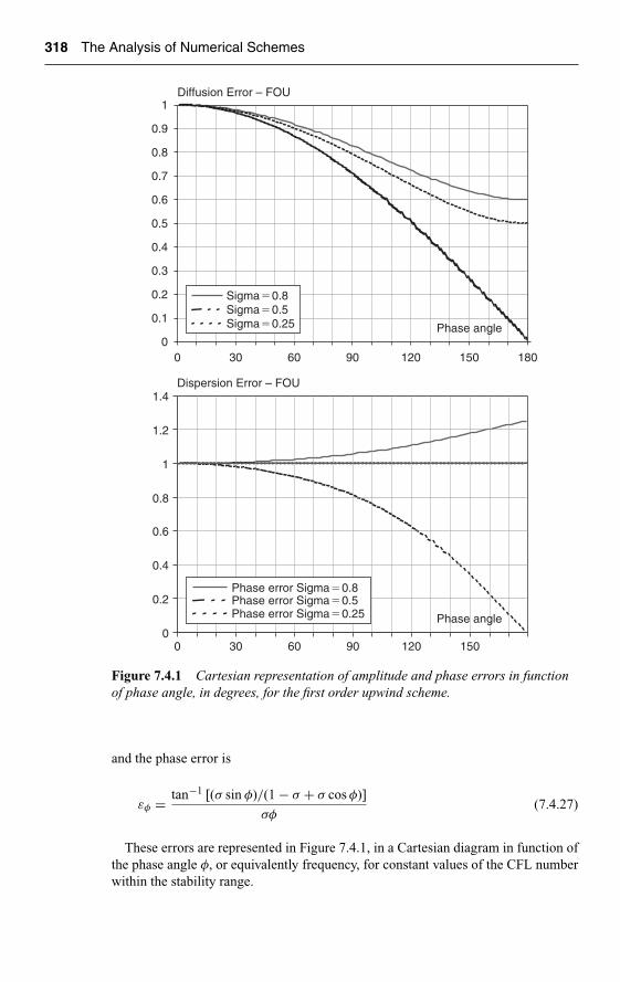
Ch07-H6594.tex 8/5/2007 12: 8 Page 318


0

0.2

0.4

0.6

0.8

1

1.2

1.4

Diffusion Error – FOU

0

0.1

0.2

0.3

0.4

0.5

0.6

0.7

0.8

0.9

1

0 30 60 90 120 150

0 30 60 90 120 150

180

Phase angle

Phase angle

Sigma�0.8Sigma�0.5Sigma�0.25

Dispersion Error – FOU

Phase error Sigma�0.8Phase error Sigma�0.5Phase error Sigma�0.25

Figure 7.4.1 Cartesian representation of amplitude and phase errors in functionof phase angle, in degrees, for the first order upwind scheme.

and the phase error is

εφ = tan−1 [(σ sin φ)/(1 − σ + σ cos φ)]

σφ(7.4.27)

These errors are represented in Figure 7.4.1, in a Cartesian diagram in function ofthe phase angle φ, or equivalently frequency, for constant values of the CFL numberwithin the stability range.

Ch07-H6594.tex 8/5/2007 12: 8 Page 319


0.975

0.98

0.985

0.99

0.995

1

0 10 20

Phase angle


Diffusion Error – FOU

Figure 7.4.2 Zoom of amplitude errors in the low frequency region, in function ofphase angle, in degrees, for the first order upwind scheme.

For σ = 0.5, the phase error εφ = 1, but for σ < 0.5, εφ < 1 indicating a laggingerror, while the numerical speed of propagation becomes larger than the physicalspeed when εφ > 1 for Courant numbers σ > 0.5 (see also Problem P.7.7).

We observe that the diffusion error, which is always equal to 1 for φ = 0, forconsistency reasons, drops rapidly when the frequency increases. This explains thedramatic behavior of the FOU scheme in the examples shown in the previous section.

Remember here that the highest frequency that can be represented on the meshcorresponds to the shortest wavelength λ = 2�x, i.e. to φ = π. Hence we designate theregions around φ = 0 and φ = π as the low and high frequency regions, respectively.

At the lowest phase angle φ = π/12.5 = 14.4 deg, treated in Figure 7.3.7, the dif-fusion error is equal to 0.995, as can be seen from the zoom on the low frequencyregion shown in Figure 7.4.2. Hence, we can estimate quantitatively the decrease inamplitude after the 80 iterations at σ = 0.8 observed in Figure 7.3.7.

In general, after n iterations, the amplitude is reduced by a factor |G|n, asshown by equation (7.4.7). Hence in this case the amplitude will be decreased by(0.995)80 = 0.67, which is the value you can find on Figure 7.3.7 for this first orderupwind scheme. At the highest frequency of Figure 7.3.8, φ = π/6.25 = 28.8◦, the dif-fusion error is equal to 0.98 and the amplitude is decreased by (0.98)80 = 0.2, whichcorresponds to what you observe on Figure 7.3.8 for this FOU scheme.

This very rapid decease of the modulus of G, is typical for first order schemes andexplains the observed behavior.

Observe also the very strong sensitivity of the numerical amplitude variation to thevalues of the diffusion error. An error of only 1%, i.e. a value of |G| = 0.99, leadsafter 100 time steps to a reduction in amplitude of 36.6% of the initial value. Evenfor an error of 0.5%, i.e. |G| = 0.995, the amplitude reduction is of 60%.

Reversing the question, if we would require an amplitude reduction less than 1%after 100 time steps, we should have |G| > 0.9999!

Ch07-H6594.tex 8/5/2007 12: 8 Page 320


7.4.1.2 Error analysis of the Lax–Friedrichs scheme for theconvection equation

The accuracy of the scheme is obtained from the modulus and phase of theamplification factor (7.3.10)

|G| = [ cos2 φ + σ2 sin2 φ]1/2

� = tan−1 (σ tan φ) (7.4.28)

This defines the dissipation error

εD = |G| = [ cos2 φ + σ2 sin2 φ]1/2 (7.4.29)

and the dispersion error

εφ = �

σφ= tan−1 (σ tan φ)

σφ(7.4.30)

As can be seen the choice σ = 1 gives the exact solution, but lower values of σ willgenerate amplitude and phase errors.

Cartesian representations of |G| and εφ in function of the phase angle φ = k�x,are shown in Figure 7.4.3. For small values of σ, the amplitudes are strongly damped,indicating that this scheme is generating a strong numerical dissipation, even largerthan the FOU scheme. The phase error is everywhere larger or equal one, show-ing a leading phase error. Observe that for φ = π we have εφ = 1/σ, as seen fromequation (7.4.30) (See also Problem P.7.6).

An interesting difference with the FOU scheme is the behavior of the diffusionerror for the highest frequency φ = π. It is seen here that the LF scheme has nodiffusion error for φ = π, while this error takes its maximum value for the FOUscheme. This explains the double solution of Figure 7.3.6, which corresponds to anodd–even decoupling, i.e. an error oscillation of wavelength 2�x, or a phase angleφ = π. Hence, in order to avoid these high frequency oscillations, we need to haveG(π) < 1. When this is satisfied the scheme is said to be dissipative in the sense ofKreiss (Kreiss, 1964).

7.4.1.3 Error analysis of the Lax–Wendroff scheme for the convection equation

We refer here to the amplification factor (7.3.17), from which we derive the dissipationerror as:

|G| = [1 − 4σ2(1 − σ2) sin4 φ/2]1/2 (7.4.31)

and the phase error as

εφ = tan−1 [(σ sin φ)/(1 − 2σ2 sin2 φ/2)]

σφ(7.4.32)

Ch07-H6594.tex 8/5/2007 12: 8 Page 321


Diffusion Error – LF

0

0.1

0.2

0.3

0.4

0.5

0.6

0.7

0.8

0.9

1

0 30 60 90 120 150 180

0 30 60 90 120 150 180

Phase angle

Phase angle


Dispersion Error – LF

0

1

2

3

4

5

6

Phase error Sigma�0.75Phase error Sigma�0.5Phase error Sigma�0.25

Figure 7.4.3 Amplitude and dispersion errors for the Lax–Friedrichs scheme, infunction of phase angle in degrees, applied to the linear convection equation.

The diffusion and dispersion errors are represented in Figure 7.4.4, in function ofphase angle (in degrees) for constant values of the CFL number σ.

To the lowest order, we can expand the above expressions around φ = 0,leading to

|G| ≈ 1 − σ2

8(1 − σ2)φ4 + O(φ6)

εφ ≈ 1 − 1

6(1 − σ2)φ2 + O(φ4) (7.4.33)

Ch07-H6594.tex 8/5/2007 12: 8 Page 322


0

0.1

0.2

0.3

0.4

0.5

0.6

0.7

0.8

0.9

1

0

0.2

0.4

0.6

0.8

1

1.2

Diffusion Error – LW

0 30 60 90 120 150 180

0 30 60 90 120 150 180

Phase angle

Phase angle

Dispersion Error – LW



Figure 7.4.4 Dispersion and diffusion errors for Lax–Wendroff scheme.

The relative phase error is mostly lower than one, indicating a dominating laggingphase error and showing that the numerical convection velocity is lower than thephysical one.

This explains why the numerical solution of the LW scheme lags behind the exactsolution, as seen in Figure 7.3.8.

In terms of accuracy, we also clearly see the reasons behind the frequency depen-dence of the numerical solutions, seen by comparing Figures 7.3.7 and 7.3.8. Fromthe zoom on the diffusion error, shown in Figure 7.4.5, we can again estimatequantitatively the amplitude errors.

Observe first that the region where the diffusion error is very close to one, whichwe can consider as the ‘accuracy region’ of the scheme, is much larger than with the

Ch07-H6594.tex 8/5/2007 12: 8 Page 323


0.988

0.99

0.992

0.994

0.996

0.998

1

0

Phase angle

Diffusion Error – LW

20 40


Figure 7.4.5 Zoom on diffusion error for the Lax–Wendroff scheme.

FOU scheme, as seen by comparing with Figure 7.4.2. This is typical of second orderschemes.

Actually, the higher the order of the scheme, the larger this accuracy region.At the higher frequency of Figure 7.3.8, where φ = π/6.25 = 28.8◦, the diffusion

error, for σ = 0.8, is |G| ∼ 0.9985. This leads to the amplitude reduction, after 80time steps of 0.89, which corresponds to what you can observe on Figure 7.3.8.

7.4.1.4 Error analysis of the leapfrog scheme for the convection equation

The leapfrog scheme is the three time level scheme defined by equation (7.3.2), withsecond order accuracy in space and time. It has the interesting property of beingconditional stable with |G| = 1, i.e. this scheme has no diffusion errors.

Hence, this explains the behavior seen in Figure 7.3.8, where you can observe thatthe numerical amplitude remains equal to 1.

For this reason, the leapfrog scheme is very useful for long-term simulations,and is applied in some weather forecasting codes, where the accuracy of the pre-dicted weather for a longer term of 3 to 4 days is essential for the reliability of thepredictions.

The dispersion error is given by

εφ = ± tan−1 [(σ sin φ)/√

1 − σ2 sin2 φ]

σφ= ± sin−1 (σ sin φ)

σφ(7.4.34)

and its dispersion error is shown on Figure 7.4.6.We observe that this error is below 1 and again explains why the numerical solution

is lagging behind the exact solution on Figures 7.3.7 and 7.3.8.

Ch07-H6594.tex 8/5/2007 12: 8 Page 324


Dispersion Error – Leapfrog scheme

0

0.1

0.2

0.3

0.4

0.5

0.6

0.7

0.8

0.9

1

0 30 60 90 120 150 180

Phase angle


Figure 7.4.6 Dispersion error for the leapfrog scheme in function of the phaseangle in degrees, at constant CFL numbers.

The leapfrog scheme should give accurate results when the function u has a smoothvariation, since the amplitudes are correctly modeled, so more that for low frequenciesthe phase error is close to one.

However, the fact that this scheme is neutrally stable, |G| = 1 for all σ < 1 has alsounfavorable consequences, as high frequency errors will not be damped, this schemebeing non-dissipative in the sense of Kreiss. This explains why the oscillations onFigures 7.3.6–7.3.8 are larger with the leapfrog scheme, compared to the LW scheme.

When applied to the inviscid Burgers equation ut + uux = 0, the computationsbecome in certain circumstances unstable, as can be seen from Figure 7.4.7. Thisfigure shows the computed solutions of Burgers equation for a stationary shock, after10, 20 and 30 time steps at a Courant number of 0.8 and a mesh size of �x = 0.05.The continuous line indicates the exact solution.

The amplitude of the errors increases continuously and the solution is completelydestroyed after 50 time steps. The instability is entirely due to the nonlinearity ofthe equation, since the same scheme applied to the linear convection equation doesnot diverge, although strong oscillations are generated. In the present case, the highfrequency errors are generated by the fact that the shock is located on a mesh point.This point has zero velocity and with an initial solution passing through this point,a computed shock structure is enforced with this internal point fixed, creating highfrequency errors at the two adjacent points. This is clearly seen on Figure 7.4.7,looking at the evolution of the computed solutions.

For these reasons, the leapfrog scheme is not recommended for simulations ofhigh-speed flows where high gradients and shocks can occur.

7.4.2 The Issue of Numerical Oscillations

The origin of the oscillations observed with the second order LW and leapfrogschemes, cannot be explained by the error properties discussed up to here.

Ch07-H6594.tex 8/5/2007 12: 8 Page 325


Leapfrog scheme burgers equation CFL�0.8 after 10, 20 and 30 time steps

�2

�1.5

�1

�0.5

0

0.5

1

1.5

2

1 1.5 2 2.5 3 3.5 4 4.5 5

Figure 7.4.7 Solutions of Burgers’ equation with the leapfrog scheme after 10, 20,30 time steps, for a stationary shock located on a mesh point.

Their explanation will require the introduction of an additional property, calledmonotonicity. This will be discussed in details in Chapter 8.

But what we can explain here is why the oscillations appear only at the upstream endof the discontinuities with the LW and leapfrog schemes. The numerical oscillationsare clearly of high frequency as they are dominated by point-to-point variations ofwavelength 2�x, that is associated to the high frequency φ = π.

Since the phase error is predominantly below one and largest in the high frequencyregion for both schemes, the associated errors will have a convection velocity sig-nificantly lower than the physical one and hence travel at a much lower velocity.They will therefore tend to accumulate on the upstream side of the moving discon-tinuity. This is what we observe in Figures 7.3.6–7.3.8 with the two second orderschemes.

With the leapfrog scheme, the high frequency errors tend to remain stationary sinceεφ → 0 for φ → π and since they are not damped, they accumulate on the upstreamside and destroy the accuracy of the numerical solution. The leapfrog scheme there-fore generates stronger high frequency oscillations compared to the Lax–Wendroffscheme, whose amplification factor is lower than one at the phase angle φ = π, whereG(π) = 1 − 2σ2.

If the phase error is dominantly higher than one in the high frequency region, thenthe numerical oscillations will accumulate on the downstream side of the discontinu-ities. This will be the case with the second order upwind (SOU) scheme of Warmingand Beam (1976), obtained by repeating the procedure leading to the Lax–Wendroffscheme, but introducing second order backward differences in equation (7.3.13),instead of central differences. This leads to the scheme

un+1i = un

i − σ

2(3un

i − 4uni−1 + un

i−2) + σ2

2(un

i − 2uni−1 + un

i−2) (7.4.35)

Ch07-H6594.tex 8/5/2007 12: 8 Page 326


The stability analysis gives the amplification function (see Problem P.7.12):

G = 1−Iσ[1+2(1−σ) sin2 φ/2] sin φ−2σ[1−(1−σ) cos φ] sin2 φ/2 (7.4.36)

It is easily shown that this scheme is conditionally stable under the CFL condition:

0 ≤ σ ≤ 2 (7.4.37)

Observe that the scheme is unstable for negative convection velocities, and has anupper CFL limit of 2.

The diffusion and dispersion errors are given by

εD = |G| =√

1 − σ(1 − σ)2(2 − σ)(1 − cos φ)2 (7.4.38)

and

εφ = 1

σφtan−1 σ[1 + 2(1 − σ) sin2 φ/2] sin φ

1 − 2σ[1 − (1 − σ) cos φ] sin2 φ/2(7.4.39)

and are shown in Figure 7.4.8 for CFL numbers 0.25, 0.5, 0.75 and 1.5.The interesting observation here is that the dispersion error is predominantly above

one for σ < 1 and below one for σ > 1.Hence, for CFL numbers below one, for instance σ = 0.5, the numerical solu-

tion will move faster than the physical one and the numerical oscillations will beconcentrated on the downstream side of the propagating wave form. This is seenon Figures 7.4.9 and 7.4.10. As you can further see from these figures, this secondorder scheme also generates numerical oscillations, similarly to the LW and leapfrogschemes.

Figure 7.4.9 shows the convection of a square wave with the second order upwindscheme of Warming and Beam scheme for σ = 0.5 and σ = 1.5. You can clearly seethe phenomena discussed here.

Figure 7.4.10 is obtained with the Warming and Beam scheme for σ = 0.5 after 80time steps with �x = 0.02, and should be compared with Figure 7.3.8.

7.4.3 The Numerical Group Velocity

The group velocity of a wave packet, containing more than one frequency, has beendefined in Chapter 3, equation (3.4.29), and is also the velocity at which the energyof the wave is traveling. For a one-dimensional wave, we have

vG(k) = dω

dk(7.4.40)

defining the exact group velocity as the derivative of the time frequency with respectto the wave number k . For a linear wave, the group velocity is equal to the phasespeed a, as ω = ak .

Ch07-H6594.tex 8/5/2007 12: 8 Page 327


Diffusion Error – SOU

0

0.1

0.2

0.3

0.4

0.5

0.6

0.7

0.8

0.9

1

0 30 60 90 120 150 180

Phase angle

Dispersion Error – SOU

0

0.5

1

1.5

2

2.5

0 30 60 90 120 150

Phase angle

CFL�0.75CFL�0.5CFL�0.25CFL�1.5

CFL�0.75CFL�0.5CFL�0.25CFL�1.5

Figure 7.4.8 Diffusion and dispersion errors for the Warming and Beam SOUscheme.

Second order upwind scheme1.5

u

x

CFL�0.5

0.5

0.5 1.0 1.5 2.0�0.5

1.5

1.0

u

x

0.5

0.0

Second order upwind scheme

�0.51.5 2.0 2.5 3.0

CFL�1.5

Figure 7.4.9 Convection of a square wave with the second order upwind schemeof Warming and Beam scheme for σ = 0.5 and σ = 1.5.

Ch07-H6594.tex 8/5/2007 12: 8 Page 328


Second order upwind scheme

�1

�0.8

�0.6

�0.4

�0.2

0

0.2

0.4

0.6

0.8

1

0.2 0.4 0.6 0.8 1 1.2 1.4 1.6 1.8 2

U initial U calculated

0

Figure 7.4.10 Numerical solution obtained with the Warming and Beam schemefor σ = 0.5 after 80 time steps.

By writing the numerical dispersion relation ω = ω(k), we can define the numericalgroup velocity as

vG(k) =(

dω

dk

)(7.4.41)

which represents the traveling speed of numerical wave packets centered around thewave number k .

Since the errors generated by a numerical scheme generally contain a variety offrequencies it is more likely that they will travel at the numerical group velocityinstead of the numerical phase speed anum, defined by (7.4.23).

Let us apply this to the leapfrog scheme. We introduce equation (7.4.8) into (7.3.6),to relate ω to the other parameters, leading to

G = e−Iω�t ≡ cos ω�t − I sin ω�t = −Iσ sin φ ±√

1 − σ2 sin2 φ (7.4.42)

Identifying the imaginary parts, leads to the numerical dispersion relation

sin ω�t = σ sin φ (7.4.43)

from which we derive

vG(k) = acos φ

cos ω�t= a

cos φ√1 − σ2 sin2 φ

(7.4.44)

For low frequencies, the group velocity is close to the phase speed a, but for thehigh frequencies φ ≈ π, the group velocity is close to −a indicating that the high

Ch07-H6594.tex 8/5/2007 12: 8 Page 329


1

0

0 1

Initial wave-packet Wave-packet at t � 2

Exact position ofWave-packet at t � 2

�x � 1/80400 time stepsCFL � 4

2 3 4�1

Figure 7.4.11 Solution of the linear propagation of an exponential wave packet bythe leapfrog scheme, after 400 time steps, for φ = k�x = π/4, �x = 1/80.

wave number packets will travel in the opposite direction to the wave phase speed a.An instructive example is provided by the exponential wave packet

u(x, t = 0) = exp (−αx2) sin 2πkx (7.4.45)

shown on Figure 7.4.11 for a phase angle φ = k�x = π/4 corresponding to a wave-length of λ = 8�x. The solution of the linear wave equation ut + aux = 0 with theleapfrog scheme is shown on the same figure after 400 time steps, for a Courantnumber of 0.4 and �x = 1/80 for a = 1. If the initial solution is centered at x = 1,the exact solution should be located around x = 3 at time t = 400�t = 2. Howeverthe numerical solution is seen to have traveled only to the point x = 2.475, whichindicates a propagating speed of 0.7375 instead of the phase speed a = 1. This corre-sponds exactly to the computed group velocity from equation (7.4.44) which gives avalue of vG = 0.7372 at φ = π/4.

These properties of the group velocity should be kept in mind when analyzingnumerical data associated to high-frequency solutions.

More details on the applications of the concept of group velocity to the analysis ofnumerical schemes can be found in the interesting monograph of Vichnevetsky andBowles (1982), Trefethen (1982), Cathers and O’Connor (1985). This last referencepresents a detailed, comparative analysis of the group velocity properties of variousfinite element and finite difference schemes, applied to the one-dimensional, linearconvection equation. Trefethen (1983, 1984) has derived some important relationsbetween the group velocity and the stability of numerical boundary conditions ofhyperbolic problems. Trefethen’s results can be expressed by the condition that thenumerical boundary treatment should not allow group velocities at these boundariesto transport energy into the computational domain. We refer you to the originalreferences for more details and derivations.

HANDS-ON TASK 3

Extend the program you have written under the Hands-On Task 2, to apply it tothe Warming and Beam scheme and to the Burgers equation ut + uux = 0 with thetest cases defined up to now. Obtain also the results of Figures 7.4.7–7.4.11.

Ch07-H6594.tex 8/5/2007 12: 8 Page 330


7.4.4 Error Analysis for Parabolic Problems

Let us consider now the error analysis for the explicit, central discretization of theheat diffusion equation ut = αuxx, given by equation (7.2.29) with the amplificationfactor obtained from equation (7.2.30).

The exact solution corresponding to a wave number k is obtained by searching asolution of the type

u = V e−I ωteIkx (7.4.46)

Inserting into the model equation, we have

ω(k) = −Iαk = −Iβφ2/�t (7.4.47)

The exact solution of this parabolic problem is associated with a purely imaginaryeigenvalue ω, i.e. with an exponential decay in time of the initial amplitude, if α > 0.

u = V eIkxe−αk2t (7.4.48)

Since the amplification matrix G is real, there is no dispersion error for this scheme.The error in the amplitude is measured by the diffusion error

εD = 1 − 4β sin2 φ/2

e−βφ2 (7.4.49)

Expanding in powers of φ, we obtain

εD = 1 − βφ2 + βφ4/12 + · · ·1 − βφ2 + (βφ2)2/2 + . . .

= 1 − β2φ4

2+ βφ4

12+ . . .

= 1 − α2k4�t2

2+ αk4�t�x2

12+ . . . (7.4.50)

For the low frequencies, φ ∼ 0, the error in amplitude remains small; while at highfrequencies, φ ≈ π, the error could become unacceptably high, in particular for thelarger values of β ≤ 1/2. However, for β = 1/6, the two first terms of the expansioncancel, and the error is minimized, becoming of higher order, namely of the orderO(�t2, �x4) for constant values of β = α�t/�x2 and proportional to k6.

It is seen that the error is proportional to the fourth and sixth power of the wavenumber, indicating that the high frequencies are computed with large errors. However,the amplitudes of these high frequencies are strongly damped since they are equal toe−αk2t . Therefore, this will generally not greatly effect the overall accuracy, with theexception of situations where the initial solution u(x, 0) contains a large number ofhigh-frequency components (see also Problem P.7.5).

7.4.5 Lessons Learned and Recommendations

The error analysis of the different schemes provided important lessons and guidelines,as well as recommendations as to how ensure a required accuracy. Although based on

Ch07-H6594.tex 8/5/2007 12: 8 Page 331


the simplest one-dimensional convection equation, the recommendations hereafterare of general validity.

The main observations can be summarized as follows:

• First order schemes generate high levels of errors, which make them unsuitablefor unsteady problems and are too diffusive for steady problems.

• Second order schemes offer the possibility for acceptable accuracies and arepresently the best compromise between number of mesh points and accuracylevel.

• However, at higher frequencies, even second order schemes generate high errorlevels. In addition they generate unwanted oscillations around function and slopediscontinuities.

• The following guidelines should be followed for the control of accuracy whenusing second order schemes. Taking Figure 7.4.5 as a representative referencefor all second order schemes, we can establish a phase angle limit φlim, definedby the boundary of the region where the diffusion error remains very close toone. For a second order scheme, we can safely select a value of φlim ∼ 10◦ orφlim ∼ π/18.

• The key quantity defining the accuracy of time-dependent flows is the numberof mesh points per wavelength λ, Nλ = λ/�x, and we require that the associatedphase angle remains below the imposed limit. Hence we recommend:

ϕ = k�x = 2π

λ�x ≤ ϕlim (7.4.51)

or

Nλ = λ

�x≥ 2π

ϕlim(7.4.52)

For a value of φlim = π/18 (=10◦), we need at least 36 points points/wavelength,while a limit value of φlim = π/12 (=15◦) leads to 24 points/wavelength. This issatisfied for the example with the 2 wavelengths of Figure 7.3.7, where a slighterror in phase can still be seen. The case with 4 waves (Figure 7.3.8) has only12 points/wavelength, corresponding to a phase angle of 30◦, which is clearlyinadequate for a satisfactory accuracy. Note that in practice, this can be a severerequirement on the minimum grid size.

• For current applications with second order schemes, we recommend aminimum of 25 points per wavelength.

• For unsteady problems, the above recommendations have to be followedstrictly, by avoiding first order schemes and by controlling the number ofpoints/wavelength with second order schemes.

• For steady problems, the errors we are monitoring are associated to the tran-sients, and therefore we wish them to be damped as rapidly as possible,and |G| values much smaller than one are beneficial, provided the trunca-tion error is acceptable. This explains the good convergence properties of firstorder schemes for steady state problems, although their accuracy will generallybe poor.

Ch07-H6594.tex 8/5/2007 12: 8 Page 332



This chapter has introduced you to the basic methodology for understanding ‘what isbehind’ numerical schemes, in particular the consistency and stability analysis andthe subsequent estimation of the associated errors.


• The fundamental equivalence theorem of Lax ensures that consistency and sta-bility guarantees that the numerical results will converge and hence be a validapproximation of the ‘reality’ we wish to simulate.

• The consistency condition leads to the observation that the numerical solutiondoes not satisfy the mathematical model equation we are attempting to solve.Instead the numerical solution satisfies an equivalent (or modified) differen-tial equation (EDE) which incorporates the dominating terms of the truncationerror.

• The analysis of this EDE leads to crucial information on the behavior of thenumerical solution and can provide guidelines to the stability conditions.

• The Von Neumann method for stability analysis is the most reliable and easilyapplied method.

• Numerical schemes can be conditionally stable, implying a restriction on thetime step, or unconditionally stable or just unstable.

• The CFL stability condition expresses that the physical domain of dependence ofa hyperbolic problem, must always be totally included in the numerical domainof dependence.

• For hyperbolic, convection dominated problems, we distinguish diffusion errors,which are errors on amplitude from dispersion errors, which are errors on thenumerical convection or propagation velocity. Both are function of frequencyand scheme parameters.

• The critical parameter for ensuring a certain level of accuracy for time-dependentconvection problems is the number of mesh points per wavelength, with aminimum of 25 for second order schemes.

• First order schemes should be avoided for time-dependent problems, as theirresults are generally enticed with large errors.

• Parabolic, diffusion dominated problems, will generally have mostly diffusionerrors.

REFERENCES

Aspray, W. (1990). JohnVon Neumann and the Origins of Modern Computing, MIT Press,Cambridge, MA.

Cathers, B., O’Connor, B.A. (1985). The group velocity of some numerical schemes. Int.J. Numer. Method. Fluid., 5, 201–224.

Charney, J.G., Fjortoft, R., Von Neumann, J. (1950). Numerical integration of thebarotropic vorticity equation. Tellus, 2, 237–254.

Courant, R., Friedrichs, K.O., Lewy, H. (1928). Uber die Partiellen Differenzgle-ichungen der Mathematischen Physik. Mathematische Annalen, 100, 32–74. EnglischTranslation in IBM Journal, 1967, 215–234.

Ch07-H6594.tex 8/5/2007 12: 8 Page 333


Crank, J., Nicholson, P. (1947). A practical method for numerical evaluation of solu-tions of partial differential equations of the heat conduction type. Proceedings of theCambridge Philosophical Society, Vol. 43, pp. 50–67.

Kreiss, H.O. (1964). On difference approximations of the dissipative type for hyperbolicdifferential equations. Comm. Pure Appl. Math., 17, 335–353.

Lax, P.D. (1954). Weak solutions of nonlinear hyperbolic equations and their numericalcomputation. Comm. Pure Appl. Math., 7, 159–193.

Lax, P.D., Richtmyer, R.D. (1956). Survey of the stability of linear finite differenceequations. Comm. Pure Appl. Math., 17, 267–293.

Lax, P.D., Wendroff, B. (1960). Systems of conservation laws. Comm. Pure Appl. Math.,13, 217–237.

MacCormack, R.W. (1969). The effect of viscosity in hypervelocity impact cratering.AIAA Paper, 69–354.

Richtmyer, R.D., Morton, K.W. (1967). Difference Methods for Initial Value Problems,2nd edn. Interscience Publication J. Wiley & Sons, London.

Trefethen, L.N. (1982). Group velocity in finite difference schemes. SIAM Rev., 24,113–136.

Trefethen, L.N. (1983). Group velocity interpretation of the stability theory of Gustafsson,Kreiss and Sundstrom. J. Comput. Phys., 49, 199–217.

Trefethen, L.N. (1984). Instability of difference models for hyperbolic initial boundaryvalue problems. Comm. Pure Appl. Math., 37, 329–367.

Ulam, S. [John Von Neumann (1903–1957)] (1958). Bull. Amer. Math. Soc., 64, 1–49.Vichnevetsky, R., Bowles, J.B. (1982). Fourier Analysis of Numerical Approximations of

Hyperbolic Equations. SIAM Publications, Philadelphia.Warming, R.F., Beam, R.W. (1976). “Upwind Second Order Difference Schemes and

Applications in Aerodynamic Flows’’. AIAA Journal, Vol. 24, pp. 1241–1249.

PROBLEMS

P.7.1 Determine the equivalent differential equation and the truncation error forthe first order upwind scheme. Follow all the steps leading to the equivalentdifferential equation of this scheme (7.1.24), as described in Section 7.1.1.

Hint: Obtain

ut + aux = a�x

2(1 − σ)uxx + a�x2

6(1 − σ)(2σ − 1)uxxx + O(�x4)

P.7.2 Derive the truncation error for the leapfrog scheme (7.3.1), applying themethodology of Section 7.1.1. Show that the scheme is indeed of second orderaccuracy in space and time.

Hint: Obtain

ut + aux = a�x2

6(σ2 − 1)

∂3u

∂x3− a�x4

120(9σ2 − 1)(σ − 1)

∂5u

∂x5+ O(�x6)

P.7.3 Derive the truncation error for the Lax–Friedrichs scheme (7.3.9) and showthat this scheme is also only first order accurate in space and time. Derivethe truncation error dominating term and show that it corresponds to a

Ch07-H6594.tex 8/5/2007 12: 8 Page 334


numerical viscosity equal to νnum = (a�x/2σ)(1 − σ2) and compare with theFOU scheme.

Hint: Obtain

ut + aux = a�x

2σ(1 − σ2)uxx + a�x2

3(1 − σ2)uxxx + O(�x3)

P.7.4 Apply a forward space differencing, with a forward time difference (Eulermethod) to the convective equation ut + aux = 0. Analyze the stability withVonNeumann’s method and show that the scheme is unconditionally unstable fora > 0, and conditionally stable for a < 0. Derive also the equivalent differentialequation and show why this scheme is unstable when a > 0.

P.7.5 Solve the one-dimensional diffusion equation ut = αuxx for the followingconditions, with k an integer:

u(x, 0) = sin kπx 0 < x < 1

u(0, t) = 0

u(1, t) = 0

applying the explicit central scheme (7.2.29).Compare with the exact solution for different values of β, in particular

β = 1/3 and β = 1/6 (which is the optimal value). Consider initial functionswith different wave numbers k , namely k = 1,5,10.

The exact solution is u = exp (−αk2π2t) sin (kπx).Choose xi = i�x with i ranging from 0 to 30.Make plots of the computed and of exact solutions in function of x.Perform the calculations for 5 and 10 time steps and control the error by

comparing with equation (7.4.50) for the diffusion error for β = 1/3.Calculate the higher order terms in εD , for β = 1/6, by taking more terms

in the expansion.P.7.6 Calculate the amplitude and phase errors for Lax–Friedrichs scheme (7.3.9)

after 10 time steps, for an initial wave of the form

u(x, 0) = sin kπx 0 < x < 1

for k = 1,10.Consider �x = 0.02 and a velocity a = 1.Perform the calculations for σ = 0.25 and σ = 0.75. Plot the computed

and exact solutions for these various cases; compare and comment theresults.

Hint: The exact solution is u = sin πk(x − t). The exact numerical solutionis un

i = |G|n sin πk(xi − anumn�t) where anum = aεφ is the numerical speed ofpropagation (see equation (7.4.30)).

Show that we can write uni = |G|n sin [πk(xi − an�t) + n(� − �)], where

� is the exact phase, given by equation (7.4.20).P.7.7 Apply the same problem as P.7.6 to the first order upwind scheme (7.2.21).P.7.8 Apply the same problem as P.7.6 to the leapfrog scheme (7.3.2).

Ch07-H6594.tex 8/5/2007 12: 8 Page 335


P.7.9 Apply the central difference in time (leapfrog scheme) to the diffusion equationut = αuxx with the space differences of second order accuracy

un+1i − un−1

i = 2α�t

�x2(un

i+1 − 2uni + un

i−1)

Calculate the amplification matrix and show that the scheme is unconditionallyunstable.

P.7.10 Apply the leapfrog scheme with the upwind space discretization of theconvection equation ut + aux = 0. This is the scheme

un+1i − un−1

i = 2σ(uni − un

i−1)

Calculate the amplification matrix, and show that the scheme is uncondition-ally unstable.

P.7.11 Find the numerical group velocity for the first order upwind (FOU),Lax–Friedrichs (LF) and Lax–Wendroff (LW) schemes for the linear convec-tion equation, applying the relation (7.4.41) to the dispersion relation of thescheme.

Plot the ratios vG/a, in function of φ and observe the deviations from theexact value of 1.

Hint: Obtain

FOU: vG = a[(1 − σ) cos φ + σ]

[1 + σ( cos φ − 1)]2 + σ2 sin2 φ

LF: vG = a/[ cos2 φ + σ2 sin2 φ]

LW: vG = a[(1 − 2σ2 sin2 φ/2) cos φ + σ2 sin2 φ]

(1 − 2σ2 sin2 φ/2)2 + σ2 sin2 φ

P.7.12 Consider the second order upwind scheme of Warming and Beam, equa-tion (7.4.35). Apply a stability Von Neumann analysis and obtain the amplifi-cation factor (7.4.36). show that the scheme is conditionally stable under theCFL condition 0 ≤ σ ≤ 2.

Ch08-H6594.tex 8/5/2007 14: 18 Page 337

Chapter 8

General Properties and High-ResolutionNumerical Schemes


In Chapter 7, we learned about the stability and error properties of numerical schemesand we have provided a methodology for the quantitative estimation of the associatederrors. We have also derived some guidelines on mesh sizes to achieve a presetlevel of accuracy, particularly with the very demanding simulation of time-dependentproblems.

In addition, we studied a certain number of second order schemes for the convectionequations, in particular the leapfrog and the celebrated Lax–Wendroff schemes, bothbased on central difference formulas, and we have briefly mentioned the second orderupwind scheme of Warming and Beam.

At this stage you might have asked yourself about the eventual existence of otherschemes? This would be totally justified, as we have noticed already in Chapter 4, thatan unlimited number of finite difference formulas can be defined and that for everymathematical model, an unlimited number of schemes could indeed be written down.However, they will not be equally acceptable in practice, as we have learned fromChapter 7. Stability limits, error properties can vary significantly between variousschemes and it would be very useful to rely on guidelines for the evaluation of thebest-adapted schemes for a given application.

In response to this objective, we will introduce in this chapter a general approach toderive conditions on families of schemes having a predetermined support and orderof accuracy. The presented methodology will allow you to either select a new schemewith preset properties, or to evaluate an existing scheme.

However, we are still faced with some unanswered questions and remaining issues,such as the unwanted appearance of wiggles in the numerical solutions with thesecond order schemes. This is a major problem, which has marked the history ofCFD for more than 30 years and required, for its resolution, a deep mathematicalunderstanding of the properties of nonlinear conservation equations and of nonlinearnumerical schemes. It has finally led to the introduction of nonlinear components,called limiters, even for the simplest linear convection equation, in order to develophigh resolution, monotone schemes without numerical wiggles.

We will also answer, in this chapter, the following questions:

• Why do numerical oscillations (wiggles) appear in second (and higher) orderschemes for the convection equation and why do they not occur with first orderschemes?

• Why are wiggles absent with second, or higher, order schemes when appliedto the diffusion equation?

337

Ch08-H6594.tex 8/5/2007 14: 18 Page 338


• How could we remove these unwanted effects, which can severely spoil thequality and reliability of the numerical solution?

We will focus essentially on hyperbolic systems, that is convection type problems.You might wonder why do we focus so strongly on the convection dominated models?

This is a direct consequence, as seen in Chapter 1, of the high Reynolds numberbehavior of the overwhelming majority of flow systems, in nature and in technology.

You will remember that the Reynolds number is a measure of the ratio betweenconvection and diffusion effects and therefore, a high Reynolds number means thatconvection is the dominating feature of the flow systems. It is also the most challeng-ing part, since the convection terms of the Navier–Stokes equations are associated topropagation phenomena and moreover are the main sources of nonlinearities. Diffu-sion terms on the other hand are mostly linear, at least for constant flow propertiesand due to their intrinsic nature as elliptic, Laplace type operators, they should alwaysbe discretized with central second order schemes. In addition, these diffusion termsdo not generate numerical wiggles, as they tend to diffuse any strong variation. Youcan actually observe the typical behavior of diffusion phenomena on the results ofthe first order upwind scheme, as shown on Figures 7.1.2, although in this case thediffusion is of numerical origin.

This chapter is organized as follows: Section 8.1 will introduce a general formula-tion of two-level schemes, with arbitrary support and we will derive general propertieson the coefficients of the scheme to achieve a prescribed order of accuracy. We willalso establish an explicit relation between the stability analysis, the error evaluationand the equivalent differential equation of the considered scheme. In addition animportant property, known as the accuracy barrier, will give an indication to themaximum accuracy that can be achieved by a stable scheme on the considered sup-port. Two more advanced subsections provide additional relations and properties onthe last two topics.

Section 8.2 is focusing on the analysis of two one-parameter families of schemes,respectively of first order on a 3-point support and of second order on a 4-point support.Applications will be given for the convection and convection-diffusion equations.

Section 8.3 is focused on the critical issue of the numerical oscillations appearing insecond (and higher) order schemes. We will explain why these over- and undershootsappear, based on the celebrated Godunov theorem, and will derive the methodologytowards their cure. This will require a deep understanding of the fundamental conceptof monotonicity properties and related terminology. The outcome of the analysis willbe the introduction of high-resolution schemes, containing nonlinear terms, basedon limiter functions, which eliminate the unwanted numerical oscillations of thecomputed solution, while remaining of order higher than one.

Section 8.4 will introduce the finite volume form of the investigated schemes,as a synthesis and a framework towards the generalization to nonlinear and multi-dimensions, as required for practical applications, identifying them by a uniquelyassociated numerical flux. It will also introduce an alternative vision and descriptionof limiters, through the concept of normalized variables.

Figure 8.0.1 summarizes the roadmap to this chapter.You will notice that this chapter has a somewhat more ‘theoretical’ flavor than the

previous chapters. We need this approach to be able to address properties such aslimits on order of accuracy in function of number of points, the critical issue of the

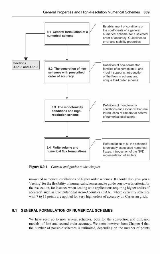
Ch08-H6594.tex 8/5/2007 14: 18 Page 339

General Properties and High-Resolution Numerical Schemes 339

Establishment of conditions onthe coefficients of a generalnumerical scheme, for a selectedorder of accuracy. Guidelines toerror and stability properties

SectionsA8.1.5 and A8.1.6

8.1 General formulation of anumerical scheme

Definition of one-parameterfamilies of schemes on 3- and4-point supports. Introductionof the Fromm scheme andunique third order scheme

8.2 The generation of newschemes with prescribedorder of accuracy

Definition of monotonicityconditions and Godunov theorem.Introduction of limiters for controlof numerical oscillations

8.3 The monotonicityconditions and high-resolution scheme

Reformulation of all the schemesto uniquely associated numericalfluxes. Introduction of the NVDrepresentation of limiters

8.4 Finite volume andnumerical flux formulations

Figure 8.0.1 Content and guides to this chapter.

unwanted numerical oscillations of higher order schemes. It should also give you a‘feeling’ for the flexibility of numerical schemes and to guide you towards criteria fortheir selection, for instance when dealing with applications requiring higher orders ofaccuracy, such as Computational Aero-Acoustics (CAA), where currently schemeswith 7 to 15 points are applied for very high orders of accuracy on Cartesian grids.

8.1 GENERAL FORMULATION OF NUMERICAL SCHEMES

We have seen up to now several schemes, both for the convection and diffusionmodels, of first and second order accuracy. We know however from Chapter 4 thatthe number of possible schemes is unlimited, depending on the number of points

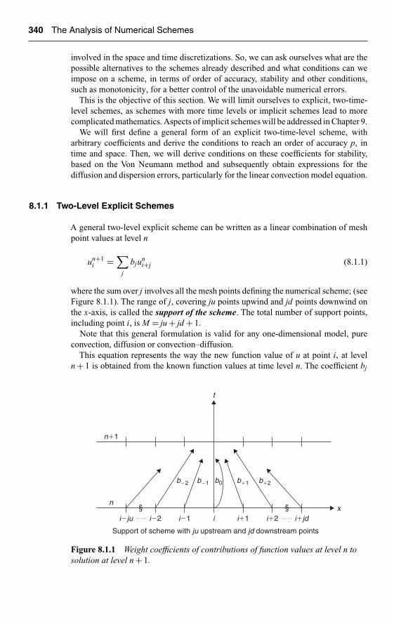
Ch08-H6594.tex 8/5/2007 14: 18 Page 340


involved in the space and time discretizations. So, we can ask ourselves what are thepossible alternatives to the schemes already described and what conditions can weimpose on a scheme, in terms of order of accuracy, stability and other conditions,such as monotonicity, for a better control of the unavoidable numerical errors.

This is the objective of this section. We will limit ourselves to explicit, two-time-level schemes, as schemes with more time levels or implicit schemes lead to morecomplicated mathematics. Aspects of implicit schemes will be addressed in Chapter 9.

We will first define a general form of an explicit two-time-level scheme, witharbitrary coefficients and derive the conditions to reach an order of accuracy p, intime and space. Then, we will derive conditions on these coefficients for stability,based on the Von Neumann method and subsequently obtain expressions for thediffusion and dispersion errors, particularly for the linear convection model equation.

8.1.1 Two-Level Explicit Schemes

A general two-level explicit scheme can be written as a linear combination of meshpoint values at level n

un+1i =

∑j

bjuni+j (8.1.1)

where the sum over j involves all the mesh points defining the numerical scheme; (seeFigure 8.1.1). The range of j, covering ju points upwind and jd points downwind onthe x-axis, is called the support of the scheme. The total number of support points,including point i, is M = ju + jd + 1.

Note that this general formulation is valid for any one-dimensional model, pureconvection, diffusion or convection–diffusion.

This equation represents the way the new function value of u at point i, at leveln + 1 is obtained from the known function values at time level n. The coefficient bj

n�1

n

b�2 b�1 b�1 b�2

x

b0

i�ju i�2 i�2 i�1 i�1i i�jd

Support of scheme with ju upstream and jd downstream points

t

§ §

Figure 8.1.1 Weight coefficients of contributions of function values at level n tosolution at level n + 1.

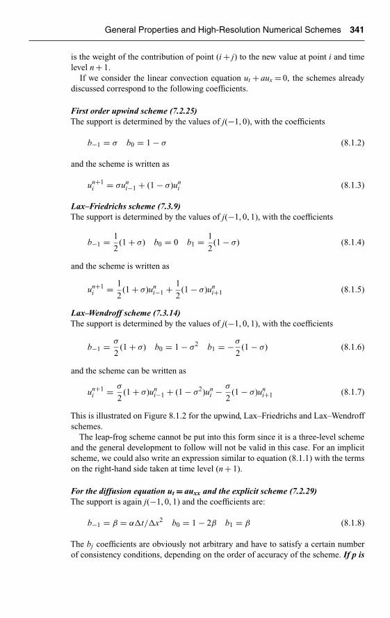
Ch08-H6594.tex 8/5/2007 14: 18 Page 341


is the weight of the contribution of point (i + j) to the new value at point i and timelevel n + 1.

If we consider the linear convection equation ut + aux = 0, the schemes alreadydiscussed correspond to the following coefficients.

First order upwind scheme (7.2.25)The support is determined by the values of j(−1, 0), with the coefficients

b−1 = σ b0 = 1 − σ (8.1.2)

and the scheme is written as

un+1i = σun

i−1 + (1 − σ)uni (8.1.3)

Lax–Friedrichs scheme (7.3.9)The support is determined by the values of j(−1, 0, 1), with the coefficients

b−1 = 1

2(1 + σ) b0 = 0 b1 = 1

2(1 − σ) (8.1.4)

and the scheme is written as

un+1i = 1

2(1 + σ)un

i−1 + 1

2(1 − σ)un

i+1 (8.1.5)

Lax–Wendroff scheme (7.3.14)The support is determined by the values of j(−1, 0, 1), with the coefficients

b−1 = σ

2(1 + σ) b0 = 1 − σ2 b1 = −σ

2(1 − σ) (8.1.6)

and the scheme can be written as

un+1i = σ

2(1 + σ)un

i−1 + (1 − σ2)uni − σ

2(1 − σ)un

i+1 (8.1.7)

This is illustrated on Figure 8.1.2 for the upwind, Lax–Friedrichs and Lax–Wendroffschemes.

The leap-frog scheme cannot be put into this form since it is a three-level schemeand the general development to follow will not be valid in this case. For an implicitscheme, we could also write an expression similar to equation (8.1.1) with the termson the right-hand side taken at time level (n + 1).

For the diffusion equation ut = auxx and the explicit scheme (7.2.29)The support is again j(−1, 0, 1) and the coefficients are:

b−1 = β = α�t/�x2 b0 = 1 − 2β b1 = β (8.1.8)

The bj coefficients are obviously not arbitrary and have to satisfy a certain numberof consistency conditions, depending on the order of accuracy of the scheme. If p is

Ch08-H6594.tex 8/5/2007 14: 18 Page 342


t t

n �1

i �2 i �1 i �1 i �2x x

x

i

n

� 1��

(a)

(1��)/2 (1��)/2

n �1

i �2 i �1 i �1 i �2i

n

(b)

�(1��)/2 �(��1)/2

t

n�1

i �2 i �1 i �1 i �2i

n

(c)

1��2

Figure 8.1.2 Weight coefficients of contributions of function values at level n tosolution at level n + 1, for: (a) first order upwind scheme, (b) Lax–Friedrichsscheme and (c) Lax–Wendroff scheme.

the order of the scheme, there are clearly (p + 1) relations to be satisfied . A firstcondition is obtained from the requirement that a constant should be a solution of thenumerical scheme. This leads to the first consistency condition:

∑j

bj = 1 (8.1.9)

The other conditions can be derived from a consistency analysis, following the guide-lines of Chapter 7, obtaining the truncation error and the equivalent differentialequation for scheme (8.1.1).

We introduce the Taylor series expansion in space,

uni+j = un

i +∞∑

m=1

( j · �x)m

m!(

∂mu

∂xm

)(8.1.10)

and in time written as

un+1i = un

i +∞∑

m=1

(�t)m

m!(

∂mu

∂tm

)(8.1.11)

Ch08-H6594.tex 8/5/2007 14: 18 Page 343


Inserting these developments into equation (8.1.1), leads to

�t∂u

∂t+

∞∑m=2

(�t)m

m!(

∂mu

∂tm

)=∑

j

(bj · j�x)∂u

∂x+∑

j

bj

∞∑m=2

( j · �x)m

m!(∂mu

∂xm

)

(8.1.12)

To go further, we need to specify the mathematical model we are simulating.If we consider the diffusion equation ut = αuxx , then there is no first space derivative

and the second consistency relation requires that

∑j

(bj · j) = 0 (8.1.13)

The first term of the m-summation is a second derivative, which has to be equal tothe diffusion coefficient for consistency, leading to the relation, with β = α �t/�x2

∑j

(bj · j2) = 2β (8.1.14)

If we consider a support j(−1, 0, 1), then the relations (8.1.9), (8.1.13) and (8.1.14)lead to the coefficients (8.1.8). The remaining terms form the truncation error.

8.1.2 Two-Level Schemes for the Linear Convection Equation

Our main interest lies however with the linear convection equation, for the reasonsalready explained.

In this case, the coefficient of the first space derivative in equation (8.1.12) hasto be equal to (−a �t) for consistency. Hence, a second consistency condition isobtained as

∑j

(bj · j) = −σ (8.1.15)

With this condition, the development (8.1.12) becomes

∂u

∂t+ a

∂u

∂x= −

∞∑m=2

(�t)m−1

m!(∂mu

∂tm

)+ 1

�t

∑j

bj

∞∑m=2

( j · �x)m

m!(∂mu

∂xm

)(8.1.16)

The full equivalent differential equation is obtained by replacing the time derivativesin equation (8.1.16) by space derivatives derived from the equivalent differentialequation. Rewriting equation (8.1.16) by replacing the summation index m by n,

∂u

∂t= −a

∂u

∂x+ 1

�t

∑j

bj

∞∑n=2

( j · �x)n

n!(∂nu

∂xn

)−

∞∑n=2

(�t)n−1

n!(∂nu

∂tn

)(8.1.17)

Ch08-H6594.tex 8/5/2007 14: 18 Page 344


we can evaluate the time derivatives by expanding the first terms to the power m.To the lowest order, we have by applying the Taylor development of (x + y + z)m as(HOT stands for Higher Order Terms)

(x + y + z)m = xm + mxm−1y + mxm−1z + HOT

In the third line, we have replaced the time derivative by the first term of this line

∂mu

∂tm=⎡⎣−a

∂

∂x+ 1

�t

∑j

bj

∞∑n=2

(j · �x)n

n!(

∂n

∂xn

)−

∞∑n=2

�tn−1

n!(

∂n

∂tn

)⎤⎦

m

u

= (−a)m ∂mu

∂xm+ m(−a)m−1 1

�t

∑j

bj

∞∑n=2

(j · �x)n

n!(

∂n+m−1

∂xn+m−1

)u

− m(−a)m−1 ∂m−1

∂xm−1

∞∑n=2

�tn−1

n!(

∂n

∂tn

)u + HOT

= (−a)m ∂mu

∂xm+ m(−a)m−1 �x

�t

∑j

∞∑n=2

bj jn �xn−1

n!(

∂n+m−1

∂xn+m−1

)u

− m(−a)m−1∞∑

n=2

�tn−1

n! (−a)n(

∂n

∂xn

)u + HOT

= (−a)m ∂mu

∂xm+ m(−a)m−1 �x

�t

∞∑n=2

�xn−1

n!

⎧⎨⎩∑

j

bjjn − (−σ)n

⎫⎬⎭

×(

∂n+m−1

∂xn+m−1

)u + HOT (8.1.18)

Introducing this relation in the development (8.1.16), we obtain the followingequivalent differential equation for the scheme (8.1.1):

∂u

∂t+ a

∂u

∂x= 1

�t

∑j

bj

∞∑m=2

( j · �x)m

m!(

∂mu

∂xm

)−

∞∑m=2

(−a)m (�t)m−1

m!(

∂mu

∂xm

)

−∞∑

m=2

(�t)m−1

m! m(−a)m−1 �x

�t

∞∑n=2

�xn−1

n!

⎧⎨⎩∑

j

bjjn −(−a�t

�x

)n⎫⎬⎭

×(

∂n+m−1

∂xn+m−1

)u + HOT

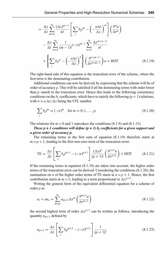
Ch08-H6594.tex 8/5/2007 14: 18 Page 345


= �x

�t

∞∑m=2

(�x)m−1

m!

⎡⎣∑

j

bjjm −

(−a�t

�x

)m⎤⎦(

∂mu

∂xm

)

− �x

�t

∞∑m=2

1

(m − 1)! (−σ)m−1∞∑

n=2

�xm+n−2

n!

×⎧⎨⎩∑

j

bjjn −(−a�t

�x

)n⎫⎬⎭(

∂n+m−1

∂xn+m−1

)u + HOT (8.1.19)

The right-hand side of this equation is the truncation error of the scheme, where thefirst term is the dominating contribution.

Additional conditions can now be derived, by expressing that the scheme will be oforder of accuracy p. This will be satisfied if all the dominating terms with order lowerthan p vanish in the truncation error. Hence this leads to the following consistencyconditions on the bj coefficients, which have to satisfy the following (p + 1) relations,with σ = a �t/�x being the CFL number

∑j

bjjm = (−σ)m for m = 0, 1, . . . , p (8.1.20)

The relations for m = 0 and 1 reproduce the conditions (8.1.9) and (8.1.15).These p + 1 conditions will define (p + 1) bj coefficients for a given support and

a given order of accuracy p.The remaining terms in the first sum of equation (8.1.19) therefore starts at

m = p + 1, leading to the first non-zero term of the truncation error:

TE = �x

�t

⎡⎣∑

j

bjjp+1 − (−σ)p+1

⎤⎦ (�x)p

(p + 1)!(

∂ p+1u

∂x p+1

)+ HOT (8.1.21)

If the remaining terms in equation (8.1.18) are taken into account, the higher orderterms of the truncation error can be derived. Considering the conditions (8.1.20), thesummation on n of the higher order terms of TE starts at n = p + 1. Hence, the firstcontribution starts at m = 2, leading to a term proportional to �x p+1.

Writing the general form of the equivalent differential equation for a scheme oforder p as

ut + aux =∞∑

m=p

am+1�xm(

∂m+1u

∂xm+1

)(8.1.22)

the second highest term of order �xp+1 can be written as follows, introducing thequantity αp+1 defined by

αp+1 = �x

�t

⎡⎣∑

j

bjjp+1 − (−σ)p+1

⎤⎦ 1

(p + 1)! (8.1.23)

Ch08-H6594.tex 8/5/2007 14: 18 Page 346


leading to

ap+1 = αp+1 (8.1.24)

and, as seen from equation (8.1.19):

ap+2 = αp+2 + σαp+1 (8.1.25)

For a second order scheme, (p = 2), we find for the next term associated to m = 3

ap+3 = αp+3 + σap+2 + σ2

2ap+1 (8.1.26)

Higher order terms can be obtained by further inspection, if necessary (see alsoProblem P.8.1).

8.1.3 Amplification Factor, Error Estimation and EquivalentDifferential Equation

The stability of the scheme can be partly analyzed by an investigation of the propertiesof the truncation error and the equivalent differential equation, as shown initially byHirt (1968).

Examples have been given in Section 7.1, where the explicit, central scheme forthe convection equation, was shown to correspond to a negative numerical viscositycoefficient and hence could only be unstable and where the conditional stability ofthe first order upwind scheme was also derived.

Generally, this method will lead to necessary conditions for stability, althoughsufficient conditions can in some cases also be derived, in particular for hyperbolicequations.

Warming and Hyett (1974) have shown that for a wide range of schemes, necessaryas well as sufficient stability conditions can be derived from the coefficients of theequivalent differential equation. In these cases, the method of the equivalent differ-ential equation can be considered on equal foot with the Von Neumann method, withregard to the stability analysis.

This analysis can be extended to nonlinear conservation laws, with attention to thenonlinear contributions from the physical fluxes. It appears that they can generateadditional dissipation, but also anti-dissipation which can reduce under certain con-ditions the oscillatory behavior of higher order schemes, without being sufficient toremove it totally.1

1 More detailed investigations, relating the structure of the truncation error to the stability of thescheme have been developed by Warming and Hyett (1974) and in a very systematic way byYanenkoand Shokin (1969). The extensive application of the equivalent differential equation developed by theRussian authors, called the method of Differential Approximation, can be found in a book by Shokin(1983). A most important application of this method is the analysis of the nature and properties ofthe truncation error. In particular the errors generated from non-linear terms can be investigated bythis approach and schemes can be defined in order to minimize the non-linear error sources (Leratand Peyret, 1974, 1975; Lerat, 1979; Shokin, 1983).

Ch08-H6594.tex 8/5/2007 14: 18 Page 347


In order to investigate the stability and accuracy of the general scheme we rewritethe equivalent differential equation (8.1.22), by separating the even and odd orderderivatives. The motivation of this step is connected to the properties of the errors,since we will show next that the even order derivatives contribute to the diffusionerror, while the odd order derivatives define the dispersion errors. Hence, we write,where the a2l and a2l+1 coefficients are uniquely defined by the bj coefficients:

ut + aux =∞∑

l=1

[a2l

(∂2lu

∂x2l

)�x2l−1 + a2l+1

(∂2l+1u

∂x2l+1

)�x2l

](8.1.27)

If the scheme is of order p in space, the first non-zero coefficient is proportional to�xp. Therefore,

a2l = a2l−1 = 0 for 2l, 2l − 1 < p (8.1.28)

The connection to the stability analysis is based on the fundamental property of theequivalent differential equation, as representing the behavior of the numerical solu-tion, as seen in Section 7.1. Therefore the analytical amplification factor of the aboveequation for a harmonic k, obtained by inserting a solution of the form e−Iωt eIkx

represents the Von Neumann amplification factor of the numerical scheme.Hence, we have, following the definition (7.4.8):

G = e−Iω �t (8.1.29)

where

Iω = Iak − 1

�x

∑l

[a2l(−)lφ2l + I (−)la2l+1φ2l+1] (8.1.30)

Observe that the even derivatives lead to a real component of ω, and the unevencoefficients contribute to the imaginary part.

If you refer to equations (7.4.11)–(7.4.13), you will notice that the diffusion erroris defined by the real part and the dispersion error by the imaginary part of ω.Hence we see the very important association between even order derivatives anddissipation of the scheme, through the diffusion error; while the uneven derivativeterms contribute to the dispersion error.

From the definition of the numerical errors, following Section 7.4, we write theamplification factor (8.1.29) as

G = |G|e−I� (8.1.31)

where the modulus of G is defined by the real part of ω, and the phase of G, is fullydefined by the imaginary part.

This defines directly the diffusion error as

εD = |G| = exp

[∑l

(−)la2lφ2l �t

�x

](8.1.32)

Ch08-H6594.tex 8/5/2007 14: 18 Page 348


and the dispersion error as

εφ = �

ak�t= 1 − 1

a

∑l

(−)lφ2la2l+1 (8.1.33)

Observe again that the dispersion error contains only odd order coefficients, whilethe diffusion error is totally defined by the even order coefficients.

A Taylor expansion as a function of φ, around φ = 0, gives from equation (8.1.32)the amplitude of the diffusion error, for small values of φ

εD = |G| = 1 +∑

l

(−)la2lφ2l �t

�x+ · · · (8.1.34)

A necessary condition for stability is directly obtained form the diffusion error, sinceit has to be lower than one for stability. Hence, to the lowest order, the necessarycondition for stability, is

(−)ra2r < 0 with 2r = (2l)min (8.1.35)

if 2r is the lowest even derivative of the expansion.For a first order scheme, p = 1, the lowest value of 2l is 2, hence r = 1. In this case

the coefficient a2 will be different from zero, and correspond to a term a2uxx. Thisterm is interpreted as a numerical viscosity generated by the discretization error ofthe scheme, and has to be positive for stability.

For second or third order schemes, p = 2 or 3, the lowest value of 2l is equal to 4and r = 2 and the first non-zero term in the expansion of the truncation error is a thirdorder derivative a3uxxx, associated to a dispersion error. Since the phase error can beof either sign, no stability condition can be deduced from the dispersion term.

However, the fourth order derivative term a4(∂4u/∂x4) contributes a dissipationerror

εD = exp

[a4φ

4 �t

�x

](8.1.36)

and the coefficient a4 has to be negative, according to equation (8.1.35).

Dissipative schemesAn important criterion for stability when the coefficients are not constant or when theproblem is not linear is related to the dissipation property in the sense of Kreiss, asmentioned in Section 7.4. In particular, this property requires that the amplificationfactor, and hence the diffusion error, be different from one for the high frequencywaves associated to the 2�x waves, or φ ≈ π. From equation (8.1.44), we have

G(π) =∑

j

bj cos jπ =∑jeven

bj −∑jodd

bj (8.1.37)

The condition

|G(π)| ≤ 1

Ch08-H6594.tex 8/5/2007 14: 18 Page 349


is satisfied if

−1 ≤⎛⎝∑

jeven

bj −∑jodd

bj

⎞⎠ ≤ 1 (8.1.38)

or, taking into account the consistency condition, �jbj = 1, we obtain (Roe, 1981)

0 ≤∑jeven

bj ≤ 1 (8.1.39)

The equality signs on these limits are valid for stability, but have to be excluded forthe Kreiss’ dissipative property. For Lax–Friedrichs scheme b0 = 0 and the condition(8.1.39) is not satisfied, indicating that this scheme is not dissipative in the sense ofKreiss. For the upwind scheme, b0 = 1 − σ, and the scheme is stable and dissipativefor 0 < σ < 1. For Lax–Wendroff scheme, b0 = 1 − σ2, and the scheme is stable anddissipative for 0 < |σ| < 1.

Some more advanced additions are to be found in Section A8.1.5, at the end of thissection.

8.1.4 Accuracy Barrier for Stable Scalar Convection Schemes

We can ask ourselves, when we select the number of support points, what is themaximum possible order of accuracy.

Referring to the general explicit scheme, we can be more specific by indicatingseparately the number of upstream and downstream points, denoted by ju and jd.The summation over j extends from −ju to +jd including j = 0; hence the support ofthe scheme is (i − ju, i − ju + 1, . . . , i − 1, i, i + 1, . . . , i + jd − 1, i + jd) containingM = ( ju + jd + 1) points. The general form of the scheme is rewritten as

un+1i =

+jd∑j=−ju

bjuni+j (8.1.40)

As stated above, if p is the order of accuracy of the scheme, there are (p + 1) con-sistency conditions and hence (M − p − 1) = ( ju + jd − p) free parameters to select.Therefore p has to satisfy

p ≤ ju + jd (8.1.41)

indicating that the maximum possible order of accuracy of the scheme (8.1.40) ispmax = ju + jd.

That is, the number of points in the support, excluding point i, defines the maximumpossible order of accuracy.

However, additional conditions are to be considered if we add the requirement ofstability and we could wonder as to what is the maximum order of accuracy for astable scheme with ju upstream and jd downstream points.

Several investigations have been pursued in order to provide a response to this ques-tion. The first result was obtained by Iserles (1982), showing that stable schemes haveto satisfy the following condition, when a > 0, referred to as the accuracy barrier,

p ≤ 2 min (ju, jd + 1) (8.1.42)

Ch08-H6594.tex 8/5/2007 14: 18 Page 350


Table 8.1.1 Maximum order ofaccuracy of an explicit stable schemefor the linear convection equation,using ju upstream and jd downstreampoints.

2

3 2

2

4

44

5 6

6 7 8

6

2 3 4 4 4

0

0 0 0 0 0 0

1

1 1 2 2 2 2

2 3 4jujd

Additional analysis along this line can be found in Iserles and Strang (1983), Jeltsch(1985), Jeltsch and Smit (1987).

The maximum order of accuracy for a stable scheme is obtained with the equalsigns and is satisfied for ju = jd; ju = jd + 1 or ju = jd + 2, as seen from the followingTable 8.1.1.

A remarkable property emerges from this result for a pure upwind explicit scheme,that is for jd = 0 when the convection speed a > 0. In this case, the maximum orderof accuracy cannot exceed two, whatever the number of upwind points, although thespatial accuracy of the space discretization for ju ≥ 3 can be higher than 2.

On the other hand, an explicit scheme with two upstream points and one down-stream point, ju = 2, jd = 1, can achieve third order accuracy, indicating that theaddition of the point (i + 1), although outside the physical domain of dependence,increases the maximum order of accuracy. Hence, restricting the numerical schemesto follow strictly some of the physical propagation properties, such as the domain ofdependence, is not necessarily the most effective choice. A pure downwind schemewith ju = 0 for a > 0 is unstable reflecting the CFL condition which forbids schemesgoing against the domain of dependence rule expressed in Section 7.2.

On the other hand, the central schemes with ju = jd, reach the highest accuracywith the lowest number of points, for a fixed value of ju, as can be seen from lookingat the diagonal of Table 8.1.1. With ju = jd = s, j covers the interval (−s, +s) and thenumber of support mesh points is M = 2s + 1.

The consistency relations (8.1.20) represent (p + 1) conditions for the M = 2s + 1coefficients bj to obtain a scheme of order of accuracy p. Therefore we can achieve amaximum accuracy of pmax = 2s.

In the case of a symmetric scheme, these consistency relations form a linear non-homogeneous system of the Vandermonde type, which can be solved exactly, usingCramer’s rule, see Karni (1994), defining completely the central schemes of order 2s.The general form of the bj coefficients is defined by

bj =k=s∏k=−sk �=j

σ + k

k − j(8.1.43)

Ch08-H6594.tex 8/5/2007 14: 18 Page 351


For s = 1, we recover the Lax–Wendroff scheme, while a fourth order accurate schemeis obtained for s = 2.

The restrictions expressed by equation (8.1.42) are connected to the choice ofan explicit scheme involving two time levels. Therefore, other choices for the timeintegration, to be discussed in Chapter 9, will not necessarily suffer from the samerestriction.

Some more advanced considerations for the accuracy barrier of multi-time-levelschemes are presented in Section A8.1.6, to be found at the end of this section.

A8.1.5 An Addition to the Stability Analysis

An exact expression for the amplification matrix of the scheme (8.1.1) is obtainedby applying the Von Neumann method, following the guidelines seen in the previouschapter.

For a Fourier mode uni+j ⇒ V neI (i+j)φ (φ = k�x) and the definition of the

amplification factor G(φ) = V n+1/V n, we obtain

G(φ) =∑

j

bjeIjφ =

∑j

bj cos jφ + I∑

j

bj sin jφ (8.1.44)

The stability condition requires that the modulus of the amplification factor shouldbe lower or equal to one. This modulus can be written directly as follows, since allthe bj coefficients are real, as

|G(φ)|2 =∣∣∣∣∣∣∑

j

bjeIjφ

∣∣∣∣∣∣2

=∣∣∣∣∣∣∑

j

bj cos jφ

∣∣∣∣∣∣2

+∣∣∣∣∣∣∑

j

bj sin jφ

∣∣∣∣∣∣2

=∑

j

∑k

bjbk cos( j − k)φ (8.1.45)

Note that ( j − k) ranges from (−2ju, 2jd), generating ( ju + jd)2 = (M − 1)2 terms.For ju = jd = 1, we have at most m = 4 terms.

With the trigonometric relation

cos mφ = 1 +m∑

l=1

(−)l 22l

(2l)!l−1∏k=0

(m2 − k2) sin2l φ/2 (8.1.46)

equation (8.1.45) can be written as a polynomial in the variable

z = sin2 φ/2 (8.1.47)

under the form

|G(φ)|2 = 1 −m∑

l=1

βlzl (8.1.48)

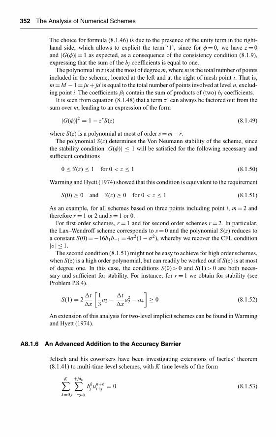
Ch08-H6594.tex 8/5/2007 14: 18 Page 352


The choice for formula (8.1.46) is due to the presence of the unity term in the right-hand side, which allows to explicit the term ‘1’, since for φ = 0, we have z = 0and |G(φ)| = 1 as expected, as a consequence of the consistency condition (8.1.9),expressing that the sum of the bj coefficients is equal to one.

The polynomial in z is at the most of degree m, where m is the total number of pointsincluded in the scheme, located at the left and at the right of mesh point i. That is,m = M − 1 = ju + jd is equal to the total number of points involved at level n, exclud-ing point i. The coefficients βl contain the sum of products of (two) bj coefficients.

It is seen from equation (8.1.48) that a term zr can always be factored out from thesum over m, leading to an expression of the form

|G(φ)|2 = 1 − zrS(z) (8.1.49)

where S(z) is a polynomial at most of order s = m − r.The polynomial S(z) determines the Von Neumann stability of the scheme, since

the stability condition |G(φ)| ≤ 1 will be satisfied for the following necessary andsufficient conditions

0 ≤ S(z) ≤ 1 for 0 < z ≤ 1 (8.1.50)

Warming and Hyett (1974) showed that this condition is equivalent to the requirement

S(0) ≥ 0 and S(z) ≥ 0 for 0 < z ≤ 1 (8.1.51)

As an example, for all schemes based on three points including point i, m = 2 andtherefore r = 1 or 2 and s = 1 or 0.

For first order schemes, r = 1 and for second order schemes r = 2. In particular,the Lax–Wendroff scheme corresponds to s = 0 and the polynomial S(z) reduces toa constant S(0) = −16b1b−1 = 4σ2(1 − σ2), whereby we recover the CFL condition|σ| ≤ 1.

The second condition (8.1.51) might not be easy to achieve for high order schemes,when S(z) is a high order polynomial, but can readily be worked out if S(z) is at mostof degree one. In this case, the conditions S(0) > 0 and S(1) > 0 are both neces-sary and sufficient for stability. For instance, for r = 1 we obtain for stability (seeProblem P.8.4).

S(1) = 2�t

�x

[1

3a2 − �t

�xa2

2 − a4

]≥ 0 (8.1.52)

An extension of this analysis for two-level implicit schemes can be found in Warmingand Hyett (1974).

A8.1.6 An Advanced Addition to the Accuracy Barrier

Jeltsch and his coworkers have been investigating extensions of Iserles’ theorem(8.1.41) to multi-time-level schemes, with K time levels of the form

K∑k=0

+jdk∑j=−juk

bkj un+k

i+j = 0 (8.1.53)

Ch08-H6594.tex 8/5/2007 14: 18 Page 353


with the consistency condition

K∑k=0

+jdk∑j=−juk

bkj = 0 (8.1.54)

where the bkj coefficients depend only on the Courant number σ = a �t/�x.

Note that the explicit two-time-level scheme (8.1.40) is obtained for K = 1,ju1 = jd1 = 0 with b1

0 = −1.For other values of the coefficients of the highest time index K , bK , when j �= 0,

equation (8.1.53) represents an implicit scheme (see Figure 8.1.3).The maximum order of accuracy of the considered schemes, excluding the stabil-

ity restrictions, is equal to the total number of variables minus the two consistencyconditions given by equation (8.1.54) and by the generalization of condition (8.1.15),written as

K∑k=0

+jdk∑j=−juk

jbkj = σ

K∑k=0

+jdk∑j=−juk

kbkj (8.1.55)

Hence, we obtain

pmax = JU + JD − 2 (8.1.56)

where JU and JD are respectively the sum of the number of upstream and downstreampoints at all time levels with respect to the characteristic issued from the point i attime level n + K . As seen from Figure 8.1.3 we have

JU =K∑

k=0

juk JD =K∑

k=0

jdk + K (8.1.57)

t

i �ju0

i �ju1

i � ju2 i �jd2

i �jd1

i �2 i �1 i �1 i �2 i �jd0i

n x

n �1

n � 2

Characteristic dx/dt �a

Figure 8.1.3 Support of multi-level scheme with juk upstream and juk downstreampoints at time level k.

Ch08-H6594.tex 8/5/2007 14: 18 Page 354


provided the characteristic intersects the mesh at time level n between i and i − 1.If this is not the case, the counts for JU and JD can easily be adapted accordingly.

This extension appears to be extremely difficult to prove in general and at thetime of writing, the following accuracy barrier for stable multi-time-level schemes(8.1.53) has only been proven in special cases and is conjectured for general cases tobe given by

p ≤ 2 min(JU , JD) (8.1.58)

See Strang and Iserles (1983), Jeltsch and Smit (1987), Jeltsch (1988), Jeltsch, Kianiand Raczek (1991).

More results can be proven for three-level-schemes, K = 2, following Jeltsch,Renaut and Smit (1997), where the relation (8.1.58) is demonstrated based on thevalidity of a conjecture related to the multiplicity of order stars. The concept of orderstars, introduced by Wanner, Hairer and Nørsett (1978) and further developed byHairer and Wanner (1991), Iserles and Nørsett (1991), allows an elegant geometricalinterpretation of the relationship between accuracy and stability in the space of com-plex analytical functions. We refer the interested reader to the original references formore details about the mathematical definition and properties of order stars.

The three-level schemes are implicit if ju2 > 0 and jd2 > 0 and explicit onlyfor ju2 = jd2 = 0. Jeltsch, Renaut and Smit (1997) restrict their analysis to convexschemes with an increasing stencil for which the number of points at a given timelevel is increasing with decreasing time index k , as displayed on Figure 8.1.3, i.e.

ju2 ≤ ju1 ≤ ju0 with ju0 − ju1 ≤ ju1 − ju2

jd2 ≤ jd1 ≤ jd0 with jd0 − jd1 ≤ jd1 − jd2 (8.1.59)

Hence, this excludes for instance the implicit Euler scheme (7.2.25), which is uncon-ditionally stable, or the explicit leapfrog scheme for which ju0 = jd0 = 0, ju1 = jd1 = 1together with ju2 = jd2 = 0.

Stronger results are obtained for the convex schemes with maximal accuracy pmax,in particular for a > 0, the authors show that for stability

pmax ≤ 2JU when a > 0 (8.1.60)

for which the above mentioned conjecture is shown to be true. For other cases, therelation (9.3.28) is proven, assuming the conjectured proposition.

8.2 THE GENERATION OF NEW SCHEMES WITH PRESCRIBEDORDER OF ACCURACY

An interesting outcome of the analysis derived in the previous section is the possibilityto generate new families of schemes, having a given support and a given order ofaccuracy. The following derivation is based on an elegant analysis by Phil Roe (1981).

The consistency conditions (8.1.20), for a scheme of order of accuracy p, define(p + 1) relations for the bj coefficients. If the support of the scheme covers M pointsthere are M values bj , and (M − p − 1) coefficients bj can be chosen arbitrarily. IfM = p + 1, there is a unique solution and therefore there is always a unique scheme on

Ch08-H6594.tex 8/5/2007 14: 18 Page 355


a support of M points having the maximum possible order of accuracy of p = M − 1.However, as seen above, not all of these schemes are valid, as some can be unstable,if they do not satisfy the accuracy barrier of Iserles.

When M > p + 1, families of schemes with (M − p − 1) parameters can be definedby analyzing all the possible solutions of the system of equations (8.1.20).

8.2.1 One-Parameter Family of Schemes on the Support (i − 1, i, i + 1)

Let us consider the 3-point support j = −1, 0, 1, (M = 3), on which we can definea one-parameter family of first order accurate schemes by satisfying the two firstconditions (8.1.20):

b−1 + b0 + b1 = 1b−1 − b1 = σ

(8.2.1)

If, following Roe (1981), the schemes are identified by the set S(b−1, b0, b1),the Lax–Friedrichs scheme corresponds to SLF((1 + σ)/2, 0, (1 − σ)/2) and the firstorder upwind scheme to SFOU(σ, (1 − σ), 0). The unstable, central scheme (7.1.7) isrepresented by SC(σ/2, 1, −σ/2).

If we consider a particular solution of this system, a general solution can be gen-erated by adding an arbitrary multiple of the homogeneous solution of the system(8.2.1) to this particular solution. The homogenous system is obtained by putting tozero all the right-hand side terms and is defined by

b−1 + b0 + b1 = 0b−1 − b1 = 0

(8.2.2)

It has the solution, b−1 = b1 = −b0/2.Because of the homogeneity, this solution is always defined up to a constant, which

we call here γ . If we write the homogenous solution as H (b−1, b0, b1), we have

H (b−1, b0, b1) = γH (1, −2, 1) (8.2.3)

It is of interest to consider the different solutions as corrections to the unstable centralscheme, as already commented for the Lax–Wendroff scheme. Hence we select thescheme SC, as the particular solution, writing the general expression as

S(b−1, b0, b1) = SC(σ/2, 1, −σ/2) + γH (1, −2, 1) (8.2.4)

This equation describes a family of first order schemes. For instance, with γ = σ/2we recover the upwind scheme and with γ = 1/2 the Lax–Friedrichs scheme.

Note that because of the form (8.2.4) the choice of the particular solution is notconstrained, as another choice would only have as consequence a redefinition of theparameter γ .

Hence, all the possible schemes on the 3-point support (i − 1, i, i + 1) with firstorder accuracy are defined by the parameter γ and the bj values b−1 = σ/2 + γ ,b0 = 1 − 2γ , b1 = γ − σ/2.

Ch08-H6594.tex 8/5/2007 14: 18 Page 356


They can be written as follows:

un+1i = un

i − σ

2(un

i+1 − uni−1) + γ(un

i+1 − 2uni + un

i−1) (8.2.5)

where γ appears as a numerical viscosity coefficient. The third term, which stabilizesthe instability generated by the first two terms, is the discretization of a numericalviscosity term of the form γ�x2uxx.

The stability condition can be obtained, through a direct analysis, as developed inChapter 7. Alternatively we can apply the results obtained in Section 8.1, in particularfrom equations (8.1.39) and (8.1.35).

From the first of these equations, we obtain

0 ≤ b0 = 1 − 2γ ≤ 1 (8.2.6)

leading to the condition

0 ≤ γ ≤ 1

2(8.2.7)

We notice, what we know already from the earlier chapters, that the coefficient γ ofthe numerical viscosity must be positive in order to represent a diffusion or dissipationeffect, as opposed to an ‘explosion’ behavior for negative diffusion coefficient.

In addition, an upper limit is set on the γ-coefficient for stability, namely γ = 1/2,which corresponds to the Lax–Friedrich scheme.

Since the condition (8.1.39) is only necessary, it cannot represent the whole ofthe stability requirements. Considering the more general condition (8.1.35) withr = 1 and

α2 = �x

�t

⎡⎣∑

j

bjj2 − (−σ)2

⎤⎦ 1

2= �x

�t

[(b−1 + b1) − σ2] 1

2

= �x

2�t

[2γ − σ2] ≥ 0 (8.2.8)

leads to the condition

2γ − σ2 ≥ 0 (8.2.9)

Summarizing the two results, we find the stability condition as

σ2

2≤ γ ≤ 1

2(8.2.10)

Note that this condition implies the CFL condition |σ| ≤ 1 for stability.From the above considerations, adding the third consistency condition (8.1.20),

which reads here for the support j(−1, 0, 1),

b−1 + b1 = σ2 (8.2.11)

Ch08-H6594.tex 8/5/2007 14: 18 Page 357


gives three conditions for the three coefficients, leading to the unique explicit schemeon the domain j(−1, 0, 1), with second order accuracy and two-time-levels, that iscentrally defined with respect to the mesh point i. This is the Lax–Wendroff schemecorresponding to γ = σ2/2. It represents the lowest limit of the stability region of γ ,as seen from equation (8.2.10).

8.2.2 The Convection–Diffusion Equation

We can apply the above results to analyze and gain an understanding of a critical issuerelated to the central discretization of the convection–diffusion equation:

ut + aux = αuxx (8.2.12)

The simplest scheme combines first order in time and second order in space to ensurethat the steady state solutions will be second order accurate. Considering a centraldifference for the convection term and the standard central difference for the diffusionterm, we obtain the scheme

un+1i = un

i − σ

2(un

i+1 − uni−1) + β(un

i+1 − 2uni + un

i−1) (8.2.13)

with β = α �t/�x2.This scheme is of the form (8.2.5), where here the parameter γ has a physical

interpretation as representing a physical instead of a purely numerical diffusion.The stability condition (8.2.10) becomes here

σ2 ≤ 2β ≤ 1 (8.2.14)

leading to the stability condition on the time step

�t ≤ min

(2α

a2,�x2

2α

)(8.2.15)

An important quantity in simulations of viscous flows is the cell Reynolds number(also called cell Peclet number when the diffusivity coefficient is not the kinematicviscosity), based on the cell size �x, defined by

Re�x�= a�x

α(8.2.16)

The stability condition can be rewritten, taking into account the relation

σ

β= a �x

α= Re�x (8.2.17)

as

σ ≤ Re�x

2≤ 1

σ(8.2.18)

Ch08-H6594.tex 8/5/2007 14: 18 Page 358


This stability region is shown in the diagram (σ, Re�x) in Figure 8.2.1, showing thatthere is a stability domain for all values of the cell Reynolds number.

This is of interest in view of the history behind this scheme and its stability condi-tions. It is a remarkable fact that historically, a first Von Neumann stability conditionwas incorrectly derived by Fromm (1964), and quoted in the book of Roache (1972),as well as in some later textbooks.

The correct results have been obtained initially by Hirt (1968) applying a differentapproach, but remained largely unnoticed, and a regain of concern has generated avariety of publications for one- and multidimensional stability analyses of the dis-cretized convection–diffusion equation, see for instance the papers of Rigal (1979),Leonard (1980), Chan (1984), Hindmarsh, Gresho and Griffiths (1984).

This erroneous condition was stated as

σ ≤ 2β ≤ 1 (8.2.19)

to be compared with the correct condition (8.2.14). This condition had a remarkableconsequence, considering the relation (8.2.17) leading to a condition

σ

β= Re�x ≤ 2 (8.2.20)

which implies a restriction on the mesh size, instead of the expected stabilityrestriction on the time step.

This incorrect concept of a mesh size limitation for stability, has generated anintense discussion between experts and considerable confusion, see for instanceThompson et al. (1985) for an additional clarification.

Stability region for convection�diffusion equation

0

0.2

0.4

0.6

0.8

1

1.2

Cou

rant

num

ber

0 1 2 3 4 5 6 7 8 9 10

Cell Reynolds number

Stability region

Figure 8.2.1 Stability region for the central scheme for the convection–diffusionequation

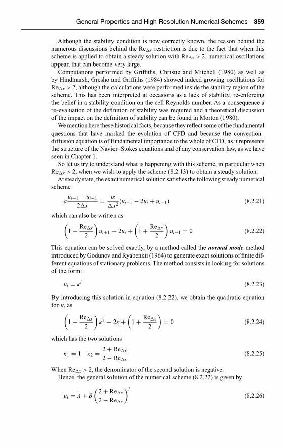
Ch08-H6594.tex 8/5/2007 14: 18 Page 359


Although the stability condition is now correctly known, the reason behind thenumerous discussions behind the Re�x restriction is due to the fact that when thisscheme is applied to obtain a steady solution with Re�x > 2, numerical oscillationsappear, that can become very large.

Computations performed by Griffiths, Christie and Mitchell (1980) as well asby Hindmarsh, Gresho and Griffiths (1984) showed indeed growing oscillations forRe�x > 2, although the calculations were performed inside the stability region of thescheme. This has been interpreted at occasions as a lack of stability, re-enforcingthe belief in a stability condition on the cell Reynolds number. As a consequence are-evaluation of the definition of stability was required and a theoretical discussionof the impact on the definition of stability can be found in Morton (1980).

We mention here these historical facts, because they reflect some of the fundamentalquestions that have marked the evolution of CFD and because the convection–diffusion equation is of fundamental importance to the whole of CFD, as it representsthe structure of the Navier–Stokes equations and of any conservation law, as we haveseen in Chapter 1.

So let us try to understand what is happening with this scheme, in particular whenRe�x > 2, when we wish to apply the scheme (8.2.13) to obtain a steady solution.

At steady state, the exact numerical solution satisfies the following steady numericalscheme

aui+1 − ui−1

2�x= α

�x2(ui+1 − 2ui + ui−1) (8.2.21)

which can also be written as(1 − Re�x

2

)ui+1 − 2ui +

(1 + Re�x

2

)ui−1 = 0 (8.2.22)

This equation can be solved exactly, by a method called the normal mode methodintroduced by Godunov and Ryabenkii (1964) to generate exact solutions of finite dif-ferent equations of stationary problems. The method consists in looking for solutionsof the form:

ui = κi (8.2.23)

By introducing this solution in equation (8.2.22), we obtain the quadratic equationfor κ, as

(1 − Re�x

2

)κ2 − 2κ +

(1 + Re�x

2

)= 0 (8.2.24)

which has the two solutions

κ1 = 1 κ2 = 2 + Re�x

2 − Re�x(8.2.25)

When Re�x > 2, the denominator of the second solution is negative.Hence, the general solution of the numerical scheme (8.2.22) is given by

ui = A + B

(2 + Re�x

2 − Re�x

)i

(8.2.26)

Ch08-H6594.tex 8/5/2007 14: 18 Page 360


When Re�x > 2, the second term will be positive for even values of i and negative onuneven points, while its absolute values is increasing with the mesh point number i.Hence, the numerical solution will alternate between increasingly positive and nega-tive values and the amplitude of the oscillations will grow as the mesh point numberincreases. This can indeed become very large, for instance for a value of Re�x = 3,the amplitude will grow exponentially like 5i.

The analytical solution of the differential equation ut = αuxx, with the boundaryconditions u(0) = 0, u(1) = 1, is

u(x) = exRe − 1

eRe − 1(8.2.27)

where Re is the global Reynolds number Re = aL/α. The exact solution is shownon the left side of Figure 8.2.2, for Re-numbers from 1 to 10, showing the growingboundary layer behavior of the solution.

The exact and numerical solutions are shown on Figure 8.2.2, for Re = 50, with8 mesh points, for which Re�x = 50/8 = 6.25 showing the oscillatory behavior of thenumerical solution (points marked CDS).

In order to eliminate this problem, one option is to reduce mesh size in order toalways satisfy Re�x < 2, but this requires adaptive grids or very fine grids. Anotherapproach is to change the scheme to a ‘hybrid scheme’, by which the convectiveterm is discretized by a first order upwind formula when Re�x > 2 and centrallywhen Re�x < 2. This is obtained by the scheme (8.3.17) and the result is shown onFigure 8.2.2 as HOC. But this leads generally to large regions where the scheme isreduced to first order.

Another alternative, which we recommend, is to introduce nonlinear limiters toenforce monotonicity, as we will see in Section 8.3.

1.0

0.0

0.2

0.4

0.6

0.8

0.0 0.2 0.4

x0.6 0.8 1.0

1.00

�0.75

0.25

�0.25

0.00

0.50

�0.50

0.75

0.0 0.2 0.4

x0.6 0.8 1.0

Exa

ct s

olut

ion

Re � 1.0

Re � 2.0

Re � 5.0

Re � 10.0

Exact

CDS

HOC

Figure 8.2.2 Left diagram: Exact solution for Re-numbers from 1 to 10, Rightdiagram: Numerical solution at Re = 50, with 8 mesh points, for whichRe�x = 50/8 = 6.25, with the central scheme, marked CDS. The solution with thehybrid scheme is marked HOC.

Ch08-H6594.tex 8/5/2007 14: 18 Page 361


8.2.3 One-Parameter Family of Schemes on the Support (i − 2, i − 1, i, i + 1)

By repeating the same methodology on the support (i − 2, i − 1, i, i + 1), we candefine a one-parameter family of schemes with second order accuracy, identified asS(b−2, b−1, b0, b1).

Second order upwind scheme on the support (i − 2, i − 1, i)If we make a first attempt to a scheme with b1 = 0, for a > 0, of the form,

un+1i = b0un

i + b−1uni−1 + b−2un

i−2 (8.2.28)

we have the three conditions for the three coefficients:

b0 + b−1 + b−2 = 1

−2b−2 − b−1 = −σ

4b−2 + b−1 = σ2

(8.2.29)

There is only one solution, namely

b−2 = σ

2(σ − 1) b−1 = σ(2 − σ) b0 = 1

2(1 − σ)(2 − σ) (8.2.30)

leading to the second order accurate upwind scheme of Warming and Beam, alreadyintroduced in Chapter 7.

The truncation error is obtained from the above relations, leading to the equivalentdifferential equation:

ut + aux = a

6�x2(1 − σ)(2 − σ)uxxx − a

8�x3σ(1 − σ)2(2 − σ)uxxxx + O(�x4)

(8.2.31)

The stability condition (8.1.35) reduces to the condition:

σ(2 − σ) ≥ 0 or 0 ≤ σ ≤ 2 (8.2.32)

Both the Lax–Wendroff and the Warming and Beam schemes are the uniqueschemes of second order accuracy on the supports (i − 1, i, i + 1) and (i − 2, i − 1, i),respectively.

Family of second order schemes on the support (i − 2, i − 1, i, i + 1)Since we dispose of four coefficients we can satisfy the first three consistency condi-tions (8.1.20), ensuring second order accuracy. These conditions define the followingsystem

b1 + b0 + b−1 + b−2 = 1

b1 − b−1 − 2b−2 = −σ

b1 + b−1 + 4b−2 = σ2

(8.2.33)

Ch08-H6594.tex 8/5/2007 14: 18 Page 362


which can be solved, with for instance b−2 as parameter, leading to the solution

b0 = 3b−2 + 1 − σ2

b1 = −b−2 + σ

2(σ − 1)

b−1 = −3b−2 + σ

2(σ + 1)

(8.2.34)

Writing again the general scheme S(b−2, b−1, b0, b1) as a particular solution plus thegeneral homogenous solution of system (8.2.33), we have first to find this homogenoussolution H (b−2, b−1, b0, b1). It is easily seen that this solution is, up to a factorH (−1, 3, −3, 1).

We know that the case b−2 = 0 is the Lax–Wendroff scheme, as it is the uniquesecond order scheme on the support (i − 1, i, i + 1), identified here as

SLW(0, σ(1 + σ)/2, (1 − σ2), −σ(1 − σ)/2) (8.2.35)

Hence, if we take the Lax–Wendroff scheme SLW as the particular solution we canwrite the general one-parameter family of second order schemes on the support(i − 2, i − 1, i, i + 1), as

S(b−2, b−1, b0, b1) = SLW + γH (−1, 3, −3, 1) (8.2.36)

By comparing with the solution (8.2.34), we see that the parameter γ is equal to thecoefficient (−b−2).

The one-parameter family of second order schemes is written as

un+1i = un

i − σ

2(un

i+1 − uni−1) + σ2

2(un

i+1 − 2uni + un

i−1)

+ γ(−uni−2 + 3un

i−1 − 3uni + un

i+1) (8.2.37)

The last term can be interpreted as the discretization of an additional dispersionterm of the form (γ�x3uxxx).

In order to derive conditions on the parameter γ and on stability, we apply themethodology of Section 8.1.

We leave it to you as an exercise to derive the amplification factor, the dispersionand diffusion errors and to look for the series expansion of these errors in function ofthe phase angle φ, as a way to obtain the first two terms of the equivalent differentialequation (8.1.27), based on the expansions (8.1.33) and (8.1.34). (see Problem P.8.8).

The diffusion error is obtained as

εD = 1 − 1

2

[γ(1 − 2σ) + 1

4σ2(1 − σ2)

]φ4

+[

γ2

2+ γ

12(1 − 5σ + 3σ2) + σ2

48(1 − σ2)

]φ6 + O(φ8) (8.2.38)

The necessary condition for stability (8.1.35) requires the first coefficient to bepositive, i.e.

γ(1 − 2σ) + 1

4σ2(1 − σ2) ≥ 0 (8.2.39)

Ch08-H6594.tex 8/5/2007 14: 18 Page 363


As γ is a function of the CFL number σ, this condition is not so useful, as it stands.However, for selected values of γ this condition will lead to necessary stabilityconditions on σ. We can simplify it by introducing the parameter �, defined by

� = 2γ

σ(1 − σ)

leading to

�(1 − 2σ) + 1

2σ(1 + σ) ≥ 0

The dispersion error is given by

εφ = 1 + 1

6[6γ − σ(1 − σ2)]φ2

−[

γ

4σ(1 − 2σ + 2σ2) − 1

120(1 − σ2)(6σ2 + 1)

]φ4 + O(φ6) (8.2.40)

Collecting the first terms, we obtain the equivalent differential equation of thescheme (8.2.38):

ut + aux = a

6[6γ − σ(1 − σ2)]�x2uxxx

− a

8

[γ(1 − 2σ) + 1

4σ2(1 − σ2)

]�x3uxxxx + O(�x4) (8.2.41)

From equation (8.2.30) we see that the Warming and Beam scheme is defined by thevalue of γ equal to the corresponding (−b−2) value, γ = σ(1 − σ)/2. That is we have

SWB(b−2, b−1, b0, b1) = SLW + σ(1 − σ)

2H ( − 1, 3, −3, 1) (8.2.42)

Fromm’s schemesWe have seen in Chapter 7 that the Lax–Wendroff and Warming–Beam schemes havephase errors of opposite signs in the range 0 < σ < 1. Therefore an attempt to derivea scheme with reduced dispersion error could be obtained by taking the arithmeticaverage of the Lax–Wendroff SLW and the Warming–Beam second order upwindschemes, SWB.

This is the scheme of Fromm (1968), which has indeed a significant reduceddispersion error. It is defined by γ = σ(1 − σ)/4, leading to

SF

(σ(σ − 1)

4,σ(5 − σ)

4,

(1 − σ)(4 + σ)

4,σ(σ − 1)

4

)(8.2.43)

Under the form (8.2.42), Fromm’s scheme is written as a correction to the Lax–Wendroff scheme

un+1i = un

i − σ

2(un

i+1 − uni−1) + σ2

2(un

i+1 − 2uni + un

i−1)

+ σ(1 − σ)

4(−un

i−2 + 3uni−1 − 3un

i + uni+1) (8.2.44)

Ch08-H6594.tex 8/5/2007 14: 18 Page 364


2.5 3.02.01.0 1.50.5

1.0

0.5

0.0

0.0

0.75

0.25

CFL�0.75

CFL�0.5

CFL�1

CFL�0.25

Diffusion Error–Fromm Scheme

Phase angle

1.25

0.0

0.25

3.02.52.01.51.0

1.0

0.5

0.75

0.5

0.0

CFL�0.5

CFL�0.25

CFL�0.75

Dispersion Error–Fromm Scheme

Phase angle

Figure 8.2.3 Diffusion and dispersion errors for Fromm’s scheme, forCFL = 0.25; 0.5; 0.75 and 1.

or under the form

un+1i = un

i − σ

4(un

i+1 + 3uni − 5un

i−1 + uni−2) + σ2

4(un

i+1 − uni − un

i−1 + uni−2)

(8.2.45)

This scheme is stable for 0 ≤ σ ≤ 1.The diffusion and dispersion errors are shown on Figure 8.2.3. You can clearly see,

by comparing with Figures 7.4.4 and 7.4.8, that the dispersion error is significantlyreduced, as it remains close to 1 up to a phase angle over (π/2) (see Problem P.8.5).

The unique third order schemeAs seen from Table 8.1.1, the maximum accuracy for schemes with the support(i − 2, i − 1, i, i + 1) is of order 3. This unique third order accurate scheme, Warming,Kutler, Lomax (1973), is obtained by adding the fourth consistency condition to thesystem (8.2.33) (see Problem P.8.9).

This fourth equation is given by

−8b−2 − b−1 + b1 = −σ3 (8.2.46)

and when introduced in the solution (8.2.34) leads to

b−2 = −γ = σ

6(σ2 − 1) (8.2.47)

This gives the scheme

S3

(σ(σ2 − 1)

6,σ(2 − σ)(σ + 1)

2,

(2 − σ)(1 − σ2)

2,σ(σ − 1)(2 − σ)

6

)

(8.2.48)

Ch08-H6594.tex 8/5/2007 14: 18 Page 365


1.0

1.51.00.5 3.0

0.75

0.5

2.5

0.0

2.00.0

0.25

CFL�0.75

CFL�0.5

CFL�1

CFL�0.25

Phase angle

Diffusion Error–Third Order Scheme

1.50.50.0

0.5

3.02.52.01.0

1.25

0.75

0.25

0.0

1.0 CFL�0.5

CFL�0.25

CFL�0.75

Dispersion Error–Third Order Scheme

Phase angle

Figure 8.2.4 Diffusion and dispersion errors for the third order scheme, forCFL = 0.25; 0.5; 0.75 and 1.

or, written as

un+1i = un

i − σ

2(un

i+1 − uni−1) + σ2

2(un

i+1 − 2uni + un

i−1)

+ σ(1 − σ2)

6( − un

i−2 + 3uni−1 − 3un

i + uni+1) (8.2.49)

This can also be seen from equation (8.2.41), where the third order term disappears,leading to the equivalent differential equation

ut + aux = − a

24[σ(1 − σ2)(2 − σ)]�x3uxxxx + O(�x4) (8.2.50)

confirming that the scheme is indeed of third order accuracy.This scheme is also stable for the CFL condition 0 ≤ σ ≤ 1.Its error properties are quite close to Fromm’s scheme, although the latter is only

second order accurate. This can be seen by comparing with Figure 8.2.4, showing thediffusion and dispersion errors for this third order scheme.

8.3 MONOTONICITY OF NUMERICAL SCHEMES

We are now ready to address the major problem that we have observed with numer-ical schemes of second or higher orders of accuracy, namely the appearance of anoscillatory behavior, as seen on the solutions presented in Chapter 7, see Figures 7.3.6–7.3.8. This creates regions of high errors, compared to the exact solution, which arenot only un-esthetical but can lead to non-physical values. This can occur with any

Ch08-H6594.tex 8/5/2007 14: 18 Page 366


quantity that is physically bounded, such as density or turbulent kinetic energy, whichhave to remain positive, or values such as ‘volume of fluid’ or ‘combustion mix-ture fraction’ which have to remain between zero and one in order to be physicallymeaningful. With these types of variables, the occurrence of numerical wiggles mightlead to unphysical values that could arm considerably the reliability of the numericalsimulation.

Hence, accurate numerical schemes should not allow such an oscillatorybehavior to occur.

A systematic analysis of the conditions required by a scheme to satisfy this require-ment has been developed, initiated by Godunov (1959) who introduced the importantproperty of monotonicity. There is an extensive literature on this very importanttopic of CFD and many different definitions and criteria can be found. For nonlinearequations the criterion of bounded total variation, under the name of Total VariationDiminishing (TVD), of the solution has been introduced by Harten (1983), (1984)as a general concept to ensure that unwanted oscillations are not generated by anumerical scheme. Spekreijse (1987) expressed monotonicity as a positivity condi-tion, while a Convection Boundedness Criterion (CBC) was explicitly formulatedby Gaskell and Lau (1988) based on the concept of NormalizedVariables introducedby Leonard (1979), (1988). A more recent general analysis, has been developed byJameson (1993), (1995a, b), based on a definition of Local Extremum Diminishing(LED) schemes.

We will not enter here in the subtleties of the theoretical differences between thesevarious concepts, as they basically all lead to the same conditions, at least for linearschemes. A discussion of the differences between these various definitions, whenapplied to nonlinear scalar, or systems of, conservation laws can be found in thebooks of Laney (1998) and Leveque (2002).

We will therefore refer in the following essentially to the notion of monotonicity.The monotonicity requirement for a numerical scheme can be stated as the require-

ment that no new extrema be created by the numerical scheme, other than thoseeventually present in the initial solution. In other words, the numerical solutionshould have a monotone behavior, whereby the new solution value un+1

i at timeindex (n+1) should not reach values outside the range covered by the solutionvalues (ui+j )n at time step n.

Clearly, the observed oscillatory behavior does not satisfy this property, while thesolutions of the first order upwind and Lax–Friedrichs solutions do show the requiredmonotone behavior.

8.3.1 Monotonicity Conditions

We will now derive the explicit conditions on a numerical scheme to satisfy thisrequirement.

Consider the general explicit scheme with two time levels, which we repeat herefor convenience:

un+1i =

∑j

bjuni+j (8.3.1)

Ch08-H6594.tex 8/5/2007 14: 18 Page 367


We know that the bj coefficients have to satisfy the consistency condition (8.1.9), alsorepeated here

∑j

bj = 1 (8.3.2)

Theorem: the monotonicity condition is satisfied if all the bj coefficients arenon-negative.

Indeed, if

bj ≥ 0 for all j (8.3.3)

the condition (8.3.2) implies that all bj ≤ 1. Hence, the new solution un+1i is the

convex sum, i.e. a weighted average with positive coefficients lower than one, ofthe old solution. If un

max and unmin are the boundaries of the variation range of un

i+jthen for

unmin ≤ un

i+j ≤ unmax (8.3.4)

we obtain, after multiplying by the positive bj coefficient and summing over allvalues of j,

∑j

bjunmin ≤ un+1

i+j =∑

j

bjuni+j ≤

∑j

bjunmax (8.3.5)

or, taking equation (8.3.2) into account

unmin ≤ un+1

i ≤ unmax (8.3.6)

This relation shows that the new solution at time step (n + 1) is also contained withinthe same range. This excludes therefore any oscillatory behavior whereby new valueswould exceed the initial variation range of the solution at an earlier time step.

An alternative, but equivalent, way of looking at the monotonicity condition (8.3.3)is obtained by rewriting the general scheme (8.3.1) with the condition (8.3.2) asfollows:

un+1i = un

i +∑

j

bj(uni+j − un

i ) (8.3.7)

If uni is a local minimum all (un

i+j − uni ) ≥ 0, and if the monotonicity condition is

satisfied, that is all the bj are positive, then we have un+1i ≥ un

i , indicating that the localminimum will not decrease. Similarly, if un

i is a local maximum, then (uni+j − un

i ) ≤ 0;

consequently un+1i ≤ un

i and the local maximum will not increase.Let us look at this monotonicity property for certain of the schemes we have

encountered, for the diffusion and the convection equations.

Ch08-H6594.tex 8/5/2007 14: 18 Page 368


Monotonicity condition for the diffusion equationIf we consider the diffusion equation (7.2.28) and the explicit scheme (7.2.29)

un+1i = un

i + β(uni+1 − 2un

i + uni−1) β = α �t

�x2(8.3.8)

The bj coefficients are

b−1 = β b0 = 1 − 2β b1 = β (8.3.9)

and we observe that all the bj coefficients are positive in the stability region β ≤ 1/2.Hence, this scheme is monotone.

Monotonicity condition for the convection equation: first order schemesThe general form for first order schemes on the 3-point support (i − 1, i, i + 1) isdefined by equation (8.2.5), with the following coefficients:

b−1 = γ + σ

2b0 = 1 − 2γ b1 = γ − σ

2(8.3.10)

with the stability condition (8.2.10), repeated here

σ2

2≤ γ ≤ 1

2(8.3.11)

The condition for monotonicity is satisfied when all coefficients are non-negative,that is for the parameter γ satisfying the following relation

σ

2≤ γ ≤ 1

2(8.3.12)

The limits of the monotonicity range of this artificial viscosity coefficient are preciselythe upwind (γ = σ/2) and Lax–Friedrichs (γ = 1/2) schemes. Both these schemes aremonotone.

This example shows that first order schemes are not always monotone, inparticular for values of γ between σ2/2 and σ/2, this scheme is stable but notmonotone.

Monotonicity condition for the convection equation: second order schemesThe second order Lax–Wendroff scheme is defined by

un+1i = un

i − σ

2(un

i+1 − uni−1) + σ2

2(un

i+1 − 2uni + un

i−1) (8.3.13)

with the coefficients

b−1 = σ

2(1 + σ) b0 = 1 − σ2 b1 = −σ

2(1 − σ) (8.3.14)

Ch08-H6594.tex 8/5/2007 14: 18 Page 369


Within the stability region |σ| ≤ 1, the coefficient b1 is always negative when σ > 0and the scheme is non-monotone.

Similarly, the Warming and Beam scheme defined by the coefficients (8.2.30) isnon-monotone, since the coefficient b−2 is negative when σ < 1, while b0 is negativewhen 1 < σ < 2.

More generally, the one-parameter family of second order schemes (8.2.37), hasthe coefficients

b−2 = −γ b−1 = σ

2(1 + σ) + 3γ b0 = 1 − σ2 − 3γ

b1 = −σ

2(1 − σ) + γ (8.3.15)

It is easily seen that these schemes can never be monotone, since the positivity condi-tion on the coefficients requires γ < 0 and on the other hand from b1, γ > σ(1 − σ)/2.This can never be satisfied within the CFL stability condition |σ| < 1, which impliesγ > 0. Hence these schemes are non-monotone.

Monotonicity condition for the convection–diffusion equationThe discussion on the oscillations associated with the cell Reynolds number of theprevious section has a straightforward explanation, looking at the coefficients of thescheme (8.2.13):

b−1 = σ/2 + β = β

(Re�x

2+ 1

)b0 = 1 − 2β,

b1 = β − σ/2 = β

(1 − Re�x

2

)(8.3.16)

We see that the scheme is non-monotone for Re�x > 2, since the coefficient b1 isnegative in this case, which explains the appearance of oscillations. On the otherhand, when Re�x < 2, the scheme is monotone in its stability domain 2β < 1 and nooscillations will appear.

If we look at a scheme where the convection term is discretized by a first orderupwind scheme, we obtain the following scheme, for a > 0

un+1i = un

i − σ(uni − un

i−1) + β(uni+1 − 2un

i + uni−1) (8.3.17)

The coefficients of this scheme are

b−1 = σ + β = β(Re�x + 1) b0 = 1 − σ − 2β = 1 − β(Re�x + 2)

b1 = β (8.3.18)

with the stability condition (see Problem P.8.12):

0 ≤ σ + 2β ≤ 1 (8.3.19)

Hence, all the b-coefficients are positive and the scheme is monotone.

Ch08-H6594.tex 8/5/2007 14: 18 Page 370


This explains its use in the hybrid approach, to eliminate the oscillations generatedwith the central scheme when Re�x > 2, as seen by the solution HOC in figure 8.2.2.

The introduction of monotonicity is a significant achievement, as we have finallyfound the explanation for the behavior of the results shown by the Figures 7.3.6–7.3.8, or for the Re�x problem occurring with the central explicit scheme of theconvection–diffusion equation discussed in the previous section.

The answer to the questions raised has become clear: the numerical oscillationsare the consequence of the non-monotone behavior of the second order schemesconsidered.

We also understand why the first order schemes do not generate these wiggles,and also why the diffusion terms, centrally discretized, are also free of unwantedoscillations.

We have now to find a cure to these non-monotone effects. This will be the subjectof the following Section 8.3.4, but before addressing this problem, we have to look atthese issues in more general terms. The crucial information is based on the Godunovtheorem, which states that all linear monotone schemes for the convection equationare necessarily first order accurate. Hence how could we make second or higher orderschemes to have a monotone behavior?

The other issue we have to deal with is the generalization of the monotonicityconcepts for more general time discretizations than the two-level explicit schemesdiscussed up to now.

8.3.2 Semi-Discretized Schemes or Method of Lines

The above analysis is based on the explicit form of the schemes (8.3.1) and we couldquestion the generality of the derived monotonicity properties.

For instance we could ask ourselves: could we possibly reduce or eliminate numeri-cal oscillations by considering implicit instead of explicit schemes; or by consideringother formulas for the time derivative than the forward difference leading to theexplicit scheme formulations?

Referring to equation (8.3.7) we can view this equation as an explicit time dis-cretization of the semi-discretized form of the scheme (also called method of lines),whereby the space discretization is separated from the time integration, as follows:

dui

dt=∑

j

βjui+j (8.3.20)

where the right-hand side represents only the discretized space derivatives.Equation (8.3.20) is a system of ordinary differential equations in time, which can

be integrated in various ways.This important general approach to the discretization of conservation laws will

be discussed in more details in Chapter 9.The consistency condition for the semi-discretized system, replacing equation

(8.3.2), is obviously given by

∑j

βj = 0 (8.3.21)

Ch08-H6594.tex 8/5/2007 14: 18 Page 371


expressing that the scheme has to remain valid for a constant valued function u = 1.Hence, the scheme can be also written as

dui

dt=∑

j, j �=0

βj(ui+j − ui) (8.3.22)

obtained from

β0 = −∑

j, j �=0

βj (8.3.23)

The monotonicity, positivity, or Local Extremum Diminishing (LED) conditionrequires that

βj ≥ 0 for all j �= 0 (8.3.24)

The above demonstration applies here without change, i.e. if ui is a local minimum and(8.3.24) is verified, then dui/dt ≥ 0 and the minimum cannot decrease, and similarlya local maximum cannot increase for a monotone scheme.

It is important to note here that this condition depends only on the space discretiza-tion and does not involve the coefficient β0 associated to j = 0 (point i). Thereforecondition (8.3.24) does not guarantee that the time integrated scheme is monotone,since an additional condition has to be added, related to β0.

For instance, if an explicit, forward time difference is applied to equation (8.3.22)then, comparing to the formulation (8.3.1), we have, observing that β0 < 0 for amonotone scheme

bj = �tβj ≥ 0 for j �= 0

b0 = 1 − �t|β0| (8.3.25)

and the monotonicity condition (8.3.3) requires that in addition the scheme alsosatisfies �t|β0| ≤ 1, which can be considered as a stability condition. For the linearconvection equation (�t|β0|) is the CFL number (see also Problem P.8.13).

Let us consider as an example the case of the convection–diffusion equation,centrally discretized, which we write as

dui

dt= −a

ui+1 − ui−1

2 �x+ α

�x2(ui+1 − 2ui + ui−1) (8.3.26)

Writing this scheme into the general form (8.3.22), we obtain

β−1 = α

�x2

(1 + Re�x

2

)β1 = α

�x2

(1 − Re�x

2

)(8.3.27)

This confirms again that the scheme is non-monotone when Re�x > 2, which leadsto an oscillatory behavior for any stable time integration scheme.

This is an important observation as it indicates that in order to remove theunwanted oscillations, we have to act on the space discretization and not on thetime integration.

Ch08-H6594.tex 8/5/2007 14: 18 Page 372


If we consider the first order upwind difference for the convection term, we obtainthe scheme, for a > 0,

dui

dt= −a

ui − ui−1

�x+ α

�x2(ui+1 − 2ui + ui−1) (8.3.28)

the coefficients

β−1 = α

�x2(1 + Re�x) β1 = α

�x2(8.3.29)

indicating that this scheme is monotone.Summarizing what we have learned from this section, we realize that the domi-

nating problem for the monotonicity of a scheme comes from the convection term,as the diffusion, also by its intrinsic physical properties, will not give rise to numer-ical oscillations. Hence in order to find cures, we have to focus on the convectionterms.

This explains why the following fundamental theorem concerning monotonicity,particularly for the convection equation, is of major significance.

8.3.3 Godunov’s Theorem

Theorem:All linear monotone schemes for the convection equation are necessarilyfirst order accurate.

This important theorem, due to Godunov (1959), can be demonstrated in variousways and we will focus here on the explicit schemes of the form (8.3.1).

The condition for second order accuracy of this scheme is given by the secondconsistency condition (8.1.20) for m = 2,

∑j

bjj2 = σ2 (8.3.30)

We will show that this condition cannot be satisfied for a monotone scheme, whereall bj coefficients are non-negative. Instead, for a monotone scheme, we would have

∑j

bjj2 ≥ σ2 (8.3.31)

indicating that the first term of the right-hand side of the equivalent differential equa-tion (8.1.21) for p = 1, is positive and hence that the scheme is only first order accurate.Indeed, if we take the square of the consistency relation for m = 1

∑j

bjj = −σ (8.3.32)

we obtain successively

σ2 =⎡⎣∑

j

bjj

⎤⎦

2

=⎡⎣∑

j

(j√

bj

)√bj

⎤⎦

2

≤⎛⎝∑

j

j2bj

⎞⎠⎛⎝∑

j

bj

⎞⎠ =

∑j

j2bj

(8.3.33)

Ch08-H6594.tex 8/5/2007 14: 18 Page 373


The inequality results from applying the Schwartz inequality, expressing that thesquare of a sum of products is lower or equal to the product of the sums of thesquares (or in other words that the scalar product of two vectors is lower or equalto the product of their lengths �a · �b ≤ |�a||�b|). The last equal sign results from theconsistency condition (8.3.2).

If we separate the upwind from the downwind points, following the form (8.1.40),the consistency condition (8.3.32) can be rewritten as follows:

∑j

bjj = −σ =jd∑

j=1

bjj −ju∑

j=1

bjj < 0 (8.3.34)

If the scheme is monotone, all the bj coefficients are non-negative and each of the twosummations is positive, which implies that the upwind points have a greater ‘weight’than the downwind points, i.e. the scheme has to be upwind biased to be monotone,since this equation indicates that, for a > 0

0 ≤jd∑

j=1

bjj ≤ju∑

j=1

bjj (8.3.35)

The theorem of Godunov can also be demonstrated for more general discretizationsof the nonlinear conservation laws, see for instance Harten, Hyman and Lax (1976).

The concepts of monotonicity and Godunov’s theorem are of considerable impor-tance, with the awareness that all linear second, or higher, order schemes for theconvection equation will necessarily generate undesirable oscillations in presence ofdiscontinuities or very high gradients of the solution or its derivatives. On the otherhand, practical applications require high-resolution schemes, that is schemes of atleast second order accuracy without numerical oscillations and therefore a way aroundGodunov’s theorem has to be found.

There are not many options available and the only way to circumvent this theoremis to move away from the linearity property of the schemes.

As a consequence, only nonlinear schemes can be made to be monotone whilebeing at the same time essentially of higher order accuracy.

This will be made possible by the introduction of nonlinear components, known aslimiters.

8.3.4 High-Resolution Schemes and the Concept of Limiters

The basic idea behind the concept of limiters is to control the process of generation ofover- and undershoots by preventing gradients to exceed certain limits, or to changesign between adjacent points.

In this way, the non-monotone schemes will be ‘controlled’, at each time step andwithin each cell, such as to keep the gradients within the proper bounds. This approachtowards high-resolution schemes consists actually in preventing the generation ofoscillations by acting somehow on their generation mechanism.

Ch08-H6594.tex 8/5/2007 14: 18 Page 374


This concept was initially introduced by Van Leer (1973, 1974) and Boris and Book(1973, 1976). Various approaches can be followed and a general framework has beenset by Van Leer (1977a, b, 1979) in a series of papers leading to second order upwindschemes without numerical oscillations and where many of the ideas at the basis ofmodern high-resolution schemes have been developed.

To illustrate the main idea behind the limiters, let us consider a second orderdifference for the convection equation ut + aux = 0 and the formulation, a > 0

dui

dt= − a

2�x(ui+1 − ui−1) = − a

2�x[−(ui−1 − ui) + (ui+1 − ui)] (8.3.36)

The last term is in the form of equation (8.3.22) and we can see that one of thecoefficients is negative, indicating that this scheme is non-monotone.

Since the concept of limiters is based on monitoring the ratio of successivegradients, we write he above scheme under the form:

dui

dt= − a

2�x

[1 − ui+1 − ui

ui − ui−1

](ui − ui−1) (8.3.37)

We observe that this scheme could become monotone if the term between the squarebrackets would remain positive, that is if the ratio between successive gradientsremains lower than 1.

ri�= ui+1 − ui

ui − ui−1≤ 1 (8.3.38)

This is illustrated in Figure 8.3.1, where the ratio r = a/b, with a = ui+1 − ui andb = ui − ui−1. The figure on the left satisfies the condition for monotonicity (8.3.38) asa < b, while the figure on the right does not, since a > b. On this figure at point i + 1,the ratio of gradients becomes negative, showing a pattern of over- and undershoots,with ri+1 < 0.

ca

ui�2ui�1

ui

ui�1

i �1 i �1 i �2ix

u

b

c

a

ui�1

ui

ui�1

i �1 i �1 i �2ix

u

b

Figure 8.3.1 Illustration of the relation between successive gradients.

Ch08-H6594.tex 8/5/2007 14: 18 Page 375


This guides the methodology behind the definition of limiter functions �, as func-tions of ratio of successive gradients � = �(ri), defined to ensure that conditionssuch as (8.3.38) are satisfied.

This methodology can be defined as follows:

1. Select a first order monotone space discretization, generally the first orderupwind discretization, as reference and write the higher order scheme as themonotone scheme plus additional terms.

2. Multiply the additional terms by a ‘limiting function’ �, expressed as afunction of a ratio of successive gradients.

3. Express the monotonicity conditions to derive the conditions on the ‘limiters’.

We have seen in the conclusion of Section 8.3.2 that the non-monotone conditionsare predominantly conditioned by the space discretization and not by the time inte-gration. Therefore, we will focus on the spatial gradients to develop the methodologyfor high-resolution schemes and for the definition of limiters.

To illustrate the main idea behind the limiters, let us consider a second orderbackward difference for the convection equation ut + aux = 0 and the formulation,for a > 0

dui

dt= − a

2�x(3ui − 4ui−1 + ui−2) = − a

2�x[3(ui − ui−1) − (ui−1 − ui−2)]

= − a

2�x[−4(ui−1 − ui) + (ui−2 − ui)] (8.3.39)

The last equality is in the form of equation (8.3.22) and we can see that one of thecoefficients is negative, indicating that this scheme is non-monotone.

Let us apply the proposed methodology, step by step.

Step 1: Rewrite the scheme as a correction to the monotone first order upwinddifference, writing the correction terms in the form of successive gradients

dui

dt= − a

�x(ui − ui−1)

︸︷︷︸First order monotoneupwind scheme

− a

�x

[+1

2(ui − ui−1) − 1

2(ui−1 − ui−2)

](8.3.40)

Step 2: Multiply the two non-monotone terms by functions �(ri) and �(ri−1), where

ri−1 = ui − ui−1

ui−1 − ui−2ri = ui+1 − ui

ui − ui−1(8.3.41)

leading to

dui

dt= − a

�x

[(ui − ui−1) + 1

2�(ri)(ui − ui−1) − 1

2�(ri−1)(ui−1 − ui−2)

]

= − a

�x

[1 + 1

2�(ri) − 1

2

�(ri−1)

ri−1

](ui − ui−1) (8.3.42)

Ch08-H6594.tex 8/5/2007 14: 18 Page 376


Step 3: Derive the conditions on the limitersThis scheme will be monotone if the term in the brackets is positive, that is the

limiters should satisfy the condition

�(ri−1)

ri−1− �(ri) ≤ 2 (8.3.43)

A detailed analysis of the properties of the � limiters has been given by Roe (1981,1984), Sweby (1984) and also, from a different standpoint, by Roe (1985).

The above functional relations can be satisfied by a large variety of � functions.However, a certain number of constraints can be identified or imposed. First of all,we restrict � to be a positive function, i.e.

�(r) ≥ 0 for r ≥ 0 (8.3.44)

In addition, when r < 0, that is when an extremum is encountered in the variation ofthe solution u, it seems logical to set � = 0 corresponding to a zero slope in the intervalconsidered. This avoids non-monotone behaviors with changes of slope directions, atthe expense of a certain loss of accuracy.

Note the important property that when Ψ = 0 the scheme reduces locally to firstorder accuracy.

Hence, we set

�(r) = 0 for r ≤ 0 (8.3.45)

With these assumptions, we have the sufficient condition

0 ≤ �(r) ≤ 2r (8.3.46)

A logical requirement is the symmetry property, which expresses that forward andbackward gradients are treated in the same way:

�(r)

r= �

(1

r

)(8.3.47)

which implies, from equation (8.3.43), the sufficient condition:

�(r) ≤ 2 (8.3.48)

Therefore, the second order upwind scheme will be monotone if the limiting func-tion � lies within the shaded area of Figure 8.3.2, which summarizes the aboverelations as

0 ≤ �(r) ≤ min(2r, 2) (8.3.49)

Figure 8.3.2, displaying the limiter in function of the gradient ratio r, is called theSweby diagram.

Ch08-H6594.tex 8/5/2007 14: 18 Page 377


�(r ) = 1WB scheme

�(r )

1

1 2

�(r ) � rLW scheme�(r ) � 2r

2

r

Figure 8.3.2 Monotonicity region for limiter functions, based on relation (8.3.49).

Limiters for the second order upwind (SOU) scheme of Warming and BeamLet us re-apply the methodology to the unique second order upwind (SOU) schemeof Warming and Beam on the support (i − 2, i − 1, i). We will subsequently applyit to the centrally discretized Lax–Wendroff scheme on the support (i − 1, i, i + 1),with an amazing consequence, namely that, after introduction of the limiters, the high-resolution versions of these two schemes will be viewed as leading to the same results.

We consider the Warming and Beam scheme with the coefficients defined byequation (8.2.30):

un+1i = un

i + σ(2 − σ) (uni−1 − un

i ) + σ

2(σ − 1) (un

i−2 − uni ) (8.3.50)

Step 1: rewrite the scheme as a correction to the monotone first order upwind scheme,with the additional terms under the form of differences between adjacent points

un+1i = un

i − σ (uni − un

i−1)︸︷︷︸Monotone scheme

− σ

2(1 − σ) (un

i − uni−1) + σ

2(1 − σ) (un

i−1 − uni−2)

︸︷︷︸Non-monotone terms

(8.3.51)

Step 2: multiply the two non-monotone terms by functions �(ri) and �(ri−1),leading to

un+1i = un


i−1) − σ

2(1 − σ)�(ri) (un

i − uni−1)

+ σ

2(1 − σ) �(ri−1)(un

i−1 − uni−2)

= uni − σ

{1 + 1

2(1 − σ)

[�(ri) − �(ri−1)

ri−1

]}(un

i − uni−1) (8.3.52)

Ch08-H6594.tex 8/5/2007 14: 18 Page 378


Step 3: this ‘limited’scheme will be monotone if the term between the curled bracketsis positive, leading to the condition

�(ri−1)

ri−1− �(ri) ≤ 2

1 − σ(8.3.53)

This relation is satisfied by the sufficient relation, Roe (1981), Roe and Baines (1981),Sweby (1984):

0 ≤ �(r) ≤ min

(2r

σ,

2

1 − σ

)(8.3.54)

which generalizes the sufficient condition (8.3.49) on the � function.This condition is more adequate for time-dependent problems, although in practice

the simpler condition (8.3.49) is more often applied, being also more suitable forstationary problems.

Observe that the ‘unlimited’, non-monotone second order upwind scheme ofWarming and Beam corresponds to � = 1.

Remark: There is a large amount of flexibility in the choice of the gradient ratios,as defined by equation (8.3.41). In this equation the ratios are based on comparingupwind gradients, but one could also define downstream ratios, such as

Ri = ui − ui−1

ui+1 − ui= 1

riRi+1 = ui+1 − ui

ui+2 − ui+1= 1

ri+1(8.3.55)

Limiters for the Lax–Wendroff schemeApplying the methodology to the Lax–Wendroff scheme, the three steps develop asfollows:

Step 1: rewrite the LW scheme as a correction to the monotone first order upwindscheme,

un+1i = un


i−1)︸︷︷︸Monotone scheme

− σ

2(1 − σ) (un

i+1 − uni ) + σ

2(1 − σ) (un

i − uni−1)

︸︷︷︸Non-monotone terms

(8.3.56)

Step 2: multiply the two non-monotone terms by functions �(Ri) and �(Ri−1),leading to

un+1i = un


i−1) − σ

2(1 − σ) �(Ri)(u

ni+1 − un

i )

+ σ

2(1 − σ)�(Ri−1) (un

i − uni−1)

un+1i = un


i−1)

{1 + 1

2(1 − σ)

[�(Ri)

Ri− �(Ri−1)

]}(un

i − uni−1)

(8.3.57)

Ch08-H6594.tex 8/5/2007 14: 18 Page 379


Step 3: this ‘limited’scheme will be monotone if the term between the curled bracketsis positive, leading to the condition:

�(Ri−1) − �(Ri)

Ri≤ 2

(1 − σ)(8.3.58)

The interesting observation is that, with the symmetry property (8.3.47) and therelation (8.3.55), this condition is identical to (8.3.53).

If we take the WB scheme as reference, the ‘limited’ version (8.3.42) reproducesthe LW scheme for �(r) = r, as can be readily verified and recovers the WB schemefor �(r) = 1. The same conditions can be expressed in function of the Ri = 1/ri ratios,taking into account the symmetry property. Indeed with the relation

�(ri) = �

(1

Ri

)= �(Ri)

Ri(8.3.59)

the LW scheme is recovered for �(R) = 1, while the WB scheme is obtained for�(R) = R.

In order to narrow down further the choices for limiters, we should consider thecase of a linear solution, for which r = 1. In this case, the second order schemesshould be satisfied exactly, which implies that the limiter functions should be equalto 1, in order to recover the ‘non-limited’ version.

Hence, we require all limiters to satisfy the additional condition

�(1) = 1 (8.3.60)

which is a necessary requirement for second order accuracy on smooth solutions.In addition, Leonard (1988) has shown that if the slope of the (�, r) curve in thispoint (1, 1) is equal to 3/4, than the scheme is locally third order accurate.

As seen in Section 8.2 any linear second order explicit scheme on the support(i − 2, i − 1, i, i + 1) can be viewed as a linear combination of the Warming and Beamand the Lax–Wendroff schemes. Consequently, any second order ‘limited’ schemecould be based on a limiter function �, which lies between the lines � = r and � = 1.This restricts the region of validity of the limiters to the domain shown on Figure 8.3.3,for second order explicit monotone schemes.

As reported by Sweby (1984) the regions of Figure 8.3.2 outside the domain between� = r and � = 1 are theoretically acceptable, but lead to schemes which are ‘over-compressive’, that is turning sine waves into square wave forms.

Actually, the analysis of the monotonicity of the Lax–Wendroff schemes was atthe basis of the generalization of the concept of limiters, Davis (1984), Roe (1984),Sweby (1984). It may seem surprising that this led to the same constraints on thelimiter function � as the second order upwind schemes, but demonstrates, on theother hand, the generality of the hereby defined limiters.

In addition, as observed by Sweby (1984), the fact that the second order (in time)explicit upwind scheme of Warming and Beam and the second order explicit Lax–Wendroff schemes can both be made monotone by the same set of limiters, justifiesthe subset of the monotonicity region of Figure 8.3.3, where the ‘limited’ explicitschemes remain globally second order accurate in time and space.

Ch08-H6594.tex 8/5/2007 14: 18 Page 380


�(r ) � 1WB scheme

�(r )

1

1 2

�(r ) � rLW scheme�(r ) � 2r

2

r

Figure 8.3.3 Region of monotonicity for second order schemes.

The drawback of the limiters is that they reduce the scheme locally to first orderat extrema, when r = 0. This is justified when it serves to suppress oscillations, sincefirst order schemes are generally monotone, but if the exact solution has extrema, likea sine wave, then the solution will be locally deformed by the action of the limiters.

This has to be considered as the ‘price’to pay for the achievement of high-resolutionschemes.

It has to be said that the development of high-resolution schemes is one of themost remarkable achievements of the history of CFD.

Various limiter functions have been defined in the literature and are currentlyapplied.

Van Leer (1974) proposed initially the formula

�(r) = r + |r|1 + r

(8.3.61)

shown in Figure 8.3.4a.A similar limiter, with a smoother behavior, has been applied by Van Albada et al.

(1982),

�(r) = r2 + r

1 + r2(8.3.62)

It has the property of tending to 1 for large values of r, while the Van Leer limitertends to 2 asymptotically.

The lowest boundary of the considered TVD domain is an often applied limiter. Itis shown on Figure 8.3.4b and can be represented by

�(r) ={

min (r, 1) if r ≥ 00 if r ≤ 0

(8.3.63)

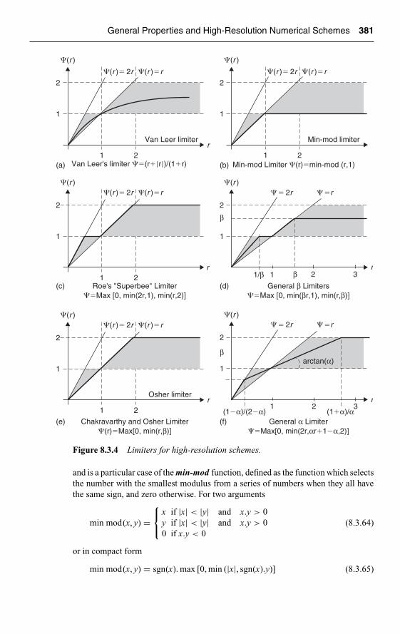
Ch08-H6594.tex 8/5/2007 14: 18 Page 381


�(r )

rVan Leer limiter

�(r )� 2r

�(r )� 2r

1

1

2

2

�(r )�r

�(r )� 2r � � 2r � �r

� � 2r � �r

�(r )�r

�(r )� 2r �(r )�r

�(r )�r

�(r )

r1

1

2

1

2

β

β

2

�(r )

rOsher limiter

1

1

2

2

�(r )

r

Min-mod limiter

1

1

2

2

�(r )

�(r )

r1

(1�α)/(2�α) (1�α)/α

1

2

2 3

Roe's "Superbee" Limiter��Max [0, min(2r,1), min(r,2)]

Min-mod Limiter �(r)�min-mod (r,1)Van Leer's limiter ��(r��r�)/(1�r)

Chakravarthy and Osher Limiter�(r)�Max[0, min(r,β)]

General β Limiters��Max [0, min(βr,1), min(r,β)]

General α Limiter��Max[0, min(2r,αr�1�α,2)]

(a)

(c)

(e)

(b)

(d)

(f)

11/β 2β 3

arctan(α)

Figure 8.3.4 Limiters for high-resolution schemes.

and is a particular case of the min-mod function, defined as the function which selectsthe number with the smallest modulus from a series of numbers when they all havethe same sign, and zero otherwise. For two arguments

min mod(x, y) =⎧⎨⎩

x if |x| < |y| and x.y > 0y if |x| < |y| and x.y > 00 if x.y < 0

(8.3.64)

or in compact form

min mod(x, y) = sgn(x). max [0, min (|x|, sgn(x).y)] (8.3.65)

Ch08-H6594.tex 8/5/2007 14: 18 Page 382


Equation (8.3.63) can therefore be written as �(r) = min mod (1, r).The upper limit of the second order monotonicity domain has been considered by

Roe, Roe and Baines (1981), Roe (1985) under the nickname of superbee and shownto have excellent resolution properties for jump discontinuities. It is shown on Figure8.3.4c and defined by

�(r) = max [0, min (2r, 1), min (r, 2)] (8.3.66)

This limiter actually amplifies certain contributions, when � > 1, while remainingwithin the monotonicity bounds. This explains the property of this ‘superbee’ limiterin counteracting the excessive spreading of jump discontinuities. It has a remarkableproperty, shown by Roe and Baines (1983), namely that it allows linear disconti-nuities to propagate indefinitely without numerical diffusion. This is illustrated onFigures 8.3.6 and 8.3.7.

The limits of the monotonicity region are members of a family of limiters, basedon a single parameter β, in the range 1 ≤ β ≤ 2, Sweby (1984),

�(r) = max [0, min (βr, 1), min (r, β)] 1 ≤ β ≤ 2 (8.3.67)

These β-limiters are shown on Figure 8.3.4d. It is seen by inspection that it reducesto the min-mod limiter for β = 1, and to the Superbee limiter for β = 2.

All of these limiters share the symmetry property (8.3.47).Let us also mention the limiter used by Chakravarthy and Osher (1983):

�(r) = max [0, min (r, β)] 1 ≤ β ≤ 2 (8.3.68)

shown on Figure 8.3.4e. Note that this limiter does not satisfy the symmetry condition(8.3.47), excepted for β = 1, where it reduces to the min-mod limiter.

More limiters can be found in the literature; see for instance Waterson andDeconinck (1995, 2007) for a general review.

In particular, the SMART limiter of Gaskell and Lau (1988), controls the slope ofthe (�, r) curve in point (1, 1), putting it equal to the optimum value of 0.75, for localthird order accuracy. This SMART limiter is defined by

�(r) =

⎧⎪⎪⎪⎪⎪⎨⎪⎪⎪⎪⎪⎩

0 for r ≤ 0

2r for 0 ≤ r ≤ 1

53

4r + 1

4for

1

5≤ r ≤ 5

4 for 5 ≤ r

(8.3.69)

or in a compact form as �(r) = max [0, min (2r, 0.75r + 0.25, 4)].Note that this limiter does not respect the sufficient condition (8.3.48) (� ≤ 2), but

it neither satisfies the symmetry property.If we impose the condition (8.3.49), but add a control of the slope (α) of the limiter

in point (1, 1), we can define the following ALFA family, in the range 0 ≤ α ≤ 1, asfollows:

�(r) = max [0, min (2r, αr + 1 − α, 2)] (8.3.70)

which is shown on Figure 8.3.4f. Note that α indicates the slope of the line through(1, 1), but is not the angle of that line with the horizontal direction. Actually this angleis equal to arctan α.

Ch08-H6594.tex 8/5/2007 14: 18 Page 383


This family of limiters has been considered initially by Roe and Baines (1981), andlater taken up by Jeng and Payne (1995) and by Arora and Roe (1997), showing it hasexcellent properties.

For α = 0, it is close to the superbee limiter but restricted to a maximum value� = 1, while α = 1 reproduces the Chakravarthy and Osher limiter at β = 2. Asit follows the � = 2r limit for small values of r, like the superbee limiter, it willbehave in a ‘compressive way’ in this region, while having a smooth behavior aroundpoint (1, 1).

The value α = 0.5 satisfies the symmetry condition, and actually corresponds to theFromm scheme, for which �(r) = (1 + r)/2. It is mentioned by Van Leer (1979), inassociation with the development of the Monotone Upstream-centered Scheme forConservation Laws (MUSCL) and referred to in the literature as the MUSCL limiter.For α = 3/4, the SMART limiter is followed, up to a maximum value of � = 2. Thevalue α = 2/3 has been considered by Koren (1993).

A fully symmetric ALFA family can be considered, satisfying (8.3.47), leading to

�(r) = max [0, min (2r, αr + 1 − α, (1 − α)r + α, 2) (8.3.71)

The value α = 3/4 has been introduced by Lien and Leschziner (1994) and consideredby Waterson and Deconinck (1995, 2007) under a general form similar to (8.3.71).This family has the advantage of symmetry, but suffers from the slope discontinuityat the point r = 1, � = 1.

Much of the recent and current research is oriented at the non-trivial extensionof the concept of limiters to arbitrary unstructured grids. This extension, importantin practice, will be dealt within Volume II. The impatient reader will find additionalinformation for instance in Barth (1993), Venkatakrishnan and Barth (1993), Jasaket al. (1999), Darwish and Moukalled (2000).

It is important to observe at this point that all these high-resolution schemes arestrictly nonlinear due to the dependence on the �u ratios, even when applied to thelinear convection equation.

More insight into the action of the limiters is obtained by considering the specificcontribution of the second order terms to the new solution at point i at time leveln + 1.

The term (ui − ui−1) is modified by a nonlinear correction �(ui − ui−1). With the‘min-mod’ limiter, we actually set the following restrictions:

• If the gradient (ui+1 − ui)/�x < (ui − ui−1)/�x, that is if r < 1, then �(r) = rand the contribution (ui − ui−1) to the solution at time step (n + 1) is replacedby the smaller quantity (ui+1 − ui).

• If r > 1, the contribution (ui − ui−1) remains unchanged.• If the slopes of consecutive intervals change sign, the updated point i receives

no contribution from the upstream interval.

With the superbee limiter, on the other hand, some contributions are enhancedinstead of reduced, while remaining within the monotonicity region. If r < 1/2, � = 2rand the contribution (ui − ui−1) to the solution at time step (n + 1) is replaced by thesmaller quantity 2(ui+1 − ui), while for 1/2 < r < 1, the larger quantity is kept. For

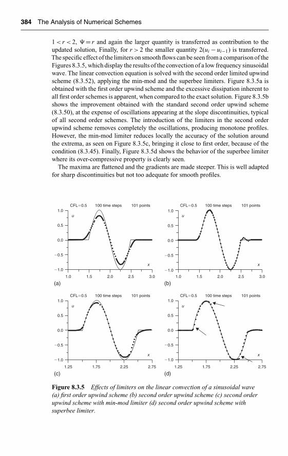
Ch08-H6594.tex 8/5/2007 14: 18 Page 384


1 < r < 2, � = r and again the larger quantity is transferred as contribution to theupdated solution, Finally, for r > 2 the smaller quantity 2(ui − ui−1) is transferred.The specific effect of the limiters on smooth flows can be seen from a comparison of theFigures 8.3.5, which display the results of the convection of a low frequency sinusoidalwave. The linear convection equation is solved with the second order limited upwindscheme (8.3.52), applying the min-mod and the superbee limiters. Figure 8.3.5a isobtained with the first order upwind scheme and the excessive dissipation inherent toall first order schemes is apparent, when compared to the exact solution. Figure 8.3.5bshows the improvement obtained with the standard second order upwind scheme(8.3.50), at the expense of oscillations appearing at the slope discontinuities, typicalof all second order schemes. The introduction of the limiters in the second orderupwind scheme removes completely the oscillations, producing monotone profiles.However, the min-mod limiter reduces locally the accuracy of the solution aroundthe extrema, as seen on Figure 8.3.5c, bringing it close to first order, because of thecondition (8.3.45). Finally, Figure 8.3.5d shows the behavior of the superbee limiterwhere its over-compressive property is clearly seen.

The maxima are flattened and the gradients are made steeper. This is well adaptedfor sharp discontinuities but not too adequate for smooth profiles.

CFL�0.5 100 time steps 101 points1.0

1.25 1.75

x

u

2.25 2.75

0.5

0.0

�0.5

�1.0

1.0CFL�0.5 100 time steps 101 points

1.0 1.5

x

u

2.0 2.5 3.0

0.5

0.0

�0.5

�1.0

(a)


1.0 1.5

x

u

2.0 2.5 3.0

0.5

0.0

�0.5

�1.0

(b)


1.25 1.75

x

u

2.25 2.75

0.5

0.0

�0.5

�1.0

(c) (d)

Figure 8.3.5 Effects of limiters on the linear convection of a sinusoidal wave(a) first order upwind scheme (b) second order upwind scheme (c) second orderupwind scheme with min-mod limiter (d) second order upwind scheme withsuperbee limiter.

Ch08-H6594.tex 8/5/2007 14: 18 Page 385


The effects of the limiters on discontinuities can also be seen from the convectionof a square wave. Figures 8.3.6 and 8.3.7 compare the linear convection of a squarewave, after 120 and 400 time steps at a Courant number of 0.5. Figure 8.3.6a isobtained with the first order upwind scheme, showing its excessive diffusion; Fig-ure 8.3.6b is obtained with the second order upwind scheme, showing the strongoscillations around the discontinuities. Figures 8.3.6c–e are computed with the min-mod, Van Leer and superbee limiters, respectively, and generate monotone profiles.

1.2

1.0

0.8

0.6

0.4

0.2

0.0

1.0 1.5 2.0

x

u

CFL�0.5

(a)

120 time steps 101 points

2.5 3.0

1.2

1.0

0.8

0.6

0.4

0.2

0.0

1.0 1.5 2.0

x

u

CFL�0.5

(c)


2.5 3.0

1.2

1.0

0.8

0.6

0.4

0.2

0.0

1.0 1.5 2.0

x

u

CFL�0.5

(e)


2.5 3.0

1.2

1.0

0.8

0.6

0.4

0.2

0.0

1.0 1.5 2.0

x

u

CFL�0.5

(d)


2.5 3.0

1.2

1.0

0.5

0.0

�0.5

1.0 1.5 2.0

x

u

CFL�0.5

(b)


2.5 3.0

Figure 8.3.6 Effects of limiters on the linear convection of a square wave after120 time steps: (a) first order upwind scheme, (b) second order upwind scheme,(c) second order upwind scheme with min-mod limiter, (d) second order upwindscheme with Van Leer limiter and (e) second order upwind scheme with superbeelimiter.

Ch08-H6594.tex 8/5/2007 14: 18 Page 386


�0.5

4.0 4.5

(b)5.0 5.5 6.0

x

u

0.0

0.5

1.0


0.0

4.0 4.5

(c)5.0 5.5 6.0

x

u

0.2

0.4

0.6

0.8

1.0


0.0

4.0 4.5

(a)5.0 5.5 6.0

x

u

0.2

0.4

0.6

0.8

1.0


0.0

4.0 4.5

(d)5.0 5.5 6.0

x

u

0.2

0.4

0.6

0.8

1.0


Figure 8.3.7 Effects of limiters on the linear convection of a square wave after400 time steps: (a) first order upwind scheme, (b) second order upwind scheme, (c)second order upwind scheme with Van Leer limiter and (d) second order upwindscheme with superbee limiter.

The min-mod limiter however is still too diffusive, while the superbee limiter pro-duces excellent results, with extremely sharp discontinuities. The Van Leer limiterhas properties between the previous two. Superbee maintains the sharpness of theprofile indefinitely, as can be seen by comparing with a similar calculation after 400time steps, shown on Figure 8.3.7c. The points in the transition region are practi-cally unchanged from time step 120 to step 400, while it is seen that the Van Leerlimiter still continues to generate a small, but continuous, diffusion of the transitionprofiles.

Figure 8.3.8 shows results obtained with the high-resolution LW scheme (8.3.57)on the same test case as the previous figures for the linear convection equation. Hereagain the superbee limiter leads to very sharp, non-diffusive transition profiles, whilethe other limiters, the min-mod and the Van Leer limiters, still have some diffusivecomponents. Note in particular the symmetrical shape of the profiles, compared to thesimilar profiles obtained with the upwind method, which show traces of the upwinddiscretizations.

Ch08-H6594.tex 8/5/2007 14: 18 Page 387


1.0

�0.5

0.0

0.5

1.0

1.5

u

2.0 3.0

x

2.51.5 1.0

0.0

0.2

0.4

0.6

0.8

1.0

1.2

u

2.0 3.0

x

2.51.5

1.0

0.0

0.4

0.2

0.6

0.8

1.0

1.2

u

2.0 3.0

x

2.51.5 1.0

0.0

0.2

0.4

0.6

0.8

1.0

1.2

u

2.0 3.0

x

2.51.5

(a) (b)

(c) (d)

CFL�0.5 120 time steps 101 points CFL�0.5 120 time steps 101 points

CFL�0.5 120 time steps 101 points CFL�0.5 120 time steps 101 points

Figure 8.3.8 Effects of limiters on the linear convection of a square wave after120 time steps: (a) standard LW scheme, (b) second order high-resolution LWscheme with min-mod limiter, (c) second order high-resolution LW scheme with VanLeer limiter and (d) second order high-resolution LW scheme with superbee limiter.

HANDS-ON TASK 4

Extend the program you have written under the Hands-On Task 2 (Chapter 7),introducing the limiters to obtain high-resolution schemes. Obtain the variousresults displayed in Figures 8.3.5–8.3.9.

Introduce also other limiters and test various cases. In particular, apply thehigh-resolution schemes to the test cases of the propagating waves of 7.3.7 and7.3.8. Observe the positive effect of the limiters on the reduction of the dispersionerrors, in particular with the LW and WB schemes.

Limiters for time-dependent problemsTime-dependent problems, in particular moving discontinuities such as movingshocks, or free surface problems between two fluids such as surface waves in shiphydrodynamics or sloshing problems in tanks, put very severe constraints on thenumerical schemes, in order to be able to follow the motion of the discontinuity overlonger times. The main challenge is to avoid the effects of the numerical diffusion ofthe interface.

Ch08-H6594.tex 8/5/2007 14: 18 Page 388


�(r)

r

�(r ) � 2r /s �(r ) � 2r �(r ) �r

�(r ) � 2/(1�σ)

1

1

2

2

Figure 8.3.9 Region of monotonicity for CFL-dependent limiters and secondorder schemes.

In these cases it is recommended to consider the CFL-dependent conditions (8.3.54)and introduce an explicit CFL effect in the limiters. If we add the condition for secondorder accuracy on the limiters (8.3.60), we obtain an extended validity domain forthe limiters, where the upper limit is given by � = 2/(1 − σ) instead of � = 2 andthe left side limit is now defined by � = 2r/σ instead of � = 2r. This leads to thevalidity domain shown in Figure 8.3.9, to be compared with Figure 8.3.3.

The upper limit of this region is the generalization of the superbee limiter and hasbeen nicknamed as the ultrabee limiter by Roe and Baines (1981). It is defined by

�(r) = max

[0, min

(2r

σ, 1

), min

(r,

2

1 − σ

)](8.3.72)

This limiter is also considered by Leonard (1991), as part of the ultimate strategy forlimiters.

The generalization of the ALFA family (8.3.70) to CFL dependent conditions hasbeen initially considered by Roe and Baines (1981), and applied by Jeng and Paine(1995), Arora and Roe (1997), under the form

�(r) = max

[0, min

(2r

σ, α(r − 1) + 1,

2

1 − σ

)](8.3.73)

where the parameter α can be made CFL dependent.The value α = (2 − σ)/3 is advocated by Arora and Roe (1997) as it corresponds to

the third order scheme (8.2.49) (see Problem P.8.17). These authors also recommendto restrict the limiter region to the stationary limits � = 2 and � = 2r for nonlinearwaves. This leads to the alternative

�(r) = max [0, min (2r, α(r − 1) + 1, 2)] with α = α(σ) (8.3.74)

These limiters are represented in Figure 8.3.10, that you can compare withFigure 8.3.4.

Ch08-H6594.tex 8/5/2007 14: 18 Page 389


�(r )

r

�(r ) � 2r /s �(r ) � 2r /s

�(r )�2r

�(r ) � r �(r ) � r�(r ) � 2/(1�s ) �(r )�2r �(r ) � 2/(1�s )

1

1

2

2

�(r)

r1

1

2

2

Figure 8.3.10 Ultrabee and CFL-dependent ALFA family of limiters.

As you will have noticed at this stage, a very large variety of limiters can be definedand applied and some guidelines can be put forward based on experiences with manytest cases:

• Limiters with continuous slopes generally favor convergence.• For sharp discontinuities, compressive limiters such as superbee or ultrabee show

an excellent behavior in removing numerical diffusion.• For smooth discontinuities, continuous limiters, such as Van Leer or Van Albada

are a good choice.

Another approach to the definition and interpretation of limiters has been devel-oped by Gaskell and Lau (1988) and Leonard (1988), (1991), based on a differentestimation of gradient ratios, as NormalizedVariables and a graphical representationin a Normalized Variable Diagram (NVD). This approach will be presented in thenext section, where the one-to-one relation to the limiters defined in this section andthe Sweby diagram will be shown.

8.4 FINITE VOLUME FORMULATION OF SCHEMES AND LIMITERS

The objective of this section is to set the framework towards the generalization of thevarious methods and schemes discussed up to now for the simplified linear models, to:

• More general time integration methods, which will form the subject of Chapter 9;• Nonlinear conservation laws;• The multidimensional configurations.

We refer you at this stage to Chapter 5 and the Finite Volume method, which offersthe appropriate framework and where two essential concepts have been introduced: thedefinition of numerical fluxes and their face value definition, based on cell-averagedquantities. The finite volume formulation of a general conservative numerical scheme,is defined by two components:

1. The numerical flux which identifies completely the scheme, formulated either inthe explicit form (5.2.6) or when the space and time discretizations are separated,defined by equation (5.2.7) which represents only the space discretization.

Ch08-H6594.tex 8/5/2007 14: 18 Page 390


i � 1 i � 2i � 1 i

�xi � 1 �xi � 1�xi

xi � 1/2 xi � 1/2

x

Figure 4.3.3 Finite volume subdivision of a non-uniform, one-dimensional meshpoint distribution. Cell-centered approach.

2. The definition of cell-face values, as these are the sole contributions to thenumerical scheme, in function of the cell-averaged quantities, which are theonly available variables.

Let us specify this for the one-dimensional case, as illustrated by the cell-centeredmesh of Figure 4.3.3, which we reproduce here for convenience.

8.4.1 Numerical flux

Considering the one-dimensional conservation law

∂u

∂t+ ∂f

∂x= 0 (8.4.1)

we define the numerical flux at cell face (i + 1/2), as a function of the surroundingfunction values

f ∗i+1/2 = f ∗

i+1/2(ui, ui+1, ui−1, . . . .) (8.4.2)

with the consistency condition, that for equal values of u, the numerical flux shouldreduce to the physical flux f (u). That is,

f ∗i+1/2(u, u, u, . . . .) = f (u) (8.4.3)

The explicit finite volume scheme (5.2.6) reduces to the following form:

un+1i = un

i − �t

�xi(f ∗

i+1/2 − f ∗i−1/2)n (8.4.4)

If we keep the time integration separate, then equation (5.2.7) reduces to the systemof ordinary differential equations in time

dui

dt= − 1

�xi(f ∗

i+1/2 − f ∗i−1/2) (8.4.5)

For linear convection f = au; for the Burgers equation f = u2/2, while for the linearconvection–diffusion model, f = au − a∂u/∂x.

The important observation is that every scheme is uniquely identified by itsnumerical flux, that is by the way the cell-face value ui+1/2 is interpolated betweenthe surrounding points.

Ch08-H6594.tex 8/5/2007 14: 18 Page 391


If we refer to the explicit form (8.4.4), we can write all the schemes defined up tonow in the above conservative forms, summarized in the following Table 8.4.1. Wedefine, for the linear case f = au.

f ∗i+1/2

�= aui+1/2 (8.4.6)

and the rules for defining the cell-face values of the variable u, will be representativeof the rules to be applied in more general cases on the numerical flux.

Note that the dependence on the CFL number is a direct result of the combinedspace and time discretization.

We leave it as an exercise to you to put all other schemes, not listed in the table,under this form.

See also problem P.8.17.The second form (8.4.5) is actually more general, as it is based on a two-step

discretization approach, namely:

1. First step define the space discretization in a conservative form, for instance bythe finite volume approach, where the choice of the numerical flux, representscompletely the space discretization.

2. The second step is the choice of the time integration. This will be discussed inChapter 9, but is not considered here.

This approach has already been introduced occasionally in Section (8.3.2), equation(8.3.20) or (8.3.22), and also in Section 8.3.4, equation (8.3.39).

We wish now to generalize this approach by considering, a general scheme on thesupport (i − 2, i − 1, i, i + 1), along the lines of Section 8.2, concentrating only on thespace discretization.

Hence if we write the scheme under the form (8.4.5), then the cell-face valueui + 1/2 should be defined as an interpolation between the function values at the points(i − 1, i, i + 1); while ui − 1/2 will be defined as an interpolation between the functionvalues at the points (i − 2, i − 1, i).

As a guideline, we can look at the finite difference formulas of second and thirdorder accuracy for the first derivatives, as derived in Chapter 4. In particular, weconsider the analysis of Section 4.3.2, where equation (4.3.12) is the general formulawe are looking for.

We rewrite this equation as

ui+1/2 = ui + αi(ui+1 − ui) + βi(ui − ui−1) (8.4.7)

with an additional condition between the two parameters, to ensure second orderaccuracy (see Problem P.4.17). On uniform grids, the condition becomes

α + β = 1

2(8.4.8)

leading to the equivalent form

ui+1/2 = 1

2(ui + ui+1) − β(ui+1 − 2ui + ui−1) (8.4.9)

Ch08-H

6594.tex8/5/2007

14:18Page

392

Table 8.4.1 Definition of numerical fluxes for explicit schemes.

Scheme Definition Numerical flux f ∗i+1/2 = aui+1/2

FOU un+1i = un

i − σ(uni − un

i−1) ui+1/2 = ui

Warming–Beam ui+1/2 = ui +1

2(1 − σ) (ui − ui−1)

(SOU)

un+1i = un


i−1) − σ

2(1 − σ) (un

i − uni−1)

+ σ

2(1 − σ) (un

i−1 − uni−2)

Lax–Wendroff ui+1/2 = ui +1

2(1 − σ) (ui+1 − ui)

(LW)

un+1i = un


i−1) − σ

2(1 − σ) (un

i+1 − uni )

+ σ

2(1 − σ) (un

i − uni−1)

Family of ui+1/2 = ui +1

2

(1 − 2γ

σ

)(ui+1 − ui)

first orderschemes (8.2.5)

un+1i = un


i−1)

−(σ

2− γ)

[(uni+1 − un

i ) − (uni − un

i−1)]

Family ofsecond orderschemes (8.2.37)

un+1i = un


i−1) − σ

2(1 − σ) (un

i+1 − uni )

+ σ

2(1 − σ) (un

i − uni−1)

+ γ[(ui+1 − 2ui + ui−1) − (uni−2 − 2un

i−1 + uni )]

ui+1/2 = ui + 1

2(1 − σ) (ui+1 − ui)

− γ

σ[(ui+1 − ui) − (ui − ui+1)

Ch08-H6594.tex 8/5/2007 14: 18 Page 393


This formula expresses the cell-face value as a central discretization (first term) plus acorrection proportional to the second order difference, controlled by the coefficient β.

In the literature, it is customary to write the cell-face values under the form knownas the κ-scheme, corresponding to β = (1-κ)/4, for uniform grids

ui+1/2 = ui + ε

4[(1 − κ)(ui − ui−1) + (1 + κ)(ui+1 − ui)] (8.4.10)

This general form covers all the possible schemes on the considered 4-point support.The value ε = 0 gives the first order upwind discretization, as identified in the firstline of Table 8.4.1.

When ε = 1, we have second order discretizations, with some well-known particularcases: κ = −1 reproduces the second order upwind space discretization, already seenin equation (8.3.40); while κ = 1 is a central discretization and κ = 0 correspondsto Fromm’s scheme. The value κ = 1/2 or β = 1/8 leads to a third order accurateinterpolation of the cell-face value, which is known as the Quick scheme, Leonard(1979), while the third order accurate scheme (8.2.49) corresponds to κ = 1/3. Therevarious schemes are summarized in Table 8.4.2.

The generalization to an arbitrary flux is straightforward, and is obtained byreplacing the u-variables by the flux function.

Hence, for the first order upwind scheme, we would write f ∗i+1/2 = fi; while for the

κ-scheme we would define f ∗i+1/2 = fi + 1

4 [(1 − κ)( fi − fi−1) + (1 + κ)( fi+1 − fi)].

For scalar nonlinear fluxes f = f (u), such as the Burgers equation with f = u2/2,we define the ‘convection’ velocity a(u) by a(u) = ∂f /∂u, with ∂f /∂x = a(u)∂u/∂x;leading to the quasi-linear form of equation (8.4.1), as ∂u/∂t + a(u)∂u/∂x = 0.

Note the various forms in the right column. All the expressions correspond todifferent approximations for the first derivative, and when writing them as a correctionto the central difference, the additional term represents a discretization of the thirdderivative uxxx, with different coefficients. This is in accordance with the derivationsof Section 8.2.3 and equation (8.2.37), in particular.

Comment on the Quick schemeThere is some controversy in the literature, as to the claim of the third order accuracyof the Quick scheme. As seen from Problem P.4.17, the formula in the middle columnof the above table is indeed a third order approximation for the mid-cell value ui + 1/2,as is shown by comparing with the Taylor expansion of ui + 1/2 around ui. However,when considered as a formula for the first derivative based solely on the mesh pointvalues, and applying Taylor expansions of the points ui − 2, ui − 1, ui + 1, around ui, theformula for the first order derivative shown in the last column of table 8.4.2 is onlysecond order accurate. Referring to Problem P.4.13 in Chapter 4, the finite differenceformula for the first derivative is of third order for the parameter a = 1/6; while theQuick scheme corresponds to a = 1/8, leading to a dominating truncation error equalto −1/8�x2 · uxxx.

On the other hand, if we would work with cell-face values ui + 1/2 and ui − 1/2

as basic variables, then the Quick approximation would indeed lead to third orderaccuracy. However, this is rarely the case in practice, where in many codes the meshpoint variables or the cell-averaged values are the reference quantities.

The introduction of the limiters on the cell-face values, or on the numerical fluxes,follows the steps described in the previous section.

Ch08-H

6594.tex8/5/2007

14:18Page

394

Table 8.4.2 Definition of numerical fluxes for space discretized fluxes.

Scheme Numerical flux f ∗i+1/2 = aui+1/2 Scheme

a > 0dui

dt= − 1

�x(f ∗

i+1/2 − f ∗i−1/2)

FOU ui+1/2 = uidui

dt= − a

�x(ui − ui−1)

κ − scheme ui+1/2 = ui + 1

4[(1 − κ)(ui − ui−1)

dui

dt= − a

�x(ui − ui−1) − a

4�x[(1 − κ)(ui − 2ui−1)

+ (1 + κ)(ui+1 − ui)] + (1 + κ)(ui+1 − 2ui + ui−1)]

Central scheme ui+1/2 = ui + 1

2(ui+1 − ui) = 1

2(ui+1 + ui)

κ = 1

dui

dt= − a

�x(ui − ui−1) − a

2�x(ui+1 − 2ui + ui−1)

= − a

2�x(ui+1 − ui−1)

Upwind scheme ui+1/2 = ui + 1

2(ui − ui−1)

κ = −1

dui

dt= − a

�x(ui − ui−1) − a

2�x(ui − 2ui−1 + ui−2)

= − a

2�x(3ui − 4ui−1 + ui−2)

= − a

2�x(ui+1 − ui−1)

− a

2�x(−ui+1 + 3ui − 3ui−1 + ui−2)

Ch08-H

6594.tex8/5/2007

14:18Page

395

Fromm scheme ui+1/2 = ui + 1

4(ui − ui−1) + 1

4(ui+1 − ui)

κ = 0

dui

dt= − a

�x(ui − ui−1) − a

4�x[ui+1 − ui − ui−1 + ui−2]

= − a

4�x(ui+1 + 3ui − 5ui−1 + ui−2)

= − a

2�x(ui+1 − ui−1) − a

4�x(−ui+1 + 3ui − 3ui−1 + ui−2)

Quick scheme ui+1/2 = ui + 1

8(ui − ui−1) + 3

8(ui+1 − ui)

κ = 1/2

dui

dt= − a

�x(ui − ui−1) − a

8�x(3ui+1 − 5ui + ui−1 + ui−2)

= − a

8�x(3ui+1 + 3ui − 7ui−1 + ui−2)

= − a

2�x(ui+1 − ui−1) − a

8�x(−ui+1 + 3ui − 3ui−1 + ui−2)

Third order scheme ui+1/2 = ui + 1

6(ui − ui−1) + 1

3(ui+1 − ui)

κ = 1/3

dui

dt= − a

�x(ui − ui−1) − a

6�x(2ui+1 − 3ui + ui−2)

= − a

6�x(2ui+1 + 3ui − 6ui−1 + ui − 2)

= − a

2�x(ui+1 − ui−1) − a

6�x(−ui+1 + 3ui − 3ui−1 + ui−2)

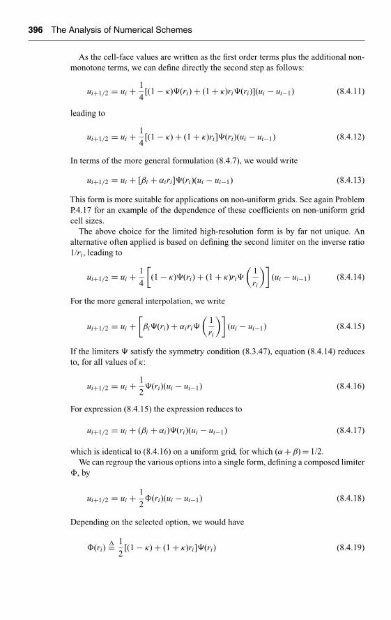
Ch08-H6594.tex 8/5/2007 14: 18 Page 396


As the cell-face values are written as the first order terms plus the additional non-monotone terms, we can define directly the second step as follows:

ui+1/2 = ui + 1

4[(1 − κ)�(ri) + (1 + κ)ri�(ri)](ui − ui−1) (8.4.11)

leading to

ui+1/2 = ui + 1

4[(1 − κ) + (1 + κ)ri]�(ri)(ui − ui−1) (8.4.12)

In terms of the more general formulation (8.4.7), we would write

ui+1/2 = ui + [βi + αiri]�(ri)(ui − ui−1) (8.4.13)

This form is more suitable for applications on non-uniform grids. See again ProblemP.4.17 for an example of the dependence of these coefficients on non-uniform gridcell sizes.

The above choice for the limited high-resolution form is by far not unique. Analternative often applied is based on defining the second limiter on the inverse ratio1/ri, leading to

ui+1/2 = ui + 1

4

[(1 − κ)�(ri) + (1 + κ)ri�

(1

ri

)](ui − ui−1) (8.4.14)

For the more general interpolation, we write

ui+1/2 = ui +[βi�(ri) + αiri�

(1

ri

)](ui − ui−1) (8.4.15)

If the limiters � satisfy the symmetry condition (8.3.47), equation (8.4.14) reducesto, for all values of κ:

ui+1/2 = ui + 1

2�(ri)(ui − ui−1) (8.4.16)

For expression (8.4.15) the expression reduces to

ui+1/2 = ui + (βi + αi)�(ri)(ui − ui−1) (8.4.17)

which is identical to (8.4.16) on a uniform grid, for which (α + β) = 1/2.We can regroup the various options into a single form, defining a composed limiter

�, by

ui+1/2 = ui + 1

2�(ri)(ui − ui−1) (8.4.18)

Depending on the selected option, we would have

�(ri)�= 1

2[(1 − κ) + (1 + κ)ri]�(ri) (8.4.19)

Ch08-H6594.tex 8/5/2007 14: 18 Page 397


or

�(ri)�= 1

2

[(1 − κ)�(ri) + (1 + κ)ri�

(1

ri

)](8.4.20)

or

�(ri)�= 2[βi + αiri]�(ri) (8.4.21)

or

�(ri)�= 2

[βi�(ri) + αiri�

(1

ri

)](8.4.22)

If the limiters � satisfy the symmetry condition (8.3.47), and we consider uniformgrids, then � = � for the options (8.4.20) and (8.4.22). Hence, we will consider thiscase in the following.

All the conditions on the limiters derived in the previous Section 8.3 remain valid.

8.4.2 The Normalized Variable Representation

An alternative representation of the nonlinear limiters has been introduced byGaskell & Lau (1988) and Leonard (1988). It is based on the definition of Nor-malizedVariables (NV), which lead to a reduction of the number of explicit variablesin the relation between the cell-face values and the surrounding points. This reductionis of particular interest for non-uniform grids.

The reduced variable φ, is defined as follows:

φ�= u − ui−1

ui+1 − ui−1(8.4.23)

Denoting by a subscript f the cell-face value, and by C the reference point i, thecorresponding normalized variables are

φf = ui+1/2 − ui−1

ui+1 − ui−1φC = ui − ui−1

ui+1 − ui−1(8.4.24)

The relation between the gradient ratio ri and φC , is readily obtained from thedefinitions, as

1

φC= ui+1 − ui−1

ui − ui−1= 1 + ri (8.4.25)

Note that the normalized variable is a ratio of differences and not a ratio of gradients,particularly if the grid is non-uniform. Referring to Figure 8.3.1, in point i, we haveφC = b/(a + b) and in point (i + 1), we have (φC )i + 1 = a/(a + c). Hence, when anextremum appears, as in point (i + 1) on the figure on the right, then φC > 1.

If we consider the functional dependence of the cell-face value ui + 1/2, it is trans-lated in a relation of the form φf = F(φC ) which is only function of φC , at least

Ch08-H6594.tex 8/5/2007 14: 18 Page 398


Table 8.4.3 Correspondence between the Sweby diagram and the NVD for various referenceschemes on uniform grids.

LIMITER relation NVD relation Comment

�(r) = 0 φf = φC First order monotone upwind scheme�(r) = 2r φf = 1 Upper bound of monotonicity region� = 2 φf = 2φC Bound for limiter domain� = 1 φf = 3φC/2 Second order non-monotone upwind

(SOU) discretization (κ = −1)�(r) = r φf = (1 + φC )/2 Central (Lax–Wendroff) scheme (κ = 1)�(r) = (1 + r)/2 φf = φC + 1/4 Fromm scheme (κ = 0) defined by

the average of SOU and LW�(r) = (1 + 3r)/4 φf = 3/4(φC + 1/2) Quick scheme (κ = 1/2)�(r) = (1 + 2r)/3 φf = (φC + 5/2)/3 Third order scheme (κ = 1/3)

for uniform grids. On non-uniform grids, an additional dependence on the ratio ofconsecutive cell sizes has to be added.

For the unlimited case, corresponding to � = 1, we have a linear dependencebetween the normalized variables, as summarized in Table 8.4.3.

Referring to the form (8.4.18), the general relation between the normalizedvariables and the limiters � is given by

φf =[

1 + 1

2�(ri)

]φC (8.4.26)

which reduces, for the case � = � to

φf =[

1 + 1

2�(ri)

]φC (8.4.27)

With this definition, we can translate the Sweby diagram into a Normalized VariableDiagram (NVD), where φf = F(φC ) is displayed in function of φC .

We restrict ourselves in the following to the case of a uniform grid for simplicity.The extension to the more general cases will be straightforward and left as an exercise.

The condition for second order accuracy, namely that all limiters should containthe point (r = 1, � = 1), is translated into the condition on the normalized variablesthat it should contain the point (φC = 1/2, φf = 3/4).

We can now express the monotonicity conditions and the various limiters in theNVD diagram, applying the above correspondence relations. In particular, the mono-tonicity conditions (8.3.49) and (8.3.60), defining the region of monotonicity forsecond order schemes, as shown on Figure 8.3.3, translate into the shaded region ofFigure 8.4.1, with the correspondences derived formTable 8.4.3. To perform this trans-lation, we have to notice that the region around r = 0 corresponds to very large valuesof φC , as a consequence of relation (8.4.25). Indeed, when r covers the range of pos-itive values, or 0 < r < ∞, the variable φC covers the range 1 > φC > 0. Accordingly,the region of large values of r is concentrated around the origin of the NVD diagram.

Ch08-H6594.tex 8/5/2007 14: 18 Page 399


0.5

0.5

1

1.5

1 1.5

Φf � 2Φc (� � 2) Φf � 3/2Φc (� � 1) SOU

Φf � Φc (� � 0)FOU

Φf � (1� Φc )/2(� �r ) Central

Φf � 1 (� � 2r )

Φc

Φf

Quick

Figure 8.4.1 Region of monotonicity for second order schemes in the NVDrepresentation.

Hence, the monotonicity region r > 1 to the right of point (1,1) in Figure 8.3.3,is found in the region 0 < φC < 0.5; while the region 0 < r < 1 is translated into theregion 0.5 < φC < ∞.

In Figure 8.4.1, you can see the lines corresponding to the schemes listed in Table8.4.3 and the shaded region corresponds to the shaded monotonicity region of Figure8.3.3. Notice that this region represents a small part of the NVD diagram, as opposedto the Sweby diagram where the different regions and limiters are much more visible.

Some of the limiters shown on Figure 8.3.4 are displayed in Figure 8.4.2, based onthe correspondence between the limiters listed in Table 8.4.4.

Note that all the limiters satisfy the condition corresponding to � = 0 for r < 0,which translates into φf = φC for φC > 1.

Observe that the SMART limiter is outside the shaded area of Figure 8.4.1, for0 < φC < 0.3, corresponding to the upper limit of � = 4 as seen from equation(8.3.69).

Compared to the (�, r) representation of Figure 8.3.4, the different limiters in theabove representation are more difficult to distinguish visually, since the monotonicityregion is concentrated into a small subregion of the NV diagram.

Therefore we would prefer the Sweby diagram, such as shown on Figures 8.3.4,to distinguish between different limiters as this representation offers indeed morevisibility. But in any case, the two representations are fully equivalent, where the

Ch08-H6594.tex 8/5/2007 14: 18 Page 400


1.25

1.0

0.75

PH

I

0.5

0.25

0.0

0.0 0.25 0.5

PHIC

Min mod limiter ALFA limiter for ALFA�1

SUPERBEE limiter ALFA limiter for ALFA�0.75

Van Leer limiter Smart limiter

1.00.75 1.25

0.0 0.25 0.5

PHIC

1.00.75 1.25

0.0 0.25 0.5

PHIC

1.00.75 1.25

1.25

1.0

0.75

PH

I

0.5

0.25

0.0

1.25

1.0

0.75

PH

I

0.5

0.25

0.0

1.25

1.0

0.75

PH

I

0.5

0.25

0.0

0.0 0.25 0.5

PHIC

1.00.75 1.25

0.0 0.25 0.5

PHIC

1.00.75 1.25

0.0 0.25 0.5

PHIC

1.00.75 1.25

1.25

1.0

0.75

PH

I

0.5

0.25

0.0

1.25

1.0

0.75

PH

I

0.5

0.25

0.0

Figure 8.4.2 Representation of the most current limiters in the NVD variables.

NVD option has a more direct physical meaning, as the variables φf and φC are directtranslations of the interpolation rules for the cell-face values.


This Chapter contains many topics of general significance for numerical schemes andis of importance for the understanding of some key properties, such as monotonicity.This central concept has led us to understand the origin of the numerical oscillationsoccurring with second or higher order schemes. Based on this understanding, the curesto these unwanted effects have been developed, leading to high-resolution schemes,based on the introduction of nonlinear limiters.

We have analyzed a general form of two level schemes on an arbitrary support,which led us to a synthetic view, under the form of general conditions on thecoefficients of the scheme. In addition, the stability, accuracy, diffusion and dispersion

Ch08-H

6594.tex8/5/2007

14:18Page

401

Table 8.4.4 Definition of limiters in the NVD diagram

LIMITER function NVD definition Comment

�(r) = max [0, min (r, 1)] φf = max [0, min (3φC/2, (φC + 1)/2, 1)] Min-mod limiter�(r) = max [0, min (r, 2), min (2r, 1)] φf = max [0, min (1, 3φC/2), min (2φC , Superbee limiter

(φC + 1)/2)]�(r) = (r + |r|)/(1 + r) φf = φC [(1 − φC ) + |(1 − φC )|) Van Leer limiter�(r) = (r + r2)/(1 + r2) φf = (φC − 1)/(1 − 2φC + 2φ2

C ) Van Albada limiter�(r) = max [0, min (2r, (3r + 1)/4, 4)] φf = max [0, min (3(φC + 1/2)/4, 3φC , 1, φC )] SMART limiter�(r) = max [0, min (r, β), min (βr, 1)] φf = max [0, min (β/2 + (1 − β/2)φC , 3φC/2), β-family1 ≤ β ≤ 2 min ((1 + β/2)φC , (φC + 1)/2), φC ]�(r) = max [0, min (2r, αr + 1 − α, 2)] φf = max [0, min ((3/2 − α)φC + α/2, 2φC , 1)] α-family

Ch08-H6594.tex 8/5/2007 14: 18 Page 402


errors are all fully defined by these coefficients. Some of the important points are thefollowing:

• A very close relation exists between the equivalent differential equation of ascheme and its diffusion and dispersion errors. In particular, remember thateven order derivatives in the equivalent differential equation contribute to thereal parts of the amplification factor, while the uneven coefficients contribute tothe imaginary part.

• Consequently, the even order coefficients totally define the diffusion error andthe odd order coefficients determine the dispersion error.

• Inversely, after having derived the dispersion and diffusion errors of a numericalscheme, you can easily recover the dominating terms of its equivalent differ-ential equation, by expanding these errors in a power series around φ = 0. Byidentifying the terms in these developments with equations (8.1.33) and (8.1.34),you immediately obtain the equivalent differential equation of the scheme underconsideration.

We have also learned about the accuracy barrier, that is the maximum order ofaccuracy that can be achieved by a stable explicit scheme on a given support. Ingeneral, the more points the higher the possible order of accuracy. Note in particularthat central schemes reach the highest possible accuracy, and that combining upwindand downwind points is the next good choice for higher accuracy, on a given support.

The weakest choice is the pure upwind case, where only one-sided points areconsidered. Here we have found that an explicit scheme with two-time-levels cannotbe of order higher than 2, whatever the number of points involved in the scheme.

Section 8.2 focuses on the analysis of the most current schemes applied in practice,defined either on 3- or 4-point supports. Study carefully the properties of the one-parameter families of schemes of first order (on 3 points) and second order (on 4points). The presented analysis offers a unified approach, which should help youunderstand the common points and the differences between selected schemes.

A most significant contribution of this chapter is the concept and conditions formonotonicity introduced in Section 8.3. This is of utmost importance as it identifiesthe source of the numerical wiggles that we have encountered with second, or higher,order schemes. Study carefully the celebrated Godunov theorem, which shows thatmonotone linear schemes can be at best of first order accuracy. We have also learnedin this section how to easily identify the non-monotone contributions to a higher orderscheme.

Based on this knowledge, we have introduced one of the most significant advancesmade in the history of CFD, namely the development of high-resolution schemes(HRS), which avoid the limitations of Godunov’s theorem, through the introductionof nonlinear limiters in the numerical schemes, whose role is to control the gradientsof the solution by avoiding unphysical growth.

Study carefully these sections, and work out the Hands-on task, as for any of theselected limiters, you will be able to discover that the practical implementation isquite easy and straightforward. The essential points to remember are:

• HRS combine second order accuracy with monotonicity, avoiding hereby theappearance of oscillations.

Ch08-H6594.tex 8/5/2007 14: 18 Page 403


• As the limiters depend on ratios of solution gradients, the schemes have becomenonlinear.

• The key property of the HRS is that they reduce, through the nonlinear action ofthe limiters, locally to first order accuracy, in the vicinity of extrema. They cantherefore loose some accuracy near extrema present in the solutions.

• HRS are a major achievement of CFD and should be applied when necessary, inorder to have more flexibility with regard to grid requirements.

• An additional observation is the unification of the second order LW and WBschemes after application of the limiters.

Finally the last section opens the way towards the introduction of general timeintegration methods, to nonlinear conservation laws of fluid mechanics and theirmultidimensional components, through the numerical flux concept. This is tied to thegeneral finite volume approach, based on estimations of cell-face values. With thesecell-face values, an alternative view and representation of the limiters, through thedefinition of normalized variables, is introduced. This approach has the advantageof providing a more direct interpretation of the ‘limited’ interpolation of the cell-face values, although the visibility of the limiters in the NVD representation is moredifficult to identify.

REFERENCES

Arora, M., Roe, P.L. (1997). A well-behaved TVD limiter for high-resolution calculationsof unsteady flow. J. Comput. Phys., 132, 3–11.

Barth, T.J. (1993). Recent Development in High Order k-Exact Reconstruction onUnstructured Meshes. AIAA paper 93-0668.

Boris, J.P., Book D.L. (1973). Flux corrected transport: I. SHASTA, a fluid transportalgorithm that works. J. Comput. Phys., 11, 38–69.

Boris, J.P., Book D.L. (1976). Solution of the continuity equation by the method of fluxcorrected transport. J. Comput. Phys., 16, 85–129.

Chakravarthy, S.R., Osher S. (1983). High Resolution Applications of the Osher UpwindScheme for the Euler Equations. Proceedings of AIAA 6th Computational FluidDynamics Conference, AIAA Paper 83–1943, pp.363–373.

Chan, T.F. (1984). Stability analysis of finite difference schemes for the advection–diffusion equation. SIAM J. Num. Anal., 21, 272–283.

Darwish, M.S. (1993). A new high-resolution scheme based on the normalized variableformulation. Num. Heat. Trans. B, 24, 353–371.

Darwish, M.S. and Moukalled, F. (2000). B-EXPRESS: A new Bounded EXtremaPREServing Strategy for Convective Schemes, Num. Heat. Trans. B, 37 (2), 227–246.

Fromm, J. (1964): The time dependent flow of an incompressible viscous fluid. In Methodsin Computational Physics, Vol. 3. Academic Press, New York, pp. 345–382.

Fromm, J.E. (1968). A method for reducing dispersion in convective difference schemes.J. Comput. Phys., 3, 176–189.

Gaskell, P.H., Lau, A.K.C. (1988). Curvature compensated convective transport: SMART,a new boundedness preserving transport algorithm. Int. J. Num. Meth. Fluids, 8,617–641.

Godunov, S.K. (1959). A difference scheme for numerical computation of discontinu-ous solution of hydrodynamic Equations. Math. Sbornik, 47, 271–306 (in Russian).Translated US Joint Publ. Res. Service, JPRS 7226 (1969).

Ch08-H6594.tex 8/5/2007 14: 18 Page 404


Godunov, S.K., Ryabenkii, V.S. (1964). TheTheory of Difference Schemes. North HollandPubl., Amsterdam.

Griffiths, D.F., Christie, I. and Mitchell, A.R. (1980). Analysis of error growth for explicitdifference schemes in conduction–convection problems. Int. J. Num. Meth. Eng., 15,1075–1081.

Hairer E. and Wanner G. (1991), Solving ordinary differential equations II. Springer-Verlag, Berlin.

Harten, A., Hyman J.M. and Lax P.D. (1976). On finite difference approximations andentropy conditions for shocks. Commun. Pure Appli. Math., 29, 297–322.

Harten, A. (1983). High resolution schemes for hyperbolic conservation laws. J. Comput.Phys., 49, 357–393.

Harten, A. (1984). On a class of high resolution total variation stable finite differenceschemes. SIAM J. Num. Anal., 21, 1–23.

Hindmarsh, A.C., Gresho, P.M., Griffiths, D.F. (1984). The stability of explicit eulertime integration for certain finite difference approximations of the multidimensionaladvection diffusion equation. Int. J. Num. Meth. Fluid., 4, 853–897.

Hirt, C.W. (1968). Heuristic stability theory for finite difference equations. J. Comput.Phys., 2, 339–355.

Iserles, A. (1982). Order stars and a saturation theorem for first order hyperbolics, IMAJ. Num. Anal., 2, 49–61.

Iserles, A., Strang, G. (1983). The optimal accuracy of difference schemes, Trans. Amer.Math. Soc., 277, 779–803.

Iserles, A., Nørsett, S.P. (1991). Order stars. Chapman & Hall, Boca Raton, Florida, USAJasak, H., Weller, H.G. and Gosman, A.D. (1999). High resolution NVD differenc-

ing scheme for arbitrarily unstructured meshes. Int. J. Numer. Meth. Fluid., 31,431–449.

Jameson, A. (1993). Artificial diffusion, upwind biasing, limiters and their effect onaccuracy and multigrid convergence in transonic and hypersonic flows. AIAA 11thComputational Fluid Dynamics Conference, AIAA Paper 93-3359.

Jameson, A. (1995a). Analysis and design of numerical schemes for gas dynamics 1:artificial diffusion, upwind biasing, limiters and their effect on multigrid convergence.Int. J. Comp. Fluid Dynamic., 4, 171–218.

Jameson, A. (1995b). Analysis and design of numerical schemes for gas dynamics2: Artificial diffusion and discrete shock structure. Int. J. Comp. Fluid Dynamic.,5, 1–38.

Jeltsch, R. (1985). Stability and accuracy of difference schemes for hyperbolic problems.J. Comput. Appl. Math., 12–13, 91–108.

Jeltsch, R., Smit, J.H. (1987). Accuracy barriers of difference schemes for hyperbolicequations. SIAM J. Num. Anal., Vol.24, pp.1–11.

Jeltsch, R. (1988). Order barriers for difference schemes for linear and nonlinear hyper-bolic problems, Numerical Analysis, Proceedings 1987 Dundee Conference, Griffithset al. (Eds.), Pitman.

Jeltsch, R., Kiani P. and Raczek K. (1991). Stability of a family of multi-time-leveldifference schemes for the advection equation, Numer. Math., 60, 77–95.

Jeltsch, R., Renaut, R.A. and Smit J.H. (1997). An accuracy barrier for stable three-time-level difference schemes for hyperbolic equations, Research Report 97–10, Seminarfûr Angewandte Mathematik, Swiss Federal Institute of Technology ETH-Zurich.

Jeng, Y.N., Payne U.J., (1995). An adaptive TVD limiter. J. Comput. Phys., 118,229–241.

Ch08-H6594.tex 8/5/2007 14: 18 Page 405


Karni, S. (1994). On the group velocity of symmetric and upwind numerical schemes,Int. J. Num. Meth. Fluid., 18, 1073–1081.

Koren, B. (1998). A robust upwind discretization method for advection, diffu-sion and source terms, In Numerical Methods for Advection–Diffusion Problems,C.B. Vreugdenhil and B. Koren (Eds.). Vieweg, Braunschweig, p. 117.

Laney, C. (1998). Computational Gasdynamics. Cambridge University press,Cambridge, UK.

Lax, P.D. (1973). Hyperbolic Systems of Conservation Laws and the MathematicalTheoryof Shock Waves. SIAM Publications, Philadelphia.

Leonard, B.P. (1979). A stable and accurate convective modeling procedure based onquadratic upstream interpolation. Comp. Meth. Appl. mech. engr., 19, 58–98.

Leonard, B.P. (1980). Note on the Von Neumann stability of the explicit FTCS convectiondiffusion equation. Appl. Math. Model., 4, 401–402.

Leonard, B.P. (1988). Simple High-Accuracy Resolution Program (SHARP) for convec-tive modeling of discontinuities. Int. J. Num. Meth. Eng., 8, 1291–1318.

Leonard, B.P., (1991). The ULTIMATE conservative difference scheme applied tounsteady one-dimensional advection. Comp. Meth. Appl. Mech. Eng., 88, 17–74.

Lerat, A. (1979). Numerical Shock Structure and Non Linear Corrections for DifferenceSchemes in Conservation Form. Lecture Notes in Physics, Vol 20. Springer Verlag,New York, pp. 345–351.

Lerat, A. and Peyret, R. (1974). Non centered schemes and shock propagation problems.Comput. Fluid., 2, 35–52.

Lerat, A. and Peyret, R. (1975). The Problem of Spurious Oscillations in the NumericalSolution of the Equations of Gas Dynamics. Lecture Notes in Physics, Vol. 35. SpringerVerlag, New York, pp. 251–256.

Leveque, R.J. (2002). Finite Volume Methods for Hyperbolic Problems. CambridgeUniversity Press, Cambridge, UK.

Lien, F.S. and Leschziner, M.A. (1994). Upstream monotonic interpolation for scalartransport with application to complex turbulent flows. Int. J. Num. Meth. Eng.,19, 527.

Morton, K.W. (1980). Stability of finite difference approximations to a diffusion–convection equation. Int. J. Num. Meth. Eng., 15, 677–683.

Rigal, A. (1978). Stability analysis of explicit finite difference schemes for theNavier–Stokes equations. Int. J. Num. Meth. Eng., 14, 617–620.

Richtmyer, R.D. and Morton, K.W. (1967). Difference Methods for InitialValue Problems.J. Wiley & Sons, New York.

Roache, P.J. (1972). Computational Fluid Dynamics. Hermosa Publication. Albuquerque,USA.

Roe, P.L. (1981). Numerical Algorithms for the Linear Wave Equation. Royal AircraftEstablishment, TR 81047, April 1981.

Roe, P.L. (1984). Generalized Formulation ofTVD Lax–Wendroff Schemes, ICASE Report84-53, NASA CR-172478, NASA Langley Research Center.

Roe, P.L. (1985). Some Contributions to the Modeling of Discontinuous Flows, Pro-ceedings of 1985 AMS-SIAM Summer Seminar on Large Scale Computing in FluidMechanics, Lectures in Applied Mathematics, Vol.22, Springer Verlag, New York,pp. 163–193.

Roe, P. L. and Baines, M.J. (1981). Algorithms for advection and shock problems, Pro-ceedings of the Fourth GAMM Conference on Numerical Methods in Fluid Mechanics,Notes on Numerical Fluid Mechanics, Vol. 5, H. Viviand (Ed.). Vieweg, p. 281.

Ch08-H6594.tex 8/5/2007 14: 18 Page 406


Roe, P.L. and Baines, M.J. (1983). Asymptotic behavior of some non-linear schemes forlinear advection. Proceedings of the Fifth GAMM Conference on Numerical Methodsin Fluid Mechanics, Notes on Numerical Fluid Mechanics, Vol. 7, M. Pandolfi andR. Piva (Eds.). Vieweg, p. 283.

Shokin, Yu.I. (1983). The Method of Differential Approximation. Springer Verlag,New York.

Spekreijse, S.P. (1987). Multigrid solution of monotone second order discretizations ofhyperbolic conservation laws. Math. Comp., 49, 135–155.

Strang, G. and Iserles, A. (1983). Barriers to stability. SIAM J. Num.Anal., 20, 1251–1257.Sweby, P.K. (1984). High resolution schemes using flux limiters for hyperbolic

conservation laws. SIAM J. Num. Anal., 21, 995–1011.Thompson, H.D., Webb, B.W. and Hoffmann, J.D. (1985). The Cell Reynolds Number

Myth. Int. J. Num. Meth. Fluid., 5, 305–310.Van Albada, G.D., Van Leer, B. and Roberts, W.W. (1982). A comparative study of

computational methods in cosmic gas dynamics. Astron. Astrophy., 108, 76–84.Van Leer, B.(1973). Towards the Ultimate Conservative Difference Scheme. I: The Quest

of Monotinicity, Lecture Notes in Physics, Vol.18, pp.163–168.Van Leer, B.(1974). Towards the ultimate conservative difference scheme. II: Mono-

tinicity and Conservation Combined in a Second Order Scheme J. Comput. Phys., 14,361–370.

Van Leer, B.(1977a). Towards the ultimate conservative difference scheme. III: Upstream-centered finite difference schemes for ideal compressible flow. J. Comput. Phys., 23,263–275.

Van Leer, B. (1977b). Towards the Ultimate Conservative Difference Scheme. IV. A NewApproach to Numerical Convection, J. Comput. Phys., 23, 276–299.

Van Leer, B.(1979). Towards the ultimate conservative difference scheme. V: A secondorder sequel to Godunov’s method, J. Comput. Phys., 32, 101–136.

Venkatakrishnan, V. and Barth, T.J. (1993). Application of Direct Solvers to UnstructuredMeshes, J. Comput. Phys., 105, 83–91.

Wanner G., Hairer E. and Nørsett S.P. (1978). Order Stars and Stability Theorems, BIT,Vol. 18, pp. 475–489.

Warming, R.F., Kutler, P. and Lomax, H. (1973). Second and third order non centereddifference schemes for non linear hyperbolic equations. AIAA J., 11, 189–195.

Warming, R.F., Hyett, B.J. (1974). The modified equation approach to the stability andaccuracy of finite difference methods. J. Comput. Phys., 14, 159–179.

Warming, R.F., and Beam, R.W. (1976). Upwind second order difference schemes andapplications in aerodynamic flows. AIAA J., 24, 1241–1249.

Waterson, N.P. and Deconinck, H. (1995). A unified approach to the design and applica-tion of bounded higher-order convection schemes. In Numerical Methods in LaminarTurbulent Flow, Volume IX, pp. 203–214. C. Taylor and P. Durbetaki (Eds). PineridgePress, Swansea, U.K.

Waterson, N.P. and Deconinck, H. (2007). Design principles for bounded higher-orderconvection scheme – a unified approach. J. Comput. Phys. (In Press).

PROBLEMS

P.8.1 Apply the methodology of Section 8.1 to obtain the first three terms of theequivalent differential equation for the upwind and Lax–Friedrichs schemes.Compare with the power expansions of |G| and εφ.

Ch08-H6594.tex 8/5/2007 14: 18 Page 407


Hint: Obtain for theFOU scheme

ut + aux = a�x

2(1 − σ)uxx + a�x2

6(2σ − 1)(1 − σ)uxxx

+ a�x3

24(1 + 6σ2 − 6σ)(1 − σ)uxxxx + O(�x4)

Lax–Friedrichs scheme

ut + aux = �x2

2�t(1 − σ2)uxx + a�x2

3(1 − σ2)uxxx + O(�x3)

P.8.2 Develop the general relations of Section 8.1, for a three-level scheme of the form

un+1i = un−1

i +∑

j

bjuni+j

by applying equation (8.1.11) at t = (n + 1)�t and t = (n − 1)�t, to the con-vective linear equation ut + aux = 0. Obtain the consistency relations on the bj

coefficients.P.8.3 Apply the form (8.1.49) of the modulus squared of the Von Neumann amplifica-

tion factor, to the first order upwind, Lax–Friedrichs and Lax–Wendroff schemes,for the linear convection equation. Determine for each case the polynomial S(z).

P.8.4 Obtain the relation (8.1.52) for the linear convection equation.P.8.5 Obtain the amplification factor for the second order upwind schemes of Fromm

and Warming and Beam. Generate a polar plot of the amplitude and phase errorsand analyze the differences, in particular for the dispersion and diffusion errors.Derive, by identification with the power expansion of the dispersion and diffusionerror around φ = 0, the dominating terms of the equivalent differential equation(see also Problem P.8.8).

P.8.6 Solve the convective equation ut + aux = 0 for a sinus wave packet with fourcycles, on meshes with 10, 15, 20 points per wavelength with a = 1. The wavepacket is defined by

u(t = 0) = sin (2πkx) 0 < x < 1 and k = 4= 0 x < 0 and x > 1

Compute the numerical transported wave after 50, 100 and 200 time steps andplot the exact solutions with the numerical solution. Take σ = 0.1, 0.5, 0.9 andcompare the results with the second order upwind scheme and Fromm’s schemeswith the results you have obtained in Chapter 7.

Hint: The exact solution after n time steps is

un = sin 2πk(x − n · �t) n�t < x < (n + 1)�t= 0 x < n�t and x > (n + 1)�t

Ch08-H6594.tex 8/5/2007 14: 18 Page 408


P.8.7 Repeat the same problem for a moving discontinuity

u(t = 0) = 1 x < 0= 0 x > 0

after 10, 50, 100 time steps, for σ = 0.1, 0.5, 0.9.P.8.8 Apply the analysis of Section 8.1 to obtain the equivalent differential equations,

the lowest order terms of the dissipation and dispersion errors for the generalscheme (8.2.37). Derive the amplification factor, the dispersion and diffusionerrors and the series expansion of these errors in function of the phase angle φ, asa way to obtain the first two terms of the equivalent differential equation (8.1.27),based on the expansions (8.1.33) and (8.1.34). Apply this to the Fromm schemeand compare with the two other schemes, Lax–Wendroff and Warming–Beam,SLW, SWB.

P.8.9 Derive the third order scheme (8.2.49) and apply the analysis of Section 8.1 toobtain the fist two terms of the equivalent differential equation, as well as thedispersion and diffusion first terms in function of phase angle.

P.8.10 Solve Problem P.8.6 with the third order accurate scheme (8.2.49). Compare andanalyze the results.

P.8.11 Solve Problem P.8.7 with the third order accurate scheme. Compare and analyzethe results.

P.8.12 Obtain the stability condition (8.3.19) for the upwind-discretized convection–diffusion equation (8.3.17).

P.8.13 Consider the linear convection equation ut + aux = 0 and the semi-discretizedschemes obtained from applying successively the following space discretizationsto the space term (−aux):1. first order upwind difference,2. second order backward difference,3. second order central difference.

Writing the schemes in the form (8.3.22) obtain the βj coefficients and theconditions for monotonicity.

Apply an explicit, forward difference for the time discretization and obtainthe form (8.3.1) and all the bj coefficients. Define the additional stability andmonotonicity condition for b0. Show that only scheme (i) is monotone and thatwhen applied to the second order schemes (ii) and (iii), the schemes are unstable.

Derive the amplification factors for these schemes.P.8.14 Repeat the Problems P.8.6 and P.8.7 after introduction of limiters. Compare the

results with min-mod, and superbee limiters.P.8.15 Repeat the Problem P.8.14 with the α-family of limiters, in particular compare

α = 1/3 and α = 3/8. Repeat with the SMART limiter to evaluate the effects ofthe upper bounds on this limiter.

P.8.16 Derive the correspondence Table 8.4.4 between the Sweby and NVD diagrams.P.8.17 Consider the general family of second order schemes on the support

(i − 2, i − 1, i, i + 1), as expressed in function of the γ-parameter in Table 8.4.1:1. Express the cell-face value ui + 1/2 under the form (8.4.7) and show that for

this CFL-dependent extrapolation, second order accuracy is satisfied by thecondition α + β = (1 − σ)/2.

Ch08-H6594.tex 8/5/2007 14: 18 Page 409


2. Introduce the limiters under the form (8.4.17) and define the function �(r)associated to the linear schemes of Lax–Wendroff, Warming–Beam, Frommand for the third order scheme. Express also the limiters in function of theinverse gradient ratio Ri = 1/ri

Hint: Referring to Table 8.4.1, write the schemes under the form

ui+1/2 = ui + 1

2(1 − σ)[K + (1 − K)ri](ui − ui−1) K = 2γ/(1 − σ)

generalized to

ui+1/2 = ui + 1

2(1 − σ)�(ri)(ui − ui−1) = ui + 1

2(1 − σ)

�(ri)

ri(ui+1 − ui)

�= ui + 1

2(1 − σ)�(Ri)(ui+1 − ui) where Ri = 1

ri

Obtain the following correspondence:LW scheme K = 0 Ψ(r) = 1 Ψ(R) = RWB scheme K = 1 Ψ(r) = r Ψ(R) = 1Fromm scheme K = 1/2 Ψ(r) = (1 + r)/2 Ψ(R) = (1 + R)/2Third order scheme K = (1 + σ)/3 Ψ(r) = (1 + σ)/3 Ψ(R) = R(1 + σ)/3

+ r(2 − σ)/3 + (2 − σ)/3

P.8.18 Convert the Symmetric ALFA limiters (8.3.71) and the CFL-dependent limiters(8.3.72) and (8.3.73) to the NVD representation.

P.8.19 Determine the exact solutions of the scheme obtained by discretizing the con-vection term in the convection–diffusion equation aux =αuxx, with a first orderbackward formula (for a > 0). Show that the solution will always remainoscillation free for a > 0.

Analyze the exact numerical solutions for the boundary conditions u(0) = u0,u(L) =uL, for N · �x = Ly applying the normal mode method and compare withequation (8.2.26). Calculate the error εi = u − ui and show that the scheme isonly first order accurate.

Hint: The scheme is

a(ui − ui−1) = α

�x(ui+1 − 2ui + ui−1)

and obtain κ1 = 1, κ2 = (1 + Re�x).

Ch09-H6594.tex 26/4/2007 16: 59 Page 411

Part IV

The Resolution of NumericalSchemes

We have now reached the fourth part in the succession of steps and componentsrequired to set up a CFD model, and we are, at this stage, faced with a set of space-discretized, or semi-discretized, equations.

As seen in Part III, Section 8.4, we have to make an essential decision as to thetime dependence of our numerical formulation. If the physical problem is time depen-dent, there is obviously no choice; the mathematical initial value problem has to bediscretized in time and the numerical solution has to be time accurate. On the otherhand, for physical stationary problems, we can decide either to discretize the equationsin space and deal with a time-independent numerical scheme or maintain the timedependency and discretize the equations in space and time, but aim only at the timeasymptotic, steady, numerical solution. Remember that we have advocated that lastoption, as a standard discretization approach for convection–diffusion equations,such as the conservation laws.

When we select to discretize the time-dependent form, we can either develop acombined space and time discretization, such as the Lax–Wendroff schemes, as seenin the previous chapters, or perform first a separate space discretization, based onthe definition of the numerical flux, leading to a semi-discretized set of ordinarydifferential equations (ODEs) in time.

In the next two chapters we will investigate some of the most currently appliedtechniques for either the resolution of semi-discretized equations that is, systems ofordinary differential equations in time (Chapter 9) or algebraic systems of equationsto which they reduce for stationary or implicit time integration problems (Chapter 10).

A large number of techniques have been developed to define and analyze numericalmethods for systems of ODEs in time, or more precisely, initial value problems. Themost widely applied methods, as well as the techniques for the analysis of theirstability properties and the related error properties, will be presented in Chapter 9.

By combining an arbitrary time integration method with an arbitrary space dis-cretization, we are faced with all kinds of possible schemes. We have therefore togeneralize the analysis methods derived in Chapters 7 and 8, to these general situa-tions. This will be the main subject of this Chapter, which will lead to a generalizationof the Von Neumann method for stability and error analysis. The methodology to bepresented has many common features with the Von Neumann method, as it will relyon the same spectral Fourier decomposition of the solutions and their errors.

411

Ch09-H6594.tex 26/4/2007 16: 59 Page 412

412 The Resolution of Numerical Schemes

With a stationary formulation in space or with implicit time integration, we willdeal with an algebraic system of equations. This algebraic system has to be solved inthe lowest possible number of numerical operations. Various iterative techniques forachieving this goal will be introduced in Chapter 10.

A bridge between stationary and non-stationary formulations can be established,which enlarges the family of methods to be applied to obtain solutions to physicalstationary problems. We can indeed select pseudo-time operators in order to acceleratethe convergence of the scheme and an illustration is provided by the preconditioningmethods. This bridge has also as important consequence that an iterative methodcan be analyzed by the techniques used for the stability analysis of time-dependentschemes, for instance by their Fourier symbol.

From the spectral analysis of the errors of an iterative method, appropriate oper-ations can be defined in order to damp selectively certain frequency domains of theerror spectrum. This philosophy is at the basis of the most powerful of the presentlyavailable convergence acceleration techniques, namely the multigrid method to bepresented in Chapter 10.

Ch09-H6594.tex 26/4/2007 16: 59 Page 413

Chapter 9

Time Integration Methods for Space-discretizedEquations


If we look back at some of the schemes introduced and analyzed in the previous chap-ters, for instance for the convection equation, we notice that various combinations ofspace and time discretizations show widely different behaviors. Referring to Chapter7 and to the central second order space discretization for the convection term a∂u/∂x,we have seen that associated to a forward time difference in an explicit scheme, theresulting scheme is unstable; while associated to a backward time difference (leadingto an implicit scheme) it is unconditionally stable, and when selecting a central differ-ence in time (the leapfrog scheme) it is conditionally stable under the CFL condition.Similar properties have been seen with other space discretizations.

This raises several questions:

• How can we understand, and predict, these properties?• What criteria are to be satisfied by a time integration method, applied to a given

space discretization, in order to lead to a stable and accurate scheme.• Inversely, if we pre-select a time integration method, what are the properties

of space discretizations required in order to generate a stable scheme, with thelowest possible diffusion and dispersion errors.

The methodologies allowing to answer these questions and to guide you through thisselection process form the essential objectives of this chapter.

We consider here the general formulation of a numerical scheme, as already intro-duced in Section 8.4, where we separate the time from the space discretizations.Hereby, we first perform a space discretization, defined for instance by a numericalflux in a general finite volume formulation, leading to a system of first order ordinarydifferential equations (ODEs) in time. In the second step we have to integrate thissystem in time, by selecting an appropriate method.

A general methodology for the analysis of the association of a given spacediscretization with a time integration method, can be defined by the followingsteps:

1. Express the space discretization into a matrix form, including the boundaryconditions.

2. Perform a spectral analysis of its representative matrix, obtaining hereby itseigenvalue spectrum.

413

Ch09-H6594.tex 26/4/2007 16: 59 Page 414


3. This leads us to a first set of stability conditions on the space discretizationby expressing that the exact time integrated solution of the considered spacediscretized system of ODEs should not grow exponentially with time. We willshow that the ODE system is stable when the eigenvalues � of the space dis-cretization matrix have non-positive real parts, that is, are located in the lefthalf, imaginary axis included, of the complex �-plane.

These three steps will form the subject of Section 9.1.Next, we proceed as follows:

• Select a time integration method for the semi-discretized system of ODEs anddefine the methodology for its stability analysis, as a function of the eigenvaluesof the space discretization.

• The stability condition of the time integration scheme has to be compatible withthe range of the eigenvalue spectrum, namely the stability region of the timediscretization method must include the whole spectrum of eigenvalues.

This will be developed in Section 9.2.

• Finally we apply the methodology to some of the most current methods of interestin CFD, such as the family of implicit multistep methods, the family of explicitpredictor–corrector methods or the multistage Runge–Kutta methods.

This will be considered in section 9.3 and illustrated by various examples.As a glimpse of typical issues related to multidimensional methods, an advanced

Section A9.4 is devoted to some specific properties of implicit schemes for mul-tidimensional problems, in particular when applying alternating direction implicitmethods (ADI), also called approximate factorization methods.

The roadmap to this chapter is summarized in Figure 9.0.1.

9.1 ANALYSIS OF THE SPACE-DISCRETIZED SYSTEMS

The general form of a conservation law, can be considered mathematically as aninitial, boundary value differential problem, over the domain �, with boundary �

∂u

∂t+ �∇ · �F = 0

Initial condition: u(�x, 0) = u0(�x) for t = 0 and �x ∈ �(9.1.1)

Boundary condition: u(�x, t) = g(�x, t) for t > 0 and �x ∈ �

Referring to Sections 8.3.2 and 8.4.1, for a one-dimensional case, we can discretizethe flux differential operator via the general definition of a numerical flux and obtainthe system of ordinary differential equations in time, written as equation (8.4.5),which we repeat here for convenience

dui

dt= − 1

�xi(f ∗

i+1/2 − f ∗i−1/2) (9.1.2)

Ch09-H6594.tex 26/4/2007 16: 59 Page 415

Time Integration Methods for Space-discretized Equations 415

Matrix representation of a spacediscretization and introduction ofthe Fourier modesAmplification factor and Fouriersymbol of central and upwindschemes

Stability analysis and definition ofdispersion and diffusion errors oftime and space discretizations

Introduction of multistep,predictor�corrector and Runge�Kutta methodsApplications and analysis ofseveral examples

A9.4 Implicit schemesand approximatefactorization formultidimensionalproblems

9.1 Analysis of the space-discretized systems

9.3 A selection of timeintegration methods

9.2 Analysis of timeintegration schemes


If we group all the mesh point values ui in a column vector U , the right-hand sidecan be written in the matrix form

dU

dt= S · U + Q (9.1.3)

where S is the matrix representing the space discretization and Q contains contri-butions from the boundary conditions. The matrix S therefore depends on the spacediscretization and on the boundary conditions. Within the finite volume framework,see equation (5.2.7) in Chapter 5, the right-hand side is the residual, defined asthe balance of fluxes though all the cell faces plus sources and boundary conditionterms.

Equation (9.1.3) is a system of ordinary differential equations (ODE) in time andforms a semi-discretized representation, also called method of lines.

Important noteThe semi-discretized approach has to be compared with the two-step explicitschemes derived in Sections 8.1 and 8.2, with the Lax–Wendroff scheme as typ-ical reference. These schemes are characterized by a combined space and timediscretization, which is translated by their specific behavior when applied to obtaina steady state solution. Take for instance the Lax–Wendroff scheme

un+1i = un

i − σ

2(un

i+1 − uni−1) + σ2

2(un

i+1 − 2uni + un

i−1)

Ch09-H6594.tex 26/4/2007 16: 59 Page 416


where σ is the CFL number, σ = a�t/�x. When the steady state is reached, ui issolution of the system

−(uni+1 − un

i−1) + σ(uni+1 − 2un

i + uni−1) = 0

which contains σ as parameter, that is �t, although the time step has no physicalsignificance for a time-independent problem. This is mathematically correct, buton the conceptual level it is somehow disturbing to generate a numerical solutiondepending on a non-physical and non-relevant parameter.

This explains the success of the semi-discretized approach in contemporaryCFD, whereby the space and time discretizations are kept totally separated. Here,the steady state solution is independent of �t, since it is solution of the systemS · U + Q = 0, which does not contain any non-relevant, non-physical parameters,such as �t.

Note that the following developments are valid for an arbitrary number of spacevariables, when U is defined accordingly.

When the problem is linear, S will be independent of U, otherwise (S · U ) is anonlinear function of U. This option and the issue of the necessary linearization willbe discussed in Section 9.3.

Let us illustrate the derivation of the semi-discretized form (9.1.3) and its S-matrixby some examples of the representative linear diffusion and convection operators,associated to specific boundary conditions.

9.1.1 The Matrix Representation of the Diffusion Space Operator

For the linear diffusion equation ut = auxx, a central difference of the space secondderivative leads to the semi-discretized scheme of second order accuracy:

dui

dt= α

�x2(ui+1 − 2ui + ui−1) (9.1.4)

In order to derive the complete matrix S, we have to include the boundary conditionsand their numerical implementation:

(a) Dirichlet boundary conditionsFor a domain on the x-axis between (0, +L), with (N + 1) mesh points, suchthat xi = i�x and �x = L/N , a Dirichlet type of condition will be defined by

u0 = u(0, t) = a uN = u(+L, t) = b (9.1.5)

For the first mesh point, i = 1, the discretized equation will be

du1

dt= α

�x2(u2 − 2u1 + a) (9.1.6)

where the mesh point value u0 has been replaced by its imposed boundary value.Similarly the equation for the point i = N − 1 can be written as

duN−1

dt= α

�x2(b − 2uN−1 + uN−2) (9.1.7)

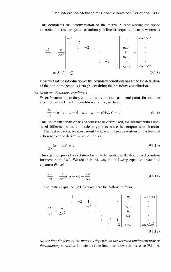
Ch09-H6594.tex 26/4/2007 16: 59 Page 417


This completes the determination of the matrix S representing the spacediscretization and the system of ordinary differential equations can be written as

dU

dt= α

�x2

∣∣∣∣∣∣∣∣∣∣∣∣∣∣

−2 1 · · ·1 −2 1 ·

1 −2 1· · ·

·1 −2 1

· 1 −2

∣∣∣∣∣∣∣∣∣∣∣∣∣∣

∣∣∣∣∣∣∣∣∣∣∣∣∣∣

u1

·ui−1

ui

ui+1

·uN−1

∣∣∣∣∣∣∣∣∣∣∣∣∣∣

+

∣∣∣∣∣∣∣∣∣∣∣∣∣∣

aα/�x2

·····

bα/�x2

∣∣∣∣∣∣∣∣∣∣∣∣∣∣≡ S · U + Q (9.1.8)

Observe that the introduction of the boundary conditions has led to the definitionof the non-homogeneous term Q containing the boundary contributions.

(b) Neumann boundary conditionsWhen Neumann boundary conditions are imposed at an end-point, for instanceat x = 0, with a Dirichlet condition at x = L, we have

∂u

∂x= a at x = 0 and uN = u(+L, t) = b (9.1.9)

This Neumann condition has of course to be discretized, for instance with a one-sided difference, so as to include only points inside the computational domain.

The first equation, for mesh point i = 0, would then be written with a forwarddifference of the derivative condition as

1

�x(u1 − u0) = a (9.1.10)

This equation provides a relation for u0, to be applied in the discretized equationfor mesh point i = 1. We obtain in this way the following equation, instead ofequation (9.1.6)

du1

dt= α

�x2(u2 − ui) − aα

�x(9.1.11)

The matrix equation (9.1.8) takes here the following form,

dU

dt= α

�x2

∣∣∣∣∣∣∣∣∣∣∣∣∣∣

−1 1 · · ·1 −2 1 ·

1 −2 1· · ·

·1 −2 1

· 1 −2

∣∣∣∣∣∣∣∣∣∣∣∣∣∣

∣∣∣∣∣∣∣∣∣∣∣∣∣∣

u1

·ui−1

ui

ui+1

·uN−1

∣∣∣∣∣∣∣∣∣∣∣∣∣∣

+

∣∣∣∣∣∣∣∣∣∣∣∣∣∣

−aα/�x·····

bα/�x2

∣∣∣∣∣∣∣∣∣∣∣∣∣∣(9.1.12)

Notice that the form of the matrix S depends on the selected implementation ofthe boundary condition. If instead of the first order forward difference (9.1.10),

Ch09-H6594.tex 26/4/2007 16: 59 Page 418


we had selected a second order forward difference, we would obtain a differentmatrix S, with different properties.

This is a first indication that the stability conditions of a numericalscheme can be influenced by the boundary conditions and their numericalimplementation.

This is a major issue in CFD and should retain your careful attention, eitherif writing a code, or when using an existing one. The detailed analysis of theimpact of boundary conditions on a numerical scheme is very complicated, sinceit is in general not possible to derive analytical expressions for the eigenvalues.Therefore, the knowledge of the adequacy of certain boundary conditions, orcertain implementations, can mostly be gained by practical experience. Prob-lems occurring with an implementation of boundary conditions would be anindication that the mathematical problem is not well-posed either numerically,or analytically.

(c) Periodic boundary conditionsA third type of boundary condition, with great practical and theoreticalimportance, is the imposition of periodic conditions. This implies that

u0 = uN and u−1 = uN−1 (9.1.13)

The first discretized equation is written here for i = 0 (instead of i = 1), as

du0

dt= α

�x2(u1 − 2u0 + uN−1) (9.1.14)

and the last equation, written for i = N − 1, becomes

duN−1

dt= α

�x2(u0 − 2uN−1 + uN−2) (9.1.15)

The resulting matrix structure is similar to the matrix obtained from Dirichletconditions, but with the addition of a coefficient 1 in the upper right and lower leftcorners. This is typical for ‘periodic’ matrices:

dU

dt= α

�x2

∣∣∣∣∣∣∣∣∣∣∣∣∣∣

−2 1 · · 11 −2 1 ·

1 −2 1· · ·

·1 −2 1

1 1 −2

∣∣∣∣∣∣∣∣∣∣∣∣∣∣

∣∣∣∣∣∣∣∣∣∣∣∣∣∣

u0

·ui−1

ui

ui+1

·uN−1

∣∣∣∣∣∣∣∣∣∣∣∣∣∣

(9.1.16)

Notice here that there is no Q matrix generated with periodic boundary conditions.This is an important property, as it will make it easier to derive analytical eigenvalues,as we will see next.

9.1.2 The Matrix Representation of the Convection Space Operator

For convection equations, the problem of the boundary conditions is much moresevere and its impact on the schemes is often dominating. The reason for this strong

Ch09-H6594.tex 26/4/2007 16: 59 Page 419


influence is to be found in the physical nature of the convection or propagationphenomenon, since they describe ‘directional’ phenomena in space. For instance,in one-dimension, the propagation or convection of the quantity u in the positivex-direction, when a > 0, implies that the value of u at the downstream end point ofthe computational region 0 < x < L, is determined by the upstream behavior of u andcannot be imposed arbitrarily. However, from numerical point of view, dependingon the space discretization, we might need information on uN = u(x = L) in order toclose the algebraic system of equations. In this case, the condition to be imposed onuN cannot be taken from physical sources and has to be defined numerically. Thisis called a numerical boundary condition. The choice of this numerical boundarycondition is critical for the whole scheme. Intuitively we suspect that a good choiceshould be compatible with the physics of the problem but the stability analysis isthe ultimate criterion. For a > 0, we have obviously to impose, on physical grounds,boundary values at the left end of the domain; while when a is negative, the propa-gation occurs in the negative x-direction and the physical boundary condition has tobe defined at the right end of the domain.

This is a difficult task, since even for very simple cases, we cannot find analyticallythe eigenvalues of the matrix S. For a hyperbolic system of equations, with thesimultaneous presence of positive and negative propagation speeds, as is the casefor the Euler equations in subsonic flows, the problem becomes even more complex.More detailed information, in the framework of the Euler equations, will be presentedin Chapter 11 and in Volume II.

The reader interested in more mathematical-oriented work will refer to the workof Kreiss (1968, 1970), Gustafsson et al. (1972), Gustafsson and Kreiss (1979) andto an interesting review of Helen Yee (1981) where additional references can befound.

Upwind space discretizationLet us consider a first order upwind space discretization for the linear convectionequation ut + aux = 0, with a > 0. We obtain the following system of ODEs in time

dui

dt= − a

�x(ui − ui−1) (9.1.17)

for the interior points, also called the interior scheme. A boundary value

u(x = 0, t) = g(t) (9.1.18)

will be imposed at the left end boundary, when a > 0.For the first mesh point i = 1, we would write see Figure 9.1.1.

du1

dt= − a

�x(u1 − u0) = − a

�xu1 + a

�xg(t) (9.1.19)

At, the downstream end, the equation for i = N is

duN

dt= − a

�x(uN − uN−1) (9.1.20)

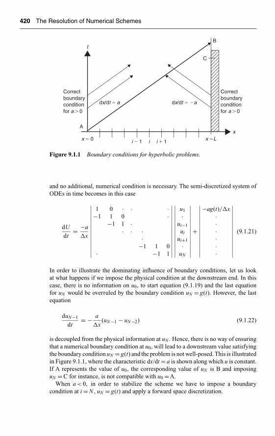
Ch09-H6594.tex 26/4/2007 16: 59 Page 420


A

B

C

t

x

i � 1 i i � 1 x �Lx � 0

dx/dt � a dx/dt � �a

Correctboundaryconditionfor a � 0

Correctboundaryconditionfor a � 0

Figure 9.1.1 Boundary conditions for hyperbolic problems.

and no additional, numerical condition is necessary. The semi-discretized system ofODEs in time becomes in this case

dU

dt= −a

�x

∣∣∣∣∣∣∣∣∣∣∣∣∣∣

1 0 · · ·−1 1 0 ·

−1 1 ·· · ·

·−1 1 0

· −1 1

∣∣∣∣∣∣∣∣∣∣∣∣∣∣

∣∣∣∣∣∣∣∣∣∣∣∣∣∣

u1

·ui−1

ui

ui+1

·uN

∣∣∣∣∣∣∣∣∣∣∣∣∣∣

+

∣∣∣∣∣∣∣∣∣∣∣∣∣∣

−ag(t)/�x······

∣∣∣∣∣∣∣∣∣∣∣∣∣∣

(9.1.21)

In order to illustrate the dominating influence of boundary conditions, let us lookat what happens if we impose the physical condition at the downstream end. In thiscase, there is no information on u0, to start equation (9.1.19) and the last equationfor uN would be overruled by the boundary condition uN = g(t). However, the lastequation

duN−1

dt= − a

�x(uN−1 − uN−2) (9.1.22)

is decoupled from the physical information at uN . Hence, there is no way of ensuringthat a numerical boundary condition at u0, will lead to a downstream value satisfyingthe boundary condition uN = g(t) and the problem is not well-posed. This is illustratedin Figure 9.1.1, where the characteristic dx/dt = a is shown along which u is constant.If A represents the value of u0, the corresponding value of uN is B and imposinguN = C for instance, is not compatible with u0 =A.

When a < 0, in order to stabilize the scheme we have to impose a boundarycondition at i = N , uN = g(t) and apply a forward space discretization.

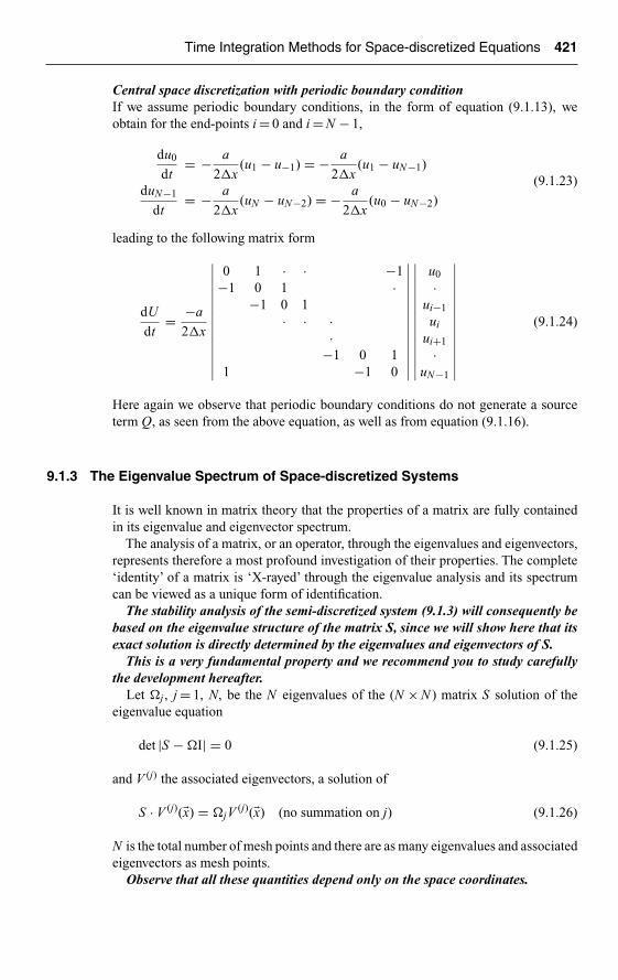
Ch09-H6594.tex 26/4/2007 16: 59 Page 421


Central space discretization with periodic boundary conditionIf we assume periodic boundary conditions, in the form of equation (9.1.13), weobtain for the end-points i = 0 and i = N − 1,

du0

dt= − a

2�x(u1 − u−1) = − a

2�x(u1 − uN−1)

(9.1.23)duN−1

dt= − a

2�x(uN − uN−2) = − a

2�x(u0 − uN−2)

leading to the following matrix form

dU

dt= −a

2�x

∣∣∣∣∣∣∣∣∣∣∣∣∣∣

0 1 · · −1−1 0 1 ·

−1 0 1· · ·

·−1 0 1

1 −1 0

∣∣∣∣∣∣∣∣∣∣∣∣∣∣

∣∣∣∣∣∣∣∣∣∣∣∣∣∣

u0

·ui−1

ui

ui+1

·uN−1

∣∣∣∣∣∣∣∣∣∣∣∣∣∣

(9.1.24)

Here again we observe that periodic boundary conditions do not generate a sourceterm Q, as seen from the above equation, as well as from equation (9.1.16).

9.1.3 The Eigenvalue Spectrum of Space-discretized Systems

It is well known in matrix theory that the properties of a matrix are fully containedin its eigenvalue and eigenvector spectrum.

The analysis of a matrix, or an operator, through the eigenvalues and eigenvectors,represents therefore a most profound investigation of their properties. The complete‘identity’ of a matrix is ‘X-rayed’ through the eigenvalue analysis and its spectrumcan be viewed as a unique form of identification.

The stability analysis of the semi-discretized system (9.1.3) will consequently bebased on the eigenvalue structure of the matrix S, since we will show here that itsexact solution is directly determined by the eigenvalues and eigenvectors of S.

This is a very fundamental property and we recommend you to study carefullythe development hereafter.

Let �j , j = 1, N, be the N eigenvalues of the (N × N ) matrix S solution of theeigenvalue equation

det |S − �I| = 0 (9.1.25)

and V (j) the associated eigenvectors, a solution of

S · V (j)(�x) = �jV(j)(�x) (no summation on j) (9.1.26)

N is the total number of mesh points and there are as many eigenvalues and associatedeigenvectors as mesh points.

Observe that all these quantities depend only on the space coordinates.

Ch09-H6594.tex 26/4/2007 16: 59 Page 422


The matrix S is supposed to be of rank N and hence, have N linearly independent

eigenvectors. Each eigenvector consists of a set of mesh point values v(j)i , that is

V ( j) =

∣∣∣∣∣∣∣∣∣∣∣∣∣∣

·v( j)

i−1

v( j)i

v( j)i+1

··

∣∣∣∣∣∣∣∣∣∣∣∣∣∣

(9.1.27)

The (N × N ) matrix T formed by the N columns V (j), diagonalizes the matrix S, sinceall the equations (9.1.26) for the N eigenvalues can be grouped as

S · T = T · � (9.1.28)

where � is the diagonal matrix of the eigenvalues

� =

∣∣∣∣∣∣∣∣∣∣∣∣

�1

�2

··

·�N

∣∣∣∣∣∣∣∣∣∣∣∣(9.1.29)

Hence, we have

� = T−1 · S · T (9.1.30)

Since, the eigenvectors V (j) form a complete set of basis vectors in the consideredspace of the mesh-point functions, we can always write the exact solution U ofequation (9.1.3) as a linear combination of the V (j) eigenvectors,

U (t, �x) =N∑

j=1

U j(t) · V (j)(�x) (9.1.31)

where the U j coefficients depend only on time, while the full space depen-dence is contained exclusively in the eigenvectors V (j)(�x). This is called a modaldecomposition.

Similarly the non-homogenous term Q, assumed independent of time, can bedecomposed in the same modal space of the V (j) eigenvectors

Q =N∑

j=1

Qj · V (j) (9.1.32)

Ch09-H6594.tex 26/4/2007 16: 59 Page 423


The time dependent coefficients U j(t) are obtained from the differential system(9.1.3), by inserting (9.1.31), leading to the modal equation

dU j

dt= �jU j + Qj (no summation on j) (9.1.33)

The exact solution of this modal equation is easily obtained as the sum of the solutionof the homogenous modal equation

dU jT

dt= �jU jT (no summation on j) (9.1.34)

U jT (t) = c0je�j t (9.1.35)

and a particular solution, for instance a solution of the ‘steady state’ equation

�jU jS + Qj = 0 (no summation on j) (9.1.36)

U jS = − Qj

�j(9.1.37)

We obtain hereby the modal solution

U j(t) = c0je�j t − Qj

�j(9.1.38)

The coefficient c0j is related to the coefficients of the expansion of the initial solutionu0(�x) at t = 0, and its matrix representation

U 0 =

∣∣∣∣∣∣∣∣∣∣∣

·u0

i−1

u0i

u0i+1·

∣∣∣∣∣∣∣∣∣∣∣(9.1.39)

in series of the basis vectors V (j)

U 0 =N∑

j=1

U 0j · V (j) (9.1.40)

Considering the solution (9.1.38) at t = 0, we have

c0j = U 0j + Qj/�j (9.1.41)

and the solution (9.1.38) can be written as

U j(t) = U 0j e�j t + Qj

�j(e�j t − 1) (9.1.42)

Ch09-H6594.tex 26/4/2007 16: 59 Page 424


Notice here the essential property of the eigenvalues of the space discretizationmatrix S, which determine completely the time behavior of the semi-discretizedsystem (9.1.3) of ODEs in time.

The exact solution of the system of ordinary differential equations (9.1.3) isobtained now by inserting the modal components (9.1.42) in the summation (9.1.31).

Stability conditionThe ODE system will be well-posed, or stable, if its exact solution (9.1.31) remainsbounded. This implies that all the modal components are also bounded, since if anyof them would grow exponentially with time, the full solution would also have thisunwanted behavior.

Hence, we have to require that the exponential terms in the modal components(9.1.42) do not grow exponentially with time, that is we have to require that the realpart of the eigenvalues be negative or zero.

The stability condition is therefore

Re(�j) ≤ 0 for all j (9.1.43)

In addition, if an eigenvalue is zero, it has to be a simple eigenvalue.In the complex �-plane, the stability conditions states that the eigenvalue spectrum

has to be restricted to the left half plane, including the imaginary axis.If the space discretization, including the boundary conditions, leads to eigenvalues

with non-positive real parts, the system of ODEs will be stable at the level of the semi-discretized formulation and a stable time integration method will always be possible.

Each mode j contributes a time behavior of the form exp(�j t) to the time dependentpart of the solution, called the transient solution. The remaining part of the generalsolution is the modal decomposition of the steady state solution, defined as the solu-tion remaining for large values of time when all the eigenvalues have real negativecomponents. In this case the transient will damp out in time, and asymptotically wewould have from (9.1.42) and (9.1.43)

limt→∞ U (t) = −

N∑j=1

Qj

�j· V (j) = U S (9.1.44)

which is a solution of the stationary problem,

S · U S + Q = 0 (9.1.45)

For stationary problems, solved by a time-dependent formulation, we are interestedin obtaining the steady state solution in the shortest possible time, that is, with thelowest possible number of time steps. This will be the case, if the eigenvalues �j

have large negative real parts, since exp(−|Re �j|t) will rapidly decrease in time. Onthe other hand, if (Re �j) is negative but close to zero the corresponding mode willdecrease very slowly and a large number of time steps will be necessary to reach thestationary conditions.

Unfortunately, in practical problems, the spectrum of �j is very wide, includingvery large and very small magnitudes simultaneously. In this case when the ratio

Ch09-H6594.tex 26/4/2007 16: 59 Page 425


|�max|/|�min|, called the condition number of the matrix, is very much larger thanone, the convergence to the steady state is dominated by the eigenvalues close tothe minimum �min, and this would lead to very slow convergence. One method toaccelerate convergence, consists in a preconditioning technique, whereby equation(9.1.45) is multiplied by a matrix M , such that the preconditioned matrix MS has aspectrum of eigenvalues with a more favorable condition number and larger negativevalues of �min. This is an important technique for accelerating the convergence ofnumerical algorithms to steady state solutions and several examples will be discussedin the next chapter.

9.1.4 Matrix Method and Fourier Modes

If you go back to the explicit forms of the matrices derived in Sections 9.1.1 and9.1.2, you can observe that they strongly depend on the boundary conditions andtheir specific implementation. Consequently, the same will be true for their eigenvalueand eigenvector structure and therefore the stability conditions can be significantlyaffected by the nature and implementation of these boundary conditions.

Hence, this provides a general method for the analysis of the influence of bound-ary conditions on stability of numerical schemes, also known as the matrix methodfor stability analysis. In addition, through the numerical estimation of the eigen-values, we could also evaluate effects such as non-uniform meshes or non-constantcoefficients. It is basically a more general approach than the Von Neumann methodbased on the assumption of periodic boundary conditions leading to a Fourier modaldecomposition.

The price of this generality is its complication, as it is quite difficult, and mostlyimpossible, to derive analytical expressions for the eigenvalues for general boundaryconditions. However, it is a current practice to derive the eigenvalues numerically, byapplying for instance, existing numerical or symbolic algebra codes, such as MAPLE,Mathematica or MATLAB.

Therefore we will assume from now on that we apply periodic boundary condi-tions, with the immediate consequence that the eigenvectors are the Fourier modes,as defined in Chapter 7 .

Hence, we can obtain the expressions of the eigenvalues in a straightforward way,following the methodology developed in Chapter 7 for the Von Neumann analysis.

The eigenvectors are defined by the Fourier modes, following Section 7.2.1,equation (7.2.6), for a one-dimensional space variable x

V ( j)(x) = eIkj ·x (9.1.46)

At point xi, this eigenvector becomes

v( j)i = eIkj ·i�x = eIijπ/N = eIiφj (9.1.47)

with

φj ≡ kj�x = jπ

Nj = −N , . . . , N (9.1.48)

Ch09-H6594.tex 26/4/2007 16: 59 Page 426


When applied to the space discretization operator S, the resulting eigenvaluesresult from

S · eIkj ·i�x = �(φj)eIkj ·i�x (9.1.49)

The eigenvalue �(φj) is also called the Fourier symbol of the space discretizationmatrix. Its derivation is identical to the derivation of the Von Neumann amplificationfactor defined in Chapter 7.

Let us apply this to some of the well-known schemes for the diffusion andconvection operators.

Example E.9.1.1: Diffusion operator (9.1.4)

The central discretized diffusion operator is defined by

dui

dt= α

�x2(ui+1 − 2ui + ui−1)

�= S · ui

With the eigenfunctions (9.1.46), we obtain for this system of ODEs

S · eIkj ·i�x = α

�x2(eIkj ·(i+1)�x − 2eIkj ·i�x + eIkj ·(i−1)�x)

= α

�x2(eIkj ·�x − 2 + e−Ikj ·�x)eIkj ·i�x

= 2α

�x2(cos φj − 1)eIkj ·i�x ≡ �(φj)e

Ikj ·i�x (E.9.1.1)

The eigenvalues are real and negative, covering the range (−4α/�x2, 0),

�(φj) = 2α

�x2( cos φj − 1) (E.9.1.2)

Example E.9.1.2: First order upwind space discretization for the convectionequation (9.1.17)

With(

a∂u

∂x

)i= − a

�x(ui − ui−1) = S · ui

we obtain

S · eIkj ·i�x = − a

�x(eIkj ·i�x − eIkj ·(i−1)�x) = − a

�x(1 − e−Ikj ·�x)eIkj ·i�x

= − a

�x(1 − cos φj + I sin φj)e

Ikj ·i�x ≡ �(φj)eIkj ·i�x (E.9.1.3)

�(φj) = − a

�x(1 − cos φj + I sin φj) (E.9.1.4)

Ch09-H6594.tex 26/4/2007 16: 59 Page 427


Im (ΩΔt )

Re (ΩΔt )

ΩΔtSpectrum of centraldiscretized diffusion terms

Spectrum of first order upwinddiscretized convection terms

Region of instabilityof space discretizations

Spectrum of centraldiscretized convectionterms

Figure 9.1.2 Representation of stability regions in the complex � (spacediscretization) plane.

The eigenvalues are complex, with a negative real part, covering the range[(−2a/�x, 0) + I(−a/�x, +a/�x)]. In the complex �-plane, the eigenvalues are ona circle of radius a/�x centered at (−a/�x, 0), when φj covers the range (−π, +π)(see Figure 9.1.2).

Example E.9.1.3: Central space discretization for the convection equation

With(

a∂u

∂x

)i= − a

2�x(ui+1 − ui−1)

�= S · ui

we obtain

S · eIkj ·i�x = − a

2�x(eIkj ·(i+1)�x − eIkj ·(i−1)�x)

= −Ia

�xsin φje

Ikj ·i�x ≡ �(φj)eIkj ·i�x (E.9.1.5)

�(φj) = −Ia

�xsin φj (E.9.1.6)

The eigenvalues are purely imaginary, covering the range I[(−a/�x, +a/�x)].Clearly, these three cases satisfy the stability condition and are represented in

Figure 9.1.2.In Figure 9.1.2, the vertical imaginary axis of the �-plane contains the spectrum

of the central discretized convection operator, while the negative real axis contains

Ch09-H6594.tex 26/4/2007 16: 59 Page 428


the spectrum of the central discretized diffusion terms. Note also that the spectrum ofthe first order upwind scheme for the convection equation covers the same part of theimaginary axis as central differencing, but with the inclusion of a negative real part.

It is important here to observe that a negative real part will generate a contributioneRe(�)t in the solution (9.1.38). This creates a damping of the solution of the spacediscretized equations, there where the analytical solution of the convection equationut + aux = 0, is a pure wave with no damping.

Hence, the appearance of negative real parts in the eigenvalues of the spacediscretization of convective, hyperbolic equations indicates that this discretizationhas generated a numerical dissipation.

This is to be put in relation with the numerical viscosity appearing in the equiva-lent differential equation, as well as to the presence of even order derivatives in thedevelopment of the truncation error, as seen in Chapter 7.

9.1.5 Amplification Factor of the Semi-discretized System

As we have seen from equations (9.1.34) and (9.1.35), the stability of the semi-discretized system (9.1.3) is completely determined by the time behavior of thetransient and consequently, it is sufficient for this purpose to investigate the timebehavior of the homogeneous part of equation (9.1.3).

Assuming therefore Q = 0, the exact transient solution of the homogeneous semi-discretized equation at time level t = n�t can be written as, following equation(9.1.42):

U T (n�t) =N∑

j=1

U Tj(n�t) · V (j) =N∑

j=1

U 0j e�jn�t · V (j) (9.1.50)

Hence, for an arbitrary mode �, we can define an amplification factor G(�) of theexact solution of the semi-discretized system of ODEs in time by

U Tj(n�t)�= G(�j) · U Tj((n − 1)�t) = U 0

j e�jn�t

= e�j�t[U 0j e�j(n−1)�t] (9.1.51)

leading to

G(�) = e��t (9.1.52)

The stability condition (9.1.43) ensures that the transient will not be amplifiedand that the modulus of the amplification function is lower than or equal to one:

|G| ≤ 1 for all φ ∈ [−π, +π] (9.1.53)

A major consequence of this analysis is that we can investigate the full system ofsemi-discretized equations by isolating a single mode. Indeed, since the exact solution

Ch09-H6594.tex 26/4/2007 16: 59 Page 429


(9.1.31) with (9.1.42) is expressed as a contribution from all the modes of the ini-tial solution, which have propagated or (and) diffused with the eigenvalue �j , anda contribution from the source terms Q, all the properties of the time integrationschemes, and most essentially their stability properties, can be analyzed separately foreach mode with the scalar modal equation (9.1.33), dropping the subscript j, writtenhere as

dw

dt= �w (9.1.54)

We introduce the notation w to designate an arbitrary component of the modal equa-tions, as its canonical form. The space operator S is replaced by an eigenvalue � andthe ‘modal’ equation (9.1.54) will serve as the basic equation for the analysis of thestability of a time integration method.

9.1.6 Spectrum of Second Order Upwind Discretizations of theConvection Operator

We have seen in Section 8.4.1, several options for second order upwind biaseddiscretizations of the convection term, summarized in Table 8.4.2.

Following the methodology of Section 9.1.4, we can easily find the Fourier symbols,or eigenvalues, of the second order upwind schemes listed in this table. They aresummarized in Table 9.1.1, and we leave it to you to work out the derivation.

We compare the eigenvalue spectra in the complex ��t-plane, for several val-ues of the CFL number in Figure 9.1.3 for the five listed schemes at CFL = 0.5 andCFL = 1. Observe that the range on the negative real axis indicates the level of numer-ical dissipation generated by the upwind biased discretization. The largest dissipationis generated by the second order upwind scheme (κ = −1), while the lowest dissipa-tion is provided, as can be expected, by the third order scheme (κ = −1/3). The sameproperties can be observed at CFL = 1. You also can see from these figures the higherrange of the eigenvalues in the vertical direction, for some of the schemes, com-pared to the first and second order upwind schemes. This will lead to a reduction ofthe maximum CFL value when associated with conditionally stable time integrationmethods.

9.2 ANALYSIS OF TIME INTEGRATION SCHEMES

In the previous section, we have developed guidelines to the analysis of the proper-ties of a selected space discretization. We have shown that its eigenvalue spectrumcompletely defines its behavior, and we have derived the conditions required on thespace discretization, to obtain a stable, or well-posed , semi-discretized system ofODEs in time. As a consequence, we can select an arbitrary mode, represented bythe canonical modal equation (9.1.54), to move to next step, namely the analysisof the stability conditions of time integration numerical methods, associated to aneigenvalue �.

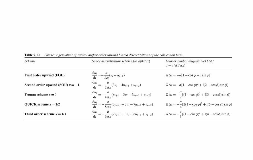
Ch09-H

6594.tex26/4/2007

16:59Page

430

Table 9.1.1 Fourier eigenvalues of several higher order upwind biased discretizations of the convection term.

Scheme Space discretization scheme for a(∂u/∂x) Fourier symbol (eigenvalue) ��tσ = a(�t/�x)

First order upwind (FOU)dui

dt=− a

�x(ui − ui−1) ��t = −σ[1 − cos φ + I sin φ]

Second order upwind (SOU) κ = −1dui

dt= − a

2�x(3ui − 4ui−1 + ui−2) ��t = −σ[1 − cos φ)2 + I(2 − cos φ) sin φ]

Fromm scheme κ = 0dui

dt= − a

4�x(ui+1 + 3ui − 5ui−1 + ui−2) ��t = −σ

2[(1 − cos φ)2 + I(3 − cos φ) sin φ]

QUICK scheme κ = 1/2dui

dt= − a

8�x(3ui+1 + 3ui − 7ui−1 + ui−2) ��t = −σ

4[2(1 − cos φ)2 + I(5 − cos φ) sin φ]

Third order scheme κ = 1/3dui

dt= − a

6�x(2ui+1 + 3ui − 6ui−1 + ui−2) ��t = −σ

3[(1 − cos φ)2 + I(4 − cos φ) sin φ]

Ch09-H6594.tex 26/4/2007 16: 59 Page 431


0.75

Third order

Fromm

SOUFOU

QUICK0.5

0.25

0.0�0.4�0.6�0.8�1.0�1.2�1.6 �1.4�2.0 �1.8

�0.25

�0.5

�0.75

0.0�0.2

(a) CFL � 0.5 CFL � 1

Third order

Fromm

SOUFOU

QUICK

1.5

1.0

0.5

0.0

�0.5

�1.0

�1.5

�0.8�1.2�1.6�2.0�2.4�3.2 �2.8�4.0 �3.6 0.0�0.4

(b)

Figure 9.1.3 Fourier symbol (eigenvalues) for the five upwind biaseddiscretizations of the convection term, listed in Table 9.1.1, at CFL = 0.5 andCFL = 1.

9.2.1 Stability Regions in the Complex � Plane and Fourier Modes

In order to define a general integration method, we introduce the time shift operator

E (Ek

is E to the power k)

Ewn = wn+1

Ekwn = wn+k (9.2.1)

We write a general time integration method of the canonical equation (9.1.54) underthe form

wn+1 = P(E, ��t) · wn (9.2.2)

where the operator P depends on the single parameter ��t. We will see next that theoperator P can always be written as a rational fraction of E.

The operator P is in fact the numerical amplification factor and will be comparedwith the exact amplification factor (9.1.52) to assess the accuracy.

Indeed, repeating the operator P successively, we obtain

wn = [P(E, ��t)] · wn−1 = · · · = [P(E, ��t)]n · w0 (9.2.3)

where w0 is the initial solution at t = 0.The stability condition requires that the solution wn remains bounded, which will

be satisfied if the operator Pn (P to the power n) remains uniformly bounded for all nand �t, in particular for n → ∞, �t → 0 with n�t fixed. That is, we should have,in a selected norm, for finite T

||Pn|| < K for 0 < n�t < T (9.2.4)

with K independent of n and �t.

Ch09-H6594.tex 26/4/2007 16: 59 Page 432


The norm of Pn is often very difficult to analyze and instead a necessary, butnot always sufficient condition can be obtained from a local mode analysis on theeigenvalues of P.

If we designate the eigenvalues of P by zP , solution of

zP = P(zP , ��t) (9.2.5)

the necessary stability condition is that all the eigenvalues zP should be of moduluslower than, or equal to, one.

|zP| ≤ 1 for all eigenvalues � (9.2.6)

When some values lie on the unit circle, |zP| = 1, they have to be simple, otherwisethe solution would increase with time as tm where (m + 1) is the multiplicity of theeigenvalue.

This condition establishes a relation between the selected time discretization and thespace discretization as characterized by the eigenvalues � of the space discretizationscheme, since

zP = zP(��t) (9.2.7)

The condition (9.1.43) on the space discretization has to be always satisfied for thesystem of ordinary differential equations (9.1.3) to be stable (or well-posed).

For all the space discretizations, which satisfy this condition, the associatednumerical discretization in time will be stable if condition (9.2.6) is satisfied.

The space discretization generates a representative set of eigenvalues ��t whichcover a certain region of the complex ��t plane – to be situated on the left side of theplane including the imaginary axis for stability. If we consider the trace of every rootzP(��t), as ��t covers the whole spectrum, in a complex z-plane, this trace will berepresented by some line which has to remain inside a circle of radius one. If someroots come outside the stability circle when ��t covers the range of its spectrum,the scheme is unstable (Figure 9.2.1).

A method with two or more time levels steps, will generate more than one eigen-value; in particular a two-step method, which involves three time levels, will generatetwo solutions, a three-step method, involving four time levels, will generate threesolutions and so on, and this for the same value of ��t.

When more than one value is present, the consistency of the scheme requires thatone of the eigenvalues should represent an approximation to the physical behavior.This solution of the eigenvalue equation, called the principal solution, is to be rec-ognized by the fact that it tends to one when ��t goes to zero. Denoting by zP1 theprincipal (‘physical’) solution we have

lim��t→0

zP1(�) = 1 (9.2.8)

The other solution, called the spurious solution, represents a ‘non-physical’ timebehavior of the numerical solution introduced by the scheme, and could destroy itsstability. For instance, we will see in the following section that the leapfrog schemehas two roots since it is a three-level scheme, and its first root is accurate up to second

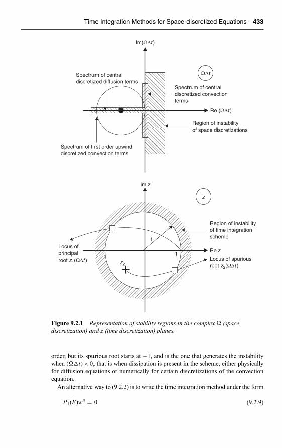
Ch09-H6594.tex 26/4/2007 16: 59 Page 433


Im(ΩΔt )

Re (ΩΔt )

ΩΔtSpectrum of centraldiscretized diffusion terms

Spectrum of first order upwinddiscretized convection terms

Region of instabilityof space discretizations

Spectrum of centraldiscretized convectionterms

Re z

Im z

1Locus ofprincipalroot z1(ΩΔt ) Locus of spurious

root z2(ΩΔt )

Region of instabilityof time integrationscheme

z2

1

z

Figure 9.2.1 Representation of stability regions in the complex � (spacediscretization) and z (time discretization) planes.

order, but its spurious root starts at −1, and is the one that generates the instabilitywhen (��t) < 0, that is when dissipation is present in the scheme, either physicallyfor diffusion equations or numerically for certain discretizations of the convectionequation.

An alternative way to (9.2.2) is to write the time integration method under the form

P1(E)wn = 0 (9.2.9)

Ch09-H6594.tex 26/4/2007 16: 59 Page 434


which by comparison establishes the relation,

P = E + P1 (9.2.10)

Hence, the amplification factor zP is solution of the relation zP = zP + P1(zP) andtherefore the eigenvalues zP are solutions of the characteristic polynomial

P1(zP) = 0 (9.2.11)

9.2.2 Error Analysis of Space and Time Discretized Systems

In order to define the errors of the combined space and time discretizations, we shouldcompare the numerical amplification factor zp with the exact amplification factor. Letus consider equation (9.2.3), which becomes

wn = znP(��t) · w0 (9.2.12)

where znP is zP to the power n. This amplification factor of the scheme, associated to the

mode �, is an approximation to the exact amplification factor G, defined by equation(9.1.52) and represents the errors introduced by the selected time integration. Hence,zP(��t) is the numerical approximation to e��t, which we can write as

zP(��t) ≈ e��t = 1 + ��t + (��t)2

2! + (��t)3

3! + (��t)4

4! + · · · (9.2.13)

Therefore, if we write the Taylor expansion of zP(��t), the first term in the expan-sion of zP(��t) which differs from the Taylor development of the exponentialdefines the order of the method.

For instance, for the explicit Euler method, zP(��t) = 1 + ��t, which is clearlyof first order accuracy. The backward Euler method is defined by

zP = 1

1 − ��t≈ 1 + ��t + (��t)2 + · · · (9.2.14)

and since the quadratic term is not equal to the quadratic term in equation (9.2.13),the method is only first order accurate.

9.2.2.1 Diffusion and dispersion errors of the time integration

Following the approach of Section 7.4, we define here the diffusion and dispersionerrors of the time integration method , after writing the numerical factor zP = P, as

zP = |zP|eI�P (9.2.15)

The global error is defined, after we decompose the eigenvalue � = Re(�) + I Im(�)in its real and imaginary parts, by

εT = zP

G= |zP|

eRe(��t)

eI�P

eI Im(��t)(9.2.16)

Ch09-H6594.tex 26/4/2007 16: 59 Page 435


The error in amplitude, the diffusion or dissipation error, is defined by the ratio ofthe modulus of |zP| and the amplitude of the exact solution of the semi-discretizedsystem (9.1.52)

εTD = |zP|

|G| = |zP|eRe(��t)

(9.2.17)

and the phase error, or dispersion error, will be defined by the ratio of the phase �P

of zP , to the phase of this exact solution, that is Im(��t)

εTφ = �P

Im(��t)(9.2.18)

The superscript T indicates that the respective errors are related to the selected timediscretization.

Since all quantities in these equations are function of (��t), the error (9.2.16) ofthe time integration method can also be represented in the complex (��t)-plane.

9.2.2.2 Diffusion and dispersion errors of space and time discretization

The errors just derived take as reference the exact solution of the semi-discretizedsystem, for a given space discretization, uniquely characterized by its eigenvaluespectrum. However, the space discretization itself generates dissipation and dispersionerrors, which can be evaluated by comparing with the exact solution of the analyticalmodel. This depends of course on the considered model.

For the reference linear convection model ut + aux = 0, we have seen in Section7.4 that the analytical amplification factor is given by

G = e−Iω�t = e−Iak�t (9.2.19)

where k is the wave number of the space component of the wave solution eIkx.The space discretization error is defined, with the superscript S referring to the

space discretization errors, by

εS = G

e−Iak�t= eRe(��t)

1

eI Im(��t)

e−Iak�t

�= εSD

eI Im(��t)

e−Iak�t

= εSDe−Iak�t(εS

φ−1) (9.2.20)

the spatial diffusion and dispersion errors being defined as

εSD

�= eRe(��t)

1= eRe(��t) εS

φ�= − Im(��t)

ak�t(9.2.21)

The total errors of the combined space and time discretizations are obtained bycomparing the amplification factor zP with the analytical factor (9.2.19), leading to

ε�= zP

e−Iak�t= zP

G

G

e−Iak�t= εT · εS (9.2.22)

Ch09-H6594.tex 26/4/2007 16: 59 Page 436


The global dissipation and dispersion errors are therefore defined by

εD = εTD · εS

D = |zP| and εφ = εTφ · εS

φ = − �P

ak�t= −�P

σφ(9.2.23)

This generalizes the definitions derived from the Von Neumann analysis andallows to separately evaluate the error sources from the space and from the timediscretizations.

We can see here the very important relation between the eigenvalues � and theerrors. The real part of � will contribute to the dissipation error, while its imagi-nary part determines the dispersion error. This imaginary part, divided by the wavenumber k , is a measure of the numerical wave speed and the dispersion error isdefined as the ratio between the numerical and physical wave speeds.

9.2.2.3 Relation with the equivalent differential equation

The development of Section 8.1.3, defining the general form of the equivalent differ-ential equation of a numerical scheme for the linear convection equation, equation(8.1.27), and its relation with the dispersion and dissipation errors, remains totallyvalid, when extended to an arbitrary combination of time and space discretizations.

Therefore, we have hereby a simple way of obtaining the equivalent differentialequation of the scheme resulting from the time integration of the system of spacediscretized ODEs. To achieve this objective, it suffices to develop the expressionsof the dispersion and diffusion errors in power series of the phase angle aroundφ = 0, and identify the terms, following equations (8.1.33) and (8.1.34).

Note that the diffusion error expansion will provide the coefficients of the evenorder derivatives of the equivalent differential equation, while the expansion of thedispersion error will provide the odd order derivative coefficients.

Each time discretization scheme is represented by a unique relation between zP

and �, determined by the dependence zP = zP(�). When the stability limit for zP ,equation (9.2.6), is introduced in this equation, under the form zP = eIθ , 0 < θ < 2π,representing the stability circle of radius 1, a corresponding stability region is definedin the (��t)-plane, through the mapping function zP = zP(�).

For a two-level scheme, where P is independent of E the stability curve is givenby the condition |P(�)| = 1.

Let us illustrate these relations with the examples of the previous section based onthe Fourier modes, associated to periodic boundary conditions, and some of the timediscretization methods applied in the previous chapters, in particular the forward,backward and central differences in time.

9.2.3 Forward Euler Method

The forward Euler method corresponds to a forward difference in time in an explicitmode. Applied to the canonical modal equation (9.1.54), it is defined by

wn+1 − wn = ��t wn (9.2.24)

Ch09-H6594.tex 26/4/2007 16: 59 Page 437


Im(ΩΔt )

Re(ΩΔt )�1

1

Stable

Unstable

Figure 9.2.2 Stability region for the Euler explicit method in the complex (��t)plane.

leading to

zP = P = 1 + ��t (9.2.25)

The scheme is therefore stable for all space discretizations associated to an eigenvaluespectrum such that

|(1 + ��t)| ≤ 1 (9.2.26)

or

[1 + Re(��t)]2 + [Im(��t)]2 ≤ 1 (9.2.27)

In the (��t) plane, this stability region is a circle of radius one centered around��t = −1 (Figure 9.2.2).

Diffusion operator (9.1.4)The eigenvalues are given by equation (E.9.1.2) and since all �-values are real andnegative, the stability condition is

−2 ≤ −|Re(��t)| ≤ 0 (9.2.28)

or

0 ≤ α�t

�x2≤ 1

2(9.2.29)

as derived by the Von Neumann method in Chapter 7.

Central space discretization for the convection equationWith equation (E.9.1.6), ��t becomes

��t = −Ia�t

�xsin φ = −Iσ sin φ (9.2.30)

with the CFL number σ = a�t/�x

Ch09-H6594.tex 26/4/2007 16: 59 Page 438


All eigenvalues � are purely imaginary, and are outside the stability circle of theforward Euler method. The scheme is therefore unstable.

Upwind space discretization for the convection equation (9.1.17)The eigenvalues are given by equation (E.9.1.4),

��t = −σ(1 − cos φ + I sin φ) (9.2.31)

In the complex ��t-plane all the eigenvalues are located along a circle centered at−σ, with radius σ. This circle will be inside the stability circle of radius 1, if σ liesbetween 0 and 1. We recover the CFL condition of the upwind explicit scheme asseen in Chapter 7.

0 ≤ σ ≤ 1 (9.2.32)

9.2.4 Central Time Differencing or Leapfrog Method

The leapfrog method corresponds to a central difference in time, with an explicitformulation, leading to a three level, two-step method:

wn+1 − wn−1 = 2 ��t wn (9.2.33)

Hence

P(E, ��t) = E−1 + 2 ��t (9.2.34)

The eigenvalues zP are obtained from

zP = 2��t + 1/zP (9.2.35)

This quadratic equation results from the three levels in time

z2P − 2��t zP − 1 = 0

leading to the two solutions

zP = ��t ±√

(��t)2 + 1 (9.2.36)

which behave as follows, when �t → 0

z1 = ��t +√

(��t)2 + 1 = 1 + ��t + (��t)2

2− (��t)4

8+ · · · (9.2.37)

z2 = ��t −√

(��t)2 + 1 = −1 + ��t − (��t)2

2+ (��t)4

8+ · · · (9.2.38)

The first solution is the physical one, while the second one starts at −1 and is thespurious value. Observe, by comparing (9.2.37) with the expansion (9.2.13), that the

Ch09-H6594.tex 26/4/2007 16: 59 Page 439


Im(ΩΔt )

Re(ΩΔt )

1

�1

Figure 9.2.3 Stability region for the leapfrog method.

first three terms are exact and therefore the scheme is second order accurate in time,as we would expect indeed from the central difference.

From

2(��t) = zp − 1

zP(9.2.39)

with the stability limit zP = eIθ , we obtain

��t = I sin θ (9.2.40)

The stability region of the leapfrog method is therefore a strip of amplitude ±1 alongthe imaginary axis, Figure 9.2.3.

It is seen immediately that the diffusion operator with its real negative eigenvaluesor the upwind convection operators, which also generate a negative real component,lead to unstable schemes when solved by the leapfrog method. Since negative valuesof (��t) correspond to the presence of a dissipative mechanism (or numericalviscosity), for hyperbolic equations, it results that the leapfrog scheme is totallyunadapted to the presence of dissipative terms.

On the other hand, the leapfrog scheme applied to the central differenced convectiveequation, which does not generate dissipation is stable under the CFL condition.

9.2.5 Backward Euler Method

The backward Euler method corresponds to a backward difference in time in animplicit mode. Applied to the canonical modal equation (9.1.54), it is defined by

wn+1 − wn = ��t wn+1 or (1 + ��t)wn+1 = wn (9.2.41)

leading to

P(E, ��t) = 1 + ��t · E (9.2.42)

Ch09-H6594.tex 26/4/2007 16: 59 Page 440


Im(ΩΔt )

Re(ΩΔt )1

Region of instability

Figure 9.2.4 Stability region for implicit Euler scheme.

The eigenvalue zP is obtained from

zP = 1 + ��t · zP or zP = 1

1 − ��t(9.2.43)

For zP = eIθ , the limit of the stability region in the ��t-plane is defined by

(��t) = 1 − e−Iθ (9.2.44)

and represents a circle centered on ��t = 1 of radius one, Figure 9.2.4.Since for |zP| < 1, |1 − ��t| > 1, the stability region is outside the circle and is

seen to cover even regions in the �-plane where the space-discretized equations areunstable. Hence, all the schemes seen up to now will be stable with the implicitEuler time integration.

The approach developed here allows also us to analyze separately the propertiesof the space discretization and of the time integration. For a given discretization inspace, we can select appropriate time integrations with stability regions containingthe spatial eigenvalue spectrum. Hence, a space discretization cannot be said to beunstable by itself, at least if the condition Re � ≤ 0 is satisfied. It is only when it iscoupled to a time integration that we can decide upon stability.

For instance, the explicit Euler scheme has a stability region that does not containthe imaginary axis of the ��t-plane, and will not be stable for a ��t-spectrum on theimaginary axis like the one generated by the central discretization of the convectionequation. However, it will be stable, conditionally, for the diffusion equation if all thereal eigenvalues are contained within the range −2 < (��t) < 0, or for the upwinddiscretization of the convection term, under a CFL condition. Similarly, the leapfrogscheme is unstable in this latter case since its stability region is limited to a segmentof the imaginary axis. Hence, as already noticed, the leapfrog scheme is totallyunadapted for dissipative problems, while the Euler explicit scheme is not suitablefor non-dissipative space discretizations.

Ch09-H6594.tex 26/4/2007 16: 59 Page 441


HANDS-ON TASK 5Apply the methodology described above to analyze the combinations of the threetime integration methods of Sections 9.2.3–9.2.5, with various discretizations ofthe convection and diffusion model equations. For the linear convection equation,consider the central, as well as the first and second order upwind discretizationsfor the space term. For the diffusion equation, consider a central discretization ofthe second derivative term.

Develop the following steps:

• Convection terms: Find the trajectories of the eigenvalues ��t in the complex��t-plane, by applying a Fourier analysis. Consider the range of phaseangles φ = k�x in the interval (−π, +π) for the three discretizations options(central, first and second order upwind). Plot the results for values of the CFLnumber, CFL = 0.25, 0.5, 0.75, 1, 1.5.

• Define the stability conditions for all the combinations by comparing withthe stability domain of the time integration method.

• Determine the dissipation and dispersion errors for the same combinationsand display them in function of the phase angle for the various values of theCFL number.

• Comment and analyze these results.• Diffusion terms: Repeat the same development for the central discretization

of the second derivative term.• Plot the eigenvalue trajectories in the ��t-plane for several values of the

scheme parameter β = α�t/�x2, in the range (0, 1), in function of the phaseangle φ = k�x in the interval (−π, +π).

• Define the stability conditions for the three considered time integrationmethods.

• Determine the dissipation and dispersion errors for the same combinationsand display them in function of the phase angle for the various values of theβ-parameter number.

• Comment and analyze these results.

Apply symbolic mathematical software tools, such as MAPLE, Mathematica orMATLAB.

9.3 A SELECTION OF TIME INTEGRATION METHODS

A large number of methods are available for the solution of the system of ordinarydifferential equations obtained after the space discretization.

If you have to choose a time integration method, the first question to ask yourselfis: Do I favor an explicit or an implicit method? The debate between implicit andexplicit methods is still open and no definitive recommendation can be given, as bothoptions are valid. We can state the pros and cons as follows:

Explicit methods• Are at best conditionally stable and have a limitation on the maximum allowable

time step (�t)stab. This maximum time step is generally quite small, particularly

Ch09-H6594.tex 26/4/2007 16: 59 Page 442


for convection dominated compressible flows, with (�t)stab < (CFL) �x/a,where a is of the order of the speed of sound.

• For CFL = 1, �x ≈ 10−2 m and a ≈ 330 m/s, we would have (�t)stab < 3.10−5 s.• The CPU cost per iteration is low, since no matrices have to be inverted.• But the low stability limit will require a large number of time steps.

Implicit methods• Are generally unconditionally stable and large time steps can be applied,

theoretically even tending to infinity.• In practice, due to nonlinearities of the flow equations, time step restric-

tions will nevertheless appear. Moreover, for unsteady flow problems accuracyrequirements will also tend to restrict the maximum time step.

• The resulting time step will nearly always be significantly higher than the explicitCFL-based time limit (�t)stab.

• The CPU cost per iteration of implicit methods is significantly higher comparedto explicit methods, since matrices have to be inverted at each time step. Thesematrices also lead to requirements for additional memory, depending on theselected resolution method. Some of the available methods are described inChapter 10.

• One of the guidelines toward the selection of the time step is related to the lowestphysical time scale (�t)phys that the simulation intends to capture:– If the physical time step (�t)phys is of the same order as the stabil-

ity limit (�t)stab, then explicit methods are clearly the most appropriatechoice.

– If the physical time step (�t)phys is significantly higher than the stability limit(�t)stab, then implicit methods are a valid option. This will be the case forsteady state problems.

• For nonlinear problems, linearization techniques have to be applied with implicitmethods, which might restrict the linear stability conditions.

Finally, the choice between explicit and implicit methods will be guided by theproduct (cost per time step)*(number of time steps), as implicit methods require alower number of time steps, but are more costly for each time step.

Therefore, we have to balance the higher allowable time step against thehigher number of operations necessary to resolve the implicit algebraic system ofequations.

We can classify the most relevant time integration methods for steady or unsteadyflow simulations into three groups:

1. Multistep methods, which allow implicit time integration options.2. Predictor–corrector methods, restricted in their simplest form to second order,

are explicit, and easy to program:– They have a widespread range of applications, the most popular being the

explicit McCormack scheme.– They can be considered, for nonlinear problems, as an approximation to the

implicit linearization techniques.

Ch09-H6594.tex 26/4/2007 16: 59 Page 443


3. Runge–Kutta multistage methods, which are explicit and allow arbitrary highorders in time:– They are in particular well adapted to convection problems with central

discretizations.– They apply without additional modifications to nonlinear and multidimen-

sional problems.

In terms of stability terminology, the time integration schemes are said to be:

• Unconditionally unstable: If the stability domain is found in the right-hand sideof the complex ��t-plane.

• Conditionally stable: If the stability domain covers part of the left-hand side ofthe complex ��t-plane.

• A-stable or unconditionally stable: If the domain of stability covers the wholeof the left-hand side of the complex ��t-plane.

In practical applications, the vector U contains a large number of variables, namelyN = m · M ; M is the total number of mesh points where the m independent variableshave to be determined. Generally, these variables have to be stored for each time leveland increasing the number of time levels could rapidly put severe restrictions on theallowable space variables and mesh points. It is therefore very exceptional to considerapplications with more than three time levels (two-step methods) to fluid mechanicalproblems, the overwhelming majority of schemes being limited to one-step methodswith two time levels.

In the ‘advanced’ Section A9.4, we introduce you to some multidimensional prob-lems, solved by implicit multistep methods. In these cases, the matrices are too largefor direct inversions and factorization methods, reducing the problem to a successionof one-dimensional implicit operators, can be defined. These methods are also knownas Alternating Direction Implicit (ADI) methods. The factorization process is by nomeans trivial, since it can destabilize the numerical scheme, as will be shown for thethree-dimensional convection equation with central differenced space derivatives.

We refer you to the literature for more details and general presentations. In par-ticular, Gear (1971), Lambert (1973–1991), Dahlquist and Bjorck (1974), Beam andWarming (1982). The following books also present very general and complete pre-sentations of methods for ODEs, Hairer et al. (1993), Hairer and Wanner (1996),Hundsdorfer and Verwer (2003).

9.3.1 Nonlinear System of ODEs and their Linearization

For a general system of ordinary differential equations (9.1.3), the right-hand sidemay, and often will be, nonlinear. If we write the system in the more general form:

dU

dt= H (U ) (9.3.1)

where H is a nonlinear function or matrix operator, acting on the vector U as definedpreviously, the vector H (U , t) generalizes the space-discretized operators (SU + Q)

Ch09-H6594.tex 26/4/2007 16: 59 Page 444


of equation (9.1.3), and is represents the residual, divided by the local cell volume(see equation (5.2.7)).

The link with the linear form, where the S-matrix is independent of U , can beobtained through an adequate linearization procedure.

Performing a series development around a reference value Ue, we can write

H (U ) = H (Ue) +(

∂H

∂U

)e· (U − Ue) + O(U − Ue)2 (9.3.2)

where (∂H/∂U ) is the Jacobian of the operator H with respect to the dependentvariable U . We introduce the notation

J (U ) = ∂H

∂U(9.3.3)

and if we select the reference solution Ue as the steady state solution of H (Ue) = 0,we can rewrite the system (9.3.1) as

dU

dt= J (Ue)(U − Ue) (9.3.4)

Comparing with equation (9.1.3), we see that the matrix S is identical to the Jaco-bian matrix J(Ue) and the eigenvalue spectrum is determined by the Jacobianeigenvalues. The Jacobian plays therefore a central role in the stability properties ofthe selected schemes. Note here that J(Ue) is the Jacobian of the space-discretizedflux balance of the conservation law, that is the Jacobian of the residual, and NOTthe analytical Jacobian of the flux terms.

Hence, we will apply the general methodology, as defined in the previous sections,for the stability analysis, by the following steps:

• Find the Fourier mode eigenvalues � (the Fourier symbol) of the Jacobian matrixof the space-discretized operator H (U ).

• Introduce the canonical modal equation:

dw

dt= � · w (9.3.5)

Define the selected time integration method by its operator P, by rewriting theselected method under the form of equations (9.2.2) or (9.2.9), repeated here

wn+1 = P(E, ��t) · wn or P1(E, ��t) · wn = 0

• Find the eigenvalues of the operator P, following (9.2.5), or solve the charac-teristic equation (9.2.11), and apply the stability condition |z| = |P| ≤ 1 for thesubsequent stability analysis of the combined time and space-discretized scheme.

We will now analyze several important methods.

Ch09-H6594.tex 26/4/2007 16: 59 Page 445


9.3.2 General Multistep Method

Linear multistep methods have been analyzed systematically by Dahlquist (1963)and with special attention to fluid mechanical simulations by Beam and Warming(1976–1980), who developed them further into operational computer codes for theEuler and Navier–Stokes equations. See for instance Pulliam (1984) for a descriptionof the structure and properties of these codes.

Following Beam and Warming (1980), we introduce the most general consistenttwo-step method (three time levels) under the form of a three-parameter family:

(1 + ξ)U n+1 − (1 + 2ξ)U n + ξU n−1 = �t[θH n+1 + (1 − θ + φ)H n − φH n−1]

(9.3.6)

The three parameters have clear distinct roles:

1. ξ controls the order of the finite difference formula for dU /dt.2. θ controls the implicitness of the method: θ = 0 generates explicit methods.3. φ controls the number of time levels of the space-discretized terms: φ = 0

reduces to a two time level family when ξ = 0.

The characteristic polynomial becomes

P1(E) = (1 + ξ)E2 − (1 + 2ξ)E + ξ − ��t[θE

2 + (1 − θ + φ)E − φ] (9.3.7)

It can be shown that for second order accuracy in time, we should have the relation

ξ = θ + φ − 1/2 (9.3.8)

and if, in addition

ξ = 2φ − 1/6 (9.3.9)

the method is third order accurate. These conditions for third order accuracy reduceto θ = φ + 1/3 and ξ = 2φ − 1/6.

Finally a unique fourth order accurate method is obtained for

θ = −φ = −ξ/3 = 1/6 (9.3.10)

This is easily shown from a Taylor series expansion of the principal root of thecharacteristic polynomial (9.3.7) (see Problem P.9.7).

A certain number of properties have been proven by Dahlquist (1963) with regardto the order of accuracy of A-stable methods:

• The two-step scheme (9.3.6) is A-stable if and only if

θ ≥ φ + 1/2

ξ ≥ −1/2 (9.3.11)

ξ ≤ θ + φ − 1/2

Ch09-H6594.tex 26/4/2007 16: 59 Page 446


q� 1/2

q

x� �1/2

x� q�1/2x

Region of A-stability

2

1

1 2 3

0

�1

Figure 9.3.1 Domain of A-stability in the plane (ξ, θ) for second order, two-stepmethods with φ = 0.

This is shown on Figure 9.3.1, for the family of second order schemes, satisfying(9.3.8):

• An A-stable linear multistep method cannot have an order of accuracy higherthan two.

• The trapezoidal scheme (ξ = φ = 0, θ = 1/2) has the smallest truncation error ofall second order A-stable methods.

A classification of several well-known methods is listed in Table 9.3.1. Note thatthe schemes with θ = 0 are explicit. It is also seen that not all the implicit methods(θ �= 0) are A-stable, showing that implicitness does not ensure always that theschemes will be unconditionally stable.

Figure 9.3.2 shows the stability domain of some of the methods listed in the table.TheAdams–Moulton method is implicit but conditionally stable, within the domain

limited on the real axis to B = −6, while the backward difference method is uncon-ditionally stable, as its stability domain is outside the curve on the right side ofthe ��t-plane. The same is true for the A-stable Adams-type method. The Adams–Bashworth method on the other hand, is conditionally stable, with an upper boundon the real negative axis of B = −1, and will not be suitable for centrally discretizedconvection terms, whose spectrum is on the imaginary axis. We need to add dissipa-tion terms in order to push the eigenvalues of the space discretization in the left sideof the ��t-plane.

In unsteady CFD applications, some of the most widely used methods of the three-parameter family (9.3.6) are the methods of Adams–Bashworth (explicit), and theimplicit Crank–Nicholson and Gear or Backward Differencing methods.

They are often written in incremental form, for the unknowns�U n = U n+1− U n, as

(1 + ξ)�U n − ξ�U n−1 = �t[θH n+1 + (1 − θ + φ)H n − φH n−1] (9.3.12)

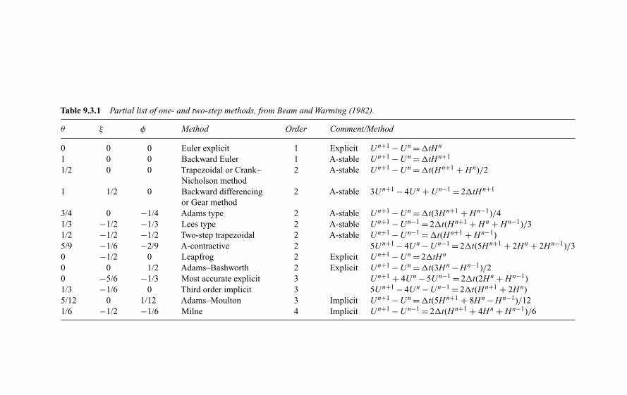
Ch09-H

6594.tex26/4/2007

16:59Page

447

Table 9.3.1 Partial list of one- and two-step methods, from Beam and Warming (1982).

θ ξ φ Method Order Comment/Method

0 0 0 Euler explicit 1 Explicit U n+1 − U n = �tH n

1 0 0 Backward Euler 1 A-stable U n+1 − U n = �tH n+1

1/2 0 0 Trapezoidal or Crank– 2 A-stable U n+1 − U n = �t(H n+1 + H n)/2Nicholson method

1 1/2 0 Backward differencing 2 A-stable 3U n+1 − 4U n + U n−1 = 2�tH n+1

or Gear method3/4 0 −1/4 Adams type 2 A-stable U n+1 − U n = �t(3H n+1 + H n−1)/41/3 −1/2 −1/3 Lees type 2 A-stable U n+1 − U n−1 = 2�t(H n+1 + H n + H n−1)/31/2 −1/2 −1/2 Two-step trapezoidal 2 A-stable U n+1 − U n−1 = �t(H n+1 + H n−1)5/9 −1/6 −2/9 A-contractive 2 5U n+1 − 4U n − U n−1 = 2�t(5H n+1 + 2H n + 2H n−1)/30 −1/2 0 Leapfrog 2 Explicit U n+1 − U n = 2�tH n

0 0 1/2 Adams–Bashworth 2 Explicit U n+1 − U n = �t(3H n − H n−1)/20 −5/6 −1/3 Most accurate explicit 3 U n+1 + 4U n − 5U n−1 = 2�t(2H n + H n−1)1/3 −1/6 0 Third order implicit 3 5U n+1 − 4U n − U n−1 = 2�t(H n+1 + 2H n)5/12 0 1/12 Adams–Moulton 3 Implicit U n+1 − U n = �t(5H n+1 + 8H n − H n−1)/121/6 −1/2 −1/6 Milne 4 Implicit U n+1 − U n−1 = 2�t(H n+1 + 4H n + H n−1)/6

Ch09-H6594.tex 26/4/2007 16: 59 Page 448


3

2.5

0

�1

�2

�3

10.0�2.5�5.0

2

Adams–Moulton

Adams–Bashworth

Backward difference

Adams type method

Im(ΩΔt )

Re(ΩΔt )

Figure 9.3.2 Stability regions in the ��t-plane for some of the schemes ofTable 9.3.1.

The subset φ = 0A particular family of schemes, extensively applied, are the schemes with φ = 0.

(1 + ξ)U n+1 − (1 + 2ξ)U n = �t[θH n+1 + (1 − θ)H n] − ξU n−1 (9.3.13)

They are second order accurate in time for ξ = θ − 1/2.When applied to the Euler and Navier–Stokes equations with central space dif-

ferencing, these schemes have become known as the Beam and Warming schemes,when a Jacobian linearization is introduced. The characteristic polynomial reduces to

P1(z) = (1 + ξ)z2 − (1 + 2ξ)z + ξ − (��t)z(θz + 1 − θ) = 0 (9.3.14)

For fixed values of θ, the stability domain in the ��t-plane is obtained from thecondition |z| < 1.

For ξ = 0, we obtain a two-level, one-step, scheme, known as the generalizedtrapezoidal method ,

U n+1 − U n = �t[θH n+1 + (1 − θ)H n] (9.3.15)

For θ = 1/2, the method is second order in time and is known as the Trapezium methodor the Crank–Nicholson method when applied to the diffusion equation:

U n+1 − U n = �t

2(H n+1 + H n) (9.3.16)

The root of the characteristic equation (9.3.14), after removal of the trivial root z = 0, is

z = 1 + (1 − θ)��t

1 − θ(��t)(9.3.17)

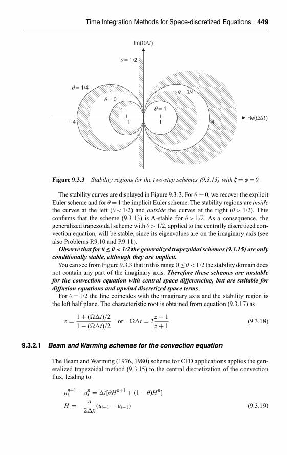
Ch09-H6594.tex 26/4/2007 16: 59 Page 449


q� 1/2

q� 1/4q� 3/4

q� 0

q� 1

�1�4 41

Im(ΩΔt )

Re(ΩΔt )

Figure 9.3.3 Stability regions for the two-step schemes (9.3.13) with ξ = φ = 0.

The stability curves are displayed in Figure 9.3.3. For θ = 0, we recover the explicitEuler scheme and for θ = 1 the implicit Euler scheme. The stability regions are insidethe curves at the left (θ < 1/2) and outside the curves at the right (θ > 1/2). Thisconfirms that the scheme (9.3.13) is A-stable for θ > 1/2. As a consequence, thegeneralized trapezoidal scheme with θ > 1/2, applied to the centrally discretized con-vection equation, will be stable, since its eigenvalues are on the imaginary axis (seealso Problems P.9.10 and P.9.11).

Observe that for 0 ≤ θ < 1/2 the generalized trapezoidal schemes (9.3.15) are onlyconditionally stable, although they are implicit.

You can see from Figure 9.3.3 that in this range 0 ≤ θ < 1/2 the stability domain doesnot contain any part of the imaginary axis. Therefore these schemes are unstablefor the convection equation with central space differencing, but are suitable fordiffusion equations and upwind discretized space terms.

For θ = 1/2 the line coincides with the imaginary axis and the stability region isthe left half plane. The characteristic root is obtained from equation (9.3.17) as

z = 1 + (��t)/2

1 − (��t)/2or ��t = 2

z − 1

z + 1(9.3.18)

9.3.2.1 Beam and Warming schemes for the convection equation

The Beam and Warming (1976, 1980) scheme for CFD applications applies the gen-eralized trapezoidal method (9.3.15) to the central discretization of the convectionflux, leading to

un+1i − un

i = �t[θH n+1 + (1 − θ)H n]

H = − a

2�x(ui+1 − ui−1) (9.3.19)

Ch09-H6594.tex 26/4/2007 16: 59 Page 450


With ��t = −Iσ sin φ, we obtain

z = 1 − Iσ sin φ

1 + Iσθ sin φ(9.3.20)

The diffusion error is

εD = |z| =√

1 + σ2(θ − 1)2 sin2 φ

1 + σ2θ2 sin2 φ(9.3.21)

and the dispersion error is given by

εφ = 1

σφtan−1

(σ sin φ

1 + σ2θ(θ − 1) sin2 φ

)(9.3.22)

The Crank–Nicholson or trapezium method, θ = 1/2, leads to |z| = 1 for all φ andconsequently has no dissipation error with the centrally discretized convection oper-ator. This is a very favorable property. However, the lack of dissipation makes thescheme marginally stable and quite sensitive to nonlinearities and high frequency errorsources. Therefore, the scheme will require some additional artificial dissipation tobe added to the convective flux terms (see Section 9.3.6).

Note that all these schemes have a large lagging phase error, as can be seen fromFigure 9.3.4. Figure 9.3.4 compares the behavior of the Euler implicit and the back-ward Gear implicit methods, at four different CFL values, namely CFL = 0.5, 2, 10and 100, showing the dissipation and the dispersion errors in function of the phaseangle from 0 to π. Both schemes are unconditionally stable. Observe that all theschemes have z = 1 at φ = π, indicating a lack of dissipation of the high frequencyerrors.

Of particular significance are the increasingly large errors when the CFL numberincreases. Remember that the objective of implicit methods is to allow high values ofthe time steps to gain faster convergence.

Hence, we have to ask ourselves if this is acceptable? The answer depends on thetype of problem we are solving:

• If we solve a steady state problem, then we wish the transients, which are ofnumerical significance only, to be damped as fast as possible. This will be thecase at the high CFL numbers and fast convergence will be obtained with theseschemes.

• For unsteady flow problems, these errors are unacceptable and the high CFL val-ues are not acceptable. Hence, these schemes loose much of their interest, sincereducing the CFL number implies a reduction of the time step and the high cost ofthese implicit methods might become prohibitive compared to explicit methods.

9.3.2.2 Nonlinear systems and approximate Jacobian linearizations

Considering scheme (9.3.13), H n+1 = H (U n+1) has to be evaluated numerically insome way, since U n+1 is unknown.

Ch09-H6594.tex 26/4/2007 16: 59 Page 451


1.0

0.95

0.9

0.85

0.8

0.75

0.7

0.65

0.6

0.55

0.5

0.45

0.4

0.35

0.3

0.25

0.2

0.15

0.1

0.0 0.2 0.4 0.6 0.8 1.0 1.2 1.4 1.6

p

1.8 2.0 2.2 2.4 2.6 3.02.8

(a)

CFL�100

CFL�0.5

CFL�2

CFL�10

p

1.0

0.95

0.9

0.85

0.8

0.75

0.7

0.65

0.6

0.55

0.5

0.45

0.4

0.35

0.3

0.25

0.2

0.15

0.1

0.05

0.0

0.0 0.2 0.4 0.6 0.8 1.0 1.2 1.4 1.6 1.8 2.0 2.2 2.4 2.6 3.02.8

(b)

CFL�100

CFL�0.5

CFL�2

CFL�10

p

1.0

0.95

0.9

0.85

0.8

0.75

0.7

0.65

0.6

0.55

0.5

0.45

0.4

0.35

0.3

0.25

0.2

0.15

0.1

0.05

0.00.0 0.2 0.4 0.6 0.8 1.0 1.2 1.4 1.6 1.8 2.0 2.2 2.4 2.6 3.02.8

(c)

CFL�100

CFL�0.5

CFL�2

CFL�10

p

1.0

0.95

0.9

0.85

0.8

0.75

0.7

0.65

0.6

0.55

0.5

0.45

0.4

0.35

0.3

0.25

0.2

0.15

0.1

0.05

0.00.0 0.2 0.4 0.6 0.8 1.0 1.2 1.4 1.6 1.8 2.0 2.2 2.4 2.6 3.02.8

(d)

CFL�100

CFL�0.5

CFL�2

CFL�10

Figure 9.3.4 Plots of amplification factors and phase errors for different implicitBeam and Warming algorithms at CFL = 0.5, 2, 10 and 100, in function of phaseangle in radians, from 0 to π (a) Amplitude error for θ = 1, ξ = 1/2 backwarddifferencing scheme. (b) Phase error for θ = 1, ξ = 1/2 backward differencingscheme. (c) Amplitude error for θ = 1, ξ = 0 backward Euler (implicit) scheme.(d) Phase error for θ = 1, ξ = 0 backward Euler (implicit) scheme.

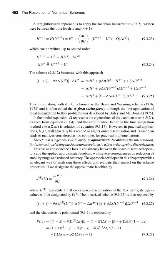
Ch09-H6594.tex 26/4/2007 16: 59 Page 452


A straightforward approach is to apply the Jacobian linearization (9.3.2), writtenhere between the time levels n and (n + 1)

H n+1 = H (U n+1) = H n +(

∂H

∂U

)· (U n+1 − U n) + O(�U 2) (9.3.23)

which can be written, up to second order

H n+1 = H n + J (U n) · �U n

�U n �= U n+1 − U n (9.3.24)

The scheme (9.3.12) becomes, with this approach

[(1 + ξ) − θ�tJ (U n)] · �U n = �tH n + φ�t(H n − H n−1) + ξ�U n−1

= �tH n + φ�tJ (U n−1)�U n−1 + ξ�U n−1

= �tH n + [ξ + φ�tJ (U n−1)]�U n−1 (9.3.25)

This formulation, with φ = 0, is known as the Beam and Warming scheme (1976,1978) and is often called the �-form (delta-form), although the first application oflocal linearization to flow problems was developed by Briley and Mc Donald (1975).

In the modal expansion, � represents the eigenvalues of the Jacobian matrix J (U ),as seen from equation (9.3.4), and the amplification factor of the time integrationmethod z = z(��t) is solution of equation (9.3.14). However, in practical applica-tions, H (U ) will generally be a second or higher order discretization and its Jacobianleads to matrices considered as too complex for practical implementations.

Therefore it is a general rule to apply an approximate Jacobian in the linearization,for instance by selecting the Jacobian associated to a first order upwind discretization.

This has as consequence a loss in consistency between the space-discretized opera-tors and the applied approximate Jacobian, with severe consequences on reduction ofstability range and reduced accuracy. The approach developed in this chapter providesan elegant way of analyzing these effects and evaluate their impact on the schemeproperties. If we designate the approximate Jacobian by

J (1)(U ) = ∂H (1)

∂U(9.3.26)

where H (1) represents a first order space-discretization of the flux terms, its eigen-values will be designated by �(1). The linearized scheme (9.3.25) is then replaced by

[(1 + ξ) − θ�tJ (1)(U n)] ·�U n = �tH n +[ξ + φ�tJ (U n−1)]�U n−1 (9.3.27)

and the characteristic polynomial (9.3.7) is replaced by

P1(z) = [(1 + ξ) − θ(�(1)�t)](z − 1) − (��t) − [ξ + φ(��t)](1 − 1/z)

= (1 + ξ)z2 − (1 + 2ξ)z + ξ − θ(�(1)�t) z(z − 1)

− (��t)z − φ(��t)(z − 1) (9.3.28)

Ch09-H6594.tex 26/4/2007 16: 59 Page 453


Its solutions, and the scheme properties will depend on the two eigenvalues � and �(1)

Actually, the Beam and Warming scheme (9.3.25) is applied in practice under theform (9.3.27) with φ = 0, where the approximate Jacobian is derived from a first orderupwind discretization of the convective fluxes.

This can be extended to other time discretization methods and can be applied ina straightforward way when associated to the eigenvalues obtained from the Fouriermodes. See Section 9.3.5 for a detailed application.

9.3.3 Predictor–Corrector Methods

When H (U ) is nonlinear in U we can avoid the evaluation of Jacobians, by considering

an iterative approach, whereby a first guess Un+1

of U n+1 is obtained, for instanceby applying an explicit scheme, eventually of lower order, called a predictor step,followed by a second step, using the ‘predicted’ value as a basis for improving thesolution. This is called a predictor–corrector method and many variants have beenstudied and applied in practice.

We will present here the most widely known of these methods.Applied for instance to the scheme (9.3.13), the corrector step would become


This defines the predictor–corrector sequence, with H n+1 = H (Un+1

).This approach can be pursued at the same time level, by repeating equation (9.3.29)

for s steps, until some form of convergence between two consecutive estimations of

the corrector step solutions Un+1

is achieved. This implies an evaluation of H ateach ‘local’ iteration step and this procedure is generally not recommended, sincethe evaluation of H is often the most costly operation in the numerical simulation.Repeating the corrector sequence implies that the solution of equation (9.3.29), nowdesignated by U n+1, is obtained after the second corrector step as


where U n+1 is the new value for U n+1 and H n+1 = H (Un+1

).A detailed analysis of various options and of the influence of the number of ‘local’

iterations, can be found in Lambert (1973). One of the essential conclusions, from acomparison of the effect of different numbers of corrector steps coupled to the samepredictor, is that the unique sequence of a predictor step followed by a single correctorstep appears as being optimal, in view of the reduction of the number of evaluationsof the right-hand side.

In order to analyze the order of accuracy and the stability of a predictor–corrector

sequence, we can combine the predictor Un+1

and the known value U n in a singlevector and write the sequence as a system of two equations. The characteristic poly-nomial is obtained by setting the determinant of the matrix to zero, for the modalequation H = �U .

Let us illustrate this for the two-level schemes (9.3.13). By definition, we requirethe predictor to be explicit; hence we set θ = ξ = 0 and obtain the first order Euler

Ch09-H6594.tex 26/4/2007 16: 59 Page 454


method as predictor (see, however, Problem P.9.23 for an implicit predictor–correctorapproach):

Un+1 = U n + �tH n (9.3.31)

The corrector is equation (9.3.29) written in operator form as

[(1 + ξ)E − (1 + 2ξ)]U n = �t[θHn+1 + (1 − θ)H n] − ξU n−1 (9.3.32)

and can be treated as an explicit equation.Inserting the modal equation H = �U , we obtain the system

∣∣∣∣∣E −(1 + ��t)

−θ(��t)E ξE−1 + (1 + ξ)E − (1 + 2ξ) − ��t(1 − θ)

∣∣∣∣∣∣∣∣∣U

n

U n

∣∣∣∣ =∣∣∣∣ 0

0

∣∣∣∣(9.3.33)

leading to the polynomial equation obtained from the determinant of the system setto zero:

P1(z) = (1 + ξ)z2 − (1 + 2ξ)z + ξ − (��t)z(1 + θ ��t) = 0 (9.3.34)

It is interesting to compare this equation with (9.3.14) derived for the implicit system,in particular when ξ = 0. The above equation becomes, removing a trivial root z = 0:

z = 1 + (��t) + θ (��t)2 (9.3.35)

This solution is typical of explicit schemes, and the predictor–corrector sequence hasbecome explicit for all values of θ. The sequence is only first order accurate in time,excepted for θ = 1/2 where it is second order, since the quadratic term is equal to thecorresponding term in the Taylor development of exp(��t) as seen from equation(9.2.13).

Figure 9.3.5 shows the stability regions for the cases θ = 0, θ = 1/2 and θ = 1. Thecase θ = 0 is the explicit Euler method. Only for θ = 1, does the stability domaininclude part of the imaginary axis, which indicates that it can be applied with centraldiscretizations of the convection terms. This is not the case anymore when θ = 1/2.

The choice θ = 1/2 corresponds to a second order accurate sequence and is knownas Henn’s method. It forms the basis of the McCormack scheme and can be written as

Un+1 = U n + �tH n

U n+1 = U n + 1

2�t(H n+1 + H n) (9.3.36)

= 1

2(U

n+1 + U n) + 1

2�tH

n+1

This scheme is unstable for the convection equation, when central differencesare applied, as can be seen from Figure 9.3.4. On the other hand, for θ = 1 we obtain

Ch09-H6594.tex 26/4/2007 16: 59 Page 455


x0.0�2.0 �1.8 �1.6 �1.4 �1.2 �1.0 �0.8 �0.6 �0.4 �0.2

1.8

1.6

1.0

1.2

0.8

0.6

0.4

0.2

0.0

�0.2

�0.4

�0.6

�0.8

�1.0y

�1.2

�1.4

�1.6

�1.8

1.4

θ�1/2

θ�1

θ�0

Figure 9.3.5 Stability regions of the predictor–corrector methods (9.3.34), withξ = 0 and for θ = 0, θ = 1/2 and θ = 1.

the following scheme

Un+1 = U n + �tH n

(9.3.37)U n+1 = U n + �tH n+1

which is stable for the convection equation with central differences under the CFLcondition |σ| ≤ 1.

Variants of this scheme have been applied by Brailowskaya (1965) to the Navier–Stokes equations by keeping the viscous diffusion terms in the corrector step atlevel n.

Ch09-H6594.tex 26/4/2007 16: 59 Page 456


In particular, for the linear convection equation, the method (9.3.37) becomes witha central discretization:

un+1i = un

i − σ

2(un

i+1 − uni−1)

(9.3.38)un+1

i = uni − σ

2(un+1

i+1 − un+1i−1 )

Combining the two steps leads to a scheme of second accuracy in space and firstorder in time, which involves the points i − 2 and i + 2 and is stable under the CFLcondition |σ| ≤ 1 (see Problem P.9.15).

If scheme (9.3.37) is applied with upwind differences, we obtain the algorithm

un+1i = un

i − σ(uni − un

i−1) + σ2(uni − 2un

i−1 + uni−2) (9.3.39)

This scheme is only first order accurate, both in space and time. Comparing withthe unique upwind second order accurate scheme of Warming and Beam, equation(7.4.35) or (8.2.30), this scheme differs by the coefficient in front of the last term.The stability conditions can be obtained by plotting the spectrum of eigenvalues ofthe first order upwind space discretization on the stability curves of Figure 9.3.5. Thisis shown in Figure 9.3.6, where you can see that the stability condition for θ = 1 isrestricted to 0 < σ ≤ 1/2 (see also Problem P.9.16). Observe also that the case θ = 1/2has a stability limit of 0 < σ ≤ 1, while the three predictor–corrector schemes are allunstable for CFL = 1.1, as some of the eigenvalues are outside the stability limitsshown by the full lines.

When an upwind differencing is applied to the convection terms, Henn’s method(9.3.36) takes the following form for the linear convection equation

un+1i = un

i − σ(uni − un

i−1)

un+1i = un

i − σ

2

(un+1

i − un+1i−1 + un

i − uni−1

)(9.3.40)

or

un+1i = un

i − σ(uni − un

i−1) + σ2

2(un

i − 2uni−1 + un

i−2) (9.3.41)

This scheme differs also by the coefficient in front of the last term from the secondorder Warming and Beam scheme and is also only first order accurate. A stabilityanalysis leads to the CFL condition 0 < σ ≤ 1 (see Problem P.9.17).

McCormack’s schemeIn order to obtain a second order accurate scheme with Henn’s predictor–correctorsequence, and a first order space differencing for H n, we could attempt to compensatethe truncation errors in the combined sequence by applying a different space operatorin the corrector step.

Considering scheme (9.3.36) and a space truncation error ap+1�xp in the predictor.We could obtain a higher global accuracy if the corrector would generate an equal,

Ch09-H6594.tex 26/4/2007 16: 59 Page 457


x

y

0.00.0�0.2�0.4�0.6�0.8�1.0�1.2�1.4�1.6�1.8�2.0�2.2

0.2

0.4

0.6

0.8

1.0

1.2

1.4

1.6

1.8

�0.2

�0.4

�0.6

�0.8

�1.0

�1.2

�1.4

�1.6

�1.8

θ�1/2

θ�1

θ�0

CFL�1

CFL�0.5

CFL�1.1

Figure 9.3.6 Stability domains of the first order upwind space discretization forCFL = 0.5, 1 and 1.1 (symbols) in the ��t-plane, together with thepredictor–corrector methods (9.3.31) and (9.3.32) for ξ = 0 and θ = 0, 1/2, 1.

but opposite in sign, truncation error. That is, we would have

U n+1 = U n + �tH n + �xp(ap+1 + �xp+1ap+2) (9.3.42a)

and

U n+1 = 1

2(U

n+1 + U n) + 1

2�t[H n+1

1 + (�xpap+1 + �xp+1ap+2)] (9.3.42b)

Ch09-H6594.tex 26/4/2007 16: 59 Page 458


where H1 is a different space operator from H . If ap+1 = −ap+1, the overall accuracyis increased by one unit, and becomes of order (p + 1). For the convection equation,this would be realized if the corrector step would contain a forward space difference,when the predictor contains a backward difference, or vice-versa. This leads to thesecond order accurate (in space and in time) McCormack scheme, which is widelyapplied for resolution of Euler and Navier–Stokes equations (McCormack, 1969,1971).

un+1i = un

i − σ(uni − un

i−1)

un+1i = 1

2(un+1

i + uni ) − σ

2(un+1

i+1 − un+1i ) (9.3.43)

Since the unique second order scheme for the linear wave equation on the sup-port (i − 1, i, i + 1) is the Lax–Wendroff scheme, they should be identical (seeProblem P.9.18).

However, this is not the case anymore for nonlinear problems. Many variants canbe derived if we allow for the freedom of different space operators in the two stepsof the predictor–corrector sequence.

For instance, McCormack’s scheme becomes for a general flux function f , afterone-sided space discretizations of ∂f/∂x

un+1i = un

i − �t

�x( f n

i − f ni−1)

(9.3.44)

un+1i = 1

2(un+1

i + uni ) − �t

2�x( f n+1

i+1 − f n+1i )

9.3.4 The Runge–Kutta Methods

An important family of explicit time integration techniques, of high order of accu-racy, limited to two time levels, is provided by the family of Runge–Kutta methods.Compared with the linear multistep method, the Runge–Kutta schemes achieve highorders of accuracy by introducing multiple stages, while the former achieve highaccuracy by involving multiple time steps.

A detailed description of Runge–Kutta methods can be found in the books of Gear(1971), Lambert (1973, 1991), Van der Houwen (1977).

These methods have been applied to the solution of Euler equations by Jamesonet al. (1981), and further developed to highly efficient operational codes, Jamesonand Baker (1983, 1984). They are also widely used in high order methods for Com-putational Aero-Acoustics (CAA), see for instance Hu et al. (1996) and the reviewsby Tam (2004), Kurbatskii and Mankbadi (2004).

The basic idea of Runge–Kutta (RK) methods is to evaluate the right-hand sideof the differential system (9.3.1) at several values of U in the interval, between n�tand (n + 1)�t, and to combine them in order to obtain a high order approxima-tion of U n+1. The number of intermediate values is referred to as the Runge–Kuttastages.

Ch09-H6594.tex 26/4/2007 16: 59 Page 459


The most general form of a K-stage Runge–Kutta method is as follows:

U (1) = U n

U (2) = U n + �tα12H (1)

.

U ( j) = U n + �tj−1∑k=1

αkjH(k) (9.3.45)

.

U (K) = U n + �tK−1∑k=1

αkjH(k)

U n+1 = U n + �tK∑

k=1

βk H (k)

The notation H (k) implies

H (k) = H (U (k)) (9.3.46)

written here for the case where H is explicitly independent of time which is generallythe case in fluid mechanical problems.

This formulation requires a large memory storage, since at each stage j all inter-mediate H (k) of the previous stages need to be stored. Therefore, a low-storageRunge–Kutta method is usually applied, given by

U (1) = U n

U (2) = U n + �tα2H (1)

U (3) = U n + �tα3H (2)

. (9.3.47)

.

U (K) = U n + �tαK H (K−1)

U n+1 = U n + �tK∑

k=1

βk H (k)

where for consistency

K∑k=1

βk = 1 (9.3.48)

A particular choice, often applied, is

βi = 0 for i = 1, . . . , K − 1 and βK = 1 (9.3.49)

Ch09-H6594.tex 26/4/2007 16: 59 Page 460


leading to

U n+1 = U n + �tH (K) (9.3.50)

For each number of stages K, an infinite number of Runge–Kutta schemes can bedefined, with maximum order of accuracy, or when the requirement on the order ofaccuracy is relaxed. Various conditions can be imposed on the coefficients of the RKscheme, for instance to minimize dispersion and diffusion errors. See for instanceHu et al. (1996) for a representative example, where several Runge–Kutta schemes areoptimized for their dispersion and dissipation behavior and known as low-dissipationand low-dispersion Runge–Kutta methods (LDDRK). Another family of optimizedRK schemes has been proposed by Ramboer et al. (2006).

A popular version is the fourth order Runge–Kutta method, defined by thecoefficients

α2 = 1

2α3 = 1

2α4 = 1

(9.3.51)

β1 = 1

6β2 = β3 = 1

3β4 = 1

6

leading to

U (1) = U n

U (2) = U n + 1

2�tH (1)

(9.3.52)

U (3) = U n + 1

2�tH (2)

U (4) = U n + �tH (3)

U n+1 = U n + �t

6(H n + 2H (2) + 2H (3) + H (4)) (9.3.53)

where H (1) has been written as H n.The first order Runge–Kutta method is the Euler explicit scheme.A well-known two-step Runge–Kutta method, Henn’s method, is defined by the

predictor–corrector scheme (9.3.36). With the restriction to order two, there exist aninfinite number of two-stage Runge–Kutta methods with order two, but none withorder higher than two. They all can be considered as predictor–corrector schemes.Another popular, second order scheme, of this family is defined by

U n+1 = U n + 1

2�tH n

(9.3.54)U n+1 = U n + �tH n+1

9.3.4.1 Stability analysis for the Runge–Kutta method

The properties of the Runge–Kutta methods can be analyzed by the generalmethodology described in the previous sections.

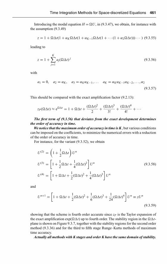
Ch09-H6594.tex 26/4/2007 16: 59 Page 461


Introducing the modal equation H = �U , in (9.3.47), we obtain, for instance withthe assumption (9.3.49)

z = 1 + ��t(1 + αK��t(1 + αK−1��t(1 + · · · (1 + α2��t))) · · · ) (9.3.55)

leading to

z = 1 +K∑

j=1

aj(��t) j (9.3.56)

with

a1 = 0, a2 = αK , a3 = αKαK−1, . . . aK = αKαK−1αK−2, . . . , α2

(9.3.57)

This should be compared with the exact amplification factor (9.2.13):

zP(��t) ≈ e��t = 1 + ��t + (��t)2

2+ (��t)3

3! + (��t)4

4! + · · ·

The first term of (9.3.56) that deviates from the exact development determinesthe order of accuracy in time.

We notice that the maximum order of accuracy in time is K , but various conditionscan be imposed on the coefficients, to minimize the numerical errors with a reductionof the order of accuracy in time.

For instance, for the variant (9.3.52), we obtain

U (2) =(

1 + 1

2��t

)U n

U (3) =[

1 + 1

2��t + 1

4(��t)2

]U n (9.3.58)

U (4) =[

1 + ��t + 1

2(��t)2 + 1

4(��t)3

]U n

and

U n+1 =[

1 + ��t + 1

2(��t)2 + 1

6(��t)3 + 1

24(��t)4

]U n ≡ zU n

(9.3.59)

showing that the scheme is fourth order accurate since zP is the Taylor expansion ofthe exact amplification exp(��t) up to fourth order. The stability region in the ��t-plane is shown on Figure 9.3.7, together with the stability regions for the second ordermethod (9.3.36) and for the third to fifth stage Runge–Kutta methods of maximumtime accuracy.

Actually all methods with K stages and order K have the same domain of stability.

Ch09-H6594.tex 26/4/2007 16: 59 Page 462


A very important property of the third and higher order RK methods is that theycontain a segment of the imaginary axis of the ��t-plane in their stability region.The length of this segment (−Iβ, +Iβ) is increasing with the stage number K ofthe method, depending on the order of accuracy which is not necessarily equal to itsmaximum value. Hence, the higher order RK methods are very well adapted for cen-trally discretized convection, with a conditional stability condition of |σ| ≤ β. Thisexplains their widespread use for the Euler and Navier–Stokes equations, as initiallyintroduced by Jameson et al. (1981). For the methods with maximum order of accu-racy, the imaginary segment inside the stability region is limited by β = √

3 = 1.73,β = 2

√2 = 2.828, β = 3.44 for the third, fourth and fifth order methods,

respectively.Note that this does not apply to first or second order RK methods, such as (9.3.36)

or (9.3.54), which do not include any portion of the imaginary axis. Hence, they arenot adapted to central discretizations of the convection terms. On the other hand, allRK methods are adapted to upwind discretized convection, since the correspondingeigenvalue spectrum is located in the left-hand side of the ��t-plane, as seen fromFigure 9.1.3.

For second order time accurate methods, the limit value β = K − 1 can be obtainedfor K-odd and certain combination of coefficients, Van der Houwen (1977). For evennumber of stages, for instance K = 4, Vichnevetsky (1983) has shown that the value(K − 1) is also an upper limit and Sonneveld and Van Leer (1984) showed that thislimit can indeed be reached for first order accurate methods and K > 2.

On the other hand, the limits of the RK stability domain on the real negative axiswill provide a stability limit on the dissipation terms, this dissipation being eithernumerical, as obtained from upwind-discretized convection operators, or physical,from centrally discretized diffusion equations.

The limits (−B) on the real axis are −2, −2.51, −2.78, −3.2 for the second, third,fourth and fifth, order respectively, as can be seen from Figure 9.3.5 (see also Lambert,1973, 1991).

For stationary problems it is important to be able to allow the highest possible timesteps and therefore the extension of the stability region is more important than theirorder. By relaxing the order, one can obtain Runge–Kutta methods of a given stagenumber, with higher stability regions; for instance a third order Runge–Kutta methodwith second order accuracy can be defined which cuts the real axis at (−4.52, 0),Lambert (1973).

Other applications of the large number of degrees of freedom available in theselection of the αk and βk coefficients of equation (9.3.47) can be directed towardthe selective damping of high frequency error components, suitable for integrationinto multigrid iterative methods (Jameson and Baker, 1983) or for aero-acousticapplications (Hu et al., 1996; Ramboer et al., 2006).

Example E.9.3.1 Diffusion equation ut = auxx with second order central spacedifferences

If the system

dui

dt= α

�x2(ui+1 − 2ui + ui−1) (E.9.3.1)

Ch09-H6594.tex 26/4/2007 16: 59 Page 463


0.0

0.4

x

y

0.0

�0.4

�0.8

�1.2

�1.6

�2.0

�2.4

�2.8

�3.2

0.8

1.2

1.6

2.0

RK-5

RK-4 RK-3

RK-2

RK-1

Forward Euler

2.4

2.8

3.2

0.4�0.4�0.8�1.2�1.6�2.0�2.4�2.8�3.2

Figure 9.3.7 Stability limits for Runge–Kutta methods in the complex ��t-plane,from 1 to 5 stages (RK-1 to RK-5).

is solved by a Runge–Kutta method whose stability domain cuts the real axis at(−B, 0), then the method will be stable for

0 ≤ α�t

�x2≤ B

4(E.9.3.2)

For instance, for the fourth order method the limit is 2.78/4, which is only marginallylarger than the single step, first Euler explicit method.

Ch09-H6594.tex 26/4/2007 16: 59 Page 464


Example E.9.3.2 Convection equation ut + aux = 0 with second order centralspace difference

The system

dui

dt= − a

2�x(ui+1 − ui−1) (E.9.3.3)

solved by a fourth order Runge–Kutta method has a stability range on the imaginaryaxis limited to ±I2·√2. Hence, with

��t = −Iσ sin φ (E.9.3.4)

the stability condition becomes

|σ| < 2√

2 (E.9.3.5)

This scheme therefore allows a Courant number close to three times the usual CFLlimit of one. However, for φ = π, that is for high frequencies, � = 0 and the amplifi-cation factor z becomes equal to one. Therefore, it is to be expected that this schemewill become unstable when applied to nonlinear hyperbolic problems with centraldifferences, if some dissipation is not added to the scheme. See Section 9.3.6, wherethe notion of artificial dissipation is introduced.

These two examples show that there is little to be gained in applying high orderRunge–Kutta methods to pure diffusion problems, with regard to maximum allowabletime step, when compared to the one-step explicit Euler method. However, this is notthe case for convection equations where high stage Runge–Kutta methods have anincreasing segment of the imaginary axis of the ��t-plane in their stability region.

Example E.9.3.3 Convection equation ut + aux = 0 with Fromm’s second orderupwind biased scheme

We consider here the system

dui

dt= − a

4�x(ui+1 + 3ui − 5ui−1 + ui−2) (E.9.3.6)

and envisage to solve it with a Runge–Kutta method. Plotting the stability domains ofthe space discretization for CFL = 0.5, 1, 1.25 and 1.5 in the ��t-plane, together withthe RK methods of order 1 to 4 on Figure 9.3.8, we observe that for the one-stage RK-1method, that is the Euler explicit method, the resulting scheme will be unstable. For thetwo-stage RK-2 method, we would have a stability condition of CFL ≤ 1. The three-stage RK-3 method has clearly a somewhat higher CFL limit of stability, although youclearly can see that the eigenvalues of the space discretization are not totally inside theRK-3 stability curve. The fourth order RK-4 method is still stable at CFL = 1.35, ascan be seen from Figure 9.3.9, but a plot for CFL = 1.4 shows that the combination isunstable. Applying the definitions seen earlier, we can now determine the accuracy ofthe resulting scheme by considering the amplification factor zP(�(φ)) in the complexz-plane (Figure 9.3.9a). From there we derive the dissipation and dispersion errors infunction of the phase angle, at constant CFL (Figure 9.3.9b and c).

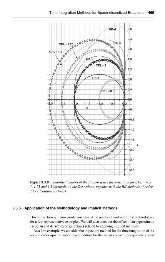
Ch09-H6594.tex 26/4/2007 16: 59 Page 465


0.8

1.2

2.4

x

0.0�0.5�1.0�1.5�2.0�2.5�3.0 0.0

1.6

y

2.8

2.0

0.4

�2.0

�0.8

�1.6

�0.4

�1.2

�2.4

�2.8

CFL�0.5

CFL�1

CFL�1.25

CFL�1.5

RK-1

RK-2

RK-3

RK-4

Figure 9.3.8 Stability domains of the Fromm space discretization for CFL = 0.5,1, 1.25 and 1.5 (symbols) in the ��t-plane, together with the RK methods of order1 to 4 (continuous lines).

9.3.5 Application of the Methodology and Implicit Methods

This subsection will now guide you toward the practical workout of the methodologyfor a few representative examples. We will also consider the effect of an approximateJacobian and derive some guidelines related to applying implicit methods.

As a first example, we consider the trapezium method for the time integration of thesecond order upwind space discretization for the linear convection equation. Based

Ch09-H6594.tex 26/4/2007 16: 59 Page 466


0.25

p3.02.52.01.51.00.0

(a)

0.5

0.0

1.0

0.75

0.5 CFL�0.5

CFL�1

CFL�1.35

(b)

1.8

1.5

1.0

0.6

0.5

0.2

p2.5 3.0

2.0

1.6

2.0

1.41.2

0.8

1.0

0.4

0.0

0.0

CFL�1CFL�0.5

CFL�1.35

0.6 1.00.4 0.80.20.0

0.6

0.4

�0.4

�0.2

�0.6

�0.8

�1.0

0.8

0.20.0�0.2�0.4�0.6�0.8�1.0

CFL�0.5CFL�1

CFL�1.35

(c)

1.0

Figure 9.3.9 Errors of the combination of a fourth order Runge–Kutta methodwith Fromm’s scheme at constant CFL, in function of the phase angle for the sameparameters as in Figure 9.3.8: (a) dissipation error; (b) dispersion error; (c) errorin the complex z-plane; at CFL = 0.5, 1 and 1.35.

on Table 9.1.1, we have the system of ODE’s in time

dui

dt= − a

2�x(3ui − 4ui−1 + ui−2) (9.3.60)

leading to the scheme, based on (9.3.16) (see Problem P.9.8)

un+1i = un

i − σ

4[(3ui − 4ui−1 + ui−2)n+1 + (3ui − 4ui−1 + ui−2)n] (9.3.61)

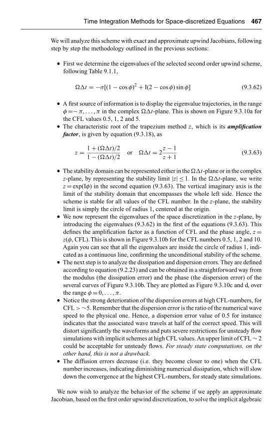
Ch09-H6594.tex 26/4/2007 16: 59 Page 467


We will analyze this scheme with exact and approximate upwind Jacobians, followingstep by step the methodology outlined in the previous sections:

• First we determine the eigenvalues of the selected second order upwind scheme,following Table 9.1.1,

��t = −σ[(1 − cos φ)2 + I(2 − cos φ) sin φ] (9.3.62)

• A first source of information is to display the eigenvalue trajectories, in the rangeφ =− π, . . . , π in the complex ��t-plane. This is shown on Figure 9.3.10a forthe CFL values 0.5, 1, 2 and 5.

• The characteristic root of the trapezium method z, which is its amplificationfactor, is given by equation (9.3.18), as

z = 1 + (��t)/2

1 − (��t)/2or ��t = 2

z − 1

z + 1(9.3.63)

• The stability domain can be represented either in the ��t-plane or in the complexz-plane, by representing the stability limit |z| ≤ 1. In the ��t-plane, we writez = exp(Iφ) in the second equation (9.3.63). The vertical imaginary axis is thelimit of the stability domain that encompasses the whole left side. Hence thescheme is stable for all values of the CFL number. In the z-plane, the stabilitylimit is simply the circle of radius 1, centered at the origin.

• We now represent the eigenvalues of the space discretization in the z-plane, byintroducing the eigenvalues (9.3.62) in the first of the equations (9.3.63). Thisdefines the amplification factor as a function of CFL and the phase angle, z =z(φ, CFL). This is shown in Figure 9.3.10b for the CFL numbers 0.5, 1, 2 and 10.Again you can see that all the eigenvalues are inside the circle of radius 1, indi-cated as a continuous line, confirming the unconditional stability of the scheme.

• The next step is to analyze the dissipation and dispersion errors. They are definedaccording to equation (9.2.23) and can be obtained in a straightforward way fromthe modulus (the dissipation error) and the phase (the dispersion error) of theseveral curves of Figure 9.3.10b. They are plotted as Figure 9.3.10c and d, overthe range φ = 0, . . . , π.

• Notice the strong deterioration of the dispersion errors at high CFL-numbers, forCFL > ∼5. Remember that the dispersion error is the ratio of the numerical wavespeed to the physical one. Hence, a dispersion error value of 0.5 for instanceindicates that the associated wave travels at half of the correct speed. This willdistort significantly the waveforms and puts severe restrictions for unsteady flowsimulations with implicit schemes at high CFL values. An upper limit of CFL ∼ 2could be acceptable for unsteady flows. For steady state computations, on theother hand, this is not a drawback.

• The diffusion errors decrease (i.e. they become closer to one) when the CFLnumber increases, indicating diminishing numerical dissipation, which will slowdown the convergence at the highest CFL-numbers, for steady state simulations.

We now wish to analyze the behavior of the scheme if we apply an approximateJacobian, based on the first order upwind discretization, to solve the implicit algebraic

Figure 9.3.10 Stability and error analysis for the combination of the trapeziumimplicit time integration applied to the second order upwind space discretization forthe linear convection equation. CFL values: 0.5, 1, 2, 10. (a) Eigenvalues of thesecond order upwind scheme in the ��t-plane; (b) Amplification factors for thesecond order upwind scheme with the trapezium method in the z-plane. (c) Diffusionerror. (d) Dispersion error.

system. This leads to

�uni + σ(�ui − �ui−1)n = −σ

2(3ui − 4ui−1 + ui−2)n (9.3.64)

Hence, we apply the same steps, but with the modified characteristic polynomial(9.3.28), whose roots are the modified amplification factors. For the trapezium


Ch09-H6594.tex 26/4/2007 16: 59 Page 469


method, ξ = φ = 0, θ = 1/2, we obtain the solution, after removal of the trivialroot z = 0:

zmod = 2 − (�(1)�t) + 2(��t)

2 − (�(1)�t)(9.3.65)

• Introduce the first upwind eigenvalues from Table 9.1.1:

�(1)�t = −σ[(1 − cos φ) + I sin φ] (9.3.66)

• We can now represent the modified amplification factors for various CFL num-bers in the range φ = −π, . . . , π in the complex z-plane and the associated errors.This is shown on Figure 9.3.11.

• You immediately notice that the modified scheme, with the first order Jacobian,has lost its unconditional stability, since the curves for CFL > 1 all move partlyoutside the stability domain of the unit circle. This can also be seen on thediffusion error curves, which become larger than one for these CFL values.

• This is a very severe penalty, since the stability limit is now restricted to anexplicit type limit of CFL ≤ 1. Hence, this approach becomes useless, as theadvantages of running an implicit method with large time steps is totally lost.This explains why in practice, trapezium methods are never used with upwindspace discretizations and an approximate Jacobian.

You can repeat these developments with a central discretization and you will thenobserve that the application of the approximate Jacobian does not restrict the uncon-ditional stability and has only a marginal impact on the accuracy. This explains thesuccessful application of the Beam and Warming schemes (9.3.27), coupled to acentral space discretization of the convective flux terms.

A very similar behavior is observed when the trapezium method is applied to otherupwind options of Table 9.1.1. Therefore, other A-stable methods have to be con-sidered for applications with upwind space discretizations; for instance a backwarddifferencing, or Gear’s method, with second order upwind discretization leads to anunconditionally stable scheme, even with the approximate first order Jacobian (seeProblem P.9.9).

9.3.6 The Importance of Artificial Dissipation with Central Schemes

We have seen that central discretizations of the convection terms lead to purely imag-inary eigenvalues with the consequence that the high frequencies, corresponding tothe 2�x shortest waves on the mesh, or φ = π, are not damped by the scheme, ascan be seen on Figure 9.3.4. This can also lead to marginal stability conditions withimplicit time integration methods, since the stability condition reduces to the modulusof the amplification factor equal to one for all values of the phase angle. This createsa risk for weak instabilities generated by the nonlinearity of the convection terms inthe conservation laws. We have already encountered this problem with the leapfrogmethod in Chapter 7.

One way of introducing some high frequency dissipative component, that is pro-viding some real negative part to the eigenvalues, is the selection of an upwinddiscretization for the convection terms.

Ch09-H6594.tex 26/4/2007 16: 59 Page 470


Figure 9.3.11 Stability and error analysis for the combination of the trapeziumimplicit time integration applied to the second order upwind space discretization forthe linear convection equation, with an approximate, first order upwind, Jacobian.CFL values: 0.5, 1, 2 and 10. (a) Amplification factors for the second order upwindscheme with the trapezium method in the z-plane, based on exact Jacobian.(b) Amplification factors for the second order upwind scheme with the trapeziummethod in the z-plane with an approximate first order upwind Jacobian. (c) Diffusionerror with approximate Jacobian. (d) Dispersion error with approximate Jacobian.

The other alternative is to add artificial dissipation terms, also referred to as artifi-cial viscosity terms (AVT) to the centrally discretized convection operator.1The objec-tive is to add a dissipative contribution to the scheme, that is an even order derivative,

1 There is some terminology confusion in the literature between numerical dissipation and artificialdissipation. Take good notice that numerical dissipation refers to the dissipation generated by theselected discretization, while artificial dissipation refers to the contributions from terms added tothe selected scheme, in a somewhat ‘artificial’ way, as opposed to the ‘natural’ dissipation present inthe selected discretization of the model derivatives.

Ch09-H6594.tex 26/4/2007 16: 59 Page 471


with a truncation error lower than the truncation error of the selected discretization.For instance, with a second order discretization, the artificial dissipation term couldbe of order four, while selecting a fourth order discretization of the convection term,would require at least a sixth order derivative artificial dissipation term.

Let us consider the standard second order discretization of the convection term(

a∂u

∂x

)i= − a

2�x(ui+1 − ui−1) (9.3.67)

to which we add a fourth order artificial dissipation term (AVT4) of the form:

γ�x3(

∂4u

∂x4

)i

∼= γ

�x(ui+2 − 4ui+1 + 6ui − 4ui−1 + ui−2) (9.3.68)

As the truncation error of the central discretization is of second order, the addedfourth order term should not affect the global accuracy of the simulation. Actually,we solve the model

ut + aux = γ�x3 ∂4u

∂x4(9.3.69)

instead of the homogenous convection equation.Let us investigate the influence of this term and the eventual stability condition

on the dissipation coefficient γ , for several time integration methods. We proceedaccording to the steps outlined in the previous section:

• We first determine the eigenvalues of the combined space discretization, that isthe Fourier symbol, leading to, with ε = γ�t/�x

��t = −Iσ sin φ − 4ε(1 − cos φ)2 (9.3.70)

• The eigenvalues deviate now from the imaginary axis, due to the real, negativecontribution of the added dissipation terms. They are represented in the ��t-plane on Figure 9.3.12a, for CFL = 2 and values of ε = 1/20, 1/8, 1/5 and 1/2.

• Selecting the trapezium method and applying equation (9.3.63), we obtain thescheme:

un+1i = un

i − σ

4[(ui+1 − ui−1)n+1 + (ui+1 − ui−1)n]

+ ε

2[(ui+2 − 4ui+1 + 6ui − 4ui−1 + ui−2)n+1

+ (ui+2 − 4ui+1 + 6ui − 4ui−1 + ui−2)n] (9.3.71)

• Deriving the stability curves, you can observe that they deviate from the unit cir-cle when ε = 0, as shown in Figure 9.3.12b, for CFL = 2 and values of ε = 1/20,1/8, 1/5 and 1/2, but they still remain fully inside the stability circle for all valuesof ε. This can also be seen from the stability condition |z| ≤ 1, in particular forφ = π, where the artificial dissipation reaches its maximum effect, leading to

z(φ = π) = 2 − 16ε

2 + 16ε(9.3.72)

Ch09-H6594.tex 26/4/2007 16: 59 Page 472


�0.8

0

�1.6 0.0

1

�1�2.4�4.8

2

�2

�3.2 0.8�4.0�5.6�6.4�7.2�8.0

(a)

ε�1/2ε�1/5

ε�1/8ε�1/20

�0.6

�0.8

0.8

�0.2

0.4

0.0

0.2

0.6

�0.4

�1.0

�0.8�0.6�0.4�0.2 0.0 2.0 0.4 0.6�1.0 1.00.8

1.0

ε�1/5

ε�1/2

ε�1/8

ε�1/20

(b)

�1.6�1.4

ε�1/2ε�1/5 ε�1/8

ε�1/20

�1.2�1.0�0.8�0.6�0.4�0.2 0.0 0.2 0.4 0.6 0.8 1.0

�1.0

�0.8

�0.6

�0.4

�0.2

0.0

0.2

0.4

0.6

0.8

1.0

(c)

Figure 9.3.12 Eigenvalues in the ��t-plane (a) and stability curves in thez-plane for the exact (b) and modified Jacobians (c) for CFL = 2; ε = 1/20, 1/8, 1/5and 1/2, for the central scheme with fourth order artificial dissipation and thetrapezium method. This is the Beam and Warming scheme.

• It is easily shown that the stability condition is satisfied for all positive val-ues of the dissipation coefficient. Hence, the trapezium scheme with centraldiscretization and AVT remains unconditionally stable.

• When the approximate, first order Jacobian is applied, the scheme is modified to

�uni + σ(�ui − �ui−1)n = −σ

2(3ui − 4ui−1 + ui−2)n

+ ε(ui+2 − 4ui+1 + 6ui − 4ui−1 + ui−2)n

(9.3.73)

• Applying now equation (9.3.65), for φ = π, we obtain

zmod(φ = π) = 1 + σ − 16ε

1 + σ(9.3.74)

Ch09-H6594.tex 26/4/2007 16: 59 Page 473


which leads to the stability condition on the dissipation coefficient

0 ≤ ε ≤ 1 + σ

8(9.3.75)

• Hence, the dissipation coefficient has to satisfy the condition 0 < ε < 1/8, inorder to satisfy the stability condition for all values of the CFL number. Thisis not a very severe condition, since the ε-parameter has to remain small forreasons of accuracy.

• The corresponding stability diagram is shown on Figure 9.3.12c, for the samevalues of the parameters, where the instability for ε = 1/2 can clearly be seen, asthe corresponding curve is partly outside the stability circle.

The combination of space centered discretizations with fourth order Runge–Kuttamethods is a very widely applied scheme for the convection terms for general Eulerand Navier–Stokes equations, following its introduction by Jameson et al. (1981). Itforms the basis for many CFD codes and the addition of a fourth order dissipationplays an important role in the elimination of high frequency errors.

Figure 9.3.13a shows the stability domains in the ��t-plane, for the valuesCFL = 2 and ε = 1/20; 1/8; 1/5, superimposed on the stability domains of the sec-ond, third and fourth order Runge–Kutta methods. You can clearly see that the valueε = 1/5 leads to an unstable scheme, as the value on the negative real axis, for φ = π,equal to −16ε, is outside the stability region of the fourth order RK method. Thestability condition is easily derived, if we denote by −B the intersection of the RKstability curve with the real axis, leading to

ε ≤ B

16(9.3.76)

for stability. For the fourth order RK method, we have B ≈ 2.78, giving the conditionε < 0.174.

Figure 9.3.13b and c show in addition the effect of the artificial dissipation termson the diffusion error of the scheme, in particular on the high frequency behavior, thescheme being now dissipative. The dissipation error larger than one for the highestε-value reflects the instability of the scheme for this value.

HANDS-ON TASK 6Apply the methodology described above to analyze combinations of a set of timeintegration methods, with various discretizations of the convection and diffusionmodel equations, along the lines of Section 9.3.5.

Follow the steps as outlined with the objective to understand the properties interms of stability limits and accuracy in function of the scheme parameters:

• Comment and analyze these results.

Apply symbolic mathematical software tools, such as MAPLE, Mathematicaor MATLAB.

Ch09-H6594.tex 26/4/2007 16: 59 Page 474


2.8

2.4

2.0

�0.4�3.0 �2.5 �2.0 �1.5 �1.0 �0.5 0.0

�0.8

�1.2

�1.6

�2.0

�2.4

�2.8

1.6

1.2

0.4

0.8

0.0

(a)

x

y

ε�1/5

ε�1/20

ε�1/8

Rk-1

Rk-2

Rk-3Rk-4

2.51.5p

0.5

(b)

3.02.01.00.0

1.0

0.95

0.9

0.8

0.75

0.85

CFL�0.5

CFL�1.25

CFL�2

p

(c)

2.5

1.0

1.5

0.5

1.75

1.5

3.0

1.25

2.01.0

0.75

0.50.0

0.25 ε�1/8

ε�1/20

ε�1/5

Figure 9.3.13 Space centered discretization with fourth order Runge–Kuttamethod and fourth order artificial dissipation. (a) Eigenvalues in the ��t-planefor CFL = 2, ε = 1/20, 1/8 and 1/5; (b) dissipation error curves for ε = 0, forCFL = 0.5, 1.25 and 2, compared to the curves (c) at CFL = 2 fordissipation coefficients of 1/20, 1/8 and 1/5. The last value leads to anunstable scheme.

Ch09-H6594.tex 26/4/2007 16: 59 Page 475


HANDS-ON TASK 7Experiment with several of the methods discussed in this chapter by applying themto solve the test cases of Chapter 7, as described in the Hands-On Tasks 2 and 3,as well as the cases of Problems P.7.5:

• Refer also to Problems P.9.13, P.9.14, P.9.19, P.9.20 as part of this task.• Experiment by yourself with various combinations of time integration

methods and space discretizations for the convection and diffusion equations.• Write a general program to solve the mentioned problems.

A9.4 IMPLICIT SCHEMES FOR MULTIDIMENSIONAL PROBLEMS:APPROXIMATE FACTORIZATION METHODS

When implicit schemes are applied to multidimensional problems, the resultingimplicit matrix system is not tridiagonal anymore as for three point discretizationson one-dimensional equations. For instance, the two-dimensional parabolic diffusionequation, with constant diffusion coefficient α,

ut = α(uxx + uyy) (9.4.1)

discretized with a five point finite difference Laplace scheme, leads to the system(�x = �y):

duij

dt= α

�x2(ui+1, j + ui−1, j + ui, j+1 + ui, j−1 − 4uij) (9.4.2)

With a backward Euler scheme for instance, we obtain a pentadiagonal matrix system

un+1ij − un

ij = α�t

�x2(un+1

i+1, j + un+1i−1, j + un+1

i, j+1 + un+1i, j−1 − 4un+1

ij ) (9.4.3)

On an arbitrary mesh, or with higher order discretizations, or with finite elements,more mesh points appear in the Laplace discretization at point i, j, and the implicitmatrix will have a more complicated structure than the pentadiagonal one.

The principle of the Approximate Factorization or Alternating Direction Implicitmethod (ADI), is to separate the operators into one-dimensional components and splitthe scheme into two (or three, for three-dimensional problems) steps, each one involv-ing only the implicit operations originating from a single coordinate. This method hasbeen introduced by Peaceman and Rachford (1955), Douglas and Rachford (1956)and generalized by Douglas and Gunn (1964). Many developments and extensionshave been brought to this approach by Russian authors and given different names,Fractional step method by Yanenko (1971) or Splitting method by Marchuk (1975).An excellent description of ADI methods can be found in Mitchell (1969), Mitchelland Griffiths (1980).

If the matrix operator S on the right-hand side of

dU

dt= S · U + Q (9.4.4)

Ch09-H6594.tex 26/4/2007 16: 59 Page 476


is separated into submatrices acting on the U components in a single direction, that isS = Sx + Sy + Sz , each operator in the right-hand side acting on the variable indicatedas subscript, then equation (9.4.4) becomes

dU

dt= (Sx + Sy + Sz) · U + Q (9.4.5)

In equation (9.4.2), Sx and Sy represent the second order derivatives in the x and ydirection, respectively, with the shift operators Ex and Ey,

Sx · U = α

�x2(Ex − 2 + E−1

x )U (9.4.6)

Sy · U = α

�y2(Ey − 2 + E−1

y )U (9.4.7)

or explicitly

Sx · uij = α

�x2(ui+1, j − 2uij + ui−1, j) (9.4.8)

Sy · uij = α

�y2(ui, j+1 − 2uij + ui, j−1) (9.4.9)

With the implicit scheme (9.3.13), with ξ = 0, θ = 1, defining the first order in time,backward Euler method, we obtain

U n+1 − U n = �t(Sx + Sy + Sz) · U n+1 + Q�t (9.4.10)

The implicit operators appear from

[1 − �t(Sx + Sy + Sz)] · U n+1 = U n + Q�t (9.4.11)

The basic idea behind the ADI method consists in a factorization of the right-handside operator in a product of one-dimensional operators. This equation is replaced by

[(1 − τ�tSx)(1 − τ�tSy)(1 − τ�tSz)] · U n+1 = U n + Q�t (9.4.12)

where τ is a free parameter. Developing equation (9.4.12), leads to

U n+1 − U n = τ�t(Sx + Sy + Sz) · U n+1 + τQ�t

− τ2�t2(SxSy + SySz + SzSx) · U n+1 + τ3�t3(SxSySz) · U n+1

(9.4.13)

to be compared with equation (9.4.10).The factorization (9.4.12) has introduced two additional terms, which represent

errors with respect to the original scheme to be solved. However, these are higherorder errors, proportional to �t2 and �t3, and since the backward Euler method is

Ch09-H6594.tex 26/4/2007 16: 59 Page 477


first order in time, these error terms are of the same order as the truncation error anddo not affect the overall accuracy of the scheme.

The parameter τ appears as a relaxation parameter and has to be taken equal toone, if this scheme is to be used for time-dependent simulations.

However, the ADI technique is mostly of application for stationary problems,whereby one attempts to reach the convergence limit as fast as possible. In this connec-tion, the relaxation parameter can be chosen to accelerate this convergence process,since it represents a scaling of the time step (see Chapter 10 for more details).

The factorized scheme is then solved in three steps:

(1 − τ�tSx) · U n+1 = [1 + τ�t(Sy + Sz)] · U n + τ�tQ

(1 − τ�tSy) · U n+1 = U n+1 − τ�tSyU n (9.4.14)

(1 − τ�tSz) · U n+1 = U n+1 − τ�tSzU n

Introducing the variations

�U n = U n+1 − U n �U n = U n+1 − U n �U n = U n+1 − U n

the ADI scheme can be rewritten as

(1 − τ�tSx) · �U n = τ�t(S · U n + Q)

(1 − τ�tSy) · �U n = �U n (9.4.15)

(1 − τ�tSz) · �U n = �U n

This is sometimes called the �-formulation.By recombining the factors, the ADI approximation can be redefined by the

formulation:

[(1 − τ�tSx)(1 − τ�tSy)(1 − τ�tSz)] · �U n = τ�t(S · U n + Q) (9.4.16)

For τ = 1, we obtain the Douglas–Rachford scheme.The Splitting or fractional step method , leads to another ADI formulation, based

on a factorization of the Crank–Nicholson scheme and is therefore second order intime. Equation (9.4.10) is replaced by

U n+1 − U n = �t(Sx + Sy + Sz) · U n+1 + U n

2+ Q�t (9.4.17)

or [1 − �t

2(Sx + Sy + Sz)

]·U n+1 =

[1 + �t

2(Sx + Sy + Sz)

]·U n +Q�t (9.4.18)

This equation is factorized as follows:[(

1 − �t

2Sx

)(1 − �t

2Sy

)(1 − �t

2Sz

)]· U n+1

=[(

1 + �t

2Sx

)(1 + �t

2Sy

)(1 + �t

2Sz

)]· U n + Q�t (9.4.19)

Ch09-H6594.tex 26/4/2007 16: 59 Page 478


and represents an approximation to equation (9.4.17) of second order accuracy, sinceequation (9.4.19) is equal to

[1 − �t

2(Sx + Sy + Sz)

]· U n+1 =

[1 + �t

2(Sx + Sy + Sz)

]· U n + Q�t

− �t2

4(SxSy + SySz + SzSx) · (U n+1 − U n) + �t3

8(SxSySz) · (U n+1 − U n)

(9.4.20)

Since (U n+1 − U n) is of order �t, the error terms are 0(�t3). Equation (9.4.19) isthen solved as a succession of one-dimensional Crank–Nicholson schemes

(1 − �t

2Sx

)· U n+1 =

(1 + �t

2Sx

)· U n + �tQ

(1 − �t

2Sy

)· U n+1 =

(1 + �t

2Sy

)· U n+1 (9.4.21)

(1 − �t

2Sz

)· U n+1 =

(1 + �t

2Sz

)· U n+1

When the Si commute we recover (9.4.19) by elimination of U n+1 and U n+1. If theSi operators do not commute, the approximation (9.4.21) is still valid, but is reducedto first order in time.

A9.4.1 Two-Dimensional Diffusion Equation

Considering equation (9.4.1), with the central space discretizations, we can write thefactorized ADI scheme (9.4.14) as

(1 − τ�tSx) · U n+1 = (1 + τ�tSy) · U n

(1 − τ�tSy) · U n+1 = U n+1 − τ�tSyU n (9.4.22)

Written out explicitly, we obtain the following tridiagonal systems, with �x = �yand β = α�t/�x2,

un+1ij − τβ(un+1

i+1, j − 2un+1ij + un+1

i−1, j) = unij + τβ(un

i, j+1 − 2unij + un

i, j−1)

un+1ij − τβ(un+1

i, j+1 − 2un+1ij + un+1

i, j−1) = un+1ij − τβ(un

i, j+1 − 2unij + un

i, j−1)

(9.4.23)

The first equation is solved as a tridiagonal system along all the horizontal j-lines,sweeping the mesh from j = 1 to j = jmax. After this first step, the intermediate solution

un+1ij is obtained at all mesh points. The second equation represents a succession of

tridiagonal systems along the i-columns and the solution un+1ij is obtained after having

swept through the mesh along the vertical lines, from i = 1 to i = imax.

Ch09-H6594.tex 26/4/2007 16: 59 Page 479


A Von Neumann stability analysis can be performed for this system by defining anintermediate amplification factor G, by

U n+1 = G · U n (9.4.24)

For the first step, with φx and φy being the Fourier variables in the x- and y-directions,respectively, we have

G = 1 − 4τβ sin2 φy/2

1 + 4τβ sin2 φx/2(9.4.25)

G = G + 4τβ sin2 φy/2

1 + 4τβ sin2 φy/2(9.4.26)

and by combining these two equations

G = 1 + 16τ2β2 sin2 φx/2 · sin2 φy/2

(1 + 4τβ sin2 φx/2)(1 + 4τβ sin2 φy/2)(9.4.27)

The scheme is clearly unconditionally stable since |G| < 1. A similar calculation forthree dimensions confirms this property.

Another version of the ADI technique is the Peaceman–Rachford method, basedon the following formulation, with τ = 1/2, in two dimensions

(1 − �t

2Sx

)· U n+1 = (1 + τ�tSy) · U n

(9.4.28)(1 − �t

2Sy

)· U n+1 =

(1 + �t

2Sx

)· U n+1

We leave it to you to show that this scheme is also unconditionally stable for thediffusion equation of the previous example.

In addition, this form of the ADI method is second order accurate in time, as canbe seen by eliminating the intermediate solution U n+1. We obtain

U n+1 − U n = �t(Sx + Sy) · U n+1 + U n

2− �t2

4SxSy · (U n+1 − U n) (9.4.29)

and since U n+1 − U n is of order �t, the last term is 0(�t3). The intermediate val-

ues �U and �U have not necessarily a physical meaning and boundary conditionshave to be defined for these variables in accordance with the physical boundaryconditions of U .

Boundary conditions for the intermediate steps can be obtained from the structureof the system (9.4.13). In particular for Dirichlet conditions, we would write for theboundary values ( )B:

�U∣∣∣B

= (1 − τ�tSz) · (U n+1 − U n)B(9.4.30)

�U∣∣B = (1 − τ�tSy)(1 − τ�tSz) · (U n+1 − U n)B

More details can be found in Mitchell and Griffiths (1980).

Ch09-H6594.tex 26/4/2007 16: 59 Page 480


A9.4.2 ADI Method for the Convection Equation

Considering the three-dimensional convection equation

ut + aux + buy + cuz = 0 (9.4.31)

the operators Sx, Sy and Sz can be written, for a second order central difference of thespace derivatives, as

�tSxuijk = − a�t

2�x(ui+1, jk − ui−1, jk ) ≡ −σx

2(ui+1, jk − ui−1, jk )

�tSyuijk = − b�t

2�y(ui, j+1,k − ui, j−1,k ) ≡ −σy

2(ui, j+1,k − ui, j−1,k ) (9.4.32)

�tSzuijk = − c�t

2�z(uij,k+1 − uij,k−1) ≡ −σz

2(uij,k+1 − uij,k−1)

Considering first the two-dimensional case, the ADI scheme (9.4.14) can be written

un+1ij + τ

σx

2(un+1

i+1, j − un+1i−1, j) = un

ij − τσy

2(ui, j+1 − ui, j−1)

(9.4.33)un+1

ij + τσy

2(un+1

i, j+1 − un+1i, j−1) = un+1

ij + τσy

2(un

i, j+1 − uni, j−1)

The amplification factors are given by

G = 1 − Iτσy sin φy

1 + Iτσx sin φx(9.4.34)

G = G + Iτσy sin φy

1 + Iτσy sin φy= 1 − τ2σxσy sin φx sin φy

(1 + Iτσx sin φx)(1 + Iτσy sin φy)(9.4.35)

Since G is of the form

G = 1 − τ2σxσy sin φx sin φy

1 − τ2σxσy sin φx sin φy + Iτ(σx sin φx + σy sin φy)(9.4.36)

we have always |G| ≤ 1 and the scheme is unconditionally stable.However, in three dimensions, this is not the case anymore; theADI scheme applied

to the three-dimensional convection equation, centrally discretized (without dissipa-tion contributions) is unconditionally unstable as shown by Abarbanel et al. (1982).

In three dimensions, the above procedure leads to the following amplificationmatrix writing sx = σx sin φx and similarly for the y and z components,

G = 1 − τ2(sxsy + sysz + szsx) − Iτ3sxsysz

(1 + Iτsx)(1 + Iτsy)(1 + Iτsz)(9.4.37)

It can be shown that there are always values of sx, sy, sz such that |G| > 1. Thefollowing proof is due to Saul Abarbanel and Eli Turkel (private communication).

Ch09-H6594.tex 26/4/2007 16: 59 Page 481


The amplification matrix G is written as

G = α1 + Iβ1

α1 + Iβ2(9.4.38)

and since the real parts are equal, stability is obtained if

|β1| ≤ |β2| (9.4.39)

With

β2 = β1 + τ(sx + sy + sz) ≡ β1 + γ

the condition (11.4.39) implies

(β1 + γ)2 ≥ β21

or

γ(2β1 + γ) ≥ 0

If we select values of φx, φy, φz such that γ > 0, assuming τ > 0, the stability condition(9.4.39) becomes

2τ2sxsysz ≤ (sx + sy + sz) = γ/τ (9.4.40)

However, we can always find values of these variables which do not satisfy thisinequality. For instance, take γ = ε through

sx = −1/4 sy = −1/4 sz = ε + 1/2 (9.4.41)

the above condition becomes

ε ≥ τ2

16(1 + 2ε)

or

τ2 ≥ 16ε

1 + 2ε(9.4.42)

We can always select a value of ε sufficiently small, such that this condition is neversatisfied for any fixed finite value of τ, since the right-hand side goes to zero with ε.For instance, for τ = 1, ε < 1/14 leads to an unstable scheme.

This instability is associated with low frequencies, since equation (9.4.41) impliesthat sx + sy + sz = ε/τ is a small quantity and can only be satisfied by small values ofthe wave numbers φx, φy, φz . In addition it can be considered as a weak instabilitysince, from equation (9.4.38), for ε small

|G|2 = α21 + β2

1

α21 + (β1 + ε)2

≈ 1 − 2εβ1

α21 + β2

1

(9.4.43)

Ch09-H6594.tex 26/4/2007 16: 59 Page 482


where β1 is defined, in the assumption (9.4.41), by

β1 = − τ3

16

(1

2+ ε

)< 0

and is a small negative quantity. Hence, |G| is higher than one by an amount pro-portional to ε and therefore the amplification of errors should remain limited. This isconfirmed by computations performed by Compton and Whitesides (1983) with thefull system of Euler equations. However, the addition of adequate damping terms canremove the instability as shown by Abarbanel et al. (1982).

Actually, the three-dimensional fractional step method (9.4.21) is stable in threedimensions for the convection equation, although neutrally stable since it is a productof one-dimensional Crank–Nicholson schemes.

An essential difference between the fractional step method and the ADI methodin its form (9.4.15), is connected to their behavior for stationary problems. In thiscase, convergence toward steady state �U n = 0 is sought implying (SU n + Q) = 0,according to equation (9.4.16), when this limit is reached. Hence, the steady statelimit resulting from the computation will be independent of the time step �t, since Sis a pure space discretization. Equation (9.4.20), on the other hand, shows that in thelimit �U n → 0, we solve, with (U n+1 + U n)/2 ≈ U n

[1 − �t2

4(SxSy + SySz + SzSx)

]· �U n = �t(S · U n + Q) + �t3

4SxSySz · U n

(9.4.44)

which produces a stationary solution with a vanishing right-hand side. That is, theobtained stationary solution satisfies

S · U n + Q = −�t2

4SxSySz · U n (9.4.45)

and is function of the time step. In addition, for large time steps, which is what weaim at with implicit methods, the right hand side might become unacceptably high.


This chapter generalizes the approach of the previous Chapter 7, by extending therange of schemes toward the modern approach of separate space and time discretiza-tions, as opposed to the Lax–Wendroff family where the time and space discretizationsare intertwined.

The essential outcome of this chapter is the methodology enabling you to analyzethe association of a time integration method to a pre-selected space discretization.The developed methodology establishes the stability conditions and the accuracy, interms of dispersion and diffusion errors. We summarize the methodology as follows:

• Select a space discretization method for the flux terms and define the semi-discretized system of ODEs in time.

Ch09-H6594.tex 26/4/2007 16: 59 Page 483


• Apply a Fourier mode analysis to the space discretization to derive its spectrumof eigenvalues (its Fourier symbol) in function of the phase angle φ = k�x,covering the range (−π, +π).

• Verify that the real part of the eigenvalues is in the negative part of the ��t-plane,for the space discretization to be acceptable.

• Select a time integration method for the system of semi-discretized system ofordinary differential equations (ODEs) in time.

• Apply the selected method to the canonical form of the system of ODE’s in timedw/dt = �w and derive the stability domain of the time integration method inthe complex ��t-plane.

• Verify now the compatibility between the space and the time discretizations, byplotting the trajectories of the eigenvalues of the space discretization in the ��t-plane, or in the z-plane. The conditions ensuring that these eigenvalues remainfully within the time integration stability domain will determine the stabilityconditions of the combined scheme.

• Investigate the dissipation and dispersion errors of the combined scheme, todetermine the accuracy level of the selected combination, by analyzing theamplification factor behavior in function of the phase angle.

• A most important topic to remember is related to the amount of dissipation of thespace discretization scheme, with the necessity of adding artificial dissipationterms to centrally discretized convection terms.

A distinction has to be made between steady and unsteady simulations:

• For steady problems, the transient is not physical and should decrease as fastas possible. Hence, large dissipation errors are favorable for convergence anddispersion errors are not significant.

• Unsteady simulations are much more demanding in terms of accuracy as theyrequire very low dispersion and diffusion errors. Refer you to the relevantdiscussion of Section 7.4 and the final conclusions of this chapter.

• Implicit methods, at high CFL, have very strong numerical dissipation, which isexcellent for steady problems, since all modes will be rapidly damped, lead-ing to fast convergence. For unsteady problems, this is unacceptable and asevere restriction of the maximum CFL might be required to maintain the desiredaccuracy.

REFERENCES

Abarbanel, S., Dwoyer, D.D. and Gottlieb, D. (1982). Stable implicit finite differencemethods for three dimensional hyperbolic systems. ICASE Report 82-39. ICASE,NASA Langley RC, Hampton, Virginia, USA.

Beam, R.M. and Warming, R.F. (1976). An implicit finite-difference algorithm forhyperbolic systems in conservation law form. J. Comput. Phys., 22, 87–109.

Beam, R.M. and Warming, R.F. (1978). An implicit factored scheme for the compressibleNavier–Stokes equations. AIAA J., 16, 393–402.

Beam, R.M. and Warming, R.F. (1980). Alternating direction implicit methods forparabolic equations with a mixed derivative. SIAM J. Sci. Stat. Comp., 1, 131–159.

Ch09-H6594.tex 26/4/2007 16: 59 Page 484


Beam, R.M. andWarming, R.F. (1982). Implicit Numerical Methods for the CompressibleNavier–Stokes and Euler Equations. Von Karman Institute Lecture Series 1982-04,Rhode Saint Genese, Belgium.

Brailovskaya, I. (1965). A difference scheme for numerical solutions of the two-dimensional nonstationary Navier–Stokes equations for a compressible gas. Sov. Phys.Dokl., 10, 107–110.

Briley, W.R. and Mc Donald, H. (1975). Solution of the three-dimensional compressibleNavier–Stokes equations by an implicit technique. Proceedings of the Fourth Interna-tional Conference on Numerical Methods in Fluid Dynamics, Lecture Notes in Physics,Vol. 35, Springer, Berlin.

Briley, W.R. and Mc Donald, H. (1980). On the structure and use of linearized blockimplicit schemes. J. Comp. Phys., 6, 428–453.

Compton II, W.B. and Whitesides, J.L. (1983). Three-dimensional Euler solutions forlong duct nacelles. AIAA 21st Aerospace Sciences Meeting, AIAA Paper 83-0089.

Dahlquist, G. (1963). A Special Stability Problem for Linear Multistep Methods. BIT,Copenhagen, Vol. 3, 27–43.

Dahlquist, G. and Bjorck, A. (1974). Numerical Methods. Prentice Hall, New Jersey.Douglas, J. and Gunn, J.E. (1964). A general formulation of alternating direction methods:

parabolic and hyperbolic problems. Numerische Mathematik, 6, 428–453.Douglas J. and Rachford, H.H. (1956). On the numerical solution of heat conduction

problems in two and three space variables. Trans. Am. Math. Soc., Vol. 82, 421–439.Gear, G.W. (1971). Numerical Initial Value Problems in Ordinary Differential Equations.

Prentice-Hall, New Jersey.Gustafsson, B. and Kreiss, H.O. (1979). Boundary conditions for time dependent

problems with an artificial boundary. J. Comput. Phys., 30, 333–351.Gustafsson, B., Kreiss, H.O. and Sundstršm, A. (1972). Stability theory of differ-

ence approximations for mixed initial boundary value problems. Math. Comput., 26,649–686.

Hu, F.Q., Hussaini, M.Y. and Manthey, J.L. (1996). Low-dissipation and low-dispersionRunge–Kutta schemes for computational acoustics. J. Comput. Phys., 124, 177–191.

Hairer, E., Wanner, G. (1996). Solving Ordinary Differential Equations II – Stiff andDifferential-Algebraic Problems. Springer Verlag, Berlin.

Hairer, E., Norsett, S.P. and Wanner, G. (1993). Solving Ordinary Differential EquationsI – Non-stiff Problems. Springer Verlag, Berlin.

Hundsdorfer, W. and Verwer, J.G. (2003). Numerical Solution of Time-DependentAdvection–Diffusion-Reaction Equations. Springer Verlag, Berlin.

Jameson, A. and Baker, T.J. (1983). Solutions of the Euler equations for complexconfigurations. AIAA 6th Computational Fluid Dynamics Conference. AIAA Paper83-1929.

Jameson, A. and Baker, T.J. (1984). Multigrid solution of the Euler equations for aircraftconfigurations. AIAA Paper 84-0093, AIAA 22nd Aerospace Sciences Meeting.

Jameson, A., Schmidt, W., and Turkel, E. (1981). Numerical simulation of the Eulerequations by finite volume methods using Runge–Kutta time stepping schemes. AIAA5th Computational Fluid Dynamics Conference, AIAA Paper 81-1259.

Kreiss, H.O. (1968). Stability theory for difference approximations of mixed initialboundary value problems, I. Math. Comput., 22, 703–714.

Kreiss, H.O. (1970). Initial boundary value problem for hyperbolic systems. Comm. Pureand Appl. Math., 23, 273–298.

Kurbatskii, K.A. and Mankbadi, R.R. (2004). Review of Computational AeroacousticsAlgorithms. Int. J. Comput. Fluid Dyn., 18(6), 533–546.

Ch09-H6594.tex 26/4/2007 16: 59 Page 485


Lambert, J.D. (1973). Computational Methods in Ordinary Differential Equations. J.Wiley & Sons, New York.

Lambert, J.D. (1991). Numerical Methods for Ordinary Differential Equations. J. Wiley &Sons, New York.

Mc Cormack, R.W. (1969). The effect of viscosity in hypervelocity impact cratering.AIAA Paper 69-354.

Mc Cormack, R.W. (1971). Numerical solution of the interaction of a shock wave witha laminar boundary layer. Proceedings of the Second International Conference onNumerical Methods in Fluid Dynamics, Lecture Notes in Physics, Vol. 8, Springer,Berlin, pp. 151–163.

Mitchell, A.R. (1969). Computational Methods in Partial Differential Equations. J. Wiley& Sons, New York.

Mitchell, A.R. and Griffiths, D.F. (1980). The Finite Difference Method in PartialDifferential Equations. J. Wiley & Sons, New York.

Peaceman, D.W. and Rachford, H.H. (1955). The numerical solution of parabolic andelliptic differential equations. SIAM Journal, 3, 28–41.

Pulliam, T.H. (1984). Euler and thin layer Navier–Stokes codes: ARC2D, ARC3D. Pro-ceedings of the Computational Fluid Dynamics User’s Workshop. The University ofTennessee Space Institute Tullahoma, Tennessee.

Ramboer, J., Smirnov, S., Broeckhoven, T. and Lacor, C. (2006). Optimization of timeintegration schemes coupled to spatial discretization for use in CAA applications. J.Comput. Phys., 213(2), 777–802.

Sonneveld, P. and Van Leer, B. (1984). A minimax problem along the imaginary axis.Nieuw Archief voor Wiskunde, Vol. 3, pp. 19–22.

Tam, C. (2004). Computational aeroacoustics: an overview of computational challengesand applications. Int. J. Comput. Fluid Dynamics, 18(6), 547–567.

Van der Houwen, P.J. (1977). Construction of Integration Formulas for Initial ValueProblems. North Holland Publ. Co, Amsterdam.

Vichnevetsky, R. (1983). New Stability Theorems Concerning One-Step NumericalMethods for Ordinary Differential Equations. Math. Comput. Simul., 25, 199–211.

Yanenko, N.N. (1979). The Method of Fractional Steps. Springer Verlag, New York.Yee, H.C. (1981). Numerical approximation of boundary conditions with applications to

inviscid gas dynamics. NASA Report TM-81265.

PROBLEMS

P.9.1 Derive the discretization matrix S for the diffusion equation ut = auxx with theconditions (9.1.9), by applying a central difference at x = 0, between i = −1and i = 1. Use this equation to eliminate u−1 in the equation written for u0.Obtain the matrix equation for the vector U T = {u0, u1, . . . , uN−1}.

P.9.2 Analyze the stability of the two-step (three-level) method, corresponding to themultistep parameters of Table 9.3.1, θ = 1/2; ξ = −5/6; φ = −1/2, leading to

U n+1 + 4U n − 5U n−1 = 3�t(2H n+1 + H n)

Calculate the characteristic polynomial, its roots and display the stabilityboundary |z| = 1. Plot also the lines of constant amplification factor with val-ues lower (stable) and higher (unstable) than 1. Show that the scheme is always

Ch09-H6594.tex 26/4/2007 16: 59 Page 486


unstable, as the instability region of the time integration method covers partof the negative �-domain. Verify also by a Taylor expansion of the roots z(�)that the spurious root is not contained in the domain |z| < 1.

P.9.3 Consider the two-step (three-level) Adams–Bashworth method

U n+1 − U n = �t(3H n − H n−1)/2

corresponding to the multistep parameters of Table 9.3.1, θ = 0; ξ = 0; φ = 1/2,applied to the diffusion equation with a central second order discretization asdefined by equation (9.1.4), with periodic boundary conditions. Apply the pro-cedures outlined in Section 9.3.5. Show that the resulting scheme is stableunder the condition β = α�t/�x2 ≤ 1/4. Write out the schemes in full.

P.9.4 Repeat the analysis of Problem P.9.3 by combining the Adams–Bashworthmethod with first order upwind (FOU) and with central discretizations of theconvection terms.

Show that the resulting scheme is unstable for the central discretization ofthe convection terms and conditionally stable for the FOU discretization, underthe condition CFL ≤ 0.5. Write out the schemes in full.

P.9.5 Consider the space operator of the Lax–Friedrichs scheme for the convectionequation and the associated semi-discretized system of ODE’s in time:

dui

dt= − a

2�x(ui+1 − ui−1) + 1

2(ui+1 − 2ui + ui−1)

Determine the Fourier eigenvalues and represent them in the complex ��t-plane. Show that with an Euler explicit method, the scheme is stable under theCFL condition.

P.9.6 Repeat the analysis of Problem P.9.5 with the four stages Runge–Kutta method(9.3.51) and show that the resulting scheme is stable for a CFL limit close to2.4. Determine the dispersion and diffusion errors for several CFL values.

Derive the equivalent differential equation, by identifying its dominatingterms with the coefficients of the series expansion of the dispersion anddiffusion errors in powers of φ. (refer to Section 8.1.3).

Consider the combination of the Runge–Kutta method with the first orderupwind (FOU) scheme and repeat the analysis. Show that this combination isstable for CFL < B, where −B is the abscissa where the stability domain cutsthe real negative axis. Determine the dispersion and diffusion errors for severalCFL values, for the fourth order Runge–Kutta mehtod.

P.9.7 Consider the general multistep method in the formulation of Beam and Warm-ing, given by equation (9.3.6). Find the roots of the characteristic polynomial(9.3.7) and select the physical root. Apply a Taylor series development in pow-ers of ��t to this root and compare with the exact solution (9.2.13) in orderto derive the relations (9.3.8)–(9.3.10).

P.9.8 Consider the scheme (9.3.61) and derive the Jacobian matrix based on thedefinition (9.3.3) and the general formulation (9.3.25). Write the Jacobian inoperator form with the space shift operators Ek ui = ui+k .

Consider the approximate Jacobian (9.3.26), based on the first orderupwind space discretization and write the corresponding scheme, based onthe formulation (9.3.27)

Ch09-H6594.tex 26/4/2007 16: 59 Page 487


Hint: Obtain

J (U ) = − a

2�x(3 − 4E−1 + E−2)ui

J (1)(U ) = − a

�x(1 − E−1)ui

and the approximate Jacobian scheme

�un+1i + σ�(ui − ui−1)n+1 = −σ

2(3ui − 4ui−1 + ui−2)n

or

un+1i + σ(ui − ui−1)n+1 = un

i − σ(ui − ui−1)n − σ

2(3ui − 4ui−1 + ui−2)n

P.9.9 Consider the Gear backward differencing method with the Fromm second orderupwind biased scheme for the convection equation.

Write down the complete form of the scheme.Develop the analysis of the scheme and plot the stability curves for various

values of the CFL number.Show that the scheme remains unconditionally stable even with the approxi-

mate first order Jacobian. Compare the behavior of the diffusion and dispersionerrors for the exact and approximate Jacobians at all values of the CFL numbersand notice particularly the behavior at large CFL.

P.9.10 Apply the Crank–Nicholson scheme (9.3.16) to the diffusion equationut = αuxx with central second order space discretization. Show that the result-ing scheme is unconditional stable for α > 0. Draw plots of the dissipationerror and compare with the dissipation error generated by the explicit forwardEuler scheme. Observe the absence of dispersion errors.

Hint: Obtain with β = α�t/�x2 the equivalent differential equation

ut − αuxx = α�x2

12

(∂4u

∂x4

)+ α�x4

12

(β2 + 1

30

)(∂6u

∂x6

)

P.9.11 Repeat Problem P.9.10 for the convection–diffusion equation ut + aux = αuxx

with a central difference discretization. Apply the global methodology forstability and error analysis.

Calculate the amplitude and phase errors in function of the scheme param-eters, and draw plots of both quantities, in function of the phase angle.Observe that the scheme is not dissipative and therefore oscillations mightappear in nonlinear problems. Derive the equivalent differential equation byidentification with the series development of the dispersion and diffusionerrors.

P.9.12 Apply the Euler implicit scheme to the second order space discretized diffu-sion equation. Determine the root of the characteristic polynomial and obtainthe amplification factor. Draw plots of the dissipation error and compare withthe results of Problem P.9.10. Determine the equivalent differential equation

Ch09-H6594.tex 26/4/2007 16: 59 Page 488


by identification with the series development of the dispersion and diffusionerrors.

P.9.13 Solve the Problem P.8.6 with the upwind implicit Euler backward scheme forσ = 0.5, 1, 2, after 10, 20, 50, 150 time steps.

Generate a plot of the numerical solution and compare with the exactsolution.

P.9.14 Solve the moving shock Problem of P.8.7 with the upwind implicit Eulerscheme for σ = 0.5, 1, 2, after 10, 20, 50, 150 time steps.

Generate a plot of the numerical solution and compare with the exactsolution.

P.9.15 Consider the predictor–corrector scheme (9.3.38) and show that is equivalentto the following one-step scheme with five-point support i, i±1, i±2:

un+1i = un

i − σ

2(un

i+1 − uni−1) + σ2

4(un

i+2 − 2uni + un

i−2)

Derive the stability CFL condition |σ| < 1 from the general methodology andanalyze the dispersion and diffusion errors.

P.9.16 Show that equation (9.3.39) is obtained from the first order predictor–correctormethod (9.3.37) when a first order upwind difference is applied to the linearconvection equation.

Obtain from the general stability analysis the stability condition 0 < σ ≤ 1/2.Obtain and plot the dissipation and dispersion errors in function of phaseangle. Determine also the equivalent differential equation and compare withthe second order Warming and Beam scheme (8.2.30).

P.9.17 Repeat Problem P.9.16 for the scheme (9.3.41), derived from Henn’s methodapplied with first order upwind space discretization.

P.9.18 Show that the Mc Cormack scheme (9.3.43) is identical to the Lax–Wendroffscheme. Write the scheme by taking a forward space difference in the predictorand a backward difference in the corrector. Analyze the stability by the methodof the characteristic polynomial, and obtain the CFL condition for stability.

P.9.19 Solve Burgers equation with Mc Cormack’s scheme (9.3.44), wherefi = (ui)2/2, for a stationary discontinuity (+1, −1) and a moving disconti-nuity (1, −0.5). Consider the values CFL = 0.25, 0.5 and 0.75 and analyze thesolutions after 10, 20, 30 and 50 time steps.

P.9.20 Repeat Problem P.9.19 with the Euler implicit scheme and with the trapezoidalscheme. Observe the appearance of strong oscillations and explain their ori-gin by the analysis of the amplification function and by the truncation errorstructure.

P.9.21 Solve the Problems P.8.6 and P.8.7 with Mc Cormack’s scheme (9.3.44).Compare with the previous results.

P.9.22 Analyze the stability conditions for the convection–diffusion equationut + aux = αuxx discretized with central differences, when solved with a fourthorder Runge–Kutta method. Determine the eigenvalues in the ��t-plane, fordifferent CFL numbers σ and for constant values of β = α�t/�x2. Show thatthe stability condition on the diffusion coefficient is defined by 4β < B, where(−B) is the intersection of the RK stability curve with the real axis.

Ch09-H6594.tex 26/4/2007 16: 59 Page 489


P.9.23 Consider a predictor–corrector method with an implicit corrector step, appliedto the one-dimensional diffusion equation ut = αuxx. The general form of themethod is defined by

Un+1 = U n + �tH n

L · (U n+1 − U n) = Un+1 − U n

Take L = 1 − ε�x2 ∂2

∂x2 as implicit operator, where ε is a free parameter andperform a central discretization.

Determine the stability properties of the resulting scheme, by applying thegeneral methodology and show that the scheme is unconditional stable for allε > 0. Show that the implicit corrector step increases the time step limit of theexplicit corrector step, without modification of the spatial order of accuracy.

Hint: Show that the amplification factor is

z = 1 − 4β sin2 φ/2

1 + 4ε sin2 φ/2

Ch10-H6594.tex 27/4/2007 12: 16 Page 491

Chapter 10

Iterative Methods for the Resolutionof Algebraic Systems


The outcome of any discretization method is an algebraic system for the flow vari-ables associated to the mesh points. In CFD this system can be very large, with anumber of unknowns equal to the product of the number of flow variables by thenumber of mesh points. For a 3D turbulent RANS flow simulation with one millionpoints, and a two-equation turbulence model, we will have 7 flow variables, lead-ing to an algebraic system with 7 million equations for 7 million unknowns. Notethat nowadays, one million mesh point for a 3D simulation is considered as a rathercoarse grid.

For explicit schemes, the solution of the algebraic system is trivial, as there areno matrices to invert. Full algebraic systems of equations are obtained either asa result of the application of implicit time integration schemes to time-dependentformulations as shown in the previous chapter, or from space discretization of steadystate formulations.

Two large families of methods are available for the resolution of a linear algebraicsystem: the direct and the iterative methods. Direct methods are based on a finitenumber of arithmetic operations leading to the exact solution of a linear algebraicsystem.

Iterative methods, on the other hand, are based on a succession of approximatesolutions, leading to the exact solution after, in theory, an infinite number of steps. Inpractice however, the number of arithmetic operations of a direct method can be veryhigh, as they can increase up to N 3, where N is the number of unknowns.

In nonlinear problems, we have to set up an iterative scheme to solve for thenonlinearity, even when the algebraic system, at each iteration step, is solved by adirect method. In these cases, it is often more economical, for large-sized problems,to insert the nonlinear iterations into an overall iterative method for the algebraicsystem.

The basis of iterative methods is to perform a small number of operations onthe matrix elements of the algebraic system in an iterative way, with the aim ofapproaching the exact solution, within a preset level of accuracy, in a finite, andhopefully small, number of iterations.

Since fluid mechanical problems mostly require fine meshes in order to obtainsufficient resolution, direct methods are seldom applied, with the exception of tridi-agonal systems. For these often occurring systems, a very efficient direct solver,known as Thomas algorithm, is applied and because of its importance, the methodand FORTRAN subroutines are presented in Appendix A for the scalar case with

491

Ch10-H6594.tex 27/4/2007 12: 16 Page 492


Dirichlet or Neumann boundary conditions as well as for the case of periodic boundaryconditions.

Resolution methods for algebraic systems have been treated extensively in theliterature and are still a subject of much research with the aim of improving thealgorithms and reducing the total number of operations. Some excellent expositionsof direct and iterative methods can be found in the following books: Varga (1962),Wachspress (1966), Young (1971), Dahlquist and Bjork (1974), Marchuk (1975),Hageman andYoung (1981), Meis and Morcowitz (1981), Golub and Meurant (1983),Barrett et al. (1994) and Saad (2003).

A general presentation of matrix properties can be found, for instance in Strang(1976), Berman and Plemmons (1979), Saad (1993). An updated version of the bookby Saad is available on http://www-users.cs.umn.edu/∼saad/books.html.

With the development of Internet, several texts can be downloaded and varioussoftware systems for efficient solutions of algebraic systems are available as free-ware. A list of freely available software for linear algebra on the web can be foundon http://www.netlib.org/utk/people/JackDongarra/la-sw.html. A highly developedset of routines for sparse iterative solvers is the system known as PETSc (Portable,Extensible Toolkit for Scientific Computation) a suite of data structures and routinesfor the scalable (parallel) solution of scientific applications modeled by partial differ-ential equations, employing the MPI standard for all message-passing communica-tion. It can be freely downloaded from http://www-unix.mcs.anl.gov/petsc/petsc-as/and is gaining widespread popularity due to its excellent documentation andreliability.

A very large number of methods are available with various rates of convergenceand levels of complexity, but it is not our intention of this introductory text to coverall of them. We wish to introduce you to some basic concepts and to the simplest ofthe methods, as a guideline to the methodology behind iterative techniques.

Section 10.1 will introduce the iterative methods of Jacobi and Gauss–Seidel,firstly on the standard test case of a Poisson equation on a regular grid, followed by ageneralization to arbitrary algebraic systems. This will lead us to a general analysisof the stability and convergence rate of an iterative method.

The critical issue with iterative methods is their rate of convergence, as func-tion of the number of unknowns, and the objective is to reach the lowest possiblerate. The following sections cover some of the current methods for the accelerationof the convergence, such as overrelaxation in Section 10.2 and the more generalapproach of preconditioning in Section 10.3, including the Alternating Direc-tion Implicit (ADI) methods which, when optimized, have excellent convergenceproperties.

Due to the nonlinearity of the flow equations, the algebraic systems are generallynonlinear, and a proper linearization procedure is required. Section 10.4 introducesthe treatment of nonlinear algebraic systems, based essentially on a Newton methodand some of its approximations.

The most efficient of the iterative techniques, although delicate to program, is theMultigrid Method . It is the most general method available to obtain fast convergencerates, as it leads theoretically to the same asymptotic convergence rate, or operationcount, as the best Fast Poisson Solvers, without being limited by the same restrictedconditions of applicability. It will be introduced in Section 10.5. The roadmap to thischapter is summarized in Figure 10.0.1.

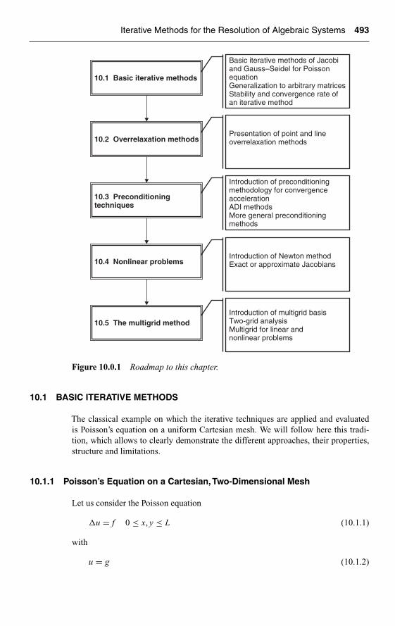
Ch10-H6594.tex 27/4/2007 12: 16 Page 493

Iterative Methods for the Resolution of Algebraic Systems 493

Basic iterative methods of Jacobiand Gauss–Seidel for PoissonequationGeneralization to arbitrary matricesStability and convergence rate ofan iterative method

Presentation of point and lineoverrelaxation methods

Introduction of preconditioningmethodology for convergenceaccelerationADI methodsMore general preconditioningmethods

Introduction of Newton methodExact or approximate Jacobians

Introduction of multigrid basisTwo-grid analysisMultigrid for linear andnonlinear problems

10.1 Basic iterative methods

10.2 Overrelaxation methods

10.3 Preconditioningtechniques

10.4 Nonlinear problems

10.5 The multigrid method


10.1 BASIC ITERATIVE METHODS

The classical example on which the iterative techniques are applied and evaluatedis Poisson’s equation on a uniform Cartesian mesh. We will follow here this tradi-tion, which allows to clearly demonstrate the different approaches, their properties,structure and limitations.

10.1.1 Poisson’s Equation on a Cartesian,Two-Dimensional Mesh

Let us consider the Poisson equation

�u = f 0 ≤ x, y ≤ L (10.1.1)

with

u = g (10.1.2)

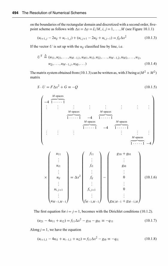
Ch10-H6594.tex 27/4/2007 12: 16 Page 494


on the boundaries of the rectangular domain and discretized with a second order, five-point scheme as follows with �x = �y = L/M , i, j = 1, . . . , M (see Figure 10.1.1)

(ui+1, j − 2uij + ui−1, j) + (ui, j+1 − 2uij + ui, j−1) = fij�x2 (10.1.3)

If the vector U is set up with the uij classified line by line, i.e.

U T �= (u11, u21, . . . , uM−1,1, uM1, u12, u22, . . . , uM−1,2, uM2, . . . , u1j ,

u2j , . . . , uM−1, j , uMj , . . . ) (10.1.4)

The matrix system obtained from (10.1.3) can be written as, with S being a (M 2 × M 2)matrix

S · U = F�x2 + G ≡ −Q (10.1.5)

⎛⎜⎜⎜⎜⎜⎜⎜⎜⎜⎜⎜⎜⎜⎜⎜⎜⎝

−4

M -spaces︷︸︸︷1 · · · · · 1

......

......

......

......

M -spaces︷︸︸︷1 · · · · · 1 −4

M -spaces︷︸︸︷1 · · · · · 1

M -spaces︷︸︸︷1 · · · · · 1 −4

M -spaces︷︸︸︷1 · · · · · 1

......

......

......

M -spaces︷︸︸︷1 · · · · · 1 −4

⎞⎟⎟⎟⎟⎟⎟⎟⎟⎟⎟⎟⎟⎟⎟⎟⎟⎠

×

⎛⎜⎜⎜⎜⎜⎜⎜⎜⎜⎜⎜⎜⎜⎜⎜⎜⎜⎝

u11...

ui1...

uij...

ui, j+1...

uM−1,M−1

⎞⎟⎟⎟⎟⎟⎟⎟⎟⎟⎟⎟⎟⎟⎟⎟⎟⎟⎠

= �x2

⎛⎜⎜⎜⎜⎜⎜⎜⎜⎜⎜⎜⎜⎜⎜⎜⎜⎜⎝

f11...

fi1...

fij...

fi, j+1...

fM−1,M−1

⎞⎟⎟⎟⎟⎟⎟⎟⎟⎟⎟⎟⎟⎟⎟⎟⎟⎟⎠

−

⎛⎜⎜⎜⎜⎜⎜⎜⎜⎜⎜⎜⎜⎜⎜⎜⎜⎜⎝

g10 + g01...

gi0...

0...

0...

gM ,M−1 + gM−1,M

⎞⎟⎟⎟⎟⎟⎟⎟⎟⎟⎟⎟⎟⎟⎟⎟⎟⎟⎠

(10.1.6)

The first equation for i = j = 1, becomes with the Dirichlet conditions (10.1.2).

(u21 − 4u11 + u12) = f11�x2 − g10 − g01 ≡ −q11 (10.1.7)

Along j = 1, we have the equation

(ui+1,1 − 4ui1 + ui−1,1 + ui2) = f11�x2 − gi0 ≡ −qi1 (10.1.8)

Ch10-H6594.tex 27/4/2007 12: 16 Page 495


M

M

x

y

1

1

1

1 �4j �1

j �1

j �0

i �0 i �1 i �1i1 2

1

j

Figure 10.1.1 Cartesian mesh for Laplace operator.

Similar equations can be written for the other boundaries (see Problem P.10.1). Thevectors F , G are defined by equation (10.1.5). The vector Q will represent the sumof the right-hand side vectors.

By inspection, it is seen that S has the following properties:

(i) S is irreducible diagonal dominant (see the first line).(ii) S is symmetric and hence non-singular and positive definite.

In order to relate the notation in the system (10.1.6) to the classical notations oflinear algebra, we consider the vector U, with elements uI , I = 1, . . . , N = M 2, whereN = M 2 is the total number of mesh points. Hence, to each component uij we associatethe component uI , where I is for instance defined by I = i + ( j − 1)M as would bethe case in a finite element discretization.

Equation (10.1.5) will be written as

N∑J=1

sIJ uJ = −QI I = 1, . . . , N (10.1.9)

The coefficients sIJ represent the space discretization of the Laplace operator.

10.1.2 Point Jacobi Method/Point Gauss–Seidel Method

In order to solve for the unknowns in system (10.1.3), we could define an initialapproximation to the vector U, and attempt to correct this approximation by solvingequation (10.1.3) sequentially, sweeping through the mesh, point by point, startingat i = j = 1, following the mesh line by line or column per column.

If we indicate by unij (or un

I ) the assumed approximation (n will be an iteration

index); the corrected approximation is un+1ij (or un+1

I ) and can be obtained (seeFigure 10.1.2a) as

un+1ij = 1

4(un

i+1, j + uni−1, j + un

i, j+1 + uni, j−1) + 1

4qn

ij (10.1.10)

Ch10-H6594.tex 27/4/2007 12: 16 Page 496


Unknown at iteration n �1

Known from iteration n

Known from iteration n �1

i

j

i

j

Figure 10.1.2 Point relaxation method: (a) Jacobi method and (b) Gauss–Seidelmethod.

where qij represents the right-hand side.In a general formulation, for the system (10.1.9), the point Jacobi method is defined

by the algorithm

un+1I = 1

sII

⎛⎜⎝−qn

I −N∑

J=1J �=I

sIJ unJ

⎞⎟⎠ (10.1.11)

The general formulation is best represented in matrix form, if we decompose S ina sum of three matrices containing the main diagonal D, the upper triangular part Fand the lower triangular part E. That is we write

S = D + E + F (10.1.12)

with

D =

⎛⎜⎜⎜⎜⎝

s11

·sII

·sNN

⎞⎟⎟⎟⎟⎠ E =

⎛⎜⎜⎜⎜⎜⎜⎝

0 0s21 ·· · 0

sI1 sI2 · 0· · · · 0 0

sN1 sN2 · sN , N−1 0

⎞⎟⎟⎟⎟⎟⎟⎠

F =

⎛⎜⎜⎜⎜⎜⎜⎝

0 s12 · s1J · s1N

· s2J · s2N

0 · · ·0 ·

0 sN−1,N

0 0

⎞⎟⎟⎟⎟⎟⎟⎠

(10.1.13)

For the Laplace operator, this splitting is obvious from the form of the matrix (10.1.6).

Ch10-H6594.tex 27/4/2007 12: 16 Page 497


Equation (10.1.11) can be written as

D · U n+1 = −Qn − (E + F) · U n (10.1.14)

defining the iterative point Jacobi method for the system (10.1.9) written as

(D + E + F) · U = −Q (10.1.15)

The iterative Jacobi scheme can also be written in �-form (delta-form) by introducingthe Residual Rn at iteration n

Rn ≡ R(U n)�= S · U n + Qn = (D + E + F) · U n + Qn (10.1.16)

Equation (10.1.14) can be rewritten, after subtraction of DU n on both sides,

D · �U n = −Rn (10.1.17)

where

�U n �= U n+1 − U n (10.1.18)

The residual is an important quantity, since it is a measure of the error at a giveniteration number n.

Obviously, the iterative method will have to generate a sequence of decreasingvalues of �U n and Rn when the number of iterations increases, since the convergedsolution corresponds to a vanishing residual.

For equation (10.1.10), the residual form (10.1.17) is obtained by subtracting unij

from both sides, leading to

4(un+1ij − un

ij) = (uni+1, j + un

i1, j + uni, j+1 + un

i, j−1 − 4unij) + qn

ij (10.1.19)

Point Gauss–Seidel methodIn Figure 10.1.2a, we observe that the points (i, j − 1) and (i − 1, j) have already beenupdated at iteration (n + 1) when uij is calculated. We are therefore tempted to usethese new values in the estimation of un+1

ij as soon as they have been calculated. We canexpect thereby to obtain a higher convergence rate since the influence of a perturbationon un is transmitted more rapidly. With the Jacobi method, a perturbation of un+1

i−1, j willbe felt on uij only after the whole mesh is swept since it will occur for the first time atthe next iteration through the equation for un+2

ij . With the Gauss–Seidel method, this

influence already appears at the current iteration since un+1ij is immediately affected

by un+1i−1, j (see Figure 10.1.2b). As a by-product, it can be observed that as soon as a

new value un+1i, j is calculated the ‘old’ value un

i, j is not needed anymore. Hence, thenew value can be stored in the same location and overwrite, in the coding, the localvalue un

i, j . Therefore only one vector U of length N has to be stored, while two vectors

U n+1 and U n have to be saved in the Jacobi method.

Ch10-H6594.tex 27/4/2007 12: 16 Page 498


The Gauss–Seidel method is, from every point of view more advantageous thanthe Jacobi method, and is defined by the iterative scheme

un+1ij = 1

4(un

i+1, j + un+1i−1, j + un

i, j+1 + un+1i, j−1) + 1

4qn

ij (10.1.20)

For the general system (10.1.9), the Gauss–Seidel method takes all the variablesassociated to the lower diagonal of the matrix S, at the new level (n + 1).

Hence, instead of equation (10.1.11), we have

un+1I = 1

sII

(−qn

I −I−1∑J=1

sIJ un+1J −

N∑J=I+1

sIJ unJ

)(10.1.21)

In operator form, this scheme can be written as

(D + E) · U n+1 = −Qn − F · U n (10.1.22)

and in residual form

(D + E) · �U n = −Rn (10.1.23)

By comparing this equation with (10.1.17) it can be seen that the Gauss–Seidelmethod corresponds to another choice for the matrix which ‘drives’ �U n to zero,that is to convergence, or equivalently, to another splitting of the matrix S.

This observation leads us to the following general analysis of an iterative method.

10.1.3 Convergence Analysis of Iterative Schemes

An iterative method is said to be convergent if the error tends to zero as the number ofiterations goes to infinity. If U is the exact solution of the system (10.1.5), the errorat iteration n is

en = U n − U (10.1.24)

Let us consider an arbitrary splitting of the matrix S

S = P + A (10.1.25)

and an iterative scheme

P · U n+1 = −Qn − A · U n (10.1.26)

or equivalently

P · �U n = −Rn (10.1.27)

The matrix P will be called a convergence or (pre)conditioning matrix (operator)and is selected such that the system (10.1.26) is easily solvable. It is important to

Ch10-H6594.tex 27/4/2007 12: 16 Page 499


observe here that the iterative scheme (10.1.27) replaces the full iterative scheme,corresponding to a direct method,

S · U n+1 = −Qn or S · �U n = −Rn (10.1.28)

Subtracting from equation (10.1.26), the relation defining the exact solution U

S · U ≡ (P + A) · U = −Q (10.1.29)

we obtain, assuming that Q is independent of U ,

P · en+1 = −A · en (10.1.30)

or

en+1 = −(P−1 · A) · en = −(P−1 · A)n · e1 = (1 − P−1 · S)n · e1 (10.1.31)

where (P−1A)n is the matrix P−1A to the power n.If ||en+1|| is to go to zero for increasing n, the matrix P−1A should be a

convergent matrix and its spectral radius has to be lower than one.The iterative scheme will be convergent, if and only if the matrix G, called the

iteration or amplification matrix (operator)

G = 1 − P−1 · S (10.1.32)

is a convergent matrix, i.e., satisfying the condition on the spectral radius

ρ(G) ≤ 1 (10.1.33)

or

|λJ (G)| ≤ 1 for all J (10.1.34)

All the eigenvalues λJ (G) of G = (1 − P−1S) have to be lower than one in modulusfor the iterative scheme to converge.

Hence, it is seen that we can replace equation (10.1.28) and the matrix S acting onthe corrections �U n, by another operator P, which is expected to be easier to invert,provided the above conditions are satisfied.

What do we mean by ‘easy to invert’? The main conditions on the convergencematrix P are:

• The number of arithmetic operations required for the computation of P−1 shouldnot be higher than O(N ), with a proportional coefficient as low as possible.

• P should be as close as possible to S.

Except for these conditions, the choice of P is arbitrary. If P = S we obtain theexact solution but this corresponds to a direct method, since we have to invert thematrix S of the system.

Ch10-H6594.tex 27/4/2007 12: 16 Page 500


The residual Rn is connected to the error vector en, by the following relationobtained by subtracting Rn from R = SU + Q ≡ 0, assuming Q to be independent of U ,

Rn = S · en (10.1.35)

This shows the quantitative relation between the error and the residual and proofsthat the residual will go to zero when the error tends to zero.

In practical computations, the error is not accessible since the exact solution is notknown. Therefore we generally use the norm of the residual ||Rn|| as a measure ofthe evolution toward convergence and practical convergence criteria will be set byrequiring that the residual drops by a predetermined number of orders of magnitude.Observe that even when the residual is reduced to machine accuracy (machine zero),it does not mean that the solution U n is within machine accuracy of the exact solution.When SU results from a space discretization, achieving machine zero on the residualwill produce a solution U n which differs from the exact solution U of the differentialproblem by the amount of the truncation error. For example, a second order accuratespace discretization, with �x = 10−2, will produce an error of the order of 10−4 onthe solution, which cannot be reduced further even if the residual equals 10−14.

Equation (10.1.26) can also be written as

U n+1 = (1 − P−1 · S) · U n − P−1 · Q

= G · U n − P−1 · Q (10.1.36)

Comparing equation (10.1.31), written here as

en+1 = G · en = (G)n+1 · e0 (10.1.37)

with similar relations in Chapter 7 or 9, interpreting the index n as a pseudo-timeindex, the similitude between the formulation of an iterative scheme of a stationaryproblem, and a time-dependent formulation of the same problem clearly appears.The matrix G, being the amplification matrix of the iterative method can be analyzedalong the lines developed in Chapters 7 and 9. We will return to this very importantlink below.

Convergence conditions for the Jacobi and Gauss–Seidel methodsFor the Jacobi method G = −D−1 · (E + F) = 1 − D−1S and for the Gauss–Seidelmethod G = −(D + E)−1 · F = 1 − (D + E)−1S. From the properties of matrices,it can be shown that the Jacobi and Gauss–Seidel methods will converge if S isirreducible diagonal dominant. When S is symmetric, it is sufficient for convergencethat S, or (−S) is positive definite for both methods and in addition for the Jacobimethod, (2D − S), or (S − 2D) in our case, has also to be positive definite.

Estimation of the convergence rateAn important issue of iterative methods is the estimation of the rate of reduction ofthe error with increasing number of iterations. The average rate of error reduction

Ch10-H6594.tex 27/4/2007 12: 16 Page 501


over n iterations can be defined by

�en�=(

‖en‖∥∥e0∥∥)1/n

(10.1.38)

From equation (10.1.37) we have

�en ≤ ‖(G)n‖1/n (10.1.39)

Asymptotically it can be shown, Varga (1962), that this quantity tends to the spectralradius of G for n → ∞:

s ≡ limn→∞‖(G)n‖1/n = ρ(G) (10.1.40)

The logarithm of s is the average convergence rate, measuring the number of iterationsneeded to decrease the error by a given factor.

If we consider s to be a valid measure of �en, the norm of the error will be reducedby an order of magnitude (factor 10), in a number of iterations n, such that

(1

10

)1/n

≤ s = ρ(G) (10.1.41)

or

n ≥ −1/ log ρ(G) (10.1.42)

Remember that the spectral radius ρ(G) < 1 is always lower than one for stabilitywhich explains the negative sign of this relation.

This relation is valid asymptotically for large n, and is generally not to be relied onat small values of n. In the early stages of the iterative process it is not uncommon,particularly with nonlinear problems to observe even an increase in the residual beforeit starts to decrease at larger n. Also, we can often observe different rates of residualreduction, usually an initial reduction rate much higher than s, slowing down graduallyto the asymptotic value. The explanation for this behavior is to be found in thefrequency distribution of the error and in the way a given iterative method treats thedifferent frequencies in the spectrum. The residual history of curve a of Figure 10.1.3is typical for a method which damps rapidly the high frequency components butdamps poorly the low frequency errors while the opposite is true for curve b. Thereason for this behavior is explained from an eigenvalue analysis.

10.1.4 Eigenvalue Analysis of an Iterative Method

The frequency response, as well as the asymptotic convergence rate of an iterativemethod, are defined by the eigenvalue spectrum of the amplification matrix G, and bythe way the matrix P−1 treats the eigenvalues of the matrix S. Referring to Section9.1.3, the solution U n+1 can be written as a linear combination of the eigenmodes V (J )

Ch10-H6594.tex 27/4/2007 12: 16 Page 502


n

a

b

�R �

Figure 10.1.3 Typical residual history of a relaxation method.

of the matrix S (which represents the space discretization of the differential operator).Each term represents the contribution from the initial component U0J damped by thefactor (λJ )n, where (λJ ) is the eigenvalue of the matrix G, associated to the eigenvalue(�J ) of the matrix S. We suppose here that S and G commute and have the same setof eigenfunctions, although this will not always be the true, even in simple cases.For the present example of Poisson’s equation on a Cartesian mesh, this propertyis satisfied for the Jacobi iteration but not for the Gauss–Seidel method, since thematrices (D + E)−1 and S do not commute. However, the conclusions of this sectionwith regard to the convergence properties of iterative methods and their relation tothe eigenvalues of the space operator will remain largely valid, independently of thishypothesis, as can be seen from the analysis of Section 9.1.3. Hence, we assume

U n =∑J=1

(λJ )nU0J · V (J ) −∑J=1

QJ

�J[1 − (λJ )n] · V (J ) (10.1.43)

Note that (λJ )n is (λJ ) to the power n.The first term is the ‘transient’ behavior of the homogeneous solution while the last

term is a transient contribution from the source term. Since, for convergence, all the(λJ ) are in modulus lower than one, after a sufficiently large number of iterations, weare left with the ‘converged’ solution

limn→∞U n = −

∑J=1

QJ

�J· V (J ) (10.1.44)

which is the eigenmode expansion of the solution U = −S−1 · Q. Indeed, by writing

U =∑J=1

UJ · V (J ) (10.1.45)

Ch10-H6594.tex 27/4/2007 12: 16 Page 503


we obtain

S · U =∑J=1

�J UJ · V (J ) = −∑J=1

QJ · V (J ) (10.1.46)

Since the U n form a basis of the U -space, we have

UJ = − QJ

�J(10.1.47)

which shows that equation (10.1.44) is indeed the solution. Equation (10.1.43) showsthat the transient will, for large n, be dominated by the largest eigenvalue (λJ ); thisexplains the relation (10.1.42).

It is seen from equation (10.1.31) that the error en behaves like the homogeneouspart of (10.1.43). Therefore, if e0

J is the initial error distribution, after n iterations theerror is reduced to

en =∑J=1

(λJ )ne0J · V (J ) (10.1.48)

The residual Rn can also be expanded in a series of eigenfunctions V (J ) since fromequation (10.1.35) we can write

Rn =∑J=1

(λJ )ne0J S · V (J ) =∑J=1

(λJ )n�J e0J · V (J ) (10.1.49)

If we assume the eigenvectors to be orthonormal, then the L2-norm of the residual,will be

∥∥Rn∥∥

L2=∑J=1

[(λJ )n�J e0J ]2 (10.1.50)

When the iteration number n increases, the low values of (λJ ) will be damped morerapidly, and at large values of n we will be left with the highest (λJ ), in particular thosewho are the closest to the upper limit of one. Hence, if the iterative scheme is suchthat the highest eigenvalues λJ = λ(�J ) are close to one, the asymptotic convergencerate will be poor. Since generally, the high frequencies of the operator S generate thelowest values of (λJ ), we will tend to have a behavior such as shown on curve a ofFigure 10.1.3, where the initial rapid decrease of the residual is due to the damping ofthe high frequencies (low A), and where one is left, at large n, with the low frequencyend (high(λJ )) of the error spectrum.

On the other hand, if such an iterative method is combined with an algorithm whichdamps effectively the low frequencies of S, that is the large (λJ ) region, then we willobtain a behavior of the type shown on curve b of Figure 10.1.3. This is the principleat the basis of the multigrid method, to be described in Section 10.5.

The relation λJ = λ(�J ) can be computed explicitly only in simple cases. Forinstance, for the Jacobi method we have, representing by G the amplification matrix,

GJ = 1 − D−1S (10.1.51)

Ch10-H6594.tex 27/4/2007 12: 16 Page 504


and since D is a diagonal matrix

λJ = 1 − 1

dJ�J (S) (10.1.52)

Note that we define S as the matrix representation of the discretized differential oper-ator, which has to satisfy the condition of stability of the time-dependent counterpart,and therefore have eigenvalues with negative real parts, as seen in Section 9.1. Hence,S will be negative definite when all the eigenvalues are real.

10.1.5 Fourier Analysis of an Iterative Method

The Fourier analysis allows a simple estimation of eigenvalues, when periodic condi-tions are assumed, such that the Fourier modes are eigenvectors of the S matrix andof the amplification matrix G. This is the case for the Jacobi method, but not for theGauss–Seidel iterations.

For the discretization (10.1.3) with Dirichlet boundary conditions, the eigenfunc-tions of S reduce to sin(iφx) · sin ( jφy) and the eigenvalues are equal to, dropping theindex J ,

� = −4( sin2 φx/2 + sin2 φy/2)

φx = lπ/M φy = mπ/M J = l + (m − 1)M l, m = 1, . . . , M (10.1.53)

The eigenvalues of GJ are therefore, with d = −4

λ(GJ ) = 1 − (sin2 φx/2 + sin2 φy/2) = 1

2(cos φx + cos φy) (10.1.54)

At the low frequency end, around φx = φy = 0, the damping rate is very poor, sinceλ = 1. The intermediate frequency range is strongly damped, that is for the frequenciescorresponding to high values of �. The spectral radius ρ(GJ ) is defined by the highesteigenvalue, which corresponds to the lowest frequencies of the �-spectrum. Theseare obtained for φx = φy = π/M

ρ(GJ ) = cos π/M (10.1.55)

Hence the convergence rate becomes, for �x = �y that is, for large number of meshpoints

ρ(GJ ) ≈ 1 − π2

2M 2= 1 − π2

2N= 1 − O(�x2) (10.1.56)

and, from equation (10.1.42), the number of iterations, needed to reduce the error byone order of magnitude is, asymptotically (2N/0.43π2). Since each Jacobi iterationrequires 5N operations, the Jacobi method will require roughly 2kN 2 operations fora reduction of the error by k orders of magnitude.

Ch10-H6594.tex 27/4/2007 12: 16 Page 505


Gauss–Seidel methodApplying a straightforward Neumann analysis to the homogeneous part of equation(10.1.20), leads to

(4 − e−Iφx − e−Iφy )λGS = eIφx + eIφy (10.1.57)

However, this does not give the eigenvalues of the matrix GGS , since this matrixdoes not commute with S. It can be shown, Young (1971), that the correspondingeigenvalues of the amplification matrix of the Gauss–Seidel method are equal to thesquare of the eigenvalues of the Jacobi method.

λ(GGS ) = 1

4(cos φx + cos φy)2 = λ(GJ )2 (10.1.58)

Hence, the spectral radius is

ρ(GGS ) = ρ(GJ )2 = cos2 π/M (10.1.59)

and for large M ,

ρ(GGS ) ≈ 1 − π2

M 2= 1 − π2

N(10.1.60)

and the method converges twice as fast as the Jacobi method, since the number ofiterations for one order of magnitude reduction in error, is N/(0.43π2).

For a more general case, it can be shown, Varga (1962), that the Gauss–Seidelmethod converges if S is an irreducible diagonal dominant matrix, or if (−S) issymmetric, positive definite. In this latter case we have λ(GGS ) = λ(GJ )2. Interestingconsiderations with regard to the application of Fourier analysis to iterative methodscan be found in LeVeque and Trefethen (1986).

10.2 OVERRELAXATION METHODS

We could be tempted to increase the convergence rate of an iterative method, by‘propagating’ the corrections �U n = U n+1 − U n faster through the mesh. This ideais the basis of the overrelaxation method, introduced independently by Frankel andYoung in 1950; see Young (1971) and Hageman and Young (1981).

The overrelaxation method is formulated as follows: if U n+1 is the value obtainedfrom the basic iterative scheme, the value introduced at the next level U n+1 isdefined by

U n+1 = ωU n+1 + (1 − ω)U n (10.2.1)

where ω is the overrelaxation coefficient. Alternatively, a new correction is defined

�U n = U n+1 − U n with �U n = ω�U n (10.2.2)

When appropriately optimized for maximum convergence rate, a considerable gaincan be achieved as will be seen next.

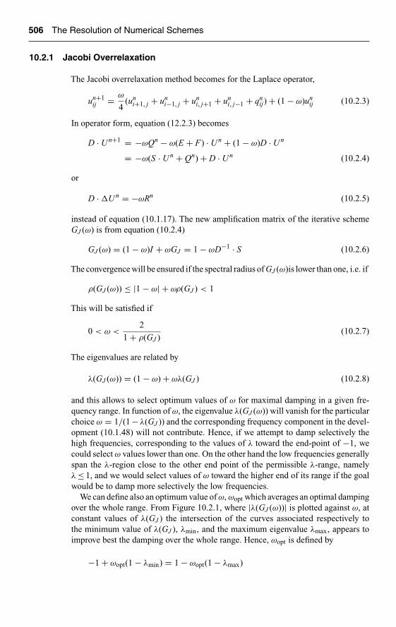
Ch10-H6594.tex 27/4/2007 12: 16 Page 506


10.2.1 Jacobi Overrelaxation

The Jacobi overrelaxation method becomes for the Laplace operator,

un+1ij = ω

4(un

i+1, j + uni−1, j + un

i, j+1 + uni, j−1 + qn

ij) + (1 − ω)unij (10.2.3)

In operator form, equation (12.2.3) becomes

D · U n+1 = −ωQn − ω(E + F) · U n + (1 − ω)D · U n

= −ω(S · U n + Qn) + D · U n (10.2.4)

or

D · �U n = −ωRn (10.2.5)

instead of equation (10.1.17). The new amplification matrix of the iterative schemeGJ (ω) is from equation (10.2.4)

GJ (ω) = (1 − ω)I + ωGJ = 1 − ωD−1 · S (10.2.6)

The convergence will be ensured if the spectral radius of GJ (ω)is lower than one, i.e. if

ρ(GJ (ω)) ≤ |1 − ω| + ωρ(GJ ) < 1

This will be satisfied if

0 < ω <2

1 + ρ(GJ )(10.2.7)

The eigenvalues are related by

λ(GJ (ω)) = (1 − ω) + ωλ(GJ ) (10.2.8)

and this allows to select optimum values of ω for maximal damping in a given fre-quency range. In function of ω, the eigenvalue λ(GJ (ω)) will vanish for the particularchoice ω = 1/(1 −λ(GJ )) and the corresponding frequency component in the devel-opment (10.1.48) will not contribute. Hence, if we attempt to damp selectively thehigh frequencies, corresponding to the values of λ toward the end-point of −1, wecould select ω values lower than one. On the other hand the low frequencies generallyspan the λ-region close to the other end point of the permissible λ-range, namelyλ ≤ 1, and we would select values of ω toward the higher end of its range if the goalwould be to damp more selectively the low frequencies.

We can define also an optimum value of ω, ωopt which averages an optimal dampingover the whole range. From Figure 10.2.1, where |λ(GJ (ω))| is plotted against ω, atconstant values of λ(GJ ) the intersection of the curves associated respectively tothe minimum value of λ(GJ ), λmin, and the maximum eigenvalue λmax, appears toimprove best the damping over the whole range. Hence, ωopt is defined by

−1 + ωopt(1 − λmin) = 1 − ωopt(1 − λmax)

Ch10-H6594.tex 27/4/2007 12: 16 Page 507


w

Unstable

w opt1

1�l min

1

1�l max

�l (w )�

Figure 10.2.1 Optimal relaxation for Jacobi method.

or

ωopt = 2

2 − (λmin + λmax)(10.2.9)

For the Laplace operator, from equation (10.1.54)

λmax = −λmin = cos π/M (10.2.10)

and ωopt = 1. Hence the Jacobi method is optimal by this definition.

10.2.2 Gauss–Seidel Overrelaxation: Successive Overrelaxation (SOR)

The benefits of the overrelaxation concept take on their full range when applied tothe Gauss–Seidel method, and in this case the methods are usually called succes-sive overrelaxation methods, indicated by the symbol SOR. Applying the definition(10.2.1) to the Gauss–Seidel method for the Laplace operator, leads to the followingiterative scheme:

un+1ij = 1

4(un

i+1, j + un+1i−1, j + un

i, j+1 + un+1i, j−1) + 1

4qn

ij

un+1ij = ωun+1

ij + (1 − ω)unij (10.2.11)

In operator form, this corresponds to the general residual formulation

D · �U n = −Rn − E · �U n (10.2.12)

and the overrelaxation method is defined by the iteration operator (D + ωE), sinceequation (10.2.12) reads

(D + ωE) · �U n = −ωRn (10.2.13)

Ch10-H6594.tex 27/4/2007 12: 16 Page 508


The amplification matrix GSOR(ω) is now

GSOR(ω) = 1 − ω(D + ωE)−1 · S

= (D + ωE)−1 · [(1 − ω)D − ωF] (10.2.14)

Condition on the relaxation parameter zSince GSOR(ω) is a product of triangular matrices, its determinant is the product ofits diagonal elements. Hence,

det GSOR(ω) = det(I + ωD−1E)−1 · det[(1 − ω)I − ωD−1F]

= I · det[(1 − ω)I − ωD−1F] = (1 − ω)N (10.2.15)

On the other hand, the determinant of a matrix is equal to the product of its eigenvalues,and hence

ρ(GSOR(ω))N ≥ |det GSOR(ω)| = (1 − ω)N (10.2.16)

The spectral radius will be lower than one if

|(1 − ω)| ≤ ρ(GSOR(ω)) < 1 (10.2.17)

or

0 < ω < 2 (10.2.18)

For irreducible diagonal dominant matrices, it can be shown (Young, 1971) that theSOR method will converge, if

0 < ω <2

1 + ρ(GGS )(10.2.19)

More information can be obtained for symmetrical matrices. The eigenvalues ofGSOR(ω) satisfy the following relations, for symmetrical matrices of the form

S =(

D1 FFT D2

)(10.2.20)

where D1 and D2 are block diagonal, writing λ(ω) for λ(GSOR(ω)):

(i) The eigenvalues of the SOR amplification factor satisfy the relation

λ(ω) = 1 − ω + ωλ1/2(ω) · λ(GJ ) (10.2.21)

(ii) For ω = 1, we recover relation (10.1.58)

λ(ω = 1) ≡ λ(GGS ) = λ2(GJ ) (10.2.22)

Ch10-H6594.tex 27/4/2007 12: 16 Page 509


(iii) an optimal relaxation coefficient can be defined, rendering ρ(GSOR(ω))minimum, as

ωopt = 2

1 +√1 − ρ2(GJ )(10.2.23)

with

ρ(GSOR(ωopt)) = ωopt − 1 (10.2.24)

Note the role played by the eigenvalues of the Jacobi point iteration matrix GJ . ForLaplace’s operator, we have

ρ(GJ ) = cos π/M (10.2.25)

ωopt = 2

1 + sin π/M≈ 2

(1 − π

M+ π2

M 2

)(10.2.26)

and the spectral radius at optimum relaxation coefficient is

ρ(GSOR(ωopt)) =1 − sin π/M

1 + sin π/M≈ 1 − 2π

M+ O

(1

M 2

)(10.2.27)

The number of iterations for a one order of magnitude reduction in error normis of the order of 2.3M/π ≈ √

N . Compared to the corresponding values for Jacobiand Gauss–Seidel iterations, the optimal SOR will require kN · √N operations, for areduction of the error of k orders of magnitude. Hence, this represents a considerablegain in convergence rate.

For non-optimal relaxation parameters however, this rate can seriously deterio-rate. Since, for more general problems, the eigenvalues are not easily found, onecan attempt to find numerical estimates of the optimal relaxation parameter. Forinstance, for large n, the error being dominated by the largest eigenvalue, we havefrom equations (10.1.36) and (10.1.48)

ρ(G) = limn→∞

‖en+1‖‖en‖ (10.2.28)

and when this ratio stabilizes, we can deduct ρ(GJ ) from equation (10.2.21) by intro-ducing this estimation of ρ(G) for λ(ω) and find ωopt from equation (10.2.23). Otherstrategies can be found in Wachspress (1966), Hageman and Young (1981).

10.2.3 Symmetric Successive Overrelaxation (SSOR)

The SOR method, as described by equation (10.2.11), sweeps through the mesh fromthe lower left corner to the right upper corner. This gives a bias to the iterationscheme, which might lead to some error accumulations, for instance, if the physicsof the system to be solved is not compatible with this sweep direction. This can be

Ch10-H6594.tex 27/4/2007 12: 16 Page 510


avoided by alternating SOR sweeps in both directions. We obtain a two-step iterativemethod (a form of predictor–corrector approach), whereby a predictor U n+1/2 isobtained from a SOR sweep (10.2.12), followed by a sweep in the reverse directionstarting at the end-point of the first step.

The SSOR can be described in residual form by the equations

(D + ωE) · �U n+1/2 = −ωRn (10.2.29)

(D + ωF) · �U n = −ωR(U n+1/2) (10.2.30)

with

U n+1/2 = U n + �U n+1/2

U n+1 = U n+1/2 + �U n = U n + �U n+1/2 + �U n (10.2.31)

This method converges under the same conditions as the SOR method and an optimalrelaxation parameter can only be estimated approximately as

ωopt ≈ 2

1 +√2(1 − ρ2(GJ ))(10.2.32)

Hence, the SSOR method converges twice as fast as SOR, but since it requires twice asmuch work, there is not much to be gained in convergence rate. However, SSOR mightlead to better error distributions and is a good candidate for preconditioning matri-ces. Also, when applied in conjunction with non-stationary relaxation, significantimprovements in convergence rate over SOR can be achieved (Young, 1971).

10.2.4 Successive Line Overrelaxation Methods (SLOR)

We could still accelerate the convergence of the SOR method by increasing the waythe variations �U n are transmitted throughout the field, if we are willing to increasethe workload per iteration by solving small systems of equations.

Referring to Figure 10.2.2, for the Laplace operator, we could consider the threepoints on a column i, or on a line j, as simultaneous unknowns and solve a tridiag-onal system along each vertical line, sweeping through the mesh column by columnfrom i = 1 to i = M (Figure 10.2.2a). or along horizontal lines as in Figure 10.2.2b,from j = 1 to j = M . This is called line Gauss–Seidel (ω = 1) or line successiveoverrelaxation, generally abbreviated as SLOR, when ω �= 1.

For the Laplace operator, the SLOR iterative scheme along vertical lines (VLOR)is defined by

un+1ij = 1

4(un

i+1, j + un+1i−1, j + un+1

i, j+1 + un+1i, j−1) + 1

4qn

ij

un+1ij = ωun+1

ij + (1 − ω)unij (10.2.33)

Ch10-H6594.tex 27/4/2007 12: 16 Page 511


Unknown at iteration n �1

Known from iteration n

Known from iteration n �1

i

j

(a)

i

j

(b)

Figure 10.2.2 Line relaxation method.

or in incremental form

4�U nij − �U n

i, j−1 − �U ni, j+1 − ω�U n

i−1, j = ωRnij (10.2.34)

which is solved by the tridiagonal Thomas algorithm in 5M operations for each line.Hence 5M 2 = 5N operations are required for all the tridiagonal systems. This numberis to be roughly doubled to take into account the computation of the right-hand sideterms.

A Jacobi line relaxation method can also be defined and written as

un+1ij = 1

4(un

i+1, j + uni−1, j + un+1

i, j+1 + un+1i, j−1) + 1

4qn

ij

un+1ij = ωun+1

ij + (1 − ω)unij (10.2.35)

or in incremental form

4�U nij − �U n

i, j−1 − �U ni, j+1 = ωRn

ij (10.2.36)

and corresponds in Figure 10.2.2 to a replacement of the triangles by a circle symbol.Many variants of the relaxation method can be derived by combining point or line

relaxations on alternate positions, or on alternate sweep directions. It can be shownthat the line relaxations for the Laplace operator have a convergence rate twice fasterthan the point relaxations. The overrelaxation method SLOR, is

√2 times faster than

SOR at the same value of the optimal ω.

(a) Red–Black point relaxationIn this approach, the relaxation method is applied to two distinct series of mesh points,called red and black points, where the red points can be considered as having an evennumber I = i + (j − 1)M and the black points an odd number (see Figure 10.2.3).

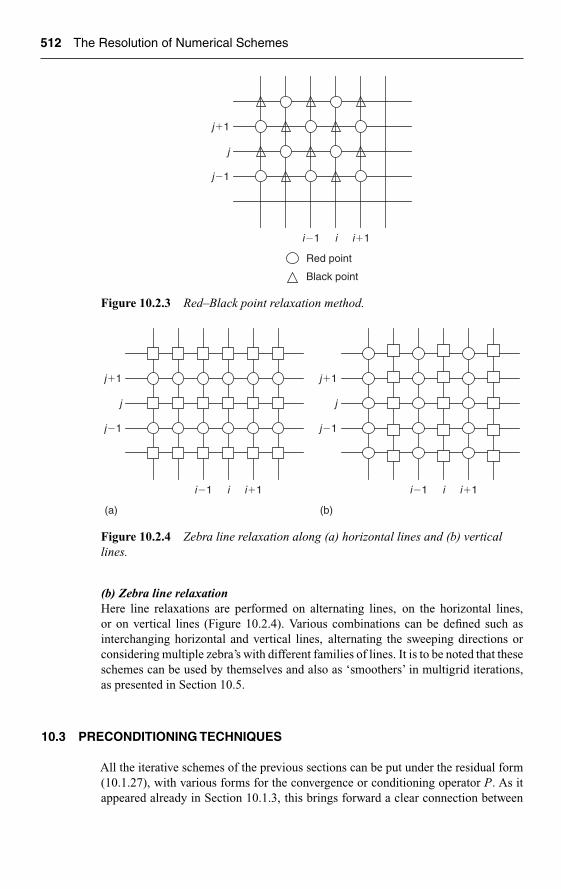
Ch10-H6594.tex 27/4/2007 12: 16 Page 512


ii �1 i �1

j �1

j �1

j

Red point

Black point

Figure 10.2.3 Red–Black point relaxation method.

ii �1 i �1

j �1

j �1

j

(a)

ii �1 i �1

j �1

j �1

j

(b)

Figure 10.2.4 Zebra line relaxation along (a) horizontal lines and (b) verticallines.

(b) Zebra line relaxationHere line relaxations are performed on alternating lines, on the horizontal lines,or on vertical lines (Figure 10.2.4). Various combinations can be defined such asinterchanging horizontal and vertical lines, alternating the sweeping directions orconsidering multiple zebra’s with different families of lines. It is to be noted that theseschemes can be used by themselves and also as ‘smoothers’ in multigrid iterations,as presented in Section 10.5.

10.3 PRECONDITIONING TECHNIQUES

All the iterative schemes of the previous sections can be put under the residual form(10.1.27), with various forms for the convergence or conditioning operator P. As itappeared already in Section 10.1.3, this brings forward a clear connection between

Ch10-H6594.tex 27/4/2007 12: 16 Page 513


the behavior of iterative schemes with the iteration number n, and the behavior oftime-dependent formulations where n is a time step index. Hence if we view n in thisway, we can consider the general iterative scheme

P�U n

τ= −ω(S · U n + Qn) = −ωRn (10.3.1)

as the explicit Euler integration, with time step τ, of the differential system

PdU

dt= −ω(S · U + Q) (10.3.2)

where we are only interested in the asymptotic steady state. The operator P can bechosen in an arbitrary way, with the only restriction that the amplification matrix G

G = 1 − ωτP−1 · S (10.3.3)

should have all its eigenvalues lower than one, i.e.

ρ(G) ≤ 1 (10.3.4)

In addition, we know that the operator (−ωτP−1 · S) must have eigenvalues with non-positive real parts for stability. The parameter τ appears as a pseudo-time step, whichcan eventually be absorbed by ω or left as an additional optimization parameter, orsimply set equal to one.

It is seen from equation (10.3.3) that for P = (ωτ · S), G = 0 implying that we havethe exact solution in one iteration. But of course, this amounts to the solution ofthe stationary problem. Therefore, the closer P/ωτ approximates S, the better theiterative scheme, but on the other hand P has to be easily solvable. Let us consider afew well-known examples.

10.3.1 Richardson Method

This is the simplest case, where P/τ = −1. The choice (−1) is necessary because Shas eigenvalues with real negative parts. For the Laplace equation all the eigenvaluesof S are negative. The iterative scheme is

U n+1 = U n + ω(S · U n + Qn) = (1 + ωS) · U n + ωQn

≡ GR · U n + ωQn (10.3.5)

defining the iteration or amplification operator GR as GR = 1 + ωS. The eigenvalues ofGR satisfy the relations (where the eigenvalues �J of S, have non-positive real parts),

λJ (GR) = 1 + ω�J (10.3.6)

The parameter ω can be chosen to damp selectively certain frequency bands of the�J -spectrum, but has to be limited for stability by the following condition,

0 < ω <2

|�J |max= 2

ρ(S)(10.3.7)

Ch10-H6594.tex 27/4/2007 12: 16 Page 514


w

Unstable

w opt1

�Ωj�max

1

1

�Ωj�min

�l�

Figure 10.3.1 Spectrum of Richardson relaxation operator for real negative �.

An optimal relaxation parameter can be selected, following Figure 10.3.1 as

ωopt = 2

|�J |max + |�J |min(10.3.8)

The corresponding spectral radius of the Richardson iteration operator is

ρ(GR) = 1 − 2|�J |max

|�J |max + |�J |min= κ(S) − 1

κ(S) + 1(10.3.9)

where the condition number of the S matrix has been introduced

κ(S) = |�J |max

|�J |min(10.3.10)

For the Laplace operator, the eigenvalue (10.1.53) leads to

|�J |max = 8 |�J |min = 8 sin2 π

2M≈ 2π2

N

and the condition number is

κ(S) = 1

sin2 π2M

≈ 4N

π2(10.3.11)

The approximate equality refers to the case of large values of M . On a mesh 50 × 50points κ(S) ≈ 1000.

The convergence rate (10.1.40) becomes, for large M

ρ(GR) = 1 − 2π2

N= 1 − 2

κ(S)(10.3.12)

Ch10-H6594.tex 27/4/2007 12: 16 Page 515


giving the same (poor) convergence rate as the point Jacobi method, see equation(10.1.56).

We could improve the convergence properties by adopting a series of differentvalues of ω, such as to cover the whole range from 1/|�J |max to 1/|�J |min. Such aprocess, whereby ω changes from one iteration to another, is called non-stationaryrelaxation. When ω is constant, we deal with a stationary relaxation.

The selection of ω in a sequence of p-values covering this range can be optimizedto yield the maximal convergence rate. This is realized when the intermediate valuesof ω are distributed between the two extreme values 1/|�J |max to 1/|�J |min, as thezeros of the Chebyshev polynomials, Young (1971) and Marchuk (1975).

1

ωk= |�J |max + |�J |min

2+ |�J |max − |�J |min

2cos

(2k − 1

p

π

2

)

k = 1, 2, . . . , p (10.3.13)

Observe, that for antisymmetric S matrices (S = −ST), the eigenvalues are purelyimaginary, for instance with the centrally discretized first space derivative in the con-vection equation. In this case, the eigenvalues of the Richardson iteration matrixbecome equal to λ(GR) = 1 + Iω�, and the iterative method will diverge since|λ(GR)| > 1. This is in full agreement with the instability of the Euler explicit schemefor the central differenced convection equation.

10.3.2 Alternating Direction Implicit Method (ADI)

An effective iterative method is obtained by using as conditioning operator P, theADI-space factorized operators described in Section A9.4. Referring to equation (9.4.16),the ADI iterative method is defined by

(1 − τSx)(1 − τSy)(1 − τSz) = τω(S · U n + Qn) (10.3.14)

and solved in the sequence

(1 − τSx)�U = τω(S · U n + Qn)

(1 − τSy)�U = �U

(1 − τSz)�U n = �U (10.3.15)

The parameters ω and τ have to be optimized in order to make the ADI iterationsefficient. For optimized parameters, the convergence rate can be of the order ofN log N and is an order of magnitude faster than SOR. However, the ADI method isdifficult to optimize for general problems. A discussion of this topic is to be found inthe books of Wachspress (1966), Mitchell (1969) and Mitchell and Griffiths (1980).

It can be shown that an optimal value of ω is ωopt ≈ 2. A guideline to selections ofτ is

τopt = 1√|�J |min|�J |max

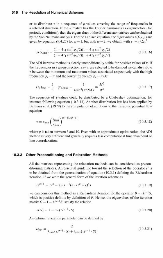
Ch10-H6594.tex 27/4/2007 12: 16 Page 516


or to distribute τ in a sequence of p-values covering the range of frequencies ina selected direction. If the S matrix has the Fourier harmonics as eigenvectors (forperiodic conditions), then the eigenvalues of the different submatrices can be obtainedby the Von Neumann analysis. For the Laplace equation, the eigenvalues λ(GADI) aregiven by equation (9.4.27) for ω = 1, but with ω = 2, we obtain, with τ1 = τ/�x2

λ(GADI) = (1 − 4τ1 sin2 φx/2)(1 − 4τ1 sin2 φy/2)

(1 + 4τ1 sin2 φx/2)(1 + 4τ1 sin2 φy/2)(10.3.16)

The ADI iterative method is clearly unconditionally stable for positive values of τ. Ifthe frequencies in a given direction, say y, are selected to be damped we can distributeτ between the minimum and maximum values associated respectively with the highfrequency φy = π and the lowest frequency φy = π/M

(τ1)min = 1

4(τ1)max = 1

4 sin2(π/2M )≈ M 2

π2(10.3.17)

The sequence of τ-values could be distributed by a Chebyshev optimization, forinstance following equation (10.3.13). Another distribution law has been applied byBallhaus et al. (1978) to the computation of solutions to the transonic potential flowequation

τ = τmin

(τmax

τmin

)(k−1)/(p−1)

(10.3.18)

where p is taken between 5 and 10. Even with an approximate optimization, the ADImethod is very efficient and generally requires less computational time than point orline overrelaxation.

10.3.3 Other Preconditioning and Relaxation Methods

All the matrices representing the relaxation methods can be considered as precon-ditioning matrices. An essential guideline toward the selection of the operator P isto be obtained from the generalization of equation (10.3.1) defining the Richardsoniteration. If we write the general form of the iteration scheme as

U n+1 = U n − τ ω P−1(S · U n + Qn) (10.3.19)

we can consider this method as a Richardson iteration for the operator B = τP−1S,which is positive definite by definition of P. Hence, the eigenvalues of the iterationmatrix G = 1 − τP−1S, satisfy the relation

λ(G) = 1 − ωλ(τP−1 · S) (10.3.20)

An optimal relaxation parameter can be defined by

ωopt = 2

λmin(τP−1 · S) + λmax(τP−1 · S)(10.3.21)

Ch10-H6594.tex 27/4/2007 12: 16 Page 517


and the spectral radius of G, becomes

ρ(G) = κ(τP−1S) − 1

κ(τP−1S) + 1(10.3.22)

The Richardson iteration has a poor convergence rate, because of the very highvalue of the condition number. In practical problems, the mesh is often dense incertain regions and more importantly, not uniform. A large variation in mesh spacingcontributes to an increase in the condition number, and values of 105–106 are notuncommon in large-size problems. On the other hand, a condition number closeto one leads to an excellent convergence rate. Therefore, various methods have beendeveloped which aim at choosing P such that the eigenvalues of τP−1S are much moreconcentrated. We mention here a few of them, referring the reader to the literaturecited for more details.

Incomplete Choleski factorization, Meijerink and Van Der Vorst (1977, 1981),Kershaw (1978)During an LU factorization of the banded matrix S, elements appear in L and U , atpositions where the S matrix has zero-elements. If an approximate matrix P is definedformed by L and U , P = LU where L and U are derived from L and U by maintainingonly the elements which correspond to the location of non-zero elements of S, wecan expect P to be a good approximation to S and that ρ(P−1S) will be close to one.Hence, L is defined by

lIJ = lIJ if sIJ �= 0= 0 if sIJ = 0

(10.3.23)

and similarly for U . Since P is very close to S, the matrix P−1S = (LU )−1LU will beclose to the unit matrix and the condition number of P−1S will be strongly reducedcompared to the condition of the S matrix. Hence, λ(G) = 1 − P−1S will be smalland high convergence rates can be expected. When used with a conjugate gradientmethod, very remarkable convergence accelerations on symmetric, positive definitematrices, have been obtained, Kershaw (1978). The coupling with the conjugategradient method is essential, since the P matrix obtained from the incomplete Choleskidecomposition although close to unity, still has a few extreme eigenvalues, whichwill be dominant at large iteration numbers. The conjugate gradient method, whenapplied to this preconditioned system, rapidly eliminates the extreme eigenvalues andcorresponding eigenmodes. We are then left with a system where all the eigenvaluesare close to one and the amplification matrix becomes very small.

Strongly Implicit Procedure (SIP), Stone (1968), Schneider and Zedan (1981)This is also an incomplete factorization technique, based on the matrix structurearising from the discretization of elliptic operators. The obtained matrix is block tridi-agonal or block pentadiagonal for the most current discretizations. The SIP methoddefines a conditioning matrix P as P = L ·U , where U = LT for symmetrical matricessuch that L and U have the non-zero elements in the same location as the S matrix. Aprocedure is derived allowing the determination of L and LT and the resulting system

Ch10-H6594.tex 27/4/2007 12: 16 Page 518


is solved by a forward and backward substitution as

L�U = −Rn

(10.3.24)LT�U n = �U

The L and LT matrices are obtained by a totally different procedure from the Choleskifactorization.

Conjugate Gradient Method, Reid (1971), Concus et al. (1976), Kershaw (1978)This method, originally developed by Hestenes and Stiefel is actually a direct method,which did not produce the expected results with regard to convergence rates. Howeveras an acceleration technique, coupled to preconditioning matrices, it can produceextremely efficient convergence accelerations. Coupled to the incomplete Choleskifactorization, the conjugate gradient method converges extremely rapidly, see Goluband Meurant (1983) and Hageman andYoung (1981) for some comparisons on elliptictest problems. However they require more storage than the relaxation methods andthis might limit their application for three-dimensional problems.

Generalized Minimum Residual (GMRES), Saad and Schultz (1985), Saad (2003)The Generalized Minimum Residual (GMRES) method can be considered as anextension of the family of conjugate gradient methods, and has been developed fornon-symmetric linear systems. It can be very efficient, once the iterative solution isclose enough to the converged solution. However, memory requirements could beprohibitive for very large-scale problems.

We refer you the recent literature, in particular Barrett et al. (2000), Saad (2003) formore information on these methods, as well as to the PETSc library for applicationsto complex problems.

For simplified problems, as will be presented in Chapters 11 and 12, we suggest youprogram the simplest iterative methods, described in Sections 10.1 and 10.2 yourself,in order to develop a ‘feeling’ for their properties.

10.4 NONLINEAR PROBLEMS

In a nonlinear problem, we define a Newton linearization in order to enter an iterativeapproximation sequence. If the nonlinear system is of the form

S(U ) = −Q (10.4.1)

the Newton iteration for U n+1 is

S(U n+1) = S(U n + �U ) = S(U n) +(

∂S

∂U

)· �U = −Q

J (U )�=(

∂S

∂U

)(10.4.2)

Ch10-H6594.tex 27/4/2007 12: 16 Page 519


where higher order terms in �U have been neglected. The Jacobian of S with respectto U , also called tangential stiffness matrix in the finite element literature, defines theiterative system,

J (U ) · �U n = −Rn (10.4.3)

In the linear case J = S and (10.4.3) is identical to the basic system (10.1.28). In thenonlinear case, the Newton formulation actually replaces the basic system (10.4.1).Indeed, close enough to the converged solution, the higher order terms can be madeas small as we wish and the algebraic system (10.4.3) can be considered as an ‘exact’equation.

If this equation would be solved by a direct method, we would obtain the exactsolution U as

U = U n − J (U )−1 · Rn (10.4.4)

The error en = U n − U , with respect to this exact solution satisfies the relation

J (U )en = Rn (10.4.5)

If the system (10.4.3) is solved by an iterative method, represented by the conditioningoperator P/τ,

P

τ· �U n = −Rn (10.4.6)

the error en will be amplified by the operator G, such that

en+1 = U n+1 − U = en + �U = en − τP−1Rn

= (1 − τP−1J )en ≡ Gen (10.4.7)

Hence, for a nonlinear system of equations, we can consider that the conditioningoperator should be an approximation to the jacobian matrix of the system (10.4.1).

The iterative scheme (10.4.6) will converge if the spectral radius of

G = 1 − τP−1J (10.4.8)

is lower or equal one.Equation (10.4.8) replaces therefore (10.3.3) for a nonlinear system. Actually, since

J = S for linear equations, (10.4.8) is the most general form of the amplification matrixof an iterative scheme with operator P/τ, applied to linear or nonlinear equations.

The definition (10.4.8) allows therefore the analysis of convergence conditions fornonlinear systems when the jacobian operator J (U ) can be determined.

Constant and secant stiffness methodThis denomination originates from finite element applications, where the followingconditioning matrices are often used, essentially for elliptic equations.

Ch10-H6594.tex 27/4/2007 12: 16 Page 520


Constant stiffness

P = S(U 0) (10.4.9)

The convergence matrix P is taken as the operator S at a previous iteration and keptfixed.

Secant stiffness

P = S(U n) (10.4.10)

The systems obtained can be solved by any of the mentioned methods, direct or iter-ative. In the former case we have a semi-direct method in the sense that the iterationstreat only the nonlinearity.

10.5 THE MULTIGRID METHOD

The multigrid method is the most efficient and general iterative technique knowntoday. Although originally developed for elliptic equations, such as the discretizedPoisson equation, Fedorenko (1962, 1964), the full potential of the multigrid approachwas put forward and systemized by Brandt (1972, 1977, 1982).

It has since then been applied to a variety of problems with great success, rangingfrom potential equations to Euler and Navier–Stokes discretizations on structuredas well as unstructured grids, and is still subject to considerable research anddevelopment (see for instance Thomas et al., 2003).

The following books provide more information on the basics of multigrid methodswith selected applications: Hackbusch and Trottenberg (1982), Briggs et al. (2000),Trottenberg et al. (2000) and Wesseling (2004).

The multigrid method finds its origin in the properties of conventional iterativetechniques, discussed in the previous sections. Their asymptotic slow convergence,consequence of the poor damping of the low frequency errors (long wavelengths) isa major problem of most iterative techniques. Indeed, as can be seen from equations(10.1.48) and (10.1.50) the asymptotic behavior of the error (or of the residual) isdominated by the eigenvalues of the amplification matrix close to one (in absolutevalue). These are associated to the eigenvalues of the space discretization operator Swith the lowest absolute value, i.e. to the lowest frequencies. For the Laplace operatorfor instance, the lowest eigenvalue |�J |min is obtained from equation (10.1.53) forthe low frequency component φx = φy = π/M .

We can therefore consider, on a fairly general basis, that the error componentssituated in the low frequency range of the spectrum of the space discretization operatorS, are the slowest to be damped in the iterative process. On the other hand, the higherfrequencies are very effectively damped and after a few iterations, a large part ofthe high frequency error spectrum will be significantly reduced. Remember that eachmode of the Fourier spectrum is reduced by a factor (λJ )n, where λJ is the eigenvalueof the amplification matrix, as seen from equation (10.1.50). In practical terms, ifλJ = 0.5, the associated mode will have decreased by a factor 2n after n iterations,while when λJ = 0.9999, it requires 23,000 iterations to reduce the associated errorby a factor 10 (see equation (10.1.42)).

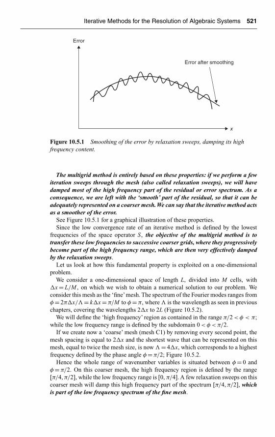
Ch10-H6594.tex 27/4/2007 12: 16 Page 521


Error after smoothing

Error

x

Figure 10.5.1 Smoothing of the error by relaxation sweeps, damping its highfrequency content.

The multigrid method is entirely based on these properties: if we perform a fewiteration sweeps through the mesh (also called relaxation sweeps), we will havedamped most of the high frequency part of the residual or error spectrum. As aconsequence, we are left with the ‘smooth’ part of the residual, so that it can beadequately represented on a coarser mesh.We can say that the iterative method actsas a smoother of the error.

See Figure 10.5.1 for a graphical illustration of these properties.Since the low convergence rate of an iterative method is defined by the lowest

frequencies of the space operator S, the objective of the multigrid method is totransfer these low frequencies to successive coarser grids, where they progressivelybecome part of the high frequency range, which are then very effectively dampedby the relaxation sweeps.

Let us look at how this fundamental property is exploited on a one-dimensionalproblem.

We consider a one-dimensional space of length L, divided into M cells, with�x = L/M , on which we wish to obtain a numerical solution to our problem. Weconsider this mesh as the ‘fine’mesh. The spectrum of the Fourier modes ranges fromφ = 2π�x/� = k�x = π/M to φ = π, where � is the wavelength as seen in previouschapters, covering the wavelengths 2�x to 2L (Figure 10.5.2).

We will define the ‘high frequency’ region as contained in the range π/2 < φ < π;while the low frequency range is defined by the subdomain 0 < φ < π/2.

If we create now a ‘coarse’ mesh (mesh C1) by removing every second point, themesh spacing is equal to 2�x and the shortest wave that can be represented on thismesh, equal to twice the mesh size, is now � = 4�x, which corresponds to a highestfrequency defined by the phase angle φ = π/2; Figure 10.5.2.

Hence the whole range of wavenumber variables is situated between φ = 0 andφ = π/2. On this coarser mesh, the high frequency region is defined by the range[π/4, π/2], while the low frequency range is [0, π/4]. A few relaxation sweeps on thiscoarser mesh will damp this high frequency part of the spectrum [π/4, π/2], whichis part of the low frequency spectrum of the fine mesh.

Ch10-H6594.tex 27/4/2007 12: 16 Page 522


0 p /2 p�x

C1

p /2p /40 p2�x

C2

p /20 pp /4p /84�x

C3

p /20 pp /4p /8

p /16

8�x

Figure 10.5.2 Fine and three coarse grid levels with associated parts of thespectrum damped by the relaxation sweeps. The shaded area indicates the dampedregions in the phase variable φ.

We can now repeat this process on the next coarser grid (mesh C2) by removingagain every second point; we obtain a grid with mesh size 4�x and the Fourierspectrum covers the range [0,π/4], with a high frequency range [π/8, π/4]. Performingagain a few relaxation sweeps will damp the spectrum in this range. Hence, after thisaction on the second coarse grid, we have damped the fine grid spectrum from π toπ/8. Note that these coarse grid actions have very reduced costs, since the numberof unknowns has been divided by 2 (for grid C1) and by 4 (for grid C2). For aGauss–Seidel method, for which the cost per iteration is proportional to N 2, this meansthat the cost is reduced respectively by 4 and 16, compared to a fine grid iteration.

For each additional coarser grid, this strategy will damp in a very effective wayadditional parts of the low frequency fine grid spectrum. On the last of the successivecoarser grids, we perform a larger number of sweeps to damp all the remainingfrequency. If this is the fourth grid level, e.g. the cost per iteration will divided by afactor 256!

As a consequence, in a single multigrid sequence, the complete error spectrumhas been damped. This is a remarkable property and explains the high performancelevel of the multigrid methods.

The general multigrid methodology is defined by the following succession ofsteps:

(i) Define a series of successive coarser grids by removing every second line ineach direction.

(ii) Transfer the system to be solved from the fine grid to the coarser grids.(iii) Apply one or more sweeps of an iterative method with good smoothing

properties of the higher frequency components, on each of the coarse grids.(iv) Transfer the corrected solution back to the fine grid in order to generate a new

approximation of the solution.

These different steps will be defined more precisely in the next sections, but itshould be clear that the error smoothing on the fine mesh is the essential property ofmultigrid methods.

Ch10-H6594.tex 27/4/2007 12: 16 Page 523


fx

fy

High frequencydomain

p

p

�p

�p

Low frequencydomain

�p /2

Hh

p /2

p /2

�p /2

Coarse mesh points

Figure 10.5.3 Low and high frequency domains for two-dimensional problems.

10.5.1 Smoothing Properties

The smoothing qualities of an iterative (relaxation) method can be estimated by eval-uating the maximum eigenvalues of the amplification matrix in the high frequencydomain of the associated wave number variable φ = [π/2, π].

In two dimensions, the high frequency domain is defined by the region π/2 ≤ φx,φy ≤ π (Figure 10.5.3), when the Fourier modes are considered, with a coarseningwhereby every second point is removed along the coordinate lines. This is the so-calledstandard coarsening. Hence, the smoothing factor μ is defined by

μ = Maxπ2 ≤φ≤π

|λ(G)| (10.5.1)

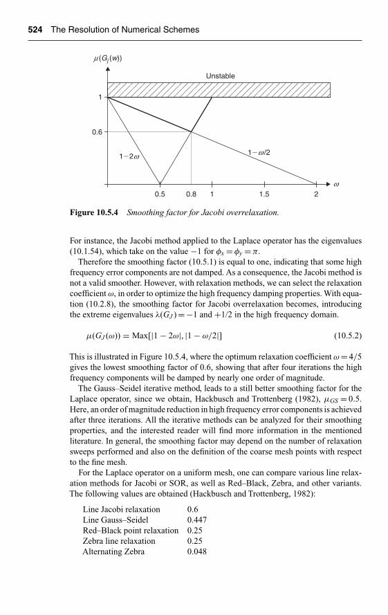
Ch10-H6594.tex 27/4/2007 12: 16 Page 524


w

Unstable

1

0.6

0.5 0.8 1 1.5 2

m (Gj (w))

1�2w 1�w /2

Figure 10.5.4 Smoothing factor for Jacobi overrelaxation.

For instance, the Jacobi method applied to the Laplace operator has the eigenvalues(10.1.54), which take on the value −1 for φx = φy = π.

Therefore the smoothing factor (10.5.1) is equal to one, indicating that some highfrequency error components are not damped. As a consequence, the Jacobi method isnot a valid smoother. However, with relaxation methods, we can select the relaxationcoefficient ω, in order to optimize the high frequency damping properties. With equa-tion (10.2.8), the smoothing factor for Jacobi overrelaxation becomes, introducingthe extreme eigenvalues λ(GJ ) = −1 and +1/2 in the high frequency domain.

μ(GJ (ω)) = Max[|1 − 2ω|, |1 − ω/2|] (10.5.2)

This is illustrated in Figure 10.5.4, where the optimum relaxation coefficient ω = 4/5gives the lowest smoothing factor of 0.6, showing that after four iterations the highfrequency components will be damped by nearly one order of magnitude.

The Gauss–Seidel iterative method, leads to a still better smoothing factor for theLaplace operator, since we obtain, Hackbusch and Trottenberg (1982), μGS = 0.5.Here, an order of magnitude reduction in high frequency error components is achievedafter three iterations. All the iterative methods can be analyzed for their smoothingproperties, and the interested reader will find more information in the mentionedliterature. In general, the smoothing factor may depend on the number of relaxationsweeps performed and also on the definition of the coarse mesh points with respectto the fine mesh.

For the Laplace operator on a uniform mesh, one can compare various line relax-ation methods for Jacobi or SOR, as well as Red–Black, Zebra, and other variants.The following values are obtained (Hackbusch and Trottenberg, 1982):

Line Jacobi relaxation 0.6Line Gauss–Seidel 0.447Red–Black point relaxation 0.25Zebra line relaxation 0.25Alternating Zebra 0.048

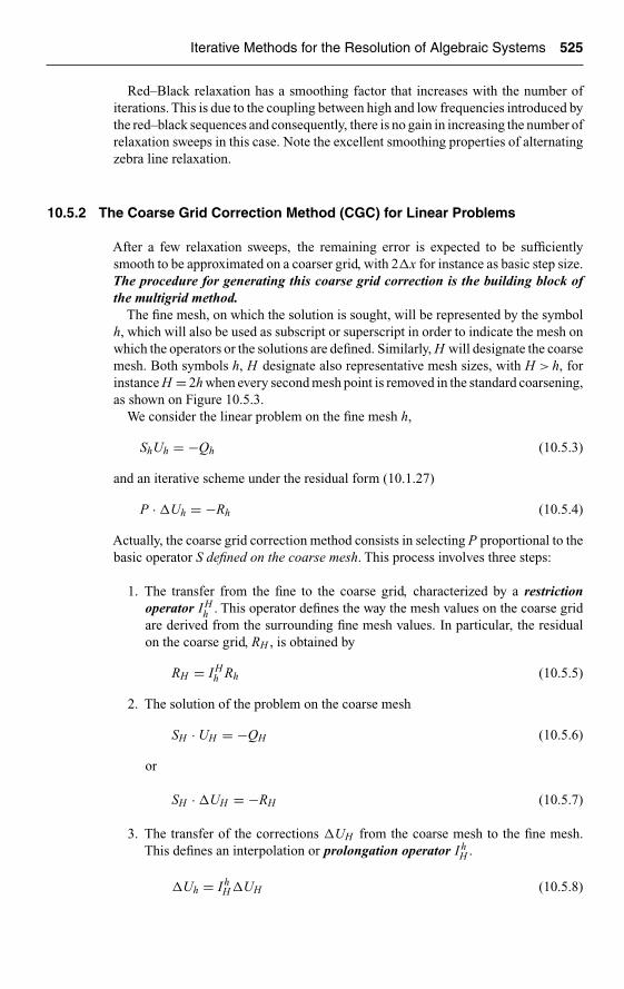
Ch10-H6594.tex 27/4/2007 12: 16 Page 525


Red–Black relaxation has a smoothing factor that increases with the number ofiterations. This is due to the coupling between high and low frequencies introduced bythe red–black sequences and consequently, there is no gain in increasing the number ofrelaxation sweeps in this case. Note the excellent smoothing properties of alternatingzebra line relaxation.

10.5.2 The Coarse Grid Correction Method (CGC) for Linear Problems

After a few relaxation sweeps, the remaining error is expected to be sufficientlysmooth to be approximated on a coarser grid, with 2�x for instance as basic step size.The procedure for generating this coarse grid correction is the building block ofthe multigrid method.

The fine mesh, on which the solution is sought, will be represented by the symbolh, which will also be used as subscript or superscript in order to indicate the mesh onwhich the operators or the solutions are defined. Similarly, H will designate the coarsemesh. Both symbols h, H designate also representative mesh sizes, with H > h, forinstance H = 2h when every second mesh point is removed in the standard coarsening,as shown on Figure 10.5.3.

We consider the linear problem on the fine mesh h,

ShUh = −Qh (10.5.3)

and an iterative scheme under the residual form (10.1.27)

P · �Uh = −Rh (10.5.4)

Actually, the coarse grid correction method consists in selecting P proportional to thebasic operator S defined on the coarse mesh. This process involves three steps:

1. The transfer from the fine to the coarse grid, characterized by a restrictionoperator I H

h . This operator defines the way the mesh values on the coarse gridare derived from the surrounding fine mesh values. In particular, the residualon the coarse grid, RH , is obtained by

RH = I Hh Rh (10.5.5)

2. The solution of the problem on the coarse mesh

SH · UH = −QH (10.5.6)

or

SH · �UH = −RH (10.5.7)

3. The transfer of the corrections �UH from the coarse mesh to the fine mesh.This defines an interpolation or prolongation operator I h

H .

�Uh = I hH �UH (10.5.8)

Ch10-H6594.tex 27/4/2007 12: 16 Page 526


2k �2 2k 2k �2

k �1 k k �1

Fine mesh

Coarse mesh

I Hh 1/4 1/4

1/2

Figure 10.5.5 Restriction operator for one-dimensional problem.

Restriction operatorLet us consider a one-dimensional mesh and a second order derivative discretized bythe central difference operator, h = �x,

Rh = 1

h2(ui+1 − 2ui + ui−1) + qi (10.5.9)

where i represents the fine mesh points (Figure 10.5.5). In order to relate i to thecoarse mesh points, obtained by removing every second point, we will set i = 2k .The coarse mesh points are then designated by k − 1, k , k + 1, . . .. Hence, equation(10.5.9) becomes, for constant q

Rh = 1

h2(u2k+1 − 2u2k + u2k−1) + q (10.5.10)

The full weighting restriction operator is defined by the distribution of Figure 10.5.5,such that each coarse mesh point receives a contribution from itself and the twoneighbouring fine mesh points, weighted respectively by the factors 1/2, 1/4, 1/4. Thesum of the weighting factors should always be equal to one for consistency.

The coarse mesh residual RH is obtained by

RH = I Hh Rh (10.5.11)

leading to

RH = 1

4h2(uk+1 − 2uk + uk−1) + q (10.5.12)

which is the discretization of the second derivative on the coarse mesh.This restriction operator is represented here by a matrix M /2 × M , where M is the

number of cells in the fine mesh.

I Hh =

k − 1k

k + 1

∣∣∣∣∣∣∣∣∣∣∣∣

2k − 1 2k 2k + 1· · · · · · · ·

1/4 1/2 1/4 · · · ·· · 1/4 1/2 1/4

1/4 1/2 1/4

∣∣∣∣∣∣∣∣∣∣∣∣(10.5.13)

Ch10-H6594.tex 27/4/2007 12: 16 Page 527


h

H

(a) Injection

1

1/16*

12 1

2

121

2

(b) Full weighting

4

(c) Half-weighting

1/4*

11

11

2

Figure 10.5.6 Restriction operator in two-dimensions on a uniform mesh.

Another choice is referred to as Simple Injection, whereby the coarse mesh functionsare taken equal to their fine mesh value H .

I Hh = 1 for all 2k fine mesh points

I Hh =

∣∣∣∣∣∣∣∣∣∣

. . . . . . . .

0 1 00 1 0

0 1 0. . . . . . . .

∣∣∣∣∣∣∣∣∣∣(10.5.14)

In two dimensions, the simple injection is represented by the molecule on Figure10.5.6a, where the central coarse mesh point is shown surrounded by its fine meshneighbors. The number inside the circle shows the local weight factor between thefine and coarse mesh functions in this point. Full weighting restriction is shown by themolecule of Figure 10.5.6b, while a half-weighting restriction operator is indicatedon Figure 10.5.6c.

Prolongation operatorProlongation or interpolation operators are generally defined by tensor products ofone-dimensional interpolation polynomials of odd order, such as the linear (or cubic)finite element interpolation functions. For the previous one-dimensional exampleof Figure 10.5.5, a linear interpolation would lead to the representation shown onFigure 10.5.7.

This is represented by a matrix M × M/2

I hH =

2k − 12k

2k + 1

∣∣∣∣∣∣∣∣∣∣∣∣∣∣

k − 1 k k + 1· · · · · · · ·

0 1/2 1/2 0 · · ·0 0 1 0 0

0 1/2 1/2 0 . .

0 1 01/2 1/2

∣∣∣∣∣∣∣∣∣∣∣∣∣∣

(10.5.15)

Generalized to a uniform two-dimensional mesh, we obtain the molecule shown onFigure 10.5.8.

Ch10-H6594.tex 27/4/2007 12: 16 Page 528


2k �2 2k 2k �2

k �1 k k �1

Fine mesh

Coarse mesh

1/2 1/2

1

I Hh

Figure 10.5.7 One-dimensional prolongation operator.

1/4*

1 1

1 1 2

2

22

1

11

4

Coarse mesh points

Fine mesh points

Figure 10.5.8 Two-dimensional prolongation operator.

Coarse grid correction operatorCombining the three steps mentioned above, the conditioning operator for the coarsegrid correction method PCGC

PCGC · �Uh = −Rh (10.5.16)

is obtained by combining equations (10.5.5), (10.5.7) and (10.5.8), leading to

�Uh = I hH �UH

= −I hH S−1

H · RH (10.5.17)

= −I hH S−1

H · I Hh Rh

Hence

P−1CGC = I h

H S−1H · I H

h (10.5.18)

The amplification matrix associated to equation (10.5.16), is defined by

U n+1h = GCGCU n

h − P−1CGCQ (10.5.19)

Ch10-H6594.tex 27/4/2007 12: 16 Page 529


with

GCGC = 1 − P−1CGCSh

= 1 − I hH S−1

H · I Hh Sh (10.5.20)

It is assumed here that the problem is solved exactly on the coarse grid H , i.e. that Scan be evaluated.

10.5.3 The Two-Grid Iteration Method for Linear Problems

The multigrid method on the two grids h, H is now completely defined when thesmoothing is combined with the coarse grid correction. Hence, the two-grid iterationmethod is obtained by the following sequence:

1. Perform n1 relaxation sweeps with smoother S1 on the fine mesh solution U nh

2. Perform the coarse grid correction; obtaining U n + 1h = U n

h + �Uh

3. Perform n2 relaxation sweeps with a smoother S2 on the fine mesh solution U n + 1h

Denoting by Gh,H the amplification matrix of the two-grid iteration method, byGS the amplification matrix of the relaxation method selected as smoothing operator,we obtain

Gh,H = Gn2S2

· GCGC · Gn1S1

= Gn2S2

· [1 − I hH S−1

H · I Hh Sh] · Gn1

S1(10.5.21)

Typical values for n1, n2 are one or two, and the smoothers S1 and S2 may bedifferent. For instance when an alternating line relaxation technique is applied (oneof the most efficient smoothers for elliptic equations), S1 could be connected to thehorizontal lines and S2 to the vertical lines. Another option is to modify the value ofsome relaxation coefficients between S1 and S2.

Convergence propertiesThe two-grid method will converge, if the spectral radius of Gh,H is lower than one

ρ(Gh, H ) ≤ 1 (10.5.22)

The convergence properties of the two-grid method can be analyzed on simple prob-lems, such as the Poisson equation and uniform meshes, by a Fourier–Von Neumannmethod, whereby the eigenvalues of the different operators in (10.5.21) are deter-mined. Examples of this approach can be found in Hackbusch amd Trottenberg(1982), where the spectral radius ρ(Gh,H ) ≤ 1 is obtained for various combinationsand choices of the operators in (10.5.21).

The two-grid method has remarkable convergence properties, which have beenproved by W. Hackbusch (see Hackbusch and Trottenberg (1982)), for a rather largeclass of problems. Namely, the asymptotic convergence rate is independent of themesh size h, that is independent of the number of mesh points.

Hence the computational work, in a two-grid method is determined essentiallyby the work required to perform the smoothing steps. Since the relaxation sweepsrequire a number of operations proportional to the number of fine mesh points N,the total work will vary linearly with N.

Ch10-H6594.tex 27/4/2007 12: 16 Page 530


(b) W-cycle (g �2)(a) V-cycle (g �1)

Smoothing

Exact resolution

Figure 10.5.9 Multigrid strategies on a four-grid method.

10.5.4 The Multigrid Method for Linear Problems

In the two-grid method, the solution step on the coarser grid, that is obtaining �UH

from (10.5.7), is supposed to have been performed accurately. In the multigridapproach, this solution is obtained by application of another two-grid iteration ona coarser grid, for instance a grid of size 2H = 4h. This can be repeated for the solu-tion of (10.5.7) on the grid 2H , and so on. The multigrid method is therefore definedon a succession of coarser and coarser grids, applying recursively the two-grid itera-tion, whereby the ‘exact’ solution of (10.5.7) has only to be obtained on the last, verycoarse grid.

Usually, four to five grids are used and various strategies can be chosen in thesequences of transfer and smoothing between successive grids. The V-cycle, shownon Figure 10.5.9a, consists in a succession of smoothing (symbol 0) and transfer tothe next coarser grid, with a unique exact solution (symbol �) on the coarsest grid,followed by a unique sequence of transfer and smoothing, back to the finest grid. Inthe W-cycles intermediate V-cycles are performed on the coarser grids, as shown onFigure 10.5.4b, where (γ) indicates the number of internal V-cycles.

The amplification matrix of the multigrid operator is obtained from equation(10.5.21) by replacing S−1

H in Gh,H by

S−1H ⇒ (1 − GH ,2H )S−1

H (10.5.23)

and performing the same replacement for the operator S−12H appearing in GH ,2H until

the coarsest grid is reached.It can be shown, that the convergence properties of the two-grid method apply

also to the multigrid approach, under fairly general conditions, namely the mesh-size independence of the convergence rate. Therefore the computational work of amultigrid cycle is essentially dominated by the number of operations required forthe two-grid computation from the finest to the next grid. Hence, the total work willremain proportional to the number of mesh points N of the fine grid. Note that W-cycles are roughly 50% more expensive than V-cycles, but are generally more robustand should be preferred, particularly for sensitive problems.

Other iterative techniques, require a number of operations for an error reduction ofone order of magnitude, of the order of N 3/2 (optimal SOR) or N 5/4 for preconditioned

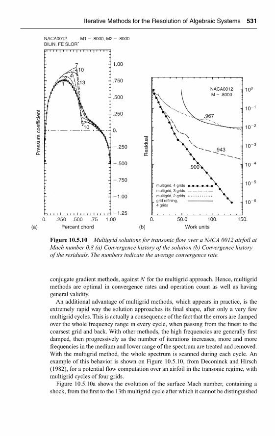
Ch10-H6594.tex 27/4/2007 12: 16 Page 531


50.0 100.

Work units

150.0.0. .250 .500

Percent chord(a) (b)

.75 1.00�1.25

�1.00

�.750

�.500

�.250

0.

.250

.500

.750

1.00

Pre

ssur

e co

effic

ient

12 4

710

13

10

NACA0012BILIN. FE SLOR-

NACA0012M � .8000

M1 � .8000, M2 � .8000

Res

idua

l

10�6

10�5

10�4

10�3

10�2

10�1

100

.967

.943

.900

multigrid, 4 gridsmultigrid, 3 gridsmultigrid, 2 gridsgrid refining,4 grids

Figure 10.5.10 Multigrid solutions for transonic flow over a NACA 0012 airfoil atMach number 0.8 (a) Convergence history of the solution (b) Convergence historyof the residuals. The numbers indicate the average convergence rate.

conjugate gradient methods, against N for the multigrid approach. Hence, multigridmethods are optimal in convergence rates and operation count as well as havinggeneral validity.

An additional advantage of multigrid methods, which appears in practice, is theextremely rapid way the solution approaches its final shape, after only a very fewmultigrid cycles. This is actually a consequence of the fact that the errors are dampedover the whole frequency range in every cycle, when passing from the finest to thecoarsest grid and back. With other methods, the high frequencies are generally firstdamped, then progressively as the number of iterations increases, more and morefrequencies in the medium and lower range of the spectrum are treated and removed.With the multigrid method, the whole spectrum is scanned during each cycle. Anexample of this behavior is shown on Figure 10.5.10, from Deconinck and Hirsch(1982), for a potential flow computation over an airfoil in the transonic regime, withmultigrid cycles of four grids.

Figure 10.5.10a shows the evolution of the surface Mach number, containing ashock, from the first to the 13th multigrid cycle after which it cannot be distinguished

Ch10-H6594.tex 27/4/2007 12: 16 Page 532


from the final converged solution. After one single cycle, we are already very close tothe overall shape of the converged solution, and basically 10–15 multigrid cycles aresufficient for a fully converged solution. Figure 10.5.10b compares the convergencerates of the residual for a line relaxation SLOR iterative method and the multigrid withtwo, three and four grids. The numbers indicated represent the average convergencerate of the residuals and are an approximation of the spectral radius of the multigridamplification matrix. One work unit on the horizontal scale corresponds to one SLORiteration on the fine grid. The improvement with respect to SLOR is spectacular andwe can also notice the influence of the number of grids on the overall convergencerates. Note that these computations have been performed for a nonlinear problem bythe method presented in the following section.

10.5.5 The Multigrid Method for Nonlinear Problems

For nonlinear problems, the multigrid method can be applied in association with alinearization process such as the Newton linearization (10.4.3). However, we can alsoadapt the multigrid approach directly to the nonlinear equations by operating simul-taneously on the residuals Rh and on the solution Uh itself instead of the corrections�Uh. This is known as the Full Approximation Scheme (FAS) (Brandt, 1977).

Considering the nonlinear problem on mesh h,

Sh(Uh) = −Qh (10.5.24)

the two-grid nonlinear FAS solves for U new = (Uh + �Uh), solution of

Sh(Uh + �Uh) − Sh(Uh) = −Rh (10.5.25)

by a transfer to a coarser grid H .After n1 relaxation sweeps on Uh, a transfer of residuals and of the solution to the

coarse grid is defined by two restriction operators I Hh and I H

h

RH = I Hh Rh (10.5.26)

UH = I Hh Uh (10.5.27)

The two restriction operators may be different, since they are operating on differentspaces. Hence, on the coarse grid H , equation (10.5.25) becomes

SH (UH + �UH ) − SH (UH ) = −RH (10.5.28)

or

SH (UH + �UH ) = −I Hh Rh + SH (I H

h Uh)

= −I Hh Qh − I H

h Sh(Uh) + SH (I Hh Uh) (10.5.29)

In the multigrid method, equation (10.5.29) is solved by subsequent transfer to a nextcoarser grid. On the final grid, this nonlinear equation has to be solved exactly. Thekey motivation behind this formulation is to ensure that the coarse grid solutionsmaintain the truncation errors of the fine grid.

Ch10-H6594.tex 27/4/2007 12: 16 Page 533


When transferring from the coarse to the fine grid, a prolongation operator is appliedto the corrections �UH defined by

�UH = U newH − UH (10.5.30)

leading to

�Uh = I hH �UH (10.5.31)

and to the fine grid solution

U newh = Uh + I h

H �UH (10.5.32)

The multigrid cycle is closed after performing n2 smoothing relaxation sweeps onthe new solution U new

h . In the full approximation scheme no global linearizationis required, except on the last coarsest mesh and for the local linearizations of therelaxation sweeps.


Iterative methods for the solution of algebraic systems are an important componentof many CFD methods. We have provided in this chapter a brief introduction in orderto allow you to grasp the basic components and some of the essential properties ofiterative methods. In particular, the following properties are to be kept in mind:

• Each iterative method, also called relaxation method, can be defined by aconvergence, or preconditioning, matrix P.

• Iterative methods are very effective in damping effectively the lowest eigenvaluesof the amplification matrix G = 1 − P−1S.

• The low eigenvalues of G are associated with the high frequencies of the spacediscretization matrix S, represented by their Fourier modes, and inversely, thehigh eigenvalues of G are associated with the low frequencies of the matrix S.

• Many variants of preconditioning are available, such as overrelaxation methods.The field of preconditioned methods is very wide and we recommend to theinterested reader to consult the cited references for in-depth information.

• From all the current methods, multigrid is by far the most effective and themost general of all convergence acceleration techniques. It has the remarkableproperty of a convergence rate independent of the number of mesh points; i.e. itreaches the ideal situation of a cost of the order of O(N ). Hence, application ofmultigrid is highly recommended.

REFERENCES

Ballhaus, W.F., Jameson, A. and Albert, T.J. (1978). Implicit approximate factorizationschemes for steady transonic flow problems. AIAA J., 16, 573–579.

Barrett, R. et al. (10 authors) (1994). Templates for the Solution of Linear Systems:Building Blocks for Iterative Methods. SIAM, Philadelphia, Can be downloaded fromhttp://netlib2.cs.utk.edu/linalg/html_templates/Templates.html

Ch10-H6594.tex 27/4/2007 12: 16 Page 534


Berman, A. and Plemmons, R.J. (1979). Non-Negative Matrices in the MathematicalSciences. Academic Press, New York.

Brandt, A. (1972). Multilevel adaptive technique for fast numerical solution to boundaryvalue problems. Proceedings of the 3rd International Conference on Numerical Meth-ods in Fluid Dynamics. Lecture Notes in Physics, Vol. 18. Springer Verlag, New York,pp. 82–89.

Brandt, A. (1977). Multilevel adaptive solutions to boundary value problems. Math.Comput., 31, 333–390.

Brandt, A. (1982). Guide to multigrid development. In Multigrid Methods, Lecture Notesin Mathematics, Vol. 960. Springer Verlag, New York.

Briggs, W., Van Emden, H. and McCormick, H. (2000). A multigrid tutorial. SIAM –Society for Industrial and Applied Mathematics, 2nd edn., Philadelphia

Concus, P., Golub, G.H. and O’Leary, D.P. (1976). A generalized conjugate gra-dient method for the numerical solution of elliptic partial differential equations.In Space Matrix Computations, J.R. Bunch and D.J. Rose (Eds). Academic Press,New York.

Dahlquist, G. and Bjork, A. (1974). Numerical Methods. Prentice Hall, New Jersey.Deconinck, H. and Hirsch, Ch. (1982). A multigrid method for the transonic full potential

equation discretized with finite elements on an arbitrary body fitted mesh. J. Comput.Phys., 48, 344–365.

Fedorenko, R.P. (1962). A relaxation method for solving elliptic differential equations.USSR Comput. Math. and Math. Phys., 1, 1092–1096.

Fedorenko, R.P. (1964). The speed of convergence of an iterative process. USSR Comput.Math. and Math. Phys., 4, 227–235.

Golub, G.H. and Meurant, G.A. (1983). Resolution Numerique des Grands SystemesLineaires. Eyrolles, Paris.

Hackbusch, W. and Trottenberg, U. (Eds) (1982). Multigrid Methods. Lecture Notes inMathematics, Vol. 960. Springer Verlag, New York.

Hageman, L. and Young, D.M. (1981). Applied Iterative Methods. Academic Press,New York.

Kershaw, D.S. (1978). The incomplete Cholesky conjugate gradient method for theiterative solution of linear equations. J. Comput. Phys., 26, 43–65.

LeVeque, R.A. and Trefethen, L.N. (1986). Fourier analysis of the SOR iteration. NASA-CR 178191, ICASE Report 86-63.

Marchuk, G.I. (1975). Method of Numerical Mathematics. Springer Verlag, Berlin.Meijerink, J.A. and Van Der Vorst, H.A. (1977). An iterative solution method for lin-

ear systems of which the coefficient matrix is a M-matrix. Math. Comput., 31,148–162.

Meijerink, J.A. and Van Der Vorst, H.A. (1981). Guidelines for the usage of incompletedecompositions in solving sets of linear equations as they occur in practice. J. Comput.Phys., 44, 134–155.

Meis, T. and Marcowitz, U. (1981). Numerical Solution of Partial Differential Equations.Springer Verlag, New York.

Mitchell, A.R. (1969). Computational Methods in Partial Differential Equations.J. Wiley & Sons, New York.

Mitchell, A.R. and Griffiths, D.F. (1980). The Finite Difference Method in PartialDifferential Equations. J. Wiley & Sons, New York.

Reid, J.K. (1971). On the method of conjugate gradients for the solution of large sparsesystems of linear equations. In Large Sparce Sets of Linear Equations, J.K. Reid (Ed.).Academic Press, New York

Ch10-H6594.tex 27/4/2007 12: 16 Page 535


Saad, Y. (1993). Numerical Methods for Large Eigenvalue Problems, Manchester Uni-versity Press Series. Out of print. An updated version is available on: http://www-users.cs.umn.edu/∼saad/books.html.

Saad, Y. (2003). Iterative Methods for Sparse Linear Systems, 2nd edn. SIAM.An updated first edition, originally published in 1996, can be downloaded fromhttp://www-users.cs.umn.edu/∼saad/books.html.

Saad, Y. and Schultz, M. (1985). Conjugate gradient-like algorithms for solving non-symmetric linear systems. Math. Comput., 44, 417–424.

Schneider, G.E. and Zedan, M. (1981). A modified strongly implicit procedure for thenumerical solution of field problems. Num. Heat Transfer, 4, 1–19.

Stone, H.L. (1968). Iterative solution of implicit approximations of multidimensionalpartial differential equations. SIAM J. Num. Anal., 5, 530–558.

Strang, G. (1976). Linear Algebra and Its Applications. Academic Press, New York.Thomas, J.L., Diskin, B. and Brandt, A. (2003). Textbook multigrid efficiency for fluid

simulations. Ann. Rev. Fluid Mech., 35, 317–340.Trottenberg, U., Oosterlee, C.W. and Schuller, A. (2000). Multigrid. Academic Press,

New YorkVarga, R.S. (1962). Matrix Iterative Analysis. Prentice Hall, Inc., New Jersey.Wachspress, E.L. (1966). Iterative Solution of Elliptic Systems. Prentice Hall, New Jersey.Wesseling, P. (2004). An Introduction to Multigrid Methods. R.T. Edwards, Inc,

PhiladelphiaYoung, D.M. (1971). Iterative Solution of Large Linear Systems. Academic Press,

New York.

PROBLEMS

P.10.1 Write the discretized equations for the nodes close to all the boundaries forPoisson’s equation (10.1.1), (10.1.2) based on Figure 10.1.1. Repeat the sameexercise for Neumann conditions along the boundary j = 0 (y = 0), of the form

∂u

∂y= g y = 0

by applying a one sided difference.P.10.2 Consider the stationary diffusion equation αuxx = q in the domain 0 < x < 1 and

the boundary conditions

x = 0 u(0) = 0x = 1 u(1) = 0

with q/α = −4. Apply a central second order difference and solve the schemewith the tridiagonal algorithm for �x = 0.1 and �x = 0.02 and compare withthe analytical solution.

P.10.3 Solve Problem P.10.2 with the Jacobi method. Write the matrices D, E, F astridiagonal matrices B(a, b, c).

P.10.4 Solve Problem P.10.2 with the Gauss–Seidel method and compare the conver-gence rate with the Jacobi method.

P.10.5 Obtain the eigenvalue λ(GADI) of equation (10.3.16), for the ADI precondition-ing operator.

Ch10-H6594.tex 27/4/2007 12: 16 Page 536


P.10.6 Consider the steady state convection–diffusion equation aux = αuxx discretizedwith second order central differences. Write explicitly the tridiagonal systemobtained and apply a Gauss–Seidel method.

Repeat and compare to a SOR method.P.10.7 Solve the Poisson equation

�u=−2π2 sin πx · sin πy

on a square 0 < x < 1, 0 < y < 1, with the homogeneous Dirichlet boundaryconditions, u = 0 on the four sides. Select a five-point discretization on arectangular mesh.

Consider a 11 × 11 mesh and solve with a Jacobi iteration and compare theconvergence rate with the same computation on a 21 × 21 mesh. Compare theresults with the exact solution u = sin πx sin πy.

P.10.8 Repeat Problem P.10.7 with a Gauss–Seidel, SOR, SLOR and ADI meth-ods. Try different relaxation parameters and compare convergence rates andcomputational times.

P.10.9 Consider the alternative definition of a line overrelaxation method, where theintermediate values are obtained with the fully updated values in the right-handside. Instead of (10.2.33), define

un+1ij = 1

4(un

i+1, j + un+1i−1, j + un+1

i, j+1 + un+1i, j−1) + 1

4qn

ij

un+1ij = ωun+1

ij + (1 − ω)unij

and obtain the incremental form

4�U nij − ω�U n

i, j−1 − ω�U ni, j+1 − ω�U n

i−1, j = ωRnij

Apply to Problems P.10.7, P.10.8 and compare with the other methods.

APPENDIX A:Thomas Algorithm For Tridiagonal Systems

A.1 Scalar Tridiagonal Systems

For tridiagonal systems, the LU decomposition method leads to an efficient algorithm,known as Thomas’ algorithm. For a system of the form

ak xk−1 + bk xk + ck xk+1 = fk k = 1, . . . , N (A.1)

with

a1 = cN = 0 (A.2)

the following algorithm is obtained

Forward stepCalculate successively

β1 = b1 βk = bk − akck−1

βk−1k = 2, . . . , N

γ1 = f1β1

γk = −akγk−1 + fkβk

k = 2, . . . , N(A.3)

Ch10-H6594.tex 27/4/2007 12: 16 Page 537


Backward step

xN = γN

xk = γk − xk+1ck

βkk = N − 1, . . . , 1 (A.4)

This requires in total 5N operations.It can be shown that the above algorithm will always converge if the tridiagonal

system is diagonal dominant, i.e. if

|bk | ≥ |ak | + |ck | k = 2, . . . , N−1|b1| ≥ |c1| and |bN | ≥ |aN | (A.5)

If a, b, c are matrices, we have a block-tridiagonal system, and the same algorithm canbe applied. Due to the importance of tridiagonal system, we present here a subroutine,which can be used for an arbitrary scalar tridiagonal system.

Subroutine TRIDAG

SUBROUTINE TRIDAG(AA,BB,CC,FF,N1,N)CC***********************************************************************C SOLUTION OF A TRIDIAGONAL SYSTEM OF N-N1+1 EQUATIONS OF THE FORMCC AA(K)*X(K-1) + BB(K)*X(K) + CC(K)*X(K+1) = FF(K) K=N1,...,NCC K RANGING FROM N1 TO NC THE SOLUTION X(K) IS STORED IN FF(K)C AA(N1) AND CC(N) ARE NOT USEDC AA,BB,CC,FF ARE VECTORS WITH DIMENSION N, TO BE SPECIFIED IN THEC CALLING SEQUENCECCC***********************************************************************C

DIMENSION AA(1),BB(1),CC(1),FF(1)BB(N1)=1./BB(N1)AA(N1)=FF(N1)*BB(N1)N2=N1+1N1N=N1+NDO 10 K=N2,NK1=K-1CC(K1)=CC(K1)*BB(K1)BB(K) =BB(K)-AA(K)*CC(K1)BB(K) =1./BB(K)AA(K) =(FF(K)-AA(K)*AA(K1))*BB(K)

10 CONTINUECC BACK SUBSTTUTIONC

FF(N)=AA(N)DO 20 K1=N2,NK=N1N-K1

Ch10-H6594.tex 27/4/2007 12: 16 Page 538


FF(K)=AA(K)-CC(K)*FF(K+1)20 CONTINUE

RETURNEND

A.2 Periodic Tridiagonal Systems

For periodic boundary conditions, and a tridiagonal matrix with one in the extremecorners as in equation (9.1.16), the above method does not apply. The followingapproach leads to an algorithm whereby two tridiagonal systems have to be solved.

If the periodic matrix Bp(�a, �b, �c) has (N + 1) lines and columns resulting from a peri-odicity between points 1 and N + 2, the solution X is written as a linear combination

X = X (1) + xN+1X (2) or xk = x(1)k + xN+1 · x(2)

k (A.6)

where the vectors X (1) and X (2) are solutions of tridiagonal systems obtained byremoving the last line and last column of Bp, containing the periodic elements. If this

modified matrix is called B(N )(�a, �b, �c), we solve successively, where the right-handside terms fk are put in a column vector F .

B(N )(�a, �b, �c)X (1) = F (A.7)

followed by

B(N )(�a, �b, �c)X (2) = G (A.8)

with

GT = ( − a1, . . . , 0, −cN ) (A.9)

The last unknown xN+1 is obtained from the last equation by back-substitution

xN+1 = fN+1 − cN+1x(1)1 − aN+1x(1)

N

bN+1 + cN+1x(2)1 + aN+1x(2)

N

(A.10)

The periodicity condition, determines x as

xN+2 = x1 (A.11)

The subroutine TRIPER is included here, based on this algorithm. Note that if theperiodicity condition is

xN+2 = x1 + C (A.12)

then the periodicity constant C has to be added to the right-hand side of the lastinstruction, defining FF(N + 2).

Subroutine TRIPERSUBROUTINE TRIPER(AA,BB,CC,FF,N1,N,GAM2)

CC**********************************************************************C SOLUTION OF A TRIDIAGONAL SYSTEM OF EQUATIONS WITH PERIODICITYC BETWEEN THE POINTS K=N1 AND K=N+2

Ch10-H6594.tex 27/4/2007 12: 16 Page 539


CC AA(K)*X(K-1) + BB(K)*X(K) + CC(K)*X(K+1) = FF(K) K=N1,...,N+1CC THE ELEMENT IN THE UPPER RIGHT CORNER IS STORED IN AA(N1)C THE ELEMENT IN THE LOWER LEFT CORNER IS STORED IN CC(N+1)C AA,BB,CC,FF,GAM2 ARE VECTORS WITH DIMENSION N+2, TO BE SPECIFIEDC IN THE CALLING SEQUENCEC GAM2 IS AN AUXILIARY VECTOR NEEDED FOR STORAGEC THE SOLUTION X(K) IS STORED IN FF(K)CC***********************************************************************C

DIMENSION AA(1),BB(1),CC(1),FF(1), GAM2(1)BB(N1)=1./BB(N1)GAM2(N1)=-AA(N1)*BB(N1)AA(N1)=FF(N1)*BB(N1)N2=N1+1N1N=N1+NDO 10 K=N2,NK1=K-1CC(K1)=CC(K1)*BB(K1)BB(K) =BB(K)-AA(K)*CC(K1)BB(K) =1./BB(K)GAM2(K)=-AA(K)*GAM2(K1)*BB(K)AA(K) =(FF(K)-AA(K)*AA(K1))*BB(K)

10 CONTINUEGAM2(N)=GAM2(N)-CC(N)*BB(N)

CC BACK SUBSTTUTIONC

FF(N)=AA(N)BB(N)=GAM2(N)DO 20 K1=N2,NK=N1N-K1K2=K+1FF(K)=AA(K)-CC(K)*FF(K2)NN(K)=GAM2(K)-CC(K)*BB(K2)

20 CONTINUEC

K1=N+1ZAA=FF(K1)-CC(K1)*FF(N1)-AA(K1)*FF(N)ZAA=ZAA/(BB(K1)+AA(K1)*BB(N)+CC(K1)*BB(N1))FF(K1)=ZAADO 30 K=N1,NFF(K)=FF(K)+BB(K)*ZAA

30 CONTINUEC

FF(N+2)=FF(N1)RETURNEND

Ch11-H6594.tex 8/5/2007 20: 8 Page 541

Part V

Applications to Inviscid andViscous Flows

We have now reached the stage where you can start applying the acquired methodologyto compute realistic flows.

You certainly have gained the awareness from the previous chapters, that for anymathematical model an unlimited number of options are available to set up the numeri-cal model, although practical experience reduces the choice to a more restricted range.In the previous chapters, we have focused essentially on numerical schemes of secondorder accuracy in space, which is generally considered as providing the best com-promise in terms of cost to accuracy ratio. This still leaves many options open, asdifferent schemes have different dissipation and dispersion error properties.

Writing CFD codes is a learning process where many components have to be takeninto account, step by step. Whatever mathematical model you select, from the simplestpotential flow to Euler equations, up to laminar and turbulent full Navier–Stokesmodels, you have to make a choice on each of the following topics and to evaluatetheir impact on the solution accuracy, on convergence behavior and on computationaltime:

• The type of grid and its mesh point density, cell-centered or cell-vertexconfigurations.

• The numerical scheme, defined by the selected time and space discretization.For steady state simulations, you need to select only the space discretization.

• The boundary conditions and their numerical implementation.• The resolution method of the obtained algebraic system and the treatment of the

nonlinearities.

Once your code runs without bugs, you should give great attention to verifica-tion and validation. This is a fundamental step in assuring that your code not onlyworks properly, but even more importantly, in assessing the accuracy dependencewith varying grid density and with parameters of the numerical scheme and itsimplementation.

As you will experience when writing your own code, ‘the devil is in the details’,since as soon as you deviate from the ideal configuration of a uniform Cartesiangrid, you have to make choices at any step of the discretization on non-uniform gridsand with the nonlinear components. We refer here to issues such as the selection of

541

Ch11-H6594.tex 8/5/2007 20: 8 Page 542

542 Applications to Inviscid and Viscous Flows

the points where face quantities are evaluated, at mid-point, or by taking averagesof neighboring points; the evaluation of gradients; the discretization of boundaryconditions and the choice of interpolation between near-boundary points; and manyother details that you will face with increasing complexity of the CFD models.

Verification and validation are critical issues of any simulation and refer to twodifferent steps in code development and code assessment. Formal definitions of theseconcepts are subject to much debate among experts, and the definitions agreed uponin the AIAA1 Committee on Standards in CFD, AIAA (1998), or the ASME2 PTC 60Committee on Verification and Validation in Computational Solid Mechanics, ASME(2006), are not identical. Our own definition of verification is a synthesis, aimingat clarity and simplicity, compatible with the more advanced options from theseCommittees.

Verification: The process of determining that a model implementation accuratelyrepresents the underlying mathematical model and its solutions.

Verification is thus defined as the steps by which you verify that the mathematicalmodel is correctly programmed. It is based on comparing the numerical results withexact, analytical solutions, and should help you assess the correctness and the accuracyof the numerical discretization, as well as its grid dependence.

Validation: The process of determining the degree to which a model is an accuraterepresentation of the real world from the perspective of the intended uses of the model.

Validation refers to comparisons with real world experimental data and will allowyou to assess the accuracy of the physical model assumptions entering in yourmathematical model. For instance, validating turbulence models, two-phase models,empirical data related to real gas effects, temperature dependence of viscosity, etc,can only be achieved by comparing with experimental data, when and if available.

The relation between the real world, the conceptual mathematical models selectedto describe it and the numerical simulation tool, is summarized in Figure V.1, fromOberkampf et al. (2004), where more details on the implications of verification andvalidation can be found.

The issue of validation of CFD codes for industrial relevant applications is anextremely complex process as it is hardly possible to generate experimental data atthe same level of details as provided by the CFD simulation. In addition, both experi-mental and numerical data are subjected to many error and uncertainty sources, withthe consequence that an absolute validation of simulation results remains an unreach-able objective. It requires, at the end, to take into account the uncertainties and tocall upon good judgment and expert knowledge, both of the physical properties ofthe investigated system and of the numerical properties of the selected scheme, toassess the validity range and the confidence level that we can attach to a numericalresult. These uncertainties associated to real life problems, make the issue of veri-fication even more essential, with the objective to ensure that at least the numericaldiscretization is full proof and has a controllable accuracy.

Verification is therefore a prerequisite, upstream of the validation process andrequires a dedicated effort and an adequate and systematic methodology, to coverall the numerical aspects of a CFD code.

1 AIAA: American Institute for Aeronautics and Astronautics.2 ASME: American Society of Mechanical Engineers.

Ch11-H6594.tex 8/5/2007 20: 8 Page 543

Applications to Inviscid and Viscous Flows 543

Analysis

Programming

Computersimulation

Modelvalidation

Modelqualification

Modelverification

Reality

Conceptualmodel

Computerizedmodel

Figure V.1 Conceptual relation between the real world, the conceptual modelsand the computer model.

Consequently, we will restrict your first steps in the world of CFD code developmentto this verification phase and we will select flow configurations having analyticalor well-established reference solutions (obtained for instance on very fine meshes),enabling you an in-depth verification of all the steps of the numerical implementation.

Keep in mind that when comparing with exact solutions, as opposed to experimentalresults, you are considering only the numerical error sources and it is essential todevelop a good understanding of their impact on the solution accuracy. In particular,the verification process should lead to an evaluation of grid dependence, in terms ofeffects of grid quality and grid density on accuracy. In practical terms, you should beable to establish guidelines on grid density for a pre-selected level of accuracy, as youwill wish to know for instance how many mesh points you need for an accuracy of 1%or for an accuracy of 0.1% on a selected quantity. Note also that the response to thisquestion will vary according to the selected quantity. Requiring an accuracy of 0.1%on drag or on a heat transfer coefficient will lead to more severe requirements on thegrid density compared to a similar level of accuracy on less sensitive quantities, suchas lift or pressure coefficients, since the latter are basically of inviscid origin.

This part contains two chapters, separated into inviscid flow models and laminarflows. Chapter 11 will guide you through the steps for writing a program for inviscidflows, modeled by the potential equation and the Euler equations. We will first selecta flow case with an exact solution, such as the incompressible potential flow around acircular cylinder in 2D, which will help us illustrate some major differences betweenpotential and Euler equation models. We will handle next a representative internalcompressible flow case of the flow on a circular bump on a lower wall, with a flat upperwall. This flow has no analytical solution, but a reference solution can be obtained byselecting a very fine grid. As third case, a supersonic flow over a wedge, generatingan oblique shock with an analytical solution, will be treated, with the objective tointroduce you to some aspects of transonic and supersonic flows.

Ch11-H6594.tex 8/5/2007 20: 8 Page 544


Chapter 12 will concentrate on viscous, laminar flows in two dimensions and somewell-known laminar flow cases, such as the Couette flow between two plates, includingthermal effects and the flat plate laminar boundary layer, for which exact numericalsolutions are known. This chapter will allow us to introduce an alternative solutionmethods, particularly well adapted to incompressible flows, namely the pressurecorrection method, which you will be able to compare with the compressible basedmethod developed in Chapter 11. It will be applied to another standard test case,namely the lid driven cavity, for which reference solutions on fine grids are available.

Our main objective with these two chapters is not to show nice or perfect solutions,but on the contrary, to draw your attention to all the potential error sources that arehidden behind a CFD code, and which can affect the accuracy of your solution. Thisapplies in very much the same way to your own code or to a third party code thatyou would apply as a ‘user’. By putting the emphasis on the details of the algorithmimplementation, the associated options and eventual user dependent parameters, suchas artificial viscosity coefficients, relaxation parameters, boundary conditions, con-vergence levels and behavior, . . . , we wish to raise your awareness so as to be able toexercise your critical judgment when evaluating a CFD application. We also expectit will guide you in your readiness to ask the right questions to CFD developers orCFD code providers.

The sections on the applications in these chapters have been written with the activeparticipation of Dr. Benoit Tartinville, from Numeca International, who producedalso the results of the three inviscid test cases of Chapter 11 and the two viscous casesof Section 12.3, and of Dr. Sergey Smirnov, at the Vrije Universiteit Brussel, whocontributed to the sections on the pressure correction method, Sections 12.4 and 12.5,and produced the program and the results for the lid driven cavity of Section 12.5.Their contribution is gratefully acknowledged.

Ch11-H6594.tex 8/5/2007 20: 8 Page 545

Chapter 11

Numerical Simulation of Inviscid Flows


In this first chapter dedicated to the practical implementation of the simplest of inviscidflows, we will guide you through the various steps required to write a CFD code.

Inviscid flows are modeled in general by the system of Euler equations. Consideringflow conditions with uniform inflow, that is an irrotational flow far upstream, weknow from inviscid flow theory and Helmholtz theorem, that the flow will remainirrotational everywhere. In other words, it is equivalent to a potential flow. The latteris the highest level of simplification of a flow description, as all the flow variables canbe obtained from the single scalar potential function.

The main difference between the potential and the time-dependent Euler equationmodels, as identified in Chapter 3, lies in their mathematical properties. We haveseen, and we refer you to Chapter 3, Sections 3.2.2 and 3.4.1, that the steady potentialequation is elliptic at subsonic speeds and hyperbolic in the supersonic range; whilethe unsteady Euler equations are always hyperbolic in space and time, independentlyof the flow regime. This has major consequences on the discretization approach, as theschemes for Laplace-like equations of subsonic potential flows, fail when applied tosupersonic conditions; while this will not be the case with the Euler equations. Hence,we will focus on time-dependent discretization methods for the Euler equations,looking for the numerical steady solution, as advocated in the previous chapters.

The other important difference is connected to the possible generation of numericalentropy with the Euler equation model, as a consequence of the numerical dissipationof the selected scheme. This will allow you to identify one of the most importantproperties of numerical CFD solutions, namely the ‘visible’effects of the numericaldissipation. We will show that numerical dissipation generates vorticity and entropyand as a consequence regions of entropy increase provide a picture of the influence ofnumerical dissipation. Since potential flows are by definition irrotational, this markerof numerical dissipation is not present with the potential model.

Another important property of flows around solid bodies is the generation of liftand drag, resulting from the balance of pressure and shear stresses on the surface.With inviscid flows, there is no viscous drag and the numerical ‘production’ of dragis also a global marker of the influence of numerical viscosity.

As the Euler equations form the basis for the full Navier–Stokes solutions, par-ticularly at high Reynolds numbers where the flow properties are dominated byconvection, the observed properties will be of critical importance when the samediscretization of the convective terms is applied to viscous flows. Indeed, when thenumerical viscosity is too high, for instance when applying first order schemes oncoarse grids, or when the grid resolution or quality is not sufficient with second order

545

Ch11-H6594.tex 8/5/2007 20: 8 Page 546


schemes, the effects of this numerical dissipation on the flow behavior can overshadowthe effects of the molecular or turbulent viscosity. Therefore, an accurate identifica-tion of the level and of the flow areas where this is likely to happen is essential inorder to establish the reliability of your numerical results.

It is therefore advocated, when you run a Navier–Stokes simulation, to firstperform an Euler simulation of the same test case and on the same grid, looking forthe regions influenced by numerical dissipation, by tracking the growth of entropy.

Before starting, we also wish to provide you with some general guidelines onhow to structure and organize your program. The key issue is to be able to verify, ateach step, the correctness of groups of instructions, as well as your input and outputsections. This requires a systematic and modular construction of your program, basedon ‘building bocks’ formed by separate subroutines or modules, each one of thembeing verified separately.

We recommend you to proceed as follows:

• Start with a main program whose function is exclusively to control all the stepsof your algorithm, as well as the input and output modules. Do not intro-duce algorithmic elements in the main program, concentrating them in separatesubroutines.

• Define subroutines with a single objective, i.e. avoid different functionalitiesin the same subroutine. For instance, if you need to solve algebraic systems,consider a routine that fulfills this objective without adding other functionalities,such as preparing output plots for instance.

• Verify each of these subroutines as an isolated subprogram. For the examplementioned, create algebraic systems with known exact solutions and applyyour subprogram to verify that it operates correctly. Once this is achieved,and if errors appear in your program, you will be assured that it does notcome form the verified subroutine, but most probably from incorrect or invalidinput data.

• During the debugging phase, introduce print instructions at all steps of yourprogram, before and after the instructions, which you will remove when all thebugs are fixed. For instance, when you read in geometrical or flow data from afile, we recommend printing immediately these data, to make sure that they arecorrectly read, in the proper format and in the expected units. Similarly, whenthe main program calls a subroutine, put print instructions before and after thecall, to verify that the input data as well as the output data are as expected.

The potential and Euler models and some of their essential properties are presentedin Sections 11.1 and 11.2. The steady potential flow solutions are treated in Section11.3. The flow case suggested for the development of your first CFD program is thepotential flow around a cylinder, for which we know an exact solution in the limit ofincompressible flows. This will allow you to verify the accuracy of your numericalsolution, in function of discretization options and grid density. The extension tocompressible potential flows will be included, and when keeping the Mach numberlow enough, you will also be able to verify your numerical solution by comparisonwith the exact incompressible solution.

Section 11.4 focuses on the application of the Finite Volume Method (FVM) tothe system of Euler equations, on a cell-centered grid. We will select a central space

Ch11-H6594.tex 8/5/2007 20: 8 Page 547

Numerical Simulation of Inviscid Flows 547

discretization, requiring the introduction of artificial dissipation, which we willcouple to a Runge–Kutta time integration method. A most critical issue with theEuler equations is the definition and the number of physical boundary conditionswe are allowed to impose. This will be related to the hyperbolic properties and theassociated characteristic speeds of propagation.

Section 11.5 will guide you to the applications of your FVM code to three testcases. The first one is the flow around the cylinder, as a first verification case. Thesecond case is the compressible internal flow between two solid walls, with a circularbump on the lower wall. Although this flow has no known exact solution, a numericalsolution obtained on a fine grid will serve as a reference solution for verification. Athird case, with an exact solution, is the supersonic flow over a wedge, generating anoblique shock and will put you in a first contact with some important issues relatedto the presence of shock discontinuities.

Figure 11.0.1 summarizes the guide through this chapter.

11.1 The inviscid Euler equations

11.2 The potential flow model

11.3 Numerical solutions for thepotential equation

11.4 Finite volume discretizationof the euler equations

11.5 Numerical solutions for theEuler equations

Conservative form of the two-dimensional Euler equationsInfluence of compressibilityDiscontinuous solutions of EulerequationsLift and drag calculation

Potential flow equations: propertiesand limitations

Exact solution of theincompressible cylinder flowDescription of grids and of thenumerical discretizationExtensions to compressiblepotential flows

Implementation of a finite volumecell-centered method with centralspace discretizationTime integrationAnalysis of boundary conditionsfor inviscid flows

Application of the FVM to flowaround the cylinderInternal channel flow over acircular bumpSupersonic wedge flow

Figure 11.0.1 Content and guide to this chapter.

Ch11-H6594.tex 8/5/2007 20: 8 Page 548


11.1 THE INVISCID EULER EQUATIONS

The system of Euler equations describes flows where the influence of viscous shearstresses and heat conduction effects can be neglected.

Referring to Section 2.7, the system of Euler equations, is written in a compact,conservative form as

∂U

∂t+ �∇ · �F = 0 (11.1.1)

This system of first order partial differential equations is hyperbolic in time andspace, and in two dimensions the flux vector �F has the Cartesian components ( f , g)given by

f =

∣∣∣∣∣∣∣∣

ρuρu2 + p

ρuvρuH

∣∣∣∣∣∣∣∣g =

∣∣∣∣∣∣∣∣

ρvρvu

ρv2 + pρvH

∣∣∣∣∣∣∣∣U =

∣∣∣∣∣∣∣∣

ρ

ρuρvρE

∣∣∣∣∣∣∣∣(11.1.2)

Note that when combining the continuity equation (first equation) with the energyconservation equation (fourth equation), we obtain

∂H

∂t+ u

∂H

∂x+ v

∂H

∂y= 1

ρ

∂p

∂t(11.1.3)

which reduces, for steady flows, to the constancy of total enthalpy H :

H = Hinlet along each streamline (11.1.4)

It is important to notice the properties of the entropy variations in an inviscidflow. From equation (2.7.3) and in absence of heat sources, the entropy equation forcontinuous flow variations reduces to

T

(∂s

∂t+ �v · �∇s

)= 0 (11.1.5)

expressing that entropy is constant along a flow path. For steady flows, we have

s = sinlet along each streamline (11.1.6)

The value of the entropy can however vary from one flow path to another. This isbest seen from Crocco’s form of the momentum equation (1.5.13), which reduces,for a stationary inviscid flow in absence of external forces, to

−(�v × �ζ) = T �∇s − �∇H (11.1.7)

In an intrinsic coordinate system with unit vectors (�el , �en, �eb), where 1 is directed alongthe velocity and b is the binormal direction, this equation becomes, when projectedin the normal direction n, for a uniform total enthalpy,

|�v|ζb = T∂s

∂n(11.1.8)

Ch11-H6594.tex 8/5/2007 20: 8 Page 549


This relation shows that entropy variations in the direction normal to the local velocitydirection are connected to vorticity. Hence entropy variations will generate vorticityand inversely, vorticity will create entropy gradients.

11.1.1 Steady Compressible Flows

The constancy of the total enthalpy, identical to the constancy of the total temperatureT0, takes the following form, assuming perfect gas conditions, where A is a point onthe inlet surface:

H = cpT0 = HA = cpT0A

T0 = T + �v2

2cp= T

(1 + γ − 1

2M 2)

(11.1.9)

The isentropic relations between pressure, temperature and density, are

ρ

ρ0=[

T

T0

]1/(γ−1)

=[

p

p0

]1/γ

(11.1.10)

Important propertyCombining the isentropic condition s = const., with equation (11.1.9), expressing theconstancy of total temperature or total enthalpy, and taking into account equation(1.4.36), repeated here for convenience


(H/HA)γ/(γ−1)(11.1.11)

we see immediately that the total pressure has to be constant

p0 = p

[1 + γ − 1

2M 2]γ/(γ−1)

= p0A (11.1.12)

Hence, all stagnation conditions are constant along streamlines. Note that theseconstant values can change from one streamline to the other. However, if the incom-ing flow is uniform, leading to a potential flow, then there is only one constant valueover the whole flow field.

11.1.2 The Influence of Compressibility

An important question in practical applications is related to the choice between acompressible flow model and a purely incompressible model, for low velocity flowsof gases, such as air.

In other words, below which velocity, or Mach number levels, can we consider aflow of air as incompressible?

The answer to this question can be obtained from the above relations, for instanceby evaluating the numerical influence of Mach number on total pressure, equation(11.1.12).

Ch11-H6594.tex 8/5/2007 20: 8 Page 550


Table 11.1.1 Mach number influence on compressibility effects.

M γM 4/8 M 2/4

0.01 1.75 × 10−9 0.0000250.05 1.09375 × 10−6 0.0006250.1 1.75 × 10−5 0.00250.2 0.000280 0.010.3 0.00141750 0.0225

It is known from basic fluid mechanics and Bernoulli equation in particular, thatin an incompressible flow with constant density, the stagnation pressure is defined by

p0 = p + ρ�v2

2(11.1.13)

Referring to the general definition (11.1.12), we can expand this equation in powerseries of Mach number M , in order to compare with equation (11.1.13).

We obtain

p0

p=[

1 + γ − 1

2M 2]γ/(γ−1) ∼= 1 + γ

2M 2 + γ

8M 4 + 2 − γ

48γM 6 + O(M 8)

(11.1.14)

With the definition of Mach number as

M 2 = �v2

γrT(11.1.15)

where the speed of sound is defined as c = √γrT , and with the perfect gas law

p = ρrT , we obtain

p0 ∼= p + ρ�v2

2+ γ

8pM 4 + p

2 − γ

48γM 6 + O(M 8) (11.1.16)

The dominating correction factor for compressibility influence is the third termof this equation γpM 4/8, but we prefer to evaluate the ratio of this correction to thesecond term, ratio equal to M 2/4, as seen from equation (11.1.14). For the standardvalue of γ = 1.4, valid in particular for air, these factors take the following values forvarious Mach numbers (Table 11.1.1).

The second column is the ratio between the third term and the static pressure p (firstterm), while the third column is the ratio between the third term and the dynamicpressure (second term). At M = 0.1, the compressibility effect represents a correctionto the dynamic pressure of 0.25% and reaches 1% at M = 0.2.

For practical reasons we may consider a 1% error as acceptable and concludethat for M ≤ 0.2, the compressibility effects can be neglected and the gas flow can beconsidered as incompressible. For a flow of air at atmospheric conditions (T = 288 K),the speed of sound is c ≈ 340 m/s and the limit M = 0.2 corresponds to a velocity of68 m/s or 250 km/h. This can be considered as a serious storm if we think about it asan atmospheric wind speed.

Ch11-H6594.tex 8/5/2007 20: 8 Page 551


A

V

B C

C

ΔΣ

D

Figure 11.1.1 Control volume around a moving discontinuity surface � (� is aninfinitesimal distance normal to �).

11.1.3 The Properties of Discontinuous Solutions

As is known, the set of Euler equations allows also discontinuous solutions in certaincases, namely vortex sheets, contact discontinuities or shock waves occurring insupersonic flows. The properties of these discontinuous solutions can only be obtainedfrom the integral form of the conservation equations, since the gradients of the fluxesare not defined at discontinuity surfaces.

For a discontinuity surface �, moving with velocity �C, the integral conservationlaws are applied to the infinitesimal volume V of Figure 11.1.1.

Referring to equation (1.1.2) in absence of source terms, the integral form of theEuler equations, takes the following form:

∂

∂t

∫V

U d� +∮

S

�F · d�S = 0 (11.1.17)

The time derivative of the volume integral has to take into account the motion of thesurface � and hence of the control volume V , through

∂

∂t

∫V

U d� =∫

V

∂U

∂td� +

∫V

U∂

∂t(d�)

=∫

V

∂U

∂td� −

∮S

U �C · d�S (11.1.18)

expressing the conservation of the volume V in the translation with velocity �C.The flux term in equation (11.1.17) can be rewritten for vanishing volumes

V (� → 0) as

∮S

�F · d�S =∫

�

(�F2−�F1) · d �� ≡∫

�

[�F · �en]d� (11.1.19)

Ch11-H6594.tex 8/5/2007 20: 8 Page 552


where d �� is normal to the discontinuity surface � and where the notation

[A] ≡ A2 − A1 (11.1.20)

denotes the jump in the variable A when crossing the discontinuity.Combining (11.1.18) and (11.1.19) we obtain, for vanishing volumes V,

∫

�

([�F] − �C[U ]) · d �� = 0 (11.1.21)

leading to the local form of the conservation laws over a discontinuity, called theRankine–Hugoniot relations

[�F] · �en − �C[U ] · �en = 0 (11.1.22)

If �(�x, t) = 0 is the discontinuity surface, then we have

d�

dt≡ ∂�

∂t+ ( �C · �∇)� = 0 (11.1.23)

With the unit vector along the normal �en defined by

�en = �∇�∣∣∣ �∇�

∣∣∣(11.1.24)

equation (11.1.22) takes the form

[�F] · �∇� + [U ]∂�

∂t= 0 (11.1.25)

Various forms of discontinuities are physically possible:

• Shocks where all flow variables undergo a discontinuous variation.• Contact discontinuities and vortex sheets, also called slip lines, across which

no mass transfer takes place but where density, as well as the tangential velocity,maybe discontinuous, although pressure and normal velocity remain continuous.

The properties of these discontinuous solutions can best be seen from a referencesystem moving with the discontinuity. In this system the discontinuity surface is sta-tionary, C = 0, and the Rankine–Hugoniot relations for the Euler equations become

[ρvn] = 0 (11.1.26a)

[ρvn�v] + [p] �en = 0 (11.1.26b)

ρvn[H ] = 0 (11.1.26c)

where vn is the normal component of the velocity vector vn = �v · �en.

Ch11-H6594.tex 8/5/2007 20: 8 Page 553


The third equation shows that total enthalpy always remains constant throughthe discontinuity.

This system admits solutions with the following properties.

11.1.3.1 Contact discontinuities

They are defined by the condition of no mass flow through the discontinuity:

vn1 = vn2 = 0 (11.1.27)

and, following equation (11.1.26) , by continuity of pressure

[p] = 0 (11.1.28)

allowing non-zero values for the jump in specific mass, as seen from equation(11.1.26a)

[ρ] �= 0 (11.1.29)

The tangential velocity variation over the discontinuity could be continuous or not,as seen from the tangential projection of equation (11.1.26b).

When the tangential velocity is continuous, we have a contact discontinuity

[vt] = 0 (11.1.30)

11.1.3.2 Vortex sheets or slip lines

They are also defined by the conditions of no mass flow through the discontinuity,continuous pressure and discontinuous density, as for the contact discontinuity, butwith a jump in tangential velocity:

vn1 = vn2 = 0

[p] = 0

[ρ] �= 0

[vt] �= 0 (11.1.31)

11.1.3.3 Shock surfaces

Shocks are solutions of the Rankine–Hugoniot relations with non-zero mass flowthrough the discontinuity, which appear with supersonic flows. Consequently, pres-sure and normal velocity undergo discontinuous variations, while the tangentialvelocity remains continuous. Hence, shocks satisfy the following properties:

[vn] �= 0

[p] �= 0

[ρ] �= 0

[vt] = 0 (11.1.32)

Ch11-H6594.tex 8/5/2007 20: 8 Page 554


Note that since the stagnation pressure p0 is not constant across the shock, theinviscid shock relations imply a discontinuous entropy variation through the shock.This variation has to be positive, corresponding to compression shocks and excludinghereby expansion shocks, for physical reasons connected to the second principle ofthermodynamics, (Shapiro, (1953); Zucrow and Hoffmann, (1976)).

It has to be added that expansion shocks, whereby the entropy jump is negative, arealso valid solutions of the inviscid equations. Hence, there is no mechanism allowingto distinguish between discontinuities with entropy increase (positive entropy jump)or entropy decrease (negative entropy variation). An additional condition, called theentropy condition has therefore to be added to the inviscid equation in order toexclude these non-physical solutions, (Lax, 1973). This is necessary for all inviscidflow models and a more detailed discussion of the entropy condition is presented inVolume II.

The mathematical formulation of the second principle of thermodynamics can beexpressed, for an adiabatic flow without heat conduction nor heat sources qH = 0,following equation (1.4.18)

ρT

(∂s

∂t+ �v · �∇s

)= εv (11.1.33)

Since εv is the viscous dissipation and always positive, this equation states that anysolution of the Euler equations which has a physical sense as a limit, for vanishingviscosity, of real fluid flow phenomena, has to satisfy the following entropy inequality:

(∂s

∂t+ �v · �∇s

)≥ 0 (11.1.34)

In addition, a non-uniform discontinuity such as a shock with varying intensity willgenerate a non-uniform entropy field in the direction normal to the velocity. Equation(11.1.8) then shows that as a consequence, vorticity will be generated downstreamof the shock. Hence, even for irrotational flow conditions upstream of the shock, arotational flow will be created by a non-uniform shock intensity.

11.1.4 Lift and Drag on Solid Bodies

The lift and drag resulting forces exerted by the flow on a solid body can be obtainedby an extension of the momentum conservation law in integral form, equation (1.3.9).See also the ‘Advanced’ section A1.6.1 in Chapter 1.

If the control volume � contains a solid body, then an additional force (−�R) has tobe added to the right-hand side of equation (1.3.9), where �R is the total force exertedby the fluid on the body. The total force �R is composed of the lift force �L, defined asthe component normal to the incoming velocity, and the drag force �D defined as thecomponent parallel and opposed to the incoming velocity direction.

We obtain, in absence of external forces, for stationary flows:

∮Sρ�v(�v · d�S) = −

∮S

p d�S +∮

S

¯τ · d�S − �R (11.1.35)

Ch11-H6594.tex 8/5/2007 20: 8 Page 555


S

Solid bodyU∞

Sb

Figure 11.1.2 Far-field control surface for lift and drag determination on enclosedsolid body.

Based on this equation, two methods can be applied to calculate lift and drag forces:

(i) For a surface S located in the far field (Figure 11.1.2), where the viscous shearstresses can be considered as negligible, the sum of the stationary lift and dragforces are given by the following relation, for stationary flows:

−�R = −(�L + �D) =∮

Sρ�v(�v · d�S) +

∮S

p d�S (11.1.36)

(ii) On the other hand, if the control surface S is taken on the solid body surfaceSb, where the velocity field is either zero due to the non-slip condition ofviscous flows or having zero normal velocity with inviscid flows, then the liftand drag forces are also defined by the following relation, since the left-handside term of equation (11.1.35) is zero

�R = �L + �D = −∮

Sb

p d�S +∮

Sb

¯τ · d�S (11.1.37)

This is an important relation, which is currently applied to determine lift and dragforces from computed flow fields.

For inviscid flows, there are no shear stresses and the lift force over the body isthe resultant of the pressure forces:

�L = −∮

Sb

p d�S (11.1.38)

Note that, for aeronautical applications, the lift force is often considered as defined bythe vertical component of the pressure forces and its horizontal component is calledthe pressure drag, as it will act alongside the drag force, although it results from theinviscid pressure forces.

Ch11-H6594.tex 8/5/2007 20: 8 Page 556


11.2 THE POTENTIAL FLOW MODEL

The most impressive simplification of the mathematical description of a flow systemis obtained with the approximation of a non-viscous, irrotational flow.

The condition of zero vorticity

�ζ = �∇ × �v = 0 (11.2.1)

will be automatically satisfied if the three-dimensional velocity field can be describedby a single scalar potential function φ, defined by

�v = �∇φ (11.2.2)

since the rotation of a gradient is identical zero, for any value of the function φ.This reduces the knowledge of the three velocity components to the determination

of a single scalar function φ.It is known from the theory of inviscid flows, that the vorticity remains constant in

any streamtube. Hence, in a flow where the rotation free condition (11.2.1) is satisfiedat the inlet boundary, it will remain so everywhere in the flow domain. In particular,since a uniform flow is rotation free, any subsonic inviscid flow with uniform inletconditions will remain rotation free everywhere.

This has far-reaching consequences, namely that all the flow variables of a 3D invis-cid potential flow are completely defined by the single potential function. Hence we areleft with one unknown instead of five, which represents a considerable simplification.

The applications handled in this chapter will be restricted to steady potential flows,which offers an additional simplification.

It is seen from equation (11.1.8) that a potential flow is always isentropic,and with the isentropic relation (11.1.10), the density itself is completely definedby the potential function, as shown by equation (2.8.6), assuming perfect gasconditions:

ρ

ρ0=[

1 − �v2

2H

]1/(γ−1)

=[

1 − ( �∇φ)2

2H

]1/(γ−1)

(11.2.3)

where ρ0 is the stagnation density, constant throughout the whole flow field and γ isthe specific heat ratio, equal to γ = 1.4 for air.

Since all stagnation conditions are constant throughout the whole flow field allthermodynamic properties are known as soon as we know the potential function.This demonstrates the simplification introduced by potential flows, where the knowl-edge of the single scalar potential function determines all the five flow variablesin 3D.

From equation (2.8.5) we obtain the steady potential equation:

�∇ · (ρ �∇φ) = 0 (11.2.4)

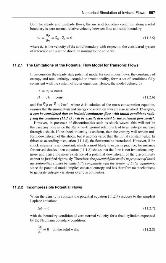
Ch11-H6594.tex 8/5/2007 20: 8 Page 557


Both for steady and unsteady flows, the inviscid boundary condition along a solidboundary is zero normal relative velocity between flow and solid boundary

vn = ∂φ

∂n= �uw · �en = 0 (11.2.5)

where �uw is the velocity of the solid boundary with respect to the considered systemof reference and n is the direction normal to the solid wall.

11.2.1 The Limitations of the Potential Flow Model for Transonic Flows

If we consider the steady state potential model for continuous flows, the constancy ofentropy and total enthalpy, coupled to irrotationality, form a set of conditions fullyconsistent with the system of Euler equations. Hence, the model defined by

s = s0 = const.

H = H0 = const. (11.2.6)

and �v = �∇φ or �∇ × �v = 0, where φ is solution of the mass conservation equation,ensures that the momentum and energy conservation laws are also satisfied. Therefore,it can be considered that an inviscid continuous flow, with initial conditions satis-fying the condition (11.2.1) , will be exactly described by the potential flow model.

However, in presence of discontinuities such as shock waves, this will not bethe case anymore since the Rankine–Hugoniot relations lead to an entropy increasethrough a shock. If the shock intensity is uniform, then the entropy will remain uni-form downstream of the shock, but at another value than the initial constant value. Inthis case, according to equation (11.1.8), the flow remains irrotational. However, if theshock intensity is not constant, which is most likely to occur in practice, for instancefor curved shocks, then equation (11.1.8) shows that the flow is not irrotational any-more and hence the mere existence of a potential downstream of the discontinuitycannot be justified rigorously. Therefore, the potential flow model in presence of shockdiscontinuities cannot be made fully compatible with the system of Euler equations,since the potential model implies constant entropy and has therefore no mechanismsto generate entropy variations over discontinuities.

11.2.2 Incompressible Potential Flows

When the density is constant the potential equation (11.2.4) reduces to the simplestLaplace equation:

�φ = 0 (11.2.7)

with the boundary condition of zero normal velocity for a fixed cylinder, expressedby the Neumann boundary condition:

∂φ

∂n= 0 on the solid walls (11.2.8)

Ch11-H6594.tex 8/5/2007 20: 8 Page 558


In the far field, where the inflow velocity �U is constant, we have from the definitionof the potential function:

φ − φ0 = �U · �x (11.2.9)

11.3 NUMERICAL SOLUTIONS FOR THE POTENTIAL EQUATION

We will deal here with a single case, defined by the flow around a cylinder, forwhich an exact solution is available in the incompressible limit. It will offer a firstopportunity to illustrate several aspects of a CFD code related to grid properties andto the accuracy dependence with grid density.

Although applied to the simplest of the models, the conclusions will neverthelessbe of more general validity.

11.3.1 Incompressible Flow Around a Circular Cylinder

We start with one of the simplest potential flows, the 2D incompressible flow arounda circular cylinder of radius a, with uniform inlet velocity U , as illustrated inFigure 11.3.1.

An exact solution is known from classic fluid dynamics, defined by the complexpotential function ζ = φ + Iψ (I = √−1), where ψ is the streamfunction

ζ(z) = φ(x, y) + Iψ(x, y) z = x + Iy (11.3.1)

The complex velocity is defined by

u − Iv = dζ

dz(11.3.2)

leading to the relations

u = ∂φ

∂x= ∂ψ

∂y

v = ∂φ

∂y= −∂ψ

∂x(11.3.3)

a

uq

ur

xBA

U

2UC

y

q

Figure 11.3.1 Two-dimensional, incompressible potential flow around a circularcylinder for a uniform incident velocity field.

Ch11-H6594.tex 8/5/2007 20: 8 Page 559


The exact incompressible potential solution for a cylinder of radius a, is defined by

ζ(z) = φ(x, y) + Iψ(x, y) = U

(z + a2

z

)(11.3.4)

leading to

φ(x, y) = Uxx2 + y2 + a2

x2 + y2ψ(x, y) = Uy

x2 + y2 − a2

x2 + y2(11.3.5)

and

u − Iv = U

(1 − a2

z2

)(11.3.6)

or

u = U

[1 − a2(x2 − y2)

(x2 + y2)2

]v = −2Ua2 xy

(x2 + y2)2(11.3.7)

On the cylinder surface, that is for x2 + y2 = a2, we have

φ = 2Ux ψ = 0

u = 2U

(1 − x2

a2

)v = −2U

xy

a2

(11.3.8)

Another representation is obtained when replacing the complex position variable z byits polar, instead of its Cartesian, form

z = x + Iy = reIθ = r( cos θ + I sin θ) (11.3.9)

The exact solution to this potential flow becomes, in cylindrical coordinates

ζ(z) = φ(r, θ) + Iψ(r, θ) = U

(reIθ + a2

re−Iθ

)

φ(r, θ) = U

(r + a2

r

)cos θ ψ(r, θ) = U

(r − a2

r

)sin θ (11.3.10)

The polar velocity components are defined by

ur = ∂φ

∂r= 1

r

∂ψ

∂θ= U

(1 − a2

r2

)cos θ

uθ = 1

r

∂φ

∂θ= −∂ψ

∂r= −U

(1 + a2

r2

)sin θ (11.3.11)

In particular on the cylinder surface, defined by

z = aeIθ = a( cos θ + I sin θ) (11.3.12)

Ch11-H6594.tex 8/5/2007 20: 8 Page 560


the complex potential function on the surface reduces to

φ(r, θ) = 2Ua cos θ ψ(r, θ) = 0 (11.3.13)

and the velocity components take the following values:

ur = 0 uθ = −2U sin θ (11.3.14)

This confirms that the cylinder surface is a streamline where the velocity is alongthe tangential direction. The negative sign results from the definition of the tangen-tial velocity component as being positive in the anti-clockwise direction, while theincoming velocity is in the positive x-direction, as shown on Figure 11.3.1. Note thatthe velocity is zero at the stagnation points A, B, but reaches a value equal to 2U , thatis twice the incoming velocity at the top of the cylinder in point C, at θ = 90◦.

The pressure field is obtained from the constancy of the stagnation pressure(11.1.13), written here for incompressible flows

p0 = p + ρ�v2

2= p∞ + ρ

U 2

2(11.3.15)

and is best expressed by a non-dimensional pressure coefficient Cp, which isindependent of the inlet velocity:

Cp = p − p∞

ρU 2

2

= 1 − �v2

U 2= 1 −

∣∣∣ �∇φ

∣∣∣2U 2

(11.3.16)

The pressure coefficient on the surface (indicated by a subscript S) is generally plottedin function of the solid wall arc length, and becomes here, with (11.3.14)

Cp∣∣S = pS − p∞

ρU 2

2

= 1 − �v2S

U 2= 1 − 4 sin2 θ (11.3.17)

Figure 11.3.2 displays the streamlines and potential lines, as well as the surfacepressure coefficient.

We now proceed by following the steps of the previous chapters, as developed inParts I–IV:

(a) Select the mathematical model.(b) Define the grid.(c) Define the numerical scheme.(d) Establish the stability and accuracy properties of the scheme, based on the

material of the previous chapters. If necessary, perform a new analysis.(e) Solve the algebraic system.(f) Analyze the results and evaluate the grid dependence and overall accuracy.

These steps should be translated into a flowchart, establishing the structure of yourmain program, as seen on Figure 11.3.3. Each box should represent a call to one or

Ch11-H6594.tex 8/5/2007 20: 8 Page 561


(a)

(b) (c)

1.0

0.5

0.00 50

�0.5

�1.0

�1.5

�2.0

�2.5

�3.0

100 150 200theta

250 300 350

Figure 11.3.2 Potential flow on a circular cylinder: (a) streamlines, (b) potentiallines and (c) surface pressure coefficient CpS in function of angular position θ.

more separate subroutines, each one having a single objective. It is recommendedduring the debugging phase, to add print instructions before and after each call to asubroutine, to verify that the intended operations are correctly executed.

Let us now apply this to the mathematical model of the incompressible potentialflow equation (11.2.17) with the boundary conditions (11.2.18) and (11.2.9).

11.3.1.1 Define the grid

We will select a straightforward analytical grid in polar coordinates, formed by circlesand radial lines, allowing you to have full control of mesh density and mesh spacing.

You are now faced with your first decision, namely you have to fix the outer bound-ary of your computational domain for this external flow problem. This is an importantdecision, since we apply free undisturbed flow conditions on this boundary and there-fore it should be located far enough from the solid body in order to ensure that itsinfluence is negligible. Keep in mind that in subsonic flows, all the points in the flowdomain influence each other, as is typical for elliptic equations. Hence, in theory

Ch11-H6594.tex 8/5/2007 20: 8 Page 562


Print/plot andanalyze the results

Call the routine for solution of thealgebraic system

Monitor the convergence by followingthe residual drop

Discretize the mathematical model,including treatment of thenonlinearities when present

Discretize the boundary conditions

Define the main variables for flowand grid-related quantities

Set the program structure

Read-in or define the grid densityand coordinates

Read-in the inlet flow conditions

Figure 11.3.3 Structure of main program.

we will always have some disturbance from uniform flow conditions on the outerboundary, but if far enough it could be neglected.

In practical terms, a distance of the order of 40–50 times the radius should berecommended for the outer boundary, at least for non-lifting bodies.

For lift generating airfoils, the far field is influenced by a free vortex singularitydefined by the circulation around the airfoil, which tends to zero like the inverse ofthe distance. Either this correction is introduced in the far field, or we have to increasethe distance of the outer boundary to values closer to 100 chords.

This initial decision can be a first source of errors, and in case of doubt, youshould apply your code with several positions of the downstream boundary, andverify its influence on the solution.

How to choose the grid spacing?

Option 1: Select circles equally spaced in radius value (index i) and radial lines equallyspaced in angular position (index j), as shown on Figure 11.3.4. If the outer boundaryis fixed at 40 times the cylinder radius a, then if we consider a mesh with Ni points inthe radial direction, the radial spacing between the circles should be equal to 40a/Ni.

Option 2: The first option might seem straightforward, but at second thought it is notsuch a good idea. Indeed, an important guideline to a good grid is to concentrate more

Ch11-H6594.tex 8/5/2007 20: 8 Page 563


Δr rΔq

j

x

i

Figure 11.3.4 Equidistant mesh for circular cylinder.

grid points in regions of stronger flow variations that is in regions of strong gradientsof the flow variables. If we denote du/dn a gradient of a variable u in the n-direction, agood criterion is to aim at a grid where the numerical variation �u (∂u/∂n) �n overthe cells remains of the same order over the flow domain. This implies that the gridspacing �n in the n-direction should be inversely proportional to the local gradientintensity. This guideline leads to smaller grid spacing near the solid boundaries,where the flow gradients will always be significant and larger grid spacing whenapproaching the far field, where the flow approaches uniform conditions. Hence,we should select a grid where the radial spacing increases from the solid body surfaceto the far field with a clustering factor R, as defined for instance by equation (4.3.1),written here as

ri+1 = aRi or �ri�= ri+1 − ri = ri(R − 1) (11.3.18)

The factor R is defined by the position of the outer boundary and the number of meshpoints Ni in the radial direction:

rNi = aRNi−1 (11.3.19)

For instance, selecting Ni = 33 points in the radial direction and an outer boundaryat 40a, we obtain

40a = aR32 or R = 401/32 = 1.12218478 (11.3.20)

The resulting radial coordinates are listed in Table 11.3.1, as the second column,applying equation (11.3.18), for a = 1.

Option 3: This grid can still be improved in terms of quality, if we look at the curvi-linear polar grid (r, θ) as a transformation from the grid in the physical space. For theconsidered polar grid, we have

x = r cos θ y = r sin θ (11.3.21)

Ch11-H6594.tex 8/5/2007 20: 8 Page 564


The arc length in the radial direction is �r and the arc length of a cell side alongthe circular mesh lines is r�θ. Since the Cartesian grid is considered as the idealgrid, having equal spacing in both directions, we can improve the generated grid byrequiring that the polar grid also satisfies the condition of equal arc lengths in theradial and circular directions: �ri = ri�θ.

This condition can be satisfied on a grid defined by equation (11.3.18), leadingto (R − 1) = �θ, and on a mesh with 128 points in the circular direction, we wouldhave R = 1 + 2π/128 = 1.04908738522. This value does not allow controlling the

Table 11.3.1 Radial coordinates for grid options around circular cylinder ofradius 1, based on equations (11.3.18) and (11.3.24).

Radius number i + 1 = a · Ri Radius number i + 1Radial index i equation (11.3.18) equation (11.3.24)

1 1 12 1.122185 0.34543 1.259299 0.4026194 1.413166 0.4693185 1.585833 0.5470656 1.779598 0.6376927 1.997038 0.7433338 2.241045 0.8664749 2.514867 1.01001510 2.822145 1.17733411 3.166968 1.37237312 3.553924 1.59972113 3.988159 1.86473214 4.475452 2.17364515 5.022284 2.53373216 5.63593 2.95347217 6.324555 3.44274718 7.09732 4.01307519 7.964504 4.67788420 8.937645 5.45282621 10.02969 6.35614622 11.25516 7.40910923 12.63037 8.63650824 14.17361 10.0672425 15.90541 11.7349926 17.84881 13.6790127 20.02967 15.9450928 22.47699 18.5865629 25.22333 21.6656330 28.30524 25.2547731 31.76371 29.438532 35.64475 34.315333 40 40

Ch11-H6594.tex 8/5/2007 20: 8 Page 565


outer boundary position with a user defined number of mesh points in the radialdirection. To reach an outer boundary of 40a, this value of R would require 77 radialmesh points. Inversely, if we keep the value of R defined by condition (11.3.20),we would be constrained in the number of points Nj in the circular direction by(R − 1) = �θ = 2π/Nj, leading to Nj ∼ 51.

To keep full control of the number of mesh points in both directions, we shouldintroduce an additional mesh scaling parameter. The straightforward attempt to rescalethe clustered grid defined by equation (11.3.18), with a factor k .

ri+1 = kaRi or �ri�= ri+1 − ri = kri(R − 1) (11.3.22)

leads to the values R = 1.165660769 and k = 0.296312673. Because of the low valueof k , the first few circular mesh lines are at a radius below the cylinder radius. Hence,this option is not acceptable.

Instead, we could require a mesh clustering, defined by

ri+1 = ri + kaRi (11.3.23)

leading to

ri+1 = a

(1 + k

i∑m=0

Rm

)(11.3.24)

The condition of equal arc lengths of the curvilinear cells, �ri = ri�θ implies

�ri = kaRi = ri�θ = ri2π

Nj(11.3.25)

which clearly cannot be satisfied for all cells, as it would require a relation such as(11.3.22), which is different from the choice (11.3.24). However, you could satisfythis condition in an approximate way, by applying it at one point, for instance at thecenter of the computational domain, for a certain value of the mesh index i. Anothersimple option is to approach this condition at the level of the cylinder, for i = 1,with the choice k = 2π/Nj, neglecting the effect of the factor R. For Nj = 128 withk = 2π/128, applying (11.3.24) at a distance of 40a with 33 mesh points in the radialdirection, using symbolic algebra software tools, such as MAPLE or Mathematica,you can obtain the value of the clustering factor R, as R = 1.1580372. The resultingradial coordinates are given in the third column of Table 11.3.1 for a = 1.

The main message at this initial stage of the mesh generation of your first CFDcode is that each step requires sound judgment and a readiness to make choicesand approximations.

It is up to you to choose, either to satisfy the equality of arc lengths everywhere,giving away the full control of the grid density and number of mesh points, or tofully control the number of mesh points in both directions, giving away the arc lengthuniformity.

And of course many other options for generation of grids around the circularcylinder are possible, as presented in Chapter 6.

We consider in the following table that you have selected one of the meshes justdescribed, summarized in Table 11.3.1.

Ch11-H6594.tex 8/5/2007 20: 8 Page 566


11.3.1.2 Define the numerical scheme

Here again, you are faced with many choices for the discretization of the Laplaceequation (11.2.7) and its associated boundary conditions. We can write the potentialequation in Cartesian coordinates or in cylindrical coordinates and apply a finitedifference method (FDM). Alternatively, we can write the equation in integral formand apply a finite volume method (FVM), after having made a selection between thelarge numbers of possible choices for the control volumes. Finally, you could alsoapply a finite element method.

We will focus here on the FDM, while the FVM will be applied for the Eulerequations.

Finite difference method in cylindrical coordinates

The Laplace equation for the potential function (11.2.7) in cylindrical coordinates iswritten as

∂

∂r

(r∂φ

∂r

)+ ∂

∂θ

(1

r

∂φ

∂θ

)= 0 (11.3.26)

and we wish to discretize this equation directly in the (r, θ) space, based on the meshformed by circles and radial lines.

We refer you to Chapter 4 and equation (4.2.17) for a second order central dis-cretization of this equation. Applied to the configuration of Figure 11.3.5, we obtainthe scheme

1

(ri+1/2, j − ri−1/2, j)

(ri+1/2, j

φi+1, j − φi, j

�ri− ri−1/2, j

φi, j − φi−1, j

�ri−1

)

+ 1

�θ

(1

ri, j+1/2

φi, j+1 − φi, j

�θ− 1

ri, j−1/2

φi, j − φi, j−1

�θ

)= 0 (11.3.27)

The mid-point radii are defined as follows:

ri±1/2, j = 1

2(ri±1, j + ri, j) ri, j±1/2 = ri, j (11.3.28)

where ri, j is independent of j, as the mesh line i is of constant radius and the sum

ri+1/2, j − ri−1/2, j = 1

2(ri+1, j − ri−1, j) (11.3.29)

Also

�ri = ri+1 − ri �ri−1 = ri − ri−1 (11.3.30)

All these quantities are defined by the selected grid point distribution.Refer here to Section 4.3.1.1 in Chapter 4 for an evaluation of the truncation

errors associated to these conservative finite difference formulas, in particular

Ch11-H6594.tex 8/5/2007 20: 8 Page 567


i�1

j�1

i�1 Δri�1ri�1Δq

Δq

Δri

i,j�1/2

i,j�1/2

i�1/2,j i�1/2,j

j�1

j

i

(i,j)

Figure 11.3.5 Flow around a cylinder: mesh formed by circular and radial lines.The i-index refers to constant radii mesh lines and the j-index to constant angularpositions.

formula (4.3.9). As point (i, j) is not at the center between the points (i − 1/2, j)and (i + 1/2, j), the formulas are first order accurate in general, but in the presentcase, with the smooth grid variations defined by (11.3.18) or (11.3.24) the factor(�ri+1 − �ri) ∼ O(�r2) and the scheme remains of second order accuracy.

Boundary conditions

Equation (11.3.27) can be applied from the value i = 2 on, while for i = 1, whichis the surface of the cylinder, we have to apply the Neumann boundary condition(11.2.8). This condition can be discretized by a forward difference along the normaldirection to connect the points at i = 2 to the points at i = 1. With the selected meshthis is straightforward since the radial mesh lines are the normals to the cylindersurface.

This is a clear example of the importance of a grid selection adapted to the geometry,since in more general cases the FDM discretization of the normal derivative is slightlymore complicated. We will come back to this important issue when applying the finitevolume method.

Along a constant radial j-line, the Neumann boundary condition can beapproximated as

φ1, j = φ2, j (11.3.31)

Ch11-H6594.tex 8/5/2007 20: 8 Page 568


When introduced in equation (11.3.20), written for i = 2, we obtain

2

(r3, j − r1, j)

(r5/2, j

φ3, j − φ2, j

r3, j − r2, j

)

+ 1

�θ

(1

r2, j+1/2

φ2, j+1 − φ2, j

�θ− 1

r2, j−1/2

φ2, j − φ2, j−1

�θ

)= 0 (11.3.32)

once φ2, j is obtained from the solution of the algebraic system, the wall value isknown from equation (11.3.31).

You will notice that the accuracy of the forward difference (11.3.31) will beenhanced if the distance between the two first radii at i = 2 and i = 1 is small. Thisadds to the requirements for a higher grid density close to the solid boundaries.

On the far-field side, we have to apply the Dirichlet condition (11.2.9), where weput φ0 = 0, leading to, if Ni is the index of the outer boundary circle

φNi, j = �U · �xNi, j = UrNi, j cos θNi, j (11.3.33)

This value will be inserted in the system equation (11.3.27), written for i = Ni − 1.We have hereby completed the algebraic system of unknowns for the potential

function by combining equations (11.3.32) for i = 2, (11.3.27) from i = 3 to i = Ni − 1,while equation (11.3.33) fixes the values at the outer boundary i = Ni.

This system can be written in condensed form, defining the coefficients a(i, j),b(i, j), c(i, j), d(i, j), e(i, j) and the right-hand side f (i, j), by

a(i, j)φi+1, j + b(i, j)φi−1, j + c(i, j)φi, j+1 + d(i, j)φi, j−1 − e(i, j)φi, j = f (i, j)

(11.3.34)

with the consistency condition

e(i, j) = a(i, j) + b(i, j) + c(i, j) + d(i, j) − f (i, j) (11.3.35)

For i = 2, we have

1

(r3, j − r1, j)

((r3, j + r2, j)

φ3, j − φ2, j

r3, j − r2, j

)

+ 1

�θ

(1

r2, j

φ2, j+1 − φ2, j

�θ− 1

r2, j

φ2, j − φ2, j−1

�θ

)= 0

a(2, j) = 1

(r3, j − r1, j)

r3, j + r2, j

r3, j − r2, jb(2, j) = 0

c(2, j) = 1

r2, j(�θ)2d(2, j) = 1

r2, j(�θ)2f (2, j) = 0

e(2, j) = a(2, j) + c(2, j) + d(2, j) (11.3.36)

Ch11-H6594.tex 8/5/2007 20: 8 Page 569


For i = 3 to Ni − 2

1

(ri+1, j − ri−1, j)

((ri+1, j + ri, j)

φi+1, j − φi, j

ri+1, j − ri, j− (ri−1, j + ri, j)

φi, j − φi−1, j

ri, j − ri−1, j

)

+ 1

�θ

(1

ri, j

φi, j+1 − φi, j

�θ− 1

ri, j


�θ

)= 0

a(i, j) = 1

(ri+1, j − ri−1, j)

ri+1, j + ri, j

ri+1, j − ri, jb(i, j) = 1

(ri+1, j − ri−1, j)

ri, j + ri−1, j

ri, j − ri−1, j

c(i, j) = 1

ri, j(�θ)2d(i, j) = 1

ri, j(�θ)2f (i, j) = 0 (11.3.37)

For i = Ni − 1, the system generates a right-hand side as a consequence of theboundary condition (11.3.33), leading to

1

(rNi, j − rNi−2, j)

((rNi, j + rNi−1, j)

φNi, j − φNi−1, j

rNi, j − rNi−1, j

−(rNi−2, j + rNi−1, j)φNi−1, j − φNi−2, j

rNi−1, j − rNi−2, j

)

+ 1

�θ

(1

rNi−1, j

φNi−1, j+1 − φNi−1, j

�θ− 1

rNi−1, j

φNi−1, j − φNi−1, j−1

�θ

)= 0

a(Ni − 1, j) = 0 b(Ni − 1, j) = 1


rNi−1, j + rNi−2, j

rNi−1, j − rNi−2, j

c(Ni − 1, j) = 1

rNi−1, j(�θ)2d(Ni − 1, j) = 1

rNi−1, j(�θ)2

f (Ni − 1, j) = − 1


rNi, j + rNi−1, j

rNi, j − rNi−1, jUrNi, j cos θNi, j

e(i, j) = 1


rNi, j + rNi−1, j

rNi, j − rNi−1, j+ b(Ni − 1, j)

+ c(Ni − 1, j) + d(Ni − 1, j) (11.3.38)

We are now ready to move to the next step, the resolution of the algebraic system.

11.3.1.3 Solve the algebraic system

To solve the system (11.3.34), we refer you to Chapter 10 and you can apply any ofthe presented methods.

We suggest that you start with the Jacobi method, which can be applied in astraightforward way.

Ch11-H6594.tex 8/5/2007 20: 8 Page 570


Next you can program the Gauss–Seidel method, taking into account that the coef-ficients b(i, j) and d(i, j) coefficients form the lower diagonal matrix E of equation(10.1.13).

11.3.1.4 Analyze the results and evaluate the accuracy

Select a grid among the three options described above, selecting a distance of 40 timesthe radius a = 1, for the outer boundary of the computational domain. Define a seriesof grids Ni * Nj with 33 * 128, 17 * 64, 9 * 32, 5 * 16 mesh points. The first numberNi refers to the circular mesh lines and the second number Nj to the radial lines.

Perform the following tests:

• Monitor the convergence rate by plotting the residual in function of the iterationnumber.

• Compare the convergence rates of Jacobi and Gauss–Seidel methods.• Plot the wall pressure coefficients CpS and compare with the exact solution

for different grid densities. Compare in particular the uniform grid option ofFigure 11.3.4 with the other two options, where the grid density in clusterednear the solid surface.

• Compare the velocity components with the exact values by applying appropri-ate finite difference formulas to the potential mesh point values, based on thedefinitions (11.3.11), since the mesh lines follow the cylindrical coordinates.

Here again you are faced with various options, as you can choose to derivethe velocity components in the mesh points (i, j), or at the mid-face values(i ± 1/2, j) and (i, j ± 1/2). Referring to Figure 11.3.5, you can apply thefollowing formulas of nominally second order accuracy.

At mid-points:

(ur)i±1/2, j = φi±1, j − φi, j

ri±1, j − ri, j

(uθ)i, j±1/2 = ±φi, j±1 − φi, j

ri, j�θ(11.3.39)

At the mesh points, a good approximation is provided by

(ur)i, j = 1

2[(ur)i+1/2, j + (ur)i−1/2, j]

(uθ)i, j = 1

2[(uθ)i, j+1/2 + (uθ)i, j−1/2] (11.3.40)

You can also apply other formulas based on Chapter 4, Section 4.3.Compare the numerical values of the velocity components with their exact

values.• Calculate lift and drag by applying equation (11.1.38). In the present case, this

can be calculated as follows:

�L = −∮

Sb

p d�S = −∮

Sb

p dx �ey +∮

Sb

p dy �ex

=∮

Sb

pr dθ �er

=∮

Sb

pr cos θ dθ �ex +∮

Sb

pr sin θ dθ �ey (11.3.41)

Ch11-H6594.tex 8/5/2007 20: 8 Page 571


based on the relations between the cylindrical and Cartesian coordinates, on thecylinder surface of radius r = a

d�S = −dy �ex + dx �ey = −r dθ �er = −r dθ( cos θ�ex + sin θ�ey)

= −r cos θ dθ �ex − r sin θ dθ �ey (11.3.42)

The integrals in the last line of equation (11.3.41) are easily evaluated numer-ically by applying a trapezium formula, over the Nj points in the circulardirection.

For the circular cylinder, apply

Ly = aNj−1∑j=1

1

2[p1, j sin θ1, j + p1, j+1 sin θ1, j+1]�θ

Lx = aNj−1∑j=1

1

2[p1, j cos θ1, j + p1, j+1 cos θ1, j+1]�θ (11.3.43)

• Check the influence of the far-field boundary position by comparing the wallpressure for ratios of distance to radius, ranging from 20 to 80.

• Apply a series of grids: 33 * 128, 17 * 64, 9 * 32, 5 * 16 and plot the error (forinstance the L2-norm of the surface pressure) in function of number of meshpoints in log scale. The slope should be close to 2 for second order accuracy.

11.3.2 Compressible Potential Flow Around the Circular Cylinder

Extend your program to handle compressibility by introducing the density based onequation (11.2.4).

The modification to the numerical scheme (11.3.27) is straightforward and leadsto the scheme:

1

(ri+1/2, j − ri−1/2, j)

(ρi+1/2, jri+1/2, j

φi+1, j − φi, j

�ri

− ρi−1/2, jri−1/2, jφi, j − φi−1, j

�ri−1

)

+ 1

�θ

(ρi, j+1/2

ri, j+1/2

φi, j+1 − φi, j

�θ− ρi, j−1/2

ri, j−1/2


�θ

)= 0 (11.3.44)

However, two additional complications arise now, since the density is not constantand secondly its dependence on the potential function is not linear. Hence, you haveto make choices on these two issues.

11.3.2.1 Numerical estimation of the density and its nonlinearity

The density is function of the velocity, following equation (11.2.3) and you canapply directly formulas (11.3.39) to obtain the densities at these mid-point values.

Ch11-H6594.tex 8/5/2007 20: 8 Page 572


However, you need the two velocity components in the same mesh points:

ρi±1/2, j = ρ0

[1 − (�v2)i±1/2, j

2H

]1/(γ−1)

(�v2)i±1/2, j = (u2r )i±1/2, j + (u2

θ )i±1/2, j (11.3.45)

We leave it to you now to apply various formulas for the uθ components at the points(i ± 1/2, j), and similarly for the ur components at the points (i, j ± 1/2).

In equation (11.3.44), the density depends on the potential values and you haveto linearize the system by either an explicit or an implicit method. The simplestmethod is obviously the explicit option, whereby you estimate the density based onthe velocities of the previous iteration.

You can also consider improving this approximation by performing a few localiterations on this nonlinear treatment, for each of the relaxation iterations.

Solve the compressible potential flow for a low Mach number value, for instance,M = 0.05, and compare with the incompressible exact solution. As seen in Table11.1.1, at this low value of Mach number the compressibility effect is of the orderof 0.0625% of the dynamic pressure, which should correspond to a deviation on thevelocity of the order of 0.03125%. Even at M = 0.1, the compressibility effect on thedynamic pressure is of 0.25% or 0.125% on the velocity.

11.3.2.2 Transonic potential flow

If you push your curiosity to increase the incident Mach number for the compressibleversion of your program, say at M = 0.6 or higher, a shock will appear on the uppersurface of the cylinder in the region around θ = 90◦ and your program will ‘blow up’and no convergent solution will be possible.

This is due to the fact that the potential equation becomes hyperbolic in the variables(x, y) in the supersonic regions, as seen in Chapter 3. The method to cure this problemis to take into account the physical properties of hyperbolic supersonic flows at thelevel of the discretization.

The first successful computation of a steady transonic potential flow was obtainedby Murman and Cole (1971) for the small disturbance equation in two dimensions.This basic work marked a breakthrough that initiated considerable activity in this field,giving rise to an extremely rapid development which led, in about 10 years time, tothe situation where the computation of transonic potential flows could be consideredas a practically solved problem. A large number of operational codes exist by now,which compute three-dimensional transonic potential flows in a few seconds of CPUtime on the most advanced computers, (Holst and Thomas, 1983).

The original idea of Murman and Cole consisted of using different finite differenceformulas in the supersonic and subsonic regions. In the subsonic, elliptic, region a cen-tral difference is adequate and compatible with the physics of diffusion; while in thesupersonic, hyperbolic, region the direction of propagation has to be respected, whichleads to the choice of an upwind difference. As with many ideas which appear simpleafterwards, the original development required deep understanding of the underlyingproblems both numerical and physical.

Ch11-H6594.tex 8/5/2007 20: 8 Page 573


This work was a major landmark in the history of CFD. It is a beautiful exampleof how new discoveries and progress are made in science in general, and CFD inparticular. It is fascinating and instructive to read the historical account of the genesisof these ideas, as reported by Hall (1981) and we hope that you will share our pleasurein quoting this account:

Earll Murman had been working for a year or so at Boeing on finite differ-ence methods for integrating the compressible Navier–Stokes equations when,in 1968, Julian Cole arrived on a 1-year visit.

Cole writes: ‘It was Goldberg who suggested that transonic flow was a timelysubject. I decided on a joint analytical and numerical approach and he saidthat Earll and I could work together (since my programming was feeble)’. Ourapproach was founded on several bits of previous experience.

(iii) The fact that (the) Lax–Wendroff (scheme) could give the correct shockjumps (had) made a deep impression and I (had) learned about artificial vis-cosity, diffusion and dispersion of difference schemes.Yosh (Yoshihara) wasconvinced that steady flows could not be calculated directly but I decidedwhile at Boeing to try using a conservative scheme (a la Lax) in order tocatch shocks.

(iv) I was aware of Howard Emmons very early ‘successful’ relaxation calcu-lations of mixed flows in nozzles and decided to try a relaxation method.

(v) I had studied the fundamentals of small disturbance theory … rather exten-sively earlier. I knew it had all the essential difficulties and could even bea good approximation. It was clear that it would make the numerical workeasier.

Murman writes that Cole ‘spent several months systematically deriving a(transonic) small disturbance (TSP) theory from the complete Euler equations.It laid the theoretical groundwork for our later developments. In January 1969we started some computations solving Laplace equations and then theTSP usingcentered finite differences. By April we found that we could not get the calcula-tions to converge for supercritical flow. It was in the following several monthsthat we hit upon the idea of switching and type dependent schemes. I believethat the idea grew out of an afternoon brainstorming session when we were dis-cussing finite difference methods for elliptic and hyperbolic problems and howthe two were basically different. Julian, I believe, threw out a comment thatmaybe we could combine them somehow.

I have often reflected back on that event to realize how important it is inresearch to be open-minded, imaginative, and receptive to unconventionalsuggestions’.

Cole adds, ‘I knew enough numerical analysis to know that hyperbolic schemeswere unstable if the domain of dependence was incorrect. Even though thetime-like direction was unclear I thought that perhaps we should have onlydownstream influence. So we decided to switch schemes: explicit hyperbolicwas ruled out by the CFL condition near the sonic line’.

Murman continues ‘My experience the previous year on the Navier–Stokescomputations allowed us to make rapid progress. It was clear that we should

Ch11-H6594.tex 8/5/2007 20: 8 Page 574


maintain conservation form to calculate shock waves. Unfortunately we missedthe essential point of the shock point operator. For stability reasons, the hyper-bolic operator had to be implicit. This naturally led to a line relaxation algorithmso that the method would work in the limits of both purely supersonic and purelysubsonic flow. In July we programmed up the first code and it worked almostimmediately’.

After this initial work, Murman and Cole’s procedure was extended to three dimen-sions by Ballhaus and Bailey (1972); to the non-conservative full potential equationfor two dimensions by Steger and Lomax (1972), Garabedian and Korn (1972),and three dimensions by Jameson (1974). The conservative full potential equationwas solved initially by Jameson (1975) for two-dimensional flows and extended tothree-dimensional configurations by Jameson and Caughey (1977).

These developments will be dealt with in Volume II.

11.3.3 Additional Optional Tasks

If you have successfully achieved the tasks suggested in the previous section, you havenow a good basis to go a step further and extend your experience to other options. Welist here a few of them for your consideration, and of course you can think of manyothers, based on your personal interest and curiosity:

• Apply other iterative methods, such as point and line relaxation methods, asdescribed in Chapter 10.

• The streamfunction ψ is also a solution of the Laplace equation:

�ψ = 0 (11.3.46)

with the boundary conditions

ψ = 0 on the solid surface

ψ = Uy in the far field(11.3.47)

You can apply the same discretization as defined by equation (11.3.27), the onlychange will occur for the values i = 2 and i = Ni − 1, due to the change in boundarycondition.

11.4 FINITE VOLUME DISCRETIZATION OF THE EULER EQUATIONS

This section introduces you to the numerical solutions for the system of Euler equa-tions in two dimensions, and we will guide you through the steps required to solvethe same inviscid flow around the cylinder as treated in the previous section, as wellas two new test cases. One is typical of internal flows and is represented by the flowon a bump placed on a flat plate, while the second case is a supersonic flow over awedge with an oblique shock, introducing you to some of the issues related to thenumerical simulation of shocks.

In the subsonic range, the solutions of the Euler equations for uniform inflowconditions should be identical to the potential flow solutions, although we have to

Ch11-H6594.tex 8/5/2007 20: 8 Page 575


solve four differential equations, instead of a single one for the potential equation.But the main difference, as stated in the introduction to this chapter, is that Eulerequations do not guarantee that the calculated flow remains irrotational or isentropic.Although equation (11.1.5) indicates that in an inviscid subsonic flow with uniforminlet conditions, entropy remains constant and uniform in the whole flow domain, youshould be aware that the numerical dissipation generated by the numerical schemewill ‘mimic’ in some way the physical dissipation of viscous flows. Seen from thepoint of view of the discretized system, we have to realize indeed that the com-puter cannot distinguish physical dissipation from numerical dissipation. Therefore,the numerical system will obey equation (11.1.33) instead, where the right-handside represents the global dissipation of the numerical model. As a consequence,entropy will not remain constant and we can consider it as a unique indicator of thepresence of numerical dissipation in the scheme. In regions where the calculatedentropy increases, we can be assured that these regions are influenced by numericaldissipation. This is a very important property, which provides a direct measure ofthe quality of the numerical scheme on the selected grid, by monitoring and post-processing the evolution of entropy. Since the numerical dissipation is proportionalto a power of the mesh size, the only way to reduce the dissipation of the selectedscheme is to refine the grid in the regions where an excessive entropy generationwould occur. This will be the case in regions with high-velocity gradients, such asleading edges, trailing edges of airfoils, or regions with abrupt geometry changes,such as sharp corners, and these regions will require higher mesh densities to keepthe numerical dissipation influence below an acceptable level.

The system of time-dependent Euler equations is hyperbolic in space and time andwe will select the time-dependent numerical formulation, as recommended in theprevious chapters, to find the steady state solution.

There is however a problem with incompressible flows, since taking constant den-sity removes the time-dependent term in the continuity equation and this requiresspecial methods to overcome this absence, namely methods of artificial compress-ibility (Chorin, 1967) also called preconditioning methods (Merkle and Choi, 1985).These methods extend the time-dependent approach to cover all speed regimes,including the incompressible limit, but their presentation is outside the scope ofthis introductory text. It will be treated in more details in Volume II.

Hence, we will handle the cylinder case in the domain of small Mach numbers,for instance at values below M = 0.1, where compressibility is present but remainssmall, so that a comparison with the incompressible solution remains meaningful.

We will select a most representative scheme of the family of separate space and timediscretizations, combining a centered space discretization with an explicit Runge–Kutta method, as described in Sections 9.3.4 and 9.3.6.

Also, we will apply here a finite volume method , in order to generate a programthat you can apply to any grid configuration.

11.4.1 Finite Volume Method for Euler Equations

We refer you to Chapter 5 for the general formulation of finite volume methods (FVM)and their practical discretization. If needed, we suggest you study again this chapter torefresh your memory with the main properties of finite volume methods. In particular,

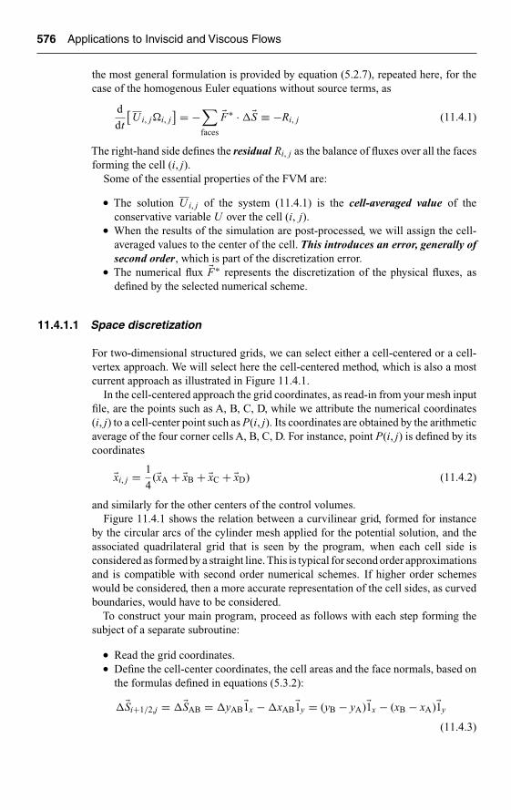
Ch11-H6594.tex 8/5/2007 20: 8 Page 576


the most general formulation is provided by equation (5.2.7), repeated here, for thecase of the homogenous Euler equations without source terms, as

d

dt

[U i, j�i, j

] = −∑faces

�F∗ · ��S ≡ −Ri, j (11.4.1)

The right-hand side defines the residual Ri, j as the balance of fluxes over all the facesforming the cell (i, j).

Some of the essential properties of the FVM are:

• The solution U i, j of the system (11.4.1) is the cell-averaged value of theconservative variable U over the cell (i, j).

• When the results of the simulation are post-processed, we will assign the cell-averaged values to the center of the cell. This introduces an error, generally ofsecond order, which is part of the discretization error.

• The numerical flux �F∗ represents the discretization of the physical fluxes, asdefined by the selected numerical scheme.

11.4.1.1 Space discretization

For two-dimensional structured grids, we can select either a cell-centered or a cell-vertex approach. We will select here the cell-centered method, which is also a mostcurrent approach as illustrated in Figure 11.4.1.

In the cell-centered approach the grid coordinates, as read-in from your mesh inputfile, are the points such as A, B, C, D, while we attribute the numerical coordinates(i, j) to a cell-center point such as P(i, j). Its coordinates are obtained by the arithmeticaverage of the four corner cells A, B, C, D. For instance, point P(i, j) is defined by itscoordinates

�xi, j = 1

4(�xA + �xB + �xC + �xD) (11.4.2)

and similarly for the other centers of the control volumes.Figure 11.4.1 shows the relation between a curvilinear grid, formed for instance

by the circular arcs of the cylinder mesh applied for the potential solution, and theassociated quadrilateral grid that is seen by the program, when each cell side isconsidered as formed by a straight line. This is typical for second order approximationsand is compatible with second order numerical schemes. If higher order schemeswould be considered, then a more accurate representation of the cell sides, as curvedboundaries, would have to be considered.

To construct your main program, proceed as follows with each step forming thesubject of a separate subroutine:

• Read the grid coordinates.• Define the cell-center coordinates, the cell areas and the face normals, based on

the formulas defined in equations (5.3.2):

��Si+1/2,j = ��SAB = �yAB�1x − �xAB�1y = (yB − yA)�1x − (xB − xA)�1y

(11.4.3)

Ch11-H6594.tex 8/5/2007 20: 8 Page 577


C B

ΔSi�1/2, j

ΔSi, j�1/2

AD

P (i, j )(i �1,j )

(i, j�1)(i �1, j �1)

Figure 11.4.1 Cell-centered finite volume space discretization on a structuredgrid.

and the area, following equation (5.3.4)

�i, j = �ABCD = 1

2|�xAC × �xBD|

= 1

2[(xC − xA)(yD − yB) − (xD − xB)(yC − yA)]

= 1

2(�xAC�yBD − �xBD�yAC) (11.4.4)

• The numerical flux �F∗ is written as the addition of a central flux, representingthe central scheme, plus a dissipation term, under the following form:

(�F∗ · ��S)i+1/2,j ≡[

1

2(�Fi, j + �Fi+1, j) − Di+1/2, j

]· ��Si+1/2, j (11.4.5)

where the dissipation term di+1/2, j is either part of the numerical dissipationor/and contains artificial dissipation terms.

• For the central scheme, an artificial viscosity term is added, following theformulation of Section 9.3.6. It is written here as a difference of third orderderivatives, with

Di+1/2, j = γi+1/2, j(Ui+2, j − 3Ui+1, j + 3Ui, j − Ui−1, j) (11.4.6)

Ch11-H6594.tex 8/5/2007 20: 8 Page 578


• Organize the subroutine for the calculation of this artificial dissipation term, asit requires mesh point values from two additional rows of cells. The value ofthe γ-coefficient is based on the formulation of Jameson et al. (1981), with thespectral radius of the Jacobian as coefficient

γi+1/2, j = 1

2κ(4)[�v · ��S + c|��S|]i+1/2, j (11.4.7)

where c is the speed of sound and κ(4) is a non-dimensional coefficient ofdissipation, with the minimum value of κ(4) = 1/256.

• Calculate the cell residuals by programming a loop over all the cell faces. Foreach face, calculate the associated flux, following formula:

(�F∗ · ��S)i+1/2, j = (�F∗ · ��S)AB = f ∗AB(yB − yA) − g∗

AB(xB − xA) (11.4.8)

• Send the contribution to the right cell and its negative value to the left cell, basedon an anti-clockwise positive orientation.

• For the faces situated on the boundaries, take into account the particular boundaryconditions, as defined hereafter. In particular on a solid boundary face, all theconvective fluxes are zero, since the normal velocity vn has to be zero and thedissipation term is set to zero.

11.4.1.2 Time integration

Apply the fourth stage Runge–Kutta time integration method, following Section 9.3.4,equations (9.3.47–9.3.50), with the following coefficient:

U (1)i, j = U n

i, j − �t

�i, jα1Rn

i, j

U (2)i, j = U n

i, j − �t

�i, jα2R(1)

i, j

U (3)i, j = U n

i, j − �t

�i, jα3R(2)

i, j

U n+1i, j = U n

i, j − �t

�i, jα4R(3)

i, j (11.4.9)

with

α1 = 1

4α2 = 1

3α3 = 1

2α4 = 1 (11.4.10)

Another option, which optimizes the dissipation of the scheme, is given by

α1 = 1

8α2 = 0.306 α3 = 0.587 α4 = 1 (11.4.11)

• Choose the CFL number, under the stability condition CFL < 2.8.• The time step has to be evaluated based on the sufficient condition expressing

that the physical domain of dependence should be completely contained in the

Ch11-H6594.tex 8/5/2007 20: 8 Page 579


numerical domain of dependence. However, as we are not interested in the tran-sient behavior of the solution, we can choose a local time step, whereby eachcell progresses at its maximum possible time step �ti, j . This looses the timeconsistency of the transient since each cell has its own time step, but providessignificant convergence acceleration. Hence, we make �ti, j proportional to thelocal cell size �i, j and is calculated as follows:

�ti, j ≤ CFL�i, j

|(�v + c)i, j · ��Si| + |(�v + c)i, j · ��Sj+1/2|

��Si = 1

2(��Si+1/2, j + ��Si−1/2, j) ��Sj = 1

2(��Si, j+1/2 + ��Si, j−1/2)

(11.4.12)

• To start the calculation you need to define an initial solution. By lack of knowl-edge it is customary to take a uniform initial solution corresponding to the inletcondition, distributed uniformly over the mesh. Note that the convergence behav-ior can be very sensitive to the initial solution: the closer this initial guess is tothe final solution, the faster the convergence.

Observe here that once again many ‘local’ decisions have to be taken as to where toevaluate the velocities and speed of sound. We have in these simulations, where allquantities vary from point to point, to continuously decide if we evaluate the valuesat the mesh points or at the cell faces, and how we connect one to the other.

11.4.1.3 Boundary conditions for the Euler equations

The last item of importance in the generation of your program for the Euler equationsis the definition of the boundary conditions. This is a most critical component of anyCFD code, and has to be compatible with both physical and numerical properties ofthe problem to be solved.

The time-dependent hyperbolic system of Euler equations contains four unknowndependent variables, and we have to determine how to handle these variables at theboundaries of the computational domain. These boundaries are of three types: solidwalls, inlet and outlet boundaries, and each one of them will require a dedicatedtreatment.

We know from Chapter 3 that the system of time-dependent Euler equations ispropagation dominated and we are faced therefore with the following questions:

(i) How many conditions of physical origin are to be imposed at a given boundary?(ii) What physical quantities are to be imposed at a boundary?

(iii) How are the remaining variables to be defined at the boundaries?

Go back to Chapter 3, Section 3.4.1 and to the Example E.3.4.3 dealing with theisentropic form of the Euler equation, where the energy equation has been removed.The three eigenvalues of the system, which correspond to the speed of propagation

Ch11-H6594.tex 8/5/2007 20: 8 Page 580


of three characteristic quantities, are given by

λ1 = �v · �κ/κ

λ2 = �v · �κ/κ + c

λ3 = �v · �κ/κ − c (11.4.13)

where �κ is the wave number vector. The last two correspond to the speeds of theacoustic waves.

It can be shown, that by adding the energy equation a fourth eigenvalue appearsequal to the first one, which becomes double valued.

Since, the transport properties at a surface are determined by the normal com-ponents of the fluxes, the number and type of conditions at a boundary of a multi-dimensional domain will be defined by the eigenvalue spectrum of the Jacobianmatrices associated to the normal to the boundary. Hence, at a boundary surface, thebehavior of the Euler system will be determined by the propagation of waves withthe following speeds:

λ1 = �v · �en = vn

λ2 = �v · �en = vn

λ3 = �v · �en + c = vn + c

λ4 = �v · �en − c = vn − c (11.4.14)

where vn is the normal velocity component at the considered surface.This defines locally quasi-one-dimensional propagation properties and we can

therefore look at how the propagation of information behaves at a boundary, in func-tion of the sign of these quantities. The first two eigenvalues are equal to the normalcomponent of the velocity and correspond to the entropy and vorticity waves, whilethe two remaining eigenvalues, are associated to the acoustic waves. Hence, the signof these eigenvalues will be determined by the velocity components normal to theboundary surfaces.

The key to the understanding of the issue of the number of boundary condi-tions is indeed the awareness that the characteristics convey information in the (n, t)space formed by the local normal direction and time. If λ represents the propagationspeed, the trajectory of the corresponding information path is given by dn/dt = λ.When information is propagated from outside toward the inside of the computationaldomain, it means that this information has to be defined from outside and representsa physical boundary condition. When λ is positive, the information carried by theassociated characteristics, propagates from the boundary toward the interior of theflow domain and a physical boundary condition has to be imposed. On the other hand,when the eigenvalue λ is negative and the propagation occurs from the interior of thedomain toward the boundary, it means that the related information is determined atthe boundary by the interior flow and cannot be imposed from the outside. It willhave to be expressed numerically, through numerical boundary conditions.

In summary, the number of physical conditions to be imposed at a boundarywith normal vector �n, pointing toward the flow domain, is defined by the numberof characteristics entering the domain.

Ch11-H6594.tex 8/5/2007 20: 8 Page 581


Referring to Figure 11.4.2 for an inlet boundary, if the inlet flow is subsonic inthe direction normal to the inlet surface, three eigenvalues are positive and one,λ4 = vn − c is negative. Therefore, three quantities will have to be fixed by thephysical flow conditions at the inlet of the flow domain, while the remaining one willbe determined by the interior conditions, through a numerical boundary condition.

At an outlet boundary (Figure 11.4.3) with subsonic normal velocity, three eigen-values are negative, since the normals are defined as pointing toward the interiorflow domain. Three numerical boundary conditions have therefore to be set, whilethe fourth condition, associated to the positive eigenvalue (−|vn| + c), propagates

U

(vn�c)en

en

Interior domain

Inlet boundary

Interior domain

dn/dt �vn�c dn/dt �vn�c

dn/dt �vn

t

n(vn�c)en

Figure 11.4.2 Characteristic propagation properties at an inlet boundary withsubsonic conditions.

v

(��vn��c)en

�(�vn��c)en

��vn�en

en

Interior domain

n

Interior domain

dn/dt ��vn��c dn/dt ��(�vn��c)

dn/dt ��vn�

Outlet boundary

Figure 11.4.3 Characteristic propagation properties at an outlet boundary withsubsonic conditions.

Ch11-H6594.tex 8/5/2007 20: 8 Page 582


information from the boundary toward the flow region. It is consequently associatedto a physical boundary condition.

This is a very important result, as it indicates that we cannot fix all four quantitiesat a subsonic inlet, but only three of them, neither can we know all quantities at asubsonic outlet, where we have to impose one variable, the other three being definedfrom the inlet flow properties.

If the flow is supersonic normal to the inlet surface, all boundary conditions arephysical. With the same circumstances at outlet, all eigenvalues are of negative signand no physical conditions have to be given. All the boundary variables are definedby the interior flow, for instance via extrapolation formulas.

The next question to answer is: What quantities should be fixed as physicalboundary conditions?

This question has no unique answer and forms a vast complex subject, which isoutside the scope of this introductory text. It is treated more in details in Volume II.For practical applications, you can proceed as follows:

Inlet boundary: You can select to fix the inlet velocity and inlet temperature for anexternal flow problem.

Another option, often applied to internal flows such as channels or cascade com-putations, is to specify two thermodynamic variables such as the upstream stagnationpressure and temperature, and an inlet Mach number or velocity magnitude, andhave the inlet flow angle defined by the computed flow, or inversely, fix the incidentflow angle, determining inlet Mach number from the computed flow. This has asconsequence that the mass flow is not defined, but is a result from the computation.

Outlet boundary: The most appropriate physical condition, particularly for internalflows and corresponding to most experimental situations, consists in fixing the down-stream static pressure. This can also be applied for external flow problems. Howeverin this latter case, free stream velocity could also be imposed.

At a solid wall boundary: The normal velocity is zero, since no mass or otherconvective flux can penetrate the solid body. Hence, only one eigenvalue is positiveand only one physical condition can be imposed, namely vn = 0. The other variablesat the wall, in particular tangential velocity components and pressure have to bedetermined by extrapolation from the interior to the boundary (Figure 11.4.4).

vn�0 Interior domainInterior domain

Solid surface

dn/dt ��c

dn/dt ��c

n

t

Solid surface

cen�cen

en

Figure 11.4.4 Characteristic propagation properties at a solid surface boundary.

Ch11-H6594.tex 8/5/2007 20: 8 Page 583


Numerical boundary conditions: The other issue to be fixed in your program isto implement the numerical boundary conditions, in order to obtain the numericalvalues of the remaining variables at the boundaries. This is particularly important forsolid walls, where we want to determine the pressure variations.

We suggest you apply a simple extrapolation from the inside point to the nextsurface point along the mesh lines. This is strictly valid if they are orthogonal to thesurface, but should be acceptable for regular grids of the type suggested here. Aneven simpler way is to take the value at the boundary equal to the value at the cellcenter of the associated cell. This assumes the quantity to be piecewise constant inthe considered cell and is a form of zero order extrapolation.

A more accurate way, but less robust, is to perform a linear extrapolation from twocells in the normal direction.

11.5 NUMERICAL SOLUTIONS FOR THE EULER EQUATIONS1

We will treat here in detail several test cases, in order to apply the numerical methodsto a variety of flow conditions and identify the associated numerical effects. We willhandle first the cylinder flow, in order to compare with the potential flow model andillustrate in particular the effects of numerical dissipation though the entropy field.

The next case will be typical of internal channel flows for several Mach numberflow conditions; while the last case will be representative of supersonic flows with anoblique shock. All these cases will be treated assuming perfect gas relations for theconsidered fluid.

11.5.1 Application to the Flow Around a Cylinder

Proceed as follows:

• Consider the grids applied in the previous section, following equation (11.3.18)with 33 points in the radial direction and 128 points in the circumferential direc-tion (see Figure 11.5.1). By removing every second point in both directions, newgrids with a reduced density can be constructed, defining hereby a fine mesh(33 × 128), an intermediate mesh (17 × 64) and a coarse mesh (9 × 32).

• Assume atmospheric conditions, for pressure and temperature with pa =101300 Pa, Ta = 288 K, and take M = 0.1 as incoming flow conditions.

• In order to match these inlet conditions, the total pressure and total tempera-ture are fixed at the inlet to 102010 Pa and 288.6 K, respectively, by followingequations (11.1.9) and (11.1.12). The inlet velocity direction is imposed alongthe x-direction. The atmospheric pressure is also imposed at the outlet. Since thecomputational domain is circular, we will consider that the left half circle ofthe outer boundary forms the inlet section, while the right half circle will formthe outlet section of the computational domain.

• Apply the Runge–Kutta method (11.4.9) with the coefficients (11.4.11) and takeCFL = 2. You can choose here between a local time step based on equations

1 This section has been written with the active participation of Dr. Benoit Tartinville, who producedalso the results of the three test cases.

Ch11-H6594.tex 8/5/2007 20: 8 Page 584


y

x

Figure 11.5.1 Fine mesh used for the circular cylinder flow.

�5

�4

�3

�2

�1

0

Log(

x-m

omen

tum

equ

atio

n re

sidu

al)

Iteration number

0 5000 10,000 15,000

Figure 11.5.2 Convergence history of the normalized L2-norm of the momentumresidual for the calculation on the fine mesh.

(11.4.12), or a global time step by taking the minimum value of all the local timesteps. We choose here the first alternative, but you can experience with bothoptions.

• To start the calculation take a uniform initial solution equal to the values definedby the boundary conditions.

• Solve the Euler equations for the different grid densities considered, until asteady state is reached, by selecting a value of the artificial dissipation coefficientκ(4) = 1/50, in equation (11.4.7).

• Monitor and plot the L2-norm of the residuals in function of number of time steps.Figure 11.5.2 shows the evolution of the axial velocity residual, normalized by

Ch11-H6594.tex 8/5/2007 20: 8 Page 585


�4

�3

�2

�1

0

1

2

Cp

Angle (degree)

�180 �135 �90 �45 0

Figure 11.5.3 Circumferential distribution of pressure coefficient from thenumerical result (plus signs), compared to the exact solution (continuous line).

the residual of the initial solution for the finest mesh, with the ordinate plotted ona logarithmic scale. The residual has dropped by nearly 5 orders of magnitude,which is close to single precision machine accuracy.

• If you cannot reach machine accuracy, if the residual drops for instance by3 orders of magnitude only, it will not necessarily mean that your solution isnot valid, but it indicates that somewhere in the flow domain, often aroundthe boundaries, there is a local error source. This error could result from aninaccuracy in the implementation or from some small local oscillation betweenvalues at neighboring points. This is called a ‘limit cycle’ in the convergencebehavior. You can sometimes detect it by looking at the flow regions with thehighest values of the residual.

• Observe that the convergence requires many time steps before reaching machineaccuracy. To accelerate the convergence, you would need to apply the multigridmethod, which would reduce the number of iterations easily by a factor of theorder of 10 or more. Alternatively you could apply an implicit method, which ishowever also more complicated to implement.

• Note also the oscillatory behavior of the residual. This is generally an indicationthat the acoustic waves, which transport part of the initial errors, are reflectedat the boundaries prior to their damping by the numerical scheme. This occurswhen the boundary condition implementation does not allow these error wavesto leave the computational domain without being reflection. The imposition ofthe outlet pressure is typical of what is called a reflecting boundary condition.To avoid these effects, we have to impose non-reflecting boundary conditions,based on the characteristic properties associated to the reflected waves. This isoutside the scope of this introductory text and will be dealt with in more detailsin Volume II.

• Plot the wall surface pressure coefficient and compare with the exact incom-pressible solution, equation (11.3.17), as shown on Figure 11.5.3.

Ch11-H6594.tex 8/5/2007 20: 8 Page 586


(a) (b)

(c)

Figure 11.5.4 Distribution of entropy as computed on three different meshes:(a) fine mesh, (b) intermediate mesh and (c) coarse mesh (for color image referPlate 11.5.4).

• In the front part of the cylinder, between the points A and C of Figure 11.3.1, thesolution is nearly perfect. However in the back part, between C and B a growingdiscrepancy can be noticed, with a significant deviation in the wake region aroundpoint B.You can observe that the left–right symmetry of the exact solution is lost.This is a major property of Euler calculations and is due, as explained above,to the numerical dissipation and the related numerical generation of entropy, asseen from Figures 11.5.4.

• Plot the entropy isolines and color maps, by monitoring the quantity:

s − s∞ = p

ργ−(

p

ργ

)∞

(11.5.1)

where the subscript ∞ refers to the far field upstream conditions.• For an inviscid flow, the entropy has to remain constant and equal to its upstream

value, which is clearly not the case for the results of the Euler calculations onthe three grids, as you see from Figure 11.5.4. Looking at the entropy evolutionalong the axis of symmetry and the cylinder surface, you observe that the entropyincreases already from the upstream stagnation point (point A of Figure 11.3.1)along the solid surface, which appears as a source of entropy, like in a viscousboundary layer and keeps increasing further downstream, forming a wake.

Ch11-H6594.tex 8/5/2007 20: 8 Page 587


Fine mesh Magnitude of V (m/s)70

60

50

40

30

20

10Y

X0

Figure 11.5.5 Distribution of velocity magnitude and iso-velocity lines, ascomputed on the finest mesh (for color image refer Plate 11.5.8).

• Observe also that the level of entropy decreases when the mesh is refined. Itwould require finer grids to reduce this effect to an acceptable low level and werecommend that you further refine the grid by dividing the cell sizes by two ineach direction, until you reduce the entropy to a sufficiently low level, reachedwhen you recover a nearly symmetrical solution.

• This effect can be seen also on the iso-velocity plot of Figure 11.5.5, where the‘numerical’wake is clearly visible. The behavior of the downstream region mim-ics viscous flows, and is the direct consequence of the presence of the numericaldissipation.

This is a major requirement on accuracy.You should always attempt to refinethe grids up to a level where the numerical dissipation is sufficiently low as tominimize the numerical entropy generation.

• Calculate the lift and drag components following equation (11.3.43). Both quan-tities should be zero and their non-zero values are a direct measure of thenumerical errors of the simulation. Since the mesh is symmetrical in the presenttest case, the calculated lift should reflect the machine accuracy and only thedrag coefficient is a measure of the numerical dissipation. The drag coefficient isdefined by

CD = Lx12ρU 2S

with S = 2πa (11.5.2)

It should tend to zero, as the mesh is refined as seen from Table 11.5.1.

11.5.2 Application to the Internal Flow in a Channel with a Circular Bump

This is a representative example of an internal flow configuration. It consists of achannel of height L and length 3L with, along the bottom wall, a circular arc of lengthL and thickness equal to 0.1L. We have no analytical exact solution for this case, buta reference solution can be obtained from a fine mesh simulation.

Ch11-H6594.tex 8/5/2007 20: 8 Page 588


Table 11.5.1 Drag coefficient on the cylinder,computed on three different meshes.

Drag coefficient

Exact 0128 × 32 0.0094

65 × 17 0.078433 × 9 0.1867

Upper wall

Inlet

X

Y

Lower wall

Outlet

Figure 11.5.6 Mesh used for the channel flow test case.

Proceed now as follows:

• An H-grid can be constructed using 65 points in the axial direction with equalspacing and 33 points in-between walls. A quasi-uniform grid distribution isselected by taking �x = 3L/64 and dividing each vertical mesh line in 32 uniformsteps (see Figure 11.5.6).

• Assume atmospheric conditions, for pressure and temperature withpa = 101300 Pa and Ta = 288 K, and M = 0.1 as inlet flow condition.

• In order to match these flow conditions, the total pressure and temperature arefixed at the inlet to 102010 Pa and 288.6 K, respectively, by following equations(11.1.9) and (11.1.12). The inlet velocity vector is imposed in the axial direction.The atmospheric pressure is also imposed at the outlet.

• At the solid walls, obtain the pressure and tangential velocity by taking themequal to the values of the corresponding cell centers.

• Apply the Runge–Kutta method (11.4.9) with the coefficients (11.4.11) and takeCFL = 2. Select a local time step, based on equations (11.4.12).

• To start the calculation take a uniform initial solution equal to the values definedby the boundary conditions.

• Solve the Euler equations until a steady state is reached, with CFL = 2 andκ(4) = 1/256.

• For internal flows, an important consistency check is the satisfaction of mass flowconservation, that is the mass flow rate through any section should be equal, upto an acceptably level of accuracy, to the inlet mass flow. The mass flow ratethrough a vertical mesh line i is equal to

m =∫

section

ρ�v · d�S =∑

j

[(ρu)i, j + (ρu)i, j+1

2(yi, j+1 − yi, j)

](11.5.3)

Ch11-H6594.tex 8/5/2007 20: 8 Page 589


41.8In

let a

nd o

utle

t mas

s flo

w

Iteration number

41.6

41.4

41.2

410 2000 4000 6000 8000 10,000

Outlet mass flow

Inlet mass flow

Figure 11.5.7 Convergence history of the inlet and outlet mass flow (kg/s/m).

referring to Figure 11.4.1, and applying a second order trapezium formula forthe integration,

• Typically you should aim at mass flow errors between inlet and exit, below 0.1%.Note that this can only be achieved when the steady state is reached, since duringthe compressible transient the time derivative of density is not zero and hencethe mass flow rate, as defined by equation (11.5.3), will not be constant.

• This is clearly seen on Figure 11.5.7, which shows the evolution of the inlet andexit mass flows (in kg/s/m) during the iterative process. You observe that after5000 time steps, we have reached a satisfactory level of mass conservation, withan error below 0.01%.

• The Mach number isolines and color maps are shown on Figure 11.5.8 for the(65 × 33) mesh superimposed on the color map of a reference solution on a(225 × 113) mesh. One isoline has been drawn on the color map every 0.001ranging from 0.07 to 0.13. The bottom figure compares the Mach number iso-lines of the two solutions, where the darkest line is the reference solution. Youcan observe here again the loss of symmetry between the upstream and down-stream parts of the circular bump. The reference solution, obtained on a gridof 225 × 113 mesh points, has still a small deviation from symmetry, while thenumerical solution on the selected grid shows a larger loss of symmetry in thewake region.

• If we compare the distribution of the wall surface pressure coefficient with thereference solution, shown on Figure 11.5.9, you observe that we cannot distin-guish them. This indicates that the pressure is less sensitive to the numericaldissipation than entropy or drag.

• Compare the solutions obtained at lower and higher Mach numbers (for instance0.01, 0.05, 0.1 and 0.7) to investigate the effects of compressibility. This can beseen on Figure 11.5.10.You can observe that within the low Mach number range,the solution does not greatly depend on Mach number and is practically identical

Ch11-H6594.tex 8/5/2007 20: 8 Page 590


Mach number

0.13

0.12

0.11

0.1

0.09

0.08

0.07

Y

X

Y

X

Figure 11.5.8 Isolines of Mach number as computed using the (65 × 33) meshsuperimposed on the color map of a reference solution on a (225 × 113) mesh. Oneisoline has been drawn every 0.001 ranging from 0.07 to 0.13. The bottom figurecompares the Mach number isolines of the two solutions, where the darkest line isthe reference solution (for color image refer Plate 11.5.8).

1

0.75

0.5

0.25

Cp 0

0 0.5 1 1.5

X

2 2.5 3

�0.25

�0.5

�0.75

�1

Figure 11.5.9 Axial distribution of pressure coefficient as computed using the(65 × 33) mesh (plus signs) and compared to the (225 × 113) mesh (continuousline).

to the incompressible flow. When increasing the Mach number, compressibilityeffects become more important and for an inlet Mach number slightly above0.6, the sonic speed of M = 1 is reached on the bump surface, followed by asupersonic region terminated by a shock. This can be seen for the case of anincident velocity of M = 0.7.

Ch11-H6594.tex 8/5/2007 20: 8 Page 591


M�0.01Mach number

0.012

0.011

0.01

0.009

0.008

M�0.1Mach number

0.12

0.11

0.1

0.09

0.08

M�0.05Mach number

0.012

0.011

0.01

0.009

0.008

M�0.7Mach number

1.4

1.2

1

0.8

0.6

X

Y

X

Y

X

Y

X

Y

Figure 11.5.10 Distribution of velocity as computed on the (65 × 33) mesh, fordifferent values of the incident Mach number, from 0.01 to 0.7. Observe the shockappearing at M = 0.7 (for color image refer Plate 11.5.10).

11.5.3 Application to the Supersonic Flow on a Wedge at M = 2.5

This example of a supersonic flow over a wedge of angle 15◦ generates an obliqueshock. The Mach number upstream of the shock is fixed to 2.5. This test case has anexact analytical solution, satisfying the Rankine–Hugoniot relations (11.1.26); seefor instance Anderson (1982), formed by two regions of constant states, separated bythe oblique shock.

The downstream flow conditions are listed in Table 11.5.2.

Table 11.5.2 Analytical solution for thesupersonic flow on a 15◦ wedge at M = 2.5.

Downstream Mach number (M2) 1.87Pressure ratio (p2/p1) 2.47Entropy ratio (s2/s1) 1.03

This problem cannot be solved with the implementation of the Euler solver asapplied for the two previous test cases. Indeed, in presence of shocks, we have toadd an additional dissipation term to control the numerical oscillations appearing inpresence of discontinuities, as shown for linear convection in Chapters 7 and 8. Tothis end, a second order artificial dissipation term is added to capture numericallystrong gradients such as shock waves. Therefore, equation (11.4.6) is reformulatedby adding a nonlinear dissipation term of second order, that reduces locally to firstorder at shock positions, in order to achieve a nearly monotone behavior, following

Ch11-H6594.tex 8/5/2007 20: 8 Page 592


(Jameson et al. 1981):

Di+1/2, j = ηi+1/2, j(Ui+1, j − Ui, j) + γi+1/2, j(Ui+2, j − 3Ui+1, j

+ 3Ui, j − Ui−1, j) (11.5.4)

The coefficient η and γ are based on the following relations:

ηi+1/2, j = 1

2κ(2)[�v · ��S + c|��S|]i+1/2, j max (νi−1, νi, νi+1, νi+2)

γi+1/2, j = max

(0,

1

2κ(4)[�v · ��S + c|��S|]i+1/2, j − ηi+1/2, j

)(11.5.5)

where the variable νi are sensors that activate the second order dissipation in regionsof strong gradients. They are based on the pressure variations and are defined as

νi =∣∣∣∣pi+1, j − 2pi, j + pi−1, j

pi+1, j + 2pi, j + pi−1, j

∣∣∣∣ (11.5.6)

Observe that the numerator is proportional to the second derivative of the pressureand is a second order discretization of �x2(∂2p/∂x2) when the pressure variations aresmooth. In the shock region, however, this term becomes close to 1 and the first termof equation (11.5.4) reduces to first order.

κ(2) is a non-dimensional coefficient of the order of unity.You can notice that if the pressure variations are linear, the sensor νi vanishes, the

second order dissipation is not activated and the dissipation term is identical to theexpression (11.4.6) defined for the subsonic applications.

With the addition of the second order dissipation to the inviscid numerical fluxes,we can proceed as follows:

• A uniform H-grid can be constructed using 97 points in the axial direction and65 points in-between walls. The distribution of grid points is set to uniform alongthe x-direction and in-between walls (see Figure 11.5.11).

• In order to match the flow conditions, the static pressure and temperature arefixed at the inlet to 101353 Pa and 288.9 K, respectively. The inlet velocity vectoris fixed to axial with a magnitude of 852.4 m/s.

• Since the outlet is supersonic, none of the characteristics enter the domainthrough this boundary. Therefore, all the variables are extrapolated at thisboundary.

• Apply the Runge–Kutta method (11.4.9) with the coefficients (11.4.11) and takeCFL = 2. Select here a local time step, based on equations (11.4.12).

• To start the calculation take a uniform initial solution equal to the values definedby the inlet boundary conditions.

• Solve the Euler equations until a steady state is reached, with CFL = 2, κ(2) = 1and κ(4) = 1/10.

• Monitor the L2-norm of the axial momentum residual in function of numberof time steps (see Figure 11.5.12). The residual has decreased by more thanfive orders of magnitude, which is in accordance with single precision machine

Ch11-H6594.tex 8/5/2007 20: 8 Page 593


Upper wall

Outlet

Inlet

Lower wall

x

y

Figure 11.5.11 Mesh used for the wedge test case.

�6

�5

�4

�3

�2

�1

0

Log(

x-m

omen

tum

equ

atio

n re

sidu

al)

0 100 200 300 400Iteration number

Figure 11.5.12 Convergence history of the normalized L2-norm of thex-momentum residual.

accuracy. You can reproduce the same calculation by using double precisionmachine accuracy and observe the drop in residual to much lower levels.

• If you compare this convergence behavior with the two previous test cases, youcan notice how much faster the supersonic case converges, requiring only 150iterations, compared to thousands for the subsonic cases. This is very typical andis largely connected to the boundary conditions and to the intrinsic propertiesof supersonic flows, which do not allow for upstream wave propagation of anyquantity, including numerical errors.

Ch11-H6594.tex 8/5/2007 20: 8 Page 594


1.7

1.8

1.9

2

2.1

2.2

2.3

2.4

2.5

2.6

Mac

h nu

mbe

r

�0.15 �0.1 �0.05 0 0.05 0.1 0.15 0.2 0.25 0.3x

Figure 11.5.13 Axial distribution of Mach number along the bottom wall for theexact solution (continuous line) and from the numerical result (plus signs).

• Plot the Mach number variations along the bottom wall, and compare with theexact solution (see Figure 11.5.13). Upstream of the wall corner the solution isnearly perfect. Downstream of the shock, along the inclined wall, the numericalsolution shows an oscillatory behavior of the Mach number. This illustrates thenon-monotonic behavior of the second order central scheme with the dissipationterm (11.5.4), which does not take into account the monotonicity requirements,discussed in Chapter 8.

• In addition, the first undershoot of the Mach number after the shock is due to thezero order interpolation of the pressure from the cell center to the wall, whichis incorrect when the cell center is located upstream of the shock in the cellsnear the wedge corner. This illustrates the difficulties in imposing numericalboundary conditions, in presence of sharp local changes in geometry and flowconditions.

• Plot the iso-Mach numbers and iso-entropy lines, and observe the non-uniformbehavior upstream and downstream of the shock wave, resulting from thenon-monotone behavior of the scheme (see Figures 11.5.14 and 11.5.15). Animportant numerical error source is generated at the wedge corner, as a result ofthe local treatment of the wall boundary condition.

• Increase the mesh size in both directions and observe the progressive reductionof the errors.

This example clearly shows that, although a representative solution can be obtainedfor this simple supersonic flow, additional work has still to be done to eliminate thenumerical oscillations, by imposing more severe monotone schemes with appropriatelimiters, as discussed in Chapter 8.

Ch11-H6594.tex 8/5/2007 20: 8 Page 595


1.7

1.8

1.9

2

2.1

2.2

2.3

2.4

2.5

2.6Mach number

x

y

Figure 11.5.14 Distribution of computed Mach number (for color image referPlate 11.5.14).

76,000

77,000

78,000

79,000

80,000

81,000

Entropy

x

y

Figure 11.5.15 Distribution of computed entropy (for color image referPlate 11.5.15).

11.5.4 Additional Hands-On Suggestions

With the developed programs, you can now extend the range of applications andexperience with many other set-ups. In particular, you can investigate the effects of

Ch11-H6594.tex 8/5/2007 20: 8 Page 596


many parameters, such as inflow conditions; grid densities and qualities, numericalalgorithms. Some suggested actions are:

• Exercise with different grid types and grid densities to develop a ‘feeling’ andexperience with ill-conditioned grids. In particular, introduce grid distortionsand grid discontinuities close to the solid walls to observe their effects on thequality of the numerical solution.

• Look at the influence of the artificial dissipation coefficients κ(4) and κ(2) onconvergence rate and calculated solution accuracy.

• Investigate the effects of compressibility by applying your potential or Euler codeto the considered flow cases, with increasing incident Mach number. Observewhat is happening to your code when shocks appear and in particular the non-monotone behavior over the shock with the Euler equations.

• Observe the sensitivity of the Mach number distribution downstream of the shockwave to the second and fourth order dissipation coefficients κ(2) and κ(4), for thewedge flow test case.

• Try other time integration methods, such as the Beam and Warming schemesintroduced in Chapter 9.

Other options are left to your imagination and creativity.


The main objective of this chapter is to guide you in writing your first CFD codes forinviscid potential and Euler flows on simple configurations, for which we have eitheran analytic solution or a reference numerical solution obtained on fine grids.

In running these test cases, we have insistently drawn you attention to the manyerror sources associated to the discretization of the inviscid Euler equations, at thelevel of implementation issues, boundary conditions as well as grid sensitivity.

On all the three test cases, you will have observed that the obtained results are notperfect and the errors shown are highly representative of ‘real life’ CFD simulationsof industrial relevant systems. When you do not have a reference solution to com-pare with, the internal consistency checks, such as mass flow conservation, and themonitoring of entropy will provide you with a clear picture of the error levels of yoursimulation.

Main topics to remember are:

• Great care has to be exercised at all levels of the detailed implementation andprogramming choices.

• Give great attention to the implementation of boundary conditions.• Perform as many ‘consistency’ checks as possible, by monitoring global con-

served quantities, such as mass flow with internal flows, or total enthalpy. Thevariations of these quantities are indicators of local error sources.

• The issue of the entropy generated by the numerical dissipation is a most criticalissue in CFD. Applying the Euler equation model is a unique method to identifythe regions where this dissipation has a significant influence on the numericalsolution. This should be your guide toward the required mesh refinement, in

Ch11-H6594.tex 8/5/2007 20: 8 Page 597


order to bring this effect below an acceptable level. The same is true for thenumerical calculated drag forces, which should be zero for inviscid flows.

• Grid quality and grid density have a major influence on the accuracy of thenumerical simulation.

REFERENCES

AIAA (1998). Guide for theVerification andValidation of Computational Fluid DynamicsSimulations. American Institute of Aeronautics and Astronautics, AIAA-G-077-1998,Reston, VA.

Anderson, J.D. (1982). Modern Compressible Flow. McGraw Hill Inc., New York.ASME (2006).V&V 10-2006 Guide forVerification andValidation in Computational Solid

Mechanics. ASME Publications; http://catalog.asme.org/Codes/PrintBook.Ballhaus, W.F. and Bailey, F.R. (1972). Numerical Calculation of Transonic Flow about

Swept Wings. AIAA Paper 72-677.Chorin, A.J. (1967). A numerical method for solving incompressible viscous flow

problems. J. Computational Physics 2, 12.Garabedian, P.R. and Korn, D. (1972). Analysis of transonic airfoils. Commun. PureAppl.

Math 24, 841–851.Hall, M.G. (1981). Computational Fluid Dynamics – A Revolutionary Force in Aero-

dynamics. AIAA Paper 81-1014 – Proc. Fifth AIAA Computational Fluid DynamicsConference , pp.176–188.

Holst, T. and Thomas, S. (1983). Numerical solution of transonic wing flow fields. AIAAJournal 21, 863–870.

Jameson, A. (1974). Iterative solutions of transonic flows over airfoils and wings,including flows at Mach 1. Commun. Pure Appl. Math, 27, 283–309.

Jameson, A. (1975). Transonic potential flow calculations using conservative form. Pro-ceedings of the AIAA Second Computational Fluid Dynamics Conference, Hartford,pp.148–161.

Jameson, A. and Caughey, D.E. (1977). A Finite Volume Method for Transonic Poten-tial Flow Calculations. Proc. AIAA 3rd Computational Fluid Dynamics Conference,Albuquerque, pp. 35–54.

Jameson, A., Schmidt, W. and Turkel, E. (1981). Numerical Simulation of the EulerEquations by Finite Volume Methods using Runge–Kutta Time Stepping Schemes.AIAA Paper 81-1259, AIAA 5th Computational Fluid Dynamics Conference.

Lax, P.D. (1973). Hyperbolic Systems of Conservation Laws and the MathematicalTheoryof Shock Waves, SIAM Publications, Philadelphia, USA.

Merkle, C.L. and Choi, Y.-H. (1985). Computation of low speed compressible flows withtime-marching methods. Int. J. Numer. Method. Eng., 25, 293–311.

Murman, E.M. and Cole, J.D. (1971). Calculation of plane steady transonic flows. AIAAJ. 9, 114–121.

Oberkampf, W.L., Trucano, T.G. and Hirsch, Ch. (2004). Verification, validation andpredictive capability in computational engineering and physics. Appl. Mech. Rev.,57(5), pp. 345–384.

Shapiro, A.H. (1953). The Dynamics and Thermodynamics of Compressible Fluid Flow.Ronald Press, New York.

Steger, J.L. and Lomax, H. (1972). Transonic flow about two-dimensional airfoils byrelaxation procedures. AIAA J. 10, 49–54.

Zucrow, M.J., Hoffman, J.D. (1976). Gas DynamicsVol. I & II. J.Wiley & Sons, NewYork.

Ch12-H6594.tex 8/5/2007 20: 19 Page 599

Chapter 12

Numerical Solutions of Viscous Laminar Flows


This chapter will guide you into the programming of CFD codes for viscous laminarflows, modeled by the Navier–Stokes equations, where the main additions to theinviscid model are the viscous internal friction stresses and the thermal conduction,both being diffusion type terms, represented by second order derivatives. The basicequations are summarized in Section 12.1.

This is a major change from inviscid flows, as it affects the solid wall boundaryconditions, where all the velocity components have to vanish, following the non-slipboundary condition for viscous flows. The main consequence of it is the presenceof viscous and thermal boundary layers near solid walls, where the velocity andtemperature profiles can vary extremely rapidly over a short distance, requiring herebyhigh density grids in these near-wall regions.

We will consider essentially low speed flows and this will provide us with theopportunity to introduce an alternative numerical approach for the solution of theNavier–Stokes equations, namely the pressure correction method. The method iswidely used, also in several commercial codes, and was initiated many years ago, forlow speed industrial flows.

This particular numerical approach is to be put in relation with the method presentedin the previous chapter for the Euler equations, which has been developed within theaeronautical community and oriented at high speed flows where the variations ofdensity can become dominant. Hence, they are considered as density-based methods.Today, both families of methods have been extended to handle flows at all speedregimes, although the pressure correction methods might display some difficultiesfor high supersonic flow conditions.

Very few viscous test cases are known having analytical solutions. Among the bestknown is the Couette flow, generated by the uniform motion of a flat plate at a certaindistance from a fixed plate, leading to a linear velocity distribution as a result of theviscous effects. When a temperature difference is imposed between the plates, theexact parabolic solution for the temperature profile allows the verification of thermaleffects.

Another fundamental test case is the laminar boundary layer flow over a flat plate,with the well-known Blasius profile, considered as an exact solution. Despite itssimple geometry, it displays most of the flow features encountered in viscous externalor internal flows, such as the flow over a wing or a turbomachinery blade row, withthe presence of leading edge, although of zero thickness, a boundary layer flow anda wake.

Section 12.2 will first guide you to the extension toward viscous flows of the pro-gram developed for the Euler equations in Chapter 11. This is not so straightforward

599

Ch12-H6594.tex 8/5/2007 20: 19 Page 600


12.1. Navier–Stokes equationsfor laminar flows

12.2. Density-based methodsfor viscous flows

Basic equations and boundaryconditions for two-dimensionallaminar flows

Finite volume discretization ofviscous and thermal fluxes.Implementation of boundaryconditions

12.3. Numerical solutions with thedensity-based method

Application of the programto the thermal Couette flowand the laminar flat plate Blasiusboundary layer

12.4. Pressure correction method

Detailed description andimplementation of thepressure correction method forcompressible Navier–Stokes flows

12.5. Numerical solutions with thepressure correction method

Application of the pressurecorrection method to the liddriven cavity

12.6. Best practice adviceGuidelines for best practicein the development or applicationof CFD codes

Figure 12.0.1 Content and guide to this Chapter.

extension, particularly on a general finite volume structured grid, as it requires theaddition of the flux terms associated to the central discretized viscous and heat con-duction fluxes, and a modification of the wall boundary conditions.You will be able toapply your program to the thermal Couette flow and to the laminar flat plate boundarylayer flow, following Section 12.3.

Section 12.4 will introduce you to the pressure correction method and will guide youto its programming, with an application to the well-known test case of the lid driven

Ch12-H6594.tex 8/5/2007 20: 19 Page 601

Numerical Solutions of Viscous Laminar Flows 601

cavity flow in Section 12.5. The lid driven cavity case has no analytical solution, butis representative of a complex internal flow structure and is considered as a standardtest case.

Finally the last section 12.6 will provide some Best Practice Advice for either thedevelopment of a CFD code, or the use of existing, commercial or research, CFDcodes.

Figure 12.0.1 summarizes the roadmap of this chapter.Sections 12.2 and 12.3 have been written with the active participation of Dr. Benoit

Tartinville, from Numeca International, who produced also the results of the two vis-cous cases of Section 12.3. Dr. Sergey Smirnov, from the Vrije Universiteit Brussel,contributed significantly to Section 12.4 on the pressure correction method, and pro-duced the program and the results for the lid driven cavity of Section 12.5. Theircontribution is gratefully acknowledged.

12.1 NAVIER–STOKES EQUATIONS FOR LAMINAR FLOWS

The system of Navier–Stokes equations can be written in various ways based on thederivations in Chapter 1. We refer you to Table 1 of Chapter 1 for a summary of theconservation laws in different forms. A general differential form is provided by thefollowing equations, in absence of external forces and heat fluxes:

∂ρ

∂t+ �∇ · (ρ�v) = 0

∂ρ�v∂t

+ �∇ · (ρ�v ⊗ �v + pI − ¯τ) = 0 (12.1.1)

∂ρE

∂t+ �∇ · (ρ�vH − k �∇T − ¯τ · �v) = 0

Assuming Newtonian fluids, the shear stress tensor has the following Cartesiancomponents, based on equation (1.3.6):

τij = μ

[(∂vj

∂xi+ ∂vi

∂xj

)− 2

3( �∇ · �v)δij

](12.1.2)

In two-dimensions and Cartesian coordinates, we obtain the system:

∂ρ

∂t+ ∂ρu

∂x+ ∂ρv

∂y= 0

∂ρu

∂t+ ∂(ρu2 + p)

∂x+ ∂(ρuv)

∂y= ∂τxx

∂x+ ∂τyx

∂y

∂ρv

∂t+ ∂(ρuv)

∂x+ ∂(ρv2 + p)

∂y= ∂τxy

∂x+ ∂τyy

∂y

∂ρE

∂t+ ∂(ρuH )

∂x+ ∂(ρvH )

∂y= ∂(τxxu + τxyv)

∂x+ ∂(τyxu + τyyv)

∂y

+ ∂

∂x

(k∂T

∂x

)+ ∂

∂y

(k∂T

∂y

)(12.1.3)

Ch12-H6594.tex 8/5/2007 20: 19 Page 602


The right-hand side collects the terms to be added to the inviscid fluxes.The energy equation can be written in many equivalent forms, for instance equation

(1.4.15) for the internal energy:

ρde

dt≡ ρ

[∂e

∂t+ (�v · �∇)e

]= −p( �∇ · �v) + �∇ · (k �∇T ) + (¯τ · �∇) · �v (12.1.4)

For incompressible flows, the above equations simplify further, since the continuityequation reduces to the condition of divergence free velocity:

�∇ · �v = 0 (12.1.5)

and the shear stress definition becomes

τij = μ

(∂vj

∂xi+ ∂vi

∂xj

)(12.1.6)

leading to the following non-conservative momentum equation (1.4.40)

∂�v∂t

+ (�v · �∇)�v = − 1

ρ�∇p + ν��v (12.1.7)

and the energy equation for the temperature, writing e = cvT

ρcv

[∂T

∂t+ (�v · �∇)T

]= �∇ · (k �∇T ) + (¯τ · �∇) · �v (12.1.8)

Note that for liquids the specific heat coefficients at constant volume and constantpressure are equal, i.e. cv = cp and either values can be used in equation (12.1.8),when applied to incompressible liquids.

You can choose to discretize directly this system by applying finite differences, ifyou can generate a Cartesian grid for your problem. For a general curvilinear grid,we recommend that you apply the finite volume method, by extending directly theprogram you have developed for the Euler equations.

With reference to equation (11.4.1), we have to add the contributions from theviscous and thermal fluxes to the momentum and energy conservation equations.

This gives the following finite volume discretized equation:

d

dt[U i, j�i, j] = −

∑faces

[�F∗ · ��S − �Fv · ��S] ≡ −Ri, j (12.1.9)

where �FV represents the viscous and thermal fluxes, with components fv and gv:

fv =

∣∣∣∣∣∣∣∣∣

0τxx

τxy

τxxu + τxyv + k∂T

∂x

∣∣∣∣∣∣∣∣∣gv =

∣∣∣∣∣∣∣∣∣

0τyx

τyy

τyxu + τyyv + k∂T

∂y

∣∣∣∣∣∣∣∣∣(12.1.10)

Ch12-H6594.tex 8/5/2007 20: 19 Page 603


The estimation of the viscous and thermal fluxes requires the calculation of the velocityand temperature gradients. Since these terms describe diffusion effects, they have tobe discretized by central formulas.

12.1.1 Boundary Conditions for Viscous Flows

The presence of the viscous and thermal fluxes makes the time-dependentNavier–Stokes equations of the mixed parabolic–hyperbolic type, as seen in Chapter3, and this has an impact on the number and nature of boundary conditions to beimposed, in particular at solid walls.

We consider here high Reynolds number flows, which is the most often occurringsituation in both industrial as environmental systems. If you recall the significance ofthe Reynolds number as the ratio of convective to viscous effects, a high Reynoldsnumber means that the flow system will be dominated by the convective terms, thatis will be dominated by its inviscid properties. This can be clearly seen when ana-lyzing viscous flows, with the important exception of the near-wall regions, wherethe viscous effects, leading to a boundary layer configuration, dominate the flowbehavior.

The main consequence is that at inlet and outlet boundaries, we can keep thesame boundary conditions as for the inviscid computations, but the wall boundaryconditions will change drastically.

At solid walls, the velocity relative to the wall has to vanish. This is the no-slipboundary condition, whereby the three velocity components are zero at the bodysurface.

We have to add a boundary condition for the temperature status of the solid wall.You can encounter several situations; the most current being:

• Adiabatic walls: Whereby we express that there is no heat flux through the solidsurface. This is expressed by the Neumann condition

∂T

∂n= 0 at the solid wall (12.1.11)

• Constant temperature wall: Here we assume that the solid surface is kept at afixed temperature Tw, leading to a Dirichlet type boundary condition

T = Tw at the solid wall (12.1.12)

• Imposed heat flux: In this case, the solid wall is the source of a fixed heat fluxqe to or from the fluid flow, for instance when the solid surface is part of aheat exchanger system. This flux will be positive for a heated wall or negativefor a cooled wall. The boundary condition generalizes the adiabatic condition(12.1.11) to

∂T

∂n= qe at the solid wall (12.1.13)

Ch12-H6594.tex 8/5/2007 20: 19 Page 604


j�2

j�1

j�n

j�1

‘Inviscid’ mesh‘Viscous’ mesh

First ‘Inviscid’ mesh line

�x �x

n~15�25

Figure 12.1.1 Difference between an inviscid grid and a boundary layeroriented grid.

12.1.2 Grids for Boundary Layer Flows

The presence of boundary layers has dramatic consequences on the gridrequirements.

If you consider a flat plate, the developing boundary layer, as already discussedin Section 4.3, when we introduced the discretization for non-uniform grids, has athickness to length ratio of the order of 1/

√Re. Hence, for a Reynolds number of

106 and a plate with a length of 1 m, the boundary layer thickness will be of theorder of 1 mm at the end of the plate. For an incoming moderate velocity of say30 m/s, the velocity will vary from zero at the wall to 30 m/s over a distance of1mm, which is a very strong variation. As a consequence you need to arrange for aminimum number of grid points, of the order of 20–25 mesh points over this shortdistance, as illustrated on Figure 12.1.1. You can consider that the boundary layermesh is inserted between the wall and the fist grid line of the inviscid mesh ( j = 2).Moreover, since the velocity gradients take their highest values near the wall anddecrease progressively toward the edge of the boundary layer, it is recommendedto cluster the grid points close to the solid surface with a progressive coarseningwhen moving away from the wall. Refer to Section 4.3 for a discussion of thisimportant issue.

Hence, viscous grids must be highly concentrated near solid walls.

12.2 DENSITY-BASED METHODS FOR VISCOUS FLOWS

To extend your inviscid finite volume program developed in Chapter 11, proceed asfollows:

• Add an option in the main program to distinguish between inviscid or viscoussimulations.

• Add subroutines to calculate the velocity and temperature gradients.• Add subroutines to calculate the viscous stresses and thermal fluxes.• Add subroutines for the viscous solid wall boundary conditions.

Ch12-H6594.tex 8/5/2007 20: 19 Page 605


Referring to the cell-centered configuration of Figure 11.4.1, the viscous and ther-mal fluxes are calculated directly for each face, in a finite volume formulation, asdescribed hereafter.

12.2.1 Discretization of Viscous and Thermal Fluxes

All the points and grid coordinates used in the following equations refer toFigure 11.4.1. Independently of the choice made for the inviscid part of the solver –either using an upwind or a central scheme – the viscous and thermal fluxes shouldalways be discretized using a central scheme.

Following equations (12.1.9) and (12.1.10), the viscous and thermal fluxes at thecell face (i + 1/2, j) can be expressed as

(�Fv · ��S)i+1/2, j = (�Fv · ��S)AB = fv, AB(yB − yA) − gv, AB(xB − xA) (12.2.1)

The main difficulty resides in the dependence of the flux components fv and gv onthe velocity and temperature gradients, and we have to decide how to estimate thesegradients at the cell faces. Note that all quantities appearing in the flux terms are tobe considered as face-averaged values.

Again we are confronted with a ‘local’decision, as several options can be selectedto evaluate the gradients.

They can be computed directly at a mid-point of the cell face, or evaluated at thecell corners and averaged to obtain an average cell-face value.

Though the first approach is more direct, it is more expensive than the second one.Indeed for a two-dimensional calculation, the total number of cell faces is about twotimes the number of corners. Nonetheless, the first approach will be retained here, asit is more robust.

Thus, we can proceed as follows:

• Calculate the face velocity and temperature gradients by programming a loopover all the cell faces.

• Compute the face-averaged gradients by using the Gauss divergence theoremover a selected control volume, following equation (5.3.16), where the overbarindicates the cell average value:∫

�

( �∇U )d��= �∇U� =

∮S

Ud�S (12.2.2)

This equation is interpreted here in a two-dimensional space, where � is the facearea and the contour integral is performed over the face boundaries.

• In order to obtain the gradients on face AB of Figure 12.2.1, we consider thecontrol volume 1234 around AB, indicated as the shaded area. As faces 1 and 3pass through the cell centers of cells (i, j) and (i + 1, j), the values at these pointscan be used directly. However, for the faces 2 and 4, an arithmetic average overfour cells is required in order to compute the variables on these faces. Thus, thecomputation of the gradients at a cell face requires an access to the quantities atsix different points. For instance, the gradient on face AB, labeled (i + 1/2, j),requires the quantities at points (i, j), (i, j − 1), (i, j + 1), (i + 1, j), (i + 1, j − 1),

Ch12-H6594.tex 8/5/2007 20: 19 Page 606


C B

�Si , j�1/2

3

D

4 A

2

(i , j�1) (i�1, j�1)

(i�1, j )P (i , j )1

�Si�1/2, j

Figure 12.2.1 Control volume used for computing the velocity and temperaturegradients at face i + 1/2, j (dashed area). The faces around this volume arenumbered 1234.

and (i + 1, j + 1) following:⎧⎪⎪⎪⎪⎪⎪⎪⎨⎪⎪⎪⎪⎪⎪⎪⎩

Uface1 = Ui, j

Uface2 = 1

4(Ui, j + Ui+1, j + Ui, j+1 + Ui+1, j+1)

Uface3 = Ui+1, j

Uface4 = 1

4(Ui, j + Ui+1, j + Ui, j−1 + Ui+1, j−1)

( �∇U )i+1/2, j = 1

�1234(Uface1��Sface1 + Uface2��Sface2 + Uface3��Sface3

+Uface4��Sface4)

(12.2.3)

The x- and y-derivatives are obtained by projecting the average gradients in thecorresponding direction. For instance, for the temperature gradients:

∂T

∂x

∣∣∣∣i+1/2, j

= ( �∇T )i+1/2, j · �ex

∂T

∂y

∣∣∣∣i+1/2, j

= ( �∇T )i+1/2, j · �ey

(12.2.4)

Ch12-H6594.tex 8/5/2007 20: 19 Page 607


• In case the viscosity is not constant, for instance when the temperature is variable,the dynamic viscosity at cell faces is estimated by using arithmetic averaging ofcell-center values.

• Compute the shear stresses at cell faces by using equation (12.1.2), following:

(τxx)i+1/2, j = μi+1/2, j

[2

∂u

∂x

∣∣∣∣i+1/2, j

− 2

3

(∂u

∂x

∣∣∣∣i+1/2, j

+ ∂v

∂y

∣∣∣∣i+1/2, j

)]

(τxy)i+1/2, j = μi+1/2, j

[∂u

∂y

∣∣∣∣i+1/2, j

= ∂v

∂x

∣∣∣∣i+1/2, j

](12.2.5)

• For faces located on boundaries, take into account the particular boundaryconditions, as defined hereafter.

• Compute the fluxes using equation (12.2.1) and send the contribution to the rightcell and its negative value to the left cell, in a counter-clockwise sense.

12.2.2 Boundary Conditions

As you certainly have experienced by now, if you have followed the code the devel-opment in Chapter 11, the numerical translation of the boundary conditions is one ofthe most critical issues in CFD.

12.2.2.1 Physical boundary conditions

As already mentioned above the boundary treatment described in Chapter 11 can stillbe applied for inlet and outlet boundaries. But the boundary conditions on walls haveto be adapted to the viscous flow solver. Therefore, it is recommended to make twoindependent subroutines for inviscid and viscous wall boundary conditions.

As mentioned above, the major change compared to the inviscid code is the solidwall no-slip boundary condition, which imposes that all the velocity componentsvanish at the solid body surface. This is expressed by the Dirichlet type condition:

�v = 0 at the solid walls. (12.2.6)

The computation of the cell-face gradients, following equation (12.2.3), requiresan access to all the neighboring cell values, which are not available for faces on thesolid boundaries. Hence, a special treatment has to be implemented for these cells,by selecting control volumes entirely inside the computational domain. The controlvolume 1234, defined to compute the gradients at wall faces, is modified accordingto Figure 12.2.2, and the formulas (12.2.3) are replaced by

⎧⎪⎪⎪⎪⎪⎪⎨⎪⎪⎪⎪⎪⎪⎩

Uface1 = Ui, j

Uface2 = 1

4(Ui, j + Ui+1/2, j + Ui, j+1 + Ui+1/2, j+1)

Uface3 = Ui+1/2, j

Uface4 = 1

4(Ui, j + Ui+1/2, j + Ui, j−1 + Ui+1/2, j−1)

Ch12-H6594.tex 8/5/2007 20: 19 Page 608


A

BC

D

Solid surface

1

2

3

4

Figure 12.2.2 Control volume used for computing the velocity and temperaturegradients at face i + 1/2, j which corresponds to a viscous wall (dashed area). Thefaces around this volume are numbered 1234.

( �∇U )i+1/2, j = 1

�1234(Uface1��Sface1 + Uface2��Sface2 + Uface3��Sface3

+Uface4��Sface4) (12.2.7)

where the values at locations i + 1/2 are the values imposed on the solid boundaries.This requires an additional loop on all the cells close to the solid body.Another method, which does not require a special loop over the boundary cells,

consists in adding a row of additional cells outside of the computational domain.The flow variables are imposed in these ‘ghost’ cells in order to match the requiredboundary condition at the corresponding cell faces. The external loop on all the facesof the computational domain can be directly used. Though this method is less timeconsuming it requires to store variables in ‘ghost’ cells and therefore requires morememory.

You are here confronted with a representative choice between time and memoryconsumption.

For the energy equations three boundary conditions can be used: adiabatic, isother-mal and with imposed heat flux. Depending on the type of boundary conditionspecified, i.e. Dirichlet or Neumann, either the temperature or its gradient has tobe specified on the wall cell face.

If a Neumann type condition is applied the temperature gradient is directly definedand does not need to be calculated. The wall temperature can be inferred by writingthe normal temperature gradient as a function of the temperature derivatives alonggrid lines:

(�n · �∇T )i+1/2, j = ��Si+1/2, j

|��Si+1/2, j|�i, j·[��Si+1/2, j

∂T

∂ξ

∣∣∣∣wall

+ ��Sj∂T

∂η

∣∣∣∣wall

]

(12.2.8)

where ξ, η represent the coordinate in the i, j directions, and assuming i as being thedirection away from the wall. The surface ��Sj is defined as in equation (11.4.12).

Ch12-H6594.tex 8/5/2007 20: 19 Page 609


This allows to estimate the gradients along the mesh line direction:

∂T

∂ξ

∣∣∣∣wall

= − 1

|��Si+1/2, j|2[��Si+1/2, j · ��Sj

∂T

∂η

∣∣∣∣wall

]

+ �i, j

|��Si+1/2, j|(�n · �∇T )i+1/2, j (12.2.9)

The temperature difference along the j-direction can be deduced following:

∂T

∂η

∣∣∣∣wall

= 1

2(Ti, j+1 − T1, j−1) (12.2.10)

and the temperature at the cell face can be computed as

Ti+1/2, j = Ti, j + 1

2

∂T

∂ξ

∣∣∣∣wall

(12.2.11)

If a Dirichlet type condition is imposed, the same procedure used for the momen-tum equations should be used. Either the subroutines that compute the gradients areadapted to this boundary condition, or the values inside the ‘ghost’ cells have to beadapted to the imposed condition.

12.2.2.2 Numerical boundary conditions

As for the inviscid flow solver, other variables have to be imposed on the solid wallboundaries. Since we have already imposed the condition on the velocity vector andon the temperature, only the pressure remains. A common assumption is that thepressure gradient normal to the wall vanishes. Since this gradient can be expressedas function of the pressure derivative along grid lines, following equation (12.2.8),we can write

(�n · �∇p)i+1/2, j = ��Si+1/2, j∣∣∣��Si+1/2, j

∣∣∣�i, j

·[��Si+1/2, j

∂p

∂ξ

∣∣∣∣wall

+ ��Sj∂p

∂η

∣∣∣∣wall

]

(12.2.12)

Therefore, following the same procedure as for the temperature, the pressure dif-ference along the i-direction can be obtained on the boundary cell faces, and thepressure at the wall can be computed.

The density follows from the knowledge of pressure and temperature at the wallsurface.

12.2.2.3 Periodic boundary conditions

Periodic boundary conditions are often used when a periodicity is observed in thegeometry of the domain to be meshed or in the flow motion to be represented. Thisis often the case in problems where the flow does not vary in a given direction, such

Ch12-H6594.tex 8/5/2007 20: 19 Page 610


as axisymmetric problems, or for turbomachinery applications, where the geometryhas a periodicity, allowing only one blade passage to be meshed.

Another application of a periodic boundary condition occurs for simple one-dimensional problems, for which the streamwise direction is infinite without anyflow variation, and we need to handle this problem with a two-dimensional code.In this case, we define a two-dimensional mesh with a few cells in the streamwisedirection, selecting 2 or 3 cells in that direction. The constancy of all variables in thatdirection will be modeled by imposing a periodicity condition to connect the upstreamand downstream boundaries in the streamwise direction, expressing equality of allthe flow variables between these two boundaries.

Such a boundary condition is used hereafter for the simulation of the one-dimensional Couette flow problem with your 2D code.

12.2.3 Estimation of Viscous Time Step and CFL Conditions

As for the inviscid flow solver, since we are not interested in the transient behavior, alocal time step could be used. Therefore, each cell will progress at its maximum timestep. Following equation (E.9.3.1) the local viscous time step is defined as

�ti, j ≤ VNN�2

i, j

8μ(|��Si|2 + |��Sj|2 + 2|��Si��Sj|)��Si = 1

2(��Si+1/2, j + ��Si−1/2, j) ��Sj = 1

2(��Si, j+1/2 + ��Si, j−1/2)

(12.2.13)

where VNN is the von Neumann number, defined by α�t/�x2, for the one-dimensional diffusion equation. Here the diffusion coefficient is replaced by thekinematic viscosity for the momentum equation and by the thermal diffusivity for theenergy equation.

For the complete Navier–Stokes equations the local time step to be applied is theminimum between the inviscid and viscous time steps, along the lines of equation(8.2.15).

12.3 NUMERICAL SOLUTIONS WITH THE DENSITY-BASED METHOD

We will guide you now to the application of the general finite volume code, developedalong the guidelines just described in Section 12.2, to two problems with a simplegeometry, where in fact Cartesian grids can be used. However, once you have acquiredthe first experience in solving viscous and thermal problems, you will also be able toapply your code to more general cases, such as the cylinder flow, the internal bumpcase of Chapter 11, and to many other cases you might be interested in, requiringmore general curvilinear grids.

The first test case of the Couette flow is rather simple, as it does not have a stream-wise variation and is essentially one-dimensional. Nevertheless, the incorporation ofthermal effects makes the case of interest, as it will help us illustrate some of therequirements associated with thermal problems.

Ch12-H6594.tex 8/5/2007 20: 19 Page 611


The second test case is the laminar flat plate boundary layer, with the Blasius profileas reference solution.

The exact solutions of these two test cases are for incompressible conditions, butwill be treated here in the low Mach number compressible mode.

12.3.1 Couette Thermal Flow

One of the simplest cases to verify the discretization of viscous effects is the laminarflow between two parallel walls, a fixed wall and a moving one at a distance L withvelocity U . In order to include the computation of the thermal fluxes both walls areconsidered as isothermal, at different temperatures. The moving upper wall has ahigher fixed temperature than the static wall (see Figure 12.3.1).

The analytical solution for incompressible flow conditions is easily derived. Sincethe plates have infinite lengths, there is no physically relevant length scale in thestreamwise direction and therefore all x-derivatives have to vanish. In addition, sincethe flow has only a streamwise velocity component, the normal velocity componentis zero everywhere, i.e. v = 0, reducing the momentum equation to its streamwisecomponent. The shear stress tensor (12.1.6) is also reduced to a single component τ12.

τ12 = μ∂u

∂yall other τij = 0 (12.3.1)

Consequently, equations (12.1.7) and (12.1.8) simplify considerably to the one-dimensional system:

∂u

∂t= ν

∂u2

∂y2

ρcv∂T

∂t= k

∂2T

∂y2+ μ

(∂u

∂y

)2

(12.3.2)

Moving wall T�T1

Static wall T�T0

x�a

y

x

x�b

Figure 12.3.1 Representation of the Couette flow test case.

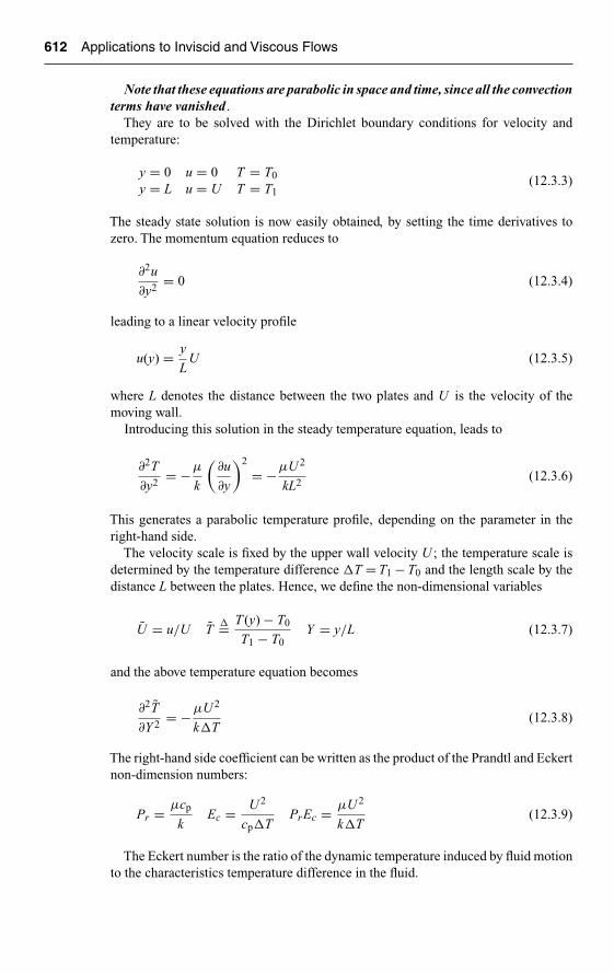
Ch12-H6594.tex 8/5/2007 20: 19 Page 612


Note that these equations are parabolic in space and time, since all the convectionterms have vanished .

They are to be solved with the Dirichlet boundary conditions for velocity andtemperature:

y = 0 u = 0 T = T0

y = L u = U T = T1(12.3.3)

The steady state solution is now easily obtained, by setting the time derivatives tozero. The momentum equation reduces to

∂2u

∂y2= 0 (12.3.4)

leading to a linear velocity profile

u(y) = y

LU (12.3.5)

where L denotes the distance between the two plates and U is the velocity of themoving wall.

Introducing this solution in the steady temperature equation, leads to

∂2T

∂y2= −μ

k

(∂u

∂y

)2

= −μU 2

kL2(12.3.6)

This generates a parabolic temperature profile, depending on the parameter in theright-hand side.

The velocity scale is fixed by the upper wall velocity U ; the temperature scale isdetermined by the temperature difference �T = T1 − T0 and the length scale by thedistance L between the plates. Hence, we define the non-dimensional variables

U = u/U T�= T (y) − T0

T1 − T0Y = y/L (12.3.7)

and the above temperature equation becomes

∂2T

∂Y 2= −μU 2

k�T(12.3.8)

The right-hand side coefficient can be written as the product of the Prandtl and Eckertnon-dimension numbers:

Pr = μcp

kEc = U 2

cp�TPrEc = μU 2

k�T(12.3.9)

The Eckert number is the ratio of the dynamic temperature induced by fluid motionto the characteristics temperature difference in the fluid.

Ch12-H6594.tex 8/5/2007 20: 19 Page 613


The analytical velocity and temperature profiles are then easily obtained as

U (Y ) = Y

T (Y ) = T (y) − T0

T1 − T0=[

1 + 1

2PrEc(1 − Y )

]Y (12.3.10)

The wall heat transfer coefficient is an important quantity in engineering applicationsand is generally expressed by the non-dimensional Nusselt number, defined here as ameasure of the intensity of the heat flux via

Nu�= ∂T

∂Y= L

�T

∂T

∂y(12.3.11)

For the Couette flow, it takes the following values at the wall

Nu = 1 + PrEc

2at y = 0

Nu = 1 − PrEc

2at y = L (12.3.12)

An interesting property of this solution is that the fluid maximum temperature isgreater than the upper wall temperature, when the product PrEc is greater than two.

12.3.1.1 Numerical simulation conditions

If you exercise your critical judgment, referring to the scheme properties developedin Chapter 9, you might recognize that we have here a purely parabolic problemand wonder as to the adequacy of the application of the explicit Runge–Kutta timeintegration method to this diffusion dominated test case. It is true indeed that thisoption is not optimal for the Couette flow test case, but we wish to guide you here in thepractice of a general finite volume code, valid for low and high speeds, so that you canverify for yourself the range of applications you can cover. As seen in Chapter 9, thedomain of stability of the Runge–Kutta method includes a part of the negative real axisof the eigenvalue spectrum, and therefore it remains valid for pure diffusion problems.

A first issue is the treatment of a one-dimensional flow case, where nothing ishappening in the x-direction. This can be treated by generating a two-dimensionalmesh with a limited number of mesh points in the x-direction, and applying periodicboundary conditions at the two ends of the domain, between x = a and x = b, in Figure12.3.1. The periodic boundary conditions express that all quantities at x = b are equalto their corresponding values at the same ordinate at x = a. In principle two or threemesh points should be sufficient in the x-direction.

Another issue is connected to the numerical values of the flow variables. Althoughthe non-dimensional solution (12.3.10) is independent of the levels of temperaturedifferences and physical distances between the two walls, your code is written for thephysical variables and consequently their numerical values can influence the overallaccuracy of the computed results. Moreover, we apply here a density-based code, forwhich we consider low compressible conditions, with a Mach number around 0.1.

Ch12-H6594.tex 8/5/2007 20: 19 Page 614


As seen in Chapter 11, this is totally acceptable for the analysis of incompressibleflows, assuming perfect gas relations for the considered fluid. Because of the thermaleffects, we have to ensure that numerically the perfect gas relations still remain closeto constant density conditions and therefore we have to limit the absolute values ofthe temperature difference between the two endplates.

Since the non-dimensional solution only depends on the product PrEc, this param-eter defines completely the numerical solution, when solved in the non-dimensionalform.As this is not the case here, we have to select all the physical quantities of the fluidand the physical set-up, in order to fully define the dimensional form of the solution.

We select here the following values:

• The fluid is a perfect gas with the following properties:Specific Heat: cp = 1006 J/kg/KGamma: γ = 1.4Kinematic viscosity: ν = 1.57 × 10−5 m2/sPrandtl number: Pr = 0.708.

• The Reynolds numbers based on the velocity of the moving wall is 4000.• The physical conditions of this Couette flow are chosen as PrEc = 4, with the

following variables set according to:L = 0.83 mmT0 = 293◦KT1 = 294◦KU = 75.4 m/s

• Note the very small temperature difference selected of 1◦K, which requiresdouble precision arithmetic.

Since this problem is slightly more complex than the simple Couette flow withoutany thermal effect, it is recommended that you verify first the implementation of theviscous effects, without taking into account the thermal fluxes, to check the obtainedlinear velocity distribution.

12.3.1.2 Grid definition

A regular grid has been set-up for this case with 65 points in-between walls and3 points in the axial direction, over a length L.

The two lateral sides of the computational domain are connected assuming aperiodic repetition of the channel.

In order to investigate the sensitivity of the numerical results to the grid density,coarser meshes are constructed by simply removing each second point in the verticalthe wall-to-wall direction. Hereby we generate four different grids: (65 × 3), (33 × 3),(17 × 3) and (9 × 3).

12.3.1.3 Results

The Navier–Stokes equations are solved using the cell-centered approach until asteady state is reached, with CFL and Von Neumann numbers put to 1.8 and with thedissipation coefficient κ(4) = 1/100.

Ch12-H6594.tex 8/5/2007 20: 19 Page 615


Iteration number

0

�2

�4

�6

�80 1e�05 2e�05 3e�05 4e�05 5e�05

Log

(ene

rgy

resi

dual

)

Mesh 65�3

Mesh 33�3

Mesh 17�3

Mesh 9�3

Figure 12.3.2 Convergence history of the normalized L2-norm of the energyresidual on four different meshes.

A Runge–Kutta time integration method is also applied with the coefficients pro-vided by equation (11.4.11). The computations are stopped when the residuals havedecreased by more than 6 orders of magnitude.

The convergence history of the energy equation is provided in Figure 12.3.2. Theenergy residual is decreased by about 8 orders of magnitude. Such a convergencelevel can only be obtained by using a double precision version of your code. It is seenthat the rate of convergence strongly depends on the mesh used. A coarser mesh isassociated to a more rapid convergence, whereas the convergence rate decreases ifthe grid density is refined.

The very slow convergence results largely from the application of the generalcode you have developed, which is oriented at 2D convection dominated inviscidor viscous flows. The Couette flow, on the other hand, is a pure one-dimensionalparabolic problem since convection does not play any role in this particular case, andthe applied algorithms are therefore not optimal.

Note also that in a more advanced code, multigrid acceleration will normally beavailable, reducing considerably the required number of iterations.

In practice, 3–4 orders of magnitude might be sufficient for an ‘engineering solu-tion’, but is it important that you verify that your code can reach machine accuracy,to ensure that the algorithm is correctly programmed, in all its details.

The accuracy of the solution is also strongly influenced by the grid density used.On the one hand, all the meshes used are able to reproduce the linear distribution ofaxial velocity in-between walls (see Figure 12.3.3) demonstrating the second orderaccuracy of the scheme, for which a linear variation has to be exactly reproduced.On the other hand, the quadratic distribution of temperature is not accurately capturedwhen using too coarse meshes (see Figure 12.3.4). The meshes with 33 and 65 pointsfrom wall to wall are able to accurately predict the analytical solution. This findingillustrates that a sufficient refinement is necessary in order to capture the flow featurespresent in laminar boundary layers.

Ch12-H6594.tex 8/5/2007 20: 19 Page 616


0.0008

0.0007

0.0006

0.0005

0.0004

0.0003

Y

Vx (m/s)

0.0002

00 10 20 30 40 50 60 70

Mesh 65 � 3

1e�04

0.0008

0.0007

0.0006

0.0005

0.0004

0.0003

Y

Vx (m/s)

0.0002

00 10 20 30 40 50 60 70

Mesh 33 � 3

1e�04

0.0008

0.0007

0.0006

0.0005

0.0004

0.0003

Y

Vx (m/s)

0.0002

00 10 20 30 40 50 60 70

Mesh 17 � 3

1e�04

0.0008

0.0007

0.0006

0.0005

0.0004

0.0003

Y

Vx (m/s)

0.0002

00 10 20 30 40 50 60 70

Mesh 9 � 3

1e�04

Figure 12.3.3 Wall-to-wall distribution of axial velocity as deduced fromanalytical result (continuous line) and from the numerical result (plus signs)(for color image refer Plate 12.3.3).

An important aspect of many engineering flow problems is the ability to predictlocal extrema of important flow variables. Since thermal stresses have an impacton solid structure lifetime, it is of importance to accurately predict the maximumtemperature inside a flow. Therefore, we will perform a grid convergence study basedon the prediction of the maximum temperature between the solid walls. According toequation (12.3.10) the maximum temperature inside the flow is obtained at a positiony/L =3/4 from the static wall and its value is 294.125 K. The computed maximumtemperatures are reported in Table 12.3.1, including the relative error in % of the walltemperature difference. As expected, the maximum temperature error is reduced ifthe mesh is refined, and an error lower than 1% of the temperature variation can beobtained with a mesh having at least 33 grid cells in the wall normal direction. Thisnumber has to be doubled if we need a precision of less than 0.1%.

Another critical quantity in presence of thermal effects is the heat flux through aboundary, as expressed by the Nusselt number, defined here by equation (12.3.11).This is generally highly grid dependent, although in the present case, as the temper-ature gradient is linear, it will be less sensitive to the grid, as seen from Table 12.3.2.

12.3.1.4 Other options for solving the Couette flow

The method applied here, based on a more general finite volume formulation, isof course not optimal for this simple Couette flow. Since the problem is actuallymono-dimensional, you can solve equations (12.3.2) and (12.3.3) much easier and

Ch12-H6594.tex 8/5/2007 20: 19 Page 617


Static temperature (K)

293 293.5 294 294.5

0.0008

0.0007

0.0006

0.0005

0.0004

0.0003

Y

0.0002

0

Mesh 33 � 3

1e�04


293 293.5 294 294.5

0.0008

0.0007

0.0006

0.0005

0.0004

0.0003

Y

0.0002

0

Mesh 17 � 3

1e�04


293 293.5 294 294.5

0.0008

0.0007

0.0006

0.0005

0.0004

0.0003

Y

0.0002

0

Mesh 9 � 3

1e�04

0.0008

0.0007

0.0006

0.0005

0.0004

0.0003

Y


0.0002

0293 293.5 294 294.5

1e�04

Mesh 65 � 3

Figure 12.3.4 Wall-to-wall distribution of static temperature (line with plus signs),compared to the analytical solution (continuous line), for the four different grids(for color image refer Plate 12.3.4).

Table 12.3.1 Maximum temperature computed using the different meshes.

Error in Relative error inTemperature (K) temperature (K) temperature (%)

Analytical 294.1250 – –65 × 3 294.1255 5 × 10−4 0.0533 × 3 294.1284 3.4 × 10−3 0.3417 × 3 294.1462 2.12 × 10−2 2.12

9 × 3 294.1898 6.48 × 10−2 6.48

Table 12.3.2 Estimated values of the Nusselt number on several grids.

Nusselt number Nusselt number Relative error at Relative error atat lower wall at upper wall lower wall (%) upper wall (%)

Analytical 3 −1 – –65 × 3 3.0072 −1.0034 0.24 0.3433 × 3 3.0075 −1.0030 0.25 0.3017 × 3 3.0070 −1.0025 0.23 0.25

9 × 3 3.0008 −0.9993 0.17 −0.07

Ch12-H6594.tex 8/5/2007 20: 19 Page 618


faster, by applying a dedicated algorithm for parabolic problems. For instance animplicit Crank–Nicholson scheme to the centrally discretized diffusion terms, willlead to a much faster code. We recommend that you program equations (9.3.16),referring also to Problem P.9.10.

12.3.2 Flat Plate

One of the most popular applications of laminar viscous flows is the boundary layerdevelopment along a flat plate. The main advantages of this case are its relevance fora number of practical flow problems and the availability of an exact solution, obtainedby solving the Blasius equation.

As for the Couette flow problem, we consider here weak compressible conditions,with a free stream Mach number around 0.2, which is still acceptable for the analysisof incompressible flows, assuming perfect gas relations for the considered fluid.

The fluid is a perfect gas fluid with the following properties:

Specific Heat: cp = 1006 J/kg/KGamma: γ = 1.4Kinematic viscosity: ν = 1.57 × 10−5 m2/sPrandtl number: Pr = 0.708

We select the length of the plate equal to 0.2 m and the free stream velocity is fixedto match a Mach number of 0.2, leading to U = 68.3 m/s.

The Reynolds number based on the free stream velocity and the plate length is8.7 × 105.

12.3.2.1 Exact solution

The exact solution of the development of a laminar boundary layer over a flat platewith an incoming uniform velocity U in the axial plat direction has been solved byBlasius nearly a century ago. It is based on the self-similarity of the velocity profilesalong the plate for an incompressible fluid. A detailed description of the Blasiussolution can be found in Schlichting (1979).

After a few simplifications of the Navier–Stokes equations, and assuming theboundary layer approximations, we obtain to the Blasius equation:

fd2f

dη2+ 2

d3f

dη3= 0 (12.3.13)

with the following boundary conditions

f (0) = 0

f ′(0) = 0

f ′(η) → 1 if η → ∞ (12.3.14)

Ch12-H6594.tex 8/5/2007 20: 19 Page 619


where f is the function solution of the Blasius equation. η is a non-dimensionalcoordinate normal to the plate

η = y(νx

U

)1/2 (12.3.15)

Equation (12.3.13) is an ordinary differential equation and can be solved numericallywith an arbitrary accuracy. The two components of the velocity vector can be inferredfrom the function f

u = Udf

dη

v = 1

2

(Uν

x

)1/2 (η

df

dη− f

)(12.3.16)

where U is the free stream velocity.From this solution we can deduced the distribution of the friction coefficient along

the single sided plate

Cf = 0.664√Rex

Rex = Ux

ν(12.3.17)

The Blasius solution is tabulated in Table 12.3.3.

12.3.2.2 Grid definition

A first important decision is the selection of the computational domain. We haveactually two options, each with its specific problems:

Option 1: Locate the computational domain boundaries upstream and downstreamof the leading and trailing edges of the plate. This is the most realistic choice, with theadvantage of allowing the simulation of the approach of the flow toward the leadingedge and the downstream wake. However, it requires a very dense mesh around theleading and trailing edges, and the associated range of boundary conditions.

Option 2: Select the computational domain between the leading edge and the trail-ing edge of the plate. This avoids the grid concentrations of option 1, but creates a non-realistic flow at the leading edge, since a uniform flow is assumed at the leading edge.

Due to its simplicity we choose here the second option.To close the computational domain, an outlet boundary has to be defined at a certain

distance parallel to the plate. This boundary may not influence the development ofthe boundary layer and it should be placed sufficiently far from the plate. Accordingto the Blasius solution, the thickness of the boundary layer at a distance x from itsleading edge is of the order:

δ∞(x) ∼= 5x√Rex

(12.3.18)

For the above-mentioned conditions, the boundary layer thickness at the end of theplate x = 0.2 m, is of the order of 1 mm. Therefore, the outlet boundary parallel to the

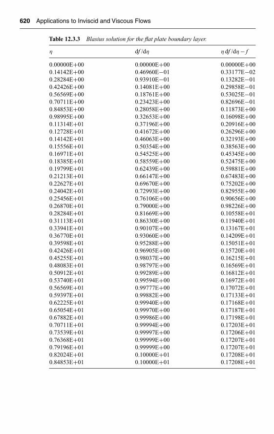
Ch12-H6594.tex 8/5/2007 20: 19 Page 620


Table 12.3.3 Blasius solution for the flat plate boundary layer.

η df /dη η df /dη − f

0.00000E+00 0.00000E+00 0.00000E+000.14142E+00 0.46960E−01 0.33177E−020.28284E+00 0.93910E−01 0.13282E−010.42426E+00 0.14081E+00 0.29858E−010.56569E+00 0.18761E+00 0.53025E−010.70711E+00 0.23423E+00 0.82696E−010.84853E+00 0.28058E+00 0.11873E+000.98995E+00 0.32653E+00 0.16098E+000.11314E+01 0.37196E+00 0.20916E+000.12728E+01 0.41672E+00 0.26296E+000.14142E+01 0.46063E+00 0.32193E+000.15556E+01 0.50354E+00 0.38563E+000.16971E+01 0.54525E+00 0.45345E+000.18385E+01 0.58559E+00 0.52475E+000.19799E+01 0.62439E+00 0.59881E+000.21213E+01 0.66147E+00 0.67483E+000.22627E+01 0.69670E+00 0.75202E+000.24042E+01 0.72993E+00 0.82955E+000.25456E+01 0.76106E+00 0.90656E+000.26870E+01 0.79000E+00 0.98226E+000.28284E+01 0.81669E+00 0.10558E+010.31113E+01 0.86330E+00 0.11940E+010.33941E+01 0.90107E+00 0.13167E+010.36770E+01 0.93060E+00 0.14209E+010.39598E+01 0.95288E+00 0.15051E+010.42426E+01 0.96905E+00 0.15720E+010.45255E+01 0.98037E+00 0.16215E+010.48083E+01 0.98797E+00 0.16569E+010.50912E+01 0.99289E+00 0.16812E+010.53740E+01 0.99594E+00 0.16972E+010.56569E+01 0.99777E+00 0.17072E+010.59397E+01 0.99882E+00 0.17133E+010.62225E+01 0.99940E+00 0.17168E+010.65054E+01 0.99970E+00 0.17187E+010.67882E+01 0.99986E+00 0.17198E+010.70711E+01 0.99994E+00 0.17203E+010.73539E+01 0.99997E+00 0.17206E+010.76368E+01 0.99999E+00 0.17207E+010.79196E+01 0.99999E+00 0.17207E+010.82024E+01 0.10000E+01 0.17208E+010.84853E+01 0.10000E+01 0.17208E+01

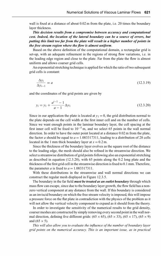
Ch12-H6594.tex 8/5/2007 20: 19 Page 621


wall is fixed at a distance of about 0.02 m from the plate, i.e. 20 times the boundarylayer thickness.

This decision results from a compromise between accuracy and computationalcost. Indeed, the location of the lateral boundary can be a source of errors, butputting this limit too far from the plate will result in a higher number of points inthe free stream region where the flow is almost uniform.

Based on the above definition of the computational domain, a rectangular grid isset-up, with an adequate refinement in the regions of strong flow variations, i.e. inthe leading edge region and close to the plate. Far from the plate the flow is almostuniform and allows coarser grid cells.

An exponential stretching technique is applied for which the ratio of two subsequentgrid cells is constant:

�yi

�yi−1= a (12.3.19)

and the coordinates of the grid points are given by

yi = y1 + ai−1 − 1

a − 1�y1 (12.3.20)

Since in our application the plate is located at y1 = 0, the grid distribution normal tothe plate depends on the cell width at the first inner cell and on the number of cells.Since we want enough points in the laminar boundary layer, the cell spacing at thefirst inner cell will be fixed to 10−5 m, and we select 65 points in the wall normaldirection. In order to have the outer point located at a distance 0.02 m from the plate,the factor a should be equal to a = 1.083317311, leading to a distribution of 28 cellslocated in the 1 mm thick boundary layer at x = 0.2 m.

Since the thickness of the boundary layer evolves as the square root of the distanceto the leading edge, the mesh should also be refined in the streamwise direction. Weselect a streamwise distribution of grid points following also an exponential stretchingas described in equation (12.3.20), with 65 points along the 0.2 long plate and thethickness of the first grid cell in the streamwise direction is fixed to 0.1 mm. Therefore,the parameter a is fixed to a = 1.083317311.

With these distributions in the streamwise and wall normal directions we canconstruct the regular mesh displayed in Figure 12.3.5.

The boundary in the far field must be treated as an outlet boundary through whichmass flow can escape, since due to the boundary layer growth, the flow field has a non-zero vertical component at any distance from the wall. If this boundary is consideredas an inviscid boundary on which the free stream velocity is imposed, this will imposea pressure force on the flat plate in contradiction with the physics of the problem as itwill not allow the vertical velocity component to expand as it should from the theory.

In order to investigate the sensitivity of the numerical results to the grid density,coarser meshes are constructed by simply removing every second point in the wall nor-mal direction, defining five different grids: (65 × 65), (65 × 33), (65 × 17), (65 × 9)and (65 × 5).

This will also allow you to evaluate the influence of the number of boundary layergrid points on the numerical accuracy. This is an important issue, as in practical

Ch12-H6594.tex 8/5/2007 20: 19 Page 622


Outlet

Outlet

Flat plate

InletY

X

Figure 12.3.5 Mesh defined for the laminar flat plate test case.

0

0 25,000 50,000 75,000 1e�05 1.25e�05 1.5e�05 1.75e�05 2e�05

�2

�4

�6

�8

�10

Log

(x-m

omen

tum

res

idua

l)

Iteration number

Mesh 65�65Mesh 65�33Mesh 65�17Mesh 65�9Mesh 65�5

Figure 12.3.6 Convergence history of the normalized L2-norm of the x-momentumresidual on five different meshes.

industrial case, it is quite difficult and costly to ensure 25–30 points in boundarylayers of complex 3D geometries.

Boundary conditions are specified at the inlet and outlet of the computationaldomain. Assuming atmospheric condition for the static temperature and pressure andan inlet Mach number of 0.2, the inlet total pressure and total temperature are fixed to104165 Pa and 290.304 K, respectively (following equations (11.1.9) and (11.1.12)).The inlet velocity vector is imposed in the x-direction. At the outlet boundaries, asshown on Figure 12.3.5, the static pressure is fixed to the atmospheric value, i.e.101300 Pa.

12.3.2.3 Results

The Navier–Stokes equations are solved using the cell-centered approach until asteady state is reached, with CFL and Von Neumann numbers put to 1.5 and thedissipation coefficient κ(4) = 1/100.

A Runge–Kutta time integration method is also used with the coefficients pro-vided by equation (11.4.11). The computations are stopped when the residuals havedecreased by more than 6 orders of magnitude.

The convergence history of the x-momentum equation is provided in Figure 12.3.6.This residual is decreased by about 8 orders of magnitude. Such a convergence level

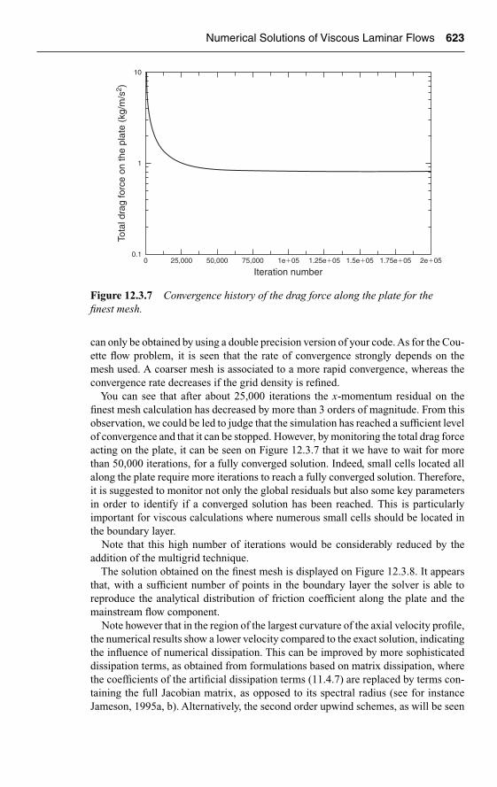
Ch12-H6594.tex 8/5/2007 20: 19 Page 623


10

1

0.10 25,000 50,000 75,000 1e�05 1.25e�05 1.5e�05 1.75e�05 2e�05

Iteration number

Tota

l dra

g fo

rce

on th

e pl

ate

(kg/

m/s

2 )

Figure 12.3.7 Convergence history of the drag force along the plate for thefinest mesh.

can only be obtained by using a double precision version of your code. As for the Cou-ette flow problem, it is seen that the rate of convergence strongly depends on themesh used. A coarser mesh is associated to a more rapid convergence, whereas theconvergence rate decreases if the grid density is refined.

You can see that after about 25,000 iterations the x-momentum residual on thefinest mesh calculation has decreased by more than 3 orders of magnitude. From thisobservation, we could be led to judge that the simulation has reached a sufficient levelof convergence and that it can be stopped. However, by monitoring the total drag forceacting on the plate, it can be seen on Figure 12.3.7 that it we have to wait for morethan 50,000 iterations, for a fully converged solution. Indeed, small cells located allalong the plate require more iterations to reach a fully converged solution. Therefore,it is suggested to monitor not only the global residuals but also some key parametersin order to identify if a converged solution has been reached. This is particularlyimportant for viscous calculations where numerous small cells should be located inthe boundary layer.

Note that this high number of iterations would be considerably reduced by theaddition of the multigrid technique.

The solution obtained on the finest mesh is displayed on Figure 12.3.8. It appearsthat, with a sufficient number of points in the boundary layer the solver is able toreproduce the analytical distribution of friction coefficient along the plate and themainstream flow component.

Note however that in the region of the largest curvature of the axial velocity profile,the numerical results show a lower velocity compared to the exact solution, indicatingthe influence of numerical dissipation. This can be improved by more sophisticateddissipation terms, as obtained from formulations based on matrix dissipation, wherethe coefficients of the artificial dissipation terms (11.4.7) are replaced by terms con-taining the full Jacobian matrix, as opposed to its spectral radius (see for instanceJameson, 1995a, b). Alternatively, the second order upwind schemes, as will be seen

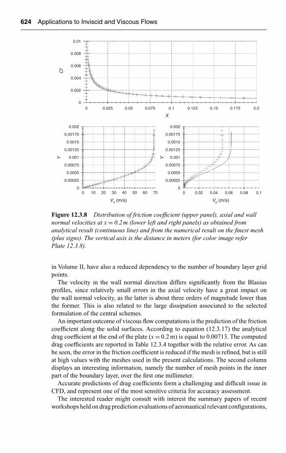
Ch12-H6594.tex 8/5/2007 20: 19 Page 624


0.01

0.008

0.006

0.004

0.002

00 0.025 0.05 0.075 0.1 0.150.125 0.175 0.2

X

Cf

0 0.02 0.04 0.06 0.08 0.1

0.002

0.00175

0.0015

0.00125

0.001

0.00075

0.0005

0.00025

0

Y

Vy (m/s)

0.002

0.00175

0.0015

0.00125

0.001

0.00075

0.0005

0.00025

00 10 20 30 40 50 60 70

Y

Vx (m/s)

Figure 12.3.8 Distribution of friction coefficient (upper panel), axial and wallnormal velocities at x = 0.2 m (lower left and right panels) as obtained fromanalytical result (continuous line) and from the numerical result on the finest mesh(plus signs). The vertical axis is the distance in meters (for color image referPlate 12.3.8).

in Volume II, have also a reduced dependency to the number of boundary layer gridpoints.

The velocity in the wall normal direction differs significantly from the Blasiusprofiles, since relatively small errors in the axial velocity have a great impact onthe wall normal velocity, as the latter is about three orders of magnitude lower thanthe former. This is also related to the large dissipation associated to the selectedformulation of the central schemes.

An important outcome of viscous flow computations is the prediction of the frictioncoefficient along the solid surfaces. According to equation (12.3.17) the analyticaldrag coefficient at the end of the plate (x = 0.2 m) is equal to 0.00713. The computeddrag coefficients are reported in Table 12.3.4 together with the relative error. As canbe seen, the error in the friction coefficient is reduced if the mesh is refined, but is stillat high values with the meshes used in the present calculations. The second columndisplays an interesting information, namely the number of mesh points in the innerpart of the boundary layer, over the first one millimeter.

Accurate predictions of drag coefficients form a challenging and difficult issue inCFD, and represent one of the most sensitive criteria for accuracy assessment.

The interested reader might consult with interest the summary papers of recentworkshops held on drag prediction evaluations of aeronautical relevant configurations,

Ch12-H6594.tex 8/5/2007 20: 19 Page 625


Table 12.3.4 Friction coefficient computed using the different meshes.

Number of cells in theboundary layer (first Relative errorone millimeter) Cf in Cf (%)

Analytical 0.000713 –65 × 65 28 0.00075 5.265 × 33 14 0.000803 12.765 × 17 7 0.000917 28.765 × 9 4 0.001371 92.365 × 5 2 0.002196 208.0

in Hemsch and Morrison (2004), also referred to in the general introduction tothis book.

The errors on the friction coefficient are a consequence of the reduced accuracy onthe velocity profiles, when the mesh is coarsened. This can be seen from Figure 12.3.9,where the distributions of skin friction and velocity are displayed on the two successivecoarser grids, namely 65 × 33 and 65 × 17, having respectively, 14 and 7 points in theboundary layer. You will notice that 14 points might still be acceptable, for ‘engineer-ing’ accuracy, but the error on the skin friction is of 12%, as seen from Table 12.3.4.

12.4 PRESSURE CORRECTION METHOD

The methods known as pressure correction are among the first developed for thenumerical solutions of the full Navier–Stokes equations for incompressible flows. Themethod was originally applied by Harlow and Welch (1965) in the MAC, Marker-and-Cell, method for the computation of free surface incompressible flows. It is closelyrelated to the fractional step method , also called projection method , developedindependently by Chorin (1967), (1968) and Temam (1969); see also Temam (1977).

It has been adapted to industrial flow simulations by Patankar and Spalding (1972)and described in details in several books (Patankar (1980); Anderson (1995); Ferzigerand Peric (1997); Wesseling (2001)).

The methods falling in this class can be applied to the stationary as well as tothe time-dependent incompressible flow equations. They consist of a basic iterativeprocedure between the velocity and the pressure fields. For an initial approximationof the pressure, the momentum equation can be solved to determine the velocityfield. The obtained velocity field does not satisfy the divergence free, continuityequation and has therefore to be corrected. Since this correction has an impact on thepressure field, a related pressure correction is defined, obtained by expressing that thecorrected velocity satisfies the continuity equation. This leads to a Poisson equationfor the pressure correction.

The pressure correction methods have been extended to compressible flows, andvarious approaches can be defined. Weak compressibility can be handled through asimplified system of equations obtained by developing a low Mach number expansionof the Navier–Stokes equations, omitting then the terms that are of higher order in

Ch12-H6594.tex 8/5/2007 20: 19 Page 626


0.01

0.008

0.006

0.004

0.002

00 0.025 0.05 0.075 0.1 0.150.125 0.175 0.2

X

Cf

0 0.02 0.04 0.06 0.08 0.1

0.002

0.00175

0.0015

0.00125

0.001

0.00075

0.0005

0.00025

0

Y

Vy (m/s)

0.002

0.00175

0.0015

0.00125

0.001

0.00075

0.0005

0.00025

00 10 20 30 40 50 60 70

Y

Vx (m/s)

(a)

0.01

0.008

0.006

0.004

0.002

00 0.025 0.05 0.075 0.1 0.150.125 0.175 0.2

X

Cf

0 0.02 0.04 0.06 0.08 0.1

0.002

0.00175

0.0015

0.00125

0.001

0.00075

0.0005

0.00025

0

Y

Vy (m/s)

0.002

0.00175

0.0015

0.00125

0.001

0.00075

0.0005

0.00025

00 10 20 30 40 50 60 t

Y

Vx (m/s)

(b)

Figure 12.3.9 Distributions of skin friction and velocity on the two successivecoarser grids of 65 × 33 and 65 × 17, having respectively, 14 and 7 points in theboundary layer. (a) Numerical solution on 65 × 33 mesh with 14 points in theboundary layer and (b) numerical solution on 65 × 17 mesh with 7 points in theboundary layer.

Ch12-H6594.tex 8/5/2007 20: 19 Page 627


the Mach number (see, for instance, Majda and Sethian (1985)). A full compressibleextension can be found in the book of Ferziger and Peric (1997).

12.4.1 Basic Approach of Pressure Correction Methods

We restrict the presentation here to strictly incompressible, isothermal flows, definedin Section 1.4.4 by the system formed by the continuity and momentum equations,written here in non-conservative form.

The mass conservation equation reduces in the case of incompressible flows to

�∇ · �v = 0 (12.4.1)

which appears as a constraint to the general time-dependent equation of motion,written here in absence of external volume forces

∂�v∂t

+ (�v · �∇)�v = − 1

ρ�∇p + ν��v (12.4.2)

The only unknowns are velocity and pressure.An equation for the pressure can be obtained by taking the divergence of the momen-

tum equation (12.4.2), and introducing the divergence free velocity condition (12.4.1),leading to

1

ρ�p = −�∇ · (�v · �∇)�v (12.4.3)

which can be considered as a Poisson equation for the pressure for a given velocityfield. Note that the right-hand side contains only products of first order velocityderivatives, because of the incompressibility condition (12.4.1). Indeed, in tensornotations, the velocity term in the right-hand side term is equal to (∂jvi) · (∂ivj).

Before describing the pressure correction method we have to select a time integra-tion scheme for the momentum equations, considering the pressure gradient as known.For reasons of simplicity and in order to point out the essential properties of the pres-sure correction approach, we will select an explicit method of first order accuracy intime, although it is not recommended in practice. Even for time-dependent problemsthe time step restriction imposed by stability conditions for the parabolic, convection–diffusion momentum equations is generally smaller than the physical time constant ofthe flow. Hence, the time steps allowed by the requirements of physical accuracy arelarge enough to allow the larger numerical time steps of implicit schemes. Typically,semi-implicit time integration schemes are recommended. For instance, the viscousfluxes can be treated implicitly by means of the Crank–Nicholson formulation, whileconvective fluxes can be handled with an Adams–Bashworth second order method.This provides a higher accuracy for time-dependent simulations and allows for largetime steps leading to more efficient calculations in terms of computational costs.

The fundamental approach of pressure correction methods is the decoupling of thepressure field from the velocity field. This is expressed by solving the momentum

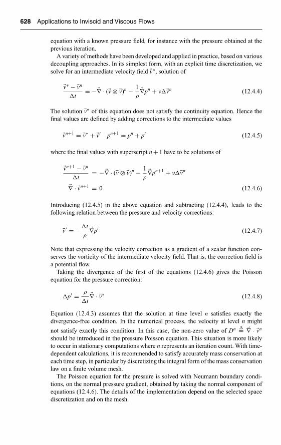
Ch12-H6594.tex 8/5/2007 20: 19 Page 628


equation with a known pressure field, for instance with the pressure obtained at theprevious iteration.

A variety of methods have been developed and applied in practice, based on variousdecoupling approaches. In its simplest form, with an explicit time discretization, wesolve for an intermediate velocity field �v∗, solution of

�v∗ − �vn

�t= −�∇ · (�v ⊗ �v)n − 1

ρ�∇pn + ν��vn (12.4.4)

The solution �v∗ of this equation does not satisfy the continuity equation. Hence thefinal values are defined by adding corrections to the intermediate values

�vn+1 = �v∗ + �v′ pn+1 = pn + p′ (12.4.5)

where the final values with superscript n + 1 have to be solutions of

�vn+1 − �vn

�t= −�∇ · (�v ⊗ �v)n − 1

ρ�∇pn+1 + ν��vn

�∇ · �vn+1 = 0 (12.4.6)

Introducing (12.4.5) in the above equation and subtracting (12.4.4), leads to thefollowing relation between the pressure and velocity corrections:

�v′ = −�t

ρ�∇p′ (12.4.7)

Note that expressing the velocity correction as a gradient of a scalar function con-serves the vorticity of the intermediate velocity field. That is, the correction field isa potential flow.

Taking the divergence of the first of the equations (12.4.6) gives the Poissonequation for the pressure correction:

�p′ = ρ

�t�∇ · �v∗ (12.4.8)

Equation (12.4.3) assumes that the solution at time level n satisfies exactly thedivergence-free condition. In the numerical process, the velocity at level n might

not satisfy exactly this condition. In this case, the non-zero value of Dn �= �∇ · �vn

should be introduced in the pressure Poisson equation. This situation is more likelyto occur in stationary computations where n represents an iteration count. With time-dependent calculations, it is recommended to satisfy accurately mass conservation ateach time step, in particular by discretizing the integral form of the mass conservationlaw on a finite volume mesh.

The Poisson equation for the pressure is solved with Neumann boundary condi-tions, on the normal pressure gradient, obtained by taking the normal component ofequations (12.4.6). The details of the implementation depend on the selected spacediscretization and on the mesh.

Ch12-H6594.tex 8/5/2007 20: 19 Page 629


An alternative approach is the fractional step, or projection, method based on aslightly different definition of the intermediate pressure, whereby the pressure term issimply omitted, leading to the complete decoupling of the intermediate velocity field

�v∗ − �vn

�t= −�∇ · (�v ⊗ �v)n + ν��vn (12.4.9)

followed by the pressure equation

�vn+1 − �v∗

�t= − 1

ρ

−→∇ pn+1 (12.4.10)

The final value of velocity field is obtained from equation (12.4.10). The pressure iscalculated in such a way that the velocity field at level (n + 1) satisfies the divergencefree condition:

ρ

�t[ �∇ · �vn+1 − �∇ · �v∗] = −�pn+1 (12.4.11)

leading to the an equation similar to (12.4.8)

�pn+1 = ρ

�t�∇ · �v∗ (12.4.12)

The final value of the velocity field �vn+1 velocities are updated from (12.4.10).The numerical resolution of the pressure Poisson equation is a crucial step of

the whole approach, since the overall efficiency of the code will depend on its per-formance. Hence all possible convergence optimization and acceleration techniquesshould be applied. In particular preconditioning and multigrid techniques are stronglyrecommended for this step of the computation, and eventually for other steps.

12.4.2 The Issue of Staggered Versus Collocated Grids

The choice of a space discretization is, as for compressible flows, between centered orupwind methods, at least for the convection terms, since the diffusive contributionsare always centrally discretized.

The most current choice is the central discretization of the convection terms, whichraises a particular problem with the pressure correction approach.

The central discretization for the convection terms requires the addition of higherorder artificial dissipation terms to create the required damping of high frequencyerrors, as introduced in the previous examples. However the absence of the timederivative of the density in the continuity equation creates an additional decou-pling in the centrally discretized equations, with pressure correction methods. Thisis best illustrated on the one-dimensional system of incompressible Navier–Stokesequations. The conservation equations take the form

∂u

∂x= 0

∂u

∂t+ ∂u2

∂x= − 1

ρ

∂p

∂x+ ν

∂2u

∂x2(12.4.13)

Ch12-H6594.tex 8/5/2007 20: 19 Page 630


�x�x

i�2

i�3/2 i�1/2 i�1/2 i�3/2

i�1 i�1 i�2i

(ui,pi)

�x�x

i�2

i�3/2 i�1/2 i�1/2 i�3/2

i�1 i�1 i�2i

pi

ui�1/2 ui�1/2

(a)

(b)

Figure 12.4.1 Standard ‘collocated’ and staggered grids: (a) standard collocatedgrid and (b) staggered grid.

We consider a central finite difference discretization of the above equations on astandard uniform grid, where all the variables are defined on the same mesh points.This is called a collocated mesh, in the context of pressure correction methods (seeFigure 12.4.1a). The centrally discretized equations become

un+1i+1 − un+1

i−1

2�x= 0 (12.4.14)

un+1i − un

i

�t+ (un

i+1)2 − (uni−1)2

2�x= − 1

ρ

pi+1 − pi−1

2�x+ ν

uni+1 − 2un

i + uni−1

�x2

(12.4.15)

In the framework of the pressure correction method, the momentum equation is splitinto two parts by introducing the intermediate velocity u∗, based on the fractional stepmethod, solution of

u∗i − un

i

�t+ (un

i+1)2 − (uni−1)2

2�x= ν

uni+1 − 2un

i + uni−1

�x2(12.4.16)

un+1i − u∗

i

�t= − 1

ρ

pi+1 − pi−1

2�x(12.4.17)

The expression for un+1i , obtained from equation (12.4.17), can be substituted into

(12.4.14), resulting in the following 1D equation:

pi+2 − 2pi + pi−2

4�x2= ρ

�t

u∗i+1 − u∗

i−1

2�x(12.4.18)

Ch12-H6594.tex 8/5/2007 20: 19 Page 631


This is a Poisson equation for the pressure, which ensures that the continuity equa-tion (12.4.14) is satisfied for the newly updated velocity un+1

i . The stencil on whichthe Laplace operator is discretized (i + 2, i, i − 2) contains, however, only odd or evenindices, which leads to a decoupling of the discrete pressure field and often results inhigh frequency oscillations of pressure.

As can be seen indeed, the pressure at point i is not influenced by the velocitycomponent un

i of the same point and in return uni is not affected by pi. Hence velocity

and pressure are decoupled on even and odd points; see also Section 4.2 and thediscussion around the Lax–Friedrichs scheme in Chapter 7, for an illustration ofanalog cases. This decoupling is not present with compressible flows due to thedensity–velocity coupling in the continuity equation. It will generate additional highfrequency oscillations, requesting the introduction of artificial dissipation terms.

A solution to the odd–even decoupling problem, has been introduced by Harlowand Welch (1965), by defining a staggered mesh, where the velocity and pressure arenot defined in the same mesh points. As seen in Figure 12.4.1b, the velocity is directlydefined at the half mesh points, while the pressure remains defined at the central meshpoint. The central discretization of the continuity equation of (12.4.13) now becomes

un+1i+1/2 − un+1

i−1/2

�x= 0 (12.4.19)

With the fractional step method, equation (12.4.17) becomes on the staggered mesh

un+1i+1/2 − u∗

i+1/2

�t= − 1

ρ

pi+1 − pi

�x(12.4.20)

By substituting expressions for un+1i+1/2 and un+1

i−1/2 derived from (12.4.20) into thisequation, we obtain

pi+1 − 2pi + pi−1

�x2= ρ

�t

u∗i+1/2 − u∗

i−1/2

�x(12.4.21)

In this discrete Poisson equation the pressure and velocity in all nodes are fullycoupled, which completely eliminates the problem of odd–even decoupling.

Staggered meshes are currently applied with central discretization and the mostpopular two-dimensional arrangement is shown in Figure 12.4.2, where the u and vvelocity components are located on different cell faces. The equations are discretizedin conservation form, the control volumes depending on the considered equations.The mass equation is discretized on the volume centered on the point (i, j), while thex-momentum conservation is expressed on the volume centered for the location of u,i.e. (i + 1/2, j). Similarly, the y-momentum conservation is expressed on the volumecentered on the location of v, i.e. (i, j + 1/2).

The Poisson equation for the pressure is obtained from the divergence of the dis-cretized momentum equation. This step should be performed by exactly the samediscrete operations as applied to express mass conservation. This is required forglobal consistency and conservation. It is fairly straightforward on a Cartesian mesh,but becomes essential on arbitrary meshes.

The Poisson equation for the pressure is solved with Neumann boundary conditionson the normal pressure gradient on the walls and at the inlet, while at the outlet

Ch12-H6594.tex 8/5/2007 20: 19 Page 632


� � �

� � �

� � �

vi,j�1/2

pi,j�1

vi,j�1/2

pi,j pi,j�1

ui�1/2,j ui�1/2,j

Control cell for mass conservation

Control cell for x -momentum conservation

Control cell for y -momentum conservation

Figure 12.4.2 Staggered, two-dimensional finite difference mesh for centrallydiscretized pressure correction methods.

the pressure is set to a certain value (e.g. atmospheric pressure). The details of theimplementation depend on the selected space discretization and on the mesh.

An additional condition is essential for the numerical accuracy of the resolution ofthe pressure equation, namely that the compatibility condition, obtained from Green’stheorem applied to the Poisson equation, should be identically satisfied by the spacediscretization. Applied to equation (12.4.12), we should have identically, for the inte-gral of the normal pressure gradient on boundary �S of the computational domain �:

∫�

�pn+1d� =∮

S

�∇p · d�S =∮

S

∂p

∂ndS = ρ

�t

∫�

∇ · �v∗d� = ρ

�t

∮S�v∗ · d�S(12.4.22)

12.4.3 Implementation of a Pressure Correction Method

We consider the application of the fractional step method to the simulation of incom-pressible flows. The method is described for a cell-centered finite volume method ona Cartesian mesh, with all flow variables defined in the same points at the centers ofthe computational cells, although the staggered grid approach is applied to connectvalues at the cell centers with face defined values, as seen on Figure 12.4.3, wheredifferent control volumes are shown. Boundaries of the computational domain are

Ch12-H6594.tex 8/5/2007 20: 19 Page 633


8

7 5

6

4

2

3 1

B

�xiA

C

D

i�1/2

j�1/2

i�1/2

j�1/2

i,j i�1, j�yj

Figure 12.4.3 Cell-centered finite volume mesh for pressure correction method onnon-uniform Cartesian grid.

located on cell faces and you can follow the treatment of the boundary conditions asdescribed in Section 12.2.

Another way to impose boundary conditions in such a configuration can be con-sidered through introduction of ghost or dummy cells, i.e. rows of cells neighboringthe computational domain and having the same size as the first row of cells inside thedomain.

You can extend the generality of your code by allowing for non-uniform Cartesiangrids to account for clustered grids near solid walls. We consider a rectangular domainwith side lengths Lx and Ly with Nx and Ny mesh points in both directions andvariable mesh sizes. The Cartesian mesh has Nx × Ny nodes, dividing the domaininto (Nx − 1)(Ny − 1) rectangular cells, the sides of varying sizes: �xi = xi+1 − xi,�yi = yi+1 − yi.

The two-dimensional incompressible Navier–Stokes equations are discretized onthe non-uniform Cartesian grid of Figure 12.4.3. A cell-centered second order finitevolume discretization is selected, with an explicit first order time integration.

∂u

∂x+ ∂v

∂y= 0

∂u

∂t+ ∂u2

∂x+ ∂uv

∂y= − 1

ρ

∂p

∂x+ 1

ρ

∂τxx

∂x+ 1

ρ

∂τxy

∂y= − 1

ρ

∂p

∂x+ ν

∂2u

∂x2+ ν

∂2u

∂y2

∂v

∂t+ ∂uv

∂x+ ∂v2

∂y= − 1

ρ

∂p

∂y+ 1

ρ

∂τxy

∂x+ 1

ρ

∂τyy

∂y= − 1

ρ

∂p

∂y+ ν

∂2v

∂x2+ ν

∂2v

∂y2

(12.4.23)

Ch12-H6594.tex 8/5/2007 20: 19 Page 634


12.4.3.1 Numerical discretization

In the pressure correction method, the velocities are updated from the momentumequations, while pressure is obtained by solving the Poisson equation derived bytaking a divergence of the momentum equations and taking conservation of mass intoaccount.

We refer to Figure 12.4.3 and apply a finite volume formulation on the contourABCD for the velocity components u and v at the cell centers.

Applying the fractional step formulation of equations (12.4.9) to (12.4.12), wewrite the scheme as follows, for the intermediate velocity components u∗ and v∗

u∗i, j − un

i, j

�t+ (u2)n

i+1/2, j − (u2)ni−1/2, j

�xi+ (uv)n

i, j+1/2 − (uv)ni, j−1/2

�yj

= 1

ρ

(τxx)ni+1/2, j − (τxx)n

i−1/2, j

�xi+ 1

ρ

(τxy)ni, j+1/2 − (τxy)n

i, j−1/2

�yj(12.4.24)

v∗i, j − vn

i, j

�t+ (uv)n

i+1/2, j − (uv)ni−1/2, j

�xi+ (v2)n

i, j+1/2 − (v2)ni, j−1/2

�yj

= 1

ρ

(τyx)ni+1/2, j − (τyx)n

i−1/2, j

�xi+ 1

ρ

(τyy)ni, j+1/2 − (τyy)n

i, j−1/2

�yj(12.4.25)

where the interface values are obtained by the weighted averages

ui+1/2, j = �xiui+1, j + �xi+1ui, j

�xi + �xi+1

vi, j+1/2 = �yjvi, j+1 + �yj+1vi, j

�yj + �yj+1(12.4.26)

and similarly for the other variables.You can calculate the shear stress components as follows:

(τxx)ni+1/2, j = 2μn

i+1/2, j(ux)ni+1/2, j

(τxy)ni+1/2, j = μn

i+1/2, j((uy)ni+1/2, j + (vx)n

i+1/2, j)

(ux)ni+1/2, j = un

i+1, j − uni, j

(�xi+1 + �xi)/2(vx)n

i+1/2, j = vni+1, j − vn

i, j

(�xi+1 + �xi)/2

(uy)ni+1/2, j = 1

2

[un

i+1, j+1 − uni+1, j−1

(�yj+1 + 2�yj + �yj−1)/2+ un

i, j+1 − uni, j−1

(�yj+1 + 2�yj + �yj−1)/2

]

(vy)ni+1/2, j = 1

2

[vn

i+1, j+1 − vni+1, j−1

(�yj+1 + 2�yj + �yj−1)/2+ vn

i, j+1 − vni, j−1

(�yj+1 + 2�yj + �yj−1)/2

]

(12.4.27)

Ch12-H6594.tex 8/5/2007 20: 19 Page 635


(τyy)ni, j+1/2 = 2μn

i, j+1/2(vy)ni+1/2, j

(τyx)ni, j+1/2 = μn

i, j+1/2((uy)ni, j+1/2 + (vx)n

i, j+1/2)

(uy)ni, j+1/2 = un

i, j+1 − uni, j

(�yj+1 + �yj)/2(vy)n

i, j+1/2 = vni, j+1 − vn

i, j

(�yj+1 + �yj)/2

(ux)ni, j+1/2 = 1

2

[un

i+1, j+1 − uni−1, j+1

(�xi+1 + 2�xi + �xi−1)/2+ un

i+1, j − uni−1, j

(�xi+1 + 2�xi + �xi−1)/2

]

(vx)ni, j+1/2 = 1

2

[vn

i+1, j+1 − vni−1, j+1

(�xi+1 + 2�xi + �xi−1)/2+ vn

i+1, j − vni−1, j

(�xi+1 + 2�xi + �xi−1)/2

]

(12.4.28)

Once the intermediate velocity components are estimated, you can obtain the valuesof the updated velocity and pressure variables, satisfying the continuity equation,following (12.4.10). Applying a finite volume formulation on the contour ABCD tothis equation and projecting in the x- and y-directions, we obtain

un+1i, j − u∗

i, j

�t= − 1

ρ

pi+1/2, j − pi−1/2, j

�xi

vn+1i, j − v∗

i, j

�t= − 1

ρ

pi, j+1/2 − pi, j+1/2

�yj(12.4.29)

The pressure is obtained by expressing that the velocity components at level (n + 1)satisfy the divergence free continuity equation, as in (12.4.6). Discretized on the finitevolume mesh ABCD we obtain

un+1i+1/2, j − un+1

i−1/2, j

�xi+ vn+1

i, j+1/2 − vn+1i, j−1/2

�yj= 0 (12.4.30)

The interface velocities at the (n + 1) level are obtained by applying once again thefinite volume formulation of equation (12.4.10), but this time on a staggered controlvolume such as 1234, Figure 12.4.3, centered on face AB, for the x componentequation

ρun+1

i+1/2, j − u∗i+1/2, j

�t�yj

�xi+1 + �xi

2= (pn+1

i+1, j − pn+1i, j )�yj (12.4.31)

and on the control volume 5678, centered around BC, for the vertical component,leading to

ρvn+1

i, j+1/2 − v∗i, j+1/2

�t�xi

�yj+1 + �yj

2= (pn+1

i, j+1 − pn+1i, j )�xi (12.4.32)

The values on faces CD and DA are obtained similarly.

Ch12-H6594.tex 8/5/2007 20: 19 Page 636


The intermediate values u∗ and v∗ on the cell faces are obtained from the relations(12.4.26).

Substituting these relations in equation (12.4.30), leads to the pressure Poissonequation:

1

�xi

[pn+1

i+1, j − pn+1i, j

(�xi+1 + �xi)/2− pn+1

i, j − pn+1i−1, j

(�xi + �xi−1)/2

]

+ 1

�yj

[pn+1

i, j+1 − pn+1i, j

(�yj+1 + �yj)/2− pn+1

i, j − pn+1i, j−1

(�yj + �yj−1)/2

]

= ρ

�t

[u∗

i+1/2, j − u∗i−1/2, j

�xi+ v∗

i, j+1/2 − v∗i, j−1/2

�yj

](12.4.33)

The whole procedure of updating the solution is the following:

• Calculate the intermediate velocity field u∗i, j , v∗

i, j from (12.4.24) and (12.4.25).• Obtain the pressure by solving the Poisson equation (12.4.33).• Obtain the solution at the next time step un+1

i, j , vn+1i, j from (12.4.29), where the

pressure at the cell faces is obtained by applying relations (12.4.26).

We have now to focus on the most critical issue of pressure correction methods,namely the efficient resolution of the pressure Poisson equation. This is a crucial stepof the whole approach, since the overall efficiency of your code will depend on itsperformance.

12.4.3.2 Algorithm for the pressure Poisson equation

The pressure Poisson equation (12.4.33) is a standard elliptic equation and you cancall upon the various methods introduced in Chapter 10. In advanced codes, vari-ous convergence optimization and acceleration techniques are applied, in particularpreconditioning and multigrid techniques are strongly recommended for this stepof the computation, and many of these techniques are described in the literature onpressure correction methods.

Here, we suggest you to choose a simple line Gauss–Seidel method along a verticalline. As a first approximation of the pressure, its discrete values obtained on theprevious time level are used. Given an approximation of the pressure pk , the next oneis obtained from the following relation:

1

�xi

[pk

i+1, j − pk+1i, j

(�xi+1 + �xi)/2− pk+1

i, j − pk+1i−1, j

(�xi + �xi−1)/2

]

+ 1

�yj

[pk+1

i, j+1 − pk+1i, j

(�yj+1 + �yj)/2− pk+1

i, j − pk+1i, j−1

(�yj + �yj−1)/2

]= Qi, j (12.4.34)

where Qi, j is the right-hand side of (12.4.33). Not that the k index denotes an iterationnumber and not a time level (n in the previous section). Equation (12.4.34) can be

Ch12-H6594.tex 8/5/2007 20: 19 Page 637


rewritten as follows:

ai, jpk+1i, j−1 + bi, jp

k+1i, j + ci, jp

k+1i, j+1

= Qi, j − 1

�xi

[pk

i+1, j

(�xi+1 + �xi)/2+ pk+1

i−1, j

(�xi + �xi−1)/2

](12.4.35)

where

ai, j = 2

�yj

1

�yj + �yj−1

ci, j = 2

�yj

1

�yj+1 + �yj(12.4.36)

bi, j = − 2

�xi

[1

�xi+1 + �xi+ 1

�xi + �xi−1

]− (ai, j + ci, j)

We have to add the boundary conditions, for instance for i = 1 and a Neumann bound-ary condition (12.4.35) can be rewritten taking into account the boundary conditionat i = 1/2:

a1, jpk+11, j−1 +

(b1, j + 1

�x1

2

�x1 + �x0

)pk+1

1, j + c1, jpk+11, j+1

= Q1, j − 1

�x1

pk2, j

(�x2 + �x1)/2(12.4.37)

where the Neumann boundary condition is expressed as pk+10 = pk+1

1 .You can apply this similarly for the other boundary conditions. If the pressure is

imposed at certain boundaries, as a Dirichlet condition, then you can introduce thisvalue directly in the corresponding equation.

The algebraic system can be efficiently solved with the Thomas Algorithm (seeAppendix A in Chapter 10).

The iterations are to be repeated until a prescribed convergence criterion is satisfied(e.g. maxi, j |pk+1

i, j − pki, j| < ε).

For reasons of accuracy, it is recommended to alternate this algorithm witha line Gauss–Seidel method in the horizontal direction (at j = constant), apply-ing the Thomas algorithm in two different mesh directions. Equation (12.4.34) isreplaced by

1

�xi

[pk+1

i+1, j − pk+1i, j

(�xi+1 + �xi)/2− pk+1

i, j − pk+1i−1, j

(�xi + �xi−1)/2

]

+ 1

�yj

[pk

i, j+1 − pk+1i, j

(�yj+1 + �yj)/2− pk+1

i, j − pk+1i, j−1

(�yj + �yj−1)/2

]= Qi, j (12.4.38)

We leave it to you as an exercise to work out the details of its implementation.

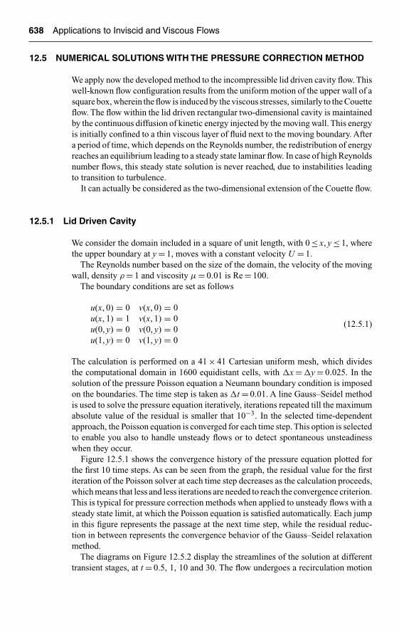
Ch12-H6594.tex 8/5/2007 20: 19 Page 638


12.5 NUMERICAL SOLUTIONS WITH THE PRESSURE CORRECTION METHOD

We apply now the developed method to the incompressible lid driven cavity flow. Thiswell-known flow configuration results from the uniform motion of the upper wall of asquare box, wherein the flow is induced by the viscous stresses, similarly to the Couetteflow. The flow within the lid driven rectangular two-dimensional cavity is maintainedby the continuous diffusion of kinetic energy injected by the moving wall. This energyis initially confined to a thin viscous layer of fluid next to the moving boundary. Aftera period of time, which depends on the Reynolds number, the redistribution of energyreaches an equilibrium leading to a steady state laminar flow. In case of high Reynoldsnumber flows, this steady state solution is never reached, due to instabilities leadingto transition to turbulence.

It can actually be considered as the two-dimensional extension of the Couette flow.

12.5.1 Lid Driven Cavity

We consider the domain included in a square of unit length, with 0 ≤ x, y ≤ 1, wherethe upper boundary at y = 1, moves with a constant velocity U = 1.

The Reynolds number based on the size of the domain, the velocity of the movingwall, density ρ = 1 and viscosity μ = 0.01 is Re = 100.

The boundary conditions are set as follows

u(x, 0) = 0 v(x, 0) = 0u(x, 1) = 1 v(x, 1) = 0u(0, y) = 0 v(0, y) = 0u(1, y) = 0 v(1, y) = 0

(12.5.1)

The calculation is performed on a 41 × 41 Cartesian uniform mesh, which dividesthe computational domain in 1600 equidistant cells, with �x = �y = 0.025. In thesolution of the pressure Poisson equation a Neumann boundary condition is imposedon the boundaries. The time step is taken as �t = 0.01. A line Gauss–Seidel methodis used to solve the pressure equation iteratively, iterations repeated till the maximumabsolute value of the residual is smaller that 10−3. In the selected time-dependentapproach, the Poisson equation is converged for each time step. This option is selectedto enable you also to handle unsteady flows or to detect spontaneous unsteadinesswhen they occur.

Figure 12.5.1 shows the convergence history of the pressure equation plotted forthe first 10 time steps. As can be seen from the graph, the residual value for the firstiteration of the Poisson solver at each time step decreases as the calculation proceeds,which means that less and less iterations are needed to reach the convergence criterion.This is typical for pressure correction methods when applied to unsteady flows with asteady state limit, at which the Poisson equation is satisfied automatically. Each jumpin this figure represents the passage at the next time step, while the residual reduc-tion in between represents the convergence behavior of the Gauss–Seidel relaxationmethod.

The diagrams on Figure 12.5.2 display the streamlines of the solution at differenttransient stages, at t = 0.5, 1, 10 and 30. The flow undergoes a recirculation motion

Ch12-H6594.tex 8/5/2007 20: 19 Page 639


Convergence history of the Poisson equation

1000 2000 3000 4000 5000 6000 7000 8000

Iteration

3

2

1

0

�4

�3

�2

�1Log 1

0Res

Figure 12.5.1 Convergence history of the Poisson equation for the pressure.

imposed by the viscous effects. The solution at t = 0.5 and t = 1 represent a transientstage of the solution, where the circular motion of the fluid is still developing. Att = 10 and t = 30 the flow in the cavity is fully developed and has reached its steadystate.

On a quantitative basis, Figure 12.5.3 compares the velocity distributions alongthe centerlines x = 0.5 and y = 0.5, with a reference solution obtained by Dr. SergeySmirnov, at the Vrije Universiteit Brussel, Belgium, on a fine grid of 161 × 161 witha fourth order accurate compact scheme for the space discretization.

The maximum error on the velocity distribution is of the order of 10% on this41 × 41 mesh, indicating that a finer resolution is required.

12.5.2 Additional Suggestions

You can now run your code on many other cases, such as:

• The lid driven cavity by increasing the Reynolds number of your simulation,until you start detecting the initial process toward transition. This will requireyou to increase the grid resolution.

• The flat plate problem.• Other cases with a Cartesian grid, such as the backward facing step.• You could also extend now your code to more general grids and run the cylinder

case in laminar mode.

Ch12-H6594.tex 8/5/2007 20: 19 Page 640


0.2 0.3 0.4 0.5 0.6 0.7 0.8 0.90.1

0.9

0.8

0.7

0.6

y 0.5

0.4

0.3

0.2

0.1

x0.2 0.3 0.4 0.5 0.6 0.7 0.8 0.90.1

0.9

0.8

0.7

0.6

y 0.5

0.4

0.3

0.2

0.1

x

0.2 0.3 0.4 0.5 0.6 0.7 0.8 0.90.1

0.9

0.8

0.7

0.6

y 0.5

0.4

0.3

0.2

0.1

x0.2 0.3 0.4 0.5 0.6 0.7 0.8 0.90.1

0.9

0.8

0.7

0.6

y 0.5

0.4

0.3

0.2

0.1

x

(a) Transient solution at t � 0.5 (b) Transient solution at t �1

(c) Solution at t �10 (d) Solution at t � 30

Figure 12.5.2 Streamlines of the flow field at different transient stages, for t = 0.5,1, 10 and 30 (for color image refer Plate 12.5.2).

12.6 BEST PRACTICE ADVICE

CFD software systems form today an essential part of the world of Computer AidedEngineering (CAE), supporting the design and analysis of industrial products involv-ing fluid flows. Many design decisions of systems, whose performance depends ontheir internal or external flow behavior, are based on the results of CFD simula-tions, either with in-house or commercial CFD codes. This raises the question of

Ch12-H6594.tex 8/5/2007 20: 19 Page 641


0 0.1 0.2 0.3 0.4 0.5 0.6 0.7 0.8 0.9 1 0 0.1 0.2 0.3 0.4 0.5 0.6 0.7 0.8 0.9 1

0.2

0.15

0.1

0.05

0

�0.25

�0.2

�0.15

�0.1

�0.05

1

0.8

0.6

0.4

0.2

0

�0.2

�0.4

Velocity components at themid-cross-section y�0.5

Velocity components at themid-cross-section x�0.5

u,v

u,v

x y

u : reference solution

u : numerical solution

v : reference solution

v : numerical solution

u : reference solution

u : numerical solution

v : reference solution

v : numerical solution

Figure 12.5.3 Comparison of the computed velocity distributions along thecenterlines x = 0.5 and y = 0.5, with a reference solution.

the reliability and the confidence we can attach to the results of CFD, in presence ofnumerous sources of errors and of uncertainties.

The overwhelming majority of industrial and environmental fluid flow systems areturbulent and the modeling of turbulence remains a dominant factor of uncertainty, asnone of the available models today are fully satisfactory in their prediction capabilityof the complex phenomena of turbulence.

We have not dealt with turbulence, in this introductory text on the basics of CFD,and left this important issue to the Volume II, although it has a considerable effect onthe level of uncertainty of CFD results.

In order to respond to the needs of the increasing number of CFD users in industry,a demand has arisen for recommendations of best practices in the application of CFDcodes, in regard of the complexity of industrial flow systems.

One of the first efforts toward the establishment of best practice guidelines (BPG)for CFD has been generated by the ERCOFTAC (European Research Community onFlow, Turbulence And Combustion) association; http://www.ercoftac.org. This efforthas led to a document, Casey and Wintergerste (2000), providing an extensive set ofrecommendations, and is available from this organization.

As we have considered here only the numerical issues and since we attemptedto develop your awareness of the various pitfalls and error sources, particularly inthe last two chapters, we will summarize here some of the basic guidelines andrecommendations in applying CFD codes, based essentially on the content of thisERCOFTAC document.

Ch12-H6594.tex 8/5/2007 20: 19 Page 642


12.6.1 List of Possible Error Sources

The first issue is to attempt to summarize all the possible error sources. We candistribute them as follows:

• Discretization or numerical error: These errors are due to the approxima-tions resulting from the space and time numerical discretization, and have beenanalyzed in details in Parts III and IV of this book.

• Iteration or convergence error: These errors occur due to the difference betweena fully converged solution on a finite number of grid points and a solution that isnot fully converged. Ideally, each calculation should be run up to the reductionof the residuals to machine accuracy. Although this can be performed on simplecases as illustrated in the last two chapters, it is hardly ever possible on industrialsimulations with million of points.

• Round-off errors: These errors are due to the fact that the difference betweentwo values of a parameter is below the machine accuracy of the computer. This iscaused by the limited number of computer digits available for storage of a givenphysical value. It might require to shift to double precision arithmetic, whendealing with very small variations between flow variables, or when very shortdistances between mesh points are introduced.

• Application uncertainties: Many variables defining the flow conditions, suchas operational and/or geometrical data are often not precisely defined or notwell known. Examples of this are uncertainties in the precise geometry due tomanufacturing tolerances, uncertain inflow data or models, such as turbulenceproperties or fluid properties.

• User errors: Errors can arise from mistakes introduced by the user. They cancover various aspects, such as inadequate or poor grid generation; incorrectboundary condition; incorrect choice of numerical parameters, such as time stepor relaxation coefficients; post-processing errors. Experience and great care arerequired to minimize their risk of occurrence.

• Code errors: Errors due to bugs in the software cannot be excluded, despite allverification efforts, as it is humanly impossible to cover all possible combinationsof code parameters with a finite number of verification tests.

• Model uncertainties: It refers to the physical models that have to be intro-duced to describe complex flow properties, such as turbulence, multiphase flows,combustion, real Newtonian or non-Newtonian fluids.

To minimize the effects of these error sources, a series of recommendations can becollected, that we recommend to your attention, as a kind of checklist when runninga CFD code.

12.6.2 Best Practice Recommendations

As seen in the previous chapters, an essential component of a CFD simulation anda major potential source of errors is the choice of the grid and the resulting gridquality.

Ch12-H6594.tex 8/5/2007 20: 19 Page 643


RECOMMENDATIONS ON GRIDS

The key recommendation is to ensure smooth grids, avoiding abrupt changes ingrid size or shape, as this can lead to a significant loss of accuracy. Hence takegood care to:

• Define the computational domain, in order to minimize the influence andinteractions between the flow and the far-field conditions. In particular,– Place inlet and outlet boundaries as far away as possible from the region

of interest. In particular, if uniform far-field conditions are imposed, youshould ensure that the boundary is not in a region where the flow may stillvary significantly.

– Avoid inlet or outlet boundaries in regions of strong geometrical changesor in regions of recirculation.

• Avoid jumps in grid density or in grid size.• Avoid highly distorted cells or small grid angles.• Ensure that the grid stretching is continuous.• Avoid unstructured tetrahedral meshes in boundary layer regions.• Refine the grids in regions with high gradients, such as boundary layers,

leading edges of airfoils and any region where large changes in flow propertiesmight occur.

• Make sure that the number of points in the boundary layers is sufficient forthe expected accuracy. Avoid less than 10 points over the inner part of theboundary layer thickness.

• Monitor the grid quality by adequate mesh parameters, available in most ofthe grid generators, such as aspect ratio, internal angle, concavity, skewness,negative volume.

RECOMMENDATIONS ON SOLUTION ASSESSMENT

Once you run your code, the following recommendations will be useful to enhanceyour confidence in the results obtained:

• Check very carefully the selected boundary conditions for correctness andcompatibility with the physics of the flow you are modeling.

• Verify all the numerical settings and parameters, before launching theCFD run.

• Verify that your initial solution is acceptable for the problem to be solved.• Monitor the convergence to ensure that you reach machine accuracy. It is

recommended to monitor, in addition to the residuals, the convergence ofrepresentative quantities of your problem, such as a drag force or coefficient,a velocity, temperature or pressure at selected points in the flow domain.

• Look carefully at the behavior of the residual convergence curve in functionof number of iterations. If the behavior is oscillatory, or if the residual doesnot converge to machine accuracy by showing a limit cycle at a certain levelof residual reduction, it tells you that some inaccuracy affects your solutionprocess.

Ch12-H6594.tex 8/5/2007 20: 19 Page 644


• Apply internal consistency and accuracy criteria, by verifying:– Conservation of global quantities such as total enthalpy and mass flow in

steady flow calculations.– The entropy production and drag coefficients with inviscid flows, which

are strong indicators of the influence of numerical dissipation, as theyshould be zero.

• Check, whenever possible, the grid dependence of the solution by comparingthe results obtained on different grid sizes.

• Some quantities are more sensitive than others to error sources. Pressurecurves are less sensitive than shear stresses, which in turn are less sensitivethan temperature gradients or heat fluxes, which require finer grids for a givenaccuracy level.

• If your calculation appears difficult to converge, you can– Look at the residual distribution and associated flow field for possible

hints, e.g. regions with large residuals or unrealistic levels of the relevantflow parameters.

– Reduce the values of parameters controlling convergence, such as the CFLnumber or some under-relaxation parameter, when available.

– Consider the effects of different initial flow conditions.– Check the effect of the grid quality on the convergence rate.– Use a more robust numerical scheme, such as a first order scheme, during

the initial steps of the convergence and switch to more accurate numericalschemes as the convergence improves.

RECOMMENDATIONS ON EVALUATION OF UNCERTAINTIES

This is a very difficult issue, as the application uncertainties are generally not welldefined and require a sound judgment about the physics of the considered flowproblem. Some recommendations can be offered:

• Attempt to list the most important uncertainties, such as– Geometrical simplifications and manufacturing tolerances around the

CAD definition.– Operational conditions, such as inlet velocity or inlet flow angle.– Physical approximations, such as handling an incompressible flow as a low

Mach number compressible flow. This type of uncertainty is manageable,as it can more easily be quantified.

– Uncertainties related to turbulence or other physical models.• Perform a sensitivity analysis of the relevant uncertainty to investigate its

influence.


If you have followed closely the guidelines of this chapter, you have now available ageneral 2D finite volume density-based code, which allows you to handle practically

Ch12-H6594.tex 8/5/2007 20: 19 Page 645


any flow configuration, from low to supersonic speed. You can even simulate incom-pressible flow conditions, by considering low Mach numbers, say below 0.2, for whichthe numerical solution is an excellent approximation of incompressible fluid flows.

You also have available another option, with a code based on the pressure correctionmethod, suitable for compressible and incompressible flows, although it is restrictedto the subsonic range.

You have certainly experienced, by following the steps of the last two chapters inrunning the various proposed test cases, that the way to achieve high accuracy andreliability of the CFD results on general grids is a difficult process, requiring a closeattention to all the details of the implementation of a selected scheme.

Our main ambition with these two chapters was to introduce you to this awarenessand to guide you in your ability to ask the ‘right questions’ when faced with thedevelopment of a CFD code or when using a third party code.

The main topics to remember are summarized in the best practice guidelines ofSection 12.6. The main message being that you have to exercise critical judgmentat all stages of the code development. If you apply a third party code, your criticaljudgment should apply to your assessment of all aspects of the schemes and itsimplementation as proposed by the options you select. Make sure that you haveenough information on:

• Formal order of the scheme, but also on its behavior on a non-uniform grid.• The level of numerical dissipation generated on your grid. This can be obtained

by running the same case as an inviscid problem, monitoring the entropydistribution.

• The details of the boundary condition implementation and their effect on theaccuracy and convergence.

• Convergence levels of the solution, in terms of residuals, but also by monitoringsome of the quantities relevant for the problem you are interested in.

We also hope that these exercises will have stimulated your interest and enthusiasmfor the beautiful world of numerical flow simulations.

REFERENCES

Anderson, J.D. (1995). Computational Fluid Dynamics. The Basics with Applications.McGraw-Hill, New York.

Casey, M. and Wintergerste, T. (2000). Best Practice Guidelines. ERCOFTAC SpecialInterest Group on Quality and Trust in Industrial CFD. ERCOFTAC, http://www.ercoftac.org.

Chorin, A.J. (1967). A numerical method for solving incompressible viscous flowproblems. J. Comput. Phys., 2, 12–26.

Chorin, A.J. (1968). Numerical solution of the Navier–Stokes equations. Math. comput.,23, 341–54.

Ferziger, J.H. and Peric, M. (1997). Computational Methods for Fluid Dynamics. SpringerVerlag, Berlin.

Harlow, F.H. and Welch, J.E. (1965). Numerical calculation of time-dependent viscousincompressible flow of fluid with free surface. Phys. Fluid., 8, 2182–2189.

Ch12-H6594.tex 8/5/2007 20: 19 Page 646


Hemsch, M.J. and Morrison, J.H. (2004). Statistical analysis of CFD solutions from 2nddrag prediction workshop. 42ndAIAAAerospace Sciences Meeting, Reno, AIAA Paper2004-556.

Jameson, A. (1995a). Analysis and design of numerical schemes for gas dynamics. 1.Artificial diffusion, upwind biasing, limiters and their effect on multigrid convergence.Int. J. Comp. Fluid Dyn., 4, 171–218.

Jameson, A. (1995b). Analysis and design of numerical schemes for gas dynamics. 2.Artificial diffusion and discrete shock structure. Int. J. Comp. Fluid Dyn., 5, 1–38.

Majda, A. and Sethian, J. (1985). The derivation and numerical solution of the equationsfor zero Mach number combustion. Combust. Sci. Technol., 42, 185.

Patankar, S.V. (1980). Numerical Heat Transfer and Fluid Flow. Hemisphere Publ. Co.,New York.

Patankar, S.V. and Spalding, D.B. (1972). A calculation procedure for heat, mass andmomentum transfer in three-dimensional parabolic flows. Int. J. Heat Mass Transfer,15, 1787–1806.

Schlichting, H. (1979). Boundary Layer Theory. McGraw-Hill, New York.Temam, R. (1969). Sur l’approximation de la solution de equations de Navier–Stokes

par la methode des pas fractionnnaires. Arch. Rational Mech. Anal., 32, 135–153; (II):Arch. Rational Mech. Anal., 33, 377–385.

Temam, R. (1977). Navier–Stokes Equations. North-Holland, Amsterdam.Wesseling, P. (2001). Principles of Computational Fluid Dynamics. Springer Verlag,

Berlin.

Index-H6594.tex 27/4/2007 19: 59 Page 647

Index

Accuracy barrier 338, 349, 352–354for stable scalar convection schemes

349–351Agglomerate process 265, 266Alternating Direction Implicit (ADI) method

414, 443, 477, 515–516see also Approximate factorization

methodsAmplification factor 296, 302, 305, 317,

347, 434methodology 296–300of semi-discretized system 428–429

Analysis phase 15–16Analytical grids 275Application uncertainties 642Approximate factorization methods 475

for convection equation 480–482two-dimensional diffusion equation

478–479see also Alternating Direction Implicit

methodApproximate Jacobian linearization

450–453Approximation, dynamical levels of

boundary layer approximation 95–96distributed loss model 96–97hierarchy 71inviscid flow model 97–98Navier–Stokes equations 70Parabolized Navier–Stokes equations

94–95potential flow model 98–101simplified model equations 68thin shear layer (TSL) 94time and length scales 66–67turbulent flows 86–94

Arbitrary shaped elements 265–267Artificial compressibility 575Artificial dissipation terms 469–473Artificial viscosity terms (AVT) 470Averaging operator 180

Backward difference formulas 172, 180,183

Backward Euler forward 434, 439–440

Beam and Warming schemes 448, 452,472

for convection equation 449–450Body-fitted grids 13, 251, 254–256Boundary condition

for Dirichlet condition 416–417for Euler equations 579–583for hyperbolic problems 420and mathematical nature of flow equations

105for Neumann condition 417–418, 567for numerical boundary condition 419,

580, 583, 609for periodic condition 418, 421, 580,

609–610for physical boundary condition

607–609for reflecting boundary condition 585for viscous flows 603–604

Boundary layer approximation 70, 95–96Bubnow–Galerkin method (see Galerkin

method)Burgers’ equation 109‘butterfly’ grids, for internal flows 258–259

Cartesian grids 252non-uniform 252–254

Cartesian mesh 160around solid boundary 254central scheme 218–219upwind scheme 220–221

Cell-centered grids 171, 177–179, 210–211Cell face areas, evaluation 269–270Cell Peclet number (see cell Reynolds

number)Cell Reynolds number 357, 358, 359, 369Cell vertex configuration 171, 211Central difference formulas 150, 183–184,

185Central scheme 350

and artificial dissipation 469–475on Cartesian mesh 218–219

Central time differencing method (seeLeapfrog scheme)

Centrifugal force 54

647

Index-H6594.tex 27/4/2007 19: 59 Page 648

648 Index

CFD simulation systemcomponents 11–18structure 12

CFD software systems 640C–H mesh 258Characteristic surfaces 111, 118–120, 132Chimera technique (see Overset grids

technique)Circular cylinder 558

equidistant mesh 563flow around 77–83incompressible flow around 558–571incompressible potential flow around

571–574potential flow 561

C-mesh 255Coarse grid correction (CGC) method

525–529Code errors 642Collocated mesh 630Compatibility relation 132–136Complex velocity 558Compressibility 79, 549–551Computational fluid dynamics (CFD) 1, 3–5Computational solid mechanics (CSM) 3Conforming element 228Conjugate gradient method 518Conservation law 29

convection–diffusion form 33–37differential form 32–33finite element Galerkin method 237–238for linear triangles 239–241momentum 43–47for moving control volume 58–60scalar conservation law 30vector conservation law 38–40

Conservative discretization 204formal expression 208–209

Consistency condition 287interpretations 289methodology 287–289

Constant stiffness 520Contact discontinuities 553Continuity equation (mass conservation

equation) 39, 40, 50Control cell volumes 270–274Control surface 30Control volume 30, 203

advanced applicationsconservation law, for moving control

volume 58–60lift and drag estimations 57–58

Convection boundedness criterion (CBC)366

Convection–diffusion equation 35, 37,357–360

1D 108–109monotonicity condition 369–370pure convection 109–110pure diffusion

in space 111in time 110–111

stability region 358Convection space operator, matrix

representation 418–421central space discretization 421numerical boundary condition 419upwind space discretization 419–420, 429

Convective flux 34, 36, 43, 105Convergence analysis, of iterative schemes

498convergence rate, estimation 500–501Jacobi and Gauss–Seidel methods 500

Coriolis force 54Couette thermal flow 611

grid definition 614numerical simulation conditions 613–614results 614–616solution 616–618

Courant Friedrichs–Lews (CFL) number(see Courant number)

Courant number 292Crank–Nicholson scheme 160, 448, 450Crocco’s form of equation of motion 56Cut-cells 253, 254Cylinder surface 559, 560Cylindrical coordinates, finite difference

method in 566–567

Definition phase 2–3Degrees of freedom 226delta-form 452, 477Density 571–572Density-based methods 599

for viscous flows 604–610, 610–625numerical boundary conditions 609numerical solutions 610periodic boundary conditions 609–610physical boundary conditions 607–609viscous and thermal fluxes,

discretization 605–607viscous time step and CFL conditions

610Differential operator 181

Index-H6594.tex 27/4/2007 19: 59 Page 649

Index 649

Diffusion equationlinear 159–160monotonicity condition 368

Diffusion error 284, 316, 347Diffusion space operator, matrix

representationDirichlet boundary conditions 416–417Neumann boundary conditions 417–418periodic boundary conditions 418

Diffusive flux 34, 35, 37, 105Direct numerical simulation (DNS) 13, 69

of turbulent flows 83–86Dirichlet boundary condition 416–417Discontinuous solutions 551

contact discontinuities 553lift and drag, on solid bodies 554–555shock surfaces 553–554vortex sheets/slip lines 553

Discretization/numerical error 642Discretization process 13–15Dispersion error 316, 317, 320, 323, 363

of time integration 434–435Dispersion relation 314Displacement operator 180Dissipation error 316, 320, 348, 435Dissipative schemes 348–349Distributed loss model 70, 96–97Domain of dependence

elliptic problems 122parabolic problems 120–122

Drag force 554Dual grids 266, 268

Eckert number 612E-coefficients 275Eigenvalue analysis, of iterative method

501–504Eigenvalue spectrum, of space discretized

systems 421Elliptic problems 122Energy conservation equation 47

conservative formulation 49incompressible fluid model 53–54internal energy and entropy 49–50perfect gas model 50–53in relative system 55–56

Entropy condition 554Equation of motion 43

crocco’s form 56Euler 46Navier–Stokes 46in relative system 54–55

Equivalence Theorem of Lax 286Equivalent differential equation (EDE) 283,

287, 288, 289, 290, 346, 436rules 290–292

ERCOFTAC association 641Error analysis 316

2D finite volume schemes 274–275explicit first order upwind scheme

317–319hyperbolic problems 316Lax–Friedrichs scheme 320Lax–Wendroff scheme 320–323leapfrog scheme 323–324numerical group velocity 326–329numerical oscillations 324–326parabolic problems 330space and time discretized systems

diffusion and dispersion errors434–436

equivalent differential equation,relation with 436

Error sources 642Euler equations 46, 105, 548–555

applicationto flow around cylinder 583–587to internal flow with circular bump

587–591to supersonic flow 591–595

compressibility, influence of 549–551discontinous solutions, properties 551finite volume discretization 574–583finite volume method 575

boundary conditions 579–583properties 576space discretization 576–578time integration 578–579

inviscid Euler equations 548–555inviscid flow model 97–98in one dimension 126–127, 128steady compressible flows 549in two dimensions 114–115

Euler method 155backward Euler method 439–441forward Euler method 436–438

Favre-averaging 91Finite difference method 143, 144, 145,

147, 174cylindrical coordinates 566–567first order derivatives 150–153

difference formulas 172generation 181–184

Index-H6594.tex 27/4/2007 19: 59 Page 650

650 Index

Finite difference method (Contd.)fourth order derivatives 189higher order derivatives 184implicit formulas 189–195multidimensional formulas 160–169

Laplace operator 162–166mixed derivatives 166–169

on non-uniform grids 169–180one-dimensional model equations

154–160second order derivatives 153–154,

186–187third order derivatives 187–188

Finite element method (FEM) 203, 225Galerkin method 234

for conservation law 237–238integral formulation 232interpolation functions 226

one-dimensional linear elements228–231

two-dimensional linear elements 231method of weighted residuals 232–233subdomain collocation 238–241

Finite volume discretization 212–213of Euler equations 574–583

Finite volume formulationof schemes and limiters 389–400

Finite Volume Method (FVM) 144, 203,209, 241

conditions on selections 210–212conservation discretization 204

formal expression 208–209for Euler equations 575–583finite element method 225finite volume discretization 212–213numerical scheme, general formulation

213–215practical implementation

gradients estimation 221–223two-dimensional method 216–221

First derivatives, difference formulas150–153, 172–174

generation 181–184First order partial differential equations

112–115First-order upwind scheme 341, 342

error analysis 317–319Flat plate 604, 618

Blasius solution 620exact solution 618–619grid definition 619–622results 622–625

Flow around circular cylinder 77compressibility effects and

non-uniqueness 79Euler equation application 583–587three-dimensional effects 79–83two-dimensional configuration 77–79

Flow descriptions 106Fluid dynamics, basic equations 27

conservation law, general form 29convection–diffusion form 33–37scalar conservation law 30–33vector conservation law 38–39

energy conservation equation 47conservative formulation 49incompressible fluid model 53–54internal energy and entropy 49–50perfect gas model 50–53

mass conservation equation 40–43momentum conservation law 43–47

Fluid mechanics, equations of 39–40Flux 29, 31Forward difference formulas 172, 180Forward Euler method 436Fourier analysis 504Fractional step method 475, 625, 629Fromm’s schemes 362–364Full Approximation Scheme (FAS) 532

Galerkin method 234finite element method, for conservation

law 237–238one-dimensional equation 234–235triangular uniform mesh, Laplace

equation on 235–237Gauss–Seidel method 524

point relaxation method 497–498Gauss–Seidel overrelaxation 507–509Generalized Minimum Residual (GMRES)

method 518Generalized trapezoidal method 448Godunov’s theorem 280, 372–373Gradients estimation

in finite volume method 221–223Grid 13, 561Grid adaptation 261–262Grid definition

for Couette thermal flow 614for flat plate 619–622

Grid generation 249software methods 249

Grid quality

Index-H6594.tex 27/4/2007 19: 59 Page 651

Index 651

2D finite volume schemes, error analysis274–275

recommendations and best practice advice276

Grid spacing 562–565

Helmholtz equation 47Henn’s method 454, 460Hermitian elements 228Hermitian schemes 190Hexahedra cells 264–265Hexahedron, volume 273–274High-resolution numerical schemes

and concept of limiters 373, 381general properties 337see also Numerical schemes

H-mesh 254H–O–H mesh 258Hybrid grids 264, 265Hybrid scheme 360Hyperbolic problems 316

Imax 165I-mesh 255–256Immersed boundary method 252Implicit finite difference formulas 189–195

first and second derivatives 191–195two-point relation 194–195

Implicit schemes 353Implicit time integration methods 442

and methodology application 465–469Incomplete Choleski factorization 517Incompressible flow around circular cylinder

558accuracy evaluation 570–571algebraic system solving 569–570grid definition 561–565numerical scheme definition 566–569

Incompressible fluid model 43, 53–54Initial–boundary value problems 130

elliptic system 130hybrid problems 131hyperbolic problems 130–131parabolic problem 130, 131

Integral formulation 232Internal energy and entropy 49–50Internal stress tensor 44–45Internet 492Interpolation functions, in FEM 226

one-dimensional linear elements228–231

two-dimensional linear elements 231Inviscid flows 97, 545

Euler equations 548–555compressibility, influence of 549–551discontinous solutions, properties

551–554finite volume discretization 574–583lift and drag, on solid bodies 554–555numerical solutions 583steady compressible flows 549

potential equation, numerical solutions558

potential flow model 556–558Isoparametric mapping 231Iteration/amplification matrix 499Iteration/convergence error 642Iterative methods, for algebraic systems

resolution 491basic methods 493

convergence analysis 498–501eigenvalue analysis 501–504Fourier analysis 504–505point Gauss–Seidel method 497–498point Jacobi method 495–497Poisson’s equation on Cartesian,

two-dimensional mesh 493–495multigrid method 520

CGC method, for linear problems525–529

for linear problems 530–532for nonlinear problems 532–533smoothing properties 523–525two-grid iteration method, for linear

problems 529nonlinear problems 518–520overrelaxation methods 505

Gauss–Seidel overrelaxation method507–509

Jacobi overrelaxation method 506–507Successive Line Overrelaxation

Methods (SLOR) 510–512Symmetric Successive Overrelaxation

(SSOR) 509–510preconditioning techniques 512

Alternating Direction Implicit (ADI)method 515–516

conjugate gradient method 518GMRES method 518incomplete Choleski factorization 517Richardson method 513–515SIP method 517–518

Jacobi line relaxation method 511Jacobi overrelaxation method 506–507

Index-H6594.tex 27/4/2007 19: 59 Page 652

652 Index

Jacobi point relaxation method 495–498Jacobian matrices 123

Kinematic viscosity coefficient 45Knudsen number 22Kutta–Joukowski condition 99–100

Lagrangian elements 228Laminar flows 69

Navier–Strokes equations 601–604Laplace operator 162–166

Cartesian mesh 495Large Eddy Simulation (LES) 24, 69

of turbulent flows 87–88Law of Fick 35Lax–Friedrichs (LF) scheme 305–306, 341,

342error analysis 320

Lax–Wendroff (LW) scheme 306–308, 341,342

error analysis 320–323limiters 378–379, 387

Leapfrog scheme 157, 304–305, 438–439error analysis 323–324

Lift and drag estimations 57–58Lift force 554Limit cycle 585Limiters 337, 373, 393

for Lax–Wendroff scheme 378–379for second order upwind (SOU) scheme

377–378for time-dependent problems 387–389

Linear convection equationLax–Friedrichs scheme 305–306Lax–Wendroff scheme 306–308leapfrog scheme 304–305two-level schemes 343–346

Linear diffusion equation 159–160Linear one-dimensional convection equation

154–159explicit scheme 155–156implicit scheme 156

Linear problemsCGC method 525–529multigrid method 530–532two-grid iteration method 529

Linearized potential flows 100Liquid bridge 73

Marangoni thermo-capillary flow in73–76

Local extremum diminishing (LED)schemes 366

Mach number 52, 550, 572, 589Manufacturing cycle phase 5–11Marangoni effect 73

and liquid bridge 73–76Marangoni number 74Mass conservation equation (continuity

equation) 40, 53Mass lumping 238Mass matrix 238Material derivative 41, 42Mathematical flow model 11–13, 105

convection–diffusion equation 108–111hyperbolic and parabolic equations

117–122initial and boundary conditions 130–132PDEs 111–117

time-dependent and conservation form122–129

Matrix method and Fourier modes 425–428McCormack’s scheme 454, 456–458Mesh 13Mesh topology 250Method of Characteristics 119Method of lines (see Semi-discretized

schemes)Methodology and implicit methods,

application 465–469Min-mod function 381Modal decomposition 422Model uncertainties 642Modified differential equation (see

Equivalent differential equation)Momentum conservation law 43–47Monotonicity condition 280, 366

convection–diffusion equation 369–370convection equation

first order schemes 368second order schemes 368–369

for diffusion equation 368Moving control volume, conservation law

for 58–60Multi-block grids 256Multidimensional FD formulas 160

for Laplace operator 162–166mixed derivatives 166–169

Multigrid method 492, 520for linear problems 530–532

CGC method 525–529two-grid iteration method 529

for nonlinear problems 532–533smoothing properties 523–525

Multi-level scheme 353

Index-H6594.tex 27/4/2007 19: 59 Page 653

Index 653

Multistep methods, of time integration 442,445–453

Beam and Warming schemes 449–450nonlinear systems and Jacobian

linearizations 450–453MUSCL limiter 383

Navier–Stokes equations 40, 46, 70–87,132, 614, 622

direct numerical simulation, of turbulentflows 83–86

for laminar flows 601grids for boundary layer flows 604viscous flows, boundary conditions for

603–604non-uniqueness, in viscous flows 73Parabolized Navier–Stokes (PNS)Reynolds Averaged Navier–Stokes

Equations (RANS)Neumann boundary condition 417, 567Non-cartesian grids 267Non-conforming element 228Nonlinear problems 518–520

multigrid method 532–533Non-stationary relaxation 515Non-uniform Cartesian grids 252–254Non-uniform grids, finite difference

formulas 169cell-centered grids 177–179first derivatives 172–174general formulation 174–177guidelines 179–180

Normalized variable diagram (NVD) 389,397–399

limiters in 401Numerical boundary condition 419, 580,

581, 583, 609Numerical diffusion 290, 291Numerical discretization 106, 141, 634–636Numerical dispersion relation 315Numerical errors, spectral analysis of 313

hyperbolic problems 316–324numerical group velocity 326–329numerical oscillations 324–326parabolic problems 330

Numerical flux 214, 390for explicit schemes 392for space discretized fluxes 394–395

Numerical group velocity 326–329Numerical oscillations 324–326Numerical schemes 15, 16, 283, 337,

566–569

finite volume formulation 389general formulation 213–215, 339monotonicity 365new schemes, generation 354see also High-resolution numerical

schemesNumerical solutions 610

Couette thermal flow 611–618for potential equation 558–574for Euler equations 583–596

Numerical viscosity (see Numericaldiffusion)

Nusselt number 613, 616

OBI diffuser 92–94Odd–even decoupling 164O–H grids 259O-mesh 2551D convection–diffusion equation 108–109One-dimensional FD methods 149

difference formulas 149–154difference schemes 154–160

One-dimensional space 128–129One-parameter family of schemes on support

first order accurate schemes 355–357Fromm’s schemes 363–364second order schemes 361–363third order scheme 364–365

Optimal relaxation parameter 516Overrelaxation methods 505

Gauss–Seidel overrelaxation 507–509Jacobi overrelaxation method 506–507Successive Line Overrelaxation Methods

(SLOR) 510–512Symmetric Successive Overrelaxation

(SSOR) 509–510Overset grids technique 259–261

Parabolic problems 120–122, 131error analysis 330

Parabolized Navier–Stokes (PNS) equations94

Partial differential equations (PDEs) 105,111

first order 112–115second order 116–117time-dependent and conservation form

122nonlinear definitions 129one-dimensional space 128–129plane wave solutions 123–128

Peclet number 37, 357Perfect gas model 50–53

Index-H6594.tex 27/4/2007 19: 59 Page 654

654 Index

Periodic boundary conditions 418, 609–610and central space discretization 421

PETSc 492Physical boundary condition 580, 582,

607–609Plane wave solutions, with time variable

123–128Point relaxation method

Gauss–Seidel method 497–498Jacobi method 495–497

Poisson equation 165, 625, 631on Cartesian, two-dimensional mesh

493–495Polar velocity components 559Potential equation

numerical solutionscircular cylinder 558

small difference approximation 100Potential flow model 70, 98, 556

compressible flow 571–574incompressible flow 557–558Kutta–Joukowski condition 99–100limitations 557linearized potential flows 100–101small disturbance potential equation 100steady potential flows 99subsonic potential flows 100supercritical airfoils 100

Prandtl number 48Preconditioning methods (see Artificial

compressibility)Predictor–corrector methods 442, 453–458

McCormack scheme 454, 456–458Predictor step 453Pressure correction method 599, 625

basic approach 627–629implementation 632

numerical discretization 634–636pressure Poisson equation 636–637

numerical solutions 638lid driven cavity 638suggestions 639–640

staggered versus collocated grids629–632

Pressure drag 555Principal solution 432Projection method (see Fractional step

method)Prolongation operator 525, 527–528Pseudo unsteady method 142Pure downwind explicit scheme 350Pure upwind explicit scheme 350

Pyramid, volume 272–273

Quadrilateral/hexahedra cells 264–265Quadtree–octree grid 252–254Quick scheme 393

Rankine–Hugoniot relations 552, 553Red–black point relaxation 511, 512, 525Reflecting boundary condition 585Relative convective flux 60Resolution phase 16–18Restriction operator 525, 526–527Reynolds Averaged Navier–Stokes equations

(RANS) 69, 87, 89turbulent averaged quantities 91–94

Reynolds number 47, 74, 603, 604versus Strouhal number 81

Richardson method 513–515Rotating frame of reference

crocco’s form of equation of motion 56relative system

energy equation in 55–56equation of motion in 54–55

Rothalpy 56Round-off errors 280, 642Runge–Kutta methods 443, 458, 613, 615,

622stability analysis 460–465

Scalar conservation law 30–33, 58–60differential form, of conservation law

32–33integral conservation form 32

Schemes and limitersfinite volume formulation 389

Secant stiffness 520Second derivatives 177

difference formulas 153–154, 186–187Second order one-sided differences

152–153Second order partial differential equations

116–117Second order upwind (SOU) scheme

361–363of Warming and Beam 377–378

Second order upwind space discretization429

Semi-discretized schemes 155, 370, 415,416

amplification factor 428Shock surfaces 553–554Shocks 552Simple Injection 527

Index-H6594.tex 27/4/2007 19: 59 Page 655

Index 655

Simplified model equations 68Simulation and analysis phase 3–5Slip lines 552, 553Small disturbance potential equation 100,

119, 135–136SMART limiter 382Smoothing properties 523–525Space discretization 576–578, 629Space discretization error 435Space-discretized equations 413, 414

convection space operator 418central space discretization 421numerical boundary condition 419upwind space discretization 419–420

diffusion space operator 416Dirichlet boundary conditions

416–417Neumann boundary conditions

417–418periodic boundary conditions 418

eigenvalue spectrum 421–425matrix method and Fourier modes

425–428semi-discretized system, amplification

factor of 428–429time integration methods 413

Splitting method 475Spurious solution 432Stability analysis 351–352

Von Neumann method 292–303Stable scalar convection schemes

accuracy barrier for 349–351Staggered mesh 631Stagnation pressure 550Standard coarsening 523Stationary Euler equations 114–115Stationary potential equation 117Stationary relaxation 515Steady flow descriptions 106Steady potential flows 99Steady state solution 424Stiffness matrix 234Strongly implicit procedure (SIP) method

517–518Strouhal number 79, 81Structured grids 14, 15, 141, 250

body-fitted structured grids 254–256Cartesian grids 252drawback 252finite difference method 145multi-block grids 256–261non-uniform Cartesian grids 252–254

Subdomain collocation 238–241Subgrid scale models 88Subsonic potential flows 100Successive Line Overrelaxation Methods

(SLOR) 510–512, 532Successive overrelaxation (SOR) 507–509Superbee limiter 382, 383Supercritical airfoils 100Surface and volume estimations 267

cell face areas 269–270control cell volumes 270–274

Sweby diagram 376Symmetric Successive Overrelaxation

(SSOR) 509–510

Taylor expansions 148, 289Telescoping property 207Tetrahedra cells 262–263Tetrahedron, volume 271–272Thin shear layer (TSL) 94, 101Third order scheme 364–365Time and length scales 66Time-dependent Euler equations 126–128Time-dependent shallow water equations

126Time-independent model 111Time integration methods 429, 576–577

approximate factorization methods 475ADI method, for convection equation

480–482two-dimensional diffusion equation

478–479backward Euler forward 439–440error analysis, of space and time

discretized systemsdiffusion and dispersion errors

434–436equivalent differential equation,

relation with 436forward Euler method 436–438leapfrog method 438–439selection

artificial dissipation 469–473explicit methods 441–442general multistep method 445–453implicit methods 442methodology application and implicit

methods 465–469nonlinear ODEs and linearization

443–444predictor–corrector method 453–458Runge–Kutta methods 458–465

Index-H6594.tex 27/4/2007 19: 59 Page 656

656 Index

Time integration methods (Contd.)for space-discretized equations 413, 414stability regions 431–434

principle solution 432spurious solution 432

Time-marching approach 122, 142Total variation diminishing (TVD) schemes

366Transient solution 424Transonic potential flow 572–574Trapezium method (see Crank–Nicholson

scheme)Triangle/tetrahedra cells 262–263Truncation error 163, 182, 287, 288Turbulence 69Turbulent flows

approximations 86large Eddy simulation (LES) 87–88Reynolds Averaged Navier–Stokes

equations (RANS) 89direct numerical simulation (DNS) 83–86

Two-dimensional diffusion equation224–225, 478, 479

2D finite volume schemes, error analysis274–275

Two-dimensional finite volume method216–221

Two-grid iteration method, for linearproblems 529

Two-level explicit schemes 340–343amplification factor 347, 348equivalent differential equation 346, 347error estimation 347, 348for linear convection equation 343–346

Unsteady flow descriptions 106Unstructured grids 15, 141, 250, 261

arbitrary shaped elements 265–267hybrid grids 264quadrilateral/hexahedra cells 264–265triangle/tetrahedra cells 262–263

User errors 642

Validation 542Van Leer limiter 386Variable mesh sizes 252Vector conservation law 38–40, 60Verification 542Virtual phototyping 3Viscid–inviscid interaction approximation

96Viscous and thermal fluxes, discretization

605–607Viscous dissipation rate 49Viscous flows

boundary conditions 603–604density-based methods 604–610non-uniqueness in 73

Viscous laminar flow 599density-based methods 604–610

numerical solutions 610Navier–Stokes equations 601–604pressure correction method 625

numerical solutions 638–639Viscous time step and CFL conditions 610Von Karman street 73, 77Von Neumann, J. 292

biographical note 293Von Neumann method 292

amplification factor 296–300CFL condition 300–303Fourier decomposition 293–296

Von Neumann number 610Vortex sheets 553Vorticity equation 46–47

Wave number vector 124Wavefront surface 119Weak formulation (see Weighted residuals

method)Weighted residuals method 232–233

Zebra line relaxation 512

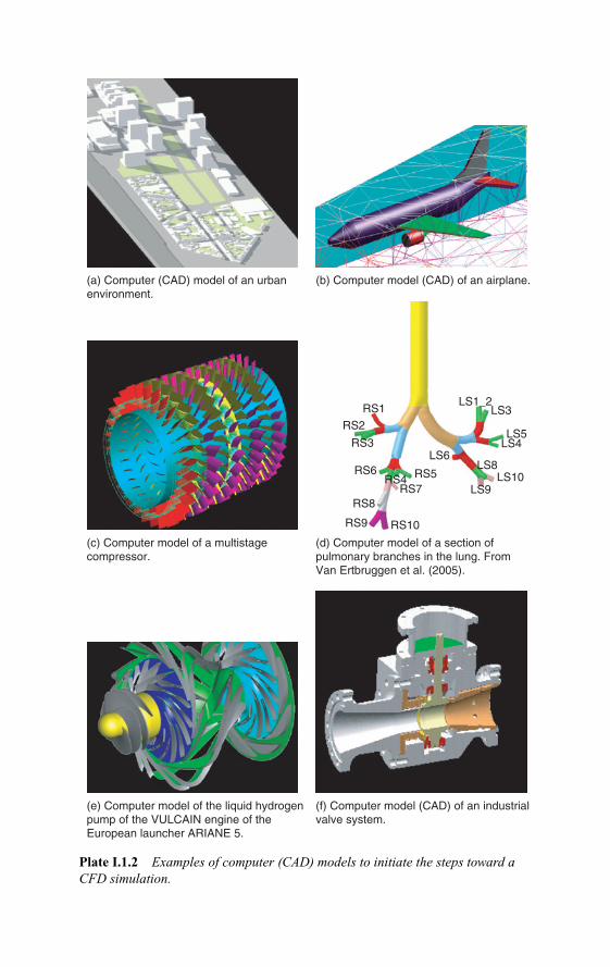
Plates-H6594.tex 30/4/2007 17: 3 Page 1

(a) Computer (CAD) model of an urbanenvironment.

(c) Computer model of a multistagecompressor.

(e) Computer model of the liquid hydrogenpump of the VULCAIN engine of theEuropean launcher ARIANE 5.

(b) Computer model (CAD) of an airplane.

(f) Computer model (CAD) of an industrialvalve system.

(d) Computer model of a section ofpulmonary branches in the lung. FromVan Ertbruggen et al. (2005).

RS1

RS2

RS3

RS6LS6

RS4 RS5RS7

RS10

LS10

LS4LS5

LS3

LS9

LS8

LS1_2

RS8

RS9

Plate I.1.2 Examples of computer (CAD) models to initiate the steps toward aCFD simulation.

Plates-H6594.tex 30/4/2007 17: 3 Page 2

Plate I.1.3 Simulation of the interaction between the cooling flow and the mainexternal gas flow around a cooled turbine blade. Courtesy NUMECA Int. and KHI.

1970 1975 1980 1985 1990 1995 2000

2 points

Effi

cien

cy (

at c

ruis

e)

Potential

Euler3D

Navier–Stokes2.5D

Navier–Stokes3D

Design year

Plate I.1.4 Impact of CFD on SNECMA fan performance, over a period of 30years. From Escuret et al. (1998).

Plates-H6594.tex 30/4/2007 17: 3 Page 3

Chronology and impact

38

1811

77

Num

ber

ofw

ings

test

ed

1980 1985 1990 1995 2000 2005

767 737-300 777 737NG757 787

NASATech

BoeingTools

PANAIR

A502 A488

FLO22A411

TRANAIR

CartesianGrid Tech.

TRANAIROptimization

HSR &IWD

TLNS3D-MB/ZEUS

TLNS3D-MBoverflowTLNS3D

BoeingProducts

1980 state of the art Modern close couplednacelle installation,0.02 Mach faster than737-200

21% thicker fasterwing than 757,767 technology

Highly constrainedwing designFaster wing than737-300

Successfulmultipointoptimizationdesign

CFD forloads and

stability, andcontrol

11

UnstructuredAdaptive Grid

3-D N-S

Faster andmore efficientthan previousaircraft

CFL3D/ZEUSoverflowCFD��

CFL3Doverflow

Plate I.1.6a Evolution of the CFD tools over the last 40 years at Boeing, with anindication of the influence of CFD on the reduction of the number of wing tests.Courtesy Enabling Technology and Research Organization, Boeing CommercialAirplanes.

Eulerequations

A310

Potentialequation

1975


Viscousflow

Turbulentflow


Simplevortex models

Subsonicflow

Flowproperties

Problem sizein service

Model

Inviscidflow


Vortexflow


Wake vortex

Separation

Navier–Stokesequations

A321

A319A330/340

1965 1975 19951985

A340–500/600MEGAFLOW

102

104

106

108

2000

A318A320

A310A300

Configuration

Refinement of models Complexconfigurations

2002

A380

Plate I.1.6b Evolution of the CFD tools over the last 40 years at Airbus, with anindication of the evolution of the applied models. From Becker (2003).

Plates-H6594.tex 30/4/2007 17: 3 Page 4

Unstructured tetrahedral grid for an engine.From ICEM-CFD.

Unstructured hexahedral grid for an oil valve.HEXPRESS mesh. Courtesy NUMECA Int.

From D´Alascio et al. (2004).A middle plane section of an helicopter fuselage with structured and unstructured grids.

Figure 3: ICEM-Hexa structuredmultiblock N.-S.mesh around the EC145

isolated fuselage: middle plane.

Figure 4: CENTAUR hybrid N.-S.mesharound the EC145 isolated fuselage:

middle plane.

Plate I.2.3 Examples of unstructured grids.

Plates-H6594.tex 30/4/2007 17: 3 Page 5

(a) Cartesian plot of pressure distribution atvarious positions along a wing–body–nacellemodel, compared to experimental data.From Tinoco and Su (2004),Reproduced by permission from AIAA.

(b) Instantaneous iso-surfaces of vorticitycolored by the span-wise component ofvorticity of a 70� delta wing.From: Morton (2004)

(c) Perturbation pressure distribution for anaero-acoustic simulation of the noisegenerated by a landing gear.From Lockard et al. (2004).Reproduced by permission from AIAA.

(d) Color plot and velocity vectors in onecross-section of the lung bifurcations shown inFigures I.1.2 and I.2.2. From VanErtbruggen et al. (2005).

Time history

3.0E�031.5E�030.0E�00

�1.5E�03�3.0E�03

M�0.2

p'/(P�C2�)

(b) Perturbation pressure on solid surfaces

Magnitude V(m/s)4.5

4

3.5

3

2.5

2

1.5

1

0.5

0

�1.6

�0.8

0.0

Cp

Cp

0.0 0.2 0.4 0.6 0.8 1.0

�1.6

�0.8

0.8

0.8

0.00.0 0.2 0.4 0.6 0.8 1.00.0 0.2 0.4 0.6 0.8 1.0

0.0 0.2 0.4X/CX/C

X/CX/C

0.6 0.8 1.0

Plate I.2.4 Examples of visual results from CFD simulations.

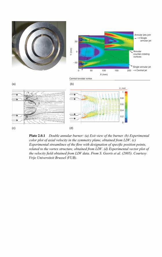
Plates-H6594.tex 30/4/2007 17: 3 Page 6

50

0

0 50 100

X (mm)

Central toroidal vortex

150 200

Annular jets join

Annularcounter-rotatingvortices

Y (

mm

)

�50

e d c

b

a

U_mod

1

0.8

0.6

0.4

0.2

0

(a) (b)

(c) (d)

Single annular jet

Central jet

Single annular jet

Plate 2.0.1 Double annular burner: (a) Exit view of the burner. (b) Experimentalcolor plot of axial velocity in the symmetry plane, obtained from LDV. (c)Experimental streamlines of the flow with designation of specific position points,related to the vortex structure, obtained from LDV. (d) Experimental vector plot ofthe velocity field obtained from LDV data. From S. Geerts et al. (2005). CourtesyVrije Universiteit Brussel (VUB).

Plates-H6594.tex 30/4/2007 17: 3 Page 7

Marangoniflow

Perturbation unsteadytemperature filed

Perturbation unsteady flow filed

(a)

Pul

satin

g w

ave

Ma�8773

Pr�8.9; A�1

m�2 mode

Red color:hot region

Blue color:cold region

(b)

Tra

velli

ng w

ave

Ma�35,092;Pr�8.9;A�1Symmetrybreakingwith perioddoubling ofmode m�2Red color:hot regionBlue color:cold region

(c)

Tra

velli

ng w

ave

Ma�28,255;Pr�7;A�0.73Symmetrybreakingwith quasi-periodicpattern ofmode m�3Red color:hot regionBlue color:cold region

(d)

Tra

velli

ng w

ave

Plate 2.1.2 Liquid bridge and Marangoni effect. Representation of variousunsteady and symmetry broken solutions for velocity and temperature Perturbationfields. Each group of four figures represents four snapshots of the correspondingunsteady peturbation field. From Dinescu and Hirsch (2001), Hirsch and Dinescu(2003).

Plates-H6594.tex 30/4/2007 17: 3 Page 8

(a) (b)D

Plate 2.1.7 Spanwise undulation of the main vortex rows and streamwise vortices,at Re = 220; shown by iso-contours of vorticity components. (b) Spanwiseexperimental flow visualization, provided by Williamson (1992). The frame showscorrespondence to the computational region explored. From Persillon and Braza(1998). Courtesy M. Braza. IMFT, Toulouse.

D D(a) (b)

S

(c)

Plate 2.1.8 Modification of the spanwise vortex structures as Reynolds numberincreases; passage to mode B; (a) Re = 270; (b) Re = 300. (c) Spanwiseexperimental flow visualization, provided by Williamson (1992, 1996a, b). Theframe shows correspondence to the computational region explored. From Persillonand Braza (1998). Courtesy M. Braza. IMFT, Toulouse.

Plates-H6594.tex 30/4/2007 17: 3 Page 9

(a) (b)

(c) (d)

z�12D

z�0

(e) (f)

Plate 2.1.9 Spanwise and streamwise iso-vorticity contours showing mode Aformation and the transition to the vortex dislocations pattern at Re = 220. FromBraza et al. (2001). Courtesy M. Braza. IMFT, Toulouse.

Plates-H6594.tex 30/4/2007 17: 3 Page 10

Plate 2.1.10 Instantaneous view of the turbulent vortices colored with theirdistance to the wall (red is closest to the wall and yellow is at the center of thechannel. Only 1/4 of the channel is shown (full length, half-width and half-height),and the flow direction is from bottom-left to top-right. From del Alamo et al. (2004).Courtesy J. Jimenez and coworkers.

0.8

0.6

0.4

0.2

00

0.5

1

1.5 0

0.5

1

1.5

2

2.5

3

Plate 2.1.11 Instaneous realization of a complex clustering of vortices in aturbulent channel flow at a Reynolds number of 100,000 (Retau = 2000). The flow isfrom left to right and the vortices are colored with their distance to the wall (blue isnear the wall while red is far from the wall). From Hoyas and Jimenez (2006).Courtesy J. Jimenez and coworkers.

Plates-H6594.tex 30/4/2007 17: 3 Page 11

Time : 6,000

Tu�0% at inlet

Tu�7% at inlet

x/L�0.6x/L�0.7

x/L�0.6x/L�0.7

Vort.x

�150 �75 0 70 150

Plate 2.1.12 Snapshots of a DNS simulation at a Reynolds number of 60,000,showing the effects of an external turbulence on the transition, comparing thevorticity field of a laminar incoming separation bubble with no turbulence and with7% turbulence intensity. Courtesy J. Wissink and W. Rodi, University of Karlsruhe.

Plates-H6594.tex 30/4/2007 17: 3 Page 12

Computedin RANS Modeled in RANS

Computed in LESModeled in

LES

10�2 10�1 10010�3

10�2

10�1

100

101

102

E

Largescales

Energycontaining

integralscales

Inertialsubrange

Viscoussubrange

k

k�5/3k�5/3

1/��1/�� 1/�1/� 1/�1/�

Computed in DNS

Plate 2.2.1 Energy spectrum of turbulence in function of wave number k, withindication of the range of application of the DNS, LES and RANS models. Thelength scales lT and lI are associated with the LES and RANS approximations,respectively. Courtesy C. Fureby (FOI, Sweden).

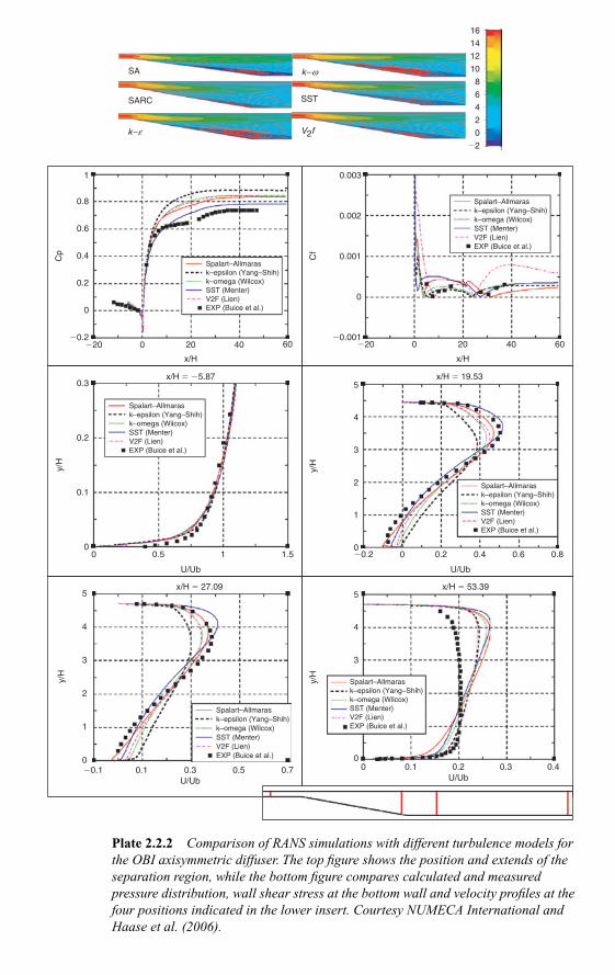
Plates-H6594.tex 30/4/2007 17: 3 Page 13

x/H

1

0.8

0.6

0.4Cp

0.2

0

�0.2�20 0 20 40


60

x/H � 19.535

4

3

2

y/H

1

0


�0.2 0 0.2

U/Ub

0.4 0.80.6

0.003

0.002

0.001

0

�0.001

Cf


�20 0 20

x/H

40 60

x/H � 27.095

4

3

2

y/H

1

0


�0.1 0.1 0.3U/Ub

0.5 0.7

0.3x/H � �5.87

0.2

0.1

00 0.5 1 1.5

U/Ub

y/H


U/Ub


x/H � 53.395

4

3

y/H

00 0.1 0.2 0.3 0.4

SA

SARC

k–e

k–w

SST

V2f

16

14

12

10

8

6

4

2

0

�2

Plate 2.2.2 Comparison of RANS simulations with different turbulence models forthe OBI axisymmetric diffuser. The top figure shows the position and extends of theseparation region, while the bottom figure compares calculated and measuredpressure distribution, wall shear stress at the bottom wall and velocity profiles at thefour positions indicated in the lower insert. Courtesy NUMECA International andHaase et al. (2006).

Plates-H6594.tex 30/4/2007 17: 3 Page 14

(a) (b)

(c)

Plate 11.5.4 Distribution of entropy as computed on three different meshes:(a) fine mesh, (b) intermediate mesh and (c) coarse mesh.

Fine mesh Magnitude of V (m/s)70

60

50

40

30

20

10Y

X0

Plate 11.5.5 Distribution of velocity magnitude and iso-velocity lines, ascomputed on the finest mesh.

Plates-H6594.tex 30/4/2007 17: 3 Page 15

Mach number

0.13

0.12

0.11

0.1

0.09

0.08

0.07

Y

X

Y

X

Plate 11.5.8 Isolines of Mach number as computed using the (65 × 33) meshsuperimposed on the color map of a reference solution on a (225 × 113) mesh. Oneisoline has been drawn every 0.001 ranging from 0.07 to 0.13. The bottom figurecompares the Mach number isolines of the two solutions, where the darkest line isthe reference solution.

M�0.01Mach number

0.012

0.011

0.01

0.009

0.008

M�0.1Mach number

0.12

0.11

0.1

0.09

0.08

M�0.05Mach number

0.012

0.011

0.01

0.009

0.008

M�0.7Mach number

1.4

1.2

1

0.8

0.6

X

Y

X

Y

X

Y

X

Y

Plate 11.5.10 Distribution of velocity as computed on the (65 × 33) mesh, fordifferent values of the incident Mach number, from 0.01 to 0.7. Observe the shockappearing at M = 0.7.

Plates-H6594.tex 30/4/2007 17: 3 Page 16

1.7

1.8

1.9

2

2.1

2.2

2.3

2.4

2.5

2.6Mach number

x

y

Plate 11.5.14 Distribution of computed Mach number.

76,000

77,000

78,000

79,000

80,000

81,000

Entropy

x

y

Plate 11.5.15 Distribution of computed entropy.

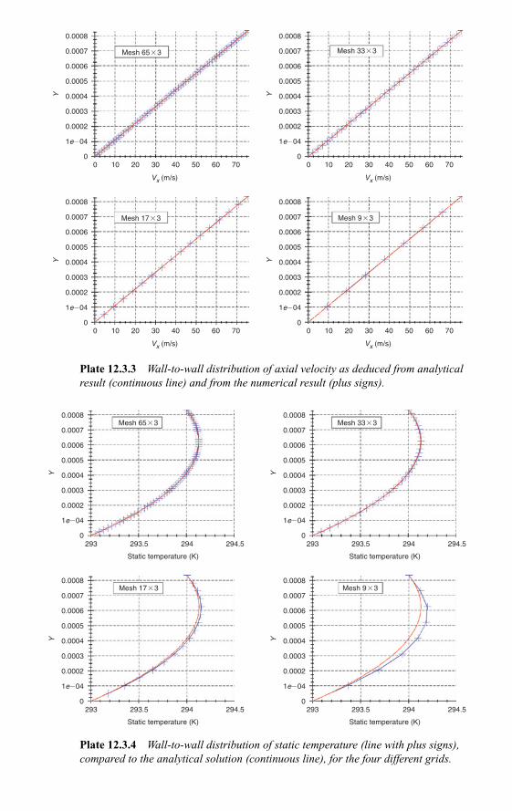
Plates-H6594.tex 30/4/2007 17: 3 Page 17

0.0008

0.0007

0.0006

0.0005

0.0004

0.0003

Y

Vx (m/s)

0.0002

00 10 20 30 40 50 60 70

Mesh 65 � 3

1e�04

0.0008

0.0007

0.0006

0.0005

0.0004

0.0003

Y

Vx (m/s)

0.0002

00 10 20 30 40 50 60 70

Mesh 33 � 3

1e�04

0.0008

0.0007

0.0006

0.0005

0.0004

0.0003

Y

Vx (m/s)

0.0002

00 10 20 30 40 50 60 70

Mesh 17 � 3

1e�04

0.0008

0.0007

0.0006

0.0005

0.0004

0.0003

Y

Vx (m/s)

0.0002

00 10 20 30 40 50 60 70

Mesh 9 � 3

1e�04

Plate 12.3.3 Wall-to-wall distribution of axial velocity as deduced from analyticalresult (continuous line) and from the numerical result (plus signs).


293 293.5 294 294.5

0.0008

0.0007

0.0006

0.0005

0.0004

0.0003

Y

0.0002

0

Mesh 33 � 3

1e�04


293 293.5 294 294.5

0.0008

0.0007

0.0006

0.0005

0.0004

0.0003

Y

0.0002

0

Mesh 17 � 3

1e�04


293 293.5 294 294.5

0.0008

0.0007

0.0006

0.0005

0.0004

0.0003

Y

0.0002

0

Mesh 9 � 3

1e�04

0.0008

0.0007

0.0006

0.0005

0.0004

0.0003

Y


0.0002

0293 293.5 294 294.5

1e�04

Mesh 65 � 3

Plate 12.3.4 Wall-to-wall distribution of static temperature (line with plus signs),compared to the analytical solution (continuous line), for the four different grids.

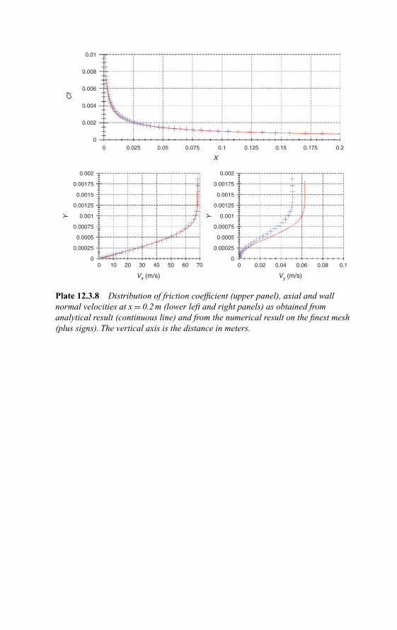
Plates-H6594.tex 30/4/2007 17: 3 Page 18

0.01

0.008

0.006

0.004

0.002

00 0.025 0.05 0.075 0.1 0.150.125 0.175 0.2

X

Cf

0 0.02 0.04 0.06 0.08 0.1

0.002

0.00175

0.0015

0.00125

0.001

0.00075

0.0005

0.00025

0

Y

Vy (m/s)

0.002

0.00175

0.0015

0.00125

0.001

0.00075

0.0005

0.00025

00 10 20 30 40 50 60 70

Y

Vx (m/s)

Plate 12.3.8 Distribution of friction coefficient (upper panel), axial and wallnormal velocities at x = 0.2 m (lower left and right panels) as obtained fromanalytical result (continuous line) and from the numerical result on the finest mesh(plus signs). The vertical axis is the distance in meters.

Plates-H6594.tex 30/4/2007 17: 3 Page 19

0.2 0.3 0.4 0.5 0.6 0.7 0.8 0.90.1

0.9

0.8

0.7

0.6

y 0.5

0.4

0.3

0.2

0.1

x0.2 0.3 0.4 0.5 0.6 0.7 0.8 0.90.1

0.9

0.8

0.7

0.6

y 0.5

0.4

0.3

0.2

0.1

x

0.2 0.3 0.4 0.5 0.6 0.7 0.8 0.90.1

0.9

0.8

0.7

0.6

y 0.5

0.4

0.3

0.2

0.1

x0.2 0.3 0.4 0.5 0.6 0.7 0.8 0.90.1

0.9

0.8

0.7

0.6

y 0.5

0.4

0.3

0.2

0.1

x

(a) Transient solution at t � 0.5 (b) Transient solution at t �1

(c) Solution at t �10 (d) Solution at t � 30

Plate 12.5.2 Streamlines of the flow field at different transient stages, for t = 0.5,1, 10 and 30.

Numerical Computation of Internal and External Flows

Documents

Transcript of Numerical Computation of Internal and External Flows