lable at ScienceDirect

Atmospheric Environment 94 (2014) 11e21

Contents lists avai

Atmospheric Environment

journal homepage: www.elsevier .com/locate/atmosenv

Multivariate methods for indoor PM10 and PM2.5 modelling innaturally ventilated schools buildings

Maher Elbayoumi a, Nor Azam Ramli a, Noor Faizah Fitri Md Yusof a,*,Ahmad Shukri Bin Yahaya a, Wesam Al Madhoun b, Ahmed Zia Ul-Saufie c

aClean Air Research Group, School of Civil Engineering, Universiti Sains Malaysia, Penang, Malaysiab Environment and Earth Science Department, The Islamic University at Gaza, Palestinec Faculty of Computer and Mathematical Sciences, Universiti Teknologi Mara, Malaysia

h i g h l i g h t s

� Indoor particle matter was predicted by using multiple linear regression models.� Outdoor PM2.5, outdoor PM10 and temperature were significant predictors.� PM10 model tend to underestimate the prediction of indoor PM10 concentrations.� To compare between the models performance indicators were used.

a r t i c l e i n f o

Article history:Received 18 February 2014Received in revised form30 April 2014Accepted 2 May 2014Available online 5 May 2014

Keywords:Regression modelsPCAPM10

PM2.5

Air pollution

* Corresponding author.E-mail addresses: noorfaizah@usm.my, elbayoumi

Yusof).

http://dx.doi.org/10.1016/j.atmosenv.2014.05.0071352-2310/� 2014 Elsevier Ltd. All rights reserved.

a b s t r a c t

In this study the concentrations of PM10, PM2.5, CO and CO2 concentrations and meteorological variables(wind speed, air temperature, and relative humidity) were employed to predict the annual and seasonalindoor concentration of PM10 and PM2.5 using multivariate statistical methods. The data have beencollected in twelve naturally ventilated schools in Gaza Strip (Palestine) from October 2011 to May 2012(academic year). The bivariate correlation analysis showed that the indoor PM10 and PM2.5 were highlypositive correlated with outdoor concentration of PM10 and PM2.5. Further, Multiple linear regression(MLR) was used for modelling and R2 values for indoor PM10 were determined as 0.62 and 0.84 for PM10

and PM2.5 respectively. The Performance indicators of MLR models indicated that the prediction for PM10

and PM2.5 annual models were better than seasonal models. In order to reduce the number of inputvariables, principal component analysis (PCA) and principal component regression (PCR) were applied byusing annual data. The predicted R2 were 0.40 and 0.73 for PM10 and PM2.5, respectively. PM10 models(MLR and PCR) show the tendency to underestimate indoor PM10 concentrations as it does not take intoaccount the occupant’s activities which highly affect the indoor concentrations during the class hours.

� 2014 Elsevier Ltd. All rights reserved.

1. Introduction

Indoor environmental quality in schools is a very importantelement in providing a healthy and comfortable learning environ-ment for students (Daisey et al., 2003; Kwok and Chun, 2003). Thequality of air inside the classrooms is one of primary concern aschildren spend approximately seven or more hours a day in schoolof their time indoors (Almeida et al., 2011; Pegas et al., 2010).

maher@gmail.com (N.F.F. Md

Particulate matter (PM10 and PM2.5) is considered one of themain pollutants that can exist inside schools buildings in way thatcan affect the student’s health. Several studies in natural ventilatedbuilding around the world indicated that the concentration of PM10

and PM2.5 was exceeding the limits recommended byWorld HealthOrganization (WHO) (Chithra and Nagendra, 2012; Diapouli et al.,2007; Habil and Taneja, 2011; Lee and Chang, 1999; Massey et al.,2012).

Several population based studies have established a strongcorrelation between exposures to fine particulate matter (PM) andincreasing rates of mortality, morbidity, respiratory and cardio-vascular problems especially among children (Pope et al., 2006;Pope III et al., 2009; WHO, 2005). As reported by World HealthOrganization (WHO), a short-term increase of 10 mg/m3 of PM for

M. Elbayoumi et al. / Atmospheric Environment 94 (2014) 11e2112

several days is associated with more coughing, lower respiratorysymptoms, and hospital admissions increments due to respiratoryproblems (WHO, 2000).

The Middle East region is considered one of the most contro-versial regions for aerosol particle concentrations (Zereini andWiseman, 2010). The location of Middle East area at the intersec-tion of air masses circulating among the three continentsmakes theaerosol concentrations governed by several important phenom-ena’s such as long range aerosol transportation (Matvev et al.,2002), seasonal dust storms (Dayan et al., 1991; Koçak et al.,2010; Zereini and Wiseman, 2010), sea salt aerosol formation(Krom et al., 2004), the elevation of road dust due to the low rainfallrates (Zereini and Wiseman, 2010) and several anthropogenic re-sources such as car exhausts, industry, agricultural operations,combustion of wood and fossil fuels, construction and demolitionactivities.

The difficulties involved in continuous measurement of indoorconcentration level of PM10 and PM2.5 have led to the developmentof modelling techniques enabling the researchers to predict the in-door concentration with acceptable accuracy (Chaloulakou andMavroidis, 2002). Indoor air quality (IAQ) models predict indoor airpollutant concentration as a function of several input parameterssuch as outdoor air pollutant, air exchange rate and meteorologicalparameters. In air qualitymodelling studies one of themost commonmodels available to predict outdoor and indoor air pollutant con-centrations are the statistical regression methods (Özbay, 2012).These entirely empirical techniques are quick and easy to be appliedcomparing with other types of modelling since they do not requirecomplicated input parameters (Milner et al., 2004).

Multiple linear regression (MLR) is one of the most widely usedmethodologies for expressing the dependence of a response vari-able on several independent (predictor) variables. Several studiesused MLR to correlate the outdoor PM10, PM2.5, ozone and meteo-rological variables with indoor concentration of such pollutant (El-Shobokshy and Hussein, 1988; Fromme et al., 2007; Gold et al.,1996; Goyal and Khare, 2010; Ozkaynak et al., 1996). Although ofthe wide and success applications, MLR approach can face seriousdifficulties particularly when the environmental variables arecorrelated with each other which are called multicollinearity Themost common methods for removing such multicollinearity areprincipal component analysis (PCA) and partial least square (PLS)(Poupard et al., 2005; Ul-Saufie et al., 2010; Yeniay and Goktas,2002).

A preliminary study by Elbayoumi et al. (2013), which was un-dertaken in the samemonitoring schools, revealed that high indoorand outdoor levels of PM10 and PM2.5. These compounds could beintroduced to the indoor environment either by infiltration ofoutdoor air, indoor source, or both. Therefore, the objectives of thisstudy are as follows: (Abdul-Wahab et al., 2005) to developregression models (MLR) using annual (academic year) and sea-sonal periods because PM10 and PM2.5 exhibit seasonal variationsby incorporating building ventilation rate, meteorological param-eters, and outdoor levels; (Agirre-Basurko et al., 2006) to developprincipal component regression (PCR) models for indoor PM10 andPM2.5 using building ventilation rate, meteorological parameters,and outdoor levels as predictor variables; (Al-Alawi et al., 2008) andto compare the two developed models using performance in-dicators to measure the accuracy of the models.

2. Method

2.1. Description of study area

Gaza strip (365 km2, 40 km long and between 6 and 12 kmwide)is located on the eastern coast of the Mediterranean Sea. The area

forms a transitional zone between the sub-humid coastal zone ofIsrael in the north, the semiarid plains of the northern Negev Desertin the east and the arid SinaiDesert of Egypt in the south (PMD, 2012).

The climate in Gaza strip is characterized by mild and humidwinter (DecembereMarch) which dominated by rainfall. Thesummer months (JuneeSeptember) are characterized by high hu-midity and the lack of wet precipitation. The spring season(MarcheJune) is characterized by unsettled winter type weatherfor the first month, associated with North African cyclones; the restof this period is very similar to that in the summer. Fall season(SeptembereDecember) usually characterized by an abrupt sum-mer type weather in the first month; the rest of this period ischaracterized by the unsettled weather of winter (Koçak et al.,2010; PMD, 2012).

2.2. Sampling locations

The selected schools are located in different geographical loca-tion in Gaza strip (urban, suburban and camps) in order to obtain arealistic diagnosis of the spatial distribution of PM10 and PM2.5 inarea as seen in Fig. 1 and Table 1. A total of 12 schools buildingswhich are naturally ventilated through openable windows anddoors were monitored. The buildings have three storeys and areused in double sessions (morning and afternoon shifts). The num-ber of students per class is ranged from 30 to 45. In each selectedschool, three representative classrooms on the windward side ofthe building were selected for three sampling days.

2.3. Sampling method

The sampling campaign took place between October 2011 toMay 2012 at the 12 monitoring schools to cover fall, winter, andspring seasons. From Saturday to Thursday, during the schoolshours from 7:00 in the morning to 12:00 noon in the winter andspring seasons, and from 12:00 noon to 5:00 in the afternoon in thefall season sampling was performed in 3 classrooms per school.Sampling was performed inside and outside the 3 selected class-rooms per school. Following the WHO guideline and teachers’request in order to allow the freemovement within the classrooms,the sampling equipment’s were placed in the opposite of theblackboard (back of the classroom) to avoids direct contaminationof the filters with chalk dust. The sampling instruments werepositioned at a distance of around 1 m from the bottomwall and ata height of about 1.5 m above floor (Blondeau et al., 2005; WHO,2011). For outdoor sampling, the samplers were placed at thefront side of the building. Due to the lack of multiple samplers,indoor and outdoor measurements were taken alternately aftereach 15 min within class hour (45 min) (Habil and Taneja, 2011).Massey et al. (2009) reported that a variation between 4% and 12%was observed in the mass concentration of PM between alternatelyand continuously sampled in indoor and outdoor measurement forone successive week. Therefore, the individual 540 (270 indoor and270 outdoor) measurements at each school were obtained everyseason in order to cover meteorological conditions and pollutantconcentrations. The surface wind speed, ambient temperature,carbonmonoxide, carbon dioxide and relative humidity in each sitewere simultaneously measured at the same time with particulatematter measurement.

The mass concentration of particles (PM10 and PM2.5) has beenmonitored using handheld optical particle counter (HAL-HPC300).Themonitor performs particulate sizemeasurements by using laserlight scattering. Air with multiple particle sizes passes through aflat laser beam produced by an ultra-low maintenance laser diode.A 3-channel pulse height analyser for size classification detects thescattering signals. The particle counter was factory calibrated, prior

Fig. 1. Map of Gaza strip and the monitoring schools.

M. Elbayoumi et al. / Atmospheric Environment 94 (2014) 11e21 13

to the sampling campaign and the calibration was repeated everyweek using Zero-Count filter (Hal, 2012). A Kanomax IAQ Monitorwas used for temperature, relative humidity, CO and CO2 mea-surements. The IAQ monitor was calibrated in Islamic University e

Gaza laboratory for CO2 and CO in accordance with manufacturerinstructions. Meanwhile, Smart Sensor Electronic anemometer wasused for wind speed. The ventilation rate was calculated using theindoor concentration of carbon dioxide as a surrogate of theventilation levels per occupant (Kulshreshtha and Khare, 2011;WHO, 2011).

For a qualitative control of the measurements, a 5 min intervalfor the device stability was maintained after each 15 min mea-surement period. In addition, a protocol of information had to befilled out every day. The protocol included the time in which eachmeasurement was taken, current weather conditions such as rain,wind, fog and dusty storm and other relevant observations.

2.4. Statistical analysis

All data were normalized before application of MLR procedure.Normalized data were calculated according to following Equation(Abdul-Wahab et al., 2005).

NIi;j ¼Iði; jÞ �minðjÞmaxðjÞ �minðjÞ (1)

where, I is the input value, NI is the normalized value, i is thenumber of measurements, j is the measured value of the variable,

min and max are the global minimum and maximum of the entiredataset (Özbay et al., 2011).

The analysis of the data was carried out using the statisticalsoftware, SPSS (Statistical Package for Social Science, version 20)andMATLAB, version10. The data had been classified randomly intotwo sets using MATLAB software. Set 1 which consists of 70% of theoriginal data, were used for model formulation and dataset 2 (30%)were used for model validation.

2.4.1. Bivariate correlation analysisBivariate correlation analysis is used to assess the measure of

pair wise association among the various variables. Pearson’s coef-ficient (r) is used for measuring linear association, the strength anddirection of the relationship between two variables. Pearson’s r canbe expressed with the following equation (Özbay, 2012):

r ¼P�

X � X��Y � Y

�ffiffiffiffiffiffiffiffiffiffiffiffiffiffiffiffiffiffiffiffiffiffiffiffiffiffiffiffiffiffiffiffiffiffiffiffiffiffiffiffiffiffiffiffiffiffiffiffiffiffiP �

X � X�2 P�

Y � Y�2q (2)

where X and Y represent variables and X and Y are the means of thevariables.

2.4.2. Multiple linear regressionsStepwise multiple regressions were carried for PM10 and PM2.5

and the results were checked formulticollinearity by examining thevariance inflation factors (VIF) of the predictor variables. DurbinWatson statistic used to check if the model does not have any first

Table 1Characteristics of monitoring schools.

School name Code Number of students Distance from main road (m) Classroom cleaning activity Location area

Nusirate Prep Boys A MCB 733 43 Daily in the morning Over populated campNusirate Prep Boys D MOB 712 65 Daily in the morning Over populated campElburaj Prep Girls B MCG 903 50 Daily in the morning and between school hours Over populated campDier Elbalah Prep Girls MOG 1024 50 Daily in the morning and between school hours Small townBany Suhiela Prep Boys SOG 1132 40 Daily in the morning Urban areaBany Suhiela Prep Girls B SOB 1448 55 Daily in the morning Urban areaAhmad Abed Elaziz Prep Boys B SCB 729 50 Daily in the morning Urban areaRafah Prep Girls B SCG 578 55 Daily in the morning and between school hours Over populated campElzaytoon Prep Girls B NOG 883 58 Daily in the morning and between school hours Urban areaNew Gaza Prep Boys A NCB 1066 30 Daily in the morning and between school hours Urban areaBeach Prep Girls B NCG 1183 50 Daily in the morning and between school hours Over populated campSalah Eldien Prep Boys NOB 623 43 Daily in the morning and between school hours Urban area

M. Elbayoumi et al. / Atmospheric Environment 94 (2014) 11e2114

order autocorrelation problem. MLR can be expressed according tothe following Equation (Al-Alawi et al., 2008):

y ¼ b0 þ b1x1i þ b2x2i þ.þ bkxki þ ε (3)

where, bk is the regression coefficients, xk is the explanatory vari-ables, i ¼ 1,2, . .k and ε is stochastic error associated with theregression (Agirre-Basurko et al., 2006). The residuals (or error)were checked to evaluate if they were normally distributed withzero mean and constant variance to verify the adequacy of thestatistical model (Al-Alawi et al., 2008).

2.4.3. Principal components analysisThe principal components of the predictor variables were ob-

tained using a data reduction technique which achieved by findinglinear combinations of the original variables. The linear combina-tions account for as much of the original total variance as possible.The successive linear combinations are extracted in such away thatthey are uncorrelated with each other and account for successivesmaller amounts of the total variance. PCs are expressed by thefollowing Equation (Almeida et al., 2011):

PCi ¼ a1iv1 þ a2iv2 þ.þ anivn (4)

Where PCi is principal component i and ani is the loading (corre-lation coefficient) of the original variable V1 (Özbay et al., 2011). Thescores of high loadings components with an eigenvalue greaterthan or equal to 1 and explain most of the variation in all dataset isideal to use as in regression equations as independent or predictorvariables; thus, PCR establishes the relationship between the

Table 2Seasonal difference of different pollutants and meteorological variables.

Parameters Fall Win

Minemax Mean (�S. Dev) Min

PM10 indoor (mg/m3) 134.6e845.2 360.1 (�133.7) 176PM10 outdoor (mg/m3) 16.3e330.4 98.1 (�42.5) 83PM2.5 indoor (mg/m3) 19.9e161.5 55.2 (�24.1) 71PM2.5 outdoor (mg/m3) 8.4e90.3 26.5 (�11.3) 23COindoor (ppm) 0.1e1.6 0.4 (�0.3) 0COoutdoor (ppm) 0.1e3.5 0.5 (�0.4) 0Tempindoor (�C) 11.8e30.6 25.1 (�4.3) 10Tempoutdoor (�C) 10.6e31.6 25.4 (�4.8) 8Ventilation rate (L/s. person) 4.7e29.1 9.8 (�5.1) 1CO2 indoor (ppm) 457.6e1881.9 787.1 (�225.1) 486CO2 outdoor (ppm) 308.6e705.5 401.8 (�85.3) 325RHindoor (%) 41.9e96.3 61.9 (�8.6) 37RHoutdoor (%) 29.5e95.0 59.5 (�7.8) 28WS (m/s) 0.1e7.0 3.5 (�1.5) 0

dependent or response variable and the selected PCs of the inde-pendent variables (Gvozdi�c et al., 2011).

2.4.4. Performance indicatorsThe analysis of prediction performance typically involves

calculation of errors between observed y and predicted y values. Inthis study five performance indicators were used which arenormalized absolute error (NAE), root mean square error (RMSE),predication accuracy (PA), coefficient of determination (R2) andindex of agreement (IA). For a good model NAE and RMSE valueshould approach zero, while PA, R2 and IA should be closer to one.

2.4.4.1. The normalized absolute error (NAE). Normalized absoluteerror is the average of the difference between predicted andobserved values in all cases divided by sum of observed values(Gervasi, 2008). NAE is expressed by the following Equation:

NAE ¼PN

i¼1jPi � OijPNi¼1Oi

(5)

Where N is the number of sample, Oi is the indoor PM10 or PM2.5concentrations values and Pi is the predicted PM10 or PM2.5.

2.4.4.2. The root mean square error (RMSE). The root mean squareerror is used to measure the success of numerical prediction. RMSEis shown by Equation (Alshitawi et al., 2009) (Karppinen et al.,2000) .

ter Spring

emax Mean (�S. Dev) Minemax Mean (�S. Dev)

.9e1545.0 492.5 (�209.4) 69.1e812.5 195.80 (�100.52)

.2e839.4 248.2 (�103.3) 17.3e354.0 102.26 (�43.98)

.6e569.6 197.9 (�84.8) 21.1e171.5 58.82 (�25.05)

.2e464.8 57.4 (�134.7) 6.3e69.9 20.12 (�8.72)

.1e6.1 1.2 (�0.9) 0.1e2.7 0.79 (�0.48)

.1e5.0 1.4 (�1.0) 9.0e0.1 1.0 (�0.8)

.9e28.8 16.1 (�4.0) 11.1e33.1 19.2 (�3.2)

.3e29.7 15.5 (�4.5) 9.0e33.80 18.2 (�3.70)

.5e17.7 6.6 (�3.2) 3.1e19.1 8.1 (�2.9)

.3e2370.9 1155.8 (�321.7) 666.7e1537.7 956.8 (�167.2)

.6e717.6 568.0 (�92.4) 367.0e583.0 487.3 (�39.8)

.3e100.0 65.6 (�11.7) 18.5e100.0 79.3 (�16.8)

.4e94.0 63.7 (�13.7) 15.0e100.0 73.10 (�18.10)

.1e13.0 3.2 (�2.5) 0.1e9.0 2.6 (�2.0)

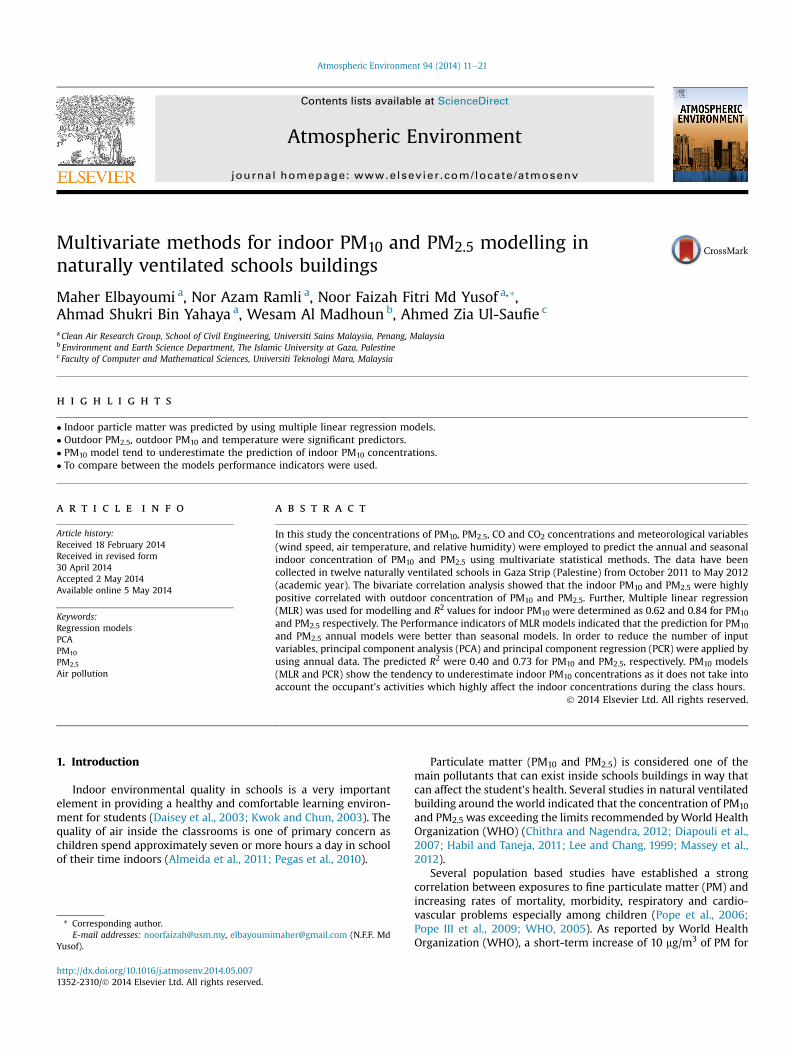
Table 3Pearson correlation matrix of different variables. Correlation is significant at the 0.01 level (2-tailed).a

PM2.5

(In)PM2.5

(Out)PM10

(In)PM10

(Out)RH(In)

RH(Out)

Temp(In)

Temp(Out)

Building ventilation rate Wind speed CO(In)

CO(Out)

CO2

(In)CO2

(Out)

PM2.5 (in) (mg/m3) 1.00 0.92 0.65 0.76 �0.09 0.01 �0.61 �0.57 �0.16 0.11 0.31 0.25 0.40 0.60PM2.5 (out) (mg/m3) 1.00 0.63 0.79 �0.13 �0.05 �0.60 �0.57 �0.19 0.10 0.31 0.25 0.46 0.65PM10 (in) (mg/m3) 1.00 0.75 �0.19 �0.03 �0.21 �0.19 �0.14 0.09 0.15 0.10 0.24 0.23PM10 (out) (mg/m3) 1.000 �0.09 0.03 �0.53 �0.51 �0.26 0.08 0.34 0.29 0.50 0.57RH (in) (ppm) 1.00 0.87 �0.29 �0.30 �0.09 �0.06 �0.06 �0.03 0.05 0.06RH (out) (ppm) 1.00 �0.28 �0.32 0.01 �0.07 �0.03 �0.01 0.01 0.06Temp (in) (�C) 1.00 0.98 0.33 0.08 �0.40 �0.38 �0.64 L0.80Temp (out) (�C) 1.00 0.32 0.07 �0.39 �0.38 �0.63 �0.78Building ventilation rate (l/s. person) 1.00 0.08 �0.18 �0.19 �0.70 �0.25Wind speed 1.00 �0.10 �0.10 �0.13 �0.08CO (in) (ppm) 1.00 0.57 0.37 0.43CO (out) (ppm) 1.00 0.36 0.39CO2 (in) (ppm) 1.00 0.63CO2 (out) (ppm) 1.00

a Sample size 9720.

M. Elbayoumi et al. / Atmospheric Environment 94 (2014) 11e21 15

RMSE ¼ffiffiffiffiffiffiffiffiffiffiffiffiffiffiffiffiffiffiffiffiffiffiffiffiffiffiffiffiffiffiffiffiffiffiffiffiffiffiffiffiffiffi1

N � 1

XN

i�1

ðPi � OiÞ2vuut (6)

Where N is the number of sample, Oi is the indoor PM10 or PM2.5concentrations values and Pi is the predicted PM10 or PM2.5.

2.4.4.3. The coefficient of determination (R2). The coefficient ofdetermination explains how much the variability in the predicteddata can explain by the fact that they are related to the observedvalues. R2 is expressed by the following Equation (Gervasi, 2008):

R2 ¼0@PN

i�1�Pi � P

��Oi � O

�

N:Spred:Sobs

1A

2

(7)

Where N is the number of sample, Oi is the indoor PM10 or PM2.5concentrations values and Pi is the predicted PM10 or PM2.5, P is theaverage of predicted indoor PM10 or PM2.5, O is the average ofmeasured indoor PM10 or PM2.5 Spred is a standard deviation of thepredicted PM10 or PM2.5, Sobs is a standard deviation of the observedPM10 or PM2.5.

2.4.4.4. The prediction accuracy (PA). The prediction accuracy iscomputed using by the following Equation (Gervasi, 2008):

PA ¼PN

i¼1�Pi � P

�PN

i¼1

�Oi � O

� (8)

Where N is the number of sample, Oi is the indoor PM10 or PM2.5concentrations values and Pi is the predicted PM10 or PM2.5, P is the

Table 4Results of the MLR analysis for indoor PM2.5.

Season R2 Rang of VIF Equation

PM2.5 Fall 0.72 1.0 PM2.5(in) ¼ 0.02Winter 0.59 1.0e1.8 PM2.5(in) ¼ �0.0Spring 0.54 1.0e1.3 PM2.5(in) ¼ 0.05Annual 0.84 1.1e3.7 PM2.5(in) ¼ 0.48

PM10 Fall 0.47 1.2e1.7 PM10(in) ¼ 0.09Winter 0.59 1.1e1.2 PM10(in) ¼ 0.01Spring 0.54 1.0e1.2 PM10(in) ¼ �0.0Annual 0.62 1.5e3.5 PM10(in) ¼ �0.0

average of predicted indoor PM10 or PM2.5. O is the average ofmeasured indoor PM10 or PM2.5.

2.4.4.5. The index of agreement (IA). Equation (Branis et al., 2005)shows the index of agreement (Gervasi, 2008).

IA ¼ 1�

264

PNi¼1ðP � OiÞ2

PNi¼1

���Pi � O��þ ��Oi � O

���2

375 (9)

Where N is the number of sample, Oi is the indoor PM10 or PM2.5concentrations values and Pi is the predicted PM10 or PM2.5, P is themean of predicted indoor PM10 or PM2.5, O is the mean of measuredindoor PM10 or PM2.5.

3. Results and discussion

3.1. Descriptive statistics

The average PM10 concentrations of indoor and outdoor for allthe schools during the study period were 349.5 (�196.6)mg/m3 and149.5 (�98.4)mg/m3 respectively. The indoor and outdoor concen-tration for PM2.5 were 104.0 (�85.0)mg/m3 and 60.5 (�50.7)mg/m3

respectively. The indoor and outdoor averages of PM10 and PM2.5concentrations for most of the schools were higher than the rec-ommended WHO 24-h limits (50 mg/mg3 for PM10 and 25 mg/mg3

for PM2.5) in the three seasons. The elevated concentration of in-door PM10 and PM2.5 indoor was due to high concentration ofoutdoor source (dust storm in winter), resuspended of particulatematter from the classroom floors due to student’s activities, usingchalk in the blackboard and unpaved schools playground. Differentstudies showed that there is a growing evidence of comparativelyhigh concentrations of atmospheric particles in classrooms due to

þ 0.98[PM2.5 (out)] � 0.08RH (in)1 þ 0.58[PM2.5 (out)] þ 0.15[PM10 (out)] þ 0.21Vent þ 0.16WS � 0.17 Temp (In)þ 0.72[PM2.5 (out)] þ 0.14[PM10(out)] � 0.01[CO2 (out)]þ 0.88[PM2.5 (out)] þ 0.07[PM10 (out)] þ 0.03Vent � 0.06Temp (In)e 0.49[PM2.5 (out)] þ 0.03RH(In) þ 1.35[PM10 (out)]þ 0.75[PM10(out)] þ 0.13RH (in) � 0.01Temp (out)9 þ 0.49[PM10 (out)] þ 0.34[PM2.5 (out)] þ 0.12RH (out)4 þ 0.56[PM10 (out)] þ 0.20[PM2.5 (out)] þ 0.15Temp (out)

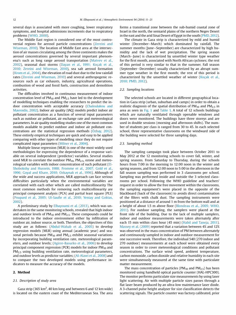
Fig. 2. MLR analysis of seasonally observed vs. predicted (a) PM10 and (b) PM2.5 using validation data.

M. Elbayoumi et al. / Atmospheric Environment 94 (2014) 11e2116

low air exchange, inadequate cleaning and physical activity of thestudents (Almeida et al., 2011; Goyal and Khare, 2010; Habil andTaneja, 2011). In a previous study in the same monitoring schoolsElbayoumi et al. (2013) reported that the indoor/outdoor ratios forPM10 and PM2.5 were found to bemuch greater than 1.00 for all casestudy schools due the elevation of the indoor particle emission rateof deposited particles from the floors. .Table 2 depicted the seasonaldifference among the three seasons where the concentrations ofPM10 and PM2.5 in winter season were higher than the remainingseasons. During winter, the mean indoor PM10 was 1.3 and 2.5times higher than fall and spring concentrations respectively.

Meanwhile, PM2.5 concentration in winter was 3.0 times higherthan fall and spring concentrations. The seasonal changes seem tobe predominantly due to different contribution of dust emissionsources, both indoors and outdoors (Elbayoumi et al., 2013).

The PM2.5 and PM10 concentrations variation are shown bylocation within the building. A comparison of the PM10 concen-tration in three floor level indicate that the ground level(Mean ¼ 406.21) had significantly higher concentration than the2nd floor level (Mean ¼ 302.11). On contrary, PM2.5 concentrationfor the three storey levels was not differed significantly (Elbayoumiet al., 2013). The average concentration of PM10 and PM2.5 varied

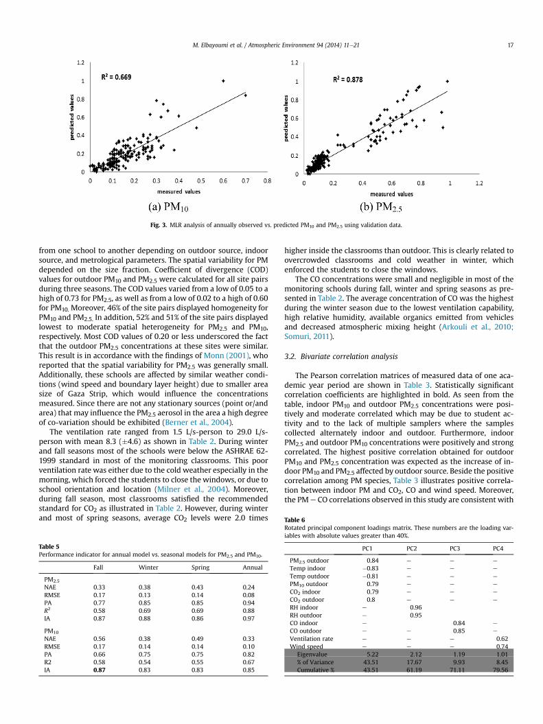
Fig. 3. MLR analysis of annually observed vs. predicted PM10 and PM2.5 using validation data.

Table 6

M. Elbayoumi et al. / Atmospheric Environment 94 (2014) 11e21 17

from one school to another depending on outdoor source, indoorsource, and metrological parameters. The spatial variability for PMdepended on the size fraction. Coefficient of divergence (COD)values for outdoor PM10 and PM2.5 were calculated for all site pairsduring three seasons. The COD values varied from a low of 0.05 to ahigh of 0.73 for PM2.5, as well as from a low of 0.02 to a high of 0.60for PM10. Moreover, 46% of the site pairs displayed homogeneity forPM10 and PM2.5. In addition, 52% and 51% of the site pairs displayedlowest to moderate spatial heterogeneity for PM2.5 and PM10,respectively. Most COD values of 0.20 or less underscored the factthat the outdoor PM2.5 concentrations at these sites were similar.This result is in accordance with the findings of Monn (2001), whoreported that the spatial variability for PM2.5 was generally small.Additionally, these schools are affected by similar weather condi-tions (wind speed and boundary layer height) due to smaller areasize of Gaza Strip, which would influence the concentrationsmeasured. Since there are not any stationary sources (point or/andarea) that may influence the PM2.5 aerosol in the area a high degreeof co-variation should be exhibited (Berner et al., 2004).

The ventilation rate ranged from 1.5 L/s-person to 29.0 L/s-person with mean 8.3 (�4.6) as shown in Table 2. During winterand fall seasons most of the schools were below the ASHRAE 62-1999 standard in most of the monitoring classrooms. This poorventilation rate was either due to the cold weather especially in themorning, which forced the students to close the windows, or due toschool orientation and location (Milner et al., 2004). Moreover,during fall season, most classrooms satisfied the recommendedstandard for CO2 as illustrated in Table 2. However, during winterand most of spring seasons, average CO2 levels were 2.0 times

Table 5Performance indicator for annual model vs. seasonal models for PM2.5 and PM10.

Fall Winter Spring Annual

PM2.5

NAE 0.33 0.38 0.43 0.24RMSE 0.17 0.13 0.14 0.08PA 0.77 0.85 0.85 0.94R2 0.58 0.69 0.69 0.88IA 0.87 0.88 0.86 0.97

PM10

NAE 0.56 0.38 0.49 0.33RMSE 0.17 0.14 0.14 0.10PA 0.66 0.75 0.75 0.82R2 0.58 0.54 0.55 0.67IA 0.87 0.83 0.83 0.85

higher inside the classrooms than outdoor. This is clearly related toovercrowded classrooms and cold weather in winter, whichenforced the students to close the windows.

The CO concentrations were small and negligible in most of themonitoring schools during fall, winter and spring seasons as pre-sented in Table 2. The average concentration of CO was the highestduring the winter season due to the lowest ventilation capability,high relative humidity, available organics emitted from vehiclesand decreased atmospheric mixing height (Arkouli et al., 2010;Somuri, 2011).

3.2. Bivariate correlation analysis

The Pearson correlation matrices of measured data of one aca-demic year period are shown in Table 3. Statistically significantcorrelation coefficients are highlighted in bold. As seen from thetable, indoor PM10 and outdoor PM2.5 concentrations were posi-tively and moderate correlated which may be due to student ac-tivity and to the lack of multiple samplers where the samplescollected alternately indoor and outdoor. Furthermore, indoorPM2.5 and outdoor PM10 concentrations were positively and strongcorrelated. The highest positive correlation obtained for outdoorPM10 and PM2.5 concentration was expected as the increase of in-door PM10 and PM2.5 affected by outdoor source. Beside the positivecorrelation among PM species, Table 3 illustrates positive correla-tion between indoor PM and CO2, CO and wind speed. Moreover,the PMe CO correlations observed in this study are consistent with

Rotated principal component loadings matrix. These numbers are the loading var-iables with absolute values greater than 40%.

PC1 PC2 PC3 PC4

PM2.5 outdoor 0.84 e e e

Temp indoor �0.83 e e e

Temp outdoor �0.81 e e e

PM10 outdoor 0.79 e e e

CO2 indoor 0.79 e e e

CO2 outdoor 0.8 e e e

RH indoor e 0.96RH outdoor e 0.95CO indoor e 0.84 e

CO outdoor e e 0.85 e

Ventilation rate e e e 0.62Wind speed e e e 0.74

Eigenvalue 5.22 2.12 1.19 1.01% of Variance 43.51 17.67 9.93 8.45Cumulative % 43.51 61.19 71.11 79.56

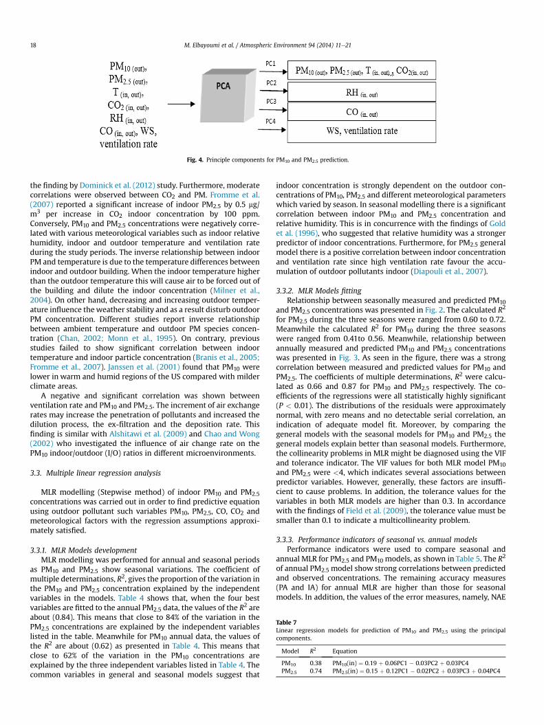
Fig. 4. Principle components for PM10 and PM2.5 prediction.

Table 7Linear regression models for prediction of PM10 and PM2.5 using the principalcomponents.

Model R2 Equation

PM10 0.38 PM10(in) ¼ 0.19 þ 0.06PC1 � 0.03PC2 þ 0.03PC4PM2.5 0.74 PM2.5(in) ¼ 0.15 þ 0.12PC1 � 0.02PC2 þ 0.03PC3 þ 0.04PC4

M. Elbayoumi et al. / Atmospheric Environment 94 (2014) 11e2118

the finding by Dominick et al. (2012) study. Furthermore, moderatecorrelations were observed between CO2 and PM. Fromme et al.(2007) reported a significant increase of indoor PM2.5 by 0.5 mg/m3 per increase in CO2 indoor concentration by 100 ppm.Conversely, PM10 and PM2.5 concentrations were negatively corre-lated with various meteorological variables such as indoor relativehumidity, indoor and outdoor temperature and ventilation rateduring the study periods. The inverse relationship between indoorPM and temperature is due to the temperature differences betweenindoor and outdoor building. When the indoor temperature higherthan the outdoor temperature this will cause air to be forced out ofthe building and dilute the indoor concentration (Milner et al.,2004). On other hand, decreasing and increasing outdoor temper-ature influence theweather stability and as a result disturb outdoorPM concentration. Different studies report inverse relationshipbetween ambient temperature and outdoor PM species concen-tration (Chan, 2002; Monn et al., 1995). On contrary, previousstudies failed to show significant correlation between indoortemperature and indoor particle concentration (Branis et al., 2005;Fromme et al., 2007). Janssen et al. (2001) found that PM10 werelower in warm and humid regions of the US compared with milderclimate areas.

A negative and significant correlation was shown betweenventilation rate and PM10 and PM2.5. The increment of air exchangerates may increase the penetration of pollutants and increased thedilution process, the ex-filtration and the deposition rate. Thisfinding is similar with Alshitawi et al. (2009) and Chao and Wong(2002) who investigated the influence of air change rate on thePM10 indoor/outdoor (I/O) ratios in different microenvironments.

3.3. Multiple linear regression analysis

MLR modelling (Stepwise method) of indoor PM10 and PM2.5concentrations was carried out in order to find predictive equationusing outdoor pollutant such variables PM10, PM2.5, CO, CO2 andmeteorological factors with the regression assumptions approxi-mately satisfied.

3.3.1. MLR Models developmentMLR modelling was performed for annual and seasonal periods

as PM10 and PM2.5 show seasonal variations. The coefficient ofmultiple determinations, R2, gives the proportion of the variation inthe PM10 and PM2.5 concentration explained by the independentvariables in the models. Table 4 shows that, when the four bestvariables are fitted to the annual PM2.5 data, the values of the R2 areabout (0.84). This means that close to 84% of the variation in thePM2.5 concentrations are explained by the independent variableslisted in the table. Meanwhile for PM10 annual data, the values ofthe R2 are about (0.62) as presented in Table 4. This means thatclose to 62% of the variation in the PM10 concentrations areexplained by the three independent variables listed in Table 4. Thecommon variables in general and seasonal models suggest that

indoor concentration is strongly dependent on the outdoor con-centrations of PM10, PM2.5 and different meteorological parameterswhich varied by season. In seasonal modelling there is a significantcorrelation between indoor PM10 and PM2.5 concentration andrelative humidity. This is in concurrence with the findings of Goldet al. (1996), who suggested that relative humidity was a strongerpredictor of indoor concentrations. Furthermore, for PM2.5 generalmodel there is a positive correlation between indoor concentrationand ventilation rate since high ventilation rate favour the accu-mulation of outdoor pollutants indoor (Diapouli et al., 2007).

3.3.2. MLR Models fittingRelationship between seasonally measured and predicted PM10

and PM2.5 concentrations was presented in Fig. 2. The calculated R2

for PM2.5 during the three seasons were ranged from 0.60 to 0.72.Meanwhile the calculated R2 for PM10 during the three seasonswere ranged from 0.41to 0.56. Meanwhile, relationship betweenannually measured and predicted PM10 and PM2.5 concentrationswas presented in Fig. 3. As seen in the figure, there was a strongcorrelation between measured and predicted values for PM10 andPM2.5. The coefficients of multiple determinations, R2 were calcu-lated as 0.66 and 0.87 for PM10 and PM2.5 respectively. The co-efficients of the regressions were all statistically highly significant(P < 0.01). The distributions of the residuals were approximatelynormal, with zero means and no detectable serial correlation, anindication of adequate model fit. Moreover, by comparing thegeneral models with the seasonal models for PM10 and PM2.5 thegeneral models explain better than seasonal models. Furthermore,the collinearity problems in MLR might be diagnosed using the VIFand tolerance indicator. The VIF values for both MLR model PM10and PM2.5 were <4, which indicates several associations betweenpredictor variables. However, generally, these factors are insuffi-cient to cause problems. In addition, the tolerance values for thevariables in both MLR models are higher than 0.3. In accordancewith the findings of Field et al. (2009), the tolerance value must besmaller than 0.1 to indicate a multicollinearity problem.

3.3.3. Performance indicators of seasonal vs. annual modelsPerformance indicators were used to compare seasonal and

annual MLR for PM2.5 and PM10 models, as shown in Table 5. The R2

of annual PM2.5 model show strong correlations between predictedand observed concentrations. The remaining accuracy measures(PA and IA) for annual MLR are higher than those for seasonalmodels. In addition, the values of the error measures, namely, NAE

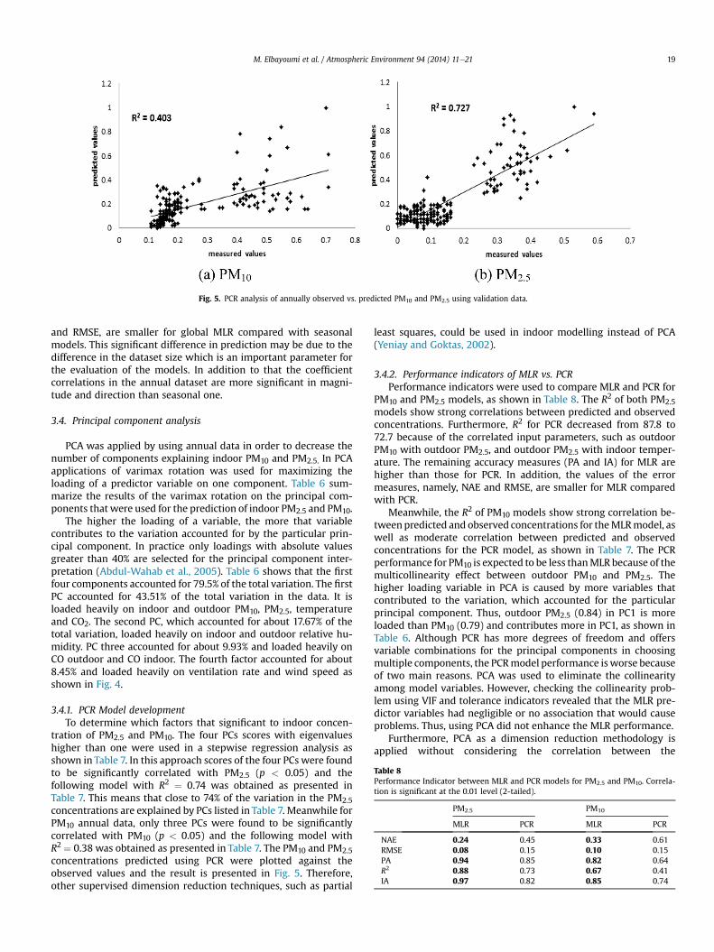
Fig. 5. PCR analysis of annually observed vs. predicted PM10 and PM2.5 using validation data.

Table 8Performance Indicator between MLR and PCR models for PM2.5 and PM10. Correla-tion is significant at the 0.01 level (2-tailed).

PM2.5 PM10

MLR PCR MLR PCR

NAE 0.24 0.45 0.33 0.61RMSE 0.08 0.15 0.10 0.15PA 0.94 0.85 0.82 0.64R2 0.88 0.73 0.67 0.41IA 0.97 0.82 0.85 0.74

M. Elbayoumi et al. / Atmospheric Environment 94 (2014) 11e21 19

and RMSE, are smaller for global MLR compared with seasonalmodels. This significant difference in prediction may be due to thedifference in the dataset size which is an important parameter forthe evaluation of the models. In addition to that the coefficientcorrelations in the annual dataset are more significant in magni-tude and direction than seasonal one.

3.4. Principal component analysis

PCA was applied by using annual data in order to decrease thenumber of components explaining indoor PM10 and PM2.5. In PCAapplications of varimax rotation was used for maximizing theloading of a predictor variable on one component. Table 6 sum-marize the results of the varimax rotation on the principal com-ponents that were used for the prediction of indoor PM2.5 and PM10.

The higher the loading of a variable, the more that variablecontributes to the variation accounted for by the particular prin-cipal component. In practice only loadings with absolute valuesgreater than 40% are selected for the principal component inter-pretation (Abdul-Wahab et al., 2005). Table 6 shows that the firstfour components accounted for 79.5% of the total variation. The firstPC accounted for 43.51% of the total variation in the data. It isloaded heavily on indoor and outdoor PM10, PM2.5, temperatureand CO2. The second PC, which accounted for about 17.67% of thetotal variation, loaded heavily on indoor and outdoor relative hu-midity. PC three accounted for about 9.93% and loaded heavily onCO outdoor and CO indoor. The fourth factor accounted for about8.45% and loaded heavily on ventilation rate and wind speed asshown in Fig. 4.

3.4.1. PCR Model developmentTo determine which factors that significant to indoor concen-

tration of PM2.5 and PM10. The four PCs scores with eigenvalueshigher than one were used in a stepwise regression analysis asshown in Table 7. In this approach scores of the four PCs were foundto be significantly correlated with PM2.5 (p < 0.05) and thefollowing model with R2 ¼ 0.74 was obtained as presented inTable 7. This means that close to 74% of the variation in the PM2.5

concentrations are explained by PCs listed in Table 7. Meanwhile forPM10 annual data, only three PCs were found to be significantlycorrelated with PM10 (p < 0.05) and the following model withR2 ¼ 0.38 was obtained as presented in Table 7. The PM10 and PM2.5concentrations predicted using PCR were plotted against theobserved values and the result is presented in Fig. 5. Therefore,other supervised dimension reduction techniques, such as partial

least squares, could be used in indoor modelling instead of PCA(Yeniay and Goktas, 2002).

3.4.2. Performance indicators of MLR vs. PCRPerformance indicators were used to compare MLR and PCR for

PM10 and PM2.5 models, as shown in Table 8. The R2 of both PM2.5models show strong correlations between predicted and observedconcentrations. Furthermore, R2 for PCR decreased from 87.8 to72.7 because of the correlated input parameters, such as outdoorPM10 with outdoor PM2.5, and outdoor PM2.5 with indoor temper-ature. The remaining accuracy measures (PA and IA) for MLR arehigher than those for PCR. In addition, the values of the errormeasures, namely, NAE and RMSE, are smaller for MLR comparedwith PCR.

Meanwhile, the R2 of PM10 models show strong correlation be-tweenpredicted and observed concentrations for theMLRmodel, aswell as moderate correlation between predicted and observedconcentrations for the PCR model, as shown in Table 7. The PCRperformance for PM10 is expected to be less thanMLR because of themulticollinearity effect between outdoor PM10 and PM2.5. Thehigher loading variable in PCA is caused by more variables thatcontributed to the variation, which accounted for the particularprincipal component. Thus, outdoor PM2.5 (0.84) in PC1 is moreloaded than PM10 (0.79) and contributes more in PC1, as shown inTable 6. Although PCR has more degrees of freedom and offersvariable combinations for the principal components in choosingmultiple components, the PCRmodel performance isworse becauseof two main reasons. PCA was used to eliminate the collinearityamong model variables. However, checking the collinearity prob-lem using VIF and tolerance indicators revealed that the MLR pre-dictor variables had negligible or no association that would causeproblems. Thus, using PCA did not enhance the MLR performance.

Furthermore, PCA as a dimension reduction methodology isapplied without considering the correlation between the

Table 9Performance of different pollutants forecasting methods from other studies.

Source Season Site Indoor Pollutant Model type R2

Ozkaynak et al. (1996) All Residential buildings California PM10 Linear Regression 0.60Goyal and Khare (2011) Winter and non- winter School India PM10 Mass Based Balance 0.42Goyal and Khare (2010) Winter and non- winter School in India PM10 MLR 0.40Tippayawong and Khuntong (2007) All Schools in Thailand PM2.5 Mass Based Balance 0.78Goyal and Khare (2010) Winter and non- winter School in India PM2.5 MLR 0.70Goyal and Khare (2011) Winter and non-winter School India PM2.5 Mass Based Balance 0.87Weichenthal et al. (2008) Winter Schools in Ontario PM1.0 MLR 0.39Goyal and Khare (2011) Winter and non- winter School India PM1.0 Mass Based Balance 0.86

M. Elbayoumi et al. / Atmospheric Environment 94 (2014) 11e2120

dependent variable (indoor PM10) and independent variables(outdoor PM10, indoor, and outdoor CO). Therefore, PCA is called anunsupervised dimension reduction methodology. The first fourprincipal components explained approximately 80% of the vari-ables. However, we noticed that the rank of the predictive powerdid not line up with the order of the principal components. Forinstance, the second principal component was less explanatory forthe target compared with the fourth, even though the secondprincipal component contained more information on the originalvariables. Furthermore, the third factor, which accounted for 10% ofthe total variation compared with the fourth 8%, was excluded fromthe PCR model. In accordance with the findings of Chatterjee andHadi (2013), one important PCR drawback was the correct identi-fication of the importance of all variables involved in determiningindoor pollutants, such as PM10 and PM2.5 concentrations. How-ever, PCR was not more precise than the multiple linear regressionfor prediction. Furthermore, Martin (2011) revealed that MLR out-performed PCR in modelling outdoor air pollutants.

Several previous international field studies for naturally venti-lated buildings are summarized in Table 9. The predicted indoorPM2.5 concentration is proven to satisfactorily follow changes in theobserved indoor concentration, as well as predicted concentrationlevels with reasonable accuracy. This result may be caused by thefact that the fine particles have higher infiltration rate comparedwith coarse particles. In addition, indoor concentration of the fineparticles are least affected by occupant activities and movements.Different studies worldwide reported that occupant activities ormovements, which could cause either resuspension of depositedcoarse particle or delay in the deposition process, was the majorsource of indoor PM (Blondeau et al., 2005; Chithra and Nagendra,2012; Diapouli et al., 2007; Goyal and Khare, 2011; Heudorf et al.,2009; Ozkaynak et al., 1996; Stranger et al., 2008). Thatcher andLayton (1995) and Ferro et al. (2004) concluded that particleresuspension depended on particle diameter, subjecting the parti-cles larger than 5 mm to resuspension even with low activity(walking). Meanwhile, particles less than 5 mm in size were notreadily resuspended. In addition to that and basing from experi-ments, the aforementioned researchers concluded that resus-pension was a function of occupant activities, and floor materialtype.

In this study and other studies presented in Table 9, the R2 forPM10 shows moderate correlation in the seasonal models and PCRmodel. The PM10 models are unable to consider the resuspensionand delayed deposition or setting caused by occupant activities andresulting in higher observed concentrations.

4. Conclusions

Deterministic models have the advantage of providing accurateresults. However, these models require a large amount of data asinputs (deposition rate, resuspension, and infiltration coefficient).

These data are difficult to find. Therefore, MLR and PCR are usedbecause they are relatively simple and sufficiently reliable.

Results demonstrated that indoor PM10 and PM2.5 levels wereaffected by outdoor concentrations of PM10 and PM2.5. In addition,meteorological factors were evident in the studied region. The re-sults of bivariate correlation analysis, which exhibited high positivecorrelation of indoor PM10 and PM2.5 with outdoor PM10, PM2.5, CO,and CO2 confirmed this assumption. The result of fitting the bestregression models on the PM10 and PM2.5 annual data gave strongvalues of coefficient of determinations 0.66 and 0.87 respectively.The common variables that appeared in both models were theoutdoor concentrations of PM10 and PM2.5. Among the meteoro-logical variables, temperature tended to contribute significantly tothe PM10 and PM2.5 concentrations. For the seasonal modelling, thecommon variables that appeared in all models were the outdoorconcentration of PM10 and PM2.5 and the relative humidity.

A variable selection method based on principal componentregression method was applied in order to account for multi-collinearity problem and to reduce the number of predictor vari-ables. The coefficients of determination for PCR models were 0.40and 0.72 for PM10 and PM2.5, respectively. Both method MLR andPCR were evaluated via performance indicators (NAE, RMSE, PA, IAand R2) and the results indicated that the performance of MLR isbetter than the performance of PCR.

Furthermore, The result from this study indicated that differentfactors such as such as number of students inside the classroom(resuspension factor), background concentration of PM inside thebuilding and outdoor PM concentration in the previous day may begood independent variables that contributed to indoor PM in theschools especially PM10.

Acknowledgement

The authors wish to acknowledge the Universiti Sains Malaysia(USM) for partly financing the study under RUI 814183 and RUI811206.

References

Abdul-Wahab, S.A., Bakheit, C.S., Al-Alawi, S.M., 2005. Principal component andmultiple regression analysis in modelling of ground-level ozone and factorsaffecting its concentrations. Environ. Model. Softw. 20, 1263e1271.

Agirre-Basurko, E., Ibarra-Berastegi, G., Madariaga, I., 2006. Regression and multi-layer perceptron-based models to forecast hourly O3 and NO2 levels in theBilbao area. Environ. Model. Softw. 21, 430e446.

Al-Alawi, S.M., Abdul-Wahab, S.A., Bakheit, C.S., 2008. Combining principalcomponent regression and artificial neural networks for more accurate pre-dictions of ground-level ozone. Environ. Model. Softw. 23, 396e403.

Almeida, S.M., Canha, N., Silva, A., Freitas, M.C., Pegas, P., Alves, C., Evtyugina, M.,Pio, C.A., 2011. Children exposure to atmospheric particles in indoor of Lisbonprimary schools. Atmos. Environ. 45, 7594e7599.

Alshitawi, M., Awbi, H., Mahyuddin, N., 2009. Particulate matter mass concentration(PM10) under different ventilation methods in classrooms. Int. J. Vent. 8, 93e108.

Arkouli, M., Ulke, A., Endlicher, W., Baumbach, G., Schultz, E., Vogt, U., Muller, M.,Dawidowski, L., Faggi, A., Wolf-Benning, U., 2010. Distribution and temporal

M. Elbayoumi et al. / Atmospheric Environment 94 (2014) 11e21 21

behavior of particulate matter over the urban area of Buenos Aires. Atmos.Pollut. Res. 1, 1e8.

Berner, A., Galambos, Z., Ctyroky, P., Frühauf, P., Hitzenberger, R., Gomi�s�cek, B.,Hauck, H., Preining, O., Puxbaum, H., 2004. On the correlation of atmosphericaerosol components of mass size distributions in the larger region of a centralEuropean city. Atmos. Environ. 38, 3959e3970.

Blondeau, P., Iordache, V., Poupard, O., Genin, D., Allard, F., 2005. Relationship betweenoutdoor and indoor air quality in eight French schools. Indoor Air 15, 2e12.

Branis, M., Rezácová, P., Domasová, M., 2005. The effect of outdoor air and indoorhuman activity on mass concentrations of PM10, PM2. 5, and PM1 in a class-room. Environ. Res. 99, 143e149.

Chaloulakou, A., Mavroidis, I., 2002. Comparison of indoor and outdoor concen-trations of CO at a public school. Evaluation of an indoor air quality model.Atmos. Environ. 36, 1769e1781.

Chan, A.T., 2002. Indooreoutdoor relationships of particulate matter and nitrogenoxides under different outdoor meteorological conditions. Atmos. Environ. 36,1543e1551.

Chao, C.Y., Wong, K.K., 2002. Residential indoor PM10 and PM2.5 in Hong Kong andthe elemental composition. Atmos. Environ. 36, 265e277.

Chatterjee, S., Hadi, A.S., 2013. Regression analysis by example, fifth ed. John Wiley& Sons.

Chithra, V., Nagendra, S., 2012. Indoor air quality investigations in a naturallyventilated school building located close to an urban roadway in Chennai, India.Build. Environ. 54, 159e167.

Daisey, J.M., Angell, W.J., Apte, M.G., 2003. Indoor air quality, ventilation and healthsymptoms in schools: an analysis of existing information. Indoor Air 13, 53e64.

Dayan, U., Heffter, J., Miller, J., Gutman, G., 1991. Dust intrusion events into theMediterranean basin. J. Appl. Meteorol. 30, 1185e1199.

Diapouli, E., Chaloulakou, A., Spyrellis, N., 2007. Indoor and outdoor particulate matterconcentrations at schools in the Athens area. Indoor Built Environ. 16, 55e61.

Dominick, D., Juahir, H., Latif, M.T., Zain, S.M., Aris, A.Z., 2012. Spatial assessment ofair quality patterns in Malaysia using multivariate analysis. Atmos. Environ. 60,172e181.

El-Shobokshy, M., Hussein, F., 1988. Correlation between indoor-outdoor inhalableparticulate concentrations and meteorological variables. Atmos. Environ. (1967)22, 2667e2675.

Elbayoumi, M., Ramli, N., Md Yusof, N., Al Madhoun, W., 2013. Spatial and seasonalvariation of particulate matter (PM10 and PM2.5) in Middle Eastern classrooms.Atmos. Environ. 80, 389e397.

Ferro, A.R., Kopperud, R.J., Hildemann, L.M., 2004. Source strengths for indoor hu-man activities that resuspend particulate matter. Environ. Sci. Technol. 38,1759e1764.

Field, A., 2009. Discovering statistics using SPSS, third ed. Sage Publications.Fromme, H., Twardella, D., Dietrich, S., Heitmann, D., Schierl, R., Liebl, B., Rüden, H.,

2007. Particulate matter in the indoor air of classrooms e exploratory resultsfrom Munich and surrounding area. Atmos. Environ. 41, 854e866.

Gervasi, O., 2008. Computational Science and its Applications e ICCSA 2008.Springer, Italy.

Gold, D.R., Allen, G., Damokosh, A., Serrano, P., Hayes, C., Castiilejos, M., 1996.Comparison of outdoor and classroom ozone exposures for school children inMexico City. J. Air Waste Manage. Assoc. 46, 335e342.

Goyal, R., Khare, M., 2010. Indoor Air Quality in Naturally Ventilated Schools, firsted. VDM Verlag Dr. Muller Aktiengesellschaft & Co. KG, Germany.

Goyal, R., Khare, M., 2011. Indoor air quality modeling for PM10, PM2.5, and PM1.0 innaturally ventilated classrooms of an urban Indian school building. Environ.Monit. Assess. 176, 501e516.

Gvozdi�c, V., Kova�c-Andri�c, E., Brana, J., 2011. Influence of meteorological factors NO2,SO2, CO and PM10 on the concentration of O3 in the urban atmosphere ofEastern Croatia. Environ. Model. Assess. 16, 491e501.

Habil, M., Taneja, A., 2011. Children’s exposure to indoor particulate matter innaturally ventilated schools in India. Indoor Built Environ. 20, 430e448.

Hal, 2012. HAL-HPC300 User Manual. Hal Technology Company, USA. http://www.haltechnologies.com/Docs/HAL-HPC300%20User%20Manual.pdf.

Heudorf, U., Neitzert, V., Spark, J., 2009. Particulate matter and carbon dioxide inclassroomsethe impact of cleaning and ventilation. Int. J. Hyg. Environ. Health.212, 45e55.

Janssen, N., Van Vliet, P., Aarts, F., Harssema, H., Brunekreef, B., 2001. Assessment ofexposure to traffic related air pollution of children attending schools nearmotorways. Atmos. Environ. 35, 3875e3884.

Karppinen, A., Kukkonen, J., Elolähde, T., Konttinen, M., Koskentalo, T.,Rantakrans, E., 2000. A modelling system for predicting urban air pollution:model description and applications in the Helsinki metropolitan area. Atmos.Environ. 34, 3723e3733.

Koçak, M., Kubilay, N., Tugrul, S., Mihalopoulos, N., 2010. Atmospheric nutrientinputs to the northern levantine basin from a long-term observation: sourcesand comparison with riverine inputs. Biogeosciences 7, 4037e4050.

Krom, M., Herut, B., Mantoura, R., 2004. Nutrient budget for the Eastern Mediter-ranean: implications for phosphorus limitation. Limnol. Oceanogr. 49, 1582e1592.

Kulshreshtha, P., Khare, M., 2011. Indoor exploratory analysis of gaseous pollutantsand respirable particulate matter at residential homes of Delhi, India. Atmos.Pollut. Res. 2, 337e350.

Kwok, A., Chun, C., 2003. Thermal comfort in Japanese schools. Sol. Energy 74, 245e252.

Lee, S., Chang, M., 1999. Indoor air quality investigations at five classrooms. IndoorAir 9, 134e138.

Martin, E., 2011. Comparative Performance of Different Statistical Models for Pre-dicting Ground-level Ozone (O3) and Fine Particulate Matter (PM2.5) Concen-trations in Montréal, Canada. The Department of Building, Civil andEnvironmental Engineering. Concordia University, Montréal, Canada.

Massey, D., Masih, J., Kulshrestha, A., Habil, M., Taneja, A., 2009. Indoor/outdoorRelationship of Fine Particles Less than 2.5 mm (PM2.5) in Residential HomesLocations in Central Indian region, vol. 44, pp. 2037e2045.

Massey, D., Kulshrestha, A., Masih, J., Taneja, A., 2012. Seasonal trends of PM10,PM5.0, PM2.5 and PM1.0 in indoor and outdoor environments of residentialhomes located in North-Central India. Build. Environ. 47, 223e231.

Matvev, V., Dayan, U., Tass, I., Peleg, M., 2002. Atmospheric sulfur flux rates to andfrom Israel. Sci. Total. Environ. 291, 143e154.

Milner, J., Dimitroulopoulou, C., ApSimon, H., 2004. Indoor Concentrations inBuildings from Sources Outdoors. UK Atmospheric Dispersion Modeling LiaisonCommittee. ADMLC/2004/2.

Monn, C., 2001. Exposure assessment of air pollutants: a review on spatial het-erogeneity and indoor/outdoor/personal exposure to suspended particulatematter, nitrogen dioxide and ozone. Atmos. Environ. 35, 1e32.

Monn, C., Braendli, O., Schaeppi, G., Schindler, C., Ackermann-Liebrich, U.,Leuenberger, P., 1995. Particulate matter 10 mm (PM10) and total suspendedparticulates (TSP) in urban, rural and alpine air in Switzerland. Atmos. Environ.29, 2565e2573.

Özbay, B., 2012. Modeling the effects of meteorological factors on SO2 and PM10concentrations with statistical approaches. Clean Soil, Air, Water 40, 571e577.

Özbay, B., Keskin, G.A., Do�gruparmak, S.Ç., Ayberk, S., 2011. Multivariate methods forground-level ozone modeling. Atmos. Res. 102, 57e65.

Ozkaynak, H., Xue, J., Spengler, J., Wallace, L., Pellizzari, E., Jenkins, P., 1996. Personalexposure to airborne particles and metals: results from the Particle TEAM studyin Riverside, California. J. Expo. Anal. Environ. Epidemiol. 6, 57.

Pegas, P.N., Evtyugina, M.G., Alves, C.A., Nunes, T., Cerqueira, M., Franchi, M., Pio, C.,Almeida, S.M., Freitas, M.C., 2010. Outdoor/indoor air quality in primary schoolsin Lisbon: a preliminary study. Quím. Nova 33, 1145e1149.

PMD, 2012. Climate Bulletine. Palestinian Meteorological Department, Ramallah.http://www.pmd.ps/ar/mna5palestine.php.

Pope, C.A., Young, B., Dockery, D., 2006. Health effects of fine particulate airpollution: lines that connect. J. Air, Waste Manage. Assoc. 56, 709e742.

Pope III, C.A., Ezzati, M., Dockery, D.W., 2009. Fine-particulate air pollution and lifeexpectancy in the United States. N. Engl. J. Med. 360, 376e386.

Poupard, O., Blondeau, P., Iordache, V., Allard, F., 2005. Statistical analysis of pa-rameters influencing the relationship between outdoor and indoor air quality inschools. Atmos. Environ. 39, 2071e2080.

Somuri, D.C., 2011. Study of Particulate Number Concentrations in Buses Runningwith Bio diesel and Ultra Low Sulfur Diesel. University of Toledo.

Stranger, M., Potgieter-Vermaak, S., Van Grieken, R., 2008. Characterization of in-door air quality in primary schools in Antwerp, Belgium. Indoor Air 18, 454e463.

Thatcher, T.L., Layton, D.W., 1995. Deposition, resuspension, and penetration ofparticles within a residence. Atmos. Environ. 29, 1487e1497.

Tippayawong, N., Khuntong, P., 2007. Model prediction of indoor particle concen-trations in a public school classroom. J. Chin. Inst. Eng. 30, 1077e1083.

Ul-Saufie, A., Yahya, A., Ramli, N., 2010. Improving multiple linear regression modelusing principal component analysis for predicting PM10 concentration inSeberang Prai, Pulau Pinang. Int. J. Environ. Sci. 2, 403e408.

Weichenthal, S., Dufresne, A., Infante-Rivard, C., Joseph, L., 2008. Characterizing andpredicting ultrafine particle counts in Canadian classrooms during the wintermonths: model development and evaluation. Environ. Res. 106, 349e360.

WHO, 2000. Air Quality Guidelines for Europe World Health Organization. WHO,Copenhagen.

WHO, 2005. WHO Air Quality Guidelines Global Update 2005. World Health Or-ganization (WHO), Bonn, Germany.

WHO, 2011. Methods for Monitoring Indoor Air Quality in Schools World HealthOrganization. WHO, Bonn, Germany.

Yeniay, O., Goktas, A., 2002. A comparison of partial least squares regression withother prediction methods. Hacettepe J. Math. Stat. 31, 99e111.

Zereini, F., Wiseman, C.L.S., 2010. Urban Airborne Particulate Matter: Origin,Chemistry, Fate and Health Impacts. Springer.