Insights into the primary–secondary and regional–local contributions to organic aerosol and PM...

ARTICLE IN PRESS

1352-2310/$ - se

doi:10.1016/j.at

�CorrespondE-mail addr

1Current add

Atmospheric Environment 41 (2007) 7414–7433

www.elsevier.com/locate/atmosenv

Insights into the primary–secondary and regional–localcontributions to organic aerosol and PM2.5 mass in

Pittsburgh, Pennsylvania

R. Subramaniana,1, Neil M. Donahueb, Anna Bernardo-Brickerc,Wolfgang F. Roggec, Allen L. Robinsona,�

aDepartment of Mechanical Engineering, Carnegie Mellon University, Pittsburgh, PA 15213, USAbDepartment of Chemistry and Department of Chemical Engineering, Carnegie Mellon University, Pittsburgh, PA 15213, USA

cDepartment of Civil and Environmental Engineering, Florida International University, Miami, FL 33199, USA

Received 24 January 2007; received in revised form 27 May 2007; accepted 30 May 2007

Abstract

This paper presents chemical mass balance (CMB) analysis of organic molecular marker data to investigate the sources

of organic aerosol and PM2.5 mass in Pittsburgh, Pennsylvania. The model accounts for emissions from eight primary

source classes, including major anthropogenic sources such as motor vehicles, cooking, and biomass combustion as well as

some primary biogenic emissions (leaf abrasion products). We consider uncertainty associated with selection of source

profiles, selection of fitting species, sampling artifacts, photochemical aging, and unknown sources. In the context of the

overall organic carbon (OC) mass balance, the contributions of diesel, wood-smoke, vegetative detritus, road dust, and

coke-oven emissions are all small and well constrained; however, estimates for the contributions of gasoline-vehicle and

cooking emissions can vary by an order of magnitude. A best-estimate solution is presented that represents the vast

majority of our CMB results; it indicates that primary OC only contributes 2778% and 50714% (average7standard

deviation of daily estimates) of the ambient OC in the summer and winter, respectively. Approximately two-thirds of the

primary OC is transported into Pittsburgh as part of the regional air mass. The ambient OC that is not apportioned by the

CMB model is well correlated with secondary organic aerosol (SOA) estimates based on the EC-tracer method and

ambient concentrations of organic species associated with SOA. Therefore, SOA appears to be the major component of

OC, not only in summer, but potentially in all seasons. Primary OC dominates the OC mass balance on a small number of

nonsummer days with high OC concentrations; these events are associated with specific meteorological conditions such as

local inversions. Primary particulate emissions only contribute a small fraction of the ambient fine-particle mass, especially

in the summer.

r 2007 Elsevier Ltd. All rights reserved.

Keywords: Organic aerosol; Particulate matter; Source apportionment; Molecular markers; CMB; Regional transport; Secondary organic

aerosol; Photochemical decay; Pittsburgh Air Quality Study

e front matter r 2007 Elsevier Ltd. All rights reserved.

mosenv.2007.05.058

ing author. Tel.: +1 412 268 3657; fax: +1 412 268 3348.

ess: [email protected] (A.L. Robinson).

ress: Droplet Measurement Technologies, Boulder, CO 80301, USA.

www.elsevier.com/locate/atmosenv

dx.doi.org/10.1016/j.atmosenv.2007.05.058

mailto:[email protected]

ARTICLE IN PRESSR. Subramanian et al. / Atmospheric Environment 41 (2007) 7414–7433 7415

1. Introduction

Organic carbon (OC) is a major component of fineparticulate matter in all regions of the atmosphere.OC is directly emitted to the atmosphere from sources(primary OC); it is also formed in the atmospherefrom low-volatility products produced by the oxida-tion of gas-phase anthropogenic and/or biogenicprecursors (secondary OC or secondary organicaerosol—SOA). Although a number of approachesare used to estimate the primary–secondary split, eachhas its shortcomings, and the relative contribution ofprimary and secondary OC to the overall OC budgetremains controversial.

One approach to investigate the sources of OC ischemical mass balance (CMB) analysis with organicmolecular markers (Schauer et al., 1996; Watsonet al., 1998a; Schauer and Cass, 2000; Zheng et al.,2002, 2006; Fraser et al., 2003b). This approach usesindividual organic compounds such as hopanes,cholesterol, and levoglucosan as markers to esti-mate the contribution of emissions from majorprimary sources such as gasoline and diesel vehicles,food cooking, and wood combustion to ambient OCand fine-particle mass. Since CMB with molecularmarkers only considers primary sources, the OC notapportioned to these sources (the unapportionedOC) is commonly attributed to SOA.

The published CMB analyses of molecular-marker data indicate that the relative importanceof primary sources varies widely with season andwith location. Schauer et al. (1996) attributed 85%of the ambient OC in Los Angeles in 1982 toprimary sources. Zheng et al. (2002) attributedessentially all of the wintertime ambient OC at bothurban and rural sites in the Southeastern US toprimary sources. During summer (Zheng et al.,2002) and photochemical smog episodes (Schaueret al., 2002a) the majority of the ambient OC oftencannot be apportioned to sources in the model. Inremote locations, very little of the OC is appor-tioned to primary sources (Sheesley et al., 2004).These trends are qualitatively consistent with spatialand temporal characteristics of SOA formation andreasonable correlation has been reported betweenthe unapportioned OC and different indicators ofsecondary aerosol production (Schauer et al., 2002a;Zheng et al., 2002; Sheesley et al., 2004). Overallthe published CMB results suggest a dominantcontribution of primary sources to OC in urbanareas, especially in winter. Such a conclusion issupported by estimates of SOA based on using EC

as a tracer for primary organic aerosol (Turpin andHuntzicker, 1995; Lim and Turpin, 2002; Cabadaet al., 2004; Polidori et al., 2006). However, recentanalyses of aerosol mass spectrometer (AMS) datasuggest that SOA dominates OC levels, even inurban areas (Zhang et al., 2005; Volkamer et al.,2006; Zhang et al., 2007). In addition, a recent CMBstudy reports significant amounts of unapportionedOC in cities in the Southeastern US in the winter(Zheng et al., 2006).

A number of factors complicate the use of CMBanalysis with molecular-marker data to quantita-tively constrain the overall OC budget. OC is notfitted by the model because markers and sourceprofiles do not exist for SOA. The CMB approach issensitive to the selection of source profiles andfitting species (Robinson et al., 2006c, d; Subrama-nian et al., 2006a). Sampling artifacts—adsorptionof organic vapors and evaporation of organicparticles—influence filter measurements of OCboth in the ambient atmosphere and from sourceemissions (Subramanian et al., 2004; Lipskyand Robinson, 2006). Photochemical decay ofmarkers during regional transport may bias sourcecontribution estimates (Robinson et al., 2006a).Finally, unknown sources of compounds fit byCMB—i.e., sources not included in the model—maybias source apportionment estimates (Robinsonet al., 2006b).

This is the final paper in a series that uses a largedatabase of organic molecular-marker data andCMB to investigate the sources of organic aerosol inPittsburgh, Pennsylvania. Previous papers haveconsidered in detail the contributions of motor-vehicle, biomass-burning, and food-cooking emis-sions to ambient OC (Robinson et al., 2006c, d;Subramanian et al., 2006a). Here we combine theseearlier results with estimates for other primarysources to evaluate the overall OC budget and toexamine the relative importance of local andregional primary sources. The analysis explicitlyconsiders the uncertainty associated with source-profile variability and selection of fitting species.The CMB-unapportioned OC is compared toestimates of SOA based on the EC-tracer technique(Cabada, 2003; Cabada et al., 2004; Polidori et al.,2006) and ambient concentrations of organiccompounds associated with SOA. Uncertaintiesdue to unknown primary sources, photochemicaldecay, and sampling artifacts are discussed. Finally,we consider the contribution of primary emissionsto PM2.5 mass.

ARTICLE IN PRESSR. Subramanian et al. / Atmospheric Environment 41 (2007) 7414–74337416

2. Methods

CMB analysis was performed on the datasetcollected as part of the Pittsburgh Air Quality Study(PAQS) (Wittig et al., 2004), using the EPA’s CMB8model (http://www.epa.gov/scram001/). The ana-lysis uses ambient concentrations of individualorganic compounds, PM2.5 elemental carbon, andPM2.5 elemental composition measured on 100 daysbetween July 2001 and July 2002 (Wittig et al.,2004). CMB analysis was performed using data forindividual days; all reported averages were calcu-lated from these daily estimates.

Daily 24-h samples were collected at the Pitts-burgh Supersite in July 2001 and most of January2002; during other periods 24-h samples werecollected on a 1-in-6-day schedule. The Supersitewas located in a large urban park next to theCarnegie Mellon University campus; it was notstrongly influenced by any local sources (Wittiget al., 2004). Pittsburgh aerosol is dominated byregional transport (Tang et al., 2004). To character-ize fine-particle concentrations in the regional airmass, a limited number of measurements were alsomade at a rural site in Florence, Pennsylvania(Wittig et al., 2004). This site was located 40 kmwest–southwest of Pittsburgh next to a large statepark on a lightly traveled dirt road. There are nomajor roads or stationary sources within severalkilometers of the Florence site. Florence is typicallyupwind of Pittsburgh, and the fine-particle mass andbulk constituents measured at the site are quitesimilar to those measured at other sites in the region(Tang et al., 2004). Thirteen sets of parallel 24-hsamples were collected in Pittsburgh and Florenceduring January 2002 and four paired sets in July2002.

PM2.5 and semivolatile organics were collected usingmedium-volume quartz-filter/polyurethane-foam-plug(PUF) samplers. Each quartz/PUF sample wassolvent extracted and the extract was analyzed byhigh-resolution gas chromatography-mass spectro-metry, providing a large dataset of daily organiccomposition (Robinson et al., 2006a). For theorganic speciation measurements, identical samplersand procedures were used at both sites. At theSupersite, OC/EC samples were collected on quartzfilters and analyzed using a thermal/optical trans-mission method (Subramanian et al., 2004; Sub-ramanian et al., 2006b). Trace-metal data weremeasured by inductive coupled plasma-mass spec-trometry (ICP-MS) analysis of samples collected on

cellulose filters (Pekney et al., 2006). EC and tracemetal data for the Florence site were collected andanalyzed as part of the EPA speciation trendsnetwork.

CMB results are sensitive to the specific combina-tion of source profiles and fitting species (Robinsonet al., 2006b–d; Subramanian et al., 2006a). Forexample, different combinations of source profilestypically yield well-correlated source-contributionestimates (especially if they are applied to the sameset of fitting species), but biases between theestimates can exceed the uncertainties calculatedby CMB. This underscores the fact that CMB-reported uncertainties are typically based on themeasurement uncertainty and quality of the fit, anddo not include the source profile variability.

To account for the uncertainty associated withselection of source profiles and fitting species, wepresent results for a large number of different CMBmodels, each of which was fit to the entire datasetusing a different combination of source profiles andfitting species. The majority of the models use thesame core set of fitting species: EC, iron, titanium,and 22 organic markers (individually or as groupsof compounds): n-heptacosane, n-nonacosane,n-hentriacontane and n-tritriacontane; iso-hentria-contane, anteiso-dotriacontane; octadecanoic acid,hexadecanoic acid, 9-hexadecenoic (palmitoleic)acid, and cholesterol; syringaldehyde, sum of resinacids, acetosyringone, levoglucosan; 17a(H),21b(H)-29-norhopane, 17a(H),21b(H)-hopane, 22R+S-17a(H),21b(H)-30-homohopane, 22R+S,17a(H),21b(H)-30-bishomohopane; benzo[e]pyrene, inde-no[1,2,3-cd]pyrene, benzo[g,h,i]perylene, and coro-nene. Certain models used slightly different sets ofspecies, as described in the online supportingmaterial. OC is not included (‘‘fitted’’) by anymodel because molecular markers and sourceprofiles for SOA are not known. Uncertainties forindividual compounds are based on relative andabsolute uncertainties determined from replicateanalysis of samples from collocated samplers.Absolute uncertainties are based on multiples ofthe minimum detection limits, while relative un-certainties range from 710% to 730%.

Each model fits source profiles for eight sourceclasses: diesel vehicles, gasoline vehicles, road dust,biomass combustion, cooking emissions, coke pro-duction, vegetative detritus, and cigarette smoke.Source profiles for coke-oven emissions, vegetativedetritus and road dust were developed as part ofthe PAQS (Robinson et al., 2006b, 2007b); the rest

http://www.epa.gov/scram001/


of the profiles are taken from the literature.A complete list of the source profiles is providedin the online Supplementary Material.

Except for the addition of metallurgical cokeproduction, our list of sources and marker species isbased on the original CMB analyses of molecularmarker data by Schauer et al. (1996) and Schauerand Cass (2000). Therefore, like previous studies, weassume that all major sources of each compound areincluded in the model and the marker species areconserved during transport from source to receptor.These assumptions are examined in detail later inthis paper.

The sensitivity analysis considered different com-binations of input species and source profiles. Elevendifferent combinations of motor-vehicle-specificsource profiles and/or fitting species were used toapportion OC to motor vehicles (Subramanianet al., 2006a). Three different combinations ofbiomass-smoke-specific source profiles and/or fit-ting species were used to apportion OC to biomassburning (Robinson et al., 2006c). Three differentcombinations of cooking-specific source profilesand/or fitting species were used to apportion OCto food-cooking emissions (Robinson et al., 2006d).The variability in the contribution of metallurgicalcoke production is estimated using two differentprofiles developed from a series of samples collectedat a fence-line site adjacent to a coke productionfacility (Weitkamp et al., 2005). The variability inthe road-dust contribution is bounded by use ofurban and rural road-dust profiles as well as bysubstituting calcium for iron as a fitting species. Toinvestigate the uncertainty in the contribution ofvegetative detritus, we fit both the PAQS and theLos Angeles profiles (Rogge et al., 1993), as well asdifferent combinations of the higher odd n-alkanes.

The sensitivity analysis did not exhaustivelyevaluate every possible combination of sourceprofiles and fitting species; for example, all elevendifferent motor vehicle scenarios were not evaluatedwith each of the three different food cookingscenarios. Instead we quantified the range ofsolutions for each source class using a few base setsof profiles and compounds for the other sourceclasses. A more exhaustive analysis is not necessarybecause of the source-specificity of molecularmarkers. For example, the contribution of food-cooking emissions is determined by cholesterol,alkenoic acids and alkanoic acids, while motor-vehicle emissions are determined by hopanes andEC. Therefore, the estimated food-cooking contri-

bution changes minimally as we vary the motor-vehicle source profiles. There are some exceptions,most notably gasoline and diesel vehicles, whichshare markers (hopanes and EC). Therefore, wefocus here on the total vehicle OC and not thegasoline–diesel split. Also, a number of sourcescontribute to ambient EC. We assessed this issue byrunning the different motor vehicle scenarios withvarious biomass smoke scenarios and found that itposed a problem on only a few days with highbiomass smoke. The conclusions of this paper arebased on the results of almost 100 different CMBmodels.

Our discussion of the overall OC mass balancefocuses on the results from four CMB models: bestestimate, maximum gasoline, maximum cooking,and maximum gasoline and cooking. As discussedbelow, the best-estimate model falls within the vastmajority of the solutions, while the other modelsrepresent outlier solutions. These four models usethe same set of profiles and fitting species for thenon-vehicular and non-food-cooking source classes.For biomass smoke, one set of profiles is used forthe fall/winter seasons and another set for thesummer/spring seasons to account for the expectedseasonal changes in the nature of biomass smokesources. Three profiles are used in each season toaccount for the widely varying ratios of biomasssmoke markers (Robinson et al., 2006c). The fall/winter data are fitted with the Fine et al. (2001)eastern hemlock, eastern white pine, and red-mapleprofiles. Of the viable combinations of space-heating profiles, this combination apportions themaximum amount of ambient OC to biomasssmoke (Robinson et al., 2006c). The summer/springdata are fitted using three simulated open-burningprofiles: the Hays et al. (2002) mixed hardwoodforest foliage (MHFF) and Florida palmetto andslash pine profiles; and the Hays et al. (2005) wheat-straw profile. For the other source classes, we usePittsburgh-specific vegetative-detritus and road-dustprofiles (Robinson et al., 2007b), the Pittsburghcoke-production profile that yields the maximumOC contribution (Robinson et al., 2006b), and theRogge et al. (1994) cigarette-smoke profile. Thesupporting online information provides more in-formation on the CMB scenarios.

These four models use different combinations offitting species and source profiles to estimatecooking and/or gasoline-vehicle emissions, the twosource categories that exhibit the most variability(Robinson et al., 2006d; Subramanian et al., 2006a).


For cooking emissions, the best-estimate model fitsthree cooking profiles: average red-meat frying,Schauer et al. (1999a) charbroiling, and averageseed-oil cooking; it provides the most plausibleestimate of cooking emissions (Robinson et al.,2006d). The models that yield the maximumcooking estimate fit an average red-meat charbroil-ing profile and do not fit palmitic acid and stearicacid (Robinson et al., 2006d). For vehicle emissions,the best-estimate model fits the Northern FrontRange Air Quality Study (NFRAQS, Watson et al.,1998a) heavy-duty diesel profile and a compositeNFRAQS gasoline profile that assumes 6.8% of thefleet is high emitters and smokers, split evenly(Subramanian et al., 2006a). Of the 11 differentcombinations of vehicle profiles and fitting specieswe have considered, this scenario yields the medianestimate of the total (gasoline+diesel) vehicularcontribution to OC. The model that yields themaximum gasoline estimate used three sourceprofiles: the Schauer et al. (2002b) catalytic andnoncatalytic gasoline profiles fitted separately,and a composite of the Schauer et al. (1999b) andFraser et al. (2002) diesel profiles. Two additionaln-alkanes (C24 and C26) are included as fittingspecies in CMB to separate the two gasoline sources(Subramanian et al., 2006a).

On the vast majority of the days, all of the CMBsolutions presented here meet the established good-ness-of-fit criteria (Watson et al., 1998b). Theregression coefficients (R2) were 0.80 or higher forover 96% of all CMB runs, with median valuesabove 0.90 for each solution set (CMB analysis forall samples with a given set of profiles and fittingspecies). The confidence levels (based on the w2 anddegrees of freedom) on all solutions were 95% orbetter for 99.8% of the runs. The degrees offreedom for each CMB run were between 12 and17 depending on the number of species fitted andthe number of nonzero sources apportioned byCMB; the CMB specifications for a good fit requirea minimum of 5. Over 90% of the fitted species in allruns were estimated by CMB to within a factor oftwo of the ambient concentration, i.e., the ratios ofCMB-calculated concentrations to the measuredvalues (C/M ratios) were between 0.5 and 2.0,another requirement for a good fit. The ‘‘percentagemass apportioned’’ criterion cannot be applied sinceSOA is a significant fraction of the ambient OC andis not included (‘‘fitted’’) in the CMB model.Excluding the days in which the models do notmeet the CMB performance criteria does not alter

our conclusions. Table S1 in supporting onlineinformation lists R2 and w2 values for the best-estimate model. More information on the statisticalquality of the various solutions is also presented inthe companion papers (Robinson et al., 2006b–d;Subramanian et al., 2006a).

3. Results and discussion

3.1. Source apportionment of primary OC and the

regional– local split

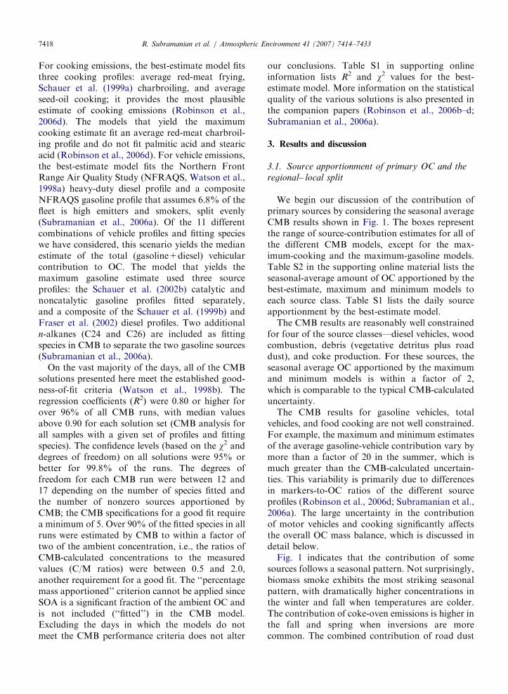
We begin our discussion of the contribution ofprimary sources by considering the seasonal averageCMB results shown in Fig. 1. The boxes representthe range of source-contribution estimates for all ofthe different CMB models, except for the max-imum-cooking and the maximum-gasoline models.Table S2 in the supporting online material lists theseasonal-average amount of OC apportioned by thebest-estimate, maximum and minimum models toeach source class. Table S1 lists the daily sourceapportionment by the best-estimate model.

The CMB results are reasonably well constrainedfor four of the source classes—diesel vehicles, woodcombustion, debris (vegetative detritus plus roaddust), and coke production. For these sources, theseasonal average OC apportioned by the maximumand minimum models is within a factor of 2,which is comparable to the typical CMB-calculateduncertainty.

The CMB results for gasoline vehicles, totalvehicles, and food cooking are not well constrained.For example, the maximum and minimum estimatesof the average gasoline-vehicle contribution vary bymore than a factor of 20 in the summer, which ismuch greater than the CMB-calculated uncertain-ties. This variability is primarily due to differencesin markers-to-OC ratios of the different sourceprofiles (Robinson et al., 2006d; Subramanian et al.,2006a). The large uncertainty in the contributionof motor vehicles and cooking significantly affectsthe overall OC mass balance, which is discussed indetail below.

Fig. 1 indicates that the contribution of somesources follows a seasonal pattern. Not surprisingly,biomass smoke exhibits the most striking seasonalpattern, with dramatically higher concentrations inthe winter and fall when temperatures are colder.The contribution of coke-oven emissions is higher inthe fall and spring when inversions are morecommon. The combined contribution of road dust

ARTICLE IN PRESS

Su F W Sp --

Su F W Sp --

Su F W Sp --

Su F W Sp --

Su F W Sp --

Su F W Sp --

Su F W Sp

0

400

800

1200

1600

2000RangeBest estimate

Low cookingHigh gasoline/cooking

Am

bie

nt org

anic

carb

on (

ng-C

/m3)

Diesel GasolineTotal

Vehicles

Biomass

smokeCooking

Road dust

+ Veg. Det.Coke

Fig. 1. CMB estimates of the seasonal average contributions of major primary sources of organic aerosol. Boxes show the range of the

vast majority of the models (excluding the maximum gasoline and the maximum and minimum cooking). No range is indicated for

cooking. The maximum gasoline and cooking scenarios, discussed in the text, are due to ‘‘outlier’’ profiles with relatively small marker-to-

OC ratios. Error bars indicate CMB calculated uncertainty for selected results.

R. Subramanian et al. / Atmospheric Environment 41 (2007) 7414–7433 7419

and vegetative detritus peaks in the fall and is at aminimum in the winter. Diesel vehicles exhibitessentially no seasonal variability.

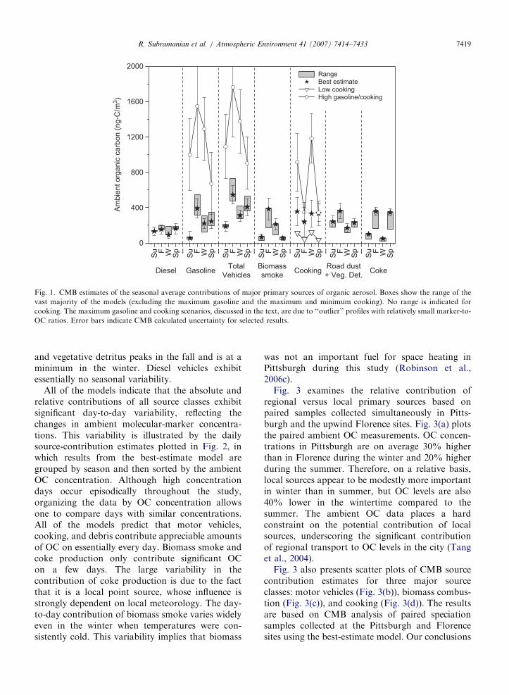
All of the models indicate that the absolute andrelative contributions of all source classes exhibitsignificant day-to-day variability, reflecting thechanges in ambient molecular-marker concentra-tions. This variability is illustrated by the dailysource-contribution estimates plotted in Fig. 2, inwhich results from the best-estimate model aregrouped by season and then sorted by the ambientOC concentration. Although high concentrationdays occur episodically throughout the study,organizing the data by OC concentration allowsone to compare days with similar concentrations.All of the models predict that motor vehicles,cooking, and debris contribute appreciable amountsof OC on essentially every day. Biomass smoke andcoke production only contribute significant OCon a few days. The large variability in thecontribution of coke production is due to the factthat it is a local point source, whose influence isstrongly dependent on local meteorology. The day-to-day contribution of biomass smoke varies widelyeven in the winter when temperatures were con-sistently cold. This variability implies that biomass

was not an important fuel for space heating inPittsburgh during this study (Robinson et al.,2006c).

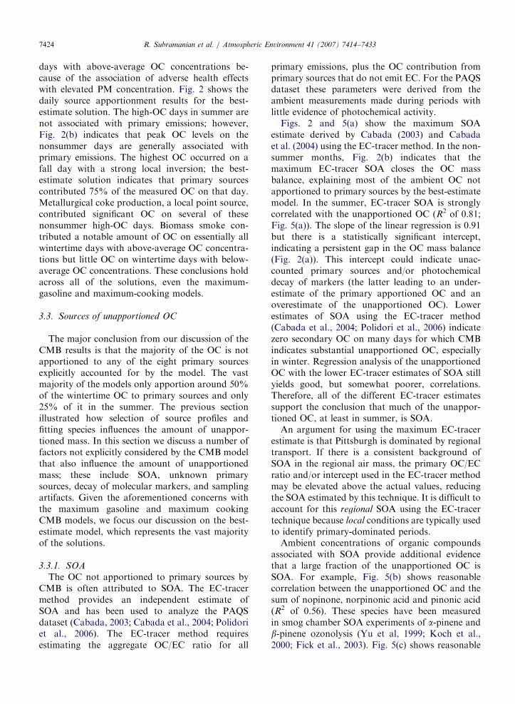
Fig. 3 examines the relative contribution ofregional versus local primary sources based onpaired samples collected simultaneously in Pitts-burgh and the upwind Florence sites. Fig. 3(a) plotsthe paired ambient OC measurements. OC concen-trations in Pittsburgh are on average 30% higherthan in Florence during the winter and 20% higherduring the summer. Therefore, on a relative basis,local sources appear to be modestly more importantin winter than in summer, but OC levels are also40% lower in the wintertime compared to thesummer. The ambient OC data places a hardconstraint on the potential contribution of localsources, underscoring the significant contributionof regional transport to OC levels in the city (Tanget al., 2004).

Fig. 3 also presents scatter plots of CMB sourcecontribution estimates for three major sourceclasses: motor vehicles (Fig. 3(b)), biomass combus-tion (Fig. 3(c)), and cooking (Fig. 3(d)). The resultsare based on CMB analysis of paired speciationsamples collected at the Pittsburgh and Florencesites using the best-estimate model. Our conclusions

ARTICLE IN PRESS

0

1000

2000

3000

4000

5000

6000

7000

8000

1 5 9

Am

bie

nt

org

an

ic c

arb

on

(n

g-C

/m3)

Secondary

OtherCokeCookingWood smoke

Vehicles

Ambient OC

Summer days (June-August, 2001 and 2002)

3 7 11 13 15 17 19 21 23 25 27 29 31 33 35 37 39 41

0

1000

2000

3000

4000

5000

6000

7000

8000

9000

10000

1 7

Am

bie

nt

org

an

ic c

arb

on

(n

g-C

/m3)

Fall (Sept-Nov)

Winter (Dec-March)

Spring (April-May)

Non-summer days

4 10 13 16 18 21 24 27 30 33 36 39 42 45 47 50 53

Fig. 2. Daily OC mass balance from the best-estimate CMB solution for (a) summer and (b) fall, winter and spring months. Data are first

sorted by season and then by decreasing ambient OC concentration. The secondary OC is the upper bound for SOA using the EC-tracer

technique (Cabada, 2003; Cabada et al., 2004). ‘‘Other’’ is the sum of vegetative detritus and road dust.

R. Subramanian et al. / Atmospheric Environment 41 (2007) 7414–74337420

are not sensitive to the specific CMB model, as longas the data from both sites are analyzed using thesame profiles and fitting species.

The wintertime CMB results shown in Fig. 3indicate modestly higher levels of primary OC inthe city than in Florence. For example, the averagewintertime vehicular OC in Florence is 230752 ng-Cm�3 versus 345770 ng-Cm�3 in Pittsburgh(Fig. 3(b)). This implies that, on average, two-thirdsof the wintertime primary vehicular OC in Pitts-

burgh is associated with regional transport and onlyone-third is due to local emissions. The wintertimecooking estimates shown in Fig. 3(c) indicate asimilar regional–local split. The wintertime bio-mass-smoke contributions at the two sites aregenerally similar, except for a few days whenbiomass-smoke levels are enhanced at one of thetwo sites (Fig. 3(d)). The days with elevated biomasssmoke in the city are associated with hardwoodsmoke, presumably due to local wood combustion

ARTICLE IN PRESS

0 4 8 10 12 140

2

4

6

8

10

12

14

0 200 400 600 800 10000

200

400

600

800

1000

FlorenceP

itts

bu

rgh

Vehicle OC (ng-C m-3)

1:11.5:19:1

0 300 600 900 12000

300

600

900

1200

Pit

tsb

urg

h

Florence

Biomass OC (ng-C m-3)

1:12:1 1.25:1

0 300 600 900 12000

300

600

900

1200

Pit

tsb

urg

h

Florence

Cooking OC (ng-C m-3)

1:11.5:1

Winter Summer

Pit

tsb

urg

h

Florence

1:1

OC (μg-C m-3)

1.25:1

2 6

Fig. 3. Scatter plots of (a) measured ambient OC and (b)–(d) CMB source contribution estimates for Pittsburgh and an upwind, rural site

in Florence, Pennsylvania. CMB results are shown for (b) motor vehicles (gasoline plus diesel), (c) biomass combustion, and (d) food

cooking. The source apportionment results are based on the best-estimate CMB model. The lines indicate different ratios of the

Pittsburgh-to-Florence results; for example, the 2:1 line in panel (c) indicates that CMB estimated biomass smoke contribution in

Pittsburgh is twice that in Florence. Error bars are CMB-propagated uncertainties.


for space heating. During PAQS, high biomasssmoke concentrations were typically observed onwinter weekend days (Robinson et al., 2006c). Onaverage, the wintertime CMB results indicate that70% of the primary OC in Pittsburgh is emitted byregional and not local sources, consistent with therelatively uniform spatial distribution of ambientOC (Fig. 3(a)).

Interpretation of the summertime CMB data atthe two sites is more complicated. During the

summer, biomass-smoke and meat-cooking contri-butions at the two sites are usually comparable, butthe OC attributed to motor vehicles in Pittsburghexceeds that in Florence by a factor of 9, as CMBapportions less than 50 ng-Cm�3 of the ambient OCin Florence to motor vehicle emissions. In fact, thepeak summertime concentration of vehicular OC inFlorence is more than a factor of 2 smaller thaneven the lowest winter day. One interpretation ofthe Florence CMB results is that motor vehicles are


not a major source of OC in the regional air mass inthe summer; however, this is inconsistent with thewinter data. The underlying cause of this discre-pancy is that in the summertime ambient hopanesconcentrations are much lower in Florence than inthe city; for example, summertime norhopane levelsare three to twelve times higher in Pittsburgh than inFlorence (Robinson et al., 2006a). The low sum-mertime concentrations of hopanes in Florenceseverely constrain the OC apportioned to motorvehicles. Robinson et al. (2006a) argues that there issignificant photochemical decay of hopanes in theregional air mass in the summer. If true, then theambient hopanes in Pittsburgh during summer onlyrepresent local vehicular emissions because thehopanes in the regional air mass have beenphotochemically degraded. Photochemical decayof hopanes would violate one of the underlyingassumptions of CMB and is discussed in more detaillater.

3.2. Evaluation of the OC mass balance

We begin our discussion of the overall OC massbalance by considering the contribution of the fourwell-constrained source classes (diesel vehicles,biomass smoke, debris, and coke). The maximumCMB solution indicates that together these fourclasses contribute on average 23711% of theambient OC (average7standard deviation of thedaily source-contribution estimates). The relativecontribution of these four source classes variesseasonally; it is lowest in the summer, 1674% ofthe daily OC, and highest in the fall, 35713% of thedaily OC. However, the key point is that onessentially all days these well-constrained primarysources contribute relatively little ambient OC, evenif one considers the maximum solution. Fig. 2indicates that on only a handful of nonsummer daysdo any of the four well-constrained sources con-tribute large amounts of OC; for example the spikesin coke-oven emissions in the spring and spikes inbiomass smoke in the fall.

The amount of OC not apportioned to primarysources therefore depends strongly on which model isused to represent the two poorly constrained sourceclasses, gasoline vehicles and cooking. This isillustrated in Fig. 4, which compares seasonal-averageresults of four CMB models: the best-estimate,maximum-gasoline, maximum-cooking, and maxi-mum-gasoline-and-maximum-cooking models. Allof the models show a similar seasonal pattern with

a maximum primary contribution in winter and aminimum in summer, but they indicate very differentsplits between primary and unapportioned OC. Onaverage these models apportion between 25% and75% of the ambient OC to primary sources insummer and between 50% and 140% in winter. Ofthe four models shown in Fig. 4, the minimumestimate corresponds to the best-estimate model.The maximum primary estimate corresponds to themodel that apportions the maximum OC to bothfood cooking and gasoline vehicles, the two poorlyconstrained source classes.

The maximum primary estimate shown in Fig. 4is clearly implausible as it apportions more than140% of the wintertime OC on average. Theproblems are even more apparent if one examinesthe daily source contribution estimates, as themaximum model overapportions the measured OCby as much as a factor of 3 on many individual days.Many of these problematic days are not lowconcentration days. Overapportionment of ambientOC by CMB analysis of molecular-marker datahas been reported by other studies; it has beenattributed to missing sources for specific markers(Sheesley et al., 2004) or sampling artifacts (Zhenget al., 2002). We believe that the problem is largelydue to the specific combinations of sources profilesand fitting species, which maximize the contributionof cooking and gasoline vehicles. Fig. 1 indicatesthat, in comparison to the other solutions, modelsthat apportion the maximum OC to cooking and/orvehicles appear to be outliers.

From the perspective of the seasonal-average OCmass balance, the other three solutions (maximumgasoline, best estimate, and maximum cooking)plotted in Fig. 4 appear plausible. In fact, modelsthat apportion the maximum amount of OC toeither meat cooking or gasoline vehicles attributeessentially all of the wintertime OC to primarysources, consistent with the conceptual model thatprimary sources are dominant in the winter.However, more detailed examination of these twosolutions raises important concerns. For example,on one-fifth of the winter days, the maximum-gasoline and the maximum-cooking models appor-tion more than 120% of the ambient OC to primarysources. This exceeds the CMB-stipulated ‘‘allow-able uncertainty’’ on the overall OC mass balance(the ‘‘percentage mass apportioned’’ criterion,720%), assuming no missing sources. These modelsalso apportion about 60% of ambient OC to asingle source—either gasoline vehicles or meat

ARTICLE IN PRESS

Best estim

ate

Max G

asolin

e

Max C

ookin

g

Max G

as+

Cook

Best estim

ate

Max G

asolin

e

Max C

ookin

g

Max G

as+

Cook

Best estim

ate

Max G

asolin

e

Max C

ookin

g

Max G

as+

Cook

Best estim

ate

Max G

asolin

e

Max C

ookin

g

Max G

as+

Cook

0

500

1000

1500

2000

2500

3000

3500

4000A

mb

ien

t O

rga

nic

Carb

on

(n

g-C

m-3

) Summer

Fall

Winter Spring

Ambient

Gasoline

Cooking

Other Primary

Biomass

Diesel

Fig. 4. Seasonal average contributions to the ambient OC from primary sources based on the four CMB models discussed in the text: best

estimate, maximum cooking, maximum gasoline, and maximum gasoline and cooking. ‘‘Other primary’’ is the sum of coke, vegetative

detritus, and road dust.


cooking—because of the specific combinations ofprofiles and fitting species. In the maximum-gaso-line model the primary OC is dominated by the low-emitter Schauer et al. (2002b) catalytic gasolineprofile which has extremely small marker-to-OCratios (Subramanian et al., 2006a). One does notexpect low-emitting gasoline vehicles to be thedominant pollutant source (Beaton et al., 1995).Combining the Schauer et al. (2002b) catalyticgasoline profile with any other gasoline vehicleprofile to create a more realistic fleet-average profiledramatically reduces the amount of OC appor-tioned to gasoline vehicles (Subramanian et al.,2006a). Similarly, the maximum-cooking model isbased on an average charbroiling profile with verysmall marker-to-OC ratios, which maximizes theamount of ambient OC apportioned to cookingsources (Robinson et al., 2006d). This model alsooverapportions stearic and palmitic acids by morethan a factor of 3 in the winter (Robinson et al.,

2006d). These concerns diminish the probabilitythat either of the maximum-gasoline and themaximum-cooking solutions is a reasonable expla-nation of the ambient data.

Fig. 1 indicates that the best-estimate modelrepresents the vast majority of the solutionsconsidered here. This and many other models onlyapportion on average 25% of the OC to primarysources in summer and about 50% in winter. Whilecomparably large amounts of unapportioned OChave been reported by previous CMB studies,especially in rural areas (Zheng et al., 2002; Sheesleyet al., 2004), the relatively small contribution ofprimary sources in an urban area, especially inwinter, is surprising. Potential explanations includeSOA, missing primary sources, sampling artifacts,and photochemical decay of tracers; these issues areconsidered in detailed in the next section.

We also examined the relative importance ofprimary emissions on a daily basis, focusing on the


days with above-average OC concentrations be-cause of the association of adverse health effectswith elevated PM concentration. Fig. 2 shows thedaily source apportionment results for the best-estimate solution. The high-OC days in summer arenot associated with primary emissions; however,Fig. 2(b) indicates that peak OC levels on thenonsummer days are generally associated withprimary emissions. The highest OC occurred on afall day with a strong local inversion; the best-estimate solution indicates that primary sourcescontributed 75% of the measured OC on that day.Metallurgical coke production, a local point source,contributed significant OC on several of thesenonsummer high-OC days. Biomass smoke con-tributed a notable amount of OC on essentially allwintertime days with above-average OC concentra-tions but little OC on wintertime days with below-average OC concentrations. These conclusions holdacross all of the solutions, even the maximum-gasoline and maximum-cooking models.

3.3. Sources of unapportioned OC

The major conclusion from our discussion of theCMB results is that the majority of the OC is notapportioned to any of the eight primary sourcesexplicitly accounted for by the model. The vastmajority of the models only apportion around 50%of the wintertime OC to primary sources and only25% of it in the summer. The previous sectionillustrated how selection of source profiles andfitting species influences the amount of unappor-tioned mass. In this section we discuss a number offactors not explicitly considered by the CMB modelthat also influence the amount of unapportionedmass; these include SOA, unknown primarysources, decay of molecular markers, and samplingartifacts. Given the aforementioned concerns withthe maximum gasoline and maximum cookingCMB models, we focus our discussion on the best-estimate model, which represents the vast majorityof the solutions.

3.3.1. SOA

The OC not apportioned to primary sources byCMB is often attributed to SOA. The EC-tracermethod provides an independent estimate ofSOA and has been used to analyze the PAQSdataset (Cabada, 2003; Cabada et al., 2004; Polidoriet al., 2006). The EC-tracer method requiresestimating the aggregate OC/EC ratio for all

primary emissions, plus the OC contribution fromprimary sources that do not emit EC. For the PAQSdataset these parameters were derived from theambient measurements made during periods withlittle evidence of photochemical activity.

Figs. 2 and 5(a) show the maximum SOAestimate derived by Cabada (2003) and Cabadaet al. (2004) using the EC-tracer method. In the non-summer months, Fig. 2(b) indicates that themaximum EC-tracer SOA closes the OC massbalance, explaining most of the ambient OC notapportioned to primary sources by the best-estimatemodel. In the summer, EC-tracer SOA is stronglycorrelated with the unapportioned OC (R2 of 0.81;Fig. 5(a)). The slope of the linear regression is 0.91but there is a statistically significant intercept,indicating a persistent gap in the OC mass balance(Fig. 2(a)). This intercept could indicate unac-counted primary sources and/or photochemicaldecay of markers (the latter leading to an under-estimate of the primary apportioned OC and anoverestimate of the unapportioned OC). Lowerestimates of SOA using the EC-tracer method(Cabada et al., 2004; Polidori et al., 2006) indicatezero secondary OC on many days for which CMBindicates substantial unapportioned OC, especiallyin winter. Regression analysis of the unapportionedOC with the lower EC-tracer estimates of SOA stillyields good, but somewhat poorer, correlations.Therefore, all of the different EC-tracer estimatessupport the conclusion that much of the unappor-tioned OC, at least in summer, is SOA.

An argument for using the maximum EC-tracerestimate is that Pittsburgh is dominated by regionaltransport. If there is a consistent background ofSOA in the regional air mass, the primary OC/ECratio and/or intercept used in the EC-tracer methodmay be elevated above the actual values, reducingthe SOA estimated by this technique. It is difficult toaccount for this regional SOA using the EC-tracertechnique because local conditions are typically usedto identify primary-dominated periods.

Ambient concentrations of organic compoundsassociated with SOA provide additional evidencethat a large fraction of the unapportioned OC isSOA. For example, Fig. 5(b) shows reasonablecorrelation between the unapportioned OC and thesum of nopinone, norpinonic acid and pinonic acid(R2 of 0.56). These species have been measuredin smog chamber SOA experiments of a-pinene andb-pinene ozonolysis (Yu et al, 1999; Koch et al.,2000; Fick et al., 2003). Fig. 5(c) shows reasonable

ARTICLE IN PRESS

Summer Fall/Spring Winter

0 1000 2000 3000 4000 5000 60000

1000

2000

3000

4000

5000

6000

EC

-tra

cer

SO

A (

ng

-C/m

3)

Unapportioned OC (ng-C/m3)

All data: Y = (0.75±0.05)∗X - (152±106), R

2 = 0.71

Summer: Y = (0.91±0.07)∗X - (805±203), R

2 = 0.81

Winter: Y = (0.73±0.16)∗X - (13±193), R

2 = 0.42

0 1000 2000 3000 4000 5000 60000

4

8

12

16

20

6,1

0,1

4-t

rim

eth

yl-

2-p

en

tad

ecan

on

e

(ng

/m3)


All data: Y = (2.79±0.25)∗X/1000 + (0.89±0.56), R

2 = 0.56

Summer: Y = (2.44±0.38)∗X/1000 + (2.31±1.08), R

2 = 0.51

Winter: R2 = 0.15

0 1000 2000 3000 4000 5000 60000

5

10

15

20

25

30

Su

m o

f b

iog

en

ic S

OA

mark

ers

(n

g/m

3)


All data: Y = (3.43±0.31)∗X/1000 + (2.12±0.69), R

2 = 0.56

Summer: Y = (2.56±0.51)∗X/1000 +(5.54±1.44), R

2 = 0.40

Winter: R2 = 0.26

0 1000 2000 3000 4000 5000 60000

3

6

9

129,1

0-a

nth

racen

ed

ion

e (

ng

/m3)


All data: Y = (1.07±0.15)∗X/1000 + (0.47±0.32), R

2 = 0.35

Summer: Y = (1.42±0.21)∗X/1000 - (0.56±0.59), R

2 = 0.54

Winter: R2 = 0.04

Fig. 5. Scatter plots of the ambient OC not apportioned by the best-estimate CMBmodel to primary sources with (a) SOA estimated using

the EC-tracer method; (b) sum of three terpene oxidation products, nopinone, norpinonic acid and cis-pinonic acid; (c) 6,10,14-trimethyl-

2-pentadecanone (a ketone associated with both biogenic or anthropogenic emissions); and (d) 9,10-anthracenedione (an oxy-PAH). Lines

indicate linear regression of entire dataset. Results of linear regression for all of the data, summer data, and winter data given in each

panel.


correlation between the unapportioned OC and6,10,14-trimethyl-2-pentadecanone (R2 of 0.56).This branched ketone has been used as an indicatorof biogenic SOA formation in rural or remote areas(Simoneit and Mazurek, 1982; Simoneit et al., 1988;Alves et al., 2001; Engling et al., 2006). It is alsoformed from the incomplete combustion of pristaneand phytane present in motor vehicle fuel (Simoneit,1985); thus, its presence in urban areas cannotbe uniquely attributed to SOA. The unapportionedOC is similarly correlated with 1,3-benzenedicarboxylic acid (R2 of 0.55; not shown), whichhas been associated with primary vehicular emis-

sions (Fraser et al., 2003a). Finally, some correla-tion is observed between the unapportioned OCand oxy-PAHs such as 9-fluorenone and 9,10-anthracenedione (R240.4, Fig. 5(d)). These PAHoxidation products can be formed in the atmosphereor during combustion (Ramdahl, 1983; Simoneitet al., 1991).

Previous studies have proposed 1,2-benzenedicar-boxylic acid and aliphatic diacids as indicators ofanthropogenic SOA (Schauer et al., 2002a; Fraseret al., 2003a; Sheesley et al., 2004). However, theunapportioned OC is not correlated with thesecompounds (R2o0.2).


AMS data collected in Pittsburgh also suggestthat SOA is the dominant component of the organicaerosol in Pittsburgh. Zhang et al. (2005) estimatesthat 50% of the OC in Pittsburgh in September 2002was secondary (assuming an organic-mass-to-organic-carbon ratio of 2.2 and 1.2 for oxygenatedorganic aerosol (OOA) and hydrocarbon-like or-ganic aerosol (HOA), respectively). This is consis-tent with the results from the best-estimate solutionshown in Fig. 2(b) for September 2001.

Overall these multiple independent indicators ofSOA all provide strong evidence that the dominantcomponent of the summertime unapportioned OC,and thus the ambient OC, is SOA. However, thepotential contribution of SOA in winter is less clear.While the wintertime unapportioned OC is some-what correlated with the maximum EC-tracerestimate of SOA (R2

¼ 0.45; Fig. 5(a)), littlecorrelation is observed with organic compoundscommonly associated with SOA.

3.3.2. Unknown primary sources

Our CMB analysis only accounts for emissionsfrom eight primary source classes. Except for theaddition of metallurgical coke production, our listof sources is largely the same as that used in otherstudies. It includes major anthropogenic sourcessuch as motor vehicles, cooking and biomasscombustion as well as some primary biogenicemissions (leaf abrasion products). However, thereare certainly other primary sources of OC. The factthat most of our CMB models do not apportion asignificant fraction of the wintertime OC raises thepossibility that unaccounted primary sources maybe significant. In addition, Fig. 2(a) indicates that,even after including the maximum EC-tracerestimate of SOA in the OC mass balance, about1 mg-Cm�3 of the ambient OC remains unexplainedin summer.

First we consider the potential contribution ofunaccounted local sources. Not all local industrialsources are represented in the CMB model. TheAllegheny County PM2.5 point-source emissioninventory is dominated by facilities related to steelproduction and coal-fired boilers (Hochhauser,2004). The CMB analysis does include the largestpoint-source category, metallurgical coke produc-tion. The inventory estimates that coke productioncontributes 25% of the county-wide point-sourceemissions of PM2.5 mass, and 40% of cokeemissions are OC (Weitkamp et al., 2005). Althoughthe CMB results indicate that coke production was

an important source on a few study days (Fig. 2), itonly contributed 7079 ng-Cm�3 or 2% of thestudy-average ambient OC. Therefore, one mustcarefully distinguish between the daily and long-term average contributions of a local point source.Given the fact that the Pittsburgh Supersite was notlocated close to any major local sources, it is highlyunlikely that emissions from some unaccountedlocal point source strongly influenced the long-termaverage OC measurements at the site. In fact, highlytime-resolved measurements made during PAQSreveal few periods with even modestly elevated OCspikes that would indicate strong influence of anOC-rich plume from a local source.

Another strong piece of evidence that unac-counted local sources are not strongly influencingOC concentrations at the Pittsburgh site is theambient OC data shown in Fig. 3(a). As previouslydiscussed, OC concentrations at the PittsburghSupersite are on average only 20–30% higher thanlevels in the regional air mass (Tang et al., 2004).This modest bump in urban OC concentrationsrepresents the aggregate contribution of all localsources. Notably, this bump is substantially smallerthan the amount of unapportioned OC. Further-more, the CMB results from the Pittsburgh andFlorence sites such as those shown in Fig. 3 indi-cate that about half of the bump can be accountedfor by sources in the model. Therefore, a reason-able estimate for the contribution of unaccountedlocal sources is 10–15% of the long-term ambientOC, which is a small fraction of the unappor-tioned OC.

We cannot rule out an unaccounted, regional

primary source. Fig. 2 indicates that after account-ing for EC-tracer estimates of SOA, a larger fractionof the summertime OC remains unexplained com-pared to other seasons. This pattern is consistentwith a primary biogenic source. Our CMB modeldoes account for primary emissions from leafabrasion, using the higher odd n-alkanes (C27,C29, C31, and C33) as markers. However, this is aminor source, contributing only 120740 ng-Cm�3

or 3% of the study-average OC. Recent studies havesuggested that biogenic materials such as fungalcells can contribute significant fine organic aerosolmass (Womiloju et al., 2003).

A potential explanation for the large amounts ofunapportioned OC in winter is that we are system-atically underestimating the contribution of biomasssmoke. For example, our estimates of biomasssmoke OC in Pittsburgh are much lower than


estimates made in the Southeast (Zheng et al., 2002).A challenge is that source profile levoglucosan-to-OC or levoglucosan-to-PM-mass ratios can varywidely depending on combustion conditions andfuel type (Hedberg and Johansson, 2006; Mazzoleniet al., 2007), which can create substantial variabilityin the CMB results. If one uses a source profilewith a small levoglucosan-to-OC ratio one canattribute much more OC to biomass smoke. In facton days when biomass smoke marker concentra-tions in Pittsburgh are high, a profile with avery small levoglucosan-to-OC ratio will attributemore than 100% of the ambient OC to biomasssmoke.

Robinson et al. (2006c) examined in detail thecontribution of biomass smoke to ambient OC inPittsburgh using the PAQS dataset. The analysisconsidered a large number of fireplace, woodstove,and simulated open burning profiles and differentcombinations of molecular markers. A majorchallenge with the Pittsburgh dataset is the widelyvarying ambient ratios of different biomass smokemakers. This variability means that the composition(and the aggregate source profile) of the agedbiomass smoke influencing Pittsburgh changessubstantially from day to day, presumably becauseof the poorly controlled, highly variable nature ofbiomass combustion. In order to account for thisvariability one needs to use different profiles foreach day, with little basis for selecting which profileto use. Alternatively, one can include multipleprofiles simultaneously in the model. We haveadopted the second approach. Therefore, on eachday CMB calculates a weighted average contribu-tion of three different source profiles, whichultimately better constrains the amount of biomasssmoke OC compared to estimates based on a single(potentially outlier) profile. Another advantage ofour approach is that CMB produces a solution ofhigh statistical quality for the entire dataset with thesame set of profiles. While different three-profilecombinations yield different amounts of biomasssmoke OC, much less variability is observedcompared to solutions based on a single profile.Of the solutions derived by Robinson et al. (2006c),here we use the scenario that apportions themaximum OC to biomass smoke. Removinglevoglucosan from the fitting dataset does notappreciably change the amount of OC apportionedto biomass smoke. Therefore, it seems unlikelythat biomass OC explains the unapportionedwintertime OC.

3.3.3. Photochemical degradation of molecular

markers

CMB analysis assumes that the compounds areconserved as source tracers during transport fromsource to the receptor. Therefore, any photochemi-cal decay of molecular markers will reduce theCMB source-contribution estimates, increasing theamount of unapportioned OC. Schauer et al. (1996)concluded that most of the compounds used inCMB were stable in the context of Los Angeles.Robinson et al. (2006a) presented evidence fordecay of molecular markers in the regional air massin the summertime. Numerous lab studies have alsoreported rapid oxidation of individual organiccompounds in simple mixtures (Rudich et al.,2007). Here we examine the solutions for evidenceof photochemical decay and discuss whether suchdecay could strongly influence the amount ofunapportioned OC.

Given the strong seasonal pattern of photoche-mical activity, significant marker decay shouldcause unexpected seasonal patterns in the sourceapportionment results. However, to attribute aseasonal pattern to photochemistry one needs tocontrol for other factors that influence pollutantconcentrations such as source strength and pollu-tant dispersion. Normalizing the source-contribu-tion estimates using an inert tracer is one approachto control for variable dispersion. This tracer shouldbe a condensed-phase compound so that it has asimilar atmospheric lifetime as OC. EC is commonlyused as the normalizing tracer to account for theeffects of dilution.

Fig. 6 shows the monthly averages of the CMBresults from the best-estimate model normalized bythe monthly average ambient EC. This is anestimate of the primary OC/EC ratio. We considermonthly averages to smooth out the significantday-to-day variability in the solution. The primaryOC/EC ratio varies seasonally with larger values inwinter than in summer. Some of this variation isexpected; for example, the largest OC/EC ratios arepredicted in the winter and fall when wood smokecontributes significant OC but little EC.

Fig. 2 shows there is a strong seasonal pattern inthe ratio of vehicular OC to ambient EC: 0.69 insummer versus 0.33 in winter. This shift is driven byseasonal changes in the ambient hopanes-to-ECratios (Subramanian et al., 2006a). Assuming thatthe shift is due to photochemistry and not season-ally varying source profiles, Fig. 6 suggests thatphotochemistry reduces the CMB estimates of

ARTICLE IN PRESS

Jul-0

1

Aug

-01

Sep

-01

Oct-0

1

Nov

-01

Dec

-01

Jan-

02

Feb-0

2

Mar

-02

Apr

-02

May

-02

Jun-

02

0.0

0.5

1.0

1.5

2.0

2.5

3.0

OC

so

urc

e c

on

trib

uti

on

/EC

DebrisCokeCookingWoodsmokeVehicles

Fig. 6. Monthly average OC source contribution estimates from

the best-estimate CMB model normalized by ambient EC.

R. Subramanian et al. / Atmospheric Environment 41 (2007) 7414–74337428

motor vehicle OC in summer by about a factor of 2,on average, relative to the winter. However, averagesummertime vehicular OC based on the bestestimate CMB solutions is only 186 ng-Cm�3, whichis less than a tenth of the unapportioned OC.Therefore even doubling the summertime vehicularcontributions to account for any photochemicaldecay (as a rough estimate) only negligibly influ-ences the overall OC mass balance.

Under the assumption that markers are stable inwinter, the data shown in Fig. 6 suggests that themarkers for other sources are not being severelydepleted. Therefore, we conclude that the largeamounts of unapportioned OC are not due tophotochemical decay of molecular markers.

3.3.4. Sampling artifacts

OC measurements are often strongly influencedby sampling artifacts (Turpin et al., 2000) andprevious studies have cited artifacts as explanationfor unexpectedly high levels of unapportioned OC(Zheng et al., 2006). The effects of artifacts on theCMB results were not quantitatively exploredbecause data are needed for both the source andthe ambient samples. The sampling artifacts for thePAQS ambient samples were well characterized(Subramanian et al., 2004), but information onartifacts is not available for many source profiles.Therefore, our CMB results are based on noncor-rected data from undenuded quartz filters for bothsource and ambient samples.

Subramanian et al. (2004) showed that there wasa net positive organic sampling artifact of �0.5 mg-Cm�3 on the PAQS ambient samples, whichcorresponds to less than 20% of the measuredOC. A positive artifact is due to adsorption oforganic vapors by the filter, causing an overestimateof the particulate OC. Therefore, correcting theambient measurements for a positive artifactreduces the amount of unapportioned OC.

Positive artifacts also appear to be the domi-nant artifact in emission measurements of OC(Hildemann et al., 1991; Schauer et al., 1999b,2002b; Lipsky and Robinson, 2006; Robinson et al.,2006c). The effect of sampling artifacts on sourceprofiles can be understood in terms of marker-to-OC ratios, which are used to convert CMB resultsto an OC basis. Correcting for a positive artifactincreases the source profile marker-to-OC ratios,which decreases the amount of OC apportioned tothe source. Therefore, correcting source profiles fora net positive artifact will increase the amount ofunapportioned OC.

The key point is that the net effect of samplingartifacts on the unapportioned OC depends on therelative magnitude of the artifacts on both thesource and the ambient samples. If they arecomparable, the effects of artifacts will cancel outin the analysis. Given the relatively small positiveartifacts of the Pittsburgh samples, this seems to bethe best-case scenario (Subramanian, 2004). How-ever, the published emissions data indicate thatpositive artifacts contribute 30% or more of the OCemissions measured with an undenuded quartz filter(Hildemann et al., 1991; Schauer et al., 1999b,2002b; Lipsky and Robinson, 2006; Robinson et al.,2006c). They are therefore most likely larger thanthe artifacts on the PAQS ambient samples, andcorrecting both the source and the ambient samplesfor artifacts may modestly increase the amount ofunapportioned OC. The bottom line is that sam-pling artifacts do not explain the high levels ofunapportioned OC.

3.4. Source contributions to fine-particle mass

Fig. 7 presents the contribution of the primarysources considered by CMB to fine-particle mass inthe context of the overall PM2.5 mass balance. Thefigure only considers days with PM2.5 concentra-tions greater than 25 mgm�3—approximately 25%of the days with organic speciation data. Three-quarters of these high-PM days occur in summer,

ARTICLE IN PRESS

0

10

20

30

40

50

60

7/1

/2002

∗

8/1

/2001

8/2

/2001

6/1

0/2

002

∗

8/3

/2001

7/1

8/2

001

∗

6/2

2/2

002

∗

7/3

1/2

001

7/2

3/2

001

7/1

9/2

001

7/2

4/2

001

7/2

2/2

001

8/1

2/2

001

7/1

7/2

001

7/2

5/2

001

7/1

0/2

001

6/4

/2002

∗

7/8

/2001

9/7

/2001

∗

4/1

7/2

002

∗

11/1

4/2

001

∗

9/1

8/2

001

∗

9/1

3/2

001

∗

5/2

3/2

002

∗

0.0

0.1

0.2

0.3

0.4

0.5

0.6

0.7

0.8

0.9

1.0

1.1

1.2

Fra

cti

on

of

am

bie

nt

PM

2.5

ma

ss

Summer Fall/Spring

Secondary

Water

Ammonium

Nitrate

Sulfate

OC/EC SOA

Primary

Unapportioned OM

Other primary OM

Coke ovens

Cooking

Wood smoke

Vehicles

Am

bie

nt

PM

2.5

(μg

/m3)

Fig. 7. Fine particle mass balance on days when ambient PM2.5 mass was greater than 25mgm�3. Ambient PM2.5 levels measured using

the Federal Reference Method are shown by the open circles and plotted against the right-hand y-axis. The bars indicate fractional

contribution of primary sources calculated using CMB, SOA, other organics (unapportioned OM), inorganic ions, and water, as described

in the text. Measurements of aerosol-bound water were not available on the dates indicated by the asterisks.


a fraction that is consistent with the entire PAQSdataset. The PM2.5 mass did not exceed 35 mgm�3

(the revised 24-h standard proposed by the USEPA) on any of the non-summer days with organicspeciation data; this level was only exceeded onthree nonsummer days during the entire study.

In addition to the PM2.5 mass apportioned toprimary sources by the CMB model, Fig. 7 showsan estimate of SOA—either the maximum estimatefrom the EC-tracer method (Cabada 2003; Cabadaet al., 2004) or the CMB-unapportioned OC,whichever is less, multiplied by an OM/OC ratioof 2.2. The OM/OC ratio for SOA was takenfrom the AMS results of Zhang et al. (2005). Any

remaining OC is multiplied by an OM/OC ratio of1.8 and labeled ‘‘other primary OM’’. This repre-sents the organic aerosol not apportioned by CMBand not attributed to SOA, and its OM/OC ratio isthat suggested by Rees et al. (2004) for the totalPittsburgh OC. Fig. 7 also shows the measuredcontribution of major inorganic ions (sulfate,nitrate, and ammonium). Fig. 7 does not accountfor crustal elements, which contribute a smallfraction of the particle mass on high-concentrationdays (Rees et al., 2004). In order to close the massbalance, one must account for sampling artifactsand aerosol-bound water (Rees et al., 2004). Fig. 7plots measurements of aerosol-bound water on the


days for which the data are available (Rees et al.,2004; Khlystov et al., 2005). The data are notcorrected for potential sampling artifacts.

The major conclusion of Fig. 7 is that PM2.5

concentrations in Pittsburgh on high-concentrationdays are dominated by secondary species. Inorganicions alone contribute about 50% of the particulatemass on these high-PM days. Unapportionedorganic PM, much of which is likely SOA, is thenext biggest contributor, followed by aerosol-boundwater. Water data were available for only 13 of the18 summer days; on these days, water contributes anaverage of 17% of the PM2.5 mass. The contributionof water is associated with acidic conditionscommon in summer (Rees et al., 2004).

Primary sources considered by CMB contributeonly a small fraction of the ambient PM2.5 onpolluted days (Fig. 7). For example, the aggregatecontribution from motor vehicles, biomass burning,cooking, coke ovens and other primary sourcesincluded in the CMB model is less than 15% ofambient fine PM on all high-concentration days insummer. Their aggregate contribution ranges be-tween 10% and 39% of the fine-particle mass onnon-summer ‘‘high-PM’’ days.

4. Conclusions

CMB analysis of molecular-marker data wasperformed to quantify the contribution of primarysources to organic aerosol concentrations in Pitts-burgh, Pennsylvania. The model accounts foremissions from eight primary source classes, includ-ing major anthropogenic sources such as motorvehicles, cooking, and biomass combustion, as wellas some primary biogenic emissions (leaf abrasionproducts).

Although our results demonstrate that the CMBresults can depend strongly on the profiles andfitting species used in the model, the majorconclusion of the study is that the eight primarysources included in the CMB model only contributeabout 25% of the ambient OC in summer and about50% of it in winter. Local sources not accounted forin the model are estimated to contribute at mostanother 10–15% of the ambient OC. A fewsolutions do apportion substantially more OC toprimary sources, but these CMB models use gaso-line and meat-cooking profiles that appear to beoutliers relative to other published profiles.

Our estimates for the contribution of primarysources fall towards the low end of the range of

previous CMB analyses of molecular-marker dataperformed in urban areas (Schauer et al., 1996,2002a; Schauer and Cass, 2000; Zheng et al., 2002,2006). However, study-to-study differences may bedue in part due to the sensitivity of the CMB resultsto the selection of source profiles and fitting species.These issues have not been routinely considered andcan strongly influence the overall CMB solution andinferences regarding the overall OC mass balance.We have accounted for these issues by considering alarge number of CMB models based on differentcombinations of source profiles and fitting species.

During the summertime, the dominant fraction ofthe unapportioned OC, and thus the total ambientOC, appears to be SOA. The summertime unappor-tioned OC is strongly correlated with SOA estimatesusing the EC-tracer method. The summertimeunapportioned OC is also correlated with ambientconcentrations of organic species associated withSOA and/or photochemical processing. Largeamounts of SOA are also consistent with the factthat regional transport dominates fine-particleconcentrations in Pittsburgh, which allows signifi-cant time for photochemical processing. While thereis some evidence for photochemical decay ofmolecular markers in the summertime, this decaydoes not appear to significantly alter the CMBestimates of the total primary OC. Samplingartifacts and unaccounted local sources also appearto minimally influence the amount of unappor-tioned OC.

Our summertime results contribute to the grow-ing body of evidence that SOA dominates OCambient concentrations, even in urban areas. Factoranalysis of aerosol mass spectrometer (AMS)measurements indicates that oxygenated organicaerosol that appears strongly associated withsecondary production is the dominant componentof OC in many urban areas (Zhang et al., 2005,2007; Volkamer et al., 2006). Recent field studieshave also observed rapid and substantial SOAproduction that cannot be explained by currentSOA models (de Gouw et al., 2005; Volkamer et al.,2006). This unexpected SOA may be explained byoxidation of low volatility organic vapors that arenot accounted for in current models (Robinsonet al., 2007a). Accounting for SOA production fromthese vapors creates a regional organic aerosoldominated by SOA.

The vast majority of the CMB models attributedonly about half of the wintertime OC to primarysources. Although EC-tracer estimates of SOA can


explain much of the wintertime unapportioned OC,little correlation is observed between the wintertimeunapportioned OC and organic species associatedwith SOA. Therefore, the wintertime unapportionedOC cannot be definitively linked with SOA. Sub-stantial amounts of SOA in winter may appearsurprising, given the low levels of wintertimephotochemical activity in a northern city such asPittsburgh. A potential explanation might beregional transport of SOA produced in more-temperate areas of the country. Factor analysis ofwintertime AMS data collected in New York Cityhas indicated substantial amounts of oxygenatedorganic aerosol (Zhang et al., 2007). However,association of this wintertime oxygenated organicaerosol with SOA is complicated by the potentialcontributions of primary, oxygenated emissionsfrom biomass combustion.

We also examined the contribution of primaryemissions to fine-particle mass concentrations.Primary particulate emissions from motor vehicles,cooking, biomass burning and coke ovens onlycontribute a small fraction of the ambient fine-particle mass, especially in summer. On days withPM2.5 mass concentrations greater than 25 mgm�3,primary emissions contribute less than 20% of themass in summer and less than 40% of the mass inwinter. This underscores the importance of controlstrategies focusing on precursor emissions. Inaddition, human exposures on high concentrationdays in Pittsburgh are dominated by secondaryaerosol. Primary OC dominates the OC massbalance on a small number of non-summer dayswith high OC concentrations; these events appear tobe related to specific meteorological conditions suchas local inversions.

Acknowledgments

This research was conducted as part of thePittsburgh Air Quality Study, which was supportedby US Environmental Protection Agency underContract R82806101 and the US Department ofEnergy National Energy Technology Laboratoryunder Contract DE-FC26-01NT41017. This re-search was also supported by the EPA STARprogram through the National Center for Environ-mental Research (NCER) under Grant R832162.This paper has not been subject to EPA’s requiredpeer and policy review, and therefore does notnecessarily reflect the views of the Agency. Noofficial endorsement should be inferred.

Appendix A. Supplementary material

Supplementary data associated with this articlecan be found in the online version at doi:10.1016/j.atmosenv.2007.05.058.

References

Alves, C., Pio, C., Duarte, A., 2001. Composition of extractable

organic matter of air particles from rural and urban

Portuguese areas. Atmospheric Environment 35 (32),

5485–5496.

Beaton, S.P., Bishop, G.A., Zhang, Y., Ashbaugh, L.L., Lawson,

D.R., Stedman, D.H., 1995. On-road vehicle emissions—

regulations, costs, and benefits. Science 268 (5213), 991–993.

Cabada, J.C., 2003. Sources and physical characteristics of

atmospheric carbonaceous aerosols. PhD thesis, Department

of Chemical Engineering, Carnegie Mellon University,

Pittsburgh, PA.

Cabada, J.C., Pandis, S.N., Subramanian, R., Robinson, A.L.,

Polidori, A., Turpin, B., 2004. Estimating the secondary

organic aerosol contribution to PM2.5 using the EC tracer

method. Aerosol Science and Technology 38 (S1), 140–155.

de Gouw, J.A., Middlebrook, A.M., Warneke, C., Goldan, P.D.,

Kuster, W.C., Roberts, J.M., Fehsenfeld, F.C., Worsnop,

D.R., Canagaratna, M.R., Pszenny, A.A.P., Keene, W.C.,

Marchewka, M., Bertman, S.B., Bates, T.S., 2005. Budget

of organic carbon in a polluted atmosphere: results from

the New England Air Quality Study in 2002. Journal

of Geophysical Research 110 (D16305), doi:10.1029/

2004JD005623.

Engling, G., Herckes, P., Kreidenweis, S.M., Malm, W.C.,

Collett, J.L., 2006. Composition of the fine organic aerosol

in Yosemite National Park during the 2002 Yosemite Aerosol

Characterization Study. Atmospheric Environment 40 (16),

2959–2972.

Fick, J., Pommer, L., Nilsson, C., Andersson, B., 2003. Effect of

OH radicals, relative humidity, and time on the composition

of the products formed in the ozonolysis of alpha-pinene.

Atmospheric Environment 37 (29), 4087–4096.

Fine, P.M., Cass, G.R., Simoneit, B.R.T., 2001. Chemical

characterization of fine particle emissions from fireplace

combustion of woods grown in the northeastern United

States. Environmental Science and Technology 35 (13),

2665–2675.

Fraser, M.P., Lakshmanan, K., Fritz, S.G., Ubanwa, B., 2002.

Variation in composition of fine particulate emissions from

heavy-duty diesel vehicles. Journal of Geophysical Re-

search—Atmospheres 107 (D21), doi:10.1029/2001JD000558.

Fraser, M.P., Cass, G.R., Simoneit, B.R.T., 2003a. Air quality

model evaluation data for organics. 6. C-3-C-24 organic acids.

Environmental Science and Technology 37 (3), 446–453.

Fraser, M.P., Yue, Z.W., Buzcu, B., 2003b. Source apportion-

ment of fine particulate matter in Houston, TX, using organic

molecular markers. Atmospheric Environment 37 (15),

2117–2123.

Hays, M.D., Geron, C.D., Linna, K.J., Smith, N.D., Schauer,

J.J., 2002. Speciation of gas-phase and fine particle emissions

from burning of foliar fuels. Environmental Science and

Technology 36 (11), 2281–2295.



dx.doi.org/10.1029/2004JD005623

dx.doi.org/10.1029/2004JD005623

dx.doi.org/10.1029/2001JD000558


Hays, M.D., Fine, P.B., Gerona, C.D., Kleeman, M.J., Gulletta,

B.K., 2005. Open burning of agricultural biomass: physical

and chemical properties of particle-phase emissions. Atmo-

spheric Environment 39 (36), 6747–6764.

Hedberg, E., Johansson, C., 2006. Is levoglucosan a suitable

quantitative tracer for wood burning? Comparison with

receptor modeling on trace elements in Lycksele, Sweden.

Journal of the Air and Waste Management Association 56

(12), 1669–1678.

Hildemann, L.M., Markowski, G.R., Cass, G.R., 1991. Chemi-

cal-composition of emissions from urban sources of fine

organic aerosol. Environmental Science and Technology 25

(4), 744–759.

Hochhauser, M.L., 2004. Point source emission inventory report

for 2002. Air Quality Program 77, Allegheny County Health

Department, Pittsburgh, PA.

Khlystov, A., Stanier, C.O., Takahama, S., Pandis, S.N., 2005.

Water content of ambient aerosol during the Pittsburgh air

quality study. Journal of Geophysical Research—Atmo-

spheres 110 (D07S10), doi:10.1029/2004JD004651.

Koch, S., Winterhalter, R., Uherek, E., Kolloff, A., Neeb, P.,

Moortgat, G.K., 2000. Formation of new particles in the gas-

phase ozonolysis of monoterpenes. Atmospheric Environ-

ment 34 (23), 4031–4042.

Lim, H.J., Turpin, B.J., 2002. Origins of primary and

secondary organic aerosol in Atlanta: results of time-

resolved measurements during the Atlanta supersite

experiment. Environmental Science and Technology 36 (21),

4489–4496.

Lipsky, E.M., Robinson, A.L., 2006. Effects of dilution on fine

particle mass and partitioning of semivolatile organics in

diesel exhaust and wood smoke. Environmental Science and

Technology 40 (1), 155–162.

Mazzoleni, L.R., Zielinska, B., Moosmuller, H., 2007. Emissions

of levoglucosan, methoxy phenols, and organic acids from

prescribed burns, laboratory combustion of wildland fuels,

and residential wood combustion. Environmental Science and

Technology 41 (7), 2115–2122.

Pekney, N.J., Davidson, C.I., Robinson, A.L., Zhou, L., Hopke,

P.K., Eatough, D., 2006. Identification of major sources of

PM2.5 in Pittsburgh using PMF and UNMIX. Aerosol

Science and Technology 40, 910–924.

Polidori, A., Turpin, B.J., Lim, H.-J., Cabada, J.C., Subrama-

nian, R., Pandis, S.N., Robinson, A.L., 2006. Local and

regional secondary organic aerosol: insights from a year of

semi-continuous carbon measurements at Pittsburgh. Aerosol

Science and Technology 40 (10), 861–872.

Ramdahl, T., 1983. Polycylic aromatic ketones in environmental-

samples. Environmental Science and Technology 17 (11),

666–670.

Rees, S.L., Robinson, A.L., Khlystov, A., Stanier, C.O., Pandis,

S.N., 2004. Mass balance closure and the federal reference

method for PM2.5 in Pittsburgh, Pennsylvania. Atmospheric

Environment 38 (20), 3305–3318.

Robinson, A.L., Donahue, N.M., Rogge, W.F., 2006a. Photo-

chemical oxidation and changes in molecular composition of

organic aerosol in the regional context. Journal of Geophy-

sical Research—Atmospheres 111 (D03302), doi:10.1029/

2005JD006265.

Robinson, A.L., Subramanian, R., Donahue, N.M., Bernardo-

Bricker, A., Rogge, W.F., 2006b. Source apportionment of

molecular markers and organic aerosol-1. Polycyclic aromatic

hydrocarbons and methodology for data visualization.



Bricker, A., Rogge, W.F., 2006c. Source apportionment of

molecular markers and organic aerosol-2. Biomass smoke.



Bricker, A., Rogge, W.F., 2006d. Source apportionment of

molecular markers and organic aerosol-3. Food cooking

emissions. Environmental Science and Technology 40 (24),

7820–7827.

Robinson, A.L., Donahue, N.M., Shrivastava, M.K., Weitkamp,

E.A., Sage, A.M., Grieshop, A.P., Lane, T.E., Pierce, J.R.,

Pandis, S.N., 2007a. Rethinking organic aerosols: semivolatile

emissions and photochemical aging. Science 315 (5816),

1259–1262.

Robinson, A.L., Subramanian, R., Lipsky, E.M., Rogge, W.F.,

Lucas, L.J., Wynne, D., 2007b. Speciated organic profiles for

source-apportionment of the road-dust and vegetative detri-

tus contribution to ambient fine particulate matter. Aerosol

Science and Technology, in preparation.

Rogge, W.F., Hildemann, L.M., Mazurek, M.A., Cass, G.R.,

Simoneit, B.R.T., 1993. Sources of fine organic aerosol. 4.

Particulate abrasion products from leaf surfaces of urban

plants. Environmental Science and Technology 27 (13),

2700–2711.

Rogge, W.F., Hildemann, L.M., Mazurek, M.A., Cass, G.R.,

1994. Sources of fine organic aerosol. 6. Cigarette-smoke in

the urban atmosphere. Environmental Science and Technol-

ogy 28 (7), 1375–1388.

Rudich, Y., Donahue, N.M., Mentel, T.F., 2007. Aging of

organic aerosol: bridging the gap between laboratory and

field studies. Annual Reviews of Physical Chemistry 58,

321–352.

Schauer, J.J., Cass, G.R., 2000. Source apportionment of

wintertime gas-phase and particle-phase air pollutants using

organic compounds as tracers. Environmental Science and

Technology 34 (9), 1821–1832.

Schauer, J.J., Rogge, W.F., Hildemann, L.M., Mazurek, M.A.,

Cass, G.R., 1996. Source apportionment of airborne particu-

late matter using organic compounds as tracers. Atmospheric

Environment 30 (22), 3837–3855.

Schauer, J.J., Kleeman, M.J., Cass, G.R., Simoneit, B.R.T.,

1999a. Measurement of emissions from air pollution sources.

1. C-1 through C-29 organic compounds from meat

charbroiling. Environmental Science and Technology 33

(10), 1566–1577.


1999b. Measurement of emissions from air pollution sources.

2. C-1 through C-30 organic compounds from medium duty

diesel trucks. Environmental Science and Technology 33 (10),

1578–1587.

Schauer, J.J., Fraser, M.P., Cass, G.R., Simoneit, B.R.T., 2002a.

Source reconciliation of atmospheric gas-phase and

particle-phase pollutants during a severe photochemical smog

episode. Environmental Science and Technology 36 (17),

3806–3814.


2002b. Measurement of emissions from air pollution sources.

5. C-1-C-32 organic compounds from gasoline-powered

motor vehicles. Environmental Science and Technology 36

(6), 1169–1180.

dx.doi.org/10.1029/2004JD004651

dx.doi.org/10.1029/2005JD006265

dx.doi.org/10.1029/2005JD006265


Sheesley, R.J., Schauer, J.J., Bean, E., Kenski, D., 2004. Trends

in secondary organic aerosol at a remote site in Michigan’s

upper peninsula. Environmental Science and Technology 38

(24), 6491–6500.

Simoneit, B.R.T., Mazurek, M.A., 1982. Organic-matter of the

troposphere. 2. Natural background of biogenic lipid matter

in aerosols over the rural western United States. Atmospheric

Environment 16 (9), 2139–2159.

Simoneit, B.R.T., 1985. Application of molecular marker analysis

to vehicular exhaust for source reconciliations. International

Journal of Environmental Analytical Chemistry 22 (3–4),

203–233.

Simoneit, B.R.T., Cox, R.E., Standley, L.J., 1988. Organic matter

of the troposphere. 4. Lipids in Harmattan aerosols of

Nigeria. Atmospheric Environment 22 (5), 983–1004.

Simoneit, B.R.T., Sheng, G.Y., Chen, X.J., Fu, J.M., Zhang, J.,

Xu, Y.P., 1991. Molecular marker study of extractable

organic matter in aerosols from urban areas of China.

Atmospheric Environment Part A—General Topics 25 (10),

2111–2129.

Subramanian, R., 2004. Sampling, Analysis, and Source-Appor-

tionment of Ambient Carbonaceous Aerosols. PhD thesis,

Department of Mechanical Engineering, Carnegie Mellon

University, Pittsburgh, PA.

Subramanian, R., Khlystov, A.Y., Cabada, J.C., Robinson, A.L.,

2004. Positive and negative artifacts in particulate organic

carbon measurements with denuded and undenuded sampler

configurations. Aerosol Science and Technology 38 (S1),

27–48.

Subramanian, R., Donahue, N.M., Bernardo-Bricker, A., Rogge,

W.F., Robinson, A.L., 2006a. Contribution of motor vehicle

emissions to the ambient organic carbon and fine particle

mass in Pittsburgh, Pennsylvania: effects of varying source

profiles and seasonal trends in ambient marker concentra-

tions. Atmospheric Environment 40 (40), 8002–8019.

Subramanian, R., Khlystov, A.Y., Robinson, A.L., 2006b. Effect

of peak inert-mode temperature on elemental carbon mea-

sured using thermal-optical analysis. Aerosol Science and

Technology 40 (10), 763–780.

Tang, W., Raymond, T., Wittig, A.E., Davidson, C.I., Pandis,

S.N., Robinson, A.L., Crist, K., 2004. Spatial variations of

PM2.5 during the Pittsburgh Air Quality Study. Aerosol

Science and Technology 38 (S2), 80–90.

Turpin, B.J., Huntzicker, J.J., 1995. Identification of secondary

organic aerosol episodes and quantitation of primary and

secondary organic aerosol concentrations during Scaqs.

Atmospheric Environment 29 (23), 3527–3544.

Turpin, B.J., Saxena, P., Andrews, E., 2000. Measuring and

simulating particulate organics in the atmosphere: problems

and prospects. Atmospheric Environment 34 (18), 2983–3013.

Volkamer, R., Jimenez, J.L., San Martini, F., Dzepina, K.,

Zhang, Q., Salcedo, D., Molina, L.T., Worsnop, D.R.,

Molina, M.J., 2006. Secondary organic aerosol formation

from anthropogenic air pollution: rapid and higher than

expected. Geophysical Research Letters 33 (L17811),

doi:10.1029/2006GL026899.

Watson, J.G., Fujita, E.M., Chow, J.C., Zielinska, B., 1998a.

Northern Front Range Air Quality Study Final Report and

Supplemental Volumes. Desert Research Institute.

Watson, J.G., Robinson, N.F., Fujita, E.M., Chow, J.C., Pace,

T.G., Lewis, C., Coulter, T., 1998b. CMB8 Applications and

Validation Protocol for PM2.5 and VOCs. US EPA, USA.

Weitkamp, E.A., Lipsky, E.M., Pancras, P.J., Ondov, J.M.,

Polidori, A., Turpin, B.J., Robinson, A.L., 2005. Fine particle

emission profile for a large coke production facility based on

highly time-resolved fence line measurements. Atmospheric

Environment 39 (36), 6719–6733.

Wittig, A.E., Anderson, N., Khlystov, A.Y., Pandis, S.N.,

Davidson, C.I., Robinson, A.L., 2004. Pittsburgh Air

Quality Study overview. Atmospheric Environment 38 (20),

3107–3125.

Womiloju, T.O., Miller, J.D., Mayer, P.M., Brook, J.R., 2003.

Methods to determine the biological composition of particu-

late matter collected from outdoor air. Atmospheric Environ-

ment 37 (31), 4335–4344.

Yu, J.Z., Cocker, D.R., Griffin, R.J., Flagan, R.C., Seinfeld,

J.H., 1999. Gas-phase ozone oxidation of monoterpenes:

gaseous and particulate products. Journal of Atmospheric

Chemistry 34 (2), 207–258.

Zhang, Q., Worsnop, D.R., Canagaratna, M.R., Jimenez, J.L.,

2005. Hydrocarbon-like and oxygenated organic aerosols in

Pittsburgh: insights into sources and processes of organic

aerosols. Atmospheric Chemistry and Physics 5, 3289–3311.

Zhang, Q., Jimenez, J.L., Canagaratna, M.R., Allan, J.D., Coe,

H., Ulbrich, I., Alfarra, M.R., Takami, A., Middlebrook,

A.M., Sun, Y.L., Dzepina, K., Dunlea, E., Docherty, K.,

DeCarlo, P.F., Salcedo, D., Onasch, T., Jayne, J.T., Miyoshi,

T., Shimono, A., Hatakeyama, S., Takegawa, N., Kondo, Y.,

Schneider, J., Drewnick, F., Weimer, S., Demerjian, K.,

Williams, K., Bower, K., Bahreini, R., Cotrell, L., Griffin,

R.J., Rautiainen, J., Sun, J.Y., Zhang, Y.M., Worsnop, D.R.,

2007. Ubiquity and dominance of oxygenated species in

organic aerosols in anthropogenically influenced northern

hemisphere mid-latitudes. Geophysical Research Letters,

in press.

Zheng, M., Cass, G.R., Schauer, J.J., Edgerton, E.S., 2002.

Source apportionment of PM2.5 in the southeastern United

States using solvent-extractable organic compounds as

tracers. Environmental Science and Technology 36 (11),

2361–2371.

Zheng, M., Ke, L., Edgerton, E.S., Schauer, J.J., Dong, M.Y.,

Russell, A.G., 2006. Spatial distribution of carbonaceous

aerosol in the southeastern United States using molecular

markers and carbon isotope data. Journal of Geophysical

Research—Atmospheres 111 (D10S06), doi:10.1029/

2005JD006777.

dx.doi.org/10.1029/2006GL026899

dx.doi.org/10.1029/2005JD006777

dx.doi.org/10.1029/2005JD006777

Insights into the primary–secondary and regional–local contributions to organic aerosol and PM...

Documents

Transcript of Insights into the primary–secondary and regional–local contributions to organic aerosol and PM...