Term Project - University of Pittsburgh

Term Project

MEMS1041, Mechanical Measurements IDr. John Whitefoot

Lab Instructor: Siming ZhangSubmitted by:Noah SargentSeth Strayer

December 5, 2018

Contents

List of Parameters . . . . . . . . . . . . . . . . . . . . . . . . . . . . . . . . . . . . . . . . ii

1 Abstract 1

2 Theory 22.1 Strain Gage Theory . . . . . . . . . . . . . . . . . . . . . . . . . . . . . . . . . . . . 22.2 Beam Theory used for Gage Placement . . . . . . . . . . . . . . . . . . . . . . . . . 32.3 Wheatstone Bridge Theory . . . . . . . . . . . . . . . . . . . . . . . . . . . . . . . . 32.4 Signal Conditioning Theory . . . . . . . . . . . . . . . . . . . . . . . . . . . . . . . . 4

3 Procedure 63.1 Relating Forces to Strain Gage Output . . . . . . . . . . . . . . . . . . . . . . . . . . 63.2 Gage Placement Procedure . . . . . . . . . . . . . . . . . . . . . . . . . . . . . . . . 93.3 Mounting and Wiring of Strain Gages . . . . . . . . . . . . . . . . . . . . . . . . . . 93.4 Amplify & Condition Signal from Strain Gages . . . . . . . . . . . . . . . . . . . . . 103.5 Calibrate Sensor & Calculate Actual Young’s Modulus . . . . . . . . . . . . . . . . . 113.6 Create Data Acquisition Program . . . . . . . . . . . . . . . . . . . . . . . . . . . . . 113.7 Breakage Force . . . . . . . . . . . . . . . . . . . . . . . . . . . . . . . . . . . . . . . 113.8 Uncertainty Analysis . . . . . . . . . . . . . . . . . . . . . . . . . . . . . . . . . . . . 12

4 Results 134.1 Calibration . . . . . . . . . . . . . . . . . . . . . . . . . . . . . . . . . . . . . . . . . 134.2 Ball Drop Results . . . . . . . . . . . . . . . . . . . . . . . . . . . . . . . . . . . . . . 144.3 Breakage Stress . . . . . . . . . . . . . . . . . . . . . . . . . . . . . . . . . . . . . . . 154.4 Breakage Height . . . . . . . . . . . . . . . . . . . . . . . . . . . . . . . . . . . . . . 16

5 Discussion 175.1 Comparison to Theory . . . . . . . . . . . . . . . . . . . . . . . . . . . . . . . . . . . 175.2 Comparison of Breakage Stress . . . . . . . . . . . . . . . . . . . . . . . . . . . . . . 17

6 Appendix 196.1 Uncertainty Analysis . . . . . . . . . . . . . . . . . . . . . . . . . . . . . . . . . . . . 196.2 Additional Figures . . . . . . . . . . . . . . . . . . . . . . . . . . . . . . . . . . . . . 21

i

List of Parameters

A - cross-sectional area [m2]b - cross-sectional base [m]c = h/2 - maximum distance from neutral axis [m][d, δ] - displacement [m]ε - strain [ε]E - energy [J ]E - Young’s Modulus [Pa]F - force [N ]f - frequency [Hz]g - gain [−]GF - Gage Factor [−]h - cross-sectional height [m]I - Second Moment of Area [m4]k - Bride Constant [−]K - Sitffness [N/m]L - length [m]M - moment [N ·m]P - load [N ]R - resistance [Ω]σ - stress [Pa]V - velocity [m/s]V - voltage [V ]z - height [m]

ii

Chapter 1

Abstract

The majority of people check their phone hundreds of times every day. Just think about how manytimes you send a text, email, make a call, or use an app daily. You quickly realize that phone glassis one of the most important materials we use in daily life. All this interaction creates a uniquedesign challenge that is critical to the function of our phones. In this report, the breakage stress ofthe Corning Gorilla Glass aftermarket iPhone 6 glass screen is measured using strain gages andsimply supported beam theory. The testing apparatus utilized in this experiment uses a fullWheatstone Bridge to measure the strain resulting from simply supported bending of the glass dueto a falling mass. The results of our experiment confirm the accuracy of the Young’s Modulusprovided by Corning and estimates the breakage stress to be close to the expected value. Breakagestress was calculated to be 245 [MPa] which is nearly within the range of expected value of 200 ±30 [MPa]. Young’s Modulus was calculated to be 68.9 [GPa] and is almost exactly the expectedvalue of 69.3 [GPa]. Calculation of the drop height at the breakage point was the one thing thatstood out as flawed during this experiment. The theoretically calculated breakage height was0.23748 [m] using a 0.066068 [kg] steel ball. However, the experiment showed that three steel ballsdropped from a height of 1.905 [m] was necessary to reach the breakage stress.

Uncertainty of the measurement system used in this experiment is 11.4% which seems to bereasonable given the multiple factors that contribute to error in the experiment. Factors thatcontribute to error in this experiment include inconsistencies in the glass dimensions, errorassociated with the actual resistance and capacitance values, strain gage uncertainty, andmultimeter measurement error, among several others. Test results significantly varied from thetheoretically calculated drop height at the breakage stress. It is believed that this inconsistency isa result of the highly dynamic loading conditions present during the drop test. Since the glass issimply supported, it absorbs the impact of the falling mass like a spring and therefore doesn’t seethe full potential of the impact. Furthermore, the theory assumes that all of the kinetic energy ofthe falling mass was transferred into the glass screen upon impact, which is likely not the case. Forthese reasons, the experimental drop height did not agree with the theoretical drop height. Apossible change that could correct this would be altering the test apparatus to support the glassacross the entirety of its area. Using this apparatus would more closely represent the actualconditions phone glass sees during use. However, the simply supported beam model used in thisexperiment would no longer be applicable. Hertzian contact would be the proper theoretical modelto use under the newly proposed loading conditions. Ultimately, the experimental results detailedin this report show that the simply supported beam testing apparatus accurately measures theproperties of Corning Gorilla Glass.

1

Chapter 2

Theory

2.1 Strain Gage Theory

Strain gages are made of thin metal wires whose resistance changes whenever it is strained. As thewire is strained, its length, L, and cross-sectional area, A, changes, which leads to a change inresistance R given by the formula:

R =ρL

A(2.1)

When the wire is stretched, L will increase, A will decrease, and resistance R will increase. Notethat the wires resistivity, ρ, will also change when the wire is strained, but will not be taken intoaccount here. As shown below, if the change in resistance can be measured, then strain and stresscan be calculated. Taking the derivative of equation (2.1) with respect to each variable (derivationomitted):

dR

R=dL

L+dρ

ρ− dA

A(2.2)

From equation (2.2), we can define gage factor, GF , as:

GF =dR/R

ε(2.3)

Where ε is strain in the specified direction. Finally, the relationship between strain and the changein resistance of the wire is given by:

ε =δR/R

GF(2.4)

In this way, the wires in the strain gage on top of a beam will be compressed, inducing a negativestrain and thus negative δR. The wires in the strain gage on the bottom of a beam will bestretched, inducing a positive strain and thus positive δR. A similar process is used to determinethe strain in our cantilever beam model. If the strain and Young’s Modulus, E, of the beam isknown, then stress can be solved for using Hooke’s Law:

σ = Eε (2.5)

2

(Section Reproduced from MEMS 1041 Lab #3, via Seth Strayer)

2.2 Beam Theory used for Gage Placement

The phone screen is approximated by a simply supported beam with a central load. The bendingstress along the length of the beam is given by:

σ(x) =M(x)(h/2)

I(2.6)

Plugging in for the moment at the center of the glass:

σmax =P (Lbend/2)(h/2)

I(2.7)

Using the stress strain relationship, the strain along the length of the beam is given by:

ε(x) =Pxh

4EI(2.8)

Equation (2.8) calculates the theoretical strain at any location along the length of the phone glass.This is used to decide the placement of strain gages for the experiment.

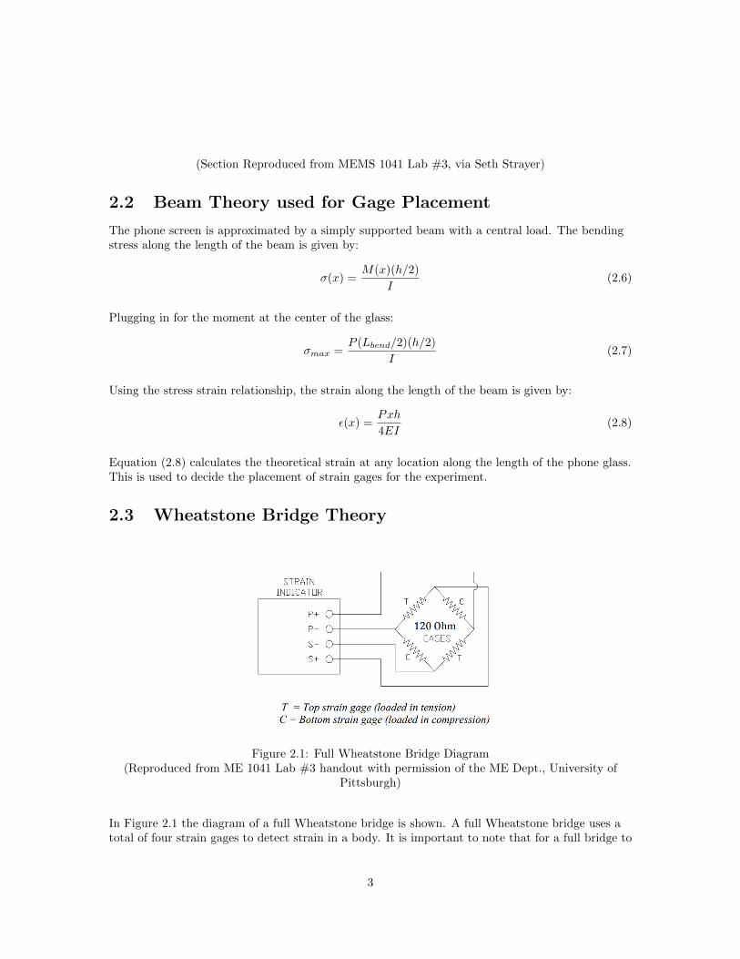
2.3 Wheatstone Bridge Theory

Figure 2.1: Full Wheatstone Bridge Diagram(Reproduced from ME 1041 Lab #3 handout with permission of the ME Dept., University of

Pittsburgh)

In Figure 2.1 the diagram of a full Wheatstone bridge is shown. A full Wheatstone bridge uses atotal of four strain gages to detect strain in a body. It is important to note that for a full bridge to

3

operate accurately, all gages must have equal resistances. If each gage has equal resistance, thebridge will be balanced and yield accurate results. Two strain gages are placed on both the topand bottom of the simply supported glass beam to create the desired arrangement. The full bridgeis widely considered to be the more accurate than quarter and half bridges because the greateramount of strain gages averages the strain and compensates for temperature affects. Below is theequation relating the bridge output to the measured strain:

δE

Eout=GF

4(εt1 − εc2 + εt3 − εc4) = GF · εavg (2.9)

(Section Reproduced from MEMS 1041 Lab #3, via Noah Sargent)

2.4 Signal Conditioning Theory

Signal conditioning is necessary to accurately measure the voltage output from a Wheatstonebridge. The circuit in this experiment utilizes a differential amplifier and a low pass filter to yield asignal without high-frequency noise and a large gain. A schematic of this circuit and a descriptionof the theory used to design the differential amplifier and low pass filter used in this experiment isprovided below.

Figure 2.2: Differential Amplifier and Low Pass Filter Layout(Reproduced from ME 1041 Semester Project - Circuitry Guidelines with permission of the ME

Dept., University of Pittsburgh)

A differential amplifier calculates the voltage difference between two signals and amplifies it. Inthis circuit, the differential amplifier calculates the difference of the output voltages from theWheatstone bridge according to Equation (2.10) as provided below:

V1gamp

= VA − VB (2.10)

The calculated voltage difference is then amplified by the ratio of the resistors shown in Equation(2.11):

4

gamp = R2/R1 (2.11)

The amplified difference of the inputted signal is then passed to the low pass filter.

Low pass filters reduce or eliminate frequencies above the cutoff frequency and amplify the outputvoltage. The low pass filter in this circuit filters out frequencies above the cutoff frequency which iscalculated using Equation (2.12), shown below:

fc =1

2πCR4(2.12)

The filter then amplifies the portion of the signal below the cutoff frequency by the ratio of theresistors shown in Equation (2.13) and outputs the signal:

gfilter = R4/R3 (2.13)

Lastly, the total gain of the circuit can be calculated by finding the product of the two gainsaccording to Equation (2.14), shown below:

gtotal = gamp · gfilter (2.14)

5

Chapter 3

Procedure

3.1 Relating Forces to Strain Gage Output

Consider the model shown in Figure 3.1, shown below. In this orientation, the glass screen can bemodeled as a simply-supported beam. The ball drop can be modeled as a point force localized atthe center of the beam. The supports will not be placed at the edges of the glass to eliminate anypossible stress concentrating effects of the holes in the glass. Thus, the bending length of the beammodel will be Lbend = 100 [mm].

Figure 3.1: Idealized Beam Orientation

Using this setup, the strain at the breakage point, displacement at the center of the glass, andmaximum force on the glass due to dropping the steel ball can be calculated. From the CorningGorilla Glass 3 Spec Sheet, the Elastic Modulus of the glass is E = 69.3 [GPa], and the breakagestress is predicted to be σult = 200 [MPa]. Thus, the ultimate strain at the point of breakage isgiven by:

εult =σultE

=200 · 106

69.3 · 109= 2886µε (3.1)

6

Next, solve for the maximum force on the glass due to dropping the steel ball. This result will beused to calculate the theoretical displacement at the center of the glass. The maximum stress inthe beams cross-section is given by:

σmax =Mmax(h/2)

I=

(Pmax/2)(x)(h/2)

I(3.2)

Let:

σmax = σult = 200 [MPa]x = Lbend/2 = 100/2 = 50 [mm] = 50 · 10−3 [m]h = 0.75 [mm] = 0.75 · 10−3 [m]b = 64 [mm] = 64 · 10−3 [m]

The second moment of area, I, is given by:

I =1

12bh3 =

1

12(64 · 10−3)(0.75 · 10−3)3 = 2.25 · 10−12[m4] (3.3)

Substituting this result into equation (3.2) and rearranging, the maximum anticipated forcenecessary to break the glass, say Pult, is:

Pult =2σultI

x(h/2)=

2(200 · 106)(2.25 · 10−12)

(50 · 10−3)(0.75 · 10−3/2)= 48[N ] (3.4)

This result can be used to solve for the maximum displacement. The maximum deflection of thebeam occurs at the center of the glass and is given by:

δ =PultL

3bend

48EI(3.5)

Substituting the values from above, the deflection at the point of breakage is:

δ =(48)(100 · 10−3)3

48(69.3 · 109)(2.25 · 10−12)= 6.4133[mm] (3.6)

Next, solve for the displacement at the center of the glass, say, d, as a function of the ball dropheight, z. By doing so, we are able to determine the height at which we expect the glass to break,given our result from equation (3.6). The ball is a 1.0” (25.4 mm) nominal diameter stainless steelsphere. The impact with the glass will cause the glass to bend elastically until the kinetic energy ofthe ball is stored in the “spring” deflection of the glass (or until the glass breaks). Thus, the glassis modeled as a linear spring with stiffness, K, given by:

K =48EI

L3bend

(3.7)

The force of the linear spring is a function of the displacement, d:

F = Kd (3.8)

7

Its stored energy, when compressed, is given by:

E =1

2Kd2 (3.9)

The kinetic energy of the ball when it impacts the glass is equal to the potential energy of the ballbefore it is dropped. Thus, if the ball is dropped from some height, z:

E =1

2mV 2 = mgz (3.10)

Combinining equations (3.9) and (3.10), and assuming that the glass ”spring” will absorb all of thekinetic energy upon impact:

E =1

2Kd2 = mgz (3.11)

The mass of the ball, m, is given by:

m = ρssV = ρss(4

3πR3) (3.12)

Substituting values into equation (3.12):

m = (7700)(4

3π(12.7 · 10−3)3) = 0.066068[kg] (3.13)

Then, from equations (3.7) and (3.11):

z =Kd2

2mg=

48EId2

2mgL3bend

=24EId2

mgL3bend

(3.14)

Substituting values, the ball drop height as a function of displacement is given by:

z =24EId2

mgL3bend

=24(69.3 · 109)(2.25 · 10−12)d2

(100 · 10−3)3(0.066068)(9.81)= 5773.9d2 (3.15)

Theoretically, the glass should break at the maximum displacement given by the result in (3.6).Thus, the ball drop height necessary to break the glass can be calculated by substitutingd = 6.4133 [mm] into equation (3.15):

zbreak = 5773.9(6.4133 · 10−3)2 = 0.23748[m] (3.16)

8

3.2 Gage Placement Procedure

To ensure that the strain gages are sensitive enough to detect the strain at the breakage force, themeasured strain should exceed 40µε while also being below 3000µε. The decision to place ourstrain gages 25 [mm] away from the central impact location was made by using the estimatedbreakage force and equation (2.8). We have:

ε(x) =(48)(0.050 − 0.025)(0.75 · 10−3)

4(69.3 · 109)(2.25 · 10−12)= 1443[µε] (3.17)

The predicted theoretical strain of 1443[µε] at 25 [mm] from the impact location is within thesensitivity range of the strain gage and far enough away from the impact location to avoid contactwith the steel ball. Thus, 25 [mm] away from the center of the glass is an acceptable location forstrain gage placement.

To compensate for temperature differences resulting from electrical heat generation and achieve anaverage strain value a full bridge arrangement is used. Four gages are placed on the top andbottom of the glass 25 [mm] away from the impact location in both directions. The strain gageswere placed along the centerline of the glass to limit the effects caused by three dimensionalbending. A diagram of the full bridge setup is shown below in Figure 3.2.

Figure 3.2: Gage Placement Diagram

3.3 Mounting and Wiring of Strain Gages

Achieving a proper bond between the glass and the strain gage is critical to achieving an accuratestrain measurement. First, a neutralizer is applied to the glass to ensure the application area isclean. Second, the gage is placed on a piece of scotch tape which is then attached to the screensuch that someone can apply a catalyst to the bottom. Third, a catalyst is applied to the bottomof the strain gage and allowed to dry for aproximately one minute. Finally, the adhesive is appliedto the application area and the strain gage is pressed to the glass and held until the bond is secure.Careful consideration must be given to the location of the application area so that it closelymatches the designed gage placement described previously.

The strain gage leads must be soldered to wire extensions so that the full bridge can be wired intothe breadboard circuit. Strain gages in tension must be wired opposite each other in the full bridgeto create the adding effect shown in Equation (2.9) and strain gages in compression must also bewired opposite each other. In this wiring arrangement, the signs of the resistance changes result in

9

a bridge constant, k, of 4, temperature effects cancel out, and the average of the four strain gageoutputs is measured, as shown in Equation (2.9).

3.4 Amplify & Condition Signal from Strain Gages

Signal amplification and conditioning are necessary to yield a measurable signal that is free ofhigh-frequency noise. In Theory Section 2.4, the design calculations for a circuit using a differentialamplifier and low pass filter combination to achieve the proper amplification and signalconditioning was laid out. Through mixing and matching the available resistors and capacitors it ispossible to design a circuit that fits the following criteria. First, the gain of the low pass filter anddifferential amplifier should be similar in value. Second, the product of the two gains should bearound 200 to ensure the signal is large enough to measure. Lastly, high-frequency noise must beeliminated by setting the cutoff frequency close to 100 [Hz]. Using the multimeter to measure thereal values of the selected resistors and capacitors, it is possible to calculate the overall gain andcutoff frequency of the circuit. The design calculations for the circuit used in this experiment areshown below:

Measured values:

R1 = 3.266[kΩ]R2 = 47.27[kΩ]R3 = 3.263[kΩ]R4 = 47.25[kΩ]C = 43.30[nF ]

From Equation (2.11):

gamp = R2/R1 =47.27

3.266= 14.47


fc =1

2πCR4=

1

2π(47.25 · 103)(43.30 · 10−9)= 77.8[Hz]


gfilter = R4/R3 =47.25

3.266= 14.60


gtotal = gamp · gfilter = 14.47 · 14.60 = 214.6

10

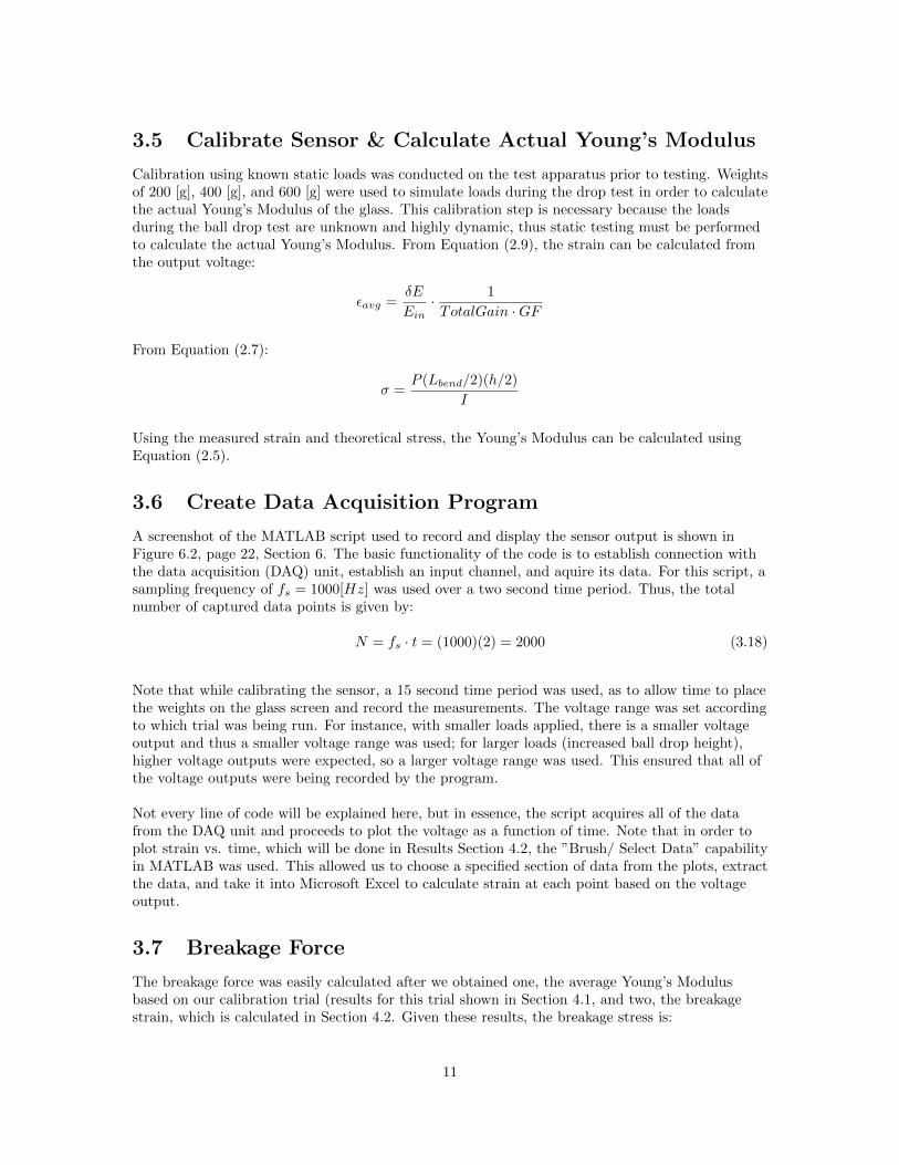
3.5 Calibrate Sensor & Calculate Actual Young’s Modulus

Calibration using known static loads was conducted on the test apparatus prior to testing. Weightsof 200 [g], 400 [g], and 600 [g] were used to simulate loads during the drop test in order to calculatethe actual Young’s Modulus of the glass. This calibration step is necessary because the loadsduring the ball drop test are unknown and highly dynamic, thus static testing must be performedto calculate the actual Young’s Modulus. From Equation (2.9), the strain can be calculated fromthe output voltage:

εavg =δE

Ein· 1

TotalGain ·GF


σ =P (Lbend/2)(h/2)

I

Using the measured strain and theoretical stress, the Young’s Modulus can be calculated usingEquation (2.5).

3.6 Create Data Acquisition Program

A screenshot of the MATLAB script used to record and display the sensor output is shown inFigure 6.2, page 22, Section 6. The basic functionality of the code is to establish connection withthe data acquisition (DAQ) unit, establish an input channel, and aquire its data. For this script, asampling frequency of fs = 1000[Hz] was used over a two second time period. Thus, the totalnumber of captured data points is given by:

N = fs · t = (1000)(2) = 2000 (3.18)

Note that while calibrating the sensor, a 15 second time period was used, as to allow time to placethe weights on the glass screen and record the measurements. The voltage range was set accordingto which trial was being run. For instance, with smaller loads applied, there is a smaller voltageoutput and thus a smaller voltage range was used; for larger loads (increased ball drop height),higher voltage outputs were expected, so a larger voltage range was used. This ensured that all ofthe voltage outputs were being recorded by the program.

Not every line of code will be explained here, but in essence, the script acquires all of the datafrom the DAQ unit and proceeds to plot the voltage as a function of time. Note that in order toplot strain vs. time, which will be done in Results Section 4.2, the ”Brush/ Select Data” capabilityin MATLAB was used. This allowed us to choose a specified section of data from the plots, extractthe data, and take it into Microsoft Excel to calculate strain at each point based on the voltageoutput.

3.7 Breakage Force

The breakage force was easily calculated after we obtained one, the average Young’s Modulusbased on our calibration trial (results for this trial shown in Section 4.1, and two, the breakagestrain, which is calculated in Section 4.2. Given these results, the breakage stress is:

11

σbreak = εbreakEavg (3.19)

Relating to moment by the bending equation:

σbreak =Mbreakc

I(3.20)

Such that:

Mbreak =σbreakI

c(3.21)

Force can be related to moment by the following:

Pbreak =M

x(3.22)

Thus, not only the breakage force, but the force for any trial during the ball drop test, can becalculated. Note that by definition of elementary mechanics, the force P is the reaction forceexperience at either support of the beam. Thus, the actual force submitted by the ball drop will betwice that as calculated above.

These force values were verified by making a plot of Force vs. Stress, based on our experimentalball drop data. This plot is shown in Figure 6.1, page 21, Section 6. By plotting a line of best fit,the anticipated force for any value of stress can be calculated. Thus, the process can essentially be”reverse engineered”. Indeed, by plugging in a value of σ = 200[MPa], we receive a value ofP = 48[N ], as anticipated in Section 3.1. These calculations are not directly stated, but they canbe easily verified by the graph.

3.8 Uncertainty Analysis

Uncertainty analysis is a tool used to estimate the measurement error associated with ameasurement system. During this experiment, multiple factors such as the error associated withelectrical components, dimensional error in the glass, differences in the gage factor, and multimetermeasurement error introduce uncertainty into the system. All these sources of error propagatethrough the measuring system. It is possible to estimate the combined uncertainty of the voltageoutput from the measurement system in this experiment by calculating the square root of the sumof squared uncertainties. The calculated uncertainty of the voltage output from the entiremeasurement system is ±11.4%. A detailed calculation of the combined uncertainty is shown inthe appendix section of this report (Section 6).

12

Chapter 4

Results

4.1 Calibration

A plot of stress vs. time for the calibration portion of the experiment is shown in Figure 4.1.

Figure 4.1: Calibration Trial - Strain vs. Time

Based on the equations provided in Section 3.5, Sensor Calibration, the actual Young’s Modulus ateach weight value can be calculated. These results are summarized in Table 1.The average Young’s Modulus based on all three calibration points is calculated to be:

Eavg = 6.89 · 1010 = 68.9[GPa] (4.1)

The result given by (4.1) is within 0.60 percent of the theoretical Young’s Modulus ofE = 69.3[GPa]. This result is used to calculate the experimental breakage stress, as shown inSection 4.3.

13

Table 1 - Calibration Trial Results

4.2 Ball Drop Results

Since many more trials had to be run than what was expected, only three ball drop plots areshown in the report. Particularly, Trial 1 - 30 in. ball drop height with 1 ball, Trial 5 - 50 in. balldrop height with 2 balls, and Trial 7 - 75 in. ball drop height with 3 balls. Note that Trial 7corresponded to the final breakage drop.

A plot of strain vs. time for Trial 1 is shown in Figure 4.2.

Figure 4.2: Trial 1 - Strain vs. Time

The maximum strain for this trial is:

ε1 = 8.92 · 10−4 = 892µε (4.2)

A plot of stain vs. time for Trial 5 is shown in Figure 4.3.The maximum strain for this trial is

14


ε5 = 1.83 · 10−3 = 1830µε (4.3)

A plot of stain vs. time for Trial 7, the final breakage drop, is shown in Figure 4.4, page 16.The maximum breakage strain is gven by:

εbreak = ε7 = 3.56 · 10−3 = 3560µε (4.4)

A table showing the results of all of the trials, including stress and force values, can be found inTable 2.

4.3 Breakage Stress

With our measured breakage strain given in (4.4), along with our calculated Young’s Modulus asin (4.1), the breakage stress can be calculated using Hooke’s Law:

σbreak = εbreakEavg = (3.56 · 10−3)(68.9 · 109)

σbreak ≈ 245[MPa] (4.5)

Given that the theoretical breakage strain was σult = 200[MPa] ± 30[MPa], we can use thenominal value to calculate the percent error in our breakage stress:

Errorσ = (245 − 200

200) · 100 = 22.5% (4.6)

15


Table 2 - Trial Results

A picture of the broken glass screen assembly is shown in Figure 6.3, page 23, Section 6.

4.4 Breakage Height

It has become obvious that the actual breakage height is much larger than the expected breakageheight, however the actual breakage stress is still somewhat within the range of the theoreticalbreakage stress. We can conclude that the glass ”spring” is not absorbing all of the kinetic energyfrom the ball, and thus there is a lower force associated with each ball height. In particular, from(3.16), and the result given from Trial 7 (4.4), the percent difference in breakage height values is:

Errorheight = (1.905 − 0.23748

0.23748) · 100 ≈ 702% (4.7)

16

Chapter 5

Discussion

5.1 Comparison to Theory

We wish to discuss how the expected strain due to known forces differs from the actual strainobtained from the experiment. This was partially discussed in the Calibration Results Section(4.1). The expected strain due to known forces was calculated using the stress values obtainedfrom such known forces and the reported elastic modulus of the glass, namely, E = 69.3[GPa]. Theactual strain obtained from measuerments was calculated by means of Equation 2.9, which relatesvoltage output, total gain, and the gage factor to the calculated strain. The results for thesecalibration trials are shown in Table 1. We note that there is very little error between any twovalues. In particular, by using the calculated strain values, we calculate an average Young’sModulus of

Eavg = 68.9[GPa]

which is within 0.60 % of the reported Young’s Modulus value. Therefore, the strain gage systemwas very accurate in obtaining strain measurements.

5.2 Comparison of Breakage Stress

From the Breakage Stress Results Section (4.3), the calculated breakage stress is

σbreak ≈ 245[MPa]

which maintains a 22.5% error with the theoretical breakage stress, namely σult = 200[MPa].Although this error is not negligable, if we consider the amount of uncertainty in ourmeasurements, the results are fairly accurate.

Furthermore, when calculating the percent error in the stress, given by Equation (4.6), we used thenominal value for theoretical stress. If the upper bound was used, we would calculate a percenterror of:

Errorσ = (245 − 230

230) · 100 = 6.52% (5.1)

17

This result should be very inspiring, given all of the uncertainties in the measurements (which israther plentiful for this large experiment). When taking into account the ± 11.4% uncertaintycalculated for our measuring system, the 6.25% error associated with experimental and expectedbreakage stress is well within the expected range. From this we can confidently say that ourcalculation for uncertainty is in agreement with our experimental results when compared to theexpected value for breakage stress.

We also wish to touch on the fact that our calculated breakage height was much higher than theanticapated breakage height. This was explained earlier in the report (Section 4.4) by the fact thatthe glass ”spring” is not absorbing all of the kinetic energy from the ball, and thus there is a lowerforce associated with each ball height.

On another note, the experimental error calculated during this experiment is exceptional. We wereable to predict the Young’s Modulus within 1% error of the expected value and experimentalbreakage stress was within the calculated uncertainty. This clearly shows that the full bridgearrangement and circuit design used in this experiment was able to accurately determine the strainin the glass. Based off of the varied results of other groups, we believe that full bridge is necessaryto capture the highly dynamic loading conditions during the drop test. If future experiments aredone, the use of a full bridge should be required and special care should be taken to ensure thegages are located far enough away from the impact area to prevent unwanted collisions.

As previously stated, a potential improvement to this measurement system would be supportingthe entire area of the phone glass. In this setup, simply supported beam theory would be replacedwith Hertzian contact as the theoretical model. This change would more closely replicate the realconditions of an actual phone. Also, the breakage height would be easier to calculate given thatphone glass is rigid and thus, will take the full brunt of the impact.

Overall, we are satisfied with our results. We have created a measurement system from scratch andbeen able to validate its results by applying the concepts of strain gage theory, beam theory,wheatstone bridge theory, signal conditioning theory, data acquisition, and uncertainty analysis. Inconclusion, the aftermarket iPhone 6 glass screen bodes well as a replacement to that of an originalscreen, given the calculated breakage stress of this measurement system.

18

Chapter 6

Appendix

6.1 Uncertainty Analysis

Consider the strain equation given by Equation (2.8). We can manipulate this equation to derivethe uncertainty in our beam strain measurement. We have that:

ε =3Px

Ebh2(6.1)

Then the uncertainty in the beam strain measurement is given by:

uεε

= [(uxx

)2 + (uPP

)2 + (uEE

)2 + (ubb

)2 + (2uhh

)2]].5

We will assume zero uncertainty in the load, P , and Young’s Modulus, E, since these are knownquantities. Then

uεε

= [(uxx

)2 + (ubb

)2 + (2uhh

)2]].5 (6.2)

Equation (6.2) represents the uncertainty in our beam strain measurement. Next consider theuncertainty in the strain gages themselves. Since

δR = GFεR0 (6.3)

The strain gage uncertainty is given by

uδRδR

= [(uGFGF

)2 + (uεε

)2 + (R0

R0)2]].5 (6.4)

Equation (6.4) represents the uncertainty in our strain gages. Next consider the uncertainty in ourWheatstone Bridge. We have that

E0 = Eik

4

δR

R0(6.5)

19

where the bridge constant, k, is equal to 4 for our full-bridge setup. If we assume zero uncertaintyfor this value, we have that

uE0

E0= [(

uEi

Ei)2 + (

uδRδR

)2 + (R0

R0)2]].5 (6.6)

Equation (6.6) represents the uncertainty in our Wheatstone Bridge. Next conisder the uncertaintyin our differential amplifier circuit. We have that

V1 =R2

R1(E01 − E02) (6.7)

Then the uncertainty in our differential amplifier circuit is given by

uV1

V1= [(

uR2

R2)2 + (

uR1

R1)2 + (

E0

E0)2]].5 (6.8)

Finally, consider the uncertainty in the low pass filter. We have that

Vout =R4

R3V1 (6.9)

Then the uncertainty in the low pass filter is given by

uVout

Vout= [(

uR3

R3)2 + (

uR4

R4)2 + (

V1V1

)2]].5 (6.10)

Using Equations (6.2), (6.4), (6.6), (6.8), (6.10), we can calculate the uncertainty at breakage. Theuncertainty values are given by the following:

R1 = R3 = 3.3[kΩ] ± 5%R2 = R4 = 47[kΩ] ± 5%GF = 2.105 ± 0.5%R0 = 120 ± 0.3%Ei = 10 ± 0.3%h = 0.75 ± 0.02[mm]b = 64 ± 0.5[mm]x = 100 ± 0.5[mm]

Then from (6.2),

uεε

= [(0.5

100)2 + (

0.5

64)2 + (2

.02

0.75)2]].5 = 5.41% (6.11)

Plugging this result into equation (6.4):

uδRδR

= [(0.5)2 + (5.41)2 + (0.3)2]].5 = 5.44% (6.12)


uE0

E0= [(0.3)2 + (5.44)2 + (0.3)2]].5 = 5.46% (6.13)

20


uV1

V1= [(5)2 + (5)2 + (5.46)2]].5 = 8.93% (6.14)


uVout

Vout= [(5)2 + (5)2 + (8.93)2]].5 = 11.4% (6.15)

6.2 Additional Figures

Figure 6.1: Force vs. Stress

21

Figure 6.2: Data Aquisition Script

22

Figure 6.3: Broken Glass Screen Assembly

23

List of Figures

2.1 Full Wheatstone Bridge Diagram . . . . . . . . . . . . . . . . . . . . . . . . . . . . . 32.2 Differential Amplifier and Low Pass Filter Layout . . . . . . . . . . . . . . . . . . . . 4

3.1 Idealized Beam Orientation . . . . . . . . . . . . . . . . . . . . . . . . . . . . . . . . 63.2 Gage Placement Diagram . . . . . . . . . . . . . . . . . . . . . . . . . . . . . . . . . 9

4.1 Calibration Trial - Strain vs. Time . . . . . . . . . . . . . . . . . . . . . . . . . . . . 134.2 Trial 1 - Strain vs. Time . . . . . . . . . . . . . . . . . . . . . . . . . . . . . . . . . . 144.3 Trial 5 - Strain vs. Time . . . . . . . . . . . . . . . . . . . . . . . . . . . . . . . . . . 154.4 Trial 7 - Strain vs. Time . . . . . . . . . . . . . . . . . . . . . . . . . . . . . . . . . . 16

6.1 Force vs. Stress . . . . . . . . . . . . . . . . . . . . . . . . . . . . . . . . . . . . . . . 216.2 Data Aquisition Script . . . . . . . . . . . . . . . . . . . . . . . . . . . . . . . . . . . 226.3 Broken Glass Screen Assembly . . . . . . . . . . . . . . . . . . . . . . . . . . . . . . 23

24

Term Project - University of Pittsburgh

Documents

Transcript of Term Project - University of Pittsburgh