290

A Comparison between the Pittsburgh and Michigan Approaches for theBinary PSO Algorithm

Alejandro CervantesComputer Science Department

Universidad Carlos III de MadridAvda. de la Universidad 30,

2891 1-Leganes, Madrid, Spain.alejandro.cervantes@uc3m.es

Ines GalvainComputer Science Department

Universidad Carlos III de MadridAvda. de la Universidad 30,

2891 1-Leganes, Madrid, Spain.ines.galvan@uc3m.es

Pedro IsasiComputer Science Department

Universidad Carlos III de MadridAvda. de la Universidad 30,

2891 1-Leganes, Madrid, Spain.pedro.isasi@ uc3m.es

Abstract- This paper shows the performance of the Bi-nary PSO Algorithm as a classification system. Thesesystems are classified in two different perspectives: thePittsburgh and the Michigan approaches. In order toimplement the Michigan Approach Binary PSO Algo-rithm, the standard PSO dynamic equations are modi-fied, introducing a repulsive force to favor particle com-petition. A dynamic neighborhood, adapted to classi-fication problems, is also defined. Both classifiers aretested using a reference set of problems, where both clas-sifiers achieve better performance than many classifi-cation techniques. The Michigan PSO classifier showsclear advantages over the Pittsburgh one both in termsof success rate and speed. The Michigan PSO can alsobe generalized to the continuous version of the PSO.

1 Introduction

The Particle Swarm Optimization algorithm (describedin [1]) is a biologically-inspired algorithm motivated by asocial analogy. Sometimes it is related to the EvolutionaryComputation (EC) techniques, basically with Genetic Algo-rithms (GA) and Evolutionary Strategies (ES), but there aresignificant differences with those techniques.A review of PSO fields of application can be found in [2].

There are also some good theoretical studies of PSO [3, 4,5] that address the topics of convergence, trajectory analysisand parameter selection. Also some modifications on thebasic algorithm are discussed in [4].

The algorithm is population-based: a set of potential so-lutions evolves to approach a convenient solution (or set ofsolutions) for a problem. Being an optimisation method, theaim is finding the global optimum of a real-valued function(fitness function) defined in a given space (search space).

The social metaphor that led to this algorithm can besummarized as follows: the individuals that are part of asociety hold an opinion that is part of a "belief space" (thesearch space) shared by every possible individual. Individ-uals may modify this "opinion state" based on three factors:

* the knowledge of the environment (its fitness value)* their previous history of states* the previous history of states of their neighborhood.An individual's neighborhood may be defined in several

ways, configuring somehow the "social network" of the in-dividual. Several neighborhood topologies exist (full, ring,star, etc.) depending on whether an individual interacts with

all, some, or only one of the rest of the population.In PSO terms, each individual is called a "particle", and

is subject to a movement in a multidimensional space thatrepresents the belief space. Particles have memory, thus re-taining part of their previous state. There is no restriction forparticles to share the same point in belief space, but in anycase their individuality is preserved. Each particle's move-ment is the composition of an initial random velocity andtwo randomly weighted influences: individuality, the ten-dency to return to the particle's best previous position, andsociality, the tendency to move towards the neighborhood'sbest previous position.

The base PSO algorithm uses a real-valued multidimen-sional space as belief space, and evolves the position of eachparticle in that space using the following equations:

Vid Wid C1l*1 *(Ptd-Xtdid)+C2*/2*(Ptgd-Xitd) (1)

t+l- t 1 t+lLid - id + 0id (2)vtd Component in dimension d of the ith particle

velocity in iteration t.Xid: Component in dimension d of the zt particle

position in iteration t.Cl ,C2: Constant weight factors.pi: Best position achieved so long by particle i.pg: Best position found by the neighbors

of particle i./1i ,12: Random factors in the [0,1] interval.w: Inertia weight.

A constraint (vtmax) is imposed on vtd to ensure con-vergence. Its value is usually kept within the interval_Xma'X,max], being XTaax the maximum value for the par-Lid Xid id

ticle position [6].A large inertia weight (w) favors global search, while a

small inertia weight favors local search. If inertia is used, itis sometimes decreased linearly during the iteration of thealgorithm, starting at an initial value close to 1 [6, 7].

An alternative formulation of Eq. 1 adds a constrictioncoefficient that replaces the velocity constraint (vmax) [3].

The PSO algorithm requires tuning of some parameters:the individual and sociality weights (cl ,C2), and the inertiafactor (w). Both theoretical and empirical studies are avail-able to help in selection of proper values [1, 3, 4, 5, 6, 7].A binary PSO algorithm has been developed in [1, 8].

This version has attracted much lesser attention in previouswork. In the binary version, the particle position is not a

0-7803-9363-5/05/$20.00 ©2005 IEEE.

Authorized licensed use limited to: Univ Carlos III. Downloaded on March 26, 2009 at 11:31 from IEEE Xplore. Restrictions apply.

291

real value, but either the binary 0 or 1. The logistic functionof the particle velocity is used as the probability distributionfor the position, that is, the particle position in a dimensionis randomly generated using that distribution. The equationthat updates the particle position becomes the following:

t+l 4 1 if 4 < ,t(3X - 1+e %'d (3)0 otherwise

vtj Component in dimension d of the ith particlevelocity in iteration t.

xtj+l: Component in dimension d of the ith particleposition in iteration t + 1.

b3: Random factor in the [0,1] interval.

This means that a binary PSO without individual and so-cial influences (cl = C2 = 0.0) would still perform a ran-dom search on the space (the position in each dimensionwould have a 0.5 chance of being a zero or one).

The selection of parameters for the binary version ofthe PSO algorithm has not been a subject of deep study inknown works.

This binary PSO has not been widely studied and somesubjects are still open [9]. Some modifications on the binaryalgorithm equations propose a quantic approach [10]. Aprevious article [11] also addresses classification problems.Recently, Clerc [12] proposes and performs an analysis ofalternative and more promising binary PSO algorithms.

The aim of this work is to evaluate the capacity of thebinary PSO algorithm in classification tasks. With this pur-pose, we have tested the algorithm using the two classicalapproaches taken from the GA community: the Pittsburghand the Michigan [13] approaches:

* In the Pittsburgh approach, each particle representsa full solution to the problem; in classification prob-lems, a single particle is able to produce a classifica-tion of the data by itself.

* In the Michigan approach, each particle representspart of the solution to the problem. A set of parti-cles or even the whole swarm is used to classify thedata.

In this paper we propose the introduction of the Michi-gan approach PSO classifier to solve certain problems thatarise when using the Pittsburgh version: its high dimension-ality and its difficulty to represent variable-length solutions.A reference set of problems (the Monk's set) has been

chosen for experimentation, so the results can be comparednot only between the two approaches but also with the re-sults of other techniques on these problems [14, 15].

This paper is organised as follows: section 2 describeshow the particles in the binary PSO algorithm may encodethe solution to a classification problem; section 3 describeshow the two approaches (Pittsburgh and Michigan) can beapplied to PSO; section 4 includes the modifications madeto the original PSO algorithm to implement the Michiganapproach; section 5 details the experimental setting and re-sults of experimentation; finally, section 6 discusses ourconclusions and future work related to the present study.

2 Binary Encoding for Classification Problems

The PSO algorithm will be tested on binary (two classes)classification problems with discrete attributes. The solu-tion will be expressed in terms of rules. Rule-based classi-fiers have the advantage that the result is readable, and someknowledge about the reasons behind the classifications maybe extracted from the rules.

The PSO will generate a set of rules that assign a classfrom the set {0,1} to a pattern set, part of which is usedto train the system (train set). Quality of the solution isevaluated testing the set of rules on a different set of patterns(test set) not used for the system training. Patterns are setsof values for each of the attributes in the domain.

Patterns and rules coding is taken from the GABIL sys-tem [16], an incremental learning system based on GeneticAlgorithms. This coding is described below.A pattern is a binary array with a set of bits for each

attribute in the domain, plus one bit for its expected classi-fication. Each attribute contributes a number of bits corre-sponding to the number of different values that the attributemay take. For each of the attributes, a single bit is set, cor-responding to the value of the attribute for that pattern. Theclass bit is set to 0 if the pattern expected class is class 0,and 1 if not.A rule is an array of the same length and structure as

patterns. The sets of bits for the attributes are interpretedas a conjunction of conditions over the set of attributes, andwill be called "attribute masks". Each condition refers toa single attribute; each bit set for an attribute means thatthe rule "matches" patterns with the corresponding valuefor that attribute. Attribute masks may have more than onebit set. Finally, the class bit of the rule is the class that therule assigns to every pattern it matches.

For instance, if the domain has two attributes (X, Y) andthree (Vo, VI', V2x) and two (vOT,V1Y) values respectivelyfor the attributes, a bit string such as "011 10 1" representsthe following rule: If (X = V,' or V2) and (Y = V0y) thenclass is 1. A more compact representation of this samplefollows:

Attributes E {X, Y}Values(X) (E {vo, v , v }Values(Y) E {v", v }Classes = {0,1}

0 1 1 1 0 1vb v v2 vY vy 1

Rule: (X= vxVX= vx)AY= vy Class - 1

3 Approaches for the PSO Algorithm

3.1 The Pittsburgh approach

As said in the Introduction, in this approach, each particlerepresents a full solution (a classifier).

Thus, each particle in a binary swarm will encode one ormore rules. The rules are read from left to right, and eval-uated in that order to provide the class that the particle as-

291

Authorized licensed use limited to: Univ Carlos III. Downloaded on March 26, 2009 at 11:31 from IEEE Xplore. Restrictions apply.

292

signs to a pattern. The first rule (from the left) that matchesa pattern assigns the class that is set in its class part, to thepattern, and classification stops; if no rule classifies the pat-tern it can either be marked as "unclassified" or assigned adefault class.

If some of the rules in a particle classify the pattern, wesay that the particle "matches" the pattern.

3.2 The Michigan approach

The former approach has problems for complex domains.The number of rules required to express the solution, whichis not known in advance, determines the dimension of thesearch space. Some estimation has to be made on start andthis can't be easily changed while the algorithm is running.That is, the equivalent to variable-length solutions in GAcan't be implemented easily.

If dimension is overestimated, the swarm has to updateexcess dimensions for each particle, with the correspondingloss in performance. In essence, this method will have trou-ble if it has to scale up to be able to solve complex problems(defined by many rules).We propose a modification of the PSO algorithm that

adopts a collective interpretation of the solution of the prob-lem. This is usually called the "Michigan approach" in thecontext of GA-based classifier systems.

In this approach, the solution to the posed problem is nota single particle in the swarm, but a subset of its particles.The Michigan approach classifier system was first proposedby Holland, the Learning Classifier System (LCS), in [13].A more recent example of a classifier system based on LCSisXCS [17].

Many of the classifier systems based on LCS implementa reinforcement learning mechanism. In this case, usefulpartial classifiers are rewarded in a way that increases theirchance to be present in the final solution.

However, in this paper, we use supervised learning. Inthis case each partial classifier (a single particle) is givena fitness value depending on the comparison between theexpected results (that are available for the training set), andthe actual results of the classification the classifier makes.In [18], different trends inside the LCS family are studied,and a supervised learning Michigan-style classifier based onGAs (UCS) is proposed.

For the Michigan approach to work in a supervised learn-ing context, the "local" fitness function used to calculatethe fitness of a single particle has to be such that favors theglobal evolution of the system to a good solution for thewhole problem.

The basic operation of the PSO algorithm is not modi-fied. Particle dimension depends only on the problem's do-main (rule length), while population depends on the numberof rules that may possibly conform a solution. On each iter-ation, the particle positions are updated using the PSO equa-tions. However, the swarm is also evaluated as a whole. Inour system, the global evaluation of the swarm is calculatedas follows:

1. In each iteration of the PSO algorithm, after particlesare updated, we obtain the set of particles that classify

the pattern (that is, the set of particles that don't markthe pattern as "unclassified"). This set is called the"matching set" for that pattern.

2. A class is assigned to the pattern using a selectionmethod among the particles in the matching set. Inthe experiments that follow, the selection methodwe've used is plain "best particle" selection; thatmeans that the class assigned to the pattern is the classassigned by the best particle (in terms of fitness) inthe matching set for that pattern. A voting selectionmethod might also be used. If the matching set forthe pattern is void, the pattern is unclassified by theswarm system.

3. Once a class (or no class) is assigned to each patternin the test set, the swarm may be numerically eval-uated with any measure that takes into account thesuccesses and failures in the classification. In our ex-periments we use Eq. 4, which gives the percentageof good classifications that we use to compare ourresults with the results of other techniques in [14].With this equation, unclassified patterns are countedas wrongly classified patterns.

Good classificationsSwazrm Evaluation = .100 (4)Total patterns

4 PSO Algorithm Modifications for the Michi-gan Approach

For the success of the Michigan approach, the algorithm hasto avoid convergence towards a single high-fitness particle,as this particle can only represent a very limited solution(only one rule).

Given Eq. 1, the sociality term tries to attract particlesto the proximity of the good solutions. As a consequence,to change the swarm behavior, in the Michigan approachwe dropped the sociality term and introduced the followingtwo modifications in the algorithm. Both have the purposeof maintaining population diversity among particles.

4.1 Competitive Particles

The intention is to enforce competition between particlesby making successful particles repel their neighbors. As aparticle represents one rule, if a particle with good fitness isalready in a given section of the search space, then the restwill explore different parts of that space.

There is previous work concerning repelling particles;for instance, in [19], repulsion is used to increase popula-tion diversity inside the standard attractive swarm.

The standard PSO updating equations include an indi-vidual and a social factor, that move each particle towardsthe best positions in its knowledge. To implement competi-tion, the social term in Eq. 1 is replaced by a repulsive term,as shown in Eq. 5 and Eq. 6, that replace the standard PSOequation for the velocity update (Eq. 1).

292

Authorized licensed use limited to: Univ Carlos III. Downloaded on March 26, 2009 at 11:31 from IEEE Xplore. Restrictions apply.

293

id+ = WV+Cl '01- (PAd-Xtd)+C2 - 2 (Pd )(5

,where

r1 if Ptd= Xtd -0d(Ptdi Xtd) = -1 if Pyd =4xd 1 (6)

0 if Pgd # X?d

Note that, except for the particles positions, Eq. 5 oper-ates with real arguments, while Eq. 3 transforms velocitiesto binary positions.

The function d(p'd, XSd) ensures that the particle is re-pelled by the best particle in its neighborhood when theirpositions are equal in a given dimension. Additionally, thisfactor is set to 0 if the best particle in the neighborhood isthe same particle whose position is being updated.

If the particle (binary) position is 0, the velocity changedue to this term will be in the positive direction (for ve-locities), making the position of the particle more likely tobecome a 1 when Eq. 3 is applied. The reverse is true whenits (binary) position is 1.

The repulsion term is weighted by a random factor (p2)and a fixed weight (c2) that becomes a new parameter forthe algorithm.

The modifications above can be generalized to the con-tinuous version of the PSO by changing the definition of thefunction d(pgd, Xid) with a distance based on the particles'positions.

4.2 Dynamic Neighborhood

The standard version of PSO uses a fixed neighborhoodtopology that represents the social influences. Particles areusually organized in a ring (or circle) topology; for N neigh-bors, neighborhood is usually defined as the particle itselfplus the closest (N-1) particles in the ring. We'll use theterm "static neighborhood" to refer to this topology.

However, when the repulsion factor is included (Eq. 5),neighborhood is better defined dynamically depending onthe proximity of the particles. We'll refer to this topologyas "dynamic neighborhood".

For each particle, this dynamic neighborhood is calcu-lated each iteration, based on a proximity criteria. For clas-sification problems, the proximity criteria used is the fol-lowing: two particles are "close" if they match some com-mon patterns in the training set. This is a phenotype cri-terium; a correspondent genotype criterium may also be de-fined (based on binary similarity). The neighborhood index(N) then determines the maximum number of particles se-lected as neighbors as follows: take the particle itself as thefirst neighbor, then the particle that shares more patterns assecond, and continue in decreasing order of number of pat-terns shared until N neighbors are selected.

The dynamic neighborhood version requires extra calcu-lations; however, pattern matching for each particle has tobe calculated to determine the particle fitness, so these cal-culations can be cached at some extra space cost to speedup the algorithm.

Suganthan [20] proposed a swarm with a local neighbor-hood whose size was gradually increased. Brits (in [21])justifies the introduction of topological neighborhood whensearching for multiple solutions in the context of nichingtechniques, which might be applied to the present work. Adifferent dynamic neighborhood has been proposed in [22]for multiobjective optimisation. The notion of selecting anindividual from a neighborhood has also been modified touse the center of clusters of particles in [23].

5 Experimentation

5.1 The Monk's problems

The Monk's set [14] is used to evaluate the binary PSO al-gorithm described in previous sections. Several techniquesused in machine learning were tested on these problemsin [14, 15].

The Monk's problems use a domain with 6 attributes(Ao, A1, A2,A3,A4, A5), with respectively 3, 3, 2, 3, 4 and2 discrete values (represented by integers), and two classesfor classification. There are 432 different possible attributepatterns in the set.

5.1.1 Monk's 1

The first Monk's problem provides a training set of 124 pat-terns and a test set of 432 patterns (the whole pattern set).Patterns include neither unknown attributes nor noise. Thesolution to the problem can be expressed as: "Class is 1 ifAO = A1 or A4 1, 0 otherwise".

In our rule syntax this condition may be expressed by thefollowing set of rules:

* (A4 - 1) -* classl* (Ao = 0)A (A1 = 0) classl* (Ao = 1) A (A1 = 1) classl* (Ao - 2) A (A1 - 2) classl* Extra rules for class 0 or a final rule that matches all

the patterns and assigns class 0.In the rules above, if an attribute is missing, its value

is irrelevant; with the selected codification, the rules thatrepresent this situation have all the bits that correspond tothose attributes set to 1.

5.1.2 Monk's 2

This problem is considered the hardest of the three, being aparity-like classification. The solution may be expressed asfollows: "If exactly two of the attributes have its first value,class is one, otherwise 0".

If the encoding allowed the representation of the inequal-ity, the classification might be expressed as several rules(one per combination of two attributes) of the followingform:

* (Ao = O)A(A1 = O)A(A2 $ O) A (A3 $& O) A (A4 5$0) A (A5 7$ 0) -> classl, etc.

With the encoding we used, rules above have to bechanged to express inequality in terms of the values avail-

293

Authorized licensed use limited to: Univ Carlos III. Downloaded on March 26, 2009 at 11:31 from IEEE Xplore. Restrictions apply.

294

able to for each attribute as follows:* (Ao = 0)A(A1 = 0)A(A2 = 1)A((A3 = 1)V(A3 -

2)) A ((A4 = 1) V (A4 = 2) V (A4 = 3)) A (A5 =1) -* classl, etc.

Again, either their complementary rules for class 0 or afinal rule that matches all the patterns and assigns class 0are also required.

The training set is composed of 169 patterns taken ran-domly, and the 432 patterns are used as test set.

5.1.3 Monk's 3

This problem is similar in complexity to Monk's 1, but the122 training patterns (taken randomly) have a 5% of mis-classifications. The whole pattern set is used for testing.The intention is to check the algorithm's behavior in pres-ence of noise. The solution is:

* (A3 = 0) A (A4 = 2) -* classl

* ((Al = 0) V (Al = 1)) A ((A4 = 0) V (A4 -1) V (A4 = 2)) -* classl

Again, either their complementary rules for class 0 or afinal rule that matches all the patterns and assigns class 0are also required.

5.2 Experimental Setting

5.2.1 Fitness Function

The fitness function used to evaluate the particles in thePittsburgh approach is given by Eq. 7:

Fitness { Good (7)Total

Good: Patterns correctly classified by the particleTotal: Number of patterns in the training set

In the Michigan approach, fitness for each particle is cal-culated using Eq. 8, which takes into account rules that onlymake good classifications, but also evaluates rules that makebad classifications, with a lower fitness.

(Good if BdJ Total Bad =0Fitness = (8)

Good Bad 1.0 otherwiseGood+Bad

Good:Bad:Total:

Patterns correctly classified by the particlePatterns wrongly classified by the particleNumber of patterns in the training set

5.2.2 Global Swarm Evaluation

The fitness functions defined above are "local" fitness func-tions, applied only when evaluating an isolated particle. Toevaluate the whole swarm as a classifier system, the proce-dure in section 3.2 is used, where the swarm evaluation isgiven by Eq. 4.

The system stores the best swarm evaluation obtainedand the particles that composed that swarm. This swarm isreturned as solution when the maximum number of itera-tions is reached.

5.2.3 Parameter selection

As it was mentioned before, the binary swarm has not beenas widely studied as the continuous version. This leads touncertainty about how the knowledge from the continuousversion can be extrapolated to the binary version.

One known difference is that the velocity constraintvmax operates in a different way in the binary version. Thisvalue gives the minimum probability for each value of theparticle position, so if this value is low, it becomes moredifficult for the particle to remain in a given position. Be-ing -vmax the minimum velocity, this probability may becalculated from Eq. 3:

P(Xlj1 = 1) > I+ (9)

To give particles some stability in a given position, thesetting for Vmax should be high, while in the continous(real) PSO it has to be low to ensure convergence.

The inertia weight was fixed to a constant value (1.0)because its influence on the binary PSO is not clear.We have compared the results of the Pittsburgh and

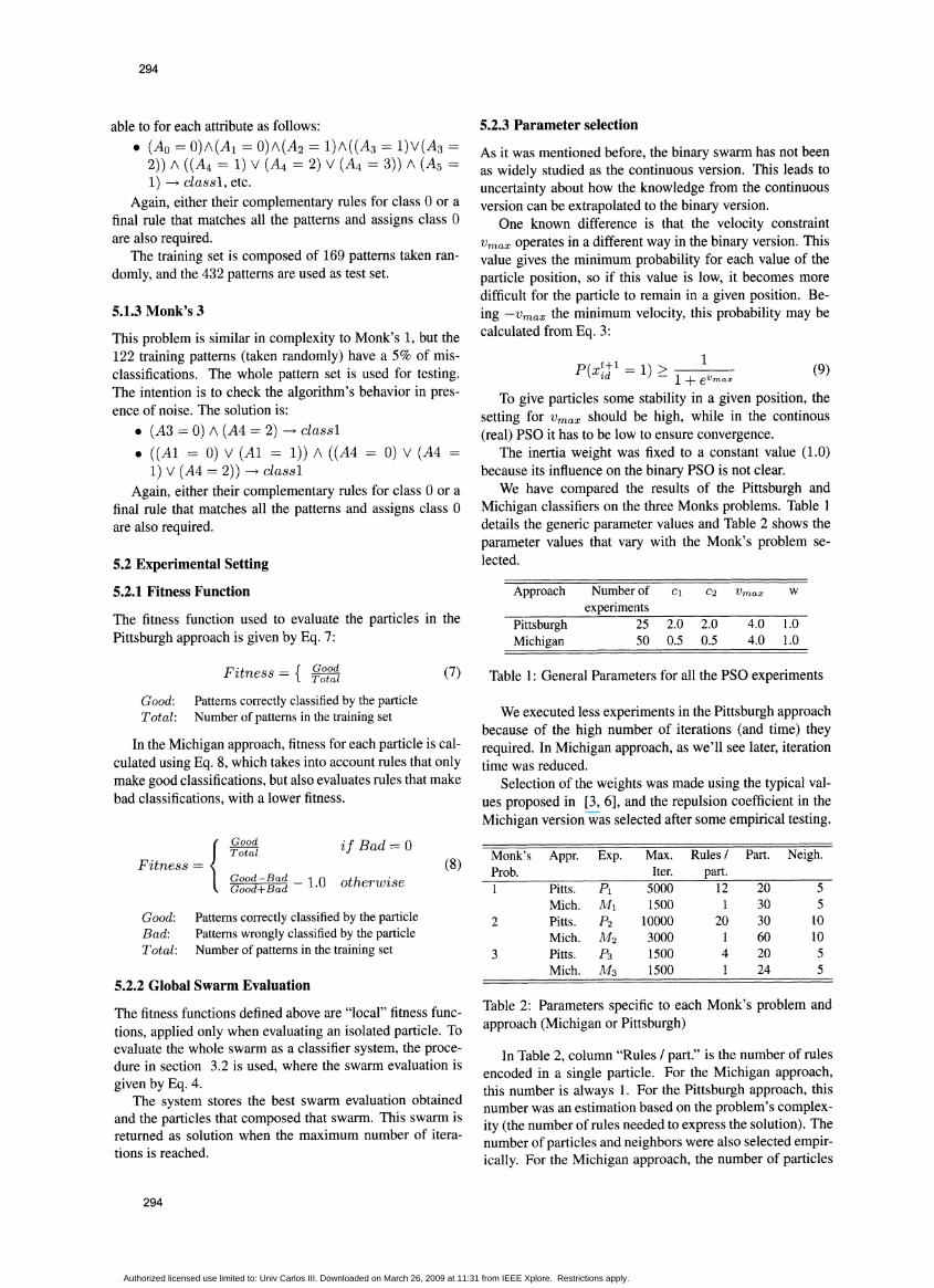
Michigan classifiers on the three Monks problems. Table 1details the generic parameter values and Table 2 shows theparameter values that vary with the Monk's problem se-lected.

Approach Number of cl C2 Vmax wexperiments

Pittsburgh 25 2.0 2.0 4.0 1.0Michigan 50 0.5 0.5 4.0 1.0

Table 1: General Parameters for all the PSO experiments

We executed less experiments in the Pittsburgh approachbecause of the high number of iterations (and time) theyrequired. In Michigan approach, as we'll see later, iterationtime was reduced.

Selection of the weights was made using the typical val-ues proposed in [3, 6], and the repulsion coefficient in theMichigan version was selected after some empirical testing.

Monk's Appr. Exp. Max. Rules / Part. Neigh.Prob. Iter. part.I Pitts. P1 5000 12 20 5

Mich. M1 1500 1 30 52 Pitts. P2 10000 20 30 10

Mich. M2 3000 1 60 103 Pitts. P3 1500 4 20 5

Mich. M3 1500 1 24 5

Table 2: Parameters specific to each Monk's problem andapproach (Michigan or Pittsburgh)

In Table 2, column "Rules / part." is the number of rulesencoded in a single particle. For the Michigan approach,this number is always 1. For the Pittsburgh approach, thisnumber was an estimation based on the problem's complex-ity (the number of rules needed to express the solution). Thenumber of particles and neighbors were also selected empir-ically. For the Michigan approach, the number of particles

294

(9)

Authorized licensed use limited to: Univ Carlos III. Downloaded on March 26, 2009 at 11:31 from IEEE Xplore. Restrictions apply.

295

has to be enough to represent the number of rules in thesolution.

5.3 Experimental Results

Success rate for every experiment is an average of the bestresult achieved by a particle (in the Pittsburgh approach) ora swarm (in the Michigan approach). That is, the best resultis recorded when running an instance of every experiment.

Table 3 reports the average results for the experimentsand the percentage of optimum solutions (solutions with100% accuracy) found. The column "Iter. number" showsthe average number of iterations that required the algorithmto reach the given success rate. The column "Rule Eval." isa measure of the number of times the algorithm had to applya rule to a set of patterns: it is the product of the number ofparticles, rules per particle and iterations.

Monk's Exp. Iter. Rule Succ. Optim.Prob. number Eval. Rate Found1 P1 1,561 374,640 96.8% 44.0%

ml 464 13,905 97.6% 40.0%2 P2 5,398 3,238,800 68.9% 0%

M2 1,516 90,936 75.0% 0%3 P3 955 76,400 96.9% 4.0%

M3 706 16,947 94.1% 0%

Table 3: Results of the experiments for Pittsburgh andMichigan approaches, for each of the Monk's problems

Table 4 shows the minimum and maximum success rateachieved for the Monk's 2 experiment and the distributionof results by ranges.

Exp. Min. Max. > 70% > 75% > 80%Succ Succ

P2 64.1% 75.9% 44.4% 4% 0%M2 68.8% 80.8% 94.0% 52% 2%

Table 4: Success rate distribution for the Monk's 2 prob-lem in both approaches, and frequency of results in differentsuccess levels

Fig. 1 shows the evolution of the actual (not the best)swarm evaluation at the iteration shown as the horizontalaxis, for the Michigan approach. This shows that the wholeswarm is converging. Note that this figure is not plotting thesame result shown in Table 3, that corresponds to the bestsolution achieved by the swarm during the iteration of thealgorithm.

5.4 Analysis of Results

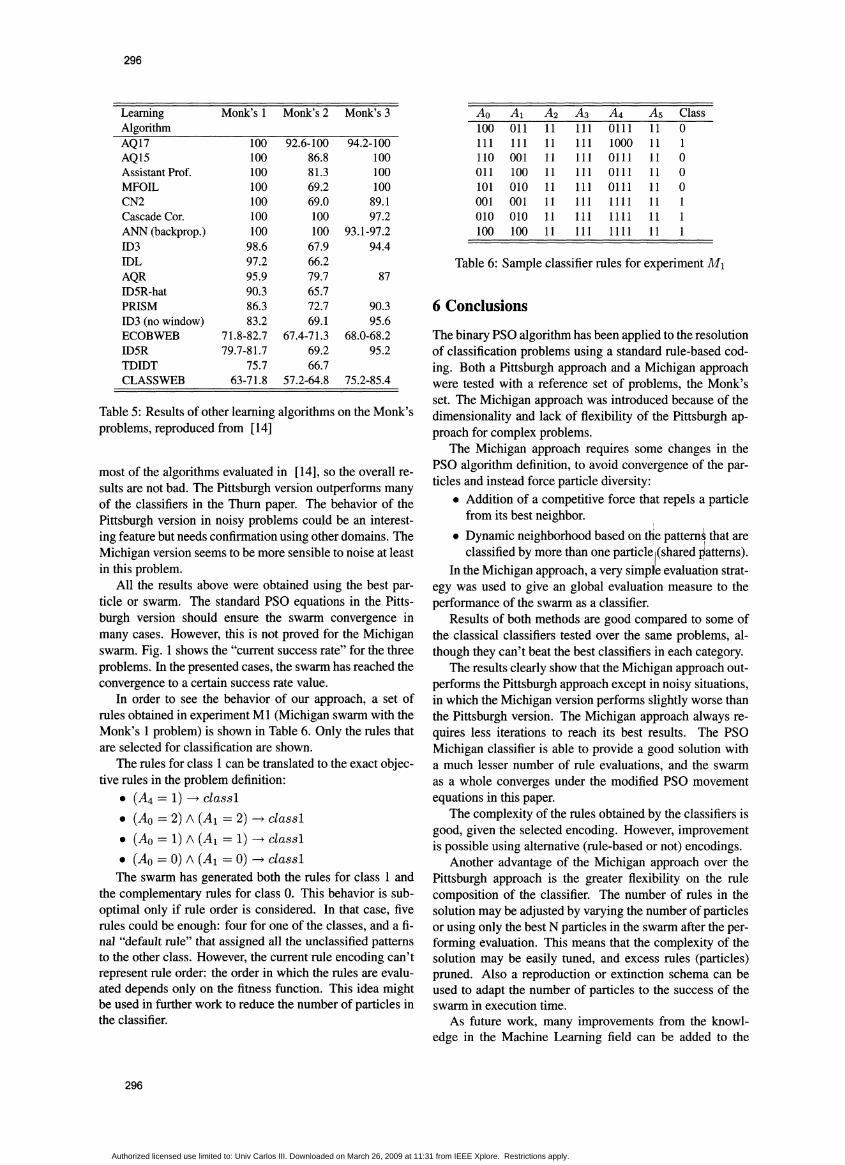
For reference, the results obtained in [14] by several ma-chine learning algorithms on the Monk's problems areshown in Table 5.

For the Monk's 1 problem, described in [14] as an"easy" problem, both the Pittsburgh and Michigan ap-proaches achieve not only high success rate but they arealso able to find the optimum. This is interesting as thelack of ability to find optimum values is one of the binary

c2

0C4

ct

u:

100%

90%

80%

70%

60%

50%

40%

30%

20%

10%

./ MvlonK s 1

7 Monk's 2Monk's 32 40 60 .. 1000 1 1400

0 200 400 600 800 1000 1200 1400Iterations

Figure 1: Actual swarm evaluation by iteration number inthe Michigan approach, for the Monk's problems 1 to 3 (av-erage of 50 experiments)

PSO drawbacks according to [9]. The Michigan approachachieves a slighter higher success rate and it needs a muchsmaller number of iterations to reach that success rate.

The motivation of trying the Michigan approach isclearly shown checking the rule evaluations column in Ta-ble 3. The Michigan approach outperforms the Pittsburghhapproach by an order of magnitude.

For the Monk's 2 problem, which is described as a com-plex problem, with a XOR-like distribution of patterns, theMichigan approach also clearly achieves a better successrate than the Pittsburgh one. In [14] the results for thisproblem were in the range 65-70% for most of the classi-fiers, so the results of PSO in this case are comparable oreven better than many of them.

The iteration and number of rule evaluations is quite fa-vorable to the Michigan approach again in this problem.The high evaluation cost for the Pittsburgh approach is dueto two reasons:

* the high number of rules needed to represent thisproblem (high dimensionality).

* the fact that Pittsburgh instances needed a muchhigher number of iterations in order to reach a bettersuccess rate.

Table 4 strongly suggests that the Michigan approach isclearly better than the Pittsburgh approach, because it wasable to find classifiers with a success rate better than 70%in the most (94%) of the runs of the Michigan experiment,while Pittsburgh approach is unable to find good solutionsin more than half of the runs. This difference is even greaterwhen trying to find more accurate solutions. Pittsburgh ap-proach is almost unable to find solutions with better than75% success , while Michigan approach reached this valuemore than 50% of the times.

The Monk's 3 problem, that includes noise, is the one inwhich the Michigan version is unable to improve the Pitts-burgh version. Noise severely degrades the performance of

295

Authorized licensed use limited to: Univ Carlos III. Downloaded on March 26, 2009 at 11:31 from IEEE Xplore. Restrictions apply.

296

Learning Monk's 1 Monk's 2 Monk's 3AlgorithmAQ17 100 92.6-100 94.2-100AQ15 100 86.8 100Assistant Prof. 100 81.3 100MFOIL 100 69.2 100CN2 100 69.0 89.1Cascade Cor. 100 100 97.2ANN (backprop.) 100 100 93.1-97.2ID3 98.6 67.9 94.4IDL 97.2 66.2AQR 95.9 79.7 87ID5R-hat 90.3 65.7PRISM 86.3 72.7 90.3ID3 (no window) 83.2 69.1 95.6ECOBWEB 71.8-82.7 67.4-71.3 68.0-68.2ID5R 79.7-81.7 69.2 95.2TDIDT 75.7 66.7CLASSWEB 63-71.8 57.2-64.8 75.2-85.4

Table 5: Results of other learning algorithms on the Monk'sproblems, reproduced from [14]

most of the algorithms evaluated in [14], so the overall re-sults are not bad. The Pittsburgh version outperforms manyof the classifiers in the Thurn paper. The behavior of thePittsburgh version in noisy problems could be an interest-ing feature but needs confirmation using other domains. TheMichigan version seems to be more sensible to noise at leastin this problem.

All the results above were obtained using the best par-ticle or swarm. The standard PSO equations in the Pitts-burgh version should ensure the swarm convergence inmany cases. However, this is not proved for the Michiganswarm. Fig. 1 shows the "current success rate" for the threeproblems. In the presented cases, the swarm has reached theconvergence to a certain success rate value.

In order to see the behavior of our approach, a set ofrules obtained in experiment MI (Michigan swarm with theMonk's 1 problem) is shown in Table 6. Only the rules thatare selected for classification are shown.

The rules for class 1 can be translated to the exact objec-tive rules in the problem definition:

* (A4 = 1) -+ classl* (Ao = 2) A (A1 = 2) - classl* (Ao = 1) A (A1 = 1) - classl* (Ao = 0) A (A1 = 0) classlThe swarm has generated both the rules for class 1 and

the complementary rules for class 0. This behavior is sub-optimal only if rule order is considered. In that case, fiverules could be enough: four for one of the classes, and a fi-nal "default rule" that assigned all the unclassified patternsto the other class. However, the current rule encoding can'trepresent rule order: the order in which the rules are evalu-ated depends only on the fitness function. This idea mightbe used in further work to reduce the number of particles inthe classifier.

Ao A1 A2 A3 A4 A5 Class100 011 11 111 0111 11 0ill ill 11 ill 1000 11 I110 001 11 111 0111 11 0011 100 11 111 0111 11 0101 010 11 111 0111 11 0001 001 11 111 1111 11 1010 010 11 111 1111 11 1100 100 11 111 1111 11 1

Table 6: Sample classifier rules for experiment Ml

6 Conclusions

The binary PSO algorithm has been applied to the resolutionof classification problems using a standard rule-based cod-ing. Both a Pittsburgh approach and a Michigan approachwere tested with a reference set of problems, the Monk'sset. The Michigan approach was introduced because of thedimensionality and lack of flexibility of the Pittsburgh ap-proach for complex problems.

The Michigan approach requires some changes in thePSO algorithm definition, to avoid convergence of the par-ticles and instead force particle diversity:

* Addition of a competitive force that repels a particlefrom its best neighbor.

* Dynamic neighborhood based on the patternA that areclassified by more than one particle (shared patterns).

In the Michigan approach, a very simple evaluation strat-egy was used to give an global evaluation measure to theperformance of the swarm as a classifier.

Results of both methods are good compared to some ofthe classical classifiers tested over the same problems, al-though they can't beat the best classifiers in each category.

The results clearly show that the Michigan approach out-performs the Pittsburgh approach except in noisy situations,in which the Michigan version performs slightly worse thanthe Pittsburgh version. The Michigan approach always re-quires less iterations to reach its best results. The PSOMichigan classifier is able to provide a good solution witha much lesser number of rule evaluations, and the swarmas a whole converges under the modified PSO movementequations in this paper.

The complexity of the rules obtained by the classifiers isgood, given the selected encoding. However, improvementis possible using alternative (rule-based or not) encodings.

Another advantage of the Michigan approach over thePittsburgh approach is the greater flexibility on the rulecomposition of the classifier. The number of rules in thesolution may be adjusted by varying the number of particlesor using only the best N particles in the swarm after the per-forming evaluation. This means that the complexity of thesolution may be easily tuned, and excess rules (particles)pruned. Also a reproduction or extinction schema can beused to adapt the number of particles to the success of theswarm in execution time.

As future work, many improvements from the knowl-edge in the Machine Learning field can be added to the

296

Authorized licensed use limited to: Univ Carlos III. Downloaded on March 26, 2009 at 11:31 from IEEE Xplore. Restrictions apply.

297

Michigan classifier; specifically, a more sophisticated par-ticle evaluation strategy is being investigated.

Also, we are performing more exhaustive investigationon the repulsion term introduced in the algorithm and thedynamic neighborhood topology, that may lead to improve-ment on the Michigan PSO and deeper understanding of itsconvergence and stagnation conditions. The modificationsmade to the PSO equations will also be generalized to thecontinuous version of the PSO algorithm.

Acknowledgments

This article has been financed by the Spanish founded re-search MCyT project TRACER, (TIC2002-04498-C05-04).

Bibliography

[1] J. Kennedy, R.C. Eberhart, and Y. Shi. Swarm intelli-gence. Morgan Kaufmann Publishers, San Francisco,2001.

[2] K. E. Parsopoulos and M. N. Vrahatis. Recent ap-proaches to global optimization problems through par-ticle swarm optimization. Natural Computing: an in-ternationaljournal, 1(2-3):235-306, 2002.

[3] Maurice Clerc and James Kennedy. The particleswarm - explosion, stability, and convergence in amultidimensional complex space. IEEE Trans. Evo-lutionary Computation, 6(1):58-73, 2002.

[4] Frans van den Bergh. An analysis ofparticle swarmoptimizers. PhD thesis, University of Pretoria, SouthAfrica, 2002.

[5] loan Cristian Trelea. The particle swarm optimizationalgorithm: convergence analysis and parameter selec-tion. Inf: Process. Lett., 85(6):317-325, 2003.

[6] Y. Shi and R.C. Eberhart. Parameter selection in parti-cle swarm optimization. In Proceedings of the Sev-enth Annual Conference on Evolutionary Program-ming, pages 591-600, 1998.

[7] Y. Shi and R.C. Eberhart. Empirical study of parti-cle swarm optimization. In Proceedings of the IEEECongress on Evolutionary Computation (CEC), pages1945-1950, 1999.

[8] J. Kennedy and R.C. Eberhart. A discrete binary ver-sion of the particle swarm algorithm. In Proceedingsof the World Multiconference on Systemics, Cybernet-ics and Informatics, pages 4104-4109, 1997.

[9] Xiaohui Hu, Yuhui Shi, and Russ Eberhart. Recentadvances in particle swarm. In Proceedings of IEEECongress on Evolutionary Computation 2004 (CEC2004), pages 90-97, 2004.

[10] Shuyuan Yang, Min Wang, and Licheng Jiao. A quan-tum particle swarm optimization. In Proceedings ofIEEE Congress on Evolutionary Computation 2004(CEC 2004), pages 320-331, 2004.

[11] Tiago Sousa, Arlindo Silva, and Ana Neves. Particleswarm based data mining algorithms for classificationtasks. Parallel Comput., 30(5-6):767-783, 2004.

[12] Maurice Clerc. Binary particle swarm optimis-ers: toolbox, derivations and mathematical insights.http://clerc.maurice.free.fr/psolbinary-pso.

[13] J.H. Holland. Adaptation. Progress in theoretical bi-ology, pages 263-293, 1976.

[14] S. B. Thrun et al. The MONK's problems: A per-formance comparison of different learning algorithms.Technical Report CS-91-197, Pittsburgh, PA, 1991.

[15] Shaun Saxon and Alwyn Barry. XCS and the monk'sproblems. In Wolfgang Banzhaf, Jason Daida, Agos-ton E. Eiben, Max H. Garzon, Vasant Honavar, MarkJakiela, and Robert E. Smith, editors, Proceedings ofthe Genetic and Evolutionary Computation Confer-ence, volume 1, page 809, Orlando, Florida, USA, 13-17 1999. Morgan Kaufmann.

[16] Kenneth A. De Jong and William M. Spears. Learningconcept classification rules using genetic algorithms.In Proceedings of the Twelfth International Confer-ence on Artificial Intelligence (IJCAI), volume 2,1991.

[17] Steward W. Wilson. Classifier fitness based on accu-racy. Evolutionary Computation, 3(2):149-175, 1995.

[18] Ester Bemado-Mansilla and Josep M. Garrell-Guiu.Accuracy-based learning classifier systems: models,analysis and applications to classification tasks. Evol.Comput., 11(3):209-238, 2003.

[19] T. M. Blackwell and Peter J. Bentley. Dynamic searchwith charged swarms. In Proceedings of the Ge-netic and Evolutionary Computation Conference 2002(GECCO), pages 19-26, 2002.

[20] P. N. Suganthan. Particle swarm optimiser withneighbourhood operator. In Proceedings of the IEEECongress on Evolutionary Computation (CEC), pages1958-1962, 1999.

[21] Riaan Brits. Niching strategies for particle swarm op-timization. Master's thesis, University of Pretoria, Pre-toria, 2002.

[22] X. Hu and R.C. Eberhart. Multiobjective optimizationusing dynamic neighborhood particle swarm optimi-sation. In Proceedings of the IEEE Congress on Evo-lutionary Computation (CEC), pages 1677-16, 2002.

[23] J. Kennedy. Stereotyping: improving particle swarmperformance with cluster analysis. In Proceedingsof the IEEE Congress on Evolutionary Computation(CEC), pages 1507-1512, 2000.

297

Authorized licensed use limited to: Univ Carlos III. Downloaded on March 26, 2009 at 11:31 from IEEE Xplore. Restrictions apply.