Carnegie Mellon UniversityResearch Showcase

Department of Physics Mellon College of Science

2-1-2009

Multiscale modeling of emergent materials:biological and soft matterTeemu MurtolaHelsinki University of Technology

Alex BunkerUniversity of Helsinki

Ilpo VattulainenHelsinki University of Technology

Markus DesernoCarnegie Mellon University, deserno@andrew.cmu.edu

Mikko KarttunenUniversity of Western Ontario

Follow this and additional works at: http://repository.cmu.edu/physics

This Article is brought to you for free and open access by the Mellon College of Science at Research Showcase. It has been accepted for inclusion inDepartment of Physics by an authorized administrator of Research Showcase. For more information, please contact research-showcase@andrew.cmu.edu.

Recommended CitationMurtola, Teemu; Bunker, Alex; Vattulainen, Ilpo; Deserno, Markus; and Karttunen, Mikko, "Multiscale modeling of emergentmaterials: biological and soft matter" (2009). Department of Physics. Paper 32.http://repository.cmu.edu/physics/32

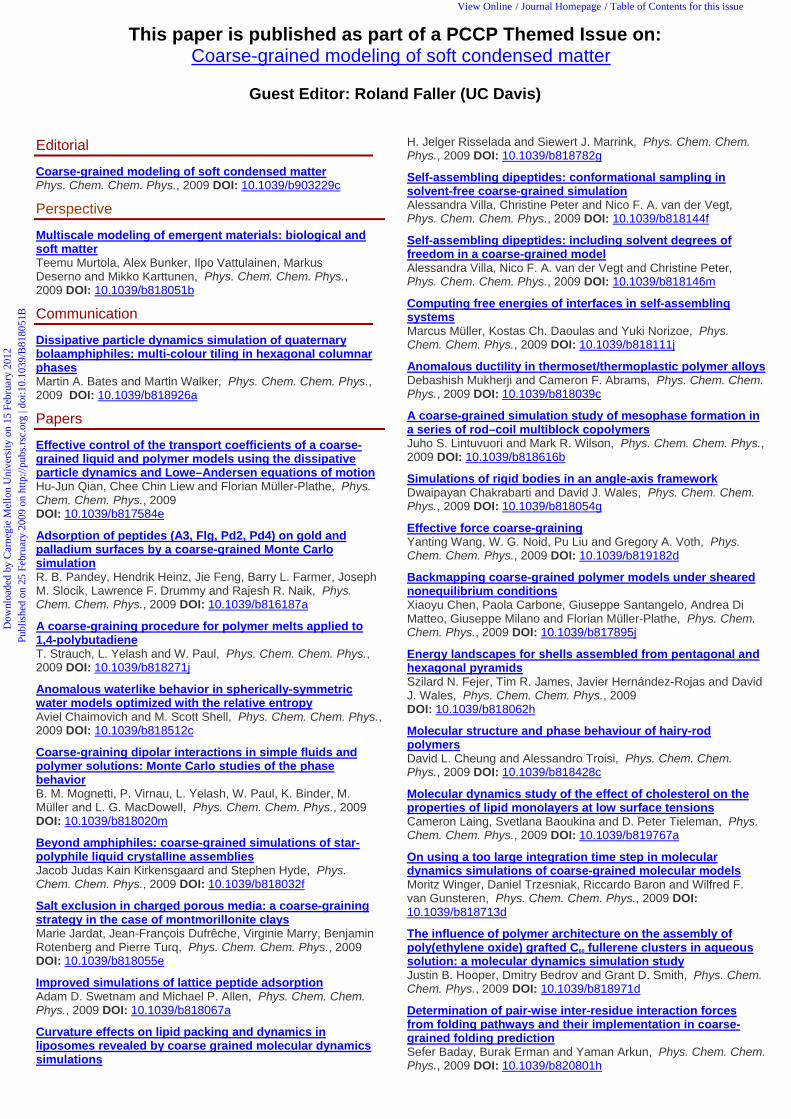
This paper is published as part of a PCCP Themed Issue on: Coarse-grained modeling of soft condensed matter

Guest Editor: Roland Faller (UC Davis)

Editorial

Coarse-grained modeling of soft condensed matter Phys. Chem. Chem. Phys., 2009 DOI: 10.1039/b903229c

Perspective

Multiscale modeling of emergent materials: biological and soft matter Teemu Murtola, Alex Bunker, Ilpo Vattulainen, Markus Deserno and Mikko Karttunen, Phys. Chem. Chem. Phys., 2009 DOI: 10.1039/b818051b

Communication

Dissipative particle dynamics simulation of quaternary bolaamphiphiles: multi-colour tiling in hexagonal columnar phases Martin A. Bates and Martin Walker, Phys. Chem. Chem. Phys., 2009 DOI: 10.1039/b818926a

Papers

Effective control of the transport coefficients of a coarse-grained liquid and polymer models using the dissipative particle dynamics and Lowe–Andersen equations of motion Hu-Jun Qian, Chee Chin Liew and Florian Müller-Plathe, Phys. Chem. Chem. Phys., 2009 DOI: 10.1039/b817584e

Adsorption of peptides (A3, Flg, Pd2, Pd4) on gold and palladium surfaces by a coarse-grained Monte Carlo simulation R. B. Pandey, Hendrik Heinz, Jie Feng, Barry L. Farmer, Joseph M. Slocik, Lawrence F. Drummy and Rajesh R. Naik, Phys. Chem. Chem. Phys., 2009 DOI: 10.1039/b816187a

A coarse-graining procedure for polymer melts applied to 1,4-polybutadiene T. Strauch, L. Yelash and W. Paul, Phys. Chem. Chem. Phys., 2009 DOI: 10.1039/b818271j

Anomalous waterlike behavior in spherically-symmetric water models optimized with the relative entropy Aviel Chaimovich and M. Scott Shell, Phys. Chem. Chem. Phys., 2009 DOI: 10.1039/b818512c

Coarse-graining dipolar interactions in simple fluids and polymer solutions: Monte Carlo studies of the phase behavior B. M. Mognetti, P. Virnau, L. Yelash, W. Paul, K. Binder, M. Müller and L. G. MacDowell, Phys. Chem. Chem. Phys., 2009 DOI: 10.1039/b818020m

Beyond amphiphiles: coarse-grained simulations of star-polyphile liquid crystalline assemblies Jacob Judas Kain Kirkensgaard and Stephen Hyde, Phys. Chem. Chem. Phys., 2009 DOI: 10.1039/b818032f

Salt exclusion in charged porous media: a coarse-graining strategy in the case of montmorillonite clays Marie Jardat, Jean-François Dufrêche, Virginie Marry, Benjamin Rotenberg and Pierre Turq, Phys. Chem. Chem. Phys., 2009 DOI: 10.1039/b818055e

Improved simulations of lattice peptide adsorption Adam D. Swetnam and Michael P. Allen, Phys. Chem. Chem. Phys., 2009 DOI: 10.1039/b818067a

Curvature effects on lipid packing and dynamics in liposomes revealed by coarse grained molecular dynamics simulations

H. Jelger Risselada and Siewert J. Marrink, Phys. Chem. Chem. Phys., 2009 DOI: 10.1039/b818782g

Self-assembling dipeptides: conformational sampling in solvent-free coarse-grained simulation Alessandra Villa, Christine Peter and Nico F. A. van der Vegt, Phys. Chem. Chem. Phys., 2009 DOI: 10.1039/b818144f

Self-assembling dipeptides: including solvent degrees of freedom in a coarse-grained model Alessandra Villa, Nico F. A. van der Vegt and Christine Peter, Phys. Chem. Chem. Phys., 2009 DOI: 10.1039/b818146m

Computing free energies of interfaces in self-assembling systems Marcus Müller, Kostas Ch. Daoulas and Yuki Norizoe, Phys. Chem. Chem. Phys., 2009 DOI: 10.1039/b818111j

Anomalous ductility in thermoset/thermoplastic polymer alloys Debashish Mukherji and Cameron F. Abrams, Phys. Chem. Chem. Phys., 2009 DOI: 10.1039/b818039c

A coarse-grained simulation study of mesophase formation in a series of rod–coil multiblock copolymers Juho S. Lintuvuori and Mark R. Wilson, Phys. Chem. Chem. Phys., 2009 DOI: 10.1039/b818616b

Simulations of rigid bodies in an angle-axis framework Dwaipayan Chakrabarti and David J. Wales, Phys. Chem. Chem. Phys., 2009 DOI: 10.1039/b818054g

Effective force coarse-graining Yanting Wang, W. G. Noid, Pu Liu and Gregory A. Voth, Phys. Chem. Chem. Phys., 2009 DOI: 10.1039/b819182d

Backmapping coarse-grained polymer models under sheared nonequilibrium conditions Xiaoyu Chen, Paola Carbone, Giuseppe Santangelo, Andrea Di Matteo, Giuseppe Milano and Florian Müller-Plathe, Phys. Chem. Chem. Phys., 2009 DOI: 10.1039/b817895j

Energy landscapes for shells assembled from pentagonal and hexagonal pyramids Szilard N. Fejer, Tim R. James, Javier Hernández-Rojas and David J. Wales, Phys. Chem. Chem. Phys., 2009 DOI: 10.1039/b818062h

Molecular structure and phase behaviour of hairy-rod polymers David L. Cheung and Alessandro Troisi, Phys. Chem. Chem. Phys., 2009 DOI: 10.1039/b818428c

Molecular dynamics study of the effect of cholesterol on the properties of lipid monolayers at low surface tensions Cameron Laing, Svetlana Baoukina and D. Peter Tieleman, Phys. Chem. Chem. Phys., 2009 DOI: 10.1039/b819767a

On using a too large integration time step in molecular dynamics simulations of coarse-grained molecular models Moritz Winger, Daniel Trzesniak, Riccardo Baron and Wilfred F. van Gunsteren, Phys. Chem. Chem. Phys., 2009 DOI: 10.1039/b818713d

The influence of polymer architecture on the assembly of poly(ethylene oxide) grafted C60 fullerene clusters in aqueous solution: a molecular dynamics simulation study Justin B. Hooper, Dmitry Bedrov and Grant D. Smith, Phys. Chem. Chem. Phys., 2009 DOI: 10.1039/b818971d

Determination of pair-wise inter-residue interaction forces from folding pathways and their implementation in coarse-grained folding prediction Sefer Baday, Burak Erman and Yaman Arkun, Phys. Chem. Chem. Phys., 2009 DOI: 10.1039/b820801h

Dow

nloa

ded

by C

arne

gie

Mel

lon

Uni

vers

ity o

n 15

Feb

ruar

y 20

12Pu

blis

hed

on 2

5 Fe

brua

ry 2

009

on h

ttp://

pubs

.rsc

.org

| do

i:10.

1039

/B81

8051

BView Online / Journal Homepage / Table of Contents for this issue

Multiscale modeling of emergent materials: biological and soft matter

Teemu Murtola,aAlex Bunker,

bcIlpo Vattulainen,

adeMarkus Deserno

f

and Mikko Karttunen*g

Received 14th October 2008, Accepted 12th February 2009

First published as an Advance Article on the web 25th February 2009

DOI: 10.1039/b818051b

In this review, we focus on four current related issues in multiscale modeling of soft and biological matter.

First, we discuss how to use structural information from detailed models (or experiments) to construct

coarse-grained ones in a hierarchical and systematic way. This is discussed in the context of the so-called

Henderson theorem and the inverse Monte Carlo method of Lyubartsev and Laaksonen. In the second part, we

take a different look at coarse graining by analyzing conformations of molecules. This is done by the application

of self-organizing maps, i.e., a neural network type approach. Such an approach can be used to guide the

selection of the relevant degrees of freedom. Then, we discuss technical issues related to the popular dissipative

particle dynamics (DPD) method. Importantly, the potentials derived using the inverse Monte Carlo method can

be used together with the DPD thermostat. In the final part we focus on solvent-free modeling which offers a

different route to coarse graining by integrating out the degrees of freedom associated with solvent.

I. Introduction

A Emergent properties

In biological and soft matter systems a broad spectrum of modes

of motion, operating over an immense range of length and time

scales, are simultaneously active at ambient temperature. These

modes can not be trivially uncoupled, resulting in multiscale

behaviour: the systems self-organize and express what can be

referred to as ‘‘emergent properties’’. What is referred to as

‘‘Life’’ is a subset of these materials; the importance of

understanding the physics in biological systems may be

summarized by the famous quote from Richard Feynman1

‘‘Certainly no subject or field is making more progress on so

many fronts at the present moment than biology, and if we

were to name the most powerful assumption of all, which leads

one on and on in an attempt to understand life, it is that all

things are made of atoms, and that everything that living

things do can be understood in terms of the jigglings and

wigglings of atoms.’’

No biological phenomenon has been encountered whose

compliance with the laws of physics has been seriously

challenged.

aDepartment of Applied Physics and Helsinki Institute of Physics,Helsinki University of Technology, Finland

bCentre for Drug Research, Faculty of Pharmacy,University of Helsinki, Finland

c Laboratory of Physical Chemistry and Electrochemistry,Helsinki University of Technology, Finland

dMEMPHYS—Center for Biomembrane Physics, PhysicsDepartment, University of Southern Denmark, Odense, Denmark

eDepartment of Physics, Tampere University of Technology, FinlandfDepartment of Physics, Carnegie Mellon University, 5000 ForbesAve., Pittsburgh, PA 15213, USA

gDepartment of Applied Mathematics, The University of WesternOntario, London, Ontario, Canada.E-mail: mkarttu@uwo.cawww.softsimu.org

Teemu Murtola

Teemu Murtola is currently aPhD student at the Depart-ment of Applied Physics atthe Helsinki University ofTechnology, Finland. Histhesis, supervised by Prof. IlpoVattulainen, focuses on the useof structural information fromdetailed simulations in con-structing coarse-grained models.

Alex Bunker

Alex Bunker currently has ajoint position in the Faculty ofPharmacy at the University ofHelsinki and the Departmentof Chemistry at the HelsinkiUniversity of Technology. Heobtained his PhD in physicsfrom the University of Georgiain 1998, and has subsequentlyworked at the Max PlanckInstitute for Polymer Re-search and Unilever R&DPort Sunlight. His expertiseis in the use of Monte Carlo,molecular dynamics and dissi-pative particle dynamics simu-

lation techniques, the hybridization of these methods and theirapplication to a wide range of problems in material science, softmatter physics, colloid chemistry and biological physics.

This journal is �c the Owner Societies 2009 Phys. Chem. Chem. Phys., 2009, 11, 1869–1892 | 1869

PERSPECTIVE www.rsc.org/pccp | Physical Chemistry Chemical Physics

Dow

nloa

ded

by C

arne

gie

Mel

lon

Uni

vers

ity o

n 15

Feb

ruar

y 20

12Pu

blis

hed

on 2

5 Fe

brua

ry 2

009

on h

ttp://

pubs

.rsc

.org

| do

i:10.

1039

/B81

8051

B

View Online

This review outlines some of the recent developments in

modeling techniques capable of simultaneously studying

multiple length and time scales, collectively referred to as

‘‘multiscale modeling’’, that make theoretical understanding

of these emergent materials possible. Their multiscale nature is

best illustrated through examples.

1 Example: different scales in biological systems. Water is

the most common and crucial element in all biological

systems.2 A water molecule is approximately 10�10 m in size,

and the relevant time scale is defined by molecular vibrations

which occur at times of the order of 10�15 s. The biologically

important problem of protein folding, however, can take

anything from 1 ms up to about 1000 s depending on the size

of the protein.3 This huge spread in time scales is due to the

fact that proteins express a hierarchy of spatial ordering, i.e.,

primary, secondary and tertiary structure, see e.g. ref. 4, on

different interdependent scales. Proteins may, and often do,

form complexes with other proteins, the complexes of several

proteins acting as biological machines performing functions as

intricate as moving flagella to propel cells. Finally, from a

cell’s point of view, the largest time scale corresponds to the

lifetime of a cell, which is usually of the order of months.

Double stranded (ds) DNA can often be viewed as a

relatively stiff polymer with a persistence length of about

50 nm. The total length of all dsDNA in every (diploid)

human cell is about 2 meters, distributed over 23 pairs of

chromosomes, and it is hierarchically compacted inside the

cell nucleus through an incredibly elaborate self-organized

structure with specially designed protein complexes composed

of elements on many length scales: 8 proteins form a disc

shaped nucleosome around which the dsDNA is wound 123

times. The whole complex has a thickness of 6 nm and a

diameter of 10 nm. These nucleosomes in turn self assemble

into chromatin fibres, tubes with a diameter of 30 nm,

which are wound to form the four lobed structure of the

chromosomes. Not only is this structure complex, with

elements on many length scales, but within the intricacies of

its structure are elements primed to trigger exact subsets to

unwind for expression.5–7

Protein complexes and DNA operate with a variety of

other metabolically important molecules in a water solvent

encapsulated in a phospholipid membrane that forms a cell,

typically with a size of approximately 10 mm. All components

of the cell interact in an interplay of feedback upon feedback,

ultimately setting up a flow of free energy that creates

order inside the cells—this is the essence of cell metabolism

(see e.g., ref. 8).

2 Example: different scales in polymers and colloids.

Biological systems can be seen as combinations of two types

of molecular structures: colloids and polymers. It is really the

field of polymers where the ideas of linking many time and

length scales have developed the fastest. This is easy to

understand through the following simple example: the time

scales associated with bond vibrations are roughly 10�15 s

while conformational transitions associated with individual

bonds occur typically in time scales of 10�11 s. The related

Ilpo Vattulainen

Ilpo Vattulainen is a professorof biological physics atTampere University of Tech-nology in Finland leading ateam of about 25 people. Hisgroup is affiliated to two cen-tres of excellence, one in theHelsinki University of Tech-nology and another in theUniversity of SouthernDenmark. The group focuseson computational and theo-retical studies of biomembranes,membrane proteins, drugs,sterols, carbohydrates, nano-materials, lipoproteins and the

related processes and phenomena associated with these systems.During his free time, he travels by train between Tampere andHelsinki.

Markus Deserno

Markus Deserno studied phy-sics at the universities Erlangen/Nuremberg (Germany) andYork (GB). In his PhD workat the Max Planck Institute forPolymer Research (MPI-P) inMainz (Germany) he studiedcounterion condensation forrigid linear polyelectrolytesusing theory and simulation.During a postdoctoral stay atthe department of chemistryand biochemistry at UCLA hebegan to focus on lipidmembrane biophysics. Hereturned to the MPI-P and led

a research group dedicated to studying the biophysics of mesoscopicmembrane processes using continuum theory and coarse-grainedsimulation. He is currently associate professor of physics atCarnegie Mellon University.

Mikko Karttunen

Mikko Karttunen studiedphysics at Tampere Universityof Technology, Finland. HisPhD at the Dept. of Physicsat McGill University inMontreal focused on drivencharge-density waves andsuperconductors. He shiftedhis focus toward soft matterand biological systems duringhis postdoctoral stay at theMax Planck Institute forPolymer Research in Mainzand while working as anAcademy of Finland Fellowin Helsinki University of

Technology. He is currently an Associate Professor of AppliedMathematics at the University of Western Ontario in London,Canada, leading a group of about 10 people. In his free time heenjoys running and cooking.

1870 | Phys. Chem. Chem. Phys., 2009, 11, 1869–1892 This journal is �c the Owner Societies 2009

Dow

nloa

ded

by C

arne

gie

Mel

lon

Uni

vers

ity o

n 15

Feb

ruar

y 20

12Pu

blis

hed

on 2

5 Fe

brua

ry 2

009

on h

ttp://

pubs

.rsc

.org

| do

i:10.

1039

/B81

8051

B

View Online

changes taking place along the chain take orders of magnitude

longer than these time scales. Furthermore, processes such as

spinodal decomposition, or phase separation in general, have

characteristic times of at least seconds.

The intricate multiscale structures of colloids result from the

extremely complex interplay of different competing enthalpic

and entropic intermolecular forces, some short range such as

van der Waals and steric forces operating on the length scale

of Angstroms, and some long range including electrostatic

interactions and entropic effective forces which operate

over much longer length scales. For example, the Coulomb

interaction behaves as 1/r (in 3D), which makes it long-ranged.

Screening of interactions and correlations typically complicate

matters for both electrostatic and hydrodynamic interactions.

The interacting structural units of colloid materials can be

very large, in the range 500 nm–10 mm, for example. All of

these factors result in a material whose macroscopic properties

can be altered dramatically through very subtle changes in

their ingredients. In some cases, adding trace amounts, as little

as a few mole percent, can induce a transformation from a thin

liquid to the consistency of butter. For example, the problem

of creating household cleaners that appear ‘‘thick’’ and thus

effective, but still pour and spread, at minimal amount of

(expensive) surfactant added to (cheap) water is of great

interest to colloid scientists working in the home and personal

care industry. As a result of this flexibility, colloid science has

a very broad range of applications from food science and

cosmetics to materials science and chemical and biomedical

engineering. In addition to the complete range of length scales,

colloids exhibit dynamics and structural changes of the full

range of time scales, from interatomic vibrations on the scale

of femtoseconds to gelation and separation that can occur on

the time scale of days to weeks.

B Principles of molecular modeling

While the computational approach has in the past met with

some degree of skepticism, today, there is no doubt about

the value of computer simulations; advances in theory,

experiments, and computational modeling go hand in hand.

This is particularly so in interdisciplinary fields such as soft

matter and biophysics.9–12 In a nutshell, computer simulations

allow us to do theoretical experiments under perfectly

controlled approximations, thus providing a bridge between

theory and experiments. Indeed, molecular modeling has been

aptly described as ‘‘the science and art of studying

molecular structure and function through model building

and computation’’.13

Constructing a model is a process independent from the use of

any computational methods but is the key central element upon

which any computational simulation is based. The structure of

DNA, for example, was first discovered using this approach,

using an actual physical model (on display at the Science

Museum of London) assembled out of clamps and stands from

the chemistry lab. The discovery of C60 buckminsterfullerene

provides another example, as the first prototype of its structure

created by Richard E. Smalley was made of paper sheets.14

For a model to be used in a computer simulation, the

starting point of building the model is the topology and initial

structures of molecules that typically need input from

experiments such as nuclear magnetic resonance (NMR),

various scattering, and spectroscopic techniques. Having done

this, one needs to write down the Hamiltonian operator, H,

that includes all interactions present in the model system.

Then, the ‘‘force field’’, i.e., all the physical parameters

of the Hamiltonian operator (in classical simulations), is

constructed.

Finally, all molecular systems are embedded in a thermal

environment that dictates their thermodynamic properties.

While the pathway from a Hamiltonian to a free energy is

perfectly clear, the necessary computation of the partition

function is essentially always technically impossible.

Computers have become an invaluable tool to arrive at

equilibrated thermal properties by cleverly sampling the phase

space of the system using a variety of tricks that have been well

documented elsewhere, see e.g. ref. 15–17. Of course, not all

important questions are related to static thermal equilibrium,

but even this seemingly simplest of all problems generally

requires a massive investment of intelligent computing, and

it warns us how much more complicated other tasks

(nonequilibrium, kinetics, rare events, etc.) are likely

going to be.

C Multiscale modeling

There exists a large number of different computational

methods for modeling materials, each optimal for addressing

a different length/time scale. Starting at the bottom, ab initio

simulations take quantum mechanical details of electron orbital

structure into account, limiting the obtainable system sizes to a

few hundred atoms. This is because for these methods the

required computational effort scales very unfavorably with

the number of particles. For example a commonly used

approach, density functional theory, scales as O(N3)21,22 while

classical molecular dynamics scales as O(N).

Consequently, quantum mechanical approaches are

appropriate for issues where electronic degrees of freedom

cannot be neglected. In the context of coarse graining, they

can be used to develop force fields for classical molecular

dynamics (MD) simulations which are able to reach time

scales of the order of 100 ns, and linear system sizes of some

tens of nanometers, see e.g. Niemela et al.23

Despite this massive increase in tractable system size, many

questions of practical importance involve system sizes and

time scales that significantly exceed what can be treated in

classical atomistic simulations—not just now, but for many

years to come. The time scales are the main obstacle. Unlike

individual chemical bonds, larger aggregates of matter are

not necessarily stiff. The implied weak forces that restore

any perturbation away from equilibrium thus imply long

equilibration times. Moreover, the complex modes of

relaxation typically scale again very unfavorably with system

size, such that looking at seemingly slightly enlarged length

scales forces one to invest orders of magnitude more

computation time just to equilibrate the system, because the

dynamical time-range has increased so much.

The solution to this problem lies in continuing the process

that we have begun when we developed force fields for use in

This journal is �c the Owner Societies 2009 Phys. Chem. Chem. Phys., 2009, 11, 1869–1892 | 1871

Dow

nloa

ded

by C

arne

gie

Mel

lon

Uni

vers

ity o

n 15

Feb

ruar

y 20

12Pu

blis

hed

on 2

5 Fe

brua

ry 2

009

on h

ttp://

pubs

.rsc

.org

| do

i:10.

1039

/B81

8051

B

View Online

classical molecular dynamics (MD) simulations using the

results of the quantum mechanical calculation. The results of

the classical MD calculation can in turn be used to create

parameters for a new simulation capable of exploring length

and time scales of yet-greater orders of magnitude, an example

of this is the simulation of viral capsids by Arkhipov et al.24

Theoretically this process can be continued indefinitely and is

commonly referred to as coarse graining, Fig. 1 and 2 show

examples of a coarse-grained lipid and high density lipoprotein

particles, colloquially referred to as ‘good cholesterol’. A

theoretically inclined physicist will recognize the ideas of

renormalization group (RG) theory at work, see e.g. ref. 25.

Indeed, the process of systematic coarse graining requires

‘‘integrating out’’ degrees of freedom and arriving, on a larger

scale, at effective degrees of freedom between which renorma-

lized interactions operate. Just as in RG, this ‘‘integrating out’’

is the difficult component, but this is exactly where the power

of simulations to create equilibrated ensembles comes in so

usefully.

We thus have established the concept called multiscale

modeling: a linked hierarchy of different methods, each

being valid and useful over a certain well-defined length and

time scale used together to gain mechanistic insight into the

structure and dynamics of materials. Multiscale modeling has

recently attracted a rapidly increasing amount of attention in

computational materials research. There are a large number of

reviews and books regarding soft and biological matter of

which the most recent ones with a focus on coarse graining are,

to our knowledge, ref. 26–31.

The multiscale approach, as we have just described it,

sounds like a universal algorithm, capable of simulating

any material regardless of complexity on all length scales

simultaneously, capable of rendering the scientist who runs

and analyzes the simulation results omnipotent regarding all

aspects of the system’s function. This of course sounds far too

good to be true and it is, as within the heart of the approach

lies a fundamental problem: while multiscaling is a universal

idea, there is no ready-to-use algorithm appropriate for every

conceivable situation. In other words, there is no unique way

to perform coarse graining.

In addition to coarse-graining, multiscale modeling

involves a second process: fine graining. Coarse graining, the

transformation of detailed models to simplified descriptions

with less degrees of freedom, effectively averages over some

chosen properties of microscopic entities to form larger basic

units. In fine graining, the opposite is achieved as one maps a

coarser model to a more detailed one where configurational

properties are generally the key quantities. A typical application

of fine graining would be this: after one has successfully

equilibrated a complicated system by using a coarse-grained

model, thus relaxing the soft modes (which live on large length

and time-scales), one would like to re-introduce the original

detail, for instance in order to learn how the structure of the

equilibrated large-scale matrix affects the local chemistry.

D Beyond molecules

The above discussion focused on molecular properties as

coarse-graining molecular systems is the main theme of this

review. Let us, for completeness, briefly discuss modelling of

biologically motivated systems beyond molecules.

Fig. 1 A detailed atomistic and a coarse-grained model, using the

MARTINI18–20 model, of a cholesteryl oleate molecule. Different

moieties are marked in red (short polar moiety), green (sterol ring),

and blue (oleate chain).

Fig. 2 Modeling high density lipoprotein (HDL) particles using detailed atomistic approach and coarse-grained MARTINI18–20 model. The first

snapshots (A) show the atomistic model and the other four (B) the coarse-grained model (Figure courtesy of Andrea Catte). Coarse graining and

remodeling of a HDL system is discussed in detail by Catte et al.32 Fig. 1 shows the coarse graining used for cholesterol molecules.

1872 | Phys. Chem. Chem. Phys., 2009, 11, 1869–1892 This journal is �c the Owner Societies 2009

Dow

nloa

ded

by C

arne

gie

Mel

lon

Uni

vers

ity o

n 15

Feb

ruar

y 20

12Pu

blis

hed

on 2

5 Fe

brua

ry 2

009

on h

ttp://

pubs

.rsc

.org

| do

i:10.

1039

/B81

8051

B

View Online

On the analytical side, methods based on the projection

operator formalism of Mori and Zwanzig33,34 have recently

emerged through works of several groups, including the

works by Akkermans and Briels,35 the so-called GENERIC

approach36–38 of Ottinger et al., and Majaniemi and Grant.39

Ideally, the operator formalism offers a more rigorous and

systematic approach.

Integral equations,40 often viewed as a combination of the

Ornstein–Zernike equation with some closure relation, offer

another approach. The hypernetted chain (HNC) closure is a

particularly popular choice in soft matter systems41,42 and

coarse graining.43–45 At best, this approach can yield very

accurate results,46 but the analytical or numerical treatment

gets complicated very quickly. It is important to notice that the

HNC theory does not provide an exact solution since it uses an

approximative closure relation. Integral equations have

achieved a very high level of sophistication and constitute a

field of research on their own right, and we refer the reader to

the above references and references therein.

Other coarse-grained approaches which are more focused

on hydrodynamics include the lattice Boltzmann method47

and the stochastic rotation method (also referred to as

‘multiparticle collision dynamics’ or the ‘Malevanets–Kapral

method’) developed by Malevanets and Kapral.48,49 It couples

a molecular level description with a mesoscale treatment of

solvent conserving hydrodynamics. Malevanets and Yeomans

have further developed a variant of the stochastic rotation

dynamics method and applied that to study structural and

dynamical properties of individual polymer chains in a

hydrodynamic medium.50,51 Recent developments of the

technique are discussed in ref. 52–57. Yet another new

approach is Green’s function-based molecular dynamics

(GFMD) simulations.58 Thus far the method has been applied

to contact mechanics and it remains to be seen how it can

applied to soft elastic manifolds.

In the context of membranes, elastic continuum theories

have been very successful as evidenced by a very rich literature

starting with the seminal works of Canham,59 Evans60 and in

particular Helfrich.61 Here, membranes are described as two-

dimensional fluid surfaces with an energy density that can be

expanded in local geometric invariants—the curvature terms

being of particular significance.

In recent years approaches using finite element methods62 have

also gained popularity in modeling biological and soft matter.

The most recent models in 2D63 and with full 3D elasticity64–66

have been introduced to explain the behaviours of cytoskeletal

networks with and without molecular motors, such as myosin.

These models do not link directly to molecular properties but use

time- and length scales, elastic constants and frequencies. There

are, however, on-going attempts to combine the molecular level

approach with these finite-element-like models.

The methods we have discussed so far span from classical

MD to coarse-grained techniques. There has also been a great

amount of activity in coupling quantum mechanical and

classical MD level models. We refer the reader to the article

by Kalibaeva and Ciccotti in ref. 26 for an in-depth discussion.

Algorithmic developments are an equally important issue,

and we refer the reader to recent textbooks in the field, such as

the ones by Leach17 and Frenkel and Smit.15

E Routes to coarse graining

The methods that have been developed to achieve coarse-

grained descriptions of physical systems in general—and soft

materials in particular—can be roughly divided into five

categories:

1. Phenomenological methods such as dissipative particle

dynamics or Ginzburg–Landau type approaches

2. Analytical approaches based on the operator projection

formalism

3. Construction of coarse-grained potentials by matching

structure or forces between the two tiers of resolution

4. The analysis of the occurrence rates of different processes

5. Techniques such as self-organizing maps to coarse-grain

molecular representations

Some approaches for selecting the coarse-grained degrees of

freedom have already been proposed. Some of these methods

are based on the analysis of a single structure, either using

rigidity67 or topology68 to define the interacting units. Another

class of methods uses dynamic information from the detailed

model, either in the form of normal modes69 or representing

the detailed model as a complex network.70 Here, we discuss

a somewhat different approach based on analysis of the

conformations produced by the simulation.

F Summary of article structure

In this article we will begin, in the following section, with a

general discussion of the relevant issues pertaining to coarse

graining, the Henderson theorem, and the inverse Monte

Carlo method to obtain coarse-grained potentials. This will

be followed by a detailed treatment of a particularly promising

new method to aid the selection of good coarse-grained

degrees of freedom: the use of self-organizing maps in

section III. In section IV we will present an overview of a

method for solving the dynamical equations of motion for

coarse-grained systems: dissipative particle dynamics (DPD).

In section V we discuss the next step in coarse graining: the

removal of the physically often-uninteresting solvent and

replacement with implicit functions.

The above seemingly different methods are directly related

to each other: self-organizing maps can be used to select the

relevant degrees of freedom, inverse Monte Carlo can be,

and has been, used to obtain coarse-grained potentials from

atomistic simulations, and those potentials have been used

together with the DPD thermostat. Finally, solvent-free

modeling offers a step towards even longer time and length

scales and a possibility to study structures in even larger systems.

II. Using structural information: iterative methods

and density functional theory

In the introduction, we discussed multiscale modeling in terms

of coarse graining and fine graining. One possible method to

generate the pairwise potentials at the coarse-grained level, i.e.

perform coarse graining, is to first obtain them through

phenomenological means, then justify them a posteriori. This

is the method used, for example, in the case of DPD or the

MARTINI model.18–20 It is, however, also possible to derive

the interaction potentials in a systematic fashion, and this is

This journal is �c the Owner Societies 2009 Phys. Chem. Chem. Phys., 2009, 11, 1869–1892 | 1873

Dow

nloa

ded

by C

arne

gie

Mel

lon

Uni

vers

ity o

n 15

Feb

ruar

y 20

12Pu

blis

hed

on 2

5 Fe

brua

ry 2

009

on h

ttp://

pubs

.rsc

.org

| do

i:10.

1039

/B81

8051

B

View Online

what we will be discussing in the this section. Several of the

methods that achieve this rely on what is known as the

Henderson theorem, to be derived in section IIA.

One of the original tasks that integral equations were

designed for is the estimation of pair correlation functions,

g(r), given the interaction potentials between the particles in

the system, in the simplest case the particle particle pair

potentials, U(r). A key step to achieve coarse graining is

performing essentially the inverse of this calculation.

Performing an MD simulation on the fine grained model of

the system gives us a result for the effective pair correlation

function for the coarse-grained particles. This result must then

be used to determine the interaction potentials between the

coarse-grained particles. This problem has received considerable

attention: which interaction potential would give rise to a

pair-correlation function that matches the pair correlations in

a fine grained system? While this inverse calculation is clearly

far more complex than the original, there exists a far more

fundamental problem: does a unique solution even exist?

The theoretical basis on which one could begin to

contemplate this problem was given by Henderson,71 who

proved that under rather weak conditions two pair potentials

which give rise to the same g(r) cannot differ by more than a

constant. This constant itself is not of great significance and

can be fixed by the condition V(r - N) - 0, where r is the

interparticle distance. A proof that such a pair potential

always exists, again under rather weak conditions, has been

given by Chayes et al.72,73

This approach is analogous to the Hohenberg–Kohn

theorem74 which states that all ground state properties are

determined by the electron density, in the sense that a unique

functional exists which can represent them exactly. This

theorem is one of the cornerstones of modern density

functional theory.

It is important to notice that the RDF obtained from a

simulation includes effects from the many-body interactions.

Furthermore, in this way it is possible to define new

interaction sites and to compute the RDF between them,

and thus readily obtain new coarse-grained models at different

levels of description.

A Henderson theorem—relation to density functional theory

The Henderson theorem, powerful as it is, is remarkably

simple to prove. Let us summarize here the essence of the

argument. Uniqueness of the potential follows as a beautiful

application of the Gibbs–Bogoliubov inequality (also referred

to as Gibbs–Bogoliubov–Feynman or Feynman–Kleinert

variational principle75 depending on the context). For two

systems with HamiltoniansH1 andH2 the following inequality

holds for their free energies:

F1 r F2 + hH2 � H1i1, (2.1)

where h� � �i1 denotes the (canonical) average appropriate for

H1. The key point is that equality holds if, and only if,

H1 � H2 is independent of all degrees of freedom, which

implies that the pair potentials can differ only by a constant.

Consider now two systems which are identical in all respects

except that the pair potential in one is u1 and the pair potential

in the other is u2. The corresponding two particle distributions

are g1 and g2. The uniqueness theorem asserts that if g1 � g2then u1 � u2 is a constant. Now, if u1 and u2 differ by more than

just a constant, the same holds forH1 andH2, and thus equality

in eqn (2.1) cannot hold, i.e., we have F1o F2 + hH2�H1i1, ormore explicitly

f1 o f2 +12nRd3r[u2(r) � u1(r)]g1(r). (2.2)

where the fi are the free energies per particle and n is the

average particle density. The clue is that the above argument

can be repeated with system 1 and 2 interchanged, which

leads to

f2 o f1 +12nRd3r[u1(r) � u2(r)]g2(r). (2.3)

If we now use the fact that g1 � g2 and add the inequalities

(2.2) and (2.3), we obtain the contradiction 0 o 0. This proves

that the initial assumption that u1 and u2 differ by more than a

constant must be wrong.

Uniqueness of the pair potential is thus an almost trivial

matter. The same does not hold, however, for its existence.

Much more work needs to be done in order to find out,

whether the search for a pair potential that reproduces a

desired g(r) is a quest worth beginning. Luckily, the answer

is in the affirmative, as Chayes et al. have proven in their

important papers from 1984.72,73 The rigorous proof for the

existence72,73 is rather lengthy and will not be reproduced here.

Basically, if the given RDF is a two-particle reduction of any

admissible N-particle probability distribution, there always

exists a pairpotential that reproduces it.73 Admissible in this

case refers to certain finiteness conditions. In addition, the

above theorem holds even if the Hamiltonian of the system

contains a fixed N-particle interaction term W(x1,. . .,xN)

(satisfying certain conditions): any such W can be augmented

by a pair potential such that the system reproduces the

given RDF.

B Methods to solve the inverse problem

There are a number of different approaches to find a practical

solution to the inverse problem (see, e.g., ref. 76 and references

therein). Most of these determine the pair potential with

iterative adjustments, starting from an initial guess such as

the potential of mean force VPMF = �kT ln g(r). Here, we

focus on the inverse Monte Carlo (IMC) method introduced

by Lyubartsev and Laaksonen in 1995.77 We would also like

to point out that there are new simplex-algorithm based

optimization procedures developed by Muller-Plathe

et al.78–80 that exploit the above described relation. Next, we

will focus on the IMC method, and in section IID we present

two examples of how to use IMC to construct potentials for

lipid membrane systems.

C The inverse Monte Carlo method—a simple case

We start by considering a single-component system with

pairwise interactions only. In the following, we will also leave

out the kinetic energy term, which has no bearing on this

analysis. The Hamiltonian is then given as

H ¼Xi;j

VðrijÞ; ð2:4Þ

1874 | Phys. Chem. Chem. Phys., 2009, 11, 1869–1892 This journal is �c the Owner Societies 2009

Dow

nloa

ded

by C

arne

gie

Mel

lon

Uni

vers

ity o

n 15

Feb

ruar

y 20

12Pu

blis

hed

on 2

5 Fe

brua

ry 2

009

on h

ttp://

pubs

.rsc

.org

| do

i:10.

1039

/B81

8051

B

View Online

where V(rij) is the pair potential and rij is the distance between

particles i and j. Let us assume that we know the radial

distribution function (RDF) g(rij). Our aim is now to find

the corresponding interaction potential V(rij).

To proceed, we introduce the following grid approximation

to the Hamiltonian,

V(r) = V(ra) � Va (2.5)

for

ra �1

2Morora þ

1

2Mand ra ¼ ða� 0:5Þ rcut=M; ð2:6Þ

where a = 1,. . .,M, and M is the number of grid points within

the interval [0,rcut], and rcut is a chosen cut-off distance. Then,

the Hamiltonian in eqn (2.4) can be rewritten as

H ¼Xa

VaSa; ð2:7Þ

where Sa is the number of pairs with interparticle distances

inside the a-slice. Evidently, Sa is an estimator of the RDF:

hSai = 4pr2r(r)N2/(2V). The average values of Sa are

some functions of the potential Va and can be written as an

expansion

DhSai ¼Xg

@hSai@Vg

DVg þ OðDV2Þ: ð2:8Þ

The derivatives qhSai/qVg can be obtained from a slightly

generalized version of the fluctuation-response theorem of

statistical mechanics:77

@hSai@Vg

¼ @

@Vg

RdqSaðqÞ expð�b

Pl VlSlðqÞÞR

dq expð�bP

l VlSlðqÞÞ

¼ 1

kBTCovðSa;SgÞ: ð2:9Þ

Importantly, eqn (2.8) and (2.9) allow us to find the interaction

potential Va iteratively from the RDFs hSai. Let V(0)a be a trial

potential for which the most natural choice is the potential of

mean force

V(0)a = �kBT ln r(ra), (2.10)

where r is the density. By carrying out standard Monte Carlo

simulations, one can evaluate the expectation values hSai andtheir deviations from the reference values S*a defined from the

RDF as DhSai(0) = hSai(0) � S*a. By solving the system of

linear equations eqn (2.8) with coefficients defined by eqn (2.9),

and omitting terms O(DV2), we obtain corrections to the

potential DV(0)a . The procedure is then repeated with the new

potential V(1)a = V(0)

a + DV(0)a until convergence is reached.

This procedure resembles a solution of a multidimensional

non-linear equation using the well-known Newton–Raphson

method.

It may occur that the initial approximation of the potential

is poor. In that case a regularization of the iteration procedure

is needed. To accomplish that, we multiply the required

change of the RDF by a small factor that is typically between

0 and 1. By doing so, the term O(DV2) in eqn (2.8) can be made

small enough to guarantee convergence, although the number

of iterations will increase.

Importantly, the above algorithm provides us also with a

method to evaluate the error of the procedure. An analysis of

the eigenvalues and eigenvectors of the matrix in eqn (2.9)

allows one to make conclusions of which changes in g(r)

correspond to which changes in the potential. For example,

eigenvectors with eigenvalues close to zero correspond to

changes in the potential which have almost negligible effect

on the RDF. The presence of these small eigenvalues makes

the inverse problem not well-defined and in some cases may

pose serious problems in the inversion procedure.81

There are a few important practical issues that must be

considered. First, the Newton–Raphson approach rests on

inverting the covariance matrix, which is only known

approximately. If one is unlucky, inverting it amplifies

these errors and the method does not converge. Second,

convergence problems may arise if the number of degrees of

freedom is large, and third, there may be ‘‘almost degenerate’’

potentials; the RDFs may look very different but give rise to

rather similar pair potentials. It is possible, however, to limit

these effects to a certain extent by using a regularization

approach as discussed in ref. 82.

D Constructing the potentials: examples

As an example of constructing the potentials using IMC, let us

consider a two-component model membrane consisting of

phospholipids (DPPC, dipalmitoylphosphatidylcholine) and

cholesterol. Length and time scales involved in large-scale

structural reorganization of membranes are well beyond

the reach of detailed simulations, similarly to the systems

discussed in the Introduction. Thus, a coarse-grained simpler

model is needed to assess the large-scale structure. Here, we

will discuss two models that we have constructed.82,83 It is also

important to notice that the interaction potentials obtained

using IMC can be used together, in a straightforward manner,

with the dissipative particle dynamics thermostat which will be

discussed in section IV. Interested readers will find an example

of such a study in Lyubartsev et al.84 We will now discuss IMC

in membrane modeling.

Both models are based on similar ideas, namely, we focus on

only one of the monolayers in the bilayer; that is justified when

interaction between the two leaflets is weak. We then construct

2D models in which each molecule is described by one83 or a

few82 particles. Each particle represents the center-of-mass

position of (the part of) the corresponding molecule, and

the target RDFs are calculated based on atomistic MD

simulations of DPPC–cholesterol bilayers at several cholesterol

concentrations using the IMC procedure as described in the

previous sections. A separate set of potentials is constructed

for each cholesterol concentration. The details of the atomistic

simulations are reported in ref. 85. Briefly, the simulations

were carried out at five different cholesterol molar concentra-

tions (0%, 5%, 13%, 20%, 30%), with explicit water and

with 128 lipid/cholesterol molecules at each simulation. Each

simulation was run for 100 ns.

In the simpler model,83 DPPC and cholesterol molecules are

described by a single particle each, resulting in two particle

types and three distinct interaction potentials. In the second

model,82 each cholesterol is still described by a single particle,

This journal is �c the Owner Societies 2009 Phys. Chem. Chem. Phys., 2009, 11, 1869–1892 | 1875

Dow

nloa

ded

by C

arne

gie

Mel

lon

Uni

vers

ity o

n 15

Feb

ruar

y 20

12Pu

blis

hed

on 2

5 Fe

brua

ry 2

009

on h

ttp://

pubs

.rsc

.org

| do

i:10.

1039

/B81

8051

B

View Online

but three particles are now used for DPPC. One of the

particles describes the headgroup, and the two others the

tails, i.e., the acyl chains. In addition to the non-bonded

interactions, the model includes three distinct bonded

interactions, one between each pair of particles in a DPPC.

For intramolecular tail–tail and tail–cholesterol interactions,

all the tail particles are treated as identical. In total, this

results in a model with four particle types, seven non-bonded

interactions, and three bonded interactions. The model is still

completely two-dimensional; the fact that the headgroup and

the tails occupy mostly separate regions in space is reflected

only in the weakness of the interaction between such

non-bonded pairs. For a detailed discussion of the models,

the reader is referred to the original publications.82,83

One additional point about the three-particle model is worth

noticing: at high cholesterol concentrations, the interactions

derived using the standard IMC result in unphysical behavior

for large systems.82 This is also visible in the 2D pressure of the

CG model, which is significantly negative for the highest

cholesterol concentrations. To obtain physical interactions,

we have implemented an additional constraint to the IMC

procedure which forces the 2D pressure to take a determined

value. Details can be found in ref. 82. Varying the target

pressure results mostly in changes in the interactions involving

the particles representing the head groups of lipids, while

other interactions (as well as qualitative results) are largely

independent of the target pressure, as long as the pressure

is positive.

Fig. 3 shows the effective potentials constructed for

cholesterol–cholesterol pairs for both models. At each

concentration, the general shape of the potentials is similar

for the model. The same holds when comparing the changes

between concentrations between different models. However,

the potentials are more attractive for the model with three

particles per DPPC. Also, there is more structure in the

potentials for the simpler model, i.e., there are more local

minima at larger separations than with the three-particle

model. Hence, although the definition of a cholesterol

particle is identical in both models (i.e., the target cholesterol–

cholesterol RDF is the same), changes in other properties

of the model also change the cholesterol–cholesterol RDFs.

The reduction in the number of local minima in the potentials

indicates that the three-particle model is better able to capture

the underlying structural features of the system, because

the cholesterol–cholesterol interaction no longer needs to

create the structure at length scales much longer than the

nearest-neighbor distance.

Both of the models allow simulations of the structure of

membrane patches whose linear size is of the order of 100 nm.

Fig. 3 shows snapshots of how the cholesterol molecules

organize at different cholesterol concentrations. A snapshot

from two cholesterol concentrations, 13% and 30%, is shown

for both models. The snapshots indicate, and other quantities

confirm,82,83 that at 30%, the cholesterol distribution is

uniform, but at 13%, there are regions of higher and lower

density. Also, the difference is substantially larger with the

more detailed model. At 20% concentration, the distribution

is similar to 13%, i.e., not uniform, while at 5%, the

distribution is uniform.82,83 This in agreement with the phase

diagram of the binary mixture, based on which coexistence of

cholesterol-poor and cholesterol-rich phase is expected at

intermediate cholesterol concentrations.

In addition to the cholesterol results above, the model with

three particles per DPPC predicts interesting behavior for the

pure DPPC system:82 the chains seem to form denser and

sparser domains (results not shown). After the CG model

studies, we have confirmed that this also occurs in large-scale

atomistic simulations of the same system.86

Both the organization of cholesterol and the results for the

pure DPPC show that even such a simple model, if carefully

constructed, can be used to extract at least qualitative

information on the behavior of the system at much larger

length scales than those accessible through atomistic

simulations. Quantitative analysis with such a simple model

is not straightforward, however, as the exact quantitative

behavior can depend on details of the interactions.82

Also, the comparison between the different models gives

some insight into the effect of the degrees of freedom

selected for the model. The formation of cholesterol-rich and

cholesterol-poor domains is much stronger in the model in

Fig. 3 (a) Cholesterol–cholesterol effective potentials for different cholesterol concentrations. Solid line corresponds to the simpler model (one

particle/DPPC), and the dashed line to the three-particle model. (b) Distribution of cholesterol for both models at 13% and 30% cholesterol

concentrations. Each dot represents a single cholesterol molecule, and the rest of the particles are not shown.

1876 | Phys. Chem. Chem. Phys., 2009, 11, 1869–1892 This journal is �c the Owner Societies 2009

Dow

nloa

ded

by C

arne

gie

Mel

lon

Uni

vers

ity o

n 15

Feb

ruar

y 20

12Pu

blis

hed

on 2

5 Fe

brua

ry 2

009

on h

ttp://

pubs

.rsc

.org

| do

i:10.

1039

/B81

8051

B

View Online

which the tails are represented explicitly, and also the strong

density fluctuations in pure DPPC are only captured by the

more detailed model. The issue of selecting the degrees of

freedom is discussed in some more detail in section III.

E Is there more to pair potentials?

RDF-based inversion discussed above is not the only possible

approach for constructing the effective potentials systemati-

cally from a detailed model. It is also possible to calculate the

forces on coarse-grained particles from a detailed model, and

minimize the difference between the detailed force and the

coarse-grained force. This is the basis of the force matching

procedure recently developed by Voth and co-workers.87–89 In

the context of biological systems, the method has been applied

to construct semi-atomistic models for phospholipid bilayers

with and without cholesterol,90,91 for monosaccharide

solutions,92 for short peptides in water93 and even an atomistic

protein within a coarse-grained bilayer.94

To compare the methods more closely, it is useful to define

exactly what we would like to achieve with systematic coarse

graining. The logical definition is the reproduction of the

equilibrium probability distribution functions of the

coarse-grained coordinates95 (for this discussion, we neglect

the momentum part of the Hamiltonian). Following the

presentation by Noid et al.,95 let RN be the coarse-grained

degrees of freedom and rn the detailed degrees of freedom, and

define a mapping operatorMN that maps the detailed model to

the coarse-grained model: RN = MN(rn). We can then define

the coarse-grained model to be exactly consistent with the

detailed model if95

exp{�U(RN)/kBT}

p

Rdrn exp{�u(rn)/kBT}d(MN(rn) � Rn), (2.11)

where U and u are the potential energy functions of the

coarse-grained and the detailed model, respectively (U is

actually a free energy, as is evident from the form of

eqn (2.11)). If this condition holds, any quantity that depends

only on the coarse-grained positions RN can be calculated

exactly from the coarse-grained model, i.e., the result is the

same as from the detailed model. Noid et al. have carefully

analyzed the conditions that the mapping MN has to satisfy to

allow eqn (2.11) to hold,95 and here it is sufficient to note that

for a typical mapping that uses the centers of mass of groups

of atoms, these conditions are always satisfied.

The relationship of force matching to eqn (2.11) is simple,

and is analyzed in detail in ref. 95 & 96: if we take the

logarithm (i.e., calculate the free energy) and differentiate with

respect to RN, the left side becomes the total coarse-grained

force, and the right side becomes the average atomistic force

(evaluated keeping the RN fixed). For the RDF-based method,

it follows from the form of the Hamiltonian in eqn (2.7) that

the RDF, i.e., the target function, is the derivative of the free

energy with respect to the coarse-grained potential. Hence,

both methods use derivatives of the free energy as their target

function in constructing the coarse-grained interactions. For

force-matching, the target function is the derivative of the

constrained free energy U(RN) with respect to the positions

RN, while RDF-based methods use the derivative of the total

free energy with respect to the coarse-grained potential.

Another view on the similarities and differences between the

two approaches has been provided by Noid et al.96 They

showed that for a homogeneous, isotropic system with a

central pair potential, the force matching equations are in fact

identical to the Yvon–Born–Green (YBG) equation.40 For a

fluid with a central pair potential, the YBG equation provides

a relationship that links the force to the two- and three-particle

correlation functions. Hence, the force matching algorithm

provides an effective potential that, assuming that such a

potential would exist, reproduces both the two- and

three-particle correlation functions. Typically, such a potential

does not exist, and the force-matched interaction does not

produce either correlation function exactly. Instead, it is a

solution to two YBG equations, one with the atomistic

correlation functions and one with the actual coarse-grained

ones. In contrast, the RDF-based effective interaction

reproduces the two-particle correlation function exactly,

but does not guarantee anything about the three-particle

correlation function.

The above discussion naturally leads to the conclusion that

there typically is no single effective (pairwise) interaction that

could reproduce all the quantities of interest. Instead, one has

to choose the method for constructing the interactions based

on what one wants to study,97 also taking into account

the possibly different computational costs of the different

alternatives.

Another issue to note about the effective interactions is that

the interactions are specific to the state point in which they

were constructed. This is an inherent property of the

coarse-graining process, and is not related to the pairwise

assumption; indeed, it is clearly seen from eqn (2.11) that the

optimal effective interaction U is a free energy, and as such,

depends on the thermodynamic state. However, interactions

constructed in different ways can have different transferability

properties, and careful study is needed on a case-by-case basis.

As a final point, we would like to briefly discuss other

approaches to coarse graining where the requirement for exact

match with the atomistic model is relaxed, and macroscopic

quantities are used as the target. This is the leading idea

behind the MARTINI force field,18–20 where thermodynamic

quantities have been used in the parameterization. Because the

input information in these approaches is less detailed, the

functional form of the pairwise forces is assumed to be, e.g., of

the Lennard-Jones form, and the interaction parameters are

fitted to reproduce experimental densities and other quantities

of interest using simulations of model substances. This process

resembles the parameterization of atomistic force fields. In the

MARTINI model, the partition free energies between water

and oil have been taken as the target quantities. This also aims

to reproduce the free energy of the detailed system, although in

a much more heuristic fashion. Hence, the (quantitative)

agreement with atomistic models is not as good as with models

constructed from RDFs or the forces, but on the other hand,

the dependence on the thermodynamical state may not be as

strong as with the more detailed CG models, because it does

not explicitly enter the parameterization (there are still issues,

because typically at least some of the target quantities depend

This journal is �c the Owner Societies 2009 Phys. Chem. Chem. Phys., 2009, 11, 1869–1892 | 1877

Dow

nloa

ded

by C

arne

gie

Mel

lon

Uni

vers

ity o

n 15

Feb

ruar

y 20

12Pu

blis

hed

on 2

5 Fe

brua

ry 2

009

on h

ttp://

pubs

.rsc

.org

| do

i:10.

1039

/B81

8051

B

View Online

on temperature). Indeed, the MARTINI force field has been

successfully used to study phase behavior of lipid systems: it

qualitatively reproduces the main phase transition of lipid

bilayers,98 as well as the lamellar to inverted hexagonal

transition.99,100 It has also been successfully applied to studies

of monolayers as a function surface tension.101

III. Coarse graining of molecular structures with

self-organizing maps

A Introduction to SOMs and clustering in coarse graining

The degrees of freedom used for a coarse-grained model can

have a profound effect on the properties of the model. In

principle, a good choice of interactions can remedy some

deficiencies in the degrees of freedom, but in practice,

computational considerations limit the interactions to

relatively simple forms. As a simple example, interactions

between particles are typically chosen to be pairwise and

isotropic. In such cases, if the particles are not chosen to

describe approximately spherical parts of the system, the

model may not be able to adequately describe the underlying

system. Hence, methods for evaluating the quality of the

selected degrees of freedom, and in particular methods for

finding good degrees of freedom, are of great interest for

coarse graining. One major goal would be to select the degrees

of freedom based on information from a more detailed model.

For example, atomistic simulations provide a wealth of

data on the structures and interactions in the system, and

systematic methods for using this data for selecting the

coarse-grained description would provide an attractive

alternative for the more ad-hoc methods, in many cases just

educated guesses, that are currently used.

Several methods developed in the context of data analysis

may yield information useful for coarse graining. The

relationship is perhaps the most direct for dimensionality-

reduction techniques, where one tries to construct a mapping

of the data points onto a lower dimensional space while trying

to preserve, e.g., distances between the data points. Such

techniques could be applied to, e.g., internal coordinates of a

macromolecule to distinguish characteristic conformational

changes from local fluctuations.102–104 Traditional methods

such as principal component analysis are linear, and are

not always suitable for analysis of complex data where

the relationships are typically non-linear.105 Traditional

non-linear projection techniques, such as Sammon mapping,

can be computationally costly for large amounts of data.

However, in many cases only local similarity is important

and longer distances do not need to be preserved in the

mapping. Recent methods such as locally linear embeddings

and diffusion maps take advantage of this to find the

local geometry of a submanifold on which the data

approximately lies.106–109

Clustering methods provide a somewhat different

approach.110,111 These methods try to classify the data into

clusters such that points within one cluster are similar to each

other and dissimilar with points in the other clusters. The

clusters can then be represented using simpler representations,

e.g., average conformation within the cluster, and analysis of

the clustering can yield information on the typical features of

the data.110,111 Such information could also be used to design

coarse-grained models that are able to represent the major

differences between the clusters, in the hope of being thus able

to capture the rough features of the original system.

Let us now focus on self-organizing maps (SOMs),112 which

is an approach somewhere in between dimensionality

reduction and clustering. In essence, it is a mapping from

the input data onto a (typically) two-dimensional output space

such that similar data points are generally mapped to locations

close to each other. The SOM itself consists of a grid of model

vectors, also called neurons, each describing a set of data

vectors. In other words, each neuron has two conceptually

different ‘‘positions’’ associated to it: the neurons lay on a 2D

grid in the output space, and the model vector describes some

kind of average conformation associated with the neuron. The

former define the topology of the map, and do not change at

any point, while the latter are first initialized to some values

and then modified in a process called training. The training

algorithm is inspired by studies of learning in the brain. Hence,

SOM can be thought of as a neural network-based

approach.113 The training method is unsupervised, i.e., no

a priori knowledge of the data is needed for constructing the

map. After the training, each data vector can then be

associated with the neuron whose model vector is most similar,

resulting in a grouping of the data that can easily be visualized

using the 2D positions of the neurons.

The map is constructed by first initializing the model vectors

either randomly or based on the variance of the data.112 The

map is then trained by sequentially selecting a data vector,

finding the neuron whose model vector that is most similar to

it (the so-called best-matching unit, BMU), and updating that

model vector as well as those of the neighboring neurons to be

more similar to the data vector. The equation used in the

update process has the form

mi = m0i + a(t)hi,BMU(x)(t)(x � mi

0), (3.1)

where x is the data vector, m0i and mi are the model vectors

before and after the update, a(t) A [0,1] sets the magnitude for

the change, and hi,j(t) is a so-called neighborhood function

that determines how the model vectors near the BMU are

updated. hi,j is a decreasing function of the distance between

the neurons, such that the changes are the largest for the

BMU, and decrease as model vectors farther away in the map

are considered. Note that the 2D distance between neurons is

used in the neighborhood function, forcing the model vectors

of neurons that are close to each other in the output space to

change in a generally similar fashion. t represents the time

that has passed since the beginning of the training, and the

functions a and h are such that in the beginning of the training,

each data vector results in large changes of the BMU as well as

a relatively large neighborhood, while towards the end of the

training, only small changes to the BMU, and perhaps its

nearest neighbors, are made. Fig. 4 illustrates the training step

for a single data vector x.

An intuitive picture of a two-dimensional SOM is a

stretchable membrane that is stretched such that it tries to

adopt the distribution of the data points. Initially, the

1878 | Phys. Chem. Chem. Phys., 2009, 11, 1869–1892 This journal is �c the Owner Societies 2009

Dow

nloa

ded

by C

arne

gie

Mel

lon

Uni

vers

ity o

n 15

Feb

ruar

y 20

12Pu

blis

hed

on 2

5 Fe

brua

ry 2

009

on h

ttp://

pubs

.rsc

.org

| do

i:10.

1039

/B81

8051

B

View Online

membrane is planar and the tension is high. During training,

each data point pulls the nearest point on the membrane. As

the training proceeds, the tension is relaxed and the membrane

is able to adapt to finer features of the data. For technical

details, as well as discussion of the different training

parameters, the reader is referred to ref. 112 and 114.

Ref. 114 also explores the effect of the training parameters

on the results, and gives reasonable values that are applicable

(at least) to lipid systems.

As discussed above, SOM is only one method that could be

used to extract information useful for coarse graining. We

have chosen to study it in more detail for several reasons.

First, the unsupervised nature of the method makes it ideal for

analysis of complex data where it is difficult to establish

a priori what might be the most important features. Second,

the SOM results are easy to visualize since the output space is

two-dimensional. The visualization methods developed for

SOMs are a powerful tool in finding non-trivial characteristics

of the data, also for assessing the validity of the results.

Finally, SOMs are relatively easy to implement, and a com-

prehensive SOM Toolbox is freely available for the MatLab

environment.115 The computational cost of SOMs is also

modest, although training a big map with a large amount of

data can take a few days. In many ways, SOM is more

qualitative than many other approaches, but this is not just

a disadvantage; this allows a careful interpreter to get around

other limitations of the results up to a certain extent, in

particular since the training algorithm and its possible effects

on the final map are relatively easy to understand.

B Example application to a membrane system

Let us now focus on a particular application of SOMs to a

PLPC bilayer. Full account of the analysis is presented in

ref. 114, and here we show some additional results and discuss

the application to coarse graining in detail. The conformations

for the analysis were obtained from a 50 ns simulation of

128 fully hydrated lipid molecules (total of B500 000

conformations), and the conformations were described using

dihedral angles, i.e., angles that describe rotations around

bonds (see Fig. 4). The molecule was analyzed in parts to

reduce the computational cost, in particular the size of the

map that is needed to describe the conformational space

adequately.114 A map with 48 � 72 neurons was trained for

each region, and the results were visualized and analyzed. A

visualization of the map typically consists of the 2D grid of

neurons colored and/or labeled based on some quantity.

Fig. 5 shows the map trained for the headgroup region

consisting of 12 dihedral angles,114 together with some

quantities visualized on the map; only the dihedral angles of

the molecule have been used to train the map. In the first

sub-Figure, Fig. 5 shows the unified distance matrix

(U-matrix), in which different regions are colored based on

local similarity: light colors denote regions where the

neighboring model vectors are similar to each other, and in

darker regions the differences are larger. The second and the

third sub-Figure visualize average orientations (with respect to

the bilayer normal) of the conformations mapped to each

neuron. The second sub-Figure shows the average angle

between the P–N vector (from the phosphorous atom in the

head group to the nitrogen atom in the same entity) and the

bilayer normal, while the third sub-Figure shows the average

angle between the glycerol plane (formed by the three carbons)

and the bilayer normal. For both Figures, the sizes of the

symbols are proportional to the number of conformations for

which that model vector is the most similar. Note that

orientational data has not been used in training of the map.

Fig. 4 (A) Schematic diagram of SOM training step with data vector x.

BMU (best-matching unit) is the model vector that is most similar to

x and m0i and mi are the model vectors before and after the update.

Each model vector is made more similar to the data vector,

the magnitude of the change determined by the learning rate a and

the proximity of the BMU (in the topological sense, i.e., using the

positions of the neurons on the 2D grid) through the neighborhood

function hi,j (see text for details). (B) Illustration of a dihedral angle.

Fig. 5 Visualization of selected SOM results for headgroup region of PLPC. The first sub-Figure shows the U-matrix; light colors denote regions

where model vectors are similar to their neighbors, while darker regions mark larger differences. The color in the second sub-Figure shows the

angle between the P–N vector and the bilayer normal, while the right-handfigure shows the angle between the bilayer normal and the normal of the

glycerol plane (defined by the three glycerol carbon atoms). The sizes of the symbols are proportional to the number of configurations represented

by the neuron. Each map is divided into distinct regions based on the dynamics of the lipids as described in ref. 114. Note that only the dihedral

angles of the molecule have been used to train the map, i.e., the quantities shown have not been used.

This journal is �c the Owner Societies 2009 Phys. Chem. Chem. Phys., 2009, 11, 1869–1892 | 1879

Dow

nloa

ded

by C

arne

gie

Mel

lon

Uni

vers

ity o

n 15

Feb

ruar

y 20

12Pu

blis

hed

on 2

5 Fe

brua

ry 2

009

on h

ttp://

pubs

.rsc

.org

| do

i:10.

1039

/B81

8051

B

View Online

The U-matrix in Fig. 5 shows several light-colored clusters

separated by darker boundaries. Some of the boundaries are

stronger, such as the one dividing the map from the lower left

corner to the upper right corner. This boundary is also clearly

seen in the orientation of the glycerol plane, and it divides the

map into two parts with different structure: the bottom half

has a small number of large clusters, while the upper half

varies more. Many of the cluster boundaries also correspond

to clear changes in P–N vector orientation, the glycerol

orientation, and/or the angle between the P–N vector and

the vector connecting the first carbons in the acyl chains

(the last one not shown). Although only intramolecular

information has been used in training the data, the map also

captures several orientational characteristics of the molecules.

In general, analysis such as the one presented in Fig. 5 gives

insight into the typical conformations of the headgroup region

in the studied lipid bilayer.

Similar analysis can also be done for other parts of the

molecule, and the results can be combined to get an overview

of the most relevant conformational degrees of freedom of the

whole molecule.114

How could such information then be used in coarse

graining? As outlined above, the knowledge of the features

that distinguish the major conformations from each other can

be used to select a minimal model that contains these features.

For the case of PLPC, the basic idea of such a deduction is

shown in Fig. 6 for the case of a semi-atomistic model. To

arrive at the description shown in Fig. 6, we focus separately

on the headgroup/glycerol region and the tail, as SOM shows

very different behavior in these regions.114

The maps for the headgroup and the glycerol regions show

very similar structure, partly due to the fact that they share

some of the dihedrals used in the training.114 Looking at the

model conformations of the clusters, as well as the data shown

in Fig. 5, it seems that the most important conformational

feature of the headgroup is the orientation of the P–N vector

with respect to the glycerol backbone. For the glycerol region,

the orientation of the chains with respect to the glycerol

backbone is a similar factor. For both maps, one of the most

important factors in dividing the map into clusters is the

orientation of the glycerol plane. A minimal representation

that could describe these conformations should contain three

to four atoms: two to define the orientation of the P–N vector,

and one to two for describing the glycerol region. The glycerol

region itself does not seem to have any significant internal

degrees of freedom, but seems to act as a joint between

the headgroup and the chains. However, the joint is not

necessarily freely rotating, as indicated by a clear division of

the conformations into clusters. Hence, if the conformations

need to be reproduced accurately, care should be taken in

determining the intramolecular interactions, in particular if

only one particle is used for the glycerol region.

For the chains (sn–2 analyzed in ref. 114), the trained SOM

is very homogeneous. This indicates that there are no specific

favored conformations, not even in the chain with the double

bonds. Hence, the general shape of the chains should be the

only concern for selecting the representation, and the

differences between saturated and unsaturated chains only

come into play at the intramolecular interactions.

For a complete model, the interactions between the different

particles should also be determined. Any systematic method,

such as the structure-based schemes discussed earlier, could be

used for this, but such analysis is beyond the scope of the

present discussion. It is also interesting to note that many

successful coarse-grained models for lipid systems, such as the

one developed in ref. 18, incorporate the main features seen in

SOM analysis of atomistic structures. The earlier models

used knowledge and experiences from extensive atomistic

simulations, and the fact that SOM analysis can provide

similar information demonstrates its potential as an aid in

designing coarse-grained models. SOM analysis also indicates

that special attention needs to be paid to the glycerol region if

the conformations need to be accurately reproduced.

C Further discussion

The application of SOM to coarse graining is still on a very

preliminary level, as also exemplified by the general nature of

the discussion above. Nevertheless, the potential of SOM has

been scarcely explored even in the (somewhat simpler) context

of conformational analysis: there exists an SOM study which

analyzes the 3D structure of amino acid sequences,116 as well

as another preliminary application of SOM to lipids.117

Instead of directly analyzing the conformations, SOM has

been applied to higher-level data. For example, most SOM

studies of proteins have focused on analysis on the sequence

level. Examples include sequence classification within a

protein family,118 identification of overrepresented motifs in

sequences,119,120 prediction of HIV protease cleavage sites,121

and a study of ammonium salts as ligands of the neuronal

nicotinic acetylcholine receptor.122

The results from basic SOM analysis, such as those shown

in Fig. 5, can also be used as a basis for further analysis. For

example, more quantitative analysis of the clusters can be

done, or other clustering algorithms could be applied to the

SOM model vectors.114,123 The dynamics of the molecules can

also be studied by analyzing the trajectories of the molecules

on the map.114 The map itself could also possibly be used for

assessing correlations between nearby molecules, or a separate

map could be trained to study such phenomena by including

intermolecular variables into the data. This could give insight,

e.g., into specific interactions between the molecules. All these

Fig. 6 Schematic description of how SOM data could be used in

constructing coarse-grained representations (see text for details).

Adapted from ref. 114.

1880 | Phys. Chem. Chem. Phys., 2009, 11, 1869–1892 This journal is �c the Owner Societies 2009

Dow

nloa

ded

by C

arne

gie

Mel

lon

Uni

vers

ity o

n 15

Feb

ruar

y 20

12Pu

blis

hed

on 2

5 Fe

brua

ry 2

009

on h

ttp://

pubs

.rsc

.org

| do

i:10.

1039

/B81

8051

B

View Online

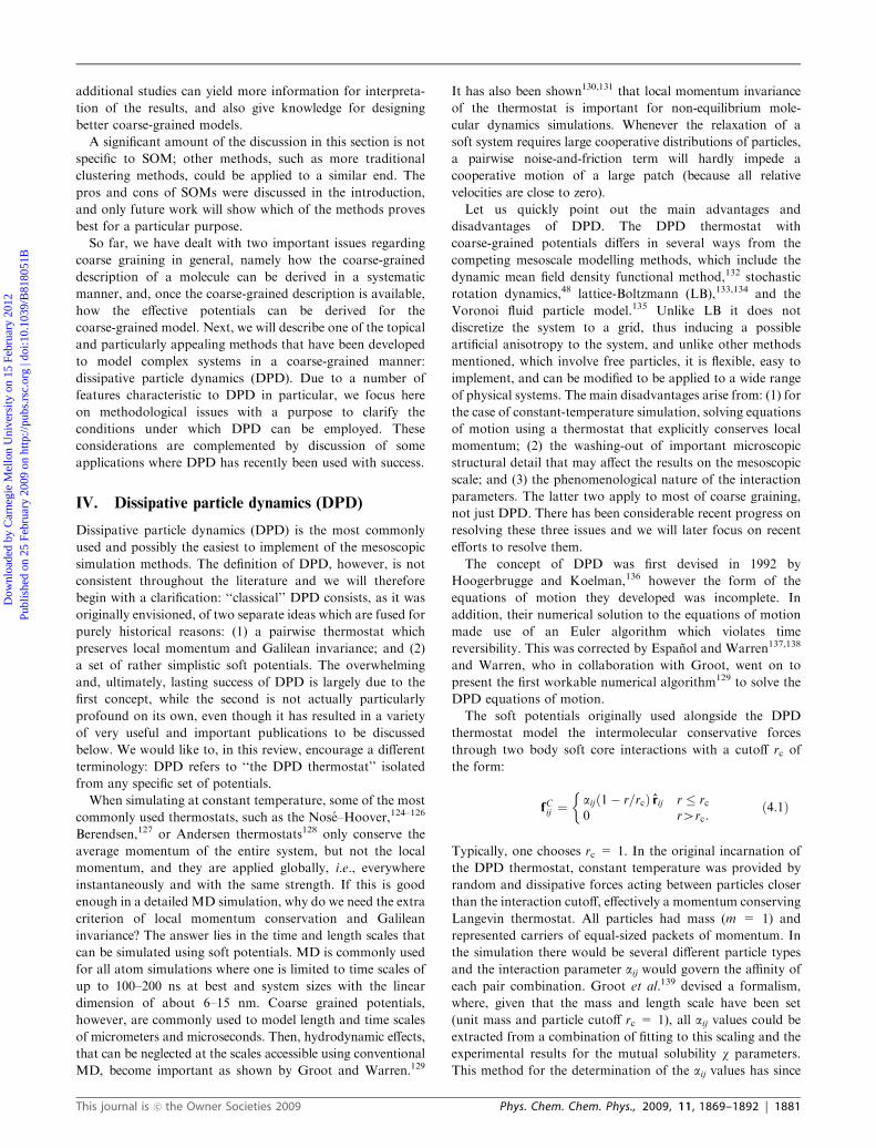
additional studies can yield more information for interpreta-

tion of the results, and also give knowledge for designing

better coarse-grained models.

A significant amount of the discussion in this section is not

specific to SOM; other methods, such as more traditional

clustering methods, could be applied to a similar end. The

pros and cons of SOMs were discussed in the introduction,

and only future work will show which of the methods proves

best for a particular purpose.

So far, we have dealt with two important issues regarding

coarse graining in general, namely how the coarse-grained

description of a molecule can be derived in a systematic

manner, and, once the coarse-grained description is available,

how the effective potentials can be derived for the

coarse-grained model. Next, we will describe one of the topical

and particularly appealing methods that have been developed

to model complex systems in a coarse-grained manner:

dissipative particle dynamics (DPD). Due to a number of

features characteristic to DPD in particular, we focus here

on methodological issues with a purpose to clarify the

conditions under which DPD can be employed. These

considerations are complemented by discussion of some

applications where DPD has recently been used with success.

IV. Dissipative particle dynamics (DPD)

Dissipative particle dynamics (DPD) is the most commonly

used and possibly the easiest to implement of the mesoscopic

simulation methods. The definition of DPD, however, is not

consistent throughout the literature and we will therefore

begin with a clarification: ‘‘classical’’ DPD consists, as it was

originally envisioned, of two separate ideas which are fused for

purely historical reasons: (1) a pairwise thermostat which

preserves local momentum and Galilean invariance; and (2)

a set of rather simplistic soft potentials. The overwhelming

and, ultimately, lasting success of DPD is largely due to the

first concept, while the second is not actually particularly

profound on its own, even though it has resulted in a variety

of very useful and important publications to be discussed

below. We would like to, in this review, encourage a different

terminology: DPD refers to ‘‘the DPD thermostat’’ isolated

from any specific set of potentials.

When simulating at constant temperature, some of the most

commonly used thermostats, such as the Nose–Hoover,124–126

Berendsen,127 or Andersen thermostats128 only conserve the

average momentum of the entire system, but not the local

momentum, and they are applied globally, i.e., everywhere

instantaneously and with the same strength. If this is good

enough in a detailed MD simulation, why do we need the extra

criterion of local momentum conservation and Galilean

invariance? The answer lies in the time and length scales that

can be simulated using soft potentials. MD is commonly used

for all atom simulations where one is limited to time scales of

up to 100–200 ns at best and system sizes with the linear

dimension of about 6–15 nm. Coarse grained potentials,

however, are commonly used to model length and time scales

of micrometers and microseconds. Then, hydrodynamic effects,

that can be neglected at the scales accessible using conventional

MD, become important as shown by Groot and Warren.129

It has also been shown130,131 that local momentum invariance

of the thermostat is important for non-equilibrium mole-

cular dynamics simulations. Whenever the relaxation of a

soft system requires large cooperative distributions of particles,

a pairwise noise-and-friction term will hardly impede a

cooperative motion of a large patch (because all relative

velocities are close to zero).

Let us quickly point out the main advantages and

disadvantages of DPD. The DPD thermostat with

coarse-grained potentials differs in several ways from the

competing mesoscale modelling methods, which include the

dynamic mean field density functional method,132 stochastic

rotation dynamics,48 lattice-Boltzmann (LB),133,134 and the

Voronoi fluid particle model.135 Unlike LB it does not

discretize the system to a grid, thus inducing a possible

artificial anisotropy to the system, and unlike other methods

mentioned, which involve free particles, it is flexible, easy to

implement, and can be modified to be applied to a wide range

of physical systems. The main disadvantages arise from: (1) for

the case of constant-temperature simulation, solving equations

of motion using a thermostat that explicitly conserves local

momentum; (2) the washing-out of important microscopic

structural detail that may affect the results on the mesoscopic

scale; and (3) the phenomenological nature of the interaction

parameters. The latter two apply to most of coarse graining,

not just DPD. There has been considerable recent progress on

resolving these three issues and we will later focus on recent

efforts to resolve them.

The concept of DPD was first devised in 1992 by

Hoogerbrugge and Koelman,136 however the form of the

equations of motion they developed was incomplete. In

addition, their numerical solution to the equations of motion

made use of an Euler algorithm which violates time

reversibility. This was corrected by Espanol and Warren137,138

and Warren, who in collaboration with Groot, went on to

present the first workable numerical algorithm129 to solve the

DPD equations of motion.

The soft potentials originally used alongside the DPD

thermostat model the intermolecular conservative forces

through two body soft core interactions with a cutoff rc of

the form:

fCij ¼aijð1� r=rcÞ rij r � rc0 r4rc:

�ð4:1Þ

Typically, one chooses rc = 1. In the original incarnation of

the DPD thermostat, constant temperature was provided by

random and dissipative forces acting between particles closer

than the interaction cutoff, effectively a momentum conserving

Langevin thermostat. All particles had mass (m = 1) and

represented carriers of equal-sized packets of momentum. In

the simulation there would be several different particle types

and the interaction parameter aij would govern the affinity of

each pair combination. Groot et al.139 devised a formalism,

where, given that the mass and length scale have been set

(unit mass and particle cutoff rc = 1), all aij values could be

extracted from a combination of fitting to this scaling and the

experimental results for the mutual solubility w parameters.

This method for the determination of the aij values has since

This journal is �c the Owner Societies 2009 Phys. Chem. Chem. Phys., 2009, 11, 1869–1892 | 1881

Dow

nloa

ded

by C

arne

gie

Mel

lon

Uni

vers

ity o

n 15

Feb

ruar

y 20

12Pu

blis

hed

on 2

5 Fe

brua

ry 2

009

on h

ttp://

pubs

.rsc

.org

| do

i:10.

1039

/B81

8051

B

View Online

been found to create inaccurate results for several cases140 and

other, more accurate formalisms have since been proposed.141

With only the above interactions DPD is restricted to

observing the trivial problem of phase coexistence and

separation of binary fluids with mutual solubility parameter w.The first step made towards developing this into an algorithm

that can be used to simulate a real system was insertion of

harmonic ‘‘springs’’ between particles by Schlijper et al.142 to

simulate mesoscopic ‘‘bead-spring’’ models of polymers. The

behavior of such a model of a polymer melt was examined by

Spenley,143 who showed the dynamics to obey Rouse dynamics,

over the full range of polymer lengths without the expected

crossover into reptation dynamics of the bead spring model.

The reason for this is that the soft DPD interactions are too soft

to inhibit chains from crossing through each other. Recently

techniques have been developed to rectify this failing of the

model by adding specific interactions to inhibit chain

crossover,144,145 though for a large class of complex fluids this

is not necessary because:146 (1) the chain lengths of the polymers

involved are short enough or the system is dilute enough for

their dynamic behavior to be Rouse-like; and (2) the rheology

of these systems is dominated by the self organization of

microstructure resulting from phase separation instead of

polymer chain dynamics. One of the most relevant mesoscopic

phenomena of a complex fluid is its rheology, and studying

rheology through the application of shear to a DPD system was

one of the main initial purposes of the development of the

method. Some of the earliest DPD studies have been of the

shear rheologies of fluids.147,148 The application of shear to a

DPD simulation through the use of Lees–Edwards boundary

conditions has been concisely described by Sims and Martys.149

The original conception of DPD described above has been

successfully applied to model a wide variety of soft

matter systems, including block copolymers,150,151 oil/water/

surfactant systems,152 polymer surfactant solutions,153 multi-

component fluids,154 bilayer membranes155 (including cell

membranes139) and vesicles.156,157 A particularly fruitful field

of study has been the study of mesoscopic structures made up

of lipid membranes. In one of the first applications of the

parameterization of DPD with the solubility w parameters

Groot and Rabone139 showed that the presence of surfactant

molecules greatly diminishes the stress and extensibility of a

phospholipid bilayer, and Yamamoto et al. demonstrated the

spontaneous formation of lipid vesicles.158

It is at this point that we feel it is very important to dispel

several further common misconceptions concerning DPD

simulation. We are not limited to NVT; a technique to

perform DPD simulation with either constant pressure or

constant surface tension has been developed and applied by

Jakobsen et al.159 This is in fact not such a difficult problem, as

any barostat which varies the box size isotropically will

maintain the transport phenomena of the DPD system. A

more elegant barostat than that proposed by Jakobsen et al.,

that also could be applied to DPD simulation, but as of yet has

not been is the isotropic barostat of Kolb and Dunweg.160 We

are also not limited to soft single parameter intermolecular

forces or uniform particle mass and force cutoff as the

DPD thermostat has been used outside of this context.161

Intra-molecular forces other than harmonic ‘‘springs’’ have

been implemented including 2–4 interactions,140 FENE

springs161 and the accuracy of the surfactant simulation has

been increased by Shillcock et al.155 through the addition of a

three body potential acting between consecutive bead triples.

We are finally not limited to the thermostating being provided

by dissipative and random forces, as the now widely used

Lowe–Andersen themostat162 and the extension of this

method proposed by Stoyanov and Groot163 attest.

One final warning seems appropriate: The use of the DPD

thermostat with, in particular, soft interactions has encouraged

people to use substantially longer integration time steps than

are typically employed in conventional simulations with harder

potentials, such as Lennard-Jones. Indeed, Groot and Warren

showed that a time step roughly five times longer than the

conventional t = 0.05 (in reduced units) suffices to achieve 1%

accuracy in kinetic temperature.129 When using additional

interactions, however, such as bonds between DPD particles,

this state of affairs ought to be carefully revisited. Indeed, Allen

has shown that in some cases the resulting inaccuracies are

disastrous:164 even if the kinetic temperature is within a few

percent of its target value, the configurational temperature

(derived via a hypervirial condition) can be off by more than

a factor of 2.

Before going to the technical matters, let us finish this

discussion with an example. Shillcock and Lipowski used the

‘‘classical DPD’’ (soft potentials and thermostat) to study

tension induced fusion of vesicle membranes.156 Artificial

vesicles are very promising for drug delivery and in order for

the vesicle to deliver the desired contents to a cell, the

membranes of the cell and the vesicle must fuse. Since cell

membranes must maintain their integrity for the cell to

survive, and vesicles used for drug delivery must stay intact

until the cell is reached, there clearly exists an intrinsic

resistance to membrane rupture and fusion. Shillcock and

Lipowski used a coarse-grained representation with the DPD

thermostat of a 30 nm diameter vesicle interacting with a

50 nm wide section of membrane. They monitored the time

evolution of 93 fusion attempts and characterize the

dependence of fusion on the initial tension within the vesicle

and membrane. They were able to determine that fusion

induced by relatively large tension occurs on the timescale of

roughly 350 ns. This kind of studies of large system sizes and

long time scales are only possible using coarse-grained

methods; as a comparison, using classical MD, it has been

possible to study micellation165–168 and micelle fission169 in

systems only up to a few hundred surfactants (the difference

is, though, that one obtains very detailed information fromMD

simulations). In addition to DPD, other coarse-grained models

have been applied to micelles and vesicles, see e.g. ref. 170.

The current activity in the field of using the DPD thermostat

to study biological and soft matter systems is far too great to

be comprehensively covered here. A demonstration of its

breadth is made by these 10 articles published between May

and September of 2008 alone.171–180

A Deriving and solving the DPD equations of motion

Thermostating in DPD using random and dissipative forces

can be seen as making use of a momentum conserving

1882 | Phys. Chem. Chem. Phys., 2009, 11, 1869–1892 This journal is �c the Owner Societies 2009

Dow

nloa

ded

by C

arne

gie

Mel

lon

Uni

vers

ity o

n 15

Feb

ruar

y 20

12Pu

blis

hed

on 2

5 Fe

brua

ry 2

009

on h

ttp://

pubs

.rsc

.org

| do

i:10.

1039

/B81

8051

B

View Online

Langevin thermostat. In the Langevin thermostat all particles

are subjected to dissipative forces (FCI ) and random impulses

( _pRi ). As a result the particle dynamics will be governed by the

Langevin equations of motion:

_ri = (pi/mi) (4.2)

_pi = FCi + FD

i + _pRi, (4.3)

where the conservative, frictional, and random forces are

given by

FCi ¼

Xiaj

fCij ð4:4Þ

FDi = �G_ri (4.5)

_pRi= xi(t). (4.6)

Here, xi(t) is a Gaussian white noise correlated noise with zero

mean and a variance adjusted via the fluctuation–dissipation

theorem to reproduce the fluctuations present in the

canonical state:

hxi(t)i = 0 (4.7)

hxi(t)xi(t0)i = 2kBTGdijd(t � t0). (4.8)

The Langevin thermostat can thus be seen to mimic the

presence of a viscous medium, with G being the coefficient of

the induced drag and the random impulse representing

random collisions with Brownian particles within the medium.

The random impulses and dissipative forces of the Langevin

thermostat are incorporated, but instead of applying them to

the individual particles independently, hence losing the local

momentum conservation, the dissipative forces and random

impulses are applied through pairwise interactions between the

particles. The DPD equations of motion have the same form

as the Langevin equations of motion, however the dissipative

forces and random impulses are now given by

FDi ¼ �g

Xiaj

oDðrijÞð_rij � rijÞ rij ð4:9Þ

_pRi¼ s

Xiaj

oRðrijÞ rij _W ; ð4:10Þ

where g and s are the coefficients of dissipative and random

force, respectively, oR(rij) and oD(rij) are functions specifying

the strength of noise and dissipation in a distance depen-

dent fashion, and _W is the time derivative of a Wiener process.

As far as we are aware, there are only two publications in

which the weight function is approached in a systematic

fashion.181,182

It has been shown by Espanol and Warren137 that in order

to satisfy the fluctuation dissipation theorem, and thus recover

the Gibbs distribution as a stationary solution to the

Fokker–Planck equation, the following relations must hold

oD(rij) = (oR(rij))2 (4.11)

s ¼ffiffiffiffiffiffiffiffiffiffiffiffiffiffi2gkBT

pð4:12Þ

thus reducing four free parameters to two. They also found

that this only applies in the limit of small time step of the

numerical algorithm applied to solve the DPD equations of

motion. So far in its application the most common choice for

the dissipative and random force coefficients are g = 4.5 and

s = 3.

Given the DPD equations of motion in this form, transport

equations for the mass and momentum density fields have

been analytically derived by Espanol138 that, as expected, have

the form of Navier–Stokes equations. In addition, in the same

paper Espanol derives expressions for the pressure, and bulk

and shear viscosities, for a system governed by the DPD

equations of motion. Observing the form of the equations of

motion under the DPD thermostat we see that there is a very

elegant direct intuitive correspondence to the actual dynamics

of a mesoscopic system. Since each DPD particle is composed

of several atoms it can be seen itself as a subsystem with its

own degrees of freedom. The dissipative and random forces

thus represent transfer of energy between the internal and

external degrees of freedom occurring in collisions with other

particles, and one no longer has to postulate the system of

particles being connected to an external heat bath.

1 Derivation of effective dissipative and random ‘‘forces’’ for

algorithm with timestep Dt. Given the random impulse _Wij and

finite timestep Dt, each DWij will be a random number chosen

from a Gaussian distribution with variance Dt and zero mean,

with the restrictions of DWij = DWji and time reversibility. In

the limit of large number of steps and small timestep, which we

can safely assume for any realistic DPD algorithm, the central

limit theorem permits us to replace the set of Gaussian random

numbers of zero mean and variance Dt by a set of random

numbers chosen from a uniform distribution with zero

mean and variance 12Dt, thus considerably reducing the

computational overhead.183

_Wij �ffiffiffiffiffiffiffiffiffiffi12Dtp

ðyij � 0:5Þ; ð4:13Þ

where yij is a uniform random number on the range (0,1) and

yij = yji. Thus given the above approximation and the para-

meter relations determined by Espanol and Warren (4.12), we

have the following equations for the dissipative force and

effective ‘‘random force’’ acting on each particle, for time step

Dt given by:

FDi ¼ �g

Xiaj

oRðrijÞ2ð_rij � rijÞ rij ð4:14Þ

FRi ¼

ffiffiffiffiffiffiffiffiffiffiffiffiffiffiffiffi24gkBT

Dt

r Xiaj

oRðrijÞ rijðyij � 0:5Þ ð4:15Þ

2 Uncoupling the dissipative force. The standard algorithm

that can be used to solve the equations of motion, while

obeying time reversibility as specified by the Wiener process

is the velocity-Verlet (VV) algorithm, which performs a second

order splitting between the velocity and position degrees of

freedom:

1. _ri ¼ _ri þ Dt2miðFC

i þ FRi þ FD

i Þ2. ri = ri + _riDt3. calculate FC

i (ri), FRi (ri) and FD

i (ri,_ri)

4. _ri ¼ _ri þ Dt2miðFC

i þ FRi þ FD

i Þ

This journal is �c the Owner Societies 2009 Phys. Chem. Chem. Phys., 2009, 11, 1869–1892 | 1883

Dow

nloa

ded

by C

arne

gie

Mel

lon

Uni

vers

ity o

n 15

Feb

ruar

y 20

12Pu

blis

hed

on 2

5 Fe

brua

ry 2

009

on h

ttp://

pubs

.rsc

.org

| do

i:10.

1039

/B81

8051

B

View Online

It should be noted that, unlike the references where the

DPD algorithm has been formulated, we explicitly include the

masses of the individual particles.

The key complicating factor in the development of a

numerical algorithm to solve the DPD equations of motion

is the fact that the dissipative force is simultaneously coupled

to the relative velocities and positions of the interacting

particle pairs. As a result the standard time reversible

numerical algorithms to solve the equations of motion with

a finite small timestep Dt, the velocity-Verlet (VV) and leap

frog algorithms, which perform a splitting between the

position and velocity updates, break down. The first workable

algorithm to solve the DPD equations of motion was

developed by Groot and Warren.129 The algorithm (GW) is

a modification of the VV algorithm, where all the forces, like

in VV, are only modified once per timestep, however the

dissipative forces are modified based on intermediate

‘‘predicted’’ velocities, evaluated at a timestep determined by

a phenomenological parameter l. The GW algorithm consists

of the following steps:

1. _ri ¼ _ri þ Dt2miðFC

i þ FRi þ FD

i Þ2. ~r

:

i ¼ _ri þ l DmitðFC

i þ FRi þ FD

i Þ3. ri = ri + _riDt4. calculate FC

i (ri), FRi (ri) and FD

i ðri;~r:

iÞ5. _ri ¼ _ri þ Dt

2miðFC

i þ FRi þ FD

i Þ

Clearly setting l = 1/2 recovers the original VV algorithm.

Groot and Warren found that this algorithm is optimized by

setting l = 0.65. While this algorithm was found to work, and

is actually relatively efficient,184 the fact that it contains a

phenomenological parameter complicates how it can be

predicted to behave when applied to new systems, as DPD is

further developed. Several algorithms have been developed

attempting to improve on the GW algorithm, that do not

make use of a phenomenological parameter. These include the

OC algorithm developed by Otter and Clarke,185 the S1

algorithm, a symplectic Trotter decomposition scheme,

developed by Shardlow,186 the DPD-VV algorithm

developed by Besold et al.,187 and the self consistent

velocity-Verlet algorithm, (SC-VV), of Paganobarraga and

Frenkel.188 All these algorithms, along with GW were tested

and benchmarked by Nikunen et al.189 Of these algorithms,

OC was found to be sub-optimal, and while SC-VV

performed very well, the self consistent renormalization of

the temperature that is a part of the algorithm creates new

problems that make this algorithm more trouble than it

is worth.

The two algorithms which rate detailed description are

the DPD-VV which is trivial to implement, has an

acceptable accuracy in the appropriate time step range of

the algorithm (Dt E 0.05 in reduced units), and has

been thoroughly tested, and the S1 algorithm which

preserves conserved quantities better than the DPD-VV, has

not been as widely used, and is not as trivial (though not so

incredibly difficult) to implement as the DPD-VV algorithm.

A very recent development is a generalization of the

Trotter integration scheme used by Shardlow, proposed by

Serrano et al.190

The DPD-VV algorithm is simply the VV algorithm with the

dissipative force recalculated on the half timestep:

1. _ri ¼ _ri þ Dt2miðFC

i þ FRi þ FD

i Þ2. ri = ri + _riDt3. calculate FC

i (ri), FRi (ri) and FD

i (ri,_ri)

4. _ri ¼ _ri þ Dt2miðFC

i þ FRi þ FD

i Þ5. calculate FD

i (ri,_ri)

The S1 algorithm involves performing a Trotter first order

splitting of the velocity-Verlet algorithm between the effect of

the random and dissipative forces, and the effect of the

conservative force. In the resulting algorithm each timestep

contains a constant energy VV step alongside an extra step

where the particle velocities are updated due to the effects of

the dissipative and random forces, as follows:

If we consider:

fDij = �goR(rij)2(_rij�rij)rij (4.16)

fRij ¼ffiffiffiffiffiffiffiffiffiffiffiffiffiffiffiffi24gkBT

Dt

roRðrijÞ rijðyij � 0:5Þ ð4:17Þ

sDij ¼ �1

1þ goRðrijÞ2Dtð4:18Þ

sRij ¼ 1� goRðrijÞ2Dt1þ goRðrijÞ2Dt

ð4:19Þ

for each interacting particle pair ij

(a) Calculate _rij, fDij , f

Rij , s

Dij and sRij ,

(b) _ri ¼_ri þ Dt2miðf R

ij þ f Dij Þ

_rj ¼_rj � Dt2miðf R

ij þ f Dij Þ

(c) Recalculate _rij and fDij(d) _ri ¼ _ri þ Dt

2miðsRij f R

ij þ sDij fijDÞ

_ri ¼ _ri � Dt2miðsRij f R

ij þ sDij fDij Þ

2. _ri ¼ _ri þ Dt2mi

F Ci

3. ri = ri + _riDt4. calculate FC

i (_ri)

5. _ri ¼ _ri þ Dt2mi

F Ci

3 Recent methodological developments of DPD. As stated

previously the use of random and dissipative forces is not the

only effective thermostat for DPD simulation. The methods

of Lowe162 and the extension of this method proposed by

Stoyanov and Groot163 propose a very different alternative.

In the same way that the above described DPD algorithm

takes Langevin dynamics as the starting point, the algorithm

proposed by Lowe takes the Andersen thermostat as the

starting point, hence the name by which it is commonly

known, the ‘‘Lowe–Andersen’’ thermostat. In the same way

that the Andersen thermostat makes stochastic adjustments

directly to the velocities in the simulation, the Lowe–Andersen

thermostat performs in a pairwise fashion thus conserving

microscopic momentum. This algorithm performs extremely

well, in many cases better than any other, when it has been

benchmarked using standard conservation tests against existing

DPD algorithms.164,184,189 Thermalization is performed

1884 | Phys. Chem. Chem. Phys., 2009, 11, 1869–1892 This journal is �c the Owner Societies 2009

Dow

nloa

ded

by C

arne

gie

Mel

lon

Uni

vers

ity o

n 15

Feb

ruar

y 20

12Pu

blis

hed

on 2

5 Fe

brua

ry 2

009

on h

ttp://

pubs

.rsc

.org

| do

i:10.

1039

/B81

8051

B

View Online

collectively through a Monte Carlo process, with the prob-

ability of each individual particle pair being thermalized being

controlled by the parameter in the algorithm G. Its use in MD

simulations and influence on dynamic properties have been

recently studied by Koopman and Lowe,191 and it was shown

to work well as long as the density of the system is reasonably

large and the parameter G is not too high. For gaseous

systems Koopman and Lowe recommend the algorithm of

Stoyanov and Groot,163 that hybridizes the Lowe–Andersen

thermostat with what they claim is a momentum-conserving

Nose–Hoover algorithm. When looked at more closely the

algorithm the Lowe–Andersen thermostat is hybridized with

in actual fact bears closer resemblance to a momentum

conserving Berendsen thermostat.164 Since correct temperature

fluctuations are not reproduced by the Berendsen thermostat

the correctness of this algorithm is in doubt, and thus it needs

further testing before it can be applied.

Two very exciting recent developments to the DPD

algorithm have emerged from Jakobsen et al. The development

of a multiple time step algorithm192 promises, as it is further

developed, to alleviate one of the main problems of DPD

simulation, the inability to include important forces that act

on shorter length and time scales, but effect the structure and

dynamics on the mesoscale, without losing the advantages of

DPD that allow for the observation of the longer length and

time scales. They have also developed a new algorithm,

described in explicit detail in ref. 193 that extends DPD-VV

to allow DPD simulation to be performed in both constant

pressure and constant surface tension, which has allowed

for the simulation of biological membranes using DPD.194

Thermostating also remains an active field, and the latest

addition is the robust ‘‘extended DPD thermostat’’ by

Junghans et al.195

4 Analytical approaches: regarding a systematic derivation

of DPD. The standard DPD with soft potentials as presented

above is phenomenological. An interesting formal approach

has been presented by Flekkøy et al.196,197 who were able to

link DPD to molecular level properties by using a Voronoi

tessellation-based technique. This method can be used to

resolve different length scales simultaneously. The method is

formally akin to the well-known renormalization group

procedure extensively used in analytical treatment of critical

phenomena.25 The mathematical details can be found from the

original articles as cited above.

The approach of Flekkøy et al. provides a systematic and

computationally tractable, although not straightforward,

method to coarse-grain molecular systems. From a computa-

tional point of view their method is more demanding than

particle based methods such as the standard DPD as the

Voronoi tessellation procedure, as it requires N log N

operations and involves a fairly large additional prefactor.

V. Solvent free membranes

A Why do it?

So far we have discussed how one can proceed to coarse grain

the simulation model, and the appropriate methodology to

simulate the dynamics of systems using mesoscopic potentials.

But as stated in the introduction, for most systems we still

have the problem of the vast majority of our computational

resources being used to simulate the solvent, in which the

interesting system is immersed, interacting with itself. In this

chapter we discuss simulation methods that do away with the

solvent altogether.

Coarse graining is driven by the desire to reach larger

length- and time scales. Let us illustrate that for membranes

by asking: how does the effort to simulate a square patch of

membrane of side length L scale with L? In the absence of

embedding solvent the amount of material evidently increases

with L2, but there is a more severe limitation. It is not sufficient

to represent a bilayer patch in the computer, it is necessary to

also equilibrate it. Unfortunately, the equilibration time scales

very unfavorably with L—in the absence of hydrodynamic

interactions and at vanishing tension like L4, owing to the

nature of the underlying curvature-elastic Hamiltonian. Thus,

the entire effort scales like L6. Extending the simulation of a

fully equilibrated 20 nm bilayer,198 big enough to answer

localized questions, to maybe 200 nm, possibly necessary

to study cooperative interaction and aggregation behavior

of membrane proteins, we need a million times more

computer time.

We have seen in this review that a variety of different

techniques and models have been developed to coarse-grain

lipids and membranes. But when one arrives at these large

scales, there often is yet another effect which works against us:

membranes begin to significantly bend. By ceasing to be

essentially flat, the volume of the simulation box is no longer

given by L2b, where b is equal to the bilayer thickness plus a

hydration layer, but rather begins to scale like L3 (think for

instance of simulating a vesicle). The ratio between material and

box-volume decreases like L�1, exactly as if one were for instance

simulating a Gaussian polymer coil. And just as in the polymer

case the evident solution is to eliminate the solvent in favor of

effective interactions. Unlike in the polymer case, however, the

way to achieve this turns out to be a bit more tricky.

B Basic ideas and specific implementations

The self-assembly of a lipid bilayer is driven by the hydrophobic

effect created by the solvent, so eliminating the solvent requires

us to mimic the hydrophobic effect by some effective cohesion

potential. Unlike polymers, held together by chemical bonds,

the structural integrity of the bilayer aggregate depends on this

cohesion energy, so its form will matter. In past research it has

been found that a simple short ranged (e.g. Lennard-Jones like)

attractive interaction between coarse-grained hydrophobic lipid

chains will not usually work. Such interactions have been found

not to be able to to produce aggregates which were both

bilayer-like and fluid (for a short discussion see ref. 199). The

issue is that aggregation from a 3D lipid distribution into a 2D

aggregate seems to require a binding strength which is

incompatible with a fluid condensed phase. In order to

overcome this obstacle, various solutions have been proposed:

1 Multibody potentials. Performing a partial trace over

selected degrees of freedom in the partition function results

in new effective interactions between the remaining ones

which, however, do not necessarily have to be of equally

This journal is �c the Owner Societies 2009 Phys. Chem. Chem. Phys., 2009, 11, 1869–1892 | 1885

Dow

nloa

ded

by C

arne

gie

Mel

lon

Uni

vers

ity o

n 15

Feb

ruar

y 20

12Pu

blis

hed

on 2

5 Fe

brua

ry 2

009

on h

ttp://

pubs

.rsc

.org

| do

i:10.

1039

/B81

8051

B

View Online

simple type as the original interactions (e.g. pair-wise). Indeed,

Drouffe et al., who first successfully managed to aggregate a

fluid membrane under solvent-free conditions, implemented

a multibody-potential between its highly coarse-grained

amphiphiles.200 The latter were chosen to be spherical polar

beads with three interactions between them: (A) a hard

core repulsion; (B) a dipolar-like attraction favoring planar

alignment; and (C) a density-dependent cohesion which

prefers each bead to have 6 neighbors. This model was able

to spontaneously aggregate into two-dimensional sheets

which, due to line tension, closed to form vesicles. An

analysis of the shape fluctuation yielded a bending modulus

k E 3kBT.

Ten years later Noguchi and Takasu picked up this concept

and extended it to slightly less coarse-grained amphiphiles,

modeled as a rigid linear array of three connected beads,

two of them ‘‘hydrophobic’’.201,202 In this case the cohesive

interaction U(r) is chosen to depend on the local (somewhat

smoothed) particle density r in such a way that it is

proportional to r at sufficiently small r, but levels off beyond

a certain limit, according to

ri;j ¼X

iai0;j0¼2;3hðjri;j � ri0;j0 jÞ ð5:1aÞ

h(r) = 1/{exp[20(r/s � 1.9)] + 1} (5.1b)

UðrÞ ¼�0:5r; ror � 10:25ðr� rÞ2 � c; r � 1 � ror

�c; r � r

8<: ; ð5:1cÞ

where i, i0 numbers the lipids, j, j0 = 2,3 the two hydrophobic

tail beads, r* = 10 and c = 4.75 for j = 2 and r* = 14 and

c = 6.75 for j = 3, and where s is the bead diameter. Notice

that for small densities this just reduces to a pair attraction

h(r), while as the density increases during self-assembly, this

leveling off prevents too strong attractions which might drive

the system right away into the gel phase. With these system

bending rigidities of k/kBT = 1. . .5 were found.202

A few years later Wang and Frenkel proposed a variant of

this model,203 in which the lipids had an additional bending

degree of freedom and the density dependence of the

hydrophobic interactions was parametrized slightly differently,

in particular by evaluating the average density of hydrophobic

units inside a slightly prolate ellipsoid, oriented along the

direction of the average bilayer normal. Within their

parametrization these authors obtained a physically more

realistic bending rigidity of k/kBT E 13, as measured via a

fluctuation analysis.

2 Orientational dependencies. Even though the use of

multibody potentials led to solvent free models which showed

robust self-assembly, such potentials are usually more difficult

to manage than ordinary pair potentials. Their implementation

in ‘‘standard’’ packages might be more difficult, the

calculation of observables such as the stress tensor is more

involved, and some of the statistical mechanical intuition

based on our habitual use of pair potentials is inapplicable.

For this reason people have strived to make a pure pair

approach work. One suggestion by Brannigan and Brown

was based on the use of an orientation dependent cohesive

force.204 Using spherocylinders as the shape of their lipids,

they introduced orientation dependent alignment and

cohesion interactions in the form

Ualignðrij ; ni; njÞ ¼ �calignsjrij j

� �2sin2 yi þ sin2 yj

2; ð5:2aÞ

Ucohesionðrij ; ni; njÞ ¼ �ccohesions

jrij þ lðnj � niÞj

� �6

; ð5:2bÞ

where ni is the unit vector pointing in the direction of the long

axis of lipid i, yi and yj are the angles between the lipid axis of

lipids i and j and their separation vector rij, and l is the length

of the spherocylinder (without the two caps). The potentials

Ualign and Ucohesion are cut off and shifted to zero at r = 3sand r = 2s, respectively, and the values of the two coupling

constants calign and ccohesion were systematically varied.

Additionally, an excluded volume repulsion of the form

Ucore(dij) = ccore(s/dij)8 was included, where dij is the distance

of closest approach between the two spherocylinders i and j.

The resulting phase diagram contained regions of fluid

bilayers, with relatively high bending rigidities in the range

k/kBT = 60. . .120. However, self assembly could only be

achieved by artificially guiding the emerging aggregates

toward equilibrium, namely, by beginning in a warm dense

simulation box and ending up in a cold dilute one.

3 Highly tuned individual interactions. Farago has shown

that it is possible to completely revert to pair potentials of

Lennard-Jones (n,2n)-type, provided they are very carefully

parametrized.205 He uses again a rigid HTT-trimer and tunes

the interactions between individual beads (HH, HT1, HT2,

T1T1, T1T2, T2T2) in strength, range, and functional form

(for details see ref. 205). One can thus stabilize a fluid phase,

and he measures a bending rigidity around k/kBT C 50.

Unfortunately the effort going into the tuning of all these

potentials makes it difficult to systematically vary membrane

parameters (such as rigidity or order) without essentially

reparametrizing all of them together.

4 Longer ranged attractions. An easier way to revert to

pair forces is the use of cohesive interactions that are suffi-

ciently long ranged. The Farago model already hinted towards

the advantage of having cohesive interactions extend over a

range longer than the typical Lennard-Jones (6,12) distance.

Two models have been proposed recently, which owe their

success essentially to a systematic exploitation of this effect.

The first is due to Brannigan, Philips and Brown,206 who use a

5-bead lipid of composition ‘‘HITTT’’ (one head-bead, one

interface bead and three tail beads) with the following

interactions

Ucore(r) = ccore(s/r)12 (rcut = 2s), (5.3a)

Utail(r) = �ctail(s/r)6 (rcut = 2s), (5.3b)

Uint(r) = �cint(s/r)2 (rcut = 3s), (5.3c)

where Ucore acts between all beads except intramolecular bead

pairs separated by less than three bonds, Utail acts between all

TI and TT pairs, andUint between all II pairs; all potentials are

cut-off and shifted to zero at the indicated distance. The

1886 | Phys. Chem. Chem. Phys., 2009, 11, 1869–1892 This journal is �c the Owner Societies 2009

Dow

nloa

ded

by C

arne

gie

Mel

lon

Uni

vers

ity o

n 15

Feb

ruar

y 20

12Pu

blis

hed

on 2

5 Fe

brua

ry 2

009

on h

ttp://

pubs

.rsc

.org

| do

i:10.

1039

/B81

8051

B

View Online

rationale for additional long ranged interfacial attraction

stems from the fact that it is precisely on the hydrophilic/

hydrophobic interface between the lipid heads and tails where

the cohesive stress is localized. The chosen parameters are

ccore = 0.4e, ctail = 1.0e, cint = 3.0e, where e is the unit of

energy. Additionally, a bending term of the form cbend cos ybetween any three successive beads is implemented, and the

lipid bending stiffness cbend is varied between 5e and 10e.Corresponding membrane bending rigidities vary in the range

k/kBT = 2.5. . .16.

The second model, due to Cooke, Kremer and Deserno,207

uses again a semiflexible lipid trimer of the form ‘‘HTT’’ with

the following interactions:

Ubond(r) =12kbondr

2Nln[1 � (r/rN)2], (5.4a)

Ucoreðr; bÞ ¼ 4eb

r

� �2

� b

r

� �6)"; ðrcut ¼ 21=6bÞ; ð5:4bÞ

Uattrðr;wcÞ ¼�e; rorc�e cos2 pðr�rcÞ

2wc; rcororc þ wc

�; ð5:4cÞ

with kbond = 30e and rN = 1.5s. Additionally, the lipid

is straightened by a pseudo bending potential between

the head-bead and the second tail bead of the form12kbend(rHT2 � 4s)2 with kbend = 10e/s2. All beads interact

repulsively with Ucore(r,b), where bHH = bHT = 0.95s and

bTT = s to ensure a cylindrical shape. The cohesive potential

Uattr(r,wc) acts only between tail-beads. Its range wc can be

tuned. If it is too short (wc t 0.75s) lipids either do not

aggregate or assemble into a gel phase, while for larger wc a

fluid phase emerges within some temperature range. In this

range a fluctuation analysis shows that bending rigidities in the

range k/kBT = 3. . .30 can be reached.

C Example applications

The models described above are highly coarse grained, both in

terms of a substantially reduced number of degrees of freedom

and because the solvent has been eliminated. Yet, many

relevant insights can be gained from them, since one can both

achieve excellent statistics in static questions and large time

scales in dynamic ones. In the following we would like to

present a short list of examples which illustrate the potential of

this coarse-graining approach.

1 Elastic moduli from shape fluctuations. Bilayer

membranes show constant thermal fluctuations. It is well

known that in the continuum limit the mean squared

Fourier modes of an asymptotically flat membrane decay like

kBT/(kq4 + sq2), where q is the wave vector and k and s are

bending modulus and lateral tension, respectively. Recently

Brannigan and Brown have pointed out that a careful analysis

of the complete shape fluctuations—including undulation and

peristaltic modes—gives access to other highly relevant

observables, most notably the spontaneous monolayer

curvature.208 They derive analytical expressions for the

fluctuation spectrum at all values of q, up to the protrusion

regime, and show that it can be fit very well to both atomistic

simulations and their coarse-grained model which we briefly

described in section VB4. Not only validating the physics

which entered their coarse-graining scheme, it also suggests a

clear route for parameter optimization, if one intends to match

specific lipid systems.

Efficient sampling of the long wave length undulations, the

ones most relevant for determining the bending modulus, is

often hampered by their slow equilibration time, which is

proportional to the fourth power of their wave length in the

solvent free case. Farago has recently shown that this limita-

tion can be elegantly overcome by additional Monte Carlo

moves.209 Large scale shape changes are effected by imprinting

undulation modes with the correct expected amplitude onto

the membrane and accept such reshaped configurations

according to the usual Metropolis criterion. For a system of

9000 lipids (and a model very similar to the Cooke model from

section VB4) a speed-up by a factor of 50 has been measured

compared to single particle Monte Carlo moves.

2 Bending rigidity via tether pulling. While the membrane

bending modulus k is accessible from thermal fluctuations, this

technique displays two limitations: first, it becomes difficult

for fairly stiff membranes to resolve the small amplitude

fluctuations; and second, it invariably only probes very weak

(thermally excited) curvatures, leaving open the question

whether quadratic bending elasticity remains a faithful

description at high bending. Harmandaris and Deserno have

recently shown that the bending rigidity can alternatively be

obtained from simulating cylindrical membrane tethers, since

(up to subdominant fluctuations) k = FR/2p, where F is the

tensile force required to hold a bilayer tether of radius R,210 see

Fig. 7 for an illustration. Using the Cooke model described in

section VB4 and the ESPResSo simulation package211 they

showed that this measurement of k coincides with the one

obtained from thermal fluctuations up to curvature radii

comparable to bilayer thickness. This method is also particularly

suitable for solvent free systems, since: (i) non-flat bilayers are

essential; and (ii) no complications arise from the fact that the

Fig. 7 Simulation of a cylindrically shaped membrane tether. Notice

that due to periodic boundary conditions the tether has no open edges.

Curvature stresses result in an axial tensile force of magnitude

F=2pk/R, from which the bending modulus k can be easily extracted.210

This journal is �c the Owner Societies 2009 Phys. Chem. Chem. Phys., 2009, 11, 1869–1892 | 1887

Dow

nloa

ded

by C

arne

gie

Mel

lon

Uni

vers

ity o

n 15

Feb

ruar

y 20

12Pu

blis

hed

on 2

5 Fe

brua

ry 2

009

on h

ttp://

pubs

.rsc

.org

| do

i:10.

1039

/B81

8051

B

View Online

cylinder separates two different compartments (inside and

outside) whose pressure difference otherwise would need to

be relaxed by transporting solvent.

The same idea (in a slightly different implementation) has

recently been applied by Arkhipov et al. to a different solvent

free CG lipid model.212 These authors also find that within the

obtained accuracy the measured bending modulus does not

depend on tether radius.

3 Lipoplexes. When cationic membranes (consisting of a

mixture of cationic and neutral lipids) are brought in contact

with DNA, they form complexes called ‘‘lipoplexes’’ in which

parallel DNA strands are sandwiched between lipid bilayers.

Their cohesive energy is thus driven by a combination of

electrostatic interactions (ultimately counterion release

entropy) and the hydrophobic interactions between lipid tails.

Farago et al. have recently studied this complexation behavior

at isoelectric mixing, using the coarse-grained model discussed

in section VB3.213,214 Due to the simplicity of the model,

equilibrated complexes containing up to N = 1000 lipids

(a fraction fc of which was charged) could be studied.

In particular, the experimentally observed scaling

dDNA B f�1c could be confirmed, and it was shown that at

large fc the electrostatically induced stress can lead to local

pore opening of the bilayer phases.

4 Curvature-mediated interactions. Membranes can adsorb

particles at their surface, such as, for instance, peripheral

membrane proteins. It is known that such proteins might

locally induce quite substantial membrane deformations, as

has recently been vividly illustrated in atomistic simulations of

N-BAR domains.216 What happens, if many such membrane

benders have a chance to cooperatively affect the membrane

shape? The exciting possibility one might want to explore is

whether they could aggregate and induce a large curved

membrane bud. But if so, we immediately see that there is

very little chance to study this problem at high resolution,

since membrane extensions in the 100-nanometer range are

required, and timescales maybe up to a millisecond. Moreover,

if budding really sets in, the initially flat membrane bulges out

and calls for a genuinely three-dimensional simulation box,

which becomes extremely costly if solvent is present. These

initial thoughts show that a problem of this kind suggests very

strongly the use of a coarse-grained solvent-free approach.

Indeed, Reynwar et al. have recently performed such a

simulation, using the Cooke model described in section

VB4215 and the ESPResSo simulation package.211 They have

demonstrated that sufficiently many curved proteins, each

imposing a sufficient curvature, can indeed lead to the

formation of a membrane bud. For extremely strong

membrane deformers, such as partially adhering viral capsids

(see Fig. 8), they also demonstrated the existence of attractive

pair forces.

Using a much a more highly coarse-grained description of a

membrane as a triangulated surface, and accounting for the

presence of N-BAR domains by locally imposing a nonzero

curvature tensor, Ayton et al. have also shown that

membranes studded with curvature-imprinting proteins

spontaneously form tubules and highly curved structures.217

Moreover, Arkhipov et al. have recently studied the effectivity

with which many N-BAR domains can curve an initially

flat bilayer patch212 using a multiscaling study bridging

four scales: from atomistic simulations, over residue- and

shape-based coarse-graining up to continuum elasticity.

VI. Summary

In this article, we have focused on four issues: first, using

structural information from atomistic or detailed models

(or experiments) to construct coarse-grained models in a

hierarchical and systematic way. Our approach is based on

the Henderson theorem (section IIA) and the Inverse Monte

Carlo method of Lyubartsev and Laaksonen (section IIC)

which was then extended by the use of a thermodynamic

constraint (section IID). Second, we took a different look at

coarse graining by analyzing conformations of molecules. This

was done by the application of self-organizing maps. Third, we

discussed the dissipative particle dynamics (DPD) method in

section IV. The focus was on technical issues and integration

of the equations of motion. The final, and fourth, topic was

solvent free modeling (section V) which offers a different route

to coarse graining by integrating out the degrees of freedom

associated with solvent.

The field of multiscale modeling is very active and

both conceptual and technical matters are under rapid

development. It is impossible to cover all aspects (or even

most) in one review. To finish this review, we wish to give the

reader a few pointers to the issues we did not cover here. First,

we neglected matters related to electrostatics, yet it is one of

the most important issues in simulations of biological and soft

matter. There have been some new developments especially by

Groot218,219 with regard to DPD and Voth et al.220 in terms of

more general coarse-grained systems. The recent review of

Karttunen et al.221 covers some general aspects and new

methods related to electrostatics. We also neglected field

theoretical models. There have been several interesting

Fig. 8 Slice through a large membrane studded with partially

adhesive spheres. These spheres wrap themselves to about 34inside

the membrane, but cannot completely get covered and thus not ‘‘bud’’

off from the membrane. However, membrane mediated interactions

lead to the attraction of several such local membrane benders, which

by driving a large morphology change can then cooperatively create a

joint budding vesicle. For instance, the highly bent structure in the

middle will detach from the membrane through a fission event within

the next 30 ms.215

1888 | Phys. Chem. Chem. Phys., 2009, 11, 1869–1892 This journal is �c the Owner Societies 2009

Dow

nloa

ded

by C

arne

gie

Mel

lon

Uni

vers

ity o

n 15

Feb

ruar

y 20

12Pu

blis

hed

on 2

5 Fe

brua

ry 2

009

on h

ttp://

pubs

.rsc

.org

| do

i:10.

1039

/B81

8051

B

View Online

developments, especially the recent work of Haataja et al.222

related to lipid rafts.

Software and parameters for multiscale simulations

in soft and biological matter

Here we provide a short list of free software, parameters

(GPL or comparable license) and the related web sites as they

may be useful for the reader. We make no attempt to evaluate

the software or parameters as that is beyond the scope of this

review. We encourage the interested reader to take a look at

the sites and also to contribute him/herself. The list is not

exhaustive but rather based on our own personal experience.

We would also like to point out there is currently a lot

of activity in software development. For example, smart

middleware such as Charm++223 have helped in parallelization

of MD simulations to 1000s of processors, and new

approaches using graphics cards224,225 seem very promising.

Espresso:211 http://www.espresso.mpg.de/

Lampps:226 http://lammps.sandia.gov

Gromacs:227 http://www.gromacs.org

Parameters: http://moose.bio.ucalgary.ca/index.php?page=

Downloads

NAMD2228,229 and VMD:230 http://www.ks.uiuc.edu/

Development/

Softsimu26 software, DPD with bond crossing constraints145

and parameters: http://www.softsimu.org/downloads.shtml

MDynaMix:231 http://www.fos.su.se/Bsasha/md_prog.html

DL_POLY: http://www.cse.scitech.ac.uk/ccg/software/

DL_POLY/

OCTA:232 http://octa.jp/

Acknowledgements

We would like to thank our students, postdocs and co-workers

with whom a lot of the work reviewed here has been

conducted, in particular Petri Nikunen, Emma Falck, Michael

Patra, Andrea Catte, Aatto Laaksonen, Alexander Lyubartsev,

James Polson, Gerhard Besold, Ira Cooke, Ben Reynwar,

Gregoria Illya, Vagelis Harmandaris, Christian Holm and

Kurt Kremer.

This work has been supported by the Natural Sciences and

Engineering Research Council of Canada (M. K.) and the

German Science Foundation (M. D.). We also thank the

Southern Ontario SharcNet (http://www.sharcnet.ca)

computing facility, the Distributed European Infrastructure

for Supercomputing Applications (http://www.deisa.eu) and

the Finnish IT Centre for Science for computer resources.

References

1 R. P. Feynman, R. B. Leighton and M. Sands, The FeynmanLectures on Physics, Addison-Wesley, Reading, MA, 3rd edn,1963, vol. I.

2 M. Chaplin, Nat. Rev. Mol. Cell Biol., 2006, 7, 861.3 A. R. Fresht, Nat. Rev. Mol. Cell Biol., 2008, 9, 650.4 C. Branden and J. Tooze, Introduction to Protein Strcuture,Garland, New York, NY, 2nd edn, 1999.

5 B. Mergell, R. Everaers and H. Schiessel, Phys. Rev. E: Stat.,Nonlinear, Soft Matter Phys., 2004, 70, 011915.

6 J. Langowski and H. Schiessel, New Comp. Biochem., 2004, 39,397.

7 H. Schiessel, J. Phys.: Condens. Matter, 2003, 15, R699.8 D. L. Nelson andM.M. Cox, Lehninger Principles of Biochemistry,

W. H. Freeman, 5th edn, 2008.9 Soft Matter Physics, ed. M. Daoud and C. E. W, Springer-Verlag,

Berlin, 1999.10 Physics of Biological Systems: From Molecules to Species, ed.

H. Flyvjberg, J. Hertz, M. H. Jensen, O. G. Mouritsen andK. Sneppen, Springer-Verlag, Berlin, 1997.

11 Soft and Fragile Matter: Nonequilibrium Dynamics, Metastabilityand Flow, ed. M. E. Cates and M. R. Evans, Institute of PhysicsPublishing, Bristol, 2000.

12 B. Alberts, D. Bray, J. Lewis, M. Raff, K. Roberts andJ. D. Watson, Molecular Biology of the Cell, Garland Publishing,New York, 3rd edn, 1994.

13 T. Schlick, Molecular Modeling and Simulation, Springer-Verlag,New York, 2002.

14 H. W. Kroto, Nobel lecture, 1996.15 D. Frenkel and B. Smit, Understanding Molecular Simulation:

From Algorithms to Applications, Academic Press, San Diego,2nd edn, 2002.

16 M. P. Allen and D. J. Tildesley, Computer Simulation of Liquids,Clarendon Press, Oxford, 1987.

17 A. R. Leach, Molecular Modelling: Principles and Applications,Prentice Hall, Harlow, 2001.

18 S. J. Marrink, A. H. de Vries and A. E. Mark, J. Phys. Chem. B,2004, 108, 750.

19 S. J. Marrink, H. J. Risselada, S. Yefimov, D. P. Tieleman andA. H. de Vries, J. Phys. Chem. B, 2007, 111, 7812.

20 L. Monticelli, S. K. Kandasamy, X. Periole, R. G. Larson,D. P. Tieleman and S.-J. Marrink, J. Chem. Theory Comput.,2008, 4, 819.

21 S. J. A. Van Ginsbergen, J. G. Snijders and E. J. Baerends,J. Chem. Phys., 1995, 103, 9347.

22 C. Y. Yam, S. Yokojima and G. Chen, J. Chem. Phys., 2003, 119,8794.

23 P. S. Niemela, S. Ollila, M. T. Hyvonen, M. Karttunen andI. Vattulainen, PLoS Comput. Biol., 2007, 3, 0304.

24 A. Arkhipov, P. L. Freddolino and K. Schulten, Structure, 2006,14, 1767.

25 N. Goldenfeld, Lectures on Phase Transitions and theRenormalization Group, Addison-Wesley, Reading, MA, 1992.

26 Novel Methods in Soft Matter Simulations, ed. M. Karttunen,I. Vattulainen and A. Lukkarinen, Lecture Notes in Physics,Springer Verlag, Heidelberg, 2004.

27 M. Muller, K. Katsov and M. Schick, Phys. Rep., 2006,434, 113.

28 M. Venturoli, M. M. Sperotto, M. Kranenburg and B. Smit,Phys. Rep., 2006, 437, 1.

29 Computational Modeling of Membrane Bilayers, ed. S. K. Feller,Elsevier, Amsterdam, 2008, vol. 60.

30 Coarse-Graining of Condensed Phase and Biomolecular Systems,ed. G. Voth, CRC Press, Boca Raton, FL, 2008.

31 M. Praprotnik, L. Delle Site and K. Kremer, Annu. Rev. Phys.Chem., 2008, 59, 545.

32 A. Catte, J. C. Patterson, D. Bashtovyy, M. K. Jones, F. Gu,L. Li, A. Rampioni, D. Sengupta, T. Vuorela, P. Niemela,M. Karttunen, S. J. Marrink, I. Vattulainen and J. P. Segrest,Biophys. J., 2008, 94, 2306.

33 R. Zwanzig, J. Chem. Phys., 1960, 33, 1338.34 H. Mori, Prog. Theor. Phys., 1965, 33, 423.35 R. L. C. Akkermans and W. J. Briels, J. Chem. Phys., 2000, 113,

6409.36 M. Grmela and H. C. Ottinger, Phys. Rev. E, 1997, 56, 6620.37 M. Grmela and H. C. Ottinger, Phys. Rev. E, 1997, 56, 6633.38 H. C. Ottinger, Phys. Rev. E, 1998, 57, 1416.39 S. Majaniemi and M. Grant, Phys. Rev. B: Condens. Matter

Mater. Phys., 2007, 75.40 J.-P. Hansen and I. R. McDonald, Theory of Simple Liquids,

Academic Press, San Diego, CA, 2nd edn, 1990.41 P. G. Bolhuis, A. A. Louis, J.-P. Hansen and E. Meijer, J. Chem.

Phys., 2001, 114, 4296.42 A. A. Louis, P. Bolhuis, J.-P. Hansen and E. Meijer, Phys. Rev.

Lett., 2000, 82, 2522.

This journal is �c the Owner Societies 2009 Phys. Chem. Chem. Phys., 2009, 11, 1869–1892 | 1889

Dow

nloa

ded

by C

arne

gie

Mel

lon

Uni

vers

ity o

n 15

Feb

ruar

y 20

12Pu

blis

hed

on 2

5 Fe

brua

ry 2

009

on h

ttp://

pubs

.rsc

.org

| do

i:10.

1039

/B81

8051

B

View Online

43 L. Reatto, D. Levesque and J. J. Weis, Phys. Rev. A, 1986, 33,3451.

44 Y. Rosenfeld and G. Kahl, J. Phys.: Condens. Matter, 1997, 9,L89.

45 P. Gonzalez-Mozuelos and M. D. Carbajal-Tinoco, J. Chem.Phys., 1998, 24, 11074.

46 A. P. Lyubartsev and S. Marcelja, Phys. Rev. E: Stat., Nonlinear,Soft Matter Phys., 2002, 65, 041202.

47 S. Chen and G. D. Doolen, Annu. Rev. Fluid Mech., 1998, 30, 329.48 A. Malevanets and R. Kapral, J. Phys. Chem., 1999, 110, 8605.49 A. Malevanets and R. Kapral, J. Chem. Phys., 2000, 112, 7260.50 A. Malevanets and J. M. Yeomans, Europhys. Lett., 2000, 52,

231.51 N. Kikuchi, A. Gent and J. M. Yeomans, Eur. Phys. J. C, 2002,

E9, 63.52 T. Ihle and D. M. Kroll, Phys. Rev. E: Stat., Nonlinear,

Soft Matter Phys., 2001, 63, 020201.53 T. Ihle and D. M. Kroll, Phys. Rev. E: Stat., Nonlinear, Soft

Matter Phys., 2003, 67, 066705.54 T. Ihle and D. M. Kroll, Phys. Rev. E: Stat., Nonlinear, Soft

Matter Phys., 2003, 67, 066706.55 E. Tuzel, M. Strauss, T. Ihle and D. M. Kroll, Phys. Rev. E: Stat.,

Nonlinear, Soft Matter Phys., 2003, 68, 036701.56 A. Lamura and G. Gompper, Eur. Phys. J. E, 2002, 9, 477.57 N. Kikuchi, C. M. Pooley, J. F. Ryder and J. M. Yeomans,

J. Chem. Phys., 2003, 119, 6388.58 C. Campana and M. H. Muser, Phys. Rev. B: Condens. Matter

Mater. Phys., 2006, 74, 1781.59 P. B. Canham, J. Theor. Biol., 1970, 26, 61.60 E. A. Evans, Biophys. J., 1973, 14, 923.61 W. Helfrich, Z. Naturforsch., Teil C, 1973, 28, 693.62 S. C. Brenner and R. L. Scott, The Mathematical Theory of Finite

Element Methods, Springer, New York, 3rd edn, 2008.63 P. R. Onck, T. Koeman, T. van Dillen and E. van der Giessen,

Phys. Rev. Lett., 2005, 95.64 J. A. Astrom, S. P. Kumar, I. Vattulainen and M. Karttunen,

Phys. Rev. E: Stat., Nonlinear, Soft Matter Phys., 2008, 77,051913.

65 J. A. Astrom, P. B. S. Kumar and M. Karttunen, Soft Matter,2008, accepted.

66 F. Ziebert and I. S. Aranson, Phys. Rev. E: Stat., Nonlinear, SoftMatter Phys., 2008, 77.

67 H. Gohlke and M. F. Thorpe, Biophys. J., 2006, 91, 2115.68 A. Arkhipov, P. L. Freddolino and K. Schulten, Structure, 2006,

14, 1767.69 Z. Zhang, L. Lu, W. G. Noid, V. Krishna, J. Pfaendtner and

G. A. Voth, Biophys. J., 2008, 95, 5073.70 D. Gfeller and P. D. L. Rios, Phys. Rev. Lett., 2008, 100, 174104.71 R. L. Henderson, Phys. Lett., 1974, 49A, 197.72 J. T. Chayes, L. Chayes and E. H. Lieb, Commun. Math. Phys.,

1984, 93, 57.73 J. T. Chayes and L. Chayes, J. Stat. Phys., 1984, 36, 471.74 P. Hohenberg and W. Kohn, Phys. Rev. B, 1964, 136, 864.75 R. P. Feynman and H. Kleinert, Phys. Rev. A, 1986, 34, 5080.76 G. Toth, J. Phys.: Condens. Matter, 2007, 19, 335220.77 A. P. Lyubartsev and A. Laaksonen, Phys. Rev. E, 1995, 52,

3730.78 R. Faller, H. Schmitz, O. Biermann and F. MYller-Plathe,

J. Comput. Chem., 1999, 20, 1009.79 S. Girard and F. Muller-Plathe, Mol. Simul., 2002, 101, 779.80 D. Reith, H. Meyer and F. Muller-Plathe, Macromolecules, 2001,

34, 2235.81 A. P. Lyubartsev and A. Laaksonen, Chem. Phys. Lett., 2000,

325, 15.82 T. Murtola, E. Falck, M. Karttunen and I. Vattulainen, J. Chem.

Phys., 2007, 126, 075101.83 T. Murtola, E. Falck, M. Patra, M. Karttunen and I. Vattulainen,

J. Chem. Phys., 2004, 121, 9156.84 A. P. Lyubartsev, M. Karttunen, I. Vattulainen and

A. Laaksonen, Soft Mater., 2003, 121–137.85 E. Falck, M. Patra, M. Karttunen, M. T. Hyvonen and

I. Vattulainen, Biophys. J., 2004, 87, 1076.86 T. Murtola, T. Rog, E. Falck, M. Karttunen and I. Vattulainen,

Phys. Rev. Lett., 2006, 97, 238102.87 F. Ercolessi and J. B. Adams, Europhys. Lett., 1994, 26, 583.

88 S. Izvekov, M. Parrinello, C. J. Burnham and G. A. Voth,J. Chem. Phys., 2004, 120, 10896.

89 S. Izvekov and G. A. Voth, J. Chem. Phys., 2005, 123, 134105.90 S. Izvekov and G. A. Voth, J. Phys. Chem. B, 2005, 109, 2469.91 S. Izvekov and G. A. Voth, J. Chem. Theory Comput., 2006, 2,

637.92 P. Liu, S. Izvekov and G. Voth, J. Phys. Chem. B, 2007, 111,

11566.93 J. Zhou, I. F. Thorpe, S. Izvekov and G. A. Voth, Biophys. J.,

2007, 92, 4289.94 Q. Shi, S. Izvekov and G. A. Voth, J. Phys. Chem. B, 2006, 110,

1545.95 W. G. Noid, J.-W. Chu, G. S. Ayton, V. Krishna, S. Izvekov,

G. A. Voth, A. Das and H. C. Andersen, J. Chem. Phys., 2008,128, 244114.

96 W. Noid, J.-W. Chu, G. Ayton and G. Voth, J. Phys. Chem. B,2007, 111, 4116.

97 A. A. Louis, J. Phys.: Condens. Matter, 2002, 14, 9187.98 S. J. Marrink, J. Risselada and A. E. Mark, Chem. Phys. Lipids,

2005, 135, 223.99 S. J. Marrink and A. E. Mark, Biophys. J., 2004, 87, 3894.100 E. R. May, D. I. Kopelevich and A. Narang, Biophys. J., 2008, 94,

878.101 S. Baoukina, L. Monticelli, M. Amrein and D. P. Tieleman,

Biophys. J., 2007, 93, 3775.102 M. L. Teodoro, J. Phillips, N. George and L. E. Kavraki,

J. Comput. Biol., 2003, 10, 617.103 P. Das, M. Moll, H. Stamati, L. E. Kavraki and C. Clementi,

Proc. Natl. Acad. Sci. U. S. A., 2006, 103, 9885.104 E. Plaku, H. Stamati, C. Clementi and L. E. Kavraki, Proteins:

Struct., Funct., Genet., 2007, 67, 897.105 S. Mesenteand, S. Fischer and J. C. Smith, Proteins: Struct.,

Funct., Genet., 2006, 64, 210.106 S. T. Roweis and L. K. Saul, Science, 2000, 290, 2323.107 M. Belkin and P. Niyogi, Neural Comput., 2003, 15, 1373.108 R. R. Coifman and S. Lafon, Appl. Comput. Harmon. Anal., 2006,

21, 5.109 B. Nadler, S. Lafon, R. R. Coifman and I. G. Kevrekidis, Appl.

Comput. Harmon. Anal., 2006, 21, 113.110 P. S. Shenkin and D. Q. McDonald, J. Comput. Chem., 1994, 15,

899.111 F. A. Hamprecht, C. Peter, X. Daura, W. Thiel and W. F. van

Gunsteren, J. Chem. Phys., 2001, 114, 2079.112 T. Kohonen, Self-Organizing Maps, Vol. 30 of Springer Series in

Information Science, Springer, Berlin, 3rd edn, 2001.113 S. Haykin, Neural Networks—A Comprehensive Foundation,

Prentice-Hall, New Jersey, 1999.114 T. Murtola, M. Kupiainen, E. Falck and I. Vattulainen, J. Chem.

Phys., 2007, 126, 054707.115 J. Vesanto, J. Himberg, E. Alhoniemi and J. Parhankangas, in

Proceedings of the Matlab DSP Conference 1999, Espoo, Finland,1999, pp. 35–40.

116 J. Schuchhardt, G. Schneider, J. Reichelt, D. Schomburg andP. Wrede, Protein Eng., Des. Sel., 1996, 9, 833.

117 M. T. Hyvonen, Y. Hiltunen, W. El-Deredy, T. Ojala, J. Vaara,P. T. Kovanen and M. Ala-Korpela, J. Am. Chem. Soc., 2001,123, 810.

118 M. A. Andrade, G. Casari, C. Sander and A. Valencia,Biochemistry, 1997, 76, 441.

119 S. Mahony, D. Hendrix, T. J. Smith and A. Golden, Artif. Intell.Rev., 2005, 24, 397.

120 S. Mahony, D. Hendrix, A. Golden, T. J. Smith andD. S. Rokhsar, Bioinformatics, 2005, 21, 1807.

121 Z. R. Yang and K. C. Chou, J. Chem. Inf. Comput. Sci., 2003, 43,1748.

122 J. T. Ayers, A. Clauset, J. D. Schmitt, L. P. Dwoskin andP. A. Crooks, Am. Assoc. Pharm. Sci. J., 2005, 25, E678.

123 J. Vesanto and E. Alhoniemi, IEEE Trans. Neural Netw., 2000,11, 586.

124 W. G. Hoover, Phys. Rev. A, 1985, 31, 1695.125 S. Nose, J. Chem. Phys., 1984, 81, 511.126 S. Nose, Mol. Phys., 1984, 52, 255.127 H. J. C. Berendsen, J. P. M. Postma, W. F. van Gunsteren,

A. DiNola and J. R. Haak, J. Chem. Phys., 1984, 81, 3684.128 H. C. Andersen, J. Chem. Phys., 1980, 72, 2384.

1890 | Phys. Chem. Chem. Phys., 2009, 11, 1869–1892 This journal is �c the Owner Societies 2009

Dow

nloa

ded

by C

arne

gie

Mel

lon

Uni

vers

ity o

n 15

Feb

ruar

y 20

12Pu

blis

hed

on 2

5 Fe

brua

ry 2

009

on h

ttp://

pubs

.rsc

.org

| do

i:10.

1039

/B81

8051

B

View Online

129 R. D. Groot and P. B. Warren, J. Chem. Phys., 1997, 107,4423.

130 T. Soddemann, B. Dunweg and K. Kremer, Phys. Rev. E: Stat.,Nonlinear, Soft Matter Phys., 2003, 68, 046702.

131 J. A. Backer, C. P. Lowe, H. C. J. Hoefsloot and P. D. Ledema,J. Chem. Phys., 2005, 154503.

132 J. G. E. M. Fraaije, B. A. C. van Vlimmeren, N. M. Maurits,M. Postma, O. A. Evers, C. Hoffmann, P. Altevogt andG. Goldbeck-Wood, J. Chem. Phys., 1997, 106, 4260.

133 U. Aaltosalmi, PhD thesis, Department of Physics, University ofJyvaskyla, 2005.

134 G. Gonnella, E. Orlandini and J. M. Yeomans, Phys. Rev. E,1998, 58, 480.

135 M. Serrano, Physica A, 2006, 362, 204.136 P. J. Hoogerbrugge and J. M. V. A. Koelman, Europhys. Lett.,

1992, 19, 155.137 P. Espanol and P. Warren, Europhys. Lett., 1995, 30, 191.138 P. Espanol, Phys. Rev. E, 1995, 52, 1734.139 R. D. Groot and K. L. Rabone, Biophys. J., 2001, 81, 725.140 C. M. Wijmans, B. Smit and R. D. Groot, J. Chem. Phys., 2001,

114, 7644.141 J. Shillcock and R. Lipowsky, J. Phys.: Condens. Matter, 2006,

18, S1191.142 A. G. Schlijper, P. J. Hoogerbrugge and C. W. Manke, J. Rheol.,

1995, 39, 567.143 N. A. Spenley, Europhys. Lett., 2000, 49, 534.144 G. Pan and C. W. Manke, Int. J. Mod. Phys. B, 2003, 17, 231.145 P. Nikunen, I. Vattulainen and M. Karttunen, Phys. Rev. E:

Stat., Nonlinear, Soft Matter Phys., 2007, 75, 036713.146 K. Zhang and C. W. Manke, Comput. Phys. Commun., 2000, 129,

275.147 Y. Kong, C. W. Manke, W. G. Madden and A. G. Schlijper,

Tribology Lett., 1997, 3, 133.148 A. G. Schlijper, C. W. Manke, W. G. Madden and Y. Kong, Int.

J. Mod. Phys. C, 1997, 8, 919.149 J. S. Sims and N. Martys, J. Res. Natl. Inst. Stand. Technol., 2004,

109, 267.150 R. D. Groot and T. J. Madden, J. Chem. Phys., 1998, 108, 8713.151 R. D. Groot, T. J. Madden and D. J. Tildesley, J. Chem. Phys.,

1999, 110, 9739.152 L. Rekvig, M. Kranenburg, J. Vreede, B. Hafskjøld and B. Smit,

Langmuir, 2003, 19, 8195.153 R. D. Groot, Langmuir, 2000, 16, 7493.154 M. Laradji and M. J. A. Hore, J. Chem. Phys., 2004, 121, 0641.155 J. C. Shillcock and R. Lipowsky, in NIC Symposium 2001,

Proceedings, ed. G. Rollnik and D. Wolf, John von NeumannInstitute for Computing, Julich, 2002, vol. 9 of NIC Series,pp. 407–417.

156 J. C. Shillcock and R. Lipowsky, Nat. Mater., 2005, 4, 225.157 J. C. Shillcock and R. Lipowsky, J. Phys.: Condens. Matter, 2006,

18, S1191.158 S. Yamamoto and S.-A. Hyodo, J. Chem. Phys., 2003, 118, 7937.159 A. F. Jakobsen, J. Chem. Phys., 2005, 122, 124901.160 A. Kolb and B. Dunweg, J. Chem. Phys., 1999, 111, 4453.161 C. Pastorino, T. Kreer, M. Muller and K. Binder, Phys. Rev. E:

Stat., Nonlinear, Soft Matter Phys., 2007, 76, 026706.162 C. P. Lowe, Europhys. Lett., 1999, 47, 145.163 S. D. Stoyanov and R. D. Groot, J. Chem. Phys., 2005, 122,

114112.164 M. P. Allen, J. Phys. Chem. B, 2006, 110, 3823.165 S. J. Marrink, D. P. Tieleman and A. E. Mark, J. Phys. Chem. B,

2000, 104, 12165.166 C. D. Bruce, S. Senapati, M. L. Berkowitz, L. Perera and

M. D. E. Forbes, J. Phys. Chem. B, 2002, 106, 10902.167 A. R. Rakitin and G. R. Pack, J. Phys. Chem. B, 2004, 108,

2712.168 M. Sammalkorpi, M. Karttunen and M. Haataja, J. Phys. Chem.

B, 2007, 111, 11722.169 M. Sammalkorpi, M. Karttunen and M. Haataja, J. Am. Chem.

Soc., 2008, 130, 17977.170 S. J. Marrink and A. E. Mark, J. Am. Chem. Soc., 2003, 125.171 J. Feng, H. Liu, Y. Hu and J. Jiang, Macromol. Theory Simul.,

2008, 17, 163.172 F. Goujon, P. Malfreyt and D. J. Tildesley, J. Chem. Phys., 2008,

129, 034902.

173 C.-I. Huang, L.-F. Yang, C.-H. Lin and H.-T. Yu, Macromol.Theory Simul., 2008, 17, 198.

174 J. Huang, M. Luo and Y. Wang, J. Phys. Chem., 2008, 112,6735.

175 O. Liba, D. Kauzlari, Z. R. Abrams, Y. Hanein, A. Greiner andJ. G. Korvink, Mol. Simul., 2008, 34, 737.

176 J.-W. van de Meent, A. Morozov, E. Somfai, E. Sultan andW. van Saarloos, Phys. Rev. E: Stat., Nonlinear, Soft MatterPhys., 2008, 78, 015701.

177 H. Noguchi and G. Gompper, Phys. Rev. E: Stat., Nonlinear, SoftMatter Phys., 2008, 78, 016706.

178 C. Soto-Figueroa, M. del Rosario Rodriguez-Hidalgo,J.-M. Martinez-Magada and L. Vicente, Macromolecules, 2008,41, 3297.

179 A. Tiwari, H. Reddy, S. Mukhopadhyay and J. Abraham, Phys.Rev. E: Stat., Nonlinear, Soft Matter Phys., 2008, 78, 016305.

180 Y. Xu, J. Feng, H. Liu and Y. Hu, Mol. Simul., 2008, 34, 559.181 A. Eriksson, M. N. Jacobi, J. Nystrom and K. Tunstrom, Phys.

Rev. E: Stat., Nonlinear, Soft Matter Phys., 2008, 77.182 A. Eriksson, M. N. Jacobi, J. Nystrom and K. Tunstrom,

J. Chem. Phys., 2008, 129.183 B. Dunweg and W. Paul, Int. J. Mod. Phys. C, 1991, 2, 817.184 L.-J. Chen, Z.-Y. Lu, H.-J. Qian, Z.-S. Li and C.-C. Sun, J. Chem.

Phys., 2005, 122, 104907.185 W. K. den Otter and J. H. R. Clarke, Europhys. Lett., 2001, 53,

426.186 T. Shardlow, SIAM J. Sci. Comput., 2003, 24, 1267.187 G. Besold, I. Vattulainen, M. Karttunen and J. M. Polson, Phys.

Rev. E, 2000, 62, R7611.188 I. Pagonabarraga, M. H. J. Hagen and D. Frenkel, Europhys.

Lett., 1998, 42, 377.189 P. Nikunen, M. Karttunen and I. Vattulainen, Comput. Phys.

Commun., 2003, 153, 407.190 M. Serrano, G. De Fabritiis, P. Espanol and P. V. Coveney,

Math. Comput. Simul., 2006, 72, 190.191 E. A. Koopman and C. P. Lowe, J. Chem. Phys., 2006, 124.192 A. F. Jakobsen, G. Besold and O. G. Mouritsen, J. Chem. Phys.,

2006, 124, 094104.193 A. F. Jakobsen, J. Chem. Phys., 2006, 122, 124901 125, 01029901.194 M. Venturoli, M. M. Sperotto, M. Kranenburg and B. Smit,

Phys. Rep., 2006, 437, 1.195 C. Junghans, M. Praprotnik and K. Kremer, Soft Matter, 2008, 4,

156.196 E. G. Flekkøy, P. V. Coveney and G. De Fabritiis, Phys. Rev. E,

2000, 62, 2140.197 E. G. Flekkøy and P. V. Coveney, Phys. Rev. Lett., 1999, 83,

1775.198 E. Lindahl and O. Edholm, Biophys. J., 2000, 79, 426.199 M. Deserno, in Computer Simulation Studies in Condensed Matter

Physics XIX, ed. D. P. Landau, S. P. Lewis and H. B. Schuttler,Springer, Heidelberg, 2006.

200 J.-M. Drouffe, A. C. Maggs and S. Leibler, Science, 1991, 256,1353.

201 H. Noguchi and M. Takasu, Phys. Rev. E: Stat., Nonlinear, SoftMatter Phys., 2001, 64, 041913.

202 H. Noguchi and M. Takasu, J. Chem. Phys., 2001, 115, 9547.203 Z.-J. Wang and D. Frenkel, J. Chem. Phys., 2005, 122, 234711.204 G. Brannigan and F. L. H. Brown, J. Chem. Phys., 2004, 120,

1059.205 O. Farago, J. Chem. Phys., 2003, 119, 596.206 G. Brannigan, P. F. Philips and F. L. H. Brown, Phys. Rev. E:

Stat., Nonlinear, Soft Matter Phys., 2005, 72, 011915.207 I. Cooke, K. Kremer and M. Deserno, Phys. Rev. E: Stat.,

Nonlinear, Soft Matter Phys., 2005, 72, 011506.208 G. Brannigan and F. L. H. Brown, Biophys. J., 2006, 90, 1501.209 O. Farago, J. Chem. Phys., 2008, 128, 184105.210 V. A. Harmandaris and M. Deserno, J. Chem. Phys., 2006, 125,

204905.211 H. J. Limbach, A. Arnold, B. A. Mann and C. Holm, Comput.

Phys. Commun., 2006, 174, 704.212 A. Arkhipov, Y. Yin and K. Schulten, Biophys. J., 2008, 95, 2806.213 O. Farago, N. Grønbech-Jensen and P. Pincus, Phys. Rev. Lett.,

2006, 96, 018102.214 O. Farago, K. Ewert, A. Ahmad, H.M. Evans, N. Gronbech-Jensen

and C. R. Safinya, Biophys. J., 2008, 95, 836.

This journal is �c the Owner Societies 2009 Phys. Chem. Chem. Phys., 2009, 11, 1869–1892 | 1891

Dow

nloa

ded

by C

arne

gie

Mel

lon

Uni

vers

ity o

n 15

Feb

ruar

y 20

12Pu

blis

hed

on 2

5 Fe

brua

ry 2

009

on h

ttp://

pubs

.rsc

.org

| do

i:10.

1039

/B81

8051

B

View Online

215 B. J. Reynwar, G. Illya, V. A. Harmandaris, M. M. Muller,K. Kremer and M. Deserno, Nature, 2007, 447, 461.

216 P. D. Blood and G. Voth, Proc. Natl. Acad. Sci. U. S. A., 2006,103, 15068.

217 G. S. Ayton, P. D. Blood and G. A. Voth, Biophys. J., 2007, 92,3595.

218 R. D. Groot, J. Chem. Phys., 2003, 118, 11265.219 R. D. Groot, J. Chem. Phys., 2003, 119.220 S. Izvekov, J. M. J. Swanson and G. A. Voth, J. Phys. Chem. B,

2008.221 M. Karttunen, J. Rottler, I. Vattulainen and C. Sagui, in

Electrostatics in Biomolecular Simulations Where Are We Nowand Where Are We Heading?, ed. S. Feller, Elsevier, Amsterdam,2008, vol. 60, pp. 49–89.

222 J. Fan, M. Sammalkorpi and M. Haataja, Phys. Rev. Lett., 2008,100.

223 L. Kale and S. Kirshnan, in Parallel Programming using C++,ed. G. Wilson and P. Lu, MIT Press, Boston, 1996,pp. 175–213.

224 J. E. E. Stone, J. C. C. Phillips, P. L. L. Freddolino, D. J.J. Hardy, L. G. G. Trabuco and K. Schulten, J. Comput. Chem.,2007, 28, 1618.

225 J. A. van Meel, A. Arnold, D. Frenkel, Portegies andR. G. Belleman, Mol. Simul., 2008, 34, 259.

226 S. J. Plimpton, J. Comput. Phys., 1995, 117, 1.227 D. Van Der Spoel, E. Lindahl, B. Hess, G. Groenhof, A. E. Mark

and H. J. Berendsen, J. Comput. Chem., 2005, 26, 1701.228 L. Kale, R. Skeel, M. Bhandarkar, R. Brunner, A. Gursoy,

N. Krawetz, J. Phillips, A. Shinozaki, K. Varadarajan andK. Schulten, J. Comput. Phys., 1999, 151, 283.

229 J. C. Phillips, R. Braun, W. Wang, J. Gumbart, E. Tajkhorshid,E. Villa, C. Chipot, R. D. Skeel, L. Kale and K. Schulten,J. Comput. Chem., 2005, 26, 1781.

230 W. Humphrey, A. Dalke and K. Schulten, J. Mol. Graphics, 1996,14, 33.

231 A. P. Lyubartsev and A. Laaksonen, Comput. Phys. Commun.,2000, 128, 565.

232 M. Doi, J. Comput. Appl. Math., 2002, 149, 13.

1892 | Phys. Chem. Chem. Phys., 2009, 11, 1869–1892 This journal is �c the Owner Societies 2009

Dow

nloa

ded

by C

arne

gie

Mel

lon

Uni

vers

ity o

n 15

Feb

ruar

y 20

12Pu

blis

hed

on 2

5 Fe

brua

ry 2

009

on h

ttp://

pubs

.rsc

.org

| do

i:10.

1039

/B81

8051

B

View Online