Multiobjective anatomy-based dose optimization for HDR-

brachytherapy with constrained free deterministic

algorithms

N. Milickovic1, M. Lahanas1, M. Papagiannopoulou1,3 and D. Baltas1,2

1Department of Medical Physics & Engineering, Strahlenklinik, Klinikum Offenbach, 63069

Offenbach, Germany.

2Department of Electrical and Computer Engineering, National Technical University of Athens,

15773 Zografou, Athens, Greece.

3Department of Medical Physics, University of Patras, 26500 Rio, Greece.

Corresponding author:

N. Milickovic, PhD

Dept. of Medical Physics & Engineering

Strahlenklinik

Klinikum Offenbach

Starkenburgring 66

63069 Offenbach am Main, Germany

Tel.: +49 – 69 – 8405 –3237

Fax. : +49 – 69 – 8405 –4481 or –864480

E-mail: Milickovic@aol.com

Abstract

In high dose rate (HDR) brachytherapy, the conventional dose optimization algorithms

consider multiple objectives in the form of an aggregate function that transforms the

multiobjective problem into a single-objective problem. As a result, there is a loss of information

on the available alternative possible solutions. This method assumes that the treatment planner

exactly understands the correlation between competing objectives and knows the physical

constraints. This knowledge is provided by the Pareto trade-off set obtained by single-objective

optimization algorithms with a repeated optimization with different importance vectors. A

mapping technique avoids non-feasible solutions with negative dwell weights and allows the

use of constraint free gradient based deterministic algorithms. We compare various such

algorithms, and methods which could improve their performance. This finally allows us to

generate a large number of solutions in a few minutes.

We use objectives expressed in terms of dose variances obtained from a few hundred

sampling points in the planning target volume (PTV) and in organs at risk (OAR). We compare

2-4 dimensional Pareto sets obtained with the deterministic algorithms and with a fast

simulated annealing algorithm (FSA). For PTV based objectives, due to the convex objective

functions, the obtained solutions are global optimal. If OARs are included, then the solutions

found are also global optimal, although local minima may be present as suggested.

1. Introduction

Modern HDR brachytherapy treatment planning is image-based using the modalities of

computed tomography (CT), magnetic resonance (MR), and ultrasound (US). This makes it

possible to accurately define the target volume and the OARs in three dimensions, and at the

same time to determine the position of the HDR applicators relative to these structures

(Milickovic et al 2000, 2001). We consider the problem of the optimization of the three-

dimensional dose distribution in HDR brachytherapy using a single 192Ir stepping source. The

problem that we consider is the determination of the Nd dwell times (which sometimes are

termed dwell position weights or simply weights) for which the source is at rest and delivers a

radiation dose at each of the Nd source dwell positions such that the resulting dose distribution

fulfills predefined quality criteria.

In modern brachytherapy, the dose distribution must be evaluated with respect to the

normal tissue (NT) and the PTV that includes, besides the gross tumor volume (GTV), an

additional margin accounting for positional inaccuracies, patient movements, etc. Additionally,

for all OARs, either those located within the PTV or in its immediate vicinity, the dose should be

smaller than a critical dose value Dcrit. In practice it is difficult, if not impossible, to meet all

these objectives. Usually, the fore-mentioned objectives are mathematically quantified

separately, using different objective functions, and then added together in various proportions

to define the overall treatment’s objective function.

The numbers of dwell positions are usually in the range of 20-300. An understanding of

which objectives are competing or non-competing is a valuable information, and therefore we

use multiobjective optimization algorithms.

We consider the optimization of the dose distribution using as objectives the variance of

the dose distribution on the PTV surface and within the PTV and in OARs obtained by a few

hundred sampling points in each object. If OARs can be ignored then the objective functions

are convex and according to the Kuhn-Tucker theorem (KT) the algorithm converges to the

global optimum. For variances, and in general for quadratic convex objective functions f(x) of

the form: f(x)=(Ax-d)T (Ax-d) it is known that a weighted sum optimization method converges to

the global Pareto front (Deasy 1997), where A is a constant matrix and d is a constant vector of

the prescribed dose values within the PTV or on its surface. In the presence of OARs local

minima may exist, wherein the algorithm is trapped. Therefore we compare the Pareto fronts

obtained by gradient based deterministic algorithms, with FSA that most likely escapes from

local minima.

Today the majority of treatment planning systems in brachytherapy, such as Nucletrons

PLATO system♣ still use phenomenological optimization methods, such as geometrical

optimization (Edmundson 1990). Additionally, most of the algorithms used in planning systems

have the so-called problem of negative dwell times which in principle does not exist, and

artificial methods such as setting the negative dwell times equal to zero and applying a dose

renormalization can thus be avoided. Some 20%-50% of the dwell times that are always

negative as a result of the optimization, are set arbitrarily equal to 0. Other methods use

constrained- optimization methods (Cho et al 1998, Spirou and Chui 1998, Kneschaurek et al

1999) which do not always give a feasible solution and which additionally increases the

optimization time for a single solution.

Using a simple mapping technique solutions with negative dwell weights can be

completely avoided. It is then possible to use very efficient constrained free gradient based

deterministic optimization methods. We used this mapping method successfully in IMRT

(Cotrutz et al 2001) where also the similar problem of negative beam weights exists.

We compare various deterministic methods. Examples of 2-4 dimensional Pareto sets

obtained by deterministic algorithms and FSA are shown and compared. A comparison of the

♣ PLATO BPS 13.7

optimization results of a solution selected by a planner from the set of efficient solutions, with a

solution obtained by PLATO BPS 13.7 (including an additional manual optimization by the

treatment planner) is presented.

2. Methods

2.1 Multiobjective optimization

In a multiobjective problem, we must find a set of values of a decision variables vector x,

which optimizes a set of objective functions fk(x), k=1,..,m. In contrast to fully ordered scalar

search spaces, the concept of “optimality” needs to be defined for a multiobjective optimization

problem. A solution x1 dominates a solution x2 if the two following conditions are true:

1) x1 is no worse than x2 in all objectives, i.e. fj(x1) ≤ fj(x2) ∀ j=1,2,…,M

2) x1 is strictly better than x2 in at least one objective, i.e. fj(x1) < fj(x2) for at least one j ∈

{1,2,…,M}

We assume, without loss of generality, that this is a minimization problem. x1 is said to

be non-dominated by x2 or that x1 is non-inferior to x2 and x2 is dominated by x1. Among a set of

solutions P, the non-dominated sets of solutions P* are those that are not dominated by any

other member of the set P. When the set P* is the entire feasible search space, the set P* is

then called the global Pareto optimal set. If there exists no solution in the neighborhood of x for

every member x of a set P*, then the solutions of P* form a local Pareto optimal set. The image

of the Pareto optimal set is called the Pareto front.

2.2 Multiobjective Optimization using the weighted sum method

A representative sample of the Pareto front can be obtained using a weighted sum

approach with the deterministic algorithms or FSA, i.e. by a repeated single objective

optimization of

∑=

=M

jjj fw f

1

with different importance factor vectors w = (w1,w2,…,wM). If ∑=

=≥∀M

jjj w, wj

1

10 where the

importance vector is called a normalized importance vector.

Two different methods for the generation of importance factors can be used.

1) Randomly distributed importance factors. In this case the importance factor vectors are

generated with uniform probability using the following algorithm:

11 ()1 −−= M randw

)()1)(1( 11

1

mMm

jjm randww −−

−

=

−−= ∑

∑−

=

−=1

1

1M

nnM ww

where rand() is a function which produces uniformly distributed random numbers in [0,1]. The

advantage of this method is that the Pareto front can be sampled with continuously refined

resolution. A modification of this method also includes M additional solutions where one of the

M normalized weights is equal to totality. With this approach the best solution for each single

objective is determined, and these define the extent of the Pareto front. This is necessary since

these special vectors of importance factors are never generated fully at random. Randomly

distributed importance factors can also be used to generate weights within a given interval, in

order to explore interesting areas of the Pareto front.

2) Uniformly distributed importance factors. In this method, each importance factor of every

objective takes one of the following values: [l/k, l = 0,…,k], where k is the sampling parameter.

For M objectives and a sampling parameter of k we have

−

−+1

1M

kM such combinations. This

method requires a precalculation of the importance factors. Its benefit is that the distribution is

uniform and that it avoids clusters and voids, such as those in the random distributed sampling

case. Since there is a complex dependence between the objectives, both methods will not

necessarily produce solutions uniformly distributed on the Pareto front. Especially for poorly

scaled problems, for which the magnitude of the various objectives are vastly different, uniform

distributed sampling points will not produce uniform distributed points on the Pareto front.

If the number of objectives is large, then only small sampling parameters can be used due to

the increasing combinatorial complexity.

2.3 Selecting the Solution from the Pareto Set

For multiobjective optimization decision-making tools are necessary to filter a single

solution from a Pareto set, that fits best the goals of the treatment planner.

A utility function is a model of the decision maker’s preference that maps a set of

objective functions into a value of its utility. The goal is to maximize the utility. One such utility

function is the Conformal Index COIN (Baltas et al 1998) for the inclusion of OARs. It is also a

measure of implant quality and dose specification in brachytherapy. COIN takes into account

patient anatomy, of the tumor, NT and OARs. COIN for a specific dose value D is defined as:

The coefficient c1 is the fraction of the PTV (PTVD) with dose values of at least D. The

coefficient c2 is the fraction of the calculated (body) volume with dose values of at least D (VD)

that is covered by the PTV. It is also a measure of how much NT outside the PTV is covered by

(2) PTVPTVD

1 =c

(3) V

PTVD2

D

c =

(1) )(

11

21 V

DDV ccCOIN

ON

i OARi

criti

OARi

∏=

>−⋅=

D. ViOAR is the volume of the ith OAR and )( crit

iOAR

i DDV > is the volume of the OAR that

receives a dose that exceeds the critical dose Dicrit. The product in Eq. 1 covers all NO OARs.

In the case where an OAR receives a dose D above the critical value defined for that

structure, the conformity index will be reduced by a fraction that is proportional to the volume

that exceeds this limit. We describe the dependence of COIN on the choice of the reference

dose value as the COIN distribution. If D is chosen to be the reference dose Dref then the ideal

situation is COIN = c1 = c2 = 1. COIN assumes in this form that the PTV, the OARs and the

surrounding normal tissue are of the same importance.

COIN assumes in this form that the PTV, the OARs and the surrounding normal tissue

are of the same importance. A list is produced with the objective values for all the members of

the Pareto set.

The treatment planner sees a table of values for all solutions of the objectives that had

been considered, for example, COIN, DVHs for all OARs, the normal tissue and the PTV of

each solution is provided and then a solution is chosen, based on this information. Additionally,

the extreme dose values are presented. The entire table for every such quantity can be sorted.

Solutions can be selected and marked by the treatment planner. Constraints can also be

applied, such as: show only solutions with a PTV coverage 100·c1 larger than a specified value,

which reduces the number of solutions. In this way the planner understands the available

possibilities. The DVHs of all selected solutions can be displayed and compared.

2.4 Variance based objectives

One solution for conformal HDR brachytherapy is to obtain such a dose distribution,

where the isodose of the prescription dose coincides with the PTV surface. With this approach,

the use of an additional objective for the surrounding NT is generally not necessary. This model

assumes that for the optimal dose distribution the resulting dose variance Sf of the sampling

points (dose points) uniformly distributed on the PTV surface is as small as possible. In order to

avoid excessive high dose values inside the PTV, an additional objective is included. This is the

dose distribution variance Vf inside the PTV that must be minimized. These two objectives are

usually competing. We use normalized variances for the two objectives:

∑=

−=

SN

i S

SS

i

SS m

mdN

f1

2

2)(1, ∑

=

−=

VN

i V

VV

i

VV m

mdN

f1

2

2)(1

Where Sm and Vm are the average dose values on the PTV surface and within the PTV

respectively, and SN , VN the corresponding numbers of sampling points. The objective space

of ),( VS ff is convex and gradient-based algorithms converge to the global Pareto front. If

OARs are to be considered then an additional objective is included for each OAR:

∑=

−−Θ=

OARN

i SOAR

c

SOAR

cOAR

iSOAR

cOAR

i

OAROAR mD

mDdmDdN

f1

2

2

)())((1

, 0 00 1

)(

<>

=Θxx

x

Where iOARN is the number of sampling points in the OAR and

OAR

cD is the corresponding

critical dose as a fraction of the prescription dose or reference dose which is in this model,

equals the average dose on the PTV surface. In other words, the target objectives take into

account the dose homogenity within the PTV and they are expressed in terms of dose variance

versus the main dose. The objective functions for the OARs are of the same form as for the

PTV, but involve the dose variances versus critical dose values, which are specific only to

those particular OARs.

The individual objective functions are scale invariant, i.e. the value of the objective

function depends only on the relative magnitude of the dwell times. The weighted sum of the

objectives is also scale invariant, i.e. with

OOARi

Vs

N

i

OARi

Vs

N

i

OARi

OARi

VVSs NiwwwwwwfwfwfwfOO

,...,1,0,, ,1 ,11

=≥=++++= ∑∑==

It follows: 0 ),()( >= ααxx ff where Vs ww , and OARiw are the normalized importance

factors of Sf , Vf and OARif respectively. The dose values are normalized using the average

dose on the PTV surface. This dose value Dref is set to be equal to the prescribed dose.

2.5 Deterministic gradient based algorithms

A constrained optimization method increases the number of parameters by a factor of

two. The correction method for the negative weights reduces the quality of the optimization

results. We use a simple technique to solve this problem by replacing the decision variables,

the dwell weights x*k, with the parameters xk=x*k1/2. Using this mapping technique we avoid

non-feasible solutions.

For this unconstrained optimization we compare the Fletcher-Reeves-Polak-Ribiere

algorithm (FRPR) and the variable metric Broyden-Fletcher-Goldberg-Shanno (BFGS)

optimization algorithm. We also compare the results with the gradient free method of the

modified Powell algorithm (POWELL) from Numerical Recipes (Press et al 1992). The gradient-

based optimization algorithms require the derivatives of the objective function with respect to

the decision variables, which in our case are the square root of the dwell times. The derivatives

are

))(~~)((

4

13 ∑

=

−−=∂∂ S

i

N

iS

Si

SikSS

S

SS

k

k

S kmddmmdmNx

xf

))(~~)((

4

13 ∑

=

−−=∂∂ V

i

N

iV

Vi

VikVV

V

VV

k

k

V kmddmmdmNx

xf

))(~~)()((

)(4

132 ∑

=

−−−Θ=∂

∂ OAR

ii

N

iS

OARi

OARikSS

OARc

OARS

OARc

OAR

SOAR

cOAR

k

k

OAR kmddmmDdmDdmDN

xx

f

Where the following relations are used

∑=

=dN

l

Sill

Si dxd

1

2 ~, ∑

=

=S

SS

N

ll

S

dN

m1

1, ∑

=

==S

S

N

ld

Slk

S

,...,N kdN

km1

1 ,~1

)(~

∑=

=dN

l

Vill

Vi dxd

1

2 ~, ∑

=

=V

V

N

ll

VV d

Nm

1

1, ∑

=

==VN

ld

Vlk

VV ,...,N kd

Nkm

1

1 ,~1

)(~

∑=

=dN

l

OARill

OARi dxd

1

2 ~

Where Sid , V

id and OARid is the dose rate at the ith sampling point on the PTV surface, within

the PTV and within an OAR respectively. 2lx is the dwell time of the lth source dwell position.

OARil

Vil

Sil ddd

~,

~,

~ is the kernel for the ith sampling point and the lth source dwell position for the

sampling points on the PTV surface, within the PTV and in the OAR respectively. dN is the

number of source dwell positions.

2.6 Fast simulated annealing

We compare the results of BFGS, FRPR and POWELL with FSA (Szu and Hartley

1987). In analogy with a technique known in metallurgy, when molten metal reaches a

crystalline structure which is the global minimum thermodynamic energy of the system if it is

cooled slow enough, in simulated annealing (SA) an artificial temperature is introduced and

gradually cooled. The parameters (configurations) are produced randomly according to the so

called visiting probability distribution. The cooling schema depends on the visiting probability

distribution. In SA two consecutive configurations are compared. The temperature acting as a

source of noise helps the system to escape from local minima. Near the end of the cooling

process the system is, hopefully, inside the attractive basin of the global optimum. The

challenge is to decrease the temperature fast enough, without any irreversible trapping at any

local minimum. An SA algorithm considers three functional relationships:

1) The probability density g(x) of parameters state-space x={xi, i=1,…,N}.

2) The probability density h(x) for acceptance of new cost-function gives the just previous

value.

3) The schedule of “annealing” the temperature parameter T(k) in annealing-time steps k.

Two basic methods have been developed. The generalized SA method (GSA) that follows from

the Tsallis distribution (Tsallis and Stariolo 1996) and the adaptive SA (Ingber 1996) method

(ASA) that uses a re-annealing and adapts the cooling for each individual decision variable by

analyzing its sensitivity upon temperature changes. ASA allows very fast cooling but requires

the re-annealing. Two variants of GSA are the classic SA that uses a Boltzmann visiting

probability distribution and the FSA, with faster cooling using a Cauchy visiting probability

distribution.

2.7 Optimal distributed dose points.

The optimization time is proportional to the number of sampling points (dose points). In

order to speed up the optimization, the number of sampling points must be minimized. We

assume that the surface of the PTV is defined by a triangulation from the points of the contours

describing the PTV (Lahanas et al 2000). Sampling points in the PTV are accepted only if they

are outside catheters or OARs. This method is called Surface Based Method (SBM) and points

are uniformly distributed on the PTV surface. Other treatment planning systems such as

PLATO BPS use sampling points only on the contours, and assume that these describe the

PTV surface. We call this method Contour Based Method (CBM). When the points are limited

to the contour lines of the PTV, increasing their number will not significantly improve the

accuracy of the calculated dose distribution on the surface. The lack of dose points on the

major part of the surface of the PTV and the restriction of dose points on its contour in general,

results in less accurate Dmean, Dmin and Dmax dose values on the surface of the PTV by CBM

than by SBM (Lahanas et al 2000).

3. Results

The objective values have been obtained from 500 sampling points uniformly distributed

inside the PTV and 300 points inside each OAR. For the surrounding larger NT volume, 800

sampling points were used. The sampling points are quasi-randomly distributed. Sampling

points inside the catheters were excluded in order to avoid strong fluctuations of the dose

variances. For the sampling points on the PTV surface we used uniformly distributed points,

uniformly distributed on the triangulated PTV surface with a surface density of 5 points/cm2.

A set of 20000 sampling points in each object is used for the very fast calculation of

accurate statistics of DVHs and derived parameters such as COIN for all solutions to be used

for the decision making process. Dose calculation look-up tables (LUT) of the kernel values dij

for each dose calculation point and source dwell position pair were calculated and stored in a

preprocessing step. If we ignore the preprocessing time, then the calcucation time for the dose

distributions is independent of the form of the dosimetric kernel.

The dose distribution around a cylindrical source is not isotropic, due to the attenuation of

the photons in the active source material, the encapsulation material, the source drive cable,

etc. Due to the cylindrical rotational symmetry the dose rate in a uniform isotropic medium is a

function only of r and θ. The orientation of each source is determined from the catheter

geometry, and a dwell position vector is calculated at each source, parallel to the cylindrical

source axis and in opposite direction to the source drive cable. We used dosimetric kernels

obtained by Monte Carlo simulation ( Angelopoulos et al 1992, Sakelliou L et al 1992,

Karaiskos P et al 1998, Karaiskos P et al 1999 ) .

The calculations were performed using a 933 MHz Intel PENTIUM III Windows NT

computer with 512 MB RAM. The optimization time depended mainly on the number of possible

dwell positions. The calculation of the statistics, and of DVHs for up to 300 solutions requires

less than 2 min. We estimate that code optimization and the use of faster standard PCs can

speed up the optimization time by a factor of 4. A set of 16 clinical implants has been used in

this study. The characteristic property of the implants is shown in Table 1.

Nr Implant Site

PTV cm3

Number of

Catheters

Source Dwell

positions 1 Prostate 16.58 7 72 2 Prostate 20.95 4 36 3 Prostate 22.96 4 30 4 Prostate 24.47 4 19 5 Breast 26.24 4 26 6 Prostate 45.09 15 108 7 Prostate 55.25 16 205 8 Prostate 59.07 9 88 9 Prostate 59.66 16 107

10 Prostate 63.32 4 47 11 Prostate 71.16 15 230 12 Prostate 83.18 15 125 13 Brain 86.42 14 94 14 Cervix 114.03 4 151 15 Breast 145.66 13 272 16 Cervix 159.38 8 112

Table 1. Statistics for the 16 clinical cases used for the analysis of the deterministic multiobjective dose optimization algorithms and FSA.

3.1 Comparison of BFGS, FRPR and POWELL.

We compare the optimization time and results using BFGS, FRPR and POWELL. For

BFGS and FRPR we perform a bi-objective optimization (fS, fV) with uniformly distributed

importance factors. We compare the optimization time with different tolerance values ε=10-4

and ε=10-6 (Press et al 1992). We include a comparison with results obtained with FSA.

BFGS is the most efficient optimization algorithm. POWELL can be used only for

implants with less than 30 source dwell positions. Above this value the computational time

increases significantly and for 272 source dwell positions it requires 760 times more time than

BFGS. FSA requires 10-50 times more iterations than BFGS to obtain equivalent results. BFGS

is on the average 1.6±0.2 time faster than FRPR for ε=10-4 and 1.2±0.4 times faster for ε=10-6.

BFGS requires 3.3 ±1.2 times less time for the smaller tolerance value even if the resulting

COIN, and PTV coverage differ only by less than 1%. The optimization time for BFGS shown in

Fig. 1 increases approximately quadratic with the number of source dwell positions.

50 100 150 200 2500

10

20

30

40

Opt

imiz

atio

n Ti

me

[s]

Dwells

ε = 10-4

ε = 10-6

Figure 1. The optimization time as a function of the number of source dwell position for BFGS obtained with ε=10-4 and ε=10-6 for the 16 implants of Table 1. An approximate quadratic increase with the number of source dwell positions is observed.

3.2 The influence of corrections applied for solutions with negative weights.

A problem of dose optimization in brachytherapy is that the solutions contain a large

number of negative dwell weights. In the past a correction was applied by setting to 0 all

negative weights at each optimization step, or at the end of the optimization. We use a simple

technique by replacing the dwell weights x*k, with the parameters xk = x*k1/2 as the decision

variables. Sometimes the objective function has been modified, including artificial objectives, in

order to reduce the number of negative weights. One method includes an additional objective

that considers gradients of weights between neighboring dwells positions. Such negative

weights pose a problem. and the reason why they are sometimes obtained is that, if the

weights of closely situated dwell positions are large, the resulting high dose gradients increase

the variance. This can be compensated by negative weights. Dwells positions with the

tendency to be assigned with large negative weights are removed, and not considered in the

optimization process. This, of course, sets a limit to the dose distribution that can be obtained.

We use the singular value decomposition algorithm (SVD) (Press 1992) to study the magnitude

of negative weights, and the effect of the correction applied by setting all negative dwell weights

equal to 0.

Dose points on the PTV surface are used for the optimization with SVD. SVD was used

to solve the linear equation A*w = D. A is an (MXN) matrix, w an N-dimensional vector and D

an M-dimensional vector. M is the number of equations that is equal to the number of dose

points and N is the number of source dwell positions. This method solves linear equations

systems even if the matrices are singular or close to singular. Additional a important property is

that if there does not exists a solution for the problem then the solution minimizes the residue of

the solution |A*w-D|. SVD finds the least squares best compromise solution of the linear

equation system. We assume that the number of equations is equal or larger than the number

of unknowns, i.e. M ≥ N.

All negative weights are set equal to 0 and the weights are normalized so that the resulting

average dose on the PTV surface is equal to the prescription dose. The results were compared

with optimization using BFGS. The results are shown in Table 2. The number of dwell weights

that have negative values ranges from 37.5% to 60.6% depending on the implant.

Approximately 50% on the average of the dwell weights are negative. The DVH obtained by

SVD with the correction of negative weights and by BFGS with the mapping technique for two

prostate implants is shown in Fig. 2. The optimization with the mapping technique which avoids

negative weights results in a more homogeneous dose distribution inside the PTV, with up to

34% larger PTV coverage and a COIN value up to 52% larger.

Nr PTVDref

(%)BFGS PTVDref (%)SVD

Coin BFGS

Coin SVD

%neg. weights

1 93.05 69.97 0.85 0.53 48.61 2 72.33 70.13 0.48 0.54 47.22 3 66.37 58.87 0.43 0.35 50.00 4 80.15 71.39 0.70 0.55 47.37 5 90.79 85.02 0.82 0.71 50.00 6 95.65 80.35 0.87 0.70 37.96 7 94.73 62.18 0.82 0.39 50.24 8 96.89 86.75 0.95 0.75 37.50 9 95.18 85.29 0.90 0.73 56.07 10 61.06 53.28 0.44 0.32 48.94 11 94.02 79.67 0.87 0.62 49.13 12 95.24 83.66 0.91 0.68 52.00 13 91.66 82.63 0.84 0.69 60.64 14 90.61 65.14 0.81 0.43 51.66 15 92.87 73.76 0.86 0.59 51.47 16 91.10 80.14 0.84 0.63 44.64

Table 2. For each clinical case the PTV coverage and COIN at the reference dose is shown. The percent of the negative weights using SVD is shown. The number corresponds to the implant Nr of Table 1.

0 1 2 3 40

20

40

60

80

100

Implant Nr 14

PTV

%

D/Dref

Deterministic SVD

0 1 2 3 40

20

40

60

80

100

Implant Nr 8

PTV

%

D/Dref

Deterministic SVD

Figure 2. Example of the DVH for two prostate implants obtained by BFGS and SVD where a cut-off correction to 0 is applied for negative dwell weights.

3.3 Comparison of SBM and CBM.

We compare the optimization results of BFGS using sampling points generated with the

SBM and the CBM method. In order to minimize the surface variance, we ignore OARs and the

volume variance. In Table 3 the COIN at Dref for both methods is shown for all implants given in

Table 1.

The optimization results using high statistics CBM show a slightly larger PTV coverage

than the results using low statistics SBM. The COIN values and the surface variance obtained

with SBM are better than the corresponding values obtained with CBM i.e. the surrounding

normal tissue is better protected if SBM is used. The smaller PTV coverage can be explained

by the fact that it is impossible to form an isodose exactly matching the triangulated PTV

surface. CBM considers only a part of the PTV surface and ignores both ends of the PTV. Even

with this restriction the SBM method produces a solution with higher conformity and with much

less sampling points than CBM.

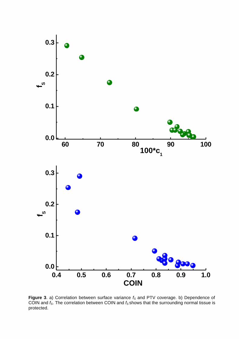
The variance based optimization assumes that the objective fS considers the NT

indirectly. The dependence of the PTV coverage on fS is shown in Fig. 3a. It shows that there is

a correlation and that very small variances correspond to solutions with a large PTV coverage.

We see the dependence between the surface variance fS and COIN in Fig. 3b. A small variance

results in a large COIN value. Therefore the protection of the surrounding normal tissue is

considered indirectly in the objective function fS as long as source dwell positions are allowed

only inside the PTV. It is therefore not necessary to include an additional objective for the

protection of NT.

Table 3. Comparison of the optimization results using CBM and SBM. The PTV coverage DVHDref the COIN at the reference dose value Dref, the maximum dose values DMax-NT in the NT and DVHNT the value of the DVH for NT at Dref with the CBM and SBM method is shown. The number corresponds to the implant Nr of Table 1.

Nr DVHDref

CBM DVHDref

SBM fS

CBM fS

SBM Coin CBM

Coin SBM

DMax-NT CBM

DMax-NT SBM

DVHNT CBM

DVHNT SBM

1 94.23 93.43 0.0159 0.0116 0.839 0.836 1.68 1.31 1.01 0.86 2 75.35 72.60 0.1490 0.1752 0.400 0.485 12.88 2.55 5.31 3.23 3 73.70 64.67 0.1747 0.2542 0.320 0.447 13.13 5.97 10.95 4.28 4 77.67 80.24 0.1042 0.0916 0.680 0.715 2.11 2.19 1.97 2.33 5 90.32 89.78 0.0480 0.0505 0.794 0.794 1.67 1.73 2.20 1.84 6 97.21 96.23 0.0060 0.0041 0.857 0.887 2.40 1.77 1.15 0.68 7 95.40 95.06 0.0204 0.0207 0.772 0.823 5.03 1.38 2.71 1.63 8 97.19 96.53 0.0065 0.0042 0.961 0.948 1.74 1.28 0.97 0.70 9 96.50 95.37 0.0108 0.0095 0.888 0.908 8.73 1.39 2.91 1.34

10 64.21 60.46 0.2176 0.2909 0.405 0.493 41.70 4.95 8.38 5.04 11 93.49 93.90 0.0159 0.0145 0.868 0.890 2.94 2.29 1.39 1.37 12 95.84 95.22 0.0112 0.0096 0.912 0.926 4.27 1.44 1.87 1.20 13 92.48 91.82 0.0487 0.0366 0.833 0.836 2.80 1.81 2.58 2.10 14 92.29 90.42 0.0209 0.0258 0.769 0.812 4.63 1.78 3.13 2.01 15 93.29 92.72 0.0218 0.0222 0.842 0.860 2.66 1.93 4.59 3.83 16 93.42 91.30 0.0181 0.0257 0.811 0.836 12.37 1.51 3.68 2.16

60 70 80 90 1000.0

0.1

0.2

0.3f S

100*c1

0.4 0.5 0.6 0.7 0.8 0.9 1.00.0

0.1

0.2

0.3

f S

COIN

Figure 3. a) Correlation between surface variance fS and PTV coverage. b) Dependence of COIN and fS. The correlation between COIN and fS shows that the surrounding normal tissue is protected.

3.4 Convergence of the deterministic algorithms.

For multiobjective optimization the repeated calculation with different set of importance

factors requires the optimal use of the deterministic algorithms. BFGS, FRPR and POWELL

continue the optimization until a predetermined number of iterations are reached, or a tolerance

condition of the aggregate objective function is met. The gradient based algorithms approach

the global Pareto front after 10-20 iterations. Then the objective function value changes are

very small. It is therefore important to increase the tolerance value and to speed-up the

optimization, since the corresponding DVHs will differ insignificantly from the results with the

smallest possible tolerance value.

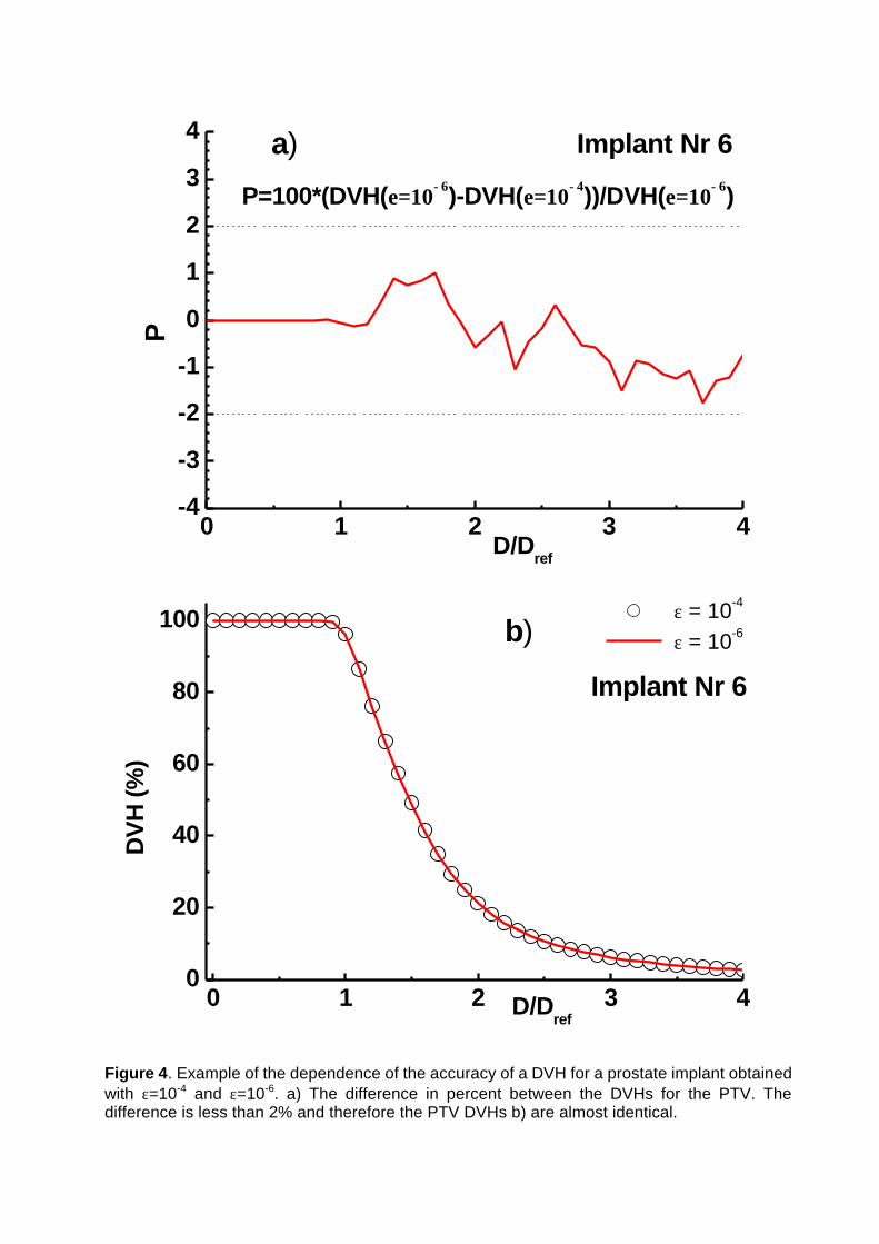
We compare the results obtained with a tolerance value ε =10-4 in comparison with a

tolerance value ε =10-6 set as a reference point. The difference between the DVHs obtained by

BFGS is shown for a prostate implant in Fig. 4a. The DVHs are compared in Fig. 4b. We

observe that the differences are less than 2%. The difference in the number of iterations and

the CPU time are very important. Increasing ε from 10-6 to 10-4 we can reduce the optimization

time by a factor of 3-5!

0 1 2 3 4-4

-3

-2

-1

0

1

2

3

4

P=100*(DVH(ε=10−6)-DVH(ε=10−4))/DVH(ε=10−6)

a) Implant Nr 6P

D/Dref

0 1 2 3 40

20

40

60

80

100 b)

Implant Nr 6

D/Dref

DV

H (%

)

ε = 10-4

ε = 10-6

Figure 4. Example of the dependence of the accuracy of a DVH for a prostate implant obtained with ε=10-4 and ε=10-6. a) The difference in percent between the DVHs for the PTV. The difference is less than 2% and therefore the PTV DVHs b) are almost identical.

3.5 Comparison of Pareto fronts obtained by BFGS and FSA.

In order to identify local minima we compare the Pareto fronts obtained by BFGS and

FSA. We compare additional the optimization time of BFGS and FSA. For FSA the D-

dimensional Cauchy visiting probability distribution is given by

21

22 })({

)()( +

∆+∝∆ D

tV

V

t

xtT

tTxg .

Where Tv(t) is the temperature at iteration t, and tx∆ is the modification of the decision vector x.

We use a D-product of 1-dimensional Cauchy distributions for which a simple random number

generator exists. FSA allows fast cooling and thus a fast optimization, but this is true only for

low dimensional problems. The temperature is decreased every 10 iterations. We modify in all

iterations all dwell times in contrast to Lessard and Pouliot 2001 where the number of dwells

weights that are modified decreases steadily.

The two-dimensional Pareto front obtained by BFGS is shown in Fig. 5 for an implant

with the largest number of source dwell positions. FSA reproduces the BFGS results after

20000 iterations. For all implants studied the Pareto front obtained by FSA and BFGS is

identical. The two-dimensional Pareto fronts for 16 clinical cases are shown in Fig. 6. Each

implant has its own characteristic Pareto front. Implants with a small surface variance also have

a relative small volume variance in general, and vice versa. For the three objectives case we

consider as an example a prostate implant with the urethra overdose as the 3rd objective with

DcUrethra = 1.25Dref. For the 4 objectives case we include for the same implant the rectum

overdose as the 4th objective with DcRectum = 0.75 Dref. This is a special treatment case with a

high dose per fraction, so that the protection of urethra and rectum from an overdose due to a

high prescription dose is very important.

0.05 0.10 0.15 0.50.1

1 Cervix implant Nr 16f V

fS

BFGS FSA t=1000 FSA t=20000

Figure 5. Example of a two-dimensional Pareto set obtained by BFGS for a cervix implant with 272 source dwell positions. The result of FSA with 1000 and 20000 iterations is included.

We use uniformly distributed normalized importance vectors with k=20 which correspond to 861

solutions for three objectives and k=16 for four objectives or 969 solutions. This number of

solutions has been chosen in order to visualize the shape of the Pareto front with details.

The three two dimensional projections of the Pareto front (fS, fV), (fS, fUrethra) and

(fV,fUrethra) obtained by BFGS and FSA with 20000 iterations are shown in Fig. 7. The distribution

of 50000 random distributed solutions is included. These solutions were produced by

generating random dwell weights uniformly distributed in [0,1]. Due to the scale invariance of

the objective functions the distribution is independent on the chosen interval [a,b] as long a≠b.

The optimization path of BFGS is shown for one particular solution that has arbitrarily been

chosen for the case (wS, wV, wUrethra) = ( 0.6, 0.1, 0.3).

0.01 0.1 1

0.1

1

9

10

15

32

13

1614

5

12

1

4

11

86

7

f V

fS

Figure 6. Pareto fronts obtained by bi-objective (fS,fV) dose optimization with BFGS for 16

implants. The number corresponds to the implant of Table 1.

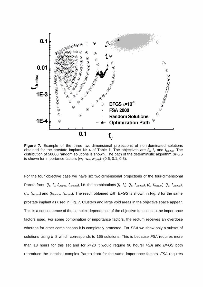
Figure 7. Example of the three two-dimensional projections of non-dominated solutions obtained for the prostate implant Nr 4 of Table 1. The objectives are fS, fV and furethra. The distribution of 50000 random solutions is shown. The path of the deterministic algorithm BFGS is shown for importance factors (wS, wV, wOAR)=(0.6, 0.1, 0.3).

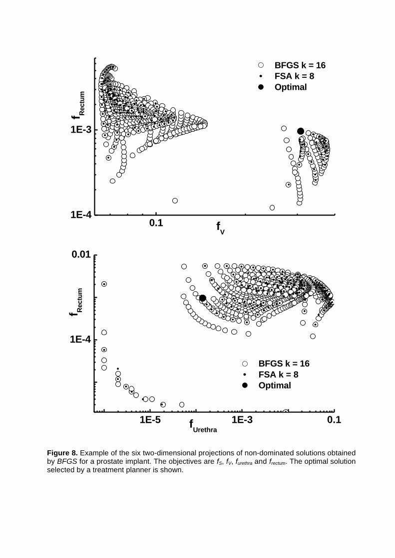
For the four objective case we have six two-dimensional projections of the four-dimensional

Pareto front (fS, fV, fUrethra, fRectum), i.e. the combinations (fS, fV), (fS, fUrethra), (fS, fRectum), (fV, fUrethra),

(fV, fRectum) and (fUrethra, fRectum). The result obtained with BFGS is shown in Fig. 8 for the same

prostate implant as used in Fig. 7. Clusters and large void areas in the objective space appear.

This is a consequence of the complex dependence of the objective functions to the importance

factors used. For some combination of importance factors, the rectum receives an overdose

whereas for other combinations it is completely protected. For FSA we show only a subset of

solutions using k=8 which corresponds to 165 solutions. This is because FSA requires more

than 13 hours for this set and for k=20 it would require 90 hours! FSA and BFGS both

reproduce the identical complex Pareto front for the same importance factors. FSA requires

40000 iterations to approach the Pareto front obtained by BFGS. This demonstrates that local

minima do not exist, or they are below any importance on the entire accessible objective space.

0.01 0.1

0.1

f V

fS

BFGS k = 16 FSA k = 8 Optimal

0.01 0.1

1E-4

1E-3

0.01

0.1

f Ure

thra

fS

BFGS k = 16 FSA k = 8 Optimal

0.01 0.11E-4

1E-3

f Rec

tum

fS

BFGS k = 16 FSA k = 8 Optimal

0.1

1E-4

1E-3

0.01

0.1

f Ure

thra

fV

BFGS k = 16 FSA k = 8 Optimal

0.11E-4

1E-3

f Rec

tum

fV

BFGS k = 16 FSA k = 8 Optimal

1E-5 1E-3 0.1

1E-4

0.01

f Rec

tum

fUrethra

BFGS k = 16 FSA k = 8 Optimal

Figure 8. Example of the six two-dimensional projections of non-dominated solutions obtained by BFGS for a prostate implant. The objectives are fS, fV, furethra and frectum. The optimal solution selected by a treatment planner is shown.

A solution has been selected from this set, for which the urethra is protected and the PTV

coverage is still significant. This solution has been obtained by setting a constraint to the PTV

coverage of at least 90%. A solution based on the COIN gives only 86% coverage. The

selected solutions give a PTV coverage of 97.2 % not so far from the maximum of 95% if only

fS is optimized and the rectum and bladder are protected from overdose in the best possible

way. The position of this solution is shown in the two-dimensional projections of Fig. 8.

The DVHs for the PTV and OARs for this selected solution are shown in Fig. 9. The importance

factors vector for this solution (wS, wV, wUrethra, wRectum) is (0.12475, 0.001 0.87325, 0.001). The

overdose of the urethra requires a very large importance factor for the corresponding objective.

There is a strong trade-off between PTV coverage determined by fS and the urethra overdose.

Therefore wS is required to be very small. This is in contrast to common assumption where the

PTV coverage is considered important and therefore a much larger wS value is used. The

corresponding best solution found by a treatment planner using PLATO BPS 13.7 is also

shown. The treatment planner further used 1 hour to further optimize this solution as good as

he could. Even if the urethra is protected from overdose much better than by the solution found

by PLATO the BFGS solution also provides a better coverage for the PTV.

0 1 2 30

20

40

60

80

100

Bladder

Rectum

Urethra

PTVImplant Nr 12Optimal BFGS

DV

H (%

)

D/Dref

BFGS PLATO

Figure 9. DVH of the PTV and OARs of the optimal solution selected by a treatment planner for the prostate implant Nr 12 of Table 1, see Fig. 8. The DVHs of the best solution found by a treatment planner using PLATO BPS 13.7 is also shown. 4. Discussion and conclusions

In the past HDR brachytherapy dose optimization methods considered only a single

solution obtained by a weighted sum approach on some unknown point, hopefully on the

convex part of the global Pareto front. This is not guaranteed since treatment-planning systems

like PLATO use artificial methods to suppress negative dwell times. Even with these methods

such non-feasible solutions cannot be avoided and correction methods are applied on the final

solution.

More important is that by using a fixed set of importance factors the solutions are not

satisfactory, and the treatment planner is often required to manually intervene and to rescale

the dwell times or even to modify individual source dwell weights based on information of dose

distributions, in order to increase the PTV coverage and/or to protect OARs from overdose.

Even if a single optimization requires only a few seconds sometimes it can require hours to

obtain a satisfactory solution manually. As the number of objectives increases, it is more

difficult to guide the optimization engine to the desired or possible result and the planner does

not know the trade-off between the various objectives.

Methods have been proposed to modify the optimization engine (e.g. in radiotherapy) to

select the correct importance factors using a weighted sum of objectives formed from DVHs

derived quantities (Xing et al 1999, Wu and Zhu 2001). In this approach, the problem of the

importance factors has been only replaced by another set of importance factors used for the

DVH based values, which steer the optimization engine and requiring some information which

is not always known. In some cases the range of the importance factors for each objectives

may differ significantly. Additionally some ideal DVHs must be used even if it is unknown what

can actually be realized due to physical constraints. Finally if a solution is presented the

planner has no insight of what alternative solutions could have been selected. In brachytherapy

it is difficult to quantify optimality in the presence of OARs and planners and physicians have

their own insight of how a dose distribution is “optimal” for a particular type of cancer in a

particular location. This requires an optimization engine that should be able to provide the

planner with all possibilities that can be realized. Souza et al. (D’Souza et al 2001) used a

weighted sum approach with a mixed-integer programming algorithm and reported that the

weights for the five objectives used should be in the range 300-500, 300-2000, 1-300, 5-100

and 104-107. Even if eventually a single set of weights was used for all optimizations the

determination of an optimal unique set is difficult and does not always give the best or even a

satisfactory result.

Using a simple mapping technique negative dwell weights are completely avoided and a

constraint optimization is not necessary. Correction techniques for negative weights that reduce

the quality of the solutions are not necessary. This method allows us to use deterministic

constrained free gradient-based algorithms and to obtain 50-100 solutions in a few minutes. In

this time only 2-3 solutions can be obtained by an FSA algorithm (Lessard and Pouliot 2001).

For PTV based objectives the solutions are global optimal, i.e. for the objectives fS and fV and

for a given set of importance factors no algorithm will provide a better solution. In the presence

of OARs, although local minima can in principle exist (Deasy et al 1997), they are either

negligible or we did not observe them. The results compared with a weighted sum based FSA

are identical but FSA requires many hours for the same number of solutions! With a high

probability, if OARs are included then the BFGS solutions are also optimal global i.e. on the

convex parts of the global Pareto front.

The dose normalization applied with the variance-based objectives protects the

surrounding normal tissue as long as there are no source dwell positions outside the PTV. The

normalization limits the maximum coverage of the PTV with the prescription dose in the case

when the reference isodose surface is such that it cannot have the shape of the PTV surface

due to a bad distribution of source dwell positions. Using sampling points limited to contours,

we compared these results, to results where the entire PTV surface is considered. Our result

indicates that the latter method finally protects better the surrounding normal tissue, although

producing a slightly smaller PTV coverage than the CBM method. A higher coverage can be

achieved by a dose rescaling, but one has to consider the effects of it on the OARs and the

surrounding NT. The obtained set of solutions shows the true physical limitations in

dependence of the objectives used, given the characteristics of the implant, the size of the

PTV, topology and geometry of the organs and the specific dose values.

The complexity of the Pareto front increases rapidly with the number of objectives. This

is a problem not only for multiobjective optimization methods but is a general problem if one

has to consider many OARs. We have transformed the dose optimization problem into a

decision-making problem. A treatment planner can filter out an appropriate solution in a few

minutes, using the simple decision making tools. If none of the objectives is preferred then

COIN can be used for the selection of a good solution. This is not always true, as for example

shown for the prostate implant case. This demonstrates that a simple utility function cannot be

used and that additional information such as provided by the non-dominated solutions is

valuable and necessary for the decision.

The result is almost better and in the worst case as good as the solution provided by

PLATO BPS which requires a manual intervention by the planner in difficult cases, and that

may take 1-3 hours in some cases, sometimes even ending without a satisfactory result. The

multiobjective approach does not require special handling or adjustment for each implant site or

type.

The deterministic gradient based algorithms are very efficient and can be used for

multiobjective post-plan dose optimization, i.e. given a set of source dwell positions determine

for the variance based objectives the Pareto set. The weighted sum provides only convex parts

of the Pareto set (Miettinen 1999, Das and Dennis 1997). The deterministic algorithm can be

used for the initialization of the population of multiobjective evolutionary algorithms (Lahanas et

al 1999, 2001) that helps to improve their performance. This class of algorithms is not restricted

to convex objective spaces and can be used for the inverse planning optimization problem

where the optimum subset of catheters out of a large set of possible catheters additionally has

to be found.

References

Angelopoulos A, Perris A, Sakellariou K, Sakelliou L, Sarigiannis K and Zarris G 1991 Accurate

Monte Carlo calculations of the combined attenuation and build-up factors, for energies (20-

1500 keV) and distances (0-10 cm) relevant in brachytherapy Phys. Med. Biol. 36 763-78

Baltas D, Kolotas C, Geramani K , Mould R F, Ioannidis G, Keckhidi M and Zamboglou N 1998

A Conformal Index (COIN) to evaluate implant quality and dose specifications in brachytherapy

Int. J. Radiation Oncology Biol. Phys. 40 512-24

Cho P S, Lee S, Marks II R J, Ohm S, Sutlief S G and Phillips M H 1998 Optimization of

intensity modulated beams with volume constraints using two methods: Cost function

minimization and projections onto convex sets Med. Phys. 25 435-43

Cotrutz C, Lahanas M, Kappas C and Baltas D 2001 A multiobjective gradient based dose

optimization algorithm for conformal radiotherapy Phys. Med. Biol. 46 2161-75

Das I and Dennis J 1997 A Closer Look at Drawbacks of Minimizing Weighted Sums of

Objectives for Pareto Set Generation in Multicriteria Optimization Problem Structural

Optimization 14

Deasy J O 1997 Multiple local minima in radiotherapy optimization problems with dose-volume

constraints Med. Phys. 24 1157-61

Edmundson G K Geometry based optimization for stepping source implants, in Brachytherapy

HDR and LDR, edited by A. A. Martinez, C. G. Orton and R. F. Mould (Nucletron, Columbia,

1990).

Ingber A. L. 1996 Adaptive simulated annealing (ASA): Lessons learned J. Control and

Cybernetics 25 33-54

Karaiskos P, Angelopoulos A, Sakelliou L, Sandilos P, Antypas C, Vlachos L and Koutsouveli E

1998 Monte Carlo and TLD dosimetry of an 192Ir high dose rate brachytherapy source Med.

Phys. 25, 1975-84

Karaiskos P, Angelopoulos A, Baras P, Sakelliou L, Sandilos P, Dardoufas K and Vlachos L

1999 A Monte Carlo investigation of the dosimetric characteristics of the VariSource 192Ir high

dose rate brachytherapy source Med. Phys. 26 1498-502

Kneschaurek P, Schiessl W and Wehrmann R 1999 Volume-based dose optimization in

brachytherapy Int. J. Radiation Oncology Biol. Phys. 45 811-5.

Lahanas M, Baltas D and Zamboglou N 1999 Anatomy-based three-dimensional dose

optimization in brachytherapy using multiobjective genetic algorithms Med. Phys. 26 1904-18

Lahanas M, Baltas D, Giannouli S, Milickovic N, and Zamboglou N 2000 Generation of

uniformly distributed dose points for anatomy-based three-dimensional dose optimization

methods in brachytherapy Med. Phys. 27 1034-46

Lahanas M, Baltas D, Karouzakis K, Papagiannopoulou M, Giannouli S, Milickovic N and

Zamboglou N 2001 Multiobjective Dose Optimization Algorithms for Anatomy Based HDR

Brachytherapy, submitted to Med. Phys.

Lessard E and Pouliot J 2001 Inverse planning anatomy-based dose optimization for HDR-

brachytherapy of the prostate using fast simulated annealing and dedicated objective functions

Med. Phys. 28 773-9

Milickovic N, Giannouli S, Baltas D, Lahanas M, Zamboglou N and Uzunoglu N 2000 Catheter

Autoreconstruction in Computed Tomography based Brachytherapy Treatment Planning.

Med Phys 27 1047-57

Milickovic N, Baltas D, Giannouli S, Lahanas M and Zamboglou N 2001 A New Algorithm for

Autoreconstruction of Catheters in Computed Tomography-Based Brachytherapy Treatment

Planning IEEE on Biomedical Engineering 48 372-83

Miettinen K M Nonlinear Multiobjective Optimization 1999 Kluwer Academic Publisher Boston

Press W H, Teukolsky S A, Vetterling W T and Flannery B. P. 1992 Numerical Recipes in

C,2nd ed. Cambridge University Press Cambridge England.

Sakelliou L, Sakellariou K, Sarigiannis K, Angelopoulos A, Perris A and Zarris G 1992 Dose

rate distributions around 60Co, 137Cs, 198Au, 192Ir, 241Am, 125I (models 6702 and 6711)

brachytherapy sources and the nuclide 99Tcm Phys. Med. Biol. 37 1859-72

D’Souza W D, Meyer R R, Thomadsen B R and Ferris M C 2001 An iterative sequential mixed-

integer approach to automated prostate brachytherapy treatment plan optimization Phys. Med.

Biol. 46 297-322

Spirou S V and Chui C S 1998 A gradient inverse planning algorithm with dose-volume

constraints Med. Phys. 25 321-33

Szu H and Hartley R 1987 Fast Simulated Annealing Phys. Lett. A 122 157-62

Tsallis C and Stariolo D A 1996 Generalized simulated annealing Physica A 233 395

Xing L, Li J G, Donaldson S, Le Q T and Boyer A L 1999 Optimization of importance factors in

inverse planning Phys Med. Biol. 44 2525-36

Wu X and Zhu Y 2001 An optimization method for importance factors and beam weights based

on genetic algorithms for radiotherapy treatment planning Phys. Med. Biol. 46 1085-99

Figure Legends Figure 1. The optimization time as a function of the number of source dwell position for BFGS obtained with ε=10-4 and ε=10-6 for the 16 implants of Table 1. An approximate quadratic increase with the number of source dwell positions is observed. Figure 2. Example of the DVH for two prostate implants obtained by BFGS and SVD where a cut-off correction to 0 is applied for negative dwell weights. Figure 3. a) Correlation between surface variance fS and PTV coverage. b) Dependence of COIN and fS. The correlation between COIN and fS shows that the surrounding normal tissue is protected. Figure 4. Example of the dependence of the accuracy of a DVH for a prostate implant obtained with ε=10-4 and ε=10-6. a) The difference in percent between the DVHs for the PTV. The difference is less than 2% and the PTV DVHs b) therefore are almost identical. Figure 5. Example of a two-dimensional Pareto set obtained by BFGS for a cervix implant with 272 source dwell positions. The result of FSA with 1000 and 20000 iterations is included. Figure 6. Pareto fronts obtained by bi-objective (fS, fV) dose optimization with BFGS for 16 implants. The number corresponds to the implant of Table 1. Figure 7. Example of the three two-dimensional projections of non-dominated solutions obtained for the prostate implant Nr 4 of Table 1. The objectives are fS, fV and furethra. The distribution of 50000 random solutions is shown. The path of the deterministic algorithm BFGS is shown for importance factors (wS, wV, wOAR)=(0.6, 0.1, 0.3). Figure 8. Example of the six two-dimensional projections of non-dominated solutions obtained by BFGS for a prostate implant. The objectives are fS, fV, furethra and frectum. The optimal solution selected by a treatment planner is shown. Figure 9. DVH of the PTV and OARs of the optimal solution selected by a treatment planner for the prostate implant Nr 12 of Table 1, see Fig. 8. The DVHs of the best solution found by a treatment planner using PLATO BPS 13.7 is also shown.

Table 1. Statistics for the 16 clinical cases used for the analysis of the deterministic multiobjective dose optimization algorithms and FSA. Table 2. For each clinical case the PTV coverage and COIN at the reference dose is shown. The percent of the negative weights using SVD is shown. The number corresponds to the implant Nr of Table 1. Table 3. Comparison of the optimization results using CBM and SBM. The PTV coverage DVHDref the COIN at the reference dose value Dref, the maximum dose values DMax-NT in the NT and DVHNT the value of the DVH for NT at Dref with the CBM and SBM method is shown. The number corresponds to the implant Nr of Table 1.